Florida State University Libraries

Electronic Theses, Treatises and Dissertations The Graduate School

2013

Application of Artificial Intelligence toRotating Machine Condition MonitoringYaw Dwamena Nyanteh

Follow this and additional works at the FSU Digital Library. For more information, please contact lib-ir@fsu.edu

THE FLORIDA STATE UNIVERSITY

COLLEGE OF ENGINEERING

APPLICATION OF ARTIFICIAL INTELLIGENCE TO ROTATING MACHINE CONDITION

MONITORING

By

YAW DWAMENA NYANTEH

A Dissertation submitted to the Department of Electrical and Computer Engineering

in partial fulfillment of the requirements for the degree of

Doctor of Philosophy

Degree Awarded: Fall Semester, 2013

Yaw Dwamena Nyanteh defended this dissertation on June 21, 2013.

The members of the supervisory committee were:

Chris S. Edrington

Professor Co-Directing Dissertation

David A. Cartes

Professor Co-Directing Dissertation

William Oates

University Representative

Rodney Roberts

Committee Member

Petru Andrei

Committee Member

Sanjeev K. Srivastava

Committee Member

The Graduate School has verified and approved the above-named committee members, and

certifies that the dissertation has been approved in accordance with university requirements.

ii

I dedicate this work to my mother who always wanted to study to this level but had to give up and support her children in their studies

iii

ACKNOWLEDGMENTS

A number of people have contributed to the eventual completion of this work. First I

would like to acknowledge my core academic and research advisors: Dr. Chris S. Edrington, Dr.

Sanjeev K. Srivastava and Dr. David A. Cartes. Without their intellectual input, fatherly

guidance and financial support, I would not have completed my studies. I would like to

acknowledge the good grace of my committee members: Dr. Rodney Roberts, Dr. Petru Andrei

and Dr. William Oates. I would like to mention Dr. Jonathan Clarke who was immensely

influential in some of the initial important critique that has gone in to make the work publicly

presentable. Special mention goes to Dr. Lukas Graber and Dr. Horatio Rodrigo whose tireless

effort made it possible for me to work on the fault prognosis aspects of this research work. I

would like to mention some of my colleagues Fletcher Fleming and Mark Stanovich who were

ever helpful when I had to either write a piece of code or get a second opinion about an issue.

iv

TABLE OF CONTENTS

List of Tables ................................................................................................................................. ix List of Figures ..................................................................................................................................x Abstract ........................................................................................................................................ xiv

CHAPTER ONE ..............................................................................................................................1 1.1 Problem Statement .........................................................................................................4 1.2 Objectives of Research ..................................................................................................5 1.3 Scope of Research ..........................................................................................................5 1.4 Originality and Contribution ..........................................................................................6

1.4.1 Publications of Research Outcome ....................................................................7

CHAPTER TWO .............................................................................................................................9 2.1 Types of Faults in Electrical Machines ..........................................................................9

2.1.1 Stator Winding Faults ......................................................................................10 2.1.1.1 Causes of stator winding faults ..........................................................10 2.1.1.2 Failure mechanisms and symptoms of stator winding faults .............10 2.1.2 Stator Core Faults ............................................................................................12 2.1.2.1 Causes of stator core faults ................................................................12 2.1.3 Rotor Faults ......................................................................................................13 2.1.3.1 Rotor winding short-circuits ..............................................................13 2.1.3.2 Induction machine rotor failure .........................................................13 2.1.3.3 PMSM rotor failure ............................................................................14 2.1.4 Eccentricity Faults ...........................................................................................14 2.1.4.1 Causes of eccentricity faults ..............................................................15 2.1.5 Bearing Faults ..................................................................................................15 2.1.5.1 Causes of bearing faults .....................................................................15

2.2 Fault Indicators ............................................................................................................16 2.2.1 Fault Indicators for Electrical Machines ..........................................................17 2.2.1.1 Mechanical and thermal fault indicators ............................................19 2.2.1.2 Chemical indicators ...........................................................................20 2.2.1.3 Indicators for stator winding faults ....................................................20 2.2.1.4 Indicators for detecting rotor faults ....................................................21 2.2.1.5 Indicators for detecting bearing faults ...............................................21 2.2.1.6 Indicators for detecting eccentricity faults .........................................23 2.2.2 Current Monitoring for Fault Diagnosis and Prognosis ...................................24 2.2.2.1 MCSA for stator winding faults .........................................................24 2.2.2.2 MCSA for rotor winding faults ..........................................................25 2.2.2.3 MCSA for bearing faults ....................................................................26 2.2.2.4 MCSA for eccentricity faults .............................................................27 2.2.2.5 Circulating currents ............................................................................28 2.2.2.6 Shaft currents .....................................................................................29 2.2.2.7 Drawbacks with the use of current monitoring ..................................29 2.2.3 Magnetic Flux Monitoring for Fault Diagnosis and Prognosis .......................29 2.2.3.1 Sensors for electromagnetic flux monitoring .....................................30

v

2.2.3.2 Electromagnetic flux region to be monitored in electrical machines 30 2.3 Electrical Machine Diagnostics and Prognostics Technique for Condition-Based Maintenance ..........................................................................................................................32

2.3.1 Effective Implementation of CBM ..................................................................33 2.3.1.1 IEEE 1451 ..........................................................................................34 2.3.1.2 IEEE 1232 ..........................................................................................35 2.3.1.3 MIMOSA and OSA-CBM .................................................................36

2.4 Analysis Tools for Electrical Machine Fault Diagnostics and Prognostics .................38 2.4.1 Finite Element Analysis ...................................................................................39 2.4.1.1 Use of the finite element method to model electrical machines ........40 2.4.1.2 Application to CBM ...........................................................................40 2.4.1.3 Description of the FEM software tool used in study .........................41 2.4.2 Data Processing ................................................................................................43 2.4.2.1 Time-domain techniques ....................................................................44 2.4.2.2 Frequency-domain techniques ...........................................................46 2.4.2.3 Time-frequency-domain techniques ..................................................48 2.4.3 Fault Diagnosis Techniques .............................................................................49 2.4.3.1 Data-driven approaches for fault diagnostics ....................................49 2.4.3.2 Model-based approaches for fault diagnostics ...................................51 2.4.3.2 Comparison of data-based and model-based approaches ..................52 2.4.4 Fault Prognosis Techniques .............................................................................52 2.4.4.1 Data-based approaches for prognosis ................................................53 2.4.4.2 Time-series methods for prognosis ....................................................53 2.4.4.3 Artificial intelligence approaches ......................................................56 2.4.4.4 Model-based approaches for prognosis .............................................58 2.4.4.5 Reliability-based approaches for prognosis .......................................60

2.5 Rotating Machine Insulation Systems .........................................................................60 2.5.1 Insulation of Rotating Electric Machines ........................................................61 2.5.2 Insulating Materials .........................................................................................62 2.5.3 Dimensioning of an Insulation .........................................................................62

2.6 Partial Discharges ........................................................................................................64 2.6.1 PD Detection ....................................................................................................64 2.6.2 PD Mechanisms ...............................................................................................65 2.6.3 Partial Discharges in Cable Specimens............................................................66 2.6.4 Partial Discharges in Transformers ..................................................................67 2.6.5 PD Mechanisms in Rotating Machines ............................................................69

CHAPTER THREE .......................................................................................................................71 3.1 Modeling the PMSM using FEA .................................................................................72 3.2 Modeling PMSM Faults ...............................................................................................75

3.2.1 Modeling Stator Short-Circuit Fault Conditions ..............................................75 3.2.2 Modeling Permanent Magnet Demagnetization Fault Conditions...................76 3.2.3 Modeling Static Eccentricity Fault Conditions ................................................77 3.2.4 Modeling Dynamic Eccentricity Fault Conditions ..........................................78

3.3 Fault Indicator Data and Feature Extraction ................................................................78 3.4 Fault Classification Technique ....................................................................................81

3.4.1 Logic-Based Classifiers ...................................................................................82

vi

3.4.2 Perceptron-Based Classifiers ...........................................................................82 3.4.3 Statistical Classifiers ........................................................................................83 3.4.4 Instance-Based Learning ..................................................................................83 3.4.5 Support Vector Machines ................................................................................84

3.5 Manifold Learning Techniques ....................................................................................85 3.5.1 Classical Approach to Dimensionality Reduction ...........................................86 3.5.2 Global Non-Linear Techniques ........................................................................87 3.5.3 Local Non-Linear Techniques .........................................................................87 3.5.4 Global Linear Alignment in Local Space ........................................................88

3.6 Fault Classification Results..........................................................................................88 3.6.1 Comparison of Techniques Based on Original Un-Transformed Dataset .......88 3.6.2 Comparison of Techniques Based on Transformed Dataset ............................89 3.6.3 Effect of Bagging on Classification Performance ...........................................92

3.7 Conclusion ...................................................................................................................94

CHAPTER FOUR ..........................................................................................................................95 4.1 Peak-to-Peak Detection for PMSM Stator Winding Short-Circuit Fault Detection ....96

4.1.1 Development of ANN Model for the Peak-to-Peak Fault Detection Method .97 4.1.2 The PSO Algorithm .........................................................................................98 4.1.2.1 Offline PSO algorithm .......................................................................98 4.1.2.2 Online PSO algorithm ......................................................................101

4.2 Turn-to-Turn Short-Circuit Fault Detection Method .................................................101 4.2.1 Development of ANN Model for the Turn-to-Turn Short-Circuit Fault Detection Method .......................................................................................................105 4.2.1.1 The Extended kalman filter method .................................................108

4.3 Fault Simulation Results ............................................................................................110 4.3.1 Description of Experimental setup .................................................................110 4.3.2 Training Results .............................................................................................111 4.3.2.1 PSO and PSO-BFGS ANN training results ....................................111 4.3.2.2 EKF ANN training results ..............................................................113 4.3.3 Fault Diagnosis Results..................................................................................116 4.3.3.1 Fault diagnosis results based on peak-to-peak method ...................119

4.3.3.2 Fault diagnosis results based on turn-to-turn short-circuit detection method...........................................................................................................121

4.4 Conclusions ................................................................................................................121

CHAPTER FIVE .........................................................................................................................127 5.1 Unique Insulation Issues in an All-Electric Ship .......................................................127 5.2 Dielectric Breakdown Testing ...................................................................................128

5.2.1 Description of Experimental Setup ................................................................129 5.3 Modified Dielectrics Breakdown Model ...................................................................140

5.3.1 Electrical Tree Simulation Results .................................................................146 5.4 Macro-Model for Prognosis .......................................................................................150 5.5 Fault Prognosis Using Artificial Neural Networks ....................................................154 5.6 Conclusions ................................................................................................................156

CHAPTER SIX ............................................................................................................................158 6.1 Fault Classification ....................................................................................................158

vii

6.2 Fault Detection ...........................................................................................................159 6.3 Fault Prognosis...........................................................................................................160 6.4 Application Limitation of Methods Presented ...........................................................161

CHAPTER SEVEN .....................................................................................................................163 7.1 Fault Diagnosis ..........................................................................................................163 7.2 Fault Detection ...........................................................................................................163 7.3 Fault Prognosis...........................................................................................................164

REFERENCES ............................................................................................................................165

BIOGRAPHICAL SKETCH .......................................................................................................184

viii

LIST OF TABLES

1 Comparing shipboard power systems and terrestrial power systems ......................................1 2 Fault indicators for rotating electrical machines ...................................................................18 3 Thermal classes of insulation materials .................................................................................62 4 Parameters of the PMSM .......................................................................................................73 5 Material properties of PMSM FEA model components ........................................................73 6 Description of fault cases ......................................................................................................80 7 PMSM simulation parameters .............................................................................................116 8 Machine simulated conditions using computer simulation .................................................116 9 Machine simulated conditions using actual PMSM drive ...................................................118 10 Characteristics of STYCAST 1266 and STYCAST 1265 ...................................................129 11 Values of parameters of PD detection circuit ......................................................................131

ix

LIST OF FIGURES

1 Summary of faults in electrical machines based on a survey by EPRI and sponsored by the General Electric Company in 1982 [8]………………………………………………………4

2 Inter-turn short circuit ............................................................................................................11 3 Types of eccentricity contrasted with the concentric condition ............................................15 4 Complex interactions of different sub-systems in an electrical drive system [32] ................19 5 Comparison of magnetic sensors for magnetic flux monitoring [92] ....................................31 6 Condition based maintenance process [114] .........................................................................40 7 A multi-layer perceptron with one hidden layer ....................................................................57 8 PD detection setup .................................................................................................................70 9 Demagnetization characteristics of sintered Samarium Cobalt (magnetic component

engineering) ............................................................................................................................74 10 Solid and 2D mesh view of the PMSM FEA model .............................................................74 11 Schematic of turn–to-turn and inter-turn-to-turn short circuit faults .....................................75 12 FEA model of short circuit faults ..........................................................................................76 13 Flux density distribution for demagnetization fault condition ..............................................77 14 FEA model of the static eccentricity fault condition showing flux density distribution .......78 15 FEA model of the dynamic eccentricity fault condition showing flux density distribution .79 16 Air gap circumferential line along which flux density is computed .....................................80 17 Power spectral estimate for a sample instantaneous power feature vector ...........................81 18 Comparison of classification techniques on un-transformed dataset ....................................90 19 Comparison of classification techniques on LLC dataset .....................................................90 20 Comparison of classification techniques on LTSA dataset ...................................................91 21 Comparison of classification techniques on MDS dataset ....................................................91

x

22 Comparison of classification techniques on PCA dataset .....................................................92 23 Application of bagging on MDS dataset ...............................................................................93 24 Application of bagging on PCA dataset ................................................................................93 25 Confusion matrix for the performance of classification techniques using J48 .....................94 26 Speed of PMSM during different loading conditions ............................................................96 27 Phase current for changing load and stator winding fault .....................................................97 28 Time window to implement PSO ........................................................................................102 29 Flow chart of real time PSO method ...................................................................................103 30 Zero-component of three phase stator current of PMSM ....................................................104 31 Diagram of the ANN during training ..................................................................................106 32 Diagram of ANN cluster during fault diagnosis ..................................................................107 33 Schematic of drive system incorporating the ANN fault diagnostic system .......................108 34 Kalman filter representation of recurrent ANN ...................................................................108 35 PMSM drive system ............................................................................................................110 36 Circuit diagram for stator short circuit winding ..................................................................111 37 Training data ........................................................................................................................112 38 Training evolution using PSO and PSO-BFGS ...................................................................114 39 Performance of ANN on training data .................................................................................115 40 Computer simulated three-phase current data with effective turns-ratio of 0.9 ..................117 41 Training evolution for computer simulated data for one ANN ...........................................117 42 Current data with effective turns-ratio of 0.95 from PMSM drive ......................................118 43 Training evolution for data obtained from actual PMSM drive with 50% loading .............119 44 ANN fault detection with no-loading on PMSM ................................................................120

xi

45 30% full loading conditions .................................................................................................122 46 50% full loading conditions .................................................................................................123 47 Fault diagnosis for computer simulated data (10% shorted turns on phase A) ...................124 48 Fault diagnosis for computer simulated data (25% shorted turns on phase A) ...................124 49 Fault diagnosis for 30% loading of the PMSM drive ..........................................................125 50 Fault diagnosis for 50% loading of the PMSM drive ..........................................................125 51 Setup for breakdown testing of dielectric material ..............................................................130 52 Setup for PD detection .........................................................................................................131 53 PD monitoring and data acquisition setup ...........................................................................132 54 Low pass filter characteristics .............................................................................................133 55 High pass filter characteristics .............................................................................................134 56 FEA simulation results ........................................................................................................134 57 Enhanced setup for PD detection ........................................................................................136 58 Characteristic PD pattern per cycle .....................................................................................137 59 PD characteristics during breakdown of STYCAST 1265 ..................................................137 60 Flow chart of simulation process .........................................................................................143 61 Model of tree link ................................................................................................................144 62 Model of dielectric material during breakdown ..................................................................145 63 Simulation results for fast breakdown .................................................................................147 64 Simulation results for slow breakdown ...............................................................................148 65 Some tree simulation results ................................................................................................151 66 Plot of time-to-breakdown versus voltage ...........................................................................152 67 Prediction using modified thermodynamic model ..............................................................153

xii

68 Adaptive system ANN dielectric breakdown prognosis .....................................................155 69 Training model for ANN dielectric breakdown prognosis system ......................................155 70 Prediction using modified ANN adaptive model ................................................................156 71 Illustration of fault prognostic system .................................................................................157

xiii

ABSTRACT

Systems with critical functionality and are prone to damage due to excessive stress level

from operation conditions and working environment requires health monitoring. Condition or

health monitoring involves acquiring data that can be analyzed to determine the occurrence of

faults, determine the type of fault, determine the severity of a fault and determine when the next

fault would occur. This research has considered new fault analysis techniques for rotating

electrical machines using Artificial Intelligence (AI) techniques. The analysis has been carried

out in three sections: fault diagnosis, fault detection and fault prognosis.

By way of fault diagnosis, Finite Element Analysis (FEA) has been used to model

different faults in a Permanent Magnet Synchronous Machine (PMSM) which has been analyzed

by way of classification using five Artificial Intelligence Techniques. The original large

dimensional dataset is first used in the classification process and the different fault classifiers

compared based on their performance using different fault classifiers from the FEA model. The

dimensions of the dataset are reduced, using four different manifold reduction techniques.

Manifold reduction is carried out to reduce the computational burden of fault classification on

high dimensionality data.

Two new techniques for fault detection using AI is presented and applied to PMSMs by

way of computer simulations and experimental data from an actual PMSM. One technique called

the Peak-to-Peak technique uses an Artificial Neural Network (ANN) trained using PSO and can

distinguish short circuit faults from loading transients. In the second method, called Turn-to-Turn

method, the zero current components is used to determine the number of shorted turns in the

stator windings using an ANN trained using the Extended Kalman Filter (EKF) method.

Finally a new method of determining the time-to-breakdown of insulation systems is

presented as a fault prognosis approach. Also a new micro simulation model is presented for

simulating the breakdown of dielectric materials. The new prognostics method is based on a

macro model developed in conjunction with ANNs. The prognosis approach is based on

associating the breakdown characteristics of dielectrics to Partial Discharge (PD) that take place

during dielectric breakdown.

xiv

CHAPTER ONE

Since the first electrical power system was installed on the USS Trenton in 1883,

Shipboard Power Systems (SPS) has undergone a multitude of technological advancements with

the most recent innovative drive aimed at an All-Electric Ship (AES) [1].The AES is a notional

concept, and very much in its infancy, that seeks to:

1. Convert steam powered, hydraulically powered and pneumatically powered propulsion

systems into an electric drive

2. Combine generation from different energy sources into a single generating unit for

propulsion and services loads

3. Reduce Ship life-cycle costs

4. Increase ship stealthiness, payload, survivability and propulsion power

Generally SPSs are different from terrestrial systems in a number of significant ways. Table 1

shows some of these differences. These distinctions between terrestrial power systems and SPSs

mean that rotating electric machines and propulsion systems, onboard, would be subjected to

increased stress levels on SPSs and lead to faults and device breakdowns and ship system total

failure.

Table 1: Comparing shipboard power systems and terrestrial power systems

Shipboard Power System Terrestrial System

Increased electromagnetic coupling of devices due to limited space on ship [2]

Space considerations less restrictive in terrestrial systems and reduced electromagnetic interference

Lack of space leads to bending and other structural deformations on the cabling [3]

Reduced cable deformation due to space availability

Low damping properties due to short cable lengths and high power density[3]

Longer line lengths resulting in higher damping

Hazardous and unpredictable conditions during different missions (battle, normal, emergency etc.) [3]

Conditions not as severe

Islanded system where vital loads cannot be shut down [5]

Vital loads have a backup supply

Ships can continue operation during single line/rail to ground faults due to specialized grounding and distribution scheme [6]

Single line to ground faults need to be cleared for continuation of service

1

Shipboard Power System Terrestrial System

Ships can continue operation during single line/rail to ground faults due to specialized grounding and distribution scheme [6]

Single line to ground faults need to be cleared for continuation of service

Multiple frequencies in the same system; less restricted frequency variation limits [7]

System frequency is maintained within tight limits around base frequency

System with low finite inertia [8] System has very large inertia

Use of power electronic devices has implications for aging of insulation system due to PWM signals [2]

Traditional power system generation, transmission and distribution have comparatively less need for power electronics devices

Shipboard power systems operate at higher bandwidth control resulting in increased interaction between components [7]

Low bandwidth control with more decoupled subsystems

Big impact of non-linear loads of a pulse nature requiring huge power (comparable to total generation) for short time intervals [5]

No such loads considerations in terrestrial systems

A recent survey of rotating machine failure by the Lloyd Register showed that in the year 2011, 6

different cruise lines in the United Kingdom reported catastrophic accidents. These accidents

involved 26 ships and involved 160 generators each with a repair cost of more than $1million.

The problems reported with these machines comprised the following:

1. Inter-turn coil insulation breakdown

2. Insulation failures under operational stress in stator windings

3. Loose stator core laminations

4. Circulating currents in the stator core

5. Thermal deterioration

6. Coil vibrations

Operators and technicians on these cruise lines could generally tell that associated with most of

these disasters was an increased partial discharge activity but were frustrated they could not tell

where and when a point of failure would occur. Fault Detection and Diagnosis (FDD) and

increasingly Prognostics are therefore important tools for the reliability, availability and

survivability of SPSs. Critical to FDD and prognostics is the condition or health monitoring of

critical devices or subsystems. Recent advances in computer and information technology have

spurred the development of effective FDD techniques. Currently the trend is towards the

extension of these techniques into completely automated real time data acquisition,

Table 1: Continued

2

classification, assimilation, correlation and cognitive function mapping modules for FDD.

Notwithstanding these advances, the area of Artificial Intelligence (AI) offers new research

opportunities in FDD and prognostics. The FDD of rotating electric machines has been the

subject of several research efforts, culminating in some important breakthroughs. Rotating

machine prognostics is relatively new and there is as yet to be developed a systematic

methodology to determine the remaining useful lifetime of rotating electrical machines. The

major drawback with prognostics studies is the fact that final machine breakdown is usually by a

catastrophic event. Most machine insulation systems are also designed to withstand much higher

stress levels than during normal operation. Electrical machines, during operations, are subjected

to a number of coupled stresses of electrical, thermal, mechanical and chemical origins. This

makes it a complex problem to determine, accurately, the Remaining Useful Life (RUL) of a

machine.

Prognostics involve the ability to accurately predict the remaining life of a failing

machine or subsystem. Normally the failing machine or subsystem is critical for the overall

operation of the system and their failure has catastrophic consequences. Prognostics are useful to

system managers to help them plan operation of dynamic systems. By accurate forecasting,

system managers can develop accurate alarm levels for different states of a dynamic system

depending on the extent of degradation of devices. Prognostics are an ongoing research area and

a lot of methodologies have been published in the literature. Most of the published works on

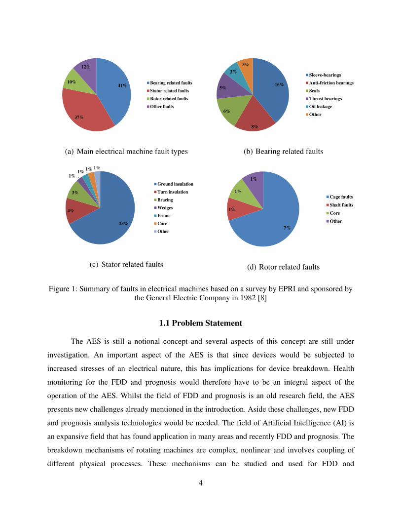
prognostics focus on the mechanical and thermal aspects of machine failure. As Figure 1 shows,

it is undeniable that most failure is ultimately of a mechanical/thermal nature. Whilst the

electrical aspects of machine breakdown have been the subject of several published research

work, there is still no clear systematic methodologies for how to predict accurately the RUL of a

rotating electrical machine based on degradation of electrical natures. This task mostly relies on

the expert knowledge of experienced technicians and operators. Fully automated systems are still

a very vibrant research field with the promise of a lot benefits to system managers. In the specific

area of SPS, system managers can rely on expert systems to plan operations on the ship. The

hazardous offshore conditions coupled with the fact that, for most modes of operation of SPS,

the propulsion motors and other critical loads cannot be shut down, makes failure forecasts about

devices on SPSs very important.

3

(a) Main electrical machine fault types

(b) Bearing related faults

(c) Stator related faults

(d) Rotor related faults

Figure 1: Summary of faults in electrical machines based on a survey by EPRI and sponsored by the General Electric Company in 1982 [8]

1.1 Problem Statement

The AES is still a notional concept and several aspects of this concept are still under

investigation. An important aspect of the AES is that since devices would be subjected to

increased stresses of an electrical nature, this has implications for device breakdown. Health

monitoring for the FDD and prognosis would therefore have to be an integral aspect of the

operation of the AES. Whilst the field of FDD and prognosis is an old research field, the AES

presents new challenges already mentioned in the introduction. Aside these challenges, new FDD

and prognosis analysis technologies would be needed. The field of Artificial Intelligence (AI) is

an expansive field that has found application in many areas and recently FDD and prognosis. The

breakdown mechanisms of rotating machines are complex, nonlinear and involves coupling of

different physical processes. These mechanisms can be studied and used for FDD and

41%

37%

10%

12%

Bearing related faults

Stator related faults

Rotor related faults

Other faults

16%

8%

6%

5%

3%

3%

Sleeve-bearings

Anti-friction bearings

Seals

Thrust bearings

Oil leakage

Other

23%

4%

3%

1%1%

1% 1%

Ground insulation

Turn insulation

Bracing

Wedges

Frame

Core

Other7%

1%

1%

1%

Cage faults

Shaft faults

Core

Other

4

prognostics systems in either a model-based approach, data-based approach or a combination of

the two. Both approaches and their combination lend themselves to the use of Artificial

Intelligence techniques in a generalized approach for FDD and prognosis for all types of

electrical machines and especially for machines on SPS.

1.2Objectives of Research

The broad aims of this research work are three-fold. First a representative subsystem, a

Permanent Magnet Synchronous Machine (PMSM), has been selected to represent a device

whose failure modes would be discussed. The nature of FDD studies makes modeling a necessity

to avoid having to actually build and destructively test machines in different fault modes. To this

end, the first objective is to develop computer simulation models of the PMSM under three fault

conditions: Short Circuit Faults, Demagnetization Faults and Eccentricity Faults. To obtain very

accurate models of the machine, the Finite Element Method (FEM) has been chosen to simulate

faults in the PMSM. Secondly different AI techniques would be developed for FDD for

comparison purposes. Towards this end, two computational tools would be extensively used.

These are MATLAB and WEKA. MATLAB is a very ubiquitous scientific and technical

computing tool that has found wide applicability. WEKA is a machine learning environment

created by the University of Waikato. The final objective of this dissertation is the important

aspect of prognostics for the insulation systems of rotating machines. The objective here is to

develop prognostic algorithms to predict the time to breakdown of the insulation systems of

rotating machines.

1.3 Scope of Research

A typical SPS has a number of sub-components which must be in good condition for the

overall availability of the system. This dissertation however only focuses on rotating machines.

The thermal, mechanical, chemical and environmental aspects of the breakdown of machines are

not pursued in this dissertation. Hence only electrical fault indicators would be considered:

Current and Voltage output analysis, Air-gap flux and Partial Discharge (PD) activity. Whilst

breakdown mechanisms of the insulations systems of machines are, for the most part, similar for

different machines with the same insulation material, the actual time to breakdown depends on

the size of the machines which also determines the type of operation of the machine. The results

of this work apply to machines in the medium to high voltage ranges: 3.3kV to 30kV [9]. The

5

actual insulation systems of machines are very complex, so the experimental setup used for

studies about dielectrics involved a simplified and abstracted representation of an insulation

system in a needle-plane electrode breakdown test. The actual dielectric used was STYCAST-

1265 to facilitate the experimental process of breakdown since simulating electrical treeing in

actual insulation systems at the voltages permissible with the experimental setup used for the

study would have taken too much time. The breakdown processes of STYCAST-1265 are,

however, similar to breakdown processes of actual insulation materials used in machines [10].

Apart from the three fault conditions, aforementioned, there are faults that involve the

bearings and rotor which would not be discussed in this dissertation. All these faults have been

the subject of lot of research work. The application of AI has only recently been applied to FDD

problems in electrical machines with a lot emphasis on induction machines. This research work

applies AI techniques to PMSMs by way of FDD computer simulation and control Hardware-In-

the-Loop testing with an actual PMSM experimental setup. This experimental setup enables the

simulation of short-circuited windings in some of the phases of the PMSM through taps on the

windings which enables a number of coil-turns to be bypassed when current bypass relays are

engaged. During fault simulation, the setup prevents the application short circuit of winding for

more than 60 seconds to avoid permanent damage to the PMSM. This setup does not truly

represent a short-circuited machine which causes a burn-out of the machine windings. For the

purpose of studying the characteristics of phase currents during short-circuits, this setup is very

ideal and has been used to test fault detection algorithms.

1.4 Originality and Contribution

This work presents a number of interesting findings that can be used in an integrated

expert system to perform health monitoring for rotating machines. These results are summarized

below.

1. Development of a novel approach to short-circuit fault detection in PMSMs using

Artificial Neural Networks

2. Application of a PSO algorithm to increase convergence time of ANN weights

3. Developments of new dielectric breakdown model to assist in the simulation of

insulation system degradation and prediction of time to breakdown of insulation of

the system

6

4. Development of a new technique to determine time to breakdown of dielectric

materials

1.4.1 Publications of Research Outcome

Several publications have been generated as part of the research work presented in this

manuscript. The following are the publications that have been presented to the public:

1. Yaw Nyanteh, Touria El-Mezyani, Chris S. Edrington, Sanjeev Srivastava, David Cartes,

“Fault Detection and Diagnosis for Condition Based Maintenance using Particle Swarm

Optimization”, Conference Proceedings, EMTS, Philadelphia, May 2010

2. Y. Nyanteh, L. Graber, C. Edrington, S. Srivastava, D. Cartes, “Overview of Simulation

Models for Partial Discharge and Electrical Treeing to Determine Feasibility for

Estimation of Remaining Life of Machine Insulation Systems,” 30th Electrical Insulation

Conference, EIC 2011, June 5, 2011 - June 8, 2011, pp. 327-332

3. Yaw Nyanteh, Chris S. Edrington, Sanjeev Srivastava, David Cartes, “Real time Particle

Swarm Optimization for Artificial Neural Network Fault Detection”, Proceedings of

Grand Challenges in Modeling and Simulation (SummerSim ’11), Hague, Netherlands,

July, 27-30, 2011

4. Y. Nyanteh, C. Edrington, S. K. Srivastava, and D. Cartes, “Application of Artificial

Intelligence to Real Time Fault Detection in Permanent Magnet Synchronous Machines,”

Accepted for publication in IAS-PCIC Journal

5. Y. Nyanteh, C. Edrington, S. K. Srivastava, and D. Cartes, “Application of Artificial

Intelligence to Stator Winding Fault Diagnosis in Permanent Magnet Synchronous

Machines,” Accepted for publication in EPSR Transactions Journal, May, 2013

6. Y. Nyanteh, L. Graber, H. Rodrigo, C. Edrington, S. K. Srivastava, and D. Cartes,

“Determination of remaining life of rotating machines on shipboard power systems by

modeling of dielectric breakdown mechanisms,” Submitted to the ESTS conference, 2013

7. Y. Nyanteh, S. K. Srivastava,C. Edrington, and D. Cartes, “Machine learning techniques

for fault diagnosis in Permanent Magnet Synchronous Machine,” Submitted to the IES

and pending review, June, 2013

8. Yaw Nyanteh, Lukas Graber, Horatio Rodrigo, Sanjeev Srivastava, Chris S. Edrington,

David Cartes, “New dielectric breakdown model to determine remaining life of rotating

7

machine insulation systems”, Submitted to the IEEE Transactions on Dielectrics and

Electrical Insulation for review, June, 2013

The manuscript is composed of 7 chapters. The second chapter presents a literature

survey on the state of the art in FDD and fault prognosis. Chapter 3 presents an application of

artificial intelligence classification techniques to fault diagnosis in a PMSM. Chapter 4 looks at a

specific application of a multi-layer perceptron for the diagnosis of short circuit faults in an

actual PMSM. Chapter 5 presents results on fault prognosis based on a study of the breakdown

of dielectric materials. Chapter 6 is a summary of the work presented and Chapter 7 is the future

outlook of the material presented in chapters 3, 4 and 5.

8

CHAPTER TWO

A fault in an electrical machine reduces the capability of the machine to perform to a minimum

of its specified capabilities as a result of degradation due to aging, manufacturing errors and

wrong use. It could also be due to a combination of these factors and many more causes. A fault

would generally become severe with time, and result in the total breakdown of the machine, if

the fault is not detected and treated [11].

The most comprehensive survey of faults in electrical machines was carried out by

General Electric Company and published in an Electric Power Research Institute (EPRI)

magazine in 1982 [8]. The results which were based on more than 5000 motors are given in

Figure 1. These results are for different machines without regard for the application area of these

machines. Due to cogging torque and the persistent stress of magnetic induction on the insulation

system of PMSMs, PMSM faults related to the stator and rotor are higher than shown in the

Figure 1 Load cycling is also a problem with machines on SPS and this also increases the

degradation of insulation systems and hence rotor and stator related faults. Other special

characteristics of SPS that make onboard machines susceptible to insulation degradation are

given in Table 1 and would be explained in more detail in Chapter 5. This chapter reviews all the

aspects of FDD and prognostics.

2.1 Types of Faults in Electrical Machines

A comprehensive listing of the types of faults electrical machines can undergo can be

found in [12]. This list is given in the enumerated list below.

1. Bearing and gearbox faults

2. Demagnetization faults

3. Rotor field winding short circuits

4. Stator field winding short circuits

5. Shearing between stator and rotor bars

6. Broken rotor bars

7. Static and dynamic eccentricity

8. Turn to ground faults

9. Wrong stator and rotor winding connections

9

2.1.1 Stator Winding Faults

Winding related faults represent a large percentage of electrical machine faults [13].

These faults begin as incipient turn-to-turn insulation related problems that become full-blown

turn-to-turn, turn-to-ground, coil-to-coil, phase-to-ground short circuits and results in an eventual

failure of the machine. Since these faults become worse with time if not addressed, it is

important to develop effective means of detecting these faults at their initial stages.

2.1.1.1 Causes of stator winding faults. The causes of winding faults are myriad and

can be addressed generally under mechanical vibrations, heating in the machine, increased

voltages stresses from adjustable speed drives and load cycling. The most frequent causes of

stator related faults have been investigated in [14] and given below.

1. Partial discharges in the winding insulation

2. Heating in the stator core

3. De-lamination of stator cores, slot wedge and joints

4. Short circuiting in the windings

5. Voltages stresses in the supply

6. Defective cooling systems

7. Chemical contamination

8. Detached end winding braces

2.1.1.2 Failure mechanisms and symptoms of stator winding faults. Ageing of the

insulation system is a combined result of thermal, electrical, mechanical, thermal and chemical

stresses during operation of the machine. Stator winding degradation or ageing starts as localized

discharges in the winding insulation resulting in small breakdown channels that grow until it is

enough to bridge two turns or coils of the stator. Once any two turns are bridged, large

circulating currents flow between these turns and causes localized heating between the shorted

turns. The increased temperature causes the defect to spread further into the machines [15]. The

circulating currents can be 10–100 times the nominal currents of the machine [16]. At this point,

the machine would experience a catastrophic failure and has to be taken out for repair. A short

circuited turn can be described by the schematic shown Figure 2. The shorted turns produces flux

that opposes the flux from the other windings. The other aspect of the circuit diagram is that the

short-circuiting produces the effect of an auto-transformer with the current flowing through the

shorted turns given by the turns-ratio between the turns of the full winding and the turns of the

10

shorted windings. If a winding has 1000 turns and 2 turns are shorted, this means a current 500

times the current flowing in windings flows in the shorted turns. As a rule, a ten degree rise in

temperature would cause a two-fold increase in deterioration of the insulation system. This

means that if an incipient short circuit is discovered early, it can obviate the need for expensive

repair on damaged machines. This also reduces the amount of time related to downtimes [17].

Figure 2: Inter-turn short circuit

High voltage machines and large low-voltage machines have a peculiar characteristic

with respect to faults since the time between detection of turn-to-turn insulation faults and

ground wall insulation failure is very short, between 1 to 5 seconds [16], it is imperative to

develop online health monitoring systems to ensure that these faults can be predicted and

condition based maintenance administered so that these short circuit faults do not develop

beyond control. In particular PD has been used with some success since the early 1970s [18]. On

SPS, these large machines cannot be shut down during operation of the vessel. Hence predicting

Tota

l ph

ase

win

din

g

Sh

orte

d tu

rns

IT

Isc

IT

-Isc

11

the development of failure can be beneficial for the continued operation of the machines as

operators can plan stops for the ship in advance for maintenance routines [19]. A common

problem with stator windings is unconnected phases that cause unbalanced operation of the

machine. This can cause the machine to operate in an unexpected manner that can permanently

damage the windings of the other phases in the circuit. It can also cause mechanical damage to

movable parts of the machine or bodily damage to the operator [20].

2.1.2 Stator Core Faults

The mechanisms of stator core faults are well understood but these are very rare faults

and hence published literature on these faults is relatively rare. These faults are about 1% of all

electrical machine faults as depicted in the Figure 1. According to [21], these faults are even

rarer in large rotating machines. In the case of large machines, repair work involving the stator

core is costly since it involves replacing the stator core. The cost is also expensive in terms of

downtimes since these repairs are also time demanding. This has engendered research in fault

diagnosis for core faults in order to forestall these expensive downtimes [17]. The stator cores

are built from thin insulated laminations to reduce eddy current losses. This improves the

efficiency of the machine. The stacks of steel sheets are compressed together to maintain

mechanical integrity and avoid vibration. The insulation system around the core should conduct

heat fast enough to prevent heating of the core [16].

2.1.2.1 Causes of stator core faults. According to [14 and [22], the causes of core failure

are as given below:

1. De-lamination as core clamping become loose due to mechanical vibrations

2. Core ends loosen due to excessive vibration and manufacturing errors

3. Manufacturing errors in lamination process such as differently sized lamination

thicknesses

4. Insulation failure within the laminations

5. Mechanical and chemical damages during rewinding of the stator

6. Shearing between the rotor and stator during operation of the machine

7. Heating due to axial flux eddy currents in the core end region

8. Heating and melting of the core resulting from the high ground fault currents

9. Temporal ageing and de-lamination of the core

10. Damages during machine inspections of the core

12

Due to the construction of the machine, core faults are difficult to monitor during

operation of the machine. The industry practice is to schedule core tests during machine

manufacture or regular maintenance when the machine is being operated. The usual practice for

detecting problems with the core has been visual inspection by experts but these diagnoses can

now be carried out by electromagnetic and thermal methods [23].

2.1.3 Rotor Faults

The rotor of electrical machines is different for different machines. Induction machines

may have rotor windings shorted on each other with a construction like a squirrel cage. Wound-

rotor induction machines have their rotor windings made from wire strands. PMSMs have

permanent magnets on the surface of the rotor core or embedded in the core of the rotor. The

rotor cores are mostly made from steel, the permanent magnets for PMSMs are now made of

Samarium-Cobalt or Neodymium-Iron-Boron and the windings are made of copper strands. As

discussed earlier, rotor related faults may be very frequent for some machines and application

types, and are also more complex to understand and diagnose. The most common rotor faults

found in the literature and industry are enumerated below:

1. Broken rotor bars and end-rings

2. Rotor winding short-circuits

3. Demagnetization

4. Eccentricity of the rotor bars

5. Magnetic pole displacements

2.1.3.1 Rotor winding short-circuits. Rotor windings are wound so that windings on

opposite poles have equal resistances with the result that resistive heating are the same on all

opposing poles sides. If there is a short circuit on one side of the rotor, the resistive balance is no

longer achieved and there is unequal heating, which causes the rotor to bend towards the side

with the less Joule heating. Unbalanced magnetic forces on the rotor also increase vibrations

inside the machine [24]. These short circuits are caused by the same causes as in stator short

circuits: mechanical, thermal, electrical and chemical. Early detection of these faults can avert

catastrophic problems that may cause the machine to be taken out of operation and serviced.

2.1.3.2 Induction machine rotor failure. The induction machine is the workhorse of the

modern industrial manufacturing setup. It has also undergone very little change over the years

and failures due to the rotor now account for about 10% of total induction machine failures [8]

13

and [15]. The successful diagnosis of broken rotor bar faults using current signature analysis has

spurred a lot of research in induction machine rotor condition based maintenance. Bearing

related faults are the most common faults but have received very little research attention in

comparison to rotor faults. Rotor faults in induction machines can happen for several reasons. A

defective casting or poorly welded end-rings can cause physical degradation of the rotor. A

defective cast would have air bubbles, would increase the resistance unevenly in the rotor bar

and cause uneven heating.

2.1.3.3 PMSM rotor failure. The lack of windings in the rotor structure eliminates slip

rings and brushes that increase maintenance cost. If the PMSM is operated at elevated

temperatures, however, the adhesive that bonds the permanent magnets to the rotor core would

weaken to a point where they cannot hold the magnets in place. Differential heating and

differential expansion of the rotor structure can also result in a weakening of the adhesive. Some

magnets also crack easily during manufacturing and rough handling during use. ALNICO has

greater tensile strength and can withstand harsh mechanical treatment but has inferior magnetic

characteristics compared to Samarium-Cobalt or Neodymium-Iron-Boron.

2.1.4 Eccentricity Faults

PMSMs are especially sensitive to eccentricity faults due to the asymmetrical distribution

of permanent magnet flux that results from dynamic and static eccentricity faults. Eccentricity in

a PMSM can therefore be as severe as in an induction machine which has a smaller air-gap

length [25]. Eccentricity is essentially a condition that results when the rotor moves out of

concentricity with the stator. An amount of eccentricity is allowed by consent between machine

OEMs and clients and can vary between 5% and 10%. The value of eccentricity is selected to

minimize noise and asymmetrical magnetic pull [12]. There are two types of eccentricity faults

as shown the Figure 3. Static eccentricity is the case where the positions of minimum and

maximum air-gap length are fixed between rotor and stator. In dynamic eccentricity, the

positions of maximum and minimum air-gap lengths change with the relative motion of the rotor

and stator. In reality there is always an amount of Unbalanced Magnetic Pull (UMP) in every

machine which gradually causes degradation of the machine with time. This UMP is also always

a combination of static and dynamic eccentricity forces. In the extreme cases of poorly designed

machines, the UMP can be excessive enough to cause a gradual increase in eccentricity until

there is a rubbing between rotor and stator.

14

(a) Concentric condition

(b) Static eccentricity

(c) Dynamic eccentricity

Figure 3: Types of eccentricity contrasted with the concentric condition

2.1.4.1 Causes of eccentricity faults. Static eccentricity is more endemic to the machine

and repair is more involving since it is either caused by an oval shaped rotor or a wrongly

aligned rotor during commissioning of the machine. Dynamic eccentricity is more easily

corrected by checking manufacturing tolerances. If it is due to wearing of components, those

components can be replaced.

2.1.5 Bearing Faults

These account for the majority of breakdowns in all types of machines. Bearings have

had a long history with the industrial revolution and as reported by [26], the cost of bearings can

vary between 3% and 10% of the manufacturing of the machine. Maintenance cost of bearings

and downtimes associated with bearings actually translate into much higher costs over the

lifetime of the machine. Bearing related faults can manifest as rotor asymmetry faults which can

be classed under eccentricity faults. Bearing faults can also manifest as defects in bearing

components: bearing surface defects, ball defects, train defects, outer bearing race defects and

inner race defects.

2.1.5.1 Causes of bearing faults. Power electronics drive systems have increased the

likelihood of bearing failures by about 12 times over line-connected machines [27]. The

increased switching frequencies of IGBTs and MOSFETs also has unintended consequences for

machine peripheral components. This effect has been extensively investigated by [28]. A host of

stresses act on the bearings of a machine. These forces are designed to be tolerable and do not

cause failure of the machine as long as they do not exceed their thresholds. The causes of bearing

faults can, therefore, be enumerated below as given in [26].

1. Mechanical overload

15

2. Excessive shock and vibration

3. Excessive loading conditions

4. Misalignment of shaft

5. Thermal overload

6. Inappropriate shaft enclosure.

7. Machining wear and tear

8. Damages due to handling and mounting

9. Installation problems

10. Thermal overload

11. High stresses on radial and axial stresses caused by shaft defection

12. Load profile over the lifetime of the machine

13. Ambient chemical composition

14. Bearing currents

15. Shear stress

2.2 Fault Indicators

General online condition monitoring, diagnostics and prognostics require the sensing and

analysis of signals that contain information that can give indications about the degradation of the

device. Consequently, the choice of what information to collect about a device is very important

and determines the effectiveness of the CBM technique. This choice can be guided by the

following listing attributed to [29]:

1. A non-invasive technique for obtaining health indicator data is better than an invasive

technique

2. CBM is predicated on good, reliable and available instrumentation and sensor devices.

Acquisition and analysis of chosen health indicator should be minimally affected by

instrumentation

3. Diagnosis and prognosis must be reliable

4. The choice of health indicator should enable quantification of machine health condition

5. Choice should enable determination of RUL

6. Choice should enable online acquisition of health indicator data

16

This list should be considered as guidelines but it should be noted that the CBM effort is

greatly enhanced if the above are established as part of the overall approach. The world-wide

interest in CBM has resulted in great advances in the past decade in health monitoring

techniques. The challenge, however, still remains with achieving guidelines 5 and 6 in most

CBM systems.

2.2.1 Fault Indicators for Electrical Machines

A health indicator is a physical quantity which can be measured, is characteristic of a

device under consideration and whose value is determined by the state of the device (age and

operation condition). Because of the wide variety of physical phenomena found in machines,

several fields of science and engineering need to be considered when designing and developing

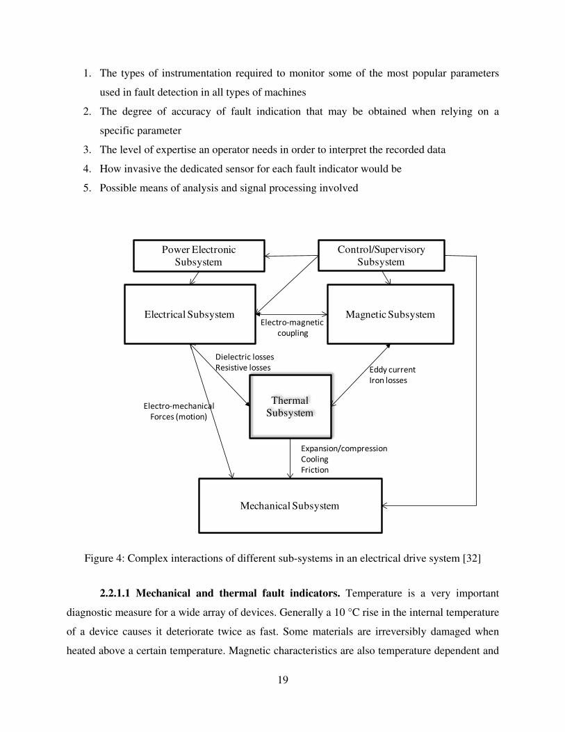
competitive monitoring and diagnosis systems. Figure 4 shows the complex interactions of

physical phenomena at play in a general electromechanical conversion device. These interactions

involve electrical, motion, thermal, fluid flow and chemical phenomenon in a complex interplay

that gradually affects the performance of the device over the course of its lifetime. Various

parameters belonging to these fields can be potential and suitable health indicators for the device.

In order to ensure safety and reliability, OEMs initially relied on simple protective additions to

machines and devices such as over-current protection, over-voltage protection and ground fault

protection [30]. However, as the tasks performed by electrical machinery grew more complex,

improvements were also sought in the area of CBM to provide a more complete device

protection scheme. CBM is therefore a very popular research topic due to increasing industrial

requirements for work place safety.

A number of potential measurement parameters can be identified for the determination of

the failure modes of devices. These can be categorized as mechanical (vibrations and acoustic),

electromechanical (current, voltage, electromagnetic flux leakages, PD), thermal (temperature)

and chemical (oil particulates and gas leakages) [14].

Table 2 is based on the work by Payne and his associates, which is reported in [31], and

provides answers to the listing below.

17

Parameter Device Information Content Intrusive On/Off

Line

Operator

skill Frequency

Part of control

strategy Means of analysis

Current Hall effect transducer Average information content No On High Continuous Yes

RMS trending, Spectral,

Phasor,

Statistical

Voltage Digital voltmeter Average information content No On High Continuous Yes RMS trending, Spectral,

Phasor, Statistical

Flux Search coil Very high information

content Yes and No On High Hourly No

RMS trending, Spectral,

Phasor, Statistical

Force Dynamometer Very high information

content No On High Continuous No

RMS trending, Spectral,

Phasor, Statistical

Vibration Accelerometer High information content Yes and No On Expert Hourly No Spectral, Statistical

Acoustics Microphone High information content No On Expert Hourly No RMS trending, Spectral,

Statistical

Temperature

Thermocouple

Thermal paint

Infra-red camera

Average information content

Low information content

High information content

Yes

Yes

No

On

Off

On

Average

Low

Expert

Continuous

Intermittent

Intermittent

Yes

No

No

RMS trending,

Visual

Instantaneous

angular speed Encoder Average information content No On High Continuous Yes Peak to peak variation

Torque Torque sensors High information content No On Expert Continuous Yes and no RMS trending, Spectral,

Statistical

Table 2: Fault indicators for rotating electrical machines

18

1. The types of instrumentation required to monitor some of the most popular parameters

used in fault detection in all types of machines

2. The degree of accuracy of fault indication that may be obtained when relying on a

specific parameter

3. The level of expertise an operator needs in order to interpret the recorded data

4. How invasive the dedicated sensor for each fault indicator would be

5. Possible means of analysis and signal processing involved

Figure 4: Complex interactions of different sub-systems in an electrical drive system [32]

2.2.1.1 Mechanical and thermal fault indicators. Temperature is a very important

diagnostic measure for a wide array of devices. Generally a 10 °C rise in the internal temperature

of a device causes it deteriorate twice as fast. Some materials are irreversibly damaged when

heated above a certain temperature. Magnetic characteristics are also temperature dependent and

Power ElectronicSubsystem

Control/Supervisory Subsystem

Electrical Subsystem Magnetic Subsystem

ThermalSubsystem

Mechanical Subsystem

Eddy current

Iron losses

Electro-magnetic

coupling

Electro-mechanical

Forces (motion)

Dielectric losses

Resistive losses

Expansion/compression

Cooling

Friction

19

have implications for the demagnetization of magnets in PMSMs. The behavior of PMSM motor

propulsion drives for ships has been studied with details of the effects of temperature on the

permanent magnets in PMSMs during transient thermal published in [25]. Temperature probes

were installed on electrical motors to obtain device temperature information which was used to

monitor the onset of bearing faults by studying thermal images of the bearings for abnormally

hot spots. Ventilation faults were detected by comparing coolant bulk outlet temperature and

inlet temperature during the operation of the machine [33].

Acoustics deal mainly with the ultra-sound range even though some systems are based on

the audible sound range. The audible sound range has shown a lot of promise in the detection of

bearing faults. The contacts between rolling elements with and without cracks generate waves

that propagate through the machine with the speed of sound. The energy of the waves is not

particularly useful since they are very low. The frequencies of the waves can be detected by

piezoelectric transducers. A study based on the principles of acoustic monitoring has also proven

feasible for the detection of loose coil faults using neural networks [34]. Vibration monitoring

uses vibration transducers such as piezoelectric materials to detect the linear frequency spectrum

of vibrations created in machines during operation. These monitors or probes perform directional

measurements of the vibrations in either a radial or axial direction [35]. These probes can also

provide extra information about uneven air-gap, stator winding faults, rotor winding faults,

asymmetrical power supply and imbalances in the driven load [36], [37], [38] and [39].

2.2.1.2 Chemical Indicators. Gas in Oil Analysis (GOA) is the usual practice for

detecting faults using chemical data. Dissolved gases in the oil produced by thermal ageing can

provide an early indication of an incipient fault. Gases normally analyzed are Hydrogen,

Oxygen, Carbon Monoxide, Carbon Dioxide, Ozone, Methane, Ethane, Ethylene and Acetylene.

GOA, together with Oil Particle Analysis using GOA has been, extensively, explored for the

detection of faults in electrical machinery [40].

2.2.1.3 Indicators for stator winding faults. The detection of stator winding faults in

low-voltage machines during operation was a difficult problem in the past since the current

signature during fault is not always distinguishable from the normal healthy state. Hence a large

body of research work was dedicated to other means of detecting these faults in all types of

machines. These techniques include the following:

1. Axial leakage component of the electromagnetic flux [41];

20

2. Electrically excited vibrations [42];

3. Negative sequence impedance [43]– [44];

4. Partial discharge testing [45];

5. Electromagnetic torque [46];

6. Instantaneous power [47];

Frequent changes in the temporal behavior of the power supply causes imbalance, which

in turn obfuscates the fault signature and causes type 1 statistical errors under the hypothesis that

the signature gives the correct indication of a fault. Such false alarms could lead one to detect the

presence of stator fault whilst the underlying problem is actually a supply imbalance. Similar

arguments have been made in connection with the impact of low-frequency load variations and

load changes on mechanical fault detection and the effectiveness of various methods in detecting

such problems [48]. To detect shorted turns in the rotor windings, several methods have been

used including the detection of air-gap flux using a search coil [49], the monitoring of circulating

current in double-circuit machines [50], measurement of the rotor shaft voltage and the

monitoring of harmonic components in the generator excitation currents for synchronous

machines [51].

2.2.1.4 Indicators for detecting rotor faults. Rotor bar problems can result in poor

starting performance, excessive vibrations and increased thermal stresses. These problems lead,

invariably, to other, sometimes more severe, problems which can influence the degradation of

stator and rotor windings. Methods for detecting rotor bar related faults rely on the monitoring of

electromagnetic flux [52], motor torque [53], rotor speed [54], machine vibration [37] and stator

current [55]. Stator current signature analysis is the most common method for detecting rotor

faults because of its simplicity of obtaining stator current information even during loading

conditions. The instantaneous power has been shown to be a good diagnostic tool for detecting

rotor related faults under various loading conditions. This method was shown to be superior to

the analysis of stator current [56].

2.2.1.5 Indicators for detecting bearing faults. Bearing faults can lead to increased

vibration and acoustic noise levels and as such research has focused on a way to use information

obtained from vibration and acoustic sensors for detecting bearing related faults. These

investigations were concerned with spectral analysis of electrical quantities [57]. They have the

added advantage of depending on current sensors that are already available in most drive

21

applications and may provide the same indication without requiring access to the motor by

correlating the characteristic bearing frequencies to the spectral components of stator currents

[58]. A fault signature is, however, distinguishable only if the bearing fault causes a

displacement of the rotor within the air-gap which results in a distortion of the air-gap field.

Hence the initial stages of a bearing fault are difficult to detect since the signal-to-noise ratio is

very low. A 15kW four-pole induction motor has been investigated to determine the feasibility of

using stator current for the detection of an outer defect in a ball bearing with normal radial

clearance [59]. The results showed that current measurement as a bearing fault indicator is not

adequate for this type of motor since the modification produced by the radial movement of the

rotor was found to be very small if the radial movement was restricted to small values. The

difficulty of distinguishing bearing fault signatures from non-fault components or noise in the

stator current has been identified as the main reason for the problems with using stator currents

to detect bearing faults [60]. The reason for the problem with using stator currents was found to

be based on peculiarities associated with the bearing faults which make their detection subtle and

unpredictable. This is the reason why it is proposed to use a modeling technique where changes

in the stator current spectrum are compared to a baseline spectrum rather than searching for

specific fault signature components. The changes are then analyzed and used to identify

developing faults. Before this modeling technique is applied, the stator current should be filtered

to remove the high non-bearing fault components so that changes can be accurately tracked.

Apart from an increase in cost, the mounting of additional sensors is another source of

expense that makes these techniques prohibitive and prevents practical implementation in terms

of operators, clients, motor design and safety regulators. It has been claimed that bearing faults

produce small torque pulsations on the shaft of the rotor and can be a major cause of some types

of faults and whilst insignificant for other types of faults [61]. It may be necessary then to

monitor very small perturbations in the torque of the shaft to determine deviations from normal

behavior even when the frequencies are not exactly known. An ANN has been used for the

purpose of characterizing the spectra of the stator current that are associated with the normal

state of the machine and then for determining spectra from abnormal operation [62]. Testing with

simulated and real machine data showed the promise of using an ANN to diagnose the severity

of bearing faults through the measurement and interpretation of motor bearing vibration

signatures.

22

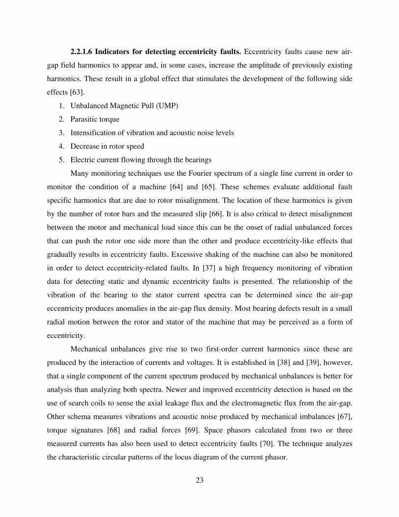
2.2.1.6 Indicators for detecting eccentricity faults. Eccentricity faults cause new air-

gap field harmonics to appear and, in some cases, increase the amplitude of previously existing

harmonics. These result in a global effect that stimulates the development of the following side

effects [63].

1. Unbalanced Magnetic Pull (UMP)

2. Parasitic torque

3. Intensification of vibration and acoustic noise levels

4. Decrease in rotor speed

5. Electric current flowing through the bearings

Many monitoring techniques use the Fourier spectrum of a single line current in order to

monitor the condition of a machine [64] and [65]. These schemes evaluate additional fault

specific harmonics that are due to rotor misalignment. The location of these harmonics is given

by the number of rotor bars and the measured slip [66]. It is also critical to detect misalignment

between the motor and mechanical load since this can be the onset of radial unbalanced forces

that can push the rotor one side more than the other and produce eccentricity-like effects that

gradually results in eccentricity faults. Excessive shaking of the machine can also be monitored

in order to detect eccentricity-related faults. In [37] a high frequency monitoring of vibration

data for detecting static and dynamic eccentricity faults is presented. The relationship of the

vibration of the bearing to the stator current spectra can be determined since the air-gap

eccentricity produces anomalies in the air-gap flux density. Most bearing defects result in a small

radial motion between the rotor and stator of the machine that may be perceived as a form of

eccentricity.

Mechanical unbalances give rise to two first-order current harmonics since these are

produced by the interaction of currents and voltages. It is established in [38] and [39], however,

that a single component of the current spectrum produced by mechanical unbalances is better for

analysis than analyzing both spectra. Newer and improved eccentricity detection is based on the

use of search coils to sense the axial leakage flux and the electromagnetic flux from the air-gap.

Other schema measures vibrations and acoustic noise produced by mechanical imbalances [67],

torque signatures [68] and radial forces [69]. Space phasors calculated from two or three

measured currents has also been used to detect eccentricity faults [70]. The technique analyzes

the characteristic circular patterns of the locus diagram of the current phasor.

23

2.2.2 Current Monitoring for Fault Diagnosis and Prognosis

This section is a detailed look at the use of current as a fault indicator and the different

monitoring techniques available. Current monitoring is given the generic name Motor Current

Signature Analysis (MCSA) and has been used successfully to detect and localize different faults

in electrical machinery. The use of vibration monitoring is the oldest known method for online

fault condition monitoring of electrical machines and has traditionally been the foundation of all

detection, diagnosis and prognosis algorithms. MCSA has, however, replaced vibration

monitoring as a more accurate technique [71]. The main problem with vibration monitoring and

other mechanical indicators is that they are by nature intrusive techniques requiring the

installation of sensors to acquire data for analysis. Besides the increase in cost, these methods

also have a practicality issue since it requires the consent of operators, manufacturers and

industrial safety legislators to agree to the installation of the sensors.

CBM based on current monitoring is very attractive from the stand point that current

sensors are designed into electric drives for machine control purposes. Current and voltage

monitoring techniques can therefore be integrated into the drive control system at no extra sensor

cost. MCSA is usually carried out under full load conditions where current and voltage levels are

large enough. MCSA may, therefore, not be applicable in cases where current measurements are

obtained from no-load testing as is the case when the machine is offline and being serviced [72].

Current monitoring, therefore, satisfies the non-invasiveness criteria, the sensor and

instrumentation reliability criteria, the reliability of diagnosis criteria, and the fault severity

criteria.

2.2.2.1 MCSA for stator winding faults. Many stator winding faults depend on the fact

that stator faults produce asymmetries in the current that increase the space harmonics of

transformed current vectors. The interaction between the electrical quantities at the supply

frequencies and the different space harmonics produce time harmonics in the stator and rotor

currents. Space harmonics of the air-gap flux has been used to produce reliable diagnostic

information [73]. Rotor slotting faults can also be detected by analyzing stator current

harmonics. On the other hand it has been reported that as a result of the nature of the rotor, no

new frequency signatures can be observed in the stator current during a stator winding short

circuit fault [74]. It is reported, however, that in the case of stator turn-to-turn faults there was an

increase in the harmonic components that already existed in case of healthy windings. Negative

24

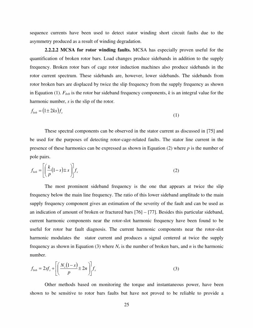
sequence currents have been used to detect stator winding short circuit faults due to the

asymmetry produced as a result of winding degradation.

2.2.2.2 MCSA for rotor winding faults. MCSA has especially proven useful for the

quantification of broken rotor bars. Load changes produce sidebands in addition to the supply

frequency. Broken rotor bars of cage rotor induction machines also produce sidebands in the

rotor current spectrum. These sidebands are, however, lower sidebands. The sidebands from

rotor broken bars are displaced by twice the slip frequency from the supply frequency as shown

in Equation (1). Fbrb is the rotor bar sideband frequency components, k is an integral value for the

harmonic number, s is the slip of the rotor.

( ) sbrb fksf 21±= (1)

These spectral components can be observed in the stator current as discussed in [75] and

be used for the purposes of detecting rotor-cage-related faults. The stator line current in the

presence of these harmonics can be expressed as shown in Equation (2) where p is the number of

pole pairs.

( ) sbrb fssp

kf

±−= 1 (2)

The most prominent sideband frequency is the one that appears at twice the slip

frequency below the main line frequency. The ratio of this lower sideband amplitude to the main

supply frequency component gives an estimation of the severity of the fault and can be used as

an indication of amount of broken or fractured bars [76] – [77]. Besides this particular sideband,

current harmonic components near the rotor-slot harmonic frequency have been found to be

useful for rotor bar fault diagnosis. The current harmonic components near the rotor-slot

harmonic modulates the stator current and produces a signal centered at twice the supply

frequency as shown in Equation (3) where Nr is the number of broken bars, and n is the harmonic

number.

( )s

rsbrb fn

p

sNsff

±

−+= 2

12 (3)

Other methods based on monitoring the torque and instantaneous power, have been

shown to be sensitive to rotor bars faults but have not proved to be reliable to provide a

25

quantitative estimate of broken bars. In this respect, a comparison and performance evaluation of

different diagnostic procedures that use input electric signals to detect and quantify rotor

breakage in induction machines supplied by electrical signals to detect and quantify rotor

breakage in induction machines supplied by mains was reported in [78]. This work reported that

MCSA provided enough information for the detection and quantification of rotor bar breakages

accurately by retrieving an effective diagnostic index that sums the amplitudes of the two

sideband components in the currents spectrum. Other methods that use space vector modulus or

instantaneous power or instantaneous torque measurements loose information since they are

affected twice by the speed reaction and, hence, are not as accurate. The investigation in [79]

showed that MCSA alone was not enough to detect partial rotor bar breakages and the suggestion

was given to combine MCSA with electromagnetic flux monitoring. Burnett and Watson in [80]

developed a methodology to find the location of broken bars within a rotor of an induction

motor. The technique used to detect the location of broken bars involved using the stator

windings as reference locations within the motor from which the distance travelled by the broken

bar can be computed. This technique, however, depended on the accurate determination of the

rotor current spectrum. A drawback of MCSA, however, is that it is difficult to distinguish the

effects of machine faults on the current spectrum from the effects of transient loading conditions

and other conditions on the current spectrum.

2.2.2.3 MCSA for bearing faults. Bearing fault detection depends on indications

provided by the motor current and vibration. The efficacy of current monitoring for bearing fault

detection by correlating the relationship between vibration and current frequencies caused by

incipient bearing faults has been investigated in [62]. In this respect, it was experimentally

shown that there is a correlation between the vibration and current frequencies, since the stator

current signature can be used to identify the presence of a bearing fault. This combined analysis

is supported by the fact that the mechanical vibrations are associated with variations in the

physical air-gap of the machine. When ball bearings support the rotor, any bearing defect will

produce radial motion between the rotor and stator of the machine. Such variations cause the air-

gap flux density to be modulated and the stator currents to be produced at predictable frequencies

related to the electrical supply and vibrational frequencies. It has been suggested that the

mechanical damages related to bearing faults introduce harmonics in the current spectrum at the

frequencies given by Equation (4).

26

bsbrng fff ±= (4)

Other frequency components can be introduced at different frequencies by load

anomalies and it should be noted that they can cause problems with understanding fault data

because these components can be confused with those caused by machine faults. In [81], a

method is shown to separate fault effects from loading effects by comparing the actual stator

current to a model reference value which includes the load effects and the difference between

these two signals provides a filtered quantity, independent of variations of load, that allow

continuous online condition monitoring to be conducted without concern for the load condition.

Simulation and actual machine test results for dynamic and static eccentricity showed the effects

on the spectrum of the air-gap flux under changing load conditions.

2.2.2.4 MCSA for eccentricity faults. Both dynamic and static eccentricity produce

changes in the air-gap flux as mentioned earlier. Stator currents are influenced by air-gap flux

and harmonic analysis can be used to detect these faults. MCSA has been used in [82] to detect

presence of static and dynamic eccentricity faults. Vibration analysis has also been used in [37]

to detect these faults and it has been observed that the effects produced by dynamic eccentricity

can be observed as a by-product of static eccentricity. According to [37], the frequencies of the

harmonics resulting from the asymmetries caused by slotting and eccentricity can be calculated

according to Equation (5).

( ) ( )

±

−±= wdsecc n

p

snkQff

12 (5)

In Equation (5), fecc is the frequency components due to the eccentricity effect, Q2 is the number

of rotor slots, nd is eccentricity order and is zero for static eccentricity and an integer for dynamic

eccentricity. nw is the order of the stator time harmonics that are present in the power supply

frequency driving the motor. Frequency components that are multiples of three of the supply

frequency cannot exist in a balanced three phase set and cannot be monitored. It has, however,

been shown in [12] that only a particular combination of machine pole-pairs and rotor slot

numbers will give rise to significant components related only to static or dynamic eccentricity

and is given by a formula for the number of rotor slots as shown in Equation (6) where is p is the

27

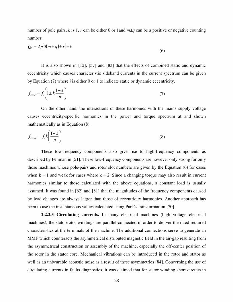
number of pole pairs, k is 1, r can be either 0 or 1and m±q can be a positive or negative counting

number.

( )[ ] krqmpQ ±±±= 322 (6)

It is also shown in [12], [57] and [83] that the effects of combined static and dynamic

eccentricity which causes characteristic sideband currents in the current spectrum can be given

by Equation (7) where i is either 0 or 1 to indicate static or dynamic eccentricity.

−±=

p

skff siecc

11, (7)

On the other hand, the interactions of these harmonics with the mains supply voltage

causes eccentricity-specific harmonics in the power and torque spectrum at and shown

mathematically as in Equation (8).

−=

p

skff specc

1, (8)

These low-frequency components also give rise to high-frequency components as

described by Penman in [51]. These low-frequency components are however only strong for only

those machines whose pole-pairs and rotor slot numbers are given by the Equation (6) for cases

when k = 1 and weak for cases where k = 2. Since a changing torque may also result in current

harmonics similar to those calculated with the above equations, a constant load is usually

assumed. It was found in [62] and [81] that the magnitudes of the frequency components caused

by load changes are always larger than those of eccentricity harmonics. Another approach has

been to use the instantaneous values calculated using Park’s transformation [70].

2.2.2.5 Circulating currents. In many electrical machines (high voltage electrical

machines), the stator/rotor windings are parallel-connected in order to deliver the rated required

characteristics at the terminals of the machine. The additional connections serve to generate an

MMF which counteracts the asymmetrical distributed magnetic field in the air-gap resulting from

the asymmetrical construction or assembly of the machine, especially the off-center position of

the rotor in the stator core. Mechanical vibrations can be introduced in the rotor and stator as

well as an unbearable acoustic noise as a result of these asymmetries [84]. Concerning the use of

circulating currents in faults diagnostics, it was claimed that for stator winding short circuits in

28

double-circuit machines, the measurement of differential current between the parallel connected

half-phases represents an accurate way to detect a fault. Single-winding stators present a more

intractable problem, although it has been observed that there are some harmonic changes in

conditions such as eccentricity and short circuits in the rotor winding of large synchronous

generators as is discussed in [85].

2.2.2.6 Shaft currents. Irregularities in the magnetic circuits of electrical machines may

result in unwanted voltages that lead to shaft currents through the shaft, bearings, bearing

supports and closing through the machine framework. The IEEE Standard Test Procedure for

poly-phase induction machines in [86] discusses the shaft current and presents a measurements

technique for recording either the voltage across the ends of the shaft or the current. It is claimed

in [87] that a Rogowski coil measurement arrangement was enough to yield accurate

measurements of shaft currents, whereas the other methods produce either inaccurate results or

may be too intrusive.

2.2.2.7 Drawbacks with the use of current monitoring. In spite of the many advantages

of using current as a fault indicator, there are important problems with current monitoring. These

demerits with the use of current as the only fault indicator can be addressed by including other

fault indicators. The lists below are some of the drawbacks of using currents monitoring for

CBM in electrical machines.

1. MCSA sometimes cannot distinguish between faults produced by different types of

electrical drive systems since the harmonics contents are similar [88].

2. The spectrum to be studied is sometimes influenced to the same extent by non-fault

events leading false alarms [89].

3. It has been noted that deriving a commercial product for fault diagnosis and prognosis

based on only MCSA becomes very complex and almost impossible to design [90].

4. MCSA also requires a large enough current to produce results that can be used for

analysis. This may be impracticable in some setups [91].

2.2.3 Magnetic Flux Monitoring for Fault Diagnosis and Prognosis

Many of the faults that electrical machines undergo such as UMP, bearing faults, and

winding faults are common to all machines and results in electro-magnetically coupled stresses.

It, therefore, has been a popular research topic to develop electro-magnetic flux monitoring

techniques for CBM. Electromagnetic monitoring has been used alone or used in combination

29

with other fault indicator for the health monitoring of electrical machines. An example is the

work presented in [76] where a number of test were conducted with the stator current and

leakage flux to practically detect broken rotor bars. Monitoring based on flux sensing are also

likely to meet a lot of the criteria required of fault indicators.

There are many ways to sense magnetic fields with the most popular based on the strong

interaction between magnetic and electrical phenomenon. Magnetic sensing techniques exploit a

broad range of physics and chemical applications. The most common sensing techniques are

presented in [92] and shown in Figure 5. A comparison of the different techniques is also

presented based on their sensitivity ranges. The sensitivity range is also affected by the electronic

measurement unit. The most important factors to consider when choosing a sensor for

electromagnetic flux monitoring are signal size range, frequency response and power of the

signal. The specifications for calibration of instruments, characteristics of magnetic fields to be

sensed and uncertainty considerations with the measurement unit can be found in [93].

2.2.3.1 Sensors for electromagnetic flux monitoring. The most common method to

estimate the air-gap flux is to use the machine windings itself to monitor the flux [94]. The stator

winding is therefore used as the search coil in this case to monitor electro-magnetic flux for to

detect rotor-related faults. The converse of this concept is that the rotor may also be used as a

search coil for stator-related faults. The spectrum of the measured flux can be studied to

determine fault in the rotor or stator by correlating the harmonic components to the line current

harmonics content. Search coils are employed to capture flux signals from inside and outside the

machine. Such coils are able to provide electrical quality signatures sensitive to conditions which

alter the electrical characteristics of the motor, such as broken rotor bars, eccentricity, unbalance

between phases and stator faults. The voltages measured in such coils are directly related to the

rate of change of flux. The occurrence of a fault in an electrical machine results in a change in

the air-gap space harmonic distribution. A search coil is able to detect the time harmonics but

cannot capture space harmonics [95]. Space harmonics in the stator causes time harmonics in the

rotating rotor. The placement of search coils in fixed locations in the machine limits the number

of space harmonics to be monitored.

2.2.3.2 Electromagnetic flux regions to be monitored in electrical machines. The best

location of the search coils is to place them in the axial direction to ensure repeatability of the of

flux coil position. The use of internally mounted search coils could also be invasive and not

30

practical for already installed machines. It should only be carried out only if the machine is

important and very sensitive to the faults to be measured and flux monitoring with internally

placed search is the best way to monitor such faults. Some faults like broken damper bars and

short-circuited turns in power generator rotor windings are best monitored using flux monitors

[49], [96] and [97]. Figure 5 presents some of the most comprehensively studied magnetic fluxes

for the identification of particular fault components produced by stator or rotor-related faults.

Figure 5: Comparison of magnetic sensors for magnetic flux monitoring [92]

The axial flux is characteristic of all electrical machines due to unavoidable asymmetries

that must exist in all machines. Leakage fluxes would therefore be produced by both the rotor

and stator sides and hence contain harmonics due to the rotor and stator [40] and [82].

Increments in the amplitudes of specific fault sideband frequencies are indicative of such

abnormalities. The axial leakage flux trajectory is not clearly defined in electrical machines but

usually this is associated with the shaft. In real implementations of this technique, the detection

Magnetic Sensor Technology Detectable Field (G)

(1T = 104G)

10-10 10-6 10-2 102 106

Search-Coil Magnetometer

Flux-Gate Magnetometer

Optically Pumped Magnetometer

Nuclear-Precession Magnetometer

SQUID Magnetometer

Hall-effect sensor

Magneto-resistive Magnetometer

Magneto-diode

Magneto-transistor

Fiber-Optic Magnetometer

Magneto-Optical Sensor

31

of axial leakage flux is fairly straightforward. The technique of measuring the axial leakage flux

is simple and non-invasive. A search coil is wound concentrically with drive shaft; it is claimed

in [98] that the coil can be external to the machine case. End winding leakage fluxes are the main

causes of axial leakage flux, which is measured using axial leakage flux. The source of the eddy

currents in the stator core end regions of large machines is the back-of-core leakage flux which is

a small component of the armature flux that is not contained by the core and which permeates the

space behind the core and tends to be drawn into the circumference members of the core frame.

The axial members of the core frame are exposed to this leakage flux and act as a squirrel cage

with the circumferential members of the members at the ends of the machine providing return

paths [99].

2.3 Electrical Machine Diagnostics and Prognostics Techniques for Condition Based

Maintenance

Industries today consider maintenance a productive activity that extends the life

expectancy of the machines that form the backbone of operations [100]. Maintenance activities

now involve managerial, administrative and technical aspects that promote productivity and

efficiency in a system. Previously maintenance was treated as an expensive undertaking with

elaborate financial instruments to track the cost of maintenance, the amount of time during which

the machine is unavailable and the number of employees temporarily unable to work as a result

of the machine under servicing. The recognition that maintenance forestalls more calamitous

problems with the machine in the future and the cost savings involved got management to

change attitudes towards to maintenance regimes. In acknowledgement of the important role of

maintenance in the overall productivity of machinery in a more complex and rapidly expanding

industrial setup, current efforts are now geared towards reducing costs involved in maintenance,

reducing lead times, improving quality of service, improving the reliability of systems and

addressing environmental issues [101].

Two main maintenance philosophies have been observed over the years in a wide range

of industrial setups. In one paradigm of thought, the oldest approach, components of a system are

serviced when they undergo failure [102]. The feedback mechanism in this case is simple,

requires no extensive analytical work and requires no staff to monitor the health of machines. On

the downside, machine failures can be expensive and so such a regime is only recommended in

32

very simple industrial setups with few sub-components whose repair is either not expensive or

not possible. Such industrial setups were the case some time back but are virtually nonexistent

today. This prompted a second plank in ideas about maintenance involving a range of techniques

aimed at prolonging the life of machinery and anticipating eventual breakdown. The attempt to

increase the lifetime of devices brought about preventive maintenance where routine servicing of

machines were based on time: to avoid complex analysis of machine health, diagnostics was

reduced to servicing machines a number of times in a given period of times irrespective of the

condition or age. This approach also did not take into consideration the overall impact of

unavailability of machines when under maintenance. Another proactive maintenance idea was

then developed to recognize the close connection between the reliability and maintenance of

components. The aerospace industry developed a routine where maintenance of a component

was based on its reliability and the effect of its total failure during normal operation. Failure

Mode Effects Analysis (FMEA) was developed as part of an overall Reliability Centered

Maintenance (RCM) approach. The only missing piece in the RCM approach was that it did not

consider that components degrade with time and only considered the case of normal operation of

the system. This led to an improved notion of maintenance called predictive maintenance which

required ongoing and sometimes online assessment of the health of machinery and sometimes is

called Condition Based Maintenance (CBM).

Condition Based Maintenance therefore continuously monitors health indicators of

components of machines to reduce the uncertainty about impending failures and can be carried

out to different degrees for different machines depending on the criticality of the machine [102].

It is assumed here that the failure of a machine can be predicted by monitoring health indicators

which are quantified and monitored continuously during the use of the machine. This procedure

takes into account the ageing of machine and has the added advantage that failure can be related

to specific component parts. CBM in principle leads to increased precision in failure prediction.

To develop CBM solutions, however, requires a coordinated effort from all levels of

management.

2.3.1 Effective Implementation of CBM

A complete CBM system is composed of a number of functional attributes that together

with a Human Machine Interface comprise a CBM panoply set. The functional aspects of a

complete CBM system includes: sensing and data acquisition, data management and

33

manipulation, condition monitoring, health assessment, diagnostics, prognostics and decision

reasoning. In line with modern trends, standards have been suggested in the CBM community of

researchers and industry stakeholders. Efforts have resulted in 3 main standards that guide an

effective CBM system. These standards include two IEEE standards (IEEE1451 and IEEE 1232),

the Open Systems Architecture for CBM (OSA-CBM) from Machinery Information

Management Open Standards Alliance (MIMOSA) [104].

2.3.1.1 IEEE 1451. At the basic level of CBM systems there are sensors or other devices

to measure the data needed for analyzing the health of an asset. This is often referred to as

Distributed Measurement and Control system (DMC). Due to the customers problem of

integrating different vendor products (transducer, sensors and actuators) when networking, a

standard for the hardware interconnection level is needed. But there is also a need for standards

in the software module of the transducers to achieve network interoperability at the network-

node level [105]. Looking to develop a standardized interface to network smart sensors the

National Institute of Standards and Technology (NIST) started to work together with the Institute

of Electrical and Electronics Engineers (IEEE) in the middle of the 1990’s on the interoperability

of CBM subsystems. To achieve easy installation and upgrading of sensors, one should link them

together like personal computers via a local area network (LAN). Through this connection one

will be able to connect many sensors via a single cable or bus. This will mean that sensors can be

detached without affecting other sensor nodes [106].

The entire IEEE 1451 family consists of four sub-standards, IEEE 1451.1, IEEE 1451.2

and the proposed sub-standards IEEE P1451.3 and IEEE P1451.4. According to [107] all sub-

standards are complimentary, made to be used either as a family or by themselves. The benefits

of the entire IEEE 1451 standard are presented by [108]:

1. Self- identification of transducers

2. Self-configuration

3. Easier to maintain long term self-documentation

4. Easier to upgrade and maintain transducers

5. An increase in data and system reliability

6. Allows for transducers to be calibrated remotely or even to calibrate themselves

The IEEE 1451.2 standard specifies the transducer to microprocessor communication

protocols and transducer electronic data sheet (TEDS) formats. The IEEE 1451.2 interface

34

defines the Smart Transducer Interface Module (STIM). Up to 255 sensors and actuators of

various digital and analog mixes can be connected to a STIM. The STIM in its turn is connected

to a network capable application processor (NCAP) [109]. The IEEE 1451.2 also defines a

Transducer Electronic Data Sheet (TEDS). According to [105], TEDS will achieve self-

identification of IEEE 1451-based sensors or actuators. This will be realized through a memory

chip physically attached to the sensor. The chip will be able to store the information of:

1. Manufacturer’s name

2. Identification number

3. Type of device

4. Serial number

5. Calibration data

According to [109] the risk of losing manufacturing and calibration data (transducer

paper data sheet) will decrease due to the fact that the information will be stored within the

sensor or actuator. The IEEE 1451.1 standard specifies the Network Capable Application

Processor (NCAP) information model. One key reason to standardize the interface at the

hardware interconnection level is the current compatibility problems transducer manufacturers’

face when integrating their devices into multi-vendor networks [105]. The NCAP in 1451.1

could be looked at as a small computer that resides in a specific network node. NCAP’s are

defined as sensor network nodes. NCAP nodes allow multiple sensors to be attached to the

network using one common point of access [107]. The proposed standard IEEE P1451.3 attempts

to define a means to connect the TEDS to the transducer via a bus. Due to potentially harsh

environmental conditions, this will be necessary in some applications. The P1451.3 document

proposes this should be done with a ‘mini-bus’, small and cheap enough to fit into a transducer.

The proposed standard IEEE P1451.4 defines a specification that will add self-describing and

configuration capabilities to analog sensors [108].

2.3.1.2 IEEE 1232. According to [110] and [111] the technical systems of today are more

complex, costly, and difficult to diagnose and repair. To address these problems the Diagnostic

and Maintenance Control (DMC) subcommittee of IEEE SCC20 developed the IEEE 1232

standard family, AI-ESTATE, The Artificial Intelligence Exchange and Service Tie to All Test

Environments. According to [111] the goals with the IEEE 1232 standard are to:

1. Incorporate domain specific terminology

35

2. Facilitate portability of diagnostic knowledge

3. Permit extensibility of diagnostic knowledge

4. Enable the consistent exchange and integration of diagnostic capabilities

Even before the vision of AI-ESTATE was fully developed IEEE 1232-1995 was published.

IEEE 1232-1995 defines the architecture of an AI-ESTATE conformant system. IEEE 1232.1-

1997 defines a standard for how knowledge and data exchange should be accomplished. The

IEEE 1232.2-1998 addresses the issues in system-level diagnosis. After IEEE 1232.2-1998 was

published, the standards all together were published as a “trial- use” standard. This means the

standard was not finalized and could be revised after comments from organizations trying to

implement or use the standard [110]. In 2002 the three standards merged into the current IEEE

Standard 1232-2002.

2.3.1.3 MIMOSA and OSA-CBM. The Machinery Information Management Open

System Alliance, MIMOSA, was founded in 1994 and introduced in the September issue 1995 of

Sound and Vibration. In December 1996 the not-for-profit organization, MIMOSA, was

incorporated. The purpose and goal of MIMOSA is to develop open conventions for information

exchange between plant and machinery maintenance information systems. The development of

MIMOSA CRIS (Common Relational Information Schema) has been openly published at their

website [112]. The CRIS provides coverage of the information (data) that will be managed

within a CBM system. This is done by a relational database schema for machinery maintenance

information. The typical information that will need to be handled is presented by [113]:

1. A description of the configuration of the system being monitored

2. A list of specific assets being tracked

3. A description of system functions, failure modes, and failure mode effects

4. A record of logged operational events

5. A description of the monitoring system and characteristics of the monitoring components

6. A record of sensor data

7. Resources of describing signal processing algorithms and resulting output data

8. A record of alarm limits and triggered alarms

9. Resources describing degradation in a system as well as prognostics of system health

trends

10. A record of recommended actions

36

11. A complete record of work request

OSA-CBM is an abbreviation for Open System Architecture for Condition Based

Maintenance and is a proposal for a de facto non-proprietary standard. This is also the most

comprehensive guide in the area of CBM. In the mission statement from the OSA-CBM

organization it is declared that the standard proposal shall cover the whole range of functions of a

CBM system, for both hardware and software components [112]. Due to the difficulty of

integrating different vendor products most CBM system users limit the flexibility and

performance of a system. The many proprietary standards that exist today have a tendency to

lock customers into a single source solution. An accepted non-proprietary open system

architecture standard would, according to the organization [113], provide:

1. Improved ease of upgrading for system components

2. A broader supplier community

3. More rapid technology development

4. Reduced prices

The OSA-CBM proposed standard divides a CBM system into seven different

layers/components [113].

1. Layer 1 (Sensor Module): The sensor module provides the CBM system with digitized

sensor or transducer data.

2. Layer 2 (Signal Processing): The signal processing module receives signals and data from

the sensor module or other signal processing modules. The output from the signal

processing module includes digitally filtered sensor data, frequency spectra, virtual

sensor signals and other CBM features.

3. Layer 3 (Condition Monitor): The condition monitor receives data from the sensor

modules, the signal processing modules and other condition monitors. Its primary focus is

to compare data with expected values. The condition monitor should also be able to

generate alerts based on preset operational limits.

4. Layer 4 (Health Assessment): The health assessment module receives data from different

condition monitors or from other health assessment modules. The primary focus of the

health assessment module is to prescribe if the health in the monitored component, sub-

system or system has degraded. The health assessment module should be able to generate

37

diagnostic records and propose fault possibilities. The diagnosing should be based upon

trends in the health history, operational status and loading and maintenance history.

5. Layer 5(Prognostics): The prognostic module should have the possibility to take account

data from all the prior layers. The primary focus of the prognostic module is to calculate

the future health of an asset, taking into account the future usage profiles. The module

should report the future health status of a specified time or the remaining useful life

(RUL).

6. Layer 6 (Decision Support): The decision support module receives data from the health

assessment module and the prognostic module. Its primary focus is to generate

recommended actions and alternatives. The actions can be related to maintenance or how

to run the asset until the current mission is completed without occurrence of breakdown.

7. Layer 7 (Presentation): The presentation module should present data from all previous

modules. The most important layers to present would be the data from the health

assessment, prognostic and decision support modules as well as alerts generated from the

condition monitors. The ability to look even further down in the layer should be a

possibility. The presentation module could be built into a regular machine interface.

The above seven layers can be organized more concisely into the three main steps of

CBM practice [114] and depicted in Figure 6. Data acquisition is a fundamental step for

machinery health monitoring, diagnostics and prognostics. Data is acquired from fault and health

indicators and stored from targeted physical assets in the CBM strategy. Secondly useful

information is mined from the acquired data by a number of data processing and analysis

techniques. The final stage of the OSA-CBM strategy is recommendations on maintenance

actions to be taken based on fault diagnostics and prognostics. Diagnostics as used here refers to

the detection and isolation of faults or failures and prognostics refers to the prediction of the

future state of the asset under consideration.

2.4 Analysis Tools for Electrical Machine Fault Diagnostics and Prognostics

Two main types of analysis are carried out in this study. First machine fault models are

analyzed using Finite Element Analysis. The modeling and analysis provides a means to obtain

38

data about electrical machines that can be used to develop diagnosis and prognosis techniques.

Second is the actual fault data analysis to develop techniques for prognostics and diagnostics.

2.4.1 Finite Element Analysis (FEA)

The finite element method is a technique used to solve complex problems, which are

represented by differential equations. It transforms the problems into a series of algebraic

problems which are easier to compute. Electromagnetic problems are described by Maxwell’s

equations [115] which relate electric fields to magnetic fields. The finite element method splits

the problem domain into a large number of small elements shaped as a triangle or a quadrilateral

in 2 dimensions or tetrahedral in 3 dimensions. Other shapes can be used for the meshing process

but triangular meshes are very common. Different techniques exist for the derivation of the

algebraic equations from the initial problem region. The two most widely used methods are the

Variational methods like the Rayleigh-Ritz method [116], [117] and [118] and the Weighted

Residuals methods like the Galerkin Method [116] and[119] with their particular advantages and

disadvantages based on the application at hand. In order to solve a problem, the following steps

are to be carried out:

1. Split the geometry into smaller regions depending on the complexity of the region.

Curved and other more complexly shaped regions should be split in much smaller chunks

than fairly simply shaped regions

2. The materials properties of each region must be determined and assigned

3. External excitations for each region must be determined and assigned

Boundary conditions be established at each discontinuous layer

The first paper to use the term finite element was published by Clough in 1960 even

though similar techniques have been used as far back as the 1940s [120]. The technique was

initially used in Civil Engineering and Aeronautical Engineering problems by large corporations

to study stress distributions in their designs. Since then the method has increased in popularity

mainly because of advances in computer power, speed and cheaply available storage devices.

The method is not pervasive in all fields of engineering and has a number of advantages over

traditional simulation methods: fidelity to actual systems, incorporation of system nonlinearities

and properties.

39

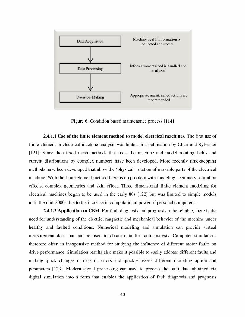
Figure 6: Condition based maintenance process [114]

2.4.1.1 Use of the finite element method to model electrical machines. The first use of

finite element in electrical machine analysis was hinted in a publication by Chari and Sylvester

[121]. Since then fixed mesh methods that fixes the machine and model rotating fields and

current distributions by complex numbers have been developed. More recently time-stepping

methods have been developed that allow the ‘physical’ rotation of movable parts of the electrical

machine. With the finite element method there is no problem with modeling accurately saturation

effects, complex geometries and skin effect. Three dimensional finite element modeling for

electrical machines began to be used in the early 80s [122] but was limited to simple models

until the mid-2000s due to the increase in computational power of personal computers.

2.4.1.2 Application to CBM. For fault diagnosis and prognosis to be reliable, there is the

need for understanding of the electric, magnetic and mechanical behavior of the machine under

healthy and faulted conditions. Numerical modeling and simulation can provide virtual

measurement data that can be used to obtain data for fault analysis. Computer simulations

therefore offer an inexpensive method for studying the influence of different motor faults on

drive performance. Simulation results also make it possible to easily address different faults and

making quick changes in case of errors and quickly assess different modeling option and

parameters [123]. Modern signal processing can used to process the fault data obtained via

digital simulation into a form that enables the application of fault diagnosis and prognosis

Data Acquisition

Data Processing

Decision-Making

Machine health information is

collected and stored

Information obtained is handled and

analyzed

Appropriate maintenance actions are

recommended

40

algorithms. The idea here is that if the algorithms do not work with computer simulation data, it

also would not work with real machine data.

2.4.1.3 Description of the FEM software tool used in study. The numerical

electromagnetic field simulation tool used in this thesis is MAGNET which is developed by

Infolytica. By using this tool one can model and monitor a wide variety of electrical parameters

and hence implement various fault types of varying severity and degrees. This method of

analysis is based on the combined solution of the magnetic field equations and the circuit

equations of the windings. The equations are discretized and solved by the Finite Element

Method. In order to keep the amount of computation at a reasonably low level, several

simplifications have been included:

1. Only a 2-dimensional model is used

2. The skin effect is neglected and the current density in the stator in the windings are

assumed constant

3. The laminated core of the machine is assumed non-conducting

4. Permanent magnets are assumed non-conducting

The magnetic vector potential A, then, satisfies Equation (9) where ν is the reluctivity of the

material and J is the current density.

( ) JA

=×∇×∇ ν (9)

To include the effects of a permanent magnet, as is the case for a PMSM, Equation (9) becomes

as shown in Equation (10) where M is the magnetization vector and µ0 is the permeability of free

space.

( ) ( )MJA

0νµν ×∇+=×∇×∇ (10)

The current density can then be expressed as a function of the vector potential and the electric

scalar potential in Equation (11) where σ is the conductivity of the material and Φ is the electric

scalar potential.

φσσ

∇−∂∂

−=t

AJ (11)

41

For a 2 dimensional Finite Element Analysis as was performed for the analysis in this study, the

vector potential has only the z-components and are given in Equation (12) and Equation (13). k is

the unit vector in the z-direction.

( )kzyxAA ,,=

(12)

( )kzyxJJ ,,=

(13)

The scalar potential, Φ, has a constant value in the cross-section of a two-dimensional conductor

and it is a linear function of the z-coordinate. The gradient of the scalar potential can be

expressed with the aid of the potential difference, E, induced between the ends of the conductor.

By substituting Equation (9) in Equation (10), we obtain Equation (14) where l is the length of a

coil side.

( ) klt

AA µσσν =

∂∂

+×∇×∇

(14)

By integrating the current density, a relation can be obtained between the total current and

potential difference across the length of a coil side as shown in Equation (15) where i is the total

current and R is the DC resistance of the conductor.

∫ ∂∂

+= dSt

ARRiE

σ (15)

The circuit equations for the machine are constructed by applying Kirchhoff’s laws and Equation

(15) above for the potential difference, E. The details of the construction of the circuit equation

have been presented in [124]. Transient 2-dimensional simulations are solved by discretizing

time into short intervals and solving the above equations at each time step using the Crank-

Nicholson time-stepping method. Using this approach, the vector potential at each time step, tk is

given by Equation (16).

k

kk

k Att

A

t

AA

+∆

∂∂

+∂∂

=+

+

1

12

1 (16)

By adding the field equations obtained at different times separated by one time step together,

Equation (17) are obtained.

42

( )

−×∇×∇−=

∆+×∇×∇

+

+++

kEl

AkEl

At

A

kkkk

kkk

σνσ

σν

1

111

2

(17)

The potential difference equation is discretized in the same way as was done with the field

equation to obtain Equation (18).

( ) ( ) ∫ •∆−

++=+ +++

S

kkkkkk Sd

t

AARiiRuu

111

2

1

2

1 σ (18)

Equation (17) and Equation (18) are the basis of the time-stepping formulation and are solved in

the transient and time-harmonic modules of MAGNET.

Some applications require that the motion of the rotor be included in the solution of the

Finite Element Model. This is particularly important to accurately model the eccentricity faults

and is carried by having a different coordinate reference for the rotor than for the stator. The

solutions are then matched with each other in the air-gap. The rotor is rotated at each time step

by an angle corresponding to the mechanical angular frequency. The rotation is accomplished by

changing the finite element mesh in the air-gap called re-meshing. The final solution method is

based on the Newton-Raphson method which is very computationally fast. The magnetic field,

the current and potential differences of the windings are obtained in the solution of the coupled

field and circuit equations described earlier. Torque is calculated by the method of virtual work

which is calculated as the partial derivative of the co-energy functional with respect to virtual

movement. The magnetic field of a healthy electrical machine is periodic in space, typically from

one pole-pair to the next one. In order to reduce the complexity of the geometry and the number

of nodes of the finite element mesh, the calculations are usually performed over the smallest

symmetrical part of the motor model. However, a fault in the machine disturbs the symmetry and

the whole machine cross-section has to be modeled. In this study triangular first-order finite

elements are used and the finite element meshes typically contain 6000 – 8000 elements.

2.4.2 Data Processing

Fault indicator data should be processed and analyzed for useful information about the

condition of the machine under study. Many different sensors and signal processing technologies

43

have been invented and presented in research paper to address the need to make sense out of the

myriad of information that can be collected about a machine. Data management systems like

Computerized Maintenance Management Systems (CMMS) have been designed for such

purposes and shown to have benefited some industries [125]. Some of these benefits reported

include: reducing cost of spares, improving uptime, increasing equipment availability, reducing

lead times, increasing morale, reducing unscheduled maintenance, streamlining work order

schedules and improved the overall maintenance of data. Raw data acquired from sensors are

pre-processed before being used for further analysis. Some waveforms require more processing

and sometimes have to be transformed from one domain of analysis to another more convenient

domain. A number of techniques are available for both pre-processing and processing to remove

background noise, sensor noise and human errors. An adaptive noise cancellation and blind de-

convolution system has been used to detect bearing faults in the presence of noise [126]. It is also

demonstrated in [127] that sensor fault data isolation is the solution for data errors caused by

sensor defects. After data acquisition, a number of techniques are applied to extract useful

information from the data. These techniques are broadly divided into time-domain and frequency

domain techniques. There are also time-frequency-domain techniques.

2.4.2.1 Time-domain techniques. Time-domain techniques are based on statistically

distinctive behaviors of time waveform signals. The simplest time-domain analysis calculates the

signal’s overall root-mean-square (RMS) level and crest factor. Other commonly used

characteristic features are peak-to-peak amplitude, standard deviation, skewness, kurtosis and

time synchronous average. The features described here are called statistical features because they

are based on only the distribution of signal samples with the time series treated as a random

variable. These features are also known as moments or cumulants. In most cases, the probability

density function (pdf) can be decomposed into its constituent moments. A change in condition

causes a change in the pdf of the signal. Hence the moments may also change. Therefore

monitoring this phenomenon can provide useful diagnostic information. The nth moment of the

dataset can be calculated using Equation (19) where N is the number of data points, Exn is the

mean random variable x at the particular point in time, t.

∑ ===

N

i

N

i

n

n xN

xEm1

1 (19)

44

The first four cumulants of the dataset have special names: Mean, Standard Deviation, Skewness,

and Kurtosis, and are calculated from Equation (19). The formulae to calculate these cumulants

are shown respectively in Equation (20), (21), (22) and (23).

1m=µ (20)

2

12 mmsd −= (21)

3

1123 23 mmmmS +−= (22)

4

1

2

1213

3

24 61243 mmmmmmmK −+−−= (23)

In addition to these, non-dimension features can also be used such as the shape factor and the

crest factor. These are calculated as with Equation (24) and (25) respectively where xrms is the

root means square of the data, xabs is the absolute value and xp is the peak value of the data set.

abs

rmsshp

x

x=σ (24)

rms

p

crstx

x=β (25)

Histograms are also used to represent the data and features selected from the histogram.

The histogram is a kind of discrete pdf calculated to put the data into a number of bins of chosen

sizes. If d bins are to be used, with hi as the column height of the ith bin, then each hi is calculated

as follows using Equation (26) and Equation (27).

( ) diixrn

hn

j

iii ≤≤∀=∑=

0,,1

0

(26)

−+

≤≤−

=Otherwise

d

xxix

d

xxiif

xriiii

i

0

)min())(max(1()min()(max(,1

)( (27)

The lower and upper bounds of each bin is calculated as in Equations (28), (29) and (30).

45

2)max(

∆+= iU xh (28)

2)max(

∆−= iU xh (29)

1

)min()max(

−−=∆

n

xx i

i (30)

Useful information can also be based on the uncertainty information from the dataset.

The measure of uncertainty about a signal can be based on entropy which measures the degree of

randomness of the distribution. Entropy estimation is a two stage process: first a histogram is

estimated and then the entropy is calculated. The entropy estimation H(xi) and the standard error

σ(xi) are defined in Equations (31) and (32) where xi is a discrete signal, P(xi) is the distribution

of the entire data set.

( ) ( ) ( )iiis PxInxPxE ∑−= (31)

( ) ( ) ( )[ ]2iiis PxInxPxE ∑= (32)

Other complex time-domain approaches apply time series models to signals. The idea of time-

series modeling is to fit the waveform data to a parametric time series model and extract features

based on this parametric model [128]. The autoregressive (AR) and autoregressive moving

average (ARMA) model are among the most favored time series modeling approaches. An AR

model was applied to vibration signals obtained from an induction motor in [129]. The features

extracted in this work were the coefficients of the AR model. An instance of the successful use

of AR model to address CBM under transient conditions is reported in [130]. It was reported that

using AR coefficients, Multi-Layer Perceptrons (MLPs) out-performed Radial Basis Functions

(RBF). Time-domain analysis, however, is not sufficient and appropriate to detect all kinds of

faults. In some cases the frequency domain techniques out-perform time domain techniques.

2.4.2.2 Frequency-domain techniques. The most widely used approach for bearing fault

detection is to perform analysis in the frequency domain. A localized defect in an electrical

machine like a broken rotor bar can generate a periodic signal with a unique characteristic

46

frequency. These frequency components can be extracted and used for fault diagnosis and

prognosis where time-domain analysis would have resulted in a complicated analysis of the

signal at a high resolution. Frequency-domain analysis usually involves the decomposition of a

signal into simpler parts. Changes in the frequency-domain parameters are associated with faults

in the machine. The conventional approach to obtaining spectral analysis is the Fast Fourier

Transform (FFT). The power spectrum is also a very popular approach that analyzes the power

distribution with frequency. The Discrete Fourier Transform (DFT) is the most common way to

obtain information about the power spectrum. Other methods like the maximum entropy method

are also applicable. The usual pieces of information for fault diagnosis and prognosis based on

frequency-domain analysis are the Frequency Center (FC), Mean Square Frequency (MSF), Root

Mean Square Frequency (RMSF), Variance Frequency (VF) and Root Variance Frequency

(RVF). These are presented, respectively, in Equations (33), (34), (35), (36) and (37).

∫∫

∞

∞

=

0

0

)(

)(

dffs

dfffsFC

(33)

∫∫

∞

∞

=

0

0

2

)(

)(

dffs

dffsfMSF

(34)

MSFRMSF = (35)

( )∫

∫∞

∞−

=

0

0

2

)(

)(

dffs

dffsFCfVF

(36)

VFRVF = (37)

High-order spectrum (bi-spectrum or tri-spectrum) has been shown to be able to extract

more diagnostic information than the power spectrum for non-Gaussian signals [128]. The

application of bi-spectral and tri-spectral analysis has been shown in that high order spectral

analysis is very sensitive to induction motor faults which modify the main spectral components

such as voltage unbalance and single-phasing effects [131]. The envelope technique is used for

the purpose of enhancing small signals and works by separating higher frequency signals from

47

low frequency signals. One of the problems with detecting time domain signals is the fact that

they occur over a very short time range and they tend to spread out over a wide range in the

frequency domain making it difficult to detect.

A number of averaging techniques exist in the frequency domain and can be discussed

under to broad labels: synchronous averaging and spectrum averaging. Synchronous averaging is

very useful in reducing the random noise component in the measurement or in the reducing the

effect of other interfering signals such as noise components from a nearby machine. A

tachometer is required to synchronize each snapshot of the signal to the running speed of the

machine. Unlike synchronous averaging, spectrum averaging does not reduce the noise. Instead,

it finds the average magnitude at each frequency, where a series of individual spectra are added

together and the sum is divided by the number of spectra. Cepstrum has seen widespread

application for fault detection in electrical machines, particularly induction machines. The value

of the main power cepstrum peak has been shown to be a good fault diagnostic [132]. A signal’s

energy is concentrated in the high frequency resonance range and when a signal is generated

from fault data, high frequency resonance technique can be used to provide envelope signals

with high signal to noise ratio. This method is enhanced in [133] to develop an adaptive noise-

cancellation method for CBM. Frequency response methods are, however, not satisfactory under

non-stationary conditions. For such conditions, time-frequency-domain techniques have been

developed.

2.4.2.3 Time-frequency-domain techniques. During startup, electrical machines are

under extreme electrical and mechanical stress. Both time and frequency response methods fail

to detect faults accurately under non-stationary conditions that exist for short durations. Under

these conditions, any UMPs are also at a maximum. The conventional time-frequency technique

uses both time and frequency distributions to more accurately reveal faults in a signal dataset

under more complicated conditions. Some common techniques that use the time-frequency

approach are Short-Time Fourier Transform (STFT) [128] and the Wigner-Ville Distribution

[134].

The wavelet transform is also very popular since it was developed to overcome the short-

coming of the STFT. The main difference between the two techniques is that the STFT give a

constant frequency resolution whilst the wavelet transform uses a multi-resolution technique.

Like the STFT, the wavelet transform decomposes a signal into a linear combination in the time

48

domain. The wavelet transform, however, organizes the transformed signal set into several

components based on the translation of the mother wavelet which changes the scale and shows

the transition of each frequency component: high frequency components are analyzed at a high

resolution and low frequency components are analyzed at a lower resolution. Wavelet transform

analysis has been successfully used to diagnose gear [135] and bearing [136] related faults since

it is impervious to noise. The wavelet transform comes in two flavors: the Continuous Wavelet

Transform (CWT) and the Discrete time Wavelet Transform (DWT). CWTs can decompose an

inspected signal into a family of elementary functions. This information is easier for machine

fault inspectors to understand and helps them to make quick decisions about the condition of a

machine. DWT is a discrete time fast implementation of the CWT which is easy to implement on

digital computers. A comparison of the effectiveness of using the wavelet transform as against

other methods for fault detection is given in [137].

2.4.3 Fault Diagnosis Techniques

Condition monitoring and fault diagnosis are key to a successful maintenance strategy.

Online condition monitoring has become the most important means for obtaining health

information about electrical machines due to its potential to detect faults at an early stage. Fault

diagnosis on the other hand aims at detecting the presence of a particular fault in a system under

test. Diagnostic techniques can be put into two categories depending on whether it is based on

deterministic information or on stochastic information. There is a third but rather uncommonly

considered category called the gray box approach. This third method combines approaches in the

first category, otherwise termed white box approach, and the second category, otherwise termed

black box approach. Both categories can be solved by techniques that are either data-driven or

model-based.

2.4.3.1 Data-driven approaches for fault diagnostics. Data driven approaches rely on a

comparative assessment of the status of a system under testing with other known occurrences and

include both signal processing algorithms and knowledge based methodologies. This method,

inherently, suffers when it encounters machine conditions out of its knowledge domain. On the

other hand, as long as the system performs within its known limits, the diagnostic technique is

expected to be able to detect faulty conditions of the system. The performance of the diagnostic

tool therefore depends on the training performance of the technique. Training algorithms used by

data-driven decision processes are many and is a matured field with an extensive literature.

49

These algorithms are especially appealing since they require no understanding of the underlying

physics of the system under consideration. Most of these intelligent training algorithms are also

able to learn online and can therefore be designed to adapt to the system under consideration.

Data driven approaches have been further separated into Artificial Intelligence

approaches and Statistical approaches. Statistical approaches are based on using statistics to

summarize information obtained about machine faults. A structured method of making decisions

based on statistical inference has been developed and is now available in commercial software.

Cluster analysis is one of the most important statistical tools available and is used to group fault

signals into categories based on characters which they share in common with each other. The

procedure minimizes within-group variances and maximizes between-group variances. The result

of cluster analysis is a number of heterogeneous groups with homogeneous contents. Cluster

analysis was used in [138] to group a nominal training set into clusters that represented each fault

condition. Measurement of new data from each group is used to classify signals obtained during

condition monitoring. New data that does not fit any cluster is considered an anomalous signal.

Other classification algorithms uses distance measures including Euclidean distance,

Mahalanobis distance and Kullback-Liebler distance. These measures form the basis for some

important classification algorithms: nearest neighbor and k-means [139].

Another classification method is based on coefficients of the feature vector and has been

used for fault detection in induction machines [140]. Fault Diagnosis can be posed as a problem

to recognize patterns in a signal dataset that correspond to machine faults. Artificial Intelligence

has been successfully applied to the pattern recognition problems. The difficulty with applying

AI to the specific case of machine fault diagnosis is due to a lack of efficient procedures to

obtain training data and specific knowledge of the faults which are required in training of the

models [141]. Some of the most commonly used AI techniques for machine fault diagnosis

include Artificial Neural Networks, Expert Systems, Fuzzy Logic and Evolutionary Algorithms.

An ANN is computational model that mimics the human brain structure and consists of simple

autonomous processing units connected in a complex layer structure which enables the model to

approximate a complex non-linear function using multiple input and multiple output features.

Each processing unit consists of a node and a weight whose parameters are discovered via

training sets consisting of input set and a desired output set. There are various neural network

models that have different structures that enable the network to better describe the system under

50

consideration. The Feed-Forward Neural Network (FFNN) structure is the most commonly used

ANN structure in machine fault diagnostics [142], [143], [144] and [145]. The FFNN Multi-

Layer Perceptron uses the back-propagation algorithm for training and is the most commonly

used ANN for pattern recognition [146] and [147].

Another type of ANN structure called the cascade correlation neural network (CCNN)

has been applied to bearing fault detection and was shown to sometimes result in the simplest

network structure for fault detection with satisfactory results [148]. CCNN can be used without

initial determination of the network structure and the number of nodes and can be used in

applications that require online training. Other neural network models applied in machine

diagnostics are radial basis function (RBF) neural network, recurrent neural networks and

counter propagation neural networks. The above ANN models usually uses supervised learning

algorithms which require external input such as prior knowledge of the target or desired input.

Supervised training of these ANNs then involves using training algorithms to map the input to

the output. Unsupervised training only takes input data and does not require any prior knowledge

about the input data. The ANN model that uses unsupervised training learns information about

the input data set without external input. One of the most common unsupervised ANN models is

the Self-Organized Map (SOM) and has been applied to rotating machine fault detection [149].

A self-commissioning and online training algorithm for FFNN with particular application to

electric machine fault diagnosis was presented in [150]. An auto-associative neural network was

used in [151] on extracted features from electrical machines to distinguish faults due to the

environmental degradation and that due to vibrations in the system. Expert Systems (ES) utilize

domain expert knowledge with an automated inference engine to perform reasoning for problem

solving.

Three main reasoning methods in the area of machine diagnostics are rule-based

reasoning, case-based reasoning and model-based reasoning [152]. More recently negative

reasoning has been introduced by Hall et al [153]. One of the main limitations with using ESs is

the exponential increase in the number of rules when the variables to be described increase.

Some machine degradation has been described by a Hidden Markov Chain and tested using

synthetic data from a fleet of aircraft [154].

2.4.3.2 Model-based approaches for fault diagnostics. Model-based approaches use a

mathematical model to describe the system under consideration based on the physics of the

51

system. These models are more robust and can better handle new inputs better than data-based

approaches since they are based on the underlying physical laws that have been proved to

describe the behavior of the system. Much work has been done in the area of machine models

with the most accurate modeling technique based on Finite Element Analysis as already

discussed in an earlier section. In [155] and [156], a model-based fault diagnosis method is

presented that uses Finite Element Analysis to model rotating machines. Model-based

commercial software are now available that can model every aspect of electrical machines. These

approaches do not require extensive training using historical data about the system that may in

some cases require extensive pre-processing. Some model-based approaches are also important

for real-time fault diagnosis since these approaches require little data processing.

2.4.3.3 Comparison of data-based and model-based approaches. The most important

difference and, to an extent, limitation of data-based approaches is that when new information

not in the training library of the diagnostic system is presented, it is impossible to predict the

performance of the diagnostic system. The performance of inference system in such cases is due

to either an over-fitted model or an under-fitted model. An under-fitted model can be likened to a

trained biologist who needs further training to be able to recall from memory all the different

types of species of a green-leafed plant. On the other hand, an over-fitted model can be likened

to a well-trained biologist who thinks every plant is green-leafed. Both cases suggest a lack of

enough data representation. Retraining is required under such circumstances whilst model-based

approaches would not require such retraining. Model-based approaches on the other hand require

much more effort and expertise to build mathematical models based on the underlying physics of

the system. Such an effort is generally more than required to build data-based models since lack

of a detailed understanding of the physics of the problem at hand would render any known

historical machine fault data useless. The figure below shows a graphical comparison of the two

approaches. A common occurrence, and strategy used in this work, is to use results from a

model-based approach to train a data-based model.

2.4.4 Fault Prognosis Techniques

The RUL of a piece of device is an important machine parameter of a device that must be

relied on for some service. Prognostics deal with the accurate estimation of the RUL. The

estimation of the RUL can be in terms of time to complete failure or time for the device to attain

some level of risk associated with some existing failure modes [152]. CBM has opened up the

52

field of prognostics to some advances in the technology. These advances mean reduced

maintenance costs, efficiency of maintenance operations and reduction in accidents in the work

place. Current prognostic methods aim to predict the RUL of a defective machine and to predict

the probability of failure at some future date. This means that a reliable prognostic tool works

well if diagnostics about faults are reliable. Prognostic methods can be associated with three

main approaches: data-driven approaches, model-based approaches and reliability-based

approaches.

2.4.4.1 Data-based approaches for prognosis. This approach is derived directly from

routinely monitored system fault indicator data. In many applications, these measured

input/output data are the main means of obtaining a deeper understanding of the system

degradation behavior. The fundamental assumption of data-driven prognostic techniques is that

the underlining statistical characteristic of the degradation process are fairly consistent and only

change when a malfunction occurs in the system. They are built based on historical records and

produce prediction output based on condition monitoring data. The data-driven approaches are

based on time-series analysis techniques and machine-learning techniques for prognostics. Two

of the main data-driven approaches reported in the literature are AI-based methods and Time

Series methods.

2.4.4.2 Time-series methods for prognosis. These methods rely on the availability of

historical data and involve the construction of a time series model of the system that can

determine the state of the system under consideration at a given time. Regression analysis is the

most popular time series technique. A generalized regression model can be represented as in

Equation (38) where Yi is a random variable that represents the value of the ith trial response, βi

are the estimated of the time series model.

ipipii XXY εβββ ++++= −− 1,11,10 (38)

This model has been used in [157] to predict the remaining life of an induction machine. The

method used in [157] estimated the parameters of the regression function, betas, in order to

obtain a representative model by the least squares method. The method of least squares defines a

value Q based on Equation (38) as shown in Equation (39).

53

( )∑ −−−−−−= 2

1,11,10 pipii XXYQ βββ (39)

The simultaneous solution to the equations formed by taking the derivative of Q with respect to

the betas provides the least squares estimates betas and the least squares solution shown in

Equation (40). Least squares estimates are desired because they are unbiased and have minimum

variance.

1,11,1ˆ

−−+++= pipib XbXbY β (40)

The method of maximum likelihood can also be used to estimate betas if the probability

distribution of the error terms is known. Li et al [158] examined an adaptive prognostics

approach where a future bearing defect size was calculated at a t+Δt given the bearing running

condition and defect size at time t. This adaptive algorithm based on a recursive least squares

algorithm was applied to derive a defect power law-based propagation model and was then

employed to account for the time-varying behavior and used to predict future impending failures.

A logistic regression model is demonstrated in [159] to calculate the probability of a failure for a

given condition of variables. Linear and nonlinear regression models are compared in their

abilities and limitations.

The Autoregressive Integrated Moving Average (ARIMA) time series model is a state

estimation technique used in prognostics for trend analysis. ARIMA is a generic construct which

incorporate an Auto-Regressive (AR) processes, Moving Average (MA) processes and an ability

to account for non-stationary trends in the data. Given a time-dependent process Tt, an AR

process of order p is mathematically defined by Equation (41) with variables having the same

definition as in Equation (38) above.

tptpttt TTTT σφφφ +++= −−− 2211 (41)

Estimates of the parameters in Equation (41) are determined by using observed data from the

system under consideration. A Moving Average (MA) process of order p is defined as in

Equation (42).

54

ptpttt tT −−− −−−−= σθσθσθα 2211 (42)

It usual to express the above AR and MA models, respectively, as in Equation (43) and Equation

(44) where B is the backshift operator.

( ) ttTB σφ = (43)

( ) tt BT σθ= (44)

A non-stationary process must be transformed into a stationary process before either MA or AR

is applied. A common transformation is the differencing technique which is a discretized

differentiation of the temporal dataset. Differencing can be done to a degree d and represented in

Equation (45).

( )dBID −≅ (45)

The complete ARIMA model can then be written as in Equation (46).

( )( ) ( ) tt

dBTBIB σθφ =−

(46)

This model can describe both stationary and non-stationary time series but requires a significant

amount of data to estimate the parameters (stuff).

Jardim-Gonclaves and his team [160] used an ARIMA model to predict when Computer

Numerical Control (CNC) lathe and Mill machines would fail. The information gathered about

the machines were vibration data, sound and power consumption in real time and was used to

forecast whether the machines required maintenance in a future time periods given acceptable

ranges on the monitored parameters. Another problem investigated was cracking in materials

under variable-amplitude loading. The developed forecasting model was shown to be adequate

for real time applications such as health monitoring and life extending control. An early warning

system was designed in [161] using a parameter estimation approach for a nonlinear model using

temperature measurements of gas turbines. An AR process to model vibration signal for

prognostics is developed in [162] but the model parameters have not physical meaning. The

55

health condition of the gear is diagnosed by characterizing the error signal between the filtered

and unfiltered signals using both numerical simulation and experimental data. A procedure to

estimate time series parameters is presented in [163] involving two stages. In the first stage,

parameter estimates are obtained from each degradation path and transformed for signals

showing wide variability and non-stationary trends. The estimates from first stage were then

combined to determined estimates of the mean, variance and covariance which were then utilized

to find the lifetime distribution. Another lifetime prediction research work was carried out using

time series models to estimate the degradation probability distribution for solar reflector material

at a given point in time and the lifetime probability distribution [164]. The degradation was

modeled as an AR process using predicted daily degradation based historical data. Sample paths

were obtained using Monte-Carlo simulation to form empirical distribution functions for the

degradation and lifetime distributions.

2.4.4.3 Artificial intelligence approaches. Artificial Neural Networks, Genetic

Algorithms, Fuzzy logic and other learning techniques belonging to the wider field of AI

techniques have the ability to learn a machine’s degradation characteristic from past information.

The most popular AI approach is the ANN. As discussed earlier, ANNs find a functional

relationship between input stimuli and desired output where the parameters of the functional

relationship need to be adjusted for optimal performance. An ANN with one hidden layer is

shown in Figure 7. Only the hidden and output layers have neurons which are the processing

units which respond to inputs to the ANN. Weights are designated from the input layer to the

hidden layer and from the hidden layer to the output layer. In recurrent networks, there can be

feedback connections from the output layer to the hidden layer or self-connections from any

layer back onto the same layer. ANN has been used in the prognosis of faults by several

researchers in the field. One report used ANN to reduce the computational time required for

solving conventional nonlinear differential equations and used the ANN designed to predict

fatigue models and other types of failure models pertaining to the RUL of structures [165].

A Progression based Prediction of Remaining of Life (PPRL) was developed using a

neural network model that combined linear and nonlinear techniques to increase the accuracy of

ARMA models. It can be used to determine the upper and lower bounds of the remaining bearing

life [166]. Another ANN architecture called the Dynamic Wavelet Neural Network (DWNN)

was implemented to transform sensor data to the time evolution of a fault pattern for predicting

56

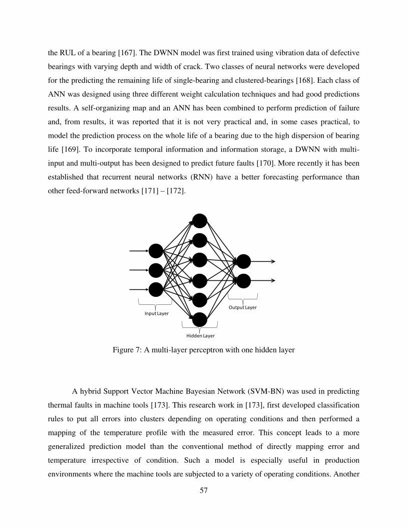
the RUL of a bearing [167]. The DWNN model was first trained using vibration data of defective

bearings with varying depth and width of crack. Two classes of neural networks were developed

for the predicting the remaining life of single-bearing and clustered-bearings [168]. Each class of

ANN was designed using three different weight calculation techniques and had good predictions

results. A self-organizing map and an ANN has been combined to perform prediction of failure

and, from results, it was reported that it is not very practical and, in some cases practical, to

model the prediction process on the whole life of a bearing due to the high dispersion of bearing

life [169]. To incorporate temporal information and information storage, a DWNN with multi-

input and multi-output has been designed to predict future faults [170]. More recently it has been

established that recurrent neural networks (RNN) have a better forecasting performance than

other feed-forward networks [171] – [172].

Figure 7: A multi-layer perceptron with one hidden layer

A hybrid Support Vector Machine Bayesian Network (SVM-BN) was used in predicting

thermal faults in machine tools [173]. This research work in [173], first developed classification

rules to put all errors into clusters depending on operating conditions and then performed a

mapping of the temperature profile with the measured error. This concept leads to a more

generalized prediction model than the conventional method of directly mapping error and

temperature irrespective of condition. Such a model is especially useful in production

environments where the machine tools are subjected to a variety of operating conditions. Another

Input Layer

Hidden Layer

Output Layer

57

popular AI technique that is used for prognostics is the fuzzy logic technique. Fuzzy Logic

provides a language into which one can translate qualitative knowledge about the problem to be

solved using linguistic variables to model dynamical systems. The meaning of a linguistic

variable may be interpreted as an elastic constraint on its value. These constraints are propagated

by fuzzy inference operations. The resulting reasoning mechanism has powerful interpolation

properties that in turn give fuzzy logic a remarkable robustness with respect to variations in the

system’s parameters and disturbances. When applied to prognostics, fuzzy logic is typically

applied in conjunction with a machine learning method and is used to deal with some of the

uncertainties that all prognostic estimates have to deal with. Fuzzy logic was employed to

produce an accurate estimate of the health of system under consideration by developing an

automatic health state estimation procedure to represent the degree of severity [174]. In a major

paper by Wang et al [175], a Neuro-Fuzzy and an RNN are applied to sunspot benchmark and

on-line gear test data. In the sunspot testing, NF without interpolation is less accurate than RNN

even though NF produces more accurate results than RNN. For online testing, NF was more

superior to RNN.

Another machine learning approach is anomaly detection algorithms that learn a model of

the nominal behavior of systems and then notice when sensor data fail to match the model,

indicating an anomaly that could be a failure precursor [176] – [177]. The strength of data driven

techniques is their ability to transform high-dimensional noisy data into lower dimensional

information for diagnostic/prognostic decision. The main drawback with data-driven approaches

is that their potency is very much dependent on the availability and quality of system operational

data.

2.4.4.4 Model-based approaches for prognosis. The model-based method relies on

accurate mathematical descriptions of the system and is the approach used in this dissertation.

The approach in model-based prognostic is to compare the model output with actual system

output and analyze residuals to predict impending faults in the system. Statistical techniques are

normally used to define thresholds to detect the presence of impending faults. The model-based

approach is applicable when mathematical models can be constructed from first principles. It is

shown in [178] that symptom models used in vibration condition monitoring for condition

recognition and prediction can in most cases be limited to Weibull and Frechet models. A

discrete-time finite-state shock model can be employed for the purpose of modeling cumulative

58

damage to an individual component. In this basic form, such models provide a means to compute

the cumulative distribution function of the random time required to reach a failure state. The

failure state in the shock model corresponds to a pre-specified level of cumulative damage which

is assumed to be a monotonically increasing function of time. Conditions about damage

processes that are important to a device’s lifetime distribution are presented in [179]. A system

was analyzed whose failure was caused by the occurrence of a shock greater than some pre-

specified level [180].

An adaptive prognostics system to estimate bearing defect size growth using an adaptive

algorithm based on Recursive Least Square (RLS) is presented in [181]. It was shown in the

study in [182] that due to the lack of parameter fine tuning, small parameter difference can result

in large prediction error as the bearing cycles increase. It is also reported that bearing lifetime

can be evaluated and predicted effectively by monitoring the changes in the dynamic stiffness

based on real-time vibration measurements. Adams in [183] reports that damage accumulation in

structural dynamic systems can be modeled as first or second order nonlinear differential

equations. In [184] degradation is modeled as a process with a time-constant applied to the actual

degradation process and a different time-constant applied to the observable subsystem to track

battery degradation. Degradation has also been modeled as a discrete-time Markov process to

represent the failure processes for computing the RUL of the system investigated [185][184].

The ability of a hidden Markov model- based clustering method in autonomous diagnostics and

prognostics is reported in [186]. The prognostic model in [186] is derived from a multivariate

distribution of the state transition points generated by HMMs.

Kalman filtering is also considered a prognosis technique by estimating some state value

at a future time. Kalman Filtering incorporates the signal embedded with noise and forms a

sequential minimum mean square error estimate of the signal. Kalman Filtering was proposed to

track the dynamics of the mode frequency of vibration signals in a tensioned steel band with a

seeded crack growth. A nonlinear model of crack dynamics for real-time computation of time-

dependent damage rate in mechanical structures has been proposed in [187] by Ray and his

associates. This model allows construction of a filter for damage state estimation and remaining

service life prediction based on an extended Kalman Filter principle instead of solving the

Kolmogorov forward equation. These authors also presents new results in that examine fatigue

crack growth prediction using Gauss-Markov processes which did not require solution of the

59

extended Kalman Filtering equation. Validation of the model was limited in experimentally-

generated statistical data. The main advantage of model-based approaches is its greater coupling

to the physical system under consideration. Features generated using model-based approaches

are also very closely related to the model parameters [184]. Parameter drift in relation to selected

prognostic features can be represented functionally. If the knowledge of the system degradation

is available, the model can be adapted to increase its accuracy and to address subtle performance

problems. Consequently, it can significantly out-perform data-driven approaches. Model-based

approaches, however, require a greater understanding of the problem at hand than is required for

data-driven approaches.

2.4.4.5 Reliability-based approaches for prognosis. Reliability engineers rely heavily

on statistics, probability theory and reliability theory. Many engineering techniques are used in

reliability engineering such as reliability prediction, Weibull analysis, thermal management,

reliability testing and accelerated aging testing. The conventional reliability-based approaches

for prognostics can be divided into two categories: failure-based and degradation-based [188].

Failure-based reliability is used to estimate the RUL distribution and its parameters when

sufficient, representative and censored failure time data exists. If prior knowledge of the lifetime

distribution exists for similar components, then the lifetime distribution is assumed to follow the

same distribution of a similar component. Compared to failure-based reliability, degradation-

based reliability focuses on using measures of component degradation, not failure data to assess

the RUL of a component.

Degradation is known as cumulative in most instances and compendium of degradation is

presented by Chao [189]. Proportional hazards models are commonly used in failure prediction

and reliability analysis. Proportional hazard models assume that hazards changes proportionally

with covariates and the proportionality constant is the same at all times. A reliability based

approach is presented in [190] for estimating the optimal maintenance policy to minimize the

total maintenance cost per unit time. They used Proportional hazard models to identify the

importance of monitored variables and total time on test plot to find the optimal policy.

2.5 Rotating Machine Insulation Systems

An insulation system consists of insulating materials and insulating distances that

function to separate components of different electrical potential. The insulating system also

60

provides mechanical strength to the machine and can act as conduits to direct heat from the

windings to the surrounding cooling system. There are many, commercially, available insulating

materials with the most the popular being the following listing: Mica, Polyester films, Aramid

paper and Epoxy resins.

There are three types of insulating distances in the electrical machine insulation systems.

The first is an air clearance and depends on the Paschen Law that says that the breakdown

characteristic of a gaseous medium is a product of the gas pressure and the gap length of the

separation. The second type of distance is created by solid insulation where the electric field is

not aligned along the interfaces of the insulators. The insulating strength in this case is

determined by the thickness of the insulation and the relative permittivity of the insulating

material. The final type of insulating distance is a creepage distance in which a bare live part is

connected to a conductive or insulated component in another electric potential such as the

grounded frame of the machine.

Generally an insulation material should be track resistant, remain with low conductivity

during operation, thermal resistant to short-term overloads during operation and also to

cumulative ageing. The insulation takes up space and this should be carefully considered when

dimensioning the machine during design.

2.5.1 Insulation of Rotating Electric Machines

There are two main broad categories of insulations in electric machines: Ground-wall

insulation and conductor insulation. The function of the ground-wall insulation is to separate

components that are not in galvanic contact with each other. This may be the case for the

winding coils and the machine iron frame. Conductor insulation separates wires and turn

insulation and are usually thinner that the ground-wall insulation. Electric machine insulation

types can also be identified based on the location of the insulation. This classification method

then identifies the following types of insulation:

1. Phase-to-phase insulation in the slow and in the coil

2. Insulation of terminals and connecting leads

3. Surface varnish and protective paint

4. Impregnating varnish and resin

5. Slot insulation and slot closer

61

2.5.2 Insulating Materials

As mentioned earlier, insulation materials should have good thermal properties. Table 3

shows the thermal classification of insulating materials adapted from the IEC 60085 and IEC

60034-1 standards. Polyester is one of the commonest insulating materials and is a suitable

material for slot insulation since it has good mechanical strength. Aramid paper is used when two

materials are employed in the slot insulation since it has better thermal resistance and

impregnation properties than polyester. For more mechanical strength, especially, for high

voltage machines, mica is used. Mica is an inorganic mono-clinic material that occurs commonly

in bedrock. Mica also has very good thermal endurance at temperatures as high as 1100 ºC. Mica

also has a high dielectric strength with very low dielectric losses. The characteristics of mica are

given in Table 3 which is adapted from the work by Paloniemi and Keskinen. Insulating films

include duraplastics with very restrictive thermal resistance properties. Some insulating films

include Polyethyleneterephthalate (PETP), Nomex and Polyimide films.

Table 3: Thermal classes of insulation materials

Thermal classes of insulating materials (based on IEC 60085 and IEC 60034-1)

Thermal class

Previous designation

Hot spot allowance

Permitted temperature rise/K when

temperature is 400C

Permitted average winding

temperature/0C 90 Y 90

105 A 105 60

120 E 120 75

130 B 130 80 120

155 F 155 100 140

180 H 180 125 165

200 200

220 220

250 250

2.5.3 Dimensioning of an Insulation

The dimensioning of insulation is based on the electrical, mechanical and thermal stresses

that the insulation would be exposed to during its lifetime. The compression stresses on the

insulation is usually higher than the tensile stresses on the machine and insulation dimensioning

62

should enable the machine be able to withstand more compression by using the appropriate the

material [191]. In some parts of the machines or for some machines, flexibility is a key aspect of

the structure of machine assembly and flexible insulation systems have to be employed.

The voltage endurance properties of the insulation system after design and construction

should be able to withstand intermittent over-voltages at operating frequencies, switching over-

voltages at higher frequencies and exposed over-voltages due to corona. The voltage handling

capability of the insulation material is the first step to determine an approximate value for the

thickness of the insulation and the relation to determine the value is given in Equation (47) below

where d is the thickness of the insulation material, U is the voltage over the insulation and Emax is

the highest allowable electric field in the material concerned.

max/ EUd = (47)

If the insulation is composed of several layers, the thicknesses of these layers can be estimated

from Equation (48).

+=+=

2

2

1

12211 εε

ddDdEdEU (48)

After the thickness is calculated, a test of the insulation is needed to ascertain the actual

withstand properties. The test for motor below 1 kV is done at a voltage given IEC standard

60034 using Equation (49), where UN is the rated line-to-line voltage and Utest is the test voltage.

Equation (50) is used for motors above 1 kV

V 5002 += Ntest UU (49)

V 10002 += Ntest UU (50)

For high voltage machines, the insulation material should be able to withstand high impulse

voltages which are calculated using Equation (51) where Upeak is the peak value of the impulse

voltage.

VUU Npeak 50004 += (51)

63

2.6 Partial Discharges

The subject of Partial Discharges can be traced to the beginning of the twentieth century and thus

is a well-developed field. The continued interest in investigations in the field of PD has been due

to its importance as the preeminent tool for assessing the quality and performance characteristics

of insulation systems of High Voltage equipment [192].Over the years, the level of investigative

effort has varied greatly in terms of the type of equipment under investigation and discharge

behavior being studied: nature and form of discharge, detection sensitivity, degradation of

insulation, discharge quantities recorded, pulse repetition rate, energy loss, distributions of pulse

heights, discharge epochs, pulse separation time intervals and pattern recognition for source

location detection.

The most important area where PD studies have had the most remarkable influence is in power

distribution cables. This is attributable to a number of factors: the simple geometry of power

cables and easy to describe transmission line behavior which enables easy interpretation of PD

measurements. Discharge behavior for transformers and, especially, for rotating machines are

relatively more complex to analyze due to the complex geometries involved, complex

transmission line behavior of coils as well as coupling and resonance effects between windings.

In the case of rotating machines, there is the other issue that detected pulses vary widely from

low levels for discharges in the stator bar insulation to very high levels for slot discharges. This

wide variability in PD pulses for rotating machines leads to the problem of calibration which is

still a controversial issue since a school of thought is pushing for calibration as a prerequisite for

rotating machine PD measurements whilst another school of thought wants to relax calibration as

a prerequisite.

2.6.1 PD Detection

Early PD detection systems were developed in the 1930s and were analog devices that were

reliable for detecting PD inception and PD extinction voltages. These early detectors displayed

PD patterns oscillographically on a power frequency time base and calibrated ordinate scale. The

development of crystal controlled pulse counters in the 1950s allowed the counting of PD pulses

per unit time and thereby the determination of pulse density of discharge patterns. The advent of

PC computers in the 1980s and their extensive use in the 1990s rapidly altered the approach in

the PD pulse distribution analysis area in that the instrumentation shifted away from the

64

hardware based instrumentation to software dominated techniques [193]. This development led

to extensive research work in pattern recognition and classification [194]. The studies by van

Brunt indicated that magnitude of a discharge pulse and its epoch or phase of occurrence is

strongly influenced by the occurrence of a preceding pulse or pulses [195]. This non-Markovian

point process tended to pose problems for PD pattern recognition and classification techniques.

The 1990s also saw the rapid expansion of digital circuits for PD measurement. With the

availability of GHz bandwidth oscilloscopes, it is now possible to detect PD pulses with a rise

time between 1 to 2 nanoseconds.

2.6.2 PD Mechanisms

PD activity may involve a streamer discharge which is dependent on cathode emissions

and Townsend discharges which are dependent on photo-ionization of the gas in a short burst

that may assume different forms: rapid and slow rise time spark-type pulses, true pulse-less

glows or pseudo-glow discharges [196]. Streamer discharges typically occur over larger gaps

over which discharges propagate due to ionizing radiation at the streamer tips. The classical

Townsend process is characterized by weakly ionized plasma having a small space charge

producing field, which is negligible compared to the externally applied field. Its electron

temperature is approximately 104 K and the dominant ionization process is direct ionization.

True glow or pulse-less discharge consists of weakly ionizing diffused plasma generally

occupying all available inter-electrode space. Appreciable space formation occurs in both the

proximity of the anode and cathode and the discharge process as in the case of classical

Townsend discharges is maintained through cathode emission. A glow discharge is not in local

thermal equilibrium and the temperature ranges from 10000 K to 20000 K. Direct ionization

plays a big role and the step-wise ionization, while negligible at low currents, may become

important at currents in the range of 0.1 A. The pseudo-glow discharge is similar to the pulse-

less glow in the degree of ionization, electron temperature and particle densities but exhibits at

the same time the presence of minute discharge pulses having features characteristic of spark

type discharges. The presence of the minute pulses is readily detected electronically and optically

by a photomultiplier [197]. The space gap pulse or spark PD is similar to the pulse-less glow and

pseudo-glow discharges in that it is also a Townsend type discharge with the unique

characteristic that undergoes a high degree of ionization and the discharge has a high

65

conductivity. Spark type PD are commonly classified as rapidly and slowly developing sparks or

pulses.

A PD activity, in most, cases involves the simultaneous occurrence of a pulse, glow and

pseudo-glow. Most measuring instrument designs have focused on the detection of pulses and

have relegated the glows and pseudo-glows to obsolescence. If we consider an idealized cavity

occluded within an insulation system that is subjected to a sinusoidally varying applied voltage

and make the extra assumption that only pulse or spark type discharges are possible within the

cavity, then the cavity would discharge when the voltage attains the breakdown value. When the

cavity discharges, the voltage wave across the cavity collapses abruptly to some residual voltage.

The resultant voltage step would excite the PD detection circuit and the generated event would

be recorded as a discrete PD pulse. Further pulses would be detected along the ascending and

descending ends of the voltage wave each time the applied voltage exceed the breakdown value.

Greatly enhanced space charge induced photo-ionization at the cathode at voltages above

breakdown voltages leads to PD current pulses with very much reduced rise times and

augmented peak amplitudes. At high voltages across the cavity, the resultant electrical field E,

increases with the ionization frequency vi in a formulation described in Equation (52).

eei En µαν = (52)

2.6.3 Partial Discharges in Cable Specimens

Since the introduction of Polyethylene (PE) extruded cables in the power distribution

sector in the early 1950s, a rapid development of PD detection has occurred to enable the

assessment of the reliability of these new cables. Much of the development went into

characterizing the PD behavior in these cables as well determining their resistance to PD

degradation. Several PD detection instruments were designed for the purpose of measuring PD

discharges and it soon became evident that PD originated from cavities within the extruded

insulation or at interfaces between the insulation and the semiconducting conductor and

insulation shields. Polyethylene was found to be susceptible to PD discharges and could not be

operated in the presence of PD. Go-no-go tests were designed to ensure that manufactured cables

were PD free above the operating voltages [198]. Long transmission cables need to be terminated

with their characteristic impedance to avoid reflections from PD pulses.

66

The widespread use of computers has enabled the simultaneous display of three

dimensional plot of pulse magnitude and pulse count as a function of the discharge epoch over a

given time interval at a given value of applied voltage. Over the last decade a lot of effort has

been concentrated to finding site of increased PD activity that might fail from degradation due to

discharges. These efforts have resulted in two types of techniques for cable assessment: no-probe

and probe test methods. The two most notable non-probe PD site location methods are the Pulse

Polarity Correlator and Time Domain Reflectometry. Probe test methods for solid polymeric and

oil-impregnated-paper cables involve scanning probes of either capacitive or inductive types.

2.6.4 Partial Discharges in Transformers

As mentioned earlier, PD measurement and interpretation in transformers are far more

complex than in cables. Since transformers are inductive, any discharges that take place within

the transformer windings are separated from the measuring instruments by large inductive

impedance which appears in parallel with a distributed capacitance and is shunted to ground by

another distributed capacitance. The PD pulse that finally emerges at the discharge site must

travel over a complex LC network prior to reaching the terminal of the transformer. It is also

attenuated and distorted since its high frequency components are filtered out. Resonance can also

occur between the windings and turns within the windings which can introduce errors into the

PD quantities should these resonant frequencies fall within the bandwidth of the PD sensing

system.

PD tests on transformers may be performed using either the so-called induced test or by

means of a separate independent power frequency voltage source to produce the voltage stress in

the insulating system. In the induced test, the voltage is applied across the low potential winding

whereby the voltage stress is impressed between the individual turns and sections of the

windings under normal operating conditions in service. When this test is administered on larger

transformers, it is common practice to use the third harmonic of the power frequency source in

order to permit an over-voltage test on the transformer without saturating the magnetic core.

Higher harmonics can also be used for this test using higher voltages. For smaller transformers,

the power frequency voltage is generally applied to the HV winding by means of a discharge-

free test transformer. The transformer insulation is thus voltage stressed between the high

potential winding and the low potential winding as well as ground. The calibration of PD

detection for transformers is the same as for cables. A known charge is injected into a small

67

capacitor whose capacitance can vary from 50 pF to 150 pF. In the interpretation of PD

measurements it is important to stress that two main discharge mechanisms are possible are

possible with oil-filled power apparatus. In the first case, PD can occur, classically, within the

insulation materials with positive discharges occurring at start of the negative half cycle and

negative discharges occurring at the start of the positive half cycle. In addition to this, discharges

can also occur within transient cavities created at electrical field stress points.

This suggests that PD distribution patterns can be used to ascertain the extent and nature

of discharge activity in inductive power apparatus. They may also be utilized to differentiate

between the discharges emanating from within the transformers and those due to noise. The latter

may consist of thyristor pulses, modulated periodic signals, poor electrical contacts or corona

discharges form HV leads and are characterized by a different pulse distribution pattern.

Sometimes these patterns are so different, only experienced operators using conventional PD

detectors can recognize them. It was reported in that using fractal analysis, changes in PD pulse

distribution patterns could be used to detect gross defects that were artificially introduced in the

form of an aluminum rod extending from the HV sphere of a transformer or a floating shielding

electrode or an absence of shielding electrode on the test object. In another study [199], carried

out on an electrical apparatus using the shape parameters of PD pulse distribution curves, it was

shown to be possible to distinguish between defects and actual PD discharges in electrical power

apparatus. However, the recognition method used was general in the sense that it only

determined whether or not the detected discharge pulses emanated from within the test specimen.

The method proposed did not resolve important aspects of the discharge: number of defect

cavities involved, distribution throughout the affected cable and their location.

There are number of tests for PD site location that may be used on power transformers

specimens. While the theoretical basis for these tests may be sound, such tests have not found

wide use in the industry because of implementation on real transformers. The most widely used

method compares the PD magnitudes measured at the terminals of the three respective windings.

The peak voltage amplitude of the PD pulse front can be given by Equation (53).

−∆=∆

sh

set

C

CnVV exp (53)

Acoustical PD site location techniques have been reported and applied to actual transformers

using a triangulation method where three acoustic sensors are positioned randomly. An

68

oscilloscope is triggered by the arrival of the acoustic signal which is compared to signals that

arrive later to ascertain their location.

2.6.5 PD Mechanisms in Rotating Machines

The use of inorganic mica flakes in epoxy resin impregnated stator bars insulation

systems imparts substantial resistance to PD to the insulation systems of large power turbo and

hydro-generators. This explains the fact that machines can often run for decades in the presence

of PD activities of elevated intensity as compared to other electrical apparatus. As a

consequence, the approach to PD measurements in machines differs considerably from that HV

equipment in that the emphasis is more on ascertaining the discharge intensity and PD site

location in terms of density and configuration of PD pulse distribution patterns. This can be

contrasted to the cable and transformer industry where PD is never tolerated under operating

conditions. There are cases where PD magnitudes have been reported in the range of 100 pC to

1000 pC in the insulation bars at operating voltages and PD magnitudes as high as 100000 pC

recorded in the coil ends, core exits points and within the PD eroded and mechanically abraded

semiconducting paint regions.

There are number of PD detection methods developed for rotating electric machines. The

oldest method used a simple filter arrangement to detect PD across the neutral resistor of a

generator while in operation whilst the standard PD detection arrangement with a discharge-free

coupling capacitor connected sequentially in each phase with a separate power supply was used

in the offline case. This method has been improved upon over the years eliminate interference

from extraneous noise sources. These early detection methods showed the practical importance

of slot discharge in the degradation of rotating machine insulation systems. These initial

arrangements have since been superseded by more sophisticated techniques and enabled PD

pulse phase or discharge epoch analysis. These analysis of importance in rotating machines since

it can be used to ascertain whether PD activity originates from the phase under consideration or

coupled from the other phases. Offline PD tests on rotating machines are normally carried out

during general maintenance periods over which it is possible to examine machine windings for

possible discharge induced degradation and determine whether replacement of any aged bars are

needed. The HV stator bars of the machines are tested with rotors removed usually using

50/60 Hz power supplies even though frequencies as low as 0.1 Hz has been used. Offline tests

have the advantage that machine specimen can be isolated from extraneous noise as well as

69

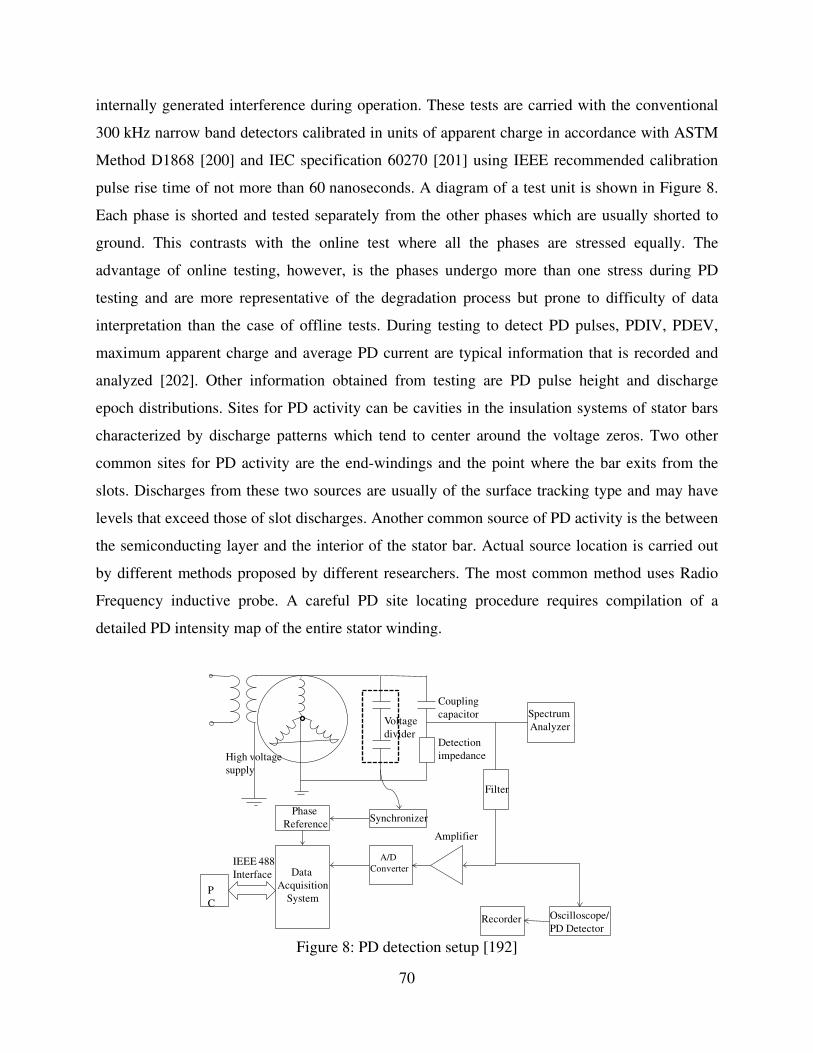
internally generated interference during operation. These tests are carried with the conventional

300 kHz narrow band detectors calibrated in units of apparent charge in accordance with ASTM

Method D1868 [200] and IEC specification 60270 [201] using IEEE recommended calibration

pulse rise time of not more than 60 nanoseconds. A diagram of a test unit is shown in Figure 8.

Each phase is shorted and tested separately from the other phases which are usually shorted to

ground. This contrasts with the online test where all the phases are stressed equally. The

advantage of online testing, however, is the phases undergo more than one stress during PD

testing and are more representative of the degradation process but prone to difficulty of data

interpretation than the case of offline tests. During testing to detect PD pulses, PDIV, PDEV,

maximum apparent charge and average PD current are typical information that is recorded and

analyzed [202]. Other information obtained from testing are PD pulse height and discharge

epoch distributions. Sites for PD activity can be cavities in the insulation systems of stator bars

characterized by discharge patterns which tend to center around the voltage zeros. Two other

common sites for PD activity are the end-windings and the point where the bar exits from the

slots. Discharges from these two sources are usually of the surface tracking type and may have

levels that exceed those of slot discharges. Another common source of PD activity is the between

the semiconducting layer and the interior of the stator bar. Actual source location is carried out

by different methods proposed by different researchers. The most common method uses Radio

Frequency inductive probe. A careful PD site locating procedure requires compilation of a

detailed PD intensity map of the entire stator winding.

Figure 8: PD detection setup [192]

Voltage

divider

High voltage

supply

Coupling

capacitor

Detection

impedance

Spectrum

Analyzer

Filter

Amplifier

Oscilloscope/

PD DetectorRecorder

A/D

Converter

SynchronizerPhase

Reference

Data

Acquisition

SystemP

C

IEEE 488

Interface

70

CHAPTER 3

AC motors are widely used in many industrial applications. Induction machine of the

squirrel cage type are particularly popular because of their simple structure, low cost production

and less maintenance. In spite of these favorable characteristics of the induction machine, it is

limited in its application areas because of the working speed which is lower than the speed of the

rotating magnetic field. More importantly the slip depends on the load torque in the sense that an

increasing load torque results in a decrease in rotor speed. Hence, the induction motors are not

suitable for applications which require an accurate control of speed and position such as servo

systems. On the other hand, speed of synchronous motors can be accurately controlled by

varying the synchronous frequency of the rotating magnetic field. However, synchronous motors

suffer from high production and maintenance costs. Permanent magnet synchronous machines

(PMSMs) are compromise between the induction machine and the conventional synchronous

machine and have been widely used in many industrial applications. Due to their compactness

and high torque density [203], PMSMs are, particularly, used in high-performance drive systems

such as submarine propulsion. The permanent magnet synchronous motor eliminates the use of

slip rings for field excitation, resulting in low maintenance and low losses in the rotor. The

PMSMs have the high efficiency and are appropriate for high performance drive systems such as

CNC machines, robotic and automatic production systems in the industry [203].

Due the specialized nature of the application areas of the PMSM, CBM for fault

diagnosis has become mandatory for all PMSM drives. Fault tolerant operation of Adjustable

Speed Motor Drives (ASMD) has become a design requirement and drives operate under

different conditions for healthy and faulted machines to ensure service availability whilst

minimizing further damage. Fault detection is an important first step in the design of fault

tolerant drive systems. Health monitoring of rotating machines is also predicated on good fault

detection techniques. Fault detection is a popular research area with different fault detection

techniques developed over the years. Recent developments have been in the area of Artificial

Intelligence (AI) to automate fault detection and diagnosis as discussed in Chapter 2. Critical to

this development has been the application of Artificial Neural Networks (ANN) in the form of

K-Nearest Neighbor (KNN) networks, Multi-Layer Perceptrons (MLP), Self-Organizing Maps

(SOM) and Radial Basis Functions (RBF).

71

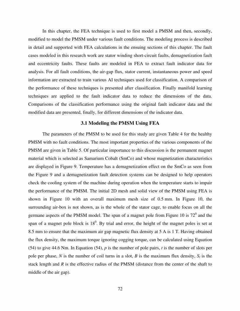
In this chapter, the FEA technique is used to first model a PMSM and then, secondly,

modified to model the PMSM under various fault conditions. The modeling process is described

in detail and supported with FEA calculations in the ensuing sections of this chapter. The fault

cases modeled in this research work are stator winding short-circuit faults, demagnetization fault

and eccentricity faults. These faults are modeled in FEA to extract fault indicator data for

analysis. For all fault conditions, the air-gap flux, stator current, instantaneous power and speed

information are extracted to train various AI techniques used for classification. A comparison of

the performance of these techniques is presented after classification. Finally manifold learning

techniques are applied to the fault indicator data to reduce the dimensions of the data.

Comparisons of the classification performance using the original fault indicator data and the

modified data are presented, finally, for different dimensions of the indicator data.

3.1 Modeling the PMSM Using FEA

The parameters of the PMSM to be used for this study are given Table 4 for the healthy

PMSM with no fault conditions. The most important properties of the various components of the

PMSM are given in Table 5. Of particular importance to this discussion is the permanent magnet

material which is selected as Samarium Cobalt (SmCo) and whose magnetization characteristics

are displayed in Figure 9. Temperature has a demagnetization effect on the SmCo as seen from

the Figure 9 and a demagnetization fault detection systems can be designed to help operators

check the cooling system of the machine during operation when the temperature starts to impair

the performance of the PMSM. The initial 2D mesh and solid view of the PMSM using FEA is

shown in Figure 10 with an overall maximum mesh size of 0.5 mm. In Figure 10, the

surrounding air-box is not shown, as is the whole of the stator cage, to enable focus on all the

germane aspects of the PMSM model. The span of a magnet pole from Figure 10 is 720 and the

span of a magnet pole block is 180. By trial and error, the height of the magnet poles is set at

8.5 mm to ensure that the maximum air gap magnetic flux density at 5 A is 1 T. Having obtained

the flux density, the maximum torque ignoring cogging torque, can be calculated using Equation

(54) to give 44.6 Nm. In Equation (54), p is the number of pole pairs, t is the number of slots per

pole per phase, N is the number of coil turns in a slot, B is the maximum flux density, Sl is the

stack length and R is the effective radius of the PMSM (distance from the center of the shaft to

middle of the air gap).

72

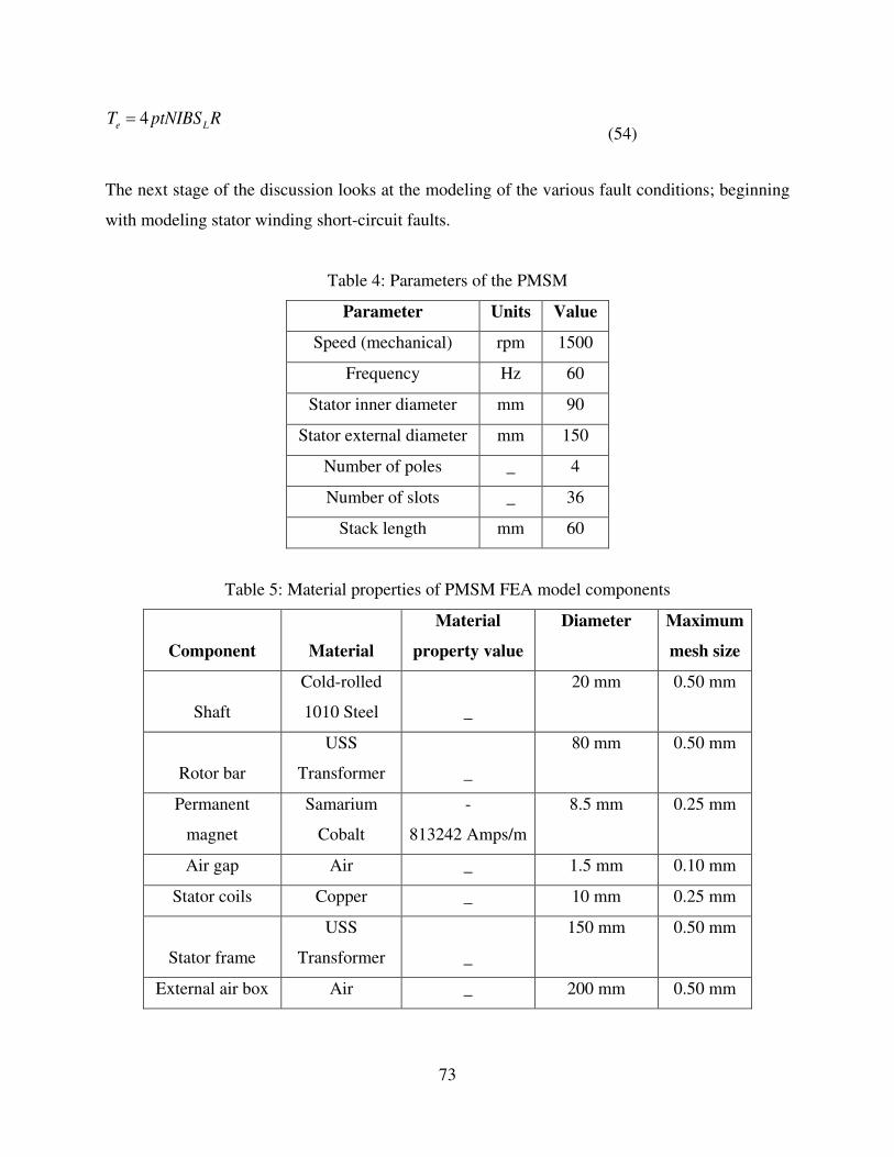
RptNIBST Le 4= (54)

The next stage of the discussion looks at the modeling of the various fault conditions; beginning

with modeling stator winding short-circuit faults.

Table 4: Parameters of the PMSM

Parameter Units Value

Speed (mechanical) rpm 1500

Frequency Hz 60

Stator inner diameter mm 90

Stator external diameter mm 150

Number of poles _ 4

Number of slots _ 36

Stack length mm 60

Table 5: Material properties of PMSM FEA model components

Component Material

Material

property value

Diameter Maximum

mesh size

Shaft

Cold-rolled

1010 Steel _

20 mm 0.50 mm

Rotor bar

USS

Transformer _

80 mm 0.50 mm

Permanent

magnet

Samarium

Cobalt

-

813242 Amps/m

8.5 mm 0.25 mm

Air gap Air _ 1.5 mm 0.10 mm

Stator coils Copper _ 10 mm 0.25 mm

Stator frame

USS

Transformer _

150 mm 0.50 mm

External air box Air _ 200 mm 0.50 mm

73

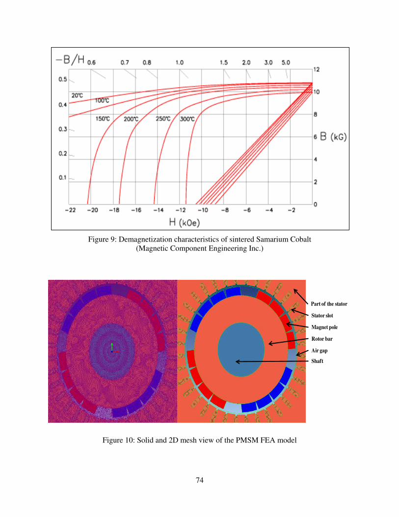
Figure 9: Demagnetization characteristics of sintered Samarium Cobalt (Magnetic Component Engineering Inc.)

Figure 10: Solid and 2D mesh view of the PMSM FEA model

Part of the stator

Rotor bar

Magnet pole

Air gap

Shaft

Stator slot

74

3.2 Modeling PMSM Faults

The PMSM model developed is modified to account for four different fault conditions:

Stator winding short-circuits, Demagnetization faults, Static Eccentricity faults and Dynamic

Eccentricity faults. These simulations are then used to generate fault analysis data for

classification using various machine learning techniques.

3.2.1 Modeling Stator Short-Circuit Fault Conditions

Stator short circuiting can be turn-to-turn and inter-turn-to-turn short circuits. These are

depicted in Figure 11 where in all examples, the shorted turns or shorted coils are electrically

separated from the rest of the healthy turns or coils. The emphasis in this study is on extracting

information from the three phase stator current output during short circuit and the discussion

presented is based on only turn-to-turn and inter-turn-to-turn short circuits without consideration

for turn-to-ground short circuits. Short circuit faults are modeled in FEA by separating out the

shorted turns into a separate coil with no electrical contact to the main coil. The separate coils are

modeled in a circuit module that comes with the FEA software used for this study and shown in

Figure 12.

Figure11: Schematic of turn–to-turn and inter-turn-to-turn short circuit faults

75

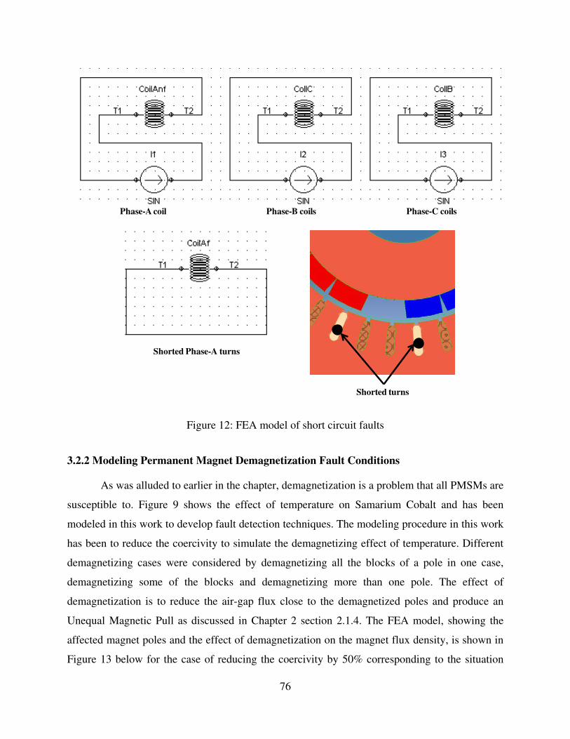
Figure 12: FEA model of short circuit faults

3.2.2 Modeling Permanent Magnet Demagnetization Fault Conditions

As was alluded to earlier in the chapter, demagnetization is a problem that all PMSMs are

susceptible to. Figure 9 shows the effect of temperature on Samarium Cobalt and has been

modeled in this work to develop fault detection techniques. The modeling procedure in this work

has been to reduce the coercivity to simulate the demagnetizing effect of temperature. Different

demagnetizing cases were considered by demagnetizing all the blocks of a pole in one case,

demagnetizing some of the blocks and demagnetizing more than one pole. The effect of

demagnetization is to reduce the air-gap flux close to the demagnetized poles and produce an

Unequal Magnetic Pull as discussed in Chapter 2 section 2.1.4. The FEA model, showing the

affected magnet poles and the effect of demagnetization on the magnet flux density, is shown in

Figure 13 below for the case of reducing the coercivity by 50% corresponding to the situation

Shorted turns

Phase-A coil Phase-B coils Phase-C coils

Shorted Phase-A turns

76

produced when the magnets are used in an ambient temperature of 500K as shown in Figure 9.

Magnets undergo other physical and material changes during demagnetization but fault

classification in this study was based on only coercivity.

Figure 13: Flux density distribution for demagnetization fault condition

3.2.3 Modeling Static Eccentricity Fault Conditions

Chapter 2 under section 2.1.4 and Figure 3 discussed and illustrated the static eccentricity

fault condition. This has been modeled in FEA by shifting the rotatable parts of the PMSM (the

shaft, rotor and permanent magnet poles) out of concentricity with the stator cage. Figure 14

shows the PMSM FEA model with the rotor part shifted by 1.0 mm towards one side of the left

side of the inside of the stator cage along the horizontal; the shifted Cartesian coordinate vector

is represented as X=-1,Y=0, Z=0. All simulations for fault conditions are carried for transient 2D

with motion carried out by repeatedly re-meshing and solving the FEA equations as discussed in

section 2.4.1.3 of Chapter 2. For the case of static eccentricity, the motion is carried out with its

center located in the center of the rotor bar as indicated in Figure 14 and not the center of the

stator cage. The result of this is that there are fixed locations in the air gap where the reluctance

is highest and fixed locations where the reluctance is lowest.

Air gap Flux reduced to 0T – 0.38T

In the region of demagnetization

77

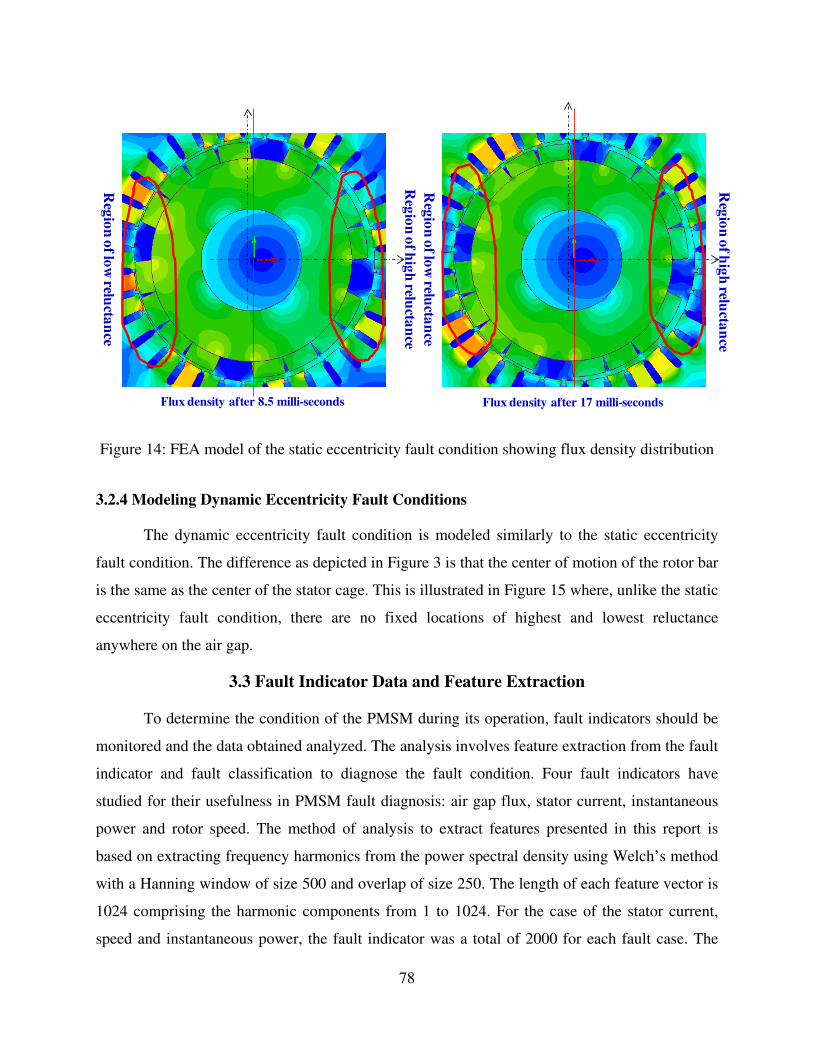
Figure 14: FEA model of the static eccentricity fault condition showing flux density distribution

3.2.4 Modeling Dynamic Eccentricity Fault Conditions

The dynamic eccentricity fault condition is modeled similarly to the static eccentricity

fault condition. The difference as depicted in Figure 3 is that the center of motion of the rotor bar

is the same as the center of the stator cage. This is illustrated in Figure 15 where, unlike the static

eccentricity fault condition, there are no fixed locations of highest and lowest reluctance

anywhere on the air gap.

3.3 Fault Indicator Data and Feature Extraction

To determine the condition of the PMSM during its operation, fault indicators should be

monitored and the data obtained analyzed. The analysis involves feature extraction from the fault

indicator and fault classification to diagnose the fault condition. Four fault indicators have

studied for their usefulness in PMSM fault diagnosis: air gap flux, stator current, instantaneous

power and rotor speed. The method of analysis to extract features presented in this report is

based on extracting frequency harmonics from the power spectral density using Welch’s method

with a Hanning window of size 500 and overlap of size 250. The length of each feature vector is

1024 comprising the harmonic components from 1 to 1024. For the case of the stator current,

speed and instantaneous power, the fault indicator was a total of 2000 for each fault case. The

Flux density after 8.5 milli-seconds Flux density after 17 milli-seconds

Reg

ion

of lo

w relu

ctan

ce

Reg

ion

of h

igh

relucta

nce

Reg

ion

of lo

w relu

ctan

ce

Reg

ion

of h

igh

relucta

nce

78

power spectral density estimates were then obtained from 100 different locations. For the case of

the air gap flux, the flux density is obtained at intervals of 0.1º for a total angular displacement of

360 along a circumferential line in the air gap of the PMSM as shown in Figure 16. The data

record obtained this way had a length of 3600 and was repeated at 100 different times for each

fault condition. The power spectral density estimation was then performed on each data record.

The fault conditions used to obtain data for the fault classification analysis to be described in

detail in a later section are shown in Table 6. In total there were four machine fault conditions

plus the healthy machine condition. Two different fault conditions were modeled for each case

and each fault condition was run under five different loading conditions to give a total of 50 fault

cases to be used for the study.

Figure 17 shows the results of power spectral density estimation for all five cases

presented in Table 6 for the case of air gap magnetic flux density. Each curve represents a feature

vector that identifies a condition of operation of the machine and the total number of such feature

vectors used for fault classification analysis was 5000 from all the various cases listed in Table 6.

Figure 15: FEA model of the dynamic eccentricity fault condition showing flux density

distribution

Reg

ion

of lo

w relu

ctan

ce

Reg

ion

of h

igh

relucta

nce

Reg

ion

of h

igh

relucta

nce

Reg

ion

of lo

w relu

ctan

ce

Center of rotation

Flux density after 8.5 milli-seconds Flux density after 17 milli-seconds

79

Figure 16: Air gap circumferential line along which flux density is computed

Table 6: Description of fault cases

Details of Fault Simulations

Fault type Fault specification Loading

No fault 0.1N 0.2N 0.3N 0.4N 0.5N

0.05N 0.15N 0.25N 0.35N 0.45N

Short circuit fault

(turn-to-turn shorts)

50% short circuit 36

slots 0.1N 0.2N 0.3N 0.4N 0.5N

50% short circuit 18

slots

Demagnetization fault

50% demagnetization

on one pole 0.1N 0.2N 0.3N 0.4N 0.5N

50% demagnetization

on two poles

Static eccentricity fault 67% eccentricity

0.1N 0.2N 0.3N 0.4N 0.5N 33% eccentricity

Dynamic eccentricity

fault

67% eccentricity 0.1N 0.2N 0.3N 0.4N 0.5N

33% eccentricity

Construction slice edge

for field contour graph

80

Figure 17: Power spectral estimate for a sample instantaneous power feature vector

3.4 Fault Classification Technique

Four classification methods are used for fault diagnosis and their performances have been

compared when applied to the original feature vectors and for the case where the dimensions of

the feature vectors have been reduced from 1024 to lower values between 5 and 40. This section

begins with a short discussion on the various techniques applied based on the book by Ian H.

Witten and Eibe Frank [204]. The discussion addresses Radial Basis functions (RBF), Support

Vector Machines (SVM), Nearest Neighbor Classifiers, Bayesian Classifiers and Decision Trees.

These are discussed under the major category they each belong. The WEKA machine learning

software tool is used for the actual classification process since WEKA implements most of the

popular classification techniques in a very user friendly way. All other aspects were carried out

in INFOLYTICA and MATLAB.

0 100 200 300 400 500 600 700 800 900 1000-20

0

20

40

60

80

100

120

140

160

180

200

Frequency (Hz)

Po

wer S

pectr

al

Est

ima

te (

dB

)

Demagnetization

Dynamic Eccentricity

No Fault

Short Circuit

Static Eccentricity

81

3.4.1 Logic-Based Classifiers

Two popular logic based approaches are decision trees and rule based classifiers. We

shall consider decision trees. The J48 algorithm is the WEKA implementation of the C4.5

algorithm for decision trees and is used in this study. When creating a decision tree for

classification purposes two choices need to be made at each new node: what attribute to select

and how to split that attribute into distinguishable classes (some attributes could be continuous

variables). The C4.5 algorithm accomplishes this by maximizing two measures: information gain

and split information. Information gain is a measure of certainty within the system and is

inversely proportional to system entropy; which is a measure of uncertainty. If, for example, all

instances were in the same class then the entropy would be zero. Unfortunately, using the

information measure alone favors those attributes with many classes. To suppress this bias the

C4.5 algorithm uses the notion of split information. Split information is a measure of how many

classes an attribute has and how those instances are distributed within the classes. If there are

two cases with the one case having all instances evenly split over all the classes and another case

in which all instances are in one class. Based on the split information measure, case one

maximizes split information while case two has split information of zero. The ratio of

information gain to split information is called the information gain ratio. By maximizing this

gain ratio at the creation of each new node, the C4.5 algorithm is able to create a compact and

efficient decision tree. Over-fitting is overcome in the C4.5 algorithm by a method called post-

pruning where branches that increase a measure of error in the system are removed. In the C4.5

algorithm this error is calculated from the number of incorrectly classified instances if the

training set were applied to the decision tree.

3.4.2 Perceptron-Based Classifiers

Both Multi-Layer Perceptron (MLP) and RBF networks are examples of perceptron

based classifiers that learn by example and are used for function approximation. These functions

act as decision boundaries in N-dimensional space when classifying an instance. Both types of

networks consist of nodes arranged in layers. As mentioned earlier in section 2.4.4.3, the first

layer is the input layer, after that there may be any number of hidden layers. It is common for a

RBF network to have only one hidden layer, which would consist entirely of RBF nodes. A

radial basis function is a Gaussian bell shaped curve. An advantage of RBF networks over MLPs

82

is that the algorithm for the RBF network is able to calculate the optimum number of these

hidden RBF nodes to use whilst in a MLP, the required amount of layers and the number of

nodes within those layers for optimal performance can be arbitrarily selected and tested. The last

layer for both these types of networks is the output layer. Therefore, RBF networks have been

chosen to act as representative for the perceptron based classifiers.

A Gaussian Radial Basis function decreases from a central position in space. For a scalar

input, x, it can be represented as h in Equation (55) where c is the central point in space and r is

the parameter that represents its radius. A Gaussian Radial Basis is implemented in WEKA but

other Radial Basis functions are possible.

−

−=2

exp)(r

cxxh (55)

With a single hidden layer, the output of a RBF can be represented as shown in Equation (56),

where wj are the network parameters from the hidden layer to the output layer with a single

output. There are many methods in the literature to solve Equation (56) with the simplest being

the least square method.

∑=

=m

j

jj xhwxf1

)()( (56)

3.4.3 Statistical Classifiers

These algorithms assume an underlying probability distribution for the system whose

output data is to be classified. Two main algorithms that rely on underlying probability function

are the Naïve Bayes and Bayesian Networks. The Bayesian network is used in this work and is

implemented in the WEKA environment as BayesNet classifier. The network is constructed such

that conditional probabilities are hardwired into the network, from this structure conditional

independence can be inferred. The most probable classification for an instance can then be

calculated.

3.4.4 Instance-Based Learning

Instance based learning algorithms implement the most basic idea of classification where

an instance is classified by the assumptions that similar features mean similar properties. These

algorithms use distance measure usually in multi-dimensional Euclidean space as the feature for

83

comparison. To classify an instance, the k-nearest neighbors to the instance are found and the

modal class of those neighbors is the predicted output class for that instance. Other distance

measures can be used as mentioned in Chapter 2 section 2.4.3.1. The IB1 algorithm is WEKA’s

implementation of a popular but simple instance-based learning algorithm that only uses the

nearest neighbors during classification.

3.4.5 Support Vector Machines

If two classes are linearly separable (that is the two classes can be dichotomized into two

classes using a line or hyper –plane), then the basic SVM can used to determine a decision

boundary. The method to determine the optimal decision boundary is called Structural Risk

Minimization which balances a model’s complexity against its success at fitting the training data

is in contra-distinction to conventional training methods that aim to minimize the error of

misclassification. The above discussion means that SVM maximizes the margin (the distance)

between the classes, whilst minimizing over-fitting due to the margin selection. This optimal

hyper-plane can be described as below in Equation (57).

( ) 0=+= bxwxf T

(57)

In Equation (57), w and x belong to a vector space of n dimensions, w is a weight set to be

determined by the SVM algorithm, x is an input data set and b is a constant vector also to be

determined. We can associate an output y to each x such that y = 1 if f(x) ≥ ∆ and y = -1 if f(x) ≤ -

∆. It is clear that the process to maximize ∆, involves minimizing the magnitude of w subject to

Equation (58).

( ) 01≥−+ bwxy ii (58)

Where ∆ is set to 1 and is true for all pairs (xi, yi). Equation (58) can be recast into a Lagrange

formulation involves introducing a Lagrange multiplier, αi, for each inequality constraint as

shown in Equation (59).

( )∑ ∑= =

++−l

i

l

i

iiiii bwxyw1 1

2

2

1 αα (59)

84

Equation (59) is a convex quadratic with a single global optimal solution unlike other

classification methods which may have several local optimal solutions. The particular values of x

which lie on the hyper-plane and whose removal from the training set changes the solution to the

quadratic program in Equation (59) are called the Support Vectors. In practice the dual

formulation of Equation (59) is solved with the Karush-Kuhn-Tucker conditions to determine w

and b.

Unfortunately the above discussion assumes the data is linearly separable. This is not the

case and to deal with the more general case of data that is not linearly separable, the original data

is mapped onto a new higher dimensional feature space where it is possible that the data can

become linearly separable. This is called the Kernal trick in the literature. If too high a dimension

is chosen then the SVM will suffer from over-fitting. To transform the data into a higher

dimensional feature space it would be possible to calculate each coordinate of the data in feature

space, this however would require a great deal of computation, especially if that data and feature

space were highly dimensional. It is however possible to sidestep this calculation by using a

kernel function. A kernel function implicitly represents the feature space by the calculation of the

inner product (or dot product) between the data in the feature space. It is therefore possible to

work in the feature space by using only an inner product function between the points, rather than

by calculating their coordinates in the feature space. This results in a reduction in the

computational requirements.

3.5 Manifold Learning Techniques

Dimensionality reduction is the transformation of high-dimensional data into a

meaningful representation of reduced dimensionality. Ideally, the reduced representation should

have a dimensionality that corresponds to the intrinsic dimensionality of the data. The intrinsic

dimensionality of data is the minimum number of parameters that are needed to account for the

observed properties of the data. Dimensionality reduction is important in many domains, since it

facilitates classification, visualization, and compression of high-dimensional data, by mitigating

the curse of dimensionality and other undesired properties of high-dimensional spaces. This

process also called manifold learning has been used to reduce the dimension of the PMSM data

obtained using FEA. Four different techniques have been used in this study to observe the

effectiveness of such techniques in reducing the computational burden of applying artificial

85

intelligence techniques to fault analysis. The four techniques applied fall into four main

categories that are discussed in the next four sub-sections. The next four subsections of this

manuscript are based on the article by Van-Maaten of the Maastricht University in Holland [205]

– [206].

3.5.1 Classical Approach to Dimensionality Reduction

Principal Components Analysis (PCA) (originally known as the Karhunen-Loeve

Transform) and Linear Discriminant Analysis (originally known as the Fisher mapping) are well

known statistical techniques that form the basis of many more recent reduction techniques. PCA

was selected in this category since it is not a supervised reduction technique and so it is simpler

to use. PCA constructs a low-dimensional representation of the data that retains as much of the

variance in the data as possible. This is done by finding a linear basis of reduced dimensionality

for the data, in which the amount of variance in the data is maximal. Mathematically this is

represented in Equation (60) below for a transformation T on a dataset X. In Equation (60),

cov(X-µ(X)), is the covariance matrix of zero-mean dataset X-µ(X) and µ(X) is the mean of X.

)))(cov(max( TXXT T µ− (60)

Hence, PCA solves the eigenvalue problem shown in Equation (61) for first d-dimensions

using obtained from the first d eigenvalues, λ, and the corresponding eigenvectors, ν. The points,

Y, in the new dimensional space are obtained using Equation (62). PCA has been used as the

benchmark to determine the number of dimensions to be used for all other classification

techniques. In the results to be shown, the original data from the PMSM FEA model are reduced

to 12 dimensions that accounts for 98% of the variability in the original data for air-gap flux,

stator current, instantaneous power and speed using PCA.

λννµ =− ))(cov( XX (61)

TXXY ))(( µ−= (62)

86

3.5.2 Global Non-Linear Techniques

Global nonlinear techniques attempt to preserve global properties of the data in the same

way as PCA but are capable of constructing nonlinear transformations between the high-

dimensional data representation X and its low-dimensional counterpart Y. The most important

technique in this category is the Multi-dimensional Scaling (MDS) technique that uses the

Sammon stress function to express the quality of the mapping between the high dimensional

space and low dimensional space. The Sammon stress function, Φ, is given in Equation (63) for

data points xi and xj in the high dimensional space and yi and yj in the low dimensional space.

The MDS technique, therefore, retains the pairwise distances between the data points as much as

possible.

( )( )

∑∑ −

−−−

−=

ji

jiji

ji xx

yyxx

xxijy

2

1φ (63)

3.5.3 Local Nonlinear Techniques

Local Tangent Space Analysis (LTSA) is a nonlinear local dimensionality reduction

technique that describes local properties of the high-dimensional data using the local tangent

space of each data point. It can be shown that if local linearity of the manifold is assumed, there

exists a linear mapping from a high-dimensional data point to its local tangent space, and that

there exists a linear mapping from the corresponding low-dimensional data point to the same

local tangent space. LTSA attempts to align these linear mappings in such a way, that they

construct the local tangent space of the manifold from the low-dimensional representation. In

other words, LTSA simultaneously searches for the coordinates of the low-dimensional data

representations, and for the linear mappings of the low-dimensional data points to the local

tangent space of the high-dimensional data. This technique starts by applying PCA on the k data

points, xij, that are neighbors of data point xi. The resulting mapping, Mi, from the neighborhood

of xi to the local tangent space Φi has the property such that there exists a linear mapping Li from

the local tangent space coordinates θij to the low-dimensional representations yij. Using this

property of the local tangent space, LTSA performs the minimization in formulation X where Jk

is the centering matrix of size k. The solution of formulation in Equation (64) is used to obtain

the new data points in the lower dimensional space.

87

2

,min∑ − iiki

LYLJY

ii

θ (64)

3.5.4 Global Linear Alignment in Local Space

Some techniques compute several linear models and then perform global alignment of

(local) linear models. In particular, the Locally Linear Coordination (LLC) technique carries out

this process in two steps. In the first stage, a mixture of linear models is computed by means of

the Expectation Maximization (EM) algorithm. The second stage aligns the local linear models

in order to obtain the low-dimensional data representation by finding a linear mapping from the

data models that minimizes the Linear Local Embedding (LLE) cost function.

3.6 Fault Classification Results

This section presents results of fault classification using five techniques as implemented

in the WEKA machine learning software. The first technique is J48, which is WEKA

implementation of a decision tree algorithm. The second technique is IB1 which implements a

nearest neighbor algorithm. The third algorithm implements Bayesian decision making algorithm

and is called BayesNet in WEKA. The remaining two techniques implement a RBF algorithm

and a SVM algorithm and respectively called RBFNetwork and SMO. The results of using these

techniques are presented for the original data without dimensionality reduction. In another

section, the results based on dimensionality reduction are presented. Later results are present

based on the application of bagging techniques to improve the results with the transformed data.

For all results, the method of training is 10-folds cross-validation. This is a standard way

of predicting the error rate of a learning technique where a given single, fixed sample of data is

divided randomly into 10 parts in which the class is represented in approximately the same

proportions as in the full dataset. Each part is held out in turn and the learning scheme trained on

the remaining nine-tenths; then its error rate is calculated on the holdout set. Thus the learning

procedure is executed a total of 10 times on different training sets. Finally, the 10 error estimates

are averaged to yield an overall error estimate.

3.6.1 Comparison of Techniques based on Original Un-transformed Dataset

Figure 18 compares the performance of the five techniques on the original un-

transformed dataset. It can be seen that all techniques perform the best with the instantaneous

88

power data followed by the results that use stator current as fault indicator. Comparing all

techniques, the J48 and IB1 technique seem to be closely matched and outperform all other

techniques. Also during fault classification these two techniques took less time than RBF and

SVM techniques.

3.6.2 Comparison of Techniques Based on Transformed Dataset

This section compares classification performance of all techniques on transformed data.

Four reduction techniques were used and Figure 19 shows the results when the data reduction

was carried out with the LLC method. The results show the same trend as observed for the

original datasets where the techniques performed well on the instantaneous power data followed

by the stator current output. The J48 and IB1 algorithms outperform all other techniques as was

observed with the un-transformed dataset. Figure 20 presents the results based on the LTSA

technique. The same trends observed earlier for the instantaneous power and stator current are

observed again as are the performances of the J48 and IB1 in comparison with the other

techniques. It is, however, noticeable that the classification methods perform better with LTSA

technique than the LLC method. In particular the performance of the classification techniques on

the air gap data is remarkably improved with LTSA reduction technique than the LLC technique.

The classification results based on the MDS dimensionality reduction method and the PCA

method are closely matched as seen Figure 21 and Figure 22; but it is seen that performance of

the classifiers are much better than with the LLC and LTSA method. Using MSD and PCA, the

percentage of correctly classified faults are all above 60% for the entire fault indicator data

considered. The PCA method, however, has slightly higher values than the MDS method with

Sammon mapping. It was noticed that the datasets obtained with LLC and LTSA showed very

little variability for the number of dimensions selected based on the PCA. It was observed that if

the number of dimensions was increased from 12 to 40, the performance of classifiers on LLC

and LTSA data improved but was still inferior to that of PCA and MDS data. The computational

effort was also more expensive and resulted in longer training and testing times for all five

classifiers.

89

Figure18: Comparison of classification techniques on un-transformed dataset

Figure 19: Comparison of classification techniques on LLC dataset

Air gap Stator Current Instantaneous Power Speed0

10

20

30

40

50

60

70

80

90

100P

ercen

tag

e C

orrectl

y C

lass

ifie

d (

%)

J48

IB1

BayN

RBF

SVM

Air gap Stator Current Instantaneous Power Speed0

10

20

30

40

50

60

70

80

90

100

Percen

tag

e C

orrectl

y C

lassif

ied

(%

)

J48

IB1

BayN

RBF

SVM

90

Figure 20: Comparison of classification techniques on LTSA dataset

Figure 21: Comparison of classification techniques on MDS dataset

Air gap Stator Current Instantaneous Power Speed0

10

20

30

40

50

60

70

80P

ercen

tag

e C

orrectl

y C

lassfi

ed

(%

)

J48

IB1

BayN

RBF

SVM

Air gap Stator Current Instantaneous Power Speed0

10

20

30

40

50

60

70

80

90

100

Percen

tag

e C

lassif

ied

Co

rrectl

y (

%)

J48

IB1

BayN

RBF

SVM

91

Figure 22: Comparison of classification techniques on PCA dataset

3.6.3 Effect of Bagging on Classification Performance

Decision trees and Neural Network are known to be unstable algorithms and would

produce very different results sometimes when presented with data that is different from the

training data. To improve their accuracy in classification a process called bagging can be applied.

The process of bagging reduces variance in classification and avoids over-fitting. To achieve

bagging a number of training sets are constructed by randomly sampling the initial training set

with replacement. The classifier is then trained on these new training sets producing an ensemble

of weak classifiers. This section shows a comparison of classification performance of all

classifiers when bagging is applied. The number of models of each classifier used in the clusters

is 10. Only results based on data transformed with the MDS method and the PCA method are

presented. The fault indicator data used is the instantaneous power and stator current data since

these showed the best results. Figure 23 and Figure 24 show that bagging has a minimal effect on

the performance of classifiers. For the cases shown in Figure 23 and Figure 24, there was little

difference between the performance without bagging and the performance with bagging. It is

also observed that for apart from the instantaneous power data, there was a drop in the

performance with the application of bagging. A comparison between the MDS method and PCA

Air gap Stator Current Instantaneous Power Speed0

10

20

30

40

50

60

70

80

90

100P

ercen

ta

ge C

orrectly

Cla

ssif

ied

(%

)

J48

IB1

BayN

RBF

SVM

92

method is indistinguishable. The only difference that must be noted is that the PCA method is

very fast during computation for new data points in the new reduced space dimension.

Figure 23: Application of bagging on MDS dataset

Figure 24: Application of bagging on PCA dataset

Air gap Stator Current Instantaneous Power Speed0

10

20

30

40

50

60

70

80

90

100

Percen

tag

e C

orrectl

y C

lassif

ied

(%

)

J48

IB1

BayN

RBF

SVM

Air gap Stator Current Instantaneous Power Speed0

10

20

30

40

50

60

70

80

90

100

Percen

tag

e C

orrectl

y C

lassif

ied

(%

)

J48

IB1

BayN

RBF

SVM

93

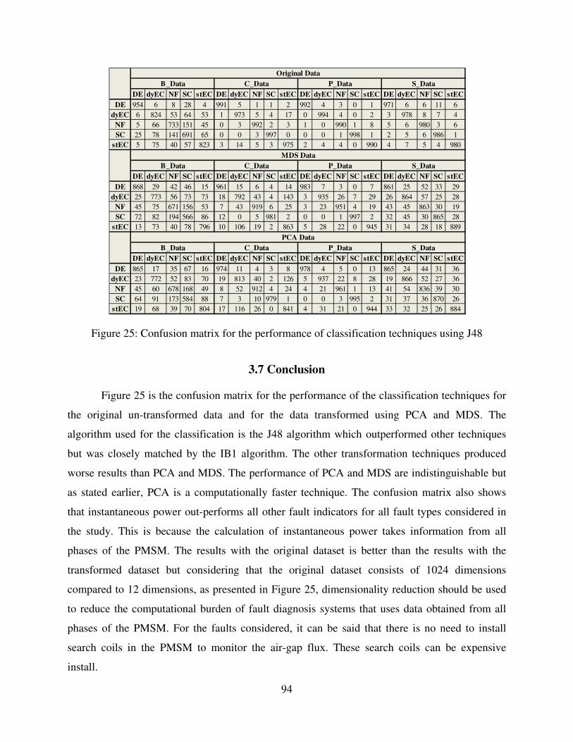
Figure 25: Confusion matrix for the performance of classification techniques using J48

3.7 Conclusion

Figure 25 is the confusion matrix for the performance of the classification techniques for

the original un-transformed data and for the data transformed using PCA and MDS. The

algorithm used for the classification is the J48 algorithm which outperformed other techniques

but was closely matched by the IB1 algorithm. The other transformation techniques produced

worse results than PCA and MDS. The performance of PCA and MDS are indistinguishable but

as stated earlier, PCA is a computationally faster technique. The confusion matrix also shows

that instantaneous power out-performs all other fault indicators for all fault types considered in

the study. This is because the calculation of instantaneous power takes information from all

phases of the PMSM. The results with the original dataset is better than the results with the

transformed dataset but considering that the original dataset consists of 1024 dimensions

compared to 12 dimensions, as presented in Figure 25, dimensionality reduction should be used

to reduce the computational burden of fault diagnosis systems that uses data obtained from all

phases of the PMSM. For the faults considered, it can be said that there is no need to install

search coils in the PMSM to monitor the air-gap flux. These search coils can be expensive

install.

DE dyEC NF SC stEC DE dyEC NF SC stEC DE dyEC NF SC stEC DE dyEC NF SC stEC

DE 954 6 8 28 4 991 5 1 1 2 992 4 3 0 1 971 6 6 11 6

dyEC 6 824 53 64 53 1 973 5 4 17 0 994 4 0 2 3 978 8 7 4

NF 5 66 733 151 45 0 3 992 2 3 1 0 990 1 8 5 6 980 3 6

SC 25 78 141 691 65 0 0 3 997 0 0 0 1 998 1 2 5 6 986 1

stEC 5 75 40 57 823 3 14 5 3 975 2 4 4 0 990 4 7 5 4 980

DE dyEC NF SC stEC DE dyEC NF SC stEC DE dyEC NF SC stEC DE dyEC NF SC stEC

DE 868 29 42 46 15 961 15 6 4 14 983 7 3 0 7 861 25 52 33 29

dyEC 25 773 56 73 73 18 792 43 4 143 3 935 26 7 29 26 864 57 25 28

NF 45 75 671 156 53 7 43 919 6 25 3 23 951 4 19 43 45 863 30 19

SC 72 82 194 566 86 12 0 5 981 2 0 0 1 997 2 32 45 30 865 28

stEC 13 73 40 78 796 10 106 19 2 863 5 28 22 0 945 31 34 28 18 889

DE dyEC NF SC stEC DE dyEC NF SC stEC DE dyEC NF SC stEC DE dyEC NF SC stEC

DE 865 17 35 67 16 974 11 4 3 8 978 4 5 0 13 865 24 44 31 36

dyEC 23 772 52 83 70 19 813 40 2 126 5 937 22 8 28 19 866 52 27 36

NF 45 60 678 168 49 8 52 912 4 24 4 21 961 1 13 41 54 836 39 30

SC 64 91 173 584 88 7 3 10 979 1 0 0 3 995 2 31 37 36 870 26

stEC 19 68 39 70 804 17 116 26 0 841 4 31 21 0 944 33 32 25 26 884

Original Data

S_DataB_Data C_Data P_Data

MDS Data

B_Data C_Data P_Data S_Data

PCA Data

B_Data C_Data P_Data S_Data

94

CHAPTER 4

As has been pointed out Chapter 3, PMSMs are receiving increasing attention in robotic,

automotive, electric traction and propulsion on ship board power systems due to their high

efficiency, high energy density and their suitability for high performance applications made

possible by advancements in permanent magnet materials. The case for efficient online condition

monitoring and accurate machine fault diagnosis has become very important due the use of

PMSMs in critical areas. PMSMs has also be proposed as one of the main types of electrical

machines to be considered for the future AES.

Even though AI was introduced a long time ago, it was in the early 90s that AI has

achieved its greatest success, prompting their application to new fields of study. In this chapter,

two methodologies that involve the use a MLP and the PSO algorithm is proposed to diagnose

faults due stator winding short circuits in a PMSM. A recurrent, multi-layer ANN model for

simulating the dynamics of an induction motor and performing online fault diagnosis is proposed

in [207] even though the load fluctuation is not discussed. The case of load fluctuation is

addressed in [208] by using negative sequence currents as the fault predictor. In the first method

to be presented in this Chapter, an ANN is designed to detect the presence of a stator winding

short circuit fault by comparing the peaks of the currents in all phases of the stator windings of

the PMSM. A threshold value is set beyond which a stator winding fault is determined to have

occurred. By comparing the all phase current peaks, the location of the fault can be determined

based on the two most closely matched peak currents. This simple method can, potentially, be

used to determine the fault severity by correlating peak current difference between the faulted

phase and the un-faulted phase with the number of short circuited turns in the stator. For a

method to determine the severity of the winding short circuit fault, a different method is

presented that also helps to determine the fault location. However, this second approach directly

relates the turns of the stator winding to the zero current component of the stator output current.

For both methods, computer simulation results and results based on an actual faulted PMSM are

presented to assess the performance of the two approaches. One important aspect of the two

approaches presented is that they both can be easily integrated into current electric drives

systems and implemented in real time. The first method, however, is less computationally

95

intensive and lends itself to ANN reconfiguration by way of real time PSO which is also outlined

in this chapter.

4.1 Peak-to-Peak Detection for PMSM Stator Winding Short-Circuit Fault

Detection

The first fault detection method to be discussed is motivated by Figure 26 and Figure 27.

Figure 26 shows the variation of speed for a given load profile for an actual PMSM drive to be

introduced later in this chapter. When the loading on the machine increases, the PMSM

momentarily losses speed but picks up again when the drive increases current supply. When the

loading of the PMSM loading drive decreases, the speed increases until the drive system restores

commanded speed again. Figure 27 is the current in phase A for the PMSM drive. The current

increases from about 30A to 38A during steady conditions within 1 second due to a slow

changing external load whilst it almost instantaneously rises from 38A to 42A due to stator

winding short circuits at 3 seconds. It is clear from Figure 27 that loading conditions and internal

short-circuit of the PMSM both cause the current supply to increase; whilst it would cause a false

alarm in the case of loading transients. The detection technique presented is able to avoid alarms

when the change in the current level is too abrupt to be due a mechanical load change.

Figure 26: Speed of PMSM during different loading conditions

0 1 2 3 4 5 6 7 8 9 109.2

9.4

9.6

9.8

10

10.2

10.4

10.6

10.8

Time(s)

Sp

ee

d(H

z)

Speed of PMSM under changing loa conditions

0 1 2 3 4 5 6 7 8 9 100

0.05

0.1

0.15

0.2

0.25

0.3

0.35

0.4

0.45

0.5L

oa

d P

rofile

Load Profile

Speed

96

Figure 27: Phase current for changing load and stator winding fault

4.1.1 Development of ANN Model for the Peak-to-Peak Fault Detection Method

The current supply to the PMSM, as discussed earlier, changes proportionally in response

to load changes to restore commanded speed. The torque is given, in general, by Equation (65) In

Equation (65), Te is the total torque on the machine, TL is the external load attached to the

machine, J is the moment of inertia, P is the number of poles of the machines and ωr is the time

derivative of the rotor angular velocity. The first term on the right of Equation (65) is called

inertial torque and is the only torque on the machine in the absence of no external load. This term

is due to machine manufacturing parameters and operating conditions. Operating conditions can

change daily when there are temperature changes on the factory floor. It can also change very

slowly over time due to aging. An ANN can be trained to relate the three-phase current supply to

the PMSM, when the machine is operated with no-load, to the inertial torque which is

approximated by a constant value of 10 Nm in this work. This value for all, intents and purposes,

can be fixed by the one designing the ANN. Using a three-layer neural network architecture as

shown in Figure 7 with 3 neurons in the hidden layer and linear activation functions, an error of

0.0889 or less is possible based on the discussion in [209] about B-spline interpolation using

ANNs. If six neurons are used an error of 0.0219 is guaranteed. With nine neurons, the error is

guaranteed to be 0.0097 or less. The assumption here is that the three phase currents are balanced

and sinusoidal. The number of ANN parameters increases from 16 weight and bias parameters

0.5 1 1.5 2 2.5 3

5

10

15

20

25

30

35

40

Time(s)

Cu

rren

t(A

)

97

when 3 neurons are used in the hidden layer to 46 weight and bias parameters when 9 neurons

are used. The balance between the guaranteed accuracy bound and the number of parameters to

be determine is used to set the ANN architecture to 9 hidden neurons. The activation function is

set as linear since as discussed earlier, current level increases proportionally with load and fault

level. The output of the neurons of the ANN in the hidden layers is represented by Equation (66)

where Y is the output of either the hidden layer or output layer of Figure 7, wij is the jth weight of

hidden or output neuron i for input j. Input j is represented by uj and the bias of neuron i is

represented by bi.

Lre TP

JT +′

= ω2

(65)

( )jnnjjj buwuwuw

Y

+++==

...2211θθφ

(66)

The weights and bias values are selected by using PSO to adjust the values till an optimal weight

set is obtained as determined by the parameters that produce the smallest mean squared deviation

from expected output which in this case is set at 10 and represents the inertial torque when there

is no torque attached to the PMSM.

4.1.2 The PSO Algorithm

Particle Swarm Optimization (PSO) is an optimization technique which uses the behavior

of flocking birds or swarming locusts to stochastically approach the local optimum of a function.

Proposed in 1995, this technique has found application in several areas due mainly to its ease of

implementation and its resistance to local optimal traps [210]. Two approaches to the

implementation of the PSO algorithm are presented in this section. The first approach is the most

common approach and is called the offline PSO algorithm. The second approach is modified

based on the offline PSO method to enable optimization in real time. This is called the online

PSO method.

4.1.2.1 Offline PSO algorithm. The offline PSO method starts by randomly selecting

feasible solutions in the solution space called particles. Each particle is then adjusted by

Equation (67).

98

( ) ( ) ( ) ( ) ( )( )( ) ( )( )

( ) ( ) ( )11

1,0

1,01

++=+

++=+

kVkXkX

kpbestrand

kgbestrandkVkWkV

iii

i

ii

(67)

In Equation (67), Vi(k) is described as the velocity of particle i at time k, Xi(k) is particle i

location at time k, W(k) is the inertia weight of the system at time k, gbest is the global best

particle location, pbesti is the personal best location of the particle under consideration and

rand(0,1) are randomly generated numbers that could come from a normal distribution or

uniform distribution. The inertia weight, W, is implemented in Equation (68) with an initial value

set by trial and error to a value of 2.

( ) ( )kW

ITER

ikW ×

+

=+exp1

11

(68)

In Equation (68), i is the iteration number, ITER is the total number of iterations of the

PSO algorithm and k is the particle number. PSO has the ability to avoid getting trapped in local

optimal locations. PSO however is deficient in exploiting the solution space to find a refined

solution at a local optimal and may take a long time in this process whilst a classical gradient

based method at a local optimal may take very few steps. This deficiency is reduced in this work

by augmenting the PSO method with the Broyden-Fletcher-Goldfarb-Shanno (BFGS) quasi-

Newton method in the offline ANN training.

The BFGS modification to the PSO algorithm is presented as follows. At each iteration

step, the global best location is either updated or remains the same during PSO update. If it is

updated it is always towards a better location. Assuming the global best location is updated, this

constitutes enough information to approximate the gradient of the fitness function at the initial

global best location. Using finite differences, the gradient in all directions of the solution space

can be computed and used by any of the available quasi-Newton methods. The BFGS quasi-

Newton method has been employed to update the global best location whenever, at an iteration

step, this location is improved. The update proceeds in the manner of Newton’s method but the

Hessian matrix is different and is obtained by Equation (69).

99

( ) ( )( ) ( ) ( )( ) )(1 kpkqIkHkqIkH +

′−××−=+ (69)

In Equation (69), H(k) is the Hessian matrix at iteration step k, I is the identity matrix with the

same matrix dimensions as the Hessian and with the row or column dimension equal to the

number of weights and biases in the ANN. Both are square matrices. q(k) and p(k) are matrices

obtained as shown in Equation (70) and with apostrophe to indicate matrix transposition.

( ) ( )( )( )

( )

kkk

kkk

kk

kk

kk

gradfgradfy

gbestgbests

sskqkp

sy

yskq

−=−=

××=

××

=

+

+

1

1

'

'

'

)()(

(70)

In Equation (70), gradfk is the gradient of the function at the kth. PSO guarantees that sk is always

negative. PSO gbest updates do not, however, ensure that yk is always negative (in the secant or

steepest descent direction). If both computed values (yk and sk) are negative, the Hessian matrix

obtained using the BFGS update, would always be positive definite and this ensures that the

updated global best location would be an improved solution [211]. Equation (70) gives the step

direction and even though quasi-Newton methods assume a step length of one, we use Equation

(71) to adapt the step length at a given point in the PSO algorithm. In Equation (71), gbestk is the

global best location at iteration step k and gradfk is the gradient approximation at iteration step k.

This approximates an exact step length assuming a quadratic approximation at the local optimal

location at any given PSO iteration step. As discussed earlier, both loading conditions and stator

winding short circuits causes an increase in supply current to the PMSM but is more abrupt for

the case of winding short circuits. The detection method has to differentiate between the two

cases of current rise which in this work is carried out by comparing the current ANN output the

next ANN output at a time step set close to the peak-to-peak currents of each phase winding.

( ) ( )k

kk

gradf

gbestgbestkq

−= +1

(71)

100

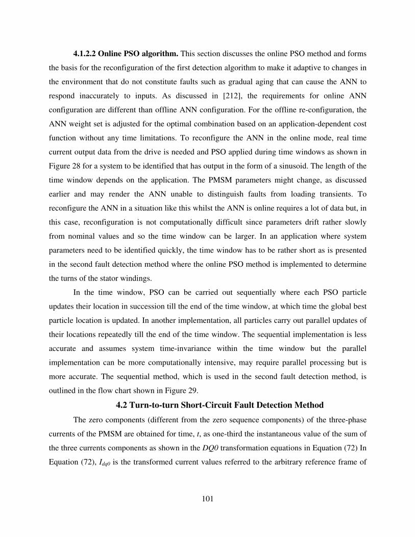
4.1.2.2 Online PSO algorithm. This section discusses the online PSO method and forms

the basis for the reconfiguration of the first detection algorithm to make it adaptive to changes in

the environment that do not constitute faults such as gradual aging that can cause the ANN to

respond inaccurately to inputs. As discussed in [212], the requirements for online ANN

configuration are different than offline ANN configuration. For the offline re-configuration, the

ANN weight set is adjusted for the optimal combination based on an application-dependent cost

function without any time limitations. To reconfigure the ANN in the online mode, real time

current output data from the drive is needed and PSO applied during time windows as shown in

Figure 28 for a system to be identified that has output in the form of a sinusoid. The length of the

time window depends on the application. The PMSM parameters might change, as discussed

earlier and may render the ANN unable to distinguish faults from loading transients. To

reconfigure the ANN in a situation like this whilst the ANN is online requires a lot of data but, in

this case, reconfiguration is not computationally difficult since parameters drift rather slowly

from nominal values and so the time window can be larger. In an application where system

parameters need to be identified quickly, the time window has to be rather short as is presented

in the second fault detection method where the online PSO method is implemented to determine

the turns of the stator windings.

In the time window, PSO can be carried out sequentially where each PSO particle

updates their location in succession till the end of the time window, at which time the global best

particle location is updated. In another implementation, all particles carry out parallel updates of

their locations repeatedly till the end of the time window. The sequential implementation is less

accurate and assumes system time-invariance within the time window but the parallel

implementation can be more computationally intensive, may require parallel processing but is

more accurate. The sequential method, which is used in the second fault detection method, is

outlined in the flow chart shown in Figure 29.

4.2 Turn-to-turn Short-Circuit Fault Detection Method

The zero components (different from the zero sequence components) of the three-phase

currents of the PMSM are obtained for time, t, as one-third the instantaneous value of the sum of

the three currents components as shown in the DQ0 transformation equations in Equation (72) In

Equation (72), Idq0 is the transformed current values referred to the arbitrary reference frame of

101

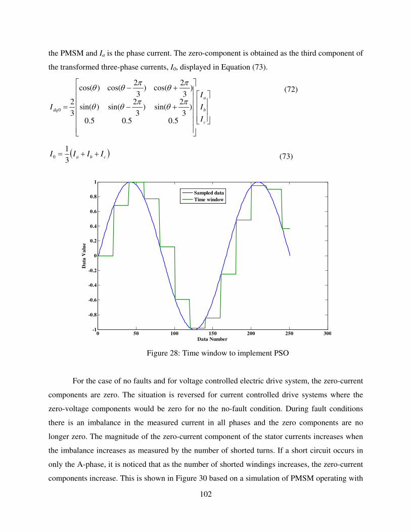
the PMSM and Ia is the phase current. The zero-component is obtained as the third component of

the transformed three-phase currents, I0, displayed in Equation (73).

+−

+−

=

c

b

a

dq

I

I

I

I

5.05.05.0

)3

2sin()

3

2sin()sin(

)3

2cos()

3

2cos()cos(

3

20

πθπθθ

πθπθθ

(72)

( )cba IIII ++=3

10 (73)

Figure 28: Time window to implement PSO

For the case of no faults and for voltage controlled electric drive system, the zero-current

components are zero. The situation is reversed for current controlled drive systems where the

zero-voltage components would be zero for no the no-fault condition. During fault conditions

there is an imbalance in the measured current in all phases and the zero components are no

longer zero. The magnitude of the zero-current component of the stator currents increases when

the imbalance increases as measured by the number of shorted turns. If a short circuit occurs in

only the A-phase, it is noticed that as the number of shorted windings increases, the zero-current

components increase. This is shown in Figure 30 based on a simulation of PMSM operating with

0 50 100 150 200 250 300-1

-0.8

-0.6

-0.4

-0.2

0

0.2

0.4

0.6

0.8

1

Data Number

Da

ta V

alu

e

Sampled data

Time window

102

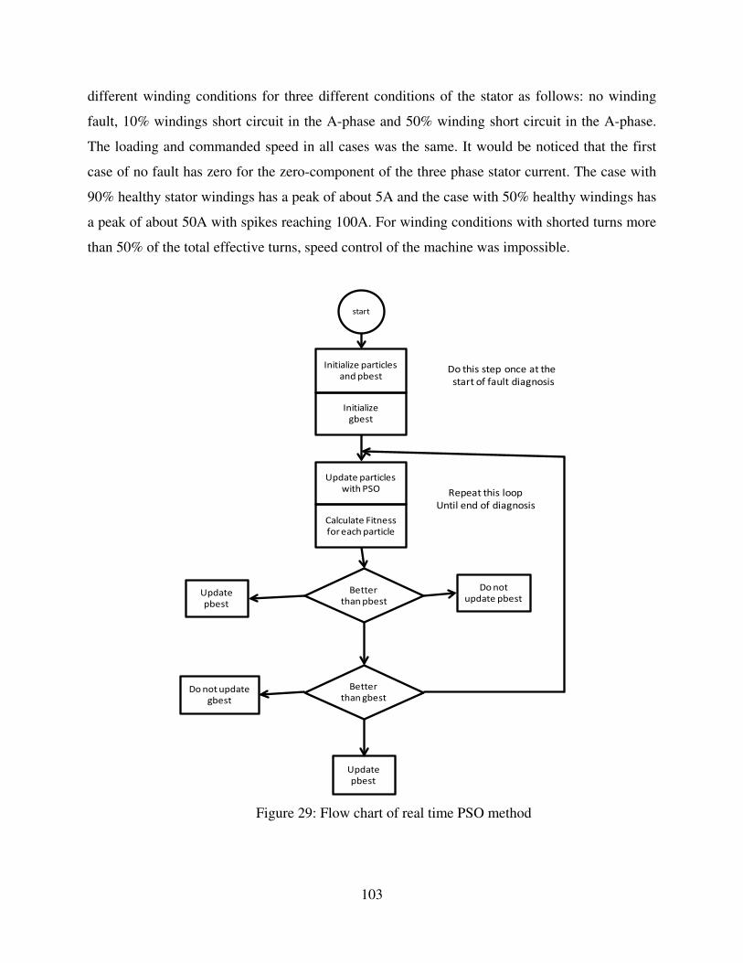
different winding conditions for three different conditions of the stator as follows: no winding

fault, 10% windings short circuit in the A-phase and 50% winding short circuit in the A-phase.

The loading and commanded speed in all cases was the same. It would be noticed that the first

case of no fault has zero for the zero-component of the three phase stator current. The case with

90% healthy stator windings has a peak of about 5A and the case with 50% healthy windings has

a peak of about 50A with spikes reaching 100A. For winding conditions with shorted turns more

than 50% of the total effective turns, speed control of the machine was impossible.

Figure 29: Flow chart of real time PSO method

Do this step once at the

start of fault diagnosis

Repeat this loop

Until end of diagnosis

start

Initialize particles

and pbest

Initialize

gbest

Update particles

with PSO

Calculate Fitness

for each particle

Better

than pbest

Better

than gbest

Update

pbest

Do not

update pbest

Do not update

gbest

Update

pbest

103

Figure 30: Zero-component of three phase stator current of PMSM

During short circuits, the windings undergo physical degradation that reduces the

effective number of turns in addition to a number of other physical modifications to the

windings. The effective number of turns is a simplification that represents the number of turns of

an equivalent balanced-sinusoidal distributed winding [213]. Several models have been

developed to describe the behavior of windings during short circuits. In one such model [214],

the inductance matrix of the three phase windings is augmented with extra fictitious winding for

each phase under fault. In Equation (74), the inductance matrix is shown for the case of a

winding fault in the B-phase where µ is the effective number of turns given as a ratio of the

number of the turns in the shorted windings to the windings in the healthy windings. The

subscripts a, b and c are for the A, B and C-phases respectively whilst f indicates a short circuit

fault condition.

10% short-circuit winding fault on phase-A

104

( )( ) ( ) ( ) ( )

( )( )

−−

−−−−−

=

ffcfbfaf

cfccbcac

bfbcbbab

afacabaa

abc

LLLL

LLLL

LLLL

LLLL

L

2

2

1

1

1111

1

µµµµµµµµµµµµ

µµ

(74)

This model has been used to develop an ABC model of the PMSM to study and obtain data to

train an ANN for a number of machine conditions. Different fault conditions have been

simulated to understand the effect of short circuits on the speed, torque, voltage and currents of

the machine. The approach used in [214] developed an optimization technique based on PSO to

determine the location of a short circuit fault and the µ term in Equation (74). The approach in

this paper uses an ANN to relate the effective number of turns given in Equation (74) to the zero-

component of the three-phase currents. PSO is then used to determine µ in Equation (74) during

online fault diagnosis.

4.2.1 Development of ANN Model for the Winding Turns-based Short-circuit Fault

Detection Method

For the second method an ANN cluster is used for fault diagnosis with each member

ANN designed for a particular machine winding and operating condition. Machine operating

condition can be speed of operation or loading conditions. Different ANN architectures were

tried for the member ANNs and a feed-forward Focused Time-Lagged Neural Network (FTLN)

was selected as the ANN architecture since it produced the best results. The architecture

comprises 3 neurons in the input layer, 20 neurons in the hidden layer and 3 neurons in the

output layer after a number of training iterations. Sigmoidal activation functions are used in the

hidden layer and linear activation functions are used in the output layer. Figure 31 shows a

diagram of a member ANN developed for fault diagnosis whilst Figure 32 shows the ANN

cluster. The diagram in Figure 32 shows the ANN, input, output and the PSO algorithm to

compute the number µ for each phase.

To train the ANN cluster, various fault conditions, that capture the range of operation of

the machine, are simulated to obtain the zero-components of the stator current for each

combination of winding fault and operating condition selected for training. Ideally one ANN

should be designed for each combination but one ANN can be designed for all fault conditions.

The input to each ANN, during training for any combination of machine fault, is obtained by

105

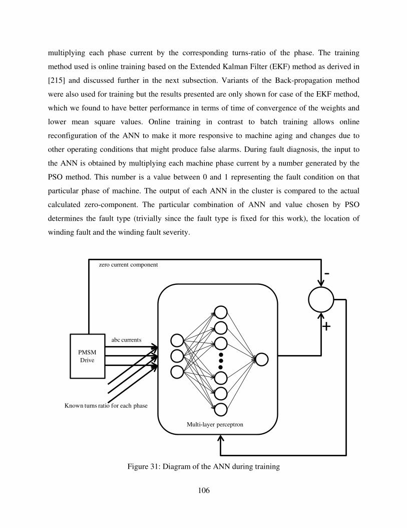
multiplying each phase current by the corresponding turns-ratio of the phase. The training

method used is online training based on the Extended Kalman Filter (EKF) method as derived in

[215] and discussed further in the next subsection. Variants of the Back-propagation method

were also used for training but the results presented are only shown for case of the EKF method,

which we found to have better performance in terms of time of convergence of the weights and

lower mean square values. Online training in contrast to batch training allows online

reconfiguration of the ANN to make it more responsive to machine aging and changes due to

other operating conditions that might produce false alarms. During fault diagnosis, the input to

the ANN is obtained by multiplying each machine phase current by a number generated by the

PSO method. This number is a value between 0 and 1 representing the fault condition on that

particular phase of machine. The output of each ANN in the cluster is compared to the actual

calculated zero-component. The particular combination of ANN and value chosen by PSO

determines the fault type (trivially since the fault type is fixed for this work), the location of

winding fault and the winding fault severity.

Figure 31: Diagram of the ANN during training

PMSM

Drive

`

-

+

zero current component

abc currents

Multi-layer perceptron

Known turns ratio for each phase

106

Figure 32: Diagram of ANN cluster during fault diagnosis

A number of methods could have been used to randomly generate values that correspond

to the turns-ratio. A random search could be implemented as well as other stochastic

computational intelligence search techniques. PSO was selected because a blind search

sometimes took too long to find the turns-ratio. The PSO method also has other features that

make it computationally less demanding than other stochastic methods like Genetic algorithms.

To implement PSO in fault diagnosis by the above method, we modified the classical PSO

algorithm into an online optimization procedure as discussed earlier in the Section 4.1.2.2 on the

Online PSO Method. The solution space for the online PSO optimization technique is the closed

interval between 0 and 1. Zero representing total breakdown of the phase winding and one

representing perfectly healthy winding conditions. The depth of the solution space was limited to

a resolution of 0.05 since in practice a depth greater than 0.05 did not reflect measurable effects

on speed, current and torque. The optimization problem solution space is therefore limited to a

discrete space from and including 0 to 1 in steps of 0.05 for each phase. The combination of

online training by the EKF method and real-time PSO makes this approach very amenable to

online diagnostic applications. Figure 33 shows the complete fault diagnosis system. The data

required for the diagnosis procedure is easily obtained with sensors that come with most standard

drive systems.

•

PSO

•

•

ANN1 ANN2 ANN3

ANN4 ANN5 ANN6

ANN7 ANN8 ANN9

ANN Cluster

∑

∑

∑

∑

∑

∑

∑

∑

∑

Current A

Current B

Current C

107

Figure 33: Schematic of drive system incorporating the ANN fault diagnostic system

4.2.1.1 The extended kalman filter method. Continuous learning based on the gradient

descent method is slow due to a reliance on instantaneous estimates of gradients. This shortfall is

overcome by considering the neural network as an optimum filtering problem. To motivate the

derivation of the formulations needed to configure the ANN based on the Kalman filter

approach, consider the signal flow graph in Figure 34 which can be represented by Equation (75)

where w(n) is the state vector of the system, d(n) is the observation vector, C(n) is the

measurement matrix and v(n) is the measurement noise.

Figure 34: Kalman filter representation of recurrent ANN

vr*q

ir*qω*q

ωrir*d vr*d

ird

ir q

iabc

θr

w(n)

v(n)

d(n)w(n+1)

z-1I

C(n)

108

( ) ( )( ) ( ) ( ) ( )nnwnCnd

nwnw

ν+==+1

(75)

Based on the discussion above, the Kalman filtering problem can be stated as one to find

minimum mean-square error estimate of the state vector at every time step of the system whose

signal flow graph is shown above by using the entire observation vector.

For an elegant derivation of the Kalman filter, the notion of innovations introduced by

Kailath [215] can be used. The innovations process associated with the observation vector is

defined in Equation (76) where d(n|n-1) is the minimum mean-square error estimate of d(n),

given all past values of the observation vector starting at time n=1 and extending up to n-1.

( ) ( ) ( )1| −−= nndndnα (76)

Using the innovations processes, the correlated measurement vector can be replaced with the

uncorrelated innovations and the Kalman filter can be derived with the set of formulations in

Equation (77). In Equation (77), Г(n) is the conversion factor that relates the filtered estimation

error e(n) to the innovations α(n). G(n) is the Kalman filter gain and K(n,n-1) is the error

covariance matrix.

( ) ( ) ( ) ( ) ( )[ ]( ) ( ) ( ) ( )( ) ( ) ( ) ( )( ) ( ) ( ) ( )( ) ( ) ( ) ( ) ( )1|1||1

1||1

1|

1|

1|1

−−−=++−=+−−=Γ−=

+−=Γ−

nnKnCnGnnKnnK

nnGnnwnnw

nnwnCnyn

nnCnnKnG

nRnCnnKnCn

T

T

αα

(77)

The above can be applied to a general recurrent neural network by setting the state vector,

w, equal to the entire synaptic weights of the neural network and linearizing Equation (75) above

to obtain Equation (78) where C(n) is a p-by-W matrix consisting of the partial derivatives of the

p outputs of the whole neural networks with respect to the W weights of the model in Figure 34.

The partial derivatives are obtained using the Back-Propagation (BP) to obtain the first

derivatives.

( ) ( ) ( ) ( )nnwnCnd ν+= (78)

109

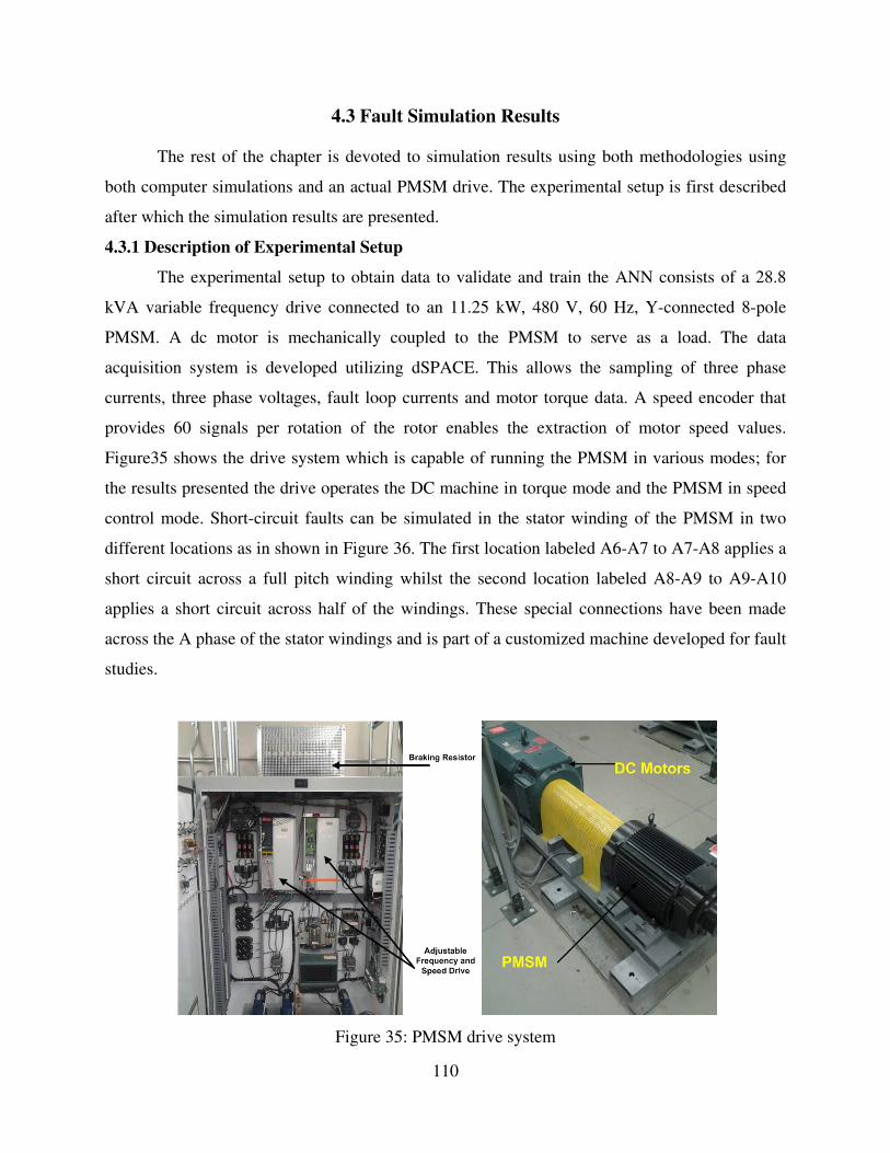
4.3 Fault Simulation Results

The rest of the chapter is devoted to simulation results using both methodologies using

both computer simulations and an actual PMSM drive. The experimental setup is first described

after which the simulation results are presented.

4.3.1 Description of Experimental Setup

The experimental setup to obtain data to validate and train the ANN consists of a 28.8

kVA variable frequency drive connected to an 11.25 kW, 480 V, 60 Hz, Y-connected 8-pole

PMSM. A dc motor is mechanically coupled to the PMSM to serve as a load. The data

acquisition system is developed utilizing dSPACE. This allows the sampling of three phase

currents, three phase voltages, fault loop currents and motor torque data. A speed encoder that

provides 60 signals per rotation of the rotor enables the extraction of motor speed values.

Figure35 shows the drive system which is capable of running the PMSM in various modes; for

the results presented the drive operates the DC machine in torque mode and the PMSM in speed

control mode. Short-circuit faults can be simulated in the stator winding of the PMSM in two

different locations as in shown in Figure 36. The first location labeled A6-A7 to A7-A8 applies a

short circuit across a full pitch winding whilst the second location labeled A8-A9 to A9-A10

applies a short circuit across half of the windings. These special connections have been made

across the A phase of the stator windings and is part of a customized machine developed for fault

studies.

Figure 35: PMSM drive system

110

Fuse

Fuse

SC1

SC2

T1 T2

T3

T4 T7

T5

T8

T6

T9

A6-A7

A7-A8

A8-A9

A9-A10

T10

Figure 36: Circuit diagram for stator short circuit winding

4.3.2 Training Results

Training results would be discussed for the two methodologies presented. The results are

shown for the training of the ANN for the case where the weights are adjusted by PSO, PSO-

BFGS and by the EKF method.

4.3.2.1 PSO and PSO-BFGS ANN training results. The training data comprising the

three phase current supply to the PMSM from the drive is shown in Figure 37(a) for times

between 2 seconds and 2.1 seconds, whilst Figure 37(b) shows the same data set pre-processed

before feeding into ANN. The ANN input training data was in total 50001 time ordered set of

three-phase current obtained from the PMSM when the latter has no load attached to it and no

fault is applied. The data is first processed to ensure that all values in the ordered set are positive.

This training data comprises only data of the healthy machine under no-load conditions but the

generalizing ability of the ANN to detect faults under load conditions is verified when the

PMSM is loaded to different extents during fault simulations even though the ANN is not

previously trained with data from the PMSM under load conditions.

The training evolution for the ANN based on PSO augmented with the BFGS method is

shown in Figure 38(a). Figure 38(b) shows the results based on only the PSO algorithm. The

sharp decline in the mean square error from iteration 21 to 24 is due the BFGS quasi-Newton

111

rapidly locating a local optimal location. The performance of the PSO algorithm alone is not as

good. The performance of the PSO-BFGS method is better because PSO provides curvature

information to enable calculation of approximate Hessian for rapidly approaching local optimal

locations. PSO also ensures a good exploration of the solution space hence avoiding local

optimal traps. The time it took for the results in Figure 38(a) was 6 minutes and 33.718 seconds

whilst the results in Figure 38(b) took 6 minutes and 23.891 seconds. The final squared error

deviation after several iterations of the PSO-BFGS algorithm was 0.00148 which validates the

error bound derived based on linear approximation techniques discussed under section V.

The differences in time of computation for both methods were in general

indistinguishable. In general the inclusion of the BFGS method did not appreciably increase the

time taken for a given number of iterations as the algorithm only updates the BFGS Hessian

matrix when a downward pointing approximate step direction is calculated and the updated

global best location is actually an improvement. This ensures that all Hessians calculated

encapsulate gradient information about the solution space that lead to only better solutions. The

approach of combining PSO and the BFGS method is also superior to classical gradient based

methods which depend heavily on starting conditions and require curvature information which

may be lacking in circumstances where, as in the present work, experimental data has a lot of

noise as shown in Figure 37.

Figure 37(a): Three-phase current input to PMSM under no-load conditions or stator short circuit winding

Figure 37: Training data

2 2.01 2.02 2.03 2.04 2.05 2.06 2.07 2.08 2.09 2.1

-30

-20

-10

0

10

20

30

Time(s)

Cur

rent

(A)

Phase-A Current Phase-B Current Phase-C Current

112

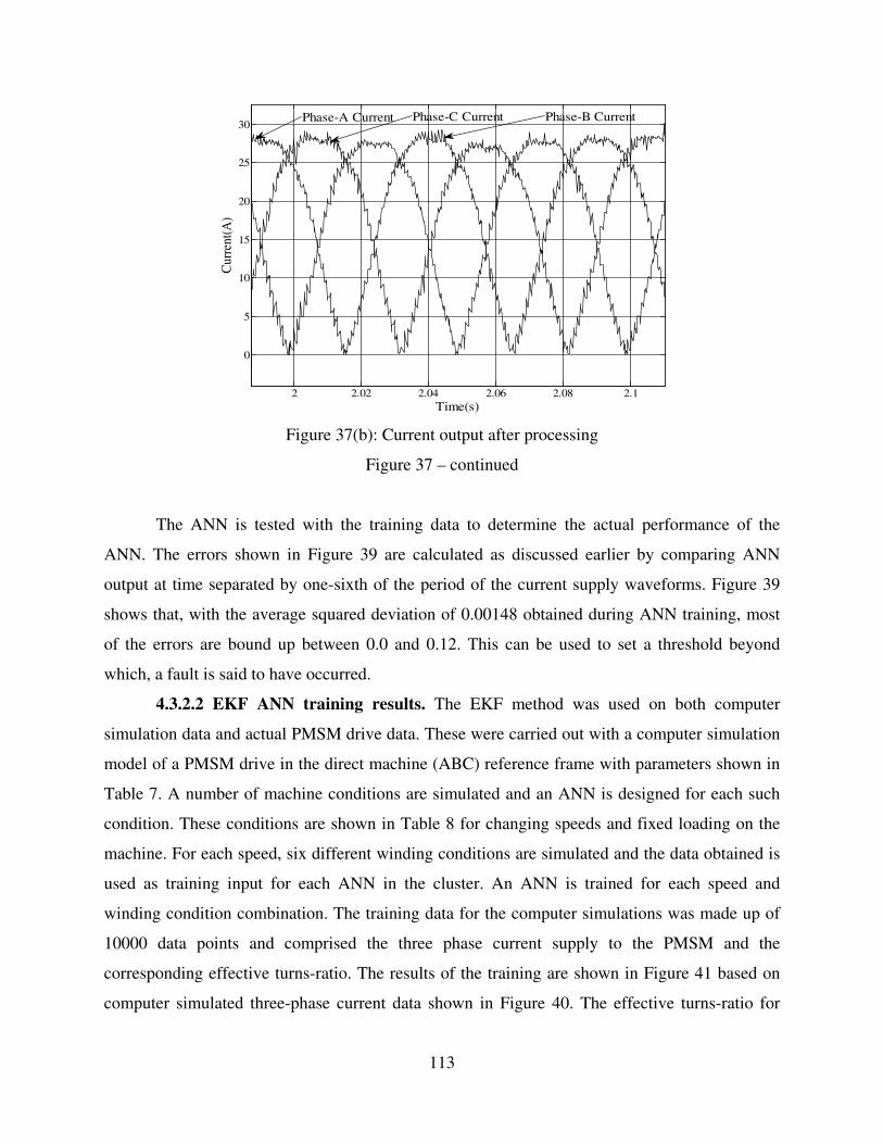
Figure 37(b): Current output after processing

Figure 37 – continued

The ANN is tested with the training data to determine the actual performance of the

ANN. The errors shown in Figure 39 are calculated as discussed earlier by comparing ANN

output at time separated by one-sixth of the period of the current supply waveforms. Figure 39

shows that, with the average squared deviation of 0.00148 obtained during ANN training, most

of the errors are bound up between 0.0 and 0.12. This can be used to set a threshold beyond

which, a fault is said to have occurred.

4.3.2.2 EKF ANN training results. The EKF method was used on both computer

simulation data and actual PMSM drive data. These were carried out with a computer simulation

model of a PMSM drive in the direct machine (ABC) reference frame with parameters shown in

Table 7. A number of machine conditions are simulated and an ANN is designed for each such

condition. These conditions are shown in Table 8 for changing speeds and fixed loading on the

machine. For each speed, six different winding conditions are simulated and the data obtained is

used as training input for each ANN in the cluster. An ANN is trained for each speed and

winding condition combination. The training data for the computer simulations was made up of

10000 data points and comprised the three phase current supply to the PMSM and the

corresponding effective turns-ratio. The results of the training are shown in Figure 41 based on

computer simulated three-phase current data shown in Figure 40. The effective turns-ratio for

2 2.02 2.04 2.06 2.08 2.1

0

5

10

15

20

25

30

Time(s)

Cur

rent

(A)

Phase-C Current Phase-B CurrentPhase-A Current

113

this simulation was 0.9 on the phase-A with no short circuits on the other phases. As shown the

training time was rather fast because of the architecture of the ANN and the training method.

Figure 38(a): Training using PSO-BFGS algorithm

Figure 38(b): Training using only PSO algorithm

Figure 38: Training evolution using PSO and PSO-BFGS

0 5 10 15 20 25 30 35 40 45 500

500

1000

1500

2000

2500

Iteration Number

Err

org g g p

0 5 10 15 20 25 30 35 40 45 5050

100

150

200

250

300

350

400

Iteration Number

Err

or

114

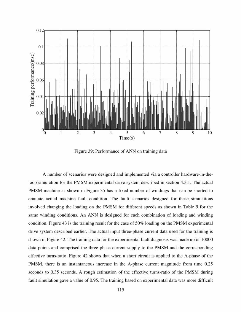
Figure 39: Performance of ANN on training data

A number of scenarios were designed and implemented via a controller hardware-in-the-

loop simulation for the PMSM experimental drive system described in section 4.3.1. The actual

PMSM machine as shown in Figure 35 has a fixed number of windings that can be shorted to

emulate actual machine fault condition. The fault scenarios designed for these simulations

involved changing the loading on the PMSM for different speeds as shown in Table 9 for the

same winding conditions. An ANN is designed for each combination of loading and winding

condition. Figure 43 is the training result for the case of 50% loading on the PMSM experimental

drive system described earlier. The actual input three-phase current data used for the training is

shown in Figure 42. The training data for the experimental fault diagnosis was made up of 10000

data points and comprised the three phase current supply to the PMSM and the corresponding

effective turns-ratio. Figure 42 shows that when a short circuit is applied to the A-phase of the

PMSM, there is an instantaneous increase in the A-phase current magnitude from time 0.25

seconds to 0.35 seconds. A rough estimation of the effective turns-ratio of the PMSM during

fault simulation gave a value of 0.95. The training based on experimental data was more difficult

0 1 2 3 4 5 6 7 8 9 100

0.02

0.04

0.06

0.08

0.1

0.12

Time(s)

Tra

inin

g p

erfo

rman

ce(m

se)

115

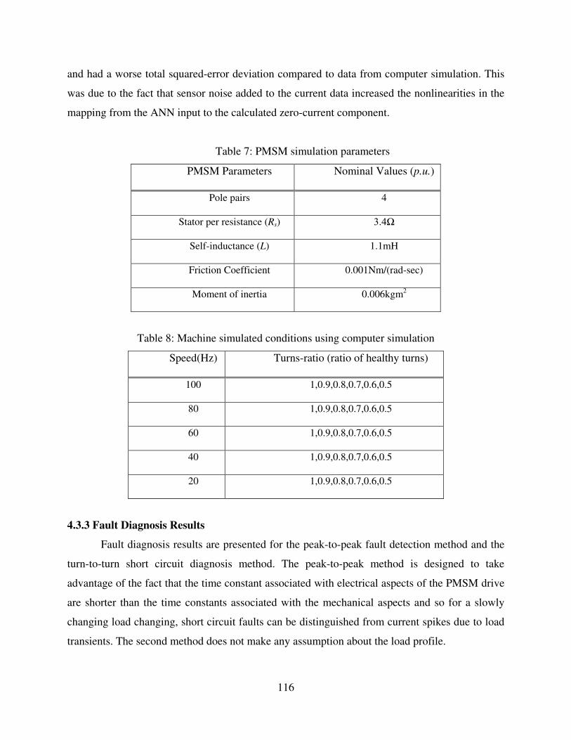
and had a worse total squared-error deviation compared to data from computer simulation. This

was due to the fact that sensor noise added to the current data increased the nonlinearities in the

mapping from the ANN input to the calculated zero-current component.

Table 7: PMSM simulation parameters

PMSM Parameters Nominal Values (p.u.)

Pole pairs 4

Stator per resistance (Rs) 3.4Ω

Self-inductance (L) 1.1mH

Friction Coefficient 0.001Nm/(rad-sec)

Moment of inertia 0.006kgm2

Table 8: Machine simulated conditions using computer simulation

Speed(Hz) Turns-ratio (ratio of healthy turns)

100 1,0.9,0.8,0.7,0.6,0.5

80 1,0.9,0.8,0.7,0.6,0.5

60 1,0.9,0.8,0.7,0.6,0.5

40 1,0.9,0.8,0.7,0.6,0.5

20 1,0.9,0.8,0.7,0.6,0.5

4.3.3 Fault Diagnosis Results

Fault diagnosis results are presented for the peak-to-peak fault detection method and the

turn-to-turn short circuit diagnosis method. The peak-to-peak method is designed to take

advantage of the fact that the time constant associated with electrical aspects of the PMSM drive

are shorter than the time constants associated with the mechanical aspects and so for a slowly

changing load changing, short circuit faults can be distinguished from current spikes due to load

transients. The second method does not make any assumption about the load profile.

116

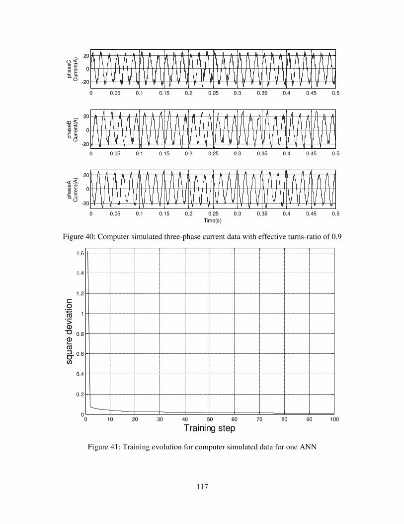
Figure 40: Computer simulated three-phase current data with effective turns-ratio of 0.9

Figure 41: Training evolution for computer simulated data for one ANN

0 0.05 0.1 0.15 0.2 0.25 0.3 0.35 0.4 0.45 0.5

-20

0

20

phaseC

Curr

ent(

A)

0 0.05 0.1 0.15 0.2 0.25 0.3 0.35 0.4 0.45 0.5

-20

0

20

phaseB

Curr

ent(

A)

0 0.05 0.1 0.15 0.2 0.25 0.3 0.35 0.4 0.45 0.5

-20

0

20

Time(s)

phaseA

Curr

ent(

A)

0 10 20 30 40 50 60 70 80 90 1000

0.2

0.4

0.6

0.8

1

1.2

1.4

1.6

Training step

square

devia

tion

117

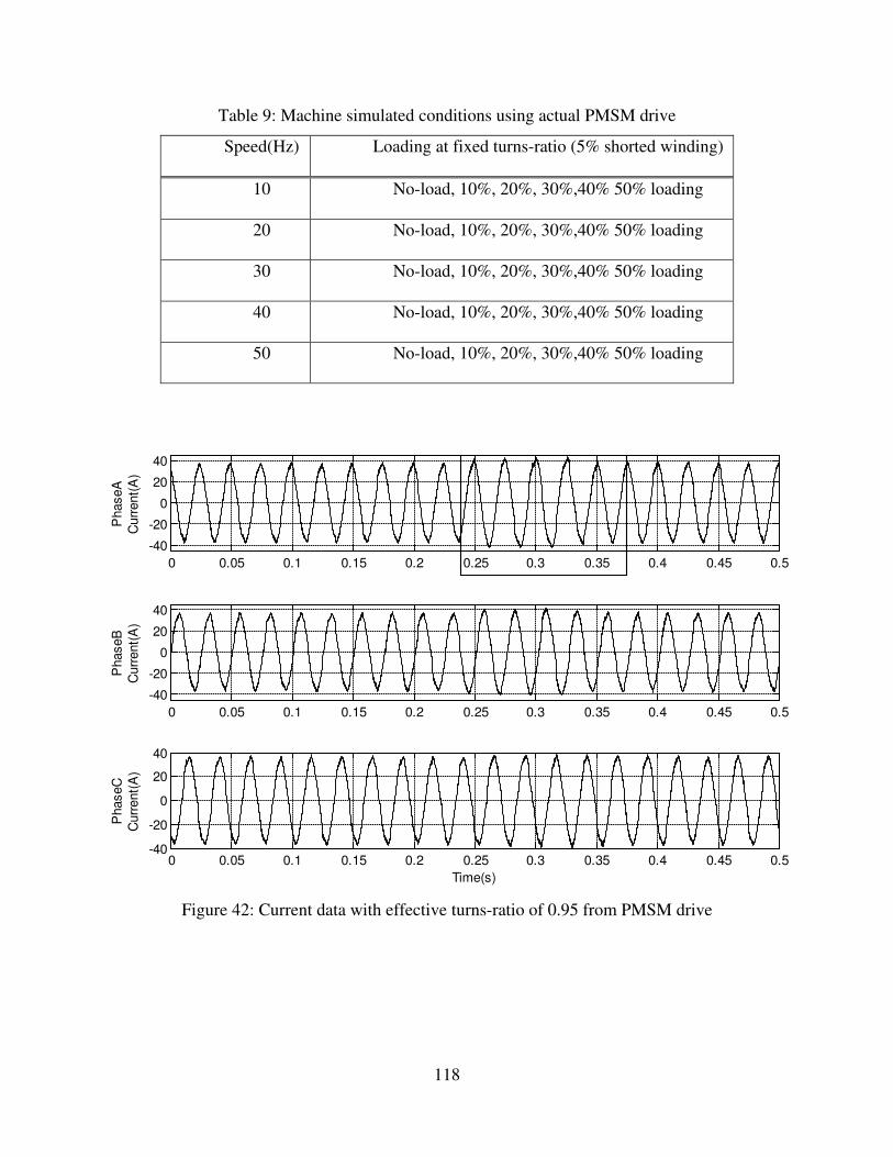
Table 9: Machine simulated conditions using actual PMSM drive

Speed(Hz) Loading at fixed turns-ratio (5% shorted winding)

10 No-load, 10%, 20%, 30%,40% 50% loading

20 No-load, 10%, 20%, 30%,40% 50% loading

30 No-load, 10%, 20%, 30%,40% 50% loading

40 No-load, 10%, 20%, 30%,40% 50% loading

50 No-load, 10%, 20%, 30%,40% 50% loading

Figure 42: Current data with effective turns-ratio of 0.95 from PMSM drive

0 0.05 0.1 0.15 0.2 0.25 0.3 0.35 0.4 0.45 0.5

-40

-20

0

20

40

PhaseA

Curr

ent(

A)

0 0.05 0.1 0.15 0.2 0.25 0.3 0.35 0.4 0.45 0.5

-40

-20

0

20

40

PhaseB

Curr

ent(

A)

0 0.05 0.1 0.15 0.2 0.25 0.3 0.35 0.4 0.45 0.5-40

-20

0

20

40

Time(s)

PhaseC

Curr

ent(

A)

118

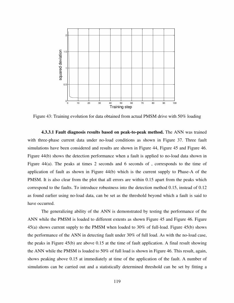
Figure 43: Training evolution for data obtained from actual PMSM drive with 50% loading

4.3.3.1 Fault diagnosis results based on peak-to-peak method. The ANN was trained

with three-phase current data under no-load conditions as shown in Figure 37. Three fault

simulations have been considered and results are shown in Figure 44, Figure 45 and Figure 46.

Figure 44(b) shows the detection performance when a fault is applied to no-load data shown in

Figure 44(a). The peaks at times 2 seconds and 6 seconds of , corresponds to the time of

application of fault as shown in Figure 44(b) which is the current supply to Phase-A of the

PMSM. It is also clear from the plot that all errors are within 0.15 apart from the peaks which

correspond to the faults. To introduce robustness into the detection method 0.15, instead of 0.12

as found earlier using no-load data, can be set as the threshold beyond which a fault is said to

have occurred.

The generalizing ability of the ANN is demonstrated by testing the performance of the

ANN while the PMSM is loaded to different extents as shown Figure 45 and Figure 46. Figure

45(a) shows current supply to the PMSM when loaded to 30% of full-load. Figure 45(b) shows

the performance of the ANN in detecting fault under 30% of full load. As with the no-load case,

the peaks in Figure 45(b) are above 0.15 at the time of fault application. A final result showing

the ANN while the PMSM is loaded to 50% of full load is shown in Figure 46. This result, again,

shows peaking above 0.15 at immediately at time of the application of the fault. A number of

simulations can be carried out and a statistically determined threshold can be set by fitting a

0 10 20 30 40 50 60 70 80 90 1000

0.5

1

1.5

2

Training step

square

d d

evia

tion

119

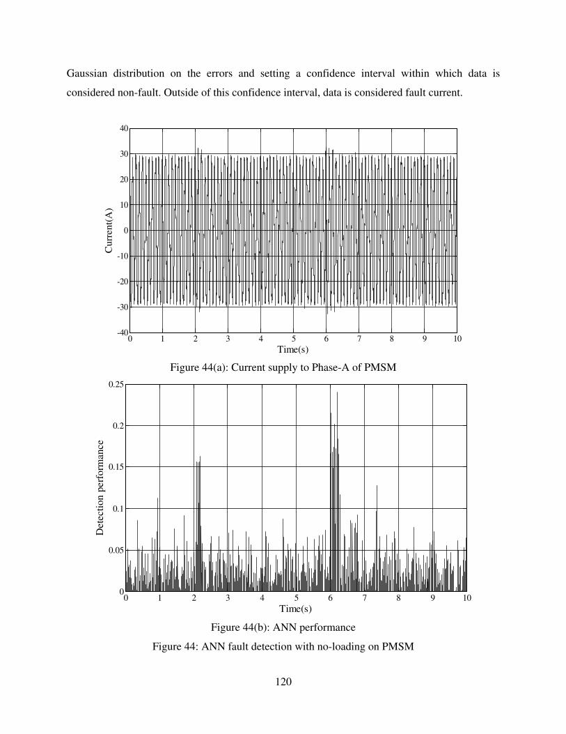
Gaussian distribution on the errors and setting a confidence interval within which data is

considered non-fault. Outside of this confidence interval, data is considered fault current.

Figure 44(a): Current supply to Phase-A of PMSM

Figure 44(b): ANN performance

Figure 44: ANN fault detection with no-loading on PMSM

0 1 2 3 4 5 6 7 8 9 10-40

-30

-20

-10

0

10

20

30

40

Time(s)

Curr

ent(

A)

0 1 2 3 4 5 6 7 8 9 100

0.05

0.1

0.15

0.2

0.25

Time(s)

Det

ecti

on

per

form

ance

120

4.3.3.2 Fault diagnosis results based on turn-to-turn short circuit detection method.

During fault diagnosis, all the trained ANNs are presented with the same input data comprising

the three phase currents multiplied by a value generated by PSO which represents a possible

value for the turns-ratio on each phase of the PMSM. Ideally one of the ANNs would respond if

the calculated turns-ratio from the PSO matches the machine condition it is trained for. One

result of fault diagnosis using the short circuit detection method based on computer simulation of

the PMSM is shown in Figure 47. Correct fault diagnosis showed that there was 10% short

circuiting on the phase-A with no fault on the other two phases and speed set at 100 Hz. The

results based on computer simulation shows that by the 30th iteration of the real time PSO

algorithm, the correct turns-ratio of the A-phase windings have been obtained. At a signal

sampling rate of 0.0002 second per sample, this result show that it took approximately 0.006

seconds for the real-time PSO algorithm to obtain the correct turns-ratio and fault location on the

machine. Similar results were obtained for other fault simulations. For the case of machine

conditions for which none of the ANNs was trained, the ANN which was trained for the

condition that closely matched the simulated conditions was able to obtain the correct turns-ratio

of the windings of the faulted phase. The results shown in Figure 48 gave correct diagnosis with

25% of the phase-A windings shorted. In a few cases none of the ANNs were able to diagnose

the correct turns-ratio. For each diagnosis, the real-time PSO algorithm is initialized with random

numbers.

Fault diagnosis results obtained using data from the PMSM drive took longer as shown in

Figure 49. Figure49 shows correct diagnosis for the PMSM at 30% loading where at about the

50th iteration, the correct turns-ratio is discovered. At a signal sampling rate of 0.0002 seconds

per sample, this result show that it took approximately 0.01 seconds for the real-time PSO

algorithm to obtain the correct turns-ratio on the machine based on the simulated condition. For

the case shown in Figure 49, the A-phase turns-ratio when a fault is applied is 0.95 and 1 for the

other phases. For all cases and as already discussed, the real-time PSO algorithm is randomly

initialized in the discrete solution space as described in section 2.

4.4 Conclusions

The methods presented in this Chapter show a promising use of AI for fault detection and

diagnosis of electrical machines with potential for real time implementation. The methods when

121

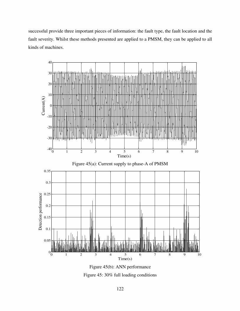
successful provide three important pieces of information: the fault type, the fault location and the

fault severity. Whilst these methods presented are applied to a PMSM, they can be applied to all

kinds of machines.

Figure 45(a): Current supply to phase-A of PMSM

Figure 45(b): ANN performance

Figure 45: 30% full loading conditions

0 1 2 3 4 5 6 7 8 9 10-40

-30

-20

-10

0

10

20

30

40

Time(s)

Curr

ent(

A)

0 1 2 3 4 5 6 7 8 9 100

0.05

0.1

0.15

0.2

0.25

0.3

0.35

Time(s)

Det

ecti

on p

erfo

rman

ce

122

Figure 46(a): Current supply to phase-A of PMSM

Figure 46(b): ANN performance

Figure 46: 50% full loading conditions

0 1 2 3 4 5 6 7 8 9 10-50

-40

-30

-20

-10

0

10

20

30

40

50

Time(s)

Cur

rent

(A)

0 1 2 3 4 5 6 7 8 9 100

0.05

0.1

0.15

0.2

0.25

0.3

0.35

Time(s)

Det

ecti

on p

erfo

rman

ce

123

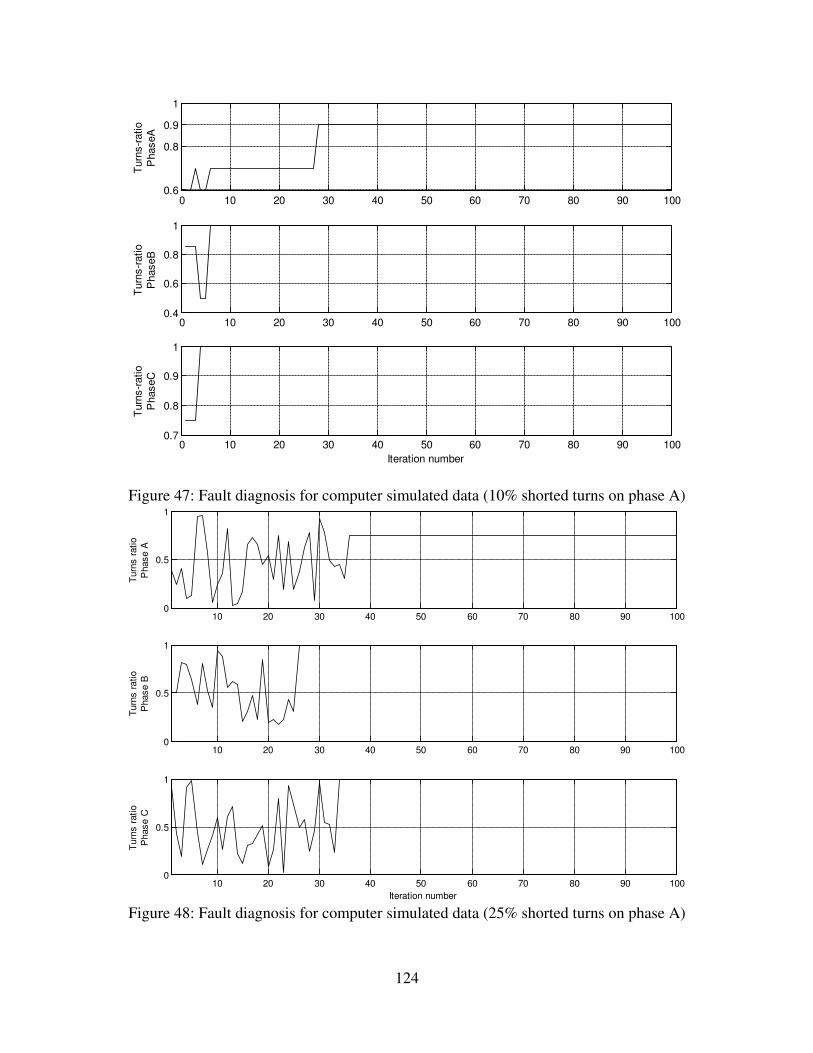
Figure 47: Fault diagnosis for computer simulated data (10% shorted turns on phase A)

Figure 48: Fault diagnosis for computer simulated data (25% shorted turns on phase A)

0 10 20 30 40 50 60 70 80 90 1000.6

0.8

0.9

1

Turn

s-r

atio

PhaseA

0 10 20 30 40 50 60 70 80 90 1000.4

0.6

0.8

1

Turn

s-r

atio

PhaseB

0 10 20 30 40 50 60 70 80 90 1000.7

0.8

0.9

1

Iteration number

Turn

s-r

atio

PhaseC

10 20 30 40 50 60 70 80 90 1000

0.5

1

Turn

s r

atio

Phase A

10 20 30 40 50 60 70 80 90 1000

0.5

1

Turn

s r

atio

Phase B

10 20 30 40 50 60 70 80 90 1000

0.5

1

Iteration number

Turn

s r

atio

Phase C

124

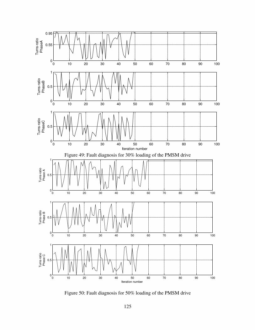
Figure 49: Fault diagnosis for 30% loading of the PMSM drive

Figure 50: Fault diagnosis for 50% loading of the PMSM drive

0 10 20 30 40 50 60 70 80 90 1000

0.55

0.95T

urn

s-r

atio

PhaseA

0 10 20 30 40 50 60 70 80 90 1000

0.5

1

Turn

s-r

atio

PhaseB

0 10 20 30 40 50 60 70 80 90 1000

0.5

1

Iteration number

Turn

s-r

atio

PhaseC

0 10 20 30 40 50 60 70 80 90 1000

0.5

1

Turn

s-r

atio

Phase A

0 10 20 30 40 50 60 70 80 90 1000

0.5

1

Turn

s-r

atio

Phase B

0 10 20 30 40 50 60 70 80 90 1000

0.5

1

Iteration number

Turn

s-r

atio

Phase C

125

In the second method, a FTLN ANN is used in this paper to correlate winding short

faults conditions to the zero-current component of a PMSM. The method also uses the zero-

current component but the method can also use the zero-voltage component in the case of a

voltage controlled drive system. The PSO method is modified to carry out optimization in real

time by performing the PSO particle update immediately after data acquisition. The performance

of the PSO algorithm in real time has been demonstrated to be good. The method presented can

also be implemented in real time using the modified PSO algorithm and the online ANN training

method using the EKF algorithm. Another advantage demonstrated with this method is the

ability to tolerate noise. In particular, we showed the system was relatively impervious to sensor

noise. In principle a single ANN can be trained but to reduce training time, an ANN cluster is

used to capture each operating condition that is considered during training. The training

methodology used, however, enables fast convergence of the ANN weights during design of the

fault diagnosis system and compensates for the increased number of ANNs used for fault

diagnosis.

126

CHAPTER 5

The health monitoring of rotating machines is an involved process since a number of

coupled and complex physical phenomena affect the aging and eventual breakdown of machines.

Broadly speaking the factors that affect machine health can be listed as electrical, thermal,

mechanical and environmental factors. Partial Discharge (PD) is a major source of electrical

degradation in rotating machines which happens in voids, de-laminations and other mechanical

defects in the insulation system. PD also expedites electrical treeing in the insulation material of

insulation system. Electrical treeing is ultimately the main indication of aging and ultimately

leads to insulation breakdown of rotating machines. Simulation of partial discharge and electrical

treeing has been carried out to understand these physical phenomenon both using experimental

and numerical simulation approaches. Experiments to understand the degradation of rotating

machines is sometimes difficult to setup and computer simulation models have been developed

which enables the effect of different parameters on these physical activities to be examined. With

these models, factors that affect partial discharge and electrical treeing can be varied and effects

studied. Numerical models can be used to develop a model-based health monitoring systems for

the insulation systems of rotating machines.

This section discusses prognostics of winding insulation systems. Firsts a new electrical

treeing simulation is presented that is able to more accurately describe the growth of trees than

other simulation models available. The simulation method is used to develop a prognostic system

based on a macro-model that relies on aspects of a growing tree. Before digging into the details

of the prognostic method, the motivation for this study is presented.

5.1 Unique Insulation Issues in an All-Electric Ship

An all-electric ship combines propulsion and service loads into a single supply system.

The conventional shipboard power system, in contrast to terrestrial systems, has unique features

that affect power supply quality as shown in Table 1. These unique characteristics mean requires

extra considerations in the particular case of fault and condition monitoring of component

devices onboard ships. The All-Electric ship is a notional concept and still undergoing research

and development but the issues with shipboard power system may actually increase in an All-

Electric ship with a single service line for propulsion and increased service loads. Increased use

127

of power electronic devices for AC/DC conversion for electric motor propulsion and pulsed-

loads unique to a ship power system may result in unique Power Supply Quality issues that may

have implications for cabling and rotation machines onboard ship a small space. These loads

include:

1. Electromagnetic aircraft launch systems

2. Electromagnetic guns: rail guns, laser guns, coil guns, high energy microwaves

3. Radars, SONARS, communication systems

The main power supply quality problems to be expected in an all-electric ship are an increase in

voltage/current transient, harmonic distortion, frequency modulation, voltage imbalance and

capacitive-current leakage. Harmonic distortion has been identified with mechanical vibrations

in machines and extra heating in cables and machines that lead to insulation breakdown by

facilitating electrical and water trees through an insulation system. Voltage transients are major

sources of PD in insulation systems as is frequency spikes sometimes called notching. Voltage

imbalance produces negative sequence currents that produce mechanical distortions leading to

aging of insulation system. Capacitive leakage current may be high enough to trip fault

monitoring systems and affect harmonic quality of power supply which can have consequences

for the insulation system. The insulation systems of ship MVDC bus, its components, and sub-

systems are stressed not only by the DC component of the electric field but also by high

frequency components caused by switching of power electronic devices and lightning strikes

either into the ship superstructure or the electrical power system directly. Considering that power

supply issues are expected to increase in an all-electric ship, PD and electrical treeing are also

expected to increase leading to faster time to breakdown of insulation and widening of electrical

tree links.

5.2 Dielectric Breakdown Testing

Dielectric breakdown testing is any experimental procedure to determine the breakdown

characteristics of insulation materials. The experimental setup can range from simple needle-

plane electrode experiments to complicated setups to determine the insulation characteristics of

devices in situ. Formettes and Motorettes, for example, have been used in electrical machine

insulation testing during manufacture. The next section describes the experimental setup to

128

determine characteristics of the breakdown of a dielectric material as part of studies in the fault

prognostics of winding insulation systems.

5.2.1 Description of Experimental Setup

Dielectric breakdown tests were carried out to establish characteristics of insulation

breakdown. Some of the characteristics that were of interest included the partial discharge during

breakdown, time to breakdown of a sample when stressed by different voltage levels and the

fractal dimension of the electrical trees. The voltage levels used for the tests were higher than

Partial Discharge Inception (PIV) voltage to cause faster degradation and eventual breakdown

than they would be subjected to by voltages that machines nominally operate at. The

experimental setup was based on the classical needle-plane electrode setup. The dielectric

material was initially chosen as an epoxy resin, with the trade name STYCAST 1266, and with

characteristics shown in Table 10. Due to experimental time constraints an epoxy gel, under the

trade name STYCAST 1265 with characteristics shown in Table 10, was later chosen to reduce

the time to breakdown of the needle-plane experiments. A drawing of the needle-plane

experimental setup is provided in Figure 51 and shows the components of the setup: Acrylic

(PMMA) mold, STYCAST 1265 dielectric material, steel pins as the high electrode, copper plate

as the ground electrode and brass as holder for the steel pins. The distance from the steel pin tip

to the ground electrode was fixed for all tests to a value of 5mm. Each steel pin was polished to

ensure that the radius of the tip was not more than 13µm and not less than 8µm.

Table 10: Characteristics of STYCAST 1266 and STYCAST 1265

STYCAST 1266

STYCAST 1265

Property Units Value Value

Hardness Shore D 138 25

Flexural Strength mPa 75 -

Compressive Strength mPa 69 -

Tensile Strength mPa 41 -

Operating temperature range 0C -65 to 105 -65 to 40

Dielectric strength kV/mm 15.7 -

Dielectric constant (60Hz) - 3 3

Dissipation factor (60Hz) - 0.02 -

Volume resistivity (250C) Ohm-cm 6x1014 -

129

As already stated, one of the aims of the tests was to determine the PD during breakdown

of the dielectric material. A PD monitoring setup was, therefore, used to detect PD and record

the measured PD. This setup to detect PD is shown pictorially and as a circuit schematic in

Figure 52. From the circuit schematic, it can be inferred that the method used for PD detection is

the capacitive method described in section 2.6.3. The parameters of the circuit elements shown in

the circuit diagram are shown in Table 11.

The PD is recorded as an apparent charge which is the charge which if injected over a

short time across the terminals of the Device-Under-Test (DUT) would give the same reading on

the measuring instrument as the PD current itself. The method of calibration used by the PD

monitor first sends a current pulse in the form of a known charge through the PD detection

circuit and through the dielectric material under test using a step voltage generator and a series

capacitor in the absence of high voltage supply. The energy dissipated during the calibration is

used to determine a scale factor that converts the voltage output at the terminals of the PD

monitor circuits into apparent charges in Pico-Coulombs and to establish the level of background

noise.

Figure 51: Setup for breakdown testing of dielectric material

130

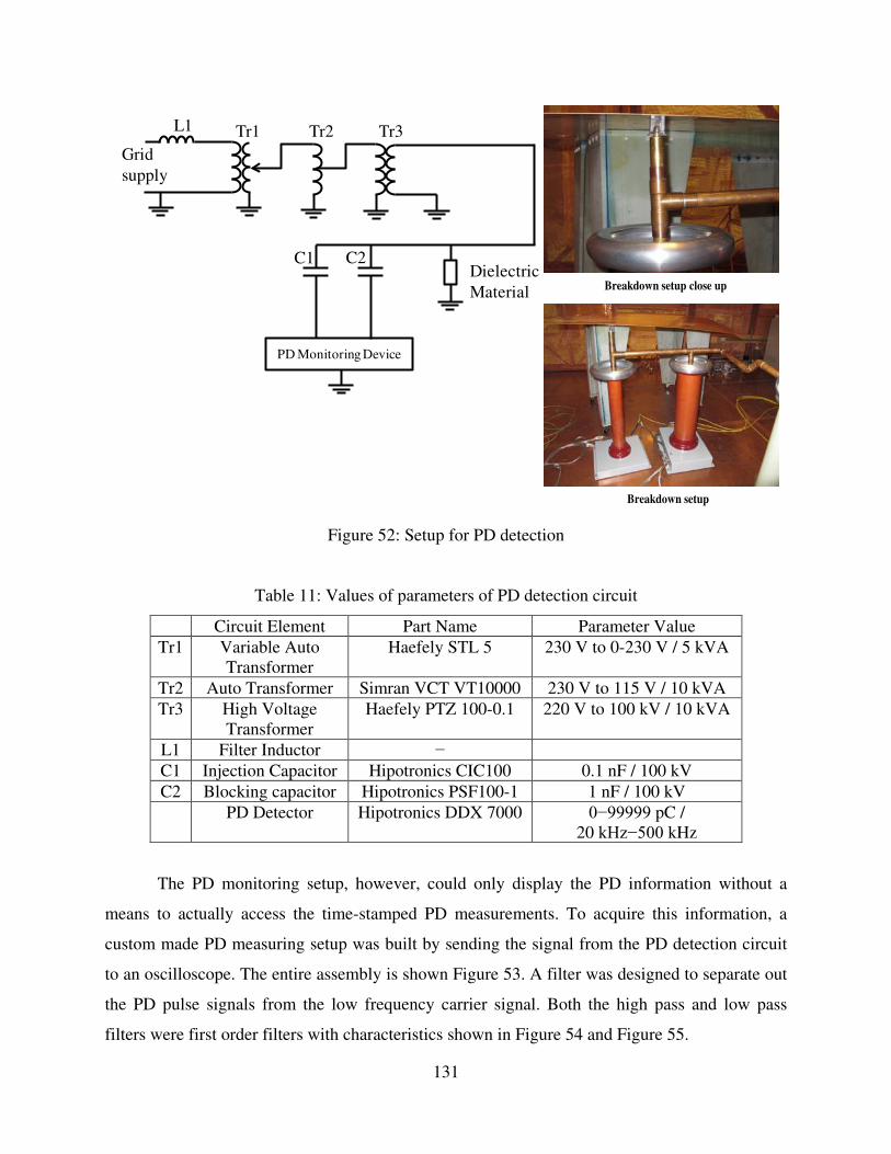
Figure 52: Setup for PD detection

Table 11: Values of parameters of PD detection circuit

Circuit Element Part Name Parameter Value

Tr1 Variable Auto Transformer

Haefely STL 5 230 V to 0-230 V / 5 kVA

Tr2 Auto Transformer Simran VCT VT10000 230 V to 115 V / 10 kVA

Tr3 High Voltage Transformer

Haefely PTZ 100-0.1 220 V to 100 kV / 10 kVA

L1 Filter Inductor −

C1 Injection Capacitor Hipotronics CIC100 0.1 nF / 100 kV

C2 Blocking capacitor Hipotronics PSF100-1 1 nF / 100 kV

PD Detector Hipotronics DDX 7000 0−99999 pC / 20 kHz−500 kHz

The PD monitoring setup, however, could only display the PD information without a

means to actually access the time-stamped PD measurements. To acquire this information, a

custom made PD measuring setup was built by sending the signal from the PD detection circuit

to an oscilloscope. The entire assembly is shown Figure 53. A filter was designed to separate out

the PD pulse signals from the low frequency carrier signal. Both the high pass and low pass

filters were first order filters with characteristics shown in Figure 54 and Figure 55.

PD Monitoring Device

Tr1 Tr2 Tr3L1

Grid

supply

C1 C2Dielectric

Material Breakdown setup close up

Breakdown setup

131

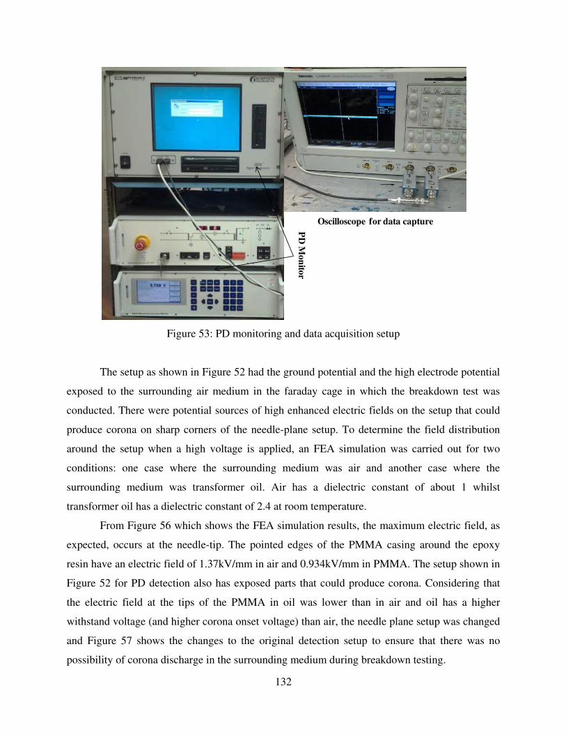
Figure 53: PD monitoring and data acquisition setup

The setup as shown in Figure 52 had the ground potential and the high electrode potential

exposed to the surrounding air medium in the faraday cage in which the breakdown test was

conducted. There were potential sources of high enhanced electric fields on the setup that could

produce corona on sharp corners of the needle-plane setup. To determine the field distribution

around the setup when a high voltage is applied, an FEA simulation was carried out for two

conditions: one case where the surrounding medium was air and another case where the

surrounding medium was transformer oil. Air has a dielectric constant of about 1 whilst

transformer oil has a dielectric constant of 2.4 at room temperature.

From Figure 56 which shows the FEA simulation results, the maximum electric field, as

expected, occurs at the needle-tip. The pointed edges of the PMMA casing around the epoxy

resin have an electric field of 1.37kV/mm in air and 0.934kV/mm in PMMA. The setup shown in

Figure 52 for PD detection also has exposed parts that could produce corona. Considering that

the electric field at the tips of the PMMA in oil was lower than in air and oil has a higher

withstand voltage (and higher corona onset voltage) than air, the needle plane setup was changed

and Figure 57 shows the changes to the original detection setup to ensure that there was no

possibility of corona discharge in the surrounding medium during breakdown testing.

PD

Mon

itor

Oscilloscope for data capture

132

Figure 54: Low pass filter characteristics

After the data is captured by the oscilloscope, it is stored in a memory device for data

processing. Due data processing speed limitations, a full cycle of PD data, as shown in Figure 58,

was stored after every 12 seconds and involved 2 mega samples at 2 nano-seconds per sample at

a resolution of 500 MHz. Figure 58 shows some characteristic features of PD patterns during tree

growth as corroborated by many other researchers in the field. It would be noticed that the PD

detected as a voltage rise is a damped signal with very high frequencies. These signals show up

characteristically in the first and third quadrants of the 60Hz carrier wave. Four PD events are

shown in Figure 58 for the complete cycle shown. At the start of the breakdown process, there

are few PDs of low magnitude. The magnitude of the PD corresponds to the peak of the PD

signal shown in Figure 58. The initial phase is the inception phase and for the testing carried out

with STYCAST 1265 epoxy resin, could take about 4 hours at an impressed voltage of 8kV. As

mentioned earlier, a number of complete cycles were saved during the tree growth for the entire

period of the breakdown process. Figure 59 shows a plot of the number of PDs in a cycle, the

average PD in a cycle, the maximum PD in a cycle and the angle of the maximum PD in a cycle

from start to breakdown of a sample of STYCAST 1265 epoxy resin.

133

Figure 55: High pass filter characteristics

Figure 56 (a): Meshing at the tip of needle

Figure 56: FEA simulation results

134

Figure 56 (b): Electric field distribution at the tip of needle

Figure 56 (c): Electric field distribution at the tip of PMMA in oil

Figure 56 - continued

135

Figure 56 (d): Electric field distribution at the tip of PMMA in air

Figure 56 - continued

Figure 57: Enhanced setup for PD detection

136

Figure 58: Characteristic PD pattern per cycle

Figure 59(a): PD count per cycle

Figure 59: PD characteristics during breakdown of STYCAST 1265

137

Figure 59(b): Maximum PD per cycle

Figure 59(c): Average PD per cycle

Figure 59 - continued

138

Figure 59(d): Angle of maximum PD per cycle

Figure 59 - continued

Several breakdown tests confirmed the following characteristics of the tree propagation

which is also confirmed in [216].

1. PD occurs characteristically in the first and third quadrants during tree growth

2. There is an initialization phase during which PD of low magnitudes (2pC to 10pC) are

recorded

3. There is a growth phase during which higher levels of PD are detected (30pC to 100pC)

4. Final stage which is instantaneous and occurs when the tree has attained a critical level of

growth

One of the major goals of this research work is to come out with ways to use PD data,

whose detection, measurement and further data processing has been improved over the decades,

to predict impending failures. Whilst the use of PD for diagnosis and prognosis is not a new

approach, the usual way has been to use PD to determine the severity of degradation in

insulation. This, usually, is a go-no-go criterion where if the PD level is above a certain

threshold, the insulation system is declared to be damaged. Figure 59 shows that during tree

growth, the PD pulse count per cycle changes over time until the final stage of tree growth in a

139

way that can be used to determine some characteristics of the tree growth that can be used to

predict the time to attain a critical length after which breakdown is instantaneous. This is also

similar for the maximum PD pulse per cycle, average PD pulse per cycle and angle of maximum

PD pulse per cycle. The process of obtaining enough data to develop prognostics approaches for

the time to breakdown of the dielectric material involves a tedious and long process to obtain

data similar to what is shown in Figure59 for a lot of samples. To make the process less tedious,

a new simulation model has been developed that accounts for the characteristic features of the

tree growth process in ways that other current models do not account for. The next section

describes the details of the simulation model.

5.3 Modified Dielectrics Breakdown Model

Experimental investigations of electrical treeing indicate that the growth of tree channels

is associated with partial discharges (PD) in the dielectric materials. The actual mechanism of

growth has been explained by several physical processes including electron avalanches,

electromechanical fracturing and photo-degradation [217]. From the point of view of a

simulation model that can generate the electrical tree structures, a number of approaches have

been suggested to account for the characteristic patterns of growth and the growth dynamics. The

NPW model, named after its inventors, Niemeyer, Pietronero and Weismann was the first model

to suggest that the tree channels were created by an advancing boundary of an injected charge

fluid from the tree tip. The model associated the branching patterns observed during tree growth

to a stepwise development in which the next branch to be added to the structures is chosen at

random from pre-specified growth direction. Each growth direction has a failure probability

proportional to En, where E is the local electric field along the bond and n is an unknown

exponent normally fixed at values between 1.5 and 2. For computations, the NPW model

assumes that local failure occurs immediately after the local electric field exceeds a critical level.

Below this level, tree extension in the pre-specified direction is not possible. Experimental

observation, however, suggests that there is high electric field, mostly, at the tips of the growing

trees and, to a lesser extent, within the tree channels due to space charges. The high electric field

induces damage generating events in the insulation and over time the tree extends in the direction

where the insulation material has been damaged the most. Including this stepwise damage

process into the NPW model suggests that there is a critical damage level where local failure is

140

possible. This constitutes the modification to the NPW model called the Discharge Avalanche

Model (DAM) which avoids the difficult-to-explain power law associated with the NPW model.

The DAM modification to the NPW model accounts for the stochastic nature of tree propagation

by using random values for the physical characteristics of the dielectric material. DAM,

however, does not account for PD in the tree channels. Several models have been proposed to

account for PD with most associating a PD activity to the damage processes that occurs when

there is a local breakdown. In this paper, we propose a new approach to electrical tree modeling

by representing the growing tree as a set of contiguous charged spheres. This idea has been

suggested in [218] to describe PD in a static electrical tree. The model proposed in this paper

extends this idea into a dynamic tree by using the DAM approach to extend the tree whilst

accounting for the PD activity in the tree channels by way of charge transfers between the

charged spheres. The new simulation model can be explained basically by the flow chart shown

in Figure 60. The process begins by setting voltages at each tree point. The voltages at each tree

point are specified by representing the tree as a low resistance channel in the dielectric material

as show in Figure 61. The number tree points are determined by the size of mesh grid used for

the simulation. The charges on each sphere are then calculated by the Charge Simulation Method

(CSM). If Qi is the charge at tree point i, the voltage Vi at that point can be determined by the

CSM method as shown in Equation (79) where k and k’ are the voltage contributions due to the

charged sphere at tree point i and its image.

( ) ( ) ( ) ( ) nnini

iiiiiiiiii QkkQkkQkkQkkV ''2

2'

2

11'

1 −+−++−+−= (79)

The voltage coefficients of the charges in Equation (79) are calculated using classical

electrostatics with Equation (80) and (81) shown below where rji is the Euclidean distance of the

charged sphere i from tree point j, εr is the permittivity of free space and ε0 is the relative

permittivity of the sample at point i.

iri

ir

k10

14

1

επε= (80)

iiri

iir

kεπε04

3= (81)

141

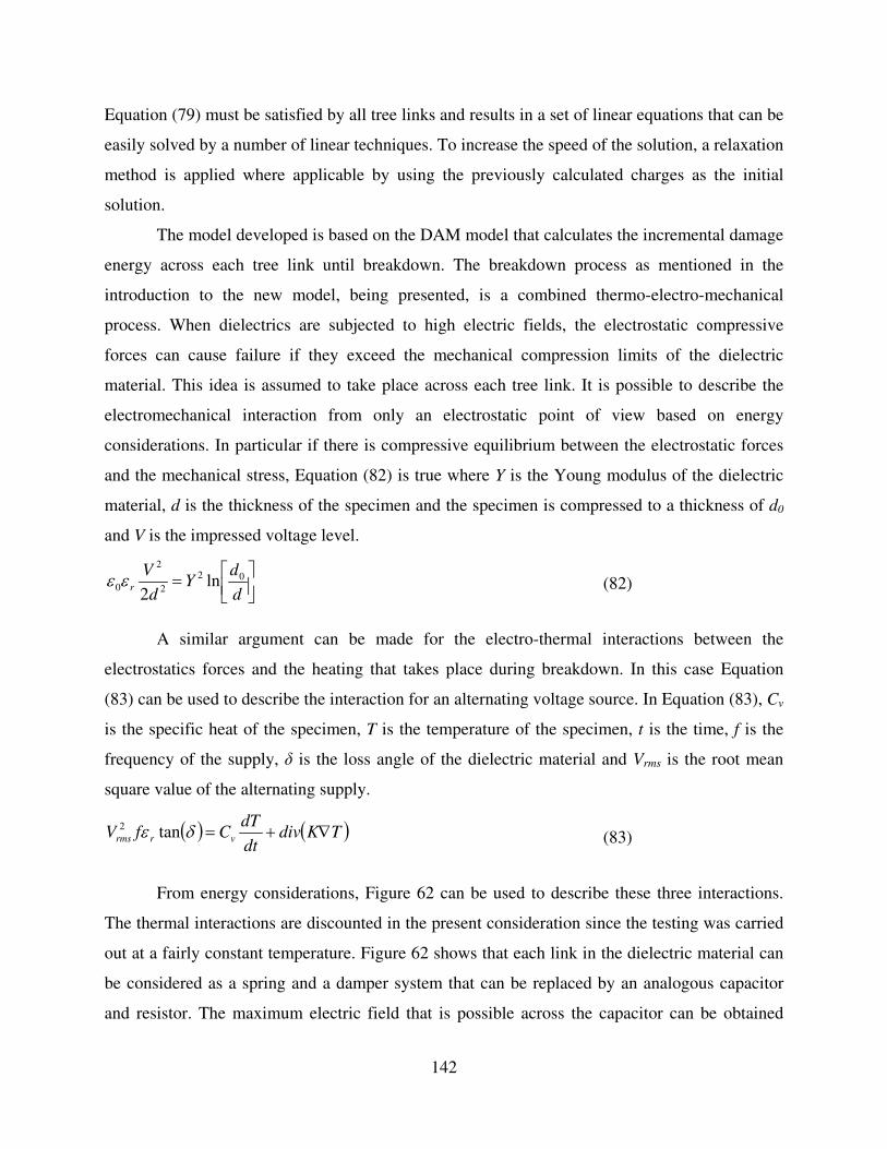
Equation (79) must be satisfied by all tree links and results in a set of linear equations that can be

easily solved by a number of linear techniques. To increase the speed of the solution, a relaxation

method is applied where applicable by using the previously calculated charges as the initial

solution.

The model developed is based on the DAM model that calculates the incremental damage

energy across each tree link until breakdown. The breakdown process as mentioned in the

introduction to the new model, being presented, is a combined thermo-electro-mechanical

process. When dielectrics are subjected to high electric fields, the electrostatic compressive

forces can cause failure if they exceed the mechanical compression limits of the dielectric

material. This idea is assumed to take place across each tree link. It is possible to describe the

electromechanical interaction from only an electrostatic point of view based on energy

considerations. In particular if there is compressive equilibrium between the electrostatic forces

and the mechanical stress, Equation (82) is true where Y is the Young modulus of the dielectric

material, d is the thickness of the specimen and the specimen is compressed to a thickness of d0

and V is the impressed voltage level.

=

d

dY

d

Vr

02

2

2

0 ln2

εε (82)

A similar argument can be made for the electro-thermal interactions between the

electrostatics forces and the heating that takes place during breakdown. In this case Equation

(83) can be used to describe the interaction for an alternating voltage source. In Equation (83), Cv

is the specific heat of the specimen, T is the temperature of the specimen, t is the time, f is the

frequency of the supply, δ is the loss angle of the dielectric material and Vrms is the root mean

square value of the alternating supply.

( ) ( )TKdivdt

dTCfV vrrms ∇+=δε tan2 (83)

From energy considerations, Figure 62 can be used to describe these three interactions.

The thermal interactions are discounted in the present consideration since the testing was carried

out at a fairly constant temperature. Figure 62 shows that each link in the dielectric material can

be considered as a spring and a damper system that can be replaced by an analogous capacitor

and resistor. The maximum electric field that is possible across the capacitor can be obtained

142

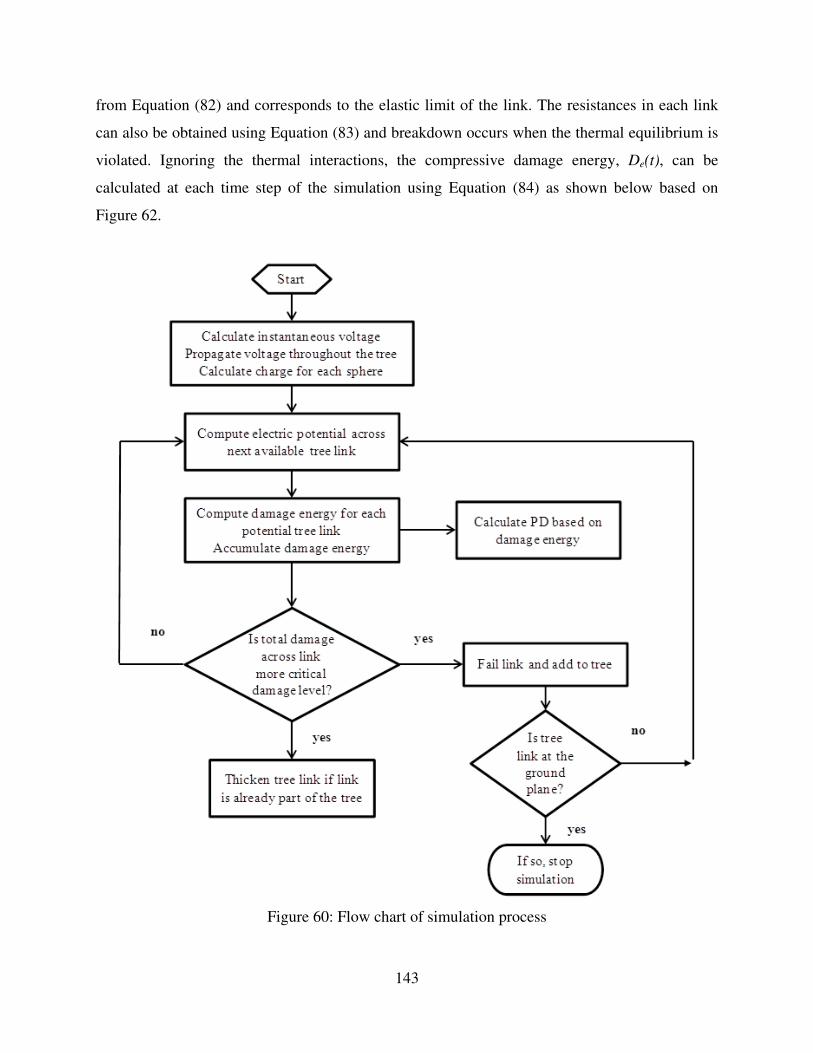
from Equation (82) and corresponds to the elastic limit of the link. The resistances in each link

can also be obtained using Equation (83) and breakdown occurs when the thermal equilibrium is

violated. Ignoring the thermal interactions, the compressive damage energy, De(t), can be

calculated at each time step of the simulation using Equation (84) as shown below based on

Figure 62.

Figure 60: Flow chart of simulation process

143

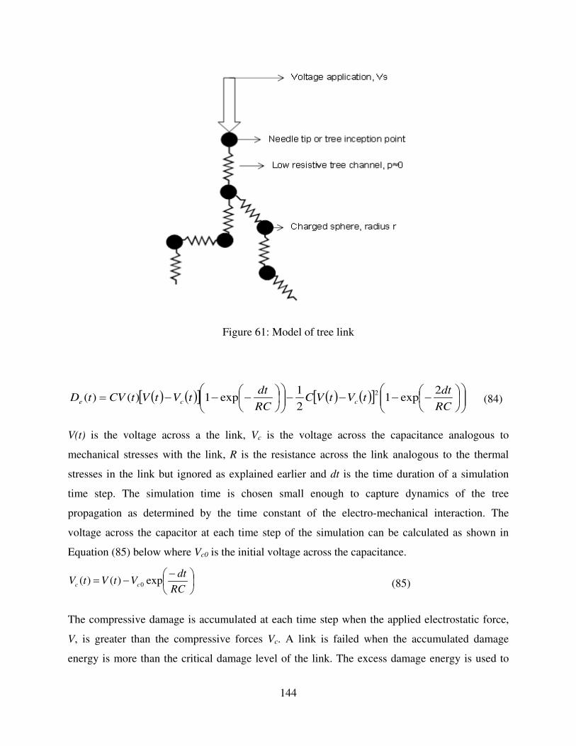
Figure 61: Model of tree link

( ) ( )[ ] ( ) ( )[ ]

−−−−

−−−=

RC

dttVtVC

RC

dttVtVtCVtD cce

2exp1

2

1exp1)()(

2 (84)

V(t) is the voltage across a the link, Vc is the voltage across the capacitance analogous to

mechanical stresses with the link, R is the resistance across the link analogous to the thermal

stresses in the link but ignored as explained earlier and dt is the time duration of a simulation

time step. The simulation time is chosen small enough to capture dynamics of the tree

propagation as determined by the time constant of the electro-mechanical interaction. The

voltage across the capacitor at each time step of the simulation can be calculated as shown in

Equation (85) below where Vc0 is the initial voltage across the capacitance.

−−=

RC

dtVtVtV cc exp)()( 0 (85)

The compressive damage is accumulated at each time step when the applied electrostatic force,

V, is greater than the compressive forces Vc. A link is failed when the accumulated damage

energy is more than the critical damage level of the link. The excess damage energy is used to

144

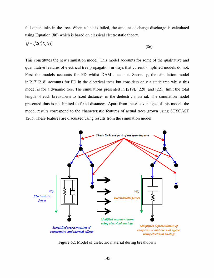
fail other links in the tree. When a link is failed, the amount of charge discharge is calculated

using Equation (86) which is based on classical electrostatic theory.

( ))(2 tDCQ e= (86)

This constitutes the new simulation model. This model accounts for some of the qualitative and

quantitative features of electrical tree propagation in ways that current simplified models do not.

First the models accounts for PD whilst DAM does not. Secondly, the simulation model

in[217][218] accounts for PD in the electrical trees but considers only a static tree whilst this

model is for a dynamic tree. The simulations presented in [219], [220] and [221] limit the total

length of each breakdown to fixed distances in the dielectric material. The simulation model

presented thus is not limited to fixed distances. Apart from these advantages of this model, the

model results correspond to the characteristic features of actual trees grown using STYCAST

1265. These features are discussed using results from the simulation model.

Figure 62: Model of dielectric material during breakdown

145

5.3.1 Electrical Tree Simulation Results

Figure 63 shows a simulation of the breakdown process for the case of applying a voltage

(100 kV) to a specimen that is 5 times the breakdown voltage of the sample. The characteristic

features of the figure traced during the breakdown process shows an inception period that lasts

about 30 micro-seconds in simulation time. The second stage is a very brief propagation phase

for the next 40 micro-seconds during which time a few PDs occur with a maximum of about 18

Pico-Coulombs occurring at time 7 micro-seconds. The final stage is complete breakdown

represented by a huge PD event of about 35 nano-Coulombs which triggers multiple breakdowns

throughout the specimen in a fashion similar to an electron avalanche. This confirms what

happens experimentally during instantaneous breakdown using high voltage levels.

Figure 64 shows another result using the simulation model for a voltage (10 kV) at half

the breakdown level. The major difference between Figure 63 and Figure 64 is the relatively

longer period of tree growth. From Figure 64, the tree growth period takes about 0.15 seconds

instead of 40 micro-seconds obtained with 100 kV. The total number of PD activities obtained at

this voltage level is 96 with a maximum discharge of about 60 pico-Coulombs. It would be

noticed that, considering a complete cycle of the carrier wave, PDs only occur at the first and

third quadrants. This is validated by experimental results as shown in Figure 58. The model

predicts harmonic distortion can results in PDs occurring in the second and fourth quadrants.

These aspects of the breakdown process are, however, not explored further in this study. After

the growth phase, the specimen breaks down instantaneously at time 0.16 seconds due to a huge

discharge that is cascaded throughout the specimen.

In summary, this simulation can be used to generate the Lichtenberg figures that

characterize the growth of trees in a dielectric. Whilst the simulation model can be extended to

account for thermal effects, the features that characterize the growth of tree in STYCAST 1265

are adequately captured using this model. As discussed earlier, the PD count per cycle, PD

maximum per cycle, angle of maximum PD per cycle and average PD per cycle appear to

contain information than can prove useful in gaining insights into the actual tree during the

growth phase. Importantly these values can now be obtained very easily using the tree growth

simulation model presented. The next presents a macro-model that connects the discussion so far

to the main discussion of predicting the time of failure of dielectric materials undergoing

breakdown.

146

Figure 63(a): Breakdown path using model using

Figure 63(b): PD events before breakdown

Figure 63: Simulation results for fast breakdown

-8 -6 -4 -2 0 2 4 6 80

10

20

30

40

50

60

70

80

90

100Brief tree growth stage

About 70 micro-seconds

Path

of in

stan

tan

eou

s brea

kd

ow

n

Distan

ce from

tip n

eedle (1

00

un

its for 1

mm

)

0 1 2 3 4 5 6 7

x 10-5

0

0.2

0.4

0.6

0.8

1

1.2

1.4

1.6

1.8

x 10-11

Simulation time (seconds)

PD

(C

ou

lom

bs)

0 1 2 3 4 5 6 7

x 10-5

0

1000

2000

3000

4000

PD

Voltage wave

147

Figure 63(c): PD events from start to breakdown

Figure 63 continued

Figure 64(a): Breakdown path using model using

Figure 64: Simulation results for slow breakdown

0 1 2 3 4 5 6 7 8

x 10-5

0

0.5

1

1.5

2

2.5

3

3.5x 10

-8

Simulation time (seconds)

PD

(C

ou

lom

bs)

0 1 2 3 4 5 6 7 8

x 10-5

0

1000

2000

3000

4000

PD

Voltage wave

-6 -4 -2 0 2 4 60

10

20

30

40

50

60

70

80

90

100

Rela

tively

lon

ger g

row

th sta

ge

Path

of in

stan

tan

eou

s brea

kd

ow

n

Distan

ce from

tip n

eedle (1

00

un

its for 1

mm

)

148

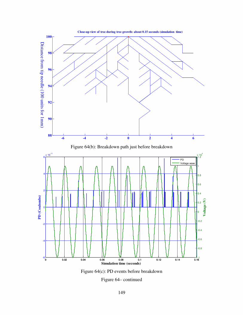
Figure 64(b): Breakdown path just before breakdown

Figure 64(c): PD events before breakdown

Figure 64– continued

-6 -4 -2 0 2 4 688

90

92

94

96

98

100

Close-up view of tree during tree growth: about 0.15 seconds (simulation time)

Distan

ce from

tip n

eedle (1

00

un

its for 1

mm

)

0 0.02 0.04 0.06 0.08 0.1 0.12 0.14 0.16-6

-4

-2

0

2

4

6x 10

-11

Simulation time (seconds)

PD

(C

ou

lom

bs)

0 0.02 0.04 0.06 0.08 0.1 0.12 0.14 0.16-1

-0.8

-0.6

-0.4

-0.2

0

0.2

0.4

0.6

0.8

1

1.2x 10

4

Vo

lta

ge

(V)

PD

Voltage wave

149

5.4 Macro-Model for Prognosis

Another feature of the growth process to be noticed in Figure 64 is that the tree has a

critical length after which it breaks down. The dynamics of the tree growth before it achieves its

critical length can be described as stable whilst the growth after the critical length can be

described as a highly unstable breakdown process resulting in the almost instantaneous channel

elongation from the point of initiation to the ground plane. These characteristics have spurred

studies into the chaotic aspects of tree growth. One result of such an approach has resulted in a

macro-model that uses the fractal dimension of the tree, before it enters the final growth phase, to

determine the time to breakdown of the tree [221]. This model is described in Equation (87)

below.

−

=

kT

ECU

kT

hN

L

Lt b

df

b

cg

200expπεα

(87)

In Equation (87), U0 is the initial energy barrier for molecular breakdown of the bonds in

the dielectric material, αC0 is the volume of material activated in the direction of the applied

field, E is the local field strength dependent on the applied voltage, kT, is the Boltzmann constant

and T is the temperature in Kelvins, hNb, is the Planck constant multiplied by the number of

bonds in a given tree branch and Lc/Lb is the ratio of the critical length before breakdown

proceeds exponentially and the instantaneous length of the tree branch farthest away from the

tree tip. Equation (87) suggests a relationship between the fractal dimension and the time to

breakdown. To confirm this empirical relationship using data based on computer simulated

electrical tree propagation, a number of simulation runs have been carried out and a plot of time-

to-breakdown versus voltage and a separate plot involving the fractal dimension and the voltage

have been obtained. Some of these simulation results used for the verification are shown together

in Figure 65. The fractal dimension, FD, is obtained using the box counting method which is

calculated using Equation (88) where Nε is the minimum number of squares required to

completely cover the propagating tree during the propagation phase and ε is the length of one of

the sides of the square.

( )

=ε

ε1

log

log

10

10 NFD (88)

150

Figure 66 is a plot of time-to-breakdown versus voltage on the left vertical axis and

fractal dimension versus voltage on the right vertical axis. It is seen that there is, an almost,

similar relationship between the time-to-breakdown and the applied voltage as between the

fractal dimension and applied voltage. The relation between voltage and time-to-breakdown on

one hand and voltage and fractal dimension on the other hand are both non-linear.

Figure 65(a): Tree simulation at 50kV

Figure 65(b): Tree simulation at 40kV

Figure 65(c): Tree simulation at 30kV

Figure 65(d): Tree simulation at 20kV

Figure 65: Some tree simulation results

The Equation in (89) is based on Equation (87) and is proposed as a model to determine

the time-to-breakdown of a dielectric material undergoing breakdown. Equation (89), however,

uses parameters that are more easily accessible by replacing the (Lc/Lb) term by the separation

distance between the electrodes in a needle plane experiment, Ds. The second term is replaced

with a constant, α, to be determined experimentally. Inside the exponential, the initial energy

-6 -4 -2 0 2 4 60

1

2

3

4

5

6

7

8

9

10

-8 -6 -4 -2 0 2 4 6 80

1

2

3

4

5

6

7

8

9

10

-6 -4 -2 0 2 4 60

1

2

3

4

5

6

7

8

9

10

-8 -6 -4 -2 0 2 4 6 80

1

2

3

4

5

6

7

8

9

10

151

barrier is replaced by a parameter in the proposed electrical tree model, the critical electric field

that is specified by Equation (89). The local electrical field is replaced by the supply voltage, Vs

and a constant, β, to be determined experimentally. λ is an exponential factor which is proposed

in this work to replace the fractal dimension. The value of this parameter plays the same role as

the fractal dimension in Equation (89) but is determined experimentally using breakdown data.

Figure 66: Plot of time-to-breakdown versus voltage

( ) ( )smsg VDDt 2exp βα λ −= (89)

The proposed RUL model in Equation (89) can, therefore, be determined by empirical curve

fitting for any dielectric material. Figure 67 is the result of such curve fitting for using computer

simulated electrical tree propagation data. Prediction using the modified thermodynamic model

is generally within the margin of error.

Experimental evidence has been used to support the contention that the electrical treeing

phenomenon is the result of a deterministic breakdown mechanism operating in a chaotic regime

at fields lower than those required for runaway breakdown hence the same voltage level would

152

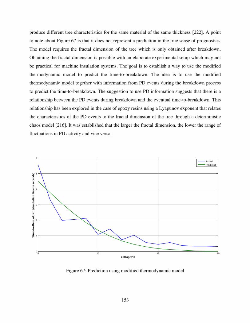
produce different tree characteristics for the same material of the same thickness [222]. A point

to note about Figure 67 is that it does not represent a prediction in the true sense of prognostics.

The model requires the fractal dimension of the tree which is only obtained after breakdown.

Obtaining the fractal dimension is possible with an elaborate experimental setup which may not

be practical for machine insulation systems. The goal is to establish a way to use the modified

thermodynamic model to predict the time-to-breakdown. The idea is to use the modified

thermodynamic model together with information from PD events during the breakdown process

to predict the time-to-breakdown. The suggestion to use PD information suggests that there is a

relationship between the PD events during breakdown and the eventual time-to-breakdown. This

relationship has been explored in the case of epoxy resins using a Lyapunov exponent that relates

the characteristics of the PD events to the fractal dimension of the tree through a deterministic

chaos model [216]. It was established that the larger the fractal dimension, the lower the range of

fluctuations in PD activity and vice versa.

Figure 67: Prediction using modified thermodynamic model

5 10 15 200

1

2

3

4

5

6

Voltage(V)

Tim

e-t

o-B

rea

kd

ow

n (

sim

ula

tio

n t

ime i

n s

eco

nd

s)

Actual

Predicted

153

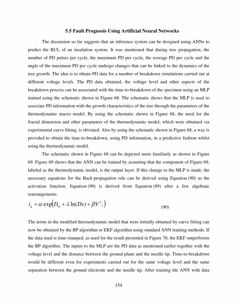
5.5 Fault Prognosis Using Artificial Neural Networks

The discussion so far suggests that an inference system can be designed using ANNs to

predict the RUL of an insulation system. It was mentioned that during tree propagation, the

number of PD pulses per cycle, the maximum PD per cycle, the average PD per cycle and the

angle of the maximum PD per cycle undergo changes that can be linked to the dynamics of the

tree growth. The idea is to obtain PD data for a number of breakdown simulations carried out at

different voltage levels. The PD data obtained, the voltage level and other aspects of the

breakdown process can be associated with the time-to-breakdown of the specimen using an MLP

trained using the schematic shown in Figure 68. The schematic shows that the MLP is used to

associate PD information with the growth characteristics of the tree through the parameters of the

thermodynamic macro model. By using the schematic shown in Figure 68, the need for the

fractal dimension and other parameters of the thermodynamic model, which were obtained via

experimental curve fitting, is obviated. Also by using the schematic shown in Figure 68, a way is

provided to obtain the time-to-breakdown, using PD information, in a predictive fashion whilst

using the thermodynamic model.

The schematic shown in Figure 68 can be depicted more familiarly as shown in Figure

69. Figure 69 shows that the ANN can be trained by assuming that the component of Figure 69,

labeled as the thermodynamic model, is the output layer. If this change to the MLP is made, the

necessary equations for the Back-propagation rule can be derived using Equation (90) as the

activation function. Equation (90) is derived from Equation (89) after a few algebraic

rearrangements.

( )smg VDsDt 2)ln(exp βλα ++= (90)

The terms in the modified thermodynamic model that were initially obtained by curve fitting can

now be obtained by the BP algorithm or EKF algorithm using standard ANN training methods. If

the data used is time-stamped, as used for the result presented in Figure 70, the EKF outperforms

the BP algorithm. The inputs to the MLP are the PD data as mentioned earlier together with the

voltage level and the distance between the ground plane and the needle tip. Time-to-breakdown

would be different even for experiments carried out for the same voltage level and the same

separation between the ground electrode and the needle tip. After training the ANN with data

154

from a number of breakdown processes, however, the ANN can enable a better prediction of the

time-to-breakdown using the modified thermodynamic model. Figure70 is the new time-to-

breakdown prediction using the ANN in conjunction with the modified thermodynamic model.

The predictive power of the thermodynamic model is greatly enhanced as shown in Figure 70.

Only a few cycles of PD information, obtained during the growth phase of the electrical tree, was

used during the ANN training. To ensure faster convergence of the ANN during training, white

Gaussian noise is added to the training data.

Figure 68: Adaptive ANN dielectric breakdown prognosis system

Figure 69: Training model for adaptive ANN dielectric breakdown prognosis system

+

−Thermodynamic

model of dielectric

breakdown

Voltage

PD

Information

ANN

∑

Actual Time-

to-breakdown

∑PD

Information

Voltage

ANN

Thermodynamic

modelActual

Time-to-breakdown

Predicted

+

−

155

Figure 70: Prediction using modified ANN adaptive model

5.6 Conclusion

In this Chapter a new approach to determining the health of insulation materials is

presented. This approach uses ANN to associate the characteristics of PD during the growth of

electrical trees with the RUL of the dielectric material. This chapter also presented a new model

for simulating electrical trees that accounts for most of the important features that characterize

the breakdown of dielectrics and was used to generate all the simulation data that was used to

develop the ANN prognosis system for dielectric materials. Figure 71 depicts the main

contribution of this Chapter to machine insulation diagnostics where the inference system

developed can be easily incorporated into the machine overall control strategy.

The model presented, however, is for a simple dielectric arrangement and does not

account for the complex geometries involved in machine insulation systems. Machine insulation

systems are also inhomogeneous and are subject to complex voltage waveforms that may prove a

challenge to using the above prognosis procedure.

5 10 15 200

1

2

3

4

5

6

Voltage (V)

Tim

e to

Bre

ak

do

wn

(si

mu

lati

on

tim

e in

sec

on

ds)

Actual

Predicted

156

Figure 71: Illustration of fault prognostic system

Prognostics system

for determination

of RUL based on

macro modelPD

detectio

n

system

Machine

Machine control

system

Insulation prognostic information

157

CHAPTER 6

This research has looked at the fault detection, fault diagnosis and fault prognosis in

electrical machines by proposing a number of novel algorithms based on AI. In this chapter, a

summary of the main findings of dissertation, including the limitations of the methods presented,

would be discussed.

Electric machines serve as the backbone of many systems: terrestrial and shipboard

power systems and airplanes. Effective FDD and prognosis is, therefore, needed for the

continuous healthy operations and reliability of the entire system. Due to its high efficiency, high

power density, and robustness, PMSM has been widely used, especially in systems that have

demanding requirements on reliability, such as navy shipboard power systems. For a Navy ship

that may operate in extreme and hostile environments, effective FDD and prognosis at the early

stage is especially important for survivability. Today, the FDD of PMSM has not been fully

explored and there is still a big gap between available theories and practical applications. This

dissertation has focused on the development novel techniques using the relatively new field of AI

to tackle rotating machine FDD and prognostics. AI is a very expansive field that aims at

developing mathematical representations how biological systems process data. AI has been

successfully deployed in the area of motion control and power electronics application with

limited success in the area of fault diagnosis and prognosis.

The contributions of this work include two new AI techniques for fault detection and

diagnosis of stator short winding faults. A new training method is proposed for PSO to enable

fast convergence of ANN weights with implications for online health monitoring based on fast

reconfiguration of the ANN structure. It is demonstrated that manifold reduction methods can be

applied to fault classification during online health monitoring. The research also proposes a new

prognostic approach using PD monitoring. A new method is presented for simulating the

breakdown of dielectric materials that has implications for the understanding of the breakdown

of insulation systems.

6.1 Fault Classification

In some cases, investigators are interested in knowing the cause of degradation of the

electrical machine. This can be a difficult task especially when performed whilst the machine is

in operating and in a situation where the number of machines is enormous. It is possible,

158

however, to extract information inexpensively from the machines even when they are operating

and then determine the type of degradation they are undergoing. The information extracted is

about a fault indicator which is a physical parameter that can be measured, monitored (preferably

online) and whose measured value changes with time and condition of the machine.

In this dissertation, the characteristics of the fault indicator has been associated with the

type of degradation the machine is undergoing using AI techniques. For carrying out these

studies using different fault indicators and different AI techniques, the machine is modeled using

FEA for accuracy. Next the various faults, Short-circuit, Demagnetization and Eccentricity

faults, are modeled using the FEA method. For assessing the performance various AI techniques

during fault diagnosis, information about these faults is extracted from these machine fault

models. To reduce the computational burden during online fault diagnosis, manifold reduction

techniques were applied the information extracted from the machine fault models and the

classification techniques applied. The results from these studies showed that instantaneous power

is the best fault indicator. The best classification techniques were found to be Decision Trees and

Nearest Neighbor techniques. When manifold reduction techniques were applied, instantaneous

power was still the best fault indicator with Decision Trees and Nearest Neighbor techniques

being classifiers. The best manifold reduction techniques were PCA and MDS techniques.

Another result from the studies is that air-gap flux is not a good indicator for the fault types

considered.

6.2 Fault Detection

Fault detection is an important first step in fault diagnosis. By the use of alarms in

integrated FDD system, the detection of commonly occurring faults like short-circuits can help to

forestall further damage to the machines. Whilst the detection of faults is carried out by different

techniques currently, the use of AI techniques has been limited mainly to offline techniques. Two

AI based techniques using ANNs were proposed for the detection of short-circuits faults using

large PMSMs for testing.

The first technique was ascribed the name Peak-to-peak short circuit method since the

method is based on an ANN that is trained to have little to no changes in its output during

mechanical load transients but has huge changes in its output during short-circuits. In the second

method, the turns-ratio of the rotating machine is directly related to the zero-components using

159

an ANN. The first method is trained by using an enhanced PSO technique based on the BFGS

quasi-Newton method to enhance the convergence of the ANN weights. Since the ANN weights

converge fast, the ANN can be reconfigured online to make fault detection with this method

completely an online method. In the second method, the EKF method is used to train the ANNs

to make continuous learning fast with a consequence that the ANNs used can also be

reconfigured online. The first method used an MLP with a single hidden layer whilst the second

method used a FTNN with a single hidden layer.

The two methods presented were demonstrated to show that both methods can detect

faults within a short amount of time to prevent total winding damage using computer simulation

models of a PMSM and actual PMSM drive. The first method, however, was limited to only fault

detection whilst the second method could determine fault severity and fault location.

6.3 Fault Prognosis

The research related to prognosis focused on dielectric breakdown due to PD. These are

also related to winding insulation breakdown. First it is established that ship board power

systems are prone to increased breakdowns due to specific characteristics of ship board power

systems. The expected increased degradation of insulation on ship board systems serves to show

a system where insulation health monitoring can be potentially very beneficial. Insulation

breakdown is directly to winding short circuits when they occur in the slots and complete

machine breakdown when it occurs in the ground wall insulation.

A new prognosis method is proposed based on the idea of linking the PD events during

dielectric breakdown to the characteristics of electrical trees produced. First a new simulation

model is presented based on the DAM model using the CSM method to calculate voltages in

several close points in the electrical tree. The number of voltage points can be made as many as

possible to increase the accuracy of the calculated voltages. Using the calculated voltages, the

electrical tree can be extended in the dielectric material using a simple electrostatic model that

relates the energy stored in the dielectric material due to the impressed voltages. Using the

simulation model PD events are recorded during dielectric breakdown and related to the growing

simulated tree using ANNs.

160

6.4 Application Limitations of Methods Presented

All the techniques which were developed in the research work have the potential of being

implemented in an online FDD and prognosis system. There are, however, limitations to their

use and these limitations would be outlined in this section.

The FEA models used in this research work ignored the effects of hysteresis, eddy

currents and the skin effect. The skin effect was ignored for the reason that the calculations were

performed at low frequencies and the skin depth, which is about 8.5mm at 60Hz, was large

enough to be ignored in FEA calculations. Eddy currents were ignored for the reason that

laminations in the stator and the rotor bars reduced the size of these currents. The effect of

hysteresis is akin to demagnetization and was not considered in the FEA models.

Demagnetization was accounted for by a reduction in the coercivity of the permanent magnet

material. A typical rotating machine can undergo more than the four faults that were considered

in this research work. These faults sometimes occur together or can be isolated faults. For fault

classification, four different faults were modeled, simulated in isolation from each other and

information obtained for training AI techniques. This means that for a completion, the approach

presented in this dissertation for fault classification should be carried out for situations where

more than one fault occurs simultaneously.

Dielectric breakdown is a complex process and the simulation method presented is

simplification of breakdown process to enable understanding of the processes involved. The

simulation model considered only a homogenous dielectric material with a uniform electric field.

Whilst the model did not consider non-uniform fields, the simulation model does not make an

assumption about the type of electric field configuration to use. An inhomogeneous dielectric

material would breakdown differently from a homogenous material but if it involves PD, an

ANN can be used to associate the PD events during breakdown with the tree growth

characteristics. Another limitation with simulating the breakdown process was the number of

possible growth directions. This limitation is a very endemic one that can only be solved by

completely different simulation approach that would fluid dynamical considerations of the flow

of charged particles in the plasma state after accounting for quantum mechanical effects. Since

such a tack is very unnecessary for our purposes, we have to assume a priori, several possible

growth directions which in this dissertation are set to five. The number of growth directions can

be increased for more realistic growth patterns but at a huge computational expense. The

161

important point here is that increasing the number of growth directions does not have any effect

on assumptions that underline the development of the prognosis approach. In practice, however,

data acquisition can be a big bottleneck for designing the prognosis system proposed. This would

involve a complex setup to artificially introduce a defect at point in the insulation system of a

rotating machine, apply a voltage and record the PD events until breakdown. This has to be

repeated painstakingly for different voltage levels, defects introduced at different points of the

insulation and at different severity levels. The machine considered for prognosis fell in the

category of medium to large voltage machine as mentioned in Chapter 1. The voltage levels at

which such machines operate can, however, be used for these tests and so the results presented in

this dissertation are representative voltages.

162

CHAPTER 7

This work has focused on techniques for Fault Detection, Diagnosis and Prognosis for

rotating machine. As mentioned earlier in the chapter, most of the discussion presented fit in the

2, 3, 4 and 5 layers of the OSA-CBM. The other aspects of integration into actual machine

diagnostics, health monitoring and prognostics systems have not been discussed. Whilst these are

not novel fields of research, the presentation in this study, suggest new ways for implementing

prognostics and diagnostics. In particular, dimensionality reduction techniques can be applied to

reduce the computational burden required during analysis, potentially making such analysis more

amenable to real-time applications.

Artificial Intelligence, which has seen massive improvements in new techniques and

application areas, has yet to be employed in actual industrial diagnostic systems. The reluctance

to setup diagnostic systems based on AI for rotating machines would mean more effort by

academia to implement such systems by way of research in close collaboration with industry. In

this chapter, further research directions that can be spawned out of this dissertation are outlined

in detail.

7.1 Fault Diagnosis

In this area, a more complete modeling of the rotating machine fault conditions is needed.

Specifically modeling rotating machine faults should be improved to include the effects of

temperature increases and mechanical effects during breakdown. As mentioned in Chapter 6,

faults should not only be considered in the isolated case only but there should be cases where

different faults occur at the same time. It is also important to consider other faults not modeled in

this study.

7.2 Fault Detection

The Peak-to-peak method can be extended to enable the determination of fault severity. It

was noticed that spike in ANN output during the occurrence of faults was higher cases of severe

faults and correspondingly lower for less severe faults. It is possible then to relate the ANN

output to the number of shorted turns during short-circuits. The Turn-to-turn method uses the

PSO method to determine the number of short-circuited turns. This requires the implementation

of real time PSO in hardware and can be carried out using FPGAs or DSP.

163

7.3 Fault Prognosis

The setup for the breakdown testing should be enhanced by installing a camera to take

photos of the electrical tree during growth. In addition to the PD recorded, accurate record of the

tree growth itself can aid in obtaining good values for the fractal dimension which is important

for the prognosis method presented. The needle-plane electrode setup should be enhanced by

using motorettes and formettes to test the endurance of realistic insulation systems.

164

REFERENCES

[1] M. Falahi, K. L. Butler-Purry, M. Ehsani, "Reactive Power Coordination of Shipboard Power Systems in Presence of Pulsed Loads", Power Systems, IEEE Transactions on, vol. PP, no.99, pp.1-8.

[2] N. H. Doerry, H. Fireman, “Designing all electric ships”, Proceedings of the Ninth International Marine Design Conference, 2006.

[3] J. Prousalidis, E. Styvaktakis, F. Kanellos, S. Perros, E. Sofras, “Electric Power Supply Quality in ship systems: an overview,” International Journal of Ocean Systems Management, vol. 1, no. 2, pp. 68-83, 2008.

[4] H. Zhang, K.L. Butler, N.D.R. Sarma, H. DoCarmo, S. Gopalakrishnan, A. Adediran, “Analysis of tools for simulation of shipboard electric power systems,” Electric Power Systems Research 58 (2001) 111-122, 2001.

[5] A. K. Srivastava, “AC/DC Power system modeling and analysis for shipboard applications”, 2007 PES General Meeting.

[6] S.K. Srivastava, K.L. Butler-Purry, N.D.R. Sarma, “Shipboard power restored for active duty,” Computer Applications in Power, IEEE, vol.15, no.3, pp.16-23, Jul 2002.

[7] “IEEE Recommended Practice for 1 kV to 35 kV Medium-Voltage DC Power Systems on Ships,” IEEE Std 1709-2010, vol., no., pp.1-54, Nov. 2, 2010.

[8] EPRI, 1982, ‘Improved Motors for Utility Applications’, Publication EL-2678, vol. 1, 1763-1, final report, October, 1982.

[9] R. Brütsch, M. Chapman, “Insulating systems for high voltage rotating machines and reliability considerations,” Electrical Insulation (ISEI), Conference Record of the 2010 IEEE International Symposium on, pp.1-5, 6-9 June 2010.

[10] Y. Nyanteh, L. Graber, S. Srivastava, C. Edrington, D. Cartes and R. Horatio, Determination of remaining life of rotating machines in shipboard power systems by modeling of dielectric breakdown mechanisms, Electric Ship Technology Symposium, 2013.

[11] O. V. Thorsen, M. Dalva, 1999, “Failure identification and analysis for high voltage induction molars in the petrochemical industry”, IEEE Transactions on Industry Applications, vol. 35, no. 4, pp. 810-818.

[12] S. Nandi, H. A. Toliyat, 1998, ’Detection of rotor slot and other eccentricity related harmonics in a three phase induction motor with different rotor cages’, Conference Proceedings of International Conference on Power Electronic Drives and Energy

165

Systems for Industrial Growth–PEDES, Perth, Australia, Nov. 30-Dec. 3, 1998, vol. 1, pp. 135-140.

[13] IEEE, 1985, ‘Motor reliability working group. Report of large motor reliability survey of industrial and commercial installations’, IEEE Transactions on Industry Applications, 1985, 1A. (4), Part I & II.

[14] P. Tavner, J. Penman, 1987, ‘Condition Monitoring of Electrical Machines’, Research studies press LTD, 1987. ISSN/ISBN: 0-86380-061-0, 302 p.

[15] G. B. Kliman, W. J. Premerlani, R. A. Koegl, D. Hoeweler,‘A new approach to on-line fault detection in ac motors’, The 1996 IEEE Industry Applications Society Conference: The 30th IAS Annual Meeting, San Diego-CA, USA, Oct. 6-10, 1996, pp. 687-693.

[16] G. C. Stone, E. A. Boutler, I. Culbert, H. Dhirani, ‘Electrical Insulation for Rotating Machines’ IEEE Series on Power Engineering, 2004, ISBN 0-471-44506-1.

[17] R. M. Tallam, S. B. Lee, G. Stone, G. B. Kliman, J. Yoo, T.G. Habetler, R. G. Harley, ‘A survey of methods for detection of stator related faults in induction machines’, 4th IEEE International Symposium on Diagnostics for Electric Machines, Power Electronics and Drives–SDEMPED, 2003, Atlanta-GA, USA, Aug. 24-26, 2003, pp. 35-46.

[18] D. A. Nattrass, ‘Partial discharge. XVII. The early history of partial discharge research’, IEEE Electrical Insulation Magazine, 1993, vol. 9, Issue 4, pp. 27-31.

[19] Y. Nyanteh, L. Graber, C. Edrington, S. Srivastava, D. Cartes, "Overview of simulation models for partial discharge and electrical treeing to determine feasibility for estimation of remaining life of machine insulation systems," Electrical Insulation Conference (EIC), 2011, pp.327-332, 5-8 June 2011.

[20] M. Negrea, P. Jover, A. Arkkio, ‘A comparative investigation of electrical parameters for fault detection and condition monitoring in induction motors–stator winding current and electromagnetic flux’, 17th International Conference on Electrical Machines–ICEM ’06, Sept. 2–5, 2006, Chania, Crete Island, Greece.

[21] P. J. Tavner, A. F. Anderson, ‘Core faults in large generators’, IEE Proceedings on Electric Power Applications, 2005, vol. 152, Issue 6, pp. 1427-1439.

[22] G. B. Kliman, B. L. Sang, M. R. Shah, Lusted, R. M., Nair, N. K., ‘A new method for synchronous generator core quality evaluation’, IEEE Transactions on Energy Conversion, 2004, vol. 19, Issue 3, pp. 576-582.

[23] S. B. Lee, G. B. Kliman, M. R. Shah, N. K. Nair, R. M. Lusted,‘An iron core probe based interlaminar core fault detection technique for generator stator cores’, IEEE Transactions on Energy Conversion, 2005, vol. 20, Issue 2, pp. 344-351.

166

[24] J. Ramirez-Nino, A. Pascacio, ‘Detecting inter-turn short circuits in rotor windings’, IEEE Computer Applications in Power, vol. 14, 2001, Issue 4, pp. 39-42.

[25] M. Negrea, A. Arkkio, T. Jokinen, M. Hakuli, ‘Thermal analysis of a permanent magnet synchronous motor’, 3rd IEEE International Symposium on Diagnostics for Electrical Machines, Power Electronics and Drives–SDEMPED, Grado, Italy, 2001 Sept. 1-3, pp. 517-522.

[26] S. Barker, ‘Avoiding premature bearing failure with inverter fed induction motors’, Power Engineering Journal, 2000, vol. 14, Issue 4, pp. 182-189

[27] I. Kerszenbaum, ‘Shaft currents in electric machines fed by solid-state drives’, IEEE Conference on Industrial and Commercial Power Systems, Pittsburgh-PA, USA, May 4-7, 1992, pp. 71-79.

[28] D. F. Busse, J. M. Erdman, R. J. Kerkman, D. W. Schlegel, G. L. Skibinski, ‘An evaluation of the electrostatic shielded induction motor: a solution for rotor shaft voltage buildup and bearing current’, IEEE Transactions on Industry Applications, 1997, Vol. 33, Issue 6, pp. 1563-1570.

[29] Thomson, W. T., 1999, ‘A review of on-line condition monitoring techniques for three-phase squirrel-cage induction motors–past, present and future’, 2nd IEEE International Symposium on Diagnostics for Electrical Machines, Power Electronics and Drives–SDEMPED ‘99, Gijon, Spain, Sept. 1-3, 1999, pp. 3-17.

[30] J. Driesen, ‘Coupled electromagnetic-thermal problems in electrical energy transducers’, Doctoral Thesis, Leuven, May, 2000.

[31] B. S. Payne, S. M. Husband, A. D. Ball, ‘Development of condition monitoring techniques for a transverse flux motor’, International Conference on Power Electronics, Machines and Drives–PEMD ‘02 (IEE Conference Publication No. 487), Bath, UK, June 4-7, 2002, pp. 139-144.

[32] J. Driesen, ‘Coupled electromagnetic-thermal problems in electrical energy transducers’, Doctoral Thesis, Leuven, May, 2000.

[33] J. Malinowski, J. McCormick, 2002, ‘AC induction motor specifications-an update on currently available procedures and options’, Conference Record of the 2002 Annual Pulp and Paper Industry Technical Conference, Toronto-ON, Canada, June 17-21, 2002, pp. 181-189.

[34] B. M. Li, Y. Chow, Y. Tipsuwan, J. C. Hung, ‘Neural-network-based motor rolling bearing fault diagnosis’, IEEE Transactions on Industrial Electronics, 2000, vol. 47, No. 5, pp. 1060-1069.

167

[35] A. Rienstra, J. Hall, ‘Applying acoustic vibration monitoring to predictive maintenance’, http://www.maintenanceworld.com/Articles/rienstraA/ultrasonic.pdf, 2004.

[36] A. Gaylard, A. Meyer, C. Landy, ‘Acoustic evaluation of faults in electrical machines’, 7th International Conference on Electrical Machines and Drives, Durham, UK, 1995, Sept. 11-13, pp. 147-150.

[37] Cameron, J.R., Thomson, W.T., Dow, A.B., 1986, ‘Vibration and current monitoring for detecting airgap eccentricity in large induction motors’, IEE Proceedings, Vol. 133, pt. B, No. 3, May, pp. 155-163.

[38] Kral, C., Habetler, T.G., Harley, R.G., 2004, ‘Detection of mechanical imbalances of induction machines without spectral analysis of time-domain signals’, IEEE Transactions on Industry Applications, Vol. 40, Issue 4, pp. 1101-1106.

[39] Liu, Z., Yin, X., Zhang, Z., Chen, D., Chen, W., 2004, ‘Online rotor mixed fault diagnosis way based on spectrum analysis of instantaneous power in squirrel cage induction motors’, IEEE Transactions on Energy Conversion, vol. 19, Issue 3, pp. 485-490.

[40] P. Tavner, J. Penman, 1987, ‘Condition Monitoring of Electrical Machines’, Research studies press LTD, 1987. ISSN/ISBN: 0-86380-061-0.

[41] J. Penman, H. G. Sedding, B. A. Lloyd, W. T. Fink, ‘Detection and location of inter-turn short circuits in the stator windings of operating motors’, IEEE Transactions on Energy Conversion, 1994, vol. 9, No. 4, pp 652-658.

[42] F. C. Trutt, J. Sottile, J. L. Kohler, ‘Condition monitoring of induction motor stator windings using electrically excited vibrations’, The 2002 IEEE Industry Applications Society Conference: The 37th IAS Annual Meeting, 2002, vol. 4, pp. 2301-2305.

[43] J. L. Kohler, J. Sottile, F. C. Trutt, ‘Condition monitoring of stator windings in induction motors: Experimental investigation of the effective negative-sequence impedance detector’, IEEE Transactions on Industry Applications, 2002, vol. 38, Issue 5, pp. 1447-1453.

[44] M. G. Melero, M. F. Cabanas, C. Rojas, G. A. Orcajo, J. M. Cano, J. Solares, ‘Study of an induction motor working under stator winding inter-turn short circuit condition’, 4th IEEE International Symposium on Diagnostics for Electric Machines, Power Electronics and Drives– SDEMPED’, 2003, Atlanta-GA, USA, Aug. 24-26, pp. 52-57.

[45] V. Green, M. Sasic, B. Wright, ‘Summary of industry practices, guides and standards related to on-line partial discharge monitoring of stator insulation condition’, Industry Applications Society 52nd Annual Petroleum and Chemical Industry Conference, 2005, Sept. 12-14, pp. 359-365.

168

[46] J. S. Hsu, ‘Monitoring of defects in induction motors through air-gap torque observation’, IEEE Transactions on Industry Applications, 1995, vol. 31, Issue 5, pp. 1016-1021.

[47] S. F. Legowski, A. H. M. Sadrul-Ula, A. M. Trzynadlowski, ‘Instantaneous power as a medium for the signature analysis of induction motors’, IEEE Transactions on Industry Applications, 1996, vol. 32, Issue 4, pp. 904-909.

[48] A. G. Parlos, K. Kim, ‘Development and experimental demonstration of a model-based fault detection system for electromechanical systems’, Proceedings of the 2001 American Control Conference, Arlington-VA, USA, June 25-27, 2001, vol. 5, pp. 3866-3871.

[49] J. Ramirez-Nino, A. Pascacio, 2001, ‘Detecting inter-turn short circuits in rotor windings’, IEEE Computer Applications in Power, Vol. 14, Issue 4, pp. 39-42.

[50] J. Muhlhaus, D. M. Ward, I. Lodge, ‘The detection of shorted turns in generator rotor windings by measurement of circulating stator currents‘, Proceedings of the 2nd International Conference on Electrical Machines Design and Applications–EMDA, 1985, IEE Publications, vol. 254, London, pp. 100-103.

[51] J. Penman, H. Jiang, ‘The detection of stator and rotor winding short circuits in synchronous generators by analyzing excitation current harmonics’, International Conference on Opportunities and Advances in International Electric Power Generation, Durham, UK, Mar. 18-20, 1996, pp. 137-142.

[52] N. M. Elkasabgy, A. R. Eastham, G. E. Dawson, ‘Detection of broken bars in the cage rotor on an induction machine’, IEEE Transactions on Industry Applications, 1992, vol. IA-22, No. 6, pp. 165-171.

[53] V. V. Thomas, K. Vasudevan, V. J. Kumar, ‘Online cage rotor fault detection using air-gap torque spectra’, IEEE Transactions on Energy Conversion, 2003, vol. 18, Issue 2, pp. 265-270.

[54] C. Hargis, B. G. Gaydon, K. Kamish, ‘The detection of rotor defects in induction motors’, Proceedings IEE - EMDA Conference, London, 1982, pp. 216-220.

[55] M. E. H. Benbouzid, G. B. Kliman, 2003, ‘What stator current processing-based technique to use for induction motor rotor faults diagnosis’, IEEE Transactions on Energy Conversion, vol. 18, No. 2, pp.238-244.

[56] A. M. Trzynadlowski, E. Ritchie, ‘Comparative investigation of diagnostic media for induction motors: a case of rotor cage faults’, IEEE Transactions on Industrial Electronics, 2000, vol. 47, Issue 5, pp. 1092-1099.

[57] R. R. Obaid, T. G. Habetler, D. J. Gritter, 2000, ‘A simplified technique for detecting mechanical faults using stator current in small induction motors’, The 2000 IEEE

169

Industry Applications Society Conference: The 35th IAS Annual Meeting, Rome, Italy, vol. 1, Oct. 8-12, 2000, pp. 479-483.

[58] G. B. Kliman, J. Stein, ‘Induction motor fault detection via passive current monitoring’, 9th International Conference in Electrical Machines–ICEM, Boston-MA, Aug. 13-15, 1990, pp. 13-17.

[59] T Lindh, J. Ahola, J. k. Kamarainen, V. Kyrki, J. Partanen, ‘Bearing damage detection based on statistical discrimination of stator current’, 4th IEEE International Symposium on Diagnostics for Electric Machines, Power Electronics and Drives–SDEMPED, Atlanta-GA, USA, Aug. 24-26, 2003, pp.177-181.

[60] R. R. Obaid, T. G. Habetler, J. R. Stack, ‘Stator current analysis for bearing damage detection in induction motors’, 4th IEEE International Symposium on Diagnostics for Electric Machines, Power Electronics and Drives–SDEMPED, Atlanta-GA, USA, Aug. 24-26, 2003, pp.182-187.

[61] G. B. Kliman, W. J. Premerlani, B. Yazici, R. A. Koegl, J. Mazereeuw, 1997, ‘Sensorless, online motor diagnostics’, IEEE Computer Applications in Power, Vol. 10, No.2, pp. 39-43.

[62] R. R. Schoen, B. K. Lin, T. G. Habetler, J. H. Schlag, S. Farag, ‘An unsupervised, on-line system for induction motor fault detection using stator current monitoring’, The 1994 IEEE Industry Applications Society Conference: The 29th IAS Annual Meeting, Denver-CO, USA, Oct. 3-6, 1994, Vol. 1, pp.103-109.

[63] Duque, O., Pérez, M., Moríñigo, D., 2004, ‘Practical application of the spectral analysis of line current for the detection of mixed eccentricity in cage induction motors fed by frequency converter’, 16th International Conference on Electrical Machines–ICEM ’04, Sept. 5-8, 2004, Krakow, Poland.

[64] W. T. Thomson, ‘On-line current monitoring to detect electrical and mechanical faults in three-phase induction motor drives’, International Conference of Life Management of Power Plants, Edinburgh-UK, 1994, Dec. 12-14, pp. 66-73.

[65] S. Nandi, H. A. Toliyat, 2002, ‘Novel frequency-domain-based technique to detect stator inter-turn faults in induction machines using stator-induced voltages after switch-off’, IEEE Transactions on Industry Applications, vol. 38, Issue 1, pp. 101-109.

[66] D. G. Dorrell, W. T. Thomson, S. Roach, ‘Analysis of air-gap flux, current, vibration signals as a function of the combination of static and dynamic eccentricity in 3-phase induction motors’, IEEE Transactions on Industry Applications, 1997, vol. 33, No. 1, pp. 24-34.

170

[67] A. Tenhunen, T. P. Holopainen, A. Arkkio, ‘Impulse method to calculate the frequency response of the electromagnetic forces on whirling cage rotors’, IEE Proceedings on Electric Power Applications, 2003, vol. 150, Issue 6, pp. 752-756.

[68] R. Wieser, C. Kral, F. Pirker, M. Schagginger, ‘On-line rotor cage monitoring of inverter-fed induction machines by means of an improved method’, IEEE Transactions on Power Electronics, 1999, vol. 14, Issue 5, pp. 858-865.

[69] A. Arkkio, ‘Unbalanced magnetic pull in cage induction motors–dynamic and static eccentricity’, 12th International Conference on Electrical Machines–ICEM’, Vigo, Spain, Sept. 10-12, 1996, pp. 192-197.

[70] A. J. M. Cardoso, S. M. A. Cruz, D. S. B. Fonseca, ‘Inter-turn stator winding fault diagnosis in three-phase induction motors by Park's Vector approach’, IEEE International Electric Machines and Drives ConferenceIEMDC’, 1997 Milwaukee-WI, USA, May 18-21, 1997, pp. MB1/5.1-MB1/5.3.

[71] M. Negrea, P. Jover, A. Arkkio, 2004, ‘A comparative investigation on the reliability and accuracy of different diagnostic media when attempting to identify specific faults in an induction motor’, Symposium on Power Electronics, Electrical Drives, Automation and Motion–SPEEDAM ‘ Capri, Italy, May 16-18, 2004, pp. 809-814.

[72] R. Burnett, J. F. Watson, S. Elder, ‘The application of modern signal processing techniques to rotor fault detection and location within three-phase induction motors’, Conference on Instrumentation and Measurement Technology, Apr. 24-26, 1995, pp. 426.

[73] F. Filippetti, G. Gentile, S. Meo, A. Ometto, and N. Rotondale, ‘High order current spectral components utilization to improve induction machine diagnostics‘, 14th International Conference on Electrical Machines––ICEM 2000, Helsinki, Finland, Aug. 28-30, 2000, pp. 941-945.

[74] G. M. Joksimovic, J. Penman, 2000, ‘The detection of inter-turn short circuits in the stator windings of operating motors’, IEEE Transactions on Industrial Electronics, Vol. 47 , Issue 5 , pp. 1078-1084.

[75] W. Deleroi, ‘Squirrel cage motor with broken bar in the rotor - physical phenomena and their experimental assessment’, 5th International Conference on Electrical Machines–ICEM ‘82, Budapest, Hungary, 1982, pp. 767-770.

[76] G. B. Kliman, R. A. Koegl, J. Stein, R. D. Endicott, M. W. Madden, ‘Noninvasive detection of broken rotor bars in operating induction motors’, IEEE Transactions on Energy Conversion, 1988, vol. 3 Issue: 4, pp. 873-879.

[77] R. Hirvonen, 1994, ‘On-line condition monitoring of defects in squirrel cage motor’, 11th International Conference on Electrical Machines–ICEM ’94, Paris, France, Vol.2, pp. 267-272.

171

[78] A. Bellini, F. Filippetti, G. Franceschini, C. Tassoni, G. B. Kliman, ‘Quantitative evaluation of induction motor broken bars by means of electrical signature analysis’, The 2000 IEEE Industry Applications Society Conference: The 35th IAS Annual Meeting, Rome, Italy, Oct. 8-12, 2000, Vol. 1, pp. 484-491.

[79] J. Siau, A. Graff, W. Soong, N. Ertugrul, ‘Broken bar detection in induction motors using current and flux spectral analysis‘, Australasian Universities Power Engineering Conference–AUPEC, Christchurch, New Zealand, Sept. 28-Oct. 1, 2003, ISBN 0-473-09867-9.

[80] R. Burnett, J. F. Watson, ‘The current analysis program-a software tool for rotor fault detection in three phase induction motors’, 7th International Conference on Electrical Machines and Drives (Conference Publication No. 412), Durham, UK, Sept. 11-13, 1995, pp. 156-160.

[81] R. R. Schoen, T. G. Habetler, ‘Evaluation and implementation of a system to eliminate arbitrary load effect in current-based monitoring of induction machines‘, IEEE Transactions on Industry Applications, 1997, vol. 33, no 6, pp. 1571-1577.

[82] P. Vas, ‘Parameter estimation, condition monitoring, and diagnosis of electrical machines’, Oxford, Clarendon, 1993, ISBN: 0198593759.

[83] J. Penman, H. G. Sedding, B. A. Lloyd, W. T. Fink, ‘Detection and location of interturn short circuits in the stator windings of operating motors’, IEEE Transactions on Energy Conversion, 1994, vol. 9, No. 4, pp 652-658.

[84] M. Berman, M. S. Erlicki, ‘Behaviour of an induction motor with equalizing connections in the stator winding’, Proceedings of the 17th Convention of Electrical and Electronics Engineers in Israel, March 5-7, 1991, pp. 324-327.

[85] A. Foggia, J. E. Torlay, C. Corenwinder, A. Audoli, J. Herigault, ‘Circulating current analysis in the parallel-connected windings of synchronous generators under abnormal operating conditions’, International Conference on Electric Machines and Drives–IEMDC '99, Seattle-WA, USA, 1999, May 9-12, pp. 634-636.

[86] IEEE, ‘IEEE standard test procedure for polyphase induction motors and generators’, Electric Machinery Committee of the IEEE Power Engineering Society, IEEE Std. 112-2004 (Revision of IEEE Std 112-1996), 2004.

[87] R. Ong, J. H. Dymond, R. D. Findlay, ‘Comparison of techniques for measurement of shaft currents in rotating machines’, IEEE Transactions on Energy Conversion, 1997, vol. 12 Issue 4, pp. 363-367.

[88] M. Negrea, S. Pöyhönen, P. Jover, A. Arkkio, H. Hyötyniemi, ‘Modelling, simulation and signal processing with application to electric machine fault diagnostics and condition monitoring’, Proceedings of the 7th International Conference on Modeling and

172

Simulation of Electric Machines, Converters and Systems–ELECTRIMACS, Montreal, Canada, Aug. 18-21, 2002.

[89] M. Negrea, P. Jover, A. Arkkio, ‘A comparative investigation on the reliability and accuracy of different diagnostic media when attempting to identify specific faults in an induction motor’, Symposium on Power Electronics, Electrical Drives, Automation and Motion–SPEEDAM ‘04, Capri, Italy, May 16-18, 2004, pp. 809-814.

[90] Thomson, W. T., 1999, ‘A review of on-line condition monitoring techniques for three-phase squirrel-cage induction motors–past, present and future’, 2nd IEEE International Symposium on Diagnostics for Electrical Machines, Power Electronics and Drives–SDEMPED ‘99, Gijon, Spain, Sept. 1-3, 1999, pp. 3-17.

[91] Burnett, R., Watson, J. F., Elder, S., 1995, ‘The application of modern signal processing techniques to rotor fault detection and location within three-phase induction motors’, Conference on Instrumentation and Measurement Technology, Apr. 24-26, 1995, pp. 426.

[92] Lenz, J.E., 1990, ‘A review of magnetic sensors’, Proceedings of the IEEE, vol. 78, Issue 6, pp. 973-989.

[93] IEEE, ‘IEEE recommended practice for instrumentation: specifications for magnetic flux density and electric field strength meters-10 Hz to 3 kHz’, IEEE Std. 1308-1994.

[94] D. G. Dorrell, W. T. Thomson, S. Roach, ‘Combined effects of static and dynamic eccentricity on air-gap flux waves and the application of current monitoring to detect dynamic eccentricity in 3-phase induction motors’, 7th International Conference on Electrical Machines and Drives Conference –EMD ‘95, Durham, U.K, Sept. 11-13, 1995, pp. 151-155.

[95] A. J. M. Cardoso, E. S. Saraiva, ‘Computer-aided detection of air-gap eccentricity in operating three-phase induction motors by Park’s Vector Approach’, IEEE Transactions on Industry Applications, vol. 29, no. 5, pp. 897-901.

[96] H. M. Connolly, L. Lodge, R. J. Jackson, I. Roberts, ‘Detection of inter-turns short-circuits in generator rotor windings using air-gap search coils’, Conference on Electrical Machines Design and Applications, 1985, pp. 11-15.

[97] H. C. Karmaker, ‘Broken damper bar detection studies using flux probe measurements and timestepping finite element analysis for salient-pole synchronous machines’, 4th IEEE International Symposium on Diagnostics for Electric Machines, Power Electronics and Drives–SDEMPED ‘03, Atlanta-GA, US, Aug. 24-26, 2003, pp. 193-197.

[98] V. Kokko, ‘Condition monitoring of squirrel-cage motors by axial magnetic flux measurements’, Doctoral thesis, OulunYliopisto, Oulu 2003, ISBN 951-42-6938-1.

173

[99] M. Negrea, P. Jover, A. Arkkio, ‘Electromagnetic flux-based condition monitoring for electrical machines’, 5th IEEE International Symposium on Diagnostics for Electric Machines, Power Electronics and Drives–SDEMPED ‘05, Wien, Austria, Sept. 7-9, 2005.

[100] K. Komonen, “A cost model of industrial maintenance for profitability analysis and benchmarking, “International Journal of Production Economy”, vol. 79, pp. 5-31, 2002.

[101] R. H. P. M. Arts, G. M. Knapp, L. J. Mann, “Some aspects of measuring maintenance performance in the process industry”, Journal of Quality in Maintenance Engineering, vol. 4, pp. 6-11, 1998.

[102] R. Kothamasu, S. H. Huang, W. H. VerDuin, “System health monitoring and prognostics a review of current paradigms and practices”, International Journal of Advanced Manufacturing Technology, vol 28, pp. 1012-1024, 2006.

[103] R. C. M. Yam, P. W. Tse, L. Li, P. Tu, “Intelligent Predictive Decision Support System for Condition_Based Maintenance”, International Journal of Advanced Manufacturing Technology, vol 17, pp. 383-391, 2001.

[104] “An Operations and Maintenance Information Open System Alliance”, Available at: http://www.mimosa.org/.

[105] Lee, K. and Schneeman, R., Distributed Measurement and Control Based on the IEEE 1451 Smart Transducer Interface Standards, “IEEE Transactions on Instrumentation and Measurement”, 2000, Vol. 49, Issue 3, pp. 621-627, http://ieeexplore.ieee.org/Xplore/DynWel.jsp (2003-03-10).

[106] Gilsinn, J. and Lee, K., Wireless Interfaces for IEEE 1451 Sensor Networks, “SIcon’01 Sensor for Industry Conference”, USA, Rosemont, IL, 2001, pp. 45-50, http://ieeexplore.ieee.org/Xplore/DynWel.jsp (2003-03-10).

[107] Potter, D., Implementation of a Plug and Play Sensor System Using IEEE P1451.4, “SIcon’01 Sensor for Industry Conference”, USA, Rosemont, IL, 2001, pp. 162-166, http://ieeexplore.ieee.org/Xplore/DynWel.jsp (2003-03-10).

[108] Conway, P., Heffeman, D., O’Mara, B., Burton, P., Miao, T., IEEE 1451.2: An Interpretation and Example Implementation, “Instrumentation and Measurement Technology Conference”, USA, Baltimore, MD, 2000, pp. 535-540, http://ieeexplore.ieee.org/Xplore/DynWel.jsp (2003-03-10).

[109] Lee, K., IEEE 1451: A Standard in Support of Smart Transducer Networking, “Instrumentation and Measurement Technology Conference”, USA, Baltimore, MD, 2000, pp. 525-528, http://ieeexplore.ieee.org/Xplore/DynWel.jsp (2003-03-10).

174

[110] Sheppard, J. W. and Kaufman, M., Formal Specification of Testability Metrics in IEEE P1522, “AUTOTESTCON Proceedings, 2001”, USA, Valley Forge, PA, 2001, pp. 71-82, http://ieeexplore.ieee.org/Xplore/DynWel.jsp (2003-03-10).

[111] IEEE Std 1232-2002, IEEE Standard for Artificial Intelligence Exchange and Service Tie To All Test Environments (AI-ESTATE), 2002, pp. 01-113, http://ieeexplore.ieee.org/Xplore/DynWel.jsp (2003-03-10).

[112] www.osacbm.org (2003-03-10).

[113] Thurston, M. G., An Open Standard for Web-Based Condition-Based Maintenance Systems, “AUTOTESTCON Proceedings, 2001”, USA, Valley Forge, PA, 2001, pp. 401-415, http://ieeexplore.ieee.org/Xplore/DynWel.jsp (2003-03-10).

[114] Hack-Eun, K, “Machine Prognosis Based on Health State Probability Estimation”, Dissertation completed and submitted to the Queensland University of Technology, 2010

[115] Maxwell, J. C., 1865, ‘A dynamical theory of the electromagnetic field’, Philosophical Transactions of the Royal Society of London 155, 459-512 (1865). (This article accompanied a December 8, 1864 presentation by Maxwell to the Royal Society).

[116] Binns, K.J., Lawrenson, P.J., Trowbridge, C.W., 1992, ‘The analytical and numerical solution of electric and magnetic fields’, John Wiley & Sons Publishers, 1992, ISBN: 0-471-92460-1.

[117] Silvester, P. P., Ferrari, R.L., 1996, ‘Finite Elements for Electrical Engineers’, Third edition, Cambridge University Press, 1996, ISBN-13: 9780521449533, ISBN-10: 0521449537.

[118] Jianming, J., 1993, ‘The finite element method in electromagnetics’, Wiley, New York, 1993, ISBN: 0-471-43818-9.

[119] Salon, S.J., 1995, ‘Finite elements analysis of electrical machines’, Kluwer Academic Publishers, ISBN: 0792395948.

[120] Clough, R., 1960, ‘Finite elements in plane stress analysis’, Proceedings of the 2nd Conference on Electronic Computation, ASCE, 1960.

[121] Chari, M.V.K., Silvester, P., 1971, ‘Finite element analysis of magnetically saturated d.c machines’, IEEE Transactions, PAS-90, pp. 2362-2368.

[122] Chari, M.V.K., Konrad, A., Palmo, M.A., Angelo, J.D., 1982, ‘Three dimensional vector potential analysis for machine field problems’, IEEE Transactions on Magnetics, vol. MAG-18, no. 2, pp. 436-446.

175

[123] Vas, P., 1999, ‘Artificial-Intelligence-based electrical machines and drives: Application of fuzzy, fuzzy-neural, and genetic-algorithm-based techniques’, New York, Oxford Press, 1999, ISBN: 019859397X.

[124] A. Arkkio, ‘Analysis of induction motors based on the numerical solution of the magnetic field and circuit equations’, Helsinki, ActaPolytechnicaScandinavica, Electrical Engineering Series no. 59, ISBN 951-666-250-1

[125] C. D. O’Donoghue and J. G. Prendergast, “Implementation and benefits of introducing a computerized maintenance management system into a textile manufacturing company”, Journal of Materials Processing Technology, pp. 226-232, 2004.

[126] A. C. C. Tan and J. Matthew, “The Adaptive Noise Cancellation and Blind Deconvolution Techniques for Detection of Rolling Elements Bearing Faults – A Comparison”, in ACSIM Proceedings, 2002.

[127] R. Xu and C. Kwan, “Robust Isolation of Sensor Failures,”, Asian Journal of Control, vol. 5, pp. 12-23, 2003.

[128] T. Burgess and L. Shimbel, “What is the prognosis of your maintenance program?”, E&MJ: Engineering and Mining Journal, vol. 196, pp. 32, 1995.

[129] S. Poyhonen, P. Jover and H. Hyotyniemi, “Signal processing of vibrations for condition monitoring of an induction motor”, ISCCSP: 2004 First International Symposium on Control, Communications and Signal Processing, New York, 2004, pp. 499-502.

[130] Y. M. Zhan and A. K. S. Jardine, “Adaptive autoregressive modeling of non-stationary vibration signals under distinct gear states. Part 1: modeling”, Journal of Sound and Vibration, vol. 286, pp. 429-450, 2005.

[131] D. Kocur and R. Stanko, “Order bispectrum: A new tool for reciprocated machine condition monitoring”, Mechanical Systems and Signal Processing, vol. 14, pp. 871-890, 2000.

[132] J. T. Kim and R. H. Lyon, “Cepstral analysis as a tool for robust processing, deverberation and detection of transients”, Mechanical Systems and Signal Processing, vol. 6, pp. 1-15, 1992.

[133] Y. Li, J. Shiroishi, S. Danyluk, T. Kurfess, and S. Y. Liang, “Bearing fault detection via high frequency resonance technique and adaptive line enhancer”, in Biennial Conference on Reliability, Stress Analysis and Failure Prevention (RSAFP), 1997.

[134] J. Urresty, J. R-. Riba Ruiz, L. Romeral, "Diagnosis of Interturn Faults in PMSMs Operating Under Nonstationary Conditions by Applying Order Tracking Filtering," Power Electronics, IEEE Transactions on , vol.28, no.1, pp.507,515, Jan. 2013.

176

[135] W. J. Wang and P. D. McFadden, “Application of wavelets to gearbox vibration signals for fault detection”, Journal of Sound and Vibration, vol 192, pp. 927-936, 1996.

[136] G. Y. Luo, D. Osypiw, and M. Irle, “Online vibration analysis with fast continuous wavelet algorithm for condition monitoring of bearing”, Journal of Vibration and Control, vol. 9, pp. 931-947, 2003.

[137] P. Tse, Y. H. Peng and R. Yam, “Wavelet analysis and envelope detection for rolling element bearing fault-diagnosis-their effectiveness and flexibility”, Transactions of the American Society of Mechanical Engineers, Journal of Vibrations and Acoustics, vol. 123, pp. 303-310, 2001.

[138] D. L. Iverson, “Inductive System Health Monitoring”, International Conference on Artificial Intelligence, IC-AI, 2004, Las Vegas, Nevada, USA, pp. 21-24, 2004.

[139] H. Ding, X, Gui and S. Yang, “An approach to state recognition and knowledge based diagnosis for engines”, Mechanical Systems and Signal Processing, vol. 5, pp. 257-266, 1991.

[140] X. Lou and K. A. Loparo, “Bearing fault diagnosis based on wavelet transform and fuzzy inference”, Mechanical Systems and Signal Processing, vol. 18, pp. 1077-1095, 2004.

[141] A. K. S. Jardine, D. Lin and D. Banjevic, “A review on machinery diagnostics and prognostics implementing condition-based maintenance”, Mechanical Systems and Signal Processing, vol. 20, pp. 1483-1520, 2006.

[142] M. Y. C. B. Li, Y. Tipsuwan, J. C. Hung, “Neural-network-based motor rolling bearing fault diagnosis, IEEE Transactions on Industrial Electronics, vol. 47, pp. 1060-1069, 2000.

[143] Y. Fan and C. J. Li, “Diagnostic rule extraction from trained feedforward neural networks”, Mechanical Systems and Signal Processing, vol. 16, pp. 1073-1081, 2002.

[144] E. C. Larson, D. P. Wipf, and B. E. Parker, “Gear and bearing diagnostics using neural network-based amplitude and phase demodulation”, 51st Meeting of the Society for Machinery Failure Prevention Technology, Virginia Beach, VA, pp. 511-521, 1997.

[145] M. J. Roemer, C. Hong and S. H. Hesler, “Machine health monitoring and life management using finite element-based neural networks, Engineering for Gas Turbines and Power – Transactions of the ASME vol. 118, pp. 830-835, 1996.

[146] B. A. Paya, I. I. Esat and M. N. M. Badi, “Artificial neural network based fault diagnostics of rotating machinery using wavelet transform as a preprocessor”, Mechanical Systems and Signal Processing, vol. 11, pp. 751-765, 1997.

177

[147] B. Samanta and K. R. Al-Balushi, “Artificial neural network based fault diagnostic of rolling element bearings using time-domain features”, Mechanical Systems and Signal Processing, pp. 317-328, 2003.

[148] J. K. Spoere, “Application of the cascade correlation algorithm CCA to bearing fault classification problems”, Computers in Industry, vol. 32, pp. 295-304, 1997.

[149] C. C. Wang and G. P. J. Too, “Rotating machine fault detection based on HOS and artificial neural networks”, Intelligent Manufacturing, vol. 13, pp, 283-293, 2002.

[150] R. M. Tallam, T. G. Habetler, and R. G. Harley, “Self-commissioning training algorithms for neural networks with applications to electric machine fault diagnostics”, IEEE Transactions on Power Electronics vol. 17, pp. 1089-1095, 2002.

[151] H. Sohn, K. Wordwn and C. R. Farrar, “Statistical damage classification under changing environmental and operation conditions”, Intelligent Material System and Structures, vol. 13, pp. 561-574, 2002.

[152] K. Hack-Eun “Machine Prognosis Based on Health State Probability Estimattion”, A dissertation submitted to the Queensland University of Technology, 2010.

[153] D. L. Hall, R. J. Hansen, D. C. Lang, “The negative information problem in mechanical diagnostics,”, Transactions of the ASME Journal of Engineering for Gas Turbines and Power, vol. 119, pp. 370-377, 1997.

[154] H. Park, R. Marley, M. James, M. Zak, M Kynard, J. Sebghati and W. Greene, “Analysis of Space Shuttle Main Engine Data Using Beacon-based Exception Analysis for Multi-Missions”, Proceedings of the IEEE Aerospace Conference, New York, USA, pp. 2835-2844, 2002.

[155] I. Howard, S. Jia and J. Wang, “The dynamic modeling of a spur gear in mesh including friction and a crack”, Mechanical Systems and Signal Processing, vol. 15, pp. 831-838, 2001.

[156] A. S. Sekhar, “Model-based identification of two cracks in a rotor system”, Mechanical Systems and Signal Processing, vol. 18, pp. 977-983, 2004.

[157] J. Neter, M. H. Kutner, C. j. Nachtsheim, and W. Wasserman, Applied Statistical Models, Irwin, 1996

[158] Y. Li, C, Zhang, T. R. Kurfess, S. Dahyluk, and S. Y. Liang, “Diagnostics and Prognostics of a single surface defect on roller bearings”, in Proceedings on the Institution of Mechanical Engineers, pp. 1173-1185, 2000.

178

[159] J. Yan, M. Koc and J. Lee, “A prognostic algorithm for machine performance assessment and its applications”, Production Planning and Control Engineering Practice, vol. 15, pp. 769-801, 2004.

[160] R. Jardim-Gonclaves, M. Martins-Barata, J. Assis-Lopes and A. Steiger-Garcao, “Application of stochastic modeling to support predictive maintenance for industrial environments, “IEEE International Conference on Systems Man and Cybernetics, vol. 1, pp. 117-122, 1996.

[161] W. Wang and A. Wong, “Autoregressive model based gear fault diagnosis”, Journal of Vibration and Acoustics, vol. 124, pp. 172-179, 2002.

[162] Q. Zhang, M. Basseville, and A. Benveniste, “Early warning of slight changes in systems”, Automatica, vol. 30, pp. 95-114, 1994.

[163] C. J. Lu and W. Q. Meker, “Using degradation measures to estimate a time-to-failure distribution”, Technometrics, vol. 35, pp. 161-174, 1993.

[164] V. Chan and W. Q. Meeker, “Estimation of degradation-based reliability in out-door environments”, Iowa State University.

[165] C. Li and A. Ray, “Neural network representation of fatigue damage dynamics”, Journal of Fatigue Damage Dynamics, pp. 126-133, 1995.

[166] Y. Shao and K. Nezu, “Prognosis of remaining bearing life using neural networks”, in Proceedings of the institution of Mechanical Engineers, Part I: Journal of Systems and Control Engineering, pp. 217-230, 2000

[167] P. Wang and G. Vachtsevanos, “Fault prognosis using dynamic wavelet neural networks”, Maintenance and Reliability Conference, MARCON, 1999.

[168] N. Gebraeel, M. Lawley, R. Liu, and V. Parmeshwaran, “Residual life predictions from vibration-based degradation signals: a neural network approach”, IEEE Transactions on Industrial Electronics, vol 51, pp. 694-700, 2004.

[169] R. Huang, L Xi, X. Li, R. Liu, H. Qiu and J Lee, “Residual life predictions for ball bearings based on self-organizing map and back propagation neural network methods”, Mechanical Systems and Signal Processing.

[170] P. Wang and G. Vacktsevanos, “Fault prognostics using dynamic wavelet neural networks”, AI EDAM, vol. 15, pp. 349-365, 2001.

[171] P. Tse and D. Atherton, “Prediction of machine deterioration using vibration based fault trends and recurrent neural networks”, Transactions of the ASME: Journal of vibration and acoustics, vol. 121, pp. 355-362, 1999.

179

[172] R. C. M. yam, P. W. Tse. L. Li and P. Tu, “Intelligent Predictive Decision Support System for CBM”, Ther International Journal of Advanced Manufacturing Technology, vol. 17, pp. 383-391, 2001.

[173] R. Ramesh, M. A. Mannan, A. N. Poo, and S. S. Keerthi, “Thermal error measurement and modeling in machine tools, Part II. Hybrid Bayesian network-support vector machine model, “International Journal of Machine Tools and Manufacture, vol. 43, pp. 405-419, 2003.

[174] C. S. Byington, M. Watson, and D. Edwards, “Dynamic Signal Analysis and Neural Network Modeling for Life Prediction of Flight Control Actuators”, in Proceedings of the American Helicopter Society 60th Annual Forum, Alexandria, VA, USA.

[175] W. Q. Wang, M. F. Golnaraghi and F. Ismail, “Prognosis of machine health condition using neuro-fuzzy systems”, Mechanical Systems and Signal Processing, vol. 18, pp. 813-831, 2004.

[176] J. R. Bock, T. Brotherton, P. Grabill, D. Gass and J. A. Keller, “On False Alarm Mitigation”, in Proceedings of the IEEE Aerospace Conference, New York, USA.

[177] D. Clifton, “Condition Monitoring of Gas-Turbine Engines, “Department of Engineering Science, University of Oxford, 2006.

[178] C. Cempel, H. G. Natke and M. Tabaszewksi, “A passive diagnostic experiment with ergodic properties, “Mechanical Systems and Signal Processing, vol. 11, pp. 107-117, 1997.

[179] G. Gottlieb, “Failure Distributions of Shock Models, “Journal of Applied Probability, vol. 17, pp. 745-752, 1980.

[180] J. G. Shanthikumar and U. Sumita, “General Shock Models Associated with Correlated Renewal Sequences, Journal of Applied Probability, vol. 20, pp. 600-614, 1983.

[181] Y. Li, S. Billington, C. Zhang. T. Kurfess, S. Danyluk and S. Liang, “Adaptive prognostics for rolling element bearing condition”, Mechanical Systems and Signal Processing, vol. 13, pp. 103-113, 1999.

[182] J. Qiu, B. B. Set, S. Y. Liang and C. Zhang, “Damage mechanics approach for bearing lifetime prognostics, “Mechanical Systems and Signal Processing, vol. 16, pp. 817-829, 2002.

[183] D. E. Adams, “Nonlinear damage models for diagnosis and prognosis in structural dynamic systems, “SPIE Conference Proceeding, vol. 4733, pp. 180-191, 2002.

[184] D. Chelidze, Multimode damage tracking and failure prognosis in electromechanical systems, SPIE Conference Proceeding, vol. 4733, pp. 1-12. 2002.

180

[185] D. Banjevic and A. K. S. Jardine, “Calculation of reliability function and remaining useful life for a Markov failure time process, “IMA Journal of Management Mathematics, vol. 17, pp. 115-130, 2006

[186] R. B. Chinnam and P. Baruah, “Autonomous diagnostics and prognostics through competitive learning driven HMM-based clustering”, in Proceedings of the International Joint Conference on Neural Networks, pp. 2466-2471, 2003.

[187] A. T. Ray and S. Tangirala “Stochastic modeling of fatigue crack dynamics for on-line failure prognostics, “IEEE Transactions on Control Systems Technology, vol. 4. pp. 443-451, 1996.

[188] A. T. Ray and S. Tangirala, “A nonlinear stochastic model of fatigue crack dynamics”, Probabilistic Engineering Mechanics, vol. 12, pp. 33-40, 1997.

[189] M. Chao, “Degradation analysis and related topics: Some thoughts and a review”, in Proceedings of the National Science Council, pp. 555-565, 1999.

[190] D. Kumar and U. Westberg, “Maintenance scheduling under age replacement policy using proportional hazards model and TTTplotting”, European Journal of Operational Research, vol. 99, pp. 507-515, 1997.

[191] J. Pyrhonen, T. Jokinen, V. Hrabovcova, Design of Rotating Electrical Machines, John WIley&SOns, 2008, ISBN: 978-0-470-69516-6.

[192] R. Bartnikas, "Detection of PD (Corona) in electrical apparatus, IEEE Transactinos on Electrical Insulation, vol. 25, pp. 111-124, 1990.

[193] E. Gulski, "Computer aided measurement of PD in H. V. equipment", IEEE Transactions on Electrical Insulation, vol. 28, pp. 969-983, 1993.

[194] G. C. Montanari, A. Contin and A. Cavalini, "Random sampling and data processing for PD pulse-height and shape analysis", IEEE Trans. DEI, vol. 7, pp. 30-39, 2000.

[195] R. I. Van Brunt, "Stochastic properties of PD phenomena", IEEE Trans. on Electrical Insulation, vol. 26, pp. 902-948, 1991.

[196] R. Bartnikas and J. P. Novak, "On the character of different forms of PD and their related terminologies", IEEE Trans on Electrical Insulation", vol. 28, pp. 956-968, 1993.

[197] C. Hudon, R. Barmikas and M. R. Wertheimer, "Analysis of degradation products on epoxy surfaces subjected to pulse and glow type discharges", 1991 Annual Report, Conference on Electrical Insulation and Dielectric Phenomena, IEEC Conf. Record 91 CH3055-1, pp. 237-243, Knoxville, Oct., 1991.

181

[198] AEIC CS6-95 Specifications far Ethylene PE Rubber Insulated Power Cables Rated 5 through 65 kV, AEIC, New-York, 1996.

[199] E. Gulski, "Diagnosis of HV components by digital PD analyzer", IEEE Trans. On Dielectrics and Electrical Insulation, vol. 4, pp. 630440.1995

[200] ASTM Method D1868, Detection and Measurement of PD Pulses in Evaluation of Insulation Systems", ASTM Book of standards, vol. 10, 2001.

[201] IEC Specification 60270, PD Measurement, Geneva, 1996.

[202] R. Morin, R. Bartnikas and P. Menard, "A three phase multi-stress accelerated aging test facility for stator bars", IEEE Trans. on Energy Conversion, vol. 15, pp. 149-156, 2000.

[203] Duane C. Hanselman, Brushless permanent-magnet motor design, McGraw-Hill, 1994, 0070260257

[204] I. H. Witten, E. Frank, M. A. Hall, "Data Mining: Practical Machine Learning Tools and Techniques", Elsevier, 2011, ISBN: 0080890369

[205] L.J.P. van der Maaten, E.O. Postma, and H.J. van den Herik. Dimensionality Reduction: A Comparative Review. Tilburg University Technical Report, TiCC-TR 2009-005, 2009

[206] L.J.P. van der Maaten and G.E. Hinton. Visualizing High-Dimensional Data Using t-SNE. Journal of Machine Learning Research 9(Nov):2579-2605, 2008

[207] F. A. Mohamed, H. Koivo, "Modelling of induction motor using non-linear neural network system identification," SICE 2004 Annual Conference, vol.2, pp. 977-982, 2004.

[208] J. Quiroga, D. A. Cartes, C. S. Edrington, L. Liu, “Neural network based fault detection of PMSM stator winding short under load fluctuation”, Power Electronics and Motion Conference, pp. 793-798, 2008.

[209] Csaji, C. B., “Approximation with Artificial Neural Networks”, Master’s Thesis completed and submitted to the Eindhoven University of Technology, pp. 13-19, 2001

[210] A. P. Engelbrecht, Fundamentals of Computational Swarm Intelligence, John-Wiley and Sons, 2006, ISBN: 0470091916

[211] J. Nocedal, S. J. Wright, Numerical Optimization, Springer Series in Operations Research, 1999, ISBN: 0-387-98793-2

[212] W. Lui, L. Liu, D. A. Cartes, “Efforts on Real-Time Implementation of PSO based PMSM Parameter Identification” IEEE Power and Energy Society General Meeting, pp. 1-7, 2008

182

[213] P. C. Krause, O. Wasynczuk, S. D. Sudhoff, Analysis of Electrical Machinery and Drive Systems, IEEE Press Series on Power Engineering-John Wiley and Sons, 2002, ISBN:0-471-14326-X

[214] L. Liu, “Robust Fault Detection and Diagnosis for Permanent Magnet Synchronous Motors”, Dissertation completed and submitted to the Florida State University, 2006

[215] S. Haykin, Neural Networks – A Comprehensive Foundation, Prentice Hall, 1999, ISBN: 0-13-273350-1

[216] H. Okubo,M. Hazeyama,N. Hayakawa,S. Honjo, T. Masuda, "V-t characteristics of partial discharge inception in liquid nitrogen/ PPLP® composite insulation system for HTS cable," Dielectrics and Electrical Insulation, IEEE Transactions on , vol.9, no.6, pp.945,951, Dec 2002

[217] L. A. Dissado, Understanding Electrical Trees in Solids: From Experiment to Theory, IEEE Transactions on Dielectrics and Electrical Insulation, vol. 9, no. 4, August 2002

[218] J. V. Champion and S. J. Dodd, "Simulation of partial discharges in conducting and non-conducting electrical tree structures", J. Phys. D: Appl. Phys. 34 (2001) 1235–1242

[219] M. D. Noskov, A. S. Malinovski, M. Sack, and A. J. Schwab, "Modeling of Partial Discharge Development in Electrical Tree Channels", IEEE Transactions on Dielectrics and Electrical Insulation, vol. 10, no. 3; June 2003

[220] M. D. Noskov, M. Sack, A. S. Malinovski and A. J. Schwab, "Measurement and simulation of electrical tree growth and partial discharge activityin epoxy resin" J. Phys. D: Appl. Phys. 34 (2001) 1389–1398

[221] L. A. Dissado, P. J. J. Sweeney, "An analytical model for discharge generated breakdown structures," Conduction and Breakdown in Solid Dielectrics, 1992., Proceedings of the 4th International Conference on , vol., no., pp.328,332, 22-25 Jun 1992

[222] H. Z. Ding, B. R. Varlow, "Thermodynamic model for electrical tree propagation kinetics in combined electrical and mechanical stresses," Dielectrics and Electrical Insulation, IEEE Transactions on ,vol.12, no.1, pp.81-89, Feb. 2005

[223] L. A. Dissado, S. J. Dodd, J. V. Champion, I. Williams and J. M. Alison, Propagation of Electrical Tree Structures in Solid Polymeric Insulation, IEEE Transactions on Dielectrics and Electrical Insulation, vol. 4 no. 3, June 1997

183

BIOGRAPHICAL SKETCH

Originally from Ghana in West Africa, Yaw Nyanteh had his undergraduate education in

the Kwame Nkrumah University of Science and Technology and obtained a first class degree. He

proceeded to the Florida A&M University for graduate studies obtaining a Masters degree in

Industrial Engineering. From the spring 2010 to the summer of 2013, MrNyanteh, worked on his

PhD at the Electrical and Computer Engineering department of the FAMU-FSU College of

Engineering and obtained his doctoral degree with the Florida State University.

184