YITP-11-44, WITS-CTP-68, OU-HET-701/2011

Quasi-normal modes for doubly rotating black holes

H. T. Cho,1, ∗ Jason Doukas,2, † Wade Naylor,3, ‡ and A. S. Cornell4, §

1Department of Physics, Tamkang University, Tamsui, Taipei, Taiwan, Republic of China2Yukawa Institute for Theoretical Physics, Kyoto University, Kyoto, 606-8502, Japan

3International College & Department of Physics,Osaka University, Toyonaka, Osaka 560-0043, Japan

4National Institute for Theoretical Physics; School of Physics,University of the Witwatersrand, Wits 2050, South Africa

(Dated: April 27, 2011)

Based on the work of Chen, Lu and Pope, we derive expressions for the D ≥ 6 dimensionalmetric for Kerr-(A)dS black holes with two independent rotation parameters and all others setequal to zero: a1 6= 0, a2 6= 0, a3 = a4 = · · · = 0. The Klein-Gordon equation is then explicitlyseparated on this background. For D ≥ 6 this separation results in a radial equation coupled to twogeneralized spheroidal angular equations. We then develop a full numerical approach that utilizesthe Asymptotic Iteration Method (AIM) to find radial Quasi-Normal Modes (QNMs) of doublyrotating flat Myers-Perry black holes for slow rotations. We also develop perturbative expansionsfor the angular quantum numbers in powers of the rotation parameters up to second order.

PACS numbers: 04.30.-w; 03.65.Nk; 04.70.-sKeywords: extra-dimensions, quasinormal modes

I. INTRODUCTION

After the advent of the brane world scenario [1] and the AdS/CFT correspondence [2], there has been a growinginterest in the study of higher-dimensional black holes. Perhaps the strongest driver behind this interest is that theLarge Hadron Collider (LHC) [3] may produce black holes in the near future and such black holes, if produced, wouldhave large angular momentum. Therefore higher dimensional generalisations of the Kerr solution are the naturalsetting for these studies.

Rotating black holes in higher dimensions were first discussed in the seminal paper by Myers and Perry [4]. One ofthe unexpected results to come from this work was that some families of solutions were shown to have event horizonsfor arbitrarily large values of their rotation parameters. The stability of such black holes is certainly in question [5, 6],but no direct proof of instability has been provided. Another new feature of the Myers-Perry (MP) solutions was thatthey in general have bD−1

2 c spin parameters, making them somewhat more complex than the four dimensional Kerrsolution. The first asymptotically non-flat five-dimensional MP metric was given in [7]. Subsequent generalizationsto arbitrary dimensions was done in [8], and finally the most general Kerr-(A)dS-NUT metric was found by Chen, Luand Pope [9].

In the literature the focus has been largely directed toward solutions with only one rotation parameter, the so calledsimply-rotating case. The reason for this is that in the brane world, collider produced black holes would initially onlyhave one dominant angular momentum direction. This is due to the particles that produce the black-hole beingconfined to our 3-brane and therefore the rotation would be largest in the plane of collision on the brane. However,there is reason to believe this picture may be too naive. In any realistic situation the brane would be expected tohave a thickness of the inverse Plank scale. At impact, the colliding particles would in general be offset in these thickdirections and therefore further non-zero angular momenta would be present in other rotation planes of the blackhole. Even though these angular momenta would be small compared with the rotation on the brane there is strongevidence [10] to suggest that such black holes would evolve into a final state in which all the angular momentumparameters were of the same order. There are also compelling theoretical reasons why one would want to go beyondthe simply-rotating case. In particular, the Quasi-Normal Modes (QNMs) of these solutions may have applications inthe AdS/CFT correspondence.

∗Email: htcho@mail.tku.edu.tw†Email: jasonad@yukawa.kyoto-u.ac.jp‡Email: naylor@het.phys.sci.osaka-u.ac.jp§Email: alan.cornell@wits.ac.za

arX

iv:1

104.

1281

v2 [

hep-

th]

26

Apr

201

1

2

The study of the wave equations in higher dimensional rotating black hole spacetimes was initiated in [11] byanalyzing the Klein-Gordon equation in five dimensions. The analysis relied crucially on the method of the separationof variables. The problem of separability of these wave equations in higher dimensions is a difficult one, even for theKlein-Gordon case; early attempts were only aimed at special cases [12]. Finally, using the Chen-Lu-Pope metric,Frolov, Krtous and Kubiznak [13] were able to separate the geodesic equation and the Klein-Gordon equation in themost general setting. This was then realized to be due to the presence of hidden symmetries, in the form of Killingtensors [14–16]. A whole tower of Killing tensors and symmetry operators [17] can be constructed with the help ofthe corresponding Killing-Yano and conformal Killing-Yano tensors. They guarantee the separability of the geodesicequation, the Klein-Gordon equation and also the Dirac equation [18]. Unfortunately, the higher spin wave equations,especially the gravitational perturbation equation, have not yet been subjected to such an analysis.

Even for the scalar wave equation, efforts so far have been focused mostly on the simply-rotating case. Notably, in[19–21], the stability of the scalar perturbation in six and higher dimensions was considered in the ultra-rotating cases,where no instability was found. Due to the interest in AdS spacetimes, the investigation was extended to Kerr-AdSblack holes [22–26]. Here the expected superradiant instability did indeed show up. In addition, Hawking radiationin these spacetimes (Kerr-dS) [27, 28] were calculated with possible applications to the production and decay of LHCblack holes [29].

In this article we show how both the D ≥ 6 two-rotation metric and the separation of the scalar wave-equation onthis metric can be achieved quite economically by working with the general Kerr-NUT-AdS metric described in [9].That is, we begin with the full set of bD−1

2 c rotation parameters, aα, and bD−22 c coordinate variables, yi, and then

take the limit that all but two of the rotations goes to zero. This then reduces the full metric down to that withonly two non-zero rotation parameters and allows us to present this metric explicitly in these coordinates, with anexpression valid for any dimension D ≥ 6 1.

In this form the separation of the Klein-Gordon equation proceeds analogously to the case with all rotations present.For simplicity we will set the NUT charges Lα = 0 although in general this is not an obstacle to separation.

The structure of the paper is as follows: In the next section (Section II), we present the general metric of Kerr-(A)dSblack holes with two rotations. The corresponding Klein-Gordon equation is separated into one radial equation andtwo angular ones. In section III we develop a full numerical method using the Asymptotic Iteration Method (AIM) tosolve for the angular eigenvalues and the radial quasinormal modes (QNMs) for two rotation parameters. Conclusionsand discussions are then given in Section IV. In Appendix A the small a1, a2 expansion for the angular quantumnumbers for two angular equations analytically are given up to second order; we call this “double perturbationtheory”. This allows us to check the AIM against the perturbative method.

II. THE METRIC AND THE SEPARATED EQUATIONS OF THE KLEIN-GORDON EQUATIONWITH TWO ROTATIONS

In this section, we shall first derive the Kerr-(A)dS metric with two rotations from the general metric obtainedin [9]. To specialize to the case with only two rotations, we take the limit a3, a4, · · · → 0, while, without loss ofgenerality, keep a1 > a2 > a3 > a4 > · · · , where the ai’s are the rotation parameters. Then we explicitly separate theKlein-Gordon equation on this metric. The separation in the general Kerr-(A)dS metric was first performed in [13].We follow their procedure for the case with only two rotations, where we find one resulting radial equation and twoangular ones.

A. General metric with two rotations

We start looking at the metric with D = 2n, that is, for even dimensions. However, the result we obtain at theend is also valid for odd dimensions. For D = 2n, there are at most n − 1 rotation directions so we have ai, withi = 1, 2, . . . , n− 1. This metric, satisfying Rµν = −3g2gµν , can be expressed as follows [9].

ds2 =U

Xdr2 +

n−1∑α=1

UαXα

dy2α −

X

U

[Wdt−

n−1∑i=1

γidφi

]2

+

n−1∑α=1

Xα

Uα

[(1 + g2r2)W

1− g2y2α

dt−n−1∑i=1

(r2 + a2i )γi

a2i − y2

α

dφi

]2

,(2.1)

1 The case with D = 5 is exceptional because even though there are two rotation parameters there is only one Jacobi coordinate variabley1. As we shall see, for D ≥ 6, in the limit of keeping only two rotation parameters a total of two Jacobi coordinates survive. TheD = 5 case will be considered in a separate work [30].

3

where

U =

n−1∏α=1

(r2 + y2α) , Uα = −(r2 + y2

α)

n−1∏β=1,β 6=α

(y2β − y2

α) , (2.2)

X = (1 + g2r2)

n−1∏k=1

(r2 + a2k)− 2Mr , Xα = −(1− g2y2

α)

n−1∏k=1

(a2k − y2

α) , (2.3)

W =

n−1∏α=1

(1− g2y2α) , γi =

n−1∏α=1

(a2i − y2

α) , (2.4)

t = t

n−1∏i=1

(1− g2a2i ) , φi = ai(1− g2a2

i )φi

n−1∏k=1,k 6=i

(a2i − a2

k) , (2.5)

with 1 ≤ α, i ≤ n− 1. φi is the azimuthal angle for each ai2. With the direction cosines µi, i = 1, . . . , n, the metric

for a unit D − 2 sphere is just

dΩ2 =

n∑i=1

dµ2i +

n−1∑i=1

µ2i dφ

2i , (2.6)

subject to the constraint∑ni=1 µ

2i = 1. This constraint can be solved in terms of the unconstrained latitude variables

yα’s,

µ2i =

∏n−1α=1(a2

i − y2α)

a2i

∏n−1k=1,k 6=i(a

2i − a2

k), µ2

n =

∏n−1α=1 y

2α∏n−1

i=1 a2i

. (2.7)

Expressed in terms of the unconstrained yi coordinates the metric for the unit sphere becomes diagonal:

dΩ2 =

n−1∑α=1

gαdy2α +

n−1∑i=1

µ2i dφ

2i , (2.8)

with

gα =

∏n−1β=1,β 6=α(y2

β − y2α)∏n−1

k=1(a2k − y2

α). (2.9)

This choice then allows for a more symmetric form of the general Kerr-(A)dS metrics [9] as we shall see below for thetwo rotations case.

To obtain a general metric with two rotations we take the limit a3, a4, . . . , an−1 → 0 while assuming thata1 > a2 > a3 > · · · > an−1. From the definition in Eq. (2.7) we see that yi is of the same order of magnitude as ai.

Bearing this in mind, in the above limit, we can consider the different terms in equation (2.1):

U

Xdr2 =

(r2 + y21)(r2 + y2

2)

∆rdr2 , (2.10)

where

∆r = (1 + g2r2)(r2 + a21)(r2 + a2

2)− 2M

rD−7. (2.11)

Note the solutions of ∆r = 0 lead to the black hole and cosmological horizons: r+ and rc, respectively, for the Kerr-dScase (g < 0).

2 Note that the metric for the odd case is slightly different, see [9]. Chen et al. also define an extra parameter an = 0 in the even case inorder to make some parts of the treatment between even and odd cases homogeneous. However, for better clarity we have elected notto do this here, i.e., we assume there are only n− 1 parameters, ai, in the even case.

4

As another example, under this limiting procedure, the quantities

U3 → −r2y21y

22(−y2

3)n−4, X3 → −a21a

22(a2

3 − y23)(−y2

3)n−4 , (2.12)

both seem to vanish in the limiting process, however, the ratio

U3

X3dy2

3 → r2

(y2

1y22

a21a

22

)1

a23 − y2

3

dy23 = r2

(y2

1y22

a21a

22

)g3dy

23 (2.13)

is actually finite. Here in defining g3 we have taken into account only the angular variables associated with a3, a4,. . . , an−1. In the same way, part of the sum in the second term of the metric in Eq. (2.1) then constitutes

n−1∑α=3

UαXα

dy2α → r2

(y2

1y22

a21a

22

) n−1∑α=3

gαdy2α . (2.14)

Similarly, part of the other sum in Eq. (2.1) gives

n−1∑α=3

Xα

Uα

[(1 + g2r2)W

1− g2y2α

dt−n−1∑i=1

(r2 + a2i )γi

a2i − y2

α

dφi

]2

→ r2

(y2

1y22

a21a

22

) n−1∑i=3

µ2i dφ

2i . (2.15)

Combining these two we obtain the metric for a D − 6 sphere,

r2

(y2

1y22

a21a

22

)(n−1∑α=3

gαdy2α +

n−1∑i=3

µ2i dφ

2i

)= r2

(y2

1y22

a21a

22

)dΩ2

D−6 , (2.16)

as indicated in Eq. (2.8).Finally, for dimensions D ≥ 6, the metric with two rotations can be given by

ds2 = − ∆r

(r2 + y21)(r2 + y2

2)

[(1− g2y2

1)(1− g2y22)

(1− g2a21)(1− g2a2

2)dt− (a2

1 − y21)(a2

1 − y22)

(1− g2a21)(a2

1 − a22)

dφ1

a1

− (a22 − y2

1)(a22 − y2

2)

(1− g2a22)(a2

2 − a21)

dφ2

a2

]2

+∆y1

(r2 + y21)(y2

2 − y21)

[(1 + g2r2)(1− g2y2

2)

(1− g2a21)(1− g2a2

2)dt− (r2 + a2

1)(a21 − y2

2)

(1− g2a21)(a2

1 − a22)

dφ1

a1

− (r2 + a22)(a2

2 − y22)

(1− g2a22)(a2

2 − a21)

dφ2

a2

]2

+∆y2

(r2 + y22)(y2

1 − y22)

[(1 + g2r2)(1− g2y2

1)

(1− g2a21)(1− g2a2

2)dt− (r2 + a2

1)(a21 − y2

1)

(1− g2a21)(a2

1 − a22)

dφ1

a1

− (r2 + a22)(a2

2 − y21)

(1− g2a22)(a2

2 − a21)

dφ2

a2

]2

+(r2 + y2

1)(r2 + y22)

∆rdr2 +

(r2 + y21)(y2

2 − y21)

∆y1

dy21 +

(r2 + y22)(y2

1 − y22)

∆y2

dy22

+r2

(y2

1y22

a21a

22

)dΩ2

D−6 , (2.17)

and

∆r = (1 + g2r2)(r2 + a21)(r2 + a2

2)− 2Mr7−D, (2.18)

∆y1 = (1− g2y21)(a2

1 − y21)(a2

2 − y21) , (2.19)

∆y2 = (1− g2y22)(a2

1 − y22)(a2

2 − y22) . (2.20)

Here we have kept the variables y1 and y2 instead of writing them in terms of angular variables. This is because therelationship, as shown in Eq. (2.7), is rather complicated to write out explicitly. If we solve y1 and y2 in terms of µ1

and µ2, we have

y21,2 =

1

2

[a2

1(1− µ21) + a2

2(1− µ22)±

√4a2

1a22(µ2

1 + µ22 − 1) + (a2

1(1− µ21) + a2

2(1− µ22))2

]. (2.21)

5

It then follows that y1 and y2 must be constrained by

a2 ≤ y1 ≤ a1 ; 0 ≤ y2 ≤ a2 (2.22)

in order for Eq. (2.7) to be well-defined.We used a similar procedure as above to show that the metric in the odd dimensional D = 2n+ 1 case reduces to

the same form as the one shown in equation (2.17).

B. Separated equations for the Klein-Gordon equation

The separation of the Klein-Gordon equation in the general Kerr-(A)dS metric has been achieved in [13]. Here weshall show explicitly how the separation goes for the case with two rotations. To begin with it is convenient to rewritethe metric in Eq. (2.17) as

ds2 = −Q1

[A

(0)1 dψ0 +A

(1)1 dψ1 +A

(2)1 dψ2

]2+Q2

[A

(0)2 dψ0 +A

(1)2 dψ1 +A

(2)2 dψ2

]2+Q3

[A

(0)3 dψ0 +A

(1)3 dψ1 +A

(2)3 dψ2

]2+

1

Q1dr2 +

1

Q2dy2

1 +1

Q3dy2

2 + r2

(y2

1y22

a21a

22

)dΩ2

D−6 , (2.23)

where

Q1 =∆r

(r2 + y21)(r2 + y2

2); Q2 =

∆y1

(r2 + y21)(y2

2 − y21)

; Q3 =∆y2

(r2 + y22)(y2

1 − y22), (2.24)

and ψk are related to t, φ1 and φ2 by

ψ0 =t

(1− g2a21)(1− g2a2

2)− a3

1φ1

(1− g2a21)(a2

1 − a22)− a3

2φ2

(1− g2a22)(a2

2 − a21)

(2.25)

ψ1 = − g2t

(1− g2a21)(1− g2a2

2)+

a1φ1

(1− g2a21)(a2

1 − a22)

+a2φ2

(1− g2a22)(a2

2 − a21)

(2.26)

ψ2 =g4t

(1− g2a21)(1− g2a2

2)− φ1

a1(1− g2a21)(a2

1 − a22)− φ2

a2(1− g2a22)(a2

2 − a21), (2.27)

or conversely,

t = ψ0 + (a21 + a2

2)ψ1 + a21a

22ψ2 (2.28)

φ1

a1= g2ψ0 + (1 + g2a2

2)ψ1 + a22ψ2 (2.29)

φ2

a2= g2ψ0 + (1 + g2a2

1)ψ1 + a21ψ2 . (2.30)

The matrix A(k)µ is given by

A(k)µ =

1 y21 + y2

2 y21y

22

1 −r2 + y22 −r2y2

2

1 −r2 + y21 −r2y2

1

, (2.31)

with the inverse Bµ(k),

Bµ(k) =

r4

(r2+y21)(r2+y22)

−y41(r2+y21)(y22−y21)

−y42(r2+y22)(y21−y22)

r2

(r2+y21)(r2+y22)

y21(r2+y21)(y22−y21)

y22(r2+y22)(y21−y22)

1(r2+y21)(r2+y22)

−1(r2+y21)(y22−y21)

−1(r2+y22)(y21−y22)

. (2.32)

In this notation the inverse metric components are

grr = Q1 ; gy1y1 = Q2 ; gy2y2 = Q3 ; gψiψj = − 1

Q1B1

(i)B1(j) +

1

Q2B2

(i)B2(j) +

1

Q3B3

(i)B3(j) , (2.33)

6

plus the angular part related to the metric gab, and the inverse gab, for a unit (D− 6)-dimensional sphere SD−6. Thedeterminant of the metric is then given by

detgµν = −(r2 y

21y

22

a21a

22

)D−6

(r2 + y21)2(r2 + y2

2)2(y21 − y2

2)2detgab . (2.34)

Writing the Klein-Gordon field as

Φ = Rr(r)Ry1(y1)Ry2(y2)eiψ0Ψ0eiψ1Ψ1eiψ2Ψ2Y (Ω) , (2.35)

the Klein-Gordon equation ∂µ (√−ggµν∂νΦ) = 0 can be simplified to

1

(r2 + y21)(r2 + y2

2)

[1

RrrD−6∂r(rD−6∆r∂rRr

)]+

1

(r2 + y21)(y2

2 − y21)

1

Ry1

(a1

y1

)D−6

∂y1

[(y1

a1

)D−6

(1− g2y21)(a2

1 − y21)(a2

2 − y21)∂y1Ry1

]

+1

(r2 + y22)(y2

1 − y22)

1

Ry2

(a2

y2

)D−6

∂y2

[(y2

a2

)D−6

(1− g2y22)(a2

1 − y22)(a2

2 − y22)∂y2Ry2

]

+(r2 + y2

1)(r2 + y22)

∆r

[B1

(0)Ψ0 +B1(1)Ψ1 +B1

(2)Ψ2

]2− (r2 + y2

1)(y22 − y2

1)

∆y1

[B2

(0)Ψ0 +B2(1)Ψ1 +B2

(2)Ψ2

]2− (r2 + y2

2)(y21 − y2

2)

∆y2

[B3

(0)Ψ0 +B3(1)Ψ1 +B3

(2)Ψ2

]2− a2

1a22

r2y21y

22

j(j +D − 7) = 0 , (2.36)

where −j(j +D − 7) is the eigenvalue of the Laplacian on SD−6. By putting in the values of Bµ(k) and by using the

identities

1

r2y21y

22

=1

(r2 + y21)(r2 + y2

2)r2+

1

(r2 + y21)(y2

2 − y21)y2

1

+1

(r2 + y22)(y2

1 − y22)y2

2

, (2.37)

r2

(r2 + y21)(r2 + y2

2)+

y21

(r2 + y21)(y2

2 − y21)

+y2

2

(r2 + y22)(y2

1 − y22)

= 0 , (2.38)

1

(r2 + y21)(r2 + y2

2)− 1

(r2 + y21)(y2

2 − y21)− 1

(r2 + y22)(y2

1 − y22)

= 0 , (2.39)

we have the following separated equations

1

RrrD−6∂r(rD−6∆r∂rRr

)+

1

∆r

(r4Ψ0 + r2Ψ1 + Ψ

)2 − a21a

22j(j +D − 7)

r2= b1r

2 + b2 , (2.40)

1

Ry1

(a1

y1

)D−6

∂y1

[(y1

a1

)D−6

(1− g2y21)(a2

1 − y21)(a2

2 − y21)∂y1Ry1

]

− 1

∆y1

(−y4

1Ψ0 + y21Ψ1 −Ψ2

)2 − a21a

22j(j +D − 7)

y21

= b1y21 − b2 ,

1

Ry2

(a2

y2

)D−6

∂y2

[(y2

a2

)D−6

(1− g2y22)(a2

1 − y22)(a2

2 − y22)∂y2Ry2

]

− 1

∆y2

(−y4

2Ψ0 + y22Ψ1 −Ψ2

)2 − a21a

22j(j +D − 7)

y22

= b1y22 − b2 ,

(2.41)

where b1 and b2 are constants.In these equations the constants Ψi can be obtained by considering eiψ0Ψ0eiψ1Ψ1eiψ2Ψ2 = e−iωteim1φ1eim2φ2 . Using

the relationship between t, φ1, φ2 and ψ0, ψ1, ψ2 in Eqs. (2.28) to (2.30), we have

Ψ0 = −ω + g2(m1a1 +m2a2) , (2.42)

Ψ1 = −ω(a21 + a2

2) +m1a1(1 + g2a22) +m2a2(1 + g2a2

1) , (2.43)

Ψ2 = −ωa21a

22 +m1a1a

22 +m2a

21a2 . (2.44)

7

-1.0 -0.5 0.0 0.5 1.0-1.0

-0.5

0.0

0.5

1.0

a1

a 2

Ω+m1+m2 Ha1,a2L

Ω+m2+m1 Ha2,a1LΩ+m2-m1 Ha2,-a1L

Ω-m1+m2 H-a1,a2L

Ω-m1-m2 H-a1,-a2L

Ω-m2-m1 H-a2,-a1L Ω-m2+m1 H-a2,a1L

Ω+m1-m2 Ha1,-a2L

FIG. 1: Due to the symmetries of the master equations we are able to patch together the QNM solutions obtained in thea1 > a2 > 0 octant to find the solution in the whole (a1, a2)-parameter space. We are also able to find the angular eigenvaluesb1, b2 in this way.

More explicitly, the radial equation is

1

rD−6

d

dr

(rD−6∆r

dRrdr

)+

[(r2 + a2

1)2(r2 + a22)2ω2

∆r− 2ω(1 + g2r2)(r2 + a2

1)2(r2 + a22)2

∆r

(m1a1

r2 + a21

+m2a2

r2 + a22

)+

(1 + g2r2)2(r2 + a21)2(r2 + a2

2)2

∆r

(m1a1

r2 + a21

+m2a2

r2 + a22

)2

− a21a

22j(j +D − 7)

r2− b1r2 − b2

]Rr = 0 , (2.45)

and the angular equations are, for i = 1, 2,(aiyi

)D−6d

dyi

[(yiai

)D−6

(1− g2y2i )(a2

1 − y2i )(a2

2 − y2i )dRyidyi

]

+

− (a2

1 − y2i )(a2

2 − y2i )ω2

1− g2y2i

+ 2ω[m1a1(a22 − y2

i ) +m2a2(a21 − y2

i )]− 2m1a1m2a2(1− g2y2i )

−m21a

21(1− g2y2

i )(a22 − y2

i )

a21 − y2

i

− m22a

22(1− g2y2

i )(a21 − y2

i )

a22 − y2

i

− a21a

22j(j +D − 7)

y2i

− b1y2i + b2

Ryi = 0 .

(2.46)

These master equations possess the following symmetries:

(m1, a1)↔ (m2, a2) , and (mi, ai)↔ (−mi,−ai) . (2.47)

As we shall see, because of these symmetries, we only need to calculate the QNMs and eigenvalues in the a1 >a2 > 0 octant. The values in the other octants can be deduced from those with their quantum numbers transformedappropriately under the above symmetries, see figure 1.

Assuming that the rotation parameters a1 and a2 are small, the angular eigenvalues b1 and b2 in the coupled angularequations above can be found perturbatively (i.e., as a power series in ε = a2/a1 and a1), see Appendix A. The resultsare:

b1 = B1 − 2ω(m1a1 +m2a2) + 2g2m1a2m2a2 , (2.48)

b2 = a21B2 − 2ω(m1a1a

22 + a2

1m2a2) + 2m1a1m2a2 , (2.49)

where

B1 = B100 +B102 +O(ε0a41, ε

2) ,

B2 = B200 +[B220 +B222 +O(ε2a4

1)]

+O(ε4) . (2.50)

The relevant terms can be obtained from equations (A15, A19, A27, A31, A32).

8

III. NUMERICAL METHOD

As shown in Appendix A a perturbative method can be used to determine the low order eigenvalues analytically;however, we were unable to do so in general for higher order terms, as exemplified in equation (A36). This isunfortunate because if approximate analytic expressions in terms of ω existed for b1 and b2 then we could have simplysubstituted them into the radial equation and performed the QNM analysis without any further reference to the yiequations (at least for small values of a1, a2). The fact that the perturbative expansions of b1 and b2 are not algebraicexpressions makes them unusable in the computation of the QNMs, because the analysis in general requires solvingfor the zeros of some polynomial equation in ω.

In addition to this, we can only expect the perturbative values to hold in the small rotation regime a2 < a1 1.Therefore, it is desirable to have an alternative method of calculating these values. In this section we will describe amethod that can be used to calculate both the eigenvalues b1, b2 and the QNM, ω, numerically. This will serve as aconsistency check of the results obtained in Appendix A and will also allow us to go to larger values in the rotationparameters.

To achieve this we will use the improved Asymptotic Iteration Method (AIM) described in [31]. In the currentproblem this method has some advantages over that of the more commonly used Continued Fraction Method (CFM)[32]. In particular, the CFM requires lengthy calculations to prepare the recurrence relation coefficients that aresubsequently used in the algorithm. Such manipulations are prone to error, and given the complexity of the currentequations it is advantageous to use a method which bypasses this step. Furthermore, due to the existence of fourRegular Singular Points (RSP) the CFM requires a further Gaussian elimination step in order to reduce the recurrencerelation down to a three term recurrence relation [33]. As we shall see the AIM works for an Ordinary DifferentialEquation (ODE) with four RSPs in the same way as it would for a three RSP ODE and is therefore easier toimplement.3

The three equations (2.45) and (2.46) can be made to look more symmetrical by completing the square in terms ofω and defining:

ωr = ω − (1 + g2r2)

(m1a1

r2 + a21

+m2a2

r2 + a22

), (3.1)

ωyi = ω − (1− g2y2i )

(m1a1

a21 − y2

i

+m2a2

a22 − y2

i

), (3.2)

then,

0 =1

rD−6

d

dr

(rD−6∆r

dRrdr

)+

((r2 + a2

1)2(r2 + a22)2

∆rω2r −

a21a

22j(j +D − 7)

r2− b1r2 − b2

)Rr , (3.3)

0 =

(aiyi

)D−6d

dyi

[(yiai

)D−6

∆yi

dRθidyi

]−

(a21 − y2

i )2(a22 − y2

i )2

∆yi

ω2yi +

a21a

22j(j +D − 7)

y2i

+ b1y2i − b2

Rθi ,(3.4)

where i = 1, 2.In the next section we shall solve the angular equations (3.4) showing how the AIM can be used to numerically find

the b1 and b2 angular eigenvalues and then we shall study the radial equation (3.3) and use the AIM to calculate theQNM, ω. Before moving on, we shall briefly discuss the relation of ωr with super-radiance and the horizon structure.

Super-radiance and the WKB form of the potential

We can understand the form of ωr when writing the radial equation in the WKB form by transforming as:

Rr(r) = r−D/2+3(r2 + a21)−1/2(r2 + a2

2)−1/2Pr(r) , (3.5)

where we defined the tortoise coordinate by

dr?dr

=(r2 + a2

1)(r2 + a22)

∆r. (3.6)

3 Nevertheless we found that the AIM required more iterations as the rotation parameter was increased which made it prohibitive to gobeyond about a1 ∼ 1.5. Presumably the CFM would work more efficiently in this regime, however, in the current work only the smallrotation QNMs were considered.

9

0 1 2 3 4 50

1

2

3

4

5

a1

a 2

H 3 , 3 L

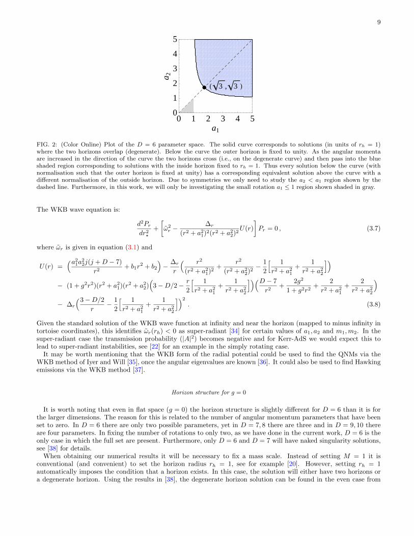
FIG. 2: (Color Online) Plot of the D = 6 parameter space. The solid curve corresponds to solutions (in units of rh = 1)where the two horizons overlap (degenerate). Below the curve the outer horizon is fixed to unity. As the angular momentaare increased in the direction of the curve the two horizons cross (i.e., on the degenerate curve) and then pass into the blueshaded region corresponding to solutions with the inside horizon fixed to rh = 1. Thus every solution below the curve (withnormalisation such that the outer horizon is fixed at unity) has a corresponding equivalent solution above the curve with adifferent normalisation of the outside horizon. Due to symmetries we only need to study the a2 < a1 region shown by thedashed line. Furthermore, in this work, we will only be investigating the small rotation a1 ≤ 1 region shown shaded in gray.

The WKB wave equation is:

d2Prdr2?

+

[ω2r −

∆r

(r2 + a21)2(r2 + a2

2)2U(r)

]Pr = 0 , (3.7)

where ωr is given in equation (3.1) and

U(r) =(a2

1a22j(j +D − 7)

r2+ b1r

2 + b2

)− ∆r

r

( r2

(r2 + a21)2

+r2

(r2 + a22)2− 1

2

[ 1

r2 + a21

+1

r2 + a22

])− (1 + g2r2)(r2 + a2

1)(r2 + a22)(

3−D/2− r

2

[ 1

r2 + a21

+1

r2 + a22

])(D − 7

r2+

2g2

1 + g2r2+

2

r2 + a21

+2

r2 + a22

)− ∆r

(3−D/2r

− 1

2

[ 1

r2 + a21

+1

r2 + a22

])2

. (3.8)

Given the standard solution of the WKB wave function at infinity and near the horizon (mapped to minus infinity intortoise coordinates), this identifies ωr(rh) < 0 as super-radiant [34] for certain values of a1, a2 and m1,m2. In thesuper-radiant case the transmission probability (|A|2) becomes negative and for Kerr-AdS we would expect this tolead to super-radiant instabilities, see [22] for an example in the simply rotating case.

It may be worth mentioning that the WKB form of the radial potential could be used to find the QNMs via theWKB method of Iyer and Will [35], once the angular eigenvalues are known [36]. It could also be used to find Hawkingemissions via the WKB method [37].

Horizon structure for g = 0

It is worth noting that even in flat space (g = 0) the horizon structure is slightly different for D = 6 than it is forthe larger dimensions. The reason for this is related to the number of angular momentum parameters that have beenset to zero. In D = 6 there are only two possible parameters, yet in D = 7, 8 there are three and in D = 9, 10 thereare four parameters. In fixing the number of rotations to only two, as we have done in the current work, D = 6 is theonly case in which the full set are present. Furthermore, only D = 6 and D = 7 will have naked singularity solutions,see [38] for details.

When obtaining our numerical results it will be necessary to fix a mass scale. Instead of setting M = 1 it isconventional (and convenient) to set the horizon radius rh = 1, see for example [20]. However, setting rh = 1automatically imposes the condition that a horizon exists. In this case, the solution will either have two horizons ora degenerate horizon. Using the results in [38], the degenerate horizon solution can be found in the even case from

10

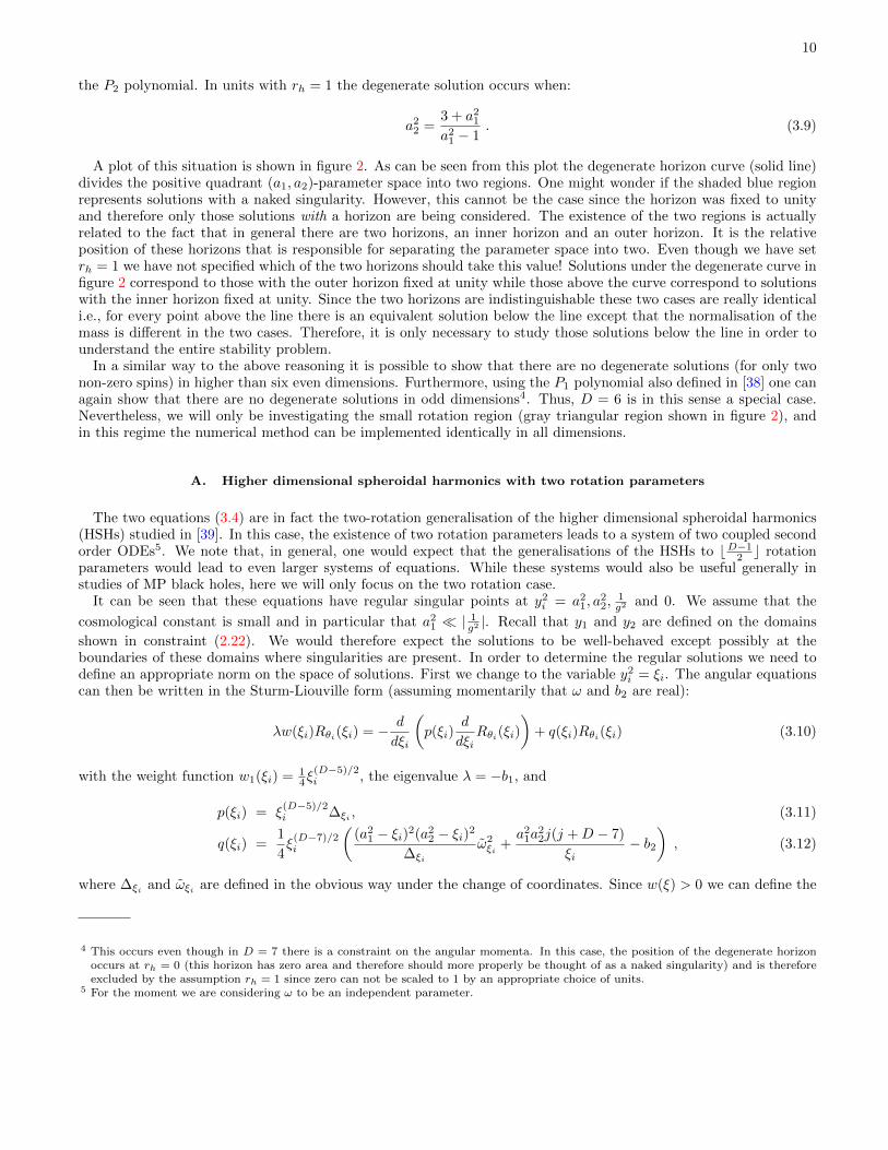
the P2 polynomial. In units with rh = 1 the degenerate solution occurs when:

a22 =

3 + a21

a21 − 1

. (3.9)

A plot of this situation is shown in figure 2. As can be seen from this plot the degenerate horizon curve (solid line)divides the positive quadrant (a1, a2)-parameter space into two regions. One might wonder if the shaded blue regionrepresents solutions with a naked singularity. However, this cannot be the case since the horizon was fixed to unityand therefore only those solutions with a horizon are being considered. The existence of the two regions is actuallyrelated to the fact that in general there are two horizons, an inner horizon and an outer horizon. It is the relativeposition of these horizons that is responsible for separating the parameter space into two. Even though we have setrh = 1 we have not specified which of the two horizons should take this value! Solutions under the degenerate curve infigure 2 correspond to those with the outer horizon fixed at unity while those above the curve correspond to solutionswith the inner horizon fixed at unity. Since the two horizons are indistinguishable these two cases are really identicali.e., for every point above the line there is an equivalent solution below the line except that the normalisation of themass is different in the two cases. Therefore, it is only necessary to study those solutions below the line in order tounderstand the entire stability problem.

In a similar way to the above reasoning it is possible to show that there are no degenerate solutions (for only twonon-zero spins) in higher than six even dimensions. Furthermore, using the P1 polynomial also defined in [38] one canagain show that there are no degenerate solutions in odd dimensions4. Thus, D = 6 is in this sense a special case.Nevertheless, we will only be investigating the small rotation region (gray triangular region shown in figure 2), andin this regime the numerical method can be implemented identically in all dimensions.

A. Higher dimensional spheroidal harmonics with two rotation parameters

The two equations (3.4) are in fact the two-rotation generalisation of the higher dimensional spheroidal harmonics(HSHs) studied in [39]. In this case, the existence of two rotation parameters leads to a system of two coupled secondorder ODEs5. We note that, in general, one would expect that the generalisations of the HSHs to bD−1

2 c rotationparameters would lead to even larger systems of equations. While these systems would also be useful generally instudies of MP black holes, here we will only focus on the two rotation case.

It can be seen that these equations have regular singular points at y2i = a2

1, a22,

1g2 and 0. We assume that the

cosmological constant is small and in particular that a21 | 1

g2 |. Recall that y1 and y2 are defined on the domains

shown in constraint (2.22). We would therefore expect the solutions to be well-behaved except possibly at theboundaries of these domains where singularities are present. In order to determine the regular solutions we need todefine an appropriate norm on the space of solutions. First we change to the variable y2

i = ξi. The angular equationscan then be written in the Sturm-Liouville form (assuming momentarily that ω and b2 are real):

λw(ξi)Rθi(ξi) = − d

dξi

(p(ξi)

d

dξiRθi(ξi)

)+ q(ξi)Rθi(ξi) (3.10)

with the weight function w1(ξi) = 14ξ

(D−5)/2i , the eigenvalue λ = −b1, and

p(ξi) = ξ(D−5)/2i ∆ξi , (3.11)

q(ξi) =1

4ξ

(D−7)/2i

((a2

1 − ξi)2(a22 − ξi)2

∆ξi

ω2ξi +

a21a

22j(j +D − 7)

ξi− b2

), (3.12)

where ∆ξi and ωξi are defined in the obvious way under the change of coordinates. Since w(ξ) > 0 we can define the

4 This occurs even though in D = 7 there is a constraint on the angular momenta. In this case, the position of the degenerate horizonoccurs at rh = 0 (this horizon has zero area and therefore should more properly be thought of as a naked singularity) and is thereforeexcluded by the assumption rh = 1 since zero can not be scaled to 1 by an appropriate choice of units.

5 For the moment we are considering ω to be an independent parameter.

11

two norm’s:

N1(Rθ1) ∝∫ a21

a22

ξ(D−5)/21 |Rθ1 |2dξ1 , (3.13)

N2(Rθ2) ∝∫ a22

0

ξ(D−5)/22 |Rθ2 |2dξ2 . (3.14)

The rationale for this choice can be explained as follows. We can rewrite the Sturm-Liouville equation as an eigenvalueequation LR = λR where

L =1

w(ξ)

(− d

dξ

[p(ξ)

d

dξ

]+ q(ξ)

). (3.15)

In analogy to the criterion discussed in [22] we note that for real ω and real b2, λ (or b1) must be real. Therefore theinner product must be chosen so that L is self-adjoint when ω and b2 are real. From the Sturm-Liouville form it iseasy to show6 that if the inner product is defined as:

〈f, g〉 =

∫f∗(ξ)g(ξ)w(ξ)dξ , (3.16)

then L is self-adjoint i.e., 〈f, Lg〉 = 〈Lf, g〉. This inner product naturally induces the norms chosen above.However, one readily sees that the choice of norm is not unique. We could for example repeat the argument made

above using λ = b2 and in this case the weight function is found to be w2(ξi) = 14ξ

(D−7)/2i . The main point, however,

is that even though the norms will give a different number (when acting on a given solution), they will agree on whichsolutions are regular (finite norm) 7.

Under either choice of weight the regular solutions are found to be:

R1 ∼ (ξ1 − a22)|m2|

2 (a21 − ξ1)

|m1|2 Ψ1; ξ1 ∈ (a2

2, a21), (3.17)

R2 ∼ ξj/22 (a2

2 − ξ2)|m2|

2 Ψ2; ξ2 ∈ (0, a22). (3.18)

Now for a given value of ω we can determine b1 and b2 simply by performing the improved AIM [31] on both ofthe angular equations separately. This will result in two equations in the two unknowns b1, b2 which we can thensolve using a numerical routine such as the built-in Mathematica functions NSolve or FindRoot. More specifically werewrite equations (3.4) using (3.17) and (3.18) and transform them into the AIM form:

d2Ψ1

dξ21

= λ01dΨ1

dξ1+ s01Ψ1 , (3.19)

d2Ψ2

dξ22

= λ02dΨ2

dξ2+ s02Ψ2 . (3.20)

The AIM requires that a special point be taken about which the λ0i and s0i coefficients are expanded. As was shownin [40] different choices of this point can worsen or improve the speed of the convergence. In the absence of a clearselection criterion we simply choose this point conveniently in the middle of the domains:

ξ01 =a2

1 + a22

2, ξ02 =

a22

2. (3.21)

Eigenvalue results and comparison with double perturbation theory

The numerical b1 and b2 eigenvalues for various parameters were computed and shown to be in good agreementwith the perturbative values, Appendix A, for small ε and ω. This serves as a consistency check between these two

6 With appropriate boundary conditions.7 In Appendix A this ambiguity is somewhat more relevant. We find that in order to be able to simplify the expressions using the Jacobi

orthonormality relations, one must choose the w1 to normalize the Rθ1 solutions and w2 to normalize the Rθ2 solutions respectively.

12

0.2 0.4 0.6 0.8 1.0Ω a1

7.58.08.59.09.5

10.0b1

Ε=0.01Ε=0.1

Ε=0.5Ε=1

0.0 0.2 0.4 0.6 0.8 1.0Ω a1

1

2

3

4

5

6b2a1

2

Ε=0.01Ε=0.1

Ε=0.5

Ε=1

FIG. 3: (Color Online) D = 6, g = 0, (j,m1,m2, n1, n2) = (0, 1, 1, 0, 0). A plot of the eigenvalues for various choices ofε ≡ a2/a1. Note that the dependence on a1 has been scaled into the other quantities.

0.2 0.4 0.6 0.8 1.0Ω a1

8

9

10

11b1

g a1=0.5 i

g a1=0g a1=0.5

0.2 0.4 0.6 0.8 1.0Ω a1

2.42.62.83.03.23.43.6b2a1

2

g a1=0.5 i

g a1=0g a1=0.5

FIG. 4: (Color Online) D = 6, ε ≡ a2/a1 = 1/2, (j,m1,m2, n1, n2) = (0, 1, 1, 0, 0). A plot of the eigenvalues for ga1 = 0.5i, 0, 0.5,corresponding to deSitter, flat, and anti-deSitter spacetimes respectively. Note that the dependence on a1 has been scaled intothe other quantities.

methods. Some results are plotted in figures 3, 4. However, some issues arose and we found that both methods hadtheir limitations, which we now briefly outline.

We found that for ε 1 there was no appreciable difference between the numerical eigenvalues found after 16 or32 iterations. In other words the convergence was quite fast. As ε → 1 however we found that the convergence wasmuch slower. For example, at a1 = 3/2, a2 = 149/100 (i.e., ε = 0.993) we needed about 80 iterations to get to thesame level of accuracy that we required for smaller epsilon. See figure 5. In this case (for small values of ω) theperturbative method outperformed the AIM.

However, we also found that the perturbative eigenvalues were very poor as ω became large. As an example, wechoose the point a1 = 1, a2 = 1/2. Since ε = 1/2 was relatively small we again found only 16 AIM iterations wererequired to get numerical convergence. However, with ω > 5 the perturbative values were clearly breaking down, seefigure 6.

The reason for this is that essentially the perturbation is expanded in the parameter ωa1 where ω is assumed to beorder unity. However, if ω is large then the error in this expansion becomes worse.

The fact that the convergence of the numerical method is not sensitive to ω makes it more robust when calculatingthe QNMs, especially since we were only able to obtain the eigenvalues in the general case to O(ε2, a2

1). Of course,what we have learned is that if we hold the number of AIM iterations at 16 then we would expect any values wecalculate to have larger errors as ε increases. In the next section we will calculate the QNMs completely numerically.

13

0 10 20 30 40 50 60nmax

5.9

6.0

6.1

6.2b1

FIG. 5: (Color Online) D = 6, a1 = 3/2, a2 = 149/100, (j,m1,m2, n1, n2) = (0, 1, 1, 0, 0) and g = 0. The dots are the numericalb1 eigenvalues for an increasing number of AIM iterations, while the straight line is the value obtained from the perturbativemethod to O(ε6, a61).

0 5 10 15 20Ω0

10

20

30

40

50b1

FIG. 6: (Color Online) D = 6, a1 = 1, a2 = 1/2, (j,m1,m2, n1, n2) = (0, 1, 1, 0, 0) and g = 0. The dotted blue line is theperturbation to order O(ε2, a21), while the dashed red line is the perturbation to order O(ε6, a61). The solid green line is theconverged numerical b1 eigenvalue.

B. Radial quasi-normal modes

Having successfully determined two independent methods for calculating the eigenvalues and having showed thatthey agree well with each other we can now proceed to calculate the QNMs with control over their range of validity.We start with the radial master equation (3.3). Thus far, when calculating the eigenvalues, we have been able towork in full generality, i.e., including the cosmological constant. However, due to the presence of new horizons anddifferent boundary conditions, the flat, deSitter and anti-deSitter QNMs will need to be calculated separately. In thiswork we will focus only on the flat case, and from here on we set g = 0.

Recall that QNMs are solutions to the radial master equation which satisfy the boundary condition that there areonly waves ingoing at the black hole horizon and outgoing at asymptotic infinity. However, we found the AIM seemsto work best on a compact domain. Therefore it is better to define the variable x = 1/r, so that infinity is mappedto zero and the outer horizon stays at xh = 1/rh = 1. The domain of x, therefore, will be [0, 1]. Thus the QNMboundary condition is translated into the statement that the waves move leftward at x = 0 and rightward at x = 1.We again choose the AIM point in the middle of the domain, i.e., at x = 1/2.

In terms of x the radial equation (3.3) becomes:

0 = −xD−4 d

dx

(−x8−D∆x

dR

dx

)+

((x−2 + a2

1)2(x−2 + a22)2

∆xω2x − a2

1a22j(j +D − 7)x2 − b1

x2− b2

)R , (3.22)

where ∆x(x) ≡ ∆r(r = 1/x) and ωx(x) ≡ ωr(r = 1/x).After performing some asymptotic analysis, keeping in mind the definition (2.35), we find that for the solutions to

satisfy the QNM boundary conditions we must have:

R ∼ (1− x)iωhαhx(D−2)/2eiωx/xy(x) , (3.23)

14

-1 -0.5 0.5 1a1

-0.2-0.3-0.4-0.5

Im @ΩD

0.2.4.6.8

Ε=1

-1 -0.5 0.5 1a1

0.650.700.750.800.850.90

Re @ΩD

0.2.4.6

.8Ε=1

FIG. 7: (Color Online) D=6. Plots of the fundamental (j,m1,m2, n1, n2) = (0, 0, 0, 0, 0) QNM. On top are plots of theimaginary part and below are plots of the Real part. Left: a surface plot over the (a1, a2)-parameter space. Middle: a contourplot. Right: a plot of the QNM along the straight lines passing through the origin with gradient ε shown in the graph.

where

ωh ≡ ωx(x = 1) , (3.24)

αh ≡(1 + a2

1)(1 + a22)

∆′x(x = 1). (3.25)

We then substitute this ansatz into equation (3.22) and rewrite into the AIM form:

y′′ = λ0y′ + s0y . (3.26)

This final step was performed in Mathematica and then the resulting expressions for λ0 and s0 were fed into the AIMroutine.

The method we use to find the QNMs proceeds in a fashion similar to that used in [39, 41]. However, as alreadymentioned we use the AIM instead of the CFM.

First we set the number of AIM iterations in both the eigenvalue and QNM calculations to sixteen8. We startwith the Schwarzschild values (b1, b2, ω), i.e., at the point (a1, a2) ∼ 09 and then increment a1 and a2 by some small

8 Ideally this should be made as large as possible, however, we found that there was little difference in the computed QNMs when using 16or 32 iterations for a1 ≤ 1. This choice also gave good agreement in the small rotation regime with the perturbed eigenvalues calculatedin appendix A. However, to go into the large rotation limit we found that much larger iterations were required to achieve convergenceand this significantly slowed down the code. Thus the AIM method we have described here does not seem robust enough to explore thelarge rotation limits.

9 Note we couldn’t take the point (0,0) exactly as this would leave the y1 and y2 domains empty. To be precise we chose the point(a1, a2) = (1/50, 1/100).

15

-1 -0.5 0.5 1a1

-0.2

-0.3

-0.4

-0.5

Im @ΩD

0.2.4.6.8

Ε=1

-1 -0.5 0.5 1a1

1.01.11.21.31.4

Re @ΩD

0.2.4.6.8

Ε=1

FIG. 8: (Color Online) D=6. Plots of the fundamental (j,m1,m2, n1, n2) = (0, 1, 0, 0, 0) QNM. On top are plots of theimaginary part and below are plots of the Real part. Left: a surface plot over the (a1, a2)-parameter space. Middle: a contourplot. Right: a plot of the QNM along the straight lines passing through the origin with gradient ε shown in the graph.

value10. We take the initial eigenvalues (b1, b2), insert them into the radial equation (3.23) then use the AIM to findthe new QNM that is closest to ω using the Mathematica routine FindRoot.

We then take this new value of omega, ω′, insert it into the two angular equations (at the same value of a1 anda2) then solve using the AIM and searching closest to the previous b1 and b2 values. Thereby obtaining the neweigenvalues b′1, b′2. We then repeat this process with the new (ω′, b′1, b

′2) as the starting point until the results converge

and we have achieved four decimal places of accuracy11. When this occurs we increment a1 and a2 again and repeatthe process. In this way, we are able to find the QNMs and eigenvalues along lines passing approximately throughthe origin (i.e., starting from the near Scwharzschild values) in the (a1, a2) parameter space. We choose 6 straightlines with gradients of (ε = 0, 0.2, 0.4, 0.6, 0.8, 1)12 and then use an interpolating function to interpolate the values inbetween these points. This then covers the a1 > a2 > 0 octant.

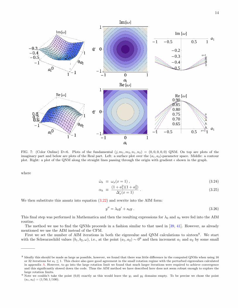
Some preliminary results are shown for D = 6, in figures 7 and 8. We see that as we increase the gradient theimaginary part of the curves appear to be bounded between the a2 = 0 to a1 = a2 curves. Indeed, if this behaviour isa general phenomenon, then the most important regime for locating instabilities (i.e., when the imaginary part crossesthe Im(ω) = 0 axis) would appear to be the a1 = a2 limit. Some general features of these plots are worth mentioning.For the case of vanishing angular modes m1,2 = 0, the solution is symmetric under horizontal and vertical reflections

10 In our results we incremented a1 by 150

at each step. The increment in a2 was then set by the gradient of the straight line taken in the(a1, a2)- parameter space

11 We found that no more than 15 repetitions were required to achieve convergence.12 Note that if these lines went exactly through the origin, ε = 0 would mean a2 = 0 and ε = 1 would mean a2 = a1 both of these situations

would be pathological to the numerical method since the yi domains would disappear. With the starting value at (1/50, 1/100), wecome very close to the single rotation and a1 = a2 cases for ε = 0 and ε = 1 respectively while remaining in a valid domain of thenumerical procedure.

16

-0.5 0.5a1

-0.2-0.3-0.4-0.5

Im @ΩD

m=1

-0.5 0.5a1

1.41.51.61.71.81.9Re @ΩD

FIG. 9: (Color Online) D=7. Plots of the fundamental (j,m1,m2, n1, n2) = (0, 1, 0, 0, 0) QNM. On top are plots of the imaginarypart and below are plots of the Real part. Left: a surface plot over the (a1, a2)-parameter space. Middle: is a contour plot.Right: is a plot of the QNM along the straight lines passing through the origin with gradient ε shown in the graph.

in the a1 and a2 axes in figure 7. Furthermore, with m1 non-zero this reflection symmetry is broken in the real partof the QNM curves shown on the bottom right of figure 8, where they are skewed to the left. We have also confirmedthis the case for m2 6= 0.

For higher dimensions such as D = 7, see figure 9, we observe similar behaviour to the D = 6 case where againwe see the skewing of the real part for non-zero m1, for example. The general dimensional dependence is shown infigure 10, where as is typical of singly rotating cases, larger dimensions lead to greater negative Im(ω) implying largerdamping. These results also seem to indicate that larger values of D are more stable with increasing a1.

IV. CONCLUDING REMARKS

The intention of this work was to initiate the study of higher-dimensional Kerr-(A)dS black holes with with morethan one rotation parameter for D > 5. In the present work we have considered those solutions with all rotationparameters set to zero except for two. As a first step in this direction, we have presented the general metric for sucha spacetime. We have also separated the Klein-Gordon equation, writing out the corresponding radial and angularequations explicitly. In the general case with all rotations, e.g., see [8, 9, 42], the separation must be performed foreach D separately. However, we found that in the doubly rotating case (a1 6= 0, a2 6= 0, a3 = a4 = · · · = 0) a generalD-dimensional expression could be obtained analogous to the one commonly used in the simply rotating case.

It is worth stressing that in five dimensions there is only one one spheroidal equation, while in six and higherdimensions there are two angular equations, therefore in this work we only focussed on the D ≥ 6 case (the fivedimensional case will be considered elsewhere [30, 43]). We evaluated the QNM frequencies of the low-lying modesusing a numerical AIM approach for both the angular and radial equations. In Appendix A, to get some quanti-tative understanding of the angular equations, we also developed perturbative expansions in powers of the rotationparameters ε = a2/a1 and a1 for the angular eigenvalues.

17

0.2 0.4 0.6 0.8 1.0a1

-1.0

-0.8

-0.6

-0.4

-0.2

Im@ΩD

D=6

7

8

910

11

0.2 0.4 0.6 0.8 1.0a1

1.5

2.0

2.5

3.0

3.5

Re@ΩD

D=6

7

8

9

10

11

FIG. 10: (Color Online) Dimensional dependence of fundamental (j,m1,m2, n1, n2) = (0, 1, 0, 0, 0) QNM for a2 = 0.4a1 for0 < a1 < 1.

Our preliminary results for the QNMs suggest that slowly rotating black holes with two rotations are stable althoughour numerical code became slow for values of a1, a2 ≥ 1, which unfortunately is also the region of most concern. Morework in this direction, particularly for larger rotations and g > 0 (Kerr-AdS), would also be worthy of investigation.

On the other hand, to discuss the stability of the ultra-spinning simply rotating black holes the angular eigenvaluein the large, imaginary, rotation limit [39], is typically relevant. For our case there are two rotation parameters. Withone rotation parameter small and the other large, the situation will be very much like the simply rotating case [19, 20]and no instability is expected. Therefore it would more interesting to consider the other case with both rotationparameters large. This work will be pursued subsequently.

In terms of other future work, with these separated equations we could also start to ask questions about the spectraof Hawking radiation (for five dimensions see [10]) and investigate the phenomenon of super-radiance in more detail.

Acknowledgments

HTC was supported in part by the National Science Council of the Republic of China under the Grant NSC 99-2112-M-032-003-MY3, and the National Science Centre for Theoretical Sciences. The work of JD was supported bythe Japan Society for the Promotion of Science (JSPS), under fellowship no. P09749.

Appendix A: Double Perturbation Theory

In this appendix we develop expansions in powers of the parameters ε = a2/a1 and a1 for the angular separationconstants b1 and b2 defined in the equations (2.46). Since without loss of generality we have taken a1 > a2, ε < 1,furthermore, we assume a1 < 1.

For brevity we shall outline the main steps and refer the reader to reference [30] for a more detailed account of thefive-dimensional case13. Since the latitude coordinates are restricted to a2 ≤ y1 ≤ a1 and 0 ≤ y2 ≤ a2, it is convenientto change variables to x1 and x2 with

y21 =

1

2

(a2

1 + a22

)− 1

2

(a2

1 − a22

)x1 ; y2

2 =1

2a2

2 (1− x2) , (A1)

where −1 ≤ x1, x2 ≤ 1.By making the convenient choice

B1 ≡ b1 + 2ω(m1a1 +m2a2)− 2g2m1a1m2a2, (A2)

B2 ≡1

a21

[b2 + 2ω(m1a1a

22 + a2

1m2a2)− 2m1a1m2a2

](A3)

13 For D = 5 there are two rotation parameters, but there is only one angular equation. This makes the perturbative analysis easier.

18

in Eq. (2.46) the perturbative expansion then only develops even powers of ε and a1. In this case the operatorequations are:

O1 = −1 + x1

2

[(1− x1) + ε2(1 + x1)

] 2− g2a2

1

[(1− x1) + ε2(1 + x1)

] d2

dx21

+

[1

2((D − 5) + (D − 1)x1)− 1

4g2a2

1(1− x1) ((D − 3) + (D + 1)x1)

]−ε

2

2

(1 + x1

1− x1

)[((D − 5)− (D − 1)x1) + (D + 1)g2a2

1x1(1− x1)]

+ε4g2a2

1(1 + x1)2

4(1− x1)[(D − 3)− (D + 1)x1]

d

dx1

+

a2

1ω2(1 + x1)(1− ε2)2

4 [2− g2a21 ((1− x1) + ε2(1 + x1))]

+

[m2

1(1− x1)2 +m22ε

2(1 + x1)2] [

2− g2a21

((1− x1) + ε2(1 + x1)

)]4(1− x1)2(1 + x1)

− ε2j(j +D − 7)

(1− x1) [(1− x1) + ε2(1 + x1)]− B1ε

2(1 + x1)

4(1− x1)+

B2

2(1− x1)

, (A4)

and

O2 = −1

4(1− x2

2)[2− ε2(1− x2)

] [2− g2a2

1ε2(1− x2)

] d2

dx22

+

1

2[(D − 7) + (D − 3)x2]− ε2

4(1 + g2a2

1)(1− x2) [(D − 5) + (D − 1)x2]

+ε4

8g2a2

1(1− x2)2 [(D − 3) + (D + 1)x2]

d

dx2a2

1ω2ε2(1 + x2)

[2− ε2(1− x2)

]8 [2− g2a2

1ε2(1− x2)]

+

[2− g2a2

1ε2(1− x2)

] [m2

1ε2(1 + x2)2 +m2

2

(2− ε2(1− x2)

)2]8(1 + x2) [2− ε2(1− x2)]

+j(j +D − 7)

2(1− x2)+B1ε

2(1− x2)

8

, (A5)

where

OiRi =Bi4Ri . (A6)

We first expand the operators with respect to ε. For each equation i = 1, 2 we have:

(Oi0 +Oi2 +Oi4 +Oi6 + · · · ) (Ri0 +Ri2 +Ri4 +Ri6 + · · · )

=1

4(Bi0 +Bi2 +Bi4 +Bi6 + · · · ) (Ri0 +Ri2 +Ri4 +Ri6 + · · · ) , (A7)

where the next subscript after the i refers to the power of ε = a2/a1 contained by those terms. Before going on weshall also need to look at the implications of the normalization condition to higher order terms. We first recall thatthe normalization conditions14 are given by:

1

4

∫ 1

−1

(1− x1)D−5

2 R21 = 1 , (A8)

1

4

∫ 1

−1

(1− x2)D−7

2 R22 = 1 . (A9)

14 See subsection (III A).

19

For convenience we define Ri =√wiRi/2. Then schematically we have:∫ 1

−1

dxi

(Ri0 + Ri2 + Ri4 + Ri6 + · · ·

)(Ri0 + Ri2 + Ri4 + Ri6 + · · ·

)= 1 , (A10)

⇒∫ 1

−1

dxiR2i0 = 1 ;

∫ 1

−1

dxi Ri0Ri2 = 0 ;

∫ 1

−1

dx1 Ri0Ri4 = −1

2

∫ 1

−1

dx1 R2i2 ;

∫ 1

−1

dxi Ri0Ri6 = −∫ 1

−1

dxi Ri2Ri4 .

1. Zeroth order in epsilon O(ε0)

To the zeroth order in ε, the eigenvalue equations are

Oi0Ri0 =Bi04Ri0, (A11)

where,

O10 = − (1− x21)

2

[2− g2a2

1(1− x1)] d2

dx21

+

[1

2((D − 5) + (D − 1)x1)− 1

4g2a2

1(1− x1) ((D − 3) + (D + 1)x1)

]d

dx1

+

a2

1ω2(1 + x1)

4[2− g2a21(1− x1)]

+m2

1[2− g2a21(1− x1)]

4(1 + x1)+

B20

2(1− x1)

, (A12)

O20 = −(1− x22)d2

dx22

+1

2(D − 7 + (D − 3)x2)

d

dx2+

m22

2(1 + x2)+j(j +D − 7)

2(1− x2)≡ O200 . (A13)

We first consider the O20 equation. We note that the O20 operator does not involve powers of a1 at O(ε0) order,therefore we can write O20 = O200 + O202 + · · · = O200 where the third subscript refers to the power of a1 in thoseterms. To fix notation we also redefine the solution R20 = R200 and the eigenvalue B20 = B200.

One then observes that the corresponding eigenvalue equation

O200R200 =B200

4R200 , (A14)

is exactly solvable in terms of Jacobi polynomials. The solution is given by

R200(n2) = c2n2m2j(1− x2)j/2(1 + x2)|m2|/2P(j+D−7

2 ,|m2|)n2 (x2) ,

B200(n2) = (2n2 + |m2|+ j)(2n2 + |m2|+ j +D − 5) , (A15)

where n2 = 0, 1, 2, . . . . The normalization condition:

1

4

∫ 1

−1

dx2(1− x2)(D−7)

2 R100(n1)R100(n′1) = δn1n′1, (A16)

is satisfied if 15

c2n2m2j =

(2j + 2|m2|+ 4n2 +D − 5)Γ(n2 + 1)Γ

(j + |m2|+ n2 + D−5

2

)2

12 (2j+2|m2|+D−7)Γ(|m2|+ n2 + 1)Γ

(j + n2 + D−5

2

) 1/2

. (A17)

For the properties of Jacobi polynomials see [44].Next we work on the O10 equation. Following the same method we have used for ε we expand the eigenvalue

equation in powers of a1. The operator at zeroth order is

O100 = −(1− x21)d2

dx21

+1

2(D − 5 + (D − 1)x1)

d

dx1+

B200

2(1− x1)+

m21

2(1 + x1), (A18)

15 This can be found using the orthonormality of the Jacobi polynomials.

20

where, unlike O200, the O100 operator is coupled to O200 through B200.The zeroth order eigenvalue equation O100R100 = 1

4B100R100 can again be solved and the solutions and eigenvaluesare found to be:

R100(n1) = c1n1m1(1− x1)(2κ+5−D)

4 (1 + x1)|m1|

2 P (κ,|m1|)n1

(x1) ,

B100(n1) = (2(n1 + n2) + |m1|+ |m2|+ j)(2(n1 + n2) + |m1|+ |m2|+ j +D − 3) , (A19)

where n1 = 0, 1, 2, . . . , and for clarity we have defined

κ =

√B200 +

(D − 5

2

)2

= 2n2 + |m2|+ j +1

2(D − 5) . (A20)

The orthonormality condition

1

4

∫ 1

−1

dx1(1− x1)(D−5)

2 R100(n1)R100(n′1) = δn1n′1, (A21)

is satisfied with the normalisation

c1n1m1 =

(2n1 + κ+ |m1|+ 1)Γ(n1 + 1)Γ (n1 + κ+ |m1|+ 1)

2κ+|m1|−1Γ (n1 + κ+ 1) Γ(n1 + |m1|+ 1)

1/2

. (A22)

We now describe how given both the zeroth order eigenvalues and eigenfunctions we can go to higher order in theperturbative series.

Second order in a21, O(ε0, a21)

At next order in the perturbative expansion for O1 we find:

O102R100 +O100R102 =1

4(B102R100 +B100R102) . (A23)

Where the O102 operator is found to be:

O102 =1

2a2

1g2(1− x1)(1− x2

1)d2

dx21

− 1

4a2

1g2(1− x1)(D − 3 + (D + 1)x1)

d

dx1+

1

8a2

1ω2(1 + x1)− 1

4a2

1g2m2

1

1− x1

1 + x1.

We also need to look at the effect of the normalization condition (A21) to higher order terms. We again find aseries of conditions analogous to (A10), i.e.,∫ 1

−1

dx1R2100 = 1 ;

∫ 1

−1

dx1 R100R102 = 0 · · · . (A24)

Using these relations and the hermiticity of the operators we are able to find B102 by contracting equation (A23) withR100:

B102 =

∫ 1

−1

dx1(1− x1)(D−5)

2 R100(n1)O102R100(n′1) . (A25)

Using the equation O100R100 = 14B100R100 to remove the second derivative we obtain:

O102R100 =[− 1

2a2

1g2(1− x2

1)d

dx1+

1

4a2

1g2B200 +

1

8a2

1ω2(1 + x1)− 1

8B100a

21g

2(1− x1)]R100 . (A26)

After applying various identities for Jacobi polynomials [44] to remove the derivative and x1 dependence in equation(A18) we obtain:

B102 =a2

1

2(ω2 + g2B100 + 4g2n1 + g2(2κ+ 5−D) + 2g2|m1|)

( (m2

1 − κ2)

(2n1 + |m1|+ κ)(2n1 + |m1|+ κ+ 2)

)

+a2

1

2(ω2 + 2g2B200 − g2B100 + g2(2κ+ 5−D)− 2g2|m1|)− 2a2

1g2n1

(κ− |m1|)2n1 + |m1|+ κ

. (A27)

21

Note that in the single rotation limit (a2 → 0) with g = 0 we find agreement with the result obtained in [39] usinginverted continued fractions. The result does not, however, agree with that for g 6= 0 using inverted fractions inpowers of c1 = a1ω and α1 = a2

1g2 [40] because we used an expansion in different parameters: ε = a2/a1 and a1.16

In theory we could continue to go to higher order in a21, however, we stop at this order, to point out an issue that

arises in the general case for the second order in ε terms.

2. Second order in epsilon O(ε2)

We now consider the next order in ε, firstly for O2 we have the operator equation,

O22R20 +O20R22 =1

4(B20R22 +B22R20) . (A28)

After using the orthonormality of the doubly perturbed eigenfunctions up to second order in a21, the hermiticity of

the operators and also the fact that many of the terms are simply zero in the O2 case, we find again that:

B22i =

∫ 1

−1

dx2(1− x2)D−7

2 R200O22iR200 , (A29)

where i = 0, 2.The ε2 operator takes the following form:

O22 =ε2

2(1 + x2)(1− x2)2

(1 + a2

1g2) d2

dx22

− ε2

4(1− x2)

(1 + a2

1g2)

(D − 5 + (D − 1)x2)d

dx2

+ε2

8(1 + x2)(a2

1ω2 +m2

1) +ε2

8B10(1− x2)− ε2

(1 + a2

1g2) m2

2(1− x2)

4(1 + x2).

Thus, working up to second order in a21, we have:

O220R200 =[− ε2

2(1− x2

2)d

dx2+ε2

8m2

1(1 + x2) +ε2

8B100(1− x2) +

ε2

4j(j +D − 7)− ε2

8B200(1− x2)

]R200

O222R200 =[− 1

2(1− x2

2)ε2a21g

2 d

dx2+ε2a2

1

8ω2(1 + x2) +

ε2

8B102(1− x2) +

1

4ε2a2

1g2j(j +D − 7)

−1

8ε2a2

1g2B200(1− x2)

]R200 , (A30)

where in the above steps we used O200R200, cf. equation (A13), to remove second derivatives. Again using thefunctional properties of the Jacobi polynomials [44] we find:

B220 =ε2

2

(m2

1 −B100 +B200 + 4n2 + 2j + 2|m2|) (

m22 − α2

)(2n2 + |m2|+ α)(2n2 + |m2|+ α+ 2)

+ε2

2

(m2

1 −B200 +B100

)+ ε2j(D + j − 7)− 2ε2n2

(α− |m2|)2n2 + |m2|+ α

+ ε2(j − |m2|) , (A31)

B222 =ε2

2

(a2

1ω2 −B102 + a2

1g2B200 + 4a2

1g2n2 + 2a2

1g2j + 2a2

1g2|m2|

) (m2

2 − α2)

(2n2 + |m2|+ α)(2n2 + |m2|+ α+ 2)

+ε2

2

(a2

1ω2 +B102 − a2

1g2B200

)+ ε2a2

1g2j(D + j − 7)− 2ε2a2

1g2n2

(α− |m2|)2n2 + |m2|+ α

+ ε2a21g

2(j − |m2|) ,

(A32)

where we defined α = j + (D − 7)/2.

16 We have verified that perturbation theory (using orthogonal polynomials) for small c1, c2 and α1, α2 does indeed give the correct secondorder answer when c2, α2 → 0 for D = 5 [30, 43] (cf. [40] using inverted continued fractions).

22

Second order in O1

It is in the O(ε2) order of the O1 operator that our method runs into some difficulty in the general case. For theO1 operator at O(ε2, a0

1) order we find:

O120R100 +O100R120 =1

4(B100R120 +B120R100) , (A33)

where after performing manipulations similar to those in the previous sections we find:

B120 =

∫ 1

−1

dx1(1− x1)(D−5)

2 R100O120R100 . (A34)

As such, an expansion of O12 in powers of a21 leads to

O120 = −ε2 (1 + x1)2 d2

dx21

− 1

2ε2(D − 5− (D − 1)x1)

1 + x1

1− x1

d

dx1+ε2m2

2

2

(1 + x1)

(1− x1)2− ε2 j(j +D − 7)

(1− x1)2

+B220

2(1− x1)− ε2 1 + x1

1− x1

B100

4.

(A35)

Now we can use O100R100, see equation (A18), to remove second derivative terms, and we obtain:

B120 =

∫ 1

−1

dx1(1− x1)(D−5)

2 R100

[− ε2(D − 5)

(1 + x1)

(1− x1)

d

dx1+ ε2

(m22 −B200)(1 + x1)− 2j(j +D − 7)

2(1− x1)2

+B220 − ε2m2

1

2(1− x1)

]R100 .

(A36)

Unfortunately, the terms with factors of (1 − x) in the denominator do not appear to allow any simplification viastandard Jacobi identities [44]. Thus, in the general case it does not seem possible to find the solution to B120 inclosed algebraic form. In principle one could still numerically integrate these expressions, however, as explained insection (III), when calculating the QNM’s it is more advantageous to perform a full numerical calculation than totake this route.

Nevertheless, we have found that the offending terms vanish for the special choice of parameters D = 6, j = 0,m1 = m2 = 1 and n1 = n2 = 0, and in this case, B120 = 0.

3. Sixth order in the special case: D = 6, j = 0, m1 = m2 = 1 and n1 = n2 = 0

We also found that this special case allowed us to go to higher orders without encountering the above mentionedissue. To go to higher orders equation’s like (A34) often can not be written simply in terms of the zeroth ordereigenfunctions. In such cases we had to decompose the higher order functions in terms of linear superpositions of

23

zeroth order ones. We will give a more detailed explanation of this method in [30]. Here we just list the result:

B1 =

[10 +

2

9

(2ω2 − 17g2

)a2

1 −20

8019(ω4 − 53g2ω2 + 196g4)a4

1

+20

8444007(2ω6 − 645g2ω4 + 28959g4ω2 − 105644g6)a6

1

]+ε2

[2

9(2ω2 − 17g2)a2

1 +32

8019(ω4 − 53g2ω2 + 196g4)a4

1 −32

2814669(ω6 − 147g2ω4 + 5178g4ω2 − 18424g6)a6

1

]+ε4

[− 20

8019(ω4 − 53g2ω2 + 196g4)a4

1 −32

2814669(ω6 − 147g2ω4 + 5178g4ω2 − 18424g6)a6

1

]+ε6

[20

8444007(2ω6 − 645g2ω4 + 28959g4ω2 − 105644g6)a6

1

]+ · · · , (A37)

B2 = 2 + ε2[2 +

2

9(4ω2 − 7g2)a2

1 −4

8019(ω4 − 53g2ω2 + 196g4)a4

1

+4

8444007(2ω6 − 645g2ω4 + 28959g4ω2 − 105644g6)a6

1

]+ε4

[− 4

8019(ω4 − 53g2ω2 + 196g4)a4

1 −32

8444007(4ω2 − 25g2)(ω4 − 53g2ω2 + 196g4)a6

1

]+ε6

[4

8444007(2ω6 − 645g2ω4 + 28959g4ω2 − 105644g6)a6

1

]+ · · · . (A38)

These results are compared to the AIM in figures 5 and 6. In figure 5 we see that ∼ 80 iterations are required tobe as good as the perturbative value, where a similar plot was found for b2. In figure 6 we see that the perturbativeeigenvalues break down for ω larger than ∼ 5.

[1] L. Randall and R. Sundrum, Phys. Rev. Lett. 83, 3370 (1999), hep-ph/9905221.[2] J. M. Maldacena, Adv. Theor. Math. Phys. 2, 231 (1998), hep-th/9711200.[3] P. Kanti, Int. J. Mod. Phys. A19, 4899 (2004), hep-ph/0402168.[4] R. C. Myers and M. J. Perry, Ann. Phys. 172, 304 (1986).[5] R. Emparan and R. Myers, J. High Energy Phys. (2003).[6] R. A. Konoplya and A. Zhidenko (2011), 1102.4014.[7] S. W. Hawking, C. J. Hunter, and M. Taylor, Phys. Rev. D59, 064005 (1999), hep-th/9811056.[8] G. W. Gibbons, H. Lu, D. N. Page, and C. N. Pope, Phys. Rev. Lett. 93, 171102 (2004), hep-th/0409155.[9] W. Chen, H. Lu, and C. N. Pope, Class. Quant. Grav. 23, 5323 (2006), hep-th/0604125.

[10] H. Nomura, S. Yoshida, M. Tanabe, and K.-i. Maeda, Prog. Theor. Phys. 114, 707 (2005), hep-th/0502179.[11] V. P. Frolov and D. Stojkovic, Phys. Rev. D67, 084004 (2003), gr-qc/0211055.[12] M. Vasudevan and K. A. Stevens, Phys. Rev. D72, 124008 (2005), gr-qc/0507096.[13] V. P. Frolov, P. Krtous, and D. Kubiznak, JHEP 02, 005 (2007), hep-th/0611245.[14] P. Krtous, D. Kubiznak, D. N. Page, and V. P. Frolov, JHEP 02, 004 (2007), hep-th/0612029.[15] V. P. Frolov and D. Kubiznak, Phys. Rev. Lett. 98, 011101 (2007), gr-qc/0605058.[16] V. P. Frolov and D. Kubiznak, Class. Quant. Grav. 25, 154005 (2008), 0802.0322.[17] A. Sergyeyev and P. Krtous, Phys. Rev. D77, 044033 (2008), 0711.4623.[18] T. Oota and Y. Yasui, Phys. Lett. B659, 688 (2008), 0711.0078.[19] Y. Morisawa and D. Ida, Phys. Rev. D71, 044022 (2005), gr-qc/0412070.[20] V. Cardoso, G. Siopsis, and S. Yoshida, Phys. Rev. D71, 024019 (2005), hep-th/0412138.[21] H. Kodama, R. A. Konoplya, and A. Zhidenko, Phys. Rev. D81, 044007 (2010), 0904.2154.[22] H. Kodama, R. A. Konoplya, and A. Zhidenko, Phys. Rev. D79, 044003 (2009), 0812.0445.[23] N. Uchikata, S. Yoshida, and T. Futamase, Phys. Rev. D80, 084020 (2009).[24] V. Cardoso, O. J. C. Dias, and S. Yoshida, Phys. Rev. D74, 044008 (2006), hep-th/0607162.[25] V. Cardoso, O. J. C. Dias, J. P. S. Lemos, and S. Yoshida, Phys. Rev. D70, 044039 (2004), hep-th/0404096.[26] V. Cardoso and O. J. C. Dias, Phys. Rev. D70, 084011 (2004), hep-th/0405006.[27] J. Doukas, H. T. Cho, A. S. Cornell, and W. Naylor, Phys. Rev. D80, 045021 (2009), 0906.1515.[28] P. Kanti, H. Kodama, R. A. Konoplya, N. Pappas, and A. Zhidenko, Phys. Rev. D80, 084016 (2009), 0906.3845.[29] P. Kanti, J. Phys. Conf. Ser. 189, 012020 (2009), 0903.2147.[30] H. T. Cho, A. S. Cornell, J. Doukas, and W. Naylor, in preparation.

24

[31] H. T. Cho, A. S. Cornell, J. Doukas, and W. Naylor, Class. Quant. Grav. 27, 155004 (2010), 0912.2740.[32] E. W. Leaver, Phys. Rev. D41, 2986 (1990).[33] A. Zhidenko, Phys. Rev. D74, 064017 (2006), gr-qc/0607133.[34] B. S. DeWitt, Phys. Rept. 19, 295 (1975).[35] S. Iyer and C. M. Will, Phys. Rev. D35, 3621 (1987).[36] E. Seidel and S. Iyer, Phys. Rev. D41, 374 (1990).[37] A. S. Cornell, W. Naylor, and M. Sasaki, JHEP 02, 012 (2006), hep-th/0510009.[38] J. Doukas (2010), 1009.6118.[39] E. Berti, V. Cardoso, and M. Casals, Phys. Rev. D73, 024013 (2006), gr-qc/0511111.[40] H. T. Cho, A. S. Cornell, J. Doukas, and W. Naylor, Phys. Rev. D80, 064022 (2009), 0904.1867.[41] E. Berti, V. Cardoso, and C. M. Will, Phys. Rev. D 73, 064030 (2006).[42] G. W. Gibbons, H. Lu, D. N. Page, and C. N. Pope, J. Geom. Phys. 53, 49 (2005), hep-th/0404008.[43] A. N. Aliev and O. Delice, Phys. Rev. D79, 024013 (2009), 0808.0280.[44] I. S. Gradshteyn and I. M. Ryzhik, Table of Integrals, Series, and Products (Academic Press, UK, 2000).