New theoretical approaches to black holes
10
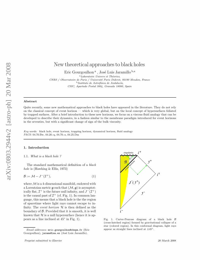
arXiv:0803.2944v2 [astro-ph] 20 Mar 2008 New theoretical approaches to black holes Eric Gourgoulhon a , Jos´ e Luis Jaramillo b,a a Laboratoire Univers et Th´ eories, CNRS / Observatoire de Paris / Universit´ e Paris Diderot, 92190 Meudon, France b Instituto de Astrof´ ısica de Andaluc´ ıa, CSIC, Apartado Postal 3004, Granada 18080, Spain Abstract Quite recently, some new mathematical approaches to black holes have appeared in the literature. They do not rely on the classical concept of event horizon — which is very global, but on the local concept of hypersurfaces foliated by trapped surfaces. After a brief introduction to these new horizons, we focus on a viscous fluid analogy that can be developed to describe their dynamics, in a fashion similar to the membrane paradigm introduced for event horizons in the seventies, but with a significant change of sign of the bulk viscosity. Key words: black hole, event horizon, trapping horizon, dynamical horizon, fluid analogy PACS: 04.70.Bw, 04.20.-q, 04.70.-s, 04.25.Dm 1. Introduction 1.1. What is a black hole ? The standard mathematical definition of a black hole is (Hawking & Ellis, 1973) B := M− J − (I + ), (1) where M is a 4-dimensional manifold, endowed with a Lorentzian metric g such that (M, g) is asymptot- ically flat, I + is the future null infinity, and J − (I + ) is the causal past of I + (cf. Fig. 1). In common lan- guage, this means that a black hole is the the region of spacetime where light rays cannot escape to in- finity. The event horizon H is then defined as the boundary of B. Provided that it is smooth, it is well known that H is a null hypersurface (hence it is ap- pears as a line inclined at 45 ◦ in Fig. 1). Email addresses: [email protected] (Eric Gourgoulhon), [email protected] (Jos´ e Luis Jaramillo). Fig. 1. Carter-Penrose diagram of a black hole B (cross-hatched region) formed by gravitational collapse of a star (colored region). In this conformal diagram, light rays appear as straight lines inclined at ±45 ◦ . Preprint submitted to Elsevier 20 March 2008
-
Upload
independent -
Category
Documents
-
view
6 -
download
0
Transcript of New theoretical approaches to black holes
arX
iv:0
803.
2944
v2 [
astr
o-ph
] 2
0 M
ar 2
008 New theoretical approaches to black holes
Eric Gourgoulhon a , Jose Luis Jaramillo b,a
aLaboratoire Univers et Theories,CNRS / Observatoire de Paris / Universite Paris Diderot, 92190 Meudon, France
bInstituto de Astrofısica de Andalucıa,CSIC, Apartado Postal 3004, Granada 18080, Spain
Abstract
Quite recently, some new mathematical approaches to black holes have appeared in the literature. They do not rely
on the classical concept of event horizon — which is very global, but on the local concept of hypersurfaces foliated
by trapped surfaces. After a brief introduction to these new horizons, we focus on a viscous fluid analogy that can be
developed to describe their dynamics, in a fashion similar to the membrane paradigm introduced for event horizons
in the seventies, but with a significant change of sign of the bulk viscosity.
Key words: black hole, event horizon, trapping horizon, dynamical horizon, fluid analogyPACS: 04.70.Bw, 04.20.-q, 04.70.-s, 04.25.Dm
1. Introduction
1.1. What is a black hole ?
The standard mathematical definition of a blackhole is (Hawking & Ellis, 1973)
B := M− J−(I+), (1)
whereM is a 4-dimensional manifold, endowed witha Lorentzian metric g such that (M, g) is asymptot-ically flat, I+ is the future null infinity, and J−(I+)is the causal past of I+ (cf. Fig. 1). In common lan-guage, this means that a black hole is the the regionof spacetime where light rays cannot escape to in-finity. The event horizon H is then defined as theboundary of B. Provided that it is smooth, it is wellknown that H is a null hypersurface (hence it is ap-pears as a line inclined at 45 in Fig. 1).
Email addresses: [email protected] (EricGourgoulhon), [email protected] (Jose Luis Jaramillo).
Fig. 1. Carter-Penrose diagram of a black hole B
(cross-hatched region) formed by gravitational collapse of astar (colored region). In this conformal diagram, light raysappear as straight lines inclined at ±45.
Preprint submitted to Elsevier 20 March 2008
1.2. Drawbacks of the classical definition
As noticed by Jean-Pierre Lasota and MarekDemianski long time ago (Demianski & Lasota,1973), definition (1) is not applicable is cosmology,for usually a cosmological spacetime (M, g) is notasymptotically flat.
Moreover, even when applicable, definition (1) ishighly non-local: the determination of J−(I+) re-quires the knowledge of the entire future null infinity.In addition this definition has no direct relation withthe notion of strong gravitational field: as shown byAshtekar & Krishnan (2004) and Krishnan (2008)on an example based on the Vaidya metric, an eventhorizon can form in a flat region of spacetime, whereby flat it is meant a vanishing Riemann tensor, i.e.no gravitational field at all. This means that no localphysical experiment whatsoever can locate an eventhorizon.
Another non-local feature of event horizons istheir teleological nature (Hawking & Hartle, 1972;Damour, 1979; Thorne et al., 1986). The classicalblack hole boundary, i.e. the event horizon, respondsin advance to what will happen in the future. Thisis shown by Booth (2005) on the explicit exampleof a black hole formed by the collapse of two succes-sive matter shells: after the first shell has collapsedto form the event horizon, the latter remains sta-tionary for a while and then starts to grow beforethe second collapsing shell reaches it, as if it wasanticipating its venue.
If one would like to deal with black holes as “ordi-nary” physical objects, like for instance in quantumgravity or numerical relativity, the non-local (bothin space and time) behavior of the event horizonmentioned above would be problematic. This hasmotivated the search for local characterizations ofblack holes.
2. New approaches to black holes
2.1. Local characterizations of black holes
The local definitions of black holes can be tracedback to the “perfect horizons” of Haicek (1973).However this applied only to equilibrium black holes.More recently, the local approach has been extendedto black holes out of equilibrium, with the introduc-tion of– trapping horizons by Hayward (1994),– isolated horizons by Ashtekar et al. (1999)
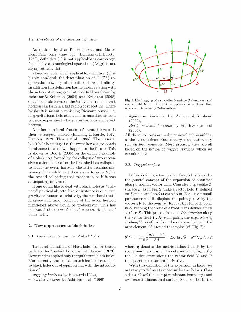
Fig. 2. Lie dragging of a spacelike 2-surface S along a normalvector field V . In this plot, S appears as a closed line,whereas it is actually 2-dimensional.
– dynamical horizons by Ashtekar & Krishnan(2002),
– slowly evolving horizons by Booth & Fairhurst(2004).
All these horizons are 3-dimensional submanifolds,as the event horizon. But contrary to the latter, theyrely on local concepts. More precisely they are allbased on the notion of trapped surfaces, which weexamine now.
2.2. Trapped surface
Before defining a trapped surface, let us start bythe general concept of the expansion of a surfacealong a normal vector field. Consider a spacelike 2-surface S, as in Fig. 2. Take a vector field V definedon S and normal to S at each point. For a given smallparameter ε ∈ R, displace the point p ∈ S by thevector εV to the point p′. Repeat this for each pointin S, keeping the value of ε fixed. This defines a newsurface S′. This process is called Lie dragging alongthe vector field V . At each point, the expansion ofS along V is defined from the relative change in thearea element δA around that point (cf. Fig. 2):
θ(V ) := limε→0
1
ε
δA′ − δA
δA= LV ln
√q = qµν∇µVν , (2)
where q denotes the metric induced on S by thespacetime metric g, q the determinant of qµν , LV
the Lie derivative along the vector field V and ∇the spacetime covariant derivative.
With this definition of the expansion in hand, weare ready to define a trapped surface as follows. Con-sider a closed (i.e. compact without boundary) andspacelike 2-dimensional surface S embedded in the
2
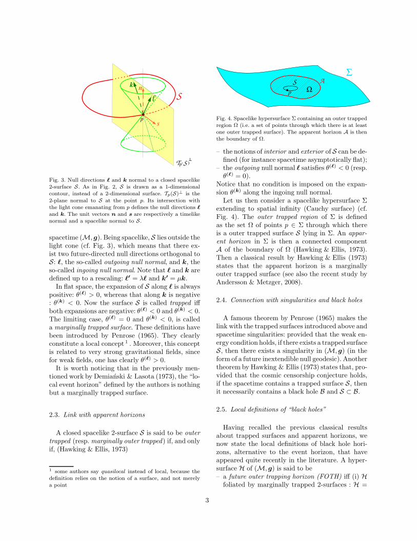
Fig. 3. Null directions ℓ and k normal to a closed spacelike2-surface S. As in Fig. 2, S is drawn as a 1-dimensionalcontour, instead of a 2-dimensional surface. Tp(S)⊥ is the
2-plane normal to S at the point p. Its intersection withthe light cone emanating from p defines the null directions ℓ
and k. The unit vectors n and s are respectively a timelikenormal and a spacelike normal to S.
spacetime (M, g). Being spacelike, S lies outside thelight cone (cf. Fig. 3), which means that there ex-ist two future-directed null directions orthogonal toS: ℓ, the so-called outgoing null normal, and k, theso-called ingoing null normal. Note that ℓ and k aredefined up to a rescaling: ℓ′ = λℓ and k′ = µk.
In flat space, the expansion of S along ℓ is alwayspositive: θ(ℓ) > 0, whereas that along k is negative: θ(k) < 0. Now the surface S is called trapped iffboth expansions are negative: θ(ℓ) < 0 and θ(k) < 0.The limiting case, θ(ℓ) = 0 and θ(k) < 0, is calleda marginally trapped surface. These definitions havebeen introduced by Penrose (1965). They clearlyconstitute a local concept 1 . Moreover, this conceptis related to very strong gravitational fields, sincefor weak fields, one has clearly θ(ℓ) > 0.
It is worth noticing that in the previously men-tioned work by Demianski & Lasota (1973), the “lo-cal event horizon” defined by the authors is nothingbut a marginally trapped surface.
2.3. Link with apparent horizons
A closed spacelike 2-surface S is said to be outertrapped (resp. marginally outer trapped) if, and onlyif, (Hawking & Ellis, 1973)
1 some authors say quasilocal instead of local, because thedefinition relies on the notion of a surface, and not merelya point
Fig. 4. Spacelike hypersurface Σ containing an outer trappedregion Ω (i.e. a set of points through which there is at leastone outer trapped surface). The apparent horizon A is thenthe boundary of Ω.
– the notions of interior and exterior of S can be de-fined (for instance spacetime asymptotically flat);
– the outgoing null normal ℓ satisfies θ(ℓ) < 0 (resp.θ(ℓ) = 0).
Notice that no condition is imposed on the expan-sion θ(k) along the ingoing null normal.
Let us then consider a spacelike hypersurface Σextending to spatial infinity (Cauchy surface) (cf.Fig. 4). The outer trapped region of Σ is definedas the set Ω of points p ∈ Σ through which thereis a outer trapped surface S lying in Σ. An appar-ent horizon in Σ is then a connected componentA of the boundary of Ω (Hawking & Ellis, 1973).Then a classical result by Hawking & Ellis (1973)states that the apparent horizon is a marginallyouter trapped surface (see also the recent study byAndersson & Metzger, 2008).
2.4. Connection with singularities and black holes
A famous theorem by Penrose (1965) makes thelink with the trapped surfaces introduced above andspacetime singularities: provided that the weak en-ergy condition holds, if there exists a trapped surfaceS, then there exists a singularity in (M, g) (in theform of a future inextendible null geodesic). Anothertheorem by Hawking & Ellis (1973) states that, pro-vided that the cosmic censorship conjecture holds,if the spacetime contains a trapped surface S, thenit necessarily contains a black hole B and S ⊂ B.
2.5. Local definitions of “black holes”
Having recalled the previous classical resultsabout trapped surfaces and apparent horizons, wenow state the local definitions of black hole hori-zons, alternative to the event horizon, that haveappeared quite recently in the literature. A hyper-surface H of (M, g) is said to be– a future outer trapping horizon (FOTH) iff (i) H
foliated by marginally trapped 2-surfaces : H =
3
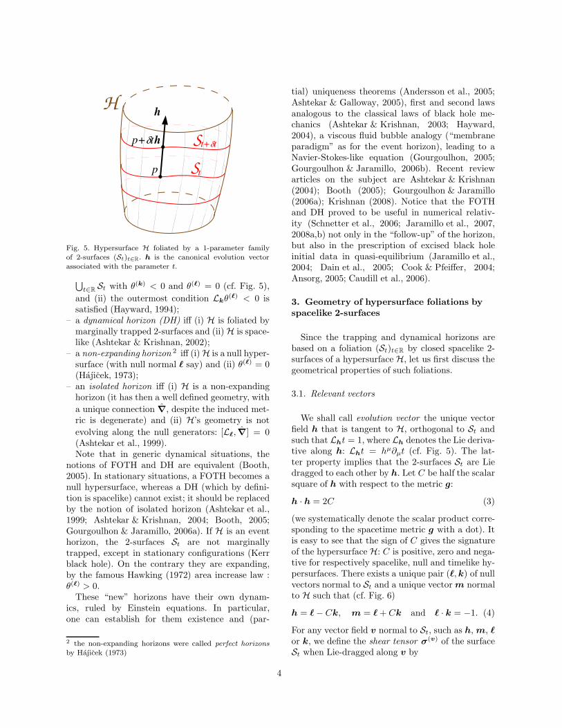
Fig. 5. Hypersurface H foliated by a 1-parameter familyof 2-surfaces (St)t∈R. h is the canonical evolution vectorassociated with the parameter t.
⋃
t∈RSt with θ(k) < 0 and θ(ℓ) = 0 (cf. Fig. 5),
and (ii) the outermost condition Lkθ(ℓ) < 0 issatisfied (Hayward, 1994);
– a dynamical horizon (DH) iff (i) H is foliated bymarginally trapped 2-surfaces and (ii) H is space-like (Ashtekar & Krishnan, 2002);
– a non-expanding horizon 2 iff (i) H is a null hyper-surface (with null normal ℓ say) and (ii) θ(ℓ) = 0(Haicek, 1973);
– an isolated horizon iff (i) H is a non-expandinghorizon (it has then a well defined geometry, with
a unique connection ∇, despite the induced met-ric is degenerate) and (ii) H’s geometry is not
evolving along the null generators: [Lℓ, ∇] = 0(Ashtekar et al., 1999).Note that in generic dynamical situations, the
notions of FOTH and DH are equivalent (Booth,2005). In stationary situations, a FOTH becomes anull hypersurface, whereas a DH (which by defini-tion is spacelike) cannot exist; it should be replacedby the notion of isolated horizon (Ashtekar et al.,1999; Ashtekar & Krishnan, 2004; Booth, 2005;Gourgoulhon & Jaramillo, 2006a). If H is an eventhorizon, the 2-surfaces St are not marginallytrapped, except in stationary configurations (Kerrblack hole). On the contrary they are expanding,by the famous Hawking (1972) area increase law :θ(ℓ) > 0.
These “new” horizons have their own dynam-ics, ruled by Einstein equations. In particular,one can establish for them existence and (par-
2 the non-expanding horizons were called perfect horizonsby Haicek (1973)
tial) uniqueness theorems (Andersson et al., 2005;Ashtekar & Galloway, 2005), first and second lawsanalogous to the classical laws of black hole me-chanics (Ashtekar & Krishnan, 2003; Hayward,2004), a viscous fluid bubble analogy (“membraneparadigm” as for the event horizon), leading to aNavier-Stokes-like equation (Gourgoulhon, 2005;Gourgoulhon & Jaramillo, 2006b). Recent reviewarticles on the subject are Ashtekar & Krishnan(2004); Booth (2005); Gourgoulhon & Jaramillo(2006a); Krishnan (2008). Notice that the FOTHand DH proved to be useful in numerical relativ-ity (Schnetter et al., 2006; Jaramillo et al., 2007,2008a,b) not only in the “follow-up” of the horizon,but also in the prescription of excised black holeinitial data in quasi-equilibrium (Jaramillo et al.,2004; Dain et al., 2005; Cook & Pfeiffer, 2004;Ansorg, 2005; Caudill et al., 2006).
3. Geometry of hypersurface foliations by
spacelike 2-surfaces
Since the trapping and dynamical horizons arebased on a foliation (St)t∈R by closed spacelike 2-surfaces of a hypersurface H, let us first discuss thegeometrical properties of such foliations.
3.1. Relevant vectors
We shall call evolution vector the unique vectorfield h that is tangent to H, orthogonal to St andsuch that Lht = 1, where Lh denotes the Lie deriva-tive along h: Lht = hµ∂µt (cf. Fig. 5). The lat-ter property implies that the 2-surfaces St are Liedragged to each other by h. Let C be half the scalarsquare of h with respect to the metric g:
h · h = 2C (3)
(we systematically denote the scalar product corre-sponding to the spacetime metric g with a dot). Itis easy to see that the sign of C gives the signatureof the hypersurface H: C is positive, zero and nega-tive for respectively spacelike, null and timelike hy-persurfaces. There exists a unique pair (ℓ, k) of nullvectors normal to St and a unique vector m normalto H such that (cf. Fig. 6)
h = ℓ − Ck, m = ℓ + Ck and ℓ · k = −1. (4)
For any vector field v normal to St, such as h, m, ℓ
or k, we define the shear tensor σ(v) of the surfaceSt when Lie-dragged along v by
4
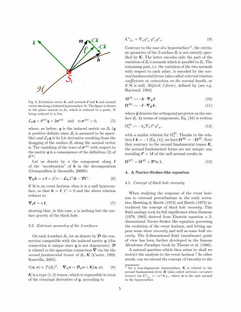
Fig. 6. Evolution vector h, null normals ℓ and k and normal
vector m along a foliated hypersurface H. The figure is drawnin the plane normal to St, which is reduced to a point, H
being reduced to a line.
Lvq = θ(v)q + 2σ(v) and tr σ(v) = 0, (5)
where, as before, q is the induced metric on St (qis positive definite since St is assumed to be space-like) and Lvq is its Lie derivative resulting from thedragging of the surface St along the normal vectorv. The vanishing of the trace of σ(v) with respect tothe metric q is a consequence of the definition (2) ofθ(v).
Let us denote by κ the component along ℓ
of the “acceleration” of h in the decomposition(Gourgoulhon & Jaramillo, 2006b)
∇hh = κ ℓ + (Cκ − Lh C)k − DC. (6)
If H is an event horizon, then it is a null hypersur-face, so that h = ℓ, C = 0 and the above relationreduces to
∇ℓℓ = κ ℓ, (7)
showing that, in this case, κ is nothing but the sur-face gravity of the black hole.
3.2. Extrinsic geometry of the 2-surfaces
On each 2-surface St, let us denote by D the con-nection compatible with the induced metric q (thisconnection is unique since q is not degenerate). D
is related to the spacetime connection ∇ via the thesecond fundamental tensor of St, K (Carter, 1992;Senovilla, 2005):
∀(u, v) ∈ T (St)2, ∇uv = Duv + K(u, v). (8)
K is a type (1, 2) tensor, which is expressible in termof the covariant derivative of q, according to
Kαβγ = ∇µqα
ν qµβqν
γ . (9)
Contrary to the case of a hypersurface 3 , the extrin-sic geometry of the 2-surface St is not entirely spec-ified by K. The latter encodes only the part of thevariation of St’s normals which is parallel to St. Theremaining part, i.e. the variation of the two normalswith respect to each other, is encoded by the nor-mal fundamental forms (also called external rotationcoefficients or connection on the normal bundle, orif H is null, Haicek 1-form), defined by (see e.g.Hayward, 1994)
Ω(ℓ) := −k · ∇~q ℓ (10)
Ω(k) := −ℓ · ∇~q k, (11)
where ~q denotes the orthogonal projector on the sur-face St. In terms of components, Eq. (10) is written
Ω(ℓ)α := −kµ∇νℓµ qν
α, (12)
with a similar relation for Ω(ℓ)α . Thanks to the rela-
tion ℓ·k = −1 [Eq. (4)], we have Ω(k) = −Ω(ℓ). Notethat contrary to the second fundamental tensor K,the normal fundamental forms are not unique: anyrescaling ℓ′ = λℓ of the null normal results in
Ω(ℓ′) = Ω(ℓ) + D lnλ. (13)
4. A Navier-Stokes-like equation
4.1. Concept of black hole viscosity
When studying the response of the event hori-zon to external perturbations in the early seven-ties, Hawking & Hartle (1972) and Hartle (1973) in-troduced the concept of black hole viscosity. Thisfluid analogy took its full significance when Damour(1979, 1982) derived from Einstein equation a 2-dimensional Navier-Stokes like equation governingthe evolution of the event horizon, and letting ap-pear some shear viscosity and well as some bulk vis-cosity. The 2-dimensional fluid (membrane) pointof view has been further developed in the famousMembrane Paradigm book by Thorne et al. (1986).
A natural question which then arises is: shall werestrict the analysis to the event horizon ? In otherwords, can we extend the concept of viscosity to the
3 for a non-degenerate hypersurface, K is related to thesecond fundamental form K (also called extrinsic curvaturetensor) via Kα
βγ= −nαKβγ , where n is the unit normal
to the hypersurface
5
local characterizations of black hole recently intro-duced, i.e. FOTH and DH ?
A priori this does not seem obvious because, froma pure geometrical point of view, the event horizonand the “local” horizons are of different type: theevent horizon is always a null hypersurface (hence isendowed with a degenerate metric), whereas a DHis always a spacelike surface (hence with a positivedefinite metric) and a FOTH can be either null orspacelike. We shall see that nevertheless the fluidanalogy can also be extended to these horizons, withsome significant change in the sign of the bulk vis-cosity.
4.2. Original Damour-Navier-Stokes equation
Damour considered the case where H is a blackhole event horizon. In particular it is a null hyper-surface and the null vector ℓ is normal to it. Fromthe Einstein equation, he has derived the relation(Damour, 1979, 1982) (see also Damour & Lilley,2008)
SLℓ π + θ(ℓ)π =−DP + 2µD · ~σ(ℓ) + ζDθ(ℓ)
+f , (14)
where– π := −1/(8π) Ω(ℓ) is analogous to some momen-
tum surface density,– P := κ/(8π) is analogous to the pressure [κ being
defined by Eq. (7)],– µ := 1/(16π) is analogous to the shear viscosity,– ζ := −1/(16π) is analogous to the bulk viscosity,– f := −T (ℓ, ~q) is the external force surface den-
sity, T being the stress-energy tensor of any mat-ter or electromagnetic field present around thehorizon.
Equation (14) is structurally identical to a Navier-Stokes equation for a 2-dimensional fluid. The readeris referred to Chap. VI of Thorne et al. (1986) for anextended discussion of this analogy with a viscousfluid (see also Sec. 2.3 of Damour & Lilley, 2008).
A striking feature of the above Navier-Stokesequation (14) is that the bulk viscosity is negative:
ζ = ζEH = − 1
16π< 0, (15)
where the subscript EH stands for “event horizon”.For an ordinary fluid, this negative value wouldyield to a dilation or contraction instability. Thisis in agreement with the well-known tendency of anull hypersurface to continually contract or expand.
However the event horizon is stabilized by the tele-ological condition that its expansion must vanish inthe far future, when an equilibrium state has beenreached (Damour, 1979).
4.3. Generalization to the non-null case
In order to generalize Eq. (14) to the case whereHis not necessarily a null hypersurface, it is worth tonotice that in Eq. (14), the vector ℓ plays two role:it is the natural evolution vector along H and it isalso the normal to H. In the non null case, these tworole are played respectively by the vectors h and m
introduced in Sec. 3.1. Of course, at the null limit(C = 0), h = m = ℓ [cf. Eq. (4)].
Having realized this, the starting point of the cal-culation is the contracted Ricci identity applied tothe vector m and projected onto St:
(∇µ∇νmµ −∇ν∇µmµ) qνα = Rµνmµqν
α, (16)
where Rµν is the spacetime Ricci tensor, to be re-placed ultimately by its expression in terms of thematter stress-energy tensor Tµν according to Ein-stein equation. After some manipulations, one ar-rives at (Gourgoulhon, 2005)
SLh Ω(ℓ) + θ(h) Ω(ℓ) = Dκ − D · ~σ(m) +
1
2Dθ(m)
−θ(k)DC + 8πT (m, ~q). (17)
In the null limit, C = 0, h = m = ℓ, and the aboveequation reduces to the original Damour-Navier-Stokes equation (14). On the other side, if H is aFOTH or a DH, then θ(m) = −θ(h) (since in thiscase θ(ℓ) = 0 and we can deduce from Eq. (4) therelation θ(m) = −θ(h) + 2θ(ℓ)) and Eq. (17) can bewritten
SLℓ π + θ(h)π =−DP +
1
8πD · ~σ(m) + ζDθ(h)
+f , (18)
where f := −T (m, ~q) + θ(k)/(8π)DC and, as inEq. (14), π := −1/(8π) Ω(ℓ), P := κ/(8π), butcontrary to Eq. (14),
ζ = ζFOTH :=1
16π> 0. (19)
This positive value of the bulk viscosity shows thatFOTHs and DHs behave as “ordinary” physical ob-jects.
6
4.4. Angular momentum flux law
In general relativity, the angular momentum isusually well defined only if there exists a Killing vec-tor field ϕ which generates a symmetry around someaxis. To generalize the definition of angular momen-tum to the cases where no symmetry is present, letus follow Booth & Fairhurst (2005) and introduce avector field on H which– is tangent to St
– has closed orbits– has vanishing divergence with respect to the in-
duced metric on St:
D · ϕ = 0. (20)
Notice that (20) is a condition weaker than being aKilling vector of (St, q), which would write Dαϕβ +Dβϕα = 0. For dynamical horizons, θ(h) 6= 0 andthere is a unique choice of ϕ as the generator (con-veniently normalized) of the curves of constant θ(h)
(Hayward, 2006).The generalized angular momentum associated
with ϕ is then defined by
J(ϕ) := − 1
8π
∮
St
〈Ω(ℓ), ϕ〉 ǫS , (21)
where 〈Ω(ℓ), ϕ〉 stands for the normal fundamen-tal form Ω(ℓ) applied to the vector ϕ and ǫS is thevolume element on St associated with the metricq. Note that the definition of J(ϕ) does not de-pend upon the choice of null vector ℓ, thanks to thedivergence-free property of ϕ and to the transforma-tion law (13) of Ω(ℓ) under a change of ℓ. Formula(21) coincides with Ashtekar & Krishnan (2003)’sdefinition. It also coincides with Brown-York angu-lar momentum (Brown & York, 1993) if H is time-like and ϕ a Killing vector.
Under the supplementary hypothesis that ϕ istransported along the evolution vector h : Lh ϕ =0, Eq. (17) leads to (Gourgoulhon, 2005)
d
dtJ(ϕ) = −
∮
St
T (m, ϕ) ǫS
− 1
16π
∮
St
[
~~σ(m)
: Lϕ q − 2θ(k)ϕ · DC
]
ǫS , (22)
where a double arrow stands for the double “indexraising” via the metric q and the colon denotes adouble contraction. There are two interesting limit-
ing cases for this equation. First of all, if H is a nullhypersurface (C = 0 and m = ℓ), it reduces to
d
dtJ(ϕ) = −
∮
St
T (ℓ, ϕ)ǫS − 1
16π
∮
St
~~σ(ℓ)
: Lϕ q ǫS ,
(23)
i.e. we recover Eq. (6.134) of the MembraneParadigm book (Thorne et al., 1986). Second, if His a FOTH, one may show that the last term inEq. (22) vanishes (Gourgoulhon, 2005), so that itreduces to
d
dtJ(ϕ) =−
∮
St
T (m, ϕ)ǫS
− 1
16π
∮
St
~~σ(m)
: Lϕ q ǫS . (24)
Thus for a FOTH, the Navier-Stokes like equation(18) leads to an evolution equation for the angularmomentum which is as simple as Eq. (23) for anevent horizon. In particular the r.h.s. has only twoterms, which are interpretable as respectively (i) theflux of angular momentum due to some matter orelectromagnetic field near the horizon and (ii) theflux of angular momentum due to “gravitational ra-diation”. The latter interpretation is pretty vagueand relies on the fact that Lϕ q = 0 in axisymme-try, where gravitational radiation does not carry anyangular momentum.
5. Area evolution and energy equation
5.1. Evolution of the expansion
Let us search for an evolution equation for the ex-pansion θ(h), which governs the evolution of the areaof the surfaces St via Eq. (2). The starting pointturns out to be the Ricci identity applied to the nor-mal vector m, as in Sec. 4.3, but instead of project-ing it onto St [Eq. (16)], we shall project it along thenormal direction to St lying in H, namely h:
(∇µ∇νmµ −∇ν∇µmµ)hν = Rµνmµhν . (25)
By means of the Einstein equation, and after somecomputations, we arrive at (Gourgoulhon & Jaramillo,2006b):
Lh θ(m) = κ θ(h) − 1
2θ(h)θ(m) − σ(h) : σ(m)
7
+θ(k)Lh C + D ·
(
2C~Ω(ℓ) − ~DC)
−8πT (m, h), (26)
where an upper arrow indicates “index raising” withthe metric q and the colon stands for the double
contraction, i.e. σ(h) : σ(m) := σ(h)ab σ(m)ab. If we
specialize Eq. (26) to the cases of (i) an event horizonand (ii) a FOTH or a DH, we obtain respectively
Lℓ θ(ℓ) + (θ(ℓ))2 − κ θ(ℓ) =1
2(θ(ℓ))2 − σ(ℓ) : σ(ℓ)
−8πT (ℓ, ℓ) (27)
Lh θ(h) + (θ(h))2 + κ θ(h) =1
2(θ(h))2 + σ(h) : σ(m)
−θ(k)Lh C + D ·
(
~DC − 2C~Ω(ℓ))
+8πT (m, h). (28)
For the event horizon, we have used the null charac-ter of H, which implies C = 0 and h = m = ℓ, yield-ing Eq. (27). It is nothing but the null Raychaud-huri equation for a surface-orthogonal congruence(Hawking & Hartle, 1972). For the FOTH/DH case[Eq. (28)], we have used the property θ(m) = −θ(h)
already encountered in Sec. 4.3. Notice the changeof some signs between Eqs. (27) and (28).
5.2. Energy dissipation and bulk viscosity
In the fluid membrane approach to black holes,Price & Thorne (1986) and Thorne et al. (1986) de-fined the surface energy density of an event hori-zon as ε := −θ(ℓ)/8π and interpreted Eq. (27) asan energy balance law, with heat production result-ing from viscous stresses. By analogy, let us definethe surface energy density of a FOTH/DH as ε :=−θ(m)/8π, where the role of the normal to H is nowtaken by m instead of ℓ. Since θ(m) = −θ(h) for aFOTH/DH, we have
ε =θ(h)
8π(29)
and we may rewrite Eq. (28) as
Lh ε + θ(h)ε = − κ
8πθ(h) +
1
8πσ(h) : σ(m) +
(θ(h))2
16π
−D · Q + T (m, h) − θ(k)
8πLh C,(30)
with Q := 14π
[
C~Ω(ℓ) − 1/2 ~DC]
= − C4π
~ , where
is the anholonomicity 1-form (or twist 1-form) of
the 2-surface St (Hayward, 1994) (see also Sec. IV.Aof Gourgoulhon, 2005) and ~ denotes its vectordual.
It is striking that Eqs. (18) and (30) are fullyanalogous to the equations that govern a two-dimensional non-relativistic fluid of internal en-ergy density ε, momentum density π, pressureκ/8π, shear stress tensor σ(m)/8π, bulk viscos-ity ζ = 1/16π, shear strain tensor σ(h), expan-sion θ(h), subject to the external force density−T (m, ~q) + θ(k)/8π DC, external energy produc-tion rate T (m, h) − θ(k)/8π Lh C and heat flux Q
(see e.g. Rieutord, 1997). In particular the value ofthe bulk viscosity read on Eq. (30) (the coefficientof (θ(h))2) is the same as that obtained from theNavier-Stokes equation (18) and given by Eq. (19).
Besides, let us notice that the shear viscosityµ does not appear in Eqs. (18) and (30), becausethe standard Newtonian-fluid relation between theshear stress tensor σ(m)/8π and the shear straintensor σ(h), namely σ(m)/8π = 2µσ(h), does nothold. Here we have σ(m)/8π = [σ(h) + 2Cσ(k)]/8π,so that the Newtonian-fluid assumption is fulfilledonly if C = 0 (isolated horizon limit). On the con-trary, it appears from Eqs. (18) and (30) that thetrace part of the viscous stress tensor Svisc doesobey the Newtonian-fluid law, being proportionalto the trace part of the strain tensor (i.e. the ex-pansion θ(h)): tr Svisc = 3ζθ(h).
We may point out two differences with the eventhorizon case (Damour, 1979, 1982; Price & Thorne,1986; Thorne et al., 1986). First the heat flux Q isnot vanishing for a FOTH/DH, whereas it was zerofor an EH. Notice that Q is a vector tangent to St sothat the integration of Eq. (30) over the closed sur-face St to get a global internal energy balance lawwould not contain any net heat flux. The second ma-jor difference is that, as already stressed in Sec. 4.3,the bulk viscosity ζ is positive, being equal to 1/16π[Eq. (19)], whereas it was found to be negative, be-ing equal to −1/16π [Eq. (15)], for an event hori-zon. As commented in Sec. 4.2, this negative valueis related to the teleological character of event hori-zons. On the contrary the positive value of the bulkviscosity for FOTHs and DHs that these objects be-have as “ordinary” physical objects and is in perfectagreement with their local nature.
8
Acknowledgements EG would like to express hisdeep gratitude to Jean-Pierre Lasota, who as a pro-fessor in a master course in Meudon, initiated himto the wonderful field of relativistic astrophysicsand black holes. Since then, Jean-Pierre has been ofunfailing support and it is a great pleasure to dedi-cate this paper to him. We would also like to thankgreatly Marek Abramowicz for having organizedthe splendid Trzebieszowice conference in honour ofJean-Pierre. This work was supported by the ANRgrant 06-2-134423 Methodes mathematiques pour larelativite generale.
ReferencesAndersson L., Mars M. & Simon W., 2005, Local
Existence of Dynamical and Trapping Horizons,Phys. Rev. Lett. 95 111102
Andersson L. & Metzger J., 2008, The areaof horizons and the trapped region, preprintarXiv:0708.4252.
Ansorg M., 2005, A double-domain spectral methodfor black hole excision data, Phys. Rev. D 72,024018
Ashtekar A., Beetle C. & Fairhurst S., 1999, Isolatedhorizons: a generalization of black hole mechanics,Class. Quantum Grav. 16, L1
Ashtekar A. & Galloway G.J., 2005, Some unique-ness results for dynamical horizons, Adv. Theor.Math. Phys. 9, 1
Ashtekar A. & Krishnan B., 2002, Dynamical Hori-zons: Energy, Angular Momentum, Fluxes andBalance Laws, Phys. Rev. Lett. 89 261101
Ashtekar A. & Krishnan B., 2003, Dynamical hori-zons and their properties, Phys. Rev. D 68, 104030
Ashtekar A. & Krishnan B., 2004, Isolated anddynamical horizons and their applications, Liv-ing Rev. Relativity 7, 10 [Online article],http://www.livingreviews.org/lrr-2004-10
Booth I, 2005, Black hole boundaries, Canadian J.Phys. 83, 1073
Booth I. & Fairhurst S., 2004, The first law for slowlyevolving horizons, Phys. Rev. Lett. 92, 011102
Booth I. & Fairhurst S., 2005, Horizon energy andangular momentum from a Hamiltonian perspec-tive, Class. Quantum Grav. 22, 4545
Brown J. D. & York J. W., 1993, Quasilocal energyand conserved charges derived from the gravita-
tional action, Phys. Rev. D 47, 1407Carter B., 1992, Outer curvature and conformal ge-
ometry of an imbedding, J. Geom. Phys. 8, 53Caudill M., Cook G. B., Grigsby J. D. & Pfeiffer
H. P., 2006, Circular orbits and spin in black-holeinitial data, Phys. Rev. D 74, 064011
Cook G. B. & Pfeiffer H. P., 2004, Excision boundaryconditions for black-hole initial data, Phys. Rev.D 70, 104016
Dain S., Jaramillo J. L. & Krishnan B., 2005, On theexistence of initial data containing isolated blackholes, Phys. Rev. D 71, 064003
Damour T., 1979, Quelques proprietes mecaniques,electromagnetiques, thermodynamiques et quan-tiques des trous noirs, These de doctorat d’Etat,Universite Paris 6
Damour T., 1982, Surface effects in black holephysics, in Proceedings of the Second MarcelGrossmann Meeting on General Relativity, Ed.R. Ruffini, North Holland, p. 587
Damour T. & Lilley M., 2008, String theory, gravityand experiment, lectures at Les Houches SummerSchool in Theoretical Physics (2-27 July 2007);preprint arXiv:0802.4169.
Demianski M. & Lasota J.-P., 1973, Black holes inan expanding Universe, Nature Phys. Sci. 241, 53
Gourgoulhon E., 2005, Generalized Damour-Navier-Stokes equation applied to trapping horizons, Phys.Rev. D 72, 104007
Gourgoulhon E. & Jaramillo J.L., 2006a, A 3+1 per-spective on null hypersurfaces and isolated hori-zons, Phys. Rep. 423, 159
Gourgoulhon E. & Jaramillo J.L., 2006b, Area evo-lution, bulk viscosity, and entropy principles fordynamical horizons, Phys. Rev. D 74, 087502
Haicek P., 1973,Exact models of charged black holes.I. Geometry of totally geodesic null hypersurface,Commun. Math. Phys. 34, 37
Hartle J.B., 1973, Tidal friction in slowly rotatingblack holes, Phys. Rev. D 8, 1010
Hawking S.W., 1972, Black holes in general relativ-ity, Commun. Math. Phys. 25, 152
Hawking S.W. & Ellis G.F.R., 1973, The largescale structure of space-time, Cambridge Univer-sity Press, Cambridge
Hawking S.W. & Hartle J.B., 1972, Energy and an-gular momentum flow into a black hole, Commun.Math. Phys. 27, 283
Hayward S.A., 1994, General laws of black hole dy-namics, Phys. Rev. D 49, 6467
Hayward S.A., 2004, Energy and entropy conserva-tion for dynamical black holes, Phys. Rev. D 70,
9
104027Hayward S.A., 2006, Angular momentum conserva-
tion for dynamical black holes, Phys.Rev. D 74,104013
Jaramillo J.L., Ansorg M. & Limousin F., 2007, Nu-merical implementation of isolated horizon bound-ary conditions, Phys.Rev. D 75, 024019
Jaramillo J.L., Gourgoulhon E., Cordero-Carrion I.& Ibanez J.M., 2008a, Trapping Horizons as in-ner boundary conditions for black hole spacetimes,Phys. Rev. D 77, 047501
Jaramillo J. L., Gourgoulhon E. & Mena MaruganG. A., 2004, Inner boundary conditions for blackhole initial data derived from isolated horizons,Phys. Rev. D 70, 124036
Jaramillo J.L., Valiente Kroon J.A. & GourgoulhonE., 2008b, From Geometry to Numerics: inter-disciplinary aspects in mathematical and numer-ical relativity, Class. Quantum Grav., in press,preprint arXiv:0712.2332
Krishnan B., 2008, Fundamental properties and ap-plications of quasi-local black hole horizons, to ap-pear in the Proceedings of the 18th InternationalConference on General Relativity and Gravita-tion (Sidney, Australia, 8-13 July 2007); preprintarXiv:0712.1575
Penrose R., 1965, Gravitational collapse and space-time singularities, Phys. Rev. Lett. 14, 57
Price R.H. & Thorne K.S., 1986, Membrane view-point on black holes: Properties and evolution ofthe stretched horizon, Phys. Rev. D 33, 915
Rieutord M., 1997, Une introduction a la dynamiquedes fluides, Masson, Paris
Schnetter E., Krishnan B. & Beyer F., 2006, Intro-duction to dynamical horizons in numerical rela-tivity, Phys.Rev. D 74, 024028
Senovilla J.M.M., 2005, Trapped submanifolds inLorentzian geometry, in Proc. XIII Fall Work-shop on Geometry and Physics (Murcia, Spain,2004), edited by L.J. Alıas, A. Ferrandez, M.A.Henandez, P. Lusca, and J.A. Pastor, Pub-lic. Real Soc. Mat. Esp. 9; also available asarXiv:math.DG/0412256
Thorne K.S., Price R.H. & MacDonald D.A., 1986,Black holes : the membrane paradigm, Yale Uni-versity Press, New Haven
10