Theoretical Aerodynamics
561
Ethirajan Rathakrishnan Theoretical Aerodynamics
-
Upload
khangminh22 -
Category
Documents
-
view
1 -
download
0
Transcript of Theoretical Aerodynamics

Ethirajan Rathakrishnan
Rathakrishnan
TheoreticalAerodynamics
TheoreticalAerodynamics
TheoreticalAerodynamics
DO NOT PRINT PANTONE 032 RED GUIDELINES. FOR PROOFING ONLY.
Ethirajan Rathakrishnan Indian Institute of Technology Kanpur, India
Theoretical Aerodynamics is a user-friendly text for a full course on theoretical aerodynamics. The author systematically introduces aerofoil theory, its design features and performance aspects,beginning with the basics required, and then gradually proceeding to a higher level. The mathematicsinvolved is presented so that it can be followed comfortably, even by those who are not strong inmathematics. The examples are designed to fix the theory studied in an effective manner. Throughoutthe book, the physics behind the processes are clearly explained. Each chapter begins with anintroduction and ends with a summary and exercises.
This book is intended for graduate and advanced undergraduate students of Aerospace Engineering, as well as researchers and designers working in the area of aerofoil and blade design.
• Provides a complete overview of the technical terms, vortex theory, lifting line theory, and numerical methods
• Presented in an easy-to-read style making full use of figures and illustrations to enhanceunderstanding, and moves from simpler to more advanced topics
• Includes a complete section on fluid mechanics and thermodynamics, essential background topics for aerodynamic theory
• Blends mathematical and physical concepts of design and performance aspects of lifting surfaces, and introduces the reader to thin aerofoil theory, panel method, and finite aerofoil theory
• Includes a Solutions Manual for end-of-chapter exercises, and Lecture slides on the book’sCompanion Website
www.wiley.com/go/rathakrishnan


THEORETICALAERODYNAMICS


THEORETICALAERODYNAMICS
Ethirajan RathakrishnanIndian Institute of Technology Kanpur, India

This edition first published 2013© 2013 John Wiley & Sons Singapore Pte. Ltd.
Registered officeJohn Wiley & Sons Singapore Pte. Ltd., 1 Fusionopolis Walk, #07-01 Solaris South Tower, Singapore 138628
For details of our global editorial offices, for customer services and for information about how to apply for permission toreuse the copyright material in this book please see our website at www.wiley.com.
All Rights Reserved. No part of this publication may be reproduced, stored in a retrieval system or transmitted, in any formor by any means, electronic, mechanical, photocopying, recording, scanning, or otherwise, except as expressly permitted bylaw, without either the prior written permission of the Publisher, or authorization through payment of the appropriatephotocopy fee to the Copyright Clearance Center. Requests for permission should be addressed to the Publisher, John Wiley& Sons Singapore Pte. Ltd., 1 Fusionopolis Walk, #07-01 Solaris South Tower, Singapore 138628, tel: 65-66438000,fax: 65-66438008, email: [email protected].
Wiley also publishes its books in a variety of electronic formats. Some content that appears in print may not be available inelectronic books.
Designations used by companies to distinguish their products are often claimed as trademarks. All brand names and productnames used in this book are trade names, service marks, trademarks or registered trademarks of their respective owners. ThePublisher is not associated with any product or vendor mentioned in this book. This publication is designed to provideaccurate and authoritative information in regard to the subject matter covered. It is sold on the understanding that thePublisher is not engaged in rendering professional services. If professional advice or other expert assistance is required, theservices of a competent professional should be sought.
Library of Congress Cataloging-in-Publication Data
Rathakrishnan, E.Theoretical aerodynamics / Ethirajan Rathakrishnan.
pages cmIncludes bibliographical references and index.ISBN 978-1-118-47934-6 (cloth)
1. Aerodynamics. I. Title.TL570.R33 2013629.132′3–dc23
2012049232
Typeset in 9/11pt Times by Thomson Digital, Noida, India

This book is dedicated to my parents,
Mr Thammanur Shunmugam Ethirajanand
Mrs Aandaal Ethirajan
Ethirajan Rathakrishnan


ContentsAbout the Author xv
Preface xvii
1 Basics 11.1 Introduction 11.2 Lift and Drag 11.3 Monoplane Aircraft 4
1.3.1 Types of Monoplane 51.4 Biplane 5
1.4.1 Advantages and Disadvantages 61.5 Triplane 6
1.5.1 Chord of a Profile 71.5.2 Chord of an Aerofoil 8
1.6 Aspect Ratio 91.7 Camber 101.8 Incidence 111.9 Aerodynamic Force 121.10 Scale Effect 151.11 Force and Moment Coefficients 171.12 The Boundary Layer 181.13 Summary 20Exercise Problems 21Reference 22
2 Essence of Fluid Mechanics 232.1 Introduction 232.2 Properties of Fluids 23
2.2.1 Pressure 232.2.2 Temperature 242.2.3 Density 242.2.4 Viscosity 252.2.5 Absolute Coefficient of Viscosity 252.2.6 Kinematic Viscosity Coefficient 272.2.7 Thermal Conductivity of Air 272.2.8 Compressibility 28
2.3 Thermodynamic Properties 282.3.1 Specific Heat 282.3.2 The Ratio of Specific Heats 29

viii Contents
2.4 Surface Tension 302.5 Analysis of Fluid Flow 31
2.5.1 Local and Material Rates of Change 322.5.2 Graphical Description of Fluid Motion 33
2.6 Basic and Subsidiary Laws 342.6.1 System and Control Volume 342.6.2 Integral and Differential Analysis 352.6.3 State Equation 35
2.7 Kinematics of Fluid Flow 352.7.1 Boundary Layer Thickness 372.7.2 Displacement Thickness 382.7.3 Transition Point 392.7.4 Separation Point 392.7.5 Rotational and Irrotational Motion 40
2.8 Streamlines 412.8.1 Relationship between Stream Function and Velocity Potential 41
2.9 Potential Flow 422.9.1 Two-dimensional Source and Sink 432.9.2 Simple Vortex 452.9.3 Source-Sink Pair 462.9.4 Doublet 46
2.10 Combination of Simple Flows 492.10.1 Flow Past a Half-Body 49
2.11 Flow Past a Circular Cylinder without Circulation 572.11.1 Flow Past a Circular Cylinder with Circulation 59
2.12 Viscous Flows 632.12.1 Drag of Bodies 652.12.2 Turbulence 702.12.3 Flow through Pipes 75
2.13 Compressible Flows 782.13.1 Perfect Gas 792.13.2 Velocity of Sound 802.13.3 Mach Number 802.13.4 Flow with Area Change 802.13.5 Normal Shock Relations 822.13.6 Oblique Shock Relations 832.13.7 Flow with Friction 842.13.8 Flow with Simple T0-Change 86
2.14 Summary 87Exercise Problems 97References 102
3 Conformal Transformation 1033.1 Introduction 1033.2 Basic Principles 103
3.2.1 Length Ratios between the Corresponding Elements in thePhysical and Transformed Planes 106
3.2.2 Velocity Ratios between the Corresponding Elements in thePhysical and Transformed Planes 106
3.2.3 Singularities 107

Contents ix
3.3 Complex Numbers 1073.3.1 Differentiation of a Complex Function 110
3.4 Summary 112Exercise Problems 113
4 Transformation of Flow Pattern 1154.1 Introduction 1154.2 Methods for Performing Transformation 115
4.2.1 By Analytical Means 1164.3 Examples of Simple Transformation 1194.4 Kutta−Joukowski Transformation 1224.5 Transformation of Circle to Straight Line 1234.6 Transformation of Circle to Ellipse 1244.7 Transformation of Circle to Symmetrical Aerofoil 125
4.7.1 Thickness to Chord Ratio of Symmetrical Aerofoil 1274.7.2 Shape of the Trailing Edge 129
4.8 Transformation of a Circle to a Cambered Aerofoil 1294.8.1 Thickness-to-Chord Ratio of the Cambered Aerofoil 1324.8.2 Camber 134
4.9 Transformation of Circle to Circular Arc 1344.9.1 Camber of Circular Arc 137
4.10 Joukowski Hypothesis 1374.10.1 The Kutta Condition Applied to Aerofoils 1394.10.2 The Kutta Condition in Aerodynamics 140
4.11 Lift of Joukowski Aerofoil Section 1414.12 The Velocity and Pressure Distributions on the Joukowski Aerofoil 1444.13 The Exact Joukowski Transformation Process and Its Numerical Solution 1464.14 The Velocity and Pressure Distribution 1474.15 Aerofoil Characteristics 155
4.15.1 Parameters Governing the Aerodynamic Forces 1574.16 Aerofoil Geometry 157
4.16.1 Aerofoil Nomenclature 1574.16.2 NASA Aerofoils 1614.16.3 Leading-Edge Radius and Chord Line 1614.16.4 Mean Camber Line 1614.16.5 Thickness Distribution 1624.16.6 Trailing-Edge Angle 162
4.17 Wing Geometrical Parameters 1624.18 Aerodynamic Force and Moment Coefficients 166
4.18.1 Moment Coefficient 1694.19 Summary 171Exercise Problems 180Reference 181
5 Vortex Theory 1835.1 Introduction 1835.2 Vorticity Equation in Rectangular Coordinates 184
5.2.1 Vorticity Equation in Polar Coordinates 186

x Contents
5.3 Circulation 1885.4 Line (point) Vortex 1925.5 Laws of Vortex Motion 1945.6 Helmholtz’s Theorems 1955.7 Vortex Theorems 196
5.7.1 Stoke’s Theorem 2005.8 Calculation of uR, the Velocity due to Rotational Flow 2045.9 Biot-Savart Law 207
5.9.1 A Linear Vortex of Finite Length 2105.9.2 Semi-Infinite Vortex 2115.9.3 Infinite Vortex 2115.9.4 Helmholtz’s Second Vortex Theorem 2165.9.5 Helmholtz’s Third Vortex Theorem 2205.9.6 Helmholtz’s Fourth Vortex Theorem 220
5.10 Vortex Motion 2205.11 Forced Vortex 2235.12 Free Vortex 224
5.12.1 Free Spiral Vortex 2265.13 Compound Vortex 2295.14 Physical Meaning of Circulation 2305.15 Rectilinear Vortices 235
5.15.1 Circular Vortex 2365.16 Velocity Distribution 2375.17 Size of a Circular Vortex 2395.18 Point Rectilinear Vortex 2395.19 Vortex Pair 2405.20 Image of a Vortex in a Plane 2415.21 Vortex between Parallel Plates 2425.22 Force on a Vortex 2445.23 Mutual action of Two Vortices 2445.24 Energy due to a Pair of Vortices 2445.25 Line Vortex 2475.26 Summary 248Exercise Problems 254References 256
6 Thin Aerofoil Theory 2576.1 Introduction 2576.2 General Thin Aerofoil Theory 2586.3 Solution of the General Equation 261
6.3.1 Thin Symmetrical Flat Plate Aerofoil 2626.3.2 The Aerodynamic Coefficients for a Flat Plate 265
6.4 The Circular Arc Aerofoil 2696.4.1 Lift, Pitching Moment, and the Center of Pressure Location
for Circular Arc Aerofoil 2716.5 The General Thin Aerofoil Section 2756.6 Lift, Pitching Moment and Center of Pressure Coefficients for a Thin Aerofoil 2786.7 Flapped Aerofoil 283
6.7.1 Hinge Moment Coefficient 286

Contents xi
6.7.2 Jet Flap 2886.7.3 Effect of Operating a Flap 288
6.8 Summary 289Exercise Problems 294References 295
7 Panel Method 2977.1 Introduction 2977.2 Source Panel Method 297
7.2.1 Coefficient of Pressure 3007.3 The Vortex Panel Method 302
7.3.1 Application of Vortex Panel Method 3027.4 Pressure Distribution around a Circular Cylinder by Source Panel Method 3057.5 Using Panel Methods 309
7.5.1 Limitations of Panel Method 3097.5.2 Advanced Panel Methods 309
7.6 Summary 329Exercise Problems 330Reference 330
8 Finite Aerofoil Theory 3318.1 Introduction 3318.2 Relationship between Spanwise Loading and Trailing Vorticity 3318.3 Downwash 3328.4 Characteristics of a Simple Symmetrical Loading – Elliptic Distribution 335
8.4.1 Lift for an Elliptic Distribution 3368.4.2 Downwash for an Elliptic Distribution 3368.4.3 Drag Dv due to Downwash for Elliptical Distribution 338
8.5 Aerofoil Characteristic with a More General Distribution 3398.5.1 The Downwash for Modified Elliptic Loading 341
8.6 The Vortex Drag for Modified Loading 3438.6.1 Condition for Vortex Drag Minimum 345
8.7 Lancaster – Prandtl Lifting Line Theory 3478.7.1 The Lift 3498.7.2 Induced Drag 350
8.8 Effect of Downwash on Incidence 3538.9 The Integral Equation for the Circulation 3558.10 Elliptic Loading 356
8.10.1 Lift and Drag for Elliptical Loading 3578.10.2 Lift Curve Slope for Elliptical Loading 3598.10.3 Change of Aspect Ratio with Incidence 3598.10.4 Problem II 3608.10.5 The Lift for Elliptic Loading 3638.10.6 The Downwash Velocity for Elliptic Loading 3668.10.7 The Induced Drag for Elliptic Loading 3668.10.8 Induced Drag Minimum 3698.10.9 Lift and Drag Calculation by Impulse Method 370

xii Contents
8.10.10 The Rectangular Aerofoil 3718.10.11 Cylindrical Rectangular Aerofoil 372
8.11 Aerodynamic Characteristics of Asymmetric Loading 3728.11.1 Lift on the Aerofoil 3728.11.2 Downwash 3728.11.3 Vortex Drag 3738.11.4 Rolling Moment 3748.11.5 Yawing Moment 376
8.12 Lifting Surface Theory 3788.12.1 Velocity Induced by a Lifting Line Element 3788.12.2 Munk’s Theorem of Stagger 3818.12.3 The Induced Lift 3828.12.4 Blenk’s Method 3838.12.5 Rectangular Aerofoil 3848.12.6 Calculation of the Downwash Velocity 385
8.13 Aerofoils of Small Aspect Ratio 3878.13.1 The Integral Equation 3888.13.2 Zero Aspect Ratio 3908.13.3 The Acceleration Potential 390
8.14 Lifting Surface 3918.15 Summary 394Exercise Problems 401
9 Compressible Flows 4059.1 Introduction 4059.2 Thermodynamics of Compressible Flows 4059.3 Isentropic Flow 4099.4 Discharge from a Reservoir 4119.5 Compressible Flow Equations 4139.6 Crocco’s Theorem 414
9.6.1 Basic Solutions of Laplace’s Equation 4189.7 The General Potential Equation for Three-Dimensional Flow 4189.8 Linearization of the Potential Equation 420
9.8.1 Small Perturbation Theory 4209.9 Potential Equation for Bodies of Revolution 423
9.9.1 Solution of Nonlinear Potential Equation 4259.10 Boundary Conditions 425
9.10.1 Bodies of Revolution 4279.11 Pressure Coefficient 428
9.11.1 Bodies of Revolution 4299.12 Similarity Rule 4299.13 Two-Dimensional Flow: Prandtl-Glauert Rule for Subsonic Flow 429
9.13.1 The Prandtl-Glauert Transformations 4299.13.2 The Direct Problem-Version I 4319.13.3 The Indirect Problem (Case of Equal Potentials): P-G
Transformation – Version II 4349.13.4 The Streamline Analogy (Version III): Gothert’s Rule 435
9.14 Prandtl-Glauert Rule for Supersonic Flow: Versions I and II 4369.14.1 Subsonic Flow 4369.14.2 Supersonic Flow 436

Contents xiii
9.15 The von Karman Rule for Transonic Flow 4399.15.1 Use of Karman Rule 440
9.16 Hypersonic Similarity 4429.17 Three-Dimensional Flow: The Gothert Rule 444
9.17.1 The General Similarity Rule 4449.17.2 Gothert Rule 4469.17.3 Application to Wings of Finite Span 4479.17.4 Application to Bodies of Revolution and Fuselage 4489.17.5 The Prandtl-Glauert Rule 4509.17.6 The von Karman Rule for Transonic Flow 454
9.18 Moving Disturbance 4559.18.1 Small Disturbance 4569.18.2 Finite Disturbance 457
9.19 Normal Shock Waves 4579.19.1 Equations of Motion for a Normal Shock Wave 4579.19.2 The Normal Shock Relations for a Perfect Gas 458
9.20 Change of Total Pressure across a Shock 4629.21 Oblique Shock and Expansion Waves 463
9.21.1 Oblique Shock Relations 4649.21.2 Relation between β and θ 4669.21.3 Supersonic Flow over a Wedge 4699.21.4 Weak Oblique Shocks 4719.21.5 Supersonic Compression 4739.21.6 Supersonic Expansion by Turning 4759.21.7 The Prandtl-Meyer Function 4779.21.8 Shock-Expansion Theory 477
9.22 Thin Aerofoil Theory 4799.22.1 Application of Thin Aerofoil Theory 480
9.23 Two-Dimensional Compressible Flows 4859.24 General Linear Solution for Supersonic Flow 486
9.24.1 Existence of Characteristics in a Physical Problem 4889.24.2 Equation for the Streamlines from Kinematic Flow Condition 489
9.25 Flow over a Wave-Shaped Wall 4919.25.1 Incompressible Flow 4919.25.2 Compressible Subsonic Flow 4929.25.3 Supersonic Flow 4939.25.4 Pressure Coefficient 494
9.26 Summary 495Exercise Problems 509References 512
10 Simple Flights 51310.1 Introduction 51310.2 Linear Flight 51310.3 Stalling 51410.4 Gliding 51610.5 Straight Horizontal Flight 51810.6 Sudden Increase of Incidence 52010.7 Straight Side-Slip 521

xiv Contents
10.8 Banked Turn 52210.9 Phugoid Motion 52310.10 The Phugoid Oscillation 52510.11 Summary 529Exercise Problems 531
Further Readings 533
Index 535

About the AuthorEthirajan Rathakrishnan is Professor of Aerospace Engineering at the Indian Institute of TechnologyKanpur, India. He is well-known internationally for his research in the area of high-speed jets. Thelimit for the passive control of jets, called Rathakrishnan Limit, is his contribution to the field of jetresearch, and the concept of breathing blunt nose (BBN), which reduces the positive pressure at thenose and increases the low-pressure at the base simultaneously, is his contribution to drag reductionat hypersonic speeds. He has published a large number of research articles in many reputed interna-tional journals. He is a fellow of many professional societies, including the Royal Aeronautical Society.Professor Rathakrishnan serves as editor-in-chief of the International Review of Aerospace Engineering(IREASE) Journal. He has authored nine other books: Gas Dynamics, 4th ed. (PHI Learning, New Delhi,2012); Fundamentals of Engineering Thermodynamics, 2nd ed. (PHI Learning, New Delhi, 2005); FluidMechanics: An Introduction, 3rd ed. (PHI Learning, New Delhi, 2012); Gas Tables, 3rd ed. (UniversitiesPress, Hyderabad, India, 2012); Instrumentation, Measurements, and Experiments in Fluids (CRC Press,Taylor & Francis Group, Boca Raton, USA, 2007); Theory of Compressible Flows (Maruzen Co., Ltd.,Tokyo, Japan, 2008); Gas Dynamics Work Book (Praise Worthy Prize, Napoli, Italy, 2010); Applied GasDynamics (John Wiley, New Jersey, USA, 2010); and Elements of Heat Transfer, (CRC Press, Taylor &Francis Group, Boca Raton, USA, 2012).


PrefaceThis book has been developed to serve as a text for theoretical aerodynamics at the introductory level forboth undergraduate courses and for an advanced course at graduate level. The basic aim of this book is toprovide a complete text covering both the basic and applied aspects of aerodynamic theory for students,engineers, and applied physicists. The philosophy followed in this book is that the subject of aerodynamictheory is covered by combining the theoretical analysis, physical features and application aspects.
The fundamentals of fluid dynamics and gas dynamics are covered as it is treated at the undergraduatelevel. The essence of fluid mechanics, conformal transformation and vortex theory, being the basicsfor the subject of theoretical aerodynamics, are given in separate chapters. A considerable number ofsolved examples are given in these chapters to fix the concepts introduced and a large number of exerciseproblems along with answers are listed at the end of these chapters to test the understanding of the materialstudied.
To make readers comfortable with the basic features of aircraft geometry and its flight, vital parts ofaircraft and the preliminary aspects of its flight are discussed in the first and final chapters. The entirespectrum of theoretical aerodynamics is presented in this book, with necessary explanations on everyaspect. The material covered in this book is so designed that any beginner can follow it comfortably. Thetopics covered are broad based, starting from the basic principles and progressing towards the physicsof the flow which governs the flow process.
The book is organized in a logical manner and the topics are discussed in a systematic way. First, thebasic aspects of the fluid flow and vortices are reviewed in order to establish a firm basis for the subject ofaerodynamic theory. Following this, conformal transformation of flows is introduced with the elementaryaspects and then gradually proceeding to the vital aspects and application of Joukowski transformationwhich transforms a circle in the physical plane to lift generating profiles such as symmetrical aerofoil,circular arc and cambered aerofoil in the tranformed plane. Following the transformation, vortex genera-tion and its effect on lift and drag are discussed in depth. The chapter on thin aerofoil theory discusses theperformance of aerofoils, highlighting the application and limitations of the thin aerofoils. The chapteron panel methods presents the source and vortex panel techniques meant for solving the flow aroundnonlifting and lifting bodies, respectively.
The chapter on finite wing theory presents the performance of wings of finite aspect ratio, where thehorseshoe vortex, made up of the bound vortex and tip vortices, plays a dominant role. The procedurefor calculating the lift, drag and pitching moment for symmetrical and cambered profiles is discussed indetail. The consequence of the velocity induced by the vortex system is presented in detail, along withsolved examples at appropriate places.
The chapter on compressible flows covers the basics and application aspects in detail for both subsonicand supersonic regimes of the flow. The similarity consideration covering the Parandtl-Glauert I andII rules and Gothert rule are presented in detail. The basic governing equation and its simplificationwith small perturbation assumption is covered systematically. Shocks and expansion waves and theirinfluence on the flow field are discussed in depth. Following this the shock-expansion theory and thinaerofoil theory and their application to calculate the lift and drag are presented.

xviii Preface
In the final chapter, some basic flights are introduced briefly, covering the level flight, gliding andclimbing modes of flight. A brief coverage of phugoid motion is also presented.
The selected references given at the end are, it is hoped, a useful guide for further study of thevoluminous subject.
This book is the outgrowth of lectures presented over a number of years, both at undergraduate andgraduate level. The student, or reader, is assumed to have a background in the basic courses of fluidmechanics. Advanced undergraduate students should be able to handle the subject material comfortably.Sufficient details have been included so that the text can be used for self study. Thus, the book canbe useful for scientists and engineers working in the field of aerodynamics in industries and researchlaboratories.
My sincere thanks to my undergraduate and graduate students in India and abroad, who are directlyand indirectly responsible for the development of this book.
I would like to express my sincere thanks to Yasumasa Watanabe, doctoral student of AerospaceEngineering, the University of Tokyo, Japan, for his help in making some solved examples along withcomputer codes. I thank Shashank Khurana, doctoral student of Aerospace Engineering, the University ofTokyo, Japan, for critically checking the manuscript of this book. Indeed, incorporation of the suggestionsgiven by Shashank greatly enhanced the clarity of manuscript of this book. I thank my doctoral studentsMrinal Kaushik and Arun Kumar, for checking the manuscript and the solutions manual, and for givingsome useful suggestions.
For instructors only, a companion Solutions Manual is available from John Wiley and contains typedsolutions to all the end-of-chapter problems can be found at www.wiley.com/go/rathakrishnan. Thefinancial support extended by the Continuing Education Centre of the Indian Institute of TechnologyKanpur, for the preparation of the manuscript is gratefully acknowledged.
Ethirajan Rathakrishnan

1Basics
1.1 Introduction
Aerodynamics is the science concerned with the motion of air and bodies moving through air. In otherwords, aerodynamics is a branch of dynamics concerned with the study of motion of air, particularlywhen it interacts with a moving object. The forces acting on bodies moving through the air are termedaerodynamic forces. Air is a fluid, and in accordance with Archimedes principle, an aircraft will bebuoyed up by a force equal to the weight of air displaced by it. The buoyancy force Fb will act verticallyupwards. The weight W of the aircraft is a force which acts vertically downwards; thus the magnitude ofthe net force acting on an aircraft, even when it is not moving, is (W − Fb). The force (W − Fb) will actirrespective of whether the aircraft is at rest or in motion.
Now, let us consider an aircraft flying with constant speed V through still air, as shown in Figure 1.1,that is, any motion of air is solely due to the motion of the aircraft. Let this motion of the aircraft ismaintained by a tractive force T exerted by the engines.
Newton’s first law of motion asserts that the resultant force acting on the aircraft must be zero, whenit is at a steady flight (unaccelerated motion). Therefore, there must be an additional force Fad, say, suchthat the vectorial sum of the forces acting on the aircraft is:
T + (W − Fb) + Fad = 0
Force Fad is called the aerodynamic force exerted on the aircraft. In this definition of aerodynamic force,the aircraft is considered to be moving with constant velocity V in stagnant air. Instead, we may imaginethat the aircraft is at rest with the air streaming past it. In this case, the air velocity over the aircraftwill be −V . It is important to note that the aerodynamic force is theoretically the same in both cases;therefore we may adopt whichever point of view is convenient for us. In the measurement of forces on anaircraft using wind tunnels, this principle is adopted, that is, the aircraft model is fixed in the wind tunneltest-section and the air is made to flow over the model. In our discussions we shall always refer to thedirection of V as the direction of aircraft motion, and the direction of −V as the direction of airstreamor relative wind.
1.2 Lift and Drag
The aerodynamic force Fad can be resolved into two component forces, one at right angles to V and theother opposite to V , as shown in Figure 1.1. The force component normal to V is called lift L and the
Theoretical Aerodynamics, First Edition. Ethirajan Rathakrishnan.© 2013 John Wiley & Sons Singapore Pte. Ltd. Published 2013 by John Wiley & Sons Singapore Pte. Ltd.

2 Theoretical Aerodynamics
(W − Fb)
Fad
θ
T
V
LD
Figure 1.1 Forces acting on an aircraft in horizontal flight.
component opposite to V is called drag D. If θ is the angle between L and Fad, we have:
L = Fad cos θ
D = Fad sin θ
tan θ = D
L.
The angle θ is called the glide angle. For keeping the drag at low value, the gliding angle has to be small.An aircraft with a small gliding angle is said to be streamlined.
At this stage, it is essential to realize that the lift and drag are related to vertical and horizontal directions.To fix this idea, the lift and drag are formally defined as follows:
“Lift is the component of the aerodynamic force perpendicular to the direction of motion.”“Drag is the component of the aerodynamic force opposite to the direction of motion.”
Note: It is important to understand the physical meaning of the statement, “an aircraft with a small glidingangle θ is said to be streamlined.” This explicitly implies that when θ is large the aircraft can not be regardedas a streamlined body. This may make us wonder about the nature of the aircraft geometry, whether it isstreamlined or bluff. In our basic courses, we learned that all high-speed vehicles are streamlined bodies.According to this concept, an aircraft should be a streamlined body. But at large θ it can not be declaredas a streamlined body. What is the genesis for this drastic conflict? These doubts will be cleared if weget the correct meaning of the bluff and streamlined geometries. In fluid dynamics, we learn that:
“a streamlined body is that for which the skin friction drag accounts for the major portion of thetotal drag, and the wake drag is very small.”“A bluff body is that for which the wake drag accounts for the major portion of the total drag, andthe skin friction drag is insignificant.”
Therefore, the basis for declaring a body as streamlined or bluff is the relative magnitudes of skin frictionand wake drag components and not just the geometry of the body shape alone. Indeed, sometimes theshape of the body can be misleading in this issue. For instance, a thin flat plate kept parallel to the flow,as shown is Figure 1.2(a), is a perfectly streamlined body, but the same plate kept normal to the flow, asshown is Figure 1.2(b), is a typical bluff body. This clearly demonstrates that the streamlined and bluffnature of a body is dictated by the combined effect of the body geometry and its orientation to the flowdirection. Therefore, even though an aircraft is usually regarded as a streamlined body, it can behave asa bluff body when the gliding angle θ is large, causing the formation of large wake, leading to a largevalue of wake drag. That is why it is stated that, “for small values of gliding angle θ an aircraft is said

Basics 3
(b)(a)
Figure 1.2 A flat plate (a) parallel to the flow, (b) normal to the flow.
to be streamlined.” Also, it is essential to realize that all commercial aircraft are usually operated withsmall gliding angle in most portion of their mission and hence are referred to as streamlined bodies. Allfighter aircraft, on the other hand, are designed for maneuvers such as free fall, pull out and pull up,during which they behave as bluff bodies.
Example 1.1
An aircraft of mass 1500 kg is in steady level flight. If the wing incidence with respect to the freestreamflow is 3◦, determine the lift to drag ratio of the aircraft.
Solution
Given, m = 1500 kg and θ = 3◦.In level flight the weight of the aircraft is supported by the lift. Therefore, the lift is:
L = W = mg
= 1500 × 9.81
= 14715 N.
The relation between the aerodynamic force, Fad, and lift, L, is:
L = Fad cos θ.
The aerodynamic force becomes:
Fad = L
cos θ
= 14715
cos 3◦= 14735.2 N.
The relation between the aerodynamic force, Fad, and drag, D, is:
D = Fad sin θ.

4 Theoretical Aerodynamics
Therefore, the drag becomes:
D = 14735.2 × sin 3◦
= 771.2 N.
The lift to drag ratio of the aircraft is:
L
D= 14715
771.2
= 19 .
Note: The lift to drag ratio L/D is termed aerodynamic efficiency.
1.3 Monoplane Aircraft
A monoplane is a fixed-wing aircraft with one main set of wing surfaces, in contrast to a biplane ortriplane. Since the late 1930s it has been the most common form for a fixed wing aircraft.
The main features of a monoplane aircraft are shown in Figure 1.3. The main lifting system consistsof two wings; the port (left) and starboard (right) wings, which together constitute the aerofoil. The tailplane also exerts lift. According to the design, the aerofoil may or may not be interrupted by the fuselage.The designer subsequently allow for the effect of the fuselage as a perturbation (a French word whichmeans disturbance) of the properties of the aerofoil. For the present discussion, let us ignore the fuselage,and treat the wing (aerofoil) as one continuous surface.
The ailerons on the right and left wings, the elevators on the horizontal tail, and the rudder on thevertical tail, shown in Figure 1.3, are control surfaces. When the ailerons and rudder are in their neutralpositions, the aircraft has a median plane of symmetry which divides the whole aircraft into two parts,each of which is the optical image of the other in this plane, considered as a mirror. The wings are thenthe portions of the aerofoil on either side of the plane of symmetry, as shown in Figure 1.4.
The wing tips consist of those points of the wings, which are at the farthest distance from the plane ofsymmetry, as illustrated in Figure 1.4. Thus, the wing tips can be a point or a line or an area, accordingto the design of the aerofoil. The distance between the wing tips is called the span. The section of a wingby a plane parallel to the plane of symmetry is called a profile. The shape and general orientation of theprofile will usually depend on its distance from the plane of symmetry. In the case of a cylindrical wing,shown in Figure 1.5, the profiles are the same at every location along the span.
Starbo
ardwing
V
Tail plane
Aileron
Elevator
Rudder
Fin
Engine
Fuselage
y
z
x
Flap
Portwin
g
Figure 1.3 Main features of a monoplane aircraft.

Basics 5
b
TipStarboard wingTip
Plane of symmetry
Port wing
Span
b
Figure 1.4 Typical geometry of an aircraft wing.
Profile
Figure 1.5 A cylindrical wing.
1.3.1 Types of Monoplane
The main distinction between types of monoplane is where the wings attach to the fuselage:
Low-wing: the wing lower surface is level with (or below) the bottom of the fuselage.Mid-wing: the wing is mounted mid-way up the fuselage.High-wing: the wing upper surface is level with or above the top of the fuselage.Shoulder wing: the wing is mounted above the fuselage middle.Parasol-wing: the wing is located above the fuselage and is not directly connected to it, structural support
being typically provided by a system of struts, and, especially in the case of older aircraft, wire bracing.
1.4 Biplane
A biplane is a fixed-wing aircraft with two superimposed main wings. The Wright brothers’ Wright Flyerused a biplane design, as did most aircraft in the early years of aviation. While a biplane wing structurehas a structural advantage, it generates more drag than a similar monoplane wing. Improved structuraltechniques and materials and the quest for greater speed made the biplane configuration obsolete for mostpurposes by the late 1930s.
In a biplane aircraft, two wings are placed one above the other, as in the Boeing Stearman E75 (PT-13D)biplane of 1944 shown in Figure 1.6. Both wings provide part of the lift, although they are not able toproduce twice as much lift as a single wing of similar size and shape because both the upper and lowerwings are working on nearly the same portion of the atmosphere. For example, in a wing of aspect ratio6, and a wing separation distance of one chord length, the biplane configuration can produce about 20%more lift than a single wing of the same planform.

6 Theoretical Aerodynamics
Figure 1.6 Boeing Stearman E75 (PT-13D) biplane of 1944.
In the biplane configuration, the lower wing is usually attached to the fuselage, while the upper wing israised above the fuselage with an arrangement of cabane struts, although other arrangements have beenused. Almost all biplanes also have a third horizontal surface, the tailplane, to control the pitch, or angleof attack of the aircraft (although there have been a few exceptions). Either or both of the main wings cansupport flaps or ailerons to assist lateral rotation and speed control; usually the ailerons are mounted onthe upper wing, and flaps (if used) on the lower wing. Often there is bracing between the upper and lowerwings, in the form of wires (tension members) and slender inter-plane struts (compression members)positioned symmetrically on either side of the fuselage.
1.4.1 Advantages and Disadvantages
Aircraft built with two main wings (or three in a triplane) can usually lift up to 20% more than can asimilarly sized monoplane of similar wingspan. Biplanes will therefore typically have a shorter wingspanthan a similar monoplane, which tends to afford greater maneuverability. The struts and wire bracing ofa typical biplane form a box girder that permits a light but very strong wing structure.
On the other hand, there are many disadvantages to the configuration. Each wing negatively interfereswith the aerodynamics of the other. For a given wing area the biplane generates more drag and producesless lift than a monoplane.
Now, one may ask what is the specific difference between a biplane and monoplane? The answer is asfollows.
A biplane has two (bi) sets of wings, and a monoplane has one (mono) set of wings. The two sets ofwings on a biplane add lift, and also drag, allowing it to fly slower. The one set of wings on a monoplanedo not add as much lift or drag, making it fly faster, and as a result, all fast planes are monoplanes, andmost planes these days are monoplanes.
1.5 Triplane
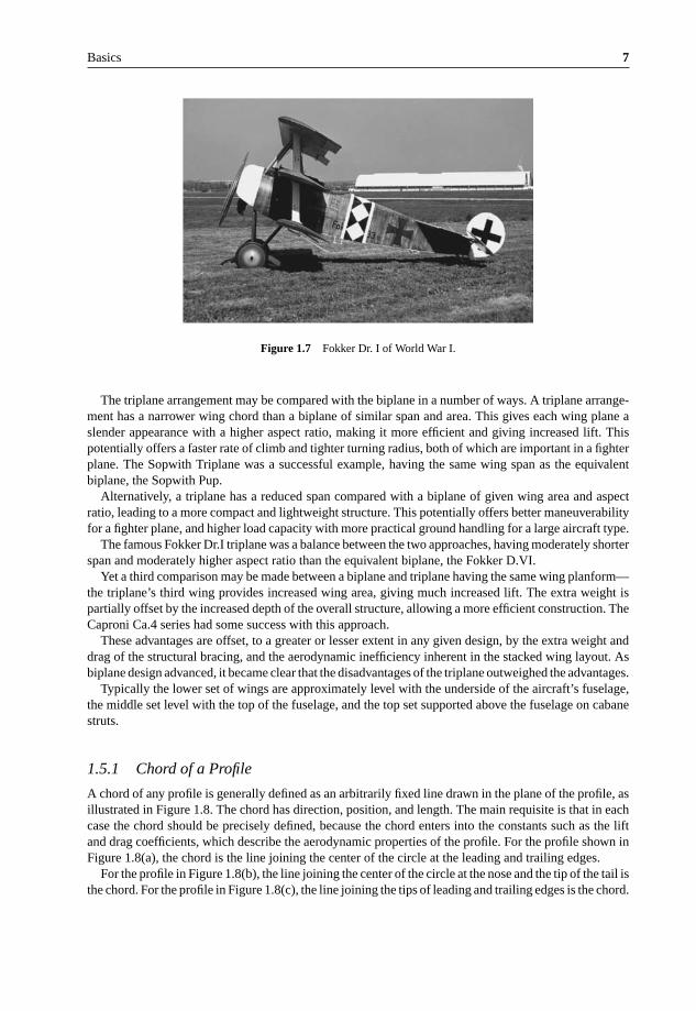
A triplane is a fixed-wing aircraft equipped with three vertically-stacked wing planes. Tailplanes andcanard fore-planes are not normally included in this count, although they may occasionally be. A typicalexample for triplane is the Fokker Dr. I of World War I, shown in Figure 1.7.
Basics 7
Figure 1.7 Fokker Dr. I of World War I.
The triplane arrangement may be compared with the biplane in a number of ways. A triplane arrange-ment has a narrower wing chord than a biplane of similar span and area. This gives each wing plane aslender appearance with a higher aspect ratio, making it more efficient and giving increased lift. Thispotentially offers a faster rate of climb and tighter turning radius, both of which are important in a fighterplane. The Sopwith Triplane was a successful example, having the same wing span as the equivalentbiplane, the Sopwith Pup.
Alternatively, a triplane has a reduced span compared with a biplane of given wing area and aspectratio, leading to a more compact and lightweight structure. This potentially offers better maneuverabilityfor a fighter plane, and higher load capacity with more practical ground handling for a large aircraft type.
The famous Fokker Dr.I triplane was a balance between the two approaches, having moderately shorterspan and moderately higher aspect ratio than the equivalent biplane, the Fokker D.VI.
Yet a third comparison may be made between a biplane and triplane having the same wing planform—the triplane’s third wing provides increased wing area, giving much increased lift. The extra weight ispartially offset by the increased depth of the overall structure, allowing a more efficient construction. TheCaproni Ca.4 series had some success with this approach.
These advantages are offset, to a greater or lesser extent in any given design, by the extra weight anddrag of the structural bracing, and the aerodynamic inefficiency inherent in the stacked wing layout. Asbiplane design advanced, it became clear that the disadvantages of the triplane outweighed the advantages.
Typically the lower set of wings are approximately level with the underside of the aircraft’s fuselage,the middle set level with the top of the fuselage, and the top set supported above the fuselage on cabanestruts.
1.5.1 Chord of a Profile
A chord of any profile is generally defined as an arbitrarily fixed line drawn in the plane of the profile, asillustrated in Figure 1.8. The chord has direction, position, and length. The main requisite is that in eachcase the chord should be precisely defined, because the chord enters into the constants such as the liftand drag coefficients, which describe the aerodynamic properties of the profile. For the profile shown inFigure 1.8(a), the chord is the line joining the center of the circle at the leading and trailing edges.
For the profile in Figure 1.8(b), the line joining the center of the circle at the nose and the tip of the tail isthe chord. For the profile in Figure 1.8(c), the line joining the tips of leading and trailing edges is the chord.

8 Theoretical Aerodynamics
chord c
chord c
(a) Leading and trailing edges are circular arcs.
(b) Circular arc leading edge and sharp trailing edge.
(c) Faired leading edge and sharp trailing edge.
chord c
Figure 1.8 Illustration of chord for different shapes of leading and trailing edges.
Chord c
Figure 1.9 Chord of a profile.
A definition which is convenient is: the chord is the projection of the profile on the double tangentto its lower surface (that is, the tangent which touches the profile at two distinct points), as shown inFigure 1.9. But this definition fails if there is no such double tangent.
1.5.2 Chord of an Aerofoil
For a cylindrical aerofoil (that is, a wing for which the profiles are the same at every location along thespan, as shown in Figure 1.5), the chord of the aerofoil is taken to be the chord of the profile in which theplane of symmetry cuts the aerofoil. In all other cases, the chord of the aerofoil is defined as the mean oraverage chord located in the plane of symmetry.
Let us consider a wing with rectangular Cartesian coordinate axes, as shown in Figure 1.10. The x-axis,or longitudinal axis, is in the direction of motion, and is in the plane of symmetry; the y-axis, or lateral
z
y
o
x
Figure 1.10 A wing with Cartesian coordinates.

Basics 9
axis, is normal to the plane of symmetry and along the (straight) trailing edge. The z-axis, or normal axis,is perpendicular to the other two axes in the sense that the three axes form a right-handed system. Thismeans, in particular, that in a straight horizontal flight the z-axis will be directed vertically downwards.Consider a profile whose distance from the plane of symmetry is |y|. Let c be the chord length of thisprofile, θ be the inclination of the chord to the xy plane, and (x, y, z) be the coordinates of the quarterpoint of the chord, that is, the point of the chord at a distance c/4 from the leading edge of the profile.This point is usually referred to as the quarter chord point. Since the profile is completely defined wheny is given, all quantities characterizing the profile, namely, the mean chord, its position and inclinationto the flow, are functions of y.
The chord of an aerofoil is defined by averaging the distance between the leading and trailing edges ofthe profiles at different locations along the span. Thus, if cm is the length of the mean chord, (xm, 0, zm)its quarter point, and θm its inclination, we take the average or mean chord as:
cm = 1
2b
∫ +b
−b
c dy
θm = 1
2b
∫ +b
−b
θ dy
xm = 1
2b
∫ +b
−b
x dy
zm = 1
2b
∫ +b
−b
z dy.
These mean values completely define the chord of the aerofoil in length (cm), direction (θm), and position(xm, zm).
1.6 Aspect Ratio
Aspect ratio of a wing is the ratio of its span 2b to chord c. Consider a cylindrical wing shown in Figure1.10. Imagine this to be projected on to the plane (xy-plane), which contains the chords of all the sections(this plane is perpendicular to the plane of symmetry (xz-plane) and contains the chord of the wing). Theprojection in this case is a rectangular area S, say, which is called the plan area of the wing. The plan areais different from the total surface area of the wing. The simplest cylindrical wing would be a rectangularplate, and the plan area would then be half of the total surface area.
The aspect ratio of the cylindrical wing is then defined by:
= 2b
c= (2b)2
S,
where S = span × chord = 2b × c.In the case of a wing which is not cylindrical, the plan area is defined as the area of the projection on
the plane through the chord of the wing (mean chord) perpendicular to the plane of symmetry, and theaspect ratio is defined as:
= (2b)2
S.
A representative value of aspect ratio is 6.

10 Theoretical Aerodynamics
Example 1.2
The semi-span of a rectangular wing of planform area 8.4 m2 is 3.5 m. Determine the aspect ratio of thewing.
Solution
Given, S = 8.4 m2 and b = 3.5 m.The planform area of a wing is S = span × chord. Therefore, the wing chord becomes:
c = S
2b
= 8.4
2 × 3.5= 1.2 m.
The aspect ratio of the wing is:
= Span
Chord
= 2 × 3.5
1.2
= 5.83 .
1.7 Camber
Camber is the maximum deviation of the camber line (which is the bisector of the profile thickness) fromthe chord of the profile, as illustrated in Figure 1.11.
Let zu and zl be the ordinates on the upper and lower parts of the profile, respectively, for the samevalue of x. Let c be the chord, and the x-axis coincide with the chord. Now, the upper and lower camberare defined as:
Upper camber = (zu)max
c
Lower camber = (zl)max
c,
AA
HH
P
Pl
Pu
(a) (b)
Chord, c
Camber line
CamberM
Chord
z
Figure 1.11 Illustration of camber, camberline and chord of aerofoil profile.

Basics 11
where the subscript “max” refers to that ordinate which is numerically the greatest. Camber is taken aspositive or negative according to the sign of (zu)max and (zl)max. Also, at a given x, the magnitudes of(zu)max and (zl)max may be different for unsymmetrical profiles.
The camber line is defined as the locus of the point (x, 12 (zu + zl)). In the case of symmetrical profile
zu + zl = 0, and the camber line is straight and coincides with the chord. Denoting the numericallygreatest ordinate of the camber line by zmax, we define:
Mean camber = zmax
c.
Note that the mean camber, in general, is not the same as the mean of upper and lower camber, and themean camber of a symmetrical profile is zero. Usually the word camber refers to the mean camber.
The thickness ratio of an aerofoil is the ratio of the maximum thickness (measured perpendicular tothe chord) to the chord. The thickness ratio is essentially tmax/c.
From the above discussions, it is evident that:
• Camberline of an aerofoil is essentially the bisector of its thickness.• Camber is the deviation of the camberline from the chord, namely the shortest line joining the leading
and trailing edges of the aerofoil profile.• The local camber can vary continuously from the leading edge to the trailing edge. Therefore, the max-
imum camber is taken as the representative camber. That is, the maximum ordinate of the camberlinefrom the chord is taken as the camber of an aerofoil.
• The thickness of an aerofoil profile also varies continuously from the leading edge to the trailing edge.Therefore, the ratio of the maximum thickness:
tmax = (zu,max + zl,max
)/2
to chord c is used to represent the thickness-to-chord ratio of an aerofoil.
1.8 Incidence
When an aircraft travels in the plane of symmetry (that is, the direction of flight is parallel to the planeof symmetry), the angle between the direction of motion and the direction of the chord of a profile, asshown in Figure 1.12, is called the geometrical incidence of the profile, denoted by the Greek letter α.The angle α is also called angle of attack.
For an airplane as a whole the geometrical incidence will be defined as the angle between the directionof motion and the chord of the aerofoil. When the chords of various profiles of a wing are parallel theincidence is the same at each section. When the chords are not parallel the incidence varies from sectionto section and the wing has twist. The value of the geometrical incidence would be altered if a differentline were chosen as chord.
In this situation, it will be beneficial to understand the difference between the wing with the chords ofits profiles at different locations along the span parallel to each other and the wing with the chords of its
α
Chord line
Direction of motion
Figure 1.12 Illustration of geometrical incidence.

12 Theoretical Aerodynamics
profiles at different locations along the span not parallel. We know that the profiles are the cross-sectionsof the wing geometry, at different locations of the span, in planes parallel to the mid-plane (xz-plane inFigure 1.3) passing through the nose and tail tips of the airplane. Therefore, only for a wing which hasits left and right wings parallel to the y-axis in Figure 1.3 the chords of its profile will be parallel, and thewing will be termed cylindrical wing. For a wing with its left and right parts not parallel to the y-axis,the chords will not be parallel, and the wing will be termed a twisted wing.
1.9 Aerodynamic Force
Aerodynamic force acting on an aircraft is the force due to the pressure distribution around it, caused bythe motion of the aircraft. Thus, the gravity does not enter into the specification of aerodynamic force.Assuming the motion of the aircraft to be steady without rotation, the aerodynamic force on the wingor on the complete aircraft may be expected to depend on the forward speed V , air density ρ, speed ofsound a and kinematic viscosity ν, of the environment in which it is flying, and the total length l of theaircraft.
If the air is assumed to be incompressible and inviscid, we have the density ρ = constant and theviscosity coefficient μ = 0. Therefore, the speed of sound becomes:
a =√
dp
dρ.
Assuming the flow over the aircraft to be isentropic, we have:
p
ργ= constant.
Differentiating with respect to ρ, we have:
dp
dρ= (constant) γ ρ(γ−1).
Now, replacing the “constant” withp
ργ, we get:
dp
dρ= p
ργγ ρ(γ−1)
= γ p
ρ.
Substituting this, we get the speed of sound as:
a =√
γ p
ρ.
For incompressible flow with dρ = 0, we have the speed of sound as:
a = ∞

Basics 13
For inviscid fluid, the kinematic viscosity becomes:
ν = μ
ρ= 0.
Therefore, for incompressible flows, the aerodynamic force Fad does not depend on the speed of sounda and kinematic viscosity ν. Thus, Fad can be assumed to depend only on ρ, V and l. The Fad would begiven by a formula such as:
Fad = 1
2kρaV blc, (1.1)
where1
2k is a dimensionless number and the indices a, b, c on the right-hand-side can be determined
by dimensional theory as follows.In terms of the fundamental dimensions of mass (M), length (L) and time (T ), we can express Equation
(1.1) as:
ML
T 2=
(M
L3
)a (L
T
)b
Lc.
Equating the dimensions M, L, T on the left-hand-side and right-hand-side, we get:
M : 1 = a
L : 1 = −3a + b + c
T : − 2 = −b.
Solving for a, b and c, we get:
a = 1, b = 2, c = 2.
Substituting for a, b, c into Equation (1.1), we get:
Fad = 1
2kρV 2l2. (1.2)
This is valid only for steady incompressible and inviscid flows. If we wish to account for compressibilityand viscosity, a and ν should be included in Equation (1.1) and expressed as:
Fad =∑ 1
2k1ρ
aV blcadνe, (1.3)
where∑ 1
2k1 is a dimensionless number, and each side must have the dimension of force. Here
∑denotes the sum of all allowable terms. In terms of basic dimensions M, L and T , Equation (1.3) becomes:
ML
T 2=
(M
L3
)a (L
T
)b
Lc
(L
T
)d(
L2
T
)e
.

14 Theoretical Aerodynamics
Equating the dimensions M, L, T on the left- and right-hand-sides, we have:
M : 1 = a
L : 1 = −3a + b + c + d + 2e
T : − 2 = −b − d − e.
Solving for a, b and c, in terms of d and e, we get:
a = 1
b = 2 − d − e
c = 2 − e.
Thus, Equation (1.3) becomes:
Fad =∑ 1
2k1ρ V 2−d−e l2−e ad νe
or
Fad =∑ 1
2k1ρV 2l2
(V
a
)−d(
Vl
ν
)−e
. (1.4)
The ratio (V/a) is called the Mach number M, which is essentially a dimensionless speed. Mach numberis the ratio of local flow speed to the local speed of sound or the ratio of inertial force to elastic force. Itis a measure of compressibility. For an incompressible fluid, M = 0.
The dimensionless group (Vl/ν) is called the Reynolds number Re. Reynolds number is the ratio ofinertial force to viscous force. For an inviscid fluid Re = ∞. For air, the kinematic viscosity ν is smalland Re is large unless Vl is small.
Thus, Equation (1.4) becomes:
Fad = 1
2ρV 2l2
∑k1M
−dRe−e
= 1
2ρV 2S f (M, Re),
where l2 has been replaced by the plan area S, a proportional number of the same dimensions, andf (M, Re) is a function, whose form is not determined by the present method, with values which areindependent of physical units.
The dimensionless number:
CFad= Fad
12 ρV 2S
= f (M, Re) (1.5)
is called the (dimensionless) coefficient of the aerodynamic force Fad. The effect of compressibility canusually be neglected if M < 0.3, and the flow is termed incompressible. Thus, for an incompressibleflow, the aerodynamic force coefficient is a function of Reynolds number only. That is:
CFad= f (Re).

Basics 15
At this stage, we may wonder about the definition of incompressible flow. The mathematical definitionof incompressible flow is that “it is a flow with Mach number zero.” But it is obvious that, for M = 0, theflow velocity is zero, and hence there is no flow. But mathematics, as an abstract science, stipulates the limitof M = 0, with the sole idea of rendering the density to become invariant. But when V = 0, engineeringscience will declare it as a stagnant field and not as a flow field. Therefore, the engineering definition ofincompressible flow is drastically different from the mathematical definition. From an engineering pointof view, when the density change associated with V is insignificant the flow can be termed incompressible.Also, for engineering applications, any change less than 5% is usually regarded as insignificant. Withthis consideration, any flow with density change less than 5% can be called incompressible. For air flowat standard sea level conditions (p = 101325 Pa and T = 288 K), 5% density change corresponds toM = 0.3 [1]. Therefore, flows with Mach number less than 0.3 are regarded as incompressible flows andthe density ρ0 corresponding to the stagnation state is taken as the density of an incompressible flow.
1.10 Scale Effect
From our studies on similarity analysis in fluid mechanics, we know that, for dynamic similarity betweenthe forces acting on an actual (or full-scale) machine and a scaled-down model used for testing (usuallywind tunnel tests), the actual machine and the scale model must satisfy geometric and kinematic similar-ities. Thus, the test model and the actual machine should be geometrically similar, and if the model testsgive an aerodynamic coefficient Cad,m for a test conducted at a Reynolds number Rem, the scale effecton the aerodynamic force coefficient Cad of the actual machine is given by:
Cad
Cad,m= f (Re)
f (Rem),
where Re is the Reynolds number of the flow around the actual machine and Rem is the Reynolds numberof the flow around the model. The model tests will give aerodynamic coefficient (Cad = Cad,m) directly,if Re = Rem. If the viscosity μ and density ρ are kept the same in the flow fields of the actual machineand its scale model, then both the flow velocity V and the characteristic length (for example, chord foran aerofoil) should be adjusted in such a way to keep Re = Rem. But the characteristic length lm for themodel will be, usually, smaller than the l for the actual machine. Therefore, the test speed for the modelhas to be greater than the speed of the actual machine.
If there is provision to use compressed air wind tunnel, then the density ρ also can be increased toadjust the model Reynolds number to match the Reynolds number of the actual machine. In this kindof studies, it is essential to make a statement about the length scale used for calculating the Reynoldsnumber.
Example 1.3
An aircraft wing profile has to be tested in a wind tunnel. If the actual wing of mean chord 1.2 m hasto fly at an altitude, where the pressure and temperature are 50 kPa and 2 ◦C, respectively, with a speedof 250 km/h. Determine the chord of the wing model to be tested in the wind tunnel, ensuring dynamicsimilarity, if the test-section conditions are 90 m/s, p = 100 kPa, T = 22 ◦C.
Solution
Let the subscripts p and m refer to the prototype (actual) wing and the wing model to be tested in thewind tunnel, respectively.

16 Theoretical Aerodynamics
Given, cp = 1.2 m, pp = 50 kPa, Tp = 2 + 273.15 = 275.15 K, Vp = 250/3.6 = 69.44 m/s.Vm = 90 m/s, pm = 100 kPa, Tm = 22 + 273.15 = 295.15 K.
The density and viscosity of the actual and test-section flows are:
ρp = pp
RTp
= 50000
287 × 275.15= 0.633 kg/m3
ρm = pm
RTm
= 100000
287 × 295.15= 1.180 kg/m3
μp = (1.46 × 10⁻⁶
) × T 3/2
T + 111
= (1.46 × 10⁻⁶
) × 275.153/2
275.15 + 111
= 1.73 × 10⁻⁵ kg/(m s)
μm = (1.46 × 10⁻⁶
) × 295.153/2
295.15 + 111
= 1.82 × 10⁻⁵ kg/(m s).
The aerodynamic forces, and hence the coefficients of these forces, acting on the actual wing and modelwing will the same if the Reynolds number of the flow field around the actual wing and model wing arethe same.The Reynolds number for the prototype is:
Rep = ρpVpcp
μp
= 0.633 × 69.44 × 1.2
1.73 × 10−5
= 3.05 × 10⁶.
This Reynolds number should be equal to Rem. Therefore:
Rem = ρmVmcm
μm
= 3.05 × 10⁶.
This gives the chord of the wing model as:
cm = (3.05 × 10⁶) × μm
ρmVm
= (3.05 × 106) × 1.82 × 10−5
1.18 × 90
= 0.523 m .

Basics 17
1.11 Force and Moment Coefficients
The important aerodynamic forces and moment associated with a flying machine, such as an aircraft,are the lift L, the drag D, and the pitching moment M. The lift and drag forces can be expressed asdimensionless numbers, popularly known as lift coefficient CL and drag coefficient CD, by dividing L
and D with 12 ρV 2S. Thus:
CL = L12 ρV 2S
(1.4a)
CD = D12 ρV 2S
(1.4b)
The variation of CL and CD with the geometrical incidence α is shown in Figure 1.13. The pitchingmoment, which is the moment of the aerodynamic force about an axis perpendicular to the plane ofsymmetry (about y-axis in Figure 1.3), will depend on the particular axis chosen. Denoting the pitchingmoment about the chosen axis by M (note that M is also used for denoting Mach number, which is theratio of local flow speed and local speed of sound), we define the pitching moment coefficient as:
CM = M12 ρV 2Sc
, (1.4c)
where c is the chord of the wing. A typical variations of CL, CD and CM with angle of attack α are shownin Figure 1.13.
Note that the aerodynamic coefficients CL, the drag CD and the moment CM are dimensionlessparameters.
Incidence
0º 10º 20º
CD
− 10º
0.4
0.8
1.0
1.2
0.2
0.6
CL
CM
Figure 1.13 Variation of lift, drag and pitching moment coefficients with geometrical incidence.

18 Theoretical Aerodynamics
Example 1.4
An aircraft weighing 20 kN is in level flight at an altitude where the pressure and temperature are 45 kPaand 0 ◦C, respectively. If the flight speed is 400 km/h and the span and mean chord of the wings are 10 mand 1.5 m, determine the lift coefficient.
Solution
Given, W = 20, 000 N, 2b = 10 m, c = 1.5 m, V = 400/3.6 = 111.11 m/s, p = 45 kPa, T = 0 +273.15 = 273.15 K.The density of air is:
ρ = p
RT
= 45, 000
287 × 273.15= 0.574 kg/m3.
The planform area of the wing is:
S = 2b × c
= 10 × 1.5
= 15 m2.
In level flight, the weight of the aircraft is equal to the lift. Thus:
L = 20, 000 N.
Therefore, by Equation (1.4a), the lift coefficient becomes:
CL = L12 ρV 2S
= 20, 00012 × 0.574 × 111.112 × 15
= 0.376 .
1.12 The Boundary Layer
Boundary layer is a thin layer, adjacent to a solid surface, in which the flow velocity increases from zeroto about 99% of the freestream velocity, as shown in Figure 1.14.
The boundary layer may also be defined as a thin layer adjacent to a solid surface where the viscouseffects are predominant. Thus, inside the boundary layer the effect of viscosity is predominant. Outsidethe boundary layer the effect of viscosity is negligible. Also, greater the Reynolds number the thinnerwill be the boundary layer, and we have practically the case of an inviscid flow past an object. But,however small the viscosity may be, the plate is subjected to a tangential traction or drag force acting inthe direction of flow velocity. This force is known as the skin friction or the frictional drag, and this forcecan never be completely eliminated. On the other hand, the flow outside the boundary layer behaves likean inviscid flow.

Basics 19
V∞
V∞
l
Boundary layerVelocity profile
Figure 1.14 Boundary layer on a flat plate.
Figure 1.15 An aerofoil in an uniform flow.
For flow past a bluff body, such as a circular cylinder, an eddying wake forms behind the cylinder,greatly increasing the drag. The problem of flow separation or break away of the boundary layer froma bluff body can be minimized by streamlining the body. For properly streamlined bodies the boundarylayer will not break away and the wake will remain almost insignificant. This has been achieved in theprofiles like that shown in Figure 1.15 which are generally referred to as aerofoils.
For aerofoils there is a narrow wake but, to a first approximation, the problem of the flow past sucha streamlined shape can be assumed as an inviscid flow past the body. In other words, the flow pastan aerofoil can be regarded as flow without wake. The above considerations give rise to the followinggeneral observations:
1. It is found that to delay the breaking away of the boundary layer from the region where the fluid ismoving against increasing pressure (that is, adverse pressure gradient, as in the case of the rear of acircular cylinder) the flow should turn as gradually as possible. To enable this gradual turning of flow,the body should have a large radius of curvature.
2. It is essential to keep the surface of the object smooth, because even small projections above thesurface (in general) may disturb the boundary layer considerably, causing a breaking away of theflow. Furthermore, a projection such as a rivet, whose head projects above the boundary layer, mayentirely alter the character of the flow. An exaggerated flow over an aerofoil with such a rivet head isschematically shown in Figure 1.16.
3. Good streamlined shapes will have the breaking away of the flow just close to thetrailing edge.
Figure 1.16 Flow separation caused by a rivet head projection.

20 Theoretical Aerodynamics
1.13 Summary
Aerodynamics is the science concerned with the motion of air and bodies moving through air. In otherwords, aerodynamics is a branch of dynamics concerned with the steady motion of air, particularly whenit interacts with a moving object. The forces acting on the bodies moving through the air are termedaerodynamic forces.
The aerodynamic force Fad can be resolved into two component forces, one at right angles to V andthe other opposite to V . The force component normal to V is called lift L and the component opposite toV is called drag D.
A streamlined body is that for which the skin friction drag accounts for the major portion of the totaldrag, and the wake drag is very small.
A bluff body is that for which the wake drag accounts for the major portion of the total drag, and theskin friction drag is insignificant.
The main lifting system of an aircraft consists of two wings which together constitute the aerofoil. Thetail plane also exerts lift. The ailerons on the right and left wings, the elevators on the horizontal tail, andthe rudder on the vertical tail are control surfaces.
The distance between the wing tips is called the span. The section of a wing by a plane parallel to theplane of symmetry is called a profile.
Chord of any profile is generally defined as an arbitrarily fixed line drawn in the plane of the profile.The chord has direction, position, and length.
For a cylindrical aerofoil (that is, a wing for which the profiles are the same at every location along thespan), the chord of the aerofoil is taken to be the chord of the profile in which the plane of symmetry cutsthe aerofoil. In all other cases, the chord of the aerofoil is defined as the mean or average chord locatedin the plane of symmetry.
The aspect ratio of a wing is the ratio of its span 2b to chord c.
• Camberline of an aerofoil is essentially the bisector of its thickness.• Camber is the deviation of the camberline from the chord, namely the shortest line joining the leading
and trailing edges of the aerofoil profile.• The local camber can vary continuously from the leading edge to the trailing edge. Therefore, the max-
imum camber is taken as the representative camber. That is, the maximum ordinate of the camberlinefrom the chord is taken as the camber of an aerofoil.
When an aircraft travels in the plane of symmetry (that is, the direction of flight is parallel to the planeof symmetry), the angle between the direction of motion and the direction of the chord of a profile, iscalled the geometrical incidence of the profile, denoted by the Greek letter α. The angle α is also calledangle of attack.
Aerodynamic force on an aircraft is the force due to the pressure distribution around it, caused by themotion of the aircraft. Thus, the gravity does not enter into the specification of aerodynamic force.
Mach number is the ratio of local flow speed to the local speed of sound or the ratio of inertial forceto elastic force. It is a measure of compressibility. For an incompressible fluid the M = 0.
The dimensionless group (Vl/ν) is called the Reynolds number Re. Reynolds number is the ratio ofinertial force to viscous force. For an inviscid fluid Re = ∞. For air, ν is small and Re is large unless Vl
is small.The dimensionless number:
CFad= Fad
12 ρV 2S
= f (M, Re)
is called the (dimensionless) coefficient of the aerodynamic force Fad.

Basics 21
The important aerodynamic forces and moment associated with a flying machine, such as an aircraft,are the lift L, the drag D, and the pitching moment M. The lift and drag forces can be expressed asdimensionless numbers, popularly known as lift coefficient CL and drag coefficient CD, by dividing L
and D with 12 ρV 2S. Thus:
CL = L12 ρV 2S
CD = D12 ρV 2S
.
The pitching moment, which is the moment of the aerodynamic force about an axis perpendicular tothe plane of symmetry (about y-axis in Figure 1.3), will depend on the particular axis chosen. Denotingthe pitching moment about the chosen axis by M (note that M is also used for denoting Mach num-ber, which is the ratio of local flow speed and local speed of sound), we define the pitching momentcoefficient as:
CM = M12 ρV 2Sc
.
Boundary layer is a thin layer, adjacent to a solid surface, in which the flow velocity increases fromzero to about 99% of the freestream velocity. The boundary layer may also be defined as a thin layeradjacent to a solid surface where the viscous effects are predominant. Thus, inside the boundary layerthe effect of viscosity is predominant. Outside the boundary layer the effect of viscosity is negligible.
For flow past a bluff body, such as a circular cylinder, an eddying wake forms behind the cylinder,greatly increasing the drag. The problem of flow separation or break away of the boundary layer froma bluff body can be minimized by streamlining the body. For properly streamlined bodies the boundarylayer will not break away and the wake will remain almost insignificant.
Exercise Problems
1. An aircraft of total mass 10000 kg cruises steadily at an altitude. If the aerodynamic efficiency is 4,find the thrust required to propel the aircraft.
[Answer: 24.525 kN]2. An aircraft of mass 3000 kg in a steady level flight is at an angle of incidence of 5◦ to the freestream.
Determine the thrust generated by the engine.[Answer: 2574.8 N]
3. An aircraft weighing 200 kN is in level flight at sea level with a speed of 600 km/h. Thewing span and chord are 8 m and 1.8 m, respectively. Determine the lift coefficient ofthe wing.
[Answer: 0.816]4. Determine the speed of sound in air at sea level conditions.
[Answer: 340.3 m/s]5. If the aerodynamic efficiency of an aircraft in a steady flight is 10, determine the incidence of the
wing to the freestream direction.[Answer: 5.71◦]

22 Theoretical Aerodynamics
6. A sail plane of mass 270 kg flies straight and level with an incidence of 4◦. Determine the aerodynamicforce acting on the wings and the aerodynamic efficiency.
[Answer: 2655.17 N, 14.30]7. A wing of rectangular planform has 10 m span and 1.2 m chord. In straight and level flight at
240 km/h the total aerodynamic force acting on the wing is 20 kN. If the aerodynamic efficiency ofthe wing is 10, calculate the lift coefficient. Assume air density to be 1.2 kg/m3.
[Answer: CL = 0.622]
Reference
1. Rathakrishnan, E., Applied Gas Dynamics, John Wiley & Sons Inc., New Jersey, 2010.

2Essence of Fluid Mechanics
2.1 Introduction
Gases and liquids are generally termed fluids. Though the physical properties of gases and liquids aredifferent, they are grouped under the same heading since both can be made to flow unlike a solid. Underdynamic conditions, the nature of the governing equations are the same for both gases and liquids.Hence, it is possible to treat them under the same heading, namely, fluid dynamics or fluid mechanics.However, certain substances known as viscoelastic materials behave like a liquid as well as a solid,depending on the rate of application of the force. Pitch and silicone putty are typical examples ofviscoelastic material. If the force is applied suddenly, the viscoelastic material will behave like a solid,but with gradually applied pressure the material will flow like a liquid. The flow of such materials isnot considered in this book. Similarly, non-Newtonian fluids, low-density flows, and two-phase flowssuch as gas liquid mixtures are also not considered in this book. The theory presented in this book is forwell-behaved simple fluids such as air.
2.2 Properties of Fluids
Fluid may be defined as a substance which will continue to change shape as long as there is a shearstress present, however small it may be. That is, the basic feature of a fluid is that it can flow, and thisis the essence of any definition of it. Examine the effect of shear stress on a solid element and a fluidelement, shown in Figure 2.1.
It is seen from this figure that the change in shape of the solid element is characterized by an angle�α, when subjected to a shear stress, whereas for the fluid element there is no such fixed �α, even for aninfinitesimal shear stress. A continuous deformation persists as long as shearing stress is applied. The rateof deformation, however, is finite and is determined by the applied shear force and the fluid properties.
2.2.1 Pressure
Pressure may be defined as the force per unit area which acts normal to the surface of any object whichis immersed in a fluid. For a fluid at rest, at any point the pressure is the same in all directions. Thepressure in a stationary fluid varies only in the vertical direction, and is constant in any horizontal plane.That is, in stationary fluids the pressure increases linearly with depth. This linear pressure distribution iscalled hydrostatic pressure distribution. The hydrostatic pressure distribution is valid for moving fluids,provided there is no acceleration in the vertical direction. This distribution finds extensive application inmanometry.
Theoretical Aerodynamics, First Edition. Ethirajan Rathakrishnan.© 2013 John Wiley & Sons Singapore Pte. Ltd. Published 2013 by John Wiley & Sons Singapore Pte. Ltd.

24 Theoretical Aerodynamics
Δα
(a) Solid (b) Fluid
ττ
Figure 2.1 Solid and fluid elements under shear stress.
When a fluid is in motion, the actual pressure exerted by the fluid in the direction normal to the flowis known as the static pressure. If there is an infinitely thin pressure transducer which can be placedin a flow field without disturbing the flow, and made to travel with the same speed as that of the flowthen it will record the exact static pressure of the flow. From this stringent requirement of the probe forstatic pressure measurement, it can be inferred that exact measurement of static pressure is impossible.However, there are certain phenomena, such as “the static pressure at the edge of a boundary layer isimpressed through the layer,” which are made use of for the proper measurement of static pressure. Thepressure which a fluid flow will experience if it is brought to rest, isentropically, is termed total pressure.The total pressure is also called impact pressure. The total and static pressures are used for computingflow velocity.
Since pressure is intensity of force, it has the dimensions:
Force
Area= MLT −2
L2= [
ML−1T −2]
and is expressed in the units of newton per square meter (N/m2) or simply pascal (Pa). At standardsea level condition, the atmospheric pressure is 101325 Pa, which corresponds to 760 mm of mercurycolumn height.
2.2.2 Temperature
In any form of matter the molecules are continuously moving relative to each other. In gases the molecularmotion is a random movement of appreciable amplitude ranging from about 76 × 10−9 m, under normalconditions (that is, at standard sea level pressure and temperature), to some tens of millimeters, at verylow pressures. The distance of free movement of a molecule of a gas is the distance it can travel beforecolliding with another molecule or the walls of the container. The mean value of this distance for allmolecules in a gas is called the molecular mean free path length. By virtue of this motion the moleculespossess kinetic energy, and this energy is sensed as temperature of the solid, liquid or gas. In the case ofa gas in motion, it is called the static temperature. Temperature has units kelvin (K) or degrees celsius(◦C), in SI units. For all calculations in this book, temperatures will be expressed in kelvin, that is, fromabsolute zero. At standard sea level condition, the atmospheric temperature is 288.15 K.
2.2.3 Density
The total number of molecules in a unit volume is a measure of the density ρ of a substance. It is expressedas mass per unit volume, say kg/m3. Mass is defined as weight divided by acceleration due to gravity. At

Essence of Fluid Mechanics 25
standard atmospheric temperature and pressure (288.15 K and 101325 Pa, respectively), the density ofdry air is 1.225 kg/m3.
Density of a material is a measure of the amount of material contained in a given volume. In a fluidsystem, the density may vary from point to point. Consider the fluid contained within a small sphericalregion of volume δV, centered at some point in the fluid, and let the mass of fluid within this sphericalregion be δm. Then the density of the fluid at the point on which the sphere is centered can be defined by:
ρ =lim
δV→ 0δm
δV. (2.1)
There are practical difficulties in applying the above definition of density to real fluids composed ofdiscrete molecules, since under the limiting condition the sphere may or may not contain any molecule.If it contains, say, just a single molecule, the value obtained for the density will be fictitiously high. If itdoes not contain any molecule the resultant value of density will be zero. This difficulty can be avoidedover the range of temperatures and pressures normally encountered in practice, in the following two ways:
1. The molecular nature of a gas may be ignored, and the gas is treated as a continuous medium orcontinuous expanse of matter, termed continuum (that is, does not consist of discrete particles).
2. The decrease in size of the imaginary sphere may be assumed to reach a limiting size, such that,although it is small compared to the dimensions of any physical object present in a flow field, forexample an aircraft, it is large enough compared to the fluid molecules and, therefore, contains areasonably large number of molecules.
2.2.4 Viscosity
The property which characterizes the resistance that a fluid offers to applied shear force is termedviscosity. This resistance, unlike for solids, does not depend upon the deformation itself but on the rateof deformation. Viscosity is often regarded as the stickiness of a fluid and its tendency is to resist slidingbetween layers. There is very little resistance to the movement of the knife-blade edge-on through air,but to produce the same motion through a thick oil needs much more effort. This is because the viscosityof the oil is higher compared to that of air.
2.2.5 Absolute Coefficient of Viscosity
The absolute coefficient of viscosity is a direct measure of the viscosity of a fluid. Consider the twoparallel plates placed at a distance h apart, as shown in Figure 2.2(a).
The space between them is filled with a fluid. The bottom plate is fixed and the other is moved in itsown plane at a speed u. The fluid in contact with the lower plate will be at rest, while that in contact withthe upper plate will be moving with speed u, because of no-slip condition. In the absence of any otherinfluence, the speed of the fluid between the plates will vary linearly, as shown in Figure 2.2(b). As adirect result of viscosity, a force F has to be applied to each plate to maintain the motion, since the fluidwill tend to retard the motion of the moving plate and will tend to drag the fixed plate in the direction ofthe moving plate. If the area of each plate in contact with fluid is A, then the shear stress acting on eachplate is F/A. The rate of sliding of the upper plate over the lower is u/h.
These quantities are connected by Maxwell’s equation, which serves to define the absolute coefficientof viscosity μ. Maxwell’s definition of viscosity states that:
“the coefficient of viscosity is the tangential force per unit area on either of two parallel plates atunit distance apart, one fixed and the other moving with unit velocity”.

26 Theoretical Aerodynamics
u
u = 0
τ
(a) (b)
u(y)
δx
δθ δθ du
dy
Velocity profile
τ = μdu
dy
o x
h
τ / ∂θ∂t
y
No slip at wall
Figure 2.2 Fluid shear between a stationary and a moving parallel plates.
Maxwell’s equation for viscosity is:
F
A= μ
(u
h
). (2.2)
Hence,
[ML−1T −2
] = [μ][LT −1L−1
] = [μ][T −1
]that is,
[μ] = [ML−1T −1
].
Therefore, the unit of μ is kg/(m s). At 0 ◦C the absolute coefficient of viscosity of dry air is 1.716 ×10⁻⁵
kg/(m s). The absolute coefficient of viscosity μ is also called the dynamic viscosity coefficient.The Equation (2.2), with μ as constant, does not apply to all fluids. For a class of fluids, which includes
blood, some oils, some paints and so called “thixotropic fluids,” μ is not constant but is a function ofdu/dh. The derivative du/dh is a measure of the rate at which the fluid is shearing. Usually μ is expressedas (N.s)/m2 or gm/(cm s). One gm/(cm s) is known as a poise.
Newton’s law of viscosity states that “the stresses which oppose the shearing of a fluid are proportionalto the rate of shear strain,” that is, the shear stress τ is given by:
τ = μ∂u
∂y, (2.3)
where μ is the absolute coefficient of viscosity and ∂u/∂y is the velocity gradient. The viscosity μ is aproperty of the fluid. Fluids which obey the above law of viscosity are termed Newtonian fluids. Somefluids such as silicone oil, viscoelastic fluids, sugar syrup, tar, etc. do not obey the viscosity law given byEquation (2.3) and they are called non-Newtonian fluids.
We know that, for incompressible flows, it is possible to separate the calculation of velocity boundarylayer from that of thermal boundary layer. But for compressible flows it is not possible, since the velocityand thermal boundary layers interact intimately and hence, they must be considered simultaneously.This is because, for high-speed flows (compressible flows) heating due to friction as well as temperaturechanges due to compressibility must be taken into account. Further, it is essential to include the effectsof viscosity variation with temperature. Usually large variations of temperature are encountered inhigh-speed flows.

Essence of Fluid Mechanics 27
The relation μ(T ) must be found by experiment. The voluminous data available in literature leads tothe conclusion that the fundamental relationship is a complex one, and that no single correlation functioncan be found to apply to all gases. Alternatively, the dependence of viscosity on temperature can becalculated with the aid of the method of statistical mechanics, but as of yet no completely satisfactorytheory has been evolved. Also, these calculations lead to complex expressions for the function μ(T ).Therefore, only semi-empirical relations appear to be the means to calculate the viscosity associated withcompressible boundary layers. It is important to realize that, even though semi-empirical relations arenot extremely precise, they are reasonably simple relations giving results of acceptable accuracy. For air,it is possible to use an interpolation formula based on D. M. Sutherland’s theory of viscosity and expressthe viscosity coefficient, at temperature T , as:
μ
μ0=
(T
T0
)3/2T0 + S
T + S,
where μ0 denotes the viscosity at the reference temperature T0, and S is a constant, which assumes thevalue 110 K for air.
For air the Sutherland’s relation can also be expressed [1] as:
μ = 1.46 × 10⁻⁶
(T 3/2
T + 111
)(N s)/m2 , (2.4)
where T is in kelvin. This equation is valid for the static pressure range of 0.01 to 100 atm, whichis commonly encountered in atmospheric flight. The temperature range in which this equation is validis from 0 to 3000 K. The absolute viscosity is a function of temperature only because, in the abovepressure and temperature ranges, the air behaves as a perfect gas, in the sense that intermolecular forcesare negligible, and that viscosity itself is a momentum transport phenomenon caused by the randommolecular motion associated with thermal energy or temperature.
2.2.6 Kinematic Viscosity Coefficient
The kinematic viscosity coefficient is a convenient form of expressing the viscosity of a fluid. It is formedby combining the density ρ and the absolute coefficient of viscosity μ, according to the equation:
ν = μ
ρ. (2.5)
The kinematic viscosity coefficient ν is expressed as m2/s, and 1 cm2/s is known as stoke.The kinematic viscosity coefficient is a measure of the relative magnitudes of viscosity and inertia
of the fluid. Both dynamic viscosity coefficient μ and kinematic viscosity coefficient ν are functions oftemperature. For liquids, μ decreases with increase of temperature, whereas for gases μ increases withincrease of temperature. This is one of the fundamental differences between the behavior of gases andliquids. The viscosity is practically unaffected by the pressure.
2.2.7 Thermal Conductivity of Air
At high-speeds, heat transfer from vehicles becomes significant. For example, re-entry vehicles encounteran extreme situation where ablative shields are necessary to ensure protection of the vehicle during its

28 Theoretical Aerodynamics
passage through the atmosphere. The heat transfer from a vehicle depends on the thermal conductivity k
of air. Therefore, a method to evaluate k is also essential. For this case, a relation similar to Sutherland’slaw for viscosity is found to be useful, and it is:
k = 1.99 × 10⁻³
(T 3/2
T + 112
)J/(s m K),
where T is temperature in kelvin. The pressure and temperature ranges in which this equation is applicableare 0.01 to 100 atm and 0 to 2000 K, respectively. For the same reason given for viscosity relation, thethermal conductivity also depends only on temperature.
2.2.8 Compressibility
The change in volume of a fluid associated with change in pressure is called compressibility. When afluid is subjected to pressure it gets compressed and its volume changes. The bulk modulus of elasticityis a measure of how easily the fluid may be compressed, and is defined as the ratio of pressure change tovolumetric strain associated with it. The bulk modulus of elasticity, K, is given by:
K = Pressure increment
Volume strain= −V dp
dV
It may also be expressed as:
K =lim
�v → 0−�p
�v/v= dp
(dρ/ρ), (2.6)
where v is specific volume. Since dρ/ρ represents the relative change in density brought about by thepressure change dp, it is apparent that the bulk modulus of elasticity is the inverse of the compressibilityof the substance at a given temperature. For instance, K for water and air are approximately 2 GN/m2
and 100 kN/m2, respectively. This implies that air is about 20,000 times more compressible than water.It can be shown that, K = a2/ρ, where a is the speed of sound. The compressibility plays a dominantrole at high-speeds. Mach number M (defined as the ratio of local flow velocity to local speed of sound)is a convenient nondimensional parameter used in the study of compressible flows. Based on M theflow is divided into the following regimes. When M < 1 the flow is called subsonic, when M ≈ 1 theflow is termed transonic flow, M from 1.2 to 5 is called supersonic regime, and M > 5 is referred to ashypersonic regime. When flow Mach number is less than 0.3, the compressibility effects are negligiblysmall, and hence the flow is called incompressible. For incompressible flows, density change associatedwith velocity is neglected and the density is treated as invariant.
2.3 Thermodynamic Properties
We know from thermodynamics that heat is energy in transition. Therefore, heat has the same dimensionsas energy and is measured in units of joule (J).
2.3.1 Specific Heat
The inherent thermal properties of a flowing gas become important when the Mach number is greaterthan 0.5. This is because Mach 0.5 corresponds to a speed of 650 km/h for air at sea level state, therefore

Essence of Fluid Mechanics 29
for flow above Mach 0.5, the temperature change associated with velocity becomes considerable. Hence,the energy equation needs to be considered in the study and owing to this both thermal and caloricalproperties need to be accounted for in the analysis. The specific heat is one such quantity. The specificheat is defined as the amount of heat required to raise the temperature of a unit mass of a medium by onedegree. The value of the specific heat depends on the type of process involved in raising the temperatureof the unit mass. Usually constant volume process and constant pressure process are used for evaluatingspecific heat. The specific heats at constant volume and constant pressure processes, respectively, aredesignated by cv and cp. The definitions of these quantities are the following:
cv ≡(
∂u
∂T
)v
, (2.7)
where u is internal energy per unit mass of the fluid, which is a measure of the potential and moreparticularly the kinetic energy of the molecules comprising the gas. The specific heat cv is a measure ofthe energy-carrying capacity of the gas molecules. For dry air at normal temperature, cv = 717.5 J/(kg K).
The specific heat at constant pressure is defined as:
cp ≡(
∂h
∂T
)p
, (2.8)
where h = u + p v, the sum of internal energy and flow energy is known as the enthalpy or total heatconstant per unit mass of fluid. The specific heat at constant pressure cp is a measure of the ability of thegas to do external work in addition to possessing internal energy. Therefore, cp is always greater than cv.For dry air at normal temperature, cp = 1004.5 J/(kg K).Note: It is essential to understand what is meant by normal temperature. For gases, up to certain temper-ature, the specific heats will be constant and independent of temperature. Up to this temperature the gasis termed perfect, implying that cp, cv and their ratio γ are constants, and independent of temperature.But for temperatures above this limiting value, cp, cv will become functions of T , and the gas will ceaseto be perfect. For instance, air will behave as perfect gas up to 500 K. The temperature below this liminglevel is referred to as normal temperature.
2.3.2 The Ratio of Specific Heats
The ratio of specific heats:
γ = cp
cv
(2.9)
is an important parameter in the study of high-speed flows. This is a measure of the relative internalcomplexity of the molecules of the gas. It has been determined from kinetic theory of gases that the ratio ofspecific heats can be related to the number of degrees of freedom, n, of the gas molecules by the relation:
γ = n + 2
n. (2.10)
At normal temperatures, there are six degrees of freedom, namely three translational and three rotational,for diatomic gas molecules. For nitrogen, which is a diatomic gas, n = 5 since one of the rotational

30 Theoretical Aerodynamics
degrees of freedom is negligibly small in comparison with the other two. Therefore:
γ = 7/5 = 1.4.
Monatomic gases, such as helium, have 3 translational degrees of freedom only, and therefore:
γ = 5/3 = 1.67.
This value of 1.67 is the upper limit of the values which the ratio of specific heats γ can take. In generalγ varies from 1 to 1.67, that is:
1 ≤ γ ≤ 1.67 .
The specific heats of a gas are related to the gas constant R. For a perfect gas this relation is:
R = cp − cv .
2.4 Surface Tension
Liquids behave as if their free surfaces were perfectly flexible membranes having a constant tension σ
per unit width. This tension is called the surface tension. It is important to note that this is neither a forcenor a stress but a force per unit length. The value of surface tension depends on:
• the nature of the fluid;• the nature of the surface of the substance with which it is in contact;• the temperature and pressure.
Consider a plane material membrane, possessing the property of constant tension σ per unit length.Let the membrane have a straight edge of length l. The force required to hold the edge stationary is:
p = σ l. (2.11)
Now, suppose that the edge is pulled so that it is displaced normal to itself by a distance x in the plane ofthe membrane. The work done, F , in stretching the membrane is given by:
F = σ l x = σ A, (2.12)
where A is the increase in the area of the membrane. It is seen that σ is the free energy of the membraneper unit area. The important point to be noted here is that, if the energy of a surface is proportional toits area, then it will behave exactly as if it were a membrane with a constant tension per unit width, andthis is totally independent of the mechanism by which the energy is stored. Thus, the existence of surfacetension, at the boundary between two substances, is a manifestation of the fact that the stored energycontains a term proportional to the area of the surface. This energy is attributable to molecular attractions.
An associated effect of surface tension is the capillary deflection of liquids in small tubes. Examinethe level of water and mercury in capillaries, shown in Figure 2.3.
When a glass tube is inserted into a beaker of water, the water will rise in the tube and display a concavemeniscus, as shown in Figure 2.3(a). The deviation of water level h in the tube from that in the beaker

Essence of Fluid Mechanics 31
d
(a) Water (b) Mercury
d
h
h θ
θ
Figure 2.3 Capillary effect of water and mercury.
can be shown to be:
h ∝ σ
dcos θ, (2.13)
where θ is the angle between the tangent to the water surface and the glass surface. In other words, aliquid such as water or alcohol, which wets the glass surface makes an acute angle with the solid, andthe level of free surface inside the tube will be higher than that outside. This is termed capillary action.However, when wetting does not occur, as in the case of mercury in glass, the angle of contact is obtuse,and the level of free surface inside the tube is depressed, as shown in Figure 2.3(b).
Another important effect of surface tension is that a long cylinder of liquid, at rest or in motion, witha free surface is unstable and breaks up into parts, which then assume an approximately spherical shape.This is the mechanism of the breakup of liquid jets into droplets.
2.5 Analysis of Fluid Flow
Basically two treatments are followed for fluid flow analysis. They are the Lagrangian and Euleriandescriptions. Lagrangian method describes the motion of each particle of the flow field in a separate anddiscrete manner. For example, the velocity of the nth particle of an aggregate of particles, moving inspace, can be specified by the scalar equations:
(Vx)n = fn(t) (2.14a)
(Vy
)n
= gn(t) (2.14b)
(Vz)n = hn(t), (2.14c)
where Vx, Vy, Vz are the velocity components in x-, y-, z-directions, respectively. They are independentof the space coordinates, and are functions of time only. Usually, the particles are denoted by the spacepoint they occupy at some initial time t0. Thus, T (x0, t) refers to the temperature at time t of a particlewhich was at location x0 at time t0.
This approach of identifying material points, and following them along is also termed the particleor material description. This approach is usually preferred in the description of low-density flow fields(also called rarefied flows), in describing the motion of moving solids, such as a projectile and so on.However, for a deformable system like a continuum fluid, there are infinite number of fluid elementswhose motion has to be described, the Lagrangian approach becomes unmanageable. For such cases, we

32 Theoretical Aerodynamics
can employ spatial coordinates to help to identify particles in a flow. The velocity of all particles in aflow field, therefore, can be expressed in the following manner:
Vx = f (x, y, z, t) (2.15a)
Vy = g(x, y, z, t) (2.15b)
Vz = h(x, y, z, t). (2.15c)
This is called the Eulerian or field approach. If properties and flow characteristics at each position inspace remain invariant with time, the flow is called steady flow. A time dependent flow is referred to asunsteady flow. The steady flow velocity field would then be given as:
Vx = f (x, y, z) (2.16a)
Vy = g(x, y, z) (2.16b)
Vz = h(x, y, z). (2.16c)
2.5.1 Local and Material Rates of Change
The rate of change of properties measured by probes at fixed locations are referred to as local rates ofchange, and the rate of change of properties experienced by a material particle is termed the material orsubstantive rates of change.
The local rate of change of a property η is denoted by ∂η(x, t)/∂t, where it is understood that x is heldconstant. The material rate of change of property η shall be denoted by Dη/Dt. If η is the velocity V,then DV/Dt is the rate of change of velocity for a fluid particle and thus is the acceleration that the fluidparticle experiences. On the other hand, ∂V/∂t is just a local rate of change of velocity recorded by astationary probe. In other words, DV/Dt is the particle or material acceleration and ∂V/∂t is the localacceleration.
For a fluid flowing with a uniform velocity V∞, it is possible to write the relation between the localand material rates of change of property η as:
∂η
∂t= Dη
Dt− V∞
∂η
∂x. (2.17)
Thus, the local rate of change of η is due to the following two effects:
1. Due to the change of property of each particle with time.2. Due to the combined effect of the spatial gradient of that property and the motion of the fluid.
When a spatial gradient exists, the fluid motion brings different particles with different values of η to theprobe, thereby modifying the rate of change sensed by the probe. This effect is termed convection effect.Therefore, V∞(∂η/∂x) is referred to as the convective rate of change of η. Even though Equation (2.17)has been obtained with uniform velocity V∞, note that in the limit δt → 0 it is only the local velocity V
which enters into the analysis and Equation (2.17) becomes:
∂η
∂t= Dη
Dt− V
∂η
∂x. (2.18)

Essence of Fluid Mechanics 33
Equation (2.18) can be generalized for a three-dimensional space as:
∂η
∂t= Dη
Dt− (V · ∇)η, (2.19)
where ∇ is the gradient operator (≡ i ∂/∂x + j ∂/∂y + k ∂/∂z) and (V · ∇) is a scalar product(= Vx ∂/∂x + Vy ∂/∂y + Vz ∂/∂z). Equation (2.19) is usually written as:
Dη
Dt= ∂η
∂t+ V · ∇η, (2.20)
when η is the velocity of a fluid particle, DV/Dt gives acceleration of the fluid particle and the resultantequation is:
DV
Dt= ∂V
∂t+ (V · ∇)V . (2.21)
Equation (2.21) is known as Euler’s acceleration formula.Note that the Euler’s acceleration formula is essentially the link between the Lagrangian and Euleriandescriptions of fluid flow.
2.5.2 Graphical Description of Fluid Motion
The following are the three important concepts for visualizing or describing flow fields:
• The concept of pathline.• The concept of streakline.• The concept of streamline.
Pathline
Pathline may be defined as a line in the flow field describing the trajectory of a given fluid particle.From the Lagrangian view point, namely, a closed system with a fixed identifiable quantity of mass, theindependent variables are the initial position, with which each particle is identified, and the time. Hence,the locus of the same particle over a time period from t0 to tn is called the pathline.
Streakline
Streakline may be defined as the instantaneous loci of all the fluid elements that have passed the pointof injection at some earlier time. Consider a continuous tracer injection at a fixed point Q in space. Theconnection of all elements passing through the point Q over a period of time is called the streakline.
Streamlines
Streamlines are imaginary lines, in a fluid flow, drawn in such a manner that the flow velocity is alwaystangential to it. Flows are usually depicted graphically with the aid of streamlines. These are imaginarylines in the flow field such that the velocity at all points on these lines are always tangential. Streamlinesproceeding through the periphery of an infinitesimal area at some instant of time t will form a tube calledstreamtube, which is useful in the study of fluid flow.

34 Theoretical Aerodynamics
From the Eulerian viewpoint, an open system with constant control volume, all flow properties arefunctions of a fixed point in space and time, if the process is transient. The flow direction of variousparticles at time ti forms streamline. The pathline, streamline and streakline are different in general butcoincide in a steady flow.
Timelines
In modern fluid flow analysis, yet another graphical representation, namely timeline, is used. When apulse input is periodically imposed on a line of tracer source placed normal to a flow, a change in the flowprofile can be observed. The tracer image is generally termed timeline. Timelines are often generated inthe flow field to aid the understanding of flow behavior such as the velocity and velocity gradient.
From the above mentioned graphical descriptions, it can be inferred that:
• There can be no flow through the lateral surface of the streamtube.• An infinite number of adjacent streamtubes arranged to form a finite cross-section is often called a
bundle of streamtubes.• Streamtube is a Eulerian (or field) concept.• Pathline is a Lagrangian (or particle) concept.• For steady flows, the pathline, streamline and streakline are identical.
2.6 Basic and Subsidiary Laws
In the range of engineering interest, four basic laws must be satisfied by any continuous medium.They are:
• Conservation of matter (continuity equation).• Newton’s second law (momentum equation).• Conservation of energy (first law of thermodynamics).• Increase of entropy principle (second law of thermodynamics).
In addition to these primary laws, there are numerous subsidiary laws, sometimes called constitutiverelations, that apply to specific types of media or flow processes (for example, equation of state forperfect gas, Newton’s viscosity law for certain viscous fluids, isentropic and adiabatic process relationsare some of the commonly used subsidiary equations in flow physics).
2.6.1 System and Control Volume
In employing the basic and subsidiary laws, any one of the following modes of application maybe adopted:
• The activities of each and every given element of mass must be such that it satisfies the basic laws andthe pertinent subsidiary laws.
• The activities of each and every elemental volume in space must be such that the basic laws and thepertinent subsidiary laws are satisfied.
In the first case, the laws are applied to an identified quantity of matter called the control mass system. Acontrol mass system is an identified quantity of matter, which may change shape, position, and thermalcondition, with time or space or both, but must always entail the same matter.

Essence of Fluid Mechanics 35
For the second case, a definite volume called control volume is designated in space, and the boundaryof this volume is known as control surface. The amount and identity of the matter in the control volumemay change with time, but the shape of the control volume is fixed, that is, the control volume maychange its position in time or space or both, but its shape is always preserved.
2.6.2 Integral and Differential Analysis
The analysis in which large control volumes are used to obtain the aggregate forces or transfer rates istermed integral analysis. When the analysis is applied to individual points in the flow field, the resultingequations are differential equations, and the method is termed differential analysis.
2.6.3 State Equation
For air at normal temperature and pressure, the density ρ, pressure p and temperature T are connected bythe relation p = ρRT , where R is a constant called gas constant. This is known as the thermal equationof state. At high pressures and low temperatures, the above state equation breaks down. At normalpressures and temperatures, the mean distance between molecules and the potential energy arising fromtheir attraction can be neglected. The gas behaves like a perfect gas or ideal gas in such a situation. Atthis stage, it is essential to understand the difference between the ideal and perfect gases. An ideal gas isfrictionless and incompressible. The perfect gas has viscosity and can therefore develop shear stresses,and it is compressible according to state equation.
Real gases below critical pressure and above the critical temperature tend to obey the perfect-gas law.The perfect-gas law encompasses both Charles’ law and Boyle’s law. Charles’ law states that at constantpressure the volume of a given mass of gas varies directly as its absolute temperature. Boyle’s law(isothermal law) states that for constant temperature the density varies directly as the absolute pressure.
2.7 Kinematics of Fluid Flow
Kinematics is the branch of physics that deals with the characteristics of motion without regard for theeffects of forces or mass. In other words, kinematics is the branch of mechanics that studies the motionof a body or a system of bodies without consideration given to its mass or the forces acting on it. Itdescribes the spatial position of bodies or systems, their velocities, and their acceleration. If the effectsof forces on the motion of bodies are accounted for the subject is termed dynamics. Kinematics differsfrom dynamics in that the latter takes these forces into account.
To simplify the discussions, let us assume the flow to be incompressible, that is, the density is treatedas invariant. The basic governing equations for an incompressible flow are the continuity and momentumequations. The continuity equation is based on the conservation of matter. For steady incompressibleflow, the continuity equation in differential form is:
∂Vx
∂x+ ∂Vy
∂y+ ∂Vz
∂z= 0 , (2.22)
where Vx, Vy and Vz are the velocity components along x-, y- and z-directions, respectively.Equation (2.22) may also be expressed as:
∇ · V = 0,

36 Theoretical Aerodynamics
where:
∇ ≡ i∂
∂x+ j
∂
∂y+ k
∂
∂z
and V = i Vx + j Vy + k Vz.The momentum equation, which is based on Newton’s second law, represents the balance between
various forces acting on a fluid element, namely:
1. Force due to rate of change of momentum, generally referred to as inertia force.2. Body forces such as buoyancy force, magnetic force and electrostatic force.3. Pressure force.4. Viscous forces (causing shear stress).
For a fluid element under equilibrium, by Newton’s second law, we have the momentum equation as:
Inertia force + Body force + Pressure force + Viscous force = 0 . (2.23)
For a gaseous medium, body forces are negligibly small compared to other forces and hence can beneglected. For steady incompressible flows, the momentum equation can be written as:
Vx
∂Vx
∂x+ Vy
∂Vx
∂y+ Vz
∂Vx
∂z= − 1
ρ
∂p
∂x+ ν
(∂2Vx
∂x2+ ∂2Vx
∂y2+ ∂2Vx
∂z2
)(2.23a)
Vx
∂Vy
∂x+ Vy
∂Vy
∂y+ Vz
∂Vy
∂z= − 1
ρ
∂p
∂y+ ν
(∂2Vy
∂x2+ ∂2Vy
∂y2+ ∂2Vy
∂z2
)(2.23b)
Vx
∂Vz
∂x+ Vy
∂Vz
∂y+ Vz
∂Vz
∂z= − 1
ρ
∂p
∂z+ ν
(∂2Vz
∂x2+ ∂2Vz
∂y2+ ∂2Vz
∂z2
). (2.23c)
Equations (2.23a), (2.23b), (2.23c) are the x, y, z components of momentum equation, respectively.These equations are generally known as Navier–Stokes equations. They are nonlinear partial differentialequations and there exists no known analytical method to solve them. This poses a major problem influid flow analysis. However, the problem is tackled by making some simplifications to the equation,depending on the type of flow to which it is to be applied. For certain flows, the equation can be reducedto an ordinary differential equation of a simple linear type. For some other type of flows, it can be reducedto a nonlinear ordinary differential equation. For the above types of Navier–Stokes equation governingspecial category of flows, such as potential flow, fully developed flow in a pipe or channel, and boundarylayer over flat plates, it is possible to obtain analytical solutions.
It is essential to understand the physics of the flow process before reducing the Navier-Stokes equationsto any useful form, by making appropriate approximations with respect to the flow. For example, let usexamine the flow over an aircraft wing, shown in Figure 2.4.
This kind of problem is commonly encountered in fluid mechanics. Air flow over the wing createshigher pressure at the bottom, compared to the top surface. Hence, there is a net resultant force componentnormal to the freestream flow direction, called lift, L, acting on the wing. The velocity varies along thewing chord as well as in the direction normal to its surface. The former variation is due to the shapeof the aerofoil, and the latter is due to the no-slip condition at the wall. In the direction normal towing surface, the velocity gradients are very large in a thin layer adjacent to the surface and the flowreaches asymptotically to the freestream velocity within a short distance, above the surface. This thin

Essence of Fluid Mechanics 37
L
V∞
Streamline
Figure 2.4 Flow past a wing.
region adjacent to the wall, where the velocity increases from zero to freestream value, is known as theboundary layer. Inside the boundary layer the viscous forces are predominant. Further, it so happens thatthe static pressure outside the boundary layer, acting in the direction normal to the surface, is transmittedto the boundary through the boundary layer, without appreciable change. In other words, the pressuregradient across the boundary layer is zero. Neglecting the inter-layer friction between the streamlines,in the region outside the boundary layer, it is possible to treat the flow as inviscid. Inviscid flow is alsocalled potential flow, and for this case the Navier-Stokes equation can be simplified to become linear.It is possible to obtain the pressures in the field outside the boundary layer and treat this pressure tobe invariant across the boundary layer, that is, the pressure in the freestream is impressed through theboundary layer. For low-viscous fluids such as air, we can assume, with a high degree of accuracy, thatthe flow is frictionless over the entire flow field, except for a thin region near solid surfaces. In the vicinityof solid surface, owing to high velocity gradients, the frictional effects become significant. Such regionsnear solid boundaries, where the viscous effects are predominant, are termed boundary layers.
In general, boundary layer over streamlined bodies are extremely thin. There may be laminar andturbulent flow within the boundary layer, and its thickness and profile may change along the direction ofthe flow. Consider the flow over a flat plate shown in Figure 2.5. Different zones of boundary layer over aflat plate are shown in Figure 2.5. The laminar sublayer is that zone adjacent to the boundary, where theturbulence is suppressed to such a degree that only the laminar effects prevail. The various regions shownin Figure 2.5 are not sharp demarcations of different zones. There is actually a gradual transition fromone region, where certain effect predominates, to another region, where some other effect is predominant.
Although the boundary layer is thin, it plays a vital role in fluid dynamics. The drag on ships, aircraft andmissiles, the efficiency of compressors and turbines of jet engines, the effectiveness of ram jets and turbo-jets, and the efficiencies of numerous other engineering devices, are all influenced by the boundary layer toa significant extent. The performance of a device depends on the behavior of boundary layer and its effecton the main flow. The following are some of the important parameters associated with boundary layers.
2.7.1 Boundary Layer Thickness
Boundary layer thickness δ may be defined as the distance from the wall in the direction normal to thewall surface, where the fluid velocity is within 1% of the local main stream velocity. It may also be
Laminar flow
Laminar sublayer
V∞
Boundary layer edge
Transition flow Turbulent flow
V∞
Figure 2.5 Flow past a flat plate.

38 Theoretical Aerodynamics
δ
V∞ Edge of boundary layer
V∞
Figure 2.6 Illustration of boundary layer thickness.
defined as the distance δ, normal to the surface, in which the flow velocity increases from zero to somespecified value (for example, 99%) of its local main stream flow velocity. The boundary layer thicknessδ may be shown schematically as in Figure 2.6.
2.7.2 Displacement Thickness
Displacement thickness δ∗ may be defined as the distance by which the boundary would have to bedisplaced if the entire flow field were imagined to be frictionless and the same mass flow is maintainedat any section.
Consider unit width in the flow over an infinite flat plate at zero angle of incidence, and let the x-component of velocity to be Vx and the y-component of velocity be Vy. The volume flow rate �q throughthis boundary layer segment of unit width is given by:
�q =∫ ∞
0
(Vm − Vx) dy,
where Vm is the main stream (frictionless flow) velocity component and Vx is the actual local velocitycomponent. To maintain the same volume flow rate q for the frictionless case, as in the actual case, theboundary must be shifted out by a distance δ∗ so as to cut off the amount �q of volume flow rate. Thus:
Vmδ∗ = �q =∫ ∞
0
(Vm − Vx)dy
δ∗ =∫ ∞
0
(1 − Vx
Vm
)dy . (2.24)
The displacement thickness is illustrated in Figure 2.7. The main idea of this postulation is to permitthe use of a displaced body in place of the actual body such that the frictionless mass flow around thedisplaced body is the same as the actual mass flow around the real body. The displacement thicknessconcept is made use of in the design of wind tunnels, air intakes for jet engines, and so on.
The momentum thickness θ and energy thickness δe are other (thickness) measures pertaining to bound-ary layer. They are defined mathematically as follows:
θ =∫ ∞
0
(1 − Vx
Vm
)ρVx
ρmVm
dy (2.25)

Essence of Fluid Mechanics 39
Vm
velocity profileInviscid
velocity profile
x
Actual
Vm
y
displaced boundaryHypothetical flow withActual flow
δ∗
Figure 2.7 Illustration of displacement thickness.
δe =∫ ∞
0
(1 − V 2
x
V 2m
)ρVx
ρmVm
dy , (2.26)
where Vm and ρm are the velocity and density at the edge of the boundary layer, respectively, and Vx andρ are the velocity and density at any y location normal to the body surface, respectively. In addition toboundary layer thickness, displacement thickness, momentum thickness and energy thickness, we candefine the transition point and separation point also with the help of boundary layer.
A closer look at the essence of the displacement, momentum and energy thicknesses of a boundary layerwill be of immense value from an application point of view. First of all, δ∗, θ and δe are all length parame-ters, in the direction normal to the surface over which the boundary layer prevails. Physically, they accountfor the defect in mass flow rate, momentum and kinetic energy, caused by the viscous effect. In other words:
• The displacement thickness is the distance by which the boundary, over which the boundary layerprevails, has to be hypothetically shifted, so that the mass flow rate of the actual flow through distanceδ and the ideal (inviscid) flow through distance (δ − δ∗), illustrated in Figure 2.7, will be the same.
• The momentum thickness is the distance by which the boundary, over which the boundary layerprevails, has to be hypothetically shifted, so that the momentum associated with the mass passingthrough the actual thickness (distance) δ and the hypothetical thickness (δ − θ) will be the same.
• The energy thickness is the distance by which the boundary, over which the boundary layer prevails,has to be hypothetically shifted, so that the kinetic energy of the flow passing through the actualthickness (distance) δ and the hypothetical thickness (δ − δe) will be the same.
2.7.3 Transition Point
Transition point may be defined as the end of the region at which the flow in the boundary layer on thesurface ceases to be laminar and begins to become turbulent. It is essential to note that the transition fromlaminar to turbulent nature takes place over a length, and not at a single point. Thus the transition pointmarks the beginning of the transition process from laminar to turbulent nature.
2.7.4 Separation Point
Separation point is the position at which the boundary layer leaves the surface of a solid body. If theseparation takes place while the boundary layer is still laminar, the phenomenon is termed laminarseparation. If it takes place for a turbulent boundary layer it is called turbulent separation.

40 Theoretical Aerodynamics
The boundary layer theory makes use of Navier-Stokes Equation (2.23) with the viscous terms in itbut in a simplified form. On the basis of many assumptions such as, boundary layer thickness is smallcompared to the body length and similarity between velocity profiles in a laminar flow, the Navier-Stokesequation can be reduced to a nonlinear ordinary differential equation, for which special solutions exist.Some such problems for which Navier-Stokes equations can be reduced to boundary layer equations andclosed form solutions can be obtained are: flow past a flat plate or Blassius problem; Hagen-Poiseuilleflow through pipes; Couette flow between a stationary and moving parallel plates; and flow betweenrotating cylinders.
2.7.5 Rotational and Irrotational Motion
When a fluid element is subjected to a shearing force, a velocity gradient is produced perpendicularto the direction of shear, that is, a relative motion occurs between two layers. To encounter this relativemotion the fluid elements have to undergo rotation. A typical example of this type of motion is the motionbetween two roller chains rubbing each other, but moving at different velocities. It is convenient to usean abstract quantity called circulation , defined as the line integral of velocity vector between any twopoints (to define rotation of the fluid element) in a flow field. By definition:
= ∮cV. dl , (2.27)
where dl is an elemental length, c is the path of integration.Circulation per unit area is known as vorticity ζ,
ζ = /A. (2.28)
In vector form, ζ becomes:
ζ = ∇ × V = curl V , (2.29)
where V is the flow velocity, given by V = i Vx + j Vy, and:
∇ ≡ i∂
∂x+ j
∂
∂y.
For a two-dimensional flow in xy-plane, vorticity ζ becomes:
ζz = ∂Vy
∂x− ∂Vx
∂y, (2.30a)
where ζz is the vorticity about the z-direction, which is normal to the flow field. Likewise, the othercomponents of vorticity about x- and y-directions are:
ζx = ∂Vz
∂y− ∂Vy
∂z(2.30b)
ζy = ∂Vx
∂z− ∂Vz
∂x. (2.30c)
If ζ = 0, the flow is known as irrotational flow. Inviscid flows are basically irrotational flows.

Essence of Fluid Mechanics 41
2.8 Streamlines
Streamlines are imaginary lines in the flow field such that the velocity at all points on these lines arealways tangential to them. Flows are usually depicted graphically with the aid of streamlines. Streamlinesproceeding through the periphery of an infinitesimal area at some time t forms a tube called streamtube,which is useful for the study of fluid flow phenomena. From the definition of streamlines, it can beinferred that:
• Flow cannot cross a streamline, and the mass flow between two streamlines is conserved.• Based on the streamline concept, a function ψ called stream function can be defined. The velocity
components of a flow field can be obtained by differentiating the stream function.
In terms of stream function ψ, the velocity components of a two-dimensional incompressible flow aregiven as:
Vx = ∂ψ
∂y, Vy = −∂ψ
∂x. (2.31)
If the flow is compressible the velocity components become:
Vx = 1
ρ
∂ψ
∂y, Vy = − 1
ρ
∂ψ
∂x. (2.32)
It is important to note that the stream function is defined only for two-dimensional flows, and thedefinition does not exist for three-dimensional flows. Even though some books define ψ for axisymmetricflow, they again prove to be equivalent to two-dimensional flow. We must realize that the definition ofψ does not exist for three-dimensional flows, because such a definition demands a single tangent at anypoint on a streamline, which is not possible in three-dimensional flows.
2.8.1 Relationship between Stream Function and Velocity Potential
For irrotational flows (the fluid elements in the field are free from rotation), there exists a function φ
called velocity potential or potential function. For a steady two-dimensional flow, φ must be a functionof two space coordinates (say, x and y). The velocity components are given by:
Vx = ∂φ
∂x, Vy = ∂φ
∂y. (2.33)
From Equations (2.31) and (2.33), we can write:
∂ψ
∂y= ∂φ
∂x,
∂ψ
∂x= −∂φ
∂y. (2.34)
These relations between stream function and potential function, given by Equation (2.34), are the famousCauchy-Riemann equations of complex-variable theory. It can be shown that the lines of constant φ orpotential lines form a family of curves which intersect the streamlines in such a manner as to have thetangents of the respective curves always at right angles at the point of intersection. Hence, the two setsof curves given by ψ = constant and φ = constant form an orthogonal grid system or flow-net. That is,the streamlines and potential lines in flow field are orthogonal.

42 Theoretical Aerodynamics
Unlike stream function, potential function exists for three-dimensional flows also, because there is nocondition like the local flow velocity must be tangential to the potential lines imposed in the definitionof φ. The only requirement for the existence of φ is that the flow must be potential.
2.9 Potential Flow
Potential flow is based on the concept that the flow field can be represented by a potential function φ
such that:
∇2φ = 0 . (2.35)
This linear partial differential equation is popularly known as Laplace equation. Derivatives of φ withrespect to the space coordinates x, y and z give the velocity components Vx, Vy and Vz, respectively, alongx-, y- and z- directions. Unlike the stream function ψ, the potential function can exist only if the flowis irrotational, that is, when viscous effects are absent. All inviscid flows must satisfy the irrotationalitycondition:
∇ × V = 0 . (2.36)
For two-dimensional potential flows, by Equation (2.30), we have the vorticity ζ as:
ζz = ∂Vy
∂x− ∂Vx
∂y= 0.
Using Equation (2.33), we get the vorticity as:
ζz = ∂2φ
∂x∂y− ∂2φ
∂x∂y= 0.
This shows that the flow is irrotational. For two-dimensional incompressible flows, the continuity equationis:
∂Vx
∂x+ ∂Vy
∂y= 0.
In terms of the potential function φ, this becomes:
∂2φ
∂x2+ ∂2φ
∂y2= 0
that is:
∇2φ = 0.
This linear equation is the governing equation for potential flows.For potential flows, the Navier-Stokes equations (2.23) reduce to:
Vx
∂Vx
∂x+ Vy
∂Vx
∂y+ Vz
∂Vx
∂z= − 1
ρ
∂p
∂x(2.37a)

Essence of Fluid Mechanics 43
Vx
∂Vy
∂x+ Vy
∂Vy
∂y+ Vz
∂Vy
∂z= − 1
ρ
∂p
∂y(2.37b)
Vx
∂Vz
∂x+ Vy
∂Vz
∂y+ Vz
∂Vz
∂z= − 1
ρ
∂p
∂z. (2.37c)
Equation (2.37) is known as Euler’s equation.At this stage, it is natural to have the following doubts about the streamline and potential function,
because we defined the streamline as an imaginary line in a flow field and potential function as a mathe-matical function, which exists only for inviscid flows. The answers to these vital doubts are the following:
• Among the graphical representation concepts, namely the pathline, streakline and streamline, only thefirst two are physical, and the concept of streamline is only hypothetical. But even though imaginary,the streamline is the only useful concept, because it gives a mathematical representation for the flowfield in terms of stream function ψ, with its derivatives giving the velocity components. Once thevelocity components are known, the resultant velocity, its orientation, the pressure and temperatureassociated with the flow can be determined. Thus, streamline plays a dominant role in the analysis offluid flow.
• Knowing pretty well that no fluid is inviscid or potential, we introduce the concept of potential flow,because this gives rise to the definition of potential function. The derivatives of potential function withthe spatial coordinates give the velocity components in the direction of the respective coordinates andthe substitution of these velocity components in the continuity equation results in Laplace equation.Even though this equation is the governing equation for an impractical or imaginary flow (inviscid flow),the fundamental solutions of Laplace equation form the basis for both experimental and computationalflow physics. The basic solutions for the Laplace equation are the uniform flow, source, sink and free orpotential vortex. These solutions being potential can be superposed to get the mathematical functionsrepresenting any practical geometry of interest. For example, superposition of a doublet (source anda sink of equal strength in proximity) and uniform flow would represent flow past a circular cylinder.In the same manner, suitable distribution of source and sink along the camberline and superpositionof uniform flow over this distribution will mathematically represent flow past an aerofoil. Thus, anypractical geometry can be modeled mathematically, using the basic solutions of the Laplace equation.
2.9.1 Two-dimensional Source and Sink
Source is a potential flow field in which flow emanating from a point spreads radially outwards, as shownin Figure 2.8(a). Sink is potential flow field in which flow gushes towards a point from all radial directions,as illustrated in Figure 2.8(b).
VrVr
(a) Source (b) Sink
Potential line
Streamline r
θ θ
r
Figure 2.8 Illustration of two-dimensional (a) source and (b) sink.

44 Theoretical Aerodynamics
Consider a source at origin, shown in Figure 2.8(a). The volume flow rate q crossing a circular surfaceof radius r and unit depth is given by:
q = 2πrVr, (2.38)
where Vr is the radial component of velocity. The volume flow rate q is referred to as the strength of thesource. For a source, the radial lines are streamlines. Therefore, the potential lines must be concentriccircles, represented by:
φ = A ln(r), (2.39)
where A is a constant. The radial velocity component Vr = ∂φ/∂r = A/r.Substituting this into Equation (2.39), we get:
2πrA
r= q
or
A = q
2π.
Thus, the velocity potential for a two-dimensional source of strength q becomes:
φ = q
2πln (r) . (2.40)
In a similar manner as above, the stream function for a source of strength q can be obtained as:
ψ = q
2πθ , (2.41)
where θ is the orientation (inclination) of the streamline from the x-direction, measured in the counter-clockwise direction, as shown in Figure 2.8(a). Similarly, for a sink, which is a type of flow in which thefluid from infinity flows radially towards the origin, we can show that the potential and stream functionsare given by:
φ = − q
2πln (r)
and
ψ = − q
2πθ ,
where q is the strength of the sink. Note that the volume flow rate is termed the strength of source andsink. Also, for both source and sink the origin is a singular point.

Essence of Fluid Mechanics 45
2.9.2 Simple Vortex
A simple or free vortex is a flow field in which the fluid elements simply translate along concentric circles,without spinning about their own axes. That is, the fluid elements have only translatory motion in a freevortex. In addition to moving along concentric circular paths, if the fluid elements spin about their ownaxes, the flow field is termed forced vortex.
A simple or free vortex can be established by selecting the stream function, ψ, of the source to be thepotential function φ of the vortex. Thus, for a simple vortex:
φ = q
2πθ . (2.42)
It can be easily shown from Equation (2.42) that the stream function for a simple vortex is:
ψ = − q
2πln (r) . (2.43)
It follows from Equations (2.42) and (2.43) that the velocity components of the simple vortex, shown inFigure 2.9, are:
Vθ = q
2πr, Vr = 0. (2.44)
Here again the origin is a singular point, where the tangential velocity Vθ tends to infinity, as seen fromEquation (2.44). The flow in a simple or free vortex resembles part of the common whirlpool found whilepaddling a boat or while emptying water from a bathtub. An approximate profile of a whirlpool is asshown in Figure 2.10. For the whirlpool, shown in Figure 2.10, the circulation along any path about theorigin is given by:
=∮
V · dl
=∫ 2π
0
Vθrdθ.
θ
r
Streamline
Vθ
Potential line
Figure 2.9 A simple or potential vortex flow.

46 Theoretical Aerodynamics
Core
z
r
Figure 2.10 A whirlpool flow field.
By Equation (2.44), Vθ = q
2πr, therefore, the circulation becomes:
=∫ 2π
0
q
2πrrdθ = q.
Since there are no other singularities for the whirlpool, shown in Figure 2.10, this must be the circulationfor all paths about the origin. Consequently, q in the case of vortex is the measure of circulation aboutthe origin and is also referred to as the strength of the vortex.
2.9.3 Source-Sink Pair
This is a combination of a source and sink of equal strength, situated (located) at a distance apart. Thestream function due to this combination is obtained simply by adding the stream functions of source andsink. When the distance between the source and sink is made negligibly small, in the limiting case, thecombination results in a doublet.
2.9.4 Doublet
A doublet or a dipole is a potential flow field due to a source and sink of equal strength, brought togetherin such a way that the product of their strength and the distance between them remain constant. Considera point P in the field of a doublet formed by a source and a sink of strength q and − q, respectively, keptat a distance ds, as shown in Figure 2.11, with sink at the origin.
r
y
ds
SourceSink
r +dr
P
xθ
Figure 2.11 Source and sink.

Essence of Fluid Mechanics 47
By Rankine’s theorem, the velocity potential of the doublet, φD, can be expressed as the sum of thevelocity potentials of the source and sink. Thus, we have:
φD = q
2πln (r + dr) − q
2πln (r)
= q
2πln
(r + dr
r
)
= q
2πln
(1 + dr
r
).
Expanding ln
(1 + dr
r
), we get:
ln
(1 + dr
r
)= dr
r− 1
2
(dr
r
)2
+ · · ·
Butdr
r� 1, therefore, neglecting the second and higher order terms, we get the potential function for a
doublet as:
φD = q
2π
dr
r.
By the definition of doublet, ds → 0, therefore:
dr = ds cos θ
Hence,
φD = q
2πrds cos θ.
Also, for a doublet, by definition, q ds = constant. Let this constant, known as the strength of the doubletbe denoted by m, then:
m = q ds
and
φD = m
2πrcos θ . (2.45)
In Cartesian coordinates, the velocity potential for the doublet becomes:
φD = m
2π
(x
x2 + y2
).

48 Theoretical Aerodynamics
x
y
Streamline
Figure 2.12 Doublet with source and sink on the x-axis (source located on the left and sink on the right of the origin).
From the above equations for φD, the expression for the stream function ψD can be obtained as:
ψD = − m
2πrsin θ .
In Cartesian coordinates, the stream function becomes:
ψD = − m
2π
(y
x2 + y2
).
If the source and sink were placed on the x-axis, the streamlines of the doublet will be as shown inFigure 2.12.
If the source and sink are placed on the y-axis, the resulting expressions for the φD and ψD will become:
φD(yy) = m
2πrsin θ
= m
2π
(y
x2 + y2
)
ψD(yy) = − m
2πrcos θ
= − m
2π
(x
x2 + y2
).
The streamlines of the doublet will be as shown in Figure 2.13. The expression for the stream function:
ψD(yy) = − m
2π
(x
x2 + y2
)
can be arranged in the form:
ψD(yy) = − c x
x2 + y2.

Essence of Fluid Mechanics 49
x
y
Streamline
Figure 2.13 Doublet with source and sink on the y-axis (source located below the origin and sink above the origin).
where c = m/(2π), is a constant. This can be expressed as:
x2 + y2 + c x
ψD(yy)= 0
(x + c
2ψD(yy)
)2
+ y2 =(
c
2ψD(yy)
)2
.
Thus, the streamlines represented by ψD(yy) = constant are circles with their centers lying on the x-axisand are tangent to the y-axis at the origin (Figure 2.13). Direction of flow at the origin is along the negativey-axis, pointing outward from the source of the limiting source-sink pair, which is called the axis ofthe doublet.
The potential and stream functions for the concentrated source, sink, vortex, and doublet are all singularat the origin. It will be shown in the following section that several interesting flow patterns can be obtainedby superposing a uniform flow on these concentrated singularities.
2.10 Combination of Simple Flows
In Section 2.9 we saw that flow past practical shapes of interest can be represented or simulated withsuitable combination of source, sink, free vortex and uniform flow. In this section let us discuss somesuch flow fields.
2.10.1 Flow Past a Half-Body
An interesting pattern of flow past a half-body, shown in Figure 2.14, can be obtained by combining asource and a uniform flow parallel to x-axis. By definition, a given streamline (ψ = constant) is associated
ψ = q/2
a
ψ = q/2
o
y
hmax
xS
Figure 2.14 Irrotational flow past a two-dimensional half-body.
50 Theoretical Aerodynamics
with one particular value of the stream function. Therefore, when we join the points of intersection of theradial streamlines of the source with the rectilinear streamlines of the uniform flow, the sum of magnitudesof the two stream functions will be equal to the streamline of the resulting combined flow pattern. If thisprocedure is repeated for a number of values of the combined stream function, the result will be a pictureof the combined flow pattern.
The stream function for the flow due to the combination of a source of strength q at the origin, immersedin a uniform flow of velocity V∞, parallel to x-axis is:
ψ = V∞ r sin θ + q
2πθ.
The streamlines of the resulting flow field will be as shown in Figure 2.14.The streamline passing through the stagnation point S is termed the stagnation streamline. The stag-
nation streamline resembles a semi-ellipse. This shape is popularly known as Rankine’s half-body. Thestreamlines inside the semi-ellipse are due to the source and those outside the semi-ellipse are due to theuniform flow. The boundary or stagnation streamline is given by:
ψ = q
2.
It is seen that S is the stagnation point where the uniform flow velocity V∞ cancels the velocity of theflow from the source. The stagnation point is located at (a, π). At the stagnation point, both Vr and Vθ
should be zero. Thus:
Vr = 1
r
∂ψ
∂θ
= V∞ cos θ + q
2π r= 0.
This gives:
V∞ − q
2π a= 0
a = q
2πV∞.
Therefore, the stream function of the stagnation point is:
ψs = V∞ r sin θ + q θ
2π.
At the stagnation point S, r = a and θ = π, therefore:
ψs = V∞ a sin π + q
2ππ
= q
2.
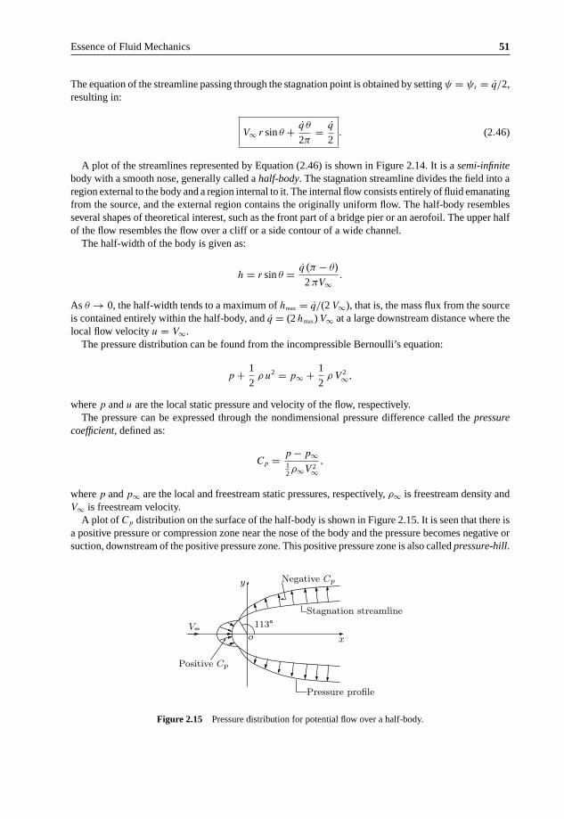
Essence of Fluid Mechanics 51
The equation of the streamline passing through the stagnation point is obtained by setting ψ = ψs = q/2,resulting in:
V∞ r sin θ + q θ
2π= q
2. (2.46)
A plot of the streamlines represented by Equation (2.46) is shown in Figure 2.14. It is a semi-infinitebody with a smooth nose, generally called a half-body. The stagnation streamline divides the field into aregion external to the body and a region internal to it. The internal flow consists entirely of fluid emanatingfrom the source, and the external region contains the originally uniform flow. The half-body resemblesseveral shapes of theoretical interest, such as the front part of a bridge pier or an aerofoil. The upper halfof the flow resembles the flow over a cliff or a side contour of a wide channel.
The half-width of the body is given as:
h = r sin θ = q (π − θ)
2 πV∞.
As θ → 0, the half-width tends to a maximum of hmax = q/(2 V∞), that is, the mass flux from the sourceis contained entirely within the half-body, and q = (2 hmax) V∞ at a large downstream distance where thelocal flow velocity u = V∞.
The pressure distribution can be found from the incompressible Bernoulli’s equation:
p + 1
2ρ u2 = p∞ + 1
2ρ V 2
∞,
where p and u are the local static pressure and velocity of the flow, respectively.The pressure can be expressed through the nondimensional pressure difference called the pressure
coefficient, defined as:
Cp = p − p∞12 ρ∞V 2∞
,
where p and p∞ are the local and freestream static pressures, respectively, ρ∞ is freestream density andV∞ is freestream velocity.
A plot of Cp distribution on the surface of the half-body is shown in Figure 2.15. It is seen that there isa positive pressure or compression zone near the nose of the body and the pressure becomes negative orsuction, downstream of the positive pressure zone. This positive pressure zone is also called pressure-hill.
x
y Negative Cp
oV∞ 113°
Positive Cp
Stagnation streamline
Pressure profile
Figure 2.15 Pressure distribution for potential flow over a half-body.

52 Theoretical Aerodynamics
The net pressure force acting on the body can easily be shown to be zero, by integrating the pressurep acting on the surface. The half-body is obtained by the linear combination of the individual streamfunctions of a source and a uniform flow, as per the Rankine’s theorem which states that:
“the resulting stream function of n potential flows can be obtained by combining the stream functionsof the individual flows.”
The half-body shown in Figure 2.15 is also referred to as Rankine’s half-body.
Example 2.1
A two-dimensional source of strength 4.0 m2/s is placed in a uniform flow of velocity 1 m/s parallel tox-axis. Determine the flow velocity and its direction at r = 0.8 m and θ = 140◦.
Solution
The given flow is an ideal flow around a half-body. The stream function for the flow around a half-body,by Equation (2.46), is:
ψ = V∞ r sin θ + q
2πθ.
Given that V∞ = 1 m/s and q = 4 m2/s. Thus:
ψ = r sin θ + 4
2πθ.
The tangential and radial components of velocity, respectively, are:
Vθ = − ∂ψ
∂r
= − sin θ = − sin (140◦)
= − 0.643 m/s
and
Vr = 1
r
∂ψ
∂θ
= 1
r
(r cos θ + 4
2π
)
= 1
0.8×
(0.8 × cos (140◦) + 2
π
)
= 0.0297 m/s.

Essence of Fluid Mechanics 53
r
V
α
Vθ
Vrα
140°
Flow
x
θ
Source
Figure 2.16 Velocity field.
The resultant velocity, at r = 0.8 and θ = 140◦, is:
V =√
V 2r + V 2
θ
=√
(0.0297)2 + (−0.643)2
= 0.644 m/s .
The velocity field is as shown in the Figure 2.16.If θ is the angle the velocity makes with the horizontal, as shown in the figure, then:
θ = 140◦ − α.
Also:
tan α = Vθ
Vr
= 0.643
0.0297= 21.65
α = tan−1(21.65)
= 87.36◦.
Thus:
θ = 140◦ − 87.36◦
= 52.64◦ .
Example 2.2
A two-dimensional flow field is made up of a source at the origin and a flow given by φ = r2 cos 2θ.Locate any stagnation points in the upper half of the coordinate plane (0 ≤ θ ≤ π).
Solution
The potential function of the flow is:
φ = m
2πln r + r2 cos 2θ,
wherem
2πln r is the velocity potential for the source, with strength m m2/s.

54 Theoretical Aerodynamics
The velocity components are given by:
Vr = ∂φ
∂r
Vθ = 1
r
∂φ
∂θ
Vr = m
2πr+ 2r cos 2θ
Vθ = −2r sin 2θ.
At the stagnation point, Vr = 0 and Vθ = 0. Thus, we have:
cos 2θ = − m
4πr2(i)
and
sin 2θ = 0
2θ = 0 or π
θ = 0 orπ
2.
Thus, θs = π/2 at the stagnation point. Substitution of this into Equation (i) gives:
rs =(
m
4π
)1/2
Example 2.3
A certain body has the shape of Rankine’s half-body of maximum thickness of 0.5 m. If this body is tobe placed in an air stream of velocity 30 m/s, find the source strength required to simulate flow aroundthe body?
Solution
The half-body can be represented as a combination of a source and a uniform flow.The resulting stream function is:
ψ = ψuniform flow + ψsource
ψ = U r sin θ + m
2πθ, (i)
where m is source strength. At the stagnation point S:
Vr = 1
r
∂ψ
∂θ= 0.

Essence of Fluid Mechanics 55
That is:
U cos θ + m
2πr= 0.
But at S, θ = π, thus:
−U + m
2πr= 0
U = m
2πr.
If x = b is the stagnation point, then at r = b:
U = m
2πb
or
b = m
2πU.
The value of the stream function of the streamline passing through the stagnation point can be obtainedby evaluating Equation (i), at r = b and θ = π, which yields:
ψstag = m
2= 2πbU
2= πbU.
Thus, from Equation (i), we get:
πbU = U r sin θ + m
2πθ
= U r sin θ + θ
ππbU.
Solving, we get:
r = b (π − θ)
sin θ. (ii)
The width of the half-body asymptotically approaches 2 πb, as shown below. Equation (ii) can bewritten as:
r sin θ = b(π − θ).
But y = r sin θ, thus:
y = b(π − θ). (iii)
From Equation (iii), it is seen that as θ → 0 or θ → 2 π the half-width approaches ± bπ.

56 Theoretical Aerodynamics
For θ = 0, Equation (iii) gives:
y = bπ.
But:
b = m
2πU.
Therefore:
y = m
2πUπ
or
m = 2Uy.
For U = 30 m/s and y = 0.5 m, we have:
m = 2 × 30 × 0.25
= 15 m2/s .
The source strength required is 15 m2/s.
Example 2.4
Check whether the flow represented by the stream function:
ψ = V∞ r sin θ + q
2 πθ,
where q is the volume flow rate, which is a constant, is irrotational.
Solution
The radial and tangential velocity components of the given flow are:
Vr = 1
r
∂ψ
∂θ
= V∞ cos θ + q
2 π r
Vθ = − ∂ψ
∂r
= − V∞ sin θ.
The irrotationality condition given by Equation (2.36) is:
ζ = ∂Vy
∂x− ∂Vx
∂y= 0.

Essence of Fluid Mechanics 57
In terms of r and θ, this becomes:
1
r
∂
∂r(r Vθ) − 1
r
∂Vr
∂θ= 0.
Thus:
1
r
∂
∂r(−r Vθ sin θ) − 1
r
∂
∂θ
(V∞ cos θ + q
2 π r
)= 0
− Vθ sin θ
r+ 1
rVθ sin θ = 0.
The irrotational condition is satisfied and hence the flow is irrotational.
2.11 Flow Past a Circular Cylinder without Circulation
A flow pattern equivalent to an irrotational flow over a circular cylinder can be obtained by combining auniform stream and a doublet with its axis directed against the stream, as shown in Figure 2.17.
The points S1 and S2 are the stagnation points. The combined stream function becomes:
ψ = ψdoublet + ψuniform flow
= − m
2πrsin θ + V∞r sin θ
=(V∞r − m
2πr
)sin θ.
The potential function for the flow is:
φ =(
V∞r + m
2πr
)cos θ. (2.47)
It is seen that ψ = 0 for all values of θ, showing that the streamline ψ = 0 represents a circular cylinderof radius r = √
m/(2πV∞). Let r = a = √m/(2πV∞). For a given velocity of the uniform flow and a
given strength of the doublet, the radius a is constant. Thus, the stream function and potential function
ψ = 0
2V∞
y
S1 ψ = 0x
S2
ψ=
0
V∞
Figure 2.17 Irrotational flow past a circular cylinder without circulation.

58 Theoretical Aerodynamics
of the flow past a cylinder can also be expressed as:
ψ = V∞
(r − a2
r
)sin θ (2.48)
φ = V∞
(r + a2
r
)cos θ. (2.49)
From the flow pattern shown in Figure 2.17, it is evident that the flow inside the circle has no influenceon the flow outside the circle. The normal and tangential components of velocity around the cylinder,respectively, are:
Vr = ∂φ
∂r= V∞
(1 − a2
r2
)cos θ
Vθ = 1
r
∂φ
∂θ= −V∞
(1 + a2
r2
)sin θ.
The flow speed around the cylinder is given by:
∣∣V ∣∣r=a
=∣∣Vθ
∣∣r=a
= 2 V∞ sin θ.
where what is meant by |Vθ| is the positive value of sin θ. This shows that there are stagnation points onthe surface at (a, 0) and (a, π). The flow velocity reaches a maximum of 2V∞ at the top and bottom ofthe cylinder, where θ = π/2 and 3π/2, respectively.
The nondimensional pressure distribution over the surface of the cylinder is given by:
Cp = p − p∞12 ρV 2∞
= 1 − V 2
V 2∞= 1 − 4 sin2 θ . (2.50)
Pressure distribution at the surface of the cylinder is shown by the continuous line in Figure 2.18.The symmetry of the pressure distribution in an irrotational flow implies that “a steadily moving bodyexperiences no drag.” This result, which is not true for actual (viscous) flows where the body experiences
Cp
0◦ 30◦− 3
− 2
− 1
0
1
60◦ 90◦ 120◦ 150◦ 180◦
Distance from the forward stagnation point
Subcritical
Invisci
dflow
flowSupercritical
flow
Figure 2.18 Comparison of irrotational and actual pressure over a circular cylinder.

Essence of Fluid Mechanics 59
drag, is known as d’Alembert’s paradox. This discrepancy between the results of inviscid and viscousflows is because of:
• the existence of tangential stress or skin friction and• drag due to the separation of the flow from the sides of the body and the resulting formation of wake
dominated by eddies, in the case of bluff bodies, in the actual flow which is viscous.
The surface pressure in the wake of the cylinder in actual flow is lower than that predicted by irrotationalor potential flow theory, resulting in a pressure drag.Note: For flow past a circular cylinder, there are two limits for the Cp, as shown in Figure 2.18. These twolimits are Cp = +1 and Cp = −3, at the forward and rear stagnation points (at 0◦ and 180◦, respectively),and at the top and bottom locations of the cylinder (at 90◦ and 270◦, respectively). At this stage, it isnatural to question about the validity of these limiting values of the pressure coefficient Cp for flow pastgeometries other than circular cylinder. Clarifying these doubts is essential from both theoretical andapplication points of view.
• The positive limit of +1 for Cp, at the forward stagnation point, is valid for all geometries and forboth potential and viscous flow, as long as the flow speed is subsonic.
• When the flow speed becomes supersonic, there will be a shock ahead of or at the nose of a blunt-nosedand sharp-nosed bodies, respectively. Hence, there are two different speeds at the zones upstreamand downstream of the shock. Therefore, the freestream static pressure p∞ and dynamic pressure(
1
2ρV 2
∞
)to be used in the Cp relation:
Cp = p − p∞12 ρV 2∞
have two options, where p is the local static pressure. This makes the Cp at the forward stagnationpoint sensitive to the freestream static and dynamic pressures, used to calculate it. Therefore, Cp = +1can not be taken as the limiting maximum of Cp, when the flow speed is supersonic.
• The limiting minimum of −3, for the Cp over the cylinder in potential flow, is valid only for circularcylinder. The negative value of Cp can take values lower than −3 for other geometries. For example,for a cambered aerofoil at an angle of incidence can have Cp as low as −6.
• Another important aspect to be noted for viscous flow is that there is no specific location for rearstagnation point on the body. The flow separates from the body and establishes a wake. The separationis taking place at two locations, above and below the horizontal axis passing through the center of thebody. Also, these upper and lower separations are not taking place at fixed points, but oscillate aroundthe separation location, because of vortex formation. Therefore, the negative pressure at the rear ofthe body does not assume a specified minimum at any fixed point, as in the case of potential flow. Formany combinations of the geometries and flow Reynolds numbers, the negative Cp at the separatedzone of the body can assume comparable magnitudes over a large portion of the wake.
2.11.1 Flow Past a Circular Cylinder with Circulation
We saw that there is no net force acting on a circular cylinder in a steady irrotational flow withoutcirculation. It can be shown that a lateral force identical to a lift force on an aerofoil, results whencirculation is introduced around the cylinder. When a clockwise line vortex of circulation is superposedaround the cylinder in an irrotational flow, the stream function [sum of Equations (2.43) and (2.48)]

60 Theoretical Aerodynamics
becomes:
ψ = V∞
(r − a2
r
)sin θ +
2πln r.
The tangential velocity component at any point in the flow is:
Vθ = −∂ψ
∂r= −V∞
(1 + a2
r2
)sin θ −
2π r. (2.51)
At the surface of the cylinder of radius a, the tangential velocity becomes:
Vθ
∣∣r=a
= −2 V∞ sin θ −
2π a.
At the stagnation point, Vθ = 0, thus:
sin θ = −
4 π a V∞. (2.52)
For = 0, the potential flow past the cylinder is symmetrical about both x- and y-directions, as shownin Figure 2.19(a). For this case there is no drag acting on the cylinder.
For < 4 π a V∞, two values of θ satisfy Equation (2.52). This implies that there are two stagnationpoints on the surface, as shown in Figure 2.19(b).
When = 4 π a V∞, the stagnation points merge on the negative y-axis, as shown in Figure 2.19(c).For > 4 π a V∞ the stagnation points merge and stay outside the cylinder, as shown in Figure 2.19(d).
The stagnation points move away from the cylinder surface, since sin θ cannot be greater than 1. The
(a) Γ = 0 (b) Γ < 4πaV∞
(c) Γ = 4πaV∞ (d) Γ > 4πaV∞
xxθ
x
S1,2
Γ Γ
x
y y
S1↪2
y
S1
y
S1
ΓS2
r
S2
Figure 2.19 Flow past a circular cylinder (a) without circulation and (b), (c) and (d) with circulation.

Essence of Fluid Mechanics 61
radial distance of the stagnation points for this case can be found from:
Vθ|θ=− π2
= V∞
(1 + a2
r2
)−
2 π r= 0
This gives:
r = 1
4 π V∞
[ ±
√ 2 − (4 π a V∞)2
].
One root of this is r > a, and the flow field for this is as shown in Figure 2.19(d), with the stagnation pointsS1 and S2, overlapping and positioned outside the cylinder. The second root corresponds to a stagnationpoint inside the cylinder. But the stagnation point for flow past a cylinder cannot be inside the cylinder.Therefore, the second solution is an impossible one.
As shown in Figure 2.19, the location of the forward and rear stagnation points on the cylinder can beadjusted by controlling the magnitude of the circulation . The circulation which positions the stagnationpoints in proximity, as shown in Figure 2.19(b), is called subcritical circulation, the circulation whichmakes the stagnation points coincide at the surface of the cylinder, as shown in Figure 2.19(c), is calledcritical circulation, and the circulation which makes the stagnation points coincide and take a positionoutside the surface of the cylinder, as shown in Figure 2.19(d), is called supercritical circulation.
To determine the magnitude of the transverse force acting on the cylinder, it is essential to find thepressure distribution around the cylinder. Since the flow is irrotational, Bernoulli’s equation can be appliedbetween a point in the freestream flow and a point on the surface of the cylinder. Bernoulli’s equation forincompressible flow is:
p + ρ V 2
2= p∞ + ρ V 2
∞2
.
Using Equation (2.52), the surface pressure can be found as follows.At the surface r = a and Equation (2.51) gives the local velocity at any point on the surface as:
Vθ
∣∣r=a
= −2 V∞ sin θ −
2π a
Substituting this into Bernoulli’s equation, we get:
pr=a + 1
2ρ
(− 2V∞ sin θ −
2π a
)2
= p∞ + ρV 2∞
2,
that is:
pr=a = p∞ + 1
2ρ
[V 2
∞ −(− 2V∞ sin θ −
2π a
)2]
. (2.53)
The symmetry of flow about the y-axis implies that the pressure force on the cylinder has no componentalong the x-axis. The pressure force acting in the direction normal to the flow (along y-axis) is called thelift force L in aerodynamics.
Consider a cylinder of radius a in a uniform flow of velocity V∞, shown in Figure 2.20.

62 Theoretical Aerodynamics
o
p
θ
a
dθ
V∞
x
y
Figure 2.20 Circular cylinder in a uniform flow.
The lift acting on the cylinder is given by:
L = −∫ 2π
0
pr=a a sin θ dθ.
Substituting Equation (2.53), and integrating we obtain the lift as:
L = ρ V∞ , (2.54)
where we have used:
∫ 2π
0
sin θ dθ =∫ 2π
0
sin3 θ dθ = 0.
It can be shown that Equation (2.54) is valid for irrotational flows around any two-dimensional shape,not just for circular cylinders alone. The expression for lift in Equation (2.54) shows that the lift forceproportional to circulation is of fundamental importance in aerodynamics. Wilhelm Kutta (1902), theGerman mathematician, and Nikolai Zhukovsky (1906), the Russian aerodynamicist, have proved therelation for lift, given by Equation (2.54), independently; this is called the Kutta-Zhukovsky lift theorem(the name Zhukovsky is transliterated as Joukowsky in older Western texts). The circulation developed bycertain two-dimensional shapes, such as aerofoil, when placed in a stream can be explained with vortextheory. It can be shown that the viscosity of the fluid is responsible for the development of circulation.The magnitude of circulation, however, is independent of viscosity, and depends on the flow speed V∞,the shape and orientation of the body to the freestream direction.
For a circular cylinder in a potential flow, the only way to develop circulation is by rotating it in a flowstream. Although viscous effects are important in this case, the observed pattern for high rotational speedsdisplays a striking similarity to the ideal flow pattern for > 4πaV∞. When the cylinder rotates at lowspeeds, the retarded flow in the boundary layer is not able to overcome the adverse pressure gradient overthe rear surface (downstream of θ = 90◦) the cylinder. This leads to the separation of the real (actual)flow, unlike the irrotational flow which does not separate. However, even in the presence of separation,observed speeds are higher on the upper surface of the cylinder, implying the existence of a lift force.
A second reason for a rotating cylinder generating lift is the asymmetry to the flow pattern, caused bythe delayed separation on the upper surface of the cylinder. The asymmetry results in the generation ofthe lift force. The contribution of this mechanism is small for two-dimensional objects such as circularcylinder, but it is the only mechanism for the side force experienced by spinning three-dimensional

Essence of Fluid Mechanics 63
objects such as soccer, tennis and golf balls. The lateral force experienced by rotating bodies is calledthe Magnus effect. The horizontal component of the force on the cylinder, due to the pressure, in generalis called drag. For the cylinder, shown in Figure 2.20, the drag is given by:
D =∫ 2π
0
pr=a a cos θ dθ.
It is interesting to note that the drag is equal to zero. It is important to realize that this result is obtainedon the assumption that the flow is inviscid. In real (actual or viscous) flows the cylinder will experiencea finite drag force acting on it due to viscous friction and flow separation.
2.12 Viscous Flows
In the previous sections of this chapter, we have seen many interesting concepts of fluid flow. With thisbackground, let us observe some of the important aspects of fluid flow from a practical or applicationpoint of view.
We are familiar with the fact that the viscosity produces shear force which tends to retard the fluidmotion. It works against inertia force. The ratio of these two forces governs (dictates) many propertiesof the flow, and the ratio expressed in the form of a nondimensional parameter is known as the famousReynolds number, ReL:
ReL = ρVL
μ, (2.55)
where V , ρ are the velocity and density of the flow, respectively, μ is the dynamic viscosity coefficientof the fluid and L is a characteristic dimension. The Reynolds number plays a dominant role in fluidflow analysis. This is one of the fundamental dimensionless parameters which must be matched forsimilarity considerations in most fluid flow analyses. At high Reynolds numbers, the inertia force ispredominant compared to viscous forces. At low Reynolds numbers the viscous effects predominateeverywhere, whereas at high Re the viscous effects confine to a thin region, just adjacent to the surfaceof the object present in the flow, and this thin layer is termed boundary layer. Since the length andvelocity scales are chosen according to a particular flow, when comparing the flow properties at twodifferent Reynolds numbers, only flows with geometric similarity should be considered. In other words,flow over a circular cylinder should be compared only with flow past another circular cylinder, whosedimensions can be different but not the shape. Flow in pipes with different velocities and diameters andflow over aerofoils of the same kind are also some geometrically similar flows. From the above-mentionedsimilarity consideration, we can infer that geometric similarity is a prerequisite for dynamic similarity.That is, dynamically similar flows must be geometrically similar, but the converse need not be true. Onlysimilar flows can be compared, that is, when comparing the effect of viscosity, the changes in flow patterndue to body shape should not interfere with the problem.
For calculating Reynolds number, different velocity and length scales are used. Some popular shapesand their length scales we often encounter in fluid flow studies are given in Table 2.1. In the descriptionof Reynolds number here, the quantities with subscript ∞ are at the freestream and quantities withoutsubscript are the local properties. Reynolds number is basically a similarity parameter. It is used todetermine the laminar and turbulent nature of flow. Below a certain Reynolds number the entire flow islaminar and any disturbance introduced into the flow will be dissipated out by viscosity. The limitingReynolds number below which the entire flow is laminar is termed the lower critical Reynolds number.

64 Theoretical Aerodynamics
Table 2.1 Some popular shapes and their characteristic lengths
Cylinder:
Red = ρ∞V∞d
μ∞d is cylinder diameter
Aerofoil:
Rec = ρ∞V∞c
μ∞c is aerofoil chord
Pipe flow (fully developed):
Red = ρVd
μV is the average velocity
d is pipe diameterChannel flow (two-dimensionaland fully developed):
Reh = ρVh
μV is the average velocity
h is the height of the channelFlow over a grid:
Rem = ρVm
μV is the velocity upstream
or downstream of the gridm is the mesh size
Boundary layer:
Reδ = ρ V δ
μV is the outer velocity
δ is the boundary layer thickness
Reθ = ρ V θ
μθ is the momentum thickness
Rex = ρ V x
μx is the distance from the leading edge
Some of the well-known critical Reynolds number are listed below:
Pipe flow - Red = 2300: based on mean velocity and diameter d.Channel flow - Reh = 1000 (two-dimensional): based on height h and mean velocity.Boundary layer flow - Reθ = 350: based on freestream velocity and momentum thickness θ.Circular cylinder - Rew = 200 (turbulent wake): based on wake width w and wake defect.Flat plate - Rex = 5 × 10⁵: based on length x from the leading edge.Circular cylinder - Red = 1.66 × 10⁵: based on cylinder diameter d.
It is essential to note that, the transition from laminar to turbulent nature does not take place at aparticular Reynolds number but over a range of Reynolds number, because any transition is gradual andnot sudden. Therefore, incorporating this aspect, we can define the lower and upper critical Reynoldsnumbers as follows.
• Lower critical Reynolds number is that Reynolds number below which the entire flow is laminar.• Upper critical Reynolds number is that Reynolds number above which the entire flow is turbulent.• Critical Reynolds number is that at which the flow field is a mixture of laminar and turbulent flows.
Note: It is important to note that when the Reynolds number is low due to large viscosity μ the flow istermed stratified flow, for example, flow of tar, honey etc. are stratified flows. When the Reynolds number

Essence of Fluid Mechanics 65
Yawing moment
Drag force
Lift force
Rolling moment
Pitching moment
Side force
V∞
Figure 2.21 Forces acting on an arbitrary body.
is low because of low density, the flow is termed rarefied flow. For instance, flow in space and very highaltitudes, in the Earth’s atmosphere, are rarefied flows.
2.12.1 Drag of Bodies
When a body moves in a fluid, it experiences forces and moments due to the relative motion of the flowtaking place around it. If the body has an arbitrary shape and orientation, the flow will exert forces andmoments about all the three coordinate axes, as shown in Figure 2.21. The force on the body along theflow direction is called drag.
The drag is essentially a force opposing the motion of the body. Viscosity is responsible for a part ofthe drag force, and the body shape generally determines the overall drag. The drag caused by the viscouseffect is termed the frictional drag or skin friction. In the design of transport vehicles, shapes experiencingminimum drag are considered to keep the power consumption at a minimum. Low drag shapes are calledstreamlined bodies and high drag shapes are termed bluff bodies.
Drag arises due to (a) the difference in pressure between the front and rear regions and (b) the frictionbetween the body surface and the fluid. Drag force caused by the pressure imbalance is known as pressuredrag, and (b) the drag due to friction is known as skin friction drag or shear drag. A body for whichthe skin friction drag is the major portion of the total drag is called streamlined body, and that with thepressure drag as the major portion of the total drag is called a bluff body.
2.12.1.1 Pressure Drag
The pressure drag arises due to the separation of boundary layer, caused by adverse pressure gradient.The phenomenon of separation, and how it causes the pressure drag, can be explained by consideringflow around a body, such as a circular cylinder. If the flow is assumed to be potential, there is no viscosityand hence no boundary layer. The flow past the cylinder would be as shown in Figure 2.22, without anyseparation.
Potential flow around a cylinder will be symmetrical about both the horizontal and vertical planes,passing through the center of the cylinder. The pressure distribution over the front and back surfaceswould be identical, and the net force along the freestream direction would be zero. That is, there would

66 Theoretical Aerodynamics
θS1
A
B
S2
Figure 2.22 Potential flow past a circular cylinder.
not be any drag acting on the cylinder. But in real flow, because of viscosity, a boundary layer is formedover the surface of the cylinder. The flow experiences a favorable pressure gradient from the forwardstagnation point S1 to the topmost point A on the cylinder at θ = 90◦, shown in Figure 2.22.
Therefore, the flow accelerates from point S1 to A (that is, from θ = 0◦ to 90◦). However, beyondθ = 90◦ the flow is subjected to an adverse pressure gradient and hence decelerates. Note that beyondthe topmost point A the fluid elements find a larger space to relax. Therefore, in accordance with massconservation (for subsonic flow) [2], as the flow area increases the flow speed decreases and the pressureincreases. Under this condition there is a net pressure force acting against the fluid flow. This processestablishes an adverse pressure gradient, leading to flow separation, as illustrated in Figure 2.23. In aboundary layer, the velocity near the surface is small, and hence the force due to its momentum is unableto counteract the pressure force. Flow within the boundary layer gets retarded and the velocity near thewall region reduces to zero at some point downstream of A and then the flow is pushed back in theopposite direction, as illustrated in Figure 2.23. This phenomenon is called flow separation.
The location where the flow leaves the body surface is termed separation point. For flow past acylinder, there are two separation points on either side of the horizontal axis through the center of thecylinder. The separated flow is chaotic and vortex dominated. The separated flow behind an object is alsoreferred to as wake. Depending on the Reynolds number level, the wake may be laminar or turbulent.An important characteristics of the separated flow is that it is always unsymmetrical, even for laminar
Unseparated
dp/dx = 0
dp/dx < 0
dV/dx > 0
dV/dx = 0,About to separate
Separated reverse flow(Back flow at the wall)
Surface
Wake
S1
B
θ
A
Figure 2.23 Illustration of separation process.

Essence of Fluid Mechanics 67
separation. This is because of the vortices prevailing in the separated zone. As we know, for every vortexthere is a specific frequency and amplitude. Therefore, when the vortices formed at the upper and lowerseparation points of the cylinder are of the same size and leave the cylinder at the same time, the wakemust be symmetric. But this kind of formation of vortices of identical size and leaving the upper andlower separation points at the same time is possible only when the geometry of the cylinder is perfectlysymmetrical and the freestream flow is absolutely unperturbed and symmetrical about the horizontalplane bisecting the cylinder. But in practice it is not possible to meet these stringent requirements of flowand geometrical symmetry to establish symmetrical separation. Owing to this practical constraints allseparated flows are unsymmetrical. Indeed, the formation of the vortices at the upper and lower separationpoints itself is unsymmetrical. When one of them, say the upper one, grows faster, the other one is unableto grow at the same rate. Therefore, only after the faster growing vortex reaches a limiting size possible,for the geometry and Reynolds number combination, and leaves the surface, the growth of the vortex atthe opposite side picks up. This retards the growth of the new vortex formed at the location where thevortex left the surface. Thus, alternative shedding of vortices from the upper and lower separation pointsis established. The alternative shedding of vortices makes the wake chaotic.
Across the separated region, the total pressure is nearly a constant and lower than what it would havebeen if the flow did not separate. The pressure do not recover completely as in the case of potential flow.Thus, on account of the incomplete recovery of pressure due to separation, a net drag force opposing thebody motion is generated. We can easily see that the pressure drag will be small if the separation had takenplace later, that is, the area over which the pressure unrecovered is small. To minimize pressure drag,the separation point should be as far as possible from the leading edge or forward stagnation point. Thisis true for any shape. Streamlined bodies are designed on this basis and the adverse pressure gradient iskept as small as possible, by keeping the curvature very small. At this stage, it is important to realize thatthe separated region behind an object is vortex dominated and these vortices cause considerable pressureloss. Thus the total pressure p0,rear behind the object is significantly lower than the total pressure p0,faceat the face of the object. This difference
(p0,rear − p0,face
), termed pressure loss, is a direct measure of
the drag. This drag caused by the pressure loss is called the pressure drag. This is also referred to asform drag, because the form or shape of the moving object dictates the separation and the expanse ofthe separated zone. The separation zone behind an object is also referred to as wake. That is, wake is theseparated region behind an object (usually a bluff body) where the pressure loss is severe. It is essential tonote that what is meant by pressure loss is total pressure loss, and there is nothing like static pressure loss.
The separation of boundary layer depends not only on the strength of the adverse pressure gradient butalso on the nature of the boundary layer, namely, laminar or turbulent. A laminar flow has tendency toseparate earlier than a turbulent flow. This is because the laminar velocity profiles in a boundary layer haslesser momentum near the wall. This is conspicuous in the case of flow over a circular cylinder. Laminarboundary layer separates nearly at θ = 90◦ whereas, for a highly turbulent boundary layer the separation isdelayed and the attached flow continues up to as far as θ = 150◦ on the cylinder. The reduction of pressuredrag when the boundary layer changes from laminar to turbulent is of the order of 5 times for bluff bodies.The flow behind a separated region is called the wake. For low drag, the wake width should be small.
Although separation is shown to take place at well defined locations on the body, in the illustrationin Figure 2.23, it actually takes places over a zone on the surface which can not be identified easily.Therefore, theoretical estimation of separation especially for a turbulent boundary layer is difficult andhence the pressure drag cannot be easily calculated. Some approximate methods exist but they can serveonly as guidelines for the estimation of pressure drag.
At this stage, we may wonder about the level of static pressure in the separated flow region or thewake of a body. The total pressure in the wake is found to be lower than that in the freestream, becauseof the pressure loss caused by the vortices in the wake. But the static pressure in the wake is almost equalto the freestream level. But it is essential to realize that just after separation, the flow is chaotic and thestreaklines do not exhibit any defined pattern. Therefore, the static pressure does not show any specificmean value in the near-wake region and keeps fluctuating. However, beyond some distance behind the

68 Theoretical Aerodynamics
object, the wake stabilizes to an extent to assume almost constant static pressure across its width. Thisdistance is about 6 times the diameter for a circular cylinder. Thus, beyond 6 diameter distance the staticpressure in the wake is equal to the freestream value.Note: It may be useful to recall what is meant by pressure loss is the total pressure loss and there isnothing like static pressure loss.
2.12.1.2 Skin Friction Drag
The friction between the surface of a body and the fluid causes viscous shear stress and this force isknown as skin friction drag. Wall shear stress τ at the surface of a body is given by:
τ = μ∂Vx
∂y, (2.56)
where μ is the dynamic viscosity coefficient and ∂Vx/∂y is the velocity gradient at body surface y = 0.If the velocity profile in the boundary layer is known, then the shear stress can be calculated.
For streamlined bodies, the separated zone being small, a major portion of the drag is because of skinfriction. We saw that bodies are classified as streamlined and bluff, based on which is dominant amongthe drag components. A body for which the skin friction drag is a major portion of the total drag istermed streamlined body. A body for which the pressure (form) drag is the major portion is termed bluffbody. Turbulent boundary layer results in more skin friction than a laminar one. Examine the skin frictioncoefficient cf variation with Reynolds number, for a flat plate kept at zero angle of attack in a uniformstream, plotted in Figure 2.24. The characteristic length for Reynolds number is the plate length x, fromits leading edge. It can be seen from Figure 2.24 that the cf is more for a turbulent flow than laminarflow. The friction coefficient is defined as:
cf = Frictional force12 ρV 2∞S
, (2.57)
where V∞, ρ are the freestream velocity and density, respectively, and S is the wetted surface area of theflat plate.
cf
Turbulent
0.01
0.001
Laminar
Re = (ρV x)/μ
cf = Average skin friction
104 106 108 1010
coefficient
Rex
Figure 2.24 Skin friction coefficient variation with Reynolds number.

Essence of Fluid Mechanics 69
For bluff bodies, the pressure drag is substantially greater than the skin friction drag, and for streamlinedbodies the condition is the reverse. In the case of streamlined bodies, such as aerofoil, the designer aims atkeeping the skin friction drag as low as possible. Maintaining laminar boundary layer conditions all alongthe surface is the most suitable arrangement to keep the skin friction low. Though such aerofoils, knownas laminar aerofoils, have been designed, they have many limitations. Even a small surface roughnessor disturbance can make the flow turbulent, and spoil the purpose of maintaining the laminar flow overthe entire aerofoil. In addition, for laminar aerofoils there is a tendency for the flow to separate even atsmall angles of attack, which severely restricts the use of such aerofoils.
2.12.1.3 Comparison of Drag of Various Bodies
In low-speed flow past geometrically similar bodies with identical orientation and relative roughness, thedrag coefficient should be a function of the Reynolds number only.
CD = f (Re). (2.58)
The Reynolds number is based upon freestream velocity V∞ and a characteristic length L of the body.The drag coefficient CD could be based upon L2, but it is customary to use a characteristic area S of thebody instead of L2. Thus, the drag coefficient becomes:
CD = Drag12 ρV 2∞S
. (2.59)
The factor1
2, in the denominator of the CD expression, is our traditional tribute to Euler and Bernoulli.
The area S is usually one of the following three types:
1. Frontal area of the body as seen from the flow stream. This is suitable for thick stubby bodies, suchas spheres, cylinders, cars, missiles, projectiles, and torpedos.
2. Planform area of the body as seen from above. This is suitable for wide flat bodies such as aircraftwings and hydrofoils.
3. Wetted area. This is appropriate for surface ships and barges.
While using drag or other fluid (aerodynamic) force data, it is important to note what length and areaare being used to scale the measured coefficients.
Table 2.2 gives a few data on drag, based on frontal area, of two-dimensional bodies of various cross-section, at Re ≥ 104.
Drag coefficient of sharp-edged bodies, which have a tendency to experience flow separation regardlessof the nature of boundary layer, are insensitive to Reynolds number. The elliptic cylinders, being smoothlyrounded, have the “laminar-turbulent” transition effect and are therefore quite sensitive to the nature ofthe boundary layer (that is, laminar or turbulent).
Table 2.3 lists drag coefficients of some three-dimensional bodies. For these bodies also we canconclude that sharp edges always cause flow separation and high drag which is insensitive to Reynoldsnumber.
Rounded bodies, such as ellipsoid, have drag which depends upon the point of separation, so that bothReynolds number and the nature of boundary layer are important. Increase of body length will generallydecrease the pressure drag by making the body relatively more slender, but sooner or later the skin frictiondrag will catch up. For a flat-faced cylinder, the pressure drag decreases with L/d but the skin friction

70 Theoretical Aerodynamics
Table 2.2 Drag of two-dimensional bodies at Re ≥ 104 (Fluid dynamic drag,Hoerner, 1975)
Shape
1.20
2.20
1.16
1.60+
1.55
1.55
1.98
2.30
2.05+
1.17+
2.00
CD
+ In subcritical flow
V
Vortex street
drag increases, so that minimum drag occurs at about L/d = 2, where L/d is the slenderness ratio ofthe body.
2.12.2 Turbulence
Turbulent flow is usually described as flow with irregular fluctuations. In nature, most of the flows areturbulent. Turbulent flows have characteristics which are appreciably different from those of laminarflows. We have to explain all the characteristics of turbulent flow to completely describe it. Incorporat-ing all the important characteristics, the turbulence may be described as a three-dimensional, randomphenomenon, exhibiting multiplicity of scales, possessing vorticity, and showing very high dissipation.Turbulence is described as a three-dimensional phenomenon. This means that even in a one-dimensionalflow field the turbulent fluctuations are always three-dimensional. In other words, the mean flow maybe one- or two- or three-dimensional, but the turbulence is always three-dimensional. From the abovediscussions, it is evident that turbulence can only be described and cannot be defined.

Essence of Fluid Mechanics 71
Table 2.3 Drag of three-dimensional bodies at Re ≥ 104 (Fluid dynamic drag,Hoerner, 1975)
Shape
Cube
Sting support
Cube
+ Tested on wind tunnel floor
Separation
V
CD
0.47+
0.38
0.42
0.59+
0.80+
1.05+
1.17
0.50
1.17
1.42
1.38
60◦
A complete theoretical approach to turbulent flow similar to that of laminar flow is impossiblebecause of the complexity and apparently random nature of the velocity fluctuations in a turbulent flow.Nevertheless, semi-theoretical analysis aided by limited experimental data can be carried out for turbulentflows, with instruments which have the capacity to detect high-frequency fluctuations. For flows at verylow-speeds, say around 20 m/s, the frequencies encountered will be 2 to 500 Hz. Hot-wire anemometer iswell suited for measurements in such flows. A typical hot-wire velocity trace of a turbulent flow is shownin Figure 2.25. Turbulent fluctuations are random, in amplitude, phase and frequency. If an instrumentsuch as a pitot-static tube, which has a low frequency response of the order of 30 seconds, is used for themeasurement of velocity, the manometer will read only a steady value, ignoring the fluctuations. Thismeans that the turbulent flow consists of a steady velocity component which is independent of time, overwhich the fluctuations are superimposed, as shown in Figure 2.25(b). That is:
U(t) = U + u′(t), (2.60)
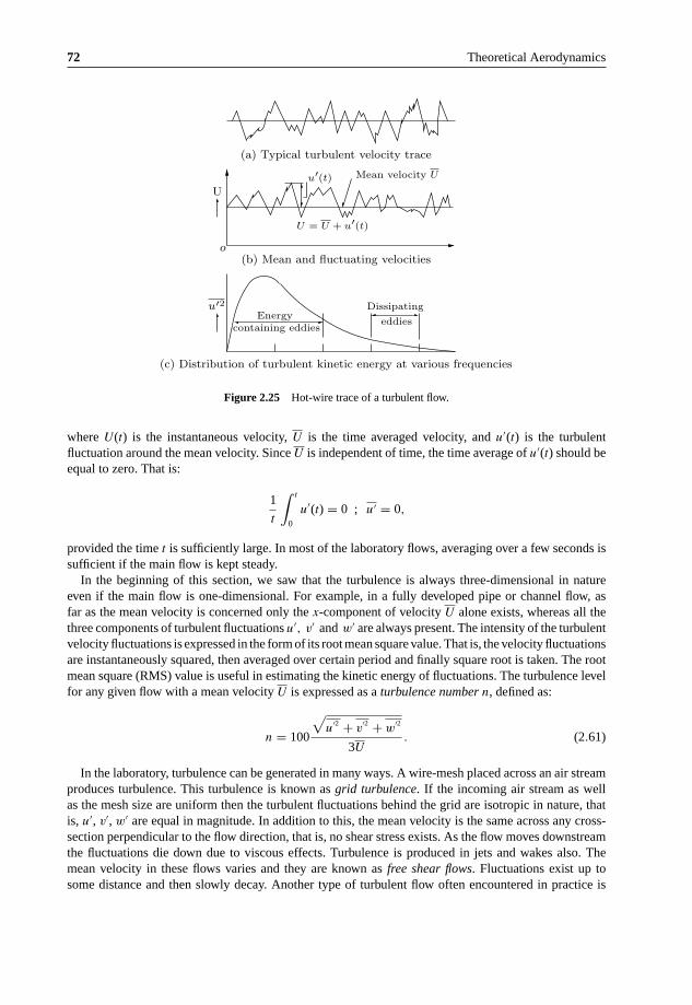
72 Theoretical Aerodynamics
o
U = U + u′(t)
eddiesEnergy
(b) Mean and fluctuating velocities
(a) Typical turbulent velocity trace
Mean velocity U
containing eddies
U
u′2 Dissipating
u′(t)
(c) Distribution of turbulent kinetic energy at various frequencies
Figure 2.25 Hot-wire trace of a turbulent flow.
where U(t) is the instantaneous velocity, U is the time averaged velocity, and u′(t) is the turbulentfluctuation around the mean velocity. Since U is independent of time, the time average of u′(t) should beequal to zero. That is:
1
t
∫ t
0
u′(t) = 0 ; u′ = 0,
provided the time t is sufficiently large. In most of the laboratory flows, averaging over a few seconds issufficient if the main flow is kept steady.
In the beginning of this section, we saw that the turbulence is always three-dimensional in natureeven if the main flow is one-dimensional. For example, in a fully developed pipe or channel flow, asfar as the mean velocity is concerned only the x-component of velocity U alone exists, whereas all thethree components of turbulent fluctuations u′, v′ and w′ are always present. The intensity of the turbulentvelocity fluctuations is expressed in the form of its root mean square value. That is, the velocity fluctuationsare instantaneously squared, then averaged over certain period and finally square root is taken. The rootmean square (RMS) value is useful in estimating the kinetic energy of fluctuations. The turbulence levelfor any given flow with a mean velocity U is expressed as a turbulence number n, defined as:
n = 100
√u
′2 + v′2 + w
′2
3U. (2.61)
In the laboratory, turbulence can be generated in many ways. A wire-mesh placed across an air streamproduces turbulence. This turbulence is known as grid turbulence. If the incoming air stream as wellas the mesh size are uniform then the turbulent fluctuations behind the grid are isotropic in nature, thatis, u′, v′, w′ are equal in magnitude. In addition to this, the mean velocity is the same across any cross-section perpendicular to the flow direction, that is, no shear stress exists. As the flow moves downstreamthe fluctuations die down due to viscous effects. Turbulence is produced in jets and wakes also. Themean velocity in these flows varies and they are known as free shear flows. Fluctuations exist up tosome distance and then slowly decay. Another type of turbulent flow often encountered in practice is
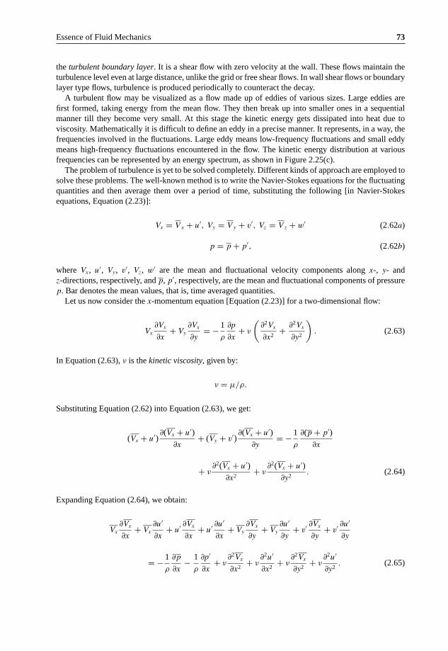
Essence of Fluid Mechanics 73
the turbulent boundary layer. It is a shear flow with zero velocity at the wall. These flows maintain theturbulence level even at large distance, unlike the grid or free shear flows. In wall shear flows or boundarylayer type flows, turbulence is produced periodically to counteract the decay.
A turbulent flow may be visualized as a flow made up of eddies of various sizes. Large eddies arefirst formed, taking energy from the mean flow. They then break up into smaller ones in a sequentialmanner till they become very small. At this stage the kinetic energy gets dissipated into heat due toviscosity. Mathematically it is difficult to define an eddy in a precise manner. It represents, in a way, thefrequencies involved in the fluctuations. Large eddy means low-frequency fluctuations and small eddymeans high-frequency fluctuations encountered in the flow. The kinetic energy distribution at variousfrequencies can be represented by an energy spectrum, as shown in Figure 2.25(c).
The problem of turbulence is yet to be solved completely. Different kinds of approach are employed tosolve these problems. The well-known method is to write the Navier-Stokes equations for the fluctuatingquantities and then average them over a period of time, substituting the following [in Navier-Stokesequations, Equation (2.23)]:
Vx = Vx + u′, Vy = Vy + v′, Vz = Vz + w′ (2.62a)
p = p + p′, (2.62b)
where Vx, u′, Vy, v′, Vz, w′ are the mean and fluctuational velocity components along x-, y- andz-directions, respectively, and p, p′, respectively, are the mean and fluctuational components of pressurep. Bar denotes the mean values, that is, time averaged quantities.
Let us now consider the x-momentum equation [Equation (2.23)] for a two-dimensional flow:
Vx
∂Vx
∂x+ Vy
∂Vx
∂y= − 1
ρ
∂p
∂x+ ν
(∂2Vx
∂x2+ ∂2Vx
∂y2
). (2.63)
In Equation (2.63), ν is the kinetic viscosity, given by:
ν = μ/ρ.
Substituting Equation (2.62) into Equation (2.63), we get:
(Vx + u′)∂(Vx + u′)
∂x+ (Vy + v′)
∂(Vx + u′)∂y
= − 1
ρ
∂(p + p′)∂x
+ ν∂2(Vx + u′)
∂x2+ ν
∂2(Vx + u′)∂y2
. (2.64)
Expanding Equation (2.64), we obtain:
Vx
∂Vx
∂x+ Vx
∂u′
∂x+ u′ ∂Vx
∂x+ u′ ∂u
′
∂x+ Vy
∂Vx
∂y+ Vy
∂u′
∂y+ v′ ∂Vx
∂y+ v′ ∂u
′
∂y
= − 1
ρ
∂p
∂x− 1
ρ
∂p′
∂x+ ν
∂2Vx
∂x2+ ν
∂2u′
∂x2+ ν
∂2Vx
∂y2+ ν
∂2u′
∂y2. (2.65)

74 Theoretical Aerodynamics
In this equation, time average of the individual fluctuations is zero. But the product or square terms ofthe fluctuating velocity components are not zero. Taking time average of Equation (2.65), we get:
Vx
∂V x
∂x+ u′ ∂u
′
∂x+ Vy
∂V x
∂y+ v′ ∂u
′
∂y= − 1
ρ
∂p
∂x+ ν
∂2Vx
∂x2+ ν
∂2Vx
∂y2. (2.66)
Equation (2.66) is slightly different from the laminar Navier-Stokes equation (Equation 2.63).The continuity equation for the two-dimensional flow under consideration is:
∂(Vx + u′)∂x
+ ∂(Vy + v′)∂y
= 0 .
This can be expanded to result in:
∂Vx
∂x+ ∂V y
∂y= 0 (2.67a)
and
∂u′
∂x+ ∂v′
∂y= 0 . (2.67b)
The terms involving turbulent fluctuational velocities u′ and v′ on the left-hand side of Equation (2.66)can be written as:
u′ ∂u′
∂x+ v′ ∂u
′
∂y= ∂
∂x(u′2 ) − u′ ∂u
′
∂x+ v′ ∂u
′
∂y.
Using Equation (2.67) the above equation can be expressed as:
u′ ∂u′
∂x+ v′ ∂u
′
∂y= ∂
∂x(u′2 ) + ∂
∂y(u′v′). (2.68)
Combination of Equations (2.66) and (2.68) results in:
ρVx
∂Vx
∂x+ ρVy
∂V x
∂y= −∂p
∂x+ ∂
∂x
(μ
∂Vx
∂y− ρu
′2)
+ ∂
∂y
(μ
∂Vx
∂y− ρu′v′
). (2.69)
The terms −ρu′2 and −ρu′v′ in Equation (2.69) are due to turbulence. They are popularly known
as Reynolds or turbulent stresses. For a three-dimensional flow, the turbulent stress terms are
ρu′2, ρv
′2, ρw
′2, ρu′v′, ρv′w′ and ρw′u′. Solutions of Equation (2.69) is rather cumbersome. Assumptions
like eddy viscosity, mixing length are made to find a solution for this equation.

Essence of Fluid Mechanics 75
At this stage, it is important to have proper clarity about the laminar and turbulent flows. The laminarflow may be described as “a well orderly pattern where fluid layers are assumed to slide over one another,”that is, in laminar flow the fluid moves in layers, or laminas, one layer gliding over an adjacent layer withinterchange of momentum only at molecular level. Any tendencies toward instability and turbulence aredamped out by viscous shear forces that resist the relative motion of adjacent fluid layers. In other words:
“laminar flow is an orderly flow in which the fluid elements move in an orderly manner such thatthe transverse exchange of momentum is insignificant”
and
“turbulent flow is a three–dimensional random phenomenon, exhibiting multiplicity of scales, pos-sessing vorticity, and showing very high dissipation.”
Turbulent flow is basically an irregular flow. Turbulent flow has very erratic motion of fluid particles,with a violent transverse exchange of momentum.
The laminar flow, though possesses irregular molecular motions, is macroscopically a well-orderedflow. But in the case of turbulent flow, there is the effect of a small but macroscopic fluctuating velocitysuperimposed on a well-ordered flow. A graph of velocity versus time at a given position in a pipe flowwould appear as shown in Figure 2.26(a), for laminar flow, and as shown in Figure 2.26(b), for turbulentflow. In Figure 2.26(b) for turbulent flow, an average velocity denoted as V has been indicated. Becausethis average is constant with time, the flow has been designated as steady. An unsteady turbulent flowmay prevail when the average velocity field changes with time, as shown in Figure 2.26(c).
2.12.3 Flow through Pipes
Fluid flow through pipes with circular and noncircular cross-sections is one of the commonly encounteredproblems in many practical systems. Flow through pipes is driven mostly by pressure or gravity or both.
V ′ (measured from V )V
V
V
V
t
t(a) Steady laminar flow
(b) Steady turbulent flow
(c) Unsteady turbulent flow
V
V ′ (measured from V )
t
Figure 2.26 Variation of flow velocity with time.

76 Theoretical Aerodynamics
o
(developing region) flow region
Linear pressure drop
profile u(r)
x
Pressure
Fully developed
pressure drop
Boundary layers merge
flow region
Le
r
Growing boundary layer
Entrance length Le
in fully developed
Developed velocityInvisicidcore flow
x
Entrance
u(r, x)
Figure 2.27 Flow development in a long duct.
Consider the flow in a long duct, shown in Figure 2.27. This flow is constrained by the duct walls. Atthe inlet, the freestream flow (assumed to be inviscid) converges and enters the tube.
Because of the viscous friction between the fluid and pipe wall, viscous boundary layer grows down-stream of the entrance. The boundary layer growth makes the effective area of the pipe to decreaseprogressively downstream, thereby making the flow along the pipe to accelerate. This process continuesup to the point where the boundary layer from the wall grows and meets at the pipe centerline, that is,fills the pipe, as illustrated in Figure 2.27.
The zone upstream of the boundary layer merging point is called the entrance or flow developmentlength Le and the zone downstream of the merging point is termed fully developed region. In the fullydeveloped region, the velocity profile remains unchanged. Dimensional analysis shows that Reynoldsnumber is the only parameter influencing the entrance length. In the functional form, the entrance lengthcan be expressed as:
Le = f (ρ, V, d, μ)
Le
d= f1
(ρVd
μ
)= f1(Re),
where ρ, V and μ are the flow density, velocity and viscosity, respectively, and d is the pipe diameter.For laminar flow, the accepted correlation is:
Le
d≈ 0.06 Red
At the critical Reynolds number Rec = 2300, for pipe flow, Le = 138d, which is the maximum develop-ment length possible.

Essence of Fluid Mechanics 77
φ
φ
2
r = R
1
τw
z2
r
u(r)
τ(r)
p2
p1 = (p2 + Δp)
x
Datum
g
gx = g sin φ
ΔL = (x2 − x1)
z1
Figure 2.28 Fully developed flow in an inclined pipe.
For turbulent flow the boundary layer grows faster, and Le is given by the approximate relation:
Le
d≈ 4.4 (Red)
16 . (2.70)
Now, examine the flow through an inclined pipe, shown in Figure 2.28, considering the control volumebetween sections 1 and 2.
Treating the flow to be incompressible, by volume conservation, we have:
Q1 = Q2 = constant
V1 = Q1
A1= V2 = Q2
A2,
where Q1 and Q2, respectively, are the volume flow rates and A1, A2, V1 and V2 are the local areas andvelocities, at states 1 and 2. The velocities V1 and V2 are equal, since the flow is fully developed and alsoA1 = A2.
By incompressible Bernoulli’s equation, we have:
p1
ρ+ 1
2V 2
1 + gz1 = p2
ρ+ 1
2V 2
2 + gz2. (2.71)
Since V1 = V2, we can write from Equation (2.71) the head loss due to friction as:
hf =(
z1 + p1
ρg
)−
(z2 + p2
ρg
)= �z + �p
ρg, (2.72)
where �z = (z1 − z2) and �p = (p1 − p2). That is, the head loss (in a pipe), due to friction is equal tothe sum of the change in gravity head and pressure head.
By momentum balance, we have:
�pπR2 + ρg(πR2)�L sin θ − τw(2πR)�L = m(V1 − V2) = 0. (2.73)

78 Theoretical Aerodynamics
Dividing throughout by (πR2)ρg, we get:
�p
ρg+ �L sin θ = 2τw
ρg
�L
R.
But �L sin θ = �z. Thus:
�p
ρg+ �z = 2τw
ρg
�L
R.
Using Equation (2.72), we obtain:
�p
ρg+ �z = hf = 2τw
ρg
�L
R. (2.74)
In the functional form, the wall shear τw may be expressed as:
τw = F (ρ, V, μ, d, ε), (2.75)
where μ is viscosity of the fluid, d is the pipe diameter, and ε is the wall roughness height. By dimensionalanalysis, Equation (2.75) may be expressed as:
8τw
ρV 2= f = F
(Red ,
ε
d
), (2.76)
where f is called the Darcy friction factor, which is a dimensionless parameter.Combining Equations (2.74) and (2.76), we obtain the pipe head loss as:
hf = fL
d
V 2
2g. (2.77)
This is called the Darcy-Weisbach equation, valid for flow through ducts of any cross-section. Further,in the derivation of the above relation, there was no mention about whether the flow was laminar orturbulent and hence Equation (2.77) is valid for both laminar and turbulent flows. The value of frictionfactor f for any given pipe (that is, for any surface roughness ε and d) at a given Reynolds number canbe read from the Moody chart (which is a plot of f as a function of Red and ε/d).
It is essential to note that in our discussions here it is mentioned that, decrease of pipe area due toboundary layer, results in increase of flow velocity. This is possible only in subsonic flows. When theflow is supersonic, decrease in area will decelerate the flow [2].
2.13 Compressible Flows
In the preceding sections of this chapter, the discussions were for incompressible flows, where thedensity can be regarded as constant. But in many engineering applications, such as designing buildingsto withstand winds, the design of engines and of vehicles of all kinds – cars, yachts, trains, aeroplane,missiles and launch vehicles require a study of the flow with velocities at which the gas cannot be treatedas incompressible. Indeed, the flow becomes compressible. Study of such flows where the changes inboth density and temperature associated with pressure change become appreciable is called gas dynamics.In other words, gas dynamics is the science of fluid flows where the density and temperature changesbecome important. The essence of the subject of gas dynamics is that the entire flow field is dominated

Essence of Fluid Mechanics 79
by Mach waves, expansion waves and shock waves, when the flow speed is supersonic. It is throughthese waves that the change of flow properties from one state to another takes place. In the theory of gasdynamics, change of state in flow properties is achieved by three means: (a) with area change, treatingthe fluid to be inviscid and passage to be frictionless, (b) with friction, treating the heat transfer betweenthe surrounding and system to be negligible and (c) with heat transfer, assuming the fluid to be inviscid.These three types of flows are called isentropic flow, frictional or Fanno type flow and Rayleigh type flow,respectively.
All problems in gas dynamics can be classified under the three flow processes described above, ofcourse with the assumptions mentioned. Although it is impossible to have a flow process which is purelyisentropic or Fanno type or Rayleigh type, in practice it is justified in assuming so, since the resultsobtained with these treatments prove to be accurate enough for most practical problems in gas dynamics.Even though it is possible to solve problems with mathematical equations and working formulae asso-ciated with these processes, it is found to be extremely useful and time saving if the working formulaeare available in the form of tables with a Mach number which is the dominant parameter in compressibleflow analysis.
2.13.1 Perfect Gas
In principle, it is possible to do gas dynamic calculations with the general equation of state relations, forfluids. But in practice most elementary treatments are confined to perfect gases with constant specificheats. For most problems in gas dynamics, the assumption of the perfect gas law is sufficiently in accordwith the properties of actual gases, hence it is acceptable.
For perfect gases, the pressure-density-temperature relation or the thermal equation of state, isgiven by:
p = ρRT , (2.78)
where R is the gas constant and T is absolute temperature. All gases obeying the thermal state equationare called thermally perfect gases. A perfect gas must obey at least two calorical state equations, inaddition to the thermal state equation. The cp, cv relations given below are two well-known caloricalstate equations:
cp = ∂h
∂T
cv = ∂u
∂T,
where h is specific enthalpy and u is specific internal energy, respectively. Further, for perfect gases withconstant specific heats, we have:
R = cp − cv
γ = cp
cv
, (2.79)
where cp and cv are the specific heats at constant pressure and constant volume, respectively, and γ is theisentropic index. For all real gases cp, cv and γ vary with temperature, but only moderately. For example,cp of air increases about 30 percent as temperature increases from 0 to 3000 ◦C. Since we rarely deal withsuch large temperature changes, it is reasonable to assume specific heats to be constants in our studies.

80 Theoretical Aerodynamics
2.13.2 Velocity of Sound
In the beginning of this section, it was stated that gas dynamics deals with flows in which both compress-ibility and temperature changes are important. The term compressibility implies variation in density. Inmany cases, the variation in density is mainly due to pressure change. The rate of change of density withrespect to pressure is closely connected with the velocity of propagation of small pressure disturbances,that is, with the velocity of sound “a.”
The velocity of sound may be expressed as:
a2 =(
∂p
∂ρ
)s
. (2.80)
In Equation (2.80), the ratio dp/dρ is written as partial derivative at constant entropy because the variationsin pressure and temperature are negligibly small, and consequently, the process is nearly reversible. More-over, the rapidity with which the process takes place, together with the negligibly small magnitude of thetotal temperature variation, makes the process nearly adiabatic. In the limit, for waves with infinitesimallysmall thickness, the process may be considered both reversible and adiabatic, and thus, isentropic.
It can be shown that, for an isentropic process of a perfect gas, the velocity of sound can beexpressed as:
a = √γRT , (2.81)
where T is absolute static temperature.
2.13.3 Mach Number
Mach number M is a dimensionless parameter, expressed as the ratio between the magnitudes of localflow velocity and local velocity of sound, that is:
M = Local flow velocity
Local velocity of sound= V
a. (2.82)
Mach number plays a dominant role in the field of gas dynamics.
2.13.4 Flow with Area Change
If the flow is assumed to be isentropic for a channel flow, all states along the channel or stream tube lie ona line of constant entropy and have the same stagnation temperature. The state of zero velocity is calledthe isentropic stagnation state, and the state with M = 1 is called the critical state.
2.13.4.1 Isentropic Relations
The relations between pressure, temperature, and density for an isentropic process of a perfect gas are:
p
p0=
(ρ
ρ0
)γ
(2.83a)

Essence of Fluid Mechanics 81
T
T0=
(p
p0
) γ−1γ
. (2.83b)
Also, the pressure-temperature density relation of a perfect gas is:
p
ρT= p0
ρ0T0= R. (2.84)
The temperature, pressure, and density ratios as functions of Mach number are:
T0
T=
(1 + γ − 1
2M2
)(2.85)
p0
p=
(1 + γ − 1
2M2
) γ
γ−1
(2.86)
ρ0
ρ=
(1 + γ − 1
2M2
) 1γ−1
, (2.87)
where T0, p0 and ρ0 are the temperature, pressure and density, respectively, at the stagnation state. Theparticular value of temperature, pressure, and density ratios at the critical state (that is, at the chokedlocation in a flow passage) are found by setting M = 1 in Equations (2.85)–(2.87). For γ = 1.4, thefollowing are the temperature, pressure and density ratio at the critical state:
T ∗
T0= a∗2
a20
= 2
γ + 1= 0.8333 (2.88)
p∗
p0=
(2
γ + 1
) γ
γ−1
= 0.5283 (2.89)
ρ∗
ρ0=
(2
γ + 1
) 1γ−1
= 0.6339, (2.90)
where T ∗, p∗ and ρ∗ are the temperature, pressure and density, respectively at the critical state.The critical pressure ratio p∗/p0 is of the same order of magnitude for all gases. It varies almost
linearly with γ from 0.6065, for γ = 1, to 0.4867, for γ = 1.67.The dimensionless velocity M∗ is one of the most useful parameter in gas dynamics. Generally it is
defined as:
M∗ ≡ V
a∗ ≡ V
V ∗ , (2.91)
where a∗ is the critical speed of sound. This dimensionless velocity can also be expressed in terms ofMach number as:
M∗2 = (γ + 1)M2
(γ − 1)M2 + 2. (2.92)

82 Theoretical Aerodynamics
2.13.4.2 Area-Mach Number Relation
For an isentropic flow of a perfect gas through a duct, the area-Mach number relation may be expressed,assuming one-dimensional flow, as:
(A
A∗
)2
= 1
M2
[2
γ + 1
(1 + γ − 1
2M2
)] γ+1γ−1
, (2.93)
where A∗ is called the sonic or critical throat area.
2.13.4.3 Prandtl-Meyer Function
The Prandtl-Meyer function ν is an important parameter to solve supersonic flow problems involvingisentropic expansion or isentropic compression. Basically the Prandtl-Meyer function is a similarityparameter. The Prandtl-Meyer function can be expressed in terms of M as:
ν = γ + 1
γ − 1arc tan
√γ − 1
γ + 1(M2 − 1) − arc tan
√M2 − 1 . (2.94)
From Equation (2.94) it is seen that, for a given M, ν is fixed.
2.13.5 Normal Shock Relations
The shock may be described as a compression front, in a supersonic flow field, across which the flowproperties jump. The thickness of the shock is comparable to the mean free path of the gas molecules inthe flow field. When the shock is normal to the flow direction it is called normal shock, and when it isinclined at an angle to the flow it is termed oblique shock. For a perfect gas, it is known that all the flowproperty ratios across a normal shock are unique functions of specific heats ratio, γ , and the upstreamMach number, M1.
Considering the normal shock shown in Figure 2.29, the following normal shock relations, assumingthe flow to be one-dimensional, can be obtained:
M22 = 2 + (γ − 1) M2
1
2γM21 − (γ − 1)
(2.95)
p2
p1= 1 + 2γ
γ + 1
(M2
1 − 1)
(2.96)
Normal shock
ρ1
T1
p1
ρ2
T2
p2
M1 M2
Figure 2.29 Flow through a normal shock.

Essence of Fluid Mechanics 83
ρ2
ρ1= V1
V2= (γ + 1)M2
1
(γ − 1)M21 + 2
(2.97)
T2
T1= h2
h1= a2
2
a21
= 1 + 2(γ − 1)
(γ + 1)2
(γM2
1 + 1)
M21
(M2
1 − 1)
. (2.98)
In Equation (2.98), h1 and h2 are the static enthalpies upstream and downstream of the shock, respectively.The stagnation pressure ratio across a normal shock, in terms of the upstream Mach number is:
p02
p01=
[1 + 2γ
γ + 1(M2
1 − 1)
] −1γ−1
[(γ + 1)M2
1
(γ − 1)M21 + 2
] γ
γ−1
. (2.99)
The change in entropy across the normal shock is given by:
s2 − s1 = R lnp01
p02. (2.100)
2.13.6 Oblique Shock Relations
Consider the flow through an oblique shock wave, as shown in Figure 2.30.The component of M1 normal to the shock wave is:
Mn1 = M1sin β, (2.101)
where β is the shock angle. The shock in Figure 2.29 can be visualized as a normal shock with upstreamMach number M1sin β. Thus, replacement of M1 in the normal shock relations, Equations (2.95) to (2.99),by M1sin β, results in the corresponding relations for the oblique shock.
M2n2 =
M21 sin2β + 2
γ − 12γ
γ − 1M2
1 sin2β − 1(2.102)
p2
p1= 1 + 2γ
γ + 1
(M2
1 sin2β − 1)
(2.103)
β
M1 θ
M2
Oblique shock
Figure 2.30 Flow through an oblique shock.

84 Theoretical Aerodynamics
ρ2
ρ1= (γ + 1)M2
1 sin2β
(γ − 1)M21 sin2β + 2
(2.104)
T2
T1= a2
2
a21
= 1 + 2(γ − 1)
(γ + 1)2
M21 sin2β − 1
M21 sin2β
(γM2
1 sin2β + 1)
(2.105)
p02
p01= 1 + 2γ
γ + 1
(M2
1 sin2β − 1) −1
γ−1(γ + 1)M2
1 sin2β
(γ − 1)M21 sin2β + 2
. (2.106)
The entropy change across the oblique shock is given by:
s2 − s1 = R lnp01
p02.
Equation (2.102) gives only the normal component of Mach number Mn2 behind the shock. But the Machnumber of interest is M2. It can be obtained from Equation (2.102) as follows:
From the geometry of the oblique shock flow field, it is seen that M2 is related to Mn2 by:
M2 = Mn2
sin (β − θ), (2.107)
where θ is the flow turning angle across the shock. Combining Equations (2.102) and (2.107), the Machnumber M2 after the shock can be obtained.
2.13.7 Flow with Friction
In the Section 2.13.4, on flow with area change, it was assumed that the changes in flow properties, forcompressible flow of gases in ducts, were brought about solely by area change. That is, the effects ofviscosity and heat transfer have been neglected. But, in practical flow situations like, stationary powerplants, aircraft engines, high vacuum technology, transport of natural gas in long pipe lines, transport offluids in chemical process plants, and various types of flow systems, the high-speed flow travels throughpassages of considerable length and hence the effects of viscosity (friction) cannot be neglected for suchflows. In many practical flow situations, friction can even have a decisive effect on the resultant flowcharacteristics.
Consider one-dimensional steady flow of a perfect gas with constant specific heats through a constantarea duct. Assume that there is neither external heat exchange nor external shaft work and the difference inelevation produces negligible changes in flow properties compared to frictional effects. The flow with theabove said conditions, namely adiabatic flow with no external work, is called Fanno line flow. For Fannoline flow, the wall friction (due to viscosity) is the chief factor bringing about changes in flow properties.
Working Formulae for Fanno Type Flow
Consider the flow of a perfect gas through a constant area duct shown in Figure 2.31. Choosing aninfinitesimal control volume as shown in the figure, the relation between Mach number M and friction

Essence of Fluid Mechanics 85
V + dV
Control surface
p
T
V
M
ρ
p + dp
T + dT
M + dM
ρ + dρ
τw
Figure 2.31 Control volume for Fanno flow.
factor f can be written as:
∫ Lmax
0
4fdx
D=
∫ 1
M2
1 − M2
γM4
(1 + γ − 1
2M2
) dM2. (2.108)
In this relation, the integration limits are taken as (1) the section where the Mach number is M, and thelength x is arbitrarily set equal to zero, and (2) the section where Mach number is unity and x is themaximum possible length of duct, Lmax and D is the hydraulic diameter, defined as:
D ≡ 4 (cross-sectional area)
wetted perimeter.
On integration, Equation (2.108) yields:
4fLmax
D= 1 − M2
γM2+ γ + 1
2γln
⎛⎜⎜⎝ (γ + 1)M2
2
(1 + γ − 1
2M2
)⎞⎟⎟⎠ , (2.109)
where f is the mean friction coefficient with respect to duct length, defined by:
f = 1
Lmax
∫ Lmax
0
fdx.
Likewise, the local flow properties can be found in terms of local Mach number. Indicating the propertiesat M = 1 with superscripted with “asterisk,” and integrating between the duct sections with M = M andM = 1, the following relations can be obtained [2]:
p
p∗ = 1
M
⎡⎢⎢⎣ γ + 1
2
(1 + γ − 1
2M2
)⎤⎥⎥⎦
12
(2.110)

86 Theoretical Aerodynamics
V
V ∗ = M
⎡⎢⎢⎣ γ + 1
2
(1 + γ − 1
2M2
)⎤⎥⎥⎦
12
(2.111)
T
T ∗ = a2
a∗2 =
⎡⎢⎢⎣ γ + 1
2
(1 + γ − 1
2M2
)⎤⎥⎥⎦ (2.112)
ρ
ρ∗ = V ∗
V= 1
M
⎡⎢⎢⎣
2
(1 + γ − 1
2M2
)
γ + 1
⎤⎥⎥⎦
12
(2.113)
p0
p∗0
= 1
M
⎡⎢⎢⎣
2
(1 + γ − 1
2M2
)
γ + 1
⎤⎥⎥⎦
γ+12(γ−1)
(2.114)
F
F ∗ = 1 + γM2
M
(2(γ + 1)
(1 + γ − 1
2M2
)) 12
. (2.115)
In Equation (2.115), the parameter F is called Impulse Function, defined as:
F ≡ pA + ρAV 2 = pA(a + γM2).
2.13.8 Flow with Simple T0-Change
In the section on flow with area change, the process was considered to be isentropic with the assumptionthat the frictional and energy effects were absent. In Fanno line flow, only the effect of wall frictionwas taken into account in the absence of area change and energy effects. In the present section, theprocesses involving change in the stagnation temperature or the stagnation enthalpy of a gas stream,which flows in a frictionless constant area duct are considered. From a one-dimensional point of view,this is yet another effect producing continuous changes in the state of a flowing stream and this factoris called energy effect, such as external heat exchange, combustion, or moisture condensation. Thougha process involving simple stagnation temperature (T0) change is difficult to achieve in practice, manyuseful conclusions of practical significance may be drawn by analyzing the process of simple T0-change.This kind of flow involving only T0-change is called Rayleigh type flow.
Working Formulae for Rayleigh Type Flow
Consider the flow of a perfect gas through a constant-area duct without friction, shown in Figure 2.32.

Essence of Fluid Mechanics 87
Heat
p1
T1
M1
T01
V1 V2 T2
p2
M2
T02
Control surface
Figure 2.32 Control volume for Rayleigh flow.
Considering a control volume, as in Figure 2.32, the normalized expressions (working formulae) forthe flow process involving only heat transfer can be obtained as [2].
p
p∗ = γ + 1
1 + γM2(2.116)
ρ
ρ∗ = V ∗
V= 1 + γM2
(γ + 1)M2(2.117)
T
T ∗ = (γ + 1)2M2
(1 + γM2)2(2.118)
T0
T ∗0
=2(γ + 1)M2
(1 + γ − 1
2M2
)
(1 + γM2)2(2.119)
p0
p∗0
= γ + 1
1 + γM2
⎡⎢⎢⎣
2
(1 + γ − 1
2M2
)
γ + 1
⎤⎥⎥⎦
γ
γ−1
. (2.120)
2.14 Summary
Gases and liquids are generally termed fluids. Under dynamic conditions, the nature of governingequations is the same for both gases and liquids.
Fluid may be defined as a substance which will continue to change shape as long as there is a shearstress present, however small it may be.
Pressure may be defined as the force per unit area which acts normal to the surface of any objectwhich is immersed in a fluid. For a fluid at rest, at any point the pressure is the same in all directions.In stationary fluids the pressure increases linearly with depth. This linear pressure distribution is calledhydrostatic pressure distribution.
When a fluid is in motion, the actual pressure exerted by the fluid in the direction normal to the flowis known as the static pressure. The pressure which a fluid flow will experience if it is brought to rest,

88 Theoretical Aerodynamics
isentropically, is termed total pressure. The total pressure is also called impact pressure. The total andstatic pressures are used for computing flow velocity.
The total number of molecules in a unit volume is a measure of the density ρ of a substance. It isexpressed as mass per unit volume, say kg/m3. Mass is defined as weight divided by acceleration due togravity. At standard atmospheric temperature and pressure (288.15 K and 101325 Pa, respectively), thedensity of dry air is 1.225 kg/m3.
The property which characterizes the resistance that a fluid offers to applied shear force is termedviscosity. This resistance, unlike for solids, does not depend upon the deformation itself but on the rateof deformation.
Maxwell’s definition of viscosity states that:“the coefficient of viscosity is the tangential force per unit area on either of two parallel plates at unit
distance apart, one fixed and the other moving with unit velocity.”Newton’s law of viscosity states that “the stresses which oppose the shearing of a fluid are proportional
to the rate of shear strain,” that is, the shear stress τ is given by:
τ = μ∂u
∂y.
Fluids which obey the above law of viscosity are termed Newtonian fluids. Some fluids such as siliconeoil, viscoelastic fluids, sugar syrup, tar, etc. do not obey the viscosity law given by Equation (2.3) andthey are called non-Newtonian fluids.
For air the viscosity coefficient is expressed as:
μ = 1.46 × 10⁻⁶
(T 3/2
T + 111
)(N s)/m2 ,
where T is in kelvin.The kinematic viscosity coefficient is a convenient form of expressing the viscosity of a fluid. It is
formed by combining the density ρ and the absolute coefficient of viscosity μ, according to the equation:
ν = μ
ρ.
The kinematic viscosity coefficient ν is expressed as m2/s, and 1 cm2/s is known as stoke.The kinematic viscosity coefficient is a measure of the relative magnitudes of viscosity and inertia of
the fluid.The change in volume of a fluid associated with change in pressure is called compressibility.The specific heats at constant volume and constant pressure processes, respectively, are designated by
cv and cp. The definitions of these quantities are the following:
cv ≡(
∂u
∂T
)v
,
where u is internal energy per unit mass of the fluid, which is a measure of the potential and moreparticularly the kinetic energy of the molecules comprising the gas. The specific heat cv is a measure ofthe energy-carrying capacity of the gas molecules. For dry air at normal temperature, cv = 717.5 J/(kg K).
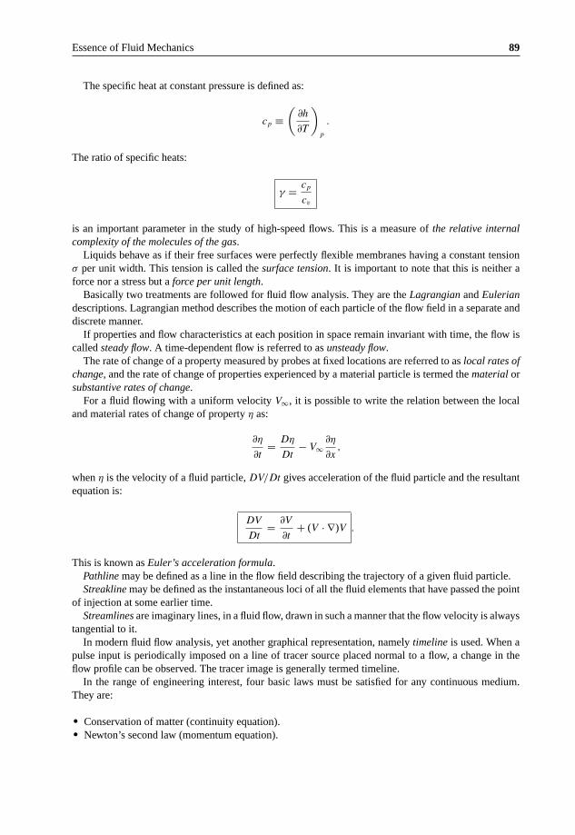
Essence of Fluid Mechanics 89
The specific heat at constant pressure is defined as:
cp ≡(
∂h
∂T
)p
.
The ratio of specific heats:
γ = cp
cv
is an important parameter in the study of high-speed flows. This is a measure of the relative internalcomplexity of the molecules of the gas.
Liquids behave as if their free surfaces were perfectly flexible membranes having a constant tensionσ per unit width. This tension is called the surface tension. It is important to note that this is neither aforce nor a stress but a force per unit length.
Basically two treatments are followed for fluid flow analysis. They are the Lagrangian and Euleriandescriptions. Lagrangian method describes the motion of each particle of the flow field in a separate anddiscrete manner.
If properties and flow characteristics at each position in space remain invariant with time, the flow iscalled steady flow. A time-dependent flow is referred to as unsteady flow.
The rate of change of a property measured by probes at fixed locations are referred to as local rates ofchange, and the rate of change of properties experienced by a material particle is termed the material orsubstantive rates of change.
For a fluid flowing with a uniform velocity V∞, it is possible to write the relation between the localand material rates of change of property η as:
∂η
∂t= Dη
Dt− V∞
∂η
∂x,
when η is the velocity of a fluid particle, DV/Dt gives acceleration of the fluid particle and the resultantequation is:
DV
Dt= ∂V
∂t+ (V · ∇)V .
This is known as Euler’s acceleration formula.Pathline may be defined as a line in the flow field describing the trajectory of a given fluid particle.Streakline may be defined as the instantaneous loci of all the fluid elements that have passed the point
of injection at some earlier time.Streamlines are imaginary lines, in a fluid flow, drawn in such a manner that the flow velocity is always
tangential to it.In modern fluid flow analysis, yet another graphical representation, namely timeline is used. When a
pulse input is periodically imposed on a line of tracer source placed normal to a flow, a change in theflow profile can be observed. The tracer image is generally termed timeline.
In the range of engineering interest, four basic laws must be satisfied for any continuous medium.They are:
• Conservation of matter (continuity equation).• Newton’s second law (momentum equation).
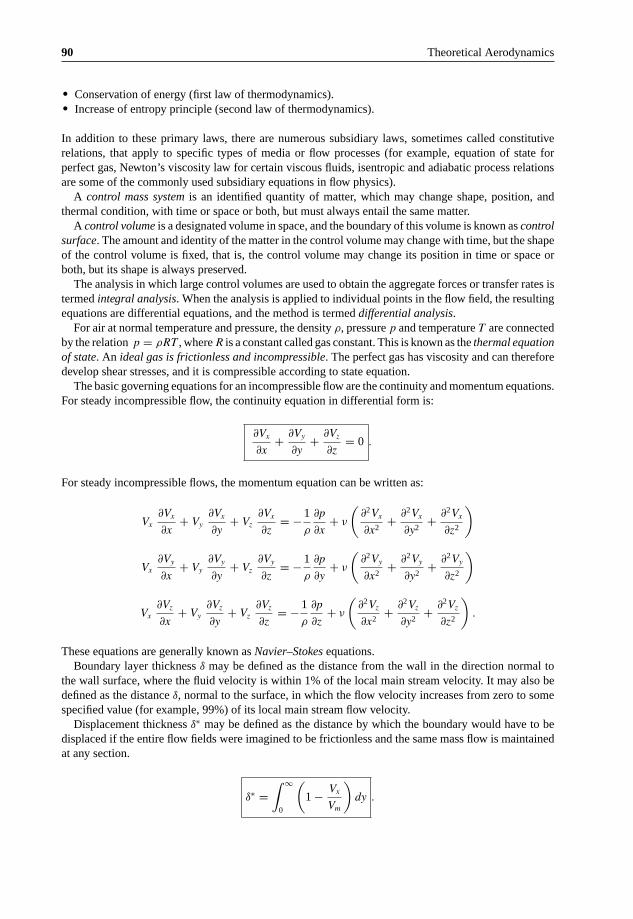
90 Theoretical Aerodynamics
• Conservation of energy (first law of thermodynamics).• Increase of entropy principle (second law of thermodynamics).
In addition to these primary laws, there are numerous subsidiary laws, sometimes called constitutiverelations, that apply to specific types of media or flow processes (for example, equation of state forperfect gas, Newton’s viscosity law for certain viscous fluids, isentropic and adiabatic process relationsare some of the commonly used subsidiary equations in flow physics).
A control mass system is an identified quantity of matter, which may change shape, position, andthermal condition, with time or space or both, but must always entail the same matter.
A control volume is a designated volume in space, and the boundary of this volume is known as controlsurface. The amount and identity of the matter in the control volume may change with time, but the shapeof the control volume is fixed, that is, the control volume may change its position in time or space orboth, but its shape is always preserved.
The analysis in which large control volumes are used to obtain the aggregate forces or transfer rates istermed integral analysis. When the analysis is applied to individual points in the flow field, the resultingequations are differential equations, and the method is termed differential analysis.
For air at normal temperature and pressure, the density ρ, pressure p and temperature T are connectedby the relation p = ρRT , where R is a constant called gas constant. This is known as the thermal equationof state. An ideal gas is frictionless and incompressible. The perfect gas has viscosity and can thereforedevelop shear stresses, and it is compressible according to state equation.
The basic governing equations for an incompressible flow are the continuity and momentum equations.For steady incompressible flow, the continuity equation in differential form is:
∂Vx
∂x+ ∂Vy
∂y+ ∂Vz
∂z= 0 .
For steady incompressible flows, the momentum equation can be written as:
Vx
∂Vx
∂x+ Vy
∂Vx
∂y+ Vz
∂Vx
∂z= − 1
ρ
∂p
∂x+ ν
(∂2Vx
∂x2+ ∂2Vx
∂y2+ ∂2Vx
∂z2
)
Vx
∂Vy
∂x+ Vy
∂Vy
∂y+ Vz
∂Vy
∂z= − 1
ρ
∂p
∂y+ ν
(∂2Vy
∂x2+ ∂2Vy
∂y2+ ∂2Vy
∂z2
)
Vx
∂Vz
∂x+ Vy
∂Vz
∂y+ Vz
∂Vz
∂z= − 1
ρ
∂p
∂z+ ν
(∂2Vz
∂x2+ ∂2Vz
∂y2+ ∂2Vz
∂z2
).
These equations are generally known as Navier–Stokes equations.Boundary layer thickness δ may be defined as the distance from the wall in the direction normal to
the wall surface, where the fluid velocity is within 1% of the local main stream velocity. It may also bedefined as the distance δ, normal to the surface, in which the flow velocity increases from zero to somespecified value (for example, 99%) of its local main stream flow velocity.
Displacement thickness δ∗ may be defined as the distance by which the boundary would have to bedisplaced if the entire flow fields were imagined to be frictionless and the same mass flow is maintainedat any section.
δ∗ =∫ ∞
0
(1 − Vx
Vm
)dy .

Essence of Fluid Mechanics 91
The momentum thickness θ and energy thickness δe are other (thickness) measures pertaining toboundary layer. They are defined mathematically as follows:
θ =∫ ∞
0
(1 − Vx
Vm
)ρVx
ρmVm
dy
δe =∫ ∞
0
(1 − V 2
x
V 2m
)ρVx
ρmVm
dy .
Transition point may be defined as the end of the region at which the flow in the boundary layer onthe surface ceases to be laminar and becomes turbulent.
Separation point is the position at which the boundary layer leaves the surface of a solid body. Ifthe separation takes place while the boundary layer is still laminar, the phenomenon is termed laminarseparation. If it takes place for a turbulent boundary layer it is called turbulent separation.
Circulation , is defined as the line integral of velocity vector between any two points (to definerotation of the fluid element) in a flow field. By definition:
= ∮cV. dl .
Circulation per unit area is known as vorticity ζ:
ζ = /A
In vector form, ζ becomes:
ζ = ∇ × V = curl V .
For a two-dimensional flow in xy-plane, vorticity ζ becomes:
ζz = ∂Vy
∂x− ∂Vx
∂y,
where ζz is the vorticity about the z-direction, which is normal to the flow field. Likewise, the othercomponents of vorticity about x- and y-directions are:
ζx = ∂Vz
∂y− ∂Vy
∂z
ζy = ∂Vx
∂z− ∂Vz
∂x.
If ζ = 0, the flow is known as irrotational flow. Inviscid flows are basically irrotational flows.In terms of stream function ψ, the velocity components of a two-dimensional incompressible flow are
given as:
Vx = ∂ψ
∂y, Vy = −∂ψ
∂x.

92 Theoretical Aerodynamics
If the flow is compressible the velocity components become:
Vx = 1
ρ
∂ψ
∂y, Vy = − 1
ρ
∂ψ
∂x.
For irrotational flows (the fluid elements in the field are free from rotation), there exists a function φ
called velocity potential or potential function. For a steady two-dimensional flows, φ must be a functionof two space coordinates (say, x and y). The velocity components are given by:
Vx = ∂φ
∂x, Vy = ∂φ
∂y.
We can relate ψ and φ as:
∂ψ
∂y= ∂φ
∂x,
∂ψ
∂x= −∂φ
∂y.
These relations between stream function and potential function are the famous Cauchy-Riemann equationsof complex-variable theory.
Potential flow is based on the concept that the flow field can be represented by a potential functionφ such that:
∇2φ = 0 .
This linear partial differential equation is popularly known as Laplace equation.All inviscid flows must satisfy the irrotationality condition:
∇ × V = 0 .
For two-dimensional incompressible flows, the continuity equation is:
∂Vx
∂x+ ∂Vy
∂y= 0.
In terms of the potential function φ, this becomes:
∂2φ
∂x2+ ∂2φ
∂y2= 0
that is:
∇2φ = 0,
This linear equation is the governing equation for potential flows.For potential flows, the Navier-Stokes equations reduce to:
Vx
∂Vx
∂x+ Vy
∂Vx
∂y+ Vz
∂Vx
∂z= − 1
ρ
∂p
∂x
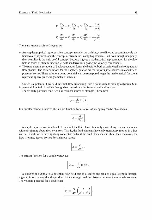
Essence of Fluid Mechanics 93
Vx
∂Vy
∂x+ Vy
∂Vy
∂y+ Vz
∂Vy
∂z= − 1
ρ
∂p
∂y
Vx
∂Vz
∂x+ Vy
∂Vz
∂y+ Vz
∂Vz
∂z= − 1
ρ
∂p
∂z.
These are known as Euler’s equations.
• Among the graphical representation concepts namely, the pathline, streakline and streamline, only thefirst two are physical, and the concept of streamline is only hypothetical. But even though imaginary,the streamline is the only useful concept, because it gives a mathematical representation for the flowfield in terms of stream function ψ, with its derivatives giving the velocity components.
• The fundamental solutions of Laplace equation forms the basis for both experimental and computationflow physics. The basic solutions for the Laplace equation are the uniform flow, source, sink and free orpotential vortex. These solutions being potential, can be superposed to get the mathematical functionsrepresenting any practical geometry of interest.
Source is a potential flow field in which flow emanating from a point spreads radially outwards. Sinkis potential flow field in which flow gushes towards a point from all radial directions.
The velocity potential for a two-dimensional source of strength q becomes:
φ = q
2πln (r) .
In a similar manner as above, the stream function for a source of strength q can be obtained as:
ψ = q
2πθ .
A simple or free vortex is a flow field in which the fluid elements simply move along concentric circles,without spinning about their own axes. That is, the fluid elements have only translatory motion in a freevortex. In addition to moving along concentric paths, if the fluid elements spin about their own axes, theflow is termed forced vortex: For a simple vortex:
φ = q
2πθ .
The stream function for a simple vortex is:
ψ = − q
2πln (r) .
A doublet or a dipole is a potential flow field due to a source and sink of equal strength, broughttogether in such a way that the product of their strength and the distance between them remain constant.The velocity potential for a doublet is:
φD = m
2π
(x
x2 + y2
).

94 Theoretical Aerodynamics
The stream function for a doublet is:
ψD = − m
2π
(y
x2 + y2
).
The stream function for the flow due to the combination of a source of strength q at the origin, immersedin a uniform flow of velocity V∞, parallel to x-axis is:
ψ = V∞ r sin θ + q
2πθ.
The streamline passing through the stagnation point S is termed the stagnation streamline. The stagnationstreamline resembles a semi-ellipse. This shape is popularly known as Rankine’s half-body.
The stream function and potential function of the flow past a cylinder can be expressed as:
ψ = V∞
(r − a2
r
)sin θ
φ = V∞
(r + a2
r
)cos θ.
The nondimensional pressure distribution over the surface of the cylinder is given by:
Cp = p − p∞12 ρV 2∞
= 1 − V 2
V 2∞= 1 − 4 sin2 θ .
The symmetry of the pressure distribution in an irrotational flow implies that “a steadily moving bodyexperiences no drag.” This result, which is not true for actual (viscous) flows where the body experiencesdrag, is known as d’Alembert’s paradox.
• The positive limit of +1 for Cp, at the forward stagnation point, is valid for all geometries and forboth potential and viscous flow, as long as the flow speed is subsonic.
• The limiting minimum of −3, for the Cp over the cylinder in potential flow, is valid only for circularcylinder. The negative value of Cp can take values lower than −3 for other geometries. For example,for a cambered aerofoil at an angle of incidence can have Cp as low as −6.
There is no net force acting on a circular cylinder in a steady irrotational flow without circulation.It can be shown that a lateral force identical to a lift force on an aerofoil, results when circulation isintroduced around the cylinder.
The location forward and rear stagnation points on the cylinder can be adjusted by controlling themagnitude of the circulation . The circulation which positions the stagnation points in proximity, asshown in Figure 2.19(b) is called subcritical circulation, the circulation which makes the stagnationpoints to coincide at the surface of the cylinder, as shown in Figure 2.19(c), is called critical circulation,and the circulation which makes the stagnation points to coincide and take a position outside the surfaceof the cylinder, as shown in Figure 2.19(d), is called supercritical circulation.
For a circular cylinder in a potential flow, the only way to develop circulation is by rotating it in aflow stream. Although viscous effects are important in this case, the observed pattern for high rotationalspeeds displays a striking similarity to the ideal flow pattern for > 4πaV∞. When the cylinder rotates atlow speeds, the retarded flow in the boundary layer is not able to overcome the adverse pressure gradientbehind the cylinder. This leads to the separation of the real (actual) flow, unlike the irrotational flow

Essence of Fluid Mechanics 95
which does not separate. However, even in the presence of separation, observed speeds are higher on theupper surface of the cylinder, implying the existence of a lift force.
A second reason for a rotating cylinder generating lift is the asymmetry to the flow pattern, caused bythe delayed separation on the upper surface of the cylinder. The asymmetry results in the generation ofthe lift force. The contribution of this mechanism is small for two-dimensional objects such as circularcylinder, but it is the only mechanism for the side force experienced by spinning three-dimensionalobjects such as soccer, tennis and golf balls. The lateral force experienced by rotating bodies is calledthe Magnus effect. The horizontal component of the force on the cylinder, due to the pressure, in generalis called drag. For the cylinder, shown in Figure 2.20, the drag given by:
D =∫ 2π
0
pr=a a cos θ dθ.
It is interesting to note that the drag is equal to zero. It is important to realize that this result is obtainedon the assumption that the flow is inviscid. In real (actual or viscous) flows the cylinder will experiencea finite drag force acting on it due to viscous friction and flow separation.
We are familiar with the fact that the viscosity produces shear force which tends to retard the fluidmotion. It works against inertia force. The ratio of these two forces governs (dictates) many propertiesof the flow, and the ratio expressed in the form of a nondimensional parameter is known as the famousReynolds number, ReL:
ReL = ρVL
μ.
The Reynolds number plays a dominant role in fluid flow analysis. This is one of the fundamentaldimensionless parameters which must be matched for similarity considerations in most of the fluid flowanalysis. At high Reynolds numbers, the inertia force is predominant compared to viscous forces. At lowReynolds numbers the viscous effects predominate everywhere. Whereas, at high Re the viscous effectsconfine to a thin region, just adjacent to the surface of the object present in the flow, and this thin layeris termed boundary layer.
Reynolds number is basically a similarity parameter. It is used to determine the laminar and turbulentnature of flow.
• Lower critical Reynolds number is that Reynolds number below which the entire flow is laminar.• Upper critical Reynolds number is that Reynolds number above which the entire flow is turbulent.• Critical Reynolds number is that at which the flow field is a mixture of laminar and turbulent flows.
When a body moves in a fluid, it experiences forces and moments due to the relative motion of theflow taking place around it. The force on the body along the flow direction is called drag.
The drag is essentially a force opposing the motion of the body. Viscosity is responsible for a part ofthe drag force, and the body shape generally determines the overall drag. The drag caused by the viscouseffect is termed the frictional drag or skin friction. In the design of transport vehicles, shapes experiencingminimum drag are considered to keep the power consumption at a minimum. Low drag shapes are calledstreamlined bodies and high drag shapes are termed bluff bodies.
Drag arises due to (a) the difference in pressure between the front and back regions and (b) the frictionbetween the body surface and the fluid. Drag force caused by the pressure imbalance is known as pressuredrag, and (b) the drag due to friction is known as skin friction drag or shear drag.
The location where the flow leaves the body surface is termed separation point. For flow past a cylinder,there are two separation points on either side of the horizontal axis through the center of the cylinder. The

96 Theoretical Aerodynamics
separated flow is chaotic and vortex dominated. The separated flow behind an object is also referred toas wake. Depending on the Reynolds number level, the wake may be laminar or turbulent. An importantcharacteristics of the separated flow is that it is always unsymmetrical, even for laminar separation.
The friction between the surface of a body and the fluid causes viscous shear stress and this force isknown as skin friction drag. Wall shear stress τ at the surface of a body is given by:
τ = μ∂Vx
∂y.
A body for which the skin friction drag is a major portion of the total drag is termed streamlined body.A body for which the pressure (form) drag is the major portion is termed bluff body. Turbulent boundarylayer results in more skin friction than a laminar one.
The turbulence level for any given flow with a mean velocity U is expressed as a turbulence numbern, defined as:
n = 100
√u
′2 + v′2 + w
′2
3U.
“A laminar flow is an orderly flow in which the fluid elements move in an orderly manner such thatthe transverse exchange of momentum is insignificant”
and
“A turbulent flow is a three–dimensional random phenomenon, exhibiting multiplicity of scales,possessing vorticity, and showing very high dissipation.”
Flow through pipes is driven mostly by pressure or gravity or both. In the functional form, the entrancelength can be expressed as:
Le = f (ρ, V, d, μ)
Le
d= f1
(ρVd
μ
)= f1(Re).
For laminar flow, the accepted correlation is:
Le
d≈ 0.06 Red .
At the critical Reynolds number Rec = 2300, for pipe flow, Le = 138d, which is the maximum develop-ment length possible.
For turbulent flow the boundary layer grows faster, and Le is given by the approximate relation:
Le
d≈ 4.4 (Red )
16 .
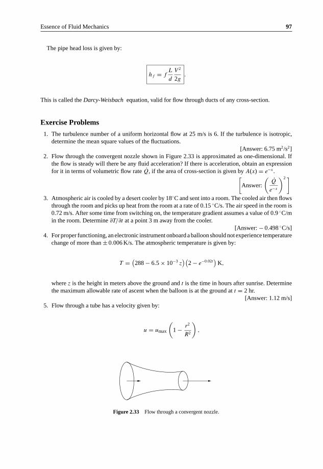
Essence of Fluid Mechanics 97
The pipe head loss is given by:
hf = fL
d
V 2
2g.
This is called the Darcy-Weisbach equation, valid for flow through ducts of any cross-section.
Exercise Problems
1. The turbulence number of a uniform horizontal flow at 25 m/s is 6. If the turbulence is isotropic,determine the mean square values of the fluctuations.
[Answer: 6.75 m2/s2]2. Flow through the convergent nozzle shown in Figure 2.33 is approximated as one-dimensional. If
the flow is steady will there be any fluid acceleration? If there is acceleration, obtain an expressionfor it in terms of volumetric flow rate Q, if the area of cross-section is given by A(x) = e−x.[
Answer:
(Q
e−x
)2 ]
3. Atmospheric air is cooled by a desert cooler by 18◦C and sent into a room. The cooled air then flowsthrough the room and picks up heat from the room at a rate of 0.15 ◦C/s. The air speed in the room is0.72 m/s. After some time from switching on, the temperature gradient assumes a value of 0.9 ◦C/min the room. Determine ∂T/∂t at a point 3 m away from the cooler.
[Answer: − 0.498 ◦C/s]4. For proper functioning, an electronic instrument onboard a balloon should not experience temperature
change of more than ± 0.006 K/s. The atmospheric temperature is given by:
T = (288 − 6.5 × 10⁻³ z
)(2 − e−0.02t
)K,
where z is the height in meters above the ground and t is the time in hours after sunrise. Determinethe maximum allowable rate of ascent when the balloon is at the ground at t = 2 hr.
[Answer: 1.12 m/s]5. Flow through a tube has a velocity given by:
u = umax
(1 − r2
R2
),
Figure 2.33 Flow through a convergent nozzle.

98 Theoretical Aerodynamics
Cross-sectional area A1
HV1
a
Cross-sectional area A2
Figure 2.34 A tank on an elevator moving up.
where R is the tube radius and umax is the maximum velocity, which occurs at the tube centerline. (a)Find a general expression for volume flow rate and average velocity through the tube, (b) computethe volume flow rate if R = 25 mm and umax = 10 m/s, and (c) compute the mass flow rate if ρ =1000 kg/m3. [
Answer: (a)1
2umax πR2,
1
2umax, (b) 0.00982 m3/s, (c) 9.82 kg/s
].
6. A two-dimensional velocity field is given by:
V =(x − y2
)i + (xy + 2y) j
in arbitrary units. At x = 2 and y = 1, compute (a) the acceleration components ax and ay, (b)the velocity component in the direction θ = 30◦, and (c) the directions of maximum velocity andmaximum acceleration.
[Answer: (a) −7 units, 17 units, (b) 2.87 units, (c) V = 4.123 units at 75.96◦
from x-axis, a = 18.385 units at 292.38◦ from x-axis]7. A tank is placed on an elevator which starts moving upwards at time t = 0 with a constant acceleration
a. A stationary hose discharges water into the tank at a constant rate as shown in Figure 2.34.Determine the time required to fill the tank if it is empty at t = 0.
[Answer:
−V1 ±√
V 21 + 2
A2
A1aH
a
]
8. Develop the differential form of continuity equation for cylindrical polar coordinates shown by takingan infinitesimal control volume, as shown in Figure 2.35.[
Answer:∂ρ
∂t+ 1
r
∂(ρrVr)
∂r+ 1
r
∂(ρVθ)
∂θ+ ∂(ρVz)
∂z= 0
]9. A flow field is given by:
V = 3x i + 4y j − 5t k.
(a) Find the velocity at position (10,6) at t = 3 s. (b) What is the slope of the streamlines for thisflow at t = 0 s? (c) Determine the equation of the streamlines at t = 0 up to an arbitrary constant.(d) Sketch the streamlines at t = 0.
[Answer: (a) V = (30 i + 24 j − 15 k) m/s, (b) 4y/3x, (c) y = 45 x + c, where c is an arbitrary
constant, (d) At t = 0, the streamlines are straight lines at an angle of 38.66◦ to the x-axis]10. For the fully developed two-dimensional flow of water between two impervious flat plates, shown
in Figure 2.36, show that Vy = 0 everywhere.

Essence of Fluid Mechanics 99
dθ r
elementInfinitesimal
Base line
r
Vθ
Cylindrical axis
P(r, θ, z) dr
dr
Vr
Vx
x
dθ
Figure 2.35 Cylindrical polar coordinates.
x
z
y
Figure 2.36 Fully developed two-dimensional flow between two impervious flat plates.
11. Water enters section 1 at 200 N/s and exits at 30◦ angle at section 2, as shown in Figure 2.37.
Section 1 has a laminar velocity profile u = um1
(1 − r2
R2
), while section 2 has a turbulent profile
u = um2
(1 − r
R
)1/7
. If the flow is steady and incompressible (water), find the maximum velocities
um1 and um2 in m/s. Assume uav = 0.5 um, for laminar flow, and uav = 0.82 um, for turbulent flow.[Answer: 5.2 m/s, 8.79 m/s]
12. Consider a jet of fluid directed at the inclined plate shown in Figure 2.38. Obtain the force necessaryto hold the plate in equilibrium against the jet pressure. Also, obtain the volume flow rates Q1 andQ2 in terms of the incoming flow rate Q0. Assume that V0 = V1 = V2 and the fluid is inviscid.[
Answer: ρV0Q0sin α, Q1 = Q0
2(1 + cos α), Q2 = Q0
2(1 − cos α)
]
30◦
D2 = 6 cm
D1 = 10 cm
2
1
Figure 2.37 Flow through a passage with bend.

100 Theoretical Aerodynamics
Q0, V0
Q1, V1
F
Q2, V2
α2
1
Figure 2.38 Jet impingement on an inclined plate.
13. Consider a laminar fully developed flow without body forces through a long straight pipe of circularcross–section (Poiseuille flow) shown in Figure 2.39. Apply the momentum equation and show that:
τrz = p1 − p2
l
r
2.
Assuming (p1 − p2)/l = constant, obtain the velocity profile using the relation:
τrz = −μ
(dVz
dr
).
[Answer: Vz =
(p1 − p2
l
) 1
4μ
(R2 − r2
)]14. A liquid of density ρ and viscosity μ flows down a stationary wall, under the influence of gravity,
forming a thin film of constant thickness h, as shown in Figure 2.40. An up flow of air next to thefilm exerts an upward constant shear stress τ on the surface of the liquid layer, as shown in the figure.The pressure in the film is uniform. Derive expressions for (a) the film velocity Vy as a functionof y, ρ, μ, h and τ, and (b) the shear stress τ that would result in a zero net volume flow rate inthe film.
[Answer: (a) Vy =
ρg
(hx − x2
2
)− τx
μ, (b) τ = 2
3ρgh
]
CV
τw
y
r
p1p2
x
zR
l
τw
Vz(r)
Figure 2.39 Fully developed flow in a pipe.

Essence of Fluid Mechanics 101
h
Vy
Air
τ
y
x
Figure 2.40 Flow down a stationary wall.
15. Show that the head loss for laminar, fully developed flow in a straight circular pipe is given by:
hl = 64
Re
L
D
V 2av
2g,
where Re is the Reynolds number defined as (ρVavD) /μ.16. A horizontal pipe of length L and diameter D conveys air. Assuming the air to expand according to
the law p/ρ = constant and that the acceleration effects are small, prove that:
p1
ρ1
(ρ2
1 − ρ22
) = 16 f L m2
π2 D5,
where m is the mass flow rate of air through the pipe, f is the average friction coefficient, and 1 and2 are the inlet and discharge ends of the pipe, respectively.
17. In the boundary layer over the upper surface of an airplane wing, at a point A near the leadingedge, the flow velocity just outside the boundary layer is 250 km/hour. At another point B, which isdownstream of A, the velocity outside the boundary layer is 470 km/hour. If the temperature at A is288 K, calculate the temperature and Mach number at point B.
[Answer: 281.9 K, 0.388]18. A long right circular cylinder of diameter a meter is set horizontally in a steady stream of velocity
u m/s and made to rotate at an angular velocity of ω radians/second. Obtain an expression in termsof ω and u for the ratio of pressure difference between the top and bottom of the cylinder to thedynamic pressure of the stream. [
Answer: −8aω
u
]19. The velocity and temperature fields of a fluid are given by:
V = x i + (3y + 3t2y
)j + 12 k
T = x + y2z + 5t.
Find the rate of change of temperature recorded by a floating probe (thermocouple) when it is at3 i + 5 j + 2 k at time t = 2 units.
[Answer: 1808]

102 Theoretical Aerodynamics
20. A parachute of 10 m diameter when carrying a load W descends at a constant velocity of 5.5 m/s inatmospheric air at a temperature of 18◦ and a pressure of 105 Pa. Determine the load W if the dragcoefficient for the parachute is 1.4.
[Answer: 1.991 kN]
References
1. Heiser, W.H. and Pratt, D.T., Hypersonic Air Breathing Propulsion, AIAA Education Series, 1994.
2. Rathakrishnan, E., Applied Gas Dynamics, John Wiley & Sons Inc., New Jersey, 2010.

3Conformal Transformation
3.1 Introduction
The transformation technique which transforms an orthogonal geometric pattern (Figure 3.1(a)),composed of elements of certain shape, into an entirely different pattern (Figure 3.1(b)), whilst theelements retain their form and proportion is termed conformal transformation.
3.2 Basic Principles
As shown in Figure 3.1, the elements will, in the limit, retain their similar geometrical form. For this tobe true, the angle between the intersecting lines in plane 1 must remain the same when the two lines aretransformed to plane 2. Let us examine the point p in the (x, iy)-plane (z-plane), referred to as physicalplane and the corresponding point P in the (ξ, iη)-plane (ζ-plane), called transformed plane, shown inFigure 3.2.
In the z-plane (physical plane) point p is located by z = x + iy, and in the ζ-plane (transformed plane),the corresponding point P is located by ζ = ξ + iη. The relation between z and ζ is a particular specifiedfunction of ζ, in terms of z. That is:
ζ = f (z)
This function is known as the transformation function.Consider the specific points, located at z1 and z2, on an arc segment p1p2 in the physical plane, as
shown in Figure 3.3(a). The corresponding points in the transformed plane are ζ1 and ζ2 and the arcsegment p1p2 in the z-plane is transformed to curve P1P2, shown in Figure 3.3(b).
For transforming the points in the z-plane to ζ-plane, the transformation function used is:
ζ = f (z). (3.1)
Differentiating Equation (3.1), with respect to z, we get:
dζ = f ′(z) dz. (3.2)
In the limit of arc length p1p2 → 0, δz → dz and in the limit of arc length P1P2 → 0, δζ → dζ. FromEquation (3.2), it is seen that the length dζ of the segment, in the transformed plane, becomes the vector
Theoretical Aerodynamics, First Edition. Ethirajan Rathakrishnan.© 2013 John Wiley & Sons Singapore Pte. Ltd. Published 2013 by John Wiley & Sons Singapore Pte. Ltd.

104 Theoretical Aerodynamics
aD
(a) Plane 1 (b) Plane 2
A
cd
B
C
b
Figure 3.1 Conformal transformation.
ζ-plane
P (ξ, iη)
p(x, iy)
zζ
o o
iy iη
ξx
z-plane
Figure 3.2 Transformation of a general point.
dz, in the physical plane, multiplied by the vector f ′(z), that is:
dζ = (vector dz) × (vector f ′(z)) .
Now, to understand this operation of the multiplication of vectors, consider the function f (z) rewrittenin its exponential form, that is:
f (z) = reiθ,
where r is the modulus of function f (z). Then:
|dζ| = |dz| r
(a) z-plane
o o
iy
(b) ζ-plane
z1 ζ2
P1
iη
ζ1δz δζz2p1
p2
P2
x ξ
Figure 3.3 Transformation of an arc segment.

Conformal Transformation 105
p2
p4p3
b A
D
P2
βp
P
iy iη
o o
β
(b) ζ-plane(a) z-plane
C
dB
β
β
c
x ξ
a P1P3
P4p1
Figure 3.4 Transformation of crossing arc segments.
is in the direction of dz, after it has been rotated through θ, and the angular displacement of f (z) (ofthe transformed element) is equal to the the length of the original element rotated through angle θ andmultiplied by r. The shape of the transformed element is given by P1P2, as shown in Figure 3.3(b), andnot by Equation (3.2).
Consider the arc segments ab and cd, cutting each other at point p in the z-plane, as shown inFigure 3.4(a). At point p the angle subtended by the crossing arc ab and cd is β. In the transformedplane (ζ-plane), in Figure 3.4(b), the corresponding point is P and the transformed curves AB and CD
are crossing with the same angle β, in accordance with the conformal transformation, which stipulatesthat the “angle subtended by two crossing arcs in the physical plane and the angle subtended by thecorresponding transformed curves in the transformed plane must be the same.”
Let us consider the actual elements of the crossing arc segments. Since the transformed elements arecrossing at point P , with the same angle of intersection as in the z-plane, their lengths would be affectedby the same value of the transformation function f (z), in the transformation. Therefore:
P1P2 = p1p2 r, and rotated through θ
P3P4 = p3p4 r, and rotated through θ,
where f (z) = r eiθ .In the transformation, both the elements of the crossing arc segments are rotated through the same
angle. Therefore, the angle of intersection must remain unchanged during the transformation, that is:
Turning angle (β) in the z-plane = Turning angle (β) in the ζ-plane.
This method can be used to show that a small element abcd in z-plane is transformed to a geometricallysimilar element ABCD in the ζ-plane, as shown in Figure 3.5.
This type of transformation satisfies the condition required for conformal transformation. The trans-formation function is essentially of the vector type:
ζ = f (z),
where z = x + iy and ζ = ξ + iη.
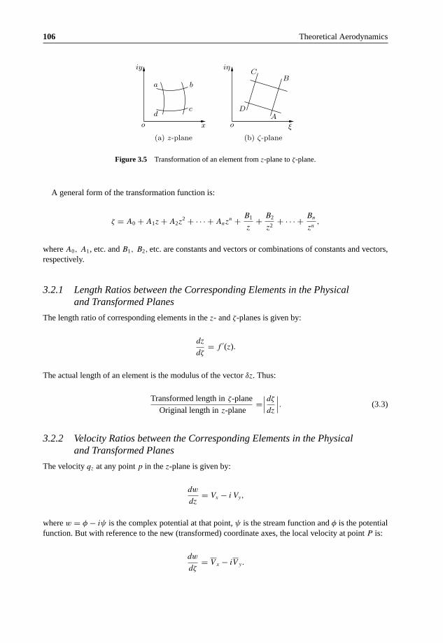
106 Theoretical Aerodynamics
b
c
Ba
o
iy iη
o
(a) z-plane (b) ζ-plane
d A
ξ
C
D
x
Figure 3.5 Transformation of an element from z-plane to ζ-plane.
A general form of the transformation function is:
ζ = A0 + A1z + A2z2 + · · · + Anz
n + B1
z+ B2
z2+ · · · + Bn
zn,
where A0, A1, etc. and B1, B2, etc. are constants and vectors or combinations of constants and vectors,respectively.
3.2.1 Length Ratios between the Corresponding Elements in the Physicaland Transformed Planes
The length ratio of corresponding elements in the z- and ζ-planes is given by:
dz
dζ= f ′(z).
The actual length of an element is the modulus of the vector δz. Thus:
Transformed length in ζ-plane
Original length in z-plane=
∣∣∣dζ
dz
∣∣∣. (3.3)
3.2.2 Velocity Ratios between the Corresponding Elements in the Physicaland Transformed Planes
The velocity qz at any point p in the z-plane is given by:
dw
dz= Vx − i Vy,
where w = φ − iψ is the complex potential at that point, ψ is the stream function and φ is the potentialfunction. But with reference to the new (transformed) coordinate axes, the local velocity at point P is:
dw
dζ= Vx − iV y.

Conformal Transformation 107
At the corresponding points between the original plane (z-plane) and the transformed plane (ζ-plane),considering only the magnitudes, we can express:
Velocity in the transformed plane (ζ-plane)
Velocity in the original plane (z-plane)=
∣∣∣dw
dζ
∣∣∣/∣∣∣dw
dz
∣∣∣ =∣∣∣dz
dζ
∣∣∣. (3.4)
It is seen that the velocity ratio between corresponding points in the original and transformed planes isthe inverse of the length ratio.
3.2.3 Singularities
The relation between the corresponding elements in the physical and transformed planes is adequatelydefined by:
dζ = f ′(z)dz.
In most situations, the correspondence between the elements is the modulus and argument of the vector:
f ′(z) = dζ
dz
as outlined in the previous sections. This arrangement clearly breaks down where f ′(z) = dζ/dz is zero orinfinite. In both the cases, the conformability of the transformation is lost. The points at which dζ/dz = 0or ∞, in any transformation, are known as singular points, commonly abbreviated as singularities.
3.3 Complex Numbers
To have an understanding about the complex numbers will be of great value to deal with the Joukowskitransformation, to be taken up in Chapter 4. Let us briefly discuss the essential aspects of complexnumbers in this section.
A complex number may be defined as a number consisting of a sum of real and imaginary parts. Letx and y be the real numbers; positive or negative. Let i be a symbol which obeys the ordinary laws ofalgebra, and also satisfies the relation:
i2 = −1. (3.5)
The combination of x and y in the following form:
z = x + iy (3.6)
is then called a complex number.A complex number z can be represented by a point p whose Cartesian coordinates are (x, y), as shown
in Figure 3.6.The picture, such as Figure 3.6, in which the complex number is represented by a point is called the
Argand diagram. In this representation the complex number z represents the point p or (x, y).

108 Theoretical Aerodynamics
p
o x
θ x
y
iy
Figure 3.6 Representation of a complex number in xy-plane.
The numbers x and y in Equation (3.6) are called the real and imaginary parts of the complex numberz, that is:
x = Real part of z,
y = Imaginary part of z.
When y = 0 the complex number z is said to be purely real and when x = 0 the complex number z is saidto be purely imaginary. Two complex numbers which differ from the sign of i are said to be conjugates.Usually a conjugate number is represented with an “overline.” For example:
z = x + iy (3.7a)
z = x − iy. (3.7b)
The simple fact that:
z + z = 2x
z − z = 2iy
imply the following two simple but important theorems:
Theorem 1: The real part of the difference of two conjugate complex numbers is zero.Theorem 2: The imaginary part of the sum of two conjugate complex numbers is zero.
The point p which represents a complex number in the xy-plane can also be described by polarcoordinates (r, θ), in which r is necessarily positive. By Euler’s theorem, we have:
cos θ + i sin θ = eiθ.
Therefore:
z = x + iy = r cos θ + ir sin θ

Conformal Transformation 109
or
z = r (cos θ + i sin θ) = r eiθ (3.8)
zn = (x + iy)n
= rn (cos nθ + i sin nθ)
= rneniθ .
Note that:
2 cos θ = eiθ + e−iθ
2i sin θ = eiθ − e−iθ.
When polar coordinates are used the positive number r is called the modulus of z, expressed as:
r = mod z = |z|=
√x2 + y2
= √zz.
Then the product of two conjugate complex numbers is the square of the modulus of either.The angle θ is called the argument of z, expressed as:
θ = arg z.
Therefore, all complex numbers whose moduli are the same and whose arguments differ by an integermultiple of 2π are represented by the same part in the Argand diagram. The value of arg z (that is, angleθ) that lies between −π and +π is the principal value. The principal value of the argument of a positivereal number is zero, and the argument of a negative real number is π.
Let us consider a curve C1 encircling the origin and curve C2 which does not encircle the origin, asshown in Figure 3.7. If θ is the initial value of the arg z and if z is represented by the point P , it is clearthat when a point Q originally coinciding with P is moved round C1 in the clockwise direction, thecorresponding value of its argument increases, and when we finally return to P after going one round, wehave the arg z = θ + 2π. On the other hand, if we go round C2, the argument of Q decreases at first untilOQ becomes a tangent to C2, then increases until OQ again becomes a tangent and finally decreases tothe initial value. Thus if arg z has a given value at one point of a curve such as C2 which does not encirclethe origin, the value to the argument of z is one-valued at every point inside and on C2, provided whenthe arg z is assumed to vary continuously with z.
Q
x
Q
y
θ
2πθ
C1
C2
P
P
ox
y
Figure 3.7 Two curves in the xy-plane.
110 Theoretical Aerodynamics
Now consider:
log z = log (reiθ) = log r + iθ. (3.9)
If we take z once round C1, θ increases by 2π and therefore log z increases by 2πi. Thus log z is amany-valued function if z moves inside or upon a curve which encircles the origin. On the other hand,log z can be regarded as a one-valued function if z is restricted to the interior of a curve such as C2 whichdoes not encircle the origin.
If z1 = r1eiθ1 , z2 = r2e
iθ2 are two complex numbers then their product is:
z1z2 = r1r2ei(θ1+θ2).
Thus the modulus of the product is the product of the moduli, while the argument of the product is thesum of the argument, that is:
|z1z2| = |z1| |z2| (3.10a)
arg (z1z2) = arg (z1) + arg (z2). (3.10b)
In applying Equation (3.10b) it is well to bear in mind that each of the arguments may be many-valuedand therefore the right-hand member is only one of the possible values of arg (z1z2).
Similarly we can express:
arg(
z1
z2
)= arg (z1) − arg (z2). (3.11)
3.3.1 Differentiation of a Complex Function
Let us consider the complex function zn, where n is a positive integer. Then we define:
d
dzzn = lim
z1→z
zn1 − z
z1 − z
= limz1→z
(zn−1
1 + zn−21 z + · · · + zn−1
) × z1 − z
z1 − z
= nzn−1.
Example 3.1
A particle moves in the xy-plane such that its position (x, y) as a function of time t is given by:
z = i + 2t
t − i.
Find the velocity and acceleration of the particle in terms of t.

Conformal Transformation 111
Solution
The complex velocity is given by:
V =∣∣∣dz
dt
∣∣∣=
√(dz
dx
)2
+(
dz
dy
)2
=√
dz
dt· dz
dt.
Given:
z = x + iy = i + 2t
t − i.
Therefore:
dz
dt= d
dt
(i + 2t
t − i
)
= (t − i)2 − (i + 2t)
(t − i)2
= −3i
(t − i)2.
The conjugate ofdz
dtis:
dz
dt= 3i
(t + i)2.
Thus:
V =√( −3i
(t − i)2
)·(
3i
(t + i)2
)
= 3
t2 + 1.
The acceleration is given by:
a =∣∣∣d2z
dt2
∣∣∣=
√d2z
dt2· d2z
dt2.

112 Theoretical Aerodynamics
We have:
d2z
dt2= −(−3i) 2(t − i)
(t − i)4
= 6i
(t − i)3
d2z
dt2= −6i
(t + i)3.
Thus:
a =√
6i
(t − i)3· −6i
(t + i)3
= 6
(t2 + 1)3/2.
3.4 Summary
The transformation technique which transforms an orthogonal geometric pattern, composed of elementsof certain shape, into an entirely different pattern, whilst the elements retain their form and proportion istermed conformal transformation.
In the z-plane (physical plane) point p is located by z = x + iy, and in the ζ-plane (transformed plane),the corresponding point P is located by ζ = ξ + iη. The relation between z and ζ is a particular specifiedfunction of ζ, in terms of z. That is:
ζ = f (z) .
This function is known as the transformation function. In the transformation, both the elements of thecrossing arc segments are rotated through the same angle. Therefore, the angle of intersection must remainunchanged during the transformation.
The transformation function is essentially of the vector type:
ζ = f (z),
where z = x + iy and ζ = ξ + iη.A general form of the transformation function is:
ζ = A0 + A1z + A2z2 + · · · + Anz
n + B1
z+ B2
z2+ · · · + Bn
zn,
where A0, A1, etc. and B1, B2, etc. are constants and vectors or combinations of constants and vectors,respectively.
The length ratio of corresponding elements in the z- and ζ-planes is given by:
dz
dζ= f ′(z).

Conformal Transformation 113
The actual length of an element is the modulus of the vector δz. Thus:
Transformed length in ζ-plane
Original length in z-plane=
∣∣∣dζ
dz
∣∣∣.The velocity qz at any point p in the z-plane is given by:
dw
dz= Vx − i Vy,
where w = φ − iψ is the complex potential at that point, ψ is the stream function and φ is the potentialfunction. But with reference to the new (transformed) coordinate axes, the local velocity at point P is:
dw
dζ= Vx − iV y.
At the corresponding points between the original plane (z-plane) and the transformed plane (ζ-plane),considering only the magnitudes, we can express:
Velocity in the transformed plane (ζ-plane)
Velocity in the original plane (z-plane)=
∣∣∣dw
dζ
∣∣∣/∣∣∣dw
dz
∣∣∣ =∣∣∣dz
dζ
∣∣∣.It is seen that the velocity ratio between corresponding points in the original and transformed planes isthe inverse of the length ratio.
Exercise Problems
1. Find the absolute value of:
5 − 2i
5 + 2i.
[Answer: 1]2. Find the polar form of (1 + i)2.
[Answer: 2eiπ/2]3. Express:
1
2 (cos 20◦ + i sin 20◦)
in (x + iy) form.[Answer: 0.47 − 0.17i]
4. Find x and y if:
(x + iy)2 = 2i.
[Answer: x = 1, y = ±1]5. What is the curve made up of the points (x, y)-plane satisfying the equation |z| = 3?
[Answer: a circle of radius 3 units with center at the origin.]


4Transformation of Flow Pattern
4.1 Introduction
Any flow pattern can be considered to consist of a set of streamlines and potential lines (ψ and φ lines).Thus, transformation of a flow pattern essentially amounts to the transformation of a set of streamlinesand potential lines, whilst the transformation of individual lines implies the transformation of a numberof points.
4.2 Methods for Performing Transformation
Choose a transformation function ζ = f (z) to transform the points specified by the Cartesian coordinatesx and y, in the physical plane, given by z = x + iy, to a transformed plane given by ζ = ξ + iη. To carryout this transformation, we need to expand the transformation function ζ = f (z) = ξ + iη, equate thereal and imaginary parts and find the functional form of ξ and η, in terms of x and y, that is, find:
ξ = f1(x, y)
η = f2(x, y).
Thus, any point p(x, iy) in the physical plane (z-plane) gets transformed to point P(ξ, iη) in the trans-formed plane (ζ-plane).
Example 4.1
Transform a point p(x, iy) in the physical plane to ζ-plane, with the transformation function ζ = 1/z.
Solution
Given, ζ = 1/z. Also, z = x + iy.
Theoretical Aerodynamics, First Edition. Ethirajan Rathakrishnan.© 2013 John Wiley & Sons Singapore Pte. Ltd. Published 2013 by John Wiley & Sons Singapore Pte. Ltd.

116 Theoretical Aerodynamics
Therefore, from the transformation function ζ = 1/z, we get:
ζ = 1
z= 1
x + iy
= x − iy
x2 + y2
= x
x2 + y2− iy
x2 + y2.
But ζ = ξ + iη, therefore:
ξ + iη = x
x2 + y2− iy
x2 + y2.
Comparing the real and imaginary parts, we get the coordinates of the transformed point P(ξ, η), in theζ-plane, as:
ξ = x
x2 + y2
η = − y
x2 + y2.
Using these expressions for ξ and η, any point in the physical plane, with coordinates (x, y), can betransformed to a point, with coordinates (ξ, η), in the transformed plane. That is, from any point of thegiven flow pattern in the original plane, values of the coordinates x and y can be substituted into theexpressions of ξ and η to get the corresponding point (ξ, η), in the transformed plane.
4.2.1 By Analytical Means
For a given flow pattern in the physical plane, each streamline of the flow can be represented by a separatestream function. Transferring these stream functions, using the transformation function, ζ = f (z), thecorresponding streamlines in the transformed plane can be obtained. For example, the streamlines in thephysical plane given by the stream function:
ψ = f (x, y) = constant
can be expanded, using the transformation function:
ζ = f (z),
where z = x + iy, to obtain the following three equations:
ζ = constant = f (x, iy)
= f1(x, y) + if2(x, y).

Transformation of Flow Pattern 117
But ζ = ξ + iη, therefore:
ξ + iη = f1(x, y) + if2(x, y).
Comparing the real and imaginary parts, we have:
ξ = f1(x, y)
η = f2(x, y).
From these equations, ξ and η can be isolated, by eliminating x and y. The resulting expressions for ξ
and η will represent the transformed line in the ζ-plane.
Example 4.2
Transform the straight lines, parallel to the x-axis in the physical plane, with the transformation functionζ = 1/z.
Solution
From the transformation function ζ = 1/z, we have:
ζ = 1
z
= 1
x + iy.
Multiplying and dividing the numerator and denominator of the right-hand side by (x − iy), we get:
ζ = x − iy
(x + iy)(x − iy)
= x − iy
x2 + y2
= x
x2 + y2− iy
x2 + y2.
But
ζ = ξ + iη.
Therefore:
ξ + iη = x
x2 + y2− iy
x2 + y2.

118 Theoretical Aerodynamics
Equating the real and imaginary parts, we get the coordinates for the points on the transformed lines, inζ-plane, as:
ξ = x
x2 + y2
η = − y
x2 + y2.
Taking the flow pattern in the physical plane to be an uniform flow parallel to x-axis, we have the streamfunction as:
ψ = Vxy = constant
or
y = ψ
Vx
= k (say). (a)
For given values of ψ and Vx, k is a constant.
Also:
ξ = x
x2 + y2(b)
η = − y
x2 + y2. (c)
From Equation (c), we have:
x =√
−y
η− y2.
Substituting this into Equation (b), we get:
ξ =
√−y
η− y2
−y
η
.
Substituting y = k, we get:
ξ =
√− k
η− k2
− k
η
.
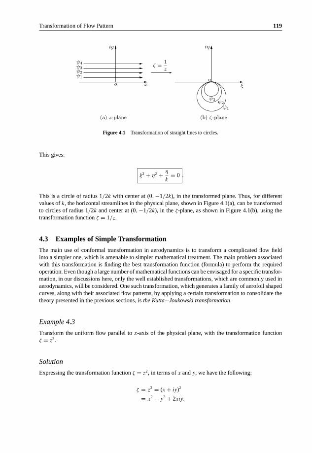
Transformation of Flow Pattern 119
x
iy
o
ψ3
(b) ζ-plane(a) z-plane
iη
ψ1
ψ2
ζ =1
z
ξ
ψ4ψ3ψ2ψ1
o
Figure 4.1 Transformation of straight lines to circles.
This gives:
ξ2 + η2 + η
k= 0 .
This is a circle of radius 1/2k with center at (0, −1/2k), in the transformed plane. Thus, for differentvalues of k, the horizontal streamlines in the physical plane, shown in Figure 4.1(a), can be transformedto circles of radius 1/2k and center at (0, −1/2k), in the ζ-plane, as shown in Figure 4.1(b), using thetransformation function ζ = 1/z.
4.3 Examples of Simple Transformation
The main use of conformal transformation in aerodynamics is to transform a complicated flow fieldinto a simpler one, which is amenable to simpler mathematical treatment. The main problem associatedwith this transformation is finding the best transformation function (formula) to perform the requiredoperation. Even though a large number of mathematical functions can be envisaged for a specific transfor-mation, in our discussions here, only the well established transformations, which are commonly used inaerodynamics, will be considered. One such transformation, which generates a family of aerofoil shapedcurves, along with their associated flow patterns, by applying a certain transformation to consolidate thetheory presented in the previous sections, is the Kutta−Joukowski transformation.
Example 4.3
Transform the uniform flow parallel to x-axis of the physical plane, with the transformation functionζ = z2.
Solution
Expressing the transformation function ζ = z2, in terms of x and y, we have the following:
ζ = z2 = (x + iy)2
= x2 − y2 + 2xiy.

120 Theoretical Aerodynamics
But ζ = ξ + iη. Thus:
ξ + iη = x2 − y2 + i 2xy.
Equating the real and imaginary parts, we get the coordinates ξ and η, in the transformed plane, as:
ξ = x2 − y2
η = 2xy.
The stream function for uniform flow parallel to x-axis, in the physical plane, is:
ψ = Vxy.
Therefore:
ψ
Vx
= y.
Letψ
Vx
= k.
Also:
x = η
2y.
Therefore, ξ becomes:
ξ = η2
4y2− y2.
Replacing y with k, we get:
ξ = η2
4k2− k2
or:
η = 2k√
ξ + k2.
For a constant value of k, this gives a parabola. Therefore, horizontal streamlines, shown inFigure 4.2(a), in the z-plane, transform to parabolas in the ζ-plane, as shown in Figure 4.2(b). Thus,applying the transformation function ζ = z2 to an uniform flow parallel to x-axis in the physical plane,we get parabolas in the ζ-plane.
Note that the flow zones above or below x-axis, in the z-plane, transform to occupy the whole of theζ-plane. These zones of the z-plane must be treated separately. In this case, the streamlines in the lowerpart of the z-plane, extending along the negative y-direction, will be taken with the flow streaming fromleft to right, in Figure 4.2(b). The streamlines for this flow is given by:
ψ = Vxy,
where y is always negative. Thus, the stream function is negative in this zone.

Transformation of Flow Pattern 121
ψ2
iη
ζ = z2
ψ1
iy
ψ0ψ3
x ξ
ψ4
(a) z-plane (b) ζ-plane
o o
Figure 4.2 Transformation of horizontal lines to parabolas.
Example 4.4
Find the transformation of the uniform flow parallel to the y-axis, in the z-plane, using the transformationfunction ζ = z2.
Solution
The given flow field is as shown in Figure 4.3(a).For the transformation function ζ = z2, from Example 4.3, we have:
ξ = x2 − y2
η = 2xy.
The stream function for the downward uniform flow, parallel to y-axis, shown in Figure 4.3(a), is:
ψ = Vyx.
ψ2
ψ0
ξ
iη
o
(b) ζ-plane
xo
(a) z-plane
iy
ζ = z2
ψ4
ψ3
ψ0
ψ1
Figure 4.3 Transformation of vertical lines to parabolas.

122 Theoretical Aerodynamics
Thus, for a given ψ and Vy:
x = ψ
Vy
= constant.
Let x = ψ
Vy
= k.
The coordinates ξ and η can be arranged as follows:
ξ = x2 − y2
= x2 −(
η
2x
)2
η = 2x√
x2 − ξ.
Replacing x with k, we get:
η = 2k√
k2 − ξ .
For different values of k this represents a set of parabolas, as shown in Figure 4.3(b).
4.4 Kutta−Joukowski Transformation
Kutta−Joukowski transformation is the simplest of all transformations developed for generating aerofoilshaped contours. Kutta used this transformation to study circular-arc wing sections, while Joukowskishowed how this transformation could be extended to produce wing sections with thickness t as well ascamber. In our discussions here, we make another simplification that the transformation is confined tothe study of the actual contour of the circle, and to show how its shape changes on transformation.
In our discussion on Kutta−Joukowski transformation, it is important to note the following:
• The circle considered, in the physical plane, is a specific streamline. Essentially the circle is thestagnation streamline of the flow in the original plane 1 (z-plane).
• The transformation can be applied to the circle and all other streamlines, around the circle, to generatethe aerofoil and the corresponding streamlines in plane 2 (ζ-plane) or the transformed plane. That is, thetransformation can result in the desired aerofoil shape and the streamlines of the flow around the aerofoil.
It is convenient to use polar coordinates in the z-plane and Cartesian coordinates in ζ-plane. TheKutta−Joukowski transformation function is:
ζ = ξ + iη = z + b2
z,
where b is a constant.

Transformation of Flow Pattern 123
Now, expressing z as z = reiθ , where r and θ are the polar coordinates, and on expanding, we get:
ξ + iη = reiθ + b2
reiθ
= r (cos θ + i sin θ) + b2
r(cos θ − i sin θ) .
Equating the real and imaginary parts, we get:
ξ =(
r + b2
r
)cos θ (4.1a)
η =(
r − b2
r
)sin θ . (4.1b)
These expressions for ξ and η are the general expressions for the transformation of the basic shape,namely the circle in the z-plane, to any desired shape in the ζ-plane. This can be achieved by assigningsuitable values to the constant b in the transformation function (z + b2/z) and locating the center of thecircle at the origin, or at a suitable location on the x-axis or y-axis, or (usually) in the first quadrant ofthe z-plane.
4.5 Transformation of Circle to Straight Line
For transforming a circle of radius a to a straight line, the constant b in the Joukowski transformationfunction should be set equal to a, and the center of the circle should be at the origin, as shown inFigure 4.4(a).
Substituting r = a = b in the ξ and η expressions in Equation (4.1), we get:
ξ = 2a cos θ (4.2a)
η = 0 . (4.2b)
iη
ξ
a
Circlez = aeiθ
2a 2a
Pθ
p
(b) ζ-plane(a) z-plane
ζ = z2 +b2
z
iy
oo x
Figure 4.4 Transformation of circle to straight line.

124 Theoretical Aerodynamics
These ξ and η represent a straight line coinciding with the ξ-axis in the ζ-plane. The transformed line isthus confined to ξ-axis, as shown in Figure 4.4(b), and as θ varies from 0 to π, point P moves from +2a
to −2a. Thus, the chord of the locus of point P is 4a.
Note that the singularities at z = ± b produce sharp edges at ζ = ± 2a. That is, the extremities of thestraight line are sharp.
4.6 Transformation of Circle to Ellipse
For transforming a circle to an ellipse using the Kutta−Joukowski transformation function:
ζ = z + b2
z
the circle should have its center at the origin in the z-plane, but the radius of the circle should be greaterthan the constant b, in the above transformation function, that is, a > b.
With the radius of the circle r = a, we can express the ξ and η expressions in Equation (4.1) as:
ξ =(
a + b2
a
)cos θ
η =(
a − b2
a
)sin θ.
Eliminating θ in the ξ and η expressions above, we get:
ξ2(a + b2
a
)2 + η2(a − b2
a
)2 = 1 (4.3)
This is an ellipse with its major and minor axes, respectively, along the ξ and η axes in the ζ-plane, asshown in Figure 4.5(b).
(a) z-plane (b) ζ-plane
ζ = z +b2
z
z = reiθ
x
a
oo
η = a b2
asin θ
Pp
ξ
θ
iy iηξ = a + b2
acos θ
Figure 4.5 Transformation of circle to ellipse.

Transformation of Flow Pattern 125
The major and minor axes of the ellipse, given by Equation (4.3), are the following:
The chord or the major axis of the ellipse = 2
(a + b2
a
)
Maximum thickness or the minor axis of the ellipse = 2
(a − b2
a
).
The fineness ratio of the ellipse, defined as the ratio of the chord to maximum thickness, becomes:
Fineness ratio = Chord
Maximum thickness
=a + b2
a
a − b2
a
= a2 + b2
a2 − b2
or
Fineness ratio = (a/b + b/a)
(a/b − b/a). (4.3a)
From this relation it is evident that for every value of the ratio a/b a new ellipse can be obtained.
4.7 Transformation of Circle to Symmetrical Aerofoil
To transform a circle into a symmetrical aerofoil, the center of the circle in the z-plane should be shiftedfrom the origin and located slightly downstream of the origin, on the x-axis, as shown in Figure 4.6(a).This shift would cause asymmetry to the profile (about the ordinates of the transformed plane) of thetransformed shape obtained with the Kutta−Joukowski transformation function.
Let the horizontal shift of the center of the circle c, from the origin o, also called as the eccentricity tobe e. The actual distance of the center of the circle from the origin is be, as shown in Figure 4.6(a). Thus,
P
c x
iy
ar
p
iη
ξ
2b
(a) z-plane
2b
(b) ζ-plane
oo
ζ = z +b2
z
2b cos θ
θ
be
θ′
b
η
Figure 4.6 Transformation of circle to a symmetrical aerofoil.

126 Theoretical Aerodynamics
θ
be
ar = op = be cos θ + a cos γ
o
r
p
c
γ
aco
sγ
beco
s θ
Figure 4.7 A general point p on a circle in polar coordinates.
the radius of the circle is (b + be). Let us represent the general point p on the circle, in polar coordinates,as shown in Figure 4.7.
The distance of point p from the origin, shown in Figure 4.7, is:
op = r = b e cos θ + a cos γ
where e and γ are small. Therefore, the above distance r simplifies to:
r = b e cos θ + a
Substituting a = (b + be), we get:
r = b e cos θ + b + be
= b(1 + e + e cos θ).
This can be arranged as:
b
r= [1 + e (1 + cos θ)]−1.
But the eccentricity e is very small. Therefore, the term e (1 + cos θ) is very small compared to 1. Thus,expanding the right-hand-side of the above equation and retaining up to the first order terms, we get:
b
r= 1 − e − e cos θ .
Thus, r and b can be expressed in terms of the horizontal shift e of the circle being transformed.
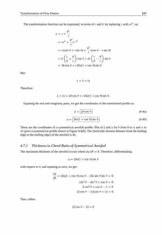
Transformation of Flow Pattern 127
The transformation function can be expressed, in terms of r and θ, by replacing z with reiθ , as:
ζ = z + b2
z
= reiθ + b2
re−iθ
= r (cos θ + i sin θ) + b2
r(cos θ − i sin θ)
= b
(r
b+ b
r
)cos θ + ib
(r
b− b
r
)sin θ
= 2b cos θ + i 2be(1 + cos θ) sin θ.
But:
ζ = ξ + iη
Therefore:
ξ + iη = 2b cos θ + i 2be(1 + cos θ) sin θ.
Equating the real and imaginary parts, we get the coordinates of the transformed profile as:
ξ = 2b cos θ (4.4a)
η = 2be(1 + cos θ) sin θ . (4.4b)
These are the coordinates of a symmetrical aerofoil profile. Plot of ξ and η for θ from 0 to π and π to2π gives a symmetrical profile shown in Figure 4.6(b). The chord (the shortest distance from the leadingedge to the trailing edge) of the aerofoil is 4b.
4.7.1 Thickness to Chord Ratio of Symmetrical Aerofoil
The maximum thickness of the aerofoil occurs where dη/dθ = 0. Therefore, differentiating
η = 2be(1 + cos θ) sin θ
with respect to θ, and equating to zero, we get:
dη
dθ= 2be(1 + cos θ) cos θ − 2be sin θ sin θ = 0
cos2 θ − sin2 θ + cos θ = 0
2 cos2 θ + cos θ − 1 = 0
(2 cos θ − 1) (cos θ + 1) = 0.
Thus, either:
(2 cos θ − 1) = 0

128 Theoretical Aerodynamics
or
(cos θ + 1) = 0.
From the above relation, we get the following conditions corresponding to the maximum and minimumthickness of the aerofoil:
• cos θ = 1/2, giving θ = π/3 = 60◦, at the maximum thickness location.• cos θ = −1, giving θ = π, at the minimum thickness location.
Therefore, the maximum thickness is at the chord location, given by:
ξ = 2b cosπ
3= b.
This point (b, 0), from the leading edge of the aerofoil, in Figure 4.6(b), is the quarter chord point. Thus,the maximum thickness tmax is at the quarter chord point. The maximum thickness tmax is given by 2η,with θ = π/3 in Equation (4.4b).
tmax = 2η = 2×[2be(1 + cos θ) sin θ
]= 2×
[2be(1 + cos 60◦) sin 60◦]
= 2 × 2be ×(
1 + 1
2
)×
√3
2.
That is:
tmax = 3√
3 be (4.5)
Thus, the thickness to chord ratio of the aerofoil becomes:
t
c= 3
√3 be
4b= 1.299e
or
t
c≈ 1.3 e . (4.6)
From the above relation for maximum thickness and thickness-to-chord ratio, it is seen that the thicknessis dictated by the shift of the center of the circle or eccentricity e. The eccentricity serves to fix the finenessratio (t/c ratio) of the profile. For example, a 20% thick aerofoil section would require an eccentricity of:
e = 0.2/1.3 = 0.154.

Transformation of Flow Pattern 129
4.7.2 Shape of the Trailing Edge
At the trailing edge of the aerofoil, the slope of its upper and lower surfaces merge. Therefore:
dη
dξ= dη
dθ
/dξ
dθ
= 2be(2 cos2 θ + cos θ − 1)
−2b sin θ
= e
(2 cos2 θ + cos θ − 1
− sin θ
).
At the trailing edge, θ = π; because of this dη/dξ becomes indeterminate. But, by l’Hospital’s rule,1 wecan expresses dη/dξ as follows:
(dη
dξ
)= −e
(2 cos2 θ + cos θ − 1
sin θ
)
= −e
(2 × 2 cos θ × (− sin θ) − sin θ
cos θ
)
= e
(4 cos θ sin θ + sin θ
cos θ
)
At θ = π:
(dη
dξ
)θ=π
= e
(4 cos θ sin θ + sin θ
cos θ
)θ=π
= 0.
Thus, at the trailing edge, both upper and lower surface are tangential to the ξ-axis, and therefore, toeach other. In other words, the trailing edge is cusped. This kind of trailing edge would ensure that theflow will leave the trailing edge without separation. But this is possible only when the trailing edge iscusped with zero thickness. Thus, this is only a mathematical model. For actual aerofoils, the trailingedge will have a finite thickness, and hence, there is bound to be some separation, even for the thinnestpossible trailing edge.
Note: Transformation of a circle with its center at a distance be on the negative side of the x-axis, in thephysical plane, will result in a symmetrical aerofoil, with its leading edge on the negative side of theξ-axis (mirror image of the aerofoil profile about the η-axis, in Figure 4.6), in the transformed plane.Similarly, positioning the center of the circle, with an offset, on the y-axis, will get transformed to asymmetrical aerofoil, with its leading and trailing edges on the η-axis, in the transformed plane.
4.8 Transformation of a Circle to a Cambered Aerofoil
For transforming a circle to a cambered aerofoil, using Joukowski transformation, the center of the circlein the physical plane has to be shifted to a point in one of the quadrants. Let us consider the center in thefirst coordinate of z-plane, as shown in Figure 4.8(a).
1l’Hospital’s rule can be used to circumvent the indeterminate forms such as 00 , 0
∞ , ∞0 , ∞
∞ . This rule solves the indeterminate formsby differentiating the numerator and denominator separately till a finite form is arrived with the given condition.

130 Theoretical Aerodynamics
θ
z = reiθ
iη
c
2b cos θ
m
p
P
o ξηl
no
(b) ζ-plane
θ′
(a) z-plane
ηu
x
γ
iy
β
Figure 4.8 Transformation of a circle to a cambered aerofoil.
As seen in Figure 4.8(a):
• the center c of the circle is displaced horizontally as well as vertically from the origin, in the physicalplane.
• let the horizontal shift of the center be “on = be,” and• the vertical shift be “cn = h.”
The point p on the circle and its distance from the origin can be represented as shown in Figure 4.9.Both the vertical shift h and eccentricity e are small. Therefore, the angle β, subtended at point m, by
om and cm is small, hence, cos β ≈ 1, also cos γ ≈ 1. Therefore, the radius of the circle becomes:
a = (b + be) cos β
= (b + be).
aco
sγ
a
γ
m nβ
r
p
c
h
o
be cos θ
hsinθ
θ′
θ
Figure 4.9 Location of point p on a circle in polar coordinates.

Transformation of Flow Pattern 131
The vertical shift of the center can be expressed as:
h = a sin β
= b (1 + e)β.
But e and β are small, therefore, h becomes:
h ≈ b β
By dropping perpendiculars on to op, from n and c, it can be shown that:
op = r = a cos γ + h sin θ + be cos θ.
The angle γ is small, therefore, cos γ ≈ 1, thus:
r = a + h sin θ + be cos θ.
Substituting for a = (b + be) and h = bβ, r becomes:
r = b + be + bβ sin θ + be cos θ.
This can be expressed as:
r
b= 1 + e + e cos θ + β sin θ (4.7a)
or
b
r= [
1 + (e + e cos θ + β sin θ)]−1
.
Expanding and retaining only the first order terms, we have:
b
r= 1 − e − e cos θ − β sin θ (4.7b)
since e and β are small, their powers are assumed to be negligibly small.The Joukowski transformation function is:
ζ = z + b2
z.
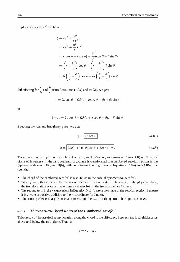
132 Theoretical Aerodynamics
Replacing z with r eiθ , we have:
ζ = r eiθ + b2
r eiθ
= r eiθ + b2
re−iθ
= r(cos θ + i sin θ) + b2
r(cos θ − i sin θ)
=(
r + b2
r
)cos θ +
(r − b2
r
)i sin θ
= b
(r
b+ b
r
)cos θ + ib
(r
b− b
r
)sin θ.
Substituting forr
band
b
rfrom Equations (4.7a) and (4.7b), we get:
ζ = 2b cos θ + i2b(e + e cos θ + β sin θ) sin θ
or
ξ + iη = 2b cos θ + i2b(e + e cos θ + β sin θ) sin θ.
Equating the real and imaginary parts, we get:
ξ = 2b cos θ (4.8a)
η = 2be(1 + cos θ) sin θ + 2bβ sin2 θ . (4.8b)
These coordinates represent a cambered aerofoil, in the ζ-plane, as shown in Figure 4.8(b). Thus, thecircle with center c in the first quadrant of z-plane is transformed to a cambered aerofoil section in theζ-plane, as shown in Figure 4.8(b), with coordinates ξ and η, given by Equations (4.8a) and (4.8b). It isseen that:
• The chord of the cambered aerofoil is also 4b, as in the case of symmetrical aerofoil.• When β = 0, that is, when there is no vertical shift for the center of the circle, in the physical plane,
the transformation results in a symmetrical aerofoil in the transformed or ζ-plane.• The second term in the η expression, in Equation (4.8b), alters the shape of the aerofoil section, because
it is always a positive addition to the η-coordinate (ordinate).• The trailing edge is sharp (η = 0, at θ = π), and the tmax is at the quarter chord point (ξ = b).
4.8.1 Thickness-to-Chord Ratio of the Cambered Aerofoil
Thickness t of the aerofoil at any location along the chord is the difference between the local thicknessesabove and below the mid-plane. That is:
t = ηu − ηl,

Transformation of Flow Pattern 133
where the subscripts u and l, respectively, refer to the upper and lower surfaces of the aerofoil profile.The upper and lower thicknesses of the aerofoil are given, by Equation (4.8b), as:
ηu = 2be (1 + cos θu) sin θu + 2bβ sin2 θu
ηl = 2be (1 + cos θl) sin θl + 2bβ sin2 θl.
But ηu and ηl are at the same location on the abscissa (ξ-axis), therefore, θl = − θu. The thicknessbecomes:
t = ηu − ηl
= 4be (1 + cos θu) sin θu.
The thickness-to-chord ratio becomes:
t
c= 4be (1 + cos θu) sin θu
4b
or
t
c= e (1 + cos θu) sin θu . (4.9)
For (t/c)max, the condition is d(t/c)/dθ = 0, and d2(t/c)/dθ2 < 0. Thus:
d(t/c)/dθ = 0
e(cos θu + cos2 θu − sin2 θu) = 0
cos θu + cos2 θu − (1 − cos2 θu) = 0
2 cos2 θu + cos θu − 1 = 0
cos θu = −1 ± √1 + 8
4.
This gives:
cos θu = −1, or 1/2.
We can express this as:
cos θu = −1, at θu = π
and
cos θu = 1
2, at θu = π/3.
Thus, θu is either π or π/3. At θu = π, t/c = 0, which is the trailing edge of the aerofoil. Hence, t/c
should be maximum at θu = π/3.The thickness-to-chord ratio is maximum at θu = 60◦. Thus:
(t
c
)max
≈ 1.3e .
This maximum is also at the quarter chord point, as in the case of symmetrical aerofoil.

134 Theoretical Aerodynamics
4.8.2 Camber
The camber of an aerofoil is the maximum displacement of the mean camber line from the chord. Themean camber line is the locus of mid-points of lines drawn perpendicular to the chord. In other words,the camber line is the bisector of the aerofoil profile thickness distribution from the leading edge to thetrailing edge. The camber line is given by:
Camber = 1
2(ηu + ηl)max .
Making this nondimensional, by dividing with the chord, the camber can be expressed as a fraction ofthe chord:
Percentage camber = (ηu + ηl)max
2 × chord× 100 %.
By Equation (4.8b), we have:
ηu = 2be(1 + cos θ) sin θ + 2bβ sin2 θ
ηl = 2be(1 + cos (−θ)) sin (−θ) + 2bβ sin2(−θ)
= −2be(1 + cos θ) sin θ + 2bβ sin2 θ.
Thus:
(ηu + ηl)max = 4b β (sin2 θ)max.
The chord of the aerofoil is c = 4b. Therefore:
(ηu + ηl)max
2 × chord= 4b β (sin2 θ)max
2 × 4b
= β
2
(sin2 θ
)max
.
In this relation, sin2 θ is maximum at θ = π/2, that is, at the mid-chord. Therefore:
Percentage camber = β
2× 100 %.
From the above discussions it is evident that the vertical shift of the circle center is responsible for thecamber of the aerofoil, and the horizontal shift determines the thickness-to-chord ratio of the aerofoil.
4.9 Transformation of Circle to Circular Arc
Transformation of a circle with its center shifted above (or below) the origin, on the ordinate in thez-plane, with the transformation function ζ = z + b2/z results in a circular arc, as shown in Figure 4.10.
A general point p on the circle with center above the origin, on the y-axis, in Figure 4.10, can berepresented as shown in Figure 4.11.

Transformation of Flow Pattern 135
(b) ζ-plane(a) z-plane
iηiy
2bβ
2b 2bxm n
β c
oo ξ
Figure 4.10 Transformation of circle to circular arc.
m b
a
r
c
p
a
βlh
γ
θ
o
Figure 4.11 The point p on the circle with its center on the ordinate in the physical plane.
From Figure 4.11, it is seen that:
h = b tan β ≈ b β
ol = oc cos θ = b β cos θ
lp = a cos γ = (b + be) cos γ
≈ b + be (because γ is small, cos γ ≈ 1).
Therefore,
op = ol + lp
r = b β cos θ + (b + be)
= b (1 + e + β cos θ)r
b= 1 + e + β cos θ
or
b
r=[
1 + (e + β cos θ)]−1
.

136 Theoretical Aerodynamics
But, (e + β cos θ) � 1, therefore, expanding the above, retaining only the first-order terms, we get:
b
r= 1 − e − β cos θ.
The Joukowski transformation function is:
ζ = z + b2
z.
Replacing z = reiθ , we have:
ζ = reiθ + b2
reiθ
= r(cos θ + i sin θ) + b2
r(cos θ − i sin θ)
= r cos θ + b2
rcos θ + ir sin θ − i
b2
rsin θ
= b
(r
b+ b
r
)cos θ + ib
(r
b− b
r
)sin θ.
Substituting forr
band
b
r, we get:
ζ = 2b cos θ + ib(2e + 2β cos θ) sin θ
ξ + iη = 2b cos θ + ib(2e + 2β cos θ) sin θ.
Comparing the real and imaginary parts, we get:
ξ = 2b cos θ (4.10a)
η = 2b(e + β cos θ) sin θ . (4.10b)
Equations (4.10a) and (4.10b), respectively, are the expressions for the abscissa and ordinates of thecircular arc, in the transformed plane.
The chord is given by:
ξ
∣∣∣π0
= (2b cos θ)∣∣∣π
0= 4b.
The camber becomes:
η
∣∣∣max
= η
∣∣∣θ=π/2
= (2b(e + β cos θ) sin θ)∣∣∣θ=π/2
= 2be.
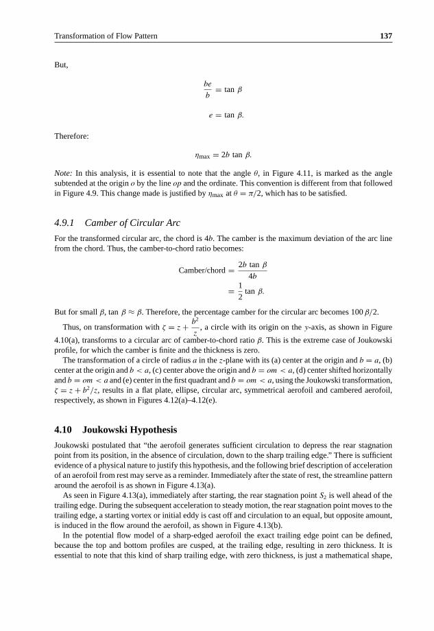
Transformation of Flow Pattern 137
But,
be
b= tan β
e = tan β.
Therefore:
ηmax = 2b tan β.
Note: In this analysis, it is essential to note that the angle θ, in Figure 4.11, is marked as the anglesubtended at the origin o by the line op and the ordinate. This convention is different from that followedin Figure 4.9. This change made is justified by ηmax at θ = π/2, which has to be satisfied.
4.9.1 Camber of Circular Arc
For the transformed circular arc, the chord is 4b. The camber is the maximum deviation of the arc linefrom the chord. Thus, the camber-to-chord ratio becomes:
Camber/chord = 2b tan β
4b
= 1
2tan β.
But for small β, tan β ≈ β. Therefore, the percentage camber for the circular arc becomes 100 β/2.
Thus, on transformation with ζ = z + b2
z, a circle with its origin on the y-axis, as shown in Figure
4.10(a), transforms to a circular arc of camber-to-chord ratio β. This is the extreme case of Joukowskiprofile, for which the camber is finite and the thickness is zero.
The transformation of a circle of radius a in the z-plane with its (a) center at the origin and b = a, (b)center at the origin and b < a, (c) center above the origin and b = om < a, (d) center shifted horizontallyand b = om < a and (e) center in the first quadrant and b = om < a, using the Joukowski transformation,ζ = z + b2/z, results in a flat plate, ellipse, circular arc, symmetrical aerofoil and cambered aerofoil,respectively, as shown in Figures 4.12(a)–4.12(e).
4.10 Joukowski Hypothesis
Joukowski postulated that “the aerofoil generates sufficient circulation to depress the rear stagnationpoint from its position, in the absence of circulation, down to the sharp trailing edge.” There is sufficientevidence of a physical nature to justify this hypothesis, and the following brief description of accelerationof an aerofoil from rest may serve as a reminder. Immediately after the state of rest, the streamline patternaround the aerofoil is as shown in Figure 4.13(a).
As seen in Figure 4.13(a), immediately after starting, the rear stagnation point S2 is well ahead of thetrailing edge. During the subsequent acceleration to steady motion, the rear stagnation point moves to thetrailing edge, a starting vortex or initial eddy is cast off and circulation to an equal, but opposite amount,is induced in the flow around the aerofoil, as shown in Figure 4.13(b).
In the potential flow model of a sharp-edged aerofoil the exact trailing edge point can be defined,because the top and bottom profiles are cusped, at the trailing edge, resulting in zero thickness. It isessential to note that this kind of sharp trailing edge, with zero thickness, is just a mathematical shape,

138 Theoretical Aerodynamics
(a) b = a, center at the origin
x
iy
ξ
iη
o o
(b) b < a, center at the origin
x
iy
ξ
iη
oo
o
(c) b = om < a, center above the origin
iy iη
ξx
c o
o c
iη
ξx
iy
o
(d) b = om < a, center shifted horizontally
x
(e) b = om < a, center in the first quadrant
iη
ξ
iy
oc
o
Figure 4.12 Transformation of a circle to (a) flat plate, (b) ellipse, (c) circular arc, (d) symmetrical aerofoil,(e) cambered aerofoil.

Transformation of Flow Pattern 139
Γ
(b)
S2
(a)
S2
S1 S1
Figure 4.13 Streamline pattern around an aerofoil (a) just after start, (b) after the starting vortex is established.
and cannot be realized in practice. Actual wing profiles are with a rounded trailing edge of finite thickness.Because of the rounded trailing edge of the wings, in actual flow where viscous boundary layer andwake exist, the position of the rear stagnation point may differ from the location predicted by potentialflow theory, and the full Joukowski circulation, may not be established. This is because for realizing fullJoukowski circulation, the trailing edge should be of zero thickness and without any wake. This conditionof realizing full Joukowski circulation, resulting in flow without wake, is known as Kutta condition.
The Kutta condition is a principle in steady flow fluid dynamics, especially aerodynamics, that isapplicable to solid bodies which have sharp corners such as the trailing edges of aerofoils. It is namedafter the German mathematician and aerodynamicist Martin Wilhelm Kutta.
The Kutta condition can be stated as follows:
“A body with a sharp trailing edge which is moving through a fluid will ‘create about itself acirculation’ of sufficient strength to hold the rear stagnation point at the trailing edge.”
In fluid flow around a body with a sharp corner the Kutta condition refers to the flow pattern in whichfluid approaches the corner from both directions, meets at the corner and then flows away from the body.None of the fluid flows around the corner remaining attached to the body.
The Kutta condition is significant when using the Kutta−Joukowski theorem to calculate the liftgenerated by an aerofoil. The value of circulation of the flow around the aerofoil must be that valuewhich would cause the Kutta condition to exist.
4.10.1 The Kutta Condition Applied to Aerofoils
When a smooth symmetric body, such as a cylinder with oval cross-section, moves with zero angle ofattack through a fluid it generates no lift. There are two stagnation points on the body - one at the frontand the other at the back. If the oval cylinder moves with a nonzero angle of attack through the fluid thereare still two stagnation points on the body – one on the underside of the cylinder, near the front edge; andthe other on the topside of the cylinder, near the back edge. The circulation around this smooth cylinderis zero and no lift is generated, despite the positive angle of attack.
If an aerofoil with a sharp trailing edge begins to move with a positive angle of attack through air,the two stagnation points are initially located on the underside near the leading edge and on the topsidenear the trailing edge, just as with the cylinder. As the air passing the underside of the aerofoil reachesthe trailing edge it must flow around the trailing edge and along the topside of the aerofoil toward thestagnation point on the topside of the aerofoil. Vortex flow occurs at the trailing edge and, because theradius of the sharp trailing edge is zero, the speed of the air around the trailing edge should be infinitelyfast! Real fluids cannot move at infinite speed but they can move very fast. The very fast airspeed aroundthe trailing edge causes strong viscous forces to act on the air adjacent to the trailing edge of the aerofoiland the result is that a strong vortex accumulates on the topside of the aerofoil, near the trailing edge. Asthe aerofoil begins to move, it carries this vortex, known as the starting vortex, along with it. Pioneeringaerodynamicists were able to photograph starting vortices in liquids to confirm their existence.
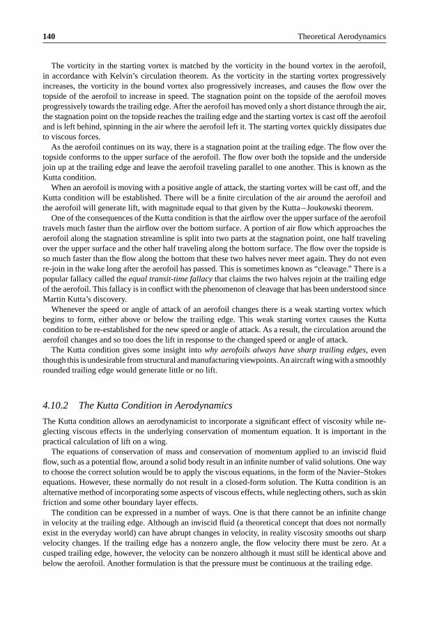
140 Theoretical Aerodynamics
The vorticity in the starting vortex is matched by the vorticity in the bound vortex in the aerofoil,in accordance with Kelvin’s circulation theorem. As the vorticity in the starting vortex progressivelyincreases, the vorticity in the bound vortex also progressively increases, and causes the flow over thetopside of the aerofoil to increase in speed. The stagnation point on the topside of the aerofoil movesprogressively towards the trailing edge. After the aerofoil has moved only a short distance through the air,the stagnation point on the topside reaches the trailing edge and the starting vortex is cast off the aerofoiland is left behind, spinning in the air where the aerofoil left it. The starting vortex quickly dissipates dueto viscous forces.
As the aerofoil continues on its way, there is a stagnation point at the trailing edge. The flow over thetopside conforms to the upper surface of the aerofoil. The flow over both the topside and the undersidejoin up at the trailing edge and leave the aerofoil traveling parallel to one another. This is known as theKutta condition.
When an aerofoil is moving with a positive angle of attack, the starting vortex will be cast off, and theKutta condition will be established. There will be a finite circulation of the air around the aerofoil andthe aerofoil will generate lift, with magnitude equal to that given by the Kutta−Joukowski theorem.
One of the consequences of the Kutta condition is that the airflow over the upper surface of the aerofoiltravels much faster than the airflow over the bottom surface. A portion of air flow which approaches theaerofoil along the stagnation streamline is split into two parts at the stagnation point, one half travelingover the upper surface and the other half traveling along the bottom surface. The flow over the topside isso much faster than the flow along the bottom that these two halves never meet again. They do not evenre-join in the wake long after the aerofoil has passed. This is sometimes known as “cleavage.” There is apopular fallacy called the equal transit-time fallacy that claims the two halves rejoin at the trailing edgeof the aerofoil. This fallacy is in conflict with the phenomenon of cleavage that has been understood sinceMartin Kutta’s discovery.
Whenever the speed or angle of attack of an aerofoil changes there is a weak starting vortex whichbegins to form, either above or below the trailing edge. This weak starting vortex causes the Kuttacondition to be re-established for the new speed or angle of attack. As a result, the circulation around theaerofoil changes and so too does the lift in response to the changed speed or angle of attack.
The Kutta condition gives some insight into why aerofoils always have sharp trailing edges, eventhough this is undesirable from structural and manufacturing viewpoints. An aircraft wing with a smoothlyrounded trailing edge would generate little or no lift.
4.10.2 The Kutta Condition in Aerodynamics
The Kutta condition allows an aerodynamicist to incorporate a significant effect of viscosity while ne-glecting viscous effects in the underlying conservation of momentum equation. It is important in thepractical calculation of lift on a wing.
The equations of conservation of mass and conservation of momentum applied to an inviscid fluidflow, such as a potential flow, around a solid body result in an infinite number of valid solutions. One wayto choose the correct solution would be to apply the viscous equations, in the form of the Navier–Stokesequations. However, these normally do not result in a closed-form solution. The Kutta condition is analternative method of incorporating some aspects of viscous effects, while neglecting others, such as skinfriction and some other boundary layer effects.
The condition can be expressed in a number of ways. One is that there cannot be an infinite changein velocity at the trailing edge. Although an inviscid fluid (a theoretical concept that does not normallyexist in the everyday world) can have abrupt changes in velocity, in reality viscosity smooths out sharpvelocity changes. If the trailing edge has a nonzero angle, the flow velocity there must be zero. At acusped trailing edge, however, the velocity can be nonzero although it must still be identical above andbelow the aerofoil. Another formulation is that the pressure must be continuous at the trailing edge.

Transformation of Flow Pattern 141
The Kutta condition does not apply to unsteady flow. Experimental observations show that the stag-nation point (one of two points on the surface of an aerofoil where the flow speed is zero) begins on thetop surface of an aerofoil (assuming positive effective angle of attack) as flow accelerates from zero, andmoves backwards as the flow accelerates. Once the initial transient effects have died out, the stagnationpoint is at the trailing edge as required by the Kutta condition.
Mathematically, the Kutta condition enforces a specific choice among the infinite allowed values ofcirculation.
4.11 Lift of Joukowski Aerofoil Section
Joukowski hypothesis directly relates the lift generated by a two-dimensional aerofoil to its incidence,as well as indicates the significance of the thickness to chord ratio and camber of the aerofoil in the liftgeneration.
We know that, applying the Joukowski transformation, ζ = z + b2/z, to an offset circle, as shown inFigure 4.14(a), a cambered aerofoil shape can be obtained, as illustrated in Figure 4.14(b).
If the remaining streamlines of the flow around the circle, in the physical plane, are also transformed,they will be distorted in the transformed plane to the shape of the streamlines around the aerofoil, asshown in Figure 4.14(b).
If the freestream flow approaches the circle at some angle of incidence α, as shown in Figure 4.15(a),but continue to transform about the original axes, the corresponding flow around the transformed aerofoil,in the ζ-plane, will be as shown in Figure 4.15(b).
ζ = z +b2
z
ξS2S2 c S1
xo
S1
iηiy
(a) z-plane (b) ζ-plane
Figure 4.14 Streamline pattern around (a) a circle in the z-plane, and (b) an aerofoil in the ζ-plane.
o
(b) ζ-plane
ζ = z +b2
z
α
ξc
iyiη
x
(a) z-plane
S2
S1
S2
α
S1
Figure 4.15 Streamline pattern of a freestream flow at some incidence α around (a) a circle in the z-plane, and (b)the corresponding flow around the transformed aerofoil in the ζ-plane.

142 Theoretical Aerodynamics
ζ = z + b2
z
(a) z-plane (b) ζ-plane
iy iη
Γ
ξNo
V∞
x
α
c θ
Γ
V∞
M
S1
αm
n
S2
S1S2
Figure 4.16 Streamline pattern of a freestream flow and circulation around (a) a circle in the z-plane, and (b) thecorresponding flow around the transformed aerofoil in the ζ-plane.
This flow (regime) around the aerofoil is not sustained, although it is initiated every time an aerofoilstarts moving from rest.
In practice, the generation of starting vortex shifts (dips) the rear stagnation point S2 to the trailingedge, that is to point M, shown in Figure 4.16(b). As the flow process develops, which takes place veryquickly, the circulation around the aerofoil section is generated and the aerofoil experiences lift.
In the z-plane, the rear stagnation pointS2 on the circle must have now been depressed to the correspond-ing point m to the trailing edge, as shown in Figure 4.16(a). In the transformed plane, the correspondingrear stagnation point S2 of the aerofoil is dipped to point M, as shown in Figure 4.16(b). This depressionof the stagnation point enables the evaluation of the magnitude of the circulation.
At the same time, because of the circulation �, the forward stagnation point S1 on the circle wouldhave been depressed by a corresponding amount to point n. The angular displacement being (α + β), asillustrated in Figure 4.17.
In Figure 4.17, by geometry, angle subtended by ∠S2cm = ∠S1cn = (α + β). The velocity at anypoint p on the circle, with θc measured from the diameter S2cS1, given by Equation (2.51), is:
Vc = 2V∞ sin θc + �
2πa,
α
θc
iy
S2
m
p
Γ
V∞
c
α + βn
α + β
xS1
oβ
Figure 4.17 Depression of stagnation points.

Transformation of Flow Pattern 143
where a is the radius of the circle, V∞ is the freestream velocity and � is the circulation. At point n thevelocity is zero and θc = −(α + β). Therefore, at n:
Vc = 0 = 2V∞ sin [−(α + β)] + �
2πa.
This gives the circulation as:
� = 4πV∞a sin (α + β).
Therefore, the velocity becomes:
Vc = 2V∞ sin θc + 4πV∞a sin (α + β)
2πa.
This simplifies to:
Vc = 2V∞[sin θc + sin (α + β)] (4.11)
The lift per unit span is:
L = ρV∞�
= ρV∞4πV∞a sin (α + β)
= 4πρV 2∞a sin (α + β).
The lift can also be expressed as:
L = 1
2ρV 2
∞SCL,
where CL is the lift coefficient and S is the projected area of the wing planform, normal to the directionof freestream flow. The area S is given by:
S = span × chord.
The chord of the profile is 4b. Therefore, the area of the profile, per unit span, becomes S = 4b. Thus,the lift is:
L = 1
2ρV 2
∞4b CL
= 2ρV 2∞b CL.
Equating the above two expressions for lift, we get the lift coefficient as:
CL = 2πa
bsin (α + β).
But,
a/b = (1 + e).
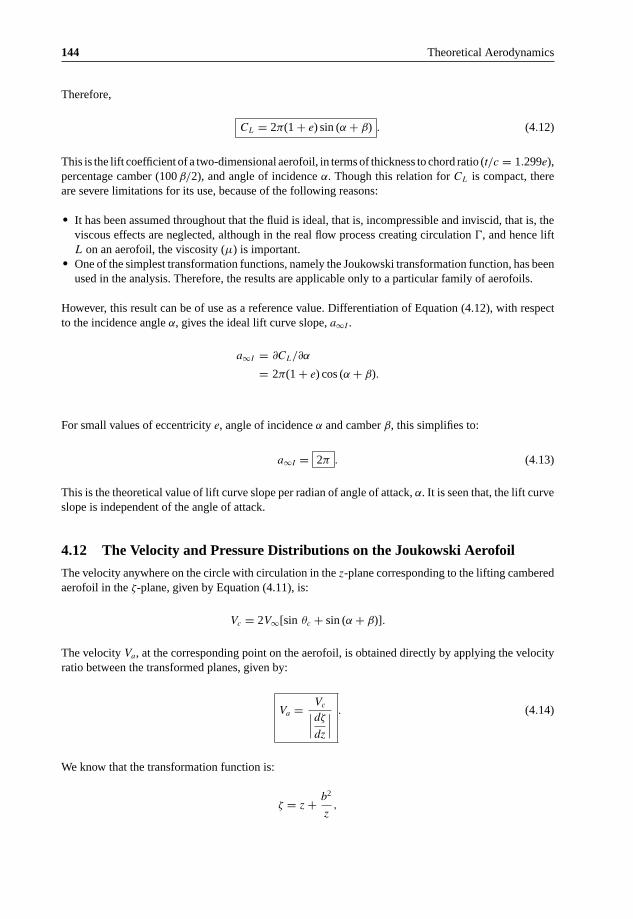
144 Theoretical Aerodynamics
Therefore,
CL = 2π(1 + e) sin (α + β) . (4.12)
This is the lift coefficient of a two-dimensional aerofoil, in terms of thickness to chord ratio (t/c = 1.299e),percentage camber (100 β/2), and angle of incidence α. Though this relation for CL is compact, thereare severe limitations for its use, because of the following reasons:
• It has been assumed throughout that the fluid is ideal, that is, incompressible and inviscid, that is, theviscous effects are neglected, although in the real flow process creating circulation �, and hence liftL on an aerofoil, the viscosity (μ) is important.
• One of the simplest transformation functions, namely the Joukowski transformation function, has beenused in the analysis. Therefore, the results are applicable only to a particular family of aerofoils.
However, this result can be of use as a reference value. Differentiation of Equation (4.12), with respectto the incidence angle α, gives the ideal lift curve slope, a∞I .
a∞I = ∂CL/∂α
= 2π(1 + e) cos (α + β).
For small values of eccentricity e, angle of incidence α and camber β, this simplifies to:
a∞I = 2π . (4.13)
This is the theoretical value of lift curve slope per radian of angle of attack, α. It is seen that, the lift curveslope is independent of the angle of attack.
4.12 The Velocity and Pressure Distributions on the Joukowski Aerofoil
The velocity anywhere on the circle with circulation in the z-plane corresponding to the lifting camberedaerofoil in the ζ-plane, given by Equation (4.11), is:
Vc = 2V∞[sin θc + sin (α + β)].
The velocity Va, at the corresponding point on the aerofoil, is obtained directly by applying the velocityratio between the transformed planes, given by:
Va = Vc∣∣∣dζ
dz
∣∣∣. (4.14)
We know that the transformation function is:
ζ = z + b2
z,

Transformation of Flow Pattern 145
where b is a constant. Therefore:
dζ
dz= 1 − b2
z2.
Replacing z with reiθ , we get:
dζ
dz= 1 − b2
r2e−2iθ
= 1 − b2
r2(cos 2θ − i sin 2θ)
∣∣∣dζ
dz
∣∣∣ =[(
1 − b2
r2cos 2θ
)2
+(
b2
r2sin 2θ
)2]1/2
=[
1 − 2b2
r2cos 2θ + b4
r4
]1/2
.
Hence:
Va = Vc[1 − 2b2
r2cos 2θ + b4
r4
]1/2
= 2V∞[sin θc + sin (α + β)][1 − 2b2
r2cos 2θ + b4
r4
]1/2 .
We have r/b, (Figure 4.9), as:
r
b= 1 + e + e cos θ + β sin θ.
Substituting this, further simplification can be made. The resulting equation is compact for obtaining thevelocity distribution around the aerofoil profile. However, the velocity appears as square in the pressurecoefficient, Cp, expression, which implies that, computing the pressure coefficient is a tedious process.The approximation that the eccentricity e is very small compared to unity (e � 1) progressively becomesunrealistic when thicker and more cambered aerofoil sections are required. Use of this approximation isjustified only when they produce significant simplification at the expense of acceptable small deviationsfrom the exact solutions of the velocity and pressure distributions around the aerofoil profile generated.In the present case, the utility of the approximate method largely ceases after the expressions for ξ andη, for the profile:
ξ = 2b cos θ
η = 2be(1 + cos θ) sin θ + 2bβ sin2 θ.
have been obtained. For obtaining velocity and pressure distribution numerical solution may be employed.

146 Theoretical Aerodynamics
4.13 The Exact Joukowski Transformation Process and Its NumericalSolution
The coordinates of the transformed aerofoil profile are obtained as follows. The transformation functioncan be expressed:
ζ = z + b2
z
ξ + iη = x + iy + b2
x + iy
= (x + iy)2 + b2
x + iy.
Dividing and multiplying the numerator and denominator, on the right-hand side, by (x − iy), we get:
ξ + iη = (x + iy)2(x − iy) + b2(x − iy)
(x + iy)(x − iy)
= (x2 + 2ixy − y2)(x − iy) + b2(x − iy)
x2 + y2
= x[(x2 + y2) + b2] + iy[(x2 + y2) − b2]
x2 + y2
= x
(1 + b2
x2 + y2
)+ iy
(1 − b2
x2 + y2
).
Comparing the real and imaginary parts, we get the coordinates of the aerofoil sections as:
ξ = x
(1 + b2
x2 + y2
)(4.15a)
η = y
(1 − b2
x2 + y2
). (4.15b)
Referring to Figures 4.8 and 4.9, we have the distance op of point p from the origin in the z-plane, as:
op = r = be cos θ + h sin θ + a cos γ.
The x and y coordinates of point p are:
x = a cos θ′ + be
y = a sin θ′ + bβ(1 + e).
With a = (b + be), the above coordinate expressions become:
x = (b + be) cos θ′ + be, (4.16a)
y = (b + be) sin θ′ + bβ(1 + e). (4.16b)

Transformation of Flow Pattern 147
where e and β represent the thickness and camber of a given aerofoil, respectively. Therefore, the valuesof x and y can be found for the given values of θ′, round the circle, from 0 to 2π. Substituting these x
and y in to Equations (4.15a) and (4.15b), the aerofoil coordinates ξ and η can be obtained.This method may be used with both singularities within the circle, when:
x = a cos θ′ + be
a = b (1 + e)
e � 1.
4.14 The Velocity and Pressure Distribution
For finding the velocity distribution around a given aerofoil, it is necessary to relate the angle of incidenceα to the circulation � around the aerofoil. This is done by applying the Joukowski hypothesis. In reality,the full Joukowski circulation required to bring the rear stagnation point to the trailing edge is not realized,because of the following:
• Air is a viscous fluid, and the flow near the trailing edge of an aerofoil is modified by the presence ofthe boundary layer and wake, caused by the viscosity.
• The zero thickness for the trailing edge, stipulated by the Joukowski hypothesis, is not possible inpractice. Therefore, the trailing edge must be rounded to some degree of curvature. The finite thicknessof the trailing edge owing to this rounding-off forces the rear stagnation point to deviate from theposition given in the ideal case.
Therefore, if � is the full Joukowski circulation (theoretical circulation), it can be assumed that thepractical value of circulation is only k�, where k is less than unity.
The velocity Vc, anywhere on the circle, given by Equation (4.11), is:
Vc = 2V∞ sin θc + �
2πa.
But the practical value of circulation is k�, therefore:
Vc = 2V∞ sin θc + k�
2πa
Vc
V∞= 2 sin θc + k�
2πaV∞.
Substituting � = 4πV∞a sin (α + β), we get:
Vc
V∞= 2 sin θc + k4πV∞a sin (α + β)
2πaV∞
= 2 sin θc + 2k sin (α + β)
or
Vc
V∞= 2 [sin θc + k sin (α + β)] .

148 Theoretical Aerodynamics
The velocity Va at corresponding points on the transformed aerofoil can be found by using the relation,Equation (4.14):
Va
Vc
= 1∣∣∣dζ
dz
∣∣∣.
The Joukowski transformation function is:
ζ = z + b2
z.
Differentiating with respect to z, we get:
dζ
dz= 1 − b2
z2.
But z = x + iy. Therefore:
dζ
dz= 1 − b2
z2
= 1 − b2
(x + iy)2
= (x + iy)2 − b2
(x + iy)2
= (x + iy)2(x − iy)2 − b2(x − iy)2
(x + iy)2(x − iy)2
= [(x + iy)(x − iy)]2 − b2(x − iy)2
[(x + iy)(x − iy)]2
= (x2 + y2)2 − b2(x2 − y2 − 2ixy)
(x2 + y2)2
=[
1 − b2(x2 − y2)
(x2 + y2)2
]+ i
[2b2xy
(x2 + y2)2
]
= A + iB,
where
A =[
1 − b2(x2 − y2)
(x2 + y2)2
]
and
B =[
2b2xy
(x2 + y2)2
].
Therefore,
∣∣∣dζ
dz
∣∣∣ =√
A2 + B2.

Transformation of Flow Pattern 149
Thus, the velocity on the aerofoil becomes:
Va = Vc√A2 + B2
.
Dividing both sides by the freestream velocity V∞, we get:
Va
V∞= Vc/V∞√
A2 + B2.
Substituting for Vc/V∞, we have:
Va
V∞= 2[sin θc + k sin (α + β)]√
A2 + B2.
Now, it is easy to obtain Va/V∞, for different values of θ′, since θc = (θ′ + α).Substituting this, the velocity on the aerofoil becomes:
Va
V∞= 2[sin (θ′ + α) + k sin (α + β)]√
A2 + B2. (4.17)
For incompressible flow, the pressure coefficient is given by:
Cp = p − p∞1
2ρV 2
∞
= 1 −(
Va
V∞
)2
. (4.18)
Knowing the distribution of Va/V∞, over the aerofoil, from Equation (4.17), the pressure coefficientaround the aerofoil can be estimated.
Note that, with Equations (4.14), (4.15) and (4.17), the aerofoil shape, the velocity around it, and the Cp
distribution around it can be computed, for the given values of b and e.
Example 4.5
For an aerofoil with b = 100 mm, e = 1/10 and (a) k = 1.0 and (b) k = 0.95, kept at α = 5◦, determinethe velocity and pressure around the transformed aerofoil.
Solution
The aerofoil shape, the streamline pattern over the profile and the pressure coefficient variation aroundit, for the values b, e and α, listed in the problem were computed for � = 1.0 and 0.95, with the routinegiven below. The results are given in Figures 4.18(a)–(d).
For � = 1, the aerofoil shape, the streamlines and the pressure coefficient distribution around the aerofoilare shown in Figure 4.18(a). It is interesting to note that the flow leaving the aerofoil, at the trailingedge, is smooth and there is no wake, in accordance with Joukowski’s hypothesis. The Cp distribution

150 Theoretical Aerodynamics
(a)
(b)
Figure 4.18 (a) Aerofoil shape, the streamline pattern over the profile and the pressure coefficient variation aroundit, (b) Cp distribution over the aerofoil for � = 1 and (c) the streamline pattern over the profile and the pressurecoefficient variation around it, (d) Cp distribution over the aerofoil for � = 0.95.

Transformation of Flow Pattern 151
(c)
(d)
Figure 4.18 (Continued)
around the aerofoil, shown in Figure 4.18(b), clearly illustrates the higher pressure at the bottom and thelower pressure at the top of the profile, causing lift.
The streamlines and Cp variation around the aerofoil, for � = 0.95 are shown in Figures 4.18(c) and4.18(d), respectively. It is seen that, when � is less than 1, the rear stagnation point is upstream of the

152 Theoretical Aerodynamics
trailing edge, and there is a narrow wake. With decrease of �, the wake width will increase, leading tohigher drag.
The routine for calculating the aerofoil shape, the streamlines and the pressure distribution around itis given below:
Program maincc----------------(1) Parameter Settingsc Number of Grid Pointsc MX: number of points along the aerofoil surfacec MY: number of points in the directionc perpendicular to the aerofoil surface
parameter(mx = 501, my = 301)cc----------------(2) Variablesc z0 : Center of a Cylinderc z, zeta : Grid Meshc w : Complex potentialc dwdz : dw/dzc dwdzet : dw/dzetac theta, betac : angle [radians]c alpha : Attack angle [radians]c Uinf : flow speedc Gamma : Circulationc zetaLe : xi-coordinate of leading edgec zetaTe : xi-coordinate of trailing edgec chord : Chord length of the aerofoilc a : Cylinder Radiusc b, c : Parameters for Cylinder Geometryc ClAf : Lift coefficient of Airfoilc Cl2dfp : Lift coefficient of 2-dimensional flat platec CpCyl : Pressure coefficient of the cylinderc CpAf : Pressure coefficient of the aerofoilc cK : Constant s.t. Gamma = 4*pi*Uinf*sin(alpha+beta)*cKc
complex z0, z, zeta, w, dwdz, dwdzet, uIdimension z(mx,my), zeta(mx,my)dimension w(mx,my), dwdz(mx,my), dwdzet(mx,my)dimension theta(mx)dimension CpCyl(mx,my), CpAf(mx,my)
c *** pi = 3.1415... = 4 x arctan 1pi = 4.0 * atan(1.0)
c --- uI = imaginary unituI = cmplx(0.0, 1.0)
cc----------------(3) Set Calc. Conditions and Parameters
z0 = cmplx(-10.0, 0.95)c = 400.0alpha = 5.0Uinf = 1.0cK = 1.0b = c / 4.0
c *** cylinder radius
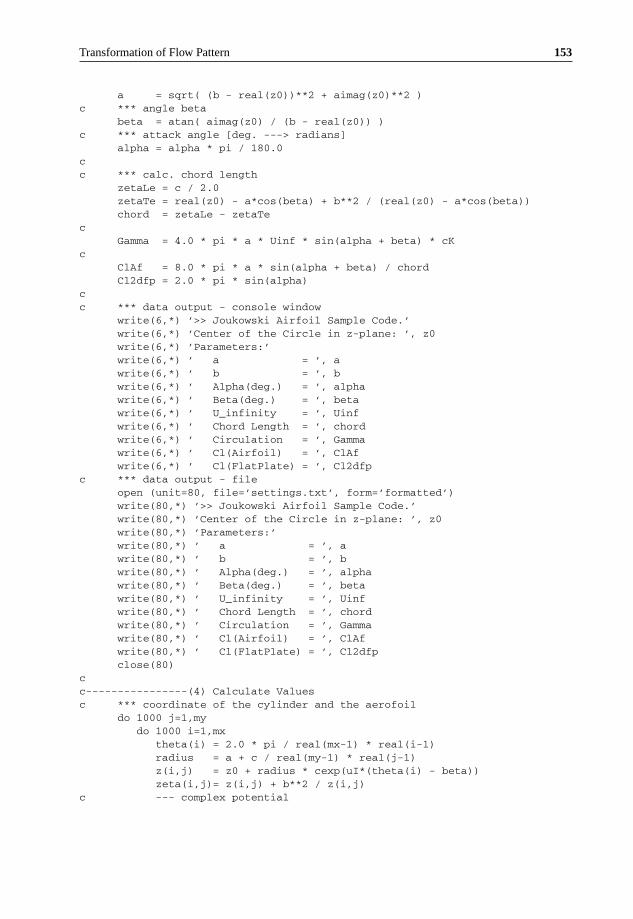
Transformation of Flow Pattern 153
a = sqrt( (b - real(z0))**2 + aimag(z0)**2 )c *** angle beta
beta = atan( aimag(z0) / (b - real(z0)) )c *** attack angle [deg. ---> radians]
alpha = alpha * pi / 180.0cc *** calc. chord length
zetaLe = c / 2.0zetaTe = real(z0) - a*cos(beta) + b**2 / (real(z0) - a*cos(beta))chord = zetaLe - zetaTe
cGamma = 4.0 * pi * a * Uinf * sin(alpha + beta) * cK
cClAf = 8.0 * pi * a * sin(alpha + beta) / chordCl2dfp = 2.0 * pi * sin(alpha)
cc *** data output - console window
write(6,*) ’>> Joukowski Airfoil Sample Code.’write(6,*) ’Center of the Circle in z-plane: ’, z0write(6,*) ’Parameters:’write(6,*) ’ a = ’, awrite(6,*) ’ b = ’, bwrite(6,*) ’ Alpha(deg.) = ’, alphawrite(6,*) ’ Beta(deg.) = ’, betawrite(6,*) ’ U_infinity = ’, Uinfwrite(6,*) ’ Chord Length = ’, chordwrite(6,*) ’ Circulation = ’, Gammawrite(6,*) ’ Cl(Airfoil) = ’, ClAfwrite(6,*) ’ Cl(FlatPlate) = ’, Cl2dfp
c *** data output - fileopen (unit=80, file=’settings.txt’, form=’formatted’)write(80,*) ’>> Joukowski Airfoil Sample Code.’write(80,*) ’Center of the Circle in z-plane: ’, z0write(80,*) ’Parameters:’write(80,*) ’ a = ’, awrite(80,*) ’ b = ’, bwrite(80,*) ’ Alpha(deg.) = ’, alphawrite(80,*) ’ Beta(deg.) = ’, betawrite(80,*) ’ U_infinity = ’, Uinfwrite(80,*) ’ Chord Length = ’, chordwrite(80,*) ’ Circulation = ’, Gammawrite(80,*) ’ Cl(Airfoil) = ’, ClAfwrite(80,*) ’ Cl(FlatPlate) = ’, Cl2dfpclose(80)
cc----------------(4) Calculate Valuesc *** coordinate of the cylinder and the aerofoil
do 1000 j=1,mydo 1000 i=1,mx
theta(i) = 2.0 * pi / real(mx-1) * real(i-1)radius = a + c / real(my-1) * real(j-1)z(i,j) = z0 + radius * cexp(uI*(theta(i) - beta))zeta(i,j)= z(i,j) + b**2 / z(i,j)
c --- complex potential

154 Theoretical Aerodynamics
w(i,j) = Uinf * (z(i,j) - z0) * cexp(-uI*alpha)& + Uinf * a**2 / ((z(i,j) - z0) * cexp(-uI*alpha))& + uI * Gamma / (2.0*pi)
c & * clog((z(i,j)-z0)*cexp(-uI*alpha))& * (clog((z(i,j)-z0) * cexp(-uI*alpha)& * cexp(uI*(pi+alpha+beta)))-(pi+alpha+beta))
c --- dw/dzdwdz(i,j)= Uinf * (cexp(-uI*alpha) - a**2/((z(i,j) - z0)**2
& * exp(-uI*alpha)))& + uI * Gamma / (2.0 * pi * (z(i,j) - z0))
c --- dw/dzetadwdzet(i,j) = dwdz(i,j) / (1.0 - b**2 / z(i,j)**2)
c --- Pressure CoefficientCpCyl(i,j) = 1.0 - cabs(dwdz(i,j))**2 / Uinf**2CpAf(i,j) = 1.0 - cabs(dwdzet(i,j))**2 / Uinf**2
1000 continuecc----------------(5) Output Result Filesc * Following files are written in TECPLOT format.c *** Cylinder - Shape
open (unit=81,file=’CylinderShape.plt’,form=’formatted’)write(81,*) ’TITLE="Cylinder Shape and Surface Pressure Coeff."’write(81,*) ’VARIABLES="X","Y","Cp"’write(81,*) ’ZONE T="Cylinder",I=’,mx,’,F=POINT’do 2000 i=1,mx
write(81,*) real(z(i,1)),’ ’,aimag(z(i,1)),’ ’,CpCyl(i,1)2000 continue
close(81)cc *** Cylinder - Entire Domain
open (unit=82,file=’Cylinder.plt’,form=’formatted’)write(82,*) ’TITLE="Cylinder in z-plane"’write(82,*) ’VARIABLES="X","Y","U","V","Cp","phi","psi"’write(82,*) ’ZONE T="Cylinder",I=’,mx,’,J=’,my,’,F=POINT’do 3000 j=1,my
do 3000 i=1,mxwrite(82,*) real(z(i,j)),’ ’,aimag(z(i,j)),’ ’,
& real(dwdz(i,j)),’ ’,aimag(-dwdz(i,j)),’ ’,CpCyl(i,j),& ’ ’,real(w(i,j)),’ ’,aimag(w(i,j))
3000 continueclose(82)
cc *** Airfoil - Shape
open (unit=83,file=’AirfoilShape.plt’,form=’formatted’)write(83,*) ’TITLE="Airfoil Shape and Surface Pressure Coeff."’write(83,*) ’VARIABLES="Xi","Eta","Cp"’write(83,*) ’ZONE T="Airfoil",I=’,mx-1,’,F=POINT’do 4000 i=2,mx
write(83,*) real(zeta(i,1)),’ ’,aimag(zeta(i,1)),’ ’,CpAf(i,1)4000 continue
close(83)cc *** Airfoil - Entire Domain
open (unit=84,file=’Airfoil.plt’,form=’formatted’)

Transformation of Flow Pattern 155
write(84,*) ’TITLE="Airfoil in zeta-plane"’write(84,*) ’VARIABLES="Xi","Eta","U","V","Cp","phi","psi"’write(84,*) ’ZONE T="Airfoil",I=’,mx,’,J=’,my-1,’,F=POINT’do 5000 j=2,my
do 5000 i=1,mxwrite(84,*) real(zeta(i,j)),’ ’,aimag(zeta(i,j)),’ ’,
& real(dwdzet(i,j)),’ ’,aimag(-dwdzet(i,j)),’ ’,CpAf(i,j),& ’ ’,real(w(i,j)),’ ’,aimag(w(i,j))
5000 continueclose(84)
cstopend
c
4.15 Aerofoil Characteristics
We saw that aerofoil is a streamlined body that would experience the largest value of lift-to-drag ratio, in agiven flow, compared to any other body in the same flow. In other words, in a given flow the aerodynamicefficiency (L/D) of an aerofoil will be the maximum. When an aerofoil is exposed to a flow, due to the pres-sure acting normal to the body surface and the shear force, due to viscosity, acting tangential to the bodysurface, normal and tangential forces, respectively, would act on the aerofoil, as illustrated in Figure 4.19.
The pressure and shear forces can be integrated over the surface of the aerofoil to obtain the resultantaerodynamic force, Fad, which acts at the center of pressure (kcp) of the aerofoil.
The forces acting on an aircraft in level flight are the lift L, drag D, thrust T and weight W , as shownin Figure 4.20.
In the xz-plane or pitch plane shown in Figure 4.20, the body-oriented components are the axialforces (A), which are the forces parallel to the aircraft axis, and the normal forces (N), which are
Pressure force
Shear forcePressure force
Shear force
Pressure force
Shear force
Pressure forceShear force
Figure 4.19 Normal and shear forces acting on an aerofoil in a flow field.
A
W
LN
Tα
D
kcpV∞
α
cg
Figure 4.20 Forces acting in the pitch (xz) plane on an aircraft.

156 Theoretical Aerodynamics
Lt
W
Lwb
Figure 4.21 An aircraft in flight with lift acting ahead of cg.
perpendicular to the vehicle axis. As the aircraft travels in air, its motion is determined by its weight, thethrust produced by the engine, and the aerodynamic forces acting on the vehicle.
For a steady, unaccelerated level flight in a horizontal plane:
• The sum of the forces along the flight path is zero.• The sum of the forces perpendicular to the flight path is zero.
When the angle of incidence α is small, the component of thrust parallel to the freestream flow directionis only slightly less than the thrust itself. Therefore, for equilibrium:
L = W
T = D.
Let us consider the case where the lift generated by the wing-body configuration Lwb acts ahead of thecenter of gravity (cg), as shown in Figure 4.21.
The lift acting ahead of center of gravity will produce a nose-up (positive) moment about the centerof gravity. The aircraft is said to be trimmed, when the sum of the moments about the cg is zero, that is:
∑Mcg = 0 .
Thus, a force from a control surface located aft of the cg, for example, the horizontal tail surface Lt
is required to produce a nose-down (negative) pitching moment about the cg, which could balance thepositive moment produced by Lwb. The tail surface producing Lt also produces a drag force which isknown as the trim drag. The trim drag may vary from 0.5% to 5% of the total drag of the aircraft. It isessential to note that in addition to trim drag, the tail also produces drag due to the pressure and shearacting on its geometry, known as profile drag. Thus the trim drag is that associated with Lt generated totrim the vehicle.
In addition to the lift and drag acting in the pitch or xz-plane, there is a side force acting on the aircraft.The side force is the component of force in the direction perpendicular to both the lift and the drag. Theside force acting towards the starboard (right) wing is referred to as positive.
Usually the aerodynamic force will not act through the cg (which is also taken as the origin of theairplane’s axis system). The moment due to the resultant force acts at a distance from the origin maybe divided into three components, referred to the airplane’s axes. The three moment components are thepitching moment M, the rolling moment L and the yawing moment N, as shown in Figure 4.22.
As illustrated in Figure 4.22:
• Pitching moment is the moment acting about the lateral axis (y-axis). It is the moment due to the liftand drag acting on the aircraft. Pitching moment causing nose-up is regarded as positive.

Transformation of Flow Pattern 157
Yawing
Pitchingmoment M
Rolling
Lateral
z
xLongitunial
Vertical
axis
axis
axis
moment L
moment N
y
cg
Figure 4.22 Illustration of pitching, rolling and yawing moments acting on an aircraft.
• Rolling moment is the moment acting about the longitudinal axis (x-axis) of the aircraft. Rollingmoment is generated by a differential lift generated by the ailerons, located closer to the wingtips.Rolling moment causing the right (starboard) wingtip to move downward is regarded as positive.
• Yawing moment is the moment acting about the vertical (z-axis) of the aircraft. Yawing moment tendsto rotate the aircraft nose to the right is regarded positive.
4.15.1 Parameters Governing the Aerodynamic Forces
The primary parameters governing the magnitude of the aerodynamic forces and moments are thefollowing:
• Geometry of the aerofoil.• Angle of attack, namely the aircraft attitude in the pitch (xz) plane relative to the flight direction.• Vehicle size.• Freestream velocity.• Freestream flow density.• Reynolds number (viscous effects).• Mach number (compressibility effects).
4.16 Aerofoil Geometry
The geometrical section of a wing obtained by cutting it by a vertical plane parallel to the centerline ofthe aircraft is called aerofoil section. The lift generated and the stall characteristics of a wing stronglydepends on the geometry of the aerofoil sections that make up the wing. The geometric parameters thatdictate the aerodynamic characteristics of the aerofoil section are; the leading-edge radius, the meancamber line, the maximum thickness and the thickness distribution of the profile, and the trailing-edgeangle. These parameters are shown in Figure 4.23.
4.16.1 Aerofoil Nomenclature
The tests made at Gottingen during World War I contributed significantly to the development of moderntypes of wing sections. Up to about World War II, most wing sections in common use were derived mostlyfrom the work at Gottingen. During this period many families of wing sections were tested in the labora-tories of various countries, but the work of the National Advisory Committee for Aeronautics (NACA)

158 Theoretical Aerodynamics
Lower surface
Trailing edge
Thickness
V∞
Upper surface
α
Leading edge radius
Mean camber line
Camber
Chord
(Trailing edge)
Maximum thickness
location
x
Maximum camber
location
x = cx = 0
z
(Leading edge)
Figure 4.23 Geometrical parameters of an aerofoil.
was outstanding. The NACA investigations were further refined by separation of the effects of camber andthickness distribution, and the experimental work was performed at higher Reynolds number than weregenerally obtained elsewhere. As a result, the geometry of many aerofoil sections is uniquely defined bythe NACA designation for the aerofoil.
Aerofoil geometry are usually characterized by the coordinates of the upper and lower surface. It isoften summarized by a few parameters such as: maximum thickness, maximum camber, position of maxthickness, position of max camber, and nose radius (see Figure 4.23). One can generate a reasonableaerofoil section given these parameters. This was done by Eastman Jacobs in the early 1930s to createa family of aerofoils known as the NACA Sections. The NACA aerofoils are aerofoil shapes for aircraftwings developed by the National Advisory Committee for Aeronautics (NACA). The shape of the NACAaerofoils is described using a series of digits following the word “NACA.”
The NACA 4-digit and 5-digit aerofoils were created by superimposing a simple mean-line shape witha thickness distribution that was obtained by fitting a couple of popular aerofoils of the time:
y = ±(t/0.2) × (0.2969 x0.5 − 0.126 x − 0.3537 x2 + 0.2843 x3 − 0.1015 x4).
The camber-line of 4-digit sections was defined as a parabola from the leading edge to the position ofmaximum camber, then another parabola back to the trailing edge, as illustrated in Figure 4.24.
Parabola
Meanline
Leading edge
Chord
xc
yc
Parabola
Figure 4.24 Illustration of the camber line of a 4-digit NACA aerofoil.

Transformation of Flow Pattern 159
NACA 4-Digit Series:
The first digit implies the maximum camber in percentage of chord (c), the second digit gives the positionof maximum camber in 1/10 of chord, the last two digits give the maximum thickness in percentage ofchord. For example:
1. NACA 4412 aerofoil has a maximum camber of 4% of chord, with the maximum camber located at0.4c and thickness-to-chord ratio 12%.
2. NACA 2412 aerofoil has a maximum camber of 2% located 40% (0.4c) from the leading edge witha maximum thickness of 12% of the chord. Four-digit series aerofoils by default have maximumthickness at 30% of the chord (0.3c) from the leading edge.
3. NACA 0015 aerofoil is symmetrical, the 00 indicating that it has no camber. The 15 indicates that theaerofoil has a 15% thickness to chord length ratio: it is 15% as thick as it is long.
After the 4-digit sections came the 5-digit sections such as the famous NACA 23012. These sections hadthe same thickness distribution, but used a camber-line with more curvature near the nose. A cubic wasfaired into a straight line for the 5-digit sections.
NACA 5-Digit Series:
In NACA 5-digit series the first digit gives approximate maximum camber in percentage of chord, thesecond and third digits give the position of maximum camber in 2/100 of chord and the last two digitsgive the maximum thickness in percentage of chord. This NACA 23012 is an aerofoil with maximumcamber as 2% of c, position of maximum camber at 60% of chord and t/c = 0.12.
Four- and five-digit series aerofoils can be modified with a two-digit code preceded by a hyphen inthe following sequence:
1. One digit describing the roundness of the leading edge with 0 being sharp, 6 being the same as theoriginal aerofoil, and larger values indicating a more rounded leading edge.
2. One digit describing the distance of maximum thickness from the leading edge in tens of percentageof the chord.
For example, the NACA 1234-05 is a NACA 1234 aerofoil with a sharp leading edge and maximumthickness as 50% of the chord (0.5 chords) from the leading edge.
In addition, for a more precise description of the aerofoil all numbers can be presented as decimals.
1-series:
A new approach to aerofoil design pioneered in the 1930s in which the aerofoil shape was mathematicallyderived from the desired lift characteristics. Prior to this, aerofoil shapes were first created and then hadtheir characteristics measured in a wind tunnel. The 1-series aerofoils are described by five digits in thefollowing sequence:
1. The number “1” indicating the series.2. One digit describing the distance of the minimum pressure area in tens of percent of chord.3. A hyphen.4. One digit describing the lift coefficient in tenths.5. Two digits describing the maximum thickness in percentage of chord.
For example, the NACA 16-123 aerofoil has minimum pressure 60% of the chord back with a liftcoefficient of 0.1 and maximum thickness of 23% of the chord.

160 Theoretical Aerodynamics
The 6-series of NACA aerofoils departed from this simply-defined family. These sections weregenerated from a more or less prescribed pressure distribution and were meant to achieve somelaminar flow.
NACA 6-Digit Series:
In NACA 6-digit series the first digit refers to the series, the second digit gives the location of minimumCp in 1/10 chord, the third digit gives the half width of low drag bucket in 1/10 of CL, the fourth digitgives the ideal CL in tenths of CL, the fifth and sixth digits give the max thickness in percentage of chord.
An improvement over 1-series aerofoils with emphasis on maximizing laminar flow. The aerofoil isdescribed using six digits in the following sequence:
1. The number “6” indicating the series.2. One digit describing the distance of the minimum pressure area in tens of percentage of chord.3. The subscript digit gives the range of lift coefficient in tenths above and below the design lift coefficient
in which favorable pressure gradients exist on both surfaces.4. A hyphen.5. One digit describing the design lift coefficient in tenths.6. Two digits describing the maximum thickness in tens of percentage of chord.
For example, the NACA 612-315 a = 0.5 has the area of minimum pressure 10% of the chord back,maintains low drag 0.2 above and below the lift coefficient of 0.3, has a maximum thickness of 15% ofthe chord, and maintains laminar flow over 50% of the chord.
After the six-series sections, aerofoil design became much more specialized for the particular appli-cation. Aerofoils with good transonic performance, good maximum lift capability, very thick sectionsand very low drag sections are now designed for each use. Often a wing design begins with the defi-nition of several aerofoil sections and then the entire geometry is modified based on its 3-dimensionalcharacteristics.
NACA 7-Digit Series:
Further advancement in maximizing laminar flow has been achieved by separately identifying the lowpressure zones on upper and lower surfaces of the aerofoil. The aerofoil is described by seven digits inthe following sequence:
1. The number “7” indicating the series.2. One digit describing the distance of the minimum pressure area on the upper surface in tens of
percentage of chord.3. One digit describing the distance of the minimum pressure area on the lower surface in tens of
percentage of chord.4. One letter referring to a standard profile from the earlier NACA series.5. One digit describing the lift coefficient in tenths.6. Two digits describing the maximum thickness in tens of percentage of chord.7. “a =” followed by a decimal number describing the fraction of chord over which laminar flow is
maintained. a = 1 is the default if no value is given.
For example, the NACA 712A315 has the area of minimum pressure 10% of the chord back on the uppersurface and 20% of the chord back on the lower surface, uses the standard “A” profile, has a lift coefficientof 0.3, and has a maximum thickness of 15% of the chord.

Transformation of Flow Pattern 161
NACA 8-Digit Series:
Eight digit series profiles are supercritical aerofoils designed to independently maximize airflow aboveand below the wing. The numbering is identical to the 7-series aerofoils except that the sequence beginswith an “8” to identify the series.
However, because of the rapid improvements in computer hardware and computer software, andbecause of the broad use of sophisticated numerical codes, we often encounter aerofoil sections beingdeveloped that are not described by the standard NACA geometries.
4.16.2 NASA Aerofoils
A concerted effort within the National Aeronautics and Space Administration (NASA) during the 1960sand 1970s was directed toward developing practical aerofoils with two-dimensional transonic turbulentflow and improved drag divergence Mach numbers while retaining acceptable low-speed maximumlift and stall characteristics and focused on a concept referred to as the supercritical aerofoil. Thisdistinctive aerofoil shape, based on the concept of local supersonic flow with isentropic recompression,was characterized by a large leading-edge radius, reduced curvature over the middle region of the uppersurface, and substantial aft camber.
The early phase of this effort was successful in significantly extending drag-rise Mach numbers beyondthose of conventional aerofoils such as the National Advisory Committee for Aeronautics (NACA)6-series aerofoils. These early supercritical aerofoils (denoted by the SC (phase 1) prefix), however,experienced a gradual increase in drag at Mach numbers just preceding drag divergence (referred to asdrag creep). This gradual buildup of drag was largely associated with an intermediate off-design secondvelocity peak (an acceleration of the flow over the rear upper-surface portion of the aerofoil just beforethe final recompression at the trailing edge) and relatively weak shock waves above the upper surface.
Improvements to these early, phase 1 aerofoils resulted in aerofoils with significantly reduced dragcreep characteristics. These early, phase 1 aerofoils and the improved phase 1 aerofoils were developedbefore adequate theoretical analysis codes were available and resulted from iterative contour modificationsduring wind-tunnel testing. The process consisted of evaluating experimental pressure distributions atdesign and off-design conditions and physically altering the aerofoil profiles to yield the best dragcharacteristics over a range of experimental test conditions.
The insight gained and the design guidelines that were recognized during these early phase 1 investi-gations, together with transonic, viscous, aerofoil analysis codes developed during the same time period,resulted in the design of a matrix of family-related supercritical aerofoils (denoted by the SC (phase 2)prefix). Specific details about these profiles can be found in Reference 1.
4.16.3 Leading-Edge Radius and Chord Line
The chord line is defined as the shortest (straight) line connecting the leading and trailing edges. Theleading edge of aerofoils used in subsonic applications is rounded, with a radius of about 1% of the chordlength. The leading edge of an aerofoil is the radius of a circle with its center on a line tangential tothe leading-edge camber connecting tangency points of the upper and lower surfaces with the leadingedge. The magnitude of the leading-edge radius has significant effect on the stall characteristics of theaerofoil section.
The geometrical angle of attackα is the angle between the chord line and the direction of the undisturbedfreestream.
4.16.4 Mean Camber Line
Mean camber line is the locus of the points midway between the upper and lower surfaces of the aerofoil. Inother words, mean camber line is the bisector of the aerofoil thickness. The shape of the mean camber line

162 Theoretical Aerodynamics
plays an important role in the determination of the aerodynamic characteristics of the aerofoil section. Oneof the primary effects of camber is to change the zero-lift angle of attack, α0l. For symmetrical aerofoils,zero lift is at α = 0 and for cambered aerofoils, zero lift is at negative α for positive camber and vice versa.
The camber has a beneficial effect on the maximum value of the section lift coefficient. If the maximumlift coefficient is high, the stall speed will be low, all other factors being the same. However, it is essentialto note that the high thickness and camber necessary for high maximum value of section lift coefficientproduce low critical Mach numbers at high twisting moments at high speeds.
4.16.5 Thickness Distribution
The thickness distribution and the maximum thickness strongly influence the aerodynamics characteristicsof the aerofoil section. The maximum local velocity to which a fluid element accelerates as it flows aroundan aerofoil increases as the maximum thickness increases, in accordance with the area–velocity relationfor subsonic flow. Thus the value of the minimum pressure is the smallest for the thickest aerofoil. Asa result, the adverse pressure gradient associated with the deceleration of the flow, from the location ofthis pressure minimum to the trailing edge, is greatest for the thick aerofoil. As the adverse pressuregradient become larger, the boundary layer becomes thicker. This thickening of boundary layer is likelyto cause flow separation, leading to large increase of form drag. Thus, the beneficial effects of increasingthe maximum thickness are limited.
For a thin aerofoil section, with relatively small leading-edge radius, boundary layer separation occursearly, not far from the leading edge of the upper (leeward) surface. Because of this, the maximum sectionlift coefficient for a thin aerofoil section is relatively small. The maximum section lift coefficient increasesas the thickness ratio increases.
The thickness distribution for an aerofoil affects the pressure distribution and the character of theboundary layer. As the location of the maximum thickness moves aft, the velocity gradient in the mid-chord region decreases. The favorable pressure gradient associated with this decrease of velocity gradientin the mid-chord region promotes the boundary layer stability and increases the possibility of boundarylayer remaining laminar. As we know, the skin friction drag associated with laminar boundary layer isless than that caused by turbulent boundary layer. Further thicker aerofoils benefit more from the use ofhigh-lift devices but have a lower critical Mach number.
4.16.6 Trailing-Edge Angle
The trailing-edge angle influences the location of the aerodynamic center; the point about which thesection moment coefficient is independent of angle of angle of attack, α. The aerodynamic center of thisaerofoil section in a subsonic flow is theoretically located at the quarter-chord point.
4.17 Wing Geometrical Parameters
Aircraft wings are made up of aerofoil sections, placed along the span. In an aircraft, the geometry of thehorizontal and vertical tails, high-lifting devices such as flaps on the wings and tails and control surfacessuch as ailerons are also made by placing the aerofoil sections in spanwise combinations.
The relevant parameters used to define the aerodynamic characteristics of a wing of rectangular,unswept trapezoidal, swept and delta configurations are illustrated in Figure 4.25.
Wing Area S
This is the plan surface area of the wing. Thus, the representative area of the wing may be regardedas the product of the span (2b) and the average chord (c). Although a portion of the area may be

Transformation of Flow Pattern 163
Swept wing Delta wing
2b2b
2b 2b
^c/4
c/4 line c/4 line
c/4lin
e
c/4
line ^c/4
^le
ct
c ct cr
cr
Rectangular wing Unswept, traperzoidal wing
Figure 4.25 Geometric parameters of some wing planforms.
covered by fuselage, the pressure distribution over the fuselage surface is accounted in the representativewing area.
Wing Span 2b
This is the distance between the tips of port and starboard wings.
Average Chord c
This is the geometric average of the chord distribution over the length of the wing span.
Aspect Ratio
Aspect ratio is the ratio of the span and the average chord. For a rectangular wing, the aspect ratio is:
= 2b
c.
For a nonrectangular wing:
= (2b)2
S.
The is a fineness ratio of the wing and it varies from 35 for sailplanes to about 2 for supersonic fighterplanes.
Root Chord cr
Root chord is the chord at the wing centerline, that is, at the middle of the span, as shown in Figure 4.25.The tip chord ct is the chord at the wing tip.

164 Theoretical Aerodynamics
Taper Ratio λ
Taper ratio is the ratio of the tip chord to root chord, for the wing planforms with straight leading andtrailing edges.
λ = ct
cr
.
The taper ratio affects the lift distribution of the wing. A rectangular wing has a taper ratio of 1.0 whilethe pointed tip delta wing has a taper ratio of 0.0.
Sweep Angle ∧Sweep angle is usually measured as the angle between the line of 25% chord and a perpendicular to theroot chord. The sweep of a wing affects the changes in maximum lift, the stall characteristics, and theeffects of compressibility.
Mean Aerodynamic Chord mac
Mean aerodynamic chord is an average chord which, when multiplied by the product of the averagesection moment coefficient, the dynamic pressure, and the wing area, gives the moment for the entirewing. The mean aerodynamic chord is given by:
mac = 1
S
∫ +b
−b
[c(y)]2dy.
Dihedral Angle
Dihedral angle is the angle between a horizontal plane containing the root chord and a plane midwaybetween the upper and lower surfaces of the wing. If the wing lies below the horizontal plane, it is termedas anhedral angle. The dihedral angle affects the lateral stability of the aircraft.
Geometric Twist
Geometric twist defines the situation where the chord lines for the spanwise distribution of all the aerofoilsections do not lie in the same plane. Thus, there is a spanwise variation in the geometric angle of incidencefor the sections. The chord of the root section of the wing shown in Figure 4.26 is inclined at 4◦ relativeto the vehicle axis.
The chord at the wing tip, however, is parallel to the longitudinal axis of the vehicle. In this case, wherethe incidence of the aerofoil sections relative to the vehicle axis decrease toward the tip, the wing has a“wash-out.” The wings of most subsonic aircraft have wash-out to control the spanwise lift distributionand, hence, the boundary layer characteristics. If the angle of incidence increases toward wing tip, thewing has “wash-in.”
Example 4.6
For a wing with root chord 18 m, tip chord 3.5 m and span 25 m, calculate the wing area, aspect ratio,taper ratio and the mean aerodynamic chord.

Transformation of Flow Pattern 165
ct
Parallel to thevehicle longitudinal axis
c/4 (unswept)
y = 0
Vehicle longitudinal axis
cr
Figure 4.26 Unswept, tapered wing with geometric twist (wash-out).
Solution
Given, cr = 18 m, ct = 3.5 m, 2b = 25 m.
The average chord is:
c = cr + ct
2
= 18 + 3.5
2= 10.75 m.
Therefore, the wing area becomes:
S = 2b × c = 25 × 10.75
= 268.75 m2 .
The aspect ratio is:
= 2b
c= 25
10.75
= 2.33 .
The taper ratio is:
λ = ct
cr
= 3.5
18
= 0.194 .

166 Theoretical Aerodynamics
For calculating the mac, the expression for the chord as a function of the distance from the plane ofsymmetry is required. The required expression for the given wing is:
c(y) = cr + ct − cr
by
= 18 + 3.5 − 18
25/2y
= 18 − 1.16 y.
The mean aerodynamic chord becomes:
mac = 1
S
∫ +b
−b
[c(y)
]2dy
= 2
S
∫ b
0
[c(y)
]2dy
= 2
268.75
∫ 12.5
0
[18 − 1.16 y
]2dy
= 2
268.75
∫ 12.5
0
[324 − 41.76 y + 1.346 y2
]dy
= 2
268.75
[324 y − 41.76
y2
2+ 1.346
y3
3
]25
0
= 2
268.75× (4050 − 3262.5 + 876.3)
= 12.38 m .
4.18 Aerodynamic Force and Moment Coefficients
For thin aerofoils at low angle of attack, the lift results mainly from the pressure distribution (thatis, pressure forces), as shown in Figure 4.19. The shear forces due to viscosity acts primarily in thechordwise direction and contributes mainly to the drag. Therefore, we need to consider only the pressurecontributions, illustrated in Figure 4.27, to calculate the force in the z-direction.
Let us consider a wing section in a flow field, as shown in Figure 4.28. Let p be the pressure acting ona differential area (dxdy).
z
x
Figure 4.27 Pressure distribution over an aerofoil.

Transformation of Flow Pattern 167
dy
x
dx
p
zy
V∞
Figure 4.28 Pressure acting over an elemental surface area of a rectangular wing.
The pressure force component in the z-direction is:
dFz = p (dxdy). (4.19)
The net force in the z-direction acting over the entire wing surface (that is, over the upper and lowersurfaces) is given by:
Fz =∫∫
p (dxdy). (4.20)
But the resultant force in any direction due to a constant pressure over a closed surface is zero. Therefore:
∫∫p∞ (dxdy) = 0, (4.21)
where p∞ is the freestream pressure.Combining Equations (4.20) and (4.21), the resultant force component can be expressed as:
Fz =∫∫
(p − p∞) (dxdy) = 0. (4.22)
This equation can be nondimensionalized by a suitable reference force. For this, the product of freestreamdynamic pressure q∞, wing chord c and wing span 2b can be taken as the reference force. Thus dividingthe left-hand and right-hand sides of Equation (4.22) by q∞c2b, we have:
Fz
q∞c2b=
∫∫p − p∞
q∞d
(x
c
)d
(y
2b
).
But c × 2b = S and (p − p∞)/q∞ = Cp, therefore:
Fz
q∞S=
∫∫Cpd
(x
c
)d
(y
2b
). (4.23)
When the boundary layer is thin, the pressure distribution around the aerofoil can be regarded equivalentto that due to an inviscid flow. Thus, the pressure distribution is independent of Reynolds number and

168 Theoretical Aerodynamics
does not depend on whether the boundary layer is laminar or turbulent. When the boundary layer is thin,the pressure coefficient at a particular location on the surface, given by the coordinates (x/c, y/2b), isindependent of vehicle scale and of the flow conditions. Over a range of flow conditions for which thepressure coefficient is a unique function of the dimensionless coordinates (x/c, y/2b), the value of theintegral equation (4.23) depends only on the aerofoil geometry and the angle of attack. Thus, the resultingdimensionless force coefficient is independent of model scale and flow conditions.
A similar analysis can be used to calculate the lift coefficient, defined as:
CL = L
q∞S, (4.24)
where L is the lift and S is the wing planform area.In the same manner, lift coefficient per unit length of wing span, termed section lift coefficient can be
expressed as:
Cl = l
q∞c, (4.25)
where l is the lift per unit length of wing span and c is the chord length.Typical variation of section lift coefficient with angle of attack is shown in Figure 4.29.It has been experimentally verified that the section lift coefficient is a linear function of angle of attack
α from −10◦ to +10◦. The slope of the linear portion of the curve is called the two-dimensional lift curveslope. Theoretical value of two-dimensional lift curve slope is 2π, that is:
Cl,α = dCl
dα= 2π.
The section lift coefficient for a wing which experiences zero lift at α = 0 can be expressed as:
Cl = Cl,αα.
Cl
− 1.6
− 0.8
0.0
0.8
1.6
2.4
0 20− 20 − 10 10
α, degrees
Figure 4.29 Theoretical variation of section lift coefficient with angle of attack.
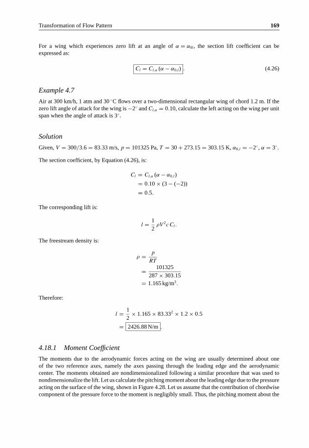
Transformation of Flow Pattern 169
For a wing which experiences zero lift at an angle of α = α0l, the section lift coefficient can beexpressed as:
Cl = Cl,α (α − α0,l) . (4.26)
Example 4.7
Air at 300 km/h, 1 atm and 30 ◦C flows over a two-dimensional rectangular wing of chord 1.2 m. If thezero lift angle of attack for the wing is −2◦ and Cl,α = 0.10, calculate the left acting on the wing per unitspan when the angle of attack is 3◦.
Solution
Given, V = 300/3.6 = 83.33 m/s, p = 101325 Pa, T = 30 + 273.15 = 303.15 K, α0,l = −2◦, α = 3◦.
The section coefficient, by Equation (4.26), is:
Cl = Cl,α (α − α0,l)
= 0.10 × (3 − (−2))
= 0.5.
The corresponding lift is:
l = 1
2ρV 2c Cl.
The freestream density is:
ρ = p
RT
= 101325
287 × 303.15= 1.165 kg/m3.
Therefore:
l = 1
2× 1.165 × 83.332 × 1.2 × 0.5
= 2426.88 N/m .
4.18.1 Moment Coefficient
The moments due to the aerodynamic forces acting on the wing are usually determined about oneof the two reference axes, namely the axes passing through the leading edge and the aerodynamiccenter. The moments obtained are nondimensionalized following a similar procedure that was used tonondimensionalize the lift. Let us calculate the pitching moment about the leading edge due to the pressureacting on the surface of the wing, shown in Figure 4.28. Let us assume that the contribution of chordwisecomponent of the pressure force to the moment is negligibly small. Thus, the pitching moment about the

170 Theoretical Aerodynamics
leading edge due to the pressure force acting on the surface element of area (dxdy) located at a distancex from the leading edge is:
dM0 = p × (dxdy) × x. (4.27)
The net pitching moment due to the pressure force acting on the wing can be obtained by integratingEquation (4.27) over the entire wing surface. The net pitching moment is given by:
M0 =∫∫
p x dxdy. (4.28)
when a uniform pressure acts on any closed surface, the resultant force due to this constant pressure iszero. Thus,
∫∫p∞x dxdy = 0. (4.29)
Combining Equations (4.28) and (4.29), the resultant moment about the leading edge can be expressed as:
M0 =∫∫
(p − p∞) x dxdy. (4.30)
To make this moment relation nondimensional, let us divide both sides by q∞c22b:
M0
q∞c22b=
∫∫p − p∞
q∞
x
cd
(x
c
)d
(y
2b
).
The product of c × 2b = S and (p − p∞)/q∞ = Cp, thus:
M0
q∞c22b=
∫∫Cp
x
cd
(x
c
)d
(y
2b
). (4.31)
Thus, the pitching moment coefficient becomes:
CM0 = M0
q∞c22b=
∫∫Cp
x
cd
(x
c
)d
(y
2b
). (4.32)
In Equation (4.32) the wing chord c is used as a parameter because this derivation is for a rectangularwing in Figure 4.28. That is the mean aerodynamic chord is used together with wing area S tonondimensionalize the pitching moment.
The pitching moment coefficient for a wing section of unit span, referred to as section pitching momentcoefficient, becomes:
Cm0 = m0
q∞ × (1 × c) × c= m0
q∞c2, (4.33)
where m0 is the section pitching moment. The section pitching moment coefficient depends on the camberand thickness ratio of the wing. Similar to section lift coefficient cl, section pitching moment coefficient

Transformation of Flow Pattern 171
CMc/4
− 0.4
− 0.2
0.0
0.2
0.4
− 20− 10 0 10 20
α, degrees
Figure 4.30 Variation of section pitching moment coefficient with angle of attack.
cm about the aerodynamic center is independent of angle of attack. Typical variation of section pitchingmoment coefficient about the aerodynamic center with angle of attack is as shown in Figure 4.30.
Thus, the aerodynamic center is that point along the chord where all changes in lift effectively takeplace. Since the moment about the aerodynamic center is the product of a force (the lift that acts at thecenter of pressure) and an arm length (the distance from the aerodynamic center to the center of pressure),the center of pressure must move toward the aerodynamic center as the lift increases.
4.19 Summary
Transformation of a flow pattern essentially amounts to the transformation of a set of streamlines andpotential lines, whilst the transformation of individual lines implies the transformation of a numberof points.
To transform the points specified by the Cartesian coordinates x and y, in the physical plane, given byz = x + iy, to a transformed plane given by ζ = ξ + iη we need to expand the transformation functionζ = f (z) = ξ + iη, equate the real and imaginary parts and find the functional form of ξ and η, in termsof x and y.
For a given flow pattern in the physical plane, each streamline of the flow can be represented bya separate stream function. Transferring these stream functions, using the transformation function,ζ = f (z), the corresponding streamlines in the transformed plane can be obtained.
The main use of conformal transformation in aerodynamics is to transform a complicated flow fieldinto a simpler one, which is amenable to simpler mathematical treatment.
The main problem associated with this transformation is finding the best transformation function(formula) to perform the required operation. Even though a large number of mathematical functions canbe envisaged for a specific transformation.
A transformation, which generates a family of aerofoil shaped curves, along with their associated flowpatterns, by applying a certain transformation to consolidate the theory presented in the previous sections,is the Kutta−Joukowski transformation.
Kutta−Joukowski transformation is the simplest of all transformations developed for generating aero-foil shaped contours. Kutta used this transformation to study circular-arc wing sections, while Joukowskishowed how this transformation could be extended to produce wing sections with thickness t as wellas camber.
In our discussion on Kutta−Joukowski transformation, it is important to note the following:
• The circle considered, in the physical plane, is a specific streamline. Essentially the circle is thestagnation streamline of the flow in the original plane 1 (z-plane).

172 Theoretical Aerodynamics
• The transformation can be applied to the circle and all other streamlines, around the circle, to generatethe aerofoil and the corresponding streamlines in plane 2 (ζ-plane) or the transformed plane. Thatis, the transformation can result in the desired aerofoil shape and the streamlines of the flow aroundthe aerofoil.
It is convenient to use polar coordinates in the z-plane and Cartesian coordinates in ζ-plane. TheKutta−Joukowski transformation function is:
ζ = ξ + iη = z + b2
z,
where b is a constant.Now, expressing z as z = reiθ , where r and θ are the polar coordinates, and on expanding, we get:
ξ + iη = reiθ + b2
reiθ
= r (cos θ + i sin θ) + b2
r(cos θ − i sin θ) .
Equating the real and imaginary parts, we get:
ξ =(
r + b2
r
)cos θ
η =(
r − b2
r
)sin θ .
These expressions for ξ and η are the general expressions for the transformation of the basic shape,namely the circle in the z-plane, to any desired shape in the ζ-plane.
For transforming a circle of radius a to a straight line, the constant b in the Joukowski transformationfunction should be set equal to a, and the center of the circle should be at the origin.
For transforming a circle to an ellipse using the Kutta−Joukowski transformation function:
ζ = z + b2
z
the circle should have its center at the origin in the z-plane, but the radius of the circle should be greaterthan the constant b, in the above transformation function, that is, a > b.
To transform a circle into a symmetrical aerofoil, the center of the circle in the z-plane should beshifted from the origin and located slightly downstream of the origin, on the x-axis. This shift wouldcause asymmetry to the profile (about the ordinates of the transformed plane) of the transformed shapeobtained with the Kutta−Joukowski transformation function.
ξ = 2b cos θ
η = 2be(1 + cos θ) sin θ
are the coordinates of a symmetrical aerofoil profile. The chord of the aerofoil is 4b. The maximumthickness of the aerofoil occurs where dη/dθ = 0.

Transformation of Flow Pattern 173
The maximum thickness is at the chord location, given by:
ξ = 2b cosπ
3= b.
This point (b, 0), from the leading edge of the aerofoil, is the quarter chord point.The thickness to chord ratio of the aerofoil is:
t
c≈ 1.3 e .
At the trailing edge of the aerofoil, the slope of its upper and lower surfaces merge. This kind of trailingedge would ensure that the flow will leave the trailing edge without separation. But this is possible onlywhen the trailing edge is cusped with zero thickness. Thus, this is only a mathematical model. For actualaerofoils, the trailing edge will have a finite thickness, and hence, there is bound to be some separation,even for the thinnest possible trailing edge.
For transforming a circle to a cambered aerofoil, using Joukowski transformation, the center of thecircle in the physical plane has to be shifted to a point in one of the quadrants.
ξ = 2b cos θ
η = 2be(1 + cos θ) sin θ + 2bβ sin2 θ
are the coordinates representing a cambered aerofoil.The thickness-to-chord ratio for a cambered aerofoil is:
t
c= e (1 + cos θu) sin θu .
The thickness-to-chord ratio is maximum at θu = 60◦. Thus:
(t
c
)max
≈ 1.3e .
This maximum is also at the quarter chord point, as in the case of symmetrical aerofoil.The camber of an aerofoil is the maximum displacement of the mean camber line from the chord. The
mean camber line is the locus of mid-points of lines drawn perpendicular to the chord. In other words,the camber line is the bisector of the aerofoil profile thickness distribution from the leading edge to thetrailing edge.
Percentage camber = β
2× 100 %.
Transformation of a circle with its center shifted above (or below) the origin, on the ordinate in thez-plane, with the transformation function ζ = z + b2/z results in a circular arc.
ξ = 2b cos θ
η = 2b(e + β cos θ) sin θ ,

174 Theoretical Aerodynamics
where ξ and η, respectively, are the expressions for the abscissa and ordinates of the circular arc, in thetransformed plane.
For the transformed circular arc, the chord is 4b.
Camber/chord = 2b tan β
4b
= 1
2tan β.
But for small β, tan β ≈ β. Therefore, the percentage camber for the circular arc becomes 100 β/2.The postulation that “the aerofoil generates sufficient circulation to depress the rear stagnation point
from its position, in the absence of circulation, down to the sharp trailing edge” is known as Joukowskihypothesis. This condition of realizing full Joukowski circulation, resulting in flow without wake isknown as Kutta condition.
The Kutta condition can be stated as follows:
“A body with a sharp trailing edge which is moving through a fluid will create about itself acirculation of sufficient strength to hold the rear stagnation point at the trailing edge.”
The Kutta condition is significant when using the Kutta−Joukowski theorem to calculate the liftgenerated by an aerofoil. The value of circulation of the flow around the aerofoil must be that valuewhich would cause the Kutta condition to exist.
The Kutta condition allows an aerodynamicist to incorporate a significant effect of viscosity whileneglecting viscous effects in the conservation of momentum equation. It is important in the practicalcalculation of lift on a wing.
The Kutta condition does not apply to unsteady flow. Mathematically, the Kutta condition enforces aspecific choice among the infinite allowed values of circulation.
Joukowski hypothesis directly relates the lift generated by a two-dimensional aerofoil to its incidence,as well as indicates the significance of the thickness to chord ratio and camber of the aerofoil in the liftgeneration.
As the flow process develops, which takes place very quickly, the circulation around the aerofoil sectionis generated and the aerofoil experiences lift.
L = 1
2ρV 2
∞SCL,
where CL is the lift coefficient and S is the projected area of the wing planform, normal to the directionof freestream flow. The area S is given by:
S = span × chord.
The chord of the profile is 4b. Therefore, the area of the profile, per unit span, becomes S = 4b. Thus,the lift is:
L = 1
2ρV 24b CL
= 2ρV 2b CL.

Transformation of Flow Pattern 175
Equating the above two expressions for lift, we get the lift coefficient as:
CL = 2πa
bsin (α + β).
But,
a/b = (1 + e).
Therefore,
CL = 2π(1 + e) sin (α + β) .
This is the lift coefficient of a two-dimensional aerofoil, in terms of thickness to chord ratio (t/c = 1.299e),percentage camber (100 β/2), and angle of incidence α.
The ideal lift curve slope, a∞I , for small values of eccentricity e, angle of incidence α and camberβ, is:
a∞I = 2π .
This is the theoretical value of lift curve slope per radian of angle of attack, α. It is seen that, the lift curveslope is independent of the angle of attack.
The coordinates of the transformed aerofoil profile are:
x = a cos θ′ + be
y = a sin θ′ + bβ(1 + e).
With a = (b + be), the above coordinate expressions become:
x = (b + be) cos θ′ + be
y = (b + be) sin θ′ + bβ(1 + e).
For finding the velocity distribution around a given aerofoil, it is necessary to relate the angle ofincidence α to the circulation � around the aerofoil. This is done by applying the Joukowski hypothesis.In reality, the full Joukowski circulation required to bring the rear stagnation point to the trailing edge isnot realized, because of the following:
• Air is a viscous fluid, and the flow near the trailing edge of an aerofoil is modified by the presence ofthe boundary layer and wake, caused by the viscosity.
• The zero thickness for the trailing edge, stipulated by the Joukowski hypothesis, is not possible inpractice. Therefore, the trailing edge must be rounded to some degree of curvature. The finite thicknessof the trailing edge owing to this rounding-off forces the rear stagnation point to deviate from theposition given in the ideal case.
Therefore, if � is the full Joukowski circulation (theoretical circulation), it can be assumed that, thepractical value of circulation is only k�, where k is less than unity.
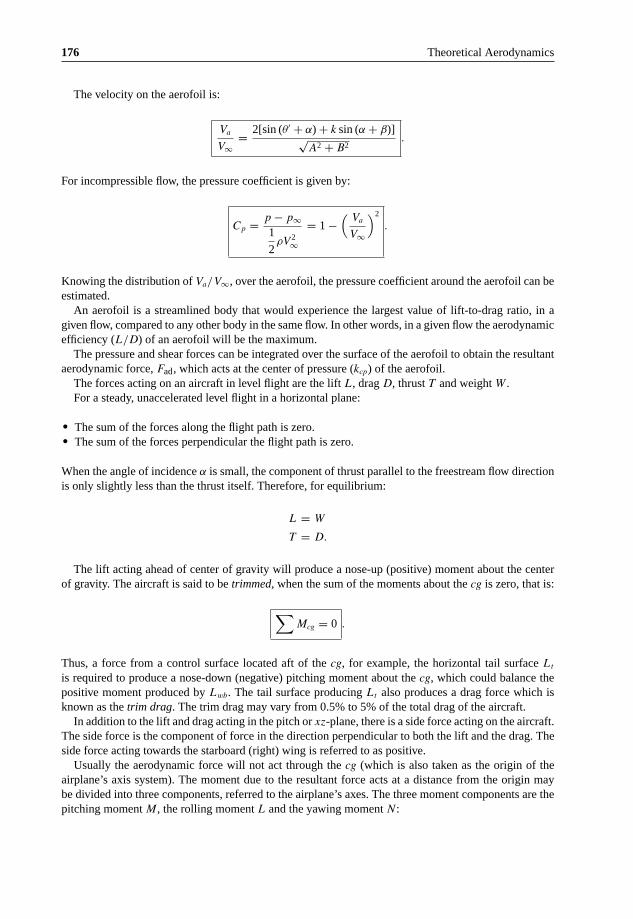
176 Theoretical Aerodynamics
The velocity on the aerofoil is:
Va
V∞= 2[sin (θ′ + α) + k sin (α + β)]√
A2 + B2.
For incompressible flow, the pressure coefficient is given by:
Cp = p − p∞1
2ρV 2
∞
= 1 −(
Va
V∞
)2
.
Knowing the distribution of Va/V∞, over the aerofoil, the pressure coefficient around the aerofoil can beestimated.
An aerofoil is a streamlined body that would experience the largest value of lift-to-drag ratio, in agiven flow, compared to any other body in the same flow. In other words, in a given flow the aerodynamicefficiency (L/D) of an aerofoil will be the maximum.
The pressure and shear forces can be integrated over the surface of the aerofoil to obtain the resultantaerodynamic force, Fad, which acts at the center of pressure (kcp) of the aerofoil.
The forces acting on an aircraft in level flight are the lift L, drag D, thrust T and weight W .For a steady, unaccelerated level flight in a horizontal plane:
• The sum of the forces along the flight path is zero.• The sum of the forces perpendicular the flight path is zero.
When the angle of incidence α is small, the component of thrust parallel to the freestream flow directionis only slightly less than the thrust itself. Therefore, for equilibrium:
L = W
T = D.
The lift acting ahead of center of gravity will produce a nose-up (positive) moment about the centerof gravity. The aircraft is said to be trimmed, when the sum of the moments about the cg is zero, that is:
∑Mcg = 0 .
Thus, a force from a control surface located aft of the cg, for example, the horizontal tail surface Lt
is required to produce a nose-down (negative) pitching moment about the cg, which could balance thepositive moment produced by Lwb. The tail surface producing Lt also produces a drag force which isknown as the trim drag. The trim drag may vary from 0.5% to 5% of the total drag of the aircraft.
In addition to the lift and drag acting in the pitch or xz-plane, there is a side force acting on the aircraft.The side force is the component of force in the direction perpendicular to both the lift and the drag. Theside force acting towards the starboard (right) wing is referred to as positive.
Usually the aerodynamic force will not act through the cg (which is also taken as the origin of theairplane’s axis system). The moment due to the resultant force acts at a distance from the origin maybe divided into three components, referred to the airplane’s axes. The three moment components are thepitching moment M, the rolling moment L and the yawing moment N:

Transformation of Flow Pattern 177
• Pitching moment is the moment acting about the lateral axis (y-axis). It is the moment due to the liftand drag acting on the aircraft. Pitching moment causing nose-up is regarded positive.
• Rolling moment is the moment acting about the longitudinal axis (x-axis) of the aircraft. Rollingmoment is generated by a differential lift generated by the ailerons, located closer to the wingtips.Rolling moment causing the right (starboard) wingtip to move downward is regarded positive.
• Yawing moment is the moment acting about the vertical (z-axis) of the aircraft. Yawing moment tendsto rotate the aircraft nose to the right is regarded positive.
The primary parameters governing the magnitude of the aerodynamic forces and moments are thefollowing:
• Geometry of the aerofoil.• Angle of attack, namely the aircraft attitude in the pitch (xz) plane relative to the flight direction.• Vehicle size.• Freestream velocity.• Freestream flow density.• Reynolds number (viscous effects).• Mach number (compressibility effects).
The geometrical section of a wing obtained by cutting it by a vertical plane parallel to the centerline of theaircraft is called aerofoil section. The lift generated and the stall characteristics of a wing strongly dependson the geometry of the aerofoil sections that make up the wing. The geometric parameters that dictate theaerodynamic characteristics of the aerofoil section are; the leading-edge radius, the mean camber line,the maximum thickness and the thickness distribution of the profile, and the trailing-edge angle.
The geometry of many aerofoil sections is uniquely defined by the NACA designation for the aerofoil.Aerofoil geometry are usually characterized by the coordinates of the upper and lower surface. It is
often summarized by a few parameters such as: maximum thickness, maximum camber, position of maxthickness, position of max camber, and nose radius.
The shape of the NACA aerofoils is described using a series of digits following the word “NACA.”In NACA 4-Digit series the first digit implies the maximum camber in percentage of chord (c), the
second digit gives the position of maximum camber in 1/10 of chord, the last two digits give the maximumthickness in percentage of chord. For example,
In NACA 5-digit series the first digit gives approximate maximum camber in percentage of chord, thesecond and third digits give the position of maximum camber in 2/100 of chord and the last two digitsgive the maximum thickness in percentage of chord. This NACA 23012 is an aerofoil with maximumcamber as 2% of c, position of maximum camber at 60% of chord and t/c = 0.12.
Four- and five-digit series aerofoils can be modified with a two-digit code preceded by a hyphen inthe following sequence:
1. One digit describing the roundness of the leading edge with 0 being sharp, 6 being the same as theoriginal aerofoil, and larger values indicating a more rounded leading edge.
2. One digit describing the distance of maximum thickness from the leading edge in tens of percentageof the chord.
1-series:
A new approach to aerofoil design pioneered in the 1930s in which the aerofoil shape was mathematicallyderived from the desired lift characteristics. Prior to this, aerofoil shapes were first created and then had

178 Theoretical Aerodynamics
their characteristics measured in a wind tunnel. The 1-series aerofoils are described by five digits in thefollowing sequence:
1. The number “1” indicating the series.2. One digit describing the distance of the minimum pressure area in tens of percent of chord.3. A hyphen.4. One digit describing the lift coefficient in tenths.5. Two digits describing the maximum thickness in percentage of chord.
In NACA 6-digit series the first digit refers to the series, the second digit gives the location of minimumCp in 1/10 chord, the third digit gives the half width of low drag bucket in 1/10 of CL, the fourth digitgives the ideal CL in tenths of CL, the fifth and sixth digits give the max thickness in percentage of chord.
In NACA 7-Digit Series:
1. The number “7” indicating the series.2. One digit describing the distance of the minimum pressure area on the upper surface in tens of
percentage of chord.3. One digit describing the distance of the minimum pressure area on the lower surface in tens of
percentage of chord.4. One letter referring to a standard profile from the earlier NACA series.5. One digit describing the lift coefficient in tenths.6. Two digits describing the maximum thickness in tens of percentage of chord.7. “a =” followed by a decimal number describing the fraction of chord over which laminar flow is
maintained. a = 1 is the default if no value is given.
In NACA 8-Digit series profiles are supercritical aerofoils designed to independently maximize airflowabove and below the wing. The numbering is identical to the 7-series aerofoils except that the sequencebegins with an “8” to identify the series.
NASA Aerofoils
A concerted effort within the National Aeronautics and Space Administration (NASA) during the 1960sand 1970s was directed toward developing practical aerofoils with two-dimensional transonic turbulentflow and improved drag divergence Mach numbers while retaining acceptable low-speed maximumlift and stall characteristics and focused on a concept referred to as the supercritical aerofoil. Thisdistinctive aerofoil shape, based on the concept of local supersonic flow with isentropic recompression,was characterized by a large leading-edge radius, reduced curvature over the middle region of the uppersurface, and substantial aft camber.
The early phase of this effort was successful in significantly extending drag-rise Mach numbers beyondthose of conventional aerofoils such as the National Advisory Committee for Aeronautics (NACA)6-series aerofoils. These early supercritical aerofoils (denoted by the SC (phase 1) prefix), however,experienced a gradual increase in drag at Mach numbers just preceding drag divergence (referred to asdrag creep). This gradual buildup of drag was largely associated with an intermediate off-design secondvelocity peak (an acceleration of the flow over the rear upper-surface portion of the aerofoil just beforethe final recompression at the trailing edge) and relatively weak shock waves above the upper surface.
The chord line is defined as the shortest (straight) line connecting the leading and trailing edges.The geometrical angle of attackα is the angle between the chord line and the direction of the undisturbed
freestream.Mean camber line is the locus of the points midway between the upper and lower surfaces of the aerofoil.
One of the primary effects of camber is to change the zero-lift angle of attack, α0l. For symmetrical

Transformation of Flow Pattern 179
aerofoils, zero lift is at α = 0 and for cambered aerofoils, zero lift is at negative α for positive camberand vice versa.
The thickness distribution and the maximum thickness strongly influence the aerodynamics charac-teristics of the aerofoil section. The thickness distribution for an aerofoil affects the pressure distributionand the character of the boundary layer.
The trailing-edge angle influences the location of the aerodynamic center; the point about which thesection moment coefficient is independent of angle of angle of attack, α. The aerodynamic center of thisaerofoil sections in a subsonic flow is theoretically located at the quarter-chord point.
Aircraft wings are made up of aerofoil sections discussed in the preceding section. Aerofoil sectionsare placed along the span of a wing.
The relevant parameters used to define the aerodynamic characteristics of a wing are rectangular,unswept trapezoidal, swept and delta configurations.
Wing area is the plan surface area of the wing.Wing span is the distance between the tips of port and starboard wings.Average chord is the geometric average of the chord distribution over the length of the wing span.Aspect ratio is the ratio of the span and the average chord.Root chord is the chord at the wing centerline. Tip chord the chord at the wing tip.Taper ratio is the ratio of the tip chord to root chord.Sweep angle is usually measured as the angle between the line of 25% chord and a perpendicular to
the root chord.Mean aerodynamic chord is an average chord which, when multiplied by the product of the average
section moment coefficient, the dynamic pressure, and the wing area, gives the moment for the entire wing.Dihedral angle is the angle between a horizontal plane containing the root chord and a plane midway
between the upper and lower surfaces of the wing. If the wing lies below the horizontal plane, it is termedan anhedral angle.
Geometric twist defines the situation where the chord lines for the spanwise distribution of all theaerofoil sections do not lie in the same plane.
If the incidence of the aerofoil sections relative to the vehicle axis decrease toward the tip, the winghas a “wash-out.” If the angle of incidence increases toward wing tip, the wing has “wash-in.”
For thin aerofoils at low angle of attack, the lift results mainly from the pressure distribution (thatis, pressure forces). The shear forces due to viscosity acts primarily in the chordwise direction andcontributes mainly to the drag.
When the boundary layer is thin, the pressure distribution around the aerofoil can be regarded equivalentto that due to an inviscid flow. Thus, the pressure distribution is independent of Reynolds number anddoes not depend on whether the boundary layer is laminar or turbulent.
The lift coefficient, is defined:
CL = L
q∞S,
where L is the lift and S is the wing planform area.Theoretical value of two-dimensional lift curve slope is 2π, that is:
Cl,α = dCl
dα= 2π.
The moments due to the aerodynamic forces acting on the wing are usually determined about oneof the two reference axes, namely the axes passing through the leading edge and the aerodynamiccenter. The moments obtained are nondimensionalized following a similar procedure that was used tonondimensionalize the lift.

180 Theoretical Aerodynamics
The net pitching moment is given by:
M0 =∫∫
(p − p∞) x dxdy.
The pitching moment coefficient is:
CM0 = M0
q∞c22b=
∫∫Cp
x
cd
(x
c
)d
(y
2b
).
Exercise Problems
1. If the pressure coefficient at a point on an aerofoil in a freestream flow of speed 70 m/s is −3.7,determine the flow velocity at that point.
[Answer: 151.76 m/s]2. A two-dimensional wing of span 20 m and chord 1.1 m, thickness-to-chord ratio 12% and percentage
camber 10% at an angle of attack of 3◦ in a uniform air stream at 1 atm and 22 ◦C and 220 km/hexperiences a lift of 15 000 N. Determine the circulation around the wing and the lift coefficient,assuming the flow as incompressible and inviscid.
[Answer: � = 10.26 m2/s, CL = 0.373]3. A tapered wing of span 15 m and root chord 4 m has a planform area of 37.5 m2. Find (a) the tip
chord and (b) the mean aerodynamic chord of the wing.[Answer: (a) 1 m, (b) 2.8 m]
4. A wing of taper ratio 3 has a planform area of 45 m2. If the span is 16 m, determine the root and tipchords of the wing.
[Answer: 4.218 m, 1.406 m]5. If the section lift acting on a two-dimensional wing of chord 2 m, flying at 250 km/h in sea level
altitude is 3000 N/m, when the angle of attack is 4◦ and section lift curve slope is 0.11, determinethe zero lift angle of attack of the wing.
[Answer: −0.618◦]6. The section lift coefficient of a two-dimensional wing flying at 3.2◦ angle of attack is 0.6. If the zero
lift angle of attack is −1.8◦, determine the lift curve slope of the wing.[Answer: 0.12]
7. A tapered wing of tip chord 3 m has wing area 220 m2 and aspect ratio 4. Find (a) the root chordand (b) the wing span. (c) Also, find the expression for the chord in terms of transverse coordinate.
[Answer: (a) 11.83 m, (b) 29.66 m, (c) 11.83 − 0.595 y]8. A NACA 612-415 aerofoil flies at 400 km/h at an altitude where the air density is 0.082 kg/m3.
Determine the wing loading of the aerofoil.[Answer: 202.5 N/m2]
9. Identify the number of the NACA profile with 3% maximum camber located at 30% from the leadingedge, with a thickness of 10% of the chord.
[Answer: NACA 3310]10. Identify the number of the NACA profile with 0 camber and thickness to chord ratio of 12%.
[Answer: NACA 0012]11. If the fineness ratio of the ellipse obtained by transforming a circle of unit radius, with
Kutta−Joukowski transformation, is 4, determine the eccentricity.[Answer: 0.29]

Transformation of Flow Pattern 181
12. A symmetrical aerofoil is obtained by transforming a circle of unit radius, with Kutta−Joukowskitransformation function. If the eccentricity is 0.1, find the maximum value of thickness to chordratio.
[Answer: 0.13]13. A cambered aerofoil is obtained by transforming a circle of unit radius, with Joukowski transfor-
mation function. If the percentage camber is 3.2, determine the location of the circle center in thephysical plane.
[Answer: (0.024, 0.064)]14. If the maximum thickness of a 14% cambered Joukowski aerofoil is at π/2.5, determine the eccen-
tricity.[Answer: 0.112]
15. If a two-dimensional Joukowski aerofoil of thickness to chord ratio 12% and camber 3% in an idealflow experiences a lift coefficient of 0.8, determine (a) the angle of incidence and (b) the lift curveslope.
[Answer: (a) 3.25◦, (b) 6.82]
Reference
1. Harris, C.D., NASA Supercritical Aerofoils – A Matrix of Family-Related Airfoils, NASA Technical Paper 2969,1990.

5Vortex Theory
5.1 Introduction
Before getting into the dynamics of vortex motion, it is essential to have a thorough understanding ofrotational and irrotational flows. Translation and rotation are the two types of basic motion in a fluidflow. These two may exist independently or simultaneously. When they coexist they may be consideredas one superimposed on the other. It should be emphasized that rotation refers to the orientation of a fluidelement and not the path followed by the element. Thus, for an irrotational flow, if a pair of small stickswere placed on a fluid element it can be observed that the orientation is retained even while the fluidelement moves along a circular path, as shown in Figure 5.1(a). In other words, in an irrotational flow,the fluid elements do not rotate about their own axes, that is, fluid elements do not spin in an irrotationalflow. But in a rotational flow, fluid elements rotate about their axes, as shown in Figure 5.1(b). Thus, inan irrotational flow, like the one shown in Figure 5.1(a), the fluid elements move along circular paths butdo not rotate about their own axes. Thus, the angular velocity of fluid elements in an irrotational flow iszero. If the flow field were rotating like a rigid body, then the fluid elements in the field would experiencea rotation about their own axes, as shown in Figure 5.1(b). This type of motion is termed rotational andcannot be described with a velocity potential.
If the possible distortion of the fluid elements caused by severe viscous traction is ignored then thereare only three possible ways in which a fluid element can move. They are the following:
(a) Pure translation – the fluid elements are free to move anywhere in space but continue to keep theiraxes parallel to the reference axes fixed in space, as shown in Figure 5.2(a). The flow in the potentialflow zone, outside the boundary layer over an aerofoil, is substantially this type of flow.
(b) Pure rotation – the fluid elements rotate about their own axes which remain fixed in space, as shownin Figure 5.2(b).
(c) The general motion in which translation and rotation are compounded. Such a motion is found, forexample, in the wake of a bluff body.
A flow in which all the fluid elements behave as in item (a) above is called potential or irrotationalflow. All other flows exhibit, to a greater or lesser extent, the spinning property of some of the constituentfluid elements, and are said to posses vorticity, which is the aerodynamic term for elemental spin. Theflow is then termed rotational flow.
From the above descriptions it is evident that a flow is either rotational, possessing vorticity, or irro-tational, for which vorticity is zero. The rotational and irrotational nature and the properties of a flow
Theoretical Aerodynamics, First Edition. Ethirajan Rathakrishnan.© 2013 John Wiley & Sons Singapore Pte. Ltd. Published 2013 by John Wiley & Sons Singapore Pte. Ltd.

184 Theoretical Aerodynamics
(b)(a)
Figure 5.1 (a) Irrotational flow, (b) rotational flow.
y
(b)(a)
x
Figure 5.2 (a) Pure translational motion, (b) pure rotational motion.
can be examined analytically, leading to the development of characteristic equations governing the flow.Using these equations, the nature of any unknown flow can be analyzed.
5.2 Vorticity Equation in Rectangular Coordinates
In a two-dimensional motion, the vorticity at a point P, which is located perpendicular to the plane, is equalto the limit of the ratio of the circulation in an infinitesimal circuit embracing P to the area of the circuit.
A flow possesses vorticity if any of its elements are rotating (spinning). It is a convenient way toinvestigate the motion of a circular element, treating it as a solid, at the instant of time considered. LetP(x, y) be the center of the circular element and u and v are the velocity components, along x- andy-directions, respectively, as shown in Figure 5.3.
Let us assume that the fluid element consists of numerous fluid particles of mass �m each, suchas one at the point Q(x + δx, y + δy). At point Q, the velocity components, along x- and y-directions,
x
u + ∂u∂x
δx + ∂u∂y
δy
v + ∂v∂x
δx + ∂v∂y
δy
Δm
v
u
Q(x + dx, y + dy)
y
o
P
Figure 5.3 A fluid element and appropriate coordinates and velocity components.

Vortex Theory 185
respectively, are:
u + ∂u
∂xδx + ∂u
∂yδy
and
v + ∂v
∂xδx + ∂v
∂yδy.
The moment of momentum (or angular momentum) of the fluid element about point P(x, y) is the sumof the moments of momentum of all the particles such as Q about point P. Taking the anti-clockwisemoment as positive, we have:
Moment of momentum of the element
=∑[(
∂v
∂xδx + ∂v
∂yδy
)δx −
(∂u
∂xδx + ∂u
∂yδy
)δy
]�m
=∑
�m∂v
∂x(δx)2 −
∑�m
∂u
∂y(δy)2
+∑
�m
(∂v
∂y− ∂u
∂x
)δxδy.
For a circular disc, about its center, we have:
∑�m δxδy = 0.
Therefore, the angular momentum of the disc becomes:
Angular momentum =∑
�m∂v
∂x(δx)2 −
∑�m
∂u
∂y(δy)2 .
If the disc were a solid disc, its angular momentum would be Iω, where I is its polar moment of inertiaabout P and ω its angular velocity about P. Thus, assuming the fluid element as a solid disc, we have:
I =∑
�m{
(δx)2 + (δy)2}
and
∑�m (δx)2 =
∑�m (δy)2 .
Thus, we have the angular momentum relation as:
ω∑
�m{
(δx)2 + (δy)2} =
∑�m
∂v
∂x(δx)2 −
∑�m
∂u
∂y(δy)2 .

186 Theoretical Aerodynamics
This gives the angular velocity as:
2ω = ∂v
∂x− ∂u
∂y.
The quantity 2ω is the elemental spin, also referred to as vorticity, which is usually denoted as ζ. Thus,
ζ = ∂v
∂x− ∂u
∂y. (5.1)
The units of ζ are radian per second. From Equation (5.1) and the angular velocity relation, it is seen that:
ζ = 2ω .
that is, the vorticity is twice the angular velocity.
5.2.1 Vorticity Equation in Polar Coordinates
In the polar coordinates, the vorticity equation can be expressed as:
ζ = qt
r+ ∂qt
∂r− 1
r
∂qn
∂θ, (5.2)
where r and θ are the polar coordinates and qt and qn are the tangential and normal components ofvelocity, respectively. The derivation of Equation (5.2) is given in Section 5.3.
If (r, θ, n) are the radial, azimuthal and normal coordinates of a polar coordinates system, the vorticityexpression is given by:
ζ = irζr + iθζθ + inζn,
where ir , iθ and in are the unit vectors in the directions of r, θ and n, respectively. The vorticity componentscan be expressed as:
ζr = 1
r
∂un
∂θ− ∂uθ
∂n
ζθ = ∂ur
∂n− ∂un
∂r
ζn = 1
r
∂(ruθ)
∂r− 1
r
∂ur
∂θ,
where ur , uθ and un are the velocity components along r, θ and n directions, respectively.
Example 5.1
Find the vorticity of the following flows.(a)
V = c(x + y)i − c(x + y)j,

Vortex Theory 187
(b)
V = (x + y + z + t)i + 2 (x + y + z + t)j − 3 (x + y + z + t)k,
(c)
ur = uθ = 0, un =(
r2
a2− 1
).
Solution
(a) Given, u = c(x + y), v = −c(x + y).
This is a two-dimensional flow in the xy-plane. Therefore, the vorticity component (with rotational axisin the z-direction, which is normal to xy-plane) is:
ζz = ∂v
∂x− ∂u
∂y
= −c − c
= −2c .
(b) Given, u = x + y + z + t, v = 2 (x + y + z + t), w = −3 (x + y + z + t).
The vorticity components are:
ζx = ∂w
∂y− ∂v
∂z
= −3 − 2 = −5
ζy = ∂u
∂z− ∂w
∂x
= 1 + 3 = 4
ζz = ∂v
∂x− ∂u
∂y
= 2 − 1 = 1.
Therefore, the vorticity becomes:
ζ = ζx i + ζy j + ζz k
= −5 i + 4 j + k .
(c) Given, ur = uθ = 0, un = c
(r2
a2− 1
).
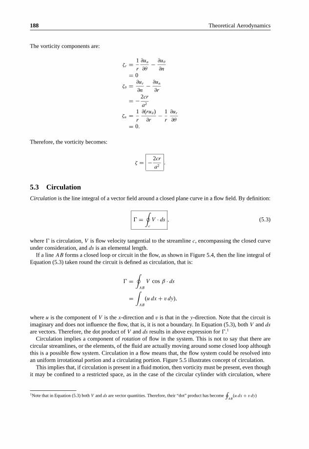
188 Theoretical Aerodynamics
The vorticity components are:
ζr = 1
r
∂un
∂θ− ∂uθ
∂n
= 0
ζθ = ∂ur
∂n− ∂un
∂r
= −2cr
a2
ζn = 1
r
∂(ruθ)
∂r− 1
r
∂ur
∂θ
= 0.
Therefore, the vorticity becomes:
ζ = −2cr
a2.
5.3 Circulation
Circulation is the line integral of a vector field around a closed plane curve in a flow field. By definition:
� =∮
c
V · ds , (5.3)
where � is circulation, V is flow velocity tangential to the streamline c, encompassing the closed curveunder consideration, and ds is an elemental length.
If a line AB forms a closed loop or circuit in the flow, as shown in Figure 5.4, then the line integral ofEquation (5.3) taken round the circuit is defined as circulation, that is:
� =∮
AB
V cos β · ds
=∫
AB
(u dx + v dy),
where u is the component of V is the x-direction and v is that in the y-direction. Note that the circuit isimaginary and does not influence the flow, that is, it is not a boundary. In Equation (5.3), both V and ds
are vectors. Therefore, the dot product of V and ds results in above expression for �.1
Circulation implies a component of rotation of flow in the system. This is not to say that there arecircular streamlines, or the elements, of the fluid are actually moving around some closed loop althoughthis is a possible flow system. Circulation in a flow means that, the flow system could be resolved intoan uniform irrotational portion and a circulating portion. Figure 5.5 illustrates concept of circulation.
This implies that, if circulation is present in a fluid motion, then vorticity must be present, even thoughit may be confined to a restricted space, as in the case of the circular cylinder with circulation, where
1Note that in Equation (5.3) both V and ds are vector quantities. Therefore, their “dot” product has become∮
AB(u dx + v dy)

Vortex Theory 189
dsV
β
C
B A
y
xo
Figure 5.4 A loop AB in a flow field.
(a) Actual flow (b) Sum of circulating and irrotational parts
V − v
v
v
V + v
v
v
v
v +
Figure 5.5 Illustration of circulation.
the vorticity at the center of the cylinder may actually be excluded from the region of flow considered,namely that outside the cylinder.
An alternative equation for circulation � can be obtained by considering the circuit of integration madeup of a large number of rectangular elements of sides δx and δy, as shown in Figure 5.6.
� =∫
c
(u dx + v dy),
Applying the integral round the element abcd with point P(x, y) at its center, where the velocitycomponents are u and v, as shown in Figure 5.6, we get:
�� =(
v + ∂v
∂x
δx
2
)δy −
(u + ∂u
∂y
δy
2
)δx −
(v − ∂v
∂x
δx
2
)δy +
(u − ∂u
∂y
δy
2
)δx
o
a
c
u +∂u
∂y
δy
2
v +∂v
∂x
δx
2
u −∂u
∂y
δy
2
b
x
y
a
d c
b
u
v
dP
P
dy
dx
c
ev −
∂v
∂x
δx
2f
Figure 5.6 A circuit of integration, c, in the flow field.

190 Theoretical Aerodynamics
Simplification of this results in:
�� =(
∂v
∂x− ∂u
∂y
)(δxδy).
The sum of the circulations of all the elemental areas in the circuit constitutes the circulation ofthe circuit as a whole. As the circulation �� of each element is added to the �� of the neighboringelement, the contributions of the common sides disappear. Applying this reasoning from an element tothe neighboring element throughout the area, the only sides contributing to the circulation, when the ��sof all areas are summed together, are those sides which actually form the circuit itself. This means that,for the total circuit c, the circulation becomes:
� =∫∫
area
(∂v
∂x− ∂u
∂y
)(dxdy)
=∮
c
(u dx + v dy)
and the vorticity ζ is given by:
ζ = ∂v
∂x− ∂u
∂y.
If the strength of the circulation � remains constant whilst the circuit shrinks to encompass an elementalarea, that is, until it shrinks to an area of the size of a rectangular element, then:
� = ζ × (δxδy) = ζ × area of element.
Therefore,
Vorticity = limarea→0
�
area of element. (5.4)
This is a result which enables an easy derivation of the vorticity relation in polar coordinates.Let us consider a segment of a fluid element of width δr, subtending angle δθ, at the origin and width
δr, as shown in Figure 5.7. If the segment is located at the point P(r, θ), where the normal and tangential
o
BP(r, θ)
C
δr
δθ
D
A
Figure 5.7 A fluid element.

Vortex Theory 191
velocity components are qn and qt , respectively, then the velocities along AB, BC, CD, DA are:
(qn − ∂qn
∂θ
δθ
2
)− along AB
(qt + ∂qt
∂r
δr
2
)− along BC
−(
qn + ∂qn
∂θ
δθ
2
)− along CD
−(
qt − ∂qt
∂r
δr
2
)− along DA,
where the direction qn is along r-direction and qt is along θ-direction. The lengths of the sides of theelements are:
AB = δr
BC =(
r + δr
2
)δθ
CD = δr
DA =(
r − δr
2
)δθ.
The circulation about the element is the line integral of the tangential component of flow velocity, that is:
� =(
qn − ∂qn
∂θ
δθ
2
)δr +
(qt + ∂qt
∂r
δr
2
)(r + δr
2
)δθ
−(
qn + ∂qn
∂θ
δθ
2
)δr −
(qt − ∂qt
∂r
δr
2
)(r − δr
2
)δθ.
This simplifies to:
� =(
qt
r+ ∂qt
∂r− 1
r
∂qn
∂θ
)rδrδθ.
We know that:
� = vorticity × area of element.
Also, the area of the element under consideration is (r δrδθ). Thus, the vorticity is:
ζ =(
qt
r+ ∂qt
∂r− 1
r
∂qn
∂θ
).
This is the vorticity expression in polar coordinates.

192 Theoretical Aerodynamics
(a) (b)
axis
Figure 5.8 (a) Straight line vortex, (b) cross-section showing the associated streamlines.
5.4 Line (point) Vortex
A line vortex is a string of rotating particles. In a line vortex, a chain of fluid particles are spinning abouttheir common axis and carrying around with them a swirl of fluid particles which flow around in circles.A cross-section of such a string of particles and the associated flow show a spinning point, outside ofwhich the flow streamlines are concentric circles, as shown in Figure 5.8.
Vortices can commonly be encountered in nature. The difference between a real (actual) vortex andtheoretical vortex is that, the real vortex has a core of fluid which rotates like a solid, although theassociated swirl outside is the same as the flow outside the point vortex. The streamlines associated witha line vortex are circular, and therefore, the particle velocity at any point must be only tangential.
Stream function of a vortex can easily be obtained as follows. Consider a vortex of strength �, at theorigin of a polar coordinate system, as shown in Figure 5.9.
Let P(r, θ) be a general point and velocity at P is always normal to OP (tangential). The radial velocityat any point P is zero, that is:
1
r
∂ψ
∂θ= 0
since in polar coordinates, the radial velocity qr and tangential velocity qθ, in terms of stream functionψ are:
qr = 1
r
∂ψ
∂θ
qt = − ∂ψ
∂r.
A
r
r 0
ψ=
0
P(r, θ)
o
Figure 5.9 A vortex at origin.

Vortex Theory 193
For qr = 0, the stream function ψ should be a function of r only. The tangential velocity at any pointP [1] is:
qt = �
2πr= − ∂ψ
∂r
Therefore,
ψ =∫
− �
2πrdr.
Integrating along a convenient boundary, such as from A to P in Figure 5.9, from radius r0 (radius ofstreamline, ψ = 0) to P(r, θ), we get the stream function as:
ψ = −[
�
2πln r
]r
r0
that is:
ψ = − �
2πln
r
r0. (5.5)
This is the stream function for a vortex, and the circulation � of a flow is positive when it is counter-clockwise.2
We know that the streamlines of a line vortex are concentric circles. Therefore, the equipotential lines(which are always orthogonal to the streamlines) must be radial lines emanating from the center of thevortex. Also, for a vortex, the normal component of velocity qn = 0. Therefore, the potential function φ
must be a function of θ only. Thus:
qt = 1
r
dφ
dθ= �
2π r.
Therefore:
dφ = �
2πdθ.
Integrating this, we get:
φ = �
2πθ + constant.
By assigning φ = 0 at θ = 0, we obtain:
φ = �
2πθ . (5.6)
This is the potential function for a vortex.
2From Equation (5.5), it is seen that the circulation is undefined for r ≤ r0, that is, around the axis of rotation the circulation is notdefined.

194 Theoretical Aerodynamics
Also, we know that the stream function for a source [1] is:
ψ = m θ
2 π,
where m is the strength of the source.Comparing the stream functions of a vortex and a source, we see that the streamlines of the source
(the radial lines emanating from a point) and the streamlines of the vortex (the concentric circles) areorthogonal.
5.5 Laws of Vortex Motion
In Section 5.4, we saw that a point vortex can be considered as a string of rotating particles surrounded byfluid at large moving irrotationally. Further, the flow investigation was confined to a plane section normalto the length or axis of the vortex. A more general definition is that a vortex is a flow system in whicha finite area in a plane normal to the axis of a vortex contains vorticity. Figure 5.10 shows a sectionalarea S in the plane normal to the axis of a vortex. The axis of the vortex is clearly, always normal to thetwo-dimensional flow plane considered and the influence of the so-called line vortex is the influence, ina section plane, of an infinitely long straight line vortex of vanishingly small area.
The axis of a vortex, in general, is a curve in space, and area S is a finite size. It is convenient to considerthat the area S is made up of several elemental areas. In other words, a vortex consists of a bundle ofelemental vortex lines or filaments. Such a bundle is termed a vortex tube, being a tube bounded by vortexfilaments.
The vortex axis is a curve winding about within the fluid. Therefore, it can flexure and influencethe flow as a whole. The estimation of its influence on the fluid at large is somewhat complex. In ourdiscussions here the vortices considered are fixed relative to some axes in the system or free to move ina controlled manner and can be assumed to be linear. Furthermore, the vortices will not be of infinitelength, therefore, the three-dimensional or end influence must be accounted for.
In spite of the above simplifications, the vortices conform to laws of motion appropriate to theirbehavior. A rigorous treatment of the vortices, without the simplifications imposed in our treatment herecan be found in Milne-Thomson (1952) [2] and Lamb (1932) [3].
yΓ
Γ
Γ
S
o x
Figure 5.10 The vorticity of a section of vortex tube.

Vortex Theory 195
5.6 Helmholtz’s Theorems
The four fundamental theorems governing vortex motion in an inviscid flow are called Helmholtz’stheorems (named after the author of these theorems). The first theorem refers to a fluid particle (orelement) in general motion possessing all or some of the following:
• Linear velocity.• Vorticity.• Distortion.
This theorem has been discussed in part in Section 5.3, where the vorticity was explained and itsexpression in Cartesian or polar coordinates were derived. Helmholtz’s first theorem states that:
“the circulation of a vortex tube is constant at all cross-sections along the tube.”
The second theorem demonstrates that:
“the strength of a vortex tube (that is, the circulation) is constant along its length.”
This is sometimes referred to as the equation of vortex continuity. It can be shown that the strength ofa vortex cannot grow or diminish along its axis or length. The strength of a vortex is the magnitude ofthe circulation around it, and is equal to the product of vorticity ζ and area S. Thus:
� = ζ S.
It follows from the second theorem that, ζ S is constant along the vortex tube (or filament), so thatif the cross-sectional area diminishes, the vorticity increases and vice versa. Since infinite vorticity isunacceptable, the cross-sectional area S cannot diminish to zero. In other words, a vortex cannot end inthe fluid. In reality the vortex must form a closed loop, or originate (or terminate) in a discontinuity inthe fluid such as a solid body or a surface of separation. In a different form it may be stated that a vortextube cannot change its strength between two sections unless vortex filaments of equivalent strength joinor leave the vortex tube, as shown in Figure 5.11.
It is seen that at section A the vortex tube strength is �. Downstream of section A an opposite vortexfilament of strength −�� joins the vortex tube. Therefore, at section B, the strength of the vortex tube is:
� = � − ��
as shown in Figure 5.11. This is of great importance to the vortex theory of lift.
Γ − ΔΓ
Section A
Γ
Section B
Figure 5.11 Vortex-tube fragmentation.

196 Theoretical Aerodynamics
The third theorem demonstrates that a vortex tube consists of the same particles of fluid, that is:
“there is no fluid interchange between the vortex tube and surrounding fluid.”
The fourth theorem states that:
“the strength of a vortex remains constant in time.”
5.7 Vortex Theorems
Now let us have a closer look at the theorems governing vortex motion. Consider the circulation of aclosed material line. By definition (Equation 5.3), we have the circulation as:
� =∮
c
V · ds.
The time rate of change of � can be expressed as:
D�
Dt= D
Dt
∮c
V · ds =∮
c
DV
Dt· ds +
∫V · dV (5.7)
since ds/dt = V , where V is the velocity, s is length and t is time. The second integral in Equation (5.7)
vanishes, since V · dV = d
(V · V
2
)is the total differential of a single valued function, and the starting
point of integration coincides with the end point.
By Euler equation, we have:
DV
Dt= FB − �p
ρ,
where FB is the body force. From Equation (5.7) and the Euler equation, we obtain the rate of change ofthe line integral over the velocity vector in the form:
D�
Dt=
∫c
FB · ds −∫
c
�p
ρ· ds. (5.8)
In Equation (5.8), D�/Dt vanishes if (FB · ds) and �p/ρ can be written as total differentials. When thebody force FB has a potential (that is, when the body force is a conservative force field); implying thatthe work done by the weight in taking a body from a point P to another point Q is independent of the pathtaken from P to Q, and depends only on the potential, the first closed integral in Equation (5.8) becomeszero because:
FB · ds = − � ψ · ds = − dψ. (5.9)
For a homogeneous density field or in barotropic flow, the density depends only on pressure, that isρ = f (p). For such a flow, the second term on the right-hand side of Equation (5.8), can be expressed as:
�p
ρ· ds = dp
ρ(p)= dp. (5.10)
Therefore, for barotropic fluids, the second integral also vanishes in Equation (5.8).

Vortex Theory 197
Equations (5.8) to (5.10) form the content of Thompson’s vortex theorem or Kelvin’s circulationtheorem. This theorem states that:
“in a flow of inviscid and barotropic fluid, with conservative body forces, the circulation arounda closed curve (material line) moving with the fluid remains constant with time,” if the motion isobserved from a nonrotating frame.
The vortex theorem can be interpreted as follows:
“The position of a curve c in a flow field, at any instant of time, can be located by following themotion of all the fluid elements on the curve.”
That is, Kelvin’s circulation theorem states that, the circulation around the curve c at the two locationsis the same. In other words:
D�
Dt= 0 , (5.11)
where D/Dt(≡ ∂/∂t + � ·) has been used to emphasize that the circulation is calculated around a materialcontour moving with the fluid.
With Kelvin’s theorem as the starting point, we can explain the famous Helmholtz’s vortex theorem,which allows a vivid interpretation of vortex motions which are of fundamental importance in aerody-namics. Before venturing to explain Helmholtz’s vortex theorems, it would be beneficial if we considerthe origin of the circulation around an aerofoil, in a two-dimensional potential flow, because Kelvin’stheorem seems to contradict the formulation of this circulation.
It is well known that, the force on an aerofoil in a two-dimensional potential flow is proportional tothe circulation. Also, the lift, namely the force perpendicular to the undisturbed incident flow direction,experienced by the aerofoil is directly proportional to the circulation, �, around the aerofoil. The lift perunit span of an aerofoil can be expressed as:
L = ρV� ,
where ρ and V , respectively, are the density and velocity of the freestream flow.Now let us examine the flow around a symmetrical and an unsymmetrical aerofoil in identical flow
fields, as shown in Figure 5.12. As seen from Figure 5.12(a), the flow around the symmetrical aerofoil atzero angle of incidence is also symmetric. Therefore, there is no net force perpendicular to the incident
ΓΓ
u
u u
u
(a) (b)
Figure 5.12 (a) Symmetrical and (b) unsymmetrical aerofoil in uniform flow.

198 Theoretical Aerodynamics
μ /= 0Aμ = 0AA
surfaceDividing
A′ A′ A′
Figure 5.13 Velocity on either side of separation surface behind the aerofoil.
flow direction. The contribution of the line integral of velocity about the upper-half of the aerofoil to thecirculation has exactly the same magnitude as the contribution of the line integral of velocity about thelower-half, but with opposite sign. Therefore, the total circulation around the symmetric aerofoil is zero.
The flow around the unsymmetrical aerofoil, as shown in Figure 5.12(b), is asymmetric. The contribu-tion of the line integral of velocity about upper-half of the aerofoil has an absolute value larger than thatof the contribution about the lower-half. Therefore, the circulation around the unsymmetrical aerofoil isnonzero. By Bernoulli theorem it can be inferred that the velocity along a streamline which runs alongthe upper-side of the aerofoil is larger on the whole than the velocity on the lower-side. Therefore, thepressure on the upper side is less than the pressure on the lower side. Thus there is a net upward forceacting on the aerofoil.
For an unsymmetrical aerofoil the flow velocity over the upper and lower surfaces are different evenwhen it is at zero angle of incidence to the freestream flow. Because of this the pressure on either sideof the dividing streamline, shown in Figure 5.13, are different. Also, the velocities on either side ofthe separation surface are different, as shown in the figure. This implies that the pressure on either sideof the separation surface are different. It is well known that the separation surface, which is also calledslipstream, cannot be stable when the pressures on either side are different [4]. The slipstream will assumea shape in such a manner to have equal pressure on either side of it. Here the pressure at the lower sideis higher than that at the upper side. Thus, the slipstream bends up, as shown in Figure 5.14(a).
At the first instant of start-up, the flow around the trailing edge of the aerofoil is at very high velocities.Also, the flow becomes separated from the upper surface. Flow field around an aerofoil at differentphases of start-up is shown in Figure 5.14. The separation at the upper surface is caused by the very largedeceleration of the flow from the maximum thickness location to the separation point S, which is formed
S
(c)
(a)
(b)
Figure 5.14 Flow past an aerofoil at start-up.

Vortex Theory 199
Free vortexBound vortex
+jΓj−jΓj
Figure 5.15 Circulation of starting and bound vortices.
on the upper surface since the flow is still circulation-free flow [Figure 5.14(a)]. This flow separates fromthe upper surface even with very little viscosity (that is, μ → 0) and forms the wake, which becomes thediscontinuity surface in the limiting case of μ = 0. The flow is irrotational everywhere except the wakeregion. Soon after start-up, the separation point is dipped to the trailing edge, as per Kutta hypothesis,and the slipstream rolls-up as shown in Figure 5.14(b). The vortex thus formed is pushed downstreamand positioned at a location behind the aerofoil, as shown in Figure 5.14(c). This vortex is called startingvortex. The starting vortex is essentially a free vortex because it is formed by the kinematics of the flowand not by the viscous effect.
By Kelvin’s circulation theorem, a closed curve which surrounds the aerofoil and the vortex still haszero circulation. In other words, the circulation of the starting vortex and the bound vortex (this is dueto the boundary layer at the surface of the aerofoil in viscous flow) are of equal magnitude, as shown inFigure 5.15.
A closed line which surrounds only the vortex has a fixed circulation and must necessarily crossthe discontinuity surface. Therefore, Kelvin’s circulation theorem does not hold for this line. A curvewhich surrounds the aerofoil only has the same circulation as the free vortex, but with opposite sign, andtherefore the aerofoil experiences a lift. The circulation about the aerofoil with a vortex lying over theaerofoil, due to the boundary layer at the surface, is called the bound vortex.
In the above discussion, we used the obvious law that the circulation of a closed loop is equal to thesum of the circulation of the meshed network bounded by the curve, as shown in Figure 5.16.
�closed loop =∑
�i (5.12)
That is, the sum of the circulations of all the areas is the neighboring circulation of the circuit as awhole. This is because, as the �� of each element is added to the �� of the neighboring element, thecontribution of the common sides (Figure 5.16) disappears. Applying this argument from one elementto the neighboring element throughout the area, the only sides contributing to the circulation when the��s of all elemental areas are summed together are those sides which actually form the circuit itself.
Γ
Γi
Figure 5.16 Circulation of meshed network.

200 Theoretical Aerodynamics
This means, that for the circuit as a whole, the circulation is:
� =∫∫ (
∂v
∂x− ∂u
∂y
)dxdy =
∮(u dx + v dy) .
In this relation, the surface integral implies that the integration is over the area of the meshed network,and the cyclic integral implies that the integration is around the circuit of the meshed network.
For discussing the physics of Helmholtz’s theorem, we need to make use of Stoke’s integral theorem.
5.7.1 Stoke’s Theorem
Stoke’s theorem relates the surface integral over an open surface to a line integral along the boundedcurve. Let S be a simply connected surface, which is otherwise of arbitrary shape, whose boundary is c,and let u be any arbitrary vector. Also, we know that any arbitrary closed curve on an arbitrary shape canbe shrunk to a single point. The Stoke’s integral theorem states that:
“The line integral∫
u · dx about the closed curve c is equal to the surface integral∫∫
(� × u) · n ds
over any surface of arbitrary shape which has c as its boundary.”
That is, the surface integral of a vector field u is equal to the line integral of u along the bounding curve:
∮c
u · dx =∫∫
s
(curl u) · n ds , (5.13)
where dx is an elemental length on c, and n is unit vector normal to any elemental area on ds, as shownin Figure 5.17.
Stoke’s integral theorem allows a line integral to be changed to a surface integral. The direction ofintegration is positive counter-clockwise as seen from the side of the surface, as shown in Figure 5.17.
Helmholtz’s first vortex theorem states that:
“the circulation of a vortex tube is constant along the tube.”
A vortex tube is a tube made up of vortex lines which are tangential lines to the vorticity vector field,namely curl u (or ζ). A vortex tube is shown in Figure 5.18. From the definition of vortex tube it is evident
ds
Line of sight
c
n
Figure 5.17 Sign convention for integration in Stoke’s integral theorem.

Vortex Theory 201
curl u
Γ1
Γ1 = Γ2
Γ2
Figure 5.18 A vortex tube.
that it is analogous to the streamtube, where the flow velocity is tangential to the streamlines constitutingthe streamtube. A vortex line is therefore related to the vorticity vector in the same way the streamlineis related to the velocity vector. If ζx, ζy and ζz are the Cartesian components of the vorticity vector ζ,along x-, y- and z-directions, respectively, then the orientation of a vortex line satisfies the equation:
dx
ζx
= dy
ζy
= dz
ζz
which is analogous to:
dx
u= dy
v= dz
w
along a streamline. In an irrotational vortex (free vortex), the only vortex line in the flow field is the axisof the vortex. In a forced vortex (solid-body rotation), all lines perpendicular to the plane of flow arevortex lines.
Now consider two closed curves c1 and c2 in a vortex tube, as shown in Figure 5.19.According to Stoke’s theorem, the two line integrals over the closed curves in Figure 5.19 vanish,
because the integrand on the right-hand side of Equation (5.13) is zero, since curl u is, by definition,perpendicular to n. The contribution to the integral from the infinitely close segments c3 and c4 of thecurve cancel each other, leading to the equation:
∫c1
u · dx +∫
c2
u · dx = 0, (5.14)
nc4
c2
c1
c3
Figure 5.19 Two loops on a vortex tube.
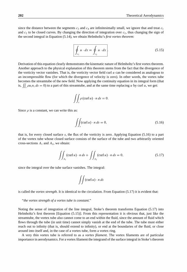
202 Theoretical Aerodynamics
since the distance between the segments c3 and c4 are infinitesimally small, we ignore that and treat c1
and c2 to be closed curves. By changing the direction of integration over c2, thus changing the sign ofthe second integral in Equation (5.14), we obtain Helmholtz’s first vortex theorem:
∮c1
u · dx =∮
c2
u · dx . (5.15)
Derivation of this equation clearly demonstrates the kinematic nature of Helmholtz’s first vortex theorem.Another approach to the physical explanation of this theorem stems from the fact that the divergence ofthe vorticity vector vanishes. That is, the vorticity vector field curl u can be considered as analogous toan incompressible flow (for which the divergence of velocity is zero). In other words, the vortex tubebecomes the streamtube of the new field. Now applying the continuity equation in its integral form (thatis,
∫∫sρuini ds = 0) to a part of this streamtube, and at the same time replacing u by curl u, we get:
∫∫s
ρ (curl u) · n ds = 0.
Since ρ is a constant, we can write this as:
∫∫s
(curl u) · n ds = 0, (5.16)
that is, for every closed surface s, the flux of the vorticity is zero. Applying Equation (5.16) to a partof the vortex tube whose closed surface consists of the surface of the tube and two arbitrarily orientedcross-sections A1 and A2, we obtain:
∫∫A1
(curl u) · n ds +∫∫
A2
(curl u) · n ds = 0, (5.17)
since the integral over the tube surface vanishes. The integral:
∫∫(curl u) · n ds
is called the vortex strength. It is identical to the circulation. From Equation (5.17) it is evident that:
“the vortex strength of a vortex tube is constant.”
Noting the sense of integration of the line integral, Stoke’s theorem transforms Equation (5.17) intoHelmholtz’s first theorem [Equation (5.15)]. From this representation it is obvious that, just like thestreamtube, the vortex tube also cannot come to an end within the fluid, since the amount of fluid whichflows through the tube (in unit time) cannot simply vanish at the end of the tube. The tube must eitherreach out to infinity (that is, should extend to infinity), or end at the boundaries of the fluid, or closearound into itself and, in the case of a vortex tube, form a vortex ring.
A very thin vortex tube is referred to as a vortex filament. The vortex filaments are of particularimportance in aerodynamics. For a vortex filament the integrand of the surface integral in Stoke’s theorem

Vortex Theory 203
[Equation (5.13)]:
∮c
u · dx =∫∫
�s
(curl u) · nds = � (5.18)
can be taken in front of the integral to obtain:
(curl u) · n�s = � (5.19)
or
2ω · n �s = 2ω �s = constant, (5.20)
where ω is the angular velocity. From this it is evident that the angular velocity increases with decreasingcross-section of the vortex filament.
It is a usual practice to idealize a vortex tube of infinitesimally small cross-section into a vortex filament.Under this idealization, the angular velocity of the vortex, given by Equation (5.20), becomes infinitelylarge. From the relation:
ω �s = constant, (5.21)
we have ω → ∞, for �s → 0.The flow field outside the vortex filament is irrotational. Therefore, for a vortex of strength � at a
particular position, the spatial distribution of curl u is fixed. In addition, if div u is also given (for example,div u = 0 in an incompressible flow), then according to the fundamental theorem of vortex analysis, thevelocity field u (which may extend to infinity) is uniquely determined provided the normal componentof velocity vanishes asymptotically sufficiently fast at infinity and no internal boundaries exist.
The fundamental theorem of vector analysis is also essentially purely kinematic in nature. Therefore,it is valid for both viscous and inviscid flows, and not restricted to inviscid flows only. Let us split thevelocity vector u into two parts, namely due to potential flow and rotational flow. Therefore:
u = uIR + uR, (5.22)
where uIR is velocity of irrotational flow field and uR is velocity of rotational flow field. Thus, uIR isvelocity of an irrotational flow field, that is:
curl uIR = � × uIR = 0, (5.23)
The second is a solenoidal (coil like shape) flow field, thus:
div uR = � · uR = 0. (5.24)
Note that Equation (5.23) is the statement that “the vorticity of a potential flow is zero” and Equation(5.24) is the statement of continuity equation of incompressible flow.
The combined field is therefore neither irrotational nor solenoidal. The field uIR is a potential flow,and thus in terms of potential function φ, we have uIR = �φ. Let us assume that the divergence u to bea given function g(x). Thus:
div u = � · uIR + � · uR = g(x),

204 Theoretical Aerodynamics
that is:
div u = � · uIR = g(x), (5.25)
since � · uR = 0. Also, uIR = �φ. Therefore:
� · � φ = ∂2φ
∂x∂x= g(x)
�2φ = g(x) . (5.26)
This is an inhomogeneous Laplace equation, also called Poisson’s equation. The theory of this partialdifferential equation is the subject of potential theory which plays an important role in many branchesof physics as in fluid mechanics. It is well known from the results of potential theory that the solution ofEquation (5.26) is given by:
φ(x) = − 1
4 π
∫∫∫∞
g(x′)|x − x′| dV, (5.27)
where x is the place where the potential φ is calculated, and x′ is the abbreviation for the integrationvariables x′
1, x′2 and x′
3, and dV = (dx′1dx′
2dx′3) is a differential volume. The domain ∞ implies that the
integration is to be carried out over the entire space.
5.8 Calculation of uR, the Velocity due to Rotational Flow
We see that Equation (5.24) is satisfied if uR is represented as the curl of a new, yet unknown, vector fielda. Thus:
uR = curl a = � × a. (5.28)
We know that the divergence of the curl always vanishes.3 Therefore:
� · (� × a) = � · uR = 0. (5.29)
Now let us form the curl of u and, from Equation (5.23), obtain the equation:
� × (u) = � × (� × a) . (5.30)
But using the vector identity:
�u = � (� · u) − � × (� × u) .
3Indeed, this is true for any vector, for example, if a and b are vectors,
a · (a × b) = [aab] = 0.
Therefore, in general, it can be expressed,
[� � a] = 0,
where � and a are vectors. The representation “[ ]” is termed “box” notation in vector algebra.

Vortex Theory 205
We can express Equation (5.30) as:
� × u = � (� · a) − �a. (5.31)
Up to now the only condition on vector a is to satisfy Equation (5.28). But this condition does not uniquelydetermine this vector, because we can always add the gradient of some other function f to a withoutchanging Equation (5.28), since � × �f ≡ 0. If, in addition, we want the divergence of a to vanish (thatis, � · a = 0), we obtain from Equation (5.31) the simpler equation:
� × u = −�a. (5.32)
In this equation, let us consider � × u as a given vector function b(x), which is determined by the choiceof the vector filament and its strength (that is, circulation). Thus, the Cartesian component form of thevector Equation (5.32) leads to three Poisson’s equations, namely:
� ai = − bi; i = 1, 2, 3. (5.33)
For each of these component equations, we can apply the solution [Equation (5.27)] of Poisson’s equation.Now, vectorially combining the result, we can write the solution for a, from Equation (5.32), in short as:
a = + 1
4 π
∫∫∫∞
b(x′)|x − x′| dV. (5.34)
Thus, calculation of the velocity field u(x) for a given distribution g(x) ≡ div u and b(x) = curl u isreduced to the following integration processes, which may have to be done numerically:
u(x) = − �[
1
4 π
∫∫∫∞
div u(x′)|x − x′| dV
]+ � ×
[1
4 π
∫∫∫∞
curl u(x′)|x − x′| dV
]. (5.35)
Now, let us calculate the solenoidal term of the velocity uR, using Equation (5.35). This is the only term inincompressible flow without internal boundaries. Consider a field which is irrotational outside the vortexfilament, shown in Figure 5.20.
The velocity field outside the filament is given by:
uR(x) = � ×[
1
4 π
∫∫∫∞
curl u(x′)|x − x′| dV
]. (5.36)
xr
x′
Γ
curl u
n
Figure 5.20 A vortex filament.
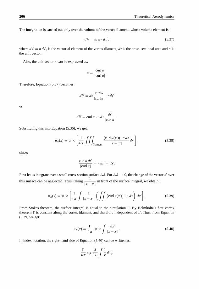
206 Theoretical Aerodynamics
The integration is carried out only over the volume of the vortex filament, whose volume element is:
dV = ds n · dx′, (5.37)
where dx′ = n ds′, is the vectorial element of the vortex filament, ds is the cross-sectional area and n isthe unit vector.
Also, the unit vector n can be expressed as:
n = curl u
|curl u| .
Therefore, Equation (5.37) becomes:
dV = dscurl u
|curl u| · nds′
or
dV = curl u · n dsds′
|curl u| .
Substituting this into Equation (5.36), we get:
uR(x) = � ×[
1
4 π
∫∫∫filament
(curl u(x′)) · n ds
|x − x′| dx′]
, (5.38)
since:
curl u ds′
|curl u| = n ds′ = dx′.
First let us integrate over a small cross-section surface �S. For �S → 0, the change of the vector x′ over
this surface can be neglected. Thus, taking1
|x − x′| in front of the surface integral, we obtain:
uR(x) = � ×[
1
4 π
∫1
|x − x′|
(∫∫ (curl u(x′)
) · n ds
)dx′
]. (5.39)
From Stokes theorem, the surface integral is equal to the circulation �. By Helmholtz’s first vortextheorem � is constant along the vortex filament, and therefore independent of x′. Thus, from Equation(5.39) we get:
uR(x) = �
4 π� ×
∫dx′
|x − x′| . (5.40)
In index notation, the right-hand side of Equation (5.40) can be written as:
�
4 πεijk
∂
∂xj
∫1
rdx′
k.

Vortex Theory 207
The operator4 εijk
∂
∂xj
can directly be taken into the integral. The term∂
∂xj
(r− 1
)(with ri = (xi − x′
i)
and r = |r|) becomes:
∂
∂xj
(r− 1
)= − 1
r2
∂r
∂xj
= − 1
r2
(xj − x′
j
) 1
r= − rj r− 3.
In vector form, this is simply:
∂
∂xj
(r− 1
) = − r
r3.
Therefore, substituting the above into Equation (5.40), we get the famous Biot-Savart law:
uR(x) = �
4 π
∫filament
dx′ × r
r3, (5.41)
where r = (x − x′). The Biot-Savart law is a useful relation in aerodynamics.
5.9 Biot-Savart Law
Biot-Savart law relates the intensity of magnitude of magnetic field close to an electric current carryingconductor to the magnitude of the current. It is mathematically identical to the concept of relating intensityof flow in the fluid close to a vorticity-carrying vortex tube to the strength of the vortex tube. It is a purekinematic law, which was originally discovered through experiments in electrodynamics. The vortexfilament corresponds there to a conducting wire, the vortex strength to the current, and the velocity fieldto the magnetic field. The aerodynamic terminology namely, “induced velocity” stems from the originof this law.
Now let us calculate the induced velocity at a point in the field of an elementary length δs of a vortex ofstrength �. Assume that a vortex tube of strength �, consisting of an infinite number of vortex filaments,to terminate in some point P, as shown in Figure 5.21.
The total strength of the vortex tube will be spread over the surface of a spherical boundary of radiusR. The vorticity in the spherical surface will thus have the total strength of �. Because of symmetry thevelocity of flow at the surface of the sphere will be tangential to the circular line of intersection of thesphere with a plane normal to the axis of the vortex tube. Such plane will be a circle ABC of radius r
subtending a conical angle 2θ at P, as shown in Figure 5.22.If the velocity on the sphere at (R, θ) from P is v, then the circulation round the circuit ABC is �′,
where:
�′ = 2πR sin θ v.
4εijk is a tensor and is positive when the subscripts i, j, k are expressed in cyclic order. That is,
εijk = εjki = εkij .
But, for noncyclic orders of i, j, k
εijk = −εjki
and so on.

208 Theoretical Aerodynamics
surrounding the ‘free’ endof the vortex-tube at point P
Spherical boundary
P1
Γ
P
Vortex-tube
Figure 5.21 Vortex-tube discharging into a sphere.
The radius of the circuit is r = R sin θ, therefore, we have:
�′ = 2πr v. (5.42)
But the circulation round the circuit is equal to the strength of the vorticity in the contained area. This ison the cap ABCD of the sphere. Since the distribution of the vorticity is constant over the surface, wehave:
�′ = Surface area of the cap
Surface area of the sphere� = 2πR2 (1 − cos θ)
4πR2�,
that is:
�′ = �
2(1 − cos θ) . (5.43)
P
R
A
D
r
θ
B
C
Γ
P1
Figure 5.22 Vortex-tube discharged into an imaginary sphere.

Vortex Theory 209
D
B
P1 P
A
Cθ
R1
θ1
R
Figure 5.23 A short vortex tube discharged into an imaginary sphere.
From Equations (5.42) and (5.43), we obtain the induced velocity as:
v = �
4πr(1 − cos θ) . (5.44)
Now, assume that the length of the vortex decreases until it becomes very short, as shown (P1P) inFigure 5.23. The circle ABC is influenced by the opposite end P1 also (that is, both the ends P and P′
of the vortex influence the circle). Now the vortex elements entering the sphere are congregating on P1.Thus, the sign of the vorticity is reversed on the sphere of radius R1. The velocity induced at P1 becomes:
v1 = − �
4πr(1 − cos θ1) . (5.45)
The net velocity on the circuit ABC is the sum of Equations (5.44) and (5.45), therefore, we have:
v − v1 = �
4πr
[(1 − cos θ) − (1 − cos θ1)
]
= �
4πr(cos θ1 − cos θ) .
As the point P1 approaches P,
cos θ → cos (θ − δθ) = cos θ + sin θ δθ
and
(v − v1) → δv.
Thus, at the limiting case of P1 approaching P, we have the net velocity as:
δv = �
4πrsin θ δθ. (5.46)
This is the velocity induced by an elementary length δs of a vortex of strength � which subtends an angleδθ at point P located by the ordinate (R, θ) from the element. Also, r = R sin θ and R δθ = δs sin θ, thus

210 Theoretical Aerodynamics
Γ
β
Bsδs
P
hr
A
θα
φ
Figure 5.24 A linear vortex of finite length.
we have:
δv = �
4πR2sin θ δs . (5.47)
It is evident from Equation (5.47) that to obtain the velocity induced by a vortex this equation has to beintegrated. This treatment of integration varies with the length and shape of the finite vortex being studied.In our study here, for applying Biot-Savart law, the vortices of interest are all nearly linear. Therefore,there is no complexity due to vortex shape. The vortices will vary only in their overall length.
5.9.1 A Linear Vortex of Finite Length
Examine the linear vortex of finite length AB, shown in Figure 5.24. Let P be an adjacent point locatedby the angular displacements α and β from A and B respectively. Also, the point P has coordinates r andθ with respect to an elemental length δs of AB. Further, h is the height of the perpendicular from P toAB, and the foot of the perpendicular is at a distance s from δs.
The velocity induced at P by the element of length δs, by Equation (5.47), is:
δv = �
4πr2sin θ δs . (5.48)
The induced velocity is in the direction normal to the plane ABP, shown in Figure 5.24.5
The velocity at P due to the length AB is the sum of induced velocities due to all elements, such asδs. However, all the variables in Equation (5.48) must be expressed in terms of a single variable beforeintegrating to get the effective velocity. A variable such as φ, shown in Figure 5.24 may be chosen for
5The induced velocity for the circulation shown (that is, clockwise when viewed from right to left), is into the page. When the circulationdirection is reversed (that is, counter clockwise) the induced velocity will be from the page to upwards.

Vortex Theory 211
this purpose. The limits of integration are:
φA = −(
π
2− α
)to φB = +
(π
2− β
),
since φ passes through zero while integrating from A to B. Here we have:
sin θ = cos φ
r2 = h2 sec2 φ
ds = d (h tan φ) = h sec2 φ dφ.
Thus, we have the induced velocity at P due to vortex AB, by Equation (5.48), as:
v =∫ + ( π
2 −β)
− ( π2 −α)
�
4πhcos φ dφ
= �
4πh
[sin
(π
2− β
)+ sin
(π
2− α
)]
v = �
4πh(cos α + cos β) . (5.49)
This is an important result of vortex dynamics. From this result we obtain the following specific resultsof velocity in the vicinity of the line vortex.
5.9.2 Semi-Infinite Vortex
A vortex is termed semi-infinite vortex when one of its ends stretches to infinity. In our case let the endB in Figure 5.24 stretches to infinity. Therefore, β = 0 and cos β = 1, thus, from Equation (5.49), wehave the velocity induced by a semi-infinite vortex at a point P as:
v = �
4πh(cos α + 1) . (5.50)
5.9.3 Infinite Vortex
An infinite vortex is that with both ends stretching to infinity. For this case we have α = β = 0. Thus, theinduced velocity due to an infinite vortex becomes:
v = �
2πh. (5.51)
For a specific case of point P just opposite to one of the ends of the vortex, say A, we have α = π/2 andcos α = 0. Thus, the induced velocity at P becomes:
v = �
4πh. (5.52)
This amounts to precisely half of the value for the infinitely long vortex filament [Equation (5.51)], aswe would expect because of symmetry.

212 Theoretical Aerodynamics
While discussing Figure 5.15, we saw that the circulation about an aerofoil in two-dimensional flow canbe represented by a bound vortex. We can assume these bound vortices to be straight and infinitely longvortex filaments (potential vortices). As far as the lift is concerned we can think of the whole aerofoilas being replaced by the straight vortex filament. The velocity field close to the aerofoil is of coursedifferent from the field about a vortex filament in cross flow, but both fields become more similar whenthe distance of the vortex from the aerofoil becomes large.
In the same manner, a starting vortex can be assumed to be a straight vortex filament which is attachedto the bound vortex at plus and minus infinity. The circulation of the vortex determines the lift, and thelift formula which gives the relation between circulation, �, and lift per unit width, l, in inviscid potentialflow is the Kutta-Joukowski theorem,6 namely:
l = − ρ �U∞, (5.53)
where l is the lift per unit span of the wing, � is circulation around the wing, U∞ is the freestream velocityand ρ is the density of the flow.
It is important to note that the lift force on a wing section in inviscid (potential) flow is perpendicularto the direction of the undisturbed stream and thus an aerofoil experiences only lift and no drag. Thisresult is of course contrary to the actual situation where the wing experiences drag also. This is becausehere in the present approach the viscosity of air is ignored whereas in reality air is a viscous fluid. TheKutta-Joukowski theorem in the form of Equation (5.53) with constant � holds only for wing sectionsin a two-dimensional plane flow. In reality all wings are of finite span and hence the flow essentiallybecomes three-dimensional. But as long as the span is much larger than the chord of the wing section,the lift can be estimated assuming constant circulation � along the span. Thus, the lift of the whole wingspan 2b is given by:
L = − ρ �U∞ 2b . (5.54)
But in reality there is flow communication from the bottom to the top at the wing tips, owing to higherpressure on the lower surface of the wing than the upper surface. Therefore, by Euler equation, the fluidflows from lower to upper side of the wing under the influence of the pressure gradient, in order to even
6The Kutta-Joukowski theorem is a fundamental theorem of aerodynamics. It is named after the German Martin Wilhelm Kutta andthe Russian Nikolai Zhukovsky (or Joukowski) who first developed its key ideas in the early 20th century. The theorem relates the liftgenerated by a right cylinder to the speed of the cylinder through the fluid, the density of the fluid, and the circulation. The circulationis defined as the line integral, around a closed loop enclosing the cylinder or aerofoil, of the component of the velocity of the fluidtangent to the loop. The magnitude and direction of the fluid velocity change along the path.
The flow of air in response to the presence of the aerofoil can be treated as the superposition of a translational flow and a rotationalflow. It is, however, incorrect to think that there is a vortex like a tornado encircling the cylinder or the wing of an airplane in flight.It is the integral’s path that encircles the cylinder, not a vortex of air. (In descriptions of the Kutta-Joukowski theorem the aerofoil isusually considered to be a circular cylinder or some other Joukowski aerofoil.)
The theorem refers to two-dimensional flow around a cylinder (or a cylinder of infinite span) and determines the lift generated byone unit of span. When the circulation �∞ is known, the lift L per unit span (or l) of the cylinder can be calculated using the followingequation:
l = ρ∞V∞�∞,
where ρ∞ and V∞ are the density and velocity far upstream of the cylinder, and �∞ is the circulation defined as the line integral,
�∞ =∮
cV cos θ ds
around a path c (in the complex plane) far from and enclosing the cylinder or airfoil. This path must be in a region of potential flowand not in the boundary layer of the cylinder. The V cos θ is the component of the local fluid velocity in the direction of and tangentto the curve c, and ds is an infinitesimal length on the curve c. The above equation for lift l is a form of the Kutta-Joukowski theorem.
The Kutta-Joukowski theorem states that, “the force per unit length acting on a right cylinder of any cross section whatsoever isequal to ρ∞V∞�∞, and is perpendicular to the direction of V∞.”

Vortex Theory 213
2b
Γt
Γt
Bound vortex
Tip vortex
Starting vortex
Γs
Γb
Figure 5.25 Simplified vortex system of a finite wing.
out the pressure difference. In this way the magnitude of the circulation on the wing tips tends to becomezero. Therefore, the circulation over the wing span varies and the lift is given by:
L = − ρ U∞
∫ + b
− b
�(x) dx, (5.55)
where the origin is at the middle of the wing, x is measured along the span, and b is the semi-span ofthe wing.
According to Helmholtz’s first vortex theorem, being purely kinematic, the above relations for lift arealso valid for the bound vortex. Thus, isolated pieces of a vortex filament cannot exist. Also, it cannotcontinue to be straight along into infinity, where the wing has not cut through the fluid and thus nodiscontinuity surface has been generated as is necessary for the formation of circulation. Therefore, freevortices, �t , which are carried away by the flow must be attached at the wing tips. Together with thebound vortex, �b, and the starting vortex, �s, they (the tip vortices) form a closed vortex ring frame inthe fluid region cut by the wing, as shown in Figure 5.25.
If a long time has passed since start-up, the starting vortex is at infinity (far downstream of the wing),and the bound vortex and the tip vortices together form a horseshoe vortex.
Even though the horseshoe vortex system represents only a very rough model of a finite wing, it canprovide a qualitative explanation for how a wing experiences a drag in inviscid flow, as already mentioned.The velocity w induced at the middle of the wing by the two tip vortices accounts for double the velocityinduced by a semi-infinite vortex filament at distance b. Therefore, by Equation (5.50), we have:
w = �
4 πb(1 + 0) = �
4πb. (5.56)
This velocity is directed downwards and hence termed induced downwash. Thus, the middle of the wingexperiences not only the freestream velocity U∞, but also a velocity u, which arises from the superpositionof U∞ and downwash velocity w, as shown in Figure 5.26.
In inviscid flow, the force vector is perpendicular to the actual approach direction of the flow stream,and therefore has a component parallel to the undisturbed flow, as shown in Figure 5.26, which manifestsitself as the induced drag Di, given by:
Di = Aw
U∞. (5.57)

214 Theoretical Aerodynamics
A
u
U
Di
L
wU
Figure 5.26 Illustration of induced drag.
It is important to note that Equation (5.57) holds if the induced downwash from both vortices is constantover the span of the wing. However, the downwash does change since at a distance x from the wingcenter, one vortex induces a downwash of:
�
4 π (b + x),
whereas the other vortex induces:
�
4 π (b − x).
Both the downwash are in the same direction, therefore adding them we get the effective downwash as:
w = �
4 π (b + x)+ �
4 π (b − x)
= �
4 π
2b
b2 − x2
= �
2 π
b
b2 − x2.
From this it can be concluded that the downwash is the smallest at the center of the wing (that is, Equation(5.57) underestimates the induced drag) and tends to infinity at the wing tips. The unrealistic value there(at wing tips) does not appear if the circulation distribution decreases towards the wing tips, as in deed ithas to. For a semi-elliptical circulation distribution over the span of the wing, the downwash distributionbecomes constant and Equation (5.57) is applicable. Helmholtz first vortex theorem stipulates that for aninfinitesimal change in the circulation in the x-direction of:
d� = d�
dxdx
and a free vortex of the same infinitesimal strength must leave the trailing edge. This process leads to animproved vortex system, as shown in Figure 5.27.
The free vortices form a discontinuity surface in the velocity components parallel to the trailing edge,which rolls them into the kind of vortices, as shown in Figure 5.28.
These vortices must be continuously renewed as the wing moves forward. This calls for continuousreplenishment of kinetic energy in the vortex. The power needed to do this is the work done per unit timeby the induced drag.

Vortex Theory 215
Γt
ΓtΓb
Figure 5.27 Simplified vortex system of a wing.
Figure 5.28 Vortices formation due to rollup of the discontinuity.
The manifestation of Helmholtz’s first theorem can be encountered in daily life. Recall the dimplesformed at the free surface of coffee in a cup when a spoon is suddenly dipped into it. The formationprocess of dimples looks like that shown schematically in Figure 5.29.
As the fluid flows together from the front and back, a surface of discontinuity forms along the rimof the spoon. The discontinuity surface rolls itself into a bow-shaped vortex whose endpoints form thedimples on the free surface, as shown in Figure 5.29.
The flow outside the vortex filament is a potential flow. Thus, by incompressible Bernoulli equation,we have:
p + 12 ρ u2 + ρ g z = constant .
Surface
Spoon
Dimple
Figure 5.29 Vortex formation due to dipping of a spoon.

216 Theoretical Aerodynamics
n
c1
Time t0
cx(t)
Figure 5.30 A closed curve on a vortex ring at times t0 and t.
This is valid both along a streamline and between any two points in the flow field.7 Also, at the freesurface the pressure is equal to the ambient pressure pa. Further, at some distance away from the vortexthe velocity is zero and there is no dimple at the free surface, and hence z = 0. Thus, the Bernoulliconstant is equal to pa and we have:
1
2ρ u2 + ρ g z = 0.
Near the end points of the vortex the velocity increases by the formula given by Equation (5.52), andtherefore z must be negative, that is, a depression of the free surface. In reality, the cross-sectional surfaceof the vortex filament is not infinitesimally small, therefore we cannot take the limit h → 0 in Equation(5.52), for which the velocity becomes infinite. However, the induced velocity due to the vortex filamentis so large that it causes a noticeable formation of dimples.
It should be noted that an infinitesimally thin filament cannot appear in actual flow because the velocitygradient of the potential vortex tends to infinity for h → 0, so that the viscous stresses cannot be ignoredeven for very small viscosity. Also, it is well known that the viscous stresses make no contribution toparticle acceleration in incompressible potential flow, but they do deformation work and thus provide acontribution to the dissipation. The energy dissipated in heat stems from the kinetic energy of the vortex.
5.9.4 Helmholtz’s Second Vortex Theorem
The second vortex theorem of Helmholtz’s states that:
“a vortex tube is always made up of the same fluid particles.”
In other words, a vortex tube is essentially a material tube. This characteristic of a vortex tube can berepresented as a direct consequence of Kelvin’s circulation theorem. Let us consider a vortex tube andan arbitrary closed curve c on its surface at time t0, as shown in Figure 5.30. By Stokes integral theorem,the circulation of the closed curve c is zero (that is, D�/Dt = 0). The circulation of the curve, which ismade up of the same material particles, still has the same (zero) value of circulation at a latter instant oftime t.
7It would be of value to note that, for a steady, incompressible viscous flow, the Bernoulli equation can be applied between any twopoints along a streamline only. But for a steady, incompressible and inviscid (that is, potential) flow, the Bernoulli equation can beapplied between any two points, in the entire flow field. That is, the two points between which the Bernoulli equation is applied neednot lie on a streamline.

Vortex Theory 217
t = t4t = t1 t = t2 t = t3
Figure 5.31 Two vortex rings passing through one another.
By inverting the above reasoning, it follows from Stokes integral theorem that these material particlesmust be on the outer surface of the vortex tube.
If we examine smoke-rings, it can be seen that the vortex tubes are material tubes. The smoke willremain in the vortex ring and will be transported with it, so that it is the smoke itself which carriesthe vorticity. This statement holds under the restrictions of barotropy (that is, ρ = ρ(p), the density isa function of pressure only) and zero viscosity. The slow disintegration seen in smoke-rings is due tofriction and diffusion. A vortex ring which consists of an infinitesimally thin vortex filament induces aninfinitely large velocity on itself (similar to the horseshoe vortex), so that the ring would move forwardwith infinitely large velocity. The induced velocity at the center of the ring remains finite (as in horseshoevortex). From Biot-Savart law, the induced velocity becomes:
u = �
4 π
∫ 2π
0
h2dφ
h3= �
2 h.
This velocity becomes infinitely large (that is, unrealistic) when the cross-section of the vortex ring isassumed to be infinitesimally small. For finite cross-section, the velocity induced by the ring on itself, thatis, the velocity with which the ring moves forward remains finite. But in reality the actual cross-sectionof the ring is not known, and probably depends on how the ring was formed.
In practice we notice that the ring moves forward with a velocity which is slower than the inducedvelocity in the center. Also, it is well known that two rings moving in the same direction continu-ally overtake each other whereby one slips through the other in front. This phenomenon, illustrated inFigure 5.31, is explained by mutually induced velocities on the rings and formula given above for thevelocity at the center of the ring.
In a similar manner it can be explained why a vortex ring towards a wall becomes larger in diameterand at the same time its velocity gets reduced. Also, the diameter decreases and the velocity increaseswhen a vortex ring moves away from a wall, as illustrated in Figure 5.32.
To work out the motion of vortex rings the cross-section of vortex must be known. Further, for in-finitesimally thin rings the calculation fails because vortex rings, such as curved vortex filaments, inducelarge velocities on themselves. However, for straight vortex filaments, that is, for vortex filaments intwo-dimensional flows, a simple description of the “vortex dynamics” for infinitesimally thin filamentsis possible, since for such a case the self-induced translational velocity vanishes. We know that vortexfilaments are material lines, therefore it is sufficient to calculate the paths of the fluid particles whichcarry the rotation in xy-plane perpendicular to the filaments, using:
dx
dt= u(x, t) or
dxi
dt= ui(xi, t),

218 Theoretical Aerodynamics
Figure 5.32 Kinematics of a vortex ring near a wall.
that is, to determine the paths of the vortex centers. The induced velocity which a straight vortex filamentat position xi induces at position x is known from Equation (5.49), that is:
v = �
4πh(cos α + cos β) .
As we have seen, the induced velocity is perpendicular to the vector hi = ri = (x − xi), and therefore
has the direction ez × hi
|hi| , so that the vectorial form of Equation (5.41) reads as:
uR = �
2 πez × x − xi
|x − xi|2 .
For x → xi the velocity tends to infinity, but because of symmetry the vortex cannot be moved by its ownvelocity field, that is, the induced translational velocity is zero. The induced velocity of n vortices withthe circulation �i (i = 1, 2, . . . n) is:
uR = 1
2 π
∑i
�i ez × x − xi
|x − xi|2 .
If there are no internal boundaries, or if the boundary conditions are satisfied by reflection, as inFigure 5.32, the last equation describes the entire velocity field, and using dx/dt = u(x, t) or dxi/dt =ui(xi, t), the “equation of motion” of the kth vortex becomes:
dxk
dt= 1
2 π
∑i(i /= k)
�i ez × x − xi
|x − xi|2 . (5.58)
For i = k, the induced translational velocity becomes zero, owing to symmetry, and hence excluded fromthe summation. Equation (5.58) gives the 2n relations for the path coordinates.
The dynamics of vortex motion have invariants which are analogous to the invariants of a point masssystem on which no external forces act. The conservation of strengths of the vortices by Helmholtz’stheorem (
∑�k = constant) corresponds to mass conservation of total mass of the point mass system.
When the Equation (5.58) is multiplied by �k, summed over k and expanded, we get:
∑�k
dxk
dt= �1
dx1
dt+ �2
dx2
dt+ �3
dx3
dt+ · · ·· =

Vortex Theory 219
ez × 1
2 π
[�1 �2
x1 − x2
|x1 − x2|2 + �1 �3x1 − x3
|x1 − x3|2 + · · ··
+�2 �1x2 − x1
|x2 − x1|2 + �2 �3x2 − x3
|x2 − x3|2 + · · ··].
In the above equation, the terms on the right-hand side cancel out in pairs, and the equation reduces to:
∑k
�k
dxk
dt= 0.
On integration this results in:
∑k
�k xk = xg
∑k
�k. (5.59)
The integration constants are written as xg, which is like a center of gravity coordinate (this is done herefor dimensional homogeneity). Equation (5.59) states that:
“the center of gravity of the strengths of the vortices is conserved.”
For a point mass system, by conservation of momentum, we have the corresponding law, namely:
“the velocity of the center of gravity is a conserved quantity in the absence of external forces.”
For∑
�k = 0, the center of gravity lies at infinity, so that, for example, two vortices with �1 = −�2
must take a turn about a center of gravity point Pg which is at a finite distance, as shown in Figure 5.33.The paths of the vortex pairs are determined by numerical integration of Equation (5.58). The paths
will look like those shown in Figure 5.34.
Pg
Γ1Γ1 > 0
Γ2 > 0
Γ2 = Γ1
Γ1 > 0
Pg
Γ2 > 0
Figure 5.33 Pathlines of a pair of straight vortices.
t = t1 t = t3t = t2
Γ1 Γ2 = Γ1
Figure 5.34 Pathlines of two straight vortex pairs.

220 Theoretical Aerodynamics
5.9.5 Helmholtz’s Third Vortex Theorem
The third vortex theorem of Helmholtz’s states that:
“the circulation of a vortex tube remains constant in time.”
Using Helmholtz’s second theorem and Kelvin’s circulation theorem, the above statement can be inter-preted as “a closed line generating the vortex tube is a material line whose circulation remains constant.”
Helmholtz’s second and third theorems hold only for inviscid and barotropic fluids.
5.9.6 Helmholtz’s Fourth Vortex Theorem
The fourth theorem states that:
“the strength of a vortex remains constant in time.”
This is similar to the fact that the mass flow rate through a streamtube is invariant as the tube moves inthe flow field. In other words, the circulation distribution gets adjusted with the area of the vortex tube.That is, the circulation per unit area (that is, vorticity) increases with decrease in the cross-sectional areaof the vortex tube and vice versa.
5.10 Vortex Motion
Vortex is a fluid flow in which the streamlines are concentric circles. The vortex motions encounteredin practice may in general be classified as free vortex or potential vortex and forced vortex or flywheelvortex. The streamline pattern for a vortex may be represented as concentric circles, as shown in Figure5.35.
When a fluid flow is along a curved path, as in a vortex, the velocity of the fluid elements along anystreamline will undergo a change due to its change of direction, irrespective of any change in magnitudeof the fluid stream. Consider the streamtube shown in Figure 5.36.
As the fluid flows round the curve there will be a rate of change of velocity, that is, an acceleration,towards the curvature of the streamtube. The consequent rate of change of momentum of the fluid must be
x
y
Streamline
Potential line
vθ
r
θ
Figure 5.35 Streamline pattern of a vortex.

Vortex Theory 221
V+δV
V
r
A
δsB C
δθ
p + δp
δr
o
D
p
Figure 5.36 Fluid element in a vortex.
due to a force acting radially across the streamlines resulting from the difference of pressure between thesides BC and AD of the streamline element, as per Newton’s second law. The control volume ABCD inFigure 5.36 subtends an angle δθ at the center of curvature O and has length δs in the direction of flow. Letthe thickness of ABCD perpendicular to the plane of diagram be ‘b’. For the streamline AD, the radiusof curvature is r and that for BC is (r + δr). The pressure and velocity at AD and BC are p, V, (p + δp)and (V + δV ), as shown in Figure 5.36. Thus, the change of pressure in the radial direction is δp.
The change of velocity in the radial direction (as shown in the velocity diagram in Figure 5.36) is:
δV = Vδθ.
But δθ = δs/r. Thus, the radial change of velocity between AB and CD is:
δV = Vδs
r.
Mass flow rate through the streamtube is = density × area × velocity
= ρ(b × δr)V.
Rate of change of momentum
in radial direction = (mass per unit time)
× radial change of velocity
= (ρbδr V )Vδs
r. (5.60)
This rate of change of momentum is produced by the force due to the pressure difference between BCand AD of the control volume, given by:
F = [(p + δp) − p
]bδs. (5.61)
According to Newton’s second law, Equation (5.60) = Equation (5.61). Thus:
δpbδs = ρbδrV 2δs/r

222 Theoretical Aerodynamics
or
δp
δr= ρV 2
r. (5.62)
For an incompressible fluid, density ρ is constant and Equation (5.62) can be expressed in terms ofpressure head h. Pressure is given by:
p = ρgh.
Therefore,
δp = ρgδh.
Substituting this into Equation (5.62), we get:
ρgδh
δr= ρV 2
r
or
δh
δr= V 2
gr.
In the limit δr → 0, this gives the rate of change of pressure head in the radial direction as:
dh
dr= V 2
gr. (5.63)
The curved flow shown in Figure 5.36 will be possible only when there is a change of pressure head ina radial direction, as seen from Equation (5.63). However, since the velocity V along streamline AD isdifferent from the velocity (V + δV ) along BC, there will also be a change in the velocity head from onestreamline to another. Such a change of velocity head in the radial direction is given by:
Rate of change of velocity head
in the radial direction = [(V + δV )2 − V 2
]/(2 g δr)
= V
g
δV
δr(neglecting the products
of small quantities)
= V
g
dV
dr(as δr → 0). (5.64)
For a planar flow (say in the horizontal plane), the changes in potential head is zero. Therefore, the changeof total head H , that is, the total pressure energy per unit weight, in a radial direction, δH/δr, is given by:
δH
δr= change of pressure head + change of velocity head.

Vortex Theory 223
Substituting Equations (5.63) and (5.64) into the results of the above equation, we get:
dH
dr= V 2
gr+ V
g
dV
dr
= V
g
(V
r+ dV
dr
). (5.65)
The term
(V
r+ dV
dr
)is also known as vorticity of the flow.
In obtaining Equation (5.65), it is assumed that the streamlines are horizontal. But this equation alsoapplies to cases where the streamlines are inclined to horizontal, since the fluid in a control volume is ineffect weightless, being supported vertically by the surrounding fluid.
5.11 Forced Vortex
Forced vortex is a rotational flow field in which the fluid rotates as a solid body with a constant angularvelocity ω, and the streamlines form a set of concentric circles. Because the fluid in a forced vortexrotates like a rigid body, the forced vortex is also called flywheel vortex. The change of total energy perunit weight in a vortex motion is governed by Equation (5.65).
The velocity at any radius r is given by:
V = ω r
From this we have:
dV
dr= ω.
and
V
r= ω.
Substituting dV/dr and V/r into Equation (5.65), we get:
dH
dr= ωr
g(ω + ω)
= 2ω2r
g.
Integrating this we get:
H = ω2r2
g+ c, (5.66)
where c is a constant. By Bernoulli equation, at any point in the fluid, we have:
H = p
ρg+ V 2
2g+ z.

224 Theoretical Aerodynamics
Free surface
Velocity
V » rvariation
Streamline
(a) (b)
Axis of rotation
r
Datum
z
Figure 5.37 Forced vortex (a) shape of free surface, (b) velocity variation.
Note that, in the above equation and Equation (5.66), the unit of the total head is meters. Substitution ofthis into Equation (5.66) results in:
p
ρg+ ω2r2
2g+ z = ω2r2
g+ c
p
ρg+ z = ω2r2
2g+ c.
If the rotating fluid has a free surface, the pressure at the surface will be atmospheric; therefore, thepressure at the free-surface will be zero.
Replacingp
ρgwith 0 in the above equation, the profile of the free surface is obtained as:
z = ω2r2
2g+ c . (5.67)
Thus, the free surface of a forced vortex is in the form of a paraboloid.Similarly, for any horizontal plane, for which z will be constant, the pressure distribution will be
given by:
p
ρg= ω2r2
2g+ (c − z). (5.68)
The typical shape of the free surface and the velocity variation along a radial direction of a forcedvortex are shown in Figure 5.37.
5.12 Free Vortex
Free vortex is an irrotational flow field in which the streamlines are concentric circles, but the variationof velocity with radius is such that there is no change of total energy per unit weight with radius, so thatdH/dr = 0. Since the flow field is potential, the free vortex is also called potential vortex.
For a free vortex, from Equation (5.65), we have:
0 = V
g
(V
r+ dV
dr
)
dV
V+ dr
r= 0.

Vortex Theory 225
The core
V =Γ
2πr
r
Figure 5.38 Velocity distribution in a free vortex core.
Integrating, we get:
ln V + ln r = constant
or
Vr = c,
where c is a constant known as the strength of the vortex at any radius r.The tangential velocity becomes:
V = c
r. (5.69)
This shows that in the flow around a vortex core the velocity is inversely proportional to the radius (seeSection 5.4). When the core is small, or assumed concentrated on a line axis, it is apparent from therelation V = c/r that when r is small V can be very large. However, within the core the fluid behaves asthough it were a solid cylinder and rotates at an uniform angular velocity. Figure 5.38 shows the variationof velocity with radius for a typical free vortex. The solid line represents the idealized case, but in realityit is not so precise, and the velocity peak is rounded off, as shown by the dashed lines.
At any point in the flow field, by Bernoulli equation, we have:
p
ρg+ V 2
2g+ z = H.
Substituting Equation (5.69), we get:
p
ρg+ c2
2gr2+ z = H.
At the free surface,p
ρg= 0. Thus, the profile of the free surface is given by:
H − z = c2
2gr2. (5.70)
This is a hyperbola asymptotic to the axis of rotation and to the horizontal plane through z = H , as shownin Figure 5.39.

226 Theoretical Aerodynamics
V 1r
(b)(a)
z
variationH
r
r
Velocity
Figure 5.39 Free vortex: (a) shape of free surface, (b) velocity variation.
For any horizontal plane, z is constant and the pressure variation is given by:
p
ρg= (H − z) − c2
2gr2. (5.71)
Thus, in a free vortex, pressure decreases and circumferential velocity increases as we move towards thecenter, as shown in Figure 5.39.
The free vortex discussed above is essentially a free cylindrical vortex. The fluid moves along stream-lines that are horizontal concentric circles; there is no variation of total energy with radius. Combinationof a free cylindrical vortex and radial flow will result in a free spiral vortex.
5.12.1 Free Spiral Vortex
A free spiral vortex is essentially the combination of a free cylindrical vortex and a radial flow. Beforegetting into the physics of free spiral vortex, let us see what is a radial flow.
Radial Flow
Examine the flow between two parallel planes as shown in Figure 5.40. In the flow the streamlines will beradial straight lines and the streamtube will be in the form of sectors. This kind of flow in which the fluidflows radially inwards, or outwards from a center is called a radial flow. The area of the flow will thereforeincrease as the radius increases, causing the velocity to decrease. The flow pattern is symmetrical andtherefore, the total energy per unit weight H will be the same for all streamlines and for all points alongeach streamline if we assume that there is no loss of energy.
If Vr is the radial velocity and p is the pressure at any radius r, then the total energy per unit weightH becomes:
H = p
ρ g+ V 2
r
2g= constant. (5.72)
Assuming the flow to be incompressible (as would be the case of a liquid), by continuity, we have thevolume flow rate Q as:
Q = area × velocity
= 2πrb × Vr,
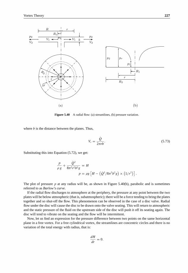
Vortex Theory 227
V1
R1p2
V2b
(b)(a)
p1
R r
p2
V2
V1
p2 pr
R1
r
p1
R2
δr
R2
r
Figure 5.40 A radial flow: (a) streamlines, (b) pressure variation.
where b is the distance between the planes. Thus,
Vr = Q
2πrb. (5.73)
Substituting this into Equation (5.72), we get:
p
ρ g+ Q2
8π2r2b2g= H
p = ρg[H −
(Q2/8π2b2g
)×
(1/r2
)].
The plot of pressure p at any radius will be, as shown in Figure 5.40(b), parabolic and is sometimesreferred to as Barlow’s curve.
If the radial flow discharges to atmosphere at the periphery, the pressure at any point between the twoplates will be below atmospheric (that is, subatmospheric); there will be a force tending to bring the platestogether and so shut-off the flow. This phenomenon can be observed in the case of a disc valve. Radialflow under the disc will cause the disc to be drawn onto the valve seating. This will return to atmosphericand the static pressure of the fluid on the upstream side of the disc will push it off its seating again. Thedisc will tend to vibrate on the seating and the flow will be intermittent.
Now, let us find an expression for the pressure difference between two points on the same horizontalplane in a free vortex. For a free cylindrical vortex, the streamlines are concentric circles and there is novariation of the total energy with radius, that is:
dH
dr= 0.

228 Theoretical Aerodynamics
Also, by Equation (5.69), we have:
V = c
r.
Let p1 and p2 be the pressures in two concentric streamlines of radii r1 and r2 which have velocities V1
and V2, respectively. Since there is no change of total energy with radius, for the same horizontal plane,by Bernoulli equation:
p1
ρg+ V 2
1
2g= p2
ρg+ V 2
2
2g
p1 − p2
ρg= V 2
2 − V 21
2g.
But V1 = c/r1 and V2 = c/r2. Thus:
p1 − p2
ρg= c2
2g
(1
r22
− 1
r21
). (5.74)
Now, let us obtain an expression for the pressure difference between two points at radii R1 and R2, on aradial line, when a fluid flows radially inward or outward from a center, neglecting friction. Flow is radialand therefore in straight line so that r, the radius of curvature of the streamlines, is infinite, dH/dr = 0,and for all streamlines:
H = p
ρg+ V 2
2g= constant.
If p1 and p2 are the pressures at radii R1 and R2, respectively, where the velocities are V1 and V2:
p1 − p2
ρg= V 2
2 − V 21
2g.
By volume conservation:
Q = 2πR1V1t = 2πR2V2t,
where Q is the volume flow rate and t is the distance between the radial passage boundaries. That is:
V1 = Q
2πR1t
V2 = Q
2πR2t.
Thus,
p1 − p2
ρg= Q2
8π2t2g
(1
R22
− 1
R21
). (5.75)

Vortex Theory 229
α
v
u
Path of a particle
Figure 5.41 A free spiral vortex.
It is evident from Equations (5.73) and (5.74) that the relation between pressure and radius and betweenvelocity and radius is similar for both free vortex and radial flow. Both types of motion may thereforeoccur together. The fluid rotates and flows radially forming a free spiral vortex in which a fluid elementwill follow a spiral path, as shown in Figure 5.41.
5.13 Compound Vortex
In the free vortex, v = c/r and thus, theoretically, the velocity becomes infinite at the center. The velocitiesnear the axis would be very high and, skin friction losses vary as the square of the velocity, they willcease to be negligible. Also, the assumption that the total head H remains constant will cease to be true.The portion of fluid around the axis tends to rotate as a solid body. Thus, the central portion essentiallyforms a forced vortex. The free surface profile of such a compound vortex and the pressure variation withradius on any horizontal plane in the vortex is shown in Figure 5.42.
R
y2
Axis
of
ForcedFree vortex Free vortex
rota
tion
y1
vortex
Free surface
Figure 5.42 Compound vortex.

230 Theoretical Aerodynamics
The velocity at the common radius R must be the same for the two vortices. For the free vortex, ify1 = depression of the free surface at radius R below the level of the surface at infinity, then:
y1 = c2
2gR2
= v2
2g
= ω2R2
2g.
For the forced vortex, if y2 is the height of the free surface at radius R above the center of the depression:
y2 = v2
2g
= c2
2gR2.
Thus, the total depression is:
y1 + y2 = c2
gR2= ω2R2
g. (5.76)
For the forced vortex, the velocity at radius R is ωR, while for the free vortex, from Equation (5.69), thevelocity at radius R is c/R. Therefore, the common radius at which these two velocity will be the sameis given by:
ωR = c/R
R =√
c
ω.
5.14 Physical Meaning of Circulation
In Equation (5.3) the vector field is taken as velocity V . But the vector field need not be the flow velocityalone. The vector field can be force, mass flow rate of a fluid, etc. Therefore, in general, the circulationmay be defined as the line integral of a vector field around a closed plane curve in a flow field. If thevector is a force F , then the integral
∮cF · ds is equal to the work done by the force. Taking the vector
as ρV , the mass flow rate per unit area, we can get a physical meaning of the circulation in the followingway. Imagine a tiny paddle-wheel probe is placed [Figure 5.43(c)] in any of the flow patterns shown inFigure 5.43.
When the flow velocity on one side is greater than the other side, as in Figure 5.43(c), the wheelwill turn. If the mass flow rate per unit area ρV is larger on one side of the wheel than the other, thenthe circulation is different from zero, but if ρV is the same on both sides as in Figure 5.43(b), then thecirculation is zero. We shall show that the component of curl m along the axis of the paddle wheel equals:
limdA→0
1
dA
∮m · ds, (5.77)

Vortex Theory 231
probePaddle-wheel
(a) (b)
(d)(c)
Figure 5.43 Streamlines in: (a) a vortex, (b) parallel flow with constant velocity, (c) parallel flow with variablevelocity, (d) flow around a corner.
where dA is the area enclosed by the curve along which we calculate circulation. The paddle wheelthen acts as a “curl meter” to measure curl m; when the wheel does not rotate, curl m = 0. In Fig-ure 5.43(c), curl m /= 0 in spite of the fact that the streamlines are parallel. In Figure 5.43(d), it is possibleto have curl m = 0 even though the streamlines go around a corner. In fact, for the flow of water arounda corner curl m = 0. We must realize that the value of curl m at a point depends upon the circulation inthe neighborhood of the point and not on the overall flow pattern.
Example 5.2
A cylindrical tank of 1 m diameter and 0.75 m height is filled with a liquid of relative density 0.9 up to0.5 m from the bottom of the tank and the rest of the tank contains atmospheric air. The tank revolvesabout its vertical axis at a speed such that the liquid begins to uncover the base. (a) Calculate the speedof rotation and (b) the upward force on the cover.
Solution
The flow field described is shown in Figure 5.44.
(a) When the tank is static, the volume of oil is:
πR2z1.
While rotating, a forced vortex is formed and the free surface will be a paraboloid CGD.
Volume of oil = Volume of cylinder ABFE − Volume of paraboloid CGD
= πR2z − 1
2πr2
1z.

232 Theoretical Aerodynamics
0.5 m
z0.75 m
FE
R
A C r D B
S
z1
G
S
Figure 5.44 Flow field in a rotating tank.
Since the volume of the paraboloid is equal to half the volume of the circumscribing cylinder, no oil isspilled out from the cylinder, therefore:
πR2z1 = πR2z − 1
2πr2
1z
r21 = 2 R2
(1 − z1
z
)
r1 = R
√2
(1 − 0.5
0.75
)
= 0.816 R
= 0.816 × 0.5
= 0.408 m
= 408 mm .
For the free surface, by Equation (5.67), we have:
z = ω2r2
2g+ constant.
Between C and G, taking G is the datum level, we have:
zA = 0, when r = 0
and
zC = z, when r = r1.

Vortex Theory 233
Thus:
z = ω2r2
2g
ω =√
2gz
r21
=√
2 × 9.81 × 0.75
0.4082
= 9.40 radians/s
= 9.40 × 60
2π
= 89.76 rpm .
(b) The top cover annular area from r = r1 to r = R is in contact with the oil. If p is the pressure at anyradius r, the force on an annular of radius r and width dr is given by:
dF = p × 2πrdr.
Integrating from r = r1 to r = R we get the force F acting on the top cover as:
F = 2π
∫ R
r1
prdr.
The pressure, given by Equation (5.68) is:
p
ρg= ω2r2
2g+ c,
since the pressure at r1 is atmospheric, p = 0 (gauge), where r = r1, thus:
c = −ω2r21
2g.
Therefore:
p = ρg
[ω2r2
2g− ω2r2
1
2g
]= ρω2
2
(r2 − r2
1
).

234 Theoretical Aerodynamics
Substituting this in the force equation above, we have:
F = 2πρω2
2
∫ R
r1
(r2 − r2
1
)rdr
= ρω2π
[r4
4− r2
2r2
1
]R
r1
= ρω2π
4
[R2 − r2
1
]2
= π
4× (
0.9 × 103) × 9.42
(0.52 − 0.4082
)2
= 435.85 N .
Example 5.3
Show that a free vortex is an irrotational motion. A hollow cylinder of diameter 1 m, open at the top,spins about its axis which is vertical, thus generating a forced vortex motion of the liquid contained in it.Calculate the height of the vessel so that the liquid just reaches the top when the minimum depth of thefree surface of the liquid (from the top) is 25 cm at 200 rpm.
Solution
The tangential velocity in a free vortex (excluding the core) is given by Equation (5.69) is:
Vθ = c
r,
where c is a constant. This field is potential if the vorticity content in the field is zero. The vorticity ζ inpolar coordinates is [Equation (5.2)]:
ζ = qt
r+ ∂qt
∂r− 1
r
∂qn
∂θ.
In free vortex, the normal component of velocity qn = 0. Thus:
ζ = qt
r+ ∂qt
∂r.
We know that:
qt
r= Vθ
r= c2
r2
and
∂qt
∂r= ∂
∂r
(c
r
)= − c
r2.

Vortex Theory 235
R
h
A C
B
zr
Figure 5.45 A spinning cylinder containing water.
Hence:
ζ = c
r2− c
r2
= 0.
Thus, the motion in a free vortex is irrotational.The spinning cylinder described in the problem is shown schematically in Figure 5.45.For a forced vortex, the free surface ABC is a paraboloid, as shown in the figure. The shape is given byEquation (5.67) as:
z = ω2r2
2g+ c.
At r = 0 on the free surface, zB = 25 cm = 0.25 m. Thus:
c = 0.25 m.
At r = R, zA = h. Therefore, we have the expression for free surface as:
h = ω2R2
2g+ 0.25.
Given, ω = 200 rpm = 200/60 rps = 200/60 × 2π radian/second. Therefore:
h = (20 π)2
32
0.52
2 × 9.81+ 0.25
= 5.84 m .
5.15 Rectilinear Vortices
A rectilinear vortex is a vortex tube whose generators are perpendicular to the plane of motion. Now, letus have a closer look at some aspects of two-dimensional vortex motion. We know that the circulation

236 Theoretical Aerodynamics
a
Vortex tube
Figure 5.46 A cylindrical vortex tube.
in an infinitesimal plane circuit is proportional to the area of the circuit. In a two-dimensional motionthe vorticity vector ζ at any point P, which is perpendicular to the plane of motion and whose magnitudeis equal to the limit of the ratio of the circulation is an infinitesimal circuit embracing P to the area ofthe circuit. That is, the vorticity vector is by definition perpendicular to the plane of the motion, so thatthe vortex lines are straight and parallel. All vortex tubes are therefore cylinders whose generators areperpendicular to the plane of motion. Such vortices are known as rectilinear vortices. For our discussionsin this section, let us consider the fluid between parallel plates at unit distance apart and parallel to theplane of the motion, which is half-way between them.
5.15.1 Circular Vortex
A circular vortex is that with the shape of its cross-section normal to its axis of rotation as circular. Forexample a single cylindrical vortex tube, whose cross-section is a circle of radius ‘a’, surrounded byunbounded fluid, as shown in Figure 5.46 is a circular vortex.
The section of this cylindrical vortex by the plane of motion is a circle, as shown in Figure 5.47.Let us assume that the vorticity ζ over the area of the circle is a constant. Outside the circle the vorticity
is zero. Consider concentric circles of radii r′ and r, where r′ < a < r, as shown in Figure 5.47. Let thetangential speeds of the fluid motion on the circles of radii r′ and r are V ′ and V , respectively.
We know that “the circulation in a closed circuit is the line integral of the tangential component of thevelocity taken round the circuit in the sense in which the arc length (elemental length along the circuit)increases.” Thus, the circulation around the circles of radii r and r′, respectively, are:
∮V ds and
∮V ′ ds,
r
V
ω r 0
a
V 0o
Figure 5.47 Section of cylindrical vortex tube.

Vortex Theory 237
where ds is an elemental arc length. Also, V and V ′ are constants. Therefore:
∮V ds = ωπa2, r > a
∮V ′ ds = ωπr′2, r < a,
where ω is the angular velocity. Thus:
2πrV = ωπa2
V = ωa2
2r, r > a
2πr′V ′ = ωπr′2
V = ωr′
2, r′ < a,
when r′ = r = a we have V ′ = V = 12 aω so that the velocity is continuous as we pass through the circle.
From the above discussions, it can be inferred that the existence of a vortex implies the co-existenceof certain distribution of velocity field. This velocity field which co-exists with the vortex is known asthe induced velocity field and the velocity at any point of it is called the induced velocity. It is importantto note that it is customary to refer to the velocity at a point in the field as the velocity induced by thevortex, but it is merely a convenient abbreviation of the complete statement that were the vortex to bealone in the otherwise undisturbed field the velocity at the point would have the value in question. Inother words, when several vortices are present in the field, each will contribute to the velocity at a point.
For circular vortex the induced velocity at the extremity of any radius vector r joining the center ofthe vortex to a point of the fluid external to the vortex is of magnitude inversely proportional to r and isperpendicular to r. Thus the induced velocity tends to zero at great distances. The fluid inside the vortexwill have velocity of magnitude proportional to r and therefore the fluid composing the vortex moveslike a rigid body rotating about the center O with angular velocity ω = 1
2 ζ. The velocity at the center iszero. That is:
“a circular vortex induces zero velocity at its center.”
Thus, a circular vortex alone in the otherwise undisturbed fluid will not tend to move.The velocities at the extremities of oppositely directed radii are of the same magnitude but of opposite
sense so that the mean velocity of the fluid within the vortex is zero. Thus, if a circular vortex of smallradius be “placed” at a point in a flow field where the velocity is u, the mean velocity at its center willstill be u and the fluid composing the vortex will move with velocity u. That is, the vortex will move withthe stream carrying its vorticity with it.
Naturally occurring tropical cyclone, hurricane and typhoon which attains a diameter of from 150 to800 kilometers, and travels at a speed seldom exceeding 25 kilometer per hour are circular vortices ona large scale. Within the area the wind can reach hurricane force, while there is a central region termed“the eye of the storm,” of diameter about 15–30 kilometers where conditions may be completely calm.
5.16 Velocity Distribution
Consider a circular vortex of strength γ , defined by:
2πγ = circulation = πa2ζ.

238 Theoretical Aerodynamics
H
ω
D
G
E
F
AC
Figure 5.48 Velocity distribution along a diameter of a circular vortex.
Thus,
γ = 1
2a2ζ.
Therefore, the velocity induced by this circular vortex is:
V ′ = γr′
a2, r′ < a
V = γ
r, r > a.
The velocities at all points of a diameter are perpendicular to that diameter, hence the extremities ofthe velocity vectors at the different points of the diameter will lie on a curve which gives the velocitydistribution as we go along the diameter from −∞ to +∞, as shown in Figure 5.48.
From points between C and D the velocity variation (along a diameter) is a straight line EAF, thevariation from C to −∞ and D to +∞ is part of a rectangular hyperbola whose asymptotes are thediameter CD and the perpendicular diameter through the center A. The ordinates DE and CF, eachrepresent the velocity γ/a. Thus, if for a circular vortex of constant strength γ , as the radius a decreases,DE will increase. Therefore, in the limit when a → 0 the velocity variation will consist of the rectangularhyperbola with the asymptote perpendicular to CD.
Now let us study the field of two identical circular vortices of radius a but with opposite vorticity(ζ and −ζ) at a finite distance apart, as shown in Figure 5.49. If the distance between their center BAis sufficiently large compared to a, as a first approximation, we can suppose that the vortices do notinterfere and remain circular. For such a case their velocity fields may be compounded by the ordinarylaw of vector addition. The effect on the velocity distribution plot of A will reduce all the velocities atpoints near A on the diameter CD (see Figure 5.48) by approximately v = γ/BA. The general shape ofthe velocity distribution plot for the pair of vortices will be as shown in Figure 5.49.
o ABV1V
4V
Figure 5.49 General shape of the velocity distribution for a pair of vortices.

Vortex Theory 239
It can be seen that the center of each vortex is now in the field of velocity induced by the other andwould therefore move with velocity v in the direction perpendicular to AB. Thus the vortices are nolonger at rest, but move with equal uniform velocity, remaining at a constant distance apart. This isan application of the theorem that “a vortex induces no velocity on itself.” The vortices and velocityfield shown in Figure 5.49 has its application to the study of the induced velocity due to the wake of amonoplane aerofoil at a distance behind the trailing edge.
5.17 Size of a Circular Vortex
It can be shown that the pressure at the center of a circular vortex of strength γ and radius a is the lowestpressure in the field of the vortex and the value is (p∞ − γρ2/a2), where p∞ is the pressure at infinityand ρ is the local density. Therefore, if the pressure in the field to be positive everywhere, a2 ≤ γ2ρ/p∞.That is, the radius of the vortex should be greater than or equal to γ2ρ/p∞. But in many occasions weare concerned with the case of a → 0. In such a case the resulting point vortex must be regarded asan abstraction. However, we can make a as small as we wish by making γ small enough, or p∞ largeenough, but we shall still have a circular vortex and the induced velocity will be everywhere finite. Theapparently infinite velocities which occur are due to the over-simplification of taking a = 0. Note that asimilar lower limit is encountered for the size of a point source in two-dimensional motion, and is givenby the same relation if γ is taken as the strength of the source.
5.18 Point Rectilinear Vortex
It is the limiting case of a circular vortex of constant strength γ with radius a tending to zero. We haveseen that any point outside a circular vortex of strength γ , at distance r from the center, the velocity γ/r
is at right angles to r. If we let the radius a of the vortex tend to zero, the circle shrinks to a point. Thislimiting vortex of zero radius is called a point rectilinear vortex, or simply a point vortex of strength γ .When the radius tends to zero, the cylindrical vortex tube shown in Figure 5.46 shrinks to a straight lineand the vortex becomes a single rectilinear vortex represented by a point in the plane of motion, as shownin Figure 5.50.
If we take the origin at the vortex, the velocity at the point P(r, θ) is represented by a complex number:
γ
rei(θ+ 1
2 π) = iγ
re−iθ.
We can relate this to the complex potential w = φ + iψ as follows:
dw
dx= dw
dz
∂z
∂x.
θ + π2
γ/r
P
θ
γ
o
r
Figure 5.50 Point rectilinear vortex at origin in xy-plane.

240 Theoretical Aerodynamics
But z = x + iy, therefore:
dw
dz= ∂φ
∂x+ i
∂ψ
∂x
= u − iv.
since u = ∂φ/∂x, v = −∂ψ/∂x.
Thus,
dw
dz= u − iv
= iγ
reiθ= iγ
z.
Integrating this, we get the complex potential w as:
w = iγ ln z + constant
Here, the constant is irrelevant and hence can be ignored, then:
w = iγ ln z
Note that the motion is irrotational except at the origin O where the vortex is positioned and so a complexpotential exists, with a logarithmic singularity at the vortex.
If the vortex were at the point z0 instead of at the origin, the complex potential would be:
w = iγ ln (z − z0).
It is essential to note that the velocity derived from the complex potential is the velocity induced by thevortex.
5.19 Vortex Pair
Two vortices of equal strength γ but opposite nature (one rotating clockwise and the other rotatingcounterclockwise) from a vortex pair, as shown in Figure 5.51.
B A
γ
y
y 0 γ/ABγ/AB
γo
Figure 5.51 A vortex pair.

Vortex Theory 241
xB A
γ
v
γ
o
Figure 5.52 Variation of v with x.
Each vortex in the pair induces a velocity γ/AB on the other, in the direction perpendicular to ABand in the same sense. Thus the vortex pair moves in the direction perpendicular to AB, remaining at theconstant distance AB apart. The fluid velocity at O, the mid-point of AB, is:
2γ
AB+ 2γ
AB= 4γ
AB.
which is four times the velocity of each vortex (see Figure 5.49).Taking O as the origin and the x-axis along OA, if AB = 2a, we have the complex potential, at the
instant when the vortices are on the x-axis, as:
w = iγ ln (z − a) − iγ ln (z + a). (5.78)
Thus,
u − iv = iγ
(1
z − a− 1
z + a
).
With y = 0, this gives the velocity distribution along the x-axis as:
u − iv = 2aiγ
x2 − a2.
Thus u = 0, v = −2aγ/(x2 − a2). The plot of v against x is shown in Figure 5.52.The curve is as per the equation v(x2 − a2) = −2aγ , so that the asymptotes are the straight portions
of Figure 5.52 go over into the asymptotes x ± a and thus the velocity of vortex A cannot be reached inFigure 5.52, although this is still one-quarter of the velocity at O.
5.20 Image of a Vortex in a Plane
For a vortex shown in Figure 5.51, because of symmetry there will not be any flux across yy′, theperpendicular bisector of AB. Thus yy′ can be regarded as a streamline and could therefore be replacedby a rigid boundary. Hence the motion due to a vortex at A in the presence of this boundary is the sameas the motion that would result if the boundary were removed and an equal vortex of opposite rotationwere placed at B. The vortex at B is called the image of the actual vortex at A with respect to the planeboundary and the complex potential is still given by Equation (5.78).

242 Theoretical Aerodynamics
a/2
η
a/2
x
(b)
γ
γ
γ
ξ+i
− i
(a)
y
Figure 5.53 (a) A vortex between two plates, (b) a vortex and its image.
5.21 Vortex between Parallel Plates
Let us consider a vortex of strength γ midway between the planes y = ±a/2 and at the origin, as shownin Figure 5.53.
The transformation ζ = ieπz/a would map the strip between the planes on the upper half of the ζ-plane(the thick and thin lines in Figures 5.53(a) and 5.53(b) indicate which parts of the boundaries correspond)as follows:
ζ = ψ + iη = ieπa (x+iy)
= i
[cos
π
a(x + iy) + sin
π
a(x + iy)
].
For z = x + iy = 0, ζ = i. That is:
ψ = 0 and η = i.
Thus, by the image system, we have vortices of strength γ at ζ = i and −γ at ζ = −i, as illustrated inFigure 5.53(b). Therefore, by Equation (5.78):
w = iγ lnζ − i
ζ + 1
= iγe
πza − 1
eπza + 1
= iγ ln(
tanhπz
2a
).
But:
dw
dz= u − iv.

Vortex Theory 243
Thus, we have:
u − iv = dw
dz
= iγd
dz
[ln
(tanh
πz
2a
)]
= iγ1
tanh πz
2a
d
dz
[tanh
πz
2a
]
= iγ1
tanh πz
2a
1
cosh2 πz
2a
π
2a
= iγ1
sinh πz
2acosh πz
2a
π
2a
= iγπ
2a
2
sinh 2 πz
2a
= iγπ
a
1
sinh πz
a
.
Thus when y = 0:
u = 0, v = −γπ
a
1
sinh πx
a
and the velocity at different points on the x-axis is given by this relation.When there are no walls present, on the x-axis, v = γ/x. Thus:
v
v0= −πx
a× 1
sinh πx
a
< 1.
Therefore, the walls reduce the velocity v at points on the x-axis. For example, for x = a:
v
v0= − π
sinh π
= − π
(eπ − e−π)/2
= − π
11.549= −0.272.
The streamlines of a vortex at the origin between two parallel plates would be as shown in Figure 5.54.
Figure 5.54 Streamlines of a vortex at origin, bounded by two parallel planes.

244 Theoretical Aerodynamics
v0
Velocity
Force
y
x
u0
o
γ
Figure 5.55 Circular vortex in a flow field.
Note that the walls increase the velocity component u when x = 0 and decrease v when y = 0. In otherwords, the walls make the vortex to stretch along the x-direction and shrink along the y-direction.
5.22 Force on a Vortex
A rectilinear vortex may be regarded as the limit of a circular vortex which rotates about its center as ifrigid. Consider a circular vortex inserted in a steady flow field as shown in Figure 5.55, so that its centeris at the point whose velocity is (u0, v0) before the vortex is inserted. The vortex would then move withthe fluid with velocity (u0, v0) soon after inserting, so that the flow motion would no longer be steady.Let us imagine the vortex to be held fixed by the application of a suitable force (in the form of pressuredistribution). This force would be equal but opposite to that exerted by the fluid on the vortex.
When the motion is steady, the force exerted by the fluid is the Kutta-Joukowski lift which is indepen-dent of the size and shape of the vortex. This force, being independent of the size, is also the force exertedby the fluid on a point vortex. The direction of the force (shown in Figure 5.55) is obtained by rotatingthe velocity vector through a right angle in the direction opposite to that of the circulation (vorticity).
5.23 Mutual action of Two Vortices
Consider two vortices of strength γ and γ ′ located at (0, 0) and (0, h), as shown in Figure 5.56. Thesetwo vortices repel one another if γ and γ ′ have the same sign, and attract if the signs are opposite. Thisresult has its application to the action between the vortices shed by the wings of a biplane.
5.24 Energy due to a Pair of Vortices
Consider two circular vortices of equal radius a and equal strength γ placed as shown in Figure 5.57 withthe distance 2b between their centers very large compared to a, so that their circular form is preserved.
γ 0 /h
γ
γ
γ/h
h
Figure 5.56 Two vortices at a finite distance between them.

Vortex Theory 245
o
y
ab
ax
γγ
b
r2r1
P
Figure 5.57 Two small circular vortices at a finite distance apart.
Neglecting the interaction between them, we can write the vorticity as:
ζ = iγ ln (z − b) − iγ ln (z + b)
The stream function is:
ψ = γ ln(
r1
r2
),
where r1, r2 are the distance of the point z from the vortices, as shown in Figure 5.57.For the region external to the vortices the kinetic energy of the fluid is:
KEo = 1
2ρ
∫∫(u2 + v2) dxdy.
Now in terms of stream function ψ:
u2 + v2 = u∂ψ
∂y− v
∂ψ
∂x
= ∂(uψ)
∂y− ∂(vψ)
∂x− ψ
∂u
∂y+ ψ
∂v
∂x
= ∂(uψ)
∂y− ∂(vψ)
∂x+ ψ
(∂v
∂x− ∂u
∂y
).
But the region outside the vortices is irrotational and hence vorticity:
ζ = ∂v
∂x− ∂u
∂y= 0.
Thus,
u2 + v2 = ∂(uψ)
∂y− ∂(vψ)
∂x.
Therefore, we have:
KEo = 1
2ρ
∫∫ (∂(uψ)
∂y− ∂(vψ)
∂x
)dxdy.

246 Theoretical Aerodynamics
By Stokes theorem:
∫∫ (∂(uψ)
∂y− ∂(vψ)
∂x
)dxdy = −
∫c
uψ dx + vψ dy.
Thus:
KEo = 1
2ρ × 2
∫c
−(uψ dx + vψ dy).
The integration is taken positively (in the counterclockwise direction) round c, and the circumferenceof the vortex at z = b. The factor 2 is to account for the two vortices contributing the same amount tothe energy.
Now:
u dx + v dy = Vs ds,
where Vs is the speed tangential to contour c and ds is arc length along c. Therefore:
∫c
Vs ds = 2πγ, the circulation.
Also, on c, r1 = a, and r2 = 2b (approximately), so that we may express the KEo as:
KEo = −ρ × 2πγ × γ ln(
a
2b
)
= 2πργ2 ln
(2b
a
).
The fluid inside the contour c is rotating (Figure 5.48) with angular velocity γ/a2 and moving as a wholewith velocity γ/2b induced by the other vortex. Thus the KE inside c is:
KEi = πa2ρ
(1
2
γ2
4b2+ 1
2× a2
2
γ2
a4
),
where the first term is the contribution due to the whole motion and the second term is due to the angularvelocity (rω). But a2/b2 is small and hence can be neglected. Hence:
KEi = 1
4πργ2.
Thus the total KE is:
KE = KEo + 2KEi
= 2πργ2
⎧⎪⎪⎩1
4+ ln
(2b
a
)⎫⎪⎪⎭ .

Vortex Theory 247
oP
x ξ
y
AB c/2
dvx
x
γdξ
Figure 5.58 Continuous line of vortices.
5.25 Line Vortex
Consider a continuous distribution of vortices on a straight line AB stretching from (−c/2, 0) to (c/2, 0),as shown in Figure 5.58.
Let the elements dξ of the line at point (ξ, 0) behave like a point rectilinear vortex of strength γdξ,where γ may be constant or a function of ξ. This element taken by itself will induce at the point P(x, 0)a velocity of dvx, in the negative y-direction, as shown in Figure 5.58, given by:
dvx = γdξ
ξ − x.
Thus the whole line of vortices will induce at P the velocity:
vx =∫ c/2
−c/2
γdξ
ξ − x. (5.79)
Note that in Equation (5.79), ξ is a variable and x is fixed. When ξ = x, the integrand is infinite. On theother hand, using the principle that a vortex induces no velocity at its own center, the point x must beomitted from the range of variation of ξ. To do this we define the “improper” integral Equation (5.79) byits “principal value,” namely:
vx = limξ→∞
⎧⎪⎪⎩∫ x−ε
−c/2
γdξ
ξ − x+
∫ c/2
x+ε
γdξ
ξ − x
⎫⎪⎪⎭ . (5.80)
In this way the point (x, 0) is always the center of the omitted portion between (x − ε) and (x + ε).In the theory of aerofoil the type of integral (Equation 5.80) in which we shall be interested is that for
which ξ = − 12 c cos φ and γ = γn sin nφ where γn is independent of φ.
Now let x = − 12 c cos θ, where θ, like x, is fixed. We get from Equation (5.79):
vx = γn
∫ π
0
sin nφ sin φdφ
cos θ − cos φ
= 1
2γn
∫ π
0
[cos (n − 1) φ − cos (n + 1) φ] dφ
cos θ − cos φ.
In this relation, we have integral of the type:
In =∫ π
0
cos nφ
cos θ − cos φdφ.

248 Theoretical Aerodynamics
It can be shown that:
In = π sin nθ
sin θ.
Therefore:
vx = 1
2γn
[In+1 − In−1
]
= 1
2πγn
sin (n + 1)θ − sin (n − 1)θ
sin θ
= πγn cos nθ.
5.26 Summary
The following are the three possible ways in which a fluid element can move.
(a) Pure translation – the fluid elements are free to move anywhere in space but continue to keep theiraxes parallel to the reference axes fixed in space.
(b) Pure rotation – the fluid elements rotate about their own axes which remain fixed in space.(c) The general motion in which translation and rotation are compounded.
A flow in which all the fluid elements behave as in item (a) above is called potential or irrotationalflow. All other flows exhibit, to a greater or lesser extent, the spinning property of some of the constituentfluid elements, and are said to posses vorticity, which is the aerodynamic term for elemental spin. Theflow is then termed rotational flow.
The angular velocity is given by:
2ω = ∂v
∂x− ∂u
∂y.
The quantity 2ω is the elemental spin, also referred to as vorticity, ζ. Thus:
ζ = ∂v
∂x− ∂u
∂y.
The units of ζ are radian per second. It is seen that:
ζ = 2ω
that is, the vorticity is twice the angular velocity.In the polar coordinates, the vorticity equation can be expressed as:
ζ = qt
r+ ∂qt
∂r− 1
r
∂qn
∂θ,
where r and θ are the polar coordinates and qt and qn are the tangential and normal components ofvelocity, respectively.

Vortex Theory 249
Circulation is the line integral of a vector field around a closed plane curve in a flow field. By definition:
� =∮
c
V · ds .
Circulation implies a component of rotation of flow in the system. This is not to say that there are circularstreamlines, or the elements, of the fluid are actually moving around some closed loop although this is apossible flow system. Circulation in a flow means that the flow system could be resolved into an uniformirrotational portion and a circulating portion.
If circulation is present in a fluid motion, then vorticity must be present, even though it may be confinedto a restricted space, as in the case of the circular cylinder with circulation, where the vorticity at thecenter of the cylinder may actually be excluded from the region of flow considered, namely that outsidethe cylinder.
The sum of the circulations of all the elemental areas in the circuit constitutes the circulation of thecircuit as a whole:
Vorticity = limarea→0
�
area of element.
A line vortex is a string of rotating particles. In a line vortex, a chain of fluid particles are spinningabout their common axis and carrying around with them a swirl of fluid particles which flow around incircles.
Vortices can commonly be encountered in nature. The difference between a real (actual) vortex andtheoretical vortex is that the real vortex has a core of fluid which rotates like a solid, although theassociated swirl outside is the same as the flow outside the point vortex. The streamlines associated witha line vortex are circular, and therefore, the particle velocity at any point must be only tangential.
The stream function for a vortex is:
ψ = − �
2πln
r
r0.
The potential function φ for a vortex is:
φ = �
2πθ .
A vortex is a flow system in which a finite area in a plane normal to the axis of a vortex containsvorticity. The axis of a vortex, in general, is a curve in space, and area S is a finite size. It is convenientto consider that the area S is made up of several elemental areas. In other words, a vortex consists of abundle of elemental vortex lines or filaments. Such a bundle is termed a vortex tube, being a tube boundedby vortex filaments.
The four fundamental theorems governing vortex motion in an inviscid flow are called Helmholtz’stheorems.
Helmholtz’s first theorem states that:
“the circulation of a vortex tube is constant at all cross-sections along the tube.”
The second theorem demonstrates that:
“the strength of a vortex tube (that is, the circulation) is constant along its length.”

250 Theoretical Aerodynamics
This is sometimes referred to as the equation of vortex continuity. It follows from the second theoremthat ζ S is constant along the vortex tube (or filament), so that if the cross-sectional area diminishes,the vorticity increases and vice versa. Since infinite vorticity is unacceptable, the cross-sectional area S
cannot diminish to zero. In other words, a vortex cannot end in the fluid. In reality the vortex must forma closed loop, or originate (or terminate) in a discontinuity in the fluid such as a solid body or a surfaceof separation. In a different form it may be stated that a vortex tube cannot change its strength betweentwo sections unless vortex filaments of equivalent strength join or leave the vortex tube.
The third theorem demonstrates that a vortex tube consists of the same particles of fluid, that is:
“there is no fluid interchange between the vortex tube and surrounding fluid.”
The fourth theorem states that:
“the strength of a vortex remains constant in time.”
By definition (Equation 5.3), we have the circulation as:
� =∮
c
V · ds.
The time rate of change of � can be expressed as:
D�
Dt= D
Dt
∮c
V · ds =∮
c
DV
Dt· ds +
∫V · dV.
By Euler equation, we have:
DV
Dt= FB − �p
ρ.
Thompson’s vortex theorem or Kelvin’s circulation theorem states that:
“in a flow of inviscid and barotropic fluid, with conservative body forces, the circulation arounda closed curve (material line) moving with the fluid remains constant with time,” if the motion isobserved from a nonrotating frame.
The vortex theorem can be interpreted as follows:
“The position of a curve c in a flow field, at any instant of time, can be located by following themotion of all the fluid elements on the curve.”
That is, Kelvin’s circulation theorem states that the circulation around the curve c at the two locations isthe same. In other words:
D�
Dt= 0 ,
whereD/Dt(≡ ∂/∂t + � · ) has been used to emphasize that the circulation is calculated around a materialcontour moving with the fluid.

Vortex Theory 251
With Kelvin’s theorem as the starting point, we can explain the famous Helmholtz’s vortex theorem,which allows a vivid interpretation of vortex motions which are of fundamental importance inaerodynamics.
The lift per unit span of an aerofoil can be expressed as:
L = ρV� ,
where ρ and V , respectively, are the density and velocity of the freestream flow.A closed line which surrounds only the vortex has a fixed circulation and must necessarily cross
the discontinuity surface. Therefore, Kelvin’s circulation theorem does not hold for this line. A curvewhich surrounds the aerofoil only has the same circulation as the free vortex, but with opposite sign, andtherefore the aerofoil experiences a lift. The circulation about the aerofoil with a vortex lying over theaerofoil, due to the boundary layer at the surface, is called the bound vortex.
The Stoke’s integral theorem states that:
“The line integral∫
u · dx about the closed curve c is equal to the surface integral∫∫
(� × u) · n ds
over any surface of arbitrary shape which has c as its boundary.”
That is, the surface integral of a vector field u is equal to the line integral of u along the bounding curve:
∮c
u · dx =∫∫
s
(curl u) · n ds ,
where dx is an elemental length on c, and n is unit vector normal to any elemental area on ds.Helmholtz’s first vortex theorem states that:
“the circulation of a vortex tube is constant along the tube.”
A vortex tube is a tube made up of vortex lines which are tangential lines to the vorticity vector field,namely curl u (or ζ).
In an irrotational vortex (free vortex), the only vortex line in the flow field is the axis of the vortex. Ina forced vortex (solid-body rotation), all lines perpendicular to the plane of flow are vortex lines.
The integral:
∫∫(curl u) · n ds
is called the vortex strength. It is identical to the circulation.A very thin vortex tube is referred to as a vortex filament. The vortex filaments are of particular
importance in aerodynamics. The angular velocity increases with decreasing cross-section of the vortexfilament.
�2φ = g(x)
is an inhomogeneous Laplace equation, also called Poisson’s equation. The theory of this partial dif-ferential equation is the subject of potential theory which plays an important role in many branches ofphysics as in fluid mechanics.
Biot-Savart law relates the intensity of magnitude of magnetic field close to an electric current carryingconductor to the magnitude of the current. It is mathematically identical to the concept of relating

252 Theoretical Aerodynamics
intensity of flow in the fluid close to a vorticity-carrying vortex tube to the strength of the vortex tube.It is a pure kinematic law, which was originally discovered through experiments in electrodynamics.The vortex filament corresponds there to a conducting wire, the vortex strength to the current, and thevelocity field to the magnetic field. The aerodynamic terminology namely, “induced velocity” stemsfrom the origin of this law.
The induced velocity is given by:
v = �
4πr(1 − cos θ) .
The velocity induced at P by the element of length δs is:
δv = �
4πr2sin θ δs .
The induced velocity at a point P above vortex AB is:
v = �
4πh(cos α + cos β) ,
where α = ∠PAB and β = ∠PBA.A vortex is termed semi-infinite vortex when one of its ends stretches to infinity. The velocity induced
by a semi-infinite vortex at a point P:
v = �
4πh(cos α + 1) ,
where α = ∠PAB and end B tends to infinity.An infinite vortex is that with both ends stretching to infinity. For this case we have α = β = 0. Thus,
the induced velocity due to an infinite vortex becomes:
v = �
2πh.
For a specific case of point P just opposite to one of the ends of the vortex, say A, we have α = π/2 andcos α = 0. Thus, the induced velocity at P becomes:
v = �
4πh.
The circulation of the vortex determines the lift, and the lift formula which gives the relation betweencirculation, �, and lift per unit width, l, in inviscid potential flow is the Kutta-Joukowski theorem.
The Kutta-Joukowski theorem states that “the force per unit length acting on a right cylinder of anycross section whatsoever is equal to ρ∞V∞�∞, and is perpendicular to the direction of V∞,” namely:
l = − ρ �U∞,
where l is the lift per unit span of the wing, � is circulation around the wing, U∞ is the freestream velocityand ρ is the density of the flow.
The lift of the whole wing span 2b is given by:
L = − ρ �U∞ 2b .

Vortex Theory 253
If a long time has passed since start-up, the starting vortex is at infinity (far downstream of the wing),and the bound vortex and the tip vortices together form a horseshoe vortex.
The velocity w induced at the middle of the wing by the two tip vortices accounts to double the velocityinduced by a semi-infinite vortex filament at distance b. Therefore:
w = �
4πb(1 + 0) = �
4πb.
This velocity is directed downwards and hence termed induced downwash.The induced drag Di, given by:
Di = Aw
U∞.
The flow outside the vortex filament is a potential flow. Thus, by incompressible Bernoulli equation,we have:
p + 12 ρ u2 + ρ g z = constant .
The second vortex theorem of Helmholtz’s states that:
“a vortex tube is always made up of the same fluid particles.”
In other words, a vortex tube is essentially a material tube. This characteristic of a vortex tube can berepresented as a direct consequence of Kelvin’s circulation theorem.
The third vortex theorem of Helmholtz’s states that:
“the circulation of a vortex tube remains constant in time.”
Using Helmholtz’s second theorem and Kelvin’s circulation theorem, the above statement can be inter-preted as “a closed line generating the vortex tube is a material line whose circulation remains constant.”
Helmholtz’s second and third theorems hold only for inviscid and barotropic fluids.The fourth theorem states that:
“the strength of a vortex remains constant in time.”
This is similar to the fact that the mass flow rate through a streamtube is invariant as the tube moves inthe flow field. In other words, the circulation distribution gets adjusted with the area of the vortex tube.That is, the circulation per unit area (that is, vorticity) increases with decrease in the cross-sectional areaof the vortex tube and vice versa.
Vortex is a fluid flow in which the streamlines are concentric circles. The vortex motions encounteredin practice may in general be classified as free vortex or potential vortex and forced vortex or flywheelvortex.
Forced vortex is a rotational flow field in which the fluid rotates as a solid body with a constant angularvelocity ω, and the streamlines form a set of concentric circles. Because the fluid in a forced vortex rotateslike a rigid body, the forced vortex is also called flywheel vortex. The free surface of a forced vortex is inthe form of a paraboloid.
Free vortex is an irrotational flow field in which the streamlines are concentric circles, but the variationof velocity with radius is such that there is no change of total energy per unit weight with radius, so thatdH/dr = 0. Since the flow field is potential, the free vortex is also called potential vortex.

254 Theoretical Aerodynamics
For a free vortex, the tangential velocity becomes:
V = c
r.
This shows that in the flow around a vortex core the velocity is inversely proportional to the radius.In a free vortex, pressure decreases and circumferential velocity increases as we move towards the
center.A free spiral vortex is essentially the combination of a free cylindrical vortex and a radial flow.Flow in which the fluid flows radially inwards, or outwards from a center is called a radial flow.A free spiral vortex is that in which a fluid element will follow a spiral path.A rectilinear vortex is a vortex tube whose generators are perpendicular to the plane of motion.A circular vortex is that with the shape of its cross-section normal to its axis of rotation as circular.The existence of a vortex implies the co-existence of certain distribution of velocity field. This velocity
field which co-exists with the vortex is known as the induced velocity field and the velocity at any pointof it is called the induced velocity.
A circular vortex induces zero velocity at its center. Thus, a circular vortex alone in the otherwiseundisturbed fluid will not tend to move.
Naturally occurring tropical cyclone, hurricane and typhoon which attains a diameter of from 150 to800 kilometers, and travels at a speed seldom exceeding 25 kilometer per hour are circular vortices ona large scale. Within the area the wind can reach hurricane force, while there is a central region termed“the eye of the storm,” of diameter about 15–30 kilometers where conditions may be completely calm.
Point rectilinear vortex is the limiting case of a circular vortex of constant strength γ with radius a
tending to zero.Two vortices of equal strength γ but opposite nature (one rotating clockwise and the other rotating
counterclockwise) from a vortex pair.
Exercise Problems
1. Evaluate the vorticity of the following two-dimensional flow.
(i) u = 2xy, v = x2.(ii) u = x2, v = −2xy.(iii) ur = 0, uθ = r.(iv) ur = 0, uθ = 1
r.
[Answer: (i) 0, (ii) −2(x + y), (iii) 2, (iv) 0]2. If the velocity induced by a rectilinear vortex filament of length 2 m, at a point equidistant from the
extremities of the filament and 0.4 m above the filament is 2 m/s, determine the circulation aroundthe vortex filament.
[Answer: 5.414 m2/s]3. A point P in the plane of a horseshoe vortex is between the arms and equidistant from all the
filaments. Prove that the induced velocity at P is:
v = �(1 + √2)
πAB,
where � is the intensity and AB is the length of the finite side of the horseshoe.

Vortex Theory 255
30◦
V1
ω
V1V1
V2
0.5 m
V1
0.5
m
30◦
Figure 5.59 A sprinkler.
4. If the velocity induced by an infinite line vortex of intensity 100 m2/s, at a point above the vortex is40 m/s, determine the height of the point above the vortex line.
[Answer: 0.398 m]5. If a wing of span 18 m has a constant circulation of 150 m2/s around it while flying at 400 km/h, at
sea level, determine the lift generated by the wing.[Answer: 367.5 kN]
6. If the tangential velocity at a point at radial distance of 1.5 m from the center of a circular vortex is35 m/s, determine (a) the intensity of the vortex and (b) the potential function of the vortex flow.
[Answer: (a) 329.87 m2/s, (b) 52.5 θ]7. Show that a circular vortex ring of intensity � induces an axial velocity �
2Rat the center of the ring,
where R is the radius of the vortex.8. A rotating device to sprinkle water is shown in Figure 5.59. Water enters the rotating device at the
center at a rate of 0.03 m3/s and then it is directed radially through three identical channels of exitarea 0.005 m2 each, perpendicular to the direction of flow relative to the device. The water leaves atan angle of 30◦ relative to the device as measured from the radial direction, as shown. If the devicerotates clock wise with a speed of 20 radians/s relative to the ground. Compute the magnitude of theaverage velocity of the fluid leaving the vane as seen from the ground.
[Answer: 9.16 m/s, at an angle of 79◦ with respect to the ground (horizontal)]9. Determine an expression for the vorticity of the flow field described by:
V = x2y i − xy2 j.
Is the flow irrotational?[Answer: ζ = ζz k = − (
x2 + y2)
k. The flow is not irrotational, since the vorticity is not zero.]10. When a circulation of strength� is imposed on a circular cylinder placed in an uniform incompressible
flow of velocity U∞, the cylinder experiences lift. If the lift coefficient CL = 2, calculate the peak(negative) pressure coefficient on the cylinder.
[Answer: − 4.373]11. A wing with an elliptical planform and an elliptical lift distribution has aspect ratio 6 and span of
12 m. The wing loading is 900 N/m2, when flying at a speed of 150 km/hr at sea level. Calculate theinduced drag for this wing.
[Answer: 969.44 N]
12. A free vortex flow field is given by v = q
2πr, for r > 0. If the flow density ρ = 103 kg/m3 and the
volume flow rate q = 20π m2/s, express the radial pressure gradient, ∂p/∂r, as a function of radialdistance r, and determine the pressure change between r1 = 1 m and r2 = 2 m.[
Answer:102ρ
r3, 37.5 kPa
]

256 Theoretical Aerodynamics
θΓ
x
y
Vo
a
Figure 5.60 A circular cylinder in a uniform stream with circulation.
13. A viscous incompressible fluid is in a two-dimensional motion in circles about the origin withtangential velocity:
uθ = 1
rf
(r2
νt
),
where ν is kinematic velocity and t is time. Find the vorticity ζ. [Answer: ζ = 2
νtf ′
(r2
νt
)]14. A circular cylinder of radius a is in an otherwise uniform stream of inviscid fluid but with a positive
circulation round the cylinder, as shown in Figure 5.60. Find the lift and drag per unit span of thecylinder. Also, sketch the streamlines around the cylinder if the circulation is subcritical.
[Answer: lift = ρV∞�, drag = 0]15. A square ring vortex of side 2a. If each side has strength �, calculate the velocity induced at the
center of the ring. [Answer:
√2
π a�
]
References
1. Rathakrishnan, E., Fluid Mechanics – An Introduction, 3rd edn. PHI Learning, New Delhi, 2012.
2. Milne-Thomson, L.M., Theoretical Aerodynamics, 2nd edn. Macmillan & Co., Ltd, London, 1952.
3. Lamb, H., Hydrodynamics, 6th edn. Dover Publications, 1932.
4. Rathakrishnan, E., Applied Gas Dynamics, John Wiley, NJ, 2010.

6Thin Aerofoil Theory
6.1 Introduction
The main limitation of Joukowski’s theory is that it is applicable only to the Joukowski family of aerofoilsections. Similar is the case with aerofoils obtained with other transformations. These aerofoils do notpermit a satisfactory solution of the reverse problem of aerofoil design, that is, to start with the loadingdistribution and from the loading, obtain the necessary aerofoil profile. For the indirect or reverse solutionto be possible, a theory which consists of more local relationships is required. That is:
• The overall lifting property of a two-dimensional aerofoil depends on the circulation it generates andthis, for the far-field or overall effects, has been assumed to be concentrated at a point within theaerofoil profile, and to have a magnitude related to the incidence, camber and thickness of the aerofoil.
• The loading on the aerofoil, or the chordwise pressure distribution, follows as a consequence ofthe parameters, namely the incidence, camber and thickness. But the camber and thickness imply acharacteristic shape which depends in turn on the conformal transformation function and the basicflow to which it is applied.
• The profiles obtained with Joukowski transformation do not lend themselves to modern aerofoil design.• However, Joukowski transformation is of direct use in aerofoil design. It introduces some features
which are the basis to any aerofoil theory, such as:
(a) The lift generated by an aerofoil is proportional to the circulation around the aerofoil profile, thatis, L ∝ �.
(b) The magnitude of the circulation � must be such that it keeps the velocity finite in the vicinity oftrailing edge.
• It is not necessary to concentrate the circulation in a single vortex, as shown in Figure 6.1(a), and animmediate extension to the theory is to distribute the vorticity throughout the region surrounded bythe aerofoil profile in such a way that the sum of the distributed vorticity equals that of the originalmodel, as shown in Figure 6.1(b), and the vorticity at the trailing edge is zero.
This mathematical model may be simplified by distributing the vortices on the camber line and disre-garding the effect of thickness. In this form it becomes the basis for the classical “thin aerofoil theory”of Munk and Glauert.
Considering the fact that the transformation ζ = z + a2
zapplied to a circle in an uniform stream gives
a straight line aerofoil (that is, a flat plate), the theory assumed that the general thin aerofoil could be
Theoretical Aerodynamics, First Edition. Ethirajan Rathakrishnan.© 2013 John Wiley & Sons Singapore Pte. Ltd. Published 2013 by John Wiley & Sons Singapore Pte. Ltd.

258 Theoretical Aerodynamics
Γ
(a) (b)
ΔΓ, Γ =§ΔΓ
Figure 6.1 Vortex distribution over an aerofoil region: (a) single vortex around an aerofoil, (b) distribution of smallervortices equivalent to the single vortex.
iy
o
a
c
iη
ζ-plane
o ξ
a
S
a
a x
x
z 0 = f(z)
z-plane z 0 -plane
iy
ζ = z 0 + a2
z′
aa
Figure 6.2 Transformation of a distorted circle into a camber line.
replaced by its camber line, which is assumed to be only a slight distortion of a straight line. Consequentlythe shape from which the camber line has to be transformed would be a similar distortion from theoriginal circle. The original circle could be found by transforming the slightly distorted shape, shown inFigure 6.2.
This transformation function defines the distortion, or change of shape, of the circle, and hence byimplication, the distortion (or camber) of the straight line aerofoil. As shown in Figure 6.2, the circle(z = aeiθ) in the z-plane is transformed to the “S” shape in the z′-plane using the transformation z′ = f (z),and then the S shape to a cambered profile using the following transformation:
ζ = z′ + a2
z′
= f (z) + a2
f (z).
It is evident that z′ = f (z) defines the shape of the camber and Glauert used the series expansion:
z′ = z
(1 + i
∑Ax
ax
zx
)
for this. Using potential theory and Joukowski hypothesis, the lift and pitching moment acting on theaerofoil section were found in terms of the coefficients Ax, that is in terms of the shape parameter.
The usefulness or advantage of the theory lies in the fact that the aerofoil characteristics could bequoted in terms of the coefficient Ax, which in turn could be found by graphical integration method fromany camber line.
6.2 General Thin Aerofoil Theory
This theory is based on the assumption that the aerofoil is thin so that its shape is effectively that of itscamber line and the camber line shape deviates only slightly from the chord line. In other words, the

Thin Aerofoil Theory 259
Leading edge
p2
(a) (b)
kδs
x δxU + u2
U + u1
cU
x
y
δs
Trailing edge p1
Figure 6.3 (a) Replacement of the camber line by a string of line vortices, (b) an element of length δs on the chord.
theory should be restricted to low angles of incidence. The modification to the aerofoil theory with theabove simplifications are the following:
• Replacement of the camber line by a string of line vortices of infinitesimal strengths, as shown inFigure 6.3(a).
• The camber line is replaced by a line of variable vorticity so that the total circulation about the chordis the sum of the vortex elements. Thus, the circulation around the camber becomes:
� =∫ c
0
k δs, (6.1)
where k is the vorticity distribution over the element of camber line, δs, circulation is taken positive(+ve) in the clockwise direction, as shown in Figure 6.3(a), and c is the chord of the profile.
Following Glauert, the leading edge is taken as the origin, ox along the chord and oy normal to it. Thebasic assumptions of the theory permit the variation of vorticity along the camber line be assumed to bethe same as the variation along ox-axis, that is, δs differs negligibly from δx. Therefore, the circulationcan be expressed as:
� =∫ c
0
k dx. (6.2)
Hence the lift per unit span is given by:
L = ρU� = ρU
∫ c
0
k dx. (6.3)
With ρUk = p, Equation (6.3) can be written as:
L =∫ c
0
ρUk dx =∫ c
0
p dx. (6.4)
Again for unit span, p has the units of force per unit area or pressure and the moment of these chordwisepressure forces about the leading edge or origin of the system is:
Mle = −∫ c
0
px dx = −ρU
∫ c
0
kx dx. (6.5)

260 Theoretical Aerodynamics
The negative sign for Mle in Equation (6.5) is because it is conventional to take the nose-down momentas negative and nose-up moment as positive. For an aircraft in normal flight with lift acting in the upwarddirection, the moment about the leading edge of the wing will be nose-down. Thus, the thin wing sectionhas been replaced by a line discontinuity in the flow in the form of a vorticity distribution. This gives riseto an overall circulation, as does the aerofoil, and produces a chordwise pressure variation. The staticpressures p1 and p2 above and below the element δs at a location with velocities (U + u1), (U + u2),respectively, over the upper and lower surfaces, are as shown in Figure 6.3(b). The overall pressuredifference is (p2 − p1). By incompressible Bernoulli equation, we have:
p1 + 1
2ρ (U + u1)2 = p∞ + 1
2ρU2
p2 + 1
2ρ (U + u2)2 = p∞ + 1
2ρU2,
where p∞ is the freestream pressure. Therefore the overall pressure difference becomes:
p2 − p1 = 1
2ρU2[
2(
u1
U− u2
U
)+(
u1
U
)2
−(
u2
U
)2].
For a thin aerofoil at small incidence, the perturbation velocity ratios u1/U and u2/U will be verysmall, and therefore, higher order terms can be neglected. Therefore, the overall pressure differencesimplifies to:
p2 − p1 = 1
2ρU2[
2(
u1
U− u2
U
)]= ρU (u1 − u2) . (6.6)
The equivalent vorticity distribution indicates that the circulation due to the element δs is kδx (δs isreplaced with δx because the camber line deviates only slightly from the ox-axis).
Evaluating the circulation around δs and taking clockwise circulation as positive in this case and bytaking the algebraic sum of the flow of fluid along the top and bottom of δs, we get:
kδx = (U + u1)δx − (U + u2)δx = (u1 − u2)δx. (6.7)
From Equations (6.6) and (6.7), it is seen that p = ρUk, as introduced earlier.The flow direction everywhere on the aerofoil must be tangential to the surface and makes an angle
tan−1(dy/dx), since the aerofoil is thin, the angle dy/dx from ox-axis is as shown in Figure 6.4.
x
vU
x
oα
x1U
y
U
dydx
vU+
u1
kdxα
Figure 6.4 Flow direction at a general point on the aerofoil.
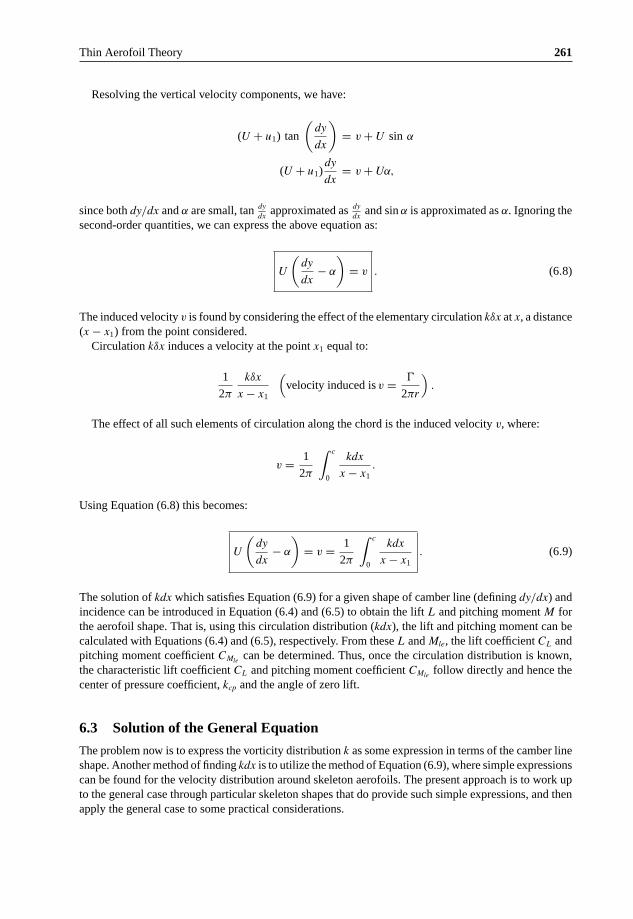
Thin Aerofoil Theory 261
Resolving the vertical velocity components, we have:
(U + u1) tan
(dy
dx
)= v + U sin α
(U + u1)dy
dx= v + Uα,
since both dy/dx and α are small, tan dy
dxapproximated as dy
dxand sin α is approximated as α. Ignoring the
second-order quantities, we can express the above equation as:
U
(dy
dx− α
)= v . (6.8)
The induced velocity v is found by considering the effect of the elementary circulation kδx at x, a distance(x − x1) from the point considered.
Circulation kδx induces a velocity at the point x1 equal to:
1
2π
kδx
x − x1
(velocity induced is v = �
2πr
).
The effect of all such elements of circulation along the chord is the induced velocity v, where:
v = 1
2π
∫ c
0
kdx
x − x1.
Using Equation (6.8) this becomes:
U
(dy
dx− α
)= v = 1
2π
∫ c
0
kdx
x − x1. (6.9)
The solution of kdx which satisfies Equation (6.9) for a given shape of camber line (defining dy/dx) andincidence can be introduced in Equation (6.4) and (6.5) to obtain the lift L and pitching moment M forthe aerofoil shape. That is, using this circulation distribution (kdx), the lift and pitching moment can becalculated with Equations (6.4) and (6.5), respectively. From these L and Mle, the lift coefficient CL andpitching moment coefficient CMle
can be determined. Thus, once the circulation distribution is known,the characteristic lift coefficient CL and pitching moment coefficient CMle
follow directly and hence thecenter of pressure coefficient, kcp and the angle of zero lift.
6.3 Solution of the General Equation
The problem now is to express the vorticity distribution k as some expression in terms of the camber lineshape. Another method of finding kdx is to utilize the method of Equation (6.9), where simple expressionscan be found for the velocity distribution around skeleton aerofoils. The present approach is to work upto the general case through particular skeleton shapes that do provide such simple expressions, and thenapply the general case to some practical considerations.

262 Theoretical Aerodynamics
6.3.1 Thin Symmetrical Flat Plate Aerofoil
For a flat plate, dy/dx = 0. Therefore, the general equation [Equation (6.9)] simplifies to:
Uα = 1
2π
∫ c
0
kdx
−x + x1. (6.10)
It is convenient to express the variable x in terms of θ, through:
x = c
2(1 − cos θ)
and x1 in terms of θ1 as:
x1 = c
2(1 − cos θ1).
The integration limits of Equation (6.10) become:
θ varies from 0 to π (that is, 0 ≤ θ ≤ π)
as x varies from 0 to c (that is, 0 ≤ x ≤ c)
and
dx = c
2sin θ dθ.
Equation (6.10) becomes:
Uα = 1
2π
∫ π
0
k sin θ dθ
cos θ − cos θ1. (6.11)
A value of k which satisfies Equation (6.11) is:
k = 2Uα(1 + cos θ)
sin θ.
Therefore:
Uα = 1
2π
∫ π
0
2Uα sin θ(1 + cos θ)dθ
sin θ(cos θ − cos θ1)
= Uα
π
∫ π
0
(1 + cos θ)
cos θ − cos θ1dθ
= Uα
π(π).
A more direct method for getting the vorticity distribution k is found as follows.Transformation of the circle z = aeiθ , through the Joukowski transformation ζ = z + a2
z, to a lifting
flat plate section at an incident angle α requires by the Joukowski hypothesis that sufficient circulation be

Thin Aerofoil Theory 263
z = aeiθ
m
iy
n
αU
Γ
P
α x
(a) Physical plane
iη
U
Γ
α ξNM
(b) Transformed plane
θ
ζ = z +a2
z
Figure 6.5 Transformation of a circle to a flat plate through Joukowski transformation.
imposed to bring the rear stagnation point down to m on the cylinder, as shown in Figure 6.5(a), wherethe velocity at a given point P(a, θ) is:
qc = 2U sin (θ + α) + �
2π a
Equating this to zero at m gives the circulation as:
� = 4πaU sin α.
Therefore,
qc = 2U sin (θ + α) + 2U sin α.
The velocity at point P(ξ, 0) (ξ = 2a cos θ, η = 0) on the flat plate in Figure 6.5(b) is:
qa = qc∣∣∣dζ
dz
∣∣∣= 2U[sin (α + θ) + sin α]∣∣∣1 − a2
z2
∣∣∣,
where qc and qa refer to velocities on the circle and aerofoil, respectively. The term∣∣∣1 − a2
z2
∣∣∣ is:
∣∣∣1 − a2
z2
∣∣∣ =∣∣∣1 − cos 2θ + i sin 2θ
∣∣∣=[
(1 − cos 2θ)2 + (sin 2θ)2]1/2
=[
1 − 2 cos 2θ + 1]1/2
= 2 sin θ.
Therefore,
qa = 2Usin (α + θ) + sin α
2 sin θ
qa
U= sin θ cos α + cos θ sin α + sin α
sin θ,

264 Theoretical Aerodynamics
that is:
qa
U= cos α + sin α
sin θ(1 + cos θ). (6.12)
For small α this simplifies to:
qa
U=[
1 + α1 + cos θ
sin θ
]. (6.13)
The variable θ in Equation (6.13) is the same as that used in the general equation [Equation (6.11)]. Thiscan be easily shown by shifting the axes in Figure 6.5(b) to the leading edge and measuring x rearward.When the chord c = 4a, the distance x becomes:
x = c
2− ξ
= c
2− c
2cos θ
= c
2(1 − cos θ) .
Then taking:
k = qa1 − qa2.
where qa1 is the velocity at the point where θ = θ1 and qa2 is the velocity at the same point on the otherside of the aerofoil where θ = −θ1. Therefore:
k = U
[1 + α
(1 + cos θ1)
sin θ1
]− U
[1 + α
(1 + cos (−θ1))
sin (−θ1)
]
= 2Uα(1 + cos θ1)
sin θ1.
Thus, in general, the elementary circulation at any point on the flat plate is:
k = 2Uα(1 + cos θ)
sin θ. (6.14)
Example 6.1
(a) Find the circulation at the mid-point of a flat plate at 2◦ to a freestream of speed 30 m/s.(b) Will this be greater than or less than the circulation at the quarter chord point?
Solution
(a) Given, α = 2◦, U = 30 m/s.At the mid-point of the plate θ = π/2.
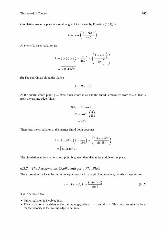
Thin Aerofoil Theory 265
Circulation around a plate at a small angle of incidence, by Equation (6.14), is:
k = 2Uα
(1 + cos θ
sin θ
).
At θ = π/2, the circulation is:
k = 2 × 30 ×(
2 × π
180
)×
⎛⎝1 + cos
π
2
sinπ
2
⎞⎠
= 2.094 m2/s .
(b) The coordinate along the plate is:
ξ = 2b cos θ.
At the quarter chord point, ξ = 3b/4, since chord is 4b and the chord is measured from θ = π, that is,from the trailing edge. Thus:
3b/4 = 2b cos θ
θ = cos−1
(3
8
)
= 68◦.
Therefore, the circulation at the quarter chord point becomes:
k = 2 × 30 ×(
2 × π
180
)×(
1 + cos 68◦
sin 68◦
)
= 3.105 m2/s .
The circulation at the quarter chord point is greater than that at the middle of the plate.
6.3.2 The Aerodynamic Coefficients for a Flat Plate
The expression for k can be put in the equations for lift and pitching moment, by using the pressure:
p = ρUk = 2ρU2α(1 + cos θ)
sin θ. (6.15)
It is to be noted that:
• Full circulation is involved in k.• The circulation k vanishes at the trailing edge, where x = c and θ = π. This must necessarily be so
for the velocity at the trailing edge to be finite.
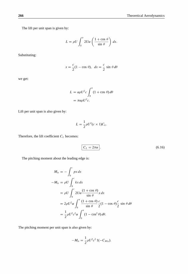
266 Theoretical Aerodynamics
The lift per unit span is given by:
L = ρU
∫ π
0
2Uα
(1 + cos θ
sin θ
)dx.
Substituting:
x = c
2(1 − cos θ), dx = c
2sin θ dθ
we get:
L = αρU2c
∫ π
0
(1 + cos θ) dθ
= παρU2c.
Lift per unit span is also given by:
L = 1
2ρU2(c × 1)CL.
Therefore, the lift coefficient CL becomes:
CL = 2πα . (6.16)
The pitching moment about the leading edge is:
Mle = −∫ c
0
px dx
−Mle = ρU
∫ c
0
kx dx
= ρU
∫ c
0
2Uα(1 + cos θ)
sin θx dx
= 2ρU2α
∫ π
0
(1 + cos θ)
sin θ
c
2(1 − cos θ)
c
2sin θ dθ
= 1
2ρU2c2α
∫ π
0
(1 − cos2 θ) dθ.
The pitching moment per unit span is also given by:
−Mle = 1
2ρU2c2 1(−CMle).

Thin Aerofoil Theory 267
Therefore, the pitching moment coefficient becomes:
−CMle = −Mle
12 ρU2c2
=12 ρU2c2α
∫ π
0(1 − cos2 θ) dθ
12 ρU2c2
= α
∫ π
0
(1 − cos2 θ) dθ
= α
∫ π
0
(1
2− cos 2θ
2
)dθ,
that is:
−CMle = απ
2. (6.17)
From Equations (6.16) and (6.17), we get:
CMle = −CL
4. (6.17a)
For small values of angle of attack, α, the center of pressure coefficient, kcp, (defined as the ratio of thecenter of pressure from the leading edge of the chord to the length is chord), is given by:
kcp = −CMle
CL
= 1
4. (6.18)
This shows that the center of pressure, which is a fixed point, coincides with the aerodynamic center.This is true for any symmetrical aerofoil section. The resultant force at the leading edge, at the quarterchord point and the center of pressure of a symmetrical aerofoil are shown in Figure 6.6.
By inspection, the quantitative relation between the three cases shown in Figure 6.6 can be expressedas:
Mle = −Lc
4+ Mc/4 = −xcpL . (6.19)
M 0le
at aerodynamic centerResultant force
at center of pressure
D 0
M 0c/4
D 0
L0 L 0L 0
D 0
Resultant force
xcpc/4
at the leading edgeResultant force
Figure 6.6 Resultant force on a symmetrical aerofoil.

268 Theoretical Aerodynamics
Thus, the momentum coefficient about the quarter-chord point is:
CM,c/4 = CMle+ CL
4.
But:
CMle= −CL
4.
Therefore:
CM,c/4 = 0 . (6.20)
This is the theoretical result that “the center of pressure is at the quarter-chord point for a symmetricalaerofoil.”
By definition the point on the aerofoil where the moments are independent of angle of attack is calledthe aerodynamic center. The point from the leading edge of the aerofoil at which the resultant pressureacts is called the center of pressure. In other words, center of pressure is the point where line of actionof the lift L meets the chord. Thus the position of the center of pressure depends on the particular choiceof chord.
The center of pressure coefficient is defined as the ratio of the center of pressure from the leadingedge of the aerofoil to the length of chord. This is represented by the symbol kcp. One of the desirableproperties of an aerofoil is that the travel of center of pressure in the working range of incidence (that isfrom zero-lift incidence to the stalling incidence) should not be large. As incidence increases the centerof pressure moves towards the quarter-chord point.
From the above result, it is seen that the moment about the quarter-chord point is zero for all values ofα. Hence, for a symmetrical aerofoil, we have the theoretical result that “the quarter-chord point is boththe center of pressure and the aerodynamic center.” In other words, for a symmetrical aerofoil the centerof pressure and aerodynamic center overlap. That is, for a symmetrical aerofoil the center of pressureand aerodynamic center coincide.
The relative position of center of pressure cp and aerodynamic center ac plays a vital role in the stabilityand control of aircraft. Let us have a closer look at the positions of cp and ac, shown in Figure 6.7.
We know that the aerodynamic center is located around the quarter chord point, whereas the centerof pressure is a moving point, strongly influenced by the angle of attack. When the center of pressure isaft of aerodynamic center, as shown in Figure 6.7(a), the aircraft will experience a nose-down pitchingmoment. When the center of pressure is ahead of aerodynamic center, as shown in Figure 6.7(b), theaircraft will experience a nose-up pitching moment. When the center of pressure coincided with theaerodynamic center, as shown in Figure 6.7(c), the aircraft becomes neutrally stable.
(c)
ac cp cp ac ac/cp
ccc
(a) (b)
Figure 6.7 Relative positions of cp and ac.

Thin Aerofoil Theory 269
From our discussions on center of pressure and aerodynamic center, the following can be inferred:
• “Center of pressure” is the point at which the pressure distribution can be considered to act–analogousto the “center of gravity” as the point at which the force of gravity can be considered to act.
• The concept of the “aerodynamic center” on the other hand, is not very intuitive. Because the lift andlocation of the center of pressure on an airfoil both vary linearly (more or less) with angle of attack,α, at least within the unstalled range of α. That is we can define a point on the chord of the airfoilat which the pitching moment remains “constant,” regardless of the α. That point is usually near thequarter-chord point and for a symmetrical airfoil the constant pitching moment would be zero. For acambered airfoil the pitching moment about the aerodynamic center would be nonzero, but constant.The usefulness of the aerodynamic center is in stability and control analysis where the aircraft can bedefined in terms of the wing and tail aerodynamic centers and the required lift and moments calculatedwithout worrying about the shift in center of pressure with α.
The horizontal position of the center of gravity has a great effect on the static stability of the wing,and hence, the static stability of the entire aircraft. If the center of gravity is sufficiently forward ofthe aerodynamic center, then the aircraft is statically stable. If the center of gravity of the aircraft ismoved toward the tail sufficiently, there is a point – the neutral point – where the moment curve becomeshorizontal; this aircraft is neutrally stable. If the center of gravity is moved farther back, the momentcurve has positive slope, and the aircraft is longitudinally unstable. Likewise, if the center of gravity ismoved forward toward the nose too far, the pilot will not be able to generate enough force on the tail toraise the angle of attack to achieve the maximum lift coefficient.
The horizontal tail is the main controllable moment contributor to the complete aircraft moment curve.A larger horizontal tail will give a more statically stable aircraft than a smaller tail (assuming, as isthe normal case, that the horizontal tail lies behind the center of gravity of the aircraft). Of course, itsdistance from the center of gravity is important. The farther away from the center of gravity it is, themore it enhances the static stability of the aircraft. The tail efficiency factor depends on the tail locationwith respect to the aircraft wake and slipstream of the engine, and power effects. By design it is made asclose to 100% efficiency as possible for most static stability.
Finally, with respect to the tail, the downwash from the wing is of considerable importance. Air isdeflected downward when it leaves a wing, and this deflection of air results in the wing reaction force orlift. This deflected air flows rearward and hits the horizontal-tail plane. If the aircraft is disturbed, it willchange its angle of attack and hence the downwash angle. The degree to which it changes directly affectsthe tail’s effectiveness. Hence, it will reduce the stability of the airplane. For this reason, the horizontaltail is often located in a location such that it is exposed to as little downwash as possible, such as high onthe tail assembly.
6.4 The Circular Arc Aerofoil
Following the same procedure as before for finding the distribution of k, it can be shown that for a circulararc aerofoil at an angle of attack α to the flow k can be expressed as:
k = 2U
[2β sin θ + α
(1 + cos θ
sin θ
)]. (6.21)
From Equations (6.12) and (6.14) is seen that the effect of camber is to increase k distribution by(2U × 2β sin θ) over that of the flat plate. Thus:
k = ka + kb,

270 Theoretical Aerodynamics
where:
ka = 2Uα1 + cos θ
sin θ
arises from the incidence of the aerofoil alone and:
kb = 4U β sin θ , (6.22)
which is due to the effect of the camber alone. Note that this distribution satisfies the Kutta-Joukowskihypothesis by allowing k to vanish at the trailing edge of the aerofoil where θ = π.
Example 6.2
If the maximum circulation caused by the camber effect of a circular arc aerofoil is 2 m2/s, when thefreestream velocity is 500 km/h, determine the percentage camber.
Solution
Given, kb = 2 m2/s, U = 500/3.6 = 138.9 m/s.By Equation (6.22), the circulation due to camber is:
kb = 4Uβ sin θ.
This circulation will be maximum when sin θ = 1, thus:
kbmax = 4Uβ.
Therefore:
β = kbmax
4U
= 2
4 × 138.9= 0.0036.
The % camber becomes:
%Camber = β
2× 100
= 0.0036
2× 100
= 0.18 .

Thin Aerofoil Theory 271
6.4.1 Lift, Pitching Moment, and the Center of Pressure Locationfor Circular Arc Aerofoil
We know that the lift L, pitching moment about the leading edge of the aerofoil Mle and the pressure p
acting on the aerofoil can be expressed as:
L = 1
2ρU2cCL
Mle = 1
2ρU2c2CMle
p = ρUk.
Now, substituting:
k = 2U
[2β sin θ + α
(1 + cos θ
sin θ
)],
the pressure becomes:
p = 2ρU2
[2β sin θ + α
(1 + cos θ
sin θ
)].
Also,
x = c
2(1 − cos θ).
Therefore, the lift becomes:
L =∫ π
0
p dx
=∫ π
0
2ρU2
[2β sin θ + α
(1 + cos θ
sin θ
)]c
2sin θ dθ
= 1
2ρU2c 2
∫ π
0
[α(1 + cos θ) + 2β sin2 θ
]dθ
= 1
2ρU2c 2
∫ π
0
[α(1 + cos θ) + 2β
(1
2− cos 2θ
2
)]dθ
= 1
2ρU2c 2
[α(θ + sin θ) + β
(θ − sin 2θ
2
)]π
0
,
that is:
L = 12 ρU2c 2π(α + β) . (6.23)
The lift coefficient is:
CL = L12 ρU2c
.

272 Theoretical Aerodynamics
This gives:
CL = 2π(α + β) . (6.23a)
Thus the lift-curve slope is:
dCL
dα= 2π .
From the above relations for CL and dCL/dα, it is evident that:
at α = 0, CL = 2πβ
at α = −β, CL = 0
and the lift-curve slope is independent of camber.For a cambered aerofoil, we have:
CL = 2π(α + β)
= dCL
dα(α + β).
For CL = 0, α = −β or −αL=0 = β. Thus:
CL = dCL
dα
(α − αL=0
). (6.24)
The pitching moment is:
Mle = −∫ π
0
px dx
= −∫ π
0
2ρU2
[2β sin θ + α
(1 + cos θ
sin θ
)]c
2(1 − cos θ)
c
2sin θ dθ
= −1
2ρU2c2 π
2(α + 2β) .
Therefore, the pitching moment coefficient becomes:
CMle= −π
2
(α + 2β
). (6.25)
In terms of CL, the CMlecan be expressed as follows. By Equation (6.23a), we have the CL as:
CL = 2π (α + β) .

Thin Aerofoil Theory 273
The expression for CMle, in Equation (6.25), can be arranged as:
CMle= −π
2
[α + β + β
]
= −1
2
[π (α + β) + π β
]
= −1
2
[2π (α + β)
2+ π β
].
But CL = 2π (α + β), thus:
CMle= −1
2
[CL
2+ π β
]
or
CMle= −CL
4− π β
2. (6.26)
The center of pressure coefficient, kcp, becomes:
kcp = −CMle
CL
= 1
4+ πβ
2CL
. (6.27)
Thus, the effect of camber is to set back the center of pressure by an amount which decreases withincreasing incidence or lift. At zero lift, the center of pressure is an infinite distance behind the aerofoil,which means that there is a moment on the aerofoil even when there is no resultant lift force.
Comparing this with Equation (6.17a) (CMle= − π
2 α) for flat plate we see that the camber of circulararc decreases the moment about the leading edge by πβ/2.
Example 6.3
(a) A flat plate is at an incidence of 2◦ in a flow; determine the center of pressure. (b) If a circular arc of3% camber is in the flow at the same incidence, where will be center of pressure?
Solution
(a) Given, α = 2◦.For a flat plate, by Equation (6.16), the lift coefficient is:
CL = 2π α
= 2π ×(
2 × π
180
)= 0.219.

274 Theoretical Aerodynamics
By Equation (6.17):
CMle= −α
π
2
= −(
2 × π
180
)× π
2= −0.0548.
The center of pressure, By Equation (6.18), is:
kcp = −CMle
CL
= − (−0.0548)
0.219
= 0.25 .
(b) Given α = 2◦, β
2 × 100 = 3, therefore:
α = 2 × π
180= 0.0349 radian
β = 3 × 2
100= 0.06 radian.
By Equation (6.23a):
CL = 2π (α + β)
= 0.596.
By Equation (6.26):
CMle= −CL
4− π β
2
= −0.596
4− π × 0.06
2= −0.243.
The center of pressure, by Equation (6.27), is:
kcp = −CMle
CL
= − (−0.243)
0.596
= 0.408 .

Thin Aerofoil Theory 275
Aliter:
Note that the kcp is also given by Equation (6.27), as:
kcp = 1
4+ π β
2CL
= 1
4+ π × 0.06
2 × 0.596= 0.408.
This is the same as that given by dividing CMlewith CL.
6.5 The General Thin Aerofoil Section
In Section 6.4, we saw that the general camber line can be replaced by a chordwise distribution ofcirculation. That is:
k = ka + kb,
where ka is the same as the distribution over the flat plate but must contain a constant (A0) to absorb anydifference between the equivalent flat plate and the actual chord line. Therefore:
ka = 2UA0
(1 + cos θ
sin θ
). (6.28)
Note that this ka distribution satisfies the Kutta-Joukowski distribution, since ka = 0 when θ = π, thatis, at x = c.
The corresponding kb is represented by a Fourier series. Providing 0 < θ < π, the end conditions aresatisfied, and any variation in shape is accommodated if it is a sine series. Thus:
kb = 2U (A1 sin θ + A2 sin 2θ + A3 sin 3θ + · · ··)
= 2U
∞∑1
An sin nθ. (6.29)
Thus, k = ka + kb becomes:
k = 2U
[A0
(1 + cos θ
sin θ
)+
n∑1
An sin nθ
]. (6.30)
Note that, for circular arc aerofoil, we have kb = 2UA1 sin θ.The coefficients A0, A1, A2, · · ··, An can be obtained by substituting for k in the general equation
(6.30), suitably converted with regard to units, that is:
U
[dy
dx− α
]= 1
2π
∫ c
0
k dx
x − x1.

276 Theoretical Aerodynamics
Substituting:
x = c
2(1 − cos θ),
we get:
U
[dy
dx− α
]= − 1
2π
∫ c
0
k sin θ
cos θ − cos θ1dθ.
Using Equation (6.30), we get:
U
[dy
dx− α
]= −2U
2π
∫ π
0
{A0(1 + cos θ)
sin θ+
n∑1
An sin nθ
}sin θ dθ
cos θ − cos θ1.
At the point x1 (or θ1) on the aerofoil:
dy
dx− α = −A0
π
∫ π
0
(1 + cos θ) dθ
cos θ − cos θ1− 1
π
∫ π
0
∑ An sin nθ sin θ dθ
cos θ − cos θ1.
Expressing∑
An sin nθ sin θ as:
∑An
1
2[cos (n − 1) θ − cos (n + 1) θ] ,
we have:
dy
dx− α = −
{A0
πG0 + A1
πG1 +
∑ An
2πGn−1 −
∑ An
2πGn+1
},
where Gn signifies the integral:
∫ π
0
cos nθ dθ
cos θ − cos θ1,
which has the solution:
π sin nθ1
sin θ1.
Therefore:
dy
dx− α = −A0
ππ −∑
An
sin (n − 1) θ1 − sin (n + 1) θ1
2 sin θ1.
For the general point x = c
2(1 − cos θ) on the aerofoil, we get:
dy
dx− α = −A0 +
∑An cos nθ,

Thin Aerofoil Theory 277
that is:
dy
dx= −A0 + α +
∑An cos nθ. (6.31)
On integrating from θ = 0 to π, the third term on the right-hand-side of Equation (6.31) vanishes.Therefore, we have:
∫ π
0
dy
dxdθ =
∫ π
0
(α − A0) dθ
= (α − A0)π.
This simplifies to:
A0 = α − 1
π
∫ π
0
dy
dxdθ . (6.32)
Multiplying Equation (6.32) by cos mθ, where m is an integer, and integrating with respect to θ, we get:
∫ π
0
dy
dxcos mθ dθ =
∫ π
0
(α − A0) cos mθ dθ
+∫ π
0
∑An cos nθ cos mθ dθ. (6.33)
The integral:
∫ π
0
∑An cos nθ cos mθ dθ = 0.
for all values of n except at n = m. Therefore, the first term on the right-hand-side of Equation (6.33)vanishes, and also the second term, except for n = m becomes:
∫ π
0
dy
dxcos nθ dθ =
∫ π
0
An cos2 nθ
= π
2An.
Thus:
An = 2
π
∫ π
0
dy
dxcos nθ dθ . (6.34)
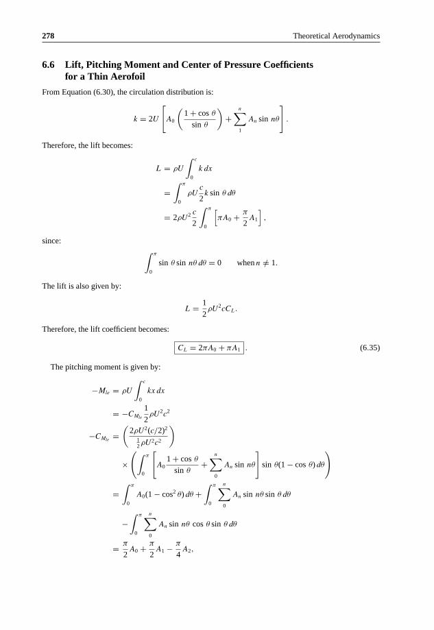
278 Theoretical Aerodynamics
6.6 Lift, Pitching Moment and Center of Pressure Coefficientsfor a Thin Aerofoil
From Equation (6.30), the circulation distribution is:
k = 2U
[A0
(1 + cos θ
sin θ
)+
n∑1
An sin nθ
].
Therefore, the lift becomes:
L = ρU
∫ c
0
k dx
=∫ π
0
ρUc
2k sin θ dθ
= 2ρU2 c
2
∫ π
0
[πA0 + π
2A1
],
since: ∫ π
0
sin θ sin nθ dθ = 0 when n /= 1.
The lift is also given by:
L = 1
2ρU2cCL.
Therefore, the lift coefficient becomes:
CL = 2πA0 + πA1 . (6.35)
The pitching moment is given by:
−Mle = ρU
∫ c
0
kx dx
= −CMle
1
2ρU2c2
−CMle=(
2ρU2(c/2)2
12 ρU2c2
)
×(∫ π
0
[A0
1 + cos θ
sin θ+
n∑0
An sin nθ
]sin θ(1 − cos θ) dθ
)
=∫ π
0
A0(1 − cos2 θ) dθ +∫ π
0
n∑0
An sin nθ sin θ dθ
−∫ π
0
n∑0
An sin nθ cos θ sin θ dθ
= π
2A0 + π
2A1 − π
4A2,

Thin Aerofoil Theory 279
since:
∫ π
0
sin nθ sin mθ dθ = 0 when n /= m.
Therefore:
CMle = −π
2
[A0 + A1 − A2
2
], (6.36)
that is:
CMle = −CL
4
[1 + A1 − A2
CL/π
].
The center of pressure coefficient is:
kcp = −CMle
CL
= 1
4+ π
4CL
(A1 − A2
). (6.37)
From Equation (6.37) it is seen that for this case also the center of pressure moves as the lift or incidenceis changed. We know that the kcp is also given by [Equation (6.19)]:
kcp = −CM 1/4
CL
+ 1
4.
Comparing Equations (6.36) and (6.37), we get:
CM 1/4 = −π
4(A1 − A2) . (6.38)
This shows that, theoretically, the pitching moment about the quarter chord point for a thin aerofoilis a constant, depending on the camber parameters only, and the quarter chord point is therefore theaerodynamic center.
Example 6.4
The camberline of a thin aerofoil is given by:
y = kx(x − 1)(x − 2),
where x and y are in terms of unit chord and the origin is at the leading edge. If the maximum camberis 2.2% of chord, determine the lift coefficient and the pitching moment coefficient when the angle ofattack is 4◦.

280 Theoretical Aerodynamics
Solution
Given, camber is 0.022 and α = 4◦.At the maximum camber location, let x = xm. At the maximum camber:
dy
dx= 0,
that is:
k(
3x2m − 6xm + 2
) = 0
3x2m − 6xm + 2 = 0
xm = 6 ± √36 − 24
6= 1 ± 0.577.
Out of the above two values of 1.577 and 0.423, the second one is the only feasible solution for xm.Therefore, the maximum camber is at xm = 0.423. Substituting this we have:
k[xm(xm − 1)(xm − 2)] = 0.022
k[0.423 × (−0.577) × (−1.577)] = 0.022
k[0.3849] = 0.022
k = 0.022
0.3849= 0.05715.
But:
x = (1 − cos θ)
2.
Substituting this, we get:
dy
dx= k
4
[3 cos2 θ + 6 cos θ − 1
].
By Equation (6.32):
A0 = α − 1
π
∫dy
dxdθ
= α − 1
π
∫ π
0
k
4
[3 cos2 θ + 6 cos θ − 1
]dθ
= α − k
8.

Thin Aerofoil Theory 281
By Equation (6.34):
A1 = 2
π
∫ π
0
dy
dxcos θ dθ
= 2
π
∫ π
0
k
4
[3 cos3 θ + 6 cos2 θ − cos θ
]dθ
= 3
2k
A2 = 2
π
∫ π
0
dy
dxcos 2θ dθ
= 2
π
∫ π
0
[3 cos2 θ cos 2θ + 6 cos θ cos2 θ − cos 2θ
]dθ
= 3
8k.
By Equation (6.35):
CL = 2π
[A0 + A1
2
]
= 2π
[α − k
8+ 3
4k
]
= 2π
[(4 × π
180
)− 0.05715
8+ 3
4× 0.05715
]
= 0.668 .
By Equation (6.38):
CM1/4 = −π
4[A1 − A2]
= −π
4
[3
2k − 3
8k
]
= −π
4
[3
2× 0.05715 − 3
8× 0.05715
]
= −0.0505 .
Note: The moment is given with a negative sign because this is a nose-down moment.
Example 6.5
A sail plane of wing span 18 m, aspect ratio 16 and taper ratio 0.3 is in level fight at an altitude where therelative density is 0.7. The true air speed measured by an error free air speed indicator is 116 km/h. Thelift and drag acting on the wing are 3920 N and 160 N, respectively. The pitching moment coefficientabout the quarter chord point is −0.03. Calculate the mean chord and the lift and drag coefficients, basedon the wing area and mean chord. Also, calculate the pitching moment about the leading edge of thewing.

282 Theoretical Aerodynamics
Solution
Given 2b = 18 m, = 16, λt/λr = 0.3, σ = 0.7, L = 3920 N, D = 160 N, Vr = 116 km/h, CMc/4 =−0.03.The relative density is:
σ = ρ
ρ0= 0.7,
where ρ0 is the sea level density, equal to 1.225 kg/m3. Therefore:
ρ = 0.7 ρ0
= 0.7 × 1.225
= 0.858 kg/m3.
Equivalent air speed is:
V = Vi√σ
= 116√0.7
= 138.65 km/h
= 138.65
3.6= 38.51 m/s.
The mean chord is:
c = span
= 2b
= 18
16
= 1.125 m .
The wing area is:
S = 2b × c
= 20.25 m2.
The lift coefficient is:
CL = L12 ρV 2S
= 2 × 3920
0.858 × 38.512 × 20.25
= 0.304 .

Thin Aerofoil Theory 283
The drag coefficient is:
CD = D12 ρV 2S
= 2 × 160
0.858 × 38.512 × 20.25
= 0.0124 .
By Equation (6.38):
CMc/4 = −π
4(A1 − A2) .
By Equation (6.36):
CMle= −CL
4
(1 + A1 − A2
CL/π
)
= −CL
4
(1 + 4CMc/4/π
CL/π
)
= −CL
4
(1 + 4CMc/4
CL
)
= −0.304
4
(1 + 4 × (−0.03)
0.304
)
= −0.046.
The pitching moment about the leading edge is:
Mle = 1
2ρV 2 S c CMle
= 1
2× 0.858 × 38.512 × 20.25 × 1.125 × (−0.046)
= −666.71 Nm .
The negative sign to the moment implies that it is a nose-down moment.
6.7 Flapped Aerofoil
The flap at the trailing edge of an aerofoil is essentially a high-lifting device, which when deflected downcauses increase of lift, essentially by increasing the camber of the profile. The thin aerofoil discussedin the previous sections of this chapter can readily be applied to aerofoils with variable camber such asflapped aerofoils. It has been found that the circulation distribution along the camber line for the generalaerofoil can comfortably be split into the circulation due to a flat plate at an incidence and the circulationdue to the camber line.
It is sufficient for the assumptions in the theory to consider the influence of a flap deflection as anaddition to the above two components. Figure 6.8 illustrates how the three contributions to lift generationcan be combined to get the resultant effect.

284 Theoretical Aerodynamics
UαU
ηx ´ U x
ηx
U
xα
y
(a) (b) (c) (d)
y y y
Figure 6.8 Linear splitting of the effect of incidence, camber of the profile and camber effect due to flap deflection,(a) camber line of profile with a flap at an angle of attack, (b) camber line effect, (c) flap deflection effect, (d) angleof attack effect.
Indeed the deflection of the flap about a hinge in the camber line effectively alters the camber of theprofile so that the contribution due to flap deflection is an addition to the effect of the camber line shape.In this manner, the problem of a cambered aerofoil with flap is reduced to the general case of fitting acamber line made up of the chord of the aerofoil and the flap deflected through an angle η, as shown inFigure 6.9.
The thin aerofoil theory stipulates that the slope of the aerofoil surface is small and that the displacementfrom the x-axis is small. In other words, the leading and/or trailing edges need not be on the x-axis.
Let us define the camber as hc so that the slope of the part AB of the aerofoil is zero, and the slope ofthe flap h/F . To find the coefficient of the circulation k for the flap camber, let us substitute these valuesof slope in Equations (6.32) and (6.34) but confining the limits of integration to the parts of the aerofoilover which the slopes occur. Thus:
A0 = α −[
1
π
∫ φ
0
0 dθ + 1
π
∫ π
φ
−ζ dθ
](6.39)
where φ is the value of θ at the hinge, that is:
(1 − F ) c = c
2(1 − cos φ) ,
hence cos φ = 2F − 1. Integrating Equation (6.39), we get:
A0 = α + η − φ
π(η),
B
α α′
y
C′
η
A
x
U
C
Figure 6.9 An aerofoil chord at an angle of incidence, with deflected flap.
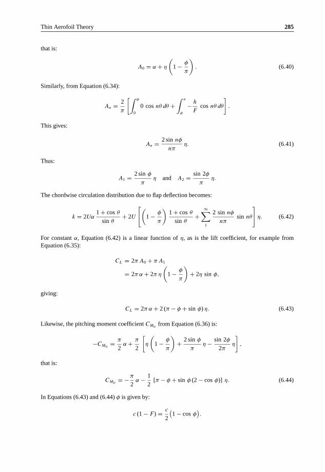
Thin Aerofoil Theory 285
that is:
A0 = α + η
(1 − φ
π
). (6.40)
Similarly, from Equation (6.34):
An = 2
π
[∫ φ
0
0 cos nθ dθ +∫ π
φ
− h
Fcos nθ dθ
].
This gives:
An = 2 sin nφ
nπη. (6.41)
Thus:
A1 = 2 sin φ
πη and A2 = sin 2φ
πη.
The chordwise circulation distribution due to flap deflection becomes:
k = 2Uα1 + cos θ
sin θ+ 2U
[(1 − φ
π
)1 + cos θ
sin θ+
∞∑1
2 sin nφ
nπsin nθ
]η. (6.42)
For constant α, Equation (6.42) is a linear function of η, as is the lift coefficient, for example fromEquation (6.35):
CL = 2π A0 + π A1
= 2π α + 2π η
(1 − φ
π
)+ 2η sin φ,
giving:
CL = 2π α + 2 (π − φ + sin φ) η. (6.43)
Likewise, the pitching moment coefficient CMlefrom Equation (6.36) is:
−CMle= π
2α + π
2
[η
(1 − φ
π
)+ 2 sin φ
πη − sin 2φ
2πη
],
that is:
CMle= −π
2α − 1
2[π − φ + sin φ (2 − cos φ)] η. (6.44)
In Equations (6.43) and (6.44) φ is given by:
c (1 − F ) = c
2
(1 − cos φ
).

286 Theoretical Aerodynamics
x′
H
Ux
αα′
p
(1 − F )c
y
x
Figure 6.10 Illustration of a flap and hinge moment.
Note that a positive (that is, downward) deflection of the flap decreases the moment coefficient, tendingto pitch the aerofoil nose down and vice versa.
6.7.1 Hinge Moment Coefficient
The characteristic of a flapped aerofoil, which is of great importance in stability and control of the aircraft,is the aerodynamic moment about the hinge line, H , shown in Figure 6.10.
Taking moments of elementary pressures p acting on the flap, about the hinge:
H = −∫ trailing edge
hinge
p x′ dx,
where:
p = ρUk
and:
x′ = x − (1 − F ) c.
Now putting:
x′ = c
2
(1 − cos θ
)− c
2
(1 − cos φ
) = c
2
(cos φ − cos θ
)
and k from Equation (6.42), we get the hinge moment as:
H = −∫ π
φ
2ρU2[⎧⎪⎪⎩α + η
(1 − φ
π
)⎫⎪⎪⎭ 1 + cos θ
sin θ
+ η
∞∑1
2 sin nφ
nπsin nθ
]c
2
(cos φ − cos θ
) c
2sin θ dθ.
Substituting:
H = CH
1
2ρU2(Fc)2

Thin Aerofoil Theory 287
and simplifying, we obtain:
−CHF 2 = α
∫ π
φ
(1 + cos θ)(cos φ − cos θ) dθ
+ η
[(1 − θ
π
)cos φ I1 −
(1 − φ
π
)I2
+∞∑1
2 sin nφ
nπcos φ I3 +
∞∑1
2 sin nφ
nπI4
], (6.45)
where:
I1 =∫ π
φ
(1 + cos θ) dθ = π − φ − sin φ
I2 =∫ π
φ
(1 + cos θ) cos θ dθ =[
π − φ
2sin φ − sin 2φ
4
]
I3 =∫ π
φ
sin nθ sin θ dθ = 1
2
[sin (n + 1) φ
n + 1− sin (n − 1) φ
n − 1
]
I4 =∫ π
φ
sin nθ sin θ cos θ dθ = 1
2
[sin (n + 2) φ
n + 2− sin (n − 2) φ
n − 2
].
In the conventional notation:
CH = b1α + b2η,
where:
b1 = ∂CH
∂αand b2 = ∂CH
∂η.
From Equation (6.45):
b1 = − 1
F 2
∫ π
φ
(1 + cos θ) (cos φ − cos θ) dθ.
That is:
b1 = − 1
4F 2
[2(π − φ)(2 cos φ − 1) + 4 sin φ − sin 2φ
]. (6.46)
Similarly from Equation (6.45):
b2 = ∂CH
∂η= 1
F 2× coefficients of η from Equation (6.45).
This will reduce to:
b2 = − 1
4π F 2
[(1 − cos φ) − 2(π − φ)2(1 − 2 cos φ) + 4(π − φ) sin φ
]. (6.47)

288 Theoretical Aerodynamics
θαU
y
x
Aerofoil camber
Jet flap
Figure 6.11 Illustration of a jet flap as a band of spanwise vortex filaments.
The parameter a1 = ∂CL/∂α is 2π and a2 = ∂CL/∂η from Equation (6.43) becomes:
a2 = 2 (π − φ + sin φ). (6.48)
Thus thin aerofoil theory provides an estimate of all the parameters of flapped aerofoil.
6.7.2 Jet Flap
Treating the jet flap as a high-velocity sheet of air issuing from the trailing edge of an aerofoil at somedownward angle θ to the chord line of the aerofoil, as shown in Figure 6.11, an analysis can be made byreplacing the jet stream as well as the aerofoil by a vortex distribution [1, 2].
The flap contributes to the lift in the following two ways:
1. The downward deflection of the efflux produces a lifting component of reaction.2. The jet affects the pressure distribution on the aerofoil in a similar manner to that obtained by an
addition to the circulation round the aerofoil.
The jet is shown to be equivalent to a band of spanwise vortex filaments which for small deflectionangles θ can be assumed to be on the ox-axis, shown in Figure 6.11.
Considering both the contributions mentioned above, it can be shown that the lift coefficient can beexpressed as:
CL = 4πA0θ + 2π(1 + 2B0) α. (6.49)
where A0 and B0 are the initial coefficients in the Fourier series associated with the deflection of the jetand the incidence of the aerofoil, respectively, and which can be obtained in terms of the momentum ofthe jet.
6.7.3 Effect of Operating a Flap
Let us consider an aerofoil whose rear part is movable about a hinge at P on the camber line, as shown inFigure 6.12(a). Essentially the rear part PH is the flap, which can be raised or lowered from the neutralposition shown in the figure.
In an aerofoil of finite aspect ratio, the flap movement affects only part of a wing. Ailerons are flapsnear the wing tips and are arranged so that the port and starboard ailerons move in opposite senses (that is,one up and one down). In our discussions here let us consider a two-dimensional problem for simplicityand assume that the aerofoil is thin, and the portion PH of the camber line is straight, and the angle ξ
through which the flap is rotated is small.

Thin Aerofoil Theory 289
o
ξ
V H
P
Pηα
A
H
A
(a) (b)
H′
Figure 6.12 (a) An aerofoil with flap, (b) simplified representation of the aerofoil and flap.
For the thin aerofoil shown in Figure 6.12(b) the eccentric angle which defines the position of hinge P
is η. In the neutral position PH of the flap we can express the lift coefficient, [see Equation (6.23a)], as:
CL = 2π α + 2
∫ π
0
dy
dx(1 + cos θ) dθ
= 2π α + 2
∫ η
0
dy
dx(1 + cos θ) dθ + 2
∫ π
η
dy
dx(1 + cos θ) dθ,
where y denotes the yc. The effect of raising the flap is to decrease dy
dxto(
dy
dx− ξ)
on the raised part PH ′
and to leave it unaltered on the part PA. The lift coefficient is thereby altered to C′L where:
C′L = 2π α + 2
∫ η
0
(dy
dx− ξ
)(1 + cos θ) dθ + 2
∫ π
η
dy
dx(1 + cos θ) dθ. (6.50)
Thus:
C′L − CL = −2ξ
∫ η
0
(1 + cos θ) dθ = −2ξ (η + sin η) . (6.51)
Thus the effect of raising the flap is to decrease the lift coefficient, the effect of lowering the flap isto increase the lift coefficient. Therefore, in particular, when the flaps are lowered just before landing,increased lift is obtained (and also increased drag). In the case of ailerons, if the port aileron is raisedand the starboard aileron depressed, the lift on the port wing is decreased and that on the starboard wingis increased, causing a rolling moment which tends to raise the starboard wing tip.
6.8 Summary
The overall lifting property of a two-dimensional aerofoil depends on the circulation it generates andthis, for the far-field or overall effects, has been assumed to be concentrated at a point within the aerofoilprofile, and to have a magnitude related to the incidence, camber and thickness of the aerofoil.
The loading on the aerofoil, or the chordwise pressure distribution, follows as a consequence ofthe parameters, namely the incidence, camber and thickness. But the camber and thickness imply acharacteristic shape which depends in turn on the conformal transformation function and the basic flowto which it is applied.
The profiles obtained with Joukowski transformation do not lend themselves to modern aerofoil design.However, Joukowski transformation is of direct use in aerofoil design. It introduces some features whichare the basis to any aerofoil theory, such as (a) the lift generated by an aerofoil is proportional to thecirculation around the aerofoil profile, L ∝ �. (b) The magnitude of the circulation � must be such that

290 Theoretical Aerodynamics
it keeps the velocity finite in the vicinity of trailing edge. It is not necessary to concentrate the circulationin a single vortex, the vorticity can be distributed throughout the region surrounded by the aerofoil profilein such a way that the sum of the distributed vorticity equals that of the original model, and the vorticityat the trailing edge is zero. This mathematical model may be simplified by distributing the vortices on thecamber line and disregarding the effect of thickness. In this form it becomes the basis for the classical“thin aerofoil theory” of Munk and Glauert.
The usefulness or advantage of the theory lies in the fact that the aerofoil characteristics could bequoted in terms of the coefficient Ax, which in turn could be found by graphical integration method fromany camber line.
General thin aerofoil theory is based on the assumption the aerofoil is thin so that its shape is effectivelythat of its camber line and the camber line shape deviates only slightly from the chord line.
The camber line is replaced by a line of variable vorticity so that the total circulation about the chordis the sum of the vortex elements. Thus, the circulation around the camber becomes:
� =∫ c
0
k δs.
The lift per unit span is given by:
L = ρU� = ρU
∫ c
0
k dx.
Again for unit span, the moment of pressure forces about the leading edge is:
Mle = −∫ c
0
px dx = −ρU
∫ c
0
kx dx.
For a flat plate, dy/dx = 0. Therefore, the general equation [Equation (6.9)] simplifies to:
Uα = 1
2π
∫ c
0
kdx
−x + x1.
The elementary circulation at any point on the flat plate is:
k = 2Uα(1 + cos θ)
sin θ.
Lift per unit span is given by:
L = 1
2ρU2(c × 1)CL.
The lift coefficient CL becomes:
CL = 2πα .
The pitching moment per unit span is:
−Mle = 1
2ρU2c2α 1(−CMle).
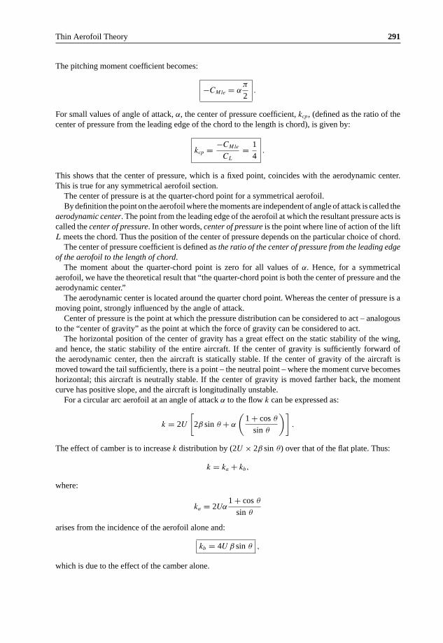
Thin Aerofoil Theory 291
The pitching moment coefficient becomes:
−CMle = απ
2.
For small values of angle of attack, α, the center of pressure coefficient, kcp, (defined as the ratio of thecenter of pressure from the leading edge of the chord to the length is chord), is given by:
kcp = −CMle
CL
= 1
4.
This shows that the center of pressure, which is a fixed point, coincides with the aerodynamic center.This is true for any symmetrical aerofoil section.
The center of pressure is at the quarter-chord point for a symmetrical aerofoil.By definition the point on the aerofoil where the moments are independent of angle of attack is called the
aerodynamic center. The point from the leading edge of the aerofoil at which the resultant pressure acts iscalled the center of pressure. In other words, center of pressure is the point where line of action of the liftL meets the chord. Thus the position of the center of pressure depends on the particular choice of chord.
The center of pressure coefficient is defined as the ratio of the center of pressure from the leading edgeof the aerofoil to the length of chord.
The moment about the quarter-chord point is zero for all values of α. Hence, for a symmetricalaerofoil, we have the theoretical result that “the quarter-chord point is both the center of pressure and theaerodynamic center.”
The aerodynamic center is located around the quarter chord point. Whereas the center of pressure is amoving point, strongly influenced by the angle of attack.
Center of pressure is the point at which the pressure distribution can be considered to act – analogousto the “center of gravity” as the point at which the force of gravity can be considered to act.
The horizontal position of the center of gravity has a great effect on the static stability of the wing,and hence, the static stability of the entire aircraft. If the center of gravity is sufficiently forward ofthe aerodynamic center, then the aircraft is statically stable. If the center of gravity of the aircraft ismoved toward the tail sufficiently, there is a point – the neutral point – where the moment curve becomeshorizontal; this aircraft is neutrally stable. If the center of gravity is moved farther back, the momentcurve has positive slope, and the aircraft is longitudinally unstable.
For a circular arc aerofoil at an angle of attack α to the flow k can be expressed as:
k = 2U
[2β sin θ + α
(1 + cos θ
sin θ
)].
The effect of camber is to increase k distribution by (2U × 2β sin θ) over that of the flat plate. Thus:
k = ka + kb,
where:
ka = 2Uα1 + cos θ
sin θ
arises from the incidence of the aerofoil alone and:
kb = 4U β sin θ ,
which is due to the effect of the camber alone.

292 Theoretical Aerodynamics
The lift L acting on the aerofoil can be expressed as:
L = 12 ρU2c 2π(α + β)
CL = 2π(α + β) .
Thus the lift-curve slope is:
dCL
dα= 2π .
From the above relations for CL and dCL/dα, it is evident that:
at α = 0, CL = 2πβ
at α = −β, CL = 0
and the lift-curve slope is independent of camber.For a cambered aerofoil, we have:
CL = 2π(α + β)
= dCL
dα(α + β).
For CL = 0, α = −β or −αL=0 = β. Thus:
CL = dCL
dα(α − αL=0) .
The pitching moment is:
Mle = −1
2ρU2c2 π
2(α + 2β) .
Therefore, the pitching moment coefficient becomes:
CMle= −π
2(α + 2β)
or
CMle= −CL
4− π β
2.
The center of pressure coefficient, kcp, becomes:
kcp = −CMle
CL
= 1
4+ πβ
2CL
.
Thus, the effect of camber is to set back the center of pressure by an amount which decreases withincreasing incidence or lift.

Thin Aerofoil Theory 293
The general camber line can be replaced by a chordwise distribution of circulation. That is:
k = ka + kb,
where
ka = 2UA0
(1 + cos θ
sin θ
).
Note that this ka distribution satisfies the Kutta-Joukowski distribution, since ka = 0 when θ = π, thatis, at x = c.
The corresponding kb is represented by a Fourier series. Providing 0 < θ < π, the end conditions aresatisfied, and any variation in shape is accommodated if it is a sine series. Thus:
kb = 2U (A1 sin θ + A2 sin 2θ + A3 sin 3θ + · · ··)
= 2U
∞∑1
An sin nθ.
Thus, k = ka + kb becomes:
k = 2U
[A0
(1 + cos θ
sin θ
)+
n∑1
An sin nθ
].
The coefficients A0, A1, A2, · · ··, An can be obtained by substituting for k in the general equation(6.30), suitably converted with regard to units.
For a thin aerofoil, the circulation distribution is:
k = 2U
[A0
(1 + cos θ
sin θ
)+
n∑1
An sin nθ
].
The lift is also given by:
L = 1
2ρU2cCL.
Therefore, the lift coefficient becomes:
CL = 2πA0 + πA1 .
The pitching moment is given by:
−Mle = −CMle
1
2ρU2c2.
The pitching moment coefficient is:
CMle = −π
2
[A0 + A1 − A2
2
].

294 Theoretical Aerodynamics
The center of pressure coefficient is:
kcp = −CMle
CL
= 1
4+ π
4CL
(A1 − A2) .
Flap at the trailing edge of an aerofoil is a high-lifting device, which when deflected down causesincrease of lift, essentially by increasing the camber of the profile. The deflection of the flap about ahinge in the camber line effectively alters the camber of the profile so that the contribution due to flapdeflection is an addition to the effect of camber line shape.
The chordwise circulation distribution due to flap deflection becomes:
k = 2Uα1 + cos θ
sin θ+ 2U
[(1 − φ
π
)1 + cos θ
sin θ+
∞∑1
2 sin nφ
nπsin nθ
]η.
The lift coefficient is:
CL = 2π α + 2 (π − φ + sin φ) η.
Likewise, the pitching moment coefficient CMleis:
CMle= −π
2α − 1
2[π − φ + sin φ (2 − cos φ)] η.
The characteristic of a flapped aerofoil, which is of great importance in stability and control of theaircraft, is the aerodynamic moment about the hinge line, H :
H = CH
1
2ρU2(Fc)2.
In an aerofoil of finite aspect ratio, the flap movement affects only part of a wing. Ailerons are flapsnear the wing tips and are arranged so that the port and starboard ailerons move in opposite senses (thatis, one up and one down). The effect of raising the flap is to decrease the lift coefficient, the effect oflowering the flap is to increase the lift coefficient. Therefore, in particular, when the flaps are loweredjust before landing, increased lift is obtained (and also increased drag). In the case of ailerons, if the portaileron is raised and the starboard aileron depressed, the lift on the port wing is decreased and that on thestarboard wing is increased, causing a rolling moment which tends to raise the starboard wing tip.
Exercise Problems
1. Determine the maximum circulation due to camber of a circular arc aerofoil of percentage camber0.05, in a flow of velocity 200 km/h.
[Answer: 0.2224 m2/s]2. If the lift coefficient and lift curve slope of an aerofoil of percentage camber 0.6 are 1.02 and 2,
respectively, determine (a) the pitching moment about the leading edge and (b) the center of pressurecoefficient.
[Answer: (a) −0.254, (b) 0.2685]

Thin Aerofoil Theory 295
3. If the elemental circulation at 30% chord of a flat plate in a flow at 40 m/s is 24 m2/s, determine theangle of attack.
[Answer: 11.25◦]4. A two-dimensional wing of NACA 4412 profile flies at an incidence of 4◦. Determine the lift
coefficient of the wing.[Answer: 1.024]
5. An aerofoil of average chord 1.2 m, at an angle of attack 2◦ to a flow at 45 m/s at sea level, experiencesa lift of 500 N per unit area. Determine the pitching moment about the leading edge, (a) assumingthe profile to be symmetrical and (b) assuming the profile is cambered with 3% camber.
[Answer: (a) −178.6 N-m, (b) −434 N-m]6. A Joukowski profile of 3.3% camber is in an air stream of speed 60 m/s at an angle of attack of 4◦.
Determine the circulation around the maximum thickness location.[Answer: 28.22 m2/s]
7. A parabolic camber line of unit chord length is at an incidence of 3◦ in a uniform flow of velocity20 m/s. If the camber line is given by:
y = CL
4π
(1 − 4x2
)
determine the velocity induced at the mid-chord location, assuming the incidence as an ideal angleof attack.
[Answer: −3.14 m/s]8. An aircraft of wing area 42 m2 and mean chord 3 m flies at 120 m/s at an altitude where the density
is 0.905 kg/m3. The center of pressure is at 0.28 times mean chord behind the leading edge of thewing when the wing lift coefficient is 0.2. (a) If the lift on the tail plane acts through a point 8m horizontally behind the center of pressure, determine the tail lift required to trim the aircraft.(b) Assuming the wing profile as a circular arc, find the percentage camber. Assume the pitchingmoments on the tail plane, fuselage and nacelles are negligibly small.
[Answer: (a) 5201 N, (b) 0.191]9. A thin aerofoil of 3% camber in a freestream has a lift coefficient of 1.2. (a) If the lift coefficient
has to be increased by 10% of the initial value, what should be the increase in the angle of attackrequired? (b) Find the percentage change in the pitching moment coefficient caused by this changein the angle of attack.
[Answer: (a) 1.15◦, (b) 7.88%]10. A flat plate of length 1.2 m and width 1 m, in a uniform air stream of pressure 1 atm, temperature
30 ◦C and velocity 30 m/s, experiences a lift of 1500 N. Determine the lift coefficient, angle of attack,pitching moment about the leading edge and the location of center of pressure.
[Answer: CL = 2.384, α = 21.71◦, CMle= −0.595, kcp = 0.25]
References
1. Spence, D.A., The lift coefficient of a thin, jet flapped wing, Proc. Roy. Soc. A., 1212, December 1956.
2. Spence, D.A., The lift on a thin aerofoil with jet augmented flap, Aeronautical Quarterly, August 1958.


7Panel Method
7.1 Introduction
Panel method is a numerical technique to solve flow past bodies by replacing the body with mathematicalmodels; consisting of source or vortex panels. Essentially the surface of body to be studied will berepresented by panels consisting of sources and free vortices. These are referred to as source panel andvortex panel methods, respectively. If the body is a lift generating geometry, such as an aircraft wing,vortex panel method will be appropriate for solving the flow past, since the lift generated is a function ofthe circulation or the vorticity around the wing. If the body is a nonlifting structure such as a pillar of ariver bridge, the source panel method might be employed for solving the flow past that.
7.2 Source Panel Method
Consider the source sheet of finite length along the s-direction and extending to infinity in the directionnormal to s, as shown in Figure 7.1.
The source strength per unit length along s-direction of the panel, shown in Figure 7.1, is λ = λ(s).Also, the small length segment ds is treated as a distinct source of strength λ ds.
Let us consider a point P as shown in Figure 7.1. The small segment of the source sheet of strengthλ ds induces an infinitesimally small velocity potential dφ at point P . That is:
dφ = λ ds
2πln r.
The complete velocity potential at point P , due to source sheet from a to b, is given by:
φ(x, y) =∫ b
a
λ ds
2πln r.
In general, the source strength λ(s) can change from positive (+ve) to negative (−ve) along the sourcesheet. That is, the ‘source’ sheet can be a combination of line sources and line sinks.
Next, let us consider a given body of arbitrary shape shown in Figure 7.2.Let us assume that the body surface is covered with a source sheet, as shown in Figure 7.2(a), where
the strength of the source λ(s) varies in such a manner that the combined action of the uniform flow andthe source sheet makes the aerofoil surface and streamlines of the flow, as shown in Figure 7.2(b).
Theoretical Aerodynamics, First Edition. Ethirajan Rathakrishnan.© 2013 John Wiley & Sons Singapore Pte. Ltd. Published 2013 by John Wiley & Sons Singapore Pte. Ltd.

298 Theoretical Aerodynamics
a
dφ =λds
2πln rr
b
z
s
a
P (x, y)
λ = λ(s)
∞
ds−∞
r
b
θ
Figure 7.1 A source sheet.
=+
V∞
Flow over the bodyUniformflow the surface of a body
Source sheet on
Figure 7.2 An arbitrary body (a) covered with source sheet, (b) the flow past it.
The problem now becomes that of finding appropriate distribution of λ(s), over the surface of the body.The solution to this problem is carried out numerically, as follows:
• Approximate the source sheet by a series of straight panels, as shown in Figure 7.3.• Let the source strength λ(s) per unit length be constant over a given general panel, but allow it to vary
from one panel to another. That is, for n panels the source strengths are λ1, λ2, λ3, ....., λn.• The main objective of the panel technique is to solve for the unknowns λj , j = 1 to n, such that the
body surface becomes a stream surface of the flow.• This boundary condition is imposed numerically by defining the mid-point of each panel to be a control
point and by determining the λjs such that the normal component of the flow velocity is zero at eachpoint.
Boundary point
Control point βi
θ
(xi, yi)p1
ithpanel
j thpanel
r Pj
s
ni
Panel
direct
ion
V∞
p2
P (x, y)
Freestr
eamdir
ection
α
Figure 7.3 A body of arbitrary shape covered with a series of straight source panels.
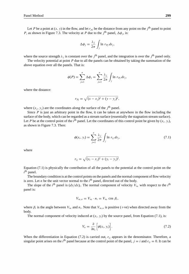
Panel Method 299
Let P be a point at (x, y) in the flow, and let rpj be the distance from any point on the jth panel to pointP , as shown in Figure 7.3. The velocity at P due to the jth panel, �φj , is:
�φj = λj
2π
∫j
ln rPj dsj,
where the source strength λj is constant over the jth panel, and the integration is over the jth panel only.The velocity potential at point P due to all the panels can be obtained by taking the summation of the
above equation over all the panels. That is:
φ(P) =n∑
j=1
�φj =n∑
j=1
λj
2π
∫j
ln rPj dsj,
where the distance:
rPj =√
(x − xj)2 + (y − yj)2,
where (xj, yj) are the coordinates along the surface of the jth panel.Since P is just an arbitrary point in the flow, it can be taken at anywhere in the flow including the
surface of the body, which can be regarded as a stream surface (essentially the stagnation stream surface).Let P be at the control point of the ith panel. Let the coordinates of this control point be given by (xi, yi),as shown in Figure 7.3. Then:
φ(xi, yi) =n∑
j=1
λj
2π
∫j
ln rij dsj, (7.1)
where
rij =√
(xi − xj)2 + (yi − yj)2.
Equation (7.1) is physically the contribution of all the panels to the potential at the control point on theith panel.
The boundary condition is at the control points on the panels and the normal component of flow velocityis zero. Let n be the unit vector normal to the ith panel, directed out of the body.
The slope of the ith panel is (dy/dx)i. The normal component of velocity V∞ with respect to the ith
panel is:
V∞,n = V∞ · ni = V∞ cos βi,
where βi is the angle between V∞ and ni. Note that V∞,n is positive (+ve) when directed away from thebody.
The normal component of velocity induced at (xi, yi) by the source panel, from Equation (7.1), is:
Vn = ∂
∂ni
[φ(xi, yi)
]. (7.2)
When the differentiation in Equation (7.2) is carried out, rij appears in the denominator. Therefore, asingular point arises on the ith panel because at the control point of the panel, j = i and rij = 0. It can be

300 Theoretical Aerodynamics
shown that when j = i, the contribution to the derivative is λi/2. Therefore:
Vn = λi
2+
n∑j=1,j /= i
λj
2π
∫j
∂
∂ni
(ln rij
)dsj, (7.3)
where λi/2 is the normal velocity induced at the ith control point by the ith panel itself.The normal component of flow velocity is the sum of the normal components of freestream velocity
V∞,n and velocity due to the source panel Vn. The boundary condition states that:
V∞,n + Vn = 0.
Therefore, the sum of Equation (7.3) and V∞,n results in:
Vn + V∞,n = λi
2+
n∑j=1,j /= i
λj
2π
∫j
∂
∂ni
(ln rij
)dsj + V∞ cos βi = 0 . (7.4)
This is the heart of source panel method. The values of the integral in Equation (7.4) depend simply onthe panel geometry, which are not the properties of the flow.
Let Ii,j be the value of this integral when the control point is on the ith panel and the integral is overthe jth panel. Then, Equation (7.4) can be written as:
λi
2+
n∑j=1,j /= i
λj
2πIi,j + V∞ cos βi = 0. (7.5)
This is a linear algebraic equation with n unknowns λ1, λ2, ......, λn. It represents the flow boundarycondition evaluated at the control point of the ith panel.
Now let us apply the boundary condition to the control points of all the panels, that is, in Equation(7.5), let i = 1, 2, 3, ...., n. The results will be a system of n linear algebraic equations with n unknowns(λ1, λ2, ......, λn), which can be solved simultaneously by conventional numerical methods:
• After solving the system of equations represented by Equation (7.5) with i = 1, 2, 3, ...., n, we havethe distribution source panel strength which, in an approximate fashion, causes the body surface to bea streamline of the flow.
• This approximation can be made more accurate by increasing the number of panels, hence more closelyrepresenting the source sheet of continuously varying strength λ(s).
7.2.1 Coefficient of Pressure
Once source strength distributions λi are obtained, the velocity tangential to the surface at each controlpoint can be calculated as follows.
Let s be the distance along the body surface, as shown in Figure 7.3, measured positive (+ve) fromfront to rear. The component of freestream velocity tangential to the surface is:
V∞,s = V∞ sin βi.

Panel Method 301
The tangential velocity Vs at the control point of the ith panel induced by all the panels is obtained bydifferentiating Equation (7.1) with respect to s. That is:
Vs = ∂φ
∂s=
n∑j=1
λj
2π
∫j
∂
∂s
(ln rij
)dsj. (7.6)
Note that the tangential velocity Vs on a flat source panel induced by the panel itself is zero; hence inEquation (7.6), the term corresponding to j = i is zero. This is easily seen by intuition, because the panelcan emit volume flow only in a direction perpendicular to its surface and not in the direction tangentialto its surface.
The surface velocity Vi at the control point of the ith panel is the sum of the contribution V∞,s fromthe freestream and Vs given by Equation (7.6).
Vi = V∞,s + Vs = V∞ sin βi +n∑
j=1
λj
2π
∫j
∂
∂s
(ln rij
)dsj. (7.7)
The pressure coefficient Cp at the ith control point is:
Cpi= 1 −
(Vi
V∞
)2
. (7.8)
Note: It is important to note that the pressure coefficient given by Equation (7.8) is valid only forincompressible flows with freestream Mach number less than 0.3. For compressible flows the pressurecoefficient becomes:
Cpi= pi − p∞
12 ρ∞V 2∞
,
where pi is the static pressure at the ith panel and p∞, ρ∞ and V∞, respectively, are the pressure, densityand velocity of the freestream flow. The dynamic pressure can be expressed as:
1
2ρ∞V 2
∞ = 1
2
p∞RT∞
V 2∞,
since by thermal state equation:
ρ∞ = p∞RT∞
.
Dividing the numerator and denominator of the right-hand side by γ , we have the dynamic pressure as:
1
2ρ∞V 2
∞ = 1
2
γp∞γRT∞
V 2∞
= γp∞2
V 2∞
a2∞,
since a2∞ = γRT∞. This simplifies to:
1
2ρ∞V 2
∞ = γp∞2
M2∞.

302 Theoretical Aerodynamics
Thus the pressure coefficient for compressible flows becomes:
Cpi= 2
γM2∞
(pi
p∞− 1
)(7.9)
7.2.1.1 Test on Accuracy
Let sj be the length of the jth panel and λj be the source strength of the jth panel per unit length. Hence,the strength of the jth panel is λjsj . For a closed body, the sum of the strengths of all the sources andsinks must of zero, or else the body itself would be adding or absorbing mass from the flow. Hence, thevalues of the λjs obtained above should obey the relation:
n∑j=1
λjsj = 0 . (7.10)
This equation provides an independent check on the accuracy of the numerical results.
7.3 The Vortex Panel Method
This method is analogous to the source panel method studied earlier. The source panel method is usefulonly for nonlifting cases since a source has zero circulation associated with it. But vortices have circu-lation, and hence vortex panels can be used for lifting cases. It is once again essential to note that thevortices distributed on the panels of this numerical method are essentially free vortices. Therefore, asin the case of source panel method, this method is also based on a fundamental solution of the Laplaceequation. Thus this method is valid only for potential flows which are incompressible.
7.3.1 Application of Vortex Panel Method
Consider the surface of an aerofoil wrapped with vortex sheet, as shown in Figure 7.4.We wish to find the vortex distribution γ(s) such that the body surface becomes a streamline of the flow.
There exists no closed-form analytical solution for γ(s); rather, the solution must be obtained numerically.This is the purpose of the vortex panel method.
The procedure for obtaining solution using vortex panel method is the following:
• Approximate the vortex sheet shown in Figure 7.4 by a series of straight panels.• Let the vortex strength γ(s) per unit length be constant over a given panel, but allow it to vary from
one panel to the next.• That is, the vortex strength per unit length of the n panels are γ1, γ2, γ3, ...., γn. These panel strengths
are unknowns. Therefore, the main objective of the vortex panel technique is to solve for γj , j = 1 ton, such that the body surface becomes a streamline of the flow and the Kutta condition is also satisfied.
SV∞
Figure 7.4 An aerofoil wrapped with vortex sheet.

Panel Method 303
• The mid-point of each panel is a control point at which the boundary condition is applied; that is, ateach control point, the normal component of flow velocity is zero.
Let P be a point located at (x, y) in the flow, and let rpj be the distance from any point on the jth panelto P . The radial distance rPj makes an angle θPj with respect to x-axis. The velocity potential induced atP due to the jth panel [Equation (2.42)] is:
�φj = − 1
2π
∫j
θPjγjdsj. (7.11)
The component of velocity normal to the ith panel is given by:
V∞,n = V∞ cos βi. (7.12)
The normal component of velocity induced at (xi, yi) by the vortex panels is:
Vn = ∂
∂ni
[φ(xi, yi)
]. (7.13)
From Equations (7.11) and (7.13), we get the normal component of velocity induced as:
Vn = −n∑
j=1
γj
2π
∫j
∂θij
∂nj
dsj. (7.14)
By the boundary conditions, at the control point of the ith, we have:
V∞,n + Vn = 0, (7.15)
that is:
V∞ cos βi −n∑
j=1
γj
2π
∫j
∂θij
∂nj
dsj = 0 . (7.16)
This equation is the crux of the vortex panel method. The values of the integrals in Equation (7.16) dependsimply on the panel geometry; they are properties of the flow.
Let Jij be the value of this integral when the control point is on the ith panel. Now, Equation (7.16)can be written as:
V∞ cos βi −n∑
j=1
γj
2πJij = 0. (7.17)
Equation (7.17) is a linear algebraic equation with n unknowns, γ1, γ2, γ3, ...., γn. It represents the flowboundary conditions evaluated at the control point of the jth panel. If Equation (7.13) is applied to thecontrol points of all the panels, we obtain a system of n linear equations with n unknowns.
The discussion so far has been similar to that of the source panel method. For source panel method,the n equations for the n unknown source strength are routinely solved, giving the flow over a nonliftingbody.

304 Theoretical Aerodynamics
i
i − 2
i + 1
i − 1
Figure 7.5 Details of vortex panels at a trailing edge.
For a lifting body with vortex panels, in addition to the n equations given by Equation (7.17) applied atall the panels, we must also ensure that the Kutta condition is satisfied. This can be done in many ways.For example, consider the trailing edge of an aerofoil, as shown in Figure 7.5, illustrating the details ofvortex panel distribution at the trailing edge.
Note that the length of each panel can be different, their length and distribution over the body is atour discretion. Let the two panels at the trailing edge be very small. The Kutta condition is applied at thetrailing edge and is given by:
γ(te) = 0.
To approximate this numerically, if points i and (i − 1) are close enough to the trailing edge, we canwrite:
γi = γi−1. (7.18)
such that the strength of the two vortex panels i and (i − 1) exactly cancel at the point where they touchat the trailing edge. Thus, the Kutta condition demands that Equation (7.18) must be satisfied.
Note that Equation (7.17) is evaluated at all the panels and Equation (7.18) constitutes an over-determined system of n unknowns with (n + 1) equations. Therefore, to obtain a determined system,Equation (7.17) is evaluated at one of the control points. That is, we choose to ignore one of the controlpoints, and evaluate Equation (7.17) at the other (n − 1) control points. This, on combination withEquation (7.18), gives n linear algebraic equations with n unknowns.
At this state, conceptually we have obtained γ1, γ2, γ3, ......, γn which make the body surface a stream-line of the flow and which also satisfy the Kutta condition. In turn, the flow velocity tangential to thesurface can be obtained directly from γ . To see this more clearly, consider the aerofoil shown in Figure 7.6.
The velocity just inside the vortex sheet on the surface is zero. This corresponds to u2 = 0. Hence:
γ = u1 − u2 = u1 − 0 = u1.
Therefore, the local velocities tangential to the aerofoil surface are equal to the local values of γ . In turnthe local pressure distribution can be obtained from Bernoulli’s equation. The total circulation aroundthe aerofoil is:
� =n∑
j=1
γjsj. (7.19)
Flow Vb
Va
γa
Inside the aerofoil, V = 0γb
Figure 7.6 Details of vortex panels and the velocity components at two specified points on an aerofoil.

Panel Method 305
Hence, the lift per unit span is:
L′ = ρ∞V∞
n∑j=1
γjsj . (7.20)
7.4 Pressure Distribution around a Circular Cylinder by Source Panel Method
Let us consider a circular cylinder with a distribution of source panels on its circumference, as shown inFigure 7.7.
To evaluate the integral Iij , let us consider the ith and jth panels, as illustrated in Figure 7.8.The control point on the ith panel is (xi, yi). Coordinates of boundary points of ith panel are (xi, yi)
and (xi+1, yi+1). An elemental length segment dsj on the jth panel is at a distance of rij from (xi, yi), asshown in Figure 7.8. The point (xj, yj) is the running point on the jth panel. The boundary points of the
1
7
8
2 4
5
6
V∞
3 Source panel
Cylindery
x
Figure 7.7 Details of source panels on a circular cylinder.
ni
ith panel
(xi+1, yi+1)
(xi, yi)
rij
βj
(xj+1, yj+1) φi
sj
φj
(xj , yj)
jth panel
dsj
y
x
βi
nj
Figure 7.8 Details of source panels i and j on the circular cylinder.

306 Theoretical Aerodynamics
jth panel are (xj, yj) and (xj+1, yj+1). The integral Iij is given by:
Iij =∫
j
∂
∂ni
(ln rij
)dsj,
where
rij =√
(xi − xj)2 + (yi − yj)2.
Therefore:
∂
∂ni
(ln rij
)= 1
rij
∂rij
∂ni
= 1
rij
1
2
[(xi − xj)2 + (yi − yj)2
]− 12
×[
2(xi − xj)dxi
dni
+ 2(yi − yj)dyi
dni
]
= (xi − xj) cos βi + (yi − yj) sin βi
(xi − xj)2 + (yi − yj)2.
Let φi and φj be the angles measured in the counter-clockwise direction from the x-axis to the bottom ofeach panel. Thus:
βi = φi + π
2sin βi = cos φi
cos βi = − sin φi.
Also, from the geometry shown in Figure 7.8, we have:
xj = Xj + sj cos φj
yj = Yj + sj sin φj,
where Xj and Yj are the projected length of the jth panel along x- and y-directions, respectively.Substituting the above expressions in Iij , we get:
Iij =∫ sj
0
Csj + D
s2j + 2Asj + B
dsj,
where
A = −(xi − Xj) cos φj − (yi − Yj) sin φj
B = (xi − Xj)2 + (yi − Yj)2
C = sin (φi − φj)
D = (yi − Yj) cos φi − (xi − Xj) sin φi
sj =√
(Xj+1 − Xj)2 + (Yj+1 − Yj)2.

Panel Method 307
Substituting:
E =√
B − A2 = (xi − xj) sin φj − (yi − Yj) cos φj
we get:
Iij = C
2ln
(s2j + 2Asj + B
B
)+ D − AC
E
[tan−1
(sj + A
E
)− tan−1
(A
E
)]. (7.21)
This is the general expression for two arbitrarily oriented panels; it is not restricted to circular cylinderonly.
Now, let us apply Equation (7.21) to the circular cylinder. Let us assume panel 4 as the ith panel andpanel 2 as the jth panel. That is, let us calculate I4,2. Assume a unit radius for the cylinder, we have:
Xj = −0.9239
Xj+1 = −0.3827
Yj = 0.3827
Yj+1 = 0.9239
φi = 315◦
φj = 45◦
xi = 0.6533
yj = 0.6533.
Substituting these numbers, we get:
A = −1.3065, B = 2.5607, C = −1, D = 1.3065, Sj = 0.7654, E = 0.9239
and
I4,2 = 0.4018.
Similarly:
I4,1 = 0.4074, I4,3 = 0.3528, I4,5 = 0.3528
I4,6 = 0.4018, I4,7 = 0.4074, I4,8 = 0.4084.
Now, returning to the equation:
mi
2+
n∑j=1, j /= i
mj
2πIi,jIi,j + V∞ cos βi,
which is evaluated for the ith panel, considering panel 4 as the ith panel, the above equation becomes(after multiplying each term by 2 and noting that βi = 45◦ for panel 4), to result in:
0.4074 m1 + 0.4018 m2 + 0.3528 m3 + π m4 + 0.3528 m5 + 0.4018 m6 + 0.4074 m7
+ 0.4084 m8 = −0.7071 2πV∞. (7.22)

308 Theoretical Aerodynamics
Evaluating Equation (7.21) for each of the seven other panels, simultaneously, we obtain a total of8 equations. Solving them we get:
m1
2πV∞= 0.3765,
m2
2πV∞= 0.2662,
m3
2πV∞= 0,
m4
2πV∞= −0.2662,
m5
2πV∞= 0.3765,
m4
2πV∞= −0.2662,
m7
2πV∞= 0,
m8
2πV∞= 0.2662.
Note that the symmetric distribution of these values of m which is to be expressed for the nonliftingcylinder, accounting:
n∑j=1
mj = 0 .
The velocity at the control point of the ith panel can be obtained from:
Vi = V∞,n + Vn.
In this expression, the integral over the jth panel is a geometrical quantity which is evaluated in a similarmanner as before. The result is:∫
j
∂
∂s
(ln rrj
)dsj = D − AC
2Eln
s2j + 2Asj + B
B− C
(tan− sj + A
E− tan−1 A
E
). (7.23)
The pressure coefficient for the ith panel is given by:
Cpi = 1 − V 2i
V 2∞.
The distribution of this coefficient of pressure around the circular cylinder is as shown in Figure 7.9.
Cp
3
π/2
− 3
− 2
− 1
2
1
π 3π/2 2π
Figure 7.9 Theoretical distribution of Cp around a circular cylinder.

Panel Method 309
7.5 Using Panel Methods
The major steps to be followed in the use of panel methods are:
• Vary the size of panels smoothly.• Concentrate panels where the flow field and/or geometry is changing rapidly.• Don’t spend more money and time (that is, numbers of panels) than required.
Panel placement and variation of panel size affect the quality of the solution. However, extreme sensi-tivity of the solution to the panel layout is an indication of an improperly posed problem. If this happens,the user should investigate the problem thoroughly. Panel methods are an aid to the aerodynamicist. Wemust use the results as a guide to help us and develop our own judgement. It is essential to realize thatthe panel method solution is an approximation of the real life problem; an idealized representation ofthe flow field. An understanding of aerodynamics that provides an intuitive expectation of the types ofresults that may be obtained, and an appreciation of how to relate your idealization to the real flow isrequired to get the most from the methods.
7.5.1 Limitations of Panel Method
1. Panel methods are inviscid solutions. Therefore, it is not possible to capture the viscous effects exceptvia user “modeling” by changing the geometry.
2. Solutions are invalid as soon as the flow develops local supersonic zones [that is, Cp < Cpcri]. For
two-dimensional isentropic flow, the exact value of Cp for critical flow is:
Cpcri= − 2
γM2∞
[1 −
(1 + γ−1
2 M2∞
(γ + 1)/2
)γ/(γ−1)]
.
7.5.2 Advanced Panel Methods
So-called “higher-order” panel methods use singularity distributions that are not constant on the panel, andmay also use panels which are nonplanar. Higher order methods were found to be crucial in obtainingaccurate solutions for the Prandtl-Glauert Equation at supersonic speeds. At supersonic speeds, thePrandtl-Glauert equation is actually a wave equation (hyperbolic), and requires much more accuratenumerical solution than the subsonic case in order to avoid pronounced errors in the solution (Magnusand Epton). However, subsonic higher order panel methods, although not as important as the supersonicflow case, have been studied in some detail. In theory, good results can be obtained using far fewer panelswith higher order methods. In practice the need to resolve geometric details often leads to the need touse small panels anyway, and all the advantages of higher order panelling are not necessarily obtained.Nevertheless, since a higher order panel method may also be a new program taking advantage of manyyears of experience, the higher order code may still be a good candidate for use.
Example 7.1
Discuss the the main differences of panel method compared to thin aerofoil theory and compile theessence of panel method.
Solution
Although thin airfoil theory provides invaluable insights into the generation of lift, the Kutta-condition,the effect of the camber distribution on the coefficients of lift and moment, and the location of the

310 Theoretical Aerodynamics
center of pressure and the aerodynamic center, it has several limitations that prevent its use for practicalapplications. Some of the primary limitations are the following:
1. It ignores the effects of the thickness distribution on lift (Cl) and mean aerodynamic chord (mac).2. Pressure distributions tend to be inaccurate near stagnation points.3. Aerofoils with high camber or large thickness violate the assumptions of airfoil theory, and, therefore,
the prediction accuracy degrades in these situations even away from stagnation points.
To overcome the limitations of thin airfoil theory the following alternatives many be considered:
1. In addition to sources and vortices, we could use higher order solutions to Laplace’s equation thatcan enhance the accuracy of the approximation (doublet, quadrupoles, octupoles, etc.). This approachfalls under the denomination of multipole expansions.
2. We can use the same solutions to Laplace’s equation (sources/sinks and vortices) but place them onthe surface of the body of interest, and use the exact flow tangency boundary conditions without theapproximations used in thin airfoil theory.
This latter method can be shown to treat a wide range of problems in applied aerodynamics, includingmulti-element aerofoils. It also has the advantage that it can be naturally extended to three-dimensionalflows (unlike stream function or complex variable methods). The distribution of the sources/sinks andvortices on the surface of the body can be either continuous or discrete.
A continuous distribution leads to integral equations similar to those we saw in thin airfoil theorywhich cannot be treated analytically.
If we discretize the surface of the body into a series of segments or panels, the integral equations aretransformed into an easily solvable set of simultaneous linear equations. These methods are called panelmethods.
There are many choices as to how to formulate a panel method (singularity solutions, variation withina panel, singularity strength and distribution, etc.). The simplest and first truly practical method wasproposed by Hess and Smith, Douglas Aircraft, in 1966. It is based on a distribution of sources andvortices on the surface of the geometry. In their method:
φ = φ∞ + φs + φv,
where, φ is the total potential function and its three components are the potentials corresponding to thefree stream (φ∞), the source distribution (φs), and the vortex distribution (φv). These last two distributionshave potentially locally varying strengths q(s) and γ(s), where s is an arc-length coordinate which spansthe complete surface of the airfoil in any way we want.
The potentials created by the distribution of sources/sinks and vortices are given by:
φs =∫
q(s)
2πln (rds)
φv =∫
γ(s)
2πθ ds.
Note that in these expressions, the integration is to be carried out along the complete surface of theairfoil. Using the superposition principle, any such distribution of sources/sinks and vortices satisfiesLaplaces equation, but we will need to find conditions for q(s) and γ(s) such that the flow tangencyboundary condition and the Kutta condition are satisfied. Notice that we have multiple options. In theory:
• We could use the source strength distribution to satisfy flow tangency and the vortex distribution tosatisfy the Kutta condition.

Panel Method 311
Figure 7.10 NACA0012 aerofoil.
• Use arbitrary combinations of both sources/sinks and vortices to satisfy both boundary conditionssimultaneously.
Hess and Smith made the following valid simplification:“take the vortex strength to be constant over the whole airfoil and use the Kutta condition to fix its
value, while allowing the source strength to vary from panel to panel so that, together with the constantvortex distribution, the flow tangency boundary condition is satisfied everywhere.”
Alternatives to this choice are possible and result in different types of panel methods.
Example 7.2
Calculate the pressure coefficient over an NACA0012 aerofoil with the source panel method, where thefreestream attack angle is zero. Show the aerofoil shape, list the code for this, plot the source strength vari-ation, tangential flow speed distribution over the aerofoil surface and the pressure coefficient distributionover the aerofoil.
Solution
NACA0012 profile used is shown in Figure 7.10.The FORTRAN program to calculate the pressure distribution over an aerofoil is given below:
c source panel methodc
program spmc
integer dimparameter (dim=200)
cc*****Variablesc num : number of panelsc (xn,yn): nodesc (xc,yc): control points (mid-point of control points (i) and (i+1)c phi : panel anglec s : panel lengthc SS : source strength (referenced as lambda in the main text)c P,Q : matrics and vectors s.t. [P][SS]=[Q]c Vinf : free-stream velocityc Vsurf : flow speed at control pointc Cp : pressure coeff.cc indx : vector that records the row permutationc
dimension xn(dim),yn(dim),xc(dim),yc(dim),phi(dim),s(dim)
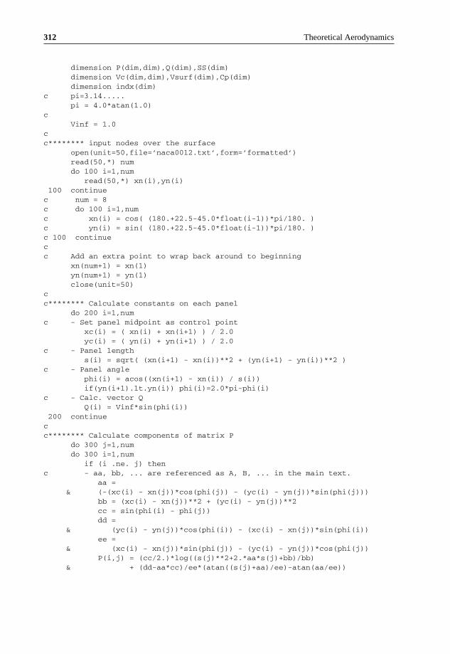
312 Theoretical Aerodynamics
dimension P(dim,dim),Q(dim),SS(dim)dimension Vc(dim,dim),Vsurf(dim),Cp(dim)dimension indx(dim)
c pi=3.14.....pi = 4.0*atan(1.0)
cVinf = 1.0
cc******** input nodes over the surface
open(unit=50,file=’naca0012.txt’,form=’formatted’)read(50,*) numdo 100 i=1,num
read(50,*) xn(i),yn(i)100 continuec num = 8c do 100 i=1,numc xn(i) = cos( (180.+22.5-45.0*float(i-1))*pi/180. )c yn(i) = sin( (180.+22.5-45.0*float(i-1))*pi/180. )c 100 continuecc Add an extra point to wrap back around to beginning
xn(num+1) = xn(1)yn(num+1) = yn(1)close(unit=50)
cc******** Calculate constants on each panel
do 200 i=1,numc - Set panel midpoint as control point
xc(i) = ( xn(i) + xn(i+1) ) / 2.0yc(i) = ( yn(i) + yn(i+1) ) / 2.0
c - Panel lengths(i) = sqrt( (xn(i+1) - xn(i))**2 + (yn(i+1) - yn(i))**2 )
c - Panel anglephi(i) = acos((xn(i+1) - xn(i)) / s(i))if(yn(i+1).lt.yn(i)) phi(i)=2.0*pi-phi(i)
c - Calc. vector QQ(i) = Vinf*sin(phi(i))
200 continuecc******** Calculate components of matrix P
do 300 j=1,numdo 300 i=1,num
if (i .ne. j) thenc - aa, bb, ... are referenced as A, B, ... in the main text.
aa =& (-(xc(i) - xn(j))*cos(phi(j)) - (yc(i) - yn(j))*sin(phi(j)))
bb = (xc(i) - xn(j))**2 + (yc(i) - yn(j))**2cc = sin(phi(i) - phi(j))dd =
& (yc(i) - yn(j))*cos(phi(i)) - (xc(i) - xn(j))*sin(phi(i))ee =
& (xc(i) - xn(j))*sin(phi(j)) - (yc(i) - yn(j))*cos(phi(j))P(i,j) = (cc/2.)*log((s(j)**2+2.*aa*s(j)+bb)/bb)
& + (dd-aa*cc)/ee*(atan((s(j)+aa)/ee)-atan(aa/ee))

Panel Method 313
P(i,j) = P(i,j) / (2.0*pi)Vc(i,j)=(dd-aa*cc)/(2.0*ee)*log((s(j)**2+2.0*aa*s(j)+bb)/bb)
& - cc*(atan((s(j)+aa)/ee) - atan(aa/ee))else
P(i,j) = 1.0/2.0Vc(i,j)= 0.0
end if300 continuecc******** Find SS by solving P.SS=Qc with LU decomposition and back-substitution
call LUdcmp(P,num,indx,d)call LUbksb(P,num,indx,Q)do 350 i=1,num
SS(i) = Q(i)350 continuecc********Calc. Pressure coeff.
do 400 i=1,numVsurf(i) = Vinf*cos(phi(i))do 410 j=1,num
if (i .ne. j) Vsurf(i) = Vsurf(i) + SS(j)/(2.0*pi)*Vc(i,j)410 continue
Cp(i) = 1.0 - (Vsurf(i)/Vinf)**2400 continuecc******** Results
open(unit=51,file=’result.txt’,form=’formatted’)write(51,*) ’x y Cp SourceStrength Vsurf’
c write( 6,*) ’x y Cp SourceStrength Vsurf’write( 6,*) ’x phi[deg] Cp SourceStrength/2piV Vsurf’do 500 i=1,num
write(51,550) xc(i),yc(i),Cp(i),SS(i),Vsurf(i)c write( 6,550) xc(i),yc(i),Cp(i),SS(i),Vsurf(i)
write( 6,550) xc(i),phi(i)*180/pi,Cp(i),SS(i)/(2.*pi*Vinf)& ,Vsurf(i)
500 continue550 format(’ ’,E15.8,’ ’,E15.8,’ ’,E15.8,’ ’,E15.8,’ ’,E15.8)
stopend
ccc================================================================c******** Subroutines
subroutine LUdcmp(a,n,indx,d)parameter(dim=200,epsln=1.0e-20)dimension indx(dim),a(dim,dim),vv(dim)
cd=1.0
cdo 100 i=1,n
aamax=0.0do 110 j=1,n
if (abs(a(i,j)) .gt. aamax) aamax = abs(a(i,j))

314 Theoretical Aerodynamics
110 continueif (aamax.eq.0.) then
write(6,*) ’singular matrix in LUdcmp’pause
end ifvv(i) = 1.0 / aamax
100 continuec
do 200 j=1,ndo 210 i=1,j-1
sum = a(i,j)do 220 k=1,i-1
sum=sum-a(i,k)*a(k,j)220 continue
a(i,j) = sum210 continue
aamax = 0.0do 230 i=j,n
sum = a(i,j)do 240 k=1,j-1
sum = sum - a(i,k) *a(k,j)240 continue
a(i,j) = sumdum = vv(i) * abs(sum)if (dum .ge. aamax) then
imax = iaamax = dum
endif230 continue
if (j .ne. imax) thendo 250 k=1,n
dum = a(imax,k)a(imax,k) = a(j,k)a(j,k) = dum
250 continued = -dvv(imax) = vv(j)
endifindx(j) = imaxif(a(i,j) .eq. 0.0) a(i,j) = epslnif(j .ne. n) then
dum = 1.0 / a(j,j)do 260 i=j+1,n
a(i,j) = a(i,j)*dum260 continue
endif200 continue
returnend
cc
subroutine LUbksb(a,n,indx,b)parameter(dim=200)dimension indx(dim),a(dim,dim),b(dim)

Panel Method 315
cii = 0do 100 i=1,n
ll = indx(i)sum = b(ll)b(ll)= b(i)if (ii .ne. 0) then
do 110 j=ii,i-1sum = sum - a(i,j)*b(j)
110 continueelse if (sum .ne. 0.0) then
ii = iendifb(i) = sum
100 continuedo 200 i=n,1,-1sum = b(i)do 210 j=i+1,N
sum = sum - a(i,j)*b(j)210 continue
b(i) = sum / a(i,i)200 continue
returnend
c
The source strength over the aerofoil surface is plotted in Figure 7.11.The tangential speed variation is shown in Figure 7.12.The Cp distribution over the aerofoil is shown in Figure 7.13.
Figure 7.11 Source strength over the aerofoil.

316 Theoretical Aerodynamics
Figure 7.12 Tangential speed variation over the aerofoil.
Figure 7.13 The Cp distribution over the aerofoil.

Panel Method 317
Example 7.3
Calculate the pressure coefficient over a cylinder with unit diameter using the source panel method. Listthe program, compute and compare the pressure coefficient variation over the cylinder, representing itwith 8 panels and with 180 panels. Also, show the source strength variation over the cylinder front torear end.
Solution
The program in FORTRAN is given below.
c source panel methodc
program spmc
implicit noneparameter, integer (dim=200)
cc*****Variablesc num : number of panelsc (xn,yn): nodesc (xc,yc): control points (mid-point of control points (i) and (i+1)c phi : panel anglec s : panel lengthc SS : source strength (referenced as lambda in the main text)c P,Q,SS : matrics and vectors s.t. [P][SS]=[Q]c Vinf : free-stream velocityc Vsurf : flow speed at control pointc Cp : pressure coeff.cc indx : vector that records the row permutationc
real, dimension xn(dim),yn(dim),xc(dim),yc(dim),phi(dim),s(dim)real, dimension P(dim,dim),Q(dim),SS(dim)real, dimension Vc(dim,dim),Vsurf(dim),Cp(dim)integer, dimension indx(dim)
c pi=3.14.....pi = 4.0*atan(1.0)
cVinf = 1.0
cc******** input nodes over the surface
num = 8do 100 i=1,num
xn(i) = cos( (-22.5+45.0*float(i-1))*pi/180. )yn(i) = sin( (-22.5+45.0*float(i-1))*pi/180. )
100 continuecc Add an extra point to wrap back around to beginning
xn(num+1) = xn(1)yn(num+1) = yn(1)close(unit=50)

318 Theoretical Aerodynamics
cc******** Calculate constants on each panel
do 200 i=1,numc - Set panel midpoint as control point
xc(i) = ( xn(i) + xn(i+1) ) / 2.0yc(i) = ( yn(i) + yn(i+1) ) / 2.0
c - Panel lengths(i) = sqrt( (xn(i+1) - xn(i))**2 + (yn(i+1) - yn(i))**2 )
c - Panel anglephi(i) = asin((yn(i+1) - yn(i)) / s(i))if(yn(i+1).lt.yn(i)) phi(i) = phi(i)+pi
c - Calc. vector QQ(i) = -Vinf*sin(phi(i))
200 continuecc******** Calculate components of matrix P
do 300 j=1,numdo 300 i=1,num
if (i .ne. j) thenc - aa, bb, ... are referenced as A, B, ... in the main text.
aa =& (-(xc(i) - xn(j))*cos(phi(j)) - (yc(i) - yn(j))*sin(phi(j)))
bb = (xc(i) - xn(j))**2 + (yc(i) - yn(j))**2cc = sin(phi(i) - phi(j))dd =
& (yc(i) - yn(j))*cos(phi(i)) - (xc(i) - xn(j))*sin(phi(i))ee =
& (xc(i) - xn(j))*sin(phi(j)) - (yc(i) - yn(j))*cos(phi(j))P(i,j) = (cc/2.)*log((s(j)**2+2.*aa*s(j)+bb)/bb)
& + (dd-aa*cc)/ee*(atan((s(j)+aa)/ee)-atan(aa/ee))P(i,j) = P(i,j) / (2.0*pi)Vc(i,j)=(dd-aa*cc)/(2.0*ee)*log((s(j)**2+2.0*aa*s(j)+bb)/bb)
& - cc*(atan((s(j)+aa)/ee) - atan(aa/ee))else
P(i,j) = 1.0/2.0Vc(i,j)= 0.0
end if300 continuecc******** Find SS by solving P.SS=Q with LU decomposition
call LUdcmp(P,num,indx,d)call LUbksb(P,num,indx,Q)
cc********Calc. Pressure coeff.
do 400 i=1,numSS(i) = Q(i)Vsurf(i) = Vinf*cos(phi(i))do 410 j=1,num
if (i .ne. j) Vsurf(i) = Vsurf(i) + SS(i)/(2.0*pi)*Vc(i,j)410 continue
Cp(i) = 1.0 - (Vsurf(i)/Vinf)**2400 continuecc******** Results

Panel Method 319
open(unit=51,file=’result.txt’,form=’formatted’)write(51,*) ’x y Cp SourceStrength Vsurf’write( 6,*) ’x phi Cp SourceStrength Vsurf’do 500 i=1,num
write(51,550) xc(i),yc(i),Cp(i),SS(i),Vsurf(i)write( 6,550) xc(i),phi(i)*180/pi,Cp(i),SS(i),Vsurf(i)
500 continue550 format(’ ’,E15.8,’ ’,E15.8,’ ’,E15.8,’ ’,E15.8,’ ’,E15.8)
stopend
c==============================================================c******** Subroutines
subroutine LUdcmp(a,n,indx,d)parameter(dim=200,epsln=1.0e-20)dimension indx(dim),a(dim,dim),vv(dim)
cd=1.0
cdo 100 i=1,n
aamax=0.0do 110 j=1,n
if (abs(a(i,j)) .gt. aamax) aamax = abs(a(i,j))110 continue
if (aamax.eq.0.) thenwrite(6,*) ’singular matrix in LUdcmp’pause
end ifvv(i) = 1.0 / aamax
100 continuec
do 200 j=1,ndo 210 i=1,j-1
sum = a(i,j)do 220 k=1,i-1
sum=sum-a(i,k)*a(k,j)220 continue
a(i,j) = sum210 continue
aamax = 0.0do 230 i=j,n
sum = a(i,j)do 240 k=1,j-1
sum = sum - a(i,k) *a(k,j)240 continue
a(i,j) = sumdum = vv(i) * abs(sum)if (dum .ge. aamax) then
imax = iaamax = dum
endif230 continue
if (j .ne. imax) thendo 250 k=1,n
dum = a(imax,k)

320 Theoretical Aerodynamics
a(imax,k) = a(j,k)a(j,k) = dum
250 continued = -dvv(imax) = vv(j)
endifindx(j) = imaxif(a(i,j) .eq. 0.0) a(i,j) = epslnif(j .ne. n) then
dum = 1.0 / a(j,j)do 260 i=j+1,n
a(i,j) = a(i,j)*dum260 continue
endif200 continue
returnend
csubroutine LUbksb(a,n,indx,b)parameter(dim=200)dimension indx(dim),a(dim,dim),b(dim)
cii = 0do 100 i=1,n
ll = indx(i)sum = b(ll)b(ll)= b(i)if (ii .ne. 0) then
do 110 j=ii,i-1sum = sum - a(i,j)*b(j)
110 continueelse if (sum .ne. 0.0) then
ii = iendifb(i) = sum
100 continuedo 200 i=n,1,-1sum = b(i)do 210 j=i+1,N
sum = sum - a(i,j)*b(j)210 continue
b(i) = sum / a(i,i)200 continue
returnend
c
Schematic of the cylinder with 8 panels is shown in Figure 7.14.Nondimensional pressure distribution over the cylinder, computed with 8 panels and 180 panels are
compared in Figure 7.15. Variation of source strength from the front end to the rear end of the cylinderis shown in Figure 7.16.

Panel Method 321
Figure 7.14 Cylinder with 8 panels.
Figure 7.15 Variation of pressure coefficient over the cylinder.

322 Theoretical Aerodynamics
Figure 7.16 Source strength variation from the front to rear end of the cylinder.
Example 7.4
Write and list the code for solving flow past a NACA0012 aerofoil, using vortex panel method. Computeand plot lift and drag coefficients and the aerodynamic efficiency for angle of attack range from −5◦ to+20◦.
Solution
The FORTRAN program for vortex panel method is listed below:
c vortex panel methodc
program vpmc
integer dimparameter (dim=200)
cc*****Variablesc num : number of panelsc (xn,yn): nodesc (xc,yc): control points (mid-point of control points (i) and (i+1)c xcl,ycl: coordinate of control point evaluated from localc coordinatesc phi : panel anglec s : panel lengthc gamma : vortex strength (referenced as lambda in the main text)

Panel Method 323
c P,Q : matrics and vectors s.t. [P][gamma]=[Q]c Vinf : free-stream velocityc alpha : angle of attackc Vsurf : flow speed at control pointc Cp : pressure coeff.cc indx : vector that records the row permutationc
dimension xn(dim),yn(dim),xc(dim),yc(dim),phi(dim),s(dim)dimension P(dim,dim),Q(dim),gamma(dim)dimension Vsurf(dim),Cp(dim)dimension indx(dim)dimension a(dim,dim),b(dim,dim),r(dim,dim)
c pi=3.14.....pi = 4.0*atan(1.0)
cc - free-stream speed
Vinf = 1.0c - angle of attack (deg.)
alpha = 8.0alpha = alpha * pi/180.
cc******** input nodes over the surface
open(unit=50,file=’naca0012.txt’,form=’formatted’)read(50,*) numdo 100 i=1,num
read(50,*) xn(i),yn(i)100 continuec Add an extra point to wrap back around to beginning
xn(num+1) = xn(1)yn(num+1) = yn(1)close(unit=50)
cc******** Calculate constants on each panel
do 200 i=1,numc - Set panel midpoint as control point
xc(i) = ( xn(i) + xn(i+1) ) / 2.0yc(i) = ( yn(i) + yn(i+1) ) / 2.0
c - Panel lengths(i) = sqrt( (xn(i+1) - xn(i))**2 + (yn(i+1) - yn(i))**2 )
c - Panel anglephi(i) = acos((xn(i+1) - xn(i)) / s(i))if(yn(i+1).lt.yn(i)) phi(i)=2.0*pi-phi(i)
c - Calc. vector QQ(i) = Vinf*sin(alpha - phi(i))
200 continueQ(num+1) = 0.0
cc******** Calculate components of matrix P
do 300 j=1,num+1do 300 i=1,num
r(i,j) = sqrt( (xc(i)-xn(j))**2 + (yc(i)-yn(j))**2 )300 continue
do 310 j=1,num

324 Theoretical Aerodynamics
do 310 i=1,numxcl = (xc(i)-xn(j))*cos(phi(j)) + (yc(i)-yn(j))*sin(phi(j))ycl =-(xc(i)-xn(j))*sin(phi(j)) + (yc(i)-yn(j))*cos(phi(j))
cbeta= atan(xcl/ycl) - atan((xcl-s(j))/ycl)
ccc = (1./(2.*pi))*(-(1.-xcl/s(j))*log(r(i,j+1)/r(i,j))
& + (1.-ycl/s(j)*beta) )dd = (1./(2.*pi))*( (1.-xcl/s(j))*beta
& - ycl/s(j)*log(r(i,j+1)/r(i,j)) )ee = (1./(2.*pi))*(-xcl/s(j)*log(r(i,j+1)/r(i,j))
& - (1.-ycl/s(j)*beta) )ff = (1./(2.*pi))*( xcl/s(j)*beta
& + ycl/s(j)*log(r(i,j+1)/r(i,j)) )c
a(i,j) = cc*cos(phi(i)-phi(j)) + dd*sin(phi(i)-phi(j))b(i,j) = ee*cos(phi(i)-phi(j)) + ff*sin(phi(i)-phi(j))
310 continuedo 320 i=1,num
do 330 j=2,numP(i,j) = a(i,j) + b(i,j-1)
330 continuec j=1
P(i,1) = a(i,1)c j=num+1
P(i,num+1)= b(i,num)320 continue
do 340 j=1,num+1P(num+1,j) = 0.if(j.eq.1.or.j.eq.num+1) P(num+1,j)=1.
340 continuecc******** Find SS by solving P.SS=Qc with LU decomposition and back-substitution
call LUdcmp(P,num+1,indx,d)call LUbksb(P,num+1,indx,Q)do 350 i=1,num+1
gamma(i) = Q(i)350 continuecc******** Calc. Induced Velocity and Pressure coeff.
do 400 i=1,numVsurf(i) = Vinf*cos(alpha-phi(i))do 410 j=1,num
if(j.ne.i)thenxcl = (xc(i)-xn(j))*cos(phi(j)) + (yc(i)-yn(j))*sin(phi(j))ycl =-(xc(i)-xn(j))*sin(phi(j)) + (yc(i)-yn(j))*cos(phi(j))beta= atan(xcl/ycl) - atan((xcl-s(j))/ycl)ulocal =
1 (1.0/(2.*pi))*(gamma(j)+(gamma(j+1)-gamma(j))*xcl/s(j))*beta2 + (1.0/(2.*pi))3 *ycl/s(j)*(gamma(j+1)-gamma(j))*log(r(i,j+1)/r(i,j))
vlocal =1 (1.0/(2.*pi))*(gamma(j)+(gamma(j+1)-gamma(j))*xcl/s(j))

Panel Method 325
2 *log(r(i,j+1)/r(i,j))3 + (1.0/(2.*pi))*(gamma(j+1)-gamma(j))*(1.-ycl/s(j)*beta)
dphi = phi(i)-phi(j)Vsurf(i) = Vsurf(i) + ulocal*cos(dphi)+vlocal*sin(dphi)endif
410 continueCp(i) = 1.0 - (Vsurf(i)/Vinf)**2
400 continuecc******** Results
open(unit=51,file=’result.txt’,form=’formatted’)write(51,*) ’x y Cp Vortex Vsurf’write( 6,*) ’x phi[deg] Cp Vortex Vsurf’do 500 i=1,num
gam=(gamma(i)+gamma(i+1))/2.write(51,550) xc(i),yc(i),Cp(i),gam,Vsurf(i)write( 6,550) xc(i),phi(i)*180/pi,Cp(i),gam,Vsurf(i)
500 continue550 format(’ ’,E15.8,’ ’,E15.8,’ ’,E15.8,’ ’,E15.8,’ ’,E15.8)cc******** Lift and Drag Coefficients & L/D
Cx = 0.0Cy = 0.0do 560 i=1,num
Cx = Cx + (yn(i+1)-yn(i))*Cp(i)Cy = Cy - (xn(i+1)-xn(i))*Cp(i)
560 continueCl =-Cx*sin(alpha) + Cy*cos(alpha)Cd = Cx*cos(alpha) + Cy*sin(alpha)write(6,*) ’======== Aerodynamic Coefficients ========’write(6,*) ’Lift Coeff. = ’,Clwrite(6,*) ’Drag Coeff. = ’,Cdwrite(6,*) ’ L / D = ’,Cl/Cdwrite(6,*) ’==========================================’stopend
c=============================================================c******** Subroutines
subroutine LUdcmp(a,n,indx,d)integer dimparameter(dim=200,epsln=1.0e-20)dimension indx(dim),a(dim,dim),vv(dim)
cd=1.0
cdo 100 i=1,n
aamax=0.0do 110 j=1,n
if (abs(a(i,j)) .gt. aamax) aamax = abs(a(i,j))110 continue
if (aamax.eq.0.) thenwrite(6,*) ’singular matrix in LUdcmp’pause
end if

326 Theoretical Aerodynamics
vv(i) = 1.0 / aamax100 continuec
do 200 j=1,ndo 210 i=1,j-1
sum = a(i,j)do 220 k=1,i-1
sum=sum-a(i,k)*a(k,j)220 continue
a(i,j) = sum210 continue
aamax = 0.0do 230 i=j,n
sum = a(i,j)do 240 k=1,j-1
sum = sum - a(i,k) *a(k,j)240 continue
a(i,j) = sumdum = vv(i) * abs(sum)if (dum .ge. aamax) then
imax = iaamax = dum
endif230 continue
if (j .ne. imax) thendo 250 k=1,n
dum = a(imax,k)a(imax,k) = a(j,k)a(j,k) = dum
250 continued = -dvv(imax) = vv(j)
endifindx(j) = imaxif(a(i,j) .eq. 0.0) a(i,j) = epslnif(j .ne. n) then
dum = 1.0 / a(j,j)do 260 i=j+1,n
a(i,j) = a(i,j)*dum260 continue
endif200 continue
returnend
csubroutine LUbksb(a,n,indx,b)integer dimparameter(dim=200)dimension indx(dim),a(dim,dim),b(dim)
cii = 0do 100 i=1,n
ll = indx(i)sum = b(ll)

Panel Method 327
b(ll)= b(i)if (ii .ne. 0) then
do 110 j=ii,i-1sum = sum - a(i,j)*b(j)
110 continueelse if (sum .ne. 0.0) then
ii = iendifb(i) = sum
100 continuedo 200 i=n,1,-1sum = b(i)do 210 j=i+1,N
sum = sum - a(i,j)*b(j)210 continue
b(i) = sum / a(i,i)200 continue
returnend
The lift and drag coefficient variation with the angle of attack for NACA0012 aerofoil, computed byvortex panel method, are shown in Figures 7.17 and 7.18, respectively. Variation of the aerodynamicefficiency of the aerofoil, calculated from the lift and drag computed with the vortex panel method, isshown in Figure 7.19.
Figure 7.17 Lift coefficient variation with angle of attack.

328 Theoretical Aerodynamics
Figure 7.18 Drag coefficient variation with angle of attack.
Figure 7.19 Aerodynamic efficiency variation with angle of attack.
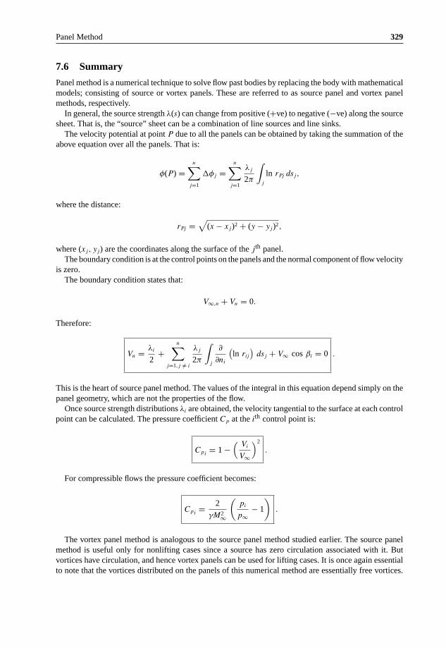
Panel Method 329
7.6 Summary
Panel method is a numerical technique to solve flow past bodies by replacing the body with mathematicalmodels; consisting of source or vortex panels. These are referred to as source panel and vortex panelmethods, respectively.
In general, the source strength λ(s) can change from positive (+ve) to negative (−ve) along the sourcesheet. That is, the “source” sheet can be a combination of line sources and line sinks.
The velocity potential at point P due to all the panels can be obtained by taking the summation of theabove equation over all the panels. That is:
φ(P) =n∑
j=1
�φj =n∑
j=1
λj
2π
∫j
ln rPj dsj,
where the distance:
rPj =√
(x − xj)2 + (y − yj)2,
where (xj, yj) are the coordinates along the surface of the jth panel.The boundary condition is at the control points on the panels and the normal component of flow velocity
is zero.The boundary condition states that:
V∞,n + Vn = 0.
Therefore:
Vn = λi
2+
n∑j=1,j /= i
λj
2π
∫j
∂
∂ni
(ln rij
)dsj + V∞ cos βi = 0 .
This is the heart of source panel method. The values of the integral in this equation depend simply on thepanel geometry, which are not the properties of the flow.
Once source strength distributions λi are obtained, the velocity tangential to the surface at each controlpoint can be calculated. The pressure coefficient Cp at the ith control point is:
Cpi= 1 −
(Vi
V∞
)2
.
For compressible flows the pressure coefficient becomes:
Cpi= 2
γM2∞
(pi
p∞− 1
).
The vortex panel method is analogous to the source panel method studied earlier. The source panelmethod is useful only for nonlifting cases since a source has zero circulation associated with it. Butvortices have circulation, and hence vortex panels can be used for lifting cases. It is once again essentialto note that the vortices distributed on the panels of this numerical method are essentially free vortices.

330 Theoretical Aerodynamics
Therefore, as in the case of source panel method, this method is also based on a fundamental solution ofthe Laplace equation. Thus this method is valid only for potential flows which are incompressible.
• The mid-point of each panel is a control point at which the boundary condition is applied; that is, ateach control point, the normal component of flow velocity is zero.
V∞ cos βi −n∑
j=1
γj
2π
∫j
∂θij
∂nj
dsj = 0 .
This equation is the crux of the vortex panel method. The values of the integrals in this equation dependsimply on the panel geometry; they are properties of the flow.
Pressure distribution around a body, given by source panel method is:
Iij = C
2ln
(s2j + 2Asj + B
B
)+ D − AC
E
[tan−1
(sj + A
E
)− tan−1
(A
E
)].
This is the general expression for two arbitrarily oriented panels; it is not restricted to circular cylinderonly.
Exercise Problems
1. Using vortex panel method, compute and plot (a) the pressure coefficient distribution over aNACA0012 aerofoil and (b) the variation of drag coefficient with lift coefficient, for Cl in the rangefrom −0.15 to 0.55, if the aerofoil is at an angle of attack of 8◦ in a uniform freestream.
2. List the procedure steps, along with equations, involved in the FORTRAN code vortex panel methodgiven in Example 7.4.
3. Compute and plot the pressure coefficient variation over a NACA0012 aerofoil in a uniform freestreamat angles of attack 0, 2, 5 and 8 degrees. Also plot the vortex distribution over the aerofoil profile forthese angles.
Reference
1. Magnus, A.E., and Epton, M.A., “PAN AIR - A computer program for predicting subsonic or supersonic linearpotential flows about arbitrary configurations using a higher order panel method”, Volume I – Theory Document(Version 1.0), NASA CR 3251, April 1980.

8Finite Aerofoil Theory
8.1 Introduction
The vortex theory of a lifting aerofoil proposed by Lancaster and the subsequent development by Prandtlmade use of for calculating the forces and moment about finite aerofoils. The vortex system around afinite aerofoil consists of the starting vortex, the trailing vortex system and the bound vortex system, asillustrated in Figure 8.1.
The horseshoe vortex system around an aerofoil, consisting of the bound and trailing vortices, can besimplified as shown in Figure 8.2.
8.2 Relationship between Spanwise Loading and Trailing Vorticity
From Helmholtz’s second theorem, the strength of the circulation around any section of a bundle of vortextubes is the sum of the strength of the vortex filaments cut by the section plane. As per this theorem, thespanwise variation of the strength of the combined bound vortex filaments may be shown as illustratedin Figure 8.3.
If the circulation curve can be described as some function of y, say f (y), then the strength of thecirculation shed by the aerofoil becomes:
δk = −df (y)
dyδy,
that is:
δk = −f ′(y) dy. (8.1)
Now at a section of the aerofoil the lift per unit span is given by:
l = ρUk,
where ρ and U are the density and velocity of the freestream. Thus, for a given flight speed and flowdensity, the circulation strength k is proportional to l. From the above discussion, it can be inferred that:
• The trailing filaments are closer showing that the vorticity strength is larger near the wing tips thanother locations. That is, near the wing tips, the vorticity content of the vortices shed are very strong.
• Aerofoils with infinite span (b → ∞) or two-dimensional aerofoils will have constant spanwiseloading.
Theoretical Aerodynamics, First Edition. Ethirajan Rathakrishnan.© 2013 John Wiley & Sons Singapore Pte. Ltd. Published 2013 by John Wiley & Sons Singapore Pte. Ltd.

332 Theoretical Aerodynamics
Bound
vort
ex
Trailing vortex
Trailing vortex
Starting vortex
Figure 8.1 Vortex system around an aerofoil.
k
k
k
Figure 8.2 Simplified horseshoe vortex system around an aerofoil.
8.3 Downwash
Let us consider the aerofoil with hypothetical spanwise variation of circulation due to the combined boundvortex filaments as shown in Figure 8.4. At some point y along the span, an induced velocity equal to:
δwy1 = − f ′(y)dy
4π(y − y1).
will be felt in the downward direction. All elements shed vorticity along the span and add theircontribution to the induced velocity at y1 so that the total influence of the trailing system at y1 is:
wy1 = − 1
4π
∫ b
−b
f ′(y)dy
(y − y1),

Finite Aerofoil Theory 333
filaments
distribution
aerofoil
Trailing vorte
x
Forward velocity
b
V
y
Bound vortex filament
Rectangular
x
Vortex
k0
V
δk
b
y
dy
k − δkk
Figure 8.3 Spanwise distribution of bound vortex filaments.
y1
δk
U
k − δk
yb
δy
kk0
Figure 8.4 Spanwise variation of the strength of the combined bound vortex filaments.

334 Theoretical Aerodynamics
w = 2wcp
w
V
wcp
α
w = 0
Figure 8.5 Variation of downwash caused by the vortex system around an aerofoil.
that is:
wy1 = − 1
4π
∫ b
−b
(dk/dy) dy
(y − y1). (8.2)
The induced velocity at y1, in general, is in the downward direction and is called downwash.The downwash has the following two important consequences which modify the flow about the aerofoil
and alter its aerodynamic characteristics:
• The downwash at y1 is felt to a lesser extent ahead of y1 and to a greater extent behind, and has theeffect of tilting the resultant wind at the aerofoil through an angle:
ε = tan−1(
w
U
)≈ w
U. (8.3)
The downwash around an aerofoil will be as illustrated in Figure 8.5.The downwash reduces the effective incidence so that for the same lift as the equivalent infinite or
two-dimensional aerofoil at incidence α, an incidence of α = α∞ + ε is required at that section of theaerofoil. Variation of downwash in front of and behind an aerofoil will be as shown in Figure 8.5. Asillustrated in Figure 8.5, the downwash will diminish to zero at locations far away from the leadingedge and will become almost twice of its magnitude wcp at the center of pressure, downstream of thetrailing edge.
• In addition to this motion of the air stream, a finite aerofoil spins the air flow near the tips into whateventually becomes two trailing vortices of considerable core size. The generation of these vorticesrequires a quantity of kinetic energy. This constant expenditure of energy appears to the aerofoil asthe trailing vortex drag.
Figure 8.6 shows the two velocity components of the relative wind superimposed on the circulationgenerated by the aerofoil. In Figure 8.6, L∞ is the two-dimensional lift, VR is the resultant velocity and V
is the freestream velocity. Note that the two-dimensional lift is normal to VR and the actual lift L is normalto V . The two-dimensional lift is resolved into the aerodynamic forces L and Dv, respectively, normal andagainst the direction of the velocity V of the aerofoil. Thus, an important consequence of the downwashis the generation of drag Dv. Also, as illustrated in Figure 8.6, the vortex system inducing downwashw tilts the aerofoil in the nose-up direction. In Figure 8.6, V is the forward speed of aerofoil, VR is theresultant velocity at the aerofoil, α is the incidence, ε (= w/V ) is the downwash angle, α∞ = (α − ε),the equivalent two-dimensional incidence and Dv is the trailing vortex drag. The trailing vortex drag isalso referred to as vortex drag or induced drag.
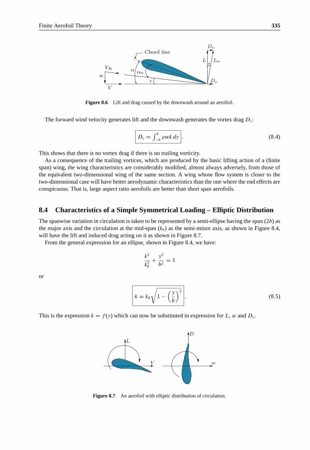
Finite Aerofoil Theory 335
V
Chord line
α α∞VR
Dv
L
Dv
L∞
w
Figure 8.6 Lift and drag caused by the downwash around an aerofoil.
The forward wind velocity generates lift and the downwash generates the vortex drag Dv:
Dv = ∫ b
−bρwk dy . (8.4)
This shows that there is no vortex drag if there is no trailing vorticity.As a consequence of the trailing vortices, which are produced by the basic lifting action of a (finite
span) wing, the wing characteristics are considerably modified, almost always adversely, from those ofthe equivalent two-dimensional wing of the same section. A wing whose flow system is closer to thetwo-dimensional case will have better aerodynamic characteristics than the one where the end effects areconspicuous. That is, large aspect ratio aerofoils are better than short span aerofoils.
8.4 Characteristics of a Simple Symmetrical Loading – Elliptic Distribution
The spanwise variation in circulation is taken to be represented by a semi-ellipse having the span (2b) asthe major axis and the circulation at the mid-span (k0) as the semi-minor axis, as shown in Figure 8.4,will have the lift and induced drag acting on it as shown in Figure 8.7.
From the general expression for an ellipse, shown in Figure 8.4, we have:
k2
k20
+ y2
b2= 1
or
k = k0
√1 −
(y
b
)2
. (8.5)
This is the expression k = f (y) which can now be substituted in expression for L, w and Dv.
L
D
wV
Figure 8.7 An aerofoil with elliptic distribution of circulation.

336 Theoretical Aerodynamics
8.4.1 Lift for an Elliptic Distribution
The general expression for the lift of an aerofoil of span 2b is:
L = ∫ b
−bρUk dy .
Substituting Equation (8.5), we have:
L =∫ b
−b
ρUk0
√1 −
(y
b
)2
dy
L = ρUk0πb
2. (8.6)
Therefore:
k0 = L12 ρUπb
.
But the lift is also given by:
L = 1
2ρU2S CL.
where S = (span × chord) is the projected area of the wing, in the direction normal to the freestreamvelocity U. Therefore:
k0 = CLUS
πb. (8.6a)
8.4.2 Downwash for an Elliptic Distribution
The circulation for elliptical distribution is:
k = k0
√1 −
(y
b
)2
.
Differentiating with y, this gives:
dk
dy= −k0
y
b2
[1 −
(y
b
)2]− 1
2
= − k0
b
y√b2 − y2
.
The downwash becomes:
wy1 = k0
4πb
∫ b
−b
y dy(√b2 − y2
)(y − y1)
.

Finite Aerofoil Theory 337
Adding and subtracting y1 to the numerator, this can be expressed as:
wy1 = k0
4πb
∫ b
−b
(y − y1) + y1(√b2 − y2
)(y − y1)
dy
= k0
4πb
[∫ b
−b
dy√b2 − y2
+ y1
∫ b
−b
dy(√b2 − y2
)(y − y1)
].
Evaluating the first integral which is in a standard form, and writing I for the second integral, we get:
wy1 = k0
4πb
[π + y1I
].
Now, as this is a symmetric flight case, the vorticity shed is the same from each side of the wing and thevalue of the downwash at point y1 is identical to that at the corresponding point −y1 on the other wing.Therefore, substituting for ±y1 for y1 in the above equation and equating them, we get:
w±y1 = k0
4πb
[π + y1I
] = k0
4πb
[π − y1I
].
This is satisfied only if I = 0. Therefore:
w = k0
4b. (8.7)
This is an important result, which implies that the downwash is constant along the wing span.
Example 8.1
If a wing of span 20 m and chord 2.5 m has elliptical load distribution. If the downwash is 0.4 m/s, findthe expression for circulation around the wing.
Solution
Given, 2b = 20 m, c = 2.5 m, w = 0.4 m/s.By Equation (8.7):
w = k0
4b.
Therefore:
k0 = 4 b w
= 4 × 10 × 0.4
= 16 m2/s.

338 Theoretical Aerodynamics
By Equation (8.5), the circulation is:
k = k0
√1 −
(y
b
)2
.
Therefore:
k = 16
√1 −
(y
10
)2
.
Note that this circulation distribution is elliptical in nature.
8.4.3 Drag Dv due to Downwash for Elliptical Distribution
The drag caused by the downwash is:
Dv =∫ b
−b
ρwk dy
=∫ b
−b
ρk0
4bk0
√1 −
(y
b
)2
dy.
On integration this results in:
Dv = π
8ρk2
0 . (8.4a)
By Equation (8.6a):
k0 = CLUS
πb.
Therefore:
Dv =(
CLUS
πb
)2π
8ρ.
The drag can also be written as:
Dv = 1
2ρU2SCDv .
Therefore, the drag coefficient becomes:
CDv= C2
L
π, (8.8)

Finite Aerofoil Theory 339
where is the aspect ratio, defined as the ratio of the span to chord of the wing, given by:
= Span
Chord
= Span × Span
Span × Chord
= Span2
Wing area
= (2b)2
S
= 4b2
S.
From the above expression for CDvit is seen that, when the lift becomes zero, CDv
becomes zero.
8.5 Aerofoil Characteristic with a More General Distribution
A more general distribution must satisfy the end conditions, namely, at the wing tips the vorticity shouldbe zero. That is:
At y = ±b k = 0.
It is found that, for plain rectangular or slightly tapered aerofoils, the spanwise distribution does notdepart drastically from elliptic distribution. The modified elliptic loading can satisfy this situation. Let:
k = k0
√1 − y2
b2
(1 + a
(y
b
)2)
.
The constant a can vary positively or negatively and therefore, can change the shape, but the end conditionsare satisfied, as illustrated in Figure 8.8. In this figure, the area enclosed by the curves for a < 0, a = 0and a > 0 are the same. That is, the total lift for elliptic and modified elliptic loading in this figure arethe same.
b
k0
Elliptic loading (a = 0)
(a > 0)
b
Modified elliptic loading (a < 0)
k(y)
y
Figure 8.8 Comparison of elliptic and modified elliptic loading.

340 Theoretical Aerodynamics
The lift for the modified elliptic loading becomes:
L =∫ b
−b
ρUk dy
=∫ b
−b
ρUk0
√1 −
(y
b
)2(
1 + a
(y
b
)2)
dy.
But the distribution is symmetrical, therefore:
L = 2ρUk0
∫ b
0
√1 −
(y
b
)2(
1 + a
(y
b
)2)
dy.
Now, let:
y = b sin φ.
Therefore, dy = b cos φ dφ and the limits become 0 and π/2.Substituting these, the lift becomes:
L = 2ρUk0b
∫ π/2
0
cos2 φ (1 + a sin2 φ) dφ.
Now, writing a = 4λ, we get:
L = 2ρUk0b
∫ π/2
0
(cos2 φ + 4λ cos2 φ sin2 φ
)dφ.
These are standard forms integrable by Walls’ rule to give:
L = 2ρUk0b
[π
4+ 4λ
π
16
]
or
L = ρUk0bπ
2(1 + λ) . (8.9)
The lift coefficient becomes:
CL = πk0b
US(1 + λ) . (8.9a)
Comparing this with the equation for the same lift, Equation (8.6), from the equivalent elliptically loadedaerofoil with mid-span circulation, for example, kE, we get:
ρUk0bπ
2(1 + λ) = ρUkEb
π
2.

Finite Aerofoil Theory 341
Therefore:
kE = k0(1 + λ) = k0
(1 + a
4
). (8.10)
Thus a distribution which diminishes fairly rapidly from the mid-span sections would have a (or λ)negative, while for flat distribution a is positive.
8.5.1 The Downwash for Modified Elliptic Loading
The downwash is given by:
wy1 = − 1
4π
∫ b
−b
(dk/dy)
y − y1dy.
Let a = 4λ and y = −b cos θ. Therefore:
y1 = −b cos θ1
dy = b sin θ dθ.
The new limits of integration are:
0 at y = −b and π at y = +b.
Therefore, wy1 becomes:
wθ1 = 1
4π b
∫ π
0
(dk/dθ)
cos θ − cos θ1dθ
and
k = k0
√1 − cos2 θ (1 + 4λ cos2 θ)
dk
dθ= k0[cos θ(1 + 4λ cos2 θ) + (−8λ sin2 θ cos θ)]
= k0[(1 − 8λ) cos θ + 12λ cos3 θ].
But:
cos3 θ = 3 cos θ + cos 3 θ
4.
Therefore:
dk
dθ= k0 [(1 + λ) cos θ + 3λ cos 3θ] .

342 Theoretical Aerodynamics
Substituting this we get the downwash as:
wθ1 = k0
4πb
∫ π
0
((1 + λ) cos θ + 3λ cos 3θ
cos θ − cos θ1
)dθ.
Integrals of the type:
Gn =∫ b
0
cos nθ
cos θ − cos θ1dθ (Glauert’s integral)
can be solved by integrating over two ranges, namely, 0 to (θ1 − ε) and (θ1 + ε) to π and taking the limitsas ε tends to zero. Thus:
Gn = limε→0
(∫ θ1−ε
0
cos nθ
cos θ − cos θ1dθ +
∫ π
θ1+ε
cos nθ
cos θ − cos θ1dθ
).
Integrating, we get:
Gn =∫ π
0
cos nθ
cos θ − cos θ1dθ = π sin nθ1
sin θ1
for all values of n > 0. When n = 0, G0 = 0, these integrals become the integrals for the case of ellipticloading.
Introducing this solution into the downwash expression, we get:
wθ1 = k
4πb
((1 + λ)
π sin θ1
sin θ1+ 3λ
π sin 3θ1
sin θ1
).
We can expresssin 3θ1
sin θ1as:
sin 3θ1
sin θ1= 3 sin θ1 − 4 sin3 θ1
sin θ1
= 3 − 4 sin2 θ1
= 3 − 4 (1 − cos2 θ1)
= 4 cos2 θ1 − 1.
Therefore:
wθ1 = k0
4b[(1 + λ) + 3λ (4 cos2 θ1 − 1)].
For the point y1 = − b cos θ1:
wθ1 = k0
4b
[(1 + λ) + 12λ
(y1
b
)2
− 3λ
].

Finite Aerofoil Theory 343
For any point y along the span the downwash is
w = k0
4b
[1 − 2λ + 12λ
(y
b
)2]
. (8.11)
From Equation (8.11), we can infer the following:
• The downwash in the general case will vary in magnitude along the span, and may even becomenegative (−ve) and give an upwash near the tips if λ < −0.1.
• If the downwash is negative (−ve) near the tips the induced (vortex) drag Dv is negative (−ve) andthat region of wing gives a thrust. This is, however, compensated by a greater drag grading over thecentral regions of the wing.
8.6 The Vortex Drag for Modified Loading
The vortex drag, by Equation (8.4), is:
Dv =∫ b
−b
ρwk dy.
But for modified loading, the downwash, by Equation (8.11), is:
w = k0
4b
[1 − 2λ + 12λ
(y
b
)2]
and the vortex distribution is:
k = k0
√1 − y2
b2
[1 + 4λ
(y
b
)2]
.
Substituting for w and k, we get the vortex drag as:
Dv =∫ b
−b
ρk0
4b
[1 − 2λ + 12λ
(y
b
)2]
k0
√1 −
(y
b
)2(
1 + 4λ
(y
b
)2)
dy.
The load is symmetrical about the mid plane, therefore the limits can be written as:
Dv = 2
∫ b
0
ρk0
4b
[1 − 2λ + 12λ
(y
b
)2]
k0
√1 −
(y
b
)2(
1 + 4λ
(y
b
)2)
dy.
Let y = b sin φ, therefore, dy = b cos φ dφ and the limits become 0 and π/2. Hence:
Dv = 2ρk20
4
∫ π/2
0
(1 − 2λ + 12λ sin2 φ) cos2 φ (1 + 4λ sin2 φ) dφ
= ρk20
2
∫ π/2
0
[(1 − 2λ) cos2 φ + (16λ − 8λ2) sin2 φ cos2 φ
+ 48λ2 sin4 φ cos2 φ] dφ.

344 Theoretical Aerodynamics
These are standard integrals which result as:
Dv = ρk20
2
[(1 − 2λ)
π
4+ (16λ − 8λ2)
π
16+ 48λ2 π
32
]
= πρk20
8
[1 − 2λ + 4λ − 2λ2 + 6λ2
].
This simplifies to:
Dv = πρk20
8[1 + 2λ + 4λ2] . (8.12)
But drag is also given by:
Dv = 1
2ρU2SCDv.
Therefore, the drag coefficient becomes:
CDv = Dv
12 ρU2S
.
Substituting for Dv, from Equation (8.12), we have:
CDv = πρk20 (1 + 2λ + 4λ2)
8 × 12 ρU2S
.
Substituting for k0 = CLUS
πb(1 + λ), from Equation (8.9a), the drag coefficient becomes:
CDv = π
4U2S(1 + 2λ + 4λ2) ×
[CLUS
πb(1 + λ)
]2
= C2LS
π4b2
[(1 + λ)2 + 3λ2
(1 + λ)2
]
= C2L
π
(2b × c)
(2b)2
[1 + 3λ2
(1 + λ)2
]
= C2L
π
[1 + 3λ2
(1 + λ)2
]
since:
(2b × c)
(2b)2= c
2b= 1
.
Writing:
δ = 3(
λ
1 + λ
)2

Finite Aerofoil Theory 345
the drag coefficient can be expressed as:
CDv = C2L
π
[1 + δ
]. (8.13)
This drag coefficient for the modified loading is more than that for elliptical loading by an amount δ,which is always positive since it contains λ2 terms only.
8.6.1 Condition for Vortex Drag Minimum
For the vortex drag Dv to be minimum, the δ in Equation (8.13) must be zero. That is, λ (or a) must bezero so that the distribution for Dv minimum becomes:
k = k0
√1 − y2
b2
[1 + 4 × 0 ×
(y
b
)2]
= k0
√1 − y2
b2.
This is an ellipse, thus the vortex distribution for drag minimum is semi-ellipse. The minimum dragdistribution produces a constant downwash along the span while all other distributions produce a spanwisevariation in induced velocity, as illustrated in Figure 8.9.
It is seen that the elliptic distribution gives constant downwash and minimum drag, non-elliptic distri-bution gives varying downwash.
If the lift for the aerofoils with elliptical and non-elliptical distribution is the same under given con-ditions, the rate of change of vertical momentum in the flow is the same for both. Thus, for ellipticaldistribution the lift becomes:
L ∝∫ b
−b
m w0dy.
For non-elliptic distribution the lift is:
L ∝∫ b
−b
m[w0 + f1(y)
]dy.
w0
(a)
´
(b) (c)
w1 = f1(y)w = f(y)
+
bbbb
w0
Figure 8.9 (a) Constant downwash due to elliptic distribution, (b) varying downwash due to non-elliptic distribution,(c) equivalent variation of downwash.

346 Theoretical Aerodynamics
where m is a representative mass flow meeting unit span. But lift L is the same on each wing, therefore:
∫ b
−b
mf1(y) dy = 0.
Now the energy transfer or rate of change of the kinetic energy of the representative mass flow is thevortex drag (or induced drag). Thus, for elliptical distribution the vortex drag is:
Dva ∝ 1
2m
∫ b
−b
w20dy.
For non-elliptic distribution the vortex drag is:
Dvb ∝ 1
2m
∫ b
−b
(w0 + f1(y)
)2dy
∝ 1
2m
∫ b
−b
[w2
0 + 2w0f1(y) + (f1(y))2]dy.
But:
∫ b
−b
mf1(y) dy = 0.
Therefore:
Dvb ∝[
1
2m
∫ b
−b
w20dy + 1
2m
∫ b
−b
(f1(y))2 dy
]
or
Dvb = Dva + 12 m
∫ b
−b(f1(y))2 dy (8.14)
and since:
∫ b
−b
f1(y)dy = 0
and f1(y) is an explicit function of y:
∫ b
−b
(f1(y))2 > 0,
since (f1(y))2 is always positive whatever be the sign of f1(y). Hence the induced drag Dvb for non-ellipticloading is always greater than the induced drag Dva for elliptic loading.

Finite Aerofoil Theory 347
dΓ
dydy
yb
Py
δy
P1
− b
y1
Figure 8.10 A representative lifting line.
8.7 Lancaster – Prandtl Lifting Line Theory
It is a representation to improve on the accuracy of the horseshoe vortex system. In lifting line theory,the bound vortex is assumed to lie on a straight line joining the wing tips (known as lifting line). Now thevorticity is allowed to vary along the line. The lifting line is generally taken to lie along the line joiningthe section quarter-chord points of the wing. The results obtained using this representation is generallygood provided that the aspect ratio of the wing is moderate or large, generally not less than 4.
Consider the lifting line as shown in Figure 8.10. At any point on the lifting line, the bound vortex is(y), and there is consequently trailing vorticity of strength d/dy per unit length shed. Note that (y) isused to represent vortex distribution, instead of k(y). This is because it is a common practice to use bothk(y) and (y) to represent the vortex distribution.
The velocity induced by the elements of trailing vorticity of strength (d/dy).dy at point P1 is givenby:
δwP1 = 1
4π
(d/dy)
y1 − ydy.
Total downwash at point P1 is:
wy1 = 1
4π
∫ b
−b
(d/dy)
y1 − ydy. (8.15)
The assumption in this analysis is that the downwash velocity w is small compared to the freestreamvelocity V , so that w/V is equal to the downwash angle ε.
Let αe(y1) be the effective angle of incidence of the wing section at point P1. The geometrical incidenceof the same section be α(y). Let both these angles be measured from the local zero-lift angle. Then:
αe(y1) = α(y1) − w(y1)
V
= α(y1) − 1
4πV
∫ b
−b
(d/dy)
y1 − ydy.
If a∞ is the lift-curve slope of the wing section at point P1, which may also vary across the span, thelocal lift coefficient CL is given by:
CL(y1) = a∞αe(y1).

348 Theoretical Aerodynamics
The lift per unit span becomes:
CL(y1)1
2ρV 2c = ρV(y1).
Therefore:
(y1) = 1
2cVCL(y1) = 1
2cVa∞αe(y1).
Thus:
αe(y1) = 2(y1)
cVa∞,
where the local chord c may vary across the span.But w/V = (α − αe), so that:
w(y1) = V[α(y1) − αe(y1)
]= Vα(y1) − 2(y1)
ca∞.
Equation (8.15) may be written as:
w(y1) = 1
4π
∫ b
−b
(d/dy)
y1 − ydy
or
w(y1) =[V α − 2(y1)
ca∞
]y=y1
. (8.16)
This is an integral equation from which the bound vorticity distribution may be determined.Let us introduce θ such that y = −b cos θ, so that θ = 0 at the port wing tip, θ = π at the starboard
wing tip, and θ = π/2 at the center line of the wing, that is, in the plane of symmetry. Now, the circulation can be expressed as a Fourier series:
(θ) = 4bV
∞∑n=1
An sin nθ. (8.17)
Note that = 0 at both the tips. Differentiating with respect to y, we get:
d
dydy = d = 4bV
∞∑n=1
nAn cos nθ.

Finite Aerofoil Theory 349
The left-hand side of Equation (8.16) gives:
bV
π
∫ π
0
∞∑n=1
nAn cos nθ
b(cos θ − cos θ1)dθ = V
π
∞∑n=1
n An
∫ π
0
cos nθ
(cos θ − cos θ1)dθ.
Using Glauert’s integral formula, this can be expressed as:
w(θ1) = V
∞∑n=1
nAn sin nθ1
sin θ1. (8.18)
From Equation (8.16), omitting the subscript 1, we get:
V
∞∑n=1
nAn sin nθ
sin θ= Vα − 8bV
∑∞n=1 An sin nθ
a∞c
∞∑n=1
nAn sin nθ
sin θ= α(θ) − 8b
a∞c
∞∑n=1
An sin nθ.
Writing μ = a∞c/8b, we get, multiplying by μ sin θ:
∞∑n=1
(μn + sin θ) An sin nθ = μα sin θ . (8.19)
From Equation (8.19), the Fourier coefficients An may be determined if α and μ, which are generalfunctions of θ, are known, that is, the wing geometry is fully specified.
8.7.1 The Lift
The lift generated by the wing, by Equation (8.6), is:
L =∫ b
−b
ρV(y) dy.
Substituting Equation (8.17), we have:
L =∫ b
−b
ρV 4bV
∞∑n=0
An sin nθ dy.
But y = −b cos θ and dy = b sin θ dθ, thus:
L = ρV
∫ b
−b
4bV
∞∑n=1
An sin nθ b sin θ dθ.

350 Theoretical Aerodynamics
At y = b, θ = 0 and at y = −b, θ = π, therefore:
L = 4ρb2V 2
∞∑n=1
∫ π
0
An sin nθ sin θ dθ
= 4ρb2V 2A1π
2.
That is:
L = 2πρb2V 2A1 , (8.20)
since all other terms vanish.The wing area is:
S = (span × chord) = 2b × c
= 2b × 2b
2b/c
= 4b2
.
since span/chord = 2b/c = .The lift coefficient becomes:
CL = L12 ρV 2S
= L
2ρV 2b2
= 2πρb2V 2A1
2ρV 2b2
or
CL = π A1 . (8.20a)
Thus, the lift coefficient CL depends on A1, which in turn depends on the values and distribution of α
and μ [Equation (8.19)].
8.7.2 Induced Drag
The induced drag, by Equation (8.4), is:
Dv =∫ b
−b
ρ(y)w(y) dy.

Finite Aerofoil Theory 351
By Equation (8.17):
(y) = 4bV
∞∑n=1
An sin nθ
and by Equation (8.18):
w(θ) = V
∞∑n=1
nAn sin nθ
sin θ.
Also, dy = b sin θ dθ, therefore:
Dv = ρ
∫ π
0
4bV
∞∑n=1
(An sin nθ) V
∞∑n=1
(nAn sin nθ
sin θb sin θ
)dθ,
that is:
Dv = 4ρb2V 2
∫ π
0
( ∞∑n=1
An sin nθ
)( ∞∑n=1
nAn sin nθ
)dθ. (8.21)
In this equation, all the terms involving a product An, ....., Am, where n /= m, vanish when integrated,and the integral becomes:
∞∑n=1
nA2n
π
2.
This can be demonstrated by multiplying, say, the first three odd harmonics, thus:
I =∫ π
0
[(A1 sin θ + 3A3 sin 3θ + 5A5 sin 5θ) (A1 sin θ + A3 sin 3θ + A5 sin 5θ)
(..........)]dθ
=∫ π
0
[(A2
1 sin2 θ + 3A23 sin2 θ + 5A2
5 sin2 θ)(
A1A3 sin θ sin 3θ and other
like terms which are different multiples of θ)]
dθ.
On integration from 0 to π all terms other than the squared terms vanish leaving:
I =∫ π
0
(A2
1 sin2 θ + 3A23 sin2 θ + 5A2
5 sin2 θ + · · · ) dθ
= π
2
[A2
1 + 3A23 + 5A2
5 + · · · ]
= π
2
∞∑n=1
nA2n.

352 Theoretical Aerodynamics
Thus:
Dv = 4ρb2V 2
∞∑n=1
n A2n
π
2
= 2πρb2V 2
∞∑n=1
n A2n
= 2πρb2V 2(A2
1 + 2A22 + 3A2
3 + · · · )
or
Dv = 2πρb2V 2A21(1 + δ) , (8.22)
where:
δ =∞∑
n=2
n A2n
A21
≥ 0
and is usually very small. Also, A1 = CL/π , so that:
CDv=
2πρb2V 2(
C2L/π2 2
)(1 + δ)
12 ρV 2S
= π
(C2
L/π2 2)
(1 + δ) .
That is:
CDv= C2
L
π(1 + δ) , (8.22a)
where (1 + δ) ≥ 1, is the induced drag factor, and hence depends on the values of the Fourier coeffi-cients, and hence on the wing geometry, especially on the planform.
Note that:
δ =(
3A23
A21
+ 5A25
A21
+ 7A27
A21
+ · · ·)
is always a positive quantity because it consists of squared terms which must be positive. The induceddrag coefficient CDv
can be a minimum only when δ = 0. That is, when A3 = A5 = A7 = · · · = 0 andthe only term remaining in the series is A1 sin θ.

Finite Aerofoil Theory 353
8.8 Effect of Downwash on Incidence
For an aerofoil:
• Geometrical incidence is the angle between the chord of the profile and the direction of motion of theaerofoil.
• Absolute incidence is the angle between the axis of zero lift of the profile and the direction of motionof the aerofoil.
When the axes of zero lift of all the profiles of the aerofoil are parallel, each profile meets the freestreamwind at the same absolute incidence, the incidence is the same at every point on the span of the aerofoil,and the aerofoil is said to be aerodynamically untwisted.
An aerofoil is said to have aerodynamic twist when the axes of zero lift of its individual profiles arenot parallel. The incidence is then variable across the span of the aerofoil.
To distinguish between the lift and induced drag coefficients and the incidences of the aerofoil (thatis, wing) as a whole and its individual profiles, let us use CL, CDv
, α for the aerofoil and CL′, CDv
′, α′
for an individual profile. The coefficients CL′, CDv
′ and α′ for a profile are functions of the coordinate y
which defines the position of the profile. For a symmetrical aerofoil they are even functions of y, that is,to say that they are the same for +y and −y.
The lift and induced drag coefficients of the profile can be expressed as:
1
2ρV 2c′dyCL
′ = ρV(y)dy (8.22)
1
2ρV 2c′dyCDv
′ = ρw(y)dy. (8.23)
Therefore the drag and lift ratio becomes:
CDv
′
CL′ = w
V= ε′ . (8.24)
For a properly designed profile, the ratio of induced drag to lift is always small in the working rangeof incidence, and therefore ε′, which is called the angle of downwash, is a small angle. It follows that ifV ′2 = √
V 2 + w2 then V ′ = V , neglecting the second order of small quantities.As shown in Figure 8.11, the resultant aerodynamic force on the strip is perpendicular to the direction
of V ′ and not to the direction of V . Since ε′ is a small angle, the coefficient of this force is CL′. Therefore
in respect to lift the strip (profile) behaves like a strip of a two-dimensional aerofoil in a relative wind inthe direction of V ′, that is at incidence α0
′, where:
α0′ = α′ − ε′ . (8.25)
Axis of zero lift
α00α0
CL0
CDv0
′
w0
V 0
V
Figure 8.11 A profile of an aerofoil moving horizontally.

354 Theoretical Aerodynamics
(b)
α00 α0
0
α
CL0
CL
(a)
Figure 8.12 Profile lift coefficient variation with incidence (a) for a two-dimensional aerofoil, (b) for a three-dimensional aerofoil.
The angle α0′ is called the effective incidence. Thus the effective downwash is the downwash velocity that
combines with the actual relative wind of speed V to produce an effective relative wind in the directionof V ′.
The lift coefficient CL′ variation with incidence will be as shown by curve a in Figure 8.12. This curve is
the graph proper to the profile operating as a two-dimensional aerofoil and the lift curve slope is given by:
a0′ = CL
′
dα0′ .
But when the profile is operating as a part of the actual wing (that is, a three-dimensional aerofoil), thevariation of CL
′ with incidence will be as shown by curve b in Figure 8.12. The lift curve slope is given by:
a′ = C′L
dα′
It is seen that the graphs of CL′ against incidence are straight lines. In Figure 8.12, the graphs a and b are
drawn with the assumption that the angle of downwash vanishes when the wind is along the axis of zerolift, that is, the axis of zero lift is assumed to be the same in the two-dimensional and three-dimensionalaerofoils. With this assumption we have:
CL′ = a0
′α0′ = a′α′. (8.26)
We know that for an actual aerofoil in a subsonic flow the main components of the drag are the profiledrag and the skin friction drag. The induced drag caused by the downwash is an additional componentof drag. Therefore, the total drag coefficient of the strip (profile), using Equation (8.24), is:
CD′ = CD0
′ + ε′CL′, (8.27)
where CD0′ is the coefficient of profile drag for the profile.
It may be noted that the profile drag is largely independent of incidence in the working range. Profiledrag is the sum of the skin friction due to viscosity, and form drag due to the shape. The part due to skinfriction is due to the no-slip caused by the viscosity of the air in the boundary layer at the surface of thebody. This viscous effect is always present, but can be reduced by smoothening the surface and reducingthe surface area.
The form drag due to the shape is owing to the high pressure at the leading edge and low pressure atthe trailing edge (that is the low pressure in the wake). By shaping the body to reduce the wake to be ofnegligible thickness, that is by streamlining, the form drag can be almost eliminated.

Finite Aerofoil Theory 355
8.9 The Integral Equation for the Circulation
For a profile of chord c′ at distance y from the plane of symmetry, the lift coefficient of the profile isgiven by:
CL′ = ρVk(y)
12 ρV 2c′ .
Therefore:
k(y) = 1
2c′VCL
′ = 1
2c′Va0
′α0′,
since CL′ = a0
′α0′, by Equation (8.26). But by Equation (8.25):
α0′ = α′ − ε′ =
(α′ − w
V
).
Therefore:
k(y) = 1
2c′Va0
′(α′ − w
V
)(8.28)
or
k(y)12 c′Va0
′ = α′ − w
V.
But by Equation (8.15):
w = 1
4π
∫ b
−b
dk(y)
y1 − ydy.
Therefore:
k(y)12 c′Va0
′ = α′ − 1
4πV
∫ b
−b
dk(y)
y1 − ydy . (8.29)
This is the integral equation from which circulation k(y) is to be determined. Using this k(y), the lift,drag, and downwash can be determined.
Note that in general α′, a0′, c′ are functions of y, since incidence, chord and profile may vary from
section to section. If the profiles are similar curves, α0′ is the same at every section, but α′ is not the same
unless the sections are also similarly situated (untwisted aerofoil).For a given wing α0
′ a0′, c′ are known functions of y, and in particular for thin wings we may assume
a0′ = 2π.The following are the two problems associated with aerofoils:
• For a given circulation k(y), the form of the aerofoil and the induced drag are to be determined.• For a given form of aerofoil, the distribution of circulation and the induced drag are to be determined.

356 Theoretical Aerodynamics
8.10 Elliptic Loading
For an elliptical load, as shown in Figure 8.4, the (k(y), y) curve is an ellipse. If P is a point on the spanwhose eccentric angle is θ, we have y = −b cos θ and therefore:
k(y) = k0 sin θ, (8.30)
where k0 is the value of k(y) at y = 0. It is easily seen that the elimination of θ gives:
(k(y)
k0
)2
+(
y
b
)2
= 1,
which is an ellipse.Substituting y = −b cos φ in Equation (8.15), the downwash velocity at the trailing edge is:
w = 1
4π
∫ π
0
k0 cos φ dφ
b (cos φ − cos θ)= k0
4b. (8.31)
Thus for elliptic loading, the downwash velocity is the same at every point on the trailing edge.Now, by substituting Equation (8.28) into Equation (8.29), we get:
k0
V
(2 sin θ
c′a0′ + 1
b
)= α′, (8.32)
where a0′ and α′ refer to the section at distance y from the plane of symmetry.
The chord c′ and incidence α′ depend, in general, on the particular profile section considered, that ison θ. Also k0/V depends on the incidence of the aerofoil. If we increase the incidence of the aerofoil byβ, the incidence of each profile section will also increase by β. Thus:
(k0
V
)1
(2 sin θ
c′a0′ + 1
b
)= α′ + β, (8.33)
where(
k0V
)1
denotes the new value of k0V
.From Equations (8.32) and (8.33), we get:
[(k0
V
)1
− k0
V
] [2 sin θ
c′a0′ + 1
b
]= β.
The only term containing θ is2 sin θ
c′a0′ , therefore, for the loading to remain elliptic at all incidence, we
shall have:
a0′c′ = a0c0 sin θ , (8.34)
where c0 is the chord of the middle section of the aerofoil (that is, at y = 0), and a0′ will be same at every
section and Equation (8.34) becomes:
c′ = c0 sin θ. (8.35)

Finite Aerofoil Theory 357
This implies that the plot of chord c′ against y is also an ellipse. This situation can be realized by anaerofoil so constructed that its planform is bounded by two half ellipses whose major axis is equal to thespan of the aerofoil. This can be proved by using the ellipses:
x21
a21
+ y2
b2= 1,
x22
a22
+ y2
b2= 1.
It follows that:
x1
a1= x2
a2= x1 ± x2
a1 ± a2
and if c′ = x1 ± x2, c0 = a1 ± a2, Equation (8.35) is satisfied.Finally, it is evident from Equations (8.32) and (8.34) that for elliptic loading, which remains elliptic
for all incidences, the incidence is the same at every profile section, and k0 is proportional to the incidence,and therefore, from Equation (8.31), the downwash is proportional to the incidence.
Another case arises for an aerofoil of rectangular planform. Here the chord c′ may be taken as constantand equal to c0. Retaining the hypothesis that a0
′ = a0, which will be true if the sections are similar, orif they are thin, Equation (8.32) becomes:
k0
V
[2 sin θ
a0c0+ 1
b
]= α′. (8.36)
This shows that the incidence at each section is different, so that the aerofoil is twisted. The incidence atthe middle section will be α, got by assigning θ = π/2 in Equation (8.36), and therefore:
α′
α=
[2 sin θ
a0c0+ 1
b
]/[2
a0c0+ 1
b
]. (8.37)
Equation (8.37) shows that if the loading is elliptic at the incidence α, it ceases to be elliptic at a differentincidence.
8.10.1 Lift and Drag for Elliptical Loading
The lift coefficient for an aerofoil in terms of the circulation k0 around it, by Equation (8.6a), is:
CL = πbk0
SU.
The aspect ratio of the aerofoil is:
= span
chord= 2b
c
= 2b × 2b
c × 2b
= 4b2
S.

358 Theoretical Aerodynamics
Therefore:
CL = πbk0
U 4b2
= πk0
4U b.
By Equation (8.7):
k0
4b= w.
Thus, the lift coefficient in terms of constant downwash velocity, at the trailing edge, is:
CL = π w
U.
By Equation (8.3), w/U = ε and by Equation (8.25):
ε = (α − α0).
Therefore:
CL = π (α − α0) . (8.38)
By Equation (8.8), the induced drag coefficient is:
CDv= C2
L
π.
The variation of CL with CDv is called the polar curve of the aerofoil.Equation (8.8) shows that the polar curve of an elliptically loaded aerofoil is a parabola, provided the
only source of the drag is the induced velocity.The polar curve is as shown in Figure 8.13. The polar curve can be graduated in incidence as indicated
in Figure 8.13. Since α is proportional to the lift coefficient CL, equal increments of incidence gradientsof the polar correspond to equal increment of CL.
10±
15±
CL
CDv
5±
Figure 8.13 Variation of lift coefficient with induced drag coefficient for elliptical loading.

Finite Aerofoil Theory 359
In practice, in addition to induced drag there is profile drag due to skin friction and wake. The coefficientof profile drag is indicated by CD0 . Thus the complete drag coefficient is:
CD = CD0 + CDv
Variation of drag coefficient CD is shown in dotted line in Figure 8.13.
8.10.2 Lift Curve Slope for Elliptical Loading
If a0 is the lift curve slope in two-dimensional motion and a is the lift curve slope for an aerofoil of finiteaspect ratio with elliptical loading, by Equation (8.38), we have:
α = α0 + CL
π.
Differentiating with respect to CL, we get:
dα
dCL
= dα0
dCL
+ 1
π
1
a= 1
a0+ 1
π,
where a and a0 are the lift curve slope. If we take the theoretical value of a0 as 2π, then:
1
a= 1
2π+ 1
π
= π + 2π
2π2.
Thus the lift curve slope becomes:
a = π
1
2+ 1
. (8.39)
For incidence below the stall, the CL verses α curves are straight lines whose slopes increase as theaspect ratio increases, as shown in Figure 8.14.
8.10.3 Change of Aspect Ratio with Incidence
By Equation (8.38), we have:
α = α0 + CL
π.
Also the induced drag coefficient, by Equation (8.8), is:
CDv = C2L
π.

360 Theoretical Aerodynamics
0
α (degrees)
0.2
CL
68
Aspec
t ratio
4
2 4 6 8 10
0.4
0.6
0.8
1.010
∞
0.0
Figure 8.14 Variation of lift coefficient with incidence.
Hence, if the aspect ratio is reduced to′and if the ‘primes’ refer to the new aerofoil with the same
incidence, we have:
α′ − α =(
1′ − 1
)CL
π. (8.40)
C′Dv
− CDv=
(1
′ − 1)
C2L
π. (8.41)
Thus for a given lift curve, decrease of aspect ratio increases both the geometrical incidence and theinduced drag coefficient.
8.10.4 Problem II
In problem I for a given circulation k(y), the form of the aerofoil has been found. Problem II is an inverseproblem in which the form of the aerofoil is known and the circulation has to be determined. To do this wemust solve the integral equation [Equation (8.29)], noting that the symmetry with respect to the medianplane of the aerofoil demands that k(y) = −k(y). In terms of the eccentric angle θ we can therefore writethe Fourier sine series, since k(y) vanishes at the tips of the aerofoil, that is at θ = 0 and θ = π.
k(y) = 4bU
∞∑1
An sin nθ. (8.42)
Note that n must be an odd integer to ensure the equality of sin nθ and sin n(π − θ). Thus:
k(y) = 4bU
∞∑n=0
A2n+1 sin (2n + 1)θ. (8.43)

Finite Aerofoil Theory 361
This formula for k(y) is unchanged when (π − θ) is written for θ, and the value at the center given byθ = π/2 is:
k0 = 4bU
∞∑n=0
A2n+1(−1)n. (8.44)
Substitution of Equation (8.43) into (8.29) gives:
8b
c′ a′0
∞∑n=0
A2n+1 sin (2n + 1)θ = α′ − b
π
∫ π
0
∞∑n=0
(2n + 1)A2n+1 cos(2n + 1)φ dφ
b (cos φ − cos θ). (8.45)
At this stage it will be useful to understand the integral on the right-hand side of this equation. Theintegral on the right-hand side of Equation (8.45) is of the type:
In =∫ π
0
cos nφ
(cos φ − cos θ)dφ,
where n is an integer.In terms of its principal value, let us define In as:
In = limε→0
[∫ θ−ε
0
cos nφ
(cos φ − cos θ)dφ +
∫ π
θ+ε
cos nφ
(cos φ − cos θ)dφ
].
This is physically equivalent to omitting the vorticity between (θ − ε) and (θ + ε) and then taking thelimit ε → 0 so that θ remains the center of the omitted portion.
If n = 0 we have, by differentiation:
∫ θ−ε
0
dφ
(cos φ − cos θ)=
[1
sin θlog
sin 12 (θ + φ)
sin 12 (θ − φ)
]θ−ε
0
∫ π
θ+ε
dφ
(cos φ − cos θ)=
[1
sin θlog
sin 12 (θ + φ)
sin 12 (θ − φ)
]π
θ+ε
.
Hence:
I0 = limε→01
sin θlog
(sin
(θ − 1
2 ε)
sin(θ + 1
2 ε))
= 0.
It follows that we may write:
In = In − I0 cos nθ =∫ φ
0
cos nφ − cos nθ
cos φ − cos θdφ.

362 Theoretical Aerodynamics
For n = 1, we have I1 = π. Now:
cos (n + 1)φ − cos (n + 1)θ + cos (n − 1)φ − cos (n − 1)θ
= 2 cos nφ (cos φ − cos θ) + 2 cos θ (cos nφ − cos nθ)
and
∫ π
0
cos nφ dφ = 0.
Therefore, we have:
In+1 + In−1 = 2 cos θ In.
To solve this let In = xn, which gives:
x2 − 2x cos θ + 1 = 0,
so that:
x = eiθ or e−iθ .
Thus:
In = A sin nθ + B cos nθ.
Since I0 = 0, we have B = 0, and since I1 = π we have A = π cosec θ and therefore:
In = πsin nθ
sin θ.
This is valid for all integer values of n including zero.Now, let us write αθ for α′ to convey that α′ is a function of θ and put:
μθ = c′a′0
8b. (8.46)
Then from Equation (8.45) we get:
∞∑n=0
A2n+1
[(2n + 1) μθ + sin θ
]sin (2n + 1)θ = μθαθ sin θ. (8.47)
To find the coefficients of A2n+1 in Equation (8.47), we need to expand each side, and each term on theleft hand side in a Fourier series, thus leading to infinite number of equations and infinite number ofunknowns. To overcome this difficulty and solve Equation (8.47), we should resort to a practical methodof solution, due to Glauert.

Finite Aerofoil Theory 363
Let us replace the infinite series of Equation (8.43) by a finite series of, say, (m + 1) terms, where m
is a given integer, thus giving:
m∑n=0
A2n+1
[(2n + 1) μθ + sin θ
]sin (2n + 1)θ = μθαθ sin θ. (8.48)
This equation cannot be satisfied identically. However, if we take a particular value of θ we get a linearequation in the coefficients A1, A3, . . . A2m+1. If (m + 1) particular values are assigned to θ we get(m + 1) linear equations from which the coefficients A2n+1 can be calculated, and the values so obtainedwill satisfy Equation (8.48), not identically, but only at the selected points. The solution will be satisfactoryif the coefficients so determined satisfy Equation (8.48) at other points within the standard of accuracyrequired for any particular case.
Since Equation (8.48) is satisfied in any case when θ = 0 or π, we have (m + 1) points other than thesepoints. The chosen points are usually taken as equally spaced in θ over the half-span. Thus if m = 3 weshould take:
θ = π
2,
3π
8,
π
4,
π
8,
and with these values we could determine four coefficients:
A1, A3, A5, A7. (8.49)
A rough approximation is obtained by taking m = 1, and θ = π/2, π/4. This will determine two coeffi-cients A′
1, A′3 but it must not be inferred that, comparing with Equation (8.49), A′
1 = A1, A′3 = A3.
If the incidence αθ has the same value α at each point on the span, Equation (8.47) shows that A2n+1 isproportional to α, and if we write A2n+1 = α B2n+1, the coefficients B2n+1 are independent of incidenceand may therefore be determined once for all.
8.10.5 The Lift for Elliptic Loading
From Equation (8.43), we have:
k(y)dy = 4b2U
∞∑0
A2n+1 sin (2n + 1) θ sin θ dθ, (8.50)
since y = −b cos θ; dy = b sin θ. Also:
∫ π
0
sin (2n + 1) θ sin θ dθ = 0, for n /= 0.
For n = 0:
∫ π
0
sin2 θ dθ = π
2.

364 Theoretical Aerodynamics
The lift is given by:
L = ρU
∫ +b
−b
k(y)dy.
With Equation (8.50), the lift becomes:
L = 4ρb2U2
∫ π
0
∞∑n=0
A2n+1 sin (2n + 1)θ sin θ dθ.
For n = 0:
L = 4ρb2U2
∫ π
0
A1 sin2 θ dθ
= 4ρb2U2A1π
2
= 1
2ρU2(2b)2πA1.
Thus the lift coefficient for the whole aerofoil is:
CL = L12 ρU2 (2b × c)
=12 ρU2(2b)2πA1
12 ρU2 (2b × c)
= πA12b
c.
That is:
CL = πA1 . (8.51)
Thus the coefficient A1 = CL/(π ), and this gives a check on the theoretical value of A1, with whichCL can be determined by wind tunnel measurements.
For elliptical loading all the A2n+1 are zero exceptA1, therefore, Equation (8.44) gives the circulation as:
k0 = 4b UA1. (8.52)
From Equations (8.51) and (8.52), we get the lift coefficient as:
CL = πk0
4b U.
If the incidence α is the same at every point of the wing span, by Equation (8.46), A1 is proportional to α.From Equation (8.51), we have:
CL = πA1 .

Finite Aerofoil Theory 365
Dividing and multiplying by α:
CL = πA1
αα.
Therefore, the lift curve slope a becomes:
a = dCL
dα= (π )
A1
α.
If a0 and α0 are the corresponding slope and incidence in two-dimensional motion, we have:
CL = a α = a0 α0.
Therefore:
α − α0 = CL
(1
a− 1
a0
).
Substituting for a, we get:
α − α0 = CL
(α
π A1
− 1
a0
). (8.53)
For a wing with aerodynamic twist, the incidence α becomes a variable across the span. We can expressthe incidence as:
αθ = αm + f (θ),
where αm is the incidence at the middle section. For this case A2n+1 in Equation (8.47) can be expressedas:
A2n+1 = A′2n+1αm + B2n+1,
rendering Equation (8.47) as equivalent to the two equations:
∑A′
2n+1 sin (2n + 1) θ [(2n + 1) μ + sin θ] = μ sin θ∑B′
2n+1 sin (2n + 1) θ [(2n + 1) μ + sin θ] = μ sin θ f (θ)
and all the numbers so determined are independent of incidence. Thus:
CL = π A1
= π[A′
1αm + B1
]= a αm + b,
where a (= π A′1) and b (= π B1) are constants for the aerofoil.

366 Theoretical Aerodynamics
8.10.6 The Downwash Velocity for Elliptic Loading
At the point of the trailing edge of an aerofoil, whose eccentric angle is θ, by Equation (8.2):
wθ = − 1
4π
∫ +b
−b
(dk/dy)
y − y1dy.
Using Equation (8.43), we can express this as:
wθ = 1
4π
∫ π
0
4b U∑
(2n + 1)A2n+1 cos (2n + 1) φ dφ
b cos φ − b cos θ.
Using the values of integrals given in Subsection (8.5.1), we have:
wθ = U
∞∑0
(2n + 1)A2n+1sin (2n + 1) θ
sin θ. (8.54)
For elliptic loading this becomes:
wθ = U A1.
By Equation (8.7), we have:
wθ = k0
4b.
Therefore:
wθ = U A1 = k0
4b,
which is constant across the wing span.
8.10.7 The Induced Drag for Elliptic Loading
The induced drag due to circulation is:
Dv =∫ +b
−b
ρwk(y)dy,
where w is the downwash.From Equations (8.50) and (8.54) we have:
w k(y)dy = 4b2U2
[ ∞∑0
A2n+1 sin (2n + 1) θ
][ ∞∑0
(2n + 1) A2n+1 sin (2n + 1) θ
]dθ.

Finite Aerofoil Theory 367
But
∫ π
0
sin (2n + 1) θ sin (2r + 1) θ dθ = 0,
where r is any integer other than n, but if r = n the value of the integral is π/2, so that:
Dv = 1
2π ρ 4b2 U2
∞∑0
(2n + 1) A22n+1.
Therefore:
CDv = Dv
12 ρU2S
=
12 π ρ 4b2 U2
∞∑0
(2n + 1) A22n+1
12 ρU2S
=π 4b2
∞∑0
(2n + 1) A22n+1
S
=π 4b2
∞∑0
(2n + 1) A22n+1
2b × c
= π2b
c
∞∑0
(2n + 1) A22n+1
= π
∞∑0
(2n + 1) A22n+1.
This can be expressed as:
CDv = π A21(1 + δ) , (8.55)
where:
δ = 3A23 + 5A2
5 + · · · + (2m + 1)A22m+1 + · · ·
A21
. (8.56)
Note that δ is never negative, and is zero only in the case of elliptic loading.The total drag coefficient is:
CD = CD0 + CDv , (8.57)

368 Theoretical Aerodynamics
0.0
1.2
7◦
CD
CL
19◦
10◦
13◦16◦
0.04
0.2
0 0.08 0.12 0.16
0.4
0.6
0.8
1.0
Figure 8.15 Drag polar of a wing with elliptic loading.
where CD0 is the profile drag coefficient, caused by the skin friction and the wake. This can be expressed,using Equation (8.55), as:
CD = CD0 + π A21(1 + δ)
= CD0 + (π2 2A2
1)
π(1 + δ).
But, π A1 = CL, therefore:
CD = CD0 + 1
πC2
L(1 + δ) . (8.58)
Equation (8.58) is the drag polar for the aerofoil. A typical drag polar is shown in Figure 8.15.For wings with loading other than elliptic, the drag polar becomes:
CD = CD0 + 1
π eC2
L(1 + δ) , (8.58a)
where e is known as the Oswald wing efficiency and for elliptic loading e = 1.For elliptic loading, δ = 0 and e = 1, therefore, the drag polar becomes:
CD = CD0 + k C2L , (8.58b)
where k = 1
π. When the lift becomes zero, that is, for CL = 0, Equation (8.58b), reduces to CD = CD0 .
Thus CD0 is referred to as zero-lift drag coefficient.If the profile drag coefficient for each profile section is a function of the position of the section, the
profile drag coefficient of the aerofoil is:
CD0 = 1
S
∫ +b
−b
C′D0
c′ dy,
where the superscript ′ refers to the section at a distance y from the plane of symmetry.

Finite Aerofoil Theory 369
8.10.8 Induced Drag Minimum
For a wing of span 2b, we have the lift and induced drag as:
L = 1
2ρU2π(2b)2A1
Dv = 1
2ρU2π(2b)2A2
1(1 + δ).
For a given lift L, the induced drag will be minimum when δ = 0. By Equation (8.56):
δ = 3A23 + 5A2
5 + · · ·A2
1
Thus for Dv minimum the condition is:
3A23 + 5A2
5 + · · · = 0.
This implies that A3 = A5 = A7 = · · · = 0. Therefore the loading is elliptic. Thus, of all the wings ofgiven span and lift, the elliptically loaded wing gives the least induced drag.
Example 8.2
For a wing of elliptic loading, in a straight level flight, find the condition for drag minimum.
Solution
The Drag D can be expressed as:
D =(
D
L
)L.
For level flight, L = W , therefore:
D = W
(D
L
).
Thus for a wing of given weight, the minimum drag occurs when (D/L) is a minimum or (L/D) is amaximum.Now
D
L=
12 ρV 2SCD
12 ρV 2SCL
= CD
CL
.
For elliptic loading, by Equation (8.58b), the drag polar is:
CD = CD0 + k C2L.

370 Theoretical Aerodynamics
Therefore:
D
L= CD0 + k C2
L
CL
= f (CL).
For drag minimum, the condition is:
d
(D
L
)dCL
= 0.
That is:
d
((CD0 + k C2
L)
CL
)
dCL
= 0.
That is:
CL(2k CL) − (CD0 + k C2L)
C2L
= 0.
This simplifies to:
2k C2L − CD0 − k C2
L = 0.
That is:
CD0 = k C2L .
Thus for minimum drag, the zero-lift drag coefficient is equal to the lift dependent drag coefficient, andthe actual drag forces associated with these coefficients are equal.
8.10.9 Lift and Drag Calculation by Impulse Method
Let us consider an aerofoil, regarded as a lifting line AB, started from rest and which moves in a straightline. Let the velocity be V at time t. Let at time t the starting vortex be assumed to be A0B0, as shown inFigure 8.16.
o
B
P
A
P 0
z
B0
− dΓ
y
x
A0
Q
Q 0V− dΓ
− dΓ
− dΓ
I
Figure 8.16 A lifting line moving straight.

Finite Aerofoil Theory 371
Let us assume that the wake ABA0B0 remains as a rectangular sheet, as shown in Figure 8.16. If P isthe point (0, y, 0) and Q is the point (−l, y, z). The flow from point P reaching the line A0B0 experiencesa circulation of −dk(y) [Equation (8.1)]. Therefore the whole wake may be regarded as resulting fromthe superposition of vortex rings, a typical one being PP ′QQ′ of circulation −dk(y).
Let PQ = h. The area of the ring is 2yh. If n is the unit normal to a small area dS separating pointsP and Q, the impulse on this area due to impulsive pressure is:
−nρφPdS at P and + nρφQdS at Q,
where:
φQ − φP = dc = k,
where c is any circuit joining points P and Q and not intersecting the plane containing P and Q. Thusthe resultant linear impulse on the system is the vector:
I =∫
S
ρ (φQ − φP ) ndS =∫
S
ρ k ndS = ρ k S n.
Thus the impulse for the area (2yh) of the vortex ring, with n as the unit normal to the plane rectangle, is:
dI = ρ [−dk(y)] 2y h n
= ρ dk(y) · 2y (kl + iz),
since −hn = kl + iz, by geometry. The impulse I of the whole wake is:
∫OA
2y dk(y) =∫
BA
y dk(y) =[y k(y)
]+b
−b−
∫ +b
−b
k(y) dy.
Thus:
I = −∫ +b
−b
ρ (kl + iz) k(y) dy.
The time rate of change of the impulse gives the force. Therefore the aerodynamic force is dI/dt anddl/dt = V , while dz/dt = w, the normal velocity at Q, which by symmetry of the ring is equal to thedownwash velocity at P . Thus the aerodynamic force is:
−k
∫ +b
−b
ρVk(y) dy − i
∫ +b
−b
ρw k(y) dy,
which consists of the same lift and induced drag as were calculated by Prandtl’s hypotheses.The method of the impulse is applicable whatever the form of the wake.
8.10.10 The Rectangular Aerofoil
This is an aerofoil whose planform is a rectangle. An aerofoil whose shape is that of a cylinder erectedon an aerofoil profile satisfies this requirement.

372 Theoretical Aerodynamics
8.10.11 Cylindrical Rectangular Aerofoil
This is the simplest type, of span 2b and chord c, which is constant at all sections. All the sections aresimilar and similarly situated.
8.11 Aerodynamic Characteristics of Asymmetric Loading
The vortex distribution k(y) for symmetrical loading falls symmetrically about the mid-span section ofan aerofoil, involving only the odd terms, and producing vortex drag and downwash variation which arealso symmetrical about the centerline. In the general case, where the loading or lift distribution is notsymmetrical about mid-span section, even terms appear in the distribution, and as a consequence of theasymmetry other characteristics of aerofoil appear.
When the lift distribution is not symmetrical about the centerline, one wing will have higher lift thanthe other. This will cause a rolling moment about the longitudinal axis passing through the mid-span ofthe wing.
Further, as the lift is not symmetric nor is the spanwise distribution of circulation, the downwashwill vary across the span without being symmetrical about the centerline and so will be the vortex draggrading. Hence, more drag will be experienced on one wing (the one with more lift) than on the otherand a net yawing moment will result about the vertical (normal) axis through the mid-span section. Inaddition to these there will be the overall lift and vortex drag force normal and parallel to the plane ofthe aerofoil in the plane of symmetry.
8.11.1 Lift on the Aerofoil
Following a similar procedure we used for determining the lift and vortex drag associated with symmet-rical loading, we can show that:
L =∫ b
−b
ρUkdy
=∫ b
−b
ρU4bU∑
An sin nθ b sin θ dθ
= 1
2ρU2SCL,
giving the lift coefficient as:
CL = πA1 ,
the same as Equation (8.20a).
8.11.2 Downwash
As given by Equation (8.18), the downwash for asymmetrical loading also becomes:
w = U∑
nAn sin nθ
sin θ.
But this will no longer be symmetrical as it contains even harmonics.

Finite Aerofoil Theory 373
8.11.3 Vortex Drag
As in the case of symmetrical loading, integrating from 1 to ∞, the drag becomes:
Dv = 2πρb2U2
∞∑n=1
nA2n.
Thus the drag coefficient becomes:
CDv= Dv
12 ρU2S
= 2πρb2U2∑∞
n=1 nA2n
12 ρU2S
= π (2b)2
(2b × c)
∞∑n=1
nA2n
= π
∞∑n=1
nA2n
= π[A2
1 + 2A22 + 3A2
3 + 4A24 + 5A2
5 + · · · ].By Equation (8.20a), A1 = CL/(π ), thus:
CDv = C2L
π[1 + δ] ,
where:
δ =(
2A22
A21
+ 3A23
A21
+ · · ·)
and δ > 0.
Example 8.3
A monoplane weighing 73575 N has elliptic wing of span 15 m. When it flies at 300 km/h at sea level,determine the circulation around sections half-way along the wings.
Solution
Given, W = 73575 N, 2b = 15 m, V = 300/3.6 = 83.33 m/s.The air density at sea level is 1.225 kg/m3 and in level flight, L = W .The lift for elliptical loading, by Equation (8.6), is:
L = ρUk0πb
2.

374 Theoretical Aerodynamics
Therefore, the circulation at the mid-span becomes:
k0 = 2L
ρUπb
= 2 × 73575
1.225 × 83.33 × π × (15/2)
= 61.18 m2/s.
The circulation for elliptical distribution, by Equation (8.5), is:
k = k0
√1 −
(y
b
)2
.
Therefore, the circulation around sections half-way along the wings, that is, at b/4, becomes:
k = k0
√1 −
(1
4
)2
= 61.18 ×√
1 −(
1
4
)2
= 59.24 m2/s .
8.11.4 Rolling Moment
Let us consider a rectangular wing with an asymmetrical lift grading and the corresponding drag grading,as shown in Figure 8.17.
drag grading
k
Asymmetric
Asymmetric loading
V
y
b
b
Yawing momentRolling moment
Figure 8.17 Schematic of asymmetrical lift and drag grading on a rectangular wing with asymmetrical vortexloading.

Finite Aerofoil Theory 375
The lift acting on any section of spanwise length δy at a distance y from the centerline (ox-axis) willproduce a negative increment of rolling moment equal to:
�LR = −l y dy, (8.59)
where l is the lift grading given by l = ρVk.The total moment becomes:
LR = −∫ b
−b
l y dy = −∫ b
−b
ρVk y dy. (8.60)
Substituting k = 4bV∑
An sin nθ and expressing y = b cos θ, we get:
LR = 4ρbV 2
∫ π
0
∑An sin nθ b cos θ b sin θ dθ
= 4ρb3V 2
∫ π
0
1
2
∑An sin nθ sin 2θ dθ
= 2ρb3V 2
∫ π
0
1
2
∑An
[cos (n − 2)θ − cos (n + 2)θ
]dθ
= ρb3V 2[∑
An
( sin (n − 2)θ
n − 2− sin (n + 2)θ
n + 2
)]π
0
or:
LR = ρb3V 2A2π . (4.60a)
The rolling moment is also given by:
LR = 1
2ρV 2SCLR
b,
where CLRis the rolling moment coefficient. Therefore:
CLR= LR
12 ρV 2Sb
= ρb3V 2A2π12 ρV 2(2b × c) b
= 2πA2b2
2b × c
= 2πA2(2b)2
4 × 2b × c
= π
2
2b
cA2.
But2b
c= , therefore:
CLR= π
2A2 . (8.61)

376 Theoretical Aerodynamics
8.11.5 Yawing Moment
The asymmetrical drag grading across the span, shown in Figure 8.17, gives rise to yawing moment N.The contribution of the vortex drag of an element of span dy, at a distance y from the oz-axis is:
�N = dvydy, (8.62)
where dv is the vortex drag per unit span and dv = ρwk. Integration over the whole span gives the yawingmoment as:
N =∫ b
−b
dvydy =∫ b
−b
ρwk ydy.
Inserting the series expressions for the circulation k and downwash w, and changing the limits andvariables from Cartesian to polar, we get:
N = −∫ π
0
ρV
∑nAn sin nθ
sin θ4bV
∑An sin nθ b cos θ b sin θ dθ
= −4ρb3V 2
∫ π
0
∑nAn sin nθ
∑An sin nθ cos θ dθ.
The yawing moment can also be expressed as:
N = 12 ρV 2SbCN , (8.63)
where CN is the yawing moment coefficient. Thus:
CN = 2
∫ π
0
∑nAn sin nθ
∑An sin nθ cos θ dθ.
Multiplying these series for a few terms, we can express the general solution as:
CN = π
2
[3A1A2 + 5A2A3 + 7A3A4 + · · · + (2n + 1)AnAn+1
], (8.63a)
since all terms other than those with coefficients which are products of A1A2, A2A3, A3A4, etc. vanishon integration.
Example 8.4
A symmetrical profile of aspect ratio 7 and chord 1.5 m flying at 200 km/h at sea level is suddenlysubjected to a downwash of 2.4 m/s. If the horizontal tail of span 3 m and chord 0.6 m is 5 m aft of theaerodynamic center of the profile, determine the tail deflection required to counter the pitching momentcaused by the sudden downwash.

Finite Aerofoil Theory 377
Solution
Given, = 7, c = 1.5 m, V = 200/3.6 = 55.56 m/s, w = 2.4 m/s, lt = 5 m.
The planform areas of the profile and horizontal tail are:
S = span × chord
= span
chord× chord2
= × c2
= 7 × 1.52
= 15.75 m2
St = 3 × 0.6
= 1.8 m2.
For the symmetrical profile, α0 = 0, therefore the lift coefficient, by Equation (8.38), is:
CL = π α.
The angle of attack, by Equation (8.3), is:
α ≈ w
V
= 2.4
55.56= 0.0432.
Thus:
CL = π × 7 × 0.0432
= 0.95.
The lift generated by the profile is:
L = 1
2ρV 2SCL
= 1
2× 1.225 × 55.562 × 15.75 × 0.95
= 28290.12 N.
For symmetrical profile, the aerodynamic center is at c/4 from the leading edge, therefore the pitchingmoment about the leading edge becomes:
Mle = L × c
4
= 28290.12 × 1.5
4= 10608.8 N-m.
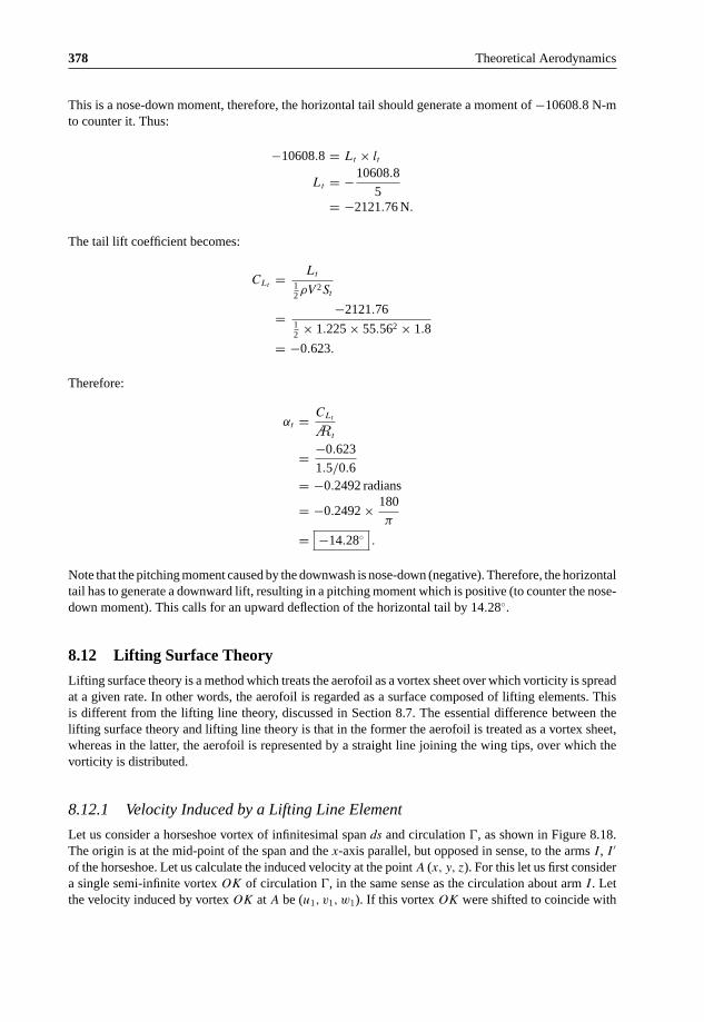
378 Theoretical Aerodynamics
This is a nose-down moment, therefore, the horizontal tail should generate a moment of −10608.8 N-mto counter it. Thus:
−10608.8 = Lt × lt
Lt = −10608.8
5= −2121.76 N.
The tail lift coefficient becomes:
CLt = Lt
12 ρV 2St
= −2121.7612 × 1.225 × 55.562 × 1.8
= −0.623.
Therefore:
αt = CLt
t
= −0.623
1.5/0.6= −0.2492 radians
= −0.2492 × 180
π
= −14.28◦ .
Note that the pitching moment caused by the downwash is nose-down (negative). Therefore, the horizontaltail has to generate a downward lift, resulting in a pitching moment which is positive (to counter the nose-down moment). This calls for an upward deflection of the horizontal tail by 14.28◦.
8.12 Lifting Surface Theory
Lifting surface theory is a method which treats the aerofoil as a vortex sheet over which vorticity is spreadat a given rate. In other words, the aerofoil is regarded as a surface composed of lifting elements. Thisis different from the lifting line theory, discussed in Section 8.7. The essential difference between thelifting surface theory and lifting line theory is that in the former the aerofoil is treated as a vortex sheet,whereas in the latter, the aerofoil is represented by a straight line joining the wing tips, over which thevorticity is distributed.
8.12.1 Velocity Induced by a Lifting Line Element
Let us consider a horseshoe vortex of infinitesimal span ds and circulation , as shown in Figure 8.18.The origin is at the mid-point of the span and the x-axis parallel, but opposed in sense, to the arms I, I ′
of the horseshoe. Let us calculate the induced velocity at the point A (x, y, z). For this let us first considera single semi-infinite vortex OK of circulation , in the same sense as the circulation about arm I. Letthe velocity induced by vortex OK at A be (u1, v1, w1). If this vortex OK were shifted to coincide with

Finite Aerofoil Theory 379
Lifiting line
I′
I
y
B
M N
A
K
− xz
φ
x
yΓ
Γ
θ
Γ
O
element
z
Figure 8.18 A horseshoe vortex of infinitesimal span.
I the induced velocity would be, by Taylor’s theorem:
u1 + ∂u1
∂y· 1
2ds, v1 + ∂v1
∂y· 1
2ds, w1 + ∂w1
∂y· 1
2ds,
because the effect on the velocity is the same as if no shift were made, and the y-coordinate of A wereincreased by 1
2 ds.The vorticity direction on arm I ′ is opposite to that on arm I, therefore the velocity induced by arm I ′
at A would be:
−(
u1 − ∂u1
∂y· 1
2ds
), −
(v1 − ∂v1
∂y· 1
2ds
), −
(w1 − ∂w1
∂y· 1
2ds
).
Therefore the total velocity induced at A by the pair I, I ′ is:
∂u1
∂yds,
∂v1
∂yds,
∂w1
∂yds.
Projecting A on the plane x = 0, the plane y = 0 and the z-axis we get the points B, N, M shown inFigure 8.18. Let OB = n, OA = r.
The vortex OK induces a velocity q1 perpendicular to plane OAB. Thus:
u1 = 0, v1 = −q1 cos φ, w1 = q1 sin φ,
where by Equation (5.50):
q1 =
4πn(1 + cos ∠KOA)
=
4πn(1 + cos θ) .

380 Theoretical Aerodynamics
Hence:
v1 = − z
4πn2(1 + sin θ)
= − z
4π(y2 + z2)
(1 − x
r
)
w1 = y
4πn2(1 + sin θ)
= y
4π(y2 + z2)
(1 − x
r
).
Thus the induced velocity at A due to I and I ′ has components:
du1 = 0
dv1 = − zds
4π
[− 2y
(y2 + z2)2
(1 − x
r
)+ xy
r3
1
(y2 + z2)
]
dw1 = ds
4π
[1
(y2 + z2)
(1 − x
r
)− 2y2
(y2 + z2)2
(1 − x
r
)+ xy2
r3
1
(y2 + z2)
].
In addition the velocity induced at A by the vortex ds has to be taken into account. This velocity(du2, dv2, dw2) is of magnitude:
dq2 = ds sin α
4πr2,
where α = ∠OAN, and is perpendicular to OAN and therefore parallel to the plane OMN. Thus:
du2 = dq2 cos γ, dv2 = 0, dw2 = dq2 sin γ,
where γ = ∠MON. Now:
sin α cos γ = ON
r· z
ON= cos θ cos φ
sin α sin γ = ON
r· −x
ON= sin θ.
Simplifying the above relations, the components of velocity induced at A, can be expressed as:
du = ds
4πr2cos θ cos φ (8.64a)
dv = ds sin 2φ
4π
(1 + sin θ
n2+ sin θ
2r2
)(8.64b)
dw = ds
4π
[(1 + sin θ) cos 2φ
n2+ sin θ(1 + cos 2φ)
2r2
]. (8.64c)

Finite Aerofoil Theory 381
φ2
φ1
A
x
O
Bz
A,B
H
H
dw
r
y
z
O
n
dwn
y
dwn
φ1
θ
V
Figure 8.19 Two parallel lifting elements on the lifting surface.
8.12.2 Munk’s Theorem of Stagger
Munk’s theorem of stagger states that “the total drag of a multiplane system does not change whenthe elements are translated parallel to the direction of the wind, provided that the circulations are leftunchanged.” Thus the total induced drag depends only on the frontal aspect. To illustrate this, let usconsider a lifting element of length ds1 placed at O, and another lifting element of length ds2 placed atA in a plane parallel to x = 0, as shown in Figure 8.19.
Let the circulations of the elements ds1 and ds2 are 1 and 2, respectively. The normal AH drawn inthe plane parallel to x = 0 makes an angle φ2 with OB and:
ε = φ1 − φ2.
If dwn is the induced velocity at A along AH , using Equation (8.64), we can express dwn as:
dwn = dv sin ε + dw cos ε
= 1ds1
4π
[(1 + sin θ) cos (2φ1 − ε)
n2+ sin θ cos (2φ1 − ε)
2r2+ sin θ cos ε
2r2
]
= 1ds1
4π
[ (1 + sin θ) cos (φ1 + φ2)
n2+ sin θ cos (φ1 + φ2)
2r2
+ sin θ cos (φ1 − φ2)
2r2
].
If there is a flow of velocity V along xO, the drag induced by ds1 on ds2 is:
d2D12 = ρ 2ds2dwn
= ρ12ds1ds2
4π×
[ (1 + sin θ) cos (φ1 + φ2)
n2+ sin θ cos (φ1 + φ2)
2r2
+ sin θ cos (φ1 − φ2)
2r2
].
382 Theoretical Aerodynamics
To get the drag induced on ds1 by ds2 let us replace θ with −θ, the angle of stagger. Then:
d2D21 = ρ 1ds1dwn
= ρ12ds1ds2
4π×
[ (1 − sin θ) cos (φ1 + φ2)
n2− sin θ cos (φ1 + φ2)
2r2
− sin θ cos (φ1 − φ2)
2r2
].
Thus the total drag mutually induced on the pair of lifting elements becomes:
d2D12 + d2D21 = ρ 12ds1ds2
2π
cos (φ1 + φ2)
n2,
which is independent of the angle of stagger. This yields Munk’s theorem of stagger, that is:
“the total drag of a multiplane system does not change when the elements are translated parallel tothe direction of the wind, provided that the circulations are left unchanged.”
When the system is unstaggered (that is, when θ = 0):
d2D12 = d2D21
and thus if the lifting systems are in the same plane normal to the wind, the drag induced in the first by thesecond is equal to the drag induced in the second by the first. This result constitutes Munk’s reciprocaltheorem.
The total mutual induced drag is:
∫∫ρ
2π
12 cos (φ1 + φ2)
n2ds1ds2,
where φ1 is the angle between the plane containing the normals to the element ds1 and the projectionof the line joining the elements on the plane normal to the wind and φ2 is the angle between the planecontaining the normals to the element ds2 and the projection of the line joining the elements on the planenormal to the wind.
8.12.3 The Induced Lift
Let us consider two vortex elements with circulations 1 and 2, as shown in Figure 8.20.The velocity induced at ds2 by ds1 along Ox is:
du = 1ds1
4πr2cos θ cos φ1.
This induced velocity is against the wind. This induces a lift in the element ds2, given by:
d2F12 = ρ 2ds2du = ρ 12
4πr2ds1 ds2 cos θ cos φ1.

Finite Aerofoil Theory 383
φ1
O
A,B
φ2
n
O Γ1
Γ2 du
x
z
d2F21
d2F12
Figure 8.20 Two vortex elements.
The velocity induced at ds1 by ds2 is with the wind, and the induced lift is:
d2F21 = ρ 12
4πr2ds1 ds2 cos θ cos φ2
Resolving along n, the projection of the line joining the elements on a plane normal to the wind, we get:
d2F12 cos φ2 − d2F21 cos φ1 = 0.
Resolving perpendicular to n, we get:
d2F21 sin φ1 − d2F12 sin φ2 = ρ 12 ds1ds2
4πr2cos θ sin (φ1 − φ2).
This vanishes when φ1 = φ2 and is small in general.
8.12.4 Blenk’s Method
This method is meant for wings of finite aspect ratio and is based on the lifting line theory of Prandtl,discussed in Section 8.7, hence limited to aerofoils moving in the plane of symmetry and with a trailingedge which could be regarded as approximately straight. This method considers the wing as a liftingsurface, that is to say the wing is replaced by a system of bound vortices distributed over its surface ratherthan along a straight line coinciding with the span. However, this method has the limitation that the wingis assumed to be thin and practically plane. The shapes considered are shown in Figure 8.21
In all cases the arrow indicates the direction of motion. The angle β, which is considered to be small,is the angle between a leading edge and the normal, in the plane of the wing, to the direction of motion.
In all the cases in Figure 8.21 it is assumed that the bound vortices are parallel to the leading edge, sothat in particular for wing shape (c) the bound vortex lines are also arrow-shaped.
The following are the two main approaches employed in Blenk’s method:
1. Given the load distribution and the plan, find the profiles of the sections.2. Given the plan and the profiles, find the load distribution (that is the vorticity distribution).

384 Theoretical Aerodynamics
V
(c)
(d)
β
β
(b)
(a)
VV
β
V
Figure 8.21 Some wing shapes meant for Blenk’s method; (a) rectangular wing moving in the plane of symmetry,(b) a skew wing in the shape of a parallelogram moving parallel to its shorter sides, (c) a symmetrical arrow-shapedwing (sweep-back), (d) rectangular wing side-slipping.
8.12.5 Rectangular Aerofoil
Let us assume that the load distribution is given for the rectangular planform of Figure 8.21(a). Now thetask is to find the profiles at different sections.
Let us assume the profile to be thin so that the whole aerofoil may be considered to lie in the xy plane,as shown in Figure 8.22.
Let γ1(x, y) be the circulation per unit length of chord at the point (x, y, 0) so that the circulationround the profile at distance y from the plane of symmetry is:
1(y) =∫ c/2
−c/2
γ1(x, y) dx. (8.65)
Introducing the dimensionless coordinates:
ξ = 2x
c, η = 2y
b,
P (x, y) Q(x, y)M 0
y
x
M
Figure 8.22 A rectangular wing moving in the plane of symmetry.
Finite Aerofoil Theory 385
[where c is the chord and b is the span (note that here b is taken as the span, instead of 2b, for convenience)]we get the circulation as:
1(η) =∫ +1
−1
γ(ξ, η) dξ. (8.66)
For γ(ξ, η), let us choose the following elliptic distribution over the span:
γ(ξ, η) = γ0(ξ)√
1 − η2
and for γ0(ξ), let us consider the following three different functions:
γ0(ξ) = a0
√1 + ξ
1 − ξ(8.67a)
γ0(ξ) = b0
√1 − ξ2 (8.67b)
γ0(ξ) = c0ξ√
1 − ξ2, (8.67c)
where a0, b0, c0 are arbitrary constants. Note that Equation (8.67a) is the distribution for a thin flat aerofoilin two-dimensional motion. The most general distribution considered here will then be of the form:
γ(ξ, η) =[a0
√1 + ξ
1 − ξ+ b0
√1 − ξ2 + c0ξ
√1 − ξ2
] √1 − η2. (8.68)
8.12.6 Calculation of the Downwash Velocity
Consider first the velocity induced at P(x, y, 0) by a vortex MM ′, shown in Figure 8.22, parallel to thespan (lifting line) and the trailing vortices which spring from it. Let Q(x′, y′, 0) be a point on the vortexMM ′. The circulation at Q is then γ1(x′, y′) dx′ and from Q there trails a vortex of circulation:
−∂γ1(x′, y′)∂y′ dy′dx′.
The downwash velocity induced by the trailing vortex caused by MM ′ (see Chapter 5) at point P is:
4πw1(x′)dx′ = −dx′
∫ +b
−b
γ1(x′, y′)(x − x′)QP3
dy′
− dx′∫ +b
−b
∂γ1(x′, y′)∂y′
(1 − x − x′
QP
)dy′
y′ − y. (8.69)
The downwash velocity induced at P by the whole aerofoil is:
w(x, y) =∫ c/2
−c/2
w1(x′) dx′. (8.70)
In terms of ξ and η, this becomes:
w(ξ, η) =∫ +1
−1
w(ξ′) dξ′, w(ξ′) = c
2w1(x
′). (8.71)
386 Theoretical Aerodynamics
Thus from Equation (8.69) we get:
w(ξ′) = 1
2πb
∫ +1
−1
∂γ1(ξ′, η′)∂η′
dη′
η − η′ − c(ξ − ξ′)2πb2
∫ +1
−1
∂γ1(ξ′, η′)∂η′
dη′
λ (η − η′)
− c(ξ − ξ′)2πb2
∫ +1
−1
γ1(ξ′, η′)λ3
dη′, (8.72)
where, being the aspect ratio:
λ2 = (ξ − ξ′)2
2 + (η − η′)2. (8.73)
Note that, if ξ′ = ξ Equation (8.72) reduces to its first term and if we put γ(ξ′, η′) = γ0(ξ′)√
(1 − η′2),the elliptic distribution across the span, we get:
w(ξ′) = γ0(ξ′)2b
+ c(ξ − ξ′)γ0(ξ′)2πb2
∫ +1
−1
η′ dη′
λ(η − η′)√
(1 − η′2)
− c(ξ − ξ′)γ0(ξ′)2πb2
∫ +1
−1
dη′
λ3
√(1 − η′2). (8.74)
Substituting Equation (8.74) into Equation (8.71) we get the downwash velocity.The induced drag is given by:
Dv = 1
2ρb
∫ +1
−1
∫ +1
−1
γ(ξ, η) w(ξ, η) dξ dη,
which includes the suction force at the leading edge and hence the leading edge should not be rounded.The integrals in Equation (8.74) are elliptic type and cannot be evaluated in terms of elementary
functions. Blenk therefore adopted an ingenious method of approximation, even though it is lengthy.However, this approximation is valid only to the middle part of the wing so that the end effects areuncertain. The approximation is better suited for larger aspect ratios. The method leads to replacingEquation (8.74) by:
w(ξ′) = γ0(ξ′)×
[A1 + B1
ξ − ξ′ + C1(ξ − ξ′) + D1log (ξ − ξ′) + E1(ξ − ξ′)log (ξ − ξ′)], (8.75)
where the coefficients A1, B1, C1, D1 and E1 are functions of η which depend on the particular caseamong the four wing shapes considered. For the rectangular wing moving in the plane of symmetry:
A1 = 1
2b, B1 = − 1
πc
√(1 − η2)
C1 = −c
2πb2√
(1 − η2)
[1
2− η2 − log 4A1(1 − η2)
], D1 = 0, E1 = c
4πb2√
(1 − η2).
The downwash may be calculated from Equation (8.71) with the aid of Equation (8.75)

Finite Aerofoil Theory 387
To determine the profile of the section at distance y from the center, let us assume the relative wind toblow along the x-axis. Since we consider the perturbations in the freestream to be small and the air mustflow along the profile, we have:
∂z
∂x= w
V.
Therefore:
z = 1
V
∫ x
0
w(x, y) dx.
Comparison of this result with the theory of the lifting line gives the following mean additions to theincidence and curvature for the rectangular wing:
�α = 0.059CL
, �1
R= 0.056
CL
b.
In the case of sweep-back wing, the mean increase of incidence, according to Blenk, should be1.6 β
(14 − |η|) percent of the absolute incidence without sweep-back.
8.13 Aerofoils of Small Aspect Ratio
For aerofoils with aspect ratio less than about unity, the agreement between theoretical and experimentallift distribution breaks down. The reason for this breakdown is found to be the consequence of Prandtl’shypothesis that the free vortex lines leave the trailing edge in the same line as the main stream. Thisassumption leads to a linear integral equation for the circulation. Let us consider a portion of a flatrectangular aerofoil whose chord c is large compared to the span 2b, as shown in Figure 8.23. Let us takethe chord axes with the origin at the center of the rectangle.
The bound vorticity γ(x) is assumed to be independent of y, that is to say is constant across a span suchas PQ but is variable along the chord. The downwash is also assumed to be independent of y and maytherefore be calculated at the center of each span. The main point of the theory developed for aerofoilsof small aspect ratio is that the trailing vortices, which leave the tips of each span such as PQ, make anangle θ with the chord which is different from α, the incidence, since the trailing vortices follow the fluid
C
z
α
yx
θ
θ
A
P
Q
− VO
B
Figure 8.23 A portion of a flat rectangular aerofoil of small aspect ratio.

388 Theoretical Aerodynamics
T
x
C
T M U
M
S
dq
Oθ
Q
C
D
dqδ
dqn
B
A
P
U
R
Figure 8.24 A representative wing surface.
particles which leave the edges of the aerofoil at angle θ will presumably be a function of x. To a firstapproximation it is assumed to be constant.
8.13.1 The Integral Equation
Let us begin with the calculation of the velocity induced at the center C(x, 0, 0) of the span PQ, shownin Figure 8.24.
Consider then the span RS, center D(ξ, 0, 0). The bound vortex associated with RS is of circulationγ(ξ) dξ and induces at C a velocity, in the z-direction:
dw1 = − γ(ξ) dξ
4π · CD(cos ∠CRS + cos ∠CSR) .
This gives the downwash due to the whole set of bound vortices as:
w1 =∫ c/2
−c/2
− γ(ξ) dξ
4π(x − ξ)
b√b2/4 + (x − ξ)2
. (8.76)
This is the velocity induced in the z-direction. If u1 is the velocity induced in the x-direction, it can beshown that:
u1 = −1
2γ(x) or + 1
2γ(x). (8.77)
To find the velocity induced at C by the vortices trailing from R and S, let T, M, U be the projectionsof P, C, Q on the plane of these vortices. Then the vortex trailing from R induces at C a velocity ofmagnitude dq perpendicular to the plane RCT , and the vortex trailing from S induces at C a velocity ofthe same magnitude perpendicular to the plane SUC. Let dqn be the resultant induced velocity and its

Finite Aerofoil Theory 389
direction is along CM. Then, if the angle ∠TCM = δ, we have:
dqn = 2dq sin δ = 2γ(ξ) dξ × b/2
4πCT 2(1 − cos ∠CRT ).
Therefore, for all the trailing vortices, the resultant induced velocity becomes:
qn = 2b
4π
∫ c/2
−c/2
γ(ξ) dξ
b2/4 + (x − ξ)2 sin2 θ
(1 − (x − ξ) cos θ√
b2/4 + (x − ξ)2
). (8.78)
If u2, w2 are the components of qn in the x- and z-directions:
w2 = qn cos θ, u2 = −qn sin θ = −w2 tan θ. (8.79)
The boundary condition is that there shall be no flow through the aerofoil, this implies that the normalinduced velocity just cancels the normal velocity due to the stream. Therefore:
w1 + w2 = V sin α. (8.80)
The required integral equation can be obtained by substituting the values from Equation (8.76) to Equation(8.79). At this stage it will be useful to employ “dimensionless” coordinates. For this problem, thedimensionless coordinates are 2x/c and 2ξ/c. Also, b/c = . In terms of the dimensionless coordinateswe can cast Equation (8.78) as:
2πV sin α = −∫ 1
−1
γ(ξ)
(x − ξ)
dξ√2 + (x − ξ)2
+∫ 1
−1
γ(ξ) cos θ dξ2 + (x − ξ)2 sin2 θ
−∫ 1
−1
γ(ξ) cos2 θ(x − ξ) dξ(2 + (x − ξ)2 sin2 θ
)√2 + (x − ξ)2
. (8.81)
This is a nonlinear equation since θ itself is a function of γ(ξ).The method proposed for the tentative solution of Equation (8.81) is to put:
γ(ξ) = γ0
√1 + ξ
1 − ξ, (8.82)
which is valid for large aspect ratios and then to use Equation (8.80) to determine γ0 in terms of θ andthen approximate to a suitable mean value for θ. This is a laborious exercise, so without venturing intothis let us examine the variation of the normal force coefficient on an aerofoil CN , defined as:
CN = N12 ρV 2S
,
where N is the normal force. Variation of CN for = 1/30 with incidence angle α is shown inFigure 8.25.
For the same profile, the variation of CN , calculated with lifting line theory, with α will be as shown bythe line of dashes. From Figure 8.25, it is seen that for aerofoils with very small aspect ratio the stallingincidence is very high and hence they can fly at high values of α, without stalling.

390 Theoretical Aerodynamics
α (degrees)
0.0
Small Aspect ratio
Lifting line theory0.2
1.2
10 20 30 40 500
0.4
0.6
0.8
1.0
CN
Figure 8.25 Variation of normal force coefficient with incidence.
8.13.2 Zero Aspect Ratio
For the limiting case of a profile with zero aspect ratio (c → ∞), it has been found that:
CN = 2 sin2 α.
This is the same as the behavior predicted by Isaac Newton for a flat plate which experiences a normalforce proportional to the time rate of change of momentum in inelastic (incompressible) fluid particlesimpinging on it. In fact here we should have the normal force:
N = ρV sin α · V sin α · S,
which gives the above CN .
8.13.3 The Acceleration Potential
Let us consider an aerofoil placed in a uniform flow of velocity −V in the negative direction of x-axis.We can as usual consider the aerofoil replaced by bound vortices at its surface enclosing air at rest andaccompanied by a wake of free trailing vortices. Outside the region consisting of the bound vortices andthe wake the flow is irrotational, and hence the flow field can be represented by a velocity potential φ
such that the air velocity is given by:
q = − φ. (8.83)
If the velocity induced by the vortex system is v, then:
q = −V + v. (8.84)
The motion is steady, therefore the acceleration is:
a = dq
dt= (q) q. (8.85)

Finite Aerofoil Theory 391
If we assume1 that the magnitude of the induced velocity v is small compared to the main flow velocityV , Equation (8.85) can be expressed, using Equation (8.83), as:
a = −(V ) q = −V∂q
∂x= V
∂
∂x( φ). (8.86)
Thus we have:
a = − �, φ = −V∂�
∂x. (8.87)
where � is the acceleration potential. Since the velocity potential φ satisfies Laplace’s equation 2φ, itfollows from Equation (8.87) that:
2� = 0. (8.88)
Assuming the flow to be incompressible and neglecting external forces, the acceleration can be expressedas:
a = dq
dt= −
(p
ρ
). (8.89)
This shows that an acceleration potential always exists. However, only with our assumption of smallmagnitude of induced velocity v this satisfies Laplace’s equation. Comparing Equations (8.87) and(8.89) we see that � and p/ρ can differ only by a constant, and we can take:
� = p − I
ρ. (8.90)
where I is the pressure at infinity.
8.14 Lifting Surface
For thin aerofoils, which can be approximated by replacing them by their plan areas in the xy-plane,the acceleration potential can be applied comfortably. Let us consider such an aerofoil, shown in Figure8.26(a), and replace it by its plan area represented by its section AB, shown in Figure 8.26(b).
If pu is the pressure at a point on the upper surface of AB and pl is the pressure at a correspondingpoint at the lower surface, then it can be shown that:
pl − pu = ρ (�l − �u) , (8.91)
where �l and �u are the corresponding values of the acceleration potential. Thus we have the lift andpitching moment as:
L = ρ
∫S
(�l − �u) dS (8.92)
M = ρ
∫S
x (�l − �u) dS, (8.93)
1This assumption will fail at a stagnation point, for then v = V . However, this will not cause any subsequent difficulty.

392 Theoretical Aerodynamics
o Bx
y
B
z
(a) (b)
A
A
Figure 8.26 (a) A thin aerofoil, (b) plan area of the thin aerofoil.
where S is the surface area of the aerofoil planform. The center of pressure is at a distance xp = M/L
from the origin.The downwash velocity w is obtained by equating the values of the z-component of the acceleration,
Equations (8.86) and (8.87). Thus:
V∂w
∂x= ∂�
∂z.
But the downwash w vanishes at x = ∞, therefore:
w = 1
V
∫ x
∞
∂�
∂zdx. (8.94)
The induced drag is given by:
Dv =∫
S
(pl − pu)w
VdS = ρ
V
∫S
(�l − �u) w dS. (8.95)
For a given y, the profile z = z(x, y) is determined by:
z = 1
V
∫ x
w(x, y) dx. (8.96)
Example 8.5
A wing with elliptical loading, with span 15 m, planform area 45 m2 is in level flight at 750 km/h, at analtitude where density is 0.66 kg/m3. If the induced drag on the wing is 3222 N, (a) determine the liftcoefficient, (b) the downwash velocity, and (c) the wing loading.
Solution
Given, 2b = 15 m, S = 45 m2, ρ = 0.66 kg/m3, V = 750/3.6 = 208.33 m/s.

Finite Aerofoil Theory 393
The aspect ratio of the wing is:
= 2b
c
= (2b)2
2b × c
= (2b)2
S
= 152
45= 5.
Given that the induced drag is 3222 N, therefore, the induced drag coefficient becomes:
CDi= Di
12 ρV 2S
= 322212 × 0.66 × 208.332 × 45
= 0.005.
(a) By Equation (8.8), the induced drag coefficient is:
CDi= C2
L
π e
0.005 = C2L
π × 1 × 5C2
L = 0.005 × π × 1 × 5
CL = √0.005 × π × 1 × 5
= 0.280 .
(b) By Equation (8.7), the downwash is:
w = k0
4b.
But k0, by Equation (8.6a) is:
k0 = CLVS
π b.
Therefore:
w = CLVS
π b 4b
= CLV (2b × c)
π b 4b
= CLV
π (2b/c)

394 Theoretical Aerodynamics
= CLV
π
= 0.280 × 208.33
π × 5
= 3.71 m/s .
(c) In level flight, L = W , therefore:
W = L = 1
2ρV 2SCL
= 1
2× 0.66 × 208.332 × 45 × 0.280
= 180462.98 N.
The wing loading is:
W
S= 180462.98
45
= 4010.29 N/m2 .
8.15 Summary
The vortex theory of a lifting aerofoil proposed by Lancaster and the subsequent development by Prandtlmade use of for calculating the forces and moment about finite aerofoils. The vortex system around afinite aerofoil consists of the starting vortex, the trailing vortex system and the bound vortex system.
From Helmholtz’s second theorem, the strength of the circulation round any section of a bundle ofvortex tubes is the sum of the strength of the vortex filaments cut by the section plane.
If the circulation curve can be described as some function of y, say f (y), then the strength of thecirculation shed by the aerofoil becomes:
δk = −f ′(y) dy.
At a section of the aerofoil the lift per unit span is given by:
l = ρUk.
The induced velocity at y1, in general, is in the downward direction and is called downwash.The downwash has the following two important consequences which modify the flow about the aerofoil
and alter its aerodynamic characteristics.
• The downwash at y1 is felt to a lesser extent ahead of y1 and to a greater extent behind, and has theeffect of tilting the resultant wind at the aerofoil through an angle,
ε = tan−1(
w
U
)≈ w
U.
The downwash reduces the effective incidence so that for the same lift as the equivalent infinite ortwo-dimensional aerofoil at incidence α, an incidence of α = α∞ + ε is required at that section of theaerofoil.

Finite Aerofoil Theory 395
• In addition to this motion of the air stream, a finite aerofoil spins the air flow near the tips into whateventually becomes two trailing vortices of considerable core size. The generation of these vorticesrequires a quantity of kinetic energy. This constant expenditure of energy appears to the aerofoil asthe trailing vortex drag.
The forward wind velocity generates lift and the downwash generates the vortex drag Dv.
Dv = ∫ b
−bρwk dy .
This shows that there is no vortex drag if there is no trailing vorticity.The expression k = f (y) which can be substituted in expression for L, w and Dv is:
k = k0
√1 −
(y
b
)2
.
The lift of an aerofoil of span 2b is:
L = ρUk0πb
2 .
The circulation for elliptical distribution is:
k = k0
√1 −
(y
b
)2
.
The downwash becomes:
w = k0
4b.
This is an important result, which implies that the downwash is constant along the wing span.The drag caused by the downwash is:
Dv = π
8ρk2
0 .
Therefore, the drag coefficient becomes:
CDv = C2L
π.
For modified elliptical loading:
L = ρUk0bπ
2(1 + λ) .

396 Theoretical Aerodynamics
The lift coefficient becomes:
CL = πk0b
US(1 + λ) .
The downwash for modified elliptic loading at any point y along the span is:
w = k0
4b
[1 − 2λ + 12λ
(y
b
)2]
.
The vortex drag for modified loading is:
Dv = πρk20
8
[1 + 2λ + 4λ2
].
The drag coefficient becomes:
CDv = C2L
π
[1 + δ
].
This drag coefficient for the modified loading is more than that for elliptical loading by an amount δ,which is always positive since it contains λ2 terms only.
If the lift for the aerofoils with elliptical and non-elliptical distribution is the same under given con-ditions, the rate of change of vertical momentum in the flow is the same for both. Thus, for ellipticaldistribution the lift becomes:
L ∝∫ b
−b
m w0dy.
For non-elliptic distribution, the lift is:
L ∝∫ b
−b
m(w0 + f1(y)
)dy,
where m is a representative mass flow meeting unit span. But lift L is the same on each wing, therefore:
∫ b
−b
mf1(y) dy = 0.
Now the energy transfer or rate of change of the kinetic energy of the representative mass flow is thevortex drag (or induced drag). Thus, for elliptical distribution the vortex drag is:
Dva ∝ 1
2m
∫ b
−b
w20dy.

Finite Aerofoil Theory 397
For non-elliptic distribution the vortex drag is:
Dvb = Dva + 12 m
∫ b
−b(f1(y))2 dy .
Lancaster–Prandtl lifting line theory is a representation to improve on the accuracy of the horseshoevortex system. In lifting line theory, the bound vortex is assumed to lie on a straight line joining thewing tips (known as lifting line). Now the vorticity is allowed to vary along the line. The lifting line isgenerally taken to lie along the line joining the section quarter-chord points. The results obtained usingthis representation is generally good provided that the aspect ratio of the wing is moderate or large –generally not less than 4.
The integral equation from which the bound vorticity distribution may be determined is:
w(y1) =[V α − 2(y1)
ca∞
]y=y1
.
The lift generated by the wing is:
L = 2πρb2V 2A1 .
The lift coefficient is:
CL = π A1 .
Thus, the lift coefficient CL depends on A1, which in turn depends on the values and distribution of α
and μ.The induced drag is:
Dv = 2πρb2V 2A21(1 + δ) ,
where:
δ =∞∑
n=2
n A2n
A21
≥ 0
and is usually very small. Also, A1 = CL/π , so that:
CDv = C2L
π2(1 + δ) ,
where (1 + δ) ≥ 1, is the induced drag factor, and hence depends on the values of the Fourier coeffi-cients, and hence on the wing geometry, especially on the planform.
For an aerofoil:
• Geometrical incidence is the angle between the chord of the profile and the direction of motion of theaerofoil.
• Absolute incidence is the angle between the axis of zero lift of the profile and the direction of motionof the aerofoil.

398 Theoretical Aerodynamics
When the axes of zero lift of all the profiles of the aerofoil are parallel, each profile meets the freestreamwind at the same absolute incidence, the incidence is the same at every point on the span of the aerofoil,and the aerofoil is said to be aerodynamically untwisted.
An aerofoil is said to have aerodynamic twist when the axes of zero lift of its individual profiles arenot parallel. The incidence is then variable across the span of the aerofoil.
The drag and lift ratio can be expressed as:
CDv
′
CL′ = w
V= ε′ .
For an actual aerofoil in a subsonic flow the main components of the drag are the profile drag andthe skin friction drag. The induced drag caused by the downwash is an additional component of drag.Therefore, the total drag coefficient of the strip (profile), using Equation (8.24), is:
CD′ = CD0
′ + ε′CL′
where CD0′ is the coefficient of profile drag for the profile.
It may be noted that the profile drag is largely independent of incidence in the working range. Profiledrag is the sum of the skin friction due to viscosity and form drag due to the shape.
The form drag due to the shape is owing to the high pressure at the leading edge and low pressure atthe trailing edge (that is the low pressure in the wake).
The following are the two problems associated with aerofoils:
• For a given circulation k(y), the form of the aerofoil and the induced drag are to be determined.• For a given form of aerofoil, the distribution of circulation and the induced drag are to be determined.
In practice, in addition to induced drag there is profile drag due to skin friction and wake. The coefficientof profile drag is indicated by CD0 . This the complete drag coefficient is:
CD = CD0 + CDv .
The lift curve slope for an aerofoil of finite aspect ratio with elliptical loading is:
a = π
1
2+ 1
.
If the aspect ratio is reduced to′and if the ‘primes’ refer to the new aerofoil with the same incidence,
we have:
α′ − α =(
1′ − 1
)CL
π
C′Dv
− CDv =(
1′ − 1
)C2
L
π.
In problem I the aerofoil shape is found for a given circulation k(y). Problem II is an inverse problemin which, for a given aerofoil geometry the circulation is determined.

Finite Aerofoil Theory 399
At the point of the trailing edge of an aerofoil, whose eccentric angle is θ, we have:
wθ = U
∞∑0
(2n + 1)A2n+1sin (2n + 1) θ
sin θ.
For elliptic loading this becomes:
wθ = U A1.
By Equation (8.7), we have:
wθ = k0
4b.
Therefore:
wθ = U A1 = k0
4b,
which is constant across the wing span.For wings with loading other than elliptic, the drag polar becomes:
CD = CD0 + 1
π eC2
L(1 + δ) ,
where e is known as the Oswald wing efficiency and for elliptic loading e = 1.For elliptic loading, δ = 0 and e = 1, therefore, the drag polar becomes:
CD = CD0 + k C2L .
For drag minimum:
CD0 = k C2L .
Rectangular aerofoil is an aerofoil whose planform is a rectangle. An aerofoil whose shape is that ofa cylinder erected on an aerofoil profile satisfies this requirement.
Cylindrical rectangular aerofoil is the simplest type, of span 2b and chord c, which is constant at allsections. All the sections are similar and similarly situated.
In the general case, where the loading or lift distribution is not symmetrical about mid-span section,even terms appear in the distribution, and as a consequence of the asymmetry other characteristics ofaerofoil appear.
When the lift distribution is not symmetrical about the centerline, one wing will have higher lift thanthe other and a net rolling moment about the longitudinal axis through the mid-span will result.
Further, as the lift is not symmetric nor is the spanwise distribution of circulation, the downwashwill vary across the span without being symmetrical about the centerline and so will be the vortex draggrading. Hence, more drag will be experienced on one wing (the one with more lift) than on the otherand a net yawing moment will result about the vertical (normal) axis through the mid-span section. In

400 Theoretical Aerodynamics
addition to these there will be the overall lift and vortex drag force normal and parallel to the plane ofthe aerofoil in the plane of symmetry.
The lift acting on any section of spanwise length δy at a distance y from the centerline (ox-axis) willproduce a negative increment of rolling moment equal to:
�LR = −l y dy,
where l is the lift grading given by l = ρVk.The total moment becomes:
LR = −∫ b
−b
l y dy = −∫ b
−b
ρVk y dy.
The asymmetrical drag grading across the span, gives rise to yawing moment N.The yawing moment can be expressed as:
N = 12 ρV 2SbCN ,
where CN is the yawing moment coefficient.Lifting surface theory is a method which treats the aerofoil as a vortex sheet over which vorticity is
spread at a given rate. In other words, the aerofoil is regarded as a surface composed of lifting elements.This is different from the lifting line theory. The essential difference between the lifting surface theoryand lifting line theory is that in the former the aerofoil is treated as a vortex sheet, whereas in the latter,the aerofoil is represented by a straight line joining the wing tips, over which the vorticity is distributed.
Munk’s theorem of stagger states that “the total drag of a multiplane system does not change whenthe elements are translated parallel to the direction of the wind, provided that the circulations are leftunchanged.” Thus the total induced drag depends only on the frontal aspect.
The total drag mutually induced on the pair of lifting elements becomes:
d2D12 + d2D21 = ρ 12ds1ds2
2π
cos (φ1 + φ2)
n2,
which is independent of the angle of stagger. This yields Munk’s theorem of stagger, that is:
“the total drag of a multiplane system does not change when the elements are translated parallel tothe direction of the wind, provided that the circulations are left unchanged.”
When the system is unstaggered (that is, when θ = 0):
d2D12 = d2D21
and thus if the lifting systems are in the same plane normal to the wind, the drag induced in the first by thesecond is equal to the drag induced in the second by the first. This result constitutes Munk’s reciprocaltheorem.
The total mutual induced drag is:
∫∫ρ
2π
12 cos (φ1 + φ2)
n2ds1ds2.

Finite Aerofoil Theory 401
Blenk’s method is meant for wings of finite aspect ratio and is based on the lifting line theory ofPrandtl, hence limited to aerofoils moving in the plane of symmetry and with a trailing edge which couldbe regarded as approximately straight. This method considers the wing as a lifting surface, that is to saythe wing is replaced by a system of bound vortices distributed over its surface rather than along a straightline coinciding with the span. However, this method has the limitation that the wing is assumed to bethin and practically plane.
The following are the two main approaches employed in Blenk’s method:
1. Given the load distribution and the plan, find the profiles of the sections.2. Given the plan and the profiles, find the load distribution (that is the vorticity distribution).
For aerofoils with aspect ratio less than about unity, the agreement between theoretical and experimentallift distribution breaks down. The reason for this break down is found to be the consequence of Prandtl’shypothesis that the free vortex lines leave the trailing edge in the same line as the main stream. Thisassumption leads to a linear integral equation for the circulation.
Exercise Problems
1. An elliptical wing of aspect ratio 8 and span 20 m is in steady level flight, at sea level at a speed of300 km/h. If the induced drag on the wing is 400 N, determine the lift acting on the wing.
[Answer: 46.146 kN]2. A wing of aspect ratio 7.5 and span 15 m has a wing loading of 1100 N/m2, while flying at 210 km/h
at sea level. Determine the induced drag acting on the wing. Assume both the wing planform andlift distribution to be elliptical.
[Answer: 739.5 N]3. If the resultant wind over an aerofoil flying at 300 km/h is tilted by 1.2◦, determine the downwash.
[Answer: 1.746 m/s]4. An aerofoil with elliptical load distribution flying at 60 m/s has lift coefficient as 1.2, at sea level
condition. If the mean chord is 2.4 m, determine the circulation about the mid-span.[Answer: 110 m2/s]
5. For an aerofoil with elliptical loading show that:
dα
d= − CL
π2 ,
dCDv
d= − C2
L
π2 .
6. A wing of elliptical loading has zero lift angle as −1.8◦. The lift coefficient of the wing at angle ofattack of 3◦ is 0.9. If the lift coefficient has to be increased by 10%, (a) what should be the angle ofattack, (b) how much will be the percentage change in induced drag due to this change in angle ofattack?
[Answer: (a) 3.48◦, (b) 21%]7. An aircraft of allup weight 160 kN is in level flight at an altitude where the air density is 0.1 kg/m3.
The span and average chord of the wing with elliptic loading are 24 m and 3 m, respectively. If theflight speed is 620 km/h and profile drag coefficient is 0.1, determine the aerodynamic efficiency.
[Answer: 7.93]8. A wing of aspect ratio 4 and efficiency of 0.8 has a profile drag coefficient of 0.12. If the total drag
coefficient experienced by the wing is 0.5, determine the lift coefficient.[Answer: 1.95]
9. A wing of aspect ratio 4 is designed for elliptic loading with a design lift coefficient of 1.2. Butin actual flight the lift coefficient is found to be 10% less than the design value. If the profile drag

402 Theoretical Aerodynamics
coefficient of the design and actual wing is 0.1 and their aerodynamic efficiencies are equal, determine(a) the percentage change of their drag and (b) the efficiency of the actual wing.
[Answer: (a) 10%, (b) 0.993]10. Consider a tapered wing kept in a uniform stream of 50 m/s. The spanwise variation of chord is given
by:
c(y) = cr
[1 + (λ − 1)
by
],
where λ is taper ratio which is 0.4, cr is root chord equal to 2 m and 2b is span of the wing equal to12 m. The lift coefficient at a section for which spanwise location is 1.2 m from the root end of thewing is found to be 0.4. Assuming standard atmospheric conditions, estimate the lift at the sectionbased on Prandtl’s lifting line theory.
[Answer: 1.078 kN/m]11. An aircraft weighing 70 kN and having a wing span of 16 m, flies straight and level at sea level. If
the flight speed is 90 m/s, find (a) the circulation around the mid-span and (b) the induced drag.[Answer: (a) 50.52 m2/s, (b) 1227.78 N]
12. The drag polar of an elliptic wing is:
CD = CD0 + KC2L
π,
where K is a constant slightly more than unity. (a) Show that when the wing is in level flight thedrag will be minimum when the speed is:
V =[
4Kw2
π ρ2CD0
] 14
,
where w is the wing loading. (b) Find the aerodynamic efficiency for this minimum drag.[Answer: (b)
1
2
√π
KCD0
]
13. A wing of elliptic planform, of aspect ratio 7, wing area 26 m2, in level flight at an altitude of 3000m with a speed of 88 m/s, supports a weight of 38 000 N. Determine (a) the lift coefficient, (b) thecirculation at the mid-span, (d) the induced drag coefficient, and (d) the downwash induced by thetrailing vortex.
[Answer: (a) 0.415, (b) 35.19 m2/s, (c) 0.00783, (d) 1.66 m/s]14. Show that in elliptic loading k0/U is a linear function of incidence.15. An elliptic wing of aspect ratio 5 has the lift and drag coefficients as 0.914, 0.0588, respectively, at
an angle of attack of 6.5◦. (a) Determine the zero lift incidence. (b) What will be the CL and CD foran identical wing of aspect ratio 8, at the same incidence, if the profile drag coefficient is the same asthat of aspect ratio 5. (c) Determine the percentage change in aerodynamic efficiency with increaseof aspect ratio from 5 to 8.
[Answer: (a) 3.17◦, (b) CL = 1.463, CD = 0.0908, (c) 3.67%]16. A rectangular wing of span 0.75 m and chord 0.1 m at an angle of attack 7◦, in a flow of 30 m/s and
1.23 kg/m3 experiences a lift of 33 N and drag of 2 N. Assuming the wing loading as elliptic, (a)calculate the coefficients of lift, drag and induced drag coefficients. (b) Find the corresponding angle
Finite Aerofoil Theory 403
of attack, and drag coefficient for a wing of the same profile, the same lift coefficient and profiledrag coefficient (as for aspect ratio 7.5), but with aspect ratio 5.
[Answer: (a) CL = 0.795, CD = 0.0482, CDv= 0.0268; (b) α′ = 7.967◦, C′
D = 0.0616]17. A wing of aspect ratio 9 and mean chord 1.5 m flies at sea level, with a speed of 200 km/h and with
an angle of attack of 3◦. (a) If the aerodynamic efficiency is 6, determine the drag force, assumingthe loading as elliptic. (b) Find the profile drag coefficient. Assume the eccentricity and camber tobe small, and the loading as elliptic.
[Answer: (a) 2099.425 N, (b) 0.051]18. An elliptic wing of aspect ratio 7 is in a minimum drag flight mode. If the profile drag coefficient is
0.01, determine the angle of attack.[Answer: 4.27◦]
19. An aircraft of = 4 flies at an altitude, when the angle of attack is 4◦. If an aircraft of = 8 hasto fly at the same altitude with the same lift coefficient, what should be angle of attack?
[Answer: 3.33◦]20. A rectangular wing of span 9 m and chord 1.2 m with an asymmetrical lift grading experiences a
rolling moment coefficient of 0.7 while flying at sea level with a velocity of 300 km/h, determinethe rolling moment.
[Answer: 144648.1 N-m]21. An aircraft with wing span 8 m and wing area 15 m2, flying at sea level at 200 km/h, is yawed. If
the yawing moment is 2000 N-m, find the yawing moment coefficient and the deflection angle ofthe vertical tail, assuming that the entire vertical tail is deflected as one unit.
[Answer: 0.0176, 0.16◦]22. An aerofoil is so shaped that the velocity along the upper and lower surfaces are respectively 25%
greater than, and 25% smaller than, the velocity of the incoming stream of velocity 320 km/h anddensity 1.25 kg/m3. (a) What is the lift force on the wing, if the span is 15 m and mean chord is 3m? (b) Also, find the lift coefficient. Assume the flow to be incompressible.
[Answer: (a) L = 222.23 kN, (b) CL = 1]

9Compressible Flows
9.1 Introduction
Our discussions so far were on incompressible flow past lifting surfaces. That is, the effect of com-pressibility of the air has been ignored. But we know that the incompressible flow is that for which theMach number is zero. This definition of incompressible flow is only of mathematical interest, since forMach number equal to zero there is no flow and the state is essentially a stagnation state. Therefore, inengineering applications we treat the flow with density change less than 5% of the freestream density asincompressible[1]. This corresponds to M = 0.3 for air at standard sea level state. Thus, flow with Machnumber greater than 0.3 is treated compressible. Compressible flows can be classified into subsonic, su-personic and hypersonic, based on the flow Mach number. Flows with Mach number from 0.3 to around 1is termed compressible subsonic, flows with Mach number greater than 1 and less than 5 are referred to assupersonic and flows with Mach number in the range from 5 to 40 is termed hypersonic. In our discussionshere, only subsonic and supersonic flows will be considered. In Chapter 2, we discussed some aspectsof compressible flows only briefly. Therefore, it will be of great value to read books specializing on gasdynamics and its application aspects, such as Rathakrishnan (2010) [1], before getting into this chapter.
In our discussion in this chapter, the air will be treated as a perfect, compressible and inviscid fluid.In other words, the important consequence of viscosity, namely, the skin friction drag due to the viscouseffects in the boundary layer will not be considered in our discussions.
9.2 Thermodynamics of Compressible Flows
In Chapter 2, we saw that a perfect gas has to be thermally as well as calorically perfect, satisfying thethermal state equation and at least two calorical state equations. Thus for a perfect gas:
pv = RT (9.1a)
or
p = ρRT, (9.1b)
where p is the pressure and R is the gas constant, given by:
R = Ru
M,
Theoretical Aerodynamics, First Edition. Ethirajan Rathakrishnan.© 2013 John Wiley & Sons Singapore Pte. Ltd. Published 2013 by John Wiley & Sons Singapore Pte. Ltd.

406 Theoretical Aerodynamics
where Ru is the universal gas constant equal to 8314 J/(kg K) andM is the molecular weight of the gas.Thus, of the four quantities p, ρ, T , R, in Equation (9.1b), only two are independent.
Taking log on both sides and differentiating Equation (9.1b), we get:
dp
p= dρ
ρ+ dT
T. (9.2)
Let us assume unit mass of a gas receiving a small quantity of heat q. By the first law of thermodynamics,we know that heat is a form of energy [2]. Thus the quantity of heat q is equivalent to q units of mechanicalenergy. Hence addition of heat q will supply energy to the gas, resulting in the increase of its specificvolume from v to (v + dv). Thus, the heat q added does a mechanical work of pdv. Let us assume thatthe expansion is taking place very slowly, so that no kinetic energy is developed. For this process, wecan write:
q = du + pdv, (9.3)
where du is the increase in the internal energy of the gas. It is essential to note from Equation (9.3) thatonly a part of the heat q supplied is converted to mechanical work pdv and the rest of the heat is dumpedinto the internal energy of the gas mass. This demonstrates that the energy conversion is 100% efficient.The work pdv is referred to as flow work. Thus, for doing, say, 1 unit of work (pdv) we need to supplyq/η amount of heat, where η is the efficiency of the work producing cycle and η is always less than 1.For example, the work producing devices, such as spark ignition (SI) engine, compression ignition (CI)engine and gas turbine (jet) engines has efficiencies of 40%, 60% and 30%, respectively.
For a perfect gas, the internal energy u is a function of the absolute temperature T alone. This hypothesisis a generalization for experimental results. It is known as Joule’s law. Thus:
du = kdT. (9.4)
Substituting this into Equation (9.3), we have:
q = kdT + pdv. (9.5)
For a constant volume (isochoric) process, dv = 0. Thus for a constant volume process, Equation (9.5)reduces to:
q = kdT.
We can express this as:
q = cvdT,
where cv is called the specific heat at constant volume. It is the quantity of heat required to raise thetemperature of the system by one unit while keeping the volume constant. Thus from Equation (9.5),with dv = 0, we get:
k = cv.
Similarly the specific heat at constant pressure, cp, defined as the quantity of heat required to raise thetemperature of the system by one unit while keeping the pressure constant. Now, for p = constant,Equation (9.2) simplifies to:
dρ
ρ= −dT
T.

Compressible Flows 407
But ρ = 1/v, therefore:
dv
v= dT
T.
Substituting dv = v dT
Tin Equation (9.5), we get:
q = kdT + pvdT
T
=(k + pv
T
)dT
= (k + R) dT.
For p = constant, q = cpdT , therefore:
cpdT = (k + R) dT
cp = k + R
cp = cv + R
or
cp − cv = R . (9.6)
This relation is popularly known as Mayer’s Relation, in honor of Julius Robert von Mayer (November 25,1814–March 20, 1878), a German physician and physicist and one of the founders of thermodynamics.He is best known for enunciating in 1841 one of the original statements of the conservation of energy orwhat is now known as one of the first versions of the first law of thermodynamics, namely, “energy canbe neither created nor destroyed.”
Another parameter of primary interest in thermodynamics is entropy s. The entropy, temperature andheat q are related as:
q = Tds. (9.7)
Substituting for q from Equation (9.5), we get:
Tds = kdT + pdv
ds = cv
dT
T+ p
Tdv.
But from state equation:
p
T= Rρ = R
v.
Thus:
ds = cv
dT
T+ R
dv
v.

408 Theoretical Aerodynamics
Replacing R with (cp − cv), we get the differential change of entropy as:
ds = cv
dT
T+ (cp − cv)
dv
v
= cv
dp
p+ cp
dv
v.
This can be expressed as:
ds = cv
(dp
p+ cp
cv
dv
v
).
Butcp
cv
= γ . Thus:
ds = cv
(dp
p+ γ
dv
v
)
= cv d ln (pvγ ) .
This shows that ds is an exact differential.When the state changes from (p1, v1) to (p2, v2), the entropy increase is given by:
s2 − s1 = cv d ln(p2v
γ
2
) − cv d ln(p1v
γ
1
)
or
s2 − s1 = cv ln
(p2
ργ
2
)− cv ln
(p1
ργ
1
). (9.8)
The second law of thermodynamics assumes that the entropy of an isolated system can never decrease,that is ds ≥ 0 .
When the entropy remains constant throughout the flow, the flow is termed isentropic flow. Thus, foran isentropic flow, ds = 0. For isentropic flows, by Equation (9.8), we have:
p2
ργ
2
= p1
ργ
1
.
This can be generalized as:
p
ργ= constant . (9.9)
This relation is known as the isentropic process relation.The continuity and momentum equations for a steady flow of air, respectively, are:
� · (ρV ) = 0 (9.10)
(V · �) V = − 1
ρ� p. (9.11)

Compressible Flows 409
There are three unknowns; the pressure p, density ρ and velocity V in Equations (9.10) and (9.11).Therefore these two equations alone are insufficient to determine the solution. To solve this motion, wecan make use of the process Equation (9.9) as the third equation, presuming that the motion is isentropic.
9.3 Isentropic Flow
The fundamental equations for isentropic flows can be derived by considering a simplified model of aone-dimensional flow field, as follows.
Consider a streamtube differential in equilibrium in a one-dimensional flow field, as represented bythe shaded area in Figure 9.1. p is the pressure acting at the left face of the streamtube and (p + ∂p
∂sds) is
the pressure at the right face. Therefore, the pressure force in positive s-direction, Fp, is given by:
Fp = p dA −⎧⎪⎩p + ∂p
∂sds
⎫⎪⎭ dA = −∂p
∂sds dA.
For equilibrium, dm (dV/dt) = sum of all the forces acting on the streamtube differential, where dm isthe mass of fluid in the streamtube element considered, and dV/dt is the substantial acceleration.
dV = ∂V
∂tdt + ∂V
∂sds
dV
dt= ∂V
∂t
dt
dt+ ∂V
∂s
ds
dt.
In the above equation for substantial acceleration, ∂V/∂t is the local acceleration or acceleration at a point,
that is, change of velocity at a fixed point in space with time. The convective acceleration∂V
∂s
ds
dt= V
∂V
∂sis the acceleration between two points in space, that is, change of velocity at a fixed time with space. Itis present even in a steady flow.
The substantial derivative is expressed as:
dV
dt= ∂V
∂t+ V
∂V
∂s. (9.12)
Therefore, the equilibrium equation becomes:
−∂p
∂sds dA = dm
dV
dt.
Area dA
p
p +∂p
∂sds
ds
Figure 9.1 Forces acting on streamtube.

410 Theoretical Aerodynamics
But dm = ρ dA ds. Substituting this into the above equation, we get:
dV
dt= − 1
ρ
∂p
∂s,
that is:
∂V
∂t+ V
∂V
∂s+ 1
ρ
∂p
∂s= 0 . (9.13)
Equation (9.13) is applicable for both compressible and incompressible flows; the only difference comesin solution. For steady flow, Equation (9.13) becomes:
V∂V
∂s+ 1
ρ
∂p
∂s= 0. (9.14)
Integration of Equation (9.14) yields:
V 2
2+
∫1
ρ
∂p
∂sds = constant . (9.15)
This equation is often called the compressible form of Bernoulli’s equation for inviscid flows. If ρ isexpressible as a function of p only, that is, ρ = ρ(p), the second expression is integrable. Fluids havingthese characteristics, namely the density is a function of pressure only, are called barotropic fluids. Forisentropic flow process:
p
ργ= constant (9.16)
ρ2
ρ1=
(p2
p1
)1/γ
, (9.17)
where subscripts 1 and 2 refer to two different states. Therefore, integrating dp/ρ between pressure limitsp1 and p2, we get:
∫ p2
p1
dp
ρ= γ
γ − 1
p1
ρ1
[⎧⎪⎩p2
p1
⎫⎪⎭(γ−1)/γ
− 1
]. (9.18)
Using Equation (9.18), Bernoulli’s equation can be written as:
V 22
2− V 2
1
2+ γ
γ − 1
p1
ρ1
[⎧⎪⎩p2
p1
⎫⎪⎭(γ−1)/γ
− 1
]= 0. (9.19)
Equation (9.19) is a form of energy equation for isentropic flow process of gases.For an adiabatic flow of perfect gases, the energy equation can be written as:
cpT2 + V 22
2= cpT1 + V 2
1
2(9.20a)

Compressible Flows 411
or
γ
γ − 1
p2
ρ2+ V 2
2
2= γ
γ − 1
p1
ρ1+ V 2
1
2(9.20b)
or
γ
γ − 1
p
ρ+ V 2
2= γ
γ − 1
p0
ρ0. (9.20c)
Equations (9.20) are more general in nature than Equation (9.19), the restrictions on Equation (9.19) aremore severe than those of Equation (9.20).
Equations (9.20) can be applied to shock, but not Equation (9.19), as the flow across the shock isnon-isentropic. With Laplace equation a2 = γp/ρ, Equation (9.20c) can be written as:
V 2
2+ a2
γ − 1= γ
γ − 1
p0
ρ0(9.20d)
or
V 2
2+ a2
γ − 1= a2
0
γ − 1. (9.20e)
The subscript “0” refers to stagnation condition when the flow is brought to rest isentropically or whenthe flow is connected to a large reservoir. All these relations are valid only for perfect gas.
9.4 Discharge from a Reservoir
Consider a reservoir as shown in Figure 9.2, containing air at high pressurep0. Let the density, temperature,speed of sound and velocity of air be ρ0, T0, a0 and V0, respectively.
Because of the large volume of the reservoir, the velocity of air inside is V0 = 0. Let the high pressureair be discharged to ambient atmosphere at pressure pa and velocity V = 0, through an opening as shownin Figure 9.2. Now the velocity V at the opening, with which the air is discharged, can be obtained bysubstituting V1 = 0, p1 = p0, ρ1 = ρ0 and p2 = pa into Equation (9.19) as:
V =√
2γ
γ − 1
p0
ρ0
[1 −
⎧⎪⎩pa
p0
⎫⎪⎭(γ−1)/γ]. (9.21)
p0, ρ0, T0
a0, V0 V
Figure 9.2 Discharge of high pressure air through a small opening.

412 Theoretical Aerodynamics
For discharge into vacuum, that is, if pa = 0, Equation (9.21) results in the maximum velocity:
Vmax =√
2γ
γ − 1
p0
ρ0= a0
√2
γ − 1. (9.22)
Vmax is the limiting velocity that may be achieved by expanding a gas at any given stagnation conditioninto vacuum. For air at T0 = 288 K, Vmax = 760.7 m/s = 2.236 a0. This is the maximum velocity that canbe obtained by discharge into vacuum in a frictionless flow. From Equation (9.22), we can see that Vmax
is independent of reservoir pressure but it depends only on the reservoir temperature. For incompressibleflow, by Bernoulli’s equation:
p + 1
2ρV 2 = p0, V =
√2
⎧⎪⎩p0 − p
ρ
⎫⎪⎭. (9.23)
Therefore:
Vmax =√
2p0
ρ0. (9.23a)
In this relation ρ is replaced by ρ0, because ρ is constant for incompressible flow. Combining Equations(9.22) and (9.23a), we get:
Vmax (comp.) =√
γ
γ − 1Vmax (incomp.).
For air, with γ = 1.4:
Vmax (comp.) ≈ 1.9 Vmax (incomp.).
That is, the error involved in treating air as an incompressible medium is 90%.For the case when the flow is not into vacuum, pa/p0 /= 0 and Equations (9.21) and (9.23) may be
expressed by dividing them by a0 as:
V
a0=
√2
γ − 1
[1 −
⎧⎪⎩pa
p0
⎫⎪⎭(γ−1)/γ]
(compressible) (9.24)
V
a0=
√2
γ
[1 −
⎧⎪⎩pa
p0
⎫⎪⎭]
(incompressible). (9.25)
In the course of discussion in this section, we came across three speeds namely, Vmax, a0 and V ∗(= a∗)repeatedly. These three speeds serve as standard reference speeds for gas dynamic study. We know thatfor adiabatic flow of a perfect gas, the velocity can be expressed as:
V =√
2cp (T0 − T ) =√
2γ
γ − 1R(T0 − T ),
where T0 is the stagnation temperature. Since negative temperatures on absolute scales are not attainable,it is evident from the above equation that there is a maximum velocity corresponding to a given stagnationtemperature. This maximum velocity, which is often used for reference purpose, is given by:
Vmax =√
2γ
γ − 1RT0.

Compressible Flows 413
Another useful reference velocity is the speed of sound at the stagnation temperature, given by:
a0 =√
γRT0.
Yet another convenient reference velocity is the critical speed V ∗, that is, velocity at Mach Number unity,or:
V ∗ = a∗.
This may also be written as:
√2γ
γ − 1R(T0 − T ∗) =
√γRT ∗.
This results in:
T ∗
T0= 2
γ + 1.
Therefore, in terms of stagnation temperature, the critical speed becomes:
V ∗0 = a∗ =
√2γ
γ + 1RT0.
From this equation, we may get the following relations between the three reference velocities (withγ = 1.4):
a∗
a0=
√2
γ + 1= 0.913
Vmax
a0=
√2
γ − 1= 2.24
Vmax
a∗ =√
γ + 1
γ − 1= 2.45.
9.5 Compressible Flow Equations
The one-dimensional analysis given in Section 9.3 is valid only for flow through infinitesimal streamtubes.In many real flow situations, the assumption of one-dimensionality for the entire flow is at best anapproximation. In problems like flow in ducts, the one-dimensional treatment is adequate. However,in many other practical cases, the one-dimensional methods are neither adequate nor do they provideinformation about the important aspects of the flow. For example, in the case of flow past the wings of anaircraft, flow through the blade passages of turbine and compressors, and flow through ducts of rapidlyvarying cross-sectional area, the flow field must be thought of as two-dimensional or three-dimensionalin order to obtain results of practical interest.
Because of the mathematical complexities associated with the treatment of the most general case ofthree-dimensional motion – including shocks, friction and heat transfer, it becomes necessary to conceivesimple models of flow, which lend themselves to analytical treatment but at the same time furnish valuableinformation concerning the real and difficult flow patterns. We know that by using Prandtl’s boundary

414 Theoretical Aerodynamics
l
2
1 Δn
V
R
p + Δp
p
n
Figure 9.3 Flow between two streamlines.
layer concept, it is possible to neglect friction and heat transfer for the region of potential flow outsidethe boundary layer.
In this chapter, we discuss the differential equations of motion for irrotational, inviscid, adiabatic andshock-free motion of a perfect gas.
9.6 Crocco’s Theorem
Consider two-dimensional, steady, inviscid flow in natural coordinates (l, n) such that l is along thestreamline direction and n is perpendicular to the direction of the streamline. The advantage of usingnatural coordinate system – a coordinate system in which one coordinate is along the streamline directionand other normal to it – is that the flow velocity is always along the streamline direction and the velocitynormal to streamline is zero.
Though this is a two-dimensional flow, we can apply one-dimensional analysis, by considering theportion between the two streamlines 1 and 2 (as shown in Figure 9.3) as a streamtube and taking the thirddimension to be ∞.
Let us consider unit width in the third direction, for the present study. For this flow, the equation ofcontinuity is:
ρ V �n = constant. (9.26)
The l-momentum equation is1:
ρ V �n dV = −dp �n.
1Momentum equation. For incompressible flow,
∑Fi = ρ
∫VxdQ,
where Q is the volume flow rate. For compressible flow,
∑Fi =
∫ρVx dQ
∑dFi = ρVx dQ = mVx.

Compressible Flows 415
The l-momentum equation can also be expressed as:
ρ V∂V
∂l= −∂p
∂l. (9.27)
The n-momentum equation is:
dV = 0.
But there will be centrifugal force acting in the n-direction. Therefore:
ρ V 2
R= − ∂p
∂n. (9.28)
The energy equation is:
h + V 2
2= h0. (9.29)
The relation between the entropy and enthalpy can be expressed as [1]:
T ds = dh − dp
ρ
Differentiation of Equation (9.29) gives dh + VdV = dh0. Therefore, the entropy equation becomes:
T ds = −(
V dV + dp
ρ
)+ dh0.
This equation can be split as follows:
(i)
T∂s
∂l= −
(V
∂V
∂l+ 1
ρ
∂p
∂l
),
becausedh0
dl= 0 along the streamlines.
(ii)
T∂s
∂n= −
(V
∂V
∂n+ 1
ρ
∂p
∂n
)+ dh0
dn.
Introducing ∂p/∂l from Equation (9.27) and ∂p/∂n from Equation (9.28) into the above two equations,we get:
T∂s
∂l= 0 (9.30a)
T∂s
∂n= −V
(∂V
∂n− V
R
)+ dh0
dn. (9.30b)

416 Theoretical Aerodynamics
But,(
V
R− ∂V
∂n
) = ζ is the vorticity of the flow. Therefore:
T∂s
∂n= dh0
dn+ Vζ . (9.31)
This is known as Crocco’s theorem for two-dimensional flows. From this, it is seen that the rotationdepends on the rate of change of entropy and stagnation enthalpy normal to the streamlines.
Crocco’s theorem essentially relates entropy gradients to vorticity, in steady, frictionless, nonconduct-ing, adiabatic flows. In this form, Crocco’s equation shows that if entropy (s) is a constant, the vorticity(ζ) must be zero. Likewise, if vorticity ζ is zero, the entropy gradient in the direction normal to thestreamline (ds/dn) must be zero, implying that the entropy (s) is a constant. That is, isentropic flows areirrotational and irrotational flows are isentropic. This result is true, in general, only for steady flows ofinviscid fluids in which there are no body forces acting and the stagnation enthalpy is a constant.
From Equation (9.30a) it is seen that the entropy does not change along a streamline. Also, Equation(9.30b) shows how entropy varies normal to the streamlines.
The circulation is:
� =∮
c
V dl =∫∫
s
curl V ds =∫∫
s
ζ ds. (9.32)
By Stokes theorem, the vorticity ζ is given by:
ζ = curl V (9.33)
ζx =(
∂Vz
∂y− ∂Vy
∂z
)
ζy =(
∂Vx
∂z− ∂Vz
∂x
)
ζz =(
∂Vy
∂x− ∂Vx
∂y
),
where ζx, ζy, ζz are the vorticity components. The two conditions that are necessary for a frictionless flowto be isentropic throughout are:
1. h0 = constant, throughout the flow.2. ζ = 0, throughout the flow.
From Equation (9.33), ζ = 0 for irrotational flow. That is, if a frictionless flow is to be isentropic, thetotal enthalpy should be constant throughout and the flow should be irrotational.
It is usual to write Equation (9.33) as follows:
ζ = (� × V )
=
∣∣∣∣∣∣∣∣
i j k
∂
∂x
∂
∂y
∂
∂z
Vx Vy Vz
∣∣∣∣∣∣∣∣.

Compressible Flows 417
When ζ /= 0
Since h0 = constant, T0 = constant (perfect gas). For this type of flow, we can show that:
ζ = T
V
ds
dn= − R T0
V p0
dp0
dn. (9.34)
From Equation (9.34), it is seen that in an irrotational flow (that is, with ζ = 0), stagnation pressure doesnot change normal to the streamlines. Even when there is a shock in the flow field, p0 changes along thestreamlines at the shock, but does not change normal to the streamlines.
Let h0 = constant (isoenergic flow). Then Equation (9.31) can be written in vector form as:
T grad s + V × curl V = grad h0 , (9.35a)
where grad s stands for increase of entropy s in the n-direction. For a steady, inviscid and isoenergic flow:
T grad s + V × curl V = 0
V × curl V = −T grad s . (9.35b)
If s = constant, V × curl V = 0. This implies that (a) the flow is irrotational, that is, curl V = 0, or (b)V is parallel to curl V .
Irrotational flow
For irrotational flows (curl V = 0), a potential function φ exists such that:
V = grad φ . (9.36)
On expanding Equation (9.36), we have:
iVx + jVy + kVz = i∂φ
∂x+ j
∂φ
∂y+ k
∂φ
∂z.
Therefore, the velocity components are given by:
Vx = ∂φ
∂x, Vy = ∂φ
∂y, Vz = ∂φ
∂z.
The advantage of introducing φ is that the three unknowns Vx, Vy and Vz in a general three-dimensionalflow are reduced to a single unknown φ. With φ, the irrotationality conditions defined by Equation (9.33)may be expressed as follows:
ζx = ∂Vz
∂y− ∂Vy
∂z
= ∂
∂y
(∂φ
∂z
)− ∂
∂z
(∂φ
∂y
)= 0.

418 Theoretical Aerodynamics
Also, the incompressible continuity equation � · V = 0 becomes:
∂2φ
∂x2+ ∂2φ
∂y2+ ∂2φ
∂z2= 0
or
�2φ = 0 .
This is Laplace’s equation. With the introduction of φ, the three equations of motion can be replaced, atleast for incompressible flow, by one Laplace equation, which is a linear equation.
9.6.1 Basic Solutions of Laplace’s Equation
We know from our basic studies on fluid flows [2] that:
1. For uniform flow (towards positive x-direction), the potential function is:
φ = V∞ x.
2. For a source of strength Q, the potential function is:
φ = Q
2πln r.
3. For a doublet of strength μ (issuing in negative x-direction), the potential function is:
φ = μ cos θ
r.
4. For a potential (free) vortex (counterclockwise) with circulation �, the potential function is:
φ = �
2πθ.
9.7 The General Potential Equation for Three-Dimensional Flow
For a steady, inviscid, three-dimensional flow, by continuity equation:
� . (ρ V ) = 0,
that is:
∂(ρ Vx)
∂x+ ∂(ρ Vy)
∂y+ ∂(ρ Vz)
∂z= 0. (9.37)
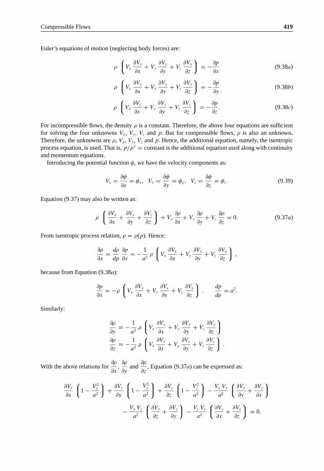
Compressible Flows 419
Euler’s equations of motion (neglecting body forces) are:
ρ
⎧⎪⎩Vx
∂Vx
∂x+ Vy
∂Vx
∂y+ Vz
∂Vx
∂z
⎫⎪⎭ = −∂p
∂x(9.38a)
ρ
⎧⎪⎩Vx
∂Vy
∂x+ Vy
∂Vy
∂y+ Vz
∂Vy
∂z
⎫⎪⎭ = −∂p
∂y(9.38b)
ρ
⎧⎪⎩Vx
∂Vz
∂x+ Vy
∂Vz
∂y+ Vz
∂Vz
∂z
⎫⎪⎭ = −∂p
∂z. (9.38c)
For incompressible flows, the density ρ is a constant. Therefore, the above four equations are sufficientfor solving the four unknowns Vx, Vy, Vz and p. But for compressible flows, ρ is also an unknown.Therefore, the unknowns are ρ, Vx, Vy, Vz and p. Hence, the additional equation, namely, the isentropicprocess equation, is used. That is, p/ργ = constant is the additional equation used along with continuityand momentum equations.
Introducing the potential function φ, we have the velocity components as:
Vx = ∂φ
∂x= φx, Vy = ∂φ
∂y= φy, Vz = ∂φ
∂z= φz. (9.39)
Equation (9.37) may also be written as:
ρ
⎧⎪⎩∂Vx
∂x+ ∂Vy
∂y+ ∂Vz
∂z
⎫⎪⎭ + Vx
∂ρ
∂x+ Vy
∂ρ
∂y+ Vz
∂ρ
∂z= 0. (9.37a)
From isentropic process relation, ρ = ρ(p). Hence:
∂ρ
∂x= dρ
dp
∂p
∂x= − 1
a2ρ
⎧⎪⎩Vx
∂Vx
∂x+ Vy
∂Vx
∂y+ Vz
∂Vx
∂z
⎫⎪⎭ ,
because from Equation (9.38a):
∂p
∂x= −ρ
⎧⎪⎩Vx
∂Vx
∂x+ Vy
∂Vx
∂y+ Vz
∂Vx
∂z
⎫⎪⎭ ,dp
dρ= a2.
Similarly:
∂ρ
∂y= − 1
a2ρ
⎧⎪⎩Vx
∂Vy
∂x+ Vy
∂Vy
∂y+ Vz
∂Vy
∂z
⎫⎪⎭∂ρ
∂z= − 1
a2ρ
⎧⎪⎩Vx
∂Vz
∂x+ Vy
∂Vz
∂y+ Vz
∂Vz
∂z
⎫⎪⎭ .
With the above relations for∂ρ
∂x,∂ρ
∂yand
∂ρ
∂z, Equation (9.37a) can be expressed as:
∂Vx
∂x
⎧⎪⎩1 − V 2x
a2
⎫⎪⎭ + ∂Vy
∂y
⎧⎪⎪⎩1 − V 2y
a2
⎫⎪⎪⎭ + ∂Vz
∂z
⎧⎪⎩1 − V 2z
a2
⎫⎪⎭ − Vx Vy
a2
⎧⎪⎩∂Vx
∂y+ ∂Vy
∂x
⎫⎪⎭
− Vy Vz
a2
⎧⎪⎩ ∂Vy
∂z+ ∂Vz
∂y
⎫⎪⎭ − Vz Vx
a2
⎧⎪⎩ ∂Vz
∂x+ ∂Vx
∂z
⎫⎪⎭ = 0.

420 Theoretical Aerodynamics
But the velocity components and their derivatives in terms of potential function can be expressed as:
Vx = ∂φ
∂x= φx, Vy = ∂φ
∂y= φy, Vz = ∂φ
∂z= φz
∂Vx
∂x= φxx,
∂Vy
∂y= φyy,
∂Vz
∂z= φzz
∂Vx
∂y= φxy,
∂Vy
∂z= φyz,
∂Vz
∂x= φzx.
Therefore, in terms of potential function φ, the above equation can be expressed as:
⎧⎪⎩1 − φ2x
a2
⎫⎪⎭φxx +⎧⎪⎪⎩1 − φ2
y
a2
⎫⎪⎪⎭φyy +⎧⎪⎩1 − φ2
z
a2
⎫⎪⎭φzz
− 2
⎧⎪⎩φx φy
a2φxy + φy φz
a2φyz + φz φx
a2φzx
⎫⎪⎭ = 0. (9.40)
This is the basic potential equation for compressible flow and it is nonlinear.The difficulties associated with compressible flow stem from the fact that the basic equation is nonlinear.
Hence the superposition of solutions is not valid. Further, in Equation (9.40) the local speed of sound ‘a’is also a variable. By Equation (2.9e) of Reference 1, we have:
⎧⎩ a
a∞
⎫⎭2
= 1 − γ − 1
2M2
∞
⎧⎪⎪⎩V 2x + V 2
y + V 2z
V 2∞− 1
⎫⎪⎪⎭ . (9.41)
To solve a compressible flow problem, we have to solve Equation (9.40) using Equation (9.41), but thisis not possible analytically. However, numerical solution is possible for given boundary conditions.
9.8 Linearization of the Potential Equation
The general equation for compressible flows, namely Equation (9.40), can be simplified for flow pastslender or planar bodies. Aerofoil, slender bodies of revolution and so on are typical examples for slenderbodies. Bodies like wing, where one dimension is smaller than others, are called planar bodies. Thesebodies introduce small disturbances. The aerofoil contour becomes the stagnation streamline.
For the aerofoil shown in Figure 9.4, with the exception of nose region, the perturbation velocity w issmall everywhere.
9.8.1 Small Perturbation Theory
Assume that the velocity at any point in the flow field is given by the vector sum of the freestream velocityV∞ along the x-axis, and the perturbation velocity components u, v and w along x, y and z-directions,respectively. Consider the flow around an aerofoil shown in Figure 9.4. The velocity components aroundthe aerofoil are:
Vx = V∞ + u, Vy = v, Vz = w, (9.42)
where Vx, Vy, Vz are the main flow velocity components and u, v, w are the perturbation (disturbance)velocity components along x, y and z directions, respectively.

Compressible Flows 421
xw
Vx
z
Vz w
V1
V
Figure 9.4 Aerofoil in an uniform flow.
The small perturbation theory postulates that the perturbation velocities are small compared to themain velocity components, that is:
u � V∞, v � V∞, w � V∞. (9.43a)
Therefore:
Vx ≈ V∞, Vy � V∞, Vz � V∞. (9.43b)
Now, consider a flow at small angle of attack or yaw as shown in Figure 9.5. Here:
Vx = V∞ cos α + u, Vy = V∞ sin α + v.
Since the angle of attack α is small, the above equations reduce to:
Vx = V∞ + u, Vy = v.
Thus, Equation (9.42) can be used for this case also.With Equation (9.42), linearization of Equation (9.40) gives:
(1 − M2)φxx + φyy + φzz = 0, (9.44)
neglecting all higher order terms, where M is the local Mach number. Therefore, Equation (9.41) shouldbe used in solving Equation (9.44).
α
V1
Figure 9.5 Aerofoil at an angle of attack in an uniform flow.
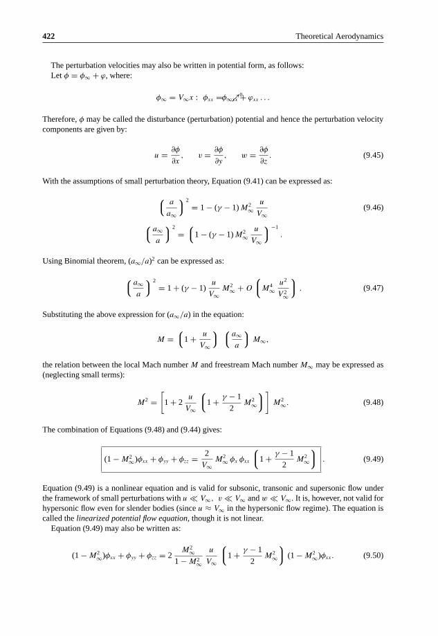
422 Theoretical Aerodynamics
The perturbation velocities may also be written in potential form, as follows:Let φ = φ∞ + ϕ, where:
φ∞ = V∞x : φxx = ↗0φ∞xx + ϕxx . . .
Therefore, φ may be called the disturbance (perturbation) potential and hence the perturbation velocitycomponents are given by:
u = ∂φ
∂x, v = ∂φ
∂y, w = ∂φ
∂z. (9.45)
With the assumptions of small perturbation theory, Equation (9.41) can be expressed as:
⎧⎩ a
a∞
⎫⎭2
= 1 − (γ − 1) M2∞
u
V∞(9.46)
⎧⎩a∞a
⎫⎭2
=⎧⎩1 − (γ − 1) M2
∞u
V∞
⎫⎭−1
.
Using Binomial theorem, (a∞/a)2 can be expressed as:
⎧⎩a∞a
⎫⎭2
= 1 + (γ − 1)u
V∞M2
∞ + O
⎧⎪⎩M4∞
u2
V 2∞
⎫⎪⎭ . (9.47)
Substituting the above expression for (a∞/a) in the equation:
M =⎧⎩1 + u
V∞
⎫⎭ ⎧⎩a∞a
⎫⎭M∞,
the relation between the local Mach number M and freestream Mach number M∞ may be expressed as(neglecting small terms):
M2 =[
1 + 2u
V∞
⎧⎪⎩1 + γ − 1
2M2
∞
⎫⎪⎭]
M2∞. (9.48)
The combination of Equations (9.48) and (9.44) gives:
(1 − M2∞)φxx + φyy + φzz = 2
V∞M2
∞ φx φxx
⎧⎪⎩1 + γ − 1
2M2
∞
⎫⎪⎭ . (9.49)
Equation (9.49) is a nonlinear equation and is valid for subsonic, transonic and supersonic flow underthe framework of small perturbations with u � V∞, v � V∞ and w � V∞. It is, however, not valid forhypersonic flow even for slender bodies (since u ≈ V∞ in the hypersonic flow regime). The equation iscalled the linearized potential flow equation, though it is not linear.
Equation (9.49) may also be written as:
(1 − M2∞)φxx + φyy + φzz = 2
M2∞
1 − M2∞
u
V∞
⎧⎪⎩1 + γ − 1
2M2
∞
⎫⎪⎭ (1 − M2∞)φxx. (9.50)

Compressible Flows 423
Further linearization is possible if:
M2∞
1 − M2∞
u
V∞� 1. (9.51)
With this condition Equation (9.50) results in:
(1 − M2∞)φxx + φyy + φzz = 0 . (9.52)
This is the fundamental equation governing most of the compressible flow regime. Equation (9.52) isvalid only when Equation (9.51) is valid and Equation (9.51) is valid only when the freestream Machnumber M∞ is sufficiently different from 1. Hence, Equation (9.51) is valid for subsonic and supersonicflows only. For transonic flows, Equation (9.49) can be used. For M∞ ≈ 1, Equation (9.49) reduces to:
− (γ + 1)
V∞φx φxx + φyy + φzz = 0 . (9.53)
The nonlinearity of Equation (9.53) makes transonic flow problems much more difficult than subsonicor supersonic flow problems.
Equation (9.52) is elliptic (that is, all terms are positive) for M∞ < 1 and hyperbolic (that is, not allterms are positive) for M∞ > 1. But in both the cases, the governing differential equation is linear. Thisis the advantage of Equation (9.52).
9.9 Potential Equation for Bodies of Revolution
Fuselage of airplane, rocket shells, missile bodies and circular ducts are the few bodies of revolutionswhich are commonly used in practice. The general three-dimensional Cartesian equations can be usedfor these problems. But it is much simpler to use cylindrical polar coordinates than Cartesian coordi-nates. Cartesian coordinates are x, y, z and the corresponding velocity components are Vx, Vy, Vz. Thecylindrical polar coordinates are x, r, θ and the corresponding velocity components are Vx, Vr , Vθ. Foraxisymmetric flows with cylindrical coordinates, the equations will be independent of θ. Thus, mathe-matically, cylindrical coordinates reduce the problem to become two-dimensional. However, for flowswhich are not axially symmetric (e.g., missile at an angle of attack), θ will be involved. The continuityequation in cylindrical coordinates is:
∂(ρ Vx)
∂x+ 1
r
∂(ρ r Vr)
∂r+ 1
r
∂(ρ Vθ)
∂θ= 0. (9.54)
Expressing the velocity components in terms of the potential function φ as:
Vx = ∂φ
∂x, Vr = ∂φ
∂r, Vθ = 1
r
∂φ
∂θ. (9.55)
The potential Equation (9.50) can be written, in cylindrical polar coordinates, as:
⎧⎪⎩1 − φ2x
a2
⎫⎪⎭ φxx +⎧⎪⎩1 − φ2
r
a2
⎫⎪⎭ φrr +⎧⎪⎩1 − 1
r2
φ2θ
a2
⎫⎪⎭ 1
r2φθθ
− 2
⎧⎪⎩φx φr
a2φxr + φx φθ
a2
1
r2φxθ + φr φθ
a2
1
r2φrθ
⎫⎪⎭ +⎧⎪⎩1 + 1
r2
φ2θ
a2
⎫⎪⎭ 1
rφr = 0. (9.56)

424 Theoretical Aerodynamics
Also,
⎧⎩ a
a∞
⎫⎭2
= 1 − γ − 1
2M2
∞
⎧⎪⎩V 2x + V 2
r + V 2θ
V 2∞− 1
⎫⎪⎭ . (9.57)
The small perturbation assumptions are:
Vx = V∞ + u, Vr = vr, Vθ = vθ
u � V∞, vr � V∞, vθ � V∞,
where Vx, Vr , Vθ are the mean velocity components and u, vr , vθ are the perturbation velocity componentsalong the x-, r- and θ-direction, respectively. Introduction of these relations in Equation (9.56) results in:
(1 − M2)φxx + φrr + 1
rφr + 1
r2φθθ = 0, (9.58)
where M is the local Mach number after Equation (9.48). The relations for u, vr , vθ in polar coordinates,under small perturbation assumption are:
u = ∂φ
∂x= φx, vr = ∂φ
∂r= φr, vθ = 1
r
∂φ
∂θ= 1
rφθ.
With these expressions for u, vr and vθ, Equation (9.49) can be written as:
(1 − M2∞)φxx + φrr + 1
rφr + 1
r2φθθ = 2
V∞M2
∞ φx φxx
⎧⎪⎩1 + γ − 1
2M2
∞
⎫⎪⎭ . (9.59)
This equation corresponds to Equation (9.49) with the same term on the right hand side. Therefore, with:
M2∞
1 − M2∞
u
V∞� 1.
Equation (9.59) simplifies to:
(1 − M2∞)φxx + φrr + 1
rφr + 1
r2φθθ = 0. (9.60)
This is the governing equation for subsonic and supersonic flows in cylindrical coordinates. For transonicflow, Equation (9.59) becomes:
−γ + 1
V∞φx φxx + φrr + 1
rφr + 1
r2φθθ = 0. (9.61)
For axially symmetric, subsonic and supersonic flows, φθθ = 0. Therefore, Equation (9.60) reduces to:
(1 − M2∞)φxx + φrr + 1
rφr = 0. (9.62)
Similarly, Equation (9.61) reduces to:
−γ + 1
V∞φx φxx + φrr + 1
rφr = 0. (9.63)

Compressible Flows 425
Equation (9.63) is the equation for axially symmetric transonic flows. All these equations are valid onlyfor small perturbations, that is, for small values of angle of attack and angle of yaw (< 15◦).
Conclusions
From the above discussions on potential flow theory for compressible flows, we can draw the followingconclusions:
1. The small perturbation equations for subsonic and supersonic flows are linear, but for transonic flowsthe equation is nonlinear.
2. Subsonic and supersonic flow equations do not contain the specific heats ratio γ , but transonic flowequation contains γ . This shows that the results obtained for subsonic and supersonic flows, withsmall perturbation equations, can be applied to any gas, but this cannot be done for transonic flows.
3. All these equations are valid for slender bodies. This is true of rockets, missiles, etc.4. These equations can also be applied to aerofoils, but not to bluff shapes like circular cylinder, etc.5. For nonslender bodies, the flow can be calculated by using the original nonlinear equation.
9.9.1 Solution of Nonlinear Potential Equation
(i) Numerical methods:The nonlinearity of Equation (9.49) makes it tedious to solve the equation analytically. However,solution for the equation can be obtained by numerical methods. But a numerical solution is nota general solution, and is valid only for a specific configuration of flow field with a fixed Machnumber and specified geometry.
(ii) Transformation (Hodograph) methods:When one velocity component is plotted against another velocity component, the resulting curvemay be linear, whereas in the physical plane, the relation may be nonlinear. This method is used forsolving certain transonic flow problems.
(iii) Similarity methods:In these methods, the boundary conditions need to be specified for solving the equation. Detaileddiscussion of this method can be found in Chapter 6 on Similarity Methods.
9.10 Boundary Conditions
Examine the streamlines around an aerofoil kept in a flow field as shown in Figure 9.6.In inviscid flow, the streamline near the boundary is similar to the body contour. The flow must satisfy
the following boundary conditions (BCs):
x
V 1
f(x, y, z)
z
Figure 9.6 Cambered aerofoil at an angle of attack.

426 Theoretical Aerodynamics
Boundary condition 1 – Kinetic flow condition
The flow velocity at all surface points are tangential on the body contour. The component of velocitynormal to the body contour is zero.
Boundary condition 2
At z → ±∞, perturbation velocities are zero or finite. The kinematic flow condition for the aerofoilshown in Figure 9.6, with small perturbation assumptions, may be written as follows.
Body contour: f = f (x, y, z)
The velocity vector V at any point on the body is tangential to the surface. Therefore, on the surface ofthe aerofoil, (V · �f ) = 0, that is:
(V∞ + u)∂f
∂x+ v
∂f
∂y+ w
∂f
∂z= 0. (9.64)
But u/V∞ � 1, therefore, Equation (9.64) simplifies to:
V∞∂f
∂x+ v
∂f
∂y+ w
∂f
∂z= 0. (9.65)
For two-dimensional flows, v = 0; ∂f/∂y = 0. Therefore, Equation (9.64) reduces to:
w
V∞ + u= −∂f/∂x
∂f/∂z=
⎧⎪⎩ ∂z
∂x
⎫⎪⎭c
, (9.66)
where the subscript “c” refers to the body contour and (∂z/∂x) is the slope of the body, and u and v arethe tangential and normal components of velocity, respectively. Expressing u and w as power series of z,we get:
u(x, z) = u(x, 0) + a1z + a2z2 + . . .
w(x, z) = w(x, 0) + b1z + b2z2 + . . .
The coefficients a′s and b′s in these series are functions of x. If the body is sufficiently slender:
w(x, 0)
V∞ + u(x, 0)=
⎧⎪⎩ dz
dx
⎫⎪⎭c
,
that is, for sufficiently slender bodies, it is not necessary to fulfill the boundary condition on the contourof the aerofoil. It is sufficient if the boundary condition on the x−axis of the body is satisfied, that is,on the axis of a body of revolution or the chord of an aerofoil. With u/V∞ � 1, the above conditionbecomes:
w(x, 0)
V∞=
⎧⎪⎩ dz
dx
⎫⎪⎭c
. (9.67)
For planar bodies: ∂f/∂y = 0 and therefore:
w(x, y, 0)
V∞=
⎧⎪⎩ dz
dx
⎫⎪⎭c
, (9.68)

Compressible Flows 427
that is, the condition is satisfied in the plane of the body. In Equations (9.67) and (9.68), the elevation ofthe body above the x−axis is neglected.
9.10.1 Bodies of Revolution
For bodies of revolution, the term 1r
∂
∂r(rvr) present in the continuity equation (9.54) becomes finite.
Because of this term, the perturbations near the body become significant. Therefore, a power series forvelocity components is not possible. However, we can apply the following approximation to express theperturbation velocity as a power series. For axisymmetric bodies:
1
r
∂
∂r(rvr) ∼ ∂u
∂x,
∂
∂r(rvr) ∼ r
∂u
∂x,
when r → 0; ∂
∂r(rvr) ≈ 0 or rvr = a0(x). Thus, even though the radial component of velocity vr on the
axis of a body of revolution is of the order of 1/r, it can be estimated near the axis similar to a potentialvortex. For a potential vortex, the radial velocity is:
vr ∝ 1
r.
Now, vr can be expressed in terms of a power series as:
rvr = a0 + a1r + a2r2 + . . .
For the axisymmetric body with its surface profile contour given by the function R(x), we have:
vr
V∞ + u=
⎧⎪⎩dR(x)
dx
⎫⎪⎭c
.
The simplified kinematic flow condition for the body in Figure 9.7 is:
(rvr)0
V∞= R(x)
dR(x)
dx, (9.69)
where subscript “0” refers to the axis of the body.Equation (9.69) is called the simplified kinematic flow condition in the sense that the kinematic flowcondition is fulfilled on the axis, rather than on the surface of the body contour.
On the axis of the body, Equation (9.69) gives:
limr→0
(rvr) = V∞ R(x)dR(x)
dx. (9.70)
x
r
V1
R(x)
Figure 9.7 An axisymmetric body in a flow.

428 Theoretical Aerodynamics
From the above discussions, it may be summarized that the boundary conditions for this kind of problemare the following.
For two-dimensional (planar) bodies:
⎧⎩ w
V∞ + u
⎫⎭c
≈ (w)0
V∞=
⎧⎪⎩ ∂z
∂x
⎫⎪⎭c
. (9.71)
For bodies of revolution (elongated bodies):
R(x)⎧⎩ vr
V∞ + u
⎫⎭c
≈ (rvr)0
V∞= R(x)
dR(x)
dx. (9.72)
9.11 Pressure Coefficient
Pressure coefficient is the nondimensional difference between a local pressure and the freestream pressure.The idea of finding the velocity distribution is to find the pressure distribution and then integrate it toget lift, moment, and pressure drag. For three-dimensional flows, the pressure coefficient Cp given by(Equation (2.54) of Reference 1) is:
Cp = 2
γ M2∞
{[γ − 1
2M2
∞
⎧⎪⎩1 − (V∞ + u)2 + v2 + w2
V 2∞
⎫⎪⎭ + 1
]γ/(γ−1)
− 1
}
or
Cp = 2
γ M2∞
{[1 − γ − 1
2M2
∞
⎧⎪⎩ 2u
V∞+ u2 + v2 + w2
V 2∞
⎫⎪⎭]γ/(γ−1)
− 1
},
where M∞ and V∞ are the freestream Mach number and velocity, respectively, u, v and w are the x, y andz-components of perturbation velocity and γ is the ratio of specific heats. Expanding the right-hand sideof this equation binomially and neglecting the third and higher-order terms of the perturbation velocitycomponents, we get:
Cp = −⎧⎪⎩2
u
V∞+ (1 − M2
∞)u2
V 2∞+ v2 + w2
V 2∞
⎫⎪⎭. (9.73)
For two-dimensional or planar bodies, the Cp simplifies further, resulting in:
Cp = −2u
V∞. (9.73a)
This is a fundamental equation applicable to three-dimensional compressible (subsonic and supersonic)flows, as well as for low speed two-dimensional flows.

Compressible Flows 429
9.11.1 Bodies of Revolution
For bodies of revolution, by small perturbation assumption, we have u � V∞, but v and w are notnegligible. Therefore, Equation (9.73) simplifies to:
Cp = −2u
V∞− v2 + w2
V 2∞. (9.74)
The above equation, which is in Cartesian coordinates, may also be expressed as:
Cp = −2u
V∞−
⎧⎩ vr
V∞
⎫⎭2
. (9.75)
Combining Equations (9.72) and (9.75), we get:
Cp = −2u
V∞−
⎧⎪⎩dR(x)
dx
⎫⎪⎭2
, (9.76)
where R is the expression for the body contour.
9.12 Similarity Rule
From Section 9.8, it is seen that the governing equation for compressible flow is elliptic for subsonicflows (that is, for M∞ < 1) and becomes hyperbolic for supersonic flows (that is, for M∞ > 1). Thischange in the nature of the partial differential equation, upon going from subsonic to supersonic flow,indicates the possibility of deriving similarity relationships between subsonic compressible flow andthe corresponding incompressible flow, and the importance of Mach wave in a supersonic solution. Inthis chapter we shall derive an expression which relates the subsonic compressible flow past a certainprofile to the incompressible flow past a second profile derived from the first principles through an affinetransformation. Such an expression is called a similarity law.
If the governing equations of motion could be solved easily, the solution themselves would indicatequite clearly the nature of any similarities which might exist among members of a family of flow patterns.Then there is no need for a separate derivation of similarity laws.
But in the majority of situations, we are unable to solve the equations of motion. However, even thoughsolutions are lacking, we may use our knowledge of the forms of the differential equations and the relatedboundary conditions to derive the similarity laws.
9.13 Two-Dimensional Flow: Prandtl-Glauert Rule for Subsonic Flow
9.13.1 The Prandtl-Glauert Transformations
Prandtl and Glauert have shown that it is possible to relate the solution of compressible flow about a bodyto incompressible flow solution.
The transformation from one to another is achieved in the following manner: Laplace equation fortwo-dimensional compressible and incompressible flows, respectively, are:
(1 − M2∞) φxx + φzz = 0 (9.77)
(φxx)inc + (φzz)inc = 0, (9.78)
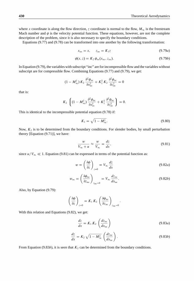
430 Theoretical Aerodynamics
where x coordinate is along the flow direction, z coordinate is normal to the flow, M∞ is the freestreamMach number and φ is the velocity potential function. These equations, however, are not the completedescription of the problem, since it is also necessary to specify the boundary conditions.
Equations (9.77) and (9.78) can be transformed into one another by the following transformation:
xinc = x, zinc = K1z (9.79a)
φ(x, z) = K2 φinc(xinc, zinc). (9.79b)
In Equation (9.79), the variables with subscript “inc” are for incompressible flow and the variables withoutsubscript are for compressible flow. Combining Equations (9.77) and (9.79), we get:
(1 − M2∞) K2
∂2φinc
∂x2inc
+ K21 K2
∂2φinc
∂z2inc
= 0
that is:
K2
⎧⎪⎩(1 − M2∞)
∂2φinc
∂x2inc
+ K21
∂2φinc
∂z2inc
⎫⎪⎭ = 0.
This is identical to the incompressible potential equation (9.78) if:
K1 =√
1 − M2∞. (9.80)
Now, K2 is to be determined from the boundary conditions. For slender bodies, by small perturbationtheory [Equation (9.71)], we have:
w
V∞ + u≈ w
V∞= dz
dx, (9.81)
since u/V∞ � 1. Equation (9.81) can be expressed in terms of the potential function as:
w =(
∂φ
∂z
)z=0
= V∞dz
dx(9.82a)
winc =(
∂φinc
∂zinc
)zinc=0
= V∞dzinc
dxinc
. (9.82b)
Also, by Equation (9.79):
(∂φ
∂z
)z=0
= K1 K2
(∂φinc
∂zinc
)zinc=0
.
With this relation and Equations (9.82), we get:
dz
dx= K1 K2
(dzinc
dxinc
)(9.83a)
dz
dx= K2
√1 − M2∞
(dzinc
dxinc
). (9.83b)
From Equation (9.83b), it is seen that K2 can be determined from the boundary conditions.

Compressible Flows 431
Equation (9.83b) simply means that the slope of the profile in the compressible flow pattern is(K2
√1 − M2∞) times the slope of the corresponding profile in the related incompressible flow pattern.
For further treatment of similarity law, let us consider the three specific versions of the problems,namely, the direct problem (Version I), in which the body profile is treated as invariant, the indirectproblem (Version II), which is the case of equal potentials (the pressure distribution around the body inincompressible flow and compressible flow are taken as the same), and the streamline analogy (VersionIII), which is also called Gothert’s rule.
9.13.2 The Direct Problem-Version I
Consider an invariant profile. In this case, there is no transformation of geometry at all. For the profile tobe invariant, from Equation (9.83b), we have the condition:
K2 = 1√1 − M2∞
. (9.84)
Therefore, Equation (9.83b) reduces to:
dz
dx= dzinc
dxinc
. (9.85)
Equation (9.85) contradicts the original transformation equations (9.79). However, the error involved inthis contradiction is not large since the Prandtl-Glauert transformation is valid only for small perturbations.
By Equation (9.79), we have:
z = zinc√1 − M2∞
. (9.86)
Equation (9.79) is valid only for streamlines away from the body. Since the Prandtl-Glauert transformationis based on small perturbation theory, the error increases with increasing thickness of the body. In additionto this, some error is introduced by the above contradiction [see Equation (9.85)].
Equation (9.86) shows that the streamlines around a body in a compressible flow are more separatedthan those around a body in incompressible flow by an amount given by 1/
√1 − M2∞. In other words,
by the existence of body in the flow field, the streamlines are more displaced in a compressible flow thanin an incompressible flow, as shown in Figure 9.8, that is the disturbances introduced by an object arelarger in compressible flow than in incompressible flow and they increase with the rise in Mach number.This is so because in compressible flow there is density decrease as the flow passes over the body due toacceleration, whereas in incompressible flow there is no change in density at all. That is to say, across thebody there is a drop in density, and hence by streamtube area-velocity relation (Section 2.4, Reference 1),the streamtube area increases as the density decreases. At M∞ = 1, this disturbance becomes infinitelylarge and this treatment is no longer valid.
(a) Incompressible flow (b) Compressible flow
Figure 9.8 Aerofoil in an uniform flow.

432 Theoretical Aerodynamics
The potential function for compressible flow given by Equation (9.79) is:
φ = φinc√1 − M2∞
. (9.87a)
By Equations (9.45) and (9.73), we have the velocity u and the pressure coefficient Cp as:
u = ∂φ
∂x, Cp = −2
u
V∞.
Using Equation (9.87a), the perturbation velocity and the pressure coefficient may be expressed asfollows:
∂φ
∂x= 1√
1 − M2∞
∂φinc
∂xinc
.
Therefore:
u = uinc√1 − M2∞
Cp = CPinc√1 − M2∞
. (9.87b)
Since the lift coefficient CL and pitching moment coefficient CM are integrals of CP , they can beexpressed following Equation (9.87b) as:
CL = CLinc√1 − M2∞
(9.87c)
dCL
dα= (dCL/dα)inc√
1 − M2∞. (9.87d)
For a flat plate in compressible flow:
dCL
dα= 2π√
1 − M2∞(9.87e)
CM = CMinc√1 − M2∞
. (9.87f )
Similarly, we can express the circulation in compressible flow in terms of circulation in incompressibleflow as:
� = �inc√1 − M2∞
. (9.87g)
From the discussion on version I of the Prandtl-Glauert transformation, the following two statementscan be made:
1. Streamlines for compressible flow are farther apart from each other by 1/√
1 − M2∞ than inincompressible flow.
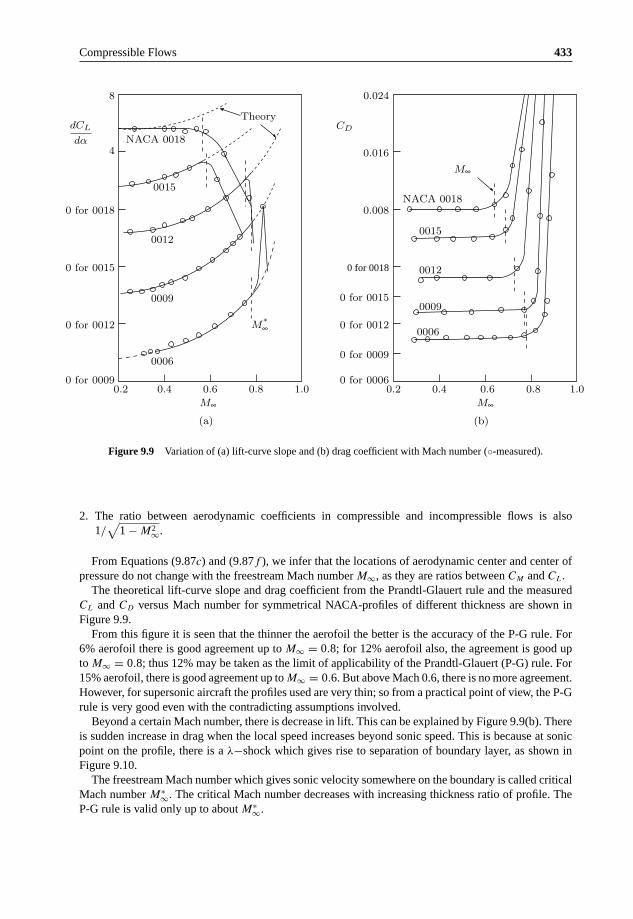
Compressible Flows 433
0 for 0018
NACA 0018
0 for 00060.2 0.4 0.6 0.8 1.0 0.80.60.40.2
Theory
M∞ M∞
M∞
1.0
0 for 0009
0 for 0012
0 for 0015
0.008
0.016
0.024
0 for 0012
0 for 0015
0 for 0018
8
4
0006
0009
0012
0015
NACA 0018
0 for 0009
0012
0009
0006
0015
dCL
dα
(b)
CD
(a)
M*∞
Figure 9.9 Variation of (a) lift-curve slope and (b) drag coefficient with Mach number (◦-measured).
2. The ratio between aerodynamic coefficients in compressible and incompressible flows is also1/
√1 − M2∞.
From Equations (9.87c) and (9.87f ), we infer that the locations of aerodynamic center and center ofpressure do not change with the freestream Mach number M∞, as they are ratios between CM and CL.
The theoretical lift-curve slope and drag coefficient from the Prandtl-Glauert rule and the measuredCL and CD versus Mach number for symmetrical NACA-profiles of different thickness are shown inFigure 9.9.
From this figure it is seen that the thinner the aerofoil the better is the accuracy of the P-G rule. For6% aerofoil there is good agreement up to M∞ = 0.8; for 12% aerofoil also, the agreement is good upto M∞ = 0.8; thus 12% may be taken as the limit of applicability of the Prandtl-Glauert (P-G) rule. For15% aerofoil, there is good agreement up to M∞ = 0.6. But above Mach 0.6, there is no more agreement.However, for supersonic aircraft the profiles used are very thin; so from a practical point of view, the P-Grule is very good even with the contradicting assumptions involved.
Beyond a certain Mach number, there is decrease in lift. This can be explained by Figure 9.9(b). Thereis sudden increase in drag when the local speed increases beyond sonic speed. This is because at sonicpoint on the profile, there is a λ−shock which gives rise to separation of boundary layer, as shown inFigure 9.10.
The freestream Mach number which gives sonic velocity somewhere on the boundary is called criticalMach number M∗
∞. The critical Mach number decreases with increasing thickness ratio of profile. TheP-G rule is valid only up to about M∗
∞.

434 Theoretical Aerodynamics
λ− shock
Separation ofboundary layer
M 1
Figure 9.10 Flow separation caused by λ-shock.
9.13.3 The Indirect Problem (Case of Equal Potentials):P-G Transformation – Version II
In the indirect problem, the requirement is to find a transformation, for the profile, by which we canobtain a body in incompressible flow with exactly the same pressure distribution, as in the compressibleflow.
For two-dimensional or planar bodies, the pressure coefficient Cp is given by Equation (9.73a) as:
Cp = −2u
V∞.
and the perturbation velocity component, u, is:
u = ∂φ
∂x.
But in this case, Cp = Cpinc ; therefore, from the above expressions for Cp and u, we have:
Cp = Cpinc , u = uinc, φ = φinc.
For this situation the transformation Equation (9.79) gives:
K2 = 1. (9.88)
From Equation (9.83b) with K2 = 1, we get:
dz
dx=
√1 − M2∞
dzinc
dxinc
. (9.89)
Equation (9.89) is the relation between the geometries of the actual profile in compressible flow and thetransformed profile in the incompressible flow, resulting in same pressure distribution around them.
From Equation (9.89), we see that in a compressible flow, the body must be thinner by the factor√1 − M2∞ than the body in incompressible flow as shown in Figure 9.11. Also, the angle of attack in
compressible flow must be smaller by the same factor than in incompressible flow.From the above relation for Cp, we have:
Cp
Cpinc
= CL
CLinc
= CM
CMinc
= 1. (9.90)

Compressible Flows 435
(a) (b)
α
V 1 V 1
α
Figure 9.11 Aerofoils in (a) incompressible and (b) compressible flows.
That is, the lift coefficient and pitching moment coefficient are also the same in both the incompressibleand compressible flows. But, because of decreased α in compressible flow:
dCL
dα= 1√
1 − M2∞
(dCL
dα
)inc
.
This is so because of the fact that the disturbances introduced in a compressible flow are larger thanthose in an incompressible flow and, therefore, we must reduce α and the geometry by that amount (thedifference in the magnitude of disturbance in a compressible and an incompressible flow). In other words,because of Equation (9.79) (z = K1zinc), every dimension in the z-direction must be reduced and so theangle of attack α should also be transformed.
9.13.4 The Streamline Analogy (Version III): Gothert’s Rule
Gothert’s rule states [3] that the slope of a profile in a compressible flow pattern is larger by the factor1/
√1 − M2∞ than the slope of the corresponding profile in the related incompressible flow pattern. But
if the slope of the profile at each point is greater by the factor 1/√
1 − M2∞, it is also true that the camber(f ) ratio, angle of attack (α) ratio, the thickness (t) ratio, must all be greater for the compressible aerofoilby the factor 1/
√1 − M2∞.
Thus, by Gothert’s rule we have:
αinc
α= finc
f= tinc
t=
√1 − M2∞.
Compute the aerodynamic coefficients for this transformed body for incompressible flow. The aerody-namic coefficients of the given body at the given compressible flow Mach number are given by:
Cp
Cpinc
= CL
CLinc
= CM
CMinc
= 1
1 − M2∞. (9.91)
The application of Gothert’s rule is much more complicated than the application of version I of theP-G rule. This is because, for finding the behavior of a body with respect to M∞, we have to calculatefor each M∞ at a time, whereas by the P-G rule (version I) the complete variation is obtained at a time.However, only the Gothert rule is exact with the framework of linearized theory and the P-G rule is onlyapproximate because of the contradicting assumptions involved.
Now, we can see some aspects about the practical significance of these results. A fairly good amountof theoretical and experimental information on the properties of classes of affinely related profiles inincompressible flow, with variations in camber, thickness ratio, and angle of attack is available. If it isnecessary to find the CL of one of these profiles at a finite Mach number M∞, either theoretically orexperimentally, we first find the lift coefficient in incompressible flow of an affinely related profile. Thecamber, thickness and angle of attack are smaller than the corresponding values for the original profile

436 Theoretical Aerodynamics
by the factor√
1 − M2∞. Then, by multiplying this CL for incompressible flow profile by 1/(1 − M2∞),
we find the desired lift coefficient for the compressible flow.This method of collecting data for incompressible flow is cumbersome, since the data is required for
a large number of thickness ratios. It would be more convenient in many respects to know how Machnumber affects the performance of a profile of fixed shape. The direct problem, discussed in Subsection9.13.2, yields information of this type.
9.14 Prandtl-Glauert Rule for Supersonic Flow: Versions I and II
In Section 9.13, we have seen the similarity rules for subsonic flows. Now let us examine the similarityrules for supersonic flows. We can visualize from our previous discussions on similarity rule for subsoniccompressible flows that the factor K1 in the transformation Equation (9.79) should have the followingrelations depending on the flow regime:
K1 =√
1 − M2∞ for subsonic flow
K1 =√
M2∞ − 1 for supersonic flow.
Therefore, in general, we can write:
K1 =√∣∣1 − M2∞
∣∣. (9.92)
However, there is one important difference between the treatment of supersonic flow and subsonic flow,that is, we cannot find any incompressible flow in the supersonic flow regime.
9.14.1 Subsonic Flow
We know that for subsonic flow the transformation relations are given by Equation (9.79) as:
xinc = x, zinc = K1z, φ = K2φinc.
The transformed equation is:
K2[(1 − M2∞) (φxx)inc + K2
1(φzz)inc] = 0.
and the condition to be satisfied by this equation in order to be identical to Equation (9.78) is:
K1 =√
1 − M2∞.
For this case the above transformed equation becomes Laplace equation.
9.14.2 Supersonic Flow
The transformation relations for supersonic flow are:
x′ = x, z′ = K1z, φ = K2φ′,

Compressible Flows 437
where the variables with “prime” are the transformed variables. The aim in writing these transformationsis to make the Mach number M∞ in the governing equation (9.77) to vanish.
With the above transformation relations, the governing equation becomes:
K2[(1 − M2∞)φ′
xx + K21φ
′zz] = 0.
For supersonic flow, M∞ > 1, therefore the above equation becomes:
K2[(M2∞ − 1)φ′
xx − K21φ
′zz] = 0.
By inspection of this equation, we can see that the Mach number M∞ can be eliminated from the aboveequation with:
K1 =√
M2∞ − 1.
The equation becomes:
φ′xx − φ′
zz = 0. (9.93a)
Now we must find out as to which supersonic Mach number this flow belongs.The original form of the governing differential equation for this kind of flow, given by Equation (9.77),
is:
(M2∞ − 1)φxx − φzz = 0. (9.93b)
For Equations (9.93a) and (9.93b) to be identical, it is necessary that:
M∞ =√
2.
By following the arguments of P-G rule for subsonic compressible flow, we can show the followingresults for versions I and II of the Prandtl-Glauert rule for supersonic flow.
9.14.2.1 Analogy Version I
For this case of invariant profile in supersonic flow:
K2 = 1√M2∞ − 1
.
Compute the flow around the given body at M∞ = √2. For any other supersonic Mach number, the
aerodynamics coefficients are given by:
Cp
C′p
= CL
C′L
= CM
C′M
= 1√M2∞ − 1
, (9.94a)
where Cp, CL and CM are at M∞ = √2 and C′
p, C′L and C′
M are at any other supersonic Mach number.

438 Theoretical Aerodynamics
9.14.2.2 Analogy Version II
Here the requirement is to find a transformation for the profile, by which we can obtain a body, for whichthe governing equation is Equation (9.93a) with exactly the same pressure distribution as the actual bodyfor which the governing equation is Equation (9.93b). For this:
K2 = 1.
The derivation of the above two results are left to the reader as an exercise. From the above results, wesee that in supersonic flow M∞ = √
2 plays the same role as M∞ = 0 in subsonic flow.For version II, we can write:
Cp
C′p
= CL
C′L
= CM
C′M
= 1. (9.94b)
9.14.2.3 Analogy Version III: Gothert Rule
For any given body, at given Mach number M∞, find the transformed shape by using the rule:
α′
α= f ′
f= t′
t=
√M2∞ − 1, (9.95)
where α is the angle of attack, f and t are the camber and thickness of the given body, respectively. Theprimed quantities are for the transformed body and unprimed ones are for the actual body.
Compute the aerodynamic coefficients of the transformed body for M∞ = √2. The aerodynamic
coefficients of the given body at the given Mach number M∞ follow from:
Cp
C′p
= CL
C′L
= CM
C′M
= 1
M2∞ − 1. (9.96)
We can state the Gothert rule for subsonic and supersonic flows by using a modulus:∣∣1 − M2
∞∣∣.
From the discussion on similarity rules for compressible subsonic and supersonic flows, it is clear that,in subsonic flow, there is a ready made linearized solution for M∞ = 0. Hence, for such cases we canuse the Prandtl-Glauert rule. But for supersonic flow the linear theory equations are very simple and,therefore, we can conveniently use the Gothert rule.
Example 9.1
A given profile has, at M∞ = 0.29, the following lift coefficients:
CL = 0.2 at α = 3◦
CL = − 0.1 at α = −2◦,
where α is the angle of attack. Plot the relation showing dCL/dα vs. M∞ for the profile for values of M∞up to 1.0.

Compressible Flows 439
Solution
At M∞ = 0.29:
dCL
dα= 0.2 + 0.1
3 + 2= 0.06/degree
= 3.438/rad
= 1.094π/rad.
By the Prandtl-Glauert rule:
⎧⎪⎩dCL
dα
⎫⎪⎭M=M∞
=
⎧⎪⎩dCL
dα
⎫⎪⎭inc√
1 − M2∞.
Therefore:
⎧⎪⎩dCL
dα
⎫⎪⎭inc
= 1.047π/radian.
For any other subsonic Mach number, by the Prandtl-Glauert rule:
dCL
dα=
⎧⎪⎩dCL
dα
⎫⎪⎭inc√
1 − M2∞= 1.047π√
1 − M2∞.
Therefore, we have the following variation:
M 0.1 0.2 0.3 0.4 0.5 0.6 0.7 0.8 0.9 1.0
dCL
dα1.05π 1.07π 1.10π 1.14π 1.21π 1.31π 1.46π 1.74π 2.40π ∞
9.15 The von Karman Rule for Transonic Flow
The potential Equation (9.49), for the present case of two-dimensional transonic flow, reduces to:
(1 − M2∞)φxx + φzz = 2
V∞
⎧⎪⎩1 + γ − 1
2M2
∞
⎫⎪⎭M2∞φxφxx. (9.97)
Equation (9.97) results in a form due to Sprieter (see also Liepmann and Roshko, 1963 [4]) for M∞ ≈ 1,as:
Cp =
⎧⎩ t
c
⎫⎭2/3
[(γ + 1)M2∞]1/3Cp(χ), (9.97a)

440 Theoretical Aerodynamics
V 1
t
c
α2θ0
Figure 9.12 Wedge at an angle of attack.
where
χ = 1 − M2∞[⎧⎩ t
c
⎫⎭ (γ + 1) M2∞
]2/3 (9.97b)
and Cp is the similarity pressure coefficient. It follows from Equation (9.97a) that the lift and dragcoefficients are given by:
CL =
⎧⎩ t
c
⎫⎭2/3
[(γ + 1) M2∞]1/3CL(χ) (9.97c)
CD =
⎧⎩ t
c
⎫⎭5/3
[(γ + 1) M2∞]1/3CD(χ). (9.97d)
Equations (9.97a), (9.97c) and (9.97d) are valid for local as well as for total values. Sometimes, insteadof thickness ratio t/c, ‘fineness ratio’ defined as in Figure 9.12 is used.
For the wedge shown in Figure 9.12:
1
2
t
c= tan θ0,
t
c= 2 tan θ0
The ratio t/c is called the fineness ratio (at angle of attack = 0).
tan (θ0 ± α) = tan
⎧⎪⎩1
2
t
c
⎧⎪⎩1 ± 2α
t/c
⎫⎪⎭⎫⎪⎭ . (9.98)
where the ‘plus’ sign is for the upper surface and the ‘minus’ sign is for the lower surface. For findingthe local values of Cp, CL and CD, we must use fineness ratio defined by these equations.
9.15.1 Use of Karman Rule
If we know the solution for one profile, we can find solutions for other affinely related profiles. Forexample, the NACA profiles designated by 8405, 8410, 8415 all have the same distribution, same noseradius etc.; only the absolute magnitude of t/c is different. This rule can be extended to transonic flowrange also. From Figure 9.13, it is seen that in the transonic range, the aerodynamic coefficients changevery quickly with Mach number, so that the proper values to be considered are not M∞, CL, CD and Cp;instead they are χ, CL, CD and Cp.

Compressible Flows 441
χ
0.08
1.00.50− 0.5− 1.0− 1.5− 2.0
1
2
3
4
5
1.0 1.1 1.2 1.3
0.08
0.10
0.06
0.04
0.02
0.06
0.10t/c = 0.12
0.7 0.8 0.9
0.08
0.06
t/c = 0.12
0.10
CD
∼CD
M1
Figure 9.13 The transonic similarity rule.
From the discussion made so far, we can make the following remarks:
1. For subsonic and supersonic flows, the governing equation(∣∣1 − M2
∞∣∣)φxx + φzz = 0 is independent
of γ , so that the results from similarity rules can be applied to any gas; but for transonic flow, thepotential equations are not independent of γ . Therefore, the results have to be properly applied todifferent gases, with suitable correction for γ , for example, a probe used for air in transonic range canbe calibrated for steam.
2. For transonic flow:
Cp ∼ CL ∼⎧⎩ t
c
⎫⎭2/3
For subsonic flow:
Cp ∼ CL ∼⎧⎩ t
c
⎫⎭
442 Theoretical Aerodynamics
For supersonic flow:
Cp ∼ CL ∼(
t
c
).
Transonic flow is characterized by the occurrence of shock and boundary layer separation. This explainsthe steep increase in CD at transonic range. We should also recall that the shock should be sufficientlyweak for small perturbation. For circular cylinder this theory cannot be applied, because the perturbationsare not small.
9.16 Hypersonic Similarity
The linear theory is not valid at high supersonic Mach numbers, since:
u
V∞� 1 is true only for supersonic flow, and
u
V∞≈ 1 for hypersonic flow.
Even slender bodies produce large disturbances in hypersonic flow. The original nonlinear equationshave to be used for such flows. So, mathematically hypersonic flow is similar to transonic flow. Insupersonic flow, slender bodies produce weak shocks and so these can be considered as Mach lines.2 Butin hypersonic flow, even slender bodies produce strong shocks and, therefore, in hypersonic flow we canno more deal with Mach lines and must deal with the actual shock waves. At high Mach numbers, theMach angle μ may be of the same order or less than the maximum deflection angle θ of the body.
From these considerations, the similarity rule can be obtained for hypersonic flow. The Mach angle μ
is given by the relation:
sin μ = 1
M∞.
For the present case of flow shown in Figure 9.14:
sin μ ≈ μ = 1
M∞≤ θ,
where θ is the half angle of the wedge in the figure, that is, for hypersonic flow:
M∞θ ≥ 1. (9.99)
But in hypersonic flows even for small disturbances, there are shock lines and the angle of shock is alwaysless than the angle of Mach line. Therefore, in reality the inequality in Equation (9.99), obtained withthe approximation that Mach angle μ is of the same order or less than the flow turning angle θ, has to bemodified since the shock angle is always less than μ. In other words, it can be stated that M∞θ is greaterthan some quantity K, whose numerical value can be less than unity also.
2It is essential to note that Mach lines are weak isentropic waves across which the changes in the flow properties are small but finite,thus, Mach lines are different from the weak isentropic waves termed Mach waves across which the changes in the flow properties arenegligible.

Compressible Flows 443
M 1 ! 1
Shock
t
c
2θ
Figure 9.14 Slender body in hypersonic flow.
It is a common practice to express:
K = M∞θ ≥ 0.5 (9.100)
K = Mθ , (9.101)
where K is called the Hypersonic similarity parameter.
Example 9.2
For θ = 10◦ (≈ 0.174 radian), M∞ = 4; the hypersonic similarity parameter K = M∞θ = 0.7. For θ =20◦ and M∞ = 2:
K = M∞θ ≈ 0.7.
That is, for a wedge with half-angle 20◦, M∞ = 2 should be considered as hypersonic. This implies thatM ≥ 5 for hypersonic flow is only a crude limit. For θ = 5◦ and M∞ = 8:
K = M∞θ ≈ 0.7.
Thus, a wedge with half-angle 5◦ in a flow with M∞ = 8 produces shocks as strong as a wedge withhalf-angle 20◦ in a flow with M∞ = 2.
Also, by Equation (9.98):
θ = θ0 ± α = 1
2
t
c
⎧⎪⎩1 ± 2α
t/c
⎫⎪⎭ . (9.102)
Whenever M∞θ is the same for a number of bodies, the flow about them will be dynamically similar,that is, to investigate the hypersonic flow about a wedge with half-angle 5◦ and M∞ = 8, we can use asupersonic tunnel with M∞ = 2 and θ = 20◦. This is of paramount importance in testing; of course thetwo bodies should be affinely related (geometrically similar). Consider two models, 1 and 2:
K1
K2=
M∞1
⎧⎩ t
c
⎫⎭1
⎧⎪⎩1 ± 2α
(t/c)1
⎫⎪⎭M∞2
⎧⎩ t
c
⎫⎭2
⎧⎪⎩1 ± 2α
(t/c)2
⎫⎪⎭K1
K2= 1 for dynamic similarity.
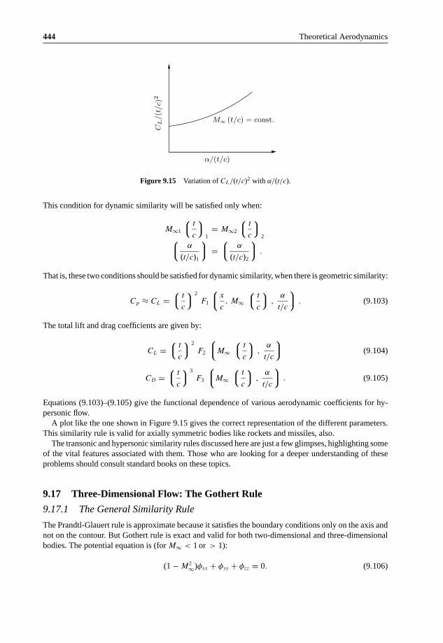
444 Theoretical Aerodynamics
CL/(t/c)
2α/(t/c)
M1 (t/c) = const.
Figure 9.15 Variation of CL/(t/c)2 with α/(t/c).
This condition for dynamic similarity will be satisfied only when:
M∞1
⎧⎩ t
c
⎫⎭1
= M∞2
⎧⎩ t
c
⎫⎭2⎧⎪⎩ α
(t/c)1
⎫⎪⎭ =⎧⎪⎩ α
(t/c)2
⎫⎪⎭ .
That is, these two conditions should be satisfied for dynamic similarity, when there is geometric similarity:
Cp ≈ CL =⎧⎩ t
c
⎫⎭2
F1
⎧⎪⎩x
c, M∞
⎧⎩ t
c
⎫⎭ ,α
t/c
⎫⎪⎭ . (9.103)
The total lift and drag coefficients are given by:
CL =⎧⎩ t
c
⎫⎭2
F2
⎧⎪⎩M∞⎧⎩ t
c
⎫⎭ ,α
t/c
⎫⎪⎭ (9.104)
CD =⎧⎩ t
c
⎫⎭3
F3
⎧⎪⎩M∞⎧⎩ t
c
⎫⎭ ,α
t/c
⎫⎪⎭ . (9.105)
Equations (9.103)–(9.105) give the functional dependence of various aerodynamic coefficients for hy-personic flow.
A plot like the one shown in Figure 9.15 gives the correct representation of the different parameters.This similarity rule is valid for axially symmetric bodies like rockets and missiles, also.
The transonic and hypersonic similarity rules discussed here are just a few glimpses, highlighting someof the vital features associated with them. Those who are looking for a deeper understanding of theseproblems should consult standard books on these topics.
9.17 Three-Dimensional Flow: The Gothert Rule
9.17.1 The General Similarity Rule
The Prandtl-Glauert rule is approximate because it satisfies the boundary conditions only on the axis andnot on the contour. But Gothert rule is exact and valid for both two-dimensional and three-dimensionalbodies. The potential equation is (for M∞ < 1 or > 1):
(1 − M2∞)φxx + φyy + φzz = 0. (9.106)

Compressible Flows 445
For M∞ < 1, the equation is elliptic in nature and for M∞ > 1, it is hyperbolic. Here also, we maketransformation by which the transformed equation does not contain M∞ explicitly any more. Let:
x′ = x, y′ = K1y, z′ = K1z, φ′ = K2φ.
With the above new variables, Equation (9.106) transforms into:
(1 − M2∞)φ′
x′x′ + K21(φ′
y′y′ + φ′z′z′ ) = 0.
M∞ vanishes from the above equation for:
K1 =√∣∣1 − M2∞
∣∣. (9.107)
With Equation (9.107), the resulting potential flow equation for subsonic flow is:
φ′x′x′ + φ′
y′y′ + φ′z′z′ = 0
and for supersonic flow:
φ′x′x′ − φ′
y′y′ − φ′z′z′ = 0.
Again, for subsonic flow, the equation is exactly the same as the Laplace equation. For supersonic flow,the equation is identical with the compressible flow equation [Equation (9.106)] with M∞ = √
2.Now:
u′ = ∂φ′
∂x′ = K2∂φ
∂x= K2 u (9.108a)
v′ = ∂φ′
∂y′ = K2
K1
∂φ
∂y= K2
K1v (9.108b)
w′ = ∂φ′
∂z′ = K2
K1
∂φ
∂z= K2
K1w (9.108c)
Cp = p − p∞12 ρV 2∞
= −2u
V∞= − 2
V∞
∂φ
∂x(9.109)
and
C′p = −2
u′
V∞. (9.110)
with the assumption that V∞ = V ′∞. This assumption really does not impose any restriction on the rule,
because in supersonic flow, the velocity itself is not important (that is, V/a is more relevant than V ).Introduction of Equation (9.108a) into Equation (9.110) results in:
C′p = −2K2
u
V∞
that is:
C′p = K2Cp. (9.111)

446 Theoretical Aerodynamics
The kinematic flow condition [Equation (9.82a)] states that:
w
V∞= ∂z
∂x
w = V∞∂z
∂x(9.112a)
w′ = V∞∂z′
∂x′ . (9.112b)
Combining Equations (9.112a) and (9.112b), we get:
w′ = ∂x
∂z
∂z′
∂x′ w = K1w,
since x′ = x and z′/z = K1. But w′ = (K2/K1)w by Equation (9.108c); therefore:
K1 = K2
K1,
that is:
K2 = K21
K2 =∣∣1 − M2
∞∣∣ . (9.113)
Therefore:
Cp = C′p∣∣1 − M2∞
∣∣ . (9.114)
Equation (9.114) is valid (exactly) at any point on the boundary of the body, as well as in the flow field.Therefore:
Cp
C′p
= CL
C′L
= CM
C′M
= 1∣∣1 − M2∞∣∣ . (9.115)
Equation (9.115) is an important equation, relating the aerodynamic coefficients for the actual and trans-formed bodies.
9.17.2 Gothert Rule
The aerodynamic coefficients of a body in three-dimensional compressible flow are obtained as follows.The geometry of the given body is transformed in such a way that its lateral and normal dimensions (both
in y and z directions) are multiplied by√∣∣1 − M2∞
∣∣. If the flow is subsonic, compute the incompressible
flow about the transformed body; if the flow is supersonic, compute the field with M∞ = √2 about the
transformed body. The aerodynamic coefficients of the given body in given flow, follow from transformedflow with Equation (9.115).
Gothert rule can be applied to two-dimensional flows also (stated as version III of the Prandtl-Glauertrule).

Compressible Flows 447
It is exact in the framework of linear theory, whereas the Prandtl-Glauert rule is only approximate. Forthicker bodies, when there is doubt about the accuracy with P-G rule, Gothert rule should be used eventhough it is tedious.
The coefficient of pressure is:
Cp = −2u
V∞.
The error involved in the pressure coefficients ratio is:
Cp
C′p
= O
([u
V∞
]2)
.
That is why the P-G rule, though approximate, can be used quite satisfactorily up to t/c = 15% (becausethe error is less). Gothert rule is still superior and is applicable not only to flow past bodies but also toflow through ducts where the diameter is small.
9.17.3 Application to Wings of Finite Span
Consider a wing planform transformation described here.
Planform
Taper ratio: λ′ = λ
Aspect ratio: A′ = A
√∣∣1 − M2∞∣∣ (9.116)
Sweep angle: cot φ′ = cot φ√∣∣1 − M2∞
∣∣A′ tan φ′ = A tan φ. (9.117)
For subsonic flow, the transformation decreases A and for supersonic flow, the transformation increasesA. Note that φ is sweep angle here.
Profile
The profile is given by the relations:
α′
α= f ′
f= t′
t=
√∣∣1 − M2∞∣∣. (9.118)
Thus, for wings (three-dimensional bodies), the Gothert rule is still more complicated; we have to trans-form not only the profile but also the planform, for each M∞. But this is the only reasonable method forwing analysis. In subsonic flow, these similarity rules are of great importance; but in supersonic flow,they are not that much important because even in two-dimensional subsonic flow, the elliptical equationis very difficult to solve, but in supersonic flow, the hyperbolic equation can be easily solved.
After making the transformations with Equations (9.116) and (9.118), find CL, CM , etc. for the incom-pressible case and then the corresponding coefficients for compressible case will be determined by therelations [Equation (9.115)]:
Cp
C′p
= CL
C′L
= CM
C′M
= 1∣∣1 − M2∞∣∣ .

448 Theoretical Aerodynamics
But it is tedious to find the variation of Cp, CL, CM with M∞ because for each M∞ we have to make theabove transformations.
9.17.4 Application to Bodies of Revolution and Fuselage
The general, three-dimensional equations can be applied to these shapes. But it is more convenient to usepolar coordinates for bodies of revolution and fuselage.
The potential equation in cylindrical polar coordinates, for incompressible flow is:
∂2φ
∂x2+ ∂2φ
∂r2+ 1
r
∂φ
∂r+ 1
r2
∂2φ
∂θ2= 0, (9.119)
where x, r and θ are the axial, radial and angular (circumferential) coordinates, respectively. For com-pressible flow, the equation is:
(1 − M2∞)
∂2φ
∂x2+ ∂2φ
∂r2+ 1
r
∂φ
∂r+ 1
r2
∂2φ
∂θ2= 0. (9.120)
The transformation is:
x′ = x, r′ = K1r, θ′ = θ, φ = K2φ′, (9.121)
where the primed parameters are the transformed ones. Equation (9.120) is independent of M∞ for:
K1 =√∣∣1 − M2∞
∣∣.From the streamline analogy:
K2 = 1∣∣1 − M2∞∣∣ .
Here again, as in Cartesian coordinates, transform the geometry and then calculate the aerodynamiccoefficients for incompressible case and then the values for compressible case are given by Equation
(9.115). If f = 0, the only transformation required will be t′/t =√∣∣1 − M2∞
∣∣. The variations ofumax
V∞,(
dCL
dα
)CL=0
andumax
V∞/
(umax
V∞
)inc
with M∞ are shown in Figures 9.16(a)–9.16(c), respectively.
In Figure 9.16(a), it is seen that beyond the chain line the results cannot be applied because once thespeed of sound is reached locally, there will be shock somewhere and this is certainly a nonlinear effect.Though the plot is for a sphere, which is not a slender body, the results of Gothert rule are quite good (atM∞ = 0.5, the error is only ∼ 5%). For slender bodies, Gothert’s rule applies very well.
In Figure 9.16(b), the results for NACA 0012 profile with Aspect Ratio (A′) 1.15 are shown. For thoseMach numbers for which locally speed of sound is not reached anywhere on the profile, Gothert’s ruleagrees very well with experimental values. The Prandtl-Glauert rule for A′ = ∞ shows that for large A′,the dCL/dα obtained is much higher.
The three-dimensional relief effect is shown in Figure 9.16(c). For an infinitely long circular cylinderin a stream of velocity V∞, umax = V∞, but for a sphere umax = 0.5V∞. From the plot, the 3-D relief effectincreases with increase in M∞. A slender body (small A′) introduces smaller perturbations, that is, thedisturbances produced by wings are much more as compared to fuselage. This difference in disturbances

Compressible Flows 449
M 1
Sphere
Gothert’s rule
Local sonic velocity
Exact solution
(a)
0 0.1 0.2 0.3 0.4 0.5 0.6 0.7
0.8
0.7
0.6
0.5
0.4
um
ax/V1
(b)
1.2
1.4
1.6
1.8
2.0
0.4 0.6 0.8 1.0
2-D P-G
Gothert’srule
rule
(dC
L/dα) C
L=
0
Experiment
0 0.2
NACA 0012
A = 1.15
M 1
um
ax/V1
(um
ax/V1
) inc
0
124
10t/c = 0.15
0.191
0.5
Aspect ratio = 1
Ellipsoidof revolution
Elliptic cross-section
1/√
1 − M21
Elliptic cylinder
Local sonic velocity
2.6
2.2
1.8
1.4
1.00.2 0.4 0.6 0.8 1.0
M1(c)
Figure 9.16 Results of Gothert’s rule for 3-D subsonic flow.

450 Theoretical Aerodynamics
of wings and fuselage is greater at larger M∞. So, locally, speed of sound is reached first on wings andnot on fuselage. That is, we should find out the critical Mach number for wings and not for the fuselage,since only the former is significant. The critical Mach number Mcr for the fuselage will be much higherthan the Mcr for the wing.
Comparison of Two-Dimensional Symmetric Body and Axially Symmetric Body
For an axisymmetric body, in any cross-section the flow will be same. But this will not be so for a two-dimensional body. Also, at any cross-section, the disturbances produced by an axisymmetric body willbe much smaller, that is, the acceleration of flow will be much less and hence the drop in the pressurecoefficient Cp is much smaller compared to a two-dimensional body.
9.17.5 The Prandtl-Glauert Rule
This is only an approximation and a greater simplification compared to Gothert’s rule. Here we need noteffect any transformation in the z-direction at all. That means Equation (9.118) is no more necessary.Only Equation (9.116) which gives transformation to planform alone is necessary.
General considerations
The P-G rule introduces the concept of affinely related profiles in incompressible flow. Affinely relatedprofiles are those for which, for example, the t/c ratio alone is different and α and f are same, that is, allthe ordinates of the two profiles are related simply by a constant.
Similarly, we can obtain affinely related profiles by changing α alone or f alone. In general, affinelyrelated profiles as shown in Figure 9.17, can be obtained by:
t′
t′′= f ′
f ′′ = α′
α′′ = K1 (9.122)
We should effect only one of these parameters in Equation (9.122), in order to get affinely relatedprofiles. For such profiles, it follows from theory and experiment that:
C′p
C′′p
= C′L
C′′L
= C′M
C′′M
= K1. (9.123)
This can be thought as: if α for one wing is K times α for the second wing, then the CL, Cp and CM
for the first wing should be correspondingly K times larger than those for the second wing. This is sobecause of the linearity of lift curve, shown in Figure 9.18.
These relationships hold only for the linear portion, because of the linearity involved in the theory.
αV1V1
αt t
Figure 9.17 Affinely related aerofoils.

Compressible Flows 451
CL
α0 α00
C00L
C0L
0 α
Figure 9.18 Lift coefficient variation with angle of attack.
P-G Rule for Two-Dimensional Flow, using Equations (9.122) and (9.123)
We have to use Equation (9.122) with (9.118) and, (9.123) with (9.115), and set K1 =√∣∣1 − M2∞
∣∣ in
Equations (9.122) and (9.123). What we have to prescribe now is our postulation for P-G rule versions Iand II:
Version I:
M∞ = 0, for subsonic flow and, therefore,
t
t′= f
f ′ = α
α′ = 1. (9.124)
where the prime refers to incompressible case.
Version II:
M∞ = √2 for supersonic flow and
t
t′′= t
t ′t′
t ′′= K1 =
√∣∣1 − M2∞∣∣.
Therefore,
Cp
C′′p
= Cp
C′p
C′p
C′′p
= 11
K1= 1√∣∣1 − M2∞
∣∣ . (9.125)
where the double prime refers to transformed profile.

452 Theoretical Aerodynamics
Application to Wings
The general relation between the pressure coefficients of closely related wing profiles [Equation (9.115)]is:
(Cp)A,α,t/c,f/c,x/c,y/s,z/t
(C′p)k1A,k1α,k1(t/c),k1(f/c),x/c,y/s,z/t
= 1∣∣1 − M2∞∣∣ ,
where “s” is the semi-span of wing. This transformed pressure coefficient ratio corresponds to M∞ = 0(Version I of P-G rule), for subsonic flow.
For M∞ = √2 (supersonic flow), by Equation (9.125) of Version II, we get:
(Cp)A,α,t/c,f/c,x/c,y/s,z/t
(C′p)k1A,α,t/c,f/c,x/c,y/s,z/t
= 1√∣∣1 − M2∞∣∣ (9.126)
(CL)A,t/c,α
(C′L)k1A,t/c,α
= (CM)A,t/c,α
(C′M)k1A,t/c,α
= 1√∣∣1 − M2∞∣∣ . (9.127)
By Gothert rule [Equation (9.115)], we have:
Cp
C′p
= CL
C′L
= CM
C′M
= 1∣∣1 − M2∞∣∣
α′
α= f ′
f= t′
t=
√∣∣1 − M2∞∣∣. (9.118)
By similarity rule for affinely related profiles in incompressible flow [Equation (9.122)], if:
t′
t′′= f ′
f ′′ = α′
α′′ = K1
then
C′p
C′′p
= C′L
C′′L
= C′M
C′′M
= K1. (9.123)
This is an empirical rule. For low speed flows, this can be explained with respect to α. But these equationsare only approximate. Actually, for supersonic flow, CL does not depend on t at all. It depends only onf and α. We relate the given profile in compressible flow (unprimed) to the transformed profile (doubleprimed) by:
t
t′′= f
f ′′ = α
α′′ = 1. (9.124a)
With Equations (9.124a) and (9.118), we find that:
t′
t′′= t′
t
t
t′′= 1
√∣∣1 − M2∞∣∣ or K1 =
√∣∣1 − M2∞∣∣.
Compressible Flows 453
Then the aerodynamic coefficients of the given profile in compressible flow are related to those of thetransformed profile (which has the same geometry) in incompressible flow or at M∞ = √
2 by:
Cp
C′′p
= CL
C′′L
= CM
C′′M
= 1√∣∣1 − M2∞∣∣ , (9.125a)
because
Cp
C′′p
= Cp
C′p
C′p
C′′p
= 1∣∣1 − M2∞∣∣√∣∣1 − M2∞
∣∣ by Equations (9.115) and (9.123).
Application to Wings of Finite Span
The Gothert’s rule [Equation (9.115)] states that:
(Cp)A,α,t/c,f/c,x/c,y/s,z/t
(C′p)k1A,k1α,k1(t/c),k1(f/c),x/c,y/s,z/t
= 1∣∣1 − M2∞∣∣
and by P-G rule, we have:
(Cp)A,α,t/c,f/c,x/c,y/s,z/t
(C′′p)k1A,α,t/c,f/c,x/c,y/s,z/t
= 1√∣∣1 − M2∞∣∣ . (9.126a)
Equation (9.126a) is only an approximate relation. Further:
(CL)A,α,t/c,f/c
(C′′L)k1A,α,t/c,f/c
= (CM)A,α,t/c,f/c
(C′′M )k1A,α,t/c,f/c
= 1√∣∣1 − M2∞∣∣ . (9.127a)
The P-G rule is only approximate, but the Gothert’s rule, though exact, is very tedious, especially inthree-dimensions, because here we have to transform the profile also. For P-G rule, only the planformhas to be transformed.
From the P-G rule, for three-dimensional wings we obtain a similarity rule in the following way: ifthe relation:
C′p = θ′F1
(λ′, A′, cot φ′,
x′
c,
y′
s
)(9.128)
for a wing is known at M∞ = 0 and M∞ = √2, then it follows for an arbitrary Mach number from
Equations (9.116), (9.117) and (9.126), that:
Cp = θ√∣∣1 − M2∞∣∣ F2
(λ, A tan φ, A
√∣∣1 − M2∞∣∣, x
c,y
s
)(9.129a)
CL = θ√∣∣1 − M2∞∣∣ F3
(λ, A tan φ, A
√∣∣1 − M2∞∣∣) (9.129b)
CD0 = θ√∣∣1 − M2∞∣∣ F4
(λ, A tan φ, A
√∣∣1 − M2∞∣∣) , (9.129c)
where λ is the taper ratio.

454 Theoretical Aerodynamics
In Equation (9.129a): θ means α or f/c or t/c.In Equation (9.129b): θ means α or f/c or t/c, but t/c only in subsonic flow.In Equation (9.129c): θ means either t/c or f/c.In Equations (9.128) and (9.129), φ is the angle of sweep for the wing.
Application to Bodies of Revolution
The application of P-G rule to bodies of revolution is similar to that for aerofoils (2-D), that is, notransformation of the body is necessary. The aerodynamic coefficients in compressible flow are the sameas in incompressible flow or at M∞ = √
2. Hence, there is no Mach number effect at all and the resultsare same as those for slender body theory.
This contradicts the more exact Gothert rule. A closer examination shows that the P-G rule for bodiesof revolution is valid only for very slender and extremely pointed (sharp-nosed) bodies. This theory isapplied to rockets, very small aspect ratio wings, etc. Of course, wave drag is influenced by M even forslender bodies. We can use the results of incompressible flow for calculation of pressure distribution, etc.
From Figure 9.16(c), it is seen that for very small aspect ratio, the effect of Mach number is very small,and at A = 0 the Mach number effect vanishes.
9.17.6 The von Karman Rule for Transonic Flow
Application to Wings
For M∞ = 1:
Cp = θ2/3F5(λ, A tan φ, Aθ1/3, x/c, y/s) (9.130a)
CL = θ2/3F6(λ, A tan φ, Aθ1/3) (9.130b)
CD = θ5/3F7(λ, A tan φ, Aθ1/3). (9.130c)
Mathematically, these can be derived from the nonlinear differential equation (9.49). These laws are alsoapproximately valid in the vicinity of M∞ = 1. The main advantage of these similarity rules is that wehave to investigate the influence of λ, A tan φ, Aθ1/3 only and not the influence of λ, A, φ and θ separately,which is very tedious. Thus, the rules are very important for experimental investigations.
Application to Bodies of Revolution
The pressure distribution of a body (unprimed) is related to the pressure distribution of an affinely relatedbody (primed) at M∞ = 1, by the relation:
Cp = C′p
⎧⎪⎪⎩ θf
θ′f
⎫⎪⎪⎭2
. (9.131)
where the subscript f stands for fuselage. This rule was derived by von Karman, but later on it was shownthat a correction factor should be applied.

Compressible Flows 455
(d) V > a
V t
atμ
(a) V = 0Mach
cone
(c) V = a
(b) V = a/2
Zone of action
Zone of silence
Figure 9.19 Propagation of disturbance waves.
9.18 Moving Disturbance
The presence of a small disturbance is felt throughout the field by means of disturbance waves traveling atthe local velocity of sound relative to the medium. Let us examine the propagation of pressure disturbancecreated by a moving object shown in Figure 9.19. The propagation of disturbance waves created by anobject moving with velocity V = 0, V = a/2, V = a and V > a is shown in Figures 9.19(a), (b), (c),(d), respectively. In a subsonic flow, the disturbance waves reach a stationary observer before the sourceof disturbance could reach him, as shown in Figures 9.19(a) and 9.19(b). But in supersonic flows ittakes considerable amount of time for an observer to perceive the pressure disturbance, after the sourcehas passed him. This is one of the fundamental differences between subsonic and supersonic flows.Therefore, in a subsonic flow the streamlines sense the presence of any obstacle in the flow field andadjust themselves well ahead of the obstacles and flow around it smoothly.
But in a supersonic flow, the streamlines feel the obstacle only when they hit it. The obstacle acts as asource and the streamlines deviate at the Mach cone as shown in Figure 9.19(d). That is in a supersonicflow the disturbance due to an obstacle is sudden and the flow behind the obstacle has to change abruptly.
Flow around a wedge shown in Figures 9.20(a) and 9.20(b) illustrate the smooth and abrupt changein flow direction for subsonic and supersonic flow, respectively. For M∞ < 1, the flow direction changessmoothly and the pressure decreases with acceleration. For M∞ > 1, there is a sudden change in flowdirection at the body and the pressure increases downstream of the shock.
Shoc
k
(b) Supersonic flow(a) Subsonic flow
M 1 < 1 M1 > 1
Figure 9.20 Flow around a wedge.

456 Theoretical Aerodynamics
In Figure 9.19(d), it is shown that for supersonic motion of an object there is a well-defined conicalzone in the flow field with the object located at the nose of the cone and the disturbance created by themoving object is confined only to the field included inside the cone. The flow field zone outside the conedoes not even feel the disturbance. For this reason, von Karman termed the region inside the cone as thezone of action and the region outside the cone as the zone of silence. The lines at which the pressuredisturbance is concentrated and which generate the cone are called Mach waves or Mach lines. The anglebetween the Mach line and the direction of motion of the body is called the Mach angle μ. From Figure9.19(d), we have:
sin μ = at
Vt= a
V
that is:
sin μ = 1
M. (9.132)
From the disturbance waves propagation shown in Figure 9.19, we can infer the following features ofthe flow regimes:
• When the medium is incompressible (M = 0, Figure 9.19(a)) or when the speed of the moving dis-turbance is negligibly small compared to the local sound speed, the pressure pulse created by thedisturbance spreads uniformly in all directions.
• When the disturbance source moves with a subsonic speed (M < 1, Figure 9.19(b)), the pressuredisturbance is felt in all directions and at all points in space (neglecting viscous dissipation), but thepressure pattern is no longer symmetrical.
• For sonic velocity (M = 1, Figure 9.19(c)) the pressure pulse is at the boundary between subsonic andsupersonic flow and the wave front is a plane.
• For supersonic speeds (M > 1, Figure 9.19(d)) the disturbance wave propagation phenomenon istotally different from those at subsonic speeds. All the pressure disturbances are included in a conewhich has the disturbance source at its apex and the effect of the disturbance is not felt upstream ofthe disturbance source.
9.18.1 Small Disturbance
When the apex angle of wedge δ is vanishingly small, the disturbances will be small and we can considerthese disturbance waves to be identical to sound pulses. In such a case, the deviation of streamlines willbe small and there will be infinitesimally small increase of pressure across the Mach cone shown inFigure 9.21.
M 1 > 1 Mac
h wave
μ
δ
Figure 9.21 Mach cone.

Compressible Flows 457
M1 > 1
Shoc
k
β
δ
Figure 9.22 Shock wave.
9.18.2 Finite Disturbance
When the wedge angle δ is finite the disturbances introduced are finite, then the wave is not called Machwave but a shock or shock wave (see Figure 9.22). The angle of shock β is always smaller than the Machangle. The deviation of the streamlines is finite and the pressure increase across a shock wave is finite.
9.19 Normal Shock Waves
In Section 2.13 of Chapter 2, we briefly discussed about the compression and expansion waves. Now, letus have a closer look at these waves and the flow process across them. Shock is a compression front acrosswhich the flow properties jump. Shock may also be described as compression front in a supersonic flowfield and the flow process across the front results in an abrupt change in fluid properties. In other words,shock is a thin region where large gradients in temperature, pressure and velocity occur, and where thetransport phenomena of momentum and energy are important. The thickness of the shocks is comparableto the mean free path of the gas molecules in the flow field.
9.19.1 Equations of Motion for a Normal Shock Wave
For a quantitative analysis of changes across a normal shock wave, let us consider an adiabatic, constant-area flow through a nonequilibrium region, as shown in Figure 9.23(a). Let sections 1 and 2 be sufficientlyaway from the non-equilibrium region so that we can define flow properties at these stations, as shownin Figure 9.23(a). Now we can write the equations of motion for the flow considered as follows:
11 2 2
p1
V1
T1
ρ1
p1
V1
T1
ρ1
p2
V2
T2
ρ2 ρ2
T2
V2
p2
(b)
ShockregionNonequilibrium
(a)
Figure 9.23 Flow through a normal shock.

458 Theoretical Aerodynamics
By continuity
ρ1V1 = ρ2V2. (9.133)
The momentum equation is
p1 + ρ1V21 = p2 + ρ2V
22 . (9.134)
The energy equation is
h1 + 1
2V 2
1 = h2 + 1
2V 2
2 . (9.135)
Equations (9.133)-(9.135) are general – they apply to all gases. Also, there is no restriction on the sizeor details of the nonequilibrium region as long as the reference sections 1 and 2 are outside of it. Thesolution of these equations gives the relations that must exist between the flow parameters at these twosections.
Since there are no restrictions on the size or details of the nonequilibrium region, it may be idealizedas a vanishingly thin region, as shown in Figure 9.23(b), across which the flow parameters jump. Thecontrol sections 1 and 2 may also be brought arbitrarily close to the thin region. Such a compression frontacross which the flow properties change suddenly is called a shock wave. Heat is neither added to nortaken away from the flow as it traverses the shock wave; hence the flow process across the shock waveis adiabatic.
In many text books shock is defined as a discontinuity. From our discussions above, the questionobviously arises; is it possible to have a discontinuity in a continuum flow field of a real fluid? Weshould realize that the above consideration is only an idealization of the very high gradients of flowproperties that actually occur in a shock wave, in the transition from state 1 to state 2. These largegradients produce viscous stress and heat transfer, that is, nonequilibrium conditions inside the shock. Theprocesses taking place inside the shock wave itself are extremely complex, and cannot be studied on thebasis of equilibrium thermodynamics. Temperature and velocity gradients inside the shock provide heatconduction and viscous dissipation that render the flow process inside the shock internally irreversible.In most practical applications, primary interest is not generally focused on the internal mechanism ofthe shock wave, but on the net changes in fluid properties taking place across the wave. However, thereare situations where the detailed information about the flow mechanism inside the shock describing itsstructure is essential for studying practical problems. But since such conditions occur only in flow regimeslike rarefied flow fields, it is not of any interest for the present study. Thus, shock is not a discontinuitybut an active continuum compression front causing sudden changes to the flow properties.
9.19.2 The Normal Shock Relations for a Perfect Gas
For a calorically perfect gas, we have the equation of state, viz.
p = ρRT (9.136)
and the enthalpy is given by:
h = cpT. (9.137)
Equations (9.133) – (9.137) form a set of five equations with five unknowns: p2, ρ2, T2, V2 and h2. Hence,they can be solved algebraically. In other words, Equations (9.133)–(9.135) are the general equations for a

Compressible Flows 459
normal shock wave and for a perfect gas, it is possible to obtain explicit solutions in terms of Mach number,M1, ahead of the shock using Equations (9.136) and (9.137) along with Equations (9.133)–(9.135), asfollows: Dividing Equation (9.134) by Equation (9.133), we get:
p1
ρ1V1− p2
ρ2V2= V2 − V1. (9.138)
Recalling that the speed of sound a = √γp/ρ, Equation (9.138) becomes:
a21
γV1− a2
2
γV2= V2 − V1. (9.139)
Now, a21 and a2
2 in Equation (9.139) may be replaced with energy equation for a perfect gas as follows.By energy equation, we have:
V 21
2+ a2
1
γ − 1= V 2
2
2+ a2
2
γ − 1= 1
2
γ + 1
γ − 1a∗2
.
From the above relation, a21 and a2
2 can be expressed as:
a21 = γ + 1
2a∗2 − γ − 1
2V 2
1
a22 = γ + 1
2a∗2 − γ − 1
2V 2
2 .
Because the flow process across the shock wave is adiabatic, a∗ in the above relations for a21 and a2
2 hasthe same constant value.
Substituting these relations into Equation (9.139), we get:
γ + 1
2
a∗2
γV1− γ − 1
2γV1 − γ + 1
2
a∗2
γV2+ γ − 1
2γV2 = V2 − V1
γ + 1
2γV1V2(V2 − V1)a∗2 + γ − 1
2γ(V2 − V1) = V2 − V1.
Dividing this equation by (V2 − V1), we obtain:
γ + 1
2γV1V2a∗2 + γ − 1
2γ= 1.
This may be solved to result in:
a∗2 = V1V2 , (9.140)
which is called the Prandtl relation.In terms of the speed ratio M∗ = V/a∗, Equation (9.140) can be expressed as:
M∗2 = 1
M∗1
. (9.141)

460 Theoretical Aerodynamics
Equation (9.141) implies that the velocity change across a normal shock must be from supersonic tosubsonic and vice versa. But, it will be shown later in this section that only the former is possible. Hence,the Mach number behind a normal shock is always subsonic. This is a general result, not limited just toa calorically perfect gas.
The relation between the characteristic Mach numberM∗ and actual Mach numberM is given [Equation(2.25) of Rathakrishnan (2010) [1]] as:
M∗2 = (γ + 1)M2
(γ − 1)M2 + 2. (9.142)
Using Equation (9.142) to replace M∗1 and M∗
2 in Equation (9.141), we get:
M22 = 1 + γ−1
2 M21
γM21 − γ−1
2
. (9.143)
Equation (9.143) shows that, for a perfect gas, the Mach number behind the shock is a function of onlythe Mach number M1 ahead of the shock. It also shows that when M1 = 1, M2 = 1. This is the case of aninfinitely weak normal shock, which is identical to a Mach wave. It is essential to realize that the Machwaves in a supersonic flow field are at an angle μ = sin−1(1/M), which is always less than π/2. In otherwords, a Mach wave is essentially an isentropic wave degenerated to a level that the flow across it will notexperience any significant change of property. But, as M1 increases above 1, the normal shock becomesstronger and M2 becomes progressively less than 1, and in the limit, as M1 → ∞, M2 approaches a finiteminimum value, M2 → √
(γ − 1)/2γ , which for air (at standard conditions), with γ = 1.4 is 0.378.The ratio of velocities may also be written as:
V1
V2= V 2
1
V1V2= V 2
1
a∗2 = M∗2
1 . (9.144)
Equations (9.142) and (9.144) are useful for the derivation of other normal shock relations.From Equation (9.133), we can write:
ρ2
ρ1= V1
V2= (γ + 1)M2
1
(γ − 1)M21 + 2
. (9.145)
To obtain pressure relation, consider the momentum Equation (9.134):
p2 − p1 = ρ1V21 − ρ2V
22
which, combined with Equation (9.133), gives:
p2 − p1 = ρ1V1(V1 − V2)
= ρ1V21
(1 − V2
V1
).
Dividing throughout by p1, we get:
p2 − p1
p1= ρ1V
21
p1
(1 − V2
V1
).
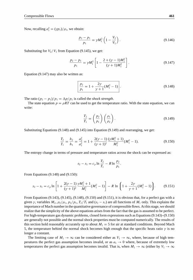
Compressible Flows 461
Now, recalling a21 = (γp1)/ρ1, we obtain:
p2 − p1
p1= γM2
1
(1 − V2
V1
). (9.146)
Substituting for V2/V1 from Equation (9.145), we get:
p2 − p1
p1= γM2
1
[1 − 2 + (γ − 1)M2
1
(γ + 1)M21
]. (9.147)
Equation (9.147) may also be written as:
p2
p1= 1 + 2γ
γ + 1(M2
1 − 1) . (9.148)
The ratio (p2 − p1)/p1 = �p/p1 is called the shock strength.The state equation p = ρRT can be used to get the temperature ratio. With the state equation, we can
write:
T2
T1=
(p2
p1
)(ρ1
ρ2
). (9.149)
Substituting Equations (9.148) and (9.145) into Equation (9.149) and rearranging, we get:
T2
T1= h2
h1= a2
2
a21
= 1 + 2(γ − 1)
(γ + 1)2
(γM21 + 1)
M21
(M21 − 1). (9.150)
The entropy change in terms of pressure and temperature ratios across the shock can be expressed as:
s2 − s1 = cp lnT2
T1− R ln
p2
p1.
From Equations (9.148) and (9.150):
s2 − s1 = cp ln
[1 + 2(γ − 1)
(γ + 1)2
γM21 + 1
M21
(M21 − 1)
]− R ln
⎧⎪⎩1 + 2γ
γ + 1(M2
1 − 1)
⎫⎪⎭. (9.151)
From Equations (9.143), (9.145), (9.148), (9.150) and (9.151), it is obvious that, for a perfect gas with agiven γ , variables M2, ρ2/ρ1, p2/p1, T2/T1 and (s2 − s1) are all functions of M1 only. This explains theimportance of Mach number in the quantitative governance of compressible flows. At this stage, we shouldrealize that the simplicity of the above equations arises from the fact that the gas is assumed to be perfect.For high-temperature gas dynamic problems, closed form expressions such as Equations (9.143)–(9.150)are generally not possible and the normal shock properties must be computed numerically. The results ofthis section hold reasonably accurately up to about M1 = 5 for air at standard conditions. Beyond Mach5, the temperature behind the normal shock becomes high enough that the specific heats ratio γ is nolonger a constant.
The limiting case of M1 → ∞ can be considered either as V1 → ∞, where, because of high tem-peratures the perfect gas assumption becomes invalid, or as a1 → 0 where, because of extremely lowtemperatures the perfect gas assumption becomes invalid. That is, when M1 → ∞ (either by V1 → ∞

462 Theoretical Aerodynamics
or by a → 0), the perfect gas assumption is not valid. But, it is interesting to examine the variation ofproperties across the normal shock, for this limiting case. When M1 → ∞, we find, for γ = 1.4:
limM1→∞
M2 =√
γ − 1
2γ= 0.378
limM1→∞
ρ2
ρ1= γ + 1
γ − 1= 6
limM1→∞
p2
p1= ∞
limM1→∞
T2
T1= ∞.
At the other extreme case of an infinitely weak normal shock degenerating into a Mach wave, that is, atM1 = 1, Equations (9.143), (9.145), (9.148) and (9.150) yield M2 = ρ2/ρ1 = p2/p1 = T2/T1 = 1. Thatis, when M1 = 1, no finite changes occur across the wave.
Equation (9.151) justifies the statement we made earlier in this section: “from Prandtl equation, al-though it is possible for the flow to decelerate from supersonic to subsonic and vice versa across a normalshock wave, only the former is physically feasible.” From Equation (9.151), if M1 = 1, then �s = 0; ifM1 < 1, �s < 0; and if M1 > 1, �s > 0. Therefore, since it is necessary that �s ≥ 0 for a physicallypossible process, from the second law of thermodynamics, M1 must be greater than or equal to 1. WhenM1 is subsonic, the entropy across the wave decreases, which is impossible. Therefore, the only physi-cally possible flow is M1 > 1, and from the above results we have M2 < 1, ρ2/ρ1 > 1, p2/p1 > 1 andT2/T1 > 1.
The changes in flow properties across the shock take place within a very short distance, of the order of10−5 cm. Hence, the velocity and temperature gradients inside the shock structure are very large. Theselarge gradients result in increase of entropy across the shock. Also, these gradients internal to the shockprovide heat conduction and viscous dissipation that render the shock process internally irreversible.
9.20 Change of Total Pressure across a Shock
There is no heat added to or taken away from the flow as it traverses a shock wave; that is, the flowprocess across the shock wave is adiabatic. Therefore, the total temperature remains the same ahead ofand behind the wave:
T02 = T01. (9.152)
Now, it is important to note that Equation (9.152), valid for a perfect gas, is a special case of the moregeneral result that the total enthalpy is constant across a normal shock, as given by Equation (9.135). Fora stationary normal shock, the total enthalpy is always constant across the wave which, for caloricallyor thermally perfect gases, translates into a constant total temperature across the shock. However, for achemically reacting gas, the total temperature is not constant across the shock. Also, if the shock waveis not stationary (that is, for a moving shock), neither the total enthalpy nor the total temperature areconstant across the shock wave.
For an adiabatic process of a perfect gas, we have:
s02 − s01 = R lnp01
p02.

Compressible Flows 463
In the above equation, all the quantities are expressed as stagnation quantities. It is seen from the equationthat the entropy varies only when there are losses in pressure. It is independent of velocity and hence thereis nothing like stagnation entropy. Therefore, the entropy difference between states 1 and 2 is expressed,without any reference to the velocity level, as:
s2 − s1 = R lnp01
p02. (9.153)
The exact expression for the ratio of total pressure may be obtained from Equations (9.153) and (9.151)as:
p02
p01=
(1 + 2γ
γ + 1(M2
1 − 1)
)−1/(γ−1) {(γ + 1)M2
1
(γ − 1)M21 + 2
}γ/(γ−1)
. (9.154)
Equation (9.154) is an important and useful equation, since it connects the stagnation pressures on eitherside of a normal shock to flow Mach number ahead of the shock. Also, we can see the usefulness ofEquation (9.154) from the application aspect. When a pitot probe is placed in a supersonic flow facing theflow, there would be a detached shock standing ahead of probe nose and, therefore, the probe measures thetotal pressure behind that detached shock. However, the portion of the shock ahead of a pitot probe mouthcan be approximated as a normal shock. Thus, what a pitot probe facing a supersonic flow measures is thetotal pressure p02 behind a normal shock. Knowing the stagnation pressure ahead of the shock, which isthe pressure in the reservoir, for isentropic flow up to the shock, we can determine the flow Mach numberahead of the shock with Equation (9.154).
9.21 Oblique Shock and Expansion Waves
The normal shock wave, a compression front normal to the flow direction. However, in a wide variety ofphysical situations, a compression wave inclined at an angle to the flow occurs. Such a wave is called anoblique shock. Indeed, all naturally occurring shocks in external flows are oblique.
In steady subsonic flows, we generally do not think in terms of wave motion. It is usually much simplerto view the motion from a frame of reference in which the body is stationary and the fluid flows over it. Ifthe relative speed is supersonic, the disturbance waves cannot propagate ahead of the immediate vicinityof the body and the wave system travels with the body. Thus, in the reference frame in which the bodyis stationary, the wave system is also stationary; then the correspondence between the wave system andthe flow field is direct.
The normal shock wave is a special case of oblique shock waves, with shock angle β = 90◦. Also, itcan be shown that superposition of a uniform velocity, which is normal to the upstream flow, on the flowfield of the normal shock will result in a flow field through an oblique shock wave. This phenomenonwill be employed later in this section to get the oblique shock relations. Oblique shocks are usuallygenerated when a supersonic flow is turned into itself. The opposite of this, that is, when a supersonicflow is turned away from itself, results in the formation of an expansion fan. These two families of wavesplay a dominant role in all flow fields involving supersonic velocities. Typical flows with oblique shockand expansion fan are illustrated in Figure 9.24.
In Figure 9.24(a), the flow is deflected into itself by the oblique shock formed at the compressioncorner, to become parallel to the solid wall downstream of the corner. All the streamlines are deflectedto the same angle θ at the shock, resulting in uniform parallel flow downstream of shock. The angle θ isreferred to as flow deflection angle. Across the shock wave, the Mach number decreases and the pressure,density and temperature increase. The corner which turns the flow into itself is called compression orconcave corner. In contrast, in an expansion or convex corner, the flow is turned away from itself through
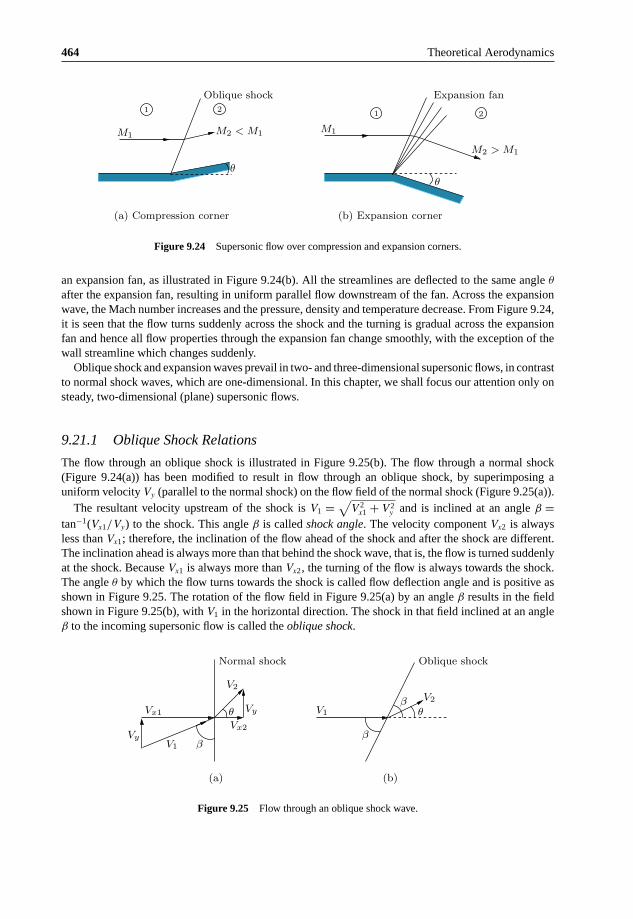
464 Theoretical Aerodynamics
(a) Compression corner
θ
Oblique shock Expansion fan
11 2
M2 < M1M1
M2 > M1
2
M1
(b) Expansion corner
θ
Figure 9.24 Supersonic flow over compression and expansion corners.
an expansion fan, as illustrated in Figure 9.24(b). All the streamlines are deflected to the same angle θ
after the expansion fan, resulting in uniform parallel flow downstream of the fan. Across the expansionwave, the Mach number increases and the pressure, density and temperature decrease. From Figure 9.24,it is seen that the flow turns suddenly across the shock and the turning is gradual across the expansionfan and hence all flow properties through the expansion fan change smoothly, with the exception of thewall streamline which changes suddenly.
Oblique shock and expansion waves prevail in two- and three-dimensional supersonic flows, in contrastto normal shock waves, which are one-dimensional. In this chapter, we shall focus our attention only onsteady, two-dimensional (plane) supersonic flows.
9.21.1 Oblique Shock Relations
The flow through an oblique shock is illustrated in Figure 9.25(b). The flow through a normal shock(Figure 9.24(a)) has been modified to result in flow through an oblique shock, by superimposing auniform velocity Vy (parallel to the normal shock) on the flow field of the normal shock (Figure 9.25(a)).
The resultant velocity upstream of the shock is V1 =√
V 2x1 + V 2
y and is inclined at an angle β =tan−1(Vx1/Vy) to the shock. This angle β is called shock angle. The velocity component Vx2 is alwaysless than Vx1; therefore, the inclination of the flow ahead of the shock and after the shock are different.The inclination ahead is always more than that behind the shock wave, that is, the flow is turned suddenlyat the shock. Because Vx1 is always more than Vx2, the turning of the flow is always towards the shock.The angle θ by which the flow turns towards the shock is called flow deflection angle and is positive asshown in Figure 9.25. The rotation of the flow field in Figure 9.25(a) by an angle β results in the fieldshown in Figure 9.25(b), with V1 in the horizontal direction. The shock in that field inclined at an angleβ to the incoming supersonic flow is called the oblique shock.
βV1
Vx1
V2βV1Vy
Vy
Vx2
V2
Normal shock Oblique shock
(a)
θθ
(b)
β
Figure 9.25 Flow through an oblique shock wave.

Compressible Flows 465
The relations between the flow parameters upstream and downstream of the flow field through theoblique shock, illustrated in Figure 9.25(b), can be obtained from the normal shock relations, since thesuperposition of uniform velocity Vy on the normal shock flow field in Figure 9.25(a) does not affect theflow parameters (e.g., static pressure) defined for normal shock. The only change is that in the presentcase the upstream Mach number is:
M1 = Resultant velocity
Speed of sound= V1
a1.
The component of the upstream Mach number M1 normal to the shock wave is:
Mn1 = M1 sin β. (9.155)
Thus, replacement of M1 with M1 sin β in normal shock relations given by Equations (9.145), (9.148),(9.150) and (9.151) results in the following relations for an oblique shock:
ρ2
ρ1= (γ + 1)M2
1 sin2 β
(γ − 1)M21 sin2 β + 2
(9.156)
p2
p1= 1 + 2γ
γ + 1(M2
1 sin2 β − 1) (9.157)
T2
T1= a2
2
a21
= 1 + 2(γ − 1)
(γ + 1)2
M21 sin2 β − 1
M21 sin2 β
(γM21 sin2 β + 1) (9.158)
s2 − s1
R= ln
⎧⎩[1 + 2γ
γ + 1(M2
1 sin2 β − 1)
]1/(γ−1)
[(γ + 1)M2
1 sin2 β
(γ − 1)M21 sin2 β + 2
]−γ/(γ−1)⎫⎭
= ln
⎧⎪⎩p01
p02
⎫⎪⎭ . (9.159)
The normal component of Mach number behind the shock Mn2 is given by:
M2n2 =
M21 sin2 β + 2
γ−12γ
γ−1 M21 sin2 β − 1
. (9.160)
From the geometry of the oblique shock flow field shown in Figure 9.25, it is seen that the Mach numberbehind the oblique shock, M2, is related to Mn2 by:
M2 = Mn2
sin(β − θ). (9.161)
In the above equations, M2 = V2/a2 and Mn2 = Vx2/a2. The Mach number M2 after a shock can beobtained by combining Equations (9.160) and (9.161).
Numerical values of the oblique shock relations for a perfect gas, with γ = 1.4, are presented ingraphical form. The same in tabular form is given in Table 3 of the Appendix of Rathakrishnan (2010) [1].
It is seen from the oblique shock relations given by Equations (9.155)–(9.159) that the ratio of ther-modynamic variables depends only on the normal component of velocity (M1 sin β) ahead of the shock.

466 Theoretical Aerodynamics
But, from normal shock analysis we know that this component must be supersonic, that is, M1 sin β ≥ 1.This requirement imposes the restriction on the wave angle β that it cannot go below a limiting minimumvalue for any given M1. At this minimum limiting value of shock angle, the shock gets degenerated to anisentropic wave (also called Mach wave) across which the change of flow properties become negligiblysmall. Such a weak isentropic wave is termed Mach wave. The maximum value of β is that for a normalshock, β = π/2. Thus for a given initial Mach number M1, the possible range of wave angle is:
sin−1
(1
M1
)≤ β ≤ π
2. (9.162)
The limiting values of the wave angle in Equation (9.162) are of special significance. The limitingminimum value is sin−1
(1M
)is the Mach angle μ and the maximum value π
2 corresponds to normalshock. Thus, the strongest wave possible in a given supersonic flow is the normal shock correspondingto the given M1. The weakest wave is the Mach wave corresponding to the given M1. It is essentialto note that the shock wave formation is not mandatory in a supersonic flow. For example, in uniformsupersonic streams such as the flow in a supersonic wind tunnel test-section, no shocks are formed whenthe test-section is empty, whereas the weakest limiting isentropic waves, namely the Mach waves, arealways present in all supersonic flows. Even in the empty test-section of a supersonic tunnel the Machwaves are present. But we know that the waves in a supersonic flow are due to perturbations in the flowfield. Therefore, it is natural to ask, “in an undisturbed uniform supersonic flow why should there beMach waves present?” The answer to this question is the following. In a uniform supersonic flow suchas that in a wind tunnel test-section, if the test-section walls are absolutely smooth there will not be anyMach wave present in the flow. However, absolute smooth surface is only a theoretical assumption. Forinstance, even surfaces such as that of a good quality Schlieren mirror has a finish of only about λ/20,where λ is the wavelength of light. Thus, any practical surface is with some roughness and not absolutelysmooth. Therefore, any supersonic flow field generated by a practical device is bound to possess Machwaves. Indeed, the size of the gas molecules are enough to cause Mach wave generation. Therefore, evenin a free supersonic flow without any solid confinement Mach waves will be present.
An important feature to be inferred here is that the Mach waves, like characteristics will be running tothe left and right in the flow field. Because of this the Mach waves of opposite families prevailing in theflow field cross each other. But being the weakest degeneration of waves, the Mach waves would continueto propagate as linear waves even after passing through a number of Mach waves. In other words, theMach waves would continue to be simple waves even after intersecting other Mach waves. Because ofthis nature of the Mach waves, a flow region traversed by the Mach waves is simple throughout.
9.21.2 Relation between β and θ
It is seen from Equation (9.161) that for determining M2 the flow deflection angle θ must be known.Further, for each value of shock angle β at a given M1 there is a corresponding flow turning angle θ.Therefore, θ can also be expressed as a unique function of M1 and β. From Figure 9.25, we have:
tan β = Vx1
Vy
(9.163)
tan(β − θ) = Vx2
Vy
. (9.164)
Combining Equations (9.163) and (9.164), we get:
tan(β − θ)
tan β= Vx2
Vx1. (9.165)

Compressible Flows 467
By continuity:
Vx2
Vx1= ρ1
ρ2.
Now, substituting for ρ1/ρ2 from Equation (9.156), we get:
tan(β − θ)
tan β= (γ − 1)M2
1 sin2 β + 2
(γ + 1)M21 sin2 β
. (9.166)
Equation (9.166) is an implicit relation between θ and β, for a given M1. With some trigonometricmanipulation, this expression can be rewritten to show the dependence of θ on Mach number M1 andshock angle β, as:
tan θ = 2 cot β
⎧⎪⎪⎩ M21 sin2 β − 1
M21 (γ + cos 2β) + 2
⎫⎪⎪⎭ . (9.167)
Equation (9.167) is called the θ–β–M relation. This relation is important for the analysis of oblique shocks.The expression on the right-hand side of Equation (9.167) becomes zero at β = π/2 and β = sin−1( 1
M1),
which are the limiting values of β, defined in Equation (9.162). The deflection angle θ is positive in thisrange and must therefore have a maximum value. The results obtained from Equation (9.167) are plottedin Figure 9.26, for γ = 1.4. From the plot of θ–β–M (Figure 9.26) curves, the following observationscan be made:
30
20
M2 < 1
0
M2
=1
θ=
θ max
M2 > 1
80604020
40
2
1.4
1.6
0Wave angle β (degree)
M1 = 1
10
5
3
4
1.2
Flo
wdefl
ection
angle
θ(d
egre
e)
10
Figure 9.26 Oblique shock solution.

468 Theoretical Aerodynamics
Detached shockDetached shock
M1 > 1
M1 > 1
θ > θmax θ > θmax
Figure 9.27 Detached shocks.
1. For any given supersonic Mach number M1, there is a maximum value of θ. Therefore, at a given M1,if θ > θmax, then no solution is possible for a straight oblique shock wave. In such cases, the shockwill be curved and detached, as shown in Figure 9.27.
2. When θ < θmax, there are two possible solutions, for each value of θ and M, having two different waveangles. The larger value of β is called the strong shock solution and the smaller value of β is referredto as the weak shock solution. For strong shock solution, the flow behind the shock becomes subsonic.For weak shock solution, the flow behind the oblique shock remains supersonic, except for a smallrange of θ slightly smaller than θmax, the zone bounded by the M2 = 1 curve and θ = θmax curve shownin Figure 9.26.
3. If θ = 0, then β = π/2, giving rise to a normal shock, or β decreases to the limiting value μ, thatis, shock disappears and only Mach waves prevail in the flow field. That is, when the flow turningangle θ is zero, the following two solutions are possible for the shock angle β, for a given M1. (a)Either β = π/2 giving rise to a normal shock which does not cause any flow deflection, but woulddecelerate the flow to subsonic level, or (b) β = sin−1(1/M1) = μ corresponding a Mach wave, whicheven though inclined to the upstream flow, would not cause any flow deflection, being the limitingcase of the weakest isentropic wave for a given M1.
A very useful form of θ–β–M relation can be obtained by rearranging Equation (9.166) in the followingmanner: Dividing the numerator and denominator of the right-hand side of Equation (9.166) by 2M2
1 sin2 β
and solving, we obtain:
1
M21 sin2 β
= γ + 1
2
tan (β − θ)
tan β− γ − 1
2.
This can be simplified further to result in:
M21 sin2 β − 1 = γ + 1
2M2
1
sin β sin θ
cos (β − θ). (9.168)
For small deflection angles θ, Equation (9.168) may be approximated as:
M21 sin2 β − 1 ≈
⎧⎪⎩γ + 1
2M2
1 tan β
⎫⎪⎭ θ. (9.169)
If M1 is very large, then β � 1, but M1β � 1 and Equation (9.169) reduces to:
β = γ + 1
2θ. (9.170)

Compressible Flows 469
Solid wall
Oblique shock
M2
M1
βθ
Figure 9.28 Supersonic flow over a compression corner.
It is important to note that oblique shocks are essentially compression fronts across which the flowdecelerates and the static pressure, static temperature and static density jump to higher values. If thedeceleration is such that the Mach number behind the shock continues to be greater than unity, the shockis termed weak oblique shock. If the downstream Mach number becomes less than unity then the shock iscalled strong oblique shock. It is essential to note that only weak oblique shocks are usually formed in anypractical flow and it calls for special arrangement to generate strong oblique shocks. One such situationwhere strong oblique shocks are generated with special arrangements is the engine intakes of supersonicflight vehicles, where the engine has provision to control its backpressure. When the backpressure isincreased to an appropriate value, the oblique shock at the engine inlet would become a strong shock anddecelerate the supersonic flow passing through it to subsonic level.
9.21.3 Supersonic Flow over a Wedge
From studies on inviscid flows, we know that any streamline can be regarded as a solid boundary. Inour present study, we treat the supersonic flow as inviscid and, therefore, here also the streamlines canbe assumed as solid boundaries. Thus the oblique shock flow results, already described, can be used forsolving practical problems like supersonic flow over a compression corner, as shown in Figure 9.28. Forany given values of M1 and θ, the values of M2 and β can be determined from oblique shock charts ortable (oblique shock charts and table are given in the Appendix of Rathakrishnan (2010)).
In a similar fashion, problems like supersonic flow over symmetrical and unsymmetrical wedges(Figure 9.29) and so on also can be solved with oblique shock relations, assuming the solid surfaces ofthe objects as streamlines in accordance with nonviscous (or inviscid) flow theory.
M2
M1
M2
M1
ββ
(b) Unsymmetrical wedge
β β1
(a) Symmetric wedge
M2 M2′
θθ
θ θ1
Figure 9.29 Flow past (a) symmetrical and (b) unsymmetrical wedges.

470 Theoretical Aerodynamics
Shock wave
M1 M2
θ
(− )
(+)
P P
β
M1
(a) Oblique shock withMach wave θ ! 0(b) Degeneration to (c) Left (− ) and right (+) running
charateristics at an arbitrarydeflection angle θ
Mach wave
Mμ
μ
μ
M2
point in the flow
Figure 9.30 Waves in a supersonic stream.
In Figure 9.29(b), the flow on each side of the wedge is determined only by the inclination of thesurface on that side. If the shocks are attached to the nose, the upper and lower surfaces are independentand there is no influence of wedge on the flow upstream of the shock waves.
In our discussion on shock angle β and flow turning angle θ, we have seen that when θ decreases tozero, β decreases to the limiting value μ giving rise to Mach waves in the supersonic flow field (seeFigure 9.30(b)), which is given from Equation (9.168) as:
M21 sin2 μ − 1 = 0 (9.171)
Also, the pressure, temperature and density jump across the shock (p2 − p1, T2 − T1 and ρ2 − ρ1) givenby Equations (9.156)–(9.158) become zero. There is, in fact, no finite disturbance in the flow. The pointP in Figure 9.30(b) may be any point in the flow field. Then the angle μ is simply a characteristic angleassociated with the Mach number M by the relation:
μ = sin−1
(1
M
). (9.172)
This is called Mach angle-Mach number relation. These lines which may be drawn at any point in the flowfield with inclination μ are called Mach lines or Mach waves. It is essential to understand the differencebetween the Mach waves and Mach lines. Mach waves are the weakest isentropic waves in a supersonicflow field and the flow through them will experience only negligible changes of flow properties. Thus,a flow traversed by the Mach waves do not experience change of Mach number. Whereas the Machlines, even though are weak isentropic waves will cause small but finite changes to the properties ofa flow passing through them. In uniform supersonic flows, the Mach waves and Mach lines are linearand inclined at an angle given by μ = sin−1 (1/M). But in nonuniform supersonic flows the flow Machnumber M varies from point to point and hence the Mach angle μ, being a function of the flow Machnumber, varies with M and the Mach lines are curved.
In the flow field at any point P (Figure 9.30(c)), there are always two lines which are inclined at angleμ and intersect the streamline, as shown in Figure 9.30(c). In a three-dimensional flow, the Mach waveis in the form of a conical surface, with vertex at P. Thus, a two-dimensional flow of supersonic streamis always associated with two families of Mach lines. These are represented with plus and minus sign.In Figure 9.30(c), the Mach lines with ‘+’ sign run to the right of the streamline when viewed throughthe flow direction and those lines with “−” sign run to the left. These Mach lines which introduce aninfinitesimal, but finite change to flow properties when a flow passes through them are also referred to

Compressible Flows 471
as characteristics, which are not physical unlike the Mach lines and Mach waves. But the mathematicalconcept of characteristics (taken as identical to the Mach lines), even though not physical forms the basisfor the numerical method termed method of characteristics, used to design contoured nozzles to generateuniform and unidirectional supersonic flows.
At this stage it is essential to note the difference between the Mach waves, characteristics and expansionwaves. Even though all these are isentropic waves, there is a distinct difference between them. Machwaves are weak isentropic waves across which the flow experiences insignificant change in its properties.Whereas, the expansion waves and characteristics are isentropic waves which introduce small, but finiteproperty changes to a flow passing them. Thus, even though we loosely state that the Mach lines andMach waves are isentropic waves in a supersonic flow, inclined at angle μ to the freestream direction,in reality they are distinctly different. Mach waves are the weakest degeneration of isentropic waves tothe limiting case of zero strength that a flow across which will not experience any change of property.Whereas, a Mach line is a weak isentropic wave in a supersonic flow field, causing small but finite changeof properties to the flow passing through it.
The characteristic lines play an important role in the compression and expansion processes in the sensethat it is only through these lines that it is possible to retard or accelerate a supersonic flow isentropically.Also, this concept will be employed in designing supersonic nozzles with Method of Characteristics.
9.21.4 Weak Oblique Shocks
We have seen that the compression of supersonic flow without entropy increase is possible only throughthe Mach lines. In the present discussion on weak shocks also, it will be shown that these weak shocks,which result when the flow deflection angle θ is small and Mach number downstream of shock M2 > 1,can also compress the flow with entropy increase almost close to zero. It is important to note that, whenwe discussed about flow through oblique shocks, we considered the shock as weak when the downstreamMach number M2 is supersonic (even though less than the upstream Mach number M1). When the flowtraversed by an oblique shock becomes subsonic (that is, M2 < 1), the shock is termed strong. But whenthe flow turning θ caused by a weak oblique shock is very small, then the weak shock assumes a specialsignificance. This kind of weak shock with both decrease of flow Mach number (M1 − M2) and flowturning angle θ, which is small, can be regarded as isentropic compression waves.
For small values of θ, the oblique shock relations reduce to very simple forms. For this case:
sin θ ≈ θ and cos (β − θ) ≈ cos β.
Therefore, Equation (9.168) simplifies to:
M21 sin2 β − 1 ≈
⎧⎪⎩γ + 1
2M2
1 tan β
⎫⎪⎭ θ.
Also, M2 > 1 for weak oblique shocks. Therefore, we may approximate this weak shock with both(M1 − M2) and θ extremely small as a Mach line. Thus, the shock angle β can be regarded as almostequal to the Mach angle μ. With this approximation, we can express tan β as follows:
sin β ≈ sin μ = 1
M
cos β =√
1 − sin2 β
= 1
M
√M2 − 1
tan β = 1√M2 − 1
.

472 Theoretical Aerodynamics
Substituting for tan β in preceding equation, we get:
M21 sin2 β − 1 ≈ γ + 1
2
M21√
M21 − 1
θ. (9.173)
Equation (9.173) is considered to be the basic relation for obtaining all other appropriate expressions forweak oblique shocks since all oblique shock relations depend on M1 sin β, which is the component ofupstream Mach number normal to the shock.
It is seen from Equations (9.157) and (9.173) that the pressure change across a shock �p
p1, termed the
shock strength can be easily expressed as:
p2 − p1
p1= �p
p1≈ γM2
1√M2
1 − 1θ. (9.174)
Equation (9.174) shows that the strength of the shock wave is proportional to the flow deflection angle θ.Similarly, it can be shown that the changes in density and temperature are also proportional to θ. But
the change in entropy, on the other hand is proportional to the third power of shock strength as shownbelow. By Equation (9.159), we have:
s2 − s1
R= ln
[⎧⎪⎩1 + 2γ
γ + 1m
⎫⎪⎭1/(γ−1)
(1 + m)−γ/(γ−1)
⎧⎪⎩γ − 1
γ + 1m + 1
⎫⎪⎭γ/(γ−1)]
, (9.175)
where m = (M21 − 1) [Note that for weak oblique shocks under consideration, that is, for weak oblique
shocks with (M1 − M2) � 1 and θ very small, M21 sin2 β is approximated as M2
1 .] For values of M1 closeto unity, m is small and the terms within the parentheses are like 1 + ε, with ε � 1. Expanding the termsas logarithmic series, we get:
s2 − s1
R= 2γ
(γ + 1)2
m3
3+ higher-order terms
or
s2 − s1
R≈ 2γ
(γ + 1)2
(M21 − 1)3
3. (9.176)
Because the entropy cannot decrease in an adiabatic flow, Equation (9.176) stipulates that M1 ≥ 1. Thus,the increase in entropy is of third order in (M2
1 − 1). This may be written in terms of shock strength,�p/p, as:
s2 − s1
R≈ γ + 1
12 γ2
⎧⎪⎩�p
p1
⎫⎪⎭3
. (9.176)
But by Equation (9.174), the shock strength is proportional to θ and hence:
�s ∼ θ3 . (9.177)
Thus, a small but finite change of pressure across a weak oblique shock, for which there are correspondingfirst-order changes of density and temperature, gives only a third-order change of entropy, that is, a weakshock produces a nearly isentropic change of state.

Compressible Flows 473
Now, let the wave angle β for the weak shock be different from the Mach angle μ by a small angle ε.That is:
β = μ + ε,
where ε � μ. Therefore, sin β = sin (μ + ε) = sin μ + ε cos μ. Also, sin μ = 1/M1 and cot μ =√M2
1 − 1. Thus:
M1 sin β ≈ 1 + ε√
M21 − 1 (9.178)
or
M21 sin2 β ≈ 1 + 2ε
√M2
1 − 1. (9.179)
From Equations (9.173) and (9.179), we obtain:
ε = γ + 1
4
M21
M21 − 1
θ. (9.180)
That is, for a finite flow deflection angle θ, the direction of weak oblique shock wave differs from theMach wave direction μ by an amount ε, which is of the same order as θ.
9.21.5 Supersonic Compression
Compressions in a supersonic flow are not usually isentropic. Generally, they take place through a shockwave and hence are nonisentropic. But there are certain cases, for which the compression process can beregarded isentropic. A compression process which can be treated as isentropic is illustrated in Figure 9.31,where the turning of the flow is achieved through large number of weak oblique shocks. These kindsof compression through a large number of weak compression waves is termed continuous compression.These kinds of corners are called continuous compression corners. Thus, the geometry of the corner shouldhave continuous smooth turning to generate large number of weak (isentropic) compression waves.
M2
Shock
M1
θ
Figure 9.31 Smooth continuous compression.

474 Theoretical Aerodynamics
The weak oblique shocks divide the field near the wall into segments of uniform flow. Away from thewall the weak shocks might coalesce and form a strong shock as illustrated in Figure 9.31. We have seenthat the entropy increase across a weak wave is of the order of third power of deflection angle θ. Let theflow turning through an angle, shown in Figure 9.31, be taking place through n weak compression waves,each wave turning the flow by an angle �θ. The overall entropy change for this compression process is:
(sn − s1) ∼ n(�θ)3 ∼ n�θ(�θ)2 ∼ θ(�θ)2.
Thus, if the compression is achieved through a large number of weak compression waves, the entropyincrease can be reduced to a very large extent, as compared to a single shock causing the same netdeflection. When �θ is made vanishingly small, a smooth continuous turning of the flow as shown inFigure 9.31 is achieved. The entropy increase associated with such a continuous smooth compressionprocess is vanishingly small, that is, the compression can be treated as isentropic.
At this stage it is natural to ask, whether this kind of isentropic compression is only of theoreticalinterest or it is used in practical devices too? The answer to this question is that it is used in practicaldevices too. For example, in the gas turbine engines used to propel supersonic aircraft such as fighters,the freestream supersonic air stream entering the engine intake needs to be decelerated to incompressibleMach numbers (of the order of 0.2) before reaching the combustion chamber, because with the presenttechnology continuous and stable combustion is possible only at low incompressible Mach numbers.This can be achieved by a single normal shock or even with a strong oblique shock to decelerate thesupersonic stream to a subsonic Mach number and then the subsonic stream can be decelerated further ina diffuser to reach the required incompressible Mach number before entering the combustion chamber.But both these decelerations will result in a large increase of entropy and the associated large pressureloss. This kind of large increase of entropy is desirable for an efficient mixing of fuel and air in thecombustion chamber, but the severe pressure loss with the nonisentropic compression through the shocksis undesirable. We know that the engine is used to generate thrust by reaction. The momentum thrustproduced by an engine is:
Thrust = m Vj.
where m is the mass flow rate of the combustion products of the fuel-air mixture burnt in the combustionchamber, expanded through the nozzle of the engine, and Vj is the flow velocity at the nozzle exit. ByBernoulli principle it is known that a large velocity Vj can be generated by expanding a gas at highstagnation pressure p0. Thus, the aim of the process through the engine is to achieve high p0. If possiblewe can use a compressor to achieve the desired level of p0. But carrying a compressor in a gas turbineengine is not a practically possible solution, mainly due to the weight penalty and the need for additionalsource of energy to run the compressor. Therefore, as an alternative, the high pressure required is achievedthrough combustion where liberation of thermal energy by burning a fuel–air mixture results in a largeincrease of total temperature T0 and the associated increase of total pressure p0. Now, we will notice aninteresting point if we keenly observe the process involved. The vehicle is flying at a supersonic Machnumber. Because of the skin friction, shock and expansion waves around the vehicle and other dragproducing causes the vehicle encounters drag. This drag has to be compensated with thrust to maintainthe supersonic flight speed. Thus, the basic work of the engine is to supply the required momentum tocompensate the momentum loss due to the drag. In other words, basically the loss caused by the dragcan be viewed as loss of total pressure p0. Therefore, the engine must compensate the pressure lossin order to maintain the constant p0 required for the supersonic flight at the given altitude. Instead ofadding the stagnation pressure equivalent to compensate for the pressure loss due to drag, we are doingthe same thing in an indirect manner. This is done through combustion. For performing combustion, thesupersonic air entering the engine is decelerated to low incompressible Mach number, fuel is mixed withthe air and combustion is performed at such a low Mach number to increase p0 through the increase

Compressible Flows 475
of stagnation temperature T0. The combustion products at low-Mach number is accelerated through theengine nozzle to achieve the required jet velocity at the nozzle exit. In the deceleration process throughshock/shocks at the engine intake, considerable total pressure is lost. Therefore, it would be appropriateand beneficial if the fuel is added to the air entering the engine with supersonic speed and the combustionis performed at the same freestream supersonic Mach number. But even though this is the most suitableand efficient situation, we are not in a position to do so. This is because the technology for performingstable combustion at supersonic Mach number is not yet established. Many research groups in variouscountries are working on establishing combustion at supersonic Mach numbers. Indeed, stable combustionat Mach number around 2 is reported by few advanced countries, such as USA, China, Britain, France andJapan. Once the technology for supersonic combustion is established, the pressure lost in deceleratingthe supersonic air stream to the incompressible Mach number to enable combustion with the presenttechnology can be eliminated to a large extent. This will result in a significant increase of the engineefficiency. In other words, the pressure loss associated with the deceleration of supersonic or hypersonicflow entering the engine to the required incompressible Mach number for stable combustion with thepresent technology can be completely eliminated if technology is developed to perform stable combustionat supersonic/hypersonic Mach numbers.
9.21.6 Supersonic Expansion by Turning
Consider the turning of a two-dimensional supersonic flow through a finite angle at a convex corner, asillustrated in Figure 9.32. Let us assume that the flow is turned by an oblique shock at the corner, asshown in the figure.
The flow turning shown in Figure 9.32 is possible only when the normal component of velocity V2n
after the shock is greater than the normal component V1n ahead of the shock, since V1t and V2t on eitherside of the shock must be equal. Although this would satisfy the equations of motion, it would lead toa decrease of entropy across the shock. Therefore, this turning process is not physically possible. Fromthe geometry of the flow shown in Figure 9.32, it follows that V2n must be greater than V1n. The normalmomentum equation yields:
p1 + ρ1V21n = p2 + ρ2V
22n.
Combining this with continuity equation:
ρ1V1n = ρ2V2n
V2n
Shock
V1n
V2
Vt1
Vt2
V1
θ
Figure 9.32 Supersonic flow over a convex corner.

476 Theoretical Aerodynamics
(a) Centered expansion
M2
(b) Continuous (simple) expansion
M1
M2
μ2
P
M1
θ
μ1
Figure 9.33 Centered and continuous expansion processes.
we obtain:
p2 − p1 = ρ1V1n(V1n − V2n).
Because V2n > V1n, it follows that the pressure downstream of the corner should be less than the pressureupstream of the corner (p2 < p1). For this, the flow should pass through an expansion fan at the corner.Thus, the wave at the convex corner must be an expansion fan, causing the flow to accelerate. In otherwords, the shock wave shown at the convex corner in Figure 9.32 is a physically impossible solution.
In an expansion process, the Mach lines are divergent, as shown in Figure 9.33 and, consequently,there is a tendency to decrease the pressure, density and temperature of the flow passing through them.In other words, an expansion is isentropic throughout.
It is essential to note that the statement “expansion is isentropic throughout” is not true always. To gainan insight into the expansion process, let us examine the centered and continuous expansion processesillustrated in Figures 9.33(a) and 9.33(b). We know that the expansion rays in an expansion fan areisentropic waves across which the change of pressure, temperature, density and Mach number are smallbut finite. But when such small changes coalesce they can give rise to a large change. One such pointwhere such a large change of flow properties occurs due to the amalgamation of the effect due to a largenumber of isentropic expansion waves is point P, which is the vertex of the centered expansion fan inFigure 9.33(a). As illustrated in Figures 9.33(a), the pressure at the wall suddenly drops from p1 to p2
at the vertex of the expansion fan. Similarly, the temperature and density also drop suddenly at point P.The Mach number at P suddenly decreases from M1 to M2. The entropy change across the vertex of theexpansion fan is:
s2 − s1 = cp lnT2
T1− R ln
p2
p1.
It is seen that entropy change associated with the expansion process at point p is finite. Thus, the expansionprocess at point P is nonisentropic. Therefore, it is essential to realize that a centered expansion processis isentropic everywhere except at the vertex of the expansion fan, where it is nonisentropic.
But for the continuous expansion illustrated in Figure 9.33(b), there is no sudden change of flowproperties. Even at the wall surface the properties change gradually as shown in the figure, due to theabsence of any point such as P in Figure 9.33(a), where all the expansion rays are concentrated. Therefore,the continuous expansion is isentropic everywhere.
The expansion at a corner (Figure 9.33(a)) occurs through a centered wave, defined by a “fan” of straightexpansion lines. This centered wave, also called a Prandtl-Meyer expansion fan, is the counterpart, for aconvex corner, of the oblique shock at a concave corner.
A typical expansion over a continuous convex turn is shown in Figure 9.33(b). Since the flow isisentropic, it is reversible.

Compressible Flows 477
9.21.7 The Prandtl-Meyer Function
It is known from basic studies on fluid flows that a flow which preserves its own geometry in space ortime or both is called a self-similar flow. In the simplest cases of flows, such motions are described bya single independent variable, referred to as similarity variable. The Prandtl-Meyer function is such asimilarity variable.
The Prandtl-Meyer function in terms of the Mach number M1 just upstream of the expansion fan canbe written as:
ν =√
γ + 1
γ − 1arc tan
√γ − 1
γ + 1(M2
1 − 1) − arc tan√
(M21 − 1) . (9.181)
Equation (9.181), expressing the Prandtl-Meyer function ν in terms of the Mach number, is a veryimportant result of supersonic flow. From this relation, it is seen that for a given M1, there is a fixed ν.For a detailed discussion about Prandtl-Meyer expansion process see Rathakrishnan (2010) [1].
9.21.8 Shock-Expansion Theory
The shock and expansion waves discussed in this chapter are the basis for analyzing large number oftwo-dimensional, supersonic flow problems by simply “patching” together appropriate combinations oftwo or more solutions. That is, the aerodynamic forces acting on a body present in a supersonic floware governed by the shock and expansion waves formed at the surface of the body. This can be easilyseen from the basic fact that the aerodynamic forces acting on a body depend on the pressure distributionaround it and in supersonic flow, the pressure distribution over an object depends on the wave pattern onit, as shown in Figure 9.34.
Consider the two-dimensional diamond aerofoil kept at zero angle of attack in a uniform supersonicflow, as shown in Figure 9.34(a). The supersonic flow at M1 is first compressed and deflected through anangle ε by the oblique shock wave at the leading edge, forcing the flow to travel parallel to the wedgesurface. At the shoulder located at mid-chord, the flow is expanded through an angle 2ε by the expansionfan. At the trailing edge, the flow is again deflected through an angle ε, in order to bring it back to theoriginal direction. Therefore, the surface pressures on the wedge segments ahead and after the shoulder,will be at a constant level over each segment for supersonic flow, according to oblique shock and thePrandtl-Meyer expansion theory.
On the diamond aerofoil, at zero angle of attack, the lift is zero because the pressure distributions onthe top and bottom surfaces are the same. Therefore, the only aerodynamic force acting on the diamond
2′
p4
1 2
2
(c)(b)
4
3
3
p1
l
p1
p4
p1
p2
α0
p3
M1
p2
p3
p2′
(a)
2ε t
Figure 9.34 Wave pattern over objects.

478 Theoretical Aerodynamics
aerofoil is due to the higher-pressure on the forward face and lower-pressure on the rearward face. Thedrag per unit span is given by:
D = 2(p2 l sin ε − p3 l sin ε) = 2 (p2 − p3) (t/2)
that is:
D = (p2 − p3) t . (9.182)
Equation (9.182) gives an expression for drag experienced by a two-dimensional diamond aerofoil, keptat zero angle of attack in an inviscid flow. This is in contrast with the familiar result from studies onsubsonic flow that, for two-dimensional inviscid flow over a wing of infinite span at a subsonic velocity,the drag force acting on the wing is zero – a theoretical result called d’Alembert’s paradox. In contrastwith this, for supersonic flow, drag exists even in the idealized, nonviscous fluid. This new component ofdrag encountered when the flow is supersonic is called wave drag, and is fundamentally different fromthe skin-friction drag and separation drag which are associated with boundary layer in a viscous fluid.The wave drag is related to loss of total pressure and increase of entropy across the oblique shock wavesgenerated by the aerofoil.
For the flat plate at an angle of attack α0 in a uniform supersonic flow, shown in Figure 9.34(c), fromthe uniform pressure on the top and bottom sides, the lift and drag are computed very easily, with thefollowing equations:
L = (p2′ − p2) c cos α0(9.183)
D = (p2′ − p2) c sin α0,
where c is the chord.
Example 9.3
A flat plate is kept at 15◦ angle of attack to a Mach 2.4 air stream, as shown in Figure 9.35. Solve theflow field around the plate and determine the inclination of slipstream to the freestream direction usingshock-expansion theory.
Solution
Using the shock and expansion wave properties, Table 9.1 can be formed.Table 9.1 lists the flow properties around the flat plate. Slip-surface inclination relative to freestream isnegligibly small. The velocity jump across the slip-surface is found to be 1 m/s.
15± Slipstream
1
2′3′
3
M1 = 2.42
Figure 9.35 A flat plate in supersonic flow.

Compressible Flows 479
Table 9.1
Region M ν μ p/p01 T/T01
1 2.4 36.8◦ 24.6◦ 0.0684 0.4652 3.11 51.8◦ 18.8◦ 0.0231 0.3413 2.33 35.0◦ 25.4◦ 0.0675 0.4802′ 1.80 20.7◦ 33.8◦ 0.1629 0.6073′ 2.36 35.7◦ 25.1◦ 0.0679 0.473
9.22 Thin Aerofoil Theory
We saw that the shock-expansion theory gives a simple method for computing lift and drag acting overa body kept in a supersonic stream. This theory is applicable as long as the shocks are attached. Thistheory may be further simplified by approximating it by using the approximate relations for the weakshocks and expansion, when the aerofoil is thin and is kept at a small angle of attack, that is, if the flowinclinations are small. This approximation will result in simple analytical expressions for lift and drag.
At this stage, we may have a doubt about the difference between shock-expansion theory and thinaerofoil theory. The answer to this doubt is the following:
“In shock-expansion theory, the shock is essentially a non-isentropic wave causing a finite increaseof entropy. Thus, the total pressure of the flow decreases across the shock. But in thin aerofoiltheory even the shock is regarded as an isentropic compression wave. Therefore, the flow across thiscompression wave is assumed to be isentropic. Thus the pressure loss across the compression waveis assumed to be negligibly small.”
From our studies on weak oblique shocks, we know that the basic approximate expression [Equation(9.174)] for calculating pressure change across a weak shock is:
�p
p1≈ γM2
1√M2
1 − 1�θ.
Because the wave is weak, the pressure p behind the shock will not be significantly different from p1, norwill the Mach number M behind the shock be appreciably different from the freestream Mach numberM1. Therefore, we can express the above relation for pressure change across a weak shock, without anyreference to the freestream state (that is, without subscript 1 to the pressure and Mach number) as:
�p
p≈ γM2
√M2 − 1
�θ.
Now, assuming all direction changes to the freestream direction to be zero and freestream pressure to bep1, we can write:
p − p1
p1= γM2
1√M2
1 − 1(θ − 0),
where θ is the local flow inclination relative to the freestream direction.The pressure coefficient Cp is defined as:
Cp = p − p1
q1,

480 Theoretical Aerodynamics
where p is the local static pressure and p1 and q1 are the freestream static pressure and dynamic pressure,respectively. In terms of freestream Mach number M1, the pressure coefficient Cp can be expressed as:
Cp = p − p1
q1= 2
γM21
p − p1
p1.
Substituting the expression for (p − p1)/p1 in terms of θ and M1, we get:
Cp = 2θ√M2
1 − 1. (9.184)
The above equation, which states that the pressure coefficient is proportional to the local flow direction,is the basic relation for thin aerofoil theory.
9.22.1 Application of Thin Aerofoil Theory
Applying the thin aerofoil theory relation, Equation (9.184), for the flat plate shown in Figure 9.34(c) ata small angle of attack α0, the Cp on the upper and lower surfaces of the plate can be expressed as:
Cp = ∓ 2α0√M2
1 − 1. (9.185)
where the minus sign is for Cp on the upper surface and the plus sign is for Cp on the lower surface. Thelift and drag coefficients are respectively given by:
CL = (pl − pu) c cos α0
q1c= (Cpl − Cpu) cos α0
CD = (pl − pu) c sin α0
q1c= (Cpl − Cpu) sin α0.
In the above expressions for CL and CD, cos α0 ≈ 1 and sin α0 ≈ α0, since α0 is small and the subscriptsl and u refer to the lower and upper surfaces, respectively and c is the chord. Therefore:
CL = (Cpl − Cpu)
CD = (Cpl − Cpu)α0.
Using Equation (9.185), the CL and CD of the flat plate at a small angle of attack may be expressed as:
CL = 4α0√M2
1 − 1
(9.186)
CD = 4α20√
M21 − 1
.

Compressible Flows 481
Now, consider the diamond section aerofoil shown in Figure 9.34(a), with nose angle 2ε, at zero angleof attack. The pressure coefficient Cp on the front and rear faces are given by:
Cp = ± 2ε√M2
1 − 1,
where the + sign is for the front face where the pressure p2 is higher than p1 and the − sign is for therear face with pressure p3 less than p1. This can be rewritten in terms of pressure difference to give:
p2 − p3 = 4ε√M2
1 − 1q1.
Therefore, the drag is given by:
D = (p2 − p3)t = (p2 − p3) ε c
D = 4ε2√M2
1 − 1q1c,
where q1 is the freestream dynamic pressure and c is the chord of the aerofoil.In terms of the drag coefficient, the above drag equation becomes:
CD = D
q1c= 4ε2√
M21 − 1
(9.187a)
or
CD = 4√M2
1 − 1
(t
c
)2
. (9.187b)
In the above two applications, the thin aerofoil theory was used for specific profiles to get expressionsfor CL and CD. A general result applicable to any thin aerofoil may be obtained as follows. Consider acambered aerofoil with finite thickness at a small angle of attack treated by linear resolution into threecomponents, each of which contributing to lift and drag, as shown in Figure 9.36.
By thin aerofoil theory, the Cp on the upper and lower surfaces are obtained as:
Cpu = 2√M2
1 − 1
(dyu
dx
)
(9.188)
Cpl = 2√M2
1 − 1
(−dyl
dx
),
o
++α0
x
yl(x)
Angle of attackc
y
yc(x)
yu(x)
´Camber
yc(x) h(x)
Thickness
Figure 9.36 Linear resolution of aerofoil into angle of attack, camber and thickness.

482 Theoretical Aerodynamics
where yu and yl are the upper and lower profiles of the aerofoil. The profile may be resolved into asymmetrical thickness distribution h(x) and a camber line of zero thickness yc(x). Thus, we have:
dyu
dx= dyc
dx+ dh
dx= −α(x) + dh
dx(9.189a)
dyl
dx= dyc
dx− dh
dx= −α(x) − dh
dx, (9.189b)
where α(x) = α0 + αc(x) is the local angle of attack of the camber line, and α0 is the angle of attack ofthe freestream and αc is the angle attack due to the camber. The lift and drag are given by:
L = q1
∫ c
0
(Cpl − Cpu) dx (9.190a)
D = q1
∫ c
0
[Cpl
(−dyl
dx
)+ Cpu
(dyu
dx
)]dx. (9.190b)
Substituting Equations (9.188) and (9.189) into Equations (9.190a) and (9.190b), we get:
L = 2q1√M2
1 − 1
∫ c
0
(−2
dyc
dx
)dx
= 4q1√M2
1 − 1
∫ c
0
α(x) dx
D = 2q1√M2
1 − 1
∫ c
0
[(dyl
dx
)2
+(
dyu
dx
)2]
dx
= 4q1√M2
1 − 1
∫ c
0
[α(x)2 +
(dh
dx
)2]
dx.
The integrals may be replaced by average values, for example:
α = 1
c
∫ c
0
α(x) dx.
Also, noting that by definition αc = 0, we get:
α = α0 + αc
= α0 + αc
= α0.
Similarly:
α2 = (α0 + αc)2
= α20 + 2α0αc + α2
c
= α20 + α2
c .

Compressible Flows 483
Using the above averages in the lift and drag expressions, we obtain the lift and drag coefficients as:
CL = 4α√M2
1 − 1= 4α0√
M21 − 1
(9.191a)
CD = 4√M2
1 − 1
[ (dh
dx
)2
+ α2(x)
]
CD = 4√M2
1 − 1
[(dh
dx
)2
+ α20 + α2
c(x)
]. (9.191b)
Equations (9.191) give the general expressions for lift and drag coefficients of a thin aerofoil in a super-sonic flow. In thin aerofoil theory, the drag is split into drag due to lift, drag due to camber and drag dueto thickness, as given by Equation (9.191b). But the lift coefficient depends only on the mean angle ofattack.
Example 9.4
A symmetric diamond aerofoil of sides 1 m and maximum thickness 150 mm is in a Mach 1.6 air streamat zero angle of attack. Determine the drag coefficient using (a) shock-expansion theory and (b) thinaerofoil theory. Also, estimate the percentage error involved in assuming the aerofoil as thin.
Solution
Given, l = 1 m, t = 0.15 m, M1 = 1.6, α = 0◦, p1 = 50 kPa.The aerofoil and the waves over that are as shown in Figure 9.37.The semi-angle at the nose is:
θ = sin−1
(t/2
l
)
= sin−1
(0.15/2
1
)
= 4.3◦.
(a) For M1 = 1.6 and θ = 4.3◦, from oblique shock chart 1:
β ≈ 44◦.
1 2 3
2θ
l
t 2θM1
Figure 9.37 A symmetric diamond aerofoil in a supersonic flow.

484 Theoretical Aerodynamics
Therefore:
M1n = M1 sin (44◦)
= 1.6 × sin (44◦)
= 1.11.
For M1n = 1.11, from normal shock table:
M2n = 0.9041,p2
p1= 1.2708.
Therefore:
M2 = M2n
sin (β − θ)
= 0.9041
sin (44 − 4.3)= 1.41.
For M2 = 1.41, from isentropic table:
ν2 = 9.276◦,p2
p02= 0.3098.
The flow from zone 2 to zone 3 is expanded by 2θ = 8.6◦. Therefore:
ν3 = ν2 + 8.6
= 9.276 + 8.6
= 17.876◦.
For ν3 = 17.876◦, from isentropic table,p3
p03= 0.1996.
The drag per unit span of the wing, by Equation (9.182), is:
D = (p2 − p3) t
= p2
(1 − p3
p2
)t
= p2
(1 − p3/p03
p2/p02
)t
= 1.2708 p1
(1 − p3/p03
p2/p02
)t
= 1.2708 p1
(1 − 0.1996
0.3098
)t
= 1.2708 p1 × 0.3557 × t.
The drag coefficient is:
CD = D
q1S,

Compressible Flows 485
where S = c × 1 = c is the planform area per unit span. The dynamic pressure q1 can be expressed as:
q1 = γ
2p1M
21
Therefore:
CD = 1.2708 p1 × 0.3557 × t1.42 p1 × 1.62 × (2 × l × cos (4.3◦))
= 1.2708 × 0.3557 × 0.15
0.7 × 1.62 × 1.994
= 0.019 .
(b) The drag coefficient given by thin aerofoil theory, Equation (9.187b), is:
CD = 4√M2
1 − 1
(t
c
)2
= 4√1.62 − 1
×(
0.15
1.994
)2
= 0.0181 .
The thin aerofoil theory underestimates the drag. The error committed in assuming the aerofoil as thin is:
%error = 0.019 − 0.0181
0.019× 100
= 4.74% .
9.23 Two-Dimensional Compressible Flows
The equations of motion in terms of velocity potential for steady, irrotational isentropic motion, as derivedin Section 9.7, turn out to be nonlinear partial differential equations. Although the equations were derivedsomewhat easily, exact solutions of these equations for particular flow problems often involve tediousmathematical procedures; in many cases, solutions are not possible. To solve this problem, the followingtwo courses of action seem to be open:
1. Find exact solutions for a simplified problem with the hope of obtaining a qualitative understandingof the nature of other flow patterns for which solutions are not available.
2. Find simple, though approximate, solutions suitable for practical applications. Both methods of ap-proach yield useful information and in a sense complement each other, as the few exact solutionsserve as a check to the validity and reliability of the approximate methods. In this chapter, we shallsee how the second method may be applied to some important problems of two-dimensional flow.
The assumption of two-dimensionality itself serves as a first approximation to the flow past the wingsof airplane, the flow through the blade system of propellers and of axial-flow in compressors and turbines.In many such applications the velocity of perturbations produced by the body immersed in the flow aresmall, because the bodies are very thin. In this fact lies the essence of the linearized method – that the flowpattern may be thought of as the combination of a uniform, parallel velocity on which small perturbationvelocities superposed.

486 Theoretical Aerodynamics
The advantage of making such an assumption lies in the fact that the governing equation of motion isgreatly simplified and also becomes linear. Further, it is shown that, from this linearized theory or smallperturbation theory, we can draw useful approximate information as to the effect of Mach number forsubsonic flow. The linearized theory also makes evident, an approximate similarity law for different flowfields.
9.24 General Linear Solution for Supersonic Flow
The fundamental equation governing most of the compressible flow regime, within the frame of smallperturbations is [Equation (9.52)]:
(1 − M2∞)φxx + φzz = 0. (9.192)
Equation (9.192) is elliptic for M∞ < 1 and hyperbolic for M∞ > 1. There is hardly any method availablefor obtaining the analytical solution of the above equation for M∞ < 1. But for M∞ > 1, analyticalsolutions are available for Equation (9.192).
Solutions of Equation (9.192) for M∞ > 1
For M∞ > 1, Equation (9.192) is of the hyperbolic type, with the form being similar to that of the waveequation. The general solution to this equation can be written as the sum of two arbitrary functions f
and g such that:
φ(x, z) = f (z − x tan μ) + g(z + x tan μ), (9.193)
where μ is the Mach angle and:
tan μ = 1√M2∞ − 1
. (9.194)
The arbitrary functions f and g are to be determined from the boundary conditions for the specificproblems.
Proof
To show that Equation (9.193) is the solution to Equation (9.192) when M∞ > 1, rewrite Equation (9.193)as:
φ = f (ξ) + g(η),
where ξ and η are the new variables, defined as:
ξ = z − x tan μ, η = z + x tan μ.
Therefore,
φx = ∂f
∂ξ
∂ξ
∂x+ ∂g
∂η
∂η
∂x
= −f ′ tan μ + g′ tan μ
= tan μ (g′ − f ′)
φxx = ∂φx
∂x= tan μ
⎧⎪⎩ ∂g′
∂η
∂η
∂x− ∂f ′
∂ξ
∂ξ
∂x
⎫⎪⎭ .

Compressible Flows 487
On simplification this yields:
φxx = tan2 μ (f ′′ + g′′) (9.195a)
φz = ∂f
∂ξ
∂ξ
∂z+ ∂g
∂η
∂η
∂z
φz = f ′ + g′.
Differentiation of the above expression for φz with respect to z gives:
φzz = f ′′ + g′′. (9.195b)
Substituting Equations (9.195) into (9.192), we get:
(1 − M2∞) tan2 μ (f ′′ + g′′) + (f ′′ + g′′) = 0.
This equation is satisfied for tan μ from Equation (9.194). That is, Equation (9.193) is the general solutionof Equation (9.192). However, the function f and g differ from problem to problem. Instead of Equation(9.193), solution to Equation (9.192) can also be written as:
φ(x, z) = f (x − βz) + g(x + βz) (9.196)
where
β = cot μ =√
M2∞ − 1. (9.197)
On inspection of the solution equation (9.193) or (9.196), it is seen that φ and hence, all the flowproperties are constant along the straight lines given by the equation:
z = ± x tan μ + constant.
This equation gives two families of straight lines as shown in Figure 9.38, one family running to the leftof the object and the other family running to the right, when viewed in the flow direction.
These are called Mach lines or characteristics. The lines of constant f that make a positive angle withthe flow direction and run to the left of the disturbance (object) are called left-running characteristics and
Mach linesRight-running
M 1
Mach lines
f=
cons
tant
g=
constant
Left-running
Figure 9.38 Flat plate in a supersonic stream.

488 Theoretical Aerodynamics
M 1 M1
Only left-running
M 1
Only right-runningMach lines
Both left- and right-runningMach linesMach lines
Figure 9.39 Characteristics on different objects in supersonic flow.
lines of constant g, making a negative angle with the flow direction and running to the right of objectare called right-running characteristics. Depending on the geometry of the object, there will only beleft-running or right-running or both the characteristics present in the field as shown in Figure 9.39.
9.24.1 Existence of Characteristics in a Physical Problem
From the above discussions it is observed that:
1. Disturbances and Mach lines can be produced only by boundaries.2. Disturbances can travel only in the downstream direction.
In Figure 9.39, we have shown that the characteristics of two families are independent of each other.This is because the geometries chosen are such that on one side of the boundary there is only one familyof Mach lines. This is not the case always. In fact, in many situations of practical importance, the oppositecharacteristics will intersect each other as shown in Figure 9.40.
By knowing the type of Mach lines present in the problems, the equations can be suitably taken.From Equation (9.196), we have the potential function as:
φ(x, z) = f (x − βz) + g(x + βz),
where f represents the left-running Mach lines, on which g = 0 and g represents the right-running Machlines, on which f = 0. The perturbation velocities are:
u = ∂φ
∂x= φx = f ′ + g′ (9.198a)
w = ∂φ
∂z= φz = β(g′ − f ′) (9.198b)
Then the pressure coefficient is given by Equation (9.73a) as:
Cp = −2u
V∞= − 2
V∞(f ′ + g′). (9.199)
M1 M1
l-r r-r
Figure 9.40 Coexistence of left-running (l − r) and right-running (r − r) characteristics.

Compressible Flows 489
That is, to compute the pressure distribution, we need to know only the derivatives of f and g. There isno need to know the functions f and g themselves.
9.24.2 Equation for the Streamlines from Kinematic Flow Condition
From Section 9.10, by kinematic flow condition we know that:
dz
dx= w
V∞ + u= w/V∞
1 + u/V∞.
To make the integration of this equation easier, we write the equation as follows:
dz
dx= w/V∞
1 + u
V∞− M2
∞u
V∞
= w/V∞
1 − β2u
V∞
.
where β =√
M2∞ − 1 and the denominator (1 + u
V∞) has been written as:
(1 + u
V∞− M2
∞u
V∞
).
This is possible becauseu
V∞� 1 and so
⎧⎩M2∞
u
V∞
⎫⎭ < 1. Hence, the error introduced by this change
is not significant. Rearranging the above equation, we get:
V∞ dz
⎧⎩1 − β2 u
V∞
⎫⎭ = w dx.
Substituting for u and w from Equation (9.198), we obtain:
V∞dz
⎧⎪⎩1 − β2
V∞(f ′ + g′)
⎫⎪⎭ = β(g′ − f ′)dx
V∞dz = β(g′dx − f ′dx) + β2(f ′dz + g′dz)
= β
⎧⎩(g′dx + βg′dz
) − (f ′dx − βf ′dz
)⎫⎭= β (dg − df ) ,
since:
df = ∂f
∂xdx + ∂f
∂zdz = f ′dx − βf ′dz
dg = ∂g
∂xdx + ∂g
∂zdz = g′dx + βg′dz.
Hence:
dz = β
V∞(dg − df ).

490 Theoretical Aerodynamics
Integrating, we get the result:
z = β
V∞(g − f ) + constant . (9.200)
This is the general solution of supersonic flow. Once the geometry is known, Equation (9.200) gives gand f and then from Equation (9.199) Cp and hence the lift and drag can be calculated. Therefore, inany problem if we are not interested in the geometry of the body present, then it is not necessary to findf and g. It is sufficient if f ′ and g′ are found, to get the Cp, which is very much simpler.
Example 9.5
The upper and lower surfaces of a symmetrical two-dimensional aerofoil are given by z = ± εx(1 − x/c)2,where c is the chord and ε � 1. The aerofoil is at zero incidence in a steady supersonic stream of Machnumber M∞ in positive x−direction. (a) Find the velocity components according to the linear theory inthe upper region of disturbance. (b) Show that the drag coefficient of the aerofoil is given by:
CD = 8
15
ε2√M2∞ − 1
.
Solution
(a) Given:
z = ± ε x(1 − x/c)2. (i)
The governing equation is:
β2 ∂2φ
∂x2− ∂2φ
∂z2= 0
φ(x, z) = f (x − βz) for z > 0 (that is, above the aerofoil),
where β =√
M2∞ − 1. On the upper surface, the boundary condition is:
⎧⎪⎩ ∂φ
∂z
⎫⎪⎭z=0
= −βf ′(x) ≡ U
⎧⎪⎩ dz
dx
⎫⎪⎭z=0
.
With Equation (i), the boundary condition becomes:
⎧⎪⎩ ∂φ
∂z
⎫⎪⎭z=0
≡ Uε
⎧⎪⎩1 − 4x
c+ 3
(x
c
)2⎫⎪⎭ .

Compressible Flows 491
Therefore:
f ′(x) = −U
βε
⎧⎪⎩1 − 4x
c+ 3
(x
c
)2⎫⎪⎭
φx = f ′(x − βz) = −U
βε
⎧⎪⎩1 − 4
c(x − βz) + 3
c2(x − βz)2
⎫⎪⎭φz = −βf ′(x − βz) = U ε
⎧⎪⎩1 − 4
c(x − βz) + 3
c2(x − βz)2
⎫⎪⎭ .
(b)
CD = 2
βc
∫ c
0
⎧⎩λ2u + λ2
l
⎫⎭ dx = 4
βc
∫ c
0
λ2t dx
λt = dz
dx= ε
⎧⎪⎩1 − 4x
c+ 3
(x
c
)2⎫⎪⎭ .
Substituting λ2t in the equation for CD and simplifying, we get:
CD = 8
15
ε2√M2∞ − 1
.
9.25 Flow over a Wave-Shaped Wall
Consider a uniform flow of velocity V∞ over a two-dimensional wave-shaped wall, as shown inFigure 9.41, with wavelength L and amplitude h.
Let the wall shape be defined by the equation:
zw = h sin (λx). (9.201)
In Equation (9.201), subscript w stands for wall and λ = 2π/L. Let us assume h � L, so that lineartheory can be applied. By kinematic flow condition [Equation (9.68)], for z → 0, we have:
w
V∞= dzw
dx= hλ cos (λx). (9.202)
Now, with this background, let us try to solve the governing equation for incompressible flow, compress-ible subsonic flow and supersonic flow.
9.25.1 Incompressible Flow
The governing equation for incompressible flow is the Laplace equation:
φxx + φzz = 0.
This can be solved by expressing the potential function as:
φ(x, z) = F (x) G(z).
Solving by separation of variables, we get:
φ(x, z) = −V∞he−λz cos (λx). (9.203)

492 Theoretical Aerodynamics
(b) Subsonic flow, V1 = 0.9a1
(a) Incompressible flow, V 1 << a 1
V1
V1
zw(x)
h
x
z
L
L
L
V1
(c) Supersonic flow, V 1 = 1.3a1
μ
Figure 9.41 Flow past a wave-shaped wall.
The potential function given by Equation (9.203) is only the perturbation potential. Obtaining the ex-pression for φ, given by Equation (9.203), is left as an exercise to the reader.
Using Equation (9.203), we can easily get the resultant velocity U and perturbation velocity w as:
U = V∞ + u = V∞⎧⎩1 + hλe−λz sin (λx)
⎫⎭ (9.204a)
w = V∞hλe−λz cos (λx). (9.204b)
9.25.2 Compressible Subsonic Flow
The governing equation for this flow is:
(1 − M2∞)φxx + φzz = 0.
Solving as before, we get the result:
φ(x, z) = − V∞h√1 − M2∞
exp⎧⎩− λz
√1 − M2∞
⎫⎭ cos (λx). (9.205)

Compressible Flows 493
Hence, we have:
U = V∞ + u = V∞
⎧⎪⎪⎪⎩1 + hλ√1 − M2∞
exp (−λz√
1 − M2∞) sin (λx)
⎫⎪⎪⎪⎭ (9.206a)
w = V∞hλ exp⎧⎩− λz
√1 − M2∞
⎫⎭ cos (λx). (9.206b)
9.25.3 Supersonic Flow
For supersonic flow the governing potential equation is:
(M2∞ − 1) φxx − φzz = 0. (9.207)
For this equation, by Equation (9.196), we have the solution as:
φ(x, z) = f (x − βz) + g(x + βz),
where β = cot μ =√
M2∞ − 1.From the geometry of the problem under consideration, since the disturbances can move only in the
direction of flow, there can be only left-running Mach lines, as shown in Figure 9.41(c). Therefore:
φ(x, z) = f (x − βz), g = 0.
Hence, the perturbation velocity w on the wall is
ww =[
∂φ
∂z
]z=0
= −β[f ′(x − βz)
]z=0
= −βf ′(x).
Equating this to w given by Equation (9.202), we get:
f ′(x) = −V∞β
λh cos (λx)
f (x) = −V∞h sin (λx)
β.
This is only on the wall. In general:
φ(x, z) = f (x − βz)
φ(x, z) = − V∞β
h sin⎧⎩λ(x − βz)
⎫⎭ (9.208)
that is:
φ(x, z) = − V∞h√M2∞ − 1
sin⎧⎩λ(x −
√M2∞ − 1 z)
⎫⎭ . (9.209)

494 Theoretical Aerodynamics
Therefore:
U = V∞ + u = V∞
⎧⎪⎪⎪⎩1 − hλ√M2∞ − 1
⎫⎪⎪⎪⎭ cos⎧⎩λ(x −
√M2∞ − 1 z)
⎫⎭ (9.210a)
w = V∞hλ cos⎧⎩λ(x −
√M2∞ − 1 z)
⎫⎭ . (9.210b)
The φ here is only the disturbance potential, and if the total potential is required, add (V∞x) to φ.
9.25.4 Pressure Coefficient
The fundamental form of expression for the coefficient of pressure applicable to two-dimensional com-pressible flow, with the frame of small perturbations, given by Equation (9.73), is:
Cp = −2u
V∞.
Therefore, in the present problem:
1. Cp = −2hλe−λz sin (λx) for incompressible flow
2. Cp = − 2hλ√1 − M2∞
exp⎧⎩−λz
√1 − M2∞
⎫⎭ sin (λx) for subsonic
compressible flow
3. Cp = 2hλ√M2∞ − 1
cos⎧⎩λ(x −
√M2∞ − 1 z)
⎫⎭ . for supersonic flow
On the surface of the wall (z = 0) and above results reduce to:
Cp = − 2hλ sin (λx) for incompressible flow (9.211)
Cp = − 2hλ√1 − M2∞
sin (λx) for subsonic flow (9.212)
Cp = 2hλ√M2∞ − 1
cos (λx) for supersonic flow. (9.213)
In the above solution we did not get f directly. The results are obtained from f ′. If only Cp on the wallis needed, it is not necessary to find f , since the Cp on the wall is given by Equation (9.199).
Cp = − 2
V∞(f ′ + g′).
Usually, for aerodynamic applications, only Cp on the wall is necessary.From the plots of incompressible, compressible subsonic and supersonic flow over wave-shaped wall,
shown in Figure 9.41, the following observations can be made:
1. For M∞ = 0, the disturbances die down rapidly because of the e−λz term in Cp expression.2. For M∞ < 1, larger the M∞, the slower is the dying down of disturbances in the transverse direction
to the wall.3. For M∞ = 1, the disturbances do not die down at all (of course the equations derived in this chapter
cannot be used for transonic flows).
Compressible Flows 495
4. For M∞ > 1, the disturbances do not die down at all. The disturbance can be felt even at ∞ (far awayfrom the wall) if the flow is inviscid.
Further, for equal perturbations, we have:
x − z√
M2∞ − 1 = constant.
As z → ∞,
• for M∞ < 1, the disturbances vanish.• for M∞ > 1, the disturbances are finite and they do not die down at all.
Equation (9.212) is symmetric with respect to wall geometry and Equation (9.213) is asymmetric withrespect to wall geometry. Therefore, when Cp is integrated along x, for M∞ < 1, Cp becomes zero andfor M∞ > 1, the magnitude of Cp is > 0. In other words, in subsonic flow, the pressure coefficient is inphase with the wall shape so that there is no drag force on the wall, but in supersonic flow, the pressurecoefficient is out of phase with the wall shape and hence there is drag force acting on the wall.
9.26 Summary
The incompressible flow is that for which the Mach number is zero. This definition of incompressibleflow is only of mathematical interest, since for Mach number equal to zero there is no flow and the state isessentially a stagnation state. Therefore, in engineering applications we treat the flow with density changeless than 5% of the freestream density as incompressible. This corresponds to M = 0.3 for air at standardsea level state. Thus flow with Mach number greater than 0.3 is treated compressible. Compressible flowscan be classified into subsonic, supersonic and hypersonic, based on the flow Mach number. Flows withMach number from 0.3 to around 1 is termed compressible subsonic, flows with Mach number greaterthan 1 and less than 5 are referred to as supersonic and flows with Mach number in the range from 5 to40 is termed hypersonic.
A perfect gas has to be thermally as well as calorically perfect, satisfying the thermal state equationand at least two calorical state equations.
For a perfect gas, the internal energy u is a function of the absolute temperature T alone. This hypothesisis a generalization for experimental results. It is known as Joule’s law. We can express this as:
q = cvdT.
where cv is called the specific heat at constant volume. It is the quantity of heat required to raise thetemperature of the system by one unit while keeping the volume constant.
Similarly the specific heat at constant pressure, cp, defined as the quantity of heat required to raise thetemperature of the system by one unit while keeping the pressure constant. For p = constant, q = cpdT ,therefore:
cpdT = (k + R) dT
cp = k + R
cp = cv + R
or
cp − cv = R .
This relation is popularly known as Mayer’s Relation.
496 Theoretical Aerodynamics
Another parameter of primary interest in thermodynamics is entropy s. The entropy, temperature andheat q are related as:
q = Tds.
The second law of thermodynamics assumes that the entropy of an isolated system can never decrease,that is ds ≥ 0 .
When the entropy remains constant throughout the flow, the flow is termed isentropic flow. Thus, foran isentropic flow, ds = 0.
V 2
2+
∫1
ρ
∂p
∂sds = constant .
This equation is often called the compressible form of Bernoulli’s equation for inviscid flows.The Bernoulli’s equation can be written as:
V 22
2− V 2
1
2+ γ
γ − 1
p1
ρ1
[⎧⎪⎩p2
p1
⎫⎪⎭(γ−1)/γ
− 1
]= 0.
This is a form of energy equation for isentropic flow process of gases.For an adiabatic flow of perfect gases, the energy equation can be written as:
cpT2 + V 22
2= cpT1 + V 2
1
2.
For air, with γ = 1.4:
Vmax (comp.) ≈ 1.9 Vmax (incomp.).
This maximum velocity, which is often used for reference purpose, is given by:
Vmax =√
2γ
γ − 1RT0.
Another useful reference velocity is the speed of sound at the stagnation temperature, given by:
a0 =√
γRT0.
Yet another convenient reference velocity is the critical speed V ∗, that is, velocity at Mach Number unity,or:
V ∗ = a∗.
The one-dimensional analysis is valid only for flow through infinitesimal streamtubes. In many realflow situations, the assumption of one-dimensionality for the entire flow is at best an approximation. Inproblems like flow in ducts, the one-dimensional treatment is adequate. However, in many other practicalcases, the one-dimensional methods are neither adequate nor do they provide information about theimportant aspects of the flow. For example, in the case of flow past the wings of an aircraft, flow throughthe blade passages of turbine and compressors, and flow through ducts of rapidly varying cross-sectionalarea, the flow field must be thought of as two-dimensional or three-dimensional in order to obtain resultsof practical interest.
Compressible Flows 497
Because of the mathematical complexities associated with the treatment of the most general case ofthree-dimensional motion – including shocks, friction and heat transfer, it becomes necessary to conceivesimple models of flow, which lend themselves to analytical treatment but at the same time furnish valuableinformation concerning the real and difficult flow patterns. We know that by using Prandtl’s boundarylayer concept, it is possible to neglect friction and heat transfer for the region of potential flow outsidethe boundary layer.
Crocco’s theorem for two-dimensional flows is:
T∂s
∂n= dh0
dn+ Vζ .
It is seen that the rotation depends on the rate of change of entropy and stagnation enthalpy normal tothe streamlines. Crocco’s theorem essentially relates entropy gradients to vorticity, in steady, frictionless,nonconducting, adiabatic flows. In this form, Crocco’s equation shows that if entropy (s) is a constant,the vorticity (ζ) must be zero. Likewise, if vorticity ζ is zero, the entropy gradient in the direction normalto the streamline (ds/dn) must be zero, implying that the entropy (s) is a constant. That is, isentropicflows are irrotational and irrotational flows are isentropic. This result is true, in general, only for steadyflows of inviscid fluids in which there are no body forces acting and the stagnation enthalpy is a constant.
The circulation is:
� =∮
c
V dl =∫∫
s
curl V ds =∫∫
s
ζ ds.
By Stokes theorem, the vorticity ζ is given by:
ζ = curl V
ζx =(
∂Vz
∂y− ∂Vy
∂z
)
ζy =(
∂Vx
∂z− ∂Vz
∂x
)
ζz =(
∂Vy
∂x− ∂Vx
∂y
).
where ζx, ζy, ζz are the vorticity components. The two conditions that are necessary for a frictionless flowto be isentropic throughout are:
1. h0 = constant, throughout the flow.2. ζ = 0, throughout the flow.
From Equation (9.33), ζ = 0 for irrotational flow. That is, if a frictionless flow is to be isentropic, thetotal enthalpy should be constant throughout and the flow should be irrotational.
For irrotational flows (curl V = 0), a potential function φ exists such that:
V = grad φ .
The advantage of introducing φ is that the three unknowns Vx, Vy and Vz in a general three-dimensionalflow are reduced to a single unknown φ.

498 Theoretical Aerodynamics
The incompressible continuity equation � · V = 0 becomes:
∂2φ
∂x2+ ∂2φ
∂y2+ ∂2φ
∂z2= 0
or
�2φ = 0 .
This is a Laplace equation. With the introduction of φ, the three equations of motion can be replaced, atleast for incompressible flow, by one Laplace equation, which is a linear equation.
The basic studies on fluid flows (Rathakrishnan, 2012) [2] say that:
1. For uniform flow (towards positive x-direction), the potential function is:
φ = V∞ x.
2. For a source of strength Q, the potential function is:
φ = Q
2πln r.
3. For a doublet of strength μ (issuing in negative x-direction), the potential function is:
φ = μ cos θ
r.
4. For a potential (free) vortex (counterclockwise) with circulation �, the potential function is:
φ = �
2πθ.
For a steady, inviscid, three-dimensional flow, by continuity equation:
� . (ρ V ) = 0.
that is:
∂(ρ Vx)
∂x+ ∂(ρ Vy)
∂y+ ∂(ρ Vz)
∂z= 0.
Euler’s equations of motion (neglecting body forces) are:
ρ
⎧⎪⎩Vx
∂Vx
∂x+ Vy
∂Vx
∂y+ Vz
∂Vx
∂z
⎫⎪⎭ = −∂p
∂x
ρ
⎧⎪⎩Vx
∂Vy
∂x+ Vy
∂Vy
∂y+ Vz
∂Vy
∂z
⎫⎪⎭ = −∂p
∂y
ρ
⎧⎪⎩Vx
∂Vz
∂x+ Vy
∂Vz
∂y+ Vz
∂Vz
∂z
⎫⎪⎭ = −∂p
∂z.

Compressible Flows 499
The basic potential equation for compressible flow is:
⎧⎪⎩1 − φ2x
a2
⎫⎪⎭φxx +⎧⎪⎪⎩1 − φ2
y
a2
⎫⎪⎪⎭φyy +⎧⎪⎩1 − φ2
z
a2
⎫⎪⎭φzz
− 2
⎧⎪⎩φx φy
a2φxy + φy φz
a2φyz + φz φx
a2φzx
⎫⎪⎭ = 0.
The difficulties associated with compressible flow stem from the fact that the basic equation is nonlinear.The general equation for compressible flows can be simplified for flow past slender or planar bodies.
Aerofoil, slender bodies of revolution and so on are typical examples for slender bodies. Bodies suchas a wing, where one dimension is smaller than others, are called planar bodies. These bodies introducesmall disturbances. The aerofoil contour becomes the stagnation streamline.
The small perturbation theory postulates that the perturbation velocities are small compared to themain velocity components, that is:
u � V∞, v � V∞, w � V∞.
Therefore,
Vx ≈ V∞, Vy � V∞, Vz � V∞.
The equation valid for subsonic, transonic and supersonic flow under the framework of small pertur-bations with u � V∞, v � V∞ and w � V∞.
(1 − M2∞)φxx + φyy + φzz = 2
V∞M2
∞ φx φxx
⎧⎪⎩1 + γ − 1
2M2
∞
⎫⎪⎭ .
This equation is called the linearized potential flow equation, though it is not linear.For transonic flows (M∞ ≈ 1), the governing equation is:
− (γ + 1)
V∞φx φxx + φyy + φzz = 0 .
The nonlinearity of this equation makes transonic flow problems much more difficult than subsonic orsupersonic flow problems.
Fuselage of airplane, rocket shells, missile bodies and circular ducts are the few bodies of revolutionswhich are commonly used in practice. The governing equation for subsonic and supersonic flows incylindrical coordinates is:
(1 − M2∞)φxx + φrr + 1
rφr + 1
r2φθθ = 0.
For transonic flow, this becomes:
−γ + 1
V∞φx φxx + φrr + 1
rφr + 1
r2φθθ = 0.

500 Theoretical Aerodynamics
For axially symmetric, subsonic and supersonic flows, φθθ = 0. Therefore, the governing equation forsubsonic and supersonic flows reduces to:
(1 − M2∞)φxx + φrr + 1
rφr = 0.
Similarly, the transonic equation reduces to:
−γ + 1
V∞φx φxx + φrr + 1
rφr = 0.
The small perturbation equations for subsonic and supersonic flows are linear, but for transonic flowsthe equation is nonlinear. Subsonic and supersonic flow equations do not contain the specific heatsratio γ , but transonic flow equation contains γ . This shows that the results obtained for subsonic andsupersonic flows, with small perturbation equations, can be applied to any gas, but this cannot be donefor transonic flows. All these equations are valid for slender bodies. This is true of rockets, missiles, etc.These equations can also be applied to aerofoils, but not to bluff shapes like circular cylinder, etc. Fornonslender bodies, the flow can be calculated by using the original nonlinear equation.
Pressure coefficient is the nondimensional difference between a local pressure and the freestreampressure. The idea of finding the velocity distribution is to find the pressure distribution and then integrateit to get lift, moment, and pressure drag. For three-dimensional flows, the pressure coefficient Cp is givenby:
Cp = 2
γ M2∞
{[γ − 1
2M2
∞
⎧⎪⎩1 − (V∞ + u)2 + v2 + w2
V 2∞
⎫⎪⎭ + 1
]γ/(γ−1)
− 1
}
or
Cp = 2
γ M2∞
{[1 − γ − 1
2M2
∞
⎧⎪⎩ 2u
V∞+ u2 + v2 + w2
V 2∞
⎫⎪⎭]γ/(γ−1)
− 1
}.
Expanding the right-hand side of this equation binomially and neglecting the third and higher-order termsof the perturbation velocity components, we get:
Cp = −⎧⎪⎩2
u
V∞+ (1 − M2
∞)u2
V 2∞+ v2 + w2
V 2∞
⎫⎪⎭.
For two-dimensional or planar bodies, the Cp simplifies further, resulting in:
Cp = −2u
V∞.
This is a fundamental equation applicable to three-dimensional compressible (subsonic and supersonic)flows, as well as for low speed two-dimensional flows.
For bodies of revolution, by small perturbation assumption:
Cp = −2u
V∞−
⎧⎪⎩dR(x)
dx
⎫⎪⎭2
,
where R is the expression for the body contour.

Compressible Flows 501
An expression which relates the subsonic compressible flow past a certain profile to the incompressibleflow past a second profile derived from the first principles through an affine transformation. Such anexpression is called a similarity law.
Prandtl and Glauert have shown that it is possible to relate the solution of compressible flow about abody to incompressible flow solution.
The direct problem (Version I), in which the body profile is treated as invariant, the indirect problem(Version II), which is the case of equal potentials (the pressure distribution around the body in incom-pressible flow and compressible flow are taken as the same), and the streamline analogy (Version III),which is also called Gothert’s rule.
Streamlines for compressible flow are farther apart from each other by 1/√
1 − M2∞ than in incom-pressible flow.
The ratio between aerodynamic coefficients in compressible and incompressible flows is also1/
√1 − M2∞.
The freestream Mach number which gives sonic velocity somewhere on the boundary is called criticalMach number M∗
∞. The critical Mach number decreases with increasing thickness ratio of profile. TheP-G rule is valid only up to about M∗
∞.In the indirect problem, the requirement is to find a transformation, for the profile, by which we can
obtain a body in incompressible flow with exactly the same pressure distribution, as in the compressibleflow. For this case:
Cp
Cpinc
= CL
CLinc
= CM
CMinc
= 1.
That is, the lift coefficient and pitching moment coefficient are also the same in both the incompressibleand compressible flows. But, because of decreased α in compressible flow:
dCL
dα= 1√
1 − M2∞
(dCL
dα
)inc
.
Gothert’s rule states that the slope of a profile in a compressible flow pattern is larger by the factor1/
√1 − M2∞ than the slope of the corresponding profile in the related incompressible flow pattern. But
if the slope of the profile at each point is greater by the factor 1/√
1 − M2∞, it is also true that the camber(f ) ratio, angle of attack (α) ratio, the thickness (t) ratio, must all be greater for the compressible aerofoilby the factor 1/
√1 − M2∞.
Thus, by Gothert’s rule we have:
αinc
α= finc
f= tinc
t=
√1 − M2∞.
Compute the aerodynamic coefficients for this transformed body for incompressible flow. The aerody-namic coefficients of the given body at the given compressible flow Mach number are given by:
Cp
Cpinc
= CL
CLinc
= CM
CMinc
= 1
1 − M2∞.
Compute the flow around the given body at M∞ = √2. For any other supersonic Mach number, the
aerodynamics coefficients are given by:
Cp
C′p
= CL
C′L
= CM
C′M
= 1√M2∞ − 1
,

502 Theoretical Aerodynamics
where Cp, CL and CM are at M∞ = √2 and C′
p, C′L and C′
M are at any other supersonic Mach number.For version II, we can write:
Cp
C′p
= CL
C′L
= CM
C′M
= 1.
Gothert rule for subsonic and supersonic flows gives:
Cp
C′p
= CL
C′L
= CM
C′M
= 1
M2∞ − 1.
We can state the Gothert rule for subsonic and supersonic flows by using a modulus:∣∣1 − M2
∞∣∣.
For transonic flow:
Cp ∼ CL ∼⎧⎩ t
c
⎫⎭2/3
.
For subsonic flow:
Cp ∼ CL ∼⎧⎩ t
c
⎫⎭ .
For supersonic flow:
Cp ∼ CL ∼(
t
c
).
Transonic flow is characterized by the occurrence of shock and boundary layer separation. This explainsthe steep increase in CD at transonic range. We should also recall that the shock should be sufficientlyweak for small perturbation. For circular cylinder this theory cannot be applied, because the perturbationsare not small.
K = Mθ ,
where K is called the Hypersonic similarity parameter.The presence of a small disturbance is felt throughout the field by means of disturbance waves traveling
at the local velocity of sound relative to the medium. The lines at which the pressure disturbance isconcentrated and which generate the cone are called Mach waves or Mach lines. The angle between theMach line and the direction of motion of the body is called the Mach angle μ.
sin μ = at
Vt= a
V.
Shock may be described as compression front in a supersonic flow field and the flow process acrossthe front results in an abrupt change in fluid properties. In other words, shock is a thin region where largegradients in temperature, pressure and velocity occur, and where the transport phenomena of momentumand energy are important. The thickness of the shocks is comparable to the mean free path of the gasmolecules in the flow field.
a∗2 = V1V2
is called the Prandtl relation.
Compressible Flows 503
In terms of the speed ratio M∗ = V/a∗, we have:
M∗2 = 1
M∗1
.
This implies that the velocity change across a normal shock must be from supersonic to subsonic and viceversa. But, it can be shown that only the former is possible. Hence, the Mach number behind a normalshock is always subsonic. This is a general result, not limited just to a calorically perfect gas.
The relation between the characteristic Mach number M∗ and actual Mach number M is:
M∗2 = (γ + 1)M2
(γ − 1)M2 + 2.
The Mach number behind is normal shock, M2, is:
M22 = 1 + γ−1
2 M21
γM21 − γ−1
2
.
The density ratio across a normal shock is:
ρ2
ρ1= V1
V2= (γ + 1)M2
1
(γ − 1)M21 + 2
.
The pressure ratio across a normal shock is:
p2
p1= 1 + 2γ
γ + 1(M2
1 − 1) .
The ratio (p2 − p1)/p1 = �p/p1 is called the shock strength.The entropy change in terms of pressure and temperature ratios across the shock can be expressed as:
s2 − s1 = cp lnT2
T1− R ln
p2
p1.
The changes in flow properties across the shock take place within a very short distance, of the order of10−5 cm. Hence, the velocity and temperature gradients inside the shock structure are very large. Theselarge gradients result in increase of entropy across the shock. Also, these gradients internal to the shockprovide heat conduction and viscous dissipation that render the shock process internally irreversible.
The flow process across the shock wave is adiabatic, therefore:
T02 = T01.
For a stationary normal shock, the total enthalpy is always constant across the wave which, for caloricallyor thermally perfect gases, translates into a constant total temperature across the shock. However, for achemically reacting gas, the total temperature is not constant across the shock. Also, if the shock waveis not stationary (that is, for a moving shock), neither the total enthalpy nor the total temperature areconstant across the shock wave.

504 Theoretical Aerodynamics
For an adiabatic process of a perfect gas, we have:
s02 − s01 = R lnp01
p02.
Therefore, the entropy difference between states 1 and 2 is expressed, without any reference to the velocitylevel, as:
s2 − s1 = R lnp01
p02.
The ratio of total pressure may be obtained as:
p02
p01=
(1 + 2γ
γ + 1(M2
1 − 1)
)−1/(γ−1) {(γ + 1)M2
1
(γ − 1)M21 + 2
}γ/(γ−1)
.
A compression wave inclined at an angle to the flow occurs. Such a wave is called an oblique shock.Indeed, all naturally occurring shocks in external flows are oblique.
The normal shock wave is a special case of oblique shock waves, with shock angle β = 90◦. Also, itcan be shown that superposition of a uniform velocity, which is normal to the upstream flow, on the flowfield of the normal shock will result in a flow field through an oblique shock wave. All the streamlinesare deflected to the same angle θ at the shock, resulting in uniform parallel flow downstream of shock.The angle θ is referred to as flow deflection angle. Across the shock wave, the Mach number decreasesand the pressure, density and temperature increase. The corner which turns the flow into itself is calledcompression or concave corner. In contrast, in an expansion or convex corner, the flow is turned awayfrom itself through an expansion fan. All the streamlines are deflected to the same angle θ after theexpansion fan, resulting in uniform parallel flow downstream of the fan. Across the expansion wave, theMach number increases and the pressure, density and temperature decrease.
Oblique shock and expansion waves prevail in two- and three-dimensional supersonic flows, in contrastto normal shock waves, which are one-dimensional.
The Mach number behind the oblique shock, M2, is related to Mn2 by:
M2 = Mn2
sin(β − θ).
For a given initial Mach number M1, the possible range of wave angle is:
sin−1
(1
M1
)≤ β ≤ π
2.
An important feature to be inferred is that the Mach waves, like characteristics will be running to theleft and right in the flow field. Because of this the Mach waves of opposite families prevailing in the flowfield cross each other. But being the weakest degeneration of waves, the Mach waves would continueto propagate as linear waves even after passing through a number of Mach waves. In other words, theMach waves would continue to be simple waves even after intersecting other Mach waves. Because ofthis nature of the Mach waves, a flow region traversed by the Mach waves is simple throughout.
Compressible Flows 505
The θ–β–M relation of oblique shock is:
tan θ = 2 cot β
⎧⎪⎪⎩ M21 sin2 β − 1
M21 (γ + cos 2β) + 2
⎫⎪⎪⎭ .
Oblique shocks are essentially compression fronts across which the flow decelerates and the staticpressure, static temperature and static density jump to higher values. If the deceleration is such that theMach number behind the shock continues to be greater than unity, the shock is termed weak obliqueshock. If the downstream Mach number becomes less than unity then the shock is called strong obliqueshock. It is essential to note that only weak oblique shocks are usually formed in any practical flow and itcalls for special arrangement to generate strong oblique shocks. One such situation where strong obliqueshocks are generated with special arrangements is the engine intakes of supersonic flight vehicles, wherethe engine has provision to control its backpressure. When the backpressure is increased to an appropriatevalue, the oblique shock at the engine inlet would become a strong shock and decelerate the supersonicflow passing through it to subsonic level.
The angle μ is simply a characteristic angle associated with the Mach number M by the relation:
μ = sin−1
(1
M
).
This is called Mach angle–Mach number relation. These lines which may be drawn at any point in the flowfield with inclination μ are called Mach lines or Mach waves. It is essential to understand the differencebetween the Mach waves and Mach lines. Mach waves are the weakest isentropic waves in a supersonicflow field and the flow through them will experience only negligible changes of flow properties. Thus, aflow traversed by the Mach waves does not experience a change of Mach number, whereas the Mach lines,even though they are weak isentropic waves, they will cause small but finite changes to the propertiesof a flow passing through them. In uniform supersonic flows, the Mach waves and Mach lines are linearand inclined at an angle given by μ = sin−1 (1/M). But in nonuniform supersonic flows the flow Machnumber M varies from point to point and hence the Mach angle μ, being a function of the flow Machnumber, varies with M and the Mach lines are curved.
Even though all these are isentropic waves, there is a distinct difference between them. Mach waves areweak isentropic waves across which the flow experiences insignificant change in its properties, whereasthe expansion waves and characteristics are isentropic waves which introduce small but finite propertychanges to a flow passing them.
It is important to note that, when we discussed about flow through oblique shocks, we considered theshock as weak when the downstream Mach number M2 is supersonic (even though less than the upstreamMach number M1). When the flow traversed by an oblique shock becomes subsonic (that is, M2 < 1),the shock is termed strong. But when the flow turning θ caused by a weak oblique shock is very small,then the weak shock assumes a special significance. These kinds of weak shocks with both decrease offlow Mach number (M1 − M2) and small flow turning angle θ can be regarded as isentropic compressionwaves.
M21 sin2 β − 1 ≈ γ + 1
2
M21√
M21 − 1
θ.
This is considered to be the basic relation for obtaining all other appropriate expressions for weak obliqueshocks since all oblique shock relations depend on M1 sin β, which is the component of upstream Machnumber normal to the shock.

506 Theoretical Aerodynamics
Similarly, it can be shown that the changes in density and temperature are also proportional to θ.Compressions in a supersonic flow are not usually isentropic. Generally, they take place through a
shock wave and hence are nonisentropic. But there are certain cases for which the compression processcan be regarded as isentropic. This kind of compression through a large number of weak compressionwaves is termed continuous compression and these kinds of corners are called continuous compressioncorners. Thus, the geometry of the corner should have continuous smooth turning to generate a largenumber of weak (isentropic) compression waves.
In an expansion process, the Mach lines are divergent, consequently, there is a tendency to decreasethe pressure, density and temperature of the flow passing through them. In other words, an expansion isisentropic throughout.
It is essential to note that the statement “expansion is isentropic throughout” is not true always. To gainan insight into the expansion process, let us examine the centered and continuous expansion processes.We know that the expansion rays in an expansion fan are isentropic waves across which the changeof pressure, temperature, density and Mach number are small but finite. But when such small changescoalesce they can give rise to a large change. Therefore, it is essential to realize that a centered expansionprocess is isentropic everywhere except at the vertex of the expansion fan, where it is nonisentropic.
The expansion at a corner occurs through a centered wave, defined by a “fan” of straight expansionlines. This centered wave, also called a Prandtl-Meyer expansion fan, is the counterpart, for a convexcorner, of the oblique shock at a concave corner.
It is known from basic studies on fluid flows that a flow which preserves its own geometry in spaceor time or both is called a self-similar flow. In the simplest cases of flows, such motions are describedby a single independent variable, referred to as similarity variable. The Prandtl-Meyer function is such asimilarity variable.
The Prandtl-Meyer function in terms of the Mach number M1 just upstream of the expansion fan as:
ν =√
γ + 1
γ − 1arc tan
√γ − 1
γ + 1(M2
1 − 1) − arc tan√
(M21 − 1) .
The shock and expansion waves discussed in this chapter are the basis for analyzing large number oftwo-dimensional, supersonic flow problems by simply “patching” together appropriate combinations oftwo or more solutions. That is, the aerodynamic forces acting on a body present in a supersonic flow aregoverned by the shock and expansion waves formed at the surface of the body.
The only aerodynamic force acting on the diamond aerofoil is due to the higher-pressure on the forwardface and lower-pressure on the rearward face. The drag per unit span is given by:
D = 2(p2 l sin ε − p3 l sin ε) = 2 (p2 − p3) (t/2),
that is:
D = (p2 − p3) t .
This gives the drag experienced by a two-dimensional diamond aerofoil, kept at zero angle of attackin an inviscid flow. This is in contrast with the familiar result from studies on subsonic flow that fortwo-dimensional inviscid flow over a wing of infinite span at a subsonic velocity, the drag force acting onthe wing is zero – a theoretical result called d’Alembert’s paradox. In contrast with this, for supersonicflow, drag exists even in the idealized, nonviscous fluid. This new component of drag encountered whenthe flow is supersonic is called wave drag, and is fundamentally different from the skin-friction drag andseparation drag which are associated with boundary layer in a viscous fluid. The wave drag is related toloss of total pressure and increase of entropy across the oblique shock waves generated by the aerofoil.
Compressible Flows 507
For the flat plate at an angle of attack α0 in a uniform supersonic flow, the lift and drag are computedvery easily, with the following equations:
L = (p2′ − p2) c cos α0
D = (p2′ − p2) c sin α0,
where c is the chord.We saw that the shock-expansion theory gives a simple method for computing lift and drag acting over
a body kept in a supersonic stream. This theory is applicable as long as the shocks are attached. Thistheory may be further simplified by approximating it by using the approximate relations for the weakshocks and expansion, when the aerofoil is thin and is kept at a small angle of attack, that is, if the flowinclinations are small. This approximation will result in simple analytical expressions for lift and drag.
At this stage we may have a doubt about the difference between shock-expansion theory and thinaerofoil theory. The answer to this doubt is the following:
“In shock-expansion theory, the shock is essentially a non-isentropic wave causing a finite increaseof entropy. Thus, the total pressure of the flow decreases across the shock. But in thin aerofoiltheory even the shock is regarded as an isentropic compression wave. Therefore, the flow across thiscompression wave is assumed to be isentropic. Thus the pressure loss across the compression waveis assumed to be negligibly small.”
Cp = 2θ√M2
1 − 1.
The above equation, which states that the pressure coefficient is proportional to the local flow direction,is the basic relation for thin aerofoil theory.
The CL and CD of the flat plate at a small angle of attack may be expressed as:
CL = 4α0√M2
1 − 1
CD = 4α20√
M21 − 1
.
For a diamond wedge of chord c:
CD = D
q1c= 4ε2√
M21 − 1
or
CD = 4√M2
1 − 1
(t
c
)2
.
In the above two applications, the thin aerofoil theory was used for specific profiles to get expressionsfor CL and CD. A general result applicable to any thin aerofoil may be obtained as follows. Consider acambered aerofoil with finite thickness at a small angle of attack treated by linear resolution into threecomponents, each of which contributing to lift and drag.

508 Theoretical Aerodynamics
By thin aerofoil theory, the Cp on the upper and lower surfaces are obtained as:
Cpu = 2√M2
1 − 1
(dyu
dx
)
Cpl = 2√M2
1 − 1
(−dyl
dx
),
where yu and yl are the upper and lower profiles of the aerofoil. The profile may be resolved into asymmetrical thickness distribution h(x) and a camber line of zero thickness yc(x). Thus, we have:
dyu
dx= dyc
dx+ dh
dx= −α(x) + dh
dx
dyl
dx= dyc
dx− dh
dx= −α(x) − dh
dx,
where α(x) = α0 + αc(x) is the local angle of attack of the camber line and α0 is the angle of attack ofthe freestream and αc is the angle attack due to the camber. The lift and drag are given by:
CL = 4α√M2
1 − 1= 4α0√
M21 − 1
CD = 4√M2
1 − 1
[(dh
dx
)2
+ α20 + α2
c(x)
].
The above two expressions give the general expressions for lift and drag coefficients of a thin aerofoil ina supersonic flow. In thin aerofoil theory, the drag is split into drag due to lift, drag due to camber anddrag due to thickness. But the lift coefficient depends only on the mean angle of attack.
The fundamental equation governing most of the compressible flow regime, within the frame of smallperturbations is:
(1 − M2∞)φxx + φzz = 0.
This is elliptic forM∞ < 1 and hyperbolic forM∞ > 1. There is hardly any method available for obtainingthe analytical solution of the above equation for M∞ < 1. But for M∞ > 1, analytical solutions areavailable.
The governing equation for compressible subsonic flow is:
(1 − M2∞)φxx + φzz = 0.
Solving as before, we get the result:
φ(x, z) = − V∞h√1 − M2∞
exp⎧⎩− λz
√1 − M2∞
⎫⎭ cos (λx).

Compressible Flows 509
Hence, we have:
U = V∞ + u = V∞
⎧⎪⎪⎪⎩1 + hλ√1 − M2∞
exp (−λz√
1 − M2∞) sin (λx)
⎫⎪⎪⎪⎭w = V∞hλ exp
⎧⎩− λz√
1 − M2∞
⎫⎭ cos (λx).
For supersonic flow the governing potential equation is:
(M2∞ − 1) φxx − φzz = 0.
For this equation, we have the solution as:
φ(x, z) = f (x − βz) + g(x + βz),
where β = cot μ =√
M2∞ − 1.The fundamental form of expression for the coefficient of pressure applicable to two-dimensional
compressible flow, with the frame of small perturbations, is:
Cp = −2u
V∞,
1. For M∞ = 0, the disturbances die down rapidly because of the e−λz term in Cp expression.2. For M∞ < 1, larger the M∞, the slower is the dying down of disturbances in the transverse direction
to the wall.3. For M∞ = 1, the disturbances do not die down at all (of course the equations derived in this chapter
cannot be used for transonic flows).4. For M∞ > 1, the disturbances do not die down at all. The disturbance can be felt even at ∞ (far away
from the wall) if the flow is inviscid.
Further, for equal perturbations, we have:
x − z√
M2∞ − 1 = constant.
As z → ∞,
• for M∞ < 1, the disturbances vanish.• for M∞ > 1, the disturbances are finite and they do not die down at all.
Exercise Problems
1. A flat plate aerofoil in a Mach 2 freestream experiencing a lift coefficient of 0.16 has an aerodynamicefficiency of 14.65, determine the drag coefficient and angle of attack.
[Answer: 0.0109, 3.97◦]2. Show that for compressible flow of a perfect gas, the variation of total pressure across a streamline
is given by:
− 1
ρ0
dp0
dn=
⎧⎪⎩1 + γ − 1
2M2
⎫⎪⎭uζ + γ − 1
2cp M2 dT0
dn,
where n is the direction normal to the streamline.
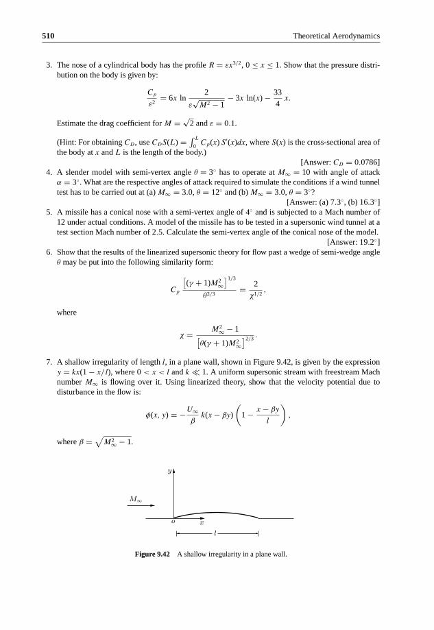
510 Theoretical Aerodynamics
3. The nose of a cylindrical body has the profile R = εx3/2, 0 ≤ x ≤ 1. Show that the pressure distri-bution on the body is given by:
Cp
ε2= 6x ln
2
ε√
M2 − 1− 3x ln(x) − 33
4x.
Estimate the drag coefficient for M = √2 and ε = 0.1.
(Hint: For obtaining CD, use CDS(L) = ∫ L
0Cp(x) S′(x)dx, where S(x) is the cross-sectional area of
the body at x and L is the length of the body.)[Answer: CD = 0.0786]
4. A slender model with semi-vertex angle θ = 3◦ has to operate at M∞ = 10 with angle of attackα = 3◦. What are the respective angles of attack required to simulate the conditions if a wind tunneltest has to be carried out at (a) M∞ = 3.0, θ = 12◦ and (b) M∞ = 3.0, θ = 3◦?
[Answer: (a) 7.3◦, (b) 16.3◦]5. A missile has a conical nose with a semi-vertex angle of 4◦ and is subjected to a Mach number of
12 under actual conditions. A model of the missile has to be tested in a supersonic wind tunnel at atest section Mach number of 2.5. Calculate the semi-vertex angle of the conical nose of the model.
[Answer: 19.2◦]6. Show that the results of the linearized supersonic theory for flow past a wedge of semi-wedge angle
θ may be put into the following similarity form:
Cp
[(γ + 1)M2
∞]1/3
θ2/3= 2
χ1/2,
where
χ = M2∞ − 1[
θ(γ + 1)M2∞]2/3 .
7. A shallow irregularity of length l, in a plane wall, shown in Figure 9.42, is given by the expressiony = kx(1 − x/l), where 0 < x < l and k � 1. A uniform supersonic stream with freestream Machnumber M∞ is flowing over it. Using linearized theory, show that the velocity potential due todisturbance in the flow is:
φ(x, y) = −U∞β
k(x − βy)
(1 − x − βy
l
),
where β =√
M2∞ − 1.
y
M1
l
xo
Figure 9.42 A shallow irregularity in a plane wall.

Compressible Flows 511
0.3c
M1 0.1c
0.7c
Figure 9.43 A two-dimensional wing profile in Mach 2.5 air stream.
M 10.03c
0.3cc
0.07c
Figure 9.44 A two-dimensional thin aerofoil in Mach 3.0 air stream.
8. A two-dimensional wing profile shown in Figure 9.43 is placed in a Mach 2.5 air stream at anincidence of 2◦. Using linearized theory, calculate the lift coefficient CL and the drag coefficient CD.
[Answer: CL = 0.06096 and CD = 0.04372].9. A two-dimensional thin aerofoil shown in Figure 9.44 is placed in Mach 3.0 air stream at an angle
of attack of 2◦. Using linearized theory, estimate Cpu and Cpl.[Answer:
Cpu = 0.211, Cpl = 0.046 (0 ≤ x ≤ 0.3c); Cpu = −0.1258, Cpl = −0.0551 (0.3c ≤ x ≤ c)]10. The two-dimensional aerofoil shown in Figure 9.45 is traveling at a Mach number of 3 and at an
angle of attack of 2◦. The thickness to chord ratio of the aerofoil is 0.1 and the maximum thicknessoccurs at 30 percent of the chord downstream from the leading edge. Using the linearized theory,show that the moment coefficient about the aerodynamic center is −0.035, the center of pressure isat 1.217c and the drag coefficient is 0.0354. Show also that the angle of zero lift is 0◦.
11. A two-dimensional wedge shown in Figure 9.46 moves through the atmosphere at sea-level, at zeroangle of attack with M∞ = 3.0. Calculate CL and CD using shock-expansion theory.
[Answer: CL = −0.0388, CD = 0.02265]12. Calculate the lift and drag coefficient experienced by a flat plate kept at an angle of attack of 5◦ to
an air stream at Mach 2.3 and pressure 101 kPa, using (a) shock–expansion theory and (b) Ackeret’stheory.
[Answer: (a) CL = 0.1735, CD = 0.0152, (b) CL = 0.1685, CD = 0.0147]
0.7c0.3c
0.1cM = 3.0
Figure 9.45 A two-dimensional aerofoil in a Mach 3 stream.
M1
c10◦
Figure 9.46 A two-dimensional wedge in a supersonic flow.

512 Theoretical Aerodynamics
13. Calculate the CL and CD for a half-wedge of wedge angle 5◦ kept in an air stream at Mach 2 and101 kPa at (a) 0◦ angle of attack, (b) at 3◦ angle of attack.
[Answer: (a) CL = − 0.054, CD = 0.00497, (b) CL = 0.1778, CD = 0.01554]14. If a2 = dP
dρgives the local speed of sound, obtain the following forms of Bernoulli’s equation.
(a) a2 dρ
ρ+ VdV = 0.
(b)2a
γ − 1da + VdV = 0.
(c)V 2
2= 1
γ − 1
(a2
0 − a2).
References
1. Rathakrishnan, E., Applied Gas Dynamics, John Wiley, NJ, 2010.
2. Rathakrishnan, E., Fluid Mechanics - An Introduction, 3rd edn. PHI Learning, Delhi, India, 2012.
3. Shapiro, A.H., The Dynamics and Thermodynamics of Compressible Fluid Flow, Vol. I, The Ronald Press Company,New York, 1953.
4. Liepmann H.W and Roshko A., Elements of Gas Dynamics, John Wiley & Sons, Inc. New York, 1957.
10Simple Flights
10.1 Introduction
So far we were focusing on the wing and its sectional profiles, considering the geometrical parameters ofthe aerofoil (wing) and the parameters of the flow to which it is exposed. The pressure loading, lift anddrag associated with aerofoil were discussed for both two-dimensional (infinite) and three-dimensionalwings. In this chapter, let us consider a complete flying machine and study some of the basic flightsassociated with it. A flying machine and its control surfaces are schematically shown in Figure 10.1
When the control surfaces are in their neutral positions the aircraft, like the aerofoil, has a medianplane of symmetry, and when properly located the center of gravity G lies in this plane.
The fixed fin of the aircraft is in the plane of symmetry, as shown in Figure 10.1. For simplicity, let usassume the aircraft to be in straight level (horizontal) flight, with all the control surfaces in their neutralpositions. The lift is generated by the wings (port and starboard wings) and tail (the lift associated withthe body of the aircraft is ignored). The thrust produced by the engine overcomes the drag, that is thethrust is assumed to be horizontal.
In Figure 10.1, the lateral axis Gy is perpendicular to the plane of symmetry and positive to starboard(that is to right). The symmetry will not be disturbed if the elevators are deflected. Raising the elevatorswill decrease the lift on the tail, and will cause a pitching moment, positive when the nose tends to belifted. Moving the rudder to starboard will cause a yawing moment, tending to deflect the nose to thestarboard, the positive sense.
The ailerons move in opposite senses, one up, one down, by a single motion by the control column.If we depress the port aileron and therefore simultaneously raise the starboard one, the lift on the portwing will increase and that on the starboard wing will decrease so that the rolling moment will be causedtending to dip the starboard wing, and this sense will be positive. This movement also causes a yawingmoment, for the drag on the two wings will likewise be altered. To minimize this the ailerons are generallygeared to move differentially so that one moves through a greater angle than the other.
Motion of ailerons or rudder will disturb the symmetry of the aircraft. A single-engine aircraft alsohas a dynamical asymmetry (tendency to tilt).
10.2 Linear Flight
When the aircraft velocity V is in a fixed straight line the flight is termed linear. When V is in the planeof symmetry the flight is termed symmetric. There are three types of linear symmetrical flight; gliding,
Theoretical Aerodynamics, First Edition. Ethirajan Rathakrishnan.© 2013 John Wiley & Sons Singapore Pte. Ltd. Published 2013 by John Wiley & Sons Singapore Pte. Ltd.
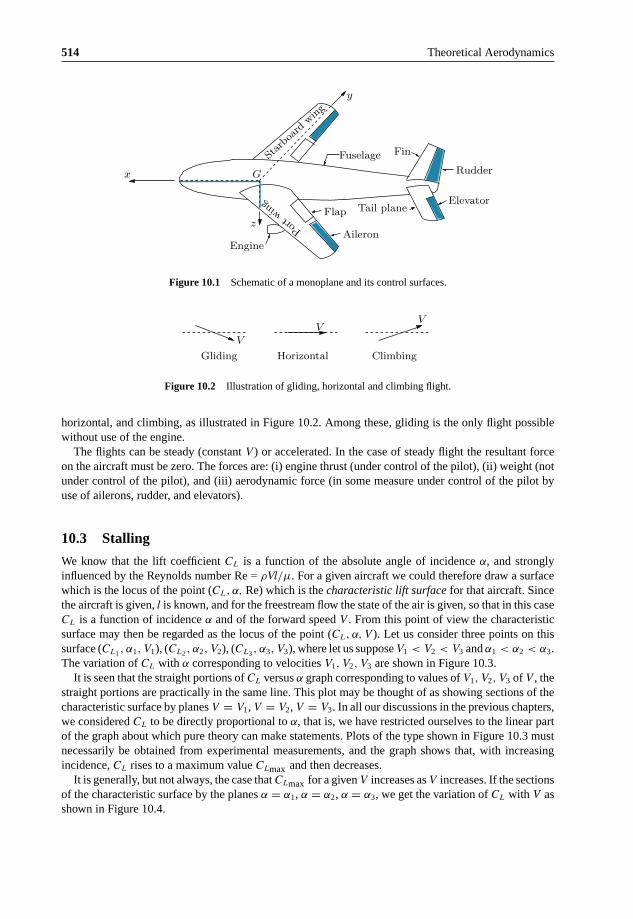
514 Theoretical Aerodynamics
Starbo
ardwing
Tail plane
Aileron
Elevator
Rudder
Fin
Engine
Fuselage
Flap
x G
z
y
Portwin
g
Figure 10.1 Schematic of a monoplane and its control surfaces.
V
Gliding Horizontal Climbing
VV
Figure 10.2 Illustration of gliding, horizontal and climbing flight.
horizontal, and climbing, as illustrated in Figure 10.2. Among these, gliding is the only flight possiblewithout use of the engine.
The flights can be steady (constant V ) or accelerated. In the case of steady flight the resultant forceon the aircraft must be zero. The forces are: (i) engine thrust (under control of the pilot), (ii) weight (notunder control of the pilot), and (iii) aerodynamic force (in some measure under control of the pilot byuse of ailerons, rudder, and elevators).
10.3 Stalling
We know that the lift coefficient CL is a function of the absolute angle of incidence α, and stronglyinfluenced by the Reynolds number Re = ρVl/μ. For a given aircraft we could therefore draw a surfacewhich is the locus of the point (CL, α, Re) which is the characteristic lift surface for that aircraft. Sincethe aircraft is given, l is known, and for the freestream flow the state of the air is given, so that in this caseCL is a function of incidence α and of the forward speed V . From this point of view the characteristicsurface may then be regarded as the locus of the point (CL, α, V ). Let us consider three points on thissurface (CL1 , α1, V1), (CL2 , α2, V2), (CL3 , α3, V3), where let us suppose V1 < V2 < V3 and α1 < α2 < α3.The variation of CL with α corresponding to velocities V1, V2, V3 are shown in Figure 10.3.
It is seen that the straight portions of CL versus α graph corresponding to values of V1, V2, V3 of V , thestraight portions are practically in the same line. This plot may be thought of as showing sections of thecharacteristic surface by planes V = V1, V = V2, V = V3. In all our discussions in the previous chapters,we considered CL to be directly proportional to α, that is, we have restricted ourselves to the linear partof the graph about which pure theory can make statements. Plots of the type shown in Figure 10.3 mustnecessarily be obtained from experimental measurements, and the graph shows that, with increasingincidence, CL rises to a maximum value CLmax and then decreases.
It is generally, but not always, the case that CLmax for a given V increases as V increases. If the sectionsof the characteristic surface by the planes α = α1, α = α2, α = α3, we get the variation of CL with V asshown in Figure 10.4.

Simple Flights 515
α
CL
V1
V2
V3
Figure 10.3 Lift curve slope variation with incidence for different velocities.
V
α3
CLmax
α2α1
CL
Figure 10.4 Lift curve slope variation with V in the sections of the characteristic surface cut by the planes α = α1,α = α2, α = α3.
The stalled state is that in which the airflow on the suction side of the aerofoil is turbulent. It isfound that, just before the stalled state sets in, the lift coefficient attains its maximum value, and thecorresponding speed is called the stalling speed. Thus the stalling speed corresponding to a given CLmaxcan be read from the continuous curve of Figure 10.4.
Stalling speed is a function of incidence. Variation of α with V in the sections of the characteristicsurface by planes CL = CL1 , CL = CL2 , CL = CL3 is as shown in Figure 10.5.
In Figure 10.5 the continuous line shows the stalling speed as a function of the stalling incidence αS .Any point (α, V ) above this curve corresponds to stalling flight, any point below it with normal flight.
It should be noted that the foregoing discussion only applies to speeds V such that the flow speed overthe aerofoil nowhere approaches the speed of sound, that is, we neglect variation with Mach number.
V
CL3
CL2
CL1
VS
αS
α
Figure 10.5 Variation of α with V in some sections of the characteristic surface.

516 Theoretical Aerodynamics
The graphs of the above type are all cases deduced from experiments, generally in wind tunnels forcondition corresponding to linear flight at constant speed. When the aircraft flies in a curved path thegraph will differ slightly from the above, but investigations made by Wieselsberger [Reference 9] showthat the changes are of the order of the square of the ratio of the span to radius of curvature of the pathand may therefore, in general, be neglected.
Moreover, for most calculations it is sufficient to substitute one of the CL graphs in Figure 10.3 for thewhole graph, namely the one which corresponds to the landing speed, because the danger of stalling isgenerally greatest when the aircraft is about to land and is therefore flying near to the stalling incidenceand at a low speed. When we substitute Reynolds number Re for velocity throughout, the foregoingconditions may be held to apply to a family of geometrically similar aircraft. For such a family there willbe one characteristic lift surface.
10.4 Gliding
For an aircraft gliding steadily with the engine off, as shown in Figure 10.6, the resultant aerodynamicforce Fad balances the weight W , that is:
Fad − W = 0.
Thus, if L and D, respectively, are the lift and drag acting on the aircraft:
L = W cos γ
D = W sin γ,
where γ is the angle which the direction of motion makes with the horizontal, called the gliding angle.Therefore:
tan γ = D
L= CD
CL
.
γ
α
G
W
D
V
L
Figure 10.6 An aircraft in steady glide.

Simple Flights 517
This equation expresses the gliding angle γ in terms of CL and CD. It should be noted that CL and CD
here are the lift and drag coefficients for the whole aircraft. The attitude of the aircraft is the angle whicha line fixed in the aircraft makes with the horizontal, as shown in Figure 10.6. If we measure the incidenceα and attitude θ from the same line we have θ = α − γ . Note that θ and α can be negative, as shown inFigure 10.6, but the glide angle γ is necessarily positive. Also note that the direction of the glide doesnot, in general, coincide with any fixed direction in the aircraft, in other words the attitude is a functionof the incidence α.
The extreme attitude is that assumed when the aircraft is diving vertically, the terminal velocity dive. Inthis case the lift vanishes, the incidence is that of zero lift, and if the dive is undertaken from sufficientlygreat height, the weight just balances the drag, the speed being the terminal speed, may be five or sixtimes the stalling speed. The attitude will then be about −90◦.
Example 10.1
A glider of aspect ratio 6 has a drag polar of:
CD = 0.02 + 0.06C2L.
Find the change in minimum angle of glide if the aspect ratio is increased to 10.
Solution
Let subscripts 1 and 2 refer to aspect ratio 6 and 10, respectively.
Given, 1 = 6, CD0 = 0.02, k = 1
πe 1
= 0.06.
Therefore, the wing efficiency is:
e = 1
0.06 × π × 6= 0.884.
For minimum glide angle, the drag should be minimum. For drag minimum, CD0 = kC2L, therefore,
0.06C2L1
= 0.02
CL1 =√
0.02
0.06= 0.577.
For 2 = 10:
k = 1
πe 2
= 1
π × 0.884 × 10= 0.036.

518 Theoretical Aerodynamics
Therefore,
CL2 =√
0.02
0.036= 0.745.
The drag coefficients for aspect ratios 6 and 10 are:
CD1 = 0.02 + 0.06 × 0.5772
= 0.04
CD2 = 0.02 + 0.036 × 0.7452
= 0.04.
Therefore, the gliding angles for these cases become:
γ1 = tan−1
(CD1
CL1
)
= tan−1
(0.04
0.577
)
= 3.966◦
γ2 = tan−1
(0.04
0.745
)
= 3.073◦.
The difference between the gliding angles is:
γ1 − γ2 = 3.966◦ − 3.073◦
= 0.893◦
= 0.893 × 60 (since 1◦ = 60′)
= 53.58′ .
10.5 Straight Horizontal Flight
The forces acting on an aircraft in straight horizontal flight is shown in Figure 10.7. There are threeforces; the thrust T , weight W , and aerodynamic force Fad acting on the aircraft. The components of Fadin the direction of V and normal to V , respectively, are the lift L and drag D.
By proper choice of chord the incidence may be taken equal to the attitude and
L = W − T sin θ
D = T cos θ.
In practice θ is small, so that T = D, L = W , and
CL = L12 ρV 2S
= W12 ρV 2S
= w12 ρV 2
, (10.1)

Simple Flights 519
T
D
W
L
GθV
Figure 10.7 Forces acting on an aircraft in steady level flight.
where w = W/S is called the wing loading, that is, the average load per unit area of wing plan. Whenw, ρ (that is altitude), and V are given, CL is determined, and therefore incidence from the CL versus α
graph (Figure 10.3).At the stalling speed VS , Equation (10.1) becomes:
CLmax = w12 ρV 2
S
. (10.2)
The stalling speed VS can be determined by plotting a graph of CLV 2 = 2w/ρ versus V and CL versusV together, as shown in Figure 10.8.
It is seen that the stalling speed VS increases with altitude (that is, with decrease of flow density ρ).From Equations (10.1) and (10.2), we have:
CL
(1
2ρV 2
)= CLmax
(1
2ρV 2
S
)= w . (10.3)
CLV2 =
2w
ρ
CL
VS V 0S V
CLV2 =
2w sec φ
ρ
CLmax
Figure 10.8 Plots of CL and CLV 2 variations with V .

520 Theoretical Aerodynamics
The air-speed indicator measures 12 ρV 2 but is graduated to read V . It is, therefore, correct only for the
particular value of the density ρ for which it is graduated, but, if we neglect variations of CLmax , it followsfrom Equation (10.3) that the aircraft will stall always at the same indicated airspeed when it is in straighthorizontal flight, whatever the height.
10.6 Sudden Increase of Incidence
Let us assume the aircraft to be flying steadily and horizontally, so that if CL′ is the lift coefficient:
CL′(
1
2ρV 2S
)= W,
a sudden increase of incidence will increase the lift coefficient to:
CL
(1
2ρV 2S
)
and the aircraft will acquire an upward acceleration f given by:
(CL − CL
′)(1
2ρV 2S
)= W
gf
so that it will begin to describe a curved path of radius of curvature r given by f = V 2/r, where:
r = 2W
Sgρ
1(CL − CL
′) = 2w
gρ
1(CL − CL
′) .
In this analysis we ignore the change in drag. If the speed is high, CL′ is small and CL cannot exceed
CLmax for speed V . Thus the absolute minimum value of r is given by:
rmin = 2w
gρCLmax= V 2
S
g, (10.4)
where VS is the appropriate stalling speed. Since CLmax is accompanied by a rather large drag, thetheoretical value of rmin in Equation (10.4) cannot be attained.
Example 10.2
An aircraft weighing 200 kN, wing span 12 m and mean chord 2 m is in steady level flight at sea level, at aspeed of 120 m/s. If the lift coefficient is suddenly increased by 10%, determine the upward accelerationcausing the lift increase.
Solution
Given, W = 200 kN, 2b = 12 m, c = 2 m, V = 120 m/s.

Simple Flights 521
In level flight:
L = W = 1
2ρV 2SC′
L.
At sea level, ρ = 1.225 kg/m3. Therefore:
C′L = L
12 ρV 2S
= 200 × 103
12 × 1.225 × 1202 × (12 × 2)
= 0.945.
The new lift coefficient is:
CL = 1.1 × C′L = 1.1 × 0.945
= 1.04.
The expression for upward acceleration f is:
W
gf = (
CL − C′L
) 1
2ρV 2S.
Hence:
f =(CL − C′
L
)12 ρV 2S g
W
= (1.04 − 0.945) 12 × 1.225 × 1202 × 24 × 9.81
200 × 103
= 0.986 m/s2 .
10.7 Straight Side-Slip
Consider an aircraft flying steadily and horizontally, as shown in Figure 10.9(a), to be rolled through anangle φ from the vertical, as shown in Figure 10.9(b) and held in this position by controls. The lift willno longer balance the weight.
LL
W
φ
W
Figure 10.9 An aircraft (a) in steady level flight and (b) rolled through an angle φ.

522 Theoretical Aerodynamics
If the aircraft is supposed to be flying towards us so that the starboard wing is dipped, the aircraft willaccelerate in the direction of the resultant of L and W , and will continue to accelerate until a steady stateis reached owing to the wind blowing across the body and producing a side force in the direction of thespan. The direction of motion is now inclined to the plane of symmetry at an angle β, say, measuredpositively when the direction of motion is to starboard. The aircraft is now moving crab-wise in thestraight path and is said to be sideslipping. If V is the speed, the component of V sin β perpendicular tothe plane of symmetry is called the velocity of side-slip.
Side-slip will neither diminish the drag nor increase the lift as compared to symmetrical flight at thesame speed. If D′ and L′ are the drag and lift, respectively, in the steady side-slip induced by the abovemaneuver then L′ < L, D′ > D. The gliding angle γ ′ will be given by:
tan γ ′(
= D′
L′
)> tan γ
(= D
L
)
or γ ′ > γ . The effect of side-slip is therefore to increase the gliding angle without reducing the speed.
10.8 Banked Turn
This is a steady motion in a horizontal circle with the plane of symmetry inclined to the vertical, as shownin Figure 10.10. The direction of motion is longitudinal and there is no side-force.
If φ is the angle of bank and r is the radius of the turn, then:
L cos φ = W
L sin φ = W
g
V 2
r
tan φ = V 2
g r.
If the differences due to the difference in speed at the outer and inner wing tips are ignored, then:
L = W sec φ
CL = w sec φ12 ρV 2
φ
V 2/r
W
L
Figure 10.10 An aircraft in a banked turn.

Simple Flights 523
and therefore, as in Figure 10.8, the stalling speed V ′S is determined by the intersection of the curves
CLV 2 versus V with CLmax versus V graph. From the relation:
CLmax
(12 ρV ′2
S
) = w sec φ (10.5)
it appears that banking increases the stalling speed, and if we treat CLmax as a constant, the increase is inthe ratio:
√sec φ : 1 .
10.9 Phugoid Motion
A phugoid is the path of a particle which moves under gravity in a vertical plane and which is acted uponby a force L normal to the path and proportional to V 2.
Since no work is done by force L, it follows that ( 12 V 2 − gz), the total energy of the particle (per unit
mass), is constant, z being the depth of the particle below horizontal line, when speed is V , as shown inFigure 10.11.
We can choose the position of this line so that the constant energy is zero, and then we shall have:
V 2 = 2g z. (10.6)
If θ is the inclination of the path to the horizontal, as in Figure 10.11, then:
L − W cos θ = W
g
V 2
R, (10.7)
where R is the radius of curvature.If we could imagine an aircraft flying at constant incidence, and so arrange that the thrust exactly
balances the drag, the center of gravity of the aircraft would describe a phugoid, for such a case L =12 ρV 2SCL and CL is constant for an incidence (if we neglect the effect of curvature of the path on liftcoefficient).
Now let us assume that V1 is the speed at which the aircraft would fly in steady straight horizontalflight at the same incidence as in the phugoid. Then:
W = 1
2ρV 2
1 SCL
θ
Datum line z = 0
z
W
V
L
Figure 10.11 An object in phugoid motion.

524 Theoretical Aerodynamics
so that Equation (10.7) will give:
V 2
V 21
− cos θ = V 2
gR
by Equation (10.6), V 2 = 2g z, V 21 = 2g z1, therefore the above equation becomes:
z
z1− cos θ = 2z
R. (10.8)
Now if ds is an element of the arc of the path in Figure 10.11, then:
1
R= dθ
ds, sin θ = −dz
ds. (10.9)
Therefore Equation (10.8) can be written in the equivalent form as follows:
d
dz
(z
12 cos θ
)= z
12
2z1
z12 cos θ = 1
2z1
z32
32
+ constant
cos θ = 1
3
z
z1+ constant
z12
.
Now let us assume that the “constant” to be C√
z1. Therefore:
cos θ = 1
3
z
z1+ C
√z1
z. (10.10)
Let us differentiate this with respect to θ:
d
dθ(cos θ) = d
dθ
[1
3
z
z1+ C
√z1
z
]
− sin θ = 1
3
1
z1
dz
dθ− C
√z1
1
2z− 3
2dz
dθ
− sin θ = dz
dθ
[1
3
1
z1− 1
2C
√z1 z− 3
2
].
From Equation (10.9), we have sin θ = −dz
ds, therefore:
dz
ds= dz
dθ
[1
3z1− C
2
√z1
z32
]
or
dθ
ds= 1
3z1− C
2
√z1
z32
.

Simple Flights 525
3z1
Datum
Figure 10.12 Phugoid along a horizontal straight line.
Datum
Figure 10.13 An aircraft in trochoidal-like paths.
Datum
Figure 10.14 An aircraft describing a loop.
But from Equation (10.9),dθ
ds= 1
R, therefore:
1
R= 1
3z1− C
2
√z1
z32
or
z1
R= 1
3− C
2
√z3
1
z3. (10.11)
It can be shown that in Equation (10.10), cos θ > 1 if C > 2/3, so that no phugoid is possible.If C = 2/3, Equation (10.10) gives cos θ = 1 so that θ = 0 and R = ∞. For this condition the phugoid
is along a horizontal straight line, at depth z, below the datum line.If C = 0, Equation (10.11) gives R = 3z1, and the phugoid reduces to a set of semicircles of radius
3z1. The cusps are on the datum line and the paths correspond to unsuccessful attempts at “loop the loop,”as shown in Figure 10.12.
For 0 < C < 2/3, the flight path will become trochoidal-like paths, as shown in Figure 10.13.If z1 and the initial values of z and θ are prescribed, Equation (10.11) shows that for a given value
of C there are two possible radii of curvature owing to the ambiguity sign of the square root. If there isa sudden gust, an aircraft describing a trochoidal-like paths as in Figure 10.13 will get into a loop, asshown in Figure 10.14.
10.10 The Phugoid Oscillation
Let an aircraft describing straight line phugoid, as shown in Figure 10.11, corresponding to C = 3/2,z = z1, cos θ = 1, have its path slightly disturbed, say by a gust. It may then begin to describe a sinuouspath of small slope, as in Figure 10.12, having the straight line as mean. This motion is called phugoid
526 Theoretical Aerodynamics
oscillation. Since the vertical upward acceleration is −d2z/dt2, and since cos θ = 1 to the first order, wehave, for the vertical motion:
L − W = −W
g
d2z
dt2
and therefore from Equation (10.10):
d2z
dt2+ gz
z1= g.
This is simple harmonic motion whose period is 2π/(z1/g), showing that the disturbed motion is stable.In terms of the speed V∞ the period is π
√2V∞/g.
Example 10.3
An aircraft weighing 105600 N flies at an altitude where the air density is 0.16 kg/m3. The wing area,aspect ratio and efficiency are 28 m2, 6 and 0.95, respectively. If the drag polar is:
CD = 0.01 + kC2L,
determine the speed and Mach number at which the aerodynamic efficiency will be maximum.
Solution
Given, W = 105600 N, S = 28 m2, = 6.Therefore:
k = 1
πe
= 1
π × 0.95 × 6= 0.05584.
For maximum aerodynamic efficiency, the drag has to be the minimum. For minimum drag, CD0 = kC2L.
Therefore, the lift coefficient becomes:
CLDmin=
√CD0
k
=√
0.01
0.05584= 0.423.

Simple Flights 527
At level flight, L = W . The speed for drag minimum becomes:
UDmin =√
W12 ρSCLDmin
=√
10560012 × 0.16 × 28 × 0.423
= 333.84 m/s .
From standard atmospheric table, for the altitude with density 0.16 kg/m3, the pressure is 11145.75 Pa.The corresponding speed of sound is:
a =√
γp
ρ
=√
1.4 × 11145.75
0.16= 312.3 m/s.
The Mach number corresponding to minimum drag is:
MDmin = UDmin
a
= 333.84
312.3
= 1.07 .
Example 10.4
An aircraft of mass 30 000 kg, with an elliptical wing of area 225 m2, aspect ratio 7 delivering constantthrust of 53 kN, is taking off at sea level. The maximum possible lift coefficient is 2.0 and the profiledrag coefficient while lift-off is 0.02 and the lift-off speed is 1.2 times the stalling speed. Assuming therolling resistance to be negligible, calculate the lift-off distance required.
Solution
Given m = 30000 kg, S = 225 m2, T = 53000 N, CLmax = 2.0, CD0 = 0.02, = 7.The stalling speed Vs is the speed in level flight, with CLmax . Thus:
Vs =√
W12 ρSCLmax
=√
30000 × 9.8112 × 1.225 × 225 × 2.0
= 32.68 m/s.

528 Theoretical Aerodynamics
Therefore, the lift-off speed is:
V = 1.2 × Vs
= 1.2 × 32.68
= 39.22 m/s.
The lift coefficient at lift-off becomes:
CL = W12 ρV 2S
= mg12 ρV 2S
= 30000 × 9.8112 × 1.225 × 39.222 × 225
= 1.388.
The drag coefficient at lift-off becomes:
CD = CD0 + C2L
πe
= 0.02 + + 1.3882
π × 1 × 7
= 0.108.
At lift-off, by force balance we have:
T − D = mdV
dt
T − 1
2ρV 2SCD = m
dV
dt
T −(
1
2× 1.225 × 225 × 0.108
)V 2 = m
dV
dt
T − 14.88 V 2 = mdV
dt.
We can writedV
dtas:
dV
dt= dV
ds
ds
dt= V
dV
ds.
where s is the distance along the run way, that is the distance travelled by the aircraft from starting to anyinstantaneous state. Therefore:
T − 14.88 V 2 = mVdV
ds.

Simple Flights 529
This gives:
ds = mV dV
T − 14.88 V 2= m
2
d(V 2)
T − 14.88 V 2.
Integrating from s = 0 (V = 0) to s = slo (V = V ), we have the lift-off distance as:
slo = m
2
∫ V
0
d(V 2)
T − 14.88 V 2
= m
2ln
(T
T − 14.88 V 2
)
= 30000
(2 × 14.88)× ln
(53000
53000 − (14.88 × 39.222)
)
= 1008.06 × ln
(53000
30111.46
)
= 569.94 m .
10.11 Summary
For a flying machine, when the control surfaces are in their neutral positions the aircraft, like the aerofoil,has a median plane of symmetry, and when properly located the center of gravity G lies in this plane.
For an aircraft in straight level (horizontal) flight, the lift generated by the wings balances the weightand the thrust produced by the engine overcomes the drag.
Raising the elevators will decrease the lift on the tail, and will cause a pitching moment and movingthe rudder will cause a yawing moment.
The ailerons move in opposite senses, one up, one down, by a single motion by the control column.If we depress the port aileron and therefore simultaneously raise the starboard one, the lift on the portwing will increase and that on the starboard wing will decrease so that the rolling moment will be causedtending to dip the starboard wing, and this sense will be positive. This movement also cause a yawingmoment, for the drag on the two wings will likewise be altered.
When the aircraft velocity V is in a fixed straight line the flight is termed linear. When V is in the planeof symmetry the flight is termed symmetric. There are three types of linear symmetrical flight; gliding,horizontal, and climbing.
The flights can be steady (constant V ) or accelerated. In the case of steady flight the resultant force onthe aircraft must be zero. The forces are: (i) engine thrust, (ii) weight, (iii) aerodynamic force.
The lift coefficient CL is a function of the absolute angle of incidence α, and strongly influenced bythe Reynolds number Re = ρVl/μ.
The stalled state is that in which the airflow on the suction side of the aerofoil is turbulent. Just beforethe stalled state sets in, the lift coefficient attains its maximum value, and the corresponding speed is calledthe stalling speed. Thus the stalling speed corresponds to a given CLmax . Stalling speed is a function ofincidence.
For an aircraft gliding steadily with the engine off the resultant aerodynamic force Fad balances theweight W , that is:
Fad − W = 0.

530 Theoretical Aerodynamics
Thus, if L and D, respectively, are the lift and drag acting on the aircraft:
L = W cos γ
D = W sin γ,
where γ is the angle which the direction of motion makes with the horizontal, called the gliding angle.The forces acting on an aircraft in straight horizontal flight are the thrust T , weight W , and aerodynamic
force Fad.By proper choice of chord the incidence may be taken equal to the attitude and
L = W − T sin θ
D = T cos θ.
In practice θ is small, so that T = D, L = W , and
CL = L12 ρV 2S
= W12 ρV 2S
= w12 ρV 2
,
where w = W/S is called the wing loading, that is, the average load per unit area of wing plan.At the stalling speed VS , CL becomes:
CLmax = w12 ρV 2
S
.
For aircraft flying steadily and horizontally, if CL′ is the lift coefficient:
CL′(
1
2ρV 2S
)= W.
A sudden increase of incidence will increase the lift coefficient to:
CL
(1
2ρV 2S
)
and the aircraft will acquire an upward acceleration f given by:
(CL − CL
′)(1
2ρV 2S
)= W
gf
so that it will begin to describe a curved path of radius of curvature r given by f = V 2/r, where:
r = 2W
Sgρ
1(CL − CL
′) = 2w
gρ
1(CL − CL
′) .

Simple Flights 531
In this analysis we ignore the change in drag. If the speed is high, CL′ is small and CL cannot exceed
CLmax for speed V . Thus the absolute minimum value of r is given by:
rmin = 2w
gρCLmax= V 2
S
g,
where VS is the appropriate stalling speed.When an aircraft flying steadily and horizontally is rolled through an angle φ from the vertical, the lift
will no longer balance the weight. If the aircraft is supposed to be flying towards us so that the starboardwing is dipped, the aircraft will accelerate in the direction of the resultant of L and W , and will continueto accelerate until a steady state is reached owing to the wind blowing across the body and producing aside force in the direction of the span. The direction of motion is now inclined to the plane of symmetryat an angle β, say, measured positively when the direction of motion is to starboard. The aircraft is nowmoving crab-wise in the straight path and is said to be sideslipping. If V is the speed, the component ofV sin β perpendicular to the plane of symmetry is called the velocity of side-slip.
Side-slip will neither diminish the drag nor increase the lift as compared to symmetrical flight at thesame speed.
A banked turn is a steady motion in a horizontal circle with the plane of symmetry inclined to thevertical. The direction of motion is longitudinal and there is no side-force.
A phugoid is the path of a particle which moves under gravity in a vertical plane and which is actedupon by a force L normal to the path and proportional to V 2.
Exercise Problems
1. If the lift coefficient of an aircraft is given by:
CL = b sin(
aα
b
),
find the maximum value of the lift coefficient, for b = 2, a = 2π.[Answer: 2]
2. Show that the minimum radius of a true banked turn, for a given angle of bank φ, is:
2w cosec φ
gρ CLmax.
3. Calculate the minimum initial radius of curvature of the path when an aircraft whose stalling speedis 110 km/h in straight flight has the incidence suddenly increased.
[Answer: 95.2 m]4. For small angle of bank, φ, show that the angle of side-slip is given by β = −2.5 CL φ, assuming the
coefficient of side force as cy = −0.4 β.5. An aircraft of wing loading 20 N/m2 makes a banked turn at an altitude where the freestream flow
density is 0.175 kg/m3. (a) If the minimum radius turn is 98 m and the bank angle is 20◦, determinethe CLmax . (b) What will be the stalling speed at that altitude if the aircraft is in level flight withoutbank?
[Answer: (a) 0.253, (b) 30.06 m/s]

532 Theoretical Aerodynamics
6. The aerodynamic efficiency of a sail plane of weight 3150 N and wing area 10 m2 is 30. If it is inlevel flight at sea level with a speed of 170 km/h, determine the drag coefficient.
[Answer: 0.0077]7. An aircraft weighing 23000 N has a span of 14 m and average chord of 1.2 m. If it flies with a velocity
of 90 m/s and angle of attack 4◦ in sea level (a) determine the lift curve slope. (b) If the aircraft glidessteadily with the same speed at a glide angle of 6◦, what will be the lift curve slope? (c) If the liftcoefficient during glide has to be the same as that in the level flight what should be the flight speed?
[Answer: (a) 3.954, (b) 2.65, (c) 90.24 m/s]8. An aircraft flies at a true speed of 350 m/s at an altitude where the pressure and temperature are
18.25 kPa and 216.5 K, respectively. (a) If a one-fourteenth scale model of the aircraft is to be tested,under dynamically similar conditions, in a wind tunnel with test-section temperature 288 K, whatshould be the pressure in the test-section? Assume the viscosity of air varies with temperature as T 3/4
approximately. (b) Show that the forces on the model will be about 10% of the corresponding forceson the prototype.
[Answer: (a) 365.26 kPa]9. An aircraft wing of span 10 m and mean chord 2 m is designed to develop 45 kN lift at freestream
velocity 400 km/h and density 1.2 kg/m3. A 1/20 scale model of the wing section is tested in a windtunnel at velocity 500 m/s and density 5.33 kg/m3. The total drag measured is 400 N. Assuming thewind tunnel data refer to a section of infinite span, calculate the total drag and aerodynamic efficiencyof the aircraft wing, assuming the load distribution to be elliptic.
[Answer: D = 2.649 kN, L/D = 16.99]

Further ReadingsAbbott, I.H. and Von Doenhoff, A.E., Theory of Wing Sections, Published by the authors, 1959.Bertin, J.J. and Smith, M.L., Aerodynamics for Engineers, Prentice-Hall International, Inc. NJ, 1988.Boas, M.L., Mathematical Methods in the Physical Sciences, 3rd edn. John Wiley & Sons, Inc., New York. 2006.Hoerner, S.F., Fluid Dynamic Drag, Published by the author, 1975.Houghten E.L and Carruthers N.R, Aerodynamics for Engineering Students, 3rd edn. Edward Arnold, London, 1982.Kuthe, A.M. and Chow, C.y., Foundations of Aerodynamics – Bases of Aerodynamic Design, 4th edn, John Wiley &
Sons, Inc., New York, 1986.Lamb, H., Hydrodynamics, 6th edn, Dover Publications, 1932.Liepmann H.W and Roshko A., Elements of Gas Dynamics, John Wiley & Sons, Inc. New York, 1957.Milne-Thomson, L.M, Theoretical Aerodynamics, 2nd edn. Macmillan & Co., Ltd, London, 1952.Rathakrishnan, E., Applied Gas Dynamics, John Wiley & Sons, Inc., NJ, 2010.Rathakrishnan, E., Fluid Mechanics – An Introduction, 3rd edn. PHI Learning, Delhi, India, 2012.Schlichting, H., Boundary Layer Theory, 4th edn. McGraw-Hill Book Co., New York, 1960.Shapiro, A.H., The Dynamics and Thermodynamics of Compressible Fluid Flow, Vol. I, The Ronald Press Company,
New York, 1953.
Theoretical Aerodynamics, First Edition. Ethirajan Rathakrishnan.© 2013 John Wiley & Sons Singapore Pte. Ltd. Published 2013 by John Wiley & Sons Singapore Pte. Ltd.


Index
Absolute incidence, 353, 397Acceleration
local, 32material, 32potential, 390
Aerodynamics, 1Aerodynamic center, 162, 268Aerodynamic efficiency, 4Aerodynamic force, 1, 12
coefficient of, 14parameters governing, 157, 177
Aerodynamic force andmoment coefficients, 17, 166
Aerodynamic twist, 353Aerofoil, 4, 19
cambered, 129definition of, 155mean camber line, 158, 161nomenclature, 157polar curve, 358section, 157symmetrical, 125, 138thickness distribution, 162trailing-edge angle, 162
Aerofoil characteristics, 155with general distribution, 339of asymmetrical loading, 372
Aerofoil geometry, 157NACA 4-digit series, 159NACA 5-digit series, 159NACA 6-digit series, 160NACA 7-digit series, 160NACA 8-digit series, 161
Aerofoils of smallaspect ratio, 387
Aileron, 4
Analysis of fluid flow, 31Angle of attack, 11, 157, 161Angle of downwash, 353Area-Mach number relation, 82Argand diagram, 107Aspect ratio, 163Average chord, 163
Banked turn, 522Barlow’s curve, 227Barotropic fluid, 410Basic and subsidiary laws, 34Bernoulli equation, 51, 216, 410Biot-Savart law, 207Biplane, 5Blenk’s method, 383Bluff body, 2Bodies of revolution, 423Boundary layer
definition of, 18equations, 40thickness, 90
Bound vortex, 199Boyle’s law, 35Bulk modulus of elasticity, 28
Calculation ofdownwash velocity, 385
Calorically perfect gas, 405Calorical state equations, 79Capillary action, 31Camber, 10, 134
of circular arc, 137lower, 10mean, 11upper, 10
Theoretical Aerodynamics, First Edition. Ethirajan Rathakrishnan.© 2013 John Wiley & Sons Singapore Pte. Ltd. Published 2013 by John Wiley & Sons Singapore Pte. Ltd.

536 Index
Camber line, 11, 134Cauchy-Riemann equations, 41Center of pressure, 155, 268Centered expansion, 476Change of aspect ratio
with incidence, 359Characteristics, 471Charles’ law, 35Chord
of an aerofoil, 8line, 11, 161of a profile, 7
Circular arc aerofoil, 269center of pressure
location of, 271Circular vortex, 236
size of, 239velocity distribution, 237
Circulation, 40, 188, 249critical, 61definition of, 188illustration of, 189physical meaning of, 230subcritical, 61supercritical, 61theorem, 250
Climbing flight, 514Coefficient of pressure, 300, 447Complex number, 107
argument of, 109conjugate of, 108principal value of, 109
Compound vortex, 229Compressibility, 28Compressible Bernoulli
equation, 410Compressible flows, 405
thermodynamics of, 405Compressible flow
basic potentialequation of, 420
equations, 413fundamental equation, 423
Compressible subsonic flow, 492Condition for vortex
drag minimum, 345Conformal transformation, 103Continuity equation, 35, 418Continuum, 25Conservation of energy, 34, 407Conservation of matter, 34Control mass system, 34Control surface, 4, 35Control volume, 34
Convection effect, 32Critical state, 80Crocco’s theorem, 414, 416Cylindrical rectangular
aerofoil, 372Cylindrical wing, 5, 9, 12
Darcy friction factor, 78d’Alembert’s paradox, 59, 94, 478Density, 24Detached shock, 463, 468Differential analysis, 35Dihedral angle, 164Dimensionless velocity, 81Displacement thickness, 38, 90Doublet, 46
axis of, 49stream function of, 48strength of, 47
Downwash, 332angle, 334for elliptic loading, 338for modified elliptic loading, 341
Drag, 2coefficient, 17induced, 213, 253, 334of bodies, 65of a supersonic profile, 483polar, 368pressure, 65profile, 156, 398
Eccentricity, 125, 128Effect of downwash
on incidence, 353Effect of operating
a flap, 288Effective incidence, 354Elevator, 4Elliptical distribution
characteristics, 335downwash for, 336drag due to downwash, 338lift for, 336
Elliptic loading, 356downwash for, 336downwash velocity for, 366induced drag for, 366lift for, 363lift and drag for, 357lift curve slope for, 359
Energy due to apair of vortices, 244
Energy thickness, 38

Index 537
Enthalpy, 29Entrance length
in a pipe, 76Entropy, 34, 407
change across a shock, 83, 461, 472Euler’s acceleration formula, 33Euler’s equation, 43Eulerian description, 32Exact Joukowski
pressure distribution, 147transformation, 146velocity distribution, 147
Expansion waves, 471
Fanno flow, 79Fin, 4Fineness ratio, 125Finite aerofoil theory, 331
spanwise loading and trailing vorticity, 331First law of thermodynamics, 34, 407Flap, 4, 162Flapped aerofoil, 283Flow deflection angle, 463Flow development length, 76Flow over a
wave-shaped wall, 491Flow past a
circular cylinder, 43with circulation, 59without circulation, 57
Flow past a half-body, 49Flow through pipes, 75
entrance length, 76fully developed, 76head loss for, 78
Flow with area change, 79–80Flow with friction, 84Flow with T0-change, 86Fluids, 23
definition of, 23Newtonian, 26non-Newtonian, 26properties of, 23
Force and momentcoefficients, 17, 166
Forced vortex, 223Force on a vortex, 244Form drag, 354Free spiral vortex, 226Free vortex, 45
strength of, 46Friction coefficient
definition of, 68Frictional drag, 95
Fully developed region, 76Fuselage, 4
Gas constant, 35, 79Gas dynamics
definition of, 78General linear solution
for supersonic flow, 486General motion, 183General thin aerofoil
theory, 258General thin aerofoil
section, 275L, M, kcp, of, 278
Geometric twist, 164Geometrical angle of attack, 161Geometrical incidence, 11Gliding, 514Gliding angle, 516Gothert’s rule, 431
for 3-D flow, 444to bodies of revolution and fuselage,
454to wings of finite span, 447
Gradient operator, 33Graphical description
of fluid motion, 33
Helmholtz’s theorems, 195first, 195, 202fourth, 220second, 216third, 220
Hinge moment coefficient, 286Horizontal flight, 2, 518Hydrostatic pressure
distribution, 23Hypersonic regime, 28Hypersonic similarity, 442
parameter, 443
Ideal gas, 35Image of a vortex, 241Impact pressure, 88Incidence, 11, 353Incompressible flow
definition of, 12, 15Increase of entropy
principle, 34Induced drag, 213, 334
for elliptic loading, 366minimum, 369
Induced downwash, 213Induced lift, 382

538 Index
Induced velocity, 389Infinite vortex, 211Integral and differential analysis, 35Integral analysis, 90Integral equation
for circulation, 355Irrotational flow, 416–417Isentropic flow, 79, 409, 497Isentropic process relation, 408Isentropic relations, 80
Jet flap, 288Joukowski hypothesis, 137Joukowski transformation, 119, 122Joule’s law, 406
Kelvin’s circulationtheorem, 197
Kinematics of fluid flow, 35Kinematic viscosity
coefficient, 88Kutta condition, 139
applied to airfoils, 139in aerodynamics, 140
Kutta-Joukowskitheorem, 212transformation
function, 122
Lagrangian description, 31Laminar aerofoil, 69Laminar flow, 75Laminar sublayer, 37Lancaster–Prandtl
lifting line theory, 347Laplace equation, 418, 429
basic solutions of, 418Lateral axis, 513Laws of vortex motion, 194Lift, 1, 2
coefficient, 17elliptic loading, 357on the aerofoil, 372of Joukowski aerofoil, 141
Lift and drag by impulse method,370
Lifting line theory, 347Lifting surface, 391Lifting surface theory, 378Line vortex, 192Linear flight, 513Linear vortex of finite length, 210Local rates of change, 32Longitudinal axis, 157
Mach angle, 456Mach angle-Mach number
relation, 470Mach line, 470Mach number
definition of, 14Mach wave, 456Magnus effect, 63, 95Mass
definition of, 24Material rates of change, 32Mayer’s relation, 407Mean aerodynamic chord, 164Mean camber line, 134, 158, 161Moment coefficient, 17, 166Momentum equation, 36, 89, 408Momentum thickness, 38Monoplane
main features of, 4types of, 5
Moving disturbance, 455Munk’s reciprocal theorem, 382Munk’s theorem of stagger, 382Mutual action of two vortices, 244
NASA aerofoils, 161Navier-Stokes equations, 36Newtonian fluid, 88Non-Newtonian fluid, 88Normal axis, 9, 372Normal shock, 82
relations, 82total pressure across, 462
Oblique shock, 463relations, 464θ-β-M relation, 467strong, 469weak, 469
Oswald wing efficiency, 368
Panel method, 297Parameters governing
the aerodynamic forces, 157Pathline, 33Percentage camber, 134Perfect gas, 79, 405Phugoid motion, 523Phugoid oscillation, 525Physical meaning of circulation, 230Physical plane, 103Pitching moment, 156
coefficient, 170Plane of symmetry, 4, 513

Index 539
Point rectilinear vortex, 239Poise, 26Poisson’s equation, 204Potential flow, 37, 42Potential equation for bodies of
revolution, 423Potential function, 41Prandtl-Glauert rule
for subsonic flow, 429supersonic flow, 436
Prandtl-Glauerttransformations, 429
Prandtl liftingline theory, 347
Prandtl-Meyer function, 82, 477Prandtl relation, 502Pressure
definition of, 23static, 24total, 24
Pressure coefficientdefinition of, 51
Pressure drag, 59, 65, 67Pressure loss, 67Pressure distribution on Joukowski
aerofoil, 144Pressure-hill, 51Profile, 4Profile drag, 156Pure rotation, 183Pure translation, 183
Quarter chord point, 9
Radial flow, 226Rankine’s half-body, 50
pressure distribution over, 51Rankine’s theorem, 52Rarefied flow, 31, 65Ratio of specific heats, 29Rayleigh flow, 79, 86Rectangular aerofoil, 371Rectilinear vortices, 235Reynolds number, 14
critical, 64lower, 64upper, 64
definition of, 14Reynolds stress, 74Rolling moment, 157Root chord, 163Rotational and irrotational motion, 40Rotational flow, 183Rudder, 4
Scale effect, 15Section lift coefficient, 168Semi-infinite vortex, 211Separation point, 39Separation, 66Separation process
illustration of, 66Shock
angle, 83definition of, 82detached, 463, 468normal, 82oblique, 82strength, 461
Shock-expansion theory, 477Side-slip, 521Similarity rule, 429Simple flights, 513Simple vortex, 45Singularities, 107Singular points, 107Skin friction, 18Skin friction coefficient
definition of, 68drag, 68
Small perturbation theory, 420Solution of nonlinear
potential equation, 425Source panel method, 297
governing equation of, 300pressure distribution
around cylinder, 305accuracy of, 302
Span, 4Specific heat, 28
at constant pressure, 29at constant volume, 29
Speed of sound, 12Stalling, 514Starting vortex, 137, 139Steady flow, 32Stoke’s theorem, 200, 206, 246Source and sink, 43Source-sink pair, 46State equation
calorical, 79thermal, 79
Straight horizontal flight, 518Streakline, 33Streamline, 33Streamline analogy, 431, 435Streamlined body, 2Stream function, 41
for simple vortex, 45

540 Index
Stream function (Continued )for sink, 44for source, 44
Streamtube, 33Subsonic flow, 28, 429, 436Supersonic flow, 28, 429, 436
over a wedge, 469Sudden increase in
incidence, 520Supersonic compression, 473Supersonic expansion, 475Supersonic flow, 405, 429Supersonic regime, 28Surface tension, 30Sweep angle, 164System and control volume, 34
Taper ratio, 164Temperature, 24
static, 24Thermal conductivity of air, 27Thermal equation of state, 35Thermally perfect gas, 79Thermodynamic properties, 28Thickness-to-chord ratio, 11, 128
of cambered aerofoil, 132Thin aerofoil theory, 257, 479
application of, 480Thompson’s vortex theorem, 197,
250Timelines, 34Tip chord, 163Tip vortex, 213Trailing vortex drag, 334Transformation of circle
to camberedaerofoil, 129
to circular arc, 134to ellipse, 124to straight line, 123to symmetrical
aerofoil, 125Transformation of flow pattern, 115Transformation function, 103, 115,
119Transformed plane, 103Transition point, 39Transonic flow, 28Trim, 156, 176Trim drag, 156Triplane, 4Turbulence, 70
description of, 70number, 72
Turbulent boundary layer, 68, 73, 96Twisted wing, 12Two-dimensional
compressible flows, 429, 485
Universal gas constant, 406Unsteady flow, 32
Velocity distribution, 147, 237on Joukowski aerofoil, 144
Velocity potential, 41, 183Velocity of sound, 80Viscosity, 25
absolute coefficient of, 25dynamic coefficient of, 26kinematic coefficient of, 27Maxwell’s equation for, 26Newton’s law of, 26Sutherland’s relation, 27
Viscous flows, 58, 63von Karman rule for
transonic flow, 439, 454application to wings, 454
Vortex betweenparallel plates, 242
Vortex drag, 334, 343condition for minimum, 345for modified loading, 343
Vortex motiondefinition of, 45
Vortex pair, 240Vortex panel method, 297, 302
application of, 302governing equation of, 303
Vortex theorems, 196Vortex theory, 183Vortex tube, 194Vorticity, 40
equation inpolar coordinates, 186rectangular coordinates, 184
Wake, 59, 66Wall shear stress, 68Wash-in, 164Wash-out, 164Wave drag, 478Weak oblique shock, 469Wing, 4
cylindrical, 5, 8geometry of, 5low-wing, 5high-wing, 5mid-wing, 5

Index 541
parasol-wing, 5planform area, 168port, 4profile, 4, 5shoulder wing, 5span, 5, 163starboard, 5tips, 4twist, 11
Wing geometricalparameters, 162
Wing loading, 519
Yawing moment, 65, 156–7, 177
Zero aspect ratio, 390Zone of action, 455–6Zone of silence, 455–6