Numerical simulations of flapping foil and wing aerodynamics

Numerical simulations of flapping foil

and wing aerodynamics

Mesh deformation using radial basis functions

Copyright c© 2009 by F.M. Bos

All rights reserved. No part of this material protected by this copyright noticemay be reproduced or utilized in any form or by any means, electronic or mechan-ical, including photocopying, recording or by any other information storage andretrieval system, without written permission from the copyright owner.

Printed by Ipskamp Drukkers B.V. in The Netherlands

ISBN: 978-90-9025173-8

An electronic version of this thesis is available at http://repository.tudelft.nl

Numerical simulations of flapping foil

and wing aerodynamics

Mesh deformation using radial basis functions

Proefschrift

ter verkrijging van de graad van doctoraan de Technische Universiteit Delft,

op gezag van de Rector Magnificus Prof. ir. K.C.A.M. Luyben,voorzitter van het College voor Promoties,

in het openbaar te verdedigen op woensdag 24 februari 2010 om 10:00 uur

door

Frank Martijn BOS

ingenieur luchtvaart en ruimtevaartgeboren te Naaldwijk.

Dit proefschrift is goedgekeurd door de promotor:

Prof. dr. ir. drs. H. Bijl

Copromotor:

Dr. ir. B.W. van Oudheusden

Samenstelling promotiecommissie:

Rector Magnificus, voorzitterProf. dr. ir. drs. H. Bijl Technische Universiteit Delft, promotorDr. ir. B.W. van Oudheusden Technische Universiteit Delft, copromotorProf. dr. ir. P.G. Bakker Technische Universiteit DelftProf. dr. ir. B. Koren Universiteit Leiden

Centrum Wiskunde & InformaticaProf. dr. H. Jasak Zagreb UniversityProf. dr. F-O. Lehmann University of UlmProf. dr. W. Shyy The University of Michigan

This research was supported by The NetherlandsOrganisation for Scientific Research (NWO),NWO-ALW grant 814.02.019.

Voor mijn ouders

Summary

Both biological and engineering scientists have always been intrigued by the flightof insects and birds. For a long time, the aerodynamic mechanism behind flap-ping insect flight was a complete mystery, until several decades ago. Experimentsshowed the presence of a vortex on top of the flapping wings, generates forceslarger than obtained by using conventional aircraft aerodynamics. Flapping wingsproduce both lifting and propulsive forces such that it becomes possible for insectsand smaller bird species, e.g. hummingbirds, to stay aloft and hover, but also toperform extreme manoeuvres. Because of this versatility, insects and smaller birdsare an inspiration for the development of flapping wing Micro Air Vehicles, smallman-made flyer’s to use in exploration and surveillance.

Several flow visualisation experiments and numerical simulations have beenperformed to improve the understanding of flapping wing aerodynamics in orderto design and optimise Micro Air Vehicles. However, the effects of wing kinemat-ics on the flow and forces is still not fully understood. We performed two- andthree-dimensional numerical simulations in order to systematically vary relevantparameters, related to the wing motion and flow physics. In order to capture theboundary layer and the near wake, it is important to maintain a high mesh qualitynear the moving wing, especially at large rotations. Therefore, an accurate meshmotion technique is necessary, which is able to cope with large mesh deformations.In order to incorporate a flapping wing in our numerical model, different mesh mo-tion techniques are compared and improved. The overall goal of this part of theresearch is to develop a reliable mesh deformation technique, in terms of accuracyand efficiency, to solve the flow around flapping wings.

The flow around flapping wings, at the scale relevant to insect flight, is highlyunsteady and vortical, described by the unsteady incompressible Navier-Stokesequations. Different dimensionless numbers are discussed, characterising the flow,i.e. Strouhal and Reynolds numbers. Since the flow at the considered Reynoldsnumber, Re = O(100), is laminar, there is no need for additional turbulencemodelling, such that our simulations, assuming laminar flow, may be treated as a

iv Summary

Direct Numerical Simulation (DNS).

In order to solve the unsteady incompressible Navier-Stokes equations, the com-mercial software Fluentr and the open-source code OpenFOAMr have been usedextensively. Different mesh motion solvers are compared. Two existing methodsare assessed, solving the Laplace and a modified stress equation. Both methodsare very efficient by using iterative solver techniques. However, these mesh motionsolvers are not able to maintain high mesh quality at large rotation angles, whichoccur in insect flight. Therefore, a new mesh motion solver is implemented, whichis based on the interpolation of radial basis functions.

This mesh motion solver is a point based method, which means that the dis-placement of all individual internal mesh points are evaluated, based on a givenboundary displacement, and updated accordingly. No mesh connectivity informa-tion is necessary, so that it can be applied to unstructured polyhedral meshes.To increase its efficiency, a coarsening is applied to the set of moving boundarypoints, such that only selected control points are used. This decreases the size ofthe system of equations and associated computational effort considerably.

After the discussion of the governing equations, finite volume discretisation inOpenFOAMr and the assessment of the mesh motion solvers, the physical andnumerical modelling are described. The incompressible Navier-Stokes equationsare rewritten in the rotating reference frame in order to identify dimensionlessnumbers related to the wing motion. The most important number is the Rossbynumber, which represents the wing stroke path curvature.

First a two-dimensional study is performed to investigate the effects of differ-ent wing kinematic models, with increasing complexity, on hovering flight perfor-mance. The results show that the ‘sawtooth’ amplitude has a small effect on themean lift but the mean drag is affected significantly. The second model simplifica-tion, the ‘trapezoidal’ angle of attack, caused the leading-edge vortex to separateduring the translational phase. This led to an increase in mean drag during eachhalf-stroke. The extra ‘bump’ in angle of attack as used by the fruit fly model isnot affecting the mean lift to a large extent. The other realistic kinematic featureis the deviation, which is found to have only a marginal effect on the mean lift andmean drag in this two-dimensional study. However, the effective angle of attack isaltered such that the deviation leads to levelling of the force distribution.

Additionally, a numerical model for two-dimensional flow was used to investi-gate the effect of foil kinematics on the vortex dynamics around an ellipsoid foilsubject to prescribed flapping motion over a range of dimensionless wavelengths,dimensionless amplitudes, angle of attack amplitudes, and stroke plane angles.Both plunging and rotating motions are prescribed by simple harmonic functionswhich are useful for exploring the parametric space despite the model simplicity.Optimal propulsion using flapping foil exists for each variable which implies thataerodynamics might select a range of preferable operating condition. The condi-tions that give optimal propulsion lie in the synchronisation region in which theflow is periodic.

Furthermore, different results relevant to three-dimensional flapping wing aero-

v

dynamics, are described. First, the flow around a dynamically scaled model wingis solved for different angles of attack in order to study the force developmentand vortex dynamics at small and large mid-stroke angle of attack. Secondly, theRossby number is varied at different Reynolds numbers. A varying Rossby numberrepresents a variation in stroke path curvature and thus angular acceleration. It isshown that a low Rossby number is beneficial for the stability of the leading-edgevortex, leading to an increase in lift and efficiency. Thirdly, the three-dimensionalwing kinematics is varied by changing the shape in angle of attack and by applyinga deviation, which may cause a ‘figure-of-eight’ pattern. As in two-dimensionalstudies, the deviation may influence the force distribution to a large extent, bychanging the effective angle of attack. Additionally, the three-dimensional flow iscompared with the two-dimensional studies performed on flapping forward flight.

Finally, a preliminary investigation is performed to show the effect of wingflexing. Therefore, a pre-defined flexing deformation is applied to a plunging airfoilin two-dimensional forward flight and to a three-dimensional flapping wing inhovering flight. Concerning the flexible airfoil in forward flight, a similar behaviourwas observed as for a rigid plunging airfoil, subjected to additional rotation.

The present simulations have led to important insight to understand the influ-ence of wing kinematics and deformation on the aerodynamic performance. Theseresults may be important to design and optimise Micro Air Vehicles.

Contents

Summary iii

1 Introduction 11.1 Motivation . . . . . . . . . . . . . . . . . . . . . . . . . . . . . . . 11.2 Physics of flapping flight . . . . . . . . . . . . . . . . . . . . . . . . 21.3 Experimental and numerical methods . . . . . . . . . . . . . . . . 71.4 Objectives and approach . . . . . . . . . . . . . . . . . . . . . . . . 9

2 Finite volume discretisation 132.1 Introduction . . . . . . . . . . . . . . . . . . . . . . . . . . . . . . . 132.2 The Navier-Stokes equations . . . . . . . . . . . . . . . . . . . . . . 16

2.2.1 Constitutive relations . . . . . . . . . . . . . . . . . . . . . 172.2.2 Incompressible laminar flow simplifications . . . . . . . . . 182.2.3 Dimensionless numbers . . . . . . . . . . . . . . . . . . . . 18

2.3 Spatial and temporal discretisation . . . . . . . . . . . . . . . . . . 192.4 Measures of cell quality . . . . . . . . . . . . . . . . . . . . . . . . 202.5 Discretisation of an incompressible momentum equation . . . . . . 21

2.5.1 Face interpolation schemes . . . . . . . . . . . . . . . . . . 232.5.2 Convection term . . . . . . . . . . . . . . . . . . . . . . . . 232.5.3 Diffusion term . . . . . . . . . . . . . . . . . . . . . . . . . 242.5.4 Temporal term . . . . . . . . . . . . . . . . . . . . . . . . . 25

2.6 Boundary conditions . . . . . . . . . . . . . . . . . . . . . . . . . . 262.7 Solution of the Navier-Stokes equations . . . . . . . . . . . . . . . 27

2.7.1 Pressure equation and Pressure-Velocity coupling . . . . . . 282.7.2 Procedure for solving the Navier-Stokes equations . . . . . 292.7.3 Arbitrary Lagrangian Eulerian approach . . . . . . . . . . . 30

viii Contents

2.8 Swept volume calculation . . . . . . . . . . . . . . . . . . . . . . . 322.9 Numerical flow solvers . . . . . . . . . . . . . . . . . . . . . . . . . 332.10 Code validation and verification . . . . . . . . . . . . . . . . . . . . 34

2.10.1 2D vortex decay and convection . . . . . . . . . . . . . . . . 352.10.2 Validation using cylinder flows . . . . . . . . . . . . . . . . 39

2.11 Conclusions . . . . . . . . . . . . . . . . . . . . . . . . . . . . . . . 46

3 Mesh deformation techniques for flapping flight 493.1 Introduction . . . . . . . . . . . . . . . . . . . . . . . . . . . . . . . 503.2 Different mesh deformation techniques . . . . . . . . . . . . . . . . 52

3.2.1 Laplace equation with variable diffusivity . . . . . . . . . . 533.2.2 Solid body rotation stress equation . . . . . . . . . . . . . . 543.2.3 Radial basis function interpolation . . . . . . . . . . . . . . 55

3.3 Mesh quality measures . . . . . . . . . . . . . . . . . . . . . . . . . 583.4 Comparison of mesh motion solvers . . . . . . . . . . . . . . . . . . 59

3.4.1 Translation and rotation of a two-dimensional block . . . . 593.4.2 Flapping of a three-dimensional wing . . . . . . . . . . . . . 623.4.3 Flexing of a two-dimensional block . . . . . . . . . . . . . . 64

3.5 Improving computational efficiency . . . . . . . . . . . . . . . . . . 663.5.1 Boundary point coarsening and smoothing . . . . . . . . . . 673.5.2 Iterative techniques and parallel implementations . . . . . . 69

3.6 Conclusions . . . . . . . . . . . . . . . . . . . . . . . . . . . . . . . 70

4 Physical and numerical modelling of flapping foils and wings 734.1 Introduction . . . . . . . . . . . . . . . . . . . . . . . . . . . . . . . 734.2 Governing equations for flapping wings . . . . . . . . . . . . . . . . 754.3 Wing shape and kinematic modelling . . . . . . . . . . . . . . . . . 78

4.3.1 Wing shape and planform selection . . . . . . . . . . . . . . 794.3.2 Kinematic modelling . . . . . . . . . . . . . . . . . . . . . . 804.3.3 Modelling of active wing flexing . . . . . . . . . . . . . . . . 824.3.4 Numerical implementation of the wing kinematics . . . . . 83

4.4 Dynamical scaling of flapping wings . . . . . . . . . . . . . . . . . 864.5 Computational domain and boundary conditions . . . . . . . . . . 884.6 Definition of force and performance coefficients . . . . . . . . . . . 894.7 Conclusions . . . . . . . . . . . . . . . . . . . . . . . . . . . . . . . 92

5 Influence of wing kinematics in two-dimensional hovering flight 935.1 Introduction . . . . . . . . . . . . . . . . . . . . . . . . . . . . . . . 94

5.1.1 Similarity and discrepancy between two- andthree-dimensional flows . . . . . . . . . . . . . . . . . . . . 94

5.1.2 Influence of kinematic modelling . . . . . . . . . . . . . . . 945.2 Numerical simulation methods . . . . . . . . . . . . . . . . . . . . 96

5.2.1 Flow solver and governing equations . . . . . . . . . . . . . 965.2.2 Mesh generation and boundary conditions . . . . . . . . . . 97

Contents ix

5.2.3 Validation using harmonic wing kinematics . . . . . . . . . 995.3 Modelling insect wing kinematics . . . . . . . . . . . . . . . . . . . 99

5.3.1 Insect wing selection and model parameters . . . . . . . . . 1005.3.2 Dynamical scaling of the wing model . . . . . . . . . . . . . 1015.3.3 Force and performance indicators . . . . . . . . . . . . . . . 1025.3.4 Different wing kinematic models . . . . . . . . . . . . . . . 103

5.4 Results and Discussion . . . . . . . . . . . . . . . . . . . . . . . . . 1055.4.1 Overall model comparison . . . . . . . . . . . . . . . . . . . 1055.4.2 Kinematic features investigation . . . . . . . . . . . . . . . 109

5.5 Conclusions . . . . . . . . . . . . . . . . . . . . . . . . . . . . . . . 118

6 Vortex wake interactions of a two-dimensional flapping foil 1216.1 Introduction . . . . . . . . . . . . . . . . . . . . . . . . . . . . . . . 1226.2 Flapping foil parametrisation . . . . . . . . . . . . . . . . . . . . . 1226.3 Force coefficients and performance . . . . . . . . . . . . . . . . . . 1246.4 Numerical model . . . . . . . . . . . . . . . . . . . . . . . . . . . . 1256.5 Results and discussion . . . . . . . . . . . . . . . . . . . . . . . . . 126

6.5.1 Influence of dimensionless wavelength . . . . . . . . . . . . 1266.5.2 Influence of dimensionless amplitude . . . . . . . . . . . . . 1276.5.3 Influence of angle of attack amplitude . . . . . . . . . . . . 1296.5.4 Influence of stroke plane angle . . . . . . . . . . . . . . . . 1306.5.5 Discussion . . . . . . . . . . . . . . . . . . . . . . . . . . . . 130

6.6 Conclusions . . . . . . . . . . . . . . . . . . . . . . . . . . . . . . . 132

7 Vortical structures in three-dimensional flapping flight 1357.1 Introduction . . . . . . . . . . . . . . . . . . . . . . . . . . . . . . . 1357.2 Three-dimensional flapping wing simulations . . . . . . . . . . . . 137

7.2.1 Modelling and parameter selection . . . . . . . . . . . . . . 1387.2.2 Simulation strategy and test matrix selection . . . . . . . . 141

7.3 Flow solver accuracy . . . . . . . . . . . . . . . . . . . . . . . . . . 1437.4 Vortex identification methods for flow visualisation . . . . . . . . . 1457.5 Flapping wings at low Reynolds numbers . . . . . . . . . . . . . . 148

7.5.1 The angle of attack in flapping flight . . . . . . . . . . . . . 1497.5.2 Influence of flapping stroke curvature . . . . . . . . . . . . . 1497.5.3 Influence of Reynolds number . . . . . . . . . . . . . . . . . 1527.5.4 Influence of ‘trapezoidal’ angle of attack . . . . . . . . . . . 1587.5.5 Influence of deviation . . . . . . . . . . . . . . . . . . . . . 160

7.6 Flapping wings in forward flight . . . . . . . . . . . . . . . . . . . . 1637.7 Conclusions . . . . . . . . . . . . . . . . . . . . . . . . . . . . . . . 166

8 Influence of wing deformation by flexing 1718.1 Airfoil flexing in two-dimensional forward flapping flight . . . . . . 1718.2 Wing flexing in three-dimensional hovering flight . . . . . . . . . . 1758.3 Conclusions . . . . . . . . . . . . . . . . . . . . . . . . . . . . . . . 177

x Contents

9 Conclusions and recommendations 1799.1 Overall conclusions . . . . . . . . . . . . . . . . . . . . . . . . . . . 1799.2 Conclusions on mesh motion techniques . . . . . . . . . . . . . . . 1809.3 Conclusions on hovering flapping flight . . . . . . . . . . . . . . . . 181

9.3.1 Two-dimensional hovering . . . . . . . . . . . . . . . . . . . 1819.3.2 Three-dimensional hovering . . . . . . . . . . . . . . . . . . 182

9.4 Conclusions on forward flapping flight . . . . . . . . . . . . . . . . 1849.4.1 Two-dimensional forward flapping . . . . . . . . . . . . . . 1849.4.2 Three-dimensional forward flapping . . . . . . . . . . . . . 184

9.5 Preliminary conclusions on wing flexing . . . . . . . . . . . . . . . 1859.6 Recommendations . . . . . . . . . . . . . . . . . . . . . . . . . . . 186

A Grid generation for flapping wings 189A.1 Introduction . . . . . . . . . . . . . . . . . . . . . . . . . . . . . . . 189A.2 BlockMesh . . . . . . . . . . . . . . . . . . . . . . . . . . . . . . . 190A.3 Gambit . . . . . . . . . . . . . . . . . . . . . . . . . . . . . . . . . 191A.4 GridPror . . . . . . . . . . . . . . . . . . . . . . . . . . . . . . . . 191A.5 Conclusions . . . . . . . . . . . . . . . . . . . . . . . . . . . . . . . 192

B Flow solver settings 195B.1 Introduction . . . . . . . . . . . . . . . . . . . . . . . . . . . . . . . 195B.2 Fluentr solver settings . . . . . . . . . . . . . . . . . . . . . . . . . 195B.3 OpenFOAMr solver settings . . . . . . . . . . . . . . . . . . . . . 197

Bibliography 201

Samenvatting 213

Acknowledgements 217

Curriculum Vitae 219

CHAPTER 1

Introduction

1.1 Motivation

The year of writing, 2009, is known as the year of Charles Darwin (1809-1882),since he was born 200 years ago. At the age of 50, he published his world famousOrigin of Species. That book describes the natural selection, inspired by his scien-tific observations during a voyage (1831-1836) around the world with his ship, theBeagle. At the Galapagos Archipelago, Darwin discovered slightly different birdspecies living on the different islands, whereas, he only knew one species on themainland of South-America. Apparently, the mainland bird species had travelledto the islands and on every different island it adapted to the differences in environ-mental circumstances. This process has become known as natural selection, whichis also applicable to the early era of flight, millions of years ago. Birds are ancientdescendants of feathered dinosaurs (Templin, 2000) which developed the skill offlight in order to migrate over large distances and to catch prey. Long before theorigin of dinosaurs and birds, insects adapted to leave the ground to take off intothe thin air. Birds and insects are both flapping their wings at different lengthscales, leading to a different flow behaviour. The larger the animal, the lower theneed for flapping wings, e.g. the Andean Condor only flaps when it looses heightin the thermal winds, whereas a small insect, a fruit fly (Weish-Fogh & Jensen,1956) flaps with about 200 times per second.

Flapping wings produce both lifting and propulsive forces, such that it becomespossible for insects and even smaller bird species, e.g. hummingbirds, to stay aloftand hover, but also to perform extreme manoeuvres. Because of this versatility,insects and smaller birds are a major inspiration of study to develop Micro AirVehicles (MAV), tiny man-made flyer’s to use in exploration and surveillance, see

2 Introduction

figure 1.1.

To optimise the flight performance of MAV’s it is important to get a thoroughunderstanding of the complex flow generated by its wings, especially at smallerlength scales (< 5 cm). The flapping wings induce complicated vortical struc-tures which influence the forces and performance characteristics in hovering andforward flight. In order to study this kind of flows, researchers performed flowvisualisations (Weish-Fogh & Jensen, 1956, Srygley & Thomas, 2002), detailedexperiments (Ellington et al., 1996, Sane & Dickinson, 2002, Poelma et al., 2006,Lentink & Dickinson, 2009b) and numerical simulations (Wang et al., 2004, Sun& Tang, 2002, Bos et al., 2008, Thaweewat et al., 2009). One limitation of doingexperiments is that they can be very expensive, in view of the need of precisionequipment and wind tunnel facilities. Secondly, the construction of models needsto be very precise, which can be very costly as well. Additionally, when performingwind tunnel experiments it is not straightforward to extract the force data, eitherdirectly or indirectly, from the flow visualisation obtained by Particle Image Ve-locimetry (PIV) (Poelma et al., 2006). Even when the most advanced techniquesare used, e.g. Digital Particle Image Velocimetry (DPIV), the flow field can notbe visualised in much detail, especially due to the reflections and shadows of themoving wings. On the other hand, when performing numerical simulations, usingComputational Fluid Dynamics (CFD), the forces and flow visualisations are adirect result of the computations. Since it is interesting to solve for the forcesacting on a flapping wing in combination with the vortical structures within thenear wake, performing CFD provides a suitable framework.

The present study deals with the development and improvement of computa-tional techniques to solve the flow around flapping wings at low Reynolds num-bers, O(100 − 1000). Section 1.2 briefly provides background information on theflow physics concerned, while section 1.3 deals with the different approaches foranalysing the flow, experiments and numerical methods. Finally, section 1.4 de-scribes the objectives and approach of the present study as well as the outline ofthis thesis.

1.2 Physics of flapping flight

In order to illustrate the necessity and difficulties with solving and visualising theflow around flapping foils and wings, different aspects of flapping wing aerody-namics are discussed. The vortex dynamics, the leading-edge vortex in particular,is briefly discussed, as well as the influence of the wing kinematic modelling intwo- and three-dimensional problems.

Vortex generation in flapping wing aerodynamics

Vortex generation in nature is fairly common in flows induced by aeroplanes, birds,insects, but also by boats and trees. Large aeroplanes generate wingtip vortices,see figure 1.2, which can cause damage to a following aeroplane which encounters

1.2 Physics of flapping flight 3

(a) Wasp. (b) Entomopter. (c) Delfly.

Figure 1.1 ‖ Different flapping wing Micro Air Vehicle concepts. At lower Reynolds numbers,flapping MAV concepts can be used for hovering and low speed forward flight, which is especiallyinteresting for intelligence and exploration. (a) Flying insect scale robotic model, which is able toperform a tethered take-off (Wood, 2008). (b) The U.S. patented Entomopter has four flapping wingspowered by chemically-fuelled propulsion system (Michelson, 2008). (c) The Delfly Micro is cameraequipped and is able to hover (designed and developed at Delft University of Technology).

(a) (b) (c)

Figure 1.2 ‖ Vortex induced force generation. (a) Wingtip vortex causes big disturbances in thewake, limiting the time between two successive aeroplane approaches. (b) Vortex generation in insectflight. A water strider generates vortices with its long legs to create the necessary propulsion (Hu et al.,2003). (c) Willmott et al. (1997) performed smoke visualisation of the vortical flow patterns inducedby a hawkmoth. It was observed that the leading-edge vortex was stabilised by the radial flow movingout towards the wing tip. Additionally, alternating vortex rings were seen in the wake, generated bysuccessive up and downstrokes.

this vortex. Another undesired effect of vortex generation is flow induced vibra-tion of cables, bridges or struts in water. On the other hand, vortex generationprovides possibilities to generate forces, which is used by birds, fish and insects,e.g. figure 1.2 shows induced propulsive vortices generated by a water strider.

It is a common story that flies could not fly according to conventional aircrafttheory as developed by Lanchester (1907) and Prandtl (1914-1918). Prandtl diddevelop a relation between the tip vortices, circulation and lift generation, butthis was not sufficient to explain the high lift generation of insects. This mysterypersisted until the discovery of the unsteady vortical flow field, figure 1.2, andespecially the generation of the leading-edge vortex.

4 Introduction

CL = 1.540

xc [−]

-3 -2 -1 0 1 2 3

(a) (b)

Figure 1.3 ‖ Forces and vortices in flapping wing aerodynamics. (a) Two-dimensional il-lustration of the wing kinematics and the resulting force vector generated by the flapping airfoil atRe = O(100) (Bos et al., 2008). (b) Three-dimensional leading-edge vortex generated by a flappingwing at Re = O(1000).

Leading-edge vortex

The potential benefit of vortices attached to the wing was already discussedby Maxworthy (1979) and Dickinson & Gotz (1993). It was Ellington et al. (1996)who identified the presence of a leading-edge vortex (LEV) generated on top of theflapping wing, increasing the lift force to values much higher than predicted by con-ventional wing theory. The stability of the helical three-dimensional leading-edgevortex is still not yet fully understood and appears to heavily depend on the wingkinematics and Reynolds number. It appears that the leading-edge vortex is morestable around a three-dimensional flapping wing compared to two-dimensionalflapping foil situations.

In flapping foil aerodynamics the vortices are shed and form either a periodicor chaotic wake pattern, depending on the kinematics, notably advance ratio anddimensionless flapping amplitude (Thaweewat et al., 2009, Lentink et al., 2008).The origin of the leading-edge vortex is the roll-up of shear layers, present inhighly viscous flows, which is the case at low Reynolds numbers. It is thought thatthe kinematics in two- and three-dimensional flapping influences the shear layerdirection and flow accelerations, which will undoubtedly influence the developmentof the leading-edge vortex (Lentink & Dickinson, 2009b).

In order to understand the physics of flapping wing aerodynamics, it is im-portant to obtain insight in how an insect moves its wing. Figure 1.3(a) showsa two-dimensional illustration of the wing kinematics of a fruit fly, operating atRe = 110, from (Bos et al., 2008).

Influence of insect wing kinematics on forces

The relevance of experiments and flow simulations of insect flight has been foundto depend on how reliably true insect wing kinematics are reproduced. Wang

1.2 Physics of flapping flight 5

et al. (2004) and Sane & Dickinson (2001) showed that the kinematic modellingsignificantly influences the mean force coefficients and its distribution. Addition-ally, Hover et al. (2004) showed that the angle of attack influences the flappingfoil propulsion efficiency to a large extent. This illustrates the appreciable effectswhich details of the wing kinematics, like parameter values and stroke patterns,may have on flight performance. It further emphasises the need to critically assessthe influence of kinematic model simplifications.

In literature, different kinematic models have been employed to investigate theaerodynamic features of insect flight. For example, Wang (2000a,b) and Lentink& Gerritsma (2003) numerically investigated pure harmonic translational motionwith respectively small and large amplitudes. Wang (2000a,b) varied flapping am-plitude and frequency and showed that at a certain parameter selection the liftis clearly enhanced. Lewin & Haj-Hariri (2003) performed a similar numericalstudy for heaving airfoils. Besides lift enhancement at certain reduced frequen-cies, they found periodic and aperiodic flow solutions which are strongly relatedto the aerodynamic efficiency. Lentink & Gerritsma (2003) varied airfoil shapewith amplitude and frequency fixed at values representative to real fruit flies.They concluded that the airfoil geometry choice is of minor influence, but largeamplitudes lead to an increase of lift by a factor of 5 compared to static forcesgenerated by translating airfoils. It was also shown that wing stroke models withonly translational motion could not provide for realistic results, such that includ-ing rotation is essential. In addition to the harmonic models with pure translation(Dickinson & Gotz, 1993), rotational parameters were investigated by Dickinson(1994). They varied rotational parameters and showed that axis-of-rotation, rota-tion speed and angle of attack during translation are of great importance for theforce development during each stroke. Harmonic wing kinematics, including wingrotation, where used by Pedro et al. (2003) and Guglielmini & Blondeaux (2004)in their numerical models to solve for forward flight. Both studies emphasised theimportance of angle of attack to influence the propulsive efficiency. Slightly morecomplex fruit fly kinematic models were used by Dickinson et al. (1999) and Sane& Dickinson (2001) with their Robofly. Based on observation of true insect flight,the wing maintains a constant velocity and angle of attack during most of thestroke, with a relatively strong linear and angular acceleration during stroke re-versal. This results in the typical ‘sawtooth’ displacement and ‘trapezoidal’ angleof attack pattern of the Robofly kinematic model. Using these models, the effectof amplitude, deviation, angle of attack and the timing of the latter were explored.

The present thesis deals with different kinematic models from literature, boththe pure harmonic and the Robofly model, in order to investigate their influenceon the aerodynamic performance (Bos et al., 2008). Furthermore, the results werecompared with more realistic fruit fly kinematics obtained from the observation offree flying fruit flies. Instead of performing a parameter study within the scope ofone kinematic model, the objective of the present study is to compare the effect

6 Introduction

(a) (b) (c)

Figure 1.4 ‖ Vortex wakes generated by cylinders and flapping wings. (a) Von Karman vortexstreet behind a stationary cylinder at Re = 150. (b) Periodic vortex wake behind a plunging airfoil atRe = 110, one single and one vortex pair is generated each plunging period. (c) Chaotic vortex wakebehind a plunging airfoil at Re = 110, depending on the kinematics a chaotic wake pattern may occurwith unpredictable forces as the result.

of the available models as a whole. This leads to better insights into the conse-quences of simplifications in kinematic modelling, which is of great importance toboth experiments and numerical simulations. Also, it may reveal the importanceof certain specific features of the stroke pattern, in relation to aerodynamic per-formance.

The similarity between two- and three-dimensional flows

To limit both the parametric space as well as the computational effort, many stud-ies have been performed as two-dimensional simulations (Thaweewat et al., 2009,Bos et al., 2008, Wang et al., 2004, Lewin & Haj-Hariri, 2003). One of the major(and partially unresolved) issues in modelling of insect flight and flapping wingpropulsion, is the possibly restrictive applicability of two-dimensional results totrue insect flight. Additional important aspects are unsteady flow mechanisms,wing flexibility (fluid structure interaction) and Reynolds number effects. In arecent paper Wang et al. (2004) compared three-dimensional Robofly results withtwo-dimensional numerical results. Both Dong et al. (2005) and Blondeaux etal. (2005b) concluded that two-dimensional studies over predict forces and per-formances since the energy-loss, which is present in three dimensions, is not re-solved. Dong et al. (2005), Blondeaux et al. (2005b) numerically investigated thewake structure behind finite-span wings at low Reynolds numbers. They observedthree-dimensional vortical structures around flapping wings with low aspect ratio,as was mentioned by Lighthill (1969).

Notwithstanding the possible discrepancy between two- and three-dimensionalflow, two-dimensional analysis has often been applied to obtain insight into theaerodynamic effects of wing kinematics and geometry. Wang et al. (2004) con-firmed that the similarities between two- and three-dimensional approaches aresufficient to warrant that a reasonable approximation of insect flight can be ob-tained using a two-dimensional approach. First, in case of advanced and symmet-ric rotation the forces were found to be similar in the two-dimensional simulationscompared to the three-dimensional experiments. Secondly it was observed thatin both simulations and experiments the leading-edge vortex did not completelyseparate for amplitude-to-chord ratios between 3-5 (Dickinson & Gotz, 1993, Dick-

1.3 Experimental and numerical methods 7

inson, 1994). The current research deals with amplitudes that are in this range.

In view of the excessive computational expense required to perform accuratethree-dimensional simulations, and with the above justification, the first part ofthis thesis makes extensive use of two-dimensional simulations. In the secondpart, various three-dimensional simulations were performed using limited varia-tions wing kinematics.

1.3 Experimental and numerical methods

In literature, different methods were used to solve and visualise the flow aroundflapping insect wings, from realistic fruit fly measurements to three-dimensionalsimulations using a representative model wing. In this section, different methodswill be briefly addressed, from experimental methods to computational fluid dy-namics simulations.

Experimental investigations and quasi steady theory

Several experimental studies considered the flight performance of insects, and re-vealed the complex nature of insect flight aerodynamics. The flow induced by themotion of insect wings is highly unsteady and vortical, as visualised by Weish-Fogh & Jensen (1956) using tethered locusts and by Willmott et al. (1997) usinga hawkmoth (Manduca Sexta), see figure 1.2. More recently, Srygley & Thomas(2002) and Thomas et al. (2004) performed free flight and tethered experimentalvisualisations using butterflies and dragonflies to show the complicated vorticalstructures. This unsteady and vortical flow behaviour is a consequence of thehigh relative frequencies, amplitudes and the very low Reynolds number involved(Re < 1000 for a large number of insects and Re ≈ 110 for the fruit fly, DrosophilaMelanogaster, in particular).

Ellington (1984) indicated that the lift in insect flight is significantly higherthan expected on the basis of quasi-steady aerodynamics, hence revealing thatimportant unsteady and vortical flow phenomena play a major role in insect flight.In several studies (Dickinson & Gotz, 1993, Dickinson, 1994, Dickinson et al.,1999) it was confirmed that important aspects, like delayed stall and wake captureenhance the lift force beyond values predicted by quasi-steady theory. Ellingtonet al. (1996) discovered that these lift increasing mechanisms are amplified bythe generation of a leading-edge vortex (LEV). It was shown that this leading-edge vortex arises during the translational part of the wing motion rather thanduring the rotational flip between up and down stroke. The lift increasing effect ofthe leading-edge vortex strongly depends on the kinematics of the flapping wing(Dickinson et al., 1999, Wang, 2000b, Sane & Dickinson, 2001, 2002, Lentink &Dickinson, 2009a,b).

In order to understand insect flight performance Dickinson et al. (1999) andWang (2000b) applied the quasi-steady theory to compare with unsteady forces.The quasi-steady approach was revised by Sane & Dickinson (2002) to include ro-

8 Introduction

tational effects but even then the results require further improvement. Accordingto Sane & Dickinson (2001) the mean lift is well predicted by quasi-steady theory,but the mean drag is underestimated. This confirms the restricted applicability ofthe quasi-steady theory due to lack of unsteady mechanisms like rotational lift andwake capture. Several experimental studies have been performed with the aim ofcharacterising the unsteady aerodynamics of insect flight. Dickinson et al. (1999)investigated the flow around a flapping Robofly model which moves in oil to meetthe same flow conditions as the real fruit fly encounters (reproduction of Reynoldsnumber in particular).

Numerical simulations

Notwithstanding important advances in experimental techniques for non-intrusiveflow field analysis, Particle Image Velocimetry in particular (Bomphrey et al., 2006,Poelma et al., 2006), it remains difficult to capture all the relevant details of theflow using only experimental techniques. An appealing approach, therefore, is tosupplement experiments with numerical flow simulations. A number of numericalstudies on full three-dimensional configurations have been reported, in relation tospecific insect geometries (moth: Liu & Kawachi (1998), fruit fly: Ramamurti &Sandberg (2002), Sun & Tang (2002), dragonfly: Young & Lai (2008), Isogai et al.(2004)).

To perform numerical simulations around moving objects, such as flappingwings, one can use either immersed boundary methods (Peskin, 2002, Mittal &Iaccarino, 2005), deforming mesh techniques (Boer de et al., 2007, Jasak, 2009),see figure 1.5, or even complete re-meshing (Young & Lai, 2008, Zuo et al.,2007). Although, the computational effort involved in three-dimensional stud-ies is presently still extremely demanding, an integrated computational study wasperformed by Aono et al. (2008) who developed a code to incorporate two wingsand a body using overset mesh techniques. In an immersed boundary method, themoving boundary is projected on a fixed Cartesian background grid, which is notallowed to deform. Besides interpolation issues, the conservation of mass and mo-mentum in current immersed boundary methods is not obvious, even not for fixedboundaries (Mittal & Iaccarino, 2005). Nevertheless, when two wings touch, as inthe manoeuvre clap-and-fling (Weish-Fogh & Jensen, 1956), one will undoubtedlyneed methods like overset, immersed boundary or re-meshing techniques.

Together with the unavailability of an accurate flow solver with parallel sup-port, it was chosen to assess and improve existing mesh motion techniques. Thecommonly used mesh motion techniques result in high quality meshes as long asthe rotation of the moving boundaries is limited. In order to cope with high ro-tation rates, mesh motion based on radial basis function (RBF) interpolation isimplemented in this thesis and improved in terms of accuracy and efficiency. Thismodern mesh motion technique is incorporated in OpenFOAMr1, which is anopen-source framework to solve the Navier-Stokes equations on three-dimensional

1OpenFOAMr is a registered trade mark of OpenCFDr Limited, the producer of the

OpenFOAMr software.

1.4 Objectives and approach 9

(a) (b)

Figure 1.5 ‖ Different mesh motion solvers. Two illustrations of mesh motion solutions, (a) showsa Laplacian mesh motion, while (b) shows the mesh motion obtained by using radial basis functioninterpolation.

unstructured grids of polyhedral cells with full parallel support. This code is thor-oughly tested and used for flapping foil and wing simulations.

Arbitrary Lagrangian-Eulerian formulation

The governing equations to solve the flow are generally discretised using the Eule-rian description, where the fluid is allowed to flow through the fixed mesh. This isin contrast to the Lagrangian formulation, where the mesh is fixed to the fluid ormaterial. If the material or fluid deforms, the mesh deforms with it. This methodis commonly used to discretise the governing equations encountered in structuremechanics. However, when the flow domain moves or deforms in time due toa moving boundary, a fixed mesh becomes inconvenient, because it requires theexplicit tracking of the domain boundary. Therefore, the Arbitrary LagrangianEulerian (ALE) formulation is used to discretise the flow equations on moving anddeforming meshes (Donea, 1982). This method incorporates and combines bothLagrangian and Eulerian frameworks. The Lagrangian contribution allows themesh to move and deform according to the boundary motion, whereas the Eule-rian part takes care of the fluid flow through the mesh. At the time of writing, theALE method has become the standard implementation in most popular codes tosolve for the flow around moving boundaries while the mesh deforms accordingly.

1.4 Objectives and approach

Flapping flight aerodynamics is governed by many parameters, like advance ratio,wing kinematics, Reynolds number, etc. In order to perform accurate numericalsimulations it is important to use an efficient code which is capable to solve for

10 Introduction

various conditions, using realistic wing kinematics. For large wing translations androtations the numerical grid needs to deform accordingly to maintain high accuracyof the flow solver. Therefore, the overall goal of this research is to develop a reliablemesh deformation technique, in terms of accuracy and efficiency, to solve the flowaround flapping wings. This method is used to study the complex vortical patternsto identify optimal strategies in flapping foil and wing aerodynamics. In order tosatisfy this aim, the following objectives are defined:

1. improve current mesh motion techniques and implementation, using an ac-curate and efficient framework,

2. validate and verify the numerical solver with the implemented and improvedmesh motion technique,

3. solve for the flow around two-dimensional flapping foils to study the wing-wake interaction as well as the influence of wing kinematics,

4. solve for the flow around three-dimensional flapping wings to assess the im-portance of parameters like flapping amplitude, frequency or Reynolds num-ber,

5. study the three-dimensional structure of vortical patterns, especially theleading-edge vortex.

Approach and outline

In order to solve for the flow around flapping foils and wings, an improved meshmotion technique, based on radial basis function interpolation, is implemented inthe open-source framework OpenFOAMr. The mesh motion technique is usedby an incompressible unsteady CFD solver to solve for the flow around a three-dimensional flapping wing on dense meshes in parallel.

To meet the objectives the current thesis is structured in the following chapters. Inorder to solve the governing equations for fluid flow, a finite volume discretisation isused, which is the subject of chapter 2. That chapter deals with the discretisationof the different terms as well as a definition of mesh quality. Furthermore, the solu-tion procedure is described together with a brief discussion about the open-sourceframework OpenFOAMr, which is thoroughly validated and verified. Within thecode, different mesh deformation techniques are incorporated. These mesh defor-mation techniques are described and assessed with respect to accuracy in chapter 3.In addition to the already implemented mesh deformation techniques, a methodbased on radial basis function interpolation is discussed. This mesh deformationtechnique is implemented and used for flapping foil and wing aerodynamics. Beforeproceeding to the numerical results of the flow around flapping foils and wings, itis important to discuss the numerical modelling for flapping flight in chapter 4.Chapters 5 and 6 deal with the numerical investigations of two-dimensional flowaround a flapping foil in hovering and forward flight conditions, respectively. It is

1.4 Objectives and approach 11

found that the kinematic modelling has a large influence on forces, performanceand wake patterns. These two-dimensional results provide good insight what toexpect of the three-dimensional flow around a flapping wing, which is discussedin chapter 7. Additionally, chapter 8 presents the preliminary results of a flexingwing in two- and three-dimensional flapping flight. Complex vortical structuresinduced by a model flapping wing can be accurately solved and analysed. It willbe seen that accurately solving the flow around a flapping wing is not an easytask when the wing performs complex rotational motion. The conclusions andrecommendations can be found in chapter 9.

CHAPTER 2

Finite volume discretisation

A second-order finite volume discretisation of the incompressible Navier-Stokesequations on arbitrary polyhedral meshes is described. In addition to the meshquality measures non-orthogonality and skewness, the boundary conditions and thesolution procedure are presented. This finite volume approach is applicable to gen-eral commercial and non-commercial CFD codes. The commercial code Fluentr

and the open-source code OpenFOAMr have been used for the simulations de-scribed in this thesis. Fluentr was already tested by Bos et al. (2008), such thatthis chapter deals with the validation of OpenFOAMr using problems relevant forlow Reynolds number insect flight. For test problems involving vortex decay andconvection, it was found that the Van Leer flux limiter provides the most accurateresults, since the flow is dominated by the convection of vortices. Furthermore,the flow around stationary and transversely oscillating cylinders showed that thecode of OpenFOAM solves the flow in detail. Spatial and temporal convergencewas proved as well.

2.1 Introduction

Important aspects concerning numerical simulations, are being described. A nu-merical simulation needs to be performed in an accurate and concise way. There-fore, different properties of a CFD simulation, like stability and convergence, areaddressed.

Important aspects of numerical simulations

Before describing the used methods in detail, four important aspects of numerical

14 Finite volume discretisation

(a) Structured (b) Unstructured

Figure 2.1 ‖ Different mesh generation methods. Meshes can be generated in an structured way(a) and using unstructured methods (b).

simulations are discussed, the governing equations, the discretisation method, thenumerical grid, and the solution method to solve the system.

In order to solve the incompressible Navier-Stokes equations, a suitable methodto discretise these equations needs to be chosen. In the field of CFD, three methodsare commonly used, the finite difference, finite element and finite volume method.Wesseling (2001) and Ferziger & Peric (2002) described these methods in moredetail. Traditionally, finite element methods are used for structural problemswhereas numerical simulations related to fluid flow are mostly solved with finitevolume methods, as is the case in the current thesis. When using the finite volumemethod, the interpolation from cell centres to cell faces and how to approximatethe surface and volume integrals, needs to be described.

The third aspect, concerning a CFD simulation, is the generation of a numericalgrid, a division of the computational domain in a finite amount of cells. There arethree types of grids, structured, block-structured and unstructured grids (Ferziger& Peric, 2002). Figure 2.1 shows an example of a structured and an unstructuredgrid. When using (block-) structured grids, the cell ordering is fairly straight-forward such that the flow solver uses this fact to solve the system in a moreefficient way. A drawback of a (block-) structured grid is that it is more difficultto create around complex geometries (commonly encountered in engineering prob-lems). This is the more important asset of unstructured grids. Besides the typeof grid, the cell shape can be varied from tetrahedral (three corners in two dimen-sions), hexahedral (four corners) to polyhedral (arbitrary number of corners) cells.However, for less complex geometries, a structured grid is favourable in terms ofaccuracy and efficiency of the flow solver. Besides the spatial discretisation, thetime is discretised as well, which is necessary to perform unsteady simulations.

2.1 Introduction 15

Finally, the fourth aspect of a CFD simulation is the iterative solver. The dis-crete system of equations needs to be solved up to a certain convergence criterion.Depending on the governing equations, discretisation method and the choice ofgrid, the system of discretised equations can be easy or difficult to solve, limitingthe iterative solver. When an appropriate iterative solver is used, a convergencecriterion needs to be applied for the inner (within the linear system) and outeriterations (to couple the non-linear parts and perform non-orthogonal corrections).

Properties of numerical solution methods

In order to solve the governing equations in a satisfactory manner, it is importantto discuss different properties of the numerical solution method, consistency, con-vergence, stability, conservation and boundedness, from (Ferziger & Peric, 2002).Since it is often not possible to find a numerical method which outperforms onall aspects, the choice of numerical method is usually a trade-off. The followingproperties are relevant concerning numerical simulations, especially when using afinite volume approach, applied in general commercial and non-commercial CFDsolvers.

The first important property is consistency. The discretisation should becomeexact when the mesh resolution tends to infinity, i.e. when the cell size approacheszero. The difference between the discretised and the exact solution is called thetruncation error. In order to check the consistency of the complete numericalscheme, a grid and time-step convergence study has to be performed using in-creasing grid resolution and decreasing time-step. The second important propertyof a numerical scheme is convergence. The solution of the discretised system ofequations should tend to the exact solution of the governing differential equationsas the mesh spacing tends to zero. Convergence is difficult to prove theoreticallyfor real engineering applications, so commonly the empirical approach is followed,where the same computation is repeated on subsequently refined meshes. Whenthe solution converges to a grid-independent solution, the solution process is saidto be converged. However, it may happen that the exact solution is not approx-imated with decreasing time-step, when the method is not stable. Therefore,stability is the third important aspect. When performing the iterations of the nu-merical process it should be the case that the numerical errors are not amplified.In that case the solution process is called stable. For general engineering prob-lems the stability of the numerical process is strongly dependent on the time-step;it should be sufficiently small, depending on the temporal discretisation scheme.The fourth property of a numerical scheme is conservation. Considering a steadyproblem, without sources or sinks, the mass flux of a conserved quantity througha specified system should be zero. Since the governing equations in finite volumeformulation are conservative, this property should be respected by the discretisedequations. One of the advantages of the finite volume approach is that conserva-tion is guaranteed for every small control volume and therefore, for the completecomputational domain as a whole. Finally, the last aspect is boundedness. Certainvariables in the governing equations contain physical bounds, like concentration or


density and all other non-negative variables. When the numerical process respectsthese physical bounds, the method is called bounded.

In this thesis, two different CFD codes, the commercial flow solver Fluentr and thenon-commercial open-source code OpenFOAMr are used. Fluentr is a general-purpose CFD solver, which has been an authority in the field of computationalfluid dynamics for decades. Two major drawbacks of a commercial solver are theunavailability of the source code and the potential lack of sufficient support fromthe company or the user community in code development. The used open-sourcesolver, OpenFOAMr, provides the source code and there is a big user community,providing support for code development.

The remainder of this chapter deals with a description of the governing equa-tions of fluid flow in section 2.2. To solve the governing equations, the spatialand temporal discretisation methods are described in section 2.3, followed by adiscussion about the cell quality measures, like skewness and non-orthogonalityin 2.4. In section 2.5 a general transport equation will be discretised to show howto deal with the different terms, like diffusion and convection. Additionally, a briefdiscussion about the treatment of boundary conditions is provided in section 2.6.When the discretised transport equation and corresponding boundary conditionsare fully explained, the solution procedure to solve the incompressible Navier-Stokes equations will be dealt in section 2.7. These numerical solution proceduresare present in the used flow solvers, Fluentr and OpenFOAMr. Section 2.9 pro-vides a brief description of the background and usage of both CFD codes. In orderto validate and verify the CFD codes for our problem, some small test problems aredefined in order to test the influence of different numerical settings, like discreti-sation schemes, grid resolution and time-step size. The validation and verificationdiscussion is the subject of section 2.10. Finally, the major conclusions of thischapter are summarised in section 2.11.

2.2 The Navier-Stokes equations

The governing equations for viscous fluid flow are a coupled set of non-linear par-tial differential equations (Anderson Jr., 1991, Panton, 2005). These equationsare derived from conservation of mass, momentum and energy within an infinitesi-mally small spatial control volume. For mass conservation, the following continuityequation is obtained:

∂ρ

∂t+ ∇ • (ρu) = 0. (2.1)

Here, ρ [kg/m3] is the density and u [m/s] the flow velocity vector. The nabla ∇

operator is defined in three dimensions as

∇ =∂.

∂x+∂.

∂y+∂.

∂z.

2.2 The Navier-Stokes equations 17

Secondly, for momentum conservation the following expression can be derived(neglecting gravity and additional body forces):

∂(ρu)

∂t+ ∇ • (ρuu) = ∇ • σ, (2.2)

where σ [N/m2] is the surface stress tensor, necessary in viscous fluid flow. Forcompressible flow calculations also the energy conservation equation is specified:

∂(ρe)

∂t+ ∇ • (ρeu) = ∇ • (σu) − ∇ • q + ρQ, (2.3)

where e [J/kg] is the total specific energy (including kinetic and potential energy),q [W/s] is the heat flux vector and Q [J·m3/kg] equals the nett energy generation.

The full set of equations describing unsteady, compressible viscous flows, are calledthe Navier-Stokes equations. The Navier-Stokes equations are non-linear, whichmakes them difficult to solve; only for very simplified problems there exists ananalytical solution.

2.2.1 Constitutive relations

In order to close the system of equations (2.1), (2.2) and (2.3), constitutive relationsare needed. For a Newtonian fluid, the stress tensor, σ, which is defined for aNewtonian fluid as

σ = −(p+ 2

3µ∇ • u)I + µ

(∇u + ∇uT

).

Here I represents the identity tensor, p [N/m2] is the pressure and µ [Ns/m2] is thedynamic viscosity. To close the energy equation, the equation of state is specified,such as the perfect gas law:

p = ρRT,

in which T [K] is the temperature and R [J/(mol·K)] the specific gas constant.The constitutive relation for the total specific energy yields as follows:

e = e(p, T ).

Additionally, the heat conduction is described using Fourier’s law:

q = λ∇T,

with λ [W/(m·K)] the heat conduction transport coefficient.

The governing equations (2.1), (2.2) and (2.3) in combination with additional tur-bulence modelling can be used in a wide variety of engineering problems. Withoutother restrictions, these equations are used for high and low speed flows, turbu-lence research, multi-phase flows and a lot of other applications. However, theseequations can be difficult to solve and simplifications can be made if applicable tothe concerning problem.


2.2.2 Incompressible laminar flow simplifications

The current research deals with the flow around flapping wings at insect scale,which is considered to be incompressible (Lentink, 2003, Bos et al., 2008) andlaminar (Williamson, 1995). Therefore, the incompressible laminar Navier-Stokesequations are solved for Reynolds numbers ranging from Re = 100 to 1000.

A flow can be assumed to be incompressible, when the velocity is lower than 0.3times the speed of sound (Lentink, 2003, Bos et al., 2008)) and thermal expansioneffects can be neglected. The incompressible Navier-Stokes equations are:

∇ • u = 0, (2.4)

∂u

∂t+ ∇ • (uu) = −∇p

ρ+ ν∇2u, (2.5)

with ν = µ/ρ [m2/s] being the kinematic viscosity. For an incompressible flow,this system of equations is closed such that there is no need to use the energyequation and additional turbulence modelling.

2.2.3 Dimensionless numbers

In general, the relative relevance of the different terms in equations (2.4) and (2.5)is revealed by making those equations dimensionless. Therefore, the main vari-ables, u, t, x, p and ρ are scaled with their reference values, as follows:

u∗ =u

Uref, t∗ = t · fref , x∗ =

x

L, p∗ =

p

ρref · U2ref

, ρ∗ =ρ

ρref. (2.6)

The star (*) is used to indicate the dimensionless variables. In case of incom-pressible flow, the density is constant, such that ρ∗ = 1. When substitutingequation (2.6) into equations (2.4) and (2.5) the following non-dimensional formof the incompressible continuity and momentum equations is obtained:

∇ • u∗ = 0, (2.7)

and

St∂u∗

∂t+ ∇ • (u∗u∗) = −∇p∗ +

1

Re∇

2u∗. (2.8)

In these equations, two main dimensionless numbers are identified as relevantparameters, the Strouhal (St) and Reynolds number (Re):

St =frefLref

Uref=

Tconv

Tmotion, (2.9)

Re =UrefLref

ν=Tvisc

Tconv. (2.10)

These dimensionless numbers represent order estimates for time-scale ratios in theflow. In (2.9) and (2.10), these relevant time-scales are, respectively, the time-scale

2.3 Spatial and temporal discretisation 19

for convective transport, Tconv, viscous transport, Tvisc and the relevant time-scaleof the body motion, Tmotion. In order for the dimensionless numbers to have aproper physical meaning, the reference values need to be chosen appropriately.

It was seen that fluid flow is governed by non-linear partial differential equa-tions, which can only be solved analytically for extremely simplified model prob-lems. The full Navier-Stokes equations, combined with the constitutive relations,are applicable to all kind of flows, where the computational costs strongly dependon the desired resolution and solution methods. When the flow is considered lam-inar and incompressible, the governing equations are significantly simplified, suchthat the costs for solving may be reduced. However, these simplifications need tobe justified by the concerned fluid flow problem. Concerning flapping wing physicsat lower Reynolds numbers (100 ≤ Re ≤ 1000) the flow inherently is incompress-ible and laminar. Therefore, solving the unsteady incompressible laminar flow canbe seen as performing a Direct Numerical Simulation, at sufficiently low Reynoldsnumbers.

2.3 Spatial and temporal discretisation

This section deals with the spatial and temporal discretisation of the governingmathematical equations. Since time can be interpreted as a parabolic coordi-nate (Patankar & Spalding, 1972), it is sufficient to specify the initial time-step,which is used to march linearly in time, starting at the initial solution. Thetime-step may vary, dependent on the maximal Courant number, which will beexplained in section 2.5. Space, however, needs to be discretised throughout theentire computational domain. The finite volume approach needs a domain sub-division into a finite number of convex polyhedral control volumes without overlap,completely filling the domain. OpenFOAMr uses a collocated variable arrange-ment (Ferziger & Peric, 2002), which means that every control volume centre isused to store the values of all variables, like pressure and velocity. Figure 2.2 showsan arbitrary polyhedral control volume VP with centre P and neighbouring centreN . The computational point xP is located at the centroid of the computationalcells, which is found from the following relation (Jasak, 1996):

∫

VP

(x − xP )dV = 0.

Every two cells, i.e. with centres P and N from figure 2.2, share an internalface whose geometric centre is denoted by f and has an outward pointed normalvector Sf . Faces which are not shared are boundary faces, consequently. Derivedboundary fields, like surface normal gradients or face fluxes, are defined in the facecentre.

After the domain is discretised into a set of control volumes, face surfacesand points, the governing equations need to be approximated over these cells.Discretisation is performed assuming a linear variation of scalar variable φ across


x

y

z

VP

rP

P

f

Sf N

df

Figure 2.2 ‖ Discretisation of the computational domain using finite volume cells. Anarbitrary polyhedral control volume is constructed around a centre P and with volume VP . The vectorfrom the cell centre to the neighbouring cell centre N is df . The faces of cell P are directed with theunit normal vector Sf and may have an arbitrary number of corners. From (Jasak, 1996).

a cell. This scalar variable φ can be seen as pressure or a velocity component.Using a Taylor series approximation, the following expression is obtained:

φ(x) = φP + (x − xP ) · (∇φ)P + O(|(x − xP )|2), (2.11)

where O(|(x − xP )|2) represents the second-order truncation error. For the tem-poral variation of this scalar variable φ a similar expression can be found:

∂φ(t)

∂t=φ(t+ ∆t) − φ(t)

∆t+ O(∆t). (2.12)

With this linear temporal behaviour of φ the truncation error is second-orderO(∆t2), similar to the spatial truncation O(∆x2). Both truncation errors can beexpanded using a full Taylor series expansion, which is not within the scope of thepresent thesis, but can be found in (Wesseling, 2001, Ferziger & Peric, 2002, Jasak,1996). Since this discretisation approach is able to cope with arbitrary polyhedralcell volumes, this method can be used for complex unstructured three-dimensionalmeshes, including local mesh refinement.

2.4 Measures of cell quality

Since the accuracy of the numerical solution heavily depends on the interpolationfrom cell to face centre, one can imagine that the cell quality is very important.We will briefly describe the cell quality based on non-orthogonality and skewness,which will both be used to assess the performance of mesh motion solvers inchapter 3.

First of all, cell non-orthogonality is defined in figure 2.3(a) by the angle αN

between the face normal vector Sf and the line connecting the two cell centres,d. This angle needs to be as small as possible in order to minimise the truncation

2.5 Discretisation of an incompressible momentum equation 21

P Nf d

SfαN

(a) Cell non-orthogonality.

PN fi

Sf f

m

d

(b) Cell skewness.

Figure 2.3 ‖ Quality measures using cell non-orthogonality and cell skewness. Two-dimensional representation of cell non-orthogonality (a) and cell skewness (b) as a measure for thefinite volume cell quality. Cell non-orthogonality is defined as the angle between the face normal vectorSf and the direction vector between two cell centres P and N . The cell skewness is defined by thevectors m and d. From (Jasak, 1996).

error of the diffusion term. The second quality criterion is the cell skewness, seefigure 2.3(b). When the line connecting the two neighbouring face centres doesnot coincide with the connecting face centre, the cell is skewed. The degree ofskewness is defined by:

ψ =|m||d| ,

where m and d are defined in figure 2.3(b). Assessing cell skewness is important,since the interpolation from cell centre to face centre strongly depends on thisquality criterion as will later be seen in this chapter.

2.5 Discretisation of an incompressible momen-

tum equation

This section deals with the temporal and spatial finite volume discretisation of theincompressible momentum equation, which forms the basis for the incompressibleNavier-Stokes equations. This partial differential equation has the following form:

∂u

∂t+ ∇ • (uu) − ∇ • (ν∇u) =

∇p

ρ. (2.13)

Here, ρ [kg/m3] is the reference density, u [m/s] the transport velocity and ν =µ/ρ [m2/s] is the kinematic viscosity. This expression contains a temporal, con-


vection and a diffusion term, given by:

∂u∂t : temporal term,

∇ • (uu) : convection term,

∇ • (ν∇u) : diffusion term.

Using the finite volume approach, the integral form of the incompressible Navier-Stokes equations is obtained by integrating over a control volume, CV :∫

VCV

∂u

∂tdV +

∫

VCV

∇ • (uu)dV −∫

VCV

∇ • (ν∇u)dV =

∫

VCV

∇p

ρdV. (2.14)

This equation is solved in both CFD codes used, Fluentr and OpenFOAMr. Inthe remainder of this section, the different terms of equation (2.14) are elaboratedin more detail.

Before dealing with the discretisation of the different terms of equation (2.14)it is important to discuss the evaluation of the volume, surface, divergence andthe gradient integrals, necessary to understand the evaluations of the convectionand diffusion terms. For this, the scalar variable φ is used, which may representthe different velocity components. When substituting equation (2.11) into thevolume integral, a second-order approximation is obtained, such that the result isa multiplication of the scalar value multiplied by the cell volume.

∫

VP

φ(x)dV =

∫

VP

(φP + (x − xP )(∇φ)P )dV

= φP

∫

VP

dV + (

∫

VP

(x − xP )dV ) · (∇φP )

≈ φPVP .

Similar, for the surface integral the following yields:∫

f

dS · a = Sf · af , (2.15)

where Sf is the face surface area. The divergence and gradient terms are evaluatedusing Gauss’ theorem (Panton, 2005, Anderson Jr., 1991), which defines a relationbetween the volume and the surface integrals. Using Gauss’ theorem, the volumeintegral of the divergence of a vector a can be written as the sum of all faces, like:

∫

VP

∇ • adV =

∮

SCV

dS • a,

=∑

f

∫

Sf

dS • a,

≈∑

f

dSf • af . (2.16)

2.5 Discretisation of an incompressible momentum equation 23

Here, CV is the control volume with surface normal vectors Sf and af is a vectorinterpolated to the cell faces using a second-order linear interpolation method.

Discretisation of the gradient integral of a scalar variable φ can be written,using Gauss’ theorem, as:

∫

VP

∇φdV =

∮

SCV

dSφ,

=∑

f

∫

Sf

dSφ,

≈∑

f

dSf .φf .

2.5.1 Face interpolation schemes

Similar to the divergence term, the flux φf is interpolated from the cell centre tothe face centres. A linear interpolation is performed using the following expression:

φf = fxφP + (1 − fx)φN ,

which is illustrated in figure 2.5. The linear interpolation factor fx is defined as theratio of two distances, fx = |fD|/|PD|. So, both divergence and gradient volumeintegrals can be reduced to a summation of the corresponding vector or scalarvariable over the cell faces. The standard face interpolation scheme is obtained bycentral differencing.

In OpenFOAMr, Jasak et al. (1999) applied extra face interpolation schemes,like upwind blending using a gamma coefficient and differencing using a flux split-ting limiter such as SuperBee (Roe, 1986), the Koren limiter (Koren, 1993), orVan Leer (Van Leer, 1979, Sweby, 1984). The SuperBee, Koren and Van Leer lim-iter are shown using the Sweby diagram in figure 2.4 (Sweby, 1984). The purposeof flux limiters is to limit the gradient of the solution in order to avoid spuri-ous oscillations and to improve the stability of the scheme. Section 2.10 shows acomparison of the results using different flux limiters on the solution of a modelproblem of vortex decay and convection.

2.5.2 Convection term

When the volume integral of the convection term from equation (2.13) is consid-ered, the following relation can be derived using equation (2.16) and a linearization


r

φ(r

)

0 0.5 1 1.5 2 2.5 30

0.5

1

1.5

2

2.5

3

(a) SuperBee (Roe)

rφ(r

)0 0.5 1 1.5 2 2.5 3

0

0.5

1

1.5

2

2.5

3

(b) Koren

r

φ(r

)

0 0.5 1 1.5 2 2.5 30

0.5

1

1.5

2

2.5

3

(c) Van Leer

Figure 2.4 ‖ Different flux splitting limiters. Flux splitting schemes are used to limit the gradientof the solution in order to avoid spurious wiggles. The flux splitting scheme are a function of r, whichrepresents the ratio of successive gradients on the mesh. Different flux limiters are employed, (a)SuperBee (Roe, 1986), (b) Koren (Koren, 1993) and (c) Van Leer (Van Leer, 1979, Sweby, 1984).

method (midpoint, least squares):

∫

VP

∇ • (uφ)dV =∑

f

Sf · (uφ)f

=∑

f

Sf · (u)fφf

=∑

f

Fφf .

Here, F is the mass flux, given by F = Sf · (u)f . The scalar variable φ needs tobe interpolated using a second-order interpolation method in combination with aflux limiter, e.g. linear, Gamma, Van Leer.

2.5.3 Diffusion term

The volume integral of the diffusion term from equation (2.13) is discretised andapproximated using linearization as

∫

VP

∇ • (ν∇φ)dV =∑

f

Sf · (ν∇φ)f

=∑

f

νf (S · ∇φ)f .

Here, the terms (S ·∇φ)f and νf need to be approximated using a proper method.The face viscosity νf is obtained by interpolation from cell centre to faces. Theother term (S · ∇φ)f is obtained on a non-orthogonal mesh by the following ex-pression:

(S · ∇φ)f = |m|φN − φP

|d| + k · (∇φ)f .

2.5 Discretisation of an incompressible momentum equation 25ts

Flow direction

U P D

φU

φP

φf

φD

f

P d f m N

Sf

αN

k

Figure 2.5 ‖ Variation of the flux φ. Thevalue of φ at the face f is determined as afunction of upstream and downstream values.

Figure 2.6 ‖ Cell non-orthogonalitytreatment. Illustration of the cell non-orthogonality correction which is usedon meshes with large skewness and non-orthogonality.

Here d is the vector between two adjacent cell centres and m is parallel to d withmagnitude of the surface normal vector Sf . The decomposition of Sf is shownin figure 2.6 and derived in Jasak (1996), Juretic (2004) such that the followingrelation holds:

Sf = m + k,

where k is orthogonal to the surface normal vector S.

2.5.4 Temporal term

Since the unsteady Navier-Stokes equations are solved, a proper discretisation ofthe temporal scheme is necessary. The time derivative represents the temporalrate of change of φ which needs to be discretised using new and old time values.This time difference is defined using prescribed time-step size ∆t such that:

φn+1 = φn + ∆t,

where φn and φn+1 are the scalar variable φ at the old and new time instances,respectively. Two implicit time discretisation methods are considered, one first-order and and one second-order scheme. The first-order discretisation is simplythe temporal difference:

∂φ

∂t=φn+1 − φn

∆t,

and the second-order discretisation, see (Wesseling, 2001, Hirsch, 1988), is givenby:

∂φ

∂t=

32φ

n+1 − φn + 12φ

n−1

∆t.

This implicit scheme is referred to as the second-order backward differencingscheme, where φn−1 is the old-old value of φ. Consequently, the corresponding


volume integrals obey the following relations:

∫

CV

∂φ

∂tdV =

φn+1 − φn

∆tVP ,

∫

CV

∂φ

∂tdV =

32φ

n+1 − 2φn + 12φ

n−1

∆tVP . (2.17)

Note, that these relations are only valid on fixed meshes and constant time-steps.According to (Wesseling, 2001, Hirsch, 1988), the explicit first-order time integra-tion method may be unstable if the Courant number is larger than 1, where theCourant number is defined as

Co =u · ∆t∆x

.

Implicit methods are in general more stable, compared to (semi-) explicit methods,such that in the current research the implicit first- and second-order backwardscheme have been used. While the implicit methods are bounded and stable, apre-defined maximal Courant number Comax is used to vary the correspondingtime-step during the simulation. In that case, the coefficients 3

2 , 2 and 12 in (2.17)

should be elaborated to incorporate the ratio of the old and current time-steps.In section 2.7.3 this will be discussed in more detail.

2.6 Boundary conditions

In order to solve the discretised governing equations, boundary conditions needto be defined at the boundaries of the computational domain. There are fourboundary conditions (Hirsch, 1988, Wesseling, 2001), which are used to close thesystem, namely:

1. zero-gradient boundary condition, defining the solution gradient to be zero.This condition is known as a Neumann-type condition, ∂φ/∂n = a,

2. fixed-value boundary condition, defining a specified value of the solution.This is a Dirichlet-type condition, φ = b,

3. symmetry boundary condition, treats the conservation variables as if theboundary was a mirror plane. This condition defines that the componentof the solution gradient normal to this plane should be fixed to zero. Theparallel components are extrapolated from the interior cells,

4. moving-wall-velocity boundary condition is used on a moving boundary tokeep the flux zero, using the Arbitrary Lagrangian Eulerian approach.

For external flow simulations, a distinction is made between the outer and theinner boundaries, the latter corresponds to the moving wing or body. To minimisethe effects of the outer boundaries it is desirable to specify a symmetry boundary

2.7 Solution of the Navier-Stokes equations 27

condition (3) at those fixed boundaries, unless a free-stream is specified. In case offorward flapping flight, two domain boundaries are defined as inflow and outflow,respectively. At the inflow boundary the velocity is defined as fixed-value (2) andthe pressure as zero-gradient (1). On the other hand, at the outflow boundary,the pressure has to be fixed-value and the velocity zero-gradient (Hirsch, 1988,Wesseling, 2001). On a stationary wall the no-slip condition needs to be guaran-teed, therefore a fixed-value (u = 0) is specified for the velocity in combinationwith a zero-gradient for the pressure. If the boundary of the wall moves, thanthe proper boundary condition is the moving-wall-velocity (4) which introducesan extra velocity in order to maintain the no-slip condition and ensures a zero fluxthrough the moving boundary.

2.7 Solution of the Navier-Stokes equations

Previously, the different terms to discretise the general momentum equation (2.13),were described. This section briefly deals with the discretisation of the Navier-Stokes equations and the solution procedure. The incompressible laminar Navier-Stokes equations were given by (2.4) and (2.5):

∇ • u = 0,

∂u

∂t+ ∇ • (uu) = −∇p

ρ+ ν∇2u.

There are two items, requiring special attention, namely the non-linear termpresent in the momentum equation and the pressure-velocity coupling (Ferziger &Peric, 2002). The non-linear term in these governing equations, ∇ • (uu), can besolved either by using a solver for non-linear systems or by Newton linearization.Previously, it was seen that the convection term can be written as:

∫

VP

∇ • (uu)dV =∑

f

Sf · (u)f (u)f

=∑

f

F(u)f

= apup +∑

N

aNuN ,

where ap, aN and F are still depending on u. ap and aN represent the diagonaland off-diagonal terms of the sparse system of equations, respectively. A completederivation can be found in (Jasak, 1996). Since F should satisfy the continuityequation (2.4), both equations (2.4) and (2.5) should be solved together as if itwas a coupled system. In order to avoid the use of expensive solvers for non-linearsystems, this convection term is linearised such that existing velocity fields will beused to calculate the matrix coefficients ap and aN .


2.7.1 Pressure equation and Pressure-Velocity coupling

Since the pressure depends on the velocity and vice-versa, a special treatment ofthis inter-equation coupling is needed. In order to derive the pressure equation, asemi-discrete formulation of the momentum equation is written as:

apup = H(u) − ∇p. (2.18)

This equation is derived from the integral form of the momentum equation usingthe previously described discretisation methods and divided by the volume. Fol-lowing Rhie & Chow (1983) the pressure gradient in equation (2.18) is not yetdiscretised. The H(u) term contains two parts, a convection and a source con-tribution. The convection part includes the matrix coefficients for all neighboursmultiplied by their corresponding velocities. The source contribution consists ofall source terms, except the pressure term, including the transient term. ThereforeH(u) can be written as follows:

H(u) = −∑

N

aNuN +u0

∆t.

Additionally, the discretised continuity equation (2.4) is given by:

∇ • u =∑

f

Sf • uf = 0, (2.19)

Now equation (2.18) is rewritten to find an expression for up:

up =H(u)

ap− 1

ap∇p. (2.20)

The velocities on the face of a finite volume cell can be expressed as the interpolatedvalue on the face of equation (2.20):

uf =

(H(u)

ap

)

f

−(

1

ap

)

f

(∇p)f . (2.21)

This equation will be used to determine the face fluxes. If equation (2.21) issubstituted into equation (2.19), the following pressure equation can be obtained:

∇ •

(1ap

∇p)

= ∇ •

(H(u)

ap

). (2.22)

The Laplacian operator is discretised using existing methods, which are previouslyexplained. Combining equations (2.18) to (2.22), the final form of the discretisedNavier-Stokes equations can be written as:

apup = H(u) −∑

f

Sf (p)f , (2.23)


and ∑

f

Sf •

((1

ap

)(∇p)f

)=∑

f

Sf •

(H(u)

ap

)

f

, (2.24)

additionally, the face flux is calculated using:

F = Sf • u = Sf •

((H(u)

ap

)

f

−(

1

ap

)(∇p)f

). (2.25)

When equation (2.22) is satisfied, the face fluxes are guaranteed to be conser-vative (Ferziger & Peric, 2002). For the discretised form of the Navier-Stokesequations (2.23) and (2.24) it can be observed that both equations are coupledthrough the pressure and velocity, which requires special attention. Since a simul-taneous approach would be too computationally demanding, this system is solvedin a segregated manner, which means that these equations are solved in sequence.The inner-equation coupling is established using either PISO (Issa, 1986) or SIM-PLE (Patankar & Spalding, 1972) based algorithms. Both flow solvers, Fluentr

and OpenFOAMr used the PISO scheme for transient flows and the SIMPLEscheme for steady flows. Since the PISO scheme was used, a brief description isgiven. The PISO algorithm consists of the following steps:

1. Momentum predictor stage. The momentum equation (2.23) is solvedusing the pressure gradient, known from the previous time-step, since theactual pressure gradient is not yet calculated. Furthermore, equation (2.23)provides an approximation of the new velocity field.

2. Pressure solution stage. Using the predicted velocity, from the previ-ous stage, the H(u) term can be constructed such that the pressure equa-tion (2.22) can be formed. Using this pressure equation a better approxima-tion of the new pressure field can be obtained.

3. Explicit velocity correction stage. The last equation in this sequenceis (2.25), which determines the conservative fluxes, which are consistent withthe new pressure field. Since the approximated pressure field, from stage 1,is replaced by a better pressure field, from stage 2, the velocity field has to becorrected accordingly. This is performed using (2.20) in an explicit fashion.For more detailed information, please consult (Jasak, 1996, Ferziger & Peric,2002, Juretic, 2004).

2.7.2 Procedure for solving the Navier-Stokes equations

After dealing with the discretisation of the Navier-Stokes equations in combinationwith the PISO algorithm, it has become possible to describe the solution procedureto obtain the solution of the Navier-Stokes equations. In unsteady simulations allother inter-equation couplings, besides the pressure-velocity equations, are lagged,such that they are included in the PISO loop. For incompressible unsteady flow


with additional turbulence modelling, the solution sequence can be summarised asfollows:

1. Initialisation of all fields, including pressure and velocity, using the initialcondition,

2. Start the simulation to obtain the velocity and pressure values at the newtime-step,

3. Create and solve the momentum predictor equations using the obtained facefluxes,

4. Iterate through the PISO loop until the pre-defined tolerance of the pressure-velocity system is reached. The pressure and velocity fields are obtained forthe current time-step, as well as a new set of conservative fluxes,

5. Using the new conservative fluxes, all remaining equations of the system aresolved. If turbulence modelling is included, update the turbulent viscosityat this stage,

6. Unless the final time is reached, go back to step 2.

This procedure results in solution fields for all solved variables, like pressure, veloc-ity and possible turbulence variables. Since the present thesis deals with deformingmesh problems, special attention is necessary to describe the modifications to thediscretised equations dealing with the Arbitrary Lagrangian Eulerian approach,commonly used to satisfy conservation on deforming meshes.

2.7.3 Arbitrary Lagrangian Eulerian approach

The governing equations to solve the flow are generally discretised using the Eule-rian description, where the fluid is allowed to flow through the fixed mesh (Ferziger& Peric, 2002). This is in contrast to the Lagrangian formulation, where the meshis fixed to the fluid or material. If the material or fluid deforms, the mesh deformswith it. This method is commonly used to discretise the governing equationsencountered in structural mechanics. However, when the flow domain moves ordeforms in time due to a moving boundary, a fixed mesh becomes inconvenient,because it requires the explicit tracking of the domain boundary. Therefore, theArbitrary Lagrangian Eulerian (ALE) formulation is used to discretise the flowequations on moving and deforming meshes (Donea, 1982). This method incorpo-rates and combines both Lagrangian and Eulerian frameworks. The Lagrangiancontribution allows the mesh to move and deform according to the boundary mo-tion, whereas the Eulerian part takes care of the fluid flow through the mesh. Atthe time of writing, the ALE method has become the standard implementation inmost popular CFD codes to solve for the flow around moving boundaries while the


mesh deforms accordingly. In general, the momentum equation (2.14) for a scalarfield φ can be derived on a moving mesh as

∂

∂t

∫

VCV

ρφdV+

∮

SCV

ρn·(u−us)φdS−∮

SCV

ρΓφn·∇φdS =

∫

VCV

Sφ(φ)dV, (2.26)

where VCV is the arbitrary volume and us the velocity of the moving surface.The relationship between the rate of change of the volume VCV and the veloc-ity us of the boundary surface S is defined by the so-called Space ConservationLaw (SCL) (Ferziger & Peric, 2002) or Geometric Conservation Law (Lesoinne &Farhat, 1996):

∂

∂t

∫

VCV

dV −∮

SCV

n · usdS = 0.

Using the current finite volume discretisation, the computational domain is splitinto a finite number of polyhedral cells with varying shape and volume, since themesh is deforming. The cells do not overlap and completely fill the domain (Jasak,2009). In time, the temporal dimension is marched using a variable time-step,corresponding to a maximal Courant number, using either an implicit first-orderEuler method or a second-order backward scheme (Tukovic & Jasak, 2007). Forefficiency, the second-order accurate three time levels backward scheme was usedthroughout this research. If equation (2.26) is discretised in space and time thefollowing relation is obtained for a constant time-step:

3ρn+1P φn+1

P V n+1P − 4ρn

PφnPV

nP + ρn−1

P φn−1P V n−1

P

2∆t+

∑

f

(mn+1f − ρn+1

f V n+1f )φn+1

f =

∑

f

(ρΓφ)n+1f Sn+1

f nn+1f

• (∇φ)n+1f + sn+1

φ V n+1P ,

where the subscript P denotes the cell values and f represents the values at theface centres. The superscripts n+1, n and n−1 are, respectively, the new, old andold-old values. The mass flux through the face is given by mf = nf • ufSf and

the cell face volume change by Vf = nf • usfSf , where us represents the cell face

velocity. The fluid mass flux m is obtained as part of the solution, satisfying massconservation. Furthermore, it is important to determine the volume face fluxsuch that it satisfies the Space Conservation Law. The temporal discretisationscheme should be similar to the one used in the momentum equation, otherwiseinconsistency could introduce numerical errors. It is very important to determinethe volume face flux in a consistent way such that it equals the swept volumecalculation, see section 2.8.

Note, that the previous equation is derived for a constant time-step, i.e. themaximal Courant number varies during the simulation. The current research uses


x

y

z

P

f

(a)

tn

V

tn+1

f

(b)

Figure 2.7 ‖ Finite volume cell decomposition to calculate swept volumes. The finite volumecell decomposition is used to form a tetrahedral mesh used for point-based mesh motion solvers and tocalculate the swept volumes. (a) shows the decomposition of a polyhedral cell into tetrahedral volumesand faces. The swept volume V of a decomposed face is shown in (b).

a defined maximal Courant number leading to a varying time-step. Therefore, thefollowing relation is derived for a non-constant time-step:

(1 +

∆tn+1

∆tn+1 + ∆tn

)ρn+1

P φn+1P V n+1

P −(

1 +∆tn+1

∆tn

)ρn

PφnPV

nP +

(1 +

(∆tn+1)2

∆tn (∆tn+1 + ∆tn)

)ρn−1

P φn−1P V n−1

P +

∑

f

(mn+1f − ρn+1

f V n+1f )φn+1

f =

∑

f

(ρΓφ)n+1f Sn+1

f nn+1f

• (∇φ)n+1f + sn+1

φ V n+1P ,

where the new and old time-steps are respectively given by ∆tn+1 = tn+1− tn and∆tn = tn − tn−1.

2.8 Swept volume calculation

The swept volume is defined as the volume swept by a face of a polyhedral cellbetween two subsequent time-steps, tn and tn+1. This calculation is necessary inorder to satisfy the Space Conservation Law, described in the previous section.If a polyhedral face is swept from one time-step to the next, it may occur thatthe volume becomes warped, such that a volume calculation will not be trivial.Therefore, the polyhedral cells and faces are decomposed into tetrahedral cells, seefigure 2.7(a). The polyhedral face is decomposed into triangles, using its centroid,

2.9 Numerical flow solvers 33

which is illustrated in figure 2.7(b). The swept volume of a polyhedral face fis equal to the sum of the swept volumes of the different decomposed triangles,which need to be accurately calculated. As is illustrated in figure 2.7(b), the sweptvolume of such a triangle is similar to a prism with a triangle-shaped bottom area.Since this prism may be warped, the volume is calculated as the sum of threetetrahedron volumes. One tetrahedron is shown in the figure, but the remainingvolume of the prism contains two more tetrahedrons. These two additional tetra-hedrons can be constructed in two different unique ways, using either one of thetwo diagonals in the right side face of the swept volume shown in figure 2.7(b),see (Zuijlen van, 2006). Therefore, the total swept volume using the two differentunique tetrahedron decompositions is:

V1 =1

6(Vp1

+ Vp2+ Vp3

),

and

V2 =1

6(Vp1

+ Vp4+ Vp5

),

where the same base tetrahedron Vp1is used and Vp2

, Vp3, Vp4

and Vp5corre-

spond to different tetrahedron volumes. To obtain the total swept volume of thedecomposed triangle Vtriangle, the average of both V1 and V2 is taken as

Vtriangle =1

2(V1 + V2).

This swept calculation is successfully validated on test cases using unsteady flowwith mesh motion and proved to be sufficiently accurate. Therefore, this methodis implemented in OpenFOAMr.

2.9 Numerical flow solvers

Section 2.7 described the solution procedure to solve the Navier-Stokes equations,necessary for fluid flow. This section deals with a brief elaboration of the computersoftware, i.e. the CFD codes, used throughout the present research. Two differentCFD codes are used, one commercial (Fluentr) and one open-source package(OpenFOAMr).

Fluentr is a well-known, easy to use and proven CFD solver, which exploitsthe finite volume approach. For completeness, the main settings that we used,are briefly discussed. The spatial discretisation was second-order upwind andthe time discretisation was first-order implicit Euler (Hirsch, 1988), which is theonly method for which the dynamic mesh module is implemented by Fluentr.The pressure-velocity coupling in incompressible flow simulations was obtainedusing the iterative PISO scheme (Ferziger & Peric, 2002). The accuracy was setto double-precision and the initial conditions were chosen to be uniform. Theboundary condition on the body was set to no-slip. The convergence criterion for


the iterative method was satisfied with mass and momentum residuals droppingO(10−5) in magnitude.

The other code used in this research, OpenFOAMr, is a general object-orientedtoolbox, written in C++, which is used to solve partial differential equations, e.g.the Navier-Stokes equations, on a finite volume mesh containing polyhedral cells,making this code very versatile. One of the main assets of the code is that theuser writes the code in an intuitive way himself, without the need to dig deep inthe underlying code.

All terms are discretised using standard second-order central differencing, ex-cept for the convection term. Section 2.10 will show that the best method todiscretise the convection term, for our low Reynolds number problems, turned outto be the linear scheme with the Van Leer limiter (Van Leer, 1979). Concerningthe temporal discretisation scheme, the implicit second-order backward scheme isused, in combination with a variable time-step corresponding a maximal Courantnumber (Wesseling, 2001, Ferziger & Peric, 2002).

Additionally, the iterative solvers and their corresponding convergence criterianeed to be specified. The convergence criterion is based on the residual, which isderived from the complete system of equations, which is written as

Ax = b,

such that the residual Res is defined by:

Res = b − Ax

The pressure equation is solved using a pre-conditioned conjugate Gradient (PCG)iterative solver, while the pressure-velocity coupling equation employs its asym-metric counterpart pre-conditioned bi-stab conjugate Gradient (PBiCG) solver.The pre-conditioning method varies from incomplete Choleski to incomplete LUdecomposition (Wesseling, 2001, Jasak et al., 2007). Appendix B summarises theused discretisation schemes and iterative solvers combined with the convergencecriteria for both flow solvers Fluentr and OpenFOAMr.

2.10 Code validation and verification

This section deals with the validation and verification of the CFD solvers thatwere used throughout the current research. The commercial flow solver Fluentr

has already been tested earlier specifically for low Reynolds number flows, relevantto flapping insect flight in (Lentink & Gerritsma, 2003, Zuo et al., 2007, Bos etal., 2008, Thaweewat et al., 2009). OpenFOAMr, however, has been tested exten-sively for fluid-structure interaction (Tukovic & Jasak, 2007), mesh motion (Jasak,2009) and Large Eddy Simulations (Jasak, 1996, Juretic, 2004, Jasak et al., 2007),but not for low Reynolds number flows. Therefore, this section only deals withthe validation and verification of the OpenFOAMr flow solver for test problemsrelevant for low Reynolds number flapping insect flight.

2.10 Code validation and verification 35

The open-source toolbox OpenFOAMr provides a framework of finite volumebased functions in order to build a specific application for solving partial dif-ferential equations. Within the context of the present research, an applicationis developed, which solves for the unsteady, incompressible flow using deformingmeshes. Besides the fluid and flow properties it is necessary to specify differentinterpolation schemes for the different terms of the governing equations. Since thisflow solver was used for low Reynolds number flows with vortex convection it isnecessary to choose the correct face interpolation scheme for the convection term.Therefore, the face interpolation for diffusion and source terms will be kept fixedat second-order linear (central) interpolation. Concerning the convection term, onthe other hand, the most accurate scheme needs to be determined from linear dif-ferencing, gamma differencing, SuperBee splitting, Koren splitting and Van Leersplitting, as was briefly discussed in section 2.5.

In order to assess the accuracy of these interpolation schemes, two test casesare investigated, the decay and convection of a Taylor vortex, described in sec-tion 2.10.1. After the selection of the proper flow solver settings, the accuracy ofthe code is assessed using unsteady flows around static and plunging cylinders insection 2.10.2.

2.10.1 2D vortex decay and convection

To validate the code, two vortex cases are considered, one concerning a decayingvortex, the other deals with the vortex convection. This problem is relevant forlow Reynolds number flapping flight, since these flows are dominated by unsteadyvortical structures. First a proper vortex definition is described, followed by thetwo vortex simulations to discuss the results.

Vortex definition

When a vortex is used for code validation it is important that a well confineddefinition is used, i.e. the vortex should have finite and monotonic velocity andvorticity profiles. The following definition is used from (Panton, 2005), but ana-logue to (Zhou & Wei, 2003):

Vθ = t−mf(η), (2.27)

where Vθ represents the radial velocity, m is a compactness coefficient and η a sim-ilarity parameter. Figure 2.8 shows the velocity profile for different values of m toshow the effect on the compactness of the vortex. In this figure some interestingcharacteristics can be observed. With decreasing m, the curve profile becomessteeper until the asymptotic behaviour is lost at negative m. Conversely, the com-pactness of the vortex is increased with increasing m, until m = 1.5 after which aregion with counter-rotation appears. When m is chosen to be 0.5 the well-knownLamb-Oseen vortex is the result, which is not of the desired compactness, althoughmaximal angular momentum (Panton, 2005) is obtained. For validation purposesa vortex corresponding to m = 1.5, a Taylor vortex (Panton, 2005, Zhou & Wei,


Figure 2.8 ‖ Different velocity profiles of a similar vortex definition. The vortex definition,from (Panton, 2005), provides different vortex profiles for varying m, ranging from −0.5 to 2 in stepsof 0.5. This m values determines the compactness of the vortex, where m = 1.5 provides the mostcompact vortex.

2003), provides a better representation of vortical flows like in low Reynolds num-ber vortex shedding problems (Panton, 2005). When the compactness coefficientm is fixed to 1.5 the velocity profile of this Taylor vortex can be derived (Panton,2005) and is given by:

Vθ = 2e12λe−2λ2

, (2.28)

where λ is a function of the similarity parameter η:

λ =η

2√

(2).

Vortex decay

As a first test problem, a Taylor vortex is considered, which decays in a two-dimensional squared domain with dimensions (5 x 5). This squared domain isdiscretised with a Cartesian finite volume grid of 100 x 100 mesh cells as is shownin figure 2.9, which shows the vorticity of the vortex at t = 0. To solve theincompressible Navier-Stokes equations, a standard OpenFOAMr solver is used,icoFoam, without mesh motion, which is not necessary for this problem.

The temporal term is discretised using a second-order backward scheme. Fur-thermore, all other terms, except for the convection term, are discretised usinga second-order linear interpolation. To study the effect of the face interpolationof the convection term, the following schemes are used: Gamma (Jasak et al.,1999), Koren limiter (Koren, 1993), SuperBee limiter (Roe, 1986), Van Leer lim-iter (Van Leer, 1979) and standard linear interpolation. The mesh size was fixedto (100 x 100) and the time-step is varying to meet a maximal Courant number ofComax = 1.0, which are both considered to be fine enough. The Reynolds number


Figure 2.9 ‖ Initial solution of a Taylor vortex on an Cartesian mesh. Starting from this initialTaylor vortex solution the flow diffusion is solved, without the presence of a convection free-stream.The velocity profiles and total energy are monitored to identify the accuracy of the flow solver.

is fixed to Re = 100 by setting the kinematic viscosity to ν = 0.01 and the velocityvector to u = (1.0, 0.0, 0.0). The flow solver solves for 40 seconds such that thetemporal effect of the different face interpolation schemes on the shape and mag-nitude of the velocity profiles can be compared. Any excess or lack in numericaldiffusion may become visible.

Results

Figure 2.10(a) and 2.10(b) show the initial and final velocity variations in X- andY -direction for the different face interpolation schemes. Besides the evolution ofthe velocity profile the total energy is shown in figure 2.10(c), which is a measurefor the diffusion. The total energy is calculated as

Etot =

N∑

i=1

0.5|ui|2,

where i represents the cell index, N the total number of cells and ui the velocityin cell i.

The first important observation, from figure 2.10, is that the total energy isincreasing for the SuperBee flux limiter. This scheme clearly introduced a largeamount of negative numerical diffusivity which causes the Taylor vortex to grow,which is not physical. The velocity profile as well as the total energy of bothGamma and linear interpolation schemes are similar, without a significant amountof diffusion. One major drawback of these methods is that the vortex looses sym-metry after 5 s, figure 2.10(b). The Koren and Van Leer limiters are slightly more


U velocity [m/s]

Ycoord

inate

[m]

Initial solutionGammaKorenSuperBeevan LeerLinear

-1 -0.6 -0.2 0.2 0.6 13

3.5

4

4.5

5

5.5

6

(a)

X coordinate [m]

Vvelo

city

[m/s]

Initial solutionGammaKorenSuperBeevan LeerLinear

3 3.5 4 4.5 5 5.5 6

-1

-0.6

-0.2

0.2

0.6

1

(b)

Time [t]

Tota

lenerg

y[m

2/s2

]

GammaKorenSuperBeevan LeerLinear

0 2 4 6 8 10 12 14 160.94

0.96

0.98

1

1.02

1.04

1.06

1.08

1.1

1.12

(c)

Figure 2.10 ‖ Velocity and total energy variations of a decaying Taylor vortex. (a) showsu(y), at t=20 s, for different face interpolation schemes, while (b) provides v(x). (c) shows thedecaying total energy due to numerical diffusion.

diffusive, see figure 2.10(c), but provide similar results. The Van Leer limiter iscalled shape preserving and provides good results for both vortex decay and con-vection as will be seen in the next section.

Vortex convection

The second validation case concerns a Taylor vortex, which is convected througha channel with dimensions (20 x 5), shown in figure 2.11. Similar to the vortexdecay problem, the discretisation of the face interpolation is varied and all otherdiscretisation terms are fixed to second-order linear interpolation. The Cartesianmesh resolution was set to (400 x 100) and the max Courant number was equal toComax = 1.0. The flow solver solved the governing equations for 20 s, such thatthe vortex was convected through the entire domain. The Reynolds number wasfixed to Re = 100 by setting a kinematic viscosity to ν = 0.01 and an inlet velocity


Figure 2.11 ‖ Initial solution of a Taylor vortex on an Cartesian mesh, representing achannel. This Taylor vortex solution is used as the initial solution for the convection validation case.At sufficiently large grid resolution and time-step size, the effect of different face interpolation schemesis compared.

to u = (1.0, 0.0, 0.0).

Results

First of all, figure 2.12(c) shows that the total energy in the entire domain is de-creasing with time for all schemes. Extra diffusion is clearly visible after t=14 swhen the vortex approaches the outlet boundary, smearing the vortex. Sinceconvection induces physical diffusion, depending on the convection velocity, theSuperBee scheme possibly still has negative numerical diffusion, as was seen inthe results for vortex decay. Furthermore, the total energy does not provide moreinformation about the accuracy of the scheme, since the integrated energy is closefor all schemes, except for the SuperBee scheme. Additionally, figure 2.12(a)and 2.12(b) show, respectively, the velocity in X- and Y -direction through thevortex core at t = 10 s. Besides the possibly negative numerical diffusion in theSuperBee scheme (Juntasaro & Marquis, 2004), another observation can be made.The second-order linear and Gamma schemes lead to an overshoot of the velocityin Y -direction. This effect increases with time and therefore these two methodsare not appropriate to study the vortical wake patterns in insect flight. Again, theKoren and Van Leer limiters are very close, without overshoots and with a propersymmetry preservation of the vortex. When looking in real detail to these results,the Van Leer limiter slightly outperforms the Koren limiter. The Van Leer limiterleads to smoother, and more symmetrical vortices (Juntasaro & Marquis, 2004,Kuzmin & Turek, 2004), such that this scheme was used throughout this study.

2.10.2 Validation using cylinder flows

To validate the accuracy of the flow solver for unsteady and vortical flow, twocylinder example problems are defined at sufficiently low Reynolds numbers. AtReynolds numbers less than Re = 47 the flow exhibits steady behaviour (seeWilliamson, 1998), which is not relevant for unsteady insect flight, so a Reynoldsnumber Re > 47 needs to be chosen. On the other hand, when taking a Reynolds


U velocity [m/s]

Ycoord

inate

[m]


0.4 0.6 0.8 1 1.2 1.4 1.60

0.5

1

1.5

2

2.5

3

3.5

4

4.5

5

(a)

X coordinate [m]

Vvelo

city

[m/s]


12 13 14 15 16 17 18-0.5

-0.4

-0.3

-0.2

-0.1

0

0.1

0.2

0.3

0.4

0.5

(b)

Time [t]

Tota

lenerg

y[m

2/s2

]


0 2 4 6 8 10 12 14 16 18 2050

50.1

50.2

50.3

50.4

50.5

50.6

50.7

50.8

50.9

51

(c)

Figure 2.12 ‖ Velocity profiles of a convected Taylor vortex. The velocity in X-direction u(y)is shown in (a) at time t=10 s. (b) illustrates the velocity profile in Y -direction as a function of theX-coordinate, v(x). (c) shows the total energy for the convected vortex.

number larger than about Re = 185, the flow becomes turbulent and additionalturbulence modelling becomes necessary. Since the main objective of this researchis to solve for unsteady, vortical flow around flapping wings, the characteristics ofthat kind of flow needs to be present in the validation cases. The flapping wingsimulations are performed in the laminar flow regime Re = O(100), with periodicforce histories. Therefore, in the range 100 ≤ Re ≤ 200, two validation caseswere selected, one concerns the flow around a stationary cylinder at Re = 150 andthe other involves a transversely oscillating cylinder at Re = 185 (Guilmineau &Queutey, 2002).

The main parameter selected for comparison is the time-averaged drag coeffi-cient, which is well-documented in literature. Figure 2.14 shows the computationaldomain used for both validation cases, the boundaries are located at 10D before,above and below the cylinder, where D is the cylinder diameter. The outflow


Reynolds number [-]

Str

ouhalnum

ber

[-]

40 60 80 100 120 140 160 180 2000.12

0.13

0.14

0.15

0.16

0.17

0.18

0.19

0.2

(a)

Reynolds number [-]

Dra

gcoeffi

cie

nt

[-]

101 102 1030

0.2

0.4

0.6

0.8

1

1.2

1.4

1.6

1.8

2

(b)

Figure 2.13 ‖ Relationships between Reynolds number, Strouhal number and drag coef-ficient. (a) shows the relation between Strouhal number, which is related to the vortex sheddingfrequency, and the Reynolds number (Williamson, 1998). The dot (•) shows a Strouhal number ofSt = 0.183 for Re = 150 at which the stationary cylinder validation case is performed. (b) relates theviscous drag coefficient (), pressure drag coefficient (•) and total drag coefficient () to the Reynoldsnumber (Henderson, 1995).

Figure 2.14 ‖ Computational grid around a cylinder. This grid, with sizes 25k, 50k and 100k isused to validate the accuracy of the flow solver. The flow is from left to right and the inlet boundaryis located 10D upstream, the outlet 40D downstream and the upper and lower boundaries are located10D from the cylinder surface, where D is the cylinder diameter.

boundary is located at a distance of 40D. Previous studies, e.g. Lentink & Ger-ritsma (2003), Bos et al. (2008), showed that boundary effects are minimal at thisdomain size.

Flow around a stationary circular cylinder

The first case, dealing with the flow around a static cylinder at Re = 150 isinherently laminar and unsteady, resulting in a periodic vortex wake. Henderson(1995) performed a spectral element numerical study which is used as the baselinereference for this case. Figure 2.13(a) shows the relation between the Strouhaland Reynolds number, according to (Williamson, 1998). A Strouhal number ofSt = 0.183 is obtained for a stationary cylinder at Re = 150. Additionally,figure 2.13(b) shows the results from an extensive study performed by Henderson(1995) to identify a relation between drag coefficient and Reynolds number. The


Figure 2.15 ‖ Vorticity visualisation of the Von Karman vortex street. The flow around astationary cylinder shows a periodic vortex street, of which the frequency depends on the Reynoldsnumber. Vorticity ω = ∇ × u is used to identify the vortical structures, which are clearly visible at aReynolds number of Re = 150.

resulting drag coefficient at Re = 150 is found to be CD = 1.333. The drag andlift coefficient are respectively defined as:

CD =D

12ρU

2ref

, CL =L

12ρU

2ref

. (2.29)

In order to investigate the temporal and spatial convergence of the solution, thegrid size is varied from 25k, 50k and 100k. The time-step is systematicallydecreased according to a maximal Courant number corresponding to Comax =2.0, 1.0, 0.5 and 0.25.

Results

To illustrate the flow behaviour, figure 2.15 shows the instantaneous vorticity(ω = ∇×u) contours, which reveals the presence of the Von Karman vortex streetbehind the stationary cylinder. In practical applications such a vortex street ex-ists behind struts in water, for example. The alternating vortex shedding patternleads to periodic force variations which can be visualised using CL-CD limit cycles.The results, obtained for different mesh resolutions (25k, 50k and 100k) are shownin figure 2.16. These limit cycles are determined by taking the periodic part ofthe force histories as shown in figure 2.19. From these periodic forces, the time-averaged drag coefficient is determined and compared with literature in table 2.1.From this table, it can be observed that the drag coefficient of the coarsest case,25k and Comax = 2.0, has the largest difference with literature, 5.63%. When thegrid is refined and the time-step decreased, it is seen that the solution decreasesasymptotically. The drag on the finest grid with the smallest time-step is about2.7% larger compared to the value obtained by Henderson (1995). In addition,the calculated time-averaged Strouhal number (shedding frequency) is shown intable 2.2. From that table, it can be seen that the Strouhal number matches thevalue from Henderson (1995) even more closely than the time-averaged drag coef-ficient. The differences of the mean Strouhal number with literature ranges from


Drag coefficient [-]

Lift

coeffi

cie

nt

[-]

Grid Size=25k

Grid Size=50k

Grid Size=100k

1.34 1.36 1.38 1.4 1.42 1.44 1.46

-0.6

-0.4

-0.2

0

0.2

0.4

0.6

(a) Comax = 2.0


Lift

coeffi

cie

nt

[-]

Grid Size=25k

Grid Size=50k

Grid Size=100k

1.34 1.36 1.38 1.4 1.42 1.44 1.46

-0.6

-0.4

-0.2

0

0.2

0.4

0.6

(b) Comax = 1.0

Figure 2.16 ‖ Lift-Drag limit cycles of the flow around a stationary cylinder. The periodicityof the flow around a stationary circular cylinder at Re = 150 is illustrated by a CL-CD limit cycle.Additionally, the grid convergence of the solution can be observed for Comax = 2.0, (a), and Comax =1.0 (b).

Drag coefficient, CD

Mesh size Comax

2.0 1.0 0.5 0.25 Richardson

25k 1.408 1.393 1.385 1.381 1.379 (+3.5%)50k 1.392 1.381 1.376 1.373 1.372 (+2.9%)100k 1.385 1.377 1.372 1.370 1.369 (+2.7%)

Henderson (1995) 1.333

Table 2.1 ‖ Drag comparison for the flow around a stationary cylinder. Comparison ofthe time-averaged drag coefficient for different grids, 25k, 50k and 100k, and different time-stepscorresponding to a maximal Courant number, Comax = 2.0, 1.0, 0.5 and 0.25.

3.28% to 1.64%, which is considered sufficiently small.

From table 2.1 and 2.2, it is clear that the flow solver produces results whichare sufficiently close to the values obtained from literature. Besides a comparisonsolely with literature it is important to investigate the convergence of the solutionwith increasing grid resolution and decreasing time-step size. If the flow solver isdeveloped in a numerically consistent way, the flow solution should converge toan asymptotically value with increasing spatial and temporal resolution. In orderto illustrate if the solution converges, figure 2.17 shows the time-averaged dragcoefficient for increasing mesh resolution (for each time-step) and for decreasingtime-step (for each mesh). As can be seen, the solution decreases asymptotically,which should be the case. The last value in these two figures, is the extrapolatedvalues, using Richardson’s extrapolation (Ferziger & Peric, 2002). The extrapo-


Spatial resolution

Dra

gcoeffi

cie

nt

[-]

Comax = 2.0

Comax = 1.0

Comax = 0.5

Comax = 0.25

1 2 4 ∞1.36

1.37

1.38

1.39

1.4

1.41

(a)

Temporal resolution

Dra

gcoeffi

cie

nt

[-]

Grid Size=25kGrid Size=50kGrid Size=100k

1 2 4 8 ∞1.36

1.37

1.38

1.39

1.4

1.41

(b)

Figure 2.17 ‖ Time-averaged drag coefficient as a function of spatial and temporal resolutionfor the stationary cylinder. A flow solver is numerically consistent if the flow solution convergeswith increasing grid resolution and decreasing time-step size. (a) shows the drag coefficient withincreasing grid refinement level for different time-steps. (b) shows the drag coefficient with decreasingtime-step size for the different grid sizes. The Richardson extrapolated values are plotted at ∞.

lated value is obtained using the following expression:

φextrap = φfine +φfine − φcoarse

2p − 1, (2.30)

where φextrap is the extrapolated value, φfine and φcoarse are the two most accuratesolutions available. Theoretically, the order of the scheme p can be obtainedusing (2.30) and should be 2 for a second-order discretisation scheme. This is truefor uniform Cartesian meshes (Ferziger & Peric, 2002) which is not the case forthe cylinder simulations. However, from table 2.1 and 2.2 it can be deduced thatfor both second-order spatial and temporal schemes, the value of p lies between1.5 and 2.

Strouhal number, St

Mesh size Comax

2.0 1.0 0.5 0.25

25k 0.186 (+1.64%) 0.187 0.188 0.188 (+2.73%)50k 0.187 (+2.19%) 0.188 0.188 0.189 (+3.28%)100k 0.188 (+2.73%) 0.188 0.188 0.189 (+3.28%)

Henderson (1995) 0.183

Table 2.2 ‖ Strouhal number comparison for the flow around a stationary cylinder. Com-parison of the time-averaged Strouhal number for different grids, 25k, 50k and 100k, and differenttime-steps corresponding to a maximal Courant number, Comax = 2.0, 1.0, 0.5 and 0.25.


Spatial resolution

Lift

coeffi

cie

nt

am

plitu

de

[-] Comax = 2.0

Comax = 1.0

Comax = 0.5

Comax = 0.25

1 2 4 ∞

0.54

0.56

0.58

0.6

0.62

0.64

(a)

Temporal resolution

Lift

coeffi

cie

nt

am

plitu

de

[-] Grid Size=25k

Grid Size=50kGrid Size=100k

1 2 4 8 ∞

0.54

0.56

0.58

0.6

0.62

0.64

(b)

Figure 2.18 ‖ Time-averaged lift convergence with grid resolution and time-step size for thestationary cylinder. (a) shows the average lift coefficient amplitude with increasing grid refinementlevel for different time-steps. (b) shows the time-averaged lift coefficient amplitude with decreasingtime-step for the different grid sizes.

Time [s]

Forc

ecoeffi

cie

nt

[-] Drag

Lift

Comax = 2.0

Comax = 1.0

Comax = 0.5

Comax = 0.25

0 50 100 150

-0.5

0

0.5

1

1.5

Figure 2.19 ‖ Forces around a stationary cylinder, 25k. Lift and drag coefficients for a stationarycircular cylinder case at Re = 150, the grid size is 25k and the time-step was varied according to amaximal Courant number of Comax = 2.0, 1.0, 0.5 and 0.25.

Additionally to the temporal and spatial convergence of the drag coefficient,figure 2.18 shows the convergence of the lift coefficient amplitude in order to provethe consistency of the flow solver. Concerning the extrapolated values of the dragcoefficient, from table 2.1, it can be determined that the differences varies from2.7% to 3.5% compared to literature with decreasing mesh resolution. For allmeshes, the differences in drag coefficient compared to the extrapolated values,are smaller than 1.0% for maximal Courant numbers Comax = 1.0, 0.5 and 0.25.Therefore, it seems sufficient to consider the mesh of 50k and Comax = 1.0 to resultin an accurate solution, these settings were used throughout the present research.

Flow around a transversely oscillating circular cylinder

The last validation case concerns the flow around a transversely oscillating cylinder


at Re = 185 using a numerical study, performed by Guilmineau & Queutey (2002).The oscillating direction is perpendicular to the free-stream direction. The cylindermotion is defined as

y(t) = −Aesin(2πfet), (2.31)

where the amplitude is set to Ae = 0.2D, with D the cylinder diameter. Thefrequency was set to fe = 0.154, corresponding to 0.8 times the natural sheddingfrequency of a stationary cylinder at a Reynolds number Re = 185. An amplitudeof 0.2D is relatively small for insect aerodynamics, which employs amplitudes ofseveral chord lengths, but sufficient to investigate the moving wing capabilitiesof the numerical model. Previously conducted simulations on stationary cylinderflow showed that a mesh of 50k provides a sufficiently accurate solution, thereforethat mesh is also used for this test case. Although, a time-step corresponding toComax = 1.0 was found to be sufficient, the following values are used to show thatthe flow solver converges to an asymptotic solution for an oscillating cylinder aswell, Comax = 2.0, 1.0, 0.5 and 0.25 were considered.

Results

To assess the accuracy of the flow solver applied to flapping wings, the results ofan oscillating cylinder case were compared with literature. Guilmineau & Queutey(2002) found a drag coefficient of CD = 1.2. Figure 2.20(a) shows the limit cy-cle results, using the present flow solver, with second-order temporal and spatialdiscretisation. From this figure it is obvious that the flow solution converges withdecreasing time-step. This statement is confirmed if the time-averaged drag coef-ficient is plotted in figure 2.20(b), for the 50k grid. The value for all time-stepswas within 2% compared to the extrapolated value, which is considered to besufficiently accurate.

2.11 Conclusions

This chapter has presented the finite volume discretisation of the incompressiblelaminar Navier-Stokes equations. The discretisation concerns arbitrary polyhedralmeshes, such that this method can easily be applied to a wide variety of problemswith complex geometries. To obtain accurate and efficient results, the mesh qual-ity should be high in terms of non-orthogonality and skewness, both mesh qualitymeasures. The different terms of the governing equation were discretised usingsecond-order schemes and different flux splitting methods were described concern-ing the face interpolation. In order to solve the flow on a computational grid, fourdifferent types of boundary conditions were specified, fixed-value (Dirichlet), zero-gradient (Neumann), symmetry and moving-wall-velocity. Using those boundaryconditions, the discretised Navier-Stokes equations can be solved using a PISOpressure velocity coupling in combination with an Arbitrary Lagrangian Eulerian(ALE) approach if dynamic meshes are used.

2.11 Conclusions 47


Lift

coeffi

cie

nt

[-]

Co = 2.0

Co = 1.0

Co = 0.5

Co = 0.25

1.2 1.25 1.3 1.35-0.2

-0.15

-0.1

-0.05

0

0.05

0.1

0.15

0.2

(a)

Temporal resolution

Dra

gcoeffi

cie

nt

[-]

1 2 4 8 ∞1.255

1.26

1.265

1.27

1.275

1.28

(b)

Figure 2.20 ‖ Forces for the flow around an oscillating cylinder. (a) shows the CD-CL limitcycles for different time-steps on a 50k mesh. (b) shows the time-averaged drag coefficient withdecreasing time-step for the 50k mesh. The Richardson extrapolated values are plotted at ∞.

In principle, the described discretisation method and solution procedure is ap-plicable to different commercial and non-commercial CFD solvers. The presentresearch used the commercial CFD solver Fluentr and the open-source CFD codeOpenFOAMr, both were briefly described. Fluentr has already been tested forvarious flows in literature, OpenFOAMr too, but not for low Reynolds flows, rel-evant for flapping insect flight. Therefore, this chapter presented a validation ofOpenFOAMr for a number of relevant test cases. Vortex decay and convectionwere used to study the influence of the face interpolation scheme with differentflux limiters. It was found that the Van Leer flux limiter provides the most accu-rate results, concerning vortex decay and convection. In addition, stationary andtransversely oscillating cylinder flows were used to successfully prove spatial andtemporal convergence. It is concluded that the open-source solver OpenFOAMr

provides an accurate and efficient framework to investigate the flow around flap-ping wings at low Reynolds numbers.

CHAPTER 3

Mesh deformation techniques for

flapping flight

Submitted to Comput. Meth. Appl. Mech. Engrg. (January 2010).

In order to use mesh deformation techniques to investigate flapping wing aerody-namics it is necessary to maintain a high mesh quality for relevant wing kinematics.Different mesh deformation techniques are compared in order to identify their ap-plicability for cases with flapping wings. The main difficulty is to maintain highmesh quality when the wing exhibits large translations and rotations. In additionto existing mesh motion methods, based on solving the Laplace and solid bodyrotation stress equations, a mesh deformation routine based on the interpolationof radial basis functions is introduced.

The radial basis function method can be used with different basis functionswith global or compact support. A globally supported basis function results inthe highest average mesh quality, but is computationally more expensive, com-pared to a function with compact support. A test case, concerning a movingtwo-dimensional block, is used to show that the radial basis function method pro-vides superior mesh quality compared to the Laplace mesh motion solver. Themesh quality, based on skewness and non-orthogonality, is found to be highestwhen the thin plate spline is used as a basis function.

Additionally, it is shown that this method can be used for mesh deformationfor three-dimensional flapping wings and can handle flexing boundaries. In orderto increase the efficiency of this method, two techniques are applied, based onboundary coarsening and smoothing of the radial basis function.

50 Mesh deformation techniques for flapping flight

3.1 Introduction

In order to solve the governing equations, using the discretisation methods fromchapter 2, a computational mesh is necessary. Using prescribed initial and bound-ary conditions, the equations are iteratively solved on the computational domain.The boundaries of the computational domain can be either fixed or deforming. Inengineering, there are numerous computational fluid dynamics (CFD) problemsin which the flow solution involves geometrically deforming boundaries. Exam-ples of such interaction problems are fluid-structure-interaction cases like bloodflow through arteries or deforming flags. A simplified type of interaction is thatwhich concerns a one-way coupling, where the flow is being influenced by a chang-ing boundary shape. This may be caused by imposed external effects, like therigid body motion, e.g. a flapping wing, or a prescribed body deformation, if thishappens to be known beforehand.

If the shape of the domain boundary is time-varying, it is important that theinternal mesh preserves its validity (no negative cell volumes) and quality (cellorthogonality and skewness). In order to deal with moving objects, it is possibleto solve this mathematical case by changing the boundary conditions as if theboundary was deforming or to deform the complete mesh. The first method iscalled the immersed boundary method (Peskin, 2002), which defines a movingboundary on a stationary Cartesian background mesh. The disadvantages of theimmersed boundary method are the difficulty to capture the boundary layer andto meet the requirements for mass and momentum conservation. An appropriateimplementation of this method is not trivial. The second method to deal with adeforming boundary, the one used in the current thesis, is the use of a mesh motionsolver which moves the internal mesh points. Current CFD solvers incorporatedifferent mesh motion techniques in order to change the location of the internalmesh points according to the varying domain shape. Preservation of high meshquality is necessary to solve the flow in an accurate and efficient way. When usinga mesh motion solver, the computational mesh points are moved in order to keeptrack of the changing location of boundary points. In order to assess the qualityof a mesh motion solver, three different aspects need to be formulated, quality,efficiency and robustness.

The quality of the resulting mesh is defined by the non-orthogonality and skew-ness of the finite volume cells. Efficiency is a measure of the used computationtime to calculate the displacements of the mesh points at the new time-step. Addi-tionally, robustness is used to identify if a method is user-friendly. A robust meshmotion solver is defined such that it needs little to no user-input. However, currentmesh motion techniques are not fully suitable to cope with the mesh deformationaround an object which moves with a large change in rotation. Therefore, existingmethods will be compared and an improved mesh motion solver is explored andincorporated.

In literature, several mesh deformation methods have been presented using dif-ferent approaches to calculate the motion of the computational mesh points. For

3.1 Introduction 51

structured meshes, there are efficient techniques available to deform the mesh, forexample Transfinite Interpolation (Wang & Przekwas, 1994). They interpolatedthe displacements of the boundary points along grid lines through the entire com-putational mesh to find the displacements of all interior mesh points. Using anadditional mapping (Wang, 2000b) the mesh quality can be improved significantlyif the boundary is subjected to significant rotation and deformation. These meth-ods are perfectly suitable for structured but unsuitable for unstructured grids.Since, unstructured meshes are used for complex geometries, possibly in combina-tion with mesh refinement, the focus is put on mesh deformation techniques whichcan be applied to unstructured meshes containing arbitrary polyhedral cells, usedin the finite volume code of OpenFOAMr (Weller et al., 1998, Jasak et al., 2004).

The most popular mesh deformation method, applicable to both structuredand unstructured meshes, is called the spring analogy (Batina, 1990) where thepoint-to-point connection of every two neighbouring mesh points is representedby a linear spring. However, this method proved to lack robustness, especially onarbitrarily unstructured meshes, as was observed by (Blom, 2000), high resultingmesh quality was only achieved by specifying a problem specific spring stiffness.Additionally, Farhat et al. (1998), Degand & Farhat (2002) proposed a method toincorporate torsional springs to improve the robustness of this method.

Other mesh deformation techniques involve solving a partial differential equa-tion on the complete field of internal mesh displacements for given boundary pointdisplacements. Concerning the governing partial differential equations, the Laplaceand bi-harmonic operators (Lohner & Yang, 1996, Helenbrook, 2003) are often usedin combination with a constant or variable distance-based diffusion coefficient toimprove the mesh quality. Another choice of equations is made by Johnson &Tezduyar (1994) who used the pseudo-solid equation, which assumes static equi-librium for small deformations of a linear elastic solid (the mesh is treated as if itwas a solid). The latter method is often used in the Arbitrary Lagrangian Eule-rian formulation of finite element codes. Dwight (2004) modified this method toincorporate rigid body rotation, which significantly improves the mesh quality formeshes subjected to large boundary translations and rotations.

Since these methods solve a partial differential equation on the complete fieldof internal mesh points the existing iterative solvers can be used, already availablein existing CFD codes (Jasak & Tukovic, 2004, Jasak, 2009). Therefore, the par-allel implementation of these methods is fairly straightforward. Depending on themethod, a variable diffusivity field needs to be defined, which acts as a stiffnessof the system of equations, this influences the efficiency. One major drawbackof these methods is that they all fail in maintaining high mesh quality when theboundary points move with high rotation angles. Therefore, a new mesh defor-mation method was developed and incorporated, based on the use of radial basisfunction (RBF) interpolation to obtain the mesh point displacements. In (Boer deet al., 2007, Bos et al., 2010a) it was shown that radial basis function interpolationcould improve mesh quality considerably.

Radial basis functions (RBF) are commonly used in literature to interpolate


scattered data, because of their good approximation properties which is discussedby Buhmann (2000). The application of radial basis functions is very wide, theyhave been used in computer graphics, geophysics, error estimation, but also in cou-pled simulations as in fluid-structure-interaction. (Boer de et al., 2007) used radialbasis function interpolation to couple two non-matching meshes at the interface ofa fluid-structure interaction computation. An RBF interpolation function is usedto transfer the known boundary point displacements to the fluid boundary mesh.Since the application of RBF’s to interpolate from and to the boundary mesh wasvery accurate and efficient, the idea was born to interpolate the boundary meshto all computational mesh points. A preliminary study was performed by Boer deet al. (2007). Previously, radial basis functions were only applied to mesh motionconcerning the boundaries in multi-block meshes (Potsdam & Guruswamy, 2001).They noted that applying this method to all mesh points would be too compu-tationally expensive. Since mesh deformation using RBF interpolation results inhigh quality meshes even with large body rotation angles, two techniques are im-plemented to improve its efficiency. Only recent studies (Jakobsson & Amoignon,2007, Rendall & Allen, 2008c,b) have been carried out to improve the efficiency ofmesh motion based on radial basis function interpolation.

In this chapter two existing mesh deformation techniques are compared, based onthe Laplace equation with variable diffusivity and a modified pseudo-solid equa-tion, with radial basis function mesh motion. Both Laplace and pseudo-solidmesh motion techniques are commonly used within the OpenFOAMr community.These different mesh motion methods are described in section 3.2. In order toassess the mesh quality, section 3.3 discusses two different criteria, based on non-orthogonality and skewness, described in chapter 2. The resulting mesh qualityof the different mesh motion methods is studied using a two-dimensional test caseof a block which translates and rotates. The mesh quality is investigated usinga visualisation and histograms of the skewness and non-orthogonality criterion.This is the subject of section 3.4. In addition to the simplified moving block, twomore relevant test cases were considered, one using a three-dimensional flappingwing and the other involves a two-dimensional flexing airfoil. Since the radial ba-sis function mesh motion method is computationally expensive, section 3.5 dealswith two techniques to increase its efficiency. Finally, the conclusions are drawnin section 3.6.

3.2 Different mesh deformation techniques

When a moving mesh problem is considered, the shape of the computational do-main is varying in time. Therefore, a distinction can be made between the motionof the boundary points and the motion of the internal (fluid) points. The displace-ment of the boundary points can be considered to be given, either it is externallydefined, i.e. a prescribed rigid body motion, or it is part of the solution, which is

3.2 Different mesh deformation techniques 53

the case in fluid-structure interaction problems. According to the given boundarypoint motion, the internal points need to be moved in order to maintain mesh qual-ity and validity. The internal point motion influences the solution only throughthe discretisation errors (Ferziger & Peric, 2002), provided that the ALE formula-tion is correctly implemented. The internal point motion can be calculated usingdifferent methods, as will be shown in the next section.

3.2.1 Laplace equation with variable diffusivity

One can think of a deforming computational domain as if it was a solid body under-going internal stresses given by the Piola-Kirchhoff stress-strain equation (Baruh,1999). That equation is non-linear and thus expensive to solve using existingnumerical techniques. Therefore, other type of equations were used, namely theLaplace equation and the solid body rotation stress (SBR Stress) equation, whichis a variant of the linear stress equation (Dwight, 2004). A mesh motion methodbased on one of these equations is computationally cheap since the resulting matrixsystem is sparse, such that existing iterative solvers can be used efficiently.

When the mesh motion is governed by the Laplace equation, the given bound-ary point motion may be arbitrary and non-uniform. The nature of the Laplaceequation is that the point displacements will be largest close to the moving bound-ary and small at large distance. Ideally, a user input is not desired, since itdecreases the robustness of the method. However, this method needs the specifi-cation of a variable diffusivity. This leads to the following definition of the Laplaceequation:

∇ • (γ∇x) = 0,

where x is the displacement field and γ the diffusion coefficient, which decreaseswith the radius r from the deforming boundary as follows:

γ(r) =1

rm. (3.1)

The resulting mesh quality strongly depends on the chosen γ(r) function, whichdepends on the distance from the moving boundary. This variable diffusion coeffi-cient can be chosen such that a region next to the deforming or moving boundaryclosely moves with the boundary. The resulting mesh contains less cell qualitydeterioration next to the boundary. The current research uses a γ(r) function likeequation (3.1). In addition to the freedom of choosing a diffusion function, it is alsopossible to define γ(r) for every internal mesh cell for all time-steps independently.This, however, appears to be very problem dependent and thus optimisation ofγ(r) seems not cost effective. To maintain robustness, in the current work we use aquadratically, m = 2, decreasing diffusion coefficient, which was found to provideefficient and a smooth mesh motion (Jasak & Tukovic, 2004). Additionally, onecould also have used an exponentially decreasing diffusion coefficient or a diffusioncoefficient related to the mesh deformation energy.


3.2.2 Solid body rotation stress equation

The second method to deform the mesh is based on the linear elasticity equationand is called the solid body rotation stress (SBR Stress) equation (Dwight, 2004).The equation of linear elasticity, valid for small displacements, may be written as

∇ • σ = f , (3.2)

where σ is the stress tensor and f the acting force vector. The stress tensor σ isgiven in terms of the strain, which is given by the following constitutive relation:

σ = λ tr (ǫ)I + 2µǫ, (3.3)

where tr is the trace and λ and µ are Lame constants (Baruh, 1999), which are aproperty of the elastic material. The constants can be related to Young’s modulus,E, as

λ =νE

(1 + ν)(1 − 2ν), µ =

E

2(1 + ν),

where ν is Poisson’s ratio, meaning the material contraction ratio as it stretches.The following equation:

ǫ =1

2(∇x + ∇xT), (3.4)

defines the relative change in length, where x is the position of an internal meshpoint, which is treated as if it was a linear solid. Although equation (3.4) doesnot allow for rotations, there is nothing against changing this strain equation suchthat rigid body rotations are allowed. In Dwight (2004) an extra term was addedto obtain the following strain relation:

ǫ =1

2(∇x + ∇xT + ∇xT · ∇x). (3.5)

Combining equations (3.5), (3.3) and (3.2), together with λ = −E and µ = E, thefollowing solid body rotation stress equation is obtained:

∇ • (γ∇x) + ∇(γ(∇x − ∇xT)) − λ tr(∇x) = 0, (3.6)

where γ is a similar diffusion coefficient as in equation (3.1). Equation (3.6) allowsfor rigid body motion and is still linear and therefore the computational costs areof the same order as the costs necessary to solve the Laplace equation.

Solving the Laplace or the SBR Stress equation leads to a sparse system of equa-tions, such that standard iterative techniques can be used, like the pre-conditionedConjugate Gradient (PCG) method. However, it is also possible to explicitly de-fine the point motion using interpolation techniques, like the transfinite interpo-lation (Wang & Przekwas, 1994) usually applied to the points of multi-blocks.In section 3.4 it is shown that both previously described methods maintain highmesh quality for problems with limited boundary rotation. In order to deal withlarge rotations, a newly implemented mesh motion solver is based on radial basisfunction interpolation, such that it can be used for flapping wing simulations.


3.2.3 Radial basis function interpolation

In the current work we use radial basis function interpolation to find the dis-placements of the internal fluid points for given boundary displacements. Theinterpolation function s(x) describing the displacement of all computational meshpoints, is approximated by a sum of basis functions:

s(x) =

Nb∑

j=1

γjφ(||x − xbj||) + q(x), (3.7)

where the known boundary value displacements are given by xbj= [xbj

, ybj, zbj

],q is a polynomial, Nb is the number of boundary points and φ is a given basisfunction as a function of the Euclidean distance ||x||. The minimal degree ofpolynomial q depends on the choice of the basis function φ (Boer de et al., 2007).A unique interpolant is given if the basis function is a conditionally positive definitefunction. If the basis functions are conditionally positive definite of order m ≤ 2, alinear polynomial can be used (Beckert & Wendland, 2001). We only applied basisfunctions that satisfy this criterion. A consequence of using a linear polynomial isthat rigid body translations are exactly recovered. The polynomial q is defined bythe coefficients γj which can be defined by evaluating the interpolation functions(x) in the known boundary points:

s(xbj) = ∆xbj

.

Here ∆xbjcontains the known discrete values of the boundary point displacements.

Together with the additional requirements:

Nb∑

j=1

γjp(xbj) = 0,

which holds for all polynomials p with a degree less or equal than that of polynomialq, the γj values can be determined (Boer de et al., 2007).

The values for the coefficients γj and the linear polynomial can be obtained bysolving the system: [

∆xb

0

]=

[Φbb Qb

QTb 0

] [γ

β

], (3.8)

where γ is containing all coefficients γj , β the four coefficients of the linear poly-nomial q, Φbb an nb × nb matrix contains the evaluation of the basis functionφbibj

= φ(||xbi− xbj

||) and can be seen as a connectivity matrix connecting allboundary points with all internal fluid points. Qb is an (nb × (d + 1)) matrixwith row j given by [ 1 xbj ]. In general, (3.8) leads to a dense matrix system,which is difficult to solve using standard iterative techniques. Therefore, it needsto be solved directly, by doing a LU decomposition. The possibilities of solvingthe system in a more efficient way are discussed in section 3.5.


When the coefficients in γ and β are obtained they are used to calculate thevalues for the displacements of all internal fluid points ∆xinj

using the evaluationfunction (3.7),

∆xinj= s(xinj

). (3.9)

The result of (3.9) is transferred to the mesh motion solver to update all internalpoints accordingly. This interpolation function is equal to the displacement of themoving boundary or zero at the outer boundaries. Every internal mesh point ismoved based on its calculated displacement, such that no mesh connectivity isnecessary. The size of the system of this method (3.8) is ((Nb + 4) x (Nb + 4)),which is considerably smaller than other techniques using the mesh connectivity.The mesh connectivity techniques encounter systems of the order (Nin x Nin),with Nin the total number of mesh points, which is a dimension higher than thetotal number of boundary points. Solving the system (3.8) gives the values of thenecessary coefficients γ and β, which are then used for step two, the evaluationusing equation (3.9).

In contrast to the Laplace and SBR Stress methods, no partial differentialequation needs to be solved and the evaluation of all internal boundary points isstraightforward to implement in parallel, since no mesh connectivity is needed.Concerning robustness, this method is not using a variable diffusion coefficientwhich has to be tuned by the user. Instead, the proper radial basis function needsto be chosen to satisfy the need for robustness.

Radial basis functions with compact support

From literature, various radial basis functions are available, which are suitable fordata interpolation. Two types of radial basis functions can be distinguished: func-tions with compact and functions with global support. Functions with compactsupport have the following property:

φ(x/r) =

f(x/r) 0 ≤ x ≤ r,0 x > r,

where f(x/r) ≥ 0 is scaled with a support radius r. When a support radius is used,only the internal mesh points inside a circle (two-dimensional problem) or a sphere(three-dimensional problem) with radius r around a centre xj are influenced bythe movement of the boundary points. When choosing r, it must be noted thatlarger values for the support radius lead to more accurate mesh motion. On theother hand, a very large support radius leads to a dense matrix system, while alow support radius results in a sparse system which can be solved efficiently usingcommon iterative techniques.

In table 3.1 various radial basis functions with compact support are shownusing the scaled variable ξ = x/r. The first four are based on polynomials (Wend-land, 1996). These polynomials are chosen in such a way that they have thelowest degree of all polynomials that create a Cn continuous basis function withn ∈ 0, 2, 4, 6. The last four are a series of functions based on the thin plate spline


Ref. nr. RBF Name f(ξ)

1 CP C0 (1 − ξ)2

2 CP C2 (1 − ξ)4(4ξ + 1)3 CP C4 (1 − ξ)6( 35

3 ξ2 + 6ξ + 1)

4 CP C6 (1 − ξ)8(32ξ3 + 25ξ2 + 8ξ + 1)5 CTPS C0 (1 − ξ)5

6 CTPS C1 1 + 803 ξ

2 − 40ξ3 + 15ξ4 − 83ξ

5 + 20ξ2 log(ξ)7 CTPS C2

a 1 − 30ξ2 − 10ξ3 + 45ξ4 − 6ξ5 − 60ξ3 log(ξ)8 CTPS C2

b 1 − 20ξ2 + 80ξ3 − 45ξ4 − 16ξ5 + 60ξ4 log(ξ)

Table 3.1 ‖ Radial basis functions with compact support. Radial basis functions with compactsupport are non-zero within the range of the support radius r. Note that ξ = x/r. Taken fromWendland (1996).

which creates Cn continuous basis functions with n ∈ 0, 1, 2 (Wendland, 1996).There are two possible CTPS C2 continuous functions which are distinguished bysubscript a and b.

Radial basis functions with global support

In contrast to the functions with compact support, functions with global supportare not equal to zero outside a certain radius, but cover the whole interpolationspace. Radial basis functions with global support generally lead to dense matrixsystems, which can be improved by multiplication with a smoothing function, aswill be discussed in section 3.5.

Table 3.2 shows six radial basis functions with global support which are com-monly used in e.g. neural networks, computer graphics (Carr et al., 2003) andfor data transfer in fluid-structure interaction computations (Smith et al., 2000,Boer de et al., 2007).

Ref. nr. RBF Name Abbrev. f(x)

9 Thin plate spline TPS x2 log(x)

10 Multiquadratic Bi-harmonics MQB√a2 + x2

11 Inverse Multiquadratic Bi-harmonics IMQB√

1a2+x2

12 Quadric Bi-harmonics QB 1 + x2

13 Inverse Quadric Bi-harmonics IQB 11+x2

14 Gaussian Gauss e−x2

Table 3.2 ‖ Radial basis functions with global support. Radial basis functions with globalsupport cover the whole interpolation space, i.e. the computational domain.


The MQB and IMQB methods use a shape parameter a, which controls theshape of the radial basis function. A large value of a gives a flat sheetlike function,whereas a small value of a gives a narrow cone-like function. The value of a istypically chosen in the range 10−5 − 10−3. More information about RBF’s andtheir error and convergence properties can be found in (Buhmann, 2000, Wend-land, 1999, 1998). Boer de et al. (2007) compared the resulting mesh quality usingall radial basis functions from table 3.1 and 3.2. The best results were obtainedusing the continuous polynomial C2, the functions based on a continuous thinplate spline, C1, C2

a and C2b and finally the globally supported thin plate spline.

In section 3.4 these six radial basis functions are applied to our test problem andthe best one is used throughout the current thesis. First, the mesh quality mea-sures, skewness and non-orthogonality, are discussed to compare the mesh qualityfor the different mesh motion solvers.

Absolute and relative radial basis function interpolation

In principle there are two different ways to implement this RBF mesh motionmethod, the absolute and the relative implementation. The absolute method per-forms a direct solve of the system (3.8) only once at the beginning of the simulation.The coefficient arrays γ and β are calculated and used to calculate the internalpoint displacements at all time-steps. This method is very efficient since the di-rect matrix solve, which is more expensive than the evaluation, is only performedinitially. On the other hand, the mesh quality is limited since the coefficients arenot defined with respect to the previous time-step. Therefore, the relative methodis used when very large boundary displacements occur, like a 180 rotation.In thismethod the inverse is calculated at every time-step and the motion is defined withrespect to the previous time-step. For reasonably small boundary displacements,it is much cheaper to use the absolute method. When using the relative imple-mentation it is important to use different techniques to decrease the number ofboundary points, resulting in lower computation costs (see section 3.5).

3.3 Mesh quality measures

In section 2.4 the skewness and non-orthogonality definition were introduced. Inorder to compare the quality of the different meshes after mesh motion it is impor-tant to elaborate on how to interpret those two mesh quality measures (Knupp,2003). These mesh quality measures are based on the cell properties such as size,orientation, shape and skewness. The skewness and non-orthogonality are writtento scalar fields such that they can be used for post-processing.

The test cases used to compare the mesh quality of the different mesh motionsolvers, contain a Cartesian grid around a square box, leading to optimal initialmesh quality, this is shown in section 3.4. It is important that the ideal meshmotion solver maintains high quality in terms of skewness and non-orthogonalityafter mesh deformation.

3.4 Comparison of mesh motion solvers 59

In section 2.4 it is shown that mesh skewness should be within 0 and 1, andthat the mesh non-orthogonality, which is an angle, should be within 0 and 90.In both cases, a lower value means a higher mesh quality. Therefore, desirablemesh quality bounds are:

0.0 ≤ fskewness ≤ 1.00 ≤ fnon−ortho ≤ 90

(3.10)

When assessing the mesh quality it is important to analyse the maximal and aver-age values. The maximal value provides an indication if the numerical simulationwill be stable and converge at all. If the worst cell quality is too low, the simulationwill diverge within a couple of iterations. On the other hand, the average valueof the mesh quality measure will provide an indication of the average quality ofthe mesh. The higher the average quality of the mesh, the more stable, accurateand efficient the computation will be. In the next section, both the average andminimal value of the skewness and non-orthogonality mesh quality measures areused to compare the mesh motion solvers.

3.4 Comparison of mesh motion solvers

In section 3.2, three different kinds of mesh motion solvers are described, based onsolving the Laplace equation, solving the solid body rotation (SBR Stress) equa-tion and based on interpolation using radial basis functions (RBF). This sectionintroduces with three numerical test cases which were performed to investigate thedifferences in mesh quality obtained with the different mesh motion solvers. Addi-tionally, the effect of different radial basis functions is discussed. The first simplecase is a two-dimensional block which performs a combination of translation androtation. The initial computational mesh is shown in figure 3.1. The domain sizeof the test problem is limited to 25D x 25D and the size of the moving blockis 5D x 1D, the grid spacing corresponds to 1D in order to obtain a Cartesiangrid as can be seen in the figure. Mesh motion simulations are performed usingthe different mesh motion solvers and a variation of the radial basis function. Af-ter this simple model problem, section 3.4.2 deals with the mesh motion arounda three-dimensional flapping wing, followed by an example of a two-dimensionalflexible moving boundary in section 3.4.3.

3.4.1 Translation and rotation of a two-dimensional block

The first test case considers a combined motion of translation and rotation to com-pare the mesh motion solvers under these conditions. The two-dimensional blockis initially centred and translates 2.5D in both X-and Y -direction. In addition,the block is rotated around its translating centre with 57.3 (1.0 rad). The outerboundary points are kept fixed, such that the influence of the moving boundarypoints on all internal points could be studied independently. The resulting mesh


Figure 3.1 ‖ Initial mesh around a moving block. The initial hexahedral mesh with optimalquality around a moving block. The domain size is (25D x 25D) around a block with size (5D x 1D),at every unit spacing, a grid point is places such that an optimal hexahedral mesh is obtained.

quality, after the combined translation and rotation, is assessed using the fields ofskewness and non-orthogonality. Using those fields, the maximal and average val-ues are obtained as well as a complete visualisation of those mesh quality measures,combined with mesh quality histograms.

Before proceeding to the results, some special settings, applicable to this testcase, need to be described. First, when using the Laplace and SBR Stress meshmotion solver it is necessary to specify the diffusivity coefficient which decreasesproportionally to the distance from the moving boundary points. Following Jasak& Tukovic (2004) and Jasak (2009), a quadratically decreasing diffusivity coef-ficient, i.e. decreasing from the moving boundary, was chosen. Secondly, theboundary conditions need to be set for the motion solver. In both cases, Laplaceand SBR Stress motion solvers, the boundary conditions on all outer boundarypoints are set to Dirichlet type with value 0, so the outer boundary points are keptfixed. Finally, the newly implemented RBF mesh motion solver is used with fivedifferent functions, CP C2, CTPS C1, CTPS C2

a , CTPS C2b and TPS, based on

the assessment performed by Boer de et al. (2007). Figure 3.2 shows the cell non-orthogonality at maximal mesh deformation for the Laplace and the SBR Stressmotion solvers. As seen in the figure, with these standard methods the mesh qual-ity near the moving boundary is low, especially near the leading and trailing edges.The mesh motion method which solves the Laplace equation with a quadraticallydecreasing diffusion coefficient, is simply not robust enough to obtain high meshquality when the boundary rotates. As can be seen in figure 3.2(a), the meshdeformation is largest near the boundary, which is not desirable. In cases wherelarge rotation angles occur, it is best to apply a mesh motion solver, which leadsto the motion of all internal mesh points, coping with the boundary deformation.The gain in mesh quality by using the SBR Stress method is marginal. From


(a) Laplace (b) SBR Stress

Figure 3.2 ‖ Cell non-orthogonality of Laplace and SBR Stress mesh motion solvers. Thecell non-orthogonality is compared of the Laplace (a) and the SBR Stress (b) motion solvers, lower(blue) is better. The non-orthogonality is visualised for a two-dimensional block with a combinedmotion of translation and rotation. The boundary points translate over a distance of 2.5D in both X-and Y -direction and rotate 57.3 (1.0 rad) around the translating centre.

figure 3.2(b) it can be seen that the cells with a high non-orthogonality occur at adistance from the moving boundary. Still, the mesh quality near the body surface,especially near the leading and trailing edges, needs improvement. Improvementcan be obtained by specifying a constraint to an inner mesh region, such that itmoves according to the body motion.

Figure 3.3(a) shows the resulted mesh obtained using RBF interpolation usinga thin plate spline function. When comparing the cell non-orthogonality withfigure 3.2(a) and 3.2(b) it may be seen that most of the cell deformation, withthe RBF mesh motion, occurs in the outer regions of the mesh and all cells aredealing with the boundary displacement. Additionally, figure 3.3(b) shows theresulting mesh, which is obtained using the relative implementation of the RBFmesh motion method. The rotation of the boundary is very large, 180, and themesh remains valid. This method is very robust but computationally expensive aswill be shown in section 3.5.

Table 3.3 shows a quantitative comparison of the resulting mesh quality ob-tained with different mesh motion solvers, including different RBF’s. The max-imal and averaged values of both skewness and non-orthogonality are compared.The mesh quality calculated by the Laplace method is low, since the maximalskewness and maximal non-orthogonality are large, respectively fsmax

= 0.95 andfomax

= 72.1. The results of the Laplace and SBR Stress mesh motion solver arevery similar, within 6.1%. Concerning the RBF method, four RBF’s with compactsupport are used (CP C2, CTPS C1, CTPS C2

a and CTPS C2b ) and one with global

support, the thin plate spline TPS. In order to neglect the effect of the support


(a) RBF absolute (b) RBF relative

Figure 3.3 ‖ Cell non-orthogonality of relative and absolute RBF mesh motion solvers.The cell non-orthogonality is shown for the relative and absolute versions of the RBF mesh motionsolver. (a) shows the absolute and (b) the relative implementation, lower (blue) is better. The non-orthogonality is visualised for a two-dimensional block with a combined motion of translation androtation. The boundary points translate a distance of 2.5D in both X- and Y -direction. The rotationis 57.3 (1.0 rad) for (a) and 180 (3.14 rad) for (b).

radius, it is set to r = 75 which is about 3 times the domain size such that theresults in table 3.3 are independent of the support radius for r > 75. The RBFmethod provides high mesh quality, maximal and averaged, for both C2 and TPScompared to the other functions. The C2 and TPS RBF’s result in an maximalskewness of respectively −32% and −45% compared to the Laplace motion solver,while the difference of the other RBF’s is only about 10%. Similar results areshown in the table for the average skewness and maximal orthogonality. Con-cerning the average orthogonality, the C2 RBF is outperformed by the TPS RBF,which is the only mesh motion solver resulting in a lower value compared to theLaplace method. Overall, the basis function thin plate spline provides the high-est mesh quality for both skewness and non-orthogonality, such that this globallysupported function was used for the current investigations.

Finally, in addition to the non-orthogonality visualisations, figure 3.4 and 3.5show the histograms of cell non-orthogonality and skewness for the Laplace andRBF mesh motion solver, which are considered to result in the worst and bestmesh quality, respectively. For both non-orthogonality and skewness, the RBFmesh motion results in a smooth profile, which emphasises the fact that all internalcells are coping with the mesh motion.

3.4.2 Flapping of a three-dimensional wing

It was shown that high mesh quality was obtained for a simplified two-dimensionaltest case, by using radial basis function interpolation. Especially, the globally sup-


Method (fs)max (fs)ave (fo)max (fo)ave

Laplace 0.95 (baseline) 0.09 (-) 72.1 (-) 20.1 (-)SBR Stress 0.96 (+0.7%) 0.08 (-4%) 75.1 (+4%) 21.3 (+6%)

CP C2 0.65 (-32%) 0.065 (-28%) 59.6 (-17%) 23.4 (+16%)CTPS C1 0.86 (-10%) 0.105 (+17%) 74.5 (+3%) 31.9 (+59%)CTPS C2

a 0.81 (-15%) 0.103 (+14%) 73.8 (+2%) 31.4 (+56%)CTPS C2

b 0.88 (-7%) 0.11 (+22%) 76.0 (+5%) 32.8 (+63%)TPS 0.52 (-45%) 0.051 (-41%) 52.5 (-27%) 19.0 (-6%)

Table 3.3 ‖ Comparison of mesh quality for different mesh motion solvers. The mean andmaximal values of the skewness fs and non-orthogonality fo are compared at maximal displacementand rotation of the two-dimensional rectangular block. Results are shown for the Laplace, SBR Stressand RBF mesh motion solver, the latter using different RBF’s.

Non-orthogonality

Num

ber

ofcells

0 10 20 30 40 50 60 70 80 900

10

20

30

40

50

60

70

80

90

(a) Laplace

Non-orthogonality

Num

ber

ofcells

0 10 20 30 40 50 60 70 80 900

10

20

30

40

50

60

70

80

90

(b) RBF

Figure 3.4 ‖ Cell non-orthogonality histograms for Laplace and RBF mesh motion solvers.Mesh quality histograms show the variation in non-orthogonality for Laplace (a) and RBF mesh motionsolvers (b) using the TPS.

ported thin plate spline (TPS) provided high quality and robust mesh deformation.To show the three-dimensional capabilities of the RBF mesh motion solver, themesh around a flapping wing is shown in figure 3.6 at mid-stroke. Figure 3.6(a)shows the non-orthogonality during the downstroke, while figure 3.6(b) presentsthe mesh quality halfway of the upstroke. The TPS was used as radial basisfunction, without any user input, since it has global support. From the figure it isclear that a large part of the near wake is deformed in order to deal with the three-dimensional wing motion. Concerning the RBF mesh motion solver, the cells closeto the wing take a larger part of the deformation compared to the Laplace method.This was already illustrated for the moving two-dimensional block in figures 3.4and 3.5, showing the histograms of the non-orthogonality and skewness, respec-


Skewness

Num

ber

ofcells

0 0.1 0.2 0.3 0.4 0.5 0.6 0.7 0.8 0.9 10

50

100

150

200

250

300

350

400

450

500

(a) Laplace

Skewness

Num

ber

ofcells

0 0.1 0.2 0.3 0.4 0.5 0.6 0.7 0.8 0.9 10

50

100

150

200

250

300

350

400

450

500

(b) RBF

Figure 3.5 ‖ Cell skewness histograms for Laplace and RBF mesh motion solvers. Meshquality histograms show the variation in skewness for Laplace (a) and RBF mesh motion solvers (b)using the TPS.

tively. The Laplace method results in a small number of cells with large valuesfor both non-orthogonality and skewness, while the RBF mesh motion techniqueleads a smoother decline of both quality measures in the histograms.

When comparing figure 3.6(a) and 3.6(b) it is seen that the mesh during boththe upstroke and downstroke is symmetric. This is caused by the fact that theradial basis function interpolation determines the new internal mesh points withrespect to the initial mesh, such that the initial mesh is recovered after everyflapping period.

As discussed in subsection 3.2.3, the radial basis function mesh motion con-tains a direct system solve and an evaluation to determine the displacement of allinternal mesh points. Therefore, the mesh deformation for three-dimensional casesmay become very expensive, such that it is necessary to implement techniques toimprove its efficiency. These techniques are described in section 3.5. But first, theRBF mesh motion solver is tested by employing the flexing of a two-dimensionalmoving boundary.

3.4.3 Flexing of a two-dimensional block

Within the context of the present research, performing a fluid-structure-interactionsimulation is too computationally demanding for a full three-dimensional flappingwing. Therefore, the effects of wing flexibility was incorporated by defining thewing flexing using harmonic functions, to mimic realistic insect wing deforma-tion (Shyy et al., 2008a). In order to show that the RBF mesh motion methodis able to deal with a flexing boundary, the model problem of a moving block isused. The motion of the two-dimensional block can be decomposed into transla-tion, rotation and flexing, all defined with respect to the initial configuration. The


(a) t = 0.25T (b) t = 0.75T

Figure 3.6 ‖ Cell non-orthogonality for a three-dimensional wing. Cell non-orthogonality ofa mesh around a three-dimensional flapping model wing, obtained with the RBF mesh motion solverwith the globally supported thin plate spline (TPS), lower (blue) is better. (a) shows the mesh qualityat t = 0.25T and (b) at t = 0.75T , respectively during the downstroke and upstroke.

translation and rotation are defined by:

xt = At · sin(2πft),

α = Aα · sin(2πft),

where, At and Aα represent the translation and rotation amplitude vectors, f thefrequency and t the time. The flexing of the boundary is defined by combiningtwo harmonic functions like:

xf = Af · cos(2πx • dc

2 · cf) · sin(2πft) • df ,

where Af is the flexing amplitude vector, dc is the direction vector in-plane of theflexing surface, cf the length of the flexing surface and df represents the directionvector of the flexing. In this model problem of a moving two-dimensional block, theamplitudes of both translation and rotation were fixed to At = (2.5, 2.5, 0.0) andAα = (0.0, 0.0, 1.0), respectively. The flexing was defined such that the main flex-ing direction is perpendicular to the flexible boundary surface, df = (0.0, 1.0, 0.0)with a flexing amplitude of Af = 0.5 which is about 10% of the flexible boundarylength, cf = 5.0. Figure 3.7 shows the resulting mesh deformation at t = 0.25Tand t = 0.75T where T = 1/f is the motion period. It can be seen that the wholemesh is deformed by the RBF mesh motion solver, like was the case with a rigidairfoil. Still, some high non-orthogonality can be observed within a region of 1− 2block lengths, which is mainly caused by the fixed points on the outer boundaryand the small computational domain. A larger domain will undoubtedly lead tohigh quality meshes when using RBF mesh motion.


(a) (b)

Figure 3.7 ‖ Deforming mesh around a flexible block using RBF mesh motion. A flexiblerectangular block which is translating, rotating and flexing using the RBF mesh motion solver withthe globally supported thin plate spline (TPS). The flexing is defined by simple harmonic functions.(a) shows the mesh deformation at t = 0.25T and (b) at t = 0.75T .

3.5 Improving computational efficiency

When using direct methods, the computational costs of the new mesh motion solverbased on radial basis function interpolation, increases fast with an increased num-ber of boundary and internal points. The method consists of two computationallyexpensive steps:

1. Solving the system of equations (3.8) for given boundary points xbiand cor-

responding displacements ∆xbito find the coefficient vectors γ and β. The

upper diagonal block matrix Φbb is in general a dense symmetric matrix ofsize (Nb x Nb). Therefore, standard direct solvers require O(N3

b ) operations.

2. Evaluation of the radial basis function summation, equation (3.7), at all Nin

(of order O(Nin)) internal mesh points, using the given boundary points xbi

and the in step 1 computed coefficient vectors γ and β. This evaluationleads to a computational cost of order O(NbNin).

For large two- and three-dimensional meshes both the system solve and the eval-uation procedures may become very computationally expensive, especially whendirect methods are used. In order to illustrate the increasing costs with increasingnumber of mesh points, a two- and three-dimensional Cartesian grid is consideredwith a uniform mesh distribution. The computational domain is square shapedwith an equal number of points on all edges of the boundary, equal toNb. Table 3.4shows the total number of internal and boundary points as a function of Nb, forboth the two- and three-dimensional example. Additionally, the total number ofoperations for a direct solve and the RBF evaluation is given in the table, which

3.5 Improving computational efficiency 67

Internal points All boundary points Direct solve RBF evaluation

2D N2b 4Nb 64N3

b 4N3b

3D N3b 6N2

b 216N6b 6N5

b

Table 3.4 ‖ Computational costs for solving the system and evaluate the RBF’s. Computa-tional costs for solving the system and evaluation the RBF’s on all internal mesh points. Illustration ofa two-dimensional and three-dimensional uniform square shaped Cartesian mesh with an equal numberof boundary nodes Nb in x- and y-direction.

shows that the computational costs for both a direct solve and evaluation scaleswith N3

b for the two-dimensional case. Concerning the three-dimensional case, thecomputational costs for the direct system solve are a factor Nb larger comparedto the costs for the RBF evaluation. So when a complex three-dimensional case,like a flapping wing, is considered, special treatment is necessary concerning thesystem solve, e.g. by reducing the number of boundary nodes or using advanceddirect solver techniques.

3.5.1 Boundary point coarsening and smoothing

From table 3.4 it is seen that the total computation costs will decrease if a con-straint is put on the number of mesh points. This can be achieved in two differentways. First, a major part of the computational cost is spent at solving the system,step 1, which is a factor Nb more expensive than the evaluation. It seems rea-sonable to reduce the number of moving boundary points by performing a soundselection procedure. Especially when the body displacement follows a rigid bodymotion, not all boundary points are necessary. Therefore, a coarsening techniquewas incorporated which selects a boundary point for every ξ points, where ξ isthe coarsening factor. More advanced coarsening techniques, based on greedyalgorithms are applied by Rendall & Allen (2008a).

Secondly, the efficiency of the RBF method is improved, by the notion thatall outer boundary points are fixed in general. Therefore, the outer boundarypoints can be neglected. This is achieved by specifying a smoothing functionsuch that the RBF contribution reduces to zero at the outer boundary, which isdefined (Jakobsson & Amoignon, 2007) as

ψ(x) =

1, x ≤ 0,1 − x2(3 − 2x), 0 ≤ x ≤ 1,0, x ≥ 1,

(3.11)

where, x is given by:

x =||xi −Rinner||Router −Rinner

, (3.12)

xi represents the coordinate of the i−th inner mesh point, to evaluate this smooth-ing function at that particular location in space. Rinner and Router are two radii,


between those radii this smoothing function is decreasing from 1.0 to 0.0. Whenthe RBF evaluation function (3.9) is multiplied by φ(x) the corrected RBF eval-uation is obtained by:

∆xinj = s(xinj ) •ψ(x). (3.13)

Within Rinner the contribution of the RBF evaluation remains unaltered, but out-side Router the value of the RBF becomes zero, such that all fixed outer boundarypoints may be neglected. In principle, the inner radius is chosen to be multipleboundary lengths (wing chords) and the outer radius is chosen as the distancefrom the moving boundary to the outer boundary. Therefore, the system to besolved, only contains the control points on the moving boundary, selected by thecoarsening function.

In addition, it is interesting to address the computing times concerning thedifferent mesh motion solvers. Figure 3.8(a) shows the computing times with in-creasing grid resolution for the Laplace, SBR Stress and RBF mesh motion solvers.Concerning the RBF mesh motion solvers, the three described variants are used,the absolute implementation, relative implementation and the relative method incombination with the previously dealt coarsening and smoothing techniques. Itis clear that the mesh motion solvers based on solving a partial differential equa-tion are very fast, since standard iterative techniques can be used for these sparsesystems. If the absolute and relative RBF methods are compared, it is observedthat these methods require very large computing times, at least an order of mag-nitude more. On the other hand, if the coarsening and smoothing techniques areapplied the computing times are of similar order compared with the fast Laplacemesh motion. The non-linear behaviour of the final curve is caused by the choiceof the coarsening ratio to select the moving boundary points. While keeping thecoarsening ratio fixed, the mesh resolution is increased, the number of boundarypoints used in the system solving is still growing non-linearly. For high resolutionmeshes, the order of computing times can be decreased further by increasing thecoarsening ratio.

Figure 3.8(b) shows the computing times, per time-step, concerning a three-dimensional flapping wing simulation (6 flapping periods). These three-dimension-al simulations are performed for grid sizes of 100k, 200k, 400k, 800k and 1600kcells and needed a total computing time of about 8, 32, 48, 103, 190 hours, respec-tively. All simulations were performed on four CPU cores of an AMD Opteronr

280 cluster. Figure 3.8(b) shows super-linear curves for both solving the flowequations and the RBF mesh motion. Validation showed that a mesh resolutionof 800k provided accurate results for flapping wing aerodynamics. Additionally,figure 3.8(b) shows that the computing time used for RBF mesh motion is lessthan 10% of the computing time for the complete time-step. This is considered tobe very efficient, it must be noted that mesh coarsening and a smoothing functionare applied for acceleration.

3.5 Improving computational efficiency 69

Grid spacing

Com

puti

ng

tim

e[s

]

100 101 102100

101

102

103

104

(a) Two-dimensional

Grid spacing

Com

puti

ng

tim

e[s

]

Mesh motionFlow equationTotal timestep

0 1 2 4 8 160

10

20

30

40

50

60

70

(b) Three-dimensional

Figure 3.8 ‖ Computing times for different mesh motion solvers. (a) shows a comparisonof computing times for the mesh motion solvers based on the Laplace equation (), the SBR Stressequation (H), RBF absolute method (N), RBF relative method (×) and RBF relative method in combi-nation with coarsening and smoothing techniques (•). The computing times for the Laplace equation() and the SBR Stress equation (H) are nearly identical. (b) shows the computing times for onetime-step of a three-dimensional flapping wing simulation. The times are subdivided by solving theRBF mesh motion and the flow equations. Meshes are used from 100k to 1600k.

3.5.2 Iterative techniques and parallel implementations

As was shown in the previous section, the two different phases of the radial ba-sis function mesh motion, solving (I) and evaluation (II) can be very expensive.However, it is not necessary to solve (I) and (II) exactly, since the internal pointmotion can be arbitrary, as long as the resulting mesh is of sufficiently high quality.Different pre-conditioning techniques are described in literature (Boer de et al.,2007) to approximate the system of equations (3.8), leading to a system which ismore efficient to solve using existing iterative solver techniques.

Furthermore, a mesh motion problem leads in general to an ill-conditionedsystem, which is difficult to solve directly and iteratively. The condition number incase of the model problem of a moving square, section 3.4, was about O(1010). Thehigh condition numbers, which occur in this type of problems, are caused by theboundary point locations. In general moving mesh applications, the combination ofcell clustering on the moving surface and the large distance to the outer boundary,causes large differences between points in Φbb. Despite the pre-conditioning, theill-conditioned system cannot be efficiently solved using iterative techniques. Apossible better choice would be to use parallel direct techniques, available in thelinear algebra packages SuperLU and ScaLAPACK, a parallel version of LAPACK.

A different way to improve the efficiency of the computation has already beenapplied in section 3.4, which is about reducing the number of boundary pointsby applying coarsening and smoothing techniques, with a significant gain in com-puting time. Concerning the coarsening, complex greedy algorithms (Rendall &


Allen, 2008a) may be applied to select the necessary boundary points such thatthe efficiency is increased even further. Another method to increase the efficiencyto solve the system (3.8) is to decrease the condition number by only taking theboundary points with a low mutual distance (Boer de et al., 2007), in addition,re-ordering can be applied for further enhancement.

Finally, the speed of the evaluation (II) can be increased by various fast evalu-ation algorithms (Boer de et al., 2007). Furthermore, the evaluation can be easilyimplemented in parallel since it only involves a matrix-vector multiplication. Themajor difficulty, concerning a parallel implementation, is that all processor parti-tions need to know which control point belongs to itself and which to the otherpartitions. Then every processor only performs the evaluation of the internalpoints, of that particular partition, using all control points and corresponding co-efficients, αi and βi, which are distributed over all partitions. Currently, this isbeing implemented in OpenFOAMr.

3.6 Conclusions

In this chapter two different mesh motion techniques were described which arecommonly used within the code of OpenFOAMr, both based on solving a partialdifferential equation. The first method solves the Laplace equation with a variablediffusion coefficient, which is used to control the final mesh quality. Secondly, thelinear stress equation was modified to include rigid body rotations in order to copewith the severe mesh deformation present in flapping wing simulations. As withthe Laplace equation, the solid body rotation stress (SBR Stress) mesh motionuses the diffusivity, acting as a stiffness, to influence the quality of the mesh. Thediffusivity, in both cases, is defined to decrease quadratically with the distancefrom the moving boundary.

Besides solving a partial differential equation the motion of mesh points canbe defined using interpolation techniques. A new mesh motion solver is incor-porated in OpenFOAMr, which uses the interpolation of radial basis functions(RBF). For given boundary point displacements the internal mesh displacementsare obtained by solving a system of equations to obtain an array of interpolationcoefficients. Using those coefficients, the internal point displacements are obtainedby evaluating the radial basis functions.

This new mesh motion technique does not need any information about the meshconnectivity and can be applied to arbitrary unstructured meshes containing poly-hedral cells, the way OpenFOAMr deals with the finite volume implementation.The three mesh motion solvers are tested using a case of a two-dimensional rect-angular block which moves through a Cartesian mesh. The cell non-orthogonalityand skewness are compared. Additionally, different radial basis functions, con-cerning the RBF mesh motion, are compared. The RBF mesh quality providessuperior mesh quality over the Laplace and SBR Stress mesh motion solvers. Es-pecially when using the thin plate spline (TPS) or the continuous polynomial C2

3.6 Conclusions 71

as radial basis functions, the mesh quality is high in terms of low skewness andnon-orthogonality. The TPS has global support, whereas the C2 basis functionhas compact support. The RBF mesh motion was successfully tested on simpletest problems and for a three-dimensional flapping wing with the possibility toincorporate a flexing moving boundary.

Since the RBF mesh motion technique encounters a dense system of equations,different methods are implemented to increase its efficiency. First of all, a subsetof the moving boundary points was selected, because not all points are necessarywhen the body performs a rigid body motion. So a coarsening algorithm selectsthose control points. Secondly, a smoothing function is used to decrease the RBFcontribution to zero at the outer domain boundaries. Therefore, it is justified toneglect the outer (fixed) boundary points, which reduces the system of equationsconsiderably. After this elaborate discussion it is concluded that, concerning thethree-dimensional wing simulations, the globally supported TPS should be usedin combination with the coarsening and smoothing techniques to increase the ef-ficiency of the RBF mesh motion method.

CHAPTER 4

Physical and numerical modelling

of flapping foils and wings

In this chapter, the physical and numerical modelling of flapping wing and foils isdescribed. The relevant dimensionless numbers (Strouhal, Reynolds and Rossbynumbers) are identified after writing the Navier-Stokes equations in a rotatingreference frame. To systematically study the aerodynamics around flapping wings,a model planform and kinematic model is defined. The kinematic model, whichdescribes the wing motion, consists of a rigid body motion appended by a flexing,representing occasional wing deformation. Both geometry and wing kinematics aredynamically scaled in order to design a sound framework for comparison, usingthe radius of gyration. Additionally, the force coefficients are used in conjuncturewith the lift-to-drag ratio to assess the flapping wing performance.

4.1 Introduction

This chapter deals with the physical and numerical modelling of flapping wings, inhovering as well as in forward flight conditions. Animals that fly or swim, which areequivalent from the fluid-dynamic perspective (Triantafyllou et al., 1993, Taylor etal., 2003) at certain scales, undergo significant interactions with the environmentalfluid in which they move. Therefore, for the mathematical analysis of swimmingor flying it is important to formulate the governing equations and accompanyingboundary conditions in an appropriate form. These equations are used to deducethe dimensionless numbers relevant for insect flight.

74 Physical and numerical modelling of flapping foils and wings

The Reynolds number

In order to improve our understanding of biological flows, like the flows aroundflapping wings or fins, it is of importance to make extensive use of dimensionlessnumbers, like the Reynolds (Re) and Strouhal (St) number in particular (e.g. Pan-ton, 2005, White, 1991). The Reynolds number is defined as the ratio betweenthe inertial and viscous forces present in a fluid. It is a property of the flow, suchthat it identifies what kind of propulsive mechanism applies to the flapping wing.For example, when a flapping wing operates at a very low Reynolds number, i.e.Re = O(100), the forces in the flow are dominated by the viscous term, comparedto the inertial component, such that viscous phenomena, like shear layers andvortex generation, will be more pronounced. Additionally, the Reynolds numberdetermines whether the flow behaves turbulent or laminar, defining implicitly thecomplexity of the mathematical model needed to solve the problem. A differentapproach to dimensionless numbers is to define them as the ratio of time or lengthscales, instead of the ratio between two distinct forces (Tennekes & Lumley, 1972,Lentink & Gerritsma, 2003, Bos et al., 2008). In that case the Reynolds numbercan be defined as the ratio between the convection time over the diffusion time,see chapter 2, which is easier to understand and to apply to a flow problem, suchas the Von Karman vortex street behind a bluff body.

The Strouhal number

Besides the Reynolds number, the Strouhal number plays an important role inflapping wing aerodynamics as well. The typical definition of the Strouhal num-ber is the flapping frequency times flapping amplitude divided by a reference flowvelocity. The first use of the Strouhal number was in the context of the naturalvortex shedding behind a stationary cylinder in a uniform flow. Williamson (1988)found a universal relation between the Reynolds and Strouhal number based on theobserved vortex-shedding frequency in the laminar flow regime. For flapping wingsor oscillating bodies, the Strouhal number can be defined based on the imposedoscillation frequency and amplitude. For moving bodies and especially flappingwings, the Strouhal number can be very useful. For example, in forward flappingflight, the Strouhal number is proportional to the maximum value of the inducedangle of attack, provided that the wing flaps in a stroke plane perpendicular to theforward velocity (Lentink & Gerritsma, 2003, Taylor et al., 2003, Thaweewat et al.,2009). This definition of the Strouhal number, based on the flapping amplitude, isclosely related to the advance ratio, as defined by Ellington (1984), J = U/4Φ0fR,which is the ratio between the forward and flapping distance, travelled by the wing.Here Φ0 is half of the total flapping angular amplitude, f the flapping frequencyand R represents the distance from root to tip of the wing, i.e. the single wingspan. Another definition was introduced by Dickinson (1994) and Wang (2000b)using the average chord length as reference, Stc = f c/U . This expression is verysimilar to the reduced frequency (Shyy et al., 2008b), which is commonly usedto relate the two velocities due to either flapping and forward flight. In generalengineering applications, the Strouhal number is commonly used to characterise

4.2 Governing equations for flapping wings 75

the vortex shedding, whereas the reduced frequency number is used in flappingwing problems. Additionally, the reciprocal of the Strouhal number is known asthe dimensionless wavelength λ∗ = U/f c which is often used in studies concerningforward flapping flight as it seems reasonably intuitive in that it corresponds tothe distance travelled over one flapping period, relative to the mean chord.

Equations and other assumptions

As previously discussed, it is appropriate to use dimensionless numbers to studythe effect of flapping characteristics on the aerodynamic performance. In orderto perform a sound and valid comparison it is important to maintain constantdimensionless numbers while kinematic parameters or flow properties are variedto study their influence. In accordance with Lentink & Dickinson (2009a), spe-cific attention is given to the appropriate definition of the governing dimensionlessnumbers to investigate the flow around flapping wings.

In view of simplicity, the present study deals with a model wing which is asimplified representation of a flying insect wing operating at Reynolds numbers,Re = 100, 500, and 1000, corresponding to the operating conditions of fruit flies,house flies and bumblebees, respectively. Furthermore, only one flapping wing isconsidered, under hovering as well as forward flight conditions, which allows thatthe induced vortical flow can be studied in more detail. This implies that nointeraction between two wings or with the body are included. Nevertheless, theconsidered flapping kinematics that result in large rotation rates put the currentnumerical techniques to a significant challenge.

In section 4.2, the governing equations are formulated for forward and hoveringflapping flight. Secondly, the model wing selection and the definition of the kine-matic model parameters are described in section 4.3, followed by the dynamicalscaling of flapping flight in section 4.4. As a prelude to the numerical solutionof the governing equations, the mesh generation in combination with the bound-ary conditions is briefly dealt with in 4.5. Section 4.6 describes the force andperformance definitions, followed by the conclusions of this chapter in section 4.7.

4.2 Governing equations for flapping wings

Concerning flapping flight in nature, like the operation of insects and fish, theflow can be considered to be incompressible since the Mach number (a measurefor compressibility) is typically Ma = U/a = O(10−3) (Brodsky, 1994), whereU [m/s] is the reference velocity and a [m/s] the speed of sound. In section 2.2 theincompressible Navier-Stokes equations were defined by equation (2.4) and (2.5),and re-stated here:

∇ • u = 0, (4.1)

∂u

∂t+ ∇ • (uu) = −1

ρ∇p+ ν∇2u, (4.2)


These equations are derived by analysis of the forces on an infinitely small fluid el-ement in an inertial reference frame. Using Computational Fluid Dynamics (CFD)techniques, these equations are solved on a discretised computational domain incombination with appropriate initial and boundary conditions. When flight underhovering conditions is considered, the initial velocity field is zero as well as theboundary conditions at the outer domain boundary. At the boundary of the flap-ping wing, a no-slip condition (White, 1991) needs to be specified, which meansthat the velocity, relative to the wing, has to be zero, in all directions. This isaccomplished by defining the mathematical velocity on the moving boundary tobe equal to the actual wing motion, which moves according to a specific kinematicmodel, derived from realistic insect data (e.g. Fry et al., 2003).

Momentum analysis in rotating reference frame

A different numerical approach to solve this problem is to transform the governingequations and boundary conditions from the inertial reference frame (XY Z) toa rotating reference frame (xyz), which is fixed to the flapping wing and movesaccordingly. In the present study, the reference frame approach is only used toidentify certain dimensionless numbers that are related to the rotation of the three-dimensional wing, i.e. the actual flow computations are made with respect to theinertial reference frame.

The rotating reference frame is attached with its origin to the joint aroundwhich the wing rotates. The resulting boundary condition on the flapping wingwill be such that the effective velocity will be zero, since the reference framemoves with the boundary. The corresponding velocity transformation, to makethe velocity at the moving boundary equal to zero, is defined as (Ginsberg, 1998,Baruh, 1999)

uXY Z = uxyz + (utrans + Ωwing × r),

where uXY Z corresponds to the velocity in the inertial reference frame, whereasuxyz represents the velocity in the local rotating reference frame, r is the distancefrom a rotating point to the origin. utrans is the translating velocity of the referenceframe itself and can be used to specify the translation of the insect body. In thepresent study, the translation velocity of the rotating reference frame is assumedto be zero, which the case in hovering flight, approximately. Ωwing is the angularvelocity of the rotating reference frame, i.e. representing the flapping motion ofthe wing.

The boundary condition needs to take care of the rotation of the referenceframe, resulting in the following expression:

uwing = uWING − (utrans + Ωwing × r),

where uWING is the flow velocity at the wing in the inertial reference frame. Thisrelation results in a no-slip condition in the rotating reference frame. Additionally,it is interesting to study the accelerations (Lentink, 2008) with respect to theinertial frame (XY Z). The accelerations in the inertial and rotating reference

4.2 Governing equations for flapping wings 77

X

Y

Z

x

y

z

O

Figure 4.1 ‖ Illustration of the rotational reference frame. The rotational reference frame xyz ismoving with the wing and obtained by rotating the inertial reference frame XY Z by three orientationangles.

frames are related using the following (Ginsberg, 1998, Baruh, 1999):

aXY Z = axyz + (aang + acen + acor).

The angular, aang [m/s2], centripetal, acen [m/s2], and Coriolis acor [m/s2] accel-erations are respectively defined as

aang = Ω × r,

acen = Ω × (Ω × r),

acor = 2Ω × uxyz.

The main parameter in these three different accelerations is the angular velocityΩ [rad/s], which strongly depends on the wing kinematics. uxyz [m/s] is thevelocity in the rotating frame. In order to explore the different acceleration terms,Ω needs to be related to the flapping motion. This will be elaborated in detailin section 4.3. Now the expressions for velocity and accelerations in the rotatingreference frame are substituted into the Navier-Stokes equations (4.1) and (4.2)such that the following transformed Navier-Stokes equations are obtained (for thesake of simplicity, the subscripts are dropped):

Du

Dt+ (Ω × r) + (Ω × (Ω × r)) + (2Ω × u) = −1

ρ∇p+ ν∇2u. (4.3)

This transformed equation describes the momentum balance for a fluid particleclose to the wing (in the boundary layer) in the rotating reference frame. With thisapproach it is possible to derive dimensionless numbers representing the differentacceleration terms, in addition to the already described Reynolds and Strouhalnumbers. These new dimensionless numbers will become available if the different


terms in equation (4.3) are scaled as

u∗ =u

Uref, t∗ =

Uref

ct, ∇∗ = c · ∇, Ω∗ =

Ω

Ω, Ω∗ =

Ω

Ω, r∗ =

r

R, p∗ =

p

ρref · U2ref

,

leading to (dropping the stars for simplicity):

Uref

f · c ·Du

Dt+

ΩRc

U2ref

·(Ω×r)+Ω2Rc

U2ref

·(Ω×(Ω×r))+Ωc

Uref·(2Ω×u) = −∇p+ ν

Urefc·∇2u,

where Uref [m/s] is the reference velocity, f [1/s] the flapping frequency, whichis defined as f = Uref

c , where c the average chord length. L [m] is the reference

length, Ω [ rad /s] and Ω [rad/s] are the average rotational velocity and acceler-ation, respectively. Furthermore, ρref [kg/m3] is the reference density (constantin incompressible flows). R [m] is a radius length. In addition to the Reynoldsand Strouhal numbers, other dimensional numbers can be identified, related tothe rotation of the reference frame, which is still attached to the wing, rewritinggives:

1

St·Du

Dt+

1

Cang· (Ω×r)+

1

Ccen· (Ω× (Ω×r))+

1

Ro· (2Ω×u) = −∇p+

1

Re·∇2u,

where the additional dimensionless number are respectively defined as

Cang =U2

ref

ΩR c, (4.4)

Ccen =U2

ref

Ω2R c, (4.5)

Ro =Uref

Ω c. (4.6)

By the rotation amplitude Ω, these dimensionless numbers strongly depend on thewing kinematics, especially the velocity and acceleration due to the wing rotation.Therefore, the effect of different kinematics and flow features may be related tothese dimensionless numbers.

4.3 Wing shape and kinematic modelling

When investigating the three-dimensional aerodynamics around flapping wings,one may try to simulate the geometry and conditions of specific species, in orderto fully understand them, or to opt for a more generic approach. Previous inves-tigations of specific insect species have been reported for e.g. a fruit fly (Sane &Dickinson, 2001, Birch & Dickinson, 2003), hawkmoth (Liu & Kawachi, 1998) or

4.3 Wing shape and kinematic modelling 79

a dragonfly (Isogai et al., 2004). The present study follows the second approachand considers a three-dimensional ellipsoidal model wing (Bos et al., 2008); a sim-ilar ellipsoid was used by Wang et al. (2004) for their two-dimensional research.Section 4.3.1 briefly describes the wing shape and morphology, while section 4.3.2deals with the kinematic modelling. The general kinematic modelling consistsof a translation and a rotation component. In addition, the kinematic modelwas appended with an active wing flexing component, which is described in sec-tion 4.3.3. The numerical implementation of the wing kinematics is the subject ofsection 4.3.4.

4.3.1 Wing shape and planform selection

The general model wing is described by an ellipsoid in the three-dimensional wingreference frame: (x

a

)2

+(yb

)2

+(zc

)2

= 1, (4.7)

where a, b and c are the semi-axes of the ellipsoidal wing. In order to obtain a wingwhich has a single wing span, bs = 2.0, a maximal chord length cmax = 1.0 and athickness of 10% of the chord, the semi-axes are chosen as a = 0.05, b = 0.5 andc = 1.0 (for the two-dimensional airfoil, a similar elliptical cross-section is appliedfor z = 0). Previous studies show that specific insect features, like the corrugatedwing planform (Luo & Sun, 2005) are of minor influence on the resulting fluidbehaviour. The three-dimensional elliptical planform is shown in figure 4.2 incomparison to a more realistic representation of the fruit fly wing planform.

Since the planform is analytically given by equation (4.7), the average chordlength can be obtained by integration of the chord distribution c(r) along the wingspan from root to tip:

c =1

R

∫ R

0

c(r)dr, (4.8)

where R [m] is the radius of the wing tip and c(r) [m] the chord distribution alongthe wing span. Assuming that the chord c(r) is represented by y(z) the followingrelation is used to calculate the average chord:

c(r) =

√b2(

1 − r2

c2

), (4.9)

which is obtained by rewriting equation (4.7). Evaluation of equation (4.8) and(4.9) leads to an average chord length of c = π/4 for c = 1.0, both defining theplanform. Figure 4.2 shows the wing planform and corresponding parameters fora fruit fly wing and a ellipsoidal model wing.

Radius of gyration

In order to define a sound framework of comparison for different three-dimensionaland two-dimensional simulations, it is necessary to define all reference parameters,


O

z

y

Rg

S

r

Rg

Rroot bs

Rtip

Axis of rotation

c(r)

dr

(a) Fruit fly shape

O

z

y

Rg

S

r

Rg

Rroot bs

Rtip

Axis of rotation

c(r)

dr

(b) Ellipsoidal shape

Figure 4.2 ‖ Model wing geometry and planform. Schematic illustration of the geometry andplanform of a fruit fly (a) and ellipsoidal model wing (b). The planform is defined by the chordvariation c(r), the single wing span bs and the planform surface area S. The radius of gyrationRg is used to define a sound framework for comparison between mutual three-dimensional and two-dimensional simulations. In three-dimensional simulations the wing revolves around the origin O, ofwhich the location is varied to study the effect of the angular accelerations.

introduced in section 4.2, at a representative cross-sectional area of the wing. Asthe local velocity of each cross-section varies during flapping, the spanwise refer-ence location is chosen to be at the radius of gyration. According to Ellington(1984), this is the location where the resulting lift acts. Besides the average chordlength c and the single wing span bs the radius of gyration is another impor-tant geometric parameter, especially when the comparison of different kinematicmodels is concerned (Bos et al., 2008). The radius of gyration, Rg is defined asthe weighted second moment of inertia (Luo & Sun, 2005, Lentink, 2008) and iscalculated as

Rg =

√1

S

∫ R

0

r2c(r)dr. (4.10)

Here S is the wing planform, r the spanwise coordinate, R the distance from therotation origin to the wing tip and c(r) represents the chord distribution alongthe wing. Additionally, Luo & Sun (2005) compared the flow induced by flappingwings with different aspect ratios and found that the radius of gyration provideda reliable framework for force comparison when the flapping velocity is varied.

4.3.2 Kinematic modelling

Besides the numerical interest in the development and improvement of mesh mo-tion techniques, described in chapter 3, the purpose of the present research is alsoto investigate the three-dimensional flow around flapping wings at low Reynoldsnumbers, the scale at which insects operate. Previous two-dimensional studies


X

Y

Z

θ(t)

φ(t)

α(t)

O

Rroot

Rtip

start downstroke

start upstroke mid-stroke

Stroke plane

Figure 4.3 ‖ Schematic illustration of the governing flapping angles. Flapping wing motionis governed by three angles, φ(t) corresponds to the stroke variation, α(t) to the geometrical angle ofattack and deviation θ(t), which is measured in a plane normal to the stroke plane.

showed the tight relationship between the aerodynamic forces or performance andthe kinematic model (Wang et al., 2004, Bos et al., 2008, Thaweewat et al., 2009).Since an accurate three-dimensional numerical method has been developed to solvefor the flow around flapping wings, the effect of different kinematic models on theaerodynamic performance can be evaluated. Besides the use of an idealisation ofthe insect wing planform, simplified kinematics was used, like harmonic motion,to study different parameters independently, e.g. the centre of rotation (which isequivalent to the Rossby number Ro) or the angle of attack amplitude.

The kinematic wing motion is defined by the variation of three independentattitude angles, see figure 4.3. In this three-dimensional model the three degreesof freedom of the wing motion are defined as the flapping angle, φ(t), in the meanstroke plane, the angle of attack, α(t), with respect to the horizontal plane andthe deviation θ(t), which is measured in a plane normal to the stroke plane, as isshown in figure 4.3. The deviation may be used to create a ‘figure-of-eight’ patternwhich is present in realistic fruit fly kinematics (Fry et al., 2003).

In literature, different kinematic models have been studied, from purely har-monic motion to complex realistic fruit fly kinematics. Using two-dimensionalnumerical techniques, Bos et al. (2008) showed that the flapping wing perfor-mance may be influenced by the specific features of a particular kinematic model.Figure 4.4 shows the least and the most complex of the kinematics models, whichare considered. Figure 4.4 illustrates (a) the harmonic model (Wang et al., 2004)compared to (b) the realistic fruit fly kinematics (Fry et al., 2003). Figure 4.4(b)shows that the realistic fruit fly kinematics is characterised by an asymmetry inflapping angle, and angle of attack. Furthermore, the angle of attack shows a dip(at t=0.1T), lowering the effective angle of attack. In addition, the shape of thefruit fly angle of attack clearly shows a plateau of constant value, which is ex-


ploited by Sane & Dickinson (2001, 2002), Lehmann et al. (2005) using a Robofly.Additionally, the realistic fruit fly kinematics in characterised by the presence ofdeviation which may result in a ‘figure-of-eight’ pattern (Shyy et al., 2008b)

In order to illustrate the variation of the motion angles, the definition of theharmonic model is described accordingly. The flapping angle, φ(t), is described bya cosine function. The geometric angle of attack, α(t), is defined by a sine functionwith respect to 90 and the deviation angle, θ(t), is given by a pure sine:

φ(t) = Aφ · cos(2πft),α(t) =

π

2−Aα · sin(2πft), (4.11)

θ(t) = Aθ · sin(2πft).

Here, Aφ is the flapping amplitude, which is defined from stroke reversal to mid-stroke. Remind that this amplitude is half times the value used in literature (e.g.Φ0 in Ellington, 1984). f is the flapping frequency and Aα represents the amplitudeof the angle of attack with respect to π/2, which is the initial position underhovering conditions. Aθ is the amplitude of the deviation angle which causesthe so-called ‘figure-of-eight’ pattern and is sinusoidal shaped (Fry et al., 2003).The corresponding angular velocities are found by taking the time-derivatives ofequation (4.11).

φ(t) = −Aφ · (2πf) · sin(2πft),

α(t) = −Aα · (2πf) · cos(2πft), (4.12)

θ(t) = Aθ · (2πf) · cos(2πft).

In general, this harmonic model is crude but fairly reasonable representation ofthe flapping motion of a fruit fly. Also, simplified (harmonic) kinematics maybe interesting for Micro Air Vehicles (MAV) implementation. As will be shown inchapter 5 (Bos et al., 2008), the flapping wing performance may be significantly in-fluenced by modifications of the basic kinematics, such as the previously describedplateau in angle of attack, modelled by a ‘trapezoidal’ shape and the presence ofdeviation (Birch & Dickinson, 2003, Fry et al., 2003, Lehmann et al., 2005, Lu& Shen, 2008, Bos et al., 2008). The ‘trapezoidal’ shaped angle of attack is im-plemented using a piece-wise continuous function and the deviation by defining anon-zero harmonically variation of θ(t).

4.3.3 Modelling of active wing flexing

In addition to the rigid body motion as shown in figure 4.3 it is possible to definean extra displacement concerning flexing of the wing. Since a full fluid structureinteraction (FSI) simulation is too expensive and beyond the scope of the currentresearch, a flexing displacement of the wing surface is defined. The flexing dis-placement is defined with respect to the initial wing position and can be written


t/T [-]

φ,α

,θ[

]

0 0.1 0.2 0.3 0.4 0.5 0.6 0.7 0.8 0.9 1

-80

-60

-40

-20

0

20

40

60

80

100

(a) Harmonic kinematics

t/T [-]

φ,α

,θ[

]

0 0.1 0.2 0.3 0.4 0.5 0.6 0.7 0.8 0.9 1

-80

-60

-40

-20

0

20

40

60

80

100

(b) Fruit fly kinematics

Figure 4.4 ‖ Comparison of the harmonic and fruit fly kinematic models. (a) shows theleast complex kinematic model, representing pure harmonic variations of the flapping angle φ(t) (•),angle of attack α(t) () and deviation θ(t) (H). The variation of realistic fruit fly kinematics (Fryet al., 2003) is shown in (b), which is the most complex kinematics available. The realistic fruit flykinematics is characterised by an asymmetric variation of flapping angle, an extra ‘bump’ and a degreeof ‘trapezoidal’ in angle of attack and the presence of deviation.

as

x(t) = Af · cos(

2πx0

ǫf

)· sin(2πft),

where the first cosine function defines the wing shape and the sine function rep-resents the time-variation. Af is the flexing amplitude vector and x0 the locationof the initial boundary points. The cosine shaped wing flexing is defined by ǫf ,which corresponds to the cosine ratio, i.e. ǫf = 0.5 means that the shape is like ahalf cosine function. Figure 4.5 shows a plunging airfoil incorporating flexing forǫf = 0.25 (a) and ǫf = 0.5 (b).

4.3.4 Numerical implementation of the wing kinematics

In previous sections the physical kinematic modelling was described. The currentsection deals with the numerical implementation of this particular wing kinematics.In general, the wing kinematics can be decomposed into a translation, a rotationand a flexing (deformation) component. The translational component is not usedin the current three-dimensional simulations, which is limited to hovering and for-ward flow conditions with stationary position of the rotation origin. However, inthe two-dimensional simulations, the flapping motion is defined by a translation incombination with one rotation angle, the angle of attack. In addition to the trans-lation and rotation, a limited number of two- and three-dimensional simulationsusing a pre-defined wing flexing have been performed.

In general, the wing kinematics is calculated beforehand and applied to thenumerical flow solver. At every time-step the location of the boundary points isdetermined leading to three distinct displacement arrays, due to translation, rota-


(a) Quarter cosine shape,ǫf = 0.25 (b) Half cosine shape, ǫf = 0.5

Figure 4.5 ‖ Illustration of a flexing two-dimensional airfoil. The two-dimensional flexing airfoilis modelled by a time-varying cosine shape. This airfoil shape is either a quarter cosine, ǫf = 0.25(a) or a half cosine, ǫf = 0.5 (b). Both figures (a) and (b) show the upstroke (left) and downstroke(right).

tion and flexing.

Translation

The displacement array of the boundary points, which is due to translation isobtained from

x(t) = At · sin(2πftt),

where x(t) = (x(t), y(t), z(t)). At and ft are respectively the translation ampli-tude and frequency vectors. The sine function in this definition is used when thewing needs to move according to an ordinary rigid body motion (Ginsberg, 1998).When a flapping motion is desired, a cosine function is used to define the motionin the inertial reference frame.

Rotation

The second boundary point displacement array, due to rotation, is calculated atsubsequent (old and new) time-steps with respect to the initial mesh:

xold = Rold · x0, (4.13)

and

xnew = Rnew · x0, (4.14)

such that:

∆xrot = xnew − xold.

Here ∆xrot is the boundary displacement due to rotation. Rold and Rnew are therotation transformation matrices at respectively the old and new time instances.


The initial boundary points are given by x0. These rotation transformation ma-trices consist of three different components, due to a rotation around the X-, Y -and Z-axis. According to (Ginsberg, 1998, Baruh, 1999), these three matrices aredefined as

RX(t) =

1 0 00 cos(θ(t)) −sin(θ(t))0 sin(θ(t)) cos(θ(t))

, (4.15)

RY (t) =

cos(φ(t)) 0 −sin(φ(t))

0 1 0sin(φ(t)) 0 cos(φ(t))

, (4.16)

and

RZ(t) =

cos(α(t)) −sin(α(t)) 0sin(α(t)) cos(α(t)) 0

0 0 1

. (4.17)

Here, the rotation around the X-, Y - or Z-axis correspond to the deviation angle,θ(t), flapping angle, φ(t), and the angle of attack, α(t), respectively. Using themotion convention, shown in figure 4.3, it is clear that a hovering wing flaps in theX-Z plane, accelerating the fluid from top to bottom. After a general sequence ofmatrix multiplications, the total rotation matrix is obtained by combining equa-tions (4.15) to (4.17) as

Rrot(t) = RX(t) · RY (t) · RZ(t), (4.18)

which is substituted into equation (4.13) and (4.14) to find the displacement ofthe boundary points at the old and new times, due to rotation:

∆xrot = [Rrot(tnew) − Rrot(told)](x0 − r0), (4.19)

where r0 is the direction vector of the initial rotation origin, which is varied sys-tematically in chapter 7.

Flexing

In addition to the translation and rotation, the flapping wing is able to perform aflexing motion as well. This wing flexing is defined as

xflex(t) = Af · cos(2πx0) · sin(2πff t),

where Af is the flexing amplitude vector, ff the flexing frequency and x0 repre-sents the initial boundary points of the flapping wing at t = 0. This definitionpermits flexing in each orientation of a three-dimensional wing, i.e. spanwise andchordwise.

When combining the previous results for the displacements due to translation,rotation and flexing, the following is obtained:

∆xb = ∆xtrans + ∆xrot + ∆xflex.


This total displacement field for the boundary points can be applied to the meshmotion solver, available in most commercial and non-commercial CFD codes.

Numerical initialisation

If a flapping wing is considered, it is desirable to start the numerical simulation atmaximal flapping angle, in order to minimise the initial acceleration of the mesh.Therefore, it was chosen to use a rigid body motion until the maximal flappingangle was reached, in general this occurs at T/4, where T is the flapping period.This approach has two major advantages. First, the mesh deformation is symmet-ric, yielding high mesh quality at the extreme wing positions. Secondly, the initialvelocity is as small as possible, yielding good conditions for numerical convergence.

4.4 Dynamical scaling of flapping wings

In section 4.2 different dimensionless numbers, concerning rotational motion, wereidentified in order to scale the Navier-Stokes equations, governing fluid flow. To de-fine these rotational dimensional numbers, Cang = U2

ref/ΩR c, Ccen = U2ref/Ω

2R cand Ro = Uref/Ω c, it is important to identify the average rotation amplitude, Ωand its time-derivative Ω for the particular kinematics implemented:

Ω =1

T

∫ T

0

|φ|dt =1

T

∫ T

0

| −Aφ · (2πf) · sin(2πft)|dt = 4Aφf, (4.20)

Ω =1

T

∫ T

0

|φ|dt =1

T

∫ T

0

|−Aφ · (2πf)2 ·cos(2πft)|dt = 8πf2Aφ = 2πfΩ, (4.21)

where the flapping velocity φ was taken from equation (4.12). As shown, evaluationgives Ω = 4Aφf and Ω = 2πfΩ. Besides the angular velocity Ω, angular accelera-

tion Ω and average chord length c it is necessary to define an appropriate referencevelocity. As previously described and in accordance with (Bos et al., 2008, Lentink,2008, Luo & Sun, 2005), the reference cross-section of the three-dimensional wingis positioned at the radius of gyration, Rg, and the reference velocity is calculatedat that particular location. This time-averaged velocity follows from:

Uref =1

T

∫ T

0

|uRg|dt =

1

T

∫ T

0

√u2(t) + v2(t) + w2(t)dt, (4.22)

where |uRg(t)| is the absolute velocity at Rg which can be decomposed into three

components u(t), v(t) and w(t) in respectively X-, Y - and Z-direction. Usingequation (4.22) it is straightforward to find Uref by multiplying the expression forΩ (4.20) by Rg:

Uref = 4AφfRg. (4.23)

These relations hold if the wing is the only driving force behind the resulting flowvelocity, but in case of forward flight conditions, there is an additional free-stream

4.4 Dynamical scaling of flapping wings 87

λ∗

90 − β

Aα

tan−1(2Stsinβ)

2A∗sinβ

Figure 4.6 ‖ Schematic illustration of the kinematic parameters in forward flight.

velocity, U∞. Lentink & Gerritsma (2003) showed that the following relation canbe used as a good approximation for both hovering (U∞ = 0) and forward flightconditions:

Uref = URg≈√U2∞ + (4AφfRg)2. (4.24)

In forward flight another important parameter is the advance ratio (Shyy et al.,2008b), J , which describes the forward speed with respect to the flapping velocityat a certain radius, R:

J =U∞

4AφfRg=

λ∗

4A∗,

where the reduced frequency (Ellington, 1984), λ∗, is given by λ∗ = U∞/fc, with fthe flapping frequency. According to (Shyy et al., 2008b, Thaweewat et al., 2009),λ∗ is also known as the dimensionless wavelength, which is illustrated in figure 4.6.The dimensionless amplitude at the radius of gyration Rg is defined as

A∗ =AφRg

c,

which is a measure for the dimensionless translation of the selected cross-sectionalarea. In order to create an appropriate framework for comparison, the dimension-less amplitude at Rg, A

∗ is kept constant for all relevant simulations. Additionally,a constant A∗ leads to similar wing-wake interactions (Birch & Dickinson, 2003)for the representing simulations. For completeness and consistency, two other im-portant parameters are kept constant as well, the Reynolds number at Rg, whichis an implicit result of keeping Rg constant and the area swept by the wing, Aswept.The Reynolds number for hovering conditions and using Rg can be written:

Re =Urefc

ν=

4AφfRgc

ν.

The area that is swept by the revolving wing (Usherwood & Ellington, 2002),Aswept, is obtained by subtracting the area swept by the wing tip from the swept


area by the wing root:

Aswept = 2Aφ · (R2tip −R2

root),

= 2Aφ · (Rtip −Rroot) · (Rtip +Rroot),

= 2Aφ · bs · (Rtip +Rroot),

where Rtip and Rroot are the radii at respectively the wing tip and root. Thedistance from Rtip to Rroot is identified as the single wing span bs. From (Lentink,2008), it is deduced that keeping the swept area constant is similar to maintaininga constant Froude efficiency (Stepniewski & Keys, 1984, Lentink, 2008). Fur-thermore, the Rossby number, Ro, which is inversely proportional to the Coriolisacceleration, needs to be obtained by rewriting equation (4.6) as

Ro =Uref

Ω c=Rg

c. (4.25)

When the reference cross-sectional area is located at the radius of gyration (Elling-ton, 1984), the Rossby number is given by Ro = Rg/ c, the radius of gyrationdivided by the average chord length. For a translating wing, the value for Ro isinfinite; for a rotating wing, Ro is finite. If Ro is varied, the effect of differentrotation origins can be investigated, from nearly translating to strongly revolving.However, the determination of Ro would be easier if defined as Ro = Rtip/ c,where Rtip is the wing tip radius, since those values are readily available from lit-erature, in general Ro = 3.0 for insect and fish (Lentink, 2008), generating thrustby moving the fluid. If the wing planform is complex, like in real insects, it may bedifficult to obtain the radius of gyration. Additionally, for Rroot = 0, the Rossbynumber is equivalent to the single wing aspect ratio ARs = Rtip/ c, a geometricwing characteristic.

4.5 Computational domain and boundary

conditions

In this section the general approach for mesh generation is described, that has beenapplied for the two- and three-dimensional flapping wing simulations. Chapter 5, 6and 7, which are dealing with respectively two-dimensional hovering, forward andthree-dimensional hovering flight, explain the specific mesh generation, domainsize and boundary conditions for these simulations in more detail.

When performing a Computational Fluid Dynamics (CFD) study, a compu-tational domain is necessary to contain the mesh on which the governing partialdifferential equations are solved. It is necessary to use a sufficiently large compu-tational domain to minimise disturbances, with appropriate boundary conditionsin order to obtain large convergence rates and the correct solution. When gener-ating a grid around a two-dimensional thin and ellipse-shaped airfoil, it is efficient

4.6 Definition of force and performance coefficients 89

X

Y

Γleft

Γwing

Γright

(a) Two-dimensional

Z X

Y

ΓwingΓleft

Γright

Γbottom

Γtop

Γfront

Γback

(b) Three-dimensional

Figure 4.7 ‖ Computational domain and boundary conditions. The two-dimensional domainuses the O-type topology (a), while the three-dimensional flapping wing simulations uses the boxedtopology (b).

to use an O-type mesh, which is shown in figure 4.7(a). Using conformal map-pings (Bos et al., 2008, Thaweewat et al., 2009), a high quality mesh is generatedbetween the ellipse-shaped wing boundary, Γwing, and the cylinder-shaped outerboundaries, Γleft and Γright. The outer boundary is split into Γleft and Γright inorder to be able to specify inflow and outflow boundary conditions, which arenecessary (Wesseling, 2001) when forward flight conditions are simulated. Whensimulating hovering flight, the flapping wing still induces a significant amount ofdownwash, leading to a small inflow and outflow at the boundaries of the compu-tational domain. The meshes for the two-dimensional simulations were generatedusing Gambit software, see appendix A.

Generation of a three-dimensional structured mesh around a wing is not an easytask, which can be very cumbersome using manual procedures used in programslike Gambit or Gridgenr. Therefore, an automated topology mesh generator isused, GridPror. Using GridPror, it was possible to generate a high quality mesharound a thin ellipsoidal wing in a three-dimensional box-shaped computationaldomain, which is shown in figure 4.7(b). Depending on the flapping configurations,the outer boundaries, Γleft, Γright, Γbottom, Γtop, Γfront, Γback, are set to inflow,outflow or symmetry planes.

4.6 Definition of force and performance

coefficients

Besides flow field analysis, using advanced visualisation techniques, the resultingforces acting on the airfoils and wings are of primary importance to assess aero-dynamic performance. In order to make a sound comparison of forces and perfor-mance for mutual two- and three-dimensional simulations (chapters 5, 6 and 7) it

90 Physical and numerical modelling of flapping foils and wingsPSfrag

X

Y

Z

Rg

FX

FY

FZ

φ

Figure 4.8 ‖ Forces on a general three-dimensional flapping wing. The forces are defined in thethree-dimensional inertial reference frame. Depending on the type of motion, hovering or forward flight,two- or three-dimensional, the lift and drag are constructed from the forces in X-, Y - or Z-direction.

is important to properly define force and performance coefficients. In this section,the general determination of the force coefficients is explained in combination withperformance characteristics.

Forces

In general three dimensions, a two-dimensional derivation is trivial, the definitionsof the forces, FX , FY and FZ are shown in figure 4.8. The centre of the axes co-incides with the origin of rotation of the three-dimensional wing. The total forcevector is integrated over the wing surface and contains a pressure and a viscouscontribution. These forces are calculated using the following expression:

Ftot =

∫

S

pdS −∫

S

µ∂u

∂ndS,

where Ftot [N] is the total force vector, S [m] the wing surface and dS [m] representsan infinitely small surface area element, p [N/m2] is the pressure and µ [Ns/m2]the dynamic viscosity. The term ∂u/∂n is the gradient of the velocity vector withrespect to the normal vector to the wall, i.e. together with µ this forms the wallshear stress.

Two different force definitions can be defined, depending on the type of three-dimensional motion, hovering or forward flapping flight. In hovering conditions,when the main flapping direction is around the Y -axis, as shown in figure 4.3, thelift force Flift is defined in the vertical direction and equal to FY . The drag forceFdrag, however, is defined in opposite direction of the flapping wing motion. Ifthree-dimensional flapping in hovering flight without deviation is considered, thefollowing lift and drag variations are found:

Flift(t) = FY (t),

Fdrag(t) = FX(t) · sin(φ(t)) − FZ(t) · cos(φ(t)),

where φ(t) is the flapping angle. If the motion includes a deviation velocity, suchthat the wing is not moving in the horizontal plane, the drag force derivationis more elaborate but similar. Besides the lift and drag, there is a force in the

4.6 Definition of force and performance coefficients 91

direction of the spanwise coordinate. This spanwise force is dominated by theviscous wall shear stress and therefore small compared to the lift and drag forces.It is justified to neglect this spanwise force, also because it has little relevance toperformance.

In forward flight conditions, the same inertial reference frame is used as shownin figure 4.3. The main flapping direction is still around the Y -axis, but thedirection of the uniform flow is from top to bottom in direction of the negativeY -axis. The complete system needs to be rotated around the Z-axis in order to geta horizontal orientation of the free-stream. In the case of forward flapping flightthe lift force is defined in the positive X-direction and the drag in the negativeY -direction, opposite to the free-stream velocity:

Flift(t) = FX(t),

Fdrag(t) = −FY (t).

Commonly the forces are made dimensionless using the dynamic pressure basedon the average velocity. With the strong variation in velocity, however, it is deemedmore appropriate to scale the forces with the mean dynamic pressure itself (Boset al., 2008). Hence, the forces are defined as:

CD =Fdrag

q · S , CL =Flift

q · S ,

where CD and CL are the drag and lift coefficients and S the wing surface. Themean dynamic pressure q is defined as:

q = 1/2ρU2ref = 1/2ρ · 1

T

∫ T

0

√(U∞ + Uflap(t))2 + (Udev(t))2dt,

where the integration is evaluated over one flapping cycle with period T [s]. Thereference velocity contains the free-stream velocity U∞, which is non-zero in for-ward flapping flight, the flapping velocity Uflap and the deviation velocity Udev,perpendicular to the horizontal plane (in hovering flight).

Performance

The force coefficients are the major parameters used to assess the influence of thedifferent wing motion models. In addition, the ratio between time-averaged liftcoefficient CL and time-averaged drag coefficient CD is used to characterise per-formance. These force averages are obtained by integration of CL and CD. Thelift is averaged over the complete flapping period, while for the drag the absolutevalues are used for averaging. The drag is opposed to the flapping motion, suchthat the sign flips at stroke reversal.

The average lift-to-drag ratio, CL/CDave is chosen as an indicator of aero-dynamic performance, also known as the glide number in aerospace engineering.When the average lift coefficients of the different kinematic models are matched,


the lift-to-drag ratio is corrected for any differences in lift. Therefore, a high lift-to-drag ratio effectively means low drag at equal lift. Additionally, the power factor,

CL3/2/CD, (see Ruijgrok, 1994), has been used to assess the required power for a

certain amount of lift (Wang, 2008).

4.7 Conclusions

This chapter dealt with the physical and numerical modelling of three-dimensionalflapping wings and two-dimensional flapping airfoils. Two important dimensionlessnumbers were identified, the Reynolds and Strouhal number. These numbers arecommon in general fluid flow, but for flapping flight the definition has been slightlychanged. In order to analyse the flow around flapping wing, the governing Navier-Stokes equations are written in a rotating reference frame. This leads to an extraimportant dimensionless number, related to the wing rotation, namely the Rossbynumber. The Rossby number is a way to describe the radius of curvature and thusthe angular accelerations in dimensionless terms.

In order to systematically study the aerodynamics around flapping wings atthe scale of insects, a model wing planform has been defined with an ellipsoidalplanform. Using that planform, the radius of gyration can be easily obtained,which is used to dynamically scale the wing kinematics. Different flapping wingkinematic models are briefly addressed, from realistic fruit fly kinematics to afully harmonic model. In addition to the rigid body rotations, a deformation ofthe wing is defined in order to study the effects of wing flexing. This flexing motionis defined with respect to the initial wing position and has a time-varying cosineshape.

Most importantly, to design a sound framework for comparison it is necessaryto dynamically scale the wing kinematics for all numerical simulations. This isachieved by scaling the motion parameters such that the dimensionless amplitude,the average Reynolds number and the area swept by the wing result in comparablevalues. The radius of gyration is used as a reference cross-section for both two-dimensional flapping foil as well as three-dimensional flapping wing simulations.

Analysis of the vortical flow around the wings and foils is primarily performedby plotting the force coefficient. The lift is defined in vertical direction, whilethe drag is opposed to the flapping velocity. The corresponding coefficients areobtained by averaging the dynamic pressure, which has proved to be proper refer-ence. In addition to the forces, the lift-to-drag ratio is used to assess the flappingwing performance.

CHAPTER 5

A 2D investigation of the influence

of wing kinematics in hovering

flight

J. Fluid Mech. (2008), vol. 594, pp. 341-368.

The influence of different wing kinematic models on the aerodynamic performanceof a hovering insect is investigated by means of two-dimensional time-dependentNavier-Stokes simulations. For this, simplified models are compared with averagedrepresentations of the hovering fruit fly wing kinematics. With increasing com-plexity, a harmonic model, a Robofly model and two more realistic fruit fly modelsare considered, all dynamically scaled to Re = 110. To facilitate the comparison,the parameters of the models were selected such that their mean quasi-steady liftcoefficient were matched. Details of the vortex dynamics, as well as the resultinglift and drag forces were studied. The simulation results reveal that the fruit flywing kinematics result in forces that differ significantly from those resulting fromthe simplified wing kinematic models. In addition, light is shed on the effect ofdifferent specific characteristic features of the insect wing motion. The angle ofattack variation used by fruit flies increases aerodynamic performance, whereasthe deviation is most likely used for levelling the forces over the cycle.

94 Influence of wing kinematics in two-dimensional hovering flight

5.1 Introduction

In order to investigate the full flow around a three-dimensional flapping wing,two-dimensional simulations are performed to get insight in the complicated flowstructures. This chapter deals with the evolution of the forces and the wakeoriginated by a flapping foil in hovering conditions.

5.1.1 Similarity and discrepancy between two- and

three-dimensional flows

In a recent paper Wang et al. (2004) compared three-dimensional Robofly resultswith two-dimensional numerical results. This showed that two-dimensional simu-lations are useful to obtain a better understanding of the flow features, which canthen be investigated more thoroughly in three dimensions.

Both Dong et al. (2005) and Blondeaux et al. (2005b) concluded that two-di-mensional studies overpredict forces and performances since the energy-loss, whichis present in three dimensions, is resolved. Dong et al. (2005) and Blondeaux etal. (2005b) numerically investigated the wake structure behind finite-span wingsat low Reynolds numbers. They observed that the flapping wings with low aspectratio generates three-dimensional vortical structures as was mentioned by Lighthill(1969).

Notwithstanding the possible discrepancy between two-dimensional and three-dimensional flow, two-dimensional analysis has often been applied to obtain insightinto the aerodynamic effects of choices in kinematics, airfoil cross-section, Reynoldsnumbers, etc. Wang et al. (2004) confirmed that the similarities between two- andthree-dimensional approaches are sufficient to warrant that a reasonable approxi-mation of insect flight can be obtained using a two-dimensional approach. First, incase of advanced and symmetric rotation the forces were found to be similar in thetwo-dimensional simulations compared to the three-dimensional experiments. Sec-ondly it was observed that in both simulations and experiments the leading-edgevortex did not fully separate for amplitude-to-chord ratios between 3-5 (Dickinson& Gotz, 1993, Dickinson, 1994), a similar amplitude range was used in the presentresearch.

In view of the excessive computational expense required for accurate three-dimensional simulations, and with the above justification, the present study wasrestricted to two-dimensional simulations. In a two-dimensional simulation ourmesh resolution can be higher compared to a three-dimensional simulation, inview of the limitation of computational resources.

5.1.2 Influence of kinematic modelling

The relevance of (experimental or numerical) simulations of insect flight has beenfound to depend on how reliable true insect wing kinematics are reproduced. Wanget al. (2004) and Sane & Dickinson (2001) showed that the kinematic modelling

5.1 Introduction 95

significantly influences the mean force coefficients and its distribution. Addition-ally, Hover et al. (2004) showed that modelling the angle of attack influences theflapping foil propulsion efficiency to a large extent. This illustrates the appreciableeffects which details of the wing kinematics, like parameter values and stroke pat-terns, may have on flight performance. It further emphasises the need to criticallyassess the influence of kinematic model simplifications.

In literature, different kinematic models have been employed to investigate theaerodynamic features of insect flight. For example, Wang (2000a,b) and Lentink& Gerritsma (2003) numerically investigated pure harmonic translational motionwith respectively small and large amplitudes. Wang (2000a,b) varied flapping am-plitude and frequency and showed that at a certain parameter selection the lift isclearly enhanced. Lewin & Haj-Hariri (2003) performed a similar numerical studyfor heaving airfoils. Besides lift enhancement at certain reduced frequencies, theyfound periodic and aperiodic flow solutions which are strongly related to the aero-dynamic efficiency. Lentink & Gerritsma (2003) varied airfoil shape with amplitudeand frequency fixed at values representative to real fruit flies. They concluded thatthe airfoil choice is of minor influence, but large amplitudes lead to an increase oflift by a factor of 5 compared to static forces generated by translating airfoils. Itwas also shown that wing stroke models with only translational motion could notprovide for realistic results, such that including rotation is essential. In additionto the harmonic models with pure translation (Dickinson & Gotz, 1993), rota-tional parameters were investigated by Dickinson (1994). They varied rotationalparameters and showed that axis-of-rotation, rotation speed and angle of attackduring translation are of great importance of the force development during eachstroke. Harmonic wing kinematics, including wing rotation, were used by Pedroet al. (2003) and Guglielmini & Blondeaux (2004) in their numerical models tosolve for forward flight. Both studies emphasised the importance of angle of at-tack modelling to influence the propulsive efficiency. Slightly more complex fruitfly kinematic models were used by Dickinson et al. (1999) and Sane & Dickinson(2001) with their Robofly. Based on observation of true insect flight, the wingmaintains a constant velocity and angle of attack during most of the stroke, witha relatively strong linear and angular acceleration during stroke reversal. Thisresults in the typical ‘sawtooth’ displacement and ‘trapezoidal’ angle of attackpattern of the Robofly kinematic model. Using these models, the effect of ampli-tude, deviation, angle of attack and the timing of the latter were explored.

In the present study, different models from literature were considered, both thepure harmonic and the Robofly model, in order to investigate their influence on theaerodynamics. Furthermore, the results were compared with more realistic fruitfly kinematics obtained from the observation of free flying fruit flies (Fry et al.,2003). Instead of performing a parameter study within the scope of one kinematicmodel, the objective of the present study is to compare the effect of the availablemodels as a whole. This leads to better insights in the consequences of simplifi-cations in kinematic modelling, which is of great importance to both experimentsand numerical simulations. Also, it can reveal the importance of certain specific


features of the stroke pattern, in relation to aerodynamic performance.

This study considers four different wing kinematic models with varying degreeof complexity. These models are implemented in a general-purpose ComputationalFluid Dynamics (CFD) code, which solves the Navier-Stokes equations under theassumption of incompressible flow. In brief, the first model describes the wingmotion using basic harmonics as derived by Wang (2000a). The second modelcontains the kinematics implemented by Dickinson et al. (1999) for their Roboflyat UC Berkeley (presently CalTech). The third model is a representation of the realkinematics used by a hovering fruit fly (Drosophila Melanogaster), based on datameasured by Fry et al. (2003). Finally, the fourth model is a slightly simplifiedversion of the latter, observed fruit fly model. All these kinematic models aredynamically scaled at a Reynolds number of Re = 110 which corresponds tothe flight conditions of the fruit fly. In addition, these kinematic models areconstructed such that their mean quasi-steady lift coefficients are comparable suchthat our performance comparison is justified. This basis of comparison is verifieda-posteriori from the force results of the actual simulations.

The outline of this chapter is as follows. In section 5.2 the numerical simulationmethods are described. In addition, the actual modelling of the insect parametersis discussed in 5.3. The results of the numerical simulations obtained with thedifferent kinematic models are treated in section 5.4 and concluding remarks aregiven in 5.5.

5.2 Numerical simulation methods

The different kinematic models are implemented in the commercial flow solverFluentr, which solves the governing incompressible Navier-Stokes equations ona two-dimensional computational mesh. The resulting model has been validatedusing stationary and moving circular cylinders and verified using harmonicallymoving wings.

5.2.1 Flow solver and governing equations

To simulate the flow around moving wings with pre-defined motions the commer-cial CFD solver Fluentr was used. The two-dimensional time-dependent Navier-Stokes equations are solved using the finite volume method, assuming incompress-ible flow which is justified since the Mach number of flapping insect flight is typi-cally O(10−3) (see Brodsky, 1994). The mass and momentum equations are solvedin a fixed inertial reference frame incorporating a moving mesh following the Ar-bitrary Lagrangian Eulerian (ALE) formulation (Ferziger & Peric, 2002).

At the considered Reynolds number, Re = O(100), the flow is assumed tobe laminar. Henderson (1995) and Williamson (1995) showed that for circularcylinders, the transition from laminar to turbulent flow occurs at Re = 180 ± 5,which supports this assumption. Therefore, the transient incompressible laminar

5.2 Numerical simulation methods 97

Γ3

Γ2

Γ1

x

y

Ω2

Ω1

x

y

0.4 0.42

0.56

0.58

Figure 5.1 ‖ O-type mesh topology withboundary conditions on Γ1,Γ2 and Γ3.

Figure 5.2 ‖ Body conformal movingmesh around a 2% ellipsoid airfoil.

Navier-Stokes equations (2.1) and (2.2) are used. Additional solver settings canbe found in (Bos et al., 2008, appendix B).

5.2.2 Mesh generation and boundary conditions

In order to compute the flow around the moving airfoils, an O-type computationaldomain is used, which is shown schematically in figure 5.1. The computationaldomain is divided into two parts: Ω1 and Ω2 for the inner and outer mesh respec-tively. The body surface Γ1 is located in the centre of the computational domain.It has the reference length L which corresponds to the wing chord length. Theouter boundary Γ3 is located at 25L such that the influence of the far field bound-ary condition is negligible (Lentink & Gerritsma, 2003). At the body surface ano-slip boundary condition is applied. Since the moving wing simulations concernhovering insect flight, such that a free-stream is absent, a symmetry boundarycondition was applied at Γ3 for numerical reasons. The influence of this symmetrycondition has been investigated and found to be sufficiently small.

For the wing, which is modelled as an ellipse of 2% thickness, generation of ahigh quality mesh is not as straightforward as for a cylinder. The geometric surfacegradient is high, especially at the leading and trailing edges. This complicates thecreation of a high quality mesh, i.e. high cell orthogonality. In order to createthis body conformal mesh (see figure 5.2) a conformal mapping was applied (seeWang, 2000b). The intermediate interface Γ2 divides the mesh into two separatefields, corresponding respectively to the inner conformal mesh (Ω1) and the outermesh (Ω2). The complete inner mesh moves according to the wing kinematics,while re-meshing takes place in the outer field Ω2. Since re-meshing occurs ata distance of 25 to 30 body lengths away from the wing, the flow around thewing is not affected by the mesh regeneration. The described computational setupwas thoroughly validated using the flow around stationary and moving circular


t+ dt

t

αref

αref + dα

y

x

Figure 5.3 ‖ Relative cell displacement in rotation.

cylinders (Bos et al., 2008, appendix C).The airfoil simulations were performed on a mesh of 50000 cells with 2000

time-steps within one motion period. At this mesh, the size of the first cell at thewing surface varies between 2% and 50% of the wing thickness at the leading-edgeand in the middle of the profile respectively. The grid resolution near the wing, upto 1 chord length, was 8800 (176x50) cells such that the leading and trailing edgevortices where captured with at least 1000 cells. One run, simulating 18 flappingperiods needed approximately 10 days on one serial AMD Athlon 2500+ CPU.

In order to minimise the interpolation errors from one time-step to the nextit is important to analyse the influence of the relative cell displacements. There-fore, the motion of a reference cell was investigated, which is illustrated for therotational motion in figure 5.3. From the relative displacements in rotational andtranslational direction follow the constraints for the size of the time-step in or-der to keep the interpolation errors within limits. The relative displacements inrotational and translational direction are defined as

ǫr =ααref

and

ǫy =yyref

=2feAeNt

yref.

Here α corresponds to the angular displacement of the reference cell, while αref

is the original radial length of this cell. The linear displacement of this cell is yand yref is the original length of this cell. Furthermore, fe, Ae and N correspondrespectively to, the frequency, amplitude and number of cells on the surface.

In (Bos et al., 2008, appendix C), it was shown that a relative displacement of10% in both rotational and translational direction leads to accurate results withdifferences in drag coefficients remaining below 5%. The computational efforts areacceptable: 2000 time-steps within one excitation period. Additionally, Bos et al.(2008) (appendix D) investigated the mesh and time-step independence for thenominal solver settings using harmonic wing kinematics for hovering flight.

5.3 Modelling insect wing kinematics 99

t/T [-]

Lift

coeffi

cie

nt

[-]

0 0.1 0.2 0.3 0.4 0.5 0.6 0.7 0.8 0.9 1-1

-0.5

0

0.5

1

1.5

(a)

t/T [-]

Dra

gcoeffi

cie

nt

[-]

0 0.1 0.2 0.3 0.4 0.5 0.6 0.7 0.8 0.9 1-1

-0.5

0

0.5

1

1.5

(b)

Figure 5.4 ‖ Comparison of force coefficients between the present simulations and Wanget al. (2004). Comparison of lift (a) and drag (b) coefficients using harmonic wing kinematics withA = 2.8, Re = 75 for the present study (•) and obtained by Wang et al. (2004) ().

5.2.3 Validation using harmonic wing kinematics

The main numerical parameters, a mesh size of 50000 cells and 2000 time-stepswithin one excitation period, are used to validate our results with those obtainedby Wang et al. (2004) for similar but not entirely identical conditions. A two-dimensional case was selected, with a moving wing according to harmonic kinemat-ics. The amplitude was 2.8 times the chord length, which corresponds to Re = 75.Figure 5.4 shows the lift and drag coefficients for validation purposes. Our forcesare normalised with the maximum of the quasi-steady force, just as in (Wang etal., 2004). In similarity to (Wang et al., 2004) the drag in figure 5.4(a) is definedto be positive in the direction opposite to the horizontal motion.

Generally, our force distribution looks similar for both cases. Only just afterstroke reversal our computation finds a larger lift and drag which is probablythe result of different numerical dissipation properties of both codes. The meanlift and drag coefficients are 0.84, 1.47 for our simulation, compared to 0.82, 1.44obtained by Wang et al. (2004), which is a difference of only 2% in lift and drag andtherefore, the computations were considered to be sufficiently accurate. Moreover,within the context of comparing results of different stroke patterns, the presentnumerical method is proved to be accurate.

Further details of the validation and verification studies can be found in (Boset al., 2008, appendix C and D).

5.3 Modelling insect wing kinematics

In order to derive the two-dimensional kinematic models the three-dimensionaldegrees of freedom need to be converted to their two-dimensional counter-parts.A common procedure is to define an equivalent two-dimensional geometry, while


Figure 5.5 ‖ Illustration of the main motion directions. φ(t) corresponds to the stroke variation,α(t) to the geometrical angle of attack and θ(t) to the deviation from the horizontal stroke plane.From (Sane & Dickinson, 2001).

maintaining the characteristic aspects of the wing motion. This two-dimensionalset-up is derived in section 5.3.1 in terms of wing selection and model parameters.The dynamical scaling and the force definitions are described respectively in 5.3.2and 5.3.3.

5.3.1 Insect wing selection and model parameters

The computational approach is applied to investigate the influence of differentkinematic wing motion models on the aerodynamic performance. The differentkinematic models are illustrated using the Robofly experimental set-up, shownin figure 5.5 (see Sane & Dickinson, 2001, Dickinson et al., 1999). In this three-dimensional model the three degrees of freedom of the wing motion are definedas the angular displacement φ in the mean stroke plane, the angle of attack α,with respect to the horizontal plane and the deviation from the horizontal planeθ, as is shown in figure 5.6. The deviation causes a ‘figure-of-eight’ pattern whichis present in real fruit fly kinematics (see Fry et al., 2003). The two-dimensionalairfoil shape is chosen to be a 2% thick ellipsoid. Lentink & Gerritsma (2003) foundthis airfoil an acceptable choice to model insect wings at low Reynolds numbers,Re = O(100). The two-dimensional projection is to be defined at a representativespanwise location such that the motion is confined to an arc around the wing root.Birch & Dickinson (2003) found strongest vorticity at a spanwise location of 0.65Rfrom the wing root, where R is the wing span. Therefore, Wang et al. (2004) usedthis distance to derive their two-dimensional model.

In the present study, a different argument for the selection of the projection


xac xcg

c

Fy Fr

Fx

M α

Figure 5.6 ‖ Force definition on the two-dimensional airfoil.

location (Lentink & Gerritsma, 2003) was used. Considering that the local velocityof each cross-section varies during flapping, the spanwise location was selected tobe at the radius of gyration where the mean lift acts (Ellington, 1984).

In view of providing completeness on the three-dimensional set-up, the usedvalues are for the wing surface S=0.0167 m2 the wing tip radius R=0.254 m,the location of centre of gravity xcg=0.0882 m, the location of the wing basexbase=0.0667 m and the moment of inertia Icg=40.42 · 10−4m4. For the radiusof gyration the following value was obtained Rg = 0.6396 · R. When comparingthis distance to the value used by (Wang et al., 2004) the current cross-sectionis less than 2% closer to the wing root. Apparently, the mean lift acts nearly atthe location where the vorticity is maximal. Another important parameter to bedefined is the reference length, Lref , based on the mean chord length. A definitionof the mean chord length based on the moment of inertia around the wing root wasproposed. This leads to a value for the mean chord length of c = 0.082 m. Finally,the conversion from three-dimensional angles to non-dimensional displacements isgiven by:

x =φ ·Rg

c, y =

θ ·Rg

c, (5.1)

where Rg is the radius of gyration. Both the displacement x and the deviationy have been made dimensionless with the mean chord c. The centre of rotationis defined in the aerodynamic centre which lies at the quarter chord point of themean chord.

5.3.2 Dynamical scaling of the wing model

Since the flapping of the wings induces highly unsteady flow the relevant flow andmotion parameters have to be scaled dynamically. The period of the motion isused to average the relevant flow velocity (Lentink & Gerritsma, 2003):

U =1

T

∫ T

0

√u2 + v2dt. (5.2)


Here T [s] is the period , u represents the non-dimensional velocity in the strokeplane and v the non-dimensional deviation velocity. Both are given by u = ∂x/∂tand v = ∂y/∂t, where t = t/T is the dimensionless time.

Substituting equation (5.1) into (5.2) and evaluating, the following relationsfor the Reynolds and Strouhal numbers were derived:

Re =Uc

ν=fRgc

ν·∫ 1

0

√(∂φ

∂t)2 + (

∂θ

∂t)2 (5.3)

and

St =fc

U=

c

Rg· 1∫ 1

0

√(∂φ

∂t)2 + (∂θ

∂t)2. (5.4)

Here f = 1/T is the frequency, φ and θ the three-dimensional kinematic an-gles for the displacement and deviation. From (5.3) and (5.4) it can be observedthat the Reynolds number Re depends solely on the frequency f for a given dis-placement φ(t) and deviation θ(t). The Strouhal number St is not to be variedindependently. We fixed the Reynolds number to Re = 110.

5.3.3 Force and performance indicators

The definition of the drag and lift forces is shown in figure 5.6. The lift is equalto the vertical force Fy, while the drag is taken equal to the horizontal forceFx, defined positive in the positive x-direction. Commonly the forces are madedimensionless using the dynamic pressure based on the average velocity. With thestrong variation in velocity, however, it is deemed more appropriate to scale theforces with the mean dynamic pressure itself. Hence, the forces are defined as

CD =Fx

q · c , CL =Fy

q · c ,

where CD and CL are the drag and lift coefficients. The mean dynamic pressureq is defined as

q = 1/2ρU2 = 1/2ρ · 1

T

∫ T

0

((∂x

∂t

)2

+

(∂y

∂t

)2)dt,

where the integration is evaluated over one flapping cycle. The force coefficientsare the major parameters used to assess the influence of the different wing motionmodels. In addition, the ratio between time-averaged lift coefficient, CL, and time-averaged drag coefficient, CD, is used to characterise performance. These forceaverages are obtained by integration of CL and CD. The lift is averaged over thecomplete period, while for the drag the averages are per half stroke. The averagelift-to-drag ratio, CL/CDave is chosen as an indicator of aerodynamic performance,also known as the glide number in aerospace engineering. Since the average liftcoefficients of the different kinematic models are matched, the lift-to-drag ratio iscorrected for any differences in lift. Therefore, a high lift-to-drag ratio effectivelymeans low drag at equal lift.


5.3.4 Different wing kinematic models

Since the main purpose of this study is to investigate the influence of wing kinemat-ics on the aerodynamic performance during hovering fruit fly flight, four differentkinematic models, with different degree of complexity, have been analysed. Twoof these models, the pure harmonic motion and the Robofly experimental kine-matics have appeared in literature. The third model represents the actual fruit flykinematics as observed in experiments and the last one was a modification of thelatter, chosen to investigate the effect of symmetry in the wing motion.

In order to facilitate the comparison the model parameters are chosen basedon matching the mean quasi-steady lift coefficient (Bos et al., 2008, appendixA). Although according to Sane & Dickinson (2001) the mean drag is stronglyinfluenced by the unsteady flow physics, which are not fully present in the quasi-steady theory, the mean lift coefficient is predicted well using this theory. Usingquasi-steady theory, different kinematic models were constructed, such that theirquasi-steady lift coefficients are matched within 1%. For the symmetric modelsthis force is equal to the resultant force. In view of the limitations of the quasi-steady theory, the difference between predicted and simulated values is expectedto exceed this 1% tolerance. However, in section 5.4 it is shown that the computedmean lift coefficient of the numerical simulations are reasonably well matched forall models, which provides an a-posteriori justification of our choices for the modelparameters.

The characteristic shapes of each model are described. Subsequently they areused to investigate the influence of the models on the force histories and the per-formance in section 5.4. Analysing those aspects leads to a better understandingof how the fruit fly may benefit from kinematic features which are absent in thesimpler models, and reveals the relevance of including these aspects in theoreticalmodels.

The first of the four models is described by pure sine and cosine functions andwill therefore be referred to as the harmonic model (see Wang et al., 2004). Thedisplacement, angle of attack and deviation, are shown in figure 5.7(a). The secondmodel takes the wing kinematics as used in the Robofly model (Dickinson et al.,1999). In figure 5.7(b) it is shown that the flip from down to upstroke is postponedto the end of the translational phase which results in the ‘sawtooth’ shape of thedisplacement. Large accelerations at stroke reversal are the result. The deviationis zero, just as in the harmonic model. The third model, shown in figure 5.7(c),is derived from measurements on real fruit flies (Fry et al., 2003) and is thereforeconsidered as the most realistic fruit fly kinematic model. This model does includethe deviation which results in a ‘figure-of-eight’ pattern. Neither the displacement,angle of attack nor deviation is symmetric during the flapping period.

In order to investigate the fact that the observed fruit fly kinematics lacks anexact symmetry in the wing stroke pattern, a symmetrical model was constructed,referred to as the symmetric fruit fly model, displayed in figure 5.7(d). Within thismodel the motion is identical for the downstroke and upstroke. Like the realistic


t/T [-]

φ,α

,θ[

]

0 0.1 0.2 0.3 0.4 0.5 0.6 0.7 0.8 0.9 1

-80

-60

-40

-20

0

20

40

60

80

100

(a)

t/T [-]

φ,α

,θ[

]

0 0.1 0.2 0.3 0.4 0.5 0.6 0.7 0.8 0.9 1

-80

-60

-40

-20

0

20

40

60

80

100

(b)

t/T [-]

φ,α

,θ[

]

0 0.1 0.2 0.3 0.4 0.5 0.6 0.7 0.8 0.9 1

-80

-60

-40

-20

0

20

40

60

80

100

(c)

t/T [-]

φ,α

,θ[

]

0 0.1 0.2 0.3 0.4 0.5 0.6 0.7 0.8 0.9 1

-80

-60

-40

-20

0

20

40

60

80

100

(d)

Figure 5.7 ‖ Kinematic angles of the different kinematic models. (a) Harmonic model. (b)Robofly model. (c) fruit fly model. (d) simplified fruit fly model. •: displacement angle φ, : angleof attack α, H: deviation angle θ.

fruit fly model this symmetric model includes a time-dependent deviation suchthat the observer sees a ‘figure-of-eight’ pattern of the wing. Neither of thoselast two realistic kinematic models can be described by using simple analyticalfunctions without losing significant detail.

When comparing the motion parameters, φ, α and θ for each model it becomespossible to identify certain important differences. The Robofly initially has alarger gradient in time of the angle of attack compared to the harmonic case, seefigure 5.7(a) and (b). During translation from about t = 0.1T to t = 0.4T theangle of attack flattens at a value of almost 40. This ‘trapezoidal’ shape of α ischaracteristic for the Robofly and may be influencing the performance. Althoughthe Robofly model clearly shows similarities with the fruit fly models the latterhas some typical additional features. The most obvious peculiarity of the realisticfruit fly models is the extra ‘bump’ in angle of attack just after stroke reversal,

5.4 Results and Discussion 105

compared to the Robofly (figure 5.7(b) and (c)). It follows the same high angularvelocity, but instead of flattening α, the fruit fly wing α descends to the ‘bump’.After the ‘bump’ the angle of attack more or less matches the plateau found inRobofly but starts to increase earlier. During stroke reversal the gradient of αmatched the harmonic model closer than the Robofly with its high gradients.

The harmonic and Robofly models lack deviation, so no ‘figure-of-eight’ ispresent. The deviation of the fruit fly model is asymmetric during the completecycle, but also during each half stroke (figure 5.7(c)). This is likely to influencethe performance since the effective angle of attack is altered due to deviation.It is also observed that the deviation is negative for a certain period during theupstroke. Therefore, the deviation of the realistic fruit fly is averaged to derive thesimplified fruit fly model, see figure 5.7(d). This last model is used to investigatethe influence of deviation on the force histories and performance.

5.4 Results and Discussion

In the previous section it was observed that the most interesting aspects of theRobofly kinematic model are the ‘sawtooth’ displacement and the ‘trapezoidal’angle of attack. This implies that strong translational and rotational accelerationsoccur at stroke reversal. The more realistic fruit fly models are characterisedby a ‘bump’ in angle of attack and the presence of deviation. Results of twocomparative studies were presented. The first is an overall comparison of thecomplete kinematic models, which is described in section 5.4.1. In the secondstudy the effect of the characteristic features identified above, are considered inmore in detail. In order to assess the effect of these kinematic features in isolation,the comparison is made using the simplest model, the harmonic model, as baseline.Hereto this baseline model is subsequently modified by adding respectively the‘sawtooth’ displacement,‘trapezoidal’ angle of attack, extra ‘bump’ in angle ofattack and the presence of deviation. The results of this comparison, in terms ofactual vortex dynamics, as well as the resulting lift and drag histories are studiedin 5.4.2.

5.4.1 Overall model comparison

In table 5.1 the mean force coefficients are given for the four complete models,the harmonic model, the Robofly model, the realistic fruit fly model and thesimplified fruit fly model. The mean drag, for each half-stroke, and lift coefficientsare given, as well as the average lift-to-drag ratio, which characterises aerodynamicperformance.

The differences of the obtained mean lift coefficient are significantly smallerthan the differences in lift-to-drag ratios. Therefore, the conclusions on the per-formance comparison are considered to be significant.

The mean drag for the harmonic and Robofly models is substantially higher


t/T [-]

Lift

coeffi

cie

nt

[-]

0 0.1 0.2 0.3 0.4 0.5 0.6 0.7 0.8 0.9 1-1

0

1

2

3

4

5

(a)

t/T [-]

Lift

coeffi

cie

nt

[-]

0 0.1 0.2 0.3 0.4 0.5 0.6 0.7 0.8 0.9 1-1

0

1

2

3

4

5

(b)

Figure 5.8 ‖ Lift coefficient histories of the baseline kinematic models. •: harmonic model,: Robofly model, H: realistic fruit fly model, : simplified fruit fly model.

t/T [-]

Dra

gcoeffi

cie

nt

[-]

0 0.1 0.2 0.3 0.4 0.5 0.6 0.7 0.8 0.9 1

-8

-6

-4

-2

0

2

4

6

8

(a)

t/T [-]

Dra

gcoeffi

cie

nt

[-]

0 0.1 0.2 0.3 0.4 0.5 0.6 0.7 0.8 0.9 1

-8

-6

-4

-2

0

2

4

6

8

(b)

Figure 5.9 ‖ Drag coefficient histories of the baseline kinematic models. •: harmonic model;: Robofly model, H: realistic fruit fly model, : simplified fruit fly model.

kinematic model CL CDdown −CDup CL/CDave

harmonic 1.483 −3.7% 1.848 1.839 0.805 −29%Robofly 1.417 −8.0% 2.466 2.448 0.577 −49%realistic fruit fly 1.540 baseline 1.387 1.335 1.132 baselinesimplified fruit fly 1.454 −5.6% 1.012 1.596 1.115 −1.5%

Table 5.1 ‖ Time-averaged force coefficients using the complete baseline models.


CL = 1.483

xc [−]

-3 -2 -1 0 1 2 3

(a)

CL = 1.417

xc [−]

-3 -2 -1 0 1 2 3

(b)

CL = 1.54

xc [−]

-3 -2 -1 0 1 2 3

(c)

CL = 1.454

xc [−]

-3 -2 -1 0 1 2 3

(d)

Figure 5.10 ‖ Force vectors during each half-stroke. (a) harmonic model, (b) Robofly model,(c) realistic fruit fly model, (d) symmetric fruit fly model.


(a) harmonic model (b) realistic fruit fly model

Figure 5.11 ‖ Vorticity contours around a flapping airfoil. Vorticity contours are shown fort = 0.1T (blue: clock-wise, corresponding to negative vorticity values).

compared to the fruit fly models. This is also illustrated in figure 5.8 and 5.9 (liftand drag histories) and figure 5.10 (force vectors). Figure 5.11 shows the vorticitycontours of the realistic fruit fly model compared with the harmonic model. It canbe seen in figure 5.7(a) that the effective angle of attack is higher in the harmoniccase, compared to the realistic fruit fly model, figure 5.7(c). Therefore, the meandrag contribution of the leading-edge vortices (LEV) is higher. The decrease ineffective angle of attack in the realistic fruit fly model is also enlarged by thepresence of the ‘bump’. This drag increasing effect is even larger in case of theRobofly model due to the ‘trapezoidal’ angle of attack. The ‘sawtooth’ shapedRobofly displacement could possibly play an important role as is discussed in thenext section. The different kinematic patterns are also illustrated in figure 5.10,which shows the resultant force vectors during a full stroke for those baselinekinematic models.

Furthermore, the mean drag coefficient of the simplified fruit fly is not sym-metric, i.e. the drag during the upstroke is about 57% higher than during thedownstroke, which is attributed to the complex vortex dynamics. Nevertheless,the average value during a complete stroke matches the mean drag coefficientobtained with the realistic fruit fly model.

When comparing the lift-to-drag ratios in table 5.1, it can be observed thatwithin the model assumptions, the fruit fly models perform better than the lesscomplex models. Compared to the harmonic model, the realistic fruit fly modelresults in a significant decrease in drag of 29% at comparable lift. The differencewith the Robofly model is even larger, 49%. These performance increases are theresult of the lower drag coefficients in both fruit fly models due to certain beneficial


kinematic features. The current results provide insight into the effects of certainspecific kinematic features. However, one has to be cautious when extrapolatingthese results to real flying flies since in reality not every flapping period displaysexactly the same kinematic profile. Next, the individual influences of the differentinteresting kinematic shapes are studied.

5.4.2 Kinematic features investigation

Influence of ‘sawtooth’ displacement used by the Robofly

The ‘sawtooth’ shaped displacement of the Robofly is investigated in isolationto assess its influence on the force histories and the aerodynamic performance.Therefore, the purely harmonic model was appended with the Robofly displace-ment and the results were compared with the ones obtained using the originalharmonic model. Figure 5.12(a) shows the force vectors acting on the wing duringthe up and downstroke. In addition, the force histories during one full stroke areshown in figure 5.13. From figure 5.13 it is observed that compared to the har-monic model the global force histories look similar. Two force peaks are observedclose to t = 0.1T and t = 0.4T , respectively, which are repeated since the motionis symmetric. The lift peaks are almost equal but the drag peaks are significantlylarger for the ‘sawtooth’ case, see figure 5.13(b). This also explains the largermean drag compared to the harmonic model which can be read from table 5.2.

In figures 5.14(a) and (b) the vorticity contours are plotted at t = 0.1T for theharmonic model and the one with the appended ‘sawtooth’ shaped displacement.From figure 5.14 it can be seen that the LEV is stronger for the ‘sawtooth’ casewhich explains the higher drag peak. The stronger LEV at the beginning ofthe downstroke in the ‘sawtooth’ case is most likely caused by the higher velocitygradient. This leads to a larger shear layer to form a stronger vortex. On the otherhand, at the end of the half-stroke the wing decelerates faster in the ‘sawtooth’case which results in a lower strength in the LEV. Since the wing orientation isalmost vertical, at t = 0.1T , the drag peak is larger than the lift peak.

The larger mean drag is reflected in the integrated values in table 5.2. Dueto this larger drag during each stroke, the ‘sawtooth’ shaped displacement leadsto a lower lift-to-drag ratio, which shows a decrease of 24.3% with respect to theharmonic case.

Influence of ‘trapezoidal’ angle of attack used by the Robofly

In combination with the ‘sawtooth’ displacement, the Robofly uses a ‘trapezoidal’shape for the angle of attack. In order to determine the effect of this shape theharmonic model is extended by this ‘trapezoidal’ angle of attack. The results arecompared with those obtained with the original harmonic model, see figure 5.12(a)for the force vectors. The lift and drag coefficients are plotted in figure 5.15. Asurprising and unexpected observation is the asymmetry in the periodic force dis-tribution for the ‘trapezoidal’ angle of attack notwithstanding the symmetry ofthe kinematics. This leads to the non-zero mean horizontal force along a complete


CL = 1.366

xc [−]

-3 -2 -1 0 1 2 3

(a)

CL = 1.351

xc [−]

-3 -2 -1 0 1 2 3

(b)

CL = 1.483

xc [−]

-3 -2 -1 0 1 2 3

(c)

CL = 1.323

xc [−]

-3 -2 -1 0 1 2 3

(d)

Figure 5.12 ‖ Force vectors during each half-stroke. (a) harmonic model with ‘sawtooth’ φ, (b)harmonic model with ‘trapezoidal’ α, (c) harmonic model with ‘extra bump’ α, (d) harmonic modelwith ‘deviation’ θ.


t/T [-]

Lift

coeffi

cie

nt

[-]

0 0.1 0.2 0.3 0.4 0.5 0.6 0.7 0.8 0.9 1

-6

-4

-2

0

2

4

6

(a)

t/T [-]

Dra

gcoeffi

cie

nt

[-]

0 0.1 0.2 0.3 0.4 0.5 0.6 0.7 0.8 0.9 1

-6

-4

-2

0

2

4

6

(b)

Figure 5.13 ‖ Lift and drag coefficients. Lift (a) and drag (b) histories to investigate the influenceof the ‘sawtooth’ displacement compared to the harmonic model. •: harmonic φ,α,θ; : harmonic α,θ and Robofly φ.

(a) harmonic model (b) harmonic model with ‘sawtooth’ displacement

Figure 5.14 ‖ Vorticity contours around a flapping airfoil. Vorticity contours are shown fort=0.1T (blue: clock-wise, corresponding to negative vorticity values)


kinematic model CL CDdown −CDup CL/CDave

harm. φ, α and θ 1.483 (baseline) 1.848 1.839 0.804 (baseline)harm. α, θ + Robofly φ 1.366 (−7.9%) 2.240 2.250 0.608 (−24.3%)harm. φ, θ + Robofly α 1.351 (−8.9%) 2.302 2.733 0.537 (−33.3%)harm. φ, θ + fruit fly. α 1.483 (0.0%) 1.221 1.969 0.930 (+15.6%)harm. φ, α + fruit fly. θ 1.323 (−10.8%) 1.807 1.776 0.738 (−8.2%)

Table 5.2 ‖ Time-averaged force coefficients to investigate the influence of kinematic shapes.Each characteristic shape is varied with respect to the harmonic motion model.

t/T [-]

Lift

coeffi

cie

nt

[-]

0 0.1 0.2 0.3 0.4 0.5 0.6 0.7 0.8 0.9 1

-6

-4

-2

0

2

4

6

(a)

t/T [-]

Dra

gcoeffi

cie

nt

[-]

0 0.1 0.2 0.3 0.4 0.5 0.6 0.7 0.8 0.9 1

-6

-4

-2

0

2

4

6

(b)

Figure 5.15 ‖ Lift and drag coefficients. Lift and drag histories to study the influence of the‘trapezoidal’ angle of attack compared to harmonic model. •: harmonic φ,α,θ; : harmonic α, φ andRobofly α.


(a) harmonic model (b) harmonic model with ‘trapezoidal’ α


stroke cycle. Although this model is symmetric, the force distributions are not,since the complex vortex dynamics are non-linear and asymmetric.

From figure 5.15 it is clear that at the beginning of a stroke the lift peak of the‘trapezoidal’ case is larger. Using figure 5.16 this is illustrated at the beginning ofthe upstroke using vorticity contours. The LEV is larger in case of the ‘trapezoidal’angle of attack. This can be explained as follows. In the ‘trapezoidal’ case thewing reaches the maximum angle of attack earlier in the stroke, see figure 5.12(b).Therefore, the angle of attack is larger at the early start of a stroke compared tothe harmonic model. Since large angle of attacks cause high velocity gradientsover the leading-edge, larger vortices occur in the beginning of a stroke.

Another interesting result is the low second peak in the lift, at the end of eachstroke, compared to the harmonic model. Taking a closer look at figure 5.17(b),one observes stronger and more pronounced vortices in the wake of the ‘trape-zoidal’ case. This could indicate a larger amount of vortex shedding during theperiod when the angle of attack is nearly constant. This results therefore in alower second peak since the LEV has decreased in size and strength. Altogether,the mean lift is slightly decreased whereas the mean drag is increased. This leadsto a significant performance decrease of 33.3% due to the ‘trapezoidal’ angle ofattack variation, see table 5.2.

Influence of extra ‘bump’ in angle of attack used by the fruit fly

The fruit fly models are subject to an extra ‘bump’ in angle of attack. To makecomparison plausible the symmetric ‘bump’ variation used in the simplified fruitfly model is used to compare results with the harmonic model. Figure 5.12(c)


(a) harmonic model (b) harmonic model with ‘trapezoidal’ α


shows the force vectors during up and down stroke. In figure 5.18 the lift anddrag forces are shown for the harmonic model with and without the symmetric‘bump’ in angle of attack. From table 5.2 it is seen that using this feature themean lift does not change significantly. However, the drag during the downstrokeis very much affected. A decrease of at least 30% in mean drag is found, comparedto the harmonic case. It is also noted that this case results in asymmetric forcedistributions as was the case when using the ‘trapezoidal’ angle of attack. On theother hand the drag is slightly increased during the upstroke such that the meanlift-to-drag ratio is still increased with more than 15.6%. From figure 5.18 it isobserved that the extra ‘bump’ generates an extra lift peak at the beginning of thedownstroke. The change in angle of attack due to the extra ’bump’ is shown whenfigure 5.19(a) and (b) are compared. The decrease in effective angle of attack asa result of the ‘bump’ is considerable compared to the harmonic case. The samewas found for the Robofly case. Therefore, for the case with the ‘bump’ in angleof attack, the LEV provides nearly complete lift since the wing orientation is ap-proximately horizontal. This is also the main reason for the lower drag during thedownstroke.

Figure 5.20 shows the vorticity at the beginning of the upstroke at the timeof the ‘bump’. The LEV is larger compared to the case with the extra ‘bump’ inangle of attack. This causes the loss in lift just after stroke reversal in case of the‘bump’ angle of attack compared to the harmonic model.

Influence of wing deviation used by the fruit fly

The last important characteristic of the kinematics is the deviation, present in the


t/T [-]

Lift

coeffi

cie

nt

[-]

0 0.1 0.2 0.3 0.4 0.5 0.6 0.7 0.8 0.9 1

-6

-4

-2

0

2

4

6

(a)

t/T [-]

Dra

gcoeffi

cie

nt

[-]

0 0.1 0.2 0.3 0.4 0.5 0.6 0.7 0.8 0.9 1

-6

-4

-2

0

2

4

6

(b)

Figure 5.18 ‖ Lift and drag coefficients. Lift (a) and drag (b) histories to study the influence ofthe extra ‘bump’ in angle of attack. •: harmonic φ,α,θ; : harmonic α, φ and fruit fly α.

(a) harmonic model (b) harmonic model with ‘extra bump’ in α



(a) harmonic model (b) harmonic model with ‘extra bump’ in α


realistic and simplified fruit fly model. This deviation causes a ‘figure-of-eight’pattern, described by the wing tip instead of wing motion solely in the strokeplane. Since deviation could introduce a large velocity component perpendicularto the stroke plane, the effective angle of attack is highly affected. This motionperpendicular to the stroke plane is illustrated in figure 5.12(d) which also showsthe force vectors.

Figure 5.21 shows the force coefficients during one flapping period with de-viation added to the harmonic model. The mean lift and drag are not stronglyinfluenced by the deviation, see table 5.2. The mean lift is decreased by 10.8% andthe mean drag is almost not affected by the presence of deviation, about 2%− 4%difference in both strokes. It is also revealed that the force distributions remainsymmetric.

The large influence of the deviation on the variation of the lift force is observedat the start (t = 0.1T and t = 0.6T ) and end (t = 0.4T and t = 0.9T ) of eachstroke. Just after stroke reversal a lift peak occurs, which is higher compared tothe harmonic case. However, at the end of each stroke the harmonic lift peak wasdecreased by the deviation. It appears that the force distribution is levelled orbalanced by the deviation.

The flow dynamic mechanism for this is shown in the vorticity visualisationsof figure 5.22 which shows the vorticity at the beginning of the stroke. Comparedto the harmonic model, the deviation causes a slightly stronger LEV at t = 0.1T .The influence of the deviation is relatively large since the deviation increases theeffective angle of attack considerably just after stroke reversal. At the end of astroke the wings move up again which leads to a decrease in effective angle of


t/T [-]

Lift

coeffi

cie

nt

[-]

0 0.1 0.2 0.3 0.4 0.5 0.6 0.7 0.8 0.9 1

-6

-4

-2

0

2

4

6

(a)

t/T [-]

Dra

gcoeffi

cie

nt

[-]

0 0.1 0.2 0.3 0.4 0.5 0.6 0.7 0.8 0.9 1

-6

-4

-2

0

2

4

6

(b)

Figure 5.21 ‖ Lift and drag coefficients. Lift (a) and drag (b) histories to study the influence ofthe deviation compared to harmonic model. •: harmonic φ,α,θ; : harmonic α, φ and fruit fly θ.

(a) harmonic model (b) harmonic model with deviation

Figure 5.22 ‖ Vorticity contours around a flapping airfoil. Vorticity contours are shown fort=0.1T (blue: clock-wise, corresponding to negative vorticity values).


(a) harmonic model (b) harmonic model with deviation

Figure 5.23 ‖ Vorticity contours around a flapping airfoil. Vorticity contours are shown fort=0.6T (blue: clock-wise, corresponding to negative vorticity values).

attack. Figure 5.23(a) and (b) show LEV’s of comparable strength for both cases.Summarising, the deviation is levelling the force distributions while the mean

lift and drag are almost unaffected. This leads to the suggestion that a fruit flymay use the deviation to level the wing loading over a flapping cycle. Three-dimensional studies are needed to investigate to what extent this effect is alsopresent in real insect flight.

5.5 Conclusions

The effect of wing motion kinematics on the aerodynamic characteristics of hov-ering insect flight was investigated by means of two-dimensional numerical flowsimulations. The results of the present two-dimensional study may provide usefulinsights in the understanding of real three-dimensional insect flight (Wang et al.,2004).

Four different kinematic models, with different complexity, have been anal-ysed using two-dimensional time-dependent Navier-Stokes simulations. Two ofthese models, pure harmonic motion and Robofly experimental kinematics haveappeared in literature. The third model represents the actual fruit fly kinematicsas observed in experiments and the last one is a modification of the latter, chosento investigate the effect of symmetry. The most prominent aspects of the Roboflykinematic model are the ‘sawtooth’ displacement and the ‘trapezoidal’ angle ofattack. The fruit fly models are characterised by a ‘bump’ in angle of attack andthe presence of deviation. To facilitate the comparison all models are dynami-cally scaled at Re = 110 and constructed such that their mean quasi-steady lift

5.5 Conclusions 119

coefficient was matched.It was found that the realistic fruit fly wing kinematics result in significantly

lower drag at similar lift compared with the simplified wing kinematic modelsused in literature. The trend that the fruit fly kinematics increases aerodynamicperformance agrees well with the predictions of the quasi-steady theory, but thenumerical flow simulations provide a more complete quantitative analysis of theflow behaviour. To investigate which aspects of the kinematic shapes are the mostimportant, they were compared to the harmonic model.

First, an overall comparison of the complete kinematic models was given. Itwas shown that the difference in performance in terms of mean lift-to-drag ratiobetween the different kinematic models was significant. The mean aerodynamicdrag at equal lift of the fruit fly models is about 49% lower compared to the Roboflymodel and about 29% lower with respect to the harmonic model. Therefore, theeffect of the characteristic features has been studied. Hereto the harmonic modelwas extended by respectively the ’sawtooth’ displacement, ‘trapezoidal’ angle ofattack, extra ‘bump’ in angle of attack and the presence of deviation. The actualvortex dynamics, as well as the resulting lift and drag histories were studied.

The results showed that the ‘sawtooth’ amplitude used in the Robofly modelhas a small effect on the mean lift but the mean drag is affected significantly. Dueto the high acceleration during stroke reversal of the ‘sawtooth’ shaped amplitude,the mean drag at comparable lift is increased by 24.3%. The second model sim-plification used by the Robofly, the ‘trapezoidal’ angle of attack, caused the LEVto separate during the translational phase. This led to an increase in mean dragduring each half-stroke. Also in this case large accelerations at stroke reversal leadto a decrease in lift-to-drag ratio of 33.3%.

The extra ‘bump’ in angle of attack, as used by the fruit fly model, is notaffecting the mean lift to a large extent. During the beginning of the up anddownstroke the ‘bump’ decreases the angle of attack such that the wing orientationis almost horizontal. This leads to a significant decrease in drag which improvesaerodynamic performance in the sense of lift-to-drag ratio by 15.6%. The otherrealistic kinematic feature is the deviation, which is found to have only a marginaleffect on the mean lift and mean drag. However, the effective angle of attack isaltered such that the deviation leads to levelling of the force distribution.

The results from the present study show that special features of insect flighthave an appreciable effect on the accuracy of performance models of insect flight.In particular they indicate that kinematic features, found in fruit fly kinematics,like the extra ‘bump’ in angle of attack and deviation, may lead to drag reductionor force levelling compared to harmonic kinematics.

CHAPTER 6

Vortex wake interactions of a

two-dimensional forward flapping

foil

AIAA paper 2009-791.

A two-dimensional numerical investigation is performed to study the vortical flowaround a flapping foil that models an animal wing, fin, or tail in forward motion.The vortex dynamics and performance are studied to determine the influence offoil kinematics. The baseline kinematic model is prescribed by harmonic functionswhich can be characterised by four variables, the dimensionless wavelength, thedimensionless flapping amplitude, the amplitude of geometric angle of attack, andthe stroke plane angle. The foil motion kinematics has a strong influence on thevortex dynamics, in particular on the vortex-wake pattern behind the foil whichcan be either periodic or aperiodic. Both symmetric and asymmetric solutionsare found. Evidence was found that the attachment of a leading-edge vortex(LEV) is not significantly advantageous for the force enhancement during thefull stroke. Plots of efficiency versus the independent variable show that, forsymmetric kinematics, the largest efficiency is achieved at an intermediate valueof each variable within the parameter range considered, where periodic flow occurs.

122 Vortex wake interactions of a two-dimensional flapping foil

6.1 Introduction

The flow around a flapping wing, fin, or tail is highly unsteady and governed by thedynamics of the generated vortices (Weish-Fogh & Jensen, 1956, Dickinson et al.,2000). An experimental study (Lentink et al., 2008) showed that these shed vor-tices interact with each other and organise themselves, similarly to an oscillatingcylinder as described by Williamson & Roshko (1988), into specific wake patternsdepending on the foil kinematics. The wake pattern can be either periodic oraperiodic and directly determines the periodicity of the aerodynamic forces actingon the foil. Periodic flow is the result of a match between the driving frequencyand the natural shedding frequency which is referred to synchronisation of theflow (Williamson & Roshko, 1988, Lentink & Gerritsma, 2003). The wake will beaperiodic if synchronisation of the vortex-wake does not occur. The synchronisa-tion band organisation for the flapping foil may be very complex due to the largeextent and high dimension of the parametric space. In contrast to the cylinder,vortex shedding from a flapping foil displays a variation of the natural sheddingfrequency as a function of angle of attack (Katz, 1981, Dickinson & Gotz, 1993).

A numerical study by Lentink & Gerritsma (2003) showed that symmetric foilkinematics can result in either a symmetric or an asymmetric wake. In the caseof an asymmetric wake, the initial condition determines the orientation of thewake and hence the orientation of the time-averaged lift over a complete flappingperiod. Several studies have shown that the wing benefits from the attachment ofthe LEV because of the low pressure core of the LEV acting on the wing duringthe full stroke (Lentink & Dickinson, 2009b,a, Ellington et al., 1996, Dickinson,1994). However, the propulsive performance of plunging foil kinematics without apitching motion is poor (Lentink & Gerritsma, 2003). Therefore, it was suggestedthat foil rotation is an important source for production of thrust to increase theaerodynamic performance.

In the present research, we studied the vortex structure generated in the wake ofan ellipsoid foil undergoing flapping motion, plunging and pitching, at a Reynoldsnumber of Re = 150 which corresponds to the flight of a small insect, e.g. a fruitfly. Here only the near wake of the foil is studied. The motivation for this isthat performance of a flapping foil is influenced mainly by near wake dynamics.The objective of the present study is to investigate the influence of different foilkinematics on the vortex-wake structure, force coefficients, and performance.

6.2 Flapping foil parametrisation

The baseline kinematic model is based on harmonic motion, such as used by Wang(2000b,a). The flow around a flapping foil and the foil kinematics can be char-acterised by dimensionless parameters. The method used to make the govern-ing equations dimensionless is the same as used by Lentink & Gerritsma (2003)and Lentink et al. (2008). This approach enables us to perform a systematic inves-

6.2 Flapping foil parametrisation 123

tigation of the influence of different foil kinematic parameters on the vortex-wakepattern. The main important parameters are the frequency f [1/s] of both thetranslation and rotation, which are coupled with a phase shift of 90, the ampli-tude of translation A [m], the amplitude of the sinusoidal foil rotation Aα (),the forward velocity of the foil U∞ [m/s], the chord length of the foil c [m] andthe stroke plane angle β (). The definition of the dimensionless parameters isschematically illustrated in figure 6.1 and described in more detail below. The di-mensionless wavelength λ∗ represents the number of chord lengths travelled duringone flapping period:

λ∗ =U∞

fc.

The dimensionless amplitude A∗ represents the ratio of amplitude of the foil trans-lation and the chord length of the foil:

A∗ =A

c.

The Strouhal number St is based on the stroke amplitude A, and is hence equalto the ratio of the dimensionless amplitude A∗ and the dimensionless wavelengthλ∗:

St =fA

U∞=A∗

λ∗.

It corresponds to the maximum induced angle of attack Aαindat mid-stroke due

to the translation of the flapping motion of the foil. The mean velocity U [m/s] isobtained by averaging the velocity components over one flapping period:

U =1

T

∫ T

0

√(U∞ + UflapX

)2 + (UflapY)2 dt .

Here T [s] is the period, UflapX[m/s], and UflapY

[m/s] the velocity of the foil kine-matics in X and Y directions respectively. The time-averaged Reynolds numberRe becomes

Re =Uc

ν,

where ν [m2/s] is the kinematic viscosity and changed for every computation tomatch the Reynolds number. For the basic model the dimensionless wavelength λ∗,the dimensionless amplitude A∗, the amplitude of geometric angle of attack Aα,and the stroke plane angle β are chosen as independent variables. The Reynoldsnumber is kept constant at Re = 150.

In order to study the influence of the kinematics, each parameter is varied fromthe baseline model, defined by λ∗ = 6.8, A∗ = 1.5, Aα = 15, and β = 90. Thedimensionless wavelength was varied from λ∗ = 24, 20, 12, 10, 7.9, 6.8, 6.3, 6.0,5.7, 5.3, 4.5, 4.0 to 3.0. The dimensionless amplitude is varied within the range of0.5 ≤ A∗ ≤ 3.0 with a 0.5 increment. The amplitude of angle of attack varies from0 ≤ Aα ≤ 45 with a 15 increment. The influence of the stroke plane angle is


λ∗

90 − β

Aα

(tan−1)2Stsin(β)

2A∗ · sin(β)

(a)

y

x

Y

X

β

β

2A

U∞

(b)

Figure 6.1 ‖ Schematic illustration of the foil kinematics in forward flight. (a) Illustrationof the foil parameters in forward flight: the dimensionless wavelength λ∗, the dimensionless amplitudeA∗, the Strouhal number St, the angle amplitude Aα, and the stroke plane angle β. In this frame ofreference the observer is fixed relative to the undisturbed air. The flight direction is from right to left.(b) The two-dimensional relation between two inertial coordinate systems. The downstroke phase isfilled by dark blue and the upstroke by light blue.

investigated for two different angle amplitudes Aα = 15 and 45 in combinationwith 15 ≤ β ≤ 90 with a 15 increment. In the cases that the stroke plane anglediffers from 90, the resulting flapping motion is asymmetric.

6.3 Force coefficients and performance

In this study two inertial coordinate systems are used, see figure 6.1. The XY -plane has the X-axis in the direction of the free-stream velocity and the Y -axis invertical direction. The xy-plane is tilted at an angle β, the stroke plane angle. Thelift force L is the component of the total aerodynamic force perpendicular to theforward velocity of the foil and is positive when it is in the positive Y -direction.The drag force D is the component of the total aerodynamic force parallel tothe forward velocity of the foil and is positive when directed in the positive X-direction. In the present study, the force and moment coefficients are scaled usingthe average dynamic pressure q [N/m2]:

q =1

2ρU2.

Using q, the force and moment coefficients are defined as:

CD =D

qc, CL =

L

qc, CM =

M

qc2.

Projecting the lift coefficient CL and drag coefficient CD onto the y- and x-axeswe obtain the foil lift coefficient Cl and the foil drag coefficient Cd respectively.

Cl = CL · sinβ + CD · cosβ ,

6.4 Numerical model 125

Cd = −CL · cosβ + CD · sinβ .Note that a negative drag coefficient CD means thrust which is necessary in forwardlocomotion whereas the foil drag coefficient Cd indicates the fluid force that theanimal must overcome for translational motion of its wing, fin, or tail and isrelevant to the required power of locomotion.

The comparative assessment of the aerodynamic performance of the differentkinematic models is based on the mechanical efficiency of the foil motion. Theefficiency η [%] is the ratio between the effective propulsive power Peff [Nm/s]and the required power Preq [Nm/s] which are given in (6.1), (6.2), and (6.3)respectively:

η =Peff

Preq· 100% , (6.1)

wherePeff = −D · U∞ , (6.2)

Preq = − 1

T

∫ T

0

d · Uflapdt−1

T

∫ T

0

M · ωflapdt . (6.3)

Here −D [N] represents thrust, U∞ [m/s] the free-stream velocity, T [s] the flappingperiod, d [N] the foil drag, Uflap [m/s] the translational velocity of the foil in thestroke plane, M [N·m] the moment about the centre of rotation and ωflap [rad/s]represents rotational velocity of the foil. Note that we have neglected inertial costof mechanical work done by the foil.

6.4 Numerical model

In the present thesis, a 2% thick ellipsoid shape with unit chord length representsthe foil. In order to obtain a good quality mesh, elliptical coordinates (µ, θ) areused following Bos et al. (2008). The constant µ and θ correspond to confocal el-lipses and hyperbolas respectively. These elliptical coordinates can be transformedto Cartesian coordinates via a conformal mapping:

x+ iy = cosh(µ+ iθ) .

The result of this conformal mapping can be seen in figure 6.2. The inner O-typemesh of 50000 cells is surrounded by a ring of tetrahedral cells. The inner meshis able to move, whereas the outer mesh is re-meshed every time-step. The radiusof the inner computational domain is chosen to be 25 chord lengths, such thatthe influence of far field boundary condition can be neglected. A uniform grid in(µ, θ) is concentrated around the leading and trailing edges. This type of grid issuitable for the problem since the vorticity is strongest near the edge of the foil.Those two-dimensional simulations are performed on mesh resolutions of about50000 cells, more information on this mapping can be found in (Bos et al., 2008,Wang, 2000a).


X

Y 0

0

0

0 0000

10

10

20

20

30

30-3-3

-2

-2

-1

-1

(a) (b)

Figure 6.2 ‖ The body conformal moving mesh around a 2% ellipsoid foil. (a) The O-typebody conformal mesh with a grid size of 50000 cells is moving within a ring of tetrahedral cells. (b)The close-up of the mesh at the foil surface shows that the grid is concentrated around the leading andtrailing edge.

6.5 Results and discussion

The simulations start with the fluid at rest in which the initial velocity vector iszero. The resulting wake patterns have been classified using a symbolic code ofletters and numbers developed by Williamson & Roshko (1988) that describes thecombination of pairs (P) and single (S) vortices shed during each flapping cycle.The moment when a LEV is shed from the wing is defined as the moment whenits core passes the trailing edge. The averaged aerodynamic force coefficients intable 6.1, 6.2, 6.3, and 6.4 are obtained using three simulation periods. Note thatthe efficiency is only calculated when the drag is negative, i.e. thrusting mode.

6.5.1 Influence of dimensionless wavelength

The wake pattern and vortex behaviour are studied as a function of the dimension-less wavelength in the range of 24 ≥ λ∗ ≥ 3. The numerical results are providedin table 6.1 by decreasing dimensionless wavelength which is equivalent to an in-crease in flapping frequency at a constant flight velocity. Our results are similar tothe experimental results found by Lentink et al. (2008) using a soap-film tunnel.At high dimensionless wavelengths λ∗ = 24 and 20 the numerical results give nostrong vortices shedding from the foil in relation to the foil oscillation. Thus thelift and drag are a function of the effective angle of attack Aαeff

which leads topositive drag. Thrusting modes are found for 12 ≥ λ∗ because of generated LEV’swhich pull the foil toward in forward direction. For dimensionless wavelengths12 ≥ λ∗ ≥ 5.7 the LEV’s are shed before stroke reversal. The amount of LEV’s

6.5 Results and discussion 127

λ∗ pattern CL CLdownstroke CLupstroke CD η

24.0 no vortices 0.002 0.324 -0.320 0.218 -20.0 no vortices 0.002 0.481 -0.478 0.185 -12.0 2P+2S -0.001 0.925 -0.927 -0.028 4.7110.0 2P+2S -0.003 1.095 -1.100 -0.092 10.667.9 2P+2S 0.009 1.495 -1.440 -0.186 13.056.8 2P+2S 0.005 1.633 -1.624 -0.252 13.476.3 2P+2S -0.004 1.704 -1.712 -0.289 13.486.0 2P+S -0.071 1.577 -1.719 -0.287 13.005.7 2P+S -0.103 1.580 -1.786 -0.302 12.705.3 2P 0.004 1.874 -1.833 -0.342 12.164.5 P+S 0.241 2.254 -1.772 -0.418 11.354.0 P+S 0.502 2.937 -1.934 -0.568 11.433.0 Aperiodic -0.494 2.034 -3.021 -0.617 9.06

Table 6.1 ‖ Influence of dimensional wavelength. The numerical results are shown for 13 differentvalues for the dimensionless wavelength, A∗ = 1.5, Aα = 15, and β = 90.

and TEV’s shed from the foil is decreasing with the dimensionless wavelength be-cause the vortices have less time to develop and shed, see figure 6.3. Therefore,the LEV’s stay attached to the foil relatively longer at lower dimensionless wave-lengths. The LEV’s increase in size and strength due to increasing effective angleof attack. As a result of this, the foil produces higher lift and thrust during eachhalf-stroke for decreasing dimensionless wavelength. A further decrease in dimen-sionless wavelength results in stronger vortex-wake interactions which lead to anaperiodic wake at λ∗ = 3, so that the forces of this case are varying with relativesmall changes from period to period. The asymmetry in the lift coefficient is aresult of the asymmetry in wake pattern. It is observed for cases when vortices areformed on the foil that the lift changes its direction before stroke reversal. Thismeans that the foil cannot produce lift enhancement just before the end of eachhalf-stroke whether the LEV is shed before or after stroke reversal, see figure 6.4.Therefore the foil does not fully benefit from the attachment of LEV’s.

6.5.2 Influence of dimensionless amplitude

Six dimensionless amplitudes are chosen to investigate the influence of this pa-rameter. In table 6.2 the numerical results are given for the six cases. At lowdimensionless amplitude A∗ = 0.5, no vortices are formed on the foil due to thelow effective angle of attack. Nevertheless, shear layers from the foil organisethemselves into a 2S pattern. As a result, the force distributions have a sinusoidalshape because the foil cannot produce force enhancement. For medium dimen-sionless amplitude A∗ = 1.0 and 1.5 the effective angle of attack is high enough to


(a) No vortices, λ∗ = 24, Aαeff= 7 (b) 2P+2S, λ∗ = 6.8, Aαeff

= 39

(c) 2P+S, λ∗ = 6.0, Aαeff= 43 (d) 2P, λ∗ = 5.3, Aαeff

= 46

(e) P+S, λ∗ = 4.5, Aαeff= 49 (f) Aperiodic, λ∗ = 3, Aαeff

= 53

Figure 6.3 ‖ Vorticity contours for decreasing wavelength. Vorticity contours of various wakepatterns for decreasing dimensionless wavelength λ∗. The flow is from left to right. All images aretaken at t = 0.35T . A∗ = 1.5, Aα = 15, and β = 90.

A∗ pattern CL CLdownstroke CLupstroke CD η

0.5 2S 0.002 0.376 -0.373 0.198 -1.0 2P+2S 0.002 1.151 -1.147 -0.109 12.701.5 2P+2S 0.005 1.633 -1.624 -0.252 13.472.0 Aperiodic -0.038 1.561 -1.638 -0.217 9.942.5 Aperiodic -0.086 1.598 -1.770 -0.274 8.713.0 Aperiodic -0.064 1.830 -1.959 -0.302 7.13

Table 6.2 ‖ Numerical results of the kinematics for six different dimensionless amplitudes. λ∗ = 6.8,Aα = 15, and β = 90.


t/T [-]

Lift

coeffi

cie

nt

[-]

k = 24, No vorticesk = 6.8, 2P+2Sk = 6.0, 2P+Sk = 5.3, 2Pk = 4.5, P+Sk = 3.0, Aperiodic

0 0.2 0.4 0.6 0.8 1-8

-6

-4

-2

0

2

4

6

8

(a)

t/T [-]

Dra

gcoeffi

cie

nt

[-]

k = 24, No vorticesk = 6.8, 2P+2Sk = 6.0, 2P+Sk = 5.3, 2Pk = 4.5, P+Sk = 3.0, Aperiodic

0 0.2 0.4 0.6 0.8 1-2

-1.5

-1

-0.5

0

0.5

1

1.5

(b)

Figure 6.4 ‖ Force coefficients to study the influence of wavelength. Lift (a) and drag (b)histories of different wake patterns for six dimensionless wavelengths. A∗ = 1.5, Aα = 15, andβ = 90.

Aα pattern CL CLdownstroke CLupstroke CD η

0 2P+S 0.216 2.282 -1.850 0.050 -15 2P+2S 0.005 1.633 -1.624 -0.252 13.4730 2P 0.001 1.097 -1.094 -0.348 28.1845 2P 0.004 0.588 -0.579 -0.089 14.58

Table 6.3 ‖ Numerical results of the kinematics for four different angle amplitudes. λ∗ = 6.8, A∗ = 1.5,and β = 90.

form a LEV which leads to lift enhancement and thrust. For high dimensionlessamplitude A∗ ≥ 2.0, vortices with a diameter larger than chord length are formed.Some of these vortices are hit by the foil during stroke reversal. Strong foil-vortexinteractions lead to an aperiodic wake pattern causing aperiodic force coefficients.

6.5.3 Influence of angle of attack amplitude

Table 6.3 shows numerical results for different angle of attack amplitudes. Theplunging kinematic model, Aα = 0, results in an asymmetric 2P+S pattern. TheLEV in the upstroke is weaker than those generated in the downstroke, which givespositive mean lift over a period. No thrust is generated for this setting. Once thefoil is allowed to rotate, non-zero angle of attack amplitude, the effective angle ofattack is lower. This results in decreasing lift in each half-stroke for increasingangle amplitude. However, the reverse trend is found for thrust. The foil rotationleads to thrust generation due to the frontal surface area for the pressure differenceacting toward in forward direction (Lentink & Gerritsma, 2003).

A peak performance of 28.18% is obtained which is considerably larger com-


β Aα pattern CL CLdownstroke CLupstroke CD η

90 15 2P+2S 0.005 1.633 -1.624 -0.252 13.4775 15 2P+S 0.518 2.124 -1.087 -0.103 5.4260 15 2P 1.092 3.053 -0.868 0.303 -45 15 Aperiodic 1.282 3.183 -0.619 0.521 -30 15 Aperiodic 1.632 3.082 0.182 2.402 -15 15 Aperiodic 1.160 2.264 0.056 2.464 -90 45 2P 0.004 0.588 -0.579 -0.089 14.5875 45 2P+S 0.600 1.262 -0.062 -0.002 0.3660 45 3P+S 0.988 1.892 0.084 0.242 -45 45 P+3S 1.344 2.624 0.063 0.626 -30 45 P+2S 1.500 2.844 0.156 1.120 -15 45 Aperiodic 1.768 3.240 0.296 2.045 -

Table 6.4 ‖ Influence of the stroke plane angle. Numerical results of the kinematics for six differentstroke plane angles in combination with two different angle amplitudes. λ∗ = 6.8 and A∗ = 1.5

pared to other cases. This is because the thrust component of the resulting aero-dynamic force is high compared to the normal component, due to the foil rotation.At Aα = 45, no significant vortices are formed on the foil because the effectiveangle of attack is low Aαeff

= 9 at mid-stroke. However, shear layers which aregenerated by the foil, form themselves into a 2P pattern. At this low effectiveangle of attack the foil produces lower lift and thrust.

6.5.4 Influence of stroke plane angle

The stroke plane angle causes an asymmetry in the kinematics. Here the resultsfor the influence of the stroke plane angle with two different angle amplitudesAα = 15 and Aα = 45 are shown in table 6.4. From the baseline kinematics thestroke plane angle is tilted backward by 15.

A similar trend is found for both angle amplitudes that the lift coefficientis increasing for decreasing stroke plane angle during the downstroke until theflow becomes aperiodic. Also the negative lift in the upstroke is decreasing inmagnitude. This is because during the downstroke of asymmetric kinematics thefoil undergoes a greater relative velocity. Therefore, the averaged lift is mainlygenerated during the downstroke. The difference in relative velocity between upand downstroke also affects the drag contribution in a similar way.

6.5.5 Discussion

In the symmetric kinematics, non-zero average lift exists only as a result of anasymmetry in wake pattern. The orientation of the mean lift depends on initial


-0.6

-0.4

-0.2

0

0.2

0.4

0.6

Aperiodic P+S 2P 2P+S 2P+2SNo vortices

CL

(a) Mean lift coefficient of symmetric kinematics.

λ∗

A∗

Present studyDiptera

No vorticesNo vortices

Aperiodic

P+S2P 2P+S

2P+2S

0 5 10 15 20 250

0.5

1

1.5

2

2.5

3

3.5

4

(b) Vortex-wake synchronisation A∗ − λ∗ dia-gram.

Figure 6.5 ‖ Influence of the kinematics on the vortex wake pattern and force generation.(a) The mean lift coefficient over a complete period of symmetric kinematics as a function of wakepattern. (b) Vortex-wake synchronisation A∗ −λ∗ diagram of our sinusoidal flapping wing. The angleamplitude and stroke plane angle are kept constant at Aα = 15 and β = 90. The dash line representsour theoretical estimate of the boundary governed by equation (6.4). We have added the operatingconditions of insects belonging to the order Diptera.

conditions. The results are summarised in figure 6.5(a), where the time-averagedlift coefficient is plotted against wake pattern. The grey bands indicate a sym-metric wake pattern in which the nearly zero mean lift is obtained. The vortexsynchronisation diagram for all models is shown in figure 6.5(b). There is an im-portant limitation in forward flapping locomotion. To begin with, the (absolute)effective angle of attack should be high enough to form a LEV in order to generateforce enhancement. This approximately restricts the values of St, i.e. the ratio ofA∗ and λ∗ as:

St =A∗

λ∗>

1

2π· tan(Aαgeo +Aαstall

) , (6.4)

which is illustrated by the dashed line. Besides, it is thought that the results couldalso shed light on the Micro Air Vehicle (MAV) design. When the wing operatesoutside the synchronisation region, the wake and consequently the forces becomeaperiodic which will influence the stability and controllability of the MAV’s. Fig-ure 6.6 shows plots of efficiency versus the independent motion parameters. Insymmetric kinematics there is an optimal value for each variable, see figure 6.6(a),(b) and, (c). The peak efficiency of 28.18% could confirm that the wing rotationplays an important role in the unsteady aerodynamic force production.


λ∗

η

Aper

iodic

P+

S

2P 2P+

S

2P+

2S

2 4 6 8 10 12 140

5

10

15

(a)

A∗

η

Aper

iodic

2P+

2S

0 0.5 1 1.5 2 2.5 3 3.5 40

5

10

15

(b)

Aα

η

2P2P+

2S

0 10 20 30 40 500

10

20

30

(c)

β

η

Aα = 15

Aα = 452P

2P+

S

2P+2S

60 65 70 75 80 85 90 95 1000

5

10

15

(d)

Figure 6.6 ‖ Influence of flapping kinematics on the efficiency. Efficiency as a function ofthe independence variables, (a) dimensionless wavelength, (b) dimensionless amplitude, (c) angleamplitude and (d) stroke plane angle.

6.6 Conclusions

A numerical model for two-dimensional flow was used to investigate the effect offoil kinematics on the vortex dynamics around an ellipsoid foil subjected to pre-scribed flapping motion over a range of dimensionless wavelengths, dimensionlessamplitudes, angle of attack amplitudes, and stroke plane angles at the Reynoldsnumber of 150. Both plunging and rotating motions are prescribed by simple har-monic functions which are useful for exploring the parametric space despite themodel simplicity.

The resulting wake patterns behind the foil are categorised using the conceptof Williamson & Roshko (1988). Although such an attempt at classifying vortexpatterns can lead to confusion due to the shedding, tearing, or merging of tinyvortices, it is suitable for straightening out the shedding vortices in our simulations.The results are in satisfactory agreement with the comparable experiments.

6.6 Conclusions 133

Optimal propulsion using flapping foil exists for each variable, which impliesthat aerodynamics might select a range of preferable operating conditions. Theconditions that give optimal propulsion lie in the synchronisation region in whichthe flow is periodic. Since the computational costs are high and the parameterscannot be varied continuously, the synchronisation band was not investigated com-pletely. However, the present study is beneficial for understanding the influenceof wing kinematics on the performance characteristics.

CHAPTER 7

Vortical structures in

three-dimensional flapping flight

Submitted to J. Fluid Mech. (January 2010).

Results are obtained by performing numerical simulations of the three-dimensionalflow around a flapping wing. A parameter study is performed to investigate theperformance in flapping flight and to get insight into the vortex dynamics and forcegeneration. Different aspects, relevant for three-dimensional flapping wing aero-dynamics, have been studied, namely the angle of attack, the Rossby number, theReynolds number and the stroke kinematics. First, the flow around a dynamicallyscaled model wing is solved for different angles of attack in order to study the forcedevelopment and vortex dynamics at small and large mid-stroke angles of attack.Secondly, the Rossby number is varied at different Reynolds numbers. A varyingRossby number represents a variation in the radius of the stroke path and thusthe magnitude of the angular acceleration. Thirdly, the three-dimensional wingkinematics is varied by changing the shape in angle of attack and by applying adeviation, which may result in a ‘figure-of-eight’, a ‘figure-of-O’ or a ‘figure-of-U’pattern. Finally, the three-dimensional flow is compared with the two-dimensionalstudies performed on flapping forward flight.

7.1 Introduction

To understand the aerodynamic performance of flapping wings at low Reynoldsnumbers, relevant for insect flight, it is important to obtain insight into the vortex

136 Vortical structures in three-dimensional flapping flight

dynamics and its influence on force development. The most important featurein flapping wing aerodynamics has been established to be the generation of astable leading-edge vortex (LEV) on top of the wing, which is responsible for theunexpectedly large force augmentation in hovering insect flight (Maxworthy, 1979,Ellington et al., 1996, Dickinson et al., 1999, Srygley & Thomas, 2002, Lentink& Dickinson, 2009b). In order to gain insight into the three-dimensional flowfield induced by the flapping wings, several two-dimensional studies have beenperformed (Dickinson & Gotz, 1993, Dickinson, 1994, Wang, 2005, Bos et al., 2008).It was shown that the leading-edge vortex generated by a two-dimensional movingfoil is shed after several travelled chord lengths, while a three-dimensional LEVremains stably attached to a three-dimensional revolving (Usherwood & Ellington,2002) or flapping (Dickinson et al., 1999, Lehmann, 2004, Birch et al., 2004) modelwing, which rotates around its base. Those results indicate that three-dimensionalflow effects are essential for the LEV stability. Previously conducted researchaddressed a possible analogy between the LEV on flapping wings and the LEVgenerated by swept and delta wings (Ellington et al., 1996, Van Den Berg &Ellington, 1997). The spiral leading-edge vortex generated by a translating sweptor delta wing is stabilised by the induced spanwise flow, which could suggestthat a spanwise flow may play an important role concerning the LEV stability ininsect flight (Ellington et al., 1996, Van Den Berg & Ellington, 1997). Lentink& Dickinson (2009b) discussed that the stability of the LEV growth specificallymight be increased by the spanwise flow through the LEV core, driven by eitherthe dynamic pressure gradient on the wing’s surface, the centrifugal acceleration ofthe boundary layer or the induced velocity field of the spiral vortex lines (Ellingtonet al., 1996). Additionally, the LEV stability may be strengthened by a reductionof the effective angle of attack as a result of the tip vortex generation (Birch &Dickinson, 2001, Shyy et al., 2008b). However, Birch & Dickinson (2001) showedno significant effect of the spanwise flow on the LEV strength and stability, usingplates at different spanwise locations to block the spanwise flow, but they did notcompletely explain the LEV stability in their experiments.

In order to investigate the vortex dynamics and the stability of the leading-edgevortex in particular, an accurate simulation method is developed to perform a CFDsimulation of a three-dimensional flapping wing. Based on the discussion aboutLEV stabilisation due to wing revolving (Usherwood & Ellington, 2002, Birch etal., 2004, Lentink & Dickinson, 2009b,a, Bos et al., 2010b), a three-dimensionalwing was modelled which was able to flap around a base of which the locationcan be varied. By varying the location of the centre of rotation, the influence ofthe revolving strength (Rossby number) and the effect of the tip vortices can bestudied. In addition, the kinematics is varied from simple harmonics by adding adeviation and ‘trapezoidal’ shaped angle of attack. Recent two-dimensional sim-ulations (Bos et al., 2008) suggested that the wing kinematics may also have alarge influence on the flapping performance in three-dimensional hovering. Addi-tionally, (Lentink, 2008) showed interesting results concerning the stability of thethree-dimensional leading-edge vortex depending on the Rossby number (equiv-

7.2 Three-dimensional flapping wing simulations 137

FX

FY

FZ

θ(t)

φ(t)

α(t)

O

Rroot

Rtip

start downstroke

start upstroke mid-stroke

Stroke plane

Fdrag

Fspan

Fnormal

Figure 7.1 ‖ Illustration of the wing motion and force definitions. Illustration of the wingmotion and force definitions. φ(t) corresponds to the stroke variation, α(t) to the geometrical angle ofattack and θ(t) to the deviation from the horizontal stroke plane.

alent to the stroke path curvature) and the Reynolds number. Therefore, theRossby number is systematically varied for different Reynolds numbers and mid-stroke angles of attack. In agreement with (Bos et al., 2008), the kinematic modelis extended with a ‘trapezoidal’ shaped angle of attack and a non-zero deviationis applied. Different deviation patterns are investigated, following the shape of‘figure-of-O’, ‘figure-of-U’ and ‘figure-of-eight’.

The flapping wing modelling is described in section 7.2, which also addresseswing geometry, kinematic models and the simulation strategy. In order to showthat the CFD method is accurate and efficient, section 7.3 briefly discusses thevalidation and verification of the flow solver. The vortical flow needs to be visu-alised in such a way that the resulting vortices are clearly visible. Different vortexidentification methods are described in 7.4. Furthermore, the results are discussedin 7.5 and 7.6, while the conclusions are summarised in 7.7.

7.2 Three-dimensional flapping wing simulations

In order to study the vortex dynamics and stability of the leading-edge vortex, theflow is solved using Computational Fluid Dynamics (CFD), of which the detailsare described in chapter 2. The three-dimensional flapping wing is modelled inorder to provide a framework for comparison, which is still representative for trueinsect flight, this is the subject of section 7.2.1. In view of limiting computingresources, a selection of geometric and kinematic parameters is made to systemi-cally investigate the flow phenomena of our interest. Additionally, the simulationstrategy is discussed in section 7.2.2.


7.2.1 Modelling and parameter selection

In general, most investigations concerning flapping wing aerodynamics make useof the modelling convention as previously described by Sane & Dickinson (2002)and Dickson & Dickinson (2004) as applied in the experiments with a dynamicallyscaled robotic fruit fly wing. The current research uses a model wing with anellipsoidal shaped planform with 10% thickness, since Lentink & Gerritsma (2003)showed that airfoil shape was of minor influence on the forces and the flow field. Inaddition, Luo & Sun (2005) showed that the airfoil corrugation, present in dragon-fly wings, did not influence the force development significantly. The length scalesof the corrugation are orders of magnitude smaller compared to the length scaleof the separated flow region or the leading-edge vortex, such that significant effectof corrugation on the flow can be neglected.

Planform selection

The single wing span is fixed to bs = 2.0 and the chord at mid-span is c = 1.0.The hinge around which the wing is able to flap is fixed to a distance of 0.5 fromthe wing root, such that the wing tip radius becomes Rtip = 2.5, while the rota-tional distance of the Robofly was fixed to 0.7 (Sane & Dickinson, 2002, Poelmaet al., 2006). Since the wing planform is chosen to be ellipsoidal, the wing sur-face is defined by S = πab, where a = 0.5 and b = 1.0 are the semi-minor andsemi-major axes, respectively, such that S = π/2. The average chord length ofthis ellipsoidal planform is found to be c = S/bs = π/4. So, the three geomet-ric parameters important for the flapping wing simulations are defined: bs, S and c.

Kinematic models

The flapping wing motion is prescribed by three different motion angles definingthe deviation angle θ(t), flapping angle φ(t) and the angle of attack α(t). The de-viation angle is the angle with respect to the horizontal stroke plane, as describedin chapter 4 and (Bos et al., 2008). During the stroke, the deviation is variedharmonically with an amplitude between Aθ = 0 and Aθ = 20. A combined devi-ation and flapping angle variation leads to a wing tip pattern. Depending on thevariation of the deviation angle, figure 7.2 shows the resulting ‘figure-of-O’, 7.2(a),‘figure-of-eight’, 7.2(b), or ‘figure-of-U’, 7.2(c).

Realistic fruit fly kinematics (Fry et al., 2003, Lentink & Dickinson, 2009b,Bos et al., 2008) resembles an harmonically varying deviation angle, a ‘sawtooth’shaped flapping angle and a ‘trapezoidal’ shaped angle of attack (Sane & Dick-inson, 2002, Dickson & Dickinson, 2004) with an incidental ‘bump’, shortly afterstroke reversal (Bos et al., 2008). A two-dimensional investigation (Bos et al.,2008) showed that the effect of the ‘trapezoidal’ angle of attack was most promi-nent.

From the discussion in section 7.1 it can be concluded that there is need for adetailed three-dimensional numerical study to investigate the effects of the Rossbynumber, Reynolds number, angle of attack and stroke kinematics, i.e. ‘trapezoidal’


Flapping angle, φ []

Devia

tion

angle

,θ

[][-]

0 20 40 60 80 100 120 140 160 180

-80

-60

-40

-20

0

20

40

60

80

upstroke

downstroke

(a) ‘figure-of-O’


Devia

tion

angle

,θ

[][-]

0 20 40 60 80 100 120 140 160 180

-80

-60

-40

-20

0

20

40

60

80

upstroke

downstroke

(b) ‘figure-of-eight’


Devia

tion

angle

,θ

[][-]

0 20 40 60 80 100 120 140 160 180

-80

-60

-40

-20

0

20

40

60

80

upstroke

downstroke

(c) ‘figure-of-U’

Figure 7.2 ‖ Different wing tip patterns. Different wing tip patterns as a result of the variationin deviation with a combined flapping motion. (a) ‘figure-of-O’. (b) ‘figure-of-eight’. (c) ‘figure-of-U’.

shape and deviation. The current study varied the Rossby number from Ro = 3.2,which is relevant for vortex induced propulsion in nature (Lentink & Dickinson,2009a,b), to a nearly translating wing, Ro = 130. In addition to the variation ofReynolds number from Re = 100, 500 and 1000, the (geometric) angle of attack isvaried from α = 15 to α = 90 with increments of α = 15. The current researchvaries the amount of the ‘trapezoidal’ shape by varying the speed of rotation justafter stroke reversal from Trot = 0.10T to Trot = 0.25T , where T is the flappingperiod, such that Trot = 0.25T corresponds to fully harmonic angle of attack vari-ation. The flapping angle was chosen to vary harmonically to isolate the effects ofthe deviation, the ‘trapezoidal’ angle of attack, the Rossby and Reynolds numbers.

Framework for comparison

In order to design a frame of comparison it is important to keep the followingthree parameters fixed: the dimensionless amplitude of the wing’s cross-section at


the radius of gyration A∗Rg

, the Reynolds number at the radius of gyration ReRg,

and the area swept by the wing Aswept. Using Rg =√

1S

∫ R

0r2c(r)dr, the radius

of gyration is determined from the rotation origin to the tip r = 0 to Rtip. Forthe baseline case, where Rtip = 2.5 the radius of gyration becomes Rg = 1.58.Using (4.23), the average Reynolds number, based on the radius of gyration isdefined as:

ReRg=

4AφfRgc

ν, (7.1)

where Aφ is the flapping angle amplitude, f the flapping frequency, c the averagechord length and ν the kinematic viscosity.

The kinematic viscosity is fixed for three selected values, ReRg= 100, 500 and

1000, provided that the wing kinematics and geometry are given. If the distanceof the rotation origin is varied, the wing tip radius changes, which is compensatedby the flapping angle amplitude in order to keep the average Reynolds numberand the displacement at Rg comparable. Therefore, the flapping angle amplitudeis determined from (7.1), for every rotation radius.

The result of this scaling is a comparable average Reynolds number, ReRg=

100, average velocity URgand displacement of the cross-section at the radius of

gyration, A∗Rg

= AφRg/c. On the other hand, maximal values, occurring at the

wing tip are still varying like ReR, UR and A∗R = AφR/c. Concerning the baseline

case, with Rtip = 2.5 the resulting amplitude of the cross-section at Rg becomesA∗

Rg≈ 2.2, which is of similar order as used in the two-dimensional analysis in (Bos

et al., 2008).In order to investigate the effect of three-dimensional wing kinematics in hov-

ering flight, which is the main subject of the present thesis, the hovering wingkinematics is substituted into the expressions for the angular and centripetal co-efficients, Cang and Ccen, and the Rossby number Ro, equation (4.6) to find thefollowing:

Cang =2

π

AφRg

c= A∗

Rg, (7.2)

Ccen =Rtip

c= ARs, (7.3)

Ro =Rtip

c= ARs. (7.4)

Here, ARs is the single wing aspect ratio. It remains clear that both the centripetalCcen, and the Rossby number Ro, are defined by the wing geometry, whereas theangular acceleration number Cang, depends on the wing kinematics.

Force and performance definitions

In order to determine the effect of the different motion and geometric parameterson the forces and performance, proper definitions are necessary. Since the wingrotates with a rotating reference frame, two different force definitions are possible,


in the inertial and the rotating reference frame, which is shown in figure 7.1 in re-lation to the motion angles. Because the present research concerns hovering flight,the lift force is by definition vertical and thus equal to FY . On the other hand,the drag force is opposite to the motion direction, derived by a decomposition ofFX , FY and FZ in the rotating reference frame. Therefore, the three-dimensionallift and drag are given by:

Flift = FY , (7.5)

andFdrag = FX · sin(φ) − FZ · cos(φ). (7.6)

The force in spanwise direction is not used throughout our analysis, since thatforce is small compared to the lift and drag. As discussed previously (Bos et al.,2008) in chapter 4, the force coefficients, CL and CD, are obtained by division

using the average dynamic pressure, q = 0.5ρU2ref . Two performance indicators

are used, the lift-to-drag ratio, also known as the glide factor, CL/CD and the

power factor, C3/2L /CD (see Ruijgrok, 1994).

7.2.2 Simulation strategy and test matrix selection

The following variables are varied throughout the current research, the Rossbynumber Ro (due to varying rotation origin), the angle of attack amplitude α, theReynolds number Re and the wing kinematic model. In order to investigate the in-fluence of the wing kinematics, the shape of the angle of attack variation, reflectedby Trot and the deviation amplitude, Aθ were varied. A systematic overview of allcases is provided here.

Influence of wing stroke curvature

The stroke curvature is varied in order to investigate if there is a possible relationbetween the angular acceleration, centripetal acceleration or the Rossby numberand the forces acting on the flapping wing, under hovering conditions. The flow issolved for different wing tip radii, equivalent to the Rossby number.

The wing tip radius is varied from fully revolving at Rtip = 2.5 to a nearlytranslating wing at Rtip = 102. This range in stroke path curvature correspondsto a changing Rossby number from Ro = 3.2 to 130. Lentink & Dickinson (2009b)found that most insects and fish operate at a Rossby number close to Ro = 3.0,which seems to be a biologically convergent solution for animals moving in fluids.

Influence of Reynolds number and angle of attack

For two selected Rossby numbers Ro = 3.2 and Ro = 130, the mid-stroke angleof attack is varied from α = 15 to α = 90 with increments of α = 15. Thisprovides insight in the force development as a function of angle of attack for afully revolving, i.e. flapping, and translating wing. Additionally, the Reynoldsnumber is varied from Re = 100, Re = 500 and Re = 1000, including a variationin angle of attack, to study its effects on the behaviour of the leading-edge vortex.


Rotation origin, Rtip

2.5 3.0 4.0 5.0 6.0 7.0 12.0 102.0A

α[

]

90 + • + • 75 + • + • 60 + • + + + + + + + • 45 + • + + + + + + + • 30 + • + • 15 + • + •

Table 7.1 ‖ Simulation matrix: wing stroke curvature origin, angle of attack and Reynoldsnumber. Simulation matrix to vary the rotation origin of the flapping wing. This matrix is used tostudy the influence of the stroke curvature on the structure of the leading-edge vortex and correspondingforces. The angle of attack at mid-stroke is varied from 90 to 15 together with the Reynolds number,+: Re = 100, •: Re = 500, : Re = 1000. The grid resolution was fixed to 800k and the time-stepwas chosen corresponding to Comax = 2.0.

Table 7.1 shows an overview of the variation of the wing stroke curvature, angleof attack and Reynolds number.

Influence of the kinematic modelling

Besides the wing stroke curvature, Reynolds number and angle of attack, it remainsinteresting to investigate the effect of two kinematic parameters, the deviation,which may cause a ‘figure-of-eight’ pattern and the ‘trapezoidal’ shape (defined byTrot) of the angle of attack variation. This ‘trapezoidal’ angle of attack variationis defined by

α =

Aαsin(2πft) 0 ≤ t < Trot,

Aα Trot ≤ t < 12T − Trot,

Aαcos(2πft)12T − Trot ≤ t < Trot + 1

2T,

−Aα Trot + 12T ≤ t < T − Trot,

−Aαcos(2πft) T − Trot ≤ t < T.

(7.7)

Here Trot is the rotation duration, such that Trot = 0.25 recovers a fully harmonicangle of attack variation. For different values of Trot, the angle of attack is plottedin figure 7.3. Note that the geometric angle of attack is given by αgeom = π

2 − α.

Table 7.2 shows different deviation amplitudes Aθ, in combination with a vary-ing, Trot, which determines the amount of ‘trapezoidal’ shape, as was alreadyillustrated in figure 7.2. The varying deviation angle amplitude, may cause dif-ferent wing tip patterns, i.e. ‘figure-of-O’, ‘figure-of-eight’ and the ‘figure-of-U’,depending on the deviation frequency.

7.3 Flow solver accuracy 143

Aθ

0 5 10 15 20

Tro

t

0.25 + + + + +0.20 +0.15 +0.10 + + + + +

Table 7.2 ‖ Simulation matrix: kinematic modelling. Simulation matrix to vary the rotationduration and the deviation of the flapping stroke. The rotation duration is varied from Trot = 0.25to Trot = 0.10 in order to get a ‘trapezoidal’ shaped angle of attack. The deviation is varied by thedeviation amplitude Aθ. Two different angle of attack amplitudes are used, 45 and 60, which isshown to result in maximal lift coefficients. The Reynolds number is fixed to Re = 100, the gridresolution to 800k and the time-step was chosen corresponding to Comax = 2.0.

t/T [-]

α[-]

Trot = 0.10Trot = 0.15Trot = 0.20Trot = 0.25

0 0.1 0.2 0.3 0.4 0.5 0.6 0.7 0.8 0.9 150

60

70

80

90

100

110

120

130

Figure 7.3 ‖ Angle of attack variation with a ‘trapezoidal’ shape. To investigate the influenceof a ‘trapezoidal’ shape in angle of attack, the amount of this shape is systematically varied by Trot.

7.3 Flow solver accuracy

In order to test the accuracy of the used flow solver, concerning highly unsteadyand vortical flows, numerical comparisons are performed. A verification is per-formed by varying the grid resolution (grid independence study) and the time-step size, by decreasing the maximum Courant number. The meshes for thesethree-dimensional simulations are constructed with GridPror using a structuredapproach. Grid refinement is uniform and the cells are clustered close to the flap-ping wing boundary. More detailed information on grid generation can be foundin appendix A.

In order to show that the numerical solution is grid and time-step indepen-dent, a verification study is performed using the flow around a three-dimensionallyflapping wing. The kinematics is according to the simple harmonic model. Theflapping angle amplitude was fixed to Aφ = 63 (1.1 rad), the mid-stroke angleof attack was given by Aα = 45 and the wing tip radius corresponds to fullyrevolving, the Rossby number was Ro = 3.2 and the average Reynolds numberReRg

= 100. Table 7.3 gives an overview of the performed simulations by varying


Mesh resolution100k 200k 400k 800k 1600k

Co m

ax 2.0 + +

1.0 + + +• +• +0.5 + +

Table 7.3 ‖ Simulation matrix: verification. Verification matrix showing the cases used forverification purposes, with varying mesh resolution (100k − 1600k) and time-step. The time-step isreflected through the maximal Courant number, Comax, which varies from 2.0, 1.0 to 0.5. Two casesare performed for two different Reynolds numbers, +: Re = 100, •: Re = 1000. The kinematics of thethree-dimensional wing is simple harmonics with Aφ = 63, Aα = 45 and Aθ = 0.

grid resolution and maximal Courant number. The smaller Comax, the smallerthe time-step. The grid resolution was varied from 100k to 1600k cells and theComax from 2.0 to 0.5. The spatial grid independence study was performed for amaximal Courant number of Comax = 1.0 and the temporal convergence for twogrid sizes of 400k and 800k cells.

In order to assess the accuracy of the flow solver, the drag and lift coefficientsare plotted in figure 7.4 for meshes from 100k to 1600k cells and Comax = 1.0. Thecorresponding limit cycles are shown in figure 7.5. As can be clearly seen fromthe figures, the flow is periodic and the force coefficients (lift and drag) appearto be close for the grid resolutions considered. In order to assess spatial andtemporal convergence both time-averaged lift and drag coefficients are plotted withincreasing spatial and temporal resolution in figure 7.6. Figure 7.6(a) and 7.6(b)shows a converging time-averaged lift and drag coefficients with increasing gridresolution, the value at ∞ is determined by Richardson extrapolation (Ferziger &Peric, 2002), see chapter 2. Temporal convergence is shown in figure 7.6(c), wherethe time-averaged lift and drag coefficients are plotted with decreasing time-step.

In order to justify the choice for grid and temporal resolution for the three-dimensional flapping wing simulations, table 7.4 and 7.5 show the spatial andtemporal errors in average lift and drag with the Richardson extrapolated values.Table 7.4 shows that even the differences in lift and drag for 100k mesh cells andComax = 1.0 are reasonably small, i.e. less than 4%. This may be explained bythe fact that the forces are mainly dependent on the near wake, with several chordlengths from the wing. Apparently, all grid resolutions considered, from 100k to1600k, are sufficiently fine to capture the near wake, on which the forces depend.However, in order to visualise the vortices in the far wake (Bos et al., 2008) at least400k, but preferably 800k mesh cells are desired. Table 7.5 shows the errors in liftand drag with respect to the Richardson extrapolated values for both 400k and800k with decreasing time-step (Comax = 2.0, 1.0 and 0.5). Again, the differencesare small, even for the largest time-step, corresponding to Comax = 2.0, the erroris less than 0.2%.

Summarising, all generated grids provide sufficiently accurate force coefficients,but to capture the far wake vortex dynamics at least 800k cells are required.

7.4 Vortex identification methods for flow visualisation 145

t/T [-]

Lift

coeffi

cie

nt

[-]

100k200k400k800k1600k

0 0.1 0.2 0.3 0.4 0.5 0.6 0.7 0.8 0.9 1

0

0.5

1

1.5

2

2.5

(a)

t/T [-]

Dra

gcoeffi

cie

nt

[-]

100k200k400k800k1600k

0 0.1 0.2 0.3 0.4 0.5 0.6 0.7 0.8 0.9 1-3

-2

-1

0

1

2

3

(b)

Figure 7.4 ‖ Three-dimensional verification: force coefficients. Lift and drag coefficients for theverification cases with varying grid size, 100k − 1600k. The time-step is taken such that Comax = 1.0.The kinematics of the three-dimensional wing is simple harmonics with Aφ = 63, Aα = 45 andAθ = 0.

N ǫlift [%] ǫdrag [%]

100k -3.66 -3.19200k -2.52 -2.32400k -1.27 -1.23800k -0.49 -0.501600k -0.12 -0.13

Table 7.4 ‖ Error values of lift and drag coefficients for varying grid sizes. Error values oflift and drag coefficients [%] with respect to the extrapolated values for varying grid sizes, rangingfrom 100k to 1600k. The time-step was determined by a max Courant number of Comax = 1.0. Thekinematics of the three-dimensional wing is simple harmonics with Aφ = 63, Aα = 45 and Aθ = 0.

Furthermore, at Comax = 2.0, the temporal errors are sufficiently small. Therefore,a grid resolution of 800k in combination with Comax = 2.0 was used for all three-dimensional flapping wing simulations, described in this chapter.

7.4 Vortex identification methods for flow

visualisation

In order to study the vortex dynamics and the stability of the leading-edge vortexin particular, a proper vortex identification criterion is essential. Different well-known techniques to detect and visualise vortices are based on the velocity gradienttensor, which requires a complete velocity field. Two different vortex identificationcriteria are discussed, namely the magnitude of vorticity |ω| (Lu & Shen, 2008)



Lift

coeffi

cie

nt

[-]

-3 -2 -1 0 1 2 3-0.5

0

0.5

1

1.5

2

2.5

3

Figure 7.5 ‖ Three-dimensional verification: limit cycle. The limit cycles, constructed from thelift and drag coefficients clearly shows periodic behaviour for the verification cases. The grid size wasfixed to 800k. The time-step is taken such that Comax = 1.0. The kinematics of the three-dimensionalwing is simple harmonics with Aθ = 0 rad, Aφ = 1.1 rad and Aα = 0.785 rad.

Comax ǫlift [%] 400k ǫdrag [%] 400k ǫlift [%] 800k ǫdrag [%] 800k

2.0 0.082 0.183 0.067 0.1591.0 0.053 0.097 0.043 0.0870.5 0.013 0.024 0.011 0.022

Table 7.5 ‖ Error values of lift and drag coefficients for varying temporal resolution. Errorvalues of lift and drag coefficients [%] with respect to the extrapolated values for varying temporalresolutions, corresponding to Comax = 2.0 to Comax = 0.5. Shown are the errors for two grid sizes,400k and 800k. The kinematics of the three-dimensional wing is simple harmonics with Aφ = 63,Aα = 45 and Aθ = 0.

and the Q criterion (Hunt et al., 1988).The first criterion is based on the magnitude of vorticity |ω|, where ω = ∇×u.

If |ω| reaches a user-defined threshold, that region is identified as a vortex. Morespecifically, within this particular region, there is a concentration of vorticity. Sinceshear layers and curved streamlines also are a source of vorticity, this criterion maylead to undesired contours of e.g. shear layers. Especially in three-dimensionalflows this may become a difficulty. In two-dimensional flow, however, |ω| is thecommon vortex visualisation method (Bos et al., 2008).

The Q criterion (Hunt et al., 1988) is the second invariant of the local velocitygradient tensor ∇u. For Q > 0 the region is identified as a vortex. This secondinvariant of ∇u is written as

Q =1

2

(|Ω|2 − |S|2

),

where the rate of strain tensor S is given by S = 12 (∇u + ∇uT) and the vorticity

tensor by Ω = 12 (∇u − ∇uT). Hence, a positive value of Q > 0 is a measure

for any excess of rotation rate (in terms of vorticity) with respect to the strain

7.4 Vortex identification methods for flow visualisation 147

Spatial resolution [-]

Avera

ge

lift

coeffi

cie

nt

[-]

12 4 8 16 ∞1.18

1.19

1.2

1.21

1.22

1.23

1.24

(a)

Spatial resolution [-]

Avera

ge

dra

gcoeffi

cie

nt

[-]

12 4 8 16 ∞1.97

1.98

1.99

2

2.01

2.02

2.03

2.04

2.05

(b)

Temporal resolution [-]

Avera

ge

dra

gcoeffi

cie

nt

[-]

400k800k

12 4 8 16 ∞

2.015

2.02

2.025

2.03

2.035

(c)

Temporal resolution [-]

Avera

ge

lift

coeffi

cie

nt

[-] 400k

800k

12 4 8 16 ∞1.21

1.212

1.214

1.216

1.218

1.22

1.222

1.224

1.226

1.228

1.23

(d)

Figure 7.6 ‖ Spatial and temporal convergence. (a) and (b) are showing the average lift and dragcoefficients for increasing spatial resolution and constant time-step, corresponding to Comax = 1.0.The final value, at ∞, is obtained using Richardson extrapolation. The temporal convergence isillustrated in (c) and (d), showing the average drag and lift coefficients for decreasing time-step attwo specific grid sizes, 400k and 800k.

rate. Therefore, a region where Q > 0 indicates a clear swirling flow (as shownby Chakraborty et al., 2005). It must be noted that Jeong & Hussain (1995)found that Q > 0 is not a sufficient condition to have a pressure minimum in thevortex core of that specific region. In most cases, however, a pressure minimumdoes occur. By neglecting these unsteady and viscous effects from the governingNavier-Stokes equations the following relation can be obtained for the symmetrictensor Ω2 + S2:

Ω2 + S2 = −1

ρ∇(∇p),

where ρ is the fluid density and p the pressure. In order to identify which vortexcriterion should be used, figure 7.7 shows iso-surfaces around a flapping wing.The wing flaps around a distance of 0.5 from the wing root and the flappingangles are varying harmonically. The iso-surface is visualised at t = 0.25T , duringthe downstroke. At t = 0.25T the leading-edge vortex is formed on the wing’s


(a) |ω| (b) Q

Figure 7.7 ‖ Comparison of the near wake flow field using different vortex identificationcriteria. The spiralling leading-edge vortex is visualised using contour plots of the magnitude ofvorticity, |ω| and Q. The arrow shows the flapping direction of a downstroke and the flow is visualisedat mid-stroke. (a) shows the contour of the vorticity magnitude, |ω| = 5.0 and (b) the Q = 2.0 value.The colours represent values of helicity, h = (u · ω)/(|u| |ω|), within the range of −1.0 ≤ h ≤ 1.0.

upper surface and rolls up into a tip vortex, the vortices from the previous strokeshould be visible as well. The leading-edge vortex, rolling up into a tip vortex, isidentified using a carefully chosen threshold of the vortex identification criteria,using the values |ω| = 5.0 and Q = 2.0, normalised by their maximal values. Thecolours show the helicity which is defined as h = (u ·ω)/(|u| |ω|), within the rangeof −1.0 ≤ h ≤ 1.0. A positive helicity, h > 0, means that the direction vector ofvorticity (ω = ∇ × u) is aligned with the local flow velocity.

In figure 7.7(a) it can be observed that |ω| shows not only the vortical struc-tures, but also the shear layers near the wing and between the vortices. This leadsto a thicker iso-surface, such that detail of the vortical structures is lost. The Q cri-terion shows more detail, in figure 7.7(b), a smooth leading-edge vortex is shown,rolling up into a tip vortex. Some of the previously shed vortices are still present.Since the Q criterion offers sufficient and adequate information about the localflow field, e.g. a rotation dominated region is identified by Q < 0, this criterion isused throughout the remainder of the present research, for all three-dimensionalsimulations.

7.5 Flapping wings at low Reynolds numbers

In order to provide insight into the vortex dynamics (for a purely harmonic flap-ping motion) and its influence on the variation of forces, different geometric andkinematic parameters are systematically varied. First, the influence of the angleof attack on the forces is briefly discussed in section 7.5.1. In that section, the in-fluence of an increasing mid-stroke angle of attack is briefly discussed on the forcedevelopment. In order to investigate the effect of the Rossby number, the radius

7.5 Flapping wings at low Reynolds numbers 149

of curvature is subsequently varied in section 7.5.2, this is performed for differentReynolds number as well. The influence of the Reynolds number on the forcesand leading-edge vortex stability is assessed in 7.5.3. Additionally, the kinematicmodel is varied by considering a ‘trapezoidal’ shape adaptation and the additionof deviation in section 7.5.4 and 7.5.5, respectively. In addition to the variety ofhovering flight simulations, section 7.6 deals with forward flapping flight with sim-ilar conditions as the two-dimensional simulations performed by Bos et al. (2008),Thaweewat et al. (2009).

7.5.1 The angle of attack in flapping flight

Previous studies showed that the angle of attack variation during the stroke in-fluences the forces considerably. This was confirmed by a recent two-dimensionalinvestigation (Bos et al., 2008), concerning hovering flight at fruit fly conditions.It was already mentioned that the angle of attack at mid-stroke is varied fromα = 15 to α = 90. Note that α = 90 implies that the wing keeps a constant up-right position during the entire stroke. Table 7.6 shows the time-averaged lift anddrag coefficient for varying angles. The Reynolds number is Re = 100 and RossbyRo = 3.2, corresponding to a flapping wing with small radius of curvature. It isseen that the maximal time-averaged lift coefficient occurs at a mid-stroke angleof attack of α = 45. However, the average lift-to-drag ratio obtains a maximalvalue at an angle of attack of α = 30, from table 7.6.

Figure 7.8 shows a variation of the lift and drag coefficients during a completeflapping cycle. It can be observed that the force variation is periodic and smooth.The average drag is maximal and lift minimal for α = 90. Furthermore, it can beseen in figure 7.8 that the maximal force values occur at approximately halfwaythrough the down and upstroke, t = 0.25T and t = 0.75T , where T is the flappingperiod.

Furthermore, it must be noted that the lift is nearly always non-negative,which means that during the hovering conditions, lift is being generated duringthe complete stroke. The drag for α = 15 shows two minor peaks within each half-stroke, due to shedding of the leading-edge vortex at low mid-stroke angle of attack.While the lift is nearly identical for α = 45 and α = 60, the drag is significantlylower for α = 45. In addition, it seems that the leading-edge vortex only growssignificantly at higher (α ≥ 45) angles of attack. The difference between themaximal (α = 45) and minimal (α = 15) lift is 57%. The next section willdiscuss the drops in more detail, since these periods of lower lift appear to occurat low angles of attack, independent of Rossby and Reynolds number.

7.5.2 Influence of flapping stroke curvature

In order to investigate the forces and development of the leading-edge vortex, theradius of curvature is increased to decrease the angular acceleration consequently.The Rossby number was increased from Ro = 3.2 to Ro = 130, typical for revolving


αgeom CL CDdownstroke CDupstroke CL/CDave

90 0.000 3.546 3.543 0.00075 0.703 3.325 3.329 0.17860 1.127 2.750 2.739 0.43645 1.224 2.034 2.028 0.66730 0.977 1.339 1.333 0.72215 0.526 0.963 0.957 0.397

Table 7.6 ‖ Force coefficients for Re = 100 and Ro = 3.2. Time-averaged lift CL, drag CD and

lift-to-drag CL/CDave are shown as a function of the mid-stroke geometrical angle of attack for givenRe = 100 and Ro = 3.2, so a flapping wing with small stroke curvature.

t/T [-]

Lift

coeffi

cie

nt

[-]

α = 15

α = 30

α = 45

α = 60

α = 75

α = 90

0 0.1 0.2 0.3 0.4 0.5 0.6 0.7 0.8 0.9 1-0.5

0

0.5

1

1.5

2

2.5

3

3.5

4

(a)

t/T [-]

Dra

gcoeffi

cie

nt

[-]

α = 15

α = 30

α = 45

α = 60

α = 75

α = 90

0 0.1 0.2 0.3 0.4 0.5 0.6 0.7 0.8 0.9 1-6

-4

-2

0

2

4

6

(b)

Figure 7.8 ‖ Variation of lift and drag coefficients for a flapping wing at Reynolds numberof Re = 100. The variation is shown for lift (a) and drag (b) coefficients induced by a flapping wing atRo = 3.2 and a Reynolds number of Re = 100. The mid-stroke angle of attack is varied from ♦ : 15,•: 30, : 45, H : 60, : 75 and N : 90.


Ro CL CDdownstroke CDupstroke CL/CDave

3.2 1.224 (baseline) 2.034 2.028 0.603 (baseline)3.8 1.175 (−3.9%) 1.983 2.981 0.593 (−1.6%)5.1 1.105 (−9.7%) 1.933 1.935 0.572 (−5.2%)6.4 1.058 (−13.6%) 1.916 1.915 0.552 (−8.4%)7.6 1.023 (−16.4%) 1.908 1.904 0.537 (−11.0%)8.9 0.997 (−18.5%) 1.903 1.899 0.525 (−13.0%)15.3 0.943 (−22.9%) 1.892 1.886 0.500 (−17.2%)130 0.922 (−24.7%) 1.883 1.877 0.490 (−18.7%)

Table 7.7 ‖ Time-averaged force coefficients for varying Rossby numbers at Re = 100. The

variation of average lift (CL), drag (CD), lift-to-drag ratio (CL/CD) are shown for Rossby numbersfrom Ro = 3.2 to Ro = 130. The mid-stroke angle of attack was fixed to α = 45 and the Reynoldsnumber to Re = 100.

and translating wings, respectively. Table 7.7 shows the time-averaged values forlift, drag and lift-to-drag ratio, with increasing Rossby number for α = 45. It isclear that both lift and drag are decreasing with increasing Rossby number, i.e.decreasing curvature of the stroke path. At Ro = 130 the wing nearly performsa two-dimensional motion leading to a decrease in lift of 24.7% in comparison tothe baseline case with Ro = 3.2. The decrease in drag is small, such that thedecrease in lift-to-drag ratio is still significant, 18.7%. Figure 7.9 shows the forcehistories concerning the nearly translating wing, i.e. Ro = 130. When comparedwith figure 7.8 (which applies to the revolving wing Ro = 3.2) it is seen thatboth lift and drag variations are significantly lower when the Rossby number islarge. This is due to the loss in energy by the tip vortices which was also studiedby (Blondeaux et al., 2005a). Figure 7.10 shows the variation of the lift anddrag coefficients during the flapping cycle and the effect of Rossby number as itincreases. It is clear that the major loss in lift for high Rossby numbers, occurs atmid-stroke t=0.25T and t=0.75T. The loss in drag, just after stroke reversal andduring mid-stroke are of similar magnitude.

Figure 7.11 shows the iso-surfaces of Q = 1.0 at t = 0.25T , which is at themidst of the downstroke. It can be clearly observed that the fully flapping wingshows a pronounced leading-edge vortex which spirals towards the tip to form atip vortex. However, the translating wing shows a leading-edge vortex which stayssymmetric with respect to the wing centre plane, feeding two wing tip vortices, atthe root and the tip. Additionally, figure 7.13 shows the streamlines to illustratethe leading-edge and tip vortices in more detail.

An additional observation, while comparing figures 7.8 and 7.9 is that the liftdrops significantly (75% at least) during mid-stroke (t = 0.2T ) for an angle ofattack of α = 15. Figure 7.12 shows the Q = 1.0 iso-surfaces of a translatingwing at Ro = 130 for α = 15 and α = 45. It is clearly seen that the leading-edge vortex for α = 15 is not yet fully developed, which results in the lower


t/T [-]

Lift

coeffi

cie

nt

[-]

α = 15

α = 30

α = 45

α = 60

α = 75

α = 90

0 0.1 0.2 0.3 0.4 0.5 0.6 0.7 0.8 0.9 1-0.5

0

0.5

1

1.5

2

2.5

3

3.5

4

(a)

t/T [-]

Dra

gcoeffi

cie

nt

[-]

α = 15

α = 30

α = 45

α = 60

α = 75

α = 90

0 0.1 0.2 0.3 0.4 0.5 0.6 0.7 0.8 0.9 1-6

-4

-2

0

2

4

6

(b)

Figure 7.9 ‖ Variation of lift and drag coefficients for a translating wing at Ro = 130. Lift(a) and drag (b) coefficients induced by a flapping wing at a Rossby number of Ro = 130, such thatthe wing approximately translates. The Reynolds number remained fixed at Re = 100. The angle ofattack amplitude is varied from ♦ : 15, •: 30, : 45, H : 60, : 75 and N : 90.

lift, compared to α = 45. It seems that the trend of the force developmentwith the angle of attack is similar for flapping and translating wings, as long asthe scaling is appropriate, such that the dimensionless amplitude A∗

Rg, average

Reynolds number ReRgand swept area Aswept are comparable.

Summarising, it can be stated that a flapping wing motion is of crucial impor-tance for lift generation at a small penalty of drag, compared to wing translation.Additionally, the leading-edge vortex is important for the gain in lift. This leading-edge vortex is larger and more stable at angles of attack larger than about 30.At smaller angles of attack, it was shown for both flapping and translating wingsat α = 15, that the leading-edge vortex development is not significant to increasethe lift, instead the lift decreases.

7.5.3 Influence of Reynolds number

In addition to the angle of attack and stroke curvature, a selection of Reynoldsnumbers is used, Re = 100, Re = 500 and Re = 1000, relevant for insect aerody-namics of a fruit fly (Sane & Dickinson, 2001, Birch & Dickinson, 2003), hawk-moth (Liu & Kawachi, 1998) and dragonfly (Isogai et al., 2004), respectively. Thetime-averaged lift and drag coefficients are plotted in figure 7.14(a) for differentangles of attack and different Reynolds numbers. In addition, the results of avariation in Rossby number are shown for Re = 100, 500 and 1000. Figure 7.14(b)

shows the power factor CL3/2/CD as a function of lift-to-drag ratio CL/CD.

From figure 7.14(a) it can be deduced that the overall lift coefficients are signif-icantly higher for the flapping (Ro = 3.2) compared to the translating (Ro = 130)wing. The drag increases as well. At maximal lift, α = 45 the difference betweenflapping (Ro = 3.2) and translating (Ro = 130) in lift coefficient is 32.8%, 33.9%


t/T [-]

Lift

coeffi

cie

nt

[-]

Ro = 3.2Ro = 3.8Ro = 6.4Ro = 8.9Ro = 130

0 0.1 0.2 0.3 0.4 0.5 0.6 0.7 0.8 0.9 1-0.5

0

0.5

1

1.5

2

2.5

3

(a)

t/T [-]

Dra

gcoeffi

cie

nt

[-]

Ro = 3.2Ro = 3.8Ro = 6.4Ro = 8.9Ro = 130

0 0.1 0.2 0.3 0.4 0.5 0.6 0.7 0.8 0.9 1-4

-3

-2

-1

0

1

2

3

4

(b)

Figure 7.10 ‖ Variation of force coefficients for a flapping wing with varying Rossby num-bers. Lift (a) and drag (b) coefficients induced by a flapping wing around varying Rossby numbers,Ro = 3.2 − 130. The amplitude of the angle of attack variation was fixed such that at mid-strokeα = 45. The average Reynolds number remained fixed at Re = 100. The Rossby number is variedfrom : 3.2, •: 3.8, : 6.4, H : 8.9, : 130.

(a) Ro = 3.2 (b) Ro = 130

Figure 7.11 ‖ Vortex visualisation of the near wake for different Rossby numbers. Iso-surfaces of Q = 1.0 are shown for Rossby numbers Ro = 3.2 and Ro = 130. A time-frame is shown atmid-stroke, t = 0.25T . The average Reynolds number was fixed to Re = 100. Colours indicate helicity.


(a) α = 45 (b) α = 15

Figure 7.12 ‖ Vortex visualisation of the near wake for a translating wing at low and highangle of attack. Iso-surfaces of Q = 1.0 are shown for α = 15 and α = 45 for a Rossby number ofRo = 130. A time-frame is shown at mid-stroke, t = 0.25T . The average Reynolds number was fixedto Re = 100. Colours indicate helicity.

(a) Ro = 3.2 (b) Ro = 130

Figure 7.13 ‖ Streamline visualisation of the near wake for different Rossby numbers.Streamlines are shown for Rossby numbers Ro = 3.2 and Ro = 130. A time-frame is shown at mid-stroke, t = 0.25T . The average Reynolds number was fixed to Re = 100. Colours indicate helicity.



Lift

coeffi

cie

nt

[-]

Re=100, Ro=3.2Re=100, Ro=130Re=500, Ro=3.2Re=500, Ro=130Re=1000, Ro=3.2Re=1000, Ro=130

0.5 1 1.5 2 2.5 3 3.5 4-0.2

0

0.2

0.4

0.6

0.8

1

1.2

1.4

1.6

(a)

Glide ratio [-]

Pow

er

facto

r[-]

Re=100, Ro=3.2Re=100, Ro=130Re=500, Ro=3.2Re=500, Ro=130Re=1000, Ro=3.2Re=1000, Ro=130

0 0.1 0.2 0.3 0.4 0.5 0.6 0.7 0.8 0.9 10

0.2

0.4

0.6

0.8

1

(b)

Figure 7.14 ‖ Force and performance polars. (a) shows the force polars as a function of angle

of attack amplitude. (b) illustrates the power factor CL3/2

/CD as a function of the lift-to-drag ratio

CL/CD. In both (a) and (b), the results are shown for three different Reynolds numbers, Re = 100,500 and 1000, and two Rossby numbers, Ro = 3.2 and Ro = 130. The angle of attack varies from 90

to 15, from right to left in (a) and from left to right in (b).

and 35.8% for increasing Reynolds numbers Re = 100, 500 and 1000, respectively.Since the difference in lift increases (although slightly) with Re, flapping is impor-tant at lower Reynolds numbers, but becomes slightly more important at higherReynolds number. The difference in drag is only significant at larger angles ofattack. At α = 45 the differences in time-averaged drag coefficient are negligi-ble when the variation in Reynolds number is concerned, while at α = 75 thedifferences in drag become significant. However, considering a flapping motion(Ro = 3.2) with respect to translating (Ro = 130), an average difference in dragof 7.5% is obtained. While lift is enhanced significantly, combined with a smalldrag penalty, there is still a large gain in lift-to-drag, which is beneficial in termsof performance.

Another observation from figure 7.14(a) is that at large mid-stroke angles ofattack, the time-averaged lift and drag coefficients show marginal variations withReynolds number, for a translating (Ro = 130) wing. On the other hand, theReynolds number has a larger effect on the lift and drag, while flapping. This maybe explained by considering that the leading-edge vortex was found to be morestable on a translating wing, compared to flapping. Looking at figure 7.14(a),the variations in lift and drag with Reynolds number are larger for lower Rossbynumbers. So, the structure of the leading-edge vortex strongly depends on theReynolds number in cases of large angular accelerations.

Figure 7.15 shows the iso-surface of Q = 1.0 to visualise the leading-edge vortexon a flapping wing (Ro = 3.2) during the downstroke for both Reynolds numbersRe = 100 and Re = 1000. As was already discussed, the leading-edge vortex be-comes slightly unstable with increasing Reynolds numbers, which is visualised byirregularities in the iso-surfaces. In addition, the streamlines for the corresponding


(a) Re = 100 (b) Re = 1000

Figure 7.15 ‖ Vortex visualisation of the near wake for different Reynolds numbers, Ro =3.2. Iso-surface of Q = 1.0 are shown for two Reynolds numbers, Re = 100 and Re = 1000, for aflapping wing Ro = 3.2. A time-frame is shown at mid-stroke, t = 0.25T . Colours indicate helicity.

comparison are shown in figure 7.16. Besides the irregularities, the leading-edgevortex clearly detaches at a smaller distance from the wing root for Re = 1000.However, although the leading-edge vortex may be less stable, the lift increasingeffects of the leading-edge vortex are larger for higher Reynolds numbers. Addi-tionally, for higher Reynolds numbers, the leading-edge vortex may burst as wasdiscussed by Lentink & Dickinson (2009b), without a significant loss in lift. In or-der to illustrate the irregular motion at larger Reynolds numbers, i.e. Re = 1000,figure 7.17 shows the vortical motion just before stroke reversal from down toupstroke.

It was noted that the leading-edge vortex may play a more important role forflapping motion, compared to translation. Figure 7.18 shows the Q iso-surfacesfor different Reynolds numbers Re = 100 and Re = 1000, for a translating wing.In case of the flapping wing Ro = 3.2, figure 7.15 shows some irregularities of theleading-edge vortex, with increasing Reynolds numbers. For a translating wingRo = 130, these irregularities are less pronounced. While the leading-edge vortexdetaches at a smaller distance from the wing tip, on a flapping wing for increasingReynolds numbers, this is not the case for a translating wing.

Therefore, it seems plausible that the generation of a leading-edge vortex isimportant for both flapping Ro = 3.2 and translating Ro = 130 flight. A Reynoldsnumber increase, leads to larger lift enhancement, but also to irregularities suchthat the flow at low Ro is more sensitive to changes in Reynolds number.


(a) Re = 100 (b) Re = 1000

Figure 7.16 ‖ Streamline visualisation of the near wake for different Reynolds numbers,Ro = 3.2. Streamlines are shown for two Reynolds numbers, Re = 100 and Re = 1000, for a flappingwing Ro = 3.2. A time-frame is shown at mid-stroke, t = 0.25T . Colours indicate helicity.

(a) Re = 100 (b) Re = 1000

Figure 7.17 ‖ Vortex visualisation of the near wake for different Reynolds numbers, Ro =3.2. Iso-surface of Q = 1.0 are shown for two Reynolds numbers, Re = 100 and Re = 1000, for aflapping wing Ro = 3.2. A time-frame is shown at the end of the downstroke, t = 0.5T . Coloursindicate helicity.


(a) Re = 100 (b) Re = 1000

Figure 7.18 ‖ Vortex visualisation of the near wake for different Reynolds numbers, Ro =130. Iso-surface of Q = 1.0 are shown for two Reynolds numbers, Re = 100 and Re = 1000, for atranslating wing Ro = 130. A time-frame is shown at mid-stroke, t = 0.25T . Colours indicate helicity.

7.5.4 Influence of ‘trapezoidal’ angle of attack

In order to study the influence of the ‘trapezoidal’ angle of attack and later com-pared to an earlier two-dimensional study (Bos et al., 2008), the shape of theangle of attack is varied. Various experimental and numerical studies have beenconducted, using a ‘trapezoidal’ shaped angle of attack variation. As previouslydescribed, the ‘trapezoidal’ shape is defined by a rotation timing Trot, which isvaried from 0.25 to 0.1, the first representing a harmonic variation, whereas thelatter corresponds to a strong rotation during stroke reversal. Figure 7.3 in sec-tion 7.2.2 shows the angle of attack as a function of the rotation duration Trot.While varying the rotation duration, the Reynolds number and mid-stroke angleof attack remained fixed.

Table 7.8 shows the time-average lift, drag and lift-to-drag values. The mostimportant observation is that with decreasing rotation duration, i.e. increasingangular acceleration during stroke reversal, a gain in average lift is obtained of10.8%. The average drag decreases with a similar amount, leading to a significantincrease in lift-to-drag ratio of 21.9%. Furthermore, it can be seen that the averagedrag coefficient, generated in both up- and downstroke, are within 1.0%, so draggeneration is symmetric during a complete stroke.

The time variation of both lift and drag is shown in figure 7.19 for varyingrotation duration during a full flapping stroke. At low rotation duration Trot =0.10, the angular acceleration just after stroke reversal is large, which leads to anincrease in lift, accompanied by a decrease in drag, which may be caused by a fastdecrease in effective angle of attack. Since the wing rotates relatively quickly afterreversal, it reaches its mid-stroke angle of attack early in the stroke, compared


Trot CL CDdownstroke CDupstroke CL/CDave

0.25 1.127 (baseline) 2.750 2.740 0.411 (baseline)0.20 1.177 (+4.5%) 2.629 2.625 0.448 (+9.2%)0.15 1.215 (+7.8%) 2.539 2.536 0.479 (+16.6%)0.10 1.248 (+10.8%) 2.496 2.493 0.500 (+21.9%)

Table 7.8 ‖ Time-averaged force coefficients for varying ‘trapezoidal’ shape of angle of

attack. The time-averaged lift CL, drag CD and lift-to-drag ratio CL/CD are shown for a rotationduration, varying from Trot = 0.25 to Trot = 0.10. This corresponds to respectively harmonic variationto a ‘trapezoidal’ shape. The average Reynolds number was maintained at Re = 100.

t/T [-]

Lift

coeffi

cie

nt

[-]


0 0.1 0.2 0.3 0.4 0.5 0.6 0.7 0.8 0.9 1-0.5

0

0.5

1

1.5

2

2.5

3

(a)

t/T [-]

Dra

gcoeffi

cie

nt

[-]


0 0.1 0.2 0.3 0.4 0.5 0.6 0.7 0.8 0.9 1-5

-4

-3

-2

-1

0

1

2

3

4

5

(b)

Figure 7.19 ‖ Force coefficients for a flapping wing with ‘trapezoidal’ angle of attack. Lift(b) and drag (c) coefficients induced by a flapping wing, such that Ro = 3.2 and Re = 100. Therotation duration is varied from Trot = 0.25 to Trot = 0.10, using an angle of attack amplitude ofAα = 60.

with the harmonic case Trot = 0.25. This causes a long period of lift enhancement,which leads to the integrated gain in lift of 10.8%. A similar, but opposite, effectapplies to the drag coefficient.

At every time instance, the lift increase and drag decrease are only marginal,but overall the results are significant, 21.9% lift-to-drag enhancement. Therefore,it can be stated that a ‘trapezoidal’ shape in angle of attack considerably increasesperformance in three-dimensional hovering flapping flight. In contrast to this, two-dimensional studies (Bos et al., 2008) showed opposite effects, due to a prematurevortex shedding of the leading-edge vortex during the long period of high angleof attack. The explanation for this discrepancy is that in the three-dimensionalsimulations the leading-edge vortex was found to remain more stable than in two-dimensional investigations. Therefore, it can be concluded that the leading-edgevortex stability should be studied with a three-dimensional approach.


7.5.5 Influence of deviation

The deviation amplitude Aθ is used to tilt the two-dimensional airfoil or three-dimensional wing out of the horizontal stroke plane. It may be used to generatecertain wing tip patterns, e,g. the well-known ‘figure-of-eight’, which is present inrealistic fruit fly kinematics (Fry et al., 2003). In (Bos et al., 2008) it was shownthat although deviation did not influence the time-averaged values, the instanta-neous lift and drag variations are significantly affected. In order to investigatethe influence of deviation the amplitude Aθ is varied from 0 to 20. In addition,three different stroke patterns are studied, by varying the deviation frequency,resulting in patterns that can be characterised as ‘figure-of-O’, ‘figure-of-U’ and‘figure-of-eight’, which are shown in figure 7.2. Considering the ‘figure-of-eight’patterns, two different deviation directions are studied, corresponding to a vari-ation of Aθ from 0 to 20 and from 0 to −20. The reference velocities areadapted correspondingly.

First, the deviation amplitude is varied from Aθ = 0 to Aθ = 20, accordingto the ‘figure-of-O’ wing tip pattern. Following figure 7.2, the wing moves consec-utive down and up during the downstroke and up and down during the upstroke.Since a downward motion increases the effective angle of attack, which is thereforesubjected to an increase, decrease, decrease and another increase during the fourconsecutive half-strokes. Table 7.9 shows the time-averaged force coefficients fora wing following this ‘figure-of-O’ motion, while the mid-stroke angle of attack isfixed to α = 45 and the Reynolds number maintained at Re = 100. It is shownthat the time-averaged lift coefficient decreases significantly with 9.8%. However,this is fully compensated by a decrease in drag with the same amount such thatthe differences in average lift-to-drag ratio are negligible. The average lift-to-dragwas obtained by using the average drag over up- and downstroke. This was nec-essary, because of the asymmetry appearing in the average drag coefficient. Thisasymmetry in drag is the result of the asymmetrical variation in effective angle ofattack, as was previously discussed. Figure 7.20 show the lift and drag variationsduring a complete flapping stroke.

Secondly, the results are considered for a flapping wing following the ‘figure-of-U’ pattern, which is similar to the one used in (Bos et al., 2008). When usingthis kinematic pattern, the wing moves down and up during every half-stroke, i.e.the upstroke is identical to the downstroke. In table 7.10 is can easily be seenthat the differences in up- and downstroke drag are negligible for all deviationamplitudes. This is in contrast to the observations, considering the ‘figure-of-O’.The time-averaged drag coefficient is constant for deviation amplitude variation,while the lift coefficient decreases with 9.4%, leading to a similar decrease in lift-to-drag ratio. Because of symmetric (similar up- and downstroke) flapping, adecrease of lift-to-drag coefficient is obtained, which is present, but not significantin comparison to the effect of varying Rossby and Reynolds numbers.

The third pattern is governed by the ‘figure-of-eight’ wing tip motion. Al-though, the previously described deviation patterns only cause marginal effects,


Aθ CL CDdownstroke CDupstroke CL/CDave

0 1.224 (baseline) 2.030 2.030 0.603 (baseline)5 1.204 (-1.6%) 2.067 1.934 0.602 (-0.15%)10 1.180 (-3.6%) 2.072 1.850 0.601 (-0.23%)15 1.151 (-5.9%) 2.056 1.767 0.602 (-0.12%)20 1.104 (-9.8%) 1.996 1.676 0.601 (-0.28%)

Table 7.9 ‖ Time-averaged force coefficients for varying deviation using a ‘figure-of-O’

pattern. The time-averaged lift CL, drag CD and lift-to-drag ratio CL/CD are shown for a deviationamplitude, varying from Aθ = 0 to 20, for a ‘figure-of-O’. The mid-stroke angle of attack was fixedat α = 45 and the average Reynolds number was maintained at Re = 100.

t/T [-]

Lift

coeffi

cie

nt

[-]

20

Aθ = 0Aθ = 5Aθ = 10Aθ = 15Aθ = 20

0 0.1 0.2 0.3 0.4 0.5 0.6 0.7 0.8 0.9 1-0.5

0

0.5

1

1.5

2

2.5

3

(a)

t/T [-]

Dra

gcoeffi

cie

nt

[-]

Aθ = 0Aθ = 5Aθ = 10Aθ = 15Aθ = 20

0 0.1 0.2 0.3 0.4 0.5 0.6 0.7 0.8 0.9 1-3

-2

-1

0

1

2

3

4

(b)

Figure 7.20 ‖ Force coefficients for a flapping wing with varying deviation using ‘figure-of-O’. Lift (a) and drag (b) coefficients induced by a flapping wing, such that Ro = 3.2 and Re = 100.The deviation amplitude is varied from Aθ = 0 to Aθ = 30, using an angle of attack amplitude ofAα = 45.

the ‘figure-of-eight’ pattern may cause significant changes in forces. Two types of‘figure-of-eight’ patterns are used, from Aθ = 0 to 20, this is called type 1 andthe second from Aθ = 0 to −20, type 2. To achieve a ‘figure-of-eight’ pattern,the deviation frequency is twice the frequency of the other two wing tip patterns.For both types of patterns, the effective angle of attack variation consists of threeparts during each half stoke, see figure 7.2. Both up- and downstroke follow exactlythe same, thus symmetrical, motion. The type 1 patterns starts each half-strokewith a downward motion, than it goes up until it has to go done just before strokereversal. This wing tip motion leads to a consecutive increase, decrease and in-crease in effective angle of attack, where the period of decrease is twice the periodof increase. The type 2 pattern follows precisely the inverse motion.

Table 7.11 shows the time-averaged lift, drag and lift-to-drag ratio’s for bothtypes of ‘figure-of-eight’ patterns. Since the variation of the effective angle of at-tack is symmetric, the drag coefficient is equal for up- and downstroke. The results


of the type 1 motion pattern are remarkable. There is a considerable decrease inboth time-averaged lift (52%) and drag (44%) when comparing Aθ = 20 withthe baseline case Aθ = 0. Since the drag decrease is of similar magnitude as thelift decrease, the loss in lift-to-drag is limited to 15.5%, which is still significant.Figure 7.20 shows the lift and drag variations for this type 1 ‘figure-of-eight’ pat-tern, where the wing tip moves down, up and down, consecutively during eachhalf-stroke. It can be observed that the short period of downward motion at thebeginning of each stroke increases lift. On the other hand, the large period ofupward motion, decreases the effective angle of attack for a relative long period,leading to a significant loss of lift, as is seen in the figure. For Aθ = 20 the lifteven shows a clear minimum at t = 0.2T , which was also present in cases withoutdeviation but at small angles of attack, e.g. α = 15, see section 7.5.1.

When considering the type 2 ‘figure-of-eight’ pattern, table 7.11 shows no sig-nificant decrease in drag. The lift, however, decreases considerably, although sig-nificantly smaller compared to the type 1 kinematic pattern, 53% versus 12.6%.The motion of the type 2 deviation is apparently equally distributed, resultingin only 12.6% less lift and no differences in drag, while increasing the deviationamplitude. The maximal difference in lift-to-drag ratio is therefore -12.0%. Thisforce balance is illustrated in figure 7.22, which shows the lift and drag during afull stroke. At the beginning of a stroke, the effective angle of attack is decreased,leading to lower lift and lower drag. During mid-stroke, the effective angle ofattack is increased, which is reflected in the higher lift and drag.

Summarising, it was shown that the variation in lift and drag can be signifi-cantly influenced by introducing deviation in the stroke pattern, i.e. ‘figure-of-O’,‘figure-of-U’ and ‘figure-of-eight’. The ‘figure-of-O’ patterns resulted in an asym-metric force variation, due to asymmetric modulation of the effective angle ofattack. Lift and drag decrease with a similar amount, such that the lift-to-dragratio was only marginally affected. The time-averaged drag was not influencedby the symmetrical ‘figure-of-U’ pattern. The average lift, however, did decrease,such that a loss in lift-to-drag was observed. Two types of ‘figure-of-eight’ patternswere investigated, differing in the direction of motion. When the wing moved up-



Table 7.10 ‖ Time-averaged force coefficients for varying deviation using a ‘figure-of-U’

pattern. The time-averaged lift CL, drag CD and lift-to-drag ratio CL/CD are shown for a deviationamplitude, varying from Aθ = 0 to 20, for a ‘figure-of-U’ pattern. The mid-stroke angle of attackwas fixed at α = 45 and the average Reynolds number was maintained at Re = 100.

7.6 Flapping wings in forward flight 163



-5 1.220 (-0.3%) 2.067 2.064 0.600 (-0.5%)-10 1.205 (-1.5%) 2.057 2.047 0.586 (-2.8%)-15 1.151 (-6.0%) 2.056 2.040 0.560 (-7.1%)-20 1.070 (-12.6%) 2.017 2.003 0.530 (-12.0%)

Table 7.11 ‖ Time-averaged force coefficients for varying deviation using a ‘figure-of-eight’

pattern. The time-averaged lift CL, drag CD and lift-to-drag ratio CL/CD are shown for a deviationamplitude, varying from Aθ = 0 to 20 and Aθ = 0 to −20, for a ‘figure-of-eight’ pattern. Themid-stroke angle of attack was fixed at α = 45 and the average Reynolds number was maintained atRe = 100.

wards during mid-stroke, decreasing the effective angle of attack for a long period,the performance was limited in terms of lift and lift-to-drag ratio. On the otherhand, if the wing moved downward during each mid-stroke, the performance wassimilar to the ‘figure-of-U’ pattern.

The lift and drag are shown to be sensitive to different stroke patterns, suchthat the forces and performance can be easily modulated. Therefore, insects coulduse stroke plane deviation in extreme hovering or manoeuvring conditions. Thesefindings are very interesting for the development of Micro Air Vehicles (MAV) aswell.

7.6 Flapping wings in forward flight

In order to relate the results of the three-dimensional flow simulations to previouslyconducted two-dimensional studies (Thaweewat et al., 2009), a three-dimensionalforward flapping wing has been studied. Based on (Thaweewat et al., 2009), thedimensionless wavelength is set to λ = 6.3 (maximal performance) in order tojustify a comparison. The mid-stroke angle of attack is varied from α = 0 to 45,while maintaining a Reynolds number of Re = 150. The three-dimensional wingmotion is harmonic and scaled such that the dimensionless amplitude A∗

Rg, based

on the radius of gyration Rg is comparable between different cases. Additionally,the average Reynolds number ReRg

is matched.In table 7.12, the time-averaged force coefficients are shown for three differ-

ent flapping situations: a two-dimensional plunging airfoil, a three-dimensionaltranslating wing (Ro = 130) and a three-dimensional flapping wing (revolving,Ro = 3.2). For both flapping and translating wings, the force coefficients are com-


t/T [-]

Lift

coeffi

cie

nt

[-]

Aθ = 0Aθ = 5Aθ = 10Aθ = 15Aθ = 20

0 0.1 0.2 0.3 0.4 0.5 0.6 0.7 0.8 0.9 1-0.5

0

0.5

1

1.5

2

2.5

3

(a)

t/T [-]

Dra

gcoeffi

cie

nt

[-]

Aθ = 0Aθ = 5Aθ = 10Aθ = 15Aθ = 20

0 0.1 0.2 0.3 0.4 0.5 0.6 0.7 0.8 0.9 1-3

-2

-1

0

1

2

3

(b)

Figure 7.21 ‖ Force coefficients for a flapping wing with varying deviation using type 1 of‘figure-of-eight’. Lift (a) and drag (b) coefficients induced by a flapping wing, such that Ro = 3.2and Re = 100. The deviation amplitude is varied from Aθ = 0 to Aθ = 20, using an angle of attackamplitude of Aα = 45.

t/T [-]

Lift

coeffi

cie

nt

[-]

Aθ = 0Aθ = −5Aθ = −10Aθ = −15Aθ = −20

0 0.1 0.2 0.3 0.4 0.5 0.6 0.7 0.8 0.9 1-0.5

0

0.5

1

1.5

2

2.5

3

3.5

(a)

t/T [-]

Dra

gcoeffi

cie

nt

[-]

Aθ = 0Aθ = −5Aθ = −10Aθ = −15Aθ = −20

0 0.1 0.2 0.3 0.4 0.5 0.6 0.7 0.8 0.9 1-4

-3

-2

-1

0

1

2

3

4

(b)

Figure 7.22 ‖ Force coefficients for a flapping wing with varying deviation using type 2 of‘figure-of-eight’. Lift (a) and drag (b) coefficients induced by a flapping wing, such that Ro = 3.2and Re = 100. The deviation amplitude is varied from Aθ = 0 to Aθ = −20, using an angle ofattack amplitude of Aα = 45.

7.6 Flapping wings in forward flight 165

Aα CLave CD CL/CDave

2D

0 2.376 (baseline) 0.0676 35.14815 1.969 (baseline) -0.401 -4.92030 1.403 (baseline) -0.580 -2.41945 0.834 (baseline) -0.429 -1.947

Ro

=13

0 0 1.710 (-28.0%) 0.028 61.57115 1.414 (-28.2%) -0.231 -6.11930 1.016 (-27.6%) -0.316 -3.21145 0.644 (-22.8%) -0.175 -3.673

Ro

=3.

2 0 1.904 (-20.9%) 0.068 27.96415 1.544 (-21.6%) -0.270 -5.71930 1.061 (-24.4%) -0.366 -2.89745 0.604 (-27.6%) -0.214 -2.824

Table 7.12 ‖ Time-averaged force coefficients in forward flight. Two- and three-dimensionaltime-averaged force coefficients for a flapping wing in forward flight at Re = 150, λ∗ = 6.3. Themid-stroke angle of attack is varied from 0 to 45. A flapping wing (Ro = 3.2) and a translating wing(Ro = 130) are compared with a two-dimensional plunging airfoil.

pared with the two-dimensional results. Note that negative drag means thrust.

It is clear that the time-averaged lift coefficient decreases with increasing an-gle of attack amplitude. This is illustrated for the flapping wing (Ro = 3.2)in figure 7.23. Maximal lift occurs without wing rotation, but the resultingthrust is minimal. The drag varies with angle of attack such that it reaches athrust optimum for Aα = 30, which is the case for both two-dimensional andthree-dimensional flapping. Concerning the three-dimensional translating wing(Ro = 130), the lift decreases with 28% compared to the two-dimensional plung-ing airfoil. This is the case for mid-stroke values of the angle of attack. Thegeneration of tip vortices causes a loss of energy, which results in a lower lift coef-ficient. The two tip vortices result in a symmetric flow, such that for all angles ofattack, a relative equal amount of energy is lost, leading to a similar decrease inlift, as is shown in table 7.12. Therefore, it can be stated that a three-dimensionalwing, performing a two-dimensional motion, leads to similar force results as if thestudy was completely two-dimensional.

The three-dimensional flapping wing (Ro = 3.2) generates larger lift coefficientscompared to the translating case, but lower compared to the two-dimensionalflapping airfoil. The difference with the translating wing becomes smaller withincreasing angle of attack amplitude. Figure 7.24 shows a comparison of the flowfields for Ro = 130 and Ro = 3.2, without an angle of attack variation. For thecase without revolving (figure 7.24(a)), a smooth ring vortex is formed by the


t/T [-]

Lift

coeffi

cie

nt

[-]

α = 0

α = 15

α = 30

α = 45

0 0.1 0.2 0.3 0.4 0.5 0.6 0.7 0.8 0.9 1-5

-4

-3

-2

-1

0

1

2

3

4

5

(a)

t/T [-]

Dra

gcoeffi

cie

nt

[-]

α = 0

α = 15

α = 30

α = 45

0 0.1 0.2 0.3 0.4 0.5 0.6 0.7 0.8 0.9 1

-1.4

-1.2

-1

-0.8

-0.6

-0.4

-0.2

0

0.2

(b)

Figure 7.23 ‖ Force coefficients for a three-dimensional wing in forward flight. Lift (a) anddrag (b) coefficients for a three-dimensional flapping wing in forward flight at Re = 150, λ∗ = 6.3 andmid-stroke angle of attack of Aα = 45.

two counter-rotating tip vortices. This vortex ring is shed and convected into thewake. The flapping wing (figure 7.24(b)), however, generates a more complex flowfield, induced by a spiralling leading-edge and tip vortex, even though the angleof attack is zero. When the angle of attack is increased, figure 7.25 shows forAα = 30 that the wake becomes more smooth, which is governed by a decrease ineffective angle of attack. The revolving wing (Ro = 3.2) induces a stable leading-edge vortex, leading to larger lift and thrust, compared to a translating (Ro = 130)three-dimensional wing.

Summarising, the conclusion can be drawn that a leading-edge vortex is veryimportant in three-dimensional flapping flight. While the leading-edge vortex de-taches and convects in two-dimensional plunging, it remains stably attached ontop of a three-dimensional wing, increasing both lift and thrust. However, theinduced vortices are strongly dependent on the Rossby number, influencing theforces accordingly. Although, the two-dimensional forces are higher, compared tothe three-dimensional cases, the force variation is similar. Therefore, performinga two-dimensional analysis may be representative to investigate three-dimensionalflapping wing aerodynamics.

7.7 Conclusions

This chapter deals with the results obtained by performing numerical simulationsof the flow around a three-dimensional flapping wing. A numerical model has beendeveloped which solves the flow around a three-dimensional wing with complexwing kinematics. The numerical code was verified by using a temporal and spatialindependence study.

Different aspects, relevant to three-dimensional flapping wing aerodynamics,

7.7 Conclusions 167

(a) Ro = 130 (b) Ro = 3.2

Figure 7.24 ‖ Vortex visualisation of the near wake of a three-dimensional flapping wingin forward flight. Iso-surface of Q = 1.0 are shown for a three-dimensional flapping wing in forwardflight at Re = 150, λ∗ = 6.3 and mid-stroke angle of attack of Aα = 0. (a) shows the wing forRo = 130, while (b) shows the iso-surfaces for Ro = 3.2. Colours indicate helicity.

(a) Ro = 130 (b) Ro = 3.2

Figure 7.25 ‖ Vortex visualisation of the near wake of a three-dimensional flapping wingin forward flight. Iso-surface of Q = 1.0 are shown for a three-dimensional flapping wing in forwardflight at Re = 150, λ∗ = 6.3 and mid-stroke angle of attack of Aα = 30. (a) shows the wing forRo = 130, while (b) shows the iso-surfaces for Ro = 3.2. Colours indicate helicity.


have been studied. First, the flow around a dynamically scaled model wing issolved for different angles of attack in order to study the force development andvortex dynamics at small and large mid-stroke angle of attack. Secondly, theRossby number is varied at different Reynolds numbers. A varying Rossby num-ber represents a variation in radius of stroke path and thus angular acceleration.Thirdly, the three-dimensional wing kinematics is varied by changing the shape inangle of attack and by applying a deviation, which may cause a ‘figure-of-eight’pattern. Finally, the three-dimensional flow is compared with the two-dimensionalstudies performed on flapping forward flight. All numerical simulations were dy-namically scaled, using the radius of gyration. The radius of gyration was usedin order to design a proper framework for comparison for the whole parameterspace investigated, two-dimensional as well as three-dimensional. The consideredparameters are subsequently investigated leading to the following results.

The effect of a variation in angle of attack in this three-dimensional study issuch that the maximal lift occurs at a mid-stroke angle of α = 45. However,the performance, in terms of maximal lift-to-drag ratio was found to be maximalat α = 30. The flapping motion induces a leading-edge vortex, which causes apeak in lift halfway during each up- and downstroke. This leading-edge vortexappears to be strong at sufficiently high angles of attack α = 30. At α = 15 theleading-edge vortex is not strong enough, causing a sudden decrease in both liftand drag during each half-stroke.

Secondly, the effects are studied of a varying stroke curvature, reflected by theRossby number. Both time-averaged lift and drag decrease significantly with in-creasing Rossby number. At Ro = 130, a nearly translating wing, the lift decreaseswith 24.7%, compared to the flapping wing with Ro = 3.2. The major decreasein lift and drag occurs during mid-stroke, between t = 0.25T and t = 0.5T . Flowvisualisations showed that the leading-edge vortex is significantly reduced in sizeand strength for the translating with at Ro = 130, compared to the flapping wing.In addition, the leading-edge vortex rolls-up to form two tip vortices instead ofone in case of the flapping wings. This causes both lift and drag to be significantlylower at Ro = 130.

To study the effect of three different Reynolds numbers (Re = 100, Re = 500and Re = 1000), the force polars are constructed which also shows the relation withthe angle of attack and Rossby numbers. It was seen that with increasing Reynoldsnumber, both time-averaged lift and drag increases, but the differences becomesmaller at Re = 1000. The effect of a changing Reynolds number is negligiblefor both lift and drag at high mid-stroke angles of attack translation. This iscaused by the larger importance of the leading-edge vortex for a flapping wing atRo = 3.2. For both flapping, Ro = 3.2, and translation Ro = 130, irregularities inthe leading-edge vortex occur, when the Reynolds number increases. For higherReynolds numbers the vortex separates earlier, but lift and drag still increases.When the Reynolds number increases even further, it probably reaches a limit,beyond which the leading-edge vortex bursts, causing a loss in performance.

Besides the influence of the angle of attack, Rossby and Reynolds numbers, the

7.7 Conclusions 169

effects of the wing kinematics has been investigated. First, the shape of the angleof attack variation is varied along various ‘trapezoidal’ shapes. The ‘trapezoidal’shape causes a fast pitch-up motion at the beginning of each up- and downstroke.Therefore, the mid-stroke angle of attack is reached earlier and maintained for alonger period, compared to cases with a simple harmonic angle of attack variation.This leads to a significant increase in time-averaged lift of 10.8%. The lift increaseis accompanied by a decrease in drag of a similar amount, such that the lift-to-drag ratio shows a significant gain of 21.9%. Two-dimensional studies showedan opposite result which was caused by the fact that the leading-edge vortexseparated, while translating at a constant angle of attack. Three-dimensionaleffects, however, lead to firm and stably attacked leading-edge vortex.

The second effect of kinematic modelling is reflected by the presence of de-viation. Three different wing tip patterns may be caused by deviation, such asthe ‘figure-of-O’, ‘figure-of-U’ and the ‘figure-of-eight’. The ‘figure-of-O’ wing tippattern leads to an asymmetric variation in effective angle of attack, leading todifferences in drag for the up- and downstroke. Nevertheless, the effect of thispattern on the time-averaged forces coefficients is negligible. On the other hand,the ‘figure-of-U’ pattern does influence the forces. The effective angle of attack issignificantly decreased during mid-stroke. The time-averaged lift coefficient is de-creased by 9.4%. While drag is maintaining nearly constant, the lift-to-drag ratiois decreased by about 9%. The ‘figure-of-eight’ affects the forces most, however,it depends on the starting direction. Two types are considered, the first startingthe downstroke with an downward deviation motion, whereas the type 2 startsupwards. The effective angle of attack is being influenced in such a way that thetype 1 ‘figure-of-eight’ decreases both lift and drag considerably. Lift decreases upto 53%. Since drag decreases fast as well, the loss in lift-to-drag ratio is limited to15.5%. The type 2 ‘figure-of-eight’ motion, which starts with an upward motionat the beginning of the stroke, the drag is maintained constant. However, liftdecreases 12.6% such that the lift-to-drag ratio decreases with about 12.0%.

In addition to the effects of Reynolds number, Rossby number and wing kine-matics in hovering flight, a preliminary study is performed to compare two- andthree-dimensional forward flapping flight. Both two- and three-dimensional simu-lations are dynamically scaled using the radius of gyration to justify comparison.For a dimensionless wavelength of k = 6.3 the lift and drag forces are comparedfor different rotation amplitudes at a Reynolds number of Re = 150. For thetranslating wing (Ro = 130), the three-dimensional simulations result in 28% lesslift compared to the two-dimensional case. This difference is mainly caused bythe loss in lift due to the generation of a tip vortex which is only present in thethree-dimensional simulations. However, an increase in Rossby number resultedin a significant gain in lift. In combination with a higher thrust this observationleads to the conclusion that a stable leading-edge vortex (induced by the revolvingmotion) plays an important role in three-dimensional flapping aerodynamics.

CHAPTER 8

Influence of wing deformation by

flexing

A preliminary study is performed to investigate the effects of wing flexing in flap-ping wing aerodynamics. The effects of a cosine-shaped wing flexing is analysedin two-dimensional forward flapping flight. For three-dimensional hovering flight,the effects of wing flexing in spanwise and chordwise directions are discussed. Intwo-dimensional forward flapping flight, the flexing of the airfoil shows similareffects as if wing rotation was applied, increasing its efficiency. Furthermore, inthree-dimensional hovering, the flexing reduces the strength of the leading-edgevortex, compared to a rigid wing. This leads to an overall decrease in lift anddrag, this influence is larger for chordwise compared to spanwise flexing.

Section 8.1 deals with the influence of flexing for the two-dimensional plungingairfoil in forward flight. Its influence on the flow induced by a three-dimensionalwing in hovering flight is subject of study in section 8.2. The conclusions aredrawn in section 8.3.

8.1 Airfoil flexing in two-dimensional forward

flapping flight

In chapter 6, the influence on the forces and vortex patterns of a variation indimensionless wavelength, flapping amplitude, angle of attack and stroke planeangle was investigated in two-dimensional forward flapping flight. These resultsare extended by using preliminary simulations of deformation airfoils, subjected toa pre-defined flexing. The boundary displacements due to the flexing are defined

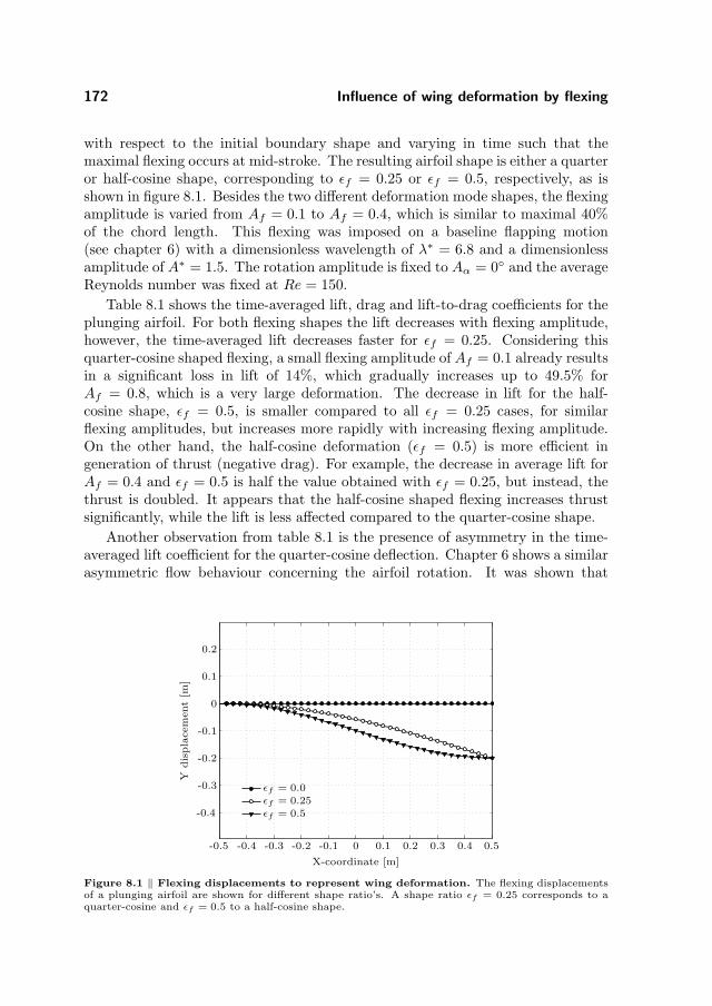
172 Influence of wing deformation by flexing

with respect to the initial boundary shape and varying in time such that themaximal flexing occurs at mid-stroke. The resulting airfoil shape is either a quarteror half-cosine shape, corresponding to ǫf = 0.25 or ǫf = 0.5, respectively, as isshown in figure 8.1. Besides the two different deformation mode shapes, the flexingamplitude is varied from Af = 0.1 to Af = 0.4, which is similar to maximal 40%of the chord length. This flexing was imposed on a baseline flapping motion(see chapter 6) with a dimensionless wavelength of λ∗ = 6.8 and a dimensionlessamplitude of A∗ = 1.5. The rotation amplitude is fixed to Aα = 0 and the averageReynolds number was fixed at Re = 150.

Table 8.1 shows the time-averaged lift, drag and lift-to-drag coefficients for theplunging airfoil. For both flexing shapes the lift decreases with flexing amplitude,however, the time-averaged lift decreases faster for ǫf = 0.25. Considering thisquarter-cosine shaped flexing, a small flexing amplitude of Af = 0.1 already resultsin a significant loss in lift of 14%, which gradually increases up to 49.5% forAf = 0.8, which is a very large deformation. The decrease in lift for the half-cosine shape, ǫf = 0.5, is smaller compared to all ǫf = 0.25 cases, for similarflexing amplitudes, but increases more rapidly with increasing flexing amplitude.On the other hand, the half-cosine deformation (ǫf = 0.5) is more efficient ingeneration of thrust (negative drag). For example, the decrease in average lift forAf = 0.4 and ǫf = 0.5 is half the value obtained with ǫf = 0.25, but instead, thethrust is doubled. It appears that the half-cosine shaped flexing increases thrustsignificantly, while the lift is less affected compared to the quarter-cosine shape.

Another observation from table 8.1 is the presence of asymmetry in the time-averaged lift coefficient for the quarter-cosine deflection. Chapter 6 shows a similarasymmetric flow behaviour concerning the airfoil rotation. It was shown that

X-coordinate [m]

Ydis

pla

cem

ent

[m]

ǫf = 0.0ǫf = 0.25ǫf = 0.5

-0.5 -0.4 -0.3 -0.2 -0.1 0 0.1 0.2 0.3 0.4 0.5

-0.4

-0.3

-0.2

-0.1

0

0.1

0.2

Figure 8.1 ‖ Flexing displacements to represent wing deformation. The flexing displacementsof a plunging airfoil are shown for different shape ratio’s. A shape ratio ǫf = 0.25 corresponds to aquarter-cosine and ǫf = 0.5 to a half-cosine shape.

8.1 Airfoil flexing in two-dimensional forward flapping flight 173

Af CLave CLdownstroke CLupstroke CD

0 1.956 (baseline) 1.758 -2.154 0.058

ǫ f=

0.25 0.1 1.683 (-14.0%) 1.880 -1.485 -0.044

0.2 1.510 (-22.8%) 1.393 -1.628 -0.1090.4 1.492 (-23.7%) 1.492 -1.492 -0.2630.8 0.988 (-49.5%) 0.988 -0.987 -0.229

ǫ f=

0.5 0.1 1.867 (-4.6%) 1.865 -1.868 -0.088

0.2 1.810 (-7.5%) 1.810 -1.810 -0.2150.4 1.732 (-11.5%) 1.632 -1.628 -0.4650.8 1.021 (-47.8%) 1.021 -1.021 -0.332

Table 8.1 ‖ Time-averaged force coefficients for a deforming plunging airfoil. The time-averaged lift and drag are shown for a deforming two-dimensional airfoil, for two flexing shapes, ǫf =0.25 and ǫf = 0.5. The Reynolds number was fixed to Re = 150, the dimensionless wavelength wask = 6.8 and the rotation amplitude remained at Aα = 0.

the force asymmetry is strongly related to the wake dynamics. Therefore, airfoilflexing using a quarter-cosine shape (ǫ = 0.25) may induce a similar effect on thewake dynamics as airfoil rotation. However, when applying the half-cosine airfoilflexing, the lift coefficient is symmetric over a complete stroke. While the quarter-cosine increases the airfoil camber, the half-cosine shape redirects the trailing-edgetowards the uniform free-stream. This redirection of the trailing-edge compensatesfor the destabilising effect of the airfoil rotation, such that a symmetric force isthe result of a symmetric wake pattern, which is beneficial in terms of efficiency.

Figure 8.2 shows the drag coefficients for both flexing shapes. It is clear that thethrust (negative drag) is more prominent for the half-cosine (ǫ = 0.5) flexing mode.The main regions of thrust enhancement are during mid-stroke, from t = 0.1T tot = 0.4T and t = 0.6T to t = 0.9T . In order to obtain a better understanding ofthe flow physics, figure 8.3 shows vorticity contours for both flexing shapes withan amplitude of Af = 0.2 at t = 0.25T , which is midway during the downstroke.Comparing figure 8.3(a) with 8.3(b), it is apparent that the leading-edge vortex isof similar size and strength for both flexing shapes. However, the trailing edge ofthe half-cosine shaped airfoil appears to enhance the speed of the vortex shedding.Therefore, at similar time instance, the shed vortices are farther away downstreamfor the half-cosine (ǫ = 0.5) flexing mode, increasing its thrust.

Summarising, this preliminary two-dimensional investigation, to understandthe effect of wing flexing, has led to some interesting results. The applied wingflexing influences the flow in a similar way as was obtained by applying airfoilrotation, indicating a similar mechanism in terms of the effects of angle of attack.With the introduction of flexing, the drag became negative to generate thrust inforward flight, and the lift decreased significantly. The lift and drag developmentstrongly depends on the shape of the wing flexing. The half-cosine flexing shape


t/T [-]

Dra

gcoeffi

cie

nt

[-]

Aflex = 0.0Aflex = 0.1Aflex = 0.2Aflex = 0.4

0 0.1 0.2 0.3 0.4 0.5 0.6 0.7 0.8 0.9 1-2

-1.5

-1

-0.5

0

0.5

(a) ǫ = 0.25

t/T [-]

Dra

gcoeffi

cie

nt

[-]

Aflex = 0.0Aflex = 0.1Aflex = 0.2Aflex = 0.4

0 0.1 0.2 0.3 0.4 0.5 0.6 0.7 0.8 0.9 1-2

-1.5

-1

-0.5

0

0.5

(b) ǫ = 0.5

Figure 8.2 ‖ Comparison of drag coefficients for a flexing airfoil. The drag coefficients are shownfor the quarter-cosine (a) and half-cosine (b) shaped airfoil flexing modes. The flexing amplitude Aflex

is varied from 0.0 to 0.4, the latter corresponds to 40% of the chord length.

(a) ǫ = 0.25 (b) ǫ = 0.5

Figure 8.3 ‖ Vorticity contours. Vorticity contours around a plunging flexing airfoil without ro-tation at Re = 150 are shown during mid-stroke at t = 0.25T . The flapping amplitude was fixed toA∗ = 1.5 and the dimensionless wavelength was set to λ∗ = 6.8. The flexing amplitude was set toAf = 0.2 using both flexing shapes, while the rotation amplitude was kept to zero Aα = 0.

results in less lift than obtained using the quarter-cosine shape. Additionally, thehalf-cosine flexing mode also generates the largest thrust. This behaviour wasrelated to the fact that the half-cosine shape caused the generated vortices toconvect faster, since the trailing-edge became aligned with the flow.

8.2 Wing flexing in three-dimensional hovering flight 175

8.2 Wing flexing in three-dimensional hovering

flight

In addition to the investigation of flexing effects on an airfoil in forward flappingflight, it was chosen to investigate a three-dimensional wing as well. Hoveringconditions are assumed, since it was extensively studied in the previous chapter.Besides the influence of the Rossby number, Reynolds number and the kinematicmodelling, applied under rigid wing conditions, it may be interesting to study theadditional effects of wing deformation. The deformation of the wing is defined by auser-defined flexing function, leading to a realistic bending of the three-dimensionalwing (Combes & Daniel, 2003a,b, Shyy et al., 2008a).

In order to investigate the effects of three-dimensional wing flexing on theforces and performance, the flexing is defined according to the model describedin section 4.3.3. The deformation model is hence similar to the one used forthe two-dimensional airfoil in the previous section. Additionally, the flexing wasindependently applied to the spanwise and the chordwise directions. The three-dimensional wing is deformed such that its shape prescribes a quarter-cosine func-tion, which is maximal at the wing tip or the trailing edge, respectively. Thiscosine shaped deformation varies harmonically in time during the stroke such thatlargest change in deformation occurs during stroke reversal, which is consideredto be realistic. The spanwise and chordwise directions are investigated separately.The flexing amplitude Af is varied from Af = 0.0 to Af = 0.4 in spanwise di-rection, while in chordwise direction the amplitude was varied from Af = 0.0 toAf = 0.2, due to limitations of the mesh motion solver. An amplitude of Af = 0.2corresponds to a maximal deflection at mid-stroke of 20% of the representativeflexing length (wing span or chord, respectively). Figure 8.1 shows an illustrationof the flexing model.

Af CL CDdownstroke CDupstroke CL/CDave

Span

0 1.234 (baseline) 2.034 2.028 0.608 (baseline)0.1 1.212 (-1.74%) 2.017 2.011 0.602 (-0.9%)0.2 1.213 (-1.73%) 2.029 2.023 0.599 (-1.5%)0.3 1.206 (-2.3%) 2.034 2.028 0.594 (-2.3%)0.4 1.190 (-3.6%) 2.031 1.992 0.592 (-2.6%)

Chor

d 0.1 1.137 (-7.9%) 2.129 2.126 0.534 (-12.1%)0.2 1.036 (-16.0%) 2.267 2.266 0.457 (-24.8%)

Table 8.2 ‖ Time-averaged force coefficients for a deforming three-dimensional wing. Time-averaged force coefficients of a three-dimensional flexing wing. The spanwise flexing amplitude is variedfrom Af = 0.0 to Af = 0.4, while the chordwise flexing amplitude varies from Af = 0.0 to Af = 0.2..


t/T [-]

Lift

coeffi

cie

nt

[-]

Af = 0.0Af = 0.2Af = 0.4Af = 0.1Af = 0.2

0 0.1 0.2 0.3 0.4 0.5 0.6 0.7 0.8 0.9 1

0

0.5

1

1.5

2

2.5

(a)

t/T [-]

Dra

gcoeffi

cie

nt

[-]

Af = 0.0Af = 0.2Af = 0.4Af = 0.1Af = 0.2

0 0.1 0.2 0.3 0.4 0.5 0.6 0.7 0.8 0.9 1

-3

-2

-1

0

1

2

3

(b)

Figure 8.4 ‖ Force coefficients for a spanwise and chordwise deforming flapping wing. Lift(a) and drag (b) coefficients induced by a flapping wing, which deforms in spanwise (Af = 0.0 − 0.4)and chordwise (Af = 0.0 − 0.2) direction. The latter are shown by N and . The angle of attack atmid-stroke remained at α = 45 and the Reynolds number remained at Re = 100..

While varying the flexing amplitude, the average Reynolds number is keptconstant at Re = 100 and the mid-stroke angle of attack is chosen to be α = 45.Table 8.2 shows the time-averaged force coefficients for different flexing amplitudes,using spanwise or chordwise deformation. The most important result is that bothtime-averaged lift and drag are only marginally influenced by the spanwise flexing,so where the wing tip bends. The maximal difference with the non-deforming case(-3.6%) occurs for 40% wing tip deflection, which is a significant deformation.The time-averaged drag remains nearly unaffected as well, such that the maximaldifference in lift-to-drag ratio is only -2.6%.

The chordwise deformation, on the other hand, influences the time-averagedforces to a large extent. As is easily seen, the time-averaged lift decrease with7.9% for only a small (Af = 0.1) chord deformation and 16% for Af = 0.2. Thedrag increases for the chordwise deforming wing, with respect to the case withoutflexing, such that the maximal difference in lift-to-drag ratio is -24.8%.

The force variation, during a full flapping stroke, is shown in figure 8.4. Itis clear that the largest difference in force coefficients occurs during mid-stroke,lowering the maximal lift coefficient. It seems that the leading-edge vortex is ex-pelled by the wing deformation, with a maximal effect at Af = 0.2 of chordwiseflexing. When the lift decreases, the drag increases during mid-stroke. Addition-ally, figure 8.5 shows the streamlines to visualise the leading-edge vortex duringmid-stroke (t = 0.25T ) for both spanwise and chordwise flexing. For comparison,also the case using no flexing is shown. Compared to the case without flexing theleading-edge vortex detaches earlier (less close to the wing tip) for both flexingcases. The spanwise flexing has less influence than the chordwise flexing modeshape. The influence of spanwise flexing is minor, which was also reflected in the

8.3 Conclusions 177

time-averaged force coefficients, which were only marginally lower. However, thechordwise flexing induced the leading-edge vortex to burst almost at the middleof the wing, leading to significantly less lift, see table 8.2.

8.3 Conclusions

In this chapter, the result have been described of a preliminary investigation tounderstand the effects of wing flexing. Therefore, a pre-defined flexing deformationhas been applied to a plunging airfoil in two-dimensional forward flight and to athree-dimensional flapping wing in hovering flight. First of all, the two-dimensionalflexing results in a similar effect on the flow and resulting forces as rotation of theairfoil. With increasing flexing amplitude, the larger effective angle of attack leadsto the generation of negative drag or thrust. In addition, the influence of the flexingshape (quarter-cosine or half-cosine) of the airfoil was studied. A quarter-cosineshaped flexing results in significantly higher thrust at less lift.

Secondly, a flexing deformation has been applied to a three-dimensional flap-ping wing in hovering flight. Two flexing directions have been considered, span-wise and chordwise flexing. While keeping the flexing amplitude constant, thechordwise flexing affects the flow the most. For a chordwise flexing amplitude ofAf = 0.2 the time-averaged lift and drag coefficients are significantly decreasedand increased, respectively, such that the lift-to-drag decreases with 24.8%. Thespanwise flexing does not show a comparable impact, only -2.6%.


(a) No flexing

(b) Spanwise flexing, Af = 0.2 (c) Chordwise flexing, Af = 0.2

Figure 8.5 ‖ Streamlines on a flexing wing in hovering flight. Iso-surface of Q = 1.0 are shownfor a three-dimensional flapping wing in hovering flight at Re = 100 and mid-stroke angle of attack ofAα = 45 at t = 0.25T . (a) shows the wing without flexing, while (b) shows the wing using spanwiseflexing and (c) using chordwise flexing, both with Af = 0.2. Colours indicate helicity.

CHAPTER 9

Conclusions and recommendations

In the present study we investigate mesh motion techniques to be able to per-form parametric variation of the flow around flapping foils and wings. Differentexisting mesh motion methods have been compared using cell quality measures.To improve the mesh quality a mesh motion technique has been implemented,based on the interpolation of radial basis functions on the mesh interior. Usingthat technique, it has become possible to efficiently solve the flow around flappingfoils and wings at low Reynolds numbers, for flow conditions corresponding to thescale of flying insects. The improved and implemented mesh motion technique,is used to solve the flow around flapping wings in hovering and forward flappingflight. Additionally, a preliminary study of the influence of wing flexing has beenconducted as well.

The overall conclusions of this research are given in section 9.1. Secondly, theconclusions on the assessment of different mesh motion techniques are drawn insection 9.2. Section 9.3 presents the conclusions of a flapping wing under hoveringconditions, for two-dimensional airfoil as well as for the three-dimensional wing.Section 9.4 shows the results for forward flapping flight, while section 9.5 describesthe conclusions of the preliminary study to understand the effects of wing flexing.Additional recommendation are made in Section 9.6.

9.1 Overall conclusions

The following overall conclusions are drawn:

1. The flow around a flapping wing, at the scale relevant to insect flight, canbe solved accurately using advanced mesh motion techniques in existing flow

180 Conclusions and recommendations

solvers.

2. Radial basis function mesh motion leads to improved mesh quality, comparedto methods based on solving the Laplace or a modified stress equation. How-ever, mesh motion based on radial basis function interpolation is much morecomputationally demanding. Different ways to improve its efficiency arediscussed.

3. The wing kinematic pattern has a large influence on the forces in two-dimensional hovering and forward flight.

4. In forward flight, thrust generation is the result of the forward tilting of thewing.

5. In two- and three-dimensional flapping flight, the leading-edge vortex is avery important lift enhancement mechanism.

6. The Rossby number, which describes the wing stroke curvature, has a largeinfluence on the time-averaged lift force. A low Rossby number significantlyincreases lift as the result of an induced spiralling leading-edge vortex.

7. Wing flexing may play an important role in insect flight to modulate theforces and to generate thrust.

9.2 Conclusions on mesh motion techniques

Two existing mesh motion techniques have been described which are commonlyused in existing CFD codes. The first method solves the Laplace equation witha variable diffusion coefficient, which is used to control the final mesh quality.Secondly, a modified stress equation was used as the basis for mesh motion. Ad-ditionally, a mesh motion solver is implemented, which uses the interpolation ofradial basis functions (RBF). The following conclusions are drawn:

1. For both existing mesh motion solvers, based on the Laplace and a modifiedstress equation, the mesh quality is not sufficient for flapping wing cases,where the rotation angles are large. However, these methods are very efficientsince existing iterative solvers can be used to solve a sparse system.

2. The mesh motion solver based on the radial basis function (RBF) interpola-tion does not need any information about the mesh connectivity and can beapplied to arbitrary unstructured meshes containing polyhedral cells. Addi-tionally, different radial basis functions, concerning the RBF mesh motion,are compared. The RBF mesh quality provides superior mesh quality overthe Laplace and modified stress equation mesh motion. Especially, whenusing the thin plate spline (TPS) or the continuous polynomial C2 as radial

9.3 Conclusions on hovering flapping flight 181

basis functions, the mesh quality is high in terms of low skewness and non-orthogonality. The TPS has global support, whereas the C2 basis functionhas compact support.

3. Since the RBF mesh motion technique encounters a dense system of equa-tions, different methods are implemented to increase its efficiency. First ofall, a subset of the moving boundary points was selected, because not allpoints are necessary if the body performs a rigid body motion. Therefore, acoarsening algorithm selects the desired control points. Secondly, a smooth-ing function is used to decrease the RBF contribution to zero at the outerdomain boundaries.

9.3 Conclusions on hovering flapping flight

9.3.1 Two-dimensional hovering

The effects of wing motion kinematics on the aerodynamic characteristics of hov-ering insect flight have been investigated by means of two-dimensional numericalflow simulations. The results of the present two-dimensional study has provideduseful insights, which may be relevant also for the understanding of realistic three-dimensional insect flight.

Four different kinematic models, with different complexity, have been analysed.Two of these models, pure harmonic motion and the Robofly experimental kine-matics have been used extensively in literature. The most prominent aspects ofthe Robofly kinematic model are the ‘sawtooth’ displacement and the ‘trapezoidal’angle of attack. The third model represents the actual fruit fly kinematics as ob-served in experiments and the last one was a modification of the latter, chosento investigate the effect of symmetry. The fruit fly models are characterised by a‘bump’ in angle of attack and the presence of deviation. To facilitate the compar-ison these models were dynamically scaled at Re = 110 and constructed such thattheir mean quasi-steady lift coefficient was matched. The following conclusionsare drawn about the two-dimensional hovering simulations:

1. It was found that the realistic fruit fly wing kinematics result in significantlylower drag at similar lift compared with the simplified wing kinematic modelsused in literature. The trend that the fruit fly kinematics increases aerody-namic performance agrees with the predictions of the quasi-steady theory,but the numerical flow simulations provide a more complete quantitativeanalysis of the flow behaviour.

2. It was shown that the difference in performance in terms of mean lift-to-dragratio between the different kinematic models was significant. The meanaerodynamic drag at equal lift of the fruit fly models is about 49% lowercompared to the Robofly model and about 29% lower with respect to theharmonic model.


3. The ‘sawtooth’ amplitude used in the Robofly model has a small effect onthe mean lift but the mean drag is affected significantly. Due to the highacceleration during stroke reversal of the ‘sawtooth’ shaped amplitude, themean drag at comparable lift is increased by 24%.

4. The second model simplification used by the Robofly, the ‘trapezoidal’ angleof attack, caused the LEV to separate during the translational phase. Thisled to an increase in mean drag during each half-stroke. Also in this caselarge accelerations at stroke reversal lead to a decrease in lift-to-drag ratioof 33%.

5. The extra ‘bump’ in angle of attack as used by the fruit fly model is notaffecting the mean lift to a large extent. During the beginning of the upand downstroke the ‘bump’ decreases the angle of attack such that the wingorientation is almost horizontal. This leads to a significant decrease in dragwhich improves aerodynamic performance in the sense of lift-to-drag ratioby 15.6%.

6. The other realistic kinematic feature is the deviation, which is found to haveonly a marginal effect on the mean lift and mean drag. However, the effectiveangle of attack is altered such that the deviation leads to levelling of the forcedistribution over the flapping cycle.

9.3.2 Three-dimensional hovering

A numerical model has been developed for solving the flow around a three-dimen-sional wing with complex wing kinematics. Different aspects, relevant to three-dimensional flapping wing aerodynamics, have been studied. First, the flow arounda dynamically scaled model wing is solved for different angles of attack in order tostudy the force development and vortex dynamics at small and large mid-strokeangle of attack. Secondly, the Rossby number is varied at different Reynolds num-bers. A varying Rossby number represents a variation in stroke path curvatureand thus angular acceleration. Thirdly, the three-dimensional wing kinematics isvaried by changing the shape in angle of attack and by applying a deviation, whichmay cause a ‘figure-of-eight’ pattern. Finally, the three-dimensional flow is com-pared with the two-dimensional studies performed on flapping forward flight. Thefollowing conclusions are drawn with respect to the three-dimensional simulations,concerning hovering flight:

1. The effect of a variation in angle of attack is such that the maximal liftoccurs at a mid-stroke angle of α = 45. However, the performance, interms of maximal lift-to-drag ratio was found to be maximal at α = 30.The flapping motion induces a leading-edge vortex which caused a peak inlift halfway during each up- and downstroke. This leading-edge vortex is

9.3 Conclusions on hovering flapping flight 183

strong at sufficiently high angles of attack α > 30. At α = 15 the leading-edge vortex is less strong, causing a sudden decrease in both lift and dragduring each half-stroke.

2. Both time-averaged lift and drag decrease significantly with increasing Ross-by number. At Ro = 130, a nearly translating wing, the lift decreaseswith 24.7%, compared to the flapping wing with Ro = 3.2. The majordecrease in lift and drag occurs during mid-stroke, between t = 0.25T and t =0.5T . Flow visualisations showed that the leading-edge vortex is significantlyreduced in size and strength for the translating wing at Ro = 130, comparedto the flapping wing. In addition, the leading-edge vortex rolls-up to formtwo tip vortices instead of one in case of the flapping wings. This causesboth lift and drag to be significantly lower at Ro = 130.

3. It was seen that for increasing Reynolds number, both time-averaged liftand drag increases, but the differences become smaller. The effect of achanging Reynolds number is negligible for both lift and drag at high mid-stroke angles of attack, when the wing is nearly translation at Re = 130. Thisis caused by the larger importance of the leading-edge vortex for a flappingwing at Ro = 3.2. For both flapping (Ro = 3.2) and translation (Ro = 130),irregularities in the leading-edge vortex occur, when the Reynolds numberincreases. For higher Reynolds numbers the vortex separates earlier, but liftand drag still increases. When the Reynolds number increases even further,a limit is reached, beyond which the leading-edge vortex bursts, causing aloss in performance.

4. The ‘trapezoidal’ shape in angle of attack causes a fast pitch-up motion atthe beginning of each up- and downstroke. Therefore, the mid-stroke angleof attack is reached earlier and maintained for a longer period, comparedto cases with a simple harmonic angle of attack variation. This leads toa significant increase in time-averaged lift of 10.8%. The lift increase isaccompanied by a decrease in drag of a similar amount, such that the lift-to-drag ratio shows a significant gain of 21.9%. Two-dimensional studies showedan opposite result which was caused by the fact that the leading-edge vortexseparated, while translating at a constant angle of attack. Three-dimensionaleffects, however, lead to a firm and stably attached leading-edge vortex.

5. Three different wing tip patterns, caused by deviation, have been studied,such as the ‘figure-of-O’, ‘figure-of-U’ and the ‘figure-of-eight’. The ‘figure-of-O’ wing tip pattern leads to an asymmetric variation in effective angle ofattack, leading to differences in drag for the up- and downstroke. Nonethe-less, the effect of this pattern on the time-averaged forces coefficients isnegligible. On the other hand, the ‘figure-of-U’ pattern does influence theforces in a non-beneficial way. The effective angle of attack is significantlydecreased during mid-stroke. The time-averaged lift coefficient is decreased


by 9.4%. While drag is maintaining nearly constant, the lift-to-drag ratio isdecreased by about 9%. The ‘figure-of-eight’ affects the forces most, how-ever, it depends on the starting direction. Two types are considered, thefirst starting the downstroke with an downward deviation motion, whereasthe type 2 starts upwards. The effective angle of attack is being influencedin such a way that the type 1 ‘figure-of-eight’ decreases both lift and dragconsiderably. Lift decreases up to 53%. Since drag decreases fast as well,the loss in lift-to-drag ratio is limited to 15.5%. The type 2 ‘figure-of-eight’motion, which starts with an upward motion at the beginning of the stroke,the drag is maintained constant. However, lift decreases 12.6% such that thelift-to-drag ratio decreases with about 12.0%.

9.4 Conclusions on forward flapping flight

9.4.1 Two-dimensional forward flapping

A numerical model for two-dimensional flow has been used to investigate the ef-fect of motion kinematics on the vortex dynamics around an ellipsoid foil subjectedto prescribed flapping motion over a range of dimensionless wavelengths, dimen-sionless amplitudes, angle of attack amplitudes, and stroke plane angles at theReynolds number of 150. Both plunging and rotating motions are prescribed bysimple harmonic functions which are useful for exploring the parametric spacedespite the model simplicity. Concerning the two-dimensional forward flappingsimulations, the following overall conclusions are drawn:

1. The resulting wake patterns behind the foil are categorised. Although suchan attempt at classifying the observed vortex patterns can lead to a degreeof uncertainty in determining the exact wake pattern due to the shedding,tearing, or merging of big and small vortices.

2. Optimal propulsion using flapping foil exists for each variable which impliesthat aerodynamics might select a range of preferable operating condition.The conditions that give optimal propulsion lie in the synchronisation regionin which the flow is periodic.

9.4.2 Three-dimensional forward flapping

In addition to the investigation of the effects of Reynolds number, Rossby numberand wing kinematics in hovering flight, a preliminary study is performed to com-pare two- and three-dimensional forward flight. Both two- and three-dimensionalsimulations are dynamically scaled using the radius of gyration to justify compar-ison. The three-dimensional simulations, concerning forward flight are performedfor a dimensionless wavelength of k = 6.3 and two Rossby numbers, Ro = 130and Ro = 3.2 at a Reynolds number of Re = 150. The following conclusions aredrawn:

9.5 Preliminary conclusions on wing flexing 185

1. For the case without rotation the three-dimensional simulations result in14.5% less lift compared to its two-dimensional counterpart. This differenceis mainly caused by the loss in lift due to the generation of a tip vortex whichis only present in the three-dimensional simulations.

2. An increase in rotation angle resulted in significant higher lift, up to 70.5%,which is the opposite as in the two-dimensional plunging wing. Togetherwith the higher thrust, this leads to the conclusion that a stable leading-edgevortex plays a more important role in three-dimensional flapping comparedto two-dimensional plunging, in the situation that the rotation angle is non-zero.

3. For a dimensionless wavelength of k = 6.3 the lift and drag forces are com-pared for different rotation amplitudes at a Reynolds number of Re = 150.For the translating wing (Ro = 130), the three-dimensional simulations re-sult in 28% less lift compared to the two-dimensional case. This difference ismainly caused by the loss in lift due to the generation of a tip vortex whichis only present in the three-dimensional simulations. However, an increase inRossby number resulted in a significant gain in lift. In combination with ahigher thrust this observation leads to the conclusion that a stable leading-edge vortex (induced by the revolving motion) plays an important role inthree-dimensional flapping aerodynamics.

9.5 Preliminary conclusions on wing flexing

A flexing deformation has been applied to a plunging airfoil in two-dimensionalforward flight and to a three-dimensional flapping wing during hovering flight.Concerning the flexible airfoil in forward flight, a comparison is made with aplunging airfoils, with additional rotation. The following conclusion are drawn:

1. The two-dimensional flexing has a comparable effect on the flow and forces asrotation of the airfoil. With increasing flexing amplitude, the larger effectiveangle of attack leads to the generation of negative drag or thrust. Besides,the flexing shape of the airfoil is important. A quarter-cosine shaped flexingresults in significantly higher thrust, while lift decreases.

2. The flexing deformation was also applied to a three-dimensional flappingwing in hovering flight. Two flexing directions were considered, spanwise andchordwise flexing. While keeping the flexing amplitude constant, the chord-wise flexing affects the flow significantly. For a chordwise flexing amplitudeof Af = 0.2 the time-averaged lift and drag coefficients are significantly de-creased and increased, respectively, such that the lift-to-drag decreases with24.8%. The spanwise flexing does not show a comparable influence, only-2.6%.


9.6 Recommendations

The current thesis describes a comparison of different mesh deformation methodsand development of an improved method, based on radial basis function interpo-lation. Additionally, these methods are used to solve the flow around two- andthree-dimensional flapping airfoils and wings under hovering and forward flightconditions. The following recommendation can be made for further research.

• The efficiency of the radial basis function mesh motion can be further im-proved by methods which selects only the necessary boundary points. Thesize of the matrix, which need to be solved, can be significantly reduced.Additionally, the implementation of parallel iterative solver techniques mayincrease its efficiency even further.

• The current implementation of the radial basis function mesh motion inOpenFOAMr should be generally implemented in parallel. The currentmethod is only able to address up to 4 processors, depending on the meshpartitioning.

• Using the RBF mesh motion solver, the flow around multiple flapping foilsor wings can be investigated. The current thesis describes the flow fields in-duced by a single two-dimensional foil or three-dimensional wing. If multiplewings are modelled, i.e. a dragonfly, the flow will be more complex and theforce development may be affected to certain extent.

• Investigate the effects of transition and turbulence modelling on the flowfields. The current research considered scales at the laminar flow regime. Itwould be interesting to study the effects of turbulence on the force develop-ment and vortex dynamics induced by a flapping three-dimensional wing.

• Investigate in more detail the vortex wake synchronisation in three-dimen-sional forward flight. Concerning two-dimensional forward flapping flight,this thesis describes the vortex wake synchronisation of a flapping foil fordifferent kinematic parameters. It would be interesting to study the vor-tex wake synchronisation of a three-dimensional flapping wing. The maindifficulty will be to define a proper framework to identify and quantify thethree-dimensional vortex structures to study the pattern formation.

• The effects of wing deformation could be investigated in more detail usingmore complex flexing models. The current thesis describes a preliminaryinvestigation of the effects of pre-defined wing flexing. Further research couldintroduce more degrees of freedom in the flexing model, possibly based onreal insects. This may lead to advanced wing shapes, which result in optimalaerodynamic efficiency, compared to rigid wings.

• It would be interesting to use fluid-structure interaction methods to studythe influence of the flow on the wing shapes. The wing shape is deformed

9.6 Recommendations 187

by inertial and aerodynamic forces. It will be interesting to couple theseforces with the flow solver and the accompanying mesh motion method. Themain difficulty will be the coupling of flow and structure, since the scaleddensity of a fruit fly wing is of similar order as the surrounding fluid. Sucha strongly coupled problem is very sensitive and a converged solution is notan easy objective.

• When advanced wing motions are desired, the possibility to implement im-mersed boundary methods needs to be explored. Using immersed boundarymethods it will become possible to model the clap-and-fling motion, whentwo wings touches each other. Another application of the immersed bound-ary method will be the use of multiple wings and bodies with extreme bodymotion to simulate advanced manoeuvring.

APPENDIX A

Grid generation for flapping wings

To solve the flow around flapping wings using Computational Fluid Dynamics(CFD), it is important to create high quality meshes. Three different tools are usedfor that purpose. The first, blockMesh, is a mesh generation utility supplied withOpenFOAMr. This utility creates a parametric mesh with grading and curvededges. A practical use of blockMesh is limited to simple domains and geometries.The second mesh generation software is Gambit, supplied with Fluentr, and is ca-pable of generating high quality meshes around complex geometries. Nevertheless,using Gambit for structured meshes can be difficult since defining an appropriategrading can be cumbersome. The third grid generation tool is the commercialGridPror package. GridPror generates a structured grid with grading using ablock strategy around a complex geometry. The user generates a topology and thegrid solver creates a structured block such that the resulting mesh quality is high.

A.1 Introduction

This appendix deals with the mesh generation in order to obtain a high qualityinitial mesh to solve for the flow around a moving airfoil or wing. There are twotypes of mesh generation, unstructured and structured. In principle, OpenFOAMr

and Fluentr are capable of solving the discretised equations in an unstructuredway, so there are no problems using one of those types. Since the meshes need todeform the initial mesh needs to be of very high quality, which can be more easilyobtained using a structured approach. Besides, the iterative solvers converge fasteron structured meshes. However, mesh generation around complex bodies is mucheasier using unstructured meshing techniques, but since the present study deals

190 Grid generation for flapping wings

b1 b2 b3

b4

b5b6b7

b8

p1 p2

p3p4

X

Y

Figure A.1 ‖ The topology used by theblockMesh utility. A blockMesh topology con-sists of points, lines and block. All need to bespecified manually, which can be cumbersome.

Figure A.2 ‖ A mesh generated by theblockMesh utility. A mesh generated byblockMesh, which can be obtained very fast,but is limited to simplified geometries.

with simplified model airfoils and wings, it is decided to choose structured meshingstrategies. The meshes used in the present thesis were generated using one of theearlier mentioned meshing tools: blockMesh, Gambit or GridPror. These threetools are described in sections A.2, A.2 and A.2, respectively.

A.2 BlockMesh

The open-source mesh generator, supplied with OpenFOAMr, is blockMesh. It isan easy to use and robust utility, applicable for simplified cases. The computationaldomain is specified by points, lines and blocks, see figure A.1. The connections be-tween the points (p1−p4) are defined by lines, which can be curved. Additionally,the domain consists of blocks (b1 − b8), specified by the lines, accordingly. Therelation between the points, lines and blocks need to be specified in a dictionaryfile, within the OpenFOAMr case. The grading to define the mesh resolution canbe set on all topology lines. For a uniform grading the mesh around a block isshown in figure A.2.

Since the manual creation of topology can be cumbersome, this mesh gener-ation utility is limited to simple computational domains. Therefore, the currentthesis used blockMesh to generate the meshes around a two-dimensional blockfor testing the mesh deformation methods (chapter 3). Additionally, the meshesare generated, concerning the two-dimensional channel cases, used to test theOpenFOAMr flow solver with vortex decay and convection (chapter 2).

A.3 Gambit 191

Figure A.3 ‖ Mesh around a circular cylinder, generated by Gambit. Meshes around complexgeometries is possible using Gambit, but clustering of cells is the main difficulty.

A.3 Gambit

The commercial flow solver Fluentr also provides the mesh generator Gambit.Gambit is able to generate structured and unstructured meshes, the latter con-taining only tetrahedral cells. It was already explained that the current thesismakes only use of structured meshes, Gambit was used to generate these meshesusing hexahedral cells. Within Gambit, a strong graphical user interface is avail-able, such that meshes around complex CAD designed geometries are possible.However, in order to generate a structured mesh with appropriate cell clusteringnear the body at regions with large geometric gradients, it is invincible to resultwith high mesh resolution throughout the computational domain, see figure A.3.It is shown that a grid is generated using multiple blocks, generated manually,in order to maintain high mesh quality. These multiple blocks, lead to an excessof cells in regions where these are not necessary. This can be solved by gener-ating more blocks, which is not straightforward. Gambit is used to generate thetwo-dimensional meshes, which are used to test both Fluentr and OpenFOAMr

using stationary and plunging cylinder flows. The next grid generator, GridPror,is capable to generate the multiple blocks automatically, which will improve themesh quality considerably, especially for three-dimensional cases.

A.4 GridPror

GridPror is an advanced commercial multi-block structured mesh generator. Theusage is different compared to other mesh generators, because the multiple blocksare automatically generated to optimise mesh quality. Figure A.4 shows the topol-ogy, which needs to be generated, this approach is different compared to the othergrid generators, blockMesh and Gambit. In figure A.4, the inner red squaredblock is snapped to the adjacent boundary Γb, and all other red squared regions

192 Grid generation for flapping wings

Γb

X

Y

Figure A.4 ‖ GridPror topology used togenerate the (block-) structured mesh.The red blocks indicate extra topology, ac-cording to which GridPror generated the mul-tiple blocks. These blocks are shaped suchthat the mesh quality is optimised.

Figure A.5 ‖ Grid around a circular

cylinder, generated by GridPror. Thegrid is generated by GridPror according tothe user-defined mesh topology, such that themesh quality is optimised.

represent structured grid blocks. An illustration of the resulting grid is shown infigure A.5. Besides the high quality meshes, GridPror is easy to use for complexgeometries. Additionally, for three-dimensional cases, it is very important to putthe multiple blocks in an optimal way such that the cell clustering is only presentin the regions of interest. Therefore, the current thesis uses GridPror to generatethe three-dimensional meshes around a flapping wing, as illustrated in figure A.6.

A.5 Conclusions

Three different mesh generators have been described, blockMesh, Gambit andGridPror. The mesh generator, blockMesh, supplied with OpenFOAMr, is easyto use for simplified problems. In the current thesis, blockMesh is used to gen-erate the two-dimensional meshes, which were used to validate the flow solvers.The second grid generator, Gambit, has more capabilities and can be used togenerated meshes around complex geometries. This mesh generator is used fortwo-dimensional flows around stationary and plunging cylinders. Using the thirdgrid generator, GridPror, a user-defined topology needs to be specified to optimisethe multiple blocks for the structured mesh generation. This topology procedureis versatile, but different compared to the other packages. GridPror is used forthe three-dimensional simulations around flapping wings.

A.5 Conclusions 193

(a) 3D GridPror mesh

(b) 3D GridPror mesh, close-up at t = 0T (c) 3D GridPror mesh, close-up at t = 0.5T

Figure A.6 ‖ Three-dimensional grid around a wing, generated by GridPror. (a) shows the

full computational domain which is used for mesh generation using GridPror. A close-up of the meshnear the three-dimensional wing is shown for two different time instances in (b) and (c), respectivelyt = 0T and t = 0.5T .

APPENDIX B

Flow solver settings

B.1 Introduction

Within the current thesis, two different flow solvers have been used, the open-source OpenFOAMr and the commercial package Fluentr. For both flow solvers,the settings are described in this appendix. Section B.2 deals with Fluentr,whereas section B.3 describes the settings used in OpenFOAMr.

B.2 Fluentr solver settings

Fluentr is a finite volume based CFD solver. This section deals with the dif-ferent flow solver settings, that are necessary to reproduce the results from thisthesis. Fluentr is used for the two-dimensional hovering simulations described inchapter 5.

Solver SegregatedSpace 2D/3DTime first-order implicitVelocity formulation AbsoluteGradient option Cell-basedViscous model laminarAccuracy double precision

Table B.1 ‖ Solver settings

196 Flow solver settings

Pressure second-orderPressure-Velocity coupling PISOEquations second-order Upwind

Table B.2 ‖ Discretisation settings

Smoothing: Spring constant 0.1Boundary node relaxation 0.3Convergence tolerance 0.01Number of iterations 20

Re-meshing: min. cell volume 1.73e-7 - 3e-7 (grid dependent)max. cell volume 0.488 - 1.39 (grid dependent)max. cell skewness 0.4

Table B.3 ‖ Dynamic mesh settings

In order to solve the flow, the user needs to specify which models are used, seetable B.1. The laminar viscous model is used which is quite misleading. No turbu-lence model is used so in fact a Direct Numerical Simulation (DNS) is performedusing the Navier-Stokes equations. For the highest accuracy the ‘double precision’version is used. According to (Lentink, 2003, Bos et al., 2008) this high accuracyis necessary since insect flow might be very sensitive to initial conditions, undercertain circumstances.

The moving wings were studied using the ‘dynamic mesh’ module. Up to nowFluentr is only capable of using this ‘dynamic mesh’ module in combination withthe first-order implicit time integration. The validation cases without mesh motionuses second-order time integration. The multi-grid settings worked fine at defaultsettings. Table B.2 shows the discretisation settings. For space discretisation asecond-order upwind scheme is used together with standard PISO scheme for thepressure-velocity coupling.

The ‘dynamic mesh’ parameters are shown in table B.3. The mesh is movingusing two methods, smoothing and re-meshing. Re-meshing means a completeexamination of the mesh and adaptation of the nodes where needed. Smoothingon the other hand holds the nodes together in such a way that they do not movearbitrarily in any direction, but stay together in a way. Re-meshing is definedby the maximal and minimal cell volumes. These values are bases on the gridin that case. The maximal skewness is needed in order to keep the mesh qualitywithin acceptable range. A value of 0.4 turned out to give satisfying results. Thesmoothing performs an iteration to smooth the mesh when it is updated. Thesmoothness is given by a spring constant which holds the nodes together and aboundary node relaxation which gives some freedom to boundary nodes to move.

Concerning unsteady cases, the solution is varying in time until the residuals

B.3 OpenFOAMr solver settings 197

reach a sufficiently small value. These values are convergence criterion’s and canbe changed by the user. In this study the solution was considered converged asthe residuals reached a value of 1 · 10−4 for every component. Per time-step afixed number of 20 iterations was needed to converge in case of using the PISOpressure-velocity coupling in case of the validation study. During the flapping wingsimulations a fixed number of 10 iterations was used. Furthermore the completesolution is written to hard-disk several times per flapping period; the lift and draghistories every time-step.

B.3 OpenFOAMr solver settings

Since Fluentr could not cope with the extreme three-dimensional mesh deforma-tion, OpenFOAMr was explored and provided good results. OpenFOAMr (OpenField Operation And Manipulation) is a C++ toolbox for the customisation andextension of numerical solvers for continuum mechanics problems, including Com-putational Fluid Dynamics (CFD). It is produced by OpenCFDr Ltd. and isfreely available and open source, licensed under the GNU General Public Licence.

Since the source-code is fully accessible, different flow solvers and utilities aredeveloped. For example, the unsteady Navier-Stokes equations were solved, usingmesh motion techniques, with icoDyMFoam or icoDyMFoamRBF, the latter using ra-dial basis function interpolation for mesh deformation. Utilities like setTaylorVorticesor meshQuality write respectively the velocities for a Taylor vortex initial con-dition or the quality of the mesh (skewness and non-orthogonality). One of themain strength’s of OpenFOAMr is the intuitive way of programming. Briefly, twodifferent illustrations are given, from the solver icoFoam and utility totalEnergy.The following piece of code is taken from icoDyMFoam, which solves the unsteadyincompressible Navier-Stokes equations:

1 for (runTime++; !runTime.end(); runTime++)2 3 Info<< "Time = " << runTime.timeName() << nl << endl;45 fvVectorMatrix UEqn6 (7 fvm::ddt(U)8 + fvm::div(phi, U)9 - fvm::laplacian(nu, U)

10 );1112 solve(UEqn == -fvc::grad(p));1314 runTime.write();15

Line 1 specifies that the equations are solved for all time-steps until the specifiedend time is reached, runTime.end(). Line 5-9 defines the implicit part of thegoverning equation, which is the unsteady incompressible Navier-Stokes equation.The implicit discretisation is performed by the fvm class such that the total systemof equations is properly constructed from the temporal, convection and diffusion


terms, i.e. ddt and div are explicit functions to generate the matrix system fora given velocity, pressure and flux field. The explicit fvc is used, on line 12,to equate the system with the source terms and the complete system is solvedusing a chosen iterative solver. This piece of code needs to be placed within apressure-velocity coupling loop.

The next code example concerns the utility totalEnergy, which calculates thetotal energy, integrated over the complete domain:

1 void Foam::calc(const argList& args, const Time& runTime, const fvMesh& mesh)2 3 IOobject Uheader4 (5 "U",6 runTime.timeName(),7 mesh,8 IOobject::MUST_READ9 );

1011 if (Uheader.headerOk())12 13 Info<< " Reading U" << endl;14 volVectorField U(Uheader, mesh);1516 Info << " Calculating totalEnergy" << endl;17 dimensionedScalar totalEnergy = fvc::domainIntegrate(0.5*magSqr(U));18 Info << " Total energy = " << totalEnergy.value() << endl;19 20 else21 22 Info << " No U" << endl;23 24

Here, from line 1-24, the time-loop is defined, calculating the total energy for everytime instance available. Line 3-9 reads the velocity field from a given solution, atthe specific time directory. The actual calculation is performed at line 17, wherefvc::domainIntegrate is an implicit function, calculating the sum over all finite-volume cells in the domain of 0.5*magSqr(U), which is equivalent to 0.5|u|2. Thestatement Info is a templated function, which is able to return strings, scalarvalues and tensor fields back to the screen. These two illustrations are only twoexamples. OpenFOAMr comes with a wide variety of solvers, utilities and tutorialcases. If there is need for a specific application, the uses should take a look in thesource-code of OpenFOAMr to find similar pieces of code.

All flow solvers that are developed for this thesis, are based on icoDyMFoam,slightly extended to use force output modifications, or to make use of modifiedmesh motion solvers. icoDyMFoam solves the unsteady incompressible laminarNavier-Stokes equations for a Newtonian fluid. Therefore, the different termsof this equation need to be discretised accordingly, e.g. diffusion, convection.Table B.4 shows the schemes that were used throughout this thesis. The convectionscheme was varied for validation purposes, but the Van Leer scheme was used forthe majority of numerical simulations.

In order to solve discretised governing equations, an iterative solver is used.Three different solvers were specified for the pressure equation, velocity equation

B.3 OpenFOAMr solver settings 199

Description Code Differencing scheme

General interpolation - second-order linearTemporal discretisation ddt(U) second-order backwardGradient discretisation div(phi,U) second-order linearDiffusion discretisation laplacian(nu,U) second-order linear

Convection discretisation grad(p) Gamma, SuperBee, Koren,Van Leer or linear

Table B.4 ‖ Differencing methods for different terms in the transport equation. The tem-poral, gradient, diffusion and convection term, present in the general transport equations needs to bediscretised properly. To minimise temporal errors all chosen schemes are of second-order, see (Welleret al., 1998, Jasak, 1996, Jasak et al., 2004).

and mesh motion, respectively. Table B.5 shows the chosen solvers, combined withthe convergence criterion. For solving the equations for pressure and velocity, thePISO coupling. Every time-step PISO evaluates an initial u and p, performsmultiple corrections (commonly twice in this thesis) until a convergence criterionis met. An iterative method like PISO can be accelerated by Krylov subspacemethods (Saad, 2003). This means that the matrix A of the system Ay = b to besolved is split as: A = M − N . M is used to pre-condition the problem, whichmeans that Ay = b is replaced by its pre-conditioned counter-part:

M−1Ay = M−1b. (B.1)

In this thesis, Incomplete Cholesky decomposition is used to pre-condition thesystem as follows:

L−1AL−T y = L−1b, y = L−T y , (B.2)

where LLT is an Incomplete Cholesky decomposition of A and L−T = (LT )−1.When Incomplete Cholesky (IC) decomposition is applied in combination withConjugate Gradient (CG), this is another Krylov subspace method for linear sys-tems Ay = b with a symmetric self-adjoint positive definite matrix A. Combining

Term iterative solver convergence criteria

pressure, p PCG with DIC precond 10−6

velocity, u PBiCG with DILU precond 10−5

mesh motion PCG with DIC precond 10−8

Table B.5 ‖ Iterative solvers for the different equations. The pressure and mesh motion equa-tions are solved using the pre-conditioned conjugate gradient (PCG) solver with an diagonal incompleteCholeski (DIC) pre-conditioner. The pressure-velocity coupling equation is solved using the asymmetricsolver pre-conditioned Bi-Stab conjugate gradient (PBiCG), with a diagonal incomplete LU decompo-sition (DILU) pre-conditioner.


IC and CG results in a new method called ICCG. If the matrix A is not self-adjoint,one can apply BiConjugate Gradient method (BCG). Using this in combinationwith IC results in BiCG. For every variable calculated the linear solver methodsand their solution tolerances are listed in table B.5. A more elaborate descriptionof iterative solvers is beyond the scope of this thesis. For more information, pleaseconsult (Wesseling, 2001, Hirsch, 1988, Ferziger & Peric, 2002, Jasak et al., 2007).

Bibliography

Anderson Jr., J. D. (1991), Fundamentals of Aerodynamics, second edn,McGraw-Hill Inc.

Aono, H., Liang, F. & Liu, H. (2008), ‘Near- and far-field aerodynamics ininsect hovering flight: an integrated computational study’, The Journal of Exper-imental Biology 211, 239–257.

Baruh, H. (1999), Analytical Dynamics, McGraw-Hill Inc.

Batina, J. T. (1990), ‘Unsteady euler airfoil solutions using unstructured dy-namic meshes’, AIAA Journal 28 (8), 1381–1388.

Beckert, A. & Wendland, H. (2001), ‘Multivariate interpolation for fluid-structure-interaction problems using radial basis functions’, Aerospace Science andTechnology 5(2), 125–134.

Birch & Dickinson, M. H. (2003), ‘The influence of wing-wake interactionson the production of aerodynamic forces in flapping flight.’, The Journal of Ex-perimental Biology 206, 2257–2272.

Birch, J. M. & Dickinson, M. H. (2001), ‘Spanwise flow and the attachmentof the leading-edge vortex on insect wings’, Nature 412, 729–733.

Birch, J. M., Dickson, W. B. & Dickinson, M. H. (2004), ‘Force productionand flow structure of the leading-edge vortex on flapping wings at high and lowreynolds numbers.’, The Journal of Experimental Biology 207, 1063–1072.

Blom, F. J. (2000), ‘Considerations on the spring analogy’, International Jour-nal for Numerical Methods in Fluids 32, 647–669.

202 Bibliography

Blondeaux, P., Fornarelli, F. & Guglielmini, L. (2005a), Vortex struc-tures generated by a finite-span oscillating foil, in ‘43rd AIAA Aerospace SciencesMeeting and Exhibit, Reno’, 2005-84.

Blondeaux, P., Fornarelli, F., Guglielmini, L., Triantafyllou, M. S. &Verzicco, R. (2005b), ‘Numerical experiments on flapping foils mimicking fish-like locomotion’, Physics of Fluids 17, 113601–12.

Boer de, A., van der Schoot, M. S. & Bijl, H. (2007), ‘Mesh deformationbased on radial basis function interpolation’, Computers & Structures 85, 784–795.

Bomphrey, R. J., Lawson, N. J., K., T. G. & Thomas, A. L. R. (2006),‘Application of digital particle image velocimetry to insect aerodynamics: mea-surement of the leading-edge vortex and near wake of a hawkmoth’, Experimentsin Fluids 40, 546–554.

Bos, F. M., Lentink, D., van Oudheusden, B. W. & Bijl, H. (2008), ‘In-fluence of wing kinematics on aerodynamic performance in hovering insect flight’,Journal of Fluid Mechanics 594, 341–368.

Bos, F. M., van Oudheusden, B. W. & Bijl, H. (2010a), ‘Mesh deforma-tion techniques for flapping flight’, Computer Methods in Applied Mechanics andEngineering (Submitted).

Bos, F. M., van Oudheusden, B. W. & Bijl, H. (2010b), ‘Three-dimensionalvortical structures in flapping flight’, Journal of Fluid Mechanics (Submitted).

Brodsky, A. K. (1994), The Evolution of Insect Flight, Oxford University PressInc.

Buhmann, M. D. (2000), ‘Radial basis functions’, Acta Numerica 9, 1–38.

Carr, J. C., Beatson, R. K., McCallum, B. C., Fright, W. R., McLennan,T. J. & Mitchell, T. J. (2003), Smooth surface reconstruction from noisyrange data, First International Conference on Computer Graphics and InteractiveTechniques.

Chakraborty, P., Balachandar, S. & Adrian, R. J. (2005), ‘On the rela-tionships between local vortex identification schemes’, Journal of Fluid Mechanics535, 189–214.

Combes, S. A. & Daniel, T. L. (2003a), ‘Flexural stiffness in insect wings i& ii’, Journal of Experimental Biology 206, 2979–2997.

Combes, S. A. & Daniel, T. L. (2003b), ‘Into thin air: contributions ofaerodynamic and inertial-elastic forces to wing bending in the hawkmoth Manducasexta’, Journal of Experimental Biology 206, 2999–3006.

Bibliography 203

Degand, C. & Farhat, C. (2002), ‘A three-dimensional torsional spring analogymethod for unstructured dynamic meshes’, Computers & Structures 80, 305–316.

Dickinson, M. H. (1994), ‘The effects of wing rotation on unsteady aerody-namic performance at low Reynolds number.’, The Journal of Experimental Biol-ogy 192, 179–206.

Dickinson, M. H., Farley, C. T., Full, R. J., Koehl, M. A. R., Kram,R. & Lehman, S. (2000), ‘How animals move: An integrated view’, Science288, 100–106.

Dickinson, M. H. & Gotz, K. G. (1993), ‘Unsteady aerodynamic performanceof model wings at low reynolds numbers’, The Journal of Experimental Biology174, 45–64.

Dickinson, M. H., Lehmann, F.-O. & Sane, S. P. (1999), ‘Wing rotationand the aerodynamic basis of insect flight.’, Science 284, 1954–1960.

Dickson, W. B. & Dickinson, M. H. (2004), ‘The effect of advance ratio onthe aerodynamics of revolving wings’, Journal of Experimental Biology 207, 4269–4281.

Donea, J. (1982), ‘An arbitrary lagrangian-eulerian finite element method fortransient fluid-structure interactions’, Computer Methods in Applied Mechanicsand Engineering pp. 689–723.

Dong, H., Mittal, R., Bozkurttas, M. & Najjar, F. (2005), Wake structureand performance of finite aspect-ratio flapping foils, in ‘43rd AIAA AerospaceSciences Meeting and Exhibit, Reno’, 2005-81.

Dwight, R. P. (2004), Robust mesh deformation using the linear elasticity equa-tions, in H. Deconinck & E. Dick, eds, ‘Computational Fluid Dynamics 2006’,Springer.

Ellington, C. P. (1984), ‘The aerodynamics of hovering insect flight’, Phil.Trans. Roy. Soc. London. B 305, 1–181.

Ellington, C. P., van den Berg, C., Willmott, A. P. & Thomas, A. L. R.(1996), ‘Leading-edge vortices in insect flight’, Nature 384, 626–630.

Farhat, C., Degand, C., Koobus, B. & Lesoinne, M. (1998), ‘Torsionalsprings for two-dimensional dynamic unstructured meshes’, Computer Methods inApplied Mechanics and Engineering 163, 231–245.

Ferziger, J. H. & Peric, M. (2002), Computational Methods for Fluid Dynam-ics, third edn, Springer-Verlag Berlin.

Fry, S. N., Sayaman, R. & Dickinson, M. H. (2003), ‘The aerodynamics offree-flight maneuvers in Drosophila’, Science 300, 295–298.

204 Bibliography

Ginsberg, J. H. (1998), Advanced Engineering Mechanics, second edn, Cam-bridge University Press.

Guglielmini, L. & Blondeaux, P. (2004), ‘Propulsive efficiency of oscillatingfoils’, European Journal of Mechanics B/Fluids 23, 255–278.

Guilmineau, E. & Queutey, P. (2002), ‘A numerical simulation of vortexshedding from an oscillating circular cylinder’, Journal of Fluids and Structures16, 773–794.

Helenbrook, B. T. (2003), ‘Mesh deformation using the biharmonic operator’,International Journal for Numerical Methods in Engineering 56 (7), 1007–1021.

Henderson, R. D. (1995), ‘Details of the drag curve near the onset of vortexshedding’, Physics of Fluids 7 (9), 2102–2104.

Hirsch, C. (1988), Numerical Computation of Internal and External Flows, Vol-ume I: Fundamentals of Numerical Discretization, John Wiley & Sons.

Hover, F. S., Haugsdal, Ø. & Triantafyllou, M. S. (2004), ‘Effect of angleof attack profiles in flapping foil propulsion’, Journal of Fluids and Structures19, 37–47.

Hu, D. L., Chan, B. & Bush, J. W. M. (2003), ‘The hydrodynamics of waterstrider locomotion’, Nature 424, 663–666.

Hunt, J. C., Wray, A. A. & Moin, P. (1988), Eddies, stream, and convergencezones in turbulent flows, in ‘Center for Turbulence Research Report’, pp. 193–208.

Isogai, K., Fujishiro, Saitoh, T., Yamamoto, M., Yamasaki, M. & Mat-subara, M. (2004), ‘Unsteady three-dimensional viscous flow simulation of adragonfly hovering’, AIAA Journal 42, 2053–2059.

Issa, R. I. (1986), ‘Solution of the implicitly discretized fluid flow equation byoperator splitting’, Journal of Computational Physics 62, 40–65.

Jakobsson, S. & Amoignon, O. (2007), ‘Mesh deformation using radial ba-sis functions for gradient-based aerodynamics shape optimization’, Computers &Fluids 36, 1119–1136.

Jasak, H. (1996), Error analysis and estimation in the finite volume method withapplications to fluid flow, PhD thesis, Imperial College, University of London.

Jasak, H. (2009), Dynamic mesh handling in openfoam, in ‘47th AIAAAerospace Sciences Meeting, Orlando’, 2009-341.

Jasak, H., Jemcov, A. & Maruszewski, J. P. (2007), Pre-conditioned linearsolvers for large eddy simulations, in ‘CFD 2007 Conference’, CFD Society ofCanada, Toronto.

Bibliography 205

Jasak, H. & Tukovic, Z. (2004), ‘Automatic mesh motion for the unstructuredfinite volume method’, Journal of Computational Physics (Submitted).

Jasak, H., Weller, H. G. & Gosman, A. D. (1999), ‘High resolution nvddifference scheme for arbitrary unstructured meshes’, International Journal forNumerical Methods in Fluids 31, 431–449.

Jasak, H., Weller, H. G. & Nordin, N. (2004), ‘In-cylinder CFD simulationusing a c++ object-oriented toolkit’, SAE Technical paper 2004-01-0110.

Jeong, J. & Hussain, F. (1995), ‘On the identification of a vortex’, Journal ofFluid Mechanics 285, 69–94.

Johnson, A. A. & Tezduyar, T. E. (1994), ‘Mesh update strategies in par-allel finite element computations of flow problems with moving boundaries andinterfaces’, Computer Methods in Applied Mechanics and Engineering 119, 73–94.

Juntasaro, V. & Marquis, A. J. (2004), ‘Comparative study of flux-limitersbased on must differencing scheme’, International Journal of Computational FluidDynamics 18 (7), 569–576.

Juretic, F. (2004), Error analysis in Finite Volume CFD, PhD thesis, ImperialCollege London.

Katz, J. (1981), ‘A discrete vortex method for non-steady separated flow overan airfoil’, Journal of Fluid Mechanics 102, 315–328.

Knupp, P. M. (2003), ‘Algebraic mesh quality metrics for unstructured initialmeshes’, Finite Elements in Analysis and Design 39, 217–241.

Koren, B. (1993), ‘A robust upwind discretisation method for advection, dif-fusion and source terms’, Numerical Methods for Advection-Diffusion Problemsp. 117.

Kuzmin, D. & Turek, S. (2004), ‘High-resolution fem-tvd schemes based on afully multidimensional flux limiter’, Journal of Computational Physics 198, 131–158.

Lehmann, F.-O. (2004), ‘The mechanisms of lift enhancements in insect flight’,Naturwissenschaften 91, 101–122.

Lehmann, F.-O., Sane, S. P. & Dickinson, M. (2005), ‘The aerodynamiceffect of wing-wing interaction in flapping insect wings’, The Journal of Experi-mental Biology 208, 3075–3092.

Lentink, D. (2003), Influence of airfoil shape on performance in insect flight,Master’s thesis, Delft University of Technology.

206 Bibliography

Lentink, D. (2008), Exploring the Biofluiddynamics of Swimming and Flight,PhD thesis, Wageningen University.

Lentink, D. & Dickinson, M. H. (2009a), ‘Biofluiddynamic scaling of flap-ping, spinning and translating fins and wings’, Journal of Experimental Biology212, 2691–2704.

Lentink, D. & Dickinson, M. H. (2009b), ‘Rotational accelerations stabilizeleading edge vortices on revolving fly wings’, Journal of Experimental Biology212, 2705–2719.

Lentink, D. & Gerritsma, M. (2003), Influence of airfoil shape on performancein insect flight, in ‘43rd AIAA Fluid Dynamics Conference and Exhibit, Orlando’,2003-3447.

Lentink, D., Muijres, F. T., Donker-Duyvis, F. J. & van Leeuwen, J. L.(2008), ‘Vortex-wake interactions of a flapping foil that models animal swimmingand flight’, The Journal of Experimental Biology 211, 267–273.

Lesoinne, M. & Farhat, C. (1996), ‘Geometric conservation laws for flow prob-lems with moving boundaries and deformable meshes, and their impact on aeroe-lastic computations’, Computer Methods in Applied Mechanics and Engineering134, 71–90.

Lewin, G. C. & Haj-Hariri, H. (2003), ‘Modelling thrust generation of atwo-dimensional heaving airfoil in a viscous flow’, Journal of Fluid Mechanics492, 339–362.

Lighthill, M. J. (1969), ‘Hydromechanics of aquatic animal propulsion’, AnnualReview of Fluid Mechanics 1, 413–446.

Liu, H. & Kawachi, K. (1998), ‘A numerical study of insect flight’, Journal ofComputational Physics 146, 124–156.

Lohner, R. & Yang, C. (1996), ‘Improved ale mesh velocities for moving bod-ies’, Communications in Numerical Methods in Engineering 12 (10), 599–608.

Luo, G. & Sun, M. (2005), ‘The effects of corrugation and wing planform onthe aerodynamic force production of sweeping model insect wings’, Acta MechSinica 21, 531–541.

Lu, Y. & Shen, G. X. (2008), ‘Three-dimensional flow structures and evolutionof the leading-edge vortices on a flapping wing’, The Journal of ExperimentalBiology 211, 1221–1230.

Maxworthy, T. (1979), ‘Experiments on the weis-fogh mechanism of lift gener-ation by insects in hovering flight. part 1. dynamics of the ‘fling”, Journal of FluidMechanics 93, 47–63.

Bibliography 207

Michelson, R. C. (2008), ‘Test and evaluation of fully autonomous micro airvehicles’, ITEA Journal 29, 367–374.

Mittal, R. & Iaccarino, G. (2005), ‘Immersed boundary methods’, AnnualReview of Fluid Mechanics 37, 239–261.

Panton, R. L. (2005), Incompressible Flow, John Wiley & Sons.

Patankar, S. V. & Spalding, D. B. (1972), ‘A calculation procedure for heat,mass and momentum transfer in three-dimensional parabolic flows’, InternationalJournal of Heat and Mass Transfer 15, 1787.

Pedro, G., Suleman, A. & Djilali, N. (2003), ‘A numerical study of thepropulsive efficiency of a flapping hydrofoil’, International Journal for NumericalMethods in Fluids 42, 493–526.

Peskin, C. S. (2002), ‘The immersed boundary method’, Acta Numericapp. 479–517.

Poelma, C., Dickson, W. B. & Dickinson, M. H. (2006), ‘Time-resolvedreconstruction of the full velocity field around a dynamically-scaled flapping wing’,Experiments in Fluids 41 (2), 1–13.

Potsdam, M. A. & Guruswamy, G. P. (2001), A parallel multiblock meshmovement scheme for complex aeroelastic applications, Technical report, AIAA-2001-0716.

Ramamurti, R. & Sandberg, W. C. (2002), ‘A three-dimensional compu-tational study of the aerodynamic mechanisms of insect flight’, The Journal ofExperimental Biology 205, 1507–1518.

Rendall, T. C. S. & Allen, C. B. (2008a), Efficient mesh motion tech-niques using radial basis functions with data reduction algorithms, in ‘46th AIAAAerospace Sciences Meeting and Exhibit’.

Rendall, T. C. S. & Allen, C. B. (2008b), ‘Improved radial basis functionfluid-structure coupling via efficient localised implementation’, International Jour-nal for Numerical Methods in Engineering 78 (10), 1188–1208.

Rendall, T. C. S. & Allen, C. B. (2008c), ‘Unified fluid-structure interpo-lation and mesh motion using radial basis functions’, International Journal forNumerical Methods in Engineering 74 (10), 1519–1559.

Rhie, C. M. & Chow, W. L. (1983), ‘Numerical study of the turbulent flowpast an airfoil with trailing-edge separation’, AIAA Journal 21, 1525–1532.

Roe, P. L. (1986), ‘Characteristic-based schemes for the euler equations’, AnnualReview of Fluid Mechanics 18, 337.

208 Bibliography

Ruijgrok, G. J. J. (1994), Elements of airplane performance, Delft UniversityPress.

Saad, Y. (2003), Iterative Methods for Sparse Linear Systems, Society for In-dustrial Mathematics.

Sane, S. P. & Dickinson, M. H. (2001), ‘The control of flight force by aflapping wing: lift and drag production’, The Journal of Experimental Biology204, 2607–2626.

Sane, S. P. & Dickinson, M. H. (2002), ‘The aerodynamic effects of wingrotation and a revised quasi-steady model of flapping flight’, The Journal of Ex-perimental Biology 205, 1087–1096.

Shyy, W., Lian, Y., Tang, J., Liu, H., Trizila, P. & Stanford, B. (2008a),Computational aerodynamics of low reynolds number plunging, pitching and flex-ible wings for mav applications, in ‘46th AIAA Aerospace Sciences Meeting andExhibit’.

Shyy, W., Lian, Y., Tang, J., Viieru, D. & Liu, H. (2008b), Aerodynamicsof low Reynolds number flyers, Cambridge University Press.

Smith, M. J., Cesnik, C. E. S. & Hodges, D. H. (2000), ‘Evaluation ofsome data transfer algorithms for noncontiguous meshes’, Journal of AerospaceEngineering 13(2), 52–58.

Srygley, R. B. & Thomas, A. L. R. (2002), ‘Unconventional lift-generatingmechanisms in free-flying butterflies’, Nature 420, 660–664.

Stepniewski, W. Z. & Keys, C. N. (1984), Rotary-wing aerodynamics, Dover.

Sun, M. & Tang, J. (2002), ‘Unsteady aerodynamic force generation by amodel fruit fly wing in flapping motion’, The Journal of Experimental Biology205, 55–70.

Sweby, P. K. (1984), ‘High resolution schemes using flux-limiters for hyperbolicconservation laws’, SIAM Journal of Numerical Analysis 21, 995–1011.

Taylor, G. K., Nudds, R. L. & Thomas, A. L. R. (2003), ‘Flying andswimming animals cruise at a strouhal number tuned for high power efficiency’,Nature 425, 707–711.

Templin, R. J. (2000), ‘The spectrum of animal flight: insect to pterosaurs’,Progress in Aerospace Sciences 36, 393–436.

Tennekes, H. & Lumley, J. L. (1972), A first course in turbulence, The MITPress.

Bibliography 209

Thaweewat, N., Bos, F. M., van Oudheusden, B. W. & Bijl, H. (2009),Numerical study of vortex-wake interactions and performance of a two-dimensionalflapping foil, in ‘47th AIAA Aerospace Sciences Meeting, Orlando’, 2009-791.

Thomas, A. L. R., Taylor, G. K., Srygley, R. B., Nudds, R. L. & Bom-phrey, R. J. (2004), ‘Dragonfly flight: free-flight and tethered flow visualizationsreveal a diverse array of unsteady lift-generating mechanisms, controlled primarilyvia angle of attack’, The Journal of Experimental Biology 207, 4299–4323.

Triantafyllou, G. S., Triantafyllou, M. S. & Grosenbaugh, M. A. (1993),‘Optimal thrust development in oscillating foils with application to fish propulsion’,Journal of Fluids and Structures 7, 205–224.

Tukovic, Z. & Jasak, H. (2007), ‘Updated lagrangian finite volume solver forlarge deformation dynamic response of elastic body’, Transactions of FAMENA31, 1.

Usherwood, J. R. & Ellington, C. P. (2002), ‘The aerodynamics of revolvingwings I-II’, Journal of Experimental Biology 205, 1547–1576.

Van Den Berg, C. & Ellington, C. P. (1997), ‘The three-dimensional leading-edge vortex of a ‘hovering’ model hawkmoth’, Phil. Trans. Roy. Soc. Lond. B Biol.Sci. 352, 329–340.

Van Leer, B. (1979), ‘Towards the ultimate conservative difference scheme v.a second order sequel to godunov’s method’, Journal of Computational Physics32, 101.

Wang, Z. J. (2000a), ‘Two dimensional mechanism for insect hovering’, PhysicalReview Letters 85(10), 2216–2219.

Wang, Z. J. (2000b), ‘Vortex shedding and frequency selection in flapping flight’,Journal of Fluid Mechanics 410, 323–341.

Wang, Z. J. (2005), ‘Dissecting insect flight’, Annual Review of Fluid Mechanics37, 183–210.

Wang, Z. J. (2008), ‘Aerodynamic efficiency of flapping flight: analysis of atwo-stroke model’, Journal of Experimental Biology 211, 234–238.

Wang, Z. J., Birch, M. B. & Dickinson, M. H. (2004), ‘Unsteady forcesand flows in low reynolds number hovering flight: two-dimensional computationsvs robotic wing experiments’, The Journal of Experimental Biology 207, 461–474.

Wang, Z. J. & Przekwas, A. J. (1994), Unsteady flow computation usingmoving grid with mesh enrichment, Technical report, AIAA-94-0285.

210 Bibliography

Weish-Fogh, T. & Jensen, M. (1956), ‘Biology and physics of locust flight. i.basic principles of insect flight: a critical review’, Phil. Trans. Roy. Soc. London239 (667), 415–458.

Weller, H. G., Tabor, G., Jasak, H. & Fureby, C. (1998), ‘A tensorial ap-proach to computational continuum mechanics using object-oriented techniques’,Computers in Physics.

Wendland, H. (1996), Konstruktion und untersuchung radialer basisfunktionenmit kompaktem trager, Technical report.

Wendland, H. (1998), ‘Error estimates for interpolation by compactly sup-ported radial basis functions of minimal degree’, Journal of Approximation Theory93, 258–272.

Wendland, H. (1999), ‘On the smoothness of positive definite and radial func-tions’, Journal of Computational and Applied Mathematics 101, 177–188.

Wesseling, P. (2001), Principles of Computational Fluid Dynamics, Springer-Verlag Berlin.

White, F. M. (1991), Viscous Fluid Flow, second edn, McGraw-Hill Inc.

Williamson, C. H. K. (1988), ‘Defining a universal and continuous strouhal-reynolds number relationship for the laminar vortex shedding of a circular cylin-der’, Physics of Fluids 31(10), 2742–2744.

Williamson, C. H. K. (1995), Fluid Vortices, Vol. 30 of Fluid Mechanics andIts Applications, Kluwer Academic Publishers, chapter Vortex dynamics in thewake of a cylinder.

Williamson, C. H. K. (1998), ‘A series in 1/√Re to represent the strouhal-

reynolds number relationship of the cylinder wake’, Journal of Fluids and Struc-tures 12, 1073–1085.

Williamson, C. H. K. & Roshko, A. (1988), ‘Vortex formation in the wakeof an oscillating cylinder’, Journal of Experimental Biology 2, 355–381.

Willmott, A. P., Ellington, C. P. & Thomas, A. L. R. (1997), ‘Flowvisualization and unsteady aerodynamics in the flight of the hawkmoth, ManducaSexta’, Phil. Trans. Roy. Soc. London 305, 303–316.

Wood, R. J. (2008), ‘The first takeoff of a biologically inspired at-scale roboticinsect’, IEEE Trans. on Robotics 24, 341–347.

Young, J. & Lai, J. C. S. (2008), ‘Simulation and parameter variation offlapping-wing motion based on dragonfly hovering’, AIAA Journal 46, 918–924.

Bibliography 211

Zhou, Y. C. & Wei, G. W. (2003), ‘High resolution conjugate filters for thesimulation of flows’, Journal of Computational Physics 189, 159–179.

Zuijlen van, A. H. (2006), Fluid-Structure Interaction Simulations, EfficientHigher Order Time Integration of Partitioned Systems, PhD thesis, Delft Univer-sity of Technology.

Zuo, D., Peng, S., Chen, W. & Zhang, W. (2007), ‘Numerical simulationof flapping-wing insect hovering flight at unsteady flow’, International Journal forNumerical Methods in Fluids 53, 1801–1817.

Samenvatting

Wetenschappers in de biologie en techniek zijn altijd al gefascineerd geweest doorde vlucht van insecten en vogels. Gedurende een lange tijd bleef het aerodynamis-che mechanisme om de vlucht van insecten met flappende vleugels te verklaren,een raadsel. Tot een paar decennia terug. Experimenten lieten zien dat flappendevleugels een voorrand wervel veroorzaken, die aanzienlijke krachten veroorzaakt.Het werd gevonden dat deze opgewekte krachten groter zijn dan bepaald met con-ventionele vliegtuig aerodynamica. Flappende vleugels produceren een lift en eenvooruit stuwende kracht, zodat insecten en zelfs kleine vogels, zoals de kolibrie,stil kunnen blijven hangen en extreme manoeuvres uit kunnen voeren. Dankzijdeze veelzijdigheid vormen insecten en kleine vogels een krachtige bron van inspi-ratie voor de ontwikkeling van micro vliegtuigjes, kleine door de mens gemaakteapparaatjes, inzetbaar voor ontdekkings- en verkenningsmissies.

Verscheidene experimentele en numerieke visualisaties zijn uitgevoerd om dekennis van de stroming rond flappende vleugels te vergroten. Met deze kennis kun-nen micro vliegtuigjes worden ontworpen en verbeterd. Het effect van de vleugel-beweging op de stroming en de krachten wordt nog steeds niet volledig begrepen.Wij hebben twee- en driedimensionale computersimulaties uitgevoerd, waarbij be-langrijke parameters voor de vleugelbeweging systematisch zijn gevarieerd. Omde grenslaag en het zog goed in beeld te brengen, is het belangrijk om de kwaliteitvan het rekenrooster dicht bij de vleugel te behouden, in het bijzonder als de ro-tatiehoeken groot zijn. Daarom is het belangrijk om een nauwkeurige methodete gebruiken om het rekenrooster te vervormen, die ook geschikt is voor groterotaties. Om in staat te zijn de stroming rond een flappende vleugel uit te reke-nen, is het noodzakelijk om de techniek voor roostervervorming te optimaliseren.Een belangrijk doel van dit proefschrift beschrijft een betrouwbare techniek voorroostervervorming, in termen van nauwkeurigheid en efficientie. Deze method istevens gebruikt om de stroming rond flappende vleugels door te rekenen.

De stroming rond flappende vleugels, op een schaal die relevant is voor de vluchtvan insecten, is sterk in-stationair, viskeus en wordt beschreven door de onsamen-

214 Samenvatting

drukbare Navier-Stokes vergelijkingen. Verschillende dimensieloze getallen die hetstromingsgedrag karakteriseren, zijn beschreven, zoals het Strouhal en Reynoldsgetal. Omdat de stroming bij het beschouwde Reynolds getal van Re = O(100)zich laminair gedraagt, is er geen noodzaak om turbulentie te modelleren. Zo-doende mogen onze simulaties voor de laminaire stroming als een Directe Nu-merieke Simulatie (DNS) worden beschouwd.

Om de onsamendrukbare Navier-Stokes vergelijkingen op te lossen, is inten-sief gebruik gemaakt van het commerciele pakket Fluentr en de open-bron codeOpenFOAMr. Verschillende technieken voor roostervervorming zijn vergeleken.Twee van deze methoden zijn gebaseerd op de Laplace vergelijking en een aangepastespanningsvergelijking. Beide methoden zijn erg efficient, omdat bestaande iter-atieve technieken kunnen worden gebruikt. Echter, de roosterkwaliteit is niet vol-doende voor gevallen met grote vleugelrotaties, wat het geval is bij het simulerenvan de vlucht van insecten. Zodoende is een nieuwe rooster deformatie techniekgeımplementeerd, gebaseerd op de interpolatie van radiale basis functies.

Deze techniek om rekenroosters te vervormen is gebaseerd op puntverplaatsin-gen, zodat de beweging van alle individuele interne roosterpunten wordt geevalu-eerd. Er is geen connectiviteit van het rooster nodig, zodat deze methode een-voudig kan worden toegepast op ongestructureerde roosters. Om de efficientie vandeze methode te verhogen, wordt een vergroving van de bewegende randpuntentoegepast. Dit verkleint het stelsel van vergelijkingen aanzienlijk, waardoor desnelheid van de radiale basis functie methode, behoorlijk wordt verhoogd.

Na een discussie van de stromingsvergelijkingen, de eindige volume discretisatiein OpenFOAMr en de vergelijking van verschillende technieken voor roosterver-vorming, beschrijven we de fysische en numerieke modellen. De onsamendrukbareNavier-Stokes vergelijkingen zijn herschreven in een roterend referentie assens-telsel, zodat dimensieloze getallen die gerelateerd zijn aan de vleugel bewegingzijn afgeleid. Een belangrijk getal is het Rossby getal, dat een representatie is vande kromming van het pad dat de vleugel aflegt.

Ten eerste is een tweedimensionale studie uitgevoerd om de invloed van ver-schillende vleugelbeweging modellen op de prestaties te onderzoeken. De con-dities voor stilhangende vlucht zijn hiervoor gebruikt. De resultaten laten ziendat de ‘zaagtand’ flap amplitude slechts een klein effect heeft op de gemiddeldeliftkracht, maar dat de weerstand aanzienlijk wordt beınvloed. De tweede modelvereenvoudiging, de ‘trapezium’ vorm van de invalshoek, leidt tot de loslating vande voorrand wervel tijdens de translatie fase. Dit leidt tot een verhoging vande gemiddelde weerstand tijdens elke halve flap periode. De extra ‘bump’ vande invalshoek, die aanwezig is bij de fruitvlieg vleugelbeweging, beınvloedt de liftniet beduidend. De laatste realistische vleugelbeweging karakteristiek, de deviatie,heeft slechts een marginaal effect op de gemiddelde lift- en weerstandskrachten indeze tweedimensionale studie. Desalniettemin verandert de effectieve invalshoekdusdanig dat de deviatie leidt tot een gelijkmatiger verdeling van de krachten.

Naast de tweedimensionale stroming voor stilhangende vlucht is een vergeli-jkbare studie uitgevoerd voor voorwaarts flappende vlucht. Een numeriek model

215

voor een tweedimensionale stroming is gebruikt om het effect van de vleugelbe-weging op de werveldynamica te onderzoeken voor een variatie van dimensielozegolflengte, amplitude van de invalshoek en de hoek van het vlak waarin de vleugelbeweegt. Zowel translerende als roterende bewegingen zijn beschreven met simpeleharmonische functies, welke nuttig zijn om de parameter ruimte te onderzoeken,ondanks de model vereenvoudigingen. Optimale voortstuwing met een flappendvleugelprofiel bestaat voor elke variabele, zodat de aerodynamica waarschijnlijkeen range van wenselijke operationele condities selecteert. De condities voor op-timale voortstuwing liggen in een synchronisatie regio waarin een periodieke stro-ming bestaat.

Voorts zijn verschillende resultaten beschreven die relevant zijn voor de dried-imensionale stroming rond een flappende vleugel. Ten eerste is de stroming rondeen dynamisch geschaalde vleugel numeriek berekend voor verschillende inval-shoeken om de ontwikkeling van de krachten en wervel dynamica te onderzoeken.Daarnaast is het Rossby getal gevarieerd bij verschillende Reynolds getallen. Eenkleiner Rossby getal betekent een sterkere kromming van het pad dat de vleugelaflegt, zodat de hoekversnelling ook hoger is. We laten zien dat een laag Rossbygetal gunstig is voor de stabiliteit van de voorrandwervel, zodat de liftkracht enefficientie worden vergroot. Ten derde is de driedimensionale vleugelbeweginggevarieerd door de vorm van de invalshoek te veranderen. Ook is een deviatietoegepast, wat kan leiden tot een acht-vormige figuur. De deviatie kan leiden toteen geleidelijke verdeling van de krachten. Tenslotte is de driedimensionale stro-ming vergeleken met de tweedimensionale stroming voor een vleugel in voorwaartsflappende vlucht.

Het laatste onderwerp dat beschreven wordt in dit proefschrift, is het effect vanvleugel vervorming. Een vooraf gedefinieerde vleugelvervorming is toegepast opeen tweedimensionaal translerend vleugelprofiel en een driedimensionale vleugel bijcondities voor stilhangende vlucht. Het vervormende vleugelprofiel in vooruit flap-pende vlucht leidt tot vergelijkbare resultaten als bij een starre vleugel, uitgebreidmet rotatie.

De huidige simulaties hebben geleid tot meer inzicht in hoe de prestaties vaneen flappende vleugel, representatief voor de vlucht van insecten en vogels, wordenbeınvloed door de vleugelbeweging en vervorming. Dit inzicht kan belangrijk zijnvoor het ontwerp en optimalisatie van micro vliegtuigjes.

Acknowledgements

This doctoral thesis presents the research that I have performed at the Aerody-namics Group of the Faculty of Aerospace Engineering at the Delft University ofTechnology. After obtaining my MSc degree (2005) in numerical studies of flap-ping foils, Professor Hester Bijl provided me the opportunity to investigate thesubject even further. I really enjoyed diving deep into the numerical techniques ofmesh motion, but also to apply these methods to real physical problems relatedto flapping wing aerodynamics. Thank you, Hester, for giving me the freedomto shape my own research framework, providing me the opportunity to attendinternational conferences and initiate several MSc projects.

Besides Hester Bijl, I would like to thank Bas van Oudheusden for his profes-sional insights and dedication. You have been a pleasant supervisor. I would alsothank all (former) PhD colleagues for the pleasant and inspiring working environ-ment. In particular, I would like to thank Alex Loeven en Peter Lucas for beingpleasant room mates and friends, having many scientific and general discussions.Sander van Zuijlen provided lots of support concerning code development, thankyou for that.

I would like to thank the OpenFOAM community, for many stimulating dis-cussions on the workshops, conferences and on-line. In particular, I would like tothank Professor Hrvoje Jasak and Henry Weller for many interesting and enlight-ening discussions. Hrvoje, thanks for your support and patience concerning myprogramming skills. Additionally, I thank Dubravko Matijasevic for early imple-mentation of mesh motion based on radial basis function interpolation.

Finally, I say thanks to all my friends from Naaldwijk, Delft and beyond, forthe many joyful times to relax, drink beer or whisky and discuss many irrelevantthings. Special recognition goes to my parents, brother and family-in-law fortheir unconditional support, love and fun. Most importantly, I thank Marieke forentering my life and having a lot of fun, together and with our beautiful son.

Frank BosNaaldwijk, January 2010

Curriculum Vitae

Frank Bos was born on March 17, 1980 in Naaldwijk, The Netherlands. He at-tended secondary school at the Interconfessionele Scholengemeenschap, Het West-land, in Naaldwijk from 1992 until he graduated the Atheneum in 1998. In 1998he started his study at the Aerospace Engineering faculty of the Delft Universityof Technology. He completed his Propedeuse year in 1999.

In order to obtain his Master of Science degree, he performed an internshipwith a duration of 5 months in 2002 at the Queen’s University of Belfast, Aero-nautical department in the United Kingdom. He numerically investigated theinteraction between induced vortical flow and a turbulent boundary layer. Heobtained his Master of Science degree at the Aerodynamics department in 2005,entitled “Influence of wing kinematics on performance in insect flight, a numericalinvestigation”, supervised by dr.ir. David Lentink, dr.ir. Bas van Oudheusden andProf.dr.ir.drs. Hester Bijl. While studying, he performed several jobs at the DelftUniversity of Technology, related to project management and supervising students.

In August 2005 he started his Ph.D. project in the Computational Aerodynam-ics group supervised by Prof.dr.ir.drs. Hester Bijl. The results of this research onthe numerical simulations of flapping foils and wings, are presented in this thesis.He implemented mesh deformation, based on radial basis functions, in the open-source CFD code OpenFOAMr. In February 2010 he successfully defended thisthesis with accompanying propositions. He presented his work in several publica-tions and conference presentations. Additionally, he initiated MSc projects andsupervised several students.

Email: [email protected]: http://www.linkedin.com/in/fmbos

Numerical simulations of flapping foil and wing aerodynamics

Documents

Transcript of Numerical simulations of flapping foil and wing aerodynamics