Attitude and Position Control of a Flapping Micro Aerial Vehicle

26

Attitude and Position Control of a Flapping Micro Aerial Vehicle

Hala Rifaï1, Nicolas Marchand1 and Guylaine Poulin2 1GIPSA-Lab, Control Systems dept. (Université de Grenoble),

2Unité Imagerie et Cerveau (Université de Tours) France

1. Introduction

Inspired from the natural flight, the flapping Micro Aerial Vehicles (MAV) combine the advantages of the rotary and fixed airfoils. They are able to achieve vertical taking off and landing, stationary flight and are characterized by their high maneuverability, soft noise and use the unsteady aerodynamics in order to develop higher lift force and theoretically reduce their energy consumption. They also get benefit from their biomimetic shape in order to execute discrete missions. The main disadvantages of such airfoils remain the complexity of analyzing the mechanisms adopted by insects during flight and maneuvers (Dudley, 2002) besides the technological reproduction of these techniques on flying robots (Hedrick & Daniel, 2006). Their development is constrained by the necessity of using low computational embedded systems, tiny sensors and actuators to ensure the free autonomous flight. Moreover, the conventional aerodynamic theory, well known for fixed aircrafts, fails for flapping wings airfoils due to the low Reynolds numbers and the influence of the unsteady airflows on the wings besides the high degrees of under actuation. Micro aerial vehicles may be used for numerous indoor and outdoor civil applications (monitoring buildings, forests, cities, seism or high voltage lines, preventing forests fires, inspecting high monuments, intervening in narrow and dangerous environments for rescuing, gaming), military applications where its discretion thanks to its biomimetic behaviour is an advantage (spying and investigating) or even for exploring other planets like Mars (Thakoor et al., 2003). Researches in flapping flight domain attract biology, aeronautic, robotic and avionic communities. The progress in microelectronic technologies, materials, sensors, actuators, embedded computational systems, communication tools, etc. is helping the feasibility and development of these aircrafts. Therefore, flapping micro aerial vehicles are in a full rise nowadays; different projects are held all over the world. The present work lies within the scope of the French project OVMI1 (Objet Volant Mimant l'Insecte) financed by the national agency for scientific research. It

1 The OVMI project involves the IEMN (Valenciennes, Lille - France) for microelectronic study and prototype design, the ONERA (Palaiseau - France) for fluid mechanics modeling, the SATIE (Cachan - France) for energy aspects, the GIPSA-lab (Grenoble - France) for modeling and control.

Aerial Vehicles

556

aims to design, develop and control a silicon-based flapping robot, of scale one, mimicking the insect in flight and size, taking into consideration fluid mechanics and energetic aspects.

Figure 1. Centimetre scale prototype of the OVMI project

The goal of the present chapter is to develop control laws able to ensure the control of a flapping micro aerial vehicle in a three dimensional space, i.e. the attitude and position stabilization should be established. Few of previous works have treated the control problem. Attitude stabilization of flapping airfoils has been treated using the linearized dynamics of the system to compute a proportional derivative controller (Deng et al., 2002). A linear quadratic optimal control law is tested in (Deng et al., 2003). State feedback controllers are proposed in (Schenato et al., 2002b; Schenato et al., 2004). Note that some of these control laws are computed using sensors measurements like halteres, ocelli, magnetometer and optic flow sensors (Deng et al., 2006a). A sensor’s measurements based control law is computed in (Reiser et al., 2004) within upwind flow. The position control of flapping MAV is treated in (Schenato et al., 2002a) through the control of the vertical force and the torques: the control law is bounded and computed using a pole placement based on the linearized dynamics of the system. A state feedback control acting directly on the position is computed in (Schenato et al., 2001). A linear quadratic Gaussian control is proposed in (Deng et al., 2006b) based on some sensors measurements. (Dickson et al., 2006) have proposed a control law using a feedback of angular and linear vertical velocities using optic flow sensor’s measurement in order to avoid obstacles in a tunnel. Time and distance optimal controls are proposed in (Sriram et al., 2005) aiming to control the MAV movement in a horizontal plane. An optimal control is also proposed in (Tanaka et al., 2006) in order to control the movement of the body in a vertical plane. Backstepping control laws are developed in (Rakotomamonjy, 2006) in order to stabilize separately the forward, vertical and pitch movements of a flapping aerofoil. Nevertheless, the control laws developed in the literature present some limitations. Linear control laws are not robust with respect to external disturbances (wind, rain drop, shock, etc.). Therefore, nonlinear control should be used. Two techniques are widely used: the input-output linearization and the backstepping. While the first one brings the problem back to the linear case, the second depends on the system’s inertia. Moreover, the proposed control laws are not bounded, except in (Schenato et al., 2002a). However, in the latter, the control is computed using the linearized dynamics and, consequently, does not ensure the global stability of the system. In the present work, bounded state feedback nonlinear control laws of the flapping body's position and orientation are proposed. They are bounded in order to respect the maximum limit of the actuators driving the flapping wings. Moreover, they are very simple and have a


557

low computational cost, which makes them suitable for embedded implementations. Besides, they are independent from the model’s parameters like the inertia matrix, for example. The control laws are designed using the averaged model over a wing beat period and applied to the time varying system. This strategy is efficient for high-frequency systems like flapping micro aerial vehicles: the aerodynamic forces and torques affect the aircraft's behavior only by their mean values since the body's dynamics are much slower than the flapping wings' ones. The chapter is organized as follows. In section 2, some mathematical background is recalled. In section 3, a simplified model of a flapping MAV is proposed. The average model is computed in order to determine and test the control laws. The problem is stated in section 4. In section 5, a bounded control law is presented in order to stabilize the body’s attitude. The control of the position is developed in section 6. The dimensions of the flapping MAV are given in section 7. The results of simulations and some robustness tests are presented in section 8. Finally, section 9 presents some conclusions and introduces future works.

2. Mathematical Background

In the present paragraph, some definitions and properties used in this work are recalled. The body’s attitude is represented by quaternion (Shuster, 1993). It is a vector of four

elements defining a rotation about an axis e of an angle ν . It is given by

0

cosq2qq

sin e2

ν⎛ ⎞⎜ ⎟ ⎛ ⎞⎜ ⎟= = ⎜ ⎟ν⎜ ⎟ ⎝ ⎠⎜ ⎟⎝ ⎠

(1)

The quaternion respects a unit norm defined by the Hamilton space

2 T0{q|q q q 1}= + =H (2)

The inverse of a unit quaternion q is determined by

T-1 T

0q = q , - q⎡ ⎤⎣ ⎦ (3)

The product of two quaternions q and Q , represented by ⊗ , is defined by

T

T T0 0 0 0q Q = (q Q - q Q), (q Q + Q q + q Q)⎡ ⎤⊗ ∧⎣ ⎦ (4)

The quaternion error defining the error between a current orientation given by a quaternion

q and a desired one given by dq is determined by

-1e dq = q q⊗ (5)

The rotation matrix representing the rotation of angle ν about axis e is expressed, function of

the quaternion, by

ˆ2 T T0 3 0R(q) = (q - q q)I + 2(qq + q q) (6)

Aerial Vehicles

558

Where

3x3 TR(q) SO(3) = {R(q) : R (q)R(q) = I, detR(q) = 1}∈ ∈R (7)

A quaternion q and its opposite −q define the same attitude: they have the same rotation

matrix. Hence, they represent two rotations about axis e , one of angle ν and the other of

angle ( )π − ν2 .

A sign function is defined as

1 if x 0

sign(x)1 if x 0

≥⎧= ⎨

− <⎩ (8)

A classical saturation function is defined by ( M is the saturation bound)

M

x if x Msat (x) =

Msign(x) if x > M

⎧ ≤⎪⎨⎪⎩ (9)

A differentiable function, bounded between 1± is defined by

[ ][ ][ ]

⎧⎪ ∈⎪σ ⎨

∈⎪⎪ ∈⎩

21 2 3

21 2 3

x > 1 + μsign(x)

x -1 - μ, - 1 +μe x + e x + e(x) =

x -1 +μ,1 +μx

x 1 - μ,1 +μ-e x + e x - e

(10)

Where 2

1 2 3

1 1 1 - 2 1e , e , e

4 2 2 4

µ µ += = + =

µ µ µ. If the function is bounded between ±M , then

M ( ) M ( )σ ⋅ = σ ⋅ .

The derivative of σ is given by

[ ][ ][ ]

1 2

1 2

x > 1 +μ0

x -1 - μ, - 1 + μ2e x + e(x) =

x -1 + μ,1 + μ1

x 1 - μ,1 +μ-2e x + e

⎧⎪ ∈⎪σ ⎨

∈⎪⎪ ∈⎩ (11)

with σ ⋅ = σ ⋅M ( ) M ( ) .

A level function is defined by

M if x > L

(x,L,M) =M+ L - x if x L

⎧γ ⎨

≤⎩ (12)

An integrator chain is a system of the form

∈⎧⎨⎩

i i+1

n

x = x i {1,…,n - 1}

x = u (13)

Where u is the control input and n the system’s order.


559

System (13) can be controlled using a bounded control law − ≤ ≤u u u using Teel’s approach

(Teel, 1992). The control law is then given by

n n-1 2 1M n M n -1 M 2 M 1u -sat (y sat (y sat (y sat (y )) ))= + + …+ + … (14)

Where ky is defined by

j

n - j n -ii=0

j!y = x

i!(j - i)!∑ (15)

The control (14), bounded between nM± globally stabilize the system (13) for +<j j 11

M M2

with }{∈ −…j 1, ,n 1 , the poles of the system are ( )− −…1, , 1 .

This control has been generalized by (Marchand, 2003) using variable saturation bounds.

n n-1 n n n-1 2 3 3 2 1 2 2 1M n (y ,L ,M ) n -1 ( y ,L ,M ) 2 (y ,L ,M ) 1u -sat (y sat (y sat (y sat (y )) ))γ γ γ= + +…+ + … (16)

Where γ j , }{∈ −…j 1, ,n 1 , is the level function defined by (12), with =nM : u , =j jL : M for

}{∈ …j 2, ,n and +=j j 11

M L1.00001

for }{∈ −…j 1, ,n 1 , n is the integrator chain order.

The control law (13) has also been generalized by (Johnson and Kannan, 2003) for a pole

placement at ( )− − −…1 2 na , a , , a . The coordinate transformation can be written as

j

n - j j+1 n-ii=0

y = a C(j,i)x j {0,…,n - 1}∈∑ (17)

Where C(j,i) is a function representing the sum of product combination of the system’s

poles (Johnson and Kannan, 2003).

3. Micro Aerial Vehicle Model

The goal of this work is to develop low computational cost control laws suitable for embedded implementation. The complete model of a flapping wing MAV will be presented at first. Then, this model is simplified such that it is based only on the steady aerodynamics and on a simple wing movement parameterization. The simplified model is averaged, thereafter, and used to compute the control laws.

3.1 Wings movement parameterization

The flapping wing is considered as a rigid body associated to a frame w(r , t ,n, , , )ψ φ θR (see

Fig. 1). The axis r is oriented from the wing base to its tip; the axis t is parallel to the wing

chord, oriented from trailing to leading edge and the axis n is perpendicular to the wing

plane oriented so that the three-sided frame (r, t ,n) is direct. The angles ( , , )ψ φ θ are used

to specify the position of the wing through three rotations about the wings axes

Aerial Vehicles

560

(r, t ,n) respectively. The flapping angle φ defines an up and down movement of the wing.

The rotation angle ψ defines a rotation of the wing about its longitudinal axis and the

deviation angle θ defines the orientation of the stroke plane. Furthermore, the wing is

characterized by other complex phenomena like the flexion and the torsion. Flexibility allows the wing to be more resistant to turbulence and provides a gentler flight than a same size rigid wing. Torsion allows the wing to twist and provides aerodynamic stability without the need of a tail.

The wings frames should be indexed left wl l l l l l l(r , t ,n , , , )ψ φ θR and right

wr r r r r r r(r , t ,n , , , )ψ φ θR for the left and right wings respectively.

Angles φ and ψ are assumed to vary according to saw tooth and pulse functions

respectively, so that the wing changes its orientation at the end of each half stroke (see Fig. 2). In order to use actuators for 2 degrees of freedom only, the wings are supposed to beat in

the mean stroke plane; therefore angle θ is taken to zero. The temporal variation of the

wings angles is given by (18).

Figure 1. The left wing frameRwl , the mobile frame Rm attached to body at its center of

gravity, and the fixed frameR f

0

0

0

2t1 0 t T

T(t)

t T2 1 T t T

(1 )T

(t) sign( T t) 0 t T

(t) 0 0 t T

⎧ ⎛ ⎞φ − ≤ ≤ κ⎜ ⎟⎪

κ⎝ ⎠⎪φ = ⎨ ⎛ ⎞− κ⎪φ − κ < ≤⎜ ⎟⎜ ⎟⎪ − κ⎝ ⎠⎩ψ = ψ κ − ≤ ≤

θ = ≤ ≤

(18)

Rf

fy

fx

fz

my

pitch

ltln

lr

Rwl

rollmx

mzyawRm


561

where sign is defined by (8), T is the wingbeat period, κ is the ratio of downstroke duration

to the wingbeat period, 0φ and ψ0 are respectively the amplitudes of flapping and rotation

angles. The last two parameters considered for both left and right wings will be taken as control variables, as explained in the following. Note that this should not be understood as the real movement of the wing, but as a reference input of the actuators. The actuators that exist on the market, in particular the piezoelectric ones, have a very fast dynamics; their influence on the MAV’s movement is consequently almost not detectable. They operate in a resonant mode, thus ensuring the movement of the wings at a predefined frequency. The alternative voltage applied to the actuator is delivered by an electronic converter. This one should be conceived especially for piezoelectric actuators, which are reactive loads (Janocha and Stiebel, 1998; Campolo et al., 2003) and present a non linear behavior (hysteresis, creep) that can be compensated using an adapted control strategy (Kuhnen et al., 2006). Therefore, it is necessary to use a low-level controller in order to control the flapping wings. The input of this controller is the reference signal (amplitudes of the flapping and rotation angles) computed via the control law of the system. Thus, the local controller and the actuator behave as a first order filter that has a low response time so the steady regime is established very quickly (19).

r 1 r 2 rA A (A A ) (A A )= − λ − − λ − (19)

With A is the amplitude of the flapping or rotation angle (actuator output), rA is the

reference amplitudes (actuator input). 1λ and 2λ are fixed so that the time constant of the

local actuation loop is verified.

Figure 2. The flapping angle φ and the rotation angle ψ : the theoretical angles are plotted

with red dashed line (actuators input) and the real angles (actuators output) with blue continuous line

Aerial Vehicles

562

3.2 Aerodynamic Forces and Torques

Different mechanisms act synergistically to produce the aerodynamic force in flapping flight (Dickinson et al., 1999; Sane, 2003): delayed stall, rotational circulation, added mass, wake capture, etc. The first one is developed during the translational movement of the wing (the flapping movement), while the others are generated due to the rotation of the wing about

the radial axis r . These forces are perpendicular to the wing surface, which means they are

collinear to the wing normal vector n . They are applied at the aerodynamic center of the

wing, located at 1x 0.65L= and at 0x 0.25l= , respectively from the wing base and leading

edge; L is the wing length and l is the wing chord. In the present work, only the steady aerodynamic force, the added mass force and the rotational lift will be considered. The others are neglected since they have a minor contribution, on the one hand, and are difficult to model, on the other hand. - Steady aerodynamic force: This force is due to the air pressure on the flapping wing surface and has the opposite direction of the wing velocity. It is given by

w w ws w w

1f = - C S v v

2ρ (20)

ρ is the air density, wS is the wing's surface, wv is the wing's velocity, wC is a coefficient of

the aerodynamic force applied on a wing.

( )

( )f

w

f

C 1 + C 0 < t < TC =

C 1 - C T < t < T

κ⎧⎪⎨κ⎪⎩ (21)

Where C 3.5≈ is the aerodynamic force coefficient, derived empirically in (Dickinson et al.,

1999; Schenato et al., 2003) and fC is a coefficient chosen so that the aerodynamic force is

20% greater during downstroke than during upstroke. This dissymmetry between the two half strokes can be justified based on (Dudley, 2002). During downstroke, the dorsal side of the wing is opposite to the air flow. The supination opposes the ventral side of the wing to the flow. Consequently, the effective area of the wing is reduced and the orientation of the air circulation about the wing reverses, leading to a wing camber alteration. Therefore, downstroke lift is likely to be higher than that of upstroke, so that the averaged force over a single wingbeat period should at least balance the body's weight. The position of the aerodynamic center of the wing is given by

[ ]Tw

1p = x , 0, 0 (22)

such that it is belongs to the radial axis r . wp is expressed in the mobile frame mR by

applying the rotation matrix mwR (the left and right wings are indexed l and r respectively,

mlR is the rotation matrix from w

lR to mR and m

rR from wrR to m

R )

m m wl l

m m wr r

p = R p

p = R p (23)


563

The derivative of the left and right aerodynamic forces expressed in the mobile frame mR is

given by m ml,r l,rv = p . The projection of the velocity in the wing frame is then given by

w w mmv = R v .

Note the relative velocity due to vortices is not considered in this work. A recent work on fish modeling seems to show that the effect, on the overall motion, of this phenomenon as well as the nonlinear dynamic phenomenon, characteristic of small Reynolds numbers, can be shrewdly taken into account with a modification of the masses and parameters of the system (Boyer et al., 2006). - Added mass force: The added mass phenomenon is due to the additional fluid mass acceleration developed around the wing when it accelerates and rotates. It can be modeled

by (Rakotomamonjy et al., 2004) ( φ is the second-order derivative of the flapping angle φ )

w 2ma 1f = l x L

4

πρ φ (24)

- Rotational force: The wing rotating about its span-wise axis, during pronation or supination, causes the deviation of the ambient fluid. As a reaction to this phenomenon, the wing generates additional rotational circulation (Sane, 2003). This force can be modeled based on (Rakotomamonjy et al., 2004) and using the simplification considered in the present work, as

( ψ is the first-order derivative of the rotation angle ψ )

w 2 wr

1f = l Lv

2πρ ψ (25)

The total aerodynamic force generated by a wing during the flapping flight is the sum of these three forces

w w w ws ma rf = f + f + f (26)

As mentioned before, the aerodynamic force is perpendicular to the wing surface, thus

collinear to the vector n : w wf f n= .

Projecting the aerodynamic force generated by the left and right wings into frame mR

( mwR is the rotation matrix from w

R to mR )

m m wl,r w l,rf R f= (27)

and summing up, the global aerodynamic force can be obtained

m m ml rf f f= + (28)

The aerodynamic force has two components, the thrust that ensures a forward movement of the MAV, and the lift that ensures a vertical one.

Aerial Vehicles

564

Angular viscous torque is negligible with respect to the aerodynamic torque (Schenato et al., 2003). The aerodynamic torque is the cross product of the force and its center of application. It is given by

m m m m ml l r r= p f + p fτ ∧ ∧ (29)

3.3 Body’s dynamics

The movement of the wings generates the aerodynamic force and torque (20, 24, 25, 29). The body is thus subject to the aerodynamic force and torque, the viscous and gravitational forces. These forces generate consequently the displacement and the maneuvers of the MAV. The translational and rotational movement of the body is computed through the dynamic equations:

f f

f T m f

T0 m

3 0

m -1 m m m

P = V

1 V = R (q)f - cV - g

m

q -q1=

ˆ2 I q - qq

= J ( - J )

⎛ ⎞ ⎛ ⎞ω⎜ ⎟ ⎜ ⎟⎜ ⎟ ⎝ ⎠⎝ ⎠

ω τ ω ∧ ω

(30)

Where f 3P ∈R and f 3V ∈R are respectively the linear position and velocity of the body's

center of gravity relative to the fixed frame fR . mω is the angular velocity with respect to

the mobile frame mR attached to the insect's body on its center of gravity. c is the viscous

coefficient and g the gravity vector. m 3f ∈R and m 3τ ∈R are respectively the aerodynamic

force and torque vectors. 3 3J ×∈R is the inertia matrix of the body relative to mR and 3I is

the identity matrix. q is the quaternion defining the attitude of the body relative to fR (3).

TR (q) is the rotation matrix defined by (6,7).

3.4 Average model

Generally, insects have a high wingbeat frequency. The averaging theory (Khalil, 1996, Bullo, 2002, Vela, 2003) shows that the averaged dynamics of high frequency oscillating systems are a good approximation of the system. Consequently, the mean model is computed using the averaged dynamics (aerodynamic force and torque) over a wingbeat period. In this work, the amplitudes of the wings angles are chosen to be the control variables.

Denoting by ( )l r l r l ru (t), (t), (t), (t), (t), (t)= φ φ ψ ψ θ θ the flapping, rotation and deviation

angles for left and right wings, ( )l r l r l r0 0 0 0 0 0v , , , , ,= φ φ ψ ψ θ θ the amplitudes of the angles (18),

f(x,u,u) the system defined by (30) and T the wingbeat period, the following theorem can

be established (Bullo, 2002). Theorem 1. Consider a time varying system and its average over a period T


565

T

0

x f(x,u,u)

u g(v,t)

v h(x)

g(v,t) g(v,t T)

x f (x,v)

1f (x,v) f(x,g(v,t),g(v, t))dt

T

v h(x)

=⎧⎪ =⎪⎨=⎪⎪ = +⎩

⎧ =⎪⎪⎪=⎨⎪⎪ =⎪⎩∫

(31)

(32)

where pn m{x,x} ,u ,v∈ ∈ ∈R R R and all functions and their derivatives are continuous up

to the second order. If x 0= is an exponentially stable equilibrium point for the averaged

system (32), then there exists k>0 such that x(t) x(t) kT− < for all [ )t 0,∈ ∞ . Moreover the

original system (31) has a unique, exponentially stable, T-periodic orbit Tx (t) with the

property Tx (t) kT< .

Theorem 1 shows that an exponentially stable equilibrium state for the averaged dynamics of a high frequency oscillating system is also an equilibrium state for the oscillating (time variant) system. Thus, a stabilizing control of the averaged system (32), which is equivalent to a rigid body, will stabilize the time varying system (31). As mentioned before, the amplitudes of the wings angles are chosen to be the control variables. Only the steady aerodynamic force is used to compute the average model. The relation between the angles defining the wings kinematics and the mean force and torque, averaged over a wingbeat period, can be written as follows.

2 2

2 2

r r r l l l0 0 0 0 0 0 x

r r r l l l0 0 0 0 0 0 h

r r l l1 0 0 0 0 1

r r l l1 0 0 0 0 3

- sin sin + sin sin = f

- sin cos + sin cos = f

x cos - cos

x sin - sin =

⎡ ⎤α φ φ ψ φ φ ψ⎣ ⎦⎡ ⎤β φ φ ψ φ φ ψ⎣ ⎦

⎡ ⎤β φ ψ φ ψ = τ⎢ ⎥⎣ ⎦⎡ ⎤α φ ψ φ ψ τ⎢ ⎥⎣ ⎦

(33)

System (33) can be written in a compact form as:

l r l r0 0 0 0 x h 1 3( , , , ) = (f , f , , )Λ φ φ ψ ψ τ τ (34)

For any averaged state feedback control of the force and torque,

x h 1 3(f , f , , ) = U(x)τ τ (35)

the wings angles amplitudes can be computed

l r l r -10 0 0 0( , , , ) = (U(x))φ φ ψ ψ Λ (36)

Finally, 1h( ) (U( ))−⋅ = Λ ⋅ in (32).

Aerial Vehicles

566

3.5 Saturation set

Physically, the flapping and rotation angles are bounded. Considering that

0 0

0 0 0

0

-

≤ φ ≤ φ

ψ ≤ ψ ≤ ψ (37)

for both left and right wings, system (33) defines a convex set Ω in the mean control

variables x h 1 3( f , f , , )τ τ (see Fig. 5). 1 3,τ τΩ and

x hf , fΩ are the projection of Ω on the planes

1 3( , )τ τ and x h( f , f ) respectively. Therefore, anywhere in the set Ω there exists a wing

configuration l r l r0 0 0 0( , , , )φ φ ψ ψ producing the mean desired forces and torques

x h 1 3(f , f , , )τ τ .

4. Problem Statement

Considering the mean behavior over a wingbeat period of system (30), the MAV is approximated by a rigid body subject to external forces and torques. Therefore, the averaged

state of the time varying model x is equivalent to a rigid body state rbx . Therefore, the

following equivalence can be established

l r l r0 0 0 0 x h 1 3( , , , ) = (f , f , , )

rigid bodyflapping wings

Λ φ φ ψ ψ τ τ (38)

The problem is thus transformed to a classic rigid body control, and is applied to the flapping wings body by computing the flapping and rotation angles given the control forces and torques. The strategy proposed in the present work consists of controlling the orientation of the flapping MAV as a first step, then to stabilize its position, in hovering mode, based on the attitude control. This strategy is adopted since the translational dynamics of the system (30) depends on the rotational ones, but the rotational dynamics are independent of the translational ones. (30) can be written in the form of a cascade system

x f(x,y)

y g(y,u)

=⎧⎨=⎩ (39)

Figure 3. The transition from a rigid body control to a flapping MAV control

1τ

1−Λx

h

1

2

3

f

f

τ

τ

τ

l0

r0

l0

r0

φ

φ

ψ

ψ

2τ3τ

xf

hf

3D movement of the flapping

MAV control forces and torques

control angles


567

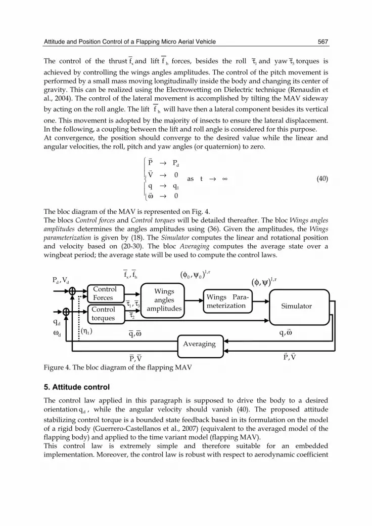
The control of the thrust xf and lift hf forces, besides the roll 1τ and yaw 3τ torques is

achieved by controlling the wings angles amplitudes. The control of the pitch movement is performed by a small mass moving longitudinally inside the body and changing its center of gravity. This can be realized using the Electrowetting on Dielectric technique (Renaudin et al., 2004). The control of the lateral movement is accomplished by tilting the MAV sideway

by acting on the roll angle. The lift hf will have then a lateral component besides its vertical

one. This movement is adopted by the majority of insects to ensure the lateral displacement. In the following, a coupling between the lift and roll angle is considered for this purpose. At convergence, the position should converge to the desired value while the linear and angular velocities, the roll, pitch and yaw angles (or quaternion) to zero.

d

I

P P

V 0as t

q q

0

⎧ →⎪⎪ →→ ∞⎨

→⎪⎪ω →⎩ (40)

The bloc diagram of the MAV is represented on Fig. 4. The blocs Control forces and Control torques will be detailed thereafter. The bloc Wings angles amplitudes determines the angles amplitudes using (36). Given the amplitudes, the Wings parameterization is given by (18). The Simulator computes the linear and rotational position and velocity based on (20-30). The bloc Averaging computes the average state over a wingbeat period; the average state will be used to compute the control laws. Figure 4. The bloc diagram of the flapping MAV

5. Attitude control

The control law applied in this paragraph is supposed to drive the body to a desired

orientation dq , while the angular velocity should vanish (40). The proposed attitude

stabilizing control torque is a bounded state feedback based in its formulation on the model of a rigid body (Guerrero-Castellanos et al., 2007) (equivalent to the averaged model of the flapping body) and applied to the time variant model (flapping MAV). This control law is extremely simple and therefore suitable for an embedded implementation. Moreover, the control law is robust with respect to aerodynamic coefficient

Control torques

d dP ,V

d

d

q

ω

1( )η

x hf , f l ,r0 0( , )φ ψ

l ,r( , )φ ψ

P,V

Simulator

Averaging

Control Forces

Wings angles

amplitudes

Wings Para- meterization

q,ω

P,V

q,ω

1 3,τ τ

2τ

Aerial Vehicles

568

errors and does not require the knowledge of the body's inertia. Let T

1 2 3, ,τ = τ τ τ⎡ ⎤⎣ ⎦ be the

roll, pitch and yaw control torques.

( )j 1, jj j j j 0 M j= -sat + sign(q )sat (q )τ⎡ ⎤τ λ δ ω⎣ ⎦ (41)

where j {1, 2, 3}∈ , 0sign(q ) takes into account the possibility of 2 rotations to drive the body

to its equilibrium orientation; the one of smaller angle is chosen. jω and jq are the averaged

angular velocities and quaternion over a single wingbeat period, representing the time

varying angular velocities and quaternion of a rigid body. jλ and jδ are positive parameters.

Differently from (Guerrero-Castellanos et al., 2007), jδ has been added in order to slow

down the convergence of the torque relative to the angular velocity. 1, jMsat and

jsatτ are

saturation functions with 1, jM and jτ the saturation bounds: 1, jM 1≥ , j j 1, j j(2M )τ ≥ δ + ε and

j 1ε > . The jτ 's are chosen in order to respect input saturations: wings Euler angles and

body's length. Based on (33, 37), the maximum flapping and rotation amplitudes, 0φ and 0ψ ,

define a set 1 3,τ τΩ of admissible torques (see Fig. 5). The saturation bounds 1τ and 3τ are

adjusted in (41) so that 1τ and 3τ remain in the limits of1 3,τ τΩ , which guarantees not to

exceed the maximum angles. 2τ should respect the saturation induced by the length of the

body, since the pitch torque is generated by a small mass moving inside it. The asymptotic stability of the closed loop system has been shown in (Guerrero-Castellanos

et al., 2007) for rigid bodies using the following Lyapunov function (the added parameter jδ

does not change the proof).

T 2 T0

1V = J + ((1 - q ) + q q)

2ω ω κ (42)

Therefore, 0ω → and Iq q→ (based on the rigid body case). By means of the averaging

theory, 1k Tω − ω < and

2q q k T− < for }{1,2

k 0> and T the wingbeat period.

6. Position control

Neglecting the viscous force fc V acting on the MAV's body by supposing that it is moving

at low speeds, the translational subsystem (30) can be transformed into a chain of

integrators. fc V will be considered as a disturbance term in simulations. Supposing that

after a sufficiently long time, the MAV is stabilized over the pitch and yaw axes

( )2 3 0η = η = thanks to the control law (41), thereby the rotation matrix defines solely a

rotation about the roll axis mx . The normalized translational subsystem, augmented of a

state representing the integral of the position, can be written (T

fx y zP P ,P ,P⎡ ⎤= ⎣ ⎦ is the current

position)


569

1 2

2 3

3 x

4 5

5 6

6 h 1

7 8

8 9

9 h 1

p p

p p

p v

p p

p p

p v sin( )

p p

p p

p v cos( ) 1

⎧ =⎪=⎨⎪ =⎩=⎧⎪ =⎪⎪ = − η⎪⎨ =⎪⎪ =⎪= η −⎪⎩

(43)

(44)

( )f f f z f f f f fx x x y y y z z z 1 9

1p P ,P ,V , P ,P ,V , P ,P ,V p , ,p

g⎛ ⎞= =⎜ ⎟⎝ ⎠∫ ∫ ∫ … is the averaged state of the

translational subsystem, x h

x h

f fv ,v

mg mg= = where xf and hf are respectively the control

thrust and lift, 1η is the roll angle and 1 is the normalized gravity (Hably et al., 2006).

The averaged normalized system (43, 44) will be used to compute the normalized control thrust

xv and lift hv . As for (41), the proposed controls are bounded and have a low

computational cost.

6.1 Stabilization of the forward movement

System (43) defines a triple integrator chain. It can be stabilized using the control based on nested saturations (14) with the variable saturation bound (16). The variable change given in

(17) developed to the third order for poles placement in 1 2 3( a , a , a )− − −

1 1 2 3 3 1 2 3 1

2 1 2 2 2

3 1 3

y a a a a (a + a ) a x

y = 0 a a a x

y 0 0 a x

⎡ ⎤ ⎡ ⎤ ⎡ ⎤⎢ ⎥ ⎢ ⎥ ⎢ ⎥⎢ ⎥ ⎢ ⎥ ⎢ ⎥⎢ ⎥ ⎢ ⎥ ⎢ ⎥⎣ ⎦ ⎣ ⎦⎣ ⎦ (45)

Which can be written in a compact form as y = xΠ , with i , jΠ the element at the i’th row

and j’th column. xv can then be written as

(

)x 3 ,3 2 x 3 x x 2 ,3 2 ,23 ,3 3 2

1 x 3 x 2 x 2 x1 1 ,3 1 ,2 1 ,12 ,3 2 ,2

x v x 3 ( p ,L ,M ) x 3 x 2

( p + p ,L ,M ) x 3 x 2 x 1

v = - p + ( p + p +…

( p + p + p ))

γ Π

γ Π Π

σ Π σ Π Π

σ Π Π Π (46)

where xv is the saturation bound of xv and respects the saturation x hf , f

Ω (see Fig. 5) in order

to guarantee wings angles lower than the maximum values. ( )σ ⋅ is the saturation function

defined in (10) and xΠ is the transformation matrix relative to the forward movement. The

asymptotic stability of 1 2 3(p ,p ,p ) is proven based on (Johnson and Kannan, 2003;

Marchand, 2003).

Aerial Vehicles

570

6.2 Stabilization of the lateral and vertical movements

The coupling between the roll angle 1η and normalized lift force hv is explicitly shown in

(44). 1η behaves like an intermediate input to (44) transforming the problem to a VTOL

(Vertical Taking Off and Landing) one. 1η should converge to a desired value 1dη given by

d

y

1

z

-v= arctan( )

v + 1η (47)

Where yv and zv will be determined thereafter. The normalized lift is determined by

2 2h y zv = v +(v + 1) (48)

The desired quaternion is computed by

d d

T

1 1

dq = cos ,sin ,0,02 2

η η⎡ ⎤⎢ ⎥⎣ ⎦ (49)

The flapping MAV should track a desired angular velocity given by

d

d

TT -1d d

T

d 1

0, 2q q

,0,0

⎡ ⎤ω = ⊗⎣ ⎦⎡ ⎤ω = η⎣ ⎦

(50)

(51)

Where 1dq− is the quaternion inverse (3) and ⊗ the quaternion product (4). The derivative of

the roll angle is given by ( yv and zv will be determined thereafter)

d

y z y z

1 2 2y z

-v (v + 1) + v v=

v + (v + 1)η (52)

The quaternion error is computed using (5) and the error of angular velocity by e d= -ω ω ω .

Applying control torque (41) on the error dynamics, the convergence of 1η to d1η is ensured.

System (44) is then transformed into two independent triple integrators.

4 5

5 6

6 y

p = p

p = p

p = v

⎧⎪⎨⎪⎩

7 8

8 9

9 z

p = p

p = p

p = v

⎧⎪⎨⎪⎩ (53)

Applying the same control law as for the forward movement, yv and zv are computed

()

y 3 ,3 2 y 6 y y 2 ,3 2 ,23 23 ,3

1 y 6 y 5 y 2 y 1 1 ,3 1 ,2 1 ,12 ,3 2 ,2

y v y 6 ( p ,L ,M ) y 6 y 5

( p + p ,L ,M ) y 6 y 5 y 4

v = - p + ( p + p +…

( p + p + p ))

γ Π

γ Π Π

σ Π σ Π Π

σ Π Π Π

()

z 3 ,3 2 Z 9 z z 2 ,3 2 ,23 23 ,3

1 z 9 z 8 z 2 z 1 1 ,3 1 ,2 1 ,12 ,3 2 ,2

z v z 9 ( p ,L ,M ) z 9 z 8

( p + p ,L ,M ) z 9 z 8 z 7

v = - p + ( p + p +…

( p + p + p ))

γ Π

γ Π Π

σ Π σ Π Π

σ Π Π Π

(54)

(55)


571

Where ( )σ ⋅ is defined by (10). yv and zv should verify

2 2h y zv = v +(v + 1) (56)

hv should respect the saturation set x hf , f

Ω in order to guarantee admissible wings angles

amplitudes 0φ and 0ψ . Finally, in order to evaluate the desired angular velocity, the

derivative of yv and zv are computed

() {

y 3 ,3 2 y 6 y y 2 ,2 2 ,33 ,3 3 2

1 y 5 y 6 y y 1 ,1 1 ,2 1 ,3 3 ,32 ,2 2 ,3 2 1

2 y 6 y y 2 ,2 2 ,33 ,3 3 2

1 y 5 y 6 y y 1 ,1 1 ,2 ,2 2 ,3 2 1

y v y 6 ( p ,L ,M ) y 5 y 6

( p + p ,L ,M ) y 4 y 5 y 6 y y

( p ,L ,M ) y 5 y 6

( p + p ,L ,M ) y 4 y

v - p + ( p + p +…

( p + p p )) . r

( p + p

( p +

γ Π

γ Π Π

γ Π

γ Π Π

= σ Π σ Π Π

σ Π Π + Π Π +

σ Π Π +

σ Π Π

…

…

)}

2 1 ,3 2 ,2

2 ,3 1 y 5 y 6 y y 1 ,1 1 ,2 1 ,3 1 ,1 1 ,2 1 ,32 ,2 3 ,3 2 1

5 y 6 y 6

y y ( p + p ,L ,M ) y 4 y 5 y 6 y 5 y 6 y y

p p )) . p

r ( p + p p ).( p p r )γ Π Π

⎡+ Π Π +⎣⎤Π + σ Π Π + Π Π + Π + Π ⎦

…

(57)

() {

z 3 ,3 2 z 9 z z 2 ,2 2 ,33 ,3 3 2

1 z 8 z 9 z z 1 ,1 1 ,2 1 ,3 3 ,32 ,2 2 ,3 2 1

2 z 9 z z 2 ,2 2 ,33 ,3 3 2

1 z 8 z 9 z z 1 ,1 1 ,2 ,2 2 ,3 2 1

z v z 9 ( p ,L ,M ) z 8 z 9

( p + p ,L ,M ) z 7 z 8 z 9 z z

( p ,L ,M ) z 8 z 9

( p + p ,L ,M ) z 7 z

v - p + ( p + p +…

( p + p p )) . r

( p + p

( p +

γ Π

γ Π Π

γ Π

γ Π Π

= σ Π σ Π Π

σ Π Π + Π Π +

σ Π Π +

σ Π Π

…

…

)}

2 1 ,3 2 ,2

2 ,3 1 z 8 z 9 z z 1 ,1 1 ,2 1 ,3 1 ,1 1 ,2 1 ,32 ,2 3 ,3 2 1

8 z 9 z 9

z z ( p + p ,L ,M ) z 7 z 8 z 9 z 8 z 9 z z

p p )) . p

r ( p + p p ).( p p r )γ Π Π

⎡+ Π Π +⎣⎤Π + σ Π Π + Π Π + Π + Π ⎦

…

(58)

( )σ ⋅ is defined in (11), yr and zr are computed by

y h 1

z h 1

r = -v sin( )

r = v cos( ) - 1

η

η (59)

The asymptotic stability of 4 9(p , ,p )… is proved based on (Johnson and Kannan, 2003;

Marchand, 2003).

Applying the proposed control law, dP P 0− → and dV V 0− → . By means of Theorem 1,

3P P k T− < and 4V V k T− < for {3,4}k 0> and T the wingbeat period.

7. MAV dimensions

Diptera insect (Dudley, 2002) is the model adopted for simulations. It has a mass of 200mg and a wingbeat frequency of 100Hz. Its maximum flapping angle amplitude is 60°. The wing is supposed to rotate up to 90° about its span-wise axis. The wingspan and wings surface are

assumed respectively to 2L=3cm and 2w2S 1.14cm= , so that a vertical ascendant movement

can be achieved using flapping angles amplitudes lower than the maximum values. Using these

numerical values, admissible sets for control forces x hf , f

Ω and torques 1 3,τ τΩ can be defined (33).

Aerial Vehicles

572

1 3,τ τΩ has been approximated to the largest ellipse rE that fits inside 1 3,τ τΩ (see Fig. 5) for

computation simplification reasons. Therefore, the control torques should respect an

ellipsoidal admissible rE set defined by

[ ] [ ]T

1 3 r 1 3P 1τ τ τ τ ≤ (60)

where rP is positive definite matrix representing the ellipse’s semi-axes. Practically, if 1 1τ ≥ τ

(41), 1τ could be saturated to 1τ and 3 0τ = . To avoid a null yaw control torque in this case,

70% of 1τ will be attributed to 1τ , 3τ will be computed by (60) defining then a set rΩ (see Fig.

5). This choice is justified by the necessity to bring the MAV on the flat (horizontal plane) first.

The admissible set of thrust and lift forces x hf , f

Ω is drawn in Fig.5. It can be approximated to

the largest semi-ellipse tE that fits inside ( tE almost coincides with x hf , f

Ω ), ( tP is positive

definite matrix representing the ellipse’s semi-axes)

T

x h t x h

h

f f P f f 1

f 0

⎡ ⎤ ⎡ ⎤ ≤⎣ ⎦ ⎣ ⎦≥

(61)

A fixed saturation level inside tE is attributed to hf since it will be decomposed in ymgv

and zmgv (for computation simplification reasons). The saturation bound is computed

such that more power is attributed to the lift since it is associated to the roll movement (99%

of tE ’s vertical semi-axis is attributed to hmgv ): the MAV is brought to the horizontal

plane rapidly. The saturation boundxmgv of the thrust xf satisfies the semi-ellipse's

equation. The saturation set of the control forces is tΩ .

Figure 5. Yaw torque versus roll torque (left), defining the saturation set 1 3,τ τΩ (dashed blue

line) approximated to an ellipse rE (red dot-dashed line) then to a set

rΩ (green continuous

line). Lift versus thrust (right), defining the saturation set x hf , f

Ω approximated to a semi-

ellipse tE , that almost coincides with x hf , f

Ω (red dot-dashed line), then to the set tΩ (green

continuous line)


573

8. Simulations and robustness tests

The control laws are tested in simulations using the complete model. The initial position is (1m, 1m, -1m) and the initial orientation (-40°, -25°, 50°). The choice for the poles placement

is the following: x x x1 2 3( a , a , a ) ( 3, 3, 3)− − − = − − − for the forward dimension,

y y y1 2 3( a , a , a ) ( 3.5, 3.5, 3.5)− − − = − − − for the lateral one, and z z z1 2 3( a , a , a ) ( 2.5, 2.5, 2.5)− − − = − − −

for the vertical one. The evolution of the linear position and velocity and the control forces are shown in Fig. 6. Due to the poles placement, the system’s dynamics are accelerated which causes an

overshoot. The saturation bound of the control thrust xf depends on the value of the control

lift hf . Besides, hf does not converge to 0 but to mg in order to balance the MAV’s weight

(in hovering mode). The roll, pitch and yaw angles, angular velocities and the control torques are plotted on Fig. 7. The dependence of the roll, lateral and vertical movements can be clearly noticed. The wings angles amplitudes are presented on Fig. 8.

8.1 Robustness with respect to external disturbances

The external disturbances are assimilated to external forces and torques applied to the body. The MAV is perturbed at t=7s during 10 wingbeat periods. The magnitude of the

disturbances, over the three axes, is 3 3 3(5.10 ,5.10 ,3.10 )N− − − for the forces and

5 5 5(3.10 ,3.10 ,3.10 )N m− − − ⋅ for the torques, values considered in mR . Note that a rain drop

weighs about 65.10 N− (almost 1000 times lighter than the disturbance). Such high values of

the disturbances are simulated to show the importance of the saturations in the divergence avoidance. Even though the disturbance is the lowest along the vertical axis, its influence on the vertical movement is the highest (Fig. 9). The control torques and forces cooperate in order to overcome the disturbances and ensure stability. They reach the saturation bounds in order to use their maximum power (Fig. 9, 10 and 11). The evolution of the angles and angular velocity (Fig. 10) zoomed around the saturation (Fig. 11) shows that the MAV executes many turns around its axes, the angular velocity reaches very high values. The relation between the roll and the yaw saturation bounds is shown clearly on Fig. 11. The disturbance is also detectable on the wings angles amplitudes which saturate (Fig. 12).

8.2 Robustness with respect to aerodynamic errors

The robustness of the control law is also tested for a bad estimation of the aerodynamic coefficient C, known to be difficult to identify. This property is essential for real time implementation where the flapping MAV can execute missions in different areas having different aerodynamic characteristics. An additive error is introduced to C

distC C C= − Δ (62)

where CΔ is a stochastic parameter subject to a uniform distribution, such that Cdist varies

within the interval [2, 3.5]. A different value of CΔ is applied at each wingbeat period. Such

a quick variation of the aerodynamic coefficient is not realistic; it is simulated only to emphasize the control law robustness. The influence of the aerodynamic coefficient

Aerial Vehicles

574

variation is shown in Fig. 13 and 14. The stochastic aspect can be seen on the vertical

position Pz and velocity Vz besides the lift force hf . The control lift has then a greater value

( )hf mg> at convergence in order to balance the reduction of the aerodynamic coefficient.

9. Conclusions and future works

The present chapter has presented a new strategy of controlling flapping MAVs. It is based on a bounded state feedback control of the forces and the torques. The control takes into consideration the saturation of the actuators driving the flapping wings. They are based on the theory of cascade, aiming to stabilize the attitude of the MAV, while driving the body to a desired position, associating the translational movement to the rotational one. The controls are extremely low cost, therefore suitable for an embedded implementation. They are computed using a simplified model of a flapping MAV (averaged over a wingbeat period). This model is based only on the steady aerodynamics. The control laws are applied at each wingbeat period. Different robustness tests are performed, especially with respect to the simplifications adopted in the proposed model, besides external disturbances, modeling errors, parameters uncertainties, etc.

Figure 6. The linear position (left) and velocity (right) of the MAV and the control forces (bottom), the saturation bounds are plotted with the red dashed line

Future works consist of developing bounded control laws based directly on a minimum number of sensors measurements in order to ensure the stability in three dimensions.


575

Figure 7. The roll, pitch and yaw angles (left), angular velocity (middle) and the control torques (right) of the MAV. The pitch and yaw components are zoomed to the first 2s

Figure 8. The envelops of the flapping and rotation angles amplitudes

Aerial Vehicles

576

Figure 9. Robustness with respect to external disturbances: Evolution of the linear position (left) and velocity (right) and the control forces (bottom)

Figure 10. Robustness with respect to external disturbances: Evolution of the roll, pitch and yaw angles (left), the angular velocities (middle) and the control torques (right)


577

Figure 11. Robustness with respect to external disturbances: Evolution of the roll, pitch and yaw angles (left), the angular velocities (middle) and the control torques (right) zoomed around the disturbance

Figure 12. Robustness with respect to external disturbances: The envelops of the wings angles amplitudes

Aerial Vehicles

578

Figure 13. Robustness with respect to the aerodynamic coefficient: Evolution of the linear position (left) and velocity (right) and the control forces (bottom)

Figure 14. Robustness with respect to the aerodynamic coefficient: Evolution of the roll, pitch and yaw angles (left), the angular velocities (middle) and the control torques (right) zoomed to the first second for the pitch and yaw


579

10. References

Boyer, F.; Porez, M. & W. Khalil, Macro-continuous computed torque algorithm for a three-dimensional eel-like robot, IEEE Transaction on Robotics and Automation, Vol. 22, No. 4, 2006, page numbers (763–775).

Bullo, F. (2002). Averaging and vibrational control of mechanical systems. SIAM Journal on Control and Optimization, Vol. 41, No. 2, page numbers (452-562)

Campolo, D.; Sitti, M. & Fearing, R. S. (2003). Efficient charge recovery method for driving piezoelectric actuators with quasi-square waves. IEEE Trans. on Ultrasonics, Ferroelectrics and Frequency Control, Vol. 50, No. 3, page numbers (237-244)

Deng, X. ; Schenato, L. & Sastry, S. (2002). Model identification and attitude control scheme for a micromechanical flying insect. Proceedings of the 7th International Conference on Control, Automation, Robotic and Vision, pp. 1007-1012, Singapore.

Deng, X.; Schenato, L. & Sastry, S. (2003). Model identification and attitude control for a micromechanical flying insect including thorax and sensor models. Proceedings of the IEEE Int. Conference on Robotics and Automation, pp. 1152-1157, Taipei, Taiwan.

Deng, X.; Schenato, L.; Wu, W.-C. & Sastry, S. (2006a). Flapping flight for biomimetic robotic insects : Part I- system modeling. IEEE Transactions on Robotics, Vol. 22, No. 4.

Deng, X.; Schenato, L.; Wu, W.-C. & Sastry, S. (2006b). Flapping flight for biomimetic robotic insects : Part II- flight control design. IEEE Transactions on Robotics, Vol. 22, No. 4, page numbers (789-803)

Dickinson, M.; Lehmann, F.-O. & Sane, S. (1999). Wing rotation and the aerodynamic basis of insect flight. Science, Vol. 284, No. 5422, page numbers (1954-1960)

Dickson, W.; Straw, A.; Poelma, C. & Dickinson, M. (2006). An integrative model of insect flight control. Proceedings of the 44th AIAA Aerospace Sciences Meeting and Exhibit, Reno, USA

Dudley, R. (2002). The biomechanics of insect flight: form, function, evolution. Princeton University Press

Guerrero-Castellanos, J.; Hably, A.; Marchand, N. & Lesecq, S. (2007). Bounded attitude stabilization : Application on four rotor helicopter. Proceedings of the 2007 IEEE Int. Conf. on Robotics and Automation, pp. 730-735, Roma, Italy.

Hably, A.; Kendoul, F.; Marchand, N. & Castillo, P. (2006). Further results on global stabilization of the PVTOL aircraft. Proceedings of the Second Multidisciplinary International Symposium on Positive Systems : Theory and Applications, pp. 303-310, Grenoble, France.

Hedrick, T. & Daniel, T. (2006). Flight control in the hawkmoth Manduca sexta : the inverse problem of hovering. The journal of experimental Biology, Vol. 209, No. 16, page numbers (3114-3130).

Janocha, H. & Stiebel, C. (1998). New approach to a switching amplifier for piezoelectric actuators. Proceedings of ACTUATOR 98, 6th International Conference on New Actuators, pp. 189-192, Bremen, Germany.

Johnson, E. & Kannan, S. (2003). Nested saturation with guaranteed real poles. Proceedings of the American Control Conference, volume 1, pp. 497-502.

Khalil, H. (1996). Nonlinear Systems. Prentice-Hall. Kuhnen, K.; Janocha, H.; Thull, D. & Kugi, A. (2006). A new drive concept for high-speed

positioning of piezoelectric actuators. Proceedings of the 10th International Conference on New Actuators, pp. 82-85, Bremen, Germany.

Aerial Vehicles

580

Marchand, N. (2003). Further results on global stabilization for multiple integrators with bounded controls. Proceedings of the IEEE Conference on Decision and Control, CDC'2003, volume 5, pp. 4440-4444, Hawai, USA.

Rakotomamonjy, T. (2006). Modelization and flight control of a flapping-wing Micro Air Vehicle. PhD thesis, University Paul Cezanne Aix Marseille.

Rakotomamonjy, T.; Le Moing, T. & Ouladsine, M. (2004). Simulation model of a flapping-wing micro air vehicle. Proceedings of the European Micro Aerial Vehicle Conf., EMAV 2004, Braunschweig, Germany.

Reiser, M. ; Humbert, J.; Dunlop, M.; Del Vecchio, D.; Murray, R. & Dickinson, M. (2004). Vision as a compensatory mechanism for disturbance rejection in upwind flight. Proceedings of the American Control Conference, volume 1, pp. 311-316, Boston, Massachusetts, USA.

Renaudin, A.; Zhang, V.; Tabourier, P.; Camart, J. & Druon, C. (2004). Droplet manipulation using SAW actuation for integrated microfluidics. Proceedings of the μTAS, pp. 551-553, Malmö, Sweden.

Sane, S. (2003). Review The aerodynamics of insect flight. The journal of experimental Biology, 206,23, page numbers (4191-4208).

Schenato, L. ; Campolo, D. & Sastry, S. (2003). Controllability issues in flapping flight for biomimetic micro aerial vehicles (MAVs). Proceedings of the IEEE International Conference on Decision and Control, Las Vegas, USA.

Schenato, L.; Deng, X. & Sastry, S. (2001). Flight control system for a micromechanical flying insect : Architecture and implementation. Proceedings of the IEEE International Conference on Robotics and Automation, pp. 1641-1646, Seoul, Korea.

Schenato, L. ; Deng, X. & Sastry, S. (2002a). Hovering flight for a micromechanical flying insect : Modeling and robust control synthesis. Proceedings of the 15th IFAC World Congress on Automatic Control, Barcelona, Spain.

Schenato, L., Wu, W.-C., and Sastry, S. (2002b). Attitude control for a micromechanical flying insect via sensor output feedback. Proceedings of the 7th International Conference on Control, Automation, Robotic and Vision, pp. 1031-1036, Singapore.

Schenato, L.; Wu, W.-C. & Sastry, S. (2004). Attitude control for a micromechanical flying insect via sensor output feedback. IEEE Journal of Robotics and Automation, Vol. 20, No. 1, page numbers (93-106).

Shuster, M. (1993). A survey of attitude representations. Journal of astronautical sciences, Vol. 41, No. 4, page numbers (439-517).

Sriram; Gopinath, A.; Van Der Weide, E.; Kim, S.; Tomlin, C. & Jameson, A. (2005). Aerodynamics and flight control of flapping wing flight vehicles : A preliminary computational study. Proceedings of the 43rd Aerospace Sciences Meeting, Reno, USA.

Tanaka, F.; Ohmi, T.; Kuroda, S. & Hirasawa, K. (2006). Flight control study of an virtual insect by a simulation. JSME Int. Journal, Vol. 49, No. 2, page numbers (556-561).

Teel, A. (1992). Global stabilization and restricted tracking for multiple integrators with bounded controls. Systems & Control Letters, Vol. 18, No. 3, page numbers (165-171).

Thakoor, S.; Cabrol, N.; Lay, N.; Chahl, J.; Soccol, D.; Hine, B. & Zornetzer, S. (2003). Review: The benefits and applications of bioinspired flight capabilities. Journal of Robotic Systems, Vol. 20, No. 12, page numbers (687-706).

Vela, P. A. (2003). Averaging and Control of Nonlinear Systems. PhD thesis, California Institute of Technology.

Attitude and Position Control of a Flapping Micro Aerial Vehicle

Documents

Transcript of Attitude and Position Control of a Flapping Micro Aerial Vehicle