Aerial Counts - State of the Salmon
60
SUPPLEMENTAL TECHNIQUES | 399 AERIAL COUNTS Aerial Counts Edgar L. Jones III, Steve Heinl, and Keith Pahlke Background Aerial counts of salmon are essential tools in Pacific salmon Oncorhynchus spp. management. In Alaska the first recorded aerial count of salmon was made by C. M. Hatton of the U.S. Bureau of Fisheries in the Lake Clark district of Bristol Bay in 1930. As fisheries management progressed, so did the need to cover more streams in shorter periods of time, inspiring the first systematic use of aerial surveys in Alaska by Agent Fred O. Lucas of the Bureau of Fisheries in 1937 (Eicher 1953). The aerial survey technique is best suited for broad, shallow, clear-water systems with limited overhanging vegetation, undercut banks, and canopy cover. Aerial counts are severely compromised in glacial or turbid waters and in excessively deep water such that fish are beyond the range of visibility (Cousens et al. 1982). Species such as steelhead O. mykiss and coho O. kisutch salmon can be difficult to survey as these fish are often cryptic in coloration and have the behavior of seeking cover, even during spawning, making them less visible. The visibility of spawning salmon to observers depends on many factors such as water quality, fish concealment, stream dimensions, and density of fish, among others (Bevan 1961). The ability of the observer to count fish accurately has been the main topic of many aerial survey studies (Bevan 1961; Neilson and Geen 1981; Cousens et al. 1982; Labelle 1994; Symons and Waldichuk 1984; Dangel and Jones 1988; Jones et. al 1998). Furthermore, biased counts of salmon abundance and associated measurement error have been seen to produce seriously biased estimates of optimum harvest rate and escapement in stock-recruitment analysis (Walters 1981; Walters and Ludwig 1981). An interesting phenomenon is that the accuracy and precision of observer counts decreases as abundance increases, and simple linear corrections for bias are not as appropriate as using allometric forms with multiplicative error structure in light of changing magnitudes of fish. In short, humans are overly conservative and tend to underestimate versus overestimate when counting objects (Jones et al. 1998; Clark 1992; Dangel and Jones 1988; Daum et al. 1992; Evensen 1992; Rogers 1984; Shardlow et al. 1987; Skaugstad 1992). Efforts should be made to minimize the influence of extraneous variables such as weather, water quality, aircraft type, and pilot performance, and observers should minimize the impacts of these variables to the best of their abilities. The density of fish may also be an important variable. Eicher (1953), in work performed in Bristol Bay, said that the accuracy of observer counts might be inversely proportional to the density of salmon. Often, salmon can be seen packed into very tight schools, and in one study on coho salmon, fish were much easier to count once they were disturbed and disbursed, in principle lowering the school density (Irvine et al. 1992). In essence, increasing the density of salmon has much the same effect as increasing the number of undercut banks, water glare and turbidity, and canopy cover (Jones et. al 1998). Prior knowledge of the stream is beneficial with regard to accuracy when performing aerial counts. One study showed that observers familiar with the stream consistently produced more accurate estimates when compared to observers not familiar with the stream (ADFG 1964).
-
Upload
khangminh22 -
Category
Documents
-
view
1 -
download
0
Transcript of Aerial Counts - State of the Salmon
S U P P L E M E N T A L T E C H N I Q U E S | 399
A E R I A L C O U N T S
Aerial Counts Edgar L. Jones III, Steve Heinl, and Keith Pahlke
BackgroundAerial counts of salmon are essential tools in Pacific salmon Oncorhynchus spp. management. In Alaska the first recorded aerial count of salmon was made by C. M. Hatton of the U.S. Bureau of Fisheries in the Lake Clark district of Bristol Bay in 1930. As fisheries management progressed, so did the need to cover more streams in shorter periods of time, inspiring the first systematic use of aerial surveys in Alaska by Agent Fred O. Lucas of the Bureau of Fisheries in 1937 (Eicher 1953). The aerial survey technique is best suited for broad, shallow, clear-water systems with limited overhanging vegetation, undercut banks, and canopy cover. Aerial counts are severely compromised in glacial or turbid waters and in excessively deep water such that fish are beyond the range of visibility (Cousens et al. 1982). Species such as steelhead O. mykiss and coho O. kisutch salmon can be difficult to survey as these fish are often cryptic in coloration and have the behavior of seeking cover, even during spawning, making them less visible. The visibility of spawning salmon to observers depends on many factors such as water quality, fish concealment, stream dimensions, and density of fish, among others (Bevan 1961). The ability of the observer to count fish accurately has been the main topic of many aerial survey studies (Bevan 1961; Neilson and Geen 1981; Cousens et al. 1982; Labelle 1994; Symons and Waldichuk 1984; Dangel and Jones 1988; Jones et. al 1998). Furthermore, biased counts of salmon abundance and associated measurement error have been seen to produce seriously biased estimates of optimum harvest rate and escapement in stock-recruitment analysis (Walters 1981; Walters and Ludwig 1981). An interesting phenomenon is that the accuracy and precision of observer counts decreases as abundance increases, and simple linear corrections for bias are not as appropriate as using allometric forms with multiplicative error structure in light of changing magnitudes of fish. In short, humans are overly conservative and tend to underestimate versus overestimate when counting objects (Jones et al. 1998; Clark 1992; Dangel and Jones 1988; Daum et al. 1992; Evensen 1992; Rogers 1984; Shardlow et al. 1987; Skaugstad 1992). Efforts should be made to minimize the influence of extraneous variables such as weather, water quality, aircraft type, and pilot performance, and observers should minimize the impacts of these variables to the best of their abilities. The density of fish may also be an important variable. Eicher (1953), in work performed in Bristol Bay, said that the accuracy of observer counts might be inversely proportional to the density of salmon. Often, salmon can be seen packed into very tight schools, and in one study on coho salmon, fish were much easier to count once they were disturbed and disbursed, in principle lowering the school density (Irvine et al. 1992). In essence, increasing the density of salmon has much the same effect as increasing the number of undercut banks, water glare and turbidity, and canopy cover (Jones et. al 1998). Prior knowledge of the stream is beneficial with regard to accuracy when performing aerial counts. One study showed that observers familiar with the stream consistently produced more accurate estimates when compared to observers not familiar with the stream (ADFG 1964).
400 | S U P P L E M E N T A L T E C H N I Q U E S
A E R I A L C O U N T S
RationaleReliable methods for estimating escapements are of critical importance to fisheries management agencies. Such information is vital in forecasting production in subsequent years as well as in measuring the relative success of management charged with achieving adequate escapements over time. Aerial counts are a common method used to index escapement, given the large number of streams around the Pacific Rim (and elsewhere) that produce salmon. Often, these counts can be quite crude, providing little more than an index of escapement from year to year (Neilson and Geen 1981). Specifically, aerial counts are valuable not so much as estimators of the actual magnitude of salmon to each and every stream surveyed; rather, observer counts are useful as general indicators of what is taking place and how it compares within a year and to prior years. Long time series are essential, and the value of observer data increases with the length of the time series of data (Symons and Waldichuk 1984).
ObjectivesThis protocol describes methods used to achieve estimates of salmon escapement using two primary types of aircraft commonly used in aerial observer counts. Since many factors can introduce bias in observer counts, this paper will detail some key points to follow when performing aerial counts in an effort to produce consistent measures of salmon abundance over time. Two long-term programs in southeastern Alaska that estimate escapement utilizing observer counts from fixed-wing aircraft and helicopter for pink salmon O. gorbuscha and chinook salmon O. tshawytscha, respectively, are described. The first and foremost objective when making an aerial count is to try and make the most accurate count possible. The second objective, and probably of equal importance to the first, is to be consistent. An observer who consistently counts at a certain rate produces a better index to abundance than does an observer who is inconsistent. After all, the consistent observer can be modeled for counting rate whereas the inconsistent observer is virtually impossible to model. For example, one aerial observer who did surveys in southeastern Alaska typically counted pink salmon in units of 100 (e.g., every click on the tally whacker equaled 100 fish). This is atypical for most pink salmon aerial observers, who normally count in units of 1,000; however, upon examination, the observer who counted in units of 100 was shown to be the most consistent observer in the group, a characteristic that is vital to creating a reliable index of abundance over time.
Fixed-wing aircraftToday fixed-wing aircraft—specifically Supercubs—are most commonly used when performing aerial counts of salmon escapement using fixed-wing aircraft. The observer sits directly behind the pilot, allowing viewing access in either direction. Often, aircraft are flown at speeds around 100 km/h and heights of 30 m, and counts are made in an upstream direction. Not knowing the results of the first count, observers will sometimes turn and count the same stretch of stream in a downstream fashion and later compare results for consistency. This has the advantage of familiarizing the observer with the stream conditions and provides a different viewing angle that may eliminate glare or other factors encountered in the first survey. Sometimes, pilots also make counts, but care should be taken
S U P P L E M E N T A L T E C H N I Q U E S | 401
A E R I A L C O U N T S
to ensure that pilots are most concerned with keeping an open view of the river channel at all times.
Helicopter surveyAlthough more expensive than using fixed-wing aircraft, helicopters are often deployed for species of conservation concern or when fixed-wing counts are not practical or safe (e.g., in dense canopy or canyons). These aircraft provide slower, more maneuverable counting platforms that can increase accuracy and precision. Jet Ranger or Hughes 500 aircraft are commonly used, and observers sit on the left side of pilots. Normally, the door is removed and observers view the streams at heights of 15 to 70 m. Counts are normally made in only one direction to cut down on fuel costs, and pilots typically are solely concerned with keeping the aircraft level and over the viewing area.
Fixed-wing aircraft: Pink salmon in southeastern AlaskaIn southeastern Alaska, the methods used to monitor pink salmon escapements and calculate annual indices of spawning abundance were described by Hofmeister (1998), Van Alen (2000), and Zadina et al. (2004). Using the current method, biologists annually estimate the peak pink salmon abundance in 718 pink salmon index streams (selected from more than 2,500 known pink salmon spawning streams in the region). This assessment is made via aerial surveys, conducted at intervals during most of the migration period. Most pink salmon stocks in southeast Alaska do not show persistent trends of odd- or even-year dominance, and for simplicity, escapement indices of both brood lines are combined (Van Alen 2000; Zadina et al. 2004). Individual observers track absolute abundance within the streams, but each observer tends to count at his/her own rate, or “bias” (Bue et al. 1998; Dangel and Jones 1988; Jones et al. 1998). In 1995, raw stream survey counts were modified in an attempt to standardize as much observer bias as possible—not by removing bias but rather by adjusting all observer counts within each of the four Alaska Department of Fish and Game (ADF&G) management areas to the same bias level (Hofmeister 1998; Van Alen 2000). The index used only stream surveys conducted by key personnel or “major observers”—individuals who had flown more than 100 surveys per year in more than 4 years. Each major observer’s counts in a given management area was converted to the counting rate of the area management biologist, whose conversion rate was set at 1.0. These observations were statistically adjusted so the estimates of the number of fish were comparable among observers within the same management area (Hofmeister 1998). The largest count for the year was then retained for each stream in the survey and termed the “peak-adjusted count” for each stream. The index for each stock group was made up of the peak-adjusted counts, which were summed over this standard set of index streams for a particular area. If a particular index stream was missing escapement counts for any given year, an algorithm (McLachlan and Krishnan 1997) was used to interpolate the missing value. Interpolations were based on the assumption that the expected count for a given year was equal to the sum of all counts for a given stream, divided by the sum of all counts over all years for all the streams in the unit of interest (i.e., row total times column total divided by grand total). (The unit of interest is the stock group, and interpolations for missing values were made at the stock group level.)
402 | S U P P L E M E N T A L T E C H N I Q U E S
A E R I A L C O U N T S
This method is based on an assumed multiplicative relation between yearly count and unit count with no interaction. This method of assessing escapement does not actually provide an estimate of the total escapement of pink salmon for all of southeast Alaska. In the past, ADFG has multiplied the escapement indices by 2.5 to approximate the total escapement. For example, we found the statement “An expansion factor of 2.5 was applied to the escapement index to convert the index to an estimate of total escapement” (Hofmeister and Blick 1991) and similar statements in published material. The 2.5 multiplier was originally intended to convert peak escapement counts to an estimate of what was actually present at the time of the survey (Dangle and Jones 1988; Jones et al. 1998; Hofmeister 1990). Another important factor to consider in relating total run size to index series of escapement is the relationship between the total fish that spawn and die and the number of fish that are present in the creek at the time of the “peak observation” (Bue et al. 1998). This factor has not been well studied for systems in southeast Alaska (Zadina et al. 2004). The 718 streams in the current index represent only about one-third of the region’s 2,500+ pink salmon streams. Thus, the 2.5 multiplier does not take into account fish that were not present at the time of the survey, nor does it take into account streams that were not surveyed. Finally, the majority of aerial surveys, particularly those conducted prior to about 1970, were conducted to monitor in-season development of salmon escapements for management purposes, not to estimate total escapements (Jones and Dangel 1981; Van Alen 2000). There is no simple way to convert the current index series to an estimate of total escapement in southeast Alaska. Moreover, escapement indices are clearly less than total escapements (Hofmeister 1990; Van Alen 2000; Zadina et al. 2004).
Helicopter surveys: chinook salmon in Southeastern AlaskaThere are 34 river systems with populations of wild chinook salmon in southeastern Alaska. Three transboundary rivers—the Taku, Stikine, and Alsek—are classed as major producers, each with potential production (harvest + escapement) greater than 10,000 fish (Kissner 1974). There are nine rivers that are classed as medium producers, each with production of 1,500 to 10,000 fish. The remaining 22 rivers are minor producers, with production of less than 1,500 fish. Small numbers of chinook salmon occur in other streams of the region but are not included in the above list because successful spawning has not been documented. Chinook salmon are counted via aerial surveys or at weirs each year in all three major producing systems, six of the medium producers, and one minor producer. Abundance in the Chilkat River is estimated only by a mark–recapture program. These index systems, along with that used in the Chilkat River, are believed to account for about 90% of the total chinook salmon escapement in southeast Alaska and transboundary rivers (Pahlke 1998). Pahlke (1997) provides detailed descriptions of the escapement goals and their origins. Escapement goals have been revised when sufficient new information warrants. Most of the revised escapement goals have been developed with spawner–recruit analysis, as ranges of optimum escapement rather than a single point estimate. Spawner–recruit analysis requires not only a long series of escapement estimates but also annual age and sex-specific estimates of escapement (McPherson and Carlile 1997).
S U P P L E M E N T A L T E C H N I Q U E S | 403
A E R I A L C O U N T S
Spawning chinook salmon are counted at 26 designated index areas in nine of the systems; total escapement in the other two systems are estimated by complete counts of chinook salmon at the Situk River weir and by annual mark–recapture estimates on the Chilkat River. Counts are made during aerial or foot surveys during periods of peak spawning or at weirs. Peak spawning times—defined as the period when the largest number of adult chinook salmon actively spawn in a particular stream or river—are well documented from surveys of these index areas conducted since 1976 (Kissner 1982; Pahlke 1997). The proportion of fish in prespawning, spawning, and postspawning condition is used to judge whether the survey timing is correct to encompass peak spawning. Index areas are surveyed at least twice unless turbid water or unsafe conditions preclude the second survey. Survey conditions on each index survey are rated as poor, normal, or excellent for that particular index area, and are coded as to whether that survey is potentially useful for indexing or estimating escapement. Factors that affect the rating include water level, clarity, light conditions, and weather. Only large chinook salmon—typically age 3-, 4-, and 5-year, and greater than or equal to 660 mm mideye-to-fork length (MEF)—are counted during aerial or foot surveys. No attempt is made to record an accurate count of small (typically age 1- and 2-year) chinook salmon less than 660 mm MEF (Mecum 1990). These small chinook salmon (also called jacks) are early maturing, precocious males that are considered to be surplus to spawning escapement needs. Under most conditions they are distinct from their older counterparts because of their short, compact bodies and lighter color. They are, however, difficult to distinguish from other smaller species such as pink salmon and sockeye salmon O. nerka salmon. In some systems, it may be difficult to avoid counting age 2-year fish that are larger than 660 mm MEF. During aerial surveys, pilots are directed to fly the helicopter 15–70 m above the river at speeds of 6–16 kph. The helicopter door on the side of the observer is removed, and the helicopter is flown sideways while observations of spawning chinook salmon are made from the open space. Foot surveys are conducted by at least two people walking in the creek bed or on the riverbank. Weather, distances, run timing, and other factors can make it difficult for a single surveyor to complete all the index surveys annually under normal or excellent conditions. Thus, alternate surveyors are selected to conduct the counts when the primary surveyor is unavailable. New surveyors also take on primary responsibilities at infrequent intervals. Since between-observer variability and bias can be significant (Jones et al. 1998), new surveyors must be trained and calibrated against the primary surveyor to provide consistency and continuity in the data. Alternate observers accompany the primary observer on regularly scheduled surveys to learn survey methods and counting techniques (on training flights). Each alternate observer also accompanies the primary observer on additional regularly scheduled surveys to independently count chinook salmon (on calibration flights). Each calibration flight consists of two passes over the index area, so that the two observers, in turn, sit in the preferred location in the helicopter during one pass along the river. Count results are not shared during the calibration surveys but are shared and discussed following the completion of the second pass of each flight. Calibration data is collected annually for several years. The relationship between observer escapement counts will be determined from accumulated data and applied to counts as appropriate.

404 | S U P P L E M E N T A L T E C H N I Q U E S
A E R I A L C O U N T S
Several chinook salmon index areas are routinely surveyed by more than one method. For example, Andrew Creek, a small tributary in the lower Stikine River in Alaska, is surveyed from airplanes, from helicopters, and by foot. The various surveys are conducted as close as possible to each other to promote comparison and calibration of the different methods. Estimates of total escapement are needed to model total production, exploitation rates, and other population parameters. Since indices are only a partial count of spawning abundance, observer counts from index areas are increased by an expansion factor to estimate escapement. The expansion factor is an estimate of the proportion of the total escapement counted in a river system during the peak spawning period. Expansion factors are based on comparisons with weir counts, mark–recapture estimates, and spawning distribution studies. They vary among rivers according to how complete the coverage of spawning areas is and the difficulties encountered in observing spawners, such as overhanging vegetation, turbid water conditions, presence of other salmon species (e.g., pink salmon and chum salmon O. keta), and protraction of run timing. In southeastern Alaska, chinook salmon expansion factors range from 1.5 for the King Salmon River to 5.2 for the Taku River. Survey expansions are not necessary for those streams in which weirs or other estimation programs are used to count all migrating chinook salmon. In southeastern Alaska, estimates of total escapement are obtained from a weir on the Situk River and by use of mark–recapture on the Chilkat River. Still, observer counts of spawning abundance are regularly conducted in these systems because managers rely on counts and observation for more than just escapement objectives. Finally, to estimate the total southeastern Alaska regional escapement, estimates from the 11 index systems are expanded to account for the unsurveyed systems. The total estimated escapement in the index areas represents approximately 90% of the region total (Pahlke 1998). Expansion factors for individual rivers have been revised based on results from experiments to estimate total escapement and spawning distribution. For example, estimated total escapement and radio-tracking distribution data were used to revise tributary expansion factors for the Taku and Unuk rivers (Pahlke and Bernard 1996; Pahlke et al. 1996; McPherson et al. 1998). Mark–recapture studies to estimate spawning abundance on the Unuk River in 1994 (Pahlke et al. 1996) and on the Chickamin River in 1995 and 1996 were used to revise expansion factors for those two rivers in 1996; results were also applied to the nearby Blossom and Keta rivers. More mark–recapture studies were conducted on all four rivers and the expansion factors for the Behm Canal systems were revised again in 2002 (McPherson et al. 2003). On Andrew Creek, a weir was operated for 4 years (1979, 1981, 1982, and 1984), during which time index counts were also conducted, establishing a new expansion factor for that system in 1995. Also in 1997, 10 years (1983–1992) of matched weir and index counts were used to revise the expansion factor for the King Salmon River (McPherson and Clark 2001). The expansion factors for the Taku River were revised in 1996 and again in 1999 based on the results of mark–recapture studies (Pahlke and Bernard 1996; McPherson et al. 2000). These studies have improved estimates of total escapement in southeastern Alaska and have shown, in most cases, that the surveyed index areas provide
S U P P L E M E N T A L T E C H N I Q U E S | 405
A E R I A L C O U N T S
reasonably accurate trends in escapements; however, Johnson et al. (1992) demonstrated that expansion factors used before 1991 on the Chilkat River system were highly inaccurate, because the index areas received less than 5% of the escapement. Consequently, since 1991, escapement to the Chilkat River has been estimated annually by mark–recapture experiments (Ericksen and McPherson 2004). Studies on the Taku, Stikine, Alsek, Unuk, Chickamin, Blossom, Keta, and King Salmon rivers, as well as on Andrew Creek, have shown that the index expansion factors used on those systems were much more accurate than those used on the Chilkat (PSC 1991).
Sampling Design
Site selection is vital when choosing a suitable location for conducting observer counts. Areas surveyed should be representative of the population of concern and readily accessible and visible from the air. During periods of low abundance, the optimal spawning habitat will be that area containing salmon (assuming that salmon will seek out optimal spawning habitat). At higher levels of abundance, salmon may choose to spawn in less suitable habitats due to any number of reasons, and pinpointing the optimal habitat may be problematic. Ideally, the optimal spawning habitat will be contained in the area surveyed along with examples of less optimal habitat so that trends in abundance are captured entirely from year to year. Multiple counts should be made annually in each area so that all components of the run are captured, especially the peak. Many programs use peak counts for index purposes, but it is well understood that these counts do not represent the total escapement due to variability in run timing and stream life. At best, observers will get an index (an unknown portion) of the number of adult salmon returning to spawn, even if corrected for the changing population. In practice, it is more convenient to estimate the peak versus the average and assume that stream life is consistent among years; the peak count is a useful index (Bevan 1961). Some programs often go one step further by expanding indices by some factor to gain an estimate of total escapement; yet this in itself may introduce error. More reliable estimates of escapement can be obtained through use of area-under-the-curve (AUC) methodologies (English et al. 1992). These methods rely heavily on multiple counts performed within a year and, when coupled with an estimate of stream life, provide the information necessary to estimate total escapement (Cousens et al. 1982).
Personnel Requirements and Training
The experience of the personnel performing the counts is vital in any program. Pilot experience is also very important because the observer and pilot must work as a team to produce dependable estimates. Fatigue can play a big role in the accuracy of counts, yet studies have shown that utilizing one observer consistently from year to year is the best means available for providing an accurate index over that time. Knowing this, observers should keep the amount of survey time at a reasonable level; yet at the same time maintain adequate site coverage (Cousens et al. 1982).
406 | S U P P L E M E N T A L T E C H N I Q U E S
A E R I A L C O U N T S
Surveys performed during adverse weather conditions can produce entirely dissimilar results from surveys performed during ideal weather conditions. Surveys can be impacted by an array of adverse conditions that can delay surveys for weeks or more, resulting in the majority of the run being missed. Nevertheless, effort should be made to perform surveys during optimal conditions whenever and wherever possible and to maintain consistency from year to year. Precision (consistency) of escapement estimates is more important than accuracy for defining long-term stock-recruitment relationships (Symons and Waldichuk 1984).
Recommendations for Aerial Surveys
Aerial surveys should be performed with the understanding that the information gathered is first and foremost useful as an index—and only with significant study can observer counts be expanded further to estimates of total escapement. Information gathered during surveys should be clearly labeled as Aerial Survey Index Information gathered through observer counts so that it will not be misinterpreted as actual numbers. Surveys should be performed each year by a single observer, and when possible, other observers should perform overlapping surveys to gain information regarding observer variability, with the eventual change in survey personnel in subsequent years. It should be understood that any factor relating one observer to the next may vary from stream to stream and from year to year (Bevan 1961). Along with safety, maintaining consistency during surveys is of the utmost priority and concern. Counting units, aircraft and pilots used, and most certainly areas surveyed should be consistent from year to year to maximize the utility of any information gathered.
Literature Cited
ADFG (Alaska Department of Fish and Game). 1964. Studies to determine optimum escapement of pink and chum salmon in Alaska. Alaska Department of Fish and Game, Final Summary Report, Contract 14-17-007-22, Juneau.
Bevan, D. E. 1961. Variability in aerial counts of spawning salmon. Journal of the Fisheries Research Board of Canada 18(3):337–348.
Bue, B. G., S. M. Fried, S. Sharr, D. G. Sharp, J. A. Wilcock, and H. J. Geiger. 1998. Estimating salmon escapement using area-under-the-curve, aerial observer efficiency, and stream-life estimates. Pages 240–250 in D. W. Welch, D. E. Eggers, K. Wakabayaski, and V. I. Karpenko, editors. Assessment and status of Pacific Rim salmonid stocks. North Pacific Anadromous Fish Commission Bulletin 1.
Clark, R. A. 1992. Abundance and age-sex-size composition of chum salmon escapements in the Chena and Salcha rivers, 1992. Alaska Department of Fish and Game, Fisheries Data Series No. 93-13, Anchorage.
Cousens, N. B., G. A. Thomas, S. G. Swann, and M. C. Healey. 1982. A review of salmon escapement estimation techniques. Canadian Technical Report of Fisheries and Aquatic Sciences 1108.
Dangel, J. R., and J. D. Jones. 1988. Southeast Alaska pink salmon total escapement and stream life studies. Alaska Department of Fish and Game, Division of Commercial Fisheries, Regional Information Report No. 1J88-24, Juneau.

S U P P L E M E N T A L T E C H N I Q U E S | 407
A E R I A L C O U N T S
Daum, D. W., R. C. Simmons, and K. D. Troyer. 1992. Sonar enumeration of fall chum salmon on the Chandalar River, 1986–1990. Alaska Fisheries Technical Report 16.
English, K. K., R. C. Bocking, and J. R. Irvine. 1992. A robust procedure for estimating salmon escapement based on the area-under-the-curve method. Canadian Journal of Fisheries and Aquatic Sciences 49:1982–1989.
Eicher, G. J., Jr. 1953. Aerial methods of assessing red salmon populations in western Alaska. Journal of Wildlife Management 17(4):521–528.
Ericksen, R. P., and S. A. McPherson. 2004. Optimal production of chinook salmon from the Chilkat River. Alaska Department of Fish and Game, Division of Sport Fish, Fishery Manuscript No. 04-01, Anchorage.
Evenson, M. J. 1992. Abundance, egg production, and age-sex-length composition of the chinook salmon escapement in the Chena River, 1992. Alaska Department of Fish and Game, Fisheries Data Series 93-6, Anchorage.
Hofmeister, K. 1990. Southeast Alaska pink and chum salmon investigations, 1989-1990. Final report for the period July 1, 1989 to June 30, 1990. Alaska Department of Fish and Game, Division of Commercial Fisheries, Regional Information Report 1J90-35, Juneau.
Hofmeister, K. 1998. Standardization of aerial salmon escapement counts made by several observers in southeast Alaska. Pages 117–125 in Proceedings of the Northeast Pacific Pink and Chum Salmon Workshop, 26-28 February 1997, Parksville, British Columbia, Department of Fisheries and Oceans, 3225 Stephenson Point Road, Nanaimo, B.C., V9T 1K3.
Hofmeister, K., and J. Blick. 1991. Pages 39–41 in H. Geiger and H. Savikko, editors. Preliminary forecasts and projections for 1991 Alaska salmon fisheries and summary of the 1990 season. Alaska Department of Fish and Game, Division of Commercial Fisheries, Regional Information Report No. 5J91-01, Juneau.
Irvine, J. R., R. C. Bocking, K. K. English, and M. Labelle. 1992. Estimating coho salmon (Oncorhynchus kisutch) spawning escapements by conducting visual surveys in areas selected using stratified random and stratified index sampling designs. Canadian Journal of Fisheries and Aquatic Sciences 49:1972–1981.
Johnson, R. E., R. P. Marshall, and S. T. Elliott. 1992. Chilkat River chinook salmon studies, 1991. Alaska Department of Fish and Game, Division of Sport Fish, Fishery Data Series No. 92-49, Anchorage.
Jones, D., and J. Dangel. 1981. Southeastern Alaska 1980 brood year pink (Oncorhynchus gorbuscha) and chum salmon (O. keta) escapement surveys and pre-emergent fry program. Alaska Department of Fish and Game, Division of Commercial Fisheries, Technical Data Report No. 66, Juneau.
Jones, E. L., III, T. J. Quinn, II, and B. W. Van Alen. 1998. Observer accuracy and precision in aerial and foot survey counts of pink salmon in a southeast Alaska stream. North American Journal of Fisheries Management 18:832–846.
Labelle, M. 1994. A likelihood method for estimating Pacific salmon escapement based on fence counts and mark–recapture data. Canadian Journal of Fisheries and Aquatic Sciences 51:552–566.
Kissner, P. D., Jr. 1974. A study of chinook salmon in southeast Alaska. Alaska Department of Fish and Game, Annual report 1973–1974, Project F-9-7, 16 (AFS-41), Anchorage.
Kissner, P. D., Jr. 1982. A study of chinook salmon in southeast Alaska. Alaska Department of Fish and Game, Annual report 1981–1982, Project F-9-14, 24 (AFS-41), Anchorage.

408 | S U P P L E M E N T A L T E C H N I Q U E S
A E R I A L C O U N T S
McLachlan, G. J., and T. Krishnan. 1997. The EM algorithm and extensions. John Wiley and Sons, New York.
McPherson, S. A., D. R. Bernard, M. S. Kelley, P. A. Milligan, and P. Timpany. 1998. Spawning abundance of chinook salmon in the Taku River in 1997. Alaska Department of Fish and Game, Division of Sport Fish, Fishery Data Series No. 98-41, Anchorage.
McPherson, S. A., D. R. Bernard, and J. H. Clark. 2000. Optimal production of chinook salmon from the Taku River. Alaska Department of Fish and Game, Division of Sport Fish, Fisheries Manuscript No. 00-2, Anchorage.
McPherson, S. A., and J. Carlile. 1997. Spawner-recruit analysis of Behm Canal chinook salmon stocks. Alaska Department of Fish and Game, Commercial Fisheries Division, Regional Information Report 1J97-06, Juneau.
McPherson, S. A., and J. H. Clark. 2001. Biological escapement goal for King Salmon River chinook salmon. Alaska Department of Fish and Game, Commercial Fisheries Division, Regional Information Report No. 1J01-40, Juneau.
McPherson, S. A., D. R. Bernard, J. H. Clark, K. A. Pahlke, E. Jones, J. Der Hovanisian, J. Weller, and R. Ericksen. 2003. Stock status and escapement goals for chinook salmon stocks in southeast Alaska. Department of Fish and Game, Division of Sport Fish, Special Publication No. 03-01, Anchorage.
Mecum, R. D. 1990. Escapement of chinook salmon in southeast Alaska and trans-boundary rivers in 1989. Alaska Department of Fish and Game, Fishery Data Series No. 90-52, Anchorage.
Neilson, J. D., and G. H. Geen. 1981. Enumeration of spawning salmon from spawner residence time and aerial counts. Transactions of the American Fisheries Society 110:554–556.
PSC (Pacific Salmon Commission). 1991. Escapement goals for chinook salmon in the Alsek, Taku, and Stikine rivers. Transboundary River Technical Report, TCTR (91)-4, Vancouver.
Pahlke, K. A. 1997. Escapements of chinook salmon in southeast Alaska and transboundary rivers in 1996. Alaska Department of Fish and Game, Division of Sport Fish, Fishery Data Series No.97-33, Anchorage.
Pahlke, K. A. 1998. Escapements of chinook salmon in southeast Alaska and transboundary rivers in 1997. Alaska Department of Fish and Game, Division of Sport Fish, Fishery Data Series No.98-33, Anchorage.
Pahlke, K. A., and D. R. Bernard. 1996. Abundance of the chinook salmon escapement in the Taku River, 1989 to 1990. Alaska Fishery Research Bulletin 3(1):8–19.
Pahlke, K. A., S. A. McPherson, and R. P. Marshall. 1996. Chinook salmon research on the Unuk River, 1994. Alaska Department of Fish and Game, Division of Sport Fish, Fishery Data Series No. 96-14, Anchorage.
Rogers, D. E. 1984. Aerial survey estimates of Bristol Bay sockeye salmon escapement in Symons , P. E. and M. Waldichuk. Proceedings of the workshop on stream indexing for salmon escapement estimation. Canadian Technical Report of Fisheries and Aquatic Sciences 1326:197–208.
Shardlow, T., Hilborn, R., and D. Lightly. 1987. Components analysis of instream escapement methods for Pacific salmon (Oncorhynchus spp.). Canadian Journal of Fisheries and Aquatic Sciences 44:1031–1037.
Skaugstad, C. 1992. Abundance, egg production, and age-sex-length composition of the chinook salmon escapement in the Salcha River, 1992. Alaska Department of Fish and Game, Fisheries Data Series 93-23, Anchorage.

S U P P L E M E N T A L T E C H N I Q U E S | 409
A E R I A L C O U N T S
Symons, P. E., and M. Waldichuk. 1984. Proceedings of the workshop on stream indexing for salmon escapement estimation. Canadian Technical Report of Fisheries and Aquatic Sciences 1326.
Van Alen, B. W. 2000. Status and stewardship of salmon stocks in southeast Alaska. Pages 161–194 in E. E Knudsen, C. R. Steward, D. D. McDonald, J. E. Williams, and D. W. Reiser, editors. Sustainable fisheries management: Pacific salmon. CRC Press, Boca Raton. Florida.
Walters, C. J. 1981. Optimum escapements in the face of alternative recruitment hypotheses. Canadian Journal of Fisheries and Aquatic Sciences 38:678–689.
Walters, C. J., and D. Ludwig. 1981. Effects of measurement errors on the assessment of stock-recruitment relationships. Canadian Journal of Fisheries and Aquatic Sciences 38:704–710.
Zadina, T. P., S. C. Heinl, A. J. McGregor, and H. J. Geiger. 2004. Pink salmon stock status and escapement goals in southeast Alaska and Yakutat. In H. J. Geiger and S. McPherson, editors. Stock status and escapement goals for salmon stocks in southeast Alaska. Alaska Department of Fish and Game, Divisions of Sport and Commercial Fisheries, Special Publication No. 04-02, Anchorage.

410 | S U P P L E M E N T A L T E C H N I Q U E S
A E R I A L C O U N T S
S U P P L E M E N T A L T E C H N I Q U E S | 411
F Y K E N E T S ( I N L E N T I C H A B I T A T S A N D E S T U A R I E S )
Fyke Nets (in Lentic Habitats and Estuaries)Jennifer S. O’Neal
Background and Objectives
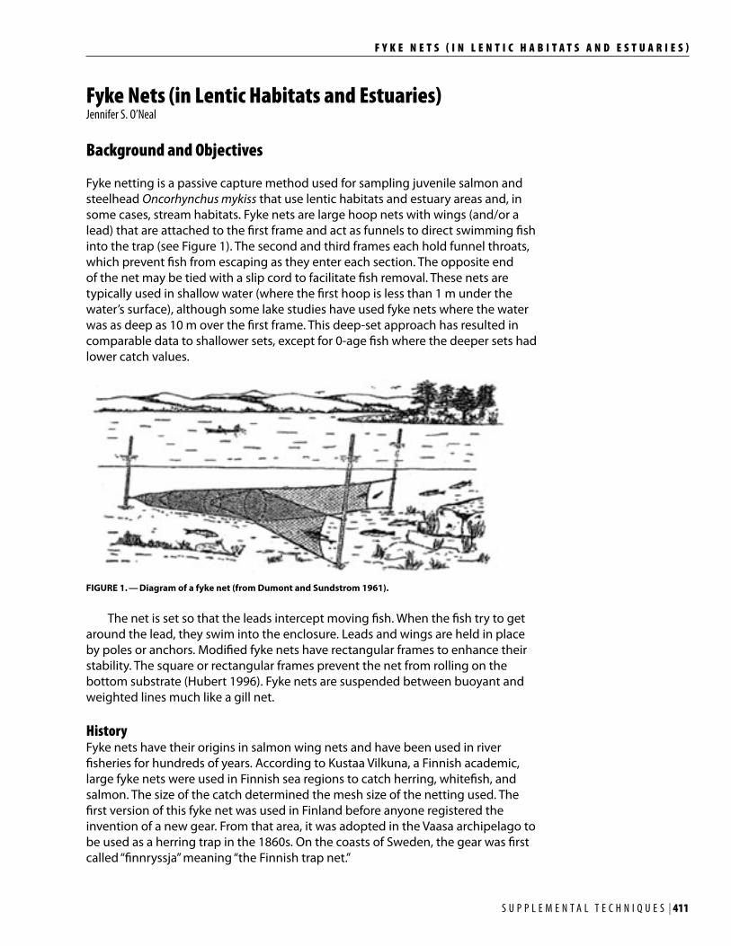
Fyke netting is a passive capture method used for sampling juvenile salmon and steelhead Oncorhynchus mykiss that use lentic habitats and estuary areas and, in some cases, stream habitats. Fyke nets are large hoop nets with wings (and/or a lead) that are attached to the first frame and act as funnels to direct swimming fish into the trap (see Figure 1). The second and third frames each hold funnel throats, which prevent fish from escaping as they enter each section. The opposite end of the net may be tied with a slip cord to facilitate fish removal. These nets are typically used in shallow water (where the first hoop is less than 1 m under the water’s surface), although some lake studies have used fyke nets where the water was as deep as 10 m over the first frame. This deep-set approach has resulted in comparable data to shallower sets, except for 0-age fish where the deeper sets had lower catch values.
FIGURE 1. — Diagram of a fyke net (from Dumont and Sundstrom 1961).
The net is set so that the leads intercept moving fish. When the fish try to get around the lead, they swim into the enclosure. Leads and wings are held in place by poles or anchors. Modified fyke nets have rectangular frames to enhance their stability. The square or rectangular frames prevent the net from rolling on the bottom substrate (Hubert 1996). Fyke nets are suspended between buoyant and weighted lines much like a gill net.
HistoryFyke nets have their origins in salmon wing nets and have been used in river fisheries for hundreds of years. According to Kustaa Vilkuna, a Finnish academic, large fyke nets were used in Finnish sea regions to catch herring, whitefish, and salmon. The size of the catch determined the mesh size of the netting used. The first version of this fyke net was used in Finland before anyone registered the invention of a new gear. From that area, it was adopted in the Vaasa archipelago to be used as a herring trap in the 1860s. On the coasts of Sweden, the gear was first called “finnryssja” meaning “the Finnish trap net.”

412 | S U P P L E M E N T A L T E C H N I Q U E S
F Y K E N E T S ( I N L E N T I C H A B I T A T S A N D E S T U A R I E S )
With fyke nets, as with many other fish collection nets, the size of the mesh used is dependent on the intended composition of the catch. Large fyke nets with mesh size of 13 mm (0.5 in.) tend to capture larger fish, since they cannot detect the bigger mesh very well, whereas fyke nets with net mesh of only 10 mm (0.38 in.) are better at capturing smaller fish. Fyke nets have been used to assess populations of salmon and steelhead juveniles in the Pacific Northwest and other regions. Fresh (2000) used fyke nets to capture juvenile chinook salmon O. tshawytscha in the Green River in Washington to assess migration patterns, growth, and habitat use. Gallagher (2000) used fyke nets to monitor downstream migration for steelhead in the Noyo River in California. The objectives of this latter study were to assess abundance, size, age, survival, migration timing, and distribution.
RationaleAssessing salmon and steelhead survival at specific life stages is critical to effective management of populations and evolutionarily significant units (ESUs). An ESU is defined as a population that (1) is substantially reproductively isolated from conspecific populations, and (2) represents an important component in the evolutionary legacy of the species (Johnson et al. 1994; McElhany et al. 2000). Identification of lifestage-specific survival and the factors limiting that survival will allow scientists and managers to better address these factors or “threats” to species recovery. NOAA Fisheries has determined that estimates of juvenile and adult abundance for listed ESUs are a critical component in the recovery of these ESUs. Assessment of juvenile abundance in areas that are turbid or in which substrate or obstructions do not allow for active capture of fish can be accomplished using fyke nets. This gear type avoids many of the issues that arise when visibility is impaired or net snagging is a problem. The use of fyke nets is presented here as an option for population assessment when other methods are not suitable for use. Fyke netting is a useful method for sampling fish that use lentic habitats and estuarine areas. It is commonly used to monitor the yearly changes in fish species abundances in sites where seining cannot be used alone or in combination with other methods for a mark–recapture study. If the habitat has large and uneven substrate, significant woody debris, or other obstructions, seining may not be possible, and fyke nets may provide a viable alternative. Fyke nets tend to be the most useful in capturing cover-seeking mobile species and migratory species that follow the shorelines, and have been used to a sample juvenile salmon in estuary habitat in the Skagit River in Washington (E. Beamer, Skagit River System Cooperative, personal communication). Fyke nets induce less stress on captured fish than do entanglement gears (Hopkins and Cech 1992), and most captured fish can be released unharmed. Fyke nets are widely used in the assessment of fisheries stocks because of the low mortality of fish and aspects of their species and size selectivity. Trap mortality for steelhead caught using fyke nets in the Noyo River in California was less than 1% (Gallagher 2000).
ObjectivesThis protocol describes methods used to capture fish using fyke nets. Objectives that could be addressed using this method include the following:

S U P P L E M E N T A L T E C H N I Q U E S | 413
F Y K E N E T S ( I N L E N T I C H A B I T A T S A N D E S T U A R I E S )
• determining relative abundance and yearly changes in abundance of juvenile fish populations in lentic and estuarine environments;
• determining population characteristics such as size, age, growth, migration timing, and distribution; and
• determining diversity of juvenile fish species in a lentic or estuarine habitat or determining the ratio of hatchery versus wild fish in these habitats.
Sampling Design
When describing the use of fyke nets or other passive sampling gears, the aspects of gear selectivity and efficiency must be addressed (Kraft and Johnson 1992). Selectivity can include a bias for species, sizes, and sexes of fish. Efficiency of a gear refers to the amount of effort expended to capture target organisms. A quantitative understanding of gear selectivity is needed to interpret the data, but little such information is available for most sampling devices. Variables that affect capture efficiency include season, water temperature, time of day or night, water level fluctuation, turbidity, and currents. Changes in animal behavior lead to variability in data collected among species and age-groups because animal capture with passive gear is a function of animal movement. Standardizing the use of fyke nets for a specific objective in a specific habitat for juvenile salmonids will be helpful in interpreting the data from different studies and for calibration of fyke nets with other capture methods. Currently, habitats where fyke nets are most often used are lentic habitats such as lakes, off-channel habitats, and estuarine areas. Estuarine use has been particularly important for the assessment of juvenile salmon use, especially where seining is not feasible due to large substrate (K. Fresh, NOAA Fisheries, personal communication). These habitats are critical to the survival of salmon species such as chinook, which require significant growth in estuarine habitat before venturing into the open ocean. Sample design will be dependant upon project objectives, but minimally, three sets with the fyke net should be used to assess variability of sampling. Other applications of fyke nets include capturing juvenile steelhead in streams or for off-channel habitat use by juvenile salmon species such as chinook salmon and coho salmon O. kisutch, where those habitats have significant obstacles that prevent effective seining. Coho salmon were observed to have a higher probability of capture as compared to steelhead when using a fyke net in the Noyo River in California. This difference may be due to stricter life cycle timing for coho, which spend one year in freshwater, versus steelhead, which have a more flexible freshwater residence time (Gallagher 2000). Fyke nets can be used to collect data on relative abundance as well as indices of change in stock abundance. Combining fyke nets with gill nets and electrofishing can be used to assess species assemblages in lake habitats (Bonar et. al 2000). Mark–recapture sampling with fyke nets has been used to assess steelhead abundance, size, growth, age, migration timing, and distribution (Gallagher 2000).
414 | S U P P L E M E N T A L T E C H N I Q U E S
F Y K E N E T S ( I N L E N T I C H A B I T A T S A N D E S T U A R I E S )
Field/Office Methods
Pre-field ActivitiesField staff should obtain standardized fyke nets for sampling. A set of multiple fyke nets of similar dimensions is effective for lake sampling, where the number of nets used is dependent on the size of the lake and the study objectives. For sampling juvenile salmonids, a typical fyke net is approximately 12 m long and consists of two rectangular steel frames, 90 cm wide by 75 cm high, and four steel hoops, all covered by 7-mm delta stretch mesh nylon netting. An 8-m long by 1.25-m deep leader net made of 7-mm delta stretch nylon netting is attached to a center bar of the first rectangular frame (net mouth). The second rectangular frame has two 10-cm-wide by 70-cm-high openings, one on each side of the frame’s center bar. The four hoops follow the second frame. The throats, 10 cm in diameter, are located between the second and third hoops. The net ends in a bag with a 20.4-cm opening at the end, which is tied shut while the net is fishing. Modified fyke nets are widely used to sample lakes and reservoirs. These nets have 1–2 rectangular frames to prevent the net from rolling on the bottom. These smaller fyke nets are 10 m long (including the lead) with one rectangular frame followed by two aluminum hoops. The aluminum frame is 98 cm wide by 82 cm tall, and is constructed of 2.5-cm tubing with an additional vertical bar. The hoops are 60 cm in diameter and constructed of 5-mm-diameter aluminum rods. The single net funnel is between the first and second hoops and is 20 cm in diameter. The lead is 8 m long, 1.25 m deep, and constructed from 7-mm delta stretch mesh. Other pre-field tasks include
• obtaining a map of the survey site before sampling. Use the map to measure the shoreline perimeter;
• determining what species and life stages are of greatest interest to sample;
• determining how to stratify habitat based on where the density of the species of interest or species diversity would be highest based on life history;
• designating strata locations on the map based on predicted level of species diversity and distribution, or on fish density or habitat;
• selecting needed sample size (see Appendix A); and
• allocating sampling effort based on nonuniform probability allocation, if the degree of difference in species diversity, distribution, or catch-per-unit-effort (CPUE) by habitat is known, or proportionally allocate effort based on habitat distribution.
Field ActivitiesEach fyke net is set in shallow water perpendicular to shore such that the net mouth is covered by about 1 m of water when possible (Fletcher et al. 1993; Hubert 1996) (see Figure 2). When the net is properly set, the lead is perpendicular to shore (vertical and not twisted), the mouth of the net is upright and facing shore, and all the hoops are upright. Fyke nets should be set in the evening or late afternoon and retrieved the next morning. All nets should be checked and emptied 12–24 h after setting (Klemm et al. 1993). Record set time, pickup time,
S U P P L E M E N T A L T E C H N I Q U E S | 415
F Y K E N E T S ( I N L E N T I C H A B I T A T S A N D E S T U A R I E S )
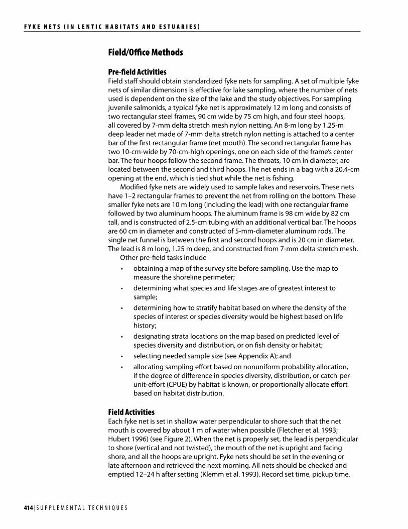
and location of the net on a map or global positioning system (GPS). If the bottom is soft and the water is shallow, the fyke nets are suspended by placing floats at the apex of each hoop and on top of the opening frames. This is done to prevent the nets from sinking into the soft sediments at the bottom of the lake. When the net is set from a small boat, it is placed on the bow with the pot on the bottom and the lead on the top. The end of the lead is staked or anchored and played out as the boat moves in reverse. When the lead is fully extended, the pot is put overboard and staked or anchored into position. Fish are then removed by lifting only the pot into the boat and placing the fish in a live well. Fyke nets may also be deployed away from shore in pairs with a single lead between them (Hubert 1996). This type of set is generally made parallel to the shore along the outer edge of vegetation or along shallow off-shore reefs.
8' codend
9' squareopening
25' wing
100' lead
5.5' square opening
4' aluminum 3/8'' diameter tube hoops
22'
FIGURE 2. — Setting a fyke net in a lake. (Diagram: Andrew Fuller from Regents of the University of Minnesota 2003).
Measurement DetailsNets should be checked and emptied 12–24 h after being set (Klemm et al. 1993). When the net is pulled in, the hoops and frames are gathered together and lifted into the boat. The net is positioned over a livewell with the net mouth upward. Frames are lifted one at a time, and any fish present are shaken down into the next chamber until all of the fish are in the bag, which is then emptied into a livewell (see Figure 3). Each fish is then identified to species, measured to the nearest millimeter, and released back into the water. Age can also be determined by removing a scale for later analysis or by using a size/age relationship. The field team should record the time that the net was set, the time it was pulled in, the total fishing time, the number of nets used, and the location of each set on the map.
Sample Processing
1. Measure each specimen to the nearest millimeter, identify to species, and weigh to the nearest gram.
2. Field data recording should be standardized and should include the following:
a. Habitat type
b. Sampling date
c. Gear type
d. Net location (shore orientation, depth, placement time, collection intervals, universal transverse mercator or latitude/longitude coordinates)
416 | S U P P L E M E N T A L T E C H N I Q U E S
F Y K E N E T S ( I N L E N T I C H A B I T A T S A N D E S T U A R I E S )
e. Hours fished
f. Species collected
g. Weight for each species
h. Length for each species
i. Names of personnel involved in sampling
Data Handling, Analysis, and Reporting
Data collection by passive sampling can be used to determine relative abundance, which is expressed as number collected per 24 h and weight (kg) collected per 24 h (Ohio EPA 1989, as cited in Klemm et al. 1993). Other data that may be collected using fyke nets would be species assemblage or diversity data or distribution data (which generally does not require significant analysis). If fyke nets are used as part of a mark–recapture study, additional analysis will need to be done depending on the other method that was used in the study. CPUE data is one type of data that can be used as an index for population density. One critical assumption is that the CPUE results are proportional to stock density (Hubert 1996). The true density of the species is still unknown, and the proportionality constant that relates CPUE to true density is also unknown. But as long as this constant is not expected to change, differences in CPUE should reflect changes in the species abundance. This method can be used for relative abundance, but total abundance estimates would not have a high level of accuracy. Variability in fish behavior can alter the accuracy of CPUE data and reduce its utility even for relative abundance. Standardized gear, methods, and sample designs must be used for estimates to be comparable. Time of year and placement of nets also affect comparability of data. Additionally, CPUE data are generally not normally distributed. At low and moderate densities, the distribution of the number of fish captured with fyke nets will not have a normal distribution. At low densities, the distribution approximates a declining logarithmic function (Hubert 1996). At moderate densities, the distributions are skewed. Only at very high densities, when the target species are caught very often is the distribution approximately normal; hence, descriptive statistics designed for normally distributed data cannot be used with CPUE data. Additionally, no single transformation can be used to address the variability in distribution that is seen as the fish density changes. Nonparametric statistics offer equivalents to most of the procedures that require an assumption of normal distribution. A more appropriate descriptor for CPUE data than the mean is the median or 50th percentile for the density. The frequency of zero catches can also be used to report an index of fish density but cannot be transformed into abundance.
Personnel Requirements and Training
Responsibilities and Staff RequirementsThe net should be set with two persons whenever possible, especially when deploying from a boat. During boat use, one person deploys the net while the
S U P P L E M E N T A L T E C H N I Q U E S | 417
F Y K E N E T S ( I N L E N T I C H A B I T A T S A N D E S T U A R I E S )
other operates the vessel. This reduces the chances of net entanglement and ensures that the net will be deployed properly. If only one person is available, initial preparation of the net is critical. During net retrieval, two persons are needed: one who pulls the net on board and another who removes fish and ensures a successful and careful transfer to the livewell. One person should be responsible to record weights, lengths, and other data on each fish.
QualificationsThe person using the fyke net needs to have been trained by an experienced field biologist who should have a degree in biology or 1 year of experience in sampling fish in the geographic area where the sampling is to occur.
TrainingTraining should be provided on the job and/or through videos and demonstrations prior to the season. On-the-job training should be provided by an experienced field biologist. All personnel on project must have training in fish identification.
Operational Requirements
Workload and field scheduleThe field schedule for setting and retrieving fyke nets is seasonal—ideally when the fish are active and before there is a lot of recreational lake activity; however, as noted above, the sampling can occur at any time, depending upon the objectives of the study and the needs of the monitoring. The collapsible nature of this trap is very popular because it allows biologists to carry many more traps per outing. Safety during deployment from a boat is also increased due to the lower space requirements for each net.
Equipment needs• Fyke net(s)
• Small motorized boat (optional, depending on habitat)
• Livewell
• Field forms
• Hip waders, boots, and rain gear
• Meter board
• Electronic scale
• Dip nets
• Net tubs/buckets
• GPS unit
• Materials for taking any biological samples (e.g., scales)
• Fish species identification guides
• Communications gear (e.g., cell phone, two-way radio, satellite phone)

418 | S U P P L E M E N T A L T E C H N I Q U E S
F Y K E N E T S ( I N L E N T I C H A B I T A T S A N D E S T U A R I E S )
Budget considerationsWith careful handling and placement, a fyke traps can be expected to last for several seasons. General guidelines for a single fyke net survey are as follows:
Equipment Cost/time
Time for two biologists to set the net, retrieve the net, and process the catch 3 h
Travel time Site dependent
Preparation time 4 h
Training 1 h
Lab work 2 h
Data analysis 2–8 h
A season of fyke netting would take far more effort than a single sampling event. In Gallagher’s study (2000), a crew of two checked six fyke nets daily for 4 months, and recommended a longer sampling season. Their effort required 13,440 person-hours for field data and 550 person-hours for data analysis and reporting; a database was created to manage the data.
Literature Cited
Bonar, S. A., B. D. Bolding, and M. Divens. 2000. Standard fish sampling guidelines for Washington state ponds and lakes. Washington Department of Fish and Wildlife Report, Olympia.
Dumont, W. H., and G. T. Sundstrom. 1961. Commercial fishing gear of the United States. Fish and Wildlife Circular 109.
Hubert, W. A. 1996. Passive capture techniques. Pages 157–192 in B. R. Murphy and D. W. Willis, editors. Fisheries techniques, 2nd edition. American Fisheries Society, Bethesda, Maryland.
Fletcher, D., S. A. Bonar, B. Bolding, A. Bradbury, and S. Zeylmaker. 1993. Analyzing warmwater fish populations in Washington State. Washington State Department of Fish and Wildlife Report, Warmwater Survey Manual, Olympia.
Fresh, K. 2000. Juvenile chinook migration, growth, and habitat use in the Lower Green River, Duamish River, and nearshore of Elliot Bay. Prepared for King County Department of Natural Resources and Parks, Water and Land Resources Division, Seattle.
Gallagher, S. P. 2000. Results of the 2000 steelhead (Oncorhynchus mykiss) fyke trapping and stream resident population estimations and predictions for the Noyo River, California with comparison to some historical information. California Department of Fish and Game Steelhead Research and Monitoring Program, Fort Bragg.
Hopkins, T. E., and J. J. Cech, Jr. 1992. Physiological effects of capturing striped bass in gill nets and fyke traps. Transactions of the American Fisheries Society 121:819–822.
Johnson, O. W., R. S. Waples, T. C. Wainwright, K. G. Neely, F. W. Waknitz, and L. T. Parker. 1994. Status review for Oregon’s Umpqua River sea-run cutthroat trout. U.S. Department of Commerce, NOAA Technical Memorandum NMFS-VWFSC-15, Seattle.
Klemm, D. J., Q. J. Stober, and J. M. Lazorchak. 1993. Fish field and laboratory methods for evaluating the biological integrity of surface waters. U.S. Environmental Protection Agency, EPA/600/R-92/111, Cincinnati, Ohio.

S U P P L E M E N T A L T E C H N I Q U E S | 419
F Y K E N E T S ( I N L E N T I C H A B I T A T S A N D E S T U A R I E S )
Kraft, C. E., and B. L. Johnson. 1992. Fyke-net and gill-net size selectivity for yellow perch in Green Bay, Lake Michigan. North American Journal of Fisheries Management 12:230–236.
McElhany, P., M. H. Ruckelshaus, M. J. Ford, T. C. Wainwright, and E. P. Bjorkstedt. 2000. Viable salmonid populations and the Recovery of Evolutionarily Significant Units. U.S. Department of Commerce, NOAA Technical Memorandum NMFS-NWFSC-42, Seattle.

420 | S U P P L E M E N T A L T E C H N I Q U E S
F Y K E N E T S ( I N L E N T I C H A B I T A T S A N D E S T U A R I E S )
Appendix A: Using sequential sampling or previous year’s data to calculate CPUE sample size during a survey
To determine appropriate sample size for the survey, first reach a decision about survey objectives. Is the survey purpose to get a point estimate of value or to measure change? What degree of confidence is required in the results (e.g., 70%)? If change is to be measured, what degree of change should be detected? Then select a sample size for fyke netting that will be appropriate to meet these goals. The best method to calculate CPUE sample sizes so they will be tailored to individual lakes is to use previous estimates of variance that are available from the specific lake, taken at the same time of year. These estimates can be obtained either through sequential sampling or through previous year’s sampling.
A.1. Calculating a sample size to estimate CPUE within certain bounds
If the biologist wants to measure CPUE within certain bounds, use the following equation to calculate needed sample sizes (Willis 1998; Cochran 1977).
n =
(t2) (s2)[(a) (x)]2
wheren = sample size requiredt = t value from a t-table at n-1 degrees of freedom for a desired sample size (1.96 for 95% confidence)s2 = variancex = mean CPUEa = precision desired in describing the mean expresses as a proportion
Simply plug in values obtained from last year’s survey or while the survey is in progress to calculate how many samples are needed to get the precision required.
(Bonar 2000)
S U P P L E M E N T A L T E C H N I Q U E S | 421
F Y K E N E T S ( I N L E N T I C H A B I T A T S A N D E S T U A R I E S )
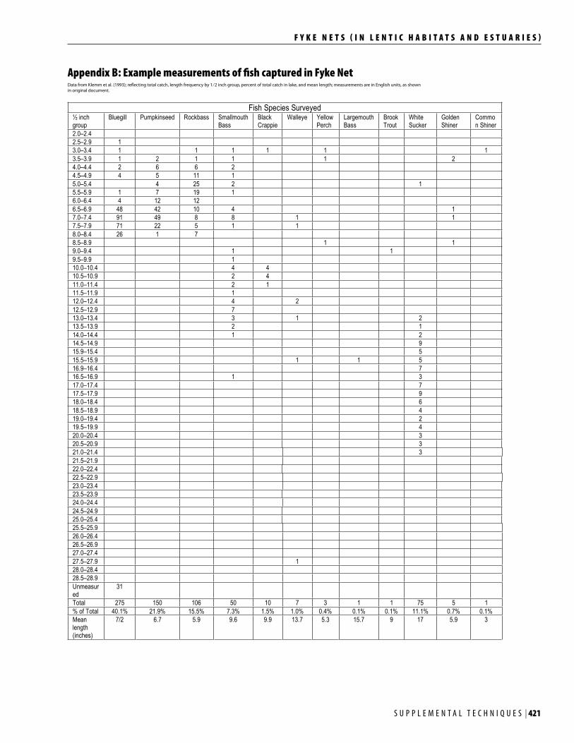
Appendix B: Example measurements of fish captured in Fyke NetData from Klemm et al. (1993); reflecting total catch, length frequency by 1⁄2 inch group, percent of total catch in lake, and mean length; measurements are in English units, as shown in original document.
Fish Species Surveyed� inch group
Bluegill Pumpkinseed Rockbass SmallmouthBass
Black Crappie
Walleye Yellow Perch
LargemouthBass
Brook Trout
White Sucker
GoldenShiner
Common Shiner
2.0–2.4
2.5–2.9 1
3.0–3.4 1 1 1 1 1 1
3.5–3.9 1 2 1 1 1 2
4.0–4.4 2 6 6 2
4.5–4.9 4 5 11 1
5.0–5.4 4 25 2 1
5.5–5.9 1 7 19 1
6.0–6.4 4 12 12
6.5–6.9 48 42 10 4 1
7.0–7.4 91 49 8 8 1 1
7.5–7.9 71 22 5 1 1
8.0–8.4 26 1 7
8.5–8.9 1 1
9.0–9.4 1 1
9.5–9.9 1
10.0–10.4 4 4
10.5–10.9 2 4
11.0–11.4 2 1
11.5–11.9 1
12.0–12.4 4 2
12.5–12.9 7
13.0–13.4 3 1 2
13.5–13.9 2 1
14.0–14.4 1 2
14.5–14.9 9
15.9–15.4 5
15.5–15.9 1 1 5
16.9–16.4 7
16.5–16.9 1 3
17.0–17.4 7
17.5–17.9 9
18.0–18.4 6
18.5–18.9 4
19.0–19.4 2
19.5–19.9 4
20.0–20.4 3
20.5–20.9 3
21.0–21.4 3
21.5–21.9
22.0–22.4
22.5–22.9
23.0–23.4
23.5–23.9
24.0–24.4
24.5–24.9
25.0–25.4
25.5–25.9
26.0–26.4
26.5–26.9
27.0–27.4
27.5–27.9 1
28.0–28.4
28.5–28.9
Unmeasured
31
Total 275 150 106 50 10 7 3 1 1 75 5 1
% of Total 40.1% 21.9% 15.5% 7.3% 1.5% 1.0% 0.4% 0.1% 0.1% 11.1% 0.7% 0.1%
Mean length (inches)
7/2 6.7 5.9 9.6 9.9 13.7 5.3 15.7 9 17 5.9 3
422 | S U P P L E M E N T A L T E C H N I Q U E S
F Y K E N E T S ( I N L E N T I C H A B I T A T S A N D E S T U A R I E S )
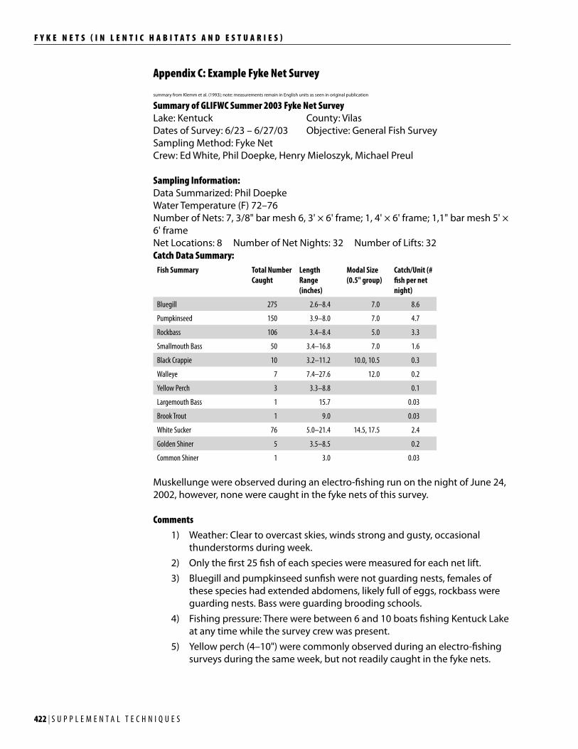
Appendix C: Example Fyke Net Survey
summary from Klemm et al. (1993); note: measurements remain in English units as seen in original publication
Summary of GLIFWC Summer 2003 Fyke Net Survey Lake: Kentuck County: VilasDates of Survey: 6/23 – 6/27/03 Objective: General Fish Survey Sampling Method: Fyke NetCrew: Ed White, Phil Doepke, Henry Mieloszyk, Michael Preul
Sampling Information: Data Summarized: Phil DoepkeWater Temperature (F) 72–76Number of Nets: 7, 3/8" bar mesh 6, 3' × 6' frame; 1, 4' × 6' frame; 1,1" bar mesh 5' × 6' frameNet Locations: 8 Number of Net Nights: 32 Number of Lifts: 32 Catch Data Summary:
Fish Summary Total Number Caught
Length Range (inches)
Modal Size (0.5" group)
Catch/Unit (# fish per net night)
Bluegill 275 2.6–8.4 7.0 8.6
Pumpkinseed 150 3.9–8.0 7.0 4.7
Rockbass 106 3.4–8.4 5.0 3.3
Smallmouth Bass 50 3.4–16.8 7.0 1.6
Black Crappie 10 3.2–11.2 10.0, 10.5 0.3
Walleye 7 7.4–27.6 12.0 0.2
Yellow Perch 3 3.3–8.8 0.1
Largemouth Bass 1 15.7 0.03
Brook Trout 1 9.0 0.03
White Sucker 76 5.0–21.4 14.5, 17.5 2.4
Golden Shiner 5 3.5–8.5 0.2
Common Shiner 1 3.0 0.03
Muskellunge were observed during an electro-fishing run on the night of June 24, 2002, however, none were caught in the fyke nets of this survey.
Comments
1) Weather: Clear to overcast skies, winds strong and gusty, occasional thunderstorms during week.
2) Only the first 25 fish of each species were measured for each net lift.
3) Bluegill and pumpkinseed sunfish were not guarding nests, females of these species had extended abdomens, likely full of eggs, rockbass were guarding nests. Bass were guarding brooding schools.
4) Fishing pressure: There were between 6 and 10 boats fishing Kentuck Lake at any time while the survey crew was present.
5) Yellow perch (4–10") were commonly observed during an electro-fishing surveys during the same week, but not readily caught in the fyke nets.

S U P P L E M E N T A L T E C H N I Q U E S | 423
F Y K E N E T S ( I N L E N T I C H A B I T A T S A N D E S T U A R I E S )
6) Two SCUBA divers spent 20 minutes searching in front of the east end boat landing in 10 to 20 feet of water; the search revealed no evidence of zebra mussels.
7) Conversations with anglers:
One pair of anglers mentioned catching and releasing a 45" muskellunge. They reported a catch rate of approximately 12 walleye per hour, and the walleye were averaging about 13 inches.
The campground hosts mentioned that fishing for panfish was slower this year than in the past. They reported catching roughly 15 fish (perch and bluegill) during a typical evening outing.

424 | S U P P L E M E N T A L T E C H N I Q U E S
F Y K E N E T S ( I N L E N T I C H A B I T A T S A N D E S T U A R I E S )

S U P P L E M E N T A L T E C H N I Q U E S | 425
V A R I A B L E M E S H G I L L N E T S ( I N L A K E S )
Variable Mesh Gill Nets (in Lakes)Bruce Crawford
Background and Objectives
BackgroundAlong areas of the Pacific Northwest coast, gill nets were traditionally constructed of a coarse fiber twine made from willow bark (Coffing 1991) and other materials, such as seal skin (as reported in 1844 by Zagoskin [Michael 1967]) and moose or caribou sinew (Oswalt 1980; Stokes 1985). Linen twine was used for making gill nets beginning in the 1920s (Coffing 1991). Gill nets were used both for set net and drift net fishing. In the 1960s, nets made from synthetic fibers such as nylon came into wider use. Most nets were 50 m or less in length until the 1980s. Nets are generally 50–70 m long, with mesh size varying depending on the salmon species targeted (Charnley 1984). Variable mesh gill nets have been used for fish population evaluation for about a century. The efficiency with which gill nets capture fish and the versatile use of these nets in lakes and streams have made them a common tool for fishery evaluation (Hamley 1975). This supplemental technique addresses the use of gill nets targeting salmonids in the Pacific Northwest but can be used for other species as well. The chapter draws extensively from the following papers: Bernabo (1986); Baklwill and Combs (1994); Bonar et al. (2000); and Klemm et al. (1993). Additional insights into use of gill nets can be found in Hubert (1996).
RationaleVariable mesh gill nets are appropriate for sampling when fish mortality is not a limiting factor. Gill nets normally kill a high percentage of fish due to the trapping mechanism of the net around the gills. Careful net tending can reduce but not eliminate the mortality percentage. The use of variable size mesh panels in the gill net allows capture of fish of different sizes. As such, this method can be used to collect data on population abundance, stock characteristics, population distribution, and species richness. Gill nets are not species-selective, and as a result, it can be expected that as many or more nontarget species will be captured as target species. In addition, small aquatic mammals and birds will also occasionally become entangled in the mesh and drown.
Objectives• Determine relative abundance of lake or stream populations by measuring
the catch-per-unit-effort (CPUE).
• Determine total abundance of lake populations by measuring the recapture rate of marked fish.
• Determine the length, sex, phenotypes, and genotypes of fish by collecting a representative catch of each sample.
• Determine the species composition and relative biomass of a lake or a stream.
426 | S U P P L E M E N T A L T E C H N I Q U E S
V A R I A B L E M E S H G I L L N E T S ( I N L A K E S )
Sampling Design
Trend information based on results of gill-net sampling will only be as reliable at the reproducibility of the sampling technique for each monitored site. Location of nets, orientation along the bottom in relation to the shoreline, diel time of placement and collection, and season of placement must be standardized for each site. Because lake sampling programs will be site specific, standardization must be within a given lake and not between lakes. Each lake has a unique morphometry, and net placement must be carefully considered according to lake characteristics and target species. The types of data acquired from gill nets include fish age, growth, relative weight, and proportional stock density calculations. Also, estimates derived from gill nets are typically given in CPUE or abundance within restricted habitat zones such as nearshore areas or coves (Dauble and Gray 1980; King et al. 1981; Johnson et al. 1988; Rider et al. 1994). CPUE methods assume that the calculated index is proportional to total population size, allowing trends through time to be detected. Unfortunately, violating this assumption is easy, but detecting the violation is not (Hillborn and Walters 1992). Given this situation, suggestions for estimating population abundance in deeper-water habitats must be tentative. Alternatively, one can use active capture gear or define a series of equally spaced transects over the entire water surface from which to sample randomly or systematically (Thompson et al. 1998). Borgstrøm (1992) assessed the effect of population density on gill-net catchability of Brown trout Salmo trutta in four Norwegian high-mountain lakes. Catchability was found to be inversely related to the number of fish present; brown trout populations with low densities were more vulnerable to gill nets than high density populations; gill-net catches as an estimator of population density were biased. While there are many ways to utilize gill nets, two examples of gill-net use in lakes are offered here. McLellan (2001) used electrofishing and gill nets to sample resident fish in eastern Washington reservoirs and streams. Of the taxa involved, four were salmonids (cutthroat trout O. clarki, rainbow trout O. mykiss, brown trout, and lake trout Salmo namaycush). A total of 10 horizontal experimental monofilament sinking gill nets (2.4 × 61.0 m; four 15.2-m panels with square mesh sizes 1.3, 2.5, 3.8, and 5.1 cm) were set at randomly selected shoreline sites per season. Two horizontal gill nets were set in reaches 1, 3, and 4, and four nets were set in reach 2. The nets were set perpendicular to the shore, with the smallest mesh size closest to shore. A total of eight monofilament vertical gill nets were set per season, four in the pelagic zones of both reaches 1 and 2, except during the spring, when flows were too high and the verticals were not set in the forebay. The nets (2.4 × 29.9 m), one of each mesh size (1.3, 2.5, 3.8, and 5.1 cm), were set in the upper 29.9 m of the water column at randomly selected pelagic locations. During the summer, two additional horizontal nets were set in the pelagic zone of the forebay, one at the surface and one at the bottom (61 m). Data collected from the pelagic horizontal gill nets were not used in the relative abundance or CPUE calculations; however, the data were included in age, growth, relative weight, and proportional stock density calculations. Gill nets in reaches 2, 3, and 4 were set at dusk and retrieved within 4 h. The gill nets set in reach 1 were set in the early morning (~02:00 hours) and retrieved within 4 h.
S U P P L E M E N T A L T E C H N I Q U E S | 427
V A R I A B L E M E S H G I L L N E T S ( I N L A K E S )
Since 1981, the Center for Limnology at the University of Wisconsin–Madison, with support from the U.S. National Science Foundation, has been administering the Northern Temperate Lakes Long-Term Ecological Research (LTER) program. The center is focusing its attention on eight deep-water lakes in Wisconsin for monitoring. Vertical gill nets are used to monitor yearly changes in the abundance of pelagic fish species (<http://lter.limnology.wisc.edu/fishproto.html>). Researchers sample the deep basins of these lakes with seven nets, each a different mesh size, hung vertically from foam rollers and chained together in a line. Each net is 4 m wide and 33 m long. From 1981 through 1990, the nets were multifilament mesh, in stretched mesh sizes of 19, 25, 32, 38, 51, 64, and 89 mm. In 1991 the multifilament nets were replaced with monofilament nets of the same sizes. One side of the net is marked in meters from top to bottom. Stretcher bars have been installed at 5 m intervals from the bottom to keep the net as rectangular as possible when deployed. The bottom end is weighted with a lead pipe to quicken the placement of the net and to maintain the position of the net on the bottom. Gill nets are set at the deepest point of all long-term ecological research lakes except Crystal Bog, Trout Bog, and Fish Lake. The nets are set for two consecutive 24-h sets. The nets are set in a straight line, each connected to the next and anchored at each end of the line. Once the nets are in position, they are unrolled until the bottom end reaches the bottom and then tied off to prevent further unrolling. The nets are pulled by placing each net onto a pair of brackets attached to the side of the boat and by rolling the net back onto its float; the fish are picked out as the net is brought up and placed in tubs according to depth. The fish are processed when the net is completely rolled up and before it is redeployed.
Field Methods
Setup
BoatsThe investigator should review the size and type of waterbody where the gill nets will be employed. Since gill nets are dangerous to work with and cannot normally be effectively set by personnel on foot, an effective boat, rubber raft, or canoe should be used. For work in remote lakes where transportation is restricted to foot travel, an inflatable rubber raft is the most effective method for setting gill nets. Where helicopters are available, a small skiff or canoe can be used. In lowland areas, a variety of boats are available depending on road access to the waterbody and the size and type of waterbody.
NetsRecommended lake gill net specifications are as follows:
1. Length: 15–48 m (50–150 ft).
2. Depth: 2–2.5 m (6–8 ft).
3. Each net includes a proportional panel of 1.25, 1.90, 3.54, and 3.80 cm (i.e., 0.5, 0.75, 1.0, and 1.5 in) mesh. This mesh is capable of capturing fish as small as 7–8 cm total length.
428 | S U P P L E M E N T A L T E C H N I Q U E S
V A R I A B L E M E S H G I L L N E T S ( I N L A K E S )
4. The gill net is designed with a braided lead line of 7 g/m (0.3 lbs/fathom).
5. Floats are attached such that the lead line lies along the bottom and the floats suspend the net in the water column. Float line must be braided nylon with corks 15–20 cm (6–8 in) apart of a size to make the net either sink or float.
6. Nets are normally constructed of double-knotted monofilament and hung on a 2:1 basis (i.e., twice as much web as lead/cork line). Monofilament is nearly invisible under water and highly entangling, and it is nearly maintenance free. Its disadvantage is that it is more dangerous to handle, and if the net is lost, it continues to fish for years thereafter.
7. All nets must have nylon gables (side panels) of approximately 18 kg test.
For some operations the net may be allowed to float on the surface of the lake. In this case, the floats would be replaced with larger, more buoyant floats capable of suspending the net and the lead line with fish (Balkwill and Combs 1994). Gill nets should be clearly labeled with the researcher’s name and contact phone number. In urban areas, the net may cause concern with the public, and special arrangements may need to be made with a local landowner or others to arrange for access and to prevent vandalism to the equipment.
Other equipmentThe sampler should plan to bring measuring boards, scale envelopes, buckets, global positioning system (GPS) unit, weighing scales, clipboards, waterproof forms, and other equipment if genetic information is also being collected. Proper collecting permits may need to be obtained depending upon species collected, jurisdictions, and other factors.
Events Sequence
Setting the net
1. Set the net along the bottom in shallow waters not exceeding 5–7 m in depth to capture a representative sample of the total fish stock when sampled at night.
2. Nets should be placed perpendicular to the shoreline in shallow water or at a 45° angle in deep water, with the small end of the mesh nearest the shoreline.
3. The deep end of the net should have a line with a float attached to it to aid in retrieving the net if it becomes snagged. The location selected should be free of sunken logs, jagged rocks, pipes, and other objects that can snag the net and keep it from being retrieved.
4. Nets should be set at dusk (one hour before sunset) and retrieved at dawn (1 h after sunrise).
5. The net is coiled in the bow of the boat with the lead line on one side and the float line on the other side. The small mesh end is tied to the shore or to a log or an anchor near the shore, and the boat is moved out towards deep water. The net is allowed to pay out over the bow. The person paying out the net should be vigilant to keep the net from snagging on the

S U P P L E M E N T A L T E C H N I Q U E S | 429
V A R I A B L E M E S H G I L L N E T S ( I N L A K E S )
vessel. When the net has been fully deployed, the net should be stretched as tightly as possible before being released. (Note: It is very important that the person deploying the net ensure that all buttons, zippers, and other apparel that could be entangled in the net are secured.)
6. Nets can be set with or without bait. Baiting is effective for many purposes and can be accomplished by dispensing the contents of a can of tuna fish along the length of the net.
7. Net sets may need to be modified when testing for presence of bass and other nonsalmonid species. Trout and salmon tend to swim forward when encountering the net and then quickly become entangled. Bass will tend to back up when encountering the net and swim perpendicular to an obstacle to avoid it. When sampling waters where bass and other non-salmonid species are present, at least a few of the sites should be set with one net perpendicular to the shore and another perpendicular to the first net to increase the probability of capturing the bass avoiding one of the nets.
8. The following morning, the net is retrieved by the sampler paddling out to the float and bringing up the deep end of the net first. This minimizes snagging and allows the sampler to work the net towards shore. If the net is pulled from shore, the net has a higher chance of snagging on the bottom obstructions as it slides along the bottom.
9. Repeat steps 1–7 for each sample site.
Setting nets on ice-covered lakes
1. Gill nets can be fished through the ice when necessary. This can be accomplished by first determining the net location during the summer when bottom contours and obstacles can be assessed.
2. During the winter, the sampler must locate the net site and then mark out the length of the net on the ice perpendicular to shore as before.
3. Use an ice saw or chain saw to cut two parallel lines in the ice the distance of the net set. Remove blocks of ice and clear the hole of debris.
4. Lower the net into the hole as described in steps 3–5 under Setting the net.
5. The next morning, the hole may have refrozen and will need to be cleared of ice either with a saw or an axe.
6. In subfreezing conditions, the net should be pulled quickly from the hole and spread out on the ice as straight as possible. This will allow the net to be picked after it freezes.
Number of netsFollowing is a rough guideline for the number of nets to use:
Lake size (ha) Number of nets
< 4 1
4–10 2
10–20 3
20–40 4
Each additional 40 ha Add 1 net
430 | S U P P L E M E N T A L T E C H N I Q U E S
V A R I A B L E M E S H G I L L N E T S ( I N L A K E S )
If the initial sampling effort yields few or no fish, the sampling stations should be moved and the sampling effort repeated. A careful description of the sampling location is important in order to find and duplicate the same location the following sampling period.
Sample ProcessingThe following steps should be used when processing fish caught in the gill net:
1. Fish should be carefully removed from the gill net. For most of the fish species, it will require untangling the gill opercles from the net mesh. Some species, such as catfish Siluriformes tend to spin once they are entangled and will require a lot of work to release.
2. Measure to the nearest millimeter, identify to species, weigh to the nearest gram, and take scale samples from the left side (just posterior to and below the dorsal fin and above the lateral line). If genetic samples are needed, take samples per the protocol being employed for DNA or electrophoresis. Depending on the purpose and need, stomach samples may be taken, most commonly via gastric lavage, and internal organ, examined for parasites, gender, and maturity.
Field data recording should be standardized and should include the following:
1. lake
2. sampling date
3. gear type
4. net location (shore orientation, depth, placement time, collection interval)
5. hours fished
6. species
7. weight (gm)
8. total length (cm)
9. scale number
10. parasites observed
11. deformities observed
12. wounds observed
13. universal transverse mercator or latitude/longitude coordinates
14. names of survey personnel
Other physical measurements such as temperature, pH, and visibility may also be taken. These factors often affect fish activity and net visibility and efficiency and should be tracked.
Personnel Requirements and Training
ResponsibilitiesThe net should be set with two people, whenever possible, with one person deploying the net and one person propelling the vessel. This reduces the chance

S U P P L E M E N T A L T E C H N I Q U E S | 431
V A R I A B L E M E S H G I L L N E T S ( I N L A K E S )
that the net will become entangled, and it helps ensure that it will be deployed properly. If only one person is available, the way the person initially prepares the net is crucial to successful deployment. In turn, during net retrieval, two persons are ideal: one person controls the vessel against water and wind conditions while the other person slowly brings the net on board and either picks the net as it is brought on or brings in the entire net and later picks the fish out of the net on shore under more stable conditions. The samplers can determine who will record and who will weigh, measure, and conduct other examinations of the fish when they are being processed.
QualificationsThe person using a gill net should have been properly trained by an experienced field biologist and should have a degree in biology or one year of experience in sampling fish in the geographic area where the sampling is to occur. The use of volunteers should be carefully evaluated due to the danger involved and potential adverse reactions with the public.
TrainingTraining should either be provided through videos and demonstrations under cover prior to the season or through on-the-job training by accompanying an experienced field biologist.
Operational Requirements
Field ScheduleThe field schedule for setting gill nets is normally during the spring when fish have become active and before there is a lot of recreational lake activity; however, as noted above, the sampling can occur at any time, including winter, depending upon the objectives of the study and the needs of the monitoring.
Equipment ListUse this list to help in developing a budget estimate.
Item Comments
4 m aluminum rowboat with oars
15 hp outboard motor
25-L gas tank and other motor repair items
One-person raft with kayak paddle Used for remote applications
Net tubs or buckets
Meter board
Anchor and anchor lines
Dissecting kit
10% formalin or 70% ethanol
Screw-top vials
Scale envelopes
Collecting permits
Secchi disk Measures transparency of water

432 | S U P P L E M E N T A L T E C H N I Q U E S
V A R I A B L E M E S H G I L L N E T S ( I N L A K E S )
Item Comments
GPS unit Location of nets
Life jackets
Sharp knives To cut loose an entangled person or net; for fish samples
First-aid kit
Ice saw or chain saw For under-ice sampling
Axe For under-ice sampling
Net labels
50-m variable mesh gill nets Number as needed
Clipboard
Sample forms
Thermometer
Wire clippers Used for catfish spine removal
Cell phone, two-way radio, or satellite phone
Communications
Personnel BudgetThe following guidelines can be used to estimate time budget for personnel:
Activity/item Cost
Staff time* 3 h
Travel time Variable
Preparation time 4 h
Training 1 h
Lab workup 2 h
Data analysis, report writing 8 h* two biologists to set the net and to retrieve and process the catch
Literature Cited
Balkwill, J. A., and D. M. V. Combs. 1994. Lake survey procedure manual for British Columbia. BC Environment, Lands and Parks Report, Victoria.
Bernabo, C., and B. Hood. 1986. Protocols for establishing current physical, chemical and biological conditions in remote alpine and subalpine ecosystems. U.S. Forest Service, Fort Collins, Colorado.
Bonar, S. A., B. D. Bolding, and M. Divens. 1993. Standard fish sampling guidelines for Washington State ponds and lakes. Washington Department of Fish and Wildlife Report, Olympia.
Borgstrøm, R. 1992. Effect of population density on gillnet catchability in four allopatric populations of Brown trout (Salmon trutta). Canadian Journal of Fisheries and Aquatic Sciences 49:1539–1545.
Charnley, S. 1984. Human ecology of two central Kuskokwim communities: Chuathbaluk and Sleetmute. Alaska Department of Fish and Game, Division of Subsistence, Technical Paper No. 81, Juneau. Available: www.subsistence.adfg.state.ak.us/TechPap/tp081.pdf (accessed August 2006).

S U P P L E M E N T A L T E C H N I Q U E S | 433
V A R I A B L E M E S H G I L L N E T S ( I N L A K E S )
Coffing, M. W. 1991. Kwethluk subsistence: contemporary land use patterns, wild resource harvest and use, and the subsistence economy of a lower Kuskokwim River area community. Alaska Department of Fish and Game, Division of Subsistence, Technical Paper No. 157, Juneau. Available: www.subsistence.adfg.state.ak.us/TechPap/tp157.pdf (accessed August 2006).
Dauble, D. D., and R. H. Gray. 1980. Comparison of small seine and backpack electro-shocker to evaluate nearshore fish populations in rivers. Progressive Fish-Culturist 42:93–95.
Hamley, J. H. 1975. Review of gillnet selectivity. Journal of the Fisheries Research Board of Canada. 32: 1943–1969.
Hillborn R., C. J. Walters. 1992. Quantitative fisheries stock assessment: choice, dynamics and uncertainty. Chapman and Hall, New York. 570 p.
Hubert, W. A. 1996. Passive capture techniques. Pages 157–192 in B. R. Murphy and D. W. Willis, editors. Fisheries techniques, 2nd edition. American Fisheries Society, Bethesda, Maryland.
Johnson, B. M., R. A. Stein, and R. F. Carline. 1988. Use of a quadrat rotenone technique and bioenergetics modeling to evaluation prey availability to stocked piscivores. Transactions of the American Fisheries Society 117:127–141.
King, T. A., J. C. Williams, W. D. Davies, and W. L. Shelton. 1981. Fixed versus random sampling of fishes in a large reservoir. Transactions of the American Fisheries Society 110:563–568.
Klemm, D. J., Q. J. Stober, and J. M. Lazorchak. 1993. Fish field and laboratory methods for evaluating the biological integrity of surface waters. U.S. Environmental Protection Agency, Office of Research and Development, Report EPA/600/R-92/111, Cincinnati, Ohio.
McLellan, J. G. 2001. 2000 WDFW Annual Report for the Project Resident Fish Stock Status above Chief
Joseph and Grand Coulee Dams. Part I. Baseline assessment of Boundary Reservoir, Pend Oreille River, and its tributaries. Pages 18–173 in N. Lockwood, J. McLellan, and B. Crossley. Resident fish stock status above Chief Joseph and Grand Coulee dams. 2000 Annual Report. Report to Bonneville Power Administration, BPA Report DOE/BP-00004619-1, Portland, Oregon.
Michael, H. N., editor. 1967. Lieutenant Zagoskin’s travels in Russian America, 1842-1844. The first ethnographic and geographic Investigations in the Yukon and Kuskokwim valleys of Alaska. Anthropology of the north: translations from Russian sources No. 7. University of Toronto Press, Toronto.
Oswalt, W. H. 1980. Kolmakovskiy redoubt: the ethnoarchaeology of a Russian fort in Alaska, Monumenta Archaeologica Volume 8. University of California, Institute of Archaeology, Los Angeles.
Rider, S. J ., M. J. Maciena, and D. R. Lowery. 1994. Comparisons of cove rotenone and electrofishing catch-depletion estimates to determine abundance of age-0 largemouth bass in unvegetated and vegetated area. Journal of Freshwater Ecology 9:19–27.
Stokes, J. 1985. Natural resource utilization of four upper Kuskokwim communities. Alaska Department of Fish and Game, Division of Subsistence, Technical Paper No. 86, Juneau.
Thompson, W. L., G. C. White, and C. Gowan. 1998. Monitoring vertebrate populations. Academic Press, New York.

434 | S U P P L E M E N T A L T E C H N I Q U E S
V A R I A B L E M E S H G I L L N E T S ( I N L A K E S )
S U P P L E M E N T A L T E C H N I Q U E S | 435
F O O T - B A S E D V I S U A L S U R V E Y S
Foot-based Visual Surveys for Spawning SalmonBruce Crawford, Thaddeus R. Mosey, and David H. Johnson
(Note to readers: this supplemental protocol complements two full protocols—Carcass Counts, page 59, and Redd Counts, page 197.)
Background and Objectives
BackgroundAdult salmonids return from the sea to spawn in their natal streams. Since adult spawner abundance is, for many populations, the principle measure of abundance and enables estimation of potential egg deposition, it is crucial to be able to obtain accurate estimates of the number of spawners to monitor abundance, relative to escapement goals or other management objectives. As salmon and steelhead Oncorhynchus mykiss enter rivers or streams over an extended period of time, and since there is continuous mortality (for salmon) and/or emigration (for steelhead), it is very difficult to obtain an estimate of the total number of spawners. Spawner counts, therefore, ideally should be replicated weekly throughout the spawning period to estimate total escapement. More frequent surveys will provide a more accurate estimate of spawner abundance. Streamflow and turbidity, among other factors, influence the accuracy of spawner counts. Given the spawn timing of salmon and steelhead, counts must often be conducted under suboptimal conditions; however, streams in many regions are relatively clear, and thus, it is possible to count spawning salmon directly as they dig their egg nests (redds) and actively mate. Counts of spawning fish are usually done on foot or from a boat (although boat-based surveys are not discussed in this chapter). Spawning counts are often done on steelhead and chinook salmon O. tshawytscha, chum salmon O. keta, and coho salmon O. kisutch. In addition to supporting spawning escapement estimates, live fish counts describe spawning timing, particularly when redd and carcass counts are also available. Comparatively high live fish and low redd and carcass numbers may indicate that spawning is just beginning. The opposite (low live fish and high redd and carcass numbers) can indicate that spawning in that stream is nearly complete. Material in this protocol has been extensively drawn from Heindl (1989). This method is mainly used where road networks are highly developed (for access) in southern British Columbia and Japan.
RationaleCounting live salmon while walking along a stream is one of the oldest and simplest methods of estimating spawner abundance. Foot surveys are an effective method of counting spawning salmon because the fish are large enough to observe directly, and when done correctly, surveyors can achieve measurable accuracy for certain species of salmon and for steelhead (Waldichuk 1984; Irvine et al. 1992; Nickelson 1998). Furthermore, by combining the estimated number of spawning fish and total redd counts, one can determine the number of carcasses needing to be recovered (sampled) to evaluate key demographic aspects of hatchery and supplementation programs. Labor costs associated with visual spawner index counts have been found to be less than those associated with
436 | S U P P L E M E N T A L T E C H N I Q U E S
F O O T - B A S E D V I S U A L S U R V E Y S
mark–recapture or fish counting weir techniques (Irvine et al. 1992); however, live fish are wary, mobile, and easily camouflaged and, in some situations relatively nocturnal in their spawning habits, thus reducing the accuracy of visual direct counting methods. Visual spawner surveys may be the basis for estimating total escapement in an entire basin or for simply monitoring spawner abundance in one or more index reaches. Surveys may seek only to estimate peak spawner abundance or to describe total spawning timing. Reaches for survey and survey frequency must, therefore, be selected carefully to achieve the desired objective.
ObjectiveThe objective of visual spawner surveys is to determine total or relative abundance of river or stream populations by directly counting the numbers of spawning fish on their redds.
Sampling Design
Site selectionSite selection for foot surveys of spawners is based on timing of returning fish, water clarity, and access to banks with a view of the stream. Foot surveys need to be conducted where the clarity of water is high enough to distinguish spawning fish from the substrate. Timing of spawning can affect potential for high water clarity. For example, spring spawners such as steelhead may be spawning at higher water levels when water is more turbulent and has higher turbidity. Foot surveys conducted for steelhead should be timed for when water clarity is expected to be the greatest. Salmon that return to spawn in the fall are generally spawning when water clarity is higher than that for steelhead. Surveys are frequently conducted under suboptimal visibility, so a visibility factor must be subjectively estimated by the surveyor and applied to counts. This can create a source of bias in visual counts. Additional insights into behavioral aspects of salmon spawning activity can be found in Perrin and Irvine (1990), Barlaup et al. (1994), Fleming (1996), Webb and Hawkins (1989), and Webb et al. (1990). Access to banks with a clear view of the stream is critical for effective implementation of the foot survey protocol. If the stream is in a steep V-notch and surveyors cannot safely get close to the stream to view spawning activity, then a foot survey is not an effective method. Similarly, if the survey is to be conducted over a considerable length of stream, thick vegetation may impede surveyors’ progress and reduce the efficiency of the survey. Surveyors should not need to walk in the stream to conduct the survey as this action would disturb the spawning fish. To improve the accuracy and precision of escapement estimates obtained using visual surveys, a variety of sampling approaches can be used to identify portions of a stream to survey for fish. The easiest approach may be to use a simple random sampling design. With this design, each section of a stream has the equal probability of being selected; however, if sampling units can be divided into homogeneous groups, then stratified random sampling is generally preferable to simple random sampling, since stratification usually results in a smaller variance than that given by comparable simple random sampling (Cochran
S U P P L E M E N T A L T E C H N I Q U E S | 437
F O O T - B A S E D V I S U A L S U R V E Y S
1977). A stratified random sampling design to estimate escapement is achieved by stratifying the watershed and then randomly selecting sample sites within each stratum. Alternatively, sample units within each stratum can be selected on the basis of easy access by surveyors and/or on the basis of expected or actual locations of fish. This latter type of sampling has been termed stratified index sampling (Johnston et al. 1987; Bocking et al. 1988). As visual surveys are typically conducted on foot, surveyors should evaluate a few representative stream reaches (e.g., 250 m long each) prior to the start of spawning surveys to determine suitability for surveys based on water depth and flows. In their 3-year project with coho salmon in British Columbia, Irvine et al. (1992) examined stratified random and stratified index sampling designs for estimating the numbers of spawning fish. The approach was evaluated in two streams with widely varying escapements; estimates of adult fish using the stratified index design were always similar to estimates obtained through an independent mark–recapture program. The stratified random design underestimated fish numbers in every case but one. Because the distribution of fish was aggregated, with random sampling there was a higher probability of sampling low fish abundance areas than high-abundance areas. Numbers of jack coho were underestimated with each sampling design, probably because the surveyors overestimated the efficiency of seeing these fish.
Sampling frequency and replicationSurveys are typically conducted on 6 (Irvine et al. 1992) to 10 (T. Mosey, Chelan County Public Utilities District, personal observation) stream reaches per crew per day. Foot counts are generally conducted every 7–10 d throughout the spawning season to observe fish on their redds. Replication of foot surveys is necessary to count the total or relative number of spawners over the spawning season. For each target species, the expected spawning season should be identified, and surveys should ideally be scheduled to start before the first spawner enters the stream and continue until after the last spawner completes the spawning process. Counts that are conducted more frequently will have a higher accuracy than those that are conducted less frequently. Estimates of residence time, as determined from redd life, vary from several days to 21 d. Irvine et al. (1992) found that the residence time of coho in their British Columbia study area was between 13 and 17 d (with one exception of 8 d). It is important to note that residence timing varies among different reaches, annually for a given population, and between rivers. A general recommendation is to conduct spawner surveys weekly.
Field/Office Methods
Setup
Prior to arrivalStreams should be divided into survey reaches prior to sampling. This can be done either through a randomized sampling design or through previous surveys that identify where the target salmonid is known to spawn. Before a survey is undertaken, the surveyors must be well aware of what reaches they are to survey, the target species, when the spawning season begins and ends, what the time
438 | S U P P L E M E N T A L T E C H N I Q U E S
F O O T - B A S E D V I S U A L S U R V E Y S
interval for the survey is, what data are needed, and what equipment is required. The project leader must ensure that each surveyor or team carries all necessary equipment.
Events Sequence
Survey DescriptionSurveys should begin at the earliest anticipated beginning of spawning in order to reflect the overall spawning interval. Live fish may be encountered practically anywhere in the stream. Prior to spawning, fish may concentrate in deep pools (e.g., chinook) or hide in the foam and boil of the riffles (e.g., steelhead). They also may hide under cut banks and in logjams. As spawning progresses fish are more often observed on or near the spawning riffles.
Live fish surveyThe following are tasks to perform upon arrival at the survey reach
(1) Turn on the global positioning system (GPS) device and after gaining satellite contact, record the coordinates (latitude–longitude or universal transverse mercators [utm]) of the beginning of the survey reach.
(2) Begin at the downstream terminus of the spawning reach and proceed slowly upstream. Fish are less likely to observe you approaching from downstream and, therefore, are less likely to swim to cover before they can be counted.
(3) Wearing polarized glasses will help reduce surface glare and allow the fish to be more easily observed; wearing dark clothing/rain gear will help the sampler blend into the streamside forest vegetation.
(4) Fish that detect your movement will usually dart downstream but may dart upstream into a nearby pool; the sampler should wait a few seconds to determine if the fish will return to the redd to avoid double counting farther upstream.
(5) Record the live fish observed as you move upstream; look carefully for auxiliary males, especially jacks that may be positioned near the actively spawning pair or the redd.
(6) It is not unusual to find live spawned-out fish in slack water below spawning riffles. These live “carcasses” should not be included in the live fish count.
(7) Walk all stream channels (side channels and backwater pools).
(8) At the end of the reach, verify your position with the GPS device and record the coordinates.
(9) Record survey data in the survey field book or on appropriate forms and transfer to a database for data management.
(10) Repeat steps 1–9 for each reach sampled and for each day sampled.
(11) Survey visits should be conducted every 7–10 d; wait until the end or termination of each survey visit to record weather, flow, and visibility for each reach surveyed.

S U P P L E M E N T A L T E C H N I Q U E S | 439
F O O T - B A S E D V I S U A L S U R V E Y S
Data Handling, Analysis, and Reporting
Data from spawner surveys should be entered into a database for data management. A combined data set for redd counts and/or carcass counts is often used; however, separate counts for live spawners should be maintained in the database. Table 1 provides metadata for variables that should be collected during the spawner surveys.
TABLE 1. — Database parameters for spawner count data.
Description Metric Format Comments
Species Text Text Note the species sampled.
Live # XXXX. Number of live fish observed.
River Text Text Record the stream name and section being surveyed.
Reach length Meters XXXX.X Record the total distance of the survey reach.
Days sampled # XXXX. Record the total number of days sampled.
Reach Text Text Record the reach description and reach code.
Date Date Record the date of the survey.
Samplers Text Record the last name of the samplers.
Start latitude D, M, S XX,XX,XX Record the latitude of the beginning survey point.
Start longitude D, M, S XX,XX,XX Record the longitude of the beginning survey point.
End latitude D, M, S XX,XX,XX Record the latitude of the end survey point.
End longitude D, M, S XX,XX,XX Record the longitude of the end survey point.
Temp °C XX.X Record the stream temperature at the time of the survey.
Time Time Time Record the time the survey began.
Conditions Text Text Record the water conditions and weather at the time of the survey.
Other Text Text Describe other samples taken and remarks.
Data analysis procedures will vary with the objectives of the survey. Generally, however, data are evaluated with respect to the abundance or relative abundance of spawners throughout the spawning season. Relative abundance could be as simple as replicated spawner counts at the same site over several spawning seasons to compare the size of the counts across years. Using these data to estimate population abundance can only be done if sample sites are representative of that population both spatially and temporally. Other methods, such as area-under-the-curve (AUC) (English et al. 1992), may be used to extrapolate the total number of spawners from the survey data.
Personnel Requirements and Training
ResponsibilitiesA crew of two surveyors should be used. They can split up part of the survey area if needed, but two persons should be employed for safety reasons.
QualificationsThe person conducting a spawning survey should have been properly trained by an experienced field biologist and should have a degree in biology or 1 year of
440 | S U P P L E M E N T A L T E C H N I Q U E S
F O O T - B A S E D V I S U A L S U R V E Y S
experience in sampling fish in the geographic area where sampling is to occur. Volunteers can be used when carefully trained and evaluated.
TrainingCrews should be trained in the classroom first with illustrations of counting techniques, equipment needed, process for location of survey reaches, and so forth. Training should include at least one survey (a paired count), with individual crew members matched up with an experienced instructor who can assist the student in locating redds and in detecting and identifying spawners as they hold in the stream. Where spawner stream reaches have been randomly selected, a pilot survey should be conducted during the summer to verify accessibility of survey segments and collect other physical information.
Operational Requirements
Field scheduleThe field schedule for spawner surveys is generally in the fall or winter for salmon species and in the spring for steelhead. The schedule is determined by the spawning season for the target species of the survey.
Equipment list
EquipmentThe foot surveyor should be equipped with hip boots or waders and dark clothing or rain gear to minimize disturbance to spawners, polarized sunglasses, appropriate survey forms, and a handheld GPS device. Additional equipment for boat/canoe surveys (as needed for access to some stream/river sections) are life vests, dry bags, a survival kit (containing matches, food, whistle, emergency blanket, etc.), helmets, and a throw line. (See equipment list below.)
Item Comments
Data forms and backing E.g., clipboard or digital data device
Pencils
GPS handheld device Used to record survey latitude and longitude or UTMs
Cell phone and/or two-way radios Useful for emergencies and for maintaining contact with other crews
Satellite phone and personal locator beacon For emergency situations; carried by crew members in areas where cell phone or two-way radio communication is restricted due to topography or limited coverage network
Polarized glasses
Wading gear (hip boots/chest waders) Not recommended if rafting
Metric measuring tape
Water thermometer
First-aid kit
Colored flagging or biodegradable spray paint For marking multiple survey reaches
Indelible markers For marking flagging

S U P P L E M E N T A L T E C H N I Q U E S | 441
F O O T - B A S E D V I S U A L S U R V E Y S
Item Comments
Day pack For carrying supplies, lunch, etc.
Extra clothing Jacket, rain gear, hat
Rubber raft If floating a river
Air pump If floating a river
Spare oar or paddle If floating a river
Spare oarlock If floating a river
Tool kit Pliers, crescent wrench, wire, heavy tape, bolts, nuts, washers, etc.
Rope If floating a river
Waterproof bag If floating a river
Flotation vest If floating a river
BudgetThe following guidelines can be used to calculate the budget:
Activity/Item Cost
Equipment
Staff time* 3 h
Travel time (dependent on survey site)
Preparation time 1 h
Training 1 h
Lab workup 2 h
Data analysis 8 h * for two biologists to walk the stream reach
Literature Cited
Barlaup, B. T., H. Lura, H. Saegrov, and R. C. Sundt. 1994. Inter- and intra-specific variability in female salmonid spawning behavior. Canadian Journal of Zoology 72:636–642.
Bocking, R. C., J. R. Irvine, K. K. English, and M. Labelle. 1988. Evaluation of random and indexing sampling designs for estimating coho salmon (Onchorhynchus kisutch) escapement to three Vancouver Island streams. Canadian Technical Report on Fisheries and Aquatic Science 1639.
Cochran, W. C. 1977. Sampling techniques. 3rd edition. John Wiley & Sons, New York.
English, K. K., R. C. Bocking, and J. R. Irvine. 1992. A robust procedure for estimating salmon escapement based on the area-under-the-curve method. Canadian Journal of Fisheries and Aquatic Science 49:1982–1989.
Fleming, I. A. 1996. Reproductive strategies of Atlantic salmon: ecology and evolution. Reviews in Fish Biology and Fisheries 6:379–416.
Heindl, A. L. 1989. Columbia River chinook salmon stock monitoring project for stocks originating above Bonneville Dam. Field operations guide. Columbia River Intertribal Fish Commission, Technical Report 87-2 (Revised), Portland, Oregon.
Irvine, J. R., R. C. Bocking, K. K. English, and M. Labelle. 1992. Estimating coho salmon (Onchorhynchus kisutch) spawning escapements by conducting visual surveys in areas selected using stratified random and stratified index sampling designs. Canadian Journal of Fisheries and Aquatic Science 49:1972–1981.

442 | S U P P L E M E N T A L T E C H N I Q U E S
F O O T - B A S E D V I S U A L S U R V E Y S
Johnston, N. T., I. R. Irvine, and C. J. Perrin. 1987. Instream indexing of coho salmon (Oncorhynchus kisutch) escapement in French Creek, British Columbia. Canadian Technical Report on Fisheries and Aquatic Science 1573.
Nickelson, T. E. 1998. ODFW coastal salmonid population and habitat monitoring program. Oregon Department of Fish and Wildlife, Corvallis.
Perrin, C. J., and J. R. Irvine. 1990. A review of survey life estimates as they apply to the area-under-the-curve method for estimating the spawning escapement of Pacific salmon. Canadian Technical Report Fisheries and Aquatic Science 1733.
Waldichuk, M. 1984. Chairman’s summary. Pages Ix–xv in P. E. K. Sumons and M. Waldichuk, editors. Proceedings of the workshop on stream indexing for salmon escapement estimation. Canadian Technical Report on Fisheries and Aquatic Science 1326.
Webb, J. H., and A. D. Hawkins. 1989. The movements and spawning behavior of adult salmon in the Girnock Burn, a tributary of the Aberdeenshire Dee, 1986. Scottish Fisheries Research Report 40.
Webb, J. H., J. L. Bagliniere, G. Maisse, and A. Nihouarn. 1990. Migratory and reproductive behavior of female adult Atlantic salmon in a spawning stream. Journal of Fish Biology 36:511–520.
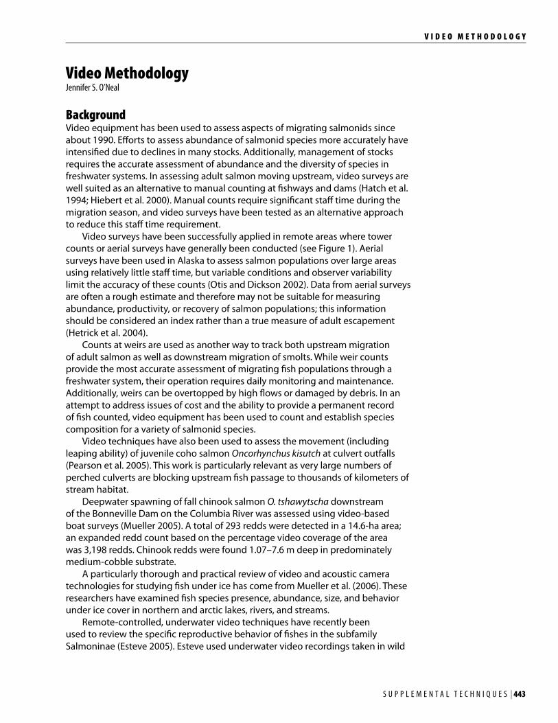
S U P P L E M E N T A L T E C H N I Q U E S | 443
V I D E O M E T H O D O L O G Y
Video MethodologyJennifer S. O’Neal
BackgroundVideo equipment has been used to assess aspects of migrating salmonids since about 1990. Efforts to assess abundance of salmonid species more accurately have intensified due to declines in many stocks. Additionally, management of stocks requires the accurate assessment of abundance and the diversity of species in freshwater systems. In assessing adult salmon moving upstream, video surveys are well suited as an alternative to manual counting at fishways and dams (Hatch et al. 1994; Hiebert et al. 2000). Manual counts require significant staff time during the migration season, and video surveys have been tested as an alternative approach to reduce this staff time requirement. Video surveys have been successfully applied in remote areas where tower counts or aerial surveys have generally been conducted (see Figure 1). Aerial surveys have been used in Alaska to assess salmon populations over large areas using relatively little staff time, but variable conditions and observer variability limit the accuracy of these counts (Otis and Dickson 2002). Data from aerial surveys are often a rough estimate and therefore may not be suitable for measuring abundance, productivity, or recovery of salmon populations; this information should be considered an index rather than a true measure of adult escapement (Hetrick et al. 2004). Counts at weirs are used as another way to track both upstream migration of adult salmon as well as downstream migration of smolts. While weir counts provide the most accurate assessment of migrating fish populations through a freshwater system, their operation requires daily monitoring and maintenance. Additionally, weirs can be overtopped by high flows or damaged by debris. In an attempt to address issues of cost and the ability to provide a permanent record of fish counted, video equipment has been used to count and establish species composition for a variety of salmonid species. Video techniques have also been used to assess the movement (including leaping ability) of juvenile coho salmon Oncorhynchus kisutch at culvert outfalls (Pearson et al. 2005). This work is particularly relevant as very large numbers of perched culverts are blocking upstream fish passage to thousands of kilometers of stream habitat. Deepwater spawning of fall chinook salmon O. tshawytscha downstream of the Bonneville Dam on the Columbia River was assessed using video-based boat surveys (Mueller 2005). A total of 293 redds were detected in a 14.6-ha area; an expanded redd count based on the percentage video coverage of the area was 3,198 redds. Chinook redds were found 1.07–7.6 m deep in predominately medium-cobble substrate. A particularly thorough and practical review of video and acoustic camera technologies for studying fish under ice has come from Mueller et al. (2006). These researchers have examined fish species presence, abundance, size, and behavior under ice cover in northern and arctic lakes, rivers, and streams. Remote-controlled, underwater video techniques have recently been used to review the specific reproductive behavior of fishes in the subfamily Salmoninae (Esteve 2005). Esteve used underwater video recordings taken in wild
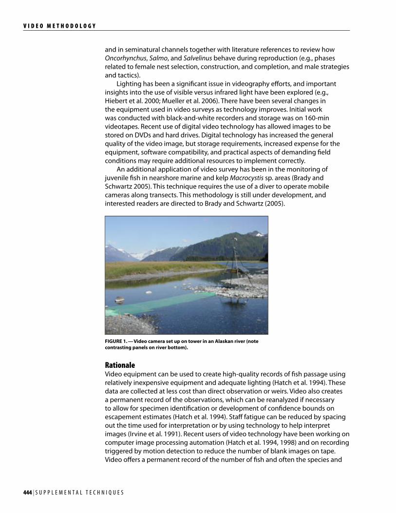
444 | S U P P L E M E N T A L T E C H N I Q U E S
V I D E O M E T H O D O L O G Y
and in seminatural channels together with literature references to review how Oncorhynchus, Salmo, and Salvelinus behave during reproduction (e.g., phases related to female nest selection, construction, and completion, and male strategies and tactics). Lighting has been a significant issue in videography efforts, and important insights into the use of visible versus infrared light have been explored (e.g., Hiebert et al. 2000; Mueller et al. 2006). There have been several changes in the equipment used in video surveys as technology improves. Initial work was conducted with black-and-white recorders and storage was on 160-min videotapes. Recent use of digital video technology has allowed images to be stored on DVDs and hard drives. Digital technology has increased the general quality of the video image, but storage requirements, increased expense for the equipment, software compatibility, and practical aspects of demanding field conditions may require additional resources to implement correctly. An additional application of video survey has been in the monitoring of juvenile fish in nearshore marine and kelp Macrocystis sp. areas (Brady and Schwartz 2005). This technique requires the use of a diver to operate mobile cameras along transects. This methodology is still under development, and interested readers are directed to Brady and Schwartz (2005).
FIGURE 1. — Video camera set up on tower in an Alaskan river (note contrasting panels on river bottom).
RationaleVideo equipment can be used to create high-quality records of fish passage using relatively inexpensive equipment and adequate lighting (Hatch et al. 1994). These data are collected at less cost than direct observation or weirs. Video also creates a permanent record of the observations, which can be reanalyzed if necessary to allow for specimen identification or development of confidence bounds on escapement estimates (Hatch et al. 1994). Staff fatigue can be reduced by spacing out the time used for interpretation or by using technology to help interpret images (Irvine et al. 1991). Recent users of video technology have been working on computer image processing automation (Hatch et al. 1994, 1998) and on recording triggered by motion detection to reduce the number of blank images on tape. Video offers a permanent record of the number of fish and often the species and

S U P P L E M E N T A L T E C H N I Q U E S | 445
V I D E O M E T H O D O L O G Y
size that pass an area, and it can be used to compare differences between years and site conditions as well (Hiebert et al. 2000). A permanent record is especially helpful when time constraints do not allow for immediate data analysis (Irvine et al. 1991). Additionally, video can be used to assess populations without any handling of the fish species, reducing potential stress on fish. Finally, video surveys have little impact on the environment and do not cause fish mortality. Video surveys can be used at existing facilities such as dams and fishways but can also be applied in remote locations (see Figure 1). Systems that are lightweight, transportable, and run under their own power (solar, wind, or hydrogenerated power) have been developed for remote application (Otis and Dickson 2002). Time savings from video surveys vary by application. Hatch et al. (1994) found that 3 d of migration could be reviewed in 6 h, or 2 h per d. Otis and Dickson (2002) determined total fish passage in an average of 38 min per d of video at one sample site and 16 min per d at another. An additional 29 min and 40 min per d of video were required to determine species composition at each site, respectively, using a subsample of the first 15 min of every h (Otis and Dickson 2002). Efficiency rates of 3.6% and 2.1% were calculated for these two sites, reducing the amount of staff time needed for results by 96.4% and 97.9%. Hatch et al. (1994) found an overall time savings of 92% using video surveys versus visual observation.
ObjectivesThe primary objectives of using videography with salmonids include
(1) determining, or estimating, total numbers of moving or migrating fish at a sampling site;
(2) determining, or estimating, species composition of moving or migrating fish at a sampling site;
(3) determining, or estimating, the numbers of hatchery versus wild fish by close examination of body markers or fin clips;
(4) characterizing the body sizes of fish moving or migrating past a sampling site;
(5) assessing spawner and redd density, distribution, and habitat characteristics (e.g., deepwater environments); and
(6) characterizing behavioral aspects of fish (e.g., mating, habitat selection, hesitation in migration).
The first five objectives are used by fisheries scientists and managers concerned with population status and trend information. While objective 6 is mainly used by behaviorists for a variety of reasons (including in the lab), video is also used in fish ladders to determine how well fish pass certain structures. Video technology can be used to provide counts of fish entering a system or passing a certain point in the system (Irvine et al. 1991; Hatch et al. 1994; Hiebert et al. 2000; Otis and Dickson 2002; Hetrick et al. 2004; Mueller et al. 2006). Video recording has been used to assess passage of chinook salmon, coho salmon (Hiebert et al. 2000), sockeye salmon O. nerka, pink salmon O. gorbuscha, and chum salmon O. keta adults (Otis and Dickson 2002), as well as counting and measuring of coho smolts (Irvine et al. 1991). Video-recording technology was implemented to reduce staff requirements and fatigue and to provide a permanent record of
446 | S U P P L E M E N T A L T E C H N I Q U E S
V I D E O M E T H O D O L O G Y
fish passage that could be analyzed or further reviewed. This technology has been applied mostly in areas with existing dams or passage facilities in the Pacific Northwest (Irvine et al. 1991; Hatch et al. 1994; Hiebert et al. 2000) but also in remote sites in Alaska without dams or counting facilities (Otis and Dickson 2002; Hetrick et al. 2004). Dolly Varden Salvelinus malmo have also been detected using this technology, but they were not the target species; their migratory movement along the margins of rivers when other species such as sockeye are densely occupying the main channel may make video a lesser choice for assessing Dolly Varden. Additional lighting is required for night surveys or for accurate species identification (e.g., Hiebert et al. 2000; Mueller et al. 2006). Hiebert et al. (2000) report that more than half of the chinook salmon counted during their study moved upstream at night; however, other studies (Otis and Dickson 2002) have found a low percentage (<1.5%) of the population that moved at night. Determining the species composition of fish passing a certain point is another common objective of using video technology (Hatch et al. 1994; Hiebert et al 2000; Hetrick et al. 2004; Otis and Dickson 2002; Pearson et al. 2005; Mueller et al. 2006). Additional image quality is required to determine the species of fish from recorded or digital images. Achieving this objective may require additional above-water or underwater cameras, and the lens of the camera generally needs to be within 2–2.5 m of the fish to identify the fish to determine species (Hetrick et al. 2004). Otis and Dickson (2002) note that the survey is simplified in areas without multiple species returning to spawn at the same time. A third objective identified in video surveys is the ability to distinguish hatchery fish from wild fish based on the presence of tags or fin clips (Hiebert et al 2000). Hatcheries are playing a role in the recovery of listed stocks, and the use of video to determine the ratio of hatchery-to-wild fish within a system is important for harvest and habitat management. A fourth objective identified in video surveys is the ability to measure fish that pass through the camera view (Irvine et al. 1991). This objective is mostly suited for fixed facilities with narrow passage chambers, where the distance of the fish from the camera can be tightly controlled and a measurement bar in the viewing screen can be used for scale. Automated measurement by computer was implemented by Irvine et al. (1991); however, correction by an observer was still required. Additional developments in this technology are anticipated. A fifth objective is in assessing spawning redd density, distribution, and habitat characteristics, especially in deepwater areas (>1 m) (Mueller 2005), which are generally not counted in surface-based (e.g., boat, aerial) surveys. Here, boat-based video transects are typically made within a determined sample area. A sixth objective is the characterization of the behavioral aspects of fish (e.g., mating) (Esteve 2005). Here, cameras are mounted underwater, with videography used to capture detailed movements and behaviors of reproducing salmonids.
S U P P L E M E N T A L T E C H N I Q U E S | 447
V I D E O M E T H O D O L O G Y
Sampling Design
Site SelectionVideo recording has often been used in places with existing counting facilities such as dams with fishways or spawning grounds. Surveys can be cost effective at remote sites or areas with multiple sites. Other work has constructed camera arrays in remote areas to reduce the need for staff to be constantly present at remote locations. Site selection requirements at remote sites are complex. If solar energy is used for power, the site needs to have adequate sun exposure and plenty of power storage capacity. Stream and river channels best suited for remote video surveys include the following characteristics (Otis and Dickson 2002):
• Relatively narrow (<30 m)
• Shallow depth (<1.5 m)
• Smooth, even bed of cobble substrate
• Smooth current flow (>6 m3/s)
• Good source for wind, solar, or hydropower
• Good water clarity
• Low surface turbulence
Power requirements from Otis and Dickson (2002) were 3.5 A/h without lighting for night surveying. A single 75-W (4.3-A) solar panel can provide this amount of power in full sunlight, but more panels are needed for overcast days and in areas with high canyon walls (Otis and Dickson 2002). Otis and Dickson (2002) found that sites influenced by tidal conditions with pink and chum runs were not the best sites for video surveys because large numbers of spawners were likely to congregate in the area, making fish counting difficult.
Field and Office Methods
Field Setup and OperationVideo recording systems vary in their setup, but all systems require one or more cameras (analog or digital; digital is recommended) and one or more recording and storage devices (e.g., a VCR with tapes, a computer with DVDs or a large hard drive attached). These elements of the system require protective housings if they are to be operated outside an enclosed facility. Additionally, review of the recorded data requires a playback device (often the same as the recording device), the ability to see footage from multiple cameras at the same time if necessary, and a high-quality monitor. Finally, the system has to have an adequate power source from the facility or use other means of power generation at remote sites. Cameras used by video survey crews vary by objective, site requirements, and budget. Since the requirements for remote sites are the most challenging, we report on the equipment used at a remote study site that can be integrated with digital technology. Hetrick et al. (2004) utilized three Toshiba IK-64WDA 24-V day/night cameras for above-water filming. The cameras were housed in outdoor enclosures, set for “super day/night” exposure (which allows the camera to activate a slow shutter speed automatically), and switched to black-and-white in low light
448 | S U P P L E M E N T A L T E C H N I Q U E S
V I D E O M E T H O D O L O G Y
situations. Power needs for this camera were less than 5 W per camera (Hetrick et al. 2004). Settings for camera recording can affect both the image quality and camera efficiency. Cameras can generally be set in several time-lapse recording modes. If using more than one camera and a multiplexer, Otis and Dickson (2002) recommend using 72-h normal mode on an analog camera to balance tape duration, the ability to track and individual fish, and reviewing efficiency. If only one camera is used, the 120-h normal mode allows a 160-min cassette to last 8 d at one image per sec. Camera lenses can greatly affect glare, and an auto-iris lens was found to allow a camera to adjust to varying light conditions (Otis and Dickson 2002). Hetrick et al. (2004) recommend using polarizing filters on all lenses and mounted their above-water cameras 6 m above the water surface. The lenses and filters they used were Pelco F1.6/5-40 mm variable focus, auto-iris lenses with 40.5 mm-Tiffen circular polarizing filters. They pointed the lens towards directional north to minimize glare. Lenses for underwater cameras likely need to be cleaned once per week, and camera enclosures should contain desiccant to reduce moisture (Hetrick et al. 2004). For digital recording, a digital video recorder (Digicorder 2000 Deluxe digital video recorder, Alpha System Laboratory, or Gyyr four-channel Digital Video Management System [DVMS 400, recommended for higher resolution]) (see Table 1) was used by Hetrick et al. (2004) for both recording and as a four-channel multiplexer to view images from multiple cameras at once. Otis and Dickson (2002) used video cassette recorders for analog recording and viewing but were not satisfied with the multiplexer because it slowed the reviewing process. Hetrick at el. (2004) captured footage at four to five frames per second, at one of four resolutions (720 × 486, 352 × 480, 352 × 240, and 176 × 120). These files were compressed and recorded to a hard drive. The date and time was recorded on each frame as well as the title of the camera from which the footage came. Video files were then loaded onto DVDs using a firewire DVD-RAM drive (Institute of Electrical and Electronics Engineers, IEEE 1394; see Table 1). Storage requirements reported by Hetrick et al. (2004) consisted of 1.2 gigabytes/h recording at 5 frames per second for one camera with a compression ratio of 10:1 and 4.7 gigabytes/h for four cameras at the same settings. Lighting techniques are critical for high image quality and the ability to determine the species of fish passing the camera. Surveyors need to balance the image quality against lighting that may affect the passage of fish over the viewing substrate (Hiebert et al. 2000). Infrared light has been tested to determine if it would present lesser disturbance to migrating fish (Hiebert et al. 2000). Visible light caused some hesitation in coho and chinook (<9 min) (but not for steelhead O. mykiss), particularly at night as compared to infrared light. Chinook salmon in this study at Prosser Dam on the Yakima River, Washington, also migrated more at night (70%) under infrared light than under visible light (49%) as compared to migration during daylight. Infrared lights operating at wavelengths longer than 800 nm can be useful for identifying fish in low light or during the nighttime; most fish species are unaffected by this infrared range because it falls beyond their spectral range (Lythgoe 1988); however, infrared light dissipates quickly in water and does not result in high image quality. Visible light was superior for determining species and hatchery origin of fish. Hetrick et al. (2004) found that a single high-beam auto headlight mounted on a tower was the most effective
S U P P L E M E N T A L T E C H N I Q U E S | 449
V I D E O M E T H O D O L O G Y
lighting system for detecting coho salmon during night video surveys. The need for image quality should be weighed against the potential for slight delays in fish passage when selecting a lighting system. Additional work has been done in lighting for video surveys. In a study of coho smolts at an enumeration fence on the Keogh River in British Columbia, Canada, Irvine et al. (1991) used a black plastic shroud around the lighting and filming setup to eliminate stray reflections. For low light situations, a super low-lux black-and-white camera with infrared lights could be used (Otis and Dickson 2002). Transmission of data from the camera to a recording device may be accomplished wirelessly if the camera used is digital. Hetrick et al. (2004) used a wireless FM video transmitter (see Table 1) to transmit the video images collected up to 210 m to a computer. Additional setup is required if the work is to be conducted at a remote site. If an enclosed facility is used, the equipment is generally mounted in an existing viewing chamber. At remote sites, a substrate needs to be installed to make fish visible as they pass the recording site; the main function of this material is to provide a contrasting background between the channel bottom and the fish passing in front of the camera. Hetrick et al. (2004) used high-density polyethylene panels to provide contrast with fish and found that they were easy to keep clean. This material was selected as it is durable under a wide range of temperatures and does not degrade underwater or in sunlight, and it has a smooth surface. The panels measured 1.2 m × 1.5 m × 3.2 mm and were anchored to the stream bottom using 9.5 mm galvanized cable, set perpendicular to the flow and 19.1-mm S-hooks. Additional connections between the panels should be made, and Hetrick et al. (2004) recommend 50–80-kg tensile strength white cable ties. Duck-bill anchors (size 68) were used to anchor the cable and the recommended spacing on these is 4 m or less (Hetrick et al. 2004). Otis and Dickson (2002) used a light-green substrate material of 0.32-cm mesh seine material, which was also attached to the bottom of the channel. Constricting the path through which fish pass has been useful in reducing the area where filming needs to be concentrated. Hetrick et al. (2004) placed substrate panels to form a “V” in the channel and found that many fish followed the edge of the panel to the small break in the “V” before crossing the viewing area. The “V” location was monitored using an underwater camera that could capture close-up images of fish to determine species. Limiting the passage space for fish can also reduce the risk of fish moving back through the viewing area a second time and the swarming of fish, which result in overestimation (if the same fish is counted twice) or underestimation (if the viewer cannot see all the fish in a large group). Towers for cameras are also required for remote site use. These can be constructed or commercially purchased, but need to be sturdy enough to prevent shaking during weather events. Placement of the towers, with respect to viewing area, angle towards the water surface, and direction is critical to reduce glare. The ability to adjust the camera position without disturbing the placement is also critical when setting up the optimum viewing system based on sight conditions. Excessive glare can ruin the image quality of the recording. Additionally, Hetrick et al. (2004) found that a viewing area greater than 10 m wide restricts the viewer’s ability to count large numbers of fish, even with very high image quality from digital cameras. Another consideration in camera placement is the use of underwater cameras. It is often necessary to capture an image of the fish in a side
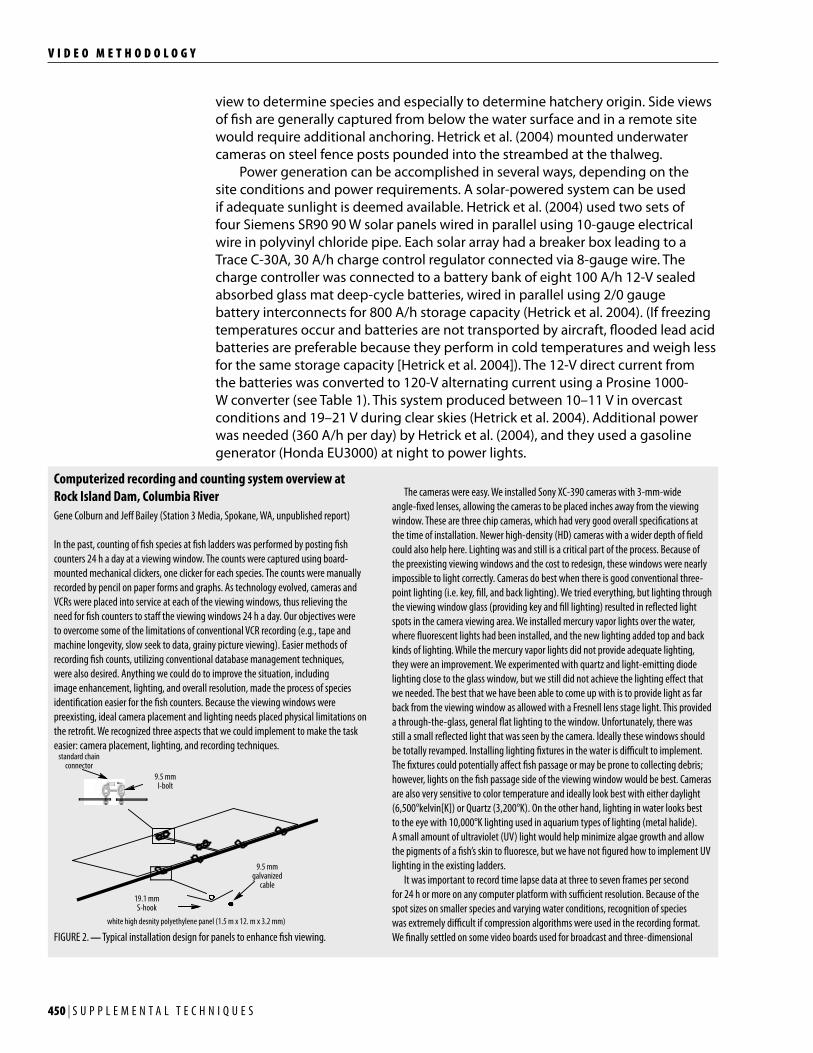
450 | S U P P L E M E N T A L T E C H N I Q U E S
V I D E O M E T H O D O L O G Y
view to determine species and especially to determine hatchery origin. Side views of fish are generally captured from below the water surface and in a remote site would require additional anchoring. Hetrick et al. (2004) mounted underwater cameras on steel fence posts pounded into the streambed at the thalweg. Power generation can be accomplished in several ways, depending on the site conditions and power requirements. A solar-powered system can be used if adequate sunlight is deemed available. Hetrick et al. (2004) used two sets of four Siemens SR90 90 W solar panels wired in parallel using 10-gauge electrical wire in polyvinyl chloride pipe. Each solar array had a breaker box leading to a Trace C-30A, 30 A/h charge control regulator connected via 8-gauge wire. The charge controller was connected to a battery bank of eight 100 A/h 12-V sealed absorbed glass mat deep-cycle batteries, wired in parallel using 2/0 gauge battery interconnects for 800 A/h storage capacity (Hetrick et al. 2004). (If freezing temperatures occur and batteries are not transported by aircraft, flooded lead acid batteries are preferable because they perform in cold temperatures and weigh less for the same storage capacity [Hetrick et al. 2004]). The 12-V direct current from the batteries was converted to 120-V alternating current using a Prosine 1000-W converter (see Table 1). This system produced between 10–11 V in overcast conditions and 19–21 V during clear skies (Hetrick et al. 2004). Additional power was needed (360 A/h per day) by Hetrick et al. (2004), and they used a gasoline generator (Honda EU3000) at night to power lights.
Computerized recording and counting system overview at Rock Island Dam, Columbia RiverGene Colburn and Jeff Bailey (Station 3 Media, Spokane, WA, unpublished report)
In the past, counting of fish species at fish ladders was performed by posting fish counters 24 h a day at a viewing window. The counts were captured using board-mounted mechanical clickers, one clicker for each species. The counts were manually recorded by pencil on paper forms and graphs. As technology evolved, cameras and VCRs were placed into service at each of the viewing windows, thus relieving the need for fish counters to staff the viewing windows 24 h a day. Our objectives were to overcome some of the limitations of conventional VCR recording (e.g., tape and machine longevity, slow seek to data, grainy picture viewing). Easier methods of recording fish counts, utilizing conventional database management techniques, were also desired. Anything we could do to improve the situation, including image enhancement, lighting, and overall resolution, made the process of species identification easier for the fish counters. Because the viewing windows were preexisting, ideal camera placement and lighting needs placed physical limitations on the retrofit. We recognized three aspects that we could implement to make the task easier: camera placement, lighting, and recording techniques.
standard chainconnector
9.5 mmI-bolt
9.5 mmgalvanized
cable
19.1 mmS-hook
white high desnity polyethylene panel (1.5 m x 12. m x 3.2 mm)
FIGURE 2. — Typical installation design for panels to enhance fish viewing.
The cameras were easy. We installed Sony XC-390 cameras with 3-mm-wide angle-fixed lenses, allowing the cameras to be placed inches away from the viewing window. These are three chip cameras, which had very good overall specifications at the time of installation. Newer high-density (HD) cameras with a wider depth of field could also help here. Lighting was and still is a critical part of the process. Because of the preexisting viewing windows and the cost to redesign, these windows were nearly impossible to light correctly. Cameras do best when there is good conventional three-point lighting (i.e. key, fill, and back lighting). We tried everything, but lighting through the viewing window glass (providing key and fill lighting) resulted in reflected light spots in the camera viewing area. We installed mercury vapor lights over the water, where fluorescent lights had been installed, and the new lighting added top and back kinds of lighting. While the mercury vapor lights did not provide adequate lighting, they were an improvement. We experimented with quartz and light-emitting diode lighting close to the glass window, but we still did not achieve the lighting effect that we needed. The best that we have been able to come up with is to provide light as far back from the viewing window as allowed with a Fresnell lens stage light. This provided a through-the-glass, general flat lighting to the window. Unfortunately, there was still a small reflected light that was seen by the camera. Ideally these windows should be totally revamped. Installing lighting fixtures in the water is difficult to implement. The fixtures could potentially affect fish passage or may be prone to collecting debris; however, lights on the fish passage side of the viewing window would be best. Cameras are also very sensitive to color temperature and ideally look best with either daylight (6,500°kelvin[K]) or Quartz (3,200°K). On the other hand, lighting in water looks best to the eye with 10,000°K lighting used in aquarium types of lighting (metal halide). A small amount of ultraviolet (UV) light would help minimize algae growth and allow the pigments of a fish’s skin to fluoresce, but we have not figured how to implement UV lighting in the existing ladders. It was important to record time lapse data at three to seven frames per second for 24 h or more on any computer platform with sufficient resolution. Because of the spot sizes on smaller species and varying water conditions, recognition of species was extremely difficult if compression algorithms were used in the recording format. We finally settled on some video boards used for broadcast and three-dimensional
S U P P L E M E N T A L T E C H N I Q U E S | 451
V I D E O M E T H O D O L O G Y
Office Methods for Footage ReviewA multiplexer can be used to view images from multiple cameras at once. Playback speeds for analog cameras are step-wise and not very flexible (Otis and Dickson 2002). Much greater flexibility is found in digital footage (Hetrick et al. 2004). Each footage day can be divided into three periods (dawn to 1159 hr, 1200 to 1759, and 1800 to dusk) (Otis and Dickson 2002). Reviewers should count the total number of fish swimming upstream and keep track of the amount of time required to review each section of footage. The time for dawn and dusk should be recorded for each footage day as well as the playback speed used to review the footage. Motion detection algorithms were used by Hetrick et al. (2004) with some success. This approach was designed to help eliminate long sections of blank footage from having to be reviewed. The algorithms undercounted coho salmon during a test by 27%. Motion detection ability could be improved by using wider substrate panels, but potential effects on fish passage over wider panels would need to be evaluated (Hetrick et al. 2004). Underwater cameras used in the fall often triggered false responses from the motion detector when leaves and debris floated in front of the camera. Use of this system during earlier migrations in the summer may reduce the number of false triggers if there are fewer leaves and less debris in the water (Hetrick et al. 2004). Motion detection is most difficult during crepuscular periods, when light conditions are changing rapidly (Hetrick et al. 2004). Hetrick et al. (2004) recommend constant recording during these periods
animation applications. They are Digital Processing Systems (DPS) Perception boards that allow 10-bit recording of uncompressed video data. They are well suited for varying frame rate recordings, with excellent playback and jog-shuttle control. The DPS graphical interface is much like a VCR which the fish counters were already accustomed to using. Using server board computer configurations, we could install two DPS boards into each computer, allowing the fish counter to view the previous day’s recordings while still recording the current day. Each video board has its own Small Computer System Interface-embedded controller that allows for the amount of Raid Array storage required for this kind of data. The embedded controller also freed up the central processing unit, allowing for a reliable multitasking environment. A custom software application was developed to allow users to track fish passage easily and analyze the empirical data. The software consisted of two tiers. The first tier handled the collecting of data by date/time and fish species. A simple user interface was developed that both mimicked the previous mechanical counting and provided more granularity and accuracy than was previously possible. At the end of each day of counting, the fish counters would “push” the passage data to the corporate office for analysis. The second tier of the software system provided a means to aggregate the passage data providing summary results as well as point-in-time analysis. Using popular spreadsheet functionality, biologists could see all data that had been collected. With a push of a button, users were now able to instantly update summary data on a Web site. Additional data could be exported and made available through a file transfer protocol site. Once a reliable computer configuration was developed, the next task was a facility implementation that would allow the fish counters at Rock Island Dam to operate these systems easily. The accompanying block diagram of the system (see Figure 1) shows the basic signal flow to each computer. All equipment is rack-mounted and powered by a power-conditioning ininterruptible power supply system. The basic signal path from each camera is fed to a time-and-date video insertion generator and then sent to distribution amplifiers to allow for additional recording by VCRs for back-up (in case of a computer crash). The signals are then passed on to a video routing switcher, allowing any computer to record any camera position. Three cameras and four computer work stations are installed at the dam. The video router provides routing as needed for overflow counts or any failure in the overall system. A second
matrix router is installed for switching keyboard, mouse, and computer monitor to each fish counter’s desk. This was provided to allow the counters to share the workload on busier count days. The video output from each computer’s two internal video boards is switched internally to the video overlay, so that each monitor station sees the actual playback video on his/her respective liquid crystal display computer monitor. The count board overlay and jog shuttle overlay appear on the same screen, making for a good logical screen layout. Included in the signal path is the video from the previous day, which is sent to a DVD recorder for archival purposes. Ergonomics plays a key role in installation. The counters sit and watch these screens 8 h a day and are continually using their mouse to input data and jog-shuttle; therefore, doing everything possible to make this more ergonomically safe is important. The improvements included proper monitor desk height, padded mouse pads, and good overhead lighting. There are a number of considerations for future improvements for this system. For example, cameras that can operate better in low light with better resolution, while maintaining an entire digital path from camera to computer. We are currently using existing analog fiber paths and will not upgrade until HD cameras and recording techniques are available. Additionally, any modifications to the fish passage area at the viewing window would need a redesign and laboratory testing before implementation. The benchmark is to make the computer overlay (i.e., video resolution) look as good as if a fish counter were still counting fish (in real time) at the viewing window.
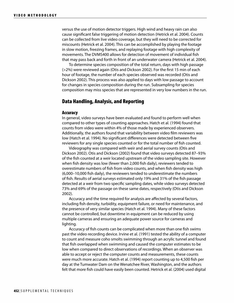
452 | S U P P L E M E N T A L T E C H N I Q U E S
V I D E O M E T H O D O L O G Y
versus the use of motion detector triggers. High wind and heavy rain can also cause significant false triggering of motion detection (Hetrick et al. 2004). Counts can be collected from live video coverage, but they will need to be corrected for miscounts (Hetrick et al. 2004). This can be accomplished by playing the footage in slow motion, freezing frames, and replaying footage with high complexity of movements. The DVMS400 allows for detection of movement of individual fish that may pass back and forth in front of an underwater camera (Hetrick et al. 2004). To determine species composition of the total return, days with high passage (>2%) were reviewed again (Otis and Dickson 2002). For the first 15 min of each hour of footage, the number of each species observed was recorded (Otis and Dickson 2002). This process was also applied to days with low passage to account for changes in species composition during the run. Subsampling for species composition may miss species that are represented in very low numbers in the run.
Data Handling, Analysis, and Reporting
AccuracyIn general, video surveys have been evaluated and found to perform well when compared to other types of counting approaches. Hatch et al. (1994) found that counts from video were within 4% of those made by experienced observers. Additionally, the authors found that variability between video film reviewers was low (Hatch et al. 1994). No significant differences were detected between five reviewers for any single species counted or for the total number of fish counted. Videography was compared with weir and aerial survey counts (Otis and Dickson 2002). Otis and Dickson (2002) found that video surveys detected 87–93% of the fish counted at a weir located upstream of the video sampling site. However when fish density was low (fewer than 2,000 fish daily), reviewers tended to overestimate numbers of fish from video counts, and when fish density was high (6,000–10,000 fish daily), the reviewers tended to underestimate the numbers of fish. Results of aerial surveys estimated only 19% and 31% of the fish passage detected at a weir from two specific sampling dates, while video surveys detected 73% and 69% of the passage on these same dates, respectively (Otis and Dickson 2002). Accuracy and the time required for analysis are affected by several factors, including fish density, turbidity, equipment failure, or need for maintenance, and the presence of very similar species (Hatch et al. 1994). Many of these factors cannot be controlled, but downtime in equipment can be reduced by using multiple cameras and ensuring an adequate power source for cameras and lighting. Accuracy of fish counts can be complicated when more than one fish swims past the video recording device. Irvine et al. (1991) tested the ability of a computer to count and measure coho smolts swimming through an acrylic tunnel and found that fish overlapped when swimming and caused the computer estimates to be low when compared to direct observations of recordings. When an observer was able to accept or reject the computer counts and measurements, these counts were much more accurate. Hatch et al. (1994) report counting up to 4,500 fish per day at the Tumwater Dam on the Wenatchee River, Washington, and the authors felt that more fish could have easily been counted. Hetrick et al. (2004) used digital
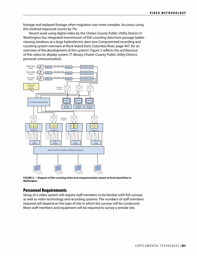
S U P P L E M E N T A L T E C H N I Q U E S | 453
V I D E O M E T H O D O L O G Y
footage and replayed footage when migration was more complex. Accuracy using this method improved counts by 7%. Recent work using digital video by the Chelan County Public Utility District in Washington has integrated transmission of fish counting data from passage ladder viewing windows at a large hydroelectric dam (see Computerized recording and counting system overview at Rock Island Dam, Columbia River, page 447, for an overview of the development of this system). Figure 3 reflects the architecture of this video-to-display system (T. Mosey, Chelan County Public Utility District, personal communication).
Fiber TxFiber Optic Cable
Fiber TxFiber Optic Cable
Fiber Tx Fiber Rx
Right LadderCamera
Center LadderCamera
Left LadderCamera
Fiber Optic Cable
Time/Date Insert
Time/Date Insert
Time/Date Insert
4 x 4 Video Routing SwitcherMonitor
Video TapeRecorder
Monitor
Video TapeRecorder
Monitor
Video TapeRecorder
Computer 1 Computer 2 Computer 3 Computer 4
V1 V2
Matrix Switcher for Monitors, Keyboards and Mouse
DVDRecorder
DVDRecorder
DVDRecorder
DVDRecorder
DistributionAmplifiers
DistributionAmplifiers
UninterruptedAC Power
Conditioner
V1 V2 V1 V2 V1 V2
Fiber Rx
Fiber Rx
FIGURE 3. — Diagram of fish-counting video and computerization system at Rock Island Dam in Washington.
Personnel RequirementsSetup of a video system will require staff members to be familiar with fish surveys as well as video technology and recording systems. The numbers of staff members required will depend on the type of site in which the surveys will be conducted. More staff members and equipment will be required to survey a remote site.
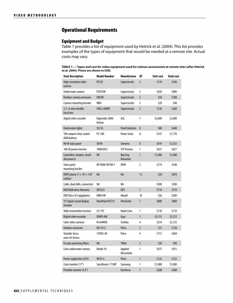
454 | S U P P L E M E N T A L T E C H N I Q U E S
V I D E O M E T H O D O L O G Y
Operational Requirements
Equipment and BudgetTable 1 provides a list of equipment used by Hetrick et al. (2004). This list provides examples of the types of equipment that would be needed at a remote site. Actual costs may vary.
TABLE 1. — Types and cost for video equipment used for salmon assessments at remote sites (after Hetrick et al. 2004). Prices are shown in USD.
Item Description Model Number Manufacture QT Unit cost Total cost
High-resolution video camera
PC33C Supercircuits 2 $170 $340
Underwater camera PC81UW Supercircuits 2 $450 $900
Outdoor camera enclosure ENCOD Supercircuits 2 $50 $100
Camera-mounting bracket MB4 Supercircuits 2 $20 $40
2.5–6-mm variable focal lens
CML2-6MMZ Supercircuits 2 $130 $260
Digital video recorder Digicorder 2000 Deluxe
ASL 1 $2,800 $2,800
Underwater lights SCL VL Pond Solutions 8 $80 $640
100-ampere-hour sealed AGM battery
PS-100 Power Sonic 8 $147 $1,176
90-W solar panel SR 90 Siemens 8 $419 $3,352
100-W power inverter 1000/GFCI STP Prosine 1 $637 $637
Controllers, beakers, fused disconnects
NA Big Frog Mountain
1 $1,000 $1,000
Solar panel mounting bracket
DP-RGM-SR100-T DPW 2 $174 $348
HDPE plastic 4’ × 10’ × 1/8” (white)
NA NA 15 $58 $870
Cable, duck-bills, connectors NA NA $500 $500
DVD RAM drive (firewire) QPS525 QPS 1 $710 $710
DVD Discs (9.4 gigabytes) DRM 94F Maxell 10 $50 $500
15” liquid crystal display monitor
ViewPanel VG151 ViewSonic 1 $800 $800
Video transmitter/receiver CV-191 Nutex Com. 1 $110 $110
Digital video recorder DVMS 400 Gyyr 1 $5,212 $5,212
Color video cameras IK-64WDA Toshiba 4 $534 $2,135
Outdoor enclosure EH-3512 Pelco 2 $75 $150
Variable-focus auto-iris lenses
13VD5-40 Pelco 4 $151 $604
Circular polarizing filters NA Tiffen 3 $30 $90
Color underwater camera Model 10 Applied Microvideo
1 $475 $475
Power supply box (24 V) WCSI-4 Pelco 1 $122 $122
Color monitor (17”) SyncMaster 171MP Samsung 1 $1,000 $1,000
Portable monitor (5.6”) Everfocus 1 $288 $288
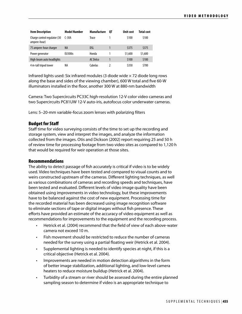
S U P P L E M E N T A L T E C H N I Q U E S | 455
V I D E O M E T H O D O L O G Y
Item Description Model Number Manufacture QT Unit cost Total cost
Charge control regulator (30 ampere-hour)
C-30A Trace 1 $100 $100
75 ampere-hour charger NA DSL 1 $375 $375
Power generator EU300is Honda 1 $1,600 $1,600
High-beam auto headlights AC Delco 1 $100 $100
4 m-tall tripod tower NA Cabelas 2 $350 $700
Infrared lights used: Six infrared modules (3 diode wide × 72 diode long rows along the base and sides of the viewing chamber), 600 W total and five 60-W illuminators installed in the floor, another 300 W at 880-nm bandwidth
Camera: Two Supercircuits PC33C high-resolution 12-V color video cameras and two Supercircuits PC81UW 12-V auto-iris, autofocus color underwater cameras.
Lens: 5–20-mm variable-focus zoom lenses with polarizing filters
Budget for StaffStaff time for video surveying consists of the time to set up the recording and storage system, view and interpret the images, and analyze the information collected from the images. Otis and Dickson (2002) report requiring 25 and 50 h of review time for processing footage from two video sites as compared to 1,120 h that would be required for weir operation at those sites.
Recommendations The ability to detect passage of fish accurately is critical if video is to be widely used. Video techniques have been tested and compared to visual counts and to weirs constructed upstream of the cameras. Different lighting techniques, as well as various combinations of cameras and recording speeds and techniques, have been tested and evaluated. Different levels of video image quality have been obtained using improvements in video technology, but these improvements have to be balanced against the cost of new equipment. Processing time for the recorded material has been decreased using image recognition software to eliminate sections of tape or digital images without fish presence. These efforts have provided an estimate of the accuracy of video equipment as well as recommendations for improvements to the equipment and the recording process.
• Hetrick et al. (2004) recommend that the field of view of each above-water camera not exceed 10 m.
• Fish movement should be restricted to reduce the number of cameras needed for the survey using a partial floating weir (Hetrick et al. 2004).
• Supplemental lighting is needed to identify species at night, if this is a critical objective (Hetrick et al. 2004).
• Improvements are needed in motion detection algorithms in the form of better image stabilization, additional lighting, and low-level camera heaters to reduce moisture buildup (Hetrick et al. 2004).
• Turbidity of a stream or river should be assessed during the entire planned sampling season to determine if video is an appropriate technique to

456 | S U P P L E M E N T A L T E C H N I Q U E S
V I D E O M E T H O D O L O G Y
use. Turbidity levels above 80 nephelometric turbidity unit resulted in significant image quality degradation (Hetrick et al. 2004).
• Otis and Dickson (2002) recommend the use of real-time microwave or satellite transmission of digital images back to a central office location. This improvement would solve some equipment and maintenance issues, reduce cost, and increase the speed in which data could be analyzed. Hetrick et al. (2004) note that advanced transmitters can send a line-of-sight signal up to 65 km. Using these transmitters could reduce the power requirements at remote sites.
Literature Cited
Brady, B. C., and J. D. M. Schwartz. 2005. Video methodology for surveying nearshore fishes at CRANE sites: with the option of underwater geo-referencing. California Department of Fish and Game, Marine Region, Santa Barbara.
Esteve, M. 2005. Observations of spawning behaviour in Salmoninae: Salmo, Oncorhynchus and Salvelinus. Reviews in Fish Biology and Fisheries 15:1–21.
Hatch, D. R., M. Schwartzberg, and P. R. Mundy. 1994. Estimation of Pacific salmon escapement with a time-lapse video recording technique. North American Journal of Fisheries Management 14:626–635.
Hatch, D. R., J. K. Fryer, M. Schwartzberg, D. R. Pederson, A. Wand. 1998. A Computerized Editing System for Video Monitoring of Fish Passage. North American Journal of Fisheries Management 18(3):694–699.
Hetrick, N. J., K. M. Simms, M. P. Plumb, and J. P. Larson. 2004. Feasibility of using video technology to estimate salmon escapement in the Ongivinuk River, a clear-water tributary of the Togiak River. U.S. Fish and Wildlife Service, King Salmon Fish and Wildlife Office, King Salmon, Alaska.
Hiebert, S., L. A. Helfrich, D. L. Weigmann, and C. Liston. 2000. Anadromous salmonid passage and video image quality under infrared and visible light at Prosser Dam, Yakima River, Washington. North American Journal of Fisheries Management 20:827–832.
Irvine, J. R., B. R. Ward, P. A. Teti, and N. B. F. Cousens. 1991. Evaluation of a method to count and measure live salmonids in the field with a video camera and computer. North American Journal of Fisheries Management 11:20–26.
Lythgoe, J. N. 1988. Light and vision in the aquatic environment. Pages 57–82 in J. Atema, R. R. Fay, A. N. Popper, and W. N. Tavolga, editors. Sensory biology of aquatic animals. Springer-Verlag, New York.
Mueller, R. P. 2005. Deepwater spawning of fall chinook salmon (Oncorhynchus tshawytscha) near Ives and Pierce Island of the Columbia River. 2004–2005 Annual Report, Project No. 199900301. Bonneville Power Administration, DOE/BP-00000652-28, Portland, Oregon.
Mueller, R. P., R. S. Brown, H. Hop, and L. Moulton. 2006. Video and acoustic camera techniques for studying fish under ice: a review and comparison. Reviews in Fish Biology and Fisheries 16:213–226.
Otis, E. O., and M. Dickson. 2002. Improved salmon escapement enumeration using remote video and time-lapse recording technology. Alaska Department of Fish and Game, Division of Commercial Fisheries. Restoration Project 00366 Final Report, Homer.

S U P P L E M E N T A L T E C H N I Q U E S | 457
V I D E O M E T H O D O L O G Y
Pearson, W. H., R. P. Mueller, S. L. Sargeant, and C. W. May. 2005. Evaluation of juvenile salmon leaping ability and behavior at the experimental culvert test bed. Final Report to the Washington State Department of Transportation, Battelle Pacific Northwest Division, WSDOT Agreement No. GCA2677, Richland.

458 | S U P P L E M E N T A L T E C H N I Q U E S
V I D E O M E T H O D O L O G Y