Potentialities of Unmanned Aerial Vehicles in Hydraulic ...
76
IN DEGREE PROJECT ENVIRONMENTAL ENGINEERING, SECOND CYCLE, 30 CREDITS , STOCKHOLM SWEDEN 2018 Potentialities of Unmanned Aerial Vehicles in Hydraulic Modelling Drone remote sensing through photogrammetry for 1D flow numerical modelling ANDREA REALI KTH ROYAL INSTITUTE OF TECHNOLOGY SCHOOL OF ARCHITECTURE AND THE BUILT ENVIRONMENT
-
Upload
khangminh22 -
Category
Documents
-
view
1 -
download
0
Transcript of Potentialities of Unmanned Aerial Vehicles in Hydraulic ...

IN DEGREE PROJECT ENVIRONMENTAL ENGINEERING,SECOND CYCLE, 30 CREDITS
, STOCKHOLM SWEDEN 2018
Potentialities of Unmanned Aerial Vehicles in Hydraulic ModellingDrone remote sensing through photogrammetry for 1D flow numerical modelling
ANDREA REALI
KTH ROYAL INSTITUTE OF TECHNOLOGYSCHOOL OF ARCHITECTURE AND THE BUILT ENVIRONMENT


Potentialities of Unmanned Aerial Vehicles in Hydraulic Modelling Drone remote sensing through photogrammetry for 1D flow numerical modelling
Andrea Reali
Dr. Luigia Brandimarte (supervisor), KTH, ABE, Stockholm Dr. Maurizio Mazzoleni (supervisor), UNESCO-IHE, Delft Dr. Paolo Paron (supervisor), UNESCO-IHE, Delft Prof. Anders Wörman (examiner), KTH ABE, Stockholm
Master Thesis, 2018 KTH Royal Institute of Technology School of Architecture and Built Environment Department of Sustainable Development, Environmental Science and Engineering. SE-100 44 Stockholm, Sweden

TRITA -ABE-MBT-18444
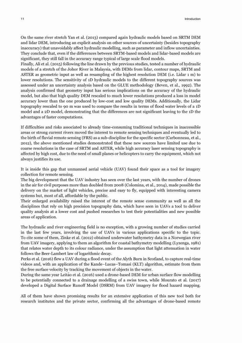
Abstract
In civil and environmental engineering numerous are the applications that require prior collection of data on the ground. When it comes to hydraulic modelling, valuable topographic and morphology features of the region are one of the most useful of them, yet often unavailable, expensive or difficult to obtain.
In the last few years UAVs entered the scene of remote sensing tools used to deliver such information and their applications connected to various photo-analysis techniques have been tested in specific engineering fields, with promising results. The content of this thesis aims contribute to the growing literature on the topic, assessing the potentialities of UAV and SfM photogrammetry analysis in developing terrain elevation models to be used as input data for numerical flood modelling.
This thesis covered all phases of the engineering process, from the survey to the implementation of a 1D hydraulic model based on the photogrammetry derived topography
The area chosen for the study was the Limpopo river. The challenging environment of the Mozambican inland showed the great advantages of this technology, which allowed a precise and fast survey easily overcoming risks and difficulties. The test on the field was also useful to expose the current limits of the drone tool in its high susceptibility to weather conditions, wind and temperatures and the restricted battery capacity which did not allow flight longer than 20 minutes.
The subsequent photogrammetry analysis showed a high degree of dependency on a number of ground control points and the need of laborious post-processing manipulations in order to obtain a reliable DEM and avoid the insurgence of dooming effects. It revealed, this way, the importance of understanding the drone and the photogrammetry software as a single instrument to deliver a quality DEM and consequently the importance of planning a survey photogrammetry-oriented by the adoption of specific precautions. Nevertheless, the DEM we produced presented a degree of spatial resolution comparable to the one high precision topography sources.
Finally, considering four different topography sources (SRTM DEM 30 m, lidar DEM 1 m, drone DEM 0.6 m, total station&RTK bathymetric cross sections o.5 m) the relationship between spatial accuracy and water depth estimation was tested through 1D, steady flow models on HECRAS. The performances of each model were expressed in terms of mean absolute error (MAE) in water depth estimations of the considered model compared to the one based on the bathymetric cross-sections. The result confirmed the potentialities of the drone for hydraulic engineering applications, with MAE differences between lidar, bathymetry and drone included within 1 m. The calibration of SRTM, Lidar and Drone based models to the bathymetry one demonstrated the relationship between geometry detail and roughness of the cross-sections, with a global improvement in the MAE, but more pronounced for the coarse geometry of SRTM
Keywords: UAV remote sensing – Structure from motion photogrammetry – 1D, steady flow hydraulic numerical modelling


Preface
The present publication represents the work for final thesis of the Master of Science in Civil and Architectural Engineering. It was carried out at the Department of Sustainable Development, Environmental Science and Engineering, Resources, Energy and Infrastructure division of the Royal Institute of Technology (KTH)
I want to take the opportunity to express all my gratitude to my supervisor, professor Lugia Brandimarte for making this possible, gifting me with a unique opportunity of personal and technical improvement. Her guidance and support have been essential to the success of this work.
More than a word of thanks is also due to prof. Maurizio Mazzoleni and prof. Paolo Paron for their precious assistance on the field and in the developing of the model.
Last but not least, I want to sincerely thank my parents and all the friends who, through their continuous support, contributed to the realisation of the thesis.
Stockholm, August 2018
Andrea Reali


Table of Contents
Abstract .................................................................................................................................. 4
Preface ................................................................................................................................... 6
1 Introduction .................................................................................................................. 10 1.1 Background, aim and scope................................................................................... 10 1.2 Study area ............................................................................................................... 13
1.2.1 Limpopo River basin ................................................................................................................... 13 1.2.2 Chokwe district ........................................................................................................................... 14
2 Methodology ................................................................................................................. 16 2.1 Field work ................................................................................................................ 16
2.1.1 Schedule ..................................................................................................................................... 16 2.1.2 Equipment................................................................................................................................... 16 2.1.3 Flight planning ............................................................................................................................ 17 2.1.4 Flight ........................................................................................................................................... 19
2.2 Photogrammetry ..................................................................................................... 22 2.3 Hydraulic modeling ................................................................................................. 30
3 Discussion on geometries .......................................................................................... 32 3.1 Bathymetry from Total Station and RTK GPS ....................................................... 33 3.2 SRTM ....................................................................................................................... 35 3.3 LIDAR....................................................................................................................... 37 3.4 Drone ....................................................................................................................... 39 3.5 Longitudinal profile................................................................................................. 42
4 Hydraulic modeling ...................................................................................................... 44 4.1 Results..................................................................................................................... 44 4.2 Calibration ............................................................................................................... 49
5 Conclusions .................................................................................................................. 56
Appendix A – Drones, batteries and camera specifics .................................................. 60
Appendix B – Flight plan calculations ............................................................................. 64
Appendix C – Modify cross-sections code for MatLab .................................................. 66
Appendix D – HEC-RAS steady flow computation procedure ...................................... 68
Bibliography ........................................................................................................................ 72


Introduction 10
1 Introduction
1.1 Background, aim and scope Hydrological and hydraulic models to be implemented, calibrated and validated require a number of different data, specific for the study area. Often, their collection has a considerable effect on the time and cost of the final product, especially when it requires the use of expensive tools, qualified personnel or it covers impervious and dangerous areas.
The core input data for most of environmental models is a topographic map of the study area in a digital form, or digital elevation models (DEM). Nowadays, DEMs can be obtained from various combinations of surveying tools and data techniques spacing from traditional ground surveying such as total stations, various form of GPS systems and echo sounders, topographic contour maps, or through remote sensing techniques applied to air or space-borne imagery acquired by light detection and ranging instruments (Lidar), the Shuttle Radar Topographic Mission (SRTM) or the Advanced Spaceborne Thermal Emission and Reflection Radiometer (ASTER). Every source gives a DEM with different accuracies and spatial resolutions which, when used as topographic input for hydraulic models, can results in countable dissimilarities in the model final performances and several studies now have shown the impact of DEM quality on the final hydraulic model.
Casas et al. (2006) tested the performances of a 1D hydraulic model for flood propagation in terms of water levels and inundated area in the flood plain, concluding that the digital terrain model (DTM) derived by contour maps gave the least accurate results when compared to GPS-based and Lidar-based models. The Lidar one was giving the closest values to the reference data and they pointed out how that was the technique showing the best cost-effective ratio for the production of DEM covering large areas. Similarly, Schumann et al. (2008) compared 1D flooding model outputs with the variation in source and resolution of the input DEM. Contour maps, SRTM and Lidar DEMs were used and the respective models calibrated with ground surveying high water marks distributed along the study area in Luxemburg. As expected, the SRTM DEM gave the highest discrepancies in the evaluation of water stages, with an RMSE of 1.07 m, preceded by the contour DEM (0.7 m) and the Lidar DEM (0.35 m). The subsequent 3D flood mapping confirmed this tendency, showing how maps based on low resolution and low precision water surface elevation data are unreliable on the small scale, due to the inaccuracies in both vertical and horizontal directions of the DEM. However, in vast and homogeneous floodplain, the SRTM DEM can be a practical source for a first assessment of flood propagation. Two years later, Schumann et al. (2010) expanded their research on a large portion (98 km) of the river Po in Northern Italy, showing how coarse resolution radar imagery in near real time of a flood event combined with SRTM terrain elevation data gave a longitudinal water slopes remarkably similar to the one obtained by combining the same satellite imagery with highly accurate airborne laser altimetry. Furthermore, the spaceborne wave approximation related well to a hydraulic model, allowing its calibration and the further assessment of its performances on a near real time event of different magnitude.
Figure 1. 1 Example of DEM from lidar (above) and SRTM (below) of the river Po in northern Italy, for the stretch between Cremona and Borgoforte.
11 Introduction
On the same river stretch Yan et al. (2013) compared again hydraulic models based on SRTM DEM and lidar DEM, introducing an explicit analysis on other sources of uncertainty (besides topography inaccuracy) that unavoidably affect hydraulic modelling, such as parameter and inflow uncertainties. They conclude that, even if the differences between SRTM-based models and lidar-based models are significant, they still fall in the accuracy range typical of large scale flood models. Finally, Ali et al. (2015) following the line drawn by the previous studies, tested a number of hydraulic models of a stretch of the Johor River in Malaysia, with DEMs from lidar, contour maps, SRTM and ASTER as geometric input as well as resampling of the highest resolution DEM (i.e. Lidar 1 m) to lower resolutions. The sensitivity of 1D hydraulic models to the different topography sources was assessed under an uncertainty analysis based on the GLUE methodology (Beven, et al., 1992). The analysis confirmed that geometry input has serious implications on the accuracy of the hydraulic model, but also that high quality DEM rescaled to much lower resolutions produced a loss in model accuracy lower than the one produced by low-cost and low quality DEMs. Additionally, the Lidar topography rescaled to 90 m was used to compare the results in terms of flood water levels of a 1D model and a 2D model, demonstrating that the differences are not significant leaving to the 1D the advantages of faster computations.
If difficulties and risks associated to already time-consuming traditional techniques in inaccessible areas or strong current rivers moved the interest to remote sensing techniques and eventually led to the birth of fluvial remote sensing (FRS) as a sub-discipline for the specific sector (Carbonneau, et al., 2012), the above mentioned studies demonstrated that these new sources have limited use due to coarse resolutions in the case of SRTM and ASTER, while high accuracy laser sensing topography is affected by high cost, due to the need of small planes or helicopters to carry the equipment, which not always justifies its use.
It is inside this gap that unmanned aerial vehicle (UAV) found their space as a tool for imagery collection for remote sensing. The big development that the UAV industry has seen over the last years, with the number of drones in the air for civil purposes more than doubled from 2008 (Colomina, et al., 2014), made possible the delivery on the market of light vehicles, precise and easy to fly, equipped with interesting camera systems but, most of all, affordable by the public. Their enlarged availability raised the interest of the remote sense community as well as all the disciplines that rely on high precision topography data, which have seen in UAVs a tool to deliver quality analysis at a lower cost and pushed researches to test their potentialities and new possible areas of application.
The hydraulic and river engineering field is no exception, with a growing number of studies carried in the last few years, involving the use of UAVs in various applications specific to the topic. To cite some of them, Zinke et al. (2012) obtained underwater bathymetry data in a Norwegian river from UAV imagery, applying to them an algorithm for coastal bathymetry modelling (Lyzenga, 1981) that relates water depth to its colour radiance, under the assumption that light attenuation in water follows the Beer-Lambert law of logarithmic decay. Perks et al. (2016) flew a UAV during a flood event of the Alyth Burn in Scotland, to capture real-time videos and, with an application of the Kande–Lucas–Tomasi (KLT) algorithm, estimate from them the free surface velocity by tracking the movement of objects in the water. During the same year Leitao et al. (2016) used a drone-based DEM for urban surface flow modelling to be potentially connected to a drainage modelling of a swiss town, while Mourato et al. (2017) developed a Digital Surface Runoff Model (DSRM) from UAV imagery for flood hazard mapping. All of them have shown promising results for an extensive application of this new tool both for research institutes and the private sector, confirming all the advantages of drone-based remote
Introduction 12
sensing with a drastic cut in risks, costs and execution time even in thorny areas, while delivering products of satisfactory quality for the intended use. However, they also spotted various problematic and difficulties in both phases of data acquisition and elaboration specifically connected to the use of UAV, suggesting the collection of valuable imagery is not as easy as just flying over the study area, but needs to take into consideration a host of variables depending to the specific area and the imagery intended use, since post-processing operations can hardly repair for errors in the surveying phase.
Acknowledging this, this study aims, on one hand, to add a piece to the puzzle testing UAV survey for the production of a DEM to be used in a hydraulic model for flooding, while, on the other, adding a small contribution to the extensive literature about impacts of different geometry input on 1D hydraulic models with the test of a drone-based model.
The area chosen for the execution of the survey was a 30 km stretch of the Mozambican section of Limpopo river, due to its characteristics of remoteness and difficult accessibility necessary to test the benefits of the use of a drone in such areas, but also due to the availability of a Lidar DEM covering the same area and some local hydraulic studies to assess the performances of our model.
Following the line of research of our predecessors, the hydraulic models are mono-dimensional, implemented on the HEC-RAS desktop platform and based on four different topographies input, which are: drone photogrammetry-derived DEM, Lidar DEM, SRTM DEM and total station field survey. Their performances are tested in the form of differences in water depth estimation before and after a calibration exercise.
The study will be presented in three parts. At first the methodology is explained with a step by step approach, following every aspect of the planning and execution of the surveying flights with the idea of highlighting difficulties and variables that need to be considered for a successful survey in similar areas. With the same idea, is given an insight on the procedures followed to generate the DEM through a Structure From Motion (SFM) software, showing the problematics encountered and the solutions adopted. Finally, the HEC-RAS software is introduced with a brief explanation of the theoretical background of 1D steady flow analysis and the values adopted for the input variables. The second part focuses on the four geometries. It presents the different sources and discusses how they will be used as input for the hydraulic model by showing some examples of cross-section extracted from each geometry source and the comparison of resulting thalweg profiles for the considered river stretch. The third and last section, shows the results of the hydraulic simulations in terms of longitudinal water profiles and water depth, comparing them between each other by the mean of the mean absolute error (MAE). The study ends showing the calibration exercise for the drone, Lidar and SRTM based model, the relationship between topography spatial accuracy and roughness coefficients and the repetition of the results analysis through the MAE for the calibrated models.

13 Introduction
1.2 Study area
1.2.1 Limpopo River basin The Limpopo river basin covers an area of 408250 km, shared between South Africa 45%, Botswana 20%, Mozambique 20% and Zimbabwe 15%. The river itself flows for 1770 km from its origin at the confluence between the Marico and Crocodile rivers in South Africa, to his estuary mouth into the Pacific Ocean near Xai Xai in Mozambique. Its variegate topography varies from mountainous areas, with peaks above 2000 m.a.s.l. in South Africa, to a vast low-lying food plain in Mozambique. (LBPTC, 2010)
In its extension, the basin covers a wide range of climates including tropical rainy conditions along the coast of Mozambique, tropical dry savannah and hot dry steppe further inside in Zimbabwe, until cool arid slopes in the mountainous areas of south Africa. (Zhu, et al., 2010)
The movement of the Intertropical Convergence Zone (ITCZ) is responsible for the alternation over the whole basin of a dry season from May to October and wet season from November to April in which falls ca. 95% of the yearly rainfall, often as a consequence to strong single storm events. The distribution, however, is not uniform over the catchment area, but varies in mean values form 200 mm/year in the western semiarid regions, up to 1500 mm/year in the south middle part and to 600 mm/year for what concerns the east coast. Consequently, the mean annual hydrograph shows flows as low as 20 m3/s for the dry season and peaks higher than 590 m3/s during January or February, with local annual peaks in the Mozambican floodplain that can reach up to 1600 m3/s. The water level varies accordingly between 0.5 and 5 m, with peaks of 13 m. (World Meteorological Organization , 2012).
Similarly, the temperature registered average maximum between 30-34 °C during summer and 22-26 °C during winter and minimum between 18-22 °C and 5-10 °C respectively, with maximum peaks of 40 °C registered in Mozambique and minimum lower than 0 °C for the mountainous region of South Africa. (FAO, 2004)
Following the same pattern once again, the evaporation is highly seasonal, occurring mainly during the rainy season and ranging from 800 mm/year to 2400 mm/year, considerably affecting the effective runoff. (LBPTC, 2010)
Figure 1. 3 – From left to right: average year rainfall, average year runoff, average year air temperature and average year evotranspiration. (LBPTC, 2010) (FAO, 2004)
Figure 1. 2 - Extension of the Limpopo River Basin (Limpopo River Awarness Kit)
Introduction 14
Occasionally extreme rainfall events can occur when tropical cyclones coming from the Indian Ocean reach to the river basin, leading to a flooding of the lower part of the river plain. An example is the flood of February 2000, caused by the passage of the Cyclone Eline, which in some areas made register as much as 1000 mm of water dropped during a single event, which is more than a half than the average annual rainfall. The consequent discharge exceeded values of 17750 m3/s with a water level that rose over 13 m and a water reaching an extension of almost 20 km in its widest point over the Mozambican flood plain. Mozambique resulted heavily damaged with around 2 million people affected, 640 registered deaths, a global property loss of USD $500 million and an estimated reduction of 20% in Gross Domestic Product as a direct consequence of the flood. (World Meteorological Organization , 2012)
The other catastrophic aspect of the episodic nature of the rainfalls are occasional severe droughts which are indicated by the (FAO, 2004) as the most common and devastating environmental disaster affecting the Limpopo basin for their social, economic and environmental consequences.
More recently, a direct relationship to the El Niño Southern Oscillation has been suggested to explain the drought occurrences in southern Africa. (Alemaw, et al., 2006)
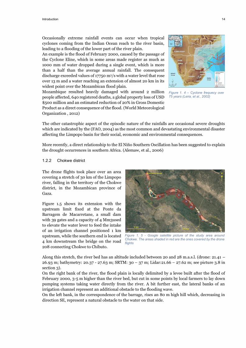
1.2.2 Chokwe district The drone flights took place over an area covering a stretch of 30 km of the Limpopo river, falling in the territory of the Chokwe district, in the Mozambican province of Gaza.
Figure 1.5 shows its extension with the upstream limit fixed at the Ponte da Barragem de Macarretane, a small dam with 39 gates and a capacity of 4 Mm3used to elevate the water lever to feed the intake of an irrigation channel positioned 1 km upstream, while the southern end is located 4 km downstream the bridge on the road 208 connecting Chokwe to Chibuto.
Along this stretch, the river bed has an altitude included between 20 and 28 m.a.s.l. (drone: 21.41 – 26.93 m; bathymetry: 20.37 - 27.63 m; SRTM: 30 – 37 m; Lidar:21.66 – 27.62 m; see picture 3.8 in section 3). On the right bank of the river, the flood plain is locally delimited by a levee built after the flood of February 2000, 3-5 m higher than the river bed, but cut in some points by local farmers to lay down pumping systems taking water directly from the river. A bit further east, the lateral banks of an irrigation channel represent an additional obstacle to the flooding wave. On the left bank, in the correspondence of the barrage, rises an 80 m high hill which, decreasing in direction SE, represent a natural obstacle to the water on that side.
Figure 1. 4 – Cyclone frequecy over 75 years (Leira, et al., 2002)
Figure 1. 5 - Google satellite picture of the study area around Chokwe. The areas shaded in red are the ones covered by the drone flights
15 Introduction
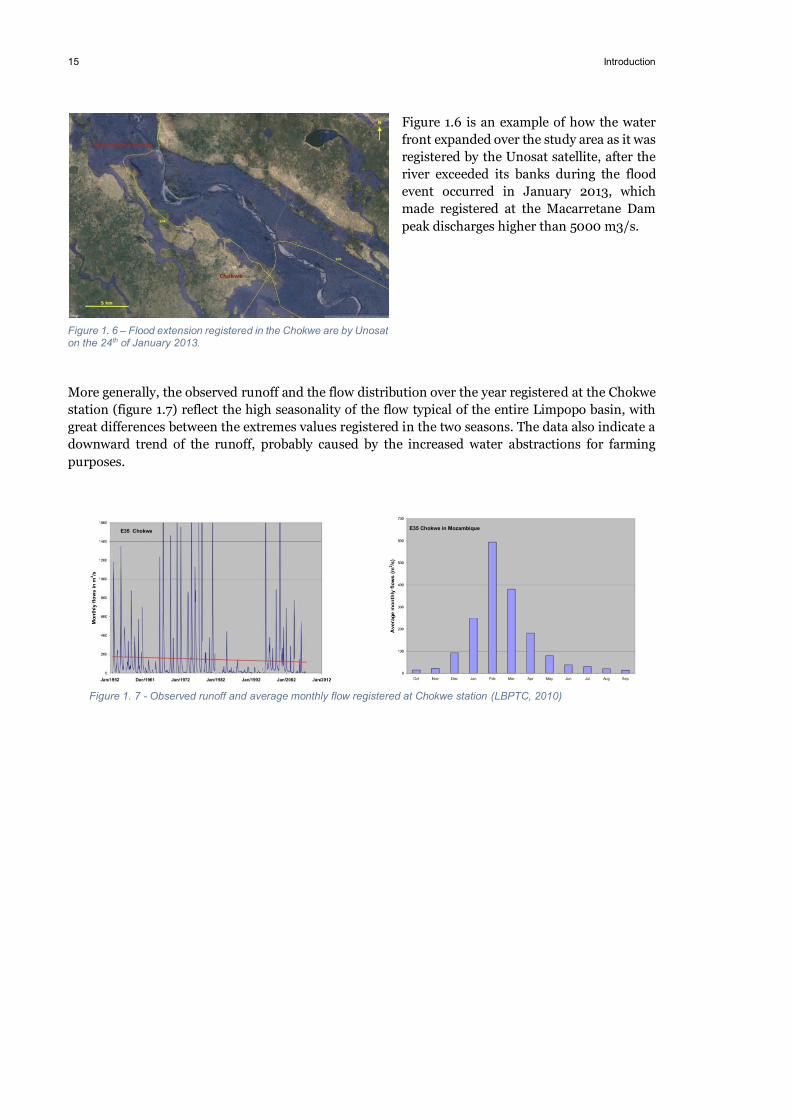
Figure 1.6 is an example of how the water front expanded over the study area as it was registered by the Unosat satellite, after the river exceeded its banks during the flood event occurred in January 2013, which made registered at the Macarretane Dam peak discharges higher than 5000 m3/s.
More generally, the observed runoff and the flow distribution over the year registered at the Chokwe station (figure 1.7) reflect the high seasonality of the flow typical of the entire Limpopo basin, with great differences between the extremes values registered in the two seasons. The data also indicate a downward trend of the runoff, probably caused by the increased water abstractions for farming purposes.
Figure 1. 6 – Flood extension registered in the Chokwe are by Unosat on the 24th of January 2013.
Figure 1. 7 - Observed runoff and average monthly flow registered at Chokwe station (LBPTC, 2010)
Methodology 16
2 Methodology
2.1 Field work
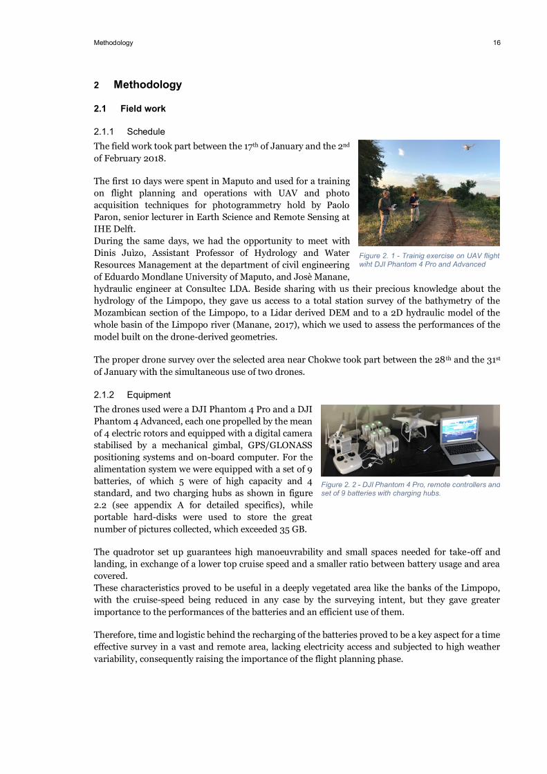
2.1.1 Schedule The field work took part between the 17th of January and the 2nd of February 2018.
The first 10 days were spent in Maputo and used for a training on flight planning and operations with UAV and photo acquisition techniques for photogrammetry hold by Paolo Paron, senior lecturer in Earth Science and Remote Sensing at IHE Delft. During the same days, we had the opportunity to meet with Dinis Juìzo, Assistant Professor of Hydrology and Water Resources Management at the department of civil engineering of Eduardo Mondlane University of Maputo, and Josè Manane, hydraulic engineer at Consultec LDA. Beside sharing with us their precious knowledge about the hydrology of the Limpopo, they gave us access to a total station survey of the bathymetry of the Mozambican section of the Limpopo, to a Lidar derived DEM and to a 2D hydraulic model of the whole basin of the Limpopo river (Manane, 2017), which we used to assess the performances of the model built on the drone-derived geometries.
The proper drone survey over the selected area near Chokwe took part between the 28th and the 31st of January with the simultaneous use of two drones.
2.1.2 Equipment The drones used were a DJI Phantom 4 Pro and a DJI Phantom 4 Advanced, each one propelled by the mean of 4 electric rotors and equipped with a digital camera stabilised by a mechanical gimbal, GPS/GLONASS positioning systems and on-board computer. For the alimentation system we were equipped with a set of 9 batteries, of which 5 were of high capacity and 4 standard, and two charging hubs as shown in figure 2.2 (see appendix A for detailed specifics), while portable hard-disks were used to store the great number of pictures collected, which exceeded 35 GB.
The quadrotor set up guarantees high manoeuvrability and small spaces needed for take-off and landing, in exchange of a lower top cruise speed and a smaller ratio between battery usage and area covered. These characteristics proved to be useful in a deeply vegetated area like the banks of the Limpopo, with the cruise-speed being reduced in any case by the surveying intent, but they gave greater importance to the performances of the batteries and an efficient use of them.
Therefore, time and logistic behind the recharging of the batteries proved to be a key aspect for a time effective survey in a vast and remote area, lacking electricity access and subjected to high weather variability, consequently raising the importance of the flight planning phase.
Figure 2. 1 - Trainig exercise on UAV flight wiht DJI Phantom 4 Pro and Advanced
Figure 2. 2 - DJI Phantom 4 Pro, remote controllers and set of 9 batteries with charging hubs.
17 Methodology
2.1.3 Flight planning The main idea behind the flight planning was to cover all the areas needed for the developing of the hydraulic model, while meeting the requirements in terms of pictures overlapping and resolution needed to derive a DEM with a satisfactory level of accuracy. Those goals had to be combined with an efficient use of the two drones and nine batteries, in order to complete the survey within the four days and accounting for unexpected events such as rain, strong wind or temperatures exceeding the devices operating range (above 40°C).
For the drawing of the flight areas, the choice was to at least overlay all the cross-sections of the bathymetric survey falling inside the study area, which happened to be a total number of 34. The decision was mainly forced by the extension of the floodplain, which resulted too vast (width between 7 and 9 km for a river stretch of 30 km) to be covered with this kind of drone, but also not strictly necessary to the purpose of a mono-dimensional modelling. The limit of the flying area was then fixed, on the right bank, correspondingly to the service road following the levee, easily accessible and favourable for take-offs, while on the left banks just a few hundred meters after the visible end of the river bed.
Once defined the area, flight altitude and degree of picture overlay needed to be set, considering that they have direct effects on pictures resolution, DEM resolution, flight time and number of batteries needed. The lower the flight altitude, the higher the resolution but also longer the flight time, while for the overlaying it is suggested not to be lower than 60%, to allow a precise picture positioning in the photogrammetry software (Leitao, et al., 2016).
A good help in this phase resulted to be the app DJI GS PRO which automatically shows an estimation of the reciprocal effects deriving from the variation of each one of these variables. Finally, it was chosen a flight altitude of 200 m, which resulted in pictures covering an area of 200x300m each, corresponding to a resolution of 6 cm/pixel in the picture and roughly 24-30 cm/px in the final DEM.
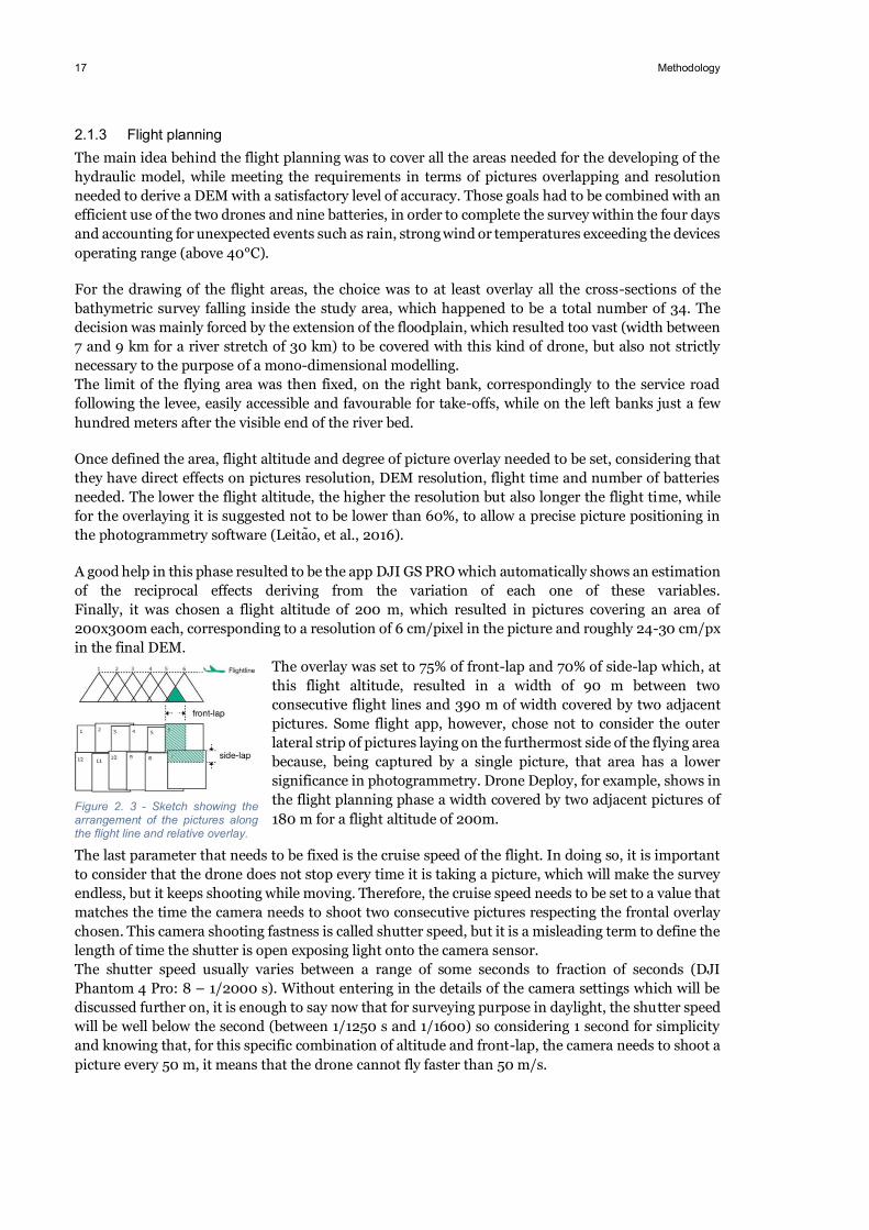
The overlay was set to 75% of front-lap and 70% of side-lap which, at this flight altitude, resulted in a width of 90 m between two consecutive flight lines and 390 m of width covered by two adjacent pictures. Some flight app, however, chose not to consider the outer lateral strip of pictures laying on the furthermost side of the flying area because, being captured by a single picture, that area has a lower significance in photogrammetry. Drone Deploy, for example, shows in the flight planning phase a width covered by two adjacent pictures of 180 m for a flight altitude of 200m.
The last parameter that needs to be fixed is the cruise speed of the flight. In doing so, it is important to consider that the drone does not stop every time it is taking a picture, which will make the survey endless, but it keeps shooting while moving. Therefore, the cruise speed needs to be set to a value that matches the time the camera needs to shoot two consecutive pictures respecting the frontal overlay chosen. This camera shooting fastness is called shutter speed, but it is a misleading term to define the length of time the shutter is open exposing light onto the camera sensor. The shutter speed usually varies between a range of some seconds to fraction of seconds (DJI Phantom 4 Pro: 8 – 1/2000 s). Without entering in the details of the camera settings which will be discussed further on, it is enough to say now that for surveying purpose in daylight, the shutter speed will be well below the second (between 1/1250 s and 1/1600) so considering 1 second for simplicity and knowing that, for this specific combination of altitude and front-lap, the camera needs to shoot a picture every 50 m, it means that the drone cannot fly faster than 50 m/s.
Figure 2. 3 - Sketch showing the arrangement of the pictures along the flight line and relative overlay.
Methodology 18
For this specific case the calculation is redundant and the flight speed was set to 15 m/s which is the maximum cruise speed of the Phantom 4, but for much lower flying altitude it can become relevant and the speed needs to be modified accordingly, remembering in any case that flying close to the speed limit can badly affect the end result with blurred or dark pictures (for example altitude 50 m and consequently area covered with one picture of 75x50 m, 75% of front lap means a picture every 12,5m, maximum flight speed 12,5 m/s).
At this point, knowing the flight speed, the area to cover and the distance between two consecutive flight lines, it is easy to calculate the flight length and an estimation of the number of batteries needed for each flight. The battery we used had an average flight time of 20 minutes and a recharging time of approximately 1 hour and 10 minutes each. For this flight altitude, roughly the 5-10% of the capacity is used between take-off and landing operations which, in the automatic mode for surveying offered by apps like Drone Deploy or Pix4D Capture, are perfectly vertical from the ground to the set flight altitude. Before every take off the drone acquires the GPS coordinates of the spot and save them as “home point” to which it will return at the end of every flight. The drone also keeps tracks of the energy usage during the flight and it will automatically return every time it calculates that the battery level is just enough to cover the distance between its current position and the home point, or in any case when the battery level drop under 20%. When the planned flight is estimated to require more than one battery, the drone will divide the flight into checkpoints, from the last one hit of which it will start again after the battery has been changed. If it is the case, the home point can be changed before every take off and moved closer the surveying restarting checkpoint, to save the energy needed for the cruise.
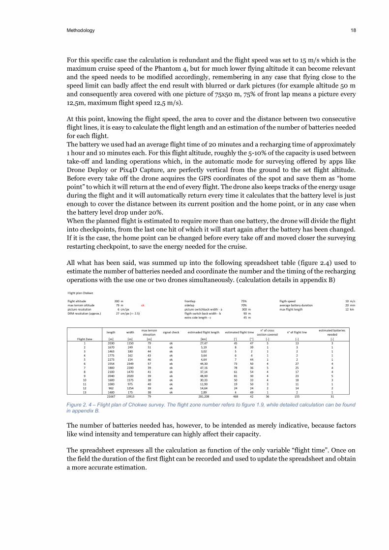
All what has been said, was summed up into the following spreadsheet table (figure 2.4) used to estimate the number of batteries needed and coordinate the number and the timing of the recharging operations with the use one or two drones simultaneously. (calculation details in appendix B)
The number of batteries needed has, however, to be intended as merely indicative, because factors like wind intensity and temperature can highly affect their capacity.
The spreadsheet expresses all the calculation as function of the only variable “flight time”. Once on the field the duration of the first flight can be recorded and used to update the spreadsheet and obtain a more accurate estimation.
Flight plan Chokwe
flight altitude 200 m frontlap 75% fligth speed 10 m/smax terrain altitude 79 m ok sidelap 70% average battery duration 20 minpicture resolution 6 cm/px picture switchback width - a 300 m max flight length 12 kmDEM resolution (approx.) 27 cm/px (+- 2.5) fligth switch back width - b 90 m
extra side length - c 45 m
length width max terrain elevation
signal check estimaded flight length n° of cross section covered
n° of flight line estimated batteries needed
Flight Zone [m] [m] [m] [km] ['] [''] [-] [-] [-]1 2030 1150 79 ok 27,47 45 47 5 13 32 1670 249 51 ok 5,19 8 39 1 3 13 1463 180 44 ok 3,02 5 2 1 2 14 1775 162 43 ok 3,64 6 4 1 2 15 2273 154 46 ok 4,64 7 44 1 2 16 1554 2349 57 ok 44,30 73 50 4 27 47 1800 2200 39 ok 47,16 78 36 5 25 48 2100 1470 41 ok 37,14 61 54 4 17 49 2040 2020 39 ok 48,90 81 30 4 23 5
10 1600 1575 38 ok 30,33 50 33 4 18 311 1000 975 40 ok 11,90 19 50 3 11 112 962 1254 39 ok 14,64 24 24 2 14 213 1400 175 38 ok 2,89 4 49 1 2 1
21667 13913 79 281,208 468 42 36 155 31
estimated flight time
Figure 2. 4 – Flight plan of Chokwe survey. The flight zone number refers to figure 1.9, while detailed calculation can be found in appendix B.
19 Methodology
For even higher predictive precision, an empirical correlation between flight time and average wind velocity can be derived to express the flight duration as a function of the average wind velocity at the flight altitude. Then the wind forecast can be used as input data to estimate the battery duration.
2.1.4 Flight The flight plans were then imported in the app Drone Deploy, which automatically manages flight execution and photo acquisition. Before taking off Drone Deploy executes a status check of the drone and transfers the flight plan to the on-board computer, so the drone can terminate the survey even in case of lost-signal with remote control before returning to the home point.
For what concerns the camera settings, they were manually adjusted before every flight through the app DJI GO.
The main parameters to be set are: aperture, ISO, and shutter speed. All of them are related to each other and affect the final exposure of each picture and, consequently, the capacity of the imagery to be manipulated by a photogrammetry software in building the DEM.
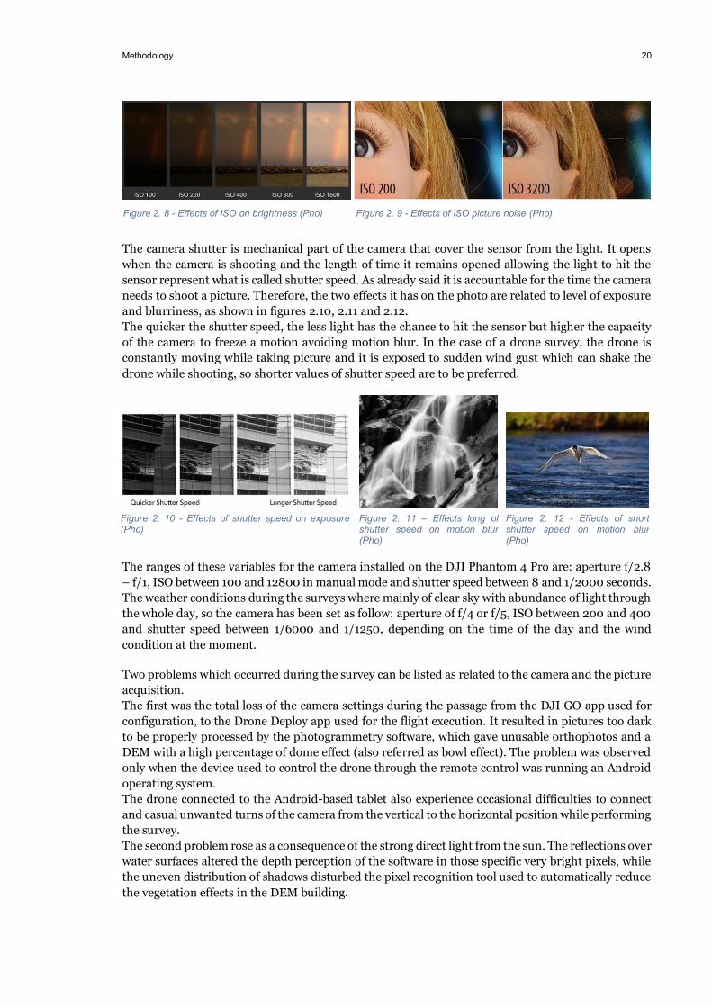
The aperture physically represents the hole within the camera lenses through which the light passes before hitting the camera sensor. The size of the aperture, like pupils in the eyes, can be shrank or enlarged to regulate the quantity of light. It has effects mainly on the exposure and the depth of fields of images as shown in figures 2.6 and 2.7. A larger aperture will result in a brighter photo, but also a larger blur of the background. On the opposite, a smaller aperture will result in a darker photo, but a wider field focused in the picture, which is typically useful for landscapes or the surveying use.
ISO is light sensitivity of a camera sensor measured according to the International Organisation for Standardisation. The ISO settings on a camera regulates the brightness of the photo and it is a tool that can be used to take picture in dark environment or to allow more flexibility with aperture and shutter speed settings. Using high ISO values results in brighter pictures, even in combination with small aperture and a fast shutter speed, therefore is a good asset when there is a high risk of motion blur. As a side effect it increases the level of noise in the photo (grained and blotchy colours), which is not a major problem in the developing of the DEM but can result in a bad looking orthophoto. ISO effects on pictures are shown in figures 2.8 and 2.9.
Figure 2. 5 - Drone Deploy mobile app interface
Figure 2. 7- Effects of aperture on exposure (Pho)
Figure 2. 6 - Effects of aperture on depth of field (Pho)
Methodology 20
The camera shutter is mechanical part of the camera that cover the sensor from the light. It opens when the camera is shooting and the length of time it remains opened allowing the light to hit the sensor represent what is called shutter speed. As already said it is accountable for the time the camera needs to shoot a picture. Therefore, the two effects it has on the photo are related to level of exposure and blurriness, as shown in figures 2.10, 2.11 and 2.12. The quicker the shutter speed, the less light has the chance to hit the sensor but higher the capacity of the camera to freeze a motion avoiding motion blur. In the case of a drone survey, the drone is constantly moving while taking picture and it is exposed to sudden wind gust which can shake the drone while shooting, so shorter values of shutter speed are to be preferred.
The ranges of these variables for the camera installed on the DJI Phantom 4 Pro are: aperture f/2.8 – f/1, ISO between 100 and 12800 in manual mode and shutter speed between 8 and 1/2000 seconds. The weather conditions during the surveys where mainly of clear sky with abundance of light through the whole day, so the camera has been set as follow: aperture of f/4 or f/5, ISO between 200 and 400 and shutter speed between 1/6000 and 1/1250, depending on the time of the day and the wind condition at the moment.
Two problems which occurred during the survey can be listed as related to the camera and the picture acquisition. The first was the total loss of the camera settings during the passage from the DJI GO app used for configuration, to the Drone Deploy app used for the flight execution. It resulted in pictures too dark to be properly processed by the photogrammetry software, which gave unusable orthophotos and a DEM with a high percentage of dome effect (also referred as bowl effect). The problem was observed only when the device used to control the drone through the remote control was running an Android operating system. The drone connected to the Android-based tablet also experience occasional difficulties to connect and casual unwanted turns of the camera from the vertical to the horizontal position while performing the survey. The second problem rose as a consequence of the strong direct light from the sun. The reflections over water surfaces altered the depth perception of the software in those specific very bright pixels, while the uneven distribution of shadows disturbed the pixel recognition tool used to automatically reduce the vegetation effects in the DEM building.
Figure 2. 9 - Effects of ISO picture noise (Pho) Figure 2. 8 - Effects of ISO on brightness (Pho)
Figure 2. 11 – Effects long of shutter speed on motion blur (Pho)
Figure 2. 10 - Effects of shutter speed on exposure (Pho)
Figure 2. 12 - Effects of short shutter speed on motion blur (Pho)

21 Methodology
If the weather was clement for most of the survey, with a huge storm falling only on the last afternoon at already completed operations, heat and wind were not. During the day, the temperature often rose above 40 °C, which is the upper operating limit for all the electronic devices used. The direct sun exposure and the heat normally produced by the electric engines of the drone harshly tested its cooling system, only partially helped by the wind.
This is an important factor to take into consideration because, if the tablet overheating resulted in a shutdown of the tablet itself with the consequent connection loss resolved by the automatic “return to home point” function, the overheating of the drone might have affected the performance of the on board sensors with the computer registering an altitude different than the one which the drone was actually flying at. This problem is not officially recognized by DJI, since it occurs outside the suggest temperature operating range, but other users seemed to have experienced similar issues. Never the less it is relevant, because every single picture is associated with details like geographical coordinates, flight altitude, view direction (yaw, pitch, and roll) and camera settings which are stored in the relative EXIF files and read by the photogrammetry software to position the picture and calculate relative depths. An incoherent altitude value in some pictures could be pointed as one of the possible causes of the bowl effect observed in some DEMs. This issue has been manually dealt with, along the DEM generating process, as extensively described in the next section.
The major environmental obstacle to drone surveying, however, is wind. The DJI Phantom 4 Pro can overcome wind as strong as 10 m/s at the cost of high energy usage, but this value does not account for sudden wind gusts which can crash the drone by flipping it upside down. Strong wind and frequent gusts badly affect the flight duration, especially on a survey flight in which the drone needs to overcome frontal wind and compensate the pushing effect of tail wind in order to respect timing and positioning of the photo acquisition. The consequences are a significant drop of the battery duration with shorter flight lengths and a frequent, invasive intrusion of the automatic return home function. Strong wind, therefore, represents a limit to the use of light quadcopter drones for surveying purpose, which cannot be resolved but just accounted for during flight planning.
As already mentioned, the Phantom 4 is equipped a with a satellite positioning system GPS/GLONASS which is able to locate the exact position of the drone within a 3 m radius. This accuracy it is not enough for precise photogrammetry calculations, but it can be enhanced with the acquisition of ground control points through a real time kinematic navigation system, commonly known as RTK. RTK is composed of a base station located in a known position, mobile units which can calculate their relative position with an accuracy up to 1 cm 2ppm horizontally and 2 cm 2ppm vertically.
Target as the one shown in figure 2.13 are positioned on the field and for each one of them coordinates and altitude are registered with the RTK. They appear them in the pictures and the software recognizes those pixels as ground control points to which the user can assign the collected positions.
A last minute inconvenient occurred to the local topographer, prevent our RTK to ever reach the study area, impeding the accurate collection of ground control points. The consequent problem of anchoring the photogrammetry-derived DEM to known positions was solved in post-production by overlaying the drone pictures to the Lidar-derived orthophoto and manually fixing those points which were recognisable in both of them, as shown in the next section.
Figure 2. 13- Ground target

Methodology 22
In the end, a few words need to be spent about the interactions with the local communities. A local guide accompanied us for the whole survey and his presence has been proved to be very helpful not only to rapidly fulfil our bureaucracy obligations within air space regulations and area accessibility, which in Mozambique could be an intricate matter, but also through the interactions with the rural communities. As mentioned, the surveying area falls in a heavily farmed region and kids and workers were driven to us by the sight and the noise of the drone flying right over their head. It was mostly curiosity, rather than fear, never the less being able to effectively communicate the purpose of our flights in a country that counts more than 43 languages spoken (Ethnologue, Languages of the World), but no English, was a big help to a quick and smooth execution of the survey.
2.2 Photogrammetry Terminated the survey, the post production phase of the 35 GB of pictures collected began, with the ultimate goal to obtain river cross-sections perfectly overlaying those from the bathymetric survey, positioned as shown in figure 2.22.
The software chosen for the task was PhotoScan Professional edition, version 1.4 by Agisoft.
In this first stage, the procedure of “DEM and Orthomosaic generation without ground control points” was adopted, as described by the user manual (Agisoft LLC, 2018). It briefly consisted in:
• Add photos and set the camera positions accordingly. The coordinate system used was set to WGS 84 (EPGS::4326).
• Check camera calibration.
• Photo alignment with high accuracy. “This is the step in which PhotoScan finds matching points between overlapping images, estimates camera position for each photo and builds sparse point cloud model.”
• Optimize camera alignment. “to achieve higher accuracy in calculating camera external and internal parameters and to correct possible distortion (e.g. “bowl effect” and etc.)”
• Build dense point cloud. “Based on the estimated camera positions the program calculates depth information for each camera to be combined into a single dense point cloud. PhotoScan tends to produce extra dense point clouds, which are of almost the same density, if not denser, as LIDAR point clouds.”
• Edit geometry. It consists in manually removing those group of pixels which we do not want to appear in the DEM, such as light reflections on water, waves or shores, in order to show them in the DEM as flat areas.
• Build Digital Elevation Model DEM. “It represents a surface model as a regular grid of height values. DEM can be rasterized from a dense point cloud, a sparse point cloud or a mesh. Most accurate results are calculated based on dense point cloud data.”
Figure 2. 14 - Curious children following the landing of the drone

23 Methodology
The outcome resulted unsatisfactory, as the DEM of a relevant number of flight zones presented a high degree of bowl effect, heavily reflected in the river cross-sections, as shown in figures 2.15, 2.16 and 2.17.
The absence of ground control points revealed to be a remarkable issue, with a higher impact on large surveying areas rather than on small transects, producing deltas between lidar a drone’s cross-section as bad as 3 meters in the worst cases. A solution to the problem was to manually create ground control point (GCP) and imposing to them coordinates and altitude acquired from the lidar derived DEM.
Figure 2. 16 - Bowl effect on flight 2 Dense Cloud
Figure 2. 17 - Bowl effect cross-section N.4
20
25
30
35
40
45
50
55
0 200 400 600 800 1000 1200 1400
SECTION 4 (N. 258821)Drone with bowl effect Drone adjusted with GCP Lidar
Figure 2. 15- Bowl effect on flight 2 DEM
Figure 2. 18 - Comparison between lidar orthophoto (right) and drone imagery (left) to recognize common points

Methodology 24
The choice seemed reasonable, since the lidar DEM is an high precision source, already anchored to the WSG 84 (EPGS::4326) coordinates system and the relative anchoring procedure between lidar and drone DEM did not affect the spatial accuracy of the latter, but just its global positioning. To do so, lidar and drone DEMs and orthophotos were overlaid using the software QGIS. By a visual comparison of each one of them, clear common points such as road intersections, house corners, recognisable trees or electricity poles were spotted. Coordinates and altitude of these points were calculated from the lidar DEM and manually assigned to the drone DEM. An example is proposed in figure 2.18, in which is clearly recognisable the frontal edge of the right pier of the westernmost gate. The coordinates of that pixel were acquired from the lidar orthophoto and assigned to the GCP 1 in the drone picture, as shown in figure 2.19.
Terminated the manual assignment procedure of ground control points, the whole photogrammetry process was repeated from the Optimize camera alignment to the Build DEM step.
The results seemed to be more depending on the GPC distribution in relation to direction of the unwanted curvature, rather than their number. We were not able to learn an exact rule about their optimal distribution (rule that in any case would have been hard to follow in the process of visual individuation of the GCP, given the uniformity of the vegetation), but for small transect like flight area 2, 3, 4, 5, 13, five GPC distributed in the four corners and one in the middle, seemed to be enough. Attempts with a bigger number of GPC on the same transects did not give better results.
Figure 2.20 shows the distribution of GPC on flight zone 3. The use of points 2, 14, 11, 6 and 4 gave better or equal results than different combination, even when more GPC where considered.
Figure 2. 19 – GPC coordinates assignment in PhotoScan
Figure 2. 20 – Test GPC distribution on transect flight 3 DEM and dense point cloud. The use of GPS number 2, 14, 11, 6 and 4 gave better or similar result of any of the other possible combinations involving a higher number of GCP.
25 Methodology
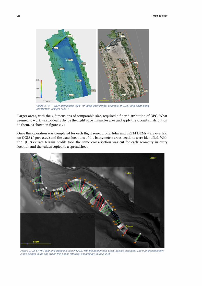
Larger areas, with the 2 dimensions of comparable size, required a finer distribution of GPC. What seemed to work was to ideally divide the flight zone in smaller area and apply the 5 points distribution to them, as shown in figure 2.21
Once this operation was completed for each flight zone, drone, lidar and SRTM DEMs were overlaid on QGIS (figure 2.22) and the exact locations of the bathymetric cross-sections were identified. With the QGIS extract terrain profile tool, the same cross-section was cut for each geometry in every location and the values copied to a spreadsheet.
Figure 2. 21 – GCP distribution “rule” for large flight zones. Example on DEM and point cloud visualization of flight zone 1
Figure 2. 22-SRTM, lidar and drone overlaid in QGIS with the bathymetric cross-section locations. The numeration shown in the picture is the one which this paper refers to, accordingly to table 2.26
Methodology 26
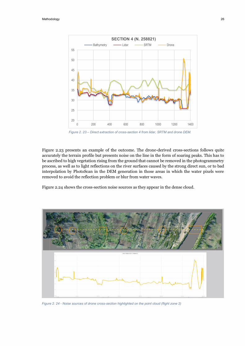
Figure 2.23 presents an example of the outcome. The drone-derived cross-sections follows quite accurately the terrain profile but presents noise on the line in the form of soaring peaks. This has to be ascribed to high vegetation rising from the ground that cannot be removed in the photogrammetry process, as well as to light reflections on the river surfaces caused by the strong direct sun, or to bad interpolation by PhotoScan in the DEM generation in those areas in which the water pixels were removed to avoid the reflection problem or blur from water waves.
Figure 2.24 shows the cross-section noise sources as they appear in the dense cloud.
20
25
30
35
40
45
50
55
0 200 400 600 800 1000 1200 1400
SECTION 4 (N. 258821)Bathymetry Lidar SRTM Drone
Figure 2. 23 – Direct extraction of cross-section 4 from lidar, SRTM and drone DEM.
Figure 2. 24 - Noise sources of drone cross-section highlighted on the point cloud (flight zone 2)

27 Methodology
The problem was solved with the use of a MatLab (Math Works) code developed at IHE Delft, which used as input the numeric x and z coordinates of each cross-section and returned the same coordinates x and z, after eliminating every point raising more than 1,5 m above the two previous one. A visual overlook of every cross-section compared to his orthophoto finalised the procedure, checking for eventual mistakes. The MatLab (Math Works) code which produced the transformation shown in figure 2.25 can be found in Appendix C.
20
25
30
35
40
45
50
55
0 200 400 600 800 1000 1200 1400
SECTION 4 (N. 258821)Drone with GCP Drone after MatLab cut
Figure 2. 25- Drone-derived cross-section 4, before and after MatLab cut
relative progressive Bathymetry LIDAR SRTM Drone Bathymetry LIDAR SRTM Drone1 262310.5 0 0 500 547 20 1001 var 1,25 35,83 0,682 262006.8 312 312 500 564 21 1001 var 1,26 35,43 0,713 260055.5 1608 1920 500 931 34 1001 var 1,01 28,51 0,944 258821 1448 3368 500 1263 49 2002 var 1,26 41,40 0,585 257865.4 956 4324 500 962 35 2002 var 1,00 28,70 0,576 256610.2 1438 5762 500 682 25 1001 var 1,01 28,64 0,697 255294.3 1358 7120 500 966 32 1001 var 0,95 29,63 0,92
254063.1 1286 84068 253249.3 974 9380 500 998 33 1001 var 0,94 29,37 0,949 252574 715 10095 500 947 31 1001 var 0,94 29,71 0,89
10 251929 693 10788 500 958 32 1001 var 0,94 29,10 0,90251313.5 658 11446
11 250753.2 601 12047 500 873 29 739 var 1,14 35,55 1,0012 250104.8 654 12701 500 1001 40 1001 var 1,38 35,47 1,3813 249445.5 687 13388 500 1001 50 1001 var 1,44 29,46 1,4414 248719.2 787 14175 500 1001 54 1001 var 1,49 28,07 1,4915 248006.1 751 14926 500 1001 56 1001 var 1,64 29,81 1,6416 247334.6 687 15613 500 1001 45 1001 var 1,65 37,49 1,6517 246645.2 710 16323 500 1001 62 1001 var 1,96 32,15 1,9618 246259.2 428 16751 500 1001 53 1001 var 1,80 38,19 1,8019 244903.8 1254 18005 500 1001 45 1001 var 1,72 39,01 1,7220 244526.2 386 18391 500 1001 54 1001 var 1,72 32,42 1,72
244091.3 462 18853243553.7 537 19390
21 243019.8 580 19970 500 1001 40 1001 var 1,36 34,97 1,3622 242474.3 554 20524 500 1001 37 1001 var 1,31 36,48 1,3123 241944.4 536 21060 500 1001 40 1001 var 1,25 31,99 1,2524 241540.9 412 21472 500 818 27 1001 var 1,28 40,25 1,0525 239448.1 2090 23562 500 514 19 2002 var 1,23 38,55 0,27
239087.6 360 2392226 239052 98 24020 500 563 20 1001 var 1,07 31,59 0,6027 238159.6 820 24840 500 571 21 1001 var 1,20 34,23 0,6828 237191.3 952 25792 500 680 23 1001 var 1,17 35,98 0,7929 234763.9 2305 28097 500 922 29 1001 var 1,11 35,33 1,02
Distancecross-section n. n° of horizontal points horizontal points' distance
Figure 2. 26 - Summary table of modelled cross-sections. Numeration and colouring matches the one of figure 2.22

Methodology 28
At the end of this operation, the situation is the one shown by the summary table of figure 2.26 that reports in grey those sections falling in areas which could not be processed by PhotoScan, in red those which had unresolvable bowl effect and in green those that could be used in the hydraulic model. Their spatial distribution can be seen in figures 2.22, which follow the same colouring.
However, the hydraulic modelling software HEC-RAS, which has been chosen for this task, supports only cross-sections of maximum 500 points, so the drone and lidar cross-section needed to be rescaled before being introduced into the software. It has been done by simply eliminating every second point, starting from the extreme sides of the cross-section and gradually moving towards the centre, until the desired number of points was reached. An example of the scaling results on a drone derived cross section is shown in figure 2.27.
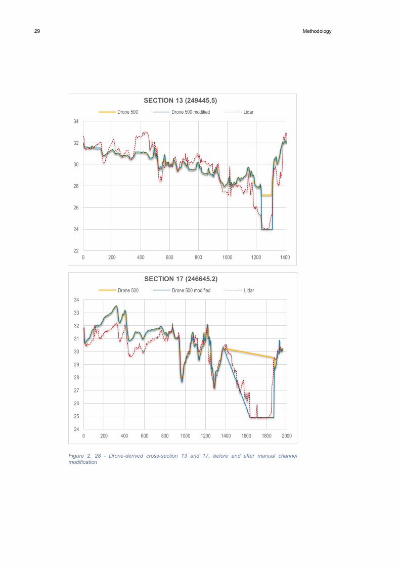
Finally, two cross-sections which presented deep water in the river channel at the time of the survey, were manually modified, to compensate the impossibility of rebuilding the river bed geometry hidden under the water, through photogrammetry. Their modification is shown in figures 2.28.
25
27
29
31
33
35
37
0 200 400 600 800 1000 1200 1400
SECTION 4 (N. 258821)Drone after MatLab cut Drone 500 points
Figure 2. 27 - Drone-derived cross-section 4, before and after rescaling to 500 points
29 Methodology
22
24
26
28
30
32
34
0 200 400 600 800 1000 1200 1400
SECTION 13 (249445,5)Drone 500 Drone 500 modified Lidar
24
25
26
27
28
29
30
31
32
33
34
0 200 400 600 800 1000 1200 1400 1600 1800 2000
SECTION 17 (246645.2)Drone 500 Drone 500 modified Lidar
Figure 2. 28 - Drone-derived cross-section 13 and 17, before and after manual channel modification

Methodology 30
2.3 Hydraulic modeling Once the 22 green cross-sections of table 2.26 were ready for each one of the four geometries, they were used to build four different hydraulic models of the studied river stretch under steady, gradually varied flow conditions.
Due to the absence of direct hydraulic data, the choice was to consider the bathymetry based 2D model of the whole Limpopo river, already calibrated and validated, (Manane, 2017) as “reality” and used as a reference model for evaluating the performances of the other models. To make them comparable, however, this model was modified in the geometry by cutting out all the irrelevant components, keeping only the cross-sections falling inside the study area and that could be overlapped by the other geometries. Bed slopes, Manning’s coefficients, contraction or expansion coefficients and reach lengths between consecutives cross sections were kept as in the original model.
The software used for the hydraulic modelling was HEC-RAS, Hydrologic Engineering Center’s River Analysis System (US Army Corps of Engineers). As specified in the reference manual “this software allows you to perform one-dimensional steady, one and two-dimensional unsteady flow hydraulics, sediment transport/mobile bed computations, water temperature modeling, and generalized water quality modeling (nutrient fate and transport)”. (HEC-RAS river analysis system, February 2006)
The 1D steady flow component is used to calculate water surface profiles under steady gradually varied flow conditions in a river or a system of channels, modelling subcritical, supercritical or mixed flow regime. The assumptions behind it are of no time dependency of any of the flow variables, but changes in water depth along the river stretch gradual enough to assume hydrostatic pressure distribution at every cross-section. Consequently, the water velocity varies along the river and the steepness of bed slope, water surface slope and energy line slope differ between each other. HEC-RAS basic computation procedure to determine the unknown water surface elevation at any cross section is based on the iterative solution of the 1D Energy equation, which relates these variables, but it is time independent. Friction and contraction/expansion energy losses are calculated respectively by the Manning equation and a contraction/expansion coefficient multiplied by the changes in velocity head. When the water surface profile varies rapidly, like in situations of mixed flow regime, hydraulic jumps, bridges flow constrictions or stream junctions, the momentum equation is used to calculate the water depth. (For more about the theory behind steady flow analysis, please refer to appendix D or HEC-RAS hydraulic reference manual). The steady flow system is designed for application in flood plain management and flood insurance studies to evaluate floodway encroachments. Also, capabilities are available for assessing the change in water surface profiles due to channel improvements, and levees. (HEC-RAS river analysis system, February 2006)
All four models were run under steady, gradually varied flow conditions in subcritical regime. The downstream boundary condition was of normal depth, with a bed slope representative of the last portion of river stretch, while upstream it was imposed a value for the discharge entering the studied river stretch. As said, the geometry of the cross-sections was different for each model, accordingly to the topography source used, but the other geometric parameters were kept equal in each model and constant along the whole river stretch, as it was done in the reference model. These values were: Manning’s roughness coefficient of nfl = 0.06 and nch = 0.022, contraction and expansion coefficients of Cc = 0.1 and Ce = 0.3 and bed slope S0 = 0.00025. Each of the model was then run with three different values of input discharge: Q1= 650 m3/s, Q2= 350 m3/s, Q3= 50 m3/s. They respectively represent the maximum average monthly flow registered at Chokwe station E35, an average yearly discharge and value for low flow conditions.

31 Methodology
The resulting water profiles were then compared with the reference model, as shown in section 4, figure 4.1.
In the end, the Lidar, SRTM and Drone based models were subjected to a calibration exercise, varying the Manning’s roughness coefficients inside the following range: nfl = 0.040 , 0.045 , … , 0.080 for the floodplain and nch = 0.010 , 0.015 , … , 0.040 for the main channel. The water levels obtained in each model for every one of the possible combinations were then compared to the water levels of the bathymetry-based model (nfl = 0.06 and nch = 0.022) with the use of the Mean Absolute Error (MAE).
The results are to be found in section 4.

Discussion on geometries 32
3 Discussion on geometries
The geometries used as input data for the hydraulic model are taken from four sources with different quality: a bathymetric cross-sections, obtained in 2010 by surveying with Total Station and RTK GPS system, resulting in a degree of spatial resolution within 0.5 m (Saimone, 2010). A DEM with 1 m of resolution, derived from a lidar flight in 2016 (World Bank, DNGRH, 2016). The void filled version of the DEM from the SRTM of February 2000, reaching a resolution of 30 m (SRTM) and the SFM-derived DEM from our drone survey in January 2018 (refer to section 2), with a final resolution included between 0.3 and o.6 m.
From the Macarratane dam, which fixes the upstream boundary of the study area, to the downstream boundary there are 34 cross sections available from the bathymetric study.
The DEMs from the Lidar and the SRTM flights fully cover the whole study area, therefore the cross sections can be extrapolated to perfectly match any of the 34. The drone flight, on the other hand, is not fully covering the study area, therefore 5/34 resulted partially or totally uncovered by the drone pictures. Of the remaining, 7 were deeply affected by the dome effect which made them unreliable for the purpose of this study. Thus, the geometry of each one of the four hydraulic models consists then of the same 22 cross sections, respectively taken form the cited geometries. The extraction procedure has been done by mean of the Extract Terrain Profile tool on the software QGIS after the DEM of each one of the geometries had been overlaid with the positions of the bathymetric cross-section.
Please refer to figure 2.22 for an overview of their distribution along the river.
33 Discussion on geometries
3.1 Bathymetry from Total Station and RTK GPS
The bathymetric survey is the result of the joint effort of the National Directorate of Water and Resource Management (DNGRH) together with two local consultancy companies, Salomon LDA and Consultec LDA, to map and build a flood model of the whole Mozambican section of the Limpopo river basin.
The operations were executed by Salomon LDA during 2010 with the use of Total Station and RTK GPS guaranteeing a resolution of 0.5 m (Saimone, 2010) and the outcome was later on used as the main geometry of the 2D HEC-RAS model built for flood management purposes (Manane, 2017).
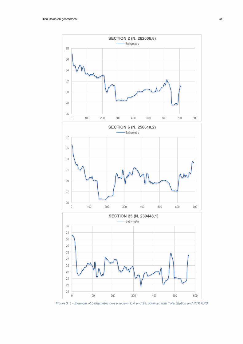
Figures 3.1 shows an example of the typical aspect of these cross-sections. The deep cut of main channel is recognisable on the right in section 2 and on the left in section 6, while both of them exhibit on the opposite side a secondary channel which can be activated by high values of discharge, separated from the main one by sand deposits for what concerns section 2 and a vegetated strip in section 6. Occasionally the river morphology loses the descripted configuration to switch to shallow, meandric channels as in the case of section 25.
Discussion on geometries 34
26
28
30
32
34
36
38
0 100 200 300 400 500 600 700 800
SECTION 2 (N. 262006,8) Bathymetry
22
23
24
25
26
27
28
29
30
31
32
0 100 200 300 400 500 600
SECTION 25 (N. 239448,1)Bathymetry
25
27
29
31
33
35
37
0 100 200 300 400 500 600 700
SECTION 6 (N. 256610,2) Bathymetry
Figure 3. 1 - Example of bathymetric cross-section 2, 6 and 25, obtained with Total Station and RTK GPS

35 Discussion on geometries
3.2 SRTM
SRTM stands for Shuttle Radar Topography Mission. It is a ten days mission of the Space Shuttle Endeavour launched on February 11, 2000, with the purpose to obtain a near-global high-resolution database of Earth's topography using a technique called Interferometric synthetic-aperture radar to learn topographic and elevation data. (Nasa, et al.) (ESA)
From 2015 the SRTM data have been released to the public with a 1 arc-second sampling corresponding to c.a. 30 meters on the equator, which is the version where the cross-sections used in this study are taken from.
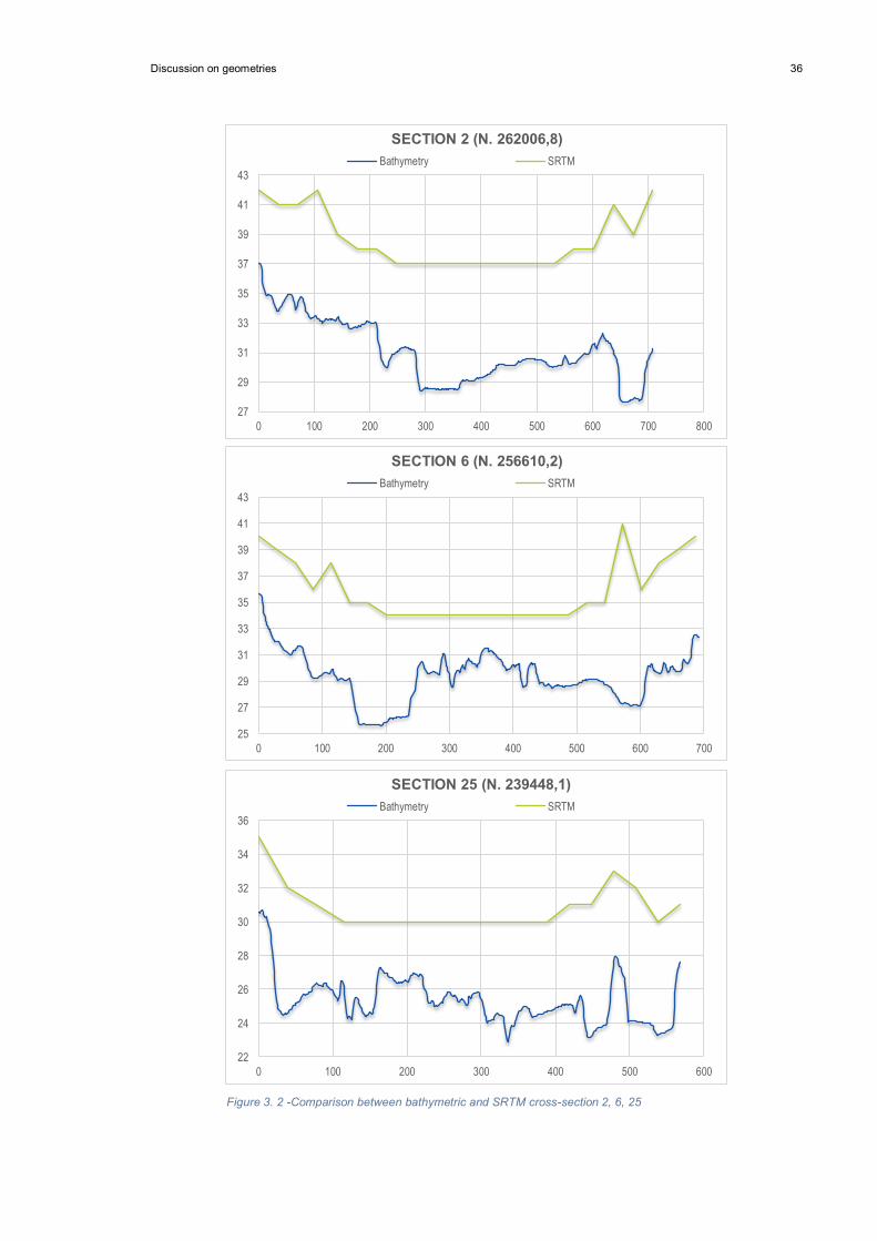
A quick comparison with the bathymetric cross-sections shows the clear difference in quality: the SRTM extracted cross sections poorly fit to study the river main channel, but their relevance might grow when the study covers much larger areas making it a convenient choice in the case of wide, uniform floodplains for its easy accessibility.
The lower precision of the spatial data not only affect the degree of detail but it is also responsible for the vertical misplacement of the cross-sections, clearly visible in figure 3.2.
Discussion on geometries 36
27
29
31
33
35
37
39
41
43
0 100 200 300 400 500 600 700 800
SECTION 2 (N. 262006,8) Bathymetry SRTM
25
27
29
31
33
35
37
39
41
43
0 100 200 300 400 500 600 700
SECTION 6 (N. 256610,2) Bathymetry SRTM
22
24
26
28
30
32
34
36
0 100 200 300 400 500 600
SECTION 25 (N. 239448,1)Bathymetry SRTM
Figure 3. 2 -Comparison between bathymetric and SRTM cross-section 2, 6, 25
37 Discussion on geometries
3.3 LIDAR
LIDAR stands for Light Imaging Detection and Ranging. The instrument works by illuminating a target with ultraviolet, visible or near infrared light beam and then measuring the differences in time and wavelength of the returning ray after it has been reflected from the target by backscattering.
Different materials adsorb and reflect different wave lengths so, by setting the instrument accordingly, the reflection of water and vegetation can be ignored when building a DEM. (Lillesand, et al., 2004)
The Lidar based DEM use in this study achieves a spatial accuracy within 1 m. The survey was executed in 2015 by the National Directorate of Water and Resource Management (DNGRH) and the Global Facility for Disaster Reduction and Recovery (GFDRR) (World Bank, DNGRH, 2016).
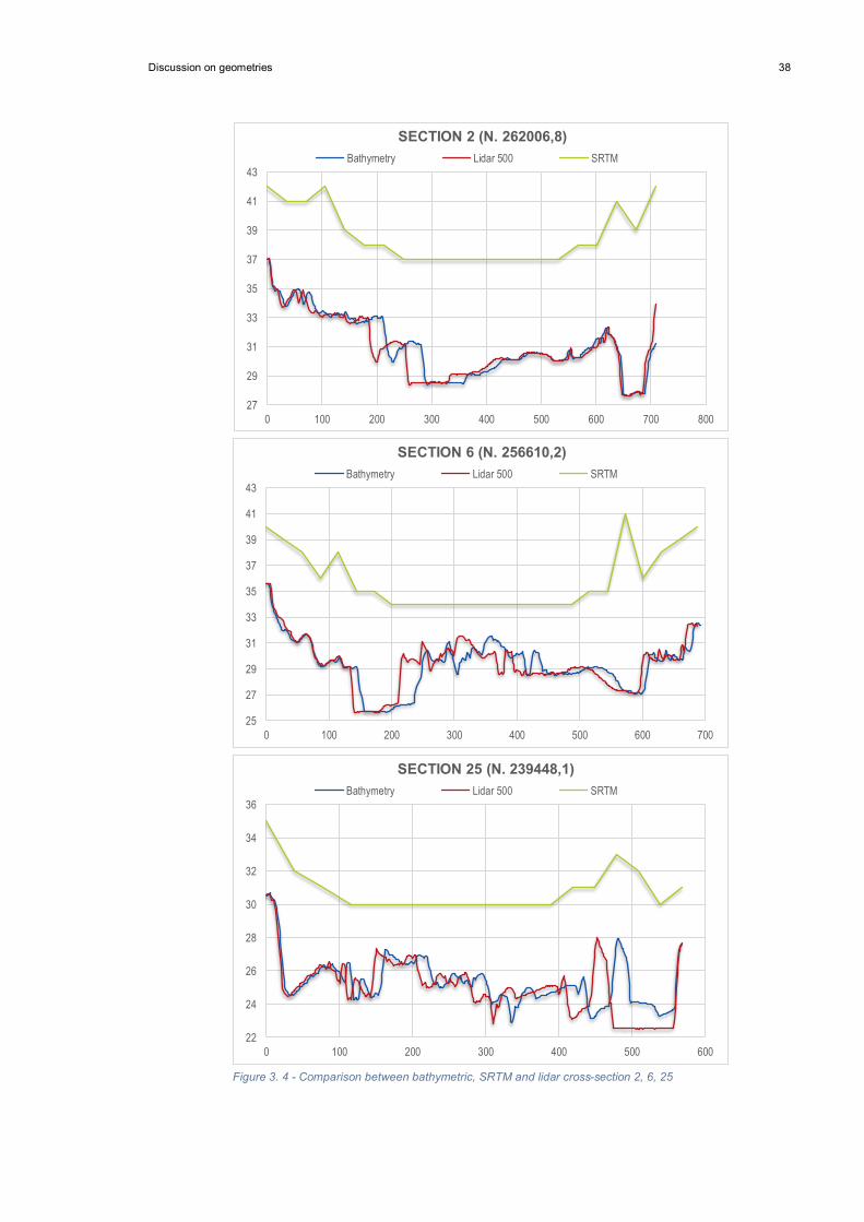
It’s accuracy and the capacity of modelling the entirety of the flood plain, including the wetted river bed, makes the cross-sections derived from it a lot more comparable to the ones from the bathymetric survey, than the ones extracted from the SRTM. Therefore, the differences between the two can be ascribed to geomorphological changes due to the fluvial process of erosion and sediment transport.
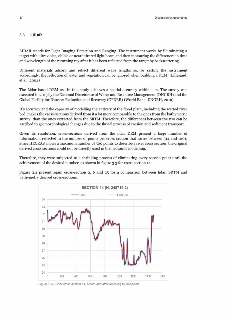
Given its resolution, cross-sections derived from the lidar DEM present a large number of information, reflected in the number of points per cross section that varies between 514 and 1001. Since HECRAS allows a maximum number of 500 points to describe a river cross section, the original derived cross sections could not be directly used in the hydraulic modelling.
Therefore, they were subjected to a shrinking process of eliminating every second point until the achievement of the desired number, as shown in figure 3.3 for cross-section 14.
Figure 3.4 present again cross-section 2, 6 and 25 for a comparison between lidar, SRTM and bathymetry derived cross-sections.
24
25
26
27
28
29
30
31
32
33
34
0 200 400 600 800 1000 1200 1400 1600
SECTION 14 (N. 248719,2)
Lidar Lidar 500
Figure 3. 3– Lidar cross-section 14, before and after rescaling to 500 points
Discussion on geometries 38
27
29
31
33
35
37
39
41
43
0 100 200 300 400 500 600 700 800
SECTION 2 (N. 262006,8) Bathymetry Lidar 500 SRTM
25
27
29
31
33
35
37
39
41
43
0 100 200 300 400 500 600 700
SECTION 6 (N. 256610,2) Bathymetry Lidar 500 SRTM
22
24
26
28
30
32
34
36
0 100 200 300 400 500 600
SECTION 25 (N. 239448,1)Bathymetry Lidar 500 SRTM
Figure 3. 4 - Comparison between bathymetric, SRTM and lidar cross-section 2, 6, 25
39 Discussion on geometries
3.4 Drone
The drone surveying process finalized to building the geometry of a hydraulic model is based on the collection of aerial pictures of the intended area and their interpretation according photogrammetry principles, which will eventually lead to the modelling of a DEM.
Nowadays, several software and online platforms are available for photo processing following a method called Structure for Motion (SfM). This technology made it first appearance back into 1976 (Ullman, 1976), but it is only after the early 2000’s that its applications have become more commons (Snavely, 2008). Like traditional photogrammetry, Structure form Motion techniques require the object to appear in several pictures taken from various viewpoints with consistent overlapping between them, but frees the user from the need of a set of ground control points at know 3D positions, since it automatically determines camera geometry, position and orientation. (Westoby, et al., 2012). However, the use of ground control points has proven to be fundamental to reduce the incidence of systemic curvature errors in the DEM (known as bowl/dome effect or doming) (Javernick, et al., 2014), especially when a set of pictures with near-parallel viewing directions is used (James, et al., 2014). SfM photogrammetry therefore opened the doors to fast, low cost 3D data acquisition, which potentially eliminates the need of specialized personnel through a high level of automation (Micheletti, et al., 2015), but despite its potentialities, the production of quality 3D terrains model, with sufficiently high level of accuracy and a low level of radial distortion, remains hitherto the major obstacle to the public spreading of this surveying technique against more traditional ones.
The growing interest on its applications, however, has pushed studies and the researches aiming to find possible solutions to lower both the impact of DEM’s dooming and the need of ground control points, in order to fully unfold the potentialities of drone surveying.
The key point seemed to be found in the degree of corner distortion produced by the camera lenses, which is one of the many optic aberrations symptomatic to the process of transferring light trough curved lenses on a rectangular surface as the camera sensor, or, in other words, to the process of shooting a picture as we know it today. Quality of the lenses, set of pictures with near-parallel viewing directions and enabling camera self-calibration appear to be the main causes of errors in the estimation of radial distortions, leading to imprecisions in the DEM, regardless of the photogrammetry technique used, but more pronounced with structure from motion, due to its limited use of control points (James, et al., 2014). Therefore, while software developers are working on tools to calculate lens distortion to be integrated into the SfM workflow (exemple Agisof Lens), a few practical instructions have been proposed to achieve a better picture collection and ease the work of SfM software:
• Use fixed focus, or in general manual camera settings, fixed at the surveying altitude and kept constant for the entire set of pictures that will be analysed in the same process. Keep a static scene and consistent light, avoid blurred, over or under-exposed pictures. (Micheletti, et al., 2015)
• Acquire multi scale images of the same object, i.e. picture of the surveying area from different altitudes (Micheletti, et al., 2015) or add a set of pictures of the surveying area with a different camera inclination (ex. 45° instead of vertical) (James, et al., 2014)
• Cover each point in at least three pictures from different spatial locations (Micheletti, et al., 2015)

Discussion on geometries 40
• Respect a degree of minimum overlapping of 60% (Leitao, et al., 2016)
• Avoid transparent or reflective surfaces (Micheletti, et al., 2015).
• “If oblique imagery is not available but suitably distributed control points are present, the relationship between deformation magnitude and radial distortion can be characterized. Through repeated bundle adjustment using an invariant camera model with different distortion parameter values, the parameter value associated with minimal systematic DEM error can be estimated, and then used for optimized processing.” (James, et al., 2014)
Our survey added the problem of flying in a very hot environment, often exceeding the operation limit temperature for the drone used, which may have led to inconsistent recorded values of altitude and camera parameters, resulting in a high degree of DEM doming after the first attempts.
On the other hand, the availability of the Lidar derived DEM complete with orthophoto, being already anchored to a coordinates system, offered a virtually endless source of ground control points. The lidar flight was sufficiently close in time to the drone flight for being able to spot and use recognizable objects as ground control points. Therefore, the SfM process was repeated with a minimum number of well-positioned ground control points, as shown in the previous section.
Once the DEMs was ready, the cross-sections were extracted as for the other geometries, but then manipulated to account for high vegetation, reflections on water surfaces and to fulfil the 500-points limit required by HEC-RAS.
A summary of the operations which a drone derived cross-section has been subjected to, accordingly to what described in section 2, is shown in figure 3.5, while in figure 3.6 the end results for cross-section 2, 6, 25 is compared to the ones from bathymetry, SRTM and lidar.
192123252729313335373941434547
0 100 200 300 400 500 600 700 800 900 1000 1100 1200 1300
SECTION 23 (N. 241944,4)Drone bowl effect Drone GPC Drone Vegetation/Reflection Cut Drone 500 Lidar
Figure 3. 5– Evolution of drone cross-section 23, from the first version affected by bowl effect, to the repeated photogrammetry analysis with GCP, noise cut and rescaling to 500 points.

41 Discussion on geometries
27
29
31
33
35
37
39
41
43
0 100 200 300 400 500 600 700 800
SECTION 2 (N. 262006,8) Bathymetry Lidar 500 SRTM Drone 500
25
27
29
31
33
35
37
39
41
43
0 100 200 300 400 500 600 700
SECTION 6 (N. 256610,2) Bathymetry Lidar 500 SRTM Drone 500
22
24
26
28
30
32
34
36
0 100 200 300 400 500 600
SECTION 25 (N. 239448,1)Bathymetry Lidar 500 SRTM Drone 500
Figure 3. 6 - Comparison between bathymetric, SRTM, lidar and drone cross-section 2, 6, 25
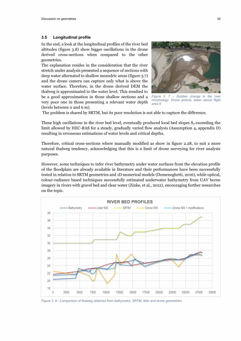
Discussion on geometries 42
3.5 Longitudinal profile In the end, a look at the longitudinal profiles of the river bed altitudes (figure 3.8) show bigger oscillations in the drone derived cross-sections when compared to the other geometries. The explanation resides in the consideration that the river stretch under analysis presented a sequence of sections with deep water alternated to shallow meandric areas (figure 3.7) and the drone camera can capture only what is above the water surface. Therefore, in the drone derived DEM the thalweg is approximated to the water level. This resulted to be a good approximation in those shallow sections and a very poor one in those presenting a relevant water depth (levels between 0 and 6 m). The problem is shared by SRTM, but its poor resolution is not able to capture the difference.
These high oscillations in the river bed level, eventually produced local bed slopes S0 exceeding the limit allowed by HEC-RAS for a steady, gradually varied flow analysis (Assumption 4, appendix D) resulting in erroneous estimations of water levels and critical depths.
Therefore, critical cross-sections where manually modified as show in figure 2.28, to suit a more natural thalweg tendency, acknowledging that this is a limit of drone surveying for river analysis purposes.
However, some techniques to infer river bathymetry under water surfaces from the elevation profile of the floodplain are already available in literature and their performances have been successfully tested in relation to SRTM geometries and 1D numerical models (Domeneghetti, 2016), while optical, colour-radiance based techniques successfully estimated underwater bathymetry from UAV borne imagery in rivers with gravel bed and clear water (Zinke, et al., 2012), encouraging further researches on the topic.
Figure 3. 7 – Sudden change in the river morphology. Drone picture, taken above flight area 9
18
20
22
24
26
28
30
32
34
36
38
0 2500 5000 7500 10000 12500 15000 17500 20000 22500 25000 27500 30000
RIVER BED PROFILESBathymetry Lidar 500 SRTM Drone 500 Drone 500 + modifications
Figure 3. 8 - Comparison of thalweg obtained from bathymetry, SRTM, lidar and drone geometries

Hydraulic modeling 44
4 Hydraulic modeling
The hydraulic modelling was the third and last part of our study and intended to explore the impact on water depth estimations of 1D hydraulic models caused by the input of bathymetry, SRTM, lidar and drone-based geometries, before and after the model calibration.
The mono-dimensional model was the one better fitting extension and distribution of the cross-sections at our disposal, adding the advantages of a reduced calculation time, allowing us to run a greater number of simulations when compared to a bi-dimensional model and justified by the negligible differences in water depth estimations between 1D and 2D (Ali, et al., 2015). Thus, a numerical model was implemented in HEC-RAS for each of the four geometries.
The original 2D bathymetry derived model (Manane, 2017) was reduced to cover the 22 cross-sections that were derived during the DEM analysis (see previous chapter) and adapted to perform 1D hydraulic simulations. Its geometry was left untouched with cross-sections shape and relative distances according to the bathymetry survey and energy loss coefficients as in the 2D model, i.e. contraction and expansion coefficients of Cc=0.1 and Ce=0.3 and Manning’s coefficients of nch=0.022 m-1/3s for the main channel and nfl=0.06 m-1/3s for the flood plain.
The models for the other geometries were built based on these values for the various parameters, with the only difference in the cross-sections shapes, which were taken from SRTM, Lidar and Drone derived DEM respectively.
For each model, a 1D, steady flow in subcritical gradually varied regime was performed. To execute the analysis, HEC-RAS uses an iterative solution of the Energy equation considering N computational nodes for each reach of river, which bound N-1 difference cells. 2N-2 equations are developed from these cells, but since there are 2N unknowns, i.e. Q and z for each node, two extra equations are required to perform the calculations. These are provided by the boundary conditions for each reach which, in the case of subcritical flow, need to be set at the upstream and downstream ends. (HEC-RAS river analysis system, February 2006)
In our analysis the upstream condition was set as value for the discharge Q constant over time, while the downstream boundary condition selected was of normal depth, which consist in the manual input of the friction slope Sf that is used by the software to calculate the value of normal depth at the last cross-section using the Manning’s equation under the assumption of uniform flow. In our analysis the value introduced was S0=0.00025, i.e. a representative value of the bed slope for the last part of the study area.
The analysis was performed for a set of discharge values Q ranging between 650 and 50 m3/s, in order to cover all the degrees of cross-section inundation, from fully covered for high flows to low flow confined in the main channel.
More details about HEC-RAS calculation procedure and its theory foundations can be found in Appendix D or in the official Hydraulic reference manual (HEC-RAS river analysis system, February 2006).
4.1 Results The results are presented for Q1= 650 m3/s, Q2= 350 m3/s and Q3= 50 m3/s, values corresponding respectively to the maximum average monthly flow registered at the Chokwe station, an average yearly flow and a significant value for low flow representations.
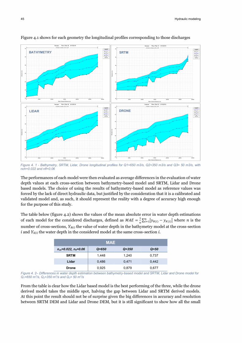
45 Hydraulic modeling
Figure 4.1 shows for each geometry the longitudinal profiles corresponding to those discharges
The performances of each model were then evaluated as average differences in the evaluation of water depth values at each cross-section between bathymetry-based model and SRTM, Lidar and Drone based models. The choice of using the results of bathymetry-based model as reference values was forced by the lack of direct hydraulic data, but justified by the consideration that it is a calibrated and validated model and, as such, it should represent the reality with a degree of accuracy high enough for the purpose of this study.
The table below (figure 4.2) shows the values of the mean absolute error in water depth estimations of each model for the considered discharges, defined as 𝑀𝐴𝐸 = 1
𝑛∑ |𝑦𝐵(𝑖) − 𝑦𝐾(𝑖)|𝑛
𝑖=1 where n is the
number of cross-sections, YB(i) the value of water depth in the bathymetry model at the cross-section i and YK(i) the water depth in the considered model at the same cross-section i.
MAE nch=0.022, nfl=0.06 Q=650 Q=350 Q=50
SRTM 1,448 1,240 0,737
Lidar 0,486 0,471 0,442
Drone 0,925 0,879 0,677 Figure 4. 2– Differences in water depth estimation between bathymetry-based model and SRTM, Lidar and Drone model for Q1=650 m3/s, Q2=350 m3/s and Q3= 50 m3/s
From the table is clear how the Lidar based model is the best performing of the three, while the drone derived model takes the middle spot, halving the gap between Lidar and SRTM derived models. At this point the result should not be of surprise given the big differences in accuracy and resolution between SRTM DEM and Lidar and Drone DEM, but it is still significant to show how all the small
0 5000 10000 15000 20000 25000 3000020
22
24
26
28
30
32
limpopo Plan: Plan 29 8/10/2018
Main Channel Distance (m)
Ele
vatio
n (m
)
Legend
WS PF 1
WS PF 2
WS PF 3
Ground
Limpopo Limpopo_DS_Confl
BATHYMETRY
0 5000 10000 15000 20000 25000 3000028
30
32
34
36
38
40
limpopo Plan: Plan 31 8/10/2018
Main Channel Distance (m)
Ele
vatio
n (m
)
Legend
WS PF 1
WS PF 2
WS PF 3
Ground
Limpopo Limpopo_DS_Confl
SRTM
0 5000 10000 15000 20000 25000 3000020
22
24
26
28
30
32
limpopo Plan: Plan 30 8/10/2018
Main Channel Distance (m)
Ele
vatio
n (m
)
Legend
WS PF 1
WS PF 2
WS PF 3
Ground
Limpopo Limpopo_DS_Confl
LIDAR
0 5000 10000 15000 20000 25000 3000020
22
24
26
28
30
32
34
limpopo Plan: Plan 33 8/10/2018
Main Channel Distance (m)
Ele
vatio
n (m
)
Legend
WS PF 1
WS PF 2
WS PF 3
Ground
Limpopo Limpopo_DS_Confl
DRONE
Figure 4. 1 - Bathymetry, SRTM, Lidar, Drone longitudinal profiles for Q1=650 m3/s, Q2=350 m3/s and Q3= 50 m3/s, with nch=0.022 and nfl=0.06
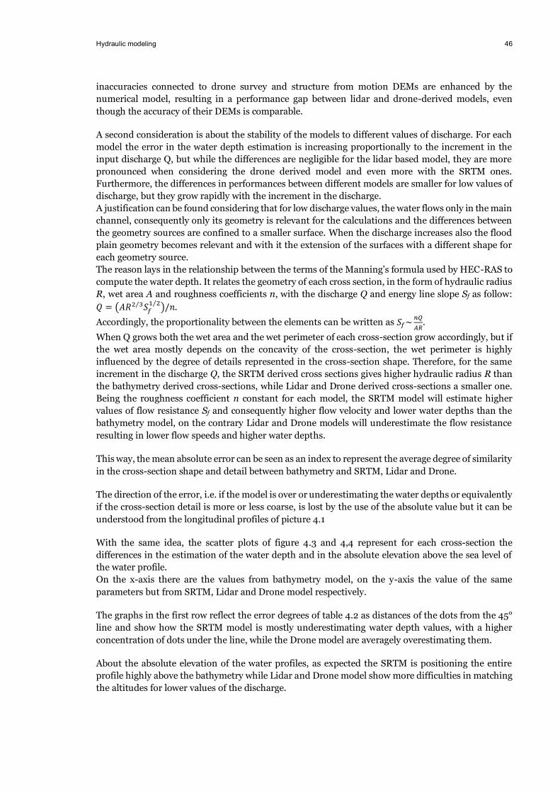
Hydraulic modeling 46
inaccuracies connected to drone survey and structure from motion DEMs are enhanced by the numerical model, resulting in a performance gap between lidar and drone-derived models, even though the accuracy of their DEMs is comparable.
A second consideration is about the stability of the models to different values of discharge. For each model the error in the water depth estimation is increasing proportionally to the increment in the input discharge Q, but while the differences are negligible for the lidar based model, they are more pronounced when considering the drone derived model and even more with the SRTM ones. Furthermore, the differences in performances between different models are smaller for low values of discharge, but they grow rapidly with the increment in the discharge. A justification can be found considering that for low discharge values, the water flows only in the main channel, consequently only its geometry is relevant for the calculations and the differences between the geometry sources are confined to a smaller surface. When the discharge increases also the flood plain geometry becomes relevant and with it the extension of the surfaces with a different shape for each geometry source. The reason lays in the relationship between the terms of the Manning’s formula used by HEC-RAS to compute the water depth. It relates the geometry of each cross section, in the form of hydraulic radius R, wet area A and roughness coefficients n, with the discharge Q and energy line slope Sf as follow: 𝑄 = (𝐴𝑅2 3⁄ 𝑆𝑓
1 2⁄ )/𝑛.
Accordingly, the proportionality between the elements can be written as 𝑆𝑓~ 𝑛𝑄𝐴𝑅
.
When Q grows both the wet area and the wet perimeter of each cross-section grow accordingly, but if the wet area mostly depends on the concavity of the cross-section, the wet perimeter is highly influenced by the degree of details represented in the cross-section shape. Therefore, for the same increment in the discharge Q, the SRTM derived cross sections gives higher hydraulic radius R than the bathymetry derived cross-sections, while Lidar and Drone derived cross-sections a smaller one. Being the roughness coefficient n constant for each model, the SRTM model will estimate higher values of flow resistance Sf and consequently higher flow velocity and lower water depths than the bathymetry model, on the contrary Lidar and Drone models will underestimate the flow resistance resulting in lower flow speeds and higher water depths.
This way, the mean absolute error can be seen as an index to represent the average degree of similarity in the cross-section shape and detail between bathymetry and SRTM, Lidar and Drone.
The direction of the error, i.e. if the model is over or underestimating the water depths or equivalently if the cross-section detail is more or less coarse, is lost by the use of the absolute value but it can be understood from the longitudinal profiles of picture 4.1
With the same idea, the scatter plots of figure 4.3 and 4,4 represent for each cross-section the differences in the estimation of the water depth and in the absolute elevation above the sea level of the water profile. On the x-axis there are the values from bathymetry model, on the y-axis the value of the same parameters but from SRTM, Lidar and Drone model respectively.
The graphs in the first row reflect the error degrees of table 4.2 as distances of the dots from the 45° line and show how the SRTM model is mostly underestimating water depth values, with a higher concentration of dots under the line, while the Drone model are averagely overestimating them.
About the absolute elevation of the water profiles, as expected the SRTM is positioning the entire profile highly above the bathymetry while Lidar and Drone model show more difficulties in matching the altitudes for lower values of the discharge.

47 Hydraulic modeling
The drone model, in particular, presents a number of values that remarkably diverge, reflecting the differences in the thalweg profile that the lower discharges find harder to mask.
WATER DEPTH [m]
Q=650 m3/s
Q=350 m3/s
Q= 50 m3/s
0
1
2
3
4
5
0 1 2 3 4 5
LID
AR
BATHYMETRY
0
1
2
3
4
5
0 1 2 3 4 5
SRTM
BATHYMETRY
0
1
2
3
4
5
0 1 2 3 4 5
DR
ON
E
BATHYMETRY
Figure 4. 3 – Comparison in water depth estimation of SRTM, lidar and drone models with the bathymetry model, for Q1=650 m3/s, Q2=350 m3/s and Q3= 50 m3/s
Hydraulic modeling 48
WATER STATION ELEVATION [m.a.s.l.]
Q=650 m3/s
Q=350 m3/s
Q= 50 m3/s
22
24
26
28
30
32
34
36
38
40
22 24 26 28 30 32 34 36 38 40
SRTM
BATHYMETRY
22
23
24
25
26
27
28
29
30
22 23 24 25 26 27 28 29 30
LID
AR
BATHYMETRY
22
23
24
25
26
27
28
29
30
31
32
22 23 24 25 26 27 28 29 30 31 32
DR
ON
E
BATHYMETRY
Figure 4. 4 – Comparison in water profile elevation of SRTM, lidar and drone models with the bathymetry model, for Q1=650 m3/s, Q2=350 m3/s and Q3= 50 m3/s

49 Hydraulic modeling
4.2 Calibration The SRTM, Lidar and Drone models were then calibrated against the bathymetry model, in order to achieve the minimum error in the water depth estimation with the variation of the Manning’s roughness coefficients.
The steady flow analysis of the three model was repeated for each one of the possible combinations of Manning’s values included in the range nch=0.01, 0.015, …, 0.04 and nfl=0.04, 0.045, …, 0.08. The water depths were once again compared to the ones of the bathymetry model with nch=0.022 and nfl=0.06 with the mean absolute error.
The minimum MAE achieved by each model for every discharge with the relative Manning’s coefficients, are shown in figure 4.5.
Q=650 MAE nch nfl
SRTM 1,045 0,04 0,08
Lidar 0,460 0,02 0,075
Drone 0,904 0,015 0,045 ÷ 0,055
Q=350 MAE nch nfl
SRTM 0,978 0,04 0,08
Lidar 0,429 0,25 0,04
Drone 0,844 0,015 0,08
Q=50 MAE nch nfl
SRTM 0,665 0,04 0,08
Lidar 0,385 0,03 0,04 ÷ 0,08
Drone 0,637 0,01 0,04 ÷ 0,08 Figure 4. 5 – Minimum MAE achieved by each model in the estimation of water depths compared to the bathymetry one (nch=0.022, nfl=0.06) and relative couples of Manning’s coefficients
The results confirmed the relationship in the calculation of the water depth between the roughness coefficients and degree of detail in the cross-section. The SRTM derived model required very high roughness values to compensate a coarser geometry while, on the opposite, Lidar and Drone finer detail resulted in smaller Manning’s coefficients. Moreover, being Drone, Lidar and bathymetry geometries of comparable resolutions, their models presented similar roughness coefficients after calibration, especially for higher flow rates.
All models registered an increment in the performances compared to their uncalibrated version, but the SRTM model was the one to benefit the most from this operation with a decrement in the error of 0.403, 0.262 and 0.072 meters for Q1, Q2 and Q3 respectively, against the 0.026, 0.042 and 0.057 m of the Lidar model and the 0.21, 0.035 and 0.040 m of the Drone model. This shows that the optimal roughness values for the SRTM were further from the Bathymetry than the one of Lidar and Drone, but also suggest a bigger impact on the calculations of the cross-section

Hydraulic modeling 50
shapes rather than its roughness, with the Lidar and Drone based models showing far more difficulties in compensating a finer geometry with Manning’s coefficients than the SRTM model.
Interesting to notice are also the opposite tendencies of achieving greater improvement with higher discharge values for the SRTM while Lidar and Drone benefit more from the calibration process when lower discharges are applied.
The relationship between mean absolute error in the water depth estimation and roughness coefficients is made explicit by the mean of the graphs below. For each geometry, figure 4.6, 4.7 and 4.8 show the trend of the MAE at different discharge values when the Manning’s coefficient is kept constant for the flood plain and varies for the main channel in the first row and the opposite situation with nch constant and nfl varying in the second one. It is easy to notice that variations in the roughness of the laterals flood plain have very small effects on the estimation of the water depth, while changes in the roughness of the main channel are definitely more relevant. Lidar and Drone model found a minimum value for the MAE inside the range of roughness explored and with values not too far from the one assigned to the bathymetry-based model, while the SRTM model shows the possibility further improvement for even higher values of roughness.
51 Hydraulic modeling
BATHYMETRY-SRTM
0.9
1.0
1.1
1.2
1.3
1.4
1.5
1.6
1.7
1.8
1.9
0.01 0.02 0.03 0.04
MAE
nCH
0.9
1.0
1.1
1.2
1.3
1.4
1.5
1.6
1.7
1.8
1.9
0.04 0.05 0.06 0.07 0.08M
AEnFL
0.9
1.0
1.1
1.2
1.3
1.4
1.5
0.01 0.02 0.03 0.04
MAE
nCH
0.9
1.0
1.1
1.2
1.3
1.4
1.5
0.04 0.05 0.06 0.07 0.08
MAE
nFL
0.65
0.70
0.75
0.80
0.85
0.01 0.02 0.03 0.04
MAE
nCH
0.65
0.70
0.75
0.80
0.85
0.04 0.05 0.06 0.07 0.08
MAE
nFL
Figure 4. 6 – MAE trendline of SRTM model in water depths estimation compared to the bathymetry ones, with the variation of Manning’s coefficient for the main channel (left) or floodplain (right) for discharges Q1= 650 m3s, Q2= 350 m3s and Q3= 50 m3s (top to bottom)
Q =
650
m3 /s
Q
= 3
50 m
3 /s
Q =
50
m3 /s
nCH = 0.01 nCH = 0.015 nCH = 0.02 nCH = 0.025 nCH = 0.03 nCH = 0.035 nCH = 0.04
nFL = 0.04 nFL = 0.045 nFL = 0.05 nFL = 0.055 nFL = 0.06 nFL = 0.065 nFL = 0.07 nfl = 0.075 nFL = 0.08

Hydraulic modeling 52
BATHYMETRY-LIDAR
0.5
0.6
0.7
0.8
0.9
1.0
1.1
0.01 0.02 0.03 0.04
MAE
nCH
0.4
0.5
0.6
0.7
0.8
0.9
1.0
1.1
0.04 0.05 0.06 0.07 0.08
MAE
nFL
0.40
0.50
0.60
0.70
0.80
0.90
0.01 0.02 0.03 0.04
MAE
nCH
0.4
0.5
0.6
0.7
0.8
0.9
0.04 0.05 0.06 0.07 0.08
MAE
nFL
0.35
0.40
0.45
0.50
0.55
0.60
0.01 0.02 0.03 0.04
MAE
nCH
0.35
0.40
0.45
0.50
0.55
0.60
0.04 0.05 0.06 0.07 0.08
MAE
nFL
Figure 4. 7 – MAE trendline of LIDAR model in water depths estimation compared to the bathymetry ones, with the variation of Manning’s coefficient for the main channel (left) or floodplain (right) for discharges Q1= 650 m3s, Q2= 350 m3s and Q3= 50 m3s (top to bottom)
nCH = 0.01 nCH = 0.015 nCH = 0.02 nCH = 0.025 nCH = 0.03 nCH = 0.035 nCH = 0.04
nFL = 0.04 nFL = 0.045 nFL = 0.05 nFL = 0.055 nFL = 0.06 nFL = 0.065 nFL = 0.07 nfl = 0.075 nFL = 0.08
Q = 50 m
3/s Q
= 350 m3/s
Q = 650 m
3/s

53 Hydraulic modeling
BATHYMETRY-LIDAR
0.8
0.9
1.0
1.1
1.2
1.3
1.4
1.5
1.6
0.01 0.02 0.03 0.04
MAE
nCH
0.8
0.9
1.0
1.1
1.2
1.3
1.4
1.5
1.6
0.04 0.05 0.06 0.07 0.08M
AEnFL
0.8
0.9
1.0
1.1
1.2
1.3
1.4
0.01 0.02 0.03 0.04
MAE
nCH
0.8
0.9
1.0
1.1
1.2
1.3
1.4
0.04 0.05 0.06 0.07 0.08
MAE
nFL
0.60
0.65
0.70
0.75
0.80
0.85
0.90
0.01 0.02 0.03 0.04
MAE
nCH
0.60
0.65
0.70
0.75
0.80
0.85
0.04 0.05 0.06 0.07 0.08
MAE
nFL
Q =
650
m3 /s
Q
= 3
50 m
3 /s
Q =
50
m3 /s
Figure 4. 8 – MAE trendline of DRONE model in water depths estimation compared to the bathymetry ones, with the variation of Manning’s coefficient for the main channel (left) or floodplain (right) for discharges Q1= 650 m3s, Q2= 350 m3s and Q3= 50 m3s (top to bottom)
nCH = 0.01 nCH = 0.015 nCH = 0.02 nCH = 0.025 nCH = 0.03 nCH = 0.035 nCH = 0.04
nFL = 0.04 nFL = 0.045 nFL = 0.05 nFL = 0.055 nFL = 0.06 nFL = 0.065 nFL = 0.07 nfl = 0.075 nFL = 0.08
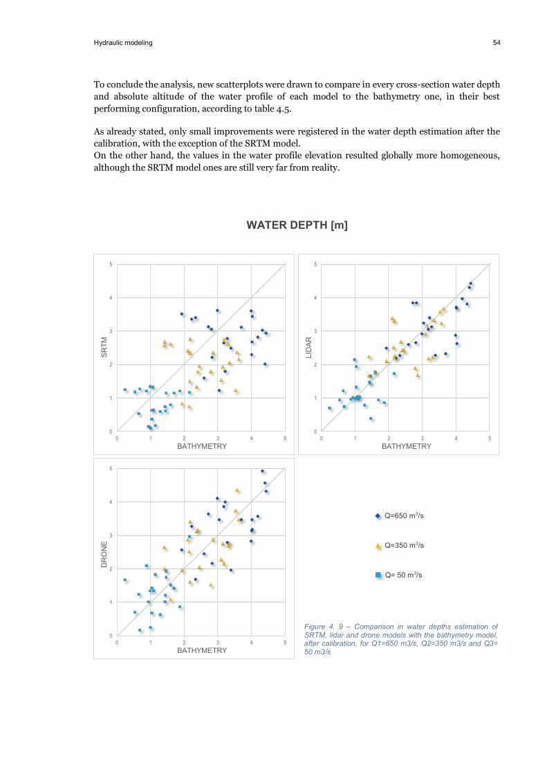
Hydraulic modeling 54
To conclude the analysis, new scatterplots were drawn to compare in every cross-section water depth and absolute altitude of the water profile of each model to the bathymetry one, in their best performing configuration, according to table 4.5.
As already stated, only small improvements were registered in the water depth estimation after the calibration, with the exception of the SRTM model. On the other hand, the values in the water profile elevation resulted globally more homogeneous, although the SRTM model ones are still very far from reality.
WATER DEPTH [m]
0
1
2
3
4
5
0 1 2 3 4 5
SRTM
BATHYMETRY
0
1
2
3
4
5
0 1 2 3 4 5
LID
AR
BATHYMETRY
0
1
2
3
4
5
0 1 2 3 4 5
DR
ON
E
BATHYMETRY
Q=650 m3/s
Q=350 m3/s
Q= 50 m3/s
Figure 4. 9 – Comparison in water depths estimation of SRTM, lidar and drone models with the bathymetry model, after calibration, for Q1=650 m3/s, Q2=350 m3/s and Q3= 50 m3/s

55 Hydraulic modeling
WATER STATION ELEVATION [m.a.s.l.]
22
24
26
28
30
32
34
36
38
40
20 22 24 26 28 30 32 34 36 38 40
SRTM
BATHYMETRY
20
22
24
26
28
30
32
20 22 24 26 28 30 32
LID
AR
BATHYMETRY
20
22
24
26
28
30
32
20 22 24 26 28 30 32
DR
ON
E
BATHYMETRY
Figure 4. 10 – Comparison in water levels estimation of SRTM, lidar and drone models with the bathymetry model, after calibration, for Q1=650 m3/s, Q2=350 m3/s and Q3= 50 m3/s
Q=650 m3/s
Q=350 m3/s
Q= 50 m3/s
Conclusions 56
5 Conclusions
This study presented an application of UAV to hydraulic flood modelling. It followed the planning and execution of a survey with a quadcopter drone leading to the modelling of a DEM through SfM photogrammetry techniques. The quality of the DEM for flood modelling applications was then assessed by comparing the water depths estimations of four HECRAS 1D steady flow models, differing in their geometry input from bathymetric cross-sections (0.5 m), SRTM DEM (30 m), lidar DEM (1 m), drone DEM (0.6 m).
The outcomes were satisfying, with a degree of accuracy in the terrain modelling which produced errors in the water depth calculations within the tolerances adopted in this typology of studies and comparable in magnitude to the ones raising from high precision laser topography models. The experience obtained from the Limpopo river will be of use in future surveys with similar intents, enabling them to be organised more effectively
Below is presented a summary of the results achieved and the consideration arisen in the various phases of our study.
The field work proved the wished advantages of the UAV tool. The use of two drones and nine batteries made possible to map, in less than three days, a total of almost 2500 hectares of terrain on a section 30 km long of the Limpopo river. The survey produced enough raw data to properly model the covered river section, while difficulties and risks connected to surveying in a remote area, covered by deep vegetation and populated by wild animals were reduced to manoeuvring a remote control from the side of a road. This phase was also useful to expose the actual limits of the use of commercial drones, not born for the specific surveying purpose. The flight capacity of the UAV used was limited to an average of 20 minutes that, given the lack of electricity access of the area, increased the importance of an optimised flight plan and weather conditions proved to be a strong limit factor, with the drone being sensible to rain and strong wind, which considerably increased the batteries usage. In addition, the peculiarity of the area and the season made register temperatures above 40 °C, testing the drone outside its operating temperature range. No malfunctions of the vehicle were registered during flight operations, but the excessive heat might have caused the onboard sensor to register uncoherent altitudes associated to each picture which could have deceived the SfM software, enhancing the impact of the bowl effect. This statement however could not be proved.
The use of a well distributed set of ground control points proved to be fundamental to restrain the appearance of bowl effect in the final DEM. At the current state of things, this factor compromises the idea of a full remote survey, forcing the user to cover the field in order to position GPC targets. However, the minimum required number of them is low enough to do not compromise the utility of drone tool.
The bowl effect (also dome effect) on DEM photogrammetry generation is known to the recent literature with growing number of studies covering the topic. Even if most of them are restricted to specific areas or situations, the bowl effect appears to be mainly connected to miscalculations by the photogrammetry software in the spatial relative distances of points captured in overlapping pictures. The main cause seems to be related to the degree of lens distortion of the camera transferred on the pictures in the form of radial distortions during the process of representing the three-dimensional reality on a bi-dimensional surface. While SfM software producers are working on algorithms able to calculate the degree of distortion from the lens specifics and account for this effect in post-production, being aware of the issue can allow the user to adopt specific preventative measure to reduce its occurrences. Reflecting surfaces,
57 Conclusions
pronounced shadows or generally any moving objects on the ground complicate the work of the photogrammetry software. On the opposite, the use of fixed focal length lenses and square picture sizes (or close to square, like 4:3) is suggested, because they keep the degree of distortion more uniform, since it grows radially from the centre to the corners. Finally, performing additional flight to add extra sets of pictures from different altitudes and angles, prevent the collection of imagery composed by pictures showing near-parallel directions, factor that seems to be connected to the incidence of bowl effect (James, et al., 2014) and increase the overall quality of the terrain model, especially in the presence of significant slopes, cliffs, canyons, high buildings or any object raising considerably form the ground level.
This study, as well as similar ones, made clear the importance of a well-planned survey, aware of the photogrammetry process and therefore focused of the acquisition of high quality imagery, since any error in this phase can hardly be solved in post processing causing imprecisions that will be spread to the hydraulic calculations, magnifying their impact on the final outcome.
A final consideration about underwater topography needs to precede the numerical modelling. Photogrammetry techniques are not able to estimate the morphology of the river bed from pictures of the water surface, therefore all the areas covered in water will be approximated to a flat surface following water level altitudes. In the specific case of the Limpopo river, this resulted to be a good approximation for those section presenting shallow meandric channels, while those section with deep channel cut or pools needed to be manually adjusted. However, the inconvenience is shared with other remote sensing sources, like SRTM or some typology of lidar and attempts to infer river bathymetry from the elevation profile of the floodplain (Domeneghetti, 2016) or from colour radiance of the water (Zinke, et al., 2012) have already been successfully tested in literature. Even if their applications remain, for now, limited to specific conditions, they show interesting area of research for future developments in the application of UAV technology to remote sensing.
With all that being said, the final resolution of DEM was still comparable to the topography obtained from lidar and total station. The cross-section extracted from it followed accurately the shape of those from bathymetry and lidar and the residual differences between them can be ascribed to natural changes in the river morphology occurred during the years spent between the different surveys.
The final outcome of the hydraulic modelling exercise has shown that, although the lidar model resulted more accurate than drone and SRTM models in reproducing the water depths of the bathymetry-based model, the differences between lidar and drone were for most included within a tolerance of 0.5 m. The mean absolute error in water depth estimation between lidar and drone was included in the range 0.439 - 0.225 m before calibration and 0.498 - 0.252 after, while between 0.925 – 0.677 and 0,904 - o,637 before and after calibration respectively when the drone model was compared to the bathymetry one. The calibration exercise revealed a bigger impact on water depth calculations of the degree of detail representation in the cross-sections, rather than the values assigned to their roughness parameters, with the SRTM model registering a maximum improvement of 0.403 m, while lidar and drone one of just o.021 and 0.057 m respectively. Never the less, water depth estimations of the calibrated drone-derived model were more accurate than the ones from calibrated SRTM and still of a magnitude comparable with the calibrated lidar model,
The results of this and similar study, suggests that the key of a successful use of light commercial UAV for engineering applications reside in the level of automation, robustness and synergy between the phases of data collection and processing. The drone needs to be intended not as the mere flying machine, but as a combination of a tool to collect data and a specific technique to analyse them for

Conclusions 58
every intended use. Its availability in terms of cost and user-friendliness during flight operations should not distract from the final goal to deliver a quality product, valuable from an engineering point of view. The UAV technology and photogrammetry have proved to be competitive and mature enough for a more consistent use in the topic explored inside the present thesis work, but still are numerous the area of possible improvements that should stimulate further researches on this and similar topics.

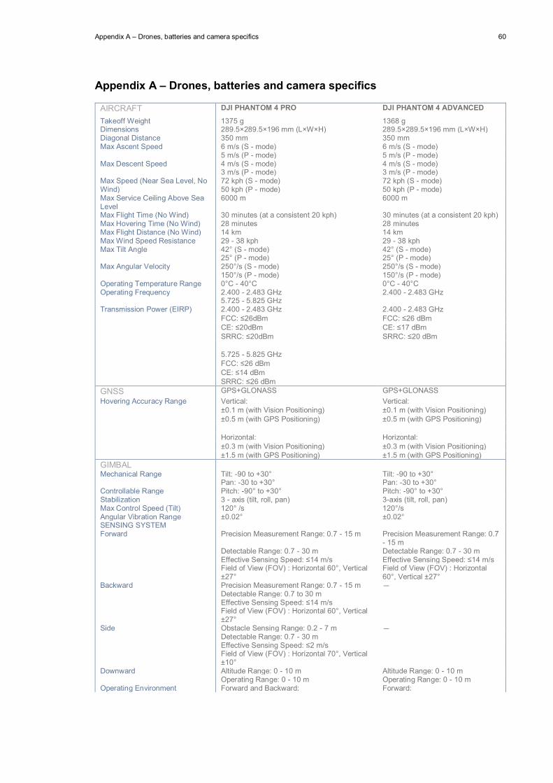
Appendix A – Drones, batteries and camera specifics 60
Appendix A – Drones, batteries and camera specifics
AIRCRAFT DJI PHANTOM 4 PRO DJI PHANTOM 4 ADVANCED
Takeoff Weight 1375 g 1368 g Dimensions 289.5×289.5×196 mm (L×W×H) 289.5×289.5×196 mm (L×W×H) Diagonal Distance 350 mm 350 mm Max Ascent Speed 6 m/s (S - mode) 6 m/s (S - mode)
5 m/s (P - mode) 5 m/s (P - mode) Max Descent Speed 4 m/s (S - mode) 4 m/s (S - mode)
3 m/s (P - mode) 3 m/s (P - mode) Max Speed (Near Sea Level, No Wind)
72 kph (S - mode) 72 kph (S - mode) 50 kph (P - mode) 50 kph (P - mode)
Max Service Ceiling Above Sea Level
6000 m 6000 m
Max Flight Time (No Wind) 30 minutes (at a consistent 20 kph) 30 minutes (at a consistent 20 kph) Max Hovering Time (No Wind) 28 minutes 28 minutes Max Flight Distance (No Wind) 14 km 14 km Max Wind Speed Resistance 29 - 38 kph 29 - 38 kph Max Tilt Angle 42° (S - mode) 42° (S - mode)
25° (P - mode) 25° (P - mode) Max Angular Velocity 250°/s (S - mode) 250°/s (S - mode)
150°/s (P - mode) 150°/s (P - mode) Operating Temperature Range 0°C - 40°C 0°C - 40°C Operating Frequency 2.400 - 2.483 GHz 2.400 - 2.483 GHz
5.725 - 5.825 GHz Transmission Power (EIRP) 2.400 - 2.483 GHz 2.400 - 2.483 GHz
FCC: ≤26dBm FCC: ≤26 dBm CE: ≤20dBm CE: ≤17 dBm SRRC: ≤20dBm SRRC: ≤20 dBm
5.725 - 5.825 GHz FCC: ≤26 dBm CE: ≤14 dBm SRRC: ≤26 dBm
GNSS GPS+GLONASS GPS+GLONASS Hovering Accuracy Range Vertical: Vertical:
±0.1 m (with Vision Positioning) ±0.1 m (with Vision Positioning) ±0.5 m (with GPS Positioning) ±0.5 m (with GPS Positioning)
Horizontal: Horizontal: ±0.3 m (with Vision Positioning) ±0.3 m (with Vision Positioning) ±1.5 m (with GPS Positioning) ±1.5 m (with GPS Positioning)
GIMBAL Mechanical Range Tilt: -90 to +30° Tilt: -90 to +30°
Pan: -30 to +30° Pan: -30 to +30° Controllable Range Pitch: -90° to +30° Pitch: -90° to +30° Stabilization 3 - axis (tilt, roll, pan) 3-axis (tilt, roll, pan) Max Control Speed (Tilt) 120° /s 120°/s Angular Vibration Range ±0.02° ±0.02° SENSING SYSTEM
Forward Precision Measurement Range: 0.7 - 15 m Precision Measurement Range: 0.7 - 15 m
Detectable Range: 0.7 - 30 m Detectable Range: 0.7 - 30 m Effective Sensing Speed: ≤14 m/s Effective Sensing Speed: ≤14 m/s Field of View (FOV) : Horizontal 60°, Vertical ±27°
Field of View (FOV) : Horizontal 60°, Vertical ±27°
Backward Precision Measurement Range: 0.7 - 15 m - Detectable Range: 0.7 to 30 m Effective Sensing Speed: ≤14 m/s Field of View (FOV) : Horizontal 60°, Vertical ±27°
Side Obstacle Sensing Range: 0.2 - 7 m - Detectable Range: 0.7 - 30 m Effective Sensing Speed: ≤2 m/s Field of View (FOV) : Horizontal 70°, Vertical ±10°
Downward Altitude Range: 0 - 10 m Altitude Range: 0 - 10 m Operating Range: 0 - 10 m Operating Range: 0 - 10 m
Operating Environment Forward and Backward: Forward:

61 Appendix A – Drones, batteries and camera specifics
Surface with clear pattern and adequate lighting (lux>15)
Surface with clear pattern and adequate lighting (lux>15)
Side: Detects diffuse reflective surfaces (>8%) larger than 20×20 cm (walls, trees, people, etc.)
Downward: Downward: Surface with clear pattern and adequate lighting (lux>15)
Surface with clear pattern and adequate lighting (lux>15)
Speed ≤14m/s (at 2 m, sufficient brightness) Speed ≤14 m/s (at 2 m, sufficient brightness)
CAMERA
Sensor 1'' CMOS 1'' CMOS Effective Pixels: 20 MP Effective Pixels: 20 MP
Lens FOV: 84 ° FOV: 84 ° 35 mm Format Equivalent: 24 mm 35 mm Format Equivalent: 24 mm Aperture: f/2.8-11 Aperture: f/2.8 - 11 Shooting Range: 1 m to ∞ (auto focus) Shooting Range: 1 m to ∞ (auto
focus) ISO Range Video: Video:
100 - 3200(auto) 100 - 3200 (auto) 100 - 6400(manual) 100 - 6400 (manual)
Photo: Photo: 100 - 3200(auto) 100 - 3200 (auto) 100 - 12800(manual) 100 - 12800 (manual)
Shutter Speed Electronic Shutter: 8 - 1/8000 s Electronic Shutter: 8 - 1/8000 s Mechanical Shutter: 8 - 1/2000 s Mechanical Shutter: 8 - 1/2000 s
Still Image Size 3:2: 5472×3648 3:2: 5472×3648 4:3: 4864×3648 4:3: 4864×3648 16:9: 5472×3078 16:9: 5472×3078
Still Image Size While Recording Video
4096×2160 (24/25/30/48/50 p) 4096×2160 (24/25/30/48/50 p) 3840×2160 (24/25/30/48/50/60 p) 3840×2160 (24/25/30/48/50/60 p) 2720×1530 (24/25/30/48/50/60 p) 2720×1530 (24/25/30/48/50/60 p) 1920×1080 (24/25/30/48/50/60/120 p) 1920×1080 (24/25/30/48/50/60/120
p) Still Photography Modes Single Shot Single Shot
Burst Shooting: 3/5/7/10/14 frames Burst Shooting: 3/5/7/10/14 frames Auto Exposure Bracketing(AEB): 3/5 bracketed frames at 0.7 EV bias
Auto Exposure Bracketing(AEB): 3/5 bracketed frames at 0.7 EV bias
Interval: 2/3/5/7/10/15/20/30/60 s Interval: 2/3/5/7/10/15/20/30/60 s Video Resolution H.265 H.265
C4K: 4096×2160 24/25/30 p @100 Mbps C4K: 4096×2160 24/25/30 p @100 Mbps
4K: 3840×2160 24/25/30 p @100 Mbps 4K: 3840×2160 24/25/30 p @100 Mbps
2.7K: 2720×1530 24/25/30 p @65 Mbps 2.7K: 2720×1530 24/25/30 p @65 Mbps
2.7K: 2720×1530 48/50/60 p @80 Mbps 2.7K: 2720×1530 48/50/60 p @80 Mbps
FHD: 1920×1080 24/25/30 p @50 Mbps FHD: 1920×1080 24/25/30 p @50 Mbps
FHD: 1920×1080 48/50/60 p @65 Mbps FHD: 1920×1080 48/50/60 p @65 Mbps
FHD: 1920×1080 120 p @100 Mbps FHD: 1920×1080 120 p @100 Mbps
HD: 1280×720 24/25/30 p @25 Mbps HD: 1280×720 24/25/30 p @25 Mbps
HD: 1280×720 48/50/60 p @35 Mbps HD: 1280×720 48/50/60 p @35 Mbps
HD: 1280×720 120 p @60 Mbps HD: 1280×720 120 p @60 Mbps
H.264 H.264 C4K: 4096×2160 24/25/30/48/50/60 p @100 Mbps
C4K: 4096×2160 24/25/30/48/50/60 p @100 Mbps
4K: 3840×2160 24/25/30/48/50/60 p @100 Mbps
4K: 3840×2160 24/25/30/48/50/60 p @100 Mbps
2.7K: 2720×1530 24/25/30 p @80 Mbps 2.7K: 2720×1530 24/25/30 p @80 Mbps
2.7K: 2720×1530 48/50/60 p @100 Mbps 2.7K: 2720×1530 48/50/60 p @100 Mbps

Appendix A – Drones, batteries and camera specifics 62
FHD: 1920×1080 24/25/30 p @60 Mbps FHD: 1920×1080 24/25/30 p @60 Mbps
FHD: 1920×1080 48/50/60 p @80 Mbps FHD: 1920×1080 48/50/60 p @80 Mbps
FHD: 1920×1080 120 p @100 Mbps FHD: 1920×1080 120 p @100 Mbps
HD: 1280×720 24/25/30 p @30 Mbps HD: 1280×720 24/25/30 p @30 Mbps
HD: 1280×720 48/50/60 p @45 Mbps HD: 1280×720 48/50/60 p @45 Mbps
HD: 1280×720 120 p @80 Mbps HD: 1280×720 120 p @80 Mbps Max Video Bitrate 100 Mbps 100 Mbps Supported File System FAT32(≤ 32 GB ) FAT32 (≤ 32 GB )
exFAT(> 32 GB) exFAT (> 32 GB) Photo Format JPEG/DNG (RAW) JPEG/DNG (RAW) Video Format MP4/MOV (H.264/AVC; H.265/HEVC) MP4/MOV (H.264/AVC;
H.265/HEVC)
REMOTE CONTROLLER
Operating Frequency 2.400 - 2.483 GHz 2.400 - 2.483 GHz
5.725 - 5.825 GHz Max Transmission Distance (Unobstructed, Free Of Interference)
2.400 - 2.483 GHz 2.400 - 2.483 GHz FCC: 7000 m FCC: 7000 m CE: 4000 m CE: 3500 m SRRC: 4000 m SRRC: 4000 m
5.725 - 5.825 GHz FCC: 7000 m CE: 2000 m SRRC: 5000 m
Operating Temperature Range 0℃ - 40℃ 0℃ - 40℃ Transmission Power (EIRP) 2.400 - 2.483 GHz 2.400 - 2.483 GHz
FCC: ≤26 dBm FCC: ≤26 dBm; CE: ≤17 dBm CE: ≤20 dBm SRRC: ≤20 dBm SRRC: ≤20 dBm
5.725 - 5.825 GHz FCC: ≤26 dBm CE: ≤14 dBm SRRC: ≤20 dBm
Battery 6000 mAh 6000 mAh Operating Current/Voltage 1.2 A ⎓ 7.4 V 1.2 A ⎓ 7.4 V Supported Mobile Device Size Max Length: 170 mm Max Length: 170 mm
Max Thickness: 13 mm Max Thickness: 13 mm
CHARGER
Input 100 - 240 V, 50/60 Hz, 1.4 A 100 - 240 V, 50/60 Hz, 1.4 A Output 17.5 V ⎓ 0~5.7 A 17.5 V ⎓ 0~5.7 A Voltage 17.5 V 17.5 V Rated Power 100 W 100 W
INTELLIGENT FLIGHT BATTERY
STANDARD HIGH CAPACITY
Energy 81.3 Wh 89.2 Wh Capacity 5870 mAh 5870 mAh Voltage 15.2 V 15.2 V Max Charging Voltage 17.4 V 17.4 V Battery Type LiPo 4S LiPo 4S Net Weight 462 g 468 g Charging Temperature Range 5℃ - 40℃ 5℃ - 40℃ Max Charging Power 100 W 100 W


Appendix B – Flight plan calculations 64
Appendix B – Flight plan calculations
The formula used in the flight plans calculation as shown in section 2.1.3 Flight planning, with reference to table 2.4 And figure 1.5, are explicated in the following lines
Input data: v = flight speed [m/s] h = flight altitude [m] ht = max terrain altitude [m] d = average battery duration [min] fl = front-lap [%] sl = side-lap [%] f = lens focal length [mm] (for DJI Phantom Pro f=8.8 mm) Iw x Ih = image size [mm] (for DJI Phantom Pro, 4:3 Aspect Ratio: 4864 × 3648 mm) x · y = sensor size [mm] (for DJI Phantom Pro: 1’’ CMOS equivalent to 13.2 x 8.8 mm) MTD = Maximum transmission distance [km] (for DJI Phantom Pro: 7 km without obstacles)
Area covered with one picture:
Width X= h·x/f Height Y= h·y/f Pixel size px = X/Iw [mm] Final DEM resolution (approx.): DEMrx = px · 4.5 ( 25) [mm] Picture switchback width: a = X Flight switchback width: b = a–sl·a Extra side length: depends on the flight app used, for Drone Deploy c = b/2, for DJI GS PRO c b Max flight length: Lmax = v·60·d/1000 [km]
For each flight zone the lengh A indicates the dimension along which the drone will do the switchbacks, while the width B indicates the dimension along which the drone will follow the flight lines, as illustrated in figure C.3.
The signal check is to control that the drone will be within the maximum transmission distance during the whole flight, avoiding this way the loss of signal between drone and remote controller. It returns “ok” when 𝑀𝑇𝐷 ≥ ( 𝐴2 + 𝐵2)1/2
𝑛𝑓𝑙 = 𝐴−2𝑐𝑏
+ 1 Number of flight lines, it is always rounded to the upper integer.
𝑡 = 𝐿·1000𝑣·60
[min] estimated flight time
𝑛 = 1+𝑡𝑑
estimated number of batteries , it is always rounded to the upper integer.
𝐿 = 𝐵·𝑛𝑓𝑙+𝑏·(𝑛−1)1000
[km] Estimated flight length, it is the effective distance covered by the drone while
preforming the survey in that area. It accounts for flight lines and switch back as in picture C.1.
Figure C. 3 – dimensions for flight zones and flight lines
Flight plan Chokwe
flight altitude 200 m frontlap 75% fligth speed 10 m/smax terrain altitude 79 m ok sidelap 70% average battery duration 20 minpicture resolution 6 cm/px picture switchback width - a 300 m max flight length 12 kmDEM resolution (approx.) 27 cm/px (+- 2.5) fligth switch back width - b 90 m
extra side length - c 45 m
length width max terrain elevation
signal check estimaded flight length n° of cross section covered
n° of flight line estimated batteries needed
Flight Zone [m] [m] [m] [km] ['] [''] [-] [-] [-]1 2030 1150 79 ok 27,47 45 47 5 13 32 1670 249 51 ok 5,19 8 39 1 3 13 1463 180 44 ok 3,02 5 2 1 2 14 1775 162 43 ok 3,64 6 4 1 2 15 2273 154 46 ok 4,64 7 44 1 2 16 1554 2349 57 ok 44,30 73 50 4 27 47 1800 2200 39 ok 47,16 78 36 5 25 48 2100 1470 41 ok 37,14 61 54 4 17 49 2040 2020 39 ok 48,90 81 30 4 23 5
10 1600 1575 38 ok 30,33 50 33 4 18 311 1000 975 40 ok 11,90 19 50 3 11 112 962 1254 39 ok 14,64 24 24 2 14 213 1400 175 38 ok 2,89 4 49 1 2 1
21667 13913 79 281,208 468 42 36 155 31
estimated flight time
Figure C. 1 – Figure 1.5, flight zones for Chokwe survey
Figure C. 2 - Table 2.4, flight plan for Chokwe survey


Appendix C – Modify cross-sections code for MatLab 66
Appendix C – Modify cross-sections code for MatLab
This code has been written by Maurizio Mazzoleni, Lecturer in Hydroinformatics at UNESCO-IHE in Delft.
It has been used to eliminate those points in a cross-section which detach from the global trend too suddenly and therefore can be appointed as high vegetation or miscalculated depth due to light reflection or bad interpolation of voids in the point cloud, as explained in section 2.2 Photogrammetry.
The input voice Threshold defines how much is considered a sudden detachment.
FUNCTION: Modify_Sections
% Modify Sections % Maurizio Mazzoleni % Delft, March 2018 function [Section_filled] = Modify_sections(Section,Thresold) SectionNaN=zeros(size(Section,1),1); index1=zeros(size(Section,1),1); for i=1:size(Section,1) if i==1 SectionNaN(i,1)=Section(i,1); index1(i+1,1)=i; elseif i>1 index2=index1(i,1); if Section(i,1)-Section(index2,1)>Thresold SectionNaN(i,1)=NaN; index1(i+1,1)=index2; else SectionNaN(i,1)=Section(i,1); index1(i+1,1)=i; end end end Section_filled = fillmissing(SectionNaN,'linear'); end RUN: Modify_Sections
% Modify Sections % Maurizio Mazzoleni % Delft, March 2018 clear Threshold=1.5; %%Read all the txt files in the folder files = dir('*.txt'); for i=1:length(files) eval(['load ' files(i).name ' -ascii']); end %%Estimate the maximum value of the time series for each section max_series_tot=zeros(length(files),1); for y=1:length(files) Sect_name=eval(strcat('Sect',num2str(y))); length_series=size(Sect_name,1); max_series_tot(y,1)=length_series;
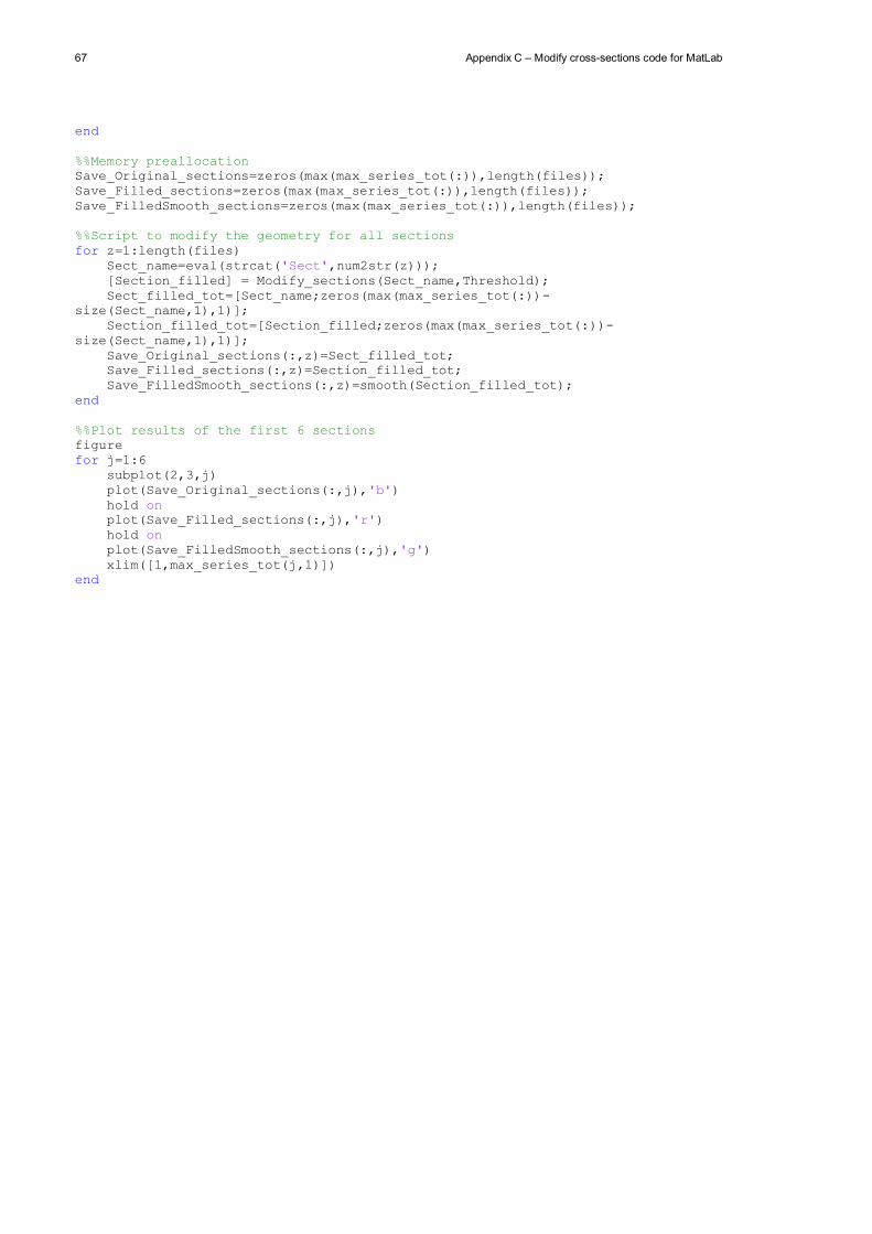
67 Appendix C – Modify cross-sections code for MatLab
end %%Memory preallocation Save_Original_sections=zeros(max(max_series_tot(:)),length(files)); Save_Filled_sections=zeros(max(max_series_tot(:)),length(files)); Save_FilledSmooth_sections=zeros(max(max_series_tot(:)),length(files)); %%Script to modify the geometry for all sections for z=1:length(files) Sect_name=eval(strcat('Sect',num2str(z))); [Section_filled] = Modify_sections(Sect_name,Threshold); Sect_filled_tot=[Sect_name;zeros(max(max_series_tot(:))-size(Sect_name,1),1)]; Section_filled_tot=[Section_filled;zeros(max(max_series_tot(:))-size(Sect_name,1),1)]; Save_Original_sections(:,z)=Sect_filled_tot; Save_Filled_sections(:,z)=Section_filled_tot; Save_FilledSmooth_sections(:,z)=smooth(Section_filled_tot); end %%Plot results of the first 6 sections figure for j=1:6 subplot(2,3,j) plot(Save_Original_sections(:,j),'b') hold on plot(Save_Filled_sections(:,j),'r') hold on plot(Save_FilledSmooth_sections(:,j),'g') xlim([1,max_series_tot(j,1)]) end
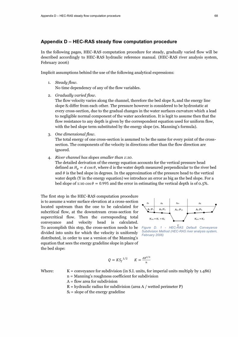
Appendix D – HEC-RAS steady flow computation procedure 68
Appendix D – HEC-RAS steady flow computation procedure
In the following pages, HEC-RAS computation procedure for steady, gradually varied flow will be described accordingly to HEC-RAS hydraulic reference manual. (HEC-RAS river analysis system, February 2006)
Implicit assumptions behind the use of the following analytical expressions:
1. Steady flow. No time dependency of any of the flow variables.
2. Gradually varied flow. The flow velocity varies along the channel, therefore the bed slope S0 and the energy line slope Sf differ from each other. The pressure however is considered to be hydrostatic at every cross-section, due to the gradual changes in the water surfaces curvature which a lead to negligible normal component of the water acceleration. It is legit to assume then that the flow resistance to any depth is given by the correspondent equation used for uniform flow, with the bed slope term substituted by the energy slope (ex. Manning’s formula).
3. One dimensional flow. The total energy of one cross-section is assumed to be the same for every point of the cross-section. The components of the velocity in directions other than the flow direction are ignored.
4. River channel has slopes smaller than 1:10. The detailed derivation of the energy equation accounts for the vertical pressure head defined as 𝐻𝑝 = 𝑑 cos 𝜃, where d is the water depth measured perpendicular to the river bed and 𝜃 is the bed slope in degrees. In the approximation of the pressure head to the vertical water depth (Y in the energy equation) we introduce an error as big as the bed slope. For a bed slope of 1:10 cos 𝜃 = 0.995 and the error in estimating the vertical depth is of 0.5%.
The first step in the HEC-RAS computation procedure is to assume a water surface elevation at a cross-section located upstream than the one to be calculated for subcritical flow, at the downstream cross-section for supercritical flow. Then the corresponding total conveyance and velocity head is calculated. To accomplish this step, the cross-section needs to be divided into units for which the velocity is uniformly distributed, in order to use a version of the Manning’s equation that sees the energy gradeline slope in place of the bed slope:
𝑄 = 𝐾𝑆𝑓1 2⁄ 𝐾 = 𝐴𝑅2 3⁄
𝑛
Where: K = conveyance for subdivision (in S.I. units, for imperial units multiply by 1.486) n = Manning’s roughness coefficient for subdivision A = flow area for subdivision R = hydraulic radius for subdivision (area A / wetted perimeter P) Sf = slope of the energy gradeline
Figure D. 1 - HEC-RAS Default Conveyance Subdivision Method (HEC-RAS river analysis system, February 2006)

69 Appendix D – HEC-RAS steady flow computation procedure
The velocity head weighting coefficient is now calculated as:
𝛼 =(𝐴𝑡)2 [𝐾𝑙𝑜𝑏
3
𝐴𝑙𝑜𝑏2 + 𝐾𝑐ℎ
3
𝐴𝑐ℎ2 + 𝐾𝑟𝑜𝑏
3
𝐴𝑟𝑜𝑏2 ]
𝐾𝑡3
Where: At = total flow area of cross section Alob, Ach, Arob = flow areas of left overbank, main channel and right overbank Kt = total conveyance of cross section Klob, Kch, Krob = conveyance of left overbank, main channel and right overbank
With the values obtained, the energy head loss is calculated as sum of friction losses and contraction or expansion losses:
ℎ𝑒 = 𝐿𝑆�� + 𝐶 |𝛼2𝑉2
2
2𝑔−
𝛼1𝑉12
2𝑔 |
Where: 𝑆�� = representative friction slope between two sections C = expansion or contraction loss coefficient
The friction slope is by the fault defined as 𝑆�� = (𝑄1+𝑄2𝐾1+𝐾2
)2, but other options are available inside the
program according to flow regime and profile type.
The contraction and expansion coefficient need to be set for each cross-section and the program will automatically assume that contraction is occurring whenever the velocity head downstream is greater than the velocity head upstream, expansion in the opposite case. Typical values for gradually varied flow are of 0.1 for contraction and 0.3 for expansion.
Finally, the water level at the desired cross-section can be calculated with the energy equation:
𝑍2 + 𝑌2 +𝛼2𝑉2
2
2𝑔= 𝑍1 + 𝑌1 +
𝛼1𝑉12
2𝑔+ ℎ𝑒
Where: Z1, Z2 = elevation of the main channel inverts Y1, Y2 = depth of water at cross sections V1, V2 = average velocities (total discharge/total flow area) 1, 2 = velocity weighting coefficients g = gravitational acceleration he = energy head loss
Figure D. 2 - Example of how mean energy is obtained (HEC-RAS river analysis system, February 2006)
Figure D. 3 - Representation of terms in the energy equation (HEC-RAS river analysis system, February 2006)

Appendix D – HEC-RAS steady flow computation procedure 70
The program now compares the value here obtained with the one assumed at the beginning and iterates the process until the two values agree within 0.003 m or the user defined tolerance.
However, the energy equation is valid only in gradually varied flow conditions, so it is not applicable whenever the water surface passes through critical depth (significant changes in channel slope, bridge constrictions, drop structures and weirs, stream junctions, hydraulic jumps). For all these cases, the program uses specific empirical equations or the momentum equation:
𝑃2 − 𝑃1 + 𝑊𝑥 − 𝐹𝑓 = 𝑄𝜌Δ𝑉𝑥
Where: P = hydrologic pressure at locations 1 and 2 Wx = force due to water weight in the x direction Ff = force due to external friction losses from 2 and 1 Q = discharge = density of water Vx = change on velocity from 2 to 1 in the x direction
Or in the operative form used in HEC-RAS:
𝑄22𝛽2
𝑔𝐴2+ 𝐴2𝑌2 + (
𝐴1 + 𝐴2
2 ) 𝐿𝑆0 − (𝐴1 + 𝐴2
2 ) 𝐿𝑆�� =𝑄1
2𝛽2
𝑔𝐴1+ 𝐴1𝑌1
Where: = momentum coefficient that accounts for a varying velocity distribution in irregular channels Q1, Q2 = discharge at cross section 1 and 2 A1, A2 = wetted area at cross section 1 and 2 Y1, Y2 = depth measured from water surface to the centroid of the cross sectional area at location 1 and 2 L = distance between sections 1 and 2 along the x axis S0 = slope of the channel, based on mean bed elevation 𝑆�� = representative friction slope between sections 1 and 2
Figure D. 4- application of momentum principle (HEC-RAS river analysis system, February 2006)


Bibliography 72
Bibliography
SRTM - https://lta.cr.usgs.gov/products_overview. Ethnologue, Languages of the World - https://www.ethnologue.com/country/MZ/languages. Advances in flash flood monitoring using unmanned aerial vehicles (UAVs) [Journal] / auth. Perks Matthew T., Russell Andrew J. and Large Andrew R. G. // Hydrology and Earth System Sciences. - 2016. - Vol. 20. - pp. 4005–4015. - doi:10.5194/hess-20-4005-2016. Agisoft Photoscan User Manual: Professional Edition, version 1.4 [Book] / auth. Agisoft LLC. - 2018. Assessing the impact of different sources of topographic data on 1-D hydraulic modelling of floods [Journal] / auth. Ali A. Md, Solomatine D. P. and Di Baldassarre G. // Hydrology and Earth System Sciences. - [s.l.] : Hydrology and Earth System Sciences, 2015. - Vol. 19. - pp. 631–643. - doi:10.5194/hess-19-631-2015. Assessing the quality of digital elevation models obtained from mini unmanned aerial vehicles for overland flow modelling in urban areas [Journal] / auth. Leitao Joao P. [et al.] // Hydrology and Earth System Sciences. - 2016. - Vol. 20. - pp. 1637–1653. - doi:10.5194/hess-20-1637-2016. Atlas for Disaster Preparedness and Response in the Limpopo Basin. [Online] / auth. Leira E.M. [et al.]. - 2002. - July 2018. - http://edmc1.dwaf.gov.za/library/limpopo/index.htm. Bathymetry of the Limpopo River surveyed with Total Station and RTK GPS / auth. Saimone Francisco // Personal Comunication. - [s.l.] : Salomon LDA, January 2010. Climate Change Implications for Water Resources in the Limpopo River Basin [Report] / auth. Zhu Tingju and Ringler Claudia / Environment and Production Technology Division. - [s.l.] : International Food Policy Research Institute, 2010. Comparison of remotely sensed water stages from LiDAR, topographic contours and SRTM [Journal] / auth. Schumann G. [et al.] // ISPRS Journal of Photogrammetry and Remote Sensing. - 2008. - Vol. 63. - pp. 283–296. DJI GO [Online] / auth. DJI. - August 2018. - https://www.dji.com/goapp. DJI GS Pro [Online] / auth. DJI. - August 2018. - https://www.dji.com/ground-station-pro. Drone Deploy, version 2.67.1 [Online] / auth. Drone Deploy // https://www.dronedeploy.com. - August 2018. Drought impact mitigation and prevention in the Limpopo River Basin, a situation analysis [Report] / auth. FAO. - Rome : Subregional Office for Southern and East Africa Harare, 2004. Enhancing Spatial Data for Flood Risk Management in the Limpopo River Basin [Online] / auth. World Bank, DNGRH. - 2016. - https://www.gfdrr.org/enhancing-spatial-data-flood-risk-management-limpopo-river-basin-bank-executed. ‘Structure-from-Motion’ photogrammetry: A low-cost, effective tool for geoscience applications [Journal] / auth. Westoby M.J. [et al.] // Geomorphology. - 2012. - Vol. 179. - pp. 300–314. - http://dx.doi.org/10.1016/j.geomorph.2012.08.021. Experiences from the use of Unmanned Aerial Vehicles (UAV) for River Bathymetry Modelling in Norway [Journal] / auth. Zinke Peggy and Flener Claude // Presented at "Technoport – Sharing possibilities". - Trondheim : [s.n.], 16-18 April 2012. Experiences from the use of Unmanned Aerial Vehicles (UAV) for River Bathymetry Modelling in Norway [Book] / auth. Zinke Peggy and Flener Claude. - [s.l.] : Presented at "Technoport – Sharing possibilities", 16-18 April 2018 in Trondheim, 2012. Exploring the potential of SRTM topographic data for flood inundation modelling under uncertainty [Journal] / auth. Yan Kun, Di Baldassarre Giuliano and Solomatine Dimitri P. // Journal of Hydroinformatics. - 2013. - Vol. 15. - pp. 849–861. - doi: 10.2166/hydro.2013.137. Fluvial Remote Sensing for Science and Management [Book] / auth. Carbonneau P. E. and Piegay H.. - Chichester/UK : Wiley-Blackwell, 2012. - ISBN: 978-0-470-71427-0. Green, waveform lidar in topo-bathy mapping – Principles and Application [Online] / auth. Nayegandhi Amar // National Geodetic Survey. - National Oceanic and Atmospheric Administration, department of National Geodetic Survey. - https://www.ngs.noaa.gov/corbin/class_description/Nayegandhi_green_lidar.pdf. HEC-RAS 2D model of the Limpopo River / auth. Manane Josè // Personal Comunication. - [s.l.] : Consultec LDA, 2017. HEC-RAS, version 5.0.5 [Online] / auth. US Army Corps of Engineers. - http://www.hec.usace.army.mil/software/hec-ras/. Hydraulic Reference Manual [Book] / auth. HEC-RAS river analysis system. - [s.l.] : U.S. Army Corps of Engineers, Institute for Water Resources, Hydraulic Engineering Center, February 2006.
73 Bibliography
Improving a DSM Obtained by Unmanned Aerial Vehicles for Flood Modelling [Journal] / auth. Mourato Sandra [et al.] // IOP Conference Series: Earth and Environmental Science. - 2017. - p. 95. - doi:10.1088/1755-1315/95/2/022014 . InSAR principles: guideline for interferometry processing and interpretation [Online] / auth. ESA // ESA. - http://www.esa.int/About_Us/ESA_Publications/InSAR_Principles_Guidelines_for_SAR_Interferometry_Processing_and_Interpretation_br_ESA_TM-19. Joint Limpopo river basin study, schoping phase [Report] / auth. LBPTC / Republica De Mocambique Ministerio Das Obras Publicas E Habitacao Direccao Nacional De Aguas. - [s.l.] : Limpopo basin permanent techninca comitee, 2010. Limpopo river basin. A proposal to improve the flood forecasting and early warning system. [Report] / auth. World Meteorological Organization . - 2012. MatLab , version R2017a [Online] / auth. Math Works. - https://se.mathworks.com/products/matlab.html. Mitigating systematic error in topographic models derived from UAV and ground-based image networks [Journal] / auth. James Mike R. and Robson Stuart // Earth Surface Processes and Landforms. - 2014. - 10.1002/esp.3609. Modeling the topography of shallow braided rivers using Structure-from-Motion photogrammetry [Journal] / auth. Javernick L., Brasington J. and Caruso B. // Geomorphology. - 2014. - Vol. 213. - pp. 166–182. - DOI: 10.1016/j.geomorph.2014.01.006. Near real-time flood wave approximation on large rivers from space: application to the River Po, Northern Italy [Journal] / auth. Schumann G. [et al.] // Water Resources Research. - 2010. - p. 46. - W05601, doi:10.1029/2008WR007672. On the use of SRTM and altimetry data for flood modeling in data-sparse regions [Journal] / auth. Domeneghetti Alessio // AGU Publications. - [s.l.] : AGU Publications, 2016. - Vol. 52. - pp. 2901–2918. - 10.1002/2015WR017967. Photography Life [Online] // Photography Life. - 2018. - https://photographylife.com. Photoscan Professional Edition, version 1.4 [Online] / auth. Agisoft. - http://www.agisoft.com. Pix4D Capture. version 2.9.2 [Online] / auth. Pix4D. - https://pix4d.com/product/pix4dcapture/. QGIS, version 2.18.15 [Online] / auth. QGIS. - August 2018. - https://qgis.org/en/site/. Remote Sensing and Image Interpretation [Book] / auth. Lillesand Thomas M., Kiefer Ralph W. and Chipman Jonathan W.. - [s.l.] : John Wiley & Sons, 2004. Remote sensing of bottom reflectance and water attenuation parameters in shallow water using aircraft and Landsat data [Journal] / auth. Lyzenga D. R. // International Journal of Remote Sensing. - 1981. - Vol. 2. - pp. 71-82. Scene Reconstruction and Visualization from Internet Photo Collections [Book] / auth. Snavely Keith N. . - [s.l.] : University of Washington, 2008. Structure from Motion (SfM) Photogrammetry [Book] / auth. Micheletti Natan, Chandler Jim, H. and Lane Stuart, N. - 2015. - ISSN 2047-0371. The 1950-1998 warm ENSO events and regional implications to river flow variability in Southern Africa. [Journal] / auth. Alemaw B.F. and Chaoka T.R. // Journal Water SA 32(4). - [s.l.] : Journal Water SA 32(4), 2006. - Vol. 32. - pp. 459-463. - ISSN 0378-4738. The future of distributed models – model calibration and uncertainty prediction [Journal] / auth. Beven K. and Binley A // Hydrological Processes. - [s.l.] : Hydrological Processes, 1992. - Vol. 6. - pp. 279– 298. - doi:10.1002/hyp.3360060305. The interpretation of structure from motion [Book] / auth. Ullman S.. - [s.l.] : M.I.T. Artificial intelligence laboratory, 1976. The Limpopo river basin [Online] / auth. Limpopo River Awarness Kit // Limpopo River Awarness Kit. - http://www.limpopo.riverawarenesskit.org/LIMPOPORAK_COM/EN/RIVER.HTM. The topographic data source of digital terrain models as a key element in the accuracy of hydraulic flood modelling [Journal] / auth. Casas A. [et al.] // Earth Surface Processes and Landforms. - [s.l.] : Earth Surface Processes and Landforms, 2006. - Vol. 31. - pp. 444–456. - doi:10.1002/esp.1278, 2006. U.S. Releases Enhanced Shuttle Land Elevation Data [Online] / auth. Nasa, JPL and CalTech // JPL. - https://www2.jpl.nasa.gov/srtm/. Unmanned Aerial Systems for Photogrammetry and Remote Sensing: A Review. [Journal] / auth. Colomina I. and Molina P. // Journal of Photogrammetry and Remote Sensing. - [s.l.] : Journal of Photogrammetry and Remote Sensing, 2014. - Vol. 92. - pp. 79-97.


TRITA -ABE-MBT-18444
www.kth.se