Unmanned Aerial System Hydra Technologies Éhecatl wing optimization using a morphing approach

Oliviu Şugar Gabor, Andreea Koreanschi, Ruxandra Mihaela Botez

Department of Automated Production Engineering, École de Technologie Supérieure, 1100 Notre Dame Ouest, Montréal, H3C1K3, Quebéc, Canada

Oliviu.Sugar-Gabor.1@ens.etsmtl.ca, Andreea.Koreanschi.1@ens.etsmtl.ca, Ruxandra.Botez@etsmtl.ca

Abstract

In this paper, we describe a practically efficient methodology of improving the aerodynamic characteristics of an UAS's wing using a morphing approach. We have replaced a part of the original wings' upper and lower surfaces with a flexible, composite material skin whose shape can be modified, according to the variable airflow conditions, using internally placed actuators. The optimal displacements of the actuators, as functions of the external flow characteristics, are determined using a genetic algorithm based optimizer, coupled with a three - dimensional numerical extension of the classical lifting line model for estimating the modified wing aerodynamic coefficients. We have used the optimization tool to decrease the overall drag coefficient of a military grade UAS' wing equipped with the flexible skin. We have obtained good quality solutions for only a fraction of the computational cost needed when performing viscous flow field calculations.

Introduction

In recent years, Unmanned Aerial Systems (UAS) have become increasingly used in both military and civil aviation. Their main goal has been performing long time surveillance flights, at various altitudes and flight speeds, and sometimes in rapidly changing weather conditions. Because of the increasing demand of UAS's, engineers and designers have searched for methods to improve their flight performances, in order to make them more adaptable for various flight missions, to improve their aerodynamic efficiency and to increase their effective range and payload.

One answer to all these aircraft design challenges is to use a morphing technique, to provide the aircraft with the capacity of detecting the changes occurring in the airflow around it and to adapt to them by modifying its geometry, usually the wing, during flight. Sofla et al [1] conducted a comprehensive study of the various aircraft morphing solutions proposed by different authors, identifying the part of the aircraft wing subjected to morphing, the design solution that was found in order to achieve the desired

modifications, as well as indicating the maturity level of the proposed solution (theoretical analysis, functional prototype, wind tunnel tests, flight tests).

A remarkable project into developing a functional morphing aircraft was Lockheed Martin's unmanned combat air vehicle (UCAV), which had wing folding capabilities. [2] [3] The goal of the project was to explore the ability of expanding an UAV's flight and mission envelope by using a radical change of the wing. The UCAV would be capable of long range cruise by minimizing fuel burn using the extended wing span, as well as transitioning into the attack mode, with higher maximum speed and increased manoeuvrability by decreasing its wing span. A functional model of the UCAV was designed, fabricated and tested in the wind tunnel, at speed ranging from the subsonic incompressible regime up to transonic conditions.[4]

Gamboa et al [5] presented another concept of a morphing wing developed for a small Unmanned Aerial Vehicle. The morphing wing created had both span and chord expansion capabilities, its purpose was to obtain the overall drag reduction with respect to the original, fixed wing, for low speeds ranging from 15 m/s up to 50 m/s. Drag reductions between 14.7% at a speed of 20 m/s and 34.5% at a speed of 50 m/s have been obtained, demonstrating the viability of using morphing wings for optimizing an UAV's aerodynamic performance for several flight conditions.

NEXTGEN Aeronautics proposed an UAV design with a wing structure capable of being transformed from a high span configuration for slow speed flights, to a configuration with a reduced wing span, adapted to high speed flight. [6] In this proposed solution, the wing was based on a moveable truss structure that could be controlled using electro - mechanical actuators, in order to adjust the wing span, area and shape according to variable flight conditions. In August 2006, NEXTGEN performed a successful flight test of the prototype. The UAV could sustain wing area changes of 40%, span changes of 30% and sweep angles varying from 15 degrees to 35 degrees, depending on the morphing position adopted. The airspeed attained during testing was around 100 knots.

The CRIAQ 7.1 project took place between 2006 and 2009 and was realized following a collaboration approach between teams form École de Technologie Supérieure (ÉTS), École Polytechnique de Montréal, Bombardier Aerospace, Thales Canada and the Institute for Aerospace Research – National Research Canada (IAR - NRC). The objective of the project was to improve and control the laminarity of the flow past a morphing wing, in order to obtain important drag reductions.

In this project, the active structure of the morphing wing combined three main subsystems: a flexible, composite material upper surface, stretching between 3% and 70% of the airfoil chord; a rigid inner surface; an actuator group located inside the wing box, which could morph the flexible skin at two points, located at 25.3% and 47.6% of the chord. The skin was manufactured from a flexible composite material, while the actuation system consisted of a Shape Metal Alloy (SMA) active element and a cam transmission system. [7]

The reference airfoil chosen was the WTEA laminar airfoil. The morphing airfoil was designed for subsonic flow conditions (from Mach = 0.2 to Mach = 0.3), and for typical cruise angles of attack (from -1 deg. to 2 deg.). A theoretical study of the morphing wing system was performed. [8] An optimizer

coupled with a subsonic aerodynamic solver with transition prediction capabilities allowed the flexible skin shape optimization, under the assumption of constant lift coefficient. In this study, very promising results were obtained; the morphing system was able to delay the transition location downstream by up to 30% of the chord, and to reduce the airfoil drag by up to 22%. The wind tunnel tests were performed in the 2 m by 3 m atmospheric closed circuit subsonic wind tunnel at IAR - NRC. The rigid part of the model was equipped with static pressure taps, while the flexible upper surface was equipped with sixteen Kulite pressure transducers, for transition location detection. In addition, infra - red camera visualizations were performed to validate the transition location. [9]

Finite Span Wing Model

Prandtl's classical lifting line theory, first published in 1918 [10], represented the first analytical model capable of accurately predicting the lift and induced drag of a finite span lifting surface. The aerodynamic characteristics predicted by the theory were repeatedly proven to be in close agreement with experimental results, for straight wings with moderate to high aspect ratio.

The theory was based on the hypothesis that a finite span wing could be replaced by a continuous distribution of vorticity bound to the wing surface, and a continuous distribution of shed vorticity that trails behind the wing, in straight lines in the direction of the free stream velocity. The intensity of these trailing vortices is proportional to rate of chance of the lift distribution along the wing span direction. The trailing vortices induce a velocity, known as downwash, normal to the direction of the free stream velocity, at every point along the span. Because of the downwash, the effective angle of attack at each section in the spanwise direction is different from the geometric angle of attack of the wing, the difference being called the induced angle of attack. Using the effective angle of attack, the downwash produced by the trailing vortices and the two - dimensional Kutta - Joukowski vortex lifting law, Prandtl developed an integral equation that allowed the calculation of the continuous bound vorticity intensity, and thus the calculation of the wing's lift and induced drag.

The solution of Prandtl's classical equation is in the form of an infinite sine series for the bound vorticity distribution. Traditionally, the series is truncated to a finite number of terms, and collocation methods are used to determine the sine series coefficients, by requiring that the lifting line equation must be satisfied at a given number of spanwise stations. The method was firstly presented by Glauert [11]. Popular methods of determining the bound vorticity distribution included those developed by Tani [12] and Multhopp [13]. Other authors have proposed modified versions of the original lifting line theory, modifications that increase the quality of the obtained results, increase the applicability or the model or make use of information regarding the wing's airfoil sections. Jones [14] presented a correction that better accounts for the chord distribution along the wing span, Weissinger [15] developed a lifting line model that could be used to determine the lift and induced drag of a swept - back wing, while Sivells and Neely [16] developed a calculation method based on the lifting line model, but also uses wind tunnel data to estimate the aerodynamic coefficients of the wing's airfoil sections, thus allowing solutions to be obtained for angles of attack close to stall, and also allowing a good estimation of the wing's viscous

drag coefficient. More modern solutions include that of Rasmussen and Smith [17], who presented a more rigorous method based on a Fourier series expansion.

With the development of more efficient and powerful computers, several authors have also proposed purely numerical methods for solving Prandtl's lifting line equation. Among these, we can mention McCormick [18], Anderson et al [19] or Katz and Plotkin [20]. However, all the above mentioned numerical methods were based on Prandtl's assumptions of a straight distribution of bound vorticity, and therefore are subjected to all the limitations of the classical lifting line model: a single lifting surface of moderate to high aspect ratio, with no sweep angle and no means of considering the effects of the various wing sections airfoils.

The method used in this paper is based on the original work of Phillips and Snyder [21]. Whereas the classical lifting line theory is based on the assumption of a straight lifting surface and the application of the two - dimensional Kutta - Joukowski vortex lifting law for a three dimensional flow, the modern adaptation uses a general horseshoe vortex distribution and uses a fully three - dimensional vortex lifting law. Because of these characteristics, the method has a much wider applicability range compared to the original theory, including multiple lifting surfaces and wings arbitrary camber, sweep and dihedral angle. Also, the method is not based on the assumption of a linear relationship between the lift coefficient and the local angle of attack of any given spanwise section of the wing, thus it can be applied for high geometric angles of attack, to account approximately for the effects of stall. The only limitation of the method is that it is no longer valid for wings with aspect ratios smaller than four, so the constraint of medium to high aspect ratio lifting surface that applies to Prandtl's original theory also applies to its' modern adaptation.

Wing Calculation Method

In numerical lifting line models, the continuous distribution of bound vorticity over the lifting surface and the continuous distribution of trailing vorticity are approximated using a finite number of horseshoe vortices. The bound portion of the vortices can be aligned with the wing's quarter chord line, thus taking into consideration the local values of the sweep and dihedral angles, while the trailing portions remain aligned with the free stream velocity, as shown in Figure 1.

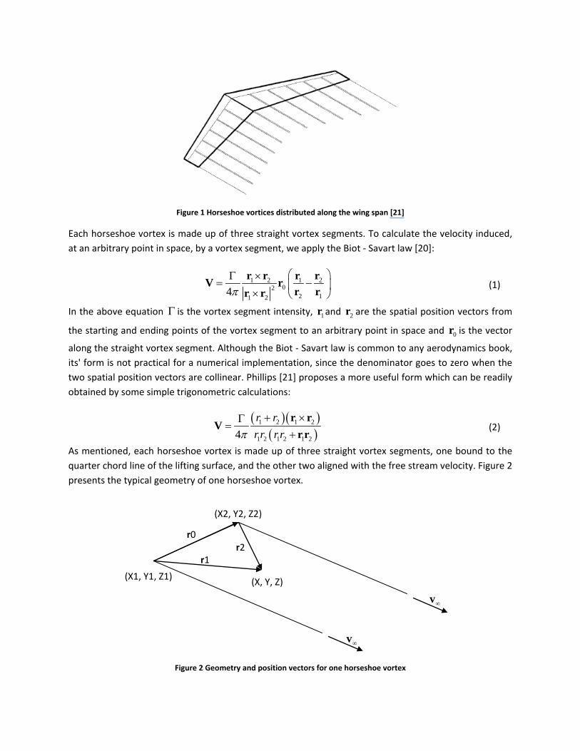
Figure 1 Horseshoe vortices distributed along the wing span [21]

Each horseshoe vortex is made up of three straight vortex segments. To calculate the velocity induced, at an arbitrary point in space, by a vortex segment, we apply the Biot - Savart law [20]:

1 2 1 202

2 11 24π

×Γ= −

×

r r r rV rr rr r

(1)

In the above equation Γ is the vortex segment intensity, 1r and 2r are the spatial position vectors from

the starting and ending points of the vortex segment to an arbitrary point in space and 0r is the vector

along the straight vortex segment. Although the Biot - Savart law is common to any aerodynamics book, its' form is not practical for a numerical implementation, since the denominator goes to zero when the two spatial position vectors are collinear. Phillips [21] proposes a more useful form which can be readily obtained by some simple trigonometric calculations:

( )( )( )

1 2 1 2

1 2 1 2 1 24r rr r r rπ+ ×Γ

=+r r

Vr r

(2)

As mentioned, each horseshoe vortex is made up of three straight vortex segments, one bound to the quarter chord line of the lifting surface, and the other two aligned with the free stream velocity. Figure 2 presents the typical geometry of one horseshoe vortex.

Figure 2 Geometry and position vectors for one horseshoe vortex

∞v

∞v

r1 r2

r0

(X1, Y1, Z1)

(X2, Y2, Z2)

(X, Y, Z)

When we apply equation (2) for all segments of the horseshoe vortex, we can determine the velocity induced at an arbitrary point in space:

( )( )( )

( ) ( )1 2 1 22 1

2 2 2 1 2 1 2 1 2 1 1 14 4 4r r

r r r r r r r rπ π π∞ ∞

∞ ∞

+ ×× ×Γ Γ Γ= + −

− + −r rv r v rV

v r r r v r (3)

When considering the distribution of horseshoe vortices over the lifting surface, equation (3) can be used to compute the velocity induced at any point on the lifting surface, by any of the horseshoe vortices, provided that the intensities Γ are known.

If we approximate the continuous distribution of bound vorticity with a finite number of N distinct horseshoe vortices, each one having its own intensity iΓ , we will need a mathematical system of Nequations relating these intensities to some known properties of the wing. In order to find such a relation, we turn to the three dimensional vortex lifting law [22]. Using the same approach as that suggested by Saffman [22] or by Phillips [21], the non - viscous force acting on a horseshoe element of the lifting surface is equal to:

i i i iρ= Γ ×F V l (4) In the above equation, ρ is the air density, iΓ is the unknown intensity of the horseshoe vortex, iV is

the local airflow velocity and il is a spatial vector along the bound segment of the horseshoe vortex,

aligned in the direction of the local circulation.

The significant difference between equation (4) and the two - dimensional Kutta - Joukowski vortex lifting law used in the classical lifting line theory is the presence of the local airfoil velocity, instead of using the free stream velocity. This allows for introduction of three - dimensional effects such as wing sweep and dihedral angle in the numerical lifting line model, and also captures more accurately the influence of local wing section airfoil characteristics.

In order to calculate the local velocity, with each horseshoe vortex we have to associate a control point at which the induced velocities will be determined. We consider the control points to be situated on the wing surface, at equal distance between the two semi-infinite trailing legs of the horseshoe vortex, at the three quarter chord point, as measured from the local section leading edge. The importance of choosing the three quarter chord point has been revealed by various authors [13], [20], [15]. Thus, the local velocity at each control point becomes:

1

N

i j ijj

∞=

= + Γ∑V V v (5)

We denote by ∞V the free stream velocity, while ijv represents the velocity induced by the horseshoe

vortex j , considered to be of strength equal to unity, at the control point i , and is given by equation(3).

From wing theory, we know that the magnitude of the non - viscous aerodynamic force acting on an iAarea section of the wing located at a control point i can be written as:

212 ii Li

V ACρ ∞=F (6)

The lift coefficient iLC is that of the local airfoil situated at the wingspan section corresponding to

control point i and it depends on the local effective angle of attack. If the lift coefficient can be determined using other means, such as experimentally determined lift curves or using a two - dimensional airfoil calculation solver, then, by replacing the local velocity given by equation(5) into equation (4), and then equating the modulus of the three - dimensional vortex lifting force with the expression give in equation (6), we obtain the following relation:

2

1

12 i

N

i j ij i i Lj

V ACρ ρ∞ ∞=

Γ + Γ × =

∑V v l (7)

By writing equation (7) for all control points along the wing span, we obtain a nonlinear system of Nequations for the calculation of the unknown horseshoe vortex intensities. The system can be solved in an iterative fashion, using Newton's method. However, in order to avoid the necessity of analytically calculating all the entries in the system's Jacobian matrix, we use Broyden's quasi - Newton method [23], in which the Jacobian is replaced by an approximation that is updated at each iteration.

Also, the right hand side of the nonlinear system must be updated each iteration, since the local lift coefficient depends on the local angle of attack, and each change in the horseshoe vortices intensities, changes that are inevitable in an iterative process, will cause a change in the local angles of attack values, as follows:

1tan i ii

i i

α − =

VnVc

(8)

As before, iV represents the local airflow velocity, in is a unit length vector in the direction normal to

the chord of the local airfoil and ic is a unit length vector in the direction of the chord of the local airfoil.

Once the intensities of the horseshoe vortices have been determined, the total non - viscous aerodynamic force can be readily calculated by summing up all the individual forces given by equation(4), resulting:

1 1

N N

i j ij ii j

ρ ∞= =

= Γ + Γ ×

∑ ∑F V v l (9)

The calculation method presented, like that developed in [16], can be used to approximate the profile drag coefficient of the wing, since the spanwise lift distribution will not only verify all the constraints imposed by the numerical lifting line theory, but also those imposed by several wingspan airfoil characteristics. As presented in [16], the profile drag coefficient of the wing is given by:

/2

0 0 01/2

1 1( ) ( )i

b N

D D D i iib

C c y c y dy c c yS S =−

= ≈ ∆∑∫ (10)

In the above equation, S represents the total wing area, b is the wing span, 0iDc is the profile drag

coefficient of wingspan section i , as calculated from the available experimental data or calculated by the two - dimensional solver, while ic is the wing's chord at the given control point section.

Two - dimensional flow solver

The code used for the calculation of the two - dimensional aerodynamic characteristics of the wing's control sections is XFOIL, version 6.96, developed by Drela and Youngren [24]. The XFOIL code was chosen because it has proven its precision and effectiveness over time, and because it reaches a converged solution very fast. The inviscid calculations in XFOIL are performed using a linear vorticity stream function panel method. A Karman - Tsien compressibility correction is added, allowing good predictions all the way to transonic flow. For the viscous calculations, XFOIL uses a two - equation lagged

dissipation integral boundary layer formulation, and incorporating the Ne transition criterion. The flow in the boundary layer and in the wake is interacted with the inviscid potential flow by using the surface transpiration model. [24]

Wing morphing technique

The main idea behind the morphing concept is to replace a part of the wing' upper and lower surfaces with a flexible skin that can be modified using actuators placed inside the wing body. To perform the optimization, the flexible skin will be chosen to start on the wings' lower surface, at 20% of the chord (as measured from the leading edge), it will go around the wings' leading edge and continue on the upper surface until 65% of the chord (as measured from the leading edge). A section of the wing equipped with the morphing skin is shown in Figure 3.

Figure 3 Extent of the morphing skin for one spanwise station

Along the wingspan direction, at several predetermined stations, we place the actuator lines. Each of the actuation lines is aligned with the local chord of the spanwise station. To modify the shape of the flexible skin, we chose a number of 10 actuation points for each spanwise actuator line, points that are distributed along the length of the skin, but with a greater density around the leading edge. The choice

20% of the chord

65% of the chord Morphing skin

of this high number was found necessary in order to accurately control the deformation of the leading edge and to avoid unrealistic shapes during the optimization process. Each actuation point is constrained to move only on the direction given by the local normal vector to the airfoil surface. Also, the magnitude of the displacement is limited between the values of 1% of the local wing chord when the actuation point is pushed towards the outside of the original airfoil curve and 0.5% of the local wing chord when the actuation point is pulled towards the inside of the original airfoil curve. The distribution of actuation points for any spanwise airfoil section is depicted in Figure 4.

Figure 4 Position of the actuation points for one spanwise station

In order to regenerate the airfoil shape of each of the spanwise stations, regeneration necessary after each movement of any of the actuation points, we have used a Non Uniform Rational B - Splines (NURBS) parameterization of the airfoil curve. [25]The initial characteristics of the NURBS curve that describes each spanwise station airfoil are determined through interpolation. As actuation points, we chose to use the NURBS curves control points, instead of points situated directly on the wing surface. However, the movement of these control points is still subjected to all the constraints listed above. The 3rd degree NURBS curves that we chose insure continuity up to the second derivative for the entire length of the elastic skin, as well as the continuity between the skin and the rigid parts of the wing.

Wing optimization technique

The objective of the aerodynamic optimization is to decrease the wing's drag coefficient. The optimization procedure consists in finding the optimal displacements of all the actuation points, for all the spanwise calculation sections, in such a way that, for any given combination of free stream Mach number and geometric angle of attack, the drag of the wing equipped with the morphing skin is as small as possible. The optimization tool is a genetic algorithm code, coupled with the numerical lifting line code for the calculation of the wing's aerodynamic coefficients.

Genetic algorithms are numerical optimization algorithms inspired by natural selection and genetics of living organisms. The algorithm is initialized with a population of guessed individuals, and uses three operators namely selection, crossover and mutation to direct the population towards convergence to the global optimum, over a series of generations. [26], [27]

Actuation points

20% of the chord

65% of the chord

Each individual in the population is defined by a matrix of real values, that of the displacements of all

the control points, ( ),i jδ , where 1,2,...,10i = , 1,2,...,j N= . The number of rows is equal to the

number of actuation points on each spanwise section, while the number of columns is equal to the predetermined number of spanwise actuation lines.

In order to evaluate all individuals in the population, an objective function, called the fitness function, must be defined. Because the goal of the optimization is to decrease the wing's drag coefficient, the following fitness function was used in the algorithm:

1

D

FitnessC

= (11)

The fitness function is calculated for all individuals of a given generation. The higher the values of the fitness function, the higher are the chances of the individual to be selected for building the next generation.

Figure 5 Outline of the genetic algorithm optimization tool

Initialization

Randomly create the initial generation

Fitness estimation

Selection

Select best individuals based on fitness

Reproduction

Create new generation by mutation and

crossover

Final generation Output results

Numerical lifting line

XFOIL

NURBS parameterization

The process of evaluation of the fitness function, selection of the best individuals to become parents, crossover and mutation of the new individuals continues in an iterative way, until the maximum number of generations is reached.

The optimization tool has already demonstrated its' capabilities with the problem of increasing the laminarity of the flow and decreasing the viscous drag coefficient of the ATR 42 airfoil, for several different flight conditions [28]. The optimization was performed for the ATR 42 airfoil, with a chord of 0.244 meters. The morphing skin stretched between 10% and 70% of the chord, only on the upper surface, with only two actuators, situated at 30% and 50% of the chord. The optimization was performed in the subsonic incompressible flow regime for three angle of attack values, -2, 0 and 2 degrees, while the Mach number varied between 0.1 and 0.2 and the Reynolds number varied between 578000 and 1156000. It has been possible to delay the transition point on the upper surface of the airfoil by as much as 24.81%, and to reduce the drag coefficient with up to 26.73%.

Brief description of the UAS

The wing optimization procedure shall focus on replacing the conventional, rigid wing of the Hydra Technologies S4 Éhecatl Unmanned Aerial System with a morphing wing. Hydra Technologies is based in Mexico. The S4 was designed and build in Mexico, and it was created as an aerial unmanned surveillance system, directed towards providing security and surveillance capabilities for the Armed Forces, as well as civilian protection in hazardous situations. It is a high performance vehicle, capable of reaching altitudes of 4500 m and cruising speeds of over 100 knots. The purpose of replacing the conventional wing with a morphing one is the ability to dynamically change its shape during flight, reduce the wing's drag coefficient, and thus, reduce engine fuel consumption. This will grant the S4 UAS extended flight times and a longer effective range, improving the cost efficiency of its operation.

Figure 6 Hydra Technologies S4 Éhecatl

Optimization of the S4 airfoil

Before proceeding to the optimization of the entire wing, thus taking into consideration all three - dimensional effect due to cross flow and wing tip vortices, we have applied the optimization tool for the improvement of the UAS's airfoil. Similar to [28], the objective of the airfoil optimization was to increase the laminarity of the flow, by delaying the transition point as close as possible to the airfoils' trailing edge, and thus reduce the drag coefficient. The optimization was performed for three values of the Mach number, Mach = 0.10, 0.15, 0.20, and for a range of angles of attack between -2 deg and 10 deg. The Reynolds number varied between 1,171,000 and 3,512,928. The chord of the airfoil was 0.5 m. The lift coefficient was not allowed to vary more than 5% from the value of the original airfoil.

Figures 7 and 8 show the variation of the airfoil drag coefficient and the variation of the upper surface transition point with the angle of attack, for both the original and the optimized airfoils, for a Mach number 0f 0.10.

Figure 7 Variation of drag coefficient with the angle of attack for Mach = 0.10

0

0.002

0.004

0.006

0.008

0.01

0.012

0.014

0.016

-3 -2 -1 0 1 2 3 4 5 6 7 8 9 10 11

CD

Angle of attack

CD for Mach = 0.10

CD original

CD optimized

Figure 8 Variation of the transition point location with the angle of attack for Mach = 0.10

Figures 9 and 10 show the variation of the airfoil drag coefficient and the variation of the upper surface transition point with the angle of attack, for both the original and the optimized airfoils, for a Mach number 0f 0.15.

Figure 9 Variation of drag coefficient with the angle of attack for Mach = 0.15

-3 -2 -1 0 1 2 3 4 5 6 7 8 9

10 11

0 0.1 0.2 0.3 0.4 0.5 0.6 0.7 0.8

Angl

e of

att

ack

Transition point location

Transition for Mach = 0.10

XTR original

XTR optimized

0

0.002

0.004

0.006

0.008

0.01

0.012

0.014

0.016

-3 -2 -1 0 1 2 3 4 5 6 7 8 9 10 11

CD

Angle of attack

CD for Mach = 0.15

CD original

CD optimized

Figure 10 Variation of the transition point location with the angle of attack for Mach = 0.15

Figures 11 and 12 show the variation of the airfoil drag coefficient and the variation of the upper surface transition point with the angle of attack, for both the original and the optimized airfoils, for a Mach number 0f 0.20.

Figure 11 Variation of drag coefficient with the angle of attack for Mach = 0.20

-3 -2 -1 0 1 2 3 4 5 6 7 8 9

10 11

0 0.1 0.2 0.3 0.4 0.5 0.6 0.7 0.8

Angl

e of

att

ack

Transition point location

Transition for Mach = 0.15

XTR original

XTR optimized

0

0.002

0.004

0.006

0.008

0.01

0.012

0.014

0.016

-3 -2 -1 0 1 2 3 4 5 6 7 8 9 10 11

CD

Angle of attack

CD for Mach = 0.20

CD original

CD optimized

Figure 12 Variation of the transition point location with the angle of attack for Mach = 0.20

Optimization of the S4 wing

Concerning the aerodynamic optimization of the complete wing, we have only obtained some preliminary results, for a Mach number of 0.10 and for three values of the geometric angle of attack. The number of cases analyzed is much too small, and does not allow us to draw any conclusions. Because of the additional induced drag, which does not appear in two - dimensional flows, the improvement values for the finite span wing are expected to be significantly lower than those obtained for the airfoil optimization. The preliminary results indicate a profile drag coefficient reduction of the order of 3 - 4% and an overall wing drag coefficient reduction of 2 - 2.5%.

Conclusions

For the S4 UAS airfoil, we have successfully obtained the delay for the onset of transition for the entire range of angles of attack and for all the three Mach numbers considered. Also, we see the reduction of the drag coefficient, due to the increased flow laminarity, while the values of the lift coefficient were constrained to remain relatively unchanged. For a Mach number of 0.10, we have obtained drag reductions of up to 13.3% and delays in the onset of transition of up to 15.7% of the chord. For a Mach number of 0.15, we have obtained drag reductions of up to 20.1% and delays in the onset of transition of up to 18.4% of the chord. For a Mach number of 0.20, we have obtained drag reductions of up to 21.7% and delays in the onset of transition of up to 18.7% of the chord.

-3 -2 -1 0 1 2 3 4 5 6 7 8 9

10 11

0 0.1 0.2 0.3 0.4 0.5 0.6 0.7 0.8

Angl

e of

att

ack

Transition point location

Transition for Mach = 0.20

XTR original

XTR optimized

References

[1] A. Sofla, S. Meguid, K. Tan and W. Yeo, "Shape morphing of aircraft wings: Status and challenges," Materials and Design, vol. 31, pp. 1284 - 1292, 2010.

[2] M. Love, P. Zink, R. Stroud, D. Bye, S. Rizk and D. White, "Demonstration of morphing technology through ground and wind tunnel tests," in AIAA/ASME/ASCE/AHS/ASC Structures, Structural Dynamics and Materials Conference, Reston, VA, USA, 2007.

[3] A. Rodriguez, "Morphing aircraft technology survey," in 45th AIAA Aerospace Sciences Meeting, Reston, VA, USA, 2007.

[4] T. Ivanco, R. Scott, M. Love, S. Zink and T. Weisshaar, "Validation of the Lockheed Martin Morphing concept with wind tunnel testing," in AIAA/ASME/ASCE/AHS/ASC Structures, Structural Dynamics and Materials Conference, Reston, VA, UAS, 2007.

[5] P. Gamboa, P. Alexio, J. Vale, F. Lau and A. Suleiman, "Design and testing of a morphing wing for an experimental UAS," in Platform Innovations and System Integration for Unmanned Air, Land and Sea Vehicles AVT - SCI Joint Symposium, Neuilly sur Seine, France, 2007.

[6] J. Flanagan, R. Strutzenberg, R. Myers and J. Rodrian, "Development and flight testing of a morphing aircraft, the NextGen MFX1," in 48th AIAA/ASME/ASCE/AHS/ASC Structures, Structural Dynamics and Material Conference, Honolulu, Hawaii, USA, 2008.

[7] V. Brailovski, P. Terriault, D. Coutu, T. Georges, E. Morellon, C. Fischer and S. Berube, "Morphing laminar wing with flexible extrados powered by shape memory alloy actuators," in Proceedings of SMASIS08 ASME Conference on Smart Materials, Adaptive Structures and Intelligent Systems, Ellicott City, Maryland, USA, 2008.

[8] L. Pages, O. Trifu and I. Paraschivoiu, "Optimized laminar flow control on an airfoil using the adaptable wall technique," in Proceedings of the Canadian Aeronautics and Space Institute Annual General Meeting, Toronto, Canada, 2007.

[9] C. Sainmont, I. Paraschivoiu, D. Coutu, V. Brailovski, E. Laurendeau, M. M. Y. Mamou and M. Khalid, "Boundary layer behaviour on an morphing wing: simulation and wind tunnel tests," in Canadian Aeronautics and Space Institute AERO09 Conference, Toronto, Canada, 2009.

[10] L. Prandtl, "Tragflugel Theorie," Nachrichten von der Gesellschaft der Wisseschaften zu Gottingen, Vols. Geschaeftliche Mitteilungen, Klasse, pp. 451 - 477, 1918.

[11] H. Glauert, The Elements of Aerofoil and Airscrew Theory, Cambridge: Cambridge University Press,

1927.

[12] I. Tani, "A simple method of calculating the induced velocity of a monoplane wing," Rep. No. 111, Vols. IX, 3, Tokyo Imperial University, 1934.

[13] E. Multhopp, "Die Berechnung der Auftriebsverteilung von Tragflugein," Luftfahrtforschung Bd. 15, vol. 4, pp. 153 - 169, 1938.

[14] R. Jones, "Correction of the lifting line theory for the effect of the chord," NACA Technical Note No. 817, 1941.

[15] J. Weissinger, "The lift distribution of swept back wings," NACA Technical Note No. 1120, 1947.

[16] J. Sivells and R. Neely, "Method for calculating wing characteristics by lifting line theory using nonlinear section lift data," NACA Technical Note No. 1269, 1947.

[17] M. Rasmussen and D. Smith, "Lifting line theory for arbitrary shaped wings," Journal of Aircraft, vol. 36, no. 2, pp. 340 - 348, 1999.

[18] B. McCormick, "The lifting line model," in Aerodynamics, Aeronautics and Flight Mechanics, 2nd Edition, New York, Wiley, 1995.

[19] J. Anderson, S. Corda and D. Van Wie, "Numerical lifting line theory applied to drooped leading edge wings below and above stall," Journal of Aircraft, vol. 17, no. 12, pp. 898 - 904, 1980.

[20] J. Katz and A. Plotkin, "Lifting line solution by horseshoe elements," in Low speed Aerodynamics, from Wing Theory to Panel Methods, New York, McGraw - Hill, 1991.

[21] W. Phillips and D. Snyder, "Modern adaptation of Prandtl's classic lifting line theory," Journal of Aircraft, vol. 37, no. 4, 2000.

[22] P. Saffman, "Vortex force and bound vorticity," in Vortex Dynamics, Cambridge, Cambridge University Press, 1992.

[23] C. Broyden, "A class of methods for solving nonlinear simultaneous equations," Mathematics of Computation, vol. 19, pp. 577 - 593, 1965.

[24] M. Drela and D. Youngren, "XFOIL, version 6.96 documentaion," 2001.

[25] L. Piegl and W. Tiller, The NURBS book, 2nd Edition, Berlin: Springer, 1997.

[26] D. Coley, An introduction to genetic algorithms for scientists and engineers, Singapore: World Scientific Publishing, 1999.

[27] F. Herrera, M. Lozano and J. Verdegay, "Tackling real coded genetic algorithms: operators and tool for behavioural analysis," Artificial Intelligence Review, vol. 12, no. 4, pp. 265 - 319, 1998.

[28] O. Sugar Gabor, A. Koreanschi and R. Botez, "Low speed aerodynamic characteristics improvement of ATR 42 airfoil using a morphing wing approach," in Proceedings of IECON 2012 Conference, Montreal, 2011.