A Low-cost Vision Based Navigation System for Small Size Unmanned Aerial Vehicle Applications

Volume 2 • Issue 2 • 1000110J Aeronaut Aerospace EngISSN: 2168-9792 JAAE, an open access journal

Open AccessResearch Article

Aeronautics & Aerospace EngineeringRoberto Sabatini et al., J Aeronaut Aerospace Eng 2013, 2:2

http://dx.doi.org/10.4172/2168-9792.1000110

Keywords: Unmanned aerial vehicle; Vision based navigation; MEMS inertial measurement unit; GPS; Low-cost navigation sensors

IntroductionIn recent years, the use of Unmanned Aerial Vehicles (UAVs) has

increased significantly as these vehicles provide cost-effective and safe alternatives to manned flights in several civil and military applications. These robotic aircraft can employ a variety of sensors, as well as multi-sensor data fusion algorithms, to provide autonomy to the platform in the accomplishment of mission- and safety-critical tasks. UAVs are characterized by higher manoeuvr ability, reduced cost, longer endurance and less risk to human life compared to manned systems. One of the most important concepts is to use a multi-sensor integrated system to cope with the requirements of long/medium range navigation and landing. This can reduce cost, weight/volume and support requirements and, with the appropriate sensors and integration architecture, give increased accuracy and integrity of the overall system. The best candidates for such integration are indeed satellite navigation receivers and inertial sensors. In recent years, computer vision and Vision-Based Navigation (VBN) systems have started to be applied to UAVs.VBN can provide a self-contained autonomous navigation solution and can be used as an alternative (or an addition) to the traditional sensors (GPS, INS and integrated GPS/INS). The required information to perform autonomous navigation can be obtained from cameras which are compact and lightweight sensors. This is particularly attractive in UAV platforms, where weight and volume are tightly constrained. Sinopoli et al. [1] used a model-based approach to develop

a system which processes image sequences from visual sensors fused with readings from GPS/INS to update a coarse, inaccurate 3D model of the surroundings. Digital Elevation Maps (DEM) was used to build the 3D model of the environment. Occupancy Grid Mapping was used in this study, in which the maps were divided into cells. Each cell had a probability value of an obstacle being present associated with it. Using this ‘risk map’ and the images from the visual sensors, the UAV was able to update its stored virtual map. Shortest path optimization techniques based on the Djikstra algorithm and Dynamic Programming were then used to perform obstacle avoidance and online computation of the shortest trajectory to the destination. Se et al. [2] proposed a system which deals with vision-based SLAM using a trinocular stereo system. In this study, Scale-Invariant Feature Transform (SIFT) was used for tracking natural landmarks and to build the 3D maps. The algorithm

*Corresponding author: Roberto Sabatini, Lecturer, Department of Aerospace Engineering, Cranfield University, Bedford MK43 0AL, UK, Tel: +44 (0)1234 758290; E-mail: [email protected]

Received December 08, 2012; Accepted April 26, 2013; Published May 04, 2013

Citation: Roberto Sabatini R, Richardson M, Bartel C, Shaid T, Ramasamy S (2013) A Low-cost Vision Based Navigation System for Small Size Unmanned Aerial Vehicle Applications. J Aeronaut Aerospace Eng 2: 110. doi:10.4172/2168-9792.1000110

Copyright: © 2013 Roberto Sabatini R, et al. This is an open-access article distributed under the terms of the Creative Commons Attribution License, which permits unrestricted use, distribution, and reproduction in any medium, provided the original author and source are credited.

AbstractA low cost navigation system based on Vision Based Navigation (VBN) and other avionics sensors is presented,

which is designed for small size Unmanned Aerial Vehicle (UAV) applications. The main objective of our research is to design a compact, lightweight and relatively inexpensive system capable of providing the required navigation performance in all phases of flight of a small UAV, with a special focus on precision approach and landing, where Vision Based Navigation (VBN) techniques can be fully exploited in a multisensory integrated architecture. Various existing techniques for VBN are compared and the Appearance-based Navigation (ABN) approach is selected for implementation. Feature extraction and optical flow techniques are employed to estimate flight parameters such as roll angle, pitch angle, deviation from the runway and body rates. Additionally, we address the possible synergies between VBN, Global Navigation Satellite System (GNSS) and MEMS-IMU (Micro-Electromechanical System Inertial Measurement Unit) sensors and also the use of Aircraft Dynamics Models (ADMs) to provide additional information suitable to compensate for the shortcomings of VBN and MEMS-IMU sensors in high-dynamics attitude determination tasks. An Extended Kalman Filter (EKF) is developed to fuse the information provided by the different sensors and to provide estimates of position, velocity and attitude of the UAV platform in real-time. Two different integrated navigation system architectures are implemented. The first uses VBN at 20 Hz and GPS at 1 Hz to augment the MEMS-IMU running at 100 Hz. The second mode also includes the ADM (computations performed at 100 Hz) to provide augmentation of the attitude channel. Simulation of these two modes is performed in a significant portion of the AEROSONDE UAV operational flight envelope and performing a variety of representative manoeuvres (i.e., straight climb, level turning, turning descent and climb, straight descent, etc.). Simulation of the first integrated navigation system architecture (VBN/IMU/GPS) shows that the integrated system can reach position, velocity and attitude accuracies compatible with CAT-II precision approach requirements. Simulation of the second system architecture (VBN/IMU/GPS/ADM) also shows promising results since the achieved attitude accuracy is higher using the ADM/VBS/IMU than using VBS/IMU only. However, due to rapid divergence of the ADM virtual sensor, there is a need for frequent re-initialisation of the ADM data module, which is strongly dependent on the UAV flight dynamics and the specific manoeuvring transitions performed.

A Low-cost Vision Based Navigation System for Small Size Unmanned Aerial Vehicle ApplicationsRoberto Sabatini R1*, Richardson M2, Bartel C1, Shaid T1 and Ramasamy S1

1Department of Aerospace Engineering, Cranfield University, Bedford MK43 0AL, UK 2UK Defence Academy, Cranfield University, Shrivenham, Swindon,Wiltshire, SN6 8LA, UK

http://dx.doi.org/10.4172/2168-9792.1000110

http://dx.doi.org/10.4172/2168-9792.1000110


of 16


built submaps from multiple frames which were then merged together. The SIFT features detected in the current frame were matched to the pre-built database map in order to obtain the location of the vehicle. Stereo vision-based navigation systems were proposed by various authors including Cui et al. [3] and Matsumoto et al. [4] proposed a representation of the visual route taken by robots in appearance-based navigation. This approach was called the View-Sequenced Route Representation (VSRR) and was a sequence of images memorized in the recording run along the required route. The visual route connected the initial position and destination via a set of images. This visual route was used for localization and guidance in the autonomous run. Pattern recognition was achieved by matching the features detected in the current view of the camera with the stored images. Criteria for image capture during the learning stage were given in the study. The visual route was learnt while the robot was manually guided along the required trajectory. A matching error between the previous stored image and current view was used to control the capture of the next key image. The current view was captured and saved as the next key image when a pre-set error threshold was exceeded. Localization was carried out at the start of the autonomous run by comparing the current view with the saved visual route images. The key image with the greatest similarity to the current view represented the start of the visual route. The location of the robot depended purely on the key image used and no assumption was made of its location in 3D space. During the autonomous run, the matching error between the current view and key images was monitored in order to identify which image should be used for guidance. The robot was controlled so as to move from one image location to another and finally reach its destination. This ‘teach-and-replay’ approach was adopted by Courbon et al. [5,6], Chen et al. [7] and Remazeilles et al. [8]. In Courbon et al. [5,6], a single camera and natural landmarks were used to navigate a quadrotor UAV along the visual route. The key images were considered as waypoints to be followed in sensor space. Zero Normalized Cross Correlation was used for feature matching between the current view and the key images. A control system using the dynamic model of the UAV was developed. Its main task was to reduce the position error between the current view and key image to zero and to stabilize and control the UAV. Vision algorithms to measure the attitude of a UAV using the horizon and runway were presented by Xinhua et al. [9] and Dusha et al. [10]. The horizon is used by human pilots to control the pitch and roll of the aircraft while operating under visual flying rules. A similar concept is used by computer vision to provide an intuitive means of determining the attitude of an aircraft. This process is called Horizon-Based Attitude Estimation (HBAE). In [9], grayscale images were used for image processing. The horizon was assumed to be a straight line and appeared as an edge in the image. Texture energy method was used to detect it and this was used to compute the bank and pitch angle of the UAV. The position of the UAV with respect to the runway was found by computing the angles of the runway boundary lines. A Canny Edge detector was applied to part of the image below the horizon. The gradient of the edges was computed using the pixel coordinates which gave a rough indication of where the UAV was situated with respect to the runway. Dusha et al. [10] used a similar approach to develop algorithms to compute the attitude and attitude rates. A Sobel edge detector was applied to each channel of the RGB image. The three channels were then combined and Hough transform was used to detect the horizon. In this research, it was assumed that the camera frame and the body frames were coincidental and equations were developed so as to calculate the pitch and roll angle. The angular rates of the UAV were derived using optical flow of the horizon. Optical flow gives us additional information of the states of the UAV and is dependent on the angular rates, velocity and the distance of

the detected features. During this research, it was observed that the image processing frontend was susceptible to false detection of the horizon if any other strong edges were present in the image. Therefore, an Extended Kalman Filter (EKF) was implemented to filter out these incorrect results. The performance of the algorithms was tested via test flights with a small UAV and a Cessna 172. Results of the test flight with the UAV showed an error in the calculated pitch and roll with standard deviations of 0.42 and 0.71 degrees respectively. Moving forward from these results, in our research we designed and tested a new VBN sensor specifically tailored for approach/landing applications which, in addition to horizon detection and image-flow, also employed runway features extraction during the approach phase. Additionally, various candidates were considered for integration with the VBN sensor, including Global Navigation Satellite Systems (GNSS) and Micro Electro Mechanical Systems (MEMS) based Inertial Measurement Units (IMUs). MEMS-IMUs are low-cost and low-volume/weight sensors particularly well suited for small/medium size UAV applications. However, their integration represent a challenge, which need to be addressed either by finding improvements to the existing analytical methods or by developing novel algorithmic approaches that counterbalance the use of less accurate inertial sensors. In line with the above discussions, the main objective of our research is to develop a low-cost and low-weight/volume Navigation and Guidance System (NGS) based on VBN and other low-cost and low-weight/volume sensors, capable of providing the required level of performance in all flight phases of a small/medium size UAV, with a special focus on precision approach and landing (i.e., the most demanding and potentially safety-critical flight phase), where VBN techniques can be fully exploited in a multisensory integrated architecture. The NGS is composed by a Multisensor Integrated Navigation System (MINS) using an Extended Kalman Filter (EKF) and an existing controller that employs Fuzzy Logic and Proportional-Integral-Differential (PID) technology.

VBN Sensor Design, Development and TestAs discussed above, VBN techniques use optical sensors (visual or

infrared cameras) to extract visual features from images which are then used for localization in the surrounding environment. Cameras have evolved as attractive sensors as they help design economically viable systems with simpler hardware and software components. Computer vision has played an important role in the development of UAVs [11]. Considerable work has been made over the past decade in the area of vision-based techniques for navigation and control [9]. UAV vision-based systems have been developed for various applications ranging from autonomous landing to obstacle avoidance. Other applications looked into the possible augmentation INS and GPS/INS by using VBN measurements [12]. As discussed above, several VBN sensors and techniques have been developed. However, the vast majority of VBN sensor schemes fall into one of the following two categories [13]: Model-based Approach (MBA) and Appearance-based Approach (ABA). MBA uses feature tracking in images and create a 3D- model of the workspace in which robots or UAV operates [14]. The 3D maps are created in an offline process using a priori information of the environment. Localisation is carried out using feature matching between the current view of the camera and the stored 3D model. The orientation of the robot is found from 3D-2D correspondence. MBA has been extensively researched in the past and is the most common technique currently implemented for vision-based navigation. However, the accuracy of this method is dependent on the features used for tracking, robustness of the feature descriptors and the algorithms used for matching and reconstruction. The reconstruction in turn relies on proper camera

http://dx.doi.org/10.4172/2168-9792.1000110


of 16


calibration and sensor noise. Knowledge of surroundings so as to develop the 3D models is also required prior to implementation which may not be case in most situations.ABA algorithms eliminate the need for a metric model as they work directly in the sensor space. This approach utilizes the appearance of the whole scene in the image, contrary to model-based approach which uses distinct objects such as landmarks or edges [4]. The environment is represented in the form of key images taken at various locations using the visual sensors. This continuous set of images describes the path to be followed by the robot. The images are captured while manually guiding the robot through the workspace. In this approach, localisation is carried out by finding the key image with the most similarity to the current view. The robot is controlled by either coding the action required to move from one key image to another or by a more robust approach using visual servoing [8,15]. The ABA approach is relatively new and has gained active interest. The modelling of the surrounding using a set of key images is more straightforward to implement compared to 3D modelling. A major drawback of this method is its limited applicability. The robot assumes that the key image database for a particular workspace is already stored in its memory. Therefore, the key images need to be recaptured each time the robot moves to a new workspace. It is limited to work in the explored regions which have been visualised during the learning stage [16]. The ABA approach has a disadvantage in requiring a large amount of memory to store the images and is computationally more costly than MBA. However, due to improvements in computer technology, this technique has become a viable solution in many application areas. We

selected the ABA approach for the design of our VBN sensor system.

Learning stage

The first step required for appearance based navigation is the learning stage. During this stage, a video is recorded using the on-board camera while guiding the aircraft manually during the landing phase. The recorded video is composed of a series of frames which form the visual route for landing. This series of frames is essentially a set of images connecting the initial and target location images. The key frames are first sampled and the selected images are stored in the memory to be used for guidance during autonomous landing of the aircraft. During the learning stage, the UAV is flown manually meeting the Required Navigation Performance (RNP) requirements of precision approach and landing. If available, Instrument Landing System (ILS) can also be used for guidance. It should be noted that the visual route captured while landing on a runway, can only be used for that particular runway. If the UAV needs to land at multiple runways according to its mission, the visual route for all the runways is required to be stored in the memory. The following two methods can be employed for image capture during the learning stage.

Method 1: Frames are captured from the video input at fixed time intervals. The key frames are selected manually in this case.

Method 2: Frames are captured using a matching difference threshold [4]. This matching difference threshold is defined in number

Start

Capture first image Mi

Move test rig. Compute the difference between current

view, V, and Mi

Is the difference between V, and Mi ,

DMi, V > x?

Capture new image and save as Mi+1

Replace Mi with Mi+1 for tracking difference

computation

Has test rig reached destination ?

Yes

End

No

No

Yes

(a) (b)

Start

Let i=1Let no.of images to be compared, X=20

Load current view, V

Load current key frame MiCompute matching difference DMi,V

Load next key frame Mi+1Compute matching difference DMi+1,V

Is DMi+1,V < DMi,V ?

Yes

Yes

No

No

Is X=0?

X=X-1

End

Current key frame (Mi) is the location of aircraft

i=i+1Select Mi+1 as current key

frame i.e. Mi+1=Mi

Figure 1: Image capture (a) and localisation (b).

http://dx.doi.org/10.4172/2168-9792.1000110


of 16


of pixels and can be obtained by tracking the features in the current view and the previously stored key image. The key images can then be selected based on the threshold and stored in the memory.

The algorithm starts by taking an image at the starting point. Let this image be Mi captured at location i. As the aircraft moves forward, the difference between the current view (V) and the image Mi increases. This difference keeps increasing until it reaches the set threshold value (x). At this point, a new image Mi+1 is taken (replacing the previous image Mi) and the process are repeated until the aircraft reaches its destination. The learning stage process is summarized in figure 1a.

Localisation

Localization is a process which determines the current location of the aircraft at the start of autonomous run. This process identifies the key image which is the closest match to the current view. The current view of the aircraft is compared with a certain number of images, preferably the ones at the start of the visual route. The key image with the least matching difference is considered to be the start of the visual route to be followed by the aircraft. At the start of the autonomous run, the aircraft is approximately at the starting position of the visual route. The current view, captured from the on-board camera is compared with a set of images (stored previously in the memory during the learning stage) in order to find the location of aircraft with respect to the visual route. The key image with the least matching difference with the current view is considered to be the location of the aircraft and marks the start of the visual route to be followed. The process is summarized in figure 1b.

In this example, the number of images to be compared (X) is taken as 20. First, the algorithm loads the current view (V) and the first key frame (Mi). Then the difference between the current view and the current key frame is computed. The algorithm then loads the next key

frame Mi+1 and again computes the difference with the current view. If this difference is less than the previous difference, Mi+1 replaces Mi, and the process is repeated again. Otherwise, Mi is considered as the current location of the aircraft.

Autonomous run

During the autonomous run phase, the aircraft follows the visual route (previously stored in memory during the learning stage) from the image identified as the current location of the aircraft during localization. The set of key images stored as the visual route can be considered as the target waypoints for the aircraft in sensor space. The current view is compared to the key images so as to perform visual servoing. The approach followed to identify the key image to be used for visual servoing, is describes as follows. Let Mj be the current key frame, i.e. image with the least matching difference with the current view. During the autonomous run, the current key image and the next key image (Mj+1) are loaded. The matching differences of the current view V with Mj and Mj+1 (which are DMj,V and DMj+1,V respectively) are tracked. When the matching difference DMj,V exceeds DMj+1,V, Mj+1 is taken as the current key image replacing Mj and the next key image is loaded as Mj+1. This same process keeps repeating until the aircraft reaches its destination, that is the final key frame. Figure 2a summarises the process of autonomous run in the form of a flow chart while the change in matching difference for different key frames during autonomous run is presented in figure 2b.

The proposed vision based navigation process is depicted in figure 3. The key frames represent the visual route the aircraft requires to follow.

The figure 4 shows that the key frame 2 is identified as the starting point of the visual route during the localization process. The onboard computer tracks the matching difference between current view and the

Start

Capture current view, V

Perform LocalisationKey frame with least matching difference is selected as start of visual route. Let this key

frame be Mj

Is DMj+1,V < DMj,V ?

j=j+1Select Mj+1 as current key frame i.e. Mj+1=Mj

Has aircraftreached its destination

(last key frame)?

Yes

End

NoNo

Load current key frame Mj and Mj+1

(next key frame in visual route)

Track differences DMj+1,V and DMj,V

Yes

(a) (b)

Matching Difference

Threshold

Distance

Aircraft

e e e e1 2 3 4

M1 M2 M3M4 M5

Figure 2: Autonomous run (a) and matching difference/key-frame selection (b).

http://dx.doi.org/10.4172/2168-9792.1000110


of 16


second and third key frames until the difference for key frame 2 and the current view exceeds the difference of key frame 3 and the current view. At this stage, key image 3 is used to control the UAV and the matching differences between key frames 3, 4 and the current view are monitored. This process is repeated until the UAV reaches its destination. To capture the outside view, a monochrome Flea camera from Point Grey Research was used. The main specification of the camera and lenses are listed in table 1.

This camera was also used in a previous study on stereo vision [17] and was selected for this project. The Flea camera is a pinhole Charged Coupled Device (CCD) camera with a maximum image resolution of 1024×768 pixels. It is capable of recording videos at a maximum rate of 30 fps. An IEEE 1394 connection was used to interface the camera and computer with a data transfer speed of 400 Mbps. A fully manual lens which allows manual focus and zoom was fitted to the camera. A UV filter was employed to protect the lens and to prevent haziness due to ultraviolet light.

Image processing module

The Image Processing Module (IPM) of the VBN system detects horizon and runway centreline from the images and computes the aircraft attitude, body rates and deviation from the runway centreline. Figure 5 shows the functional architecture of the IPM.

The detailed processing performed by the IPM isillustrated in figure 6. As a first step, the size of the image is reduced from 1024×768 pixels to 512×384 pixels. After some trials, it was found that this size reduction speeds up the processing without significantly affecting the features detection process. The features such as the horizon and the runway centreline are extracted from the images for attitude computation. The horizon is detected in the image by using canny edge detector while the

runway centreline is identified with the help of Hough Transform. The features are extracted from both, the current view (image received from the on-board camera) and the current key frame. The roll and pitch are computed from the detected horizon while the runway centreline in used to compute the deviation of aircraft from the runway centreline. Then the roll and pitch difference are computed between the current view and the current key frame. Optical flow is determined for all the points on the detected horizon line in the images. The aircraft body rates are then computed based on the optical flow values. The image processing module provides the aircraft attitude, body rates, pitch and roll differences between current view and key frame, and deviation from the runway centreline. The attitude of the aircraft is computed based on the detected horizon and the runway. The algorithm calculates the pitch and roll of the aircraft using the horizon information while aircraft deviation from the runway centreline is computed using the location of runway centreline in the current image.

Figure 6 shows the relationship between the body (aircraft) frame (Ob,Xb,Yb, Zb), camera frame (Oc, Xc,Yc, Zc) and Earth frame coordinates (Ow, Xw, Yw, Zw).

The position of a 3D space point P in Earth coordinates is represented by a vector Xp

w with components xp, yp and zp in the Earth frame. The position of aircraft centre with respect to the Earth coordinates is represented by the vector Xb

w components xb, yb and zb in the Earth frame. The vector Xp

c represents the position of the point P with respect to the camera frame with components xcp, ycp and zcp in

Key frame 1

Key frame 3

Key frame 4

Key frame 2(start of visual route)

Key frame 5(end of visual route)

Figure 3: VBN process.

Current Viewfrom camera

Canny EdgeDetector and

HoughTransform

Canny EdgeDetector and

HoughTransform

OpticalFlow Attitude Rates

Pitch Difference

Roll Difference

Deviation

Pitch, Roll andCentrelinecoordinates fromcurrent view andkey image

Key image fromMemory

+-

Figure 4: Functional Architecture of the IPM.

Sensor type Sony ICX204AQ/AL 1/3” CCD sensor Scan type:

ProgressiveResolution 1024×768 BWFormat 8-bit or 16-bit, 12-bit A to DPixel Size 4.65 μm×4.65 μmFrame Rates 1.875, 3.75, 7.5, 15, 30fpsVideo output signal 8 bits per pixel/12 bits per pixel digital dataInterfaces 6-pin IEEE-1394 for camera control and video data

transmission 4 general purpose digital input/output pins

Voltage Requirements 8-32VPower Consumption <3WGain Automatic/Manual modes at 0.035dB resolution

(0 to 24 dB)Shutter Automatic/Manual/Extended Shutter modes (20 μs

to 66 ms @ 15 Hz)Trigger Modes DCAM v1.31 Trigger Modes 0, 1 and 3SNR 50dB or better at minimum gainCamera Dimensions(no lenses)

30 mm×31 mm×29 mm

Mass 60g without opticsOperating Temperature 0° to 45°CFocal length 3.5-8.0 mmMax CCD Format 1/3”Aperture F1.4–16 (closed) - Manual controlMaximum Field of View (FOV)

Horizontal: 77.6°/Vertical: 57.6°

Min working distance 0.4mLenses Dimensions (mm) 34.0 diameter×43.5 length

Table 1: Point Grey Flea and Lenses Specifications.

http://dx.doi.org/10.4172/2168-9792.1000110


of 16


the camera frame. The position of centre of camera lens with respect to the body frame is represented by the vector Xc

b. The vector Xcw

represents the position of lens centre with respect to the ground frame with components xc, yc and zc in the ground frame. The position of point P with respect to body frame with components in the Earth frame can be computed as w w

p bX X− .The transformation matrix from Earth frame to body frame Cwb can be obtained in terms of the yaw ψ, pitch θ, and roll angle ф as:

cos cos cos sin sincos sin sin sin cos cos cos sin sin sin sin cos

sin sin cos sin cos sin cos cos sin sin cos cos

bwC

θ ψ θ ψ θφ ψ φ θ ψ φ ψ φ θ ψ φ θφ ψ φ θ ψ φ ψ φ θ ψ φ θ

− = − + + + − +

(1)

The position of point P with respect to the aircraft’s body with components in the body frame can be obtained as:

( )b b w wp w p bX C X X= − (2)

The position of point P with respect to the camera frame can also be found in a similar way as:

( ) ( )c c b b c b w w c bp b p c b w p b b cX C X X C C X X C X= − = − − (3)

Where Cbc is the constant transformation matrix from the body frame to the camera frame. With the assumption that the camera is fixed with respect to the body and the angle from the camera optical axis to the longitudinal axis of the aircraft is fixed value, c b

b cC X− is a known constant vector with components kx, ky and kz in the camera frame. In this case, the velocity and rotation rate of aircraft are the same as those of the camera. Thus, the position and attitude of the aircraft can be easily computed according to those of the camera as:

[ , , ]w w w c b w w Tb c c b c c c x y zX X C C X X C k k k= − = − (4)

cφ φ= (5)

0cθ θ θ= − (6)

cψ ψ= (7)

Where фc is the roll, θc is the pitch, ψc is the yaw and θ0 is the angle of incidence of the camera. The transformation matrix from camera frame to the ground frame, represented by Cc

w, is obtained from:

cos cos cos sin sin sin cos sin sin cos sin coscos sin cos cos sin sin sin sin cos cos sin sin

sin sin cos cos cos

c c c c c c c c c c c cbw c c c c c c c c c c c c

c c c c c

Cθ ψ φ ψ φ θ ψ φ ψ φ θ ψθ ψ φ ψ φ θ ψ φ ψ φ θ ψ

θ φ θ φ θ

− + + = + − + −

(8)

[ ]c w Tw cC C= (9)

Eq. (9) represents the transformation matrix from the Earth frame to the camera frame coordinates [2]. From now onwards, only the state estimates of the camera are considered. The position of 3D point P with respect to camera frame is given by:

( )c c w wp w p cX C X X= − (10)

With components in the camera frame given by:

( )( ) ( )( )( )( )

( )( ) ( )( )( )( )

( )( ) ( )( )

cos sin sin sin cos sin cos

cos cos sin sin sin

sin sin cos sin cos cos cos

sin cos cos sin sin

cos cos cos sin s

c c c c c p c c c p c

c c c c c p c

c c c c c p c c c p c

c c c c c p c

c c p c c c p c

X x x z z

y y

Y x x z z

y y

Z x x z z

φ ψ φ θ ψ φ θ

φ ψ φ θ ψ

φ ψ φ θ ψ φ θ

φ ψ φ θ ψ

θ ψ θ ψ

= − + − + −

+ + −

= + − + −

+ − + −

= − + − + −( )( )in c p cy yθ

−

(11)

Then, the coordinates (u,v) of P in the image plane can be obtained from:

fXuZ

= (12)

fYvZ

= (13)

Using the coordinate previously defined, the point P is assumed to be located on the detected horizon line. As the Earth’s surface is approximated by a plane [3,9], a normal vector to the plane, nw can be described as:

[ ]010 Twn = (14)

Start

Downsize image to 512x384 pixelsCurrent view

from on-board camera

Extract horizon using Canny edge

detctor

Extract runway centreline using

Hough Transform

Compute runway centreline location

in image

Compute location of horizon in image

Current key frame from

memory

Compute runway centreline location in

key frame

Compute location of horizon in key frame

Current key frame from

memory

Compute roll and pitch of the aircraft

Compute pitch and roll in key frame

Compute difference in roll between current view and key frame

Compute difference in pitch between current view and key frame

Compute deviation from centreline

Compute optical flow for all the points on the detected horizon

Compute aircraft body rates from the optical flow

Aircraft attitude, body rates anddeviation from the runway centreline

End

Figure 5: FImage processing module flowchart.

Ob

XcOc

Zc

Zw

Xw

Ow

Yw

Yc

Xb

Yb Zb

P (X, Y, Z)

Xp - Xb

w w

Xcb

Xbw XC

w

Xpw

Xpc

Figure 6: Coordinate system.

http://dx.doi.org/10.4172/2168-9792.1000110


of 16


If the horizon line is described by a point Xpw and a direction vector

lw tangential to the line of horizon visible to the image plane, then:

[ 0 ]w TpX x d= (15)

[100]Twl = (16)

Where x is an arbitrary point along x-axis and d is the distance to horizon along z-axis. If the camera is assumed to be placed directly above the origin of the ground frame, the position of camera w

cX can be described as:

[0 0]w TcX h= (17)

Then, a point on horizon may be expressed as:w c wp p cX X X= + (18)

The horizon projection on the image plane can be described by the point p and a direction vector m as:

0T

x ym m m = (19)

[ ]Tp uvf= (20)

Where ( )/y xm m gives the gradient of the horizon wpX line. As the

position of the horizon lies on the surface of the ground plane, therefore:

. 0ww pn X = (21)

Substituting Xpw gives:

) 0.( c ww p cn X X+ = (22)

The direction vector of the horizon line lw lies on the plane and is therefore orthogonal to the normal vector. Therefore:

0.w wn l = (23)

Equations (22) and (23) are in form known as line plane correspondence problem as proposed by [18]. Recalling the equations for a projective perspective camera:

u Xfv YZ

f Z

=

(24)

Substituting Eq. (24) into Eq. (22), roll angle can be derived as [6]:

1 1tan tan y

x

mm

φ − − − =

(25)

Which is an intuitive result that roll angle is dependent on the gradient of the horizon line on the image plane. Similarly, it can be shown that substituting Eq. (20) into Eq. (22), the pitch angle can be derived as [6]:

1 sin costansin cos

hf ud vddf uh vh

φ φθφ φ

− + += ± − −

(26)

If the distance to the horizon is much greater than the height of the aircraft (i.e., d h

, the expression for pitch reduces to the following:

1 sin costan u vf

φ φθ − += ±

(27)

Which shows that pitch is dependent on roll angle, focal length and the position of horizon in the image plane. Optical flow depends on the

velocity of the platform, angular rates of the platform and the distance to any features observed [6]. Differentiating Eq. (24) we obtain:

2

( )f X Z Z X f Xu X ZZ Z Z− = = −

(28)

2

( )f Y Z Z Y f Yv Y ZZ Z Z− = = −

(29)

Substituting Eq. (28) into the time derivative of Eq. (18) yields the classical optical flow equations [6]:

2

2

1 0

0 1

w

x

xw

y yw

zz

r uv uu f vf fu ff r

vZ v uvv f uf r f f

ωωω

− − + = + − + − −

(30)

If the observed point lies on the horizon, then Z will be large and the translational component will be negligible. In this case, Eq. (30) reduces to:

2

2

( )

( )

x

y

z

uv uf vu f f

v uvv f uf f

ωωω

− +

= + − −

(31)

To minimize the effect of errors, a Kalman filter is employed. The state vector consists of the roll angle, pitch angle and body rates of the aircraft. It is assumed that the motion model of the aircraft is disturbed by uncorrelated zero-mean Gaussian noise.

( ) ( )( ) ( )1 ,x k f k x k kη+ = + (32)

( ) ( )( ) ( ),z k h k x k w k= + (33)

Where ( )x k is the state vector of the aircraft while ( )kη is the uncorrelated zero-mean Gaussian random vector with diagonal covariance matrix ( )Q k . The measurement vector at time k is represented by z(k) and w(k) is the zero-mean Gaussian noise vector with a diagonal matrix R(k). If the body rates are assumed to be approximately constant during the sampling interval t∆ and first order integration is applied, then the state transition equations are as follows:

( )( )( )( )( )

( ) ( ( ))( 1)( 1) ( ) ( ( ))( 1) ( )( 1) ( )( 1) ( )

x

y

z

x x

y y

z z

k t kk kk k t k kk k kk k kk k k

φ

θ

ω

ω

ω

φ φφ ηθ θ θ ηω ω ηω ω ηω ω η

+ ∆ + + = + ∆ + + + +

(34)

Where

( ) ( ) ( )( ) ( ) ( )( ) ( )( ) ( )( sin sin cos cos tan tanx y zk k k k k k kφ ω φ ω φ φ ω= + +

(35)

( ) ( ) ( )( ) ( ) ( )( )cos cos sin sinx yk k k k kθ ω φ ω φ= −

(36)

The measurement equations are comprised of direct observations of the pitch and the roll from the horizon and i optical flow observations on the detected horizon line. Therefore, the length of the measurement

http://dx.doi.org/10.4172/2168-9792.1000110

http://dx.doi.org/10.4172/2168-9792.1000110


of 16


vector z(k) is 2(i+1). The relation of measurement vector and the states is represented by following linear equations:

( )( )

( )

( )

( )

( )

( )

( )

21 1 1

1

21 1 1

1

22 2 2

2

22 2 21

2

1

2

2

1 0 0 0 00 1 0 0 0

0 0

0 0

0 0

0 0

0 0

i

i

u v uf vf f

v u vf uf f

u v uk f vf fk

v u vu k f uf f

v k

u k u

v k

u k

v k

φθ

− +

− + −

− + =

− + −

( )( )( )( )( )

2

2

0 0

x

y

z

i i ii

i i ii

kkkkk

v uf vf f

v u vf uf f

φθωωω

− +

− + −

(37)

VBN sensor performance

Based on various laboratories, ground and flight test activities with small aircraft and UAV platforms, the performance of the VBN sensor were evaluated. Figure 7 shows a sample image used for testing the VBN sensor algorithms and the results of the corresponding horizon detection process for attitude estimation purposes.

The algorithm detects the horizon and the runway centreline from the images. The horizon is detected in the image by using canny edge detector with a threshold of 0.9 and standard deviation of 50. In this experiment, the values of the threshold and the standard deviation were

selected by hit-and-trial method. The resulting image after applying the canny edge detector is a binary image. The algorithm assigns value ‘1’ to the pixels detected as horizon while the rest of the pixels in the image are assigned value ‘0’. From this test image, the computed roll angle is 1.26° and the pitch angle is -10.17°. To detect the runway in the image, kernel filter and Hough Transform are employed. The runway detected from the same test image is shown in figure 8. For this image, the location of the runway centreline was computed in pixels as 261. The features were extracted from both the current view (image received from the on-board camera) and the current key frame. After the pitch, roll and centreline values were determined, the roll/pitch differences and the deviation from centreline are computed between the current view and the current key frame.

The algorithm also computes the optical flow for all the points on the detected horizon line in the images. The optical flow is determined based on the displacement of points in two consecutive frames of a video. The algorithm takes two consecutive frames at a time and determines the motion for each point on the horizon. These optical flow values are used to compute the body rates of the aircraft. An example of the optical flow calculation is shown in Fig. 8, where the original image (from the camera) is shown on the left and the image on the right shows the optical flow vectors (in red) computed for the detected horizon line. The vectors are magnified by a factor of 20. Since the vectors on the right half of the horizon line are pointing upwards and the vectors on the left halfare pointing downwards, the aircraft is performing roll motion (clockwise direction).

The real-time performance of the IPM algorithms were evaluated using a combination of experimental data(from the VBN camera) collected in flight and IPM simulation/data analysis performed on the ground using Matlab. The algorithm processed the video frame by frame and extracted horizon and the runway from each frame. The roll and pitch of the aircraft were computed based on the horizon detected in each frame. The algorithm also identified the location of runway centreline in each frame which was further used to calculate the deviation of the aircraft from the runway centreline. Kalman filter was employed to reduce the effect of errors in the measurements. The roll and roll-rate results obtained for 800 frames are shown in figure 9. Similarly, figure 10 depicts the results for pitch and pitch-rate. The computed location of centreline (pixels) and the centreline drift rate (pixels per second) are shown in figure 11.

Although the test activities were carried out in a limited portion of the aircraft/UAV operational flight envelopes, some preliminary error analysis was performed comparing the performance of the VBN sensor an INS. The mean and standard deviation of the VBN attitude and attitude-rate measurements are listed in table 2.

The performance of the VBN sensor is strongly dependent on the characteristics of the employed camera. The developed algorithms are

50

100

150

200

250

300

350

50

100

150

200

250

300

350

50 100 150 200 250 300 350 400 450 500 50 100 150 200 250 300 350 400 450 500

Figure 7: Horizon detected from the test image (landing phase).

50

100

150

200

250

300

350

50 100 150 200 250 300 350 400 450 500

50

100

150

200

250

300

350

50 100 150 200 250 300 350 400 450 500

Figure 8: Runway detected in the test image.

Figure 9: Received image from camera (left) and optical flow computed for the detected horizon in the image (right).

http://dx.doi.org/10.4172/2168-9792.1000110


of 16


unable to determine the attitude of the aircraft in case of absence of horizon in the image. Similarly, the deviation of the aircraft from the runway centreline cannot be computed in the absence of runway in the image. The most severe physical constrain is imposed by the FOV of the camera. The maximum vertical and horizontal FOVs of the Flea Camera are 57.6° and 77.6° respectively. Due to this limitation, the VBN sensor can compute a minimum pitch angle of -28.8° and a maximum of +28.8°. Additionally, environmental factors such as fog, night/low-light conditions or rain also affect the horizon/runway visibility and degrade the performance of the VBN system.

Integration Candidate SensorsThere are a number of limitations and challenges associated to the

employment VBN sensors in UAV platforms. VBN is best exploited at low altitudes, where sufficient features can be extracted from the surrounding. The FOV of the camera is limited and, due to payload limitations, it is often impractical to install multiple cameras. When multiple cameras are installed, additional processing is required for data exploitation. In this case, also stereo vision techniques can be implemented. Wind and turbulence disturbances must be modelled and accounted for in the VBN processing. Additionally the performance of VBN can be very poor in low-visibility conditions (performance enhancement can be achieved employing infrared sensors as well). However, despite these limitations and challenges, VBN is a promising technology for small-to-medium size UAV navigation and guidance applications, especially when integrated with other low-cost and low-weight/volume sensors currently available. In our research, we developed an integrated NGS approachemployingtwo state-of-the-art physical sensor: MEMS-based INS and GPS, as well as augmentation from Aircraft Dynamic Models (Virtual Sensor) in specific flight phases.

GNSS and MEMS-INS sensors characteristics

GNSS can provide high-accuracy position and velocity data using pseudorange, carrier phase, Doppler observables or various combinations of these measurements. Additionally, using multiple antennae suitably positioned in the aircraft, GNSS can also provide attitude data. In this research, we considered GPS Standards Positioning Service (SPS) pseudorange measurements for position and velocity

15

10

5

0

-5

-10

-15

8

6

4

2

0

-2

-4

-6

-80 100 200 300 400 500 600 700 800 0 100 200 300 400 500 600 700 800

Frames Frames

Rol

l rat

e (d

egre

es/s

ec)

Rol

l (de

gree

s)

FilteredMeasured

FilteredMeasured

Figure 10: Roll and roll-rate computed from the test video.

3

2

1

0

-1

-2

-30 100 200 300 400 500 600 700 800 0 100 200 300 400 500 600 700 800

Frames Frames

Pitc

h ra

te (d

egre

es/s

ec)

Pitc

h (d

egre

es)

FilteredMeasured

FilteredMeasured

25

20

15

10

5

0

Figure 11: Roll and roll-rate computed from the test video.

VBNMeasured Parameters Mean Standard DeviationRoll angle 0.22° 0.02°Pitch angle -0.32° 0.06° Yaw angle (centreline deviation) 0.64° 0.02°Roll Rate 0.33°/s 0.78 °/sPitch Rate -0.43°/s 0.75°/sYaw Rate 1.86°/s 2.53°/s

Table 2: VBS Attitude and Angular Rates Errors Parameters.

Errors Mean Standard DeviationNorth Position Error (m) -0.4 1.79East Position Error (m) 0.5 1.82Down Position Error (m) 0.17 3.11North Velocity Error(mm/s) 0 3.8East Velocity Error (mm/s) 0 2.9Down Velocity Error (mm/s) 2.9 6.7

Table 3: GPS position and velocity errors.

http://dx.doi.org/10.4172/2168-9792.1000110


of 16


computations. Additional research is currently being conducted on GPS/GNSS Carrier Phase Measurements (CFM) for attitude estimation. Table 3 lists the position and velocity of state-of-the-art SPS GPS receivers. Position error parameters are from [18] and velocity error parameters are from [19], in which an improved time differencing carrier phase velocity estimation method was adopted. Typically, GPS position and velocity measurements are provided at a rate of 1 Hz.

An Inertial Navigation System (INS) can determine position, velocity and attitude of a UAV based on the input provided by various kinds of Inertial Measurement Units (IMUs). These units include 3-axis gyroscopes, measuring the roll, pitch and yaw rates of the aircraft around the body-axis. They also comprise 3-axis accelerometers determining the specific forcesin the inertial reference frame. In our research, we considered a strap-down INS employing low-cost MEMS Inertial Measurement Units (IMUs). MEMS-based IMUs are low-cost and low-weight/volume devices that represent an attractive alternative to high-cost traditional INS sensors, especially for general aviation or small UAVs applications. Additionally, MEMS sensors do not necessitate high power and the level of maintenance required is far lower than for high-end INS sensors [20]. The main drawback of these sensors is the relatively poor level of accuracy of the measurements that they provide. In our research, INS-MEMS errors are modeled as White Noise (WN) or as Gauss-Markov (GM) processes [21,22]. Table 4 lists the MEMS-INS error parameters considered in our research.

ADM virtual sensor characteristics

The ADM Virtual Sensor is essentially a knowledge-based module

used to augment the navigation state vector by predicting the UAV flight dynamics (aircraft trajectory and attitude motion). The ADM can employ either a 6-Degree of Freedom (6-DOF) or a 3-DOF variable mass model with suitable constraints applied in the different phases of the UAV flight. The input data required to run these models are made available from aircraft physical sensors (i.e., aircraft data network stream) and form ad-hoc databases. Additionally, for the 3-DOF case, an automatic manoeuvre recognition module is implemented to model the transitions between the different UAV flight phases. Typical ADM error parameters are listed in table 5 [21,22]. Table 6 lists the associated error statistics obtained in a wide range of dynamics conditions for 20 seconds runtime.

Multisensor System Design and SimulationThe data provided by all sensors are blended using suitable data

fusion algorithms. Due to the non-linearity of the sensor models, an EKF was developed to fuse the information provided by the different MINS sensors and to provide estimates of position, velocity and attitude of the platform in real-time. Two different integrated navigation system architectures were defined, including VBN/IMU/GPS (VIG) and VIG/ADM (VIGA). The VIG architecture uses VBN at 20 Hz and GPS

IMU Error Parameters Error Modelsp gyro noise WN (0.53°/s)q gyro noise WN (0.45°/s)r gyro noise WN (0.44°/s)x accelerometer noise WN (0.013 m/s2)y accelerometer noise WN (0.018 m/s2)z accelerometer noise WN (0.010 m/s2)p gyro bias GM (0.0552°/s, 300 s)q gyro bias GM (0.0552°/s, 300 s)r gyro bias GM (0.0552°/s, 300 s)x accelerometer bias GM (0.0124 m/s2, 300 s)y accelerometer bias GM (0.0124 m/s2, 300 s)z accelerometer bias GM (0.0124 m/s2, 300 s)p gyro scale factor GM (10000 PPM, 18000 s)q gyro scale factor GM (10000 PPM, 18000 s)r gyro scale factor GM (10000 PPM, 18000 s)x accelerometer scale factor GM (10000 PPM, 18000 s)y accelerometer scale factor GM (10000 PPM, 18000 s)z accelerometer scale factor GM (10000 PPM, 18000 s)

Table 4: MEMS-INS error parameters.

ADM Error Parameters Error ModelsCoefficients (on all except the flap coefficients)

GM (10%,120s)

Control input WN (0.02°) aileron, rudder, elevatorCenter of gravity error [x,y,z] Constant [0.001, 0.001, 0.001]mMass error 2% of trueMoment of inertia error [Jx,Jy,Jz,Jxz] 2% of trueThrust Error Force, 5% of true, Moment 5% of trueGravity Error 1σ 36 μgAir Density Error 5% of trueSpeed of sound Error 5% of true

Table 5: ADM error parameters.

Mean Standard Deviation

North Velocity Error 4.48E-3 3.08E-2East Velocity Error -3.73E-2 1.58E-1Down Velocity Error -4.62E-2 5.03E-2Roll Error 4.68E-5 7.33E-3Pitch Error 3.87E-3 2.41E-3Yaw Error -1.59E-3 7.04E-3

Table 6: ADM error statistics.

FilteredMeasured

FilteredMeasured

Frames

Frames

0 100 200 300 400 500 600 700 800

0 100 200 300 400 500 600 700 800

Cen

trelin

e (p

ixel

s)C

entre

line

rate

(pix

els/

sec)

500

450

400

350

300

250

200

150

100

50

0

100

80

60

40

20

0

-20

-40

-60

-80

-100

Figure 12: Computed location and rate of change of centreline location from the test video.

http://dx.doi.org/10.4172/2168-9792.1000110


of 16


at 1 Hz to augment the MEMS-IMU running at 100 Hz. The VIGA architecture includes the ADM (computations performed at 100 Hz) to provide attitude channel augmentation. The corresponding VIG and VIGA integrated navigation modes were simulated using MATLABTM covering all relevant flight phases of the AEROSONDE UAV (straight climb, straight-and-level flight, straight turning, turning descend/climb, straight descent, etc.). The navigation system outputs were fed to a hybrid Fuzzy-logic/PID controller designed at Cranfield University for the AEROSONDE UAV and capable of operating with stand-alone VBN, as well as with VIG/VIGA and other sensors data [23,24].

VIG and VIGA architectures

The VIG architecture is illustrated in figure 12. The INS position and velocity provided by the navigation processor are compared to the GPS position and velocity to form the measurement input of the data fusion block containing the EKF. A similar process is also applied to the INS and VBN attitude angles, whose differences are incorporated in the

EKF measurement vector. The EKF provides estimates of the Position, Velocity and Attitude (PVA) errors, which are then removed from the sensor measurements to obtain the corrected PVA states. The corrected PVA and estimates of accelerometer and gyroscope biases are also used to update the INS raw measurements.

The VIGA architecture is illustrated in figure 13. As before, the INS position and velocity provided by the navigation processor are compared to the GPS data to form the measurement input of EKF. Additionally, in this case, the attitude data provided by the ADM and the INS are compared to feed the EKF at 100 Hz, and the attitude data provided by the VBS and INS are compared at 20 Hz and input to the EKF. Like before, the EKF provides estimations of PVA errors, which are removed from the INS measurements to obtain the corrected PVA states. Again, the corrected PVA and estimates of accelerometer and gyroscope biases are used to update INS raw measurements.

Sensor Processing and Data Sorting Multisensor Data Fusion

VBSAttitude

CorrectedAttitude

Corrected Position and

Velocity

RawPseudorange

Measurement

Accelero metersGynoscopes

Measurements

Sensors

InertialNavigation

System

GlobalPositinoing

System

Vision-BasedSensor

Vision-BasedNavigationProcessor

GNSS Filter

NavigationProcessor

INS Position and Velocity

Corrected Position and Velocity

INS Velocity

INS Position

GPS Position

GPS Velocity

VBS Attitude

VBS Attitude

INS Attitude

XOR Gate

XOR Gate

XOR Gate

OR Gate

OR Gate

OR Gate PositionVelocity

ErrorEstimation

AttitudeError

Estimation

+

+

-

-

Data FusionEKF

Figure 13: VIG architecture.

Sensors Sensor Processing and Data Sorting Multisensor Data Fusion

InertialNavigation

System

GlobalPositinoing

System

AircraftDynamics

Model

Vision-BasedSensor

Vision-BasedNavigationProcessorVBS

Attitude VBS Attitude

VBS AttitudeINS Attitude

INS Attitude

INS Velocity

INS Position

INS Position and Velocity

GPS Position

GPS Velocity

Corrected Attitude

CorrectedAttitude

Corrected Position and

Velocity

Corrected Position and Velocity

ADM Attitude

XOR Gate

XOR Gate

XOR Gate

XOR Gate

OR Gate

OR Gate

OR Gate

OR Gate

RawPseudo rangeMeasurement

Accelero metersGynoscopes

Measurements

GNSS Filter

NavigationProcessor

Data FusionEKF

PositionVelocity

ErrorEstimation

AttitudeError

Estimation

+

-

+

-

Figure 14: VIGA architecture.

http://dx.doi.org/10.4172/2168-9792.1000110


of 16


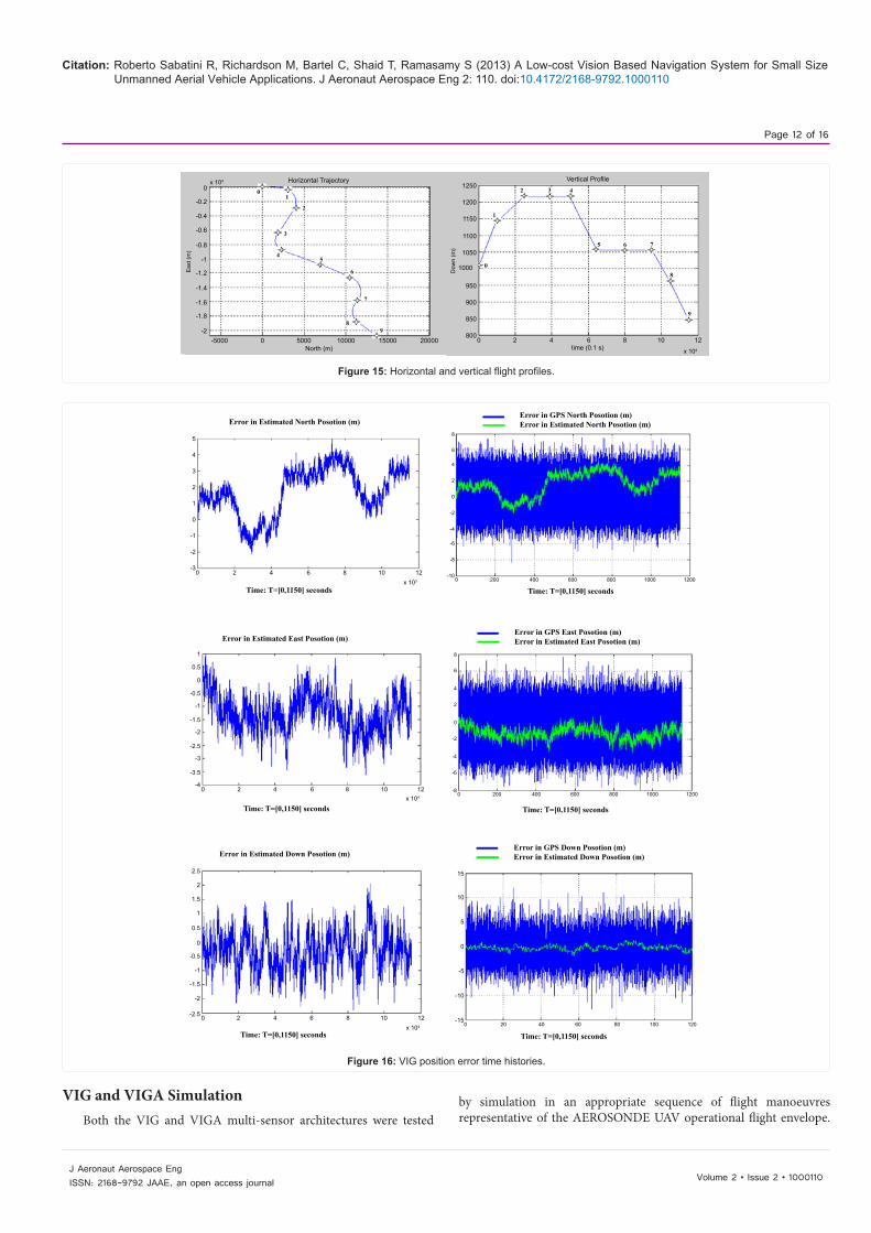
VIG and VIGA SimulationBoth the VIG and VIGA multi-sensor architectures were tested

Horizontal Trajectory Vertical Profile

North (m) time (0.1 s)0 2 4 6 8 10 12-5000 0 5000 10000 15000 20000

0

-0.2

-0.4

-0.6

-0.8

-1

-1.2

-1.4

-1.6

-1.8

-2

1250

1200

1150

1100

1050

1000

950

900

850

800

Eas

t (m

)

Dow

n (m

)

x 104

01

2

3

45

6

7

89

0

1

32 4

5 6 7

8

9

x 104

Figure 15: Horizontal and vertical flight profiles.

Error in Estimated North Posotion (m)Error in GPS North Posotion (m)Error in Estimated North Posotion (m)

Error in GPS East Posotion (m)Error in Estimated East Posotion (m)

Error in GPS Down Posotion (m)Error in Estimated Down Posotion (m)

Time: T=[0,1150] seconds Time: T=[0,1150] seconds

Time: T=[0,1150] secondsTime: T=[0,1150] seconds


Error in Estimated Down Posotion (m)

Error in Estimated East Posotion (m)

5

4

3

2

1

0

-1

-2

-30 2 4 6 8 10 12

0 2 4 6 8 10 12

0 2 4 6 8 10 120 20 40 60 80 100 120

0 200 400 600 800 1000 1200

0 200 400 600 800 1000 1200

8

6

4

2

0

-2

-4

-6

-8

-10

8

6

4

2

0

-2

-4

-6

-8

1

0.5

0

-0.5

-1

-1.5

-2

-2.5

-3

-3.5

-4

2.5

2

1.5

1

0.5

0

-0.5

-1

-1.5

-2

-2.5

15

10

5

0

-5

-10

-15

x 103

x 104

x 104

Figure 16: VIG position error time histories.

by simulation in an appropriate sequence of flight manoeuvres representative of the AEROSONDE UAV operational flight envelope.

http://dx.doi.org/10.4172/2168-9792.1000110


of 16


An FLC/PID controller was used for simulation. The duration of the simulation is 1150 seconds (approximately 19 minutes). The horizontal and vertical flight profiles are shown in figure 14.

The list of the different simulated flight manoeuvres and associated control inputs is provided in table 7. The numbered waypoints are the same shown in figure 15.

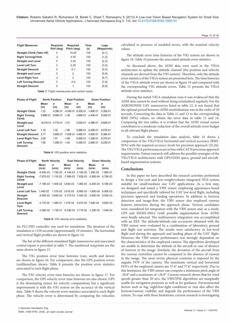
The VIG position error time histories (east, north and down) are shown in figure 16. For comparison, also the GPS position errors (unfiltered)are shown. Table 8 presents the position error statistics associated to each flight phase.

The VIG velocity error time histories are shown in figure 17. For comparison, the GPS velocity error time histories are also shown. GPS is the dominating sensor for velocity computations but a significant improvement is with the VIG system on the accuracy of the vertical data. Table 9 shows the velocity error statistics associated to each flight phase. The velocity error is determined by comparing the velocities

calculated in presence of modeled errors, with the nominal velocity values.

The attitude error time histories of the VIG system are shown in figure 18. Table 10 presents the associated attitude error statistics.

As discussed above, the ADM data were used in the VIGA architecture to update the attitude channel (the position and velocity channels are derived from the VIG system). Therefore, only the attitude error statistics of the VIGA system are presented here. The time histories of the VIGA attitude errors are shown in figure 19 and compared with the corresponding VIG attitude errors. Table 11 presents the VIGA attitude error statistics.

During the initial VIGA simulation runs it was evidenced that the ADM data cannot be used without being reinitialized regularly. For the AEROSONDE UAV manoeuvres listed in table 12, it was found that the optimal period between ADM reinitialisation was in the order of 20 seconds. Converting the data in Table 11 and 12 to the corresponding RMS (95%) values, we obtain the error data in table 13 and 14. Comparing the two tables, it is evident that the ADM virtual sensor contributes to a moderate reduction of the overall attitude error budget in all relevant flight phases.

To conclude the simulation data analysis, table 14 shows a comparison of the VIG/VIGA horizontal and vertical accuracy (RMS-95%) with the required accuracy levels for precision approach [25,26]. The VIG/VIGA performances are in line with CAT II precision approach requirements. Future research will address the possible synergies of the VIG/VIGA architectures with GPS/GNSS space, ground and aircraft-based augmentation systems.

ConclusionsIn this paper we have described the research activities performed

to design a low-cost and low-weight/volume integrated NGS system suitable for small/medium size UAV applications. As a first step, we designed and tested a VBN sensor employing appearance-based techniques and specifically tailored for UAV low-level flight, including precision approach and landing operations. In addition to horizon detection and image-flow, the VBN sensor also employed runway features extraction during the approach phase. Various candidates were considered for integration with the VBN sensor and, as a result, GPS and MEMS-IMUs (with possible augmentation from ADM) were finally selected. The multisensory integration was accomplished with an EKF. The attitude/attitude-rate accuracies obtained with the VBN sensor were evaluated by a combination of laboratory, ground and flight test activities. The results were satisfactory in low-level flight and during the approach and landing phase of the UAV flight. However, the VBN sensor performance was strongly dependent on the characteristics of the employed camera. The algorithms developed are unable to determine the attitude of the aircraft in case of absence of horizon in the image. Similarly, the deviation of the aircraft from the runway centreline cannot be computed in the absence of runway in the image. The most severe physical constrain is imposed by the angular FOV of the camera. The maximum vertical and horizontal FOVs of the employed camera are 57.6° and 77.6° respectively. Due to this limitation, the VBN sensor can compute a minimum pitch angle of -28.8° and a maximum of +28.8°. Current research shows that for wind speeds greater than 20 m/s, the VBN/IPM algorithms are marginally usable for navigation purposes as well as for guidance. Environmental factors such as fog, night/low-light conditions or rain also affect the horizon/runway visibility and degrade the performance of the VBN system. To cope with these limitations, current research is investigating

Flight Maneuver Required Roll (deg)

Required Pitch (deg)

Time (s)

Legs(Waypoints)

Straight Climb (Take off) 0 10.00 100 [0,1]Right TurningClimb -2 4.00 150 [1,2]Straight and Level 0 2.25 150 [2,3]Level Left Turn 3 2.25 100 [3,4]Straight Descent 0 -0.7 150 [4,5]Straight and Level 0 2 150 [5,6]Level Right Turn -2 2 150 [6,7]Left Turning Descent 3 -0.5 100 [7,8]Straight Descent 0 -1 100 [8,9]

Table 7: Flight manoeuvres and control inputs.

Phase of Flight North Position East Position Down PositionMean(m)

σ(m)

Mean(m)

σ(m)

Mean(m)

σ(m)

Straight Climb 1.22 4.38E-01 -4.34E-01 6.20E-01 -1.80E-01 5.30E-01Right Turning Climb

9.88E-01 8.68E-01 -1.36 4.86E-01 -2.40E-01 6.02E-01

Straight and Level

-8.01E-01 4.71E-01 -1.51 5.02E-01 -4.38E-01 6.82E-01

Level Left Turn 1.16 1.32 -1.66 5.68E-01 -5.28E-01 6.57E-01Straight Descent 2.77 3.60E-01 -7.20E-01 4.48E-01 -4.92E-01 6.36E-01Level Right Turn 2.06 1.07 -1.86 5.92E-01 -1.29E-01 8.37E-01Left Turning Descent

1.65 7.29E-01 -1.63 5.35E-01 -2.66E-01 6.23E-01

Table 8: VIG position error statistics.

Phase of Flight North Velocity East Velocity Down VelocityMean(m/s)

σ(m/s)

Mean(m/s)

σ (m/s)

Mean(m/s)

σ(m/s)

Straight Climb -6.40E-03 1.73E-02 -4.14E-03 2.14E-02 1.30E-02 1.89E-01Right Turning Climb

-7.97E-03 1.11E-02 -7.59E-03 7.93E-03 -2.90E-04 6.79E-03

Straight and Level

-7.19E-03 1.00E-02 3.63E-03 1.08E-02 -4.20E-04 6.78E-03

Level Left Turn 1.44E-02 1.51E-02 3.61E-03 6.99E-03 -1.80E-04 6.90E-03Straight Descent

-4.50E-03 3.64E-02 -3.71E-03 3.32E-02 -3.80E-04 9.55E-03

Level Right Turn

-3.11E-02 1.08E-01 1.21E-02 4.91E-02 7.64E-04 9.82E-03

Left Turning Descent

-3.28E-02 1.13E-01 -6.33E-03 3.71E-02 -1.32E-03 1.54E-02

Table 9: VIG velocity error statistics.

http://dx.doi.org/10.4172/2168-9792.1000110


of 16


Error in Estimated North Velocity (m/s)Error in GPS North Velocity (m/s)Error in Estimated North Velocity (m/s)

Error in Estimated East Velocity (m/s)Error in GPS East Velocity (m/s)Error in Estimated East Velocity (m/s)

Error in Estimated Down Velocity (m/s)Error in GPS Down Velocity (m/s)Error in Estimated Down Velocity (m/s)


Time: T=[0,1150] secondsTime: T=[0,1150] seconds


x 104

x 104

x 104

0.3

0.2

0.1

0

-0.1

-0.2

-0.3

-0.4

0.3

0.2

0.1

0

-0.1

-0.2

-0.3

-0.4

0.4

0.3

0.2

0.1

0

-0.1

-0.2

-0.3

0.4

0.3

0.2

0.1

0

-0.1

-0.2

-0.3

0.06

0.04

0.02

0

-0.02

-0.04

-0.06

0.08

0.06

0.04

0.02

0

-0.02

-0.04

-0.06

0 2 4 6 8 10 12

0 2 4 6 8 10 12

1 2 3 4 5 6 7 8 9 10 11 100 200 300 400 500 600 700 800 900 1000 1100

0 200 400 600 800 1000 1200

0 200 400 600 800 1000 1200

Figure 17: VIG velocity error time histories.

Phaseof Flight Roll (Phi) Pitch (Theta) Yaw (Psi)Mean (deg)

σ (deg)

Mean (deg)

σ (deg)

Mean (deg)

σ (deg)

Straight Climb -6.07E-02 5.54E-01 3.16E-01 2.92E-01 -2.17E-01 1.06Right Turning Climb

-4.25E-01 3.09E-01 -5.10E-02 4.65E-01 -5.39E-01 6.99E-01

Straight and Level

-4.22E-01 3.44E-01 -2.24E-02 3.80E-01 -1.38 8.02E-01

Level Left Turn 6.13E-01 4.96E-01 -1.39E-01 4.27E-01 1.39 1.36Straight Descent

3.89E-01 4.60E-01 -3.68E-01 3.50E-01 2.03 1.08

Level Right Turn

7.58E-01 7.69E-01 -5.46E-01 8.54E-01 3.91E-01 8.59E-01


1.22 7.06E-01 -5.37E-01 7.84E-01 -3.36E-01 8.86E-01

Table 10: VIG attitude error statistics.

Phase of Flight Roll (Phi) Pitch (Theta) Yaw (Psi)Mean(deg)

σ(deg)

Mean(deg)

σ(deg)

Mean(deg)

σ(deg)

Straight Climb -6.76E-02 5.19E-01 3.58E-01 2.08E-01 -1.19E-01 1.01Right Turning Climb

-4.42E-01 2.64E-01 -8.37E-02 4.07E-01 -6.07E-01 6.97E-01

Straight and Level

-4.38E-01 3.06E-01 -3.61E-02 3.27E-01 -1.44 7.92E-01

Level Left Turn 6.16E-01 4.77E-01 -1.60E-01 3.70E-01 1.45 1.31Straight Descent

3.92E-01 3.58E-01 -4.22E-01 2.37E-01 2.07 1.08

Level Right Turn

7.79E-01 6.99E-01 -6.49E-01 7.39E-01 4.73E-01 8.30E-01


9.00E-02 1.44E-01 3.74E-01 4.50E-01 -1.78E-01 8.59E-01

Table 11: VIGA attitude error statistics.

http://dx.doi.org/10.4172/2168-9792.1000110


of 16


Error in Estimated Attitude Phi (rad)

Error in Estimated Attitude Psy (rad)

Error in Estimated Attitude Theta (rad)


Time: T=[0,1150] seconds

x 104 x 104

x 104

0.06

0.04

0.02

0

-0.02

-0.04

-0.06

0.06

0.04

0.02

0

-0.02

-0.04

-0.06

-0.08

0.12

0.1

0.08

0.06

0.04

0.02

0

-0.02

-0.04

-0.06

-0.08

1 2 3 4 5 6 7 8 9 10 11

0 2 4 6 8 10 12 0 2 4 6 8 10 12

Figure 18: VAttitude error time histories.

VIGA VIG

Error in Estimated Attitude Phi (rad)Error in Estimated Attitude Phi (rad)

Time: T=[0,1150]

Time: T=[0,1150]

Time: T=[0,1150]




Error in Estimated Attitude Theta (rad)Error in Estimated Attitude Theta (rad)

Error in Estimated Attitude Psy (rad)Error in Estimated Attitude Psy (rad)

x 104

x 104

x 104x 104

x 104

x 104

0.04

0.03

0.02

0.01

0

-0.01

-0.02

-0.03

-0.04

0.03

0.02

0.01

0

-0.01

-0.02

-0.03

-0.04

-0.05

0.1

0.08

0.06

0.04

0.02

0

-0.02

-0.04

-0.06

-0.08

0.12

0.1

0.08

0.06

0.04

0.02

0

-0.02

-0.04

-0.06

-0.08

0.06

0.04

0.02

0

-0.02

-0.04

-0.06

-0.08

0.06

0.04

0.02

0

-0.02

-0.04

-0.060 2 4 6 8 10 120 2 4 6 8 10 12

0 2 4 6 8 10 120 2 4 6 8 10 12

1 2 3 4 5 6 7 8 9 10 11 1 2 3 4 5 6 7 8 9 10 11

Figure 19: Comparison of VIGA and VIG attitude errors.

http://dx.doi.org/10.4172/2168-9792.1000110


of 16


the potential synergies obtained by integrating daylight camera vision sensors with Infrared and Night Vision Imaging Sensors (IR/NVIS).Simulation of the VIG integrated navigation mode showed that this integration scheme can achieve horizontal/vertical position accuracies in line with CAT-II precision approach requirements, with a significant improvement compared to stand-alone SPS GPS. An improvement was also observed in the accuracy of the vertical velocity data. Additionally, simulation of the VIGA navigation mode showed promising results since, in most cases, the attitude accuracy is higher using the ADM/VBS/IMU rather than using VBS/IMU only. However, due to rapid divergence of the ADM virtual sensor, there is a need for a frequent re-initialization of the ADM data module, which is strongly dependent on the UAV flight dynamics and the specific manoeuvres/flight-phase transitions performed. In the considered portion of the UAV operational flight envelope, the required re-initialization interval was approximately 20 seconds. To cope with this issue, the original ADM is being modified to take into account specific manoeuvre constraints and the transition states between various manoeuvres are being carefully modeled. Additionally, an automatic manoeuvre recognition algorithm is being developed for updating the ADM in real-time and providing direct feedback to the VBN sensor. It is expected that, adopting this approach, the performances of the multisensory integrated NGS will be significantly enhanced both in terms of data accuracy and data continuity.

References

1. Sinopoli B, Micheli M, Donato G, Koo TJ (2001) Vision based navigation for an unmanned aerial vehicle. IEEE T Robotic Autom 2: 1757-1764.

2. Se S, Lowe DG, Little JJ (2005) Vision-based global localization and mapping for mobile robots. IEEE Transactions on Robotics 21: 364-375.

3. Cui P, Yue F (2007) Stereo vision-based autonomous navigation for lunar rovers. Aircr Eng Aerosp Tec 79: 398-405.

4. Matsumoto Y, Sakai K, Inaba M, Inoue H (2000) View-based approach to robot navigation. Proceedings of IEEE/RSJ International Conference on Intelligent Robots and Systems 3: 1702-1708.

5. Courbon J, Mezouar Y, Guenard N, Martinet P (2009) Visual navigation of a quadrotor aerial vehicle. The 2009 IEEE/RSJ International Conference on Intelligent Robots and Systems October, USA.

6. Courbon J, Mezouar Y, Guénard N, Martinet P (2010) Vision-based navigation of unmanned aerial vehicles. Control Eng Pract 18: 789-799.

7. Chen Z, Birchfield ST (2009) Qualitative Vision-Based Path Following. IEEE Transactions on Robotics 25: 749-754.

8. Remazeilles A, Chaumette F (2006) Image-based robot navigation from an image memory. Robot Auton Syst.

9. Liu X, Cao Y (2003) Research on the application of vision-based autonomous navigation to the landing of the UAV. Proc SPIE 5253, Fifth International Symposium on Instrumentation and Control Technology.

10. Dusha D, Mejias L, Walker R (2011) Fixed-wing attitude estimation using temporal tracking of the horizon and optical flow. Journal of Field Robotics 28: 355-372.

11. Olivares-Mendez MA, Mondragon IF, Campoy P, Martinez C (2010) Fuzzy controller for UAV-landing task using 3D-position visual estimation. IEEE International Conference on Fuzzy Systems.

12. Roumeliotis SI, Johnson AE, Montgomery JF (2002) Augmenting inertial navigation with image-based motion estimation. IEEE International Conference on Robotics and Automation 4: 4326-4333.

13. Desouza GN, Kak AC (2002) Vision for mobile robot navigation: a survey. IEEE T Pattern Anal 24: 237-267.

14. Santosh D, Supreeth A, Jawahar CV (2008) Autonomous image-based exploration for mobile robot navigation. IEEE International Conference on Robotics and Automation.

15. Rives P, Azinheira JR (2002) Visual Auto-landing of an Autonomous Aircraft.

16. Blanc G, Mezouar Y, Martinet P (2005) Indoor Navigation of a Wheeled Mobile Robot along Visual Routes. Proceedings of the 2005 IEEE International Conference on Robotics and Automation.

17. Rangasamy G (2010) Image sensor fusion algorithms for obstacle detection, location and avoidance for autonomous navigation of UAVs. School of Engineering, Cranfield University.

18. Tiberius C (2003) Handheld GPS Receiver Accuracy: Standard Positioning Service. Advanstar Communications, Incorporated USA 14: 46-51.

19. Ding W, Wang J (2011) Precise Velocity Estimation with a Stand-Alone GPS Receiver. J Navigation 64: 311-325.

20. Weston J (2004) Strapdown Inertial Navigation Technology. (2nd Edn), The Institution of Engineering and Technology, UK.

21. Bruggemann TS (2009) Investigation of MEMS Inertial Sensors and Aircraft Dynamic Models in Global Positioning System Integrity Monitoring for Approaches with Vertical Guidance. Queensland University of Technology, Brisbane, Australia.

22. Godha S (2006) Performance Evaluation of Low Cost MEMS-Based IMU Integrated With GPS for Land Vehicle Navigation Application. Department of Geomatics Engineering, University of Calgary, Alberta, Canada.

23. Sabatini R, Bartel C, Kaharkar A, Shaid T (2012) Design and integration of vision based sensors for unmanned aerial vehicles navigation and guidance. Proc SPIE 8439, Optical Sensing and Detection II, Belgium.

24. Sabatini R, Rodríguez L, Kaharkar A, Bartel C, Shaid T (2012) GNSS Data Processing for Attitude Determination and Control of Unmanned Aerial and Space Vehicles. Proceedings of the European Navigation Conference 2012 Gdansk (Poland) April 25-27 2012.

25. ICAO-ANNEX 10 (1996) Aeronautical Telecommunications.

26. CAA (2003) GPS Integrity and Potential Impact on Aviation Safety. Safety Regulation Group.

Phase of Flight RMS-95% Phi (deg)

RMS-95% Theta (deg)

RMS-95% Psi (deg)

Straight Climb 1.11 9.24E-01 2.13Right Turning Climb 1.05 9.44E-01 1.85Straight and Level 1.09 7.63E-01 3.30Level Left Turn 1.58 9.13E-01 3.97Straight Descent 1.20 1.10 4.67Level Right Turn 2.16 2.14 1.96Left Turning Descent 2.46 1.90 1.89

Table 12: VIG attitude RMS-95% errors.

Phase of Flight RMS-95% Phi (deg)

RMS-95% Theta (deg)

RMS-95% Psi (deg)

Straight Climb 1.05 7.56E-01 1.97Right Turning Climb 1.03 8.20E-01 1.76Straight and Level 1.07 6.55E-01 3.18Level Left Turn 1.56 7.90E-01 3.82Straight Descent 1.06 8.76E-01 4.60Level Right Turn 2.09 1.84 1.84Left Turning Descent 1.42 1.17 1.76

Table 13: VIGA attitude RMS-95% errors.

Category of approach

Horizontal Accuracy (m)2D RMS-95%

Vertical Accuracy (m)RMS-95% Down

Required VIG/VIGA Required VIG/VIGACAT I 16

5.84

1.61CAT II 6.9 2CAT III 4.1 2

Table 14: VIGA attitude RMS-95% errors.


http://dx.doi.org/10.4172/2168-9792.1000110

http://dx.doi.org/10.4172/2168-9792.1000110

http://ieeexplore.ieee.org/xpl/login.jsp?tp=&arnumber=932864&url=http%3A%2F%2Fieeexplore.ieee.org%2Fxpls%2Fabs_all.jsp%3Farnumber%3D932864


http://www.emeraldinsight.com/journals.htm?articleid=1615795&show=abstract


https://www2.lirmm.fr/lirmm/interne/BIBLI/CDROM/ROB/2009/IROS_2009/papers/0308.pdf

http://www.sciencedirect.com/science/article/pii/S0967066110000808

http://ieeexplore.ieee.org/xpl/login.jsp?tp=&arnumber=4814552&url=http%3A%2F%2Fieeexplore.ieee.org%2Fiel5%2F8860%2F5068831%2F04814552.pdf%3Farnumber%3D4814552

http://www.irisa.fr/lagadic/pdf/2007_ras_remazeilles.pdf

http://proceedings.spiedigitallibrary.org/proceeding.aspx?articleid=832355

http://onlinelibrary.wiley.com/doi/10.1002/rob.20387/abstract


http://ieeexplore.ieee.org/xpl/articleDetails.jsp?reload=true&arnumber=1014441&contentType=Conference+Publications



http://hal.archives-ouvertes.fr/docs/00/07/19/79/PDF/RR-4606.pdf


http://trid.trb.org/view.aspx?id=734850

http://journals.cambridge.org/action/displayAbstract;jsessionid=C32849FD4437D3737362CF74DA0D1EAC.journals?fromPage=online&aid=8194198

http://books.google.co.in/books/about/Strapdown_Inertial_Navigation_Technology.html?id=WwrCrn54n5cC&redir_esc=y

http://books.google.co.in/books/about/Investigation_of_MEMS_Inertial_Sensors_a.html?id=0cILaAEACAAJ&redir_esc=y

http://www.ucalgary.ca/engo_webdocs/MEC/06.20239.SGodha.pdf

http://proceedings.spiedigitallibrary.org/proceeding.aspx?articleid=1316653

http://academiadeaviatie.md/pdf/legislatie_internationala/ICAO%20Anx%2010-Aeronautical%20Telecommunications-Vol.1-Ed.5.1996..pdf

http://www.caa.co.uk/docs/33/CAPAP2003_09.PDF

A Low-cost Vision Based Navigation System for Small Size Unmanned Aerial Vehicle Applications

Documents

Transcript of A Low-cost Vision Based Navigation System for Small Size Unmanned Aerial Vehicle Applications