P.C. Merrell, D.J. Lee, and R.W. Beard, “Statistical Analysis of Multiple Optical Flow Values for Estimation of Unmanned Air Vehicles Height Above Ground” , SPIE Optics East, Robotics Technologies and Architectures, Intelligent Robots and Computer Vision XXII, vol. 5608, p. 298-305, Philadelphia, PA, USA, October 25-28, 2004.

Statistical analysis of multiple optical flow values for estimation of unmanned aerial vehicle height above ground

Paul Merrell, Dah-Jye Lee, and Randal Beard

Department of Electrical and Computer Engineering Brigham Young University, 459 CB

Provo, Utah 84602

ABSTRACT

For a UAV to be capable of autonomous low-level flight and landing, the UAV must be able to calculate its current height above the ground. If the speed of the UAV is approximately known, the height of the UAV can be estimated from the apparent motion of the ground in the images that are taken from an onboard camera. One of the most difficult aspects in estimating the height above ground lies in finding the correspondence between the position of an object in one image frame and its new position in succeeding frames. In some cases, due to the effects of noise and the aperture problem, it may not be possible to find the correct correspondence between an object’s position in one frame and in the next frame. Instead, it may only be possible to find a set of likely correspondences and each of their probabilities. We present a statistical method that takes into account the statistics of the noise, as well as the statistics of the correspondences. This gives a more robust method of calculating the height above ground on a UAV.

Keywords: Unmanned Aerial Vehicle, Height above Ground, Optical Flow, Autonomous Low-level Flight, Autonomous Landing

1. INTRODUCTION

One of the fundamental problems of computer vision is how to reconstruct a 3D scene using a sequence of 2D images taken from a moving camera in the scene. A robust and accurate solution to this problem would have many important applications for UAVs and other mobile robots. One key application is height above ground estimation. With an accurate estimate of a UAV’s height, the UAV would be capable of autonomous low-level flight and autonomous landing. It would also be possible to reconstruct an elevation map of the ground with a height above ground measurement. The process of recovering 3D structure from motion is typically accomplished in two separate steps. First, optical flow values are calculated for a set of feature points using image data. From this set of optical flow values, the motion of the camera is estimated, as well as the depth of the objects in the scene.

Noise from many sources prevents us from finding a completely accurate optical flow estimate. A better

understanding of the noise could provide a better end result. Typically, a single optical flow value is calculated at each feature point, but this is not the best approach because it ignores important information about the noise. A better approach would be to examine each possible optical flow value and calculate the probability that each is the correct optical flow based on the image intensities. The result would be a calculation for not just one optical flow value, but an optical flow distribution. This new approach has several advantages. It allows us to quantify the accuracy of each feature point and then rely more heavily upon the more accurate feature points. The more accurate feature points will have lower variances in their optical flow distributions. A feature point also may have a lower variance in one direction over another, meaning the optical flow estimate is more accurate in that direction. All of this potentially valuable information is lost if only a single optical flow value is calculated at each feature point.

Another advantage is that this new method allows us to effectively deal with the aperture problem. The

aperture problem occurs on points of the image where there is a spatial gradient in only one direction. At such edge points, it is impossible to determine the optical flow in the direction parallel to the gradient. However, often it is possible to obtain a precise estimate of the optical flow in direction perpendicular to the gradient. These edge points can not be used by any method which uses only a single optical flow value because the true optical flow is unknown. However, this problem can easily be avoided if multiple optical flow values are allowed. Even though edge points are

typically ignored, they do contain useful information that can produce more accurate results. In fact, it is possible to reconstruct a scene that contains only edges with no corner points at all. Consequently, this method is more robust because it does not require the presence of any corners in the image.

2. RELATED WORK

A significant amount of work has been done to try to use vision for a variety of applications on a UAV, such as

terrain-following [1], navigation [2], and autonomous landing on a helicopter pad [3]. Vision-based techniques have also been used for obstacle avoidance [4,5] on land robots. We hope to provide a more accurate and robust vision system by using multiple optical flow values.

Dellaert et al. explore a similar idea [6] to the one presented here. Their method is also based upon the principle

that the exact optical flow or correspondence between feature points in two images is unknown. They attempt to calculate structure from motion without a known optical flow. However, they do assume that each feature point in one image corresponds to one of a number of feature points in a second image. The idea we are proposing is less restrictive because it allows a possible correspondence between any nearby pixels and then calculates the probability of each correspondence.

Langer and Mann [7] discuss scenarios in which the exact optical flow is unknown, but the optical flow is

known to be one of a 1D or 2D set of optical flow. Unlike the method described here, their method does not compute the probability of each possible optical flow in the set.

3. METHODOLOGY

3.1. Optical flow probability The image intensity at position x and at time t can be modeled as a signal plus white Gaussian noise. ),(),(),( tNtStI xxx += (1)

where I(x,t) represents image intensity, S(x,t) represents the signal, and N(x,t) represents the noise. Over a sufficiently small range of positions and with a sufficiently small time step, the change in the signal can be expressed as a simple translation ),(),( dttStS +=+ xUx (2)

where U is the optical flow vector between the two frames. The shifted difference between the images, ),(),(),(),( dttNtNdttItI +−+=+−+ xUxxUx , (3)

is a Gaussian random process.

The probability that a particular optical flow, u, is the correct optical flow value based on the image intensities is proportional to:

2

2

2

)),(),((

22

1)],(),,(|[ σ

πσ

dttItI

edttItIP+−+−

∝++=xux

xuxuU , (4)

for some 2σ . Repeating the same analysis over a window of neighboring positions, W∈x , and assuming that the noise is white, the optical flow probability can be calculated as

∏∈

+−+−∝=

W

dttItI

eIPx

xux

uU2

2

2

)),(),((

22

1]|[ σ

πσ. (5)

The value of ),( tI ux + may need to be estimated through some kind of interpolation, since the image data usually

comes in discrete samples or pixels, but the value of u in general is not an integer value. Simoncelli et al. [8] describe an alternative gradient-based method for calculating the probability distribution. This method calculates optical flow based on the spatial gradient and temporal derivative of the image. Noise comes in the form of error in the temporal derivative, as well as a breakdown of the planarity assumption in equation (2). The optical flow probability distribution ends up always being Gaussian. The probability distribution calculated from equation (5) can be more complex than a Gaussian distribution.

3.2 Rotation and translation estimation

After having established an equation that relates the probability of an optical flow value with the image data, this relationship is used to calculate the probability of a particular camera rotation,

, and translation, T, given the image

data, I. This can be accomplished by taking the expected value for all possible optical flow values, u, then applying Bayes’ rule.

uIuIuT

uIuTIT

dPP

dPP

Ω=

Ω=Ω

)|(),|,(

)|,,()|,(

. (6)

Our estimate of

and T is only based on the optical flow value, so )|,(),|,( uTIuT Ω=Ω PP . Using

Bayes’ rule twice more yields:

ΩΩ=

Ω=Ω

uIuu

TuTuIuuTIT

dPP

PP

dPPP

)|()(

),|(),(

)|()|,()|,(

. (7)

The value of u is a continuous variable, so it does not come in discrete quantities. However, since we do not have a closed form solution to the integral in equation (7), the integral is approximated by computing a summation over discrete samples of u. In the following sections, each of the terms in equation (7) will be examined. Once a solution has been found for each term, the final step will be to find the most likely rotation and translation. The optimal rotation and translation can be found using a genetic algorithm.

3.3. Calculating P(u |

,T)

The optical flow vector, [ ]Tyx uu=u , at the image position (x,y) for a given rotation,

[ ]Tzyx ωωω=Ω and translation, [ ]Tzyx ttt=T , is approximately equal to

xf

xyf

f

y

Z

ytftu

yff

x

f

xy

Z

xtftu

zyxzy

y

zyxzx

x

ϖϖϖ

ϖϖϖ

−−

++

+−=

+

+−++−=

2

2

(8)

where f is the focal length of the camera and Z is the depth of the object in the scene [9]. For each possible camera rotation and translation, we can come up with a list of possible optical flow vectors. While the exact optical flow vector is unknown, since the depth, Z, is unknown, we do know from rearranging the terms in equation (8) that the optical flow vector is somewhere along an epipolar line. The epipolar line is given by:

+

+−+−−

+=

+−+−

=

+=

xff

x

f

xymx

f

xyf

f

yb

xtft

xtftm

bmuu

zyxzyx

zx

zy

xy

ϖϖωϖϖω22

(9)

Furthermore, since the depth, Z, is positive (because it is not possible to see objects behind the camera), we also

know that

yff

x

f

xyuftxt zyxxxz ϖϖϖ +

++>>

2

, and (10)

yff

x

f

xyuftxt zyxxxz ϖϖϖ +

++<<

2

.

If an expression for the probability of the depth, P(Z), is known, then the probability of an optical flow vector for a given rotation and translation is given by:

+≠

+=

+

+−

+−==Ω

bmuu

bmuu

yff

x

f

xy

xtftZP

P

xy

xy

zyx

zx

,0

,),|( 2

ϖϖϖTu (11)

3.4. Calculating P(

,T) and P(u)

The two remaining terms in equation (7) for which a solution must be found are P(

,T) and P(u). P(

,T) depends upon the characteristics of the UAV and how it is flown. We assume that the rotation is distributed normally

with a variance of 2xσ , 2

yσ , and 2zσ for each of the three components of rotation, roll, pitch, and yaw. For height above

ground estimation, the optimal position for the camera is facing directly at the ground. We assume that the motion of the UAV is usually perpendicular to the motion of the optical center of the camera and is usually along the y-axis of the camera coordinate system.

=Ω2

2

2

00

00

00

,

0

0

0

~

z

y

x

z

y

x

N

σσ

σ

ϖϖϖ

,

=2

2

2

00

00

00

,

0

1

0

~

tz

ty

tx

z

y

x

N

t

t

t

σσ

σT . (12)

Using these distributions, an expression for P(u) can also be obtained. Equation (8) can be separated in two parts that depend upon the rotation and translation of the camera.

Ω+=Ω+=

22

11

RTQ

RTQ

y

x

u

u (13)

In this case

and T are both random vectors with the distribution given in equation (12).

++++++++

ΩΩ

++=++=Ω

=Ω

222

222

222

221

221

221

221

221

221

221

221

221

2

1

221

221

221

2111

21

1

,0

0~

])[(])[(

0][

zzyyxxzzzyyyxxx

zzzyyyxxxzzyyxx

zzyyxx

zzyyxx

rrrrrrrrr

rrrrrrrrrN

rrr

rrrEE

E

σσσσσσσσσσσσ

σσσωωω

R

R

R

R

(14)

For simplicity, we will assume in the next equation that the variation in the translation, 2txσ , 2

tyσ , and 2tzσ , is

negligible. Now an expression for the value of P(u) is obtained by using the probability density function in (14) and a probability density function for the depth, P(Z)

)(2

1 zZP

z

fu

uP

u

uP

y

x

zy

x =

−=

ΩΩ

=

R

R. (15)

3.5. Depth estimation Once the rotation and translation of the camera between two frames have been estimated, we are now able to estimate the depth of the objects in the scene. For a given rotation, translation, and depth, an optical flow value can be calculated using equation (8). By using equation (5), we can find a probability for the depth Zxy at image position (x,y). The depth at position (x+1,y) is likely to be close to the depth at position (x,y), for the simple reason that neighboring pixels are likely to be part of the same object and that object is likely to be smooth. Using this information, we can obtain a better estimate of the depth at one pixel by examining those pixels around it.

∏

∏

∏

∈

∈

∈

=

=

=

Wjiijijijijxy

Wjiijijijxy

Wjiijxyxy

dZIZPZZP

dZIZZP

IZPZP

,

,

,

)|()|(

)|,(

)|()|( I

(16)

where I ij is the image data at position (i,j) and W is a set of positions close to the position (x,y). This approach adds smoothness and reduces noise. There is the possibility that this method could smooth over depth discontinuities, but it does not smooth over depth discontinuities if we have a high confidence that one exists. This method has the effect that if we are fairly confident that a pixel has a certain depth, it is left unchanged, but if we have very little depth information at that pixel we change the depth to a value closer to one of its neighbors. An additional way to improve our result is to use image data from more than just two frames to calculate the value of P(Zij|I ij).

4. RESULTS

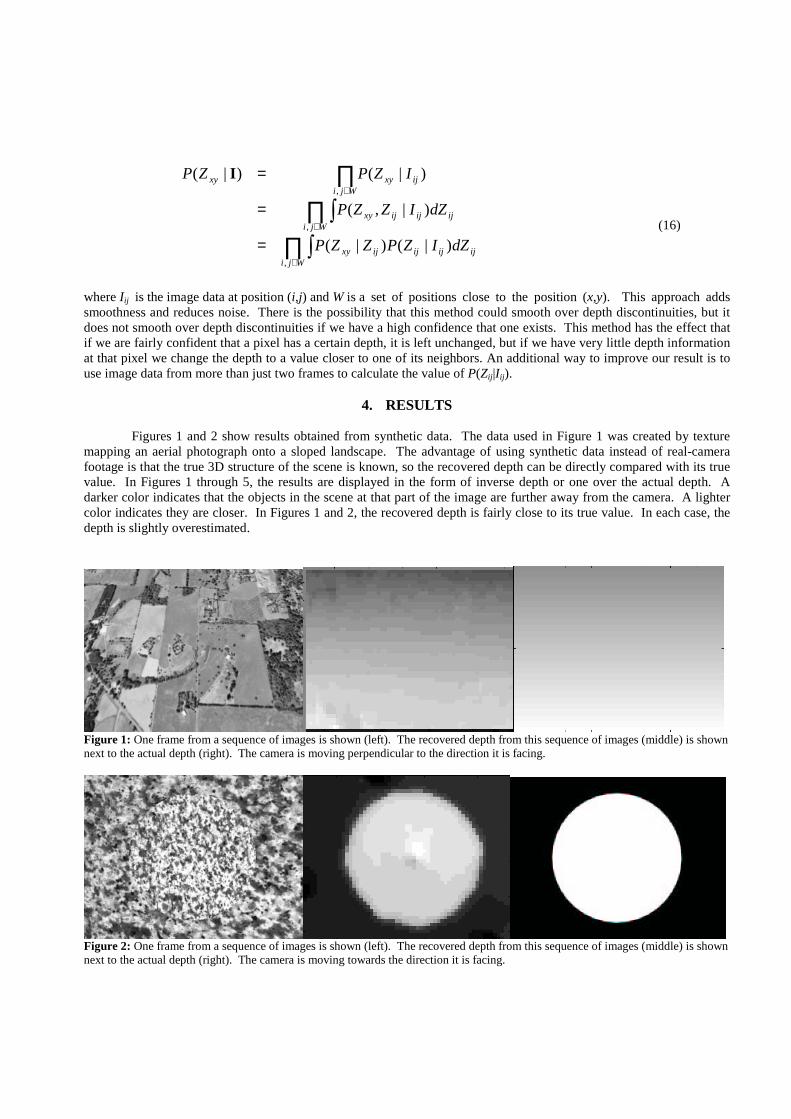
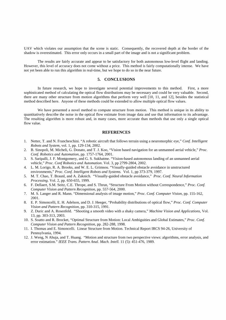
Figures 1 and 2 show results obtained from synthetic data. The data used in Figure 1 was created by texture mapping an aerial photograph onto a sloped landscape. The advantage of using synthetic data instead of real-camera footage is that the true 3D structure of the scene is known, so the recovered depth can be directly compared with its true value. In Figures 1 through 5, the results are displayed in the form of inverse depth or one over the actual depth. A darker color indicates that the objects in the scene at that part of the image are further away from the camera. A lighter color indicates they are closer. In Figures 1 and 2, the recovered depth is fairly close to its true value. In each case, the depth is slightly overestimated.

Figure 1: One frame from a sequence of images is shown (left). The recovered depth from this sequence of images (middle) is shown next to the actual depth (right). The camera is moving perpendicular to the direction it is facing.

Figure 2: One frame from a sequence of images is shown (left). The recovered depth from this sequence of images (middle) is shown next to the actual depth (right). The camera is moving towards the direction it is facing.

Figure 3: Two frames (left, middle) from a sequence of images demonstrating the aperture problem. The recovered depth is shown (right).

Figure 4: Two frames (left, middle) from a sequence of images taken directly from a camera onboard a UAV while it is flying towards a tree. The recovered depth is shown (right).

Figure 5: Two frames (left, middle) from a sequence of images taken from a camera onboard a UAV while it is flying low to the ground. The recovered depth is shown (right).

Figure 3 shows two frames from a sequence of images taken from a rotating camera moving towards a scene that has a black circle in the foreground and a white oval in the background. The scene is a bit contrived, but its purpose is to demonstrate that the aperture problem can be overcome. Every point in the image, when examined closely, is either completely blank or contains a single approximately straight edge. Essentially, every point in the image is affected by the aperture problem. However, with our new method, the aperture problem can be effectively dealt with. The camera was rotated in the z-direction one degree per frame. The camera rotation was estimated to be correct with an error of only 0.034˚. The left image in Figure 3 shows the recovered depth. The gray part of this image is where there was not enough information to detect the depth (since it is impossible to obtain depth information from a blank wall). The white oval was correctly determined to be behind the black circle. This demonstrates that it is possible to extract useful information about the camera movement, as well as the object’s depth from a scene with no corners in it.

Figures 4 and 5 show results from real data taken from a camera onboard a UAV. In Figure 4, the camera is moving towards a tree. The results are fairly noisy, but they do show a close object near where the tree should be. In Figure 5, the camera facing the ground and moving perpendicular to it. The results are fairly good with one exception. The UAV is so close to the ground that its shadow appears in the image. The shadow moves forward along with the

UAV which violates our assumption that the scene is static. Consequently, the recovered depth at the border of the shadow is overestimated. This error only occurs in a small part of the image and is not a significant problem.

The results are fairly accurate and appear to be satisfactory for both autonomous low-level flight and landing. However, this level of accuracy does not come without a price. This method is fairly computationally intense. We have not yet been able to run this algorithm in real-time, but we hope to do so in the near future.

5. CONCLUSIONS

In future research, we hope to investigate several potential improvements to this method. First, a more sophisticated method of calculating the optical flow distributions may be necessary and could be very valuable. Second, there are many other structure from motion algorithms that perform very well [10, 11, and 12], besides the statistical method described here. Anyone of these methods could be extended to allow multiple optical flow values.

We have presented a novel method to compute structure from motion. This method is unique in its ability to quantitatively describe the noise in the optical flow estimate from image data and use that information to its advantage. The resulting algorithm is more robust and, in many cases, more accurate than methods that use only a single optical flow value.

REFERENCES 1. Netter, T. and N. Francheschini. “A robotic aircraft that follows terrain using a neuromorphic eye,” Conf. Intelligent

Robots and System, vol. 1, pp. 129-134, 2002. 2. B. Sinopoli, M. Micheli, G. Donato, and T. J. Koo, “Vision based navigation for an unmanned aerial vehicle,” Proc.

Conf. Robotics and Automation, pp. 1757-1764, 2001. 3. S. Saripalli, J. F. Montgomery, and G. S. Sukhatme. “Vision-based autonomous landing of an unmanned aerial

vehicle,” Proc. Conf Robotics and Automation. Vol. 3, pp 2799-2804, 2002. 4. L. M. Lorigo, R. A. Brooks, and W. E. L. Grimsou. “Visually-guided obstacle avoidance in unstructured

environments,” Proc. Conf. Intelligent Robots and Systems. Vol. 1, pp 373-379, 1997. 5. M. T. Chao, T. Braunl, and A. Zaknich. “Visually-guided obstacle avoidance,” Proc. Conf. Neural Information

Processing. Vol. 2, pp. 650-655, 1999. 6. F. Dellaert, S.M. Seitz, C.E. Thrope, and S. Thrun, “Structure From Motion without Correspondence,” Proc. Conf.

Computer Vision and Pattern Recognition, pp. 557-564, 2000. 7. M. S. Langer and R. Mann. “Dimensional analysis of image motion,” Proc. Conf. Computer Vision, pp. 155-162,

2001. 8. E. P. Simoncelli, E. H. Adelson, and D. J. Heeger, “Probability distributions of optical flow,” Proc. Conf. Computer

Vision and Pattern Recognition, pp. 310-315, 1991. 9. Z. Duric and A. Rosenfeld. “Shooting a smooth video with a shaky camera,” Machine Vision and Applications, Vol.

13, pp. 303-313, 2003. 10. S. Soatto and R. Brocket, “Optimal Structure from Motion: Local Ambiguities and Global Estimates,” Proc. Conf.

Computer Vision and Pattern Recognition, pp. 282-288, 1998. 11. I. Thomas and E. Simoncelli. Linear Structure from Motion. Technical Report IRCS 94-26, University of

Pennsylvania, 1994. 12. J. Weng, N Ahuja, and T. Huang. “Motion and structure from two perspective views: algorithms, error analysis, and

error estimation.” IEEE Trans. Pattern Anal. Mach. Intell. 11 (5): 451-476, 1989.