APPLICATION OF AIRBORNE LASER SCANNER - AERIAL NAVIGATION

A dissertation presented to

the faculty of

the School of Electrical Engineering and Computer Science

and the Russ College of Engineering and Technology

In partial fulfillment

of the requirements for the degree

Doctor of Philosophy

Jacob L. Campbell

February 24, 2006

This dissertation entitled

APPLICATION OF AIRBORNE LASER SCANNER- AERIAL NAVIGATION

BY

JACOB L. CAMPBELL

has been approved for

the School of Electrical Engineering and Computer Science

and the Russ College of Engineering and Technology by

Maarten Uijt de Haag

Associate Professor of Electrical Engineering and Computer Science

Frank van Graas

Russ Professor of Electrical Engineering and Computer Science

Dennis Irwin

Dean, Russ College of Engineering and Technology

CAMPBELL, JACOB L. Ph.D. February 24, 2006. Electrical Engineering and Computer Science Application of Airborne Laser Scanner- Aerial Navigation (### pp.) Directors of Dissertation: Maarten Uijt de Haag, Frank van Graas

This dissertation explores the use of an Airborne Laser Scanner (ALS) for various types of

aircraft Terrain-Referenced Navigation (TRN) techniques. Using the methods explored, an ALS-

based TERRain Aided Inertial Navigator (TERRAIN) was developed, flight tested, and shown

capable of providing meter-level positioning accuracy in real-time.

The ALS-based TRN techniques discussed are constrained to the information found in the terrain

shape domain. The techniques used and position solution characteristics of ALS TRN can vary

significantly from traditional radar altimeter-based TRN; these variations are primarily due to two

differences in the information contained ALS TRN verses traditional radar altimeter-based TRN.

The first difference being that traditional radar altimeter-based TRN sense the terrain contours

traversed in the along-track direction, whereas ALS TRN measures in the along-track and in the

cross-track direction. The second difference is that the ALS’s narrow laser beamwidth (typically

less than a milli-radian) has resolution sufficient to identify not only the ground, but objects on

the ground such as buildings; whereas, a the radar altimeter’s relatively large beamwidth

(anywhere between 3 degrees to 90 degrees) primarily senses the terrain. These differences

increase the spectral content of the ground measurement data in the ALS-based system thus

permitting high-accuracy position estimates.

The ALS TRN navigation techniques explored include a method which estimates the position

based on the best match between ALS data and a high resolution/accuracy terrain database.

Variations on this technique are discussed include a method to classify non-terrain and terrain

features from the ALS data, allowing for the use of features with large gradients (sharp edges),

such as buildings. Also explored is the certification path for a ALS-based landing system.

Approved by: Maarten Uijt de Haag Associate Professor of Electrical Engineering and Computer Science and: Frank van Graas Russ Professor of Electrical Engineering and Computer Science

Acronyms......................................................................................................................................... 9 Acknowledgements........................................................................................................................ 13 1. Introduction............................................................................................................................ 14 2. Background............................................................................................................................ 17

2.1. Terrain-Referenced Navigation History ....................................................................... 18 2.1.1. The Early Years, Analog Systems............................................................................ 18 2.1.2. Digital Age of Terrain Navigation ........................................................................... 20 2.1.3. Bayesian Approaches to Terrain-Referenced Navigation Research ........................ 22 2.1.4. Beyond ‘Traditional’ Radar Altimeter Terrain-Referenced Navigation .................. 22

2.2. Survey of Terrain-Based Navigation Systems.............................................................. 25 2.2.1. ATRAN – Automatic Terrain Recognition And Navigation ................................... 25 2.2.2. TERCOM – TERrain COntour Matching ................................................................ 26 2.2.3. SITAN – Sandia Inertial Terrain-Aided Navigation ................................................ 28 2.2.4. SPARTAN – StockPot Algorithm Robust Terrain-Aided Navigation..................... 29 2.2.5. TERPROM® – TERrain PROfile Matching............................................................. 30 2.2.6. APALS® - Autonomous Precision Approach and Landing System......................... 31 2.2.7. PTAN® - Precision Terrain Aided Navigation ......................................................... 31

2.3. Summary of Survey of Terrain-Based Navigation Systems......................................... 33 2.4. System Characteristics: GPS, WAAS, INS, GPS-Aided INS, Calibrated-Coasting INS

34 2.4.1. GPS .......................................................................................................................... 34 2.4.2. WAAS...................................................................................................................... 35 2.4.3. Inertial Navigation ................................................................................................... 35 2.4.4. GPS-Aided Inertial Calibration................................................................................ 36

3. Airborne Laser Scanner & LIght Detection And Ranging (LIDAR) Mapping Systems ....... 40 3.1. ALS Characteristics and Operation .............................................................................. 40

3.1.1. ALS Laser Rangers .................................................................................................. 40 3.1.2. ALS Scanning mechanisms...................................................................................... 42 3.1.3. ALS Pointing Accuracy Characteristics................................................................... 46

3.2. ALS in a LIDAR mapping System............................................................................... 47 3.2.1. Laser Scanner Sensor Errors .................................................................................... 48 3.2.2. Kinematic GPS Sensor Errors .................................................................................. 49 3.2.3. GPS/IMU Orientation Sensor Errors........................................................................ 49

3.2.4. Total LIDAR mapping system Vertical & Horizontal System Errors ..................... 49 3.3. LIDAR Generated DSM............................................................................................... 50

3.3.1. Reno, NV LIDAR Data............................................................................................ 53 3.3.2. Braxton County Data................................................................................................ 54

3.4. Laser Safety .................................................................................................................. 54 4. Airborne Laser Scanner-Based Terrain-Referenced Position Estimation.............................. 56

4.1. Vertical-based Agreement Metric ................................................................................ 57 4.1.1. Radar Altimeter-Based Disparity Calculation.......................................................... 58 4.1.2. ALS-Based Disparity Calculation............................................................................ 59

4.2. ALS-Based Position Estimation ................................................................................... 60 4.2.1. Exhaustive Grid Search Position Estimation ........................................................... 62 4.2.2. Gradient-Based Search Position Estimation ............................................................ 64

4.3. ALS Positioning over Reno, NV .................................................................................. 66 4.3.1. Initial Positioning Results ........................................................................................ 69

5. Real-Time TERRAIN Approach System............................................................................... 72 5.1. Characteristics of the TERRAIN Approach System .................................................... 74

5.1.1. TERRAIN Approach System Integrity .................................................................... 74 5.1.2. TERRAIN Approach System Availability............................................................... 76 5.1.3. TERRAIN Approach System Continuity................................................................. 78

5.2. Terrain-Referenced Position Solutions......................................................................... 78 5.3. Inertial Velocity Error Estimation Using Integrated GPS Carrier Phase...................... 80 5.4. Proof-of-Concept Real-time TERRAIN Approach System Hardware Description ..... 82

5.4.1. NovAtel OEM 4/WAAS GPS Receiver................................................................... 83 5.4.2. Honeywell HG1150 Navigation Grade Inertial Reference Unit (IRU).................... 83 5.4.3. Riegl LMS-Q140i Airborne Laser Scanner ............................................................. 84 5.4.4. Data Collection/Distribution Computer ................................................................... 86 5.4.5. Navigation Computer ............................................................................................... 86 5.4.6. Display Computer .................................................................................................... 87

5.5. Flight Test Location and Test Plan............................................................................... 88 5.6. TERRAIN Precision Approach System Performance .................................................. 90

6. Conclusions and Future Work ............................................................................................... 96 7. References.............................................................................................................................. 99 Appendix A- Reno, Nevada LIDAR Data Metadata ................................................................... 107 Appendix B.- Glimer County LIDAR Data Metadata ................................................................. 121

List of Tables

Table 1, Summary of ALS Position Estimates (1-s updates)......................................................... 70 Table 2, Summary of TERRAIN Position Accuracy on Approach, 900 ft HAT to DH, Eight

Approaches, Nine Minutes of Data................................................................................................ 94 Table 3, Summary of TERRAIN Position Accuracy at 50 ft DH, Eight Approaches (5323

measurements) ............................................................................................................................... 94

List of Figures

Figure 2-1, British H2S Air-to-Surface Radar, Image used with permission from

http://www.doramusic.com/Radar.htm, May 2005........................................................................ 19 Figure 2-2, A. H2S Scan Pattern, Image used with permission from

http://www.doramusic.com/Radar.htm, May 2005........................................................................ 19 Figure 2-3, Example of a Lissajous Laser Scan Pattern, X angle frequency = 6 Hz, Y angle

frequency = 7 Hz, PRF = 1500 pulse/sec....................................................................................... 24 Figure 2-4, TERCOM System, figure adapted from [35]. ............................................................. 27 Figure 2-5, SITAN System, figure adapted from [35]. .................................................................. 28 Figure 2-6, feed-forward navigator design used in the implementation of the prototype real-time

TERRAIN approach system described in Chapter 5 ..................................................................... 38 Figure 2-7, Kalman filter mechanization, figure adapted from [71] pp 219................................. 39 Figure 3-1, Scan Pattern of an Oscillating Mirror Airborne Laser Scanner .................................. 43 Figure 3-2, Scan Pattern of a Rotating Mirror Airborne Laser Scanner ........................................ 44 Figure 3-3, Scan Pattern of a Nutating Mirror Airborne Laser Scanner ........................................ 45 Figure 3-4, Scan Pattern of a Nutating Mirror / Fiber Steered Airborne Laser Scanner ............... 45 Figure 3-5, Perspective View of Reno, NV, LIDAR Data; LIDAR Data Height Mapped to Point

Color, LIDAR Data Intensity Mapped to Point Brightness. Image Created in QT Viewer™

software.......................................................................................................................................... 51 Figure 3-6, Range Plot Generated by Laser Scanner of the Inside of Ohio University AEC’s

Hanger, Color Index: Blue < 3 m, and Red > 25 m. (Note: Dark blue on wings and nose

indicates all laser energy absorbed, no range measurement available).......................................... 52 Figure 3-7, Intensity Plot Generated from Laser Scanner of the Inside of Ohio University AEC’s

Hanger, Color Axis: Red = High Intensity Return, Blue = Low Intensity Return......................... 53

Figure 3-8, Perspective View of Reno, NV, LIDAR Data; LIDAR Data Height Mapped to Point

Color, LIDAR Data Intensity Mapped to Point Brightness. Image Created in QT Viewer™

software.......................................................................................................................................... 54 Figure 4-1, Parameters of a Radar Altimeter-Based Terrain Navigator ........................................ 59 Figure 4-2, Parameters of an ALS-Based Terrain Navigator......................................................... 60 Figure 4-3, SSE Surface for GPS time 314246 s of week 1229. ................................................... 62 Figure 4-4, SSE Surface for GPS time 314246 s of week 1229. ................................................... 63 Figure 4-5, Gradient Search for Minimum Error on the Sum of Squared Error Surface............... 66 Figure 4-6, NASA Dryden DC-8 Flying Laboratory, Photo courtesy of NASA Dryden. ............. 67 Figure 4-7, NASA Dryden DC-8 Cargo Bay LIDAR Installation................................................. 68 Figure 4-8, Flight Path of an Approach into KRNO...................................................................... 68 Figure 4-9, Flight Trajectories during Laser Data Collection at KRNO........................................ 69 Figure 4-10, ALS Horizontal Position Estimate Error................................................................... 70 Figure 5-1, TERRAIN Precision Approach System Position Estimator........................................ 73 Figure 5-2, Approach into St. Maarten Island. Approach over water would make the TERRAIN

approach system not available. ...................................................................................................... 75 Figure 5-3, Theoretical probability density curve of a weather condition of severity x occurring,

the area of the shaded region represents probability of a landing guidance system not available.77 Figure 5-4, TERRAIN Precision Approach Hardware Diagram ................................................... 83 Figure 5-5, Honeywell HG1150 IRU installed just aft of right-seat pilot in the DC-3.................. 84 Figure 5-6, Scanning Parameters for LMS-Q140i with Average PRF = 10 kHz........................... 85 Figure 5-7, DC-3Research Computer Rack ................................................................................... 87 Figure 5-8, DC-3 Cockpit with DELPHINS Guidance Display .................................................... 88 Figure 5-9, DC-3 on Short Final to Runway 19, K48I ................................................................. 89 Figure 5-10, trajectories flown to K48I on January 14, 2005 during the flight testing of the real-

time TERRAIN approach system: Left- perspective view, Right- plan view with North up ....... 90 Figure 5-11, TERRAIN position – KGPS for one approach, HAT: Height Above Threshold ..... 91 Figure 5-12, Histogram of error in the TERRAIN approach system navigator output in the East

direction with best fit normal distribution overlay......................................................................... 92 Figure 5-13, Histogram of error in the TERRAIN approach system navigator output in the North

direction with best fit normal distribution overlay......................................................................... 93 Figure 5-14, Histogram of error in the TERRAIN approach system navigator output in the Up

direction with best fit normal distribution overlay......................................................................... 93

Acronyms

AEC – Avionics Engineering Center (at Ohio University)

AFTI – Advanced Fighter Technology Integration

AGL – Above Ground Level

ALS – Airborne Laser Scanner

ALTM – Airborne Laser Terrain Mapper (Optech System)

APALS – Autonomous Precision Approach and Landing System

APD – Avalanche Photodiode

ATRAN – Automatic Terrain Recognition And Navigation

AWRS – Average Weighted Residual Squared

CAROTE – Correlation And Recognition Of Terrain Elevation

CEP – Circular Error Probability

CVN – Continuous Visual Navigation

DCD – Data Collection and Distribution computer

DCT – Discrete Cosine Transform

DURIP – Defense University Research Instrumentation Program

DME – Distance Measurement Equipment

DME-P – Precision Distance Measurement Equipment

DOP – Dilution Of Precision

DSM – Digital Surface Map

DSMAC – Digital Scene-Mapping Area Correlator

DTED – Digital Terrain Elevation Database

DTM – Digital Terrain Map

EGPWS – Enhanced Ground Proximity Warning System

ENU – East North Up

FAA – Federal Aviation Administration

FLOD – Forward Looking Obstacle Detection

FM-CW – Frequency Modulated Carrier Wave

GCAS – Ground Collision Avoidance System

GIS – Geographical Information System

GPS – Global Positioning System

HAT – Height Above Threshold

HDD – Heads Down Display

IAF – Initial Approach Fix

ILS – Instrument Landing System

IMU – Inertial Measurement Unit

INS – Inertial Navigation System

IRS – Inertial Reference System

IRU – Inertial Reference Unit

K48I – Braxton County Airport in West Virginia

KGPS – Kinematic Global Positioning System

KRNO – Reno, NV Airport

KUNI – Ohio University Airport in Albany Ohio

LAAS – Local Area Augmentation System

LADAR – LAser Detection And Ranging – or – Laser Radar

LaRC – NASA Langley Research Center

LCD – Liquid Crystal Display

LEP – Linear Error Probability

LIDAR – LIght Detection And Ranging

LLH – Latitude, Longitude, Height

LOS – Line Of Sight

LSO – Laser Scanner Origin

MAD – Mean Absolute Difference

MCMC – Monte Carlo Markov Chain

MSD – Mean Squared Difference

MSL – Mean Sea Level

MWx – Modified X-band Weather Radar

MLS – Microwave Landing System

NAV – NAVigation computer

NGS – National Geodetic Survey

POS – Position and Orientation System

PPI – Plan Position Indicator

PPS – Pulse Per Second

PRF – Pulse Repetition Frequency

PTAN – Precision Terrain Aided Navigation

RAM – Random Access Memory

RLG – Ring Laser Gyro

RMS – Root Mean Squared

RTOS – Real-Time Operating System

SA – Selective Availability

SAR – Synthetic Aperture Radar

SITAN – Sandia Inertial Terrain-Aided Navigation

SPARTAN – StockPot Algorithm Robust Terrain-Aided Navigation

SNR – Signal-to-Noise Ratio

SSE – Sum of the Squared Error

SV – Space Vehicle

SVS – Synthetic Vision System

TERCOM – TERrain COntour Matching

TERPROM – TERrain PROfile Matching

TLAM – Tomahawk Land Attack Missile

TRN – Terrain Referenced Navigation

TERRAIN – TERRain Aided Inertial Navigator

USAF – United States Air Force

USP – United States Patent

UTM – Universal Trans-Mercator

VOR – Very high frequency Omni Range

WAAS – Wide Area Augmentation System

To my parents -

for their examples of integrity and a positive outlook.

Acknowledgements

This dissertation would not have been possible without the help of many fellow co-

workers/students (which I prefer to call friends given all the good times we have had together

performing this research). I can honestly say that the experiences I have been part of and the

people I have met in the course of this research will be close to me for the rest of my life.

First, I thank my fellow office mates, Jeff Dickman, Lukas Marti, Andrey Soloviev, and Ananth

Vadlamani, for providing an excellent source of ideas during the countless discussions on the

research. I also thank them for helping with the development of equipment and flight tests. For

research support from NASA Langley I thank Steve Young, Rob Kudlinski, and Dan Baize who

made the LIDAR data collection effort in Reno, NV possible. For the Reno, NV DC-8 flight test

I thank the US Army for use of their LIDAR equipment, as well as the support staff from Optech

for their expertise on the installation and help in the LIDAR data processing. I also thank the

NASA DC-8 flying laboratory crew and support staff for their flexibility and help collecting the

data and NOAA for the use of a LIDAR generated terrain map of the Reno area. With respect to

the successful creation and testing of a proof-of-concept real-time laser scanner based approach

system I thank Dr. van Graas and Dr. Uijt de Haag for help with the development and funding. I

thank Jay Clark and his team at the Ohio University Airport for the customized installation of the

equipment in the DC-3 aircraft, and thank the DC-3 pilots, Dr. McFarland and Bryan Branham,

for their part in the successful flight tests at Braxton County Airport (K48I). I thank Delft

University of Technology for the use of their Synthetic Vision / Flight Director display, and I

thank the Canaan Valley Institute, specifically Sandra Frank, for providing the LIDAR data for

K48I. I also thank my Dad, Steve Campbell, for help with the survey of K48I.

I thank my Ph.D. committee members, Dr. Chris Bartone, Dr. Martin Molenkamp, and Dr. Jim

Rankin, for their ideas and guidance from the topic proposal through their reviewing of this

dissertation. And, I thank Dr. Mikel Miller for his support in editing my dissertation. Also, and

most importantly, I thank my Co-Advisors, Dr. Maarten Uijt de Haag and Dr. Frank van Graas

for the countless hours spent discussing the research in this dissertation, reviewing papers, and for

their examples not only as great advisors, but also as great people.

Finally I thank my wife, Nikki, for her support and love throughout my work on this dissertation,

and most importantly I thank God for giving me the strength to complete my Ph.D.

1. Introduction

Terrain-referenced aerial navigation has been around since the birth of flight. Terrain-referenced

navigation was the first method of aircraft navigation and it was simply performed by visual

recognition of familiar landmarks or identification of landmarks seen on a map to determine

position. Flying by visual reference was, and still is, a very popular method of aircraft

navigation, and it is based on two primary principals: the ability to see, or sense, the terrain below

the aircraft, and the ability to correlate this sensed terrain information with a map to determine the

aircraft position. However, flight by visual reference has two major shortfalls directly related to

the two primary principals listed above: the pilot must both be able to see the terrain and have a

map of the terrain to relate his observations to a position on the map. Other concerns with flight

by visual reference include inaccuracies in the position estimation, the possibility for confusing

position ambiguities, and the unfortunate case where lack of unique visible features leads to the

inability to determine position altogether.

Many technologies have been developed to overcome the shortfalls of visual reference

navigation. These technologies range from radio navigation aids located on the ground and in

space to highly accurate inertial sensors. The former allow the aircraft to estimate its position

and/or velocity from the navaid measurements, whereas the latter measures the position relative

to a known starting location by continuously sensing the aircraft’s change in velocity and

orientation. While these technologies have allowed aircraft to operate with a high degree of

safety in many types of weather, there are some trade-offs in their design. Radio navigation aids

must be located at known positions; these positions can be fixed on the ground or defined by a

known set of equations, as in the case of the satellites used by the Global Positioning System

(GPS). Maintenance is required to keep the accuracy of the navaid positions within specification

and to ensure the navaid performs its intended function. Another undesirable characteristic of

ground-based radio navigation aids is that they may require location on real-estate that is either

expensive or not available. Inertial sensor systems are not dependent on a network of sensors

external to the aircraft; however, they accumulate errors in position and velocity when they are

not aided by other sensors.

The methods proposed in this dissertation are inspired by the use of the information present in the

terrain analogous to flight by visual reference. Furthermore, these methods overcome some of the

shortfalls of the above mentioned technologies. The goal of the ideas presented herein is to use

the shape of the terrain, including man-made objects, such as buildings, to enable autonomous

and accurate positioning. The envisioned position solution methods are autonomous in the sense

that they are not dependent on navigational aids external to the aircraft after initialization. The

proposed positioning methods are accurate to the order of a meter when used with a known

terrain database. In this dissertation the proposed methods of positioning, which use an Airborne

Laser Scanner (ALS) sensor, are described, realized, simulated, and for one particular method,

flight tested. Data from an ALS are used to aid the navigation solution from an inertial sensor

system such as an Inertial Measurement Unit (IMU) or an Inertial Reference System (IRS). ALS

aiding is illustrated in Figure 1-1: it uses ALS data combined with a high accuracy/ resolution

(decimeter-level accuracy/meter-level resolution) terrain database to estimate the inertial sensor

system’s position error.

Chapter 3 will detail the operation of an ALS system including various scanning and the ranging

techniques. Also provided in Chapter 3 are the sensitivity of the ALS pointing accuracy to

component errors, such as roll, pitch and heading. Chapter 4 explores the use of the ALS system

to aid an inertial sensor based navigator. Techniques used to estimate an inertial navigator’s

Figure 1-1, Scan Pattern of a Downward-Looking ALS Terrain Referenced System

position error with respect to a known terrain database are given in Section 4.1 along with

envisioned applications.

The real-time TERrain-Referenced Aided Inertial Navigator (TERRAIN) approach system is

described in detail in Chapter 6. This system uses techniques developed in section 4.1 to aid an

IRU which provides landing approach guidance to the pilot. The real-time TERRAIN approach

system is a proof-of-concept system flown on January 14, 2005. Eight approaches into Braxton

County Airport (K48I) in West Virginia were performed. Chapter 6 details the hardware and

software as well as the results of the proof-of-concept system. While the TERRAIN approach

system lacks all-weather capabilities, up-and-coming ranging technologies, described in the

background section 2.5, and techniques, covered in section 3.5, will someday overcome this

limitation.

This research was made possible by grants and data from NASA Langley Research Center, the

Defense University Research Instrumentation Program (DURIP), West Virginia Geographical

Information Systems (GIS), and internal Ohio University Avionics Engineering Center (AEC)

funds. An introduction and history into terrain-referenced navigation is given in the following

chapter.

2. Background

The Ohio University AEC was created in 1963 with the goal of furthering the state of the art in

avionics systems as well as providing the opportunity for students to be exposed and contribute to

this goal. Through the years AEC research has encompassed aircraft landing and navigation

systems including: ILS, Microwave Landing System (MLS), Very high frequency Omni Range

(VOR), Precision Distance Measuring Equipment (DME-P), and the Local Area Augmentation

System (LAAS). Research conducted by Dr. Robert Gray at AEC introduced the use of a radar

altimeter to provide an integrity monitoring function for terrain databases [1]. This research was

based on earlier uses of radar altimeters in terrain-referenced navigators which will be discussed

in the first section of this chapter. Since its introduction, the radar altimeter based integrity

monitor concept has been extensively studied and flight tested for use in Synthetic Vision

Systems (SVS). SVS uses terrain databases to generate a synthetic perspective display of the

outside world that can be presented to the pilots. In my M.S.E.E. thesis various aspects of this

integrity monitor concept were investigated such as: the sensitivity of the radar altimeter

measurement to aircraft attitude and receiver architecture; the availability aspects of a radar

altimeter-based integrity monitor; and the monitor’s capability to detect horizontal errors [2]. The

terrain database integrity monitor work was extended to include forward looking sensors, such as

the weather radar, which increases the ability of the integrity monitor to detect systematic errors

and blunders in the horizontal direction, by Dr. Steven Young and Swarna Kakarlapudi at AEC in

their Ph.D. dissertation and M.S.E.E. thesis, respectively [3][4]. Ananth Vadlamani’s M.S.E.E.

thesis research at AEC further extended the use of the radar altimeter-based integrity monitor to

allow for simultaneous position estimations and vertical bias detection and removal [5]. This

research path has led to research conducted on high-accuracy terrain navigation covered in this

dissertation.

The similarities between the radar altimeter-based terrain database integrity monitor and terrain

navigation techniques along with Ohio University AEC’s history in aircraft navigation systems

led to the current interest in terrain navigation using ALS and high accuracy/resolution terrain

databases. This background section first provides a brief history of terrain navigation concepts

and methods, followed by a survey of candidate terrain sensing technologies. This survey of

candidate terrain sensing technologies is then summarized in a table in the third section. The

survey of terrain sensing technologies provides the rational behind the use of an ALS for current

research. Finally, brief backgrounds on the Wide Area Augmentation System (WAAS) and

inertial navigation systems are provided in Section 2.4 since they are used in the TERRAIN

approach system. The discussion will include the systems’ accuracy and integrity aspects.

2.1. Terrain-Referenced Navigation History

As was mentioned in the introduction, terrain navigation has been in use since the beginning of

aviation when the aircraft position was estimated by the pilot’s recognition of landmarks; this

technique, still in use today, is known as pilotage. This section will chronologically document the

history of terrain-referenced navigation techniques and provide a description of some of the

systems in use or in development today.

2.1.1. The Early Years, Analog Systems

British and American forces first used radar based terrain-referenced navigation in World War II

to guide bombers to German cities in cloudy and night missions. These early radar systems were

designed around the newly developed 10 cm wavelength radar. In 1941 experiments with this

radar revealed that different types of terrain could be identified. This discovery led to the

development of the H2S radar, which starting in 1943 was placed on bombers to provide

guidance to German cities during night missions [6]. The H2S user panel can be seen in Figure

2-1. Its pulsed radar is based on the magnetron and the antenna is scanned 360 degrees in

azimuth shown in Figure 2-2. The data were presented to the aircraft crew in a Plan Position

Indicator (PPI) format, also shown in Figure 2-2. Many of today’s airborne weather radar are

similar to the H2S when operating in ground mapping mode. In ground mapping mode the

weather radar scans the area in front of the aircraft, providing terrain information to the pilot.

Figure 2-1, British H2S Air-to-Surface Radar, Image used with permission from

http://www.doramusic.com/Radar.htm, May 2005.

Figure 2-2, A. H2S Scan Pattern, Image used with permission from

http://www.doramusic.com/Radar.htm, May 2005.

B. H2S PPI Display, From Radar, issue No.3, 30 June, 1944, a U.S. Army Publication

A B

A method using scanning air-to-surface radar, such as the H2S, for terrain navigation is disclosed

in U.S. Patent 2,526,682 by Henry C. Mulberger; this patent was filed in 1946 and granted in

1950 [7]. Mulberger’s invention consisted of a scanning air-to-surface radar to sense the terrain,

and a movie style projector which plays back the radar returns from a previously flown mission.

Position, ground speed, and altitude estimates are determined by overlaying the PPI display with

a 35 mm film projection of previously recorded radar measurement. One feature lacking in this

patent was a method to automatically correlate the image data with the previously collected data;

the feedback was provided through a human operator. In 1948, experiments began on the

Automatic Terrain Recognition And Navigation (ATRAN) terrain-referenced navigation system,

designated AN/DPQ-4 [8]. ATRAN was designed to be an autonomous terrain sensing guidance

system which used methods similar to Mulberger’s patent; however, it also included an optical

correlator to provide automatic cross-track course corrections. A description of the ATRAN

guidance system is given in Section 2.2.1. During the 1950’s Patent 3,064,249, which describes

an optical correlator for a PPI radar system, was filed [9].

A different approach to terrain-referenced terrain navigation is described by France B. Berger in

U.S. Patent 2,847,855 [10]. Berger’s patent describes a system which is the foundation of many

of today’s radar altimeter-based terrain-reference terrain navigation systems. This system

generates profiles of the terrain traversed by the aircraft’s flight path by subtracting radar

altimeter height from an absolute altimeter. This terrain profile is then compared with terrain

height data stored on a cylinder and obtained by using the position data from an “automatic dead-

reckoner.” This data is then compared using an optical correlator described in a second patent by

Berger [11]. The optical correlator provides a feedback signal to estimate the error in the

automatic dead reckoning system. Conceptually, Berger’s described analog navigation system is

similar to digital terrain-referenced navigation systems such as TERrain COntour Matching

(TERCOM) described in section 2.2.2.

2.1.2. Digital Age of Terrain Navigation

Patent 3,328,795 “Fix-Taking Means and Method” by W. C. Hallmark is the first terrain-

referenced navigation system patent found which uses a digital computer and digitized terrain

database and estimates a position through batch processing methods [12]. This patent was

assigned to Ling-Temco-Vought, Inc., in Dallas Texas. Ling-Temco-Vought split and formed E-

Systems in 1972, and E-Systems was purchased in 1995 by Raytheon. The invention disclosed in

patent 3,328,795 is used in E-Systems TERCOM terrain-referenced navigation system. A

significant step forward in the understanding of terrain-referenced navigation was made in a

paper from E-Systems in 1976 where the expected performance of a TERCOM system is

described based on the shape of the terrain [13]. In E-System’s paper the shape of terrain is

described in terms of the terrain elevation standard deviation, σT, and correlation length, CT(x, y).

More details on TERCOM are given in section 2.2.2

At the same time E-Systems was developing TERCOM, Sandia National Laboratories was

developing their own terrain-referenced navigation system known as Sandia Inertial Terrain-

Aided Navigation (SITAN) [14][15]. Like TERCOM, SITAN uses radar altimeter and absolute

altimeter sensors to measure the height of the terrain below the aircraft; however, it differs from

TERCOM in that processing is done in a sequential manner (aircraft state estimates updated with

each terrain measurement) rather than a batch process (aircraft state estimates made from

processing a set of measurements). Details on SITAN are given in section 2.2.3. Also developed

in this timeframe, and still in use today, is British Aerospace’s (BAE) TERrain PROfile Matching

(TERPROM) system. Several military aircraft navigation systems in use today include

TERPROM. Section 2.2.4 provides more information on TERPROM.

In 1985 a new approach for storing terrain data for terrain navigation was described in E-Systems

Patent 4,495,580 [16] and Patent 4,520,445 [17]. In these patents the terrain database is stored as

a set of Discrete Cosine Transforms (DCT) parameters. With the DCT parameters, the shape of

the terrain could be recreated, reducing the amount of data storage required when compared to a

traditional grid representation of the database. The DCT concept was expanded in Patent

4,584,646 with the discloser of the Correlation And Recognition Of Terrain Elevation (CAROTE)

invention [18]. In this patent, assigned to the Harris Corporation, it was claimed that a system

which overcomes some of the shortfalls of TERCOM and SITAN could be realized by converting

the radar altimeter data to the DCT domain and performing the correlation to determine position

in the frequency domain [18]. No records were found describing implementations or

performance of a CAROTE system, and it is possible the approach was abandoned given two

years later Harris Corporation was granted Patent 4,829,304 which uses a hybrid TERCOM-

SITAN system [19]. Patent 4,829,304 makes use of the strengths of both TERCOM and SITAN

systems by using TERCOM when position uncertainties are large and SITAN otherwise.

2.1.3. Bayesian Approaches to Terrain-Referenced Navigation Research

Recent research (spanning the mid-1980’s to present) has explored the use of statistical methods

and filtering techniques to more accurately represent the underlying processes behind downward-

looking radar altimeter-based terrain-referenced positioning and navigation. Dr. Runnalls

describes a system which applies Bayesian statistics to create a likelihood function that estimates

the probability density functions of the navigation error [20]. This approach to terrain-referenced

navigation is used in the StockPot Algorithm Robust Terrain-Aided Navigation (SPARTAN)

technique described in Section 2.2.4. Further research applying Monte Carlo Markov Chain

(MCMC) methods along with Bayesian techniques to terrain navigation is found in [21]. The

goal of this research was to improve terrain-referenced navigation by reducing the filter-induced

errors created when non-linear measurements are linearized. In the late 90’s Dr. Bergman

performed similar research on use of Bayesian statistics, MCMC methods, and particle filters and

their ability to more accurately model the TRN measurements [22][23]. More on statistical

methods and their performance can be found in the following papers by Jürgan Metzger [24][25].

2.1.4. Beyond ‘Traditional’ Radar Altimeter Terrain-Referenced Navigation

Up to the 1990’s, terrain-referenced navigation had mostly been limited to traditional C-band (~5

GHz) downward-looking radar altimeter systems which measure the contour of the terrain

traversed by the aircraft. In the 1990’s this began to change as technology advanced to the point

where other terrain sensing methods became practical. The following subsections explore several

of these terrain sensing methods such as millimeter wave radar, Synthetic Aperture Radar (SAR)

weather radar, interferometric radar altimeter, Doppler lasers and laser rangers.

2.1.4.1. Recent Radar Terrain Sensing Methods used for Aircraft Navigation

In a patent by MBB (Deutsche Aerospace) granted in 1990, a 94 GHz radar was proposed to be

used for terrain navigation [26]. In this patent, the 94 GHz radar can be pointed down, as in a

traditional downward-looking terrain navigation system, scanned downward, or scanned forward.

An improvement in terrain navigation is expected because the high frequency radar can have a

narrower radar beam allowing for more accurate, higher resolution, and less correlated terrain

measurements. No information on a flight test of such a system could be found.

A landing system which has been flight tested and is in the process of certification by the Federal

Aviation Administration (FAA) is the Autonomous Precision Approach and Landing System

(APALS®). As described in detail in section 2.2.6, APALS uses a modified weather radar which

has an increased range resolution and also creates SAR maps at the antenna scan extremes (±45

deg from aircraft longitudinal axis); the Doppler gradient at the antenna scan extremes is large

enough to generate a SAR map. In the SAR maps cultural and natural terrain features are

identified and matched to a reference SAR image using the generalized Hough transform.

Interferometric radar altimeter is used in Honeywell’s Precision Terrain Aided Navigation

(PTAN®) navigation system described in detail in section 2.2.7. The PTAN interferometric radar

altimeter operates in the C-band. Using a narrow Doppler window and two (or three) receive

antennas, the interferometric radar altimeter is able to measure the closest point to the aircraft and

the direction to the closest point.

2.1.4.2. Recent Laser Terrain Sensing Methods used for Aircraft Navigation

A patent filed in 1980 by United Technologies Corporation describes a scanning Doppler laser

system to measure aircraft velocities [27]. This system described in this patent is not strictly a

terrain navigation system in the sense where navigation states are estimated by comparing the

sensed terrain to a stored terrain database; however the system is a technology providing velocity

measurements with 1-2 cm/sec accuracies (stated results from a prototype system). The prototype

system used a 1 watt 10.6 µm laser which was scanned downward in a circular pattern at 100

rev/sec [27]. Combining these techniques to obtain a range rate along with a range measurement

in a laser scanner would be very powerful in a laser-based terrain-referenced navigation system.

In May of 1990 Dornier Luftfahrt, of Germany, filed an invention disclosure which was assigned

U.S. Patent Number 5,047,777 [28]. This patent describes the use of a laser range finder to not

only measure the terrain height, as was done with the radar altimeter, but to also make use of the

narrow laser beam and laser return intensity to classify the terrain under the aircraft. In this

patent position estimates are made as the classification of the terrain below the aircraft changes.

Dornier also filed U.S. Patent Number 5,087,916 where a scanning laser ranger is used to create

“range images” [29]. This patent has several of the same characteristics of the laser scanner

terrain navigation studied in this dissertation. However, it differs in that the range data from the

laser scanner is treated more as an image than geo-referenced points on the ground; as is stated in

the patent, course aircraft attitude data is used to correct the range image before performing an S-

transform on the image. Positioning is performed by edge matching, and segmenting the terrain

as opposed to the primary methods described in this dissertation where each laser range

measurement is geo-referenced, and this geo-referenced data is used to estimate position by

finding the best-fit against a terrain database. It appears that Dornier’s terrain-referenced

navigation research ended when it was purchased by the now bankrupt Fairchild in the mid-

1990’s [30].

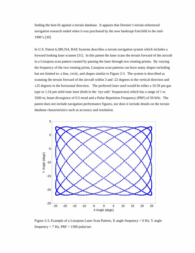
In U.S. Patent 6,389,354, BAE Systems describes a terrain navigation system which includes a

forward looking laser scanner [31]. In this patent the laser scans the terrain forward of the aircraft

in a Lissajous scan pattern created by passing the laser through two rotating prisms. By varying

the frequency of the two rotating prism, Lissajous scan patterns can have many shapes including

but not limited to: a line, circle, and shapes similar to Figure 2-3. The system is described as

scanning the terrain forward of the aircraft within 3 and -22 degrees in the vertical direction and

±25 degrees in the horizontal direction. The preferred laser used would be either a 10.59 µm gas

type or 1.54 µm solid state laser (both in the ‘eye safe’ frequencies) which has a range of 1 to

3500 m, beam divergence of 0.5 mrad and a Pulse Repetition Frequency (PRF) of 50 kHz. The

patent does not include navigation performance figures, nor does it include details on the terrain

database characteristics such as accuracy and resolution.

-25 -20 -15 -10 -5 0 5 10 15 20 25-25

-20

-15

-10

-5

0

5

X Angle (degs)

Y A

ngle

(deg

s)

Figure 2-3, Example of a Lissajous Laser Scan Pattern, X angle frequency = 6 Hz, Y angle

frequency = 7 Hz, PRF = 1500 pulse/sec

Research using an airborne laser scanner in conjunction with an optical Continuous Visual

Navigation (CVN) system is also being conducted in the United Kingdom [32]. The airborne

laser range portion of the system will be discussed here. In [32], laser range measurements are

processed in two ways. The first processing method is ‘tradition’ terrain surface matching to

estimate Inertial Navigation System (INS) drift, and the second uses feature edge information to

perform feature matching to estimate INS drift. Detailed techniques for performing the

navigation error estimations using laser range measurements and the expected navigation

performance is not given in this paper, however accuracies of ~30 m are stated using an

‘immature’ system and results are expected to improve with future work [32].

2.2. Survey of Terrain-Based Navigation Systems

A brief description of the history of terrain navigation concepts was given in section 2.1. Section

2.2 provides an overview on several popular systems referred to in section 2.1. Several of these

systems have been or are in use in aircraft systems today. While an in-depth survey of these

systems is beyond the scope of this dissertation, more information can be found in the many

references provided. The systems described in this section include ATRAN, TERCOM, SITAN,

SPARTAN, TERPROM®, APALS®, and PTAN®.

2.2.1. ATRAN – Automatic Terrain Recognition And Navigation

Labeled the “grand-daddy of missile systems” in the title of a paper at the 1980 Proceedings of

the Society of Photo-Optical Instrumentation Engineers, ATRAN was the first fully autonomous

terrain-referenced automatic guidance system [8]. Research on ATRAN began in 1947 by the

Goodyear Aerospace Corporation through what was then the Wright Air Development Center at

Wright Patterson Air Force Base [8]. Its military designation was the AN/DPQ-4 and the 1200

pound system provided guidance to for the “MACE” cruise missile in the 1950’s and 1960’s.

System testing was conducted on modified B-57’s and T-33 aircraft, and the final system found

use mounted in the nose of the MACE missile. ATRAN used a forward-looking scanning radar

to produce radar imagery, which was then correlated with reference images stored on 35 mm film

providing cross-track and along-track guidance [8]. ATRAN’s pulsed x-band radar used an

antenna consisting of two parabolic reflectors mounted back-to-back providing two scans per

antenna revolution. An optical correlator was used to estimate the position deviations by

correlating the radar generated PPI display with reference images stored on 35 mm film as

describe in United States Air Force (USAF) Manual 52-31 and U.S. Patent 3,290,675 [33][34].

Today relatively accurate digital terrain maps are available, and computers are able to transform

these terrain maps into formats needed in terrain navigation systems; however, in the 1950’s

creating 35 mm film strips containing radar return images were not as easily obtained. Over

friendly territory an aircraft equipped with scanning radar could be flown to produce the reference

trajectory on the 35 mm file, but this was not always possible over hostile territory. To overcome

this limitation, the Army Map Service created 3-D relief models with a 250,000:1 (3.43 nmi per

in) scale of the terrain of interest [8]. Towns and other objects known to produce strong radar

reflections were painted white, and a motion picture camera was “flown” over the 3-D model

along the desired reference trajectory creating the ATRAN reference trajectory film.

Using the above method to generate the ATRAN reference trajectory film, ATRAN was

described as having an accuracy of 1000 ft (305 m) and a repeatability of 500 ft (152 m) for a

given reference trajectory film after following a 600 nmi trajectory [8]. This accuracy was most

likely adequate given the MACE missile could carry a nuclear ordinance with a 2 mega-ton yield.

2.2.2. TERCOM – TERrain COntour Matching

As was mentioned above in section 2.1.2, the invention patented in the United States Patent

(USP) 3,328,795 describes a system which would become known as TERCOM [12]. TERCOM

estimates the position by matching the shape of the terrain traversed by the flight-path of an

aircraft with a digital representation of the terrain database stored onboard the aircraft. In

TERCOM, the shape of the terrain traversed by the flight-path of an aircraft is formed by sensing

the aircraft’s height above the terrain with a downward-looking radar altimeter and subtracting

this from the aircraft’s absolute height (absolute height is typically obtained by a baro-altimeter).

TERCOM is a batch terrain-referenced navigation system as opposed to the SITAN (section

2.2.3) which is a sequential terrain-referenced navigation system. In a batch terrain-referenced

navigation system a set of terrain-shape measurements is stored. The difference between the

assumed position and the position which provides the best fit between the terrain-shape

measurement set and the terrain database is used to estimate the position error. Batch processing

terrain-referenced systems are often referred to as fix-taking methods since position updates in

many systems are often performed at intervals as long a minute. A block diagram of a TERCOM

system, as described in [35], is given in Figure 2-4. Patent 3,328,795 described two metrics

which could be used to find the best fit between the terrain database and the terrain-shape data-

the Mean Absolute Difference (MAD) and the Mean Squared Difference (MSD). TERCOM

originally used a sequence of nearly 5 miles of terrain-shape measurement in the batch position

estimate process [12]. In 1974, Aviation Week also described TERCOM as using a terrain

database with a 400 ft post spacing (cell sizes); given these parameters and assuming velocity of

200 kts, position updates would be performed about every 1 ½ minutes in this early TERCOM

system [36].

Figure 2-4, TERCOM System, figure adapted from [35].

Like ATRAN, TERCOM processing has found use in military cruise missiles and is used in the

McDonnell Douglas AN/DPW-23 navigation system to aid an inertial navigator [37]. The

AN/DPW-23 is used in the U.S. Navy’s widely publicized Tomahawk cruise missile. Reference

[37] states that TERCOM is used as the primary means of updating the inertial land attack

variants of the Block II Tomahawk Land Attack Missiles (TLAM). Two block II TLAM missile

variants are the TLAM-N, armed with a nuclear warhead, and the TLAM-C, armed with a

conventional warhead. The TLAM-N uses the TERCOM-based AN/DPW-23 alone to obtain a

Circular Error Probability (CEP) accuracy of < 30.5 m, whereas the TLAM-C uses a combination

of the AN/DPW-23 with a Loral Digital Scene-Mapping Area Correlator (DSMAC) to obtain an

accuracy of 10 m CEP. To allow operation at night the DSMAC, which is an optical scene

correlator, illuminates the scene to correlate against with a flash strobe [37].

Barometric Altimeter

Radar Altimeter

Batch Method Agreement Processor

(MSD or MAD)

Terrain Database

Altitude Measured Terrain Height Inertial

Navigator Position

+ -

Position Error Estimate

Terrain Database Terrain Height

To achieve the desired position accuracies for the TERCOM+DSMAC systems, which were on

the Block II Tomahawks used in Desert Storm, a significant amount of time (24 to 80 hours) went

into mission-planning [38]. The mission-planning time was necessary to find a flight trajectory

which ensured adequate signature of the traversed terrain and DSMAC images. Many of the

terrain/image mission-planning restrictions have been eliminated in the Block III Tomahawks by

the incorporation of GPS positioning [38].

2.2.3. SITAN – Sandia Inertial Terrain-Aided Navigation

SITAN uses radar altimeter and absolute altimeter sensors to measure the height of the terrain

below the aircraft. As implied by SITAN’s name, Sandia Labs was involved with its

development in the early 1970’s. In Figure 2-5 it can be seen that SITAN contains many of the

same components as TERCOM; however, SITAN differs from TERCOM in the method of

processing of the radar altimeter data. SITAN is a sequential style terrain-referenced navigator

whereas TERCOM is a batch style terrain-referenced navigator. In a sequential terrain-

referenced navigation system, aircraft state updates (performed by the Kalman filter in Figure

2-5) are performed with each independent radar altimeter measurement [14]. This is done by

linearizing the terrain data around the assumed position (computed from the inertial system), and

solving for the users position on the linearized terrain using the absolute altimeter and radar

altimeter data [15]. It should be noted that e-systems patented a system which was very similar to

SITAN [39] in 1979.

Figure 2-5, SITAN System, figure adapted from [35].

Barometric Altimeter

Inertial Navigator

Kalman Filter

Terrain Database

Altitude

Position

Terrain Shape

Altitude Error Estimate

Position Error Estimate

Radar Altimeter

In 1977, SITAN simulations showed an expected accuracy performance of 19 m CEP [40];

however, more exhaustive testing, conducted with a prototype SITAN system (known as

AFTI/SITAN) on the Advanced Fighter Technology Integration (AFTI) F-16 in 1986-87, had a

horizontal accuracy performance of around 75 m CEP [41].

As mentioned above, SITAN uses a linearization of the terrain around an assumed position as part

of the measurement in the Kalman filter. If the assumed position has a large error, the associated

terrain slope linearization can have a large error leading to the divergence of the SITAN position

updates from the truth. Two methods to overcome this divergence are discussed in [15]; the first

uses a “modified stochastic linearization technique” which uses not only the position estimates to

determine the terrain linearization location, but also the position error estimates to determine size

of an area from the terrain database should be used to estimate slope of the surface; the second

idea presented is to use a bank of Kalman filters running in parallel, initializing each filter with a

slightly different position estimate, and then estimating the position by selecting the Kalman filter

with the smallest Average Weighted Residual Squared (AWRS). Details on the AWRS

calculation and the results of simulations of such a system are given in [15].

2.2.4. SPARTAN – StockPot Algorithm Robust Terrain-Aided Navigation

Developed by the British company GEC Avionics LTD., SPARTAN is a radar altimeter-based

terrain-referenced navigation technique based on Bayesian statistics. In a 1985 paper by Dr.

Runnalls, SPARTAN was described as a pseudo-batch processing style terrain-referenced

navigation technique which, through the use of Bayesian statistics, is able to provide position

estimation updates over short (relative to TERCOM) strips (or transects) of radar altimeter data

[20]. SPARTAN is also described in U.S. Patent 4,786,908 [42]. SPARTAN differs from

TERCOM in the method used to estimate the position error. In TERCOM the MAD or MSD is

applied to a transect to find the best-fit between the radar altimeter and terrain database, whereas

in SPARTAN position error is found by fitting a quadratic surface on what may be a multi-modal

surface of likelihood functions. The likelihood function surface is created by evaluating the

likelihood function from a short transect of data over a search area; information from this

likelihood function surface is carried forward to refine the next likelihood function surface in

what was termed a “stockpot”. In the SPARTAN system the position estimates include both the

most likely position and the standard deviation of the most likely position. The standard

deviation of the position estimations is reduced as more information is available with each new

transect in the SPARTAN technique.

It is stated in the conclusion of [20] that the concept of using short transects can be taken to the

limiting case of one radar altimeter measurement per transect creating a system similar in form to

SITAN but without the errors introduced by linearizing the terrain database derived surface. It is

also stated in the conclusion of [20] that this system would allow for the position estimates to

converge from an initial large position uncertainty. SPARTAN was selected for development on

the British Tornado aircraft; however, the system did not go into production [43]. The developer

of SPARTAN, GEC Avionics, merged with BAE Systems (which developed TERPROM) in

1999 [44].

2.2.5. TERPROM® – TERrain PROfile Matching

The most widely used terrain navigation system today is BAE’s TERPROM system. According

to the TERPROM webpage, TERPROM has been selected for or is in use for the following

airplanes: A-10, C-130, C-17, Eurofighter Typhoon, F-16, Harrier, Jaguar, Mirage 2000, and

Tornado [45], and a helicopter version of TERPROM has been tested on the SH-60B Seahawk

[46]. Also a variant of TERPROM, known as TERPROM Eagle-OWL®, incorporates a forward

looking laser scanner designed to detect obstacles by scanning a 25 cone in front of the aircraft

[47]. The TERPROM webpage states an accuracy of less than 30 m CEP horizontal and 5 m

Linear Error Probability (LEP) vertical [48]. Another variant of TERPROM, known as

TERPROM II, is stated to have improved horizontal accuracies of less than 20 m CEP [49].

As can be inferred by the list of aircraft BAE’s TERPROM has been incorporated on, TERPROM

is designed for use primarily in military systems. During the literature search only one source

was found which provided an overview on the workings of TERPROM. TERPROM is described

as a system which operates in one of the following two modes: “batch mode” which operate much

like TERCOM and is used to provide a course position initialization, and “single-shot mode”

which is a continuous mode similar to SITAN which uses individual radar altimeter

measurements with locally linearlized terrain as an input to a Kalman filter for aircraft state

estimation [50]. One interesting aspect of TERPROM, which is noted in [50] but not described in

detail, is that TERPROM not only estimates the errors of the system’s INS but also local

imperfections (errors) in the terrain database.

2.2.6. APALS® - Autonomous Precision Approach and Landing System

Designed with the goal of meeting Category III ILS guidance equivalency as defined by ICAO,

Annex 10, APALS is a terrain-referenced approach system consisting of a Modified X-band

Weather Radar (MWx), radar altimeter, IMU, GPS, and a radar feature database [51]. Position

accuracy is stated at 1 m in [52], and are shown to be around 1-2 m in vertical and 2-3 m

horizontal for system flight tests at Albuquerque, NM in [51]. These accuracies are achieved by

obtaining range (4 m resolution) and range rate (0.07 m/s Doppler resolution) updates at about

every 4 seconds from the MWx [53]. A resent email from the developers of APALS indicated

that the program is still active with the goal to provide precision approach guidance to CAT III

minimums [54].

The system was designed to work operationally with GPS Selective Availability (SA) enabled.

During the enroute portion of the flight the APALS navigator operates in INS/GPS mode; upon

crossing the Initial Approach Fix (IAF) the system switches to INS/MWx mode allowing the

position errors to be reduced from the GPS SA degraded value of 100 m Circular Error

Probability (CEP) to the MWx aided value of approximately 1 m CEP. The INS/MWx mode is

continued until ~100 ft Height Above Threshold (HAT) when the system switches to INS/Radar

Altimeter mode due to shallow MWx grazing angles preventing position error estimates [51].

The key component of APALS which provides measurements with meter-level accuracy is the

modified weather radar. The most significant modification of the weather radar allows for the

generation of SAR images, referred to as “SAR spotlight maps,” at the extremes of each weather

radar antenna scan [52]. In APALS the weather radar is scanned laterally +/- 45 deg every 4

seconds; the Doppler gradient at the antenna scan extremes is large enough to generate a SAR

map. In the SAR maps cultural and natural features which are identifiable are matched to a

reference SAR image using the generalized Hough transform [53]. More details into the

operation of weather radar are given in the latest APALS patent [53].

2.2.7. PTAN® - Precision Terrain Aided Navigation

PTAN is a C-band radar altimeter-based terrain-referenced navigation system developed by

Honeywell. Position accuracies for PTAN are stated to be 10 ft (3 m) when flying at altitudes

below 5000 ft or 100 ft (30 m) when flying at altitudes below 30,000 ft [55] with position updates

rates greater than once-a-second [56]. PTAN achieves these accuracies by using interferometric

synthetic aperture radar as opposed to a tradition pulse radar altimeter [56]. Interferometric

synthetic aperture radar uses three antennas to measure both the range of the closest object and

the cross-track direction (angle) to the closest return. Measured returns are constrained in along-

track direction by filtering out frequencies not in the Doppler frequency window found directly

under the aircraft; more information on Honeywell’s interferometric synthetic aperture radar can

be found in the following Honeywell U.S. Patents: 6,025,800 [57], 6,362,776 [58], 6,680,691

[59], and 6,856,279 [60].

Honeywell’s U.S. Patent 6,512,976 describes a navigation system which uses the interferometric

synthetics aperture [61]. This patent does not specify the method used to estimate the best fit

between the interferometric synthetic aperture radar and the terrain database; however, [56] does

mention that both TERCOM and SITAN processing as well as a combination of the two can be

used to generate position error estimations. [56] also states that a Digital Terrain Elevation

Database (DTED) Level 4, which has 3 m elevation-post spacing, is used to obtain the high

accuracy terrain navigation solution.

PTAN has been selected to be incorporated in the Tomahawk cruise missile, and future

developments in PTAN include Enhanced Ground Proximity Warning System (EGPWS), Ground

Collision Avoidance System (GCAS), and Forward Looking Obstacle Detection (FLOD) [55].

FLOD can be performed using the same interferometric altimeter as described in U.S. Patent

6,897,803 [62] which describes the use of radar altimeter side lobes to detect obstacles in the

aircraft trajectory.

2.3. Summary of Survey of Terrain-Based Navigation Systems

TRN System

Terrain Sensor

Period of Use Application Accuracy* Terrain Data Comments

ATRAN (Section 2.2.1)

X-Band Horizontal Scanning

Pulse Radar

Early 1950’s through

1960

MACE Cruise Missile

305 m with 152 m repeat-ability

Created on 35 mm film using scale

terrain models

Analog System, Weight

1200 lbs.

TERCOM (Section 2.2.2)

C-Band Downward-Looking Rad Alt

1970’s to

Present

Tomahawk Cruise Missile

30.5 m Horizontal

CEP

122 m post spacing (1974 figure)

Batch Processing

TRN System

SITAN (Section 2.2.3)

C-Band Downward-Looking Rad Alt

1970’s to

1980’s

Prototype Trials on Aircraft

Between 19 and 75 m

Horizontal CEP

Unpublished

Sequential Processing

TRN System

SPARTAN (Section 2.2.4)

C-Band Downward-Looking Rad Alt

1980’s Prototype Trials on Aircraft

Un- published Unpublished

Processing Based on Bayesian Statistics

TERPROM (Section 2.2.5)

C-Band Downward-Looking Rad Alt

1980’s to

Present

Aircraft and Cruise

Missile

30 m Horizontal

CEP 5 m Vert.

LEP

Unpublished

Widely used in military aircraft

APALS (Section 2.2.6)

X-Band Forward, Side-to-

Side Scanning Wx Radar

1990’s to

Present

Prototype Aircraft Landing System

2-3 m Horizontal

1-2 m Vertical

Spotlight SAR image

map

Currently Delayed in Certifica-

tion Process

PTAN (Section 2.2.7)

Inter-ferometric

C-Band Downward-Looking Rad Alt

1990’s to

Present

To be used on

Tomahawk Cruise Missile

3 m Horizontal (< 5000 m

AGL) 30 m

Horizontal (from 5000 to 30,000 m

AGL)

DTED Level 4 (3 meter post spacing)

Along Track

Doppler- Window

Resolution Dependent on Vehicle Velocity

* System accuracies based on information contained in references given in associated sections

2.4. System Characteristics: GPS, WAAS, INS, GPS-Aided INS, Calibrated-Coasting INS

Terrain-referenced navigation systems can be placed in a broad class of navigation systems which

use external information to provide a bound on the position (and in some cases velocity) error

growth of an INS. In Chapter 5, the prototype TERRAIN system is described. To bound INS

error growth this prototype system uses WAAS GPS data, ALS data, and high resolution terrain

data in an integrated navigation system to aid an INS providing meter-level position estimates.

This section provides a background on the characteristics of GPS, WAAS GPS, INS, GPS-aided

INS, and a Calibrated-Coasting INS which are relevant to the TERRAIN approach system. The

system characteristics described in this section are used in Chapter 5 where the path to

certification for the TERRAIN approach system is outlined.

2.4.1. GPS

The GPS system is a world-wide (and low orbit space-wide) navigation systems which provides

uses with a position, velocity and timing solutions. Run by the United States Department of

Defense (DoD), GPS consist of the following three major segments- the space segment, the

control segment and the user segment. The space segment consists of a constellation of 24

satellites with space for six addition satellites, of which five are currently filled making a

constellation of 29 satellites. The control segment consists of several stations on the ground

which monitors and provides updates to the information transmitted from and data stored in the

GPS satellites. The user segment consist of the GPS receives used to receive the signals

transmitted from the GPS satellites. Position, velocity and time are computed by a GPS receiver

through trilateration of tracked GPS satellite signals. Several good references on the GPS system

can be found in [63][64][65][66][67].

GPS was used extensively in the research performed in this dissertation, from runway surveys to

establish an aircraft approach path, to time synchronization of the networked computers in the

real-time data collection and navigation system. Augmentations and the use of measurements

obtained using GPS which are applicable to this research are described in the next several

sections.

2.4.2. WAAS

WAAS is a Space/Satellite Based Augmentation System (SBAS) for GPS. Run by the FAA,

WAAS is designed to provide vertical and horizontal aircraft guidance en-route and on approach

in the continental United States of America by augmenting the accuracy and integrity information

of GPS [68]. WAAS GPS consists of a network of ground monitoring stations continuously

monitoring the GPS signal-in-space. These signal-in-space observations are used to compute

corrections and add integrity to a GPS-based navigation solution; these corrections and added

integrity information are then broadcast through two geostationary satellites to WAAS users on

the GPS L1 frequency. In the TERRAIN navigation system WAAS GPS serves two functions–

the high integrity positioning is used for the initial position in the terrain-referenced navigator,

and measurements of GPS carrier phase data are used for in-flight calibration of the INS in the

terrain system.

2.4.3. Inertial Navigation

The inertial navigator is a dead-reckoning system and is at the center of all terrain navigation

systems. Able to provide relatively high update rate position, velocity, and attitude data (update

rates typically range from 50 to over 2000 Hz), inertial navigators are used for guidance, control

and navigation in many aircraft and missile platforms. The sensing portion of an inertial

navigator is the Inertial Sensor Assembly (ISA). The ISA typically consists of two sets of three

sensors designed to measure specific forces (accelerations) and rotation rates along three

orthogonal axes. The specific forces are measured by an orthogonal triad of accelerometers and

the rotation rates are measured by an orthogonal triad of gyros (note: in this context the term

gyros is used to describe a sensor which measures rotation rates including spinning mass

gyroscopes, fiber optical gyros, ring laser gyros, Micro-Electro Mechanical (MEMs) gyros, etc.)

Velocity of the inertial navigator is computed by integrating the accelerometer data (corrected for

attitude changes), and position is calculated by double integration of the accelerometer data

(again corrected for attitude changes). Attitude of the inertial navigator is computed by

integrating the gyro data. Unfortunately inertial navigators are not perfect in the sense that the

accelerometer data and gyro data have noise and biases which are often characterized as a

constant bias, run-to-run changing error, or a scale-factor. In addition, other factors which

contribute to errors in inertial navigators include ISA sensor misalignment (accelerometers and

gyros not perfectly orthogonally aligned) and magnitude and direction errors in the gravity model.

Since position, velocity, and attitude data are computed by integrating the sensor data, the above

mentioned errors contribute to a growth in the INS navigation solution over time. More details

on inertial navigators, including mechanization equations, technologies, error sources and baro-

aiding of the vertical channel, see [69].

Inertial navigators provide high rate, low noise, aircraft state information with bias errors which

tend to grow over time; on the other hand, many radio-based and terrain-based navigators have

characteristics complementary to an inertial navigator such as: low-rate, high-noise, and constant

bias errors. Combining an inertial navigator with a radio or terrain-based navigator is used to

create a sensor system which has the following desirable measurement characteristics: high-rate,

low-noise and constant bias error.

2.4.4. GPS-Aided Inertial Calibration

Aiding an INS with GPS can be used to create a navigation system with high-rate, low-noise and

a constant (non-growing) bias error. The techniques used to integrate a GPS receiver with an

inertial navigator are typically placed in one of the following categories: Loosely-Coupled,

Tightly-Coupled, Ultra-Tightly-Coupled, and Deeply-Integrated. This section provides

background and overview on the tightly-coupled GPS/INS technique which was used to calibrate

(estimate the error states of the inertial navigator velocities in) the inertial navigator in the

TERRAIN approach system described in Chapter 5. Details on the parameters used in the

Kalman filter for this GPS/INS calibration technique are given in Chapter 5.

Tightly-coupled GPS/INS integration can be described as a complementary Kalman filter where

the measurements (inputs into the Kalman filter) are in the range domain. In this particular

realization of the tightly-coupled system, the state estimates, kx , (outputs from the Kalman filter)

consisted of three position error states (integrated velocity), three velocity error states, a clock

rate error state, and a clock bias error state. More error states were not included due to the lack of

error state observability given the expected low aircraft dynamic environment for the system in

Chapter 5 and the relatively short periods of time given for the Kalman filter to estimate the error

states (operation time before switch to the terrain navigator << a Schuler period).

For the tightly-coupled GPS/INS integration the measurement vector, δzk to represent a

complementary filter, is computed by first projecting the integrated inertial velocities onto the

line-of-sight vectors from the user position to each tracked GPS satellite then differencing these

projected integrated inertial velocities from the integrated GPS carrier phase measurements

(which serves as the reference trajectory) as detailed in equation (1):

( )kkkk RHzz ∆−=δ (1)

where: zk is a m×1 column vector of integrated GPS carrier phase measurements where

m = the number of satellites in view. The carrier phase is integrated over the

time interval tk-1 to tk. Note: a correction value is added the integrated carrier

phase measurement to remove the effect of the satellite change in position from

tk-1 to tk; details on this correction can be found in [70].

∆Rk is a n×1 column vector of the change in the inertial navigator position (or

integrated inertial velocity) over the time interval tk-1 to tk where n = 3, the

number of delta position states in the East, North, and Up directions. Note: it is

assumed that the change in inertial navigator position is corrected for effects

caused by the lever arm between the inertial navigator and the GPS antenna.

Hk is a m×n matrix which projects the ∆Rk onto the line-of-sight vectors from the

user position to the GPS satellites at time tk, the line-of-sight vector is computed

based on the vector formed between the GPS position solution and the satellite

position based on ephemeris data- thus, to compute the line-of-sight vectors a

minimum number of 4 satellites is needed to compute the GPS position solution

(m = number of satellites in view, n = 3 delta position states in the East, North,

and Up directions)

The Kalman filter is used in a feed-forward configuration as shown in Figure 2-6; the three

position error states reset to zero with each successive GPS position solution. This design was

primarily chosen to calibrate the inertial navigator by estimating the velocity errors using GPS

carrier phase measurements. Secondarily, the design could be used to “fill in” the position

changes between GPS position solutions. This allows for the development of the system

described in Chapter 5, which uses WAAS GPS positioning for the first segment of approach

while calibrating the inertial navigator’s velocity measurements using GPS carrier phase

measurements; then, at a particular decision height the system disregards GPS and switches to

terrain-based positioning where it holds (freezes) the inertial navigator’s velocity calibration. It

should be emphasized that, during the first segment of the approach, the inertial navigator’s

position solution is not used. Instead, position measurements are provided by GPS (or WAAS

aided GPS) at a low rate (such as 1 Hz) and the higher rate (10 Hz) integrated inertial navigator

velocity (integrated from tk-1 to tk) is then added to this position then finally the Kalman filter

integrated velocity error estimates (also integrated from tk-1 to tk) are removed as is illustrated in

Figure 2-6.

Figure 2-6, feed-forward navigator design used in the implementation of the prototype real-time

TERRAIN approach system described in Chapter 5

The mechanization of the Kalman filter block shown in Figure 2-6, with n states and m

measurements, is given in Figure 2-7, where:

kH , GPS geometry matrix (GPS Satellite Unit Vectors) Note: in this filter

design the geometry matrix is computed outside the Kalman filter (ordinary

Kalman filter design) [m×n]

kφ , state transition matrix [n×n]

kzδ , measurement column vector [m×1]

kx , state (error) estimate column vector [n×1]

−kx , prior state (error) estimate column vector [n×1]

kQ , system noise covariance matrix [n×n]

Kalman

Filter

(detailed in

Figure 2-7)

GPS Computed Position and Line-of-Sight Unit Vectors

kzδ (10 Hz)

kH (10 Hz)

integrated velocity error states of kx (10 Hz) reset to 0 each GPS Position update

velocity error states of kx (10 Hz)

GPS Position (1 Hz) GPS Position + Integrated Velocity (10 Hz) +

-

-

+

inertial navigator velocity

corrected velocity

kR , measurement noise covariance matrix [m×m]

kK , Kalman gain (blending factor) [n×m]

kP , estimation error (state uncertainty) covariance matrix [n×n]

−kP , prior estimation error covariance matrix [n×n]

I , Identity Matrix [n×n]

More details on the above vectors/matrices can be found in [71]. Values and dimensions the

above vectors/matrices for the prototype real-time TERRAIN approach system are defined in

chapter 5.

Figure 2-7, Kalman filter mechanization, figure adapted from [71] pp 219.

Compute Kalman Gain:

( ) 1−−− += kTkkk

Tkkk RHPHHPK

Update Estimate with

Measurement zk:

( )−− −+= kkkkkk xHzKxx ˆˆˆ δ

Compute Error Covariance

for Updated Estimate:

( ) −−= kkkk PHKIP

Project Ahead:

kkk xx ˆˆ 1 φ=−+

kTkkkk QPP +=−

+ φφ1

Initialize with initial estimates for −

0x −0P

measurements- (δ line of sight: 0zδ , 1zδ , …)

state estimates- ( 3 δ position, 3 δ velocity, 2 δ clock:

0x , 1x , …)

Line-of-Sight Geometry computed using GPS position (Hk)

3. Airborne Laser Scanner & LIght Detection And Ranging (LIDAR) Mapping Systems

There are many characteristics of ALS technology which makes it well suited for use in a TRN

system, especially in those TRN systems where high accuracy is required at relatively low (non-

enroute) altitudes. ALS systems are capable of producing thousands of high accuracy, spatially

independent aircraft-to-ground range measurements per second (range measurements typically

have accuracies better than a decimeter). Currently, ALSs are primarily used as part of airborne

LIDAR mapping systems, enabling the generation of highly accurate Digital Surface Maps

(DSM) through the use of post-processing techniques. LIDAR DSMs are ideal for use in an

ALS-based TRN system since the LIDAR DSM has similar accuracies and resolutions as the

ALS-based TRN system. This chapter covers these aspects including:

• an overview of common ALS systems including laser modulation, scanning

techniques and laser frequencies (Section 3.1)

• an overview on the use of ALS in LIDAR mapping systems (Section 3.2)

• a description of the LIDAR created DSMs used in this dissertation (Section 3.3)

• a brief introduction to laser safety concerns (Section 3.4)

3.1. ALS Characteristics and Operation

An ALS combines a laser ranger, a scanning mechanism, and a time stamping capability to

enable use of the laser range/angle data with other sensors. ALS measurement separation and

independence in the cross-track direction of flight is typically achieved by scanning the laser in a

plane perpendicular to the body of the aircraft; whereas, ALS measurement separation and

independence in the along-track direction of flight is provided by the aircraft velocity.

3.1.1. ALS Laser Rangers

At the heart of an ALS is the laser ranger. Laser rangers are based on the measurement of the

time of flight (TOF) required for the laser energy to travel from the Laser emitter to the target and

back to the receiver. The emitter and receiver on an ALS are typically co-located. ALS system

laser frequencies vary from a wavelength of 532 nm for a blue-green laser (used in systems which

measure through water, commonly called Bathometric LIDAR) to an “eye safe” mid infra-red

wavelength of 1500 nm. Beam divergence is typically less than a mrad, however, short range

systems often increase the divergence slightly to obtain a larger spot size on the ground.

Modulation of the laser permits the time-of-flight measurement to a distant object. Modulation of

the laser can be done a number of ways including pulse modulation, CW-modulation of the laser,

or pseudorandom modulation (which can be a combination of pulsed and CW modulation). The

most common laser modulation scheme used in today’s ALS systems is pulsed modulation due to

the high peak energy output which can be obtained with current laser technology compared to the

relatively low continuous power which can be achieved with CW solid state lasers [72]. This

section is focused on the characteristics of pulse modulation.

In general, pulsed ALS ranging systems have a pulse width of about 10 ns and a pulse rise time of

1 ns. Pulsed laser rangers detect the returned pulse through the use an avalanche photodiode

(APD) detector attached to a telescope to increase the APD’s gain and reduce APD’s field of

view. Range measurements are based on the time of flight, thus the range (r) to target can be

described by:

c2tr = (2)

where t is the time between transmission and reception of the pulse, and c is the speed at which

the light travels. Most of today’s commercial laser rangers limit their pulse-rate based on the

design restriction that only one laser pulse can be in flight at any time. Thus, the maximum

pulse-rate, or the Pulse Repetition Frequency (PRF), is a function of the range to target and the

speed at which the pulse travels. Turning this around, the maximum unambiguous range

measurement (runamb) is a function of the PRF and is calculated by:

PRF2c⋅

=unambr (3)

for example: a PRF of 33 kHz would have an runamb of approximately 4500 m.

The calculation of the range accuracy (σr) is dependent on a number of factors which can be

combined into two groups, the rise time of the laser pulse (trise) and the Signal to Noise Ratio

(SNR); It is shown in [72] that the accuracy is proportional to the rise time of the laser pulse and

inversely proportional to the square root of the SNR:

SNR1

2c

riser t∝σ (4)

It is important to note that the relationship in equation (4) is only proportional. The exact

relationship depends on the actual receiver implementation. ALS systems typically have ranging

accuracies of 1 cm or better.

3.1.2. ALS Scanning mechanisms

To obtain a set of relatively evenly spaced measurements over a surface the laser beam of a high

PRF (10 kHz to 100 kHz) small beam divergence (< 1 mrad) laser ranger is deflected by a

scanning mirror mechanism. Scanning mechanisms typically scan in the aircraft’s cross-track

(lateral) direction with a total scan width ranging from 0 deg to ±160 deg. This section will

describe several scanning mechanism technologies currently in use as well as technologies in

development; these technologies can be divided into three major categories [73]:

1. (1-D: scalar range, scalar angle) one range and angle measurement per epoch

2. (2-D: vector of ranges, vector of angles) one “line” of laser measurements per epoch

3. (3-D: matrix of ranges, matrix of angles) “volume” of laser measurements per epoch

Current ALS systems primarily fall under the first category, thus this dissertation will be limited

to describing systems which fall under the 1-D category. They consist of a pulse laser ranger

with a high (>10 kHz) PRF and a scanning mirror. The first category (1-D) can further be

subdivided according to the scanning pattern of the mirror: oscillating, rotating, nutating.

Oscillating mirror ALS systems create a “zig-zag” laser measurement distribution as illustrated in

Figure 3-1. Examples of systems which use oscillating mirrors include systems made by Optech®

and Leica®. The cross-track spacing of the measurements is a function of the laser PRF, the

scanning rate, and the height of the aircraft. The along-track measurement spacing is a function

of the speed of the aircraft and scanning rate. One of the primary benefits of an oscillating mirror

is the fact that there is only one mirror whose angle encoding system must be calibrated. Other

advantages include the ability to stop scanning providing a dense line of measurements which is

useful during in-flight system calibration. One limiting factor of an oscillating mirror is that the

scanning rate is limited by the ability of the scanning mechanism to oscillate the mirror at a given

scan width and data rate, and the energy required to oscillate the mirror increases by at least the

square of the scan rate. Disadvantages of an oscillating mirror also include the larger along track

line spacing and measurement overlap (multiple measurements on one location) at the extremes

of the scan angles. Multiple measurements on the same location increases the laser energy

received at that location and may have an impact on the laser safety calculation as is described in

Section 3.4. However, it should be noted that even with these limiting factors and disadvantages,

the oscillating mirror scanner is one of the most widely in use today with airborne LIDAR

mapping systems.

Figure 3-1, Scan Pattern of an Oscillating Mirror Airborne Laser Scanner

Multi-faced rotating mirror ALS systems create a “candy-cane or striped” laser measurement

distribution as illustrated in Figure 3-2. An example of a system which uses a multi-faceted

rotating mirror includes a system made by Reigl ®. Like oscillating mirror scanners, the cross-

track spacing of the measurements is a function of the laser PRF, the scanning rate, and the height

of the aircraft. The along-track measurement spacing is a function of the speed of the aircraft and

scanning rate. A multi-faceted rotating mirror allows for the creation of very regularly spaced

measurements. Disadvantages of rotating mirrors include (i) the cost to ensure the each of the

facets of the rotating multi-faceted mirror have the same orientation with respect to the rotation

axis, (ii) and the errors which result from the error in mirror-facet orientation. Other

disadvantages include the inability to stop the scan which would have been useful during in-flight

system calibration.

Nutating mirrors create a forward moving circle, also known as a Palmer Scan, on the ground as

illustrated in Figure 3-3. An example of a system which uses a nutating mirror includes a system

made by TopEye®. The cross-track spacing of the measurements is a function of the PRF, the

scanning rate, and the height of the aircraft. The along-track measurement spacing is a function

of the speed of the aircraft, scanning rate, and unlike oscillating and rotating scanners partially

related aircraft height. One advantage with the Palmer Scan is that points on the ground are often

measured twice: once when the laser is pointing forward and once when the laser is pointing

backward. This information can be used for in-flight calibration of the system. The Palmer Scan

also benefits from only having one mirror, avoiding the errors seen in rotating mirror systems

where multi-faceted mirrors may not have perfect alignment. One characteristic which is not

ideal for many terrain mapping missions is the relatively non-uniform distribution of points with

the large concentration of the points being located on the edge of the strip scanned. This is

augmented by the fact that mapping missions almost always consist of many scanned strips with

the edges overlapped.

Figure 3-2, Scan Pattern of a Rotating Mirror Airborne Laser Scanner

One final 1-D scanner of note is a combination of a nutating mirror and fiber optics to steer the

direction of the laser measurement. This ALS system creates a striped laser measurement

distribution much like the multi-faceted rotating mirror ALS as illustrated in Figure 3-4. The

along-track spacing between the laser scans can be smaller than the multi-faceted rotating mirror

system due to the fact that there is no pause between line measurements as seen in the multi-

faceted rotating mirror system. An example of a system which uses a nutating mirror with fiber

optics includes the system made by TopoSys® [74]. The cross-track spacing of the measurements

is a function of only the height of the aircraft above the terrain. This is due to the fact that the

number of measurements and the angular spacing of the measurements is fixed by the number

and angle of the fibers which direct the laser energy. The along-track measurement spacing is a

function of the speed of the aircraft and scanning rate. Of the scanning methods described above,

the nutating mirror/fiber system can provide the most uniform coverage given proper selection

height AGL, scan rate, and aircraft velocity.

Figure 3-3, Scan Pattern of a Nutating Mirror Airborne Laser Scanner

Figure 3-4, Scan Pattern of a Nutating Mirror / Fiber Steered Airborne Laser Scanner

3.1.3. ALS Pointing Accuracy Characteristics

The ability to accurately transform the range measurement from the laser ranger to a geo-

referenced position on the ground is largely dependent on the ability to know the geo-referenced

angles of the aircraft (attitude) and the ALS scan angle from which the measurement is made.

This section examines the effects of the scan angle measurement error on the point position

calculation. These errors can be insignificant compared to the angular error in the attitude

measurement. The error in the scan angle measurement can be divided into at least the following

two independent error sources: mirror/fiber fixed error and angular measurement error.

3.1.3.1. Mirror/fiber fixed error

Mirror/fiber fixed errors are constant. The magnitude of these errors can be attributed to slight

misalignments between the mirror and the encoders, misalignments between facets on a

multifaceted mirror, and the accuracy from which the laser steering fibers are aimed. These

errors are typically constant over the life of the scanner and insignificant in the error budget given

the ability of manufacturers to control the causes of these errors during manufacturing.

3.1.3.2. Angular measurement error

Two common methods used to measure the angle at which the mirror is pointing the laser are

encoders and galvanometers. Encoders count the incremental of the mirror from which the

mirror’s angle can be determined. Since they are digital devices (they measure discrete steps of

the encoder wheel) their readings do not vary with temperature or age. The resolution of the

encoded angular measurements drives the accuracy which angular measurements can be taken.

The distribution of the angular measurement error on an encoder comes from the quantization of

the continuous angular position of the mirror and can thus be modeled as a uniform distribution

with zero mean and standard deviation defined as:

12encoder

encoder∆

=σ (5)

where ∆encoder is the angular resolution of the encoder. One of the systems that was examined

specified a ∆encoder value equal to 0.314 mrad leading to σstep = 0.026 mrad. Given this standard

deviation, the standard deviation of cross-track error due to encoder quantization errors when

flying at an altitude of 1000 m AGL would be less than 3 cm. This error is insignificant since the

laser spot size would be 1 m given the unit’s 1 mrad laser beam divergence.

A galvanometer is attached to the mirror rotation shaft and produces a voltage proportional to the

mirror angle. Galvanometers are typically found on oscillating mirror systems, and the voltage

signal from the galvanometer is digitized by an A/D converter and recorded. Systems which use

galvanometers may require calibration before a mission to measure any and remove any non-

linearities which may occur with age or temperature changes. These non-linearities are often

described as causing “smiles” or “frowns” on the data due to the shape of the error as seen across

a scan. Besides the “smile” errors there is also a quantization error due to the A/D conversion of

the galvanometer signal. The standard deviation of this quantization error is given in (5). One

system examined used a 12 bit (4096 steps) A/D converter. Given the system’s max scan width

of ±25 deg (50 degrees total), ∆step = 0.213 mrad and σstep = 0.018 mrad. Given this standard

deviation, the standard deviation of error in the cross-track direction due to the quantization of the

galvanometer signal when the aircraft is at an altitude of 1000 m AGL would be less than 2 cm.

This is rather insignificant since the laser spot size would be 30 cm given a 0.3 mrad laser beam

divergence.

3.2. ALS in a LIDAR mapping System

In the early 1990’s the development of ALS, inertial, GPS, and data storage technologies reached

the point where they could be combined in a system to create dense geo-referenced maps of the

terrain: the created system is known as a LIDAR mapping system and is described in detail in

[72]. Current LIDAR mapping systems create accurate and dense earth-referenced DSM. These

systems are accurate in the sense that horizontal measurement accuracies are typically decimeter-

level (1σ), and they are dense in the sense that independent horizontal surface measurement

spacing can be less than a meter when sensor data are post-processed [75]. Most of today’s

LIDAR mapping systems are operate in the near to mid infra-red spectrum and their eye-safety

classification ranges from Class 1 to Class 4b [76].

LIDAR-created DSMs are used in this dissertation as the reference surface database for the ALS

positioning system described in Chapter 4; a LIDAR mapping system is also similar in form to

the ALS position system described in Chapter 4. Thus, it is of interest to understand the error

characteristics of a LIDAR mapping system.

There are three major sensor components in a LIDAR system: the ALS, the IMU, and the GPS

receiver. The ALS sweeps cross-track to the aircraft, making hundreds of angle encoded range

measurements per sweep. The GPS and IMU provide position and orientation information,

respectively. Typically, the aircraft GPS data is post-processed with data from a surveyed GPS

reference station to achieve centimeter-level accuracy differential Kinematic GPS (KGPS)

position estimates. IMU data is post-processed with the KGPS solution to solve for unknown

IMU biases and drifts, thus providing high rate position and attitude measurements. The errors

from each of these sensors contribute to the error in the LIDAR mapping system’s measurement

of the terrain surface.

3.2.1. Laser Scanner Sensor Errors

As discussed in Section 3.1, most LIDAR mapping system ALSs use a pulse-modulated laser to

measure the range to the terrain and encoders or galvanometers to measure the laser scan angle.

The major ALS sensor errors can be divided into three categories: ranging, scan angle

measurement, and spot-size errors. As described in section 3.1 in equation (4), the ranging error

of a pulsed laser ranger is proportional to the SNR of the laser return. Laser ranger accuracies

given by various laser scanner manufactures range from 2-5 cm (1σ ) [77] [78]. The SNR varies

greatly depending on the target reflectivity, range to target, atmospheric conditions, and laser

detector properties.

Scan angle errors are not addressed in available airborne LIDAR manuals or literature. However,

there are specifications on angle measurement resolution; thus, it can be assumed that a small

amount of quantization error will be present. The Riegl LMQ-140 and Riegl LMQ-280, airborne

laser scanners used for the experimental parts of this dissertation, have an angular resolution of

0.018° and 0.0025° respectively [77][78]. If it is assumed the encoder measurement is accurate to

its resolution then zero mean uniformly distributed quantization errors for the LMQ-140 and

LMQ-280 would have standard deviation of 0.005° and 0.0007 ° respectively with maximum

errors of 0.009° and 0.0013°, again respectively.

The minimum ground measurement spacing where measurements can be considered independent

is dependent on the laser scanner beam divergence and the range to the measurement. Published

beam divergence values range from 0.3 mrad to 1 mrad, with divergence being defined at the

(1/e) point of the beam [77] [78] [79]. Assuming a small grazing angle and the requirement of

independent terrain measurements with a 1-meter spacing, the maximum mission altitude could

3.3 km and 1.0 km for a beam divergence of 0.3 mrad and 1.0 mrad, respectively. There is also

uncertainty in the position of the laser measurement due to the size of the illuminated spot on the

ground. If the area illuminated has a 1 m diameter, the measured point can be assumed to be

somewhere within the circle with a 0.5 m radius.

3.2.2. Kinematic GPS Sensor Errors

The final position accuracy of the LIDAR mapping system generated DSM is primarily a function

of the post-processed differential KGPS position solution. The quality of the KGPS position

measurement is dependent on many factors such as satellite geometry given by the Dilution Of

Precision (DOP), multipath, orbit errors (which are a function of distance between the airborne

and ground GPS receiver), atmospheric errors (ionospheric and tropospheric errors), dynamics of

the aircraft, and the post-processing software’s ability of to detect and correct GPS carrier-phase

tracking cycle slips. Typical accuracies, given a low-dynamic flight profile (which is common in

mapping missions,) are nominally between 5 and 15 cm (1σ) [80].

3.2.3. GPS/IMU Orientation Sensor Errors

Current Position and Orientation Systems (POS) typically use tactical grade IMUs and process

the IMU measurements with post-processed KGPS to obtain aircraft attitude and position

measurements at the IMU measurement rate of (50-200 Hz). One commonly used POS system is

the Applanix POS AV 410 system. Its system specifications are presented to provide a baseline

for a POS system. Applanix product literature states the POS AV 410 is capable of a roll & pitch

error of 0.008° Root Mean Squared (RMS) (1σ ) and a heading error of 0.015° RMS (1σ ) after

post-processed GPS/IMU integration [81].

3.2.4. Total LIDAR mapping system Vertical & Horizontal System Errors

A straightforward analysis of the vertical and horizontal performance of a LIDAR mapping

system can be done using the numbers discussed in the previous section. Errors in the vertical

measurement will be calculated from three components. In these error calculations the following

assumptions are made; a max roll of 5°, a max pitch of 5°, and a max scanner angle of 13.9°.

Also, changes in the terrain height due to horizontal measurement errors are excluded from these

three components. The first vertical error component is the error in the laser scanner range

measurement which will be given as 3 cm (1σ). The second vertical error component is a

function of the pitch, roll, pitch error, roll error, and scan angle and is given by:

( )

( ) ⎥⎦

⎤⎢⎣

⎡ ∆+−=∆

θθθ

coscos1hr (6)

where r is the range from the aircraft to the terrain, θ is the laser angle deviation from nadir

(combination of roll, pitch and scan angle), ∆θ is the angle measurement error, and ∆r is the

range error due to the angle measurement error [80]. If ∆θ is small, this equation can be

approximated by:

( )θθ tan∆≅∆ rr (7)

where ∆θ is in radians [80]. Given a scan angle of 13.9 degrees, a max pitch and roll of 5

degrees, and a ∆θ of 0.008°, 0.14 mrad, (1σ), the error component added to the vertical is

approximately 7 cm (1σ). The third vertical error component is from the post-processed

Kinematic GPS vertical position error. This will be assumed to be 15 cm (1σ).

Assuming normal distributions for these errors, they can be combined by root-sum-squaring the

value to get a total vertical error of approximately 17 cm 1σ. As was mentioned before, these

errors exclude the effect of the mapping of horizontal errors into the vertical error. These

horizontal errors could increase the vertical error component greatly in urban areas and they can

have a large impact on the assumed statistical models when using laser range data for terrain-

referenced navigation.

3.3. LIDAR Generated DSM

The accurate and dense geo-referenced point-cloud data can be used to create DSMs with

previously unimaginable accuracy and detail as is illustrated in Figure 3-5. Today’s LIDAR

systems are capable of measuring multiple returns from one laser pulse allowing for the

separation of vegetation from buildings and the terrain. The ability to measure multiple returns

has expanded from the measurement of two or three returns to complete digitization of the

detector signal over a window triggered by the first return. The intensity of each pulse is also

measured allowing for the creation of an image which can be described as an active infrared

image. Given the density of the data along and the ability to detect multiple returns, software

packages exist which separate the feature data from the terrain data, creating separate feature

databases and Digital Terrain Maps (DTM). A DTM can be described as a DSM minus feature,

or a bare earth model of the terrain. It is the detailed and accurate terrain and feature information

in these LIDAR-generated DSMs which has inspired Ohio University’s research in the area of

ALS-based terrain navigation.

Figure 3-5, Perspective View of Reno, NV, LIDAR Data; LIDAR Data Height Mapped to Point

Color, LIDAR Data Intensity Mapped to Point Brightness. Image Created in QT Viewer™

software.

As mentioned above, two types of measurements are typically made with an ALS sensor in a

LIDAR mapping systems: range(s) and intensity(s) at a particular angle. To illustrate the

differences between the range and intensity data, they data are separated in two Figure 3-6 and

Figure 3-7, respectively. Figure 3-6 and Figure 3-7 are generated from the same LIDAR scan

taken inside the Ohio University AEC hanger. In Figure 3-6 the color axis is mapped to the

horizontal distance from the scanner whereas and the color axis in Figure 3-7 is mapped to the

intensity of each measurement. It should be noted that many of “optical flow” computer vision

techniques designed to use optical information to aid an inertial navigator could be applied to the

intensity values from the ALS. One interesting aspect would be the ability to include the range

measurement to a particular intensity point to increase the accuracy of the optical flow

techniques. While it can be seen that much information is contained in the intensity plot, the

research in this dissertation is contained to the range domain.

Figure 3-6, Range Plot Generated by Laser Scanner of the Inside of Ohio University AEC’s

Hanger, Color Index: Blue < 3 m, and Red > 25 m. (Note: Dark blue on wings and nose

indicates all laser energy absorbed, no range measurement available)

Figure 3-7, Intensity Plot Generated from Laser Scanner of the Inside of Ohio University AEC’s

Hanger, Color Axis: Red = High Intensity Return, Blue = Low Intensity Return

Two LIDAR generated DSM’s are used in the research presented in this dissertation. The first

DSM is from the populated area around Reno, Nevada, and the second is from the sparsely

populated area in Braxton County, West Virginia. Details on these LIDAR generated DSM’s are

given in the next two sections.

3.3.1. Reno, NV LIDAR Data

A 10x18 km2 area of LIDAR data was collected by the National Geodetic Survey (NGS) over

Reno, Nevada. This area was centered over the Reno, NV airport (KRNO) The LIDAR mapping

system used to collect this data was an Optech Airborne Laser Terrain Mapper (ALTM) 2050

configured with a half scan angle of 13.9°, a scan frequency of 41.3 Hz, and a laser PRF of 50

kHz. The data collection was flown at an altitude of 4000 ft Above Ground Level (AGL) with an

average ground speed of 83 m/s (160 kts). Vertical accuracy of this LIDAR data was evaluated

against 2,699 control points and was found to have a positive bias of 0.160 m with a standard

deviation of 0.149 m. Although not evaluated, the horizontal standard deviation should be similar

to the vertical given the good KGPS and GPS/INS attitude processing capability of the LIDAR

system. The point cloud density for the DSM is slightly greater than 1 m along track and 1 m

cross track. More information can be found in Appendix A which includes an unpublished report

detailing the Reno, NV LIDAR data collection mission. The database was provided to Ohio

University in point cloud form (non-uniform point spacing) stored in a flat-file binary format.

Points were identified horizontally in Universal Trans-Mercator (UTM) coordinates and vertically

in height above mean sea level (MSL). The software package QT Viewer™ was used to create a

uniformly spaced grid DSM with 2 m post spacing from the several aircraft passes of point cloud

data. A portion of this data is illustrated in Figure 3-8; this data is used in as the reference terrain

data in the post-processed position solution calculated presented in Chapter 4.

Figure 3-8, Perspective View of Reno, NV, LIDAR Data; LIDAR Data Height Mapped to Point

Color, LIDAR Data Intensity Mapped to Point Brightness. Image Created in QT Viewer™

software.

3.3.2. Braxton County Data

The terrain database used as the reference terrain in the TERRAIN precision approach system

was provided by the West Virginia GIS Technical Center in Davis, WV [82] It was created by a

LIDAR system flown by the Airborne 1 company in the Spring of 2004 [83]. A rectangular 15

km by 6 km subsection of this data containing the approach to runway 19 at Braxton County

Airport was used. The database was provided to Ohio University in a point cloud form (non-

uniform point spacing) stored in ASCII format. Points were identified horizontally in Universal

Trans-Mercator (UTM) coordinates and vertically in height above mean sea level (MSL). More

details can be found in the LIDAR metadata reprinted in Appendix B. For use in the real-time

TERRAIN precision approach system described in Chapter 5, the point-cloud terrain data was

triangulated and then re-sampled into a uniform 1x1 m spaced horizontal grid [83]. This data is

used as the reference terrain data for the results presented in Chapter 5.

3.4. Laser Safety

Depending on the laser technology used in a particular ALS system, the understanding of laser

safety can be important when performing research on ALS systems. Many ALS lasers have the

potential to emit laser energy at levels which can damage the human eye or even skin if proper

safety procedures are not followed. This section is not intended to teach proper laser safety

procedures; rather it highlights the major laser safety issues which arise when using ALS systems.

The interested reader should reference the American National Standard for Safe Use of Lasers

(currently ANSI Z136.1-2000) for a detailed guide on laser safety [76].

ANSI Z136.1-2000 classifies lasers based on the potential injury which they may cause from

Class 1 (safe, no safety control measures needed) to Class IV (unsafe if proper control measures

are not used). Current ALS systems range in their safety classification from Class 1 to Class IV,

making it important to understand what precautions are needed when using a particular ALS

system. Some Class IV ALS systems emit enough laser energy to burn though cardboard at a

range of several meters (which has been demonstrated). When using laser systems with a

classification other than Class I, ANSI Z136.1-2000 can used to determine the minimum height

AGL at which the ALS can be operated to ensure that safe levels of laser energy reach people on

the ground. Several factors determine the minimum safe height above the ground including

emitted laser power, beam divergence, laser frequency, scanning mechanism, and even the

population density. The first three factors (laser power, beam divergence, and laser frequency)

are straight forward and covered directly by ANSI Z136.1-2000. The scanning mechanism must

be considered because different scanning mechanism, such as an oscillating mirror, will have a

period of zero angular velocity when the mirror is changing directions at the extreme of its scan.

During the zero angular velocity period multiple laser pulses may land on (or paint) the same

location on the ground. Some systems can paint 40 or more overlapping laser pulses during this

period. Thus, when oscillating mirror scanners are used, the ANSI Z136.1-2000 provision for

computing the minimum safe range for multiple laser pulses must be considered. The population

density and the type of mission to be flown can also be a factor. For example, if an ALS is on a

large aircraft, such as NASA’s DC-8 Airborne Laboratory, flying a mission which requires many

over-flights of a populated area, it may be wise to assume someone could be watching the aircraft

with binoculars- looking at the aircraft with binoculars can increase the laser energy delivered to

the eye by a factor of 10. ANSI Z136.1-2000 provides guidance in computing the minimum safe

altitude at which the ALS should be operated.

4. Airborne Laser Scanner-Based Terrain-Referenced Position Estimation

As was identified in the background section in Chapter 2, using the uniqueness of the terrain as a

“signal” to identify one’s location has been a topic of much previous research and is used in many

navigation systems today. This chapter details research on the use of the high-resolution/high-

accuracy data from an ALS as a sensor to estimate an aircraft’s position with respect to a high-

resolution/high-accuracy DSM. Results obtained from this research were used in the system

engineering of the real-time TERRAIN approach system detailed in Chapter 5. In this chapter, a

metric for the agreement between the ALS data and terrain database is defined based on the

disparity of vertical measurements. Using this metric, methods are explored to find the most

likely position solution.

The terrain signal characteristics (e.g. the level to which the terrain correlates with itself over a

given distance) can vary from region to region [84]. But, in the case of high-resolution/high-

accuracy LIDAR generated terrain data (which are detailed enough to include houses as can be

seen in Figure 3-5 and Figure 3-8, pages 51 and 54 respectively), the characteristics can vary for

significantly smaller areas than with traditional radar altimeters, i.e. from neighborhood to

neighborhood or even from block to block. Hence, the basic premise of the proposed TRN

method is as follows: large numbers of independent high-resolution/high-accuracy ALS

measurements are sufficient for a unique position solution to be computed. It will be necessary to

quantify the effects of the region variation on the position solution in order to validate the

position solution methodology. It is important to note, however, that this is a constrained

problem since areas with a poor or ambiguous terrain “signal” can be identified a priori and

flagged before use in a terrain-referenced navigation system. Concepts explored in this chapter

are adapted from [85].

Nearly all terrain-reference navigation systems base their position solution on the differences

between a measured terrain height and a stored terrain height. These vertical differences, or

vertical disparities, provide a relatively straight forward approach for estimation of the aerial

vehicle’s position. Both the TRN method proposed in this chapter and the TERRAIN approach

system of chapter 5 are largely based on position solutions computed by batch processing of the

vertical disparities as is detailed in the following sections.

4.1. Vertical-based Agreement Metric

Terrain-referenced positioning systems use metrics which measure the agreement between the

terrain sensor data (laser or radar) and a DSM. To perform the position update function in an

ALS-based system, measurements from the ALS are compared to data in the DSM. Since the

ALS measurements and DSM elevation values are expressed in different coordinate frames, the

first step in the TRN is the transformation of the ALS measurements in the ALS coordinate frame

to a set of elevation values expressed in the DSM coordinate frame. Thus, a set, S, of number, N,

ALS range measurements, { }NitS iiiALS ,...,1|,, == ρα , where ti = time, αi = laser scan angle,

and ρi = laser range, are transformed from the aircraft body frame to a point cloud in an East

North Up (ENU), local-level coordinate frame identified by the set,

( ){ }NittS iENUiENU ,...,1|, == x [86]. The origin of the local level coordinate frame coincides

with the Laser Scanner Optics (LSO) reference point at time t0. The transformation from body to

ENU frame requires angle estimates of the ALS (pitch,θ , roll, ϕ , and heading, ψ ), and

integrated ALS velocity starting at t0. Estimated incremental ENU frame rotations can be

included for completeness; however, for this application, the effect of the ENU frame rotations on

the generation of the ENU reference point cloud is negligible over the period of one second at

airplane velocities. Characterizing accuracy of position estimations is of primary interest in this

chapter, so attitude and position estimates, ( )iENULSO t,x are computed using a post-process

GPS/IMU solution. This is not possible in the real-time system described in Chapter 5.

The local-level point cloud coordinates are then converted to WGS-84 Latitude, Longitude,

Height (LLH) coordinates defined by the set,

( ) ( ) ( ) ( )[ ]⎭⎬⎫

⎩⎨⎧ === NithttttS iALSiiiLLHiLLH ,...,1 ˆˆˆˆ,

T λφx . The ENU to LLH coordinate

transformation at time-epoch ti is a function of the predicted position of the laser scanner optics at

the time-epoch ti. The corresponding terrain elevation, ( ) ( )( )iiDSM tth λφ ˆ,ˆ at the estimated latitude

coordinate, ( )itφ , and longitude coordinate, ( )itλ , of LLHS , is retrieved from the DSM server

using bilinear interpolation on the four closest DSM points given that the DSM is stored as a

uniformly spaced grid of elevations.

The agreement metric is then defined as the difference between the measured height and the

height synthesized from the DSM. This difference or disparity can be computed for each laser

range measurement. Thus, the set, P, of N disparities can be obtained:

( ) ( ) ( ) ( )( ){ }NitththtpP iiDSMiALSi ,...,1 ˆ,ˆˆ =−== λφ (8)

The Sum-of-Squared-Errors (SSE), as described in [84], can now be evaluated using the set of N

disparities, or:

( ){ }∑=

=N

iiN tpSSE

1

2 (9)

The agreement metric for a radar altimeter-based terrain navigation system is similar to an ALS-

based navigation system; however, they differ greatly in the number of independent samples per

second and the accuracy of the measurements as described in the next two sections.

4.1.1. Radar Altimeter-Based Disparity Calculation

For radar altimeter-based terrain navigation systems the individual disparities are computed as

follows:

( ) ( )( )iiDSMiSYNTi tththtp λφ ˆ,ˆ)()( −= (10)

where

( ) ( ) ( )iRADiiSYNT trthth −= ˆ (11)

( ) ( )( )iiDSM tth λφ ˆ,ˆ (12)

and ( )iRAD tr is the radar altimeter measurement; and ( )itφ , ( )itλ , and ( )ith are the estimated

latitude, longitude, and height of the aircraft position (or radar altimeter position) at time ti as

illustrated in Figure 4-1. Factors such as the attitude of the aircraft is not typically a concern

given the relatively large beamwidth (17 deg to 90 deg) of typical C-Band radar altimeters and

the ability of the radar altimeter to track the closest range return (typically nadir to the aircraft).

To ensure independence between measurements, disparities, p(ti), for an aircraft at 1,000 m AGL

with a radar altimeter with a 17 deg beamwidth, should have a spacing of about 300 m. If the

aircraft is traveling at 60 m/s, independent disparity measurements can be made approximately

every 5 s. Since a set of independent disparities is required for each position estimate, the time

between position estimation updates is often a minute or greater.

Figure 4-1, Parameters of a Radar Altimeter-Based Terrain Navigator

4.1.2. ALS-Based Disparity Calculation

The disparity, p(ti), for an ALS based system is computed similarly to the above described radar

altimeter system; however, the aircraft attitude and the ALS scan angle, β, become important

measurements due to the high range accuracy and narrow beamwidth of a laser ranger. As

illustrated in Figure 4-2, the attitude, scan angle, and ALS range measurements are used to derive

the ALS point cloud points or illumination points ( ) ( ) ( )[ ]iTiTiT thtt ˆ,ˆ,ˆ λφ from the aircraft’s

estimated position, ( ) ( ) ( )[ ]iAiAiA thtt ˆ,ˆ,ˆ λφ via a body-to-navigation frame coordinate

transformation. Note that, unlike the radar altimeter case, the computed height measurements are

not nadir to the aircraft. The transformed illumination point height, ( )iT th , is then subtracted

from the terrain database value ( ) ( )( )iTiTDSM tth λφ ˆ,ˆ to form the disparity, p(ti).

MSL

Terrain

rRAD(ti) Approx 300 m @ 1000 m AGL w/ 17 deg BW

ti-1 ti-2 t1

. . .

( ) ( ) ( )[ ]iAiAiA thtt ˆ,ˆ,ˆ λφ

( ) ( )( )iAiADSM tth λφ ˆ,ˆ

Figure 4-2, Parameters of an ALS-Based Terrain Navigator

The area painted by a single ALS measurement is typically less than 1 m2 at an altitude AGL of

1000 m given a typical divergence (which is similar to the beamwidth) of an ALS laser is less

than 1 mrad. Due to the scanning mechanism of the ALS, the very narrow beam divergence of

the laser, and the high resolution terrain database, thousands of independent disparities, p(ti), will

be available for position estimation every second.

4.2. ALS-Based Position Estimation

Two methods for estimating aircraft position are discussed in this section: a grid-based

(exhaustive-search) method and a gradient-based method. In case of the grid-based method, a

search area of known position offsets is defined around the initial position prediction. The size of

search area can be determined by the covariance of the position predictions. However, since

post-processed GPS/IMU is used for the position prediction, the size of the search area is set

arbitrarily large to investigate the distance between the terrain-reference position solution and the

GPS/IMU “truth” position. Thus, in grid-based methods the predicted aircraft position at each

time-epoch, it , is chosen as the center for a set of candidate aircraft positions:

( ) ( ) ( )mkjttmkjt iENULSOiENULSOiENULSO ,,,ˆˆ,,,'ˆ ,,, xxx ∆+= (13)

where

MSL

Terrain

rALS(ti)

xb

yb

zb β

( ) ( ) ( )[ ]iAiAiA thtt ˆ,ˆ,ˆ λφ

( ) ( )( )iTiTDSM tth λφ ˆ,ˆ

Aircraft Body Reference Frame

( )⎥⎥⎥

⎦

⎤

⎢⎢⎢

⎣

⎡

∆⋅∆⋅∆⋅

=∆hmykxj

mkjtiENULSO ,,,ˆ ,x (14)

for MMj ,...,−= , MMk ,...,−= , and MMm ,...,−= . x∆ and y∆ determine the resolution

of the horizontal dimensions of the search area. For clarity, the search will be divided into two

searches: a horizontal search and a vertical search. The search equation (14) simplifies to

( ) [ ] T , 0,,ˆ ykxjkjtiENULSO ∆⋅∆⋅=∆x and the disparity in equation (10) can now be

evaluated at each point ( )kjtiENULSO ,,'ˆ ,x , or

( ) ( ) ( ) ( ){ }NikjththkjtpkjP iDSMiALSi ,...,1 ,,,,, =−== (15)

Similarly, the SSE metric can be evaluated for all values of j and k, or

( ) ( ){ }∑=

=N

iiN kjtpkjSSE

1

2,,, (16)

The set of MM ⋅ points is referred to as the SSE surface. The horizontal position estimate, also

called position of best agreement, can now be obtained by finding the values of j and k for which

the SSEN value is a minimum. Mathematically this can be expressed as follows:

( ) ( ){ }kjSSEkj Nkj,minargˆ,ˆ

,= (17)

The corresponding horizontal position estimate can be derived from:

( )⎥⎥⎥

⎦

⎤

⎢⎢⎢

⎣

⎡

∆⋅+∆⋅+

=h

ykyxjx

tiENULSOˆˆˆ

ˆˆˆ ,x (18)

These equations will be used in the next two sections to evaluate both the exhaustive grid position

estimation and gradient-based position estimation.

4.2.1. Exhaustive Grid Search Position Estimation

The exhaustive grid search algorithm entails the evaluation of ( )kjSSEN , for each value of j and

k within the search grid. Two sets of exhaustive searches were performed on 60 seconds of ALS

data collected during the DC-8 flights. The first exhaustive search was over an area of ± 30 m in

the east/west and north/south directions with a 1-m step interval ( m 1y,m 1x =∆=∆ ) and a ± 4

m search around the aircraft’s a priori height (the up direction) with a 30-cm step interval. An

example of one of the horizontal search spaces is shown in Figure 4-3.

-30 -20 -10 0 10 20 30-30

-20

-10

0

10

20

30

East Offset from Truth (m)

Nor

th O

ffset

from

Tru

th (m

)

Figure 4-3, SSE Surface for GPS time 314246 s of week 1229.

30x30 m Search Area, 1-m Spacing.

The second exhaustive search was performed in the east/west and north/south direction with a ± 9

meter search area and a 30-cm step interval and a search area of ± 4 m in the up direction with a

30-cm step interval. Figure 4-4 shows the results of this horizontal search.

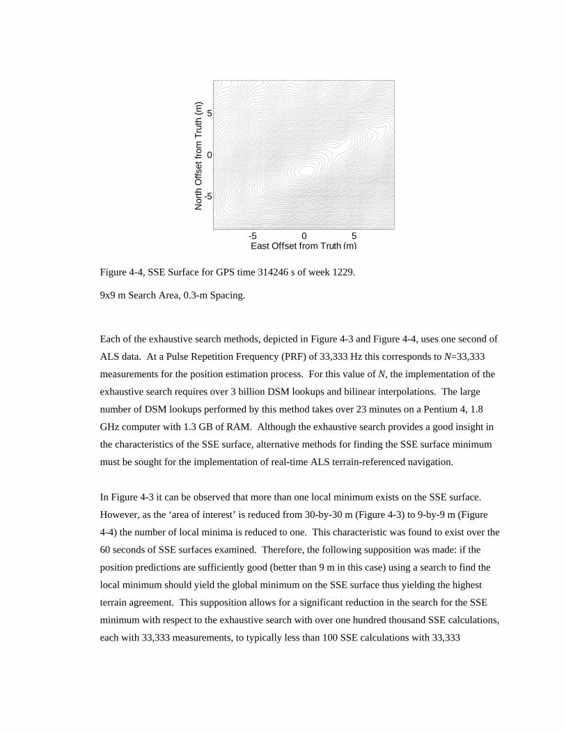
-5 0 5

-5

0

5

East Offset from Truth (m)

Nor

th O

ffset

from

Tru

th (m

)

Figure 4-4, SSE Surface for GPS time 314246 s of week 1229.

9x9 m Search Area, 0.3-m Spacing.

Each of the exhaustive search methods, depicted in Figure 4-3 and Figure 4-4, uses one second of

ALS data. At a Pulse Repetition Frequency (PRF) of 33,333 Hz this corresponds to N=33,333

measurements for the position estimation process. For this value of N, the implementation of the

exhaustive search requires over 3 billion DSM lookups and bilinear interpolations. The large

number of DSM lookups performed by this method takes over 23 minutes on a Pentium 4, 1.8

GHz computer with 1.3 GB of RAM. Although the exhaustive search provides a good insight in

the characteristics of the SSE surface, alternative methods for finding the SSE surface minimum

must be sought for the implementation of real-time ALS terrain-referenced navigation.

In Figure 4-3 it can be observed that more than one local minimum exists on the SSE surface.

However, as the ‘area of interest’ is reduced from 30-by-30 m (Figure 4-3) to 9-by-9 m (Figure

4-4) the number of local minima is reduced to one. This characteristic was found to exist over the

60 seconds of SSE surfaces examined. Therefore, the following supposition was made: if the

position predictions are sufficiently good (better than 9 m in this case) using a search to find the

local minimum should yield the global minimum on the SSE surface thus yielding the highest

terrain agreement. This supposition allows for a significant reduction in the search for the SSE

minimum with respect to the exhaustive search with over one hundred thousand SSE calculations,

each with 33,333 measurements, to typically less than 100 SSE calculations with 33,333

measurements each. The next section presents the use of a gradient search to find the minimum

on the SSE surface.

4.2.2. Gradient-Based Search Position Estimation

A reduction in required computations can be achieved by using gradient-based techniques to

search for the SSE surface minimum given the assumption that there is only one minimum in the

search area. The gradient at a point on a discrete grid surface is approximated to the first order by

differencing the data around that point. Many methods exist to approximate the gradient at

specific locations on a grid defined surface; several are described in [87].

However, to define the gradient on the SSE surface some assumptions must be made. One

parameter used in estimating the gradient is the distance from the position at which the gradient is

taken to the four points on the SSE surface which are used to compute the gradient. Several

factors which should be considered when choosing this parameter are discussed in the following

section. Unlike a DSM which is defined by a set of uniformly spaced elevation values, the SSE

surface approaches a continuous surface as the number of laser measurements used in the sum of

squares error calculation increases if the following assumptions are made. First, it is assumed

that the laser ranger measurements are spatially and temporally independent, i.e. the laser

illumination points do not overlap, and the corresponding points in the DSM are independent (the

size of the uniform grid post spacing in the DSM is small enough such that each laser

measurement uses an independent set of DSM heights to calculate the disparity). Second, it is

assumed that the laser measurements are uniform randomly distributed within the area defined by

the four closest DSM heights since bilinear interpolation is used to compute a DSM height of a

given position. The SSE surface is not defined by an explicit function, hence, empirical results

were obtained and used to identify the parameters required to estimate the SSE surface gradient

for the specific case of the flight test described in the previous sections.

In case of the gradient-based search, equation (18) is modified as follows:

( ) ( )1,11,, ˆˆ−−−

∆+=kENULSOkkiENULSOkiENULSO mtt xxx (19)

where k⋅ indicates the kth iteration in the search, km is the step size at iteration k, and

1, −∆

kENULSOx is found by:

T

kNkN

kNkENULSO dy

SSEddx

SSEd

SSE ⎥⎥⎦

⎤

⎢⎢⎣

⎡

∇−=∆ 01

,x (20)

where kNSSE∇ is the gradient of the SSE surface evaluated at ( )

kiENULSO t,x and dxSSEdkN /

and dySSEdkN / are the individual gradient components at ( )

kiENULSO t,x .

The algorithm can now be described as follows:

k = 0:

( )0,ˆ iENULSO tx = initial position estimate

Compute 0,ENULSOx∆ using equation (20)

m0 = initial step size (2.0 m in the current configuration)

k = 1 to num_iterations (20 for processing in this paper)

Compute position estimate vector ( )kiENULSO t,x using equation (19)

Compute kENULSO ,x∆ using equation (20)

mk = distance to travel in the kENULSO ,x∆ direction:

⎩⎨⎧

<−<≥−

=−−−

−−−

if 5.02or if

121

121

kkkk

kkkkk mAm

kmAmm

xxxx

where A = travel distance reduction decision constant (set to 1.5 in this research)

As described in the above algorithm, an estimated SSE surface gradient is used to determine the

direction of the next step in the gradient search. The distance traveled in each step is controlled

by another mechanism which reduces the gradient distance as oscillations around a minimum are

observed. The oscillating state is determined by computing the distance between the current

gradient calculation position and the gradient calculation made two steps before. Figure 4-5

illustrates one example of the SSE surface gradient search.

Figure 4-5, Gradient Search for Minimum Error on the Sum of Squared Error Surface

4.3. ALS Positioning over Reno, NV

While sharing many of the same components, the use of ALS technology to implement a

positioning capability is fundamentally different in function from a very similar technology

known as LIDAR mapping. LIDAR mapping systems are optimized to generate highly accurate

spatial data which is used in products such as topographic or bathymetric maps. As discussed in

Chapter 3, this optimization is achieved by post-processing the airborne data. The post-processing

methodology conflicts with the positioning system’s goal of real-time operation. An ALS

position estimation system is similar to LIDAR in form in that they both consists of a laser range

scanner, an inertial sensor, and, depending on the positioning implementation, a GPS receiver.

This similarity in form has enabled the use of data collected from a LIDAR mapping system,

flown aboard NASA Dryden’s DC-8, to evaluate the ALS position estimation system. The data

used consist of unprocessed range and scan angle data from the LIDAR’s airborne laser scanner

and the IMU outputs.

Data collected during flight tests conducted on NASA Dryden’s DC-8 Flying Laboratory are used

in conjunction with a high accuracy/resolution DSM to show the construction of the SSE space

and to illustrate aircraft position estimation using the methods described in the following sections

in this paper. The high accuracy DSM has a 2-m spatial resolution and was provided by NGS.

-5 0 5-8

-6

-4

-2

0

2

4

6

8

x offset

y of

fset

Flight tests were conducted on July 28th, July 30th, August 1st, and August 4th 2003 with NASA

Dryden’s DC-8 Flying Laboratory, pictured in Figure 4-6, as part of NASA Langley Research

Center’s (LaRC) Aviation Safety Program. The primary task of the flight test was to collect

weather radar and radar altimeter data for the NASA LaRC real-time SVS terrain elevation

database integrity monitor [88]. A data collection system was installed on this aircraft which

collected LIDAR data (kinematic GPS data, IMU attitude and velocities, laser scanner angle data,

laser scanner range data), radar altimeter data, and weather radar data. The results presented in

this chapter use the ALS from the LIDAR system along with IMU and GPS data to investigate

the ALS terrain-referenced positioning system performance. The LIDAR system used to collect

ALS data was an Optech, Inc. ALTM on loan from the US Army. The LIDAR laser unit was

mounted in the cargo bay of NASA Dryden’s DC-8 Flying Laboratory as shown in Figure 4-7.

Figure 4-6, NASA Dryden DC-8 Flying Laboratory, Photo courtesy of NASA Dryden.

Figure 4-7, NASA Dryden DC-8 Cargo Bay LIDAR Installation

Data were collected for approaches flown into KRNO. The collection of the LIDAR data was

limited to a minimum altitude AGL to satisfy eye-safe regulations. A trajectory of one approach

and its surrounding terrain is plotted in Figure 4-8.

Figure 4-8, Flight Path of an Approach into KRNO

Optech LIDAR

4.3.1. Initial Positioning Results

Over 12 GBytes of binary LIDAR/navigation data were collected during the five missions flown

during the July/August DC-8 flight tests. Much of these data were collected outside the 18-by-10

km region covered by the available NGS DSM. Several of the flight trajectories which cross the

high accuracy/resolution DSM are plotted in Figure 4-9.

-119.85 -119.8 -119.75 -119.739.42

39.44

39.46

39.48

39.5

39.52

39.54

39.56

Latit

ude

(deg

)

Longitude (deg)

Figure 4-9, Flight Trajectories during Laser Data Collection at KRNO

The laser scanner settings varied from 10 to 20 deg in scan width and from 15 Hz to 29 Hz in

scan rate. KRNO is in the center of the high accuracy/resolution DSM. Flights over the DSM

were made as approaches to the airport. It is important to note that no LIDAR measurements

were available for the center region of the DSM because in those regions the aircraft descended

below the allowed eye-safe altitude. In total, 277 s of ALS data were processed for this paper,

with the longest continuous data segment being 62 s in duration. Filter techniques were not

applied to the laser measurements to remove laser measurement outliers (returns from clouds,

birds, etc.).

A four point gradient search was used to calculate the position estimate for each one second set of

data consisting of 33,333 laser measurements. Each gradient search was permitted to iterate a

maximum of 20 times with an initial step of 20 =m m. The gradients for each iteration were

calculated by estimating the north and east slopes around a point with a ± 0.5 m spacing around

the point as described in Section 4.1.1.2. The height error space was searched by performing

several gradient searches on each one second interval of data at discrete height offsets. The

estimated vertical was found by comparison of the minima of each discrete height offset gradient

searches and identification of the point with the smallest error. A plot of the horizontal errors in

the ALS position estimations can be seen in Figure 4-10 for all 277 s of ALS data.

-40 -20 0 20 40-40

-30

-20

-10

0

10

20

30

40

x error (m)

y er

ror (

m)

Figure 4-10, ALS Horizontal Position Estimate Error

The error values in the x (east-west) and y (north-south) direction were computed by subtracting

the ALS navigation position estimate from the post-processed KGPS data (the truth reference

data). Over 90% of the position estimates fall within 10 m of the true position. Table 1 provides

a summary of the position estimate characteristics for the 277 s of data processed. In Table 1 it is

shown that the horizontal radial position error is 8.9 m (1σ), while the vertical position error is

0.51 m (1σ) for 1-s updates. If an outlier rejection method is used in conjunction with the

gradient search the positioning accuracies improve to approx. 3.2 m (1σ) and 0.5 m (1σ) for the

horizontal radial position error and the vertical position error, respectively. The outlier rejection

method discards solutions that disagree by more than 10 m with respect to the INS position

estimate.

Table 1, Summary of ALS Position Estimates (1-s updates)

Description Mean (m) Std. Dev. (m)

x error (all 277 points) 0.45 5.12

y error (all 277 points) -0.87 7.28

h error (all 277 points) -1.16 0.51

x error w/ 10 meter cutoff (251 points) 1.00 2.74

y error w/ 10 meter cutoff (251 points) -0.51 1.67

h error w/ 10 meter cutoff (251 points) -1.15 0.50

5. Real-Time TERRAIN Approach System

In Chapter 4 it was shown that position solutions on the order of a meter were possible when

performing terrain navigation with an ALS and a high resolution/high accuracy terrain database.

These results inspired the design, implementation, and flight test a proof-of-concept real-time

TERRain Aided Inertial Navigator (TERRAIN) approach system. This chapter details the real-

time TERRAIN approach system design and presents the results from the flight test performed

January 14, 2005.

The TERRAIN precision approach system includes an ALS, a high resolution/accuracy (1 m

resolution and 30 cm RMS elevation accuracy) terrain database, created using a LIDAR, WAAS

GPS and an inertial sensor system to provide vertical and horizontal guidance to a desired

runway. For this research, the approach path to the runway is defined as a straight-in 3-degree

approach, similar to Instrument Landing System (ILS) approaches currently in use. WAAS GPS

is used for guidance and calibration of the INS during the initial approach phase. During this

initial phase the TERRAIN approach system capitalizes on the position and integrity benefits

provided by WAAS GPS to reduce the size of the terrain navigator’s position search space and to

reduce the required size of the high accuracy/resolution database. Thus, WAAS GPS is used for

the initial segment of the precision approach until the minimum allowed height, or Decision

Height (DH) is reached for the particular WAAS GPS approach, at which point the system

switches to TERRAIN-based positioning to complete the final segment of the approach.

The proof-of-concept real-time TERRAIN approach system provides precision approach

guidance to the pilot via vertical and horizontal deviation cues on a Liquid Crystal Display (LCD)

Heads Down Display (HDD). As described above, the real-time system operates in one of two

modes during the approach: WAAS GPS mode or TERRAIN mode. Figure 5-1 provides a block

diagram of the approach system. During the initial approach phase, the TERRAIN approach

system is in WAAS-aided mode. In this mode WAAS is used to update the position estimates,

and GPS integrated carrier phase measurements are used to calibrate the integrated velocities

from the INS (Mode Controller = 0 in Figure 5-1). WAAS is used until the DH specified for the

WAAS approach procedure is reached at which point the mode is switched to TERRAIN mode

(Mode Controller = 1 in Figure 5-1). In TERRAIN mode, the INS velocity error estimates in the

Kalman filter (block A in Figure 5-1) are fixed and the corrected INS integrated velocities are

added to the last position estimate to form the corrected position prediction. The corrected

position predictions are used in the terrain navigator to transform the points measured by the ALS

to a geo-referenced coordinate frame. After the point cloud generation, the terrain position

estimator is used to estimate the error in the current corrected position. This estimated error is fed

back into the corrected position (block B in Figure 5-1). The prototype terrain approach system is

detailed in the following sections:

• Characteristics of the TERRAIN Approach System

• Terrain-Referenced Position Solutions

• Inertial Velocity Error Estimation Using Integrated GPS Carrier Phase

• Proof-of-Concept Real-time TERRAIN Approach System Hardware Description

• Flight Test Location and Test Plan

• TERRAIN Precision Approach System Performance

Figure 5-1, TERRAIN Precision Approach System Position Estimator

Mode Controller0 = WAAS1 = TERRAIN

GPSCarrier PhaseMeasurements

GPSUnit VectorsTo Satellites

GPSWAAS PositionMeasurements

Lever Arm Corrected

INS Velocities

ALS PositionError Estimator

0

1 S out

∫ R

SampleAndHold R

in out

ProjectIntegrated Vel.

On SV Unit Vectors

x

H

∫ R

z H∗x

8 StateGPS Carrier Phase/

INS VelocityKalman Filter

States:1-3 Int. Vel Err

4-6 Vel Err.7-8 GPS Clk. Err

-+ z-H∗x

Iterate

0

1 Sout

offReset

0

1Sout

TimingControllerWAAS

UpdateTRN Update

1Hz

1/3Hz

∫R

UncorrectedPosition

++

Integrated Velocity Error Estimates

+-

KalmanUpdate

Corrected Position

10 Hz

IntegratedVelocities

INS Attitude Measurements

+

-

Laser ScannerMeasurements

Terrain Navigator

Mode Controller0 = WAAS1 = TERRAIN

GPSCarrier PhaseMeasurements

GPSUnit VectorsTo Satellites

GPSWAAS PositionMeasurements

Lever Arm Corrected

INS Velocities

ALS PositionError Estimator

0

1 S out

0

1 S out

∫ R ∫

R

SampleAndHold R

in out

ProjectIntegrated Vel.

On SV Unit Vectors

x

H

∫ R ∫

R z

H∗x

8 StateGPS Carrier Phase/

INS VelocityKalman Filter

States:1-3 Int. Vel Err

4-6 Vel Err.7-8 GPS Clk. Err

-+ z-H∗x

Iterate

0

1 Sout

0

1 Sout

offReset

0

1Sout

0

1Sout

TimingControllerWAAS

UpdateTRN Update

1Hz

1/3Hz

∫R

∫R

UncorrectedPosition

++

Integrated Velocity Error Estimates

+-

KalmanUpdate

10 Hz

IntegratedVelocities

INS Attitude Measurements

+

-

Laser ScannerMeasurements

Terrain Navigator

D

C

EB

A

5.1. Characteristics of the TERRAIN Approach System

In the development of the proof-of-concept TERRAIN precision approach system, two goals

were defined: the first goal was to operate in real-time; and the second goal was to provide

aircraft guidance which meets the accuracy requirements similar to other precision approach

systems currently in use. A precision approach is defined as a method that provides both vertical

and horizontal guidance to the runway. Aircraft approach systems are required to meet specific

levels of accuracy, integrity, availability, and continuity. The parameter levels are dependent on

the category (CAT) of the approach. The CATs are specified by the height at which the pilot

must visually acquire the runway environment and make a decision as to whether he continues

the approach or not. This height is referred to as the decision height or DH and the pilot’s

decision will be based on visibility and/or the runway visual range (RVR). For example, a CAT I

approach has a DH of not lower than 200 ft and a visibility of not less ½ a statute mile or an RVR

of not less then 1,800 ft [89]; thus, if the pilot cannot identify the runway environment (runway

lights and/or runway) at a height of 200 ft above the runway, or the ground controllers have

measured the visibility at less than 1,800 ft, the pilot may not land using the CAT I approach.

To rigorously explore the accuracy, integrity, availability and continuity of the system is beyond

the scope of this dissertation; however, this section makes an attempt at identifying the major

factors which impact the integrity, availability, and continuity. Accuracy is discussed in Section

5.6 - TERRAIN Precision Approach System Performance.

5.1.1. TERRAIN Approach System Integrity

Arguably the most critical parameter for an approach system, integrity can be defined as the

ability of the system to provide timely warnings to users when the system should not be used for

navigation and is thus strongly related to the probability that the indicated performance of a

system (good or bad) is correct. Typically associated with integrity is the time-to-alarm

parameter; the time elapsed from the moment misleading information is presented to the moment

a warning is presented to the pilot. There are cases where the TERRAIN approach system can

not be used. For example, the famous approach into St. Maarten Island in the Caribbean, which

is completely over water since the runway is located at the edge of the island as seen in Figure

5-2. However, this condition is known a priori, thus no integrity violation would occur. There

are two aspects for the TERRAIN approach system which impact integrity: the terrain database

integrity and ambiguous position solutions.

Figure 5-2, Approach into St. Maarten Island. Approach over water would make the TERRAIN

approach system not available.

Terrain databases in use today have accuracy specifications assigned to them but no integrity

specifications. If a terrain database is to be used in a system which is certified by the FAA,

terrain database manufactures would have to develop a specification to include this information.

However, terrain can be thought of as a relatively time stationary signal. Hence, it should be

possible to qualify the segments of the terrain database used during an approach and thus provide

a level of data integrity. Qualification of an approach is not a new process; other systems which

have time stationary signals such as ILS are first qualified by the FAA to ensure accuracy and a

monitor is placed to ensure the guidance signal does not vary with time.

The second aspect of TERRAIN approach system integrity is ensuring that any ambiguous

position solutions are excluded. Since the terrain signal is known from the terrain database, an

approach to deal with ambiguous position solutions is to identify ambiguities before the terrain

database is used for an approach and evaluate the impact to the system. The impact ambiguous

position solutions have on the TERRAIN approach system is limited by two means. The first is

the use of WAAS for the initial position estimation. As described in Section 2.4.2, WAAS has

vertical and horizontal protection bounds on its position estimates. Position ambiguities which

exist outside these error bounds can therefore be disregarded. Secondly, after terrain-referenced

navigation is started, a calibrated inertial navigator is used for positioning between each terrain-

referenced position estimate. Thus, position solution ambiguities which fall outside the

protection levels assigned to the inertial position error growth during the period between terrain-

referenced position updates can be disregarded as threats to the system’s integrity. Given that

position updates are made every 3 seconds in the proof-of-concept system, position error growth

from a calibrated navigation grade inertial is minimal. One last method that can be used to

eliminate ambiguous position solutions is the examination of successive terrain-reference position

solutions. This method is valid assuming the ambiguities are not spatially correlated over

multiple transect lengths and the time-to-alarm is able to be achieved.

5.1.2. TERRAIN Approach System Availability

Availability can be loosely defined as the probability that the aircraft can use the landing aid at

the start of the approach procedure. The largest factors which contribute to the availability of an

ALS based landing system, at the current time, are atmospheric and weather conditions. These

conditions may cause large attenuation of the laser signals. Today’s ALS systems typically have

wavelengths between 300 nm to about 11 µm which makes weather particulates such as snow,

rain, fog, and even smog electrically large enough to significantly attenuate the laser energy. The

assumption is made that weather, because of the laser attenuation, is the dominate variable which

impacts the availability of an ALS-based landing system.

It is desirable for an aircraft landing system to be available in “all weather.” However, we must

first define “all weather” since there are situations where, even if the landing guidance system

was available, the aircraft would not be able to perform a landing, e.g. thunderstorms with high-

rain rates and strong down drafts; snow storms where high snow rates reduce the friction on the

runways; and other extreme case such as tornados, hurricanes, and volcanic activity. Given there

may be conditions in which the landing guidance system is not available when an aircraft could

perform a landing, it is of interest to know the probability of such a condition occurring. For

example, if Figure 5-3 defines the probability density function of a weather condition as a

function of the severity of the weather condition, the area under f(x) starting at “a” and ending at

“b” could represent the region of weather severity in which the landing system is not available

given that the aircraft could perform a landing.

Figure 5-3, Theoretical probability density curve of a weather condition of severity x occurring,

the area of the shaded region represents probability of a landing guidance system not available

With the assumption that the availability of landing guidance system is dependent mainly on the

severity of the weather, the availability of the landing system can be defined using Bayesian

statistics as follows:

( ) landingan performaircraft cvailablestem not alanding sytyavailabili P1−= (21)

or using Figure 5-3:

( )bxbxatyavaibabili <<≤−= P1 (22)

In the early 1990’s studies were performed where high update rain rate measurements were made

at various airports around the world to determine the frequency of occurrence of various rain rates

[90]. The effects of these rain rates on the ALS and the ability of the aircraft to land can be

interpreted and related to a probability density function like Figure 5-3. Another factor which

must be considered in the ALS weather sensitivity analysis, is that not every ALS range

measurement is required to produce a position estimate. Current ALS system range measurement

rates vary from 10 to 100 kHz. Accurate position solutions may only require a fraction of total

returns. Thus, the availability of the TERRAIN approach system is a combination of probability

of a particular weather event (i.e. probability of a particular rain rate), the probability of a

measurement given the ALS link budget for the weather event, and the probability that a

x, “weather condition severity”

b

a

x > a, landing guidance system cannot operate

x > b, aircraft cannot perform landing f(x)

landing guidance system not available when aircraft could land

minimum number of range measurements were made to compute a valid position estimate. It

should be noted that the impact of a weather condition on the availability of the TERRAIN

approach system is reduced by using WAAS for positioning until the WAAS DH is reached, thus

reducing the range, R4, loss factor in the laser range equation.

5.1.3. TERRAIN Approach System Continuity

System continuity can be defined as the probability that an approach will not end given it has

been successfully started. As discussed before, it can be assumed that for the TERRAIN

approach system, attenuation to the ALS measurements due to weather conditions is the largest

contributing factor for whether the terrain-based position solution can be computed. Since

continuity is based on the ability to continue operation after an approach has been successfully

started, weather conditions would have to deteriorate from the moment the approach starts to a

level that prohibits the ALS from measuring the terrain. However, a deteriorating weather

condition will not necessarily end the approach since a continuous decrease in aircraft altitude

also means in continuous decrease in laser path losses. Therefore the attenuation due to weather

must increase at a higher rate than the energy gained from flying closer to the ground. In fact, it

can be seen by looking at the laser range equation that the energy received increases by R4 as the

range decreases while the path loss due to weather, ηATM, decreases by a factor of R2 as the range

decreases. Thus, the laser power received increases quadratic as the altitude decreases improving

the probability that continuity of service is guaranteed.

5.2. Terrain-Referenced Position Solutions

At the heart of the TERRAIN approach system is the ALS position estimator seen in the bottom

left corner of Figure 5-1 (Block B). In the proof-of-concept TERRAIN approach system, the

estimator uses three seconds of ALS data, which in this realization contains 30,000 independent

laser measurements, for each batch-type position error estimate. Data collected from flight tests

performed by NASA Langley Research Center at NASA Dryden with NASA Dryden’s DC-8

aircraft were first used to prototype algorithms to solve for the position error estimate as

described in Chapter 4, [85], and [91]. However, these prototype algorithms assumed a known

Laser Scanner Optics (LSO) position, LSOx , for each laser range measurement. In Chapter 4’s

position solution algorithms, interpolated position and attitude measurements from a post-

processed GPS/INS system were used. While in the TERRAIN positioning mode, the TERRAIN

approach system computes LSOx in real-time using previous estimates of the position and

integrated INS velocities for the trajectory estimates between each position estimate:

( ) ( ) ( )dttttit

tENULSOENULSOiENULSO ∫+=

0

,0,, ˆˆˆ vxx (23)

where

( )iENULSO t,x is the position estimate at time ti in ENU (Figure 5-1, Diamond E),

( )0,ˆ tENULSOx is the position estimate at time t0 in ENU (Figure 5-1, Diamond C),

( )tENULSO,v is the velocity measured by the inertial in ENU (Figure 5-1, Diamond D).

Attitude of the LSO is computed by using the unaided INS attitude.

In Chapter 4, it is shown that a position estimation error surface can be created by performing an

exhaustive search on the ALS/terrain database agreement. Chapter 4 also shows that the position

estimate is given by the coordinates of the minimum value on the error surface. Results from data

processed in Chapter 4 demonstrate that, given constraints on the position estimation error surface

size, only one minimum is likely to exist. This characteristic permits the solution of the surface

minimum to be computed by a gradient-based algorithm rather than an exhaustive search over the

entire error surface allowing it to be implemented in a real-time architecture. For example, the

computation was reduced from the twenty-three minutes for an exhaustive grid search to near

real-time for a gradient-based search in a MatlabTM implementation. Further improvements in the

implementation of the gradient search have resulted in real-time operation. These improvements

include storage of the terrain database in Random Access Memory (RAM) and the

implementation of the algorithm in C on a Real-Time Operating System (RTOS).

The agreement between the ALS data and the terrain database is evaluated by comparing the

vertical component of a set of points illuminated by the ALS and the vertical component of a set

of heights retrieved from the terrain database to form a vertical disparity for a given ALS

horizontal position estimate. A total of 30,000 vertical disparities are compared for each position

error estimate. Since a direct comparison between the vertical components is performed, small

errors in assumed horizontal position can map into a large error in the vertical if features such as

buildings or trees are present. To improve the positioning performance these effects were

reduced by implementing a simple outlier removal filter which removes points that are more than

several standard deviations larger than the expected vertical error as is described in Chapter 4.

For the implementation reported here, the vertical error was computed to be approx. 1 m RMS,

thus a 6σ value of 6 m can be selected to remove measurements which are influenced by trees or

building edges. It should be noted that this filter rarely removed more than 1000 out of 30,000

measurements per position error estimation and these outliers were most likely due to vegetation.

Future research is focused on the identification of objects such as buildings and segmentation of

these objects to use complementary methods which make use of sharp gradients to improve the

horizontal position error estimation.

5.3. Inertial Velocity Error Estimation Using Integrated GPS Carrier Phase

The velocity error estimates for the Honeywell HG-1150 Inertial Reference Unit (IRU) are

obtained from a Kalman filter during the initial approach phase of the TERRAIN approach

system while WAAS is used for guidance. Upon the transition to the final approach phase the

Kalman filter is disabled, and the last velocity error estimates are used to complete the TERRAIN

approach. Thus, the Kalman filter is not active during the final approach phase where the

TERRAIN mode is used. The Kalman filter was implemented in C++ and a detailed description

of the filter mechanization is given in Section 2.4.4.

As described in Section 2.2.4, the observations input to the Kalman filter are the differences

between the GPS integrated carrier phase for each Space Vehicle (SV) and the integrated inertial

velocities mapped onto the Line-of-Sight (LOS) vectors between the estimated user position and

each SV. The eight state-variable Kalman filter has the following state variables: states 1 through

3 are the integrated velocity error in ENU; states 4 through 6 are the velocity error in ENU; and

states 7 and 8 are the GPS clock bias and drift, respectively. As seen in Figure 5-1, the integrated

velocity error estimates (state variables 1 through 3) are used to remove the error in the IRU

integrated velocities. It should be noted that, to meet the time window for the flight tests, the

Kalman filter implementation did not include the leverarm correction between the IRU and the

GPS antenna (which was about 8 m); however, this absence did not greatly impact the

performance of the system since the IRU calibrations were performed predominately during

straight-in approaches where the aircraft velocities were relatively constant. Calibration during a

turn would have been greatly affected by the exclusion of the leverarm.

Below are the values used in the system noise covariance matrix ( 0Q ), the measurement noise

covariance matrix ( 0R ), and the estimation error covariance matrix ( −0P ) used in the proof-of-

concept TERRAIN approach system Kalman filter. The matrix entries were derived form the

specifications of the sensors used in the TERRAIN approach system.

0Q , initial (and constant) system noise covariance matrix [n×n]

( )( )

( )

⎥⎥⎥⎥⎥⎥⎥⎥⎥⎥⎥

⎦

⎤

⎢⎢⎢⎢⎢⎢⎢⎢⎢⎢⎢

⎣

⎡

σβ

σσ

σ=

dt200000000000000000dt00000000dt00000000dt000000000000000000000000000

2clkclk

2vel_sys

2vel_sys

2vel_sys

0Q (24)

where the system velocity standard deviation is velsys _σ = 0.01 m/s

the clock standard deviation is 2101×=clkσ s

the beta value of the clock drift is 1=clkβ s

and the time step of the Kalman filter is dt = 0.1 s

0R , initial (and constant) measurement noise covariance matrix [m×m]

⎥⎥⎥⎥⎥

⎦

⎤

⎢⎢⎢⎢⎢

⎣

⎡

σ

σσ

=

2ICP

2ICP

2ICP

k

m

2

1

0000

000000

L

MOR (25)

where GPS integrated carrier phase noise estimate, m 007.0=iICPσ

−0P , initial estimation error covariance matrix [n×n]

⎥⎥⎥⎥⎥⎥⎥⎥⎥⎥⎥

⎦

⎤

⎢⎢⎢⎢⎢⎢⎢⎢⎢⎢⎢

⎣

⎡

σ

σσ

σ=−

2drift_clk

2vert_vel

2horz_vel

2horz_vel

0

000000000000000000000000000000000000000000000000000000000000

P (26)

where - the IRU horizontal velocity standard deviation, horzvel _σ , is specified as 12 kts

2σ [92] , thus assuming a normal distribution, 6 kts 1σ ≈ 3 m/s

- the IRU vertical velocity standard deviation, vertvel _σ , is specified as 30 ft/min

2σ [92], thus assuming a normal distribution, 15 ft/min 1σ ≈ 0.08 m/s

- the clock drift standard deviation, 2101×=clkσ s/s

5.4. Proof-of-Concept Real-time TERRAIN Approach System Hardware Description

One of the most challenging aspects of the proof-of-concept demonstration was the development

of a system that operates in real-time. Given the amount of data to be processed and the

characteristics of the algorithms of the real-time system, a networked architecture with three

computers was developed as shown in Figure 5-4. The first computer is the Data Collection and

Distribution (DCD) computer. Its primary task is to time-tag, store, and distribute the data from

the various sensors used in the system. The second computer is the Navigation computer, which

uses a multi-treaded architecture to perform the positioning and navigation functions. The third

computer uses the aircraft state data, computed by the Navigation computer, to render the

guidance cues displayed to the pilot. Since integrity of the data links between the computers was

not an objective of the proof-of-concept system, Ethernet UDP and TCP/IP protocols were used

to connect the three computers. This section provides a description of the GPS WAAS, IRU, and

ALS sensors connected to the Data Collection and Distribution computer, as well as a description

of the setup of the three computers used in the proof-of-concept system.

Figure 5-4, TERRAIN Precision Approach Hardware Diagram

5.4.1. NovAtel OEM 4/WAAS GPS Receiver

The WAAS position measurements and GPS carrier phase measurement, used by the Kalman

filter in the TERRAIN system during initial approach phase, are provided by a NovAtel OEM-4

L1/L2/WAAS GPS receiver. WAAS position accuracies were observed to be better than five

meters in the horizontal and vertical when compared to post-processed Kinematic GPS for the

January 14, 2005 flight test. Also provided by the OEM-4 GPS receiver is a one Pulse Per

Second (PPS) signal. This signal is used to time-synchronize the Navigation Computer and Data

Collection and Distribution computer. The synchronization is performed through the use of

interrupt service routines that synchronize the computer times through the level-converted, pulse-

extended, PPS signal fed into the Data Collection and Distribution computer’s serial port. The

PPS was also used to estimate the computers’ (crystal oscillator) clock drifts.

5.4.2. Honeywell HG1150 Navigation Grade Inertial Reference Unit (IRU)

Navigation frame-referenced velocities and aircraft attitude data were obtained from the

Honeywell HG1150 navigation grade IRU seen in Figure 5-5. Several different designs of the

proof-of-concept using data from the HG1150 were considered, including a “full” inertial

mechanization using the acceleration and body-rate data to compute position, velocity, and

attitude; as well as a mechanization which only used HG1150 position outputs. It was found that

Time Tagging / Data Storage

QNX 6.3

Honeywell HG1150 IRU

Laser Scanner Position Error

Estimation

QNX 6.3

Navigation Solution Mechanism

Riegl ALS LMS-Q140i

NovAtel OEM 4 / WAAS

100kbs Arinc 429

Parallel Port

Serial Port

PPS

PPS

PPS

Seria

l Por

t (po

sitio

n, ra

nge,

etc

.)

GPS Inputs

For Timing Only

Windows

Aircraft Guidance

(DELPHINSSoftware)

Fast Ethernet

Hub

GS

NA

E

W

SN

12

15

21

6

3

33

30 24OBS

(LS

Mod

e C

ontro

l)

(LS

Ran

ge/A

ngle

Dat

a)

the best performance was obtained by using a mechanization which fell somewhere in between

these two approaches. The navigation frame velocity data, computed by the HG1150, are used.

The use of this mechanization is necessary due to the limitations on the bandwidth and resolution

of the HG1150 data imposed by the ARINC-429 interface. The HG1150 is a standalone Ring

Laser Gyro (RLG) IRU with a 1 nmi per hour position error growth specification.

Figure 5-5, Honeywell HG1150 IRU installed just aft of right-seat pilot in the DC-3

Horizontal velocity data are provided at 20 Hz with a bandwidth of 2 Hz, vertical velocity data

are provided at 25 Hz with a bandwidth of 8 Hz, aircraft pitch and roll angles are provided at 50

Hz with a bandwidth of 8 Hz, and heading angles are provided at 20 Hz with a bandwidth of 2 Hz

[92]. Transport delays due to filtering performed inside the HG1150 and transmission over the

databus are specified to be less than 110 ms [92].

5.4.3. Riegl LMS-Q140i Airborne Laser Scanner

Measurements of the terrain are made with the Riegl LMS-Q140i airborne laser scanner. For the

real-time TERRAIN precision approaches the LMS-Q140i was configured to scan with a 60

degree cross-track scan at 15 scans per second with an average PRF of 10,000 range

measurements per second. In this configuration, assuming an altitude of 1000 ft AGL and a

ground speed of 60 m/s, the distance between scans in the along-track direction is approx. 4 m

and the distance between cross-track scans is approx. 1 m as summarized in Figure 5-6. The

LMS-Q140i scan rate can be set as high as 40 scans per seconds allowing for a more uniform

distribution of the laser measurements. The analysis of the effects of the various measurement

distributions on the position estimates is planned for future research.

The LMS-Q140i specifications are as follows [78]:

o Scan angle range: 80 deg

o Max Scan Speed: 40 scans/sec

o Scan Angular Resolution: 0.018 deg

o Measurement Range: 350 m for target reflectivity > 20%, 700m for target reflectivity > 80%

o Measurement Accuracy: ± 5 cm

o Laser beam divergence: approx. 1 mrad

o Eye Safety: Class 1 (eye safe)

Figure 5-6, Scanning Parameters for LMS-Q140i with Average PRF = 10 kHz

Scan Angle = 60 deg

1 m @ 1000 ft AGL

1150 @ 1000 ft AGL

4 m @ 60 m/s

5.4.4. Data Collection/Distribution Computer

Data from the various sensors were collected and time-tagged in the DCD computer. The DCD

computer is illustrated and pictured in Figure 5-4 and Figure 5-7, respectively. The DCD is

configured to allow for data collection and distribution as well as post-mission playback of the

real-time TERRAIN guidance system. The DCD hardware consists of a 4U 19” rack-mountable

computer configured to allow data collection from the NovAtel OEM 4/WAAS GPS Receiver via

an RS-232 serial port; a Honeywell HG1150 IRU via an ARINC 429 data bus card; a Riegl LMS-

Q140i laser scanner via an ECP parallel port and RS-232 serial port; and a Honeywell HG8505

radar altimeter via an RS-232 serial port.

Along with data collection and distribution, another critical roll of the DCD is data time-tagging.

The DCD is synchronized to GPS time using the PPS signal from the OEM-4 GPS Receiver and

time information from the OEM-4 data messages. Time synchronization is performed by pulse-

extending and level-converting the PPS signal to allow for the triggering of a serial port interrupt

in the DCD. The constant length of the pulse extension is then corrected in the DCD software.

Time accuracy in the computer is measured to be better than 10 µs.

The operating system used on the DCD computer is QNX 6.3. Data are read from each sensor by

independent resource managers (similar to a device drivers) written by Ohio University AEC.

The use of resource managers allows for the efficient division of processing time between the

data collection, distribution, and time-stamping with the ability to provide higher priority to time

sensitive tasks such as time-stamping. Once data are read and time-tagged by its corresponding

resource manager it is stored in a circular buffer allowing other programs global access to the data

by a simple read statement. Data are distributed to the NAVigation (NAV) computer via a high

speed (100 Mb) TCP/IP Ethernet link. Code in the DCD computer is compiled using the GNU C-

compiler.

5.4.5. Navigation Computer

The aircraft state (position, velocity, attitude) and the guidance cues for an approach are

computed in the NAV computer. The NAV computer receives sensor information from the DCD

computer via the TCP/IP Ethernet link, processes and extrapolates the data, and transmits the

aircraft state information to the display computer via an UDP Ethernet link. Like the DCD

computer, the NAV computer is synchronized to GPS time via the OEM-4 GPS receiver’s PPS

signal. Since time is synchronized between the DCD and NAV computer it is possible to reduce

the apparent latency in the pilot display by extrapolating the data sent to the tunnel computer

where appropriate. QNX 6.3 is also used as the operating system for the NAV computer. Like in

the DCD, this allows for multiple threads set at various priority levels to perform varied tasks

such as: DCD computer data reception, GPS time synchronization, position processing mode

selection, terrain-referenced position estimation calculations, inertial velocity error estimations,

and the transmission of data to the display computer. Code in the NAV computer is compiled

using the GNU C-compiler.

Figure 5-7, DC-3Research Computer Rack

5.4.6. Display Computer

Guidance cues are provided to the pilot through an LCD mounted for use by right seat pilot as

shown in Figure 5-8. The LCD display is driven by DELPHINS software running on the tunnel

computer. DELPHINS software was developed and is maintained by Delft University of

Technology in Delft, The Netherlands and used by Ohio University under a Memorandum of

Agreement. It provides a HDD which can provide both a flight director style guidance display

and a synthetic vision guidance display to the pilot.

Navigation Computer

Data Collection Computer

Display Computer

}}

}

Figure 5-8, DC-3 Cockpit with DELPHINS Guidance Display

5.5. Flight Test Location and Test Plan

The real-time TERRAIN precision approaches were performed at Braxton County Airport (K48I)

to runway 19. The view from the DC-3 on short final can be seen in Figure 5-9. K48I was

chosen because of the availability of a LIDAR generated DSM and the relatively short proximity

(approx. 80 nmi) to the Ohio University Airport (KUNI). Runway 19 at K48I is 4,000 ft in length

and 60 ft in width. Currently there are no FAA published approach procedures into this airport.

An airport survey was conducted and the runway touchdown point for the approach was created

to be 1,000 ft from the threshold and a straight-in 3-deg approach was extended from the

touchdown point. The LIDAR generated DSM is describe in Section 3.3.2, and the metadata for

the terrain database is reprinted in Appendix B.

Figure 5-9, DC-3 on Short Final to Runway 19, K48I

Two days of flight tests at K48I took place. The first flight test, flown on December 12, 2004

was a data collection effort. Eight approaches were flow allowing for the collection of time-

tagged GPS, HG1150 IRU and LMS-Q140 ALS data. Data collection was performed using the

DCD computer, which allowed for the real-time playback of the data enabling the development

and testing of the NAV computer in the lab with data from an actual flight test. The NAV

computer software was completed after a month of development, and the real-time TERRAIN

approach system was flown on January 14, 2005. To test the proof-of concept system, eight

approaches at K48I were flown to runway 19. The aircraft trajectories are illustrated in Figure

5-10.

Figure 5-10, trajectories flown to K48I on January 14, 2005 during the flight testing of the real-

time TERRAIN approach system: Left- perspective view, Right- plan view with North up

5.6. TERRAIN Precision Approach System Performance

For the TERRAIN precision approach system the system positioning accuracy was evaluated.

Post processed Kinematic GPS positions are used as the truth reference in this section. A set of

position accuracies from one of the approaches is shown in Figure 5-11.

Figure 5-11, TERRAIN position – KGPS for one approach, HAT: Height Above Threshold

It can be seen that for this approach the position estimates were nearly all contained within ± 5

meters of the truth. The blue shaded regions indicate when GPS WAAS positioning was enabled

whereas the non-shaded regions indicate when TERRAIN mode was enabled. Mode switching

between WAAS and TERRAIN can be observed. This effect can be attributed to variations in the

terrain that cause the height AGL to exceed the threshold height for the WAAS mode, selected at

1,200 ft Height Above Threshold (HAT), at various occasions. It must be noted that the runway

threshold is higher than much of the terrain on the approach path. The mode toggling

phenomenon results from placing the decision HAT for WAAS mode near the maximum range of

the ALS and would not occur with either a lower HAT or longer range ALS.

Performance of the system was evaluated during the final approach phase of flight starting 900 ft

HAT. 900 ft HAT was chosen as the starting height to evaluate performance to ensure quality

measurements from the LMS-Q140i laser scanner. During this phase of flight the navigator was

operating in the terrain navigation mode for the eight approaches. 5323 position estimates were

computed by the navigator. Figure 5-12, Figure 5-13, and Figure 5-14 provide histograms of the

0 50 100 150 200 250 3000

500

1000

HA

T (ft

)

0 50 100 150 200 250 300-505

Eas

t Err.

(m)

0 50 100 150 200 250 300-505

Nor

th E

rr. (m

)

0 50 100 150 200 250 300-505

Up

Err.

(m)

GPS Time - (497782) (s)

TERRAIN approach system navigator in the East, North, and Up directions. A best fit normal

distribution overlay provides an indication that the distribution of position outputs are relatively

normal, however they fail standard normal distribution tests (Jarque-Bera test with %5

significance level).

-6 -5 -4 -3 -2 -1 0 1 2 3 40

20

40

60

80

100

120

140

160

180

200

Bin

Qua

ntity

Figure 5-12, Histogram of error in the TERRAIN approach system navigator output in the East

direction with best fit normal distribution overlay.

-5 -4 -3 -2 -1 0 1 2 3 4 50

20

40

60

80

100

120

140

160

180

Bin

Qua

ntity

Figure 5-13, Histogram of error in the TERRAIN approach system navigator output in the North

direction with best fit normal distribution overlay.

-2.5 -2 -1.5 -1 -0.5 0 0.5 1 1.50

50

100

150

Bin

Qua

ntity

Figure 5-14, Histogram of error in the TERRAIN approach system navigator output in the Up

direction with best fit normal distribution overlay.

Table 2 presents a summary of the statistics from the eight approaches (9 minutes of data) flown

on January 14, 2005, at Braxton County airport while the navigator was in TERRAIN mode.

Values in Table 2 were computed from data collected while on approach, from 900 ft HAT until

the 50 ft DH, and Table 3 provides a summary of the statistics for the TERRAIN system at a 50 ft

DH (1 measurement each approach so sample size of only 8 for Table 3).

Table 2, Summary of TERRAIN Position Accuracy on Approach, 900 ft HAT to DH, Eight

Approaches, Nine Minutes of Data

Error Direction Mean (m) Standard

Deviation (m)95%

Value (m) Max Absolute

Error (m)

East -0.982 1.43 3.84 5.62

North -0.117 1.34 2.81 4.39

Up -0.645 0.615 1.87 2.35

Table 3, Summary of TERRAIN Position Accuracy at 50 ft DH, Eight Approaches (5323

measurements)

Error Direction Mean (m) Standard

Deviation (m)95%

Value (m) Max Absolute

Error (m)

East -0.55 1.55 3.65 3.23

North -0.82 1.35 3.53 2.82

Up -1.46 0.57 2.60 2.16

Accuracy requirements defined for a satellite-based CAT IIIb approach are 5.0 m in the

horizontal and 2.9 m in the vertical 95%-value under guidance to the DH [89]. If the data used to

generate the standard deviations in Table 3 are assumed to be normal then the 95%-values can be

conservatively approximated by multiplying the standard deviation by two and adding the

absolute value of the mean error. The 95%-values of the proof-of-concept TERRAIN precision

approach system in Table 3 meet the CAT IIIb horizontal accuracy requirements, but it should be

noted that this table represents only a small set of measurements (8 approaches) recorded to one

runway. While the CAT IIIb vertical accuracy requirement was not met, it is likely that errors in

the IRU-ALS lever-arm translation and orientation estimates may have contributed to the error

vertical bias given precise lever-arm measurements were not incorporated for the flight test. It is

further noted that vertical accuracies can be improved by implementing techniques which use the

runway profile after the threshold is crossed allowing cm-level vertical performance consistent

with the laser scanner ranging accuracy specifications.

6. Conclusions and Future Work

On January 14, 2005, Ohio University AEC demonstrated the use of the TERRAIN precision

approach system to provide guidance to a pilot for a precision approach. The proof-of-concept

system achieved real-time position solutions with accuracies within the requirements for a

satellite-based CAT IIIb approach system. While accuracy is only one of the requirements for an

aircraft precision approach and landing system, it is the opinion of the author that continued

research into system integrity, safety, and ALS technology will result in an operationally effective

and robust system landing system. While the use of such a system for manned aircraft has many

procedural and technical issues which need to be addressed, the application to low flying UAV’s,

in environments where GPS availability is limited, may prove a feasible solution given the

continued size and cost reduction of narrow beam scanning rangers, i.e. laser scanner and

millimeter-wave radar. It was shown that using an ALS to measure the terrain below an aircraft

and comparing the sensed terrain against a DSM with similar resolution and accuracy

characteristics leads a position estimate on-the-order of a meter even for short transect lengths (3

seconds or less). This research showed that it is possible to store and very rapidly access large

high-fidelity terrain databases on relatively inexpensive equipment.

In Chapter 4 it was shown that computing the SSE over a set of vertical disparities can be used as

a metric in position estimation. This SSE metric was used to create an SSE surface with x and y

values being position offsets and the z value being the SSE value. The SSE surface was found to

have a distinct minimum which could be used to estimate the aircraft position error. An

exhaustive search of the SSE surface to find the minimum proved to impossible in real-time with

the current personal computer technology. However, it was found that, for a constrained size of

the SSE surface, a unique minimum was likely to exist. This characteristic of the SSE surface

allowed the application of a gradient search technique to determine the minimum point on the

SSE surface. Similar gradient search techniques are used in numerical analysis. The use of the

gradient search was the breakthrough which made real-time position estimation possible with

systems that produce 10,000 or more independent terrain measurements per second. The

algorithms described in Chapter 4 were tested on terrain data collected at Reno, NV on NASA’s

DC-8 Airborne Laboratory where they were shown to provide position solutions typically on the

order-or-a meter. Chapter 4 also introduced the concept of separating features from the terrain

surface to create feature databases. Comparison of features extracted from ALS data against a

feature database will provide large amounts of horizontal position accuracy, especially in

relatively flat areas with many square features (such as the industrial buildings often found below

an approach path at relatively flat areas, i.e. Dallas/Fort Worth airport). The study of extracted

building shapes will also allow for heading estimation which will be critical if a lower grade

(non-navigation grade) inertial sensor can only be aided by the terrain navigator.

Chapter 5 described a proof-of-concept real-time TERRAIN approach guidance system. In

designing the system a great deal of thought was given to the path to FAA certification. FAA

certification requires that certain levels of accuracy, integrity, availability, and continuity be met

depending on the criticality of the application. Factors which contribute to these parameters are

addressed. However, to fully understand the parameters to levels of statistical certainty more

research is needed. Future work in this area of certification include

• Development of techniques which examine the autocorrelation properties of terrain

databases over an area which is to be used for precision approach to ensure

uniqueness (and integrity) of position solutions.

• While it may not be possible to certify that every point in a terrain database is

accurate, it may be possible to check the terrain database under an approach path

using methods similar to those used to “qualify” ILS approach systems thus

providing a level of required integrity.

• Study of the maximum altitudes at which an ALS-based TRN is capable of reliably

measuring the terrain for given weather events.

• Study of the impact of a change in weather conditions on the continuity, i.e. weather

conditions deteriorate after the start of a precision approach procedure. This study

would have to include the decrease in distance between terrain and aircraft and thus

the increased received signal strength.

Previous systems which use of the shape of the terrain for navigation have been constrained by

the sensor’s ability to accurately measure the terrain; the technology used store the terrain

database; and the technology used to compute position solutions. Based on the research

presented in this dissertation, the following two overarching conclusions can be made: technology

has reached the point where it has enabled the development of new methods of terrain-referenced

navigation and it is now possible to create terrain-referenced navigation systems with positioning

accuracies similar to GPS.

Flight crew of the January 14, 2004 proof-of-concept TERRAIN flight test, Left to right: Dave

Barner, Mark’s Lunch (the bag), Mark Smearcheck, Ananth Vadlamani, Jeff Dickman, Don

Venable, Bryan Branham (Co-Pilot), Dr. Richard McFarland (Pilot), Jacob Campbell. Not

pictured but present on the flight: Dr. Maarten Uijt de Haag. Also not pictured but essential to the

flight test: Dr. Frank van Graas, Jay Clark (Chief of Airborne Mobile Laboratories), Kadi, Mac &

Paul. Thanks guys!

7. References

[1] Gray, R. A., “In-flight Detection of Errors for Enhanced Aircraft Flight Safety and Vertical

Accuracy Improvement Using Digital Terrain Elevation Data with an Inertial Navigation System,

Global Positioning System and Radar Altimeter,” Ph.D. Dissertation, Ohio University, Athens,

Ohio, June 1999.

[2] Campbell, J. L., “Characteristics of a Real-Time Digital Terrain Database Integrity Monitor

for a Synthetic Vision System,” Master’s Thesis, Ohio University, November, 2001.

[3] Young, S. D., “On the Feasibility of In-Flight Autonomous Integrity Monitoring of Stored

Geo-Spatial Data using Forward-Looking Remote Sensing Technology,” Ph.D. Dissertation,

Ohio University, Athens, Ohio, December 2004.

[4] Kakarlapudi, S., “Application of Image Analysis Techniques in Forward Looking Synthetic

Vision System Integrity Monitors,” Master’s Thesis, Ohio University, June 2004.

[5] Vadlamani, A. K., “Performance Improvement Methods for Terrain Database Integrity

Monitors and Terrain-Referenced Navigation,” Master’s Thesis, Ohio University, March 2004.

[6] Goebel, G., The Wizard War: WW2 & The Origins Of Radar, v2.0.1, February, 01, 2005,

public domain internet book, http://www.vectorsite.net/ttwiz.html, May 19, 2005.

[7] Mulberger, H. C., J. E. Bellitt, “Flight Indicating Instrument,” United States Patent 2,526,682,

Filed: April 10 1946, Patented: October 24, 1950.

[8] Koch, R. F., D. C. Evans, “ATRAN terrain Sensing guidance – the grand-daddy system,”

Image Processing for Missile Guidance, Proceedings of the Society of Photo-Optical

Instrumentation Engineers, San Diego, California, 1980, pp. 2-9.

[9] Forbath, F. P., I. K. Williams, “Automatic Correlation Comparator,” United States Patent

3,064,249, Assignee: United States of America as represented by the Secretary of the Air Force,

Filed: June 21, 1957, Patented: November 13, 1962.

[10] Berger, F. B., “Aircraft Navigation System,” United States Patent 2,847,855, Assignee:

General Precision Laboratory Inc., Filed: February 17, 1954, Patented August 19, 1958.

[11] Berger, F. B., “Optical Cross-Correlator,” United States Patent 2,787,188, Assignee: General

Precision Laboratory Inc., Filed July 31, 1953, Patented April 2, 1957.

[12] Hallmark, W. C., “Fixtaking Means and Method,” United States Patent 3,328,795, Assignee:

Ling-Temco-Vought, Inc., Dallas, TX, Filed: November 18, 1959, Patented: June 27, 1967.

[13] Hinricks, P. R., “Advanced Terrain Correlation Techniques,” IEEE PLANS, pp. 89-95,

1976.

[14] Hostetler, L. D., “An Analysis of a Terrain-Aided Inertial Navigation System,” Sandia

Laboratories Technical Report, SAND75-0299, 1975.

[15] Hostetler, L. D., R. D. Andreas, “Nonlinear Kalman Filtering Techniques for Terrain-Aided

Navigation,” IEEE Transactions on Automatic Control, Vol. AC-28, No. 3, March 1983.

[16] Keearns, L. R., “Navigation System,” United States Patent 4,495,580, Assignee: E-Systems,

Inc., Dallas, TX, Filed: March 30, 1981, Patented: January 22, 1985.

[17] Keearns, L. R., “Method of Determining the Position and Velocity of a Vehicle,” United

States Patent 4,520,445, Assignee: E-Systems, Inc., Dallas, TX, Filed: February 7, 1984,

Patented: May 28, 1985.

[18] Chan, L. C., B. S. Franklin, “System for Correlation and Recognition of Terrain Elevation,”

United States Patent 4,584,646, Assignee: Harris Corporation, Melbourne, FL, Filed: June 29,

1983, Patented: April 22, 1986.

[19] Baird, C. A., “Map-Aided Navigation System Employing TERCOM-SITAN Signal

Processing,” United States Patent 4,829,304, Assignee: Harris Corporation, Melbourne, FL,

Filed: May 20, 1986, Patented: May 9, 1989.

[20] Runnalls, A. R., “A Bayesian Approach to Terrain Contour Navigation,” AGARD Guiance

and Control Panel 40th Symposium, May 1985.

[21] Runnalls, A. R., R. J. Handley, “The ‘Gold Standard’ Navigator,” Proceedings of Eurofusion

98, 1998. pp 77-82.

[22] Burgman, N., “Recursive Bayesian Estimation: Navigation and Tracking Applications,” Ph.

D. Dissertation, Department of Electrical Engineering, Linköping University, Sweden, 1999.

[23] Gustafsson, F., et al., “Particle Filters for Positioning, Navigation, and Tracking,” IEEE

Transactions on Signal Processing, Vol. 50, No. 2, February 2002, pp 425-437.

[24] Metzger, J., et al., “Comparison of Different Terrain Referenced Navigation Techniques,”

Institute of Navigation, Proceedings 58th Annual Meeting, Albuquerque, NM, June 24-26, 2002,

pp 132-141.

[25] Metzger, J., et al., “Covariance Estimation for Terrain Referenced Navigation with a

Comparison Technique,” Institute of Navigation, Proceedings 60th Annual Meeting, Dayton, OH,

June 7-9, 2004.

[26] Lerche, H., “Navigation of Aircraft by Correlation,” United States Patent 4,910,674,

Assignee: MBB GmbH, Filed: June 28, 1988, Patented: March 20, 1990.

[27] Mongeon, R. J., “Optical Doppler Radar System Using a Conically Scanned Laser Beam,”

Assignee: United Technologies Corporation, Filed: March 13, 1980, Patented: July 20, 1982.

[28] Metzdorff, W., P. Lux, M. Eibert, “Linear Method of Navigation,” United States Patent

5,047,777, Assignee: Dornier Luftfahrt gmbH, Fed. Rep. of Germany, Filed: May 14, 1990,

Patented: Sep. 10, 1991.

[29] Metzdorff, W., P. Lux, M. Eibert, “Method of Navigation,” United States Patent 5,087,916,

Assignee: Dornier GmbH, Fed. Rep. of Germany, Filed: May 14, 1990, Patented: Feb. 11, 1992.

[30] Aboulafia, R., “Fairchild Dornier: Phoenix into Ashes,” American Institute of Aeronautics

and Astronautics, Aerospace America, Industry Insights, Teal Group, June 2002,

www.aiaa.org/aerospace/Article.cfm?issuetocid=215&ArchiveIssueID=27, June 23, 2005.

[31] Hicks, A. C., “Terrain Navigation Apparatus,” United States Patent 6,389,354, Assignee:

BAE Systems plc, Filed: June 8, 2000, Patented: May 14, 2002.

[32] Handley, R. J., et al., “Future Terrain Referenced Navigation Techniques Exploiting Sensor

Synergy,” The European Navigation Conference, GNSS 2003, Graz, Austria, April 22-25, 2003.

[33] U.S.A.F Manual 52-31, “Guided Missiles Fundamentals,” Air Force Manual 52-31,

Washington, D. C., September 20, 1957, pp 444-446.

[34] Calhoon, T. G., “Electronic Storage for ATRAN,” United States Patent 3,290,674, Assignee:

United States of America Secretary of the Navy, Filed: March 27, 1959, Patented: December 6,

1966.

[35] Baird, C. A., M. R. Abramson, “A Comparison of Several Digital Map-Aided Navigation

Techniques,” Proceedings IEEE Plans, November 26-29, 1984, pp 286-293.

[36] Klass, P. J., “New Guidance Technique Being Tested,” Aviation Week & Space Technology,

pp 48-51, February 25, 1974.

[37] Laur, T. M., S. L. LLanso, “Encyclopedia of Modern U.S. Military Weapons,” The Army

Times Publishing Company with Berkley Publishing Group, New York, NY, ISBN 0-425-16437-

3, 1995.

[38] Pike, J., “Cruise Missile Support Activity (CMSA),” Federation of American Scientist,

November 1997, http://www.fas.org/irp/agency/dod/uspacom/cmsa/, June 27, 2005.

[39] Webber, W. F., “Vehicle Guidance System,” United States Patent 4,144,571, Assignee: E-

Systems, Inc., Dallas, TX, Filed: March 15, 1977, Patented: March 13, 1979.

[40] Hostetler, L. D., R. C. Beckmann, “The Sandia Inertial Terrain-Aided Navigation System,”

Sandia Laboratories Technical Report, SAND77-0521, 1977.

[41] Boozer, D. D., J. R. Fellerhoff, “SITAN Test Results in the AFTI/F-16 Aircraft at Edwards

Air Force Base,” Proceedings of the ION National Technical Meeting, Santa Barbara, CA,

January 26-29, 1988, pp 151-157.

[42] Runnalls, A. R., “Apparatus Incorporating Recursive Estimator,” United States Patent

4,786,908, Assignee: GEC Avionics Limited, Filed: May 15, 1986, Patented November 22, 1988.

[43] Runnalls, A. R., “Re: Terrain-Referenced Navigation Acronym…,” Personal e-mail response

sent to Jacob Campbell, July 7, 2005.

[44] BAE Systems webpage, “Merger Between British Aerospace PLC and the Marconi

Electronic Systems Business of the General Electric Company PLC,”

www.baesystems.com/mergerundertakings/pdf/SoSUNDERTAKINGS.pdf, June 29, 2005.

[45] BAE Systems webpage, “TERPROM® Status,” BAE Systems,

http://www.terprom.co.uk/Status.htm, June 29, 2005.

[46] www.helis.com, “U.S. Navy Trials BAE Systems Helicopter TERPROM,” helis.com,

February 5, 2001, http://www.helis.com/news/2001/terprom.htm, June 29, 2005.

[47] BAE Systems, “TERPROM Eagle-OWL®,”

http://www.operations.com.au/webdata/resources/files/Eagle_OWL_Feb_03.pdf, June 29, 2005.

[48] BAE Systems webpage, “Terrain Referenced Navigation (TRN),” BAE Systems,

http://www.terprom.co.uk/TRN.htm, June 29, 2005.

[49] BAE Systems webpage, “TERPROM® II – The New Standard”,

http://www.terprom.co.uk/TERPROM_II.htm, June 29, 2005.

[50] Robins, A. J., “Recent Developments in the "TERPROM" Integrated Navigation System,”

Proceedings of the 44th Annual Meeting. Annapolis, Maryland. June 1988.

[51] Hvizd, J. J., O. W. Dieffenbach, “APALSTM Program Status, Pre-Production Flight Test

Results and Production Implementation,” Institute of Navigation Proceedings of the 52nd Annual

Meeting, Cambridge, MA, June 19-21, 1996, pp. 305-311.

[52] Dieffenbach, O., “APALSTM Autonomous Precision Approach and Landing System,”

Institute of Navigation, Proceedings of the 51st Annual Meeting, Colorado Springs, CO, June 5-7,

1995, pp. 247-251.

[53] Nicosia, J. M., et al., “High Resolution Autonomous Precision Positioning System,” United

States Patent 6,865,477, Assignee: Winged Systems Corporation, Filed: February 11, 2002,

Patented: March 8, 2005.

[54] Law, S. W., “APALS Question,” Personal e-mail reponse sent to Jacob Campbell, June 28,

2005.

[55] Honeywell, “Precision Terrain Aided Navigation (PTAN),” Honeywell Brochure,

http://content.honeywell.com/dses/assets/datasheets/ptan_data_sheet.pdf, June 27, 2005.

[56] Jensen, D., “PTAN’s Potential,” Newsstand, Aviation Today,

http://www.aviationtoday.com/cgi/av/show_mag.cgi?pub=av&mon=0704&file=ptan.htm, May

12, 2005.

[57] Hager, J. R., et al., “Interferometric Synthetic Aperture Radar Altimeter,” United States

Patent 6,025,800, Assignee: Honeywell Inc., Filed: October 2, 1998, Patented: February 15, 2000.

[58] Hager, J. R., et al., “Precision Radar Altimeter with Terrain Feature Coordinate Location

Capability,” United States Patent 6,362,776, Assignee: Honeywell International Inc., Filed:

February 4, 2000, Patented: March 26, 2002.

[59] Hager, J. R., et al., “Methods and Apparatus for Accurate Phase Detection,” United States

Patent 6,680,691, Assignee: Honeywell International Inc., Filed: May 13, 2002, Patented: January

20, 2004.

[60] Hager, J. R., et al., “Methods and Apparatus for Determining an Interferometric Angle to a

Target in Body Coordinates,” United States Patent 6,856,279, Assignee: Honeywell International

Inc., Filed: May 13, 2002, Patented: February 15, 2005.

[61] Sabatino, A. E., et al., “Method and System for Terrain Aided Navigation,” United States

Patent 6,512,976, Assignee: Honeywell International Inc., Filed: April 27, 2001, Patented:

January 28, 2003.

[62] Hager, J. R., et al., “Radar Altimeter with Forward Ranging Capabilities,” United States

Patent 6,897,803, Assignee: Honeywell International Inc., Filed: June 11, 2003, Patented: May

14, 2005.

[63] Parkinson, B. W., J. J. Spilker, Global Positioning System: Theory and Application, Volume

I, ISBN 1-56347-106-X, American Institute of Aeronautics and Astronautics, Inc., USA, 1996.

[64] Parkinson, B. W., J. J. Spilker, Global Positioning System: Theory and Application, Volume

II, ISBN 1-56347-107-8, American Institute of Aeronautics and Astronautics, Inc., USA, 1996.

[65] Kaplan, E. D., Understanding GPS, Principles and Applications, ISBN 0-89006-793-7,

Artech House, Inc., Norwood, MA, 1996.

[66] Misra, P., P. Enge, Global Positioning System: Signals, Measurements, and Performance,

ISBN 0-97095-440-9, Ganga-Jamuna Press, 2001.

[67] Navstar GPS Joint Program Office, “Navstar Global Positioning System Interface

Specification: IS-GPS-200 Revision D,” December, 7, 2004, viewed: January, 17, 2006,

http://www.navcen.uscg.gov/gps/geninfo/IS-GPS-200D.pdf.

[68] RTCA, Inc., “Minimum Operational Performance Standards for Global Positioning

Systems/Wide Area Augmentation System Airborne Equipment,” prepared by SC-159,

Document No. RTCA DO-229C, Washington DC, November 28, 2001.

[69] Titterton, D. H., and J. L. Weston, Strapdown Inertial Navigation Technology, Peter

Perigrinus Ltd. on behalf of the Institution of Electrical Engineers, 1997.

[70] Soloviev, A., F. van Graas, S. Gunawardena, “Implementation of Deeply Integrated

GPS/Low-Cost IMU for Reacquisition and Tracking of Low CNR GPS Signals,” Proceedings

from the 2004 ION TM, San Diego, CA, January 2004.

[71] Brown, R. G., P. Y. C. Hwang, Introduction to Random Signals and Applied Kalman

Filtering, ISBN 0-471-12839-2, John Wiley & Sons, Inc., 1997.

[72] Wehr, A., U. Lohr, “Airborne laser scanning – an introduction and overview,” ISPRS

Journal of Photogrammetry & Remote Sensing 54, 1999, pp 68-82.

[73] Lange, R., “3D Time-of-Flight Distance Measurement with Custom Solid-State Image

Sensors in CMOS/CCD-Technology,” Dissertation, Department of Electrical Engineering and

Computer Science, University of Siegen, September 8, 2000.

[74] TopoSys, http://www.toposys.com/toposys-en/lidar-systems/falcon-technical-data.php,

November 11, 2005.

[75] Huising, E.J., L. M. Gomes Pereira, “Errors and accuracy estimates of laser data acquired by

various laser scanning systems for topographic applications,” ISPRS Journal of Photogrammetry

& Remote Sensing 53, 1998, pp 245-261.

[76] American National Standards Institute, “American National Standard for Safe Use of

Lasers,” ANSI Z-136.1, American National Standards Institute, 2000.

[77] Riegl, “Laser Mirror Scanner LMS Q280 Technical Documentation and User’s Instructions,

Preliminary,” Riegl Laser Measurement Systems, Austria , 2002.

[78] Reigl, “Laser Mirror Scanner LMS-Q140-60-HR, Technical Documentation and User’s

Instructions,” Edition 00-06, Rev 99-06-30, Riegl Laser Measurement Systems, Austria, 2001.

[79] Optech Inc., “ALTM specifications,” Optech Inc., August 17, 2005,

http://www.optech.ca/pdf/Specs/specs_altm_3100.pdf

[80] Baltsavias, E. P., “Airborne laser scanning: basic relations and formulas,” ISPRS Journal of

Photogrammetry & Remote Sensing 54, 1999, pp 199-214.

[81] Applanix, “POS AV Specifications,” Applanix, August 17, 2003,

http://www.applanix.com/media/downloads/products/specs/POSAV_5_Specifications_2005.pdf

[82] West Virginia GIS Technical Center, LIDAR data collected for FEMA Flood Restudies for

Gilmer County, http://wvgis.wvu.edu/data/dataset.php?action=search&ID=252, January 31, 2005.

[83]West Virginia GIS Technical Center, LIDAR Metadata, LIDAR_Gilmer.txt,

http://wvgis.wvu.edu/fullmetadata/LIDAR_Gilmer.txt, January 31, 2005.

[84] Hinrichs, P.R., “Advanced Terrain Correlation Techniques,” IEEE PLANS, San Diego, CA,

1989, pp 89-96.

[85] Campbell, J. L., M. Uijt de Haag, F. van Graas, Terrain Reference Navigation using

Airborne Laser SCAnner (ALASCA)- Preliminary Flight Test Results, Proceedings from the

2004 ION AM, Dayton, OH, June 2004.

[86] Vaughn, C. R., J. L. Bufton, W. B. Krabill, D. Rabine, Georeferencing of Airborne Laser

Altimeter Measurements, International Journal of Remote Sensing, Vol. 17, No. 11, 1996, pp.

2185-200.

[87] Hodgson, M. E., Comparison of Angles from Surface Slope/Aspect Algorithms, Cartography

and Geographic Information Systems, Vol. 25, No. 3, pp. 173-85, 1998.

[88] Young, S., M. Uijt de Haag, J. L. Campbell, An X-band Radar Terrain Feature Detection

Method for Low Altitude SVS Operations and Calibration Using LiDAR, in Proceedings of SPIE

Vol. 5424 Enhanced and Synthetic Vision 2004, edited by Jacques G. Verly, SPIE, Bellingham,

WA, 2004.

[89] RTCA, Inc., “Minimum Aviation System Performance Standards for the Local Area

Augmentation System (LAAS),” prepared by SC-159, Document No. RTCA DO-245A,

Washington, DC, December 9, 2004.

[90] Melson, W. E. Jr., “Observation and Comparison of Rainfall Measured at a High Sample

Rate,” Proceedings of the American Meteorological Society, 71st Annual Meeting, January 13-

18, 1991.

[91] Campbell, J. L., M. Uijt de Haag, F. van Graas, S. Young, Light Detection and Ranging-

Based Terrain Navigation- A Concept Exploration, Proceedings from the 2003 ION GNSS,

Portland, OR, September 2003.

[92] ARINC, Inertial Reference System, ARINC Characteristic 704-6, Aeronautical Radio Inc.,

March 9, 1993.

Appendix A- Reno, Nevada LIDAR Data Metadata

The metadata included below provides details on the LIDAR Terrain Database used in Chapter 5

of this dissertation. The metadata was created by Canaan Valley Institute in West Virginia for the

LIDAR data collected by Airborne 1.

Reno, Nevada LIDAR Data Collection for

NASA’s Synthetic Vision Program

Processing Information and Summary of Results

Contents: A.1. Data acquisition and processing information A.2. Kinematic Airborne GPS processing results A.3. IMU processing results A.4. Laser point computation results A.5. Accuracy Assessment/Control Point Summary A.6. Contact information

A.1. Data acquisition and processing information This document provides processing details and summarizes the results of the LIDAR collection at Reno, Nevada to support NASA’s Synthetic Vision Program. Location: Reno, Nevada Date: Collected on July 13, 2002 Aircraft: NOAA Cessna Citation N52RF Pilots: LT Will Odell and LT Mike Weaver LIDAR Operator/Data Processor: Jason Woolard Acquisition Altitude: 4000 ft AGL Airport Elevation: 4400 ft LIDAR system: Optech ALTM 2050 GPS Base Station: RNO B (Secondary Airport Control) NGS Database PID# AJ3228 NAD83/WGS-84 Ellipsoid Height Latitude: 39 30 44.52784 Longitude 119 46 15.83407 Ellipsoid height: 1320.39 m Ground GPS Equipment: Ashtech GPS Receiver/Antenna (2.0564 m to L1 phase center) Scan Half Angle: 13.9 degrees Scan Frequency: 41.3 Hz Sensor forward tilt: +7 degrees Overlap flown: 150 m Number of Flight Lines: 23 Post-processing software: Applanix POSPAC, OPTECH Realm Survey Suite 3.03d, TerraScan Viewer, Surfer 8 ASCII Output Tile Format: x y z units are in meters GPS time First UTM E First UTM N Ellip Ht. Last UTM E Last UTM N Ellip Ht. First Int Last Int 578210.500 265137.920 4382491.332 1322.536 265137.934 4382491.321 1322.472 10 10 578210.500 265138.899 4382491.247 1322.393 265138.900 4382491.245 1322.387 13 13 578210.500 265139.641 4382491.175 1322.248 265139.655 4382491.163 1322.184 19 19 578210.500 265140.380 4382491.106 1322.123 265140.392 4382491.096 1322.069 36 36 Tiling Scheme: Each tile is 2 km by 2 km. File size for each tile is ~650 MB

The NGS Data SheetSee file dsdata.txt for more information about the datasheet.DATABASE = Sybase ,PROGRAM = datasheet, VERSION = 6.61 National Geodetic Survey, Retrieval Date = JULY 30, 2002 AJ3228 *********************************************************************** AJ3228 SACS - This is a Secondary Airport Control Station. AJ3228 DESIGNATION - RNO B AJ3228 PID - AJ3228 AJ3228 STATE/COUNTY- NV/WASHOE AJ3228 USGS QUAD - RENO (1982) AJ3228 AJ3228 *CURRENT SURVEY CONTROL AJ3228 ___________________________________________________________________ AJ3228* NAD 83(1999)- 39 30 44.52784(N) 119 46 15.83407(W) ADJUSTED AJ3228* NAVD 88 - 1344.57 (meters) 4411.3 (feet) GPS OBS AJ3228 ___________________________________________________________________ AJ3228 EPOCH DATE - 1999.37 AJ3228 X - -2,447,102.024 (meters) COMP AJ3228 Y - -4,277,889.052 (meters) COMP AJ3228 Z - 4,037,203.152 (meters) COMP AJ3228 LAPLACE CORR- -2.47 (seconds) DEFLEC99 AJ3228 ELLIP HEIGHT- 1320.39 (meters) GPS OBS

AJ3228 GEOID HEIGHT- -23.98 (meters) GEOID99 AJ3228 AJ3228 HORZ ORDER - FIRST AJ3228 ELLP ORDER - FOURTH CLASS II AJ3228 AJ3228.This mark is at Reno/Tahoe Intl Airport (RNO) AJ3228 AJ3228.The horizontal coordinates were established by GPS observations AJ3228.and adjusted by the National Geodetic Survey in May 2001. AJ3228.This is a SPECIAL STATUS position. See SPECIAL STATUS under the AJ3228.DATUM ITEM on the data sheet items page. AJ3228.The horizontal coordinates are valid at the epoch date displayed above. AJ3228.The epoch date for horizontal control is a decimal equivalence AJ3228.of Year/Month/Day. AJ3228 AJ3228.The orthometric height was determined by GPS observations and a AJ3228.high-resolution geoid model. AJ3228 AJ3228.GPS derived orthometric heights for airport stations designated as AJ3228.PACS or SACS are published to 2 decimal places. This maintains AJ3228.centimeter relative accuracy between the PACS and SACS. It does AJ3228.not indicate centimeter accuracy relative to other marks which are AJ3228.part of the NAVD 88 network. AJ3228 AJ3228.The X, Y, and Z were computed from the position and the ellipsoidal ht. AJ3228 AJ3228.The Laplace correction was computed from DEFLEC99 derived deflections. AJ3228 AJ3228.The ellipsoidal height was determined by GPS observations AJ3228.and is referenced to NAD 83. AJ3228 AJ3228.The geoid height was determined by GEOID99. AJ3228 AJ3228; North East Units Scale Converg. AJ3228;SPC NV W - 4,529,149.772 697,866.051 MT 1.00002839 -0 45 20.7 AJ3228;UTM 11 - 4,377,304.119 261,770.922 MT 1.00029880 -1 45 50.1 AJ3228 AJ3228 SUPERSEDED SURVEY CONTROL AJ3228 AJ3228.No superseded survey control is available for this station. AJ3228 AJ3228_MARKER: DH = HORIZONTAL CONTROL DISK AJ3228_SETTING: 34 = CONCRETE AND STEEL DRAIN AJ3228_STAMPING: RNO B 2001 AJ3228_MARK LOGO: NGS AJ3228_MAGNETIC: N = NO MAGNETIC MATERIAL AJ3228_STABILITY: C = MAY HOLD, BUT OF TYPE COMMONLY SUBJECT TO AJ3228+STABILITY: SURFACE MOTION AJ3228_SATELLITE: THE SITE LOCATION WAS REPORTED AS SUITABLE AJ3228+FOR SATELLITE: SATELLITE OBSERVATIONS - April 30, 2001 AJ3228 AJ3228 HISTORY - Date Condition Report By AJ3228 HISTORY - 20010430 MONUMENTED NGS

A.2. Kinematic Airborne GPS processing results

CA/Code RMS Plot

Carrier Phase RMS Plot

Forward/Reverse Combined Separation Plot

Position Standard Deviation Plot

Kinematic Airborne GPS Trajectory

The airborne GPS for this project produced a very high quality solution. Forward and Reverse processed separation values did not exceed an RMS of 5 cm in any component. The total position standard deviation did not exceed 10 cm in any component. A GPS processing log details the final results below. Kinematic Airborne GPS Processing Log Program: GrafNav Version: 6.03 Project: H:\RenoNV\air\surveyA\surveyA.cfg Solution Type: Combined Fwd/Rev Number of Epochs: Total in GPB file: 24364 No processed position: 12183 Missing Fwd or Rev: 0 With bad C/A code: 0 With bad L1 Phase: 0 Measurement RMS Values: L1 Phase: 0.0186 (m) C/A Code: 0.84 (m) L1 Doppler: 0.043 (m/s) Fwd/Rev Separation RMS Values: East: 0.004 (m) North: 0.012 (m) Height: 0.046 (m) Fwd/Rev Sep. RMS for 25%-75% weighting (12175 occurrences): East: 0.004 (m) North: 0.012 (m) Height: 0.030 (m) Quality Number Percentages: Q 1: 99.4 % Q 2: 0.6 % Q 3: 0.0 % Q 4: 0.0 % Q 5: 0.0 % Q 6: 0.0 % Position Standard Deviation Percentages: 0.00 - 0.10 m: 100.0 % 0.10 - 0.30 m: 0.0 % 0.30 - 1.00 m: 0.0 % 1.00 - 5.00 m: 0.0 % 5.00 m + over: 0.0 % Percentages of epochs with DD_DOP over 10.00: DOP over Tol: 2.3 % Baseline Distances: Maximum: 23.520 (km) Minimum: 0.159 (km) Average: 10.679 (km) First Epoch: 14.447 (km) Last Epoch: 1.276 (km)

A.3. IMU processing results

GPS and IMU Data Agreement

GPS and IMU Data Agreement

GPS and IMU Data Agreement

X Accuracy of the Navigation Solution

Y Accuracy of the Navigation Solution

Z Accuracy of the Navigation Solution

The airborne GPS was blended with inertial measurements using the Applanix POS PROC software to produce a 200 Hz aircraft trajectory to be used in laser point processing. These results show no systematic errors and a reasonable agreement between the GPS and IMU measurements. IMU Processing Log ~~~~~~~~~~~~~~~~~~~~~~~~~~~~~~~~~~~~~~~~~~~~~~~~~~~~~~~~~~~~~~~~~~ IIN Integrated Inertial Navigation Post-Processing Module Version 3.0.0 Copyright (c) 2000 Applanix Corporation [11/15/2000] All rights reserved. ~~~~~~~~~~~~~~~~~~~~~~~~~~~~~~~~~~~~~~~~~~~~~~~~~~~~~~~~~~~~~~~~~~ Subsystems: IMU (Inertial Measurement Unit) PriGPS (Primary GPS) Reference->User lever arm : 0.000 0.000 0.000 [m] Reference->User Alignment Angles(R, P, Y): 0.000000 0.000000 0.000000 [deg] IMU Time Increment: 0.005000 [s] IMU Time Delay : 0.000000 [s] Reference->User0/IMU lever arm : -0.101 -0.005 -0.111 [m] Reference->User0/IMU Alignment Angles(R, P, Y): 0.000000 -0.002000 -0.200000 [deg] Primary GPS Time Increment : 1.000000 [s] Primary GPS Time Delay : 0.000000 [s] Primary GPS Solution Status: Integer Carrier Phase DGPS Reference->Primary GPS Anntenna lever arm : 1.487 0.384 -1.188 [m] Reference->Primary GPS Anntenna lever arm s.d.: 0.100 0.100 0.100 [m] Input Files: IMU Data - H:\RenoNV\extract\imu_01.dat. Primary GPS Data - H:\RenoNV\extract\gps_pri_01.dat. 571563.003838 - Processing started. 571584.003573 - IIN navigator initialized. Initial roll -0.878849 deg Initial pitch 9.978199 deg Initial heading 175.876842 deg 571584.003573 - Heading alignment started (GC_CHI_1) 571586.000000 - IIN primary GPS in use. 571586.003546 - Cold reset. 571586.008546 - IIN navigator alignment active. 571588.008521 - Heading error less than 90 deg (GC_CHI_2) 571589.008509 - Fine alignment mode started 571600.003368 - Warm reset. 571624.008063 - Navigation accuracy achieved 583743.004569 - Processing ended. Execution time = 0 hours 5 min 1.67 sec ~~~~~~~~~~~~~~~~~~~~~~~~~~~~~~~~~~~~~~~~~~~~~~~~~~~~~~~~~~~~~~~~~~ SMTH Smother Post-Processing Module Version 3.0.0 Copyright (c) 1996-2000 Applanix Corporation [11/15/2000] All rights reserved. ~~~~~~~~~~~~~~~~~~~~~~~~~~~~~~~~~~~~~~~~~~~~~~~~~~~~~~~~~~~~~~~~~~ Time = Tue Aug 06 14:38:10 2002 SMOOTHER processing started at time 583743.000000 SMOOTHER processing completed at time 571625.000000 CORRECT_NAV processing started at time 571625.000000 CORRECT_NAV processing completed at time 583742.019588 Time = Tue Aug 06 14:53:48 2002 Processing time: 0 hours 15 minutes 38 seconds

A.4. Laser point computation results Laser Point Computation Logs Report of program .............: ALSLPCOM Project identification ........: RenoNV Name of this report file ......: H:\RenoNV\database\DATA_FL\LT23.lis Date and time .................: 2002- 8-25 21:46:53 Application type ..............: Time sequential processing Applied polygon ...............: H:\RenoNV\database\DATA_FL\LT19.pol File of laser points ..........: H:\RenoNV\database\DATA_FL\LT36.lpk Strip information file ........: H:\RenoNV\database\DATA_FL\LT25.asu Scanner cut off angle .........: 1.00[deg] Minimum / maximum laser range .: 150.00[m] 3000.00[m] Max Last-First range difference: 350.00[m] Minimal intensity value .......: 1 Applied correction parameters..: IMU offset roll, pitch, head...: 0.01700[deg] 0.00000[deg] 0.00000[deg] Shift east, north, height .....: 0.00[m] 0.00[m] 0.00[m] Scanner correction ............: 0.00000[deg] 0.00000[-] 0.00000[deg] Number of sessions ............: 2 Session number ................: 1 Identification of session .....: surveyA Laser header information file .: H:\RenoNV\database\DATA_FL\LT1.lsh Laser scanner data file .......: H:\RenoNV\database\DATA_FL\LT2.lsr Time tag file .................: H:\RenoNV\database\DATA_FL\LT4.tag BET file ......................: H:\RenoNV\database\DATA_FL\LT17.bet Intensity correction table TIM1: C:\hdw_cfg_72502\altm_02D131.tbl Intensity correction table TIM2: C:\hdw_cfg_72502\altm_02D131.tbl Lab. calibration data file ....: C:\hdw_cfg_72502\labc_02D131_realtime.res Temperature / pressure ........: 15.0[°C] 1013.25[mbar] GPS antenna eccentricity ......: 1.54[m] 0.41[m] -0.70[m] Summary of all processed strips Item Count Min Max Mean St.Dev Range 161502785.0 941.88 2009.79 1300.72 75.31 Range FirstPulseMode 161502785.0 88.10 2009.80 1300.57 75.28 Terr. height 161502785.0 720.17 1726.09 1381.61 72.39 Terr. height FirstPM 161502785.0 720.15 2560.88 1381.76 72.36 Report of program .............: ALSLPCOM Project identification ........: RenoNV Name of this report file ......: H:\RenoNV\database\DATA_FL\LT31.lis Date and time .................: 2002- 8-25 23:44:15 Application type ..............: Time sequential processing Applied polygon ...............: H:\RenoNV\database\DATA_FL\LT27.pol File of laser points ..........: H:\RenoNV\database\DATA_FL\LT30.lpk Strip information file ........: H:\RenoNV\database\DATA_FL\LT33.asu Scanner cut off angle .........: 1.00[deg] Minimum / maximum laser range .: 150.00[m] 3000.00[m] Max Last-First range difference: 350.00[m] Minimal intensity value .......: 1 Applied correction parameters..: IMU offset roll, pitch, head...: 0.01700[deg] 0.00000[deg] 0.00000[deg] Shift east, north, height .....: 0.00[m] 0.00[m] 0.00[m] Scanner correction ............: 0.00000[deg] 0.00000[-] 0.00000[deg] Number of sessions ............: 2

Session number ................: 2 Identification of session .....: surveyB Laser header information file .: H:\RenoNV\database\DATA_FL\LT9.lsh Laser scanner data file .......: H:\RenoNV\database\DATA_FL\LT10.lsr Time tag file .................: H:\RenoNV\database\DATA_FL\LT12.tag BET file ......................: H:\RenoNV\database\DATA_FL\LT17.bet Intensity correction table TIM1: C:\hdw_cfg_72502\altm_02D131.tbl Intensity correction table TIM2: C:\hdw_cfg_72502\altm_02D131.tbl Lab. calibration data file ....: C:\hdw_cfg_72502\labc_02D131_realtime.res Temperature / pressure ........: 15.0[°C] 1013.25[mbar] GPS antenna eccentricity ......: 1.54[m] 0.41[m] -0.70[m] Summary of all processed strips Item Count Min Max Mean St.Dev Range 102933202.0 643.01 1403.24 1334.03 47.23 Range FirstPulseMode 102933202.0 101.29 1403.23 1333.93 47.23 Terr. height 102933202.0 1302.39 2024.24 1352.01 44.63 Terr. height FirstPM 102933202.0 1302.35 2553.01 1352.11 44.63

A.5. Accuracy Assessment/Control Point Summary For this project, 2,699 kinematic ground GPS points were compared to a section of the airborne LIDAR data to assess the vertical accuracy achieved. The results are listed below and can also be viewed point by point in the text file control_summary.txt. Average dz +0.160 m Average magnitude 0.160 m Root mean square 0.218 m Std deviation 0.149 m

A.6. Contact information: Jason Woolard NOAA/NOS/NGS Remote Sensing Division 1315 East West Hwy Station 8211 Silver Spring, MD 20910 ph 301-713-2663 x 163 e-mail jason.woolard@noaa.gov

Appendix B.- Glimer County LIDAR Data Metadata

The metadata included below provides details on the LIDAR Terrain Database used in Chapter 5

of this dissertation. The metadata was created by Canaan Valley Institute in West Virginia for the

LIDAR data collected by Airborne 1.

Identification_Information: Citation: Citation_Information: Originator: Canaan Valley Institute Publication_Date: July 2004 Title: ESRI-format LiDAR DEM and Hillshade Grids Geospatial_Data_Presentation_Form: vector digital data Online_Linkage: \\bigsandy\X\projects\gilmer_little_kanawha\lidar\reference\rawdata_tiles.shp Description: Abstract: 1-meter DEM (with values in meters) and Hillshade grids of the LiDAR data collected by Airborne 1. These grids were calculated from the LiDAR Mass Points coverages. A DEM and Hillshade grid exist for each 1/16 quad tile. These rectangular tiles are equivalent in size to 1/16 of a USGS 7.5' quadrangle. The grid data maintains a 100-meter buffer beyond the rectangluar tile boundary to enable seamless mosaicking and merging with adjacent tiles. Some grids do not constitute a full 1/16 tile due to the irregular nature of the data acquisition boundary. Purpose: DEM and Hillshade data may be used for surface analysis or display. The data represents a bare earth condition which lends itself to hydrologic investigations. The grids fully cover the Gilmer County, WV LiDAR acquisition area. This project is being conducted as part of a FEMA Cooperative Technical Partners grant for floodplain mapping initiatives.. The project is focused on Gilmer County and the Little Kanwaha subbasin below Burnsville Dam. Supplemental_Information: 272 ArcINFO grids exist with the naming convention: DEM_tileid 272 ArcINFO grids exist with the naming convention: HLSHD_tileid Time_Period_of_Content: Time_Period_Information: Range_of_Dates/Times: Beginning_Date: March 25, 2004 Ending_Date: April 7, 2004 Currentness_Reference: ground condition Status: Progress: Complete Maintenance_and_Update_Frequency: None planned Spatial_Domain: Bounding_Coordinates: West_Bounding_Coordinate: -81.130334 East_Bounding_Coordinate: -80.493656 North_Bounding_Coordinate: 39.169633 South_Bounding_Coordinate: 38.618851 Keywords: Theme: Theme_Keyword_Thesaurus: None Theme_Keyword: LiDAR Theme_Keyword: Elevation Theme_Keyword: Floodplain Place: Place_Keyword: Gilmer County Place_Keyword: Little Kanawha River Place_Keyword: West Virginia Access_Constraints: None Use_Constraints: None Point_of_Contact: Contact_Information: Contact_Organization_Primary: Contact_Organization: Canaan Valley Institute Contact_Address:

Address_Type: mailing address Address: Box 673 City: Davis State_or_Province: WV Postal_Code: 26260 Country: USA Contact_Voice_Telephone: 304 463-4739 Native_Data_Set_Environment: Microsoft Windows 2000 Version 5.1 (Build 2600) Service Pack 1; ESRI ArcCatalog 8.3.0.800 Data_Quality_Information: Attribute_Accuracy: Logical_Consistency_Report: DEM and Hillshade grids reflect the distribution of Mass Points. Gaps in the point data will manifest themselves in the gridded data as large angular areas of a uniform value. The angular areas are a remnant of an intermeadiate step between point and grid which involves the generation of an TIN surface. The angular areas represent places where large triangular faces were interpolated due to a lack of point data. Likewise, some areas have a much denser representation of points and may manifest themselves as areas with excessive noise in these derivative products. It should be noted that the DEM and Hillshade grids, like the Mass Points, may not constitute full edge-to-edge tile coverage due to the nature of the irregular data acquisition boundary. Completeness_Report: Complete Positional_Accuracy: Horizontal_Positional_Accuracy: Horizontal_Positional_Accuracy_Report: QA/QC of the raw LiDAR data by Airborne 1 demonstrated that 95% of the LiDAR points fall within +/- 0.20m when checked against the control provided by Airborne1 Corporation. Comparison of the Mass Points coverage with the raw data coordinates did demonstrate a coordinate shift. This shift is most noticable in the Y-coordinate and may be as large as 0.25 meters (less than 1 foot). The maximum shift in the X-coordinate is less than 2 centimeters. The coordinate shift is not uniform among the point features. The average shift for Y-coordinates is 0.125 meters and 0.007811 for the X-coordinate. This horizontal shift is a result of the precision applied to the point coverage during the GENERATE process in ArcINFO. The Mass Points were created with a single precision which has the effect of shortening the coordinate string and causes rounding. The precision setting has no effect on the Z or I measurement values. This shift does not significantly affect the horizontal accuracy of DEM or Hillshade grids. These grids are created from a TIN surface at a resolution of 1-meter. The shift even at maximum is less than 1/2-meter and so a representation of the surface as a 1-meter pixel exceeds the difference caused by the coordinate shift. Vertical_Positional_Accuracy: Vertical_Positional_Accuracy_Report: QA/QC of the raw LiDAR data by Airborne 1 demonstrated that 95% of the LiDAR points fall within +/- 0.20m when checked against the control provided by Airborne1 Corporation. The DEM product, when compared to the Mass Points coverage, demonstrates that 81% of the values (Z) have a difference of less than +/- 0.20m. 97% of the tested points have a difference less than +/-0.36m. Quantitative_Vertical_Positional_Accuracy_Assessment: Vertical_Positional_Accuracy_Value: Z Lineage: Source_Information: Source_Citation: Citation_Information: Originator: Airborne 1 Publication_Date: April 2004 Title: Raw LiDAR Data (bare earth) Geospatial_Data_Presentation_Form: tabular digital data Source_Scale_Denominator: Unknown Type_of_Source_Media: DVD-ROM Source_Time_Period_of_Content: Time_Period_Information: Single_Date/Time: Calendar_Date: April 2004 Source_Currentness_Reference: ground condition Source_Citation_Abbreviation: Airborne 1 Bare Earth (.lst) Text Files Source_Contribution: Text files containing values X, Y, Z, and I for each point Process_Step: Process_Description:

Canaan Valley Institute processed the Airborne 1 Bare Earth (.lst) Text Files using ArcINFO AML to create a suite of ESRI-format data products. The DEM and Hillshade grids were created through this method which involved the combination of individual text files for each 1/16 quad tile area. These text files were uploaded into an ArcINFO table which was then converted to a point coverage and joined back to the original ArcINFO table so as to retain the essential Z and I attributes. A TIN was created from the point coverage. Which, in turn, was used to interpolate a DEM surface. The DEM is a floating point grid with values in meters representing the surface elevation. The resulting DEM was then used to create a Hillshade grid. The Hillshade is an integer point grid whose values represent shadow and shading. The Hillshade was produced using default azimuth and altitude settings in ArcINFO. The DEM and Hillshade grids were then clipped to the extent of the 1/16 tile areas with a 100-meter buffer. Process_Date: July 2004 Spatial_Data_Organization_Information: Direct_Spatial_Reference_Method: Vector Point_and_Vector_Object_Information: SDTS_Terms_Description: SDTS_Point_and_Vector_Object_Type: G-polygon Point_and_Vector_Object_Count: 2178 Spatial_Reference_Information: Horizontal_Coordinate_System_Definition: Planar: Grid_Coordinate_System: Grid_Coordinate_System_Name: Universal Transverse Mercator Universal_Transverse_Mercator: UTM_Zone_Number: 17 Transverse_Mercator: Scale_Factor_at_Central_Meridian: 0.999600 Longitude_of_Central_Meridian: -81.000000 Latitude_of_Projection_Origin: 0.000000 False_Easting: 500000.000000 False_Northing: 0.000000 Planar_Coordinate_Information: Planar_Coordinate_Encoding_Method: coordinate pair Coordinate_Representation: Abscissa_Resolution: 0.000128 Ordinate_Resolution: 0.000128 Planar_Distance_Units: meters Geodetic_Model: Horizontal_Datum_Name: North American Datum of 1983 Ellipsoid_Name: Geodetic Reference System 80 Semi-major_Axis: 6378137.000000 Denominator_of_Flattening_Ratio: 298.257222 Vertical_Coordinate_System_Definition: Altitude_System_Definition: Altitude_Datum_Name: North American Vertical Datum of 1988 Altitude_Resolution: 0.01 Altitude_Distance_Units: meters Altitude_Encoding_Method: Attribute values Entity_and_Attribute_Information: Detailed_Description: Entity_Type: Entity_Type_Label: rawdata_tiles Attribute: Attribute_Label: FID Attribute_Definition: Internal feature number. Attribute_Definition_Source: ESRI Attribute_Domain_Values: Unrepresentable_Domain: Sequential unique whole numbers that are automatically generated. Attribute: Attribute_Label: Shape Attribute_Definition: Feature geometry. Attribute_Definition_Source: ESRI Attribute_Domain_Values: Unrepresentable_Domain: Coordinates defining the features. Attribute: Attribute_Label: POLYID Attribute:

Distribution_Information: Distributor: Contact_Information: Contact_Organization_Primary: Contact_Organization: Canaan Valley Institute Contact_Address: Address_Type: mailing address Address: Box 673 City: Davis State_or_Province: WV Postal_Code: 26260 Contact_Voice_Telephone: 304 463-4739 Resource_Description: ESRI-format GIS data Distribution_Liability: CVI makes no warranty, express or implied, of any nature or effect as to the data and related graphics contained herein. CVI shall not be held liable for improper or incorrect use of the data and graphics contained herein by a buyer, donee or other person relying upon the same. It is the responsibility of the person using or relying upon these data and graphics to do so appropriately and consistently within the limitations of geospatial data in general and these data in particular. Each user of these data and graphics are instructed to give careful attention to the contents of all metadata documentation associated with these data. CVI will not be liable for any direct, indirect, special, general, incidental or consequential damages arising out of the use or inability to use the data, related graphics, or any accompanying documentation. Standard_Order_Process: Digital_Form: Digital_Transfer_Information: Transfer_Size: 0.007 Metadata_Reference_Information: Metadata_Date: 20040824 Metadata_Contact: Contact_Information: Contact_Organization_Primary: Contact_Organization: Canaan Valley Institute Contact_Position: Geospatial Coordinator Contact_Address: Address_Type: mailing address Address: P.O. Box 673 City: Davis State_or_Province: WV Postal_Code: 26260 Country: USA Contact_Address: Address_Type: physical address Address: 2nd Floor, B&L Building Address: Front Street Circle Address: Douglas Road City: Thomas State_or_Province: WV Postal_Code: 26292 Country: USA Contact_Voice_Telephone: 304-463-4739 Contact_Voice_Telephone: 800-922-3601 Contact_Facsimile_Telephone: 304-463-4759 Hours_of_Service: M-F 9-5 Contact_Instructions: Please ask for the Geospatial Coordinator when calling. Metadata_Standard_Name: FGDC Content Standards for Digital Geospatial Metadata Metadata_Standard_Version: FGDC-STD-001-1998 Metadata_Time_Convention: local time Metadata_Access_Constraints: None Metadata_Use_Constraints: None Metadata_Extensions: Online_Linkage: http://www.esri.com/metadata/esriprof80.html Profile_Name: ESRI Metadata Profile Metadata_Extensions: Online_Linkage: http://www.esri.com/metadata/esriprof80.html Profile_Name: ESRI Metadata Profile