The Effects of Chilean Coho Salmon and Rainbow Trout Aquaculture on Markets for Alaskan Sockeye...

The Effects of Chilean Coho Salmon and Rainbow TroutAquaculture on Markets for Alaskan Sockeye Salmon

ABBY WILLIAMS

Madison Gas and Electric, Post Office Box 1231, Madison, Wisconsin 53717, USA

MARK HERRMANN*School of Management, University of Alaska–Fairbanks, Post Office Box 757500,

Fairbanks, Alaska 99775, USA

KEITH R. CRIDDLE

School of Fisheries and Ocean Sciences, University of Alaska–Fairbanks,17101 Point Lena Loop Road, Juneau, Alaska 99801, USA

Abstract.—A simultaneous-equation equilibrium model of international salmonid markets is used to

examine the combined effect of variability in the landings of Alaska’s sockeye salmon Oncorhynchus nerka

and increases in the production of Chile’s Atlantic salmon Salmo salar, coho salmon O. kisutch, and rainbow

trout O. mykiss on Alaska’s sockeye salmon exvessel prices and revenues. While Atlantic salmon, coho

salmon, and rainbow trout from Chile and sockeye salmon from Alaska are not identical commodities, they

compete in many of the same domestic and international markets, and Alaska’s earnings in those markets

have declined as Chile’s production has increased. Although Alaska’s average annual harvests have remained

nearly constant, Alaska’s production is now a small percentage of the total salmonid production in a world

that eats significantly more salmonids than it did 25 years ago. Nevertheless, our model indicates that sockeye

salmon prices continue to be sensitive to interannual variations in the quantity of sockeye salmon harvested in

Alaska and to changes in the quantity of Atlantic salmon, coho salmon, and rainbow trout produced in Chile.

However, the model indicates that exvessel revenues are less sensitive than exvessel prices and that Alaska’s

recent levels of sockeye salmon landings have been near the maximum of the total exvessel revenue curve. In

addition, the model suggests that because Alaska’s share of the production of high-value salmon (Chinook,

coho, and sockeye salmon) has declined, exvessel prices for sockeye salmon are now less sensitive to changes

in Chilean production of Atlantic salmon, coho salmon, and marine-reared rainbow trout. The implication of

these findings is that, under current market conditions, exvessel revenues from Alaska’s sockeye salmon

fisheries can be maximized by maintaining catches at or near historic levels and that exvessel prices are

unlikely to continue to decline as rapidly as they did in the 1990s.

In the late 1980s, Alaska’s commercial wild salmon

fishery was regarded as prosperous and thriving.

Alaska accounted for over 40% of the world’s total

salmonid production and over 48% of the world’s

production of high-value salmonids—Chinook salmon

Oncorhynchus tshawytscha, coho salmon O. kisutch,

sockeye salmon O. nerka, Atlantic salmon Salmo salar,

and marine-reared rainbow trout O. mykiss. In addition,

salmon prices were at an all-time high. However, over

the last 20 years, even though Alaskan salmon harvests

have remained high and are touted as a biological

success, real (inflation-adjusted) prices and revenues

have declined to about one-fourth of their peak values

(see Figure 1) and have triggered widespread financial

hardship for fishermen, processors, and fishery-depen-

dent communities. The decline in real exvessel salmon

prices and revenues in Alaska has been variously

attributed to unfavorable exchange rates, poor eco-

nomic conditions in import markets, fluctuating run

sizes, and collusion among processors and in the

wholesale markets. However, statistical models of the

supply and demand for salmon have consistently

suggested that the overall decline in exvessel prices

can be best explained as a consequence of competition

in product markets engendered by the rapid expansion

of salmonid aquaculture (Anderson 1985a, 1985b;

Herrmann and Lin 1988; Lin et al. 1989; Herrmann et

al. 1993a; Herrmann 1994; Clayton and Gordon 1999;

Asche et al. 2001; Knapp et al. 2007).

In 1980, Atlantic salmon aquaculture was just

emerging from trial-scale operation and yielded about

27 million lb annually, or about 2% of world

production; by 1990, salmonid aquaculture (primarily

Atlantic salmon and coho salmon) annual yields had

* Corresponding author: [email protected]

Received April 22, 2008; accepted June 2, 2009Published online November 5, 2009

1777

North American Journal of Fisheries Management 29:1777–1796, 2009� Copyright by the American Fisheries Society 2009DOI: 10.1577/M08-102.1

[Article]

expanded to almost 637 million lb, a little over 27% of

world salmonid production; in 2005, salmonid aqua-

culture yields had expanded to over 3,373 million lb,

roughly one-and-three-quarters times the total salmon

supply from capture fisheries (see Figures 2, 3).

Production-scale salmonid aquaculture commenced

with Atlantic salmon in Norway, Scotland, Ireland,

and the Faroe Islands. Canada became an important

aquaculture producer in the mid-1980s with Atlantic

salmon and coho salmon. In the last decade, Chile has

emerged as a major producer of Atlantic salmon,

rainbow trout, and coho salmon (Bjørndal and Aarland

1999; Olson and Criddle 2008). Today, Norway, Chile,

the UK, and Canada are the leading aquaculture

producers of salmon and rainbow trout and, respec-

tively, account for 42, 40, 9, and 6% of current

production. Despite persistent popular myths to the

contrary, salmon and rainbow trout produced in

confined aquaculture are readily accepted by consum-

ers in the domestic and international fresh, frozen, and

smoked markets that were traditionally served by

commercial fisheries based in Alaska, British Colum-

bia, Russia, and Japan (Lin et al. 1989; Herrmann et al.

1993b; Wessells and Holland 1998; Asche et al. 2005).

The first markets for Alaskan wild salmon to be

adversely affected by increases in salmonid aquaculture

were European markets (such as in France) where

imports of cold smoked coho salmon, Chinook salmon,

FIGURE 2.—World production of salmon from capture fisheries, by producing region (FAO 2007).

FIGURE 1.—Real (1988 base year) exvessel prices and landings for Alaskan sockeye salmon, 1988–2007 (ADFG 2007).

1778 WILLIAMS ET AL.

and chum salmon O. keta from Alaska were displaced

by imports of Atlantic salmon from Norway, Ireland,

and Scotland. This was followed by losses in the

domestic (U.S.) markets for fresh and frozen salmon,

where the quantity of coho salmon and Chinook

salmon purchased from the commercial fisheries has

remained nearly constant at about 64 million lb, but

prices have tumbled in response to imports of Atlantic

salmon from Norway, British Columbia, and Chile,

which have risen from negligible levels in the early

1980s to over 390 million lb in 2005. The most recent

losses have occurred in the most valued market, Japan,

where imports of Chilean coho salmon and Chilean and

Norwegian rainbow trout have displaced imports of

Alaskan sockeye salmon and softened prices. In the

early 1990s, Japan annually imported an average of

187 million lb of Alaskan sockeye salmon; the recent

average is 64 million lb. Between 1989 and 2005,

Japanese annual imports of pen-reared salmon and

rainbow trout increased from 24 million to 370 million

lb (Figure 4). At the same time that salmonid

aquaculture production was increasing and putting

FIGURE 3.—World production of marine-pen-reared salmon and rainbow trout, by producing region (FAO 2007).

FIGURE 4.—Japanese imports of salmon, by species and origin (NMFS 2007).

ALASKAN SOCKEYE SALMON MARKETS 1779

pressure on the fresh, frozen, and smoked markets for

high-value salmon species, markets for canned sockeye

salmon and pink salmon O. gorbuscha salmon were

dwindling as a consequence of changes in consumer

preferences (Herrmann 1994).

This study examines the effects that Chilean Atlantic

and coho salmon and rainbow trout production is

having on Alaskan sockeye salmon prices and

revenues. Sockeye salmon was chosen as a focus both

because of its historical prominence and because it is

the highest-valued commercial salmon fishery in

Alaska. From 1980–2007, sockeye salmon accounted

for an average of 58% of the total value of Alaskan

salmon landings. In addition, Alaskan sockeye salmon

has historically been sold into the Japanese market

where it has faced ever increasing competition from

Chilean exports of coho salmon and Chilean and

Norwegian exports of rainbow trout.

The USA, Chile, and Norway are the main

competitors in the Japanese market for high-value

salmonids. While Alaska supplies fresh and frozen

sockeye salmon (mostly headed and gutted fish

[H&G]) to Japanese markets, Chile supplies fresh and

frozen coho salmon and rainbow trout (a mix of

boneless fillets and H&G), and Norway supplies fresh

and frozen Atlantic salmon and rainbow trout (a mix of

boneless fillets and H&G). The Japanese Ministry of

Finance (Ministry of Finance 2006) reports that

although Japan imported approximately 500 million

lb of salmon and trout in both 1994 and 2005, the

species mix and sources changed substantially (see

Table 1). In 1994, 48% of Japan’s salmon imports were

sockeye salmon, and 93% of those sockeye salmon

came from North America. In contrast, in 2005, only

25% of Japanese salmon and trout imports were

sockeye salmon, and of those, only 55% came from

North America (Ministry of Finance 2006). Over the

same time period, Japanese imports of coho salmon

increased from 16% to 32%, rainbow trout imports

increased from 12% to 23%, and Atlantic salmon

imports increased from 8% to 14% of total Japanese

salmonid imports. Nearly all of the imported Atlantic

salmon and rainbow trout came from Chile and

Norway. The change in market share for coho salmon

is particularly dramatic: in 1994, 59% of Japan’s

imports of coho salmon came from Chile and 41%from North America; in 2005, 97% of Japanese coho

salmon imports came from Chile. The growth and

development of salmonid aquaculture in Chile is

particularly important to the following analysis because

Chile’s salmon and rainbow trout products compete

directly in the principal markets for Alaskan sockeye

salmon, whereas much of Norway’s salmon and

rainbow trout products are exported to Europe where

they have displaced Alaskan exports of coho salmon

and Chinook salmon.

Model Specification

To better understand Alaska sockeye salmon

exvessel price and revenue determination, we con-

structed an international supply and demand equilibri-

um model for sockeye salmon, coho salmon, and

rainbow trout. Market models are simplifications of

complex interactions and reflect a balancing of prior

expectations based on theoretical relationships and

empirical estimates conditioned on limitations in

available data and informed by hypothesis testing.

The model (Figure 5) incorporates those elements of

international trade in salmonids that are most influen-

tial in determining prices and revenues for Alaskan

sockeye salmon. The model does not characterize trade

flows for low-value salmon (e.g., pink salmon and

chum salmon), European demand for wild or farmed

salmon and rainbow trout, or the allocation of salmon

and rainbow trout produced in the UK and nations

other than Norway, Chile, and Canada. While it is true

that there once was a thriving market for Alaskan

salmon in Europe, and while it appears that there may

be a resurgent European demand for Alaskan salmon,

sales of Alaskan salmon to Europe were inconsequen-

tial from 1990 through 2005. Although Norwegian

Atlantic salmon has exerted a driving influence on

historical salmon prices (Asche 1997; Asche et al.

1999; Herrmann 1993, 1994; Herrmann et al. 1993b;

Kinnucan and Myrland 2002, 2005), and although

European markets are important outlets for wild and

farmed salmon and rainbow trout, including these

additional market flows would have added consider-

able complexity to the model without adding much to

our understanding of factors that currently drive price

formation for Alaskan sockeye salmon.

The model uses annual observations from 1989 to

2005. During the time period modeled, most of the

FIGURE 5.—Schematic representation of trade flows includ-

ed in the salmon model.


landings of Alaskan sockeye salmon were frozen and

sold into Japanese markets. Imports of coho salmon

from Chile and rainbow trout from Chile and Norway

are the principal substitute products that compete with

Alaskan sockeye salmon exports to Japan. During

1990–2005, Chile exported 95% of its coho salmon

production and 85% of its rainbow trout production to

Japan, meanwhile exporting 64% of its Atlantic salmon

production to the USA. Over the same period, Japan

has been the recipient of 70% of Alaska’s frozen

sockeye salmon exports and 58% of Norway’s rainbow

trout production. The USA is the leading export market

for Atlantic salmon from Chile and Canada; from 1990

through 2005, the USA absorbed 64% of Chile’s

output of Atlantic salmon and 96% of Canada’s output

of Atlantic salmon. Initially, most of the imports were

whole fresh salmon, while most current imports are

frozen fillets with substantial quantities of smoked

portions and prepared meals. Although United States

imports of fresh and frozen Atlantic salmon do not

directly influence the price of Alaskan sockeye salmon,

as important components of the world supply of

salmon, they indirectly influence sockeye salmon

prices and are included in the model.

The model includes 13 behavioral equations, 15

market clearing identities, and 28 endogenous vari-

ables. Among the behavioral equations are six demand

equations that represent the U.S. inverse demand for

Chilean and Canadian Atlantic salmon, and Japanese

inverse demand for Chilean coho salmon and rainbow

trout, Norwegian rainbow trout, and Alaskan sockeye

salmon. In addition, the behavioral equations include

six equations that describe the allocation of production

and landings of each species from their principal

sources into their principal markets: the allocation of

Atlantic salmon reared in Chile and Canada to the

USA, and the allocation of Chilean coho salmon,

Chilean and Norwegian rainbow trout, and Alaskan

sockeye salmon to Japan. The behavioral model also

includes an equation that describes exvessel price

formation for Alaskan sockeye salmon. The 13

behavioral equations are described below. The 15

market clearing identities are presented in Table 2.

Variable definitions are summarized in Table 3. Data

sources are documented in Table 4. Linear and

nonlinear model forms were examined for each of the

behavioral equations; specification of functional form

was based on maximizing goodness of fit (GOF) of

individual equations and the overall equation system,

and on minimizing the degree of serial correlation in

estimated residuals.

Demand equations.—The six demand equations

share several similarities. First, all six equations were

specified as inverse (price-dependent) demand func-

tions to reflect the fact that, in a given year, supply is

largely predetermined and world market prices adjust

to the quantity produced. Each demand equation

includes own per capita quantity imports, own price,

per capita income, and a range of substitute prices. All

prices were adjusted to eliminate the confounding

influence of inflation.1

In the equations that represent U.S. inverse demand

for Canadian and Chilean Atlantic salmon (equations 1

and 2), the demand for Atlantic salmon from each

country was modeled as a substitute for imports of

Atlantic salmon from the other country because they

have similar product attributes: they are produced using

similar production systems, systems that are, to a large

degree, owned by a handful of multinational corpora-

tions (e.g., Marine Harvest, Fjord, Cermac); they

depend on feeds manufactured by multinational

corporations that supply both markets (e.g., Skretting,

EWOS); and, during the time period modeled, virtually

all of the Atlantic salmon exported to the USA

originated from Chile and Canada. All variable

definitions are listed in Table 3.

Equation (1): U.S. inverse demand for ChileanAtlantic salmon.—The USA is the most important

export market for Chilean Atlantic salmon. The real

price of Chilean Atlantic salmon exported to the USA

was modeled as a linear function of the per capita

quantity of Chilean Atlantic salmon exported to the

USA, the real price of Canadian Atlantic salmon

TABLE 1.—Percent by weight of Japanese imports of salmon

and rainbow trout in 1994 and 2005.

Species 1994 2005

Sockeye salmon 48 25Coho salmon 16 32Rainbow trout 12 23Atlantic salmon 8 14Other salmon and trout 16 6

1 Our model is based on export data for the producingcountries rather than import data for consuming countries.This is primarily due to data limitations, particularly for Japan,where data on imports have only recently been reported at theindividual-species level. For the inverse demand curves, allprices and incomes used have been transformed into thecurrency of the importing country and deflated using anappropriate price index. Because the export prices are free onboard and the importers would pay cost, insurance, andfreight, the prices used in our model are not the actual pricespaid by the importing countries. However, lacking a completetime series of actual imported prices for the time periodmodeled, the exported prices will serve as a proxy to importedprices, and as long as changes in energy costs and the likeremain somewhat similar between exporting counties, thisshould not introduce bias into the modeled parameterestimates.


exported to the USA, U.S. real per capita income, and

the previous year’s per capita exports of Chilean

Atlantic salmon to the USA, that is,

AtlPCL!USt ¼ b10 þ b11ðAtlQCL!US

t Þ þ b12ðAtlPCA!USt Þ

þ b13ðIncUSt Þ þ b14ðAtlQCL!USt�1 Þ:

ð1ÞLagged per capita exports of Chilean Atlantic salmon

to theUSAwere included to reflect the trend of increasing

U.S. import demand for Chilean Atlantic salmon: as

importers and consumers have become more familiar

with Chilean Atlantic salmon, demand has grown.

Equation (2): U.S. inverse demand for CanadianAtlantic salmon.—The USA is also the main export

market for Canadian Atlantic salmon. The real price of

Canadian Atlantic salmon exported to the USA was

represented as a linear function of the per capita

quantity of Canadian Atlantic salmon exported to the

USA, the real price of Chilean Atlantic salmon

exported to the USA, U.S. real per capita income,

and lagged per capita exports of Chilean Atlantic

salmon to the USA, that is,

AtlPCA!USt ¼ b20 þ b21ðAtlQCA!US

t Þ þ b22ðAtlPCL!USt Þ

þ b23ðIncUSt Þ þ b24ðAtlQCL!USt�1 Þ:

ð2ÞLagged Chilean Atlantic salmon exports to the USA

are used to reflect the reduced amount that U.S.

importers were willing to pay for imports of Canadian

Atlantic salmon as U.S. importers established ever-

stronger market links with Chile.

Although the specification of equations (1) and (2) is

nearly symmetric, per capita Chilean Atlantic salmon

exports are included in both equations, while lagged

Canadian Atlantic salmon exports are omitted from

both equations. Our initial specification of equations (1)

TABLE 2.—Market clearing identities for the salmon market model (1–15) and the simulated variables (16–21).

1. Chilean Atlantic salmon export price to the USA Atl�PðCLPÞCL!USt ¼ AtlPCL!US

t ðPPIUSt Þ CLP

US$

��2. Chilean Atlantic salmon per capita exports to the USA AtlQCL!US

t ¼ Atl �QCL!USt =PopUSt

3. Canadian Atlantic salmon real export price to the USA AtlPðCA$ÞCA!USt ¼ AtlPCA!US

t

PPIUStPPICAt

�CA$

US$

��4. Canadian Atlantic salmon per capita exports to the USA AtlQCA!US

t ¼ Atl �QCA!USt =PopUSt

5. Chilean coho salmon real export price to Japan cohoPðCLPÞCL!JPt ¼ cohoPðJP¥ÞCL!JP

t

WPIJPtWPICLt

�CLP=US$

JP¥=US$

��6. Chilean coho salmon per capita exports to Japan cohoQCL!JP

t ¼ coho�QCL!JPt =PopJPt

7. Weighted real export price of Chilean and Norwegian rainbow trout to Japan

rt~PðJP¥ÞJPt ¼rtPðCLPÞCL!JP

t

�JP¥=US$

CLP=US$

�rtQCL!JP

t WPIJPt þ rtPðNOKÞNO!JPt

�JP¥=US$

NOK=US$

�rtQNO!JP

t CPINO

ðrtQCL!JPt þ rtQNO!JP

t ÞWPIJPt

8. Chilean rainbow trout real export price to Japan rtPðCLPÞCL!JPt ¼ rtPðJP¥ÞCL!JP

t

WPIJPtWPICLt

�CLP=US$

JP¥=US$

��9. Chilean rainbow trout per capita exports to Japan rtQCL!JP

t ¼ rt �QCL!JPt =PopJPt

10. Weighted real export price of Chilean coho and Alaskan sockeye salmon to Japan

salmon~PðJP¥ÞJPt ¼rtPðCLPÞCL!JP

t

�JP¥=US$

CLP=US$

�cohoQCL!JP

t WPICLt þ sockPAK!JPt

�JP¥

US$

�sockQAK!JP

t PPIUS

ðcohoQCL!JPt þsock QAK!JP

t ÞWPIJPt

11. Norwegian rainbow trout real export price to Japan rtPðNOKÞNO!JPt ¼ rtPðJP¥ÞNO!JP

t

WPIJPtCPINOt

�NOK=US$

JP¥=US$

��12. Norwegian rainbow trout per capita exports to Japan rtQNO!JP

t ¼ rt �QNO!JPt =PopJPt

13. Alaskan sockeye salmon real export price to Japan sockPAK!JPt ¼ sockPðJP¥ÞAK!JP

t

WPIJPtPPIUSt

�US$

JP¥

��14. Alaskan sockeye salmon per capita exports to Japan sockQAK!JP

t ¼ sock �QAK!JPt =PopJPt

15. Alaskan sockeye salmon landings not exported to Japan sock �QAK!Otht ¼ sock �QAKland

t � 1:35ðsock �QAK!JPt Þ

16. Canadian Atlantic salmon nominal export price to the USA Alt�PðCA$ÞCA!USt ¼ AtlPðCA$ÞCA!US

t ðPPICAt Þ17. Chilean coho salmon nominal export price to Japan coho�PðCLPÞCL!JP

t ¼ cohoPðCLPÞCL!JPt ðWPICLt Þ

18. Chilean rainbow trout nominal export price to Japan rt�PðCLPÞCL!JPt ¼ rtPðCLPÞCL!JP

t ðWPICLt Þ19. Norwegian rainbow trout nominal export price to Japan rt�PðNOKÞNO!JP

t ¼ rtPðNOKÞNO!JPt ðCPINOt Þ

20. Alaskan sockeye salmon nominal export price to Japan sock�PAK!JPt ¼ sockPAK!JP

t ðPPIUSt Þ21. Alaskan sockeye salmon nominal exvessel price sock�PAKexv

t ¼ sockPAKexvt ðPPIUSt Þ


TABLE 3.—Variables used in the estimation and simulation of the international supply and demand equilibrium model for

salmon (sources are given in Table 4).

Variable Definition Source

sock �QAKlandt Alaskan sockeye salmon landings (lb) 4

sock �QAK!JPt Alaskan sockeye salmon exports to Japan (lb) 5

sockQAK!JPt Alaskan sockeye salmon per capita exports to Japan (lb/person) 1

sock �QAK!Otht Alaskan sockeye salmon landings not exported to Japan (lb) 1

sock�PAKexvt Alaskan sockeye salmon nominal exvessel price (US$/lb) 4

sockPAKexvt Alaskan sockeye salmon real exvessel price (US$/lb) 2, 4

sock�PAK!JPt Alaskan sockeye salmon nominal export price to Japan (US$/lb) 5

sockPAK!JPt Alaskan sockeye salmon real export price to Japan (US$/lb) 1

sockPðJP¥ÞAK!JPt Alaskan sockeye salmon real export price to Japan (JP¥/lb) 2, 4

sock�TRAKexvt Alaskan sockeye salmon nominal exvessel revenue (US$) 4

Alt �QCAt Canadian Atlantic salmon total exports (lb) 3

Alt �QCA!USt Canadian Atlantic salmon exports to the USA (lb) 3

AltQCA!USt Canadian Atlantic salmon per capita exports to the USA (lb/person) 1

Alt�PðCA$ÞCA!USt Canadian Atlantic salmon nominal export price to the USA (CA$/lb) 3

AltPðCA$ÞCA!USt Canadian Atlantic salmon real export price to the USA (CA$/lb) 1

AltPCA!USt Canadian Atlantic salmon real export price to the USA (US$/lb) 2, 3

Alt �QCLt Chilean Atlantic salmon total exports (lb) 6

Alt �QCL!USt Chilean Atlantic salmon exports to the USA (lb) 6

AltQCL!USt Chilean Atlantic salmon per capita exports to the USA (lb/person) 1

Alt�PðCLPÞCL!USt Chilean Atlantic salmon nominal export price to the USA (CLP/lb) 6

AltPCL!USt Chilean Atlantic salmon real export price to the USA (US$/lb) 2, 6

Alt�PCL!USt Chilean Atlantic salmon nominal export price to the USA (US$/lb) 1

Alt�PðCLPÞCL!Otht Chilean Atlantic salmon nominal export price to other countries (CLP/lb) 6

coho �QCLt Chilean coho salmon total exports (lb) 6

coho �QCL!JPt Chilean coho salmon exports to Japan (lb) 6

cohoQCL!JPt Chilean coho salmon per capita exports to Japan (lb/person) 1

coho�PðCLPÞCL!JPt Chilean coho salmon nominal export price to Japan (CLP/lb) 6

cohoPðCLPÞCL!JPt Chilean coho salmon real export price to Japan (CLP/lb) 1

cohoPðJP¥ÞCL!JPt Chilean coho salmon real export price to Japan (JP¥/lb) 6, 7

salmon~PðJP¥ÞJPt Weighted average real price of Chilean coho and Alaskan sockeye salmon exported to Japan (JP¥/lb) 1rt~PðJP¥ÞJPt Weighted average real price of Chilean and Norwegian rainbow trout exported to Japan (JP¥/lb) 1rt �QCL

t Chilean rainbow trout total exports (lb) 6rt �QCL!JP

t Chilean rainbow trout exports to Japan (lb) 6rtQCL!JP

t Chilean rainbow trout per capita exports to Japan (lb/person) 1rt�PðCLPÞCL!JP

t Chilean rainbow trout nominal export price to Japan (CLP/lb) 6rtPðCLPÞCL!JP

t Chilean rainbow trout real export price to Japan (CLP/lb) 1rtPðJP¥ÞCL!JP

t Chilean rainbow trout real export price to Japan (JP¥/lb) 6, 7rt �QNO

t Norwegian rainbow trout total exports (lb) 9rt �QNO!JP

t Norwegian rainbow trout exports to Japan (lb) 9rtQNO!JP

t Norwegian rainbow trout per capita exports to Japan (lb/person) 1rt�PðNOKÞNO!JP

t Norwegian rainbow trout nominal export price to Japan (NOK/lb) 9rtPðNOKÞNO!JP

t Norwegian rainbow trout real export price to Japan (NOK/lb) 1rtPðJP¥ÞNO!JP

t Norwegian rainbow trout real export price to Japan (JP¥/lb) 6,7

CA$/US$ Canadian–U.S. exchange rate 2

CLP/US$ Chilean–U.S. exchange rate 2

NOK/US$ Norwegian–U.S. exchange rate 2

JP¥/US$ Japan–U.S. exchange rate 2

PPIUSt U.S. producer price index for foods and feeds (base ¼ 1982) 2

PPICAt Canadian producers price index for foods and feeds (base 1997) 3

WPICLt Chilean wholesale price index (base ¼ 1992) 7

CPINOt Norwegian consumer price index for food (base ¼ 2000) 9

WPIJPt Japanese producer price index for agricultural products (base ¼ 2000) 7fuelCPINOt Norwegian fuel price index 9

PopUSt U.S. population (thousands) 2

PopJPt Japan population (millions) 8

IncUSt U.S. real personal per capita income 2

IncJPt Real per capita Japan private final consumption expenditures 7

I91

Indicator variable for 1991

I96


I03



and (2) included both lagged variables; lagged Cana-

dian Atlantic salmon exports were dropped from these

equations because the associated coefficient estimates

were not significantly different from zero. Imports of

Chilean Atlantic salmon are the fastest-growing source

of salmon consumed in the USA, and in 2000, Chile

overtook Canada as the leading exporter of Atlantic

salmon to the USA While the USA had imported

salmon from Canada for many years (initially from the

Pacific coast capture fisheries, and currently from a

combination of capture fisheries landings and aquacul-

ture), the Chilean export market was still relatively new,

and it is hypothesized that it took time to establish the

marketing relationships where importers were as

experienced with importing salmon from Chile as they

were with importing salmon from Canada. Moreover,

since 2000, Chilean exports of Atlantic salmon to the

USA have averaged about 1.6 times the quantity of

Canadian exports of Atlantic salmon to the USA.

The next four inverse demand equations (equations 3

through 6) were developed to describe the Japanese

demand for Chilean coho salmon, Chilean rainbow trout,

Norwegian Atlantic salmon, and Alaskan sockeye

salmon. Like the USA, which mostly imports Atlantic

salmon from Chile, Japan relies on Chile as the primary

source of coho salmon and rainbow trout. The most

difficult challenge in modeling the Japanese inverse-

demand equations was that prices of Chilean coho

salmon, Chilean and Norwegian rainbow trout, and

Alaskan sockeye salmon are highly collinear, and thus it

was not possible to include prices for all of these

substitutes in each demand equation. To alleviate multi-

collinearity, we used linear combinations of the prices of

substitutes. While these instrumental variables saved

degrees of freedom and alleviated collinearity, the inter-

pretation of the associated coefficients is less specific.

Equation (3): Japanese inverse demand for Chileancoho salmon.—Japan is the principal export market for

Chilean coho salmon. The real price of Chilean coho

salmon exported to Japan was characterized as a log-

linear function of the per capita quantity of Chilean

coho salmon exports to Japan, the quantity-weighted

average real price of Chilean and Norwegian rainbow

trout exported to Japan, the real price of Alaskan

sockeye salmon exported to Japan, and Japanese real

per capita income, that is,

cohoPðJP¥ÞCL!JPt ¼ b30 þ b31logeðcohoQCL!JP

t Þþ b32loge

rt~PðJP¥ÞJPt� �

þ b33logesockPðJP¥ÞAK!JP

t

� �þ b34ðIncJPt Þ: ð3Þ

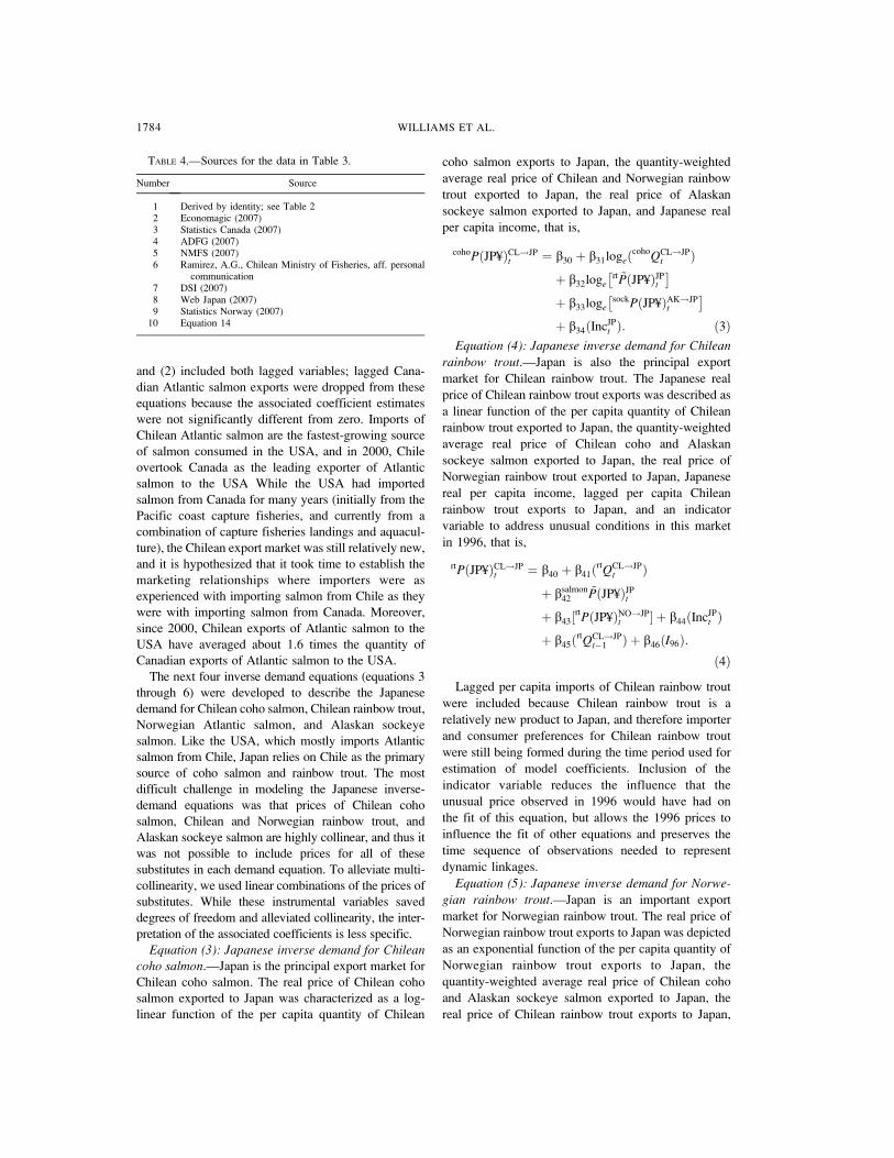
Equation (4): Japanese inverse demand for Chilean

rainbow trout.—Japan is also the principal export

market for Chilean rainbow trout. The Japanese real

price of Chilean rainbow trout exports was described as

a linear function of the per capita quantity of Chilean

rainbow trout exported to Japan, the quantity-weighted

average real price of Chilean coho and Alaskan

sockeye salmon exported to Japan, the real price of

Norwegian rainbow trout exported to Japan, Japanese

real per capita income, lagged per capita Chilean

rainbow trout exports to Japan, and an indicator

variable to address unusual conditions in this market

in 1996, that is,

rtPðJP¥ÞCL!JPt ¼ b40 þ b41ðrtQCL!JP

t Þþ bsalmon

42~PðJP¥ÞJPt

þ b43½rtPðJP¥ÞNO!JPt � þ b44ðIncJPt Þ

þ b45ðrtQCL!JPt�1 Þ þ b46ðI96Þ:

ð4ÞLagged per capita imports of Chilean rainbow trout

were included because Chilean rainbow trout is a

relatively new product to Japan, and therefore importer

and consumer preferences for Chilean rainbow trout

were still being formed during the time period used for

estimation of model coefficients. Inclusion of the

indicator variable reduces the influence that the

unusual price observed in 1996 would have had on

the fit of this equation, but allows the 1996 prices to

influence the fit of other equations and preserves the

time sequence of observations needed to represent

dynamic linkages.

Equation (5): Japanese inverse demand for Norwe-gian rainbow trout.—Japan is an important export

market for Norwegian rainbow trout. The real price of

Norwegian rainbow trout exports to Japan was depicted

as an exponential function of the per capita quantity of

Norwegian rainbow trout exports to Japan, the

quantity-weighted average real price of Chilean coho

and Alaskan sockeye salmon exported to Japan, the

real price of Chilean rainbow trout exports to Japan,

TABLE 4.—Sources for the data in Table 3.

Number Source

1 Derived by identity; see Table 22 Economagic (2007)3 Statistics Canada (2007)4 ADFG (2007)5 NMFS (2007)6 Ramirez, A.G., Chilean Ministry of Fisheries, aff. personal

communication7 DSI (2007)8 Web Japan (2007)9 Statistics Norway (2007)

10 Equation 14


Japanese real per capita income, and a categorical

variable introduced to account for unusual conditions

in this market in 1991, that is,

logertPðJP¥ÞNO!JP

t

� � ¼ b50 þ b51ðrtQNO!JPt Þ

þ bsalmon52

~PðJP¥ÞJPtþ b53

rtPðJP¥ÞCL!JPt

� �þ b54ðIncJPt Þ þ b55ðI91Þ: ð5Þ

Inclusion of the categorical variable was again

motivated by a desire to reduce the influence that the

unusual price observed in 1991 would have had on the

fit of this equation while preserving the time sequence

of observations.

Equation (6): Japanese inverse demand for Alaskansockeye salmon.—Japan has been the single largest

market for Alaskan sockeye salmon. The real price for

Alaskan sockeye salmon exports to Japan was

represented as a log-linear function of: the quantity of

Alaskan sockeye salmon exported to Japan, the real

price of Chilean exports of coho salmon to Japan,

Japanese real per capita income, the lagged sum of

exports to Japan of Chilean coho salmon and Chilean

and Norwegian rainbow trout, and a categorical

variable introduced to account for unusual conditions

in this market in 1991, that is,

sockPðJP¥ÞAK!JPt

¼ b60 þ b61 logeðsockQAK!JPt Þ

þ b62 logecohoPðJP¥ÞCL!JP

t

� �þ b63logeðIncJPt Þþ b64 logeðcohoQCL!JP

t�1 þrt QCL!JPt�1 þrt QNO!JP

t�1 Þþ b65ðI91Þ:

ð6ÞOur initial specification of this equation included the

quantity-weighted price of Japanese imports of Chilean

and Norwegian rainbow trout; this variable was

dropped from the final model specification because

the associated coefficient was not statistically signifi-

cant, possibly due to the correlation between this price

and the price of Chilean coho salmon. To overcome

this problem and to incorporate the dynamic effects of

a maturing relationship between Japanese importers

and Norwegian and Chilean exporters, the model

included the lagged sum of Japanese imports of

Chilean and Norwegian salmon and rainbow trout.

During the time period covered, there were incredible

and rapid changes in the salmon and rainbow trout

markets. In 1990, Alaskan sockeye salmon was the

dominant high-value salmon–rainbow trout species

imported into Japan. Today, Alaskan sockeye salmon

has been relegated to niche markets. Because Japanese

imports of pen-reared coho salmon, Atlantic salmon,

and rainbow trout were comparatively novel, it could

be expected that it might take Japanese importers some

time to establish market channels for these products.

Thus, over time, it could be expected that imports of

pen-reared salmonids from Chile and Norway would

have an increasingly negative effect on the export price

of Alaskan sockeye salmon to Japan. The lagged sum

of Japanese imports of pen-reared salmonids from

Chile and Norway was included to capture dynamic

changes in the willingness to pay for Alaskan sockeye

salmon that go beyond the effect of changes in current

import prices alone.

Allocation equations.—Supply equations are not

specifically modeled in this study. The production of

free-ranging salmon can be characterized as a stochas-

tic process that can be affected by natural variations in

survival and growth, changes in habitat, and catches in

capture fisheries. Alaska’s salmon fisheries are man-

aged to achieve escapement objectives and guideline

harvest levels (GHLs). The number of fishing vessels is

limited by area and gear, and vessel size and gear

characteristics are also regulated. In season, managers

use estimates of escapement and run strength to

determine the frequency and duration of open fishing

periods. The intent of management is to ensure that

fishing does not occur unless the lower-bound

escapement objective is exceeded, and that harvesting

prevents escapements from exceeding the upper-bound

escapement objective. Operating in the context of these

derby fisheries, license holders have the choice to

participate or not participate in the open fishing

periods. Exceptionally low preseason price offers have

occasionally resulted in strikes or low participation

rates. For example, nearly 40% of Bristol Bay, Alaska,

sockeye salmon drift-gill-net permit holders chose to

forego fishing in 2002; the remaining 60% of Bristol

Bay, Alaska, sockeye salmon drift-gill-net permit

holders succeeded in harvesting the GHL (Schelle et

al. 2004). Similarly, when runs are unexpectedly strong

or unusually compressed, processors have limited their

daily purchases to avoid exceeding the capacity of their

processing lines, and escapements have exceeded the

upper-bound escapement objective. While harvests of

native salmon stocks could be reduced through

mismanagement or sustained through judicious man-

agement, there is little evidence to suggest that harvests

can be augmented beyond their historic baseline.

Similarly, there is little evidence that interannual

variability can be eliminated, and there is little reason

to expect that the productivity of Alaska’s salmon

fisheries is insulated against long-term cyclic or forced

variation in climate. That is, harvests of Alaska’s native

salmon stocks can be characterized as draws from a

stationary stochastic process.


In contrast, the quantity of salmon and rainbow trout

produced in confined aquaculture systems is only

constrained by the costs and availability of production

inputs, survival rates, the availability of suitable

production sites, and differences between production

costs and product prices. The history of steadily

increasing quantities of pen-reared salmon and rainbow

trout (Figure 2) and steadily increasing efficiency in

production (Asche 1997; Asche et al. 2001; Olson and

Criddle 2008) suggests that the long-run supply of pen-

reared salmon and rainbow trout has not yet reached a

binding capacity constraint. Together, increased pro-

ductivity and increased extent of production have

fueled the long-run expansion of salmon aquaculture

and depressed the price of salmon taken in the capture

fisheries. Although modeling the supply of pen-reared

salmon and rainbow trout is outside the scope of this

work, the model developed in this paper is designed to

allow for simulations that explore the likely conse-

quences of continued increases in aquaculture produc-

tion.

In place of supply equations, we have developed

equations that describe the allocation of supply to final

markets (equations 7 through 12). The structure of

these equations takes into account a variety of factors,

including the extent to which each country’s supply is

dominated by a single buyer, the distance between

supply sources and end markets, local prices for the

product relative to prices available in alternative

markets, and the export momentum to a given market.

Equation (7): allocation of Chilean Atlantic salmonto the United States.—The USA is the primary export

market for Chilean Atlantic salmon. The quantity of

Chilean Atlantic salmon exported to the USA was

represented as a linear function of the price that

Chilean producers receive for exports of Atlantic

salmon to the USA, the price that Chilean producers

receive for exports of Atlantic salmon to other

countries, the total tonnage of Chilean exports of

Atlantic salmon to the USA and other countries, and an

indicator variable to account for unusual conditions in

this market in 2003, that is,

Atl �QCL!USt ¼ b70 þ b71

Atl�PðCLPÞCL!USt

� �þ b72

Atl�PðCLPÞCL!Otht

� �þ b73ðAtl �QCLt Þ

þ b74ðI03Þ:ð7Þ

Although the USA has been the principal export

market for Chilean Atlantic salmon, approximately

one-third of the Chilean Atlantic salmon exports during

1989–2005 went to other countries, and thus there was

some opportunity for price arbitrage. To account for

this possibility, both export market prices were

included in the equation. Because these Atlantic

salmon exports went to many other countries and were

small relative to Chilean Atlantic salmon exports to the

USA, they were modeled as an exogenous variable.

Equation (8): allocation of Canadian Atlanticsalmon to the United States.—Virtually the entire

supply of Canadian Atlantic salmon is exported to the

USA. The quantity of Canadian Atlantic salmon

allocated to the U.S. market was modeled as a linear

function of the real price of Canadian Atlantic salmon

exported to the USA and the total quantity of Canadian

Atlantic salmon available for export, that is,

Atl �QCA!USt ¼ b80 þ b81

AtlPðCA$ÞCA!USt

� �þ b82ðAtl �QCA

t Þ: ð8ÞEquation (9): allocation of Chilean coho salmon to

Japan.—Likewise, because virtually all Chilean coho

salmon is exported to Japan, the quantity of Chilean

coho salmon exported to Japan was modeled as a linear

function of the real price of Chilean coho salmon

exported to Japan and the total quantity of Chilean

coho salmon available for export, that is,

coho �QCL!JPt ¼ b90 þ b91

cohoPðCLPÞCL!JPt

� �þ b92ðcoho �QCL

t Þ: ð9ÞEquation (10): allocation of Chilean rainbow trout

to Japan.—Although approximately 85% of Chilean

rainbow trout exports for 1989–2006 went to Japan, the

allocation function modeling this behavior is a bit more

complex than the previous two allocation equations.

The quantity of Chilean rainbow trout allocated to

Japan was modeled as an exponential function of the

real price of Chilean rainbow trout exports to Japan, the

total quantity of Chilean rainbow trout available for

export, and the fraction of the total Chilean production

of rainbow trout exported to Japan during the

preceding year, that is,

logeðrt �QCL!JPt Þ ¼ b100 þ b101 loge

rtPðCLPÞCL!JPt

� �þ b102 logeðrt �QCL

t Þ

þ b103 logert �QCL!JP

t�1

rt �QCLt�1

!:

ð10ÞEquation (11), which determines the allocation of

Norwegian rainbow trout to Japan, also includes a

variable that represents a lagged export share. In both

cases, the product is relatively new, and it takes time to

build up the relationships between the exporters and

importers in the marketing chain. It is hypothesized that


as the market shares of Chilean and Norwegian

rainbow trout has increased in Japan, it has become

easier to export to Japan. As the share of Chilean

rainbow trout exported to Japan increases, it is

expected that the quantity exported to Japan in the

current year will also increase.

Equation (11): allocation of Norwegian rainbowtrout to Japan.—Three of the four modeled factors that

describe the determination of the quantity of Chilean

rainbow trout exported to Japan were also used to

model the quantity of Norwegian rainbow trout

exported to Japan: the real prices paid for Norwegian

rainbow trout exports to Japan, the total amount of

Norwegian rainbow trout available for export, and the

percent of total Norwegian rainbow trout production

that was exported to Japan during the previous year. In

addition, this allocation equation includes the deflated

consumer price index of energy in Norway. The form

of the Norwegian rainbow trout allocation equation is

logeðrt �QNO!JPt Þ ¼ b110 þ b111 loge

rtPðNOKÞNO!JPt

� �þ b112 logeðrt �QNO

t Þ

þ b113 logert �QNO!JP

t�1

rt �QNOt�1

!

þ b114 logefuelCPINOtCPINOt

� �:

ð11ÞAlthough it might be expected that the price of

energy would also be important in the Chilean

allocation equations, Chile allocated 95% of its coho

salmon and 85% of its rainbow trout exports to Japan,

while Norway exported just 58% of its rainbow trout to

Japan during this period. Energy costs are highly

correlated with overall shipping costs, and the

difference in the transportation costs to deliver rainbow

trout from Norway to Japan rather than the European

Union or Russia is substantial, so energy prices are

more influential in the choice of export market for

Norway than for Chile.2

Equation (12): allocation of Alaskan sockeye salmonto Japan.—The per capita quantity of Alaskan sockeye

salmon exported to Japan was modeled as an

exponential function of the real price for Alaskan

sockeye salmon exported to Japan, total Alaska

landings of sockeye salmon, and the per capita quantity

of Alaskan sockeye salmon exported to Japan during

the previous year, that is,

logeðsock �QAK!JPt Þ ¼ b120 þ b121 loge

sockPðJP¥ÞAK!JPt

� �þ b122 logeðsock �QAKland

t Þþ b123 logeðsock �QAK!JP

t�1 Þ:ð12Þ

The lagged quantity of Alaskan sockeye salmon

exported to Japan was used to represent the effect that

rapidly changing patterns in Alaskan sockeye salmon

exports to Japan have had over time.

Equation (13): Alaskan exvessel price of sockeyesalmon.—The model was designed to highlight trade

flows and product demands that are most influential in

the determination of exvessel price and revenue for

Alaskan sockeye salmon. An exvessel price equation

was estimated as part of the system of behavioral

equations. While not explicitly modeled as a compo-

nent of the behavioral model, exvessel revenues can be

derived from estimates of exvessel price.

The real exvessel price of Alaskan sockeye salmon

was modeled as a linear function of the real price of

Alaskan sockeye salmon exported to Japan, the

quantity of Alaskan sockeye salmon landings not

exported to Japan, and the lagged ratio of Alaskan real

exvessel price of sockeye salmon to the real export

price of Alaskan sockeye salmon exported to Japan,

that is,

sockPAKexv

t ¼ b130 þ b131ðsockPAK!JPt Þ

þ b132ðsock �QAK!Otht Þ

þ b133sockPAKexv

t�1

sockPAK!JPt�1

� �: ð13Þ

As previously discussed, during the period modeled,

70% of all Alaskan sockeye salmon harvests were

exported to Japan as minimally processed fresh or

frozen products. However, in recent years more Alaska

sockeye salmon is being sold elsewhere; since 2000,

approximately half of sockeye salmon was exported

fresh and frozen to Japan and half sold elsewhere.

Alaskan sockeye salmon catches not exported to Japan

were included in this equation to represent the effects

that increases in landings used for other markets have

on exvessel price. Finally, lagged exvessel price shares

were used to represent market friction; current exvessel

prices are a reflection of past prices.

Although not modeled explicitly, real exvessel

revenue for Alaskan sockeye salmon can be derived

from the product of estimates of Alaskan real exvessel

price of sockeye salmon for any level of landings as

follows:

2 It is noteworthy that Russia is now the largest importer ofNorwegian rainbow trout, surpassing Japan in 2004. However,Russia was not an important export market for Norwegianrainbow trout until 1999. Because of the country’s late entryinto the market, the Russian segment could not be modeledexplicitly.


sock�TRAKexv

t ¼ sockPAKexv

t ðsockQAKland

t ÞðPPIUSt Þ: ð14ÞMarket clearing identities.—Market clearing identi-

ties are equations that transform input data series so

that they are conformable for inclusion in the

behavioral equations. The transformations include

adjustments for inflation, changes in exchange rates,

and changes in population. The 15 market clearing

identities included in our model (Table 2) are used to

derive time series for the endogenous variables.

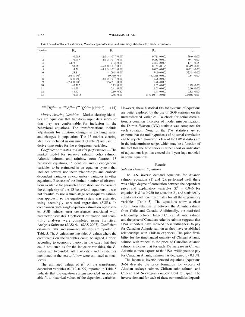
Coefficient estimates and model performance.—The

market model for sockeye salmon, coho salmon,

Atlantic salmon, and rainbow trout features 13

behavioral equations, 15 identities, and 28 endogenous

variables to be estimated in an equation system that

includes several nonlinear relationships and embeds

dependent variables as explanatory variables in other

equations. Because of the limited number of observa-

tions available for parameter estimation, and because of

the complexity of the 13 behavioral equations, it was

not feasible to use a three-stage least-squares estima-

tion approach, so the equation system was estimated

using seemingly unrelated regression (SUR). In

comparison with single-equation estimation approach-

es, SUR reduces error covariances associated with

parameter estimates. Coefficient estimation and sensi-

tivity analyses were completed using Statistical

Analysis Software (SAS) 9.1 (SAS 2007). Coefficient

estimates, SEs, and summary statistics are reported in

Table 5. The P-values are one-sided P-values where thecoefficients on the variables could be signed a priori

according to economic theory; in the cases that they

could not, such as for the indicator variables, the P-values are two-sided. All elasticities and flexibilities

mentioned in the text to follow were estimated at mean

levels.

The estimated values of R2 on the transformed

dependent variables (0.712–0.999) reported in Table 5

indicate that the equation system provided an accept-

able fit to historical values of the dependent variables.

However, these historical fits for systems of equations

are better explored by the use of GOF statistics on the

untransformed variables. To check for serial correla-

tion, a common indicator of model misspecification,

the Durbin–Watson (DW) statistic was computed for

each equation. None of the DW statistics are so

extreme that the null hypothesis of no serial correlation

can be rejected; however, a few of the DW statistics are

in the indeterminate range, which may be a function of

the fact that the time series is rather short or indicative

of adjustment lags that exceed the 1-year lags modeled

in some equations.

Results

Salmon Demand Equations

The U.S. inverse demand equations for Atlantic

salmon, equations (1) and (2), performed well; there

was a high degree of correlation between the dependent

price and explanatory variables (R2 ¼ 0.846 for

equation 1; R2¼ 0.930 for equation 2), and statistically

significant coefficient estimates for all the explanatory

variables (Table 5). The equations show a clear

substitution relationship between the Atlantic salmon

from Chile and Canada. Additionally, the statistical

relationship between lagged Chilean Atlantic salmon

and the price of Canadian Atlantic salmon suggests that

USA importers have reduced their willingness to pay

for Canadian Atlantic salmon as they have established

relationships with Chilean exporters. The price flexi-

bility for the time-lagged quantity of Chilean Atlantic

salmon with respect to the price of Canadian Atlantic

salmon indicates that for each 1% increase in Chilean

Atlantic salmon exports to the USA, willingness to pay

for Canadian Atlantic salmon has decreased by 0.10%.

The Japanese inverse demand equations (equations

3–6) describe the price formation for exports of

Alaskan sockeye salmon, Chilean coho salmon, and

Chilean and Norwegian rainbow trout to Japan. The

inverse demand for each of these commodities depends

TABLE 5.—Coefficient estimates, P-values (parentheses), and summary statistics for model equations.

Equation bn0

bn1

bn2

bn3

1 �0.013 �2.0 3 10�5 (0.00) 0.711 (0.00) 79.9 (0.00)2 0.017 �2.0 3 10�5 (0.00) 0.253 (0.00) 39.1 (0.00)3 �2,119 �71.2 (0.00) 200.3 (0.00) 17.1 (0.15)4 50.06 �6.0 3 10�5 (0.03) 0.131 (0.19) 0.549 (0.01)5 4.26 �4.1 3 10�7 (0.00) 0.003 (0.00) 0.001 (0.06)6 53.1 �109.8 (0.00) 74.0 (0.00) 325.8 (0.00)7 2.6 3 108 19,760 (0.04) �32,218 (0.00) 0.54 (0.00)8 �1.6 3 10�7 3.9 3 10�8 (0.00) 0.98 (0.00)9 �7.4 3 106 756,701 (0.01) 0.98 (0.00)10 �0.712 0.13 (0.00) 1.02 (0.00) 0.49 (0.00)11 �1.60 0.41 (0.09) 1.01 (0.00) 0.60 (0.00)12 �8.42 0.10 (0.12) 0.91 (0.00) 0.52 (0.00)13 �0.0015 0.46 (0.00) �1.5 3 10�11 (0.01) 0.0056 (0.03)


on contemporaneous or lagged prices of one or more of

the others. For all of the Japanese demand equations,

the linear functional form was the default so that the

elasticities could vary with both the mean-level value

of the dependent and independent variable. However,

using the degree of serial correlation in the error terms

as a possible indication of an incorrect functional form,

alternative functional forms were used when substantial

serial correlations were found in the residuals to the

linear model.

The estimated demand equations indicate that,

within Japanese markets, there is extensive substitution

between Chilean and Norwegian rainbow trout,

Chilean coho salmon, and Alaskan sockeye salmon.

Each of the equations provided a good fit to the historic

data (R2 ¼ 0.889 for equation 3; R2 ¼ 0.712 for

equation 4; R2¼ 0.922 for equation 5) and statistically

significant coefficient estimates for almost all of the

explanatory variables (Table 5).

In the equation that describes Japanese demand for

Chilean coho salmon (equation 3), the cross-price

flexibility between the price of Chilean coho salmon

and the price of Chilean and Norwegian rainbow trout

is 0.96, indicating that a 1% increase (decrease) in the

price of imported rainbow trout leads to a 0.96%increase (decrease) in the price of Chilean coho salmon

exported to Japan. This variable is statistically

significant (P-value , 0.00). The cross-price flexibility

associated with the price of Alaskan sockeye salmon

exports to Japan had a P-value of 0.146, indicating a

larger probability of a type I error; however, there are

strong a priori reasons to believe that these two species

are also substitutes and the elevated SE on the

estimated parameter may be an artifact of the high

degree of collinearity between the prices of Chilean

and Norwegian rainbow trout and Alaskan sockeye

salmon export prices. Nevertheless, the higher proba-

bility of a type I error—that there is not a significant

effect from price variations in imported Alaska sockeye

salmon on variations in the price of imported Chilean

coho salmon—is probably also due to the diminishing

importance of Alaskan sockeye in the Japanese market.

Cross-price elasticities indicate that Chilean coho

salmon prices exports are more strongly affected by

variations in Japanese rainbow trout import prices than

they are by variations in the import price for Alaskan

sockeye salmon. Although this may seem counterintu-

itive, in 2005 exports of Chilean and Norwegian

rainbow trout to Japan were nearly four times as large

as exports of Alaskan sockeye salmon to Japan and

now are of more importance in the Japanese consump-

tion of salmon and trout. Indeed, the residual share of

the Japanese market that continues to be filled by

Alaskan sockeye salmon may represent a niche market

(i.e., a market that is characterized by a more narrowly

defined group of specialized consumers who are

willing to pay a premium for specific sockeye salmon

products).

In the equation that characterizes Japanese inverse

demand for Chilean rainbow trout (equation 4), the

weighted real price of salmon (Alaska sockeye salmon

and Chilean coho salmon combined) and the real price

of Norwegian rainbow trout were included as substitute

prices. Norwegian exports of rainbow trout to Japan

had a statistically significant P-value. The associated

cross-price flexibility indicates that, at the mean, every

1% increase (decrease) in the price of Norwegian

rainbow trout is expected to result in a 0.56% increase

(decrease) in the price of Chilean rainbow trout in the

Japanese market. The P-value associated with the

coefficient on the real weighted price of Alaskan

sockeye salmon and Chilean coho salmon (0.193)

indicates a moderate possibility of type I error, yet it is

likely that this is a result of the high degree of

collinearity among the prices of the modeled substi-

tutes. The coefficient associated with Japanese con-

sumption expenditures returned a stronger type I error

probability of 0.393. However, economic theory and

TABLE 5.—Extended.

Equation bn4

bn5

bn6

df R2 DW

1 �1.9 3 10�5 (0.00) 11 0.846 1.912 �6.3 3 10�4 (0.00) 11 0.930 1.703 276.7 (0.01) 11 0.889 2.414 0.012 (0.39) 5.9 3 10�5 (0.03) �38.6 (0.00) 9 0.712 1.645 0.0002 (0.03) 0.197 (0.00) 10 0.922 2.116 �86.4 (0.00) �87.1 (0.00) 10 0.807 2.317 4.6 3 107 (0.00) 11 0.984 1.698 13 0.998 1.489 13 0.999 1.58

10 12 0.999 2.0311 �0.99 (0.01) 11 0.973 2.0012 12 0.973 1.6813 12 0.778 1.66


knowledge about the market suggest that both of these

explanatory variables are important determinants of the

real price of exports of Chilean rainbow trout to Japan

and, as was discussed earlier, it was considered better

to leave these variables in the equation than to risk the

biases associated with the omission of relevant

explanatory variables. While inclusion of collinear

variables does not bias model forecasts, caution should

be exercised in interpreting forecasts that involve

variations in the weighted price of Alaskan sockeye

salmon and Chilean coho salmon, and variations in

Japanese consumption expenditures.

The indicator variable (I96) was included in equation

(4) to prevent the unusual price observed in 1996 from

unduly influencing coefficient estimates. Fisheries

marketing and trade journals provide some indications

as to why 1996 might have been an unusual year with

prices substantially below those otherwise predicted by

the model. For example, industry observers indicate

that 1996 was characterized by an unexpectedly weak

demand for sashimi, which redirected a large share of

rainbow trout imports into the lower-valued tei-en

(lightly) salted fillet market, thereby depressing the

average price of Chilean rainbow trout (Atkinson

1996).

The Japanese inverse demand for Norwegian

rainbow trout (equation 5) included the weighted real

prices of Chilean coho and Alaskan sockeye salmon

and the real price of Chilean rainbow trout as substitute

variables. The weighted real price of Chilean coho and

Alaskan sockeye salmon in the Japanese market had a

mean-level, cross-price flexibility of 0.57. The real

price of Chilean rainbow trout returned a cross-price

flexibility of 0.19. The indicator variable I91

was

included to prevent the unusually higher observed than

predicted price in 1991 from unduly influencing

coefficient estimates. Industry observers suggest that

early year reports of a chaotic Japanese demand

resulted in many of the European producers shifting

away from feed additives that promoted the rich, red

flesh color that the Japanese market demands. This,

coupled with increased EU demand (resulting from

‘‘aggressive PR campaigns’’), forced Japan to bid

higher than expected for Norwegian trout, all else equal

(Atkinson 1991).

The last of the demand equations, Japanese inverse

demand for Alaska sockeye salmon (equation 6), also

performed well (R2¼ 0.807, and statistical significance

for all coefficient estimates at 5% or 10% significance

levels). The cross-price flexibility between Alaskan

sockeye salmon and Chilean coho salmon, 0.32,

indicates that a 1% increase (decrease) in the price

for Chilean coho salmon leads to a 0.32% increase

(decrease) in the price for Alaskan sockeye salmon

exported to Japan. This equation included a variable

which represented Japanese total per capita imports of

Chilean coho salmon and Chilean and Norwegian

rainbow trout. These aquaculture products started out

relatively new to Japan (during the modeled period),

especially in comparison with sockeye salmon which

has historically been Japan’s most important salmon

import. As the lagged quantity of the sum of farmed

salmon and rainbow trout exports to Japan increases by

1% at the mean, the price of Alaskan sockeye salmon

decreases by 0.37%, indicating a strong movement

between the market buildup of Chilean coho salmon

and Chilean and Norwegian rainbow trout and the

decreased Japanese willingness to pay for Alaskan

sockeye salmon. This is in addition to the effect that

increased aquaculture production has had on price and

captures the dynamically changing market shares by

importers who became evermore accustomed to

Chilean coho salmon and Chilean and Norwegian

rainbow trout over this time period. An indicator

variable was included to prevent the model from

grossly overestimating Japanese demand for Alaskan

sockeye salmon in 1991. The reason for the model’s

tendency to overestimate demand in 1991 is not

entirely clear. However, this was the year of the big

salmon price drop and has been the focus of previous

research (e.g., Herrmann 1992). Price decreases during

this time period led fishermen to charge that Japanese

purchasers and Bristol Bay processors colluded to fix

exvessel prices, a charge that the plaintiffs were unable

to substantiate in court.

Salmon Allocation Equations

The Chilean allocation of Atlantic salmon to the

USA (equation 7) explained virtually all the variation

in the allocated salmon (R2 ¼ 0.984). Most of the

attributed allocation is due to increases in total exports,

where a 1% increase in total Chilean Atlantic salmon

exports leads to a 0.84% increase in allocation to the

USA. Although the U.S. market has been the leading

outlet for Chilean Atlantic salmon exports, even during

this period, nearly one-third of Chile’s Atlantic salmon

exports have gone into other markets. This suggests

that some price arbitration may take place. It was

estimated that a 1% increase in the price of Chilean

Atlantic salmon exported to the USA would lead to a

0.17% increase in the quantity exported to the USA,

while an increase in the price of Chilean Atlantic

salmon to markets outside the USA would decrease

allocation to the USA by 0.26%. An indicator variable,

I03, was included to correct initial underestimates of

Chilean exports of Atlantic salmon to countries other

than the USA in 2003. The reasons for this temporary

dip in the Chilean allocation of Atlantic salmon to the


USA are unclear and probably reflect activities in

European markets that were not represented in our

model.

Variations in Canadian allocations of Atlantic

salmon to the USA (equation 8) are almost entirely

explained (R2 ¼ 0.998) by just two variables. This is

not surprising since the USA is nearly the sole market

for Canadian exports of Atlantic salmon, having

received nearly 95% of Canada’s Atlantic salmon

production during the time period considered in this

analysis.

The Chilean allocation of coho salmon to Japan

(equation 9) is similar, but with Japan as the sole

purchaser. Again, virtually all variation in allocation is

captured by information about variations in total

Chilean coho salmon exports and the price received

from Japanese importers (R2 ¼ 0.999).

Although all of the allocation equations were

initially specified as linear, the last three allocation

equations were estimated in double-log form to allow

for nonlinear responses and to eliminate serial

correlation in the residuals. All three equations

provided a good fit to the historic data (R2 ¼ 0.999

for equation 10; R2¼0.973 for equation 11; R2¼ 0.973

for equation 12) and statistically significant coefficient

estimates for almost all of the explanatory variables.

In addition to the logarithms of its own export price

and its own total exports, the logarithm of the

allocation of Chilean rainbow trout to Japan (equation

10) includes the logarithm of the previous year’s

percent of total Chilean rainbow trout exported to

Japan. This variable captures the momentum of this

novel commodity as it made inroads into the Japanese

market channels.

The allocation of the logarithm of Norwegian

rainbow trout exports to Japan (equation 11) is similar

to the Chilean rainbow trout allocation equation.

Recall, that of all the products modeled, the allocation

to Japan of Norwegian rainbow trout was the lowest in

percentage terms, just 58% (much of this being due to

recent increases in the allocation of Norwegian

rainbow trout to Russia).

The logarithm of the allocation of Alaskan sockeye

salmon to Japan (equation 12) was modeled using the

logarithms of own price and total landings as

explanatory variables. Additionally, the equation

included the logarithm of the previous year’s export

quantity, which helped to explain some of the current

Japanese imports. This was expected as the relationship

between Alaskan exporters and Japanese importers,

although well established, has undergone rapid changes

during this time period.

In conclusion, for the allocation equations there are

some features that hold across all equations. By far the

most influential variable in explaining the allocation of

a particular species to its principal export market is the

volume of production as indicated by total salmon or

trout exports or landings. In the six allocation

equations, the elasticity of total exports (or landings)

with respect to quantity ranged from 0.84 to 1.03,

associated P-values showing statistical significance at a1% level. The allocated goods export price was

significant in most cases at a 10% level, but less

influential and with price elasticities ranging between

0.05 and 0.41. Finally, in all equations, the variables

explained a large portion of the variation in the

allocated good (or the transformed good) as exhibited

by R2-values ranging between 0.973 and 0.999.

Sockeye Salmon Exvessel Price Equation

Equation (13) was constructed to explore factors that

directly affect the exvessel price of Alaskan sockeye

salmon. The exvessel price equation performed

acceptably as R2 was equal to 0.778 and coefficient

estimates were statistically significant at 1% and 3%significance levels. Despite recent declines in the

fraction of Alaskan sockeye salmon exported to Japan,

the price elasticity associated with variations on the

Japanese real import price is near unity indicating that,

in percentage terms, there is a nearly one-to-one

relationship between the price of Alaskan sockeye

salmon exports to Japan and exvessel prices in Alaska.

Alaskan landings of sockeye salmon going into other

markets and product forms is also a statistically

important determinant of exvessel prices, and the

elasticity of landings (going to products and places

other than the Japanese market for fresh or frozen

sockeye salmon) is �0.17, indicating that, all else

equal, as landings increase (decrease) by 1%, the

Alaska exvessel price for sockeye salmon will decrease

(increase) by 0.17%. Finally, there is a positive

relationship between the previous year’s share of the

exvessel price to the Japanese export price and the

current exvessel prices.

Goodness of Fit

Historical simulation GOF statistics are the preferred

means of assessing the predictive accuracy of a system

of equations over the estimation period. Evaluating each

equation separately does not provide information on

how they interact in the modeled system. Individual

equation GOF statistics are used to incorporate

intertemporal and intratemporal linkages, which exist

within the market response model. These interdepen-

dencies are explicitly incorporated into the dynamic

model simulation, where each of the equations in the

market response model is solved in its reduced form.

Thus, model simulation provides a more robust measure


of actual model performance. Model simulations were

conducted using the Newton algorithm in SAS (SAS

2007). The historic dynamic simulation was performed

on the system of equations for the 1990 to 2005 period.

The GOF statistics are reported in Table 6.

The GOF statistics include the correlation between

the actual and predicted values of the endogenous

variables (r), the mean percent error, the root mean

square percent error, and the Theil inequality coeffi-

cient (U1). The Theil inequality coefficient is a

measure of forecast accuracy, where 0 is a perfect

forecast, 1 is a forecast that performs no better than a

naı̈ve forecast (a forecast of repetition of the previous

time period’s value), and a value greater than 1 is

worse than the naı̈ve forecast.

The GOF statistics show that the model fits the

historical data fairly well. The lowest correlation

coefficient was 0.62 (Alaskan sockeye salmon export

price to Japan), and three equations had correlation

coefficients close to 1.00 (U.S. demand for Canadian

Atlantic salmon, Japanese demand for Chilean exports

of coho salmon, and Japanese demand for Chilean

exports of rainbow trout). The variable of most

importance for our study, Alaska sockeye salmon

revenue, had a correlation coefficient of 0.91. The

mean absolute percentage errors are within a reason-

able range, from 1.5% for Canadian exports of Atlantic

salmon to the USA to 20.6% for Alaskan sockeye

salmon exvessel prices and Alaska sockeye salmon

revenue. The CVs for the same equations are 2.3% and

29.6%. The Theil U1 statistics indicate a reliable

historical forecast, the lowest value being 0.02 (for

Canadian exports of Atlantic salmon to the USA and

Chilean exports of coho salmon to Japan) and the

highest, 0.21 (for Alaskan sockeye salmon exvessel

prices).

Sensitivity Analyses

The estimated model can be used to explore

probable changes in the dependent variables in

response to changes in exogenous variables. We used

the model to explore the market consequences of

variations in the quantity of Atlantic salmon, coho

salmon, and rainbow trout produced in Chile and to

explore the shape of the exvessel demand and revenue

curves for Alaskan sockeye salmon. In the first

scenario, we simulated potential changes in Chilean

production of Atlantic salmon, coho salmon, and

rainbow trout and examined the likely effects on

exvessel prices and revenues in Alaska’s sockeye

salmon fisheries. These simulations should not be

construed as predictions of impending changes in the

U.S. and Japanese markets; rather, the simulations

characterize what could have occurred to salmon

markets if Chile had suddenly increased its output of

salmon and rainbow trout in 2005 and disposed of the

additional production in markets as they existed in

2005. In the second scenario, we varied Alaska

sockeye salmon production to trace out exvessel

demand and revenue curves. The results are character-

izations of price changes that would have occurred in

2005 without the markets having time to adjust or for

exporting countries to develop new markets. So, these

price changes, particularly in regard to changing

farmed salmon and rainbow trout supplies, represent

an upper bound on likely long-term price changes.

Scenario 1: Increased Chilean Production of CohoSalmon and Rainbow Trout

Alaska’s sockeye salmon, once the unquestioned

champion in the Japanese salmon market, is now

dwarfed by Japanese imports of Chilean coho salmon

and rainbow trout, and Norwegian Atlantic salmon and

rainbow trout (see Figure 4). For example, in 2005,

Chile’s combined exports of coho salmon and rainbow

trout to Japan were 300 million lb, while Alaska’s 2005

sockeye salmon exports were a mere 79 million lb.

The combined total exports of Chilean coho salmon

and rainbow trout to all countries for 2005 was 338

million lb, and therefore each 1% increment represents

an increase in total coho salmon and rainbow trout

exports (mainly being exported to Japan) of 3.4 million

lb. The simulated effect on these increased exports of

Chilean coho salmon and rainbow trout to Japan are

shown in Tables 7–9. For each 1% increase in exports

of Chilean coho salmon, it is estimated that the

exvessel price of Alaskan sockeye salmon would

decrease by approximately US$0.0017/lb, average

TABLE 6.—Goodness-of-fit statistics; MA%E ¼ mean

percent error, RMS%E ¼ root mean percentage error or

coefficient of variation (CV¼1003SD/mean), r¼ correlation

between the observed and predicted values, U1 ¼ Theil

inequality coefficient (see Table 3 for variable definitions).

Equation Variable MPE RMSPE r U1

1 Atl�PðCLPÞCL!USt 6.0 8.4 0.85 0.09

2 Atl�PðCA$ÞCA!USt

4.3 5.7 0.87 0.05

3 coho�PðCLPÞCL!JPt 11.9 14.6 0.76 0.135

4 rt�PðCLPÞCL!JPt 9.7 12.2 0.84 0.11

5 rt�PðNOKÞNO!JPt 8.3 9.6 0.80 0.10

6 sock�PAK!JPt 9.9 11.7 0.62 0.123

7 Atl �QCL!USt 11.1 21.6 0.99 0.06

8 Atl �QCA!USt 1.5 2.3 1.00 0.02

9 coho �QCL!JPt 3.4 6.3 1.00 0.02

10 rt �QCL!JPt 2.9 3.3 1.00 0.03

11 rt �QNO!JPt 15.2 18.0 0.97 0.17

12 sock �QAK!JPt 8.2 10.3 0.98 0.11

13 sock�PAKexvt 20.6 29.6 0.65 0.21

14 sock�TRAKexvt 20.6 29.6 0.92 0.18


exvessel revenues decreasing by $0.46 million. For

each 1% increase in exports of Chilean rainbow trout, it

is estimated that the exvessel price of Alaskan sockeye

salmon would decrease by approximately $0.0012/lb

and that average exvessel revenues would decrease by

approximately $0.34 million. In combination, each 1%

increase in Chilean rainbow trout and coho salmon

exports would have reduced Alaskan sockeye salmon

exvessel prices by approximately $0.0030/lb and

Alaskan sockeye salmon exvessel revenues by approx-

imately $0.80 million.

Although these estimated losses to the Alaskan

sockeye salmon fishery are not trivial, they are small

in comparison with the historical effects that salmon

aquaculture has had on markets for Alaskan salmon,

especially as it is noted that an additional 25% increase

in Chilean exports to Japan would be roughly

equivalent to the current exports of Alaskan sockeye

salmon to Japan. Moreover, these estimates are upper

bounds. Actual losses would be somewhat smaller if the

increases were anticipated and sellers had time to

develop new markets. With 2005 Chilean coho salmon

and rainbow trout exports to Japan equivalent to about

four times the level of Alaskan sockeye salmon exports

to Japan, our findings suggest that the residual market

share held by Alaskan sockeye salmon in Japan may not

be as vulnerable to increased exports of Chilean coho

salmon and rainbow trout as it has been in the past.

Indeed, Alaskan exports of sockeye salmon to Japan

have stabilized since 1998 at around an average of 62.3

million lb, while the previous 8-year period (1990 to

1997) average for exports was 172.5 million lb.

Scenario 2: Alaska Sockeye Salmon Exvessel Demand

and Revenue Curves

Sockeye salmon is the most valuable and most

abundant of the high-valued salmon species harvested

in Alaska. In 2005, Alaskan sockeye salmon fisheries

yielded 267 million lb and generated $194 million in

exvessel revenue at an exvessel price of $0.73/lb. The

estimated demand and revenue curves are presented in

Figure 6. The exvessel demand curve shows prices

varying from $0.51/lb for sockeye salmon landings of

346.9 million lb to $0.98/lb for sockeye salmon

landings of 186 million lb. The model indicates that

2005 Alaskan exvessel revenues from sockeye salmon

would have been maximized at 258.4 million lb of

landings with an associated exvessel price of $0.75/lb

and exvessel revenue of $193.8 million. This is nearly

identical to the actual 2005 landings of 266.9 million

lb, exvessel price of $0.73/lb, and exvessel revenue of

$193.7 million. It is also very similar to the 2007

landings of 276.9 million lb, nominal exvessel price of

$0.75, and nominal exvessel revenue of $206.4 million,

particularly if the 2007 price and revenue are

discounted to 2005 price levels. This indicates, all else

equal, that recent Alaskan landing levels of sockeye

salmon are near the peak of the total revenue curve and

TABLE 8.—Simulated effects of increased Chilean exports

of rainbow trout on exvessel prices and revenues for Alaskan

sockeye salmon, 2005.

%Increase

Rainbow troutexports

(million lb)

Sockeye salmonprice

(US$/lb)

Sockeye salmonrevenue

(million US$)

0 164.9 0.7257 193.681 166.5 0.7245 193.352 168.2 0.7232 193.023 169.8 0.7220 192.684 171.5 0.7207 192.345 173.1 0.7194 191.9910 181.4 0.7127 190.2115 189.6 0.7057 188.3320 197.9 0.6982 186.3425 206.1 0.6903 184.2230 214.4 0.6819 181.98

TABLE 9.—Simulated effects of combined increases in

Chilean exports of coho salmon and rainbow trout on exvessel

prices and revenues for Alaskan sockeye salmon, 2005.

%Increase

Total exports(million lb)

Sockeye salmonprice

(US$/lb)


(million US$)

0 337.6 0.7257 193.681 341.0 0.7228 192.892 344.4 0.7198 192.103 347.7 0.7168 191.294 351.1 0.7137 190.485 354.5 0.7106 189.6510 371.4 0.6946 185.3715 388.2 0.6775 180.8020 405.1 0.6590 175.8825 422.0 0.6390 170.5330 438.9 0.6169 164.64

TABLE 7.—Simulated effects of increased Chilean exports

of coho salmon on exvessel prices and revenues for Alaskan

sockeye salmon, 2005.

%Increase

Coho salmonexports

(million lb)

Sockeye salmonprice

(US$/lb)


(million US$)

0 172.7 0.7257 193.681 174.4 0.7240 193.222 176.2 0.7223 192.773 177.9 0.7206 192.324 179.6 0.7189 191.865 181.3 0.7172 191.41

10 190.0 0.7088 189.1615 198.6 0.7004 186.9120 207.2 0.6920 184.6825 215.9 0.6837 182.4630 224.5 0.6753 180.23


that incremental variations from these catch levels are

unlikely to substantially impact exvessel prices or

revenues, while substantial increases of decreases from

these levels of landings can be expected to be

accompanied by substantial decreases in total exvessel

revenue. The relationship between prices, revenues,

and landings are subject to change over time as factors

outside of the model, such as potential new markets,

influence salmon markets. Likewise, the current

worldwide recession could negatively impact salmon

prices in ways the model cannot predict.

Discussion

Over the past 25 years, the wild Alaskan salmon

fishing industry has faced intense competition in key

domestic and international markets and has experi-

enced dramatic decreases in real exvessel prices. Most

of this reduction in exvessel prices can be attributed to

the increased volume of Atlantic salmon, coho salmon,

and rainbow trout produced in aquaculture. Alaska has

gone from supplying as much as 64% of the world’s

supply of high-value salmon (Chinook salmon, sock-

eye salmon, and coho salmon) in 1983 to supplying as

little as 5% in 2002. These changes have been

particularly difficult to weather because Alaska’s

fisheries have operated as limited-entry derbies that

have induced fishermen to invest in costly modifica-

tions to vessels and gear, and to bid up the price of

limited access permits to levels that could not be

afforded when salmon prices declined. Many studies

have documented the effects of ever-increasing quan-

tities of salmon and rainbow trout from aquaculture on

exvessel prices offered for salmon harvested in capture

fisheries (Anderson 1985b; Asche 1997; Asche et al.

1999; Herrmann 1993, 1994; Herrmann et al. 1993).

This study has focused on Alaskan sockeye salmon and

indicates that while the downward pressure on

Japanese import prices and on exvessel prices for

Alaskan sockeye salmon has slackened but not abated,

it appears that Alaskan sockeye salmon may now

occupy a niche position in the Japanese market and

may be somewhat insolated from the extreme down-

ward pressures of the last 25 years.

The sensitivity analyses indicate that, without

concomitant increases in consumer demand, substantial

increases in Chilean coho salmon and rainbow trout are

likely to further decrease exvessel prices and revenues

for sockeye salmon fishermen in Alaska. Nevertheless,

the relative magnitude of these impacts is likely to be

substantially less than the relative magnitude of

impacts experienced in the 1990s. It is estimated that

for each 5% increase in Japanese imports of Chilean

coho salmon, the exvessel price of Alaska sockeye

salmon will decrease by approximately $0.0084/lb and

exvessel revenues will decrease by $2.25 million.

Similarly, for increases in the Japanese imports of

Chilean rainbow trout, it is estimated that Alaskan

sockeye salmon exvessel price will decrease by

approximately $0.0063/lb for the first 5% increase,

with an associated decrease in exvessel revenue

decrease of $1.69 million. In combination, the first

5% increase in Chilean exports of coho salmon and

rainbow trout can be expected to decrease Alaskan

sockeye salmon exvessel prices by $0.0151/lb, with an

associated decrease in the exvessel revenues in the

Alaskan sockeye salmon fishery of approximately

$4.03 million.

The estimated exvessel demand curve for Alaskan

sockeye salmon indicates moderate price sensitivity,

but over a rather wide range of landings. It is estimated

that prices will vary from $0.51/lb for sockeye salmon

landings of 346.9 million lb to $0.98/lb for sockeye

salmon landings of 186 million lb. The associated total

exvessel revenue curve indicates that exvessel revenues

vary relatively little over a wide range of landings. The

maximum total revenue is estimated at $193.8 million

at landings of 258.4 million lb. For landings of 186

million lb, the estimated exvessel revenue is $182.5

million, and for landings of 346.9 million lb, total

exvessel venue is $176.8 million. This suggests that

FIGURE 6.—Simulated 2005 Alaskan sockeye salmon exvessel demand and revenue curves.


sockeye salmon exvessel revenue is not very sensitive

to changes in landings that are within the range of

recent guideline harvest levels.

With all of the changes that the Alaskan wild salmon

industry has endured over the past two and a half

decades, the model suggests that future impacts of

increased aquaculture production are unlikely to be as

substantial as were the impacts felt in the 1990s.

Although revenues are highly unlikely to approach the

highs (in real terms) of the late 1980s, they may have

finally leveled off a bit. It may be that Alaska wild

salmon marketing has been successful in securing

loyal, niche markets that provide some insulation from

the rapid price declines experienced during the 1990s.

The model presented in this paper suggests that

under current market conditions, to the extent that

Alaska’s escapement-based management regime max-

imizes expected sustainable yields, it also maximizes

expected sustainable revenues. However, in years with

particularly strong runs of sockeye salmon, allowing

escapements to exceed the upper-bound escapement

objective could help avert undesirable decreases in

exvessel price. A more likely scenario is for the

development of new niche markets for Alaskan

sockeye salmon that would insulate exvessel prices

from unusually strong runs without the need to reduce

harvest. Nevertheless, measures taken to bolster

exvessel prices will not address the root of economic

failure in the Alaskan salmon fisheries: hundreds of

vessels racing one another for a finite number of fish.

While it is convenient for fishermen and managers to

ascribe the indigence of the salmon fishery to the

onslaught of farmed salmon, the fundamental problem

is the primeval allocation structure that encourages

spendthrift investment in vessels and gear (Pearse and

Wilen 1979; Karpoff 1987). The problem is with an

allocation structure that drives up the cost of catching

fish until all profit is dissipated (Schelle et al. 2004;

Knapp et al. 2007). Regardless of the downward

pressure on Alaska salmon prices because of increased

farmed salmon production, the long-run profitability of

Alaska’s salmon fisheries will not improve until this

archaic allocation regime is replaced with an individual

or cooperative catch–share system (Knapp 2008).

Acknowledgments

This paper is a result of work funded by the Alaska

Sea Grant College Program project ASG05-00. We

also thank the anonymous reviewers as well as the

associate editor and editor for the North American

Journal of Fisheries Management for their very

thorough comments. All opinions are the authors’

and do not necessarily represent the Alaska Sea Grant

College Program.

References

ADFG (Alaska Department of Fish and Game). 2007. Salmon

fisheries in Alaska: catch, effort, and value information.

Available: www.cf.adfg.state.ak.us/. (March 2007.)

Anderson, J. L. 1985a. Private aquaculture and commercial

fisheries: bioeconomics of salmon ranching. Journal of

Environmental Economics and Management 12:353–

370.

Anderson, J. L. 1985b. Market interactions between aquacul-

ture and the common property commercial fishery.

Marine Resource Economics 2:1–24.

Asche, F. 1997. Trade disputes and productivity gains: the

curse of farmed salmon production. Marine Resource

Economics 12:67–73.

Asche, F., T. Bjørndal, and J. A. Young. 2001. Market

interactions for aquaculture products. Aquaculture Eco-

nomics and Management 5:303–318.

Asche, F., H. Bremnes, and C. R Wessells. 1999. Product

aggregation, market integration, and relationships between

prices: application to world salmon markets. American

Journal of Agricultural Economics 81:588–581.

Asche, F., A. G. Guttormsen, T. Sebulonsen, and E. H.

Sissener. 2005. Competition between farmed and wild

salmon: the Japanese salmon market. Agricultural

Economics 33:333–340.

Atkison, B. 1991. North European trout. BANR: Bill

Atkinson News Report: 1.

Atkison, B. 1996. Chilean coho. BANR: Bill Atkinson News

Report: 1–3.

Bjørndal, T., and K. Aarland. 1999. Salmon aquaculture in

Chile. Aquaculture Economics and Management 3:238–

253.

Clayton, P. L., and D. V. Gordon. 1999. From Atlantic to

Pacific: price links in the US wild and farmed salmon

market. Aquaculture Economics and Management 3:93–

104.

DSI (Data Services and Information). 2007. OECD statistics.

Available: www.statistischedaten.de/_shop/campus2.

php. (March 2007).

Economagic. 2007. Economic times series. Available: www.

economagic.com. (March 2007).

FAO (Food and Agriculture Organization of the United

Nations). 2007. Fishery statistical collections. Available:

www.fao.org/fishery/statistics. (March 2007.)

Herrmann, M. 1992. The Alaska salmon price crash of 1991.

Arctic Research of the United States 6(2):34–36.

Herrmann, M. 1993. Using an international econometric

model to forecast Alaska salmon revenues. Marine

Resource Economics 8:249–271.

Herrmann, M. 1994. The Alaska salmon fishery: an industry

in economic turmoil. Journal of Aquatic Food Product

Technology 3(3):5–22.

Herrmann, M., and B.-H. Lin. 1988. The demand and supply

of Norwegian Atlantic salmon in the United States and

the European Community. Canadian Journal of Agricul-

tural Economics 36:459–472.

Herrmann, M., R. C. Mittelhammer, and B.-H. Lin. 1992.

Applying Almon-type polynomials in modeling season-

ality of the Japanese demand for salmon. Marine

Resource Economics 7:3–14.

Herrmann, M., R. C. Mittelhammer, and B.-H. Lin. 1993a. An

international econometric model for wild and pen-reared


salmon. Pages 187–216 in U. Hatch and H. Kinnucan,

editors. Aquaculture: models and economics. Westview

Press, Boulder, Colorado.

Herrmann, M., R. C. Mittelhammer, and B.-H. Lin. 1993b.

Import demands for Norwegian farmed Atlantic salmon

and wild Pacific salmon in North America, Japan, and the

EEC. Canadian Journal of Agricultural Economics

41:111–124.

Karpoff, J. M. 1987. Suboptimal controls in common resource

management: the case of the fishery. Journal of Political

Economy 95:179–194.

Kinnucan, H. W., and Ø. Myrland. 2002. The relative impact

of the Norway–EU salmon agreement: a midterm

assessment. Journal of Agricultural Economics 53:195–

220.

Kinnucan, H. W., and Ø. Myrland. 2005. Effects of income

growth and tariffs on the world salmon market. Applied

Economics 37:1967–1978.

Knapp, G., C. A. Roheim, and J. L. Anderson. 2007. The great

salmon run: competition between wild and farmed

salmon. World Wildlife Fund, Washington, D.C.

Knapp, G. 2008. The Chignik salmon cooperative. Pages 335–

348 in R. Townsend, R. Shotton, and H. Uchida, editors.

Case studies in fisheries self-governance. FAO (Food and

Agriculture Organization of the United Nations) Fisher-

ies Technical Paper 504.

Lin, B.-H., M. Herrmann, Y. Y. Lin, and R. C. Mittelhammer.

1989. Forecasting the price of farmed Atlantic salmon: an

integrated econometric and time series approach. Agri-

business 5:477–488.

Ministry of Finance. 2006. Trade statistics of Japan. Available:

www.customs.go.jp/. (September 2006.)

NMFS (National Marine Fisheries Service). 2007. Foreign

trade information online database. Available: www.st.

nmfs.gov/st1/trade. (March 2007).

Olson, T. K., and K. R. Criddle. 2008. Industrial evolution: a

case study of Chilean salmon aquaculture. Aquaculture

Economics and Management 12:1–18.

Pearse, P. H., and J. E. Wilen. 1979. Impact of Canada’s

Pacific salmon fleet control program. Journal of the

Fisheries Research Board of Canada 36:764–769.

Schelle, K., K. Iverson, N. Free-Sloan, and S. Carlson. 2004.

Bristol Bay salmon drift gill-net fishery optimum number

report. Commercial Fisheries Entry Commission, Report

04-03N, Juneau, Alaska.

SAS (Statistical Analysis System). 2007. SAS, version 5.1 for

Windows. SAS Institute, Cary, North Carolina.

Statistics Canada. 2007. Imports and exports (international

trade statistics). Available: cansim2.statcan.ca/. (March

2007.)

Statistics Norway. 2007. Fishing and fish farming. Available:

www.ssb.no/fiskeri_havbruk_en/. (January 2007.)

Web Japan. 2007. Japan commodities. Available: web-japan.

org/stat/index.html. (January 2007.)

Wessells, C. R., and D. Holland. 1998. Predicting consumer

choices for farmed and wild salmon. Aquaculture

Economics and Management 2:49–59.


The Effects of Chilean Coho Salmon and Rainbow Trout Aquaculture on Markets for Alaskan Sockeye...

Documents

Transcript of The Effects of Chilean Coho Salmon and Rainbow Trout Aquaculture on Markets for Alaskan Sockeye...