Cell counts: Histology guidance (SXHL288) - The Open ...

SXHL288 Lab Guide: Cell counts

1 | P a g e

Cell counts: Histology guidance (SXHL288)

You may find it helpful to you print this document and have it to hand as you work onscreen with

the digital microscope and the areas in the laboratory with supporting materials to aid your

understanding of how the tissue samples you are studying were prepared.

Contents 1. Introduction ........................................................................................................................................ 2

1.1 Familiarisation with the digital microscope .................................................................................. 3

1.2 Familiarisation with the experimental samples ............................................................................ 5

Recognising adipocyte cells ............................................................................................................ 6

2. Counting cells using the grid ............................................................................................................... 7

3. Determining the number of cells in WAT and BAT tissue ................................................................... 9

3.1 Choosing your objective lens and obtaining an overview of a section ......................................... 9

3.2 Selecting a field to sample ............................................................................................................ 9

Sampling strategies ....................................................................................................................... 10

Practising your technique ................................................................................................................. 11

3.3 Final words of advice on counting cells ...................................................................................... 12

3.4 Collecting and recording your cell count data ............................................................................ 12

Recording your cell count data in the Data analysis area ............................................................. 13

3.5 Cell data for your tissues ............................................................................................................. 13

Appendix 1: Digital Microscope quick guide ..................................................................................... 15

Loading and navigating around a slide ......................................................................................... 15

Magnifying, counting and measuring ........................................................................................... 15

Capturing images for your records ............................................................................................... 15

Appendix 2: How the digital microscope compares to a standard light microscope ....................... 16

Appendix 3 Conversion of raw cell count data to a value for ‘number of cells per mg tissue’ ........ 17

(a) The mean surface area of a cell in your sections ..................................................................... 17

(b) The mean diameter of the cells in your section ...................................................................... 17

(c) The mean volume of cells in your sample ............................................................................... 17

(d) The number of cells per mg of tissue ...................................................................................... 18


2 | P a g e

1. Introduction This Lab Guide covers your work with the digital microscope and working with your cell count data.

When adipose tissue undergoes changes in mass, it is possible that this is due to changes in the

numbers of cells in the tissue, or that the number of cells remains constant, but that their

size/volume has altered.

In order to assess changes in BAT and WAT in cold adapted animals, therefore, it is necessary to

determine both the sizes of cells and the number of cells in a depot.

In this activity, you will be examining adipose tissue sections from your cold-adapted and warm rats

using a digital microscope, which replicates many features of a laboratory light microscope. Using

the microscope, you will count cells in BAT and WAT sections from your experimental animals. From

these values you will be able to assess the cellular changes that have occurred in the adipose tissues

of the cold-adapted animals.

You are asked to explore the histology lab and the digital microscope in Task 2 and then to collect

data for Task 4. To help you plan your work, the following provides you with an overview and a

checklist of the stages involved to help you plan and record your progress. An indication of

suggested times required for each of the online activities is provided with each section.

Using the digital microscope

□ Familiarisation with the microscope functionality

□ Familiarisation with your experimental samples

□ Learning to recognise BAT and WAT cells

□ Counting cell numbers using a grid

□ Developing a strategy to search slides to avoid sampling bias

Experimental data collection

□ Collecting your cell counts and representative images

o BAT (warm and cold adapted)

o WAT (warm and cold adapted)

Data analysis

□ Calculating the average cell surface area, diameter and volume

□ Calculating the number of adipocytes per mg of tissue.

You should ensure that you complete each of these stages before proceeding to the next.

A significant amount of your time in this activity will be spent developing the practical skill of using

the microscope, distinguishing cells and in collecting cell counts from your samples.


3 | P a g e

1.1 Familiarisation with the digital microscope (allow up to 1 hour)

From the lab portal page, select the Histology lab. On the first page of the lab views, navigate the lab

panorama and select the hotspot on the microscope. Read the text in the right-hand pane and then

access the microscope by selecting the ‘Launch microscope activity’ link at the bottom of the text.

You might find it more convenient to open the activity in a new tab or window. The digital

microscope will open, with a view similar to that shown in Figure 1.

Figure 1 View of WAT sample upon launching the digital microscope. The microscope has a series of control

buttons on the left-hand side, the microscope field of view in the centre, and the light box of available slides

on the right-hand side.

On the top right-hand side of the screen you have a series of small images. This is called the light box

and these are the slides that you have available to examine with the microscope. To explore the

functionality of the microscope, start by selecting one of the images. When selected, that slide is

loaded into the microscope and a view of the slide appears in the large circle in the centre of the

screen, which represents the ‘field of view’.

If you are unfamiliar with how a light microscope functions, you can find a brief description

in Appendix 2 at the end of this document.

What you see has been magnified by the use of the ‘objective’ lens (shown as circles at the top left

hand-side of Figure 1) and also by lenses in the eyepieces. Microscopes have a choice of objectives,

with lenses of different magnifications. A typical light microscope might have objectives that magnify

the view of the sample from x2 to x40. Eyepiece lenses of different magnifications can also be used

This field of view you see on screen replicates what you would see down a light microscope with an

eye piece magnification of x10, plus the additional magnification of whichever objective is being


4 | P a g e

used. The actual size you see on screen will also depend upon the device you are using to view the

images.

Below the central field of view is a thumbnail view of the slide, with the red circle indicating where

the field of view is located on the slide.

□ Select a few slides so you can see how they appear.

□ For some slides, an explanatory note will appear for that sample, with details of the specimen and features that can be seen on the slide.

At this stage, do not worry about the details of the slides’ contents. The top four rows contain your experimental samples and these are discussed in more detail later.

□ Select a sample from the 5th row. These are specimens from various tissues to help you to familiarise yourself with the microscope’s functions. They include trachea, skin, lymph node, breast and striated muscle.

□ Within the descriptive text that accompanies these tissue sections, you should note that certain words are highlighted in blue. Selecting these highlighted words positions an example of this feature or cell type into the field of view to allow you to study these features or cell types on that slide.

Now spend 10 minutes examining some of the microscope functions using the trachea sample.

□ You can select the magnification by changing the objective lens in the top left corner. Start with the lowest magnification (×2) and then work up through the higher power objectives (×4, ×10, ×20 and ×40) by selecting each one to see more details.

□ Note that at the centre of the field of view is a small red cross, this is called the cross hairs.

On the trachea slide, select the highlighted words adipose tissue and blood vessel and explore these two cell types in this tissue by increasing and decreasing the magnification.

□ You can capture a record of the present field of view by selecting the camera icon; this allows you to record examples of data collection in your notebook.

□ Familiarisation with these cell types will be helpful later when you work with your own experimental samples. Explore the other four tissue samples for examples of adipose cells and blood vessels.

□ On the samples of trachea and striated muscle, the adipose tissue that is present is white adipose tissue, seen as large cells which appear empty or white due to their poor staining. This, in part, due to the biochemical nature of adipose.

You can move around the slide using the navigation arrows on the bottom right-hand corner of the screen. As you move around a slide, you may encounter regions that are uneven and out of focus. You can also move around the slide by dragging the sample in the field of view (e.g. with a mouse or your finger on a touch-screen device).

□ The location of the cross hairs on a slide is presented as an X and Y coordinate below the boxes on the bottom left of the screen. You can specify exact positions on a slide that you have placed into the field of view by using entry boxes in the bottom left-hand corner of the screen.

□ When you carry out your study, you should note down particular X and Y coordinates for locations on a slide if you want to return to that specific position. It is good practice to record the cross hair coordinates for any images you collect.


5 | P a g e

□ On the trachea slide, note the X and Y coordinates of the cross hairs in the adipose and blood vessel areas and practise entering the coordinates to move between these areas on the slide.

□ Note that the location of the cross hairs remains identical as you increase magnification.

Selecting Grid places a grid over the sample which you will be using to count cells (more on this in Section 2, below).

Finally, although you will not be using this function in your study, for completeness the graticule and calibration functions of the microscope are also briefly described here. Selecting Graticule replicates the use of a small ruler/scale etched onto a piece of glass that you can insert into the eyepiece of a microscope in order to measure structures, such as cells. Note that one of the slides in the light box is a glass ruler. This is called the calibration slide and can be used in combination with the graticule to make measurements of cells. You will not be using either the graticule or the calibration slide to make measurements in this study, because you will be counting the number of cells present, not their size.

Once you have explored these various functions of the digital microscope and are ready to proceed with Task 4, proceed to the next section.

A summary of the basic digital microscope functions can be found in the Appendix at the end of this document.

1.2 Familiarisation with the experimental samples (allow up to 30 minutes)

BAT and WAT tissue sections from the 10 rats you selected are already pre-arranged for you, in

order, in the panel in the top right quarter of the screen. For instance, if some of your rat numbers

are 2, 3, 5, 8, 9, these are represented by sections A, B, C, D and E respectively.

Row 1: WAT samples from your control (warm) animals (A-E)

Row 2: WAT samples from your cold-adapted animals (F-J)

Row 3: BAT samples from your control (warm) animals (A-E)

Row 4: BAT samples from your cold adapted animals (F-J)

The order of samples in your light box will help you to enter your histology data in the correct order

into the Cell Counts table later on in this activity.

□ Select animal A (WAT, warm control) from the light box (which will be the first sample in the

top row of the light box).

This first slide in your experimental slide set has some explanatory notes and you can use the links to

locate examples of white adipose cells in the section. This will help you to recognise these cell types

within the tissue section.

□ Move the field of view to these cells by selecting white adipose cells and the x2 objective.

□ Notice, in the thumbnail, that the circle indicates that the entire section is within the field of

view.

□ Increase the magnification by changing the objective.

□ Now select animal A (BAT, warm control) from the light box and use the explanatory text to

explore the BAT cells identified, but also note that in this tissue, there are also some WAT

cells present.

Typical examples of WAT and BAT cells, seen using the x20 objective, are shown in Figure 2.


6 | P a g e

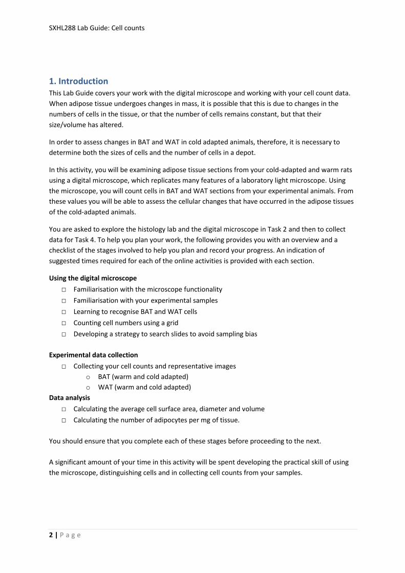
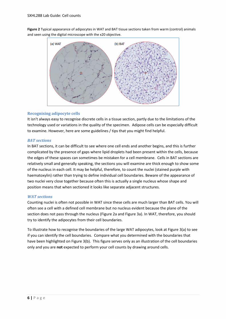
Figure 2 Typical appearance of adipocytes in WAT and BAT tissue sections taken from warm (control) animals

and seen using the digital microscope with the x20 objective.

Recognising adipocyte cells

It isn't always easy to recognise discrete cells in a tissue section, partly due to the limitations of the

technology used or variations in the quality of the specimen. Adipose cells can be especially difficult

to examine. However, here are some guidelines / tips that you might find helpful.

BAT sections

In BAT sections, it can be difficult to see where one cell ends and another begins, and this is further

complicated by the presence of gaps where lipid droplets had been present within the cells, because

the edges of these spaces can sometimes be mistaken for a cell membrane. Cells in BAT sections are

relatively small and generally speaking, the sections you will examine are thick enough to show some

of the nucleus in each cell. It may be helpful, therefore, to count the nuclei (stained purple with

haematoxylin) rather than trying to define individual cell boundaries. Beware of the appearance of

two nuclei very close together because often this is actually a single nucleus whose shape and

position means that when sectioned it looks like separate adjacent structures.

WAT sections

Counting nuclei is often not possible in WAT since these cells are much larger than BAT cells. You will

often see a cell with a defined cell membrane but no nucleus evident because the plane of the

section does not pass through the nucleus (Figure 2a and Figure 3a). In WAT, therefore, you should

try to identify the adipocytes from their cell boundaries.

To illustrate how to recognise the boundaries of the large WAT adipocytes, look at Figure 3(a) to see

if you can identify the cell boundaries. Compare what you determined with the boundaries that

have been highlighted on Figure 3(b). This figure serves only as an illustration of the cell boundaries

only and you are not expected to perform your cell counts by drawing around cells.


7 | P a g e

Figure 3 Typical appearance of adipocytes in WAT tissue sections (a) seen using the digital microscope with the

x40 objective. The outlines of 5 WAT cells have been drawn onto the image in (a) by tracing their cell

membranes (b) to illustrate the typical appearance of WAT cells. You are not expected to draw around cells;

this image serves just to help you recognise WAT cells by their boundaries.

Other cells present in sections

You will notice that each tissue is not composed exclusively of either brown or white adipocytes, but

includes blood vessels and connective tissue and, if the dissection has been over-generous, perhaps

some striated muscle too. You can remind yourself how to recognise these cell types by using the

tissue sections in row 5 of the light box. Note that lipid droplets are also not preserved in the

processed tissue sections, but the space that they once occupied can be identified.

□ Spend a little time examining the tissues; perhaps collect a few images that might be useful

for reports.

□ It is generally good practice to start examining a section on the slide at low magnification

before increasing to higher magnifications and relocating the slide to position the area of

interest in the field of view.

Before you examine the slides in detail, the next section provides additional instructions on

obtaining cell counts and measurements.

2. Counting cells using the grid (allow up to 30 minutes)

Sometimes in microscopy it is important to make measurements such as cell counts, in order to

record data on the micro-structure of a tissue. Most light microscopes have the option to add a grid

into the light path, to allow such measurements.

When viewed down the microscope, the grid remains the same size in the field of view, no matter

which magnification/objective is being used.

□ On the trachea slide (Row 5, first sample), position the adipose tissue into the field of

view using the X and Y coordinates you recorded or the link to adipose tissue in the

explanatory text.


8 | P a g e

□ Note the location of the field of view is highlighted by the small red circle in the

thumbnail image.

□ Now select ‘grid’ and a red grid will appear on the screen.

Note that there is a 6 x 6 grid square region which forms the centre of the field of view. This 6 x 6

square region has thicker grid lines indicating its outer edges.

□ Increase the magnification by progressing through x4, x10, x20 and x40. At each

magnification, note the red circle (which gets smaller) on the thumbnail indicates where

the main field of view is located within the section.

You should now see the adipocytes in the field of view, as shown in Figure 4.

Figure 4 The grid positioned over a region of adipocytes in the trachea section. The 6 x 6 central section

outlined by thicker lines covers an area of 3600 µm2 with this x40 objective.

Note that the area on the tissue sample that is covered by the grid will be different for each

magnification. For the purposes of your investigation, you should use the x40 objective for your cell

counts. Using the x40 objective, the area of the section covered by the 6 x 6 grid is 3600 µm2. You

will use this value in your calculations later.

When cells overlap the edge of the counting area grid lines

Some cells will lie over the edge of the designated counting area. In such cases, you should use

standard criteria with all your cell counts as to what is counted and what is excluded.

For BAT cells: Count BAT cell nuclei within the 6 x 6 grid; only include cells that have a

nucleus within the grid. For nuclei that fall on the grid boundary, exclude those that lie on

the left and bottom boundary, but include those that lie on the top and right boundary.


9 | P a g e

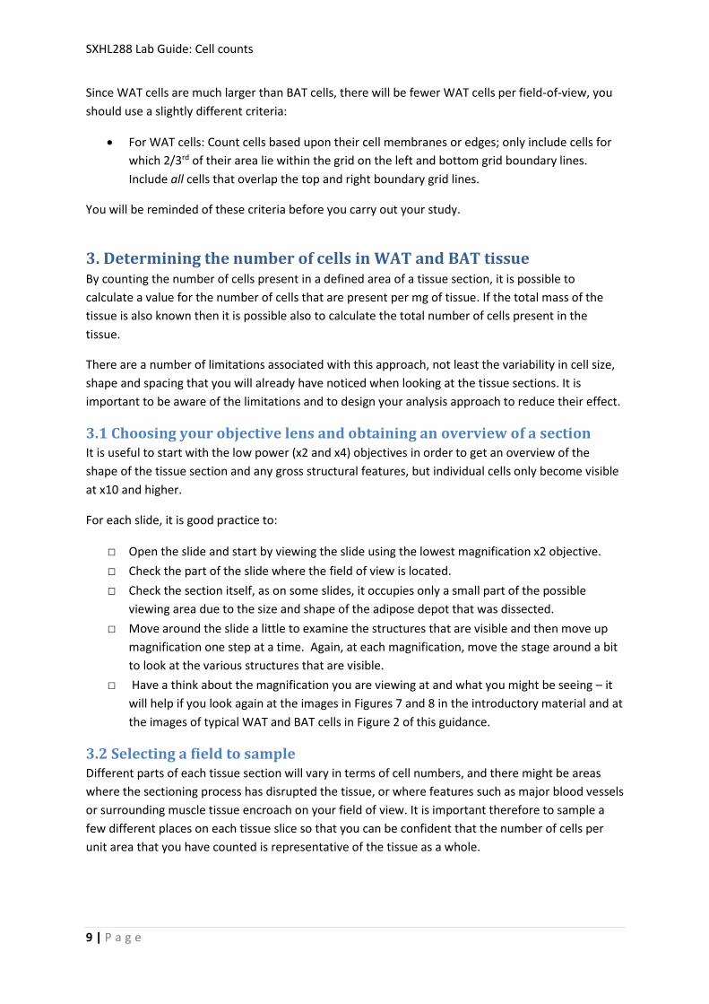
Since WAT cells are much larger than BAT cells, there will be fewer WAT cells per field-of-view, you

should use a slightly different criteria:

For WAT cells: Count cells based upon their cell membranes or edges; only include cells for

which 2/3rd of their area lie within the grid on the left and bottom grid boundary lines.

Include all cells that overlap the top and right boundary grid lines.

You will be reminded of these criteria before you carry out your study.

3. Determining the number of cells in WAT and BAT tissue By counting the number of cells present in a defined area of a tissue section, it is possible to

calculate a value for the number of cells that are present per mg of tissue. If the total mass of the

tissue is also known then it is possible also to calculate the total number of cells present in the

tissue.

There are a number of limitations associated with this approach, not least the variability in cell size,

shape and spacing that you will already have noticed when looking at the tissue sections. It is

important to be aware of the limitations and to design your analysis approach to reduce their effect.

3.1 Choosing your objective lens and obtaining an overview of a section It is useful to start with the low power (x2 and x4) objectives in order to get an overview of the

shape of the tissue section and any gross structural features, but individual cells only become visible

at x10 and higher.

For each slide, it is good practice to:

□ Open the slide and start by viewing the slide using the lowest magnification x2 objective.

□ Check the part of the slide where the field of view is located.

□ Check the section itself, as on some slides, it occupies only a small part of the possible

viewing area due to the size and shape of the adipose depot that was dissected.

□ Move around the slide a little to examine the structures that are visible and then move up

magnification one step at a time. Again, at each magnification, move the stage around a bit

to look at the various structures that are visible.

□ Have a think about the magnification you are viewing at and what you might be seeing – it

will help if you look again at the images in Figures 7 and 8 in the introductory material and at

the images of typical WAT and BAT cells in Figure 2 of this guidance.

3.2 Selecting a field to sample Different parts of each tissue section will vary in terms of cell numbers, and there might be areas

where the sectioning process has disrupted the tissue, or where features such as major blood vessels

or surrounding muscle tissue encroach on your field of view. It is important therefore to sample a

few different places on each tissue slice so that you can be confident that the number of cells per

unit area that you have counted is representative of the tissue as a whole.


10 | P a g e

Using the approach outlined in Section 3.1 above, after you have loaded a slide into view, you should

have an overview of the section and know which areas of the slide do not carry any sectioned tissue

and also any regions that are disrupted or contain a large proportion of non-adipose tissue.

For your study, you need to sample 5 different areas of adipose cells on each tissue section and

count the number of cells per designated area in each case. Choosing an area to sample is

important- you need to find areas that are representative of the tissue (e.g. don’t contain large areas

of disruption or other tissues) but you also need to try to avoid bias. Ideally you would be ‘blinded’

to the identity of the tissue section so you would not know whether it was from a cold-acclimated or

control animal, but that is not easy to achieve if you are working on your own using this digital

microscope since you will be aware of the identity of the sample. The suggested approach is outlined

below.

Sampling strategies

First, design a systematic way of sampling 5 areas of a slide without ‘hunting’ for the places you

think best illustrate the result you are predicting. The best approach is to have a standardised way of

moving to each new sampling area. For example, a sampling protocol may be;

Start in the centre of an area of adipose cells identified on the initial scan of the slide, as

outlined in section 3.1.

o Call this area 1.

Move a certain distance left by either using the stage control or using X, Y coordinates. For

example, select left arrow 3 times (area 2)

o Call this area 2.

Then move to a new area by clicking the up arrow 4 times

o Call this area 3.

And so on, until you have 5 cell counts from the slide.

You should design your own standardised protocol in this way so that you can be confident you are

not introducing bias into your sampling.

□ This can be based upon using the arrows to move around or using the X and Y coordinates.

o At x40, each ‘click’ alters the location of the cross hairs by 50 units.

o 10 ‘clicks’ moves you to a new field of view at x40

Once you have your protocol, you should bear in mind that the sampling strategy determines where

on a section you sample, and therefore influences where you should position your starting point

(area 1). For example, in Figure 5, if the sampling protocol was to move down and left, then down

and right, the best position to start the sampling from would be located at position 1, so that the

pathway used to collect data at points 1-5 would stay within the area of BAT tissue. Clearly you

couldn’t start with such a sampling strategy by placing area 1 at the bottom of a section, as you

would immediately move off the tissue section. You can also see where the field of view is located

within the section using the thumbnail view.


11 | P a g e

Figure 5 Example of how a sampling strategy determines where the starting point for data collection should be

positioned on the slide. Seen drawn onto a x2 view of a section of BAT, the starting area is selected to ensure

that the sampling strategy remains within the adipose section. This strategy can be used to assure that large

areas of non-adipose cells are avoided or that odd shaped sections can be reliably sampled.

Of course you still have the problem that if there happens to be a patch of muscle cells or a large

blood vessel in one of the fields then this will skew your data, so be prepared to have a protocol that

includes a way to deal with this

□ For example, “in the case of a feature/disruption that occupies more than 3 of the grid

squares in the 3600 µm2 counting area, I will move left/down to the first acceptable

designated area that has no disruption.”

Reducing bias and trying to obtain reliable data from inherently variable biological samples is an

important skill in practical science – there is no perfect way to do this, and it is always a good aspect

to discuss in a report!

You may also encounter regions or samples that are weakly stained. This reflects the variability of

staining in adipose tissues and in the histology techniques. You should develop a protocol to deal

with such situations and ensure that you report and discuss these in a report.

Practising your technique (allow up to 30 minutes)

□ Select a slide from one of your experimental samples.

□ Select a location to start by scanning the slide for an area that appears to be representative

of the tissue, with no obvious disruptions or interruptions from other cell types.

□ Practise your chosen protocol for sampling (don’t worry about counting at this stage) at x40.

□ Try to watch the location of the field of view on the thumbnail view; this will give you a feel

for how far you are moving on the section between your counting areas.

□ Implement your strategy for any disruptive features.

□ Once you are happy with your protocol, record the required steps in your lab note book.


12 | P a g e

Note that the development of your own experimental protocol might be useful for your Skills

Portfolio.

3.3 Final words of advice on counting cells It is actually very difficult to count cells accurately in histological specimens and it requires a great

deal of practice. You should, therefore, not agonise over your cell counts. It is more important that

you are consistent in the way that you count each field of view. You will also be reducing some of the

variability by carrying out several counts per slide, but being consistent by always using the same

criteria whilst sampling and counting cells will mean your study is more rigorous.

As mentioned earlier, when counting things within the 6 x 6 grid square, some cells will lie on one of

the grid lines. The following criteria should be used:

For BAT cells: Count BAT cell nuclei within the 6 x 6 grid; only include cells that have a

nucleus within the grid. For nuclei that fall on the grid boundary, exclude those that lie on

the left and bottom boundary, but include those that lie on the top and right boundary.

For WAT cells: Count cells based upon their cell walls; only include cells for which 2/3rd of

their area lie within the grid on the left and bottom grid boundary lines. Include all cells that

overlap the top and right boundary grid lines.

You should now be ready to collect your cell count data. Before you start:

□ It is suggested that you plan a block of time of several hours when you can work through

your slides methodically and consistently.

□ Draw up a table for your data collection, remembering that you have to collect 5 cell counts

for each slide (and that you have the animal numbers noted for each slide)

□ Have your protocol at hand for sampling the fields of view you will count E.g

o Load slide

o Familiarise with the section at various magnifications

o Identify a suitable starting position (area 1)

o Increase objective to x40, relocating on the section if required

o Observe the cells in the field of view to ensure WAT or BAT cells present

o Activate the grid and count cells, using the criteria for inclusion/exclusion

o Relocate to new area, applying criteria for disruptions

3.4 Collecting and recording your cell count data (allow up to 4 hours)

You should now work your way through your experimental slides in an ordered fashion, entering

your raw cell count data for five fields from each slide into a suitable table in your lab note book.

□ There are twenty sections that you need to examine (10 WAT, 10 BAT)


13 | P a g e

□ Recall that WAT cells are best recognised by their cell boundary and BAT cells by their

nucleus

□ Position your starting point on each slide to allow your sampling protocol to remain within

the section and avoid any large disruptive features

You should also collect images of typical areas you examined as these will be good records of your

investigation and will be helpful for your reports or your skills portfolio.

You might also note how many of your cell counts included cells that were not adipose cells, so that

you can comment upon these in your report. Note that for some fields you may have had areas of up

to 3 of the small grid squares that did not contain adipose cells. These counts will affect your final

dataset, so you should note this is your results and comment upon this as a potential source of

experimental error in your report.

Draw up a data collection table. Remember that you have twenty sections, with five fields to

collect data on for each.

When you have collected your cell count data, proceed to entering the values in the table in the

Data analysis area.

Recording your cell count data in the Data analysis area

The Data analysis area of the laboratory contains a data table into which you should enter your cell

counts.

□ Enter your cell counts in whole numbers into the correct positions in the table in the Cell counts

tab in the Data analysis area.

□ Calculate the mean of the 5 cell counts for each sample and then enter these values up to 2 d.p.

into the right hand column of the table in the Cell counts tab.

□ Select the Save WAT/BAT data button.

□ The data analysis software will check whether you have calculated your mean values correctly.

□ Once all the data values are correct and saved, the Calculations tab will be automatically filled

for you. Note: if you change any values in your Cell counts table you must re-save your data for

the Calculations table to update.

The next section takes you through the data generated automatically from your cell count data.

3.5 Cell data for your tissues From your raw cell counts, the Calculations tab spreadsheet automatically calculates the number of

cells per mg of each tissue in each animal. Details of how this is performed are shown in Appendix 3,

in summary, this value is calculated in three stages:

The mean surface area of cells for each rat sample is calculated

The mean cell volume for each rat sample is calculated

This is adjusted for the density of adipose tissue to give the number of cells contained

within, or per mg of tissue.


14 | P a g e

Enter these number of cells per mg of tissue data values for your 20 rats into your laboratory

notebook.

Once you have recorded these data, you should also note that some group data values have been

automatically graphed in various ways for you. These graphs can be found by selecting the Charts

tab. You should collect copies of the charts as these may prove helpful in your reports in TMA02. In

particular, note that in addition to the mean cell volumes being graphed, both the rat mass and the

adipose tissue depot mass data are also presented.

Knowing the number of cells present per mg of tissue will allow you to estimate the protein and lipid

content per cell (using your data collected from the lipid and protein analysis experiments you carry

out in the Physiology lab).

Finally, you can determine the total number of BAT and WAT cells in the two depots examined by

combining the mass of the dissected tissue with the cells/mg tissue value. This will allow you to

assess any change in cell numbers that accompany cold adaptation within the entire adipose depot.


15 | P a g e

Appendix 1: Digital Microscope quick guide

Loading and navigating around a slide

Light box

A small thumbnail representation of each section in your microscope is presented, with the current section in the field of view underscored in red. The 5th row contains specimens of various tissues to examine and the accompanying text can be used as a guide to explore each section. A ruler is provided to allow length measurements to be taken.

Navigation tool

This thumbnail image shows the where the present field of view (red circle) is located on the slide. The arrows can be selected to move the field of view in any direction. These arrows can be used in a sampling strategy to move around a section in a pre-determined manner.

Location tool

This provides a set of coordinates for the centre of the present field of view presented as the location of the ‘cross hairs’ (the small red cross, see below). You can return to a particular point of interest by typing its coordinates into the boxes and selecting ‘Go’. This tool can also be used in a sampling strategy to move around a section in a pre-determined manner.

Cross-hairs

This small red arrow in the centre of the field of view provides a set of X and Y coordinates for exact locations on any slide.

Magnifying, counting and measuring

Objectives

By selecting each of these buttons, a new objective is loaded and the present field of view is magnified accordingly.

Grid

This places a grid over the current field of view. The grid can be used to count cells in a fixed area of section.

Graticule This places a short red ruler into the field of view. This can be used to measure objects.

Capturing images for your records

Camera

This captures an image of the current field of view, presenting you with the option of saving, copying (in order to paste into a document) or directly printing the current view.


16 | P a g e

Appendix 2: How the digital microscope compares to a standard light

microscope There are many different types of microscope, ranging from the basic to the very complex. Which

structures can be seen using a microscope depends upon its magnifying power, and this in turn

depends upon the lenses and the type of light used. This appendix provides a simple explanation of

how a basic light (or optical) microscope works.

As can be seen in Figure A2, a beam of light from a light source is focused on the specimen by

passing it through a ‘condenser’ lens. In ‘standard’ microscopes, the light and condenser are located

beneath the specimen. After passing through the specimen (such light is described as

being transmitted through the specimen), the light then passes through an ‘objective’ lens, which

magnifies the image and passes it to the eyepiece lens, which again magnifies the image and focuses

it into the eye (or to a computer screen or digital camera). Usually the microscope has several

different objective lenses, allowing a choice of different levels of magnification.

When using the digital microscope, the magnification adjustments you can make are through make

are through selections of different objective lenses. The ‘field of view’ you see when using the digital

microscope is presented as a circular image on screen (or captured using a camera) as if you are

looking through the round eye-piece

Figure A2 A very simple conventional light microscope, accompanied by a schematic diagram illustrating how

light passing through the microscope forms an image in the eye of the observer.


17 | P a g e

Appendix 3 Conversion of raw cell count data to a value for ‘number of cells

per mg tissue’ The following guidance will take you through converting a mean cell count data value into a value

that represents the number of cells per mg of tissue, which is done in the Calculations tab for each of

the WAT and BAT samples. This is done in the four stages (a) to (d) that are outlined below. The data

table performs this calculation automatically, this example is to illustrate the stages involved using a

hypothetical set of cell count data.

(a) The mean surface area of a cell in your sections

The mean surface area of cells in the section is calculated by dividing the area of the field of view

used for data collection (which was the 6 x6 grid of 3600 µm2 ) by the mean number of cells in that

field.

□ For a sample, divide 3600 by the mean cell count. For example, if you counted an average

value of 14.01 cells in the 6 x 6 central 3600 µm2 region of the grid, then the mean cell area

would be 3600 / 14.01 = 256.96 µm2.

(b) The mean diameter of the cells in your section

Assume that the cells are circular in cross section, so that the mean cell diameter can be calculated

using the following equation:

mean cell area

Diameter = 2 μm π = piπ

To calculate mean cell diameter for the sample in row 1:

□ Divide the mean cell area from (a) above by π (or use 3.1416)

□ Take the square root of this value

□ Multiply by 2, to give the mean diameter in µm

For example, using the mean cell area 257 µm2 (rounded up for simplicity) from above, the diameter

would be;

257

2 = 2 81.8 = 2 9.04 = 18.1 μmπ

(c) The mean volume of cells in your sample

The mean volume of the cells in your sample can be calculated from the mean cell diameter using

the following equation:

3

3diameterVolume = π μm π = pi

6

To calculate the volume of cells for the sample in row 1:

□ Cube the diameter from (c)above (i.e. multiply diameter x diameter x diameter)

□ Divide this value by 6


18 | P a g e

□ Multiply by π, to give the mean volume in μm3

For example using the mean cell diameter 18.1 µm from above:

318.1 18.1 18.1

Volume = π π 988.3 3104.5 μm 6

(d) The number of cells per mg of tissue

There is one further conversion that is performed based on the mean cell volume that will tell you

the number of cells present per mg of tissue. This involves determining the mean mass of the cells

based on their volume and density.

This calculation for the number of cells per mg of tissue is carried out in three stages;

(i) Convert the volume in µm3 to a volume in picolitres (pl).

As 1 pl = 1000 µm3, this is done by simply dividing the mean cell volume from (c) above by 1000. For

example a volume of 3054 µm3 would be 3.054 pl. This volume in picolitres is the equivalent of 3.054

x 10-9 millilitres (ml) or 3.054 x 10-12 litres.

(ii) Calculate the mass of a cell

To do this, use the following equation:

Mass = volume x density

The density of adipose tissue can be assumed to be 0.96 g ml-1, therefore mean cell mass = mean cell

volume x 0.96. For example, for a volume of 3.054 pl;

Mean cell mass = 3.054 x 10-9 x 0.96 = 2.9 x 10-9 g

As 1 mg is 1/1000th of one gram, this is 2.9 x 10-6 mg.

(iii) Calculate the number of cells per mg of tissue

From the mean cell mass it is possible to determine the number of cells in one milligram (mg) of

tissue:

Number of cells per mg tissue = 1/mean cell mass

For example, a mean cell mass, from (ii) above, of 2.9 x 10-6 mg, would give the following number of

cells per mg of tissue

1 / (2.9 x 10-6) = 345,000 cells per mg tissue (approximated to 3 sf).

For ease of showing a clear example, rounding has been used in the above calculation, otherwise the precise answer would be 341,082 cells (to the nearest whole cell).

Cell counts: Histology guidance (SXHL288) - The Open ...

Documents

Transcript of Cell counts: Histology guidance (SXHL288) - The Open ...