Galaxy number counts - V. Ultradeep counts: the Herschel and Hubble Deep Fields
38
• • •
Transcript of Galaxy number counts - V. Ultradeep counts: the Herschel and Hubble Deep Fields

Durham Research Online
Deposited in DRO:
29 April 2008
Version of attached le:
Other
Peer-review status of attached le:
Peer-reviewed
Citation for published item:
Metcalfe, N. and Shanks, T. and Campos, A. and McCracken, H. J. and Fong, R. (2001) 'Galaxy numbercounts - V. Ultradeep counts : the Herschel and Hubble deep elds.', Monthly notices of the RoyalAstronomical Society., 323 (4). pp. 795-830.
Further information on publisher's website:
http://dx.doi.org/10.1046/j.1365-8711.2001.04168.x
Publisher's copyright statement:
The denitive version is available at www.blackwell-synergy.com
Additional information:
Use policy
The full-text may be used and/or reproduced, and given to third parties in any format or medium, without prior permission or charge, forpersonal research or study, educational, or not-for-prot purposes provided that:
• a full bibliographic reference is made to the original source
• a link is made to the metadata record in DRO
• the full-text is not changed in any way
The full-text must not be sold in any format or medium without the formal permission of the copyright holders.
Please consult the full DRO policy for further details.
Durham University Library, Stockton Road, Durham DH1 3LY, United KingdomTel : +44 (0)191 334 3042 | Fax : +44 (0)191 334 2971
http://dro.dur.ac.uk

arX
iv:a
stro
-ph/
0010
153v
1 7
Oct
200
0Mon. Not. R. Astron. Soc. 000, 1–37 (2000) Printed 1 February 2008 (MN LATEX style file v1.4)
Galaxy number counts - V. Ultra-deep counts: The
Herschel and Hubble Deep Fields
N. Metcalfe1, T. Shanks1, A. Campos2, H.J. McCracken1⋆ and R. Fong1
1Physics Department, University of Durham, South Road, Durham DH1 3LE2Instituto de Matematicas y Fisica Fundamental, CSIC, Spain
Accepted 2000. Received 2000; in original form 2000
ABSTRACT
We present u, b, r & i galaxy number counts and colours both from the North andSouth Hubble Space Telescope Deep Fields and from the William Herschel Deep Field.The latter comprises a 7′ × 7′ area of sky reaching b ∼28.5 at its deepest. FollowingMetcalfe et al. (1996) we show that simple Bruzual & Charlot evolutionary modelswhich assume exponentially increasing star-formation rates with look-back time andq0=0.05 continue to give excellent fits to galaxy counts and colours in the deep imagingdata. With q0=0.5, an extra population of ‘disappearing dwarf’ galaxies is requiredto fit the optical counts.
We further find that the (r − i) : (b − r) colour-colour diagrams show distinctivefeatures corresponding to two populations of early- and late-type galaxies which arewell fitted by features in the Bruzual & Charlot models. The (r− i) : (b− r) data alsosuggest the existence of an intrinsically faint population of early-types at z ∼ 0.1 withsimilar properties to the ‘disappearing dwarf’ population required if q0=0.5.
The outstanding issue remaining for the early-type models is the dwarf-dominatedIMF which we invoke to reduce the numbers of z > 1 galaxies predicted at K < 19.For the spiral models, the main issue is that even with the inclusion of internal dustabsorption at the AB = 0.3 mag level, the model predicts too blue (u − b) colours forlate-type galaxies at z ∼ 1. Despite these possible problems, we conclude that thesesimple models with monotonically increasing star-formation rates broadly fit the datato z ∼ 3.
We compare these results for the star formation rate history with those from thedifferent approach of Madau et al. (1996). We conclude that when the effects of internaldust absorption in spirals are taken into account the results from this latter approachare completely consistent with the τ=9Gyr, exponentially rising star formation ratedensity out to z ≈ 3 which fits the deepest, optical/IR galaxy count and colour data.
When we compare the observed and predicted galaxy counts for UV dropouts inthe range 2 <
∼ z <∼ 3.5 from the data of Steidel et al. (1999), Madau et al. (1996) and
new data from the Herschel and HDF-S fields, we find excellent agreement, indicatingthat the space density of galaxies may not have changed much between z = 0 andz = 3 and identifying the Lyman break galaxies with the bright end of the evolvedspiral luminosity function. Making the same comparison for B dropout galaxies in therange 3.5 <
∼ z <∼ 4.5 we find that the space density of intrinsically bright galaxies
remains the same but the space density of faint galaxies drops by a factor of ∼5,consistent with the idea that L∗ galaxies were already in place at z ≈ 4 but that dwarfgalaxies may have formed later at 3 <
∼ z <∼ 4.
Key words: galaxies: evolution - galaxies: photometry - cosmology: observations
⋆ Present address: LAS, Traverse du Siphon, Les Trois Lucs, F-13102 Marseille, France
1 INTRODUCTION
In four previous papers, Jones et al. (1991) (hereafter PaperI), Metcalfe et al. (1991) (hereafter Paper II), Metcalfe et al.
c© 2000 RAS

2 N. Metcalfe, et al.
(1995a) (hereafter Paper III) and McCracken et al. (2000)(hereafter Paper IV), we used photographic and CCD datato study the form of the galaxy number-magnitude relationat both optical (B ∼ 27.5) and infra-red (K ∼ 20) wave-lengths. In this paper we extend our observations of the B-band field of paper III to even deeper magnitudes (B ∼ 28mag), and over a much larger area of 7′
×7′, by exposing fora total of 30 hours over five nights with the Tektronix CCDat the prime focus of the 4.2 metre William Herschel tele-scope (WHT). We have also acquired ∼ 34 hours of exposurein the U -band (to U ∼ 27 mag), 8 hours in the R-band (toR ∼ 26.5 mag) and 5 hours in the I-band (to I ∼ 25.5 mag)on the same field, again with the WHT. We refer to this fieldthroughout as the William Herschel Deep Field (WHDF).
Although not competing in terms of either collectingarea or field of view with these ground-based observations,the high resolution of the Hubble Space Telescope offersthe ability to image sub-arcsecond objects to much greaterdepths than can be done from the ground. The Hubble DeepField (HDF) project (Williams et al. 1996) has provided sucha dataset in the public domain, and here we present our anal-ysis of the F300W , F450W , F606W and F814W prelimi-nary release North (HDF-N) and South (HDF-S) fields, us-ing similar data reduction techniques as for the WHT data.Roughly speaking, these passbands correspond to U , B, R& I (see section 4.2). For unresolved objects the 3σ limit ofB ∼ 29.5 mag on the F450W image is considerably deeperthan our WHT frame. However, for resolved galaxies thislimit is much brighter. Indeed, for sources more extendedthan the WHT ‘seeing’ disk (∼ 1.25′′ radius) the ground-based frame is slightly deeper, making it an ideal comple-ment to the HST images. A similar situation exists betweenthe WHT u and the HDF F300W frames, where, for a sourceat the WHT seeing limit, the WHT is actually over 0.5 magdeeper than the HDF. The same is not true for the F606Wand F814W images, which are 2-3 mag deeper (for typicalgalaxy sizes) than the deepest previous R and I-band galaxycounts (Smail et al. 1995, Hogg et al. 1997).
The modelling and interpretation of HDF-N data hasbeen discussed briefly elsewhere (Metcalfe et al. 1996). Herewe discuss the data reduction for both ground- and space-based data, and present the number counts, colour distri-butions and models in greater detail. Finally we discuss thecomparison between the models and the data.
The optical - infra-red properties of the WHDF, basedon infra-red imaging data to K ∼ 20 taken on the UnitedKingdom Infrared Telescope, and data to K ∼ 23 on onesmaller, 1.8′
× 1.8′ area, are discussed in Paper IV.We now also have infra-red imaging data covering the
whole of our WHDF to H ∼ 22.5 mag taken with the ΩPrime camera on the Calar Alto 3.5m telescope. This datawill be discussed in a subsequent paper (McCracken et. al.,in prep.).
2 THE OBSERVATIONS
2.1 New WHT observations
Our data were taken during four observing runs at WHTprime focus; one of 5 nights in September 1994 during whichall of the b-band data and about 3hrs of r-band data were
Figure 1. Filter/detector throughputs for the HDF (dashedlines) and WHDF (solid lines) observations. The WHDF curvesinclude the effects of La Palma extinction.
acquired, a further run of 4 nights in September 1995 dur-ing which the remaining r-band data and some of the u-band data were collected, and 3 nights in both October1996 and September 1997 when the rest of the u-band ex-posures and all the i-band data were taken. Observing con-ditions were much better in 1994, when 4 out of 5 nightswere photometric, than in 1995 or 1996, when the observa-tions were affected by dust and poor seeing. The 1997 run,although not completely photometric, had good seeing of≈ 1′′ FWHM. For the 1994 and 1995 runs we used the Tek-tronix CCD camera at WHT prime focus, giving a field sizeof 7.17′
×7.17′ at a scale of 0.42′′ per pixel. The gain was setto 1.7e−/ADU and the read-noise is about 7e−. However, in1996 we switched to a Loral CCD, with 2048 × 2048 pixelsat a scale of 0.26′′ per pixel and a gain of 1.22e−/ADU . In1997 we again used a Loral CCD (although not the samechip as in 1996); this time the gain was set to 1e−/ADU .These chips have a much higher (about a factor of three)short wavelength response than the Tek CCD, as a resultof which most of our u-band signal comes from the 1996/7data.
The Harris B, R and I filters were used - these are muchcloser to the standard photoelectric bands (throughout, anyreferences to standard photoelectric R and I magnitudesimply those on the Kron-Cousins system) than the KPNOfilters used in papers II and III. The U filter was a 50mmRGO filter, which caused some vignetting at the edges of theCCD. The filter response curves can be seen in Fig. 1. Toavoid confusion we use lower-case u, b, r & i to refer to thepassbands defined by the WHT filter/detector combination.
Exposures were centred on 00h19m59s.6 +0004′18′′
(B1950.0). This field encompasses the 24 hour INT and 10hour WHT images from paper III, although the centre isabout 1.5′ north of that of these previous exposures. Indi-vidual u and b-band exposures were usually 2000s, with some
c© 2000 RAS, MNRAS 000, 1–37

Galaxy number counts - V. Ultra-deep counts: The Herschel and Hubble Deep Fields 3
Table 1. Details of the WHT and HDF images. The WHT magnitudes are in uccd, bccd, rccd and iccd
(section 3.1); the HDF-N & S magnitudes are in the vega system (section 4.2); the STIS magnitudes are inthe AB system. The definition of effective exposure is given in section 2.1.
Frame Area Effective exposure FWHM 3σ measurementa 1σ isophoteb
deg2 (sec) (′′) (mag) (mag/arcsec2)
WHT u 1.29 × 10⁻² 121000 1.35 26.8 29.2WHT b 1.35 × 10⁻² 100000 1.25 27.9 30.3WHT r 1.30 × 10⁻² 27500 1.50 26.3 28.7WHT i 1.45 × 10⁻² 19000 1.20 25.6 26.5Co-added b 7.9 × 10⁻⁴ 166000 1.35 28.2 30.6HDF-N F300W 1.17 × 10⁻³ 170500 0.15 27.0 27.8HDF-N F450W 1.17 × 10⁻³ 84600 0.15 29.1 29.8HDF-N F606W 1.17 × 10⁻³ 94650 0.15 29.3 30.1HDF-N F814W 1.17 × 10⁻³ 94000 0.15 28.4 29.2HDF-S F300W 1.17 × 10⁻³ 140185 0.15 26.9 27.6HDF-S F450W 1.25 × 10⁻³ 100950 0.15 29.1 29.8HDF-S F606W 1.30 × 10⁻³ 81275 0.15 29.3 30.1HDF-S F814W 1.29 × 10⁻³ 100300 0.15 28.4 29.2STIS Unfilt. 1.4 × 10⁻⁴ 156000 0.15 30.3 31.1a Inside an aperture with radius equal to the minimum radius given in Table 2 (magnitude is total magnitudeof an unresolved object)b Inside 1 arcsec2
reduced to 1000s on occasions when the seeing was variable.For the r band we used an exposure time of 500s, and for thei band between 300 and 500s. These short exposures werenecessary in order to avoid saturating the CCDs with thebackground sky signal. To avoid excessive atmospheric ex-tinction, no u-band frames were taken at an airmass greaterthan ∼ 1.5, and no b-band frames at greater than ∼ 1.8. Ther and i-band frames, where extinction is less of a problem,were mostly taken at higher airmass than this. The field wasoffset a few arcseconds in different directions between nightsin order to avoid dud pixels always falling on the same placeon the sky. The total exposure times were 59.5ks (Tek) +88ks (Loral) in u, 112ks in b, 27.5ks in r and 21.5ks in i. Theeffective exposure times, defined as the equivalent numberof seconds at the zenith in photometric conditions (with theLoral CCD for the u), are given in Table 2. The seeing wasgood in 1994 and 1997, always less than 2′′ FWHM, andaround 0.9′′ on some nights, but ranged from 1′′
− 5′′ in1995 and 1.3′′
− 2.0′′ in 1996. The images with the worstseeing were not used in the data reduction (see section 3.1).Standard stars were taken at the beginning and end of eachnight, as were twilight flat-fields. Standards were also occa-sionally taken during the night, although we were also ableto use our image frames to monitor atmospheric conditions.
2.2 The Hubble Deep Fields
For the HDF-N we use the F300W , F450W , F606W andF814W preliminary ‘drizzled’ WFPC2 images released intothe public domain on 1996 January 15 (Williams et al. 1996).These are flat-fielded, cosmic-ray rejected, sky-subtractedstacked images, resampled to a scale of 0.04′′/pixel. Each ofthe three wide-field WFPC2 chips were analysed separately.We made no attempt to use the data from the PC chip.Note that some 25% of the observations are not included inthe F450W images and an optimal weighting scheme wasnot used for stacking these data, nor for the F300W data.For the HDF-S we use the combined WFPC2 images re-leased in November 1998. We have also analysed the un-
filtered STIS QSO field image. For unresolved objects theeffective FWHM is ∼ 0.15′′ (see Williams et al. 1996).
3 WILLIAM HERSCHEL DEEP FIELD
3.1 Data reduction
A detailed description of our data reduction procedures canbe found in Paper III. Briefly, a master bias frame is formedfrom a median of many individual bias exposures and nor-malised to the bias level in the overscan region of each ex-posure. This bias frame is then subtracted. The resultingframes are then trimmed to remove the overscan and dividedby a master flat-field, formed from the median of all the flatfields in the relevant filter throughout the run. Cosmic raysare removed by comparing each pixel in each frame with themean and standard deviation in that pixel over all other ex-posures (where necessary, normalised and re-scaled) takenthat night. Any pixels more than 4.5σ away from that meanare replaced by the mean of the surrounding 5 × 5 pixelsin the image being cleaned. Finally, each image is inspectedvisually on the computer and any remaining blemishes (e.g.satellite trails) removed interactively. All the individual im-ages are then registered with one another to the nearestinteger pixel shift by doing a pixel-pixel cross-correlationbetween images. They are then added together. Frames onwhich the seeing was equal to or greater than 2.0′′ FWHMwere discarded.
The final b-band image is 998 × 991 pixels (7.0′× 6.9′)
and has a sky surface brightness of 21.9 mag/arcsec2 . Theseeing is ∼ 1.25′′ FWHM (as in papers II and III this isjudged by comparison with a simulated Moffat profile (Mof-fat 1969)).
The final r-band image has 986×966 pixels (6.9′×6.8′)
and has a sky brightness of 20.0 mag/arcsec2 . There wasa slight rotational shift between the 1994 and 1995 datawhich was corrected for using the shear technique describedin paper III. The seeing on this frame is ∼ 1.5′′ FWHM.
c© 2000 RAS, MNRAS 000, 1–37

4 N. Metcalfe, et al.
The 1995, 1996 and 1997 u-band data were reduced sep-arately. The 1995 data were then resampled to 0.26′′/pixeland, along with the 1996 data, shear-rotated slightly in or-der to match the 1997 data. There was a problem with theLoral CCD used in 1997 in that it had a ∼ 5% non-linear re-sponse at low signal levels. This posed a particular problemfor u-band deep field data frames, where even in 2000 secexposures the sky levels were low. Extensive exposure testswere carried out with a dome lamp to enable a correctionfactor as a function of count rate to be determined. This wasthen applied to the data. As a check on this procedure onestandard star field was repeated with a series of exposuretimes, and detailed comparisons made between stars cover-ing a range of magnitudes on our field in 1997 and 1995/6.In fact, the uncorrected and corrected standards gave thesame zero-point to within 0.01 mag (as expected, as most ofthe light from these stars comes at high count rates wherethe non-linear correction is negligible). However, the correc-tion did improve the relation between the 1995/6 and 1997data frames, removing a ∼ 0.05 mag non-linearity betweenbright and faint stars. The three datasets were then stackedtogether (with appropriate weighting to allow for the differ-ent gain factors, signal strength and sky levels) and all theimage analysis was done on this final combined frame, whichencompasses 1593×1582 pixels (6.9′
×6.9′) with a ‘seeing’ of≈ 1.35′′ FWHM. The sky brightness was 21.5 mag/arcsec2 .
The 1996 and 1997 i-band data were also reduced sep-arately. The non-linearity in the 1997 Loral CCD was nota problem for the i data, as the sky levels were well intothe linear regime (and as we found for u data the zero-pointfrom the standards was not affected). As a result no correc-tion was applied. However, an extra problem with all thei-band data was the presence of fringing. To remove this itwas necessary to create a master fringe frame by taking themedian of all the data-frames. This was then scaled to suiteach individual frame (by trial and error) and subtracted.A small amount of rotation and pixel rescaling (∼1%) wererequired before the two runs could be stacked together. Thefinal i-band image has 1622 × 1747 pixels (7.0′
× 7.6′) anda sky brightness of 18.9 mag/arcsec2 . It has the best seeingof all our data, with a FWHM of only 1.2′′.
Both the present b-band data and our 26hr INT primefocus CCD data from paper III cover the ∼ 2′ diameterarea observed for 10hrs with the WHT auxiliary focus CCDcamera (paper III). By stacking all three together in thecommon area we have been able to create an ultra-deep im-age. To achieve this the INT and WHT auxiliary imageswere rotated, again using the shear technique described inpaper III, and resampled to the same pixel scale as the WHTprime image. The three were then registered to one pixel ac-curacy and added. The resulting image is 243 × 240 pixels(1.7′
× 1.7′) (as the WHT auxiliary image was circular, theeffective exposure time is lower in the corners). The ratiosof number of electrons detected in each separate image froman object are; 3.06 : 1.03 : 1.0 (WHT prime : WHT aux.: INT prime). The stacked image is therefore equivalent to1.7× the WHT prime exposure, i.e. ∼ 46hrs of 4-m time,and is ∼ 0.3 mag deeper. Fig. 2 shows a sky-subtracted sur-face brightness contour plot of this co-added image, with ageometric progression of levels starting at 1000ADU (29.4mag/arcsec2) and rising by factors of two.
Although not adding to the discussion of counts and
Figure 2. Isophotal contour plot for the 50 hour co-added b-band data. Contours start at 29.4 mag/arcsec2 and rise in 0.75mag steps.
colours in this paper, this small field has the advantage ofhaving been the subject of a 30 hour K-band exposure takenwith IRCAM3 camera (which has an almost identical fieldof view) at UKIRT. Thses data, and a detailed analysis ofthe (b−K) colour distribution, has been presented elsewhere(Paper IV).
Table 1 lists the parameters of all our final images.
3.2 Calibration
Zero-points for our data were provided by observations ofequatorial standard star fields from Landolt (1992). Mostlythey were observed close to the meridian. The CCD field ofview is large enough to see 5 ∼ 10 standards on a Landoltfield in a single exposure.
As all our WHDF frames are on the same field we adoptthe procedure of calibrating all the frames (in each run) inone band relative to ones taken on the meridian on pho-tometric nights. This is done by comparing magnitudes fora selection of bright (but not saturated) objects. The stan-dard stars observations then provide an absolute calibration.As the airmass of the standards and of the WHDF on themeridian are very similar, this way we are not sensitive toairmass extinction coefficients. In fact, by fitting a sec z lawto the relative magnitudes of objects on our WHDF field
c© 2000 RAS, MNRAS 000, 1–37

Galaxy number counts - V. Ultra-deep counts: The Herschel and Hubble Deep Fields 5
throughout a night’s observations, we were able to deriveatmospheric extinction coefficients appropriate to each runand hence apply relative airmass corrections to those stan-dards not observed at the meridian.
Where possible, colour equations measured during therun are used to convert the standards to the ‘natural’ CCDbands (which agree with standard UBRI for objects withzero colour) and the magnitudes and colours we measure forgalaxies are in these ‘natural’ systems, which we designateuccd, bccd, rccd and iccd (although, as we shall see below,these are very close to the standard photoelectric bands).
The bccd and rccd magnitudes from the Tek CCD usedin 1994 suffered a minor problem in that our observed stan-dard star magnitudes appeared to be correlated with expo-sure time (at the level of a few hundredths of a magnitude).After consultation with the RGO (T. Bridges, priv. comm.)it became apparent that a small additive shutter timing cor-rection was necessary for the WHT prime focus camera. Themagnitude of this correction was dependent on zenith angle,being ∼ +0.05s for most of our standards. Applying thissignificantly reduced the scatter between the observed andcatalogued magnitudes, and the following colour equationswere determined from n observations of 28 stars:
bccd = B − 0.012(B − R) (n = 73)
rccd = R (n = 65)
The rms scatter about the B and R relations was±0.014 mag. The range in colour covered was −0.5 <(B − R) < 2.5. Fig 3 shows examples of the data on whichthese relations were based.
In 1995 only one night was demonstrably photometricand this was used to calibrate our data independently fromthe 1994 observations. Again we found rccd = R, with a scat-ter of ±0.009 mag from measurements of 23 standards.Therccd zero-point deduced from this gave magnitudes on theWHDF which agreed to within 0.02 mag in the mean fromthose found in 1994. Note that no shutter correction was ap-plied to this data, as a series of test exposures ranging from1s to 20s were taken sequentially on the same field duringphotometric conditions and no dependence of the zero-pointon exposure time was present down to the 0.01 mag level.
The data from the uccd and iccd standards (whethertaken with Tek or Loral CCD between 1995 and 1997) showa significantly higher scatter than the bccd or rccd data. Thereasons for this are not clear; airmass corrections are notthe cause because, as already noted, all the standards weretaken at very similar airmass - also the effect exists betweenstandards on the same CCD image and is not due to varia-tions from night to night (or within a single night).
All the 1995 u-band data were tied to the one photo-metric night, although frequent standards were taken everynight (the maximum variation in zero-point from night-to-night was 0.2 mag), and we were able to utilise most of theseto derive an approximate colour equation of
uTek ≈ U − 0.1(U − B) (n = 96)
valid for −1.5 < (U −B) < 2.5, with a scatter of ±0.08 mag,excluding two standards whose magnitudes were confirmed
Figure 3. Example standard star calibration plots (cataloguecolour versus observed - catalogue magnitude) for the WHT u,b, r and i bands. The dotted lines indicate the adopted colourequations.
by repeat measurements to be ∼ 0.4 mag off the mean line.Fig 3 shows these data.
The 1996 and 1997 u-band standards taken with the Lo-ral CCD showed a similar scatter with respect to the Landoltmagnitudes of ∼ ±0.10 mag. This excludes the two stan-dards which were discrepant in the 1995 Tek data, whichwere again found to be off by ∼ 0.4 mag. Significantly, ifwe compare frames with several standards on taken bothin 1996 and 1997, the scatter between the 1996 and 1997data was only ±0.03 mag. A similar exercise between fieldsin common to 1995 and 1996/7 datasets gave ±0.06 mag.The Loral data do not show a colour term as large as the0.1(U −B) found for the Tek data, and the scatter preventsany reliable estimate of a shallower relation. However, thestandards on fields in common between the Tek and Loralobservations indicate that there is a significant colour termbetween these two CCDs. We estimate this as
uTek − uLoral ≈ −0.07(U − B) (n = 25)
which reduces the scatter to ±0.04 mag. As the 1996/7 datadominate the stacked image in terms of signal-to-noise weadopt a colour equation of
uccd ≈ U − 0.03(U − B)
as appropriate for our final dataset (for −1.5 > (U − B) >2.5).
Although there is clearly some uncertainty in the uccd
zero-point, when the 1995, 1996 and 1997 WHDF data were
c© 2000 RAS, MNRAS 000, 1–37

6 N. Metcalfe, et al.
calibrated and reduced independently, the magnitude scalesagreed to within 0.03 mag.
The scatter in the iccd-band standards (±0.10 mag)appears partly due to non-photometric variations on somenights (especially in 1997) at the 0.05 mag level. There is alsosome evidence of inaccuracies in some of the fainter Landoltstandards on the fields we used (and many of the brighterstandards were unusable due to saturation), as standards onone field taken in both 1996 and 1997 show the same offsetswith respect to the Landolt magnitudes (up to 0.2 mag, withno correlation with colour), and a scatter of < 0.01 mag be-tween the two years. Fig. 3 shows the data from 1997. As aresult of these uncertainties, and the short colour range in(V − I), we make no attempt to fit a colour equation butjust assume iccd = I .
Fortunately, in 1995 we observed an area encompass-ing the WHDF in the I-band with a Tek CCD on the INT2.5m telescope. These independent data show an offset ofonly ∼ 0.04 mag with the WHT data, giving us confidencein our zero-point (although any possible problems with thestandard magnitudes would affect these data as well).
3.3 Image analysis
Our procedure is very similar to that used in Papers I-IV(note that the data in each passband are reduced indepen-dently); the sky background is removed and images are de-tected isophotally using the limits given in Table 2. Theseimages are then removed from the frame, replaced by a localsky value, and the resulting frame smoothed heavily beforebeing subtracted from the original. This produces a veryflat background. The isophotal detection is then repeated.In order to reduce false detections, images whose centres lieonly two pixels apart are recombined into one single image.A Kron-type pseudo-total magnitude is then calculated foreach image, using a local value of sky.
One complication with both our u-band and b-band ex-posures was the presence of scattered light (at the 1% levelin b and 10% in u) on one side of the field. This had a sharpedge which proved difficult to remove by the above back-ground flattening technique. It therefore proved necessaryto remove this interactively from the frame.
Table 2 shows the limiting isophotes and magnitudesfor our isophotal detection routine and the minimum radius,radius multiplying factor (see paper III) and correction tototal magnitude for our Kron magnitudes. As in our pre-vious papers the minimum radius is set to be that for anunresolved image of high signal-to-noise, and the correctionto total is the light outside this minimum radius for suchan image. Our measurement limits (table 1) give the totalmagnitudes of unresolved objects which are a 3σ detectioninside the minimum radius.
As in paper III we measure fixed aperture colours. Forall the WHT data we use an aperture of 1.5′′ radius, andcorrect the measured colours for the difference in ‘seeing’between the different bands (this is a small effect, and is es-timated from inspection of stellar profiles). Images detectedin one band are matched with those detected in the otherwithin ∼ 1′′ of the position in the first band. Any multi-ple matches which occur are decided by visual inspection. Ifeither image is below the 3σ magnitude measurement limitfor that band then no colour is measured.
Figure 4. (a) (R − I) : (B − R) colour-colour diagrams for ob-jects identified as stars on our data (open circles) compared withthe Landolt (1992) observations of standard stars (dots). Ourmagnitudes have been corrected to the standard passbands us-ing the colour equations in section 3.2; (b) as (a) but now for(U − B) : (B − R)
We can compare (B−R) colours between our new WHTdata and our INT results in Paper III on an object by objectbasis. We find a scatter in (B − R) rising from ∼ ±0.1 magfor 22 < B < 24 mag to ∼ ±0.5 mag for 25 < B < 26mag. The much noisier INT data will, of course, dominatethe scatter.
3.4 Star/galaxy separation
Star-galaxy separation was done on the b-band frame usingthe difference between the total magnitude and that insidea 1′′ aperture, as described in paper II. This enabled us toseparate to b ∼ 24 mag. Some additional very red stars wereidentified from the r and i frames in similar fashion.
The colours of the stars can be used as an external,
c© 2000 RAS, MNRAS 000, 1–37

Galaxy number counts - V. Ultra-deep counts: The Herschel and Hubble Deep Fields 7
Table 2. Parameters used in the WHT and HDF image analysis. As in Table 1, WHT magnitudes are inthe natural ccd system, whilst the HDF magnitudes are on the vega system.
Frame Limiting isophote Limiting isophotal Minimum radius Kron multiplying Correction to total(mag/arcsec2) magnitude (′′) factor (mag)
WHT u 29.75 28.0 1.30 1.40 0.32WHT b 31.0 29.0 1.25 1.40 0.34WHT r 29.0 27.3 1.4 1.50 0.30WHT i 28.0 26.8 1.25 1.44 0.28Co-added b 32.0 30.0 1.375 1.50 0.33HDF-N F300W a
HDF-N F450W 28.5 29.5 0.35 2.0 0.11HDF-N F606W 28.7 29.7 0.35 2.0 0.11HDF-N F814W 27.7 28.9 0.35 2.0 0.11HDF-S F300W a
HDF-S F450W 28.5 29.5 0.35 2.0 0.11HDF-S F606W 28.7 29.7 0.35 2.0 0.11HDF-S F814W 27.7 28.9 0.35 2.0 0.11STIS Unfilt. 28.50 31.0 0.35 2.0 0.11a F450W -band detections used for the F300W -band - see text.
additional check on the accuracy of our calibration. Fig. 4shows the (U − B) : (B − R) and (R − I) : (B − R) colour-colour diagrams for the unsaturated stars on our frames.Also shown are the colours of the Landolt (1992) standardstars. The agreement between the stellar loci is at the 0.1mag level or better for all the colours. We note that we haveno stars on the giant branch and that nearly all our stars aretype G or later. There are, however, quite a sizeable num-ber of stars which lie well away from the expected locus, inthe sense that for their (B − R) colour they are too bluein (U − B) and, sometimes, too red in (R − I). Visual in-spection reveals that most of these are isolated objects (sonot errors due to confusion), and their appearance concurswith their automated identification as stellar. They tend tobe amongst the fainter stars identified. These may be verycompact galaxies, subdwarfs or QSO’s.
3.5 Comparison with our previous published data
In Fig. 5 we show the comparisons between our B and R INTdata from paper III and our new data on this field. Colourcorrections have been included to put all the data onto thestandard photoelectric system. We find for the mean offsetand rms scatter for over 500 objects
B(wht) − B(int) = −0.10 ± 0.20 B < 25
R(wht) − R(int) = −0.06 ± 0.19 R < 23.5
It is clear that there is significant offset between thenew and old data, in the sense that the new magnitudes arebrighter.
We have made a detailed comparison with our originalshort exposures on this field (paper II), both for aperturemagnitudes and for Kron total magnitudes, in order to de-termine the source of this discrepancy. It would appear thatthe major problem comes from an error in the exposure timerecorded in the header of one of the original B CCD frameson this field described in Paper II. This accounts for 0.06mag, and propagates to the Paper III data, as this was cali-brated using the results from Paper II. The remaining offset
Figure 5. A comparison between magnitudes from this workand those from our previous observations on part of this field:(a) WHT B-band against INT 24hr B-band, (b) WHT R-bandagainst INT 3hr R-band. Colour equations have been used asindicated on the axes.
c© 2000 RAS, MNRAS 000, 1–37

8 N. Metcalfe, et al.
Table 3. Results of adding artificial stars to the real WHT dataframes; (a) for the 30hr b-band frame; (b) for the co-added b-bandframe; (c) for the 6hr r-band frame; (d) for the stacked u-banddata; (e) for the stacked i-band data.
True Magnitude Measured Magnitude Detection rate(%)(a)
25.75 25.60 ± 0.18 8526.25 26.11 ± 0.20 7926.75 26.64 ± 0.25 7027.25 27.23 ± 0.31 5927.75 27.83 ± 0.46 43
(b)25.75 25.59 ± 0.21 9026.25 26.11 ± 0.21 7826.75 26.62 ± 0.24 7127.25 27.16 ± 0.35 6327.75 27.77 ± 0.39 5028.25 28.16 ± 0.48 46
(c)23.75 23.67 ± 0.13 8824.25 24.15 ± 0.20 8624.75 24.74 ± 0.27 7825.25 25.35 ± 0.41 7025.75 25.78 ± 0.39 60
(d)23.50 23.42 ± 0.11 9924.00 23.94 ± 0.10 9624.50 24.46 ± 0.17 9425.00 24.96 ± 0.16 9425.50 25.50 ± 0.26 9326.00 26.05 ± 0.34 8626.50 26.53 ± 0.41 63
(e)22.75 22.69 ± 0.13 9423.25 23.14 ± 0.18 9323.75 23.68 ± 0.19 8624.25 24.19 ± 0.29 8524.75 24.79 ± 0.41 7525.25 25.37 ± 0.51 48
in B, and that in R, appears to be a combination of un-certainties in the zero-pointing the Paper III data using thePaper II results, slight errors in the correction to total mag-nitudes in paper III and genuine calibration disagreements.All these effects are individually only a few hundredths ofa magnitude, and within their respective error limits, butunfortunately appear to have all summed in the same direc-tion.
From the identified sources of error, we believe that themagnitude scales for both the WHT and INT data of paperIII should be brightened by 0.08 mag in B and 0.04 mag inR. Whenever subsequently referred to, these data have beencorrected by this amount. As the counts in Paper II were anaverage of 12 fields, and the timing error was only presenton the one frame, these results are unaffected at the 0.01mag level.
3.6 Completeness corrections and simulations
The deeper the ground-based number-counts are pushedthe more important the corrections for confusion and in-completeness become. The magnitude limits in Table 1 arejust theoretical calculated values for isolated images and arebased on measured sky noise, and take no account of the
efficiency of the detection procedure or the effects of confu-sion. To make a better estimate of the completeness of ourcounts we have added numerous artificial stars of variousknown magnitudes to our real data frames and subjectedthem to the normal data reduction procedure. Fig. 6 showsthe distribution of measured magnitudes for these stars forthe 30hr b-band data. Table 3 gives the mean magnitudes,scatter, and detection rate for this data and for the stackedb-band frame and the r-, u- and i-band frames. Note thatan image is considered undetected if it is merged with an-other image and the combined brightness is a factor two ormore greater than its true magnitude, or if it is not foundwithin ±2 (Tek) or ±3 (Loral) pixels of its true position.As expected the detection rates in the real data drop as themagnitude becomes fainter. This is almost entirely due toimages being merged with other, brighter images. Hence thehigher detection rates in both the r-band and the i-banddata, where the density of objects is lower, despite the sim-ilar signal-to-noise ratios.
Although the above procedure gives a reasonable es-timate of the measurement of real images it tells us littleabout whether we are losing low surface brightness, extendedgalaxies, and nothing about the number of false detectionswe may pick up. Some of these may be genuine noise spikes,but most are actually caused by the effect of noise causingthe software to deblend single images into multiple compo-nents. The best way to account for all these effects is to cre-ate full simulated CCD images, as described in paper III, foreach evolutionary cosmological model of interest and run theimage detection and analysis software on these. The resultscan then be compared with the real data. Ideally this wouldrequire a knowledge not only of how galaxies evolve in lumi-nosity and number, but also in morphology. In practice, suchdetailed information is not available; however, much can beinferred by treating galaxies as ideal bulges and disks andwe have therefore re-created the two evolving B-band simu-lations described in paper III, with the appropriate parame-ters for our 30hr WHT data (note that in order to simulatethe noise correctly the simulations include a contributionfrom sources fainter than the measurement threshold). Fig.7 displays the true and measured counts from the two mod-els, together with that from our real data, both raw and cor-rected for the detection rates in Table 3. Two points emergefrom this. First, the corrections based simply on the detec-tion rates appear very close to those inferred from the fullsimulations. To demonstrate this further we show in Fig. 7the results of a simulation in which we have adjusted thetrue count to be very close to the real count as implied bythe detection rates. The measured count from this simu-lation is in reasonably good agreement with the raw data,apart from the faintest points where the model falls off fasterthan the data. We suspect this is a limitation of the modelsrather than an indication that the count slope suddenly risesagain. Second, the true counts appear to lie somewhere be-tween our two models. In particular, that model favoured inPaper III, with the steep luminosity function slope at highredshift, is now seen to overpredict the number of galaxies.
The corrections applied to the counts for the 30hr b-band frame are based on this simulation. For the otherbands, i.e the co-added b-band frame, where with such asmall area the corrections are particularly susceptible to theactual arrangement of images, and the u-, r- and i-band
c© 2000 RAS, MNRAS 000, 1–37

Galaxy number counts - V. Ultra-deep counts: The Herschel and Hubble Deep Fields 9
Figure 6. The results of adding simulated stars of known magnitude to the real WHT 30 hour b-band frame. Histograms of measuredmagnitude are shown for 162 simulations of stars of each of five known magnitudes (indicated by the dashed vertical lines). Non-detectionsare placed in the faintest bin.
frames which are not quite as deep, we appeal to the agree-ment between the b-band detection rate corrections andthose from the full simulations and use the detection ratecorrections determined for each band (Table 3) to correctthe counts.
None of the above tests account for the problem of thehalos of bright images, which tend to be broken into manyfaint images by isophotal detection algorithms. To some ex-tent the measurement of a local sky for the Kron magnitudesreduces this effect, but it still proved necessary to inspect allimages around the bright stars and galaxies in our frames byeye and remove detections judged to be false. The effect thishas on the counts is small (always < 10%), but it is muchmore important when attempting to measure the clusteringof galaxies.
4 THE HUBBLE DEEP FIELDS
4.1 WFPC2 Data Reduction and Image Analysis
The HDF-N and HDF-S images were reduced in similar fash-ion, except where noted.
In order to facilitate image detection, we rebinnedthe images into 0.08′′ pixels and trimmed off (HDF-N) orblanked-out (HDF-S) the regions of lower signal-to-noisearound the edge of the frames caused by the dithering tech-nique used in the observations. We then followed a similarprocedure to our WHT reductions. A 3-D polynomial of upto 3rd order was fitted to the sky background and subtractedfrom the data. An isophotal image detection algorithm wasthen run over the data and a smoothed version of the datawith the detected images removed was subtracted from theoriginal. The detection algorithm was then re-run on thisflat-background frame. We used the zero-points issued withthe data-release as the initial basis for our photometry.
Normally we would then use our isophotal detectionsas a basis for measuring total magnitude using our Kron-style algorithm. However, the HDF data, especially at theshorter wavelengths where for most galaxies we are lookingfar into the rest-UV, suffers from the ‘problem’ that most
c© 2000 RAS, MNRAS 000, 1–37

10 N. Metcalfe, et al.
Figure 7. (a) Closed and open circles represent raw and corrected(on the basis of the simulated star results) galaxy counts from theWHT b-band data compared with true (solid line) and measured(dot-dashed lines) counts from the two simulations discussed in
Paper III. (b) As for (a) but now showing our best fit simulation,where the true galaxy count has been adjusted to give a measuredcount in agreement with the data.
of the bright spiral and irregular galaxies are broken intonumerous bright knots, each detected as separate images bythe software. It was therefore necessary to re-assemble thesegalaxies, and we chose to do this by visual inspection on theframes of all pairs of objects whose centres were closer than0.35′′. On average, this resulted in ∼ 100 re-assembled ob-jects per frame, composed of an average of 4 sub-images, outof about 2500 detected objects. Inevitably it is ambiguousas to whether some images should be re-assembled or not -many of them do not resemble ‘normal’ galaxies. In makingour judgements we have borne in mind that an angular sep-aration of 0.1′′ never exceeds a true separation of ∼ 400pcfor q0 = 0.5 and is unlikely to reach even twice this for lowq0. It is difficult to conceive of images this close as separateentities.
Once the ‘broken’ images have been reassembled werun our Kron magnitude software to determine total mag-nitudes. Tables 1 and 2 give details of the magnitude limitsand isophotal and Kron parameters adopted for the HDFfields.With our choice of minimum radius (0.35′′) and mul-tiplying parameter (2.0) we should detect about 90% ofthe light from resolved or unresolved objects. However, thischoice of minimum radius is not optimal for a star (for whicha 0.15′′ radius would result in a 0.5 magnitude improve-ment in detection limit), but a compromise between signal-to-noise and the desire not to underestimate the magnitudesof faint, resolved galaxies. Many of these are likely to have
their radii set to the minimum value just due to the noise incalculating the Kron radius.
As the F300W frames are much less deep than the oth-ers (due to the poor UV response of the WFPC2 CCDs) itwas decided to use the F450W image detections as input tothe Kron magnitude routine for these frames, rather thanthose from the F300W image.
For an unresolved image, the total magnitudes whichgive a 3σ detection inside our minimum radius of 0.35′′ aregiven in Table 1. We emphasise the point that these limitswill be brighter for resolved galaxies.
Although the PC data is included in the HDF-S frames(and went through the reduction procedure), we exclude thisarea from our final sample due to the much lower signal-noiseon this chip. The final areas for the HDF-S and combinedHDF-N data are listed in Table 1. These include a small losscaused by images being too close to the edge of the fields tobe measured.
Due to the vastly improved resolution and pixel scalethe HDF images do not suffer from confusion losses due tocrowding in the way the ground-based data does, and nocorrection has been applied. Incompleteness does occur atthe faintest magnitudes due to the offset and scatter betweenour isophotal and total magnitudes, and due to isophotaleffects. These are discussed in Section 4.3.
As with the ground-based data we use fixed aperturesto measure colours (section 3.3), but with a much smallerradius of 0.35′′. No relative ‘seeing’ correction is required. Tomatch images we adopt a slightly different strategy to thatfor the WHT data, in that we use the positions of the imagesdetected in one band as input to the Kron magnitude mea-suring routine on the frames in the other bands (with theone exception of the F300W band, where, as noted above,we already use the F450W detections). The reason for thisis that, due to the high resolution of the HDF and the irreg-ular nature of many of the images, the positions of imagesdetected in one band may not coincide precisely with thosedetected independently in another. One consequence of thisis that we attempt a measurement of the colour for all theimages detected in a particular band, irrespective of whetherthe corresponding object is below the detection limit in theother bands.
4.2 WFPC2 Magnitude Systems
To compare the HST results with ground-based data it isnecessary to make some form of conversion from WFPC2magnitudes (throughout this paper we zeropoint the HDFdata onto the vega system, defined so that an A0 star haszero colour) into the standard U, B, R&I bands. This canonly be done approximately, as none of the HDF filters areparticularly close to their more standard counterparts, andin general exact colour equations have not been measured.Note that for our cosmological models we always use thecorrect filters and do not rely on these transforms.
As a starting point we adopt the synthetic colour trans-forms of Holtzman et al. (1995), except for F814 where weuse their observed values. For F450W , F606W and F814W(we defer discussion of the F300W band until the end ofthis section) the three Holtzman et al. (1995) equations we
c© 2000 RAS, MNRAS 000, 1–37

Galaxy number counts - V. Ultra-deep counts: The Herschel and Hubble Deep Fields 11
use are
B = F450vega + 0.23(B − V ) − .003(B − V )2
V = F606vega + .254(V − I) + .012(V − I)2
I = F814vega − .062(V − I) + .025(V − I)2
However, we really need these relations in terms of HDFcolour, not (B − V ) and (V − I), and to introduce a con-version for the R band. The I : F814vega relation can bededuced in terms of (F606 − F814)vega from the aboveequations, but to proceed further we use the following twoapproximate relations between the standard photoelectricbands which we have derived from the Landolt (1992) listof standard stars
(V − R) ≈ 0.58(B − V )
(V − I) ≈ 1.95(V − R)
These relations are accurate to no better than 0.05 mag, butthis is adequate for our purposes as this error gets multipliedby the colour coefficients, most of which are small. All fiveequations apply only for stars with (B −V ) <
∼ 1.4 and (V −
I) <∼ 2.0.
Combining all the above (approximating second orderterms), we can deduce
(B − V ) ≈ 0.94(F450 − F606)vega
and
(V − I) ≈ 1.44(F606 − F814)vega
and hence,
B ≈ F450vega + 0.22(F450 − F606)vega
R ≈ F606vega − 0.37(F606 − F814)vega
I ≈ F814vega − 0.07(F606 − F814)vega
For the median colour of the HDF galaxies (with F814vega <28) these approximate to
B ≈ F450vega + 0.1
R ≈ F606vega − 0.1
I ≈ F814vega
Note that the F450W colour equation is almost identi-cal to that used in Papers I, II and III for the photographicbj band. Hence
bj ≈ F450vega.
The F606W band is midway between the V and R pass-bands, and so has a large colour transform to either. Herewe have chosen to convert to R, as there are very few pub-lished V -band counts.
The F300W observations are more of a problem. Thisband is significantly shorter in wavelength than photoelec-tric U and the Holtzman et al. synthetic colour transforma-tion is large (varying by >
∼ 1 mag for −1 < (U−B) < 1) andmay be multi-valued at (U − B) ∼ 0.0. According to Holtz-man et al. there is also some question of the reliability ofthe WFPC synthetic transforms for such short wavelengthfilters. The best we can do in these circumstances is to takean approximate linear fit of the form
U ∼ F300vega − 0.75(U − B)
which reproduces the Holtzman et al. results to within ∼ 0.3
mag for −1.5 < (U − B) < 1. Combined with our B-bandtransformation this implies
U ∼ F300vega − 0.43(F300 − F450)vega +
0.09(F450 − F606)vega
For galaxies with colours near the median of our distribu-tions this roughly translates to
U ∼ F300vega + 0.4
We would hope that our B, R and I transforms are accu-rate to ∼ 0.1 mag, which is sufficient for the number-countsand colour distributions. Any comparison between HDF andground-based U can only be described as approximate.
4.3 WFPC2 Completeness
The combination of ultra-high resolution but fairly unspec-tacular surface brightness limits can potentially lead toproblems in measuring resolved images. To counter this weemphasise that our adopted magnitude limits are quite con-servative. For unresolved images the highest signal-to-noisewould be achieved inside a radius of only 0.15′′. By choos-ing a minimum radius of 0.35′′ we are sacrificing ∼ 0.5 magin depth for such objects, in the hope of better measuringextended galaxies. Even so, the 3σ limit for a galaxy with aKron radius of 1′′ will be ∼ 1 mag brighter than that listedin Table 1. As an example, Fig. 8 shows the distribution ofour measured Kron radii (containing ∼ 90 per cent of thelight) for the HDF-N F606W data. The solid line shows the3σ magnitude limit as a function of Kron radius. Althoughat the faintest magnitudes the majority of measured galax-ies have Kron radii less than 0.6′′, there is a significant tailstretching out to ∼ 1′′.
We also have to consider the scatter between the isopho-tal magnitudes used in the detection routine (which werelimited as in Table 2) and the Kron magnitudes finallyadopted. As a result of this the Kron magnitudes alwayshave a brighter completeness limit than the isophotal detec-tions.
Taking these effects into account we consider the fol-lowing are reasonable completeness limits for our counts;F300vega ∼ 27; F450vega ∼ 28.5; F606vega ∼ 28.5;F814vega ∼ 27.5 (for HDF-N) and F300vega ∼ 26.5;F450vega ∼ 28.0; F606vega ∼ 28.0; F814vega ∼ 27.0 (forHDF-S). We analysed the HDF-S data to a slightly brightermagnitude limit than the HDF-N due to the presence of ar-eas of lower signal to noise at the joins between the threethree individual WFPC chips.
As a check, we have run the simulation used to correctthe WHT b-band data (section 3.6) with parameters appro-priate to the HDF-N F450W data. This suggests that forF450Wvega >
∼ 29 we start to lose significant numbers of diskdominated (i.e. low surface brightness) objects, but that atbrighter magnitudes the measured count is a good represen-tation of the true count. However, the size of images (whichis dependent on cosmology) is a much more important factorin the HDF simulations than in those for the WHT, and itis not clear how accurate our simulations are in this respect;for now we are confident that corrections to our magnitudescale or counts will not exceed 20%.
We have also run the detection/analysis procedure on
c© 2000 RAS, MNRAS 000, 1–37

12 N. Metcalfe, et al.
Figure 8. Measured radius encompassing 90% of the light againstmagnitude for the HDF-N F606W data. Object to the left of thesolid line would give a > 3σ measurement inside this radius.
a negative image of the HDF-S F450W data. This enablesus to look for spurious noise detections, which may add tothe count. We find less than a 5% contribution from suchimages to the differential count at B ∼ 28, and nearly allthose which are found lie in the areas of reduced signal-to-noise around the edge of the field. We therefore concludethat such detections are not a significant problem.
4.4 Comparison with other reductions
There are several other versions of galaxy counts based onthe HDF frames. Ferguson (1998) has presented a compari-son of our HDF-N data with that of Williams et al. (1996)and Lanzetta et al. (1996). Clear differences exist betweenthe datasets, all three of which used different photometrypackages to analyse the HDF images.
Here we compare in detail our HDF-N data with thoseof Williams et al. (1996), as they show the largest discrep-ancy with ours. Fig. 9 shows an object by object magnitudecomparison between the two datasets for the F450W band,and a comparison of the resulting counts. It is clear thatthere is a systematic magnitude offset and that our countslope is steeper than theirs, resulting in a difference of almosta factor two in the surface density of objects at the faintestmagnitudes. Similar differences exist in the other 3 bands.
Figure 9. (a) The difference between our magnitudes andWilliams et al. (1996) (on their AB system) for all objects de-tected by us on the HDF-N F450W frames. (b) A comparison ofthe galaxy counts from the above frames - solid dots, this work,open circles, Williams et al..
As pointed out by Ferguson (1998) there are two reasonsfor this discrepancy. First, as noted above our magnitudesbecome systematically brighter as they become fainter. Theexact offset is difficult to gauge as the magnitude differencedistribution has broad wings and becomes skewed, but, as anexample, the peak in (F606this paper−F606Williams et al) ∼0.05 at F606AB ∼ 25, ∼ 0.10 at F606AB ∼ 27 and ∼ 0.20at F606AB ∼ 28. The affect of this on the counts is actuallyquite small, generally < 10%. Second, we find objects whichWilliams et al. apparently do not detect at all. This ap-pears to account for the majority of the difference betweenthe datasets. A visual inspection of these images leads tothe conclusion that virtually all are merged into adjacentimages in the Williams et al. data. We suspect Williamset al.’s claim that merging is not a significant problem is
c© 2000 RAS, MNRAS 000, 1–37
Galaxy number counts - V. Ultra-deep counts: The Herschel and Hubble Deep Fields 13
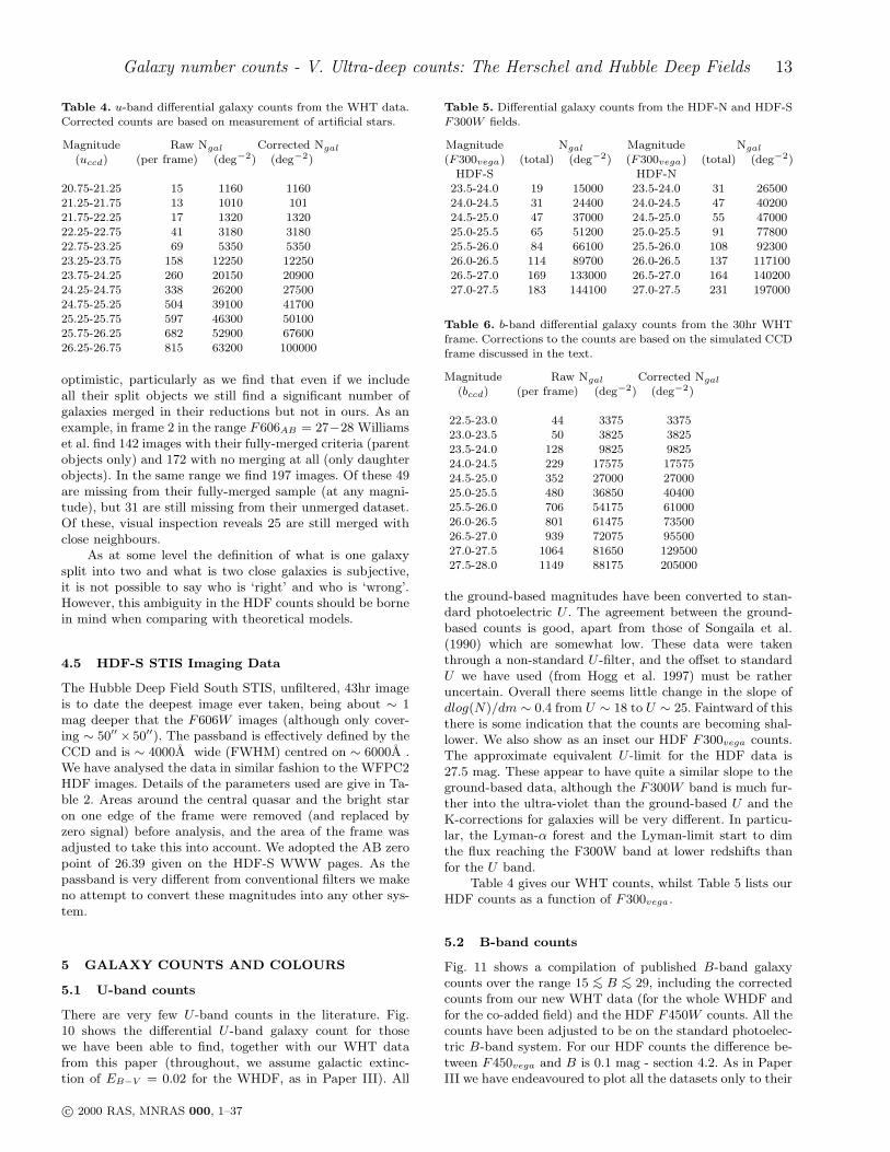
Table 4. u-band differential galaxy counts from the WHT data.Corrected counts are based on measurement of artificial stars.
Magnitude Raw Ngal Corrected Ngal
(uccd) (per frame) (deg−2) (deg−2)
20.75-21.25 15 1160 116021.25-21.75 13 1010 10121.75-22.25 17 1320 132022.25-22.75 41 3180 318022.75-23.25 69 5350 535023.25-23.75 158 12250 1225023.75-24.25 260 20150 2090024.25-24.75 338 26200 2750024.75-25.25 504 39100 4170025.25-25.75 597 46300 5010025.75-26.25 682 52900 6760026.25-26.75 815 63200 100000
optimistic, particularly as we find that even if we includeall their split objects we still find a significant number ofgalaxies merged in their reductions but not in ours. As anexample, in frame 2 in the range F606AB = 27−28 Williamset al. find 142 images with their fully-merged criteria (parentobjects only) and 172 with no merging at all (only daughterobjects). In the same range we find 197 images. Of these 49are missing from their fully-merged sample (at any magni-tude), but 31 are still missing from their unmerged dataset.Of these, visual inspection reveals 25 are still merged withclose neighbours.
As at some level the definition of what is one galaxysplit into two and what is two close galaxies is subjective,it is not possible to say who is ‘right’ and who is ‘wrong’.However, this ambiguity in the HDF counts should be bornein mind when comparing with theoretical models.
4.5 HDF-S STIS Imaging Data
The Hubble Deep Field South STIS, unfiltered, 43hr imageis to date the deepest image ever taken, being about ∼ 1mag deeper that the F606W images (although only cover-ing ∼ 50′′
× 50′′). The passband is effectively defined by theCCD and is ∼ 4000A wide (FWHM) centred on ∼ 6000A .We have analysed the data in similar fashion to the WFPC2HDF images. Details of the parameters used are give in Ta-ble 2. Areas around the central quasar and the bright staron one edge of the frame were removed (and replaced byzero signal) before analysis, and the area of the frame wasadjusted to take this into account. We adopted the AB zeropoint of 26.39 given on the HDF-S WWW pages. As thepassband is very different from conventional filters we makeno attempt to convert these magnitudes into any other sys-tem.
5 GALAXY COUNTS AND COLOURS
5.1 U-band counts
There are very few U -band counts in the literature. Fig.10 shows the differential U -band galaxy count for thosewe have been able to find, together with our WHT datafrom this paper (throughout, we assume galactic extinc-tion of EB−V = 0.02 for the WHDF, as in Paper III). All
Table 5. Differential galaxy counts from the HDF-N and HDF-SF300W fields.
Magnitude Ngal Magnitude Ngal
(F300vega) (total) (deg−2) (F300vega) (total) (deg−2)HDF-S HDF-N
23.5-24.0 19 15000 23.5-24.0 31 2650024.0-24.5 31 24400 24.0-24.5 47 4020024.5-25.0 47 37000 24.5-25.0 55 4700025.0-25.5 65 51200 25.0-25.5 91 7780025.5-26.0 84 66100 25.5-26.0 108 9230026.0-26.5 114 89700 26.0-26.5 137 11710026.5-27.0 169 133000 26.5-27.0 164 14020027.0-27.5 183 144100 27.0-27.5 231 197000
Table 6. b-band differential galaxy counts from the 30hr WHTframe. Corrections to the counts are based on the simulated CCDframe discussed in the text.
Magnitude Raw Ngal Corrected Ngal
(bccd) (per frame) (deg−2) (deg−2)
22.5-23.0 44 3375 337523.0-23.5 50 3825 382523.5-24.0 128 9825 982524.0-24.5 229 17575 1757524.5-25.0 352 27000 2700025.0-25.5 480 36850 4040025.5-26.0 706 54175 6100026.0-26.5 801 61475 7350026.5-27.0 939 72075 9550027.0-27.5 1064 81650 12950027.5-28.0 1149 88175 205000
the ground-based magnitudes have been converted to stan-dard photoelectric U . The agreement between the ground-based counts is good, apart from those of Songaila et al.(1990) which are somewhat low. These data were takenthrough a non-standard U -filter, and the offset to standardU we have used (from Hogg et al. 1997) must be ratheruncertain. Overall there seems little change in the slope ofdlog(N)/dm ∼ 0.4 from U ∼ 18 to U ∼ 25. Faintward of thisthere is some indication that the counts are becoming shal-lower. We also show as an inset our HDF F300vega counts.The approximate equivalent U -limit for the HDF data is27.5 mag. These appear to have quite a similar slope to theground-based data, although the F300W band is much fur-ther into the ultra-violet than the ground-based U and theK-corrections for galaxies will be very different. In particu-lar, the Lyman-α forest and the Lyman-limit start to dimthe flux reaching the F300W band at lower redshifts thanfor the U band.
Table 4 gives our WHT counts, whilst Table 5 lists ourHDF counts as a function of F300vega.
5.2 B-band counts
Fig. 11 shows a compilation of published B-band galaxycounts over the range 15 <
∼ B <∼ 29, including the corrected
counts from our new WHT data (for the whole WHDF andfor the co-added field) and the HDF F450W counts. All thecounts have been adjusted to be on the standard photoelec-tric B-band system. For our HDF counts the difference be-tween F450vega and B is 0.1 mag - section 4.2. As in PaperIII we have endeavoured to plot all the datasets only to their
c© 2000 RAS, MNRAS 000, 1–37

14 N. Metcalfe, et al.
Figure 10. U -band differential ground-based count compilation, together with the HDF-N and HDF-S F300W counts (inset). Themodels discussed in the text are shown for comparison. Note that the models shown in the inset are calculated for the F300W filter,whilst those on the main figure are appropriate to uccd.
Table 7. b-band differential galaxy counts from the co-added INTand WHT frames (equivalent to 46hrs WHT exposure). Correc-tions are based on the artificial star results.
Magnitude Raw Ngal Corrected Ngal
(bccd) (per frame) (deg−2) (deg−2)
25.0-25.5 38 55100 5510025.5-26.0 46 66700 7410026.0-26.5 33 47800 6170026.5-27.0 47 68100 9550027.0-27.5 69 100000 15850027.5-28.0 63 91300 18200028.0-28.5 79 114500 251200
respective 3σ limits. All the datasets have been correctedfor galactic extinction. It can be seen immediately that ourWHT and HDF counts are in good agreement, suggestingthat the WHT confusion corrections are quite accurate.
With the improved statistics and signal-to-noise overPaper III it is clear that the conclusion we drew previouslyis still supported and that the count slope has flattened atthe faintest magnitudes. However, the slope is somewhatshallower that before, d log N/dmb ∼ 0.25, which, if thisreflects the slope of the faint end of the luminosity function
Table 8. Differential galaxy counts from the HDF-N and HDF-SF450W fields.
Magnitude Ngal Magnitude Ngal
(F450vega) (total) (deg−2) (F450vega) (total) (deg−2)HDF-S HDF-N
23.5-24.0 14 11200 23.5-24.0 18 1540024.0-24.5 22 17600 24.0-24.5 24 2050024.5-25.0 38 30400 24.5-25.0 34 2910025.0-25.5 52 41600 25.0-25.5 64 5470025.5-26.0 79 63200 25.5-26.0 87 7440026.0-26.5 90 72000 26.0-26.5 129 11030026.5-27.0 122 97600 26.5-27.0 149 12740027.0-27.5 158 126400 27.0-27.5 191 16330027.5-28.0 235 188000 27.5-28.0 279 23850028.0-28.5 299 232000 28.0-28.5 389 33250028.5-29.0 232 185600 28.0-28.5 485 414600
at high redshift as we suggested in Paper III, corresponds toα ∼ −1.6. There is still no sign that the counts have stoppedrising, even at B ∼ 29 mag, and the total number of galaxiesexceeds 1.5 × 10⁶/sq. deg.
Our results for the WHDF, the WHT+INT co-addedframe and for the HDF F450vega are given in Tables 6, 7and 8.
c© 2000 RAS, MNRAS 000, 1–37

Galaxy number counts - V. Ultra-deep counts: The Herschel and Hubble Deep Fields 15
Figure 11. B-band differential count compilation. The models discussed in the text are shown for comparison, calculated for ourground-based bccd passband.
Table 9. r-band differential galaxy counts from the 6hr WHTframe. Corrections are based on artificial stars.
Magnitude Raw Ngal Corrected Ngal
(rccd) (per frame) (deg−2) (deg−2)
21.0-21.5 23 1825 182521.5-22.0 41 3275 327522.0-22.5 59 4700 470022.5-23.0 101 8050 805023.0-23.5 154 12275 1227523.5-24.0 224 17875 2040024.0-25.5 373 29750 3470024.5-25.0 493 39300 5010025.0-25.5 696 55500 7940025.5-26.0 833 66425 109600
5.3 R-band counts
The R-band count compilation, shown in Fig. 12, haschanged significantly since Paper III. Apart from our newWHT data, the deepest ground-based R-band counts pub-lished are those of Smail et al. (1995) and Hogg et al. (1997),based on observations in good seeing on the Keck telescope.However, HDF data provide the major change, extendingabout two magnitudes fainter than the ground-based data.
Table 10. Differential galaxy counts from the HDF-N and HDF-SF606W fields.
Magnitude Ngal Magnitude Ngal
(F606vega) (total) (deg−2) (F606vega) (total) (deg−2)HDF-S HDF-N
23.5-24.0 28 21500 24.0-24.5 35 2990024.0-24.5 35 26900 24.0-24.5 35 2990024.5-25.0 50 38400 24.5-25.0 51 4360025.0-25.5 80 61400 25.0-25.5 89 7610025.5-26.0 112 86000 25.5-26.0 125 10680026.0-26.5 145 111400 26.0-26.5 153 13080026.5-27.0 194 149000 26.5-27.0 198 16920027.0-27.5 258 198200 27.0-27.5 257 21960027.5-28.0 338 259600 27.5-28.0 388 33160028.0-28.5 447 361000 28.0-28.5 497 42470028.5-29.0 361 277300 28.5-29.0 509 435000
All data are plotted on the photoelectric R system. To getto R the HDF F606vega measurements have been shifted by−0.1 mag as discussed in section 4.2.
As with the B band, the counts continue to increase,with a slope dlog(N)/dm ∼ 0.37 for 20 <
∼ R <∼ 26, but
with evidence of a change to a shallower slope faintwardof this. This occurs where the HDF data take over fromthe ground-based data, and could be an artifact of the fact
c© 2000 RAS, MNRAS 000, 1–37

16 N. Metcalfe, et al.
1
10
100
1000
14 16 18 20 22 24 26 28
Figure 12. R-band differential count compilation, together with the HDF-S STIS count in the unfiltered passband (inset). The modelsdiscussed in the text are shown for comparison - for ground-based rccd in the main figure and specifically for the STIS passband in theinset.
that F606W is actually midway between V and R, andso may not have a slope appropriate to R. However, themean (F606 − F814) colour for the HDF data is fairly con-stant faintward of R ∼ 24, suggesting that any change incount slope between F606W and R is going to be mini-mal. The integral R counts reach ∼ 2 × 10⁶deg−2. We notethat the faint end slope is very similar to the B data, withd log N/dmR ∼ 0.25. The count data are presented in Tables9 and 10.
Also shown inset in Fig. 12 are the HDF-S STIS counts.These probe even deeper than the HDF F606 counts and ap-pear to continue with a similar slope of ∼ 0.25. Note thatthe apparent turn-over in the faintest bin is due to incom-pleteness.
5.4 I-band counts
This is the first time we have included an I-band count inthis series of papers. The WHDF counts are detailed in Table11, whilst the HDF counts in F814vega are listed in Table12. From section 4.2 we see that F814vega ∼ I .
The counts are plotted in Fig. 13. Note that as well asour HDF counts and the WHT I-counts, we also show in
this diagram for the first time two sets of ground-based I-band CCD counts taken at prime focus of the Isaac Newtontelescope. The first set, to I ∼ 23, is based on 10 of thefields in Paper II (total area 6.3×10⁻³ sq. deg.). These dataconsisted of 4 × 400s exposures on each field taken with anRCA CCD. The data reduction and analysis of these frameswere identical to those for the B and R frames in Paper II.The second set are taken off a 1.5hr total exposure with aTek 1024×1024 CCD (total area 2.4×10⁻² sq. deg.) centredon the WHDF (see also section 3.2). These reach I ∼ 23.75.The data reduction and analysis are similar to that describedhere for the WHT data. Once again, all magnitudes havebeen adjusted to be on the standard ground-based system.
The ground-based counts have a slope of dlog(N)/dm ∼
0.33 for 21 <∼ I <
∼ 25, which appears to flatten slightly todlog(N)/dm ∼ 0.27 for the fainter HDF data.
5.5 Colours
As noted in sections 3.3 and 4.1 we use fixed aperturecolours. However, the difference in this aperture betweenthe WHT and HDF data (1.5′′ radius as opposed to 0.35′′)certainly means that we are measuring colours (on average)
c© 2000 RAS, MNRAS 000, 1–37

Galaxy number counts - V. Ultra-deep counts: The Herschel and Hubble Deep Fields 17
1
10
100
1000
14 16 18 20 22 24 26 28
Figure 13. I-band differential count compilation. Again, the models discussed in the text are shown, calculated for our ground-basediccd band.
Table 11. i-band differential galaxy counts from the WHT data.Corrections are based on artificial stars.
Magnitude Raw Ngal Corrected Ngal
(iccd) (per frame) (deg−2) (deg−2)
20.0-20.5 17 1175 117520.5-21.0 48 3320 332021.0-21.5 56 3870 387021.5-22.0 79 5460 546022.0-22.5 125 8640 864022.5-23.0 205 14170 1550023.0-23.5 283 19560 2190023.5-24.0 413 28550 3470024.0-25.5 490 33870 4270024.5-25.0 623 43070 6170025.0-25.5 585 40440 85100
over a different metric aperture from the two data-sets. Thisshould be borne in mind when interpreting the data.
Fig 14 displays the bccd versus (b − r)ccd colour magni-tude histograms for our whole 7′
× 7′ field, split into fourmagnitude ranges. Fig 15 shows the equivalent F450vega-limited (F450−F606)vega data for the HDF-N and HDF-S.The percentage colour completeness is indicated on each ofthe histograms. This is particularly severe in the faintest
Table 12. Differential galaxy counts from the HDF-N and HDF-SF814W fields.
Magnitude Ngal Magnitude Ngal
(F814vega) (total) (deg−2) (F814vega) (total) (deg−2)HDF-S HDF-N
22.5-23.0 31 23900 22.5-23.0 22 1880023.0-23.5 27 20800 23.0-23.5 30 2560023.5-24.0 39 30100 23.5-24.0 45 3850024.0-24.5 50 38600 24.0-24.5 62 5300024.5-25.0 83 64000 24.5-25.0 92 7860025.0-25.5 117 90200 25.0-25.5 136 11620025.5-26.0 161 124100 25.5-26.0 169 14440026.0-26.5 212 163500 26.0-26.5 214 18290026.5-27.0 255 196600 26.5-27.0 282 24100027.0-27.5 315 242900 27.0-27.5 437 37340027.5-28.0 335 258300 27.5-28.0 547 46740028.0-28.5 194 149600 28.0-28.5 573 489600
ground-based bin due to the comparatively bright limit ofthe rccd data. Also shown are the predicted histogramsfor two of our evolutionary models (these are discussed insections 6.3 and 6.4). Figs 16 and 17 show similar plots,but now for bccd-limited (u − b)ccd and F450vega-limited(F300F 450)vega colours. Figs 18 and 19 show the plots for(r − i)ccd and (F606 − F814)vega colours.
c© 2000 RAS, MNRAS 000, 1–37

18 N. Metcalfe, et al.
The colour-colour diagrams for the WHDF, (r − i)ccd :(b − r)ccd and (u − b)ccd : (b − r)ccd, are shown in Fig.20(a),(b). Fig. 23 shows the equivalent plots for the spaced-based data, split into bright and faint magnitude ranges. Wediscuss these in more detail in the next section. Note, how-ever, that due to the different K-corrections between theHST and WHT passbands, especially in the ultra-violet,where the filters differ by ∼ 600A , the tracks of galaxiesin these plots are not expected to be the same.
6 GALAXY EVOLUTION MODELS
6.1 Overview
In our previous work (Shanks 1990, Paper II, Paper III)we have noted that if the B-band models are normalised atB ∼ 18 rather than B ∼ 15 then non-evolving models give areasonable representation of the B counts and redshift dis-tributions in the range 18 <
∼ B <∼ 22.5. Some support for this
high normalisation comes from work on HST galaxy countssubdivided by morphology, where non-evolving models withhigh normalisation give an excellent fit to both spiral andearly-type counts with 17 <
∼ I <∼ 22 (Glazebrook et al. 1995,
Driver et al. 1995). In Paper IV we have also shown thatthese same non-evolving models fit the K-band counts asfaint as K ∼ 23. The B counts now have the work of Bertin& Dennefeld (1997) added at the bright end, comprising pho-tographic measurements over 145 deg2. Again these show asteeper slope than the models at B < 17. The same au-thors’ R counts show a similar effect at R < 16. In the Iband the recent counts of Postman et al. (1998) also showa steep slope at I < 17. Although these counts cover only16 deg2, they are made using a CCD. Finally, the 2MASScounts (Cutri & Skrutskie 1998) which cover 158 deg2 toH = 15 and K = 14 are also found to be steeper thanthe no evolution models (see McCracken et. al. in prepara-tion). This effect therefore seems to be present over a widerange of passbands. If number count steepness were causedby evolutionary changes in star formation rate (SFR) at lowredshifts, z <
∼ 0.1, then it would be surprising if the near-IRcounts were affected as much as the B counts. We thereforecontinue to believe that the most likely interpretation is thatthis steepness at bright magnitudes is caused by large scaleinhomogeneities in the galaxy distribution on ∼ 150h−1Mpcscales (Shanks et al. 1990, Paper III). Further evidence forthis has come from preliminary luminosity function data inthe 2dF Galaxy Redshift Survey which shows a LF with thelocal M∗ and slope α (Efstathiou et al. 1988, Loveday et al.1992, Ratcliffe et al. 1998), but a φ∗ which is 50% higherthan the local value and in good agreement with the valuethat is used here. We therefore believe that these develop-ments justify our normalising the count models at B ∼ 18,corresponding to an overall value of φ∗
∼ 2.4 × 10⁻³. Theexact normalisation (φ∗) we use is given in Table 13 for theevolutionary models. In the case of no evolution we increasethese φ∗’s by 10% to give the same normalisation at B = 18as in the evolutionary models.
Metcalfe et al. (1996) presented two evolutionary mod-els with this high normalisation which gave reasonable fitsto the counts at all the wavelengths for which they had data,and to the HDF colours. These were a simple, q0 = 0.05 lu-minosity evolution model with exponentially decaying star
formation rates, and a q0 = 0.5 model, similar but for theaddition of a population of dwarf (hereafter ‘dE’) galaxieswith a constant star-formation rate until z ∼ 1 and zerothereafter.
As in Metcalfe et al. (1996), for simplicity we only con-sider two basic forms of evolution; a τ=2.5Gyr exponentiallydecaying star formation model for E/S0 and Sab galaxies,and a τ=9 Gyr model for Sbc/Scd/Sdm, both from Bruzual& Charlot (1993). This assumes that the evolution of the dif-ferent morphological types is simply governed by their SFRhistory. For q0=0.05 and q0=0.5, the present day galaxyages are assumed to be 16Gyr and 12.7Gyr, implying for-mation redshifts of zf = 6.3 and zf = 9.9. We also considera model with a cosmological constant, zero spatial curvatureand Ω0=0.3, with a present day age of 18 Gyr and a forma-tion redshift of zf = 7.9. Details of the present day lumi-nosity functions and colours used in our models are given inTable 13. All models take account of Lyman-α forest/breakabsorption as described by Madau (1995). Similar modelshave been used by Pozzetti et al. (1998).
One feature of these pure luminosity evolution (PLE)models is that they predict that z > 1 galaxies should bedetectable at reasonably bright magnitudes and this predic-tion has been broadly confirmed by B ∼ 24 redshift surveys(Cowie et al. 1995, 1996) undertaken on the Keck 10-m tele-scope. However, to provide a detailed fit to the B-band n(z)distribution it is necessary to moderate the number of high zspiral galaxies predicted by the τ=9 Gyr model by includingthe effect of internal dust extinction, with Aλ ∝ 1/λ (Met-calfe et al, 1996, cf.Campos & Shanks 1997 and refs. therein).We have, at least initially, assumed that the extinction lawand the star-formation history/metallicity evolution can betreated independently. Edmunds & Phillipps (1997) and Ed-munds & Eales (1998) have investigated the effects of drop-ping this assumption and indeed in Section 7 of this paperwe discuss possible evidence for evolution of the extinctionlaw with redshift. A similar problem exists in the K-bandn(z) with the τ=2.5Gyr model for early-type galaxies. Here,essentially passive evolution overpredicts the high z tail atK ∼ 19. We have overcome this by adopting a dwarf domi-nated IMF, with a slope x = 3, for early-type galaxies (seePaper IV). In the optical bands this produces results verysimilar to the more widely used Salpeter or Scalo IMF’s.There is some evidence that passively evolving models over-predict the HST morphological counts of early-type galaxies(see e.g. Driver et. al. 1998 and references therein), but ourmodel does a reasonable job of matching these counts, ex-cept at the faintest magnitudes, where morphological identi-fication becomes difficult. One problem for the x=3 model isthat it predicts an M/LB ∼120M/L⊙ for early-type galaxiesas opposed to M/LB=20 for x=1.35 and compared to theobserved value of M/LB=10hM/L⊙. This disagreement inthe x=3 case is caused by the excess of low-mass stars. Wehave therefore also considered a model still with τ=2.5Gyrbut with an x=3 IMF which cuts off below 0.5M⊙. Theisochrone synthesis code for this case was specially suppliedby G. Bruzual. This model then predicts M/LB=5M/L⊙, inmuch better agreement with observation. The effect on thegalaxy colour predictions is reasonably small; for example,at 16Gyr the predicted rest (V − K) colour is 3.27 for thex=3+0.5 M⊙ cutoff case compared to (V −K) = 3.67 in thex=3 uncut case and to (V −K) = 3.25 in the Salpeter case.
c© 2000 RAS, MNRAS 000, 1–37

Galaxy number counts - V. Ultra-deep counts: The Herschel and Hubble Deep Fields 19
Values observed for giant ellipticals are in the range 3.1-3.5.Vazdekis et al. (1997) have further shown that dwarf dom-inated IMF’s with a low mass-cut, solar metallicities and a16Gyr age do produce consistent population synthesis modelfits to nearby early-type galaxy spectra. Another problemfor a dwarf-dominated IMF is that it contains too few gi-ant stars to generate the observed metallicity of present-dayearly-type galaxies. However, this is also a problem for aSalpeter IMF, and a short initial burst with a much flatterIMF slope usually has to be invoked to solve this problem.(e.g Vazdekis et al. 1997). Indeed, Vazdekis et al. find thattheir chemical evolution, ‘closed-box’ model with a flat IMFduring an initial short burst and then a steeper IMF(x=2-3) plus low mass cut-off, produces an excellent fit to thespectra, and hence the observed metallicities, of local giantellipticals.
6.2 Galaxy Count Models
Galaxy counts generally constrain particular combinations
of evolutionary models and cosmological parameters. Figs10 - 13 show how our various models fit to the counts in thefour bands. The HDF-S STIS count models (see Shanks etal. in prep.) are shown inset into Fig. 12. As well as the twoevolving models described above, we also show their non-evolving counterparts, with the exception of the Λ modelwhich is very similar to the q0=0.05 no-evolution model.Also shown is the q0 = 0.5 evolutionary model without theextra dE component and a new q0=0.5 evolutionary modelwhich has a steeper luminosity function slope for Scd/Sdmgalaxies (see below). As can be seen, even at the depthsreached by STIS, our preferred evolutionary models fit thecounts reasonably well over a wide range of wavelengths.This agreement continues into the infra-red (Paper IV).
Note that both the evolution and no-evolution models inthe range 18<
∼ U <∼24 have different slopes when expressed
in the ground-based U and HST F300W passbands, withthe slope in the F300W band being steeper. This is dueto the HST band peaking at 3000A and the ground-basedband peaking at 3800A .
As the counts move bluewards from I to B, the pat-tern is that the evolutionary excess of galaxies sets in atincreasingly lower space densities of galaxies, indicating theincreased sensitivity of the bluer bands to the increased SFR.However, at U the evolutionary excess appears smaller thanat B; it also sets in no earlier in terms of galaxy numberdensity. The reason is that the U band is unique in that itlies shortward of the 4000A break even at z = 0. Thus theK-corrections for late types are less than in B by about amagnitude at z > 0.5 and indeed are negative for z > 1.This means that the no-evolution U models are intrinsicallysteeper than in B at U ∼ 24 and lie closer to the U data,which in fact has a similar slope to the B data. Thus lessU evolution might, in principle, be thought to be needed.The Bruzual & Charlot models, however, predict a similaramount of evolution in U as in B, about 1 magnitude atz > 1. This leads to the U evolution models being slightlyhigher than the data at U ∼ 24 whereas the B evolutionmodels are slightly lower than the data. This results in aproblem for the models in fitting the detailed (U−B) coloursat B >
∼ 24, as we discuss further below with regard to the
Figure 14. bccd-limited (b − r)ccd colour-magnitude histogramsfor the WHDF data, split into four magnitude bins. The percent-ages indicate the colour completeness for that magnitude range.The predictions of the q0 = 0.05 (solid line) and q0 = 0.5 dwarf
(dashed line) models are also shown.
n(u−b)ccd histograms in Fig. 16 and the (u−b)ccd : (b−r)ccd
distribution in Fig. 20(b).The q0=0.5 evolutionary model (without the added dE
component) fits the counts in the range 18 <∼ B <
∼ 25whereas the q0=0.05 and the similar k = 0, ΩΛ=0.7, Ω0=0.3models extend the fit to 18 <
∼ B <∼ 27. It is well known that
the 4× smaller volume available to z = 4 in the q0=0.5 casemakes it impossible to fit the faintest optical data with aPLE model (Yoshii & Takahara 1988, Guiderdoni & RoccaVolmerange 1990, Koo et al. 1993). Metcalfe et al. (1996)therefore invoked the extra dE population at high redshiftto improve the fit of this model. The parameters for this pop-ulation are also given in Table 13. Essentially, these galax-ies have a constant star-formation rate between zf = 9.9and z = 1 when the SFR cuts off. This causes the galaxiesto dim dramatically in brightness, till they end up at thepresent day with an M∗ some 5 magnitudes fainter than thenormal M*(z = 0) and with the colour of an E/SO. Thisis in the spirit of a disappearing dwarf model (e.g. Babul& Rees 1992, Babul & Ferguson 1996, see also Phillipps &Driver 1995 for a discussion) built in the Bruzual & Char-lot ‘single-burst’ framework. Clearly it is not unique and ifq0=0.5 then other models such as dynamical merging mayalso produce the increased numbers of galaxies required atfaint magnitudes.
A further q0=0.5 model that we consider explicitly herefor the first time is a model where we use a steeper faint endslope for the Scd and Sdm luminosity functions, α = −1.75rather than α = −1.5. Although this slope is steeper thanseen in local luminosity functions, if the local under-density
c© 2000 RAS, MNRAS 000, 1–37

20 N. Metcalfe, et al.
Table 13. Details of the luminosity evolution models (H0 = 50kms−1Mpc−1). The dE type is only employedin the q0 = 0.5 case. φ∗s are given for our evolving models; 10% higher φ∗s are used for the no-evolutionmodels.
E/S0 Sab Sbc Scd Sdm dE
φ∗(Mpc−3) 9.27 × 10⁻⁴ 4.63 × 10⁻⁴ 6.2 × 10⁻⁴ 2.73 × 10⁻⁴ 1.36 × 10⁻⁴ 1.9 × 10⁻²
α −0.7 −0.7 −1.1 −1.5 −1.5 −1.2M∗
bccd−20.85 −20.88 −21.22 −21.37 −21.38 −15.85
M∗F450vega
−21.00 −21.00 −21.32 −21.44 −21.45 −16.0
(u − b)ccd z=0 0.52 0.08 −0.10 −0.18 −0.16 0.52
(b − r)ccd z=0 1.59 1.38 1.16 0.84 0.75 1.59(r − i)ccd z=0 0.70 0.70 0.59 0.53 0.47 0.70(F300 − F450)vega z=0 1.44 0.44 0.00 −0.24 −0.20 1.44(F450 − F606)vega z=0 1.16 1.01 0.85 0.62 0.54 1.16(F606 − F814)vega z=0 1.21 1.21 1.02 0.92 0.81 1.21AB(z = 0) 0.00 0.00 0.30 0.30 0.30 0.00
Figure 15. As Figure 14 but now for the HDF-N and HDF-SF450vega-limited (F450 − F606)vega data.
is real then it could be that the local luminosity function isdeficient in faint galaxies due to biasing. Then even cluster-free luminosity function estimates may give misleading re-sults, assuming as they do that the luminosity function formis independent of galaxy environment. Alternatively, the latetype galaxy luminosity function may be assumed to evolveto steepen from α = −1.5 to α = −1.75 at z > 1. Possi-ble evidence for such steepening at lower redshift has comefrom Lilly et al. (1995). Such a model gives a good fit tothe optical UBRI counts in Figs. 10 - 13. We also find thatit is in reasonable agreement with the galaxy n(z) data atB < 22.5 and 22.5 < B < 24. McCracken et. al. (in prep.)find that the H counts are only slightly over-predicted bysuch a model at H = 28. As they point out, the flat slope ofthe H counts seems to disallow any such steepening of theluminosity function in the q0=0.05 cosmologies.
Figure 16. bccd-limited (u − b)ccd colour-magnitude histogramsfor the WHDF data. The percentages indicate the colour com-pleteness for each magnitude range. The predictions of the q0 =0.05 (solid line) and q0 = 0.5 dwarf (dashed line) models are alsoshown.
6.3 Galaxy Colour Distributions
The matching of both the q0=0.05 and the q0=0.5 (dE andsteep LF) evolutionary models to the count data over a widewavelength range does not imply that the colour distribu-tions predicted by the models will agree with the data, asthe colours are more sensitive to model details. In Figs. 16- 19 we show in the form of histograms the comparison be-tween our models and the data in both the HDF and WHDF.Generally we regard the agreement in all bands as good,at least in terms of where the broad body of the galaxycolours lie. The exception is in the UV, where both the HDF(F300 − F450)vega and the WHDF (u − b)ccd colour data
c© 2000 RAS, MNRAS 000, 1–37

Galaxy number counts - V. Ultra-deep counts: The Herschel and Hubble Deep Fields 21
Figure 17. As Figure 16 but now for the HDF-N and HDF-SF450vega-limited (F300 − F450)vega data.
Figure 18. rccd-limited (r − i)ccd colour-magnitude histogramsfor the WHDF data. The percentages indicate the colour com-pleteness for each magnitude range. The predictions of the q0 =0.05 (solid line) and q0 = 0.5 dwarf (dashed line) models are alsoshown.
Figure 19. As Figure 18 but now for the HDF-N and HDF-SF606vega-limited (F606 − F814)vega data.
peak some 0.5 magnitudes redder than do the models. Recallthat the spiral types in our models are already assumed tohave dust absorption, AB = 0.3 mag at z = 0. If we addedmore dust in the context of these models then we would havedifficulty in matching the extended n(z) in the Keck redshiftsurveys at B < 24 (Metcalfe et al. 1996). We shall also ar-gue later that simply invoking dust extinction laws with a2200A dust feature as seen in the Galaxy is not supportedby the (u − b)ccd : (b − r)ccd colour-colour data. The onlyother parameter which can potentially affect the UV colourof a star-forming galaxy is the IMF. We shall look further atwhat changes might improve the fit of the (u− b)ccd coloursin Sect 6.4.
Metcalfe et al. (1996), Madau et al. (1996) and Shankset al. (1998) all assumed on the basis of the Bruzual & Char-lot models that in the HDF (F300 − F450)vega > 0 corre-sponded to z >
∼ 2 galaxies. However, the above problem,together with the sensitivity of U − B colours to both dustand Lyman absorption encourages us to use the extensivespectroscopic data in the HDF to check the reliability of ourmodels. We shall see in Fig. 24(b) that (F300−F450)vega=0clearly discriminates spectroscopic galaxy redshifts, aboveand below z = 2. Fig. 25 also shows that the HDF UVdropout galaxies accurately fall in their predicted place forz >∼ 2 galaxies in the (F450−F606)vega : (F606−F814)vega
diagrams, which strongly suggests that z >∼ 2 galaxies can
be discriminated from z < 2 galaxies on the basis of theirground-based B −R : R− I colours (see also fig. 4a of Met-calfe et al. 1996). Thus it seems that, whatever the modeluncertainties at z = 1, by z = 2 the effects of Lyman absorp-tion dominate, leaving the model (F300−F450)vega coloursroughly correct at z = 2. Metcalfe et al. then went on to de-termine the fraction of HDF UV dropouts at 27 < B < 28
c© 2000 RAS, MNRAS 000, 1–37

22 N. Metcalfe, et al.
and found ∼47±7%, a fraction which compares well withthat predicted by the models. The results of calculating thez >∼ 2 UV luminosity density with these criteria are discussed
in Section 6.5 below (and by Shanks et al. 1998).In the WHDF a simple (u− b)ccd cut is not adequate to
discriminate high z galaxies, partly due to the difference inpassbands, but mainly due to the brighter magnitude limitand hence lower average redshift of the sample. As a resultit is necessary to apply a simultaneous cut in (b − r)ccd, inorder to eliminate low z early type galaxies (especially forr-limited samples). In order to compare with previous workin the literature we take as a starting point UV dropout cri-teria which match those of Steidel et al. (1999) as closelyas possible; these transform to a cut with approximately(u − b)ccd >1 (and −0.1 < (b − r)ccd < 1.6) in our mag-nitude system, and a limit of rccd <25.25. We also assign(u − b)ccd colours (which are really blue limits) to thosegalaxies which were not detected in u by assuming theiruccd magnitude to lie at the 3σ limit (uccd = 26.8). Giventhe relative depths of our u-band data and Steidel et al.’s,this is roughly equivalent to the 1σ magnitude they adoptedfor their non-detections. Many of these galaxies then failthe selection criteria due to being too blue in (u − b)ccd.The main purpose of this procedure is to remove faint, low-z early-type galaxies which might otherwise be mistaken forhigh-z dropouts. However it should be noted that it alsoloses potential high-z candidates in the process. We shallsee how some of these might be recovered in section 6.4.
With these criteria (and an eyeball check to excludephotometry problems such as mergers) we detect 32 UVdropouts in 49 arcmin2, i.e. 0.65±0.12 arcmin−2, to rccd <25.25 which is comparable to the 1.18±0.04 arcmin−2 skydensity for z ∼ 3 galaxies found by Steidel et al. (1999) atRAB < 25.5 (or rccd <25.25) and the upper limit of 3.3±0.3arcmin−2 for UV dropouts set by Guhathakurta et al. (1990)at a similar R-band limit. Applying the same blending cor-rections assumed by Steidel et al. (1999) for the brightergalaxies would increase these three observed sky densitiesby a factor of 1.3.
6.4 WHDF Colour-Colour Distributions
We first discuss the WHDF (r−i)ccd : (b−r)ccd colour-colourdiagram. This is shown in Fig. 20(a). The data shows twounmistakable features. The first is the plume of red galaxieswhich moves redwards from (b−r)ccd ≈ 1.6 to (b−r)ccd ≈ 3at (r − i)ccd ≈ 0.7. The second is the ‘hook’ feature whichlies below this red plume and contains the majority of thegalaxies. Interestingly, the models seem to show the samegeneric features, mostly due to the redshifting of the H/Kbreak through the passbands. The red plume is identifiedwith early type galaxies, with their decreasing UV spectrumshortward of the Ca II H/K break moving through the bband and making the (b − r)ccd colour redder until z ∼ 0.5.At 0.5 <
∼ z <∼ 0.9 the H/K feature moves through the r band
making the (b − r)ccd colour more blue and the (r − i)ccd
colour more red. This shift of the (b − r)ccd colour to theblue is helped by the τ=2.5 Gyr evolution whose effect onthe UV spectrum is increasingly felt in the b band at z >
∼ 0.5.The hook feature is identified with spiral galaxies, with againthe H/K break moving through the b band until z = 0.25when the increasing spiral UV spectrum is redshifted into
the b band. Then, helped by the H/K break moving throughthe r band at z >
∼ 0.5, (b − r)ccd continues to become blueruntil the Lyman α forest enters the b band at z ∼ 2.3. TheH/K break entering the r band at z ∼ 0.5 causes (r−i)ccd tobecome redder before the same feature entering the i bandat z > 0.8 causes (r − i)ccd to become bluer again.
The fact that the models show these features suggestthat they are broadly correct. Indeed the evolutionary mod-els show increased agreement with the data than simply us-ing the K-corrections, especially in the case of the early-types beyond z ∼ 0.8. This is shown in Fig. 21 where wecompare the colour tracks from our evolutionary models tothe K-corrections calculated from our Bruzual models. Inthe case of the spirals, the K-corrections provide a betterfirst-order description of the colour-colour tracks than forthe early-types but evolution at low redshift and dust red-dening at high redshift also help; evolution makes the spi-rals slightly bluer than the K-corrections in (b − r)ccd and(r − i)ccd at z <
∼ 1 but then the K-corrections and evolu-tionary model colours become very similar in the 1 <
∼ z <∼ 3
range. The effect of spiral dust actually makes the evolu-tionary model redder in (b − r)ccd at z >
∼ 1.5 and here it isthe effect of evolution and dust combined which improvesthe fit of the Sbc model to the data.
However, in detail there remain differences between themodels and the (r− i)ccd : (b− r)ccd data. The most seriousproblem in Fig. 20(a) is that the early-type galaxies appearto be too blue in (r − i)ccd at z >
∼ 0.5, indicating more fluxshortwards of the H/K break than predicted in the models.This problem is a feature of all models tested including thosewith a Salpeter IMF. Increasing τ helps by extending theperiod of active star-formation to lower redshifts but thenthe (b − r)ccd colours tend to turn to the blue at z = 0.5too quickly in comparison with the data. It is possible thatmodels with a less sharp H/K break at high redshift mayhelp because of decreased metallicity but so far we have nottested this hypothesis further.
Fig. 22 compares the predicted number density of galax-ies at each point in the WHDF (r − i)ccd : (b − r)ccd
colour-colour diagram with the data. It can be seen thatthe q0=0.05 and q0=0.5 dE evolutionary models both gen-erally give a good fit. In both cases the spirals are well fitted.As in Fig. 20(a), the evolutionary models predict early-typecolours which are too red in (r − i)ccd for z > 0.5. It shouldbe noted that in the case of the early-types the q0=0.5+dEmodel appears to give more low redshift early types andthus better agreement with the data than the low q0 model.These galaxies are estimated to lie at z ∼ 0.15 from theircolours and thus will have MB ∼ −16. These low luminositygalaxies are therefore excellent candidates for a disappearingdwarf’ population and spectroscopy is required to confirmtheir redshifts and investigate the nature of these galaxies.
The 32 UV dropout, rccd < 25.25, candidate 2.5 <∼ z <
∼
3.5 galaxies based on the Steidel et al. (1999) selection crite-ria discussed in the previous section have been circled in the(r−i)ccd : (b−r)ccd plane in Fig. 20. However, it is clear thatwe can use (r − i)ccd to refine further our candidate selec-tion, as some of the dropout galaxies have (r− i)ccd coloursthat are too red for them to be at high redshift. At firstglance this would seem to reduce our numbers even further.However, if we re-examine those galaxies with no measur-able u magnitudes which were assigned uccd magnitudes at
c© 2000 RAS, MNRAS 000, 1–37

Galaxy number counts - V. Ultra-deep counts: The Herschel and Hubble Deep Fields 23
Figure 20. (a) bccd-limited (r − i)ccd : (b− r)ccd and (b) (u− b)ccd : (b− r)ccd colour-colour diagrams for the WHDF data, showing theevolutionary tracks predicted from our Bruzual & Charlot models for the five galaxy types for 0 < z < 3.5. Boxes indicate 0.5z intervals.The tracks are colour coded according to redshift; 0 < z < 0.5, blue; 0.5 < z < 1, cyan; 1 < z < 2, green; 2 < z < 3, red; z > 3, magenta.Arrows show limits to colours for galaxies not detected in i, r or u, assuming the missing object has a magnitude at the 3σ limit for eachband. The enclosed, dotted area on the (u− b)ccd : (b− r)ccd plot shows the u-dropout selection of Steidel et al. (1999) transformed intoour passbands. The locations of our initial sample of 32 high-z, UV-dropout galaxies based on the criteria of Steidel et al. (1999) areshown on both plots as circles and inverted triangles, the latter symbol indicating candidates which pass the Steidel et al. criteria butare too red in (r − i)ccd. The extra candidates which increase our final sample to 43 dropouts are shown as upright triangles (note thatall the candidates are selected from an r-limited sample and so may not have corresponding data points or arrows on these plots).
the 3σ limit and subsequently failed Steidel et al.’s selectioncriteria (see section 6.3), we find that many of these have(r − i)ccd colours which indicate they are 2.5 <
∼ z <∼ 3.5
galaxies ((r− i)ccd < 0.2). The net result is that our numberof dropout candidates increases from 32 to 43, or 0.88±0.13armcmin−2. It is this sample that we take forward to our dis-cussions in Sections 6.7 and 6.8. The q0=0.05 and 0.5 evolu-tionary models predict a sky density of 2.6-2.9 arcmin−2 for2.5 <
∼ z <∼ 3.5 galaxies at rccd <25.25. Thus the sky densities
predicted by both models are in reasonable agreement withthe sky density of z ∼ 3 galaxies found in the WHDF and bySteidel et al. (see section 6.3), especially if we apply Steidelet al.’s bright-end 30% blending correction (which should berelevant to both datasets). This suggests that Lyman breakgalaxies may be interpreted as the high luminosity tail ofnormal spiral galaxies as their SFR increases exponentiallyback towards their formation epoch. This conclusion appliesboth in the q0=0.05 case where 99% of z >
∼ 3 galaxies areSbc/Scd/Sdm and even in the q0=0.5 ‘disappearing dwarf’dE case where 86% of the z >
∼ 3 galaxies are Sbc/Scd/Sdmand the remainder mostly E/SO/Sab with less than a 1%contribution from dE.
It can also be seen from Fig. 20(a) that many othergalaxies appear in the same (r − i)ccd : (b − r)ccd locationas our UV-dropout candidates but with no UV dropout.Clearly there is the possibility that these are also z ∼ 3candidates. Madau (1995) has used the incidence of Lyman
limit systems in QSO spectra to argue that almost all (∼80%) z >
∼ 3 galaxies should show UV dropout. This argu-ment works well at z >
∼ 3.5, because there is a relativelylarge redshift range between 3 <
∼ z <∼ 3.5 for a Lyman limit
system to enter the U band. However, the empirical meanredshift of the UV dropout galaxies of Steidel et al. (1999)lies at z = 3.04±0.24 and here the above argument reverses,because there is then only a very limited redshift range inwhich a Lyman limit system can intervene in the U band.Thus at z ∼ 3 there is the possibility that 80% of galaxiesdo not show UV dropout. Taking all the galaxies with simi-lar (r − i)ccd : (b− r)ccd colours to the UV dropout galaxiesi.e. those with −0.1 < (b − r)ccd < 1.6 and (r − i)ccd < 0.2,we find ∼ 220 new candidate z ≈ 3 galaxies. Spectroscopyof these candidates are required to determine how many ofthem are actually at high redshift.
The WHDF (u− b)ccd : (b− r)ccd diagram in Fig. 20(b)shows the same two populations as in (r − i)ccd : (b − r)ccd
although slightly less distinctively. The plume of early typeslies at (b − r)ccd > 1.6 with the spirals now occupying abroad strip below them. Again the E/SO model seems to fitthe E/SO plume to z ∼ 0.5 with the H/K break exiting the bband at z ∼ 0.25 and then the evolved spectrum shortwardsof 2500A entering the u band at z >
∼ 0.5 which takes the(u − b)ccd colour blueward until z ∼ 0.8, when, with bothu and b on the steep but constant slope of the UV ‘upturn’spectrum, a constant (u− b)ccd = −0.4 colour is maintained
c© 2000 RAS, MNRAS 000, 1–37

24 N. Metcalfe, et al.
Figure 21. The K-corrections compared to the evolutionary tracks plotted in both (r − i)ccd : (b − r)ccd and (u − b)ccd : (b − r)ccd
planes. Solid lines - E/S0 K-correction; short dash - E/S0 q0 = 0.05 evolution; dots - Spiral K-correction; long dash - Spiral q0 = 0.05evolution. Boxes indicate 0.5z steps for 0 < z < 3.5. Small numerals indicate redshift.
Figure 22. (a) the (r − i)ccd : (b− r)ccd colour-colour diagram for the WHDF data limited at bccd < 25.75 compared with the predictedcontours for the q0 = 0.5 dE model. The contours are equally spaced in log surface density.(b) as (a) but for the q0 = 0.05 model. (c)the data points shown without the contours for clarity - note the prominent ‘hook’ of spirals and the ‘finger’ of early-types.
until the spectrum reddens again when Lyman α absorptionenters the u passband at z >
∼ 1.5. The strong bluewardsshift in (b − r)ccd between 0.7 <
∼ z <∼ 1.5 is caused both
by the H/K break being redshifted through r and the UV‘upturn’ spectrum at λ < 2500A being redshifted throughb. The spiral (u − b)ccd : (b − r)ccd tracks again first move
bluer in (u − b)ccd and redder in (b − r)ccd due to H/Kmoving through the b band at 0 < z <
∼ 0.3. Then (b − r)ccd
becomes bluer at z >∼ 0.5 when the decreasing spectrum
shortwards of the H/K break is redshifted through r untilthe UV ‘upturn’ reaches r at z = 1.5. Both u and b lie on thesteeply increasing UV ‘upturn’ spectrum in the range 0.3 <
∼
c© 2000 RAS, MNRAS 000, 1–37

Galaxy number counts - V. Ultra-deep counts: The Herschel and Hubble Deep Fields 25
z <∼ 1.5 which maintains the (u − b)ccd roughly constant at
(u − b)ccd ∼ −0.8 before the spectrum reddens as dust andthen Lyman α increasingly affects the u band at z >
∼ 1.5.Also shown on Fig. 20(b) (enclosed by the dotted lines)
is the the area of the (u−b)ccd : (b−r)ccd colour-colour planecorresponding to the UV-dropout selection criteria of Steidelet al. (1999), as discussed in Section 6.3. The locations of ourfinal sample of 43 u-band dropouts is indicated, with distinctsymbols indicating the original 32 satisfying the criteria ofSteidel et al., and those lost and gained from invoking the(r − i)ccd selection. Note that, as the dropouts are chosenfrom an r-limited sample, not all have corresponding datapoints on this b-limited plot. It can be seen that there isgood agreement with the location of z ≈ 3 galaxies impliedby our models, for both early-types and spirals.
As shown by Fig. 21, in (u− b)ccd : (b− r)ccd the effectsof evolution are again bigger for the early-type model thanthe late-type model. At 0.5 <
∼ z <∼ 1.8 the (b − r)ccd colours
for early-type evolution model become bluer than the K-corrections and at 0.5 <
∼ z <∼ 0.9 the (u−b)ccd colours for this
model also become bluer than the K-correction. However, forz > 0.9 in (u− b)ccd and z > 1.8 in (b− r)ccd the colours forthe evolution model are redder than the K-correction andthis trend is confirmed when intervening Lyman α absorp-tion enters both u and b. For the spirals the K-correctionsseem to give a similar result everywhere to the evolutionarymodel, evolution making the colours slightly bluer than theK-correction at low redshift and dust making the evolution-ary model slightly redder at high redshift. We note that theK-corrections of Pence (1976) are similar to the Bruzual &Charlot K-corrections for z <
∼ 0.5 and, if anything, slightlybluer in (u − b)ccd at z >
∼ 0.5.Thus in the redshift range 0.3 <
∼ z <∼ 1 the predicted
(u−b)ccd colours for the spiral model are much bluer than isobserved; the spiral model reaches (u−b)ccd = −1.0 whereasthe data only reach (u− b)ccd = −0.5. The discussion of theuccd and bccd photometry zeropoints in section 3.2 indicatesthat errors in the colour zero-point of 0.1 mag or larger areunlikely. In any case we shall see below that the same effectis also seen in the independent HDF data. This discrepancyis surprising since the UV spectra of star-forming galaxiesare only governed by two parameters, dust absorption and,more weakly, the IMF. We postpone to Section 7 furtherdiscussion of possible explanations of this result.
6.5 HDF Colour-Colour Distributions
An HDF-N colour-colour comparison with similar modelshas previously been briefly discussed by Metcalfe et al.(1996). We now add in the HDF-S data and look at thecombined (F606 − F814)vega : (F450 − F606)vega and(F300 − F450)vega : (F450 − F606)vega diagrams at botha bright and a faint limit in Figs. 23. The most promi-nent feature remains the line of galaxies moving redwardin (F300 − F450)vega while remaining blue in (F450 −
F606)vega. These are the UV dropouts galaxies expectedto be at z >
∼ 2 as discussed above. In general, the tracksappear broadly consistent with the models and as suchprovide strong support for the approach used here. The(F606 − F814)vega : (F450 − F606)vega tracks again seemgood fits; the Sbc track in particular gives an excellentfit to many of the bluer galaxies, although when shifted
to the rest colours of Scd and Sdm’s gives slightly tooblue a colour in (F450 − F606)vega. In the bright data theplume of early-type galaxies is not seen as clearly as in theWHDF in either (F300 − F450)vega : (F450 − F606)vega
or (F606 − F814)vega : (F450 − F606)vega but the modelsagain give a reasonable representation of the redder galaxies.Again, as for the WHDF (u − b)ccd, the Sbc model predictstoo blue (F300− F450)vega colours for spirals at z = 1 andthe arbitrary shifting of the Sbc curve to the rest colours ofScd and Sdm galaxies leaves their tracks not fitting well inthis redshift range either. At fainter limits, it can be seenthat galaxies predicted to lie at z ∼ 2 dominate the data.
Next, in Fig. 24(a),(b) we plot the HDF-N and HDF-S galaxies with spectroscopic redshifts on the (F300 −
F450)vega : (F450 − F606)vega and (F606 − F814)vega :(F450 − F606)vega diagrams. The points are colour-codedaccording to the galaxy redshift range and the model tracksare similarly colour-coded. It can be seen there is good gen-eral agreement between the predicted and observed redshiftranges, again firmly supporting the idea that these simplemodels do an excellent job of describing the colours of faintgalaxies.
Fig. 25 shows how the HDF UV dropouts populatethe correct part of the HDF (F606 − F814)vega : (F450 −
F606)vega diagram for z >∼ 2 galaxies. Again this indicates
that ground-based (r − i) : (b − r) colour-colour combina-tions may be effectively used to discriminate z >
∼ 2 galaxieswithout the need of a UV band.
Fig. 26 compares the predicted number density of galax-ies at each point in the (F606 − F814)vega : (F450 −
F606)vega colour-colour diagrams with the data at F606 <28. It can be seen that the q0=0.05 and q0=0.5 dE evolu-tionary models both give a good fit with the density peak-ing in both the models and the data at the colours of z ∼ 2spirals. The fact that the spiral models fit so well through-out the range 0 < z <
∼ 3 is again a strong argument thatthe evolutionary history of the SFR is well described bythe τ=9Gyr exponentially increasing SFR used here. Theearly-type galaxies are not so clearly seen in this HDF datacompared to the equivalent WHDF data shown in Fig. 22.
6.6 Sizes
It has been claimed that the angular sizes of faint HDFgalaxies are small compared to local galaxies (Roche et al.1998 and references therein), suggesting there has been sizeas well as luminosity evolution. We have examined this ques-tion in the light of our simple evolutionary models by adapt-ing the simulation procedures used to replicate the WHTdata in section 3.6 to produce mock HDF frames based onour models. We are then able to apply our data-analysisprocedures to these frames and compare the angular sizesmeasured for the artificial galaxies with the real HDF data.As before (see Paper III), we assume the Freeman (1970)law to relate exponential disk size to absolute magnitudeand the diameter-magnitude relations of Sandage & Perele-muter (1990) for r1/4 bulges. Fig. 27 shows the results forour q0 = 0.05 model. The solid line represents the meanisophotal radius (at µF450 = 28.5) of our artificial galaxies,whilst the dots show the same quantity for the F450-bandHDF-N data. Although small differences exist, the agree-ment between model and data is remarkably good. It should
c© 2000 RAS, MNRAS 000, 1–37

26 N. Metcalfe, et al.
Figure 23. b-limited (F606−F814)vega : (F450−F606)vega and (F300−F450)vega : (F450−F606)vega colour-colour diagrams for theHDF-N and HDF-S data, split into bright and faint magnitude ranges. The evolutionary tracks predicted from our Bruzual & Charlotmodels are shown out to z = 4 for the five galaxy types. Filled squares show z = 0, open squares with numerals indicate 0.5z steps.
be noted that the apparent isophotal angular radii for thefaintest galaxies (∼ 0.2′′) correspond to metric radii of only∼ 2 kpc (H0 = 50 kms−1Mpc−1). This is much smallerthan local L∗ galaxies, but demonstrates both the effect ofisophotal dimming and the fact that, at F450vega ∼ 29, inthe models we are looking down the luminosity function togalaxies with low intrinsic luminosities and small sizes.
We find similar results for the q0 = 0.5 dE model, ifwe assume the “disappearing dwarf” population follows thesame Sandage & Perelemuter law as local bulge dominatedgalaxies.
6.7 Star Formation History
Our evolutionary models imply that the SFR density rises tobeyond z = 2, according to the τ=9Gyr Bruzual & Charlot
model. This is at odds with the conclusions of Madau etal. (1996) who used UV fluxes as an estimate of the SFRand, on the basis of the same HDF-N data, concluded thatthe SFR peaks at z ∼ 1 and decreases rapidly thereafter.Following Shanks et al. (1998) we first discuss the reasonsfor the differences seen between our SFR history and theoriginal SFR estimates of Madau et al. (1996).
The approach of Madau et al. (1996), following Cowie etal. (1988) and Lilly et al.(1995,1996), uses the fact that thegalaxy UV flux density is proportional to the SFR density toobtain estimates of the SFR history of the Universe. Theyuse the CFRS spiral evolving LF of Lilly et al. (1995) todetermine the 2800A flux density in the range 0 < z <
∼ 1and the HDF F300W and F450W dropouts to obtain the1620A flux density in the ranges 2 <
∼ z <∼ 3.5 and 3.5 <
∼
z <∼ 4.5. Their conclusion of a peak in the SFR at z ≈ 1 is
c© 2000 RAS, MNRAS 000, 1–37

Galaxy number counts - V. Ultra-deep counts: The Herschel and Hubble Deep Fields 27
Figure 24. (a) (F606 − F814)vega : (F450 − F606)vega and (b) (F300 − F450)vega : (F450 − F606)vegacolour-colour diagrams for theHDF-N and HDF-S data showing the location of galaxies with known redshifts (coloured dots, with redshifts as indicated in the legend)compared with the model tracks out to z = 4. The tracks are colour-coded according to redshift range in the same fashion as for thegalaxies. Arrows indicate limits to colours for galaxies not detected in one band, assuming a magnitude at the 3σ limit for the missingobjects.
Table 14. UV luminosity and SFR densities measured in the HDF and WHDF (H0 = 50kms−1Mpc−1). LFindicates luminosity function incompleteness corrected. AB = 0.3 indicates dust corrected. Veff indicatesthat the effective volumes of Steidel et al. (1999) have been assumed, rather than the boxcar volume, V. Inthe WHDF case, factors are V/Veff for q0=0.5,0.05 respectively.
ρ1500 log ρ∗ log ρ∗ log ρ∗ log ρ∗ log ρ∗ log ρ∗
(q0 = 0.5) (q0 = 0.5) (q0 = 0.05) (q0 = 0.5, (q0 = 0.05, (q0 = 0.5, LF, (q0 = 0.05, LF,LF ) LF ) AB = 0.3) AB = 0.3)
WHDF B< 26 (1 <∼ z <∼ 2) 8.9 × 1025 −2.09 −2.29 -1.80 −2.13 −1.48 −1.80WHDF R< 25.5 (1 <∼ z <∼ 2) 1.0 × 1026† −2.02 −2.22 -1.74 −2.06 −1.55 −1.87WHDF U dropouts(2.5 <∼ z <∼ 3.5) 3.0 × 1025 −2.55 −2.80 -1.94 −2.18 −1.61 −1.85WHDF ′′ (Veff , ×2.38,3.15) 7.1 × 1025 −2.17 −2.30 -1.56 −1.64 −1.23 −1.31HDF-N U dropouts(2.0 <∼ z <∼ 3.5) 2.1 × 1026 −1.70 −1.95 -1.40 −1.73 −1.07 −1.40HDF-N ′′ (Veff , ×1.13) 2.4 × 1026 −1.65 −1.90 -1.35 −1.68 −1.02 −1.35HDF-S U dropouts(2.0 <∼ z <∼ 3.5) 2.5 × 1026 −1.62 −1.87 -1.32 −1.65 −0.99 −1.32HDF-S ′′ (Veff , ×1.13) 2.8 × 1026 −1.57 −1.82 -1.27 −1.60 −0.94 −1.27WHDF B dropout(3.5 <∼ z <∼ 4.5) 2.2 × 1025 −2.68 −2.94 -1.98 −1.92 −1.65 −1.59WHDF ′′ (Veff , ×1.94,2.68) 4.2 × 1025 −2.39 −2.51 -1.69 −1.49 −1.36 −1.16HDF-N B dropout(3.5 <∼ z <∼ 4.5) 8.1 × 1025 −2.11 −2.36 -1.89 −2.17 −1.56 −1.84HDF-N ′′ (Veff , ×1.19) 9.6 × 1025 −2.03 −2.28 -1.81 −2.09 −1.48 −1.76HDF-S B dropout(3.5 <∼ z <∼ 4.5) 7.6 × 1025 −2.14 −2.33 -1.92 −2.14 −1.59 −1.81HDF-S ′′ (Veff , ×1.19) 9.0 × 1025 −2.06 −2.25 -1.84 −2.06 −1.51 −1.73†ρ2800
in contradiction with our τ=9 Gyr exponentially increasingSFR for spirals, which we have shown fits a variety of faintgalaxy count, colour and redshift data over a wide range ofpassbands. The SFR evolution rate of Madau et al. increasedmarkedly faster than our exponential in the 0 < z <
∼ 1 rangeand then quickly decreased below our rate at z >
∼ 1 (see fig.4 of Shanks et al. 1998 and also Fig. 28 below).
At z = 0, Shanks et al. suggested that the reason ourSFR density lies above that of Gallego et al. (1995) maybe related to the bright B-band count normalisation issue,discussed above. Supported by the results of Glazebrook etal. (1995) and Driver et al. (1995), we explicitly ignore thelow galaxy count at B <
∼ 17 mag as being possibly con-taminated by the effects of local large-scale structure. Fur-
c© 2000 RAS, MNRAS 000, 1–37

28 N. Metcalfe, et al.
Figure 25. The location of (F300 − F450)vega drop-out galaxies in the HDF (F606 − F814)vega : (F450 − F606)vega plane. Circleddots indicate galaxies with no measured (F300 − F450)vega. By comparing with Fig. 24(a) it can be seen that these drop-out galaxieshave colours very close to those predicted by the models for galaxies with z > 2 in this colour plane.
ther supporting evidence comes from the B < 19.5 mag 2dFgalaxy redshift survey results of e.g. Colless (1999) where theluminosity function at low z appears to move in the densityrather than the luminosity direction, as would be expectedon the basis of the large-scale structure hypothesis.
In considering possible reasons first for the differences inthe 0.2 <
∼ z <∼ 1 range, fig. 5 of Shanks et al. showed that our
exponential models reasonably fit the rest B-band luminos-ity functions determined from the CFRS data. However, theworst fit of our evolving luminosity function to the CFRSdata was in the 0.2 < z < 0.5 spiral bin and this proba-bly accounts for most of the discrepancy between our modelSFR density and the CFRS data in this range. Further un-certainty is introduced because the 2800A flux density inthis bin has to be extrapolated from the observed B-banddata (Lilly et al. 1996). Other measures of the SFR from theOII measurements of Tresse & Maddox (1998) and Treyer etal. (1998) at z∼0.2 agree much better with our exponentialmodel at low redshift.
In the 2 <∼ z <
∼ 3.5 range, the reasons that the SFR
density estimate of Madau et al. lies a factor of ≈3 belowour model in fig. 4 of Shanks et. al. (1998) are also clear.First, if we repeat the Madau et al. measurement in theHDF-N, then we obtain a factor of 1.56× bigger luminositydensity at 1620A for z >
∼ 2 UV drop-out galaxies than theseauthors, mostly due to the fact that we measure brightermagnitudes for individual galaxies (see Fig. 9). Second, ifMadau et al. were to include our AB(z=0) = 0.3 mag dustabsorption for spirals, then this would effectively increasetheir 1620A luminosity density by another factor of 2.12.Combined, these two effects give a factor of 3.3× overallwhich explains the above discrepancy of approximately afactor of 3. In the 3.5 <
∼ z <∼ 4.5 bin the same two effects
apply. However, the discrepancy here with our model is solarge that we shall suggest below that they may in fact bein genuine disagreement.
In Fig. 28(a,b) we illustrate some of these points bycomparing various observational estimates of the SFR den-sity with our evolutionary models for both the q0=0.05(τ=9Gyr, tgalaxy=16Gyr, h50 = 1) and the q0=0.5+dE
c© 2000 RAS, MNRAS 000, 1–37

Galaxy number counts - V. Ultra-deep counts: The Herschel and Hubble Deep Fields 29
Figure 26. (a) the (F606−F814)vega : (F450−F606)vega colour-colour diagram for the HDF-N and HDF-S data, limited at F606vega <28 compared with the predicted density contours of the q0 = 0.5 dE models. The contours are equally spaced in log surface density. (b)as (a) but for the q0 = 0.05 model.
(τ=9Gyr, tgalaxy=12.7Gyr, h50 = 1) models. In (a) the dis-continuity arises from the contribution of the ‘disappearingdwarfs with their constant SFR at z>1. The z = 0 normali-sation used in both cases was obtained by first estimating thelocal luminosity density in the F300W passband from theSbc/Scd/Sdm Schechter parameters in Table 13. This gaveρ3000A = 9.8 × 1025h−3
50erg s−1 Hz−1 Mpc−3. We then con-
verted to SFR density using the factors given by Madau etal. (1996) (corrected downwards by a factor of 1.25 accordingto the extrapolation to 3000A from 1500-2800A and thendownwards again by the factor 1.6 for the reasons suggestedby Connolly et al. 1997) to obtain ρ∗ = 0.00735M⊙h−3
50yr−1
Mpc−3. Finally we corrected this SFR(z) normalisation forour inclusion of AB = 0.3 mag dust absorption. Assumingour 1/λ dust model this amounts to an upwards correctionby a factor of 1.54.
All observational points based on ρ2800A are first cor-rected downwards by the factor of 1.6 recommended byConnolly et al (1997). They are then corrected using theAB = 0.3 mag dust absorption as used in our model. Fur-ther, we have LF corrected each point either by taking thepublished correction or, where these are absent, as in thecase of the HDF-N data of Madau et al. (1996), by run-ning the q0=0.05/ q0=0.5+dE evolutionary models in eachredshift range and integrating the galaxy luminosity densityto convergence. We also apply these LF corrections to ourown data. Thus if our model and the data are fully consis-tent, then they should agree in this Figure. As well as thepoints of Gallego et al. and the CFRS points of Lilly et al.(1996) (both dust/LF corrected), we have also plotted the
dust/LF corrected HDF-N points of Connolly et al. (1997)in the 1 <
∼ z <∼ 2 range.
Also shown in Fig. 28 are our new WHDF estimatesof the SFR density at 1 <
∼ z <∼ 2. These were obtained
by integrating the luminosity density of galaxies with (b −
r)ccd < 0.6 and (r − i)ccd > 0.4 which are approximatelywhere the 1 <
∼ z <∼ 2 galaxies lie in Fig. 20. The 343 galaxies
with bccd < 26 and the 267 galaxies with rccd < 25.5 givethe values for the UV luminosity density and SFR densitiesshown in Table 14; these are somewhat lower than given byConnolly et al. particularly in the q0=0.05 case. However,the colour cuts we have used are relatively crude and thismay be responsible for any difference with the HDF resultsand our own data.
In the redshift range 2.5 <∼ z <
∼ 3.5, Fig. 28 showsthe HDF-N UV dropout data of Madau et al. (1996), cor-rected for our AB = 0.3 mag dust absorption and ourLF incompleteness corrections. Also shown is the KeckUV dropout galaxy data of Steidel et al. (1999), with ourdust (AB = 0.3 mag with 1/λ giving A1500 = 0.9 mag)and LF incompleteness corrections. With their own dust(E(B − V )Calzetti=0.15 giving A1500 = 1.7 mag) and LFincompleteness corrections, Steidel et al. (1999) find theirz = 3 SFR is a factor of 3.4 higher than shown in Fig. 28(a). Fig. 28 also gives new estimates of the SFR density at2.5 <
∼ z <∼ 3.5 from WHDF u-band dropouts to rccd <25.25
together with the estimates from the data of Steidel et al.(1999). Here we have taken the 43 UV dropout candidateswe identified in Section 6.4 to give the value of ρ1500 shownin Table 14. Again using the conversion factors stated in thepaper of Madau et al. this gives the SFR densities shown
c© 2000 RAS, MNRAS 000, 1–37
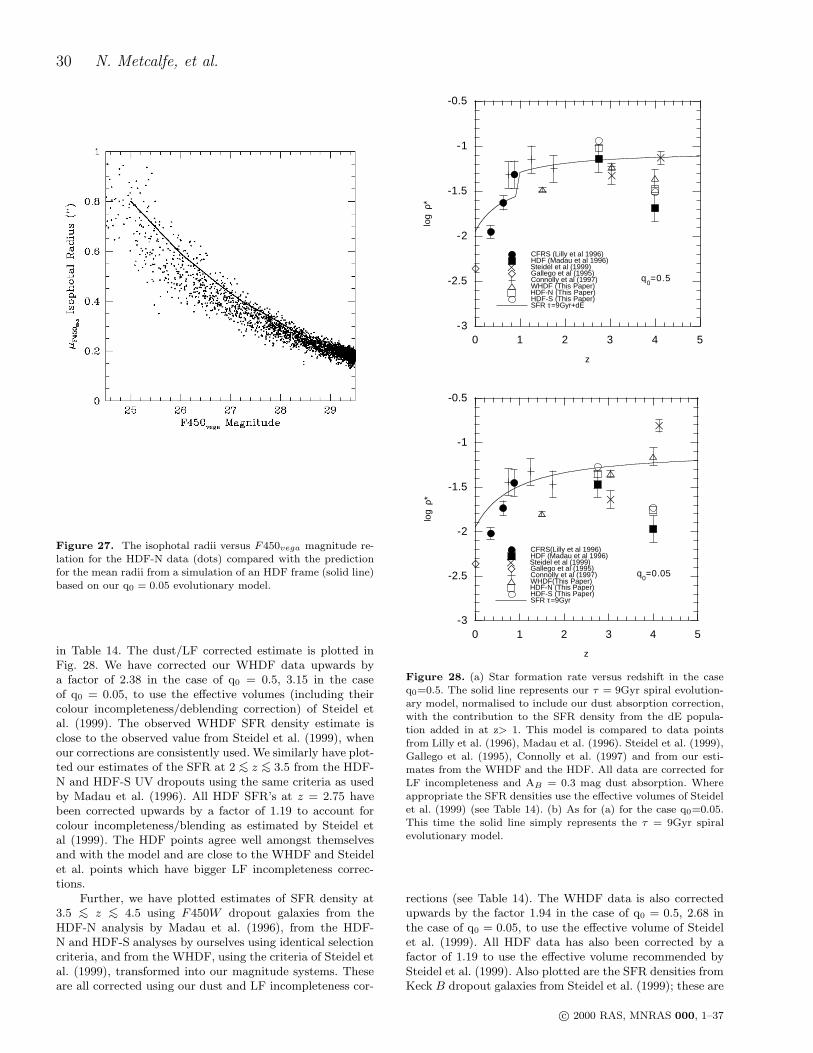
30 N. Metcalfe, et al.
Figure 27. The isophotal radii versus F450vega magnitude re-lation for the HDF-N data (dots) compared with the predictionfor the mean radii from a simulation of an HDF frame (solid line)based on our q0 = 0.05 evolutionary model.
in Table 14. The dust/LF corrected estimate is plotted inFig. 28. We have corrected our WHDF data upwards bya factor of 2.38 in the case of q0 = 0.5, 3.15 in the caseof q0 = 0.05, to use the effective volumes (including theircolour incompleteness/deblending correction) of Steidel etal. (1999). The observed WHDF SFR density estimate isclose to the observed value from Steidel et al. (1999), whenour corrections are consistently used. We similarly have plot-ted our estimates of the SFR at 2 <
∼ z <∼ 3.5 from the HDF-
N and HDF-S UV dropouts using the same criteria as usedby Madau et al. (1996). All HDF SFR’s at z = 2.75 havebeen corrected upwards by a factor of 1.19 to account forcolour incompleteness/blending as estimated by Steidel etal (1999). The HDF points agree well amongst themselvesand with the model and are close to the WHDF and Steidelet al. points which have bigger LF incompleteness correc-tions.
Further, we have plotted estimates of SFR density at3.5 <
∼ z <∼ 4.5 using F450W dropout galaxies from the
HDF-N analysis by Madau et al. (1996), from the HDF-N and HDF-S analyses by ourselves using identical selectioncriteria, and from the WHDF, using the criteria of Steidel etal. (1999), transformed into our magnitude systems. Theseare all corrected using our dust and LF incompleteness cor-
-3
-2.5
-2
-1.5
-1
-0.5
0 1 2 3 4 5
CFRS(Lilly et al 1996)HDF (Madau et al 1996)Steidel et al (1999)Gallego et al (1995)Connolly et al (1997)WHDF(This Paper)HDF-N (This Paper)HDF-S (This Paper)SFR τ=9Gyr
log
ρ*
z
q0=0.05
-3
-2.5
-2
-1.5
-1
-0.5
0 1 2 3 4 5
CFRS (Lilly et al 1996)HDF (Madau et al 1996)Steidel et al (1999)Gallego et al (1995)Connolly et al (1997)WHDF (This Paper)HDF-N (This Paper)HDF-S (This Paper)SFR τ=9Gyr+dE
log
ρ*
z
q0=0.5
Figure 28. (a) Star formation rate versus redshift in the caseq0=0.5. The solid line represents our τ = 9Gyr spiral evolution-ary model, normalised to include our dust absorption correction,with the contribution to the SFR density from the dE popula-tion added in at z> 1. This model is compared to data pointsfrom Lilly et al. (1996), Madau et al. (1996). Steidel et al. (1999),Gallego et al. (1995), Connolly et al. (1997) and from our esti-mates from the WHDF and the HDF. All data are corrected forLF incompleteness and AB = 0.3 mag dust absorption. Whereappropriate the SFR densities use the effective volumes of Steidelet al. (1999) (see Table 14). (b) As for (a) for the case q0=0.05.This time the solid line simply represents the τ = 9Gyr spiralevolutionary model.
rections (see Table 14). The WHDF data is also correctedupwards by the factor 1.94 in the case of q0 = 0.5, 2.68 inthe case of q0 = 0.05, to use the effective volume of Steidelet al. (1999). All HDF data has also been corrected by afactor of 1.19 to use the effective volume recommended bySteidel et al. (1999). Also plotted are the SFR densities fromKeck B dropout galaxies from Steidel et al. (1999); these are
c© 2000 RAS, MNRAS 000, 1–37

Galaxy number counts - V. Ultra-deep counts: The Herschel and Hubble Deep Fields 31
based on 49 3.5 <∼ z <
∼ 4.5 galaxies with spectroscopic con-firmation. Again the points shown assume our dust and LFcorrections. Using their own LF and dust absorptions wouldresult in a factor of 1.7 increase in the SFR at z = 4 over thevalue shown in Fig. 28 (a). Although Steidel et al. include1.7 magnitudes of dust absorption at 1500A as opposedto our 0.9 magnitudes, their use of the effectively gray ex-tinction law of Calzetti (1997) means that they include 1.2magnitudes of dust at 2800A compared to our 0.5 magni-tudes, so the effect of their higher dust absorption is mainlyon the normalisation of the SFR:z plot rather than its form(compare their fig. 9 to Fig. 28 (a)). In Fig. 28(a),(b) theWHDF points are close to both models at z = 4 but the Stei-del et al. point is higher than the q0=0.05 model at z = 4due to a large LF correction. However, in all cases the HDFpoints at z = 4 are lower, even though we have applied boththe dust and LF incompleteness corrections consistently. Weshall return to discuss this discrepancy between the HST andground-based SFR estimates at z = 4 in Section 6.8.
We conclude that, within the various errors and cor-rection factors, there is reasonable self-consistency with thefully corrected SFR density data and our model assuming anexponentially increasing SFR with look-back time, at leastto z ∼ 3. At 3.5 <
∼ z <∼ 4.5, the ground-based data of Steidel
et al. and ourselves is generally in much better agreementwith our exponential model than the HDF data. Steidel etal. (1999) have suggested that this may be because the HDF-N is too small to be representative. However, we note thatthe B dropout data from the HDF-S show good agreementwith the HDF-N SFR density. Therefore the picture at highredshift based on the integrated measure of UV luminosityand SFR density remains unclear. We note that because ofthe large size of the LF incompleteness and dust corrections,even where our model and the SFR density data agree, thisonly really checks the internal consistency of our model andthe SFR data. In Sect. 6.8 we shall make a more direct testof our models than afforded by Fig. 28.
Probes of the SFR at high z using SCUBA sub-millimetre observations (Smail et al. 1997, Hughes et al.1998, Barger et al. 1998) have also suggested that dust mayre-radiate absorbed UV luminosity and thus provide an ex-planation for the sub-mm counts. Busswell & Shanks (2000)have shown that dust re-radiated UV flux in our evolvingspirals, even though the B-band absorption is as low as0.3 magnitudes, can also make a significant contribution tothe steep sub-mm counts. Thus our spiral evolution modelswhich include dust may be enough in themselves to explainthe sub-mm counts, at least at faint, ∼ 1mJy fluxes.
6.8 Counts of UV and B dropout galaxies and theepoch of galaxy formation
In order to clarify the status of our model predictions at2.5 <
∼ z <∼ 4.5 we now consider Figures 29 and 30 where we
have plotted the number-magnitude counts of UV dropout(as defined in section 6.4) and B dropout (see section 6.7)galaxies and compared them to our model predictions. Thecount predictions for the q0=0.05, q0=0.5(+dE) and Λ evo-lutionary models are shown and their shapes are similar tothe galaxy luminosity functions at high redshift. The up-turn at M∗ in the q0=0.5 case is due to the extra contri-bution from the disappearing dwarf population at high red-
Table 15. WHDF Galaxy counts for UV dropouts 2.5 < z <3.5 (from section 6.4). These are the raw data and have to bemultiplied by a factor of 1.3 to account for colour incompleteness-blending after Steidel et al. (1999).
Magnitude Ngal
(rccd) (per frame) (arcmin−2)
23.0-24.0 1 0.01 ± 0.0124.0-24.5 8 0.16 ± 0.0624.5-25.0 22 0.45 ± 0.1025.0-25.25 12 0.49 ± 0.14
Table 16. HDF-N & HDF-S F606vega galaxy counts for UVdropouts 2 < z < 3.5 (from Metcalfe et al. 1996). These are theraw data and have to be multiplied by a factor of 1.19 to accountfor colour incompleteness/blending after Steidel et al. (1999).
Magnitude Ngal Magnitude Ngal
(F606vega) (N) (arcmin−2) (F606vega) (N) (arcmin−2)HDF-S HDF-N
23.0-23.5 3 0.56±0.19 23.0-23.5 1 0.19±0.1923.5-24.0 0 0.00 23.5-24.0 0 0.0024.0-24.5 4 0.75±0.38 24.0-24.5 4 0.75±0.3824.5-25.0 14 2.63±0.70 24.5-25.0 8 1.50±0.5325.0-25.5 19 3.56±0.82 25.0-25.5 24 4.50±0.9225.5-26.0 39 7.31±1.17 25.5-26.0 35 6.56±1.1126.0-26.5 19 3.56±0.82 26.0-26.5 28 5.25±0.9926.5-27.0 4 0.75±0.38 26.5-27.0 7 1.31±0.50
shift. Taking Fig. 29(a) first, which applies to the counts ofground-based UV dropouts in the redshift range 2.5 <
∼ z <∼
3.5, plotted as a function of rccd magnitude, we see that,although the new WHDF count (Table 15) is slightly lowerthan the Keck data from Steidel et al. (1999), overall thedata agree well with the model predictions at bright mag-nitudes. Similarly, in Fig. 29(b), the HDF-N UV dropoutdata from Madau et al. (1996) and our own HDF-N andHDF-S analyses in the 2 <
∼ z <∼ 3.5 range agree well with
the models at fainter F606vega magnitudes. In Fig. 29 wehave adopted the average colour incompleteness/blendingfactors suggested by Steidel et al. (1999) which means thatboth the Steidel et al. and the WHDF number counts areincreased by a factor of 1.3. We conclude that the luminosityfunction of galaxies in the redshift range 2 <
∼ z <∼ 3.5 ap-
pears reasonably consistent with the local galaxy luminosityfunction of Sbc/Scd/Sdm galaxies (which dominate at highredshifts), as modified by the effects of τ=9Gyr evolutionplus dust. In the particular case of the q0=0.5 model, thedata seem more consistent with a model which includes thedE population rather than the same model without the dEpopulation (also shown in Fig. 29). Thus there is strong ev-idence that the space density of galaxies at low redshift andz ∼ 3 may be very similar, whatever the underlying model,and this may be a stronger conclusion than any drawn fromFig. 28 above which frequently have to rely on large LF in-completeness corrections at high redshift to compare SFRdensities with low redshift measurements. Fig. 29 suggeststhat not only may the galaxy luminosity density be constantin the range 1 <
∼ z <∼ 3 but the space density and luminosity
function of galaxies may also be reasonably unchanging inthis redshift range. It also suggests that the Lyman-breakgalaxies detected by Steidel et al. may be interpreted as theevolved bright tail of the local Sbc/Scd/Sdm galaxy lumi-
c© 2000 RAS, MNRAS 000, 1–37

32 N. Metcalfe, et al.
0.0001
0.001
0.01
0.1
1
10
100
20 22 24 26 28 30 32
HDF-N Madau et al 1996HDF-N (This Paper)HDF-S (This Paper)Evoln., q
0=0.05
Evoln.+dE, q0=0.5
Evoln., Λ=0.7Evoln.-dE, q
0=0.5
N 0
.m5
-1 a
rcm
in-2
F606vega
(b) 2<z<3.5
0.0001
0.001
0.01
0.1
1
1 0
100
2 0 2 2 2 4 2 6 2 8 3 0 3 2
Steidel et al. (1999)WHDF (This Paper)Evoln., q
0=0.05
Evoln.+dE, q0=0.5
Evoln., Λ=0.7Evoln. - dE, q
0=0.5
N 0
.m5
-1 a
rcm
in-2
rCCD
(a) 2.5<z<3.5
Figure 29. (a) The rccd number count of 2.5 < z < 3.5 ground-based UV dropout galaxies, from Steidel et al. (1999) and fromthe WHDF, compared to our evolutionary model predictions withq0=0.05, 0.5 and ΩΛ=0.7. In the q0=0.5 case the contribution ofthe dE population can be seen at rccd > 25. A colour incom-pleteness/blending factor of 1.3 has been applied to the WHDFdata, the same factor used to correct the data of Steidel et al.(1999). (b) The F606vega number count of 2 < z < 3.5 HDFUV dropout galaxies compared to these same models. A colourincompleteness/blending factor of 1.19 has been applied to all theHDF data as suggested by Steidel et al. (1999). In all cases theagreement with the models is good.
nosity function. These conclusions would not be altered byassuming the Calzetti (1997) dust law with E(B−V ) = 0.15since the differential extinction between 1500A at z = 3 andthe B band at z = 0 is similar to that found in our 1/λ dustmodel with AB = 0.3 mag.
We now turn to Fig. 30 where the counts of B-banddropout galaxies from Steidel et al. (1999), Madau et al.(1996) in the HDF-N and ourselves in HDF-N and HDF-Sand in the WHDF in the range 3.5 <
∼ z <∼ 4.5 are plotted
Table 17. i-band differential galaxy counts for b-band dropoutson the WHDF. These are the raw data and have to be multipliedby a factor of 1.3 to account for colour incompleteness/blendingafter Steidel et al. (1999).
Magnitude Ngal
(iccd) (per frame) (arcmin−2)
23.0-23.5 0 0.0023.5-24.0 3 0.061 ± 0.0424.0-25.5 5 0.10 ± 0.0524.5-25.0 10 0.20 ± 0.06
Table 18. Differential galaxy counts for F450W −band dropoutsfrom the HDF-N and HDF-S fields.These are the raw data andhave to be multiplied by a factor of 1.19 to account for colourincompleteness/blending after Steidel et al. (1999).
Magnitude Ngal Magnitude Ngal
(F814vega) (N) (arcmin−2) (F814vega) (N) (arcmin−2)HDF-S HDF-N
24.0-24.5 0 0.00 24.0-24.5 3 0.56±0.3224.5-25.0 1 0.19±0.19 24.5-25.0 0 0.0025.0-25.5 4 0.75±0.38 25.0-25.5 0 0.0025.5-26.0 9 1.69±0.56 25.5-26.0 10 1.88±0.5926.0-26.5 5 0.94±0.42 26.0-26.5 4 0.75±0.3826.5-27.0 5 0.94±0.42 26.5-27.0 2 0.38±0.27
as a function of iccd magnitude. Again, the data is com-pared to the same four evolutionary models as in Fig. 29.Although the three basic models still fit the brighter dataof Steidel et al. (1999), they overpredict the fainter WHDFand HDF data by about a factor of 5. At z ∼ 4, the dataseem more similar to the fourth model shown, which is theq0=0.5 model without the extra dE population. Thus theoverall conclusion seems to be that at z ≈ 4 the observedgalaxy luminosity function appears to drop significantly be-low our basic models at absolute magnitudes fainter thanM∗.
One interpretation would be that the assumption of aconstant space density of galaxies in our models had failedby z ∼ 4 and that we were possibly detecting the epochof galaxy formation. It might also be suggested in the con-text of the q0=0.5 model that the results might imply thatthe bright galaxies were in place even as early as z ≈ 4and the dE population appeared between 3 <
∼ z <∼ 4 and
then dimmed to become the dwarf galaxy population possi-bly detected at b < 25 in the WHDF (r − i)ccd : (b − r)ccd
colour-colour diagram. This may be similar to the ‘downsiz-ing’ scenario claimed by other observers at lower redshifts(e.g. Cowie et al. 1996).
7 DISCUSSION OF MODEL SUCCESSES ANDFAILURES.
Our basic conclusion is that the galaxy counts in the opticalbands can be well fit by simple Bruzual & Charlot modelswith an exponentially increasing rate of star-formation toz ∼ 3. In the low q0 case, this type of model can fit the datato B ∼ 27 whereas in the high q0 case the model only fits toB ∼ 25, just beyond the current limit for galaxy redshift sur-veys. In this case a model with either a disappearing dwarfdE population or an increased luminosity function slope athigh redshifts must be invoked to increase the counts at faint
c© 2000 RAS, MNRAS 000, 1–37

Galaxy number counts - V. Ultra-deep counts: The Herschel and Hubble Deep Fields 33
0.001
0.01
0.1
1
10
100
1000
18 20 22 24 26 28 30
Steidel et al 99WHDF (This Paper)HDF-N Madau et al 96HDF-N (This Paper)HDF-S (This Paper)Evoln., q=0.05Evoln.+dE, q=0.5Evoln., Λ=0.7Evoln.-dE, q=0.5
N 0
.m5
-1 a
rcm
in-2
iCCD
Figure 30. The iccd number count of 3.5 < z < 4.5 B-banddropout galaxies from the ground-based data of Steidel et al.(1999) and from the WHDF and also from the HDF-N data ofMadau et al. (1996) and the HDF-N and HDF-S data from thispaper. A colour incompleteness/blending factor of 1.3 has beenapplied to the ground-based data and a factor of 1.19 to theHDF data. These data are compared to our evolutionary modelpredictions with q0=0.05, 0.5 and ΩΛ=0.7. In the q0=0.5 case thecontribution of the dE population can be seen at iccd > 25 andthe prediction for the q0=0.5 model without the dE populationis also shown. The observed faint galaxy LF appears to fall belowour model predictions by a factor of ≈5, indicating that whilebright L∗ galaxies may have been in place at z ≈4, the faintgalaxy population may have formed between z ≈ 3 and z ≈ 4.
magnitudes. We have also shown that the models producea magnitude-size relation, which for either value of q0, isconsistent with the data.
We have also presented new results from the WHDFand the HDF-N and HDF-S for the SFR density of galaxiesover the redshift range 1 <
∼ z <∼ 3.5 and the results from this
approach are broadly consistent with both previous data andthe above results if effects such as internal dust absorptionin spirals are included in the models. However, other system-atic effects may still dominate this route to the SFR history.Also, with this approach the poor fit to the faint counts ofthe q0=0.5 model using the local galaxy luminosity functionwould be missed.
At high redshifts, the number of galaxies predicted bythe simple models at z ≈ 3 agrees well with the numberof UV dropout galaxies detected at R ∼ 25 by ourselvesand by Steidel et al. (1999). Thus the PLE models seem tocontinue to fit the data as far as z≈3. However, at z ≈ 4, thePLE models start to overpredict the faintest data and thismay suggest that dwarf galaxies may have formed at z ≈ 4.We regard the agreement between the spiral models andthe bright, Lyman break galaxy data as another indicationthat the spiral model is broadly correct in the range 1 <
∼
z <∼ 3 and therefore that the star-formation rate follows our
exponential model throughout this redshift range.We have seen that the agreement between these models
and the WHDF and HDF galaxy colours is particularly goodin (R− I) : (B−R), where two faint galaxy populations areclearly seen corresponding to early- and late-type galaxies.The features seen in the data match those predicted by themodels so well that this forms a strong argument that thesemodels must be a reasonably accurate description of theevolving spectra of faint galaxies. Even in (U −B) : (B−R)they at least provide a good qualitative description of thedata.
The outstanding issue for the early-type galaxy modelsis the need to use a dwarf-dominated IMF (with a 0.5M⊙
cut-off) for early-types in order to reduce the number of z >1 galaxies predicted in K < 19 redshift surveys. The effectof using this IMF on the predicted optical colours is small.A slightly more extended initial period of star-formation isrequired with our dwarf dominated IMF(τ=2.5Gyr) thanwith Salpeter (τ=1Gyr) to match the move towards bluer(B − R) colours at z ∼ 0.5 seen in the (R − I) : (B − R)diagram. However, we note that the Salpeter/τ=1Gyr modelwould then also overpredict the numbers of z > 1 galaxiesdetected in optical (B < 24) redshift surveys too. Thus, overa wide range of wavelengths, the case against the Salpeterplus τ=1Gyr model for early-types from the redshift surveysis strong. The alternative solution to the dwarf-dominatedIMF is a merging model as considered by other authors (e.g.Kauffmann & Charlot 1998). It remains to be seen whetherthe merging model will produce as good a fit to the (R−I) :(B − R) data as the simple PLE model discussed here.
For the spiral model, the outstanding issue is that inthe redshift range 0.5 <
∼ z <∼ 1 the predicted (u − b)ccd
colours are up to 0.5 magnitudes too blue compared tothe data. Since the u and b bands peak close together at3800A and 4400A this implies quite a sizeable discrep-ancy in the redshifted spectral slope between 1500-2500A ,where the Bruzual and Charlot model predicts approxi-mately fλ ∝ λ−2.5 and the data would prefer fλ ∝ λ0.5.(u− b)ccd is more affected than (b− r)ccd because the smallwidth of the u band means there is less smoothing andbecause the wide wavelength separation of b and r meansthat they simultaneously lie in the range 1500-2500A for ashorter redshift span (at z ∼ 1.7). The (u−b)ccd discrepancyis puzzling because the UV colours of star-forming galaxiesare governed by only two parameters, dust and the IMF. Wealready have AB = 0.3 mag dust in the model and becausethe reddening vector runs parallel to the (u−b)ccd : (b−r)ccd
track at z = 1, it would take a significant increase in theamount of spiral dust to improve the fit and this would spoilthe n(b) and n(z) fits even at bccd ∼ 25.
We have experimented with including the Galactic2200A dust absorption feature but although this tends tohelp while it moves through u, it then moves through b mak-ing (u − b)ccd sharply redder and this tends to make theagreement with the data even worse at z >
∼ 0.7. We alsotried using an x=3 IMF as for the early-types with τ=9Gyrto redden the (u − b)ccd colours but although this helpedredden (u − b)ccd in the 0.5 <
∼ z <∼ 1 range, (b − r)ccd also
became too red for any agreement with the data even atlow redshift. We conclude that the original parameters ofAB = 0.3 mag, 1/λ, dust absorption and a Salpeter IMF re-mains closer to the (u− b)ccd : (b− r)ccd data than these al-ternatives. The fact that the K-corrections seem to demanda steep UV slope for galaxies locally might be thought to
c© 2000 RAS, MNRAS 000, 1–37

34 N. Metcalfe, et al.
indicate an explanation for the (u−b)ccd problem where theIMF might evolve with redshift. However, the UV spectraof local spirals has much scatter and it has long been knownthat only the bluest local galaxies (e.g. NGC4449) give spec-tra as steep as predicted by the Bruzual & Charlot modelswith an IMF that is a single power-law.
G. Bruzual has suggested (priv. comm) that an uppermass cut-off of 5-6 M⊙ in the spiral IMF rather than the 125M⊙ which we conventionally use will flatten the spiral s.e.d.shortwards of 2000A and help take the colours closer to thedata. He has supplied models which show this effect on the(u−b)ccd : (b−r)ccd diagram and it clearly helps the (u−b)ccd
colours at z = 1, while continuing to produce reasonablecolours for a spiral at z = 0. A 5-6 M⊙ cut correspondsto an IMF with no stars earlier than about B2-B3 whichmight be plausible, particularly if more massive stars areassumed to be preferentially cocooned in dust. A potentialproblem with this or any other explanation which effectivelyreduces the slope of the UV s.e.d. for spirals is that theK+evolution correction at a given SFR may produce lessbright galaxies at high redshift, causing our evolutionarymodel to underpredict the B counts, for example. Increasingthe SFR at early times to account for this might not bepossible because the galaxy would evolve to be too red fora spiral at z = 0.
Flat UV spectra have also been observed in the spectraof local starburst galaxies. For example, Gonzalez Delgado etal. (1998) have obtained UV spectra of four local starburstswith the Hopkins Ultraviolet Telescope and the GoddardHigh Resolution Spectrograph on HST. These authors showthat the spectral energy distribution follows fλ ∝ λβ withβ = −0.84 ± 0.26. This is much flatter from the β = −2.6to −2.2 they expect on similar grounds to our argumentabove. They, however, believe that the prediction for β isso stable that any deviation can be immediately interpretedas being caused by dust absorption. They obtain an averagevalue of AB = 0.73 ± 0.11 for their four starburst galaxiesusing an LMC extinction law. They also obtain the relationE(B − V ) = 0.11∆β where ∆β is the difference betweenthe observed and predicted slope. In our case ∆β ∼3 and soAB ∼ 1.3. This is so large that the dust would redden thegalaxy colour predicted for an Sbc spiral by 0.6 magnitudesand a prime motivation for adopting the τ = 9Gyr model,that it gave a blue enough colour for a present day spiral,would then be lost. Gonzalez Delgado et al. also detect SiIVand CIV absorption lines with P Cygni profiles which is asignature of O-type and early B-type stars. They suggestthat this argues against a bright IMF cut-off earlier thanB2.
Steidel et al. (1999) have fitted reddenings to theirLyman-break galaxies and find values very similar to thosewe use here, finding an average E(B − V ) = 0.15 for anaverage AB ∼ 0.5 mag using the Calzetti (1997) absorp-tion law. However, E(B − V ) = 0.15 would only producea spectral slope change of ∆β = 1.2, and this is less thanhalf what is needed to redden spiral (u − b)ccd colours towhat is observed in the WHDF. Pettini et al. (2000) havealso detected P Cygni profiles in the spectra of the lensedLyman-break galaxy MS 1512-cB58 which again may indi-cate the presence of O-stars and argue against the existenceof an upper mass cut-off. In this galaxy the spectral indeximplies E(B − V ) = 0.10 again close to what we have as-
-0.5
0
0.5
1
1.5
2
2.5
-1 -0.5 0 0.5 1 1.5 2
Sbc, q=0.05, Evoln.+1/λ dust
Sbc, q=0.05, Evoln. + Evolving dustb-
r CC
D
r-iCCD
0
0.5
1
1.5
2
2.5
3
-1.5 -1 -0.5 0 0.5 1 1.5
Sbc, q=0.05, Evoln.+1/λ dust
Sbc, q=0.05, Evoln. + Evolving dust
b-r C
CD
u-bCCD
Figure 31. (a) The effect on our Sbc evolutionary model(q0=0.05) for (u − b)ccd : (b − r)ccd of a dust reddening lawwhich evolves from a Galactic law exhibiting a 2200A absorp-
tion feature at low redshifts (z < 0.6) to a 1/λ extinction law athigh redshifts (z > 0.6). The evolution helps to redden the modelz = 1 to agree better with the data. (b) As for (a) showing theeffect of the evolving dust model on the model predictions for(r − i)ccd : (b − r)ccd.
sumed in our spiral models. However, this dust absorptionimplies a far higher dust-gas ratio than seen in comparablylow-metallicity galaxies such as the LMC and SMC.
Our view is that it may be unreasonable to invoke dustabsorption as high as E(B − V ) = 0.3 or AB = 1.3 magto explain the (u − b)ccd colours of the z = 1 spirals in theWHDF. On the other hand it is clear that P-Cygni profilesof SiIV and CIV are seen in both Lyman-break galaxies andnearby starbursts. These features are seen in stars as late asB0 and a 5-6 M⊙ cut would correspond to a cut at B2-B3.We are therefore forced to consider another model where theevolution of the dust extinction law is now invoked to explain
c© 2000 RAS, MNRAS 000, 1–37

Galaxy number counts - V. Ultra-deep counts: The Herschel and Hubble Deep Fields 35
the red (u−b)ccd colours of the WHDF data. Noting that the2200A feature helped redden (u− b)ccd as it passes throughthe u band, we suggest that the high metallicity galaxiesfound at low redshift may therefore show a 2200A featureas seen in the Milky Way. Then, since the predicted sharpfeature caused by the 2200A feature passing through the bband is not observed, we hypothesise that at higher redshiftsthan z ≈ 0.6 the extinction law evolves to look more likethe extinction law seen in the low metallicity SMC, whichis close to our 1/λ law. In this way, the strength of the2200A feature produces increased reddening as the u (andb) bands move towards 2200A than in (b − r)ccd at higherredshift when the 2200A feature has disappeared. We havetested this evolutionary model using the following simpleevolutionary prescription to mimic this effect in the u band.
Aλ = AB × 4400/λ, λ > 2500AAλ = AB × (4400/λ + (9886/λ − 3.9544) × (1 −
exp(−texp/t))), λ < 2500Awhere texp=8Gyr and t is the look back time. This ensures asmooth transition from the 2200A feature dominated law atlow z to the 1/λ law at higher redshifts. This dust evolutionthen produces a much redder (u − b)ccd at z = 1 while notdisturbing unduly the fit in (r − i)ccd : (b − r)ccd at eitherthis or higher redshift (see Fig. 31).
8 CONCLUSIONS
We have produced uccd, bccd, rccd and iccd galaxy numbercounts and (u − b)ccd, (b − r)ccd and (r − i)ccd colours fromone 7′
×7′ field, on which we have the deepest ground-basedB-band image yet taken. We also have deep H and K-bandphotometry on this field (Paper IV, McCracken et al. inprep).
We have compared these data with our analysis of theHDF-N and HDF-S, produced using the same software. Forthe UV and blue-bands, although the HDF’s are deeper forunresolved objects, in terms of surface brightness signal-to-noise our WHT image is ∼ 0.4 mag deeper, and also covers5 times the area. The counts from the datasets agree well,after the ground-based data has been corrected for confu-sion. All are still rising at the faintest magnitudes, with aslope dlog(N)/dm ∼ 0.25. The HDF F606W counts are over2 magnitudes deeper than the previous equivalent ground-based limits. They also show a still-rising count at the faintend with a slope dlog(N)/dm ∼ 0.25. The ground-based Ucounts show an almost constant slope of dlog(N)/dm ∼ 0.4to U ∼ 25.5. However the HDF F300W counts flatten to aslope dlog(N)/dm ∼ 0.15.
The deepest counts are the HDF-S STIS data, whichreach to STISAB ∼ 30, which is roughly equivalent to R ∼
30. Our evolutionary models continue to fit to the limit ofthese deepest optical number count data.
In terms of the comparison with evolutionary models,we summarise our conclusions as follows:
1. We have fitted simple exponential star-formation his-tory models to our data, and found that low q0 cosmologiesgive a good fit from U to K over a range of ∼ 10 magnitudes.To enable high q0 models to fit, an extra component mustbe added to the galaxy population at high (z >
∼ 1) redshift.One way of doing this is by adding a ‘disappearing dwarf’
dE population which is bright and blue at high redshift andfaint and red at low redshift.
2. At very bright magnitudes (B <∼ 17) our count models
fail and overpredict the counts. Since the steep count atB <
∼ 17 seems to be reproduced at the same level at R, I ,H and K, which is unlikely for an evolutionary explanation,this represents strong evidence that the high normalisationwe have adopted for the counts is substantially correct.
3. The models provide a good fit to the distributions ofcolours in (b− r)ccd and (F450−F606)vega and in (r− i)ccd
and (F606 − F814)vega, although in both (u − b)ccd and(F300 − F450)vega the spiral models are too blue by 0.5magnitudes at z = 1.
4. The same models produce elliptical and spiral tracksin the colour-colour planes with shapes very similar to theloci of the data. The fact that the fit of our models is so good,particularly in (r−i)ccd : (b−r)ccd for the ground-based dataand (F606 − F814)vega : (F450 − F606)vega for the HDF,data lends strong support to the underlying assumption thatthe star-formation rate increases exponentially to beyondz = 2 (Metcalfe et al. 1996). It is clearly possible to use(R − I) : (B − R) to probe the star-formation rate directlyover a wide redshift range 0.5 <
∼ z <∼ 3, emphasising the
power of this colour-colour diagram as a diagnostic tool forgalaxy evolution.
5. In the WHDF (r − i)ccd : (b − r)ccd plane, we detectan excess of low redshift(z ≈ 0.1), low luminosity early-type galaxies which may have parameters consistent withthe ‘disappearing dwarfs’ invoked in our q0=0.5 evolutionarymodel.
6. We have shown how the discrepancy with the z = 1SFR peak of Madau et al. (1996) comes from the differ-ent treatment of dust and photometry in the HDF. Whenwe repeat the UV dropout SFR density measurement madein the 2 <
∼ z <∼ 3.5 range by Madau et al. we find good
self-consistency with the prediction of our exponentially in-creasing SFR (τ=9Gyr) spiral model.
7. We have made new measurements of the SFR den-sity in the WHDF and in the HDF-N and HDF-S. In theredshift range 1 <
∼ z <∼ 2 the WHDF SFR density lies lower
than the measurement of Connolly et al. (1997) in the HDF.These measurements bracket the prediction of our τ=9Gyrspiral model. In the 2 <
∼ z <∼ 3.5 range our observed SFR
density based on UV dropouts, corrected for dust and LFincompleteness, and the ground-based estimates of Steidelet al. (1999) lie close to the HDF estimates and our model.At 3.5 <
∼ z <∼ 4.5 there is a wider spread, with the brighter
ground-based SFR estimates from the WHDF and Steidelet al. generally being higher and closer to the model thanthe HDF SFR estimates which are significantly lower thanthe model.
8. We have detected a population of galaxies that oc-cupy the same part of the (r − i)ccd : (b − r)ccd plane asz ∼ 3 UV dropout galaxies, but which do have measurableu-band fluxes. We have suggested that these may be candi-dates for high redshift galaxies that do not show UV dropoutand that statistics of QSO absorption lines may not rule outsuch a population at z ≈ 3. The increase in SFR density atz ≈ 3 will depend on the fraction which prove to be at highredshift.
9. We have created simulated CCD frames to checkthe apparent sizes of galaxies predicted by our evolutionary
c© 2000 RAS, MNRAS 000, 1–37

36 N. Metcalfe, et al.
models and found they are quite consistent with the sizes ofgalaxies measured on the HDF-N.
10. For the early-type models, the main remaining prob-lem is that although they produce reasonable fits to thedata at optical wavelengths, they predict too many highredshift (z >
∼ 1) galaxies at K ∼ 19 unless they have adwarf-dominated stellar IMF. This reduces the evolutionarybrightening at infra-red wavelengths whilst still allowing suf-ficient optical evolution. Dynamical merging may constitutean alternative explanation and this possibility has been ex-plored by other authors (eg Kauffmann & Charlot 1998).
11. The main outstanding question for the spiral mod-els is why do they predict (u− b)ccd and (F300−F450)vega
colours which are too blue in the range 0.5 <∼ z <
∼ 1? Wehave suggested that this problem is unlikely to be solvedby the addition of more dust to the models because theamount of dust needed is so great (AB ∼ 1.3 mag) that itwould lead to the model predicting (B − R) colours thatare ∼0.5 magnitudes too red for a z = 0 spiral. One possi-bility is that the spiral IMF is truncated above 5-6 M⊙. Itis the subject of continuing research to see if such a modelcan produce enough evolution to continue to fit the steepB-band number-count slope. Another possible explanation,suggested by the dust laws in nearby galaxies with differentmetallicities, is that the dust extinction law evolves, with the2200A dust absorption feature appearing in high metallic-ity galaxies at z <
∼ 0.5 and disappearing in lower metallicitygalaxies at higher redshift.
12. The evolutionary q0=0.05 and q0=0.5 models cor-rectly predict the sky density of Lyman break z ≈ 3 galax-ies detected by Steidel et al. (1999) from Keck spectroscopy.The models suggest that these galaxies may be spiral galax-ies which have undergone an exponentially increasing SFRwith look-back time. At z ≈ 4 these models generally over-predict the space density of sub-L∗ galaxies at faint limitsin the HDF-N and HDF-S and WHDF by a factor of 5, sug-gesting that we may have reached an epoch of significantgalaxy formation. The z ≈ 4 luminosity function matchesbest our q0=0.5 model with the dE population removed,suggesting that one interpretation might be that bright L∗
galaxies were already in place at z = 4 but many faintergalaxies formed at 3 <
∼ z <∼ 4. These then quickly dimmed
to become the red, dwarf population possibly detected in theWHDF (r − i)ccd : (b − r)ccd data at MB = −15 at z ≈ 0.1.
ACKNOWLEDGMENTS
HJMCC and NM acknowledge financial support fromPPARC. The INT and WHT are operated on the islandof La Palma by the Isaac Newton Group at the Spanish Ob-servatorio del Roque de los Muchachos of the Instituto deAstrofısica de Canarias. Data reduction facilities were pro-vided by the UK STARLINK project.
REFERENCES
Arnouts, A., D’Odorico, S., Cristiani, S., Zaggia, S., Fontana, A.,Giallongo, E., 1999, A&A, 341, 641
Babul, A., Ferguson, H.C., 1996, ApJ, 458, 100
Babul, A., Rees, M.J., 1992, MNRAS, 255, 346
Barger, A.J., Cowie, L.L., Sanders, D.B., Fulton, E., Taniguchi,
Y., Sato, Y., Kawara, K., Okuda, H., 1998, Nature, 394, 248Bertin, E., Dennefeld, M., 1997, A&A, 317, 43
Bruzual, A.G., Charlot, S., 1993, ApJ, 405, 538Busswell, G.S., Shanks, T., 2000, MNRAS submitted
Calzetti, D., 1997, in Waller, W.H., Fanelli, M.N., Hollis, J.E.,Danks, A.C., eds, The Ultraviolet Universe at Low and HighRedshift: Probing the Progress of Galaxy Evolution. AIPConf. Proc. 408, Woddbury AIP, p.403
Campos, A., Shanks, T., 1997, MNRAS, 291, 383Colless, M.M., 1999, in Colombi S., Mellier Y., Raban B., eds,
Wide Field Surveys in Cosmology. 14th IAP Colloquium, Edi-tions Frontieres, p.77
Connelly, A.J., Szalay, A.S., Dickinson, M., Subbarao, M.U.,Brunner, R.J., 1997, ApJ, 486, L11
Couch, W.J., Jurcevic, J., Boyle, B.J., 1993, MNRAS, 260, 241Couch, W.J., Newell, E.B., 1984, ApJS, 56, 143
Cowie, L.L., Lilly, S.J., Gardner, J., Mclean, I.S., 1988, ApJ 332,L29
Cowie, L.L., Hu, E.M., Songaila, A., 1995, Nature, 377, 603Cowie, L.L., E.M., Songaila, A., Hu, E.M., Cohen, J.G., 1996, AJ,
112, 938
Cutri, R.M., Skrutskie, M.F., 1998, BAAS, 30, No. 4, #81.01
Driver, S.P., Fernandez-Soto, A., Couch, W.J., Odewahn, S.C.,Windhorst R.A., Phillipps, S., Lanzetta, K., Yahil, A., 1998,ApJ, 496, L93
Driver, S.P., Phillipps, S., Davies, J.I., Morgan, I., Disney, M.J.,1994, MNRAS 268, 393
Driver S.P., Windhorst R.A., Ostrander E.J., Keel W.C., GiffithsR.E., Ratnatunga K.U., 1995, ApJ, 449, L23
Edmunds, M.G., Eales, S.A., 1998, MNRAS, 299, L29Edmunds, M.G., Phillipps, S., 1997, MNRAS, 292, 733
Efstathiou, G., Ellis, R.S., Peterson, B.A., 1998, MNRAS, 232,431
Ferguson, H.C., 1998, in Livio, M., Fall, S.M., Madua, P., eds,The Hubble Deep Field: proceedings of the 11th STScI sym-posium. CUP, New York, p181.
Freeman, K.C., 1970, ApJ, 160, 811
Gallego, J., Zamorano, J., Aragon-Salamanca, A., Rego, M., 1995,ApJ 455, L1
Glazebrook, K., Ellis, R., Santiago, B., Griffiths, R., 1995, MN-RAS, 275, L19
Gonzalez Delgado, R.M., Leitherer, C., Heckman, T., Lowenthal,J.D., Ferguson, H.C., Carmelle, R., 1998, ApJ, 495, 698
Guhathakurta, P., Tyson, J.A., Majewski, S.R., 1990, ApJ, 357,L9
Guiderdoni, B., Rocca-Volmerange, B., 1990, A&A, 227, 362Hall, P., Mackay, C.D., 1984, MNRAS, 210, 979
Heydon-Dumbleton, N.H., Collins, C.A., MacGillivray, H.G.,1989, MNRAS, 238, 379
Hogg, D.W., Pahre, M.A., McCarthy, J.K., Cohen, J.G., Bland-ford, R., Smail, I., Soifer, B.T., 1997, MNRAS, 288, 404
Holtzman, J.A., Burrows, C.J., Casertano, S., Hester, J.J.,Trauger, J.T., Watson, A.M., Worthy, G., 1995, PASP, 107,1065
Hughes, D.H. et al., 1998, Nature, 394, 241
Infante, L., Pritchet, C., Quintana, H., 1986, AJ, 91, 217Jarvis, J.F, Tyson, J.A., 1981, AJ, 86, 476
Jones, L.R., Fong, R., Shanks, T., Ellis, R.S., Peterson, B.A.,1991, MNRAS, 249, 481 (Paper I)
Kauffmann, G., Charlot, S., 1998, MNRAS, 297, L23Koo, D.C., 1986, ApJ, 311, 651
Koo, D.C., Gronwall, C., Bruzual, G.A., 1993, ApJ, 415, L21
Landolt, A.U., 1992, AJ, 104, 340Lanzetta, K.M., Yahil, A., Fernandez-Soto, A., 1996, Nature, 381,
759
Le Fevre O., Crampton D., Lilly S.J., Hammer F., Tresse L., 1995,ApJ, 455, 60
c© 2000 RAS, MNRAS 000, 1–37
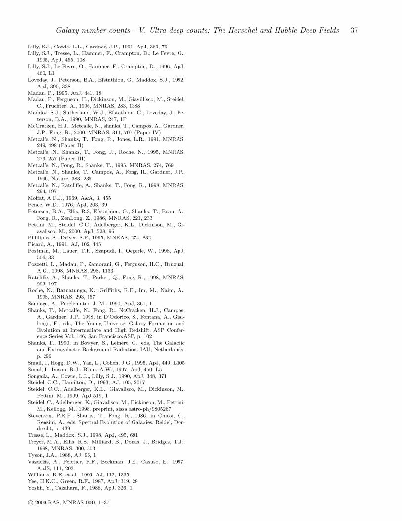
Galaxy number counts - V. Ultra-deep counts: The Herschel and Hubble Deep Fields 37
Lilly, S.J., Cowie, L.L., Gardner, J.P., 1991, ApJ, 369, 79
Lilly, S.J., Tresse, L., Hammer, F., Crampton, D., Le Fevre, O.,1995, ApJ, 455, 108
Lilly, S.J., Le Fevre, O., Hammer, F., Crampton, D., 1996, ApJ,460, L1
Loveday, J., Peterson, B.A., Efstathiou, G., Maddox, S.J., 1992,ApJ, 390, 338
Madau, P., 1995, ApJ, 441, 18
Madau, P., Ferguson, H., Dickinson, M., Giavillisco, M., Steidel,C., Fruchter, A., 1996, MNRAS, 283, 1388
Maddox, S.J., Sutherland, W.J., Efstathiou, G., Loveday, J., Pe-terson, B.A., 1990, MNRAS, 247, 1P
McCracken, H.J., Metcalfe, N., shanks, T., Campos, A., Gardner,J.P., Fong, R., 2000, MNRAS, 311, 707 (Paper IV)
Metcalfe, N., Shanks, T., Fong, R., Jones, L.R., 1991, MNRAS,249, 498 (Paper II)
Metcalfe, N., Shanks, T., Fong, R., Roche, N., 1995, MNRAS,273, 257 (Paper III)
Metcalfe, N., Fong, R., Shanks, T., 1995, MNRAS, 274, 769
Metcalfe, N., Shanks, T., Campos, A., Fong, R., Gardner, J.P.,1996, Nature, 383, 236
Metcalfe, N., Ratcliffe, A., Shanks, T., Fong, R., 1998, MNRAS,294, 197
Moffat, A.F.J., 1969, A&A, 3, 455
Pence, W.D., 1976, ApJ, 203, 39
Peterson, B.A., Ellis, R.S, Efstathiou, G., Shanks, T., Bean, A.,Fong, R., ZenLong, Z., 1986, MNRAS, 221, 233
Pettini, M., Steidel, C.C., Adelberger, K.L., Dickinson, M., Gi-avalisco, M., 2000, ApJ, 528, 96
Phillipps, S., Driver, S.P., 1995, MNRAS, 274, 832
Picard, A., 1991, AJ, 102, 445Postman, M., Lauer, T.R., Szapudi, I., Oegerle, W., 1998, ApJ,
506, 33
Pozzetti, L., Madau, P., Zamorani, G., Ferguson, H.C., Bruzual,A.G., 1998, MNRAS, 298, 1133
Ratcliffe, A., Shanks, T., Parker, Q., Fong, R., 1998, MNRAS,293, 197
Roche, N., Ratnatunga, K., Griffiths, R.E., Im, M., Naim, A.,1998, MNRAS, 293, 157
Sandage, A., Perelemuter, J.-M., 1990, ApJ, 361, 1
Shanks, T., Metcalfe, N., Fong, R., NcCracken, H.J., Campos,A., Gardner, J.P., 1998, in D’Odorico, S., Fontana, A., Gial-longo, E., eds, The Young Universe: Galaxy Formation andEvolution at Intermediate and High Redshift. ASP Confer-ence Series Vol. 146, San Francisco:ASP, p. 102
Shanks, T., 1990, in Bowyer, S., Leinert, C., eds, The Galacticand Extragalactic Background Radiation. IAU, Netherlands,p. 296
Smail, I., Hogg, D.W., Yan, L., Cohen, J.G., 1995, ApJ, 449, L105
Smail, I., Ivison, R.J., Blain, A.W., 1997, ApJ, 450, L5Songaila, A., Cowie, L.L., Lilly, S.J., 1990, ApJ, 348, 371
Steidel, C.C., Hamilton, D., 1993, AJ, 105, 2017
Steidel, C.C., Adelberger, K.L., Giavalisco, M., Dickinson, M.,Pettini, M., 1999, ApJ 519, 1
Steidel, C., Adelberger, K., Giavalisco, M., Dickinson, M., Pettini,M., Kellogg, M., 1998, preprint, sissa astro-ph/9805267
Stevenson, P.R.F., Shanks, T., Fong, R., 1986, in Chiosi, C.,Renzini, A., eds, Spectral Evolution of Galaxies. Reidel, Dor-drecht, p. 439
Tresse, L., Maddox, S.J., 1998, ApJ, 495, 691
Treyer, M.A., Ellis, R.S., Milliard, B., Donas, J., Bridges, T.J.,1998, MNRAS, 300, 303
Tyson, J.A., 1988, AJ, 96, 1
Vazdekis, A., Peletier, R.F., Beckman, J.E., Casuso, E., 1997,ApJS, 111, 203
Williams, R.E. et al., 1996, AJ, 112, 1335.Yee, H.K.C., Green, R.F., 1987, ApJ, 319, 28
Yoshii, Y., Takahara, F., 1988, ApJ, 326, 1
c© 2000 RAS, MNRAS 000, 1–37