Water in Star-forming Regions with the Herschel Space ...

University of Groningen

Water in Star-forming Regions with the Herschel Space Observatory (WISH)van Dishoeck, E. F.; Kristensen, L. E.; Benz, A. O.; Bergin, E. A.; Caselli, P.; Cernicharo, J.;Herpin, F.; Hogerheijde, M. R.; Johnstone, D.; Liseau, R.Published in:Publications of the Astronomical Society of the Pacific

DOI:10.1086/658676

IMPORTANT NOTE: You are advised to consult the publisher's version (publisher's PDF) if you wish to cite fromit. Please check the document version below.

Document VersionPublisher's PDF, also known as Version of record

Publication date:2011

Link to publication in University of Groningen/UMCG research database

Citation for published version (APA):van Dishoeck, E. F., Kristensen, L. E., Benz, A. O., Bergin, E. A., Caselli, P., Cernicharo, J., Herpin, F.,Hogerheijde, M. R., Johnstone, D., Liseau, R., Nisini, B., Shipman, R., Tafalla, M., van der Tak, F.,Wyrowski, F., Aikawa, Y., Bachiller, R., Baudry, A., Benedettini, M., ... Yildiz, U. A. (2011). Water in Star-forming Regions with the Herschel Space Observatory (WISH): I. Overview of Key Program and FirstResults. Publications of the Astronomical Society of the Pacific, 123(900), 138-170.https://doi.org/10.1086/658676

CopyrightOther than for strictly personal use, it is not permitted to download or to forward/distribute the text or part of it without the consent of theauthor(s) and/or copyright holder(s), unless the work is under an open content license (like Creative Commons).

The publication may also be distributed here under the terms of Article 25fa of the Dutch Copyright Act, indicated by the “Taverne” license.More information can be found on the University of Groningen website: https://www.rug.nl/library/open-access/self-archiving-pure/taverne-amendment.

Take-down policyIf you believe that this document breaches copyright please contact us providing details, and we will remove access to the work immediatelyand investigate your claim.

Downloaded from the University of Groningen/UMCG research database (Pure): http://www.rug.nl/research/portal. For technical reasons thenumber of authors shown on this cover page is limited to 10 maximum.

Download date: 03-10-2022

https://doi.org/10.1086/658676

https://research.rug.nl/en/publications/7e5511f7-c3ba-42dd-aaaa-e6fe4f7cca23

https://doi.org/10.1086/658676

Water in Star-forming Regions with the Herschel Space Observatory (WISH).I. Overview of Key Program and First Results

E. F. VAN DISHOECK,1,2 L. E. KRISTENSEN,1 A. O. BENZ,3 E. A. BERGIN,4 P. CASELLI,5,6 J. CERNICHARO,7 F. HERPIN,8

M. R. HOGERHEIJDE,1 D. JOHNSTONE,9,10 R. LISEAU,11 B. NISINI,12 R. SHIPMAN,13 M. TAFALLA,14 F. VAN DER TAK,13,15

F. WYROWSKI,16 Y. AIKAWA,17 R. BACHILLER,14 A. BAUDRY,8 M. BENEDETTINI,18 P. BJERKELI,11 G. A. BLAKE,19

S. BONTEMPS,8 J. BRAINE,8 C. BRINCH,1 S. BRUDERER,3 L. CHAVARRÍA,8 C. CODELLA,6 F. DANIEL,7 TH. DE GRAAUW,13

E. DEUL,1 A. M. DI GIORGIO,18 C. DOMINIK,20,21 S. D. DOTY,22 M. L. DUBERNET,23,24 P. ENCRENAZ,25 H. FEUCHTGRUBER,2

M. FICH,26 W. FRIESWIJK,13 A. FUENTE,27 T. GIANNINI,12 J. R. GOICOECHEA,7 F. P. HELMICH,13 G. J. HERCZEG,2 T. JACQ,8

J. K. JØRGENSEN,28 A. KARSKA,2 M. J. KAUFMAN,29 E. KETO,30 B. LARSSON,31 B. LEFLOCH,32 D. LIS,33 M. MARSEILLE,13

C. MCCOEY,26,34 G. MELNICK,30 D. NEUFELD,35 M. OLBERG,11 L. PAGANI,25 O. PANIĆ,36 B. PARISE,16

J. C. PEARSON,37 R. PLUME,38 C. RISACHER,13 D. SALTER,1 J. SANTIAGO-GARCÍA,39

P. SARACENO,18 P. STÄUBER,3 T. A. VAN KEMPEN,1 R. VISSER,1 S. VITI,40

M. WALMSLEY,6 S. F. WAMPFLER,3 AND U. A. YILDIZ1

Received 2010 October 18; accepted 2010 December 14; published 2011 February 11

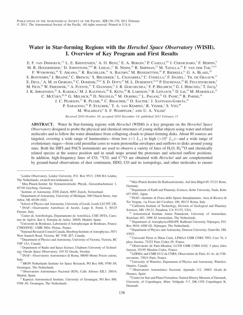
ABSTRACT. Water In Star-forming regions with Herschel (WISH) is a key program on the Herschel SpaceObservatory designed to probe the physical and chemical structures of young stellar objects using water and relatedmolecules and to follow the water abundance from collapsing clouds to planet-forming disks. About 80 sources aretargeted, covering a wide range of luminosities—from low (<1 L⊙) to high (>105 L⊙)—and a wide range ofevolutionary stages—from cold prestellar cores to warm protostellar envelopes and outflows to disks around youngstars. Both the HIFI and PACS instruments are used to observe a variety of lines of H2O, H2

18O and chemicallyrelated species at the source position and in small maps around the protostars and selected outflow positions.In addition, high-frequency lines of CO, 13CO, and C18O are obtained with Herschel and are complementedby ground-based observations of dust continuum, HDO, CO and its isotopologs, and other molecules to ensure

16Max-Planck-Institut für Radioastronomie, Auf dem Hügel 69, 53121 Bonn,Germany.

17Department of Earth and Planetary Sciences, Kobe University, Nada, Kobe657-8501, Japan.

18 INAF—Instituto di Fisica dello Spazio Interplanetario, Area di Ricerca diTor Vergata, via Fosso del Cavaliere 100, 00133 Roma, Italy.

19 California Institute of Technology, Division of Geological and PlanetarySciences, MS 150-21, Pasadena, CA 91125, USA.

20 Astronomical Institute Anton Pannekoek, University of Amsterdam,Kruislaan 403, 1098 SJ Amsterdam, The Netherlands.

21 Department of Astrophysics/IMAPP, Radboud University Nijmegen, P.O.Box 9010, 6500 GL Nijmegen, The Netherlands.

22Department of Physics and Astronomy, Denison University, Granville, OH,43023.

23 Université Pierre et Marie Curie, LPMAA UMR CNRS 7092, Case 76, 4place Jussieu, 75252 Paris Cedex 05, France.

24 Observatoire de Paris-Meudon, LUTH UMR CNRS 8102, 5 place JulesJanssen, 92195 Meudon Cedex, France.

25LERMA and UMR 8112 du CNRS, Observatoire de Paris, 61 Av. de l’Ob-servatoire, 75014 Paris, France.

26 University of Waterloo, Department of Physics and Astronomy, Waterloo,Ontario, Canada.

27 Observatorio Astronómico Nacional, Apartado 112, 28803 Alcalá deHenares, Spain

28Centre for Star and Planet Formation, Natural History Museum of Denmark,University of Copenhagen, Øster Voldgade 5-7, DK-1350 Copenhagen K,Denmark.

1 Leiden Observatory, Leiden University, P.O. Box 9513, 2300 RA Leiden,The Netherlands; [email protected].

2 Max-Planck-Institut für Extraterrestrische Physik, Giessenbachstrasse 1,85748 Garching, Germany.

3 Institute of Astronomy, ETH Zurich, 8093 Zurich, Switzerland.4Department of Astronomy, University of Michigan, 500 Church Street, Ann

Arbor, MI 48109-1042.5School of Physics and Astronomy, University of Leeds, Leeds LS2 9JT, UK.6 INAF—Osservatorio Astrofisico di Arcetri, Largo E. Fermi 5, 50125

Firenze, Italy.7 Centro de Astrobiología, Departamento de Astrofísica, CSIC-INTA, Carre-

tera de Ajalvir, Km 4, Torrejón de Ardoz. 28850, Madrid, Spain.8Université de Bordeaux, Laboratoire d’Astrophysique de Bordeaux, France;

CNRS/INSU, UMR 5804, Floirac, France.9National Research Council Canada, Herzberg Institute of Astrophysics, 5071

West Saanich Road, Victoria, BC V9E 2E7, Canada.10Department of Physics and Astronomy, University of Victoria, Victoria, BC

V8P 1A1, Canada.11Department of Radio and Space Science, Chalmers University of Technol-

ogy, Onsala Space Observatory, 439 92 Onsala, Sweden.12 INAF—Osservatorio Astronomico di Roma, 00040 Monte Porzio catone,

Italy.13 SRON Netherlands Institute for Space Research, PO Box 800, 9700 AV,

Groningen, The Netherlands.14 Observatorio Astronómico Nacional (IGN), Calle Alfonso XII,3. 28014,

Madrid, Spain.15 Kapteyn Astronomical Institute, University of Groningen, PO Box 800,

9700 AV, Groningen, The Netherlands.

138

PUBLICATIONS OF THE ASTRONOMICAL SOCIETY OF THE PACIFIC, 123:138–170, 2011 February© 2011. The Astronomical Society of the Pacific. All rights reserved. Printed in U.S.A.

a self-consistent data set for analysis. An overview of the scientific motivation and observational strategy of theprogram is given, together with the modeling approach and analysis tools that have been developed. Initial scienceresults are presented. These include a lack of water in cold gas at abundances that are lower than most predictions,strong water emission from shocks in protostellar environments, the importance of UV radiation in heating the gasalong outflow walls across the full range of luminosities, and surprisingly widespread detection of the chemicallyrelated hydrides OHþ and H2Oþ in outflows and foreground gas. Quantitative estimates of the energy budget in-dicate that H2O is generally not the dominant coolant in the warm dense gas associated with protostars. Very deeplimits on the cold gaseous water reservoir in the outer regions of protoplanetary disks are obtained that have pro-found implications for our understanding of grain growth and mixing in disks.

Online material: color figures

1. INTRODUCTION

As interstellar clouds collapse to form new stars, part of thegas and dust are transported from the infalling envelope to therotating disk out of which new planetary systems may form(Shu et al. 1987). Water has a pivotal role in these protostellarand protoplanetary environments (see reviews by Cernicharo &Crovisier 2005 and Melnick 2009). As a dominant form of oxy-gen, the most abundant element in the universe after H and He,it controls the chemistry of many other species, whether in gas-eous or solid phase. It is a unique diagnostic of warm gas andenergetic processes taking place during star formation. In coldregions, water is primarily in solid form, and its presence as anice may help the coagulation process that ultimately producesplanets. Asteroids and comets containing ice have likely deliv-ered most of the water to our oceans on Earth, where water isdirectly associated with the emergence of life. Water also con-tributes to the energy balance as a gas coolant, allowing cloudsto collapse up to higher temperatures. The distribution of watervapor and ice during the entire star- and planet-formation pro-cesses is therefore a fundamental question relevant to our ownorigins.

The importance of water as a physical diagnostic stems fromthe orders-of-magnitude variations in its gas-phase abundancebetween warm and cold regions (e.g., Cernicharo et al. 1990;van Dishoeck & Helmich 1996; Ceccarelli et al. 1996; Harwitet al. 1998; Ceccarelli et al. 1999; Snell et al. 2000; Nisini et al.2002; Maret et al. 2002; Boonman et al. 2003; van der Tak et al.2006). Thus, water acts like a switch that turns on whenever

energy is deposited in molecular clouds and elucidates key epi-sodes in the process of stellar birth; in particular, when the sys-tem exchanges matter and energy with its environment. Thisincludes basic stages like gravitational collapse, outflow injec-tion, and stellar heating of disks and envelopes. Its unique abil-ity to act as a natural filter for warm gas and to probe cold gas inabsorption make water a highly complementary diagnostic tothe commonly used CO molecule.

Studying water is also central to understanding the funda-mental processes of freeze-out, grain surface chemistry, andevaporation (e.g., Hollenbach et al. 2009). Water is the domi-nant ice constituent and can trap various molecules inside itsmatrix, including complex organic ones (e.g., Gibb et al. 2004b;Boogert et al. 2008). When and where water evaporates backinto the gas is therefore relevant for understanding the wealthof organic molecules observed near protostars (see review byHerbst & van Dishoeck 2009). Young stars also emit copiousUV radiation and X-rays that affect the physical structureand the chemistry: in particular, that of hydrides like water(Stäuber et al. 2006). Moreover, the level of deuteration of waterprovides an important record of the temperature history of thecloud and the conditions during grain surface formation, and,in comparison with cometary data, of its evolution from inter-stellar clouds to solar system objects (e.g., Jacq et al. 1990;Gensheimer et al. 1996; Helmich et al. 1996; Parise et al. 2003).

Finally, water plays an active role in the energy balance ofdense gas (e.g., Goldsmith & Langer 1978; Neufeld & Kaufman1993; Doty & Neufeld 1997). Because water has a large dipole

29 Department of Physics and Astronomy, San Jose State University, OneWashington Square, San Jose, CA 95192.

30 Harvard-Smithsonian Center for Astrophysics, 60 Garden Street, MS 42,Cambridge, MA 02138.

31Department of Astronomy, Stockholm University, AlbaNova, 106 91 Stock-holm, Sweden.

32Laboratoire d’Astrophysique de Grenoble, CNRS/Université Joseph Fourier(UMR5571) BP 53, F-38041 Grenoble Cedex 9, France.

33California Institute of Technology, Cahill Center for Astronomy and Astro-physics, MS 301-17, Pasadena, CA 91125.

34 University of Western Ontario, Department of Physics & Astronomy,London, Ontario, Canada N6A 3K7.

35 Department of Physics and Astronomy, Johns Hopkins University, 3400North Charles Street, Baltimore, MD 21218.

36 European Southern Observatory, Karl-Schwarzschild-Str. 2, 85748 Garch-ing, Germany.

37Jet Propulsion Laboratory, California Institute of Technology, Pasadena, CA91109.

38Department of Physics and Astronomy, University of Calgary, Calgary, T2N1N4, AB, Canada.

39 Instituto de RadioAstronomía Milimétrica, Avenida Divina Pastora, 7,Núcleo Central E 18012 Granada, Spain.

40Department of Physics and Astronomy, University College London, GowerStreet, London WC1E6BT, UK.

HERSCHEL WISH PROGRAM 139

2011 PASP, 123:138–170

moment, its emission lines can be efficient coolants of the gas,contributing significantly over the range of physical conditionsthat are appropriate in star-forming regions. The large dipolemoment can also lead to heating through absorption of infraredradiation, followed by collisional deexcitation (Ceccarelli et al.1996). It is therefore important to study the gaseous water emis-sion and absorption and to compare its cooling or heating effi-ciency quantitatively with that of other species.

Interstellar water was detected more than 40 years agothrough its 22 GHz maser emission toward Orion (Cheung et al.1969). While this line remains a useful beacon of star-formationactivity, its special excitation and line-formation conditionslimit its usefulness as a quantitative physical and chemical tool.Because observations of thermally excited water lines fromEarth are limited, most information on water has come fromsatellites. The Submillimeter Wave Astronomy Satellite (SWAS;Melnick et al. 2000) and the Odin satellite (e.g., Hjalmarsonet al; 2003; Bjerkeli et al. 2009) observed only the 557 GHzground-state line of ortho-H2O at spatial resolutions of ∼3:30 ×4:50 and 126″, respectively. The 557 GHz line was detected injust the brightest objects by these missions, and other lines ofwater (including those of para-H2O) and related species couldnot be observed. The short-wavelength spectrometer (SWS) andlong-wavelength spectrometer (LWS) on the Infrared SpaceObservatory (ISO) covered a large number of pure rotationaland vibrational-rotational lines, providing important insight intothe water excitation and distribution, but with limited spectraland spatial resolution and mapping capabilities (see the reviewby van Dishoeck 2004). The Spitzer Space Telescope has de-tected highly excited pure rotational H2O lines at mid-infraredwavelengths from shocks (Melnick et al. 2008; Watson et al.2007) and from the inner few AU regions of protoplanetarydisks (Salyk et al. 2008; Carr & Najita 2008; Pontoppidan et al.2010). Even higher-lying vibrational-rotational H2O lines havebeen observed at near-infrared wavelengths from the ground(Salyk et al. 2008). However, these data do not provide any in-formation on the cooler water reservoir where the bulk of thedisk mass is located.

The 3.5 m Herschel Space Observatory with its suite ofinstruments (Pilbratt et al. 2010)41 is particularly well suitedto address the distribution of cold and warm water in star- andplanet-forming regions, building on the pioneering results fromprevious missions. Its wavelength coverage of 55–671 μm(0.45–5.4 THz; 15–180 cm�1)42 includes both low- andhigh-excitation lines of water, enabling a detailed analysisof its excitation and abundance structure (Fig. 1). Compared

with the ISO-LWS beam (∼80″), Herschel has a gain of a fac-tor of ∼8 in spatial resolution at similar wavelengths and up to104 in spectral resolution. Compared with observatories withhigh spectral resolution heterodyne instruments, its diffraction-limited beam of 37″ at 557 GHz is a factor of 3–5 smallerthan that of SWAS or Odin, with a gain of >10 in sensitivitybecause of the bigger dish and improved detector tech-nology. The Heterodyne Instrument for the Far-Infrared (HIFI;de Graauw et al. 2010) has spectral resolving powers R ¼λ=Δλ > 107 up to 1900 GHz, allowing the kinematics ofthe water lines to be studied. The Photoconducting Array Cam-era and Spectrometer (PACS; Poglitsch et al. 2010) 5 × 5 pixelarray provides instantaneous spectral mapping capabilities atR ¼ 1500–4000 of important (backbone) water lines in the55–200 μm range. These enormous advances in sensitivity,spatial and spectral resolution, and wavelength coverage pro-vide a unique opportunity to observe both cold and hot waterin space, with no other space mission with similar capabilitiesbeing planned.

The goal of the Water In Star-forming regions with Herschel(WISH) key program (KP) is to use gas-phase water as aphysical and chemical diagnostic and follow its abundancethroughout the different phases of star and planet formation.A comprehensive set of water observations is carried out withHIFI and PACS toward a large sample of young stellar objects(YSOs), covering a wide range of masses and luminosities—from the lowest to the highest mass protostars– and a large rangeof evolutionary stages—from the first stages represented by theprestellar cores to the late stages represented by the pre–main-sequence stars surrounded only by disks. Lines of H2O, H2

18O,and H2

17O and the chemically related species O, OH, and H3Oþ

are targeted.43 In addition, a number of hydrides that are diag-nostic of the presence of X-rays and UV radiation are observed.Selected high-frequency lines of CO, 13CO, and C18O, as wellas dust continuum maps, are obtained to constrain the physicalstructure of the sources, independently of the chemical effects.Together with the atomic O and Cþ lines, these data also con-strain the contributions from the major coolants. The Herscheldata are complemented by ground-based maps of longer-wavelength continuum emission and lines of HDO, CO, C,and other molecules to ensure a self-consistent data set foranalysis. In terms of water, the WISH program is complemen-tary to the Chemical Survey of Star-forming Regions (CHESS;Ceccarelli et al. 2010) and Herschel Observations of Extraor-dinary Sources (HEXOS; Bergin et al. 2010b) HIFI KPs thatsurvey the entire spectral range (including many lines of water),but only for a limited number of sources and with smaller on-source integration times per frequency setting. The Dust, Ice,and Gas in Time (DIGIT; PI N.J. Evans) and Herschel OrionProtostar Survey (HOPS; PI T. Megeath) KPs complement

41Herschel is an ESA space observatory with science instruments provided byEuropean-led Principal Investigator consortia and with important participationfrom NASA.

42This article follows the common usage of giving frequencies in gigahertz forlines observed with HIFI and giving wavelengths in microns for lines observedwith PACS.

43Both H2O and water are used to denote the main H216O isotopolog through-

out this article.

140 VAN DISHOECK ET AL.

2011 PASP, 123:138–170

WISH by carrying out full PACS spectral scans for a larger sam-ple of low-mass embedded YSOs (e.g., van Kempen et al.2010a). The Probing Interstellar Molecules with AbsorptionLine Studies (PRISMAS) KP targets the water chemistry inthe diffuse interstellar gas (Gerin et al. 2010), whereas Waterand Related Chemistry in the Solar System (also known asHerschel Solar System Observations [HssO]) observes waterin planets and comets (Hartogh et al. 2010). Together, theseHerschel data on water and related hydride lines will providea legacy for decades to come.

In the following sections, background information on thewater chemistry and excitation relevant for interpreting the datais provided (§ 2). The observational details and organization ofthe WISH program are subsequently described in § 3, with thespecific goals and first results of the various subprograms pre-sented in § 4. A discussion of the results across the various evo-lutionary stages and luminosities is contained in § 5, togetherwith implications for the water chemistry, with conclusions in§ 6. Detailed information can be found at the WISH KP WorldWide Web site.44 This Web site includes links to model results,modeling tools, complementary data, and outreach material.These data and analysis tools will be useful not only forHerschel but also for planning observations with the AtacamaLarge Millimeter/submillimeter Array (ALMA) and future far-infrared missions.

2. H2O CHEMISTRY AND EXCITATION

Star formation takes place in cold dense cores with tempera-tures around 10 K and H2 densities of at least 104 cm�3. Oncecollapse starts and a protostellar object has formed, its centralluminosity heats the surrounding envelope to temperatures wellabove 100 K. Moreover, bipolar jets and winds interact with theenvelope and cloud, creating shocks in which the temperature israised to several thousand degrees Kelvin. Cloud core rotationleads to a circumstellar disk around the young star, with den-sities in the midplane of >1010 cm�3. With time, the envelopeis dispersed by the action of the outflow, leaving the pre–main-sequence star with a disk only. Once accretion onto the diskstops and the disk becomes less turbulent, the ∼0:1 μm grainsfrom the collapsing cloud coagulate to larger particles and settleto the midplane, eventually leading to planetesimals and (proto)planets. Thus, star-forming regions contain gas with a largerange of temperatures and densities, from 10 to 2000 K and104 to >1010 cm�3, and with gas/dust ratios that may vary fromthe canonical value of 100 to much larger or smaller values. Thewater chemistry responds to these different conditions.

2.1. Chemistry

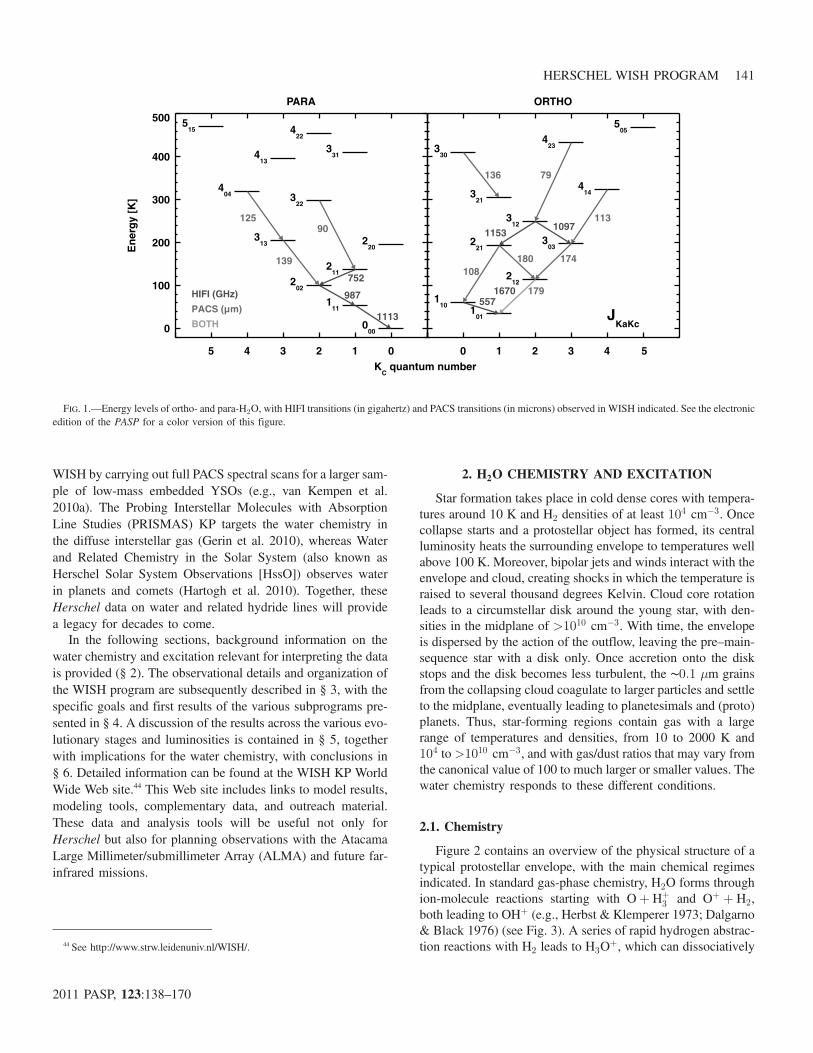
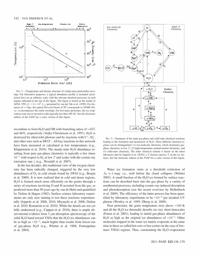
Figure 2 contains an overview of the physical structure of atypical protostellar envelope, with the main chemical regimesindicated. In standard gas-phase chemistry, H2O forms throughion-molecule reactions starting with Oþ Hþ

3 and Oþ þ H2,both leading to OHþ (e.g., Herbst & Klemperer 1973; Dalgarno& Black 1976) (see Fig. 3). A series of rapid hydrogen abstrac-tion reactions with H2 leads to H3Oþ, which can dissociatively

PARA

5 4 3 2 1 0

0

100

200

300

400

500E

ner

gy

[K]

KC quantum number

HIFI (GHz)

PACS (µm)

BOTHJ

KaKc000

111

202

211

220

313

322

404

413

331

422

515

1113

987

752

139

90125

ORTHO

0 1 2 3 4 5

101

110

212

221

303

312

321

414

330

423

505

557

11531097

108180 174

113

79136

1670 179

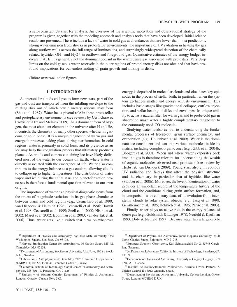
FIG. 1.—Energy levels of ortho- and para-H2O, with HIFI transitions (in gigahertz) and PACS transitions (in microns) observed in WISH indicated. See the electronicedition of the PASP for a color version of this figure.

44 See http://www.strw.leidenuniv.nl/WISH/.


2011 PASP, 123:138–170

recombine to form H2O and OH with branching ratios of ∼33%and 66%, respectively (Vejby-Christensen et al. 1997). H2O isdestroyed by ultraviolet photons and by reactions with Cþ, Hþ

3 ,and other ions such as HCOþ. All key reactions in this networkhave been measured or calculated at low temperatures (e.g.,Klippenstein et al. 2010). The steady-state H2O abundance re-sulting from pure gas-phase chemistry is typically a few times10�7 with respect to H2 at low T and scales with the cosmic-rayionization rate ζ (e.g., Woodall et al. 2007).

In the last decades, this traditional view of the oxygen chem-istry has been radically changed, triggered by the very lowabundances of O2 in cold clouds found by SWAS (e.g., Berginet al. 2000). It is now realized that in cold and dense regions,H2O is formed much more efficiently on the grains through aseries of reactions involving O and H accreted from the gas, aspredicted more than 50 years ago by van de Hulst and quantifiedby Tielens & Hagen (1982). Surface science laboratory experi-ments are only now starting to test these reactions experimen-tally (Ioppolo et al. 2008, 2010; Miyauchi et al. 2008; Dulieuet al. 2010; Romanzin et al. 2010). While the details are not yetfully understood (e.g., Cuppen et al. 2010), there is ample ob-servational evidence from 3 μm absorption spectroscopy of thesolid H2O band toward YSOs that the H2O ice abundances canbe as high as ∼10�4, much higher than results from freeze-outof gas-phase H2O (e.g., Whittet et al. 1988; Pontoppidanet al. 2004).

Water ice formation starts at a threshold extinction ofAV ≈ 5 mag: i.e., well before the cloud collapses (Whittet2003). A small fraction of the H2O ice formed by surface reac-tions can be desorbed back into the gas phase by a variety ofnonthermal processes, including cosmic-ray-induced desorptionand photodesorption (see the recent overview by Hollenbachet al. 2009). The efficiency of the latter process has been quan-tified by laboratory experiments to be ∼10�3 per incident UVphoton (Westley et al. 1995; Öberg et al. 2009).

Near protostars, the grain temperature rises above ∼100 Kand all the H2O ice thermally desorbs on very short timescales(Fraser et al. 2001), leading to initial gas-phase abundances ofH2O as high as the original ice abundances of ∼10�4. Othermolecules trapped in the water ice matrix evaporate at the sametime in these so-called hot-core or hot-corino (in the case of low-mass YSOs) regions. Thus, constraining the H2O evaporation

FIG. 2.—Temperature and density structure of a high-mass protostellar enve-lope. For illustrative purposes, a typical abundance profile is included (dash-dotted line) on an arbitrary scale, with the relevant chemical processes in eachregime indicated at the top of the figure. The figure is based on the model ofAFGL 2591 (L ¼ 6 × 104 L⊙) presented by van der Tak et al. (1999). For dis-tances of ∼1 kpc, the typical Herschel beam of 20″ corresponds to 20,000 AU;i.e., it encompasses the entire envelope. For low-mass protostars, the ice evap-oration zone moves inward to radii typically less than 100 AU. See the electronicedition of the PASP for a color version of this figure.

O

OH

O

O2O2

H

H

2

2

e

e

+

2

HCO

H+3

+

H O2

H

H+

H3+

CO

OH

ν,

e

s−HO

H2

H,

2 2

H

s−OHH2

2

H H

H

H

T,ν

ν

HCO+ +H O

ν

s−O

H

2OH

O

H,

Os−O

H2

H

H2

OH+

H O2+

H O3

2H

s−H O

3

s−H O

s−O

2

O

ν,H

ChemistrySurface

High−TChemistry

Ion−moleculeChemistry

FIG. 3.—Summary of the main gas-phase and solid-state chemical reactionsleading to the formation and destruction of H2O. Three different chemical re-gimes can be distinguished: (1) ion-molecule chemistry, which dominates gas-phase chemistry at low T ; (2) high-temperature neutral-neutral chemistry; and(3) solid-state chemistry. The latter chemical scheme is based on the latestlaboratory data by Ioppolo et al. (2010); s-X denotes species X on the ice sur-faces. See the electronic edition of the PASP for a color version of this figure.


2011 PASP, 123:138–170

zone is also critical for the interpretation of complex organicmolecules in hot cores.

At even higher temperatures, above 230 K, the gas-phase re-action Oþ H2 → OHþ H, which is endoergic by ∼2000 K,becomes significant (Elitzur & Watson 1978; Charnley 1997).OH subsequently reacts with H2 to form H2O, a reaction that isexothermic but has an energy barrier of ∼2100 K (Atkinsonet al. 2004). This route drives all the available gas-phase oxygeninto H2O, leading to an abundance of ∼3 × 10�4 at high tem-peratures, unless the H=H2 ratio in the gas is so high that theback-reactions become important. Such hot gas can be found inthe hot cores close to the protostars themselves and in the moreextended shocked gas associated with the outflows. Given therange of temperatures and densities in protostellar (Fig. 2) andprotoplanetary environments, all of the preceding chemical pro-cesses likely play a role, and the Herschel data are needed todetermine their relative importance.

H2O has a unique deuteration pattern compared with othermolecules. If grain surface formation dominates, water is deu-terated in the ice at a level that may be orders of magnitude low-er than that of other species that participate more actively in thedense cold gas chemistry (Roberts et al. 2003). Indeed, the deu-teration fraction observed in high-mass hot cores is typicallyHDO=H2O < 10�3 (e.g., Gensheimer et al. 1996; Helmich et al.1996), although higher values around 10�2 have recently beenfound for Orion (Persson et al. 2007, Bergin et al. 2010a) andfor a low-mass hot core (Parise et al. 2005b). All of these valuesare still much lower than, for example, DCN/HCN, HDCO=H2CO (e.g., Loinard et al. 2001), or CH2DOH=CH3OH (Pariseet al. 2004). In the solid phase, the HDO=H2O upper limits areless than 2 × 10�3 (Dartois et al. 2003; Parise et al. 2003). Animportant question is how similar the protostellar HDO=H2Oratios are to those observed in comets and in water in our oceanson Earth (about 2 × 10�4), since this has major implicationsfor the delivery mechanisms of water to our planet (Bockelée-Morvan et al. 1998; Raymond et al. 2004). No specific HDOlines are targeted with Herschel within the WISH program,since several HDO lines can be observed from the ground(Parise et al. 2005a). HIFI will provide the necessary data onH2O itself for comparison with those HDO data.

2.2. Excitation

H2O is an asymmetric rotor with a highly irregular set ofenergy levels characterized by quantum numbers JKAKC

. Be-cause of the nuclear spin statistics of the two hydrogen atoms,the H2O energy levels are grouped into ortho (KA þKC ¼odd) and para (KA þKC ¼ even) ladders across which no tran-sitions can occur except through chemical reactions that ex-change a H nucleus (Fig. 1). The H2O energy levels withineach ladder are populated by a combination of collisionaland radiative processes. The most important collision partnersare ortho- and para-H2, with electrons and H only significant inspecific regions and He contributing at a low level. Accurate

collisional rate coefficients are thus crucial to interpret theHerschel data. The bulk of these rates are obtained from theo-retical quantum chemistry calculations that involve two steps.First, a multidimensional potential energy surface involvingthe colliders is computed. Second, the dynamics on this surfaceare investigated with molecular scattering calculations at a rangeof collision energies. Early studies used simplifications such asreplacing H2 with He (Green et al. 1993), including only a lim-ited number of degrees of freedom of the colliding system, orusing approximations in the scattering calculations (Phillipset al. 1996). Recent calculations consider a 5D potential surfaceand compute collisions with both para-H2 and ortho-H2 sepa-rately up to high temperatures with the close coupling method(Dubernet et al. 2009; Daniel et al. 2010). This 5D potential isbased on the full 9D potential surface computed by Valiron et al.(2008). The cross sections for collisions of H2O with o-H2 arefound to be significantly larger than those with p-H2 for low J,so that explicit treatment of the o=p H2 ratio is important.

Direct comparison of absolute values of theoretical state-to-state cross sections with experimental data is not possible, butthe accuracy of the 9D potential surface has been confirmed im-plicitly through comparison with other data sets, including dif-ferential scattering experiments of H2O with H2 (Yang et al.2010). An indication of the accuracy of the calculations can alsobe obtained from recent pressure-broadening experiments (Dicket al. 2010). The high-temperature (>80 K) data agree withtheory within 30% or better, but the low-temperature experi-mental rate coefficients are an order of magnitude smaller. Thisdiscrepancy has recently been understood by realizing that theclassical impact approximation used in the analysis of the pres-sure-broadening data does not hold at very low temperatures(Wiesenfeld & Faure 2010). The computed rate coefficientsat low T by Dubernet et al. (2006) should therefore be valid.

Because of the large rotation constants of water, the energyspacing between the lower levels is much larger than that of aheavy molecule like CO. Thus, the water transitions couplemuch more efficiently with far-infrared radiation from warmdust, which can pump higher energy levels (e.g., Takahashi et al.1983). This far-infrared continuum also plays a role in the lineformation (e.g., whether the line occurs in absorption or emis-sion) and thus provides constraints on source geometry. More-over, the continuum can become optically thick at the highestfrequencies, providing an effective screen for looking to differ-ent depths in the YSO environment (Poelman & van der Tak2007; van Kempen et al. 2008).

The high transition frequencies combined with the large di-pole moment of H2O (1.85 D) also lead to high line opacities.For example, for the o-H2O 557 GHz ground-state transi-tion, the line-center optical depth is τ 0 ¼ 2:0 × 10�13

Nℓðo-H2OÞΔV , where Nℓ is the column density in the lowerlevel in cm�2, which, to first approximation, is equal to the totalo-H2O column density, and ΔV is the FHWM of the line inkm s�1 (Plume et al. 2004). Thus, even for H2O abundances


2011 PASP, 123:138–170

as low as 10�9 in typical clouds with NðH2Þ ≥ 1022 cm�2, thewater lines are optically thick at line center.

Because of the high optical depths, it is difficult to extractreliable water abundances from lines of the main isotopolog.However, because the excitation is subthermal (critical densitiesare typically 108–109 cm�3), every photon that is created willscatter and eventually escape the cloud. In this so-called effec-tively thin limit, the water column density scales linearly withintegrated intensity of a ground-state transition and is inverselyproportional to density and the value of the collisional rate coef-ficient (Snell et al. 2000; Schulz et al. 1991).

Many of the H2O transitions exhibit population inversion,either very weakly or more strongly, such as the famous 616 �523 maser at 22 GHz that is widely observed in star-formingregions (e.g., Szymczak et al. 2005). Thus, the H2O moleculeforms a formidable challenge for radiative transfer codes, andthe HIFI and PACS spectra provide a unique reference data setof thermal lines against which to test the basic assumptions inthe maser models.

2.3. Modeling Tools

The WISH team has developed a variety of tools importantfor the Herschel data analysis, several of which are publiclyavailable to the community. This includes a molecular linedatabase LAMDA45 for excitation calculations of H2O, OH,CO, and other molecules using various sets of collisional ratecoefficients discussed previously (Schöier et al. 2005). Simple1D escape probability non-LTE radiative transfer programs suchas RADEX can be run either online or downloaded to run at theresearcher’s own institute (van der Tak et al. 2007). This and themore sophisticated Monte Carlo 1D radiative transfer codeRATRAN are publicly available,46 and RADEX is also includedin the CASSIS set of analysis programs.47 The RATRAN codehas been extensively tested in a code comparison campaign (vanZadelhoff et al. 2002). Another 1D non-LTE code used by theWISH team is MOLLIE (Keto et al. 2004). A 2D version ofRATRAN and a new flexible 3D line radiative transfer codecalled LIME are available on a collaborative basis (Hogerheijde& van der Tak 2000; Brinch & Hogerheijde 2010). A 2D escapeprobability code has been written by Poelman & Spaans (2005),and a fast 3D code using a local source approximation has beendeveloped by Bruderer et al. (2010a).

Recognizing the importance and complexity of the radiativetransfer problem for H2O, the HIFI consortium organized abenchmark workshop dedicated to an accurate comparison ofradiative transfer codes in 2004. The model tests and resultsare available on a Web page48 so that future researchers can test

new codes. The reliability of existing codes has significantlyimproved from these efforts.

Predictions of water emission lines have been made for gridsof 1D spherically symmetric envelope models over a large rangeof luminosities, envelope masses, and other YSO parameters,for a range of H2O abundances (e.g., Poelman & van der Tak2007; van Kempen et al. 2008). Many of the line profiles showdeep absorptions and hornlike shapes, due to the high line-center optical depths discussed previously, with emission onlyescaping in the line wings.

Chemical models of envelopes and hot cores have been de-veloped for low- and high-mass sources (e.g., Doty et al. 2002,2004; Viti et al. 2001). In these models, the physical conditionsare kept static with time. Models in which the physical structureof the source changes with time as the cloud collapses and theluminosity evolves have been made by Ceccarelli et al. (1996),Viti & Williams (1999), Rodgers & Charnley (2003), Lee et al.(2004), Doty et al. (2006), and Aikawa et al. (2008) in 1D andby Visser et al. (2009) in 2D. Grids of 1D C-type shock modelsby Kaufman & Neufeld (1996) and bow-shock models byGustafsson et al. (2010) are also available. The effects of high-energy irradiation have been studied in spherical symmetry in aseries of articles (Stäuber et al. 2004, 2005, 2006) and have beenextended to multidimensional geometries (Bruderer et al.2009b, 2009a, 2010a).

2.4. Modeling Approach

Spherically symmetric models of protostellar envelopes suchas illustrated in Figure 2 are constructed for all sources in theWISH sample by assuming a power-law density profile and cal-culating the dust temperature with radius using a continuumradiative transfer code such as DUSTY (Ivezić & Elitzur 1997)or RADMC (Dullemond & Dominik 2004), taking the centralluminosity as input. The power-law exponent, spatial extent,and envelope dust mass are determined from χ2 minimizationto the far-infrared spectral energy distribution and submillimetercontinuum maps (see procedure by Jørgensen et al. 2002). Thegas temperature is taken to be equal to the dust temperature,which is a good approximation at these high densities wheregas-dust coupling is significant (Doty & Neufeld 1997), andthe gas mass density is obtained through multiplication ofthe dust density by a factor of 100. These models are termedpassively heated envelope models, to distinguish them fromactive shock and UV photon heating mechanisms.

At typical distances of star-forming regions, thewarmand coldregions—and thus theH2Ochemistry zones—will be largely spa-tially unresolved in theHerschel beams. However, the abundancevariations (where is the water spatially along the line of sight?)can be reconstructed through multiline, single-position observa-tions coupled with physical models of the sources and radiativetransfer analyses. This backward-modeling technique for retriev-al of the abundance profiles in protostellar envelopes has beendemonstrated for ground-based data on a variety of molecules

45 See http://www.strw.leidenuniv.nl/~moldata.46 See http://www.sron.rug.nl/~vdtak/ratran/frames.html.47 http://www.cesr.fr/~walters/web_cassis/.48 See http://www.sron.rug.nl/~vdtak/H2O.


2011 PASP, 123:138–170

such as CO (Jørgensen et al. 2002), CH3OH (e.g., van der Taket al. 2000a; Maret et al. 2005; Kristensen et al. 2010a), andH2CO (e.g., van Dishoeck et al. 1995; Ceccarelli et al. 2000b;Schöier et al. 2002; Maret et al. 2005; Jørgensen et al. 2005b)and confirmed by interferometer data (Jørgensen 2004; Schöieret al. 2004). Asymmetric rotors like H2O with many lines fromdifferent energies close in frequency are particularly well suitedfor such analyses.

Given a temperature and density structure, the molecular ex-citation and radiative transfer in the line are computed at eachposition in the envelope. The resulting sky brightness distribu-tion is convolved with the beam profile. A trial abundance ofwater is chosen (see the example in Fig. 2) and is adjusted untilthe best agreement with observational data is reached. Thevelocity structure is represented either by a turbulent broadeningwidth that is constant with position or by some function: forexample, an infall velocity profile.

The alternative forward-modeling approach starts from a fullphysicochemical model and computes the water emission at dif-ferent times in the evolution for comparison with observations(see Fig. 1 of Doty et al. 2004 for a flowchart of both proce-dures). In this case, one obtains best-fit model parameters suchas the timescale since evaporation (often labeled as the “age”of the source) or the cosmic-ray ionization rate (e.g., Dotyet al. 2006).

The spherically symmetric models are an important first step,but initial Herschel results show that they are generally not suf-ficient to interpret the data. Other components such as shocks orUV-heated cavity walls need to be added in a 2D geometry(van Kempen et al. 2010b; Visser et al. 2011, in preparation).

3. OBSERVATIONS

3.1. Source and Line Selection

The WISH program contains about 80 sources covering arange of luminosities and evolutionary stages and uses about425 hr ofHerschel time. The sources are summarized in Table 1,where they are subdivided into a set of subprograms. Multilinepointed observations at the source position are performed usingthe HIFI and PACS instruments. In addition, small maps over afew-arcminute region are made for selected sources using eitherthe on-the-fly (HIFI) or raster mapping (PACS) strategies. Thenumber of sources per (sub)category ranges from two for thecold line-poor sources to more than 10 for warm line-richobjects—large enough to allow individual source peculiaritiesto be distinguished from general trends. These deep integrationsand thorough coverage of the various types of H2O lines will setthe stage to design future Herschel programs of larger, morestatistically significant samples using fewer lines. Specificsource selection for each subprogram is discussed in § 4. Morethan 90% of our sources are visible with ALMA (δ < 40°).

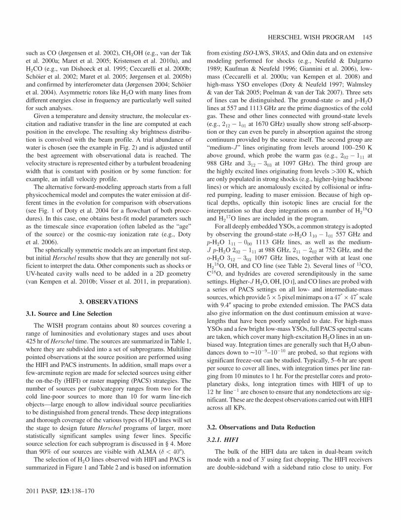
The selection of H2O lines observed with HIFI and PACS issummarized in Figure 1 and Table 2 and is based on information

from existing ISO-LWS, SWAS, and Odin data and on extensivemodeling performed for shocks (e.g., Neufeld & Dalgarno1989; Kaufman & Neufeld 1996; Giannini et al. 2006), low-mass (Ceccarelli et al. 2000a; van Kempen et al. 2008) andhigh-mass YSO envelopes (Doty & Neufeld 1997; Walmsley& van der Tak 2005; Poelman & van der Tak 2007). Three setsof lines can be distinguished. The ground-state o- and p-H2Olines at 557 and 1113 GHz are the prime diagnostics of the coldgas. These and other lines connected with ground-state levels(e.g., 212 � 101 at 1670 GHz) usually show strong self-absorp-tion or they can even be purely in absorption against the strongcontinuum provided by the source itself. The second group are“medium-J” lines originating from levels around 100–250 Kabove ground, which probe the warm gas (e.g., 202 � 111 at988 GHz and 312 � 303 at 1097 GHz). The third group arethe highly excited lines originating from levels >300 K, whichare only populated in strong shocks (e.g., higher-lying backbonelines) or which are anomalously excited by collisional or infra-red pumping, leading to maser emission. Because of high op-tical depths, optically thin isotopic lines are crucial for theinterpretation so that deep integrations on a number of H2

18Oand H2

17O lines are included in the program.For all deeply embeddedYSOs, a common strategy is adopted

by observing the ground-state o-H2O 110 � 101 557 GHz andp-H2O 111 � 000 1113 GHz lines, as well as the medium-J p-H2O 202 � 111 at 988 GHz, 211 � 202 at 752 GHz, and theo-H2O 312 � 303 1097 GHz lines, together with at least oneH2

18O, OH, and CO line (see Table 2). Several lines of 13CO,C18O, and hydrides are covered serendipitously in the samesettings. Higher-J H2O, OH, [O I], and CO lines are probed witha series of PACS settings on all low- and intermediate-masssources, which provide 5 × 5 pixelminimaps on a 47″ × 47″ scalewith 9.4″ spacing to probe extended emission. The PACS dataalso give information on the dust continuum emission at wave-lengths that have been poorly sampled to date. For high-massYSOs and a few bright low-mass YSOs, full PACS spectral scansare taken, which cover many high-excitation H2O lines in an un-biased way. Integration times are generally such that H2O abun-dances down to ∼10�9–10�10 are probed, so that regions withsignificant freeze-out can be studied. Typically, 5–6 hr are spentper source to cover all lines, with integration times per line ran-ging from 10 minutes to 1 hr. For the prestellar cores and proto-planetary disks, long integration times with HIFI of up to12 hr line�1 are chosen to ensure that any nondetections are sig-nificant. These are the deepest observations carried out with HIFIacross all KPs.

3.2. Observations and Data Reduction

3.2.1. HIFI

The bulk of the HIFI data are taken in dual-beam switchmode with a nod of 3′ using fast chopping. The HIFI receiversare double-sideband with a sideband ratio close to unity. For


2011 PASP, 123:138–170

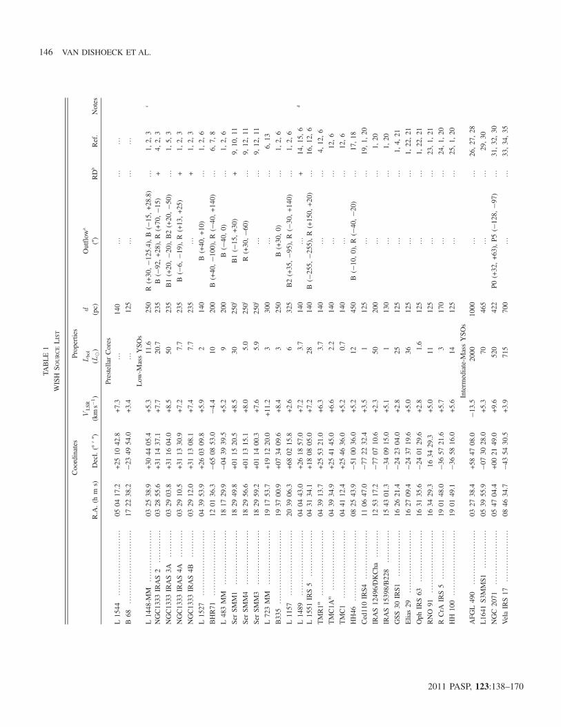
TABLE1

WISH

SOURCELIST

Coordinates

Properties

R.A.(h

ms)

Decl.(°′″)

VLSR

(kms�

1)

Lbol

(L⊙)

d (pc)

Outflow

a

(″)

RD

bRef.

Notes

PrestellarCores

L1544

........................

0504

17.2

+2510

42.8

+7.3

…140

……

…B

68...........................

1722

38.2

−2349

54.0

+3.4

…125

……

…Low

-MassYSO

sL1448-M

M...................

0325

38.9

+3044

05.4

+5.3

11.6

250

R(+30,−1

25.4),B

(−15,+28.8)

…1,

2,3

c

NGC1333

IRAS2

............

0328

55.6

+3114

37.1

+7.7

20.7

235

B(−

92,+2

8),R

(+70,−1

5)+

4,2,

3

NGC1333

IRAS3A

..........

0329

03.8

+3116

04.0

+8.5

50235

B1(+20,−2

0),B2(+20,−5

0)…

1,5,

3

NGC1333

IRAS4A

..........

0329

10.5

+3113

30.9

+7.2

7.7

235

B(−

6,−1

9),R

(+13,+25)

+1,

2,3

NGC1333

IRAS4B

..........

0329

12.0

+3113

08.1

+7.4

7.7

235

…+

1,2,

3

L1527

........................

0439

53.9

+2603

09.8

+5.9

2140

B(+40,+10)

…1,

2,6

BHR71

........................

1201

36.3

−6508

53.0

−4.4

10200

B(+40,−1

00),R

(−40,+140)

…6,

7,8

L483MM

....................

1817

29.9

−0439

39.5

+5.2

9200

B(−

40,0)

…1,

2,6

SerSM

M1

....................

1829

49.8

+0115

20.5

+8.5

30250l

B1(−

15,+30)

+9,

10,11

SerSM

M4

....................

1829

56.6

+0113

15.1

+8.0

5.0

250l

R(+30,−6

0)…

9,12,11

SerSM

M3

....................

1829

59.2

+0114

00.3

+7.6

5.9

250l

……

9,12,11

L723MM

....................

1917

53.7

+1912

20.0

+11.2

3300

……

6,13

B335

...........................

1937

00.9

+0734

09.6

+8.4

3250

B(+30,0)

…1,

2,6

L1157

........................

2039

06.3

+6802

15.8

+2.6

6325

B2(+35,−9

5),R

(−30,+140)

…1,

2,6

L1489

........................

0404

43.0

+2618

57.0

+7.2

3.7

140

…+

14,15,6

d

L1551

IRS5

.................

0431

34.1

+1808

05.0

+7.2

28140

B(−

255,

−255),R

(+150,

+20)

…16,12,6

TMR1m

........................

0439

13.7

+2553

21.0

+6.3

3.7

140

……

4,12,6

TMC1A

m......................

0439

34.9

+2541

45.0

+6.6

2.2

140

……

12,6

TMC1

.........................

0441

12.4

+2546

36.0

+5.2

0.7

140

……

12,6

HH46

..........................

0825

43.9

−5100

36.0

+5.2

12450

B(−

10,0),R

(−40,−2

0)…

17,18

Ced110IRS4

..................

1106

47.0

−7722

32.4

+3.5

1125

……

19,1,

20

IRAS12496/DKCha

..........

1253

17.2

−7707

10.6

+2.3

50200

……

1,20

IRAS15398/B228

............

1543

01.3

−3409

15.0

+5.1

1130

……

1,20

GSS

30IRS1

.................

1626

21.4

−2423

04.0

+2.8

25125

……

1,4,

21

Elias29

.......................

1627

09.4

−2437

19.6

+5.0

36125

……

1,22,21

Oph

IRS63

...................

1631

35.6

−2401

29.6

+2.8

1.6

125

……

1,22,21

RNO

91.......................

1634

29.3

1634

29.3

+5.0

11125

……

23,1,

21

RCrA

IRS5

..................

1901

48.0

−3657

21.6

+5.7

3170

……

24,1,

20

HH

100

........................

1901

49.1

−3658

16.0

+5.6

14125

……

25,1,

20

Interm

ediate-M

assYSO

sAFG

L490

....................

0327

38.4

+5847

08.0

−13.5

2000

1000

……

26,27,28

L1641

S3MMS1

..............

0539

55.9

−0730

28.0

+5.3

70465

……

29,30

NGC

2071

....................

0547

04.4

+0021

49.0

+9.6

520

422

P0(+32,+63),P5

(−128,

−97)

…31,32,30

VelaIRS17

...................

0846

34.7

−4354

30.5

+3.9

715

700

……

33,34,35


2011 PASP, 123:138–170

TABLE1(Contin

ued)

Coordinates

Properties

R.A.(h

ms)

Decl.(°′″)

VLSR

(kms�

1)

Lbol

(L⊙)

d (pc)

Outflow

a

(″)

RD

bRef.

Notes

VelaIRS19

...................

0848

48.5

−4532

29.0

+12.2

776

700

……

33,35

NGC7129

FIRS2

.............

2143

01.7

+6603

23.6

−9.8

430

1250

B(+60,+60),R

(+60,−6

0)+

36,37,38

Outflow

Only

HH211-mm

...................

0343

56.8

+3200

50+9

.24

250

C(0,0),B2(+37,−1

5)…

…IRAS04166

...................

0419

42.6

+2713

38+6

.70.4

140

B(+20,+3

5),R

(−20,−3

5)…

…VLA-1

HH1/2

................

0536

22.8

−0646

07+8

50450

450B

(+60,−8

0)…

…HH212MM1

.................

0543

51.4

−0102

53+1

.615

460

C(0,0),B

(−15,−3

5)…

…HH25MMS

....................

0546

07.3

−0013

30+1

06

400

C(0,0),SiO

(+36,−5

7)…

…HH111VLA1

.................

0551

46.3

+0248

30+8

.525

460

C(0,0),B1(−

170,

+21)

……

HH54B

........................

1255

50.3

−7656

23+2

.41

180

C(0,0)

……

VLA1623

......................

1626

26.4

−2424

30+3

.51

125

B1(+30,−2

0),R2(−

65,+25)

……

IRAS16293

...................

1632

22.8

−2428

36+4

.514

125

B(+75,−6

0),R

(+75,+45)

……

SerS68N

.....................

1829

47.5

+0116

51+8

.54

260

B(−

12,+24),C

(0,0)

……

Cep

EMM

....................

2303

13.1

+6142

26−1

1.0

75730

B(−

10,−2

0)…

…High-MassYSO

sG11.11−

0.12-N

H3-P1

........

1810

33.9

−1921

48+3

0.4

…3600

……

39,40

e

G11.11−

0.12-SCUBA-P1

.....

1810

28.4

−1922

29+2

9.2

…3600

……

40

G28.34+

0.06-N

H3-P3

.........

1842

46.4

−0404

12+8

0.2

…4800

……

40

G28.34+

0.06-SCUBA-P2

.....

1842

52.4

−0359

54+7

8.5

…4800

……

40

IRAS0

5358+3

543

.............

0539

13.1

+3545

50−1

7.6

6:3×10

31800

……

41f

IRAS1

6272−4

837

............

1630

58.7

−4843

55−4

6.2

2:4×10

43400

……

42

NGC6334-I

....................

1720

53.3

−3547

00−4

.51:7×10

41700

…+

43

W43-M

M1

....................

1847

47.0

−0154

28+9

8.8

2:3×10

45500

……

44

DR21(O

H)

....................

2039

00.8

+4222

48−4

.51:7×10

41700

……

45,46

W3-IRS5

......................

0225

40.6

+6205

51−3

8.4

1:7×10

52200

……

47,78,49

g

IRAS1

8089−1

732

............

1811

51.5

−1731

29+3

3.8

3:2×10

43600

……

50

W33A

.........................

1814

39.5

−1752

00+3

7.5

1:0×10

44000

……

51

IRAS1

8151−1

208

............

1817

58−1

207

27+3

2.0

2:0×10

42900

……

52

AFG

L2591

....................

2029

24.9

+4011

19.5

−5.5

5:8×10

41700

……

53

G327−

0.6

.....................

1553

08.8

−5437

01−4

5.0

1:0×10

53000

……

54,55

h

NGC6334-I(N

)................

1720

55.2

−3545

04−7

.71:1×10

51700

……

56

G29.96−

0.02

..................

1846

03.8

−0239

22+9

8.7

1:2×10

57400

……

57,58

G31.41+

0.31

..................

1847

34.3

−0112

46+9

8.8

1:8×10

57900

……

59,60,61

IRAS2

0126+4

104

.............

2014

25.1

+4113

32−3

.81:0×10

41700

……

50

G5.89−0

.39

...................

1800

30.4

−2404

02+1

0.0

2:5×10

42000

……

62,63

i

G10.47+

0.03

..................

1808

38.2

−1951

50+6

7.0

1:1×10

55800

……

64,65,57

G34.26+

0.15

..................

1853

18.6

+0114

58+5

7.2

2:8×10

53300

……

66,65

W51N-e1

......................

1923

43.8

+1430

26+5

9.5

1−1

0×10

55500

……

62

NGC7538-IRS1

...............

2313

45.3

+6128

10−5

7.4

2:0×10

52800

…+

67,68


2011 PASP, 123:138–170

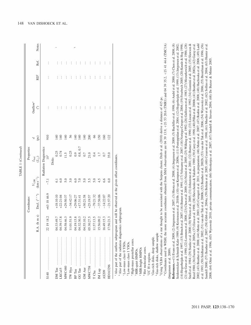
TABLE1(Contin

ued)

Coordinates

Properties

R.A.(h

ms)

Decl.(°′″)

VLSR

(kms�

1)

Lbol

(L⊙)

d (pc)

Outflow

a

(″)

RD

bRef.

Notes

Radiatio

nDiagnostics

S140

...........................

2219

18.2

+6318

46.9

−7.1

104

910

……

…Disks

DM

Tau

.......................

04:33:49.7

+18:10:10

6.1

0.25

140

……

…j

LKCa15

.......................

04:39:17.8

+22:21:04

6.0

0.74

140

……

…MWC480

......................

04:58:46.3

+29:50:37

5.0

11.5

140

……

…TW

Hya

.......................

11:01:51.9

−34:42:17

3.0

0.25

56…

……

BPTau

........................

04:19:15.8

+29:06:27

6.0

0.9

140

……

…k

GG

Tau

........................

04:32:30.3

+17:31:41

7.0

0.8,

0.7

140

……

…GM

Aur

.......................

04:55:10.2

+30:21:58

5.0

0.7

140

……

…MWC758

......................

05:30:27.5

+25:19:57

5.5

21.0

200

……

…TCha

.........................

11:57:13.5

−79:21:32

5.0

0.4

66…

……

IMLup

........................

15:56:09.2

−37:56:06

4.5

1.7

150

……

…AS2

09.........................

16:49:15.3

−14:22:07

6.6

0.7

160

……

…HD163296

....................

17:56:21.3

−21:57:20

6.0

35.0

122

……

…

aAlsopartof

theoutflow

subprogram

andwill

beobserved

atthegivenoffset

coordinates.

bAlsopartof

theradiationdiagnosticssubprogram

.cLow

-massclass0YSO

s.dLow

-massclassIYSO

s.eHigh-massprestellarcores.

fMIR-quiet

HMPO

s.gMIR-brightHMPO

shHot

molecular

cores.

iUC

HIIregions.

jGas-richdisks,deep

sample.

kGas-richdisks,shallow

sample

lUsing

VLBA

observations

ofastar

thoughtto

beassociated

with

theSerpenscluster,Dzibet

al.(2010)

derive

adistance

of415pc.

mCoordinates

used

inWISH;themoreaccurate

coordinatesobtained

from

SMA

observations

are04

3913.9,þ2

553

20.6

(TMR1)

and04

3935.2,þ2

541

44.4

(TMC1A

)(Jørgensen

etal.2009).

References.—(1)E

vans

etal.2009;

(2)Jørgensen

etal.2007;

(3)H

irotaetal.2008;

(4)Jørgensen

etal.2009;

(5)B

achilleretal.1998;(6)

Andréetal.2000;

(7)C

henetal.2008;

(8)

Seidensticker&

Schm

idt-Kaler1989;(9)

Kristensenetal.2010b;(10)v

anKem

penetal.2009c;(11)P

ontoppidan

etal.2004;(12)

Hogerheijd

eetal.199

9;(13)

Jørgensenetal.2002;

(14)

Hogerheijd

eetal.1997;(15)

Brinchetal.2007;(16)

Butneretal.1991;(17)V

elusam

yetal.2007;(18)

Noriega-Crespoetal.2004;(19)

Froebrich2005;(20)K

nude

&Hog

1998;

(21)

deGeusetal.1990;(22)

Lom

men

etal.2008;(23)

Chenetal.2009;(24)

Nisinietal.2005;(25)W

ilkingetal.1992;(26)

Gullix

sonetal.1983;(27)

Mozurkewichetal.1986;(28)

Snelletal.1984;(29)S

tankeetal.2000;

(30)

Wilson

etal.2005;

(31)

Johnstoneetal.2001;(32)

Butneretal.1990;(33)L

iseauetal.1992;(34)

Gianninietal.2005;(35)S

lawson&

Reed1988;(36)F

uenteetal.2005a;(37)E

iroa

etal.1998;(38)

Shevchenko

&Yakubov

1989;(39)C

arey

etal.1998;(40)

Pillaietal.2006b;(41)

Beutheretal.2002a;(42)G

aray

etal.

2002;(43)Beuther

etal.2008;

(44)

Motteetal.2

003;

(45)

Csengerietal.2011,inpreparation;

(46)

Motteetal.2

007;

(47)

Rodón

etal.2008;

(48)

Hachisuka

etal.2

006;

(49)

Ladd

etal.1993;(50)

Sridharanetal.2002;(51)

vanderT

aketal.2000b;(52)B

eutheretal.2002b;(53)v

anderT

aketal.2006;(54)

Wyrow

skietal.2006;(55)B

ronfman

etal.1996;(56)

Sandell2

000;

(57)

Beuther

etal.2

007;

(58)

Gibbetal.2

004a;(59)Beltrán

etal.2

005;

(60)

Cesaronietal.1998;(61)Muelleretal.2

002;

(62)

Sollins

etal.2

004;

(63)

Hunteretal.

2008;(64)

Olm

iet

al.1996;(65)

Wyrow

ski2010,privatecommunication;

(66)

Mookerjea

etal.2007;(67)

Sandell&

Sievers2004;(68)

DeBuizer&

Minier2005.


2011 PASP, 123:138–170

TABLE2

WISH

LIN

ELIST

Species

Transition

ν(G

Hz)

λ(μm)

Eu=kB

(K)

A

(s�1)

Ref.

HIFILines

H2O

110�1 0

1556.936

538.3

613.5(−3

)1

H2O

221�2 1

21661.008

180.5

194.1

3.1(−2

)1

H2O

212�1 0

11669.905

179.5

114.4

5.6(−2

)1

H2O

111�0 0

01113.343

269.3

53.4

1.8(−2

)1

H2O

202�1 1

1987.927

303.5

100.8

5.8(−3

)1

H2O

211�2 0

2752.033

398.6

136.9

7.1(−3

)1

H2O

312�3 0

31097.365

273.2

249.4

1.6(−2

)1

H2O

312�3 2

11153.127

260

249.4

2.6(−3

)1

H218O

110�1 0

1547.676

547.4

60.5

3.3(−3

)1

H218O

111�0 0

01101.698

272.1

52.9

1.8(−2

)1

H218O

202�1 1

1994.675

301.4

100.6

6.0(−3

)1

H218O

312�3 0

31095.627

273.6

248.7

1.6(−2

)1

H217O

110�1 0

1552.021

543.1

60.7

3.4(−3

)1

H217O

111�0 0

01107.167

270.8

53.1

1.8(−2

)1

OH

aΩ,J

¼1=2,3=2�1=2,1=2

1834.747

163.4

269.8

6.4(−2

)1

OH

aΩ,J

¼1=2,3=2�1=2,1=2

1837.817

163.1

270.1

6.4(−2

)1

OH

þaN

J;F

¼11;3=2�0 1

;3=2

1033.119

290.2

49.6

1.8(−2

)2

OH

þaN

J;F

¼21;3=2�1 1

;3=2

1892.227

158.4

140.4

5.9(−2

)2

H2O

þaN

KaK

b;J¼

2 02;3=2�1 1

1;3=2

746.3

401.7

89.3

5.5(−4

)3

H2O

þaN

KaK

b;J¼

1 11;3=2�0 0

0;1=2

1115.204

268.8

53.5

3.1(−2

)6

H2O

þaN

KaK

b;J¼

1 11;1=2�0 0

0;1=2

1139.6

263.1

54.7

2.9(−2

)3

H2O

þaN

KaK

b;J¼

3 12;5=2�3 0

3;5=2

999.8

299.8

223.9

2.3(−2

)3

H3O

þJk;þ

¼0 0

;��1 0

;þ984.712

304.4

54.7

2.3(−2

)1

H3O

þJk;þ

¼4 3

;þ�3 3

;�1031.294

290.7

232.2

5.1(−3

)1

H3O

þJk;þ

¼4 2

;þ�3 2

;�1069.827

280.2

268.8

9.8(−3

)1

H3O

þJk;þ

¼6 2

;��6 2

;þ1454.563

206.1

692.6

7.1(−3

)1

H3O

þJk;þ

¼2 1

;��2 1

;þ1632.091

183.7

143.1

1.7(−2

)1

CO

10−9

1151.985

260.2

304.2

1.0(−4

)1

CO

16−1

51841.346

162.8

751.7

4.1(−4

)1

13CO

5−4

550.926

544.2

79.3

1.1(−5

)1

13CO

10−9

1101.35

272.2

290.8

8.8(−5

)1

C18O

5−4

548.831

546.2

791.1(−5

)1

C18O

9−8

987.56

303.6

237

6.4(−5

)1

C18O

10−9

1097.163

273.2

289.7

8.8(−5

)1

HCO

þ6−

5535.062

560.3

89.9

1.3(−2

)1

CH

aJF;P

¼3=2 2

;��1=21;þ

536.761

558.5

25.8

6.4(−4

)2

CH

aJF;P

¼5=2 3

;þ�3=22;�

1661.107

180.5

105.5

3.8(−2

)2

CH

aJF;P

¼5=2 3

;��3=22;þ

1656.956

180.9

105.2

3.7(−2

)2

CH

þ1−

0835.138

359

40.1

6.4(−2

)2

CH

þ2−

11669.281

179.6

120.2

6.1(−2

)2

HCN

11−1

0974.487

316.4

280.7

4.6(−2

)1

NH

aN

J;F

1;F

¼1 2

;5=2;7=2�

01;3=2;5=

2

974.478

307.6

46.8

6.9(−3

)2

NH

aN

J;F

1;F

¼1 1

;3=2;5=2�

01;3=2;5=

2

999.973

299.8

485.2(−3

)2

NH

þaJP¼

3=2 �

�1=2 þ

1012.54

296.1

48.6

5.4(−2

)7


2011 PASP, 123:138–170

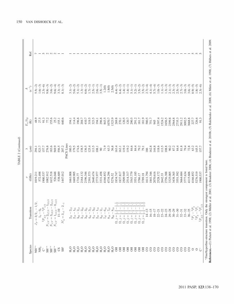
TABLE2(Contin

ued)

Species

Transition

ν(G

Hz)

λ(μm)

Eu=kB

(K)

A

(s�1)

Ref.

NH

þaJP¼

3=2 þ

�1=2�

1019.211

294.1

48.9

5.5(−2

)7

NH

310�0 0

572.498

523.7

27.5

1.6(−3

)1

Cþ

2P

3=2�

2P

1=2

1900.537

157.7

91.3

2.3(−6

)5

SHþa

NJ;F

¼2 3

;7=2�1 2

;5=2

1082.912

276.8

77.2

9.8(−3

)2

SHþa

NJ;F

¼3 4

;9=2�2 3

;5=2

1632.518

183.6

155.6

3.6(−2

)2

SHþa

NJ;F

¼1 2

;5=2�0 1

;3=2

526.048

569.9

25.2

9.6(−4

)2

CS

11−1

0538.689

556.5

155.1

3.3(−3

)1

SHa

N0 Λ¼

3 þ1�2�1

1447.012

207.2

640.6

8.1(−3

)1

PACSLines

H2O

2 21�2 1

21661.008

180.5

194.1

3.1(−2

)1

H2O

2 12�1 0

11669.905

179.5

114.4

5.6(−2

)1

H2O

3 03�2 1

21716.77

174.6

196.8

5.1(−2

)1

H2O

3 13�2 0

22164.132

138.5

204.7

1.3(−1

)1

H2O

3 30�3 2

12196.346

136.5

410.7

6.6(−2

)1

H2O

4 04�3 1

32391.573

125.4

319.5

1.7(−1

)1

H2O

4 14�3 0

32640.474

113.5

323.5

2.5(−1

)1

H2O

2 21�1 1

02773.977

108.1

194.1

2.6(−1

)1

H2O

3 22�2 1

13331.458

90296.8

3.5(−1

)1

H2O

7 07�6 1

64166.852

71.9

843.5

1.2(0)

1H

2O

8 18�7 0

74734.296

63.3

1070.7

1.8(0)

1H

2O

9 09�8 1

85276.52

56.8

1323.9

2.5(0)

1OH

Ω,j¼

1 2;3 2

�1 2;1 2

1834.747

163.4

269.8

6.4(−2

)1

OH

Ω,j¼

1 2;3 2

�1 2;1 2

1837.817

163.1

270.1

6.4(−2

)1

OH

Ω,j¼

3 2;5 2

�3 2;3 2

2509.949

119.4

120.5

1.4(−1

)1

OH

Ω,j¼

3 2;5 2

�3 2;3 2

2514.317

119.2

120.7

1.4(−1

)1

OH

Ω,j¼

3 2;7 2

�3 2;5 2

3543.779

84.6

290.5

5.1(−1

)1

OH

Ω,j¼

3 2;7 2

�3 2;5 2

3551.185

84.4

291.2

5.2(−1

)1

OH

Ω,j¼

1 2;1 2

�3 2;3 2

3786.17

79.2

181.7

3.5(−2

)1

OH

Ω,j¼

1 2;1 2

�3 2;3 2

3789.18

79.1

181.9

3.5(−2

)1

CO

14−1

31611.794

186

580.5

2.7(−4

)1

CO

16−1

51841.346

162.8

751.7

4.1(−4

)1

CO

18−1

72070.616

144.8

945

5.7(−4

)1

CO

22−2

12528.172

118.6

1397.4

1.0(−3

)1

CO

23−2

22642.33

113.5

1524.2

1.1(−3

)1

CO

24−2

32756.388

108.8

1656.5

1.3(−3

)1

CO

29−2

83325.005

90.2

2399.8

2.1(−3

)1

CO

30−2

93438.365

87.2

2564.8

2.3(−3

)1

CO

31−3

03551.592

84.4

2735.3

2.5(−3

)1

CO

32−3

13664.684

81.8

2911.2

2.7(−3

)1

CO

33−3

23777.634

79.4

3092.5

3.0(−3

)1

CO

36−3

54115.606

72.8

3668.8

3.6(−3

)1

O3P

1�

3P

24166.852

63.2

227.7

8.9(−5

)5

O3P

0�

3P

15276.519

145.5

326.6

1.8(−5

)5

Cþ

2P

3=2�

2P

1=2

1900.537

157.7

91.3

2.3(−6

)5

aFine/hyperfine-structure

transitio

n.Onlythestrongestcomponent

islistedhere.

References.—(1)Pickettet

al.1998;(2)Mülleret

al.2001;(3)Bruderer2006;(4)Brudereret

al.2010b;

(5)Ralchenko

etal.2008;(6)Mürtz

etal.1998;(7)Hüberset

al.2009.


2011 PASP, 123:138–170

line-rich sources (mostly high-mass YSOs), the local oscillatorwas shifted slightly for half of the integration time to disen-tangle lines from the upper and lower sidebands. Two polariza-tions, H and V , are measured simultaneously and are generallyaveraged together to improve the signal-to-noise ratio (S/N). Insome cases, differences of the order of 30% are found betweenthe two polarizations, in which case only the higher-quality H-band spectra are used for analysis, since the mixers have beenoptimized for the H band. Two back ends are employed: thelow-resolution back end (wideband spectrometer [WBS]) withan instantaneous bandwidth of 4 GHz at 1.1 MHz spectral res-olution (∼1100 and 0:3 km s�1 at 1 THz, respectively) and thehigh-resolution back end (high-resolution spectrometer [HRS])with a variable bandwidth and resolution (typically 230 MHzbandwidth and 250 kHz resolution, or ∼63 and 0:07 km s�1

at 1 THz, respectively).Data reduction of the HIFI spectra involves the usual steps of

checking individual exposures for bad spectra, summing expo-sures, taking out any baseline ripples, fitting a low-order poly-nomial baseline, and making Gaussian fits or integrating lineintensities, as appropriate. The data are reduced within theHerschel interactive processing environment (HIPE) (Ott2010) and can be exported to CLASS49 after level 2 for furtheranalysis. The main-beam efficiency has been determined to bearound 0.76, virtually independent of frequency, except for a15% lower value at around 1.1–1.2 THz (Olberg 2010), andthe absolute calibration is currently estimated to be better than∼15% for HIFI bands 1, 2, and 5 and ∼30% for bands 3, 4, 6,and 7. The rms noise in the WBS data is generally lower thanthat in the HRS data by a factor of 1.4 when binned to thesame spectral resolution, due to a

ffiffiffi

2p

loss factor in the HRSautocorrelator.

3.2.2. PACS

PACS is a 5 × 5 array of 9:4″ × 9:4″ spaxels (spatial pixels)with very small gaps between the pixels. Each spaxel covers the53–210 μm wavelength range, with a spectral resolving powerranging from 1000 to 4000 (the latter only below 63 μm) inspectroscopy mode. In one exposure, a wavelength segmentis observed in the first order (105–210 μm) and at the same timein the second (72–105 μm) or third order (53–72 μm). Two dif-ferent nod positions, located 6′ in opposite directions from thetarget, are used to correct for telescopic background. Data arereduced within HIPE. The uncertainty in absolute and relativefluxes is estimated to be about 10–20%, based on comparisonwith the ISO-LWS data.

The diffraction-limited beam is smaller than a spaxel of 9.4″at wavelengths shortward of 110 μm. At longer wavelengths,the point-spread function (PSF) becomes significantly larger,such that at 200 μm only 40% of the light of a well-centered

point source falls on the central pixel. Even at 100 μm, 30%of the light still falls outside the central spaxel. Thus, observedfluxes reported for a single pixel have to be corrected for thepoint-source PSF using values provided by the HerschelScience Center. For extended sources, fluxes can be summedover the spaxels to obtain the total flux. In case of a bright cen-tral source with extended emission, such as along an outflow,fluxes at the outflow positions were corrected for the leakingof light from the central spaxel into adjacent spaxels.

3.3. Archival Value

All reduced HIFI and PACS spectra will be delivered to theHerschel Science Center approximately one year after the lastKP data have been taken, assuming that reliable calibration isavailable in a timely manner. The delivery will consist of re-duced and calibrated HIFI spectra, line profile parameters(either Gaussian fits or integrated intensities, depending online), and reduced small maps, most likely in FITS format. Aquick-look spectral browser will be on the team Web site.For PACS, a data cube of calibrated images will be delivered,similar to that for integral field spectrometers.

Over the past decade, the WISH team has collected a wealthof complementary data on various molecular lines for the ma-jority of our sources using the JCMT, IRAM 30 m, APEX,CSO, Onsala, and other single-dish telescopes. These data in-clude tracers of the cloud velocity structure and column density(12CO, 13CO, C18O J ¼ 1–0, 2–1, and 3–2, probing ∼30 Kgas), high-temperature lines (CO and isotopologs 6–5, 7–6,probing ∼50–100 K gas), and high-density tracers (CS andC34S 2–1, 5–4, 7–6; HCOþ and H13COþ 3–2, 4–3, probingn > 105 cm�3), as well as the atomic [C I] line (probing UVradiation). Moreover, grain surface chemistry products are ob-served through various H2CO and CH3OH lines, whereasshocks powerful enough to disrupt grain cores are tracedthrough SiO emission. Examples of such studies are van der Taket al. (2000b), Jørgensen et al. (2004), Fuente et al. (2005b),Nisini et al. (2007), and Marseille et al. (2008).

A recent development is the use of heterodyne array receiverssuch as the 9 pixel HERA 230 GHz array at the IRAM 30 m, theHARP-B 16 pixel 345 GHz receiver at the JCMT (e.g., vanKempen et al. 2009b; Kristensen et al. 2010a), and the dual-frequency 2 × 7 pixel CHAMPþ 650=850 GHz receiver atAPEX (e.g., van Kempen et al. 2009d, 2009e). The spatial reso-lution of these telescopes is typically 7–15″: i.e., comparablewiththat of Herschel at the higher frequencies. These data also pro-vide an image of the warm dense gas contained within the ∼37″Herschel beam at 557GHz.Millimeter interferometry data downto ∼1″ resolution also exist for a significant subset of the sourcesin various molecules and lines (e.g., Fuente et al. 2005a;van der Tak et al. 2006; Benz et al. 2007; Jørgensen et al.2009; and references therein). Except for the compact hot core,however, such data cannot be compared directly with single-dish49 See http://iram.fr/IRAMFR/GILDAS.


2011 PASP, 123:138–170

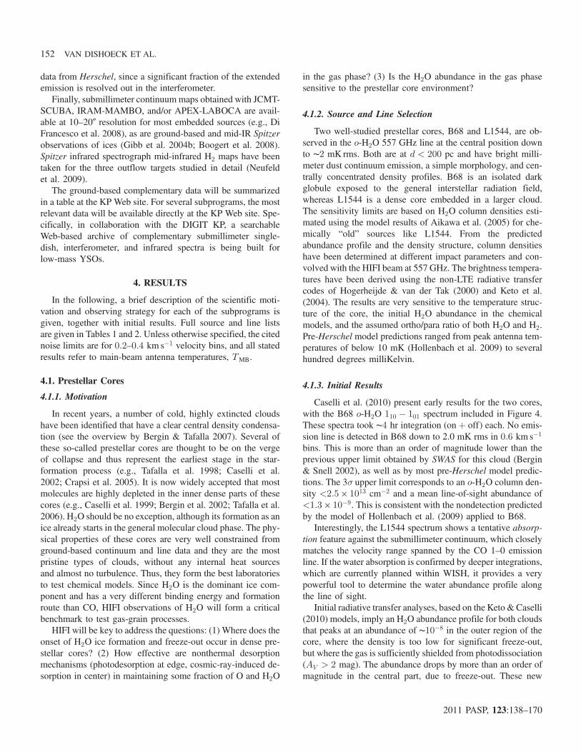
data from Herschel, since a significant fraction of the extendedemission is resolved out in the interferometer.

Finally, submillimeter continuum maps obtained with JCMT-SCUBA, IRAM-MAMBO, and/or APEX-LABOCA are avail-able at 10–20″ resolution for most embedded sources (e.g., DiFrancesco et al. 2008), as are ground-based and mid-IR Spitzerobservations of ices (Gibb et al. 2004b; Boogert et al. 2008).Spitzer infrared spectrograph mid-infrared H2 maps have beentaken for the three outflow targets studied in detail (Neufeldet al. 2009).

The ground-based complementary data will be summarizedin a table at the KP Web site. For several subprograms, the mostrelevant data will be available directly at the KP Web site. Spe-cifically, in collaboration with the DIGIT KP, a searchableWeb-based archive of complementary submillimeter single-dish, interferometer, and infrared spectra is being built forlow-mass YSOs.

4. RESULTS

In the following, a brief description of the scientific moti-vation and observing strategy for each of the subprograms isgiven, together with initial results. Full source and line listsare given in Tables 1 and 2. Unless otherwise specified, the citednoise limits are for 0:2–0:4 km s�1 velocity bins, and all statedresults refer to main-beam antenna temperatures, TMB.

4.1. Prestellar Cores

4.1.1. Motivation

In recent years, a number of cold, highly extincted cloudshave been identified that have a clear central density condensa-tion (see the overview by Bergin & Tafalla 2007). Several ofthese so-called prestellar cores are thought to be on the vergeof collapse and thus represent the earliest stage in the star-formation process (e.g., Tafalla et al. 1998; Caselli et al.2002; Crapsi et al. 2005). It is now widely accepted that mostmolecules are highly depleted in the inner dense parts of thesecores (e.g., Caselli et al. 1999; Bergin et al. 2002; Tafalla et al.2006). H2O should be no exception, although its formation as anice already starts in the general molecular cloud phase. The phy-sical properties of these cores are very well constrained fromground-based continuum and line data and they are the mostpristine types of clouds, without any internal heat sourcesand almost no turbulence. Thus, they form the best laboratoriesto test chemical models. Since H2O is the dominant ice com-ponent and has a very different binding energy and formationroute than CO, HIFI observations of H2O will form a criticalbenchmark to test gas-grain processes.

HIFI will be key to address the questions: (1) Where does theonset of H2O ice formation and freeze-out occur in dense pre-stellar cores? (2) How effective are nonthermal desorptionmechanisms (photodesorption at edge, cosmic-ray-induced de-sorption in center) in maintaining some fraction of O and H2O

in the gas phase? (3) Is the H2O abundance in the gas phasesensitive to the prestellar core environment?

4.1.2. Source and Line Selection

Two well-studied prestellar cores, B68 and L1544, are ob-served in the o-H2O 557 GHz line at the central position downto ∼2 mK rms. Both are at d < 200 pc and have bright milli-meter dust continuum emission, a simple morphology, and cen-trally concentrated density profiles. B68 is an isolated darkglobule exposed to the general interstellar radiation field,whereas L1544 is a dense core embedded in a larger cloud.The sensitivity limits are based on H2O column densities esti-mated using the model results of Aikawa et al. (2005) for che-mically “old” sources like L1544. From the predictedabundance profile and the density structure, column densitieshave been determined at different impact parameters and con-volved with the HIFI beam at 557 GHz. The brightness tempera-tures have been derived using the non-LTE radiative transfercodes of Hogerheijde & van der Tak (2000) and Keto et al.(2004). The results are very sensitive to the temperature struc-ture of the core, the initial H2O abundance in the chemicalmodels, and the assumed ortho/para ratio of both H2O and H2.Pre-Herschel model predictions ranged from peak antenna tem-peratures of below 10 mK (Hollenbach et al. 2009) to severalhundred degrees milliKelvin.

4.1.3. Initial Results

Caselli et al. (2010) present early results for the two cores,with the B68 o-H2O 110 � 101 spectrum included in Figure 4.These spectra took ∼4 hr integration (onþ off) each. No emis-sion line is detected in B68 down to 2.0 mK rms in 0:6 km s�1

bins. This is more than an order of magnitude lower than theprevious upper limit obtained by SWAS for this cloud (Bergin& Snell 2002), as well as by most pre-Herschel model predic-tions. The 3σ upper limit corresponds to an o-H2O column den-sity <2:5 × 1013 cm�2 and a mean line-of-sight abundance of<1:3 × 10�9. This is consistent with the nondetection predictedby the model of Hollenbach et al. (2009) applied to B68.

Interestingly, the L1544 spectrum shows a tentative absorp-tion feature against the submillimeter continuum, which closelymatches the velocity range spanned by the CO 1–0 emissionline. If the water absorption is confirmed by deeper integrations,which are currently planned within WISH, it provides a verypowerful tool to determine the water abundance profile alongthe line of sight.

Initial radiative transfer analyses, based on the Keto & Caselli(2010) models, imply an H2O abundance profile for both cloudsthat peaks at an abundance of ∼10�8 in the outer region of thecore, where the density is too low for significant freeze-out,but where the gas is sufficiently shielded from photodissociation(AV > 2 mag). The abundance drops by more than an order ofmagnitude in the central part, due to freeze-out. These new


2011 PASP, 123:138–170

predictions are based on an improved physical structure of theL1544 core and on an H2O abundance profile that includesthe freeze-out, a generalized desorption from Roberts & Millar(2007), and photodissociation, but no detailed gas phase and sur-face chemistry. Such abundance profiles differ from those ex-pected from chemical models by Aikawa et al. (2005), whopredict higher H2O abundances toward the core center and thusbrighter lines. Investigations are currently underway to under-stand which processes are producing the different abundancestructures.

These results demonstrate that questions 1 and 2 in § 4.1.1can be addressed by the Herschel observations, provided the

integrations are deep enough. Question 3 requires observationsof a larger sample of cores than those studied in WISH.

4.2. Low-Mass Young Stellar Objects

4.2.1. Motivation

Once the cloud has started to collapse and a protostellar ob-ject has formed, the envelope is heated from the inside by theaccretion luminosity. The physical structure of these low-massdeeply embedded objects (≲100 L⊙) is complex, with largegradients in temperature and density in the envelope, a compactdisk at the center, and stellar jets and winds creating a cavity inthe envelope and affecting the surrounding material (e.g., vanDishoeck et al. 1995; Jørgensen et al. 2005a; Chandler et al.2005) (see Fig. 5). The high spatial and spectral resolutionsat far-infrared wavelengths offered by Herschel are key to dis-entangling these processes.

Several evolutionary stages can be distinguished for low-mass YSOs (see the nomenclature by Robitaille et al. 2006).In the earliest deeply embedded stage 0, the main accretionphase, the envelope mass is still much larger than that of theprotostar or disk (Menv ≫ M� and≫Mdisk). At the subsequentstage 1, the star is largely assembled and now has a much largermass than the disk (M� ≫ Mdisk), but the envelope still domi-nates the circumstellar material (Menv > Mdisk). At stage 2, theenvelope has completely dissipated and only a gas-rich disk isleft around the young pre–main-sequence star. Observationally,low-mass YSOs are usually classified based on their spectralenergy distributions according to their spectral slopes (as inthe Lada classes) or bolometric temperatures (see the summaryin Evans et al. 2009). The classes 0 and II sources generallycorrespond well to the evolutionary stages 0 and 2 cases. In con-trast, the traditional class I sources are found to be a mix oftrue stage 1 sources and of stage 2 disks, which are either seenedge-on or which have a large amount of foreground extinction,resulting in a rising infrared spectrum (see the discussion inCrapsi et al. 2008).

ISO-LWS observations have shown that low-mass YSOs arecopious water emitters, with more than 70% of the stage 0sources detected in H2O lines with energies up to 500 K aboveground (see the summary by Nisini et al. 2002). Two scenarioshave been put forward to explain these strong lines. In onemodel, the lines arise primarily from the bulk of the envelope,with the lower-energy lines originating in the outer envelopeand the higher-energy lines originating from the inner hot core(Maret et al. 2002). In the alternative interpretation, most of theH2O emission is associated with the outflows impacting the sur-rounding gas on larger scales (e.g., Giannini et al. 2001).

In contrast, none of the low-mass stage 1 sources show H2Olines in the ISO-LWS beam (Giannini et al. 2001). Possible ex-planations given in that article include dissociation resultingfrom enhanced penetration of X-rays or UV photons or a longertimescale enhancing freeze-out. HIFI can distinguish between

FIG. 4.—HIFI spectra of the o-H2O 110 � 101 557 GHz line. From top to bot-tom: the prestellar core B68 (Caselli et al. 2010), the low-mass stage 0 YSOL1527, the low-mass stage 1 YSO TMR-1, and the protoplanetary disk DMTau (Bergin et al. 2010b). See the electronic edition of the PASP for a colorversion of this figure.


2011 PASP, 123:138–170

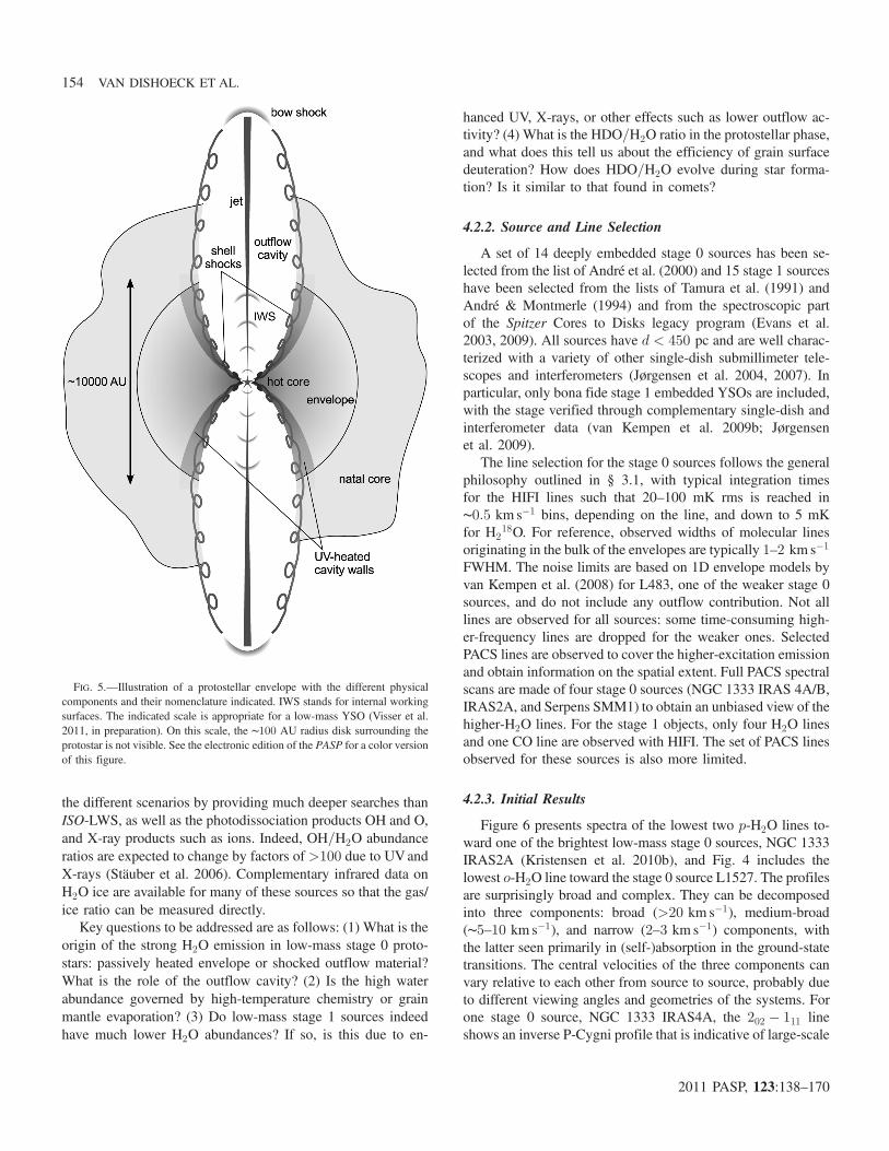
the different scenarios by providing much deeper searches thanISO-LWS, as well as the photodissociation products OH and O,and X-ray products such as ions. Indeed, OH=H2O abundanceratios are expected to change by factors of >100 due to UVandX-rays (Stäuber et al. 2006). Complementary infrared data onH2O ice are available for many of these sources so that the gas/ice ratio can be measured directly.

Key questions to be addressed are as follows: (1) What is theorigin of the strong H2O emission in low-mass stage 0 proto-stars: passively heated envelope or shocked outflow material?What is the role of the outflow cavity? (2) Is the high waterabundance governed by high-temperature chemistry or grainmantle evaporation? (3) Do low-mass stage 1 sources indeedhave much lower H2O abundances? If so, is this due to en-

hanced UV, X-rays, or other effects such as lower outflow ac-tivity? (4) What is the HDO=H2O ratio in the protostellar phase,and what does this tell us about the efficiency of grain surfacedeuteration? How does HDO=H2O evolve during star forma-tion? Is it similar to that found in comets?


A set of 14 deeply embedded stage 0 sources has been se-lected from the list of André et al. (2000) and 15 stage 1 sourceshave been selected from the lists of Tamura et al. (1991) andAndré & Montmerle (1994) and from the spectroscopic partof the Spitzer Cores to Disks legacy program (Evans et al.2003, 2009). All sources have d < 450 pc and are well charac-terized with a variety of other single-dish submillimeter tele-scopes and interferometers (Jørgensen et al. 2004, 2007). Inparticular, only bona fide stage 1 embedded YSOs are included,with the stage verified through complementary single-dish andinterferometer data (van Kempen et al. 2009b; Jørgensenet al. 2009).

The line selection for the stage 0 sources follows the generalphilosophy outlined in § 3.1, with typical integration timesfor the HIFI lines such that 20–100 mK rms is reached in∼0:5 km s�1 bins, depending on the line, and down to 5 mKfor H2

18O. For reference, observed widths of molecular linesoriginating in the bulk of the envelopes are typically 1–2 km s�1

FWHM. The noise limits are based on 1D envelope models byvan Kempen et al. (2008) for L483, one of the weaker stage 0sources, and do not include any outflow contribution. Not alllines are observed for all sources: some time-consuming high-er-frequency lines are dropped for the weaker ones. SelectedPACS lines are observed to cover the higher-excitation emissionand obtain information on the spatial extent. Full PACS spectralscans are made of four stage 0 sources (NGC 1333 IRAS 4A/B,IRAS2A, and Serpens SMM1) to obtain an unbiased view of thehigher-H2O lines. For the stage 1 objects, only four H2O linesand one CO line are observed with HIFI. The set of PACS linesobserved for these sources is also more limited.


Figure 6 presents spectra of the lowest two p-H2O lines to-ward one of the brightest low-mass stage 0 sources, NGC 1333IRAS2A (Kristensen et al. 2010b), and Fig. 4 includes thelowest o-H2O line toward the stage 0 source L1527. The profilesare surprisingly broad and complex. They can be decomposedinto three components: broad (>20 km s�1), medium-broad(∼5–10 km s�1), and narrow (2–3 km s�1) components, withthe latter seen primarily in (self-)absorption in the ground-statetransitions. The central velocities of the three components canvary relative to each other from source to source, probably dueto different viewing angles and geometries of the systems. Forone stage 0 source, NGC 1333 IRAS4A, the 202 � 111 lineshows an inverse P-Cygni profile that is indicative of large-scale

FIG. 5.—Illustration of a protostellar envelope with the different physicalcomponents and their nomenclature indicated. IWS stands for internal workingsurfaces. The indicated scale is appropriate for a low-mass YSO (Visser et al.2011, in preparation). On this scale, the ∼100 AU radius disk surrounding theprotostar is not visible. See the electronic edition of the PASP for a color versionof this figure.


2011 PASP, 123:138–170

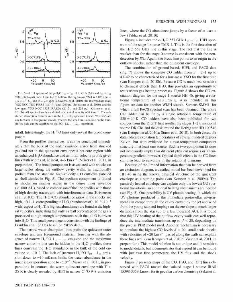
infall. Interestingly, the H218O lines only reveal the broad com-

ponent.From the profiles themselves, it can be concluded immedi-

ately that the bulk of the water emission arises from shockedgas and not in the quiescent envelope; a hot-core region withan enhanced H2O abundance and an infall velocity profile giveslines with widths of, at most, 4–5 km s�1 (Visser et al. 2011, inpreparation). The broad component is associated with shocks onlarge scales along the outflow cavity walls, as traditionallyprobed with the standard high-velocity CO outflows (labeledas shell shocks in Fig. 5). The medium component is linkedto shocks on smaller scales in the dense inner envelope(<1000 AU), based on comparison of the line profileswith thoseof high-density tracers and with interferometer data (Kristensenet al. 2010b). The H2O=CO abundance ratios in the shocks arehigh,∼0:1–1, corresponding to H2O abundances of∼10�5–10�4

with respect to H2. The highest abundances are found at the high-est velocities, indicating that only a small percentage of the gas isprocessed at high-enough temperatures such that all O is driveninto H2O. This small percentage is consistent with the findings ofFranklin et al. (2008) based on SWAS data.

The narrow water absorption lines probe the quiescent outerenvelope and any foreground material. Together with the ab-sence of narrow H2

18O 110 � 101 emission and the maximumnarrow emission that can be hidden in the H2O profiles, theselines constrain the H2O abundance in the bulk of the cold en-velope to ∼10�8. The lack of (narrow) H2

18O 202 � 111 emis-sion down to ∼10 mK rms limits the water abundance in theinner ice evaporation zone to <10�5 (Visser et al. 2011, in pre-paration). In contrast, the warm quiescent envelope with T >25 K is clearly revealed by HIFI in narrow C18O 9–8 emission

lines, where the CO abundance jumps by a factor of at least afew (Yıldız et al. 2010).

Figure 4 includes the o-H2O 557 GHz 110 � 101 HIFI spec-trum of the stage 1 source TMR-1. This is the first detection ofthe H2O 557 GHz line in this stage. The fact that the line isweaker than for the stage 0 source is consistent with the non-detection by ISO. Again, the broad line points to an origin in theoutflow shocks, rather than the quiescent envelope.

The combination of ground-based, HIFI, and PACS data(Fig. 7) allows the complete CO ladder from J ¼ 2–1 up to43–42 to be characterized for a low-mass YSO for the first time(van Kempen et al. 2010b). Because CO is much less sensitiveto chemical effects than H2O, this provides an opportunity totest various gas heating processes. Figure 8 shows the CO ex-citation diagram for the stage 1 source HH 46, giving a rota-tional temperature of 410� 25 K. Also included in thisfigure are data for another WISH source, Serpens SMM1, forwhich a full PACS spectral scan has been obtained. The entireCO ladder can be fit by a single rotational temperature of520� 20 K. CO ladders have also been published for twosources from the DIGIT first results, the stages 1–2 transitionalsource DK Cha and the disk around the Herbig star HD 100546(van Kempen et al. 2010a; Sturm et al. 2010). In both cases, thedata indicate excitation temperatures of several hundred degreesKelvin, but with evidence for a two-temperature-componentstructure in at least one source. Such a two-component fit doesnot necessarily imply two different physical regimes or a tem-perature gradient, however. Optical depth effects in the CO linescan also lead to curvature in the rotational diagrams.

Because of the limited information that can be derived froman excitation diagram, a detailed model has been developed forHH 46 using the known physical structure of the quiescentenvelope as a starting point (van Kempen et al. 2009d). Thepassively heated envelope can explain only the lowest CO rota-tional transitions, so additional heating mechanisms are needed(see Fig. 5). One possibility is UV photon heating, in which theUV photons produced in the immediate protostellar environ-ment can escape through the cavity carved by the jet and windfrom the young star and impinge on the envelope at much largerdistances from the star (up to a few thousand AU). It is foundthat this UV heating of the outflow cavity walls can well repro-duce the intermediate transitions up to J < 20, depending onthe precise PDR model used. Another mechanism is necessaryto populate the highest CO levels J > 20: small-scale shockswith velocities of ∼20 km s�1 pasted along the walls can explainthese lines well (van Kempen et al. 2010b; Visser et al. 2011, inpreparation). This model solution is not unique and is sensitiveto model details, but it demonstrates that a good fit can be foundwith just two free parameters: the UV flux and the shockvelocity.

Figure 7 presents maps of the CO, H2O, and [O I] lines ob-served with PACS toward the isolated stage 1 source IRAS15398-3359, known for its peculiar carbon chemistry (Sakai et al.

0

FIG. 6.—HIFI spectra of the p-H2O 111 � 000 1113 GHz (left) and 202 � 111988 GHz (right) lines. From top to bottom: the high-mass YSOW3 IRS5 (L ¼1:5 × 105 L⊙ and d ¼ 2:0 kpc) (Chavarría et al. 2010), the intermediate-massYSO NGC 7129 FIRS2 (430 L⊙ and 1260 pc) (Johnstone et al. 2010), and thelow-mass YSO NGC 1333 IRAS2A (20 L⊙ and 235 pc) (Kristensen et al.2010b). All spectra have been shifted to a central velocity of 0 km s�1. The red-shifted absorption features seen in the 111 � 000 spectrum toward W3 IRS5 aredue to water in foreground clouds, whereas the small emission line on the blue-shifted side can be ascribed to the SO2 139;5 � 128;4 transition.


2011 PASP, 123:138–170

2009). All lines are clearly extended in the outflow direction asmapped in lower-J CO lines (vanKempen et al. 2009a), confirm-ing their association with the shocks and outflow cavities.

The amount of cooling produced by each of the species can bequantified from the PACS data. In the central HH 46 spaxel, [O I]and OH dominate the cooling (at least 60% of the total cooling infar-infrared lines), followed by H2O (∼30%) and CO (∼10%).The total far-infrared line cooling of at least 2:4 × 10�2 L⊙ isconsistent with the kinetic luminosity found by vanKempen et al.(2009d) fromCOoutflowmaps and follows the relation found byGiannini et al. (2001) between these two quantities. The [O I]63 μm line is spectrally resolved with PACS and reveals a jetcomponent with velocities up to 170 km s�1 associated withthe blue- and redshifted outflow seen in optical atomic lines

in less extincted regions of the flow. This is the first time thatsuch a jet has been seen in a far-infrared line, providing a power-ful diagnostic of the “hidden jet” in the densest optically opaqueregions. OH is detected strongly on source, but not along the out-flow axis, in contrast with other species. Both the [O I] and OHemissions are ascribed to a dissociative shock caused by the jetimpacting on the inner dense (>106 cm�3) envelope; disk emis-sion is excluded by scaling the observed disk emission fromstage 2 sources to the distance of HH 46 (van Kempen et al.2010b). In dissociative shocks, OH is one of the first moleculesto reform after molecular dissociation, whereas the UV radiationfrom the shock and the high H=H2 ratio prevent effective H2Oformation in the postshock gas (Neufeld&Dalgarno 1989).OnceH2 is reformed, the heat of H2 formation maintains a temperature

FIG. 7.—PACS 5 × 5 spectral maps of the [O I] 3P 1 �3 P 2 63 μm (left), H2O 212 � 101 179 μm (middle) and CO J ¼ 16–15 163 μm lines (right) toward the low-massstage 1 YSO IRAS 15398-3359. All lines are extended along the outflow direction seen in the low-J CO map of van Kempen et al. (2009a).


2011 PASP, 123:138–170

plateau in the warm postshock gas in which significant H2O isproduced (Hollenbach & McKee 1989).

The OH chemistry has been further investigated byWampfleret al. (2010). The 163 μm line seen by PACS toward HH 46 wasobserved but not detected with HIFI. The upper limit implies aline width of at least 11 km s�1. Inspection of the PACS data forsix sources reveals a correlation between the OH and [O I] fluxes,which, together with the broad profiles, is consistent with pro-duction in (dissociative) shocks. The relative strengths of the var-iousOH far-infrared lines are remarkably constant from source tosource, indicating similar excitation conditions. Only the 119μmlines connecting with the ground state vary because they are af-fected by (foreground) absorption. Due to the lack of detectedquiescent OH (and H2O) emission in the HIFI spectra, no abun-dances in the envelope can yet be determined to test the modelpredictions of enhanced OH=H2O ratios due to X-rays.

The HDO=H2O ratio has been determined for the low-massprotostar NGC 1333 IRAS2A by Liu et al. (2010). Five HDOlines arising from levels ranging from 20 K up to 170 K havebeen observed using ground-based telescopes. The inner(>100 K) and outer (<100 K) HDO abundances with re-spect to H2 are well constrained to ð0:7–1:0Þ × 10�7 (3σ) andð0:1–1:8Þ × 10�9 (3σ), respectively. If the H2O and isotopologlines discussed previously can be associated with the same com-ponent as seen in HDO, the inferred limit on the warm H2Oabundance implies a HDO=H2O abundance higher than ∼1%in the inner envelope, consistent with the value found in thehot corino of IRAS16293 (∼3%; Parise et al. 2005b). Althoughabsolute abundances of HDO and H2O jump by more than oneorder of magnitude between the cold and warm envelopes, theHDO=H2O ratio in the outer cold envelope is found to have asimilar value to that of the inner part, ∼1–18%.

The detection of HDO lines in other low-mass protostellarsources has proven difficult from the ground, even under thebest weather conditions. Deep Herschel observations of high-frequency HDO lines coupled with deep H2

18O data are likelyneeded to pin down the cold HDO=H2O ratios. Alternatively,interferometric observations of the higher-excitation HDO lines,coupled with similar data of the H2

18O 313 � 220 203 GHz line(the only H2

18O line readily imaged from the ground; Jørgensen& van Dishoeck 2010a), can constrain the HDO=H2O ratio inthe warm gas in the innermost regions. Initial results byJørgensen & van Dishoeck (2010b) for the NGC 1333 IRAS4Bsystem indicate much lower values of <6 × 10�4 than thosecited previously for IRAS2A. This large difference is not yetunderstood.

Overall, it appears that the answer to the first question in§ 4,2,1 is that shocks dominate the observed water emissionin low-mass YSOs rather than the hot core. Both ice evaporationand high-temperature chemistry are likely important in produ-cing high water abundances in shocks. The answers to the othertwo questions await more data and analysis.

4.3. Outflows from Low-Mass Young Stellar Objects

4.3.1. Motivation

Deeply embedded protostars drive powerful molecular out-flows. These outflows extend over arcminute scales for nearbylow-mass objects and can be resolved spatially with Herschel.The brightest outflow knots are clearly separated, often by arc-minutes, from the dense protostellar envelopes targeted in thelow-mass subprogram (§ 4.2). Outflows exhibit a great diversityin their velocity, degree of collimation, opening angle, extent,and gas kinetic temperature (Bachiller & Tafalla 1999), raisingthe question of whether these characteristics can be linked to the

FIG. 8.—Diagram illustrating the CO excitation. The number of molecules in the upper level divided by its statistical weight is plotted versus rotational quantumnumber Ju. Left: Low-mass stage 1 YSO HH 46 (based on van Kempen et al. 2010b). Right: More luminous embedded-source SMM1 (Goicoechea et al. 2011, inpreparation). For the latter source, a complete PACS spectral scan has been obtained. For both sources, the fluxes from the central spaxel have been used. The dashedlines give the thermal distribution at the indicated temperatures. The hatched areas in the HH 46 diagram indicate the different physical processes thought to be re-sponsible for the CO emission. See the electronic edition of the PASP for a color version of this figure.


2011 PASP, 123:138–170

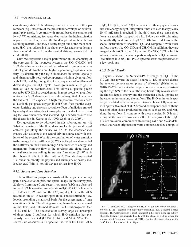
evolutionary state of the driving sources or whether other pa-rameters (e.g., structure of the protostellar envelope or environ-ment) play a role. In contrast with ground-based observations oflow-J CO transitions, Herschel data probe the high-excitationregions of the flow, where the hidden jet interacts with sur-rounding material, and they directly target one of the main cool-ants, H2O, thus addressing the shock physics and energetics as afunction of distance from the central driving source (Nisiniet al. 2000).

Outflows represent a major perturbation in the chemistry ofthe core gas. In the youngest systems, the SiO, CH3OH, andH2O abundances are increased by orders of magnitude as a re-sult of grain destruction and high-temperature gas-phase chem-istry. By determining the H2O abundances in several spatiallyand kinematically resolved components within a given outflowwith HIFI, and by doing this for a sequence of outflows ofdifferent ages, the H2O cycle—from grain mantle, to gas, tomantle—can be reconstructed. This allows a specific puzzleposed by ISO-LWS to be addressed; in most protostellar outflowregions, the H2O abundance is an order of magnitude lower thanthe value of 10�4 expected if high-temperature reactions driveall available gas-phase oxygen into H2O or if ice mantles evap-orate. Ionizing and photodissociative effects of radiation emittedby nearby dissociative shocks may play a critical role in explain-ing the lower-than-expected shocked H2O abundances (see alsothe discussion in Keene et al. 1997; Snell et al. 2005).

Key questions to be addressed in this subprogram are: (1)What is the nature of the flow: dense molecular jets or shockedambient gas along the cavity walls? Do the characteristicschange with distance to the central driving source and with evo-lution of the system? What is the contribution of water emissionto the energy lost in outflows? (2) What is the physical impact ofthe outflows on their surroundings? The transfer of energy andmomentum from the flow to the envelope and cloud plays acritical role in controlling future star formation. (3) What isthe chemical effect of the outflows? Can shock-generatedUV radiation modify the physics and chemistry of nearby mo-lecular gas? Why is not all oxygen driven into H2O?


The outflow subprogram consists of three parts: a surveypart, a line excitation part, and spatial maps. In the survey part,26 flows from stage 0 and stage 1 low-mass YSOs are observedin two H2O lines—the ground-state o-H2O 557 GHz line withHIFI down to ∼20 mK and the 179 μm p-H2O line with PACSto similar limits—in two hot spots (blue- and redshifted outflowlobes), providing a statistical basis for the assessment of timeevolution effects. The driving sources themselves are coveredin the low- and intermediate-mass YSO subprograms (see§§ 4.2 and 4.4). The line excitation survey targets a subsampleof three stage 0 outflows for which H2O emission has pre-viously been detected (L1157, L1448, and VLA1623). Thesesources are observed in 15 spectral lines with HIFI and PACS

(H2O, OH, [O I], and CO) to characterize their physical struc-ture and energy budget. Integration times are such that typically20–40 mK rms is reached. In the third part, these same threeflows are spatially mapped with HIFI down to ∼20 mK usingthe on-the-fly mode in the H2O 557 GHz line to determine thespatial distribution of shocked H2O and compare it with otheroutflow tracers like CO, SiO, and CH3OH. In addition, they areimaged with PACS in the 179 μm line. For NGC 2071, which isknown from Spitzer data to be particularly rich in H2O emission(Melnick et al. 2008), full PACS spectral scans are performed ata few positions.


Figure 9 shows the Herschel-PACS image of H2O in the179 μm line toward the stage 0 source L1157 obtained duringthe science demonstration phase of Herschel (Nisini et al.2010). PACS spectra at selected positions are included, illustrat-ing the high S/N of the data. The map beautifully reveals wherethe shocks deposit energy into the molecular cloud, lighting upthe water emission along the outflow. The H2O emission is spa-tially correlated with that of pure rotational lines of H2 observedwith Spitzer (Neufeld et al. 2009) and corresponds well with thepeaks of other shock-produced molecules such as SiO and NH3

along the outflow. In contrast with these species, H2O is alsostrong at the source position itself. The analysis of the H2O179 μm emission, combined with existing Odin and SWAS data,shows that water originates in warm compact shocked clumps of

FIG. 9.—Herschel-PACS image of the H2O 179 μm line toward the stage 0protostar L 1157, together with (spectrally unresolved) PACS spectra at threepositions. The water emission is most significant in hot spots along the outflowwhere the (rotating) jet interacts directly with the cloud, as well as toward theprotostar itself (based on Nisini et al. 2010). See the electronic edition of thePASP for a color version of this figure.


2011 PASP, 123:138–170

a few arcseconds in size, where the water abundance is of theorder of 10�4: i.e., close to that expected from high-temperaturechemistry. The total H2O cooling amounts to 23% of the totalfar-IR energy released in shocks estimated from the ISO-LWSdata (Giannini et al. 2001).

The PACS spectra contained in Figure 9 are spectrally un-resolved. HIFI spectra of H2O and CO at the B1 position inthe blue outflow lobe (see Fig. 9) have been presented and ana-lyzed by Lefloch et al. (2010) as part of CHESS, showing thatthe H2O abundance increases with shock velocity (see also § 4.2and Franklin et al. 2008). Codella et al. (2010) propose that thisreflects the two mechanisms for producing H2O: ice evaporationand high-temperature chemistry where the Oþ H2 and OHþH2 reactions become significant (see § 2.1 and Fig. 3), withthe latter reactions becoming more important at higher veloci-ties. The presence of NH3 (another grain surface product) seenby Codella et al. (2010) only at lower velocities is consistentwith this picture. The WISH data can test this proposed scenarioat many more outflow positions.

In summary, the limited data to date illustrate the potential ofwater to probe and image shock physics and chemistry along theoutflows.

4.4. Intermediate-Mass Young Stellar Objects

4.4.1. Motivation

Intermediate-mass YSOs with ∼102–104 L⊙ (stellar massesof a few to 10 M⊙) form the bridge between the low- andhigh-mass samples. In addition to covering a significant lumin-osity range between the two well-studied extremes, intermedi-ate-mass YSOs are interesting in their own right. For example,they are often found in clustered environments, so they can beused as laboratories for investigating high-mass cluster regionswhich are often more confused, due to their larger distances.Intermediate-mass YSOs may be in an interesting regime whenheating from the outside by radiation from neighboring stars issignificant compared with internal heating (Jørgensen et al.2006). This would result in a more extended warm zone anda different chemical structure of the envelope than that of theirlow- and high-mass counterparts. Also, emerging intermediate-mass YSOs have associated PDRs or reflection nebulae indicat-ing that not only shocks, but also UV photons, play a role inclearing the surroundings. Finally, they are the precursors ofHerbig Ae/Be stars, whose protoplanetary disks have been verywell studied (e.g., Meeus et al. 2001), but for which very little isknown about their formation history.

Key questions are therefore: (1) What is the structure of theenvelopes of intermediate-mass YSOs? Do they have a differenttemperature and chemistry structure compared with their low-and high-mass counterparts? Does the enhanced UV comparedwith the low-mass counterparts play a role? (2) How dointermediate-mass YSOs evolve? To what extent are the an-

swers to the questions in §§ 4.2, 4.3, 4.5 different for thesesources?


Although intermediate-mass YSOs are more energetic thantheir low-mass counterparts, they are not bright enough to ob-serve at the distances of their high-mass cousins. Surprisinglyfew nearby (<400 pc) candidates are known, so our team hasconducted an active search over the past years to identify a re-presentative sample to observe with HIFI. Six intermediate-mass YSOs with distances of <1 kpc have been selected fromthis sample, and a significant amount of complementary submil-limeter line and continuum observations have been obtained(e.g., Fuente et al. 2005b; Crimier et al. 2010). All of thesesources are still at the deeply embedded stage, comparable withstage 0 in the low-mass case. The Herschel line selection fol-lows the general criteria outlined previously, and the noise levelsare similar to those for the low-mass YSOs.


Observations of various water lines toward NGC 7129FIRS2 (430 L⊙, 1260 pc) are presented in Fich et al. (2010)and Johnstone et al. (2010), and the two lowest p-H2O linesdetected with HIFI are included in Figure 6. The line profilesare remarkably similar to those of the low-mass YSO NGC1333 IRAS2A, showing both a broad component (FWHM∼25 km s�1) due to shocks along the outflow cavity and a med-ium-broad component (FWHM ∼6 km s�1) associated withsmall-scale shocks in the inner dense envelope. Quantitativeanalysis of all the H2O and isotopolog lines observed for thisobject result in an outer-envelope (<100 K) abundance of waterof the order of ∼10�7, an order of magnitude higher than for thelow- and high-mass YSOs. Alternatively, both the high-J COand H2O lines seen with HIFI and PACS can be analyzed in asingle slab model with a temperature of ∼1000 K and density of∼107–108 cm�3, representative of a shock in the inner denseenvelope (Fich et al. 2010). This leads to a typical H2O=COabundance ratio of 0.2–0.5.

The results for this first source demonstrate that the obser-ving strategy for this subprogram is sound and that the datacan provide the quantitative information to answer the preced-ing questions, once more sources have been observed andanalyzed.

4.5. High-Mass Young Stellar Objects

4.5.1. Motivation

High-mass stars (>10 M⊙ and >104 L⊙), though few innumber, play a major role in the energy budget and shapingof the Galactic environment (e.g., Cesaroni et al. 2005). Theseare also the type of regions that dominate far-infrared observa-tions of starburst galaxies. Their formation is not at all well


2011 PASP, 123:138–170

understood, due to large distances, short timescales, and heavyextinction.

Recent results show that the embedded phase of the forma-tion of O and B stars can be divided empirically into severalclasses. The earliest stage are the massive prestellar cores,which are local temperature minima and density maxima andwhich represent the initial conditions. Their observational char-acteristics are large column densities, low temperatures, andabsence of outflow or maser activity. The next stage are thehigh-mass protostellar objects (HMPOs), where the central staris surrounded by a massive envelope with a centrally peakedtemperature and density distribution. HMPOs show signs ofactive star formation through outflows and/or masers. This sub-program distinguishes mid-IR-bright and mid-IR-quiet objectswith a boundary of 10 Jy at 12 μm. The next evolutionary phaseis represented by hot molecular cores, with large masses ofwarm and dense dust and gas and with high abundances of com-plex organic molecules evaporated off dust grains. Hot molecu-lar cores have regions of T > 100 K that are >0:1 pc in size.The final stages considered here are ultracompact H II regions(UC H II), where large pockets of ionized gas have developedbut are still confined to the star. UC H II sources have free-freeflux densities of more than a few millijanskys (for a distance of afew kiloparsecs) and sizes of 0.01–0.1 pc. As with the previouscategory, this criterion may imply a luminosity of >105 L⊙.The embedded phase ends when the ionized gas expands hydro-dynamically and disrupts the parental molecular cloud, pro-ducing a classical H II region. Although the evolutionary pathof high-mass YSOs likely runs through these different cate-gories, this is not yet as well established as for the case oflow-mass YSOs, and the physical structure and processes dom-inating each of these stages are not well characterized. Herschelobservations of water and related species will provide an impor-tant piece of this puzzle.

Abundant H2O has been observed with ISO, SWAS, andOdin toward the Orion and SgrB2 high-mass star-forming re-gions (e.g., Cernicharo et al. 2006; Polehampton et al. 2007;Persson et al. 2007). Toward other high-mass YSOs, copioushot gas phase H2O has been detected in absorption withISO-SWS (van Dishoeck & Helmich 1996; Boonman & vanDishoeck 2003) but not with ISO-LWS. SWAS data indicategenerally weak H2O 557 GHz emission (Snell et al. 2000). Ana-lysis of these data for selected high-mass star-forming regionsimplies sharp gradients in the water abundance, together withstrong excitation changes, but their origin is not yet well under-stood (Boonman et al. 2003; van der Tak et al. 2006). Moregenerally, the role of shocks and the relative importance ofshocks versus passive heating in the inner envelope duringthe high-mass evolution, either in isolated sources or in clusters,is currently unclear. In addition, the relation of these phases tothe H2O maser sources needs further study. Since individualhigh-mass sources are at much larger distances (typically afew kiloparsecs) than their low-mass counterparts and thus

spatially unresolved, disentangling the various processesrequires observations of numerous H2O transitions and highspectral resolution, as obtained within WISH using HIFIand PACS.

Key questions include: (1) What is the chemistry of the warmgas close to young high-mass stars in various evolutionarystages, specifically the distribution of H2O? (2) What is the re-lative importance of shocks vs. UV for the interaction of thestars with their environment? (3) What are the kinematics ofthe cold and warm gas close to young high-mass stars? (4) Whatare the effects of clustered star formation and feedback by pro-tostellar outflows on high-mass regions?


The WISH observations of H2O and related species covereach of the preceding phases in the formation of high-massstars. Pointed observations with HIFI are made of a sampleof four massive prestellar cores and 19 protostellar sources.The prestellar cores are taken from Carey et al. (1998) and Pillaiet al. (2006a) and are observed only in the 557 GHz line down to10 mK rms. The protostellar list consists of 10 HMPOs (fivemidinfrared bright and five quiet), four hot cores, and fiveUC H II regions. The sources are nearby (less than a few kilo-parsecs) and isolated, selected from surveys by Molinari et al.(1996), Sridharan et al. (2002), Wood & Churchwell (1989),and van der Tak et al. (2000b). The basic H2O line list is thesame as for the low-mass and intermediate-mass YSOs, but withadditional H2

18O and H217O lines added, because the main iso-

topic lines are very bright and highly optically thick. Absorptionlines of H2O at high frequencies against the optically thick con-tinuum can uniquely probe the kinematics of the protostellarenvironment (see § 2.2). Integration times are such that 50–150 mK rms is reached, depending on the line.

Full PACS spectral scans of all protostellar sources are takenand provide an unbiased overview of low- and high-excitationH2O lines (and thus the shocked ∼1000 K gas in the beam),together with OH, [O I], and CO at the position of the protostar,as well as spatial information on a 50″ scale. S/N >100 on thecontinuum are reached so that spectrally unresolved lines can bedetected. To characterize the effects of clustered star formationand feedback, including the chemistry and cooling rates of in-tracluster gas, HIFI mapping of the p-H2O 1113 GHz line com-bined with 13CO 10–9 plus PACS mapping of o-H2O 1670 and1717 GHz down to 300 mK rms is planned over a region of∼30 × 30 for six nearby cluster-forming clouds, where severalhot cores and UC H II regions are known to coexist in asmall area.


Figure 6 includes the lowest two p-H2O lines for the high-mass YSO W3 IRS5 (Chavarría et al. 2010). The profile of theexcited 202 � 111 line reveals the same broad and medium-broad


2011 PASP, 123:138–170

components as seen for their low- and intermediate-mass coun-terparts, but the profile of the ground-state line is clearly morecomplex. In addition to self-absorption and absorption of thecold envelope against the continuum, absorptions due to fore-ground clouds lying along the line of sight are seen at variousvelocities. Moreover, for line-rich sources, weak emission linesdue to species other than H2O are detected. The ability of HIFIto disentangle the different physical components is demon-strated by initial performance verification data on DR21(OH) (van der Tak et al. 2010). Using a slab model and assum-ing an o=p ratio of 3 (Lis et al. 2010), the broad component dueto the outflow is found to have an H2O abundance of afew ×10�6. Water is much less abundant in the foregroundcloud, where p-H2O has an abundance of 4 × 10�9. The outer-envelope abundance is even lower: a few ×10�10.

To investigate whether these abundances are typical of high-mass protostellar sources, Marseille et al. (2010) model fouradditional high-mass YSOs in the lowest two p-H2O lines com-bined with the ground-state p-H2

18O line. Due to the high spec-tral resolution, the envelope emission and absorption can becleanly separated from other physical components. Chavarríaet al. (2010) analyze a larger set of lines for W3 IRS5. Sincethe same modeling philosophy is used for all six sources, theinferred abundances can be directly compared. The outer-envel-ope water abundances are low in all cases but show a 2-order-of-magnitude variation from <5 × 10�10 to 4 × 10�8. The originfor these variations is not yet understood, since no correlation isfound with luminosity or evolutionary stage within this smallsample. For W3 IRS5, a jump in abundance in the inner enve-lope at T ≈ 100 K is inferred from the isotopolog lines, whichis the only indication so far of water emission from a hot core.

Broad emission profiles due to outflows associated with thehigh-mass protostars are commonly seen in the high-mass spec-tra, testifying to the importance of shocks. Moreover, the pres-ence of blueshifted absorption suggests expansion of the outerenvelope, rather than infall. Finally, the high S/N absorptiondata reveal cold clouds surrounding the protostellar envelopeat velocities offset by just a few kilometers per second, illustrat-ing the complexity of the protostellar environment and the un-ique ability of HIFI and water to detect this gas (Marseilleet al. 2010).

In summary, the available data on the first six sources showthat questions 1 and 3 in § 4.5.1 can be addressed quantitatively.Questions 2 and 4 require more data to answer.

4.6. Radiation Diagnostics

4.6.1. Motivation

The H2O chemistry can be strongly affected by high-energyradiation from YSOs, both UV and X-rays. For typical X-rayluminosities of 1028–1031 ergs s�1 appropriate for low-massYSOs, models show that the H2O abundance decreases by 2orders of magnitude or more in the inner envelope, where

the X-rays penetrate up to distances of ∼1000 AU (oneHerschel beam; Stäuber et al. 2006). UV and X-rays also affectthe chemistry in high-mass YSO envelopes, but to a differentdegree (Stäuber et al. 2004, 2005). H2O is destroyed not onlyby direct photodissociation but also by reactions with ionizedmolecules, so that it is important to understand their chemistryin relation to that of H2O (Fig. 3). Because H2O is not a uniquediagnostic of either UVor X-rays, independent diagnostics needto be observed. Small hydrides, especially OHþ, CH, CHþ, andSHþ, are particularly powerful in this regard (Stäuber et al.2005; Bruderer et al. 2010a). Recent 2D modeling has shownthat most of the emission from UV tracers originates in the out-flow walls, where their abundances are enhanced by orders ofmagnitude due to UV impinging on the walls of the outflowcavities leading to ionization, dissociation, and high-tempera-ture chemistry (Bruderer et al. 2009b, 2009a, 2010a).

Key questions are: (1) Can we establish the presence of UVand/or X-rays through chemistry in deeply embedded objects,where the UVor X-rays cannot be observed directly? If so, canwe quantify it? (2) How do protostellar UVand X-rays influencethe surroundings, both the temperature and the water chemistry?


Deep pointed observations with HIFI are made of lines ofseven hydrides that are related to the water network and are sen-sitive to either FUV or X-rays (or both) in two high-mass andone low-mass YSO down to 15 mK rms. Subsequently, a largersample of nine low-, intermediate-, and high-mass YSOs is sur-veyed in the lines of CH, CHþ, and OHþ. Lines of somehydrides are also obtained serendipitously with the mainH2O settings in the other subprograms. For example, theCH 536 GHz triplet is often obtained together with the o-H2

18O110 � 101 548 GHz line and the H2Oþ 111 � 000 1115 GHz linewith the p-H2O 111 � 000 1113 GHz line. Line frequencieshave been collected, and in some cases first predicted, byBruderer (2006).


An early surprise from allHerschel-HIFI KPs is the detectionof widespread H2Oþ absorption in a variety of Galactic sourcesincluding diffuse clouds, the envelopes of massive YSOs andoutflows (Gerin et al. 2010; Ossenkopf et al. 2010; Benz et al.2010; Bruderer et al. 2010b; Wyrowski et al. 2010b; Neufeldet al. 2010; Schilke et al. 2010; Gupta et al. 2010). H2Oþ

and OHþ lines are even seen in emission in Spectral and Photo-metric Imaging Receiver Fourier Transform Spectrometer spec-tra of the active galactic nucleus Mkr231 (van der Werf et al.2010). Model analyses point to an origin in low-density gas(<104 cm�3) with a low molecular fraction (i.e., a H2=H ratioof a few percent) to prevent H2Oþ from reacting rapidly with H2

to form H3Oþ. The low molecular fraction can be the result ofeither high UV or high X-ray fluxes.


2011 PASP, 123:138–170

Within WISH, deep integrations on two high-mass YSOs re-veal most of the targeted molecules, which is a vindication ofthe model predictions. CH, NH, OHþ, and H2Oþ are detectedtoward both W3 IRS5 and AFGL 2591 (Benz et al. 2010;Bruderer et al. 2010b). In addition, SHþ and H3Oþ are seentoward W3 and CHþ is seen toward AFGL 2591. Only SHand NHþ are not detected. H2Oþ, OHþ, and SHþ are new mo-lecules, with OHþ and SHþ only recently detected for the firsttime in ground-based observations by Wyrowski et al. (2010a)and Menten et al. (2011), respectively. Figure 10 contains a col-lection of spectra of hydrides most closely related to water.

The spectra show a surprising mix of absorption and emis-sion features. Three molecules, NH, OHþ, and H2Oþ, appear

primarily in absorption, either in diffuse foreground cloudsalong the line of sight, in blueshifted outflows, or (in somecases) in clouds close to the systemic velocity. For these mole-cules, the J ¼ 1 level lies at 47 K or higher. Limits on the ex-cited state lines give rotational temperatures <13 and <19 Kfor OHþ and H2Oþ, respectively. CH and SHþ, for which theJ ¼ 1 line lies at less than 26 K, are seen in emission, althoughCH has superposed absorption. The CHþ J ¼ 1–0 line occursmostly in absorption, but the 2–1 line is in emission in AFGL2591. For W3 IRS5, at least three H3Oþ lines from energylevels lying at a few hundred degrees Kelvin above groundare detected, which combined with ground-based data (Phillipset al. 1992) give a rotational temperature of 240� 40 K. Note

FIG. 10.—Collection of lines of hydrides related to the H2O chemistry detected toward the high-mass YSO W3 IRS5 (based on Benz et al. 2010). The dashed linesindicate the position of the main component at the LSR velocity of the protostellar envelope at �38:4 km s�1. For species with fine-structure components (OHþ andH2Oþ), the lengths of the vertical bars indicate the theoretical relative intensities. Note that strong OHþ and H2Oþ absorption occurs around V LSR ≈ 0 km s�1 in diffuseforeground clouds. The H2O line is 331 � 404 at 1894 GHz; H3Oþ is 420 � 321 at 1069 GHz. See the electronic edition of the PASP for a color version of this figure.


2011 PASP, 123:138–170

that all excitation temperatures are lower limits to the kinetictemperature of the gas, because the lines have high critical den-sities (>107 cm�3), resulting in subthermal excitation.

The observed range in line profiles and excitation conditionsimmediately indicates that the species originate in different partsof the YSO environment. The OHþ=H2Oþ abundance ratio of>1 for the blueshifted gas in both sources indicates low-densityand high-UV fields (Gerin et al. 2010), as expected along thecavity walls at large distances from the source. The CH, CHþ,and H3Oþ emission lines must originate closer to the protostar,at densities >106 cm�3 (Bruderer et al. 2010b). Their abun-dances are roughly consistent with the 2D photochemical mod-els, in which high-temperature chemistry and high UV fluxesboost their abundances along the outflow walls (Bruderer et al.2009a, 2010a). The UV field is enhanced by at least 4 orders ofmagnitude compared with the general interstellar radiation fieldin these regions.

Because the H2Oþ ground-state line occurs close to that ofp-H2O, observations of both species are available for a largesample of high-mass protostars within WISH. Using alsoH2

18O data, Wyrowski et al. (2010b) provide column densitiesfor both species for all components along 10 lines of sight.H2Oþ is always in absorption, even when H2O is seen inemission. Consistent with the preceding scenario, the highestH2Oþ column densities are found for the outflow components.Overall, H2Oþ=H2O ratios range from 0.01 to>1, with the low-er values found in the dense protostellar envelopes and the lar-ger values found in diffuse foreground clouds and outflows.

In summary,most of the targeted hydrides are readily detectedand they appear to be even more abundant and widespread thanexpected prior to Herschel. When associated with protostars,they trace regions of high temperatures and enhanced UV fluxes,such as those found along cavity outflowwalls. However, the factthat some hydrides are seen in absorption whereas others appearin emission is not yet fully understood.

4.7. Circumstellar Disks

4.7.1. Motivation

A fraction of the gas and dust from the protostellar envelopeends up in a rotating disk around the pre–main-sequence star(≤10 Myr), thereby providing the basic material from whichplanetary systems can be formed. Recent observations and mod-eling have shown that many young disks have a strongly flaringstructure in which the surface layers are exposed to intenseultraviolet radiation from the star. This results in a highlylayered structure with a hot top layer that is mostly atomic,due to rapid photodissociation; an intermediate warm layer withan active chemistry and that is responsible for most of the ob-served molecular emission; and a cold, dense midplane layerwhere most species are frozen out onto grains (e.g., Aikawa et al.2002; Bergin et al. 2007).

A major question in disk-evolution and planet-formation stu-dies is the amount of grain growth and vertical mixing as a func-tion of radial position and time. In the static models describedpreviously, little gas-phase H2O is expected in the outer disk,with most of it frozen out as H2O ice in the midplane. However,if the H2O ice is regularly circulated to the warmer upper layers,the gas-phase H2O abundance increases by orders of magnitude(Dominik et al. 2005). This in turn affects the gas temperatureand the abundances of other species, including its photodisso-ciation products OH and O. Indeed, analysis of CO observationsshows that significant gaseous CO is present at temperaturesbelow that for freeze-out (e.g., Dartois et al. 2003). Both photo-desorption of ices and rapid vertical mixing combined witha steep vertical temperature gradient and grain growth have beeninvoked to explain this (Aikawa 2007; Öberg et al. 2007;Hersant et al. 2009).

HIFI observations are uniquely suited to constrain verticalmixing models, because H2O is the major ice reservoir andits line emission is particularly sensitive to temperature. HIFIthus probes the cold H2O gas reservoir in the outer (>30 AU)part of disks. These observations are therefore highly comple-mentary to Spitzer detections of hot H2O lines that originate inthe inner few AU of disks (Salyk et al. 2008; Carr & Najita2008). Key questions are: (1) What do H2O observations of cir-cumstellar disks tell us about grain growth and the importanceof vertical mixing from the cold midplane to the warm surfacelayers where ices photodesorb or thermally vaporate? (2) Whatis the relative importance of photodissociation and desorption?(3) What are the implications of the Herschel observations ofthe cold water reservoir in disks for the transport of water tothe inner planet-forming zones of disks?


Deep integrations down to a ∼1:5 mK rms in 0:5 km s�1 binare performed for the o-H2O 557 GHz line in four targets(TW Hya, DM Tau, LkCa15, and MWC 480) and down to∼4 mK rms for the p-H2O 1113 GHz line in two targets(TW Hya and DM Tau). The primary aim of these very deepintegrations is to put stringent limits on the cold water reservoir.Shorter integrations down to 10 mK rms in the 557 GHz line areperformed for eight additional targets to determine whether thefour deep targets are unusual in their H2O emission. The excitedH2O 312 � 303 1097 GHz and CO J ¼ 10� 9 lines are ob-served in two sources to probe the warmer H2O reservoir withHIFI. Sources have been selected to be clean from sur-rounding cloud emission in single-dish observations (e.g.,Thi et al. 2001).


Deep integrations on the DM Tau disk show a tentative de-tection of the o-H2O line with a peak temperature of TMB ¼2:7 mK and a width of 5:6 km s�1 (Bergin et al. 2010b).


2011 PASP, 123:138–170

Regardless of the reality of this detection and the uncertainty inthe collisional rate coefficients, the inferred column density is afactor of 20–130 weaker than that predicted by a simple modelin which gaseous water is produced by photodesorption of icygrains in the UV illuminated regions of the disk (Dominik et al.2005). The most plausible implication of this lack of watervapor is that more than 95–99% of the water ice is lockedup in large coagulated grains that have settled to the midplaneand are not cycled back up to the higher disk layers. Thus, thedeep HIFI data can directly address the key questions of thissubprogram, even without actual detections.

5. DISCUSSION

Although less than 10% of the WISH data have been ana-lyzed to date, several general trends are emerging.

5.1. Trends with Evolutionary Stage

The development of the spectral features with evolutionaryphase is illustrated by Figure 4 for low-mass sources. Wateremission is not detected from cold dense cores prior to star for-mation, down to very low levels. The implication is that most ofthe water is frozen out as ice on dust grains in the densest re-gions with, at most, a small layer of water vapor due to photo-desorption of ice in the outer regions of the core. As soon as theprotostar turns on in the center, however, prominent H2O linesappear. One of the main surprises for the low-mass YSOs is thatthis emission has broad profiles, even for H2

18O, indicating anorigin in shocked gas. This association with outflows is directlyrevealed by imaging of the water line (Fig. 9). H2O abundancesin the outflow are high, of the order of 10�5 � 10�4 (assuming aCO=H2 abundance ratio of 10�4), increasing with higher velo-city. In contrast, quiescent envelope abundances, as derivedfrom narrow absorption features and the lack of narrow H2

18Oemission, are low, of the order of 10�8.

The last evolutionary stage of protoplanetary disks when theenvelope has dissipated again shows little H2O emission downto very low levels (Fig. 4). This is the first time that the coldwater reservoir in the outer regions of disks has been probed.The lack of emission implies that the upper layers of this diskare surprisingly dry, both in the gas and in the solid phases.About 95–99% of the water ice appears to be contained in largeicy grains in the disk midplane, which are not circled back up tohigher layers. If confirmed by observations of additionalsources, this may have profound implications for our under-standing of the chemistry and physics of the outer disks. Onthe other hand, lines of warm and hot water have been detectedin other disks with Spitzer (Pontoppidan et al. 2010) and withPACS (Sturm et al. 2010), although the latter detection needsconfirmation. Tying these data together should provide a nearlycomplete view of the distribution of water vapor from the innerto the outer disk.

For all of these stages, the availability of data on both o-H2Oand p-H2O indicates that the low water abundance is robust andindependent of any o=p ratio of water. The overall emergingpicture is therefore that most water is formed on grains inthe molecular cloud and prestellar core phases, is present mostlyas ice in the quiescent envelope, and is likely transported in thisform into the outer part of young disks without further evapo-ration, consistent with evolutionary models by Visser et al.(2011, in preparation).

5.2. Trends with Luminosity

Figure 6 illustrates the trend with luminosity for the em-bedded protostellar evolution stage. An initial conclusion is thatthe line profiles are remarkably similar in spite of the 4-order-of-magnitude range in luminosity. All profiles show a broad(FWHM 25–40 km s�1) component due to the shocks alongthe outflow cavity walls on scales >1000 AU (shell shocks)and a medium-broad (FWHM 5–10 km s�1) component as-cribed to shocks caused by the interaction of jets and winds withthe inner dense (>106 cm�3) envelope on scales <1000 AU.Thus, the processes by which the jets and winds that arelaunched close to the star interact with their environment areapparently similar across a wide range of masses and luminos-ities. The H2O medium-broad profiles clearly have larger linewidths than those of other high-density envelope tracers such asHCOþ 4–3 and CS 7–6, but generally agree with the profiles ofother grain surface products such as CH3OH.

For low- and intermediate-mass YSOs, the outflows domi-nate the H2O emission, whereas for high-mass YSOs, narrowerlines from the passively heated envelope become more promi-nent, especially for H2

18O and H217O. Inferred outer-envelope

abundances based on the isotopolog data and narrow absorptionfeatures vary between 10�8 and 10�10 with no obvious trendsacross luminosity or evolutionary stage, except for a potentiallyhigher value for one intermediate-mass source. These low abun-dances thus confirm the earlier SWAS conclusions, but can sig-nificantly refine them because of the availability of more linesfrom both o- and p-H2O, allowing more accurate determina-tions. Because of the dominance of outflow emission, it is moredifficult than expected to put firm constraints on the inner quies-cent hot-core water abundances. Generally, the stirred-up innerregion probed by the medium-broad component overwhelmsany hot-core emission, even though this warm quiescent gasis clearly seen in, for example, C18O J ¼ 9–8 or 10–9 emission.Simultaneous analysis of these CO high-J data with the H2Olines may help to further disentangle the components. Indeed,the coverage of the entire CO ladder up to J ¼ 44 with all threeinstruments on Herschel will soon become one of the most im-portant diagnostics to characterize the physical processes in awide variety of sources.

The PACS and HIFI observations of high-J CO, H2O, and[O I] illustrate the need for the development of multidimensionalmodels that include UV photon and shock heating along the


2011 PASP, 123:138–170

cavity walls for both low- and high-mass sources. This need isstrengthened by the detection of various hydrides enhanced byUV radiation, including OHþ, H2Oþ, SHþ, CH, and CHþ. In-itial quantitative estimates of the total far-infrared line emissionindicate that H2O is not the major coolant of the gas, even in thedensest (>106 cm�3) regions, but this needs to be confirmed byobservational data at more positions, both on and off source.[O I] and OH have higher luminosities and appear to trace adissociative shock in the densest inner part.

5.3. Water Chemistry

The Herschel data demonstrate that all three chemical net-works illustrated in Figure 3 are important in star-forming re-gions. Solid-state chemistry dominates in the coldest regions, asevidenced by the absence of H2O line emission from cold pre-stellar cores and the low gaseous water abundances in the outerprotostellar envelopes. Most of the water is in the form of iceformed through the reactions illustrated in the bottom part ofFigure 3. The tiny amounts of water gas detected with HIFIeither result from nonthermal desorption of water ice, or fromgas-phase ion-molecule reactions, or from a combination ofboth. If the absorption of H2O gas toward the prestellar coreL1544 is confirmed, this first direct detection of water vaporin a quiescent dark cloud will allow a quantitative test of thesechemical models. Similarly, a thorough analysis of the abun-dance structure of H2O gas and ice for those protostellar enve-lopes where both species are detected can test key aspects of thecold chemistry. Eventually, fully coupled time-dependent gas-grain chemistry models should include the new solid-state lab-oratory data on water ice formation. Such models can then alsobe used to interpret the puzzling HDO=H2O abundance ratiosfound in different regions.

The detection of all the hydrides involved in the ion-moleculescheme leading to water—OHþ, H2Oþ, H3Oþ, HCOþ, andOH—will be one of the lasting legacies of theHerschelmission.While these species have been part of the reaction networks fordecades, the ease with which rapidly reacting ions such as OHþ

and H2Oþ are detected has surprised even the astrochemists.Since all key reaction rates involved are well understood, theabundance ratios can be used to probe the physics of the regionsin which they are found, such as high-UV fields and low densi-ties. The final clue to the basic oxygen gas-phase chemistry net-workwill be provided by deep searches forO2, which are plannedfor some of the WISH sources in other key programs.

The bright water emission from protostars is dominated byC-type shocks where the temperature rises to a few thousanddegrees Kelvin. The high-quality line profiles may allow thetwo chemical regimes to be separated: sputtering of icy mantlesand high-temperature chemistry. Whether all available oxygenis driven into water at the highest temperatures and velocities isstill an open question. OH=H2O ratios derived from velocity-resolved OH line profiles could form a powerful test of theneutral-neutral reactions. If the contribution from dissociative

J-type shocks can be cleanly separated, as appears to be thecase for HH 46, the observed O/OH abundance ratios wouldprovide a further test of the high-temperature gas-phase reactionnetworks, but now under conditions with much higher H=H2

ratios in the presence of UV radiation.Finally, all three chemical networks play a role in the water

chemistry in disks, with high-temperature chemistry dominatingin the inner disk and ice chemistry dominating in the outer disk.Here, Herschel teaches us another lesson: the importance ofcoupling the water chemistry with the dynamics and physicalevolution of the disks—in particular, the growth and settlingof the icy grains to the midplane.

6. CONCLUSIONS

The goal of theWISH program is to usewater and related spe-cies as physical and chemical probes of star-forming regions overa range of luminosities and evolutionary stages. The initial resultspresented in § 4 and discussed in § 5 demonstrate thatmany of thequestions asked in the individual subprograms can indeed be ad-dressed by the WISH data, due to the combination of excellentsensitivity, fully resolved line profiles, and spatial information,thereby validating the observational strategy. Initial surprises in-clude a near absence of gaseous water in prestellar cores anddisks, the dominance of shocks rather than hot cores in control-ling the bright water emission from protostars, and the detectionof all of the ions and hydrides involved in the water chemistryschemes. For prestellar cores our observations are in agreementwithmodels that suggest near total freeze-out of water in the formof ice, whereas in disks the inferred water abundance is at levelssignificantly lower than predicted. So far, water has not yet beenfound to be the major coolant in any of these regions. All remain-ing observations are expected to be taken within the next year.Quantitative analysis will require the further development ofmultidimensional models of protostellar envelopes, outflows,and disks. Together with the results from related Herschel keyprograms, they will greatly enhance our understanding of waterin the Galactic interstellar medium and solar system andwill pro-vide a true legacy to follow the water trail from the most diffusegas to dense cores and disks—and eventually comets and planetsin our own solar system.

The authors are grateful to the HIFI project scientist, XanderTielens, for helping to ensure the powerful HIFI capabilities forwater observations and for his encouragements over the last de-cade. They salute the HIFI and PACS instrument builders forproviding two superb scientific instruments, and they are muchindebted to the laboratory and theoretical chemistry groups forproviding the necessary molecular data to analyze and interpretthe water data. They thank the referee, David Hollenbach, forhis constructive comments on the manuscript, Laurent Wiesen-feld for helpful discussions on the H2O� H2 collisional ratecoefficients, and many funding agencies for their financialsupport. HIFI has been designed and built by a consortium


2011 PASP, 123:138–170

of institutes and university departments from across Europe,Canada, and the United States under the leadership of SRONNetherlands Institute for Space Research (Groningen, The Neth-erlands) and with major contributions from Germany, France,and the United States. Consortium members are Canada:CSA and University of Waterloo; France: CESR, LAB,LERMA, and IRAM; Germany: KOSMA, MPIfR, and MPS;Ireland: NUI Maynooth; Italy: ASI, IFSI-INAF, and Osservator-io Astrofisico di Arcetri-INAF; Netherlands: SRON and TUD;Poland: CAMK and CBK; Spain: Observatorio AstronómicoNacional (IGN) and Centro de Astrobiología (CSIC-INTA).

Sweden: Chalmers University of Technology-MC2, RSS &GARD, Onsala Space Observatory, Swedish National SpaceBoard, and Stockholm University—Stockholm Observatory;Switzerland: ETH Zurich and FHNW; United States: CaliforniaInstitute of Technology, Jet Propulsion Laboratory, and NHSC.HCSS/HSpot/HIPE are joint developments by the HerschelScience Ground Segment Consortium, consisting of ESA, theNASA Herschel Science Center, and the Heterodyne Instrumentfor the Far-Infrared (HIFI), Photoconducting Array Camera andSpectrometer (PACS) and Spectral and Photometric ImagingReceiver (SPIRE) consortia.

REFERENCES

Aikawa, Y. 2007, ApJ, 656, L93Aikawa, Y., Herbst, E., Roberts, H., & Caselli, P. 2005, ApJ, 620,330

Aikawa, Y., van Zadelhoff, G. J., van Dishoeck, E. F., & Herbst, E.2002, A&A, 386, 622

Aikawa, Y., Wakelam, V., Garrod, R. T., & Herbst, E. 2008, ApJ,674, 984

André, P., & Montmerle, T. 1994, ApJ, 420, 837André, P., Ward-Thompson, D., & Barsony, M. 2000, in Protostars andPlanets IV, ed. V. Mannings, A. P. Boss, & S. S. Russell (Tucson:Univ. of Arizona), 59

Atkinson, R., Baulch, D., Cox, R., Crowley, J., Hampson, R., & Hynes,R. 2004, Atmos. Chem. Phys., 4, 1461

Bachiller, R., Codella, C., Colomer, F., Liechti, S., & Walmsley, C. M.1998, A&A, 335, 266

Bachiller, R., & Tafalla, M. 1999, The Origin of Stars and PlanetarySystems, ed. C. J. Lada, & N. D. Kylafis (NATO ASI Ser. C, 540;Dordrecht: Kluwer), 227

Beltrán, M. T., Cesaroni, R., Neri, R., Codella, C., Furuya, R. S., Testi,L., & Olmi, L. 2005, A&A, 435, 901

Benz, A. O., Stäuber, P., Bourke, T. L., van der Tak, F. F. S.,van Dishoeck, E. F., & Jørgensen, J. K. 2007, A&A, 475, 549

Benz, A. O., et al. 2010, A&A, 521, L35Bergin, E. A., Aikawa, Y., Blake, G. A., & van Dishoeck, E. F. 2007, inProtostars and Planets V, ed. B. Reipurth, D. Jewitt, & K. Keil(Tucson: Univ. of Arizona), 751

Bergin, E. A., Alves, J., Huard, T., & Lada, C. J. 2002, ApJ, 570, L101Bergin, E. A., & Snell, R. L. 2002, ApJ, 581, L105Bergin, E. A., & Tafalla, M. 2007, ARA&A, 45, 339Bergin, E. A., et al. 2000, ApJ, 539, L129———. 2010a, A&A, 521, L20———. 2010b, A&A, 521, L33Beuther, H., Schilke, P., Gueth, F., McCaughrean, M., Andersen, M.,Sridharan, T. K., & Menten, K. M. 2002a, A&A, 387, 931

Beuther, H., Schilke, P., Menten, K. M., Motte, F., Sridharan, T. K., &Wyrowski, F. 2002b, ApJ, 566, 945

Beuther, H., Walsh, A. J., Thorwirth, S., Zhang, Q., Hunter, T. R.,Megeath, S. T., & Menten, K. M. 2008, A&A, 481, 169

Beuther, H., Zhang, Q., Bergin, E. A., Sridharan, T. K., Hunter, T. R., &Leurini, S. 2007, A&A, 468, 1045

Bjerkeli, P., et al. 2009, A&A, 507, 1455Bockelée-Morvan, D., et al. 1998, Icarus, 133, 147Boogert, A. C. A., et al. 2008, ApJ, 678, 985

Boonman, A. M. S., Doty, S. D., van Dishoeck, E. F., Bergin, E. A.,Melnick, G. J., Wright, C. M., & Stark, R. 2003a, A&A, 406,937

Boonman, A. M. S., & van Dishoeck, E. F. 2003b, A&A, 403, 1003Brinch, C., Crapsi, A., Hogerheijde, M. R., & Jørgensen, J. K. 2007,

A&A, 461, 1037Brinch, C., & Hogerheijde, M. R. 2010, A&A, 523, A25Bronfman, L., Nyman, L., & May, J. 1996, A&AS, 115, 81Bruderer, S. 2006, M.S. thesis, ETH Zurich (Switzerland)Bruderer, S., Benz, A. O., Doty, S. D., van Dishoeck, E. F., & Bourke,

T. L. 2009a, ApJ, 700, 872Bruderer, S., Benz, A. O., Stäuber, P., & Doty, S. D. 2010a, ApJ,

720, 1432Bruderer, S., Doty, S. D., & Benz, A. O 2009b, ApJS, 183, 179Bruderer, S., et al. 2010b, A&A, 521, L44Butner, H. M., Evans, N. J., II, Harvey, P. M., Mundy, L. G., Natta, A.,

& Randich, M. S. 1990, ApJ, 364, 164Butner, H. M., Evans, N. J., II, Lester, D. F., Levreault, R. M., & Strom,

S. E. 1991, ApJ, 376, 636Carey, S. J., Clark, F. O., Egan, M. P., Price, S. D., Shipman, R. F., &

Kuchar, T. A. 1998, ApJ, 508, 721Carr, J. S., & Najita, J. R. 2008, Science, 319, 1504Caselli, P., Walmsley, C. M., Tafalla, M., Dore, L., & Myers, P. C.

1999, ApJ, 523, L165Caselli, P., Walmsley, C. M., Zucconi, A., Tafalla, M., Dore, L., &

Myers, P. C. 2002, ApJ, 565, 331Caselli, P., et al. 2010, A&A, 521, L29Ceccarelli, C., Castets, A., Caux, E., Hollenbach, D., Loinard, L.,

Molinari, S., & Tielens, A. G. G. M. 2000a, A&A, 355, 1129Ceccarelli, C., Hollenbach, D. J., & Tielens, A. G. G. M. 1996, ApJ,

471, 400Ceccarelli, C., Loinard, L., Castets, A., Tielens, A. G. G. M., & Caux,

E. 2000b, A&A, 357, L9Ceccarelli, C., et al. 1999, A&A, 342, L21———. 2010, A&A, 521, L22Cernicharo, J., & Crovisier, J. 2005, Space Sc. Rev., 119, 29Cernicharo, J., Thum, C., Hein, H., John, D., Garcia, P., & Mattioco, F.

1990, A&A, 231, L15Cernicharo, J, et al. 2006, ApJ, 649, L33Cesaroni, R., Hofner, P., Walmsley, C. M., & Churchwell, E. 1998,

A&A, 331, 709Cesaroni, R., Neri, R., Olmi, L., Testi, L., Walmsley, C. M., & Hofner,

P. 2005, A&A, 434, 1039


2011 PASP, 123:138–170

Chandler, C. J., Brogan, C. L., Shirley, Y. L., & Loinard, L. 2005, ApJ,632, 371

Charnley, S. B. 1997, ApJ, 481, 396Chavarría, L., et al. 2010, A&A, 521, L37Chen, J., Evans, N. J., Lee, J., & Bourke, T. L. 2009, ApJ, 705,

1160Chen, X., Launhardt, R., Bourke, T. L., Henning, T., & Barnes, P. J.

2008, ApJ, 683, 862Cheung, A. C., Rank, D. M., & Townes, C. H. 1969, Nature, 221, 626Codella, C., et al. 2010, A&A, 518, L112Crapsi, A., Caselli, P., Walmsley, C. M., Myers, P. C., Tafalla, M., Lee,

C. W., & Bourke, T. L. 2005, ApJ, 619, 379Crapsi, A., van Dishoeck, E. F., Hogerheijde, M. R., Pontoppidan,

K. M., & Dullemond, C. P. 2008, A&A, 486, 245Crimier, N., Ceccarelli, C., Maret, S., Bottinelli, S., Caux, E., Kahane,

C., Lis, D. C., & Olofsson, J. 2010, A&A, 519, A65Cuppen, H. M., Ioppolo, S., Romanzin, C., & Linnartz, H. 2010, Chem.

Phys., 12, 12077Dalgarno, A., & Black, J. H. 1976, Rep. Prog. Phys., 39, 573Daniel, F., Dubernet, M., Pacaud, F., & Grosjean, A. 2010, A&A,

517, A13Dartois, E., Thi, W., Geballe, T. R., Deboffle, D., d’Hendecourt, L., &

van Dishoeck, E. 2003, A&A, 399, 1009De Buizer, J. M., & Minier, V. 2005, ApJ, 628, L151de Geus, E. J., Bronfman, L., & Thaddeus, P. 1990, A&A, 231, 137de Graauw, T., et al. 2010, A&A, 518, L6Dick, M., Drouin, B., & Pearson, J. 2010, Phys. Rev., A, 81Di Francesco, J., Johnstone, D., Kirk, H., MacKenzie, T., &

Ledwosinska, E. 2008, ApJS, 175, 277Dominik, C., Ceccarelli, C., Hollenbach, D., & Kaufman, M. 2005,

ApJ, 635, L85Doty, S. D., & Neufeld, D. A. 1997, ApJ, 489, 122Doty, S. D., Schöier, F. L., & van Dishoeck, E. F. 2004, A&A,

418, 1021Doty, S. D., van Dishoeck, E. F., & Tan, J. C. 2006, A&A, 454, L5Doty, S. D., van Dishoeck, E. F., van der Tak, F. F. S., & Boonman, A.

M. S. 2002, A&A, 389, 446Dubernet, M., Daniel, F., Grosjean, A., & Lin, C. Y. 2009, A&A,

497, 911Dubernet, M., et al. 2006, A&A, 460, 323Dulieu, F., Amiaud, L., Congiu, E., Fillion, J., Matar, E., Momeni, A.,

Pirronello, V., & Lemaire, J. L. 2010, A&A, 512, A30Dullemond, C. P., & Dominik, C. 2004, A&A, 417, 159Dzib, S., Loinard, L., Mioduszewski, A. J., Boden, A. F., Rodríguez, L.

F., & Torres, R. M. 2010, ApJ, 718, 610Eiroa, C., Palacios, J., & Casali, M. M. 1998, A&A, 335, 243Elitzur, M., & Watson, W. D. 1978, ApJ, 222, L141Evans, N. J., et al. 2009, ApJS, 181, 321Evans, N. J., II, et al. 2003, PASP, 115, 965Fich, M., et al. 2010, A&A, 518, L86Franklin, J., Snell, R. L., Kaufman, M. J., Melnick, G. J., Neufeld,

D. A., Hollenbach, D. J., & Bergin, E. A. 2008, ApJ, 674, 1015Fraser, H. J., Collings, M. P., McCoustra, M. R. S., & Williams, D. A.

2001, MNRAS, 327, 1165Froebrich, D. 2005, ApJS, 156, 169Fuente, A., Neri, R., & Caselli, P. 2005a, A&A, 444, 481Fuente, A., Rizzo, J. R., Caselli, P., Bachiller, R., & Henkel, C. 2005b,

A&A, 433, 535

Garay, G., Brooks, K. J., Mardones, D., Norris, R. P., & Burton, M. G.2002, ApJ, 579, 678

Gensheimer, P. D., Mauersberger, R., & Wilson, T. L. 1996, A&A,314, 281

Gerin, M., et al. 2010, A&A, 518, L110Giannini, T., McCoey, C., Nisini, B., Cabrit, S., Caratti o Garatti, A.,

Calzoletti, L., & Flower, D. R. 2006, A&A, 459, 821Giannini, T., Nisini, B., & Lorenzetti, D. 2001, ApJ, 555, 40Giannini, T., et al. 2005, A&A, 433, 941Gibb, E. L., Whittet, D. C. B., Boogert, A. C. A., & Tielens,

A. G. G. M. 2004b, ApJS, 151, 35Gibb, A. G., Wyrowski, F., & Mundy, L. G. 2004a, ApJ, 616,

301Goldsmith, P. F., & Langer, W. D. 1978, ApJ, 222, 881Green, S., Maluendes, S., & McLean, A. D. 1993, ApJS, 85, 181Gullixson, C., Gehrz, R. D., Hackwell, J. A., Grasdalen, G. L., &

Castelaz, M. 1983, ApJS, 53, 413Gupta, H., et al. 2010, A&A, 521, L47Gustafsson, M., Ravkilde, T., Kristensen, L. E., Cabrit, S., Field, D., &

Pineau Des Foêts, G. 2010, A&A, 513, A5Hachisuka, K., et al. 2006, ApJ, 645, 337Hartogh, P., et al. 2010, A&A, 518, L150Harwit, M., Neufeld, D. A., Melnick, G. J., & Kaufman, M. J. 1998,

ApJ, 497, L105Helmich, F. P., et al. 1996, A&A, 315, L173Herbst, E., & Klemperer, W. 1973, ApJ, 185, 505Herbst, E., & van Dishoeck, E. F. 2009, ARA&A, 47, 427Hersant, F., Wakelam, V., Dutrey, A., Guilloteau, S., & Herbst, E. 2009,

A&A, 493, L49Hirota, T., et al. 2008, PASJ, 60, 37Hjalmarson, Å, et al. 2003, A&A, 402, L39Hogerheijde, M. R., van Dishoeck, E. F., Blake, G. A., & van

Langevelde, H. J. 1997, ApJ, 489, 293Hogerheijde, M. R., van Dishoeck, E. F., Salverda, J. M., & Blake,

G. A. 1999, ApJ, 513, 350Hogerheijde, M. R., & van der Tak, F. F. S. 2000, A&A, 362,

697Hollenbach, D., Kaufman, M. J., Bergin, E. A., & Melnick, G. J. 2009,

ApJ, 690, 1497Hollenbach, D., & McKee, C. F. 1989, ApJ, 342, 306Hübers, H. W., Evenson, K. M., Hill, C., & Brown, J. M. 2009, J.

Chem. Phys., 131, 034311Hunter, T. R., Brogan, C. L., Indebetouw, R., & Cyganowski, C. J.

2008, ApJ, 680, 1271Ioppolo, S., Cuppen, H. M., Romanzin, C., van Dishoeck, E. F., &

Linnartz, H. 2008, ApJ, 686, 1474———. 2010, Phys. Chem. Chem. Phys., 12, 12065Ivezić, Z., & Elitzur, M. 1997, MNRAS, 287, 799Jacq, T., Walmsley, C. M., Henkel, C., Baudry, A., Mauersberger, R., &

Jewell, P. R. 1990, A&A, 228, 447Johnstone, D., Fich, M., Mitchell, G. F., & Moriarty-Schieven, G.

2001, ApJ, 559, 307Johnstone, D., et al. 2010, A&A, 521, L41Jørgensen, J. K. 2004, A&A, 424, 589Jørgensen, J. K., Bourke, T. L., Myers, P. C., Schöier, F. L., van

Dishoeck, E. F., & Wilner, D. J. 2005a, ApJ, 632, 973Jørgensen, J. K., Johnstone, D., van Dishoeck, E. F., & Doty, S. D.

2006, A&A, 449, 609


2011 PASP, 123:138–170

Jørgensen, J. K., Schöier, F. L., & van Dishoeck, E. F. 2002, A&A,389, 908

———. 2004, A&A, 416, 603———. 2005b, A&A, 437, 501Jørgensen, J. K., & van Dishoeck, E. F. 2010a, ApJ, 710, L72———. 2010b, ApJ, 725, L172Jørgensen, J. K., van Dishoeck, E. F., Visser, R., Bourke, T. L., Wilner,D. J., Lommen, D., Hogerheijde, M. R., & Myers, P. C. 2009, A&A,507, 861

Jørgensen, J. K., et al. 2007, ApJ, 659, 479Kaufman, M. J., & Neufeld, D. A. 1996, ApJ, 456, 611Keene, J., Phillips, T. G., & van Dishoeck, E. F. 1997, in IAU Symp.170, CO: Twenty-Five Years of Millimeter-Wave Spectroscopy(Dordrecht: Kluwer), 382

Keto, E., & Caselli, P. 2010, MNRAS, 402, 1625Keto, E., Rybicki, G. B., Bergin, E. A., & Plume, R. 2004, ApJ,613, 355

Klippenstein, S. J., Georgievskii, Y., & McCall, B. J. 2010, J. Phys.Chem. A, 114, 278

Knude, J., & Hog, E. 1998, A&A, 338, 897Kristensen, L. E., van Dishoeck, E. F., van Kempen, T. A., Cuppen,H. M., Brinch, C., Jørgensen, J. K., & Hogerheijde, M. R.2010a, A&A, 516, A57

Kristensen, L. E., et al. 2010b, A&A, 521, L30Ladd, E. F., Deane, J. R., Sanders, D. B., & Wynn-Williams, C. G.1993, ApJ, 419, 186

Lee, J., Bergin, E. A., & Evans, N.J., II 2004, ApJ, 617, 360Lefloch, B., et al. 2010, A&A, 518, L113Lis, D. C., et al. 2010, A&A, 521, L26Liseau, R., Lorenzetti, D., Nisini, B., Spinoglio, L., &Moneti, A. 1992,A&A, 265, 577

Liu, F., et al. 2010, A&A in pressLoinard, L., Castets, A., Ceccarelli, C., Caux, E., & Tielens,A. G. G. M. 2001, ApJ, 552, L163

Lommen, D., Jørgensen, J. K., van Dishoeck, E. F., & Crapsi, A. 2008,A&A, 481, 141

Maret, S., Ceccarelli, C., Caux, E., Tielens, A. G. G. M., & Castets, A.2002, A&A, 395, 573

Maret, S., Ceccarelli, C., Tielens, A. G. G. M., Caux, E., Lefloch, B.,Faure, A., Castets, A., & Flower, D. R. 2005, A&A, 442, 527

Marseille, M., Bontemps, S., Herpin, F., van der Tak, F. F. S., & Purcell,C. R. 2008, A&A, 488, 579

Marseille, M. G., et al. 2010, A&A, 521, L32Meeus, G., Waters, L. B. F. M., Bouwman, J., vandenAncker, M. E.,Waelkens, C., & Malfait, K. 2001, A&A, 365, 476

Melnick, G. J. 2009, in ASP Conf. Ser. 417, Submillimeter Astrophy-sics and Technology: A Symposium Honoring Thomas G. Phillips(San Francisco: ASP), 59

Melnick, G. J., Tolls, V., Neufeld, D. A., Yuan, Y., Sonnentrucker, P.,Watson, D. M., Bergin, E. A., & Kaufman, M. J. 2008, ApJ, 683,876

Melnick, G. J., et al. 2000, ApJ, 539, L77Menten, K. M., Wyrowski, F., Belloche, A., Güsten, R., Dedes, L., &Müller, H. S. P. 2011, A&A, 525, A77

Miyauchi, N., Hidaka, H., Chigai, T., Nagaoka, A., Watanabe, N., &Kouchi, A. 2008, Chem. Phys. Lett., 456, 27

Molinari, S., Brand, J., Cesaroni, R., & Palla, F. 1996, A&A, 308,573

Mookerjea, B., Casper, E., Mundy, L. G., & Looney, L. W. 2007, ApJ,659, 447

Motte, F., Bontemps, S., Schilke, P., Schneider, N., Menten, K. M., &Broguière, D. 2007, A&A, 476, 1243

Motte, F., Schilke, P., & Lis, D. C. 2003, ApJ, 582, 277Mozurkewich, D., Schwartz, P. R., & Smith, H. A. 1986, ApJ, 311, 371Mueller, K. E., Shirley, Y. L., Evans, N. J., II, & Jacobson, H. R. 2002,

ApJS, 143, 469Müller, H. S. P., Thorwirth, S., Roth, D. A., & Winnewisser, G. 2001,

A&A, 370, L49Mürtz, P., Zink, L. R., Evenson, K. M., & Brown, J. M. 1998, J. Chem.

Phys., 109, 9744Neufeld, D. A., & Dalgarno, A. 1989, ApJ, 344, 251Neufeld, D. A., & Kaufman, M. J. 1993, ApJ, 418, 263Neufeld, D. A., et al. 2009, ApJ, 706, 170———. 2010, A&A, 521, L10Nisini, B., Antoniucci, S., Giannini, T., & Lorenzetti, D. 2005, A&A,

429, 543Nisini, B., Benedettini, M., Giannini, T., Codella, C., Lorenzetti, D.,

di Giorgio, A. M., & Richer, J. S. 2000, A&A, 360, 297Nisini, B., Codella, C., Giannini, T., Santiago Garcia, J., Richer, J. S.,

Bachiller, R., & Tafalla, M. 2007, A&A, 462, 163Nisini, B., Giannini, T., & Lorenzetti, D. 2002, ApJ, 574, 246Nisini, B., et al. 2010, A&A, 518, L120Noriega-Crespo, A., et al. 2004, ApJS, 154, 352Öberg, K. I., Fuchs, G. W., Awad, Z., Fraser, H. J., Schlemmer, S., van

Dishoeck, E. F., & Linnartz, H. 2007, ApJ, 662, L23Öberg, K. I., Linnartz, H., Visser, R., & van Dishoeck, E. F. 2009, ApJ,

693, 1209Olberg, M. 2010, Tech. Note ICC/2010-nnn (Groningen: HIFI ICC),

http://herschel.esac.esa.int/Docs/TechnicalNotes/HIFI_Beam_Efficiencies_17Nov2010.pdf

Olmi, L., Cesaroni, R., & Walmsley, C. M. 1996, A&A, 307, 599Ossenkopf, V., et al. 2010, A&A, 518, L111Ott, S., et al. 2010, in ASP Conf. Ser. 434, Astronomical Data Analysis

Software and Systems XIX, ed. Y. Mizumoto, K.-I. Morita, & M.Ohishi (San Francisco: ASP), 139

Parise, B., Castets, A., Herbst, E., Caux, E., Ceccarelli, C.,Mukhopadhyay, I., & Tielens, A. G. G. M. 2004, A&A, 416, 159

Parise, B., Ceccarelli, C., & Maret, S. 2005a, A&A, 441, 171Parise, B., Simon, T., Caux, E., Dartois, E., Ceccarelli, C., Rayner, J., &

Tielens, A. G. G. M. 2003, A&A, 410, 897Parise, B., et al. 2005b, A&A, 431, 547Persson, C. M., et al. 2007, A&A, 476, 807Phillips, T. G., van Dishoeck, E. F., & Keene, J. 1992, ApJ, 399,

533Phillips, T. R., Maluendes, S., & Green, S. 1996, ApJS, 107, 467Pickett, H. M., Poynter, I. R. L., Cohen, E. A., Delitsky, M. L., Pearson,

J. C., & Muller, H. S. P. 1998, J. Quant. Spectrosc. Radiat. Transf.,60, 883

Pilbratt, G. L., et al. 2010, A&A, 518, L1Pillai, T., Wyrowski, F., Carey, S. J., & Menten, K. M. 2006a, A&A,

450, 569Pillai, T., Wyrowski, F., Menten, K. M., & Krügel, E. 2006b, A&A,

447, 929Plume, R., et al. 2004, ApJ, 605, 247Poelman, D. R., & Spaans, M. 2005, A&A, 440, 559Poelman, D. R., & van der Tak, F. F. S. 2007, A&A, 475, 949


2011 PASP, 123:138–170

Poglitsch, A., et al. 2010, A&A, 518, L2Polehampton, E. T., Baluteau, J., Swinyard, B. M., Goicoechea, J. R.,

Brown, J. M., White, G. J., Cernicharo, J., & Grundy, T. W. 2007,MNRAS, 377, 1122

Pontoppidan, K. M., Salyk, C., Blake, G. A., Meijerink, R., Carr, J. S.,& Najita, J. 2010, ApJ, 720, 887

Pontoppidan, K. M., van Dishoeck, E. F., & Dartois, E. 2004, A&A,426, 925

Ralchenko, Y., Kramida, A. E., Reader, J., & NIST ASD Team 2008,NIST Atomic Spectra Database (v3.1.5), http://physics.nist.gov/asd3

Raymond, S. N., Quinn, T., & Lunine, J. I. 2004, Icarus, 168, 1Roberts, H., Herbst, E., & Millar, T. J. 2003, ApJ, 591, L41Roberts, H., & Millar, T. J. 2007, A&A, 471, 849Robitaille, T. P., Whitney, B. A., Indebetouw, R., Wood, K., &

Denzmore, P. 2006, ApJS, 167, 256Rodgers, S. D., & Charnley, S. B. 2003, ApJ, 585, 355Rodón, J. A., Beuther, H., Megeath, S. T., & van der Tak, F. F. S. 2008,

A&A, 490, 213Romanzin, C., et al. 2010, MNRAS in pressSakai, N., Sakai, T., Hirota, T., Burton, M., & Yamamoto, S. 2009, ApJ,

697, 769Salyk, C., Pontoppidan, K. M., Blake, G. A., Lahuis, F., van Dishoeck,

E. F., & Evans, N. J., II 2008, ApJ, 676, L49Sandell, G. 2000, A&A, 358, 242Sandell, G., & Sievers, A. 2004, ApJ, 600, 269Schilke, P., et al. 2010, A&A, 521, L11Schöier, F. L., Jørgensen, J. K., van Dishoeck, E. F., & Blake, G. A.

2002, A&A, 390, 1001———. 2004, A&A, 418, 185Schöier, F. L., van der Tak, F. F. S., van Dishoeck, E. F., & Black, J. H.

2005, A&A, 432, 369Schulz, A., Guesten, R., Walmsley, C. M., & Serabyn, E. 1991, A&A,

246, L55Seidensticker, K. J., & Schmidt-Kaler, T. 1989, A&A, 225, 192Shevchenko, V. S., & Yakubov, S. D. 1989, Soviet Astron., 33,

370Shu, F. H., Adams, F. C., & Lizano, S. 1987, ARA&A, 25, 23Slawson, R. W., & Reed, B. C. 1988, AJ, 96, 988Snell, R. L., Hollenbach, D., Howe, J. E., Neufeld, D. A., Kaufman,

M. J., Melnick, G. J., Bergin, E. A., & Wang, Z. 2005, ApJ, 620,758

Snell, R. L., Scoville, N. Z., Sanders, D. B., & Erickson, N. R. 1984,ApJ, 284, 176

Snell, R. L., et al. 2000, ApJ, 539, L101Sollins, P. K., et al. 2004, ApJ, 616, L35Sridharan, T. K., Beuther, H., Schilke, P., Menten, K. M., & Wyrowski,

F. 2002, ApJ, 566, 931Stanke, T., McCaughrean, M. J., & Zinnecker, H. 2000, A&A, 355, 639Stäuber, P., Doty, S. D., van Dishoeck, E. F., & Benz, A. O. 2005,

A&A, 440, 949Stäuber, P., Doty, S. D., van Dishoeck, E. F., Jørgensen, J. K., & Benz,

A. O. 2004, A&A, 425, 577Stäuber, P., Jørgensen, J. K., van Dishoeck, E. F., Doty, S. D., & Benz,

A. O. 2006, A&A, 453, 555Sturm, B., et al. 2010, A&A, 518, L129Szymczak, M., Pillai, T., & Menten, K. M. 2005, A&A, 434, 613

Tafalla, M., Mardones, D., Myers, P. C., Caselli, P., Bachiller, R., &Benson, P. J. 1998, ApJ, 504, 900

Tafalla, M., Santiago-Garcı´a, J., Myers, P. C., Caselli, P., Walmsley,C. M., & Crapsi, A. 2006, A&A, 455, 577

Takahashi, T., Silk, J., & Hollenbach, D. J. 1983, ApJ, 275, 145Tamura, M., Gatley, I., Waller, W., & Werner, M. W. 1991, ApJ,

374, L25Thi, W. F., et al. 2001, ApJ, 561, 1074Tielens, A. G. G. M., & Hagen, W. 1982, A&A, 114, 245Valiron, P., Wernli, M., Faure, A., Wiesenfeld, L., Rist, C., Kedzuch, S.,

& Noga, J. 2008, J. Chem. Phys., 129van der Tak, F. F. S., Black, J. H., Schöier, F. L., Jansen, D. J., &

vanDishoeck, E. F. 2007, A&A, 468, 627van der Tak, F. F. S., van Dishoeck, E. F., & Caselli, P. 2000a, A&A,

361, 327van der Tak, F. F. S., van Dishoeck, E. F., Evans, N. J., II, Bakker, E. J.,

& Blake, G. A. 1999, ApJ, 522, 991van der Tak, F. F. S., van Dishoeck, E. F., Evans, N. J., II, & Blake,

G. A. 2000b, ApJ, 537, 283van der Tak, F. F. S., Walmsley, C. M., Herpin, F., & Ceccarelli, C.

2006, A&A, 447, 1011van der Tak, F. F. S., et al. 2010, A&A, 518, L107van der Werf, P. P., et al. 2010, A&A, 518, L42van Dishoeck, E. F. 2004, ARA&A, 42, 119van Dishoeck, E. F., Blake, G. A., Jansen, D. J., & Groesbeck, T. D.

1995, ApJ, 447, 760van Dishoeck, E. F., & Helmich, F. P. 1996, A&A, 315, L177van Kempen, T. A., Doty, S. D., van Dishoeck, E. F., Hogerheijde,

M. R., & Jørgensen, J. K. 2008, A&A, 487, 975van Kempen, T. A., van Dishoeck, E. F., Hogerheijde, M. R., & Güsten,

R. 2009a, A&A, 508, 259van Kempen, T. A., van Dishoeck, E. F., Salter, D. M., Hogerheijde,

M. R., Jørgensen, J. K., & Boogert, A. C. A. 2009b, A&A, 498,167

van Kempen, T. A., Wilner, D., & Gurwell, M. 2009c, ApJ, 706,L22

van Kempen, T. A., et al. 2009d, A&A, 501, 633———. 2009e, A&A, 507, 1425———. 2010a, A&A, 518, L128———. 2010b, A&A, 518, L121van Zadelhoff, G., et al. 2002, A&A, 395, 373Vejby-Christensen, L., Andersen, L. H., Heber, O., Kella, D., Pedersen,

H. B., Schmidt, H. T., & Zajfman, D. 1997, ApJ, 483, 531Velusamy, T., Langer, W. D., & Marsh, K. A. 2007, ApJ, 668,

L159Visser, R., van Dishoeck, E. F., Doty, S. D., & Dullemond, C. P. 2009,

A&A, 495, 881Viti, S., Roueff, E., Hartquist, T. W., Pineau des Forêts, G., &Williams,

D. A. 2001, A&A, 370, 557Viti, S., & Williams, D. A. 1999, MNRAS, 305, 755Walmsley, M., & van der Tak, F. 2005, in Dusty and Molecular Uni-

verse: A Prelude to Herschel and ALMA, ed. A. Wilson (ESA SP-577; Noordwijk: ESA), 55

Wampfler, S. F., et al. 2010, A&A, 521, L36Watson, D. M., et al. 2007, Nature, 448, 1026Westley, M. S., Baragiola, R. A., Johnson, R. E., & Baratta, G. A. 1995,

Nature, 373, 405


2011 PASP, 123:138–170

Whittet, D. C. B. 2003, Dust in the Galactic Environment (Philadel-phia: IOP)

Whittet, D. C. B., Bode, M. F., Longmore, A. J., Adamson, A. J.,McFadzean, A. D., Aitken, D. K., & Roche, P. F. 1988, MNRAS,233, 321

Wiesenfeld, L., & Faure, A. 2010, Phys. Rev. A, 82Wilking, B. A., Greene, T. P., Lada, C. J., Meyer, M. R., & Young, E. T.1992, ApJ, 397, 520

Wilson, B. A., Dame, T. M., Masheder, M. R. W., & Thaddeus, P. 2005,A&A, 430, 523

Wood, D. O. S., & Churchwell, E. 1989, ApJ, 340, 265Woodall, J., Agúndez, M., Markwick-Kemper, A. J., & Millar, T. J.

2007, A&A, 466, 1197Wyrowski, F., Menten, K. M., Güsten, R., & Belloche, A. 2010a, A&A,

518, A26Wyrowski, F., Menten, K. M., Schilke, P., Thorwirth, S., Güsten, R., &

Bergman, P. 2006, A&A, 454, L91Wyrowski, F., et al. 2010b, A&A, 521, L34Yang, C.-H., et al. 2010, J. Chem. Phys., 11, 11Yıldız, U. A., et al. 2010, A&A, 521, L40


2011 PASP, 123:138–170

Water in Star-forming Regions with the Herschel Space ...

Documents

Transcript of Water in Star-forming Regions with the Herschel Space ...