arX

iv:1

005.

5123

v1 [

astr

o-ph

.IM]

27 M

ay 2

010

Astronomy & Astrophysicsmanuscript no. Griffin˙14159˙astroph c© ESO 2010May 28, 2010

Letter to the Editor

The Herschel -SPIRE instrument and its in-flight performance ⋆

M. J. Griffin1, A. Abergel2, A. Abreu3, P. A. R. Ade1, P. Andre4, J.-L. Augueres4, T. Babbedge5, Y. Bae6, T. Baillie7,J.-P. Baluteau8, M. J. Barlow9, G. Bendo5, D. Benielli8, J. J. Bock6, P. Bonhomme10, D. Brisbin11, C. Brockley-Blatt10,M. Caldwell12, C. Cara4, N. Castro-Rodriguez13, R. Cerulli14, P. Chanial5,4, S. Chen15, E. Clark12, D. L. Clements5, L.Clerc16, J. Coker10, D. Communal16, L. Conversi3, P. Cox17, D. Crumb6, C. Cunningham7, F. Daly4, G. R. Davis18, P.De Antoni4, J. Delderfield12, N. Devin4, A. Di Giorgio14, I. Didschuns1, K. Dohlen8, M. Donati4, A. Dowell12, C. D.

Dowell6, L. Duband16, L. Dumaye4, R. J. Emery12, M. Ferlet12, D. Ferrand8, J. Fontignie4, M. Fox5, A. Franceschini19,M. Frerking6, T. Fulton20, J. Garcia8, R. Gastaud4, W. K. Gear1, J. Glenn21, A. Goizel12, D. K. Griffin12, T. Grundy12,

S. Guest12, L. Guillemet16, P. C. Hargrave1, M. Harwit11, P. Hastings7, E. Hatziminaoglou13,22, M. Herman6, B.Hinde6, V. Hristov23, M. Huang15, P. Imhof20, K. J. Isaak1,24, U. Israelsson6, R. J. Ivison7, D. Jennings25, B. Kiernan1,K. J. King12, A. E. Lange†23, W. Latter26, G. Laurent21, P. Laurent8, S. J. Leeks12, E. Lellouch27, L. Levenson23, B.Li15, J. Li15, J. Lilienthal6, T. Lim12, J. Liu14, N. Lu26, S. Madden4, G. Mainetti19, P. Marliani24, D. McKay12, K.

Mercier28, S. Molinari14, H. Morris12, H. Moseley25, J. Mulder6, M. Mur4, D. A. Naylor29, H. Nguyen6, B.O’Halloran5, S. Oliver30, G. Olofsson31, H.-G. Olofsson31, R. Orfei14, M. J. Page10, I. Pain7, P. Panuzzo4, A.

Papageorgiou1, G. Parks6, P. Parr-Burman7, A. Pearce12, C. Pearson12,29, I. Perez-Fournon13, F. Pinsard4, G. Pisano1,32,J. Podosek6, M. Pohlen1, E. T. Polehampton12,29, D. Pouliquen8, D. Rigopoulou12, D. Rizzo5, I. G. Roseboom30, H.

Roussel33, M. Rowan-Robinson5, B. Rownd20, P. Saraceno14, M. Sauvage4, R. Savage30, G. Savini1,9, E. Sawyer12, C.Scharmberg8, D. Schmitt4,24, N. Schneider4, B. Schulz26, A. Schwartz26, R. Shafer25, D. L. Shupe26, B. Sibthorpe7, S.Sidher12, A. Smith10, A. J. Smith30, D. Smith12, L. Spencer29,1, B. Stobie7, R. Sudiwala1, K. Sukhatme6, C. Surace8, J.A. Stevens34, B. M. Swinyard12, M. Trichas5, T. Tourette4, H. Triou4, S. Tseng6, C. Tucker1, A. Turner6, M. Vaccari19,

I. Valtchanov3, L. Vigroux4,33, E. Virique4, G. Voellmer25, H. Walker12, R. Ward30, T. Waskett1, M. Weilert6, R.Wesson9, G. J. White12,35, N. Whitehouse1, C. D. Wilson36, B. Winter10, A. L. Woodcraft7, G. S. Wright7, C. K. Xu26,

A. Zavagno8, M. Zemcov23, L. Zhang26, and E. Zonca4

(Affiliations can be found after the references)

Received March 31 2010; accepted April 21 2010

ABSTRACT

The Spectral and Photometric Imaging Receiver (SPIRE), is theHerschelSpace Observatory‘s submillimetre camera and spectrometer. It containsa three-band imaging photometer operating at 250, 350 and 500 µm, and an imaging Fourier Transform Spectrometer (FTS) which covers simulta-neously its whole operating range of 194-671µm (447-1550 GHz). The SPIRE detectors are arrays of feedhorn-coupled bolometers cooled to 0.3K. The photometer has a field of view of 4′ x 8′, observed simultaneously in the three spectral bands. Its main operating mode is scan-mapping,whereby the field of view is scanned across the sky to achieve full spatial sampling and to cover large areas if desired. Thespectrometer hasan approximately circular field of view with a diameter of 2.6′. The spectral resolution can be adjusted between 1.2 and 25 GHz by changingthe stroke length of the FTS scan mirror. Its main operating mode involves a fixed telescope pointing with multiple scans of the FTS mirror toacquire spectral data. For extended source measurements, multiple position offsets are implemented by means of an internal beam steering mirrorto achieve the desired spatial sampling and by rastering of the telescope pointing to map areas larger than the field of view. The SPIRE instrumentconsists of a cold focal plane unit located inside theHerschelcryostat and warm electronics units, located on the spacecraft Service Module,for instrument control and data handling. Science data are transmitted to Earth with no on-board data compression, and processed by automaticpipelines to produce calibrated science products. The in-flight performance of the instrument matches or exceeds predictions based on pre-launchtesting and modelling: the photometer sensitivity is comparable to or slightly better than estimated pre-launch, and the spectrometer sensitivity isalso better by a factor of 1.5 - 2.

Key words. Instrumentation: photometers, Instrumentation: spectrographs, Space vehicles: Instruments, Submillimeter: general

1. Introduction

The SPIRE instrument is designed to exploit the particular ad-vantages of theHerschelSpace Observatory (Pilbratt et al. 2010)

⋆ Herschel is an ESA space observatory with science instrumentsprovided by European-led Principal Investigator consortia and with im-portant participation from NASA.

for observations in the submillimetre region: its large (3.5-m),cold (∼ 85-K), low-emissivity (∼ 1%) telescope; unrestricted ac-cess to the poorly explored 200-700µm range; and the largeamount (over 20,000 hrs) of observing time. In this paper wesummarise the key design features of the instrument, outline itsmain observing modes, and present a summary of its measured

2 M. J. Griffin et al.: TheHerschel-SPIRE instrument and its in-flight performance

in-flight performance and scientific capabilities. Furtherdetailsof the instrument calibration are given in Swinyard et al. (2010).

2. SPIRE instrument design

SPIRE consists of a three-band imaging photometer and animaging Fourier Transform Spectrometer (FTS). The photome-ter carries out broad-band photometry (λ/∆λ ∼ 3) in three spec-tral bands centred on approximately 250, 350 and 500µm, andthe FTS uses two overlapping bands to cover 194-671µm (447-1550 GHz).

Figure 1 shows a block diagram of the instrument. TheSPIRE focal plane unit (FPU) is approximately 700 x 400 x400 mm in size and is supported from the 10-KHerschelopti-cal bench by thermally insulating mounts. It contains the optics,detector arrays (three for the photometer, and two for the spec-trometer), an internal3He cooler to provide the required detectoroperating temperature of∼ 0.3 K, filters, mechanisms, internalcalibrators, and housekeeping thermometers. It has three temper-ature stages: theHerschelcryostat provides temperatures of 4.5K and 1.7 K via high thermal conductance straps to the instru-ment, and the3He cooler serves all five detector arrays.

The photometer and FTS both have cold pupil stops conju-gate with theHerschelsecondary mirror, which is the telescopesystem pupil, defining a 3.29-m diameter used portion of the pri-mary. Conical feedhorns (Chattopadhyay et al. 2003) provide aroughly Gaussian illumination of the pupil, with an edge taper ofaround 8 dB in the case of the photometer. The same3He coolerdesign (Duband et al. 2008) is used in SPIRE and in the PACS in-strument (Poglitsch et al. 2010). It has two heater-controlled gasgap heat switches; thus one of its main features is the absence ofany moving parts. Liquid confinement in zero-g is achieved bya porous material that holds the liquid by capillary attraction. AKevlar wire suspension system supports the cooler during launchwhilst minimising the parasitic heat load. The cooler contains 6STP litres of3He, fits in a 200 x 100 x 100-mm envelope andhas a mass of∼ 1.7 kg. Copper straps connect the 0.3-K stage tothe five detector arrays, and are held rigidly at various points byKevlar support modules (Hargrave et al. 2006). The supportsatthe entries to the 1.7-K boxes are also light-tight.

All five detector arrays use hexagonally close-packedfeedhorn-coupled spider-web Neutron Transmutation Doped(NTD) bolometers (Turner et al. 2001). The bolometers are AC-biased with frequency adjustable between 50 and 200 Hz, avoid-ing 1/f noise from the cold JFET readout readouts. There arethree SPIRE warm electronics units: the Detector Control Unit(DCU) provides the bias and signal conditioning for the arraysand cold electronics, and demodulates and digitises the detectorsignals; the FPU Control Unit (FCU) controls the cooler and themechanisms, and reads out all the FPU thermometers; and theDigital Processing Unit (DPU) runs the on-board software andinterfaces with the spacecraft for commanding and telemetry.

3. Photometer design

Figure 2 shows the opto-mechanical layout of the photometerside of the FPU. It is an all-reflective design (Dohlen et al. 2000)except for the dichroics used to direct the three bands onto thebolometer arrays, and the filters used to define the passbands(Ade et al. 2006). The image is diffraction-limited over the 4′

x 8′ field of view, which is offset by 11′ from the centre of theHerscheltelescope’s highly curved focal surface. The input mir-ror M3, lying below the telescope focus, receives thef /8.7 tele-scope beam and forms an image of the secondary at the flat beam

FPU

Cryostat Wall

SpacecraftElectronics

FCU

Power

Cooler, Mechanisms, Calibrators, Thermometers Detector Arrays

Commandingand Telemetry

DPU

JFETs

DCU

SPIRE WarmElectronics

Fig. 1. SPIRE instrument architecture

3He cooler

Detector array modules

Beam steering mirror

SPIRE optical bench (4.5 K)

1.7-K box

Beam

M3

M4

M5

M6

M7

M8

Fig. 2. SPIRE FPU: photometer side layout

steering mirror (BSM), M4. A calibration source (Pisano et al.2005) placed behind a hole in the centre of the BSM, is usedto provide a repeatable signal for the bolometers. It occupies anarea contained within the region of the pupil obscured by thehole in the primary. Mirror M5 converts the focal ratio tof /5 andprovides an intermediate focus at M6, which re-images the M4pupil to a cold stop. The input optics are common to the pho-tometer and spectrometer and the separate spectrometer field ofview is directed to the other side of the optical bench panel by apick-offmirror close to M6. The 4.5-K optics are mounted on theSPIRE internal optical bench. Mirrors M7, M8 and a subsequentmirror inside the 1.7-K box form a one-to-one optical relay tobring the M6 focal plane to the detectors. The 1.7-K enclosurealso contains the three detector arrays, and two dichroic beamsplitters to direct the same field of view onto the arrays so that itcan be observed simultaneously in the three bands.

The bolometer array modules are bolted to the outside wallof the 1.7-K box. Inside each one, the3He stage, accommodat-ing the detectors, feedhorns and final filters, is thermally isolatedfrom the 1.7-K mount by tensioned Kevlar threads, and cooledby a thermal strap to the3He cooler. The three arrays contain

M. J. Griffin et al.: TheHerschel-SPIRE instrument and its in-flight performance 3

Feedhorn array 300-mK stage

1.7-K stage and interface to 1.7-K box

Kevlar suspension

500 µµµµm 350 µµµµm 250 µµµµm

~ 45mm

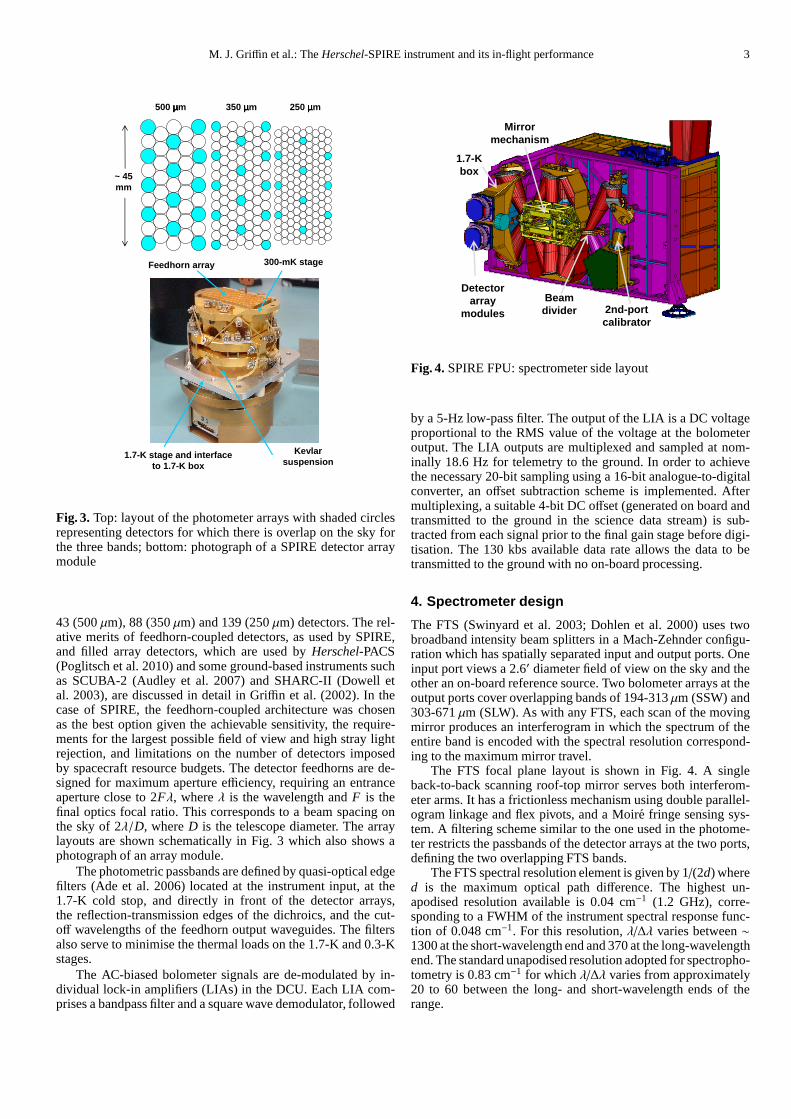
Fig. 3. Top: layout of the photometer arrays with shaded circlesrepresenting detectors for which there is overlap on the skyforthe three bands; bottom: photograph of a SPIRE detector arraymodule

43 (500µm), 88 (350µm) and 139 (250µm) detectors. The rel-ative merits of feedhorn-coupled detectors, as used by SPIRE,and filled array detectors, which are used byHerschel-PACS(Poglitsch et al. 2010) and some ground-based instruments suchas SCUBA-2 (Audley et al. 2007) and SHARC-II (Dowell etal. 2003), are discussed in detail in Griffin et al. (2002). In thecase of SPIRE, the feedhorn-coupled architecture was chosenas the best option given the achievable sensitivity, the require-ments for the largest possible field of view and high stray lightrejection, and limitations on the number of detectors imposedby spacecraft resource budgets. The detector feedhorns arede-signed for maximum aperture efficiency, requiring an entranceaperture close to 2Fλ, whereλ is the wavelength andF is thefinal optics focal ratio. This corresponds to a beam spacing onthe sky of 2λ/D, whereD is the telescope diameter. The arraylayouts are shown schematically in Fig. 3 which also shows aphotograph of an array module.

The photometric passbands are defined by quasi-optical edgefilters (Ade et al. 2006) located at the instrument input, at the1.7-K cold stop, and directly in front of the detector arrays,the reflection-transmission edges of the dichroics, and thecut-off wavelengths of the feedhorn output waveguides. The filtersalso serve to minimise the thermal loads on the 1.7-K and 0.3-Kstages.

The AC-biased bolometer signals are de-modulated by in-dividual lock-in amplifiers (LIAs) in the DCU. Each LIA com-prises a bandpass filter and a square wave demodulator, followed

Mirrormechanism

2nd-portcalibrator

Beam divider

1.7-Kbox

Detector array

modules

Fig. 4. SPIRE FPU: spectrometer side layout

by a 5-Hz low-pass filter. The output of the LIA is a DC voltageproportional to the RMS value of the voltage at the bolometeroutput. The LIA outputs are multiplexed and sampled at nom-inally 18.6 Hz for telemetry to the ground. In order to achievethe necessary 20-bit sampling using a 16-bit analogue-to-digitalconverter, an offset subtraction scheme is implemented. Aftermultiplexing, a suitable 4-bit DC offset (generated on board andtransmitted to the ground in the science data stream) is sub-tracted from each signal prior to the final gain stage before digi-tisation. The 130 kbs available data rate allows the data to betransmitted to the ground with no on-board processing.

4. Spectrometer design

The FTS (Swinyard et al. 2003; Dohlen et al. 2000) uses twobroadband intensity beam splitters in a Mach-Zehnder configu-ration which has spatially separated input and output ports. Oneinput port views a 2.6′ diameter field of view on the sky and theother an on-board reference source. Two bolometer arrays attheoutput ports cover overlapping bands of 194-313µm (SSW) and303-671µm (SLW). As with any FTS, each scan of the movingmirror produces an interferogram in which the spectrum of theentire band is encoded with the spectral resolution correspond-ing to the maximum mirror travel.

The FTS focal plane layout is shown in Fig. 4. A singleback-to-back scanning roof-top mirror serves both interferom-eter arms. It has a frictionless mechanism using double parallel-ogram linkage and flex pivots, and a Moire fringe sensing sys-tem. A filtering scheme similar to the one used in the photome-ter restricts the passbands of the detector arrays at the twoports,defining the two overlapping FTS bands.

The FTS spectral resolution element is given by 1/(2d) whered is the maximum optical path difference. The highest un-apodised resolution available is 0.04 cm−1 (1.2 GHz), corre-sponding to a FWHM of the instrument spectral response func-tion of 0.048 cm−1. For this resolution,λ/∆λ varies between∼1300 at the short-wavelength end and 370 at the long-wavelengthend. The standard unapodised resolution adopted for spectropho-tometry is 0.83 cm−1 for whichλ/∆λ varies from approximately20 to 60 between the long- and short-wavelength ends of therange.

4 M. J. Griffin et al.: TheHerschel-SPIRE instrument and its in-flight performance

The two hexagonally close-packed spectrometer arrays con-tain 37 detectors in the short-wavelength array and 19 in thelong-wavelength array. The array modules are similar to thoseused for the photometer, with an identical interface to the 1.7-Kenclosure. The feedhorn and detector cavity designs are opti-mised to provide good sensitivity across the whole wavelengthrange of the FTS. The SSW feedhorns are sized to give 2Fλpixels at 225µm and the SLW horns are 2Fλ at 389µm. Thisarrangement has the advantage that there are many co-alignedpixels in the combined field of view. The SSW beams on thesky are 33′′ apart, and the SLW beams are separated by 51′′. Athermal source, SCal (Hargrave et al. 2003), at the second inputport is available to allow the background power from the tele-scope to be nulled, thereby reducing the dynamic range neededin recording the interferograms (the amplitude of the interfero-gram central maximum is proportional to the difference in theradiant power from the two ports).

The FTS on-board signal chain is similar to that for the pho-tometer, but has a higher low-pass-filter cut-off frequency of 25Hz to accommodate the required signal frequency range, and thesampling rate is correspondingly higher (80 Hz). As with thephotometer, the 130 kbs available data rate is sufficient to allowdata transmission to Earth with no on-board processing.

5. Observing modes

The photometer was designed to have three principal observ-ing modes: point source photometry, field (jiggle) mapping,andscan mapping. The first two modes involve chopping and jig-gling with the SPIRE beam steering mirror and nodding usingthe telescope. In practice, because of the excellent performanceand simplicity of the scan-map mode, it is the optimum for mostobservations. Although its efficiency for point source and smallmap observations is low, it provides better data quality, and overa larger area, than the chopped modes, and can produce a skybackground confusion limited map in a total observing time thatis still dominated by telescope slewing overheads.

In scan-map mode, the telescope is scanned across the skyat 30 or 60′′/s. The scan angle is chosen to give the beam over-lap needed for full spatial sampling over a strip defined by onescan line, and to provide a uniform distribution of integrationtime over the area covered by the scan. One map repeat is nor-mally constituted by two scans in orthogonal directions to pro-vide additional data redundancy and cross-linking. As wellasSPIRE-only and PACS-only scan-map modes,Herschelcan im-plement simultaneous five-band photometric scan mapping inSPIRE-PACS Parallel mode. Data are taken simultaneously inthe three SPIRE bands and two of the PACS bands, providing ahighly efficient means of making multi-band maps of large areas(at least 30′ x 30′). Scan speeds of 20 or 60′′/s are available inParallel mode. The SPIRE detector sampling rate in this modeis reduced to 10 Hz to keep within the data rate budget, withminimal impact on the data quality.

The standard operating mode for the FTS is to scan the mir-ror at constant speed (nominally 0.5 mm/s) with the telescopepointing fixed, providing an optical path rate of change of 2mm/s due to the factor of four folding in the optics. Radiationfrequencies of interest are encoded by the scanning motion asdetector output electrical frequencies in the range 3-10 Hz. Themaximum scan length is 3.5 cm, corresponding to an opticalpath difference of 14 cm. Three values of spectral resolution areadopted as standard: high, medium, and low, giving unapodisedresolutions of 0.04, 0.24, and 0.83 cm−1 respectively (corre-sponding to 1.2, 7.2, and 25 GHz).

For point source observations with the FTS, the source is po-sitioned at the overlapping SSW and SLW detectors at the arraycentres; but data are acquired for all of the detectors, providing atthe same time a sparsely-sampled map of the emission from theregion around the source. Likewise, a single pointing generatesa sparse map of an extended object. Full and intermediate spatialsampling can be obtained using the SPIRE BSM to provide thenecessary pointing changes between scans while the telescopepointing remains fixed. Regions larger than the field of view aremapped using telescope rastering combined with spatial sam-pling with the BSM. Full details of the SPIRE observing modesare given in the SPIRE Observers Manual (2010).

6. Instrument in-flight optimisation and achievedperformance

6.1. In-flight functional performance

All SPIRE subsystems are fully functional and meet their keyrequirements. The3He cooler has a hold-time in excess of 46hrs, allowing two full days of SPIRE operation after a coolercy-cle. The achieved temperatures are∼ 287 mK at the3He coldtip, 310 mK for the photometer arrays and 315 mK for the FTSarrays. These values are in line with on-ground measurementsand slightly better than used in the pre-launch instrument sensi-tivity model. Detector yield is excellent, with totals of only sixunusable photometer bolometers and two unusable FTS bolome-ters. In-flight testing, carried out before theHerschelcryostat lidwas removed, allowed the main results of system-level pre-flighttesting (withHerschelin the Large Space Simulator facility atESTEC) to be reproduced. The radiant background on the de-tectors, from the thermal emission of theHerscheltelescope andany additional stray light, is consistent with on-ground character-isation of theHerscheltelescope emissivity (Fischer et al. 2004),with a stray light level somewhat less than that adopted in pre-launch estimation of the performance. It is clear that the launchof Herschelproved to be a rather benign event for the system.

6.2. Instrument optimisation and AOT characterisation

SPIRE has many parameters which are adjustable in flight toachieve best performance. These include: cooler recycle settingsand detailed timing; JFET pre-amplifier supply voltage settings;detector array bias frequencies and voltages; detector lock-inamplifier phase settings; PCal and SCal applied power settings;telescope angular scan speeds and scan angles for scan-map ob-servations; FTS mirror and BSM servo system parameters; andthe FTS mirror scan speed. A good part of the Commissioningand Performance Verification (PV) phases of theHerschelmis-sion involved systematic measurements and analysis to optimisethe values of these parameters. In the case of the detector-relatedsettings, separate optimisations were done for nominal sourcestrength (< 200 Jy for the photometer) and bright source set-tings. Most parameter optimisations resulted in values close to oridentical to those predicted before launch. Important differenceswere: (i) the necessary frequency of PCal operation to trackde-tector responsivity, planned for at least once per hour pre-launch,has been relaxed to once per observation regardless of the obser-vation length; (ii) because of the low telescope and stray lightbackground, it is possible to operate the FTS without switchingon the SCal unit. This has the advantages that the operation anddata reduction are simplified, and that the absence of SCal ther-mal emission reduces photon noise.

M. J. Griffin et al.: TheHerschel-SPIRE instrument and its in-flight performance 5

6.3. Glitches due to ionising radiation

In space, ionising radiation hits deposit thermal energy inthebolometers causing spikes in the output voltage timelines.Whilethese glitches are a nuisance, the effects for bolometric detec-tors are not as severe as in the case of low-background photo-conductive detectors, which are prone to non-linear and memoryeffects as a result of charge build-up in the semiconductor ma-terial. Photoconductors can have operating currents of hundredsof electrons/s or less, but the much higher bias current of a typi-cal cryogenic bolometer (∼ 1 nA or∼ 109 electrons/s) results inthe deposited charge being swept out very rapidly, so that afterthe initial spike has decayed (on a timescale determined by thebolometer thermal time constant) the bolometer has no memoryof the event, and its quiescent properties (responsivity and noise)are unaffected by its history of exposure to ionising radiation.

Two types of glitches are seen in the SPIRE detector time-lines: large events associated with single direct hits on individ-ual detectors, and smaller co-occurring glitches, seen simulta-neously on many detectors in a given array, that are believedto be due to ionising hits on the silicon substrate that supportsall the detectors in an array (frame hits). The glitch decay timeconstant is dictated by the bolometer thermal time constant(typ-ically 6 ms), but the on-board analogue signal chains have low-pass electrical filters (designed to eliminate aliased highfre-quency noise from the sampled timelines), which have the effectof prolonging the duration of a glitch and reducing its amplitude.Because the photometer channels have a lower cut-off frequency(5 Hz) than the spectrometer channels (25 Hz), spectrometerglitches are detected more easily above the detector noise and sohave a higher rate. With the currently adopted glitch recognitionscheme, the detected rates per photometer detector are (0.6, 0.7,1.5) glitches/detector/minute for (250, 350, 500)µm, leading to afractional data loss of less than 1% in all cases. For the FTS,theequivalent numbers are∼ 3 and 2/detector/minute/ for SSW andSLW respectively. At present, glitches are identified and flaggedin the automatic processing pipelines. The corresponding datasamples are rejected in the photometer map-making stage. IntheFTS pipeline, the flagged sections of data are replaced by lin-ear interpolation to ensure that artefacts are not introduced bysubsequent Fourier processing in the pipeline. Work continuesto improve the deglitching in both pipelines, but already glitchesare not imposing a significant sensitivity penalty.

6.4. Photometer performance

Beam profiles: The photometer beam profiles have been mea-sured using scan maps of Neptune, which provides high S/Nand appears point-like in all bands (angular diameter≈ 2′′). The(250, 350, 500)µm beams are well described by 2-D Gaussiansdown to ∼ 15 dB, with mean FWHM values of (18.1, 25.2,36.6)′′ and mean ellipticities of (7%, 12%, 9%). These values,which are very similar to pre-launch predictions, represent anaverage over each array; there are small systematic variations atthe level of∼ 5% across the arrays. Beam maps are available (viathe ESAHerschelScience Centre) allowing the detailed beamshape to be deconvolved from map data if desired. Each beammap constitutes an averaging in the map over all of the individ-ual bolometers crossing the source, and represents the realisticpoint source response function of the system, including allscan-ning artefacts or astrometric uncertainties.

Flux calibration: The primary calibrator for the photometer isNeptune, for which we adopt the model of Moreno (1998, 2010),which has an estimated absolute uncertainty of 5%. The calibra-

tion scheme is defined in detail in Swinyard et al. (2010), Griffin(2010), and in the SPIRE Observers Manual (2010). Neptunewas not observable during most of the PV phase, and an initialcalibration was established based on observations of the aster-oid Ceres. At the time of writing, the Neptune-based calibrationhas yet to be incorporated into the automatic data pipeline,butinterim cross-checks have been made to assess the accuracy ofthe Ceres-based and Neptune-based calibrations, and the overalltotal uncertainty of the current calibration is estimated as within15%. Further improvement on this figure is expected to be madeonce the Neptune-based calibration is implemented and throughincremental refinements during the course of the mission. Fluxdensities are quoted at wavelengths of 250, 350 and 500µm,based on theHerschelconvention of an assumed source SEDwith flat νS(ν) (i.e., spectral index -1). Colour correction factorsto convert to a different spectral index are small (a few percent)and within the current 15% overall uncertainty.

Sensitivity: The photometer sensitivity has been estimatedfrom repeated scan maps of dark regions of extragalactic sky.A single map repeat is constituted by two orthogonal scans asimplemented in the SPIRE-only scan-map AOT. Multiple re-peats produce a map dominated by the fixed-pattern sky con-fusion noise, with the instrument noise having integrated downto a negligible value. This sky map can then be subtracted fromindividual repeats to estimate the instrument noise. The extra-galactic confusion noise levels for SPIRE are assessed in detailby Nguyen et al. (2010), who define confusion noise as the stan-dard deviation of the flux density in the map in the limit of zeroinstrument noise. Measured confusion noise levels in the (250,350, 500)µm bands are (5.8, 6.3, 6.8) mJy. For the nominal scanspeed of 30′′/s, the instrument noise is estimated at (9.0, 7.5,10.8) mJy/sqrt(Nreps) whereNreps is the number of map repeats.These values are comparable to pre-launch estimates at 250 and500µm, and better by a factor of∼ 1.7 at 350µm. For the fastscan speed, the instrument noise levels correspond to (12.7, 10.6,15.3) mJy/sqrt(Nreps), precisely as expected given the factor oftwo reduction in integration time per repeat. For the nominalscan speed, the overall noise is within a factor of sqrt(2) ofthe(250, 350, 500)µm confusion levels for (3, 2, 2) repeats.

An important aspect of the photometer noise performance isthe knee frequency that characterises the 1/f noise of the detec-tor channels. Pre-launch, a requirement of 100 mHz with a goalof 30 mHz had been specified. In flight, the major contributor tolow frequency noise is temperature drift of the3He cooler. Activecontrol of this temperature is available via a heater-thermometerPID control system, but has not yet been used in standard AOToperation. The scan-map pipeline (see Sect. 7) includes a tem-perature drift correction using thermometers, located on each ofthe arrays, which are not sensitive to the sky signal but track thethermal drifts. This correction works well and will be improvedwith a forthcoming update of the flux calibration parameters.Use of the thermometer signals to de-correlate thermal drifts inthe detector timelines over a complete observation (E. Pascale,priv. comm.) can produce a 1/ f knee of as low as a 1-3 mHz. Thiscorresponds to a spatial scale of several degrees at the nominalscan speed.

Observing overheads: Scan-map mode is very efficient forlarge area observations, but somewhat less so for smaller fieldsdue to the time needed to turn the telescope around at the endof each scan leg. The HSpot observation preparation tool (ver-sion 4.4.4 at the time of writing) provides a detailed summaryof the on-source integration time and the various overheadsforany particular observation. For example, a 2◦ x 2◦ map with tworepeats takes a total of 7.4 hrs (including all instrument and tele-

6 M. J. Griffin et al.: TheHerschel-SPIRE instrument and its in-flight performance

scope overheads) with an the overall efficiency of 86%. For a20′ x 20′ map with two repeats, the duration is 31 min. withan overall efficiency of 51% due to the larger fraction of timetaken up by telescope turn-arounds. For the Small Map AOT (∼

5′ x 5′ map area), with two repeats, the duration is∼ 8 min.with an efficiency of 15% (but the total observing time still hasa large relative contribution from the 3-min. telescope slewingoverhead).

The photometer mapping AOTs are designed to ensure thatthe area requested by the observer is observed with full samplingand highly uniform coverage at the nominal scan speeds. Mapsalso contain a region around the target area corresponding to thetelescope turn-around periods, in which data are availableto theuser, but with a lower than nominal scan speed and with lesscomplete spatial sampling.

6.5. Spectrometer performance

Wavelength coverage and calibration: The wavelength coverageof the spectrometer is as described in Sect. 4, with the shortwavelength SSW band covering 32.0-51.5 cm−1 (194-313µm)and the long wavelength SLW band covering 14.9-33.0 cm−1

(303-671µm). Wavelength calibration, verified using CO linesin galactic sources, is accurate within 1/10 of a high-resolutionspectral resolution element across both bands.

Beam profiles: The beamwidths vary across the FTS bands,and this has been characterised using spectral mapping ofNeptune as a suitable strong point source. The FWHM variesbetween 17′′ and 21′′ between the short- and long-wavelengthends of the SSW band. The SLW FWHM exhibits a dip withinthe band, with values of 37′′ at the short-wavelength end, 42′′ atthe long-wavelength end, and a minimum of 29′′ at ∼ 425µm.More details are given in Swinyard et al. (2010).

Flux calibration: The spectrometer calibration scheme andmethods are described in detail by Swinyard et al. (2010). Atthe time of writing, the FTS flux calibration is still based ontheasteroid Vesta, but will be updated in the near future based onobservations of Neptune and Uranus using the planetary atmo-sphere models of Moreno (1998, 2010). Current overall calibra-tion accuracy is estimated at 15-30%, depending on positioninthe bands, for frequencies above 20 cm−1, and will be improvedwhen the planet-based calibration is implemented. Correctsub-traction of the thermal emission from the telescope (and from the∼ 5 K instrument enclosure at the lower frequencies) currentlyrequires expert interactive analysis, especially for faint sources,and work continues to establish an automatic pipeline calibra-tion. The current FTS calibration is adequate for point or ex-tended sources, but for sources partly extended with respect tothe beam, calibration is difficult because it requires some a prioriknowledge or modelling of the source intensity distribution.

Sensitivity: The line sensitivity (high-resolution mode;5 σ;1 hr) of the FTS, achieved to date, is typically 1.5 x 10−17 W m−2

for the SSW band and 2.0 x 10−17 W m−2 for the SLW band. Thesensitivity varies slightly across the band in the manner expectedfrom the shape of the Relative Spectral Responsivity Function(RSRF), as given in the SPIRE Observers Manual (2010). At thetime of writing, the noise level continues to integrate downas ex-pected for at least 20 repeats (20 forward and 20 reverse scans;total on-source integration time of∼ 45 min.). The FTS sensitiv-ities are better than pre-launch (HSpot) predictions by a factorof 1.5 – 2. This is attributable to the low telescope background,the fact that the SCal source is not used, and to a conservatismfactor that was applied to the modelled sensitivities to accountfor various uncertainties in the model.

Observing overheads: The telescope pointing is static formost of the time during typical FTS observations, so theoverheads are very low. For example, a single pointing high-resolution observation with 20 repeats takes approximately onehour and has an overall efficiency of 86%. A fully sampled spa-tial map, requiring 16 jiggle positions of the BSM, with fourrepeats per position, takes about 2.4 hrs and is 91% efficient.

7. Data-processing pipelines and data quality

The architecture and operation of the photometer pipeline is de-scribed by Griffin et al. (2008), and the spectrometer pipeline isdescribed by Fulton et al. (2008).

Photometer data are processed in a fully automatic man-ner, producing measured flux density timelines (Level-1 prod-ucts) and maps (Level-2 products). The pipeline includes conver-sion of telemetry packets into data timelines, calculationof thebolometer voltages from the raw telemetry, association of askyposition for each detector sample, glitch identification and flag-ging, corrections for various effects including time constants as-sociated with the detectors and electronics, conversion from de-tector voltage to flux density, and correction for detector temper-ature drifts. The Level-1 products are calibrated timelines suit-able for map-making. Maps can be made either with the max-imum likelihood map-making algorithm MADmap (Cantalupoet al. 2010) or by naıve mapping, involving simple binning ofthe measured flux densities. The pipeline can also be run inan interactive mode, with selectable parameters associated withdeglitching, baseline removal and map pixel size. Standardmappixel sizes of (6, 10, 14)′′ are adopted for the (250, 350, 500)µmbands. The most important aspect of the Level-1 data qualitythatmust be addressed prior to map-making is the amount of resid-ual thermal baseline drift on the timelines. At the time of writ-ing, the standard data products are naıve maps generated withpre-treatment of the Level-1 timelines to remove these resid-ual drifts. The results are high-quality maps, with a low levelof scan-related artefacts and with sky structures preserved overlarge spatial scales (degrees). Work continues to improve furtherthe map-making process, in particular to automate the Level-1timeline treatment step prior to creation of the maps. Once thathas been completed, the potential advantages of MADmap inproducing further enhancements will be investigated.

The FTS pipeline processes the telemetry data producing cal-ibrated spectra. It shares some elements with the photometerpipeline, including the conversion of telemetry into data time-lines and the calculation of bolometer voltages. Steps uniqueto the spectrometer are: temporal and spatial interpolation ofthe stage mechanism and detector data to create interferograms,apodisation, Fourier transformation, and creation of a hyper-spectral data cube. Corrections are made for various instrumentaleffects including first- and second-level glitch identification andremoval, interferogram baseline correction, temporal andspatialphase correction, non-linear response of the bolometers, vari-ation of instrument performance across the focal plane arrays,and variation of spectral efficiency.

8. Conclusions

The SPIRE instrument is fully functional with performance andscientific capabilities matching or exceeding pre-launch esti-mates. Flux calibration is currently accurate to 15% for thepho-tometer and 15-30% for the FTS, and the current pipelines arealready producing high-quality data. Major changes to the AOT

M. J. Griffin et al.: TheHerschel-SPIRE instrument and its in-flight performance 7

implementation are not needed or planned, but further enhance-ments to the calibration and pipelines will continue as the mis-sion progresses.

Acknowledgements.SPIRE has been developed by a consortium of institutes ledby Cardiff Univ. (UK) and including Univ. Lethbridge (Canada); NAOC (China);CEA, LAM (France); IFSI, Univ. Padua (Italy); IAC (Spain); StockholmObservatory (Sweden); Imperial College London, RAL, UCL-MSSL, UKATC,Univ. Sussex (UK); Caltech, JPL, NHSC, Univ. Colorado (USA). This develop-ment has been supported by national funding agencies: CSA (Canada); NAOC(China); CEA, CNES, CNRS (France); ASI (Italy); MCINN (Spain); SNSB(Sweden); STFC (UK); and NASA (USA).

References

Ade, P. A. R., Pisano, G., Tucker, C. E, and Weaver, S. O. 2006,Proc. SPIE 6275,62750U

Audley, D., Holland, W. S., Atkinson, D., et al. 2007, Proc. “Exploring theCosmic Frontier: Astrophysical Instruments for the 21st Century”, Springer-Verlag, p.45

Cantalupo, C., Borrill, J. D., Jaffe, A. H., et al. 2010, Ap. J. Suppl., 187, 212Chattopadhyay, G., Bock, J. J., Rownd, B., and Griffin, M. J. 2003, IEEE. Trans.

Microwave Theory and Techniques, 51, 2139Dohlen, K. Origne, A., Pouliquen, D., and Swinyard, B. 2000, Proc. SPIE 4013,

119, 2000Dowell, C. D., Allen, C. A., Bebu, R., et al. 2003, Proc. SPIE 4855, 73Duband, L., Clerc, L., Ercolani, E., et al. 2008, Cryogenics, 48, 95Fischer, J., Klassen, T., Hovenier, N., et al. 2004, Appl. Opt., 43, 3765Fulton, T., Naylor, D. A., Baluteau, J.-P., et al. 2008, Proc. SPIE, Vol. 7010,

70102TGriffin, M. J., 2010, SPIRE Photometer Flux Density Calibration, SPIRE-UCF-

DOC-3168Griffin, M. J., Bock, J.J., and Gear, W.K. 2002, Appl. Opt., 31, 6543Griffin, M. J., Dowell, C. D., Lim T., et al. 2008, Proc. SPIE, Vol. 7010, 70102QHargrave, P. C., Beeman, J. W., Collins, P. A., at al. 2003, Proc. SPIE 4850, 638Hargrave, P. C., Bock, J. J., Brockley-Blatt, C., et al. 2006, Proc. SPIE 6275,

627513Moreno, R. 1998,These de Doctorat, Universite de Paris VIMoreno, R. 2010, Neptune and Uranus planetary brightness temperature tabula-

tion, available fron ESAHerschelScience Centre.Moseley, H., Dowell, C. D., Allen, C., et al. 2000, ASP Conference Proceedings,

Vol. 217, eds J. G. Mangum and S. J. Radford, 140Nguyen, H., Schulz, B., Levenson, L., et al. 2010, A&A, in pressPilbratt, G. L., Riedinger, J. R., Passvogel, T., et al. 2010, A&A, in pressPisano, G., Hargrave, P., Griffin, M. J., et al. 2005, Appl. Opt.IP, 44, 3208Poglitsch, A., Walekens, C., Geis, N., et al. 2010, A&A, in pressSPIRE Observers’ Manual, 2010, HERSCHEL-HSC-DOC-0789, available from

ESA HerschelScience CentreSwinyard, B., Dohlen, K., Ferrand, D., et al. 2003, Proc. SPIE 4850, 698Swinyard, B. M., Ade, P. A. R., Baluteau, J.-P., et al. 2010, A&A, in pressTurner, A. D., Bock, J. J., Nguyen, H. T., et al. 2001, Appl. Opt.40, 4921

1 School of Physics and Astronomy, Cardiff University, The Parade,Cardiff, CF24 3AA, UK

2 Institut d’Astrophysique Spatiale, Universite Paris-Sud 11, 91405Orsay, France

3 ESA Herschel Science Centre, ESAC, Villaneuva de la Canada,Spain

4 Commissariat a l’Energie Atomique, Service d’Astrophysique,Saclay, 91191 Gif-sur-Yvette, France

5 Imperial College London, Blackett Laboratory, Prince ConsortRoad, London SW7, 2AZ, UK

6 NASA Jet Propulsion Laboratory, 4800 Oak Grove Drive, Pasadena,CA 91109, USA

7 UK Astronomy Technology Centre, Royal Observatory, BlackfordHill, Edinburgh EH9 3HJ, UK

8 Laboratoire d’Astrophysique de Marseille, UMR6110 CNRS, 38rue F. Joliot-Curie, F-13388 Marseille, France

9 University College London, Department of Physics and Astronomy,Gower Street, London WC1E 6BT, UK

10 University College London-Mullard Space Science Laboratory,Holmbury St. Mary, Dorking, Surrey RH5 6NT, UK

11 Cornell University, Ithaca, NY 14853, USA

12 Rutherford Appleton Laboratory, Chilton, Didcot, OxfordshireOX11 0QX, UK

13 Instituto de Astrofısica de Canarias and Departamento deAstrofısica, Universidad de La Laguna, La Laguna, Tenerife, Spain

14 Istituto di fisica dello Spazio Interplanetario, Fosso del Cavaliere100, 00133 Roma, Italy

15 National Astronomical Observatories, Chinese Academy ofSciences, 20A Datun Road, Chaoyang District, Beijing, China

16 Commissariat a l’Energie Atomique, INAC/SBT, 17 rue desMartyrs, 38054 Grenoble, France

17 Institut de Radioastronomie Millimetrique, 300 rue de la Piscine,F-38406 Saint Martin d’Heres, France

18 Joint Astronomy Centre, 660 N. A’ohoku Place, University Park,Hilo, Hawaii 96720 USA

19 University of Padua, Dipartimento di Astronomia, vicoloOsservatorio, 3, 35122 Padova, Italy

20 Blue Sky Spectroscopy Inc., Suite 9-740 4th Avenue South,Lethbridge, Alberta T1J 0N9, Canada

21 University of Colorado, Dept. of Astrophysical and PlanetarySciences, CASA 389-UCB, Boulder, CO 80309, USA

22 European Southern Observatory, Karl-Schwarzschild-Str.2, 85748Garching, Germany

23 California Institute of Technology, 1200 E. California Blvd.,Pasadena, CA 91125, USA

24 ESA ESTEC, Keplerlaan 1, NL-2201 AZ Noordwijk, TheNetherlands

25 NASA Goddard Space Flight Center, Greenbelt, MD 20771, USA26 NASA Herschel Science Centre, IPAC, 770 South Wilson Avenue,

Pasadena, CA 91125, USA27 Observatoire de Paris, LESIA/CNRS, 5 place J. Janssen, FR 92195

Meudon, France28 Centre National d’Etudes Spatiale, 18 avenue Edouard Belin, 31401

Toulouse Cedex 9, France29 University of Lethbridge, Institute for Space Imaging Science,

Department of Physics and Astronomy, Lethbridge, Alberta T1K3M4, Canada

30 University of Sussex, Dept. of Physics and Astronomy, BrightonBN1 9QH, UK

31 Stockholm University, Dept. of Astronomy, AlbaNova UniversityCenter, Roslagstullsbacken 21, 10691 Stockholm, Sweden

32 University of Manchester, School of Physics and Astronomy,Manchester, M13 9PL, UK

33 Institut d’Astrophysique de Paris, UMR7095, UPMC, CNRS, 98bisBd. Arago, 75014 Paris, France

34 University of Hertfordshire, Centre for Astrophysics Research,College Lane, Hatfield, Herts AL10 9AB, UK

35 Dept. of Physics and Astronomy, The Open University, WaltonHall,Milton Keynes MK7 6AA, UK

36 McMaster University, Dept. of Physics and Astronomy, Hamilton,Ontario, L8S 4M1, Canada