Instrument Operation and Software Guide
128
Principle of Operation & Software (standard radiometers) Code: RPG-MWR-STD-SW Date: 11.07.2011 Issue: 01/00 Pages: 128 Instrument Operation and Software Guide Principle of Operation and Software Description for RPG standard single-polarization radiometers Applicable for HATPRO, LHATPRO, TEMPRO, HUMPRO, LHUMPRO, LWP, LWP-U90, LWP-U72-82, LWP-90-150, Tau-225, Tau-225-350
-
Upload
khangminh22 -
Category
Documents
-
view
3 -
download
0
Transcript of Instrument Operation and Software Guide

Principle of Operation & Software
(standard radiometers)
Code: RPG-MWR-STD-SW
Date: 11.07.2011
Issue: 01/00
Pages: 128
Instrument Operation and Software Guide
Principle of Operation and Software Description for RPG standard single-polarization radiometers
Applicable for HATPRO, LHATPRO, TEMPRO, HUMPRO, LHUMPRO,
LWP, LWP-U90, LWP-U72-82, LWP-90-150, Tau-225, Tau-225-350

Code: RPG-MWR-STD-SW Principles of Operation & Software Guide
(standard radiometers)
Date: 11.07.2011
Issue: 01/00
Page: 2 / 128
2 Table of Contents ►
Document Change Log
Date Issue/Rev Change
11.07.2011 00/01 Work
20.07.2011 01/00 Release
Principles of Operation & Software Guide
(standard radiometers)
Code: RPG-MWR-STD-SW
Date: 11.07.2011
Issue: 01/00
Page: 3 / 128
Table of Contents ► 3
Table of Contents
Instrument Operation and Software Guide ............................................................................ 1
Document Change Log ............................................................................................................ 2
Table of Contents .................................................................................................................... 3
1 Scope of This Document ................................................................................................... 6
2. Theory of Operation ............................................................................................................. 6 2.1 General Remarks ......................................................................................................... 6 2.2 Retrieval of Atmospheric Variables ............................................................................... 9 2.3 TEMPRO / HATPRO / LHATPRO Operating Modes..................................................... 9 2.4 Vertical Resolution ..................................................................................................... 10 2.5 References ................................................................................................................. 10
3 Calibrations ...................................................................................................................... 13 3.1 Absolute Calibration ................................................................................................... 13
3.1.1 The Internal Ambient Temperature Calibration Target ...................................... 13 3.1.2 External Liquid Nitrogen Cooled Calibration Target .......................................... 14 3.1.3 General Remarks on Absolute Calibrations ...................................................... 15
3.2 Noise Injection Calibration .......................................................................................... 17 3.3 Gain Calibration (Relative Calibration) ........................................................................ 18 3.4 Sky Tipping (Tip Curve) .............................................................................................. 19 3.5 Calibration Equations ................................................................................................. 22
4 Software Description ....................................................................................................... 24 4.1 Installation of Host Software ....................................................................................... 24
4.1.1 Hardware Requirements for Host PC ................................................................ 24 4.1.2 Directory Tree ................................................................................................... 24
4.2 Getting Started ........................................................................................................... 26 4.3 Radiometer Status Information ................................................................................... 30 4.4 Data Storage Host Configuration ................................................................................ 33 4.5 Exchanging Data Files ................................................................................................ 34 4.6 Inspecting Absolute Calibration History ...................................................................... 36 4.7 Inspecting Automatic Calibration Results.................................................................... 37 4.8 Absolute Calibration ................................................................................................... 39 4.9 Defining Measurements .............................................................................................. 41
4.9.1 Sky Tipping .......................................................................................................... 41 4.9.2 Standard Calibrations .......................................................................................... 43 4.9.3 Products + Integration .......................................................................................... 44 4.9.4 Scanning .............................................................................................................. 46 4.9.5 Timing + … .......................................................................................................... 50 4.9.6 MDF + MBF Storage ............................................................................................ 52
4.10 Sending a MDF / MBF to the Radiometer ................................................................. 53 4.11 Commanding a Measurement Process ..................................................................... 54 4.12 Monitoring Data ........................................................................................................ 55 4.13 Concatenate Data Files ............................................................................................ 61 4.14 Cutting Connection ................................................................................................... 62 4.15 Data Post Processing ............................................................................................... 63 4.16 Data Display Menus ................................................................................................. 64
4.16.1 Data filters .......................................................................................................... 66 4.16.2 Import Radiosonde Files .................................................................................... 67

Code: RPG-MWR-STD-SW Principles of Operation & Software Guide
(standard radiometers)
Date: 11.07.2011
Issue: 01/00
Page: 4 / 128
4 Table of Contents ►
4.16.3 Generate Composite Temperature Profiles ........................................................ 69 4.16.4 Generate Cloud Base Height Charts .................................................................. 70 4.16.5 Housekeeping Data Display ............................................................................... 71 4.16.6 Full Sky Scanning Displays ................................................................................ 71
4.17 Manual Radiometer Control ...................................................................................... 74 4.17.1 Elevation / Azimuth ............................................................................................ 75 4.17.2 Channel Voltages ............................................................................................... 76 4.17.3 Sensor Calibration.............................................................................................. 77 4.17.4 Radiometer System ............................................................................................ 77
4.18 Transform Data Files to ASCII, netCDF and BUFR Format ...................................... 78 4.19 Auto Viewer .............................................................................................................. 79 4.20 Current Sample Files ................................................................................................ 81 4.21 Master / Slave Operation .......................................................................................... 82 4.22 The License Manager ............................................................................................... 86 4.23 Adjusting Azimuth Positioner Direction ..................................................................... 87 4.24 Software Updates ..................................................................................................... 88
5. Retrievals ............................................................................................................................ 90 5.1 Retrieval Algorithms ................................................................................................... 90
5.1.1 General remarks .................................................................................................. 90 5.1.2 Data source and applicability ............................................................................... 90 5.1.3 Data quality processing and reformatting ............................................................. 91 5.1.4 Cloud processing ................................................................................................. 91 5.1.5 Angle and frequency selection ............................................................................. 92 5.1.6 Radiative Transfer calculations ............................................................................ 92 5.1.7 Retrieval grid and type of regression .................................................................... 92 5.1.8 Algorithm performance ......................................................................................... 92 5.1.9 File Format ........................................................................................................... 93
5.2 Retrieval File Structure ............................................................................................... 94 5.2.1 Linear Regressions .............................................................................................. 95 5.2.2 Quadratic Regressions ......................................................................................... 96 5.2.3 Neural Networks .................................................................................................. 96
5.3 Retrieval File Templates ............................................................................................. 96
Appendix A (File Formats) .................................................................................................... 98 A1: LWP-Files (*.LWP), Liquid Water Path ....................................................................... 98 A2: IWV-Files (*.IWV), Integrated Water Vapour .............................................................. 98 A3: ATN-Files (*.ATN), Atmospheric Attenuation .............................................................. 99 A4: BRT-Files (*.BRT), Brightness Temperature .............................................................. 99 A5: MET-Files (*.MET), Meteorological Sensors ............................................................. 100 A6: OLC-Files (*.OLC), Oxygen Line Chart .................................................................... 100 A7: TPC-Files (*.TPC), Temperature Profile Chart (Full Trop.) ....................................... 101 A8: TPB-Files (*.TPB), Temperature Profile Chart (Boundary Layer) .............................. 101 A9: WVL-Files (*.WVL), Water Vapour Line Chart .......................................................... 102 A10(1): HPC-Files (*.HPC), Humidity Profile Chart (without RH) .................................... 102 A10(2): HPC-Files (*.HPC), Humidity Profile Chart (including RH).................................. 103 A11: LPR-Files (*.LPR), Liquid Water Profile Chart ........................................................ 103 A12a: IRT-Files (*.IRT), Infrared Radiometer Temperatures (old) ................................... 104 A12b: IRT-Files (*.IRT), Infrared Radiometer Temperatures (new) ................................. 104 A13a: BLB-Files (*.BLB), Boundary Layer BT Profiles (old) ............................................ 105 A13b: BLB-Files (*.BLB), Boundary Layer BT Profiles (new) .......................................... 106 A14: STA-Files (*.STA), Stability Indices ........................................................................ 106 A15: Structure of Calibration Log-File (CAL.LOG) .......................................................... 107

Principles of Operation & Software Guide
(standard radiometers)
Code: RPG-MWR-STD-SW
Date: 11.07.2011
Issue: 01/00
Page: 5 / 128
Table of Contents ► 5
A16: CBH-Files (*.CBH), Cloud Base Height .................................................................. 110 A17a: VLT-Files (*.VLT), Channel Voltage File (old version) .......................................... 110 A17b: VLT-Files (*.VLT), Channel Voltage File (new version) ........................................ 111 A18: HKD-Files (*.HKD), Housekeeping Data File .......................................................... 112 A19: ABSCAL.HIS, Absolute Calibration History File ...................................................... 114 A20a: LV0-Files (*.LV0), Level Zero (Detector Voltages) Files (old) ............................... 116 A20b: LV0-Files (*.LV0), Level Zero (Detector Voltages) Files (new) ............................. 118 A21: BUFR (Version 3.0) File Format ............................................................................. 120
Appendix B (ASCII File Formats) ........................................................................................ 123 B1 Housekeeping ASCII file format ................................................................................ 126
Appendix C (Web Server Application) ................................................................................ 128

Code: RPG-MWR-STD-SW Principles of Operation & Software Guide
(standard radiometers)
Date: 11.07.2011
Issue: 01/00
Page: 6 / 128
6 2. Theory of Operation ► 2.1 General Remarks
1 Scope of This Document This document contains information about:
• Theory of operation, scientific background of profiling and IWV / LWP radiometers
• Complete software description The methods and software features treated in this document apply to single-polarization radiometers of HATPRO types (profiling radiometers RPG-XXXPRO series), LWP multi-channel radiometers (RPG-LWP-XXX series) and Tau/Tipping radiometers (RPG-Tau-XXX).
2. Theory of Operation
2.1 General Remarks
Atmospheric profiles of temperature, humidity, wind direction and speed are typically measured by radiosondes launched from facilities maintained by the national weather services. Their operation is expensive and requires extended logistics, and hence results in a poor spatial (several hundred kilometres at best) and temporal (about twice a day) coverage. Remote sensing of temperature and humidity profiles from satellites yields better spatial coverage especially over oceans and sparsely populated land areas, however, the obtained horizontal and temporal resolution is coarse. Due to their viewing geometry, the vertical resolution is good in the upper troposphere but deteriorates towards the surface. Because clouds strongly absorb in the infrared spectral region several satellite instruments (e.g. the Advanced Microwave Sounding Unit AMSU and the Special Sensor Microwave/Temperature SSM/T sounder) operate in the microwave region where clouds are semi-transparent. Profiling is achieved by measuring the atmospheric emission along the wings of pressure broadened rotational lines. The 60 GHz oxygen absorption complex is typically used for temperature profiling while the 183 GHz water vapor line is used for the humidity profile. Because the atmospheric opacity is high for both bands, the problem of the unknown surface emission is eliminated.
The usefulness of ground-based microwave radiometry for the retrieval of temperature and humidity profiles has been proven for quite some time [e.g. Westwater et al, 1965; Askne et al, 1986]. Due to the low maintenance requirements of microwave radiometers, continuous atmospheric profiles can be measured which have the highest vertical resolution close to the ground in the planetary boundary layer. This feature is extremely important for the evaluation of (and incorporation into) high resolution numerical weather forecast models of the future. Due to technical improvements and the intensifying search for alternatives to radiosondes, multi-channel microwave radiometers for the operational profiling of tropospheric temperature and humidity have been developed in the last few years [Del Frate et al, 1998; Solheim et al, 1998].
An additional advantage of ground-based microwave radiometers is their sensitivity to cloud liquid water. Over the land, passive microwave remote sensing is by far the most accurate method to measure the vertically integrated liquid water content (liquid water path, LWP) other than sporadic and expensive in-situ measurements from research aircraft. More than

Principles of Operation & Software Guide
(standard radiometers)
Code: RPG-MWR-STD-SW
Date: 11.07.2011
Issue: 01/00
Page: 7 / 128
- 7 -
two decades ago [Westwater, 1978] two channel radiometers were shown to achieve high accuracy in the retrieved LWP and the integrated water vapour content (IWV).
In the last few years, further improvements to the LWP retrieval have been made by the inclusion of additional microwave channels [Bosisio and Mallet, 1998] and the combination of microwave radiometer measurements with other ground-based instrumentation [Han and Westwater, 1995]. The potential of deriving cloud liquid water profiles, rather than just the column amount, using multi-channel measurements has been suggested by Solheim et al. [1998].
Satellite based remote sensing of LWP over the oceans is a well established method [Grody, 1993], however, the inhomogeneous distribution of clouds within the satellites field of view (typical several kilometers), can lead to substantial errors (von Bremen, private communications). This effect has mostly been neglected for ground-based radiometers whose viewing geometry is often assumed to behave as a pencil beam although the spatial and temporal variability of clouds is high even on scales below the resolution of most radiometers [Rogers and Yau, 1989]. With a typical wavelength of about 1 cm, practical considerations about the antenna aperture size (about 20 cm) lead to half-power beam widths from 2° to 4° for conventional radiometers. These beam widths correspond to footprints of up to several 100 m at cloud base heights.
Fig.2.1: Atmospheric emission of liquid water, water vapour and oxygen. The frequency bands marked in blue are utilized by RPG’s radiometers to derive LWP, IWV, Humidity and Temperature Profiles (full troposphere and boundary layer).
RPG-LWP
RPG-HATPRO
RPG-TEMPRO90
23.8 GHz
36.5/31.4 GHz
90 GHz
Water vapour line
Oxygen line
Liquid water continuum

Code: RPG-MWR-STD-SW Principles of Operation & Software Guide
(standard radiometers)
Date: 11.07.2011
Issue: 01/00
Page: 8 / 128
8 2. Theory of Operation ► 2.1 General Remarks
Atmospheric water vapor profile information is derived from frequency channels covering 6 GHz of the high frequency wing of the pressure broadened, relatively weak water vapor line (22-28 GHz). With a pressure broadening coefficient of about 3 MHz/hPa information between approx. 300 and 1000 hPa can be resolved with the spectral measurements. In the center of the oxygen absorption complex the atmosphere is optically thick and the measured radiation originates from regions close to the radiometer. For frequencies further away from the line center the atmosphere gets more transparent and the channels receive radiation which originates from regions more distant to the radiometer (see Fig.2.1). Due to the known mixing ratio and the temperature dependence of the absorption coefficient of oxygen, information about the vertical temperature distribution is contained in the channels spanning the 8 GHz of the low frequency side.
For a ground based radiometer pointing to zenith, well defined weighting function peaks for each frequency are observed (see Fig.2.2b). If the elevation angle is lowered, (and hence the atmospheric path is increased), the peaks shift to lower altitudes. This demonstrates the radiometer’s superiority in the retrieval of the planetary boundary layer temperature.
The cloud liquid water contribution to the microwave signal increases roughly with the frequency squared. It depends on temperature and is proportional to the third power of the particle radius. Therefore measurements at two channels, one influenced mainly by the water vapor line and one in the 30 GHz window region lead to good estimates of LWP and IWV [for example Westwater, 1978].
Fig.2.2: Weighting functions for the oxygen line complex channels.

Principles of Operation & Software Guide
(standard radiometers)
Code: RPG-MWR-STD-SW
Date: 11.07.2011
Issue: 01/00
Page: 9 / 128
- 9 -
2.2 Retrieval of Atmospheric Variables
Artificial neural networks (ANN) are increasingly used for the retrieval of geophysical parameters from measured brightness temperatures (for example Del Frate et al, 1999; Solheim et al, 1999; Churnside et al; 1994). They can easily adapt to nonlinear problems such as the radiative transfer in the cloudy atmosphere. Additionally, input parameters of a diverse nature can be easily incorporated into neural networks.
We use a standard feed forward neural network [Jung et al., 1998] where the cost function is minimized employing the Davidon-Fletcher-Powell algorithm. The architecture of the ANN used for the retrieval includes an input layer consisting of simulated brightness temperatures for the PRG-HATPRO frequencies, a hidden layer with a certain number of neurons (nodes) and an output layer with the atmospheric variable of interest (LWP, IWV, temperature, or humidity profile). To derive the weights between the nodes of the different layers we generated a data set comprising about 15,000 possible realizations of the atmospheric state, which was divided into three sub sets; the first for training, the second for generalization (finding the optimum number of iterations to avoid over fitting), and the third for evaluating the retrieval RMS. For each output parameter the optimal network configuration – number of nodes in the hidden layer, number of iterations and initial weight – was derived and the retrieval performance was evaluated using the third data subset. Generally, it can be stated that all algorithms developed show no systematic errors.
The data set is based on atmospheric profiles of temperature, pressure and humidity measured by radiosondes. In order to analyze profiles of cloud liquid water content (LWC) from the radio soundings, we chose a relative humidity threshold of 95 % as a threshold for the presence of clouds and calculated a modified adiabatic LWC-profile as proposed by Karstens et al. [1994]. Radiation transfer calculations were performed for each radio sounding using MWMOD [Simmer, 1994, Fuhrhop]. A random noise of 1 K was added to the resulting brightness temperatures to simulate radiometric noise. Realistic noise was also added to the other potential input parameters like the standard meteorological measurements (ground level temperature (Tgr), pressure (pgr), relative humidity (qgr)) and the cloud base temperature (Tcl) as derived by an infrared radiometer (if provided).
It should be noted that a limitation to ANN algorithm, as to all statistical algorithms, is that they can only be applied to the range of atmospheric conditions, which is included in this data set. When extrapolations beyond the states included in the algorithm development are made, ANNs can behave in an uncontrolled way, while simple linear regressions will still give a reasonable, although erroneous, result. Quadratic regressions offer the robustness of a linear regression retrieval with the advantage to model nonlinearities much better than linear regressions. In many cases where unusual atmospheric conditions are likely the quadratic regression is the best choice.
2.3 TEMPRO / HATPRO / LHATPRO Operating Modes The RPG-HATPRO (and related radiometers) supports two temperature profiling modes: Full troposphere profiling (frequency scan across the oxygen line) and boundary layer scanning (elevation scan @ 54.9 and 58 GHz). 22.4 GHz WVL humidity profiling is only available for the full troposphere mode (HATPRO) due to the lack of opaque channels on the water vapour line at 22.4 GHz. The much more intense water vapour line at 183.31 GHz, observed by the RPG-LHATPRO, allows for a humidity profiling BL scanning mode.

Code: RPG-MWR-STD-SW Principles of Operation & Software Guide
(standard radiometers)
Date: 11.07.2011
Issue: 01/00
Page: 10 / 128
10 2. Theory of Operation ► 2.4 Vertical Resolution
Fig.2.3: Elevation scanning technique used for boundary layer temperature profiling.
For boundary layer temperature profiling the radiometer beam is scanned in elevation between 5° and zenith (Fig.2.3). At the frequencies in use (54.9 GHz and 58 GHz) the atmosphere is optically thick. The frequencies weighting functions peak at 500 m (58 GHz) and 1000 m (54.9 GHz), see Fig.2.2. The receiver stability and accuracy has to be optimized due to the small brightness temperature variations that must be resolved in the elevation scanning method. In the RPG-HATPRO models the receiver’s physical temperature is stabilized to better than 30 mK over the whole operating temperature range (-45°C to 50°C) to guarantee a high gain stability during measurements (>200 sec). The receiver noise temperature is minimized to be better than 700 K which optimizes the overall noise level.
2.4 Vertical Resolution From the weighting functions corresponding to the various water vapour line and oxygen line profiling frequencies, the vertical resolution of the retrieval outputs can be derived:
• Tropospheric temperature profiles (0-10000 m): 200 m (<5000 m altitude), 400 m above, profile accuracy: +/- 0.6 K RMS (0-2000 m), +/- 1.0 K RMS (>2000 m)
• Boundary layer temperature profiles (0-1200 m), 30 m vertical resolution on the ground 50 m between 300-1200 m, profile accuracy: +/- 0.7 K RMS
• Tropospheric humidity profiles (0-5000 m), 200 m vertical resolution (0-2000 m), 400 m (2000 m – 5000 m), profile accuracy: +/- 0.4 g/m3 RMS
2.5 References Bosisio, A. V., and C. Mallet, Influence of cloud temperature on brightness temperature and
consequences for water retrieval, Radio Science, 33, 929-939, 1998. Chernykh, I. V. and R. E. Eskridge 1996, determination of cloud amount and level from
radiosonde soundings, Journal of Applied Meteorology, 35, 1362-1369, 1996.

Principles of Operation & Software Guide
(standard radiometers)
Code: RPG-MWR-STD-SW
Date: 11.07.2011
Issue: 01/00
Page: 11 / 128
- 11 -
Churnside, J. H., T. A. Stermitz, and J. A. Schroeder, Temperature profiling with neural network inversion of microwave radiometer data, J. Atmos. Oceanic Technol.., 11, 105-109, 1994.
Crewell, S., U. Löhnert, and C. Simmer, Remote sensing of cloud liquid water profiles using microwave radiometry, Proc. of Remote Sensing of Clouds: Retrieval and Validation, October 21-22, 1999, Delft, Netherlands, 6 pages, 1999.
Crewell, S., G. Haase, U. Löhnert, H. Mebold, and C. Simmer, A ground based multi-sensor system for the remote sensing of clouds. Phys. Chem. Earth (B), 24, 207-211, 1999.
Czekala, H., A. Thiele, A. Hornborstel, A. Schroth, and C. Simmer, Polarized microwave radiation from nonspherical cloud and precipitation particles, Proc. of Remote Sensing of Clouds: Retrieval and Validation, October 21-22, 1999, Delft, Netherlands, 6 pages, 1999.
Czekala, H., and C. Simmer, Microwave radiative transfer with non-spherical precipitating hydrometeors. Journal of Quantitative Spectroscopy and Radiative Transfer, 60, 365-374., 1999.
Del Frate, and F., G. Schiavon, A combined natural orthogonal functions/neural network technique for the radiometric estimation of atmospheric profiles, Radio Science, 33, 405-410, 1998.
Grody, N. C., Remote sensing of the atmosphere from satellites using microwave radiometry, 259-334, in Atmospheric remote sensing by microwave radiometry, Ed. M. A. Janssen, John Wiley & Sons, 1993.
Han, Y., and E. Westwater, Remote sensing of tropospheric water vapor and cloud liquid water by integrated ground-based sensors, J. Atmos. Oceanic Technol., 12, 1050-1059, 1995.
Hogg, D. C., F. O. Guiraud, J. B. Snider, M. T. Decker, and E. R. Westwater, A steerable dual—channel microwave radiometer for measurement of water vapor and liquid in the troposphere, J. Climate Appl. Meteor., 22, 789-806, 1983.
Jung, T., E. Ruprecht, and F. Wagner, Determination of cloud liquid water path over the oceans from SSM/I data using neural networks, Journal of Applied Meteorology, 37, 832-844, 1997.
Th. Rose, R. Zimmermann, and R. Zimmermann, A precision autocalibrating 7 channel radiometer for environmental research applications, Japanese Journal for Remote Sensing, 1999 (in press).
Karstens, U., C. Simmer, and E. Ruprecht, Remote sensing of cloud liquid water, Meteorol. Atmos. Phys., 54, 157-171, 1994.
Li, L., J. Vivekanandan, C. H. Chan, and L. Tsang, Microwave radiometric technique to retrieve vapor, liquid and ice, Part I – development of a neural network-based inversion method, IEEE Transactions on Geoscience and Remote Sensing, 35, 224-236, 1997.
Löhnert, U., S. Crewell, and C. Simmer, Combining cloud radar, passive microwave radiometer and a cloud model to obtain cloud liquid water, Proc. of Remote Sensing of Clouds: Retrieval and Validation, October 21.-22, 1999, Delft, Netherlands, 6 pages, 1999.
Mätzler, C., Ground-based observation of atmospheric radiation at five frequencies between 4.9 and 94 GHz, Radio Science 27, 403-415, 1992.
Peter, R., and N. Kämpfer, Radiometric determination of water vapor and liquid water and 1st validation with other techniques, Journal of Geophysical Research, 97, 18,173-18,183, 1992.
Rogers, R. R. and M. K. Yau, A short course in cloud physics, Third Edition, International Series in Natural Philosophy, Vol. 113, 290 pages, 1989.
Simmer, C., Satellitenfernerkundung hydrologischer Parameter der Atmosphäre mit Mikrowellen, Kovac Verlag, 313 pp., 1994.

Code: RPG-MWR-STD-SW Principles of Operation & Software Guide
(standard radiometers)
Date: 11.07.2011
Issue: 01/00
Page: 12 / 128
12 2. Theory of Operation ► 2.5 References
Solheim, F., J.Godwin, E. R. Westwater, Y. Han, S. Keihm, K. Marsh, and R. Ware, Radiometric profiling of temperature, water vapor and cloud liquid water using various inversion methods, Radio Science, 33, 393-404, 1998a.
Solheim, F., and J.Godwin, Passive ground-based remote sensing of atmospheric temperature, water vapor, and cloud liquid water profiles by a frequency synthesized microwave radiometer, Meteorol. Zeitschrift, N.F.7, 370-376, 1998b. Westwater, E., The accuracy of water vapor and cloud liquid determination by dual-frequency ground-based microwave radiometry, Radio Science, 13, 667-685, 1978.
Westwater, E., Ground-based passive probing using the microwave spectrum of oxygen, Radio Science, 69D, 1201-1211, 1965.

Principle of Operation & Software
(standard radiometers)
Code: RPG-MWR-STD-SW
Date: 11.07.2011
Issue: 01/00
Pages: 128
3 Calibrations Calibration errors are the major source of inaccuracies in radiometric measurements. The standard calibration procedure is to terminate the radiometer inputs with two absolute calibration targets which are assumed to be ideal targets, meaning their radiometric temperatures are equal to their physical temperature. This assumption is valid with reasonable accuracy as long as proper absorber materials are chosen for the frequency bands in use and barometric pressure corrections are applied to liquid coolants in the determination of their boiling temperature.
3.1 Absolute Calibration A calibration target is considered to be an absolute standard when it is not calibrated by another standard. RPG’s radiometers are shipped with two calibration targets of this category.
3.1.1 The Internal Ambient Temperature Calibration Target
RPG’s profiling, LWP and tipping radiometers are equipped with an internal absolute ambient temperature calibration standard as shown in Fig.3.1. Other radiometer models, like the RPG-15-90, RPG-HALO-KV, RPG-HALO-119-90 and RPG-HALO-183 are using external ambient temperature targets. The built-in ambient temperature load is one of the instrument’s key components. The pyramidal absorber material is made from carbon loaded foam with low thermal capacity. The target is hermetically isolated by low and high density styrofoam with no exchange of air between the interior and environment (see Fig.3.1).
Fig.3.1: Ambient temperature target cross section (only profiling, LWP and tipping radiometers).

Code: RPG-MWR-STD-SW Principles of Operation & Software Guide
(standard radiometers)
Date: 11.07.2011
Issue: 01/00
Page: 14 / 128
14 Calibrations ► 3.1 Absolute Calibration
The air within the styrofoam box is dried with silica desiccant to avoid condensation of water on the inner styrofoam surfaces. Most important for the cancellation of thermal gradients across the load is the closed cycle venting of the enclosed air as indicated in Fig.4.1. The foam absorber is perforated between the pyramids so that air from the bottom of the absorber can flow into the volume above the pyramids. The air flow is driven by four miniature fans which maintain a steady exchange of air and thus thermal equalisation of the absorber material. For measuring the precise temperature of the internal calibration load the radiometer is
equipped with gauged thermo-sensors offering a guaranteed absolute accuracy of ±0.1 K. This accuracy is only realistic if the sensor is actively cooled to the air temperature inside the load which is achieved by placing the sensor into the stream of air close to one of the fans. This reduces the internal thermal gradient caused by the sensor’s bias current. The top isolation plate is made from low density styrofoam with negligible microwave absorption at frequencies up to 100 GHz. The major advantage of the ambient load is the fact that no active thermal stabilization by heaters or coolers is necessary. For a calibration load it is not essential to keep its temperature constant for all external thermal conditions but to know its precise physical temperature and to keep thermal gradients as small as possible (which is not achieved by heating or cooling the load from the bottom!). According to these requirements the described load is almost ideal. Furthermore the load has a minimized weight since it is mainly made of styrofoam and foam absorber. For the radiometer models RPG-15-90, RPG-HALO-KV, RPG-HALO-119-90 and RPG-HALO-183 an external ambient temperature target is used. Its physical temperature is measured by a certified thermometer, pushed into the foam pyramidal absorber.
3.1.2 External Liquid Nitrogen Cooled Calibration Target
Another absolute calibration standard is the liquid nitrogen cooled target that is attached externally to the radiometer box (see Fig.3.2). This standard - together with the internal ambient load - is used for the absolute calibration procedure. The cooled load is stored within a 40 mm thick polystyrene container. 25 litres of liquid nitrogen is needed for one filling. The boiling temperature of the liquid nitrogen and therefore the physical temperature of the cold load depends on the barometric pressure p. The radiometer’s pressure sensor is read during absolute calibration to determine the corrected boiling temperature according to the equation: T0 = 77.25 K is the boiling temperature at 1013.25 hPa. The calibration error due to microwave reflections at the LN/air interface is automatically corrected by the calibration software (embedded PC).
The described cold target is used for all profiling, LWP and Tipping radiometers.
)25.1013(00825.00 pTTc −⋅−=

Principles of Operation & Software Guide
(standard radiometers)
Code: RPG-MWR-STD-SW
Date: 11.07.2011
Issue: 01/00
Page: 15 / 128
- 15 -
Fig.3.2: External cold load attached to the radiometer box.
3.1.3 General Remarks on Absolute Calibrations
After the system has been turned on, at least 30 minutes are required for warming up and stabilization of all receiver components. To ensure accurate measurements, an absolute calibration should be performed only after completed warm-up. It is recommended to repeat this calibration every 5 to 6 months of operation or after transportation of the system. This will recalibrate the built-in noise standards needed for the automatic regular calibration cycles.
3.1.3.1 System Nonlinearity Correction
A common simplification in the design of calibration systems for total power receivers is the assumption of a linear radiometer response. In this case a simple two point calibration (hot/cold) is sufficient to determine the system noise equivalent temperature (Tsys, offset noise) and system gain (G, slope of the linear response). Accurate noise injection measurements [2], [3] have shown that the assumption of linear system response is not valid in general. Calibration errors of 1-2 K have been observed at brightness temperatures in between the two calibration target temperatures. This system nonlinear behaviour is mainly caused by detector diodes [1] needed for total power detection. Even in the well defined square law operating regime (input power < -30 dBm) the detector diode is not an ideal
Code: RPG-MWR-STD-SW Principles of Operation & Software Guide
(standard radiometers)
Date: 11.07.2011
Issue: 01/00
Page: 16 / 128
16 Calibrations ► 3.1 Absolute Calibration
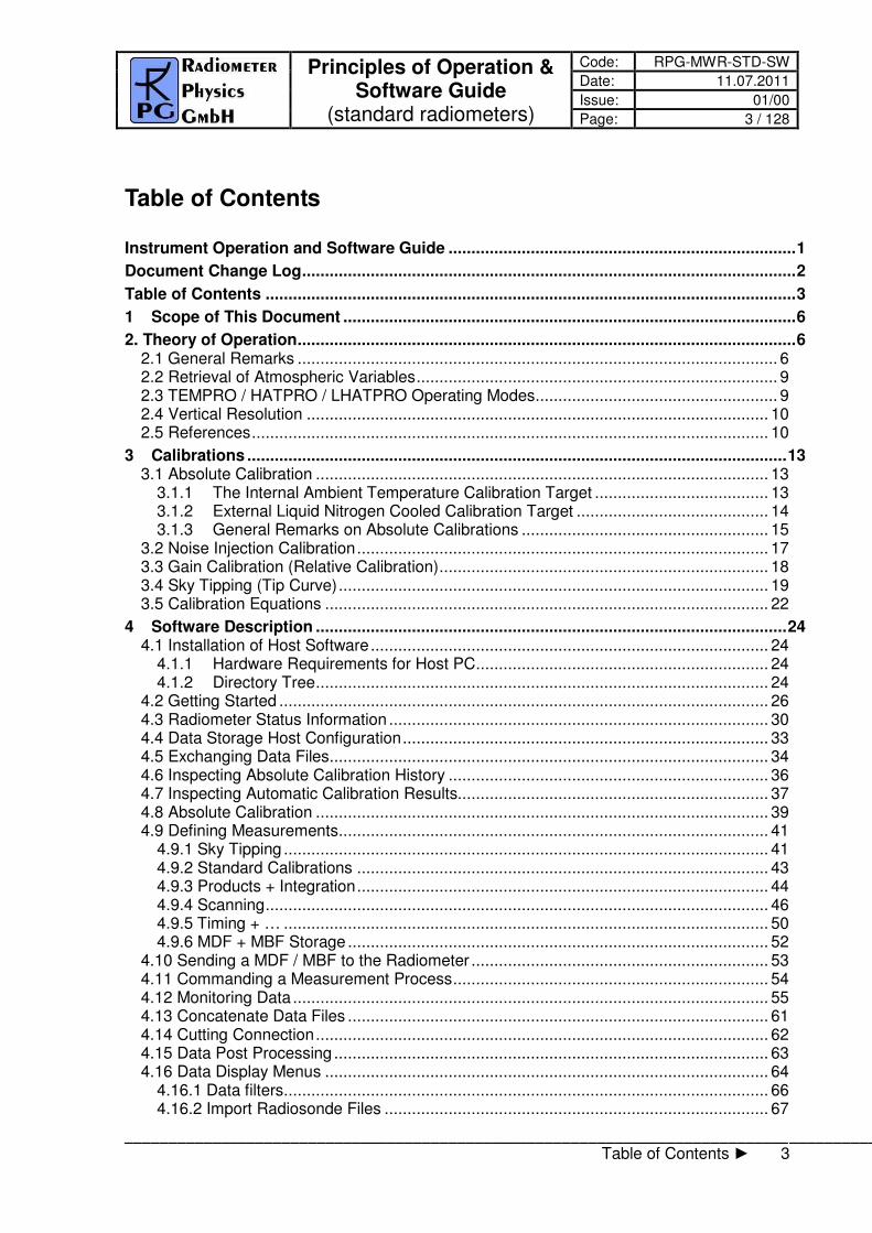
element of perfect linearity. The noise injection calibration algorithm implemented in all RPG radiometers corrects for these nonlinearity effects. The system nonlinearity is modelled by the following formula:
U GP=α
, 19.0 <≤ α (1)
where U is the detector voltage, G is the receiver gain coefficient, α is a nonlinearity factor and P is the total noise power that is related to the radiometric brightness temperature TR through the Planck radiation law: (the proportionality factor is incorporated in G). TR is the sum of the system noise temperature Tsys and the scene temperature Tsc.
Fig.3.3: Detector response as a function of total noise temperature. Tsys is the system noise temperature, Tn the additionally injected noise, Tc the total noise when the radiometer is terminated with a cold load (e.g. liquid nitrogen cooled absorber) and Th the corresponding noise temperatures for the ambient temperature load.
The problem is how to determine G, α and Tsys experimentally (three unknowns cannot be calculated from a measurement on two standards). A solution is to generate four temperature points by additional noise injection of temperature Tn which leads to four independent
equations with four unknowns (G, α , Tsys and Tn) The procedure is illustrated in Fig.3.3: During the calibration cycle the elevation mirror automatically scans the two absolute targets.
The initial calibration is performed with absolute standards and leads to the voltages U1 and U3. By injection of additional noise U2 and U4 are measured. For example U2 is given by
U G P T P T P Tsys cold n2 = + +( ( ) ( ) ( ))α (2)
Tcold is the radiometric temperature of the cold target. The evaluation of the corresponding
equations for U1, U3 and U4 results in the determination of Tsys, G, α and Tn. It is important to notice that the knowledge of the equivalent noise injection temperature Tn is not needed for the calibration algorithm. It is only assumed that Tn is constant during the measurement of U1 to U4.
P T
e
R h
k TB R
( ) ≅
−
1
1
ν
Ud
T[K]Tn TnTsys Tc Th Th2
U1
U2
U3
U4
U5
Us

Principles of Operation & Software Guide
(standard radiometers)
Code: RPG-MWR-STD-SW
Date: 11.07.2011
Issue: 01/00
Page: 17 / 128
- 17 -
After finishing the procedure the radiometer is calibrated. With the four point calibration method also the noise diode equivalent temperature Tn is determined. Assuming a high radiometric stability of the noise injection temperature, following calibrations can use this secondary standard (together with the built-in ambient temperature target) to recalibrate Tsys
and G (considering α to be constant) without the need for liquid nitrogen.
References [1] Cletus A. Hoer, Keith C. Roe, C. McKay Allred, ‘Measuring and Minimizing Diode Detector Nonlinearity’, IEEE Trans. on Instrumentation and Measurement, Vol. IM- 25, No.4, Dec. 1976, page 324 pp. [2] Sandy Weinreb, ‘Square Law Detector Tests’, Electronics Division Internal Report No.
214, National Radio Astronomy Observatory, Charlottesville, Virginia, May 1981 [3] Hvatum Hein, ‘Detector Law’ Electronics Division Internal Report No.6, National Radio Astronomy Observatory, Green Bank, West Virginia, Dec. 1962
3.1.3.2 Avoiding Errors from Variable System Noise Temperature
All losses in the receiver system contribute to the system noise temperature. A significant system noise contribution is related to the receiver optics. A corrugated feedhorn operated at 90 GHz has a typical loss of L=0.5 dB. At a physical temperature of 300 K such a feedhorn contributes with 30 K to system noise according to the formula T0 is the physical temperature of the horn. A change of the feedhorn’s physical temperature from 0°C to 30°C leads to a system noise increase of 3 K which corresponds to an error in the absolute brightness temperature. For this reason the antenna has to be thermally stabilized together with the receivers. The brightness temperature errors introduced by optics that are not thermally stabilized cannot be corrected by the implemented noise standard calibration because the noise source power enters the signal path behind the feedhorn and thus is not changed by a variable antenna temperature.
3.2 Noise Injection Calibration It is not convenient to use a liquid nitrogen cooled load for each calibration. For this reason the radiometer has two build in noise sources (one for each profiler) that can be switched to the receiver inputs. The equivalent noise temperature Tn of the noise diode is determined by the radiometer after a calibration with two absolute standards (hot/cold) and is in the range 100 K to 300 K. The noise diode is also used to correct for detector diode nonlinearity errors. The accuracy of a calibration carried out with this secondary standard and the ambient temperature load is comparable to the results obtained with a liquid nitrogen cooled load. The advantage of the secondary standard is obvious: A calibration can be automatically done at any time. All system parameters are recalibrated including system noise temperatures. The noise diode is optimized for precision built-in test equipment (BITE) applications and meets MIL-STD202 standard with 170 hours burn-in. This process guarantees highest
T TL
= −0 11
( )

Code: RPG-MWR-STD-SW Principles of Operation & Software Guide
(standard radiometers)
Date: 11.07.2011
Issue: 01/00
Page: 18 / 128
18 Calibrations ► 3.3 Gain Calibration (Relative Calibration)
reliability and performance repeatability. The repeatability error is expected to be <0.1 K / month.
Fig.3.4: Contribution of radiometer components to system noise temperature Tsys .
Due to the fact that only two calibration points are generated with this calibration type (Ta= ambient temperature target, Ta+n = ambient temperature target + noise standard), it has to be
assumed that the non-linearity factor α does not change with time. This is a reasonable
assumption because α is basically an intrinsic detector diode parameter. The duration of the noise injection calibration is about 20 seconds. It is recommended to repeat it once per day.
3.3 Gain Calibration (Relative Calibration) The most frequently performed calibration is the gain calibration method. It only corrects for gain drifts (G) but not for changes in system noise temperature Tsys. The receiver gain is most sensitive to even small changes in the physical temperature of the receiver components. During calibration the elevation mirror scans the built-in ambient temperature target (one calibration point only). With the assumption of constant Tsys the system gain can be recalibrated. The duration of the gain calibration is about 10 seconds. It is recommended to repeat it every 5-10 minutes.

Principles of Operation & Software Guide
(standard radiometers)
Code: RPG-MWR-STD-SW
Date: 11.07.2011
Issue: 01/00
Page: 19 / 128
- 19 -
3.4 Sky Tipping (Tip Curve) Sky tipping (often referred to as tip curve calibration) is a calibration procedure suitable for those frequencies where the earth’s atmosphere opacity is low (i.e. high transparency) which means that the observed sky brightness temperature is influenced by the cosmic background radiation temperature of 2.7 K. The humidity profiler channels are candidates for this calibration mode. High opacity channels like all temperature profiler channels >53 GHz are saturated in the atmosphere and must be calibrated by other methods.
Sky tipping assumes a homogeneous, stratified atmosphere without clouds or variations in the water vapour distribution. If these requirements are fulfilled the following method is applicable: The radiometer scans the atmosphere from zenith to around 14° in elevation and stores the corresponding detector readings for each frequency and angle. The path length for a given
elevation angle α is 1/sin(α) times the zenith path length (defined as one “air mass”), thus the corresponding optical thickness should also be multiplied by this factor (if the atmosphere is stratified!). When radiation of intensity Iν (ν denotes a certain frequency) passes through an infinitely thin slice of gas, Iν is reduced by dIν given as
dsIdI ννν κ−=
where κν is the absorption coefficient and includes all processes implying a loss of photons on the way down to the radiometer. Integration over a finite sheet of gas leads to:
( ) ∫⋅=⇒=−=−−
∫∫ ∫ds
eIIdsIdI
dI νκ
νννν
ν
ν κ 0ln
I0ν is the intensity before entering the sheet. The optical thickness is defined as:
ντ
νννν κτ−
⋅=⇒≡ ∫ eIIds 0
Spontaneous emission in the sheet increases the intensity. Atmospheric molecules perform rotational or vibrational transitions in the radiation field:
dsdI νν ε=
where εν is the emission coefficient at frequency ν. The emission coefficient depends on pressure, temperature and chemical composition of the gas and has to be calculated quantum mechanically. The total change of intensity for the infinitely thin gas sheet is then:
ν
ν
ν
ν
νννν
ννννν
κ
ε
τκεκε I
d
dIorI
ds
dIdsIdsdI −=−=⇔−=
We define the ratio ε / κ as the source function S. Then we get:

Code: RPG-MWR-STD-SW Principles of Operation & Software Guide
(standard radiometers)
Date: 11.07.2011
Issue: 01/00
Page: 20 / 128
20 Calibrations ► 3.4 Sky Tipping (Tip Curve)
( ) νννν τ
ν
τ
ν
ν
τ
ν
τ
ν
ν
ν
ττeSeI
d
deSeI
d
dI=⋅⇒=⋅
+
Integration leads to:
( )0)( '0'
0
0'
==⋅=−⋅ ∫ ννν
τ
τ
νν
τ
νν τττν
νν IIwheredeSIeI
This is identical to the more common version of the radiative transfer equation:
'
0
)(0'
)( ν
τ
ττ
ν
τ
ννν ττν
ννν deSeII ∫−−−
⋅+⋅=
A sheet of optical thickness τν absorbs a part of incident radiation Iν
0 and emits radiation at each position, which is partly absorbed by (τν-τν
’). In order to obtain the intensity on the ground, we have to compute the integral along the whole line of sight through the gas, τν is the total optical thickness of the gas layer. With the definition of the mean radiation temperature Tmr : the optical thickness is related to the brightness temperature by the equation:
Ground
Atmosphere
07.2 νIK ≅
νITB ≅
0=ντ
ντ
'
ντ
( )
ν
ν
νν
τ
τ
ν
ττ
ν τ
−
−−
−
⋅
≡
∫e
deS
Tmr1
0
''

Principles of Operation & Software Guide
(standard radiometers)
Code: RPG-MWR-STD-SW
Date: 11.07.2011
Issue: 01/00
Page: 21 / 128
- 21 -
Tmr is a mean atmospheric temperature in the direction θ, TB0 is the 2.7 K background radiation temperature and TB is the brightness temperature of the frequency channel.
The attenuation A in dB is related to ντ by the following formula:
Tmr is a function of frequency and is usually derived from radiosonde data. A sufficiently accurate method is to relate Tmr with a quadratic equation of the surface temperature measured directly by the radiometer.
air mass
[1/sin(Alpha)]
otical thickness
1
(zenith)
0
(space)
Wsys
Fig.3.5: Extrapolation of tipping response to 2.7 K free space temperature.
The optical thickness as a function of air mass is a straight line (see Fig.3.5) which can be extrapolated to zero air mass. The detector reading Usys at this point corresponds to a radiometric temperature which equals to the system noise temperature plus 2.7 K: Usys = G*(Tsys + 2.7 K). The proportionality factor (gain factor) G can be calculated when a second detector voltage is measured with the radiometer pointing to the ambient target with known radiometric temperature Ta. The sky tipping calibrates the system noise temperature and the gain factor for each frequency without using a liquid nitrogen cooled target. The disadvantage of this method is that the assumption of a stratified atmosphere is often questionable even with clear sky conditions due to invisible inhomogeneous water vapour distributions (e.g. often observed close to coast lines). The built-in sky tipping algorithm investigates certain user selectable quality criteria to detect those atmospheric conditions that do not fulfil the calibration requirements. The most important criteria are:
• Linear correlation factor. This measures the correlation of the optical thickness samples (as a function of air mass) with a straight line. Typical linear correlation
−
−=
Bmr
Bmr
TT
TT 0lnντ
10
10ln⋅= Aντ

Code: RPG-MWR-STD-SW Principles of Operation & Software Guide
(standard radiometers)
Date: 11.07.2011
Issue: 01/00
Page: 22 / 128
22 Calibrations ► 3.5 Calibration Equations
factor thresholds are >0.9995. The linear correlation factor is not sensitive for the noise of the optical thickness samples caused by clouds etc.
• χ2-test. This measures the variance of the optical thickness samples relative to the
straight line in Fig.3.5. Typical threshold values are <0.4 for a good quality calibration. The tip curve calibration is considered to be the most accurate calibration method. The brightness temperatures acquired in the elevation scan are close to the scene temperatures measured during zenith observations.
3.5 Calibration Equations All RPG radiometers are equipped with noise injection calibration standards. A subset of these also have Dicke switch references like the RPG-150-90 radiometer and a special version of the RPG-HATPRO. They are referred to as ‘Full Dicke Switch’ instruments (Type 2, see Technical Manual). Relation between detector voltages Ud and scene temperatures Tsc : Ud = G ( Tsys + Tsc )
Alpha , for radiometers without Full Dicke Switching Mode (Type 1) Ud = G ( Tsys + Tsc ), for radiometers with Full Dicke Switching Mode (Type 2) System Noise Temperature Tsys , Noise Diode Temp. TN and Gain G: Absolute Calibrations (Hot / Cold): detector voltages on black body target (temperature TH = Tamb): UH , cold target (LN or Skydip, temperature TC): UC : Y = ( UH / UC )1/Alpha , Tsys = (TH –Y * TC)/(Y - 1) , 0.95 < Alpha <= 1 (sec. 4.1.3.1), Type 1 Y = ( UH / UC ), Tsys = (TH –Y * TC)/(Y - 1) , Type 2 G = UH / (Tsys + TH)Alpha , Type 1 G = UH / (Tsys + TH) , Type 2 On black body target (Tamb), noise diode turned off: U-N , noise diode turned on: U+N TN = (U+N / G)1/Alpha - Tsys - Tamb , Type 1 TN = (U+N - U-N) / G , Type 2 Type 2 only: Dicke Switch (DS) ON, radiometer pointing to amb. temp. target: DelT = UDS / G – Tsys - TDSp , Dicke Switch (DS) leakage (Type 2 only): DS ON, radiometer pointing to cold target: Alpha = (TDSp + DelT – (UDS / G – Tsys)) / (TDSp + DelT - TC) If a liquid nitrogen cooled target is used, the following correction has to be applied: TC [K]= 77.36 -8.2507e-3*(1013.25- P) + 1.9 , P in mbar, 1.9 K is correction for surface reflection on LN (n = 1.2) Continuous full calibration on scene (Type 2 only): Noise Diode turned off: U-N , noise diode turned on: U+N , radiometers looking on scene temperature Tsc, Dicke switch turned ON (blocking scene), physical Dicke switch temperature TDSp: G = (U+N - U-N) / TN , Tsys = U-N / G – (TDSp + DelT – Alpha * (TDSp - Tsc)), Alpha= DS leakage (determined in absolute calibration)

Principles of Operation & Software Guide
(standard radiometers)
Code: RPG-MWR-STD-SW
Date: 11.07.2011
Issue: 01/00
Page: 23 / 128
- 23 -
Continuous noise switching on scene (Type 1 only): noise diode turned off: U-N , noise diode turned on: U+N (10 Hz), radiometers pointing to scene (temperature Tsc): D = (U+N / U-N)1/Alpha – 1 , Tsc = (TN – D * Tsys) / D , G = U-N / (Tsys + Tsc)
Alpha Calibration on ambient temp. black body target (Tamb): Tsys = (Ud / G)1/Alpha - Tamb Type 1, no noise switching: gain calibration on ambient temp. target (Tamb): G = Ud / (Tsys + Tamb)
Alpha noise calibration on ambient temp. target (Tamb): D = (U+N / U-N)1/Alpha – 1 , Tsys = (TN – D * Tamb) / D , G = U-N / (Tsys + Tamb)
Alpha

Principle of Operation & Software
(standard radiometers)
Code: RPG-MWR-STD-SW
Date: 11.07.2011
Issue: 01/00
Pages: 128
4 Software Description The following conventions are used in this software description:
• Messages generated by the program that have to be acknowledged are printed in red. Example: The specified port in ‘R2CH.CFG’ has no data cable connected to it!
• Button labels are printed in green: Cancel
• Messages that have to be answered by Yes or No are printed in light blue: Overwrite the existing file?
• Labels produced by the software are printed in grey: UTC
• Names of group boxes are printed in blue. Example: Radiometer Status on the main screen.
• Names of tabs are printed in violet: Sky Tipping
• Names of menus are printed in black: File Transfer
• Labels of Entry-Boxes are printed in light blue: Const. Elev. Angle
• When a speed button shall be pressed, this is indicated by its symbol:
• Hints to speed buttons are printed in brown: Define Serial Interface
• Selections from list boxes are printed in magenta: Celsius
• Selections from radio buttons or check boxes are printed in dark green: COM1
• File names are printed in orange: MyFileName
• Directory names are printed in dark blue: C:\Programs\RPG-HATPRO\
4.1 Installation of Host Software
4.1.1 Hardware Requirements for Host PC
The hardware requirements for running the host software are:
• Pentium based PC, 500 MHz clock rate minimum
• 400 MB free RAM for software execution
• Serial interface (RS-232), 9 pin Sub-D connector or USB connector + USB-RS-232 converter
An industrial computer is included in the standard delivery package and pre-installed software comes with it. However the host software R2CH.EXE can be installed and run on any other computer that fulfils the hardware requirements listed above.
4.1.2 Directory Tree
To operate the host software without problems a proper installation of the retrieval files (required to perform online calculations of atmospheric parameters like profiles, LWP, IWV etc.) is required.
By clicking on the desktop icon the executable host program R2CH.EXE is started (runs on Windows NT4.0®, Windows 2000®, Windows XP®, Windows Vista®, Windows 7®). On pre-installed PCs this file is located in C:\Programs\RPG-XXX\, where ‘XXX’ stands for the radiometer model (e.g. HATPRO, TEMPRO, HUMPRO, LWP-U90, etc.). This directory

Principles of Operation & Software Guide
(standard radiometers)
Code: RPG-MWR-STD-SW
Date: 11.07.2011
Issue: 01/00
Page: 25 / 128
- 25 -
path can be changed to any other path (in the following referred to as MY_DIRECTORY\RPG-XXX\). Of course the corresponding desktop link has to be modified accordingly. In the case that the user wants (or has) to install the software himself the following steps should be performed:
• Start your Windows® operating system
• Start the Windows Explorer®
• Insert the Radiometer CD-ROM
• In Windows Explorer® click on the CD-ROM drive icon
• Click on the RPG-XXX-folder and drag the whole folder to MY_DIRECTORY\ (user selectable).
Example: If ‘MY_DIRECTORY\’ is the directory D:\Programs\ the complete tree should look lik this: D: |---Programs
|---RPG-XXX | |---DATA | |---HELP | |---MDF-MBF | |---RADIOMETER PC | |---TRACKING | |---RETRIEVALS | |---ATTENUATION | |---HPROFILE | |---IWV | |---LWP | |---TPROFILE_BL | |---TPROFILE_TROP | |---TMR
The RPG-XXX -directory contains the following files:
• VCL50.BPL : System library extension file (can be different in future releases)
• VCLX50.BPL : System library extension file (can be different in future releases)
• BORLNDMM.DLL : Dynamic link library, Memory Management functions (can be different in future releases)
• CC3250MT.DLL : Dynamic link library, Core functions (can be different in future releases)
• NETCDF.DLL : Dynamic link library, netCDF file format routines
• NETCDF.LIB : netCDF library file
• R2CH.EXE : Radiometer software
• R2CH.CFG : Radiometer software configuration file
• RadWebServer.EXE : Web-Server application for R2CH.EXE
• RS.FMT : Radiosonde file format archive The MDF-MBF directory is empty after installation and is intended for the Measurement Batch Files and Measurement Definition Files needed to initiate a measurement. DATA is reserved for measurement data files including user defined sub-directories or archiving sub-

Code: RPG-MWR-STD-SW Principles of Operation & Software Guide
(standard radiometers)
Date: 11.07.2011
Issue: 01/00
Page: 26 / 128
26 Software Description ► 4.2 Getting Started
directories. Of course the user can create any other directory for his data file storage. HELP contains all RichText (*RTF) files for the help system and TRACKING is reserved for RINEX navigation files needed for the satellite tracking mode (see section 4.9.4.1). RETRIEVALS and its subdirectories should never be changed (renamed or deleted) since the software assumes to find all retrieval files here. The retrievals for humidity profiles are stored in HPROFILE, tropospheric retrievals for temperature profiling are stored in TPROFILE_TROP etc. When the user develops his own retrieval files he must store the retrieval in one of the 6 category directories. Click into MY_DIRECTORY\RPG-XXX\ and locate R2CH.EXE. When clicking on this file with the right mouse button a list of actions is displayed. Select the ‘Desktop (Create Shortcut)’ option to generate an icon on the desktop. The RadWebServer.EXE is a web-server application for R2CH.EXE. When this server is active, it listens to port number 8888 (default) and serves clients by providing the functionality of R2CH.EXE on an arbitrary browser. A detailed description of this application is given in Appendix C. The RS.FMT is an archive for radiosonde data formats. The user can extend this archive as described in 4.16.2.
4.2 Getting Started
When clicking on the desktop icon to start the host software R2CH.EXE, the following introduction window appears:

Principles of Operation & Software Guide
(standard radiometers)
Code: RPG-MWR-STD-SW
Date: 11.07.2011
Issue: 01/00
Page: 27 / 128
- 27 -
It displays the current version number, a few examples of instrument deployments, a list of supported RPG radiometer models and (in red) a hint to press <ESC> if you want to change some of the starting configuration settings (black arrow). By pressing <ESC> during software start, the user enters a menu where he can overwrite some settings of the automatically loaded configuration file R2CH.CFG. This can be very useful, e.g. when the host software is configured for ‘Auto Connect’ in auto start mode (see below) but the user wants to change a serial port or the radiometer has been turned off.
The program first tries to locate a free RS-232 host serial port and a data cable connected to one of them. If it does not find a data cable, the message The specified port in ‘R2CH.CFG’ has no data cable connected to it! is displayed as shown in Fig. 4.1. This message refers to the file R2CH.CFG (located in MY_DIRECTORY\RPG-XXX\) which is a configuration file that is loaded by R2CH.EXE at program start. This file contains information (among other data) about the standard serial interface port used for the communication link to the radiometer.
Fig.4.1: Starting host software without a data cable connected to any of the RS-232 interfaces.
For certain reasons it is desirable to operate the software even without a data link to the radiometer. For instance, the user may wish to inspect recorded data files, calibration history or prepare MDFs (Measurement Definition Files) for the next measurements etc. These tasks do not require a radiometer communication link. In this case the message The specified port in ‘R2CH.CFG’ has no data cable connected to it! can be ignored. All commands requiring a radiometer connection are then disabled. If a data cable is installed between the host and the radiometer (see Installation Manual), the user has to define the serial interface parameters for the communication. This is done by
clicking (Define Serial Interface). This command opens the menu below.

Code: RPG-MWR-STD-SW Principles of Operation & Software Guide
(standard radiometers)
Date: 11.07.2011
Issue: 01/00
Page: 28 / 128
28 Software Description ► 4.2 Getting Started
The selectable COM-ports are enabled in the upper button list. The user can only select one of the available ports for interconnection with the radiometer.
The baud rate parameter defines the communication speed. For copper cable lengths up to 50 m and for fiber optic cables, the highest baud rate should be used (115200). This is particularly important when files that have been backed up on the radiometer DOM (disk on module) need to be transferred to the host. Some of these data files might be several MBytes in size so that an optimally fast transfer rate is desirable. At 115200 baud the transfer speed is about 6 kByte/sec.
If Auto Connect is checked, the host software automatically attempts to connect to the radiometer during the starting phase (if a data cable is detected). This feature enables an auto-startup function after a power failure of the host PC. The radiometer embedded PC will automatically continue a measurement after a power failure when the power returns. To start the host software automatically after reboot of the operating system, the R2CH.EXE should be entered into the Auto Start directory of the operating system or an appropriate task should be defined in the scheduler. When using an older version of the optional azimuth positioner, the azimuth controller is connected to the host PC through a second RS-232 interface, instead of being controlled by the radiometer azimuth driver interface. This interface is also defined in the Define Serial Interface menu. The baudrate is auto-adjusted to the fixed azimuth controller baudrate. The automatic controller activation at software start is enabled by checking the Activate box. If a first attempt to connect to the radiometer fails, the program can retry a second time if the Try again, if not successful is checked. By checking Synchronize to Radiometer GPS Clock, the host PC time is synchronized to the radiometer GPS clock. A second radiometer (Slave) can be run by the same host program to combine the channels of two systems to a virtually single instrument (Master / Slave operation). In this case the Slave radiometer needs a second serial interface and must be separately activated. Fibre optics cables are available in two versions:
• 6 line fiber optic cable: This cable provides double hardware handshaking for maximum transfer speed. A special RPG made RS-232 to fibre converter has to be implemented with this cable type. A disadvantage is that commonly available RS-232 to USB converters cannot be used on the host, because such devices only offer poor speed grades for handshaking lines. Instead, if the host motherboard does not provide a serial port, an extension card must be installed (e.g. PCMCIA or Express

Principles of Operation & Software Guide
(standard radiometers)
Code: RPG-MWR-STD-SW
Date: 11.07.2011
Issue: 01/00
Page: 29 / 128
- 29 -
Card on laptops) that connect to the 6 line RS-232 to fibre converter. Maximum cable length is 2000 m.
• 2 line fibre optic cable: No hardware handshaking is implemented for these cables, only TX / RX in combination with an optimized software handshaking. The communication with the radiometer is only slightly slower compared to the 6 line version which can be neglected. An advantage of the 2 line cable is that it can be interfaced with any type of commonly available serial converters (e.g. USB, PCMCIA, Express Card) and commercially available serial to fibre converters (most of them only support TX / RX communication).
All copper cables (old version) are 6 line cables with double hardware handshaking. These cables can be run with maximum speed for cable lengths up to 50 m. The connection to a Master or Slave radiometer is realized by one of these cable types. RPG delivers cables that allow the host and radiometer PC to auto-detect the type of cable attached to it. If the radio button Auto Detect is checked, the host will use this cable feature. But if the user wants to enforce another cable type one of the other buttons 6 line Com. or 2 line Com. are checked. E.g. if a 6 line cable is installed but a 2 line communication is desired in combination with a USB to serial adapter on a laptop, the user checks the 2 line Com. radio button to enforce the host to implement no hardware handshaking in the communication with the radiometer. In this case, only 2 of the 6 lines are used. The interface parameters are stored in the configuration file (R2CH.CFG) that is loaded each time R2CH.EXE is started. This file is backed up on exiting R2CH.EXE. A definition of the serial interface parameters is only necessary at the first start of R2CH.EXE or when the transfer speed must be reduced due to longer cable length. When <ESC> is pressed during the software starting phase, the following menu is displayed:
The user can overwrite certain configuration parameters here, BEFORE the serial COM ports are scanned. E.g. a preset ‘Auto Detect’ cable type detection can be overwritten by a ‘2 Line Cable’ configuration to enforce the host to avoid hardware handshaking with the radiometer. If the host PC is not used to control a radiometer and does not have any serial interfaces, the checkbox Scan for COM ports should be unchecked. The sequence for setting up a communication link to the radiometer is the following:
• Install the interface cable between host and radiometer as described in the Installation Manual (the radiometer power has to be turned off).

Code: RPG-MWR-STD-SW Principles of Operation & Software Guide
(standard radiometers)
Date: 11.07.2011
Issue: 01/00
Page: 30 / 128
30 Software Description ► 4.3 Radiometer Status Information
• Turn on the radiometer power.
• Wait for 1 minute until the radiometer PC has booted up and the elevation mirror has moved to its index position (the mirror movement is quiet, but easily audible).
• Start the host software (if not already done) and define the serial interface parameters as described above (if necessary).
• The next step is to initiate the communication between the host and radiometer PC by
pressing (Connect to Radiometer). R2CH.EXE then establishes the same baud rate on the radiometer embedded PC as was selected in Define Serial Communication Port. This operation takes a couple of seconds. If successful, the message Connection to radiometer successfully established. Baud Rate adjusted. is displayed. Otherwise the message Radiometer does not respond! Connection could not be established... appears. In this case try the following to handle the problem:
o Repeat the command. o If not successful, check the data cable (is it properly connected to host and
radiometer?). Is the cable type the one selected in Define Serial Communication Port ?
o Check that the radiometer power is turned on. o Repeat the turn on procedure. o If not successful, contact RPG.
The connection status is displayed in the status bar (bottom line of the main screen) and includes the COM port number and baud rate. The radiometer responds to the host by sending the status report (listed in Radiometer Status on the host main screen) comprising its ID, the status of the various controllers/GPS clock, the infrared radiometer status, the system’s housekeeping data (temperatures, surface sensor readings), DOM capacity (disk on module, the embedded PC’s hard disk) and elevation stepper position. When a measurement is started, additional information is displayed here like the calibration status, reference time and date, the duration of the actual measurement, its start and end time, the measurement filename, whether file backup is enabled on the embedded PC or not and the repetition number of the running batch (explained later). The radiometer status display can
be disabled ( ) or enabled ( ) at any time. In general the display should be enabled because certain automatic tasks (like logging of all calibration activities) are only performed when the status display is enabled.
4.3 Radiometer Status Information The various status displays in the Radiometer Status group box are:
• Software Version: Indicates the version number of the radiometer PC software 2CH.EXE for reference (the host software version is printed in the main window caption).
• Instrument ID: The radiometer identifies itself by sending the instrument ID to the host when a connection is established (e.g. RPG-HATPRO, RPG-LWP, RPG-LWP-U, etc.).
• Controllers: Lists the status of the two instrument controllers:

Principles of Operation & Software Guide
(standard radiometers)
Code: RPG-MWR-STD-SW
Date: 11.07.2011
Issue: 01/00
Page: 31 / 128
- 31 -
o The main controller handles all communication activities between the radiometer PC and the radiometer hardware.
o The elevation stepper controller generates the driving signals for the elevation scanning parabola mirror. It also provides the initialization procedure for moving the mirror to its index position at system power up.
o The cal stepper controller is only implemented in certain radiometer models (e.g. RPG-DP150-90) with an internal calibration mirror but external elevation scanning.
o The azimuth positioner controller can be controlled by a host serial interface (old versions), or directly from the radiometer. If the controller is connected to the radiometer’s azimuth serial interface, the entry is ‘responding’.
o Receivers: Indicates the status of the installed receiver modules. From the radiometer model type, the host determines the number of receiver modules and displays, which of them are responding or not.
• GPS: Indicates if a GPS clock is installed or not and the global position of the radiometer location (at least 5 GPS satellites have to be visible to provide this

Code: RPG-MWR-STD-SW Principles of Operation & Software Guide
(standard radiometers)
Date: 11.07.2011
Issue: 01/00
Page: 32 / 128
32 Software Description ► 4.3 Radiometer Status Information
information). The radiometer time and date is directly derived from the GPS clock (if installed).
• Real Time Clock: Indicates if the real time clock on the radiometer PC is working properly.
• Disk on Module (DOM) Capacity: The radiometer PC is equipped with a flash memory hard disk (no movable parts) called DOM. Its capacity – when empty - is 1.0 GBytes. The status indicates the amount of memory (measured in kBytes) that is left for the backup of measurement files. If the remaining free memory is less than 20 Mbytes, the backup files should be flushed (see section 4.5).
• Infrared Radiometers: If the optional infrared radiometer(s) is (are) installed, the infrared temperature(s) is (are) displayed here. This data can also be used as input for retrievals. In combination with the temperature profiles, the cloud base height is determined. The IR temperature provides a cloud flag.
• Temperatures: Four temperature sensors are implemented: o The environmental temperature sensor is located outside of the radiometer
box below the dew blower (or inside a Met-Station in newer models). The sensor data is an important parameter for the absolute calibration cold target temperature measurement.
o The ambient temperature target sensor precisely measures the built-in calibration target temperature. The precision of that sensor is essential for ALL calibration procedures. Usually, two of these sensors are implemented to be able to generate an alarm in the case one of the sensors fails.
o Receiver1 / Receiver 2: These temperature sensors reflect the physical temperatures of the receiver modules which are stabilized to an accuracy of < 0.03 K. Typical sensor readings are around 45°C. The thermal receiver stabilisation is continuously monitored. If the receiver temperature is kept constant to within +/- 0.03 K, the status indicator on the right of the temperature display is green. If it turns to red the stability is worse than this threshold. In addition the actual stabilisation values are listed. The colour of the stability status indicator turns to yellow if not enough temperature samples have been acquired to determine the stability.
• Other Sensors: Five additional sensors are monitored: o Barometric Pressure: The pressure sensor measures the barometric pressure
in mbar (accuracy ±1.0 mbar). The data is used in the determination of the precise boiling temperature of the liquid nitrogen coolant used in the external calibration target during absolute calibration.
o Relative Humidity: The sensor is located below the dew blower system outside of the radiometer box (or inside a Met-Station in newer models). The data is used to control the dew blower fan speed when reaching a software predefined threshold. Its accuracy is ±5%.
o Rain Flag: Status of the rain sensor. The flag is used to switch the dew blower speed and is stored with all measurement samples.
• Calibrations: Here the status of automatic calibrations (gain calibration, noise calibration and sky tipping, see section 3) is monitored during measurements. All calibration data is automatically logged in the CAL.LOG file located in MY_DIRECTORY\RPG-HATPRO\. The contents of that file can be inspected with the
command (described later).
• Elevation / Azimuth Scanners: The data displayed here is the current position of the elevation and azimuth scanners. Also displayed is the status of the boundary layer scan (see section 2.3).

Principles of Operation & Software Guide
(standard radiometers)
Code: RPG-MWR-STD-SW
Date: 11.07.2011
Issue: 01/00
Page: 33 / 128
- 33 -
• Measurement: During measurements, this group box displays details like the file name of the current measurement, when the measurement was started and when it will end, the time reference (UTC or local time), if file backup is enabled on the radiometer PC and the batch repetition factor.
4.4 Data Storage Host Configuration There are two different ways of data storage during measurements:
• Data files are stored on the radiometer PC by enabling the file backup option in the measurement definition file (MDF, explained later). The data transferred to the host for online display are not stored by the host PC. If the data files need to be inspected or further processed then they have to be transferred from the radiometer to the host PC. This procedure can be quite time consuming due to the relatively low transfer speed via the RS-232 connection (8 kBytes / sec. max.). The only advantage of this storage mode is that once the measurement has started, the host can be disconnected from the radiometer while the radiometer continues its operation.
• File backup on the radiometer PC is enabled or disabled and the data transferred to the host PC is stored by the host in a predefined data directory. This is the most common operation mode for long term measurements because data files are transferred online from the radiometer to the host. Of course the host computer has to be permanently connected to the radiometer PC. When the host is connected to a network it can regularly send the data files to an FTP server located far away from the measurement site. The file backup on the radiometer is only used as a safety option for the case that the host PC has a power failure or hard disk problem.
Define Directories and Data Formats Menu including data archiving.
The Host Configuration group box on the main screen displays the data storage details. It
is possible to change the settings by clicking (Define Directories). The automatic host

Code: RPG-MWR-STD-SW Principles of Operation & Software Guide
(standard radiometers)
Date: 11.07.2011
Issue: 01/00
Page: 34 / 128
34 Software Description ► 4.5 Exchanging Data Files
data storage during measurements can be enabled or disabled and the data storage directory is selected from the directory tree shown in Data Directory. In the same menu one can specify if an ASCII, netCDF or BUFR version of the data files (which are in binary format by default) shall be generated. ASCII and / or netCDF / BUFR files will then (if this option is selected) be stored to the same data directory as the binary files. Data archiving is a useful feature to prevent the data directory to be filled with ten thousands of files which may overload the operating system. MS operating systems cannot handle many (in the order of ten thousands) files in a single directory. If Enable is checked, the software automatically creates sub-directories in the data directory and stores the data files according to the year, month and day they are generated. E.g. a file 08111623.LWP would be stored in a directory …\RPG-HATPRO\Data\Y2008\M11\D16\ if daily is checked or in …\RPG-HATPRO\Data\Y2008\M11\ if monthly is checked. Automatic file concatenation to daily files can also be enabled (same feature as in section 4.13). Quick-look files can be automatically generated and stored to a separate directory. The file formats BMP and JPG are available. When clicking the QL Diagram List button, a list of graphics windows is displayed. Each of these windows can be enabled / disabled for quick-look file generation. When enabled, a certain graphics display is periodically (defined by QL Period) converted to a JPG or Bitmap file and stored to the quick-look directory.
4.5 Exchanging Data Files The radiometer PC’s hard disk has three directories which are accessible from the host computer:
• Data Files Directory
• System Files Directory
• Root Directory The data files directory is used to store all backup measurement files with unlimited access for READ and WRITE. The system files and root directories contain files that are essential for the radiometer operation. That is why the access for these directories is READ ONLY. Its files should not be manipulated or deleted by the user. If one tries to write to these directories, the host prompts for a password to be entered. Only the radiometer administrator should know this password for software updating (overwriting 2CH.EXE). Overwriting 2CH.EXE with a non-operating software or deleting this executable file will disable all radiometer functions and requires a system re-initialisation by RPG or by accessing the radiometer PC interface (3.5”-floppy drive required)!
To get access to the radiometer directories, click (Exchange Data and System Files with the Radiometer). The menu in Fig.4.2 will be displayed. File transfer is necessary when backup data files need to be copied from the radiometer hard disk to the host computer. If file backup is enabled for a measurement, the instrument stores all data files in its Data Files Directory. The System Files Directory contains the following files:
• 32RTM.EXE runtime library
• 32STUB.EXE stub file loaded by 2CH.EXE to enter protected mode
• DPMI32VM.OVL overlay file for DOS protected mode interface
• 2CH.EXE radiometer software
• FREQU.DAT contains frequency list of radiometer

Principles of Operation & Software Guide
(standard radiometers)
Code: RPG-MWR-STD-SW
Date: 11.07.2011
Issue: 01/00
Page: 35 / 128
- 35 -
• RAD.ID holds radiometer ID code (e.g. 3 = RPG-HATPRO, etc.)
• RAD.NAM holds radiometer name, customer info, etc.
• SENSOR.SCL sensor calibration file
• ABSCAL.CLB absolute calibration parameters
• ABSCAL.HIS absolute calibration history file
• DELTA_F.ADJ only for RPG-HATPRO, RPG-LHATPRO and RPG -TEMPRO. Tuning file for oxygen line centre frequencies
Fig.4.2: File transfer menu.
2CH.EXE is the executable that boots up when the radiometer is turned on. The program handles all automatic tasks like detector readout, calibrations, elevation scanning, file storage etc. The only reason for writing to the system file directory is the installation of a 2CH.EXE software update. Write operations to the system files directory are password protected and are reserved for authorized personnel only (contact RPG for password information). Reading from the system files directory is required when the absolute calibration history file shall be inspected. The file ABSCAL.HIS stores all absolute calibrations (including successful tip curve calibrations). Once copied to any directory on the host hard disk its
contents can be browsed by the command (see section 4.6). Toggling between data files directory and system files directory display is achieved by clicking the Data Files Directory or System Files Directory radio buttons in the Radiometer group box. By double clicking on one of the files in the list, the file size in Bytes is displayed. In order to delete the backup files from the data files directory press Purge Meas. Files. This will delete all backup files from the radiometer. It is not possible to delete single backup files because they are packed together in bigger files to reduce the total number of files on the flash drive. DOMs have problems in handling large numbers of files. During a 3 month continuous operation up to 20.000 data files are generated by an RPG-HATPRO radiometer which would overload the DOM file system capabilities if they were stored as single files. Packing these files is the only way to handle the problem. Before flushing the backup files they should all be copied to the host first (if the data was not monitored on the host PC with automatic

Code: RPG-MWR-STD-SW Principles of Operation & Software Guide
(standard radiometers)
Date: 11.07.2011
Issue: 01/00
Page: 36 / 128
36 Software Description ► 4.6 Inspecting Absolute Calibration History
data storage). By dragging files to the waste bin symbol, only single files are removed from the system files directory (password entry required). When a file needs to be copied from the host to the radiometer, first browse through the host directory tree and mark the file in the file list. Then select Data Files Directory or System Files Directory and drag the marked file(s) to the destination directory. The copy progress is displayed in the Transfer Status group box. Copying in the other direction (from radiometer to host) is performed by drag and drop in the opposite direction. Multiple files may be selected for deleting and file transfer in both directions. The file transfer in progress can be aborted by clicking <ESC>.
4.6 Inspecting Absolute Calibration History As mentioned in section 4.4, the ABSCAL.HIS file located in the system file directory on the radiometer PC stores all absolute calibration results. This also includes the successful tip curve calibrations. In order to inspect this calibration history, first copy ABSCAL.HIS from the
radiometer to the host. Then press (Open Data Files) and select to open the Absolute Calibration History menu. Load the previously copied ABSCAL.HIS file with Load History File and the list of calibrations is displayed (see Fig.4.3). The listed entries are incrementally numbered (preceded by #). The entry syntax is: #calibration number: Receiver 1 cal. type / Receiver 2 cal. type, (date and time of Rec.1 calibration || date and time of Rec.2 calibration)
Fig.4.3: Loading the calibration log file ABSCAL.HIS into the calibration history list. When an entry in the list is marked, Delete Last Entries removes all entries after the marked entry. This feature is useful to remove ‘bad’ calibrations from the list (typically the last calibration). With Generate a new calibration file ABSCAL.CLB is generated using the calibration numbers specified for receiver 1 and 2. If the modified ABSCAL.CLB file is

Principles of Operation & Software Guide
(standard radiometers)
Code: RPG-MWR-STD-SW
Date: 11.07.2011
Issue: 01/00
Page: 37 / 128
- 37 -
copied to the system files directory (password protected) the radiometer will load the new calibration parameters from ABSCAL.CLB when 2CH.EXE boots up the next time. Show Current Calibration loads the newest calibration parameters from the radiometer (if connected). A double click on one of the entries opens the Calibration Results menu in Fig.4.4. For
each receiver channel the four parameters G,α, Tsys and Tn (see section 3.1.3) are listed. In addition the calibration type, calibration time and physical temperature of calibration targets and the environmental temperature are displayed.
Fig.4.4: Display of absolute calibration parameters.
4.7 Inspecting Automatic Calibration Results Automatic calibrations are those described in section 3.3, 3.4 and 3.5 (Gain, Noise, Tip Curve). These calibrations are performed automatically by the radiometer following the calibration settings in the MDF (see section 4.9). The Radiometer Status window on the main screen (if enabled) monitors automatic calibrations. The corresponding log file is CAL.LOG, located in MY_DIRECTORY\RPG-HATPRO\.
For inspecting this log file, click (Display Automatic Calibration History). The menu in Fig.4.5a appears. In the Gain Calibrations group box only gain parameters are displayed (the only parameter that is adjusted by this calibration type, see section 3.3) while also Tsys (Tsys) and Tn (Tnoise) are selectable in Noise Calibrations and Sky Tipping Calibrations. The user may zoom into the data by clicking on the graphics display (holding the left mouse button pressed) and dragging the mouse cursor to a second position. When the mouse button is released the new data window appears. Zoom Out reverts to the previous zoom. The time stamp of each calibration is marked by a dot. With and , this feature is toggled. All diagrams are synchronized (keeping the same time axis), if Synchronize Diagrams is active. Then zooming and zooming out is performed on all displays so that a common time

Code: RPG-MWR-STD-SW Principles of Operation & Software Guide
(standard radiometers)
Date: 11.07.2011
Issue: 01/00
Page: 38 / 128
38 Software Description ► 4.7 Inspecting Automatic Calibration Results
axis is maintained. Independent Diagrams switches back to the non-synchronized display mode. Below the Sky Tipping Calibrations data display, the successful calibrations are marked by a green bar while failed calibrations are marked in red (separately for receiver 1 and receiver 2). By clicking on one of these bars the tip curve calibration details are listed and a graphical display of the sky dip is shown (see Fig.4.5b).
Fig.4.5a: Display of automatic calibration parameters.

Principles of Operation & Software Guide
(standard radiometers)
Code: RPG-MWR-STD-SW
Date: 11.07.2011
Issue: 01/00
Page: 39 / 128
- 39 -
Fig.4.5b: Display of sky tipping fit and detailed result list.
4.8 Absolute Calibration
Fig.4.6: Absolute calibration menu (profiling, LWP and tipping radiometers).

Code: RPG-MWR-STD-SW Principles of Operation & Software Guide
(standard radiometers)
Date: 11.07.2011
Issue: 01/00
Page: 40 / 128
40 Software Description ► 4.8 Absolute Calibration
After setting up the external cold target as described in the Installation Manual, an absolute
calibration is initiated by clicking (Perform Absolute Calibration). The menu in Fig.4.6 is shown, if the connected instrument is a profiling, LWP or tipping radiometer.
When the absolute calibration menu is entered, the instruments frequency list is displayed in Calibrated Frequencies. The list contains the frequencies of both receivers that will be calibrated, if the related receivers are enabled for calibration (e.g. with Humid. Profiler, Temp. Profiler check boxes in Receiver Selection). The integration time Ti is selectable between 5 Seconds and 60 Seconds (Integration Time group box) and defines the integration time period for each calibrated channel. The total integration time is given by Ttotal = 4 * Ti + 10 because four integration cycles have to be passed according to section 3.1.3.1 (four point method) and calibration mirror movements take about 10 seconds.
Start Calibration starts the absolute calibration procedure. During calibration, the current activity is displayed in the message line. When the integration cycles have completed, the message Calibration successful! Save? and a display of the calibration parameters are shown. The user is prompted to confirm to save the calibration with Continue or to abort the calibration with Cancel Calibration. In the case of confirmation, the absolute calibration parameters are then stored to the radiometer PC’s hard disk. Leave the calibration menu by clicking Quit.
Fig.4.6b: Absolute calibration menu (RPG-15-90, RPG-HALO-KV, RPG-HALO-119-90 and RPG-HALO-183 models).
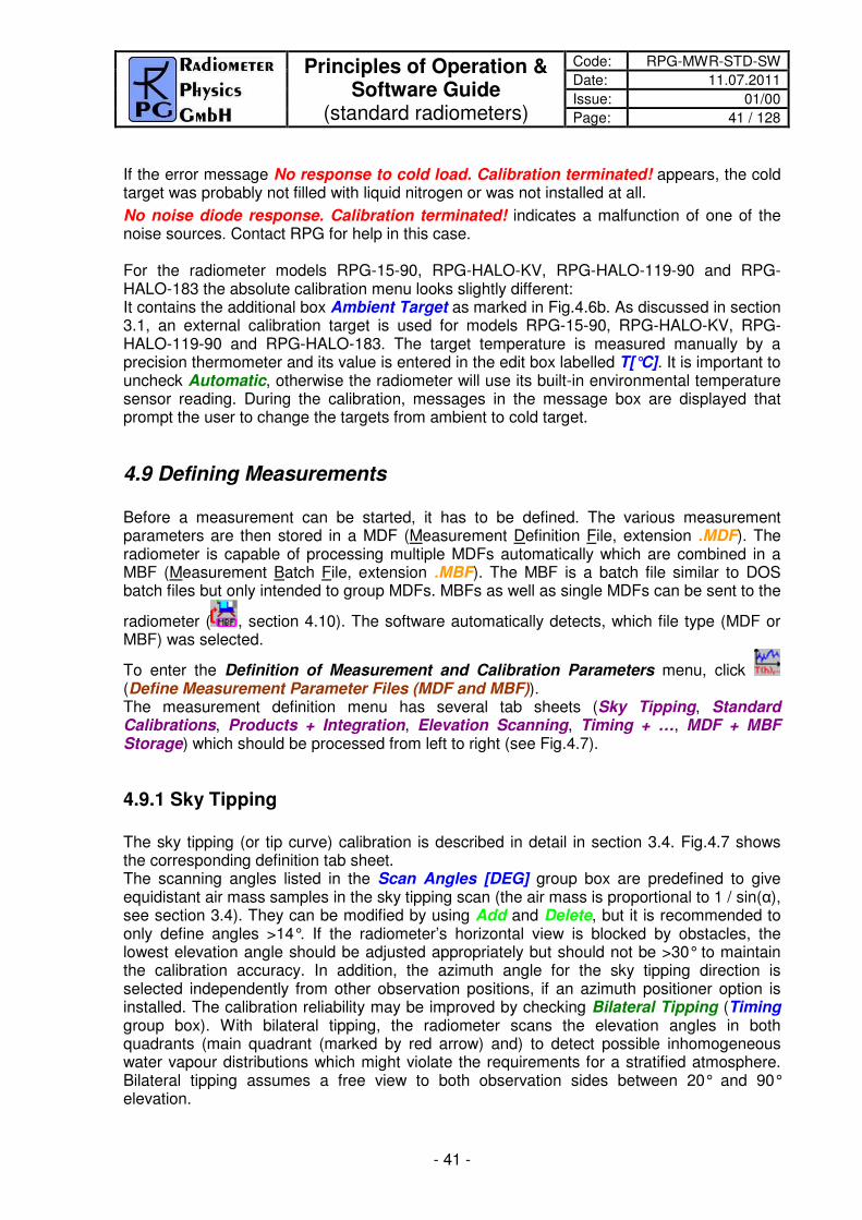
Principles of Operation & Software Guide
(standard radiometers)
Code: RPG-MWR-STD-SW
Date: 11.07.2011
Issue: 01/00
Page: 41 / 128
- 41 -
If the error message No response to cold load. Calibration terminated! appears, the cold target was probably not filled with liquid nitrogen or was not installed at all.
No noise diode response. Calibration terminated! indicates a malfunction of one of the noise sources. Contact RPG for help in this case. For the radiometer models RPG-15-90, RPG-HALO-KV, RPG-HALO-119-90 and RPG-HALO-183 the absolute calibration menu looks slightly different: It contains the additional box Ambient Target as marked in Fig.4.6b. As discussed in section 3.1, an external calibration target is used for models RPG-15-90, RPG-HALO-KV, RPG-HALO-119-90 and RPG-HALO-183. The target temperature is measured manually by a precision thermometer and its value is entered in the edit box labelled T[°C]. It is important to uncheck Automatic, otherwise the radiometer will use its built-in environmental temperature sensor reading. During the calibration, messages in the message box are displayed that prompt the user to change the targets from ambient to cold target.
4.9 Defining Measurements Before a measurement can be started, it has to be defined. The various measurement parameters are then stored in a MDF (Measurement Definition File, extension .MDF). The radiometer is capable of processing multiple MDFs automatically which are combined in a MBF (Measurement Batch File, extension .MBF). The MBF is a batch file similar to DOS batch files but only intended to group MDFs. MBFs as well as single MDFs can be sent to the
radiometer ( , section 4.10). The software automatically detects, which file type (MDF or MBF) was selected.
To enter the Definition of Measurement and Calibration Parameters menu, click (Define Measurement Parameter Files (MDF and MBF)). The measurement definition menu has several tab sheets (Sky Tipping, Standard Calibrations, Products + Integration, Elevation Scanning, Timing + …, MDF + MBF Storage) which should be processed from left to right (see Fig.4.7).
4.9.1 Sky Tipping
The sky tipping (or tip curve) calibration is described in detail in section 3.4. Fig.4.7 shows the corresponding definition tab sheet. The scanning angles listed in the Scan Angles [DEG] group box are predefined to give equidistant air mass samples in the sky tipping scan (the air mass is proportional to 1 / sin(α), see section 3.4). They can be modified by using Add and Delete, but it is recommended to only define angles >14°. If the radiometer’s horizontal view is blocked by obstacles, the lowest elevation angle should be adjusted appropriately but should not be >30° to maintain the calibration accuracy. In addition, the azimuth angle for the sky tipping direction is selected independently from other observation positions, if an azimuth positioner option is installed. The calibration reliability may be improved by checking Bilateral Tipping (Timing group box). With bilateral tipping, the radiometer scans the elevation angles in both quadrants (main quadrant (marked by red arrow) and) to detect possible inhomogeneous water vapour distributions which might violate the requirements for a stratified atmosphere. Bilateral tipping assumes a free view to both observation sides between 20° and 90° elevation.

Code: RPG-MWR-STD-SW Principles of Operation & Software Guide
(standard radiometers)
Date: 11.07.2011
Issue: 01/00
Page: 42 / 128
42 Software Description ► 4.9 Defining Measurements
Fig.4.7: Measurement definition file menu, sky tipping tab sheet.
Sky Tipping is enabled by checking Enable Sky Tipping. The user can define how often a calibration shall be performed by selecting a period between 10 Minutes and 24 Hours. Practical periods are 2 to 24 hours because the radiometer gain is normally calibrated every 5-10 minutes by a gain calibration and a full parameter recalibration (including Tsys and Tn) is not required so frequently. A tip curve interrupts the measurement for more than three minutes, therefore the number of calibrations should be minimized. Furthermore, it is possible to define the time of the first tip curve calibration in the measurement. By checking period absol. (0:0:0), the calibration will start relative to midnight time, e.g. with a period of 6 hours and a measurement start at 3:00 pm the first calibration will take place at 6:00 pm, assuming that first cal. @ mea. start is not checked. If rel. to measure. start is checked, the calibration timing is relative to measurement start time. As explained in section 3.4, tip curve calibrations are only applicable for transparent channels. Receivers with opaque channels are automatically disabled for sky tipping. Three quality checks (thresholds) are implemented:

Principles of Operation & Software Guide
(standard radiometers)
Code: RPG-MWR-STD-SW
Date: 11.07.2011
Issue: 01/00
Page: 43 / 128
- 43 -
• Zenith threshold. In the presence of clouds (which violate the assumption of a stratified atmosphere) the observed zenith brightness temperatures (BTs) are significantly higher than under clear sky conditions. The user can define a maximum BT level as a threshold for each receiver.
• Linear correlation factor. This measures the correlation of the optical thickness samples (as a function of air mass) with a straight line. Typical linear correlation factor thresholds are >0.9995. The linear correlation factor is not sensitive to the sampling noise caused by clouds etc.
• χ2-test. This measures the variance of the optical thickness samples relative to the
straight line. Typical threshold values are <0.3 for a good quality calibration. With the Define Zenith Thresh., Define CHI^2 Thresh. and Correlation Thresh. commands, the corresponding thresholds can be entered in the Threshold Definition group box. The main purpose of a sky tipping calibration is to recalibrate the noise diode secondary standards (see section 3.2). The radiometer PC is capable of averaging successful sky tipping calibrations in order to avoid sudden calibration jumps in the calculated brightness temperatures (TBs). If calibration averaging is desired, the checkbox Enable in the ‘Averaging’ sub-menu should be checked. If enabled, the averager uses the number Av. Depth of successive calibrations in the averaging process. Reasonable values are in the range 40-100. Default Settings resets all skydip parameters to reasonable standard values, optimized for the specific instrument in use.
4.9.2 Standard Calibrations
On this tab sheet the user defines if and how often automatic gain calibrations and noise calibrations shall be performed.
Relative Calibrations (Gain Drifts): During gain calibrations, only the ambient target is scanned (one point calibration), which is the fastest calibration. Reasonable repetition periods are 5-10 minutes. The gain calibration does not correct for system noise temperature variations which are subject to long term drifts only.
During noise calibration, the radiometer beam is pointing to the ambient target and the noise diode is switched on and off. Therefore, the noise calibration takes about twice as long as a gain calibration. For the RPG-HATPRO, a relative calibration takes about 10 seconds while a noise calibration takes 20 seconds. The user can enable or disable each of these automatic calibration options and define the triggering. Noise calibrations might be selected for only one of the two profilers. If a receiver is configured for ‘Noise Switching’ (see section 4.17.4), the noise diode is automatically switched with a frequency of 10 Hz to continuously compensate for gain drifts. In this case, the receiver’s settings in the Calibration with secondary standards (noise diode) are ignored.
Default Settings resets all standard calibration parameters to reasonable values, optimized for the specific instrument in use.

Code: RPG-MWR-STD-SW Principles of Operation & Software Guide
(standard radiometers)
Date: 11.07.2011
Issue: 01/00
Page: 44 / 128
44 Software Description ► 4.9 Defining Measurements
4.9.3 Products + Integration
On the Products + Integration sheet (see Fig.4.8) a selection of data products to be acquired and retrieved by the system during the execution of the MDF is defined. Only those products are enabled in the product list, which are compatible with the actual radiometer configuration, e.g. for a RPG-HUMPRO radiometer, all temperature profiling products are disabled. The product list is grouped into level 0 (raw data = detector voltages), level 1 (brightness temperature data), level 2 (atmospheric data associated with a retrieval file) and others (Met-Station and housekeeping data).
For those products with associated retrieval files (level 2 products), one of the retrievals listed in the related list box needs to be selected. The entries of these boxes reflect the data base that is currently installed in the host PC’s retrieval directories, filtered to those retrievals that are compatible with the instrument hardware (e.g. the available frequency channels, etc.).
Example: When the MDF for a RPG-LWP radiometer (two channels, 23.8 / 31.4 GHz) is defined, the only retrievals that will be listed in the LWP retrieval list box are two channel

Principles of Operation & Software Guide
(standard radiometers)
Code: RPG-MWR-STD-SW
Date: 11.07.2011
Issue: 01/00
Page: 45 / 128
- 45 -
retrievals designed for 23.8 and 31.4 GHz input. If the radiometer is the upgraded RPG-LWP-U90, three channel retrievals are also listed, if they have been developed for 23.8 / 31.4 / 90 GHz channel sets.
When a retrieval file is marked in one of the list boxes, pressing the <RETURN> button opens a text window to display the retrieval file contents. A description of retrieval files and how to create them will be given later. Modifications of these files should be restricted to qualified personal only. Otherwise the modified retrieval algorithm may not work properly.
Fig.4.8: MDF product and retrieval selection menu.
For each enabled product a separate integration time can be selected. Only the setting for Brightness Temp. (boundary layer) and Temperature Profile (boundary layer) products has to be identical, because these products are closely related to each other. In fact the temperature profile is just a further processed product derived from the brightness temperatures of the boundary layer scan.
The user may define a customized Tmr (see section 3.4) retrieval and overwrite the default radiometer Tmr retrieval. If specified and checked, the new retrieval is used for sky tipping calibrations. For explanations on Tmr see section 3.4.

Code: RPG-MWR-STD-SW Principles of Operation & Software Guide
(standard radiometers)
Date: 11.07.2011
Issue: 01/00
Page: 46 / 128
46 Software Description ► 4.9 Defining Measurements
Boundary layer scans can be combined with full troposphere temperature profiling in a single measurement. If only boundary layer scans are required, the CONTINUOUS entry in the TP-BL Repetition list box should be selected; only boundary layer profiling data, meteorological sensor data and infrared radiometer data (if an IRR is installed) will then be produced. All other selections in the TP-BL Repetition list box define a repetition period for boundary scans. After a BL scan has finished, the other products like LWP, full troposphere profiles etc. are generated and continued until the next BL period is initiated. Example: Define a TP-BL repetition period of 1200 seconds and an integration time of 200 seconds for the Temperature Profile (boundary layer) product. At measurement start, a BL scan is carried out which takes about 200 seconds. The next scan will start 1000 seconds later. In the meantime the other selected products are processed.
The boundary layer scan is available in four different modes, selectable from the Boundary Layer Scan Mode box. The radiometer is usually scanning in the main quadrant (marked by a red arrow on the radiometer’s housing underneath the microwave window) but it is possible to switch to the opposite quadrant (called 2nd quadrant). Two scans in both quadrants can be averaged and combined into a single BLB scan (Bilateral average). The two scans in the two quadrants can also be stored independently (Bilateral, two scans).
The Housekeeping Data product represents a summary of different parameters characterizing the instrumental state. These parameters are grouped into 6 categories. The monitoring of each category is selected by clicking the Specify button. The following menu pops up:
The detailed description of each category is given in appendix A18.
4.9.4 Scanning
Sometimes it is desirable to scan the radiometer’s microwave beam in elevation and azimuth while taking measurement samples. The details for scanning are defined in the Scanning tab sheet.
4.9.4.1 Observation at Constant Elevation and Azimuth Angles
When Constant Angles is selected as the Scan Type, a constant elevation and azimuth angle is used for observations, specified in Const. Elev. Angle and Const. Azi. Angle. If a IR radiometer is installed, also the entry in Const. IRR Angle is used.

Principles of Operation & Software Guide
(standard radiometers)
Code: RPG-MWR-STD-SW
Date: 11.07.2011
Issue: 01/00
Page: 47 / 128
- 47 -
4.9.4.2 General Scans
If General Scan is selected, arbitrary elevation and azimuth scan patters may be defined. When the optional azimuth scanner is not available, the radiometer ignores all azimuth angle definitions. In the case that level 2 data products are selected in the product list (section 4.9.2), a retrieval conflict may occur with the defined scan pattern. E.g. humidity profiling retrievals are usually restricted to zenith observation elevation angles (90°) and therefore the retrieval output is not defined for other elevation directions. In General Scan MDFs, only those level 2 data products should be enabled, which are associated with multi-angle retrievals. A multi-angle retrieval is identified by its file name. For example, in the retrieval file name IWV_QR_MA_FZK.V1.RET the sub-string ‘_MA’ indicates that this retrieval is capable of handling different elevation observation angles. The default retrieval set for some profiling (RPG-HATPRO, RPG-HUMPRO, RPG-LHATPRO) and LWP radiometers (RPG-LWP, RPG-LWP-U90, RPG-LWP-U72-82) contain multi-angle IWV- and LWP-retrievals. Multi-angle retrievals for temperature and humidity profiling are currently under development. Thus only IWV, LWP, brightness temperature data (BRT, IRT) and MET products may be used in general scans.
It is recommended to set all integration times of the products acquired during general scans to 1 second. Otherwise, the scan will linger on each position for the maximum integration time selected in the products list!
The elevation mirror moves are subdivided into elementary scans from a start angle to a stop angle with a certain incremental angle and a given number of samples measured at each position. These scans are numbered as Scan#1, Scan#2, ....
The radiometer does not execute single scans but only frames of scans. Each frame has a start scan and a stop scan (these can be identical) which form a ‘loop’ of scans that may be repeated arbitrarily. The concept of having two levels of movement definitions allows for the definition of complex scan procedures. A frame is defined by selecting one of the scans in the start scan list and then clicking on one in the stop scan list. After entering the repetition number, the frame is added (or inserted) to the frame list (Add or Insert). It is possible to edit a frame definition using the Overwrite command or to delete it with Delete. In addition, the frame start can be triggered to a certain time increment (if Triggered is checked). Three examples illustrate how a frame is executed:
1) Start: Scan#4, stop: Scan#6, repetitions: 3 ⇒ Scan#4,Scan#5,Scan#6,Scan#4,Scan#5,Scan#6,Scan#4,Scan#5,Scan#6
2) Start: Scan#4, stop: Scan#2, repetitions: 2 ⇒ Scan#4,Scan#3,Scan#2,Scan#4,Scan#3,Scan#2
3) Start: Scan#2, stop: Scan#2, repetitions: 1 ⇒ Scan#2
When an optional azimuth scanner is installed, a full 2D sky scan can be programmed by checking the 2D Scan check box. In this case, the radiometer software interprets the given start- and stop-angles for elevation and azimuth as edge angles and performs a 2D scan within these limits. E.g. a full sky scan is defined by setting the elevation start angle to 9.0°, the elevation stop angle to 90.0° (a 9° increment angle produces 10 elevation steps at const. azimuth angle), the azimuth start angle to 0.0° and the azimuth stop angle to 350.0° (step increment 10°). This generates a measurement of 378 scan points with an angular resolution of 10° in azimuth and 9° in elevation. The radiometer sets the integration time to 0.4 seconds / sample to reduce the time needed for a full scan. The ‘Samples / Pos.:’ entry is ignored in this mode. The full scan in this example takes only about 7 minutes! High speed scanning is

Code: RPG-MWR-STD-SW Principles of Operation & Software Guide
(standard radiometers)
Date: 11.07.2011
Issue: 01/00
Page: 48 / 128
48 Software Description ► 4.9 Defining Measurements
feasible due to the parallel architecture of the RPG radiometer’s direct detection filter bank receivers described in the Technical Manual.
In the example above, the 90° elevation angle would be scanned 36 times if the Multiple 90° Samples check box is checked. This leads to redundant zenith samples that can be used to derive a time series of other products during full sky scanning (e.g. an LWP zenith time series). But it increases the time for a full scan due to redundant samples. If the scanning time shall be optimized, Multiple 90° Samples check box is unchecked (default setting). In this case the zenith scanning angle is only encountered once during a full sky scan. When products with different integration times are selected for scanning, the radiometer adjusts all integration times to the maximum integration time in the products list. Example: A RPG-HATPRO radiometer is setup for scanning with the brightness temperature product (BRT, integration time: 10 sec.) and the IR temperature product (integration time: 5 sec.). Then the integration time during the scan will be 10 seconds (also for the IR temperature samples). After the definition of the start angle, stop angle and increment angle, the settings are stored as a scan with Add. Every scan in the scan list can be marked and overwritten with the

Principles of Operation & Software Guide
(standard radiometers)
Code: RPG-MWR-STD-SW
Date: 11.07.2011
Issue: 01/00
Page: 49 / 128
- 49 -
current settings by using the Overwrite command. By clicking on a scan number in the scan list, the actual settings of that scan are displayed. If the IRR motor driver option is installed, the infrared radiometer is moved synchronously together with the internal microwave elevation mirror, when Enable IRR Elevation Coupling is checked.
4.9.4.3 Satellite Tracking
Assuming the radiometer system is equipped with an azimuth scanner, the instrument can be run in satellite tracking mode by selecting Satellite Tracking. In satellite tracking mode, the radiometer periodically scans a number of visible GPS or Galileo satellites and measures the wet delay component, LWP and attenuation in the line of sight to each of the satellites. The user should activate the products IWV, LWP, and Attenuation (ATN) in the MDF product list with identical integration time (typically one second). The system determines the satellite positions from a RINEX navigation file stored in the TRACKING subdirectory (see section 4.1.2) and its own GPS position. The azimuth scanner’s 0.0° azimuth angle has to point to North direction (90° = West, 180° = South, 270° = East) to guarantee correct scanning positions. In Define Details the user can specify the tracking details. The Period determines, in which time intervals the scan is repeated. In Scan Objects one specifies, if all visible satellites or just a single satellite shall be scanned. In the case of a single satellite, the satellite’s number is given in Satellite Number. The angular scan range should be limited (e.g. in elevation) if not all sky directions are available due to obstacles. RINEX navigation files are loaded from the European IGS FTP data server ftp://igs.ensg.ign.fr/pub/igs/data/ and usually have the extension ‘.YYn’ where YY stands for the year, e.g. ‘.08n’ is a navigation file from 2008. For instance, the file ftp://igs.ensg.ign.fr/pub/igs/data/2008/225/dlft2250.08n is from Delft (dlft), day of the year 225 (August 12th). The RINEX navigation files are ASCII formatted files and contain the orbit information for all satellites of a certain navigation system like GPS or Galileo. The host software periodically (every hour) checks if there is an updated RINEX file in the TRACKING subdirectory and automatically loads it if available. The software calculates the current positions from the information given in the RINEX files and the actual UTC time and the radiometer GPS position on earth.

Code: RPG-MWR-STD-SW Principles of Operation & Software Guide
(standard radiometers)
Date: 11.07.2011
Issue: 01/00
Page: 50 / 128
50 Software Description ► 4.9 Defining Measurements
Tracking data files are stored in ASCII format with extension ‘*.TRK’.
4.9.5 Timing + …
Start time, end time and time reference are important parameters for a measurement setup. The time reference is set to UTC or local time which is UTC + time shift [h]. The radiometer determines UTC from a GPS clock reading which is synchronized to the radiometer’s real time clock (RTC) every 10 minutes.
There are two ways of triggering a measurement: Immediately after launching the MDF or at a certain time and date. Using a start time before the current time is equivalent to an immediate start. If the measurement start is triggered to a certain time, the check boxes Ignore Date and Ignore Hour allow for a date or hour independent triggering. This is particularly useful in a repeated multiple MDF batch measurement, where MDFs are repeated multiple times. A triggering to a certain date / time would trigger the MDF only once but not repeatedly. E.g. if Ignore Hour is checked (assumingTriggered mode is activated) and the ‘Start Time’ entry is set to 22|36|15, the measurement is triggered to 00:15:00, 01:15:00, 02:15:00, …, ignoring the current date and hour. If a more frequent trigger is required, one can use the Raster feature combined with a raster period. E.g. if a start time of 22|36|15 is defined in combination with raster mode and a raster period of 10 minutes, the trigger sequence is: 22|36|15, 22|46|15, 22|56|15, 23|06|15 etc.
Two options are available for measurement termination. In LIMITED mode the user can set a duration or termination time. If the stop time is before the start time, the measurement duration is adjusted to 100 seconds.
In the case that the measurement has a well-defined end time (automatic measurement termination, LIMITED mode) the radiometer needs a filename for storing backups. The user may enter any filename not longer than 8 characters. The host also uses this filename when it is operated in automatic storage mode. If measurement timing is set to UNLIMITED mode the radiometer automatically generates filenames deduced from the actual time and date and ignores the measurement filename entry.
In UNLIMITED mode the measurement is terminated manually. A new filename is generated every X hours where X is selected from the Filename Interval list box. The file format is one of 14 possible versions given in the Name Convention list box. In the format string HH=hours, DD=days, MM=month and YY=year are taken from the actual time and date. During measurement, this filename is also transmitted to the host, which uses it for file storage of monitored data (assuming the host is operated in Enable File Backup mode).
Since the temperature and humidity environmental sensors respond quickly to changes of the corresponding parameters (caused by turbulence in the vicinity of the radiometer) it is often desirable to smooth the temperature and relative humidity data samples. This is important if retrievals are utilizing the meteorological sensors, but the detailed surface turbulence at the radiometer location is not of interest and would only lead to noisy retrieval results if not filtered. In Data Smoothing a 10 minutes LIFO filter is activated to smooth the environmental temperature and humidity readings.
A humidity threshold can be defined for setting the dew blower fan speed to full power and turning on the heater module (Humidity Threshold).
Another feature is the enabling of a file backup on the embedded PC. When Enable File Backup is checked, all product files will be automatically stored in the radiometer’s data directory. This is usually done for safety reasons because the standard mode of

Principles of Operation & Software Guide
(standard radiometers)
Code: RPG-MWR-STD-SW
Date: 11.07.2011
Issue: 01/00
Page: 51 / 128
- 51 -
measurements is to enable automatic data storage on the host (online monitored data). Without monitoring the data on the host and only storing it on the radiometer as backup, the user will sooner or later have to transfer the data from the embedded PC to the host using the Transfer Data and System Files menu.
Fig.4.9: Timing+… definition menu.
For the RPG-HATPRO, RPG-TEMPRO, RPG-HUMPRO and RPG-LHATPRO, the radiometer PC performs quality checks on the water vapour and oxygen lines measured in zenith mode and during boundary layer scans. These tests include the detection of possible external interferences or reduced quality level 2 data caused by intensive rain. The program generates a quality flag and information for the possible reason of a reduced quality. This information is coded into the rain flag of each sample (see Appendix A). More information about quality checking can be found in appendix A18. The radiometer can be configured to filter low and medium quality samples and is capable of interpolating the brightness temperature of channels affected by external interference. In Level 2 Data Quality there are three options for filtering level 2 data (retrieved atmospheric data). The Flag Data Quality (Level 2) option does not filter the level 2 data according to the quality level but flags each

Code: RPG-MWR-STD-SW Principles of Operation & Software Guide
(standard radiometers)
Date: 11.07.2011
Issue: 01/00
Page: 52 / 128
52 Software Description ► 4.9 Defining Measurements
data sample in the rain flag byte as described in appendix A. With the option Remove Medium / Low Q., medium and low quality samples are not transmitted by the radiometer. In this case, the sample sent to the host is the repeated latest high quality sample. The filter Remove Low Quality will only remove the worst quality level data and transmits high and medium quality data. If the radiometer detects a possible interference problem (an external signal interferes with one of the receiving channels), it can automatically remove the interference signal from the spectral line by interpolating between adjacent channels. This function is enabled by checking Remove Interferences.
Another feature is the blanking or avoiding of the sun position during scanning observations and sky tipping. This implies the availability of the azimuth scanner option and a GPS clock and that the azimuth table is precisely aligned according to the procedure described in section 4.23. If Avoid Sun in Scans is checked, the radiometer will determine the sun position on the sky automatically when performing full sky scans, azimuth scans (Hovmöller plots) or sky tipping calibrations. If the sun position is encountered, the radiometer sidesteps this position by about 6° to avoid unrealistic brightness temperatures in transparent channels.
4.9.6 MDF + MBF Storage
It is possible to send a single MDF directly to the radiometer. Multiple MDFs are packed into a MBF (measurement batch file). The concept is similar to the Scan/Frame relationship for scanning. The MDFs in a batch file are executed sequentially in the order they are listed in the MDF list (see Fig.4.10). The batch repetition number has the same meaning as the frame repetition factor for scanning: The MDF list forms a loop, which is repeated an arbitrary number of times. This offers the user a flexibility of combining different measurement tasks, which would otherwise not be compatible in a single MDF, e.g. if one wants to do a scanning measurement (not possible with retrieved products) followed by a temperature profiling measurement (a retrieved product) and repeat this 100 times, the solution is to define two different MDFs, one for scanning and one for temperature profiling and combine them in a batch file with a repetition factor of 100. The only restriction for MDF definitions in multi-MDF batches is that the UNLIMITED mode must be avoided.
It is a good practice to store all MDFs in one directory (e.g. …\RPG-HATPRO\MDF-MBF). All MDFs in the selected directory are listed in the box in the lower right corner. From this list, the user may select each MDF he wants to add or insert to the MDF batch list by dragging the desired MDFs to the MDF batch list box. MDFs may also be deleted from the MDF batch list by dragging it to the waste bin. Store your measurement batch files (MBFs) in a single directory (like …\RPG-HATPRO\MDF-MBF). If file backup is enabled in the MDFs and the batch repetition factor is >1, there is only one filename for each MDF available. The data of successive executions of a certain MDF in the batch loop is stored to a single file. Each time the MDF is repeated in the loop, its measurement data is appended to the file.

Principles of Operation & Software Guide
(standard radiometers)
Code: RPG-MWR-STD-SW
Date: 11.07.2011
Issue: 01/00
Page: 53 / 128
- 53 -
Fig.4.10: Batch file configuration menu.
4.10 Sending a MDF / MBF to the Radiometer MDFs and MBFs can be sent to the radiometer (assuming the host is connected to it) from
the Send Measurement Configuration menu by clicking .
When an MDF or MBF is loaded (Load MDF/MBF File), its contents and repetition factor are displayed. In addition some pre-checks are performed, e.g. correct radiometer configuration, frequency list consistency, etc. A variety of other checks ensure that no erroneous command data is sent. When the consistency check of a MDF is finished, the test result is displayed in the Check List. The batch can only be sent to the radiometer if all consistency checks have finished with the status OK. Then the MBF is transmitted with Send. The host PC ‘remembers’ the directory where MDFs and MBFs are stored from a previous Load MDF/MBF File. This directory is marked in red and its content is listed below the directory label. In the list, MDFs are separated from MBFs by a dashed line. Dragging a file from the list and dropping it on the radiometer image on the right is equivalent to the Send command. If Auto Go and Auto Send are both checked, the MDF or MBF is sent, the Send Measurement Configuration menu is closed and the measurement is automatically started.
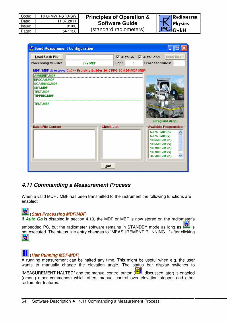
Code: RPG-MWR-STD-SW Principles of Operation & Software Guide
(standard radiometers)
Date: 11.07.2011
Issue: 01/00
Page: 54 / 128
54 Software Description ► 4.11 Commanding a Measurement Process
4.11 Commanding a Measurement Process When a valid MDF / MBF has been transmitted to the instrument the following functions are enabled:
(Start Processing MDF/MBF) If Auto Go is disabled in section 4.10, the MDF or MBF is now stored on the radiometer’s
embedded PC, but the radiometer software remains in STANDBY mode as long as is not executed. The status line entry changes to “MEASUREMENT RUNNING...” after clicking
.
(Halt Running MDF/MBF) A running measurement can be halted any time. This might be useful when e.g. the user wants to manually change the elevation angle. The status bar display switches to
“MEASUREMENT HALTED” and the manual control button ( , discussed later) is enabled (among other commands) which offers manual control over elevation stepper and other radiometer features.

Principles of Operation & Software Guide
(standard radiometers)
Code: RPG-MWR-STD-SW
Date: 11.07.2011
Issue: 01/00
Page: 55 / 128
- 55 -
(Continue Interrupted MDF/MBF) Used to continue a halted measurement. The status bar display changes back to “MEASUREMENT RUNNING” and the manual control button is disabled.
(Terminate Running MDF/MBF) This command terminates the execution of the currently running measurement. The radiometer switches to STANDBY mode and is ready to receive the next MDF/MBF.
4.12 Monitoring Data
Fig.4.11a: Radiometer status, measurement configuration and automatic calibration display.
The easiest way to perform a measurement is:
• Define a MDF (or multiple MDFs included in a MBF) ( ).
• Check Automatically store monitored data in the Define Data Directory.
• Send the MDF or MBF to the radiometer ( ).
• Start the MDF or MBF on the radiometer ( ).
automatic calibration status, timing and control
measurement information

Code: RPG-MWR-STD-SW Principles of Operation & Software Guide
(standard radiometers)
Date: 11.07.2011
Issue: 01/00
Page: 56 / 128
56 Software Description ► 4.12 Monitoring Data
The monitoring of the products that were selected in the MDF is automatically activated and the measured data is displayed. Since the data is transmitted online from the radiometer to the host no additional file transfer is required.
The data display is grouped into different tag fields that can be freely selected.
Status and Configuration: This group includes the status display of the radiometer and measurement information like the current processed MDF, current data filename, activation status of file backup and level 0 data storage, start and end time, etc. In a second box, the settings for the automatic calibrations are displayed (Automatic Calibration Timing). These settings, like calibration period and integration time, can be changed ‘on the fly’. Each calibration is performed automatically but there is the possibility to enforce a calibration by clicking the associated Execute Calibration button.
Fig.4.11b: Brightness temperature information.
Brightness Temperatures: All brightness temperatures, at both microwave and IR frequencies, are displayed in this group.
The display includes the time series of each available microwave and IR channel, the boundary layer scan information and the line profiles, if applicable (e.g. water vapour and oxygen lines). The three TB Windows 1-3 each show a subset of the microwave channels that is defined by entering the Low Limit and High Limit of the displayed frequency range.

Principles of Operation & Software Guide
(standard radiometers)
Code: RPG-MWR-STD-SW
Date: 11.07.2011
Issue: 01/00
Page: 57 / 128
- 57 -
Time series graphs can be changed by selecting a different time axis period from the time axis selection box.
Atmospheric Data (24 hours): A 24 hour history of IWV, LWP, meteorological sensors and profiles is continuously updated in this group. The IWV, LWP and sensor data displays can be individually changed to a 3, 6, 12 or 24 hour history. In the profiles boxes, colour scales, vertical axis limits and contour values may be changes for the data monitoring. The humidity profile window has a selection button for displaying absolute or relative humidity.
Fig.4.11c: 24 hour data history display.
Atmospheric Data (Time Series): This group includes time series of liquid water path (LWP), integrated water vapour (IWV), cloud base height (CBH) information and the surface sensors (temperature, rel. humidity and barometric pressure). CBH data is available for all temperature profiling radiometer models (RPG-HATPRO, RPG-TEMPRO, RPG-LHATPRO) if the IRR option is installed. LWP, IWV and CBH are retrieved data products and are therefore quality checked. The quality level (High, Medium, Low) and the possible reason for reduced data quality is shown below the time series charts. All time series include a rain flag display. Each window displays the current reference time, date, sample number, sample value, retrieval type (if applicable) and cursor position (when the mouse cursor is moved into the display area).
Current Trop. Profiles: The group summarizes all available profiles. There are three temperature profile displays, one for the boundary layer scan (TPB) with high vertical

Code: RPG-MWR-STD-SW Principles of Operation & Software Guide
(standard radiometers)
Date: 11.07.2011
Issue: 01/00
Page: 58 / 128
58 Software Description ► 4.12 Monitoring Data
resolution (range 0-2000 m), one for the zenith observation (TPC, full troposphere profile with coarser resolution in the boundary layer) and one for the composite profile (CMP.TPC). The composite temperature profile is a combination of the high vertical resolution boundary profile and the full troposphere profiles. Both profiles are linked together at the 1200 m altitude level by applying a cubic-spline fit. The temperature profiles are in blue colour while the dew point temperature profiles are in green. Dew point information is only available (and displayed), if the radiometer is equipped with a humidity profiler. Absolute humidity and dew point temperature are only different versions of the same information content. Like with all temperature displays, the temperature axis can be scaled to Celsius, Fahrenheit or Kelvin.
On the bottom of the screen the diagrams for absolute humidity (HPC), relative humidity and the liquid water profile (LPR) are shown. The LPR data product is automatically generated when the products LWP, IWV and IRT are selected in the MDF product list and a retrieval for the maximum LWC is installed in the LWP retrieval directory (must have the same retrieval filename as the LWP retrieval but starting with ‘LWM’ instead of ‘LWP’). X-axis: LWC-density [g/m3], Y-axis: altitude [m].
Fig.4.11d: Time series of atmospheric data like IWV, LWP, cloud base height and sensor data.
Because all profiles are level 2 data products, there is a quality flag assigned to each profile. This flag is stored in the rainflag byte as described in appendix A18.
Scew-T & Stability: This group includes a skew-T and a stability index display. Six of the most common stability indices (lifted index (LI), K-index (KI), KO-index, Showalter index (SI), CAPE index, total totals index (TTI)) are monitored. X-axis: measurement time, Y-axis 1: [K] index, Y-axis 2: CAPE index [J/m^3].

Principles of Operation & Software Guide
(standard radiometers)
Code: RPG-MWR-STD-SW
Date: 11.07.2011
Issue: 01/00
Page: 59 / 128
- 59 -
Fig.4.11e: Atmospheric profiles display.
The skew-T plot is automatically generated when temperature and humidity profiles are sampled. Also the stability indices are computed and stored in files of extension ‘.STA’. The displayed temperature and dew-point profiles can be analyzed graphically by using the cursor on the skew-T chart. The cursor coordinates, P and T, are monitored as the cursor is moved across the diagram. Other useful information like the LCL (Lifted Condensation Level) and LFC (Level of Free Convection) is marked on the Skew-T. By clicking the Tpp button, the pseudo-potential temperature is displayed in red which contains valuable information about the stability of the atmospheric layers (see definition of KO-index). The pseudo-potential temperature is given by:
p0 is the reference pressure (1000 mbar), Ra is the gas constant for dry air (287 J / kg K), Cp is the specific heat capacity at constant pressure (1004 J / kg K), L is the latent heat for the condensation phase transition (2.5·106 J / kg) and r is the mixing ratio.
The Skew-T diagram can be switched to other thermo-dynamical diagram types, like Tephigram, Stüve or Emagram.
In the diagrams, the altitudes of the Lifted Condensation Level (LCL) and the Level of Free Convection (LFC) are also displayed.
TC
rLCR
pp
p
pa
ep
pTT
•
=
/
0
dew point

Code: RPG-MWR-STD-SW Principles of Operation & Software Guide
(standard radiometers)
Date: 11.07.2011
Issue: 01/00
Page: 60 / 128
60 Software Description ► 4.12 Monitoring Data
Fig.5.11f: Skew-T diagram and Stability Indices display.
Attenuation: This display is similar to the brightness temperature diagram and monitors the time series of atmospheric attenuation. The vertical axis unit is dB as the standard unit for attenuation parameters. The attenuation is only calculated for the microwave channels. The standard attenuation retrievals are applicable for all elevation angles and can be used in scanning mode.
Satellite Tracking: If satellite tracking is enabled in the running MDF, the scanned satellite information, like satellite number, navigation file, satellite elevation and azimuth position, wet path delay and LWP along line of sight and atmospheric attenuation are listed for each scan.
Housekeeping: Data like GPS position, receiver stability, system temperatures (ambient target, receiver temperatures), flash memory capacity, quality flags and system status flags are monitored. By clicking the Legend button, the colour codes for the different flags are listed. An ALARM indicator warns the user if a systematic problem with the radiometer has occurred. A detailed description of housekeeping flags is given in appendix A18.
Tpp
Temp. Profile
Dewpoint Profile
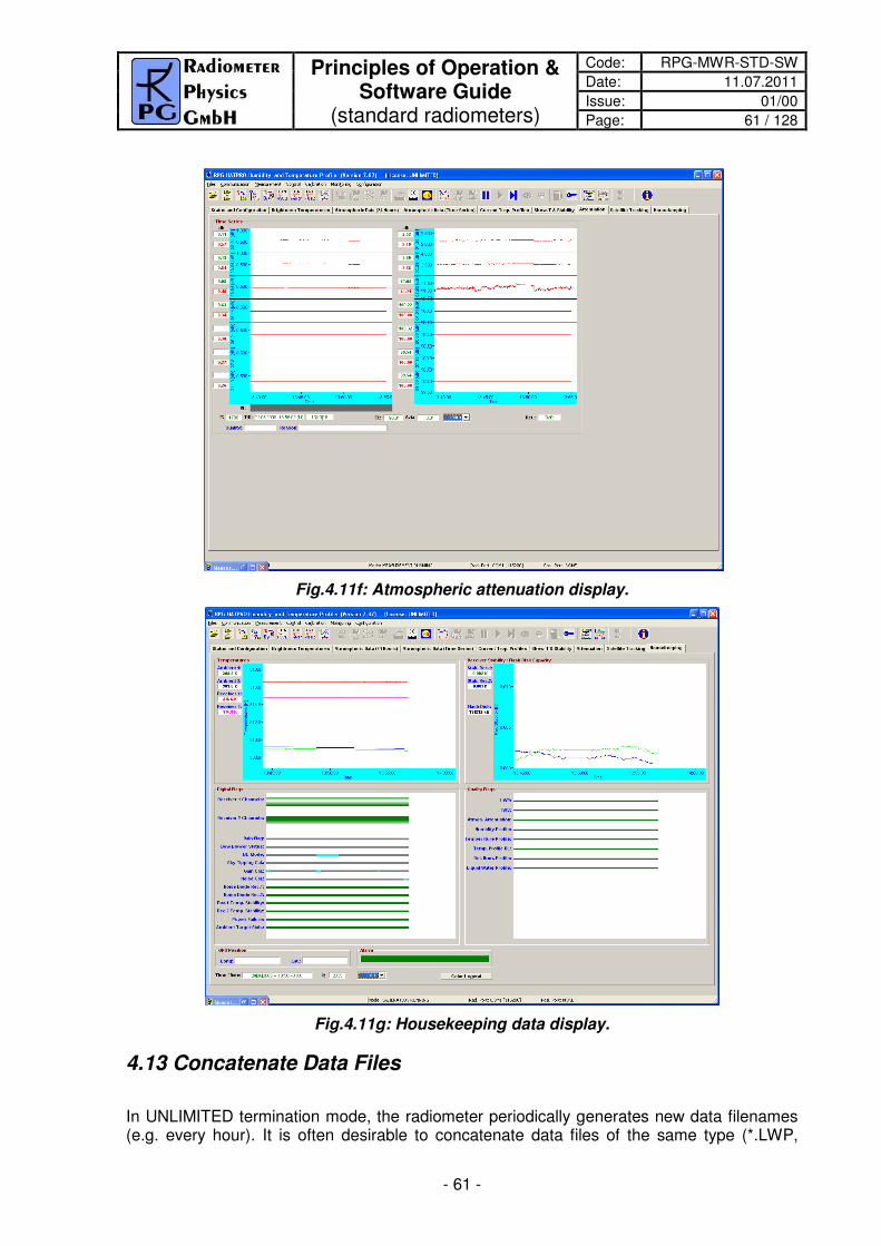
Principles of Operation & Software Guide
(standard radiometers)
Code: RPG-MWR-STD-SW
Date: 11.07.2011
Issue: 01/00
Page: 61 / 128
- 61 -
Fig.4.11f: Atmospheric attenuation display.
Fig.4.11g: Housekeeping data display.
4.13 Concatenate Data Files
In UNLIMITED termination mode, the radiometer periodically generates new data filenames (e.g. every hour). It is often desirable to concatenate data files of the same type (*.LWP,

Code: RPG-MWR-STD-SW Principles of Operation & Software Guide
(standard radiometers)
Date: 11.07.2011
Issue: 01/00
Page: 62 / 128
62 Software Description ► 4.14 Cutting Connection
*.TPC etc.) to form bigger files (e.g. 24 hour files). This is possible by clicking (Concatenate Data Files) which opens the menu in Fig.4.12. A set of filenames is selected from the list and then concatenated to a single file with Generate Concatenated File. All files in a certain directory can be automatically concatenated to daily files by using the Generate Daily Files command. Optionally, the original hourly files can be deleted, if the appropriate checkbox is checked.
Fig.4.12: Concatenating data files.
4.14 Cutting Connection
(Cut Connection to Radiometer) If the user wants to disconnect the host from the interface cable or turn off the radiometer after having been connected this command should be used first. It ensures that all communication activities between host and radiometer are disabled so that the host will not crash after disconnection.

Principles of Operation & Software Guide
(standard radiometers)
Code: RPG-MWR-STD-SW
Date: 11.07.2011
Issue: 01/00
Page: 63 / 128
- 63 -
4.15 Data Post Processing
Files of products that are based on retrievals (LWP, IWV, profiles) can be generated by combining brightness temperature files, meteorological sensor files and corresponding retrieval files. The frequencies specified in a retrieval file (see section 5) must match the frequency information in the BT (Brightness Temperature) file. Example: An LWP retrieval requires BT information at 23.8 and 31.4 GHz and input from a temperature sensor and humidity sensor. A RPG-HATPRO radiometer delivers this information in a BRT file. The calculation of the LWP data is performed in the Transform
Brightness Temperature Data to Atmospheric Data menu (click ). Fig.4.13 shows an example. The file 100520.MET (click on the filename in the list) is combined with the BRT file 100520.BRT (click on the filename in the list), both recorded at the same time and date, by applying the retrieval information of the HPT_QR_FZK_V1.RET file. Generate Humidity Profile performs a consistency check (frequency matching, additional sensor matching) and generates a new .HPT file.
Fig.4.13: Generate level 2 data (atmospheric data like LWP, IWV or profiles) from associated BT and sensor data files.
When a humidity profile MyFile.HPC is created, the software first looks for a RHP retrieval (relative humidity retrieval) file associated with the selected HPT retrieval file in order to generate relative humidity profiles in addition to absolute humidity profiles. If an RHP retrieval is not found, the host automatically looks for a MyFile.COM.TPC file (in the same directory

Code: RPG-MWR-STD-SW Principles of Operation & Software Guide
(standard radiometers)
Date: 11.07.2011
Issue: 01/00
Page: 64 / 128
64 Software Description ► 4.16 Data Display Menus
as the BRT file is located) containing a composite temperature profile chart (see section 4.16.3). If this file is found, relative humidity profiles are calculated by combining the absolute humidity profiles (calculated from the MyFile.BRT brightness temperatures) and the temperature profiles in MyFile.COM.TPC. The relative humidity profiles are then appended to the absolute humidity profile information in MyFile.HPC. If MyFile.COM.TPC is not found, the software looks for a MyFile.TPC located in the same directory as MyFile.BRT and uses the temperature profiles of this file to create the relative humidity information. Only if neither MyFile.COM.TPC nor MyFile.TPC is found, the MyFile.HPC exclusively contains absolute humidity profiles. The Rel. Hum. Button in the Display Absolute Humidity Profiles menu is then disabled when loading the MyFile.HPC.
4.16 Data Display Menus
For each measurement data product a display window is available. Click on the open button
and select a product from the pull down list. Then load a product data file. Fig.4.14a is an example of a boundary layer temperature profile chart. All data display menus indicate start time, end time, time reference, duration, and retrieval algorithm (for retrieval products).
One may zoom into the data by pressing the left mouse button in the display area and drag the mouse to a different position (mouse button still pressed) to define a rectangle (indicated by a black frame). For zooming back click Zoom Out. For coloured maps as profile charts and brightness temperature charts, by clicking Select Profile and moving the mouse into the display area the cursor changes its appearance (�||�). When clicking on the display area, another window is opened showing the line profile or profile at the time point corresponding to the cursor position (see Fig. 4.14b). A right mouse button click exits the profile selection mode. By clicking on Time Series and moving the mouse into the display area, the cursor changes its appearance ( ). When clicking on the display area, another window is opened showing the time series related to a certain altitude or frequency. A right mouse button click exits the time series selection mode. Brightness temperature data files always contain the elevation angle information for each sample. The elevation angle display can be toggled (Show Angles, Blank Angle). You can enter contour values in the profile charts (with Add and Del) to be plotted as lines in the coloured display. With Redr (Redraw) the display is updated according to the newest contour list. The contour lines are turned on and off with On and Off. Most display menus can be stretched in size (resized) by positioning the mouse on the menu window edge and drag it to the desired position. The display is then adjusted in size. All display menus show the time series of measured data with a rain flag stored for each sample in the data file. This flag is indicated underneath the data plot labelled with RF. During rain events, the flag is coloured in blue, otherwise in gray. Profile and line charts display a legend with a colour code bar. By clicking on the dark grey shaded area of the legend the sub-menu in Fig.4.15 pops up. When Auto Scaling is checked the program automatically uses the minimum and maximum numbers for the colour axis limits. When Auto Scaling is turned off, these limits are taken from the two entry lines labeled with Color-Axis Min and Color-Axis Min. Exiting this menu with OK will initiate a new plot with different colour coding.

Principles of Operation & Software Guide
(standard radiometers)
Code: RPG-MWR-STD-SW
Date: 11.07.2011
Issue: 01/00
Page: 65 / 128
- 65 -
Fig.4.14a: Boundary layer temperature profile chart window.
Fig.4.14b: Temperature profile and time series plots.
Fig.4.15: Colour code bar scaling menu.
The profile display windows (like the one in Fig.4.14b) offer a similar feature. By double-clicking on the display area in these windows a similar menu like in Fig.4.15 is displayed

Code: RPG-MWR-STD-SW Principles of Operation & Software Guide
(standard radiometers)
Date: 11.07.2011
Issue: 01/00
Page: 66 / 128
66 Software Description ► 4.16 Data Display Menus
which allows for automatic or manual scaling of the temperature and humidity axis’ in these menus. Another type of data display is the scalar type time series like LWP, IWV, meteorological sensors, infrared radiometer temperature or stability indices (Fig.4.16). No colour code is required because the data type is scalar instead of a vector (e.g. a profile). The Display Stability Indices menu has a special information feature. By double-clicking on one of the index labels a text file is shown with information about the index definition and thresholds for severe weather conditions.
Fig.4.16: Stability index display. Information about a certain index can be obtained by double-clicking on the index label.
4.16.1 Data filters
Most data displays offer a filter function sub-menu accessed by clicking Filter. The window in Fig.4.17 appears. The filter can be turned on/off by checking/unchecking Enable Filter. Three filter flags can be selected: Interpolate Rain Samples: This filter linearly interpolates the data samples taken during rain events by using the two ‘no rain’ samples before and after the rain event. E.g. the water vapour line channels are very sensitive to droplets on the microwave radome or shutter blocking. The acquired data will not be useful in this situation and can be overwritten by this filter.
index labels

Principles of Operation & Software Guide
(standard radiometers)
Code: RPG-MWR-STD-SW
Date: 11.07.2011
Issue: 01/00
Page: 67 / 128
- 67 -
Fig.4.17: Filter functions sub-menu.
Spike Clipping: This filter eliminates sharp spikes in the data caused by blocking the microwave window during the measurement (e.g. by human beings, birds etc.). The maximum spike length measured in samples can be defined in Maximum Spike Length [Samples] and a clipping threshold is entered in Clipping Difference Threshold to distinguish the spike from general noise. Enable Averaging: Noise on the data may be reduced by this filter. It generates the mean value of the number of samples given in Integration Samples for Averaging Filter. These samples are centred around the filter sample. When pressing Apply the filter with its new settings is executed. The resulting filtered data file can be stored with the Save Filtered File command.
4.16.2 Import Radiosonde Files
The temperature and humidity profile display menus offer a feature for loading radiosonde data files to directly compare with the radiometer data (Import RS Data). When a radiosonde file is loaded and the RS display toggle button shows Display RS Data, the radiosonde data is displayed in red as an additional plot when a profile is selected like in Fig.4.18: By clicking the Import RS Data button in a profile map window, one enters the Radiosonde File Format sub-menu in Fig.4.19a. Radiosonde data files (usually available in ASCII format) come in a variety of different file formats. A typical example is shown in Fig.4.19b. Usually the file starts with a header containing information about the station (e.g. station number) and a definition of the data columns and their units. The data is listed in columns separated by blanks, commas etc. Before loading such a file one has to define in which columns the program can find the three important data types Altitude, Temperature and Humidity. The user may set the right column numbers in the Radiosonde File Format sub-menu. For instance, in the file in Fig.4.19b the altitude column number is 2, the temperature column is 3 and the rel. humidity is listed in column 5.

Code: RPG-MWR-STD-SW Principles of Operation & Software Guide
(standard radiometers)
Date: 11.07.2011
Issue: 01/00
Page: 68 / 128
68 Software Description ► 4.16 Data Display Menus
Fig.4.18: Absolute humidity profile with radiosonde data in red.
Fig.4.19a: Radiosonde file format definition and file loading.
Available altitude units are m, km, hPa and Pa. Sometimes the altitude is not stored in m or km but as the barometric pressure (e.g. mbar or hPa or Pa). Units for the temperature are °C, K, F or °C*10. The last unit is sometimes used to keep the column data format as an integer number (e.g. 12.3°C is written as 123). Units for relative humidity are %, 0-1 or Dpt. The most common unit is % but rel. humidity is sometimes expressed by a number between 0 and 1. A less frequent unit is Dpt (dewpoint, expressed in the same unit as for the temperature column) and the rel. humidity has to be computed from that number and the temperature reading. Furthermore there are radiosonde file formats with reversed order, meaning that the highest altitude sample is listed first. In this case one has to check the Reverse Order checkbox.

Principles of Operation & Software Guide
(standard radiometers)
Code: RPG-MWR-STD-SW
Date: 11.07.2011
Issue: 01/00
Page: 69 / 128
- 69 -
For ground level correction it is useful to define the radiosonde station altitude (Station Alt.) and radiometer altitude (Radio. Alt.).
Fig.4.19b: Typical radiosonde data file format (ASCII). Units are m, °C and %.
All settings can be stored in a database (file RS.FMT in the home directory) by clicking Add to Database; do not forget to define an entry name first. Each entry is listed in the Current Entry list box and can be deleted from the database with Delete from Database. Once all parameters for the file definition are entered, the radiosonde file can be loaded with Load RS File.
4.16.3 Generate Composite Temperature Profiles
A special feature is available in the Display Temperature Profiles (Full Troposphere) menu. Usually the menu is used to display *.TPC files which were created in zenith observation mode. As discussed in section 2.3, the zenith observation mode leads to much coarser vertical profile resolution in the boundary layer compared to the BL (Boundary Layer) mode but works best for altitudes >2000 m. Thus it is desirable to combine the observations of both modes into a single data file. When a MyFile.TPC file is loaded to the Display Temperature Profiles (Full Troposphere) menu and a MyFile.TPB file is located in the same directory as the MyFile.TPC, a MyFile.COM.TPC file is generated when clicking the Generate Composite Temperature Profile Chart button. This file contains a composite temperature profile combined from the two MyFile.TPC and MyFile.TPB files. The temperature values below 1200 m altitude are identical in MyFile.COM.TPC and MyFile.TPB and the same is true for the temperature values above 2000 m which are identical in MyFile.COM.TPC and MyFile.TPC. In the altitude range 1200 m to 2000 m the MyFile.COM.TPC file temperature values are generated from a cubic spline fit to match both profiles in MyFile.TPC and MyFile.TPB smoothly. The cubic spline interpolation ensures that the first and second derivative of the fit match precisely the two profiles from which it has been generated.

Code: RPG-MWR-STD-SW Principles of Operation & Software Guide
(standard radiometers)
Date: 11.07.2011
Issue: 01/00
Page: 70 / 128
70 Software Description ► 4.16 Data Display Menus
Fig.4.20a: How to create a composite temperature profile chart.
Fig.4.20b: Example of a composite temperature profile.
The file structure of the composite profile chart is identical to the *.TPC files which is indicated by the same file extension. Consequently the composite file can also be displayed in the Display Temperature Profiles (Full Troposphere) menu or converted to ASCII file format with the same tool as all other *.TPC files.
4.16.4 Generate Cloud Base Height Charts
When the infrared radiometer option is installed, the RPG-TEMPRO, RPG-HATPRO and RPG-LHATPRO can measure the cloud base height by identifying the infrared radiometer temperature with the physical temperature of the cloud base (if any) and deriving the height of the cloud by using the temperature profile. The embedded radiometer PC automatically generates the cloud base height charts (*.CBH) when infrared radiometer data is acquired and temperature profile data is available. The same holds for the host PC when it monitors
Click here to generate a composite temperature profile

Principles of Operation & Software Guide
(standard radiometers)
Code: RPG-MWR-STD-SW
Date: 11.07.2011
Issue: 01/00
Page: 71 / 128
- 71 -
IR data and temperature profiles. Even though a post-processing is possible, which means a manual generation of a MyName.CBH file from a MyName.IRT + MyName.TPC or MyName.CMP.TPC file. The MyName.CMP.TPC file (if available) is always preferred over the MyName.TPC file because the composite temperature profiles are more accurate than those derived from zenith observations only. The manual post-processing of IRT and TPC data is performed in the IR data display window as shown below.
4.16.5 Housekeeping Data Display
When housekeeping data is displayed, six different display windows are available, corresponding to the six data categories System Temperatures, Receiver Stability, GPS Position, Quality Flags, System Status Flags and Flash Memory. For more details on these data types please refer to Appendix A17. After a HKD file has been loaded, one can display each of the data types by clicking the related display button. A colour legend explains the meaning of the different colour codes in the Quality Flags and Status Flags displays.
4.16.6 Full Sky Scanning Displays
By selecting the ‘2D IWV Map’ ( ) command from the Files => Open Files list, the following menu pops up:
Create a CBH file corresponding to the loaded IRT file

Code: RPG-MWR-STD-SW Principles of Operation & Software Guide
(standard radiometers)
Date: 11.07.2011
Issue: 01/00
Page: 72 / 128
72 Software Description ► 4.16 Data Display Menus
This menu displays normalized IWV data (IWV divided by airmass) that has been measured using the 2D scanning feature described in section 4.9.4. The central cell corresponds to the zenith observation angle and the data cells located at the edge of the diagram are related to horizontal observations. The numbers around the circle identify the azimuth angle (technical angle counted counter clockwise) and the sky directions N, E, S, W are marked for clarity. The instrument 0° azimuth angle corresponds to north direction. IWV is a level 2 data product which requires a retrieval file that contains the required coefficients. In a full sky scan the radiometer changes the observation elevation angle, thus a multi-angle IWV retrieval is required for a correct evaluation of the scan data. In the display above, the retrieval file name is IWV_QR_MA_FZK_V1.RET. The ‘MA’ term indicates that the IWV retrieval is a multi-angle retrieval. If the user is selecting a retrieval developed for constant observation angles, a warning message will be issued. In order to display IWV data in this menu, one has to load a *.BRT data file by clicking the Load TB File button. After loading a data file, the specified retrieval is automatically applied to convert the brightness temperature data to IWV data.

Principles of Operation & Software Guide
(standard radiometers)
Code: RPG-MWR-STD-SW
Date: 11.07.2011
Issue: 01/00
Page: 73 / 128
- 73 -
Close to the horizon the radiometer beam is often blocked by obstacles and at 0° elevation angle the beam is influenced by ground radiation. Therefore, it is desirable to define an ‘obstacle’ pattern to mark those cells that are not relevant due to beam blocking. To do so, the Enable Obstacle Mode check box has to be checked and blocking cells can be defined by toggling the enter mode with Add Cells or Delete Cells and clicking on the relevant cell in the diagram. The result might look like:
Once a cell is marked as blocked (white colour), the cell’s data content is no longer be taken into account for calculations like the displayed ‘IWV Variation’. When the cursor is located on a blocked cell, the data content displayed on the right of the diagram is showing ‘NAN’ which means Not A Number. The obstacle pattern definition can be stored and loaded using the Store and Load commands. The colour range for the IWV display is adjusted in the Colour Scaling box. For the example above the IWV variation over the full sky is about 1 kg/m^2. The full sky scanning feature is typically used every 10 or 15 minutes to monitor changes of the water vapour distribution. Each scan is automatically stored in a separate data file. A ‘movie’ of the IWV evolution can be displayed by defining the list of *.BRT full sky scanning brightness temperature files with Define WVL File List . A separate menu opens where the user may select multiple files for auto display. The Start button starts the sequence and Stop halts it. With Reverse the file sequence is processed in reversed chronological order and Reset jumps to the first data file of the list. When the auto display is halted by pressing Start , a manual file display progression can be performed by successively clicking Single. In auto display mode the pausing interval between successive data file displays can be adjusted by selecting a different time from the combo box.

Code: RPG-MWR-STD-SW Principles of Operation & Software Guide
(standard radiometers)
Date: 11.07.2011
Issue: 01/00
Page: 74 / 128
74 Software Description ► 4.17 Manual Radiometer Control
LWP map indicating cloud coverage.
A similar full sky display diagram is available for LWP data. If the IWV display is also activated, the LWP display is synchronized to the IWV display by checking the Sync. with IWV checkbox. Then the file list defined in the IWV full sky display menu is used for both diagrams and the auto display is controlled by the IWV Auto Display commands.
4.17 Manual Radiometer Control
When the host is connected to the instrument and the radiometer is in STANDBY- or
HALTED-mode, the manual control functions are enabled. Click (Manual Radiometer Control) to enter the Diagnostics and manual control menu in Fig.4.21. The reason of implementing these functions is mainly for diagnostic purposes. When a radiometer is assembled, every single electronic component must be tested. The receivers’ long term stability is checked for several weeks by monitoring the detector voltages. However, some of the diagnostic functions are also useful for other tasks.

Principles of Operation & Software Guide
(standard radiometers)
Code: RPG-MWR-STD-SW
Date: 11.07.2011
Issue: 01/00
Page: 75 / 128
- 75 -
4.17.1 Elevation / Azimuth
The Elevation / Azimuth tab sheet is used (for instance) to change the observation angle during a measurement in HALTED mode. If Reset Position is checked the stepper is reset to its original position after leaving the diagnostics menu. If the user wishes to keep the new position he must uncheck Reset Position.
Fig.4.21: The stepper / azimuth scanner control tab sheet.
Elevation stepping positions can be set relative in stepper units (600 units correspond to a full turn) or absolute in DEG. Since the stepper can move to both quadrants of the microwave window, the azimuth angle flips from 0° to 180° when the mirror crosses the zenith direction. The absolute elevation stepper positions are as follows:
• Zenith: +90°
• Horizontal: 0°
• Ambient target: -90° The angular stepper resolution is 0.6°. The azimuth value of 180° is usually not used (only in Sky Tipping Bilateral Mode). The angle range elevation 0-90°, azimuth=0° is the active quadrant and is marked on the outside radiometer housing by a red arrow. The Azimuth sub-window is only visible if an azimuth controller is connected to the host PC or radiometer PC. The same holds for the infrared radiometer elevation sub-window which is only shown if the motorized IRR option is installed.

Code: RPG-MWR-STD-SW Principles of Operation & Software Guide
(standard radiometers)
Date: 11.07.2011
Issue: 01/00
Page: 76 / 128
76 Software Description ► 4.17 Manual Radiometer Control
4.17.2 Channel Voltages
The Channel Voltages tab sheet is the main diagnostics tool (Fig.4.22). Each of the four acquisition channels (not to be mixed up with receiver channels!) can be configured to sample one of the following data sources:
• Receiver 1 detector voltage (1:1)
• Receiver 2 detector voltage (1:1)
• Receiver 1 board temperature (T=voltage*100 [K])
• Receiver 2 board temperature (T=voltage*100 [K])
• Ambient target temperature (T=voltage*100 [K])
• Environmental temperature (T=voltage*100 [K])
• Barometric pressure (P=voltage*1000 [mbar])
• Rel. humidity (H=voltage*100 [%])
Fig.4.22: Channel voltages tab sheet.
The sample integration time and maximum number of samples are set in General Parameters. While sampling detector voltages, one can manually turn the noise diodes on and off to check for a correct noise source operation (ND1 and ND2). The detector voltage display can be switched to each receiver channel by selecting its frequency from the related fixed frequency list boxes (Rec 1 and Rec 2).

Principles of Operation & Software Guide
(standard radiometers)
Code: RPG-MWR-STD-SW
Date: 11.07.2011
Issue: 01/00
Page: 77 / 128
- 77 -
The channel readings are displayed graphically and also in the Status frame. Data zooming is possible. After the sampling is halted (Stop), a ruler function becomes available to measure the precise voltage at a certain time (↕). Reset clears the acquisition display and sets the Y-axis to +5 V (maximum).
4.17.3 Sensor Calibration
This tab sheet is needed to calibrate the thermal sensors, pressure sensor, humidity sensor and infrared sensor. It is not intended for user purposes. The sensor calibration must be performed by qualified personal only and is done before the radiometer delivery.
Fig.4.23: Sensor calibration tab sheet.
4.17.4 Radiometer System
The tab sheet in Fig.4.24 comprises a manual toggle for switching the dew blower’s speed to low and maximum (Speed Toggle button) which is intended for testing the blower’s and heater’s functionality.
A useful feature is the Reset Radiometer PC function. When an update of the radiometer software has been performed by transferring a new 2CH.EXE file to the radiometer’s system file directory, a radiometer reset is required to run the new software version. When clicking on the Reset Radiometer PC button a warning message is displayed.
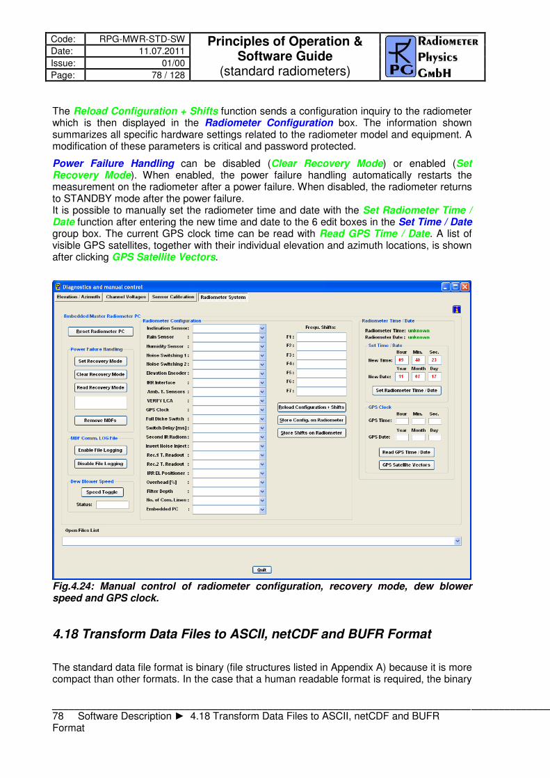
Code: RPG-MWR-STD-SW Principles of Operation & Software Guide
(standard radiometers)
Date: 11.07.2011
Issue: 01/00
Page: 78 / 128
78 Software Description ► 4.18 Transform Data Files to ASCII, netCDF and BUFR Format
The Reload Configuration + Shifts function sends a configuration inquiry to the radiometer which is then displayed in the Radiometer Configuration box. The information shown summarizes all specific hardware settings related to the radiometer model and equipment. A modification of these parameters is critical and password protected.
Power Failure Handling can be disabled (Clear Recovery Mode) or enabled (Set Recovery Mode). When enabled, the power failure handling automatically restarts the measurement on the radiometer after a power failure. When disabled, the radiometer returns to STANDBY mode after the power failure. It is possible to manually set the radiometer time and date with the Set Radiometer Time / Date function after entering the new time and date to the 6 edit boxes in the Set Time / Date group box. The current GPS clock time can be read with Read GPS Time / Date. A list of visible GPS satellites, together with their individual elevation and azimuth locations, is shown after clicking GPS Satellite Vectors.
Fig.4.24: Manual control of radiometer configuration, recovery mode, dew blower speed and GPS clock.
4.18 Transform Data Files to ASCII, netCDF and BUFR Format
The standard data file format is binary (file structures listed in Appendix A) because it is more compact than other formats. In the case that a human readable format is required, the binary
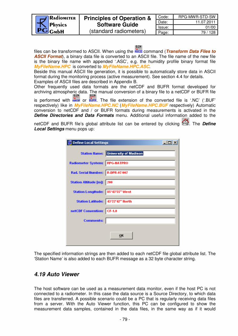
Principles of Operation & Software Guide
(standard radiometers)
Code: RPG-MWR-STD-SW
Date: 11.07.2011
Issue: 01/00
Page: 79 / 128
- 79 -
files can be transformed to ASCII. When using the command (Transform Data Files to ASCII Format), a binary data file is converted to an ASCII file. The file name of the new file is the binary file name with appended ‘.ASC’, e.g. the humidity profile binary format file MyFileName.HPC is converted to MyFileName.HPC.ASC. Beside this manual ASCII file generation, it is possible to automatically store data in ASCII format during the monitoring process (active measurement). See section 4.4 for details. Examples of ASCII files are described in Appendix B. Other frequently used data formats are the netCDF and BUFR format developed for archiving atmospheric data. The manual conversion of a binary file to a netCDF or BUFR file
is performed with or . The file extension of the converted file is ‘.NC’ (‘.BUF’ respectively) like in MyFileName.HPC.NC (MyFileName.HPC.BUF respectively) Automatic conversion to netCDF and / or BUFR formats during measurements is activated in the Define Directories and Data Formats menu. Additional useful information added to the
netCDF and BUFR file’s global attribute list can be entered by clicking . The Define Local Settings menu pops up:
The specified information strings are then added to each netCDF file global attribute list. The ‘Station Name’ is also added to each BUFR message as a 32 byte character string.
4.19 Auto Viewer
The host software can be used as a measurement data monitor, even if the host PC is not connected to a radiometer. In this case the data source is a Source Directory, to which data files are transferred. A possible scenario could be a PC that is regularly receiving data files from a server. With the Auto Viewer function, this PC can be configured to show the measurement data samples, contained in the data files, in the same way as if it would

Code: RPG-MWR-STD-SW Principles of Operation & Software Guide
(standard radiometers)
Date: 11.07.2011
Issue: 01/00
Page: 80 / 128
80 Software Description ► 4.20 Current Sample Files
receive data from a radiometer in a measurement. It is also possible to define a target directory to store the data files as hourly files. After all data samples of a source file have been displayed, the file is automatically deleted from the Source Directory.
Fig.4.25 shows the Auto Viewer Setup menu that can be entered by clicking . It lists the auto viewer’s Source Directory where it looks for data files to be displayed. In addition the Target Directory can be defined where the results of the auto viewer process are stored if Store to Archive is checked.
The Product Scan List summarizes the selected products to be scanned from the Source Directory. The display speed is set between original speed (one sample per second) up to 200 times faster. The Viewer is activated by clicking Start Viewer, halted by clicking Halt Viewer and terminated with Terminate Viewer. The user can activate the generation of ASCII, netCDF or BUFR format data files by checking the respective format(s) in the Data Directory Menu.
Fig.4.25: Auto Viewer Setup menu.

Principles of Operation & Software Guide
(standard radiometers)
Code: RPG-MWR-STD-SW
Date: 11.07.2011
Issue: 01/00
Page: 81 / 128
- 81 -
4.20 Current Sample Files During measurements data files are automatically generated on an hourly basis when UNLIMITED mode is selected. This implies that data updates are available with a delay of 60 minutes maximum when the files are remotely downloaded from the host (e.g. by an ftp server). Sometimes it is desirable to get updates more frequently. This is realized in the following way:
Enter the Define Continuous File Generation of Current Samples menu ( ). A product list is displayed as shown in Fig.4.26. For each product a separate file interval is defined. This interval determines the file length of the current samples file. E.g. whit a file interval of 10 minutes for BRT, a new file CSYYMMDDHHmm.BRT is created every 10 minutes (YY=Year, MM=Month, DD=Date, HH=Hour, mm=Minute of the date / time centred to the current CS file interval) and stored to the directory shown in the File Directory box to the left. The data in the current data files is averaged by selecting a shifting average number (measured in samples). Integration times / sample and retrievals are taken from the MDF products definition menu.
Fig.4.26: Current Samples menu showing the product list with individual file repetition and shift average settings. The current sample file generation is activated by checking Enable Current Sample File Generation. The CSYYMMDDHHmm.XXX file format is identical to the standard binary file format of the products. Automatic ASCII file generation is enabled with Add ASCII File. For CS Files the relative humidity can be blocked to be appended to absolute humidity files by un-checking Append Rel. Humidity to HP-File. If One Sample / File is activated, the program stores only the latest sample of a file interval in the CS-file. The only exception is the *.HKD CS file which is not affected by this flag. When checking File Overwrite (Name:CS.XXX), the program does not use the CSYYMMDDHHmm.XXX file convention. Instead, only CS.XXX file names are created, overwriting older files by the newest one.

Code: RPG-MWR-STD-SW Principles of Operation & Software Guide
(standard radiometers)
Date: 11.07.2011
Issue: 01/00
Page: 82 / 128
82 Software Description ► 4.21 Master / Slave Operation
When both ‘Temperature Profiles (full troposphere)’ and ‘Temperature Profiles (boundary layer)’ are selected from the list of products, a CS.COM.TPC file is automatically produced. This file contains a composite temperature profile combined from the two CS.TPC and CS.TPB files. The temperature values below 1200 m altitude are identical in CS.COM.TPC and CS.TPB and the same holds for the temperature values above 2000 m which are identical in CS.COM.TPC and CS.TPC. In the altitude range 1200 m to 2000 m, the CS.COM.TPC file temperature values are generated from a cubic spline fit to smoothly join both profiles in CS.TPC and CS.TPB. The cubic spline interpolation ensures that the first and second derivatives are continuous with the two original profiles.
4.21 Master / Slave Operation RPG’s profiler software is capable of handling multiple instruments and treating them virtually as a single radiometer. The internal instrument design limits the total number of receiver packages to two per radiometer; for instance, a humidity- and temperature-profiler (RPG-HATPRO) or a humidity profiler and 90 GHz channel (RPG-LWP-U90). Therefore e.g. a dual profiler plus 90 GHz channel cannot be combined in a single instrument. Instead, a RPG-LWP-U90 plus RPG-TEMPRO could be joined in a Master / Slave configuration to realize the dual profiler + 90 GHz frequency set. The two radiometers are connected independently to the host PC which handles all the synchronization tasks of calibrations, TB acquisition, elevation/azimuth scanning etc. between the instruments.
RPG-HATPRO
RPG-HUMPRO
RPG-LHATPRO
RPG-TEMPRO
RPG-150-90
RPG-DP150-90
RPG-LWP-U90
RPG-LWP
RPG-36-90
RPG-TEMPRO-90
RPG-15-90
RPG-TEMPRO-150
RPG-TEMPRO-150
RPG-15-90
RPG-TEMPRO-90
RPG-36-90
RPG-LWP
RPG-LWP-U90
RPG-DP150-90
RPG-150-90
RPG-TEMPRO
RPG-LHATPRO
RPG-HUMPRO
RPG-HATPRO
Fig.4.27: Possible Master/Slave combinations for current RPG models. Green: Ideal combination (no channel overlaps). Red: Channel overlaps The software combines the Master and Slave radiometers to a virtual single instrument which means that all available frequency sets from both units are stored together in brightness temperature data files (or level 0 channel voltages files), the applied online retrievals can be configured for the combined frequency set and scanning in elevation and azimuth is synchronized as well as all calibration procedures like sky tippings or other automatic

Principles of Operation & Software Guide
(standard radiometers)
Code: RPG-MWR-STD-SW
Date: 11.07.2011
Issue: 01/00
Page: 83 / 128
- 83 -
calibrations. The BL mode stores ALL TBs together with the elevation angle information into BLB files. The RPG radiometer models to be combined in a Master / Slave configuration (Fig.4.27) are the following:
• RPG-HATPRO: Humidity and Temperature Profiler (7 channels in the 22.2-31.4 GHz range, 7 channels in the 51-59 GHz range)
• RPG-HUMPRO: Humidity Profiler (7 channels in the 22.2-31.4 GHz range) for mid-latitude to tropical humidity levels >2 kg/m^2 (2mm)
• RPG-TEMPRO: Temperature Profiler (7 channels in the 51-59 GHz range)
• RPG-LHATPRO: Humidity and Temperature Profiler (7 channels in the 22.2-31.4 GHz range, 6 channels in the 183-198 GHz range), humidity profiler for ultra low humidity levels < 2 kg/m^2 (2mm)
• RPG-LWP: Two channel (23.8 / 31.4 GHz) radiometer for LWP / IWV retrieval
• RPG-LWP-U90: Humidity Profiler (7 channels in the 22.2-31.4 GHz range) plus 90 GHz channel for improved LWP accuracy
• RPG-150-90: Two channel (90 / 150 GHz) radiometer for the detection of low LWP levels
• RPG-DP150-90: Three channel (90 / dual pol. 150 GHz) radiometer for the detection of low LWP levels and ice particles
• RPG-36-90: Two channel (36 / 90 GHz) radiometer for atmospheric attenuation measurements. Intended as a Slave instrument for other models
• RPG-TEMPRO-90: Temperature Profiler (7 channels in the 51-59 GHz range) plus 90 GHz channel. Ideal combination with RPG-HUMPRO
• RPG-TEMPRO-150: Temperature Profiler (7 channels in the 51-59 GHz range) plus 150 GHz channel. Ideal combination with RPG-HUMPRO
• RPG-15-90: Two channel (15.3 / 90 GHz) radiometer for atmospheric attenuation measurements. Intended as a Slave instrument for other models
Fig.5.28: Example of serial ports definition menu for combining a Slave and Master instrument. The most effective frequency coverage results from the combination RPG-LWP-U90 / RPG-LHATPRO, which is a triple profiler for medium/low humidity, ultra low humidity and temperature plus a 90 GHz channel for improved LWP retrieval.

Code: RPG-MWR-STD-SW Principles of Operation & Software Guide
(standard radiometers)
Date: 11.07.2011
Issue: 01/00
Page: 84 / 128
84 Software Description ► 4.21 Master / Slave Operation
Both radiometers are connected to different host PC serial ports. These ports have to be defined in the Define Serial Communication Ports menu (see Fig.4.28). The Activate checkbox in the Slave Port window must be checked in order to support the second radiometer. The Define Serial Communication Ports menu provides the checkbox Try again, if not successful. If selected, the host retries a connection after a connection failure one more time. When the host PC is connecting to the Master, Slave and Azimuth scanner, it displays the current connection status as in Fig. 4.29.
Fig.4.29 : Display of the current connection status.
If a Master and Slave unit have been successfully detected, the host PC’s main window looks as shown in Fig.4.30. The difference to the single radiometer display is that there is a toggle button in the Radiometer Status window to alternatively show the Master and Slave housekeeping data and instrument calibration status. In addition, a second status bar is displayed at the bottom of the screen to indicate the Slave connection status and interface settings.

Principles of Operation & Software Guide
(standard radiometers)
Code: RPG-MWR-STD-SW
Date: 11.07.2011
Issue: 01/00
Page: 85 / 128
- 85 -
Fig.4.30 : Main window display after connecting to a Master / Slave tandem radiometer. The ‘Radiometer Status’ display can be toggled between Master and Slave instruments and there are two status bars on the bottom of the display to include the Slave connection status information.
Fig.4.31 : Example of the Radiometer Systems tag when a Slave is connected.
Several other menus are showing the same Master / Slave toggle button like the diagnostics menus, the file transfer menu or the absolute calibration menu. Before issuing a command from one of these menus, the user specifies the direction of the command by clicking the
Master / Slave Toggle
second Status Bar
toggle

Code: RPG-MWR-STD-SW Principles of Operation & Software Guide
(standard radiometers)
Date: 11.07.2011
Issue: 01/00
Page: 86 / 128
86 Software Description ► 4.22 The License Manager
toggle to Master or Slave. Where frequency channels are listed, the Master channels are preceded by ‘M:’ while the Slave channels are preceded by ‘S:’. When enabling file backup, all data files are stored on the Master’s flash memory; no data is stored to the Slave’s flash. When the HKD (housekeeping data) product is selected and a Slave radiometer is present, a second HKD monitoring window is created during measurements for the display of the Slave housekeeping data. The HKD data file names for the Slave instrument have the extension *_S.HKD instead of *.HKD (Master radiometer).
4.22 The License Manager RPG’s radiometers are delivered with a preliminary limited license of 30 days. Without activating an unlimited license, the radiometer stops operation when the limited license is expired. The common procedure to avoid this is the following:
Invoke the License Manager by clicking the button. The menu in Fig.4.32 pops up.
Fig.4.32 : License manager menu.
The user retrieves license status information with the Get License Status command. The license type (limited or unlimited) as well as the expiration date and time will be displayed. In order to obtain an unlimited license, the following steps have to be performed:

Principles of Operation & Software Guide
(standard radiometers)
Code: RPG-MWR-STD-SW
Date: 11.07.2011
Issue: 01/00
Page: 87 / 128
- 87 -
1. Connect to the radiometer and click the Get License ID from Radiometer button. The license ID code is then written to the file ‘LicID.DAT’ stored in the radiometer root directory (the directory where R2CH.EXE is located).
2. Send the ‘LicID.DAT’ file to RPG (by e-mail to [email protected]). Then the 10 digit license code will be returned (also by e-mail).
3. Enter the 10 digit license code into the edit box in the license manager and click Send License Code. The license manager will inform the user if the unlimited license installation was successful or not. If not successful, please contact RPG again.
4.23 Adjusting Azimuth Positioner Direction The host software includes the possibility of precisely adjusting the azimuth scanner’s zero index position to North direction. This is useful for volume scans or when different instruments shall be aligned to the same scanning directions. The described method assumes that the instrument stand is horizontally aligned (see Installation Manual).
The azimuth adjustment menu is entered with the command, as shown in Fig.4.33. The host software calculates the sun position in elevation and azimuth from the GPS position and UTC time available from the GPS clock. The radiometer stand should be pre-adjusted so that the azimuth scanner’s zero position is pointing to North with an accuracy of better than 30°. This can be easily achieved with a standard low cost compass. The user should start the adjustment procedure with a relatively wide azimuth scanning span (e.g. >=50°) and start the scan (click Start Scan) as shown in the upper left corner of Fig.4.33. After the scan is finished, the misalignment between the real north direction and the scanner’s north direction is printed in the ‘Misalignment’ box. A positive misalignment indicates that the stand is directed towards the West and should be rotated eastwards. In an iterative process like indicated in Fig.4.33, the stand’s orientation can be adjusted to the real North with an accuracy of better than 0.5°.

Code: RPG-MWR-STD-SW Principles of Operation & Software Guide
(standard radiometers)
Date: 11.07.2011
Issue: 01/00
Page: 88 / 128
88 Software Description ► 4.24 Software Updates
Fig.4.33: Azimuth angle adjustment using the sun position.
The radiometer uses the detector voltage of the first channel of receiver 1, if present (e.g. the 22.24 GHz channel in a RPG-HATPRO radiometer), otherwise it takes the first channel of receiver 2 (e.g. in the RPG-TEMPRO radiometer).
4.24 Software Updates Assumption: You want to install a new radiometer software version (2CH.EXE) on the embedded radiometer PC and a new version of R2CH.EXE on the host PC. 1. Step: Save the old software versions a) Create a directory to save the old software versions (e.g. C:\MyPath \SAVE).
b) Connect the host to the radiometer and enter the File Transfer Menu ( , Fig.4.34). On the right side (Host) browse to the directory for saving the files (e.g. C:\MyPath\ SAVE) and on the left side (Radiometer) in the System Files Directory mark the 2CH.EXE file. Then drag and drop the 2CH.EXE file to the C:\MyPath\ SAVE directory to initiate the copy process. c) locate the R2CH.EXE file in the MyPath\ RPG-HATPRO directory and copy this file to the C:\MyPath \SAVE directory (by using the Operating System Explorer). 2. Step: Overwrite the old versions by the new ones
a) Copy the new version of 2CH.EXE (the radiometer PC software) on an arbitrary directory on your hard disk (e.g. MyPath\RPG-HATPRO\Radiometer PC). Then enter the file transfer menu in Fig.4.2.1 and browse to that directory. Mark the 2CH.EXE file in the Files-list and drag and drop it to the System Files Directory list. Because you are now going to overwrite a file in the System Files Directory (which is password protected for write access) a password entry window pops up. Please enter the following password in exactly the way as it is printed here:

Principles of Operation & Software Guide
(standard radiometers)
Code: RPG-MWR-STD-SW
Date: 11.07.2011
Issue: 01/00
Page: 89 / 128
- 89 -
theringsofsaturn
Press OK and the 2CH.EXE on the radiometer PC will be overwritten by the new 2CH.EXE version. Exit the File Transfer Menu after that.
Fig.4.34: File Transfer Menu
b) Boot the radiometer PC to make the new 2CH.EXE the running version. You can do
this by entering the Manual Control Menu ( ) and selecting the “Radiometer System” tag. Click Reset Radiometer PC and confirm the command with YES. Wait for about 2 minutes to give the boot process time enough to finish.
c) Terminate R2CH.EXE and overwrite the old R2CH.EXE in MyPath\ RPG-HATPRO
with the new version.
d) Execute R2CH.EXE to start the new host version and reconnect to the radiometer
with .
The software upgrade is finished. You can confirm the successful upgrade by reading the software version numbers of both, the embedded radiometer PC (see main window radiometer status display) and the host PC (see main window caption).

Code: RPG-MWR-STD-SW Principles of Operation & Software Guide
(standard radiometers)
Date: 11.07.2011
Issue: 01/00
Page: 90 / 128
90 5. Retrievals ► 5.1 Retrieval Algorithms
5. Retrievals
5.1 Retrieval Algorithms In order to estimate atmospheric parameters (such as liquid water path or the humidity profile) from the radiometer data, a suitable mathematical algorithm has to be found. A statistical regression between observed atmospheric (meteorological) data and the corresponding instrument data (brightness temperatures in different channels and additional information provided by temperature, pressure, and humidity sensors within the instrument) is a widely used solution for this task, although other methods (physical retrievals) are also known to yield good results.
5.1.1 General remarks
Gathering such simultaneously observed calibration data for a specific instrument at a specific site leads to long delays before the instruments ability to deliver atmospheric data is established. Statistical reliability calls for an observation period of several years, preferably more then one decade. During this time the atmosphere would need to be measured on a regular basis (twice a day), which also adds to the costs and impracticability. A faster approach will not use real data from the actual instrument but databases of meteorological observations. Such (radio sounding) measurements are recorded for weather prediction by many stations throughout the whole world, thus covering a vast range of climates and different weather conditions. The corresponding radiometer data needs to be calculated by radiative transfer models. This simulation is called forward modelling because the dependent data (the observable brightness temperatures) are calculated from the independent atmospheric variables. Any method or algorithm that is able to invert this process and calculate the independent variables from the dependent observations is called Retrieval. Statistical retrieval methods use a training data set to derive a multi-linear regression, quadratic regression or an artificial neural network fit (which essentially is a form of non-linear multivariate regression). The coefficients of this regression will be applied to the radiometer measurements in order to calculate actual atmospheric variables. Quality control of the retrieval algorithms is, in general, performed in two ways: After using the training data set for establishing the regression coefficients we apply the retrieval to a second data set, the test data. This data set must not be contained in the training data. Comparing the retrieved results with the known “real” results from the test data allows for a thorough statistical evaluation in terms of bias error, RMS, correlation etc. In addition, the operational algorithms have to be tested with measurement campaigns where the atmospheric state is actually measured by independent instrumentation.
5.1.2 Data source and applicability
The amount and quality of the input data is crucial for the quality of the designed algorithm. Since a statistical algorithm can (when applied to real data) only cope with input data that is in the range represented by the training data, we need a sufficient number of samples. At least 10 years of data with two observations per day are needed to describe the natural variation of the atmosphere. Smaller time series might be missing some extreme situations which do not occur every year. Besides the length of the time series the geographical sampling is of major importance. If only one time series which is taken at one single station is used to derive the algorithm, then

Principles of Operation & Software Guide
(standard radiometers)
Code: RPG-MWR-STD-SW
Date: 11.07.2011
Issue: 01/00
Page: 91 / 128
- 91 -
the algorithm may only be used at this specific location. Moving the radiometer to another geographical position with different whether conditions or even different altitudes above sea level will have a negative impact on the retrieval quality. By using a multitude of weather stations for the regression data base, the algorithms will be applicable to a variety of different locations. Furthermore the larger number of input data will contribute to the overall quality of the product.
5.1.3 Data quality processing and reformatting
Raw data comes in form of radiosonde data (also known as radio soundings). Such measurements contain air pressure, ambient temperature, and relative humidity at different vertical positions. Some types of radio soundings also contain wind speed and direction, but this information is not used in out type of algorithms. The number of levels (vertical resolution) typically is in the range of 10 to 20 levels up to several thousand levels. The following steps have to be performed with the data:
1. Quality control: Depending on the data source the data may contain measurement errors, inconsistent data, and missing data. Missing data in one level leads to rejection of only that level. We check for the following error conditions and reject the sounding:
• Increasing height in subsequent levels
• Increasing pressure with height
• Temperatures larger than 330 K or smaller than 210 K (190 K at larger heights)
• Pressure larger than 1050 hPa
• Pressure smaller than 1 Pa, surface pressure smaller than 500 hPa
• Height larger than 70 km or smaller than -200 m 2. Applicability checks:
• At least a 10 km height is reached with temperature and pressure information
• At least -30 °C is reached with valid humidity information
• At least 10 levels are present in the sounding
• For some retrievals we reject raining clouds. These are detected by a threshold LWC larger than 3.5 g/m^2.
3. Reformatting: The soundings are stored in a common data format, but without interpolating or changing the data.
5.1.4 Cloud processing
From the sounding data we calculate further atmospheric parameters connected to clouds and rain. A cloud detection scheme reads the temperature and humidity vertical profiles and determines whether a cloud exists in a level or not. The criteria for cloud existence are a threshold relative humidity (usually 95 %) together with a temperature warmer than 243.15 K. These thresholds can be varied. A second stage processing calculates the amount of liquid water (LWC, liquid water content) within each layer based on the modified adiabatic water content. This number is something like an upper limit of how much water can be present in a cloud layer with respect to the current atmospheric situation. The above algorithms produce multi-layered clouds with several sounding levels in each cloud layer. The total amount of water (LWP, liquid water path) is calculated by integrating all cloud layers.

Code: RPG-MWR-STD-SW Principles of Operation & Software Guide
(standard radiometers)
Date: 11.07.2011
Issue: 01/00
Page: 92 / 128
92 5. Retrievals ► 5.1 Retrieval Algorithms
5.1.5 Angle and frequency selection
Prior to radiative transfer calculations the frequencies and elevation angles have to be selected. While the frequencies are mostly determined by the type of the retrieval, the angles have to be selected to meet the user requirements. Each observation angle needs its own set of retrieval coefficients. Those coefficients depend strongly on the observation angle and cannot be interpolated.
5.1.6 Radiative Transfer calculations
In order to calculate simulated brightness temperatures from the sounding data we have to know the interaction parameters of matter with microwave radiation (absorption and scattering coefficients) at every position and every frequency that might be considered in one retrieval algorithm. Based on gas absorption models, the mass absorption coefficients are set up in every layer according to the pressure, humidity, and temperature. Cloud water adds absorption proportional to its mass with a temperature dependent absorption coefficient. At frequencies below 100 GHz the scattering at cloud droplets can be neglected. Rain clouds are not considered in the retrieval generation. This subsection is not yet finished and still under preparation.
5.1.7 Retrieval grid and type of regression
This subsection is under preparation.
5.1.8 Algorithm performance
This subsection is under preparation.

Principles of Operation & Software Guide
(standard radiometers)
Code: RPG-MWR-STD-SW
Date: 11.07.2011
Issue: 01/00
Page: 93 / 128
- 93 -
Some users might be able to perform their own radiative transfer calculations and have access to a huge data set of radiosondes. A sophisticated design tool for the generation of system conform retrieval files is implemented in the “Files + Integration” tab sheet of the measurement definition window (see Fig.4.8). The Define Retrieval File-command activates the retrieval design window of Fig.5.1.
Fig.5.1: Retrieval file editor.
5.1.9 File Format
All retrieval files have the extension “.RET” to distinguish them from other file types. The first three characters of the file name indicate the retrieval product. For version 1.1 six products are implemented: TPT (temperature profile, troposphere), HPT (humidity profile, troposphere), LWP, IWV, ATN (Atmospheric Attenuation) and TPB (temperature profile, boundary layer). The next section (sections are separated from each other by the “_” character) of the file name is reserved for the retrieval type. Possible retrieval types are: LR (linear regression), QR (quadratic regression) and NN (neural networks). The third section contains the customer code and the forth section represents the version number. The file name sections are summarized in the editor’s “Category”-frame. The data base identifier is not used for the file name but is stored into the retrieval file for future purposes.

Code: RPG-MWR-STD-SW Principles of Operation & Software Guide
(standard radiometers)
Date: 11.07.2011
Issue: 01/00
Page: 94 / 128
94 5. Retrievals ► 5.2 Retrieval File Structure
5.2 Retrieval File Structure
With the Load Retrieval File-button load the “TPT_QR_JAP_1_V1.RET”-file from the “…\2CH\RETRIEVALS\TPROFILE_TROP\”-directory. Retrieval files are text files which can be edited by any editor that does not insert any control codes or other characters that do not belong to the text. The content of the loaded retrieval file is displayed in the blue editor window.
The file starts with an identification code (6795005) utilized by R2CH to detect non-conformities caused by future changes in the file format. Comments are preceded by the “#”-character. All other text lines contain relevant data needed for the retrieval computation routines (2CH).
The continue character “:”at the beginning of a line indicates that this line belongs to the same parameter as the previous line. The continue code is used in the definition of matrices to add rows to a matrix.
A parameter code of 2 characters followed by a “=” character (no spaces!) specifies the meaning of the data that follows the “=” sign. The codes for the retrieval category are:
• ‘RP=’: Retrieval product. 0: LWP, 1: IWV, 2: Attenuation, 3: temperature profile (troposphere), 4: temperature profile (boundary layer), 6: humidity profile (troposphere) (mandatory parameter).
• ‘RT=’: Retrieval type. 0: linear regression, 1: quadratic regression, 2: neural network (mandatory).
• ‘CC=’: Customer code (mandatory parameter).
• ‘DB=’: Data Base
• ‘VN=’: Version number (mandatory parameter).
These codes must precede all other codes (except for the retrieval basis ‘RB=’).
Some retrievals include the surface sensor data as input parameters beside the brightness temperature data. In the “Included Sensors”-frame the retrieval designer checks the sensors he is going to include in his retrieval. The associated codes are:
• ‘TS=’: Temperature sensor. 0: sensor not used for retrieval, 1: sensor used (mandatory parameter).
• ‘PS=’: Pressure sensor. 0: sensor not used for retrieval, 1: sensor used (mandatory parameter).
• ‘HS=’: Humidity sensor. 0: sensor not used for retrieval, 1: sensor used (mandatory parameter).
• ‘IS=’: Infrared radiometer. 0: sensor not used for retrieval, 1: sensor used (mandatory parameter).
A neural network retrieval parameter is the number of intermediate knots (hidden knot layer). The associated parameter is:

Principles of Operation & Software Guide
(standard radiometers)
Code: RPG-MWR-STD-SW
Date: 11.07.2011
Issue: 01/00
Page: 95 / 128
- 95 -
• ‘NK=’: Number of intermediate knots (Neural Network only)
The presence of these codes in the retrieval file is mandatory.
Some retrieval designers prefer the optical thicknesses as input parameter instead of brightness temperatures. The code is:
• ‘RB=’: Retrieval basis. 0: brightness temperatures, 1: optical thicknesses (mandatory parameter).
All retrievals are based on microwave frequency channels. The frequency list must be preceded by:
• ‘FR=’: Frequency list [GHz] (mandatory parameter).
All observations are performed at certain elevation angles:
• ‘AG=’: Elevation angle list (mandatory parameter).
Those retrievals that produce data at certain altitudes (humidity and temperature profiles) must have an altitude parameter specified:
‘AL=’: Altitude list [m]
All other parameters are specific for the retrieval type.
5.2.1 Linear Regressions
As was discussed before a linear regression retrieval calculation has the following structure:
∑∑ ++=freq
jij
sensors
jijii TbTLSrSLOSOut **
where Outi is the i-th retrieval output parameter (e.g. the temperature at altitude Ai ), OSi is the retrieval offset parameter for Outi, Srj is the surface sensor reading of the j-th checked sensor (the sequence is: TS, HS,PS,IS), SLij is the corresponding linear coefficient, Tbj is the brightness temperature or optical thickness at the j-th frequency and TLij is the corresponding linear coefficient. The surface sensor readings are measured in K (Temperature), % (Humidity), Pa (Barometric Pressure) and °C (Infrared Temperature). All brightness temperatures are measured in K.
The parameters in the retrieval file are:
Code: RPG-MWR-STD-SW Principles of Operation & Software Guide
(standard radiometers)
Date: 11.07.2011
Issue: 01/00
Page: 96 / 128
96 5. Retrievals ► 5.3 Retrieval File Templates
• ‘OS=’: offset matrix (same unit as Outi )
• ‘SL=’: linear sensor coefficient matrix
• ‘TL=’: linear brightness temperature coefficient
5.2.2 Quadratic Regressions
A quadratic regression retrieval calculation has the following structure:
∑∑∑∑ ++++=freq
jij
sensors
jij
freq
jij
sensors
jijii TbTQSrSQTbTLSrSLOSOut22
****
where Outi is the i-th retrieval output parameter (e.g. the temperature at altitude Ai ), OSi is the retrieval offset parameter for Outi, Srj is the surface sensor reading of the j-th checked sensor (the sequence is: TS, HS,PS,IS), SLij is the corresponding linear coefficient and SQij is the corresponding quadratic coefficient, Tbj is the brightness temperature or optical thickness at the j-th frequency with TLij is the corresponding linear coefficient and TQij is the corresponding quadratic coefficient. The surface sensor readings are measured in K (Temperature), % (Humidity), Pa (Barometric Pressure) and °C (Infrared Temperature). All brightness temperatures are measured in K.
The parameters in the retrieval file are:
• ‘OS=’: offset matrix (same unit as Outi )
• ‘SL=’: linear sensor coefficient matrix
• ‘SQ=’: quadratic sensor coefficient matrix
• ‘TL=’: linear brightness temperature coefficient
• ‘TQ=’: quadratic brightness temperature coefficient
5.2.3 Neural Networks
The parameters for the neural network retrieval calculation are:
• ‘IM=’: input coefficient matrix
• ‘OM=’: output coefficient matrix
The structure of these matrices can be derived from a template neural network file (see chapter below).
5.3 Retrieval File Templates
The user does not have to enter all these parameters by hand but instead defines his retrieval input and output parameters by filling the list boxes and check boxes in the retrieval

Principles of Operation & Software Guide
(standard radiometers)
Code: RPG-MWR-STD-SW
Date: 11.07.2011
Issue: 01/00
Page: 97 / 128
- 97 -
editor. In addition, five comment lines may be entered for customer related information etc. By clicking on the “Generate Template”-button the editor text window is initialized with a syntactically correct retrieval file comprising all settings and numerical data is filled with zeros.
The user must generate a text file which contains the retrieval coefficients in the same row and column order as required for the template. Then this coefficient file can be loaded with the “Load Data Matrix”-button and a second editor text window is opened containing this file. The user then copies and pastes the matrices from his coefficient file editor into the retrieval file editor text window. This concept ensures that the retrieval file syntax remains correct.

Code: RPG-MWR-STD-SW Principles of Operation & Software Guide
(standard radiometers)
Date: 11.07.2011
Issue: 01/00
Page: 98 / 128
98 Appendix A (File Formats) ► A1: LWP-Files (*.LWP), Liquid Water Path
Appendix A (File Formats)
A1: LWP-Files (*.LWP), Liquid Water Path
Variable Name Type # Bytes Description
LWPCode int 4 LWP-File Code (=934501978)
N int 4 Number of recorded samples
LWPMin float 4 Minimum of recorded LWP values
LWPMax float 4 Maximum of recorded LWP values
LWPTimeRef int 4 Time reference (1: UTC, 0: Local Time)
LWPRetrieval int 4 0: lin. Reg., 1 : quad. Reg., 2: Neur. Net.
T_1 int 4 Time of sample 1 (# of sec. since 1.1.2001)
RF_1(1) char 1 Rainflag of sample 1 (0: no rain, 1: rain)
LWP_1 float 4 LWP sample 1 [g/m^2]
LWPAng_1(2) float 4 LWP angle 1 [DEG]
… … … …
… … … …
… … … …
T_N int 4 Time of sample N (# of sec. since 1.1.2001)
RF_N(1) char 1 Rainflag of sample N (0: no rain, 1: rain)
LWP_N float 4 LWP sample N [g/m^2]
LWPAng_N(2) float 4 LWP angle N [DEG] (1) The rain flag is an 8 bit array: MSB 000yyxxr LSB, r = rain information (0= no rain, 1=raining) xx = qulity level (0=not evaluated, 1=high, 2=medium, 3=low), yy = reason for reduced quality (see appendix A18) (2) Angle is coded in the following way: ANG=sign(Elevation) * (|Elevation|+1000*Azimuth)
A2: IWV-Files (*.IWV), Integrated Water Vapour
Variable Name Type # Bytes Description
IWVCode int 4 IWV-File Code (=594811068)
N int 4 Number of recorded samples
IWVMin float 4 Minimum of recorded IWV values
IWVMax float 4 Maximum of recorded IWV values
IWVTimeRef int 4 Time reference (1: UTC, 0: Local Time)
IWVRetrieval int 4 0: lin. Reg., 1 : quad. Reg., 2: Neur. Net.
T_1 int 4 Time of sample 1 (# of sec. since 1.1.2001)
RF_1(1) char 1 Rainflag of sample 1 (0: no rain, 1: rain)
IWV_1 float 4 IWVsample 1 [kg/m^2]
IWVAng_1(2) float 4 IWV angle 1 [DEG]
… … … …
… … … …
… … … …
T_N int 4 Time of sample N (# of sec. since

Principles of Operation & Software Guide
(standard radiometers)
Code: RPG-MWR-STD-SW
Date: 11.07.2011
Issue: 01/00
Page: 99 / 128
- 99 -
1.1.2001)
RF_N(1) char 1 Rainflag of sample N (0: no rain, 1: rain)
IWV_N float 4 IWV sample N [kg/m^2]
IWVAng_N(2) float 4 IWV angle N [DEG] (1) The rain flag is an 8 bit array: MSB 000yyxxr LSB, r = rain information (0= no rain, 1=raining) xx = qulity level (0=not evaluated, 1=high, 2=medium, 3=low), yy = reason for reduced quality (see appendix A18) (2) Angle is coded in the following way: ANG=sign(Elevation) * (|Elevation|+1000*Azimuth)
A3: ATN-Files (*.ATN), Atmospheric Attenuation
Variable Name Type # Bytes Description
ATNCode int 4 ATN-File Code (=7757564)
N int 4 Number of recorded samples
ATNTimeRef int 4 Time reference (1: UTC, 0: Local Time)
ATNRetrieval int 4 0: lin. Reg., 1 : quad. Reg., 2: Neur. Net., 3: Tmr based retrieval
FreqAnz int 4 # of recorded frequencies
Freqs[i] float 4 x FreqAnz
Frequencies [GHz]
ATNMin[] float 4 x FreqAnz
Minimum of recorded ATN values
ATNMax[] float 4 x FreqAnz
Maximum of recorded ATN values
T_1 int 4 Time of sample 1 (# of sec. since 1.1.2001)
RF_1(1) char 1 Rainflag of sample 1 (0: no rain, 1: rain)
ATN_1[] float 4 x FreqAnz
ATN sample 1 (Attenuation [dB])
ANG1(2) float 4 Observation angles, sample 1
… … … …
… … … …
… … … …
T_N int 4 Time of sample N (# of sec. since 1.1.2001)
RF_N(1) char 1 Rainflag of sample N (0: no rain, 1: rain)
ATN_N[] float 4 x FreqAnz
ATN sample N (Attenuation [dB])
ANGN(2) float 4 Observation angles, sample N (1) The rain flag is an 8 bit array: MSB 000yyxxr LSB, r = rain information (0= no rain, 1=raining) xx = qulity level (0=not evaluated, 1=high, 2=medium, 3=low), yy = reason for reduced quality (see appendix A18) (2) Angle is coded in the following way: ANG=sign(Elevation) * (|Elevation|+1000*Azimuth)
A4: BRT-Files (*.BRT), Brightness Temperature
Variable Name Type # Bytes Description
BRTCode int 4 BRT-File Code (=666666)
N int 4 Number of recorded samples
BRTTimeRef int 4 Time reference (1: UTC, 0: Local Time)

Code: RPG-MWR-STD-SW Principles of Operation & Software Guide
(standard radiometers)
Date: 11.07.2011
Issue: 01/00
Page: 100 / 128
100 Appendix A (File Formats) ► A5: MET-Files (*.MET), Meteorological Sensors
FreqAnz int 4 # of recorded frequencies
Freq[] float 4 x FreqAnz Frequencies [GHz]
BRTMin[] float 4 x FreqAnz Minimum array of recorded BRT values
BRTMax[] float 4 x FreqAnz Maximum array of recorded BRT values
T_1 int 4 Time of sample 1 (# of sec. since 1.1.2001)
RF_1 char 1 Rainflag of sample 1 (0: no rain, 1: rain)
BRT_1[] float 4 x FreqAnz Br. Temp. array sample 1 [K]
ANG_1(1) float 4 Elevation/Azimuth angle of sample 1 (DEG)
… … … …
T_N int 4 Time of sample N (# of sec. since 1.1.2001)
RF_N char 1 Rainflag of sample N (0: no rain, 1: rain)
BRT_N[] float 4 x FreqAnz Br. Temp. sample N, frequency 1 [K]
ANG_N(1) float 4 Elevation/Azimuth angle of sample N (DEG) (1) Angle is coded in the following way: ANG=sign(Elevation) * (|Elevation|+1000*Azimuth)
A5: MET-Files (*.MET), Meteorological Sensors
Variable Name Type # Bytes Description
METCode int 4 MET-File Code (=599658943)
N int 4 Number of recorded samples
METMinP float 4 Minimum of recorded pressure values
METMaxP float 4 Maximum of recorded pressure values
METMinT float 4 Minimum of environmental temp. values
METMaxT float 4 Maximum of environmental temp. values
METMinH float 4 Minimum of recorded rel. humidity values
METMaxH float 4 Maximum of recorded rel. humidity values
METTimeRef int 4 Time reference (1: UTC, 0: Local Time)
T_1 int 4 Time of sample 1 (# of sec. since 1.1.2001)
RF_1 char 1 Rainflag of sample 1 (0: no rain, 1: rain)
MET_1(0) float 4 Pressure value sample 1 [mbar]
MET_1(1) float 4 Temp. value sample 1 [K]
MET_1(2) float 4 Rel. humidity value sample 1 [%]
… … … …
MET_N(0) float 4 Pressure value sample N [mbar]
MET_N(1) float 4 Temp. value sample N [K]
MET_N(2) float 4 Rel. humidity value sample N [%]
A6: OLC-Files (*.OLC), Oxygen Line Chart
Variable Name Type # Bytes Description
OLCCode int 4 OLC-File Code (=955874342)
N int 4 Number of recorded samples
OLCMin float 4 Minimum of recorded OL-Brt. values
OLCMax float 4 Maximum of recorded OL-Brt. values
OLCTimeRef int 4 Time reference (1: UTC, 0: Local Time)
FreqAnz int 4 # of recorded frequencies in oxygen line

Principles of Operation & Software Guide
(standard radiometers)
Code: RPG-MWR-STD-SW
Date: 11.07.2011
Issue: 01/00
Page: 101 / 128
- 101 -
Freq[i] float 4 x FreqAnz Frequencies [GHz]
T_1 int 4 Time of sample 1 (# of sec. since 1.1.2001)
RF_1 char 1 Rainflag of sample 1 (0: no rain, 1: rain)
O2_BRT_1(i) float 4 x FreqAnz Brightness Temp. of oxygen line [K], sample 1
ANG1(1) float 4 Observation angles, sample 1
… … … …
T_N int 4 Time of sample N (# of sec. since 1.1.2001)
RF_N char 1 Rainflag of sample N (0: no rain, 1: rain)
O2_BRT_N(i) float 4 x FreqAnz Brightness Temp. of oxygen line [K], sample N
ANGN(1) float 4 Observation angles, sample N (1) Angle is coded in the following way: ANG=sign(Elevation) * (|Elevation|+1000*Azimuth)
A7: TPC-Files (*.TPC), Temperature Profile Chart (Full Trop.)
Variable Name Type # Bytes Description
TPCCode int 4 TPC-File Code (=780798065)
N int 4 Number of recorded samples
TPCMin float 4 Minimum of recorded temperature values
TPCMax float 4 Maximum of recorded temperature values
TPCTimeRef int 4 Time reference (1: UTC, 0: Local Time)
TPCRetrieval int 4 0: lin. Reg., 1 : quad. Reg., 2: Neural Network
AltAnz int 4 # of altitude layers
Alts[i] int 4 x AltAnz Altitudes [m]
T_1 int 4 Time of sample 1 (# of sec. since 1.1.2001)
RF_1(1) char 1 Rainflag of sample 1 (0: no rain, 1: rain)
TP_1(i) float 4 x AltAnz Temperature Profile [K], sample 1
… … … …
T_N int 4 Time of sample N (# of sec. since 1.1.2001)
RF_N(1) char 1 Rainflag of sample N (0: no rain, 1: rain)
TP_N(i) float 4 x AltAnz Temperature Profile [K], sample N (1) The rain flag is an 8 bit array: MSB 000yyxxr LSB, r = rain information (0= no rain, 1=raining) xx = qulity level (0=not evaluated, 1=high, 2=medium, 3=low), yy = reason for reduced quality (see appendix A18)
A8: TPB-Files (*.TPB), Temperature Profile Chart (Boundary Layer)
Variable Name Type # Bytes Description
TPBCode int 4 TPB-File Code (=459769847)
N int 4 Number of recorded samples
TPBMin float 4 Minimum of recorded temperature values
TPBMax float 4 Maximum of recorded temperature values
TPBTimeRef int 4 Time reference (1: UTC, 0: Local Time)
TPBRetrieval int 4 0: lin. Reg., 1 : quad. Reg., 2: Neural Network
AltAnz int 4 # of altitude layers
Alts[i] int 4 x AltAnz Altitudes [m]
T_1 int 4 Time of sample 1 (# of sec. since 1.1.2001)

Code: RPG-MWR-STD-SW Principles of Operation & Software Guide
(standard radiometers)
Date: 11.07.2011
Issue: 01/00
Page: 102 / 128
102 Appendix A (File Formats) ► A9: WVL-Files (*.WVL), Water Vapour Line Chart
RF_1(1) char 1 Rainflag of sample 1 (0: no rain, 1: rain)
TP_1(i) float 4 x AltAnz Temperature Profile [K], sample 1
… … … …
T_N int 4 Time of sample N (# of sec. since 1.1.2001)
RF_N(1) char 1 Rainflag of sample N (0: no rain, 1: rain)
TP_N(i) float 4 x AltAnz Temperature Profile [K], sample N (1) The rain flag is an 8 bit array: MSB 000yyxxr LSB, r = rain information (0= no rain, 1=raining) xx = qulity level (0=not evaluated, 1=high, 2=medium, 3=low), yy = reason for reduced quality (see appendix A18)
A9: WVL-Files (*.WVL), Water Vapour Line Chart
Variable Name Type # Bytes Description
WVLCode int 4 WVL-File Code (=456783953)
N int 4 Number of recorded samples
WVLMin float 4 Minimum of recorded WVL-Brt. values
WVLMax float 4 Maximum of recorded WVL-Brt. values
WVLTimeRef int 4 Time reference (1: UTC, 0: Local Time)
FreqAnz int 4 # of recorded frequencies in WV line
Freq[i] float 4 x FreqAnz Frequencies [GHz]
T_1 int 4 Time of sample 1 (# of sec. since 1.1.2001)
RF_1 char 1 Rainflag of sample 1 (0: no rain, 1: rain)
WVL_BRT_1(i) float 4 x FreqAnz Brightness Temp. of WV line [K], sample 1
ANG1(1) float 4 Observation angle, sample 1
… … … …
T_N int 4 Time of sample N (# of sec. since 1.1.2001)
RF_N char 1 Rainflag of sample N (0: no rain, 1: rain)
WVL_BRT_N(i) float 4 x FreqAnz Brightness Temp. of WV line [K], sample N
ANGN(1) float 4 Observation angle, sample N (1) Angle is coded in the following way: ANG=sign(Elevation) * (|Elevation|+1000*Azimuth)
A10(1): HPC-Files (*.HPC), Humidity Profile Chart (without RH)
Variable Name Type # Bytes Description
HPCCode int 4 HPC-File Code (=117343672)
N int 4 Number of recorded samples
HPCMin float 4 Minimum of recorded abs. humidity values
HPCMax float 4 Maximum of recorded abs. humidity values
HPCTimeRef int 4 Time reference (1: UTC, 0: Local Time)
HPCRetrieval int 4 0: lin. Reg., 1 : quad. Reg., 2: Neural Network
AltAnz int 4 # of altitude layers
Alts[i] int 4 x AltAnz Altitudes [m]
T_1 int 4 Time of sample 1 (# of sec. since 1.1.2001)
RF_1(1) char 1 Rainflag of sample 1 (0: no rain, 1: rain)
HP_1(i) float 4 x AltAnz Humidity Profile [g/m^3], sample 1

Principles of Operation & Software Guide
(standard radiometers)
Code: RPG-MWR-STD-SW
Date: 11.07.2011
Issue: 01/00
Page: 103 / 128
- 103 -
… … … …
T_N int 4 Time of sample N (# of sec. since 1.1.2001)
RF_N(1) char 1 Rainflag of sample N (0: no rain, 1: rain)
HP_N(i) float 4 x AltAnz Humidity Profile [g/m^3], sample N (1) The rain flag is an 8 bit array: MSB 000yyxxr LSB, r = rain information (0= no rain, 1=raining) xx = qulity level (0=not evaluated, 1=high, 2=medium, 3=low), yy = reason for reduced quality (see appendix A18)
A10(2): HPC-Files (*.HPC), Humidity Profile Chart (including RH)
Variable Name Type # Bytes Description
HPCCode int 4 HPC-File Code (=117343673)
N int 4 Number of recorded samples
HPCMin float 4 Minimum of recorded abs. humidity values
HPCMax float 4 Maximum of recorded abs. humidity values
HPCTimeRef int 4 Time reference (1: UTC, 0: Local Time)
HPCRetrieval int 4 0: lin. Reg., 1 : quad. Reg., 2: Neural Network
AltAnz int 4 # of altitude layers
Alts[i] int 4 x AltAnz Altitudes [m]
T_1 int 4 Time of sample 1 (# of sec. since 1.1.2001)
RF_1(1) char 1 Rainflag of sample 1 (0: no rain, 1: rain)
HP_1(i) float 4 x AltAnz Abs. Humidity Profile [g/m^3], sample 1
… … … …
T_N int 4 Time of sample N (# of sec. since 1.1.2001)
RF_N(1) char 1 Rainflag of sample N (0: no rain, 1: rain)
HP_N(i) float 4 x AltAnz Abs. Humidity Profile [g/m^3], sample N
RHMin float 4 Minimum of recorded rel. humidity values [%]
RHMax float 4 Maximum of recorded rel. humidity values [%]
T_1 int 4 Time of sample 1 (# of sec. since 1.1.2001)
RF_1(1) char 1 Rainflag of sample 1 (0: no rain, 1: rain)
HP_1(i) float 4 x AltAnz Rel. Humidity Profile [%], sample 1
… … … …
T_N int 4 Time of sample N (# of sec. since 1.1.2001)
RF_N(1) char 1 Rainflag of sample N (0: no rain, 1: rain)
HP_N(i) float 4 x AltAnz Abs. Humidity Profile [%], sample N (1) The rain flag is an 8 bit array: MSB 000yyxxr LSB, r = rain information (0= no rain, 1=raining) xx = qulity level (0=not evaluated, 1=high, 2=medium, 3=low), yy = reason for reduced quality (see appendix A18)
A11: LPR-Files (*.LPR), Liquid Water Profile Chart
Variable Name Type # Bytes Description
LPRCode int 4 LPR-File Code (=4567)
N int 4 Number of recorded samples
LPRMin float 4 Minimum of recorded LW-density
LPRMax float 4 Maximum of recorded LW-density
LPRTimeRef int 4 Time reference (1: UTC, 0: Local Time)

Code: RPG-MWR-STD-SW Principles of Operation & Software Guide
(standard radiometers)
Date: 11.07.2011
Issue: 01/00
Page: 104 / 128
104 Appendix A (File Formats) ► A12a: IRT-Files (*.IRT), Infrared Radiometer Temperatures (old)
LPRRetrieval int 4 0: lin. Reg., 1 : quad. Reg., 2: Neural Network
AltAnz int 4 # of altitude layers
Alts[i] int 4 x AltAnz Altitudes [m]
T_1 int 4 Time of sample 1 (# of sec. since 1.1.2001)
RF_1(1) char 1 Rainflag of sample 1 (0: no rain, 1: rain)
LWD_1(i) float 4 x AltAnz LW-density profile [g/m^3], sample 1
… … … …
T_N int 4 Time of sample N (# of sec. since 1.1.2001)
RF_N(1) char 1 Rainflag of sample N (0: no rain, 1: rain)
LWD_N(i) float 4 x AltAnz LW-density profile [g/m^3], sample N (1) The rain flag is an 8 bit array: MSB 000yyxxr LSB, r = rain information (0= no rain, 1=raining) xx = qulity level (0=not evaluated, 1=high, 2=medium, 3=low), yy = reason for reduced quality (see appendix A18)
A12a: IRT-Files (*.IRT), Infrared Radiometer Temperatures (old)
Variable Name Type # Bytes Description
IRTCode int 4 IRT-File Code (=671112495)
N int 4 Number of recorded samples
IRTMin float 4 Minimum of recorded IRT values
IRTMax float 4 Maximum of recorded IRT values
IRTTimeRef int 4 Time reference (1: UTC, 0: Local Time)
T_1 int 4 Time of sample 1 (# of sec. since 1.1.2001)
RF_1 char 1 Rainflag of sample 1 (0: no rain, 1: rain)
IRT_1 float 4 Infrared temperature [°C], sample 1
… … … …
T_N int 4 Time of sample N (# of sec. since 1.1.2001)
RF_N char 1 Rainflag of sample N (0: no rain, 1: rain)
IRT_N float 4 Infrared temperature [°C], sample N
A12b: IRT-Files (*.IRT), Infrared Radiometer Temperatures (new)
Variable Name Type # Bytes Description
IRTCode int 4 IRT-File Code (=671112496)
N int 4 Number of recorded samples
IRTMin float 4 Minimum of recorded IRT values
IRTMax float 4 Maximum of recorded IRT values
IRTTimeRef int 4 Time reference (1: UTC, 0: Local Time)
FreqAnz int 4 # of recorded IRRs
Freq[] float 4 x FreqAnz Wavelengths [µm]
T_1 int 4 Time of sample 1 (# of sec. since 1.1.2001)
RF_1 char 1 Rainflag of sample 1 (0: no rain, 1: rain)
IRT[]_1 float 4 x FreqAnz Infrared temperatures [°C], sample 1
ANG_1(1) float 4 Elevation/Azimuth angle of sample 1 (DEG)

Principles of Operation & Software Guide
(standard radiometers)
Code: RPG-MWR-STD-SW
Date: 11.07.2011
Issue: 01/00
Page: 105 / 128
- 105 -
… … … …
T_N int 4 Time of sample N (# of sec. since 1.1.2001)
RF_N char 1 Rainflag of sample N (0: no rain, 1: rain)
IRT[]_N float 4 x FreqAnz Infrared temperatures [°C], sample N
ANG_N(1) float 4 Elevation/Azimuth angle of sample N (DEG) (1) Angle is coded in the following way: ANG=sign(Elevation) * (|Elevation|+1000*Azimuth)
A13a: BLB-Files (*.BLB), Boundary Layer BT Profiles (old)
Variable Name Type # Bytes Description
BLBCode int 4 BLB-File Code (=567845847)
N int 4 Number of recorded samples
BLBMin[] float 14*4 Minimum of recorded BLB values (14 channels, 22.24-31.4, 51.3-58)
BLBMax[] float 14*4 Maximum of recorded BLB values (14 channels, 22.24-31.4, 51.3-58)
BLBTimeRef int 4 Time reference (1: UTC, 0: Local Time)
Nf int 4 No. of frequencies (14)
Freq[] float Nf*4 Frequencies [GHz]
Nang int 4 No. of scanning angles (without 0°)
Ang[](1) float Nang*4 Scanning angles [DEG], without 0°
T_1 int 4 Time of sample 1 (# of sec. since 1.1.2001)
RF/Mode_1 char 1 Rainflag/Mode of sample 1. Bit1=0: no rain, Bit1=1: rain; Bit2/3=0/0: 1st Quadrant Scan, Bit2/3=1/0:2nd Quadrant Scan, Bit2/3=0/1: Averaged Two Quadrant Scan
BT1_1[] float (Nang+1)*4 BTs for channel 1 (22.4 GHz) at different angles (starting with zenith), sample 1, the temperature at 0° is added to each scan (surface sensor)
… … … …
BT14_1[] float (Nang+1)*4 BTs for channel 14 (58 GHz) at different angles (starting with zenith), sample 1, the temperature at 0° is added to each scan (surface sensor)
… … … …
T_N int 4 Time of sample N (# of sec. since 1.1.2001)
RF/Mode_N char 1 Rainflag/Mode of sample N. Bit1=0: no rain, Bit1=1: rain; Bit2/3=0/0: 1st Quadrant Scan, Bit2/3=1/0:2nd Quadrant Scan, Bit2/3=0/1: Averaged Two Quadrant Scan
BT1_N[] float (Nang+1)*4 BTs for channel 1 (22.4 GHz) at different angles (starting with zenith), sample N, the temperature at 0° is added to each scan (surface sensor)
… … … …
BT14_N[] float (Nang+1)*4 BTs for channel 14 (58 GHz) at different angles (starting with zenith), sample N, the temperature at 0° is added to each scan (surface sensor)

Code: RPG-MWR-STD-SW Principles of Operation & Software Guide
(standard radiometers)
Date: 11.07.2011
Issue: 01/00
Page: 106 / 128
106 Appendix A (File Formats) ► A13b: BLB-Files (*.BLB), Boundary Layer BT Profiles (new)
(1) Angle is coded in the following way: Ang=sign(Elevation) * (|Elevation|+1000*Azimuth)
A13b: BLB-Files (*.BLB), Boundary Layer BT Profiles (new)
Variable Name Type # Bytes Description
BLBCode int 4 BLB-File Code (=567845848)
N int 4 Number of recorded samples
Nf int 4 No. of frequencies
BLBMin[] float 4*Nf Minimum of recorded BLB values
BLBMax[] float 4*Nf Maximum of recorded BLB values
BLBTimeRef int 4 Time reference (1: UTC, 0: Local Time)
Freq[] float Nf*4 Frequencies [GHz]
Nang int 4 No. of scanning angles (without 0°)
Ang[](1) float Nang*4 Scanning angles [DEG], without 0°
T_1 int 4 Time of sample 1 (# of sec. since 1.1.2001)
RF/Mode_1 char 1 Rainflag/Mode of sample 1. Bit1=0: no rain, Bit1=1: rain; Bit6/7=0/0: 1st Quadrant Scan, Bit6/7=1/0:2nd Quadrant Scan, Bit6/7=0/1: Averaged Two Quadrant Scan, Bit6/7=1/1: Two Independent Scans
BT1_1[] float (Nang+1)*4 BTs for channel 1 at different angles (starting with zenith), sample 1, the temperature at 0° is added to each scan (surface sensor)
… … … …
BTNf_1[] float (Nang+1)*4 BTs for channel Nf at different angles (starting with zenith), sample 1, the temperature at 0° is added to each scan (surface sensor)
… … … …
T_N int 4 Time of sample N (# of sec. since 1.1.2001)
RF/Mode_N char 1 Rainflag/Mode of sample N. Bit1=0: no rain, Bit1=1: rain; Bit6/7=0/0: 1st Quadrant Scan, Bit6/7=1/0:2nd Quadrant Scan, Bit6/7=0/1: Averaged Two Quadrant Scan, Bit6/7=1/1: Two Independent Scans
BT1_N[] float (Nang+1)*4 BTs for channel 1 at different angles (starting with zenith), sample N, the temperature at 0° is added to each scan (surface sensor)
… … … …
BTNf_N[] float (Nang+1)*4 BTs for channel Nf at different angles (starting with zenith), sample N, the temperature at 0° is added to each scan (surface sensor)
(1) Angle is coded in the following way: Ang=sign(Elevation) * (|Elevation|+1000*Azimuth)
A14: STA-Files (*.STA), Stability Indices
Variable Name Type # Bytes Description
STACode int 4 STA-File Code (=454532)
N int 4 Number of recorded samples

Principles of Operation & Software Guide
(standard radiometers)
Code: RPG-MWR-STD-SW
Date: 11.07.2011
Issue: 01/00
Page: 107 / 128
- 107 -
STAMin[] float 4 Minimum of recorded indices
STAMax[] float 4 Maximum of recorded indices
STAIndexList int 6*4 Flag for each index (1: Index present in file, 0: Index not present in file). Sequence: LI, KO, TTI, KI, SI, CAPE
STATimeRef int 4 Time reference (1: UTC, 0: Local Time)
T_1 int 4 Time of sample 1 (# of sec. since 1.1.2001)
RF_1(1) char 1 Rainflag of sample 1 (0: no rain, 1: rain)
STA1_1 float 4 LI-sample 1 (if STAIndexList[0]=1)
… … … …
STA1_6 float 4 CAPE-sample 1 (if STAIndexList[5]=1)
… … … …
T_N int 4 Time of sample N (# of sec. since 1.1.2001)
RF_N(1) char 1 Rainflag of sample N (0: no rain, 1: rain)
STAN_1 float 4 LI-sample N (if STAIndexList[0]=1)
… … … …
STAN_6 float 4 CAPE-sample N (if STAIndexList[5]=1) (1) The rain flag is an 8 bit array: MSB 000yyxxr LSB, r = rain information (0= no rain, 1=raining) xx = qulity level (0=not evaluated, 1=high, 2=medium, 3=low), yy = reason for reduced quality (see appendix A18)
A15: Structure of Calibration Log-File (CAL.LOG)
Variable Name Type # Bytes Description
STACode int 4 CAL.LOG -File Code (=657644)
N_Gain int 4 Number of recorded gain cal. samples
N_Noise int 4 Number of recorded noise cal. samples
N_SkyTip int 4 Number of recorded tip curve cal. samples
N_CH_Rec1 int 4 Number of receiver 1 channels
N_CH_Rec2 int 4 Number of receiver 2 channels
Frequ[] float 4* ChanNo Frequencies of Rec1 and Rec2
CalType1 int 4 Type of calibration sample 1 (0=gain, 1=noise, 2=tip curve results, 3=tip curve with full fit information)
CalTime1 int 4 Time of sample 1 (# of sec. since 1.1.2001)
TipCurveStat1 int 4 Status of tip curve calibration (only if CalType1=2 or 3), 3 = FAILED, 2 = SUCCESS
Gain1[] float 4* ChanNo Gains of calibration sample 1
Tsys1[] float 4* ChanNo system noise temps of calibration sample 1 (only if CalType1=1 or CalType1=2 or CalType1=3)

Code: RPG-MWR-STD-SW Principles of Operation & Software Guide
(standard radiometers)
Date: 11.07.2011
Issue: 01/00
Page: 108 / 128
108 Appendix A (File Formats) ► A15: Structure of Calibration Log-File (CAL.LOG)
LinCorr1[] float 4* ChanNo Linear correlations for calibration sample 1 (only if CalType1=2 or 3)
ChiSqr1[] float 4* ChanNo Chi square factors for calibration sample 1 (only if CalType1=2 or 3)
NoiseTemp1[] float 4* ChanNo Noise source temperatures for calibration sample 1 (only if CalType1=2 or 3)
SkyTipAngAnz1 int 4 Number of sky tip for calibration sample 1 (only if CalType1= 3)
Airmass1[] float 4* SkyTipAngAnz1 Airmass array (only if CalType1=3)
Rec1Enable int 4 1=Skydip enabled for Receiver 1, 0=disabled
Rec2Enable int 4 1=Skydip enabled for Receiver 2, 0=disabled
SkyDipUs1[i][j] i=0, … , N_CH_Rec1-1
j=0, … , SkyTipAngAnz1
float 4* N_CH_Rec1* (SkyTipAngAnz1+1)
Sky dip detector voltages (only if CalType1=3). For each frequency the det. Voltage is given at all angles. The last entry is the voltage on the hot target
TauSuccess1[] int 4* N_CH_Rec1 Flag that indicates if the Tau calculation during the skydip was successful (0=no, 1=yes, 2=yes, also skydip successful) (only if CalType1=3)
TauArr1[0][j] float 4* SkyTipAngAnz1 Tau array for channel 1 (only if CalType1=3 and TauSuccess1 [0]=1)
LinFit1A[0] float 4 Linear Fit parameter A (offset) for channel 1 (only if CalType1=3 and TauSuccess1[0]=1)
LinFit1B[0] float 4 Linear Fit parameter B (slope) for channel 1 (only if CalType1=3 and TauSuccess1[0]=1)
… … … …
TauArr1[N_CH_Rec1-1][j]
float 4* SkyTipAngAnz1 Tau array for last channel (only if CalType1=3 and TauSuccess1 [N_CH_Rec1-1]=1)
LinFit1A[N_CH_Rec1-1]
float 4 Linear Fit parameter A (offset) for channel 1 (only if CalType1=3 and TauSuccess1[N_CH_Rec1-1]=1)
LinFit1B[N_CH_Rec1-1]
float 4 Linear Fit parameter B (slope) for last channel (only if CalType1=3 and TauSuccess1 [N_CH_Rec1-1] =1)
… … … …

Principles of Operation & Software Guide
(standard radiometers)
Code: RPG-MWR-STD-SW
Date: 11.07.2011
Issue: 01/00
Page: 109 / 128
- 109 -
CalTypeN int 4 Type of calibration sample N (0=gain, 1=noise, 2=tip curce)
CalTimeN int 4 Time of sample N (# of sec. since 1.1.2001)
TipCurveStatN int 4 Status of tip curve calibration (only if CalTypeN=2), 3=FAILED, 2=SUCCESS
GainN[] float 4* ChanNo Gains of calibration sample 1
TsysN[] float 4* ChanNo system noise temps of calibration sample N (only if CalTypeN=1 or CalTypeN=2)
LinCorrN[] float 4* ChanNo Linear correlations for calibration sample N (only if CalTypeN=2)
ChiSqrN[] float 4* ChanNo Chi square factors for calibration sample N (only if CalTypeN=2)
NoiseTempN[] float 4* ChanNo Noise source temperatures for calibration sample N (only if CalTypeN=2)
SkyTipAngAnzN int 4 Number of sky tip for calibration sample N (only if CalType1= 3)
AirmassN[] float 4* SkyTipAngAnzN Airmass array (only if CalType1=3)
Rec1Enable int 4 1=Skydip enabled for Receiver 1, 0=disabled
Rec2Enable int 4 1=Skydip enabled for Receiver 2, 0=disabled
SkyDipUsN[i][j] i=0, … , N_CH_Rec1-1
j=0, … , SkyTipAngAnzN
float 4* N_CH_Rec1* (SkyTipAngAnzN+1)
Sky dip detector voltages (only if CalType1=3). For each frequency the det. Voltage is given at all angles. The last entry is the voltage on the hot target, sample N
TauSuccessN[] int 4* N_CH_Rec1 Flag that indicates if the Tau calculation during the skydip was successful (0=no, 1=yes, 2=yes, also skydip successful) (only if CalType1=3), sample N
TauArrN[0][j] float 4* SkyTipAngAnzN Tau array for channel 1 (only if CalType1=3 and TauSuccessN [0]=1)
LinFit1A[0] float 4 Linear Fit parameter A (offset) for channel 1 (only if CalType1=3 and TauSuccessN[0]=1)
LinFit1B[0] float 4 Linear Fit parameter B (slope) for channel 1 (only if CalType1=3 and TauSuccessN[0]=1)
… … … …
TauArr1[N_CH_Rec1 - float 4* SkyTipAngAnzN Tau array for last channel (only

Code: RPG-MWR-STD-SW Principles of Operation & Software Guide
(standard radiometers)
Date: 11.07.2011
Issue: 01/00
Page: 110 / 128
110 Appendix A (File Formats) ► A16: CBH-Files (*.CBH), Cloud Base Height
1][j] if CalType1=3 and TauSuccessN [N_CH_Rec1 -1]=1)
LinFit1A[N_CH_Rec1 -1]
float 4 Linear Fit parameter A (offset) for channel 1 (only if CalType1=3 and TauSuccessN[N_CH_Rec1 -1]=1)
LinFit1B[N_CH_Rec1 -1]
float 4 Linear Fit parameter B (slope) for last channel (only if CalType1=3 and TauSuccessN [N_CH_Rec1 -1] =1)
with N = N_Gain + N_Noise + N_SkyTip and ChanNo = N_CH_Rec1+ N_CH_Rec2.
A16: CBH-Files (*.CBH), Cloud Base Height
Variable Name Type # Bytes Description
CBHCode int 4 CBH-File Code (=67777499)
N int 4 Number of recorded samples
CBHMin float 4 Minimum of recorded CBH values
CBHMax float 4 Maximum of recorded CBH values
CBHTimeRef int 4 Time reference (1: UTC, 0: Local Time)
T_1 int 4 Time of sample 1 (# of sec. since 1.1.2001)
RF_1(1) char 1 Rainflag of sample 1 (0: no rain, 1: rain)
CBH_1 float 4 Cloud base height [m], sample 1
… … … …
T_N int 4 Time of sample N (# of sec. since 1.1.2001)
RF_N(1) char 1 Rainflag of sample N (0: no rain, 1: rain)
CBH_N float 4 Cloud base height [m], sample N (1) The rain flag is an 8 bit array: MSB 000yyxxr LSB, r = rain information (0= no rain, 1=raining) xx = qulity level (0=not evaluated, 1=high, 2=medium, 3=low), yy = reason for reduced quality (see appendix A18)
A17a: VLT-Files (*.VLT), Channel Voltage File (old version)
Variable Name Type # Bytes Description
CBHCode int 4 VLT-File Code (=362118746)
N int 4 Number of recorded samples
IntTimeIndex int 4 Integration time index (0:1sec, 1:2sec, 2:5 sec, 3:10sec, 4:20sec, 5:30sec, 6:60sec)
DiagSource[0..3] int 4x4 Type array for the four acquisition channels; 0=disabled, 1=receiver 1 voltage data, 2=receiver 2 voltage data, 3=ambient target temp., 4=env. temp, 5=rec. 1 temp., 6=rec. 2 temp., 7=bar. Pressure, 8=rel. humidity
DataSample1, DiagSource[0]
float 4 or 7x4 Data for sample 1 (7 floats in the case of data type =1/2, one float in all other cases)
DataSample1, float 4 or 7x4 Data for sample 1 (7 floats in the case of data

Principles of Operation & Software Guide
(standard radiometers)
Code: RPG-MWR-STD-SW
Date: 11.07.2011
Issue: 01/00
Page: 111 / 128
- 111 -
DiagSource[1] type =1/2, one float in all other cases)
DataSample1, DiagSource[2]
float 4 or 7x4 Data for sample 1 (7 floats in the case of data type =1/2, one float in all other cases)
DataSample1, DiagSource[3]
float 4 or 7x4 Data for sample 1 (7 floats in the case of data type =1/2, one float in all other cases)
Time1 int 4 Time in seconds after measurement start ofr sample N
… … … …
DataSampleN, DiagSource[0]
float 4 or 7x4 Data for sample N (7 floats in the case of data type =1/2, one float in all other cases)
DataSampleN, DiagSource[1]
float 4 or 7x4 Data for sample N (7 floats in the case of data type =1/2, one float in all other cases)
DataSampleN, DiagSource[2]
float 4 or 7x4 Data for sample N (7 floats in the case of data type =1/2, one float in all other cases)
DataSampleN, DiagSource[3]
float 4 or 7x4 Data for sample N (7 floats in the case of data type =1/2, one float in all other cases)
TimeN int 4 Time in seconds after measurement start of sample N
A17b: VLT-Files (*.VLT), Channel Voltage File (new version)
Variable Name Type # Bytes Description
CBHCode int 4 VLT-File Code (=362118747)
N int 4 Number of recorded samples
IntTimeIndex int 4 Integration time index (0:1sec, 1:2sec, 2:5 sec, 3:10sec, 4:20sec, 5:30sec, 6:60sec)
SlaveRecord int 4 =0: no Slave radiometer data recorded, =1: Slave radiometer data recorded
R1FAnz int 4 Receiver 1 number of frequencies
Rec1Freqs[] float R1FAnz x4 Receiver 1 frequencies [GHz]
R2FAnz int 4 Receiver 2 number of frequencies
Rec2Freqs[] float R2FAnz x4 Receiver 2 frequencies [GHz]
SlR1FAnz int 4 If SlaveRecord =1: Slave Receiver 1 number of frequencies
SlRec1Freqs[] float SlR1FAnz x4
If SlaveRecord =1: Slave Receiver 1 frequencies [GHz]
SlR2FAnz int 4 If SlaveRecord =1: Slave Receiver 2 number of frequencies
SlRec2Freqs[] float SlR2FAnz x4
If SlaveRecord =1: Slave Receiver 2 frequencies [GHz]
DiagSource[0..3] int 4x4 Type array for the four acquisition channels; 0=disabled, 1=receiver 1 voltage data, 2=receiver 2 voltage data, 3=ambient target temp., 4=env. temp, 5=rec. 1 temp., 6=rec. 2 temp., 7=bar. Pressure, 8=rel. humidity
DataSample1, DiagSource[0]
float 4 or 7x4 Data for sample 1 (7 floats in the case of data type =1/2, one float in all other cases)
DataSample1, DiagSource[1]
float 4 or 7x4 Data for sample 1 (7 floats in the case of data type =1/2, one float in all other cases)
DataSample1, float 4 or 7x4 Data for sample 1 (7 floats in the case of data

Code: RPG-MWR-STD-SW Principles of Operation & Software Guide
(standard radiometers)
Date: 11.07.2011
Issue: 01/00
Page: 112 / 128
112 Appendix A (File Formats) ► A18: HKD-Files (*.HKD), Housekeeping Data File
DiagSource[2] type =1/2, one float in all other cases)
DataSample1, DiagSource[3]
float 4 or 7x4 Data for sample 1 (7 floats in the case of data type =1/2, one float in all other cases)
Time1 int 4 Time in seconds after measurement start ofr sample N
… … … …
DataSampleN, DiagSource[0]
float 4 or 7x4 Data for sample N (7 floats in the case of data type =1/2, one float in all other cases)
DataSampleN, DiagSource[1]
float 4 or 7x4 Data for sample N (7 floats in the case of data type =1/2, one float in all other cases)
DataSampleN, DiagSource[2]
float 4 or 7x4 Data for sample N (7 floats in the case of data type =1/2, one float in all other cases)
DataSampleN, DiagSource[3]
float 4 or 7x4 Data for sample N (7 floats in the case of data type =1/2, one float in all other cases)
TimeN int 4 Time in seconds after measurement start of sample N
A18: HKD-Files (*.HKD), Housekeeping Data File
Variable Name Type # Bytes Description
HKDCode int 4 HKD-File Code (=837854832)
N int 4 Number of recorded samples
HKDTimeRef int 4 Time reference (1: UTC, 0: Local Time)
HKDSelect(1) int 4 Selects the recorded data groups of this file
T_1 int 4 Time of sample 1 (# of sec. since 1.1.2001)
Alarm_1(2) char 1 Alarm flag of sample 1 (0: ok, 1: alarm)
Longitude_1(3) float 4 GPS longitude of sample 1 (only if bit 1 of HKDSelect is set to ‘1’)
Latitude_1(3) float 4 GPS latitude of sample 1 (only if bit 1 of HKDSelect is set to ‘1’)
T[0,..,3]_1 float 4x4 Temperatures of sample 1. T[0]=ambient target sensor 1, T[1]=ambient target sensor 2 (if present), T[2]=humidity profiler receiver(1), T[3]=temperaure profiler receiver(2) (only if bit 2 of HKDSelect is set to ‘1’), unit [K]
Stab[0,1]_1 float 2x4 Temperature stability of receiver 1 and 2 (only if bit 3 of HKDSelect is set to ‘1’), unit [K]
Flash_1 int 4 Remaining flash memory (only if bit 4 of HKDSelect is set to ‘1’), unit [kBytes]
Quality_1(4) int 4 Quality flags of sample 1 (only if bit 5 of HKDSelect is set to ‘1’)
Status_1(5) int 4 Status flags of sample 1 (only if bit 5 of HKDSelect is set to ‘1’)
… … … …
T_N int 4 Time of sample N (# of sec. since 1.1.2001)
Alarm_N(2) char 1 Alarm flag of sample N (0: ok, 1: alarm)
Longitude_N(3) float 4 GPS longitude of sample N (only if bit 1 of

Principles of Operation & Software Guide
(standard radiometers)
Code: RPG-MWR-STD-SW
Date: 11.07.2011
Issue: 01/00
Page: 113 / 128
- 113 -
HKDSelect is set to ‘1’)
Latitude_N(3) float 4 GPS latitude of sample N (only if bit 1 of HKDSelect is set to ‘1’)
T[0,..,3]_N float 4x4 Temperatures of sample N. T[0]=ambient target sensor 1, T[1]=ambient target sensor 2 (if present), T[2]=humidity profiler receiver(1), T[3]=temperaure profiler receiver(2) (only if bit 2 of HKDSelect is set to ‘1’), unit [K]
Stab[0,1]_N float 2x4 Temperature stability of receiver 1 and 2 (only if bit 3 of HKDSelect is set to ‘1’), unit [K]
Flash_N int 4 Remaining flash memory (only if bit 4 of HKDSelect is set to ‘1’), unit [kBytes]
Quality_N(4) int 4 Quality flags of sample N (only if bit 5 of HKDSelect is set to ‘1’)
Status_N(5) int 4 Status flags of sample N (only if bit 5 of HKDSelect is set to ‘1’)
(1) HKDSelect: Only the first byte of this integer value is used for selection of data groups. The meaning of the various bit settings of this byte is the following: Bit 1: When this bit is set to ‘1’, the GPS-position (longitude, latitude) is recorded in this file, otherwise not. Bit 2: When this bit is set to ‘1’, the temperature data is recorded in this file, otherwise not. Bit 3: When this bit is set to ‘1’, the receiver stability data is recorded in this file, otherwise not. Bit 4: When this bit is set to ‘1’, the remaining flash memory is recorded in this file, otherwise not. Bit 5: When this bit is set to ‘1’, quality flags are recorded in this file, otherwise not. Bit 6: When this bit is set to ‘1’, status flags are recorded in this file, otherwise not. (2) Alarm: The alarm flag is activated in the following cases:
• interference or failure of a channel that is used in one of the retrievals
• thermal receiver stability not sufficient for measurement
• noise diode failure of one of the receivers
• ambient target thermal sensor not stable (3) GPS longitude / latitude format: (-)DDDMM.mmmm, longitude is negative: West of 0- meridian, latitude is negative: South of equator. ‘DDD’ is measured in degrees (0-180 for longitude, 0-90 for latitude), ‘MM’ is measures in minutes (‘), ‘mmmm’ is the decimal fraction of ‘MM’. Example: longitude = -12245.50 means 122°45’30’’ West, latitude -3321.25 means 33°21’15’’ South. (4) Quality Flags: This 4 byte unsigned integer is subdivided into 8 groups of 4 bits: MSB yyxx yyxx yyxx yyxx yyxx yyxx yyxx yyxx LSB LP STA TPB TPC HPC DLY IWV LWP Each group represents the quality flags of a certain level 2 product (retrieved data). The ‘xx’ bits are coded in the following way:
• ‘xx’ = 0: this level 2 product is not evaluated for quality control
• ‘xx’ = 1: highest quality level
• ‘xx’ = 2: reduced quality

Code: RPG-MWR-STD-SW Principles of Operation & Software Guide
(standard radiometers)
Date: 11.07.2011
Issue: 01/00
Page: 114 / 128
114 Appendix A (File Formats) ► A19: ABSCAL.HIS, Absolute Calibration History File
• ‘xx’ = 3: low quality. This sample should not be used. The ‘yy’ bits are coding the possible reasons for reduced or low quality sampling:
• ‘yy’ = 0: unknown
• ‘yy’ = 1: possible external interference on a receiver channel or failure of a receiver channel that is used in the retrieval of this product.
• ‘yy’ = 2: LWP too high. At high rain rates the scattering on rain drops can mask the water vapour line completely and no humidity profiling or IWV determination is possible. Also the temperature profiling may be affected when the oxygen line channels are all saturated due to droplets.
• ‘yy’ = 3: free for future use. (5) Status Flags:
• Bit 1-7: status flags for channel 1 to 7 of the humidity profiler receiver. When a bit is set ‘1’, the corresponding channel is ok, otherwise the channel has a malfunction.
• Bit 8: not used
• Bit 9-15: status flags for channel 1 to 7 of the temperature profiler receiver. When a bit is set ‘1’, the corresponding channel is ok, otherwise the channel has a malfunction.
• Bit 16: not used
• Bit 17: rain flag. ‘1’ means raining, ‘0’ = no rain
• Bit 18: dew blower speed status. ‘1’ = high speed mode, ‘0’ = low speed mode
• Bit 19: BL-mode flag. ‘1’ = boundary layer scanning active, ‘0’ = BL-mode not active
• Bit 20: ‘1’ = sky tipping calibration running, ‘0’ = not active
• Bit 21: ‘1’ = gain calibration running (using internal ambient target), ‘0’ = not active
• Bit 22: ‘1’ = noise calibration running, ‘0’ = not active
• Bit 23: ‘1’ = noise diode of humidity profiler ok, ‘0’ = noise diode not working
• Bit 24: ‘1’ = noise diode of temperature profiler ok, ‘0’ = noise diode not working
• Bits 25,26: receiver 1 (humidity profiler) thermal stability. ‘0’ = unknown, not enough data samples recorded yet, ‘1’ = stability ok, ‘2’ = not sufficiently stable
• Bits 27,28: receiver 2 (temperature profiler) thermal stability. ‘0’ = unknown, not enough data samples recorded yet, ‘1’ = stability ok, ‘2’ = not sufficiently stable
• Bit 29: power failure flag. ‘1’ = a power failure has occurred recently. When a new MDF has been started automatically after a power failure, the ‘1’ flag is kept for 1000 seconds and switching back to ‘0’ afterwards. ‘0’ = no power failure occurred.
• Bit 30: ambient target stability: Some radiometers are using two ambient target temperature sensors for monitoring the target’s physical temperature. When the temperature readings of these two sensors differ by more than 0.3 K, the flag turns to ‘1’. ‘0’ = sensors ok.
• Bit 31: noise diode status: ‘0’ = noise diode is turned off for the current sample, ‘1’ = noise diode is turned on for the current sample.
A19: ABSCAL.HIS, Absolute Calibration History File
Variable Name Type # Bytes Description
HISCode int 4 HIS-File Code (=39583209)
N int 4 Number of calibration entries
EntryLen1 int 4 Length of entry #1 in bytes
Radiometer-ID1 int 4 1=TEMPRO, 2=HUMPRO, 3=HATPRO, 4=RPG-15-90, 5=LHATPRO, 6=RPG-150-90,

Principles of Operation & Software Guide
(standard radiometers)
Code: RPG-MWR-STD-SW
Date: 11.07.2011
Issue: 01/00
Page: 115 / 128
- 115 -
7= RPG-36-90, 8=RPG-LWP, 9=RPG-LWP-U90, 10 =RPG-DP150-90, 11=HALO-KV, 12=HALO-183, 13=HALO-119-90
Cal1Type1 int 4 Calibration type receiver 1, entry #1 (0: no calibration, 1: Abs. Cal. With LN, 2:Skydip calibration)
Cal2Type1 int 4 Calibration type receiver 2, entry #1 (0: no calibration, 1: Abs. Cal. With LN, 2:Skydip calibration)
T1_1 int 4 Time of calibration receiver 1 , entry #1 (# of sec. since 1.1.2001)
T2_1 int 4 Time of calibration receiver 2 , entry #1 (# of sec. since 1.1.2001)
ATemp1_1 float 4 Ambient temperature receiver 1, entry #1 [K]
ATemp2_1 float 4 Ambient temperature receiver 2, entry #1 [K]
P1_1 float 4 Barom. pressure receiver 1, entry #1 [mbar]
P2_1 float 4 Barom. pressure receiver 2, entry #1 [mbar]
HLTemp1_1 float 4 Hotload temp. receiver 1, entry #1 [K]
HLTemp2_1 float 4 Hotload temp. receiver 2, entry #1 [K]
CLTemp1_1 float 4 Coldload temp. receiver 1, entry #1 [K]
CLTemp2_1 float 4 Coldload temp. receiver 2, entry #1 [K]
Spare[5] float 4x5 20 spare bytes, entry #1
NRec1Ch int 4 Number of receiver 1 channels, entry #1
ChF1[1… NRec1Ch]
float 4x NRec1Ch Frequencies of receiver 1, entry #1
NRec2Ch int 4 Number of receiver 2 channels, entry #1
ChF2[1… NRec2Ch]
float 4x NRec2Ch Frequencies of receiver 2, entry #1
Calibrated1[] int 4x(NRec1Ch+ NRec2Ch)
Calibration flags for all channels, entry #1 (0=not calibrated, 1=calibrated)
Gain1[] float 4x(NRec1Ch+ NRec2Ch)
Receiver gains for all channels, entry #1 [V/K]
NoiseT1[] float 4x(NRec1Ch+ NRec2Ch)
Noise diode temperature for all channels, entry #1 [K]
TSys1[] float 4x(NRec1Ch+ NRec2Ch)
System noise temperature for all channels, entry #1 [K]
Alpha1[] float 4x(NRec1Ch+ NRec2Ch)
Non-linearity factors for all channels, entry #1
… … … …
EntryLenN int 4 Length of entry #N in bytes
Radiometer-IDN int 4 1=TEMPRO, 2=HUMPRO, 3=HATPRO, 4=RPG-15-90, 5=LHATPRO, 6=RPG-150-90, 7= RPG-36-90, 8=RPG-LWP, 9=RPG-LWP-U90, 10 =RPG-DP150-90, 11=HALO-KV, 12=HALO-183, 13=HALO-119-90
Cal1TypeN int 4 Calibration type receiver 1, entry #N (0: no calibration, 1: Abs. Cal. With LN, 2:Skydip calibration)
Cal2TypeN int 4 Calibration type receiver 2, entry #N (0: no

Code: RPG-MWR-STD-SW Principles of Operation & Software Guide
(standard radiometers)
Date: 11.07.2011
Issue: 01/00
Page: 116 / 128
116 Appendix A (File Formats) ► A20a: LV0-Files (*.LV0), Level Zero (Detector Voltages) Files (old)
calibration, 1: Abs. Cal. With LN, 2:Skydip calibration)
T1_N int 4 Time of calibration receiver 1 , entry #N (# of sec. since 1.1.2001)
T2_N int 4 Time of calibration receiver 2 , entry #N (# of sec. since 1.1.2001)
ATemp1_N float 4 Ambient temperature receiver 1, entry #N [K]
ATemp2_N float 4 Ambient temperature receiver 2, entry #N [K]
P1_N float 4 Barom. pressure receiver 1, entry #N [mbar]
P2_N float 4 Barom. pressure receiver 2, entry #N [mbar]
HLTemp1_N float 4 Hotload temp. receiver 1, entry #N [K]
HLTemp2_N float 4 Hotload temp. receiver 2, entry #N [K]
CLTemp1_N float 4 Coldload temp. receiver 1, entry #N [K]
CLTemp2_N float 4 Coldload temp. receiver 2, entry #N [K]
Spare[5] float 4x5 20 spare bytes, entry #N
NRec1Ch int 4 Number of receiver 1 channels, entry #N
ChF1[1… NRec1Ch]
float 4x NRec1Ch Frequencies of receiver 1, entry #N
NRec2Ch int 4 Number of receiver 2 channels, entry #N
ChF2[1… NRec2Ch]
float 4x NRec2Ch Frequencies of receiver 2, entry #N
Calibrated1[] int 4x(NRec1Ch+ NRec2Ch)
Calibration flags for all channels, entry #N (0=not calibrated, 1=calibrated)
GainN[] float 4x(NRec1Ch+ NRec2Ch)
Receiver gains for all channels, entry #N [V/K]
NoiseTN[] float 4x(NRec1Ch+ NRec2Ch)
Noise diode temperature for all channels, entry #N [K]
TSysN[] float 4x(NRec1Ch+ NRec2Ch)
System noise temperature for all channels, entry #N [K]
AlphaN[] float 4x(NRec1Ch+ NRec2Ch)
Non-linearity factors for all channels, entry #N
A20a: LV0-Files (*.LV0), Level Zero (Detector Voltages) Files (old)
Variable Name Type # Bytes Description
LV0Code int 4 LV0-File Code (=111111)
N int 4 Number of samples
MasterID(1) int 4 ID number of Master Radiometer
SlaveID(1) int 4 ID number of Slave Radiometer
TimeRef int 4 Time Reference (0=Local, 1=UTC)
FreqNo int 4 Number of Frequencies
Freqs[] float 4*FreqNo Frequencies [GHz]
Longitude float 4 GPS longitude (refer to FN (3), HKD-files)
Latitude float 4 GPS latitude (refer to FN (3), HKD-files)
Alpha[](2) float 4*FreqNo Alpha calibration parameters
DelT[](3) float 4*FreqNo DelT calibration Parameters [K]

Principles of Operation & Software Guide
(standard radiometers)
Code: RPG-MWR-STD-SW
Date: 11.07.2011
Issue: 01/00
Page: 117 / 128
- 117 -
T_1 int 4 Time of sample 1 (# of sec. since 1.1.2001)
Ud_1[] float 4*FreqNo Detector Voltages [V] of sample 1
Elevation_1 float 4 Elevation Angle [°] of sample 1
Azimuth_1 float 4 Azimuth Angle [°] of sample 1
MaTambient_1 float 4 Black Body Temperature [K] of Master radiometer, sample 1
MaDigFlags_1 int 4 Digital Flags of Master radiometer, sample 1, refer to FN (5) of HKD-files
SlTambient_1 float 4 Black Body Temperature [K] of Slave radiometer, sample 1 (only if SlaveID ≠ 0)
SlDigFlags_1 int 4 Digital Flags of Slave radiometer, sample 1, refer to FN (5) of HKD-files (only if SlaveID ≠ 0)
G_1[] float 4*FreqNo Gain calibration parameters [V/K], sample 1
Tsys_1[] float 4*FreqNo System Noise Temperature calibration parameters Tsys [K], sample 1
Tn_1[] float 4*FreqNo Noise Diode Temperature calibration parameters Tn [K], sample 1
Tenv_1 float 4 Environmental Temperature [K] of sample 1
P_1 float 4 Barometric Pressure [mbar] of sample 1
RH_1 float 4 Relative Humidity [%] of sample 1
IRT_1 float 4 Infrared Radiometer Temperature [°C] of sample 1
… … … …
T_N int 4 Time of sample N (# of sec. since 1.1.2001)
Ud_N[] float 4*FreqNo Detector Voltages [V] of sample N
Elevation_N float 4 Elevation Angle [°] of sample N
Azimuth_N float 4 Azimuth Angle [°] of sample N
MaTambient_N float 4 Black Body Temperature [K] of Master radiometer, sample N
MaDigFlags_N int 4 Digital Flags of Master radiometer, sample N, refer to FN (5) of HKD-files
SlTambient_N float 4 Black Body Temperature [K] of Slave radiometer, sample N (only if SlaveID ≠ 0)
SlDigFlags_N int 4 Digital Flags of Slave radiometer, sample N, refer to FN (5) of HKD-files (only if SlaveID ≠ 0)
G_N[] float 4*FreqNo Gain calibration parameters [V/K], sample N
Tsys_N[] float 4*FreqNo System Noise Temperature calibration parameters Tsys [K], sample N
Tn_N[] float 4*FreqNo Noise Diode Temperature calibration parameters Tn [K], sample N
Tenv_N float 4 Environmental Temperature [K] of sample N
P_N float 4 Barometric Pressure [mbar] of sample N
RH_N float 4 Relative Humidity [%] of sample N
IRT_N float 4 Infrared Radiometer Temperature [°C] of sample N

Code: RPG-MWR-STD-SW Principles of Operation & Software Guide
(standard radiometers)
Date: 11.07.2011
Issue: 01/00
Page: 118 / 128
118 Appendix A (File Formats) ► A20b: LV0-Files (*.LV0), Level Zero (Detector Voltages) Files (new)
A20b: LV0-Files (*.LV0), Level Zero (Detector Voltages) Files (new)
Variable Name Type # Bytes Description
LV0Code int 4 LV0-File Code (=111112)
N int 4 Number of samples
MasterID(1) int 4 ID number of Master Radiometer
SlaveID(1) int 4 ID number of Slave Radiometer
TimeRef int 4 Time Reference (0=Local, 1=UTC)
FreqNo int 4 Number of Frequencies
Freqs[] float 4*FreqNo Frequencies [GHz]
IRFreqNo int 4 Number of IRRs
IRRWLs[] float 4*IRFreqNo IRR wavelengths [µm]
Longitude float 4 GPS longitude (refer to FN (3), HKD-files)
Latitude float 4 GPS latitude (refer to FN (3), HKD-files)
Alpha[](2) float 4*FreqNo Alpha calibration parameters
DelT[](3) float 4*FreqNo DelT calibration Parameters [K]
T_1 int 4 Time of sample 1 (# of sec. since 1.1.2001)
Ud_1[] float 4*FreqNo Detector Voltages [V] of sample 1
Elevation_1 float 4 Elevation Angle [°] of sample 1
Azimuth_1 float 4 Azimuth Angle [°] of sample 1
MaTambient_1 float 4 Black Body Temperature [K] of Master radiometer, sample 1
MaDigFlags_1 int 4 Digital Flags of Master radiometer, sample 1, refer to FN (5) of HKD-files
SlTambient_1 float 4 Black Body Temperature [K] of Slave radiometer, sample 1 (only if SlaveID ≠ 0)
SlDigFlags_1 int 4 Digital Flags of Slave radiometer, sample 1, refer to FN (5) of HKD-files (only if SlaveID ≠ 0)
G_1[] float 4*FreqNo Gain calibration parameters [V/K], sample 1
Tsys_1[] float 4*FreqNo System Noise Temperature calibration parameters Tsys [K], sample 1
Tn_1[] float 4*FreqNo Noise Diode Temperature calibration parameters Tn [K], sample 1
Tenv_1 float 4 Environmental Temperature [K] of sample 1
P_1 float 4 Barometric Pressure [mbar] of sample 1
RH_1 float 4 Relative Humidity [%] of sample 1
IRT[]_1 float 4*IRFreqNo Infrared Radiometer Temperatures [°C] of sample 1
… … … …
T_N int 4 Time of sample N (# of sec. since 1.1.2001)
Ud_N[] float 4*FreqNo Detector Voltages [V] of sample N
Elevation_N float 4 Elevation Angle [°] of sample N
Azimuth_N float 4 Azimuth Angle [°] of sample N
MaTambient_N float 4 Black Body Temperature [K] of Master radiometer, sample N

Principles of Operation & Software Guide
(standard radiometers)
Code: RPG-MWR-STD-SW
Date: 11.07.2011
Issue: 01/00
Page: 119 / 128
- 119 -
MaDigFlags_N int 4 Digital Flags of Master radiometer, sample N, refer to FN (5) of HKD-files
SlTambient_N float 4 Black Body Temperature [K] of Slave radiometer, sample N (only if SlaveID ≠ 0)
SlDigFlags_N int 4 Digital Flags of Slave radiometer, sample N, refer to FN (5) of HKD-files (only if SlaveID ≠ 0)
G_N[] float 4*FreqNo Gain calibration parameters [V/K], sample N
Tsys_N[] float 4*FreqNo System Noise Temperature calibration parameters Tsys [K], sample N
Tn_N[] float 4*FreqNo Noise Diode Temperature calibration parameters Tn [K], sample N
Tenv_N float 4 Environmental Temperature [K] of sample N
P_N float 4 Barometric Pressure [mbar] of sample N
RH_N float 4 Relative Humidity [%] of sample N
IRT[]_N float 4*IRFreqNo Infrared Radiometer Temperatures [°C] of sample N
(1) ID number coding: 0=no rad., 1=RPG-TEMPRO, 2=RPG-HUMPRO, 3=RPG-HATPRO,
4=RPG-15-90, 5=RPR-LHUMPRO, 6=RPG-150-90, 7=RPG-36-90 8=RPG-DP150-90
(2) Alpha Parameter: Non-Linearity Parameter for radiometer which are not operated in Full-Dicke Switching mode (Dicke Switching + Noise Switching) like RPG-TEMPRO, RPG-HUMPRO, RPG-HATPRO, RPG-LHUMPRO, RPG-36-90, RPG-DP150-90
Dicke Switch Leakage for radiometers that are operated in Full-Dicke Switching mode (Dicke Switching + Noise Switching) like RPG-150-90, RPG-15-90 and RPG-HATPRO-U
(3) DelT Parameter: Difference between radiometric (TDSr) and physical (TDSp) Dicke Switch temperature: DelT = TDSr - TDSp, only relevant for Full Dicke Switching radiometers
Notes on Calibrations Relation between detector voltages Ud and scene temperatures Tsc : Ud = G ( Tsys + Tsc )
Alpha , for radiometers without Full Dicke Switching Mode (Type 1) Ud = G ( Tsys + Tsc ), for radiometers with Full Dicke Switching Mode (Type 2) System Noise Temperature Tsys , Noise Diode Temp. TN and Gain G: Absolute Calibrations (Hot / Cold): detector voltages on black body target (temperature TH = Tamb): UH , cold target (LN or Skydip, temperature TC): UC : Y = ( UH / UC )1/Alpha , Tsys = (TH –Y * TC)/(Y - 1) , 0.95 < Alpha <= 1 (sec. 4.1.3.1), Type 1 Y = ( UH / UC ), Tsys = (TH –Y * TC)/(Y - 1) , Type 2 G = UH / (Tsys + TH)Alpha , Type 1 G = UH / (Tsys + TH) , Type 2 On black body target (Tamb), noise diode turned off: U-N , noise diode turned on: U+N TN = (U+N / G)1/Alpha - Tsys - Tamb , Type 1

Code: RPG-MWR-STD-SW Principles of Operation & Software Guide
(standard radiometers)
Date: 11.07.2011
Issue: 01/00
Page: 120 / 128
120 Appendix A (File Formats) ► A21: BUFR (Version 3.0) File Format
TN = (U+N - U-N) / G , Type 2 Type 2 only: Dicke Switch (DS) ON, radiometer pointing to amb. temp. target: DelT = UDS / G – Tsys - TDSp , Dicke Switch (DS) leakage (Type 2 only): DS ON, radiometer pointing to cold target: Alpha = (TDSp + DelT – (UDS / G – Tsys)) / (TDSp + DelT - TC) If a liquid nitrogen cooled target is used, the following correction has to be applied: TC [K]= 77.36 -8.2507e-3*(1013.25- P) + 1.9 , P in mbar, 1.9 K is correction for surface reflection on LN (n = 1.2) Continuous full calibration on scene (Type 2 only): Noise Diode turned off: U-N , noise diode turned on: U+N , radiometers looking on scene temperature Tsc, Dicke switch turned ON (blocking scene), physical Dicke switch temperature TDSp: G = (U+N - U-N) / TN , Tsys = U-N / G – (TDSp + DelT – Alpha * (TDSp - Tsc)), Alpha= DS leakage (determined in absolute calibration) Continuous noise switching on scene (Type 1 only): noise diode turned off: U-N , noise diode turned on: U+N (10 Hz), radiometers pointing to scene (temperature Tsc): D = (U+N / U-N)1/Alpha – 1 , Tsc = (TN – D * Tsys) / D , G = U-N / (Tsys + Tsc)
Alpha Calibration on ambient temp. black body target (Tamb): Tsys = (Ud / G)1/Alpha - Tamb Type 1, no noise switching: gain calibration on ambient temp. target (Tamb): G = Ud / (Tsys + Tamb)
Alpha noise calibration on ambient temp. target (Tamb): D = (U+N / U-N)1/Alpha – 1 , Tsys = (TN – D * Tamb) / D , G = U-N / (Tsys + Tamb)
Alpha
A21: BUFR (Version 3.0) File Format The host software is capable of data file transformations from binary (Appendix A1-A20) to ASCII (see Appendix B), netCDF and BUFR. While netCDF is a real self-explaining format (and therefore does not require any further information for decoding), BUFR is a descriptor table based format which requires the definition of local descriptors (user defined) in the case that certain data items in the file are not listed in the WMO Table B. The local descriptors used in the host software version are listed in Table A21.1. In order to fulfil the BUFR regulations, these special descriptors are preceded by the data description operator 2 06 YYY, where YYY is the length of the local described data element in bits. E.g. the section 3 entry of a BUFR message for an atmospheric attenuation sample (refer to table A21.1), which is represented by a local descriptor, would be 2 06 016 0 21 193 (or in hex: 86 10 15 C1). The 2 06 016 operator allows a BUFR decoder software, which has no access to the information in Table A21.1, to skip the sample in the data section 4, because the operator contains its length of 16 bits.
F X Y Name Unit Scale Reference Data Width [Bits]
0 14 192 IR radiometer wavelength m 7 0 8

Principles of Operation & Software Guide
(standard radiometers)
Code: RPG-MWR-STD-SW
Date: 11.07.2011
Issue: 01/00
Page: 121 / 128
- 121 -
0 14 193 microwave frequency Hz -7 0 16 0 21 192 cloud liquid content kg/m3 6 0 16 0 21 193 atmospheric attenuation dB 2 -10000 16
Table A21.1: Host software local descriptors. The host software changes the data width of all WMO Table B entries, which are not compatible with an integer number of a full byte (8 or 16 bits). E.g. the data width of the ‘MWR water vapour content’ (this is the IWV) 0 13 096 from 14 bits (Table B) to 16 bits. This is more efficient for programming and decoding of the data segment. Nowadays, extreme bit saving is not an issue anymore and additional bits, even if not used, can improve the readability of the data segment significantly. All data files contain a 32 character ‘Station Name’ as the first entry in the data section 4 (descriptor 0 01 19). This name is taken from the ‘Station Name’ entry of the Define Local Settings menu (see section 5.18). Also the time reference is defined in all files (descriptors 0 08 025 0 26 003). Each data item (single value or profile) is preceded by a date / time and rain flag (RF). This block of information is defined by the following descriptors: 0 04 001 Year (12 bit) 0 04 002 Month (4 bits) 2 01 127 0 04 003 2 01 000 Day (reduced from 6 to 5 bits) 0 04 004 Hour (5 bits) 0 04 005 Minutes (6 bits) 0 04 006 Seconds (6 bits) 0 20 029 Rain Flag (2 bits code table) This sums up to a total of 40 bits = 5 bytes. The general rule is that all data lists of single parameters (like frequency lists, altitude lists, temperature profile, humidity profile, etc.) are coded by simple replication descriptors, e.g.: 1 01 xxx 0 10 002 : a list of xxx altitudes (e.g. in profile BUFR files) 1 01 xxx 0 12 101 : a list of xxx dry-bulb temperatures (a temp.
profile) 1 02 xxx 2 06 016 0 21 192 a list of xxx atmospheric attenuations (local
descriptor) 1 03 xxx 2 01 129 0 13 003 2 01 000 a list of xxx rel. humidity values (data width
extended from 7 to 8 bits) For the replication of blocks of parameters in the data section 4, the ‘Delayed Replication’ mechanism is used: Example of an absolute humidity data set replication: 1 15 000 0 31 002 delayed replication of 15 descriptors (16 bit
replication factor in data section) 0 04 001 Year (12 bit) 0 04 002 Month (4 bits) 2 01 127 0 04 003 2 01 000 Day (reduced from 6 to 5 bits) 0 04 004 Hour (5 bits) 0 04 005 Minutes (6 bits)

Code: RPG-MWR-STD-SW Principles of Operation & Software Guide
(standard radiometers)
Date: 11.07.2011
Issue: 01/00
Page: 122 / 128
122 ► A21: BUFR (Version 3.0) File Format
0 04 006 Seconds (6 bits) 0 20 029 Rain Flag (2 bits code table) 1 05 039 39 replications of the next 5 descriptors 2 01 137 data width extended by 9 bits (from 7 to 16) 2 02 130 scale extended by 2 bits (from 3 to 5) 0 13 005 vapour density in kg/m^3 2 02 000 2 01 000 back to Table B settings This delayed replication (16 bit number given in section 4) is representing the collection of data samples in the file. The ‘Number of Data Subsets’ in bytes 5-7 of section 3 is not used for this replication (and therefore set to 1), because this would replicate ALL descriptors of the section and not only a part of it. But the data file structure required here consists of a data header (e.g. station name, time reference, list of altitudes in a profile) which should not be repeated, followed by a repeated (the number of samples) block of descriptors defining each data sample (e.g. time, RF, profile of water vapour density (list), observation angles). In all profile BUFR messages, the sequence of items in the altitude list corresponds to the sequence of items in the repeated data list. E.g. in the example above, the HPC.BUF file has a list of altitudes in the data header and repeated lists of water vapour densitiy. The first altitude in the header list refers to the first vapour density data item in the repeated list. The altitude layers are constant throughout the whole data set and do not have to be repeated for each sample. This is why they are stored in the data header of section 4. For more details about the coding of BUFR messages, please refer to WMO’s FM 94 BUFR ‘Guide to WMO Table Driven Code Forms’, available from the WMO website’s download area.

Principle of Operation & Software
(standard radiometers)
Code: RPG-MWR-STD-SW
Date: 11.07.2011
Issue: 01/00
Pages: 128
Appendix B (ASCII File Formats) Fig.B1 shows an example of an ASCII data file structure (LWP). All ASCII files start with a header giving information about the number of samples in the file, Minimum and Maximum values of the measured or retrieved quantities for scaling purposes, the time reference (UTC or local time) and the type of retrieval if any (0 = linear regression, 1 = quadratic regression, 2 = neural network). Comments are preceded by ‘#’. Each sample line starts with the date and time (Ye = Year, Mo = Month, Da = Day, Ho = Hour, Mi = Minute, Se = Second) this sample was measured followed by the rain flag (0 = no rain, 1 = raining). All data columns are separated by ‘,’ from each other. Each line ends with CR/LF.
Fig.B1: LWP ASCII data file structure.
Fig.B2 is an example of a temperature profile ASCII file. The header contains additional information about the number of altitude levels and the altitudes in m. The altitude levels are designated with H1, H2, ... The data lines are a sequence of temperature values corresponding to these levels.

Code: RPG-MWR-STD-SW Principles of Operation & Software Guide
(standard radiometers)
Date: 11.07.2011
Issue: 01/00
Page: 124 / 128
124 Appendix B (ASCII File Formats) ► A21: BUFR (Version 3.0) File Format
Fig.B2: TPC profile ASCII data file structure.
The brightness temperature data file in Fig.B3 specifies the frequency list in the header instead of altitudes. The data lines list the brightness temperatures related to these frequencies and end with the observation elevation angle for the sample.
Fig.B3: OLC brightness temperature ASCII data file structure.
Fig.B4 is an example for a meteorological surface sensor data file (MET). Here the header lists minimum and maximum values for each sensor type. In Fig.B5 the file contains both the absolute and relative humidity chart. The latter is preceded by the minimum and maximum relative humidity values in the appended chart.

Principles of Operation & Software Guide
(standard radiometers)
Code: RPG-MWR-STD-SW
Date: 11.07.2011
Issue: 01/00
Page: 125 / 128
- 125 -
Fig.B4: MET meteorological sensor ASCII data file structure.
Fig.B5: HPC humidity profile ASCII data file structure with appended relative humidity chart.

Code: RPG-MWR-STD-SW Principles of Operation & Software Guide
(standard radiometers)
Date: 11.07.2011
Issue: 01/00
Page: 126 / 128
126 Appendix B (ASCII File Formats) ► B1 Housekeeping ASCII file format
Fig.B6: Stability indices ASCII data file structure.
B1 Housekeeping ASCII file format Fig.B7 shows the ASCII version of a HKD file (housekeeping data). The explanations for the abbreviations in the legend line are the following:
• Ye, Mo, Da, Ho, Mi, Se: Year, Month, Day, Hour, Minute and Second of the sample time
• AF: Alarm flag, refer to Appendix A17
• GPS Long: GPS Longitude
• GPS Lat.: GPS latitude
• TAmb1: temperature of ambient target sensor 1
• TAmb2: temperature of ambient target sensor 2
• TRec1: temperature of receiver 1 (humidity profiler)
• TRec2: temperature of receiver 2 (temperature profiler)
• SRec1: stability of receiver 1
• SRec2: stability of receiver 2
• Flash D: remaining flash disk capacity
• QF LWP,…,QF LPR: quality flags of LWP, …, LPR (liquid profile)

Principles of Operation & Software Guide
(standard radiometers)
Code: RPG-MWR-STD-SW
Date: 11.07.2011
Issue: 01/00
Page: 127 / 128
- 127 -
• HP CH: humidity profiler channel status flags, refer to A17
• TP CH: temperature profiler channel status flags, refer to A17
• RF: rain flag, refer to A17
• DB: dew blower speed status, refer to A17
• BLM: boundary layer mode status, refer to A17
• SCa: skydip calibration status, refer to A17
• GCa: gain calibration status, refer to A17
• NCa: noise calibration status, refer to A17
• ND1: noise diode receiver 1 status, refer to A17
• ND2: noise diode receiver 2 status, refer to A17
• R1St: receiver 1 stability status, refer to A17
• R2St: receiver 2 stability status, refer to A17
• PF: power failure status, refer to A17
• TarSt: ambient target stability status, refer to A17
Fig.B7: HKD ASCII sample file.

Principle of Operation & Software
(standard radiometers)
Code: RPG-MWR-STD-SW
Date: 11.07.2011
Issue: 01/00
Pages: 128
Appendix C (Web Server Application)
under preparation