Agilent GC-MSD ChemStation and Instrument Operation

Volume 1 G1701DA Version D.02.00

Course Number H4043A

Student Manual

Manual Part Number H4043-90000 Printed in the USA August, 2005

Agilent GC-MSD ChemStation and Instrument Operation

Volume 1 G1701DA Version D.02.00

Course Number H4043A

Student Manual

ii

Notice

The information contained in this document is subject to change without notice.

Agilent Technologies makes no warranty of any kind with regard to this material, including but not limited to the implied warranties of merchantability and fitness for a particular purpose. Agilent Technologies shall not be liable for errors contained herein or for incidental, or consequential damages in connection with the furnishing, performance, or use of this material.

No part of this document may be photocopied or reproduced, or translated to another program language without the prior written consent of Agilent Technologies, Inc. Agilent Technologies, Inc 11575 Great Oaks Way Suite 100, MS 304B Alpharetta, GA 30319

2000, 2005 by Agilent Technologies, Inc. All rights reserved

Printed in the United States of America

iii

Table Of Contents

MS BASICS AND HARDWARE CONFIGURATION............................................................ 1 WHAT YOU WILL LEARN ........................................................................................................ 2 GC DETECTORS ...................................................................................................................... 3 COMPARISON OF GC DETECTORS............................................................................................. 5 FUNCTIONAL COMPONENTS OF THE MS ................................................................................... 6 INTERFACING THE GC AND MS................................................................................................ 7 INTERFACE OVERVIEW ............................................................................................................ 8 VACUUM PUMPS ................................................................................................................... 10 TURBO PUMP ........................................................................................................................ 11 REASONS FOR VACUUM IN MS............................................................................................... 12 ELECTRON IONIZATION (EI)................................................................................................... 13 POSITIVE CHEMICAL IONIZATION (PCI).................................................................................. 15 NEGATIVE CHEMICAL IONIZATION (NCI) ............................................................................... 16 HOW DOES A QUADRUPOLE MASS FILTER WORK? ................................................................. 18 MASS FILTER FUNCTION........................................................................................................ 19 X-RAY LENS/ELECTRON MULTIPLIER DETECTOR ................................................................... 20 HIGH ENERGY DYNODE/ELECTRON MULTIPLIER DETECTOR ................................................... 21 A TYPICAL MASS SPECTRUM ................................................................................................. 23 SYSTEM HARDWARE OVERVIEW (LANED)............................................................................. 24 BOOTP SOFTWARE................................................................................................................. 25 NETWORKING MSD LOCAL CONTROL PANEL......................................................................... 26 GC-MS CONFIGURATION ...................................................................................................... 28 MS CONFIGURATION ............................................................................................................. 29 MS OPTIONS AND DC POLARITY CONFIGURATION ................................................................. 30 GC CONFIGURATION ............................................................................................................. 31 DATA ANALYSIS CONFIGURATION ......................................................................................... 32 NETWORKING INFORMATION ................................................................................................. 34

LAB EXERCISE: MSD INSTRUMENT CONFIGURATION.............................................. 35 INSTRUMENT/SYSTEM CONFIGURATION ................................................................................. 36

MS TUNING ........................................................................................................................... 43 WHAT YOU WILL LEARN ...................................................................................................... 44 WHAT DOES TUNING DO? ..................................................................................................... 45 PFTBA - THE TUNING STANDARD ......................................................................................... 46 TUNING PARAMETERS - EI..................................................................................................... 47 PARAMETER RAMPS .............................................................................................................. 49 AMU GAIN AND OFFSET ....................................................................................................... 50 HOW DO AMU GAIN AND OFFSET AFFECT PEAK WIDTHS? .................................................... 51 MASS AXIS CALIBRATION ..................................................................................................... 52 METHODS OF TUNING............................................................................................................ 53 WHY STANDARD SPECTRA TUNE? ......................................................................................... 55 STANDARD SPECTRA TUNE FLOW CHART .............................................................................. 56 STANDARD SPECTRA TUNE REPORT ....................................................................................... 57 AUTOTUNE ........................................................................................................................... 60 AUTOTUNE VERSUS STANDARD SPECTRA TUNE...................................................................... 62 AUTOTUNE REPORT............................................................................................................... 63 QUICK TUNE ......................................................................................................................... 66 TARGET TUNE....................................................................................................................... 67

iv

MANUAL TUNE ..................................................................................................................... 68 PERFORMING A MANUAL TUNE.............................................................................................. 69 PERFORMING A MANUAL TUNE (CONTINUED)......................................................................... 70

LAB EXERCISE: TUNING THE MSD ................................................................................. 71 TYPES OF TUNE ..................................................................................................................... 72 AUTOTUNING THE MSD ........................................................................................................ 73 INTERACTIVE (MANUAL) TUNING .......................................................................................... 75

DATA ACQUISITION ........................................................................................................... 77 WHAT YOU WILL LEARN ...................................................................................................... 78 WHAT IS A METHOD? ............................................................................................................ 79 SCAN ACQUISITION PRINCIPLES ............................................................................................. 80 MASS SPECTRAL DATA IS THREE-DIMENSIONAL .................................................................... 81 TOTAL ION CHROMATOGRAM (TIC)....................................................................................... 82 TIC (CONTINUED) ................................................................................................................. 83 MASS PEAK DETECTION ........................................................................................................ 84 MASS PEAK DETECTION (CONTINUED) ................................................................................... 85 THRESHOLD .......................................................................................................................... 86 THE DIGITAL SCANNING PROCESS ......................................................................................... 87 SPECTRAL TILTING - NUMBER OF SCANS ................................................................................ 89 SPECTRAL TILTING - NUMBER OF SCANS (CONTINUED) ........................................................... 90 SPECTRAL TILTING - NUMBER OF SCANS (CONTINUED) ........................................................... 91 SPECTRAL TILTING - NUMBER OF SCANS (CONTINUED) ........................................................... 92 SPECTRAL INTEGRITY............................................................................................................ 93 SELECTED ION MONITORING (SIM) PRINCIPLES ..................................................................... 94 SELECTED ION MONITORING (SIM)........................................................................................ 95 SIM VERSUS SCAN .............................................................................................................. 96 SETTING UP SIM ACQUISITION .............................................................................................. 97 SIM EXPERIMENT ................................................................................................................. 98 COMPARISON OF EXACT AND INTEGER MASS RATIOS ........................................................... 100 9-CARBOXYTHC TMS DERIVATIVE PEAK RATIOS ............................................................... 101 SAMPLE RUNS..................................................................................................................... 102 CHOOSING SIM IONS........................................................................................................... 103 CHOOSING SIM IONS - COURSE PROBLEM ............................................................................ 104 SYNCHRONOUS SIM/SCAN .................................................................................................. 105 LOW OR HIGH MASS RESOLUTION ....................................................................................... 106

SETTING UP DATA ACQUISITION.................................................................................. 107 WHAT YOU WILL LEARN .................................................................................................... 108 VIEWS - INSTRUMENT CONTROL .......................................................................................... 109 VIEWS - DATA ANALYSIS .................................................................................................... 110 EDITING THE METHOD......................................................................................................... 111 METHOD INFORMATION....................................................................................................... 113 INLET AND INJECTION PARAMETERS .................................................................................... 114 INJECTOR CONTROL ............................................................................................................ 115 VALVES .............................................................................................................................. 116 SPLIT INJECTION MODE ....................................................................................................... 117 SPLITLESS INJECTION MODE ................................................................................................ 118 INLETS - SPLIT INJECTION .................................................................................................... 119 INLETS - SPLITLESS INJECTION ............................................................................................. 121 INLETS - PULSED SPLITLESS INJECTION ................................................................................ 122 INLETS - PULSED SPLIT INJECTION ....................................................................................... 124 FLOW BURST INJECTION ...................................................................................................... 126 COLUMNS ........................................................................................................................... 127 CHANGING COLUMNS.......................................................................................................... 129

v

ADDING A NEW COLUMN TO THE INVENTORY ...................................................................... 130 INSTALLING THE COLUMN FOR USE ..................................................................................... 132 OVEN ................................................................................................................................. 133 DETECTORS ........................................................................................................................ 135 SIGNALS ............................................................................................................................. 136 AUXILIARY ......................................................................................................................... 137 RUNTIME ............................................................................................................................ 138 OPTIONS ............................................................................................................................. 139 GC REAL TIME PLOT........................................................................................................... 140 MS TUNE FILE .................................................................................................................... 141 MS SCAN MODE ................................................................................................................. 142 MS SCAN PARAMETERS (SCANNING MASS RANGE) ............................................................... 144 MS SCAN PARAMETERS (THRESHOLD & SAMPLING RATES) ................................................... 145 MS SCAN PARAMETERS (PLOTTING) .................................................................................... 146 MS SIM MODE ................................................................................................................... 147 MS SIM MODE (PARAMETERS) ............................................................................................ 148 SCAN AND SIM MODE ......................................................................................................... 150 TIMED EVENTS.................................................................................................................... 151 SELECT REPORTS ................................................................................................................ 153 SAVING THE METHOD.......................................................................................................... 154 MS MONITORS.................................................................................................................... 155 MONITOR ALARMS.............................................................................................................. 156 RUNNING THE METHOD AND ACQUIRING DATA.................................................................... 157 REAL TIME DISPLAY ........................................................................................................... 159

LAB EXERCISE: LINEAR VELOCITY............................................................................. 161 DETERMINING THE LINEAR VELOCITY ................................................................................. 162

LAB EXERCISE: SCAN DATA ACQUISITION................................................................ 165 EDITING THE ENTIRE METHOD............................................................................................. 166 ACQUIRING DATA ............................................................................................................... 187 REAL TIME DISPLAY FUNCTIONS ......................................................................................... 188

LAB EXERCISE: SIM EXPERIMENT............................................................................... 189 ION SELECTION ................................................................................................................... 190 TUNE .................................................................................................................................. 192 SIM ACQUISITION PARAMETERS.......................................................................................... 193 ACQUIRING DATA ............................................................................................................... 196 DATA ANALYSIS ................................................................................................................. 197

LAB EXERCISE: SIM.......................................................................................................... 199 SIM ACQUISITION PARAMETERS.......................................................................................... 200 ACQUIRING DATA ............................................................................................................... 202

MAINTENANCE.................................................................................................................. 203 WHAT YOU WILL LEARN .................................................................................................... 204 ROUTINE AND PREVENTIVE MAINTENANCE - GAS CHROMATOGRAPH.................................... 205 CAPILLARY DIRECT COLUMN INSTALL................................................................................. 207 ROUTINE AND PREVENTIVE MAINTENANCE - MASS SELECTIVE DETECTOR............................ 209 EARLY MAINTENANCE FEEDBACK ....................................................................................... 210 GENERAL PREVENTIVE HINTS.............................................................................................. 212 TYPICAL GC-MS PROBLEMS ............................................................................................... 213 TROUBLESHOOTING............................................................................................................. 215 MASS PEAKS OF COMMON CONTAMINANTS ......................................................................... 216 TROUBLESHOOTING VACUUM PROBLEMS............................................................................. 217 DIAGNOSTIC VALUE OF MANUAL TUNE ............................................................................... 218

vi

AIR AND WATER CHECK...................................................................................................... 219 IDENTIFYING A DIRTY SOURCE ............................................................................................ 220 DIAGNOSING FROM TUNE REPORTS...................................................................................... 221 DIAGNOSING FROM TUNE REPORTS (CONTINUED)................................................................. 222 AUTOTUNE WORKSHEET ..................................................................................................... 224

MS Basics and Hardware Configuration

MS Basics and Hardware Configuration What You Will Learn

2

What You Will Learn

2

MS Basics and Hardware Configuration

In this section you will learn:

• How the MS Compares to the Other GC Detectors• Functional Components of the MS• Fundamentals of Mass Spectrometry• How to Configure Your GC-MS System

Figure 1

In this chapter, you will learn about the basics of mass spectrometry as well as the proper way to configure your GC-MSD system.

MS Basics and Hardware Configuration GC Detectors

3

GC Detectors

3

H2

Air

REF

Thermal ConductivityFilament pair heats when sample dilutes carrier gas

Flame IonizationBurning produces charged particles which collector converts into a current

Electron CaptureLoss of slow electrons by sample absorption decreases cell current

AnalyzerIon

SourceEM

H2

H2

O2

PMT Flame PhotometricOptical filter selects wavelength specific to P or S compounds

NP ThermionicN or P compounds increase current in plasma from vaporized metal salt

Mass Selective DetectorIonized sample measured by mass analyzer

GC Detectors

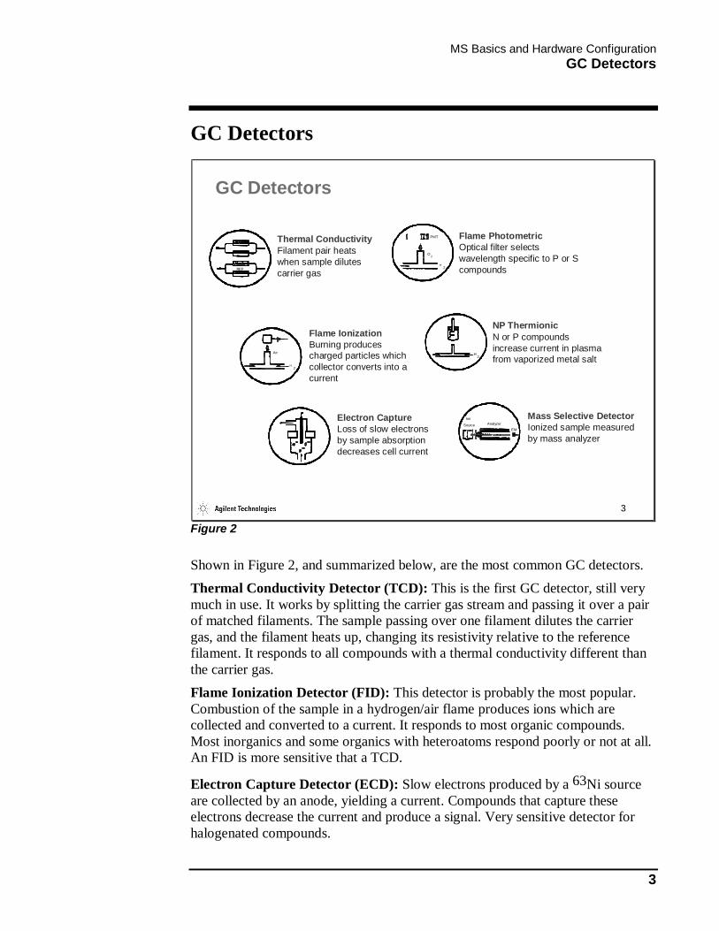
Figure 2

Shown in Figure 2, and summarized below, are the most common GC detectors. Thermal Conductivity Detector (TCD): This is the first GC detector, still very much in use. It works by splitting the carrier gas stream and passing it over a pair of matched filaments. The sample passing over one filament dilutes the carrier gas, and the filament heats up, changing its resistivity relative to the reference filament. It responds to all compounds with a thermal conductivity different than the carrier gas. Flame Ionization Detector (FID): This detector is probably the most popular. Combustion of the sample in a hydrogen/air flame produces ions which are collected and converted to a current. It responds to most organic compounds. Most inorganics and some organics with heteroatoms respond poorly or not at all. An FID is more sensitive that a TCD.

Electron Capture Detector (ECD): Slow electrons produced by a 63Ni source are collected by an anode, yielding a current. Compounds that capture these electrons decrease the current and produce a signal. Very sensitive detector for halogenated compounds.

MS Basics and Hardware Configuration GC Detectors

4

Flame Photometric Detector: Combustion of a sample in a hydrogen/oxygen flame produces optical emission from P and S compounds. A photo multiplier tube equipped with a filter to select only the desired wavelengths detects this emission. This detector is especially useful for pesticides.

NP Thermionic Detector: This detector is similar to an FID, except the collector contains an additional Rb salt element. Ions are formed when compounds are passed over this element. This detector is specific for N and P and is especially useful for pesticides.

Mass Selective Detector: Ions are formed by bombarding the sample with an electron beam ion vacuum. These ions are then separated according to mass/charge and the masses and abundances measured. This detector may be made very specific by appropriate selection of masses.

MS Basics and Hardware Configuration Comparison of GC Detectors

5

Comparison of GC Detectors

4

FPD(S)

NPD(P)

NPD(N)

ECD

FIDTCD

MSD(SIM) (SCAN)

1 ng in 1 uL Liquid (sg = 1) is 1 ppm Concentration

Mass Selective Detector is both:Specific and Universal

10-15

fg10-12

pg10-9

ng10-6

ug10-3

mg

Comparison of GC Detectors

Figure 3

Presented in Figure 3 is a diagram of the sensitivities and useful operating ranges of the various detectors. The ultimate sensitivity achievable with any of the detectors is dependent on the nature of the compound, the experimental conditions, the sample matrix, and so forth. These will vary. The MSD has a useful range equivalent to the commonly used GC detectors. It also has an ultimate sensitivity similar to these other detectors. In addition, it may be set up to detect virtually any compound; universal and specific!

MS Basics and Hardware Configuration Functional Components of the MS

6

Functional Components of the MS

5

EXHAUST

GC

HI VACPUMP

INTERFACE

CONTROLLER (ChemStation)

IONSOURCE

MASSFILTER

MECHANICALPUMP

DETECTOR

MASS SPECTROMETER

Functional Components of the MS

Figure 4

This is a functional diagram of the entire GC-MS system. The gas chromatograph serves to separate mixtures into components. The separation is based upon the retention of the analyte between two phases, the stationary liquid phase, and the mobile gas phase. The interface directs the effluent of the GC column into the mass spectrometer. The type of interface used is dependent upon the application, considerations including column type and column flow rate.

The mass spectrometer consists of three components. The ion source receives the sample and produces ions. The mass filter, or quadrupole, sorts these ions based upon their mass-to-change ratio (m/z). The detector, a continuous dynode electron multiplier, produces a signal proportional to the number of ions striking it.

All components of the system are controlled via the Windows® ChemStation. The data system software includes programs to calibrate the MSD, acquire data, and process data. It also includes utilities for file management and editing.

MS Basics and Hardware Configuration Interfacing the GC and MS

7

Interfacing the GC and MS

6INTERFACE

GC

MSD

10-5 Torr

<2 mL/min

760 Torr

0.5 - 15 mL/min

Interfacing GC and MS

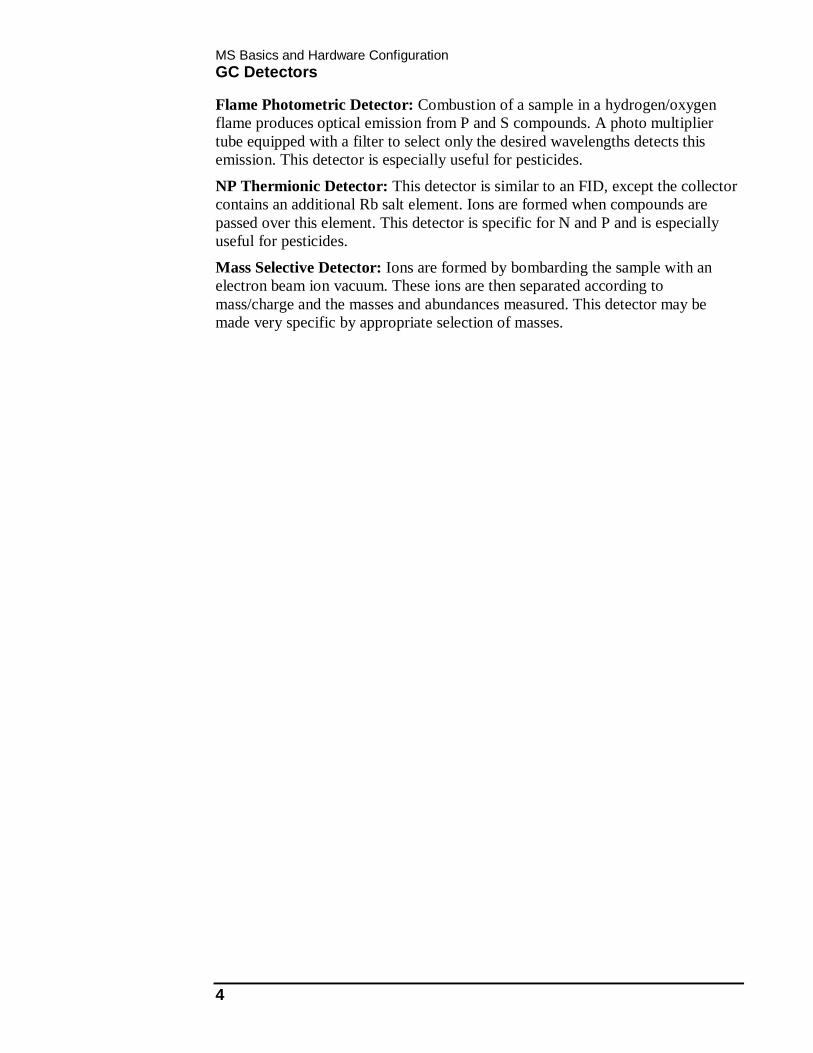
Figure 5

The major difficulty in interfacing a GC and an MS is due to the great pressure difference between the systems. The GC operates typically at about 1-3 atmospheres of pressure (760 - 2250 Torr). The MS operating pressure must be about 10-5 Torr. A good interface allows the GC and the MS to operate at or near the optimum conditions for each, yet it must also permit compounds from the GC to be transmitted to the MS without anomalous behavior, for example, no loss in sensitivity, no reactivity, no alteration of the GC peak shape.

MS Basics and Hardware Configuration Interface Overview

8

Interface Overview

7

Interface Overview

SplittersJet Separator

3 – 150.53Mega Bore

SplittersJet Separator

1 – 30.32Wide Bore

Capillary Direct0.1 – 1.00.10.20.25

Narrow Bore

InterfaceTypical Flow (mL/min)

ID (mm)

Column

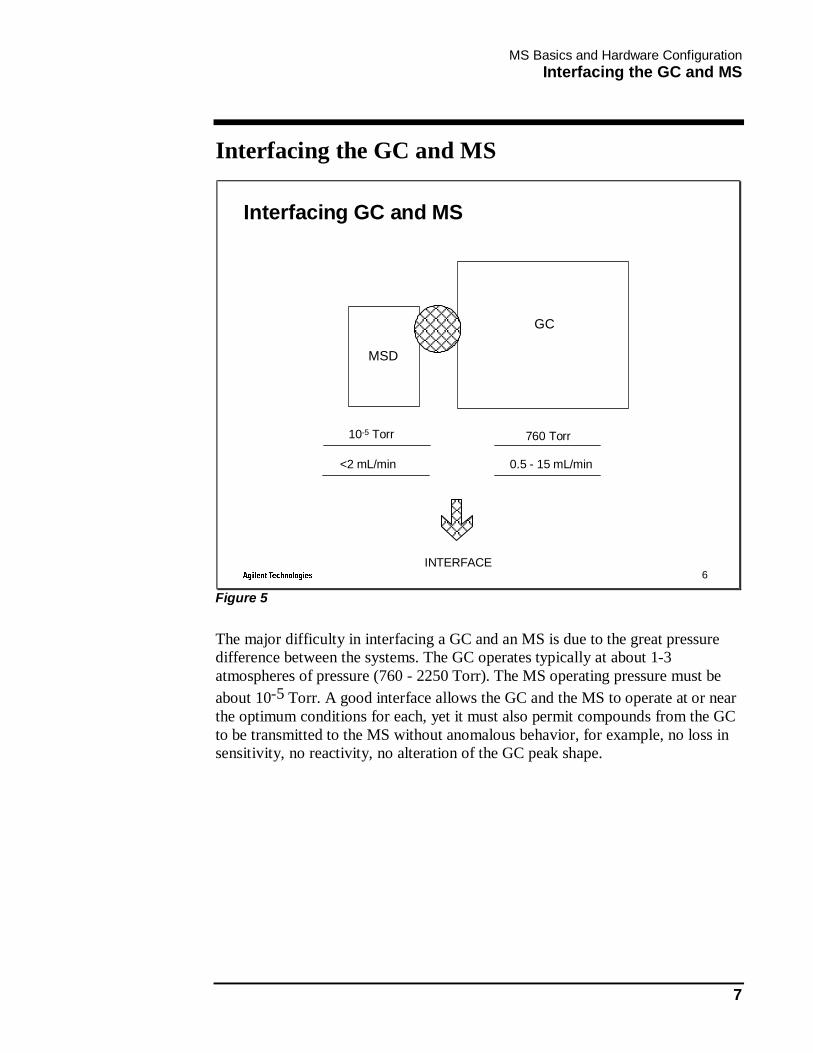
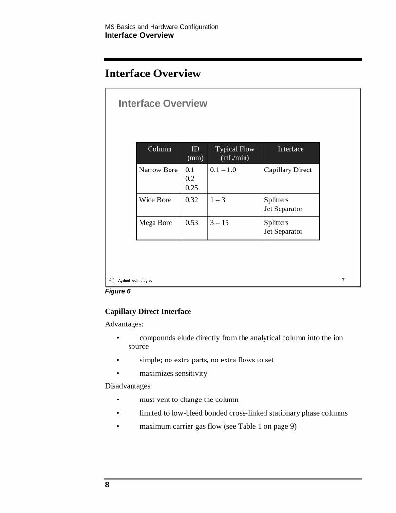
Figure 6

Capillary Direct Interface Advantages:

• compounds elude directly from the analytical column into the ion source

• simple; no extra parts, no extra flows to set

• maximizes sensitivity Disadvantages:

• must vent to change the column

• limited to low-bleed bonded cross-linked stationary phase columns

• maximum carrier gas flow (see Table 1 on page 9)

MS Basics and Hardware Configuration Interface Overview

9

MSD Maximum Flow

5973 (diffusion pump) 2.0 mL/min

5975, 5973 (turbo pump) 4.0 mL/min Table 1

Jet Separator Interface Advantages:

• higher flows can be used

• greater column capacity

• lower vacuum pressure in the manifold Disadvantages:

• numerous parameters (nozzle diameter and alignment, gap spacing, gas flow rate, and jet separator pressure) must be set correctly for optimum results

• extra parts means added sites for gas leakage

Capillary Splitters Interface Advantages:

• higher flows allowed Disadvantages:

• regulated by a non-adjustable restrictor

MS Basics and Hardware Configuration Vacuum Pumps

10

Vacuum Pumps

8

High Vacuum Pump

Inlet

Vents

Stack

Heater

.. .

..

.

. .....

....

.

....

... .

.. . .

.

...

.

.... ..

.... . .............

.......... ............. ......

Baffles(prevent oil loss)

Outlet(to Mechanical Pump)

Mechanical Pump

Rotor

Optional trap

Inlet port

Oil level

Oil refill port

Gravity drain plugStatorOil reservoir

Oil level sight glass

Anti suck-back valve

Discharge port

Gas ballast valve

10-1 - 10-2 torr

10-5 - 10-6 torr

Vacuum Pumps

Figure 7

The vacuum system of an MS consists of two devices. The first is a mechanical pump (“rough pump”, usually of the rotary type). This pump serves to reduce the vacuum in the system to the 10-1 to 10-2 Torr region. It also serves as the “backing pump” for the high vacuum pump.

The high vacuum pump reduces the system vacuum into the 10-5 to 10-6 Torr region. For the 5973 MSD, this pump is an oil diffusion pump. Oil with a low vapor pressure is used as the working fluid to achieve the high vacuum. Simply put, the oil is boiled and recondensed. Any gases in the pump are entrained in the condensing pump vapors and carried to the outlet where they are pumped away by the rough pump.

NOTE: 1 atmosphere = 760 Torr = 760 mm of Hg

MS Basics and Hardware Configuration Turbo Pump

11

Turbo Pump

9

To Foreline Pump

Axial-Flow Turbine

up to 60,000 RPM

Rotating Blades

Fixed Blades

MO

TOR

MO

TO

R

Lubricating Wick

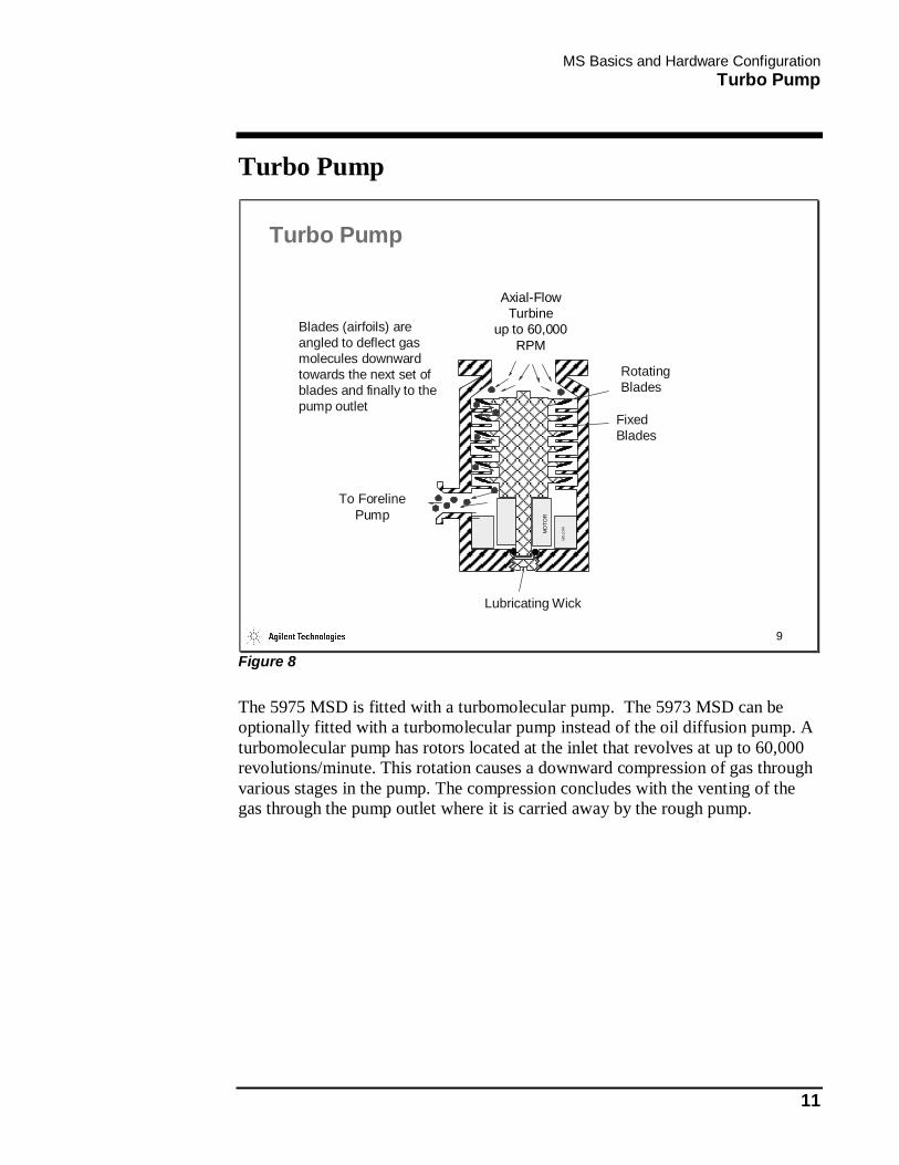
Blades (airfoils) are angled to deflect gas molecules downward towards the next set of blades and finally to the pump outlet

Turbo Pump

Figure 8

The 5975 MSD is fitted with a turbomolecular pump. The 5973 MSD can be optionally fitted with a turbomolecular pump instead of the oil diffusion pump. A turbomolecular pump has rotors located at the inlet that revolves at up to 60,000 revolutions/minute. This rotation causes a downward compression of gas through various stages in the pump. The compression concludes with the venting of the gas through the pump outlet where it is carried away by the rough pump.

MS Basics and Hardware Configuration Reasons for Vacuum in MS

12

Reasons for Vacuum in MS

10

Reasons for Vacuum in MS

• Provide adequate mean free path• Provide collision-free ion trajectories• Reduce ion-molecular reactions• Reduce background interference• Increase filament lifetime• Avoid electrical discharge• Increase sensitivity

Figure 9

The mean free path is the average distance an ion travels in an unenclosed area before it strikes something. In a mass spectrometer, the mean free path must be long enough that sample ions can travel from the ion source to the detector without colliding with other molecules. The vacuum system creates an adequate mean free path by creating a high vacuum inside the vacuum manifold.

MS Basics and Hardware Configuration Electron Ionization (EI)

13

Electron Ionization (EI)

11m/z

Abundance

C

A AC

ABABC +

+

++

+Signal

Resulting Mass Spectrum:

.

0 10 70 100 eV

Electron Energy

#ABC Depends on IP (ABC)Position of Curve

+.

ABCABCNeutralMolecule

ExcitedMolecular Ion

- -Ionization:.++ +e 2e

+ B(loss of neutral)(rearrangement)

Fragmentation:

ABC .

.

etc.

A++AB+AC

.

+. +C+ BC+ C

AB .

+

Electron Ionization (EI)

Figure 10

In mass spectrometry, bombarding molecules with electrons forms ions. Due to electron-electron interactions, the molecules lose both the incoming electron and a bound electron. The resulting molecule is an ion and has a charge (usually +1, though ions with multiple charges do occur). The number of molecular ions initially formed depends on the energy of the incoming electrons, increasing with the electron energy. Above a certain value (about 30 eV), increasing the electron energy does not increase the amount of molecular ions formed. Most ions, at least ions formed from organic compounds, are very reactive and possess an excess of energy. In the absence of other compounds (for example, in a vacuum), the molecular ions break up, or “fragment”, into other ions, radicals (species with no charge but with an unpaired electron), and neutral molecules. The masses of these fragments and the abundance of these fragments depend dramatically on the nature of the starting molecules, and this is what gives mass spectrometry its great diagnostic power.

MS Basics and Hardware Configuration Electron Ionization (EI)

14

At 70 eV electrons, this mode of operation is known as “electron ionization” (EI). In it, only the positively charged fragments are detected. It should be noted that the ionization efficiency in EI mode is only around 0.01%!

MS Basics and Hardware Configuration Positive Chemical Ionization (PCI)

15

Positive Chemical Ionization (PCI)

12

Positive Chemical Ionization (PCI)

• First forms ions from a “reagent gas” by bombardment with electrons

• Reagent gas ions undergo subsequent reactions with sample molecules to form sample ions (“Brönsted acid”)

• CI ion formation is much more “gentle” than electron ionization (EI) therefore less fragmentation

• Most common reagent gas is methane, produces ions with almost any sample molecule

• Other reagent gases (isobutane, ammonia) are more selective and even less fragmentation

• Source pressure ~ 0.2 Torr• Detection limits are generally high because of background

from the reagent gas (methane)• Most often used to determine the molecular weight of a

compound

Figure 11

Positive Chemical Ionization (PCI) is standard on the 5975 MSD. It is an option available for the 5973 MSD, requiring that you purchase and install a separate CI source along with the necessary plumbing for the reagent gas. Once the plumbing is installed, it may be left in place and unused during EI operation. Therefore, to switch back and forth between EI and CI requires only a source change and time for the system to stabilize (~ 4hours).

Chemical Ionization is a very gentle, “soft”, ionization process. As a result, there is little if any fragmentation. CI spectral libraries do not exist, so library searching is not useful. It is most often used to determine the molecular weight of an unknown. CI molecular weight information combined with EI fragmentation information make CI/EI complimentary, not competing, modes of operation. Sample molecules are ionized by collisional interaction with reagent gas ions. Reagent gas ions are formed by electron bombardment of the reagent gas in the high pressure CI source. Methane is the most common reagent gas but isobutane and ammonia may also be used.

MS Basics and Hardware Configuration Negative Chemical Ionization (NCI)

16

Negative Chemical Ionization (NCI)

13

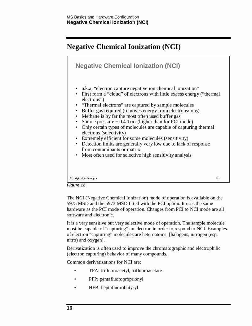
Negative Chemical Ionization (NCI)

• a.k.a. “electron capture negative ion chemical ionization”• First form a “cloud” of electrons with little excess energy (“thermal

electrons”)• “Thermal electrons” are captured by sample molecules• Buffer gas required (removes energy from electrons/ions)• Methane is by far the most often used buffer gas• Source pressure ~ 0.4 Torr (higher than for PCI mode)• Only certain types of molecules are capable of capturing thermal

electrons (selectivity)• Extremely efficient for some molecules (sensitivity)• Detection limits are generally very low due to lack of response

from contaminants or matrix• Most often used for selective high sensitivity analysis

Figure 12

The NCI (Negative Chemical Ionization) mode of operation is available on the 5975 MSD and the 5973 MSD fitted with the PCI option. It uses the same hardware as the PCI mode of operation. Changes from PCI to NCI mode are all software and electronic.

It is a very sensitive but very selective mode of operation. The sample molecule must be capable of “capturing” an electron in order to respond to NCI. Examples of electron “capturing” molecules are heteroatoms; [halogens, nitrogen (esp. nitro) and oxygen].

Derivatization is often used to improve the chromatographic and electrophilic (electron capturing) behavior of many compounds.

Common derivatizations for NCI are:

• TFA: trifluoroacetyl, trifluoroacetate

• PFP: pentafluoroproprionyl

• HFB: heptafluorobutyryl

MS Basics and Hardware Configuration Negative Chemical Ionization (NCI)

17

• PFB: pentafluorobenzyl For more information concerning CI see the following references:

• W.B. Knighton, L.J. Sears, E.P. Grumsrud, “High Pressure Electron Capture Mass Spectrometry”, Mass Spectrometry Reviews (1996), 14, 327-343.

• E.A. Stemmler, R.A. Hites, “Electron Capture Negative Ion Mass Spectra of Environmental Contaminates and Related Compounds”, VCH Publishers, New York, NY (1988), ISBN 0-89573-708-6.

• J.A. Michnowicz, “Reactant Gas Selection in Chemical Ionization Mass Spectrometry”, Application Note AN 176-13, Hewlett-Packard Company.

This is an excellent reference but is very technical and biased toward the physical chemist:

• A.G. Harrison, “Chemical Ionization Mass Spectrometry”, 2nd Edition, CRC Press, INC. Baca Raton, FL (1992) ISBN 0-8493-4254-6.

MS Basics and Hardware Configuration How Does a Quadrupole Mass Filter Work?

18

How Does a Quadrupole Mass Filter Work?

14

FILTERING LOW MASS

POSITIVE RODS

FILTERING HIGH MASS

NEGATIVE RODS

*

FILTERING SELECTED MASS

POSITIVE RODS

M+

M+

M+

*

How does a Quadrupole Mass Filter Work?

Figure 13

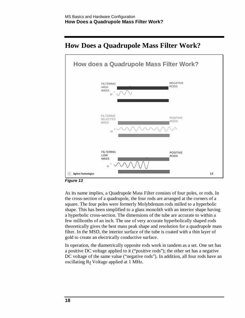
As its name implies, a Quadrupole Mass Filter consists of four poles, or rods. In the cross-section of a quadrupole, the four rods are arranged at the corners of a square. The four poles were formerly Molybdenum rods milled to a hyperbolic shape. This has been simplified to a glass monolith with an interior shape having a hyperbolic cross-section. The dimensions of the tube are accurate to within a few millionths of an inch. The use of very accurate hyperbolically shaped rods theoretically gives the best mass peak shape and resolution for a quadrupole mass filter. In the MSD, the interior surface of the tube is coated with a thin layer of gold to create an electrically conductive surface. In operation, the diametrically opposite rods work in tandem as a set. One set has a positive DC voltage applied to it (“positive rods”); the other set has a negative DC voltage of the same value (“negative rods”). In addition, all four rods have an oscillating Rf Voltage applied at 1 MHz.

MS Basics and Hardware Configuration Mass Filter Function

19

Mass Filter Function

15

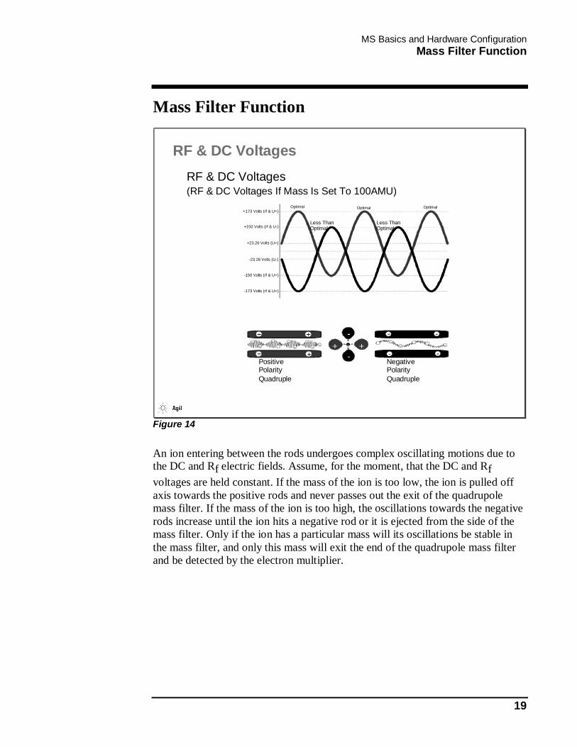
RF & DC Voltages(RF & DC Voltages If Mass Is Set To 100AMU)

Positive PolarityQuadruple

Negative PolarityQuadruple

Less Than Optimal

OptimalOptimal Optimal

Less Than Optimal

+173 Volts (rf & U+)

+150 Volts (rf & U-)

+23.26 Volts (U+)

-23.26 Volts (U-)

-150 Volts (rf & U+)

-173 Volts (rf & U+)

RF & DC Voltages

Figure 14

An ion entering between the rods undergoes complex oscillating motions due to the DC and Rf electric fields. Assume, for the moment, that the DC and Rf voltages are held constant. If the mass of the ion is too low, the ion is pulled off axis towards the positive rods and never passes out the exit of the quadrupole mass filter. If the mass of the ion is too high, the oscillations towards the negative rods increase until the ion hits a negative rod or it is ejected from the side of the mass filter. Only if the ion has a particular mass will its oscillations be stable in the mass filter, and only this mass will exit the end of the quadrupole mass filter and be detected by the electron multiplier.

MS Basics and Hardware Configuration X-Ray Lens/Electron Multiplier Detector

20

X-Ray Lens/Electron Multiplier Detector

16

(0 to -3000 V)

+Incoming Ion

X-Ray Lens(0 to 218 V)

Signal Out

EM Voltage

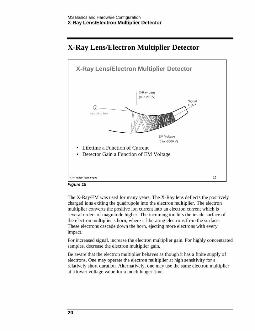
X-Ray Lens/Electron Multiplier Detector

• Lifetime a Function of Current• Detector Gain a Function of EM Voltage

Figure 15

The X-Ray/EM was used for many years. The X-Ray lens deflects the positively charged ions exiting the quadrupole into the electron multiplier. The electron multiplier converts the positive ion current into an electron current which is several orders of magnitude higher. The incoming ion hits the inside surface of the electron multiplier’s horn, where it liberating electrons from the surface. These electrons cascade down the horn, ejecting more electrons with every impact. For increased signal, increase the electron multiplier gain. For highly concentrated samples, decrease the electron multiplier gain. Be aware that the electron multiplier behaves as though it has a finite supply of electrons. One may operate the electron multiplier at high sensitivity for a relatively short duration. Alternatively, one may use the same electron multiplier at a lower voltage value for a much longer time.

MS Basics and Hardware Configuration High Energy Dynode/Electron Multiplier Detector

21

High Energy Dynode/Electron Multiplier Detector

17

++

++ ++ ++ ++++ ++ ++++++ ++++++

++++ + + + ++++++ ++ ++++++++++-------------- ----

QuadrupoleIris

Detector Focus Lens

High Energy Dynode

Electron Multiplier

Electrons

Positive Ions

SignalOut

High Energy Dynode/Electron Multiplier Detector

• Lifetime a Function of Current• Detector Gain a Function of EM Voltage

Figure 16

The HED/EM is current technology and is used in the 5973 and 5975. The high energy dynode (HED) attracts the positively charged ions exiting the quadrupole. When the ion beam hits the HED, electrons are emitted. The electrons are attracted to the electron multiplier. The incoming electrons hit the inside surface of the electron multiplier’s horn liberating more electrons from the surface. These electrons cascade down the horn, ejecting more electrons with every impact.

Electrons produced by the HED cause the EM voltage to be lower (longer EM life) when compared to the X-Ray/Electron Multiplier style systems.

Electrons, instead of ions, striking the EM do not remove as much of the EM working surface (longer EM life) when compared to the X-Ray/Electron Multiplier style systems. Mid mass response (m/z 219) is greatly increased when compared to the X-Ray/Electron Multiplier style systems. For increased signal, increase the electron multiplier gain. For highly concentrated samples, decrease the electron multiplier gain

MS Basics and Hardware Configuration High Energy Dynode/Electron Multiplier Detector

22

Be aware that the electron multiplier behaves as though it has a finite supply of electrons. You may operate the electron multiplier at high sensitivity for a relatively short duration. Alternatively, you may use the same electron multiplier at a lower voltage value for a much longer time.

MS Basics and Hardware Configuration A Typical Mass Spectrum

23

A Typical Mass Spectrum

18

Dodecane: C12H26

20 40 60 80 100 120 140 160 180

10

20

30

40

50

60

70

80

90

100

Abundance

29

43

55

57

71

85

98 113128 141 159

170

m/z->

Average spectrum of dodecane from EVALDEMO.D

M

<--[C H ]+

+.13

<--[C H ]11

<--[C H ]4

+

+(Base peak)

(Molecular ion)

9

5

6

A Typical Mass Spectrum

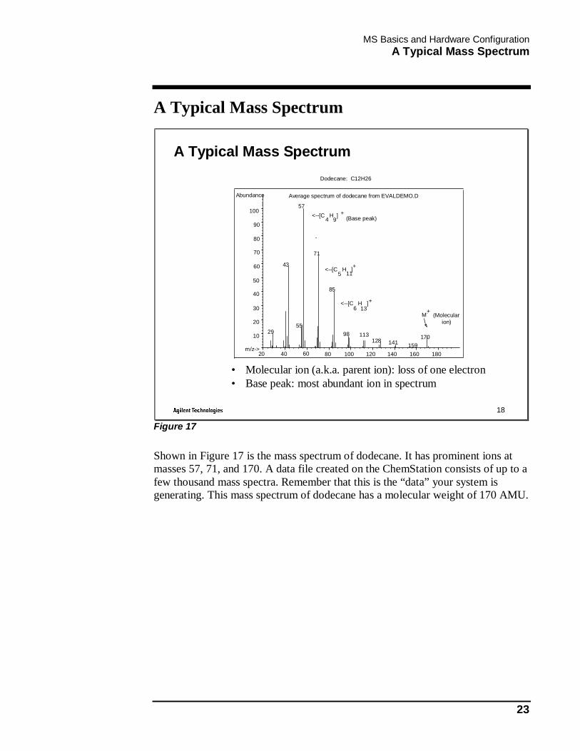
• Molecular ion (a.k.a. parent ion): loss of one electron• Base peak: most abundant ion in spectrum

Figure 17

Shown in Figure 17 is the mass spectrum of dodecane. It has prominent ions at masses 57, 71, and 170. A data file created on the ChemStation consists of up to a few thousand mass spectra. Remember that this is the “data” your system is generating. This mass spectrum of dodecane has a molecular weight of 170 AMU.

MS Basics and Hardware Configuration System Hardware Overview (LANed)

24

System Hardware Overview (LANed)

19REMOTE START

System Hardware Overview (LANed)

LAN

Active HubLAN

LAN

Figure 18

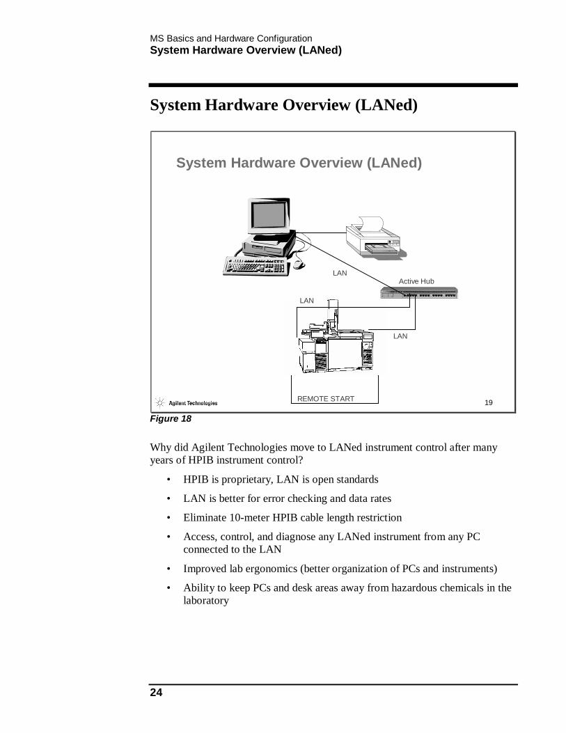
Why did Agilent Technologies move to LANed instrument control after many years of HPIB instrument control?

• HPIB is proprietary, LAN is open standards

• LAN is better for error checking and data rates

• Eliminate 10-meter HPIB cable length restriction

• Access, control, and diagnose any LANed instrument from any PC connected to the LAN

• Improved lab ergonomics (better organization of PCs and instruments)

• Ability to keep PCs and desk areas away from hazardous chemicals in the laboratory

MS Basics and Hardware Configuration Bootp Software

25

Bootp Software

20

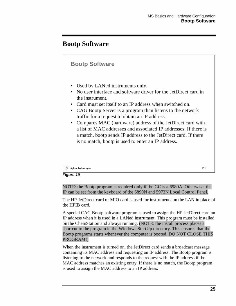
Bootp Software

• Used by LANed instruments only.• No user interface and software driver for the JetDirect card in

the instrument.• Card must set itself to an IP address when switched on.• CAG Bootp Server is a program than listens to the network

traffic for a request to obtain an IP address.• Compares MAC (hardware) address of the JetDirect card with

a list of MAC addresses and associated IP addresses. If there isa match, bootp sends IP address to the JetDirect card. If there is no match, bootp is used to enter an IP address.

Figure 19

NOTE: the Bootp program is required only if the GC is a 6980A. Otherwise, the IP can be set from the keyboard of the 6890N and 5973N Local Control Panel.

The HP JetDirect card or MIO card is used for instruments on the LAN in place of the HPIB card.

A special CAG Bootp software program is used to assign the HP JetDirect card an IP address when it is used in a LANed instrument. This program must be installed on the ChemStation and always running. (NOTE: the install process places a shortcut to the program in the Windows StartUp directory. This ensures that the Bootp programs starts whenever the computer is booted. DO NOT CLOSE THIS PROGRAM!)

When the instrument is turned on, the JetDirect card sends a broadcast message containing its MAC address and requesting an IP address. The Bootp program is listening to the network and responds to the request with the IP address if the MAC address matches an existing entry. If there is no match, the Bootp program is used to assign the MAC address to an IP address.

MS Basics and Hardware Configuration Networking MSD Local Control Panel

26

Networking MSD Local Control Panel

21

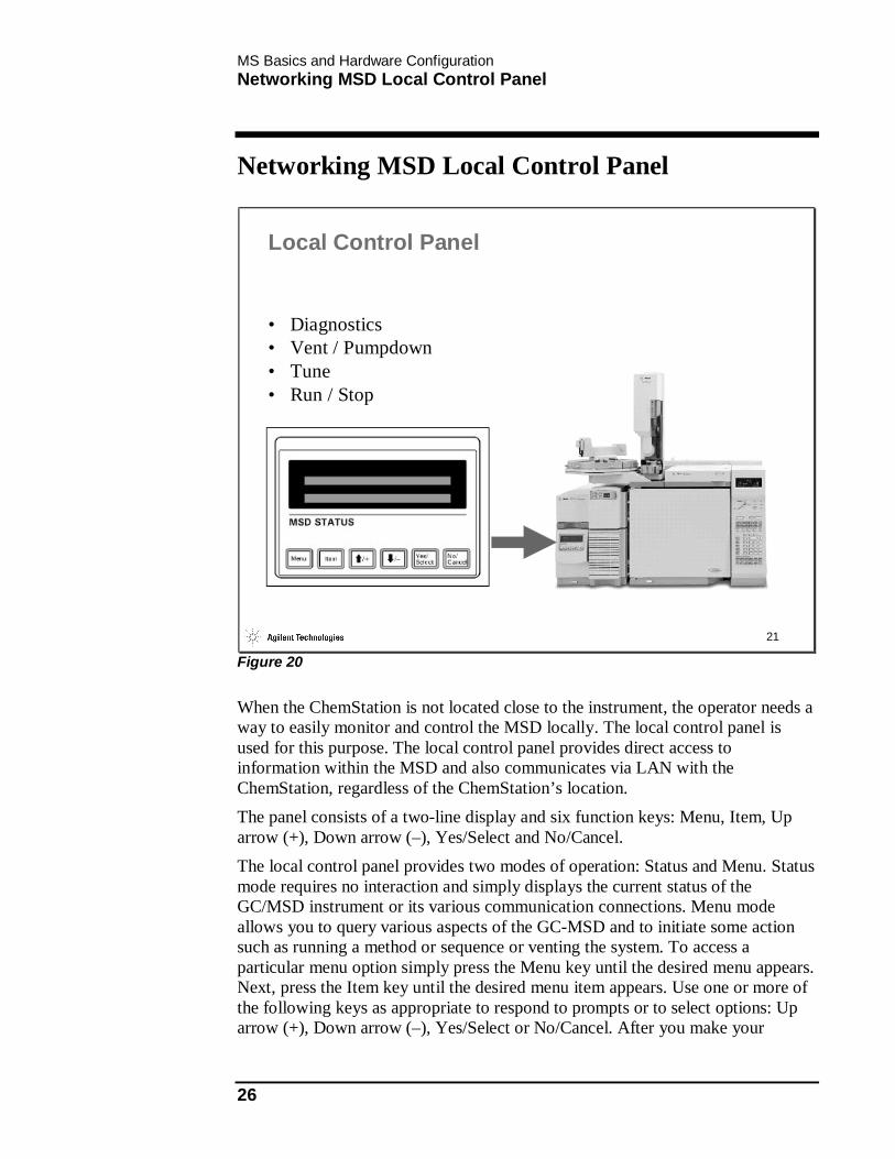
Local Control Panel

• Diagnostics• Vent / Pumpdown• Tune• Run / Stop

Figure 20

When the ChemStation is not located close to the instrument, the operator needs a way to easily monitor and control the MSD locally. The local control panel is used for this purpose. The local control panel provides direct access to information within the MSD and also communicates via LAN with the ChemStation, regardless of the ChemStation’s location. The panel consists of a two-line display and six function keys: Menu, Item, Up arrow (+), Down arrow (–), Yes/Select and No/Cancel. The local control panel provides two modes of operation: Status and Menu. Status mode requires no interaction and simply displays the current status of the GC/MSD instrument or its various communication connections. Menu mode allows you to query various aspects of the GC-MSD and to initiate some action such as running a method or sequence or venting the system. To access a particular menu option simply press the Menu key until the desired menu appears. Next, press the Item key until the desired menu item appears. Use one or more of the following keys as appropriate to respond to prompts or to select options: Up arrow (+), Down arrow (–), Yes/Select or No/Cancel. After you make your

MS Basics and Hardware Configuration Networking MSD Local Control Panel

27

selection or if you cycle through all available menus, the display automatically returns to Status mode.

MS Basics and Hardware Configuration GC-MS Configuration

28

GC-MS Configuration

22

GC-MS Configuration

Figure 21

To configure your GC-MS system, select the Config icon in the MSD ChemStation group. The System Configuration window appears. Utilize this panel to configure or reconfigure your system.

MS Basics and Hardware Configuration MS Configuration

29

MS Configuration

23

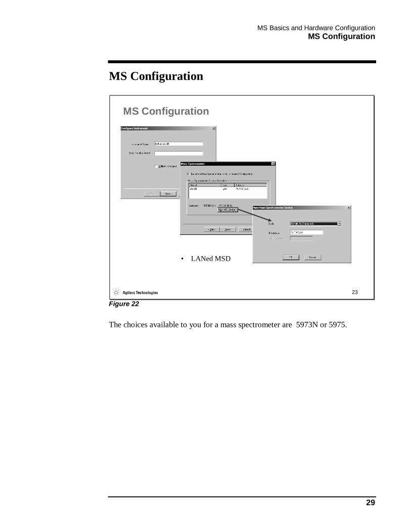
MS Configuration

• LANed MSD

Figure 22

The choices available to you for a mass spectrometer are 5973N or 5975.

MS Basics and Hardware Configuration MS Options and DC Polarity Configuration

30

MS Options and DC Polarity Configuration

24

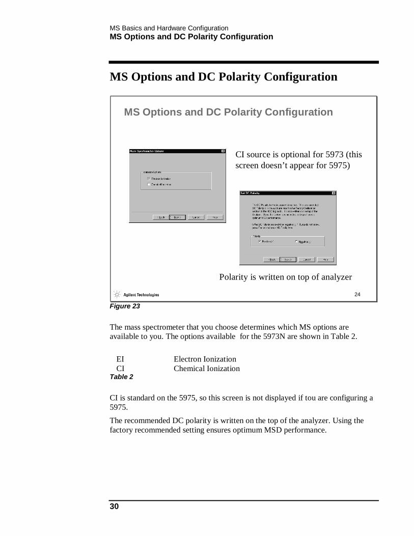
MS Options and DC Polarity Configuration

CI source is optional for 5973 (this screen doesn’t appear for 5975)

Polarity is written on top of analyzer

Figure 23

The mass spectrometer that you choose determines which MS options are available to you. The options available for the 5973N are shown in Table 2.

EI Electron Ionization CI Chemical Ionization

Table 2

CI is standard on the 5975, so this screen is not displayed if tou are configuring a 5975. The recommended DC polarity is written on the top of the analyzer. Using the factory recommended setting ensures optimum MSD performance.

MS Basics and Hardware Configuration GC Configuration

31

GC Configuration

25

GC Configuration

• LANed GC

Figure 24

Select the type of GC associated with your system. If you select a 6890 or 6850, you must enter the LAN IP address.

MS Basics and Hardware Configuration Data Analysis Configuration

32

Data Analysis Configuration

26

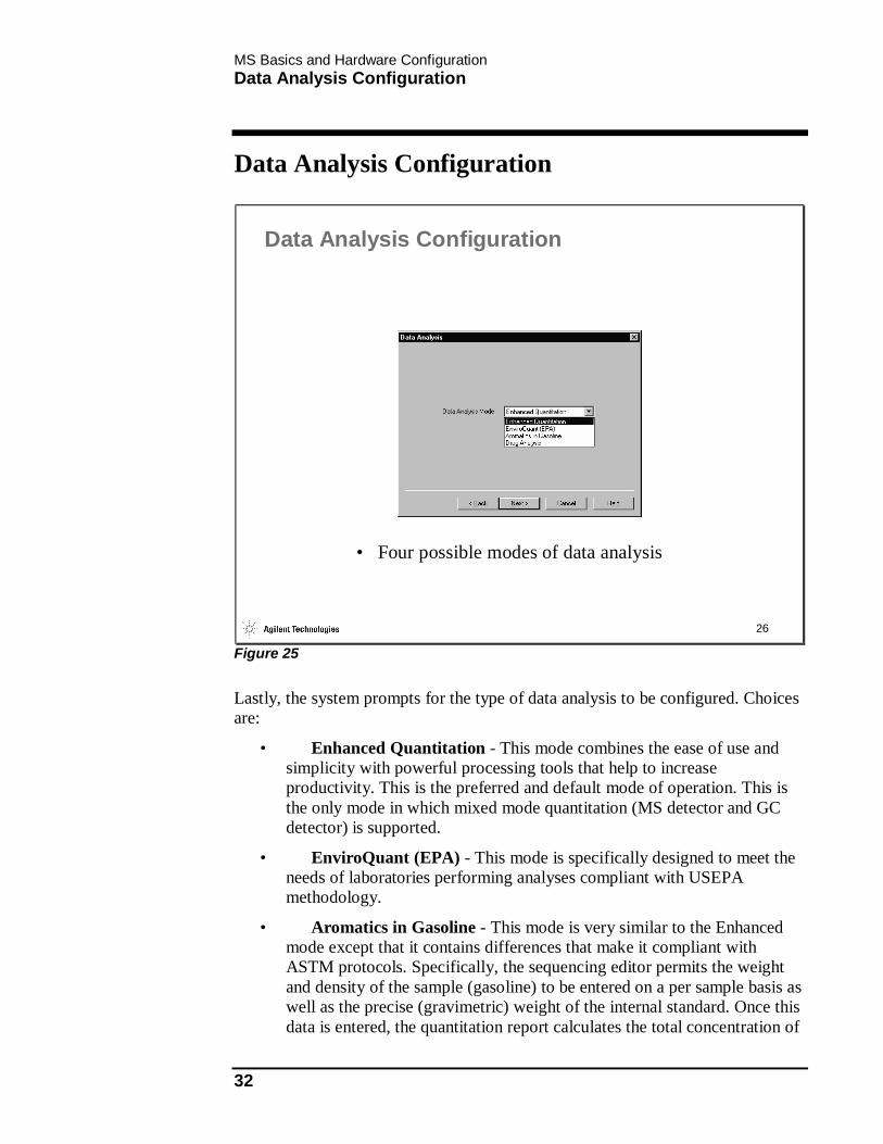
Data Analysis Configuration

• Four possible modes of data analysis

Figure 25

Lastly, the system prompts for the type of data analysis to be configured. Choices are:

• Enhanced Quantitation - This mode combines the ease of use and simplicity with powerful processing tools that help to increase productivity. This is the preferred and default mode of operation. This is the only mode in which mixed mode quantitation (MS detector and GC detector) is supported.

• EnviroQuant (EPA) - This mode is specifically designed to meet the needs of laboratories performing analyses compliant with USEPA methodology.

• Aromatics in Gasoline - This mode is very similar to the Enhanced mode except that it contains differences that make it compliant with ASTM protocols. Specifically, the sequencing editor permits the weight and density of the sample (gasoline) to be entered on a per sample basis as well as the precise (gravimetric) weight of the internal standard. Once this data is entered, the quantitation report calculates the total concentration of

MS Basics and Hardware Configuration Data Analysis Configuration

33

aromatics in gasoline. This mode should only be used when it is necessary to comply with ASTM-D5769-95.

• Drug Analysis - This mode is specifically designed to meet the needs of laboratories performing drug analyses.

MS Basics and Hardware Configuration Networking Information

34

Networking Information

27

Networking Information

Figure 26

You can display the networking information at any time by selecting Help / Show IP and Revision Information. The IP addresses for the GC, MSD and ChemStation, and the firmware revision numbers for the GC and MSD are shown in a MultiVu window.

LAB EXERCISE: MSD Instrument Configuration Networking Information

35

LAB EXERCISE: MSD Instrument Configuration

In this section you will:

• Use the MS ChemStation to configure an off-line instrument

• Examine the changes this process makes to the MSDCHEM.INI file.

LAB EXERCISE: MSD Instrument Configuration Instrument/System Configuration

36

Instrument/System Configuration

As discussed in lecture, your GC and MS communicate with the PC data system using LAN (Local Area Network). Each component of the system must have a unique LAN address.

The MSD's Local Control Panel is used to enter the LAN address for the MSD and this must agree with the LAN address entered for the MSD in this configuration program. The GC keyboard is used to enter the LAN address for the GC and this must agree with the LAN address entered for the GC in this configuration program. If your system has a 6890A, the LAN address cannot be entered from the GC keyboard. In this case, a special CAG Bootp software program is used to assign an IP address to the GC. The program must be installed on the ChemStation and must be always running. (NOTE: the installation process places a shortcut to the program in the Windows StartUp directory. This ensures that the Bootp program starts whenever the computer is booted. DO NOT CLOSE THIS PROGRAM!) When the instrument is turned on, the GC sends a broadcast message containing its MAC address and requesting an IP address. The Bootp program is listening to the network and responds to the request with the IP address if the MAC address matches an existing entry. If there is no match, the Bootp program is used to assign the MAC address to an IP address. The IP address assigned by Bootp must match the IP address entered during instrument configuration. Note: it is not necessary to enter an address for the autosampler, since it is configured through the 6890 GC. 1) Instrument configuration begins by selecting Start / Programs / MSD

ChemStation / Config. The System Configuration window appears (Figure 27).

LAB EXERCISE: MSD Instrument Configuration Instrument/System Configuration

37

Figure 27

2) Select Configure / Instrument 1.... (NOTE: Do not make changes!!) The first panel allows us to name the instrument, optionally assign an asset number, and define if it is an online or offline instrument (Figure 28). Click Next.

Figure 28

LAB EXERCISE: MSD Instrument Configuration Instrument/System Configuration

38

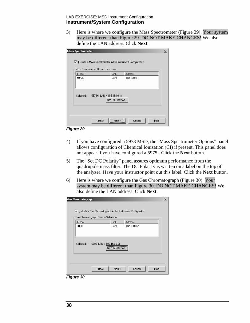
3) Here is where we configure the Mass Spectrometer (Figure 29). Your system may be different than Figure 29. DO NOT MAKE CHANGES! We also define the LAN address. Click Next.

Figure 29

4) If you have configured a 5973 MSD, the “Mass Spectrometer Options” panel allows configuration of Chemical Ionization (CI) if present. This panel does not appear if you have configured a 5975. Click the Next button.

5) The “Set DC Polarity” panel assures optimum performance from the quadrupole mass filter. The DC Polarity is written on a label on the top of the analyzer. Have your instructor point out this label. Click the Next button.

6) Here is where we configure the Gas Chromatograph (Figure 30). Your system may be different than Figure 30. DO NOT MAKE CHANGES! We also define the LAN address. Click Next.

Figure 30

LAB EXERCISE: MSD Instrument Configuration Instrument/System Configuration

39

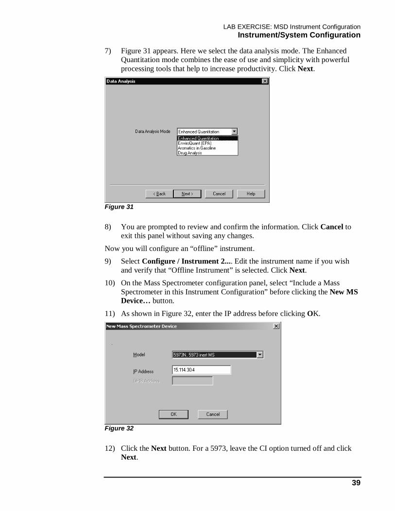
7) Figure 31 appears. Here we select the data analysis mode. The Enhanced Quantitation mode combines the ease of use and simplicity with powerful processing tools that help to increase productivity. Click Next.

Figure 31

8) You are prompted to review and confirm the information. Click Cancel to exit this panel without saving any changes.

Now you will configure an “offline” instrument. 9) Select Configure / Instrument 2.... Edit the instrument name if you wish

and verify that “Offline Instrument” is selected. Click Next. 10) On the Mass Spectrometer configuration panel, select “Include a Mass

Spectrometer in this Instrument Configuration” before clicking the New MS Device… button.

11) As shown in Figure 32, enter the IP address before clicking OK.

Figure 32

12) Click the Next button. For a 5973, leave the CI option turned off and click Next.

LAB EXERCISE: MSD Instrument Configuration Instrument/System Configuration

40

13) Locate the label on top of the analyzer that indicates the recommended DC polarity. Enter the information and click Next.

14) On the Gas Chromatograph configuration panel, select “Include a Gas Chromatograph in this Instrument Configuration” before clicking the New GC Device… button.

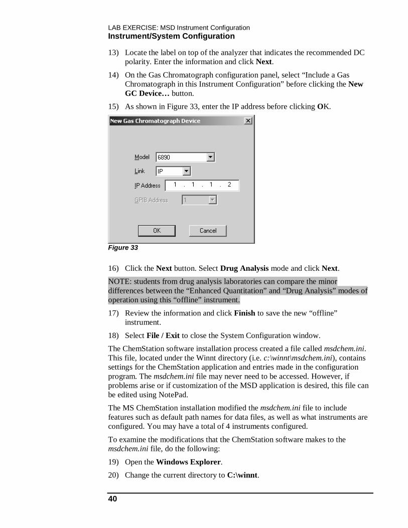
15) As shown in Figure 33, enter the IP address before clicking OK.

Figure 33

16) Click the Next button. Select Drug Analysis mode and click Next. NOTE: students from drug analysis laboratories can compare the minor differences between the “Enhanced Quantitation” and “Drug Analysis” modes of operation using this “offline” instrument.

17) Review the information and click Finish to save the new “offline” instrument.

18) Select File / Exit to close the System Configuration window. The ChemStation software installation process created a file called msdchem.ini. This file, located under the Winnt directory (i.e. c:\winnt\msdchem.ini), contains settings for the ChemStation application and entries made in the configuration program. The msdchem.ini file may never need to be accessed. However, if problems arise or if customization of the MSD application is desired, this file can be edited using NotePad. The MS ChemStation installation modified the msdchem.ini file to include features such as default path names for data files, as well as what instruments are configured. You may have a total of 4 instruments configured.

To examine the modifications that the ChemStation software makes to the msdchem.ini file, do the following:

19) Open the Windows Explorer. 20) Change the current directory to C:\winnt.

LAB EXERCISE: MSD Instrument Configuration Instrument/System Configuration

41

NOTE: Depending on your system configuration, it may be D:\winnt. 21) Double-click on msdchem.ini. What application opens the file msdchem.ini? Hint: the application and the file that is currently active in the application are always listed in the title bar. 22) Select File / Page Setup... and change the margins as shown in Figure 34

before clicking OK.

Figure 34

23) Print a copy of this file by selecting File / Print. In the file printout locate the line labeled [PCS]. Notice the PCS,1 section which is your on-line instrument. Also notice the PCS,2 section which is the off-line instrument you just created. Notice the default path names for help files, data files, library files, etc....

NOTE: Please DO NOT modify the contents of the file!! Notice that each instrument configured has a separate PCS section. Make note of the entries here and the settings of the various MS options. Note that any changes you make to the configuration in the MS Config panel would be reflected here when you select File / Save Configuration from the menu in MS Configuration.

24) Close the NotePad window by select File / Exit. If more information on the uses of msdchem.ini is required, consult your instructor.

LAB EXERCISE: MSD Instrument Configuration Instrument/System Configuration

42

MS Tuning

MS Tuning What You Will Learn

44

What You Will Learn

2

MS Tuning

In this section you will learn:

• The fundamentals of MS Tuning• The various Tuning Methods available on the ChemStation

Figure 35

In this section you will learn the principles of tuning and how to tune your system.

Question: Why tune?

MS Tuning What Does Tuning Do?

45

What Does Tuning Do?

3

What Does Tuning Do?

• Set voltages on source elements• Set amu gain and offset for correct Peakwidth• Set EM Voltage• Set the Mass Axis for proper mass assignment

Figure 36

Tuning involves adjusting a number of mass spectrometer parameters. Some parameters are purely electronic and affect only the way the electronics process the signal. Other parameters affect voltage settings or currents to parts in the MSD’s ion source, mass filter, and detector.

MS Tuning PFTBA - The Tuning Standard

46

PFTBA - The Tuning Standard

4

Perfluorotributylamine (PFTBA)

650

Scan: 10.00 - 650.00 Samples: 16 Thresh: 500 117 peaks Base: 69.00 Abundance: 1974784

Mass Abund Rel Abund Iso Mass Iso Abund Iso Ratio

69.00 1974784 100.00 70.00 20344 1.03

219.00 1161216 58.80 219.95 45968 3.96

502.00 56648 2.87 503.00 5690 10.04

50 100 150 200 250 300 350 400 450 500 550 600

0

50

100

131

219

264

69

414 502 614

F CF CF CF C

N CF CF CF CF ..

3 2 2 2

F CF CF CF C 3 2 2 2

2 2 2 3

The Tuning Standard

• Stable• Volatile• Fragments over

a wide mass range

• 13C and 15N isotopes only

• No mass defect

Figure 37

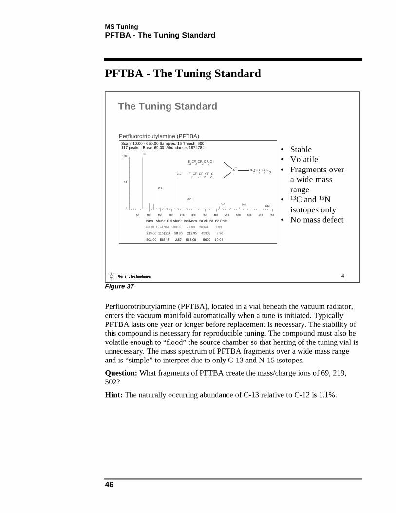
Perfluorotributylamine (PFTBA), located in a vial beneath the vacuum radiator, enters the vacuum manifold automatically when a tune is initiated. Typically PFTBA lasts one year or longer before replacement is necessary. The stability of this compound is necessary for reproducible tuning. The compound must also be volatile enough to “flood” the source chamber so that heating of the tuning vial is unnecessary. The mass spectrum of PFTBA fragments over a wide mass range and is “simple” to interpret due to only C-13 and N-15 isotopes. Question: What fragments of PFTBA create the mass/charge ions of 69, 219, 502? Hint: The naturally occurring abundance of C-13 relative to C-12 is 1.1%.

MS Tuning Tuning Parameters - EI

47

Tuning Parameters - EI

5

AMU gain, offset

HED

Electron Multiplier

Entrance Lens,

Repeller

Ion SourceVolume

InletFilament

FilamentDrawout

Ion Focus

Mass axis gain, offsetoffset

Tuning Parameters - EI

Mass assignment±499Mass Axis Offset

Mass assignment±2047Mass Axis Gain

Sensitivity0 – 3000 voltsElectron Multiplier

Converts ions to electrons-10,000 voltsHED

0 – 255AMU Offset

0 – 4095AMU Gain

Relative abundance0 – 127.5 voltsEntrance Lens Offset

Relative abundance0 – 128 mV / amuEntrance Lens

Relative abundance0 – 242.0 voltsIon Focus

Entrance aperture to lens stackGround potentialDrawout

Pushes ions out of the source0 – 42.7 voltsRepeller

Energy of electron beamNumber of electrons generated

70 eV electrons @ 300 µA emissionFilament

EffectVoltagesElement

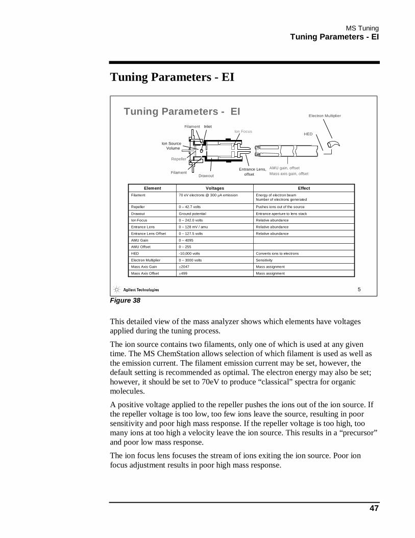
Figure 38

This detailed view of the mass analyzer shows which elements have voltages applied during the tuning process.

The ion source contains two filaments, only one of which is used at any given time. The MS ChemStation allows selection of which filament is used as well as the emission current. The filament emission current may be set, however, the default setting is recommended as optimal. The electron energy may also be set; however, it should be set to 70eV to produce “classical” spectra for organic molecules.

A positive voltage applied to the repeller pushes the ions out of the ion source. If the repeller voltage is too low, too few ions leave the source, resulting in poor sensitivity and poor high mass response. If the repeller voltage is too high, too many ions at too high a velocity leave the ion source. This results in a “precursor” and poor low mass response. The ion focus lens focuses the stream of ions exiting the ion source. Poor ion focus adjustment results in poor high mass response.

MS Tuning Tuning Parameters - EI

48

The modified Turner-Kruger entrance lens minimizes the fringing fields of the quadrupole. Increasing the entrance lens voltage increases the abundances at high mass but decreases the abundance of low mass ions. Quadrupole parameters, AMU gain and offset, affect the ratio of DC voltage to Rf voltage on the mass filter.

The High Energy Dynode (HED), operating at -10,000 volts, attracts the positively charged ions exiting the quadrupole. When the ion beam hits the HED, electrons are created and attracted to the less negatively charged electron multiplier (EM).

The electron multiplier detector amplifies the signal output by about 105. Increasing the EM voltage increases the charge density on the EM, resulting in a higher signal output.

The mass axis is calibrated by adjusting mass axis gain/offset parameters. NOTE: The MSD has independent source and quadrupole heaters that are set in the tune file.

MS Tuning Parameter Ramps

49

Parameter Ramps

6

Parameter Ramps

Figure 39

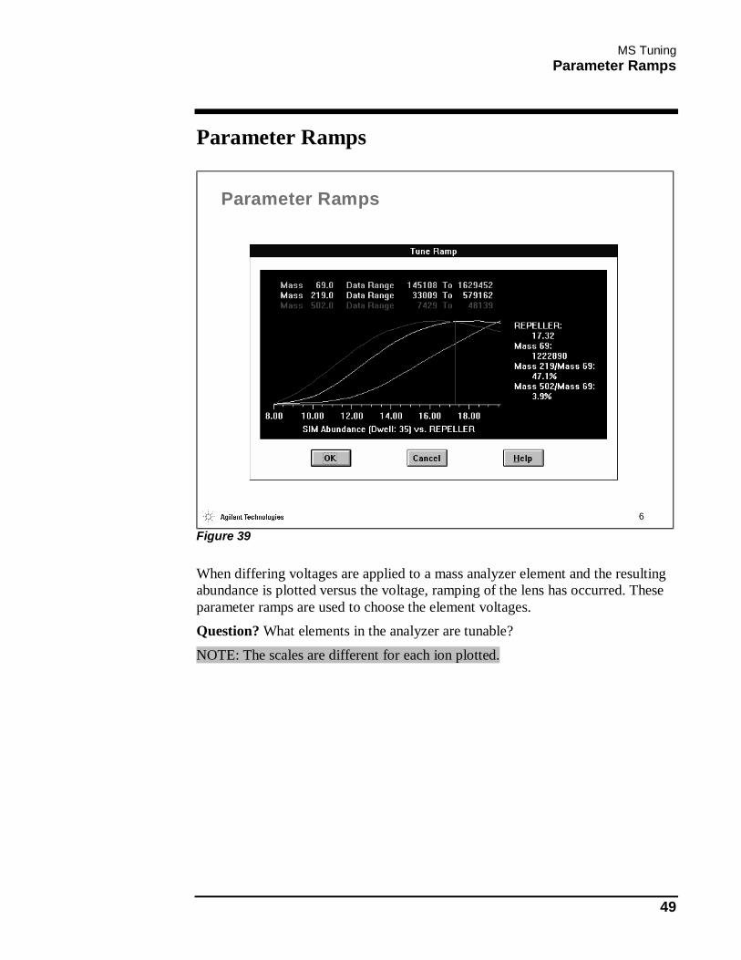
When differing voltages are applied to a mass analyzer element and the resulting abundance is plotted versus the voltage, ramping of the lens has occurred. These parameter ramps are used to choose the element voltages. Question? What elements in the analyzer are tunable?

NOTE: The scales are different for each ion plotted.

MS Tuning AMU Gain and Offset

50

AMU Gain and Offset

7

{RF VOLTAGE

SCAN LINE

502

219

69

DC VOLTAGESLOPE = AMU GAIN

Mathieu Stability Diagram

AMUOFFSET

AMU Gain and Offset

Figure 40

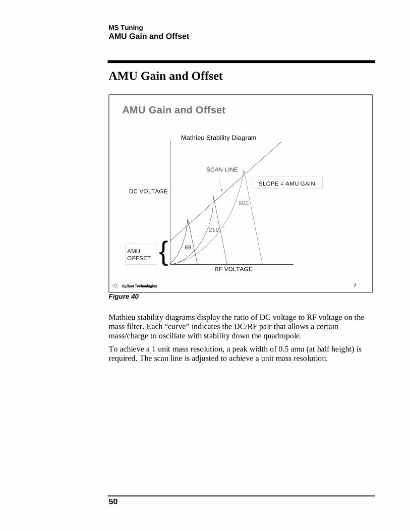
Mathieu stability diagrams display the ratio of DC voltage to RF voltage on the mass filter. Each “curve” indicates the DC/RF pair that allows a certain mass/charge to oscillate with stability down the quadrupole. To achieve a 1 unit mass resolution, a peak width of 0.5 amu (at half height) is required. The scan line is adjusted to achieve a unit mass resolution.

MS Tuning How Do AMU Gain and Offset Affect Peak Widths?

51

How Do AMU Gain and Offset Affect Peak Widths?

8

AMU GAIN

69

219

502

AMU OFFSET

69

219

502

Increasing the AMU Gain will:

Peak WidthDecrease Peak AmplitudeLarge effect at

at low mass.

effect at high and low mass.

Increasing the AMU Offset will:

Decrease

Peak Amplitude

How Do AMU Gain and Offset Affect Peak Widths?

Figure 41

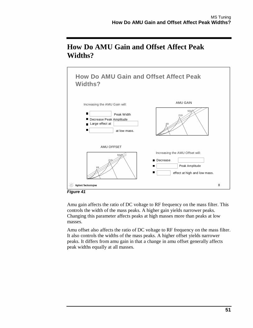
Amu gain affects the ratio of DC voltage to RF frequency on the mass filter. This controls the width of the mass peaks. A higher gain yields narrower peaks. Changing this parameter affects peaks at high masses more than peaks at low masses.

Amu offset also affects the ratio of DC voltage to RF frequency on the mass filter. It also controls the widths of the mass peaks. A higher offset yields narrower peaks. It differs from amu gain in that a change in amu offset generally affects peak widths equally at all masses.

MS Tuning Mass Axis Calibration

52

Mass Axis Calibration

9

Expected Mass

Obs

erve

d M

ass

MassAxisGain

100 200 300 400 500

500

400

300

200

100 69

219

502

Mass Axis Calibration

Figure 42

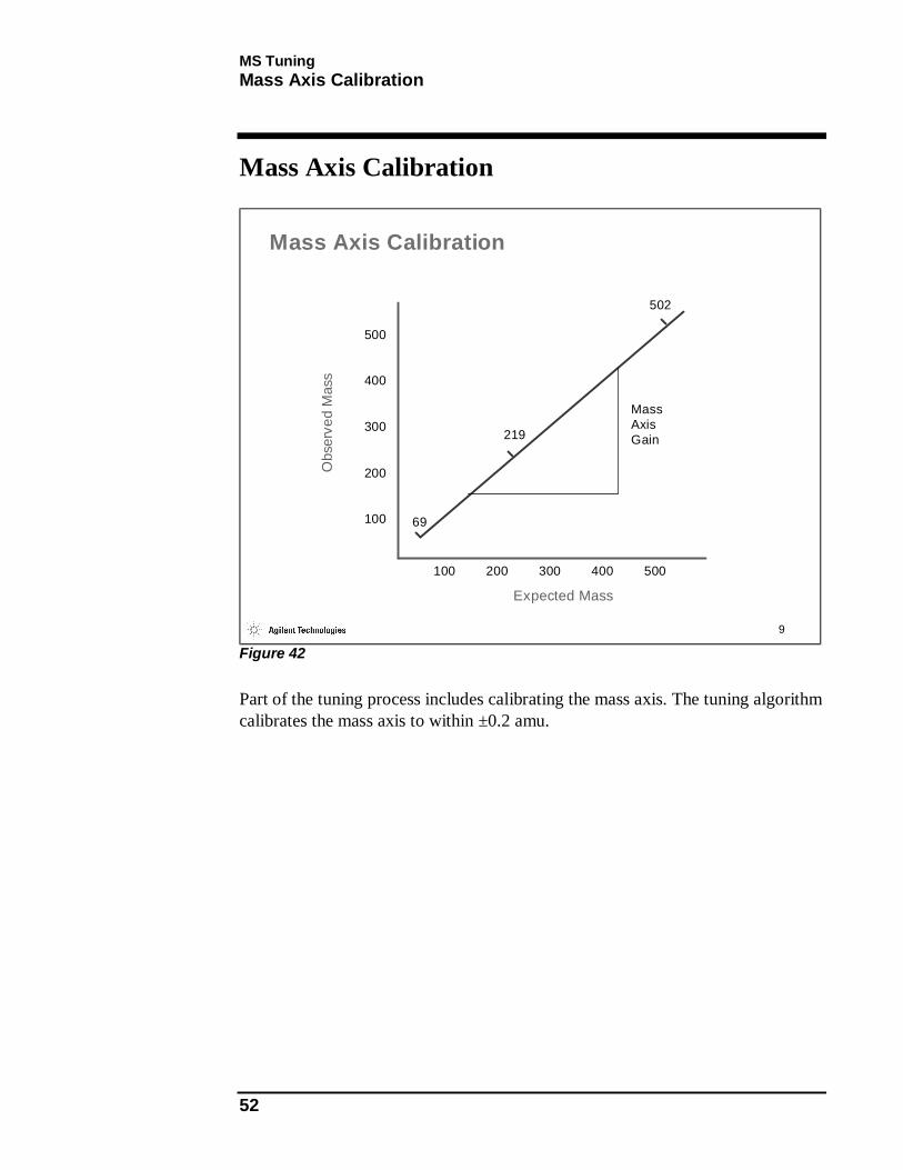
Part of the tuning process includes calibrating the mass axis. The tuning algorithm calibrates the mass axis to within ±0.2 amu.

MS Tuning Methods of Tuning

53

Methods of Tuning

10

Methods of Tuning an MSD

LOMASS.ULow Mass Autotune

NCICH4.UNCI Tune (with CI option)PCICH4.UPCI Tune (with CI option)

BFB.UDFTPP.UTARGET.U

Target TuneUser DefinedManual Tune

ATUNE.UQuick Tune

STUNE.UStandard Spectra TuneATUNE.UAutotune

Tune FileMethod

Figure 43

Figure 43 sums up the various tunes available to you on the ChemStation. The following is a brief summary of the various tunes.

Autotune

• maximizes instrument sensitivity across the entire scan range

• tunes on masses 69, 219, and 502

• suggested tune when maximum sensitivity is needed

Standard Spectra Tune

• standard response over the entire scan range

• tunes on masses 69, 219, and 502

• suggested tune when searching commercial libraries

• suggested tune for system diagnostics

Quick Tune

• fast, adjusts response (EM voltage), resolution, and mass assignments only

MS Tuning Methods of Tuning

54

Low Mass Autotune

• identical to Autotune except it tunes on masses 69, 131, and 219

• suggested tune when performing low molecular weight applications (less than 250 Daltons)

Manual Tune

• user-controlled to meet defined criteria

• suggested tune to maximize sensitivity in a particular mass region when performing SIM

Target Tune

• tunes the instrument with either BFB tune, DFTPP tune, or Target tune

• tunes PFTBA to match specified ratios stored in *.tgt files (BFB.tgt, etc.)

• suggested tune for US EPA applications

CI Tunes

• adjusts MS parameters for operation in Chemical Ionization (PCI or NCI) mode

• suggested tune for CI applications

MS Tuning Why Standard Spectra Tune?

55

Why Standard Spectra Tune?

11

Why Standard Spectra Tune?

Provides:• Reproducibility (operator-to-operator & lab-to-lab)• Diagnostic• Chronicle of system performance• Quick tuning• Starting place for manual tuning

Figure 44

Standard Spectra Tune is an automated tuning program for general-purpose MSD operation. Once initiated, it requires no operator participation. It is fast and convenient and provides satisfactory tuning for most analytical needs. A tune report gives good diagnostic information detailing system performance.

MS Tuning Standard Spectra Tune Flow Chart

56

Standard Spectra Tune Flow Chart

12

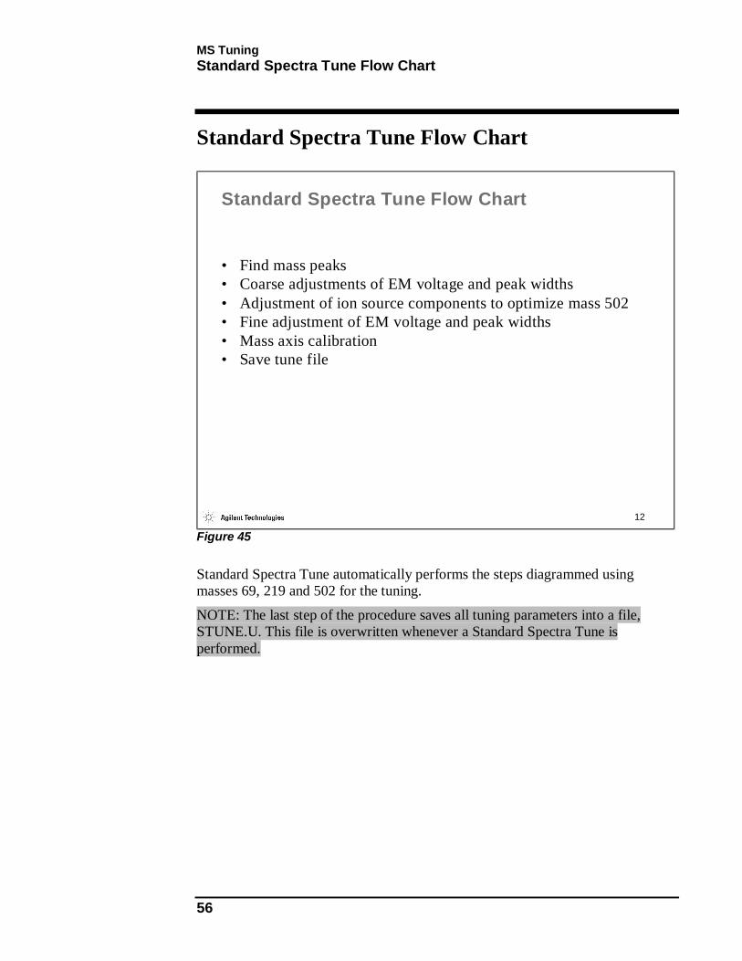
Standard Spectra Tune Flow Chart

• Find mass peaks• Coarse adjustments of EM voltage and peak widths• Adjustment of ion source components to optimize mass 502• Fine adjustment of EM voltage and peak widths• Mass axis calibration• Save tune file

Figure 45

Standard Spectra Tune automatically performs the steps diagrammed using masses 69, 219 and 502 for the tuning.

NOTE: The last step of the procedure saves all tuning parameters into a file, STUNE.U. This file is overwritten whenever a Standard Spectra Tune is performed.

MS Tuning Standard Spectra Tune Report

57

Standard Spectra Tune Report

13

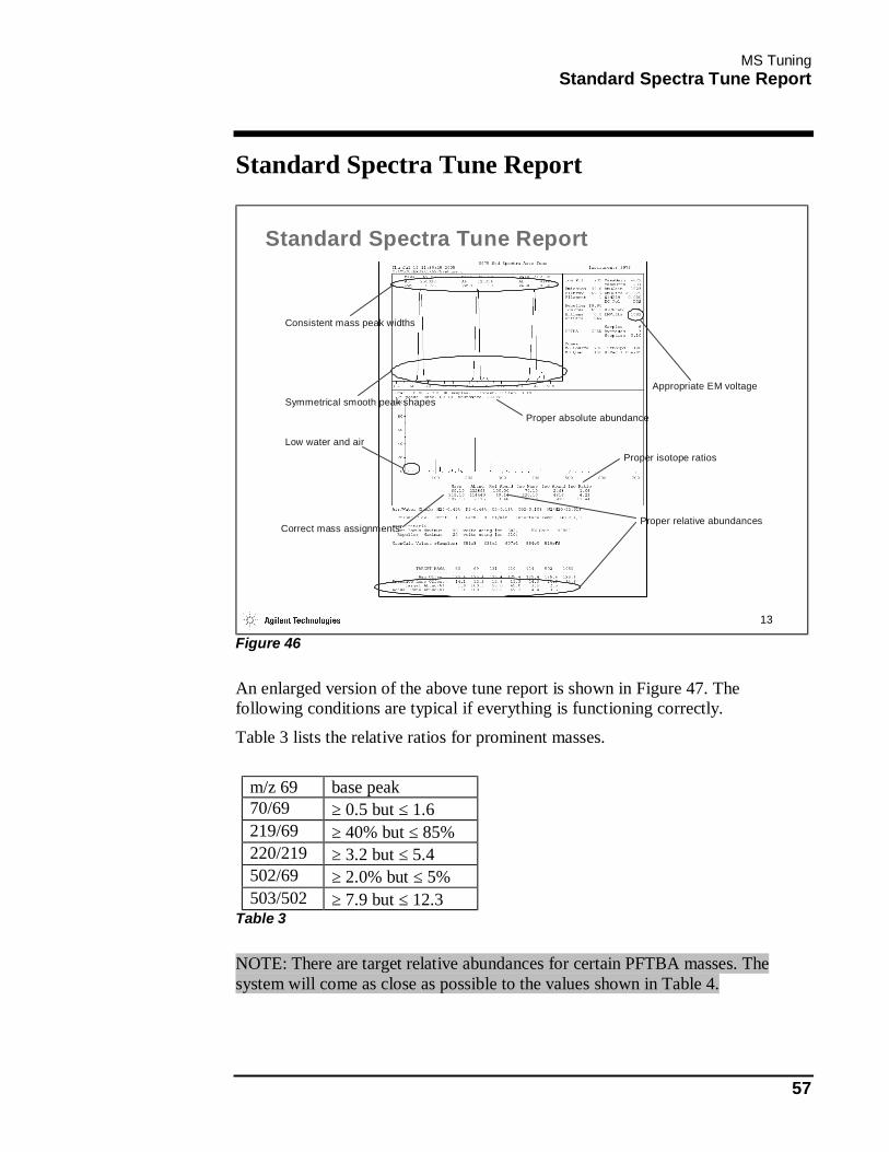
Consistent mass peak widths

Symmetrical smooth peak shapesAppropriate EM voltage

Proper absolute abundance

Low water and air

Correct mass assignmentsProper relative abundances

Proper isotope ratios

Standard Spectra Tune Report

Figure 46

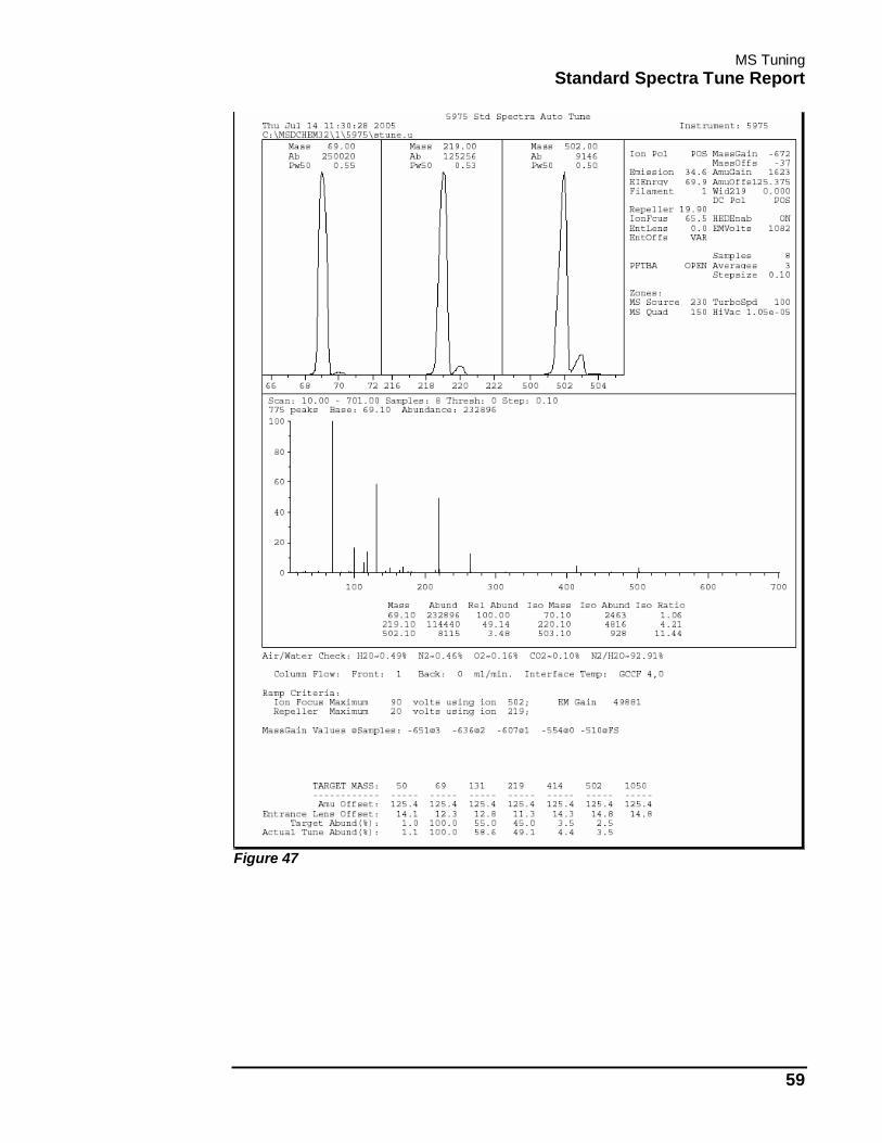
An enlarged version of the above tune report is shown in Figure 47. The following conditions are typical if everything is functioning correctly.

Table 3 lists the relative ratios for prominent masses.

m/z 69 base peak 70/69 ≥ 0.5 but ≤ 1.6 219/69 ≥ 40% but ≤ 85% 220/219 ≥ 3.2 but ≤ 5.4 502/69 ≥ 2.0% but ≤ 5% 503/502 ≥ 7.9 but ≤ 12.3

Table 3

NOTE: There are target relative abundances for certain PFTBA masses. The system will come as close as possible to the values shown in Table 4.

MS Tuning Standard Spectra Tune Report

58

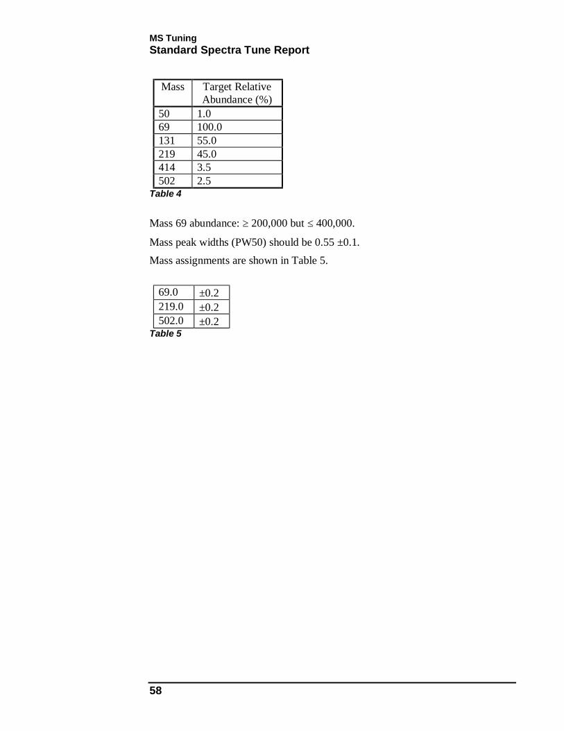
Mass Target Relative

Abundance (%) 50 1.0 69 100.0 131 55.0 219 45.0 414 3.5 502 2.5

Table 4

Mass 69 abundance: ≥ 200,000 but ≤ 400,000.

Mass peak widths (PW50) should be 0.55 ±0.1. Mass assignments are shown in Table 5.

69.0 ±0.2 219.0 ±0.2 502.0 ±0.2

Table 5

MS Tuning Standard Spectra Tune Report

59

Figure 47

MS Tuning Autotune

60

Autotune

14

69 502

69 502m/z

{E

ntra

nce

Lens

Vol

tage

ENTRRelative Abundances

219/69 = 20 - 35 %502/69 = 0.5 - 1 %

Ent.LensOffset

Autotune

Figure 48

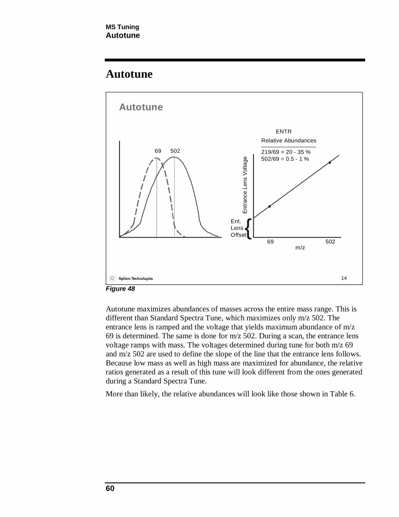
Autotune maximizes abundances of masses across the entire mass range. This is different than Standard Spectra Tune, which maximizes only m/z 502. The entrance lens is ramped and the voltage that yields maximum abundance of m/z 69 is determined. The same is done for m/z 502. During a scan, the entrance lens voltage ramps with mass. The voltages determined during tune for both m/z 69 and m/z 502 are used to define the slope of the line that the entrance lens follows. Because low mass as well as high mass are maximized for abundance, the relative ratios generated as a result of this tune will look different from the ones generated during a Standard Spectra Tune. More than likely, the relative abundances will look like those shown in Table 6.

MS Tuning Autotune

61

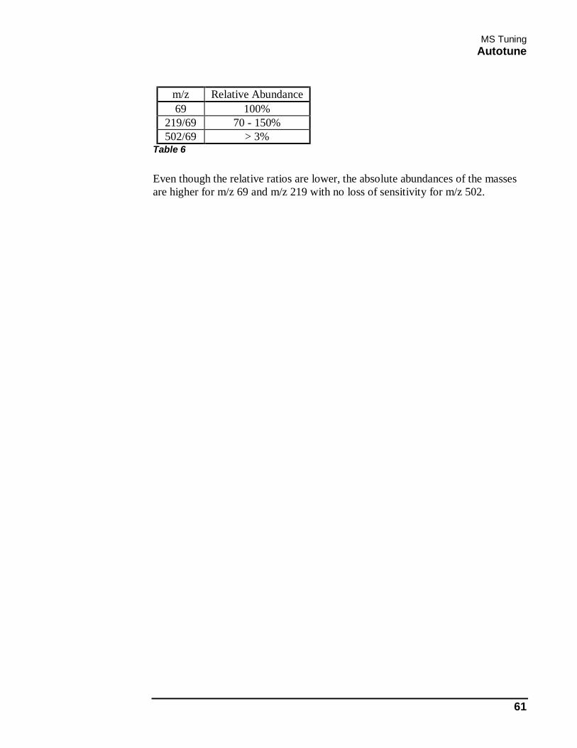
m/z Relative Abundance 69 100%

219/69 70 - 150% 502/69 > 3%

Table 6

Even though the relative ratios are lower, the absolute abundances of the masses are higher for m/z 69 and m/z 219 with no loss of sensitivity for m/z 502.

MS Tuning Autotune versus Standard Spectra Tune

62

Autotune versus Standard Spectra Tune

15

For Example:

@The abundances shown above are not exact and are for illustrative purposes only.

(Default Value)

mVamu

( )

{69 502

m/z

Ent.LensOffset

Entra

nce

Lens

Vol

tage

ENTR

(Set to Maximize m/z 69) m/z

{69 502

Ent.LensOffset

Ent

ranc

e Le

ns V

olta

geENTR

mV

(amu)

Autotune vs. Standard Spectra Tune

1X10,00010,000m/z 502

2 – 3X125,500350,000m/z 219

4X250,0001,000,000m/z 69

1600 V1600 VEMV

Net increase in abundance of m/z using Max Sensitivity

Standard Spectra

Maximum Sensitivity*

Figure 49

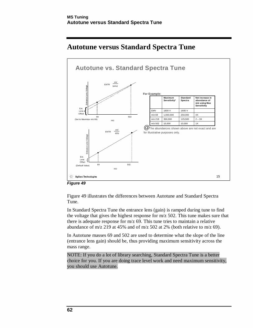
Figure 49 illustrates the differences between Autotune and Standard Spectra Tune.

In Standard Spectra Tune the entrance lens (gain) is ramped during tune to find the voltage that gives the highest response for m/z 502. This tune makes sure that there is adequate response for m/z 69. This tune tries to maintain a relative abundance of m/z 219 at 45% and of m/z 502 at 2% (both relative to m/z 69).

In Autotune masses 69 and 502 are used to determine what the slope of the line (entrance lens gain) should be, thus providing maximum sensitivity across the mass range. NOTE: If you do a lot of library searching, Standard Spectra Tune is a better choice for you. If you are doing trace level work and need maximum sensitivity, you should use Autotune.

MS Tuning Autotune Report

63

Autotune Report

16

Consistent mass peak widths

Symmetrical smooth peak shapes

Appropriate EM voltage

Proper absolute abundance

Low water and air

Correct mass assignments

Typical relative abundance

Autotune Report

Proper isotope ratios

Figure 50

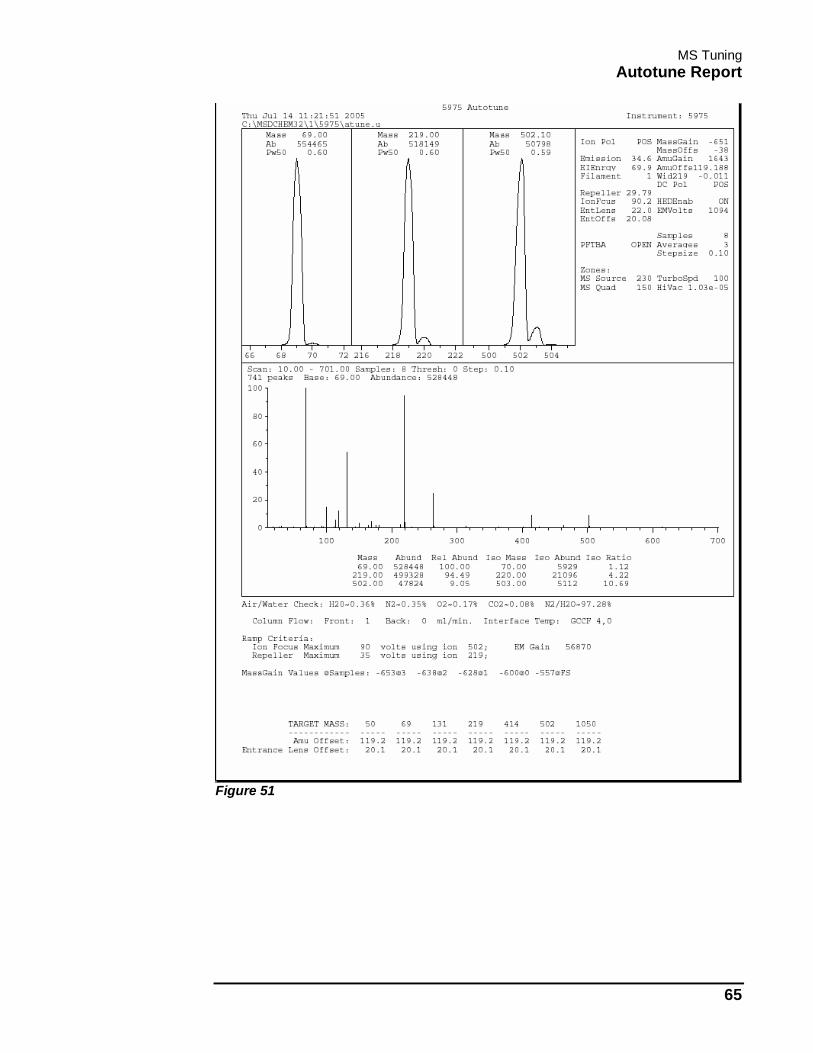
An enlarged version of the above tune report is shown in Figure 51. Once an Autotune is completed, the final report is automatically printed. The following conditions are typical. Table 7 lists relative ratios for prominent masses.

m/z 69 100% 70/69 ≥ 0.5% but ≤ 1.6% 219/69 ≥ 70% but ≤ 250% 220/219 ≥ 3.2% but ≤ 5.4% 502/69 ≥ 3% 503/502 ≥ 7.9% but ≤ 12.3%

Table 7

NOTE: there are NO target abundances. The system optimizes sensitivity across the entire mass range.

If there are peaks at 18, 28, and 32 amu there may be an air leak in the system.

MS Tuning Autotune Report

64

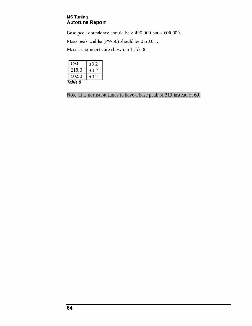
Base peak abundance should be ≥ 400,000 but ≤ 600,000.

Mass peak widths (PW50) should be 0.6 ±0.1. Mass assignments are shown in Table 8.

69.0 ±0.2 219.0 ±0.2 502.0 ±0.2

Table 8

Note: It is normal at times to have a base peak of 219 instead of 69.

MS Tuning Autotune Report

65

Figure 51

MS Tuning Quick Tune

66

Quick Tune

17

Quick Tune

• Amu gain and offset, EM voltage and mass axis calibration are set

• All other source parameters remain the same• Tunes on masses 69, 219, and 502

Figure 52

Quick Tune is a subset of Autotune. It sets mass filter and detector parameters but does not adjust the ion source parameters.

MS Tuning Target Tune

67

Target Tune

18

69 131 219 502

m/z

Entra

nce

Lens

Offs

et

Target Tune

TARGETS.TGTTARGET.U

To meet the target relative abundances specified with the Set Tune Targets menu item

Adjusts the relative abundances between the tune masses specified by the user to meet target values

Target Tune

BFB.TGTBFB.U

To meet the tuning requirements in EPA method 624

Adjusts the ratios m/z 131 and 219 in the PFTBA to meet target values

BFB Tune

DFTPP.TGTDFTPP.U

To meet the tuning requirements in EPA method 625

Adjusts the ratios of m/z 131,219, and 502 in the PFTBA spectrum to meet target values

DFTPP Tune

FilesGoalTuning Technique

Menu Item

Figure 53

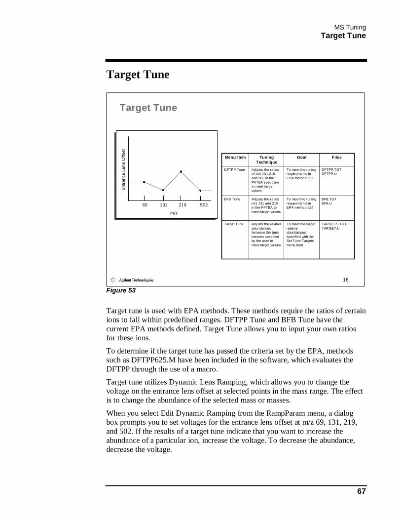
Target tune is used with EPA methods. These methods require the ratios of certain ions to fall within predefined ranges. DFTPP Tune and BFB Tune have the current EPA methods defined. Target Tune allows you to input your own ratios for these ions.

To determine if the target tune has passed the criteria set by the EPA, methods such as DFTPP625.M have been included in the software, which evaluates the DFTPP through the use of a macro. Target tune utilizes Dynamic Lens Ramping, which allows you to change the voltage on the entrance lens offset at selected points in the mass range. The effect is to change the abundance of the selected mass or masses.

When you select Edit Dynamic Ramping from the RampParam menu, a dialog box prompts you to set voltages for the entrance lens offset at m/z 69, 131, 219, and 502. If the results of a target tune indicate that you want to increase the abundance of a particular ion, increase the voltage. To decrease the abundance, decrease the voltage.

MS Tuning Manual Tune

68

Manual Tune

19

Manual Tune

• Access to MS parameters• Easy to create custom tune files• Diagnostic

Figure 54

Manual Tune allows interactive setting of individual tune parameters. It gives you the flexibility sometimes needed to alter the parameters automatically set during Autotune. Manual Tune is important when you need to perform diagnostics on the MSD. It is also extremely useful for leak testing.

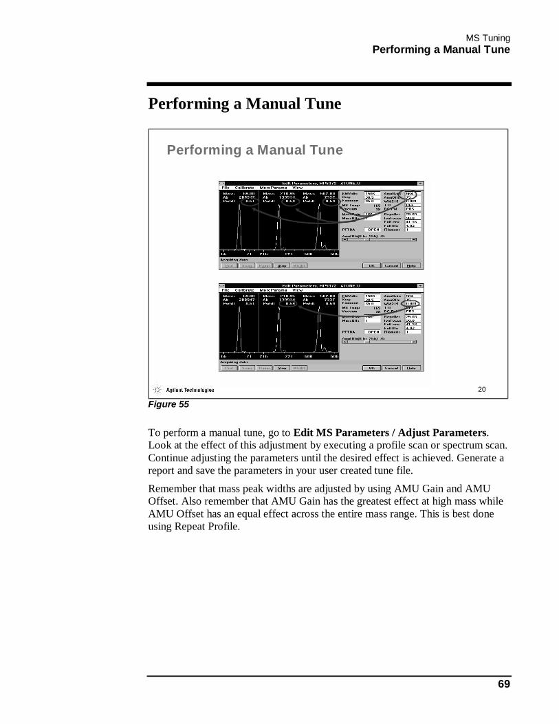
MS Tuning Performing a Manual Tune

69

Performing a Manual Tune

20

Performing a Manual Tune

Figure 55

To perform a manual tune, go to Edit MS Parameters / Adjust Parameters. Look at the effect of this adjustment by executing a profile scan or spectrum scan. Continue adjusting the parameters until the desired effect is achieved. Generate a report and save the parameters in your user created tune file.

Remember that mass peak widths are adjusted by using AMU Gain and AMU Offset. Also remember that AMU Gain has the greatest effect at high mass while AMU Offset has an equal effect across the entire mass range. This is best done using Repeat Profile.

MS Tuning Performing a Manual Tune (continued)

70

Performing a Manual Tune (continued)

21

Performing a Manual Tune (continued)

Figure 56

Remember that mass axis calibration is adjusted by using Mass Gain and Mass Offset. Also remember that Mass Gain has the greatest effect at high mass while Mass Offset has an equal effect across the entire mass range This is best done using Repeat Profile.

Remember that the EM voltage is used to adjust the absolute abundance for all masses, 69 in particular. Repeller, Ion Focus, Entrance Lens, and Entrance Lens Offset are used to adjust the relative abundance of one mass to another mass. This is best done using Repeat Scan.

LAB EXERCISE: Tuning the MSD

In this section you will:

• Explore automatic tuning of your MSD

• Explore manual tuning of your MSD

LAB EXERCISE: Tuning the MSD Types of Tune

72

Types of Tune

Several types of automatic tuning procedure are available with the MS ChemStation software. Automatic tuning uses PFTBA as the calibration compound and automatically adjusts the MS parameters to meet predefined criteria for operation in EI mode. You can select from three autotunes from the Instrument view or select manual tune or target tune from the View menu.

Autotune maximizes instrument sensitivity over the mass range, using PFTBA masses 69, 219, and 502. Use this tune for applications requiring maximum sensitivity that do not require the traditional abundance ratios of 100% m/z 69, 35 - 85% m/z 219, and 1 - 5% m/z 502. The tune file is automatically saved to ATUNE.U. Standard Spectra Autotune ensures standard response over the full scan range. Specifically, PFTBA mass 69 is the base peak, mass 219 is between 35 and 99%, and mass 502 is >1%. Use this tune if you are planning to perform mass spectral library searches. When you select this tune, certain parameters are forced to standard operating conditions: EI mode, CI Gas off and calibration valve on. The tune file is automatically saved to STUNE.U. QuickTune provides a re-tuning for optimum response and resolution and for accurate mass assignment. Only the mass axis, peak widths, and EM voltage are adjusted; the lenses are unaffected. QuickTune is useful only when the instrument has already been successfully tuned with Autotune . It ensures that the abundances, peak width, and mass axis calibrations are satisfactory. The tune file is automatically saved to ATUNE.U. Manual Tune allows the operator to specify individual tuning parameters. Within manual tune the repeller, ion focus, entrance lens and the electron multiplier voltages as well as the amu gain and amu offset can be individually varied. Manual tune may be used to optimize sensitivity around a certain mass range. Target Tune adjusts the ratios of specified ions to meet predefined target values. These targets are usually associated with EPA methods or may be user defined. Chemical Ionization (CI) Tuning automatically tunes the MSD equipped with chemical ionization.

LAB EXERCISE: Tuning the MSD Autotuning the MSD

73

Autotuning the MSD

Tuning the mass spectrometer optimizes the MSD parameters to ensure good mass spectral data when you carry out your analysis. Before starting an autotune you need to set both the MS source and MS quadrupole temperatures.

1) Start a session of your on-line instrument by selecting Start / Programs / GC_MS Instrument #1 / GC_MS Instrument #1. To set the source and quadrupole temperatures, select View / Tune and Vacuum Control... from the Instrument Control view.

2) Once the Tune and Vacuum Control view opens, choose Parameters / Edit MS Temperatures.... When the panel opens enter a setpoint of 230º for the MS Source and 150º for the MS Quad.

3) When the MS temperatures have reached their setpoints we are ready to tune. To carry out an Autotune of your instrument, select Tune / Autotune (Atune.U).

What are other automated tunes are available from this menu?

NOTE: If it is necessary to stop the MSD during a tune, select Abort from the Abort menu item. The tune window can be minimized at any time by clicking the Windows minimize button. When the tune is complete, a report is automatically printed. 4) Fill out Table 9 according to the parameters found in your tune report.

Parameters Value Acceptable? Y/N

Electron Multiplier

Relative abund of: 69

Relative abund of: 219/69

Relative abund of: 502/69

Isotope ratio: 70/69

Isotope ratio: 220/219

Isotope ratio: 503/502 Table 9

Does your system have an air leak? If yes, which masses are present?

_________________________________________________________________

LAB EXERCISE: Tuning the MSD Autotuning the MSD

74

5) Repeat tuning using Standard Spectra Tune (Stune.U). Note the differences in these tuning methods by comparing the hardcopies of each tune.

How have the absolute abundances of the tune masses changed?

_________________________________________________________________ How have the relative abundances of the tune masses changed?

_________________________________________________________________ Which other tune parameters have changed between these two tuning methods?

_________________________________________________________________ 6) Now Quick Tune the MSD: select Tune / QuickTune and note the

differences in steps and the length of time required. What tune parameters have changed?

_________________________________________________________________ 7) Repeat the Autotune.

LAB EXERCISE: Tuning the MSD Interactive (Manual) Tuning

75

Interactive (Manual) Tuning

8) From the Tune and Vacuum Control view, choose Parameters / Manual Tune .... Virtually all tasks that can be performed in manual tune can be accessed from this one window.

To see the effect certain parameters have on the PFTBA spectrum we will change a parameter value and then generate a spectrum scan. To change any parameter, click on the present value associated with the parameter, then either input the new value, or using the scroll bar displayed at the bottom of the parameters box, change the value accordingly. 9) To see how changing the voltage affects the spectrum, select Scan.

10) Change the ion focus voltage by 30 volts. 11) Generate a hardcopy of the new scan by selecting File / Print. 12) Click on the Stop button to stop the scanning process. What effect does changing the ion focus have on the mid and high mass ions?

_________________________________________________________________ 13) Return the ion focus to its original value.

14) Execute a profile scan by using the Prof button. 15) Now, lower the AmuOffs (Offset) by 50 units.

How does this affect the peak widths of the mass profiles? _________________________________________________________________

16) Return the AmuOffs to its original value and raise the AmuGain by 50 units.

How does this affect the peakwidths of the mass profiles at each end of the mass range?

_________________________________________________________________ 17) Reset the AmuGain to its original value.

18) Now select MoreParams / Tune Params.... This panel allows you to change the tune masses as well as presentation of the profiles (absolute abundances or ratios). Click OK to exit this panel and return to the Manual Tune panel.

19) Select the Repeller. Click on the Ramp button at the bottom of the screen. Print out a copy of the ramp. Using the mouse, click on the point in the ramp window where you would like the repeller voltage to be set (noting the original value on the print out before you change it). Click on the Scan button to view how changing the repeller voltage has affected the response

LAB EXERCISE: Tuning the MSD Interactive (Manual) Tuning

76

of the three tune masses. Return the repeller to the original value when completed.

What does this ramp show you? (Look at both axes and the title info) _________________________________________________________________

What is the optimum repeller voltage? For what mass has the repeller voltage been optimized?

_________________________________________________________________ 20) Toggle between Ramp and Prof to see how other source elements can be

ramped to affect responses of the various tune masses. (Remember that only the repeller, ion focus, entrance lens, and entrance lens offset produce meaningful information when ramped.)

21) Click OK to close the Manual Tune panel.

22) Return to the Instrument Control view by selecting View / Instrument Control. Do not save the tune file.

Data Acquisition

Data Acquisition What You Will Learn

78

What You Will Learn

2

Methods I - Data Acquisition

In this section you will learn:

• An Introduction to Methods• Scan Acquisition Principles• Selected Ion Monitoring Principles• Setup Up Data Acquisition as Part of a Method

Figure 57

When you finish this section, you should feel comfortable with the concept of “methods” with respect to data acquisition. You should be familiar with the different modes of acquisition available to you on the ChemStation and should be able to specify the various data acquisition parameters in a method.

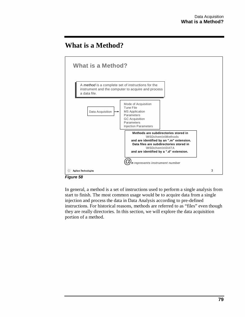
Data Acquisition What is a Method?

79

What is a Method?

3

A method is a complete set of instructions for the instrument and the computer to acquire and process a data file.

Data Acquisition

Mode of AcquisitionTune FileMS Application ParametersGC Acquisition ParametersInjection Parameters

Methods are subdirectories stored in \MSDchem\n\Methods

and are identified by an ".m" extension.Data files are subdirectories stored in

\MSDchem\n\DATA and are identified by a ".d" extension.

@n represents instrument number

What is a Method?

Figure 58

In general, a method is a set of instructions used to perform a single analysis from start to finish. The most common usage would be to acquire data from a single injection and process the data in Data Analysis according to pre-defined instructions. For historical reasons, methods are referred to as “files” even though they are really directories. In this section, we will explore the data acquisition portion of a method.

Data Acquisition Scan Acquisition Principles

80

Scan Acquisition Principles

4

Scan Acquisition Principles

Topics to be discussed:

• The usefulness of data acquisition in Scan Mode• How the various data acquisition parameters influence the data

Figure 59

There are two modes of acquisition available on the ChemStation; Scan Acquisition and Selected Ion Monitoring (SIM). This discussion covers what Scan acquisition is, and how to use it. SIM will be covered in a subsequent discussion.

Scan mode is the most frequently used since it scans all the masses (within the range specified) generated during the acquisition process rather than only a selected number of masses. It is the mode to use when analyzing unknown compounds. It is also the mode to use if you wish to perform library searches of the data in Data Analysis.

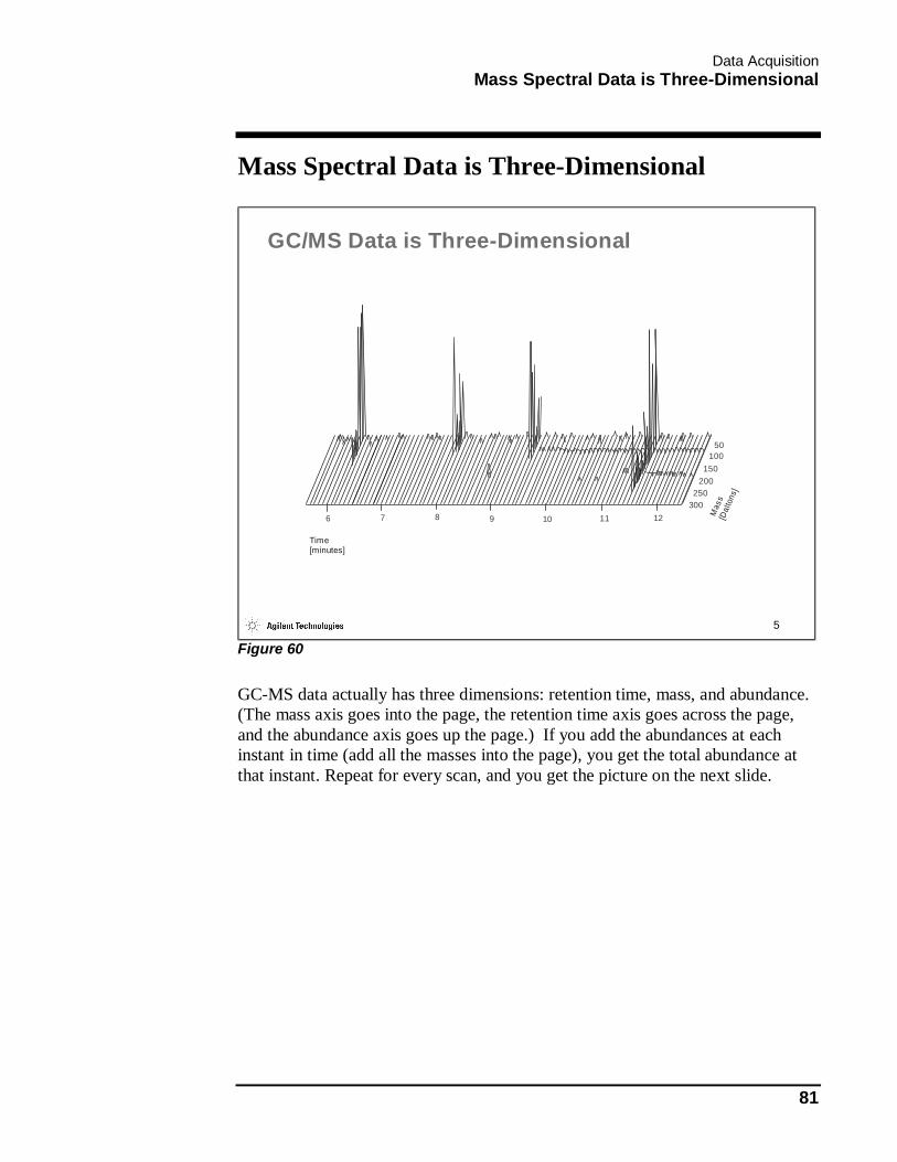
Data Acquisition Mass Spectral Data is Three-Dimensional

81

Mass Spectral Data is Three-Dimensional

5

12

50100

150200

250300

11109876

Time [minutes]

Mas

s

[Da l

tons

]

GC/MS Data is Three-Dimensional

Figure 60

GC-MS data actually has three dimensions: retention time, mass, and abundance. (The mass axis goes into the page, the retention time axis goes across the page, and the abundance axis goes up the page.) If you add the abundances at each instant in time (add all the masses into the page), you get the total abundance at that instant. Repeat for every scan, and you get the picture on the next slide.

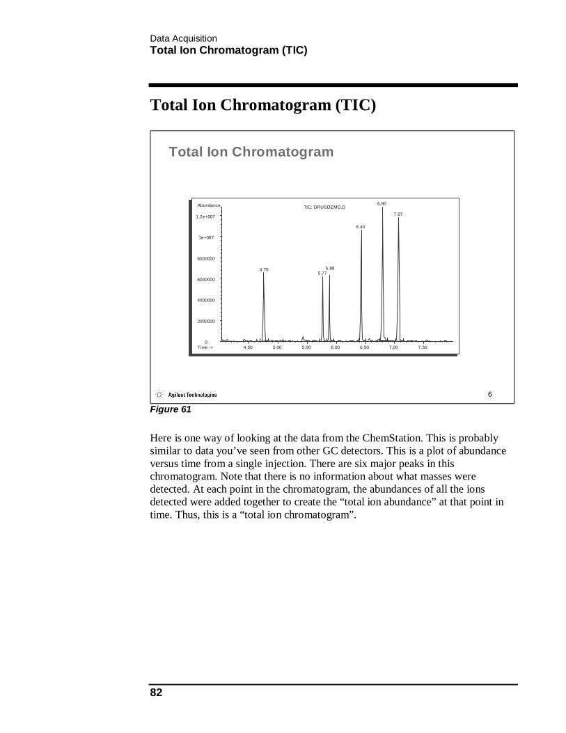
Data Acquisition Total Ion Chromatogram (TIC)

82

Total Ion Chromatogram (TIC)

6

Time ->

Abundance

4.765.77

5.88

6.43

6.80

7.07

4.50 5.00 5.50 6.00 6.50 7.00 7.500

2000000

4000000

6000000

8000000

1e+007

1.2e+007

TIC: DRUGDEMO.D

Total Ion Chromatogram

Figure 61

Here is one way of looking at the data from the ChemStation. This is probably similar to data you’ve seen from other GC detectors. This is a plot of abundance versus time from a single injection. There are six major peaks in this chromatogram. Note that there is no information about what masses were detected. At each point in the chromatogram, the abundances of all the ions detected were added together to create the “total ion abundance” at that point in time. Thus, this is a “total ion chromatogram”.

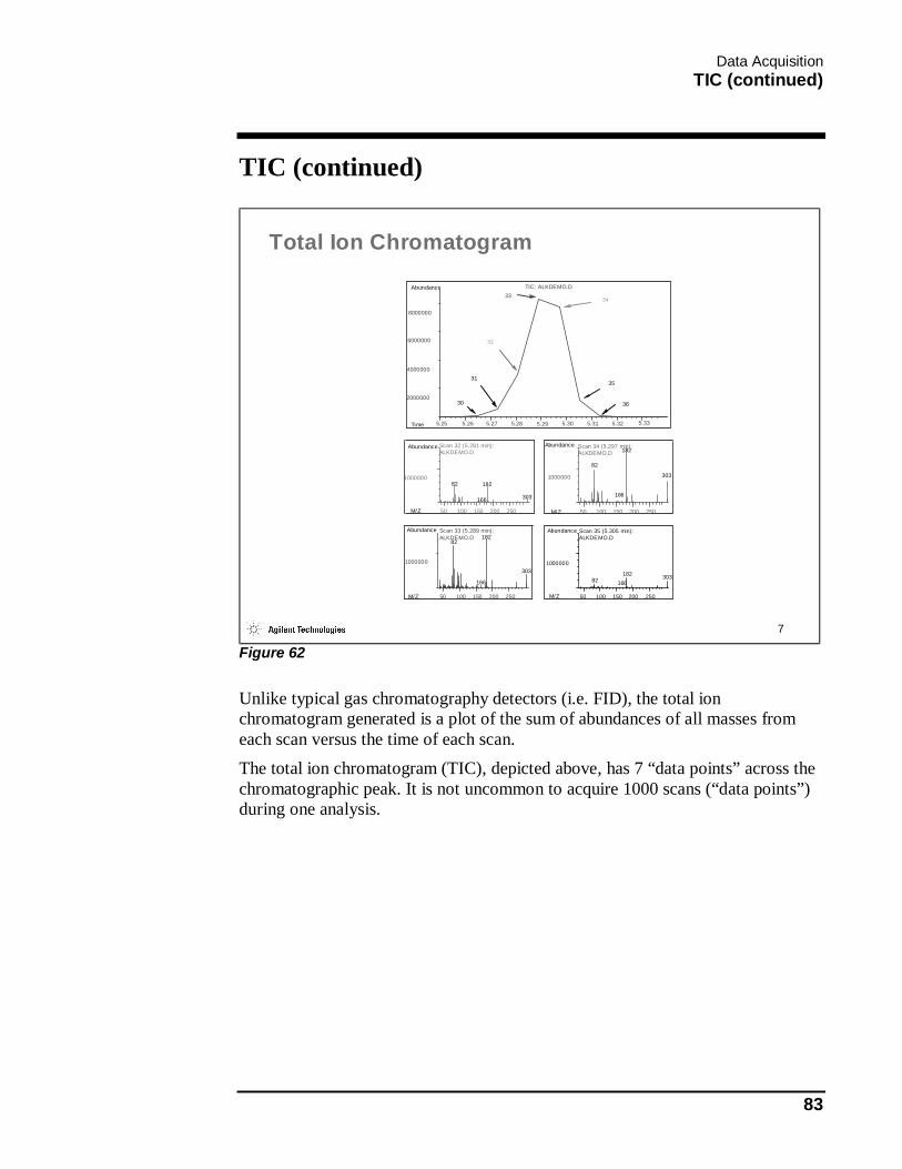
Data Acquisition TIC (continued)

83

TIC (continued)

7

M/Z

Abundance

82

166

182

303

50 100 150 200 250

1000000

Scan 32 (5.281 min): ALKDEMO.D

M/Z

Abundance

82

166

182

303

50 100 150 200 250

1000000

Scan 33 (5.289 min): ALKDEMO.D

M/Z

Abundance

82

166

182

303

50 100 150 200 250

1000000

Scan 34 (5.297 min): ALKDEMO.D

M/Z

Abundance

82 166182 303

50 100 150 200 250

1000000

Scan 35 (5.305 min): ALKDEMO.D

Time

Abundance

5.25 5.26 5.27 5.28 5.29 5.30 5.31 5.32 5.33

2000000

4000000

6000000

8000000

TIC: ALKDEMO.D

32

3334

3531

3630

Total Ion Chromatogram

Figure 62

Unlike typical gas chromatography detectors (i.e. FID), the total ion chromatogram generated is a plot of the sum of abundances of all masses from each scan versus the time of each scan. The total ion chromatogram (TIC), depicted above, has 7 “data points” across the chromatographic peak. It is not uncommon to acquire 1000 scans (“data points”) during one analysis.

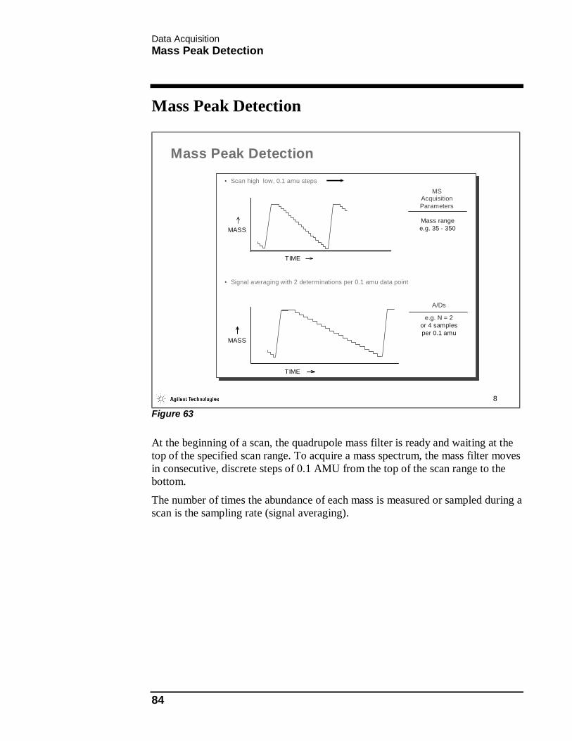
Data Acquisition Mass Peak Detection

84

Mass Peak Detection

8

MASS

TIME

MS AcquisitionParameters

Mass rangee.g. 35 - 350

A/Ds

e.g. N = 2or 4 samplesper 0.1 amu

• Scan high low, 0.1 amu steps

• Signal averaging with 2 determinations per 0.1 amu data point

MASS

TIME

Mass Peak Detection

Figure 63

At the beginning of a scan, the quadrupole mass filter is ready and waiting at the top of the specified scan range. To acquire a mass spectrum, the mass filter moves in consecutive, discrete steps of 0.1 AMU from the top of the scan range to the bottom.

The number of times the abundance of each mass is measured or sampled during a scan is the sampling rate (signal averaging).

Data Acquisition Mass Peak Detection (continued)

85

Mass Peak Detection (continued)

9

1E22E23E24E25E26E27E28E29E21E31E3

AB

UN

DA

NC

E

150.

0

151.

0

152.

0

153.

0

154.

0

155.

0

M/Z

1.1E3

THRESHOLD32

14

5

1234

5

32

1

4

5

STORES: 154.10, 1137

Mass Peak Detection (continued)

• Smoothing using five adjacent data points.• Determine "centroid" mass (mass peak maxima).• Signal level at centroid mass must exceed scan threshold.• Store mass abundance pair in data file.

Figure 64

The data is then smoothed using five adjacent data points and the apex of the mass peak determined.

The corresponding abundance and mass/charge (m/z) values are compared to the threshold value. If the computed abundance is greater than or equal to the threshold, the mass/abundance pair is stored.

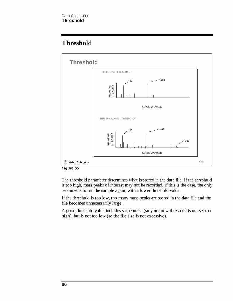
Data Acquisition Threshold

86

Threshold

10

THRESHOLD TOO HIGH

82 182

MASS/CHARGER

ELAT

IVE

INTE

NS

ITY

MASS/CHARGE

REL

ATIV

E IN

TEN

SIT

Y

82

303

182

THRESHOLD SET PROPERLY

Threshold

Figure 65

The threshold parameter determines what is stored in the data file. If the threshold is too high, mass peaks of interest may not be recorded. If this is the case, the only recourse is to run the sample again, with a lower threshold value. If the threshold is too low, too many mass peaks are stored in the data file and the file becomes unnecessarily large. A good threshold value includes some noise (so you know threshold is not set too high), but is not too low (so the file size is not excessive).

Data Acquisition The Digital Scanning Process

87

The Digital Scanning Process

11

MASS

TIME

PROCESS TIME

RESET TIMESCAN TIME

SCAN CYCLE TIME

The Digital Scanning Process

Factors affecting scan time:• Number of data points averaged per 0.1 amu increment (sampling rate)• Mass range scanned • Actual number of ions detected (scan threshold)

Try to achieve 5-10 scans across the chromatographic peak for good qualitative data!Try to achieve 10-20 scans across the chromatographic peak for good quantitative data!

Figure 66

The total time needed for one scan acquisition includes the time the quadrupole mass filter steps from high to low mass. The scan range and sampling rate affect this time. When the low end of the scan range is reached, the quadrupole mass filter is reset to the upper limit mass in preparation for the next scan. Notice that the reset time is less than the time required performing other operations, so the total cycle time is not affected by this reset time. At the same time the quadrupole is reset, the control card may initialize the data transfer to the ChemStation (process time). The ChemStation then stores the data file on the disk, updates the screen display with any real time chromatograms that are to be drawn, and other information. Scan cycle time and scan times are determined when you choose the mass spectrometer parameters in data acquisition. It is important to select these judiciously, remembering that you generally are trading chromatographic quality for mass spectral quality. The scan time depends on three factors:

Data Acquisition The Digital Scanning Process

88

1) The number of samples taken at each step (sampling rate). 2) The mass range.

3) The number of m/z values recorded during the scan. User-selected mass spectrometer parameters determine the magnitude of each of these. The system gives you an “estimate” of the scans/second you should achieve. For good qualitative data, your goal should be 10 scans across a peak (absolutely no less than 5!) For good quantitative data, your goal should be 10 - 20 scans across a peak (absolutely no less than 10!)

Data Acquisition Spectral Tilting - Number of Scans

89

Spectral Tilting - Number of Scans

12

Spectrum Tilting

• Sampling = 1• Scans = 20

Figure 67

The number of scans achieved across a chromatographic peak can have a profound influence on the quality of mass spectral data generated. Remember, a chromatographic system is not static; the analyte elutes through the column into the source. It may only last 5 seconds (as in the case of a capillary peak). As the concentration of the analyte in the source changes, the system is scanning from high mass to low mass. The length of time this scanning process takes and the amount of time the analyte is in the source need to be considered. In Figure 67 through Figure 70, notice the influence of the Sampling on the number of Scans across the chromatographic peak. Also notice the influence of the number of Scans and the quality of the spectral data that is generated.

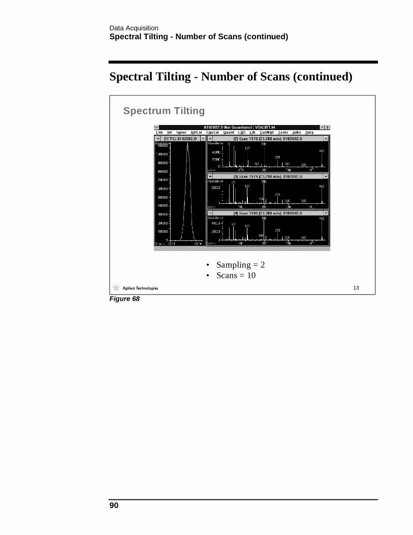
Data Acquisition Spectral Tilting - Number of Scans (continued)

90

Spectral Tilting - Number of Scans (continued)

13

Spectrum Tilting

• Sampling = 2• Scans = 10

Figure 68

Data Acquisition Spectral Tilting - Number of Scans (continued)

91

Spectral Tilting - Number of Scans (continued)

14

Spectrum Tilting

• Sampling = 3• Scans = 6

Figure 69

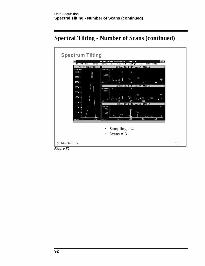
Data Acquisition Spectral Tilting - Number of Scans (continued)

92

Spectral Tilting - Number of Scans (continued)

15

Spectrum Tilting

• Sampling = 4• Scans = 3

Figure 70

Data Acquisition Spectral Integrity

93

Spectral Integrity

16

Spectral Integrity

• MS Considerations– Scan Speed/Cycle Time

• GC Considerations– Peak Width

• Data Considerations– Signal: Noise Ratio– Gaussian peak shape– Spectral tilting– Threshold

Figure 71

In choosing the mass spectrometer parameters in acquisition, there is a trade off between mass spectral quality and chromatographic quality. If you scan quickly, each chromatographic peak has many spectra taken as it elutes. This makes reconstruction of the chromatogram possible, but the quality of the spectra may be poor due to the speed at which they were taken. If you scan slowly, the quality of the mass spectral data may be good, but the chromatographic peak shape is poorly defined (non-Gaussian, spectral tilting). A threshold that is too low gives a lot of meaningless noise in the spectrum; a threshold that is too high misses important isotope information. To achieve good mass spectral quality while defining the chromatographic peak, the mass spectrometer parameters in data acquisition should be chosen to achieve 5-10 scans across the chromatographic peak. Start by setting the mass range. Modify the sampling rate to achieve 5-10 scans across the peak. A sampling rate of N=2 or N=3 is typical for narrow bore capillary chromatography.

Data Acquisition Selected Ion Monitoring (SIM) Principles

94

Selected Ion Monitoring (SIM) Principles

17

Selected Ion Monitoring Principles

Topics to be discussed:• How selected ion monitoring (SIM) differs from scanning• How varying SIM acquisition parameters can affect your data• How to use data acquisition in the SIM mode

Figure 72

We will now discuss the second mode of acquisition available to you on the ChemStation. This discussion will cover what Selected Ion Monitoring (SIM) is and how to use it.

Data Acquisition Selected Ion Monitoring (SIM)

95

Selected Ion Monitoring (SIM)

18

Selected Ion Monitoring

WHAT IS IT?– Monitoring only mass/charge ratios containing information

HOW IS IT DONE?– Control mass analyzer to only select ions of analytical interest

WHY IS IT DONE?– Greater sensitivity– Better peak shape– Better accuracy and precision

APPLICATIONS– Trace analysis– Complex matrices– Routine quantitation

Figure 73

SIM allows the mass spectrometer to detect specific compounds with very high sensitivity. In SIM mode, the instrument is set to acquire data at masses of interest instead of stepping the mass filter over a wide range of masses. Because the mass spectrometer collects data at only the masses of interest, it responds only to those compounds that possess the selected mass fragments. In essence, the instrument is focused on only the compounds of interest. Also, because only a few masses are monitored, much more time may be spent looking at these masses, with the attendant increase in sensitivity, accuracy, and precision.

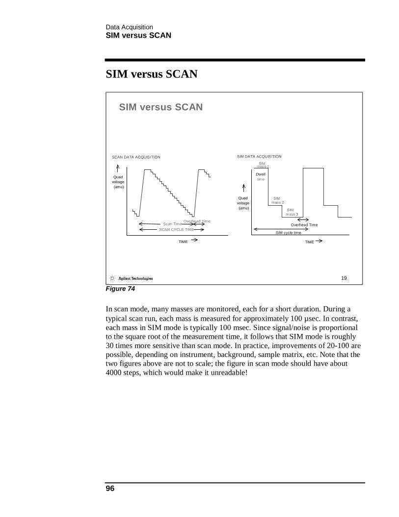
Data Acquisition SIM versus SCAN

96

SIM versus SCAN

19

SIM DATA ACQUISITION

Dwelltime

SIMmass 1

SIMmass 2

SIM cycle time

Quadvoltage(amu)

TIME

SIMmass 3

Overhead Time

SCAN DATA ACQUISITION

Scan TimeSCAN CYCLE TIME

Overhead Time

Quadvoltage(amu)

TIME

SIM versus SCAN

Figure 74

In scan mode, many masses are monitored, each for a short duration. During a typical scan run, each mass is measured for approximately 100 µsec. In contrast, each mass in SIM mode is typically 100 msec. Since signal/noise is proportional to the square root of the measurement time, it follows that SIM mode is roughly 30 times more sensitive than scan mode. In practice, improvements of 20-100 are possible, depending on instrument, background, sample matrix, etc. Note that the two figures above are not to scale; the figure in scan mode should have about 4000 steps, which would make it unreadable!

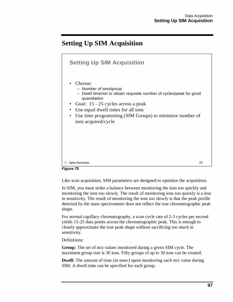
Data Acquisition Setting Up SIM Acquisition

97

Setting Up SIM Acquisition

20

Setting Up SIM Acquisition

• Choose:– Number of ions/group– Dwell time/ion to obtain requisite number of cycles/peak for good

quantitation• Goal: 15 - 25 cycles across a peak• Use equal dwell times for all ions• Use time programming (SIM Groups) to minimize number of

ions acquired/cycle

Figure 75

Like scan acquisition, SIM parameters are designed to optimize the acquisition. In SIM, you must strike a balance between monitoring the ions too quickly and monitoring the ions too slowly. The result of monitoring ions too quickly is a loss in sensitivity. The result of monitoring the ions too slowly is that the peak profile detected by the mass spectrometer does not reflect the true chromatographic peak shape.

For normal capillary chromatography, a scan cycle rate of 2-3 cycles per second yields 15-25 data points across the chromatographic peak. This is enough to closely approximate the true peak shape without sacrificing too much in sensitivity.

Definitions: Group: The set of m/z values monitored during a given SIM cycle. The maximum group size is 30 ions. Fifty groups of up to 30 ions can be created. Dwell: The amount of time (in msec) spent monitoring each m/z value during SIM. A dwell time can be specified for each group.

Data Acquisition SIM Experiment

98

SIM Experiment

21

The mass spectra from a SIM experiment of ions in 9-carboxy THC in 0.1 amu increments. Select the most abundant mass for SIM acquisition.

DYNAMIC MASS CALIBRATION

9-CarboxyTHC TMS Derivative

Mass to charge ratio in 0.1 amu increments

0

20

40

60

80

100

120

.7 .8 .9 .0 .1 .2 .3 .4 .5 .7 .8 .9 .0 .1 .2 .3 .4 .5 .7 .8 .9 .0 .1 .2 .3 .4 .5 .7 .8 .9 .0 .1 .2 .3 .4 .5

73.0\\\

488.3\

473.3371.2

Norm

aliz

ed A

bund

ance

\371.0

\473.0

\488.0

SIM Experiment

Figure 76

For the highest sensitivity in SIM mode, you should determine the SIM ion value to within 0.1 amu. Choosing ions for SIM must be done with care so as not to choose ions that result in a high background or create interfering peaks. Using a mass spectrum that displays ions labeled with integer values as the source to choose ions for a subsequent SIM acquisition may result in a loss of sensitivity and/or ion ratios may fall out of range. The easiest way of performing this experiment is to acquire data using SIM ions spaced 0.1 amu apart about the expected nominal mass, then use the mass with the highest response. This is known as a SIM experiment or a dynamic mass calibration. NOTE: Be sure to start with a calibrated mass spectrometer. Tuning the instrument provides proper lens voltages, electron multiplier voltage, and a calibration of the mass axis.

To determine which m/z values to monitor:

• Acquire multiple ions in 0.1 amu increments, bracketing the nominal mass or the calculated exact mass.

• Integrate the ion chromatograms (or “observe” the spectra).

Data Acquisition SIM Experiment

99

• Choose ion with maximum signal for all subsequent SIM acquisitions. NOTE: It is important that the SIM masses be as exact as possible. Errors of 0.3 amu in choosing a SIM mass can easily result in a 25-75% loss in signal!

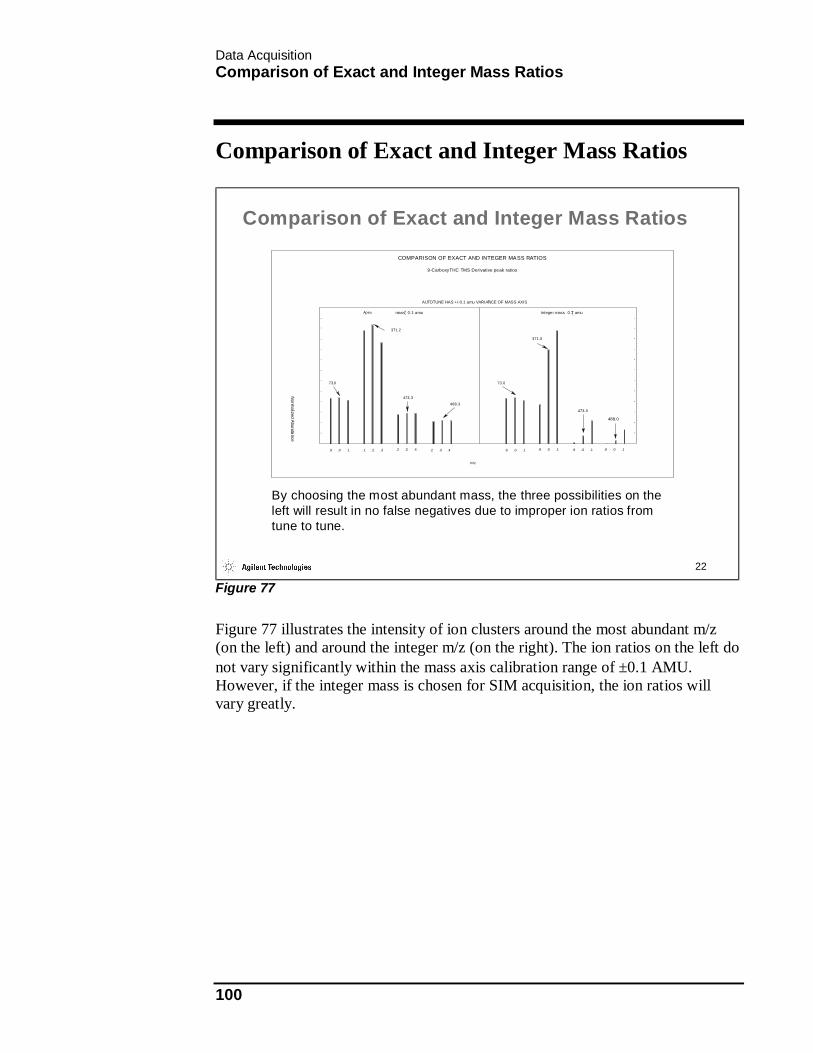
Data Acquisition Comparison of Exact and Integer Mass Ratios

100

Comparison of Exact and Integer Mass Ratios

22

By choosing the most abundant mass, the three possibilities on the left will result in no false negatives due to improper ion ratios from tune to tune.

COMPARISON OF EXACT AND INTEGER MASS RATIOS

9-CarboxyTHC TMS Derivative peak ratios

AUTOTUNE HAS +/-0.1 amu VARIANCE OF MASS AXIS

.9 .0 .1 .1 .2 .3 .2 .3 .4 .2 .3 .4 .9 .0 .1 .9 .0 .1 .9 .0 .1.9 .0 .1

+-

mass 0.1 amu Integer mass 0.1 amu+- +

-Apex

Norm

alized Abundance

m/z

-

-

-

-

-

-

-

-

-

-

-

-

-

-

-

-

-

-

-

-

-

-

-

-

73.0

371.2

473.3

488.3

73.0

371.0

473.0

488.0

Comparison of Exact and Integer Mass Ratios

Figure 77

Figure 77 illustrates the intensity of ion clusters around the most abundant m/z (on the left) and around the integer m/z (on the right). The ion ratios on the left do not vary significantly within the mass axis calibration range of ±0.1 AMU. However, if the integer mass is chosen for SIM acquisition, the ion ratios will vary greatly.

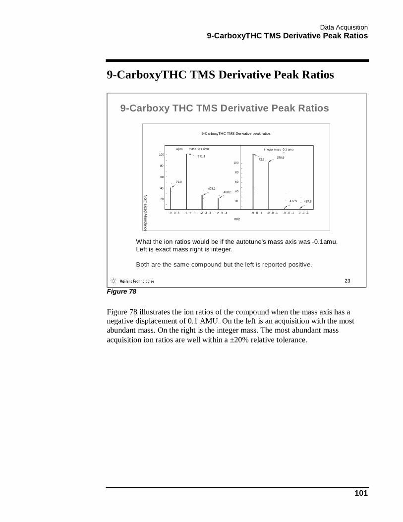
Data Acquisition 9-CarboxyTHC TMS Derivative Peak Ratios

101

9-CarboxyTHC TMS Derivative Peak Ratios

23

What the ion ratios would be if the autotune's mass axis was -0.1amu. Left is exact mass right is integer.

Both are the same compound but the left is reported positive.

9-CarboxyTHC TMS Derivative peak ratios

.9 .0 .1 .1 .2 .3 .2 .3 .4 .2 .3 .4 .9 .0 .1 .9 .0 .1 .9 .0 .1.9 .0 .1

mass -0.1 amu Integer mass 0.1 amu-

Apex

Norm

alized Abundance

m/z

-----

-----

-

-

-

-

-

-

-

-

-

-

72.9

371.1

473.2488.2

72.9 370.9

472.9 487.9

100

100

20

40

60

80

20

40

60

80

-

-

-

--

---

-

---

-

-

9-Carboxy THC TMS Derivative Peak Ratios

Figure 78

Figure 78 illustrates the ion ratios of the compound when the mass axis has a negative displacement of 0.1 AMU. On the left is an acquisition with the most abundant mass. On the right is the integer mass. The most abundant mass acquisition ion ratios are well within a ±20% relative tolerance.

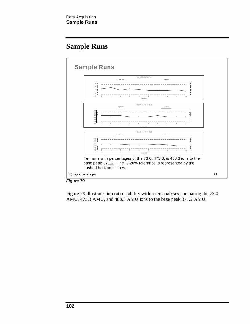
Data Acquisition Sample Runs

102

Sample Runs

24

Ten runs with percentages of the 73.0, 473.3, & 488.3 ions to the base peak 371.2. The +/-20% tolerance is represented by the dashed horizontal lines.

ANALYSES

30

35

40

45

50

1 2 3 4 5 6 7 8 9 10

High Limit Low Limit

ANALYSES

20

22

24

26

28

30

32

1 2 3 4 5 6 7 8 9 10

ANALYSES

1416182022242628

1 2 3 4 5 6 7 8 9 10

ION 73.0 RATIO TO 371.2

ION 473.3 RATIO TO 371.2

ION 488.3 RATIO TO 371.2

OO

OO O

O O O OO

OOOO

OOOOOO

O O OO O O

OO

O O

High Limit Low Limit

Low LimitHigh Limit

Sample Runs

Figure 79

Figure 79 illustrates ion ratio stability within ten analyses comparing the 73.0 AMU, 473.3 AMU, and 488.3 AMU ions to the base peak 371.2 AMU.

Data Acquisition Choosing SIM Ions

103

Choosing SIM Ions

25

Choosing SIM Ions

• Can monitor 60 ions/group, 100 groups/acquisition• Use minimum number ions/group for maximum sensitivity

and precision• Choose ions for maximum specificity

– High mass– Abundant– Unique to compound

• Can choose ions characteristic of compound class for screening purposes

Figure 80

Selecting ions for use in SIM acquisition is dependent upon the application. When fewer ions are monitored, more time can be spent on each ion. Thus there is an increase in sensitivity. However, if more specificity is needed, more ions may be necessary to “identify” the compound.

To maximize specificity and retain good sensitivity, many SIM acquisitions acquire 3-5 ions per group. One ion (typically the base peak) is used to quantitate while the other “confirming” ion(s) is used to verify the compound’s identity. Maximizing sensitivity using SIM monitoring is accomplished by a number of different steps including GC considerations, mass defect determination, choice of mass, etc.

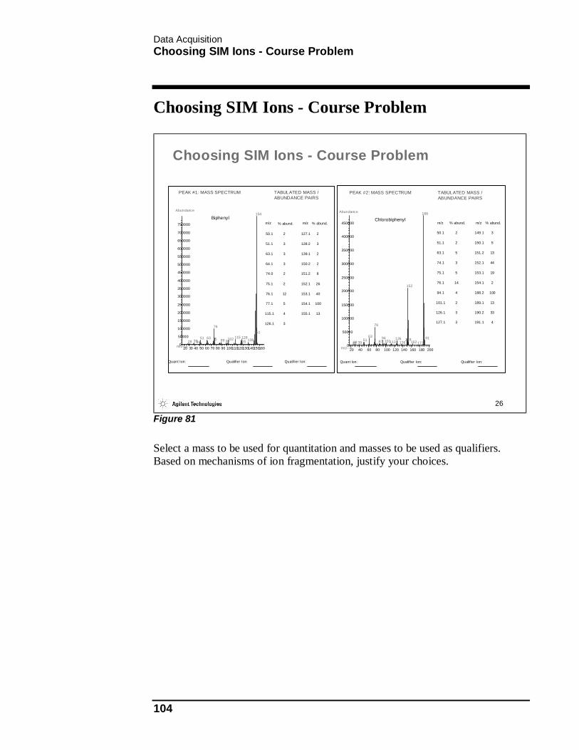
Data Acquisition Choosing SIM Ions - Course Problem

104

Choosing SIM Ions - Course Problem

26

PEAK #1: MASS SPECTRUM TABULATED MASS / ABUNDANCE PAIRS

Quant Ion: Qualifier Ion: Qualifier Ion:

20 30 40 50 60 70 80 90 1001101201301401501600

50000

100000

150000

200000

250000

300000

350000

400000

450000

500000

550000

600000

650000

700000

750000

m/z-->

Abundance

28 394451 63 75

76

89 98102 115125128

139

151

154Biphenyl

% abund.m/z % abund. m/z

50.1 2 127.1 2

51.1 3 128.2 3

63.1 3 139.1 2

64.1 3 150.2 2

74.0 2 151.2 8

75.1 2 152.1 26

76.1 12 153.1 40

77.1 5 154.1 100

115.1 4 155.1 13

126.1 3

PEAK #2: MASS SPECTRUM TABULATED MASS / ABUNDANCE PAIRS

20 40 60 80 100 120 140 160 180 2000

50000

100000

150000

200000

250000

300000

350000

400000

450000

m/z-->

Abundance

2628 3951

63

76

8794

101113126

136149

152

162177

188

191

Chlorobiphenylm/z % abund. m/z % abund.

50.1 2 149.1 3

51.1 2 150.1 5

63.1 5 151.2 13

74.1 3 152.1 44

75.1 5 153.1 19

76.1 14 154.1 2

94.1 4 188.2 100

101.1 2 189.1 13

126.1 3 190.2 33

127.1 3 191.1 4

Quant Ion: Qualifier Ion: Qualifier Ion:

Choosing SIM Ions - Course Problem

Figure 81

Select a mass to be used for quantitation and masses to be used as qualifiers. Based on mechanisms of ion fragmentation, justify your choices.

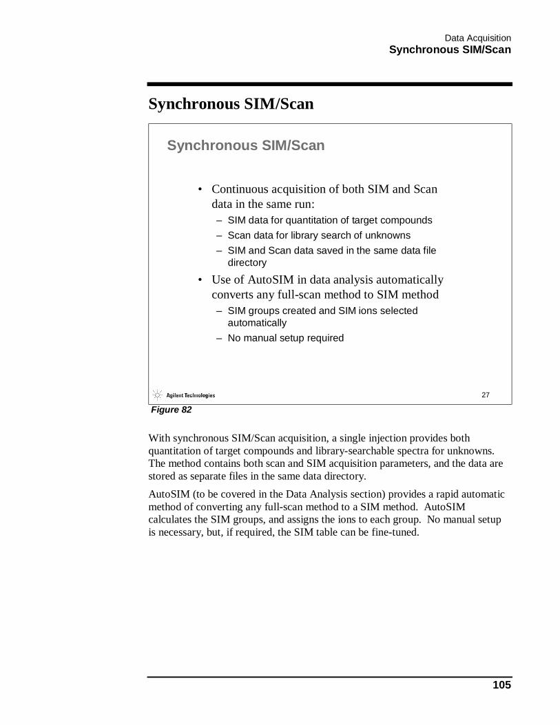
Data Acquisition Synchronous SIM/Scan

105

Synchronous SIM/Scan

27

Synchronous SIM/Scan

• Continuous acquisition of both SIM and Scan data in the same run:– SIM data for quantitation of target compounds– Scan data for library search of unknowns– SIM and Scan data saved in the same data file

directory

• Use of AutoSIM in data analysis automatically converts any full-scan method to SIM method– SIM groups created and SIM ions selected

automatically– No manual setup required

Figure 82

With synchronous SIM/Scan acquisition, a single injection provides both quantitation of target compounds and library-searchable spectra for unknowns. The method contains both scan and SIM acquisition parameters, and the data are stored as separate files in the same data directory. AutoSIM (to be covered in the Data Analysis section) provides a rapid automatic method of converting any full-scan method to a SIM method. AutoSIM calculates the SIM groups, and assigns the ions to each group. No manual setup is necessary, but, if required, the SIM table can be fine-tuned.

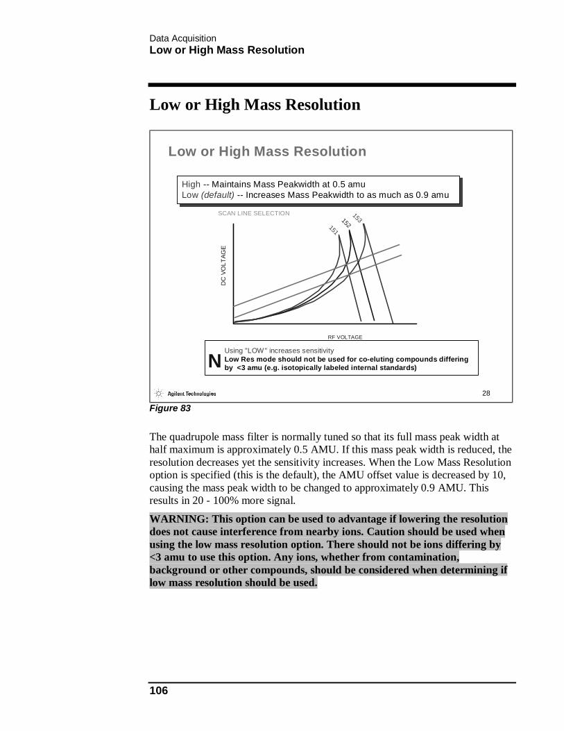
Data Acquisition Low or High Mass Resolution

106

Low or High Mass Resolution

28

RF VOLTAGE

DC

VO

LTAG

ESCAN LINE SELECTION 153

151

152

High -- Maintains Mass Peakwidth at 0.5 amuLow (default) -- Increases Mass Peakwidth to as much as 0.9 amu

Using "LOW" increases sensitivityLow Res mode should not be used for co-eluting compounds differing by <3 amu (e.g. isotopically labeled internal standards)N

Low or High Mass Resolution

Figure 83

The quadrupole mass filter is normally tuned so that its full mass peak width at half maximum is approximately 0.5 AMU. If this mass peak width is reduced, the resolution decreases yet the sensitivity increases. When the Low Mass Resolution option is specified (this is the default), the AMU offset value is decreased by 10, causing the mass peak width to be changed to approximately 0.9 AMU. This results in 20 - 100% more signal.

WARNING: This option can be used to advantage if lowering the resolution does not cause interference from nearby ions. Caution should be used when using the low mass resolution option. There should not be ions differing by <3 amu to use this option. Any ions, whether from contamination, background or other compounds, should be considered when determining if low mass resolution should be used.

Setting Up Data Acquisition

Setting Up Data Acquisition What You Will Learn

108

What You Will Learn

2

Setting Up Data Acquisition

In this section, you will learn:

• How to enter GC parameters• How to enter MS (scan) parameters• How to enter MS (SIM) parameters• How to set up system monitors

Figure 84

We begin setting up data acquisition in one of three ways. We can select icons from the Instrument Control View and edit each acquisition panel, we can select sections of the method from the Instrument menu, or we can “Edit Entire Method” and each panel appears. The number of changes to acquisition (method) parameters you need to make determines which way of editing them you choose.

When you choose “Edit Entire Method” under the Methods menu item, the panels shown in this section are displayed for change/review.

NOTE: An existing method is always used as a template to create a new method!

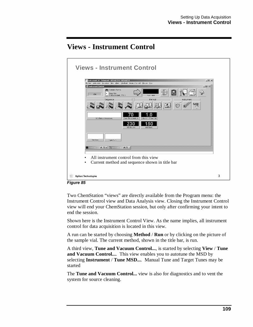
Setting Up Data Acquisition Views - Instrument Control

109

Views - Instrument Control

3

Views - Instrument Control

• All instrument control from this view• Current method and sequence shown in title bar

Figure 85

Two ChemStation “views” are directly available from the Program menu: the Instrument Control view and Data Analysis view. Closing the Instrument Control view will end your ChemStation session, but only after confirming your intent to end the session.

Shown here is the Instrument Control View. As the name implies, all instrument control for data acquisition is located in this view.

A run can be started by choosing Method / Run or by clicking on the picture of the sample vial. The current method, shown in the title bar, is run.

A third view, Tune and Vacuum Control..., is started by selecting View / Tune and Vacuum Control.... This view enables you to autotune the MSD by selecting Instrument / Tune MSD.... Manual Tune and Target Tunes may be started

The Tune and Vacuum Control... view is also for diagnostics and to vent the system for source cleaning.

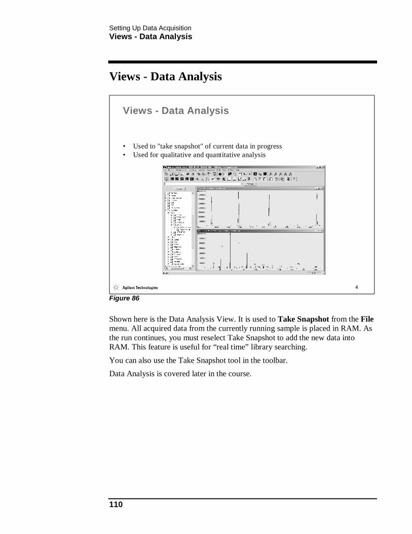
Setting Up Data Acquisition Views - Data Analysis

110

Views - Data Analysis

4

Views - Data Analysis

• Used to "take snapshot" of current data in progress• Used for qualitative and quantitative analysis

Figure 86

Shown here is the Data Analysis View. It is used to Take Snapshot from the File menu. All acquired data from the currently running sample is placed in RAM. As the run continues, you must reselect Take Snapshot to add the new data into RAM. This feature is useful for “real time” library searching.

You can also use the Take Snapshot tool in the toolbar. Data Analysis is covered later in the course.

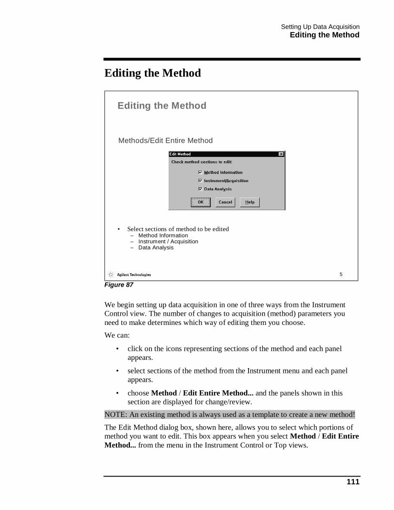
Setting Up Data Acquisition Editing the Method

111

Editing the Method

5

Methods/Edit Entire Method

Editing the Method

• Select sections of method to be edited– Method Information– Instrument / Acquisition– Data Analysis

Figure 87

We begin setting up data acquisition in one of three ways from the Instrument Control view. The number of changes to acquisition (method) parameters you need to make determines which way of editing them you choose. We can:

• click on the icons representing sections of the method and each panel appears.

• select sections of the method from the Instrument menu and each panel appears.

• choose Method / Edit Entire Method... and the panels shown in this section are displayed for change/review.

NOTE: An existing method is always used as a template to create a new method!

The Edit Method dialog box, shown here, allows you to select which portions of method you want to edit. This box appears when you select Method / Edit Entire Method... from the menu in the Instrument Control or Top views.

Setting Up Data Acquisition Editing the Method

112

When you click OK, the dialog boxes for the method sections selected are displayed sequentially for you to edit.

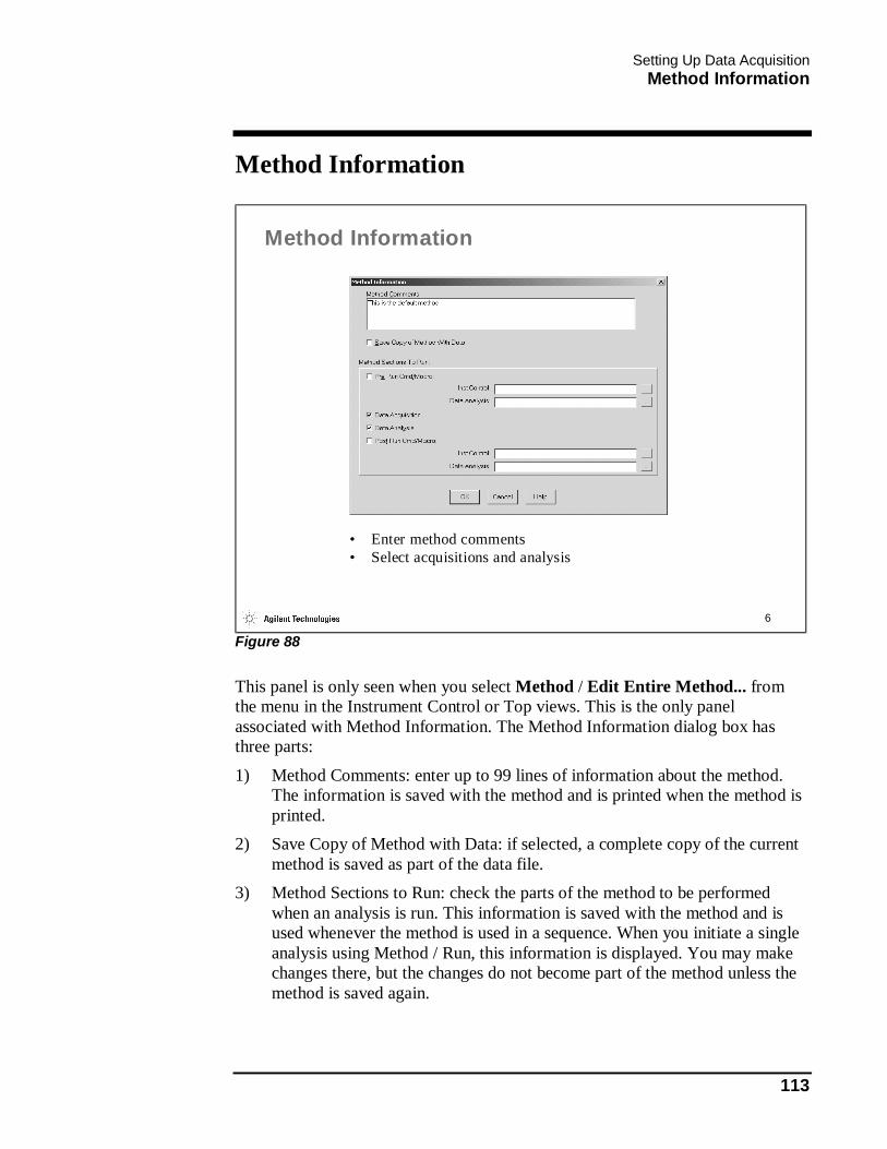
Setting Up Data Acquisition Method Information

113

Method Information

6

Method Information

• Enter method comments• Select acquisitions and analysis

Figure 88

This panel is only seen when you select Method / Edit Entire Method... from the menu in the Instrument Control or Top views. This is the only panel associated with Method Information. The Method Information dialog box has three parts:

1) Method Comments: enter up to 99 lines of information about the method. The information is saved with the method and is printed when the method is printed.

2) Save Copy of Method with Data: if selected, a complete copy of the current method is saved as part of the data file.

3) Method Sections to Run: check the parts of the method to be performed when an analysis is run. This information is saved with the method and is used whenever the method is used in a sequence. When you initiate a single analysis using Method / Run, this information is displayed. You may make changes there, but the changes do not become part of the method unless the method is saved again.

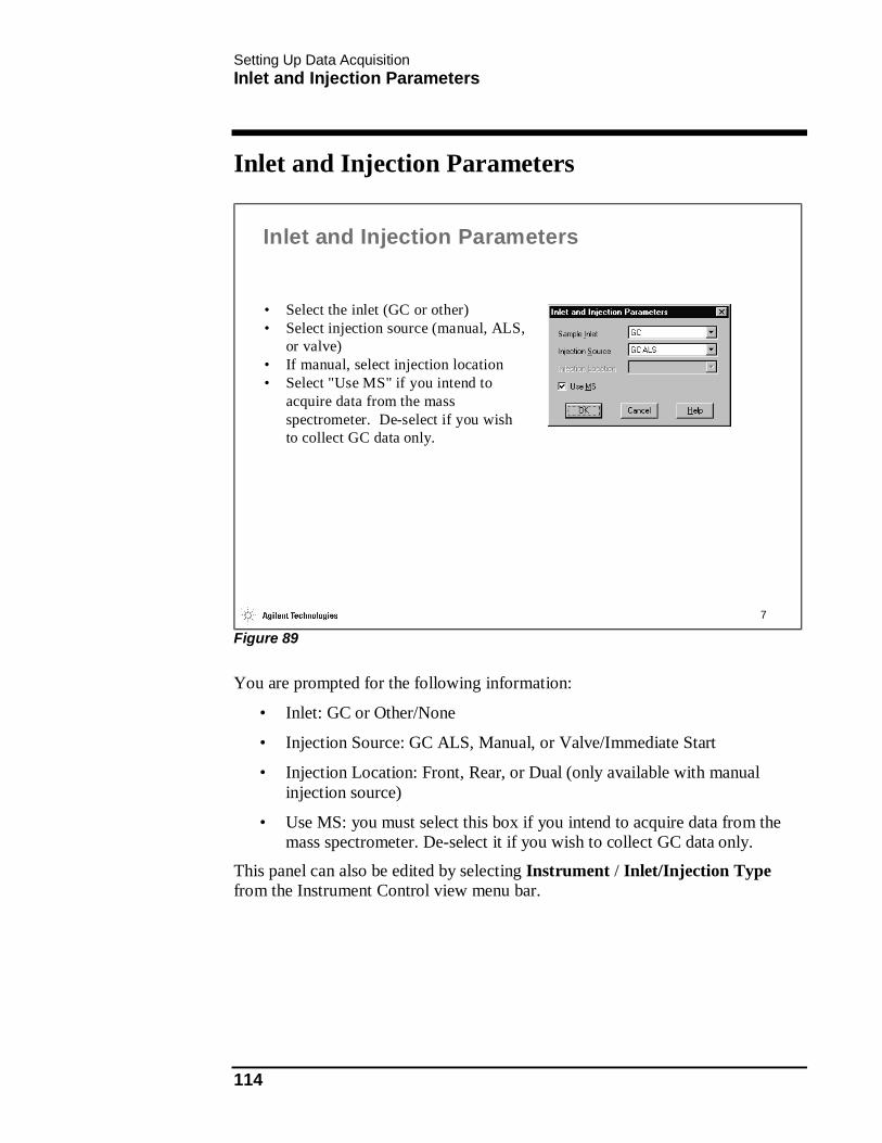
Setting Up Data Acquisition Inlet and Injection Parameters

114

Inlet and Injection Parameters

7

Inlet and Injection Parameters

• Select the inlet (GC or other)• Select injection source (manual, ALS,

or valve)• If manual, select injection location• Select "Use MS" if you intend to

acquire data from the mass spectrometer. De-select if you wish to collect GC data only.

Figure 89

You are prompted for the following information:

• Inlet: GC or Other/None

• Injection Source: GC ALS, Manual, or Valve/Immediate Start

• Injection Location: Front, Rear, or Dual (only available with manual injection source)

• Use MS: you must select this box if you intend to acquire data from the mass spectrometer. De-select it if you wish to collect GC data only.

This panel can also be edited by selecting Instrument / Inlet/Injection Type from the Instrument Control view menu bar.

Setting Up Data Acquisition Injector Control

115

Injector Control

8

Injector Control

• Set injection volume and syringe washes

• Press Configure . . . to set syringe size

• Press More . . . to set plunger speed

Figure 90

This panel can also be edited by selecting Instrument / GC Edit Parameters... from the Instrument Control view menu bar or by clicking on the Injector icon of the Instrument Control view. Syringe size and plunger speed are also configured from this panel.

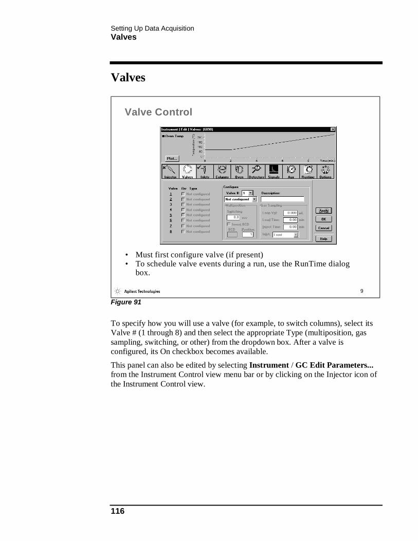
Setting Up Data Acquisition Valves

116

Valves

9

Valve Control

• Must first configure valve (if present)• To schedule valve events during a run, use the RunTime dialog

box.

Figure 91

To specify how you will use a valve (for example, to switch columns), select its Valve # (1 through 8) and then select the appropriate Type (multiposition, gas sampling, switching, or other) from the dropdown box. After a valve is configured, its On checkbox becomes available.

This panel can also be edited by selecting Instrument / GC Edit Parameters... from the Instrument Control view menu bar or by clicking on the Injector icon of the Instrument Control view.

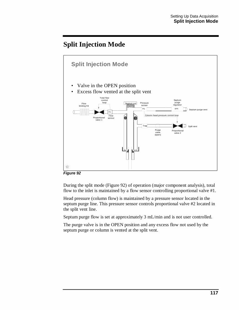
Setting Up Data Acquisition Split Injection Mode

117

Split Injection Mode

10

FS

PS SPR

Flow limiting frit

Proportional valve 1

Total flow control

loop

Trap

Flow sensor

Septum nut Pressure sensor

Septum purge

regulator

Column head pressure control loop

Septum purge vent

Split vent

Proportional valve 2

Purge valve (open)

Split Injection Mode

• Valve in the OPEN position • Excess flow vented at the split vent

Figure 92

During the split mode (Figure 92) of operation (major component analysis), total flow to the inlet is maintained by a flow sensor controlling proportional valve #1.

Head pressure (column flow) is maintained by a pressure sensor located in the septum purge line. This pressure sensor controls proportional valve #2 located in the split vent line. Septum purge flow is set at approximately 3 mL/min and is not user controlled.

The purge valve is in the OPEN position and any excess flow not used by the septum purge or column is vented at the split vent.

Setting Up Data Acquisition Splitless Injection Mode

118

Splitless Injection Mode

11

FS

PS SPR

Flow limiting frit

Proportional valve 1

Trap

Flow sensor

Septum nut

Pressure sensor

Septum purge

regulator

Septum purge vent

Split vent

Proportional valve 2

Purge valve

(closed)

Inlet pressure control loop

Splitless Injection Mode

• Valve in the CLOSED position • All flow, except septum purge, is onto the column

Figure 93

During the splitless mode (Figure 93) of operation (trace component analysis), the purge valve closes and head pressure (column flow) is maintained by a pressure sensor located in the septum purge line which controls proportional valve #1. Any flow that does not go out the septum purge is directed into the column.

Septum purge flow is set at approximately 3 mL/min and is not user controlled.

Setting Up Data Acquisition Inlets - Split Injection

119

Inlets - Split Injection

12

Inlets - Split Injection

• Select mode as "Split"• Enter all setpoints

Figure 94

The ChemStation presents the Inlets dialog boxes based on the number and type of inlet(s) you have installed on your GC. The left-hand dialog box represents the front inlet configuration. The right-hand dialog box represents the back inlet configuration.

NOTE: The installed column and column head pressure (Columns panel) should be set before completing this panel.

A split injection is generally good for:

• major component analyses, primarily for high concentration samples when you can afford to lose most of the sample out the split/purge vent

• samples that you cannot dilute During a split injection, a liquid sample is introduced into a hot inlet where it vaporizes rapidly. A small amount of the vapor enters the column while the major portion exits from the split/purge vent. You control the ratio of column flow to split flow.

Setting Up Data Acquisition Inlets - Split Injection

120

If EPC is installed and the column is defined and head pressure set, changing either the Total Flow, Split Ratio, or Split Flow automatically adjusts the other two for the current column head pressure. If installed, GasSaver reduces the carrier gas flow from the split vent after a sample is on the column. The ChemStation maintains column head pressure and the column flow rate, while purge and split vent flows decrease. GasSaver can be used in either the Const Pressure or Const Flow mode. This panel can also be edited by selecting Instrument / GC Edit Parameters... from the Instrument Control view menu bar or by clicking on the Inlets icon of the Instrument Control view.

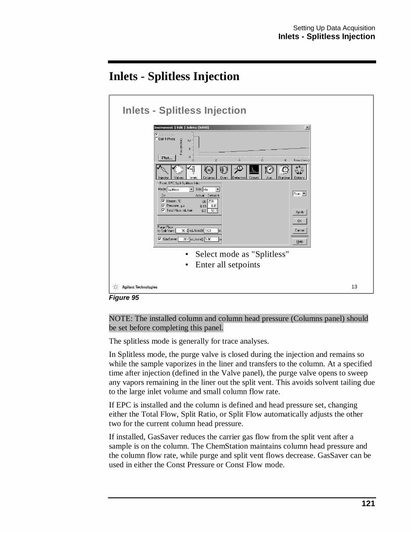
Setting Up Data Acquisition Inlets - Splitless Injection

121

Inlets - Splitless Injection

13

Inlets - Splitless Injection

• Select mode as "Splitless"• Enter all setpoints

Figure 95

NOTE: The installed column and column head pressure (Columns panel) should be set before completing this panel.

The splitless mode is generally for trace analyses. In Splitless mode, the purge valve is closed during the injection and remains so while the sample vaporizes in the liner and transfers to the column. At a specified time after injection (defined in the Valve panel), the purge valve opens to sweep any vapors remaining in the liner out the split vent. This avoids solvent tailing due to the large inlet volume and small column flow rate.

If EPC is installed and the column is defined and head pressure set, changing either the Total Flow, Split Ratio, or Split Flow automatically adjusts the other two for the current column head pressure. If installed, GasSaver reduces the carrier gas flow from the split vent after a sample is on the column. The ChemStation maintains column head pressure and the column flow rate, while purge and split vent flows decrease. GasSaver can be used in either the Const Pressure or Const Flow mode.

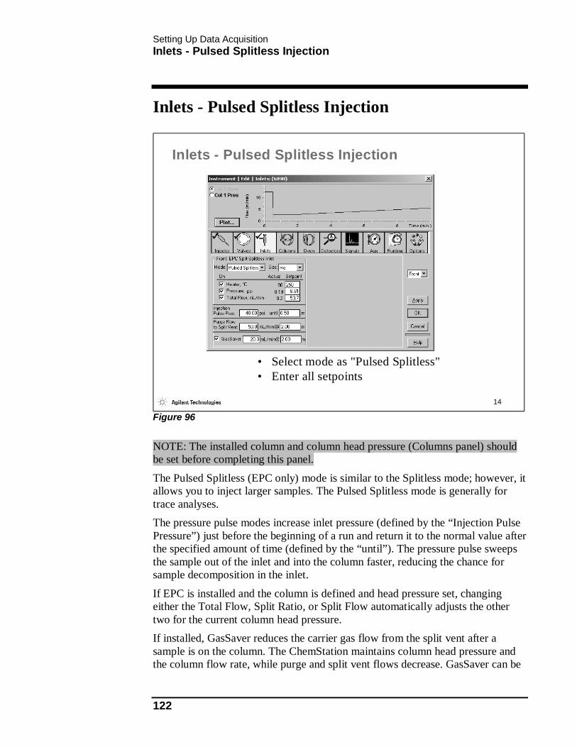
Setting Up Data Acquisition Inlets - Pulsed Splitless Injection

122

Inlets - Pulsed Splitless Injection

14

Inlets - Pulsed Splitless Injection

• Select mode as "Pulsed Splitless"• Enter all setpoints

Figure 96

NOTE: The installed column and column head pressure (Columns panel) should be set before completing this panel.

The Pulsed Splitless (EPC only) mode is similar to the Splitless mode; however, it allows you to inject larger samples. The Pulsed Splitless mode is generally for trace analyses. The pressure pulse modes increase inlet pressure (defined by the “Injection Pulse Pressure”) just before the beginning of a run and return it to the normal value after the specified amount of time (defined by the “until”). The pressure pulse sweeps the sample out of the inlet and into the column faster, reducing the chance for sample decomposition in the inlet.

If EPC is installed and the column is defined and head pressure set, changing either the Total Flow, Split Ratio, or Split Flow automatically adjusts the other two for the current column head pressure. If installed, GasSaver reduces the carrier gas flow from the split vent after a sample is on the column. The ChemStation maintains column head pressure and the column flow rate, while purge and split vent flows decrease. GasSaver can be

Setting Up Data Acquisition Inlets - Pulsed Splitless Injection

123

used in either the Const Pressure or Const Flow mode. When the GasSaver is operated in the pulsed pressure modes, the activation time should be at least one minute after the completion of the injection pulse pressure.

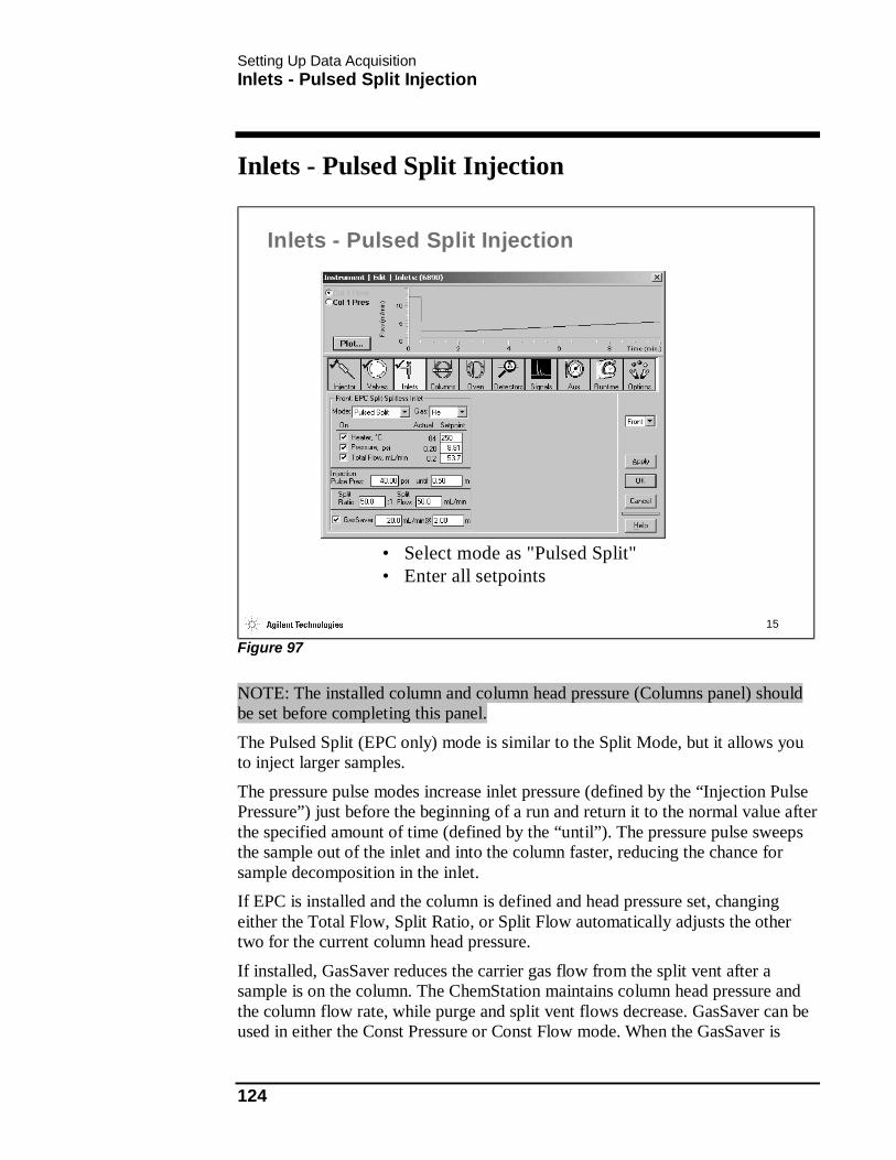
Setting Up Data Acquisition Inlets - Pulsed Split Injection

124

Inlets - Pulsed Split Injection

15

Inlets - Pulsed Split Injection

• Select mode as "Pulsed Split"• Enter all setpoints

Figure 97

NOTE: The installed column and column head pressure (Columns panel) should be set before completing this panel.

The Pulsed Split (EPC only) mode is similar to the Split Mode, but it allows you to inject larger samples.

The pressure pulse modes increase inlet pressure (defined by the “Injection Pulse Pressure”) just before the beginning of a run and return it to the normal value after the specified amount of time (defined by the “until”). The pressure pulse sweeps the sample out of the inlet and into the column faster, reducing the chance for sample decomposition in the inlet. If EPC is installed and the column is defined and head pressure set, changing either the Total Flow, Split Ratio, or Split Flow automatically adjusts the other two for the current column head pressure.

If installed, GasSaver reduces the carrier gas flow from the split vent after a sample is on the column. The ChemStation maintains column head pressure and the column flow rate, while purge and split vent flows decrease. GasSaver can be used in either the Const Pressure or Const Flow mode. When the GasSaver is

Setting Up Data Acquisition Inlets - Pulsed Split Injection

125

operated in the pulsed pressure modes, the activation time should be at least one minute after the completion of the injection pulse pressure.

Setting Up Data Acquisition Flow Burst Injection

126

Flow Burst Injection

16

Flow Burst Injection

• Column flow or pressure can be time programmed

Figure 98

Another injection technique is to use a flow or pressure “burst” injection. The column flow or pressure can be programmed just as you would program the oven temperature. In Figure 98, the column flow is sharply ramped at the moment of injection and held briefly. It is then lowered to normal operating flows. The system then automatically increases the pressure as the oven temperature increases to maintain a constant flow.

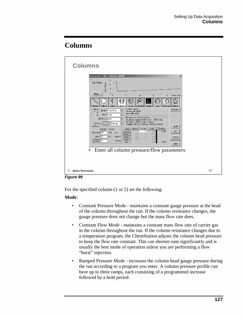
Setting Up Data Acquisition Columns

127

Columns

17

Columns

• Enter all column pressure/flow parameters

Figure 99

For the specified column (1 or 2) set the following: Mode:

• Constant Pressure Mode - maintains a constant gauge pressure at the head of the column throughout the run. If the column resistance changes, the gauge pressure does not change but the mass flow rate does.

• Constant Flow Mode - maintains a constant mass flow rate of carrier gas in the column throughout the run. If the column resistance changes due to a temperature program, the ChemStation adjusts the column head pressure to keep the flow rate constant. This can shorten runs significantly and is usually the best mode of operation unless you are performing a flow “burst” injection.

• Ramped Pressure Mode - increases the column head gauge pressure during the run according to a program you enter. A column pressure profile can have up to three ramps, each consisting of a programmed increase followed by a hold period.

Setting Up Data Acquisition Columns

128

• Ramped Flow Mode – shown in Figure 98 and discussed on page 126, increases the mass flow rate in the column during the run according to a program you enter. A column flow profile can have up to three ramps, each consisting of a programmed increase followed by a hold period.

Inlet: Front or Back Detector: MSD

Outlet psi: select Vacuum when the downstream end of the column is in a vacuum, that is, when you are using the column with a mass spectrometer. When Vacuum is selected, Outlet psi is inactive. Pressure/Flow/Average Velocity: If EPC is installed and the column is defined, changing either the Pressure, Flow, or Average Velocity automatically adjusts the other two. It is generally best to set the optimum linear velocity for the column and let the system automatically adjust the pressure and flow provided that the flow does not exceed the vacuum limitations of the MSD.

Ramps: If you selected Ramped Pressure as the column mode, you can prepare a ramped column pressure program to control the column head pressure during a run. If you selected Ramped Flow as the column mode, you can prepare a ramped column flow to control the mass flow rate in the column during a run.

This panel can also be edited by selecting Instrument / GC Edit Parameters... from the Instrument Control view menu bar or by clicking on the Columns icon of the Instrument Control view.

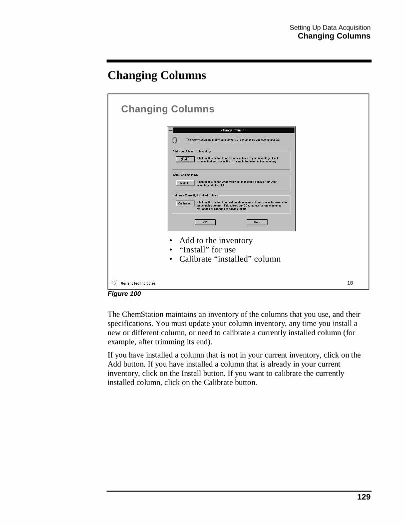
Setting Up Data Acquisition Changing Columns

129

Changing Columns

18

Changing Columns

• Add to the inventory• “Install” for use• Calibrate “installed” column

Figure 100

The ChemStation maintains an inventory of the columns that you use, and their specifications. You must update your column inventory, any time you install a new or different column, or need to calibrate a currently installed column (for example, after trimming its end).

If you have installed a column that is not in your current inventory, click on the Add button. If you have installed a column that is already in your current inventory, click on the Install button. If you want to calibrate the currently installed column, click on the Calibrate button.

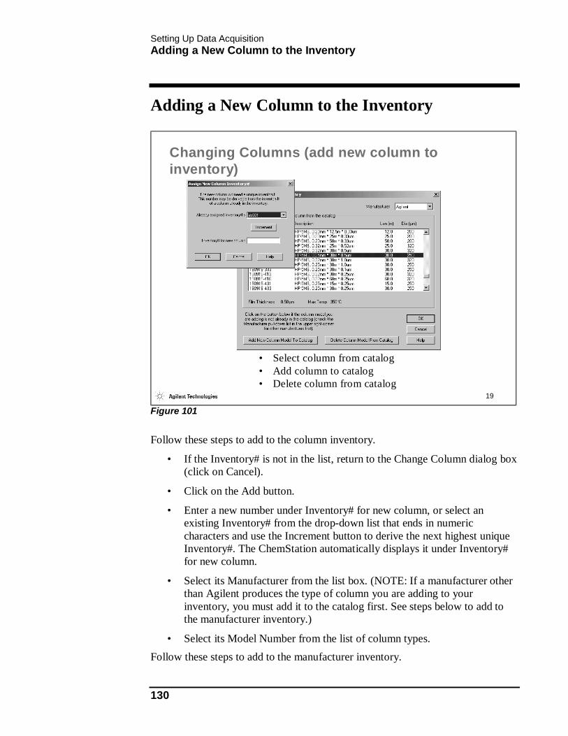
Setting Up Data Acquisition Adding a New Column to the Inventory

130

Adding a New Column to the Inventory

19

Changing Columns (add new column to inventory)

• Select column from catalog• Add column to catalog• Delete column from catalog

Figure 101

Follow these steps to add to the column inventory.

• If the Inventory# is not in the list, return to the Change Column dialog box (click on Cancel).

• Click on the Add button.

• Enter a new number under Inventory# for new column, or select an existing Inventory# from the drop-down list that ends in numeric characters and use the Increment button to derive the next highest unique Inventory#. The ChemStation automatically displays it under Inventory# for new column.

• Select its Manufacturer from the list box. (NOTE: If a manufacturer other than Agilent produces the type of column you are adding to your inventory, you must add it to the catalog first. See steps below to add to the manufacturer inventory.)

• Select its Model Number from the list of column types. Follow these steps to add to the manufacturer inventory.

Setting Up Data Acquisition Adding a New Column to the Inventory

131

• Click on the Add New Column Model To Catalog button.

• Enter the following information about the column: Manufacturer

Model Number Description

Column Type Max Temperature

Length (capillary columns only) Diameter (capillary columns only)

Film Thickness (capillary columns only)

• Click OK to return to the Add New Column to Inventory dialog box and add the new column to your inventory.

NOTE: To delete a type of column from the catalog, select it and use the Delete Column Model From Catalog button. (Models manufactured by Agilent cannot be deleted from the catalog.)

Setting Up Data Acquisition Installing the Column for Use

132

Installing the Column for Use

20

Changing Columns (“install” for use)

• Select column to be installed• Delete column from inventory

Figure 102

Follow these steps to install the column for use.

• From the Columns panel, click the Change button.

• Click the Install button.

• Select the Inventory# for this column from the list of those in your inventory. Its specifications are displayed. (NOTE: if the Inventory# is not in the list, see steps below to add to the inventory.)

• Click on OK to return to the Columns dialog box, and then click Apply to download the new settings to the GC.

Setting Up Data Acquisition Oven

133

Oven

21

Oven

• Enter oven temperature setpoints

Figure 103

Turn the oven On by selecting its checkbox. Use Setpoint to specify a desired temperature setpoint (in °C) for the oven during a run. The oven’s Actual temperature, which the GC transmits, is a read-only display. You can prepare a program of up to six levels (or “ramps”), executed in consecutive order, to control the GC’s oven temperature during a run. To program a ramped oven temperature, do the following:

• enter an initial oven temperature and an initial hold time

• up to six oven temperature Ramps, and

• a PostRun oven temperature. To prepare for an Isothermal Run do the following:

• enter the temperature (in °C) you want the oven to maintain in the Initial Next °C column.

• enter the length of time you want the run to last in the Initial Hold min column.

Setting Up Data Acquisition Oven

134

• set Ramp 1 to zero degrees per minute in the °C/min column to disable any ramped oven temperature program.

Oven Configuration sets maximum oven temperature and equilibration time. Cryo Configuration lets you operate the oven below ambient temperature. Minimum attainable oven temperature depends on the type of valve installed. This panel can also be edited by selecting Instrument / GC Edit Parameters... from the Instrument Control view menu bar or by clicking on the Oven icon of the Instrument Control view.

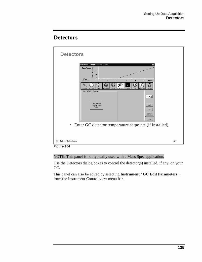
Setting Up Data Acquisition Detectors

135

Detectors

22

Detectors

• Enter GC detector temperature setpoints (if installed)

Figure 104

NOTE: This panel is not typically used with a Mass Spec application. Use the Detectors dialog boxes to control the detector(s) installed, if any, on your GC. This panel can also be edited by selecting Instrument / GC Edit Parameters... from the Instrument Control view menu bar.

Setting Up Data Acquisition Signals

136

Signals

23

Signals

• Save GC detector data (if installed)• Monitor temperatures• Monitor flows or pressure

Figure 105

NOTE: This panel is not typically used with a Mass Spec application. A signal is the analog or digital output to a data handling device. It can be the output of detectors or the output from temperature, flow, or pressure sensors. This panel can also be edited by selecting Instrument / GC Edit Parameters... from the Instrument Control.

Setting Up Data Acquisition Auxiliary

137

Auxiliary

24

Auxiliary

• Enter auxiliary temperatures• Enter auxiliary pressures

Figure 106

Use the Aux dialog box to configure up to two thermal (typically one of which is the MSD transfer line heater) and three pressure auxiliary channels, and if necessary, prepare ramped auxiliary channel temperature and pressure programs. This panel can also be edited by selecting Instrument / GC Edit Parameters... from the Instrument Control view menu bar or by clicking on the Aux icon of the Instrument Control view.

Setting Up Data Acquisition Runtime

138

Runtime

25

Runtime Events

• Used to schedule up to 25 events to occur automatically during a run

Figure 107

Use the Runtime dialog box to schedule up to 25 events to occur automatically during a run.

This panel can also be edited by selecting Instrument / GC Edit Parameters... from the Instrument Control view menu bar.

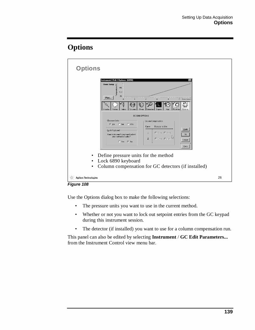
Setting Up Data Acquisition Options

139

Options

26

Options

• Define pressure units for the method• Lock 6890 keyboard• Column compensation for GC detectors (if installed)

Figure 108

Use the Options dialog box to make the following selections:

• The pressure units you want to use in the current method.

• Whether or not you want to lock out setpoint entries from the GC keypad during this instrument session.

• The detector (if installed) you want to use for a column compensation run. This panel can also be edited by selecting Instrument / GC Edit Parameters... from the Instrument Control view menu bar.

Setting Up Data Acquisition GC Real Time Plot

140

GC Real Time Plot

27

GC Real Time Plots

• Used to show or remove real time GC detector (if installed) signal monitors from the Instrument Control panel

Figure 109

NOTE: This panel is not typically used with a Mass Spec application. GC Real Time Plot is used to show or remove real time signal monitors from the Instrument Control panel. Show: Select this box if you want the plot of the designated signal to appear on the Instrument Control panel. De-select it if you want to remove the plot. Attn: The range of the detector signal to display full scale in the real time display, expressed as a power of 2. The attenuation can be changed during the run from the real time display.

Offset: The distance from the bottom of the window to start the plot. Enter the value in %, with 0 as the bottom of the window and 100 as the top. The offset cannot be changed during the run. Time: The time span (in minutes) of the chromatogram to show at one time during the run. The Time cannot be changed during the run. This panel can also be edited by selecting Instrument / GC Plot... from the Instrument Control view menu bar.

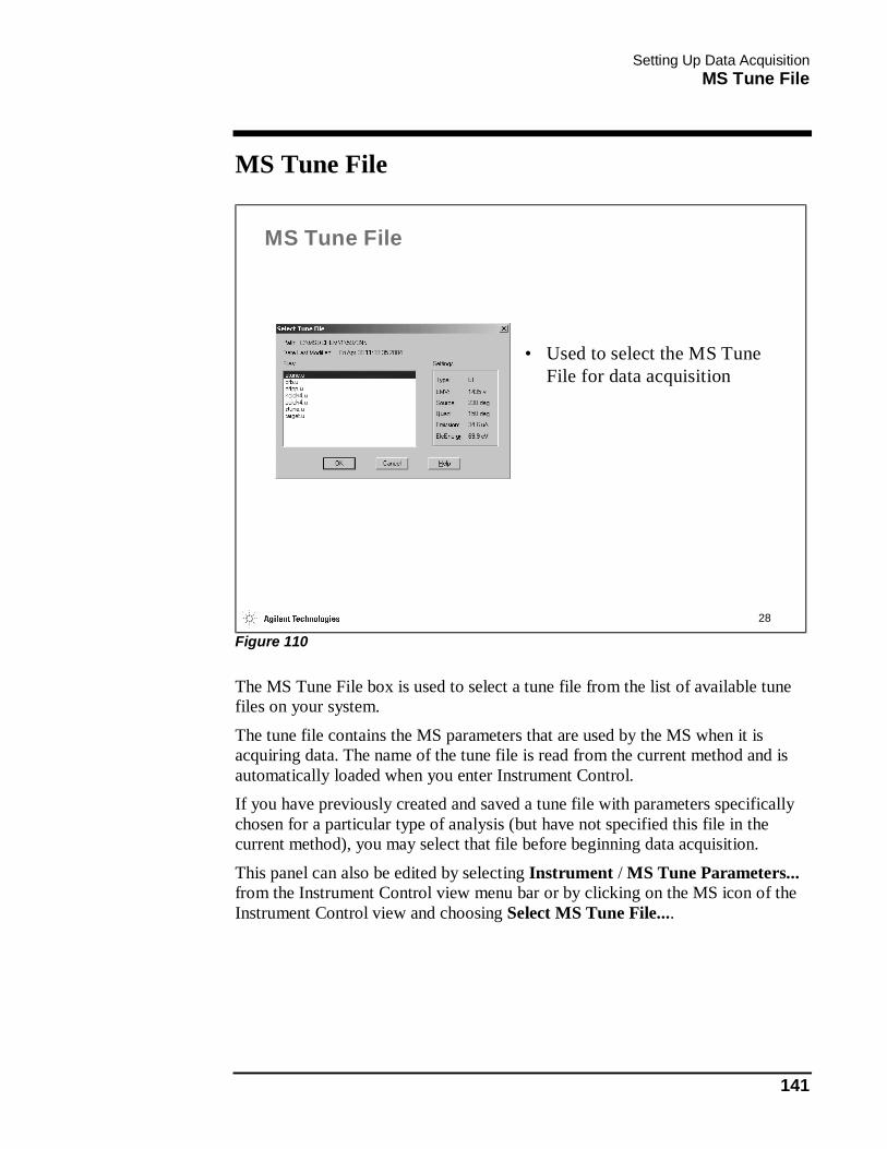
Setting Up Data Acquisition MS Tune File

141

MS Tune File

28

MS Tune File

• Used to select the MS Tune File for data acquisition

Figure 110

The MS Tune File box is used to select a tune file from the list of available tune files on your system.

The tune file contains the MS parameters that are used by the MS when it is acquiring data. The name of the tune file is read from the current method and is automatically loaded when you enter Instrument Control. If you have previously created and saved a tune file with parameters specifically chosen for a particular type of analysis (but have not specified this file in the current method), you may select that file before beginning data acquisition.

This panel can also be edited by selecting Instrument / MS Tune Parameters... from the Instrument Control view menu bar or by clicking on the MS icon of the Instrument Control view and choosing Select MS Tune File....

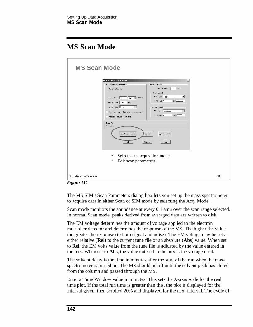
Setting Up Data Acquisition MS Scan Mode

142

MS Scan Mode

29

MS Scan Mode

• Select scan acquisition mode• Edit scan parameters

Figure 111

The MS SIM / Scan Parameters dialog box lets you set up the mass spectrometer to acquire data in either Scan or SIM mode by selecting the Acq. Mode.

Scan mode monitors the abundance at every 0.1 amu over the scan range selected. In normal Scan mode, peaks derived from averaged data are written to disk.

The EM voltage determines the amount of voltage applied to the electron multiplier detector and determines the response of the MS. The higher the value the greater the response (to both signal and noise). The EM voltage may be set as either relative (Rel) to the current tune file or an absolute (Abs) value. When set to Rel, the EM volts value from the tune file is adjusted by the value entered in the box. When set to Abs, the value entered in the box is the voltage used.

The solvent delay is the time in minutes after the start of the run when the mass spectrometer is turned on. The MS should be off until the solvent peak has eluted from the column and passed through the MS. Enter a Time Window value in minutes. This sets the X-axis scale for the real time plot. If the total run time is greater than this, the plot is displayed for the interval given, then scrolled 20% and displayed for the next interval. The cycle of

Setting Up Data Acquisition MS Scan Mode

143

displaying and scrolling the real time plot continues until the run ends. If you want to see the entire run, match this entry with the chromatographic run time of your sample (including the solvent delay time). The MS real time plots are one or two ion chromatograms plotted (abundance versus time) in windows on the Instrument Control panel as the data are acquired. In Scan mode, you may display the total abundance of all ions monitored (Total) or the total abundance of all ions in a specified mass range (Extracted ion). When you select Extracted Ion, the mass range field for that window in the Edit Scan Parameters - Plotting (page 146) part of the panel becomes active so that you can set a range.

This panel can also be edited by selecting Instrument / MS SIM/Scan... from the Instrument Control view menu bar or by clicking on the MS icon of the Instrument Control view and choosing Edit MS SIM/Scan....

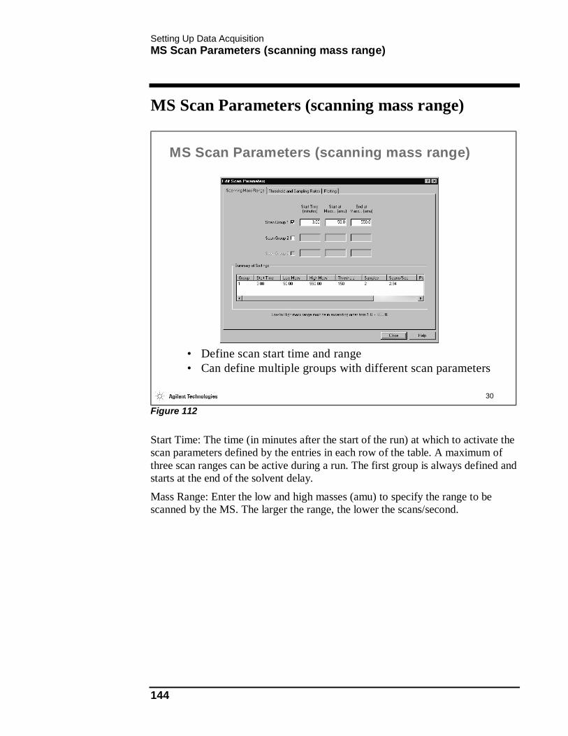
Setting Up Data Acquisition MS Scan Parameters (scanning mass range)

144

MS Scan Parameters (scanning mass range)

30

MS Scan Parameters (scanning mass range)

• Define scan start time and range• Can define multiple groups with different scan parameters

Figure 112

Start Time: The time (in minutes after the start of the run) at which to activate the scan parameters defined by the entries in each row of the table. A maximum of three scan ranges can be active during a run. The first group is always defined and starts at the end of the solvent delay.

Mass Range: Enter the low and high masses (amu) to specify the range to be scanned by the MS. The larger the range, the lower the scans/second.

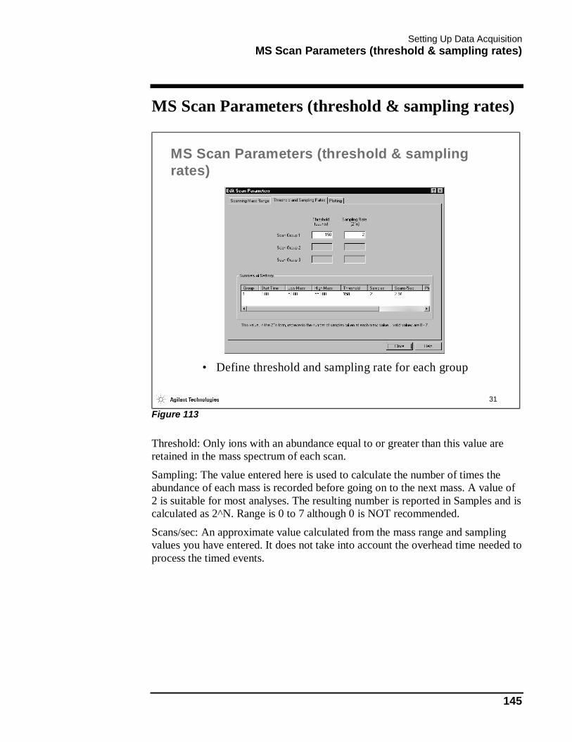
Setting Up Data Acquisition MS Scan Parameters (threshold & sampling rates)

145

MS Scan Parameters (threshold & sampling rates)

31

MS Scan Parameters (threshold & sampling rates)

• Define threshold and sampling rate for each group

Figure 113

Threshold: Only ions with an abundance equal to or greater than this value are retained in the mass spectrum of each scan.

Sampling: The value entered here is used to calculate the number of times the abundance of each mass is recorded before going on to the next mass. A value of 2 is suitable for most analyses. The resulting number is reported in Samples and is calculated as 2^N. Range is 0 to 7 although 0 is NOT recommended.

Scans/sec: An approximate value calculated from the mass range and sampling values you have entered. It does not take into account the overhead time needed to process the timed events.

Setting Up Data Acquisition MS Scan Parameters (plotting)

146

MS Scan Parameters (plotting)

32

MS Scan Parameters (plotting)

• Define mass or range to be plotted

• Active areas controlled by “Real Time Plot” area of MS SIM/Scan Parameters panel

Figure 114

Enter the ion mass range to be plotted in real time. These fields are active only when the Extracted Ion plot type is selected in the Real Time Plot Parameters section of the MS SIM/Scan Parameters (page 142) dialog box.

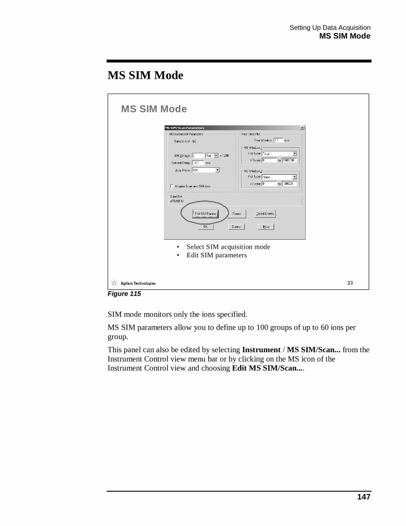
Setting Up Data Acquisition MS SIM Mode

147

MS SIM Mode

33

MS SIM Mode

• Select SIM acquisition mode• Edit SIM parameters

Figure 115

SIM mode monitors only the ions specified. MS SIM parameters allow you to define up to 100 groups of up to 60 ions per group. This panel can also be edited by selecting Instrument / MS SIM/Scan... from the Instrument Control view menu bar or by clicking on the MS icon of the Instrument Control view and choosing Edit MS SIM/Scan....

Setting Up Data Acquisition MS SIM Mode (parameters)

148

MS SIM Mode (parameters)

34

MS SIM Mode (parameters)

• Add or delete groups

• Add, modify, or delete ions per group

Figure 116

The table on the left defines each SIM group by a start time and an optional group ID. The start time of the first group should be the same as the solvent delay time. If it is not, the solvent delay time is used. The dwell time and resolution parameters are applied to each ion within the group. In the Dwell column, enter the amount of time to spend sampling a specific ion. The default of 100 ms is satisfactory for two to three ions in a typical capillary GC peak. For more than three ions, use a shorter dwell time (such as 30 or 50 ms) to ensure there are enough data points to define the peaks. If you enter a dwell time outside the allowed range (10-9999 ms), the value is changed to the nearest limit.

The Resolution column specifies the low mass resolution. High specifies the mass peak width from the tune file (usually 0.5 amu). Low specifies a mass peak width of 0.7 - 0.9 amu; the increased peak width increases sensitivity with a resulting loss in specificity.

The ions to be monitored for the current group (as shown by the arrow) must be entered in the table on the right. A maximum of two ions in each group may be selected for plotting during the real time display. To display two ions, you must

Setting Up Data Acquisition MS SIM Mode (parameters)

149

have the Plot Type in Window 2 designated as Single in the Real Time Plot Parameters section of the panel. If you do not specify an ion, the first one in the group is used. The Delete Group Button deletes an entire SIM group and its ions. The Delete Ion Button deletes an individual ion from the group.

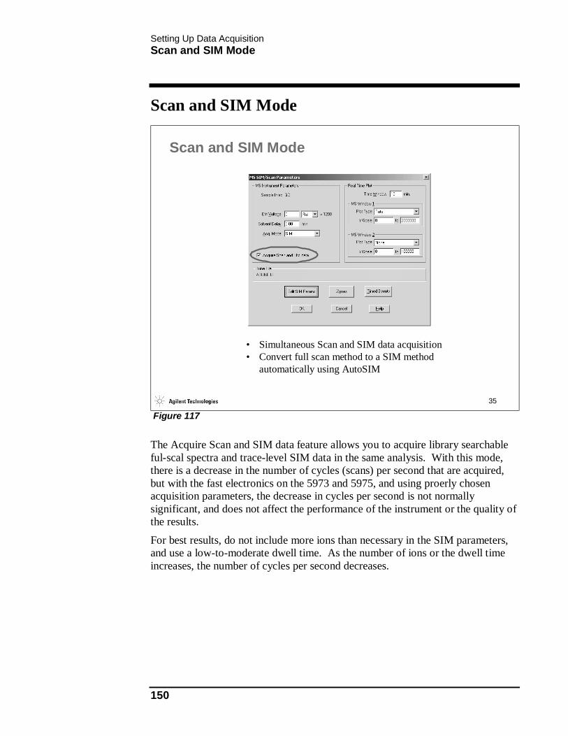
Setting Up Data Acquisition Scan and SIM Mode

150

Scan and SIM Mode

35

Scan and SIM Mode

• Simultaneous Scan and SIM data acquisition• Convert full scan method to a SIM method

automatically using AutoSIM

Figure 117

The Acquire Scan and SIM data feature allows you to acquire library searchable ful-scal spectra and trace-level SIM data in the same analysis. With this mode, there is a decrease in the number of cycles (scans) per second that are acquired, but with the fast electronics on the 5973 and 5975, and using proerly chosen acquisition parameters, the decrease in cycles per second is not normally significant, and does not affect the performance of the instrument or the quality of the results.

For best results, do not include more ions than necessary in the SIM parameters, and use a low-to-moderate dwell time. As the number of ions or the dwell time increases, the number of cycles per second decreases.

Setting Up Data Acquisition Timed Events

151

Timed Events

36

Timed Events

• Time program detector on/off• Time program changes in EM voltage• Time program valves

Figure 118

Timed Events is a list of time-programmed events that you want to occur during data acquisition. The following components of the MS may be controlled during data acquisition:

• Detector (turn all the mass spectrometer voltages on and off)

• EMV Delta (increase or decrease the EM voltage)

• Valves (Supported valves include the calibration valve and two auxiliary outputs)

To Use the MS Timed Events Table, do the following: 1) At the top of the table, under Time, enter the time in minutes after the start

of acquisition. 2) Tab to the next field and select an Event Type from the list.

3) Move to the Parameter 1 field and select one of the options displayed in the list. If you are setting an EMV Delta event, enter the difference in voltage between the tune file setting and the new setting. The tune file setting is displayed on the MS SIM/Scan Parameters panel.

Setting Up Data Acquisition Timed Events

152

4) Move to the Parameter 2 field, if it is active, and select one of the options. 5) Click the Add button. The event is displayed in the table.

6) When you have added all the events you wish, click OK.

Setting Up Data Acquisition Select Reports

153

Select Reports

37

Select Reports

• Select any qualitative, quantitative, or custom reports to be generated at the completion of the run

Figure 119

Select any qualitative, quantitative, or custom reports to be generated at the completion of the run. Each of these is covered in detail later in the course.

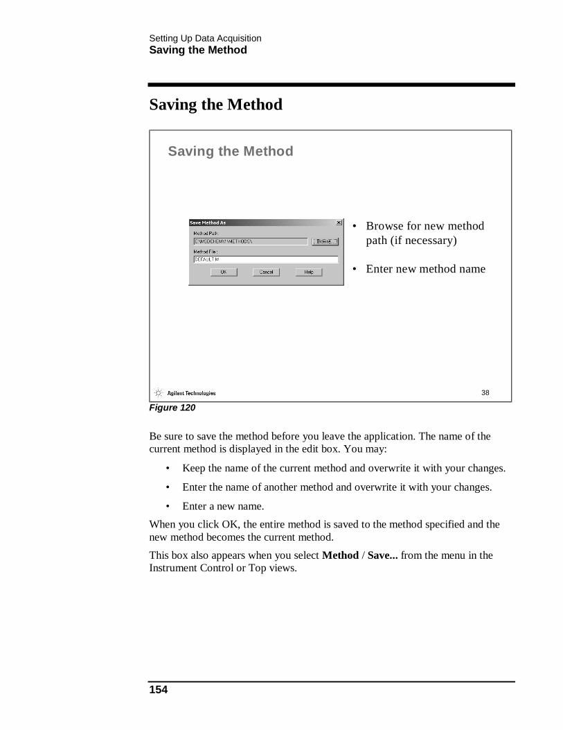
Setting Up Data Acquisition Saving the Method

154

Saving the Method

38

Saving the Method

• Browse for new method path (if necessary)

• Enter new method name

Figure 120

Be sure to save the method before you leave the application. The name of the current method is displayed in the edit box. You may:

• Keep the name of the current method and overwrite it with your changes.

• Enter the name of another method and overwrite it with your changes.

• Enter a new name. When you click OK, the entire method is saved to the method specified and the new method becomes the current method. This box also appears when you select Method / Save... from the menu in the Instrument Control or Top views.

Setting Up Data Acquisition MS Monitors

155

MS Monitors

39

MS Monitors

• Used to monitor MS source voltages, valves and MS temperature zones

Figure 121

The Edit MS Monitors panel, pictured above, does not automatically appear as a part of Edit Entire Method. It may be edited by selecting Instrument / MS Monitors... or clicking on the MS icon in the Instrument Control view. It is used to monitor MS source parameters, valve states, and/or MS source temperature.

To Use the MS Monitors Table, perform the following steps: 1) From the Type field choose Parameter, Valve, or Zone.

2) Tab to the next field and select a parameter from the list. 3) Tab to the next field and select Digital or Analog output.

4) Click the Add button. The event is displayed in the table. 5) When you have added all the events you wish, click OK.

Don’t forget to save your method after making any changes!!

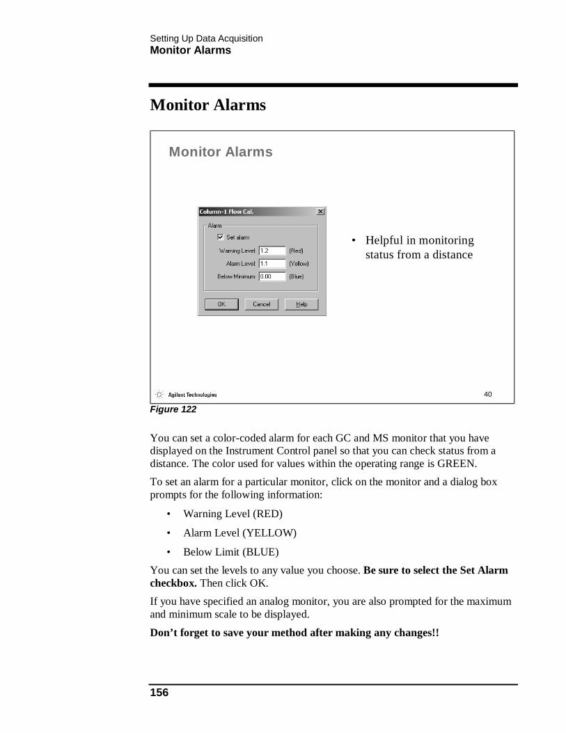
Setting Up Data Acquisition Monitor Alarms

156

Monitor Alarms

40

Monitor Alarms

• Helpful in monitoring status from a distance

Figure 122

You can set a color-coded alarm for each GC and MS monitor that you have displayed on the Instrument Control panel so that you can check status from a distance. The color used for values within the operating range is GREEN. To set an alarm for a particular monitor, click on the monitor and a dialog box prompts for the following information:

• Warning Level (RED)

• Alarm Level (YELLOW)

• Below Limit (BLUE) You can set the levels to any value you choose. Be sure to select the Set Alarm checkbox. Then click OK. If you have specified an analog monitor, you are also prompted for the maximum and minimum scale to be displayed.

Don’t forget to save your method after making any changes!!

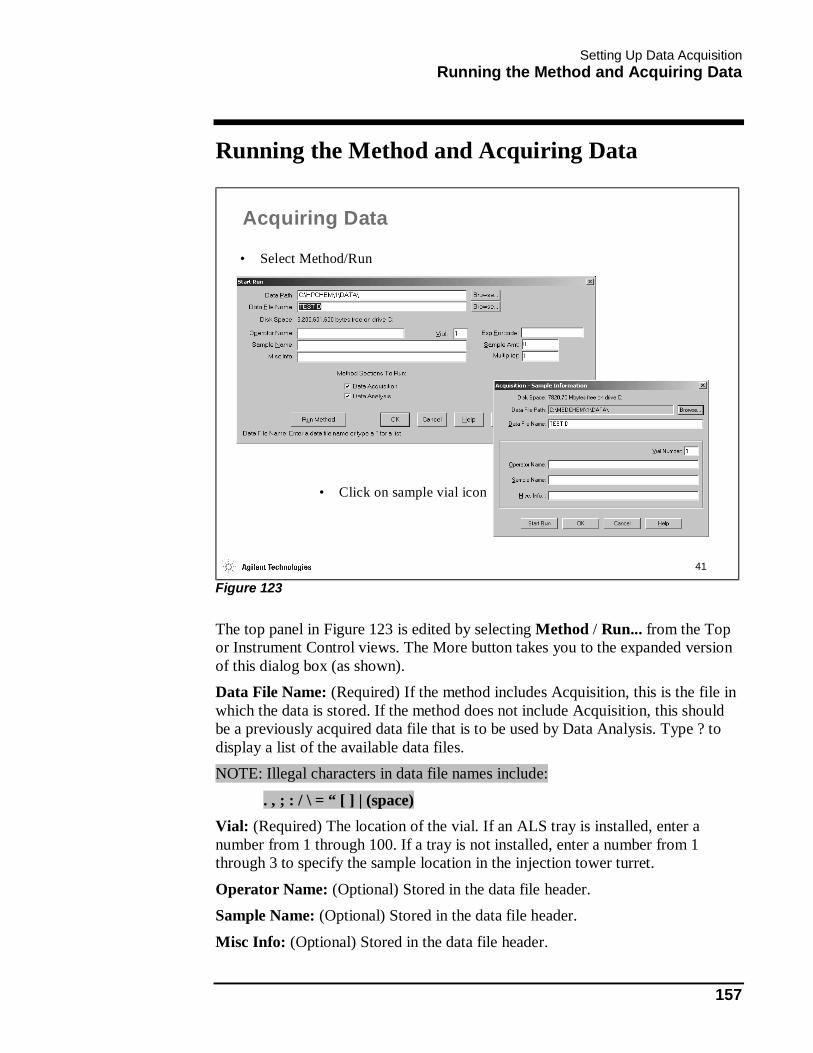
Setting Up Data Acquisition Running the Method and Acquiring Data

157

Running the Method and Acquiring Data

41

Acquiring Data

• Select Method/Run

• Click on sample vial icon

Figure 123

The top panel in Figure 123 is edited by selecting Method / Run... from the Top or Instrument Control views. The More button takes you to the expanded version of this dialog box (as shown). Data File Name: (Required) If the method includes Acquisition, this is the file in which the data is stored. If the method does not include Acquisition, this should be a previously acquired data file that is to be used by Data Analysis. Type ? to display a list of the available data files. NOTE: Illegal characters in data file names include:

. , ; : / \ = “ [ ] | (space) Vial: (Required) The location of the vial. If an ALS tray is installed, enter a number from 1 through 100. If a tray is not installed, enter a number from 1 through 3 to specify the sample location in the injection tower turret.

Operator Name: (Optional) Stored in the data file header. Sample Name: (Optional) Stored in the data file header.

Misc Info: (Optional) Stored in the data file header.

Setting Up Data Acquisition Running the Method and Acquiring Data

158

Expected Barcode: (Optional) Used to compare to bar code on sample if present. Sample Amount: A divisor to convert the absolute amounts of compounds to a percentage of the original sample. If other than 0, all calculated amounts are divided by this number and multiplied by 100. Units are reported as %.

Multiplier: A multiplier to correct for dilution or other sample handling adjustments.

Method Sections to Run: Select the parts of the method to be done during this analysis. The parts checked when the dialog box first appears are those specified in the current method. Any changes made are part of the current method (in memory); if you want them to become part of the method on disk, you need to save the method. Pre-Run Macro/Cmd and Post-Run Macro/Cmd: (Optional) Post-Run is useful for automating the transfer of results to third party software. Pre-Run can be used to tune the instrument automatically.

The bottom panel in Figure 123 is edited by clicking on the sample vial icon in the Instrument Control view. Notice that it is an abbreviated version of the acquisition panel.

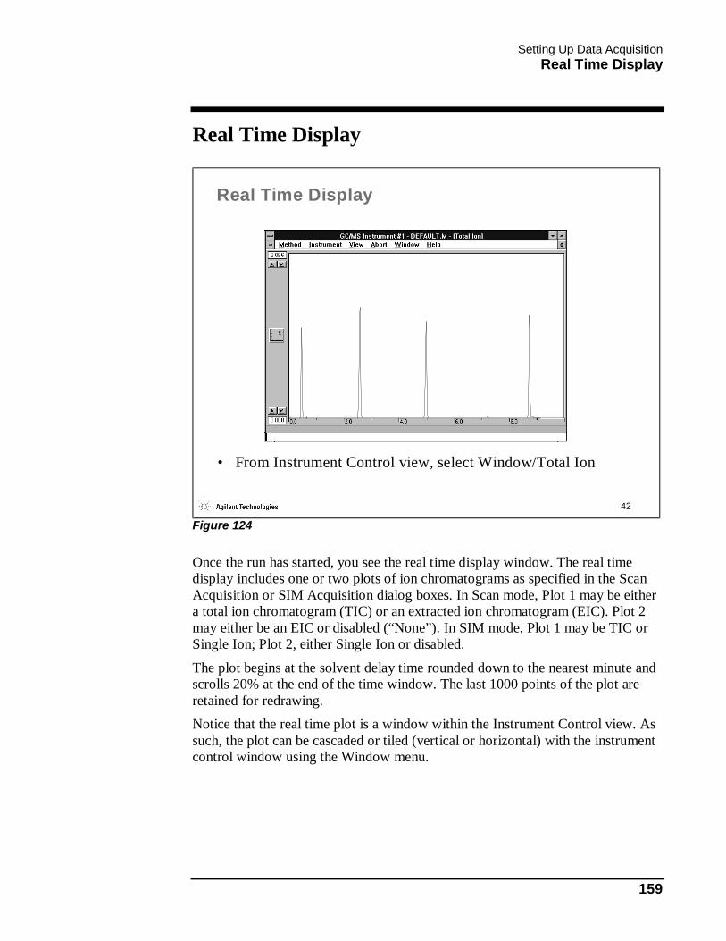
Setting Up Data Acquisition Real Time Display

159

Real Time Display

42

Real Time Display

• From Instrument Control view, select Window/Total Ion

Figure 124

Once the run has started, you see the real time display window. The real time display includes one or two plots of ion chromatograms as specified in the Scan Acquisition or SIM Acquisition dialog boxes. In Scan mode, Plot 1 may be either a total ion chromatogram (TIC) or an extracted ion chromatogram (EIC). Plot 2 may either be an EIC or disabled (“None”). In SIM mode, Plot 1 may be TIC or Single Ion; Plot 2, either Single Ion or disabled.

The plot begins at the solvent delay time rounded down to the nearest minute and scrolls 20% at the end of the time window. The last 1000 points of the plot are retained for redrawing. Notice that the real time plot is a window within the Instrument Control view. As such, the plot can be cascaded or tiled (vertical or horizontal) with the instrument control window using the Window menu.

Setting Up Data Acquisition Real Time Display

160

LAB EXERCISE: Linear Velocity

In this section you will:

• Determine the liner velocity of the carrier gas through the GC column.

• Determine the flow rate into the MSD vacuum system.

LAB EXERCISE: Linear Velocity Determining the Linear Velocity

162

Determining the Linear Velocity

In this lab, Manual Tune is used to monitor the injection of an unretained compound to determine the linear velocity of carrier gas through the capillary column. In this and subsequent acquisition labs, you will be using a 30M x 0.25 mm ID crosslinked 5% phenyl methyl silicone column. At this point we are assuming that the length of the column is 30M when in reality it probably isn’t. We’ll correct for that later when we “install” the column in our method. 1) From the keyboard of the GC or from the ChemStation software, verify

(change if necessary) the following instrument settings:

Oven temperature: 70°C

Mode: Split Gas Saver: Off Total flow: 50-60 mL/min

2) From the Instrument Control view, select View / Manual Tune. Select AdjParam / Edit MS Params... and close the PFTBA valve. Select More Params... / Acq Parms... and enter 28 for each of the tune masses. Click OK to exit the panel.

3) Click on the Prof button. Under the View menu item, select Expand so that the window is full screen. This displays three continuously updated windows each showing the mass profile centered at mass 28. Allow the system to stabilize and observe the abundance counts of mass 28. This is the background. By default the profile maximizes on mass 28 requiring you to watch for changes in the abundance counts. Instead, go to More Params / Acq Parms... and change the Scale to Fixed from 0 to about 10 times your background. Click OK.

4) Using the built-in Stopwatch feature of the GC (see your instructor if necessary), make a split injection of 5 microliters of air and determine how many seconds it takes for the air peak to elute. Watch the profile to increase significantly as your unretained air elutes at approximately 60 to 90 seconds. The repeat profile display may be stopped at any time by clicking the Stop button. Click on OK to exit the Edit MS Parameters window.

5) Record the elution time for your unretained air peak in minutes. _________________________________________________________________

Reminder: The elapsed time shown on the GC keyboard is in minutes and seconds.

6) Calculate the linear velocity using Equation 1:

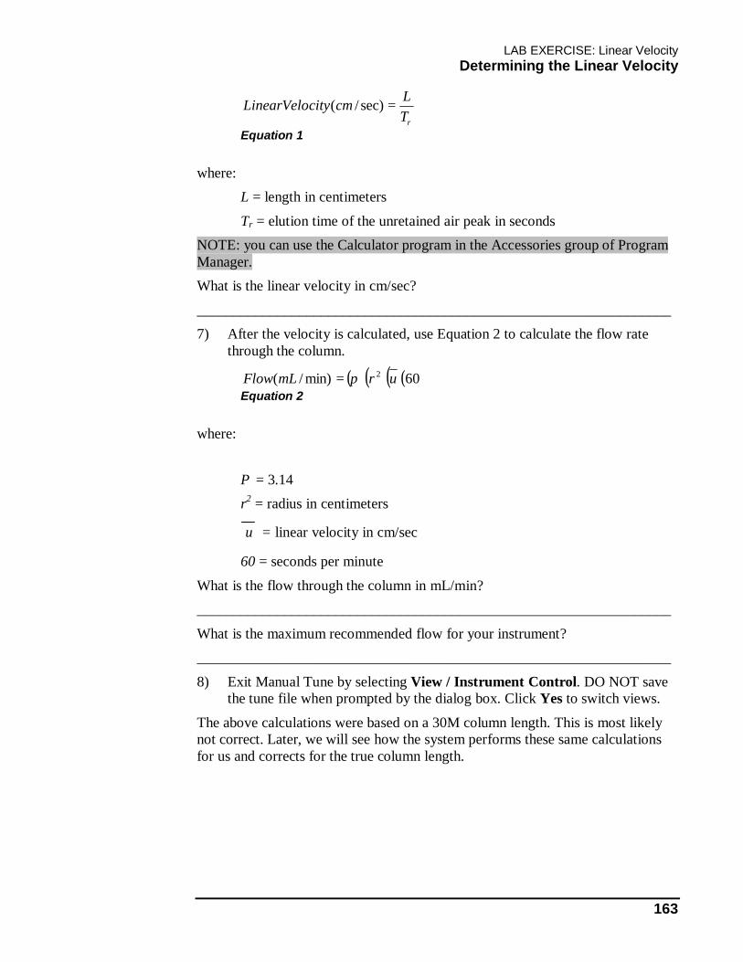
LAB EXERCISE: Linear Velocity Determining the Linear Velocity

163

rTLcmcityLinearVelo =sec)/(

Equation 1

where: L = length in centimeters

Tr = elution time of the unretained air peak in seconds NOTE: you can use the Calculator program in the Accessories group of Program Manager. What is the linear velocity in cm/sec?

_________________________________________________________________ 7) After the velocity is calculated, use Equation 2 to calculate the flow rate

through the column.

( )( )( )( )60min)/( 2 urmLFlow π= Equation 2

where:

Π = 3.14 r2 = radius in centimeters

u = linear velocity in cm/sec

60 = seconds per minute

What is the flow through the column in mL/min? _________________________________________________________________

What is the maximum recommended flow for your instrument? _________________________________________________________________

8) Exit Manual Tune by selecting View / Instrument Control. DO NOT save the tune file when prompted by the dialog box. Click Yes to switch views.

The above calculations were based on a 30M column length. This is most likely not correct. Later, we will see how the system performs these same calculations for us and corrects for the true column length.

LAB EXERCISE: Linear Velocity Determining the Linear Velocity

164

LAB EXERCISE: Scan Data Acquisition

In this section you will:

• Edit the entire “default” method to create a new “scan” method.

• Use the newly created “scan” method to acquire data.

• Evaluate real time display functions.

LAB EXERCISE: Scan Data Acquisition Editing the Entire Method

166

Editing the Entire Method

In this experiment, a sample consisting of a mixture of four components dissolved in iso-octane (Sample A) is analyzed in scan mode using the splitless injection technique.

1) The title bar in the instrument view panel should show the current method as “DEFAULT.M”. If it is not, from the Method menu select Load.... Click on “DEFAULT.M” and click OK. When the title bar shows that the default method is loaded, go to Method / Edit Entire Method....

Figure 125

2) Be sure that all three sections of the method are checked as shown in Figure 125 before clicking OK.

NOTE: Use the Tab key or the mouse to move from field to field; the Enter key in a panel is equivalent to clicking OK and the ESC key is equivalent to clicking CANCEL.

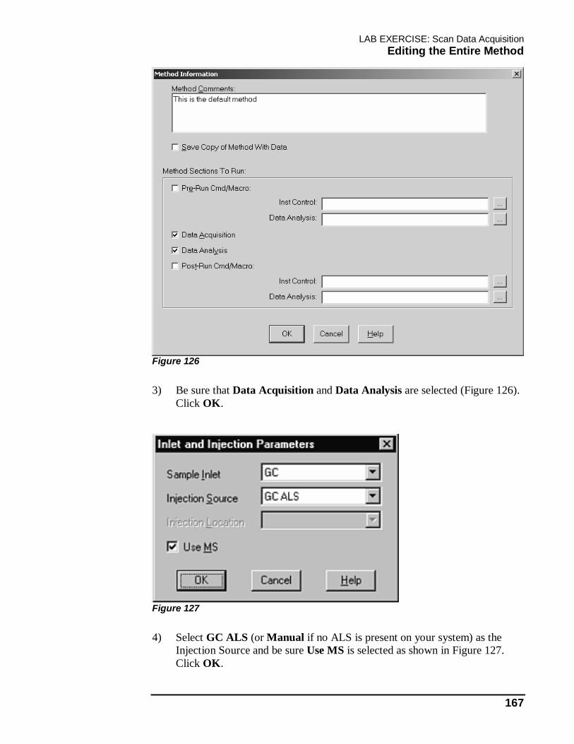
LAB EXERCISE: Scan Data Acquisition Editing the Entire Method

167

Figure 126

3) Be sure that Data Acquisition and Data Analysis are selected (Figure 126). Click OK.

Figure 127

4) Select GC ALS (or Manual if no ALS is present on your system) as the Injection Source and be sure Use MS is selected as shown in Figure 127. Click OK.

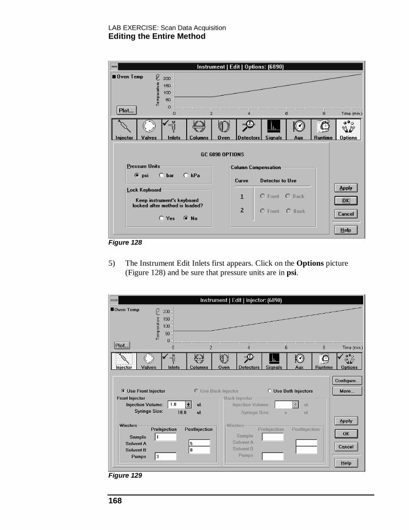
LAB EXERCISE: Scan Data Acquisition Editing the Entire Method

168

Figure 128

5) The Instrument Edit Inlets first appears. Click on the Options picture (Figure 128) and be sure that pressure units are in psi.

Figure 129

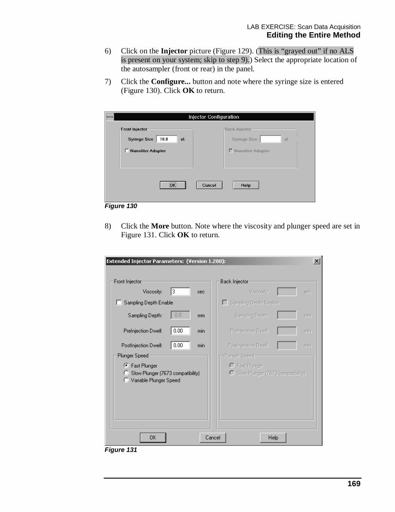
LAB EXERCISE: Scan Data Acquisition Editing the Entire Method

169

6) Click on the Injector picture (Figure 129). (This is “grayed out” if no ALS is present on your system; skip to step 9).) Select the appropriate location of the autosampler (front or rear) in the panel.

7) Click the Configure... button and note where the syringe size is entered (Figure 130). Click OK to return.

Figure 130

8) Click the More button. Note where the viscosity and plunger speed are set in Figure 131. Click OK to return.

Figure 131

LAB EXERCISE: Scan Data Acquisition Editing the Entire Method

170

Figure 132

9) Click on the Valves picture. There are no valves installed on our systems (Figure 132).

What does the blue X next to the injector indicate?

_________________________________________________________________

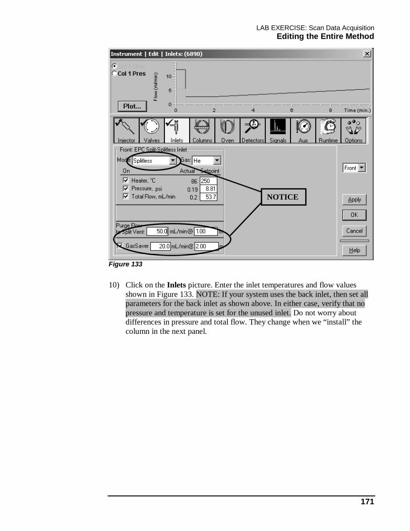
LAB EXERCISE: Scan Data Acquisition Editing the Entire Method

171

NOTICE

Figure 133

10) Click on the Inlets picture. Enter the inlet temperatures and flow values shown in Figure 133. NOTE: If your system uses the back inlet, then set all parameters for the back inlet as shown above. In either case, verify that no pressure and temperature is set for the unused inlet. Do not worry about differences in pressure and total flow. They change when we “install” the column in the next panel.

LAB EXERCISE: Scan Data Acquisition Editing the Entire Method

172

Figure 134

11) Click on the Columns picture. Do not enter the values shown in Figure 134 at this time. First, we need to change the “installed” column. Click the Change... button and Figure 135 appears.

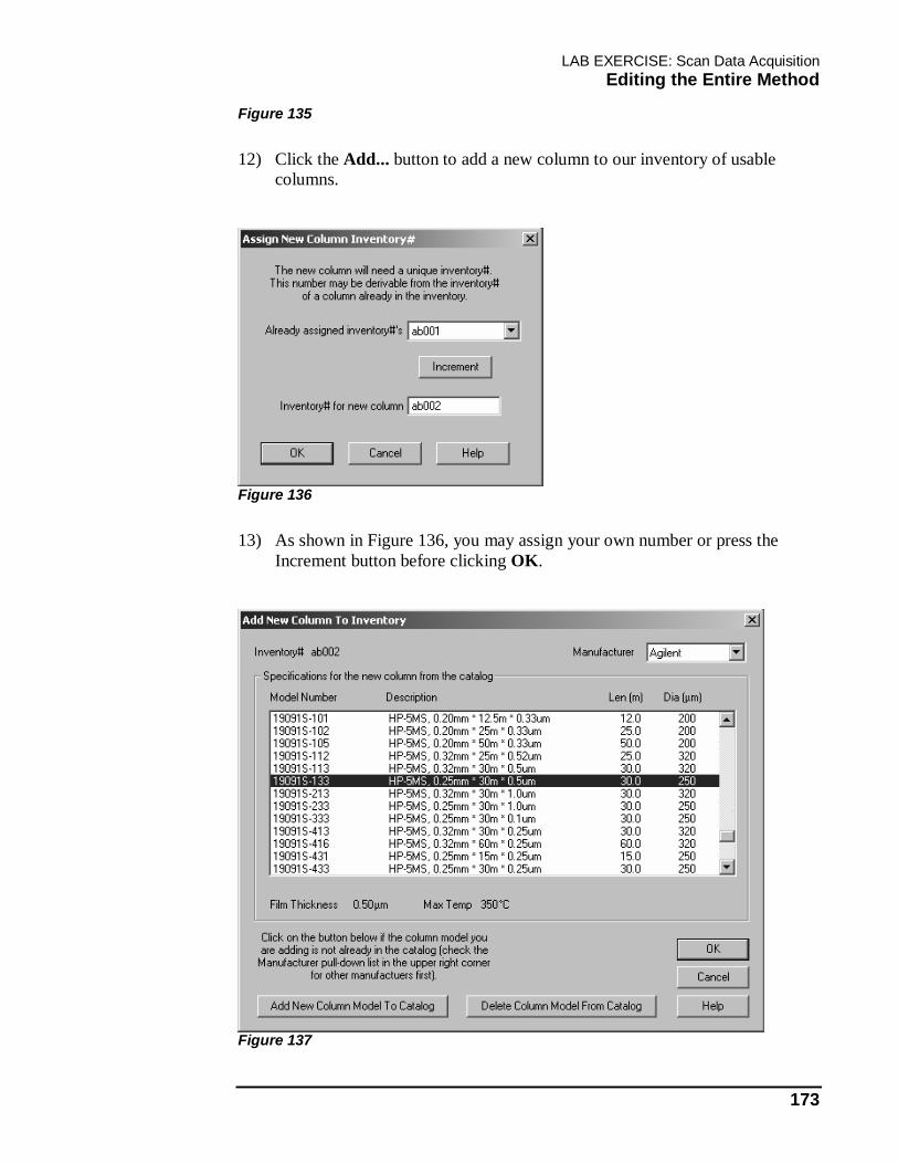
LAB EXERCISE: Scan Data Acquisition Editing the Entire Method

173

Figure 135

12) Click the Add... button to add a new column to our inventory of usable columns.

Figure 136

13) As shown in Figure 136, you may assign your own number or press the Increment button before clicking OK.

Figure 137

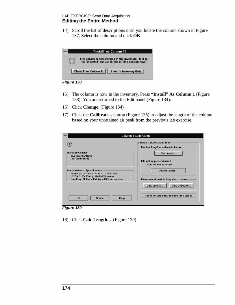
LAB EXERCISE: Scan Data Acquisition Editing the Entire Method

174

14) Scroll the list of descriptions until you locate the column shown in Figure 137. Select the column and click OK.

Figure 138

15) The column is now in the inventory. Press “Install” As Column 1 (Figure 138). You are returned to the Edit panel (Figure 134).

16) Click Change. (Figure 134)

17) Click the Calibrate... button (Figure 135) to adjust the length of the column based on your unretained air peak from the previous lab exercise.

Figure 139

18) Click Calc Length.... (Figure 139)

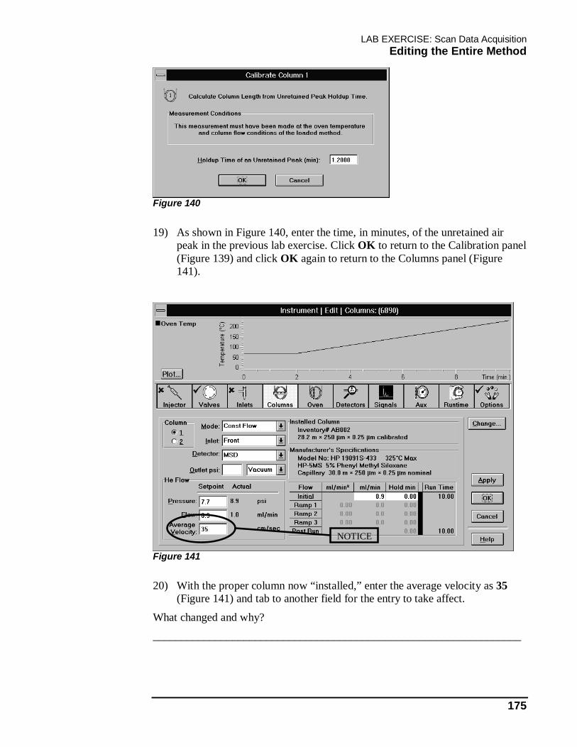
LAB EXERCISE: Scan Data Acquisition Editing the Entire Method

175

Figure 140

19) As shown in Figure 140, enter the time, in minutes, of the unretained air peak in the previous lab exercise. Click OK to return to the Calibration panel (Figure 139) and click OK again to return to the Columns panel (Figure 141).

NOTICE

Figure 141

20) With the proper column now “installed,” enter the average velocity as 35 (Figure 141) and tab to another field for the entry to take affect.

What changed and why? _________________________________________________________________

LAB EXERCISE: Scan Data Acquisition Editing the Entire Method

176

Figure 142

21) Click on the Oven picture and complete as shown in Figure 142.

What items calculated by the system in this panel change as you change the Oven Program parameters?

_________________________________________________________________

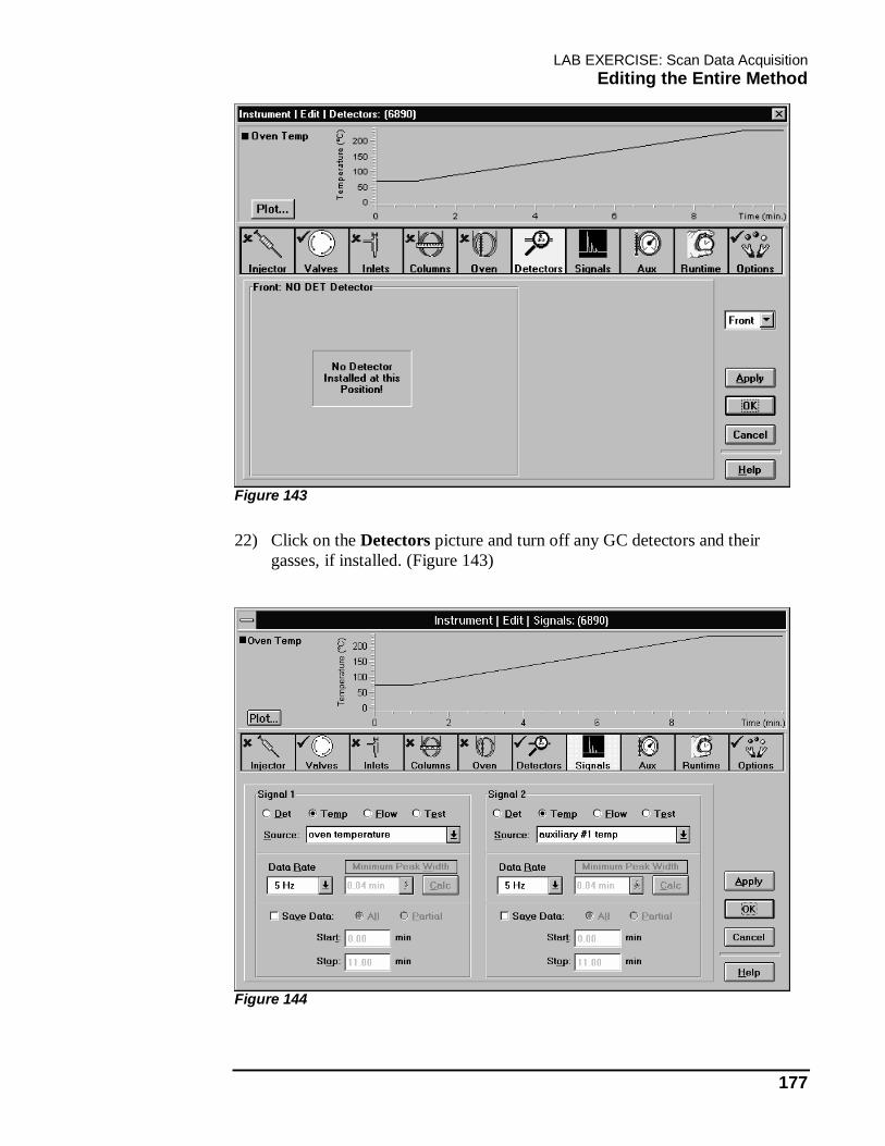
LAB EXERCISE: Scan Data Acquisition Editing the Entire Method

177

Figure 143

22) Click on the Detectors picture and turn off any GC detectors and their gasses, if installed. (Figure 143)

Figure 144

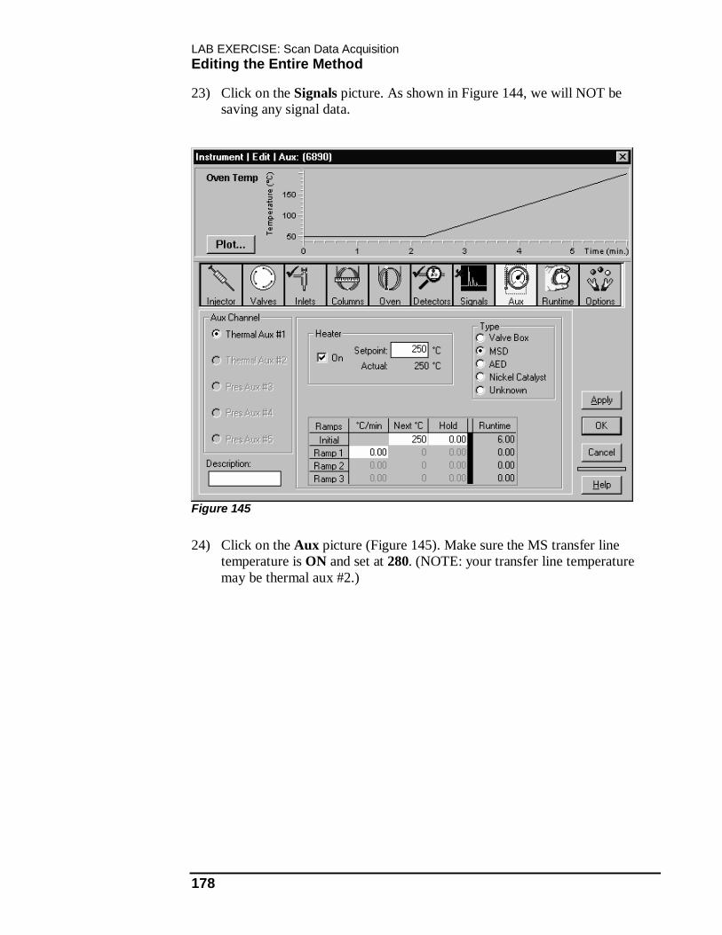
LAB EXERCISE: Scan Data Acquisition Editing the Entire Method

178

23) Click on the Signals picture. As shown in Figure 144, we will NOT be saving any signal data.

Figure 145

24) Click on the Aux picture (Figure 145). Make sure the MS transfer line temperature is ON and set at 280. (NOTE: your transfer line temperature may be thermal aux #2.)

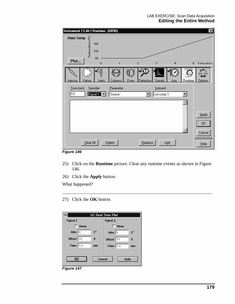
LAB EXERCISE: Scan Data Acquisition Editing the Entire Method

179

Figure 146

25) Click on the Runtime picture. Clear any runtime events as shown in Figure 146.

26) Click the Apply button. What happened?

_________________________________________________________________ 27) Click the OK button.

Figure 147

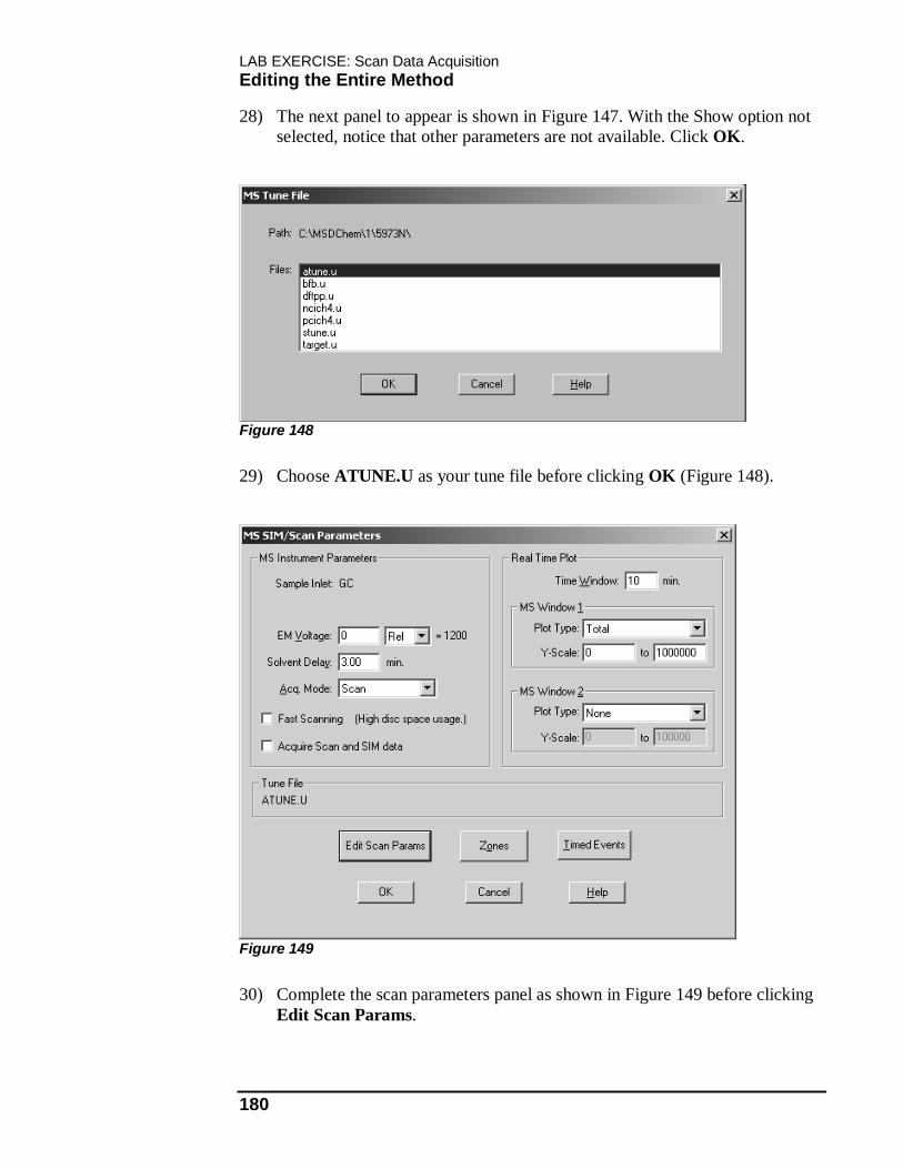
LAB EXERCISE: Scan Data Acquisition Editing the Entire Method

180

28) The next panel to appear is shown in Figure 147. With the Show option not selected, notice that other parameters are not available. Click OK.

Figure 148

29) Choose ATUNE.U as your tune file before clicking OK (Figure 148).

Figure 149

30) Complete the scan parameters panel as shown in Figure 149 before clicking Edit Scan Params.

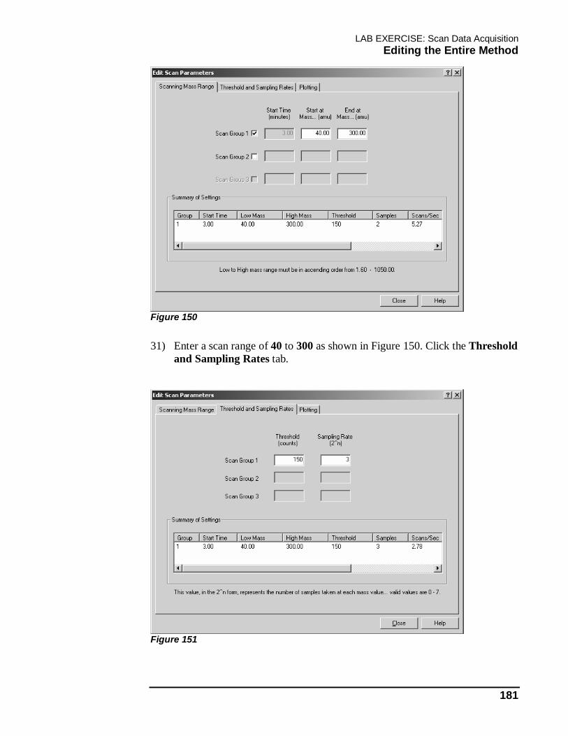
LAB EXERCISE: Scan Data Acquisition Editing the Entire Method

181

Figure 150

31) Enter a scan range of 40 to 300 as shown in Figure 150. Click the Threshold and Sampling Rates tab.

Figure 151

LAB EXERCISE: Scan Data Acquisition Editing the Entire Method

182

32) Set a threshold of 150 and a sampling rate of 3 as shown in Figure 151. Click the Plotting tab.

What MS scan parameters affect the number of scans/second? _________________________________________________________________

Figure 152

Why are all of the plot windows “grayed out?” _________________________________________________________________

33) Close the Plotting window (Figure 152). 34) Click the Zones button. Notice the setpoint and the actual before clicking

OK. Where are the source and quad temperatures set?

_________________________________________________________________ 35) Click the Timed Events button.

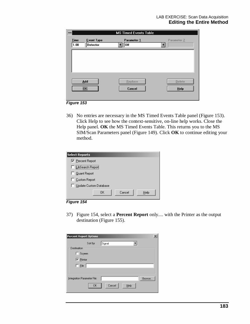
LAB EXERCISE: Scan Data Acquisition Editing the Entire Method

183

Figure 153

36) No entries are necessary in the MS Timed Events Table panel (Figure 153). Click Help to see how the context-sensitive, on-line help works. Close the Help panel. OK the MS Timed Events Table. This returns you to the MS SIM/Scan Parameters panel (Figure 149). Click OK to continue editing your method.

Figure 154

37) Figure 154, select a Percent Report only.... with the Printer as the output destination (Figure 155).

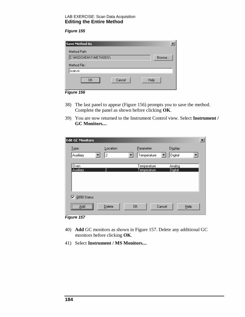
LAB EXERCISE: Scan Data Acquisition Editing the Entire Method

184

Figure 155

Figure 156

38) The last panel to appear (Figure 156) prompts you to save the method. Complete the panel as shown before clicking OK.

39) You are now returned to the Instrument Control view. Select Instrument / GC Monitors....

Figure 157

40) Add GC monitors as shown in Figure 157. Delete any additional GC monitors before clicking OK.

41) Select Instrument / MS Monitors....

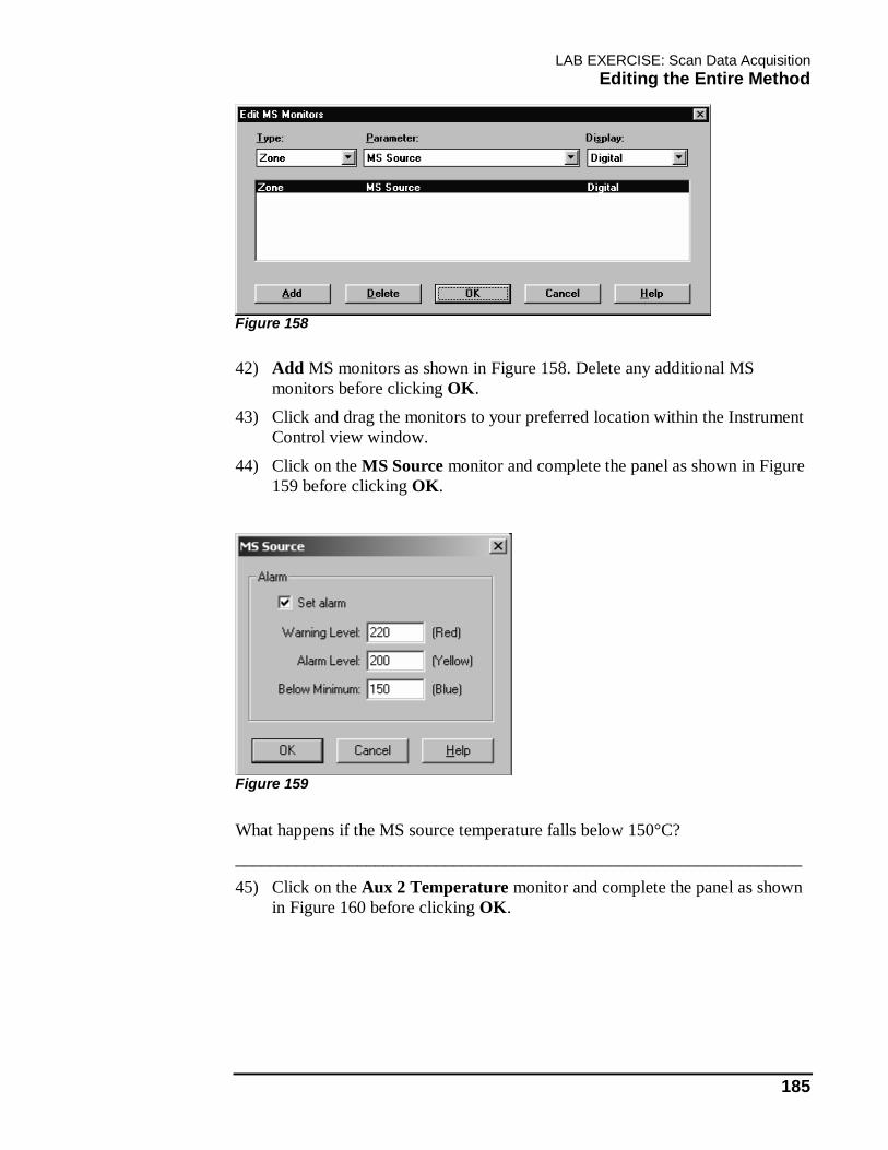
LAB EXERCISE: Scan Data Acquisition Editing the Entire Method

185

Figure 158

42) Add MS monitors as shown in Figure 158. Delete any additional MS monitors before clicking OK.

43) Click and drag the monitors to your preferred location within the Instrument Control view window.

44) Click on the MS Source monitor and complete the panel as shown in Figure 159 before clicking OK.

Figure 159

What happens if the MS source temperature falls below 150°C? _________________________________________________________________ 45) Click on the Aux 2 Temperature monitor and complete the panel as shown

in Figure 160 before clicking OK.

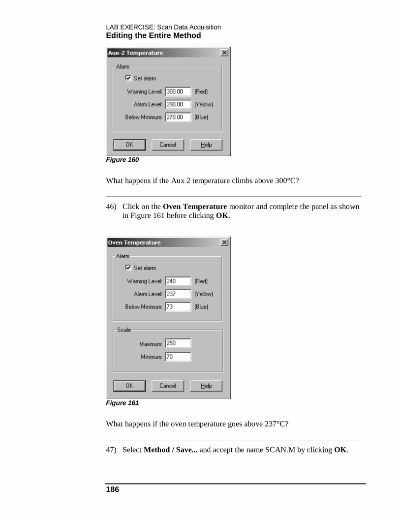
LAB EXERCISE: Scan Data Acquisition Editing the Entire Method

186

Figure 160

What happens if the Aux 2 temperature climbs above 300°C? _________________________________________________________________

46) Click on the Oven Temperature monitor and complete the panel as shown in Figure 161 before clicking OK.

Figure 161

What happens if the oven temperature goes above 237°C? _________________________________________________________________

47) Select Method / Save... and accept the name SCAN.M by clicking OK.

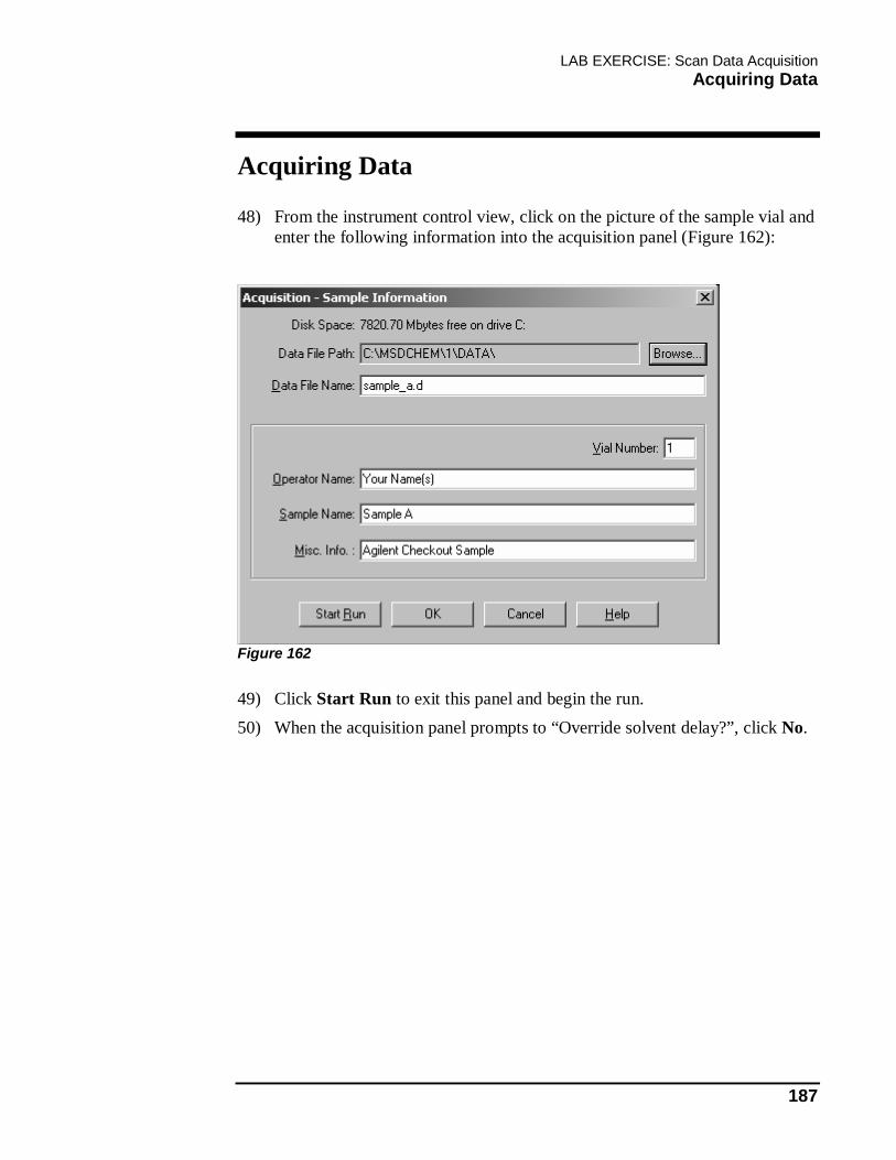
LAB EXERCISE: Scan Data Acquisition Acquiring Data

187

Acquiring Data

48) From the instrument control view, click on the picture of the sample vial and enter the following information into the acquisition panel (Figure 162):

Figure 162

49) Click Start Run to exit this panel and begin the run. 50) When the acquisition panel prompts to “Override solvent delay?”, click No.

LAB EXERCISE: Scan Data Acquisition Real Time Display Functions

188

Real Time Display Functions

51) Once the solvent delay time has elapsed, observe the run’s progress on the Real Time Display panel (which is a very small panel). For a better view select Window / Total Ion. Change the Y-axis abundance scale by clicking the scroll bar arrows up or down.

52) After the first peak elutes, switch to the Data Analysis view by selecting Start / Programs / MSD ChemStation / Instrument #1 / Data Analysis. From the Files menu select Take Snapshot File (alternatively, click the Take Snapshot tool in the toolbar). The file that is loaded is a snapshot of your data up until the time that you took the snapshot. Subsequent snapshots overwrite this file and are loaded. At the end of the run, the system overwrites this file with the complete data from the run.

How would you extend the run by 5 minutes, if necessary? _________________________________________________________________

If changes were made to the method, what steps would be necessary to make them permanent?

_________________________________________________________________

LAB EXERCISE: SIM Experiment

In this section you will:

• Acquire and analyze data to determination the exact mass to monitor in the next SIM acquisition lab exercise.

LAB EXERCISE: SIM Experiment Ion Selection

190

Ion Selection

In this experiment the data acquired in the Scan acquisition lab will be used to set up the parameters necessary for a SIM acquisition. The same mixture of four components analyzed in the Scan Acquisition lab will be used. The concentration of Sample B (100 pg / component) is tenfold less than Sample A. The four compounds in Sample A are:

Dodecane C12H26 a saturated hydrocarbon Biphenyl C12H10 an aromatic hydrocarbon

p-Chlorobiphenyl C12H9Cl a chlorinated aromatic hydrocarbon

Methyl Palmitate C17H34O2 a fatty acid methyl ester In order to optimize sensitivity and reproducibility in SIM acquisitions, the exact mass of ions to monitor must be determined. Tuning calibrates the mass axis to within +/- 0.2 amu. In this experiment we will determine the apex of the mass peaks for use in subsequent SIM acquisitions. 1) If you are not already in the Data Analysis view, select View / Data

Analysis. Load the data file acquired in Scan mode in the earlier lab with Sample A (SAMPLE_A.D) by selecting File / Load....

2) Select Chromatogram / Integrate and record the retention times for our four compounds in the SIM Ion Table for Sample B (Table 10 on page 191).

3) Zoom in on the first compound by clicking and dragging the left mouse button to define the zoom area. It’s OK to go below the base line. (NOTE: to zoom out, double click the left mouse button in the window.) Obtain an averaged spectrum from the peak by clicking and dragging the right mouse button across the peak at about half height.

4) Keep in mind that the best ions for SIM are unique and abundant. Fill out the SIM table for Dodecane. Remember that exact masses should be used in SIM acquisition for the best sensitivity, reproducibility and accuracy! Zoom in on ions in the spectrum until they are displayed in 0.1 amu by clicking and dragging the left mouse button. This information is accurate to ±0.2 amu. (NOTE: to zoom out, double click the left mouse button in the window.) This dynamic mass calibration experiment allows us to determine the exact mass of the ions we choose to monitor. In the next experiment we will set up a SIM acquisition monitoring only those ions that represent the exact mass.

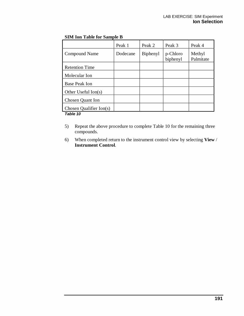
LAB EXERCISE: SIM Experiment Ion Selection

191

SIM Ion Table for Sample B

Peak 1 Peak 2 Peak 3 Peak 4

Compound Name Dodecane Biphenyl p-Chloro biphenyl

Methyl Palmitate

Retention Time

Molecular Ion

Base Peak Ion

Other Useful Ion(s)

Chosen Quant Ion

Chosen Qualifier Ion(s) Table 10

5) Repeat the above procedure to complete Table 10 for the remaining three compounds.

6) When completed return to the instrument control view by selecting View / Instrument Control.

LAB EXERCISE: SIM Experiment Tune

192

Tune

7) Perform an Autotune.

8) If necessary, manual tune the MSD to calibrate the mass axis as close to 69.0, 219.0, and 502.0 as possible. Save the tune as ATUNE.U.

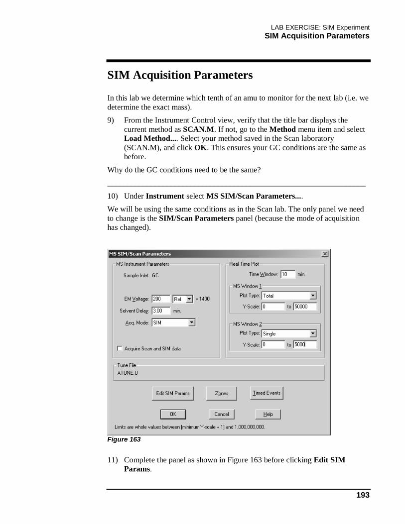
LAB EXERCISE: SIM Experiment SIM Acquisition Parameters

193

SIM Acquisition Parameters

In this lab we determine which tenth of an amu to monitor for the next lab (i.e. we determine the exact mass). 9) From the Instrument Control view, verify that the title bar displays the

current method as SCAN.M. If not, go to the Method menu item and select Load Method.... Select your method saved in the Scan laboratory (SCAN.M), and click OK. This ensures your GC conditions are the same as before.

Why do the GC conditions need to be the same? _________________________________________________________________

10) Under Instrument select MS SIM/Scan Parameters.... We will be using the same conditions as in the Scan lab. The only panel we need to change is the SIM/Scan Parameters panel (because the mode of acquisition has changed).

Figure 163

11) Complete the panel as shown in Figure 163 before clicking Edit SIM Params.

LAB EXERCISE: SIM Experiment SIM Acquisition Parameters

194

12) For each compound we will be analyzing, you need to supply the group ID, the start time for the group, and the ions that are to be monitored. The times should have been determined when you analyzed Sample A. (DO NOT USE START TIMES SHOWN IN Figure 164!)

13) Use the Add New Group button to create the four groups shown in Figure 164. Remove any extra groups using the Delete Group(s) button.

14) Select each group and add the ions using the information in Table 10 and/or Table 11. Remove any extra ions using the Delete Ion(s) button. Some of the ions for Dodecane are shown in Figure 164.

Figure 164

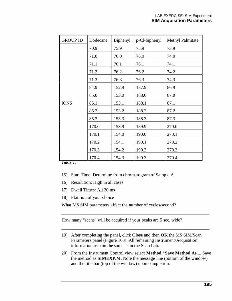
LAB EXERCISE: SIM Experiment SIM Acquisition Parameters

195

GROUP ID Dodecane Biphenyl p-Cl-biphenyl Methyl Palmitate

70.9 75.9 75.9 73.9

71.0 76.0 76.0 74.0

71.1 76.1 76.1 74.1

71.2 76.2 76.2 74.2

71.3 76.3 76.3 74.3

84.9 152.9 187.9 86.9

85.0 153.0 188.0 87.0

IONS 85.1 153.1 188.1 87.1

85.2 153.2 188.2 87.2

85.3 153.3 188.3 87.3

170.0 153.9 189.9 270.0

170.1 154.0 190.0 270.1

170.2 154.1 190.1 270.2

170.3 154.2 190.2 270.3

170.4 154.3 190.3 270.4 Table 11

15) Start Time: Determine from chromatogram of Sample A 16) Resolution: High in all cases

17) Dwell Times: All 20 ms 18) Plot: ion of your choice

What MS SIM parameters affect the number of cycles/second? _________________________________________________________________

How many “scans” will be acquired if your peaks are 5 sec. wide? _________________________________________________________________

19) After completing the panel, click Close and then OK the MS SIM/Scan Parameters panel (Figure 163). All remaining Instrument/Acquisition information remain the same as in the Scan Lab.

20) From the Instrument Control view select Method / Save Method As.... Save the method as SIMEXP.M. Note the message line (bottom of the window) and the title bar (top of the window) upon completion.

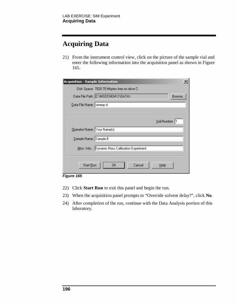
LAB EXERCISE: SIM Experiment Acquiring Data

196

Acquiring Data

21) From the instrument control view, click on the picture of the sample vial and enter the following information into the acquisition panel as shown in Figure 165.

Figure 165

22) Click Start Run to exit this panel and begin the run. 23) When the acquisition panel prompts to “Override solvent delay?”, click No.

24) After completion of the run, continue with the Data Analysis portion of this laboratory.

LAB EXERCISE: SIM Experiment Data Analysis

197

Data Analysis

The data acquired will be analyzed to determine the mass to be specified in future SIM acquisitions. 25) Select View / Data Analysis.

26) From the File menu, Load... the data file just acquired. What does the TIC displayed represent?

_________________________________________________________________ 27) Obtain an averaged spectrum of the first compound, Dodecane.

NOTE: Only the ions monitored in the SIM acquisition are present in the “spectrum”.

28) Tabulate the spectrum by selecting Spectrum / Tabulate. Click Print for a hardcopy and Done to exit the tabulation.

29) List in Table 12 the most abundant ion for each mass peak in this tabulation? The m/z for the most abundant ion represents the apex of the mass peak. This m/z value should now be used in subsequent SIM analyses to increase the sensitivity and reproducibility of the system.

What influence would tuning have on these m/z values? _________________________________________________________________

30) Repeat steps 27) through 29) for the remaining three compounds to determine the m/z for all ions to be analyzed.

Based upon the above data, list in Table 12 the ions to be used in the next SIM analysis.

Compound Quant Ion Qualifier Ion

Qualifier Ion

Dodecane

Biphenyl

p-Chlorobiphenyl

Methyl Palmitate Table 12

LAB EXERCISE: SIM Experiment Data Analysis

198

LAB EXERCISE: SIM Data Analysis

199

LAB EXERCISE: SIM

In this section you will:

• Acquire data in Selected Ion Monitoring (SIM) mode.

LAB EXERCISE: SIM SIM Acquisition Parameters

200

SIM Acquisition Parameters

In this experiment the exact masses determined in the previous Dynamic Mass Calibration lab is used to set up a SIM acquisition monitoring only those masses. 1) From the Instrument Control view, go to the Method menu and select Load

Method.... Select your method saved in the Dynamic Mass Calibration Experiment laboratory (SIMEXP.M) and click OK. This ensures your conditions are the same as before.

2) Under Instrument select MS SIM/Scan Parameters.... The SIM method previously loaded contains the correct parameters for this acquisition except for the ions to monitor.

3) Click the Edit SIM Params button.

Figure 166

4) For each compound enter the three exact masses that you determined in the previous lab. DO NOT USE TIMES OR MASSES SHOWN IN THE ABOVE EXAMPLE Figure 166!!

5) Time: Determine from chromatogram of Sample A

LAB EXERCISE: SIM SIM Acquisition Parameters

201

6) Resolution: High in all cases 7) Dwell Times: All 50 ms

8) Plot: ion of your choice All remaining Instrument/Acquisition information remain the same as in the SIM Experiment Lab. 9) After completing the panel, click Close and then OK the MS SIM/Scan

Parameters panel (Figure 166). All remaining Instrument/Acquisition information remain the same as in the SIM Experiment Lab.

10) From the Instrument Control view select Method / Save Method As.... Save the method as SIM.M. Note the message line (bottom of the window) and the title bar (top of the window) upon completion.

LAB EXERCISE: SIM Acquiring Data

202

Acquiring Data

From the instrument control view, click on the picture of the sample vial and enter the following information into the acquisition panel as shown in Figure 167.

Figure 167

11) Click Start Run to exit this panel and begin the run. 12) When the acquisition panel prompts to “Override solvent delay?”, click No.

Note the following as the run progresses:

• the group names shown on the TIC display.

• title of each display

Maintenance

Maintenance What You Will Learn

204

What You Will Learn

2

Maintenance

In this section you will learn:

• Preventive maintenance for the GC and MS• Diagnostics and tools for troubleshooting

Figure 168

This section contains information related to the maintenance of your GC-MSD system.

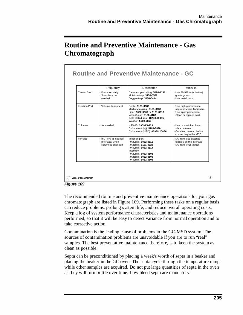
Maintenance Routine and Preventive Maintenance - Gas Chromatograph

205

Routine and Preventive Maintenance - Gas Chromatograph

3

Routine and Preventive Maintenance - GC

• DO NOT use graphite ferrules on the interface!

• DO NOT over tighten!

• Use cross-linked fused silica columns.

• Condition column before connecting to the MSD.

• Use high performance septa or Merlin Microseal.

• Use appropriate liner.• Clean or replace seal.

• Use 99.999% (or better) grade gases.

• Use metal traps.

Remarks

• Inj. Port: as needed• Interface: when

column is changed

• As needed

• Volume dependent

• Pressure: daily• Scrubbers: as

needed

Frequency

Injection port:0.20mm: 5062-35160.25mm: 5181-33230.32mm: 5062-3514

Interface:0.20mm: 5062-35080.25mm: 5062-35080.32mm: 5062-3506

Ferrules

HP5MS: 19091S-433Column nut (inj): 5181-8830Column not (MSD): 05988-20066

Columns

Septa: 5181-3383Merlin Microseal: 5181-8833Liner: 5062-3587 or 5181-3316Viton O-ring: 5180-4182Gold plated seal: 18740-20885Washer: 5160-5869

Injection Port

Clean copper tubing: 5180-4196Moisture trap: 3150-0532Oxygen trap: 3150-0414

Carrier Gas

Description

Figure 169

The recommended routine and preventive maintenance operations for your gas chromatograph are listed in Figure 169. Performing these tasks on a regular basis can reduce problems, prolong system life, and reduce overall operating costs. Keep a log of system performance characteristics and maintenance operations performed, so that it will be easy to detect variance from normal operation and to take corrective action.

Contamination is the leading cause of problems in the GC-MSD system. The sources of contamination problems are unavoidable if you are to run “real” samples. The best preventative maintenance therefore, is to keep the system as clean as possible.

Septa can be preconditioned by placing a week's worth of septa in a beaker and placing the beaker in the GC oven. The septa cycle through the temperature ramps while other samples are acquired. Do not put large quantities of septa in the oven as they will turn brittle over time. Low bleed septa are mandatory.

Maintenance Routine and Preventive Maintenance - Gas Chromatograph

206

A regulated supply of high purity GC carrier gas is required. A minimum purity of 99.9995% is recommended. Molecular sieve and Oxygen traps are recommended. Avoid “plastic” traps as plasticizers can leach into the carrier gas and be detected (m/z 149).

Condition columns prior to use by connecting the column into the injection port; ramp the temperature to the maximum temperature to be used in the analysis plus 20 degrees. Make sure there is carrier gas flowing through the column and that the upper temperature limit of the column is not exceeded!

The graphite/vespel ferrule used on the interface typically needs to be replaced when the column is changed. Take care not to overtighten the interface nut; this can restrict the column flow. The injection port must be maintained. Routinely check and replace the liners, septa, and split disks. The liner used should be chosen on the basis of the type of injection (split or splitless) and whether manual or autosampler injections are to be made. For more information about GC maintenance, please refer to the GC hardware operation/service manual that was shipped with your Gas Chromatograph.

Maintenance Capillary Direct Column Install

207

Capillary Direct Column Install

4

FerruleNut

ToMSD

Extend Column to1 mm of Interface

Injection Port

4 - 6 mm

Capillary Direct Column Install

Figure 170

To install the column in the MSD, follow these steps: 1) Unwind the ends of the column from the basket. You need about 12 inches

(30 cm) on the injection port end and about 18 inches (45 cm) on the MSD end.

2) Suspend the column from the column hanger in the oven. 3) Put the column nut on the MSD end of the column. This nut should be the

brass nut supplied with the shipping kit. CAUTION: Use of nuts made with other harder metals is not recommended. They may damage the threads on the end of the interface, making it difficult to achieve a proper seal.

4) Put the ferrule on. The narrow end of the ferrule faces the nut. 5) Cut off the end of the column squarely. Cutting off the end of the column

removes any particles which inadvertently may have been deposited in the column from the nut or ferrule.

6) Insert the column into the interface.

Maintenance Capillary Direct Column Install

208

7) Open the analyzer door to reveal the ion source end of the interface line. 8) Adjust the column until it protrudes from the interface line by about 1 mm.

9) Tighten the nut. You only need to tighten the nut until it is snug. Tightening the nut too much can crush the column or split the ferrule.

10) Put the injection port nut on the injection port end of the column. 11) Put the ferrule on the column. The narrow end of the ferrule faces the

injection port. 12) Cut off the end of the column squarely.

13) Push up the end of the column until about 4-6 mm of it projects beyond the ferrule when the ferrule is seated in the injection port nut. Mark the column below the injection port nut (use something like typewriter correction fluid or a felt tip marker).

NOTE: The position of the column in the injection port is VERY linear dependent and has a dramatic effect on the performance.

14) Insert the column into the injection port and position the mark correctly. 15) Tighten the injection port nut gently but firmly.

Maintenance Routine and Preventive Maintenance - Mass Selective Detector

209

Routine and Preventive Maintenance - Mass Selective Detector

5

Routine and Preventive Maintenance - MSD

Use solvent delay to prolong filament use

G1099-60053As neededFilaments

Replace if needed0905-1217As neededVent plug O-ring

Replace if neededG1099-80001As neededHED

Use lowest possible voltage

05971-80103As neededElectron Multiplier

Clean as necessary. Keep under vacuum.

As neededIon Source

Replace if needed6040-0809AnnuallyDiffusion Pump Oil

Replace as scheduledLiter: 6040-0834Gallon: 6040-0789Foreline trap pellets: 9301-1104

Weekly: check level and appearance.Semi-annually: change oil and foreline trap.

Mechanical Pump Oil

Refill as necessary. DO NOT overfill.

05971-60571MonthlyPFTBA

Keep as record of system performance

WeeklyStandard Spectra Tune

RemarksPart #Frequency

Figure 171

Figure 171 gives a summary of routine and preventive maintenance for your mass spectrometer. NOTE: If you are using the Chemical Ionization (CI) option, it is highly recommended that you ballast the mechanical rough pump weekly for a least 1 hour. It is also highly recommended that you change the mechanical rough pump oil on a monthly basis.

Performing these tasks on a regular basis can reduce problems, prolong system life, and reduce overall operating costs. Keep a log of system performance characteristics and maintenance operations performed so that it will be easy to detect variance from normal operation and to take corrective action.

Common consumables required for routine MSD maintenance are listed in Figure 171. The consumables catalog is available for other necessary items.

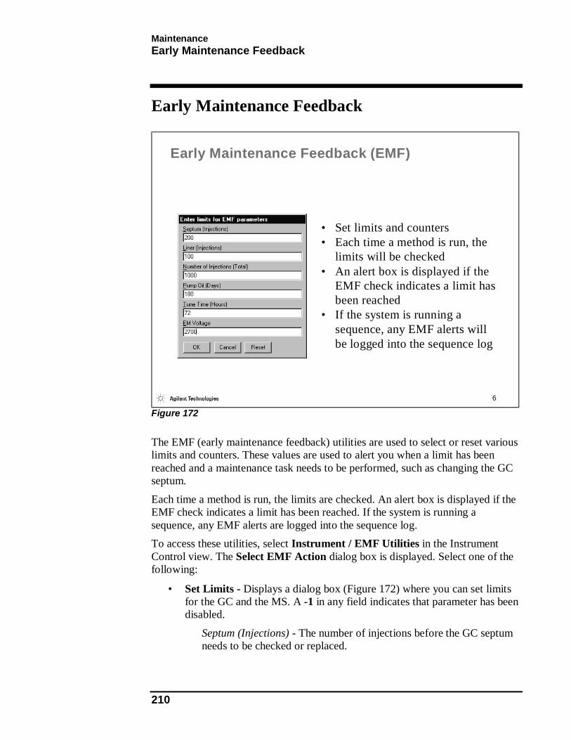
Maintenance Early Maintenance Feedback

210

Early Maintenance Feedback

6

Early Maintenance Feedback (EMF)

• Set limits and counters• Each time a method is run, the

limits will be checked• An alert box is displayed if the

EMF check indicates a limit has been reached

• If the system is running a sequence, any EMF alerts will be logged into the sequence log

Figure 172

The EMF (early maintenance feedback) utilities are used to select or reset various limits and counters. These values are used to alert you when a limit has been reached and a maintenance task needs to be performed, such as changing the GC septum.

Each time a method is run, the limits are checked. An alert box is displayed if the EMF check indicates a limit has been reached. If the system is running a sequence, any EMF alerts are logged into the sequence log. To access these utilities, select Instrument / EMF Utilities in the Instrument Control view. The Select EMF Action dialog box is displayed. Select one of the following:

• Set Limits - Displays a dialog box (Figure 172) where you can set limits for the GC and the MS. A -1 in any field indicates that parameter has been disabled.

Septum (Injections) - The number of injections before the GC septum needs to be checked or replaced.

Maintenance Early Maintenance Feedback

211

Liner (Injections) - The number of injections before the GC liner needs to be checked or replaced.

Number of Injections (Total) - The total number of injections before the column needs to be trimmed or replaced.

Pump Oil (Days) - The number of days until the foreline pump oil needs to be checked, refilled, or replaced. Depending on system usage, the foreline pump oil should be checked every week, and replaced approximately every six months.

Tune Time (Hours) - The number of hours before the MSD needs to be retuned.

EM Voltage - The voltage you use to indicate the need to retune, clean the ion source, or replace the electron multiplier.

• Set Counters - Displays a dialog box where you can set counters for the GC septum, liner and total number of injections. This dialog box is only used if a counter has been incremented unnecessarily. For example, if the ALS syringe malfunctioned and did not make actual injections during a sequence, the counter for the GC septum would still increment. In this case, you could use this dialog box to reset the GC septum counter to the number it was prior to the malfunction.

• Reset Counters - Displays a dialog box where you can reset counters for the septum, liner, number of injections, and pump oil.

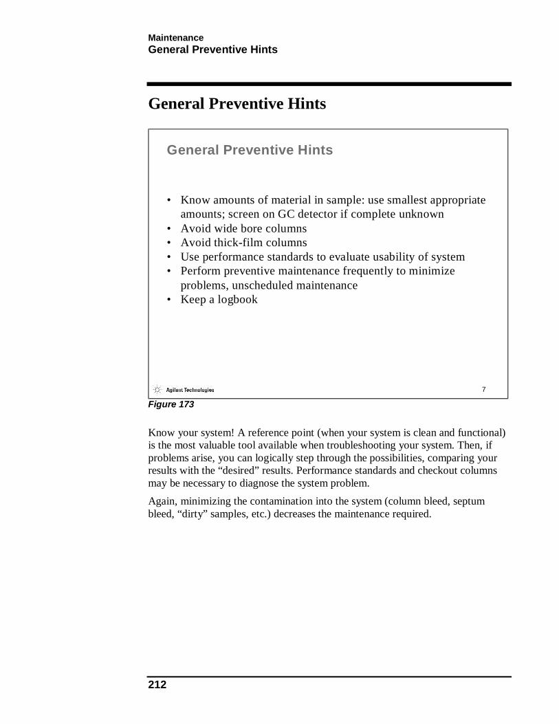
Maintenance General Preventive Hints

212

General Preventive Hints

7

General Preventive Hints

• Know amounts of material in sample: use smallest appropriate amounts; screen on GC detector if complete unknown

• Avoid wide bore columns• Avoid thick-film columns• Use performance standards to evaluate usability of system• Perform preventive maintenance frequently to minimize

problems, unscheduled maintenance• Keep a logbook

Figure 173

Know your system! A reference point (when your system is clean and functional) is the most valuable tool available when troubleshooting your system. Then, if problems arise, you can logically step through the possibilities, comparing your results with the “desired” results. Performance standards and checkout columns may be necessary to diagnose the system problem. Again, minimizing the contamination into the system (column bleed, septum bleed, “dirty” samples, etc.) decreases the maintenance required.

Maintenance Typical GC-MS Problems

213

Typical GC-MS Problems

8

Remember to use the MSD Hardware Manual's Troubleshooting section!F E

Typical GC/MS Problems

ImpatientUntrained

Operator

Air leaksColumn flowPumps

Vacuum problems

SampleCarrier gasGCMS

Contamination

GC conditions/problemsHigh backgroundVacuum problemTuning

Low sensitivityPossible CauseProblem

Figure 174

Using all diagnostic tools available (ion gauge controller, tune reports, etc.) make sure there is a problem before you try and fix it! For example, if the tune shows that the abundance for 502 has decreased, and your analysis only requires scanning up to 300 amu, you may not have a problem!

If a problem does exist, isolate the problem. Cap off the MS with a no-hole ferrule. (Remember to vent the system properly before capping off the MSD.) An alternate way to cap off the MSD is to insert a septum sideways into the inlet (GC) end of the column. This is an excellent way to determine whether the MSD or the GC is causing the problem. As can be seen from the previous example, troubleshooting your system may not always be a quick process. Therefore, try the easiest fix first! Contamination originating in the GC typically comes from one of these sources:

• Column bleed

• Septum bleed

• Dirty injector (sample)

Maintenance Typical GC-MS Problems

214

• Poor quality carrier gas An intense peak at 207 amu (dimethylpolysiloxane) can frequently identify column or septum bleed. Non cross-linked columns are a major cause. High-bleed septa are also a common cause. For this reason, cross-linked capillary columns are recommended for almost all applications. Also recommended are low bleed septa. Dirty injectors and contaminated carrier gas are harder to diagnose because the background spectra depend on the contaminants. If the contamination problem is coming from the GC, but it is not septum or column bleed, try cleaning the injector port or switching to a different source of carrier gas. Routine maintenance can eliminate many of the common problems encountered with the GC-MS system. Remember that the hardware manual has a troubleshooting section to aid you in correcting problems.

Maintenance Troubleshooting

215

Troubleshooting

9

èDetermine source of contamination from spectraèVerify site of contamination by isolating MS from GC

Troubleshooting

• Low sensitivity– GC: Septum, liner, gold seal, column temperature parameters,

split/splitless parameters, syringe or P&T– MS: Check tune reports, verify data acquisition parameters

(tune file, EM voltage), vacuum• Contamination

– Inlet/column buildup - active sites– Septum/column bleed– Cleaning solvents– Fingerprints

Figure 175

As stated in Figure 175, the source of contamination can many times be determined from the spectra. The table in Figure 176 can be helpful.

Maintenance Mass Peaks of Common Contaminants

216

Mass Peaks of Common Contaminants

10

Mass Peaks of Common Contaminants

Plasticizers in tubing, vials, caps, samples

Phthalates149

Fingerprints or pump oilHydrocarbons41, 43, 55, 57, 71, 85, 99

Septum or column bleedDimethylpolysiloxane73, 147, 207, 222, 281, 295, 355, 429

Freons85Acetone43, 58Xylenes105, 106Toluene91, 92Benzene or Xylenes77Methanol31WaterCleaning solvents18H2O, N2, O2, Ar, CO2Air18, 28, 32, 40, 44

Potential SourceCompound General Classification

Mass(es)

Figure 176

Contamination is usually identified by the presence of excessive background in the results of data acquisition. It can come from the GC or the MSD. The likely source of contamination can frequently be determined by the contamination ions present in the background. Use the list on mass peaks associated with common contaminants to identify the problem.

Maintenance Troubleshooting Vacuum Problems

217

Troubleshooting Vacuum Problems

11

Troubleshooting Vacuum Problems

• What is the vacuum?– Use ion gauge controller and tube. Pressure should be in low 10-5

torr range• How well is vacuum system pumping?

– How fast will PFTBA pump away?• Leaks

– Examine Standard Spectra Tune report for >10 % mass 28– Locate leak using Manual Tune/Repeat Profile with leak-detecting

gases:• Argon - mass 40• Carbon Dioxide - mass 44

Figure 177

Sensitivity losses may be a direst result of vacuum problems. The operating pressure should be in the low 10-5 torr range. This pressure may be monitored with an ion gauge controller. Without an ion gauge controller, determine how long it takes to pump away mass 69 on a working system. Then, if a problem exists, you can directly compare the new time it takes to pump mass 69 away from the old time. Leaks may be detected by comparing masses 28 and 32 to mass 69 in a Standard Spectra Tune report. Mass 28 (Nitrogen) should be less than 10% of mass 69. If a leak exists, Manual Tune / Repeat Profile may be used to locate the leak.

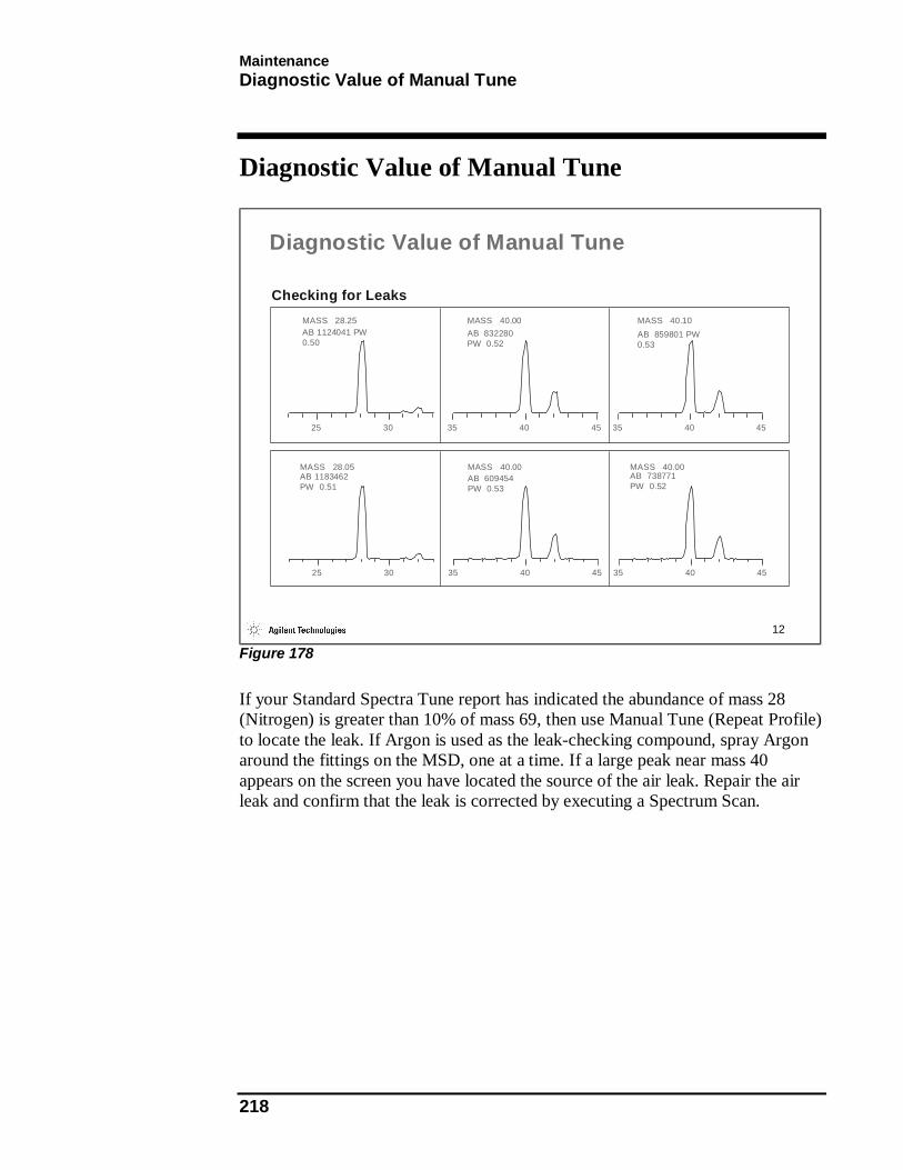
Maintenance Diagnostic Value of Manual Tune

218

Diagnostic Value of Manual Tune

12

25 30 35 40 45 35 40 45

MASS 28.25AB 1124041 PW 0.50

MASS 40.00AB 832280 PW 0.52

MASS 40.10AB 859801 PW 0.53

MASS 28.05AB 1183462 PW 0.51

MASS 40.00AB 609454 PW 0.53

MASS 40.00AB 738771 PW 0.52

Checking for Leaks

25 30 35 40 45 35 40 45

Diagnostic Value of Manual Tune

Figure 178

If your Standard Spectra Tune report has indicated the abundance of mass 28 (Nitrogen) is greater than 10% of mass 69, then use Manual Tune (Repeat Profile) to locate the leak. If Argon is used as the leak-checking compound, spray Argon around the fittings on the MSD, one at a time. If a large peak near mass 40 appears on the screen you have located the source of the air leak. Repair the air leak and confirm that the leak is corrected by executing a Spectrum Scan.

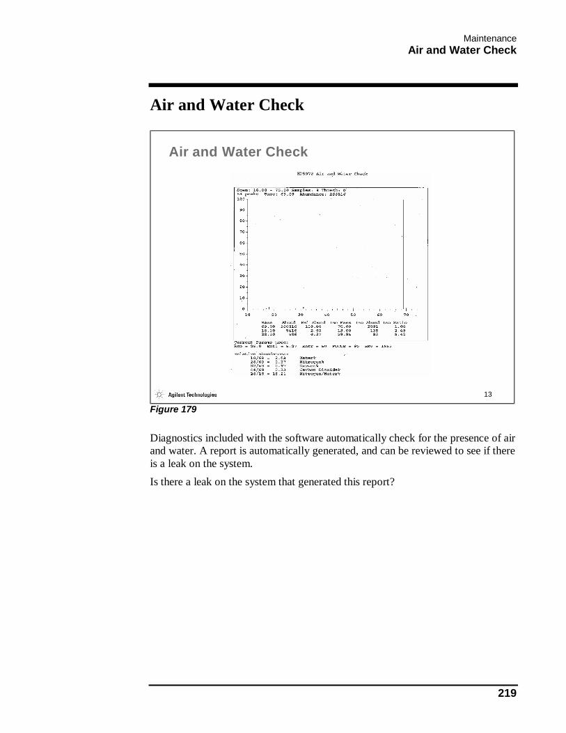
Maintenance Air and Water Check

219

Air and Water Check

13

Air and Water Check

Figure 179

Diagnostics included with the software automatically check for the presence of air and water. A report is automatically generated, and can be reviewed to see if there is a leak on the system. Is there a leak on the system that generated this report?

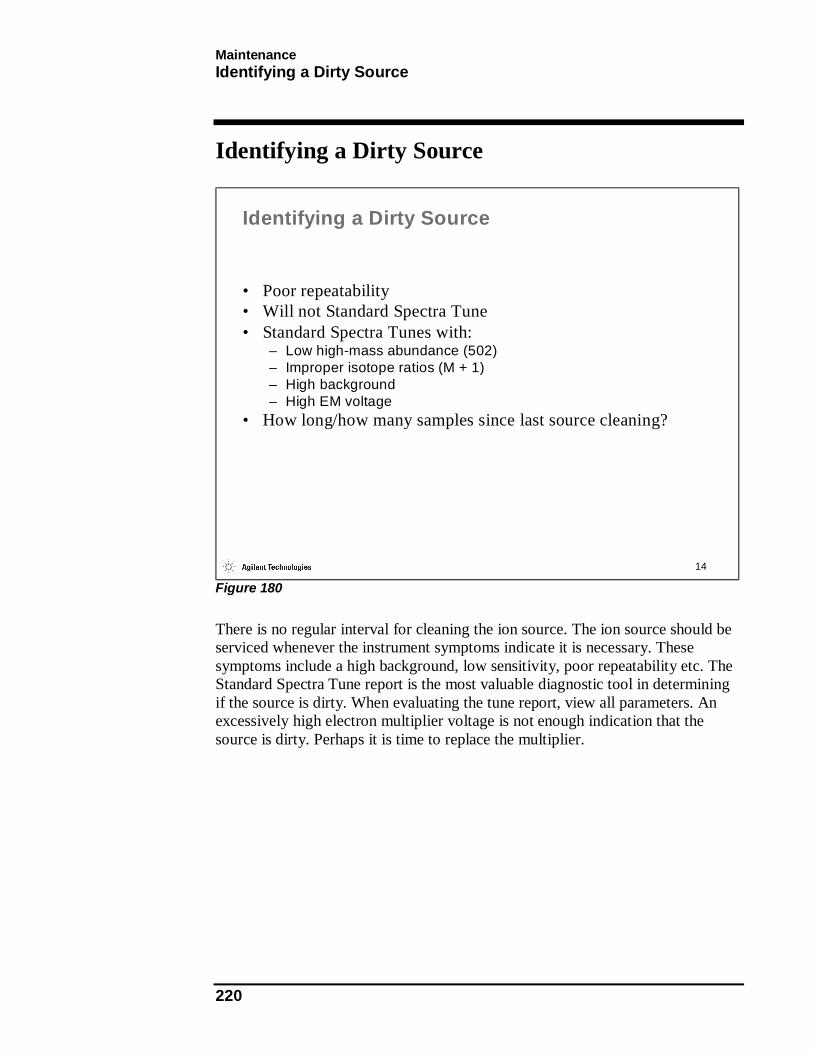
Maintenance Identifying a Dirty Source

220

Identifying a Dirty Source

14

Identifying a Dirty Source

• Poor repeatability• Will not Standard Spectra Tune• Standard Spectra Tunes with:

– Low high-mass abundance (502)– Improper isotope ratios (M + 1)– High background– High EM voltage

• How long/how many samples since last source cleaning?

Figure 180

There is no regular interval for cleaning the ion source. The ion source should be serviced whenever the instrument symptoms indicate it is necessary. These symptoms include a high background, low sensitivity, poor repeatability etc. The Standard Spectra Tune report is the most valuable diagnostic tool in determining if the source is dirty. When evaluating the tune report, view all parameters. An excessively high electron multiplier voltage is not enough indication that the source is dirty. Perhaps it is time to replace the multiplier.

Maintenance Diagnosing from Tune Reports

221

Diagnosing from Tune Reports

15

From profile scans, look for:

• Electron Multiplier setting appropriate to age of EM

• Consistent peak widths• Good peak shapes (no

"precursor" on low mass side of mass peak)

Diagnosing from Tune Reports

Figure 181

It is recommended that a copy of the Standard Spectra Tune report be kept and logged on a weekly basis. By having a historical record of tuning parameters you can observe trends in parameters settings that indicate problems in the MSD. You may notice small differences in parameters from one tune to the next. Some key areas to note when interpreting a tune are as follows:

• Mass peaks should be ±0.2 amu

• Peak widths should be 0.55±0.1 (measured as PW50)

• Peaks should be smooth and symmetrical

• Monitor the Electron Multiplier voltage for trends

• Monitor the Ion Focus voltage for trends

• Monitor the Repeller voltage for trends

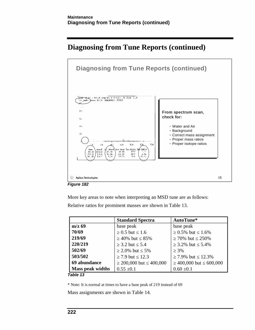
Maintenance Diagnosing from Tune Reports (continued)

222

Diagnosing from Tune Reports (continued)

16

From spectrum scan, check for:

• Water and Air• Background• Correct mass assignment• Proper mass ratios• Proper isotope ratios

Diagnosing from Tune Reports (continued)

Figure 182

More key areas to note when interpreting an MSD tune are as follows: Relative ratios for prominent masses are shown in Table 13.

Standard Spectra AutoTune* m/z 69 base peak base peak 70/69 ≥ 0.5 but ≤ 1.6 ≥ 0.5% but ≤ 1.6% 219/69 ≥ 40% but ≤ 85% ≥ 70% but ≤ 250% 220/219 ≥ 3.2 but ≤ 5.4 ≥ 3.2% but ≤ 5.4% 502/69 ≥ 2.0% but ≤ 5% ≥ 3% 503/502 ≥ 7.9 but ≤ 12.3 ≥ 7.9% but ≤ 12.3% 69 abundance ≥ 200,000 but ≤ 400,000 ≥ 400,000 but ≤ 600,000 Mass peak widths 0.55 ±0.1 0.60 ±0.1

Table 13

* Note: It is normal at times to have a base peak of 219 instead of 69

Mass assignments are shown in Table 14.

Maintenance Diagnosing from Tune Reports (continued)

223

69.0 ±0.2 219.0 ±0.2 502.0 ±0.2

Table 14

Maintenance AutoTune Worksheet

224

AutoTune Worksheet

17

What GC/MS problem(s) are indicated from this tune report?

AutoTune Worksheet

Figure 183

Based upon the tune report, what, if anything, might be the appropriate action to take?

An enlargement of the above report appears on the next page.

Maintenance AutoTune Worksheet

225