
13C-methyl formate: observations of a sample of high mass star-forming regions including Orion–KL...
31
The Astrophysical Journal Supplement Series, 215:25 (31pp), 2014 December doi:10.1088/0067-0049/215/2/25 C ⃝ 2014. The American Astronomical Society. All rights reserved. Printed in the U.S.A. 13 C–METHYL FORMATE: OBSERVATIONS OFA SAMPLE OFHIGH-MASS STAR-FORMING REGIONS INCLUDING ORION–KL AND SPECTROSCOPIC CHARACTERIZATION ∗ C´ ecile Favre 1 , Miguel Carvajal 2 , David Field 3 , Jes K. Jørgensen 4 ,5 , Suzanne E. Bisschop 4 ,5 , Nathalie Brouillet 6 ,7 , Didier Despois 6 ,7 , Alain Baudry 6 ,7 , Isabelle Kleiner 8 , Edwin A. Bergin 1 , Nathan R. Crockett 1 , Justin L. Neill 1 , Laurent Margul ` es 9 , Th´ er` ese R. Huet 9 , and Jean Demaison 9 1 Department of Astronomy, University of Michigan, 500 Church Street, Ann Arbor, MI 48109, USA; [email protected] 2 Dpto. F´ ısica Aplicada, Unidad Asociada CSIC, Facultad de Ciencias Experimentales, Universidad de Huelva, E-21071 Huelva, Spain; [email protected] 3 Department of Physics and Astronomy, University of Aarhus, Ny Munkegade 120, DK-8000 Aarhus C, Denmark 4 Centre for Star and Planet Formation, Niels Bohr Institute, University of Copenhagen, Juliane Maries Vej 30, DK-2100 Copenhagen Ø, Denmark 5 Natural History Museum of Denmark, University of Copenhagen, Øster Voldgade 5-7, DK-1350 Copenhagen K., Denmark 6 Univ. Bordeaux, LAB, UMR 5804, F-33270, Floirac, France 7 CNRS, LAB, UMR 5804, F-33270, Floirac, France 8 Laboratoire Interuniversitaire des Syst` emes Atmosph´ eriques (LISA), CNRS, UMR 7583, Universit´ e de Paris-Est et Paris Diderot, 61, Av. du G´ en´ eral de Gaulle, F-94010 Cr´ eteil Cedex, France 9 Laboratoire de Physique des Lasers, Atomes et Mol´ ecules, UMR CNRS 8523, Universit´ e Lille I, F-59655 Villeneuve d’Ascq Cedex, France Received 2014 February 21; accepted 2014 October 15; published 2014 December 2 ABSTRACT We have surveyed a sample of massive star-forming regions located over a range of distances from the Galactic center for methyl formate, HCOOCH 3 , and its isotopologues H 13 COOCH 3 and HCOO 13 CH 3 . The observations were carried out with the APEX telescope in the frequency range 283.4–287.4 GHz. Based on the APEX observations, we report tentative detections of the 13 C-methyl formate isotopologue HCOO 13 CH 3 toward the following four massive star-forming regions: Sgr B2(N-LMH), NGC 6334 IRS 1, W51 e2, and G19.61-0.23. In addition, we have used the 1 mm ALMA science verification observations of Orion–KL and confirm the detection of the 13 C-methyl formate species in Orion–KL and image its spatial distribution. Our analysis shows that the 12 C/ 13 C isotope ratio in methyl formate toward the Orion–KL Compact Ridge and Hot Core-SW components (68.4 ± 10.1 and 71.4 ± 7.8, respectively) are, for both the 13 C-methyl formate isotopologues, commensurate with the average 12 C/ 13 C ratio of CO derived toward Orion–KL. Likewise, regarding the other sources, our results are consistent with the 12 C/ 13 C in CO. We also report the spectroscopic characterization, which includes a complete partition function, of the complex H 13 COOCH 3 and HCOO 13 CH 3 species. New spectroscopic data for both isotopomers H 13 COOCH 3 and HCOO 13 CH 3 , presented in this study, have made it possible to measure this fundamentally important isotope ratio in a large organic molecule for the first time. Key words: astrochemistry – ISM: abundances – line: identification – methods: data analysis – methods: laboratory: molecular – techniques: spectroscopic Online-only material: color figures, machine-readable table 1. INTRODUCTION Determination of elemental isotopic ratios is valuable for understanding the chemical evolution of interstellar material. In this light, carbon monoxide 12 C/ 13 C can be an important tracer of the process of isotopic fractionation. Numerous mea- surements of the 12 C/ 13 C ratios toward Galactic sources have been carried out using simple molecules such as CO, CN, and H 2 CO (Langer & Penzias 1990, 1993; Wilson & Rood 1994; Wouterloot & Brand 1996; Milam et al. 2005). These studies have shown that the 12 C/ 13 C ratio becomes larger with increas- ing distance from the Galactic Center. More specifically, Wilson (1999) gives a mean 12 C/ 13 C ratio of 69 ± 6 in the local in- terstellar medium (ISM), 53 ± 4 at 4 kpc (the molecular ring) and of about 20 toward the Galactic center, showing a strong gradient that can be given for CO by (Milam et al. 2005): 12 C/ 13 C = 5.41(1.07)D GC + 19.03(7.90) (1) ∗ This publication is based on data acquired with the Atacama Pathfinder Experiment (APEX). APEX is a collaboration between the Max-Planck-Institut fur Radioastronomie, the European Southern Observatory, and the Onsala Space Observatory (under program ID 089.F-9319). with D GC the distance from the Galactic center in kiloparsecs. Furthermore, Milam et al. (2005) have shown that the 12 C/ 13 C gradient for the CO, CN, and H 2 CO molecular species can be defined by: 12 C/ 13 C = 6.21(1.00)D GC + 18.71(7.37), (2) with D GC the distance from the Galactic center in kilopar- secs. This makes these carbon isotopologue species valuable indicators of Galactic chemical evolution: although they are formed through different chemical pathways and present differ- ent chemical histories, they do not show significantly different 12 C/ 13 C ratios. Until now, the 12 C/ 13 C ratio has been measured predomi- nantly in simple species that form mostly via reactions in the gas phase. In contrast, complex molecules are believed to form, for the most part, on grain surfaces, although gas phase forma- tion cannot be ruled out (e.g., Herbst & van Dishoeck 2009; Charnley & Rodgers 2005). In this case, for complex species, the isotopic ratios might betray evidence of the grain surface for- mation as the ratio would differ from pure gas phase formation since gas phase processes, such as selective photodissociation and fractionation in low-temperature ion–molecule reactions, would impact the 12 C/ 13 C ratio which is then implanted in 1
-
Upload
univ-grenoble-alpes -
Category
Documents
-
view
2 -
download
0
Transcript of 13C-methyl formate: observations of a sample of high mass star-forming regions including Orion–KL...

The Astrophysical Journal Supplement Series, 215:25 (31pp), 2014 December doi:10.1088/0067-0049/215/2/25C⃝ 2014. The American Astronomical Society. All rights reserved. Printed in the U.S.A.
13C–METHYL FORMATE: OBSERVATIONS OF A SAMPLE OF HIGH-MASS STAR-FORMING REGIONSINCLUDING ORION–KL AND SPECTROSCOPIC CHARACTERIZATION∗
Cecile Favre1, Miguel Carvajal2, David Field3, Jes K. Jørgensen4,5, Suzanne E. Bisschop4,5,Nathalie Brouillet6,7, Didier Despois6,7, Alain Baudry6,7, Isabelle Kleiner8, Edwin A. Bergin1,
Nathan R. Crockett1, Justin L. Neill1, Laurent Margules9, Therese R. Huet9, and Jean Demaison91 Department of Astronomy, University of Michigan, 500 Church Street, Ann Arbor, MI 48109, USA; [email protected]
2 Dpto. Fısica Aplicada, Unidad Asociada CSIC, Facultad de Ciencias Experimentales, Universidad de Huelva, E-21071 Huelva, Spain; [email protected] Department of Physics and Astronomy, University of Aarhus, Ny Munkegade 120, DK-8000 Aarhus C, Denmark
4 Centre for Star and Planet Formation, Niels Bohr Institute, University of Copenhagen, Juliane Maries Vej 30, DK-2100 Copenhagen Ø, Denmark5 Natural History Museum of Denmark, University of Copenhagen, Øster Voldgade 5-7, DK-1350 Copenhagen K., Denmark
6 Univ. Bordeaux, LAB, UMR 5804, F-33270, Floirac, France7 CNRS, LAB, UMR 5804, F-33270, Floirac, France
8 Laboratoire Interuniversitaire des Systemes Atmospheriques (LISA), CNRS, UMR 7583, Universite de Paris-Est et Paris Diderot, 61,Av. du General de Gaulle, F-94010 Creteil Cedex, France
9 Laboratoire de Physique des Lasers, Atomes et Molecules, UMR CNRS 8523, Universite Lille I, F-59655 Villeneuve d’Ascq Cedex, FranceReceived 2014 February 21; accepted 2014 October 15; published 2014 December 2
ABSTRACT
We have surveyed a sample of massive star-forming regions located over a range of distances from the Galacticcenter for methyl formate, HCOOCH3, and its isotopologues H13COOCH3 and HCOO13CH3. The observations werecarried out with the APEX telescope in the frequency range 283.4–287.4 GHz. Based on the APEX observations,we report tentative detections of the 13C-methyl formate isotopologue HCOO13CH3 toward the following fourmassive star-forming regions: Sgr B2(N-LMH), NGC 6334 IRS 1, W51 e2, and G19.61-0.23. In addition, we haveused the 1 mm ALMA science verification observations of Orion–KL and confirm the detection of the 13C-methylformate species in Orion–KL and image its spatial distribution. Our analysis shows that the 12C/13C isotope ratioin methyl formate toward the Orion–KL Compact Ridge and Hot Core-SW components (68.4 ± 10.1 and 71.4 ±7.8, respectively) are, for both the 13C-methyl formate isotopologues, commensurate with the average 12C/13Cratio of CO derived toward Orion–KL. Likewise, regarding the other sources, our results are consistent with the12C/13C in CO. We also report the spectroscopic characterization, which includes a complete partition function, ofthe complex H13COOCH3 and HCOO13CH3 species. New spectroscopic data for both isotopomers H13COOCH3and HCOO13CH3, presented in this study, have made it possible to measure this fundamentally important isotoperatio in a large organic molecule for the first time.
Key words: astrochemistry – ISM: abundances – line: identification – methods: data analysis –methods: laboratory: molecular – techniques: spectroscopic
Online-only material: color figures, machine-readable table
1. INTRODUCTION
Determination of elemental isotopic ratios is valuable forunderstanding the chemical evolution of interstellar material.In this light, carbon monoxide 12C/13C can be an importanttracer of the process of isotopic fractionation. Numerous mea-surements of the 12C/13C ratios toward Galactic sources havebeen carried out using simple molecules such as CO, CN, andH2CO (Langer & Penzias 1990, 1993; Wilson & Rood 1994;Wouterloot & Brand 1996; Milam et al. 2005). These studieshave shown that the 12C/13C ratio becomes larger with increas-ing distance from the Galactic Center. More specifically, Wilson(1999) gives a mean 12C/13C ratio of 69 ± 6 in the local in-terstellar medium (ISM), 53 ± 4 at 4 kpc (the molecular ring)and of about 20 toward the Galactic center, showing a stronggradient that can be given for CO by (Milam et al. 2005):
12C/13C = 5.41(1.07)DGC + 19.03(7.90) (1)
∗ This publication is based on data acquired with the Atacama PathfinderExperiment (APEX). APEX is a collaboration between theMax-Planck-Institut fur Radioastronomie, the European Southern Observatory,and the Onsala Space Observatory (under program ID 089.F-9319).
with DGC the distance from the Galactic center in kiloparsecs.Furthermore, Milam et al. (2005) have shown that the 12C/13Cgradient for the CO, CN, and H2CO molecular species can bedefined by:
12C/13C = 6.21(1.00)DGC + 18.71(7.37), (2)
with DGC the distance from the Galactic center in kilopar-secs. This makes these carbon isotopologue species valuableindicators of Galactic chemical evolution: although they areformed through different chemical pathways and present differ-ent chemical histories, they do not show significantly different12C/13C ratios.
Until now, the 12C/13C ratio has been measured predomi-nantly in simple species that form mostly via reactions in thegas phase. In contrast, complex molecules are believed to form,for the most part, on grain surfaces, although gas phase forma-tion cannot be ruled out (e.g., Herbst & van Dishoeck 2009;Charnley & Rodgers 2005). In this case, for complex species,the isotopic ratios might betray evidence of the grain surface for-mation as the ratio would differ from pure gas phase formationsince gas phase processes, such as selective photodissociationand fractionation in low-temperature ion–molecule reactions,would impact the 12C/13C ratio which is then implanted in
1

The Astrophysical Journal Supplement Series, 215:25 (31pp), 2014 December Favre et al.
larger species (Charnley et al. 2004; Wirstrom et al. 2011).Indeed, Wirstrom et al. (2011) have shown that the isotopic12C/13C ratio in methanol (CH3OH) can be used to distinguisha gas-phase origin from an ice grain mantle one. Methanol isbelieved to be formed on dust grains from hydrogenation ofCO (e.g., Cuppen et al. 2009). If this is the case, the measured12C/13C ratios in CO and CH3OH should be similar. Otherwise,the isotopic 12C/13C ratio in methanol should be higher than theone in CO due to fractionation of species that rely on the atomic“carbon isotope pool” for formation (see Wirstrom et al. 2011;Langer et al. 1984).
In that light, we extend the 12C/13C investigation to inter-stellar methyl formate (HCOOCH3, hereafter MF or 12C-MF),which is among the most abundant complex molecules de-tected in massive star-forming regions (e.g., Liu et al. 2001;Remijan et al. 2004; Bisschop et al. 2007; Demyk et al. 2008;Shiao et al. 2010; Favre et al. 2011; Friedel & Snyder 2008;Friedel & Widicus Weaver 2012). Also, the detection of both13C-MF isotopologues, H13COOCH3 (hereafter, 13C1-MF) andHCOO13CH3 (hereafter,13C2-MF), have been reported towardOrion–KL by Carvajal et al. (2009) based on IRAM 30 mantenna observations. More specifically, we suggest that the12C/13C ratio in methyl formate could also be used as an indi-cator of its formation origin. This since methyl formate may beefficiently formed close to the surface of icy grain mantles dur-ing the hot core warm up phase via reactions involving mobileradical species such as CH3O and HCO, which are produced bycosmic-ray induced photodissociation of methanol ices and ul-timately owe their origin to hydrogenation of CO (e.g., Bennett& Kaiser 2007; Horn et al. 2004; Neill et al. 2011; Garrod &Herbst 2006; Garrod et al. 2008; Herbst & van Dishoeck 2009).In this instance, and in agreement with Wirstrom et al. (2011),if the 12C/13C ratios in methyl formate, methanol, and CO aresimilar, that would likely suggest a formation on grain surfaces.
In this paper, we investigate the carbon isotopic ratio formethyl formate isotopologues and therefore address the issueof whether the 12C/13C ratio is the same for both small andlarge molecules. Our analysis is based on recent spectroscopicand laboratory measurements of both the common isotopologueand the 13C isotopologues (see Carvajal et al. 2007, 2009,2010; Ilyushin et al. 2009; Kleiner 2010; Margules et al. 2010;Haykal et al. 2014, and this study). We would particularlylike to stress that in order to derive a 12C/13C ratio withaccuracy and to significantly reduce uncertainties, homogeneousobservational data are a necessity. In Section 2, we presentthe ALMA Science Verification observations of Orion–KLalong with the APEX observations of our massive star-formingregions sample. Spectroscopic characterization of the 13C-methyl formate molecules is presented in Section 3. Datamodeling, results, and analysis are presented and discussed inSections 4, 5, and 6, with conclusions set out in Section 7.
2. OBSERVATIONS AND DATA REDUCTION
2.1. ALMA Science Verification Observations
Orion–KL was observed with 16 antennas (each 12 m indiameter) on 2012 January 20 as part of the ALMA ScienceVerification (hereafter, ALMA-SV) program. The observationscover the frequency range 213.7 GHz to 246.6 GHz in band 6.The phase-tracking center was αJ2000 = 05h35m14.s35, δJ2000 =−05◦22′35.′′00. The observational data consist of 20 spectralwindows, each with 488 kHz channel spacing resulting in 3840channels across 1.875 GHz effective bandwidth.
We used the public release calibrated data that are availablethrough the ALMA Science Verification Portal.10 Data reductionand continuum subtraction were performed using the CommonAstronomy Software Applications (CASA) software.11 Morespecifically, the continuum emission was estimated by a zerothorder fit to the line-free channels within each spectral window(hereafter spw) and subtracted. Finally, the spectral line datacleaning was performed using the Clark (1980) method and apixel size of 0.′′4. Also, a Briggs weighting with a robustnessparameter of 0.0 was applied giving a good trade-off betweennatural and uniform weighting (Briggs 1995). The resultingsynthesized beam sizes are:
1. 1.′′6 × 1.′′1 (P.A. of about −176◦–4◦) for the spw 0, 1, 4, 5,8, 9, 12, 13, 16 and 17;
2. 1.′′7 × 1.′′2 (P.A. of about −1◦–11◦) for the spw 2, 3, 6, 7,10, 11, 14, 15, 18 and 19.
2.2. APEX Observations
2.2.1. Source Sample
Our survey is composed of a sample of seven high-mass star-forming regions that are listed in Table 1 together with theirrespective coordinates, LSR velocities, and distances from theSun as well as from the Galactic center. The seven sources wereprimarily selected using the following criteria: (1) the previousdetection of the main HCOOCH3 isotopologue, based on single-dish and/or interferometric observations (e.g., Liu et al. 2001;Remijan et al. 2004; Bisschop et al. 2007; Demyk et al. 2008;Friedel & Snyder 2008; Shiao et al. 2010; Favre et al. 2011;Belloche et al. 2009; Widicus Weaver & Friedel 2012; Fontaniet al. 2007; Olmi et al. 2003; Beuther et al. 2007, 2009; Kalenskii& Johansson 2010; Requena-Torres et al. 2006; Hollis et al.2000; Mehringer et al. 1997), with a derived column densityin the range 1016–1017 cm−2 depending on the source and theassumed source size, and (2) covering a wide range in distancefrom the Galactic center, here from 0.1 kpc to 8.9 kpc (seeTable 1).
2.2.2. Observations
The observations were performed with the APEX telescopeon Llano de Chajnantor, Northern Chile, between 2012 Marchand August (see Table 1). The Swedish Heterodyne FacilityInstrument (SHeFi) APEX-2 receiver, which operates with anIF range of 4–8 GHz, was used in single sideband mode inconnection with the eXtended bandwidth Fast Fourier Trans-form Spectrometer (XFFTS) backend in the frequency range283.4 GHz–287.4 GHz. This frequency range was chosen fromline intensity predictions based on the Orion–KL study byCarvajal et al. (2009). The half-power beam size is 22′′ forobservations at 285.4 GHz. The image rejection ratio is 10 dBover the entire band.12 Also, the XFFTS backend covers 2.5 GHzbandwidth instantaneously with a spectral resolution of about0.08 MHz (corresponding to 0.08 km s−1). However, noting thatline widths of the target lines are estimated to be between 4 and8 km s−1 based on earlier methyl formate observations referredto above, the spectra were smoothed to a spectral resolution of1.5 km s−1. Further, in this paper, the spectra are reported in
10 http://almascience.eso.org/almadata/sciver/OrionKLBand6/11 http://casa.nrao.edu12 http://www.apex-telescope.org/heterodyne/shfi/
2
The Astrophysical Journal Supplement Series, 215:25 (31pp), 2014 December Favre et al.
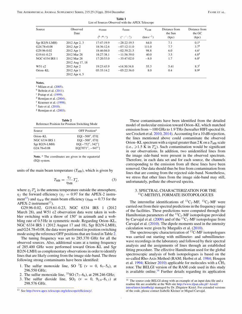
Table 1List of Sources Observed with the APEX Telescope
Source Observed αJ2000 δJ2000 VLSR Distance from Distance fromDate the Sun the GC
(h :m: .s) (◦ : ′ : .′′) (km s−1) (kpc) (kpc)
Sgr B2(N-LMH) 2012 Apr 2, 3 17:47:19.9 −28:22:19.5 64.0 7.1 0.1a
G24.78+0.08 2012 Apr 2 18:36:12.6 −07:12:11.0 111.0 7.7 3.7b
G29.96-0.02 2012 Apr 1 18:46:04.0 −02:39:21.5 98.8 6.0 4.6c
G19.61-0.23 2012 Mar 28 18:27:38.1 −11:56:39.0 40.0 3.5 4.8d
NGC 6334 IRS 1 2012 Mar 28 17:20:53.0 −35:47:02.0 −8.0 1.7 6.8e
2012 Aug 17, 18W51 e2 2012 Apr 2 19:23:43.9 +14:30:34.8 55.3 5.41 8.3f
Orion–KL 2012 Apr 1 05:35:14.2 −05:22:36.0 8.0 0.4 8.9g
2012 Apr 4, 5
Notes.a Milam et al. (2005).b Beltran et al. (2011).c Pratap et al. (1999).d Remijan et al. (2004).e Kraemer et al. (1998).f Sato et al. (2010).g Remijan et al. (2003).
Table 2Reference Position for Position Switching Mode
Source OFF Positiona
Orion–KL EQ[−500′′, 0.′′0]NGC 6334 IRS 1 EQ[−500′′, 0.′′0]Sgr B2(N-LMH) EQ[−752′′, 342′′]G24.78+0.08 EQ[7071′′, −947′′]
Note. a The coordinates are given in the equatorial(EQ) system.
units of the main beam temperature (TMB), which is given by
TMB = ηf
ηMBT ∗
A, (3)
where ηf T∗A is the antenna temperature outside the atmosphere,
ηf the forward efficiency (ηf = 0.97 for the APEX-2 instru-ment13) and ηMB the main beam efficiency (ηMB = 0.73 for theAPEX-2 instrument13).
G29.96-0.02, G19.61-0.23, NGC 6334 IRS 1 (2012March 28), and W51 e2 observation data were taken in wob-bler switching with a throw of 150′′ in azimuth and a wob-bling rate of 0.5 Hz in symmetric mode. Regarding Orion–KL,NGC 6334 IRS 1 (2012 August 17 and 18), Sgr B2(N-LMH),and G24.78+0.08, the data were performed in position switchingmode using the reference OFF positions that are listed in Table 2.
The tuning frequency was set to 285.370 GHz for all theobserved sources. Also, additional scans at a tuning frequencyof 285.400 GHz were performed toward Orion–KL and SgrB2(N-LMH) as complementary observations in order to identifylines that are likely coming from the image side-band. The threefollowing strong contaminants have been identified:
1. The sulfur monoxide line, SO 3Σ (v = 0, 67–56), at296.550 GHz;
2. The sulfur monoxide line, 33SO (77–66), at 298.246 GHz;3. The sulfur dioxide line, SO2 (v = 0, 92,8–81,7) at
298.576 GHz.
13 See http://www.apex-telescope.org/telescope/efficiency/.
These contaminants have been identified from the detailedmodel of molecular emission toward Orion–KL which matchedemission from ∼100 GHz to 1.9 THz (hereafter HIFI spectral fit,see Crockett et al. 2010, 2014). Accounting for a 10 dB rejection,the lines mentioned above could contaminate the observedOrion–KL spectrum with a signal greater than 2 K on a TMB scale(i.e., !1.5 K in T∗
A). Such contamination would be significantin our observations. In addition, two unidentified lines fromthe image side-band were present in the observed spectrum.Therefore, in each data set and for each source, the channelscorresponding to the emission from all these lines have beenremoved. Our data should thus be free from contamination fromlines that are coming from the rejected side-band. Nonetheless,we stress that other lines from the image side-band may still,unfortunately, pollute the observed spectra.
3. SPECTRAL CHARACTERIZATION FOR THE13C-METHYL FORMATE ISOTOPOLOGUES
The interstellar identifications of 13C1-MF, 13C2-MF werecarried out from their spectral predictions in the frequency rangeof the facilities. These predictions were computed through theHamiltonian parameters of the 13C2-MF isotopologue providedby Carvajal et al. (2009) and of the 13C1-MF isotopologue fromCarvajal et al. (2010). The dipole moments used in the intensitycalculation were given by Margules et al. (2010).
The spectroscopic characterization of 13C-MF isotopologueswas carried out starting with millimeter- and submillimeter-wave recordings in the laboratory and followed by their spectralanalysis and the assignments of lines through an establishedfitting procedure. The effective Hamiltonian used for the globalspectroscopic analysis of both isotopologues is based on theso-called Rho-Axis Method (RAM; Herbst et al. 1984; Hougenet al. 1994; Kleiner 2010) applicable for molecules with a CH3rotor. The BELGI version of the RAM code used in this studyis available online.14 Further details regarding its application
14 The source code BELGI along with an example of an input data file and areadme file are available at the Web site http://www.ifpan.edu.pl/∼kisiel/introt/introt.htm#belgi managed by Dr. Zbigniew Kisiel. For extended versionsof the code, please contact Isabelle Kleiner or Miguel Carvajal.
3

The Astrophysical Journal Supplement Series, 215:25 (31pp), 2014 December Favre et al.
Table 3Rotational–Torsional–Vibrational Partition Functiona
for 13C1-MF, 13C2-MF, and 12C-MF
T 13C1-MF 13C2-MF 12C-MF(K)
300.0 252230.47 255988.58 249172.44225.0 105303.23 106847.86 104015.96150.0 36879.42 37442.27 36433.4375.0 9003.31 9162.12 8894.0637.50 2920.56 2971.20 2885.3018.75 1027.71 1045.22 1015.319.375 364.76 370.95 360.33
Note. a The nuclear spin degeneracy was not considered inthese calculations (see Appendix A).
to the methyl formate isotopologues are described by Carvajalet al. (2007).
The Hamiltonian parameters were fitted to the experimentaldata of 13C2-MF (∼940 lines) which were provided only forthe ground torsional state vt = 0 (Carvajal et al. 2009). Newexperimental data for the vt = 0 ground and vt = 1 first excitedtorsional state have been recently processed (Haykal et al. 2014).A more extensive set of experimental data (∼7500 transitionlines) of the ground and first excited states of 13C1-MF has beenused in the fit of the RAM Hamiltonian. The complete set ofavailable experimental data (see Willaert et al. 2006; Carvajalet al. 2009; Maeda et al. 2008a, 2008b) was compiled in Carvajalet al. (2010).
3.1. Partition Functions
To calculate the observed intensities of the spectral lines,the populations of each level must be estimated using an accu-rate partition function in order to provide reliable estimates ofthe temperatures and column densities of the different regionsin the ISM. With this goal in mind, a convergence study forthe partition functions of 13C-isotopologues, which ensures thathigh enough energy levels have been included for a particulartemperature, has been carried out in this work. The partitionfunction calculations are described in the Appendix A. Table 3summarizes the rotational–torsional–vibrational partition func-tion values that are used here for 13C1-MF and 13C2-MF.
4. DATA ANALYSIS
4.1. Database and MF, 13C-MF Frequencies
We used the measured and predicted transitions coming fromboth the table of Ilyushin et al. (2009) and the JPL database15
(Pickett et al. 1992, 1998) for the MF line assignments, as inFavre et al. (2011). Regarding the methyl formate isotopologue13C1-MF and 13C2-MF line assignments, our present analysis isbased on this study (see Section 3) and on the spectroscopiccharacterization performed by Carvajal et al. (2007, 2009,2010). Likewise, the measured and predicted transitions of thespecies 13C1-MF species (Carvajal et al. 2010) are now availableon the CDMS database16 (Muller et al. 2001, 2005) and atSplatalogue17 (Remijan et al. 2007). Current spectroscopic datafor MF and 13C-MF treat both of the torsional substates—thosewith A symmetries and those E symmetries—simultaneously.
15 http://spec.jpl.nasa.gov/home.html16 http://www.astro.uni-koeln.de/cdms17 www.splatalogue.net
As we aim to derive accurate isotopic ratios, we should beconfident with the intensity calculation of the molecular speciesat different temperatures. Therefore, the isotope ratio accuracywill depend, on one hand, on the spectroscopic determinationof transition frequencies, assignments, and line strengths and,on the other hand, on the partition function approximation con-sidered. Accurate spectroscopic characterizations of the mainisotopologue was carried out previously (Ilyushin et al. 2009)using the RAM method, while for the 13C-MF isotopologues,we used the same values for the electric dipole moments as forthe 12C-MF species (see Section 3.1). This assumption wouldnot affect the line strengths by more than ∼1%. Hence, theaccurate derivation of the abundance ratio between differentisotopologues will rely, as far as the spectroscopic data are con-cerned, on the partition function. This was computed under thesame level of approximation for all the molecular species understudy. Table 3 shows the values of the partition function usedfor H12COOCH3. These values were computed on the basis ofthe new calculations in this manuscript to more fully accountfor the effect of vibrationally excited levels. In the JPL catalogentry, only contributions of the vt = 0 and vt = 1 level are in-corporated into the partition function, while here we account forall torsional–vibrational energy states. This results in a higherinferred 12C methyl formate abundance than would be derivedusing the value in the JPL catalog since the partition functionis now larger than in the JPL tables. The partition function usedhere is higher than that in the JPL catalog by a factor of 1.2 at atemperature of 150 K and by a factor of 2.5 at 300 K. Our moreaccurate partition functions yield a more accurate abundance ofmethyl formate than is reported in earlier publications.
It is also worthwhile to remark that the methyl formatepartition function provided in the JPL catalog file has an extrafactor of two in its formula with respect to ours. This factorarises from the product of the reduced nuclear spin and K-level degeneracy statistical weights gI , gk (Turner 1991; Favreet al. 2011). As for methyl formate, the statistical weights arecancelled in the intensity mathematical expression (see, e.g.,Equation (1) of Turner 1991); they have not been consideredin the partition function calculation of this paper. This meansthat when the comparison between the partition function of thiswork and the one provided in the JPL catalog was established,this latter was divided by a factor of 2.
Also, our spectral line analysis of the ALMA-SV observationsof Orion–KL takes into account the 12C methyl formate tran-sitions that are both in the ground and first torsionally excitedstates, since they seem to probe a similar temperature toward thisregion (see Favre et al. 2011; Kobayashi et al. 2007). However,regarding the sources observed with the APEX telescope, wehave only considered methyl formate transitions in their groundtorsional states vt = 0. More specifically, the number of de-tected transitions in the vt = 1 state (four lines with a similarupper energy level) is insufficient to determine any trend withrespect to transitions emitting in the ground state (vt = 0).
4.2. XCLASS Modeling and Herschel/HIFI Spectral Fit
Assuming local thermodynamic equilibrium (LTE), we havemodeled all the methyl formate isotopologue emission by usingthe XCLASS18 program along with the HIFI spectral fit whichare based on the observations of Orion–KL acquired withHerschel/HIFI as part of the Herschel Observations of Extra-Ordinary Sources key program (Bergin et al. 2010; Crockett
18 http://www.astro.uni-koeln.de/projects/schilke/XCLASS
4

The Astrophysical Journal Supplement Series, 215:25 (31pp), 2014 December Favre et al.
Table 4Number of Detected Transitions of 12C-MF and 13C-MF in the ALMA-SV data of Orion–KLa
Spwb Compact Ridge Hot Core-SW
HCOOCH3 H13COOCH3 HCOO13CH3 HCOOCH3 H13COOCH3 HCOO13CH3
0 1 1 2 1 . . . 21 3 . . . 6 3 . . . 12 19 10 3 19 7 33 5 6 3 5 3 34 11 7 4 10 3 45 20 13 6 19 5 56 5 12 . . . 5 4 . . .
7 6 2 13 4 . . . 68 11 11 1 8 5 . . .
9 10 13 2 9 10 210 4 1 5 4 1 311 20 10 4 20 5 212 1 . . . 15 . . . . . . 613 2 4 17 2 3 1114 3 9 2 3 6 . . .
15 6 4 . . . 6 2 . . .
16 15 12 8 15 6 617 23 16 3 21 12 218 2 3 17 2 1 519 . . . 1 11 . . . . . . 6
Notes.a The corresponding line frequencies are given in Figures 5–10.b The ALMA-SV data consist of 20 spectral windows (see Section 2).
et al. 2014). This allows us to make reliable line identificationsand determine where potential line blends may exist. Furtherdetails regarding the XCLASS modeling of the Herschel/HIFIOrion–KL spectral scan, along with fit parameters, can be foundin Crockett et al. (2014).
In the present analysis, we assumed that the 13C1-MF and13C2-MF species emit within the same source size, at the samerotational temperature and velocity, and with the same line widthas the methyl formate molecule. The only adjustable parameteris the molecular column density. To initialize the model of theALMA-SV observations of Orion–KL, we used as input pa-rameters (source size, rotational temperature, column density,vLSR, and ∆vLSR), the values derived from our previous Plateaude Bure Interferometer (PdBI) observations, which were per-formed with a similar angular resolution (1.′′8 × 0.′′8, see Favreet al. 2011). Regarding the APEX observations, we used pre-viously related and reported values derived from single-dish(JCMT, IRAM–30m, Herschel) and/or interferometric observa-tions (BIMA, CARMA) as starting values to initialize the fitting.More specifically, we used the values derived by Bisschop et al.(2007) for G24.78+0.08; by Zernickel et al. (2012) and Bisschopet al. (2007) for NGC 6334I; by Demyk et al. (2008) for W51e2; by Shiao et al. (2010) for G29.96–0.02; by Belloche et al.(2009) for Sgr B2(N); by Remijan et al. (2004) and Shiao et al.(2010) for G19.61–0.23; and by Tercero et al. (2012), Carvajalet al. (2009), and Crockett et al. (2014) for Orion–KL.
5. RESULTS
In the following section we report the main results for eachobserving facility.
5.1. ALMA-SV Observations of Orion–KL
5.1.1. Emission Maps
The mean velocity for emission observed toward the CompactRidge and Hot Core-SW regions is around 7.3 km s−1 for all
the methyl formate isotopologues. We also observed a secondvelocity component around 9 km s−1 toward the CompactRidge in HCOOCH3 (as reported by Favre et al. 2011). Thisvelocity component is not observed in 13C-MF. Figure 1 showsmaps of the MF, 13C1-MF, and 13C2-MF emission in the7.2 km s−1 channel measured at 234124 MHz, 220341 MHz,and 216671 MHz, respectively. The HCOOCH3 distributionshows an extended V-shaped molecular emission that links radiosource I to the BN object as previously observed in methylformate by Favre et al. (2011) and Friedel & Snyder (2008).Likewise, as reported by Favre et al. (2011), the main molecularpeaks are located toward the Compact Ridge and the Hot Core-SW (respectively labeled MF1 and MF2 in Figure 1; for moredetails see Favre et al. 2011). Also from the optically thickHCOOCH3 lines, we note that another cold component (T ∼40–50 K) is observed arising from the vicinity of the sourceIRC7. However, we did not analyze this component in thepresent study. Finally, the 13C-MF isotopologues are mainlydetected toward the Compact Ridge and the Hot Core-SW (5σdetection level; see Figure 1).
5.1.2. Spectra
Numerous transitions of 12C-MF and 13C-MF with Sµ2 !10 D2 and from upper energy levels of 166 K up to 504 Kfor the main molecule and Eup of 99 K up to 330 K for the13C-MF species, are present in the ALMA data. We have mod-eled each spectral window individually (see Section 6.1.3). Ta-ble 4 provides the number of clearly detected MF and 13C-MFtransitions per spectral window toward both the Compact Ridgeand the Hot Core-SW. Table 12 in Appendix B summarizes theline parameters for all detected, blended, or not detected transi-tions of 12C-MF, 13C1-MF, and 13C2-MF in all ALMA spectralwindows. Furthermore, Figures 5, 6, and 7 in Appendix C showthe 12C-MF, 13C1-MF, and 13C2-MF transitions that are detectedand/or partially blended in the ALMA-SV data along with our
5

The Astrophysical Journal Supplement Series, 215:25 (31pp), 2014 December Favre et al.
Figure 1. HCOOCH3 (12C-MF, 234124 MHz, Eup = 179 K, Sµ2 = 35 D2, top left panel), H13COOCH3 (13C1-MF, 220341 MHz, Eup = 153 K, Sµ2 = 37 D2,top right panel), and HCOO13CH3 (13C2-MF, 216671 MHz, Eup = 152 K, Sµ2 = 36 D2, bottom panel) emission channel maps at 7.22 km s−1 as observed withALMA. The first contour and level step are 500 mJy beam−1 (∼14σ ) and 100 mJy beam−1 (∼5σ ) for 12C-MF and 13C-MF, respectively. The synthesized beam size is1.′′7 × 1.′′1. The black cross indicates the centered position of the observations. The main HCOOCH3 emission peaks (MF1 to MF5) identified by Favre et al. (2011)are indicated.(A color version of this figure is available in the online journal.)
best XCLASS models toward the Compact Ridge. In addition,Figures 8, 9, and 10 in Appendix D show the emission of thesame transitions, along with our models, toward the Hot Core-SW. The quality of our models is based on the reduced χ2,which lies in the range 0.3–2.4, depending on the fit.19 Morespecifically, the bulk of the emission is best reproduced for thefollowing.
1. A source size of 3′′ (in agreement with the ALMA-SVobservations) toward both the Compact Ridge and the HotCore-SW.
19 The optically thick lines, although some of them are shown in Appendices Cand D, are excluded from our model due to an optical depth problem.
2. A rotation temperature of 80 K toward the Compact Ridgeand of 128 K toward the Hot Core-SW.
3. A vLSR of 7.3 km s−1 for both components.4. A line width of 1.2 km s−1 toward the Compact Ridge and
of 2.4 km s−1 toward the Hot Core-SW.
Only the column density differs within the different spectral win-dows between the spatial components associated with Orion–KLand between the isotopologues. The 12C-MF models includethe observed second velocity component well reproduced for avLSR of 9.1 km s−1, a source size of 3′′, a rotation temperatureof 120 K, and a column density of 7 × 1016 cm−2.
6

The Astrophysical Journal Supplement Series, 215:25 (31pp), 2014 December Favre et al.
Figure 2. Isotopic ratio distribution of the methyl formate isotopologues within each ALMA spectral window as derived toward the Orion–KL Compact Ridge (toppanel) and Hot Core-SW (bottom panel). Top sub-panels: isotopic ratio distribution for the 12C/13C1 ratio. Middle sub-panels: isotopic ratio distribution for the12C/13C2 ratio. Bottom sub-panels: isotopic ratio distribution for the 12C/13C ratio, assuming the two 13C-MF isotopologues have similar abundances. The derivedaverage isotopic ratio is indicated in each sub-panel.(A color version of this figure is available in the online journal.)
7
The Astrophysical Journal Supplement Series, 215:25 (31pp), 2014 December Favre et al.
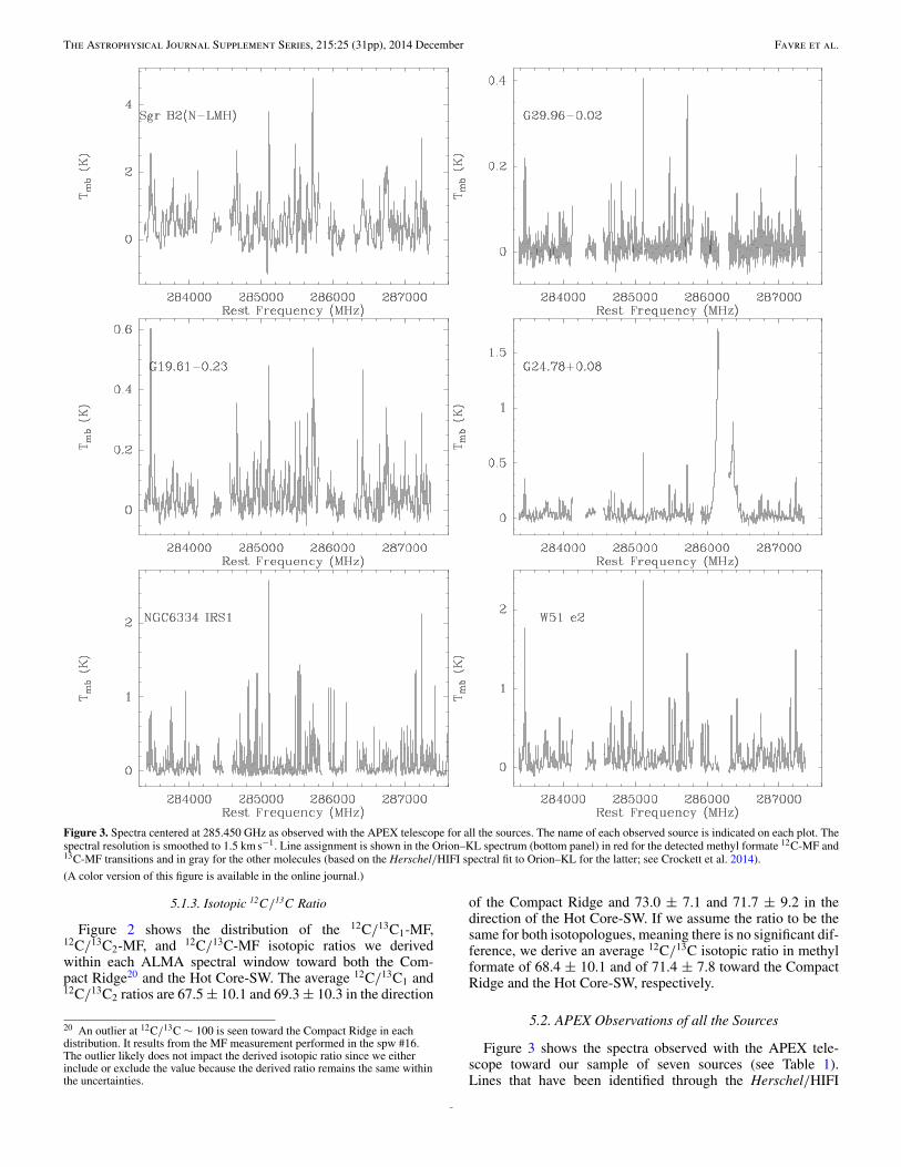
Figure 3. Spectra centered at 285.450 GHz as observed with the APEX telescope for all the sources. The name of each observed source is indicated on each plot. Thespectral resolution is smoothed to 1.5 km s−1. Line assignment is shown in the Orion–KL spectrum (bottom panel) in red for the detected methyl formate 12C-MF and13C-MF transitions and in gray for the other molecules (based on the Herschel/HIFI spectral fit to Orion–KL for the latter; see Crockett et al. 2014).(A color version of this figure is available in the online journal.)
5.1.3. Isotopic 12C/13C Ratio
Figure 2 shows the distribution of the 12C/13C1-MF,12C/13C2-MF, and 12C/13C-MF isotopic ratios we derivedwithin each ALMA spectral window toward both the Com-pact Ridge20 and the Hot Core-SW. The average 12C/13C1 and12C/13C2 ratios are 67.5 ± 10.1 and 69.3 ± 10.3 in the direction
20 An outlier at 12C/13C ∼ 100 is seen toward the Compact Ridge in eachdistribution. It results from the MF measurement performed in the spw #16.The outlier likely does not impact the derived isotopic ratio since we eitherinclude or exclude the value because the derived ratio remains the same withinthe uncertainties.
of the Compact Ridge and 73.0 ± 7.1 and 71.7 ± 9.2 in thedirection of the Hot Core-SW. If we assume the ratio to be thesame for both isotopologues, meaning there is no significant dif-ference, we derive an average 12C/13C isotopic ratio in methylformate of 68.4 ± 10.1 and of 71.4 ± 7.8 toward the CompactRidge and the Hot Core-SW, respectively.
5.2. APEX Observations of all the Sources
Figure 3 shows the spectra observed with the APEX tele-scope toward our sample of seven sources (see Table 1).Lines that have been identified through the Herschel/HIFI
8

The Astrophysical Journal Supplement Series, 215:25 (31pp), 2014 December Favre et al.
Figure 3. (Continued)
spectral fit are indicated in the Orion–KL spectrum (see bot-tom panel on Figure 3). The molecular richness of the ob-served sources is clearly seen. Also, the different spectra il-lustrate the problem of the spectral confusion for the weakeremissive lines.
5.2.1. Main Isotope: HCOOCH3
Table 5 lists the detected or partially blended methyl formatetransitions, with Sµ2 ! 2.5 D2 and Eup up to 304 K as observedwith APEX toward the different sources. Note that for some par-tially blended lines, the emission arising from the contaminanthas been identified through the Herschel template spectra inwhich emission from 35 molecules has been modeled assumingLTE (Crockett et al. 2014). The following procedure was used:(1) superposing the Herschel resulting model on the APEX ob-servations and identifying the potential contaminant(s), and (2)adjusting the observational parameters (e.g., velocity, typicalline width) to the model and checking the coherence over thefull spectrum. The adopted parameters (source size, rotationaltemperature, column density, velocity, and line width) that wereused to model the APEX observations are given in Table 6 foreach source. The quality of our models is based on the reducedχ2, which lies in the range 0.23–4.75. In addition, Figure 4shows the observed methyl formate spectrum of the transitionat 285973.267 MHz (238,15–228,14,E) along with our models foreach source.
The main observational results for the methyl formatemolecule are briefly summarized below for the individualsources.
Orion–KL. We detected 16 HCOOCH3 lines and observed15 transitions that are partially blended with Sµ2 ! 4 D2 (seeTable 5). The LSR velocity is 7.7 km s−1 and the derived columndensity is 9.7 × 1016 cm−2.
W51 e2. We detected 11 HCOOCH3 lines and observed6 transitions that are partially blended. Fourteen transitions(with Sµ2 " 12 D2) are too faint to be detected (which iscommensurate with our model of the source). The spectradisplay a vLSR of 55.6 km s−1 and we derived a column densityof 9.0 × 1016 cm−2.
G19.61-0.23. We detected 10 HCOOCH3 lines and observed7 transitions that are partially blended while 14 transitions weretoo faint to be detected. The vLSR is 39.7 km s−1 and the derivedcolumn density is 7.0 × 1016 cm−2.
Figure 4. HCOOCH3 (12C-MF, transition at 285973.267 MHz, left panel) andHCOO13CH3 (13C2-MF, transition at 284730.102 MHz, right panel) syntheticspectra (in red) overlaid on the observed spectrum (in black) as observed withAPEX. The name of the source is indicated on each plot.(A color version of this figure is available in the online journal.)
G29.96-0.02. We detected 10 HCOOCH3 lines and observed7 transitions that are partially blended. Fourteen transitions weretoo faint to be detected. Spectra display a vLSR of 97.8 km s−1
and we derived a column density of 3.5 × 1015 cm−2.G24.78+0.08. We detected 10 HCOOCH3 lines and observed
7 transitions that are partially blended while 14 transitions weretoo faint to be detected. The vLSR is 111 km s−1 and we derivedcolumn density of 6.0 × 1015 cm−2.
NGC 6334 IRS 1. We detected 11 HCOOCH3 lines and ob-served 6 transitions that are partially blended with 14 transi-tions that were too faint to be detected. Spectra exhibit a vLSR of−8 km s−1 and we derived a column density of 4.5 × 1017 cm−2.
Sgr B2(N). We detected 7 HCOOCH3 lines and observed 9transitions that are partially blended while 14 transitions weretoo faint to be detected. The vLSR is around 63.7 km s−1. Wederived a column density of 3.0 × 1017 cm−2.
9

The Astrophysical Journal Supplement Series, 215:25 (31pp), 2014 December Favre et al.
Table 5Transitions of 12C and 13C-Methyl Formate Observed with the APEX Telescope
Frequency Transition Eup Sµ2 Notea
(MHz) (K) (D2)Orion–KL W51 e2 G19.61-0.23 G29.96-0.02 G24.78+0.08 NGC 6334 IRS 1 Sgr B2(N-LMH)
HCOOCH3
283734.887 2311,12–2211,11 E 243.2 45.4 D D D D PB D D283746.738 2311,13–2211,12 A 243.2 45.4 PB PB PB PB PB PB PB283746.738 2311,12–2211,11 A 243.2 45.4 PB PB PB PB PB PB PB283760.086 2311,13–2211,12 E 243.2 45.4 D D D D D D PB284398.680 135,8–124,9 E 70.4 2.5 D ND ND ND ND ND ND284410.529 135,8–124,9 A 70.4 2.7 PB ND ND ND ND ND ND284810.313 235,19–225,18 E 180.8 55.8 PB PB PB PB PB PB PB284826.396 235,19–225,18 A 180.8 55.8 D D D D D D D284885.531 2711,16–2710,17 A 303.7 7.6 PB ND ND ND ND ND ND284886.320b 2711,16–2710,17 E 303.7 6.1 PB ND ND ND ND ND ND284920.240 239,14–229,13 E 217.0 49.8 D D D D D D D284937.218 239,15–229,14 A 217.0 49.9 PB PB PB PB PB PB PB284942.751 239,14–229,13 A 217.0 49.9 PB PB PB PB PB PB PB284945.147 239,15–229,14 E 216.9 49.8 PB PB PB PB PB PB PB285016.270 234,20–223,19 E 173.3 6.3 PB ND ND ND ND ND ND285016.977 234,20–223,19 A 173.3 6.3 PB ND ND ND ND ND ND285351.819 243,21–234,20 E 187.0 6.8 PB ND ND ND ND ND ND285370.140 243,21–234,20 A 187.0 6.8 D ND ND ND ND ND ND285515.739 225,17–215,16 E 169.4 53.7 D D D D D D D285542.584 225,17–215,16 A 169.4 53.7 D D PB PB D D PB285924.822 238,16–228,15 A 205.9 51.8 D D D D D D –285940.794 238,16–228,15 E 205.9 49.9 D D D D D D D285973.267 238,15–228,14 E 206.0 49.9 D D D D D D D286012.485 238,15–228,14 A 205.9 51.8 D D D D D D D286467.129b 2511,14–2510,15 A 272.2 5.5 PB ND ND ND ND ND ND286984.997 116,5–105,5 E 62.8 3.2 PB ND ND ND ND ND ND286994.417 116,6–105,5 A 62.8 3.2 PB ND ND ND ND ND ND287038.552 116,5–105,6 A 62.8 3.2 D ND ND ND ND ND ND287094.976 2411,14–2410,15 E 257.4 6.3 D ND ND ND ND ND ND287101.120 2411,13–2410,14 E 257.4 6.3 D ND ND ND ND ND ND287146.630 237,17–227,16 E 196.4 53.4 D D D D D D PB
H13COOCH3
283853.856 238,16–228,15 E 204.3 52.9 ND∗ ND∗ ND∗ ND∗ ND∗ ND∗ ND∗
286035.726 237,16–227,15 A 195.0 56.7 ND∗ ND∗ ND∗ ND∗ ND∗ ND∗ ND∗
HCOO13CH3
284729.511c 271,27–261,26 E 194.2 71.1 D D TD ND∗ ND∗ D TD284729.537c 270,27–260,26 E 194.2 71.1 D D TD ND∗ ND∗ D TD284730.102c 271,27–261,26 A 194.2 71.1 D D TD ND∗ ND∗ D TD284730.127c 270,27–260,26 A 194.2 71.1 D D TD ND∗ ND∗ D TD
Notes.a D: detected; TD: tentative detection; PB: partial blend; ND and ND∗: not detected (too faint emission). Also, ND∗ indicates the 13C1– and 13C2–HCOOCH3transitions that are emitting with an intensity less than or equal to three times the noise level which we used to constrain our model. The symbol “–” indicates that partof the spectrum has been removed (see Section 2.2.2).b These two transitions are predicted, i.e., not measured.c Pile-up of these four lines. Also the frequencies presented in this table are only computed (i.e., not measured) because experimental data for these transitions are notyet available.
5.2.2. H13COOCH3
The 13C1-MF lines all appear to be blended or just at orbelow the confusion limit level. We note that some transitionsoverlap with lines from strongly emissive molecules such asethyl cyanide (whose presence is known through the Herscheltemplate spectra to Orion–KL; Crockett et al. 2014), whichmight hide faint emission. We therefore do not detect the13C1–methyl formate toward any of the observed sources,excluding Orion–KL and that only in the supplementary ALMAdata.
5.2.3. HCOO13CH3
We report the detection of one transition of 13C2-MF to-ward Orion–KL, W51 e2, NGC 6334 IRS 1, and (ten-tatively) G19.61-0.23 and Sgr B2(N) (see Figure 4 andTable 5). More specifically, the spectral feature that we assignedto 13C2–HCOOCH3 is a pile-up of four lines with frequenciesin the range 284729–284730 MHz, with a line strength of 71 D2
and an upper energy level of 194 K (Table 5). Figure 4 exhibitsthe observed spectrum of the HCOO13CH3 transition emitting at284730 MHz along with our XCLASS for each source (reduced
10

The Astrophysical Journal Supplement Series, 215:25 (31pp), 2014 December Favre et al.
Table 612C-MF and 13C-MF XCLASS Model Parameters (Source Size, Rotational Temperature,
Column Density, Velocity, and Line Width) That Best Reproduce the APEX Spectra
Source θs Trot Ntot vLSR ∆v
(′′) (K) (cm−2) (km s−1) (km s−1)HCOOCH3 H13COOCH3 HCOO13CH3
Sgr B2(N-LMH)a 4 80 3.0 × 10¹⁷ !1.8 × 10¹⁶ !1.8 × 10¹⁶ 63.7 7.0G24.78+0.08b 10 121 6.0 × 10¹⁵ !3.0 × 10¹⁴ !3.0 × 10¹⁴ 111.0 6.0G29.96-0.02b 10 150 3.5 × 10¹⁵ !3.0 × 10¹⁴ !3.0 × 10¹⁴ 97.8 5.5G19.61-0.23a 3.3 230 7.0 × 10¹⁶ !5.0 × 10¹⁵ !5.0 × 10¹⁵ 39.7 4.5NGC 6334 IRS 1c 3 115 4.5 × 10¹⁷ !2.0 × 10¹⁶ !2.0 × 10¹⁶ −8.0 5.0W51 e2c 7 176 9.0 × 10¹⁶ !3.0 × 10¹⁵ !3.0 × 10¹⁵ 55.6 8.0Orion–KLc 10 100 9.7 × 10¹⁶ !1.82 × 10¹⁵ !1.82 × 10¹⁵ 7.7 3.7
Notes.a Observed sources where HCOO13CH3 is tentatively detected.b Observed sources where HCOO13CH3 is not detected.c Observed sources where one transition of HCOO13CH3 is detected.
Table 712C/13C–HCOOCH3 Ratio as Measured with ALMA and APEX, Respectively
Source 12C/13C for CO 12C/13C for CO 12C/13C–HCOOCH3c
CN and H2COa Onlyb
ALMA observations
Orion–KL—Compact Ridge 74 ± 16 67 ± 17 68.4 ± 10.1Orion–KL—Hot Core-SW 74 ± 16 67 ± 17 71.4 ± 7.8
APEX observations
Sgr B2(N-LMH)d 19 ± 7 20 ± 8 "17G24.78+0.08e 42 ± 11 39 ± 12 "20G29.96-0.02e 47 ± 12 44 ± 13 "11G19.61-0.23d 49 ± 12 45 ± 13 "14NGC 6334 IRS 1f 61 ± 14 56 ± 15 "23W51 e2f 70 ± 16 64 ± 17 "30Orion–KLf 74 ± 16 67 ± 17 "53
Notes.a Based on the following equation for CO, CN, and H2CO, 12C/13C = 6.21(1.00)DGC + 18.71(7.37) fromMilam et al. (2005) (see Equation (2)).b Based on the following equation for CO, 12C/13C = 5.41(1.07)DGC + 19.03(7.90) from Milam et al.(2005) (see Equation (1)).c This study, assuming that both 13C1-MF and 13C2-MF isotopologues have similar abundances (i.e.,(12C − MF)/(13C1 − MF) = (12C − MF)/(13C2 − MF), see Section 5.1 and Figure 2).d Observed sources where HCOO13CH3 is tentatively detected.e Observed sources where HCOO13CH3 is not detected.f Observed sources where one transition of HCOO13CH3 is detected.
χ2 of about 0.23–0.69). We infer that it is difficult to attributethis spectral feature to another molecule on the basis that:
1. The line rest frequencies of these four lines are predictedwith an uncertainty of 0.012 MHz (which corresponds to0.012 km s−1).
2. Several 13C2–methyl formate transitions with similar Sµ2
and Eup are detected in the ALMA-SV data of Orion–KL(see Section 5.1.). Furthermore, their excitation level inOrion–KL is consistent with the emission level of this line(and non-detection of other lines) in the APEX data.
3. This is the strongest line in the APEX band and the twonext highest Sµ2 lines (at 67 and 61 D2) are respectivelyblended and at the level of the confusion limit.
We note that, given the sensitivity limit in all the sourcesexcept Orion–KL (because of the ALMA-data), we cannot
claim a definitive detection of this molecule in the APEXobservations.
5.2.4. Isotopic 12C/13C Ratio
Since we do not have definitive detections of the 13C-MF,Table 7 lists the lower limits of the isotopic 12C/13C ratio thatare estimated assuming that the two 13C-MF isotopologues havesimilar abundances. Please note that the upper limits of the13C-MF column density have been set by adjusting the observa-tional parameters to the model with a resulting fit constrainedby a 3σ upper limit. The quality of our models is still based onthe reduced χ2 calculations.21
21 The reduced χ2 roughly gives a measure of how the model fits the data overthe bandpass.
11

The Astrophysical Journal Supplement Series, 215:25 (31pp), 2014 December Favre et al.
6. DISCUSSION
6.1. Measurement Caveats
The analysis above relies on some assumptions. In thefollowing section, we discuss whether they could modify theinterpretation of our derived 12C/13C ratio.
6.1.1. LTE and Radiative Pumping Effects
It is important to note that the above analysis hinges uponthe assumption that methyl formate is in LTE, which appliesat high densities in hot cores. We assumed that LTE is a rea-sonable approximation given that the model fit to the Herschelobservations of methyl formate in Orion–KL contained over athousand emissive transitions that are closely fit using an LTEmodel (Crockett et al. 2014). A strong IR radiation field couldaffect the LTE analysis. Among the observed sources, Orion–KLand Sgr B2(N) have the strongest IR radiation field. Therefore,radiative pumping effects, if present, would be the strongesttoward those sources. The Herschel observations and analysisof Orion–KL and Sgr B2(N) (Crockett et al. 2014; Neill et al.2014) have shown that 1) pumping is not needed to fit the linesas LTE closely matches the observed emission and 2) therewas evidence for radiative pumping in emission lines of othermolecules, in particular methanol, but not for methyl formate.
6.1.2. Contamination from Strong Absorption Lines in Sgr B2(N)
Contamination from strong absorption lines in Sgr B2(N) mayalso affect methyl formate emission. There are two potential lev-els of contamination that could be an issue. First is absorptionof methyl formate which lies in the foreground envelope. How-ever, all the transitions that we have detected in this study coverfairly high energy levels that are not populated in the envelope(e.g., Neill et al. 2014). Another issue would be contaminationfrom other species with ground state transitions that have similarfrequencies; we see no evidence for this in our data.
6.1.3. Scattering on the Isotopic Ratio of the Methyl FormateIsotopologues within each ALMA Spectral Window
Another possible caveat of our 12C/13C ratio estimate isthe individual modeling of each sub-band of the ALMA-SVobservations of Orion–KL. In our exploration of the ALMA-SVdata, we found that a large source of uncertainty is a roughly 10%difference in calibration between sub-bands; that is, some sub-bands have a slightly different calibration than other sub-bands.We infer that this is due to some structure (which could be aslope, a curvature, or a frequency dependence) in the calibrationthat affects the band pass and results in this slight measurementuncertainty that exists within a given sub-band.
Based upon this and due to the fact that different sub-bandshave a different number of lines (see Table 4), we have chosento fit the 12C/13C ratio in each sub-band individually and to usethe relative errors in the fit from those bands to set the absoluteuncertainty to our measurement. Nevertheless, it is importantto note that a single set of parameters (not shown here) also fitall the data and give rise, within the uncertainties, to a similarisotopic abundance ratio.
6.2. Comparison of the Derived ColumnDensities with Previous Studies
In this section, we relate our results to previous studiesperformed toward our source sample. Our models are not
unique and some differences with previously reported resultscan appear. This is in part due to the different (and moreaccurate) 12C-MF partition functions used here (see discussionin Section 4.1). Also, we note that for all the observed sources,the observed vLSR and ∆vLSR are consistent with those in theliterature.
Orion–KL. From the ALMA-SV observations of Orion–KL,we derived a methyl formate column density over all the spectralwindows of 5–8.5 × 1017 cm−2 toward the Compact Ridge andof 3.3–4.3 × 1017 cm−2 toward the Hot Core–SW. These resultsare higher by a factor of 2–5 with our reported values obtainedfrom observations using the Plateau de Bure Interferometer andperformed with a similar synthesized beam (1.′′8 × 0.′′8, seeFavre et al. 2011). This discrepancy can be explained by the factthat in this study we used a different partition function which,as discussed in Section 4.1, results in a higher inferred 12C-MF abundance compared with the 12C-MF abundance derivedusing the JPL catalog partition function used by Favre et al.(2011). The spatial and the velocity distribution are in agreementwith previous observations (Favre et al. 2011; Friedel & Snyder2008). We refer to Favre et al. (2011) for a detailed comparisonwith previous related interferometric and single-dish studiesperformed by Friedel & Snyder (2008), Beuther et al. (2005),Liu et al. (2002), Remijan et al. (2003), Hollis et al. (2003),Blake et al. (1996, 1987), Schilke et al. (1997), and Ziurys &McGonagle (1993).
For the Orion–KL observations carried out with the APEXtelescope, the bulk of the HCOOCH3 emission is well repro-duced by a single component model with a rotational temper-ature of 100 K, a source size of 10′′, and a column densityof 9.6 × 1016 cm−2. Our derived APEX rotational temperatureand column density agree with the Herschel/HIFI observations(Crockett et al. 2014) as well as with Favre et al. (2011) inwhich the authors do not separate the two HCOOCH3 velocitycomponents (Trot of 101 K, NHCOOCH3 = 1.5 × 1017 cm−2).
Regarding the H13COOCH3 and HCOO13CH3 species, theirdetection toward Orion–KL has previously been reported byCarvajal et al. (2009) based on IRAM 30 m observations.The authors used a source size of 15′′, a column densityof 7 × 1014 cm−2, and a rotational temperature of 110 Kto reproduce the emission arising from the Compact Ridgecomponent associated with Orion–KL. The 13C2-MF columndensity, derived from the APEX observations, lies in the range7–9.8 × 1015 cm−2 and differs from the one derived by Carvajalet al. (2009). This is likely due to the fact that we use a differentpartition function (see above) along with different assumptionswith regard to the beam filling factor (source size of 3′′ and aTrot of 80 K for our best models).
W51 e2. From the APEX observations, we derived a slightlylower (factor 1.8) of methyl formate column density in compar-ison to the measured column density reported by Demyk et al.(2008).
G19.61-0.23. Using CARMA observations (2′′ resolution),Shiao et al. (2010) have reported a derived column density of(9 ± 2) × 1016 cm−2 given a rotation temperature of 161 K.Likewise, using BIMA observations, Remijan et al. (2004)derived from a source average of 2.′′8 and a column densityin methyl formate of 3.4 × 1017 cm−2 given a temperature of230 K. In our analysis, we have adopted the HCOOCH3 rotationtemperature derived by Remijan et al. (2004) rather than the onereported by Shiao et al. (2010). This choice is based upon thefact that Shiao et al. (2010) used a temperature derived fromethyl cyanide observations whereas Remijan et al. (2004) used
12

The Astrophysical Journal Supplement Series, 215:25 (31pp), 2014 December Favre et al.
a rotation temperature based on methyl formate observations.Our best fit results in a methyl formate column density of 7 ×1016 cm−2 is commensurate with the value derived from theCARMA observations. Regarding the BIMA observations, thedifference between the derived column densities is likely due tobeam dilution.
G29.96-0.02. Using 2′′ resolution CARMA observations,Shiao et al. (2010) have reported a derived column density of(4 ± 1) × 1016 cm−2 which is in agreement with our results (seeTable 6), taking into account the different assumptions about thesource size with respect to beam.
G24.78+0.08. The HCOOCH3 column density derived fromthe APEX observations (see Table 6) differs from the one derivedby Bisschop et al. (2007) likely due to different assumptions withregard to the beam filling factor.
NGC 6334 IRS 1. The deviation from values reported byBisschop et al. (2007) is also likely due to different assumptionswith regard to the beam filling factor. Nonetheless, our valueof 4.5 × 1017 cm−2 is consistent with the value reported byZernickel et al. (2012) (N = 7 × 1017 cm−2 for a 3′′ source size)from Herschel/HIFI observations of this region.
Sgr B2(N). Using IRAM 30m observations of Sgr B2(N),Belloche et al. (2009) modeled methyl formate emission usingtwo velocity components associated with two sources separatedby only 5.′′3 (based on PdBI and ATCA observations; seeBelloche et al. 2008). These components differ by about9 km s−1. Our best model includes only the component emittingat the systemic velocity of the source (i.e., 63.7 km s−1) and ourderived parameters are in agreement with the study performedby Belloche et al. (2009).
6.3. Isotopologue Detection and Sensitivity
Our analysis points out the need for high sensitivity to detectisotopologues of complex molecules. Indeed, due to lack ofsensitivity in our APEX observations, only one 13C2-MF line(pile-up of four 13C2 transitions with Sµ2 of 71 D2) is detectedand, most of the 13C1-MF transitions emit below and/or at theconfusion limit level. In contrast, both 13C-MF isotopologuesare detected in observations performed with higher sensitivity(e.g., Carvajal et al. 2009, and this study for the supplementaryALMA data.).
6.4. The 13C Budget in the Galaxy
From Equation (1) for CO and Equation (2) for CO, CN,and H2CO (Milam et al. 2005), we have calculated the 12C/13Cratio in CO for each of the sources observed with the APEXtelescope and for ALMA-SV observations of Orion–KL. Thesevalues are given in Table 7. Our study shows that the derivedlower limits for the APEX 12C/13C–methyl formate ratios areconsistent within the uncertainties with the 12C/13C ratio in COfor each source. The same conclusion applies for the isotopicratios derived toward the Orion–KL Hot Core-SW and compactridge positions (ALMA-SV data).
6.5. Implications
Numerous measurements of the 12C/13C isotopic ratio havebeen performed through several molecular tracers, such asCO and OCS, toward Orion–KL. For example, from OCSand H2CS isotopologue observations Tercero et al. (2005)have reported an average ratio of 45 ± 20. Using methanolobservations, Persson et al. (2007) have found a 12C/13C
isotopic ratio 57 ± 14. Savage et al. (2002) derived a ratioof 43 ± 7 in CN. From 13CO observations, Snell et al. (1984)have reported an average 12CO/13CO isotopic ratio of 74 ±9 in the high-velocity outflow of Orion–KL. Likewise, frominfrared measurements performed with the Kitt Peak Mayall4m telescope, Scoville et al. (1983) obtained a 12CO/13COisotopic ratio of 96 ± 5. Using C18O observations, Langer &Penzias (1990) and Langer & Penzias (1993) derived ratios of63 ± 6 and 74 ± 9 according to the observed position. Thesefindings suggest that the gas in Orion–KL does not seem tobe heavily fractionated since the 12C/13C ratio in most simplespecies is almost the same. Our results are consistent with thisfinding since:
1. For each of the 13C-MF isotopologues, the derived isotopicratios (68.4 ± 10.1 toward the Compact Ridge and of 71.4 ±7.8 toward the Hot Core-SW; see Figure 2) are consistentwith each other.
2. These results are consistent within the error bars with thevalues derived for CH3OH and for CO by Persson et al.(2007), Snell et al. (1984) and Scoville et al. (1983) towardOrion–KL.
Therefore, the present observations do not support methyl for-mate formation in the gas-phase from 12C/13C fractionatedgas. In addition, regarding methyl formate gas-phase forma-tion mechanisms, Horn et al. (2004) have shown that there areno very efficient gas-phase pathways to form methyl formate,meaning that there are no efficient primary pathways to form the13C-MF isotopologues either. One possibility that could lead togas-phase formation of the 13C-MF isotopologues would bea “secondary” fractionation process involving the 12C–methylformate itself and 13C+ (E. Herbst 2014, private communica-tion). Such reactions, however, are unlikely to occur since highbarriers are expected. This would also argue against the pos-sibility of methyl formate gas–phase formation from 12C/13Cfractionated gas. This finding combined with the hypothesis ofWirstrom et al. (2011) strongly suggests that grain surface re-actions are likely the main pathways to form methyl formate(12C and 13C).
7. CONCLUSIONS
We have investigated the 12C/13C isotopic ratio in methylformate toward a sample of massive star-forming regionslocated over a range of distances from the Galactic center,through observations performed with the APEX telescope. Inaddition, we have measured the 12C/13C-methyl formate ratiotoward Orion–KL using the ALMA-SV observations. Also, wereported new spectroscopic measurements of the H13COOCH3and HCOO13CH3 species. Our study is based on this laboratoryspectral characterization and points out the importance of thesedata in deriving accurate partition functions and thereforeabundances of methyl formate. Our analysis also points out thatto accurately derive a reliable abundance ratio between differentspecies, it is necessary to use a homogeneous observationaldatabase.
We have performed LTE modeling of the observationaldata. A multitude of 13C1-MF and 13C2-MF transitions havebeen detected in the ALMA-SV observations carried out to-ward Orion–KL, (1) confirming the previous detection of the13C-MF isotopologues reported by Carvajal et al. (2009) and,(2) imaging their spatial distribution for the first time. Assumingthat the two 13C-MF isotopologues have similar abundances,we reported a 12C/13C isotopic ratio in methyl formate of
13

The Astrophysical Journal Supplement Series, 215:25 (31pp), 2014 December Favre et al.
68.4 ± 10.1 and 71.4 ± 7.8 toward the Compact Ridge and HotCore-SW components, respectively. A salient result is that thosemeasurements are consistent with the 12C/13C ratio measuredin CO and in CH3OH. Our findings suggest that grain surfacechemistry very likely prevails in the formation of methyl formatemain and 13C isotopologues.
Regarding the APEX observations, we have reported atentative detection (!3σ level) of the 13C2-MF isotopologuetoward the following four massive star-forming regions: SgrB2(N-LMH), NGC 6334 IRS 1, W51 e2, and G19.61-0.23. Thederived lower limits for the 12C/13C–methyl formate ratio areconsistent with the 12C/13C ratio measured in CO showing anincreasing ratio with distance from the Galactic center. A largersource sample and further observations with high sensitivity areessential to confirm this trend.
In addition, we used the Herschel/HIFI spectral tools, whichare available to the community (Crockett et al. 2014), to makereliable line identifications and to appreciate where potentialline blends may exist. The current work illustrates how to wecan merge the legacy of Herschel with other telescopes such asALMA.
This work was supported by the National Science Foun-dation under grant 1008800. We are grateful to the Minis-terio de Economıa y Competitividad of Spain for the finan-cial support through grant No. FIS2011-28738-C02-02 and tothe French Government through grant No. ANR-08-BLAN-0054 and the French PCMI (Programme National de PhysiqueChimie du Milieu Interstellaire). This paper makes use of thefollowing ALMA data: ADS/JAO.ALMA#2011.0.00009.SV.ALMA is a partnership of ESO (representing its member states),NSF (USA), and NINS (Japan), together with NRC (Canada)and NSC and ASIAA (Taiwan), in cooperation with the Re-public of Chile. The Joint ALMA Observatory is operatedby ESO, AUI/NRAO, and NAOJ. C.F. thanks Dahbia Talbi,Eric Herbst, and Anthony Remijan for enlightening discus-sions. Finally, we thank the anonymous referee for helpfulcomments.
Facilities: APEX, Herschel/HIFI, ALMA
APPENDIX A
PARTITION FUNCTION CALCULATIONS
Several approximations for the partition function have beenused, following, e.g., Blake et al. (1987), Turner (1991),Oesterling et al. (1999), Groner et al. (2007), Demyk et al.(2008), Maeda et al. (2008b), Favre et al. (2011), and Tu-dorie et al. (2012). In the present work, the partition func-tion was approximated as the product of the rotational(Qrot), torsional (Qtor), and vibrational (without the tor-sional contribution, Qvib) contributions (Herzberg 1991) and isgiven by:
Q = gns
!
i
(2 Ji + 1)e− EikB T ≈ gns Qrot Qtor Qvib, (A1)
where Ji stands for the rotational angular momentum of leveli, kB is the Boltzmann constant, T is the temperature, and Eiis the vibrational–torsional–rotational energy which is referredto in the ground vibrational–torsional state as the zero pointenergy. The nuclear spin degeneracy gns does not need to betaken into account in the calculations of the partition functionbecause gns is the same for all MF symmetry states (A1, A2,
Table 8Comparison between the Rotational Partition Functiona Computed
as a Direct sum Qrot (A2) and as the Approximated ExpressionQ
apprrot (A3) for 13C1-MF and 13C2-MF
T 13C1-MF 13C2-MF
(K) Qapprrot Qrot
b Qapprrot Qrot
b
300.0 32682.30 32737.70 33291.76 33289.35225.0 21227.78 21308.82 21623.63 21672.46150.0 11554.94 11599.33 11770.41 11797.7075.0 4085.29 4100.86 4161.47 4170.9237.50 1444.37 1451.06 1471.30 1475.8218.75 510.66 514.10 520.18 522.869.375 180.55 182.57 183.91 185.67
Notes.a The nuclear spin degeneracy was not considered in these calculations.b The rotational partition function obtained as a direct sum of energy levels upto J = 79 is the used in the final result.
and E). Based on the C3v(M) symmetry (Bunker & Jensen1998) gns = 16 for both 13C-MF isotopologues of methylformate.
When observed intensities are estimated, gns in the nu-merator is canceled with that of the denominator inside thepartition function. Thus, gns will henceforth be ignored andexcluded in the comparisons of partition functions of 13C-MFisotopologues.
A.1. Rotational Partition Function
The rotational partition function Qrot was obtained usingEquation (9) of Groner et al. (2007):
Qrot =!
J,Ka,Kc
(2 J + 1) e− E
(rot)i
kB T , (A2)
where E(rot)i are the rotational energies, that is, those for the
rotational states only in the A-symmetry ground torsional state.The RAM model (Herbst et al. 1984; Hougen et al. 1994;Kleiner 2010) was used to predict the torsional–rotationalstates as explained before. Also, the torsional–rotational states(vt = 0 and A-symmetry) up to J = 79 were included inEquation (A2), which is enough for the convergence studymentioned above.
A comparison was done with the asymmetric top ap-proximation for the rotational partition function of Herzberg(1991). For sufficiently high temperatures (or small rotationalconstants):
Qapprrot ≈
"π
APAM BPAM CPAM
#kBT
h
$3
, (A3)
where the rotational constants refer to the principal axis system,not to the Rho-Axis System. Therefore, an appropriate transfor-mation was performed from the rotational parameters given inCarvajal et al. (2009, 2010).
The rotational partition function computed as a direct sum(Equation (A2)) is in general, for both 13C-MF isotopologues,slightly larger than the one for the approximated partitionfunction (Equation (A3)), as shown in Table 8. For this reason,we used here the rotational partition function as a directsummation instead of using the approximated partition function
14

The Astrophysical Journal Supplement Series, 215:25 (31pp), 2014 December Favre et al.
Table 9Torsional Partition Function for 13C1-MF at Different Approximationsa
T Q0tor Q1
tor Q2tor Q4
tor Q6tor
b Qharmtor
c
(K)
300.0 1.99994 3.06540 3.71217 4.39180 4.52333 4.28020225.0 1.99991 2.86364 3.30761 3.68701 3.73003 3.52028150.0 1.99987 2.56748 2.77670 2.89625 2.90098 2.7925375.0 1.99974 2.16083 2.18274 2.18678 2.18679 2.1752037.50 1.99948 2.01246 2.01270 2.01270 2.01270 2.0130618.75 1.99896 1.99905 1.99905 1.99905 1.99905 2.000089.375 1.99793 1.99793 1.99793 1.99793 1.99793 2.00000
Notes.a The approximations are carried out by considering a number of torsional statesup to a maximum quantum number vmax
t in Equation (A4).b Computed torsional partition function used as a final result in the presentwork.c Harmonic approximation for the torsional partition function:
Qharmtor = 1
1−e− E(tor)(vt =1,A)
kB T
+ 1
1−e− E(tor)(vt =1,E)
kB T
(Equation (A3)). In Table 8 it can be seen that the differencesbetween Qrot and Q
approxrot can be around 1% for T = 9.375 K,
decreasing for higher temperatures to the error range estimatedby Herzberg (1991).
A.2. Torsional Partition Function
The torsional contribution Qtor to the partition function wasobtained through the following formula:
Qvmax
t
tor =vmax
t!
vt=0
#e− E(tor)(vt ,A)
kB T + e− E(tor)(vt ,E)
kB T
$, (A4)
where E(tor)(vt , A) and E(tor)(vt , E) are the energies of thetorsional states with a quantum number vt for the A (A1 or A2)and E symmetries, respectively, referring to the vt = 0 groundtorsional state, i.e., E(tor)(vt = 0, A) = 0 cm−1. Differentapproximations can be carried out depending on the maximumvalue vmax
t considered in the equation. The torsional energiesused in Equation (A4) are the following:
1. Torsional energies from vt = 0 to vt = 2 computedfrom the Hamiltonian parameters of the RAM model.The torsional energies of 13C1-MF are computed with theparameters of Carvajal et al. (2010) and those of 13C2-MFare computed with the parameters of Carvajal et al. (2009).These torsional energies are expected to be very reliable forthe 13C1-MF.
2. Torsional energies from vt = 3 to vt = 4 of the mainspecies of methyl formate given by Senent et al. (2005)and considered as a good approximation for both 13C-MFisotopologues.
3. Torsional energies from vt = 5 to vt = 6 were roughly es-timated in the present work, where E(tor)(vt = m,A) =m × E(tor)(vt = 1, A) and E(tor)(vt = m,E) = m ×E(tor)(vt = 1, E) and m will take values of 5 or 6.This is only an estimate to understand the contributionof these torsional levels to the torsional partition func-tion whose contribution is of 3% for T = 300 K, 1.2%for T = 225 K, 0.2% for 150 K, etc....(see Tables 9and 10).
Table 10Torsional Partition Function for 13C2-MF at different Approximationsa
T (K) Q0tor Q1
tor Q2tor Q4
tor Q6tor
b Qharmtor
c
300.0 1.99994 3.07133 3.69952 4.37914 4.51465 4.30756225.0 1.99991 2.87006 3.29709 3.67650 3.72124 3.54028150.0 1.99987 2.57382 2.77116 2.89072 2.89573 2.8049575.0 1.99974 2.16445 2.18394 2.18798 2.18798 2.1794937.50 1.99948 2.01305 2.01324 2.01324 2.01324 2.0136618.75 1.99896 1.99906 1.99906 1.99906 1.99906 2.000099.375 1.99793 1.99793 1.99793 1.99793 1.99793 2.00000
Notes.a The approximations are carried out by considering a number of torsional statesup to a maximum quantum number vmax
t in Equation (A4).b Computed torsional partition function used as a final result in the presentwork.c Harmonic approximation for the torsional partition function:
Qharmtor = 1
1−e− E(tor)(vt =1,A)
kB T
+ 1
1−e− E(tor)(vt =1,E)
kB T
As the torsional mode is very anharmonic, we cannot usethe harmonic approximation for the torsional partition function.From our results (Tables 9 and 10), when computing thetorsional partition function, the harmonic approximation couldbe assumed only for temperatures T < 100 K. Above T = 100 K,the anharmonicity has the natural effect of increasing theestimated torsional partition function. This effect can be around5% at 300 K.
In Tables 9 and 10, the torsional partition function at differentapproximations is shown for 13C1-MF and 13C2-MF isotopo-logues respectively. It can be noted that for T = 300 K theconvergence is reached to within 1% when the torsional statesabove vt = 6 are included. For temperatures T < 200 K, thecontribution of the torsional states above vt = 4 is insignificant.In fact, at temperatures close to 100 K and below, convergenceis reached (within 0.9% at T = 100 K) when only vt = 0, 1, and2 are considered.
A.3. Vibrational Partition Function
In the calculation of the vibrational partition function Qvib,it is expected that for ISM temperatures, only the informationof the vibrational frequencies at lower energies (≈300 cm−1) isnecessary. In order to check the convergence of the vibrationalpartition function, the contribution of the remaining vibrationalmodes has been taken into consideration. For this purpose, theharmonic approximation of the vibrational partition function isconsidered in general as:
Qvib = Π3N−7i=1
1
1 − eE(vib)i /kBT
(A5)
where N is the number of atoms of the molecule, and E(vib)i
is the vibrational fundamental frequencies of each vibrationalmode of the molecule. As the torsion is treated apart, theproduct in Equation (A5) will only expand to the 3N − 7small amplitude vibrational modes. It is important to notethat no experimental vibrational frequencies exist for the 13C-MF species. Therefore, to take into account the vibrationalcontribution of the partition function, we assumed that thevibrational fundamental frequencies of 13C1-MF and 13C2-MFare approximately the same as for the main isotopologue giventhe large experimental uncertainties (mostly of 6–15 cm−1;
15

The Astrophysical Journal Supplement Series, 215:25 (31pp), 2014 December Favre et al.
Table 11Vibrational Partition Function for
13C1-MF and 13C2-MF
T (K) Qvib
300.0 1.70330225.0 1.32486150.0 1.0959975.0 1.0039737.50 1.0000118.75 1.000009.375 1.00000
Chao et al. 1986). In this instance, the experimental vibrationalenergies for the main isotopologue taken from Chao et al. (1986)are also valid for their other isotopologues. The vibrationalpartition function computed with Equation (A5) is given inTable 11.
In this work, for the temperature ranges considered, all thesmall amplitude vibrational fundamentals in Equation (A5)are included. Nevertheless, when the temperatures are aroundT = 200 K, all vibrational fundamentals could be omitted in thevibrational partition function except those of ν14 and ν1 modes(around 300 cm−1). Below T = 100 K, inclusively ν14 and ν1modes could be neglected.
A.4. Rotational–torsional–vibrational Partition Function
In addition, we have assessed that the partition function sepa-rated into functions of each rotational, torsional, and vibrationalcontribution is a good enough approximation for temperaturesat least under 300 K. This assessment was set up after com-paring our partition function calculation with that derived fromits general expression, Equation (3), for vt = 0 and 1. Finally,Table 3 summarizes the rotational–torsional–vibrational par-tition function values that are used here for 13C1-MFand 13C2-MF.
APPENDIX B
TRANSITIONS OF 12C AND 13C-METHYL FORMATEOBSERVED WITH THE ALMA TELESCOPE
TOWARD ORION–KL
Table 12 summarizes the line parameters for all detected,blended, or not detected transitions of 12C-MF, 13C1-MF and13C2-MF in all ALMA spectral windows.
Table 12Transitions of 12C and 13C-Methyl Formate
Observed with the ALMA Telescope
Frequency Transition Eup Sµ2
(MHz) (K) (D2)
HCOOCH3a
214631.77 ∗ 175,12–165,11 (E, vt=0) 108 41214652.63 ∗ 175,12–165,11 (A, vt=0) 108 41214782.36 ∗ 183,16–173,15 (E, vt=0) 106 46214792.55 ∗ 183,16–173,15 (A, vt=0) 106 46214816.95 192,18–182,17 (A, vt=1) 296 49214942.87 191,18–181,17 (A, vt=1) 296 49215073.92 192,18–182,17 (E, vt=1) 296 49215193.55 191,18–181,17 (E, vt=1) 296 49215579.61 182,16–172,15 (A, vt=1) 293 46215837.59 201,20–191,19 (A, vt=1) 299 53
Notes.a This table lists the detected, blended, partially blended, andoptically thin lines of HCOOCH3. Transitions that are emitting withan intensity less than or equal to three times the noise level whichwe used to constrain our model are also listed. Transitions with the“∗” symbol are transitions we estimate to be optically thick.
(This table is available in its entirety in a machine-readable form inthe online journal. A portion is shown here for guidance regardingits form and content.)
APPENDIX C
METHYL FORMATE EMISSION TOWARDTHE ORION–KL COMPACT RIDGE AS
OBSERVED WITH ALMA
Figures 5, 6, and 7 show the respective spectra of the de-tected HCOOCH3, H13COOCH3, and HCOO13CH3 transitionsobserved with ALMA toward the Orion–KL Compact Ridgeduring the science verification program, along with our bestmodels achieved using the XCLASS program.
APPENDIX D
METHYL FORMATE EMISSION TOWARD THEORION–KL HOT CORE-SW AS OBSERVED WITH ALMA
Figures 8, 9, and 10 show the respective spectra of the de-tected HCOOCH3, H13COOCH3, and HCOO13CH3 transitionsobserved with ALMA toward the Orion–KL Hot Core-SW dur-ing the science verification program, along with our best modelsachieved using the XCLASS program.
16

The Astrophysical Journal Supplement Series, 215:25 (31pp), 2014 December Favre et al.
Figure 5. HCOOCH3 spectra (black) toward the Compact Ridge component associated with Orion–KL and model (red), as observed with ALMA. The intensity scaleis in TMB (K). The x-axis scale is about ±9.5 MHz centered on the line rest frequency, which is indicated below each plot.(A color version of this figure is available in the online journal.)
17
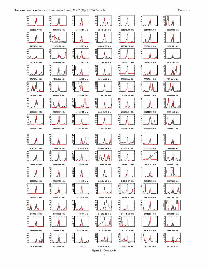
The Astrophysical Journal Supplement Series, 215:25 (31pp), 2014 December Favre et al.
Figure 5. (Continued)
18

The Astrophysical Journal Supplement Series, 215:25 (31pp), 2014 December Favre et al.
Figure 5. (Continued)
Figure 6. H13COOCH3 spectra (black) toward the Compact Ridge component associated with Orion–KL and model (red), as observed with ALMA. The intensityscale is in TMB (K). The x-axis scale is about ±9.5 MHz centered on the line rest frequency, which is indicated below each plot.(A color version of this figure is available in the online journal.)
19

The Astrophysical Journal Supplement Series, 215:25 (31pp), 2014 December Favre et al.
Figure 6. (Continued)
20

The Astrophysical Journal Supplement Series, 215:25 (31pp), 2014 December Favre et al.
Figure 7. HCOO13CH3 spectra (black) toward the Compact Ridge component associated with Orion–KL and model (red) as observed with ALMA. The intensityscale is in TMB (K). The x-axis scale is about ±9.5 MHz centered on the line rest frequency, which is indicated below each plot.(A color version of this figure is available in the online journal.)
21

The Astrophysical Journal Supplement Series, 215:25 (31pp), 2014 December Favre et al.
Figure 7. (Continued)
22

The Astrophysical Journal Supplement Series, 215:25 (31pp), 2014 December Favre et al.
Figure 8. HCOOCH3 spectra (black) toward the Hot Core-SW component associated with Orion–KL and model (red), as observed with ALMA. The intensity scaleis in TMB (K). The x-axis scale is about ±9.5 MHz centered on the line rest frequency, which is indicated below each plot.(A color version of this figure is available in the online journal.)
23
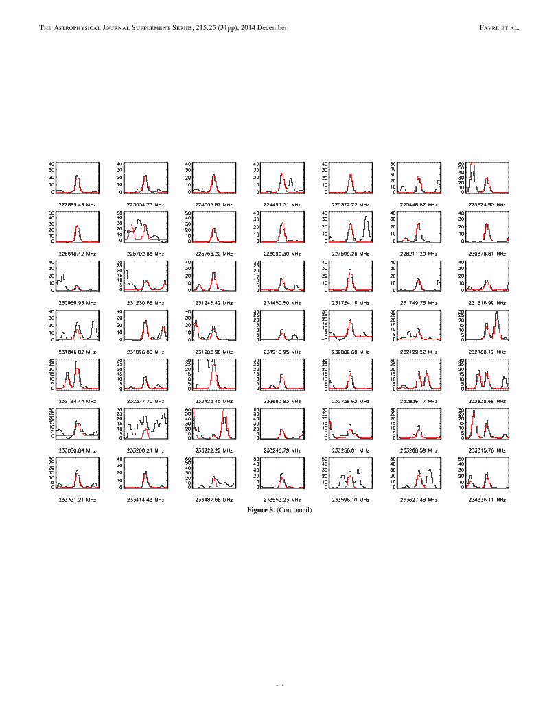
The Astrophysical Journal Supplement Series, 215:25 (31pp), 2014 December Favre et al.
Figure 8. (Continued)
24

The Astrophysical Journal Supplement Series, 215:25 (31pp), 2014 December Favre et al.
Figure 8. (Continued)
25

The Astrophysical Journal Supplement Series, 215:25 (31pp), 2014 December Favre et al.
Figure 9. H13COOCH3 spectra (black) toward the Hot Core-SW component associated with Orion–KL and model (red), as observed with ALMA. The intensity scaleis in TMB (K). The x-axis scale is about ±9.5 MHz centered on the line rest frequency, which is indicated below each plot.(A color version of this figure is available in the online journal.)
26

The Astrophysical Journal Supplement Series, 215:25 (31pp), 2014 December Favre et al.
Figure 9. (Continued)
27

The Astrophysical Journal Supplement Series, 215:25 (31pp), 2014 December Favre et al.
Figure 9. (Continued)
28

The Astrophysical Journal Supplement Series, 215:25 (31pp), 2014 December Favre et al.
Figure 10. HCOO13CH3 spectra (black) toward the Hot Core-SW component associated with Orion–KL and model (red), as observed with ALMA. The intensityscale is in TMB (K). The x-axis scale is about ±9.5 MHz centered on the line rest frequency, which is indicated below each plot.(A color version of this figure is available in the online journal.)
29

The Astrophysical Journal Supplement Series, 215:25 (31pp), 2014 December Favre et al.
Figure 10. (Continued)
30

The Astrophysical Journal Supplement Series, 215:25 (31pp), 2014 December Favre et al.
REFERENCES
Belloche, A., Garrod, R. T., Muller, H. S. P., et al. 2009, A&A, 499, 215Belloche, A., Menten, K. M., Comito, C., et al. 2008, A&A, 482, 179Beltran, M. T., Cesaroni, R., Zhang, Q., et al. 2011, A&A, 532, A91Bennett, C. J., & Kaiser, R. I. 2007, ApJ, 661, 899Bergin, E. A., Phillips, T. G., Comito, C., et al. 2010, A&A, 521, L20Beuther, H., Zhang, Q., Bergin, E. A., & Sridharan, T. K. 2009, AJ, 137, 406Beuther, H., Zhang, Q., Bergin, E. A., et al. 2007, A&A, 468, 1045Beuther, H., Zhang, Q., Greenhill, L. J., et al. 2005, ApJ, 632, 355Bisschop, S. E., Jørgensen, J. K., van Dishoeck, E. F., & de Wachter, E. B. M.
2007, A&A, 465, 913Blake, G. A., Mundy, L. G., Carlstrom, J. E., et al. 1996, ApJL, 472, L49Blake, G. A., Sutton, E. C., Masson, C. R., & Phillips, T. G. 1987, ApJ,
315, 621Briggs, D. S. 1995, BAAS, 27, 1444Bunker, P. R., & Jensen, P. (ed.) 1998, Molecular Symmetry and Spectroscopy
(Ottawa: NRC Research Press)Carvajal, M., Kleiner, I., & Demaison, J. 2010, ApJS, 190, 315Carvajal, M., Margules, L., Tercero, B., et al. 2009, A&A, 500, 1109Carvajal, M., Willaert, F., Demaison, J., & Kleiner, I. 2007, JMoSp, 246, 158Chao, J., Hall, K. R., Marsh, K. N., & Wilhoit, R. C. 1986, JPCRD, 15, 1369Charnley, S. B., Ehrenfreund, P., Millar, T. J., et al. 2004, MNRAS, 347, 157Charnley, S. B., & Rodgers, S. D. 2005, in IAU Symp. 231, Astrochemistry:
Recent Successes and Current Challenges, ed. D. C. Lis, G. A. Blake, & E.Herbst (Cambridge: Cambridge Univ. Press), 237
Clark, B. G. 1980, A&A, 89, 377Crockett, N. R., Bergin, E. A., Neill, J. L., et al. 2014, ApJ, 787, 112Crockett, N. R., Bergin, E. A., Wang, S., et al. 2010, A&A, 521, L21Cuppen, H. M., van Dishoeck, E. F., Herbst, E., & Tielens, A. G. G. M.
2009, A&A, 508, 275Demyk, K., Wlodarczak, G., & Carvajal, M. 2008, A&A, 489, 589Favre, C., Despois, D., Brouillet, N., et al. 2011, A&A, 532, A32Fontani, F., Pascucci, I., Caselli, P., et al. 2007, A&A, 470, 639Friedel, D. N., & Snyder, L. E. 2008, ApJ, 672, 962Friedel, D. N., & Widicus Weaver, S. L. 2012, ApJS, 201, 17Garrod, R. T., & Herbst, E. 2006, A&A, 457, 927Garrod, R. T., Weaver, S. L. W., & Herbst, E. 2008, ApJ, 682, 283Groner, P., Winnewisser, M., Medvedev, I. R., et al. 2007, ApJS, 169, 28Haykal, I., Carvajal, M., Tercero, B., et al. 2014, A&A, 568, A58Herbst, E., Messer, J. K., de Lucia, F. C., & Helminger, P. 1984, JMoSp,
108, 42Herbst, E., & van Dishoeck, E. F. 2009, ARA&A, 47, 427Herzberg, G. 1991, Spectra and Molecular Structure: II. Infrared and Raman
Spectra of Polyatomic Molecules (Malabar, FL: Krieger)Hollis, J. M., Lovas, F. J., & Jewell, P. R. 2000, ApJL, 540, L107Hollis, J. M., Pedelty, J. A., Snyder, L. E., et al. 2003, ApJ, 588, 353Horn, A., Møllendal, H., Sekiguchi, O., et al. 2004, ApJ, 611, 605Hougen, J. T., Kleiner, I., & Godefroid, M. 1994, JMoSp, 163, 559Ilyushin, V., Kryvda, A., & Alekseev, E. 2009, JMoSp, 255, 32Kalenskii, S. V., & Johansson, L. E. B. 2010, ARep, 54, 1084Kleiner, I. 2010, JMoSp, 260, 1Kobayashi, K., Ogata, K., Tsunekawa, S., & Takano, S. 2007, ApJL,
657, L17Kraemer, K. E., Jackson, J. M., & Lane, A. P. 1998, ApJ, 503, 785Langer, W. D., Graedel, T. E., Frerking, M. A., & Armentrout, P. B. 1984, ApJ,
277, 581Langer, W. D., & Penzias, A. A. 1990, ApJ, 357, 477
Langer, W. D., & Penzias, A. A. 1993, ApJ, 408, 539Liu, S., Girart, J. M., Remijan, A., & Snyder, L. E. 2002, ApJ, 576, 255Liu, S., Mehringer, D. M., & Snyder, L. E. 2001, ApJ, 552, 654Maeda, A., De Lucia, F. C., & Herbst, E. 2008a, JMoSp, 251, 293Maeda, A., Medvedev, I. R., De Lucia, F. C., Herbst, E., & Groner, P.
2008b, ApJS, 175, 138Margules, L., Huet, T. R., Demaison, J., et al. 2010, ApJ, 714, 1120Mehringer, D. M., Snyder, L. E., Miao, Y., & Lovas, F. J. 1997, ApJL, 480, L71Milam, S. N., Savage, C., Brewster, M. A., Ziurys, L. M., & Wyckoff, S.
2005, ApJ, 634, 1126Muller, H. S. P., Schloder, F., Stutzki, J., & Winnewisser, G. 2005, JMoSt, 742,
215Muller, H. S. P., Thorwirth, S., Roth, D. A., & Winnewisser, G. 2001, A&A,
370, L49Neill, J. L., Bergin, E. A., Lis, D. C., et al. 2014, ApJ, 789, 8Neill, J. L., Steber, A. L., Muckle, M. T., et al. 2011, JPCA, 115, 6472Oesterling, L. C., Albert, S., De Lucia, F. C., Sastry, K. V. L. N., & Herbst, E.
1999, ApJ, 521, 255Olmi, L., Cesaroni, R., Hofner, P., et al. 2003, A&A, 407, 225Persson, C. M., Olofsson, A. O. H., Koning, N., et al. 2007, A&A, 476, 807Pickett, H. M., Poynter, I. R. L., Cohen, E. A., et al. 1998, JQSRT, 60, 883Pickett, H. M., Poynter, R. L., & Cohen, E. A. 1992, NASA STI/Recon Technical
Report N, 94, 13813Pratap, P., Megeath, S. T., & Bergin, E. A. 1999, ApJ, 517, 799Remijan, A., Shiao, Y., Friedel, D. N., Meier, D. S., & Snyder, L. E. 2004, ApJ,
617, 384Remijan, A., Snyder, L. E., Friedel, D. N., Liu, S., & Shah, R. Y. 2003, ApJ,
590, 314Remijan, A. J., & Markwick-Kemper, A. ALMA Working Group on Spectral
Line Frequencies. 2007, BAAS, 38, 963Requena-Torres, M. A., Martın-Pintado, J., Rodrıguez-Franco, A., et al.
2006, A&A, 455, 971Sato, M., Reid, M. J., Brunthaler, A., & Menten, K. M. 2010, ApJ, 720, 1055Savage, C., Apponi, A. J., Ziurys, L. M., & Wyckoff, S. 2002, ApJ, 578, 211Schilke, P., Groesbeck, T. D., Blake, G. A., & Phillips, T. G. 1997, ApJS,
108, 301Scoville, N., Kleinmann, S. G., Hall, D. N. B., & Ridgway, S. T. 1983, ApJ,
275, 201Senent, M. L., Villa, M., Melendez, F. J., & Domınguez-Gomez, R. 2005, ApJ,
627, 567Shiao, Y., Looney, L. W., Remijan, A. J., Snyder, L. E., & Friedel, D. N.
2010, ApJ, 716, 286Snell, R. L., Scoville, N. Z., Sanders, D. B., & Erickson, N. R. 1984, ApJ,
284, 176Tercero, B., Cernicharo, J., & Pardo, J. R. 2005, in IAU Symp. 235, Galaxy
Evolution Across the Hubble Time, ed. F. Combes & J. Palous (Cambridge:Cambridge Univ. Press), 203
Tercero, B., Margules, L., Carvajal, M., et al. 2012, A&A, 538, A119Tudorie, M., Ilyushin, V., Auwera, J. V., et al. 2012, JCP, 137, 064304Turner, B. E. 1991, ApJS, 76, 617Widicus Weaver, S. L., & Friedel, D. N. 2012, ApJS, 201, 16Willaert, F., Møllendal, H., Alekseev, E., et al. 2006, JMoSt, 795, 4Wilson, T. L. 1999, RPPh, 62, 143Wilson, T. L., & Rood, R. 1994, ARA&A, 32, 191Wirstrom, E. S., Geppert, W. D., Hjalmarson, Å., et al. 2011, A&A,
533, A24Wouterloot, J. G. A., & Brand, J. 1996, A&AS, 119, 439Zernickel, A., Schilke, P., Schmiedeke, A., et al. 2012, A&A, 546, A87Ziurys, L. M., & McGonagle, D. 1993, ApJS, 89, 155
31