applied sciences

Article

Machine Learning Methods for Herschel–BulkleyFluids in Annulus: Pressure Drop Predictions andAlgorithm Performance Evaluation

Abhishek Kumar 1 , Syahrir Ridha 1,2,* , Tarek Ganet 1 , Pandian Vasant 3 andSuhaib Umer Ilyas 2,*

1 Petroleum Engineering Department, Universiti Teknologi PETRONAS, 32610 Seri Iskandar, Perak DarulRidzuan, Malaysia; abhi.upes01@gmail.com (A.K.); tarekarbi.ganat@utp.edu.my (T.G.)

2 Institute of Hydrocarbon Recovery, Universiti Teknologi PETRONAS, 32610 Seri Iskandar, Perak DarulRidzuan, Malaysia

3 Fundamental and Applied Sciences Department, Universiti Teknologi PETRONAS, 32610 Seri Iskandar,Perak Darul Ridzuan, Malaysia; pvasant@gmail.com

* Correspondence: syahrir.ridha@utp.edu.my (S.R.); suhaib.ilyas@utp.edu.my (S.U.I.)

Received: 9 March 2020; Accepted: 4 April 2020; Published: 9 April 2020�����������������

Abstract: Accurate measurement of pressure drop in energy sectors especially oil and gas explorationis a challenging and crucial parameter for optimization of the extraction process. Many empiricaland analytical solutions have been developed to anticipate pressure loss for non-Newtonian fluids inconcentric and eccentric pipes. Numerous attempts have been made to extend these models to forecastpressure loss in the annulus. However, there remains a void in the experimental and theoreticalstudies to establish a model capable of estimating it with higher accuracy and lower computation.Rheology of fluid and geometry of system cumulatively dominate the pressure gradient in an annulus.In the present research, the prediction for Herschel–Bulkley fluids is analyzed by Bayesian NeuralNetwork (BNN), random forest (RF), artificial neural network (ANN), and support vector machines(SVM) for pressure loss in the concentric and eccentric annulus. This study emphasizes on theperformance evaluation of given algorithms and their pitfalls in predicting accurate pressure drop.The predictions of BNN and RF exhibit the least mean absolute error of 3.2% and 2.57%, respectively,and both can generalize the pressure loss calculation. The impact of each input parameter affectingthe pressure drop is quantified using the RF algorithm.

Keywords: annulus; deep learning; energy; Herschel–Bulkley fluid; Non-Newtonian fluids;pressure loss

1. Introduction

Non-Newtonian fluids have been used extensively in drilling oil and gas wells. The accuratesimulation of such complex fluid models aid in energy conservation and efficient operation management.During drilling operation drilling fluid or mud is circulated through drill string and annular spaceand carries out drilled cutting from wellbore which results in significant pressure loss. Hershel andBulkley [1] proposed a three-parameter model which is considered to be a near optimum modelfor rheological behavior of Non-Newtonian fluids, and it has been known to replace Bingham andpower-law models in recent years [2–9].

Wellbore hydraulic modeling is a key component for a successful drilling operation as it not onlyenhances the rate of penetration (ROP) but minimizes the risk of potential problems encounteredduring drilling operations such as stuck pipe, kicks, loss circulation, and other various activities leadingto non-productive time (NPT). Calculation of pressure drop in a wellbore is a critical parameter in

Appl. Sci. 2020, 10, 2588; doi:10.3390/app10072588 www.mdpi.com/journal/applsci

Appl. Sci. 2020, 10, 2588 2 of 22

planning and improving the efficiency of a drilling operation. The pressure drop in a pipe systemis widely affected by the flow regime, frictional forces by inner walls of pipe and fitting, changes inelevation, the dimension of pipes and rheological properties of the fluid being transported. As thedrilling mud is pumped from the mud tank to the well bore, it endures pressure loss while in circulationdue to numerous pipe connections and frequent elevation changes. The estimation of flowing pressuregradient in an annulus for well control or drilling operation optimization is very crucial for accuratecalculation of pressure drop in the annulus.

American Petroleum Institute (API) RP 13D recommends Herschel–Bulkley model for drillingfluids to calculate the frictional pressure drop in drill pipe and annulus. Different studies [2–5] havebeen carried out that utilized this model for eccentric and concentric annulus geometry. Most of theliterature do not account for wide range of eccentricity of annuli and the proposed solutions are eitheriterative or involve assumptions based on laboratory experiment or theoretical studies. The aim ofthe current research is to develop an intuitive methodology based on collinearity of the features inthe dataset containing the Herschel–Bulkley fluid model parameters and geometric constraints topredict pressure drop. To the authors’ knowledge, such investigation is not been studied in the existingliterature describing the novelty of the present research. This study evaluates the performance ofmachine learning for the non-Newtonian flow under fully developed laminar flow. This emphasisof this work is to demonstrate that machine learning algorithms can be a proficient alternative toapproximated physics-based solutions. A wide range of pipe diameters, eccentricity, yield stress,fluid index, and fluid composition have been considered in this study. This study implies that RFalgorithm can model such nonlinear fluid in high as well as low pressure regime. A comprehensiveinvestigation is performed on the effectiveness of different data-driven algorithms such as SupportVector Machine (SVM), artificial neural network (ANN), and random forest (RF) in comparison to adeep neural network like the Bayesian Neural Network (BNN).

2. Related Work

Numerous theoretical and experimental studies have been reported in the literature on thenon-Newtonian fluids for the concentric and eccentric annulus, but the study on the transient andthe turbulent flows are limited. Laminar flow in the concentric annulus for power-law and Binghamfluids were studied by Fredrickson et al. [10] with an analytical approach, while Hanks et al. [11] andBuchtelova et al. [12] developed a non-analytical solution for Herschel–Bulkley fluids concluding someerrors in the former approach. The correlations developed by Heywood and Cheng [13] predictedthe head loss for turbulent flow in pipes within range of ±50% for Herschel–Bulkley fluids. Thesolution of the flow for yield power law in the concentric annulus was given by Gucuyener andMehmetoglu [14]. A model proposed by Reed and Pilehvari [15] covered the laminar, transitional, andturbulent flow in the concentric annulus for Herschel–Bulkley fluids and introduced new effectivediameter concept. The solution of laminar flow for non-Newtonian fluid in eccentric annulus wasevaluated by Haciislamoglu [16], and later Haciislamoglu and Langlinais [17] developed a correlationfor power-law fluids in eccentric annuli. This correlation was applied by Kelessidis et al. [18] todetermine the pressure drop in eccentric annulus for non-Newtonian fluids.

Ahmed [19] used the generalized hydraulic equation developed for fluids in arbitrary shapedducts. In his study, the investigations of Kozicki [20], Luo and Peden [21], and Haciislamoglu andLanglinais [17] were used to determine the frictional pressure loss in eccentric annulus for flow underlaminar conditions. To predict the pressure loss in the annulus, Computational Fluid Dynamic (CFD)was applied by Karimi et al. [22] and Titus et al. [23] to address the flow of Herschel–Bulkley fluid ineccentric annuli. A comprehensive solution for Herschel–Bulkley fluids for laminar flow in concentricannulus was presented by Kelessidis et al. [24] which was extended to transitional and turbulent flowsby Founargiotakis et al. [25]. Sorgun and Ozbayoglu [26] used the Eulerian–Eulerian CFD modelto evaluate the velocity profile and determine frictional pressure loss in non-Newtonian fluids forboth eccentric and concentric annulus. Theoretical and experimental investigations conducted by

Appl. Sci. 2020, 10, 2588 3 of 22

Ahmed et al. [27] on (Yield Power Law) YPL fluids in eccentric and concentric annulus with piperotation to estimate the overall pressure loss. In another study by Ogugbue and Shah [28], different flowregimes were investigated for YPL fluids to investigate the flow properties in eccentric and concentricannuli for drag-reducing polymers. Mokhtari et al. [29] studied the impact on both velocity profiles andpressure loss across annulus by eccentricity. Vajargah and Van Oort et al. [30] concluded that laminarflow is comparatively affected more by eccentricity in comparison to turbulent flow. Erge et al. [31]suggested that while circulating, YPL fluids eccentricity has a dominant effect on annular pressure loss.

Artificial intelligence in the past decade has played an important role in complex optimizationproblems [32,33] especially in the oil and gas industry to enhance the understanding of thenon-homogeneous subsurface conditions with application of algorithms, such as Case Based Reasoning(CBR), Artificial Neural Network (ANN), Support Vector Machine (SVM), and fuzzy logics. Osmanand Aggour [34] and Jeirani and Mohebbi [35] used ANN with backpropagation to determine thedensity of the drilling mud and mud cake permeability, while Siruvuri et al. [36], Miri et al. [37] andMurillo et al. [38] used it for prediction of the stuck pipe while drilling. Apart from these mentionedcases ANN have been applied to a variety of conditions such as, Ahmed et al. [39] predicted ROP withhigher accuracy using ANN and Elkanty [40] used ANN to predict drilling fluid rheological propertiesin real-time. Ozbayoglu et al. [41] analyzed cutting bed height in high angle and horizontal wells usingANN trained with feed-forward with back propagation (BPNN). Rooki [42,43] used General RegressionNeural Network (GRNN) and BPNN for predicting pressure drop using the Herschel–Bulkley fluidmodel. Rooki and Rakhshkhorshid [44] used Radial Basis Neural Network (RBFN) for determiningthe hole cleaning condition during foam drilling. The fuzzy logics were used for mud densityestimation by Ahmadi et al. [45]. Yunhu et al. [46] used it for identifying the loss circulation zonewhile Chhantyal et al. [47,48] predicted mud density and mud outflow. Skalle et al. [49] used CBR bycreating 50 case-based information of North Sea to solve problem of lost. Al-Azani et al. [50] used SVMfor predicting cutting concentration in directional wells. Sameni and Chamkalani [51] used SVM toevaluate the performance of drilling in shaly formations with the help of coupled simulated annealing(CSA). Ahmed et al. [39] used SVM to predict ROP with higher performance margin than achievedby theoretical equations. ANN and SVM were used by Kankar et al. [52] for fault diagnosis of ballbearing. Guo et al. [53] and Wen et al. [54] used deep convolutional neural network for diagnosingfault. Castano et al. [55] used machine learning for object detection using virtual on-chip lidar sensor.

In recent years, these data mining algorithms have been used in many aspects of drilling industry.The success of an algorithm depends on the problem, its variables, bounds, and other complexitieslike pattern within data. However, the effectiveness of an algorithm to make it a solution for a givenproblem has no guarantee that it may outperform a random search [56].

3. Methodology

3.1. Herschel–Bulkley Rheological Model

Rheology is the study of the flow of fluids or materials that accounts for the behavior ofnon-Newtonian fluids. Bingham plastic [57] and the power law [58,59] are two-parameter models thatwere initially used in several studies to describe non-Newtonian characteristics of fluids. Hershel andBulkley [1] suggested a three-parameter model, also known as Yield Power Law (YPL), and later morecomplex models up to 5 parameters have also been suggested [3]. However, these high dimensionalrheological models are uncommon due to the complexity in evaluating the flow parameters such asvelocity profile, Reynolds number, pressure drop, and the hydraulic parameters. These parameterscould only be determined by numerical simulations [24]. To maintain the simplicity and calculationaccuracy, Herschel–Bulkley model is widely used in industry. The literature reveals that it better fitsthe two-parameter models [2, 3] which describes the drilling fluids rheology precisely [18–24]. Themodel is defined in Equation (1).

τ = τγ + κγ.n (1)

Appl. Sci. 2020, 10, 2588 4 of 22

where shear stress is represented by τ,Yield stress by τy, fluid consistency by k, n is fluid behavior index and γ denotes shear rate. The

pressure loss for the concentric annulus is calculated by Equation (2).

∆P =dp f

dL=

2 fρυ2

Do −Di=

4τw

Do −Di(2)

where, Do is outer diameter of annulus (m), Di is inner tube’s diameter of annulus (m), ρ is density offluid (kg/m3), τw is shear stress of wall (Pa), ƒ is the friction factor (dimensionless). Determination ofthe friction factor (ƒ) for different flow regimes requires an iterative trial and error method.

The non-Newtonian fluids represented by Herschel–Bulkley model pose few challenges whileperforming numerical simulations because the flow around the centre is characterized as plug regionand near the wall as non-plug flow. There are certain parametric conditions imposed under which theabove-mentioned model can approximate the behaviour of such fluids, such as K > 0, τγ > 0 and 0 < n<∞. Due to such restrictions, the complexity of the derived governing equations increases making ithighly non-linear in nature and requires strenuous effort to solve it. Many analytical and experimentalwork conducted in the past have been outlined in aforementioned literature that clearly illustrate thedifficulty associated with approximating the behaviour of such nonlinear three parameter fluid model.

3.2. Data Mining Algorithms

In the current study, three different architecture of machine learning models are investigated,such as Support Vector Machine which maps the m dimensional space data with a linear or nonlinearfunction. Artificial Neural Network is also considered as black box as it depends on backpropagationof randomly initialized weights to approximate solution for the targeted output. Random Forest is anensemble machine learning technique capable of performing regression using multiple decision treeswith a statistical technique called bagging. The detailed working of the algorithms used in this study isgiven in Appendix A. The algorithms are implemented in Python 3.7 using Scikit-Learn, Tensorflowand the results can be easily reproduced using the framework and software library.

3.3. Description of Experimental Data

Ahmed et al. [19] conducted detailed experiments for fully developed laminar flow andmeasured the corresponding pressure drop in concentric and eccentric annulus for fluids withvarious concentration of Xanthan Gum (XCD) and Polyanionic Cellulose (PAC). The data from theirstudy was utilized in current investigation (details of the fluid - Appendix B). The uncertainty in thedata and its reliability for scientific analysis is crucial for algorithmic realization of a physical process,and numerous methods were proposed recently [60–62] which deal with analyzing the unreliabilityof the data. In the presented study water test were conducted to evaluate and verify the reliabilityof instrumentation and data acquisition system, followed by Yield Power Law (YPL) fluids afterestablishing strong confidence on measurement. Zero readings of differential pressure and flow ratewas verified by Ahmed [19] to minimize the uncertainty in the experimental setup. However, the exactvalues of uncertainty and inconsistency in data is not reported in the reference [19]. The flow ratewas maintained until the steady-state condition was achieved. The data acquisition system recordedmeasurements at the rate of 4 Hz (four data points per second) for one to two-minute duration. Thedimensions of the testing facility used in the prediction is tabulated in Table 1. The input parametersused to predict the pressure drop are outlined in Table 2, while the temperature is maintained from therange of 27.8–45 ◦C and the pressure from 144.37–1332 kPa. Table 3 shows the range of the data usedin this study, where Di/Do is the inner and the outer cylinder diameter ratio, e is the eccentricity, n isthe flow behavior index, flow consistency index is given by K, τy is shear stress, Q is the fluid flow rate,∆P is measured pressure drop. Fluids of varying concentrations of XCD and PAC (Appendix B) arecirculated through different di/do ratio and eccentricity. The properties of all the fluids used in the

Appl. Sci. 2020, 10, 2588 5 of 22

study were measured with pipe viscometer. Total of 903 data points are collected, where 70% of themare used for training the algorithm and 30% for testing the proposed models.

Table 1. Dimension of the annular sections used in the study.

Annulus #1 Annulus #2 Annulus #3 Annulus #4

Pipe Diameter [m] 0.009652 0.0127 0.017272 0.016002Hole Diameter [m] 0.035052 0.035052 0.035052 0.020828

Di/Do 0.27 0.36 0.49 0.76

Table 2. Input parameters for the proposed data mining algorithms.

Input Parameters Dimension

Ratio of Diameter (Di/Do) unitlessFlow Behavior Index (n) unitless

Eccentricity of Annulus (e) unitlessConsistency Index (k) Pa.sn

Yield Stress (τy) PaFlow Rate (Q) m3/s

Table 3. Range of experimental data.

Parameters Maximum Minimum

(Di/Do) (—) 0.76 0.27e (—) 1 0n (—) 0.49 0.35

K (Pa.sn) 4.49 0.64τy (Pa) 14.4 0

Q (m3/s) 1380.33× 10−6 1.55× 10−6

∆P ( k Pa) 381.23 0.196

3.4. Performance Metrics

The data collected from the flow loop experiment has a variety of different dimensional units andranges. It is evident from Tables 2 and 3 that parameters such as e is unitless and ranging from 0 to 1,whereas, pressure loss is in the range of 0.196 to 381.23 kPa. In order to bring out a common scale toanalyze the features in the data without distorting or losing the values, we have transformed the datain the range of [0, 1] using a transformation function, given in Equations (3) and (4).

xstd =(x− xmin)

xmax − xmin(3)

xscale = xstd × (max−min) + min (4)

where x is the dimensional data while xscale is the scaled transformation of x using Equation (3)and Equation (4), xscale was used as input for subsequent algorithms. Three performance metrics,namely Mean Absolute Error (MAE), Coefficient of Determination (R2), and Root Mean Squared Error(RMSE) are used to measure the effectiveness of the applied predictive algorithm. RMSE quantifies thedisagreement between the predicted and observed data points that can be determined from Equation(5). MAE is indication of the relative divergence of the measured and the predicted values are computedfrom Equation (6).

RMSE =

√∑ni=1(yi − yi)

2

N(5)

Appl. Sci. 2020, 10, 2588 6 of 22

MAE =1N

n∑1

∣∣∣yi − yi∣∣∣ (6)

The coefficient of determination can be calculated using Equation (7). It is a statistical measure ofthe regression prediction and approximation with the real data point, where 1 indicates the regressionprediction perfectly fits the data.

R2 = 1−

∑n1(yi − yi)

2∑n1

(yi − yi

)2 (7)

where yi represents the predicted values, number of observations is represented by n, yi is the givendata point and Уi is the mean of the given values. The optimal condition for a predictive algorithm iswhen the RMSE = 0 and R2 = 1, the lower the RMSE and MAE score the better the quality of the result.

Four algorithms are used in this study to predict pressure drop in concentric and eccentric annulus,i.e., SVM, ANN, BNN, and RF.

4. Result and Discussion

The algorithms are evaluated based on the previously described metrics of RMSE, MAE, and R2.The predicted and the actual values are compared for train and test datasets. In a base case scenario,the predicted and the experimental values should yield a 45◦ slope line that can be illustrated as bestfit curve to visually inspect the deviation.

4.1. Prediction and Validation

4.1.1. Predictions via Support Vector Machine (SVM)

The parameters tuned for SVM are soft margin constant (C), kernel parameter, width of Gaussiankernel (gamma), and degree of polynomial fit. Hyperparameter C is typically a regularization parameterfor trade-off between the errors of training data. Kernel is iteratively selected to be radial bias functionas it gives higher accuracy in this case compared to other functions. Gamma is defined as the extentof influence by a single training example and is used for non-linear hyper planes and the degree is aparameter basically to define the polynomial fit of a hyper plane. The pressure loss for laminar flow inconcentric and eccentric annular annulus is predicted using SVM. The predicted values for the trainingand the test data are plotted in Figure 1 with observed pressure loss in the experimental setup. TheRMSE of 21.92 kPa and MAE of 17.92% is calculated for train data set with R2 = 0.925, while for testdata RMSE is 22 kPa, MAE is 18.34% with R2 = 0.83. Figure 1 illustrates that majority of the deviationfrom the 45◦ best fit curve lies below 50 kPa data points. The deviation is observed to be slightlyincreasing towards higher pressure scale.

Figure 1. Support Vector Machine (SVM) predicted pressure plotted with observed pressure loss:(a) training dataset and (b) test dataset.

Appl. Sci. 2020, 10, 2588 7 of 22

4.1.2. Predictions via Artificial Neural Network (ANN)

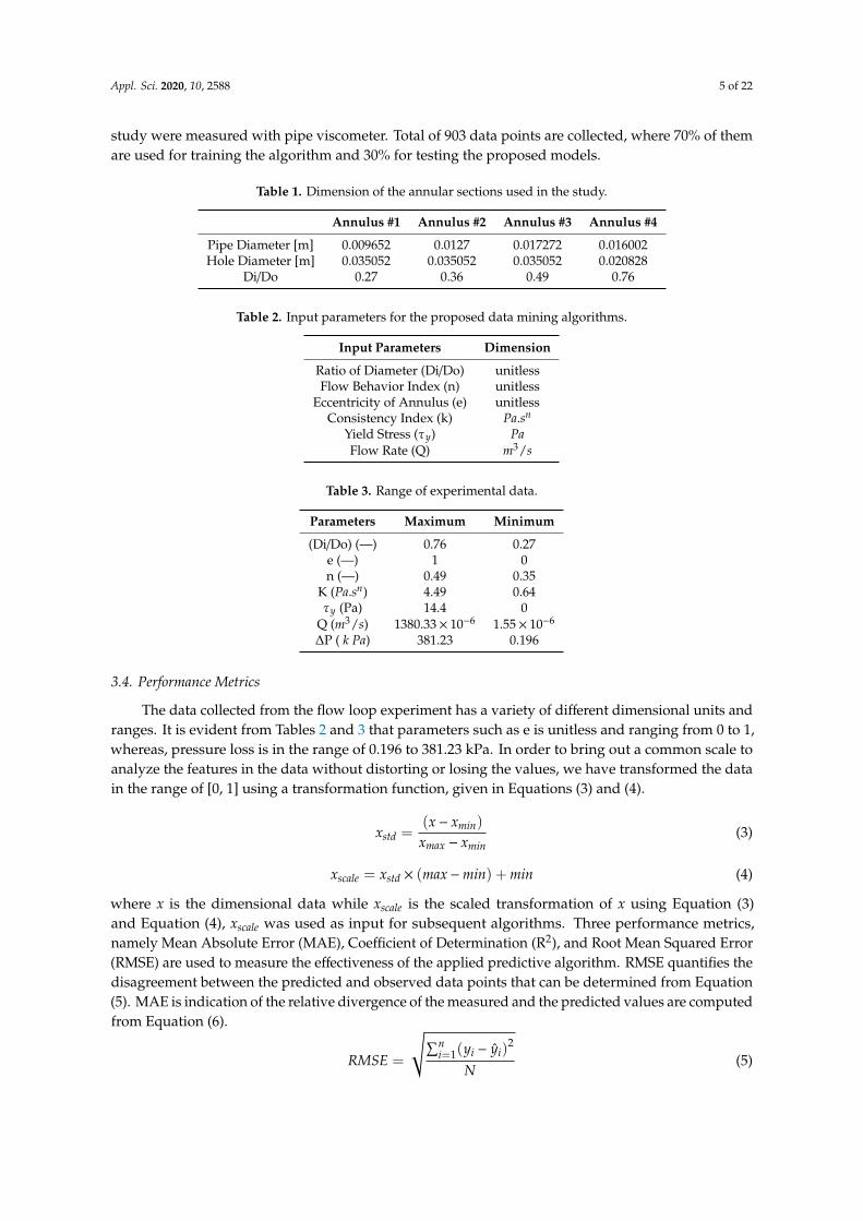
ANN is manually tuned at initial stages to yield lower error rate compared to SVM. The numberof layers is 2 and the number of neurons in each layer is 3. The activation function for input andhidden layer is ReLU and Linear for output layer. The dropout ratio is 0.15 and the number ofiterations is 1000. Figure 2 illustrates a comparison of the predicted and observed pressure loss fromthe experimental setup. The RMSE and MAE are found to be 17.8 kPa and 10.7%, respectively, withR2 = 0.915 for training data. Similarly, the obtained values for the test data are 21.36 kPa for RMSEand 12.34% for MAE with R2 = 0.904. The prediction for the test and train data is good below 50 kPaas the values are clustered around the best fit curve, but a drift from the best fit towards the upperregion can be observed. Different precautionary measures are taken to avoid overfitting, such asmonitoring the RMSE score, early stopping criteria, and dropout regularization. The proposed ANN isshallow in structure, therefore, changes in number of neuros in each layer, number of layers, and theactivation functions are also iteratively selected. The lowest RMSE score of unseen test data may leadsto generalizing better results.

Figure 2. Artificial neural network (ANN) predicted pressure plotted with observed pressure loss:(a) training dataset and (b) test dataset.

4.1.3. Predictions via Bayesian Neural Network (BNN)

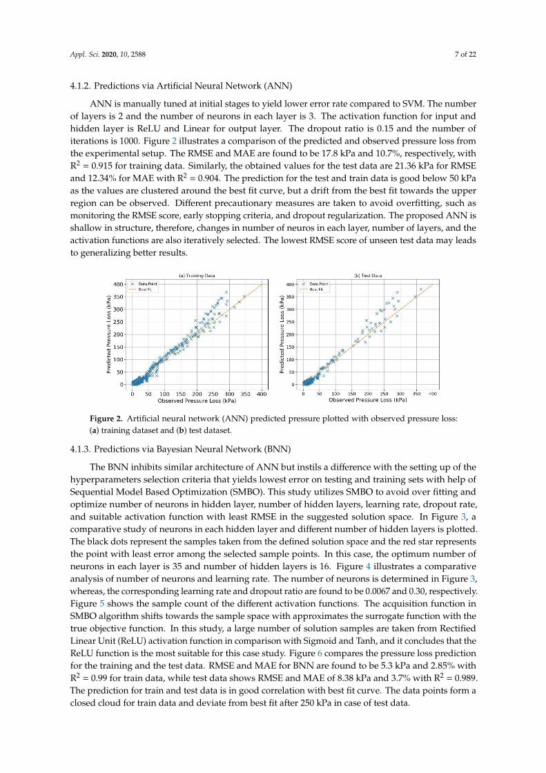
The BNN inhibits similar architecture of ANN but instils a difference with the setting up of thehyperparameters selection criteria that yields lowest error on testing and training sets with help ofSequential Model Based Optimization (SMBO). This study utilizes SMBO to avoid over fitting andoptimize number of neurons in hidden layer, number of hidden layers, learning rate, dropout rate,and suitable activation function with least RMSE in the suggested solution space. In Figure 3, acomparative study of neurons in each hidden layer and different number of hidden layers is plotted.The black dots represent the samples taken from the defined solution space and the red star representsthe point with least error among the selected sample points. In this case, the optimum number ofneurons in each layer is 35 and number of hidden layers is 16. Figure 4 illustrates a comparativeanalysis of number of neurons and learning rate. The number of neurons is determined in Figure 3,whereas, the corresponding learning rate and dropout ratio are found to be 0.0067 and 0.30, respectively.Figure 5 shows the sample count of the different activation functions. The acquisition function inSMBO algorithm shifts towards the sample space with approximates the surrogate function with thetrue objective function. In this study, a large number of solution samples are taken from RectifiedLinear Unit (ReLU) activation function in comparison with Sigmoid and Tanh, and it concludes that theReLU function is the most suitable for this case study. Figure 6 compares the pressure loss predictionfor the training and the test data. RMSE and MAE for BNN are found to be 5.3 kPa and 2.85% withR2 = 0.99 for train data, while test data shows RMSE and MAE of 8.38 kPa and 3.7% with R2 = 0.989.The prediction for train and test data is in good correlation with best fit curve. The data points form aclosed cloud for train data and deviate from best fit after 250 kPa in case of test data.

Appl. Sci. 2020, 10, 2588 8 of 22

Figure 3. Optimized Bayesian Neural Network (BNN) number of neurons in each layer plotted withnumber of layers.

Figure 4. Optimized BNN learning rate plotted with number of neurons in each layer.

Figure 5. Sample count from the different sample of the proposed solution space.

Appl. Sci. 2020, 10, 2588 9 of 22

Figure 6. BNN predicted pressure plotted with observed pressure loss: (a) training dataset and(b) test dataset.

4.1.4. Predictions via Random Forest (RF)

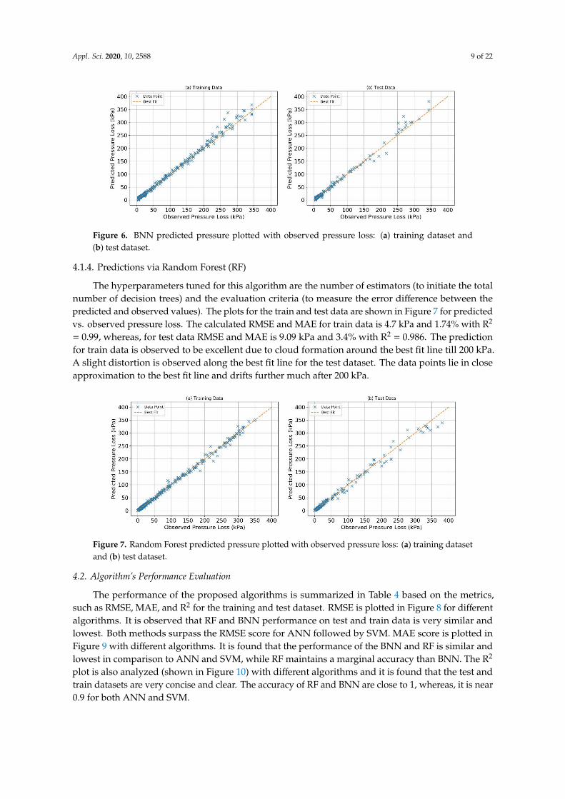
The hyperparameters tuned for this algorithm are the number of estimators (to initiate the totalnumber of decision trees) and the evaluation criteria (to measure the error difference between thepredicted and observed values). The plots for the train and test data are shown in Figure 7 for predictedvs. observed pressure loss. The calculated RMSE and MAE for train data is 4.7 kPa and 1.74% with R2

= 0.99, whereas, for test data RMSE and MAE is 9.09 kPa and 3.4% with R2 = 0.986. The predictionfor train data is observed to be excellent due to cloud formation around the best fit line till 200 kPa.A slight distortion is observed along the best fit line for the test dataset. The data points lie in closeapproximation to the best fit line and drifts further much after 200 kPa.

Figure 7. Random Forest predicted pressure plotted with observed pressure loss: (a) training datasetand (b) test dataset.

4.2. Algorithm’s Performance Evaluation

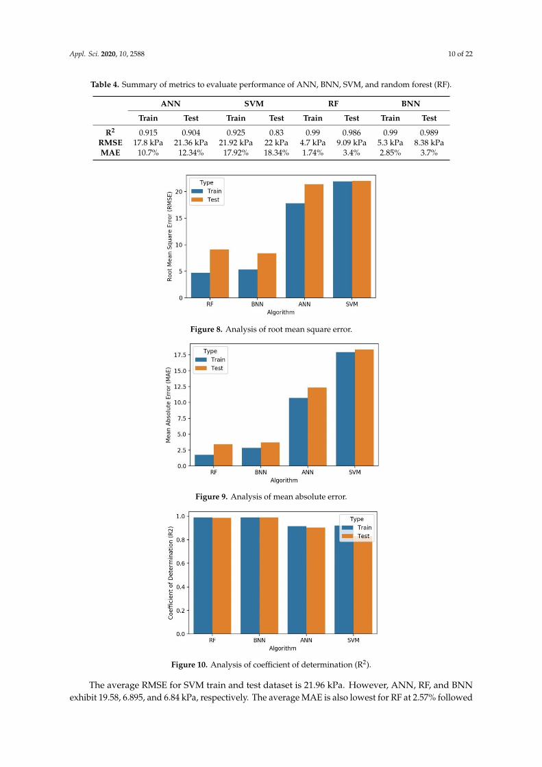
The performance of the proposed algorithms is summarized in Table 4 based on the metrics,such as RMSE, MAE, and R2 for the training and test dataset. RMSE is plotted in Figure 8 for differentalgorithms. It is observed that RF and BNN performance on test and train data is very similar andlowest. Both methods surpass the RMSE score for ANN followed by SVM. MAE score is plotted inFigure 9 with different algorithms. It is found that the performance of the BNN and RF is similar andlowest in comparison to ANN and SVM, while RF maintains a marginal accuracy than BNN. The R2

plot is also analyzed (shown in Figure 10) with different algorithms and it is found that the test andtrain datasets are very concise and clear. The accuracy of RF and BNN are close to 1, whereas, it is near0.9 for both ANN and SVM.

Appl. Sci. 2020, 10, 2588 10 of 22

Table 4. Summary of metrics to evaluate performance of ANN, BNN, SVM, and random forest (RF).

ANN SVM RF BNN

Train Test Train Test Train Test Train Test

R2 0.915 0.904 0.925 0.83 0.99 0.986 0.99 0.989RMSE 17.8 kPa 21.36 kPa 21.92 kPa 22 kPa 4.7 kPa 9.09 kPa 5.3 kPa 8.38 kPaMAE 10.7% 12.34% 17.92% 18.34% 1.74% 3.4% 2.85% 3.7%

Figure 8. Analysis of root mean square error.

Figure 9. Analysis of mean absolute error.

Figure 10. Analysis of coefficient of determination (R2).

The average RMSE for SVM train and test dataset is 21.96 kPa. However, ANN, RF, and BNNexhibit 19.58, 6.895, and 6.84 kPa, respectively. The average MAE is also lowest for RF at 2.57% followed

Appl. Sci. 2020, 10, 2588 11 of 22

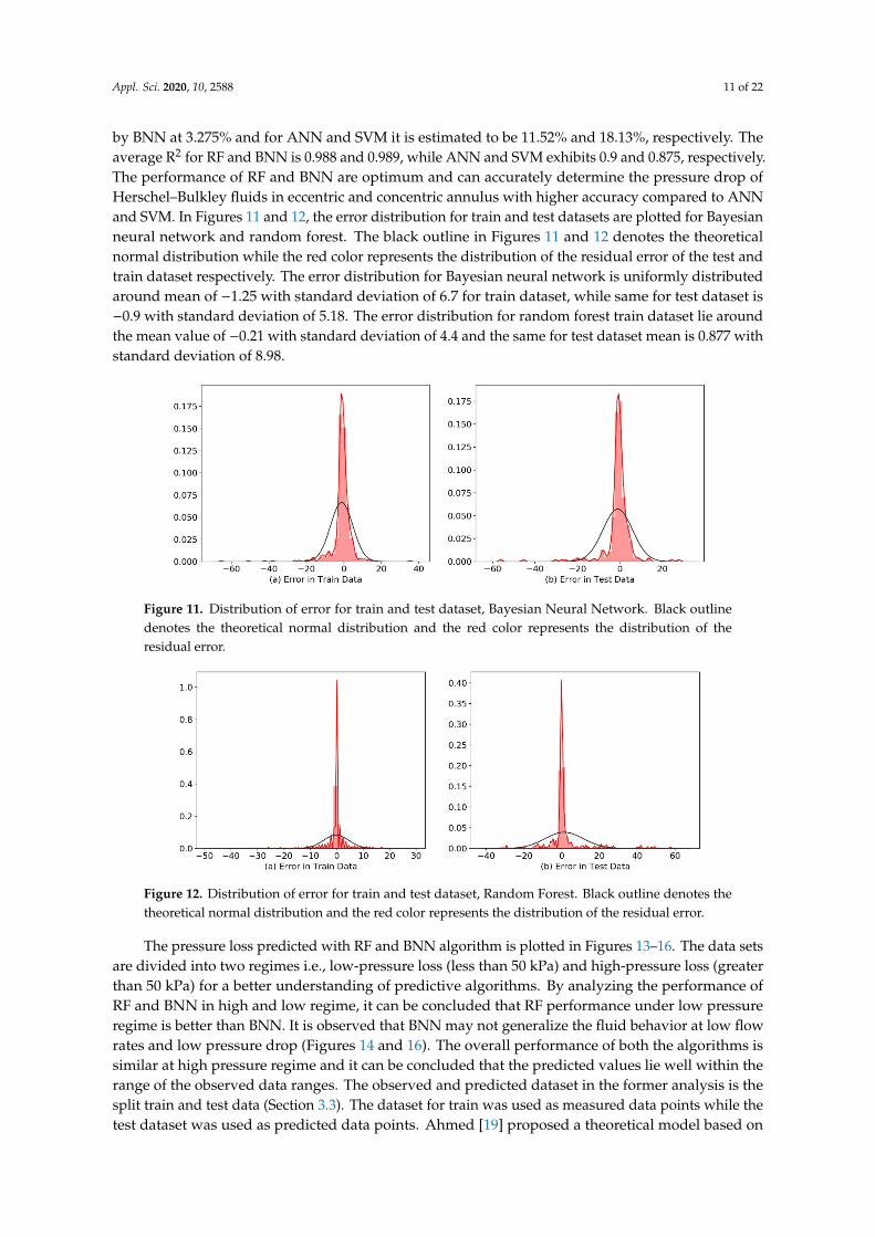
by BNN at 3.275% and for ANN and SVM it is estimated to be 11.52% and 18.13%, respectively. Theaverage R2 for RF and BNN is 0.988 and 0.989, while ANN and SVM exhibits 0.9 and 0.875, respectively.The performance of RF and BNN are optimum and can accurately determine the pressure drop ofHerschel–Bulkley fluids in eccentric and concentric annulus with higher accuracy compared to ANNand SVM. In Figures 11 and 12, the error distribution for train and test datasets are plotted for Bayesianneural network and random forest. The black outline in Figures 11 and 12 denotes the theoreticalnormal distribution while the red color represents the distribution of the residual error of the test andtrain dataset respectively. The error distribution for Bayesian neural network is uniformly distributedaround mean of −1.25 with standard deviation of 6.7 for train dataset, while same for test dataset is−0.9 with standard deviation of 5.18. The error distribution for random forest train dataset lie aroundthe mean value of −0.21 with standard deviation of 4.4 and the same for test dataset mean is 0.877 withstandard deviation of 8.98.

Figure 11. Distribution of error for train and test dataset, Bayesian Neural Network. Black outlinedenotes the theoretical normal distribution and the red color represents the distribution of theresidual error.

Figure 12. Distribution of error for train and test dataset, Random Forest. Black outline denotes thetheoretical normal distribution and the red color represents the distribution of the residual error.

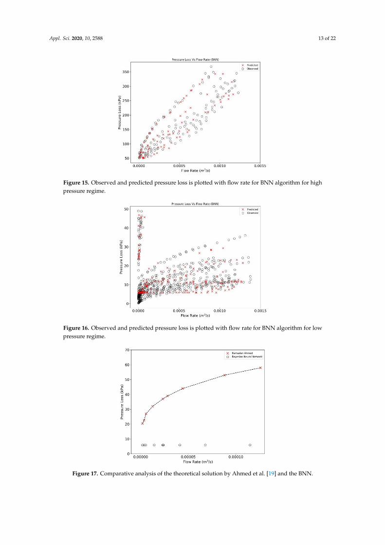
The pressure loss predicted with RF and BNN algorithm is plotted in Figures 13–16. The data setsare divided into two regimes i.e., low-pressure loss (less than 50 kPa) and high-pressure loss (greaterthan 50 kPa) for a better understanding of predictive algorithms. By analyzing the performance ofRF and BNN in high and low regime, it can be concluded that RF performance under low pressureregime is better than BNN. It is observed that BNN may not generalize the fluid behavior at low flowrates and low pressure drop (Figures 14 and 16). The overall performance of both the algorithms issimilar at high pressure regime and it can be concluded that the predicted values lie well within therange of the observed data ranges. The observed and predicted dataset in the former analysis is thesplit train and test data (Section 3.3). The dataset for train was used as measured data points while thetest dataset was used as predicted data points. Ahmed [19] proposed a theoretical model based on

Appl. Sci. 2020, 10, 2588 12 of 22

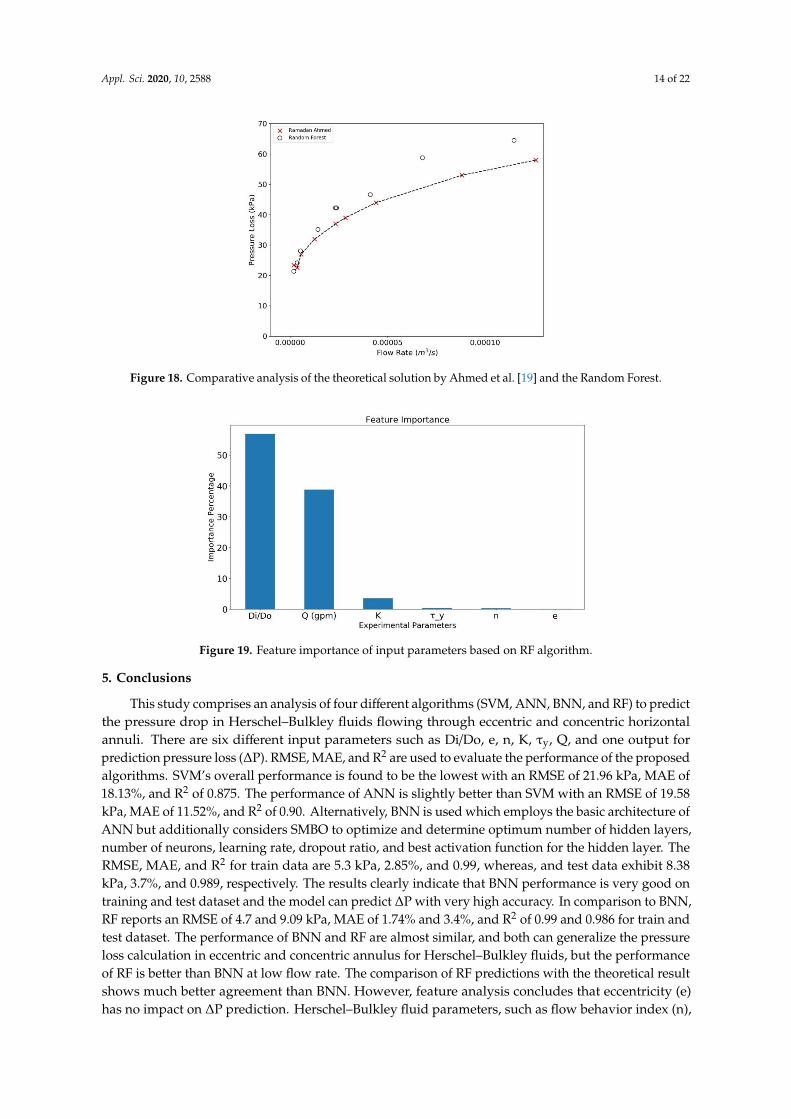
the experimental results. A comparison is performed in Figures 17 and 18 exhibiting pressure droppredictions from this study and Ahmed [19] for a selected range of annulus diameter (0.020828 m) andfluid XCD5 (Appendix B). The BNN shows a slight resemblance to the derived results of Ahmed [19],while the RF predicted data points lies around the vicinity of the theoretical results, hence, concludingthe better performance of the later method.

Figure 13. Observed and predicted pressure loss is plotted with flow rate for RF algorithm for highpressure regime.

Figure 14. Observed and predicted pressure loss is plotted with flow rate for RF algorithm for lowpressure regime.

RF is an ensemble model, where multiple decision trees are created based on randomly sampleddatasets to approximate and lower the error. The model also quantifies the contribution of eachinput parameter towards predicting output. Subsequently, this property can be used to determinethe importance of each input parameter to predict the desired output. The percentage-wise bar plotis shown in Figure 19 for each input parameter that have effect on the predicted output values. Thediameter ratio (Di/Do) is the highest dominating parameter with contribution of approximately 58%out of the six-input followed by flow rate m3/s i.e., 37%. The diameter ratio and flow rate accountfor 95% dominance in predicting the pressure loss, while the Herschel–Bulkley fluid parameters haslow accountability of remaining 5% where the consistency Index (K) has a share of 3.5% while flowindex and shear stress have less than 1% contribution and eccentricity has negligible effect of thepressure loss.

Appl. Sci. 2020, 10, 2588 13 of 22

Figure 15. Observed and predicted pressure loss is plotted with flow rate for BNN algorithm for highpressure regime.

Figure 16. Observed and predicted pressure loss is plotted with flow rate for BNN algorithm for lowpressure regime.

Figure 17. Comparative analysis of the theoretical solution by Ahmed et al. [19] and the BNN.

Appl. Sci. 2020, 10, 2588 14 of 22

Figure 18. Comparative analysis of the theoretical solution by Ahmed et al. [19] and the Random Forest.

Figure 19. Feature importance of input parameters based on RF algorithm.

5. Conclusions

This study comprises an analysis of four different algorithms (SVM, ANN, BNN, and RF) to predictthe pressure drop in Herschel–Bulkley fluids flowing through eccentric and concentric horizontalannuli. There are six different input parameters such as Di/Do, e, n, K, τy, Q, and one output forprediction pressure loss (∆P). RMSE, MAE, and R2 are used to evaluate the performance of the proposedalgorithms. SVM’s overall performance is found to be the lowest with an RMSE of 21.96 kPa, MAE of18.13%, and R2 of 0.875. The performance of ANN is slightly better than SVM with an RMSE of 19.58kPa, MAE of 11.52%, and R2 of 0.90. Alternatively, BNN is used which employs the basic architecture ofANN but additionally considers SMBO to optimize and determine optimum number of hidden layers,number of neurons, learning rate, dropout ratio, and best activation function for the hidden layer. TheRMSE, MAE, and R2 for train data are 5.3 kPa, 2.85%, and 0.99, whereas, and test data exhibit 8.38kPa, 3.7%, and 0.989, respectively. The results clearly indicate that BNN performance is very good ontraining and test dataset and the model can predict ∆P with very high accuracy. In comparison to BNN,RF reports an RMSE of 4.7 and 9.09 kPa, MAE of 1.74% and 3.4%, and R2 of 0.99 and 0.986 for train andtest dataset. The performance of BNN and RF are almost similar, and both can generalize the pressureloss calculation in eccentric and concentric annulus for Herschel–Bulkley fluids, but the performanceof RF is better than BNN at low flow rate. The comparison of RF predictions with the theoretical resultshows much better agreement than BNN. However, feature analysis concludes that eccentricity (e)has no impact on ∆P prediction. Herschel–Bulkley fluid parameters, such as flow behavior index (n),

Appl. Sci. 2020, 10, 2588 15 of 22

consistency index (K), and shear stress (τy) have less than 5% effect on ∆P prediction, while diameterratio (Di/Do) and flow rate (Q) accounts for more than 95% on ∆P.

Author Contributions: Conceptualization, A.K. and S.R.; Methodology, A.K., S.R., S.U.I., and P.V.; Software,A.K.; Validation, A.K.; Formal Analysis, A.K.; Investigation, A.K., S.R., S.U.I., and P.V.; Resources, A.K. and S.R.;Data Curation, A.K.; Writing- Original Draft Preparation, A.K.; Writing- Review and Editing, S.R., S.U.I., andT.G.; Visualization, A.K. and S.R.; Supervision, S.R., P.V., and T.G.; Project Administration, A.K., S.U.I., and T.G.;Funding Acquisition, S.R. All authors have read and agreed to the published version of the manuscript.

Funding: This research is funded by YUTP, grant number 0153AA-E87.

Acknowledgments: This work is supported by Petroleum Engineering Department and Institute of HydrocarbonRecovery at Universiti Teknologi PETRONAS, Malaysia.

Conflicts of Interest: The authors declare no conflict of interest.

Appendix A

Appendix A.1 Artificial Neural Network

Artificial neural network (ANN) is designed to mimic the working ways of the biological brain.One of the concepts widely recognized regarding ANN is its capability to map and approximatecomplex functions relationships and the natural propensity to utilize massively distributed processingcapacity to store experimental knowledge and makes its use. The common structure of ANN consists ofsome basic components, namely input layer, weights (connection strength), output layer, and activationfunction (for hidden and output layer). Each input neurons are multiplied with adjustable weights andsummed up with extra value known as bias which is then fed through a nonlinear activation functioniteratively to predict results as shown in Figure A1. The transfer function can be given as (ƒ) = WX + band the output of the network can be calculated by Equation (A1a).

Figure A1. Single artificial neuron schema [63].

o j = ϕ( f ) = ϕ(WX + b) (A1a)

where, ϕ is the activation function, W is weight matrix, b is bias, and X is input data, examples ofcommonly used activation function are Sigmoid, Tanh, ReLU, and linear (described in Equation (A1b–e)).

linear(n) = n (A1b)

Sigmoid = φ z = 11 + e − z (A1c)

ReLu = max(0, z) (A1d)

Tanh (z) =ez− e−z

ez + e−z (A1e)

Appl. Sci. 2020, 10, 2588 16 of 22

There are several combinations to train a neural network on a given data set and many possiblenumbers of hyperparameters such as number of neurons in a hidden layer, number of hidden layers,activation function, learning rate, etc., hence, determining the optimal network configuration is achallenging task. In the present work, back propagation algorithm was used to lower the error betweenthe predicted and actual datasets, and the network is optimized for hyperparameters manually.

Appendix A.2 Bayesian Neural Network

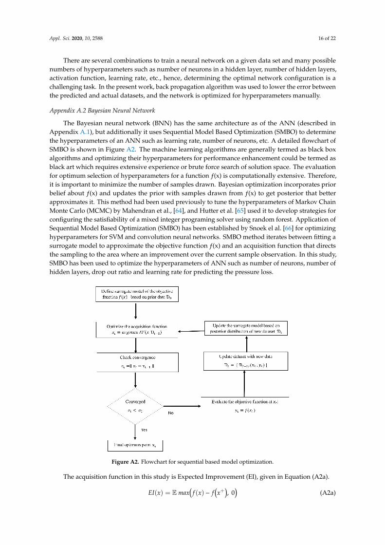
The Bayesian neural network (BNN) has the same architecture as of the ANN (described inAppendix A.1), but additionally it uses Sequential Model Based Optimization (SMBO) to determinethe hyperparameters of an ANN such as learning rate, number of neurons, etc. A detailed flowchart ofSMBO is shown in Figure A2. The machine learning algorithms are generally termed as black boxalgorithms and optimizing their hyperparameters for performance enhancement could be termed asblack art which requires extensive experience or brute force search of solution space. The evaluationfor optimum selection of hyperparameters for a function ƒ(x) is computationally extensive. Therefore,it is important to minimize the number of samples drawn. Bayesian optimization incorporates priorbelief about ƒ(x) and updates the prior with samples drawn from ƒ(x) to get posterior that betterapproximates it. This method had been used previously to tune the hyperparameters of Markov ChainMonte Carlo (MCMC) by Mahendran et al., [64], and Hutter et al. [65] used it to develop strategies forconfiguring the satisfiability of a mixed integer programing solver using random forest. Application ofSequential Model Based Optimization (SMBO) has been established by Snoek el al. [66] for optimizinghyperparameters for SVM and convolution neural networks. SMBO method iterates between fitting asurrogate model to approximate the objective function ƒ(x) and an acquisition function that directsthe sampling to the area where an improvement over the current sample observation. In this study,SMBO has been used to optimize the hyperparameters of ANN such as number of neurons, number ofhidden layers, drop out ratio and learning rate for predicting the pressure loss.

Figure A2. Flowchart for sequential based model optimization.

The acquisition function in this study is Expected Improvement (EI), given in Equation (A2a).

EI(x) = E max(

f (x) − f(x+

), 0

)(A2a)

Appl. Sci. 2020, 10, 2588 17 of 22

where ƒ(x+) is the value of the best sample so far and x+ is the location of that sample and the expectedimprovement for Gaussian model can be defined using Equation (A2b) and Equation (A2c).

EI(x) ={

(µ(x) − f (x+) − ξ) Φ(x) + σ(x)φ(z) i f σ(x) > 00 i f σ(x) = 0

(A2b)

Z =

µ(x)− f (x+)−ξσ(x) i f σ(x) < 0

0 i f σ(x) = 0(A2c)

where σ(x) and µ(x) are standard deviation and mean of the posterior prediction at x, respectively, Φand φ are the Cumulative Distribution Function and Probability Distribution Function of the standardnormal distribution and ξ is the constant of exploration during optimization and the recommendeddefault value is 0.01. An objective function is shown in Figure A3 represented by yellow dashed lineand a Gaussian based surrogate function which approximates the objective function (shown in blue)and the samples are the outcome of the expected improvement for sample selection (marked in black).

Figure A3. Plot representing an objective function, Gaussian based surrogate function and expectedimprovement-based samples selected for optimization of surrogate function to match the trueobjective function.

Appendix A.3 Support Vector Machine

Support Vector Machine (SVM) is known for supervised learning model used for regressionand classification problems. SVM employ nonlinear mapping method to transfer input into highdimensional feature space. This hypothesis of optimal hyperplane separation is the most effectivemathematical approach for prediction because it is derived from minimizing structural risk theory.The working principle of SVM is shown in Figure A4.

Figure A4. Hyperplane classification for the training dataset with weight (w) and bias (b) [63].

Appl. Sci. 2020, 10, 2588 18 of 22

Consider x separable training datasets in the range of {x1, x2, x3, . . . . . . , xn}, where each x is adimensional vector and a hyperplane H was applied to separate them using Equation (A3a).

H : w.p− b = 0 (A3a)

Here, hyperplane separator bias value is b, and w is the weight vector perpendicular to thehyperplane. In this present context of a linearly separable case, there are two classes, namely, H+ andH-, which are called support vectors and they separate the data into two planes, given in Equation(A3b) and Equation (A3c).

H+ = w.p− b = +1 (A3b)

H− = w.p− b = −1 (A3c)

The distance between these hyperplanes is a margin with no data points, so the distance betweenthem is 2/||w|| and to achieve an optimal margin hyperplane ||w|| should be minimized which meansmaximize the width.

Appendix A.4 Random Forest

Random Forest (RF) can be used for regression or classification. It is an ensemble of differentregression trees and is used for nonlinear multiple regression. Each leaf contains a distribution for thecontinuous output variables. Random forest builds multiple decision trees and merges them togetherto get a more accurate and stable prediction. For each estimator, it selects a random subsample offeatures. It can be used to rank the importance of variables in a regression or classification problemnaturally. Figure A5 exemplifies a decision tree based on flow rate and then dividing up furtherinto leaf.

Figure A5. Single leaf node of tree-based model in random forest with various decision nodes.

Appl. Sci. 2020, 10, 2588 19 of 22

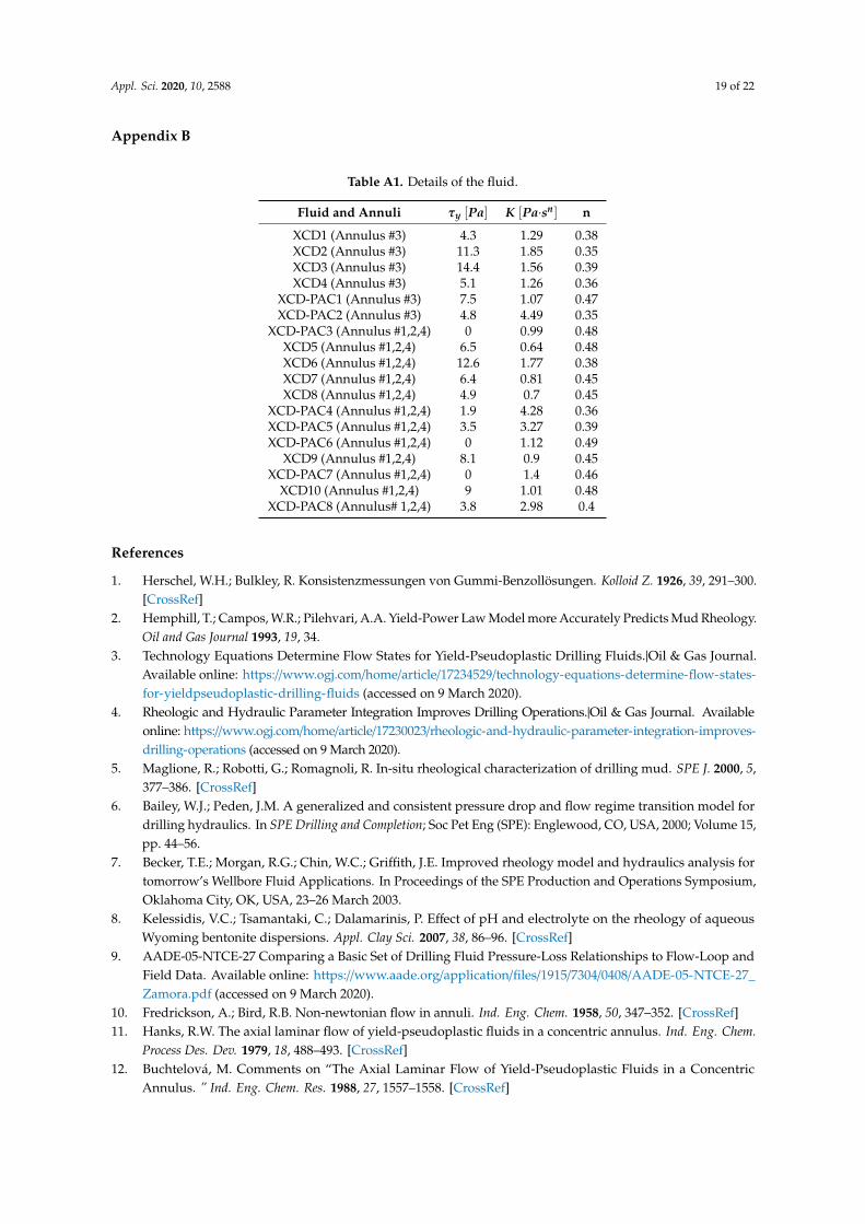
Appendix B

Table A1. Details of the fluid.

Fluid and Annuli τy [Pa] K [Pa·sn] n

XCD1 (Annulus #3) 4.3 1.29 0.38XCD2 (Annulus #3) 11.3 1.85 0.35XCD3 (Annulus #3) 14.4 1.56 0.39XCD4 (Annulus #3) 5.1 1.26 0.36

XCD-PAC1 (Annulus #3) 7.5 1.07 0.47XCD-PAC2 (Annulus #3) 4.8 4.49 0.35

XCD-PAC3 (Annulus #1,2,4) 0 0.99 0.48XCD5 (Annulus #1,2,4) 6.5 0.64 0.48XCD6 (Annulus #1,2,4) 12.6 1.77 0.38XCD7 (Annulus #1,2,4) 6.4 0.81 0.45XCD8 (Annulus #1,2,4) 4.9 0.7 0.45

XCD-PAC4 (Annulus #1,2,4) 1.9 4.28 0.36XCD-PAC5 (Annulus #1,2,4) 3.5 3.27 0.39XCD-PAC6 (Annulus #1,2,4) 0 1.12 0.49

XCD9 (Annulus #1,2,4) 8.1 0.9 0.45XCD-PAC7 (Annulus #1,2,4) 0 1.4 0.46

XCD10 (Annulus #1,2,4) 9 1.01 0.48XCD-PAC8 (Annulus# 1,2,4) 3.8 2.98 0.4

References

1. Herschel, W.H.; Bulkley, R. Konsistenzmessungen von Gummi-Benzollösungen. Kolloid Z. 1926, 39, 291–300.[CrossRef]

2. Hemphill, T.; Campos, W.R.; Pilehvari, A.A. Yield-Power Law Model more Accurately Predicts Mud Rheology.Oil and Gas Journal 1993, 19, 34.

3. Technology Equations Determine Flow States for Yield-Pseudoplastic Drilling Fluids.|Oil & Gas Journal.Available online: https://www.ogj.com/home/article/17234529/technology-equations-determine-flow-states-for-yieldpseudoplastic-drilling-fluids (accessed on 9 March 2020).

4. Rheologic and Hydraulic Parameter Integration Improves Drilling Operations.|Oil & Gas Journal. Availableonline: https://www.ogj.com/home/article/17230023/rheologic-and-hydraulic-parameter-integration-improves-drilling-operations (accessed on 9 March 2020).

5. Maglione, R.; Robotti, G.; Romagnoli, R. In-situ rheological characterization of drilling mud. SPE J. 2000, 5,377–386. [CrossRef]

6. Bailey, W.J.; Peden, J.M. A generalized and consistent pressure drop and flow regime transition model fordrilling hydraulics. In SPE Drilling and Completion; Soc Pet Eng (SPE): Englewood, CO, USA, 2000; Volume 15,pp. 44–56.

7. Becker, T.E.; Morgan, R.G.; Chin, W.C.; Griffith, J.E. Improved rheology model and hydraulics analysis fortomorrow’s Wellbore Fluid Applications. In Proceedings of the SPE Production and Operations Symposium,Oklahoma City, OK, USA, 23–26 March 2003.

8. Kelessidis, V.C.; Tsamantaki, C.; Dalamarinis, P. Effect of pH and electrolyte on the rheology of aqueousWyoming bentonite dispersions. Appl. Clay Sci. 2007, 38, 86–96. [CrossRef]

9. AADE-05-NTCE-27 Comparing a Basic Set of Drilling Fluid Pressure-Loss Relationships to Flow-Loop andField Data. Available online: https://www.aade.org/application/files/1915/7304/0408/AADE-05-NTCE-27_Zamora.pdf (accessed on 9 March 2020).

10. Fredrickson, A.; Bird, R.B. Non-newtonian flow in annuli. Ind. Eng. Chem. 1958, 50, 347–352. [CrossRef]11. Hanks, R.W. The axial laminar flow of yield-pseudoplastic fluids in a concentric annulus. Ind. Eng. Chem.

Process Des. Dev. 1979, 18, 488–493. [CrossRef]12. Buchtelová, M. Comments on “The Axial Laminar Flow of Yield-Pseudoplastic Fluids in a Concentric

Annulus. ” Ind. Eng. Chem. Res. 1988, 27, 1557–1558. [CrossRef]

Appl. Sci. 2020, 10, 2588 20 of 22

13. Heywood, N.I.; Cheng, D.C.H. Comparison of methods for predicting head loss in turbulent pipe flow ofnon-newtonian fluids. Meas. Control 1984, 6, 33–45. [CrossRef]

14. Gücüyener, I.H.; Mehmetoglu, T. Characterization of flow regime in concentric annuli and pipes foryield-pseudoplastic fluids. J. Pet. Sci. Eng. 1996, 16, 45–60. [CrossRef]

15. Reed, T.D.; Pilehvari, A.A. A new model for laminar, transitional, and turbulent flow of drilling muds.In Proceedings of the SPE Production Operations Symposium, Oklahoma City, Oklahoma, 21–23 March 1993.

16. Non-Newtonian Fluid Flow in Eccentric Annuli and Its Application to Petroleum Engineering Problems.Available online: https://digitalcommons.lsu.edu/cgi/viewcontent.cgi?referer=&httpsredir=1&article=5847&context=gradschool_disstheses (accessed on 9 March 2020).

17. Haciislamoglu, M.; Langlinais, J. Non-newtonian flow in eccentric annuli. J. Energy Resour. Technol. Trans.ASME 1990, 112, 163–169. [CrossRef]

18. Kelessidis, V.C.; Dalamarinis, P.; Maglione, R. Experimental study and predictions of pressure losses of fluidsmodeled as Herschel-Bulkley in concentric and eccentric annuli in laminar, transitional and turbulent flows.J. Pet. Sci. Eng. 2011, 77, 305–312. [CrossRef]

19. Ahmed, R. Experimental Study and Modeling of Yield Power-Law Fluid Flow in Pipes and Annuli. Availableonline: https://edx.netl.doe.gov/dataset/experimental-study-and-modeling-of-yield-power-law-fluid-flow-in-pipes-and-annuli/resource_download/131420e2-5b16-4e4b-9ceb-74b73f9393b1 (accessed on 9 March 2020).

20. Kozicki, W.; Chou, C.H.; Tiu, C. Non-newtonian flow in ducts of arbitrary cross-sectional shape. Chem. Eng. Sci.1966, 21, 665–679. [CrossRef]

21. Luo, Y.; Peden, M. Flow of Non·Newtonian Fluids Through Eccentric Annuli; Society of Petroleum Engineers:Englewood, CO, USA, 1990.

22. Vajargah, A.K.; Fard, F.N.; Parsi, M.; Hoxha, B.B. Investigating the impact of the “tool joint effect” on equivalentcirculating density in deep-water wells. In Proceedings of the Society of Petroleum Engineers—SPE DeepwaterDrilling and Completions Conference, Galveston, TX, USA, 10–11 September 2014; pp. 341–352.

23. CFD Method for Predicting Annular Pressure Losses and Cuttings Concentration in Eccentric HorizontalWells. Available online: https://www.hindawi.com/journals/jpe/2014/486423/ (accessed on 9 March 2020).

24. Kelessidis, V.C.; Maglione, R.; Tsamantaki, C.; Aspirtakis, Y. Optimal determination of rheological parametersfor Herschel-Bulkley drilling fluids and impact on pressure drop, velocity profiles and penetration ratesduring drilling. J. Pet. Sci. Eng. 2006, 53, 203–224. [CrossRef]

25. Founargiotakis, K.; Kelessidis, V.C.; Maglione, R. Laminar, transitional and turbulent flow of Herschel-Bulkleyfluids in concentric annulus. Can. J. Chem. Eng. 2008, 86, 676–683. [CrossRef]

26. Sorgun, M.; Ozbayoglu, M.E.; Aydin, I. Modeling and experimental study of newtonian fluid flow in annulus.J. Energy Resour. Technol. Trans. ASME 2010, 132. [CrossRef]

27. Ahmed, R.M.; Miska, S.; Miska, W. Friction pressure loss determination of yield power law fluid in eccentricannular laminar flow. In Proceedings of the Wiertnictwo Nafta Gaz, Krakow, Poland, 23 January 2006;Volume 23, pp. 47–53.

28. Ogugbue, C.C.; Shah, S.N. Friction pressure correlations for oilfield polymeric solutions in eccentric annulus.In Proceedings of the International Conference on Offshore Mechanics and Arctic Engineering—OMAE,Honolulu, HI, USA, 31 May–5 June 2009; Volume 7, pp. 583–592.

29. Mokhtari, M.; Ermila, M.; Tutuncu, A.N. Accurate Bottomhole Pressure for Fracture Gradient Prediction and DrillingFluid Pressure Program—Part I; American Rock Mechanics Association: Woodland Terrance, VA, USA, 2012.

30. Karimi Vajargah, A.; Van Oort, E. Determination of drilling fluid rheology under downhole conditions byusing real-time distributed pressure data. J. Nat. Gas Sci. Eng. 2015, 24, 400–411. [CrossRef]

31. Erge, O.; Karimi Vajargah, A.; Ozbayoglu, M.E.; Van Oort, E. Frictional pressure loss of drilling fluids in afully eccentric annulus. J. Nat. Gas Sci. Eng. 2015, 26, 1119–1129. [CrossRef]

32. A Novel Hybrid Bat Algorithm with Harmony Search for Global Numerical Optimization. Available online:https://www.hindawi.com/journals/jam/2013/696491/ (accessed on 9 March 2020).

33. La Fe-Perdomo, I.; Beruvides, G.; Quiza, R.; Haber, R.; Rivas, M. Automatic selection of optimal parametersbased on simple soft-computing methods: A case study of micromilling processes. IEEE Trans. Ind. Inform.2019, 15, 800–811. [CrossRef]

34. Osman, E.A.; Aggour, M.A. Determination of drilling mud density change with pressure and temperaturemade simple and accurate by ANN. In Proceedings of the Middle East Oil Show, Bahrain, 9–12 June 2003.Society of Petroleum Engineers.

Appl. Sci. 2020, 10, 2588 21 of 22

35. Jeirani, Z.; Mohebbi, A. Artificial neural networks approach for estimating filtration properties of drillingfluids. J. Jpn. Pet. Inst. 2006, 49, 65–70. [CrossRef]

36. Siruvuri, C.; Nagarakanti, S.; Samuel, R. Stuck pipe prediction and avoidance: A convolutional neuralnetwork approach. In Proceedings of the IADC/SPE Drilling Conference, Miami, FL, USA, 21–23 February2006. Society of Petroleum Engineers.

37. Miri, R.; Sampaio, J.H.B.; Afshar, M.; Lourenco, A. Development of artificial neural networks to predictdifferential pipe sticking in iranian offshore oil fields. In Proceedings of the International Oil Conference andExhibition in Mexico, Cancun, Mexico, 31 August–2 September 2006. Society of Petroleum Engineers.

38. Murillo, A.; Neuman, J.; Samuel, R. Pipe sticking prediction and avoidance using adaptive fuzzy logic andneural network modeling. In Proceedings of the SPE Production and Operations Symposium, OklahomaCity, Oklahoma, 4–8 April 2009; Society of Petroleum Engineers. pp. 244–258.

39. Abdulmalek Ahmed, S.; Elkatatny, S.; Abdulraheem, A.; Mahmoud, M.; Ali, A.Z. Prediction of rate ofpenetration of deep and tight formation using support vector machine. In Proceedings of the Society ofPetroleum Engineers—SPE Kingdom of Saudi Arabia Annual Technical Symposium and Exhibition 2018,SATS 2018, Dammam, Saudi Arabia, 23–26 April 2018. Society of Petroleum Engineers.

40. Elkatatny, S. Real-time prediction of rheological parameters of KCl water-based drilling fluid using artificialneural networks. Arab. J. Sci. Eng. 2017, 42, 1655–1665. [CrossRef]

41. Ozbayoglu, E.M.; Miska, S.Z.; Reed, T.; Takach, N. Analysis of Bed Height in Horizontal and Highly-InclinedWellbores by Using Artificial Neuraletworks; Society of Petroleum Engineers (SPE): Englewood, CO, USA, 2002.

42. Rooki, R. Estimation of pressure loss of herschel–bulkley drilling fluids during horizontal annulus usingartificial neural network. J. Dispers. Sci. Technol. 2015, 36, 161–169. [CrossRef]

43. Rooki, R. Application of general regression neural network (GRNN) for indirect measuring pressure loss ofHerschel-Bulkley drilling fluids in oil drilling. Meas. J. Int. Meas. Confed. 2016, 85, 184–191. [CrossRef]

44. Rooki, R.; Rakhshkhorshid, M. Cuttings transport modeling in underbalanced oil drilling operation usingradial basis neural network. Egypt. J. Pet. 2017, 26, 541–546. [CrossRef]

45. Ahmadi, M.A.; Shadizadeh, S.R.; Shah, K.; Bahadori, A. An accurate model to predict drilling fluid densityat wellbore conditions. Egypt. J. Pet. 2018, 27, 1–10. [CrossRef]

46. Lu, Y.; Chen, M.; Jin, Y.; Hou, B.; Jia, L.; Hui, H. Identification of leak zone pre-drilling based on fuzzy control.In Proceedings of the PEAM 2011—Proceedings: 2011 IEEE Power Engineering and Automation Conference,Wuhan, China, 8–9 September 2011; Volume 3, pp. 353–356.

47. Chhantyal, K.; Viumdal, H.; Mylvaganam, S. Ultrasonic level scanning for monitoring mass flow of complexfluids in open channels—A novel sensor fusion approach using AI techniques. In Proceedings of theProceedings of IEEE Sensors, Glasgow, UK, 29 October–1 November 2017; pp. 1–3.

48. Chhantyal, K.; Viumdal, H.; Mylvaganam, S. Soft sensing of non-newtonian fluid flow in open venturichannel using an array of ultrasonic level sensors—AI models and their validations. Sensors (Switzerland)2017, 17, 2458. [CrossRef]

49. Skalle, P.; Sveen, J.; Aamodt, A. Improved efficiency of oil well drilling through case based reasoning. InProceedings of the Lecture Notes in Computer Science (including subseries Lecture Notes in Artificial Intelligence andLecture Notes in Bioinformatics); Springer: Berlin/Heidelberg, Germany, 2000; Volume 1886 LNAI, pp. 712–722.

50. Al-Azani, K.; Elkatatny, S.; Abdulraheem, A.; Mahmoud, M.; Ali, A. Prediction of cutting concentration inhorizontal and deviated wells using support vector machine. In Proceedings of the Society of PetroleumEngineers—SPE Kingdom of Saudi Arabia Annual Technical Symposium and Exhibition 2018, SATS 2018,Dammam, Saudi Arabia, 23–26 April 2018. Society of Petroleum Engineers.

51. Sameni, A.; Chamkalani, A. The application of least square support vector machine as a mathematicalalgorithm for diagnosing drilling effectivity in shaly formations. J. Pet. Sci. Technol. 2018, 8, 3–15.

52. Kankar, P.K.; Sharma, S.C.; Harsha, S.P. Fault diagnosis of ball bearings using machine learning methods.Expert Syst. Appl. 2011, 38, 1876–1886. [CrossRef]

53. Guo, X.; Chen, L.; Shen, C. Hierarchical adaptive deep convolution neural network and its application tobearing fault diagnosis. Meas. J. Int. Meas. Confed. 2016, 93, 490–502. [CrossRef]

54. Wen, L.; Li, X.; Gao, L.; Zhang, Y. A new convolutional neural network-based data-driven fault diagnosismethod. IEEE Trans. Ind. Electron. 2018, 65, 5990–5998. [CrossRef]

55. Castaño, F.; Beruvides, G.; Haber, R.E.; Artuñedo, A. Obstacle recognition based on machine learning foron-chip LiDAR sensors in a cyber-physical system. Sensors 2017, 17, 2109. [CrossRef]

Appl. Sci. 2020, 10, 2588 22 of 22

56. Wolpert, D.H.; Macready, W.G. No free lunch theorems for optimization. IEEE Trans. Evol. Comput. 1997, 1,67–82. [CrossRef]

57. Bingham, E.C. Fluidity and Plasticity, 2nd ed.; McGraw-Hill: New York, NY, USA, 1922.58. Govier, G.W.; George, W.; Aziz, K. The Flow of Complex Mixtures in Pipes, 2nd ed.; Society of Petroleum

Engineers: Richardson, TX, USA, 2008; ISBN 9781555631390.59. Bourgoyne, A.T. Applied Drilling Engineering; Society of Petroleum Engineers: Englewood, CO, USA, 1986;

ISBN 9781555630010.60. Castaño, F.; Strzełczak, S.; Villalonga, A.; Haber, R.E.; Kossakowska, J. Sensor reliability in cyber-physical

systems using internet-of-things data: A review and case study. Remote Sens. 2019, 11, 2252. [CrossRef]61. Ding, Y.; Xiao, X.; Huang, X.; Sun, J. System identification and a model-based control strategy of motor

driven system with high order flexible manipulator. Ind. Robot 2019, 46, 672–681. [CrossRef]62. Matía, F.; Jiménez, V.; Alvarado, B.P.; Haber, R. The fuzzy Kalman filter: Improving its implementation by

reformulating uncertainty representation. Fuzzy Sets Syst. 2019. [CrossRef]63. Abbas, A.K.; Al-haideri, N.A.; Bashikh, A.A. Implementing artificial neural networks and support vector

machines to predict lost circulation. Egypt. J. Pet. 2019, 28, 339–347. [CrossRef]64. Adaptive MCMC with Bayesian Optimization. 2010. Available online: http://proceedings.mlr.press/v22/

mahendran12/mahendran12.pdf (accessed on 9 March 2020).65. Hutter, F.; Hoos, H.H.; Leyton-Brown, K. Sequential model-based optimization for general algorithm

configuration. In Proceedings of the Lecture Notes in Computer Science (Including Subseries Lecture Notes inArtificial Intelligence and Lecture Notes in Bioinformatics); Springer: Berlin/Heidelberg, Germany, 2011; Volume6683 LNCS, pp. 507–523.

66. Practical Bayesian Optimization of Machine Learning Algorithms. Available online: https://papers.nips.cc/paper/4522-practical-bayesian-optimization-of-machine-learning-algorithms.pdf (accessed on 9 March 2020).

© 2020 by the authors. Licensee MDPI, Basel, Switzerland. This article is an open accessarticle distributed under the terms and conditions of the Creative Commons Attribution(CC BY) license (http://creativecommons.org/licenses/by/4.0/).