arX

iv:1

409.

1448

v1 [

cond

-mat

.sof

t] 4

Sep

201

4

Published as J. Chem. Phys. 141, 094501 (2014). http://dx.doi.org/10.1063/1.4894137

Packing frustration in dense confined fluidsKim Nygard,1, a) Sten Sarman,2, b) and Roland Kjellander1, c)1)Department of Chemistry and Molecular Biology, University of Gothenburg, SE-412 96 Gothenburg,

Sweden2)Department of Materials and Environmental Chemistry, Stockholm University, SE-106 91 Stockholm,

Sweden

(Dated: 5 September 2014)

Packing frustration for confined fluids, i.e., the incompability between the preferred packing of the fluidparticles and the packing constraints imposed by the confining surfaces, is studied for a dense hard-spherefluid confined between planar hard surfaces at short separations. The detailed mechanism for the frustrationis investigated via an analysis of the anisotropic pair distributions of the confined fluid, as obtained fromintegral equation theory for inhomogeneous fluids at pair correlation level within the anisotropic Percus-Yevickapproximation. By examining the mean forces that arise from interparticle collisions around the periphery ofeach particle in the slit, we calculate the principal components of the mean force for the density profile – eachcomponent being the sum of collisional forces on a particle’s hemisphere facing either surface. The variationsof these components with the slit width give rise to rather intricate changes in the layer structure between thesurfaces, but, as shown in this paper, the basis of these variations can be easily understood qualitatively andoften also semi-quantitatively. It is found that the ordering of the fluid is in essence governed locally by thepacking constraints at each single solid-fluid interface. A simple superposition of forces due to the presence ofeach surface gives surprisingly good estimates of the density profiles, but there remain nontrivial confinementeffects that cannot be explained by superposition, most notably the magnitude of the excess adsorption ofparticles in the slit relative to bulk.

I. INTRODUCTION

Spatial confinement of condensed matter is known toinduce a wealth of exotic crystalline structures.1–6 Inessence this can be attributed to a phenomenon coinedpacking frustration; an incompability between the pre-ferred packing of particles – whether atoms, molecules,or colloidal particles – and the packing constraints im-posed by the confining surfaces. As an illustrative ex-ample, we can consider the extensively studied systemof hard spheres confined between planar hard surfacesat a close separation of about five particle diameters orless. This is a convenient system for studies on pack-ing frustration, because its phase diagram is determinedby entropy only. While the phase diagram of the bulkhard-sphere system is very simple,7 the dense packing ofhard-sphere particles in narrow slits has been found to in-duce more than twenty novel thermodynamically stablecrystalline phases, including exotic ones such as buckledand prism-like crystalline structures.2–4,6

In the case of spatially confined fluids, the effects ofpacking frustration are more elusive. Nevertheless, ex-tensive studies on the fluid’s equilibrium structure hasbrought into evidence this phenomenon; confinement-induced ordering of the fluid is suppressed when theshort-range order preferred by the fluid’s constituent par-

a)kim.nygard@chem.gu.seb)sarman@ownit.nuc)roland.kjellander@gu.se

ticles is incompatible with the confining surface separa-tion (see, e.g., Ref. 8 for illustrative examples). Packingfrustration also influences other properties of the con-fined fluid, such as a strongly suppressed dynamics be-cause of caging effects.9–12 However, little is known todate about the underlying mechanisms of frustration inspatially confined fluids.

A stumbling block when elucidating the mechanismsof packing frustration in fluids is the hierarchy of dis-tribution functions;13 a mechanistic analysis of distribu-tion functions requires higher-order distributions as in-put. While density profiles (i.e., singlet distributions) ininhomogeneous fluids are routinely determined today, ei-ther by theory, simulations, or experiments, structuralstudies are only seldom extended to the level of pairdistributions.14–20 The overwhelming majority of theo-retical work in the literature has been done on the sin-glet level where pair correlations from the homogeneousbulk fluid are used in various ways as approximationsfor the inhomogeneous system. Moreover, even in thecases where the pair distributions for the inhomogeneousfluid have been explicitly determined,14–18 the mechanis-tic analysis of ordering is hampered by the sheer amountof variables. A conceptually simple scheme for addressingordering mechanisms in inhomogeneous fluids is thereforemuch needed.

In this work, we deal with the mechanisms of packingfrustration in a dense hard-sphere fluid confined betweenplanar hard surfaces by means of first-principles statis-tical mechanics at the pair distribution level. For thispurpose we introduce principal components of the meanforce acting on a particle, and study their behavior as a

2

function of confining slit width. This provides a novel andconceptually simple scheme to analyze the mechanismsof ordering in inhomogeneous fluids. In contrast to theaforementioned multitude of exotic crystalline structuresinduced by packing frustration, we obtain compelling ev-idence that even for a dense hard-sphere fluid in narrowconfinement, as studied here, the ordering is in essencegoverned by the packing constraints at a single solid-fluid interface. Nonetheless, there are also some commonfeatures for the structures in the fluid and in the solidphases. Finally, we demonstrate how subtleties in theordering may lead to important, nontrivial confinementeffects.The calculations in this work are done in integral equa-

tion theory for inhomogeneous fluids at pair correlationlevel, where the density profiles and anisotropic pair dis-tributions are calculated self-consistently. The only ap-proximation made is the closure relation used for thepair correlation function of the inhomogeneous fluid. Wehave adopted the Percus-Yevick closure, which is suit-able for hard spheres. The resulting theory, called theAnisotropic Percus-Yevick (APY) approximation, hasbeen shown to give accurate results for inhomogeneoushard sphere fluids in planar confinement.15,21 In princi-ple, pair distribution data for confined fluids could also beobtained from particle configurations obtained by com-puter simulation, e.g. Grand-Canonical Monte Carlo(GCMC) simulations. However, even with the comput-ing power presently available, one would need imprac-ticably long simulations in order to obtain a reasonablestatistical accuracy for the entire pair distribution, whichfor the present case has three independent variables. Forthe confined hard sphere fluid, the pair distribution func-tion has narrow sharp peaks (see Ref. 8 for typical exam-ples), which are particularly difficult to obtain accurately.The alternative to use, for example, the Widom insertionmethod to calculate the pair distribution point-wise bysimulation is very inefficient for dense systems. It shouldbe noted, however, that in cases where direct comparisonis feasible in practice, simulations and anisotropic inte-gral equation theory are in excellent agreement in termsof pair distributions.22 In these cases, for a correspond-ing amount of pair-distribution data of essentially equalaccuracy, the integral-equation approach was found to bemany thousands times more efficient in CPU time thanthe simulations. Finally we note that other highly ac-curate theoretical approaches, such as fundamental mea-sure theory (see, e.g., Ref. 23 for a recent review), havenot yet been extended to the level of pair distributionsin numerical applications.

II. SYSTEM DESCRIPTION, THEORY AND

COMPUTATIONS

Within the present study, we focus on a dense hard-sphere fluid confined between two planar hard surfaces.For a schematic representation of the confinement geom-

H L

σ/2

σ/2

z = 0

z = L

FIG. 1. Schematic of hard spheres between planar hard walls.The sphere diameter is denoted by σ, the surface separationby H, and the reduced slit width by L. The gray region depictsthe excluded volume around the left particle, which in thisfigure is in contact with the bottom wall. The red arrowshows the collisional force exerted by the right particle on theleft one. The force acts in the radial direction.

etry, we refer to Fig. 1. The particle diameter is denotedby σ and the surface separation by H . The space avail-able for particle centers is given by the reduced slit width,which is defined as L = H − σ. The z coordinate is per-pendicular while the x and y coordinates are parallel tothe confining surfaces. The system has planar symme-try and therefore the number density profile n(z) onlydepends on the z coordinate.

Except when explicitly stated otherwise, the confinedfluid is kept in equilibrium with a bulk reservoir of num-ber density nb = 0.75σ−3. The average volume fraction

of particles in the slit, φav = (πσ3/6H)∫ L

0n(z)dz, then

varies between about 0.33 and 0.37 depending on the sur-face separation in the interval L = 1.0σ − 4.0σ.8

Due to the planar symmetry all pair functions dependon three variables only, e.g., the pair distribution func-tion g(r1, r2) = g(z1, z2, R12), where R12 = |R12| withR12 = (x2 − x1, y2 − y1) denotes a distance parallel tothe surfaces. In graphical representations of such func-tions, we let the z axis go through the center of a par-ticle at r2, i.e., we select r2 = (0, 0, z2). Then the func-tion g(z1, z2, R12) states the pair distribution function atposition r1 = (R12, z1) = (x1, y1, z1), given a particleat position (0, 0, z2). Likewise, n(z1)g(z1, z2, R12) givesthe average density at r1 around a particle located at(0, 0, z2). We plot for clarity also negative values of R12,i.e., in the following plots of pair functions R12 is to beinterpreted as a coordinate along a straight line in the xyplane through the origin.

Throughout this study, we make use of integral equa-tion theory for inhomogeneous fluids on the anisotropicpair correlation level. Following Refs. 15 and 21, we de-termine the density profiles n(z1) and pair distributionfunctions g(z1, z2, R12) of the confined hard-sphere fluidby solving two exact integral equations self-consistently:the Lovett-Mou-Buff-Wertheim equation,

d[lnn(z1) + βv(z1)]

dz1=

∫

c(z1, z2, R12)dn(z2)

dz2dz2dR12,

(1)

3

and the inhomogeneous Ornstein-Zernike equation,

h(r1, r2) = c(r1, r2) +

∫

h(r1, r3)n(z3)c(r3, r2)dr3, (2)

where h = g − 1 is the total and c the direct pair cor-relation function, while v denotes the hard particle-wallpotential

v(z) =

{

0 if 0 ≤ z ≤ L,∞ otherwise.

(3)

As the sole approximation, we thereby make use of thePercus-Yevick closure for anisotropic pair correlations,c = g − y, where y(r1, r2) denotes the cavity correlationfunction that satisfies g = y exp(−βu) and u is the hardparticle-particle interaction potential,

u(r1, r2) =

{

0 if |r1 − r2| ≥ σ,∞ if |r1 − r2| < σ.

(4)

This set of equations constitutes the APY theory.The confined fluid is kept in equilibrium with a bulk

fluid reservoir of a given density by means of a specialintegration routine, in which the rate of change of thedensity profile for varying surface separation is given bythe exact relation15,21

∂n(z1;L)

∂L= −βn(z1;L)

[

∂v(z1;L)

∂L

+

∫

n(z2;L)h(z1, z2, R12;L)∂v(z2;L)

∂Ldz2dR12

]

(5)

under the condition of constant chemical potential. Herewe have explicitly shown the L dependence of the func-tions, which is implicit in the previous equations. For aconcise review of the theory and details on the computa-tions we refer to Ref. 8.

III. RESULTS AND DISCUSSION

A. Density profiles and pair densities

The theoretical approach adopted in this work hasrecently been shown24 to be in quantitative agreementwith experiments at the pair distribution level for a con-fined hard-sphere fluid in contact with a bulk fluid ofthe same density, nb = 0.75σ−3, as used in the currentwork. Both the anisotropic structure factors from paircorrelations and the density profiles agree very well withthe experimental data. For higher densities, we comparein Fig. 2(a) our result with the density profile obtainedfrom GCMC simulations by Mittal et al.9 for an averagevolume fraction in the slit φav = 0.40 and at L = 1.40σ.For this extreme particle density, which is virtually atphase separation to the crystalline phase at this surfaceseparation,4 there are quantitative differences, but ourtheoretical profile agree semi-quantitatively with the sim-ulation data. For L = 1.0σ and 2.0σ and at the same φav,

0.0 0.5 1.0 1.50

2

4

6

z / σ

n(z)

/ σ–3

APYsimul

a b

0.0 0.5 1.0 1.50

2

4

6

z / σ

n(z)

/ σ–3

L = 1.05 σL = 1.40 σL = 1.60 σ

FIG. 2. Number density profiles n(z) for the hard-spherefluid confined between hard planar surfaces. (a) Data for theaverage volume fraction φav = 0.40 of particles in the slitof width H = 2.4σ (reduced slit width L = 1.4σ), which isvirtually at phase separation to the crystalline state for thissurface separation. The solid line depicts theoretical datawithin the Anisotropic Percus-Yevick (APY) approximation,while the crosses show data from the Grand-Canonical MonteCarlo simulation of Ref. 9. (b) Theoretical data from APYapproximation for a confined fluid in equilibrium with a bulkreservoir of number density nb = 0.75σ−3. The reduced slitwidths are L = 1.05σ (dotted line), 1.40σ (solid line), and1.60σ (dashed line). The average volume fraction φav is here0.35, 0.34, and 0.33, respectively.

the deviations between our profiles and the GCMC pro-files by Mittal et al. are larger (not shown). In the restof this paper we shall, however, treat cases with lowerparticle concentrations in the slit: φav between about0.33 and 0.37, which are less demanding theoretically. InRef. 21 we showed, for a wide range of slit widths, thatour theory is in very good agreement with GCMC simu-lations for the confined hard sphere fluid in equilibriumwith a bulk density 0.68σ−3, which is only slightly lowerthan what we consider in this work. Furthermore, ourmain concern in this paper are cases with surface separa-tions about halfway between integer multiples of spherediameters, as in Fig. 2(a).

Returning to the system in equilibrium with a bulkwith density nb = 0.75σ−3, we illustrate the concept ofpacking frustration in spatially confined fluids by present-ing the number density profile n(z) for reduced slit widthsof L = 1.05σ, 1.40σ, and 1.60σ in Fig. 2(b). The fluid inthe narrowest slit exhibits strong ordering, as illustratedby well-developed particle layers close to each solid sur-face. Such ordering is observed for the hard-sphere fluidin narrow hard slits when the surface separation is closeto an integer multiple of the particle diameter σ. In thisspecific case, the average volume fraction φav = 0.35is about 82% of the volume fraction for phase separa-tion to the crystalline phase at this surface separation,4

and the “areal” number density near each solid surface is

4

∫ L/2

0 n(z)dz ≈ 0.69σ−2, about 77% of the freezing den-

sity for the two-dimensional hard-sphere fluid.2,4

For slit widths intermediate between integer multiplesof σ, the confined fluid develops into a relatively disor-dered fluid in the slit center, despite the confining slitbeing narrow enough to support ordering across the slit.In the particular case shown in Fig. 2(b), we observeshoulders in the density peaks close to each surface whichevolve with increasing slit width into two small (or sec-ondary) density peaks in the slit center. At slightly largerslit widths (to be investigated below), these two smallpeaks merge and form a fairly broad layer in the middleof the slit. For L ≈ 2.0σ there is strong ordering again;the layers at either wall are then very sharp and the mid-layer is quite sharp (more profiles for L = 1.0σ− 4.0σ forthe current case can be found in Ref. 8 and as a videoin Ref. 25). Such a change of ordering at the interme-diate separations is usually interpreted as a signature ofpacking frustration, and in this paper we will address itsmechanisms.

How can we understand these observations? The start-ing point for our discussion will be the pair densityn(r1)g(r1, r2), i.e., the density at position r1 given a par-ticle at position r2. As will become evident below, thepair densities allow us to analyze the mechanisms lead-ing to the detailed structure of the layers in confined,inhomogeneous fluids. Here, we shall in particular in-vestigate the mechanisms of packing frustration in densehard-sphere fluids under spatial confinement.

Fig. 3 shows examples of contour plots of the pairdensity n(z1)g(z1, z2, R12) for three reduced slit widths,L = 1.50σ, 1.65σ, and 1.80σ, when a particle (the “cen-tral” particle) is located on the z axis at coordinater2 = (0, 0, z2). The density profiles for these three slitwidths are shown in the right hand side of the plot. InFig. 3(a) there is a shoulder in the profile on either side ofthe midplane, while in Fig. 3(b) two small, but distinct,peaks have formed near the slit center. In Fig. 3(c) thesesecondary peaks have merged into one peak in the mid-dle. These changes in the density profile occur withina variation in surface separation of only 0.3σ. In thecontour plots, the central particle’s center is in all casessituated at a distance of 1.55σ (about three particle radii)from the bottom surface, z2 = 1.05σ, marked by a filledcircle in the profile. Particles that form the main layerin contact with the bottom surface can then touch thecentral particle; the latter is penetrating just the edge ofthis layer. Note that the position of the secondary max-imum for the middle case, Fig. 3(b), is also located atz1 = 1.05σ.

Thus, it can be understood that particles forming thesmall secondary peak in Fig. 3(b) are in contact with,but barely penetrating, the main layer of particles at thebottom surface. The particles of this secondary peak areat the same time strongly penetrating the main layer atthe top surface. The same is, however, true for the par-ticles around the same z coordinate (1.05σ) in Figs. 3(a)and 3(c), but with a markedly different outcome for the

profile. Our task here is to understand the reason forsuch differences.In the contour plots of the pair density

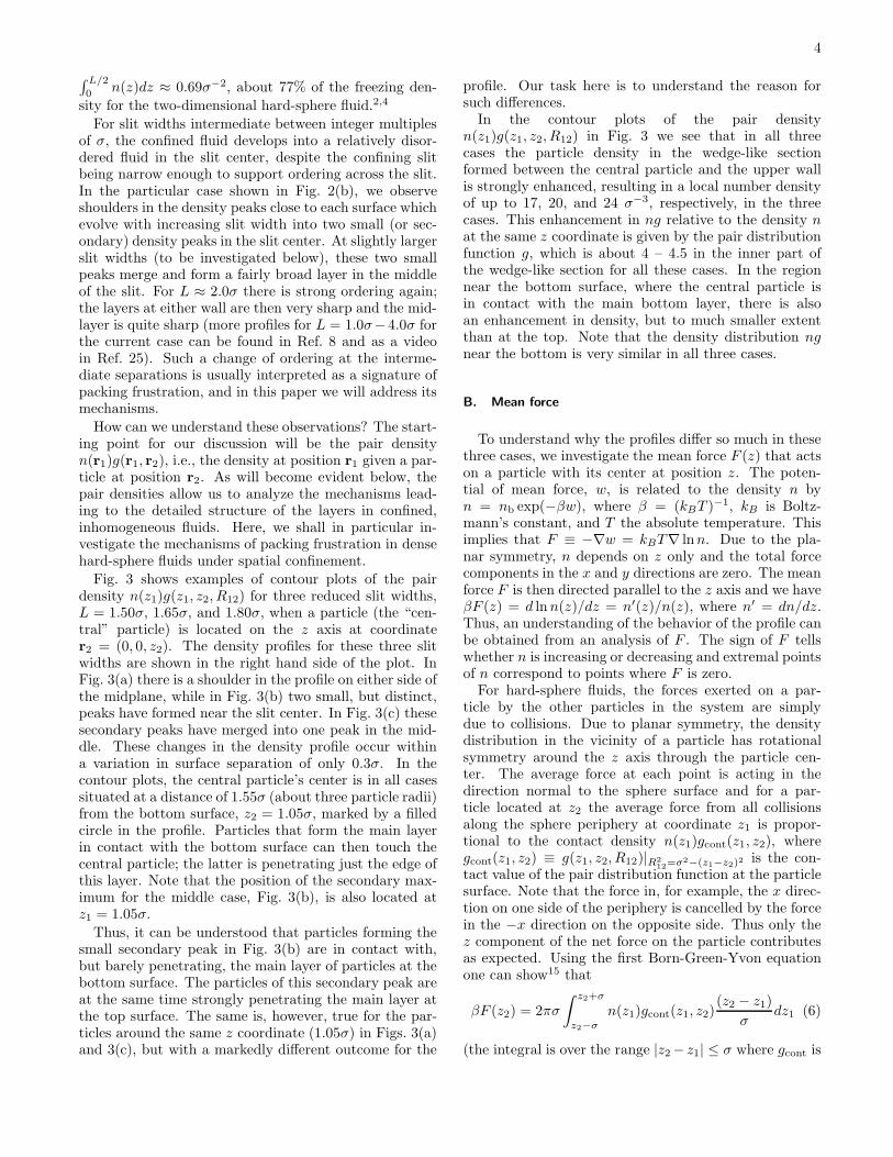
n(z1)g(z1, z2, R12) in Fig. 3 we see that in all threecases the particle density in the wedge-like sectionformed between the central particle and the upper wallis strongly enhanced, resulting in a local number densityof up to 17, 20, and 24 σ−3, respectively, in the threecases. This enhancement in ng relative to the density nat the same z coordinate is given by the pair distributionfunction g, which is about 4 – 4.5 in the inner part ofthe wedge-like section for all these cases. In the regionnear the bottom surface, where the central particle isin contact with the main bottom layer, there is alsoan enhancement in density, but to much smaller extentthan at the top. Note that the density distribution ngnear the bottom is very similar in all three cases.

B. Mean force

To understand why the profiles differ so much in thesethree cases, we investigate the mean force F (z) that actson a particle with its center at position z. The poten-tial of mean force, w, is related to the density n byn = nb exp(−βw), where β = (kBT )

−1, kB is Boltz-mann’s constant, and T the absolute temperature. Thisimplies that F ≡ −∇w = kBT∇ lnn. Due to the pla-nar symmetry, n depends on z only and the total forcecomponents in the x and y directions are zero. The meanforce F is then directed parallel to the z axis and we haveβF (z) = d lnn(z)/dz = n′(z)/n(z), where n′ = dn/dz.Thus, an understanding of the behavior of the profile canbe obtained from an analysis of F . The sign of F tellswhether n is increasing or decreasing and extremal pointsof n correspond to points where F is zero.For hard-sphere fluids, the forces exerted on a par-

ticle by the other particles in the system are simplydue to collisions. Due to planar symmetry, the densitydistribution in the vicinity of a particle has rotationalsymmetry around the z axis through the particle cen-ter. The average force at each point is acting in thedirection normal to the sphere surface and for a par-ticle located at z2 the average force from all collisionsalong the sphere periphery at coordinate z1 is propor-tional to the contact density n(z1)gcont(z1, z2), wheregcont(z1, z2) ≡ g(z1, z2, R12)|R2

12=σ2−(z1−z2)2 is the con-

tact value of the pair distribution function at the particlesurface. Note that the force in, for example, the x direc-tion on one side of the periphery is cancelled by the forcein the −x direction on the opposite side. Thus only thez component of the net force on the particle contributesas expected. Using the first Born-Green-Yvon equationone can show15 that

βF (z2) = 2πσ

∫ z2+σ

z2−σ

n(z1)gcont(z1, z2)(z2 − z1)

σdz1 (6)

(the integral is over the range |z2− z1| ≤ σ where gcont is

5

FIG. 3. Contour plot of the pair density n(r1)g(r1, r2) ≡ n(z1)g(z1, z2, R12) at coordinate r1 = (R12, z1) around a particle inthe slit between two hard surfaces, when the particle is located on the z axis at coordinate r2 = (0, 0, z2). One surface is 0.5σabove the top and one 0.5σ below the bottom of each subplot (cf. Fig. 1). The system is in equilibrium with a bulk fluid ofdensity nb = 0.75σ−3 [same as in Fig. 2(b)]. The gray region is the excluded volume zone around the particle. Data are shownfor different reduced slit widths: (a) L = 1.50σ, (b) 1.65σ, and (c) 1.80σ. The number density profile n(z1) for each case is alsoshown for clarity to the right. The particle position z2 (shown as filled circle in the profile plots) is in all cases positioned at adistance of 1.55σ from the bottom surface (at z coordinate 1.05σ). The arrows in the gray region depict z components of thecollisional forces acting on the particle (corresponding to the z projection of the red arrow in Fig. 1). The arrows displayed ata certain z1 coordinate here represent the entire force acting on the sphere periphery in a dz interval around this coordinate.In subplot (a) the sum of all arrows (with signs) is > 0, in (b) = 0 and in (c) < 0.

defined). The role of the factor (z2 − z1)/σ is to projectout the z component of the contact force. (This lineof reasoning is readily extended to systems exhibitingsoft interaction potentials, such as Lennard-Jones fluidsor electrolytes; in such cases, however, one also needsto include the interactions with the walls and all otherparticles in the system, see e.g. Refs. 16 and 26.)

Let us now return to the intriguing formation of sec-ondary density maxima for L ≈ 1.65σ. For this pur-pose, we present in Fig. 3 the z component of the con-tact forces acting on the particle. They are representedby the arrows along the sphere periphery. In these plots,there are two major contributions to the net force act-ing on the particle, namely the repulsive forces exerted

by the particle layers close to each confining wall. ForL = 1.65σ and the chosen position of the central particlein Fig. 3(b), z2 = 1.05σ, these force contributions canceleach other: the sum of the arrows (with signs) is zeroand hence dn/dz = 0 at this z coordinate, as shown tothe right in the figure. It is the subtle interplay betweenthese forces for neighboring z2 values which leads to thesecondary density maximum.

The situation is, however, markedly different for L =1.50σ and 1.80σ. While the total force exerted by theparticles in the main layer at the bottom surface is prac-tically equal for all three cases, the magnitude of the forceexerted by the particles in the main layer at the uppersurface varies strongly with L. This variation is partly

6

due to the different magnitude of the contact densitiesin the wedge-like region mentioned above and partly dueto the change in angle between the normal vector to thesphere surface there and the z axis. Recall that the con-tact force acts along this normal vector, so the z compo-nent is dependent on this angle. For L = 1.50σ, Fig. 3(a),the z component of the contact force from the upper layeris smaller than for L = 1.65σ. The sum of the arrows isthen positive, i.e. the total average force is directed to-wards the upper wall and hence dn/dz > 0 at this zcoordinate. For L = 1.80σ, Fig. 3(c), this z componentis larger compared to L = 1.65σ, thereby pushing thecentral particle towards the slit center. Hence dn/dz < 0at this z coordinate.

C. Principal components of mean force

In order to gain more insight into the formation of thesecondary maxima, we present in Fig. 4 the net forceacting on a particle for all positions z2 in the same threecases as discussed above, L = 1.50σ, 1.65σ, and 1.80σ.To facilitate the interpretation, the principal force con-tributions acting in positive (denoted F↑) and negative(F↓) directions are shown separately. The total net forceis F = F↑ − F↓, where F↑ originates from collisions onthe lower half of the sphere surface and F↓ on the upperhalf (F↑ and F↓ correspond to the absolute values of thesums of arrows in respective hemisphere in Fig. 3). InFig. 4 the red (solid) and black (dashed) curves are eachother’s mirror images with respect to the vertical dashedaxis at z2 = L/2, which shows the location of the slitcenter.Since the variation in F↑ (and F↓) is very similar for

all slit widths in Fig. 4, the following discussion will holdfor all three cases. For z2 = 0 we have F↑ = 0, becauseno spheres can collide from below since the confining sur-face precludes them from being there (cf. Fig. 1). Withincreasing z2 we observe a monotonically increasing F↑,which can be attributed both to the increasing area ex-posed to collisions on the lower half of the sphere surfaceand the decrease in angle of the sphere normal there rel-ative to the z axis. With further increase in z2, we even-tually observe a decrease in the exerted force induced bya decrease in contact density n(z1)gcont(z1, z2). Aroundz2 ≈ 1.0σ we observe a sudden onset of a rapid decreasefor F↑. This is a consequence of a rapid decrease in con-tact density, that occurs when the particle at z2 losescontact with the dense particle layer at the bottom wall.For even larger z2, where the particle is close to the topsurface, collisions with particles in the slit center aroundthe entire lower half of the sphere surface become impor-tant so that F↑ increases again.The three red curves are compared in the bottom

panel, where F↑ from the first two panels (L = 1.50σand 1.65σ) are shown as dotted curves. We see that thecurves are nearly identical apart from in a small regionto the far right. The analogous statement is true, of

0.0 0.5 1.0 1.5 2.0

0

5

10

z2 / σ

βF /

σ–1

1.50 ↑1.50 ↓

0

5

10

βF /

σ–1

1.65 ↑1.65 ↓

0.0 0.5 1.0 1.5 2.00

5

10

z2 / σ

βF /

σ–1

1.80 ↑1.80 ↓

a

b

c

FIG. 4. Net forces acting on a particle for the systems inFig. 3. The force contributions acting in positive (F↑, fullcurve) and negative (F↓, dashed curve) z directions are pre-sented separately as functions of particle position z2 acrossthe confining slit. Data are shown for reduced slit widthsL = 1.50σ, 1.65σ, and 1.80σ. The values of the forces for aparticle at the z2 coordinates in Fig. 3 are shown by filled cir-cles. The dashed vertical line denotes the slit center, while thesolid vertical line on the right-hand side indicates the upperlimit for possible z2 coordinates of the particle in the slit. Forcomparison of all three cases, F↑ is also shown for L = 1.50σ(blue dots) and 1.65σ (black dots) in the bottom panel.

course, for the black dashed curves. Thus, apart fromsmall z2 intervals to the extreme left and right, the be-havior of F = F↑ − F↓ for the different slit widths canbe understood in terms of a horizontal shift of the redand the black curves relative to each other. The forma-tion of secondary density maxima can then be explainedfrom the resulting balance of the force contributions. ForL = 1.65σ and z2 > L/2 [i.e., the right half of Fig. 4(b)],the two curves intersect at two points where the forcescancel each other and where dn/dz = 0. The intersectionmarked by the filled circle gives a local maximum of n(z)and the next one to the right gives a minimum. Together

7

0 1 2 3 4

0

5

10

z2 / σβF

/ σ–1

3.45 ↑3.45 ↓

a

b

c0

5

10

βF /

σ–1

3.60 ↑3.60 ↓

0 1 2 3 40

5

10

z2 / σ

βF /

σ–1

3.75 ↑3.75 ↓

FIG. 5. As Fig. 4, but for reduced slit widths L = 3.45σ,3.60σ, and 3.75σ.

with the minimum at the slit center, z2 = L/2, where thecurves also cross each other, these features give rise to thesecondary peak of the density profile as we have seen inFig. 3(b). This subtle balance of forces, and hence theformation of secondary maxima, is only observed in anarrow range of slit widths, as evidenced by the forceprofiles for L = 1.50σ and 1.80σ. In the latter case, theintersection at z2 = L/2 corresponds to a local maximumand the other one to a minimum. Together they give onepeak in the middle as seen in Fig. 3(c).

The formation of secondary maxima is for z2 > L/2 ac-cordingly a consequence of two phenomena: (i) the rapiddecrease of F↑ followed by the subsequent increase of F↑

and (ii) the monotonic decrease of F↓ in the same region.Together these effects lead to the force curves intersect-ing twice in the manner they do for L = 1.65σ. Therapid decrease of F↑ is, as we have seen, due to the lossof contact of the particle with the well-developed bottomlayer, while the monotonic decrease of F↓ occurs whenthe particle approaches the top surface.

For comparison, we present in Fig. 5 the principal force

0 1 2 3 40

2

4

6

8

z / σ

n(z)

/ σ–3

L = 1.65

L = 2.60

L = 3.60

L = ∞

n(z) + 3

n(z) + 2

n(z) + 1

FIG. 6. Number density profiles n(z) for the confined hard-sphere fluid. The reduced slit widths are L = 1.65σ (offsetvertically by 3.0σ−3), 2.60σ (offset by 2.0σ−3), and 3.60σ (off-set by 1.0σ−3). The systems are otherwise the same as inFig. 2(b). The solid and dotted lines depict results based onthe full APY theory and the superposition approximation, re-spectively. The density profile at a single solid-fluid interface(L = ∞) is also shown for comparison.

components for a set of larger slit widths: L = 3.45σ,3.60σ, and 3.75σ. There are no secondary maxima inthis case. Instead we observe for L = 3.60σ a broadregion in the center of the slit where F↑ and F↓ virtuallycancel each other and where, as a consequence, dn/dz ≈0. Hence, this observation implies an essentially constantn in the slit center, as can be seen in the third full curveof Fig. 6, where density profiles are shown for variouscases.The course of events shown in Fig. 5 when we increase

L from 3.45σ to 3.75σ implies the formation of a layer atthe slit center. The crossing of the principal force curvesin Fig. 5(a) at the slit center, z2 = L/2, corresponds toa density minimum, while that in Fig. 5(c) correspondsto a density maximum. Note that for L ≈ 3.0σ there arefour layers in the slit (two very sharp ones at the wallsand two less sharp on either side of the slit center) and forL ≈ 4.0σ there are five layers. The fifth layer that formsin the middle for the intermediate separations arises viathe broad flattening of the density profile in the middle,and signals the packing frustration in this case.The data of Figs. 4 and 5 indicate a qualitative differ-

ence in n(z) for L ≈ 1.65σ and ≈ 3.60σ. In the transitionfrom 2 → 3 particle layers, the third layer is formed viathe occurrence of secondary layers close to each surface,which merge to form a central layer with increasing L.This contrasts the transitions from 4 → 5 particle layersjust discussed, where the new particle layer forms directlyin the slit center. The secondary peaks for L ≈ 1.65σ arealso evident in qualitatively different anisotropic struc-ture factors S(q) for L = 1.60σ and 3.50σ presented inour previous work, Ref. 8. S(q) for confined fluids is

8

governed by an ensemble average of the anisotropic pairdensity correlations n(z1)h(z1, z2, R12) (see Ref. 25 formore slit widths). In order to address these differencesin n(z) with L, we will in the following analyze furtherthe principal force component F↑.

D. Superposition approximation

In both Figs. 4 and 5, the principal force componentsF↑ (and F↓) for different L nearly coincide for most z val-ues. In order to investigate this further, we plot F↑ fora wider set of slit widths, L = 3.0σ − 4.0σ, in Fig. 7(a).Indeed, apart from rather small deviations at large z, alldata fall on a master curve given by F↑ for L = ∞, i.e.,the force component for the single solid-fluid interface[the former curves are also shown separated in Fig. 7(b)].Although not shown here, we have verified that this ob-servation holds reasonably well for L ≥ 1.0σ, implyingthe same ordering mechanism irrespective of slit width.In order to gain further insight into the ordering mech-

anism, we have determined density profiles obtained ina simple superposition approximation.27–30 Within thisapproximation, the potential of mean force w in the slitis calculated as the sum of the corresponding potentialsfrom two single hard surfaces, i.e. w(z) ≈ w∞(z) +w∞(L−z), where w∞ denotes the potential of mean forcefor the fluid at a single solid-fluid interface in contact witha bulk fluid of density nb. This implies the superpositionfor the mean force: F (z) ≈ F∞(z) − F∞(L − z). Sincethe density profile is given by n(z) = nb exp[−βw(z)] thesuperposition approximation implies

n(z;L) ≈ nsp(z;L) =n∞(z)n∞(L− z)

nb, (7)

where we have explicitly shown that the density profilefor the slit, n(z) ≡ n(z;L), depends on L, and wheresuperscript sp indicates “superposition” and n∞(z) is thedensity profile outside a single surface.In Fig. 6 we compare n(z) for reduced slit widths of

L = 1.65σ, 2.60σ, and 3.60σ obtained via the full the-ory (solid lines) and the superposition approximationthus obtained (dotted lines). Note that there are den-sity peaks at z ≈ 1.05σ for all three slit widths and thatthey approximately coincide with the location of a den-sity peak for the single solid-fluid interface (also shown inFig. 6). This implies that the density peak at z ≈ 1.05σis strongly correlated with the bottom solid surface. Al-though the profiles obtained via the superposition ap-proximation deviate quantitatively from those of the fulltheory, especially for narrow slit widths, the qualitativeagreement implies that the main features of n(z) – thedensity peaks and shoulders of Fig. 6 – are rather un-complicated confinement effects.To substantiate this conclusion, we present in Fig. 7(b)

the principal force components F↑ for L = 3.0σ − 4.0σ,obtained both using the full theory and the superposi-tion approximation. The agreement is equally good as

0 1 2 3 4 5

0

2

4

6

8

10

12

z2 / σ

βF↑(

z 2) /

σ–1

L = 3.00 – 4.00L = ∞

a

b

c0

2

4

6

8

10

12

14

16

βF↑(

z 2) /

σ–1

L=3.00

L=3.25

L=3.50

L=3.75

L=4.00

F↑ + m

0 1 2 3 4 5

0

2

4

6

8

10

12

z2 / σ

βF↑(

z 2) /

σ–1

L=3.00L=3.25

L=3.50L=3.75L=4.00

FL↑

∆FU↑ + m

FIG. 7. Principal mean force component F↑ for the hard-sphere fluid between planar hard surfaces. The reduced sep-arations are L = 3.00σ, 3.25σ, 3.50σ, 3.75σ, and 4.00σ. Thesystems are otherwise the same as in Fig. 2(b). (a) F↑ for theconfined fluids (black lines) and for a single solid-fluid inter-face (L = ∞, red line). (b) F↑ for the confined fluids (eachoffset vertically by m = 0...4 units for clarity), obtained viathe full APY theory [solid lines, same as in (a)] and the super-position approximation (dotted lines). (c) Force componentsof the superposition approximation, FL

↑ and ∆FU↑ , for differ-

ent reduced slit widths (the latter curves are vertically offsetby m for clarity). FL

↑ is the same as the red curve in (a).

9

F!L

!F"U

FIG. 8. A sketch illustrating the force contributions FL↑ and

∆FU↑ in the superposition approximation. Each arrow rep-

resents a force that acts on the entire red half of the sphere(the location of the arrow has no significance in this sketch).The lower wall is shown in black and the upper wall is to beplaced on the location indicated by the striped rectangle. Thedashed line that connects each arrow to the respective surfaceindicates from which wall the influence originates.

for the density profile of the L = 3.60σ case in Fig. 6. Asignificant point is now that the superposition allows usto separate the contributions to F↑ from each surface in asimple manner, that will provide insights into what hap-pens during confinement. As shown in Appendix A, F↑

can be decomposed in this approximation into two com-ponents: a major contribution from the lower surface,FL↑ , and a correction due to the presence of the upper

surface, ∆FU↑ . The former is the same as the average

force component for the single solid-fluid interface plot-ted in Fig. 7(a) (denoted as “master curve” above). Wehave

F sp↑ (z2;L) = FL

↑ (z2) + ∆FU↑ (z2;L), (8)

where ∆FU↑ (z2;L) = FU

↑ (z2;L)−F b↑ , see Eq. (A3). Here,

FU↑ is the average force for the case of a single solid-fluid

interface (U) and F b↑ is the force that acts on one side of

a hard sphere (i.e. on one half) in the bulk fluid. Notethat in F sp

↑ it is only FU↑ that depends on L.

In Fig. 7(c) we show FL↑ and ∆FU

↑ for the same surfaceseparations as before. The L dependence of the latter issimply a parallel displacement along z. When FL

↑ and

∆FU↑ are added we obtain the dotted curves in Fig. 7(b).

Thus the differences between each black curve and thered curve in Fig. 7(a) is essentially contained in the con-tribution ∆FU

↑ from the upper surface (for smaller sur-face separations there will remain a minor difference asindicated by the small deviations for the superpositionapproximation in Fig. 6).

To see in more detail what this means, we have inFig. 8 shown schematically how these force contributionsact on a sphere. In the presence of only one solid-fluidinterface (L), the total force in the direction away fromthe surface (upwards) is F↑ = FL

↑ , i.e., the force on thebottom half of the sphere shown as red in the figure. Letus now place the second surface (U) some distance fromthe other, at the location indicated in the figure. Thechange in the upwards force due to this second surfaceis given by ∆F↑ ≈ ∆FU

↑ in the superposition approx-

imation. Note that the former force, FL↑ , acts on the

hemisphere that is facing the surface L, while the latter,∆FU

↑ , is a force that acts on the hemisphere away from

the corresponding surface U and in the direction towards

this surface.

If the lower wall were not present when we place the up-per wall at the indicated position, the initial state wouldbe a homogeneous bulk fluid and the final state a singlesolid-fluid interface (U) in contact with the bulk. In thissituation ∆FU

↑ equals the actual change in the average

force on the red hemisphere. In Eq. (8) we have adoptedthis value as an approximation for the correspondingchange when placing the upper wall in the presence ofthe lower one, i.e., when the initial state is an inhomoge-neous fluid in contact with the lower surface and the finalstate is a fluid simultaneously affected by both surfaces.Since this approximation obviously is very good, it fol-lows that the inhomogeneity due to one surface has onlya small influence on the effects from the other surfacethroughout the entire slit.

We saw in section III C that the seemingly compli-cated changes in structure as the surface separation variesaround half-integer σ values of L (i.e., [m + 0.5]σ withm = integer), can be mainly explained by a parallel dis-placement of upward and downwards force curves alongthe z direction. There was, however, some variation inthese force curves near one of the surfaces (the upper sur-face for the upward forces and the lower surface for thedownwards forces) that remained unexplained there. Inthe current section we have seen that this variation toocan be mainly explained by a parallel displacement – inthis case a displacement of the contributions to F↑ (orF↓) due to each surface as seen in Fig. 7(c).

To summarize our results in this section we make twoimportant conclusions: First, by considering the meanforce due to one surface (here the lower one) and bytreating the influence from the other (upper) surface as acorrection ∆FU

↑ according the the superposition approx-imation, one obtains nearly quantitative agreement withthe full theory. Our approach of defining principal com-ponents of the mean force thereby provides a means tounderstand the contributions of each confining surface.Second, the principal force components obtained withinthe full theory and the superposition approximation arevirtually in quantitative agreement for L ≥ 3.0σ. Fornarrower slit widths (down to L = 1.0σ), quantitativediscrepancies become more pronounced. These quanti-tative differences, which will be discussed in the next

10

subsection, are nontrivial confinement effects. Neverthe-less, the semi-quantitative agreement in the whole rangeof slit widths, down to L = 1.0σ, further strengthens thenotion that ordering of confined hard-sphere fluids can,to a good approximation, be explained as a single-wallphenomenon. In essence, the fluid conforms locally withonly one of the confining surfaces at a time. In somelocal regions it will thereby conform to one surface andin other regions to the other surface – regions that arecontinuously changing (recall that the distributions wecalculate are time averages of the various possible struc-tures). We emphasize that this reasoning holds for allslit widths, irrespective of whether L is close to an inte-ger or a half-integer multiple of the particle diameter (cf.Fig. 7). In other words, from a mechanistic point of viewthere is little difference between ordering in frustratedand more ordered confined hard-sphere fluids. In the lat-ter case, the local ordering near one surface essentiallyagrees with the local ordering at the other one, wherebyfor the density profiles there appear only small mutualeffects of the ordering from both surfaces beyond what isgiven by superposition.An interesting similarity between the structures ob-

served in the fluid and solid phases should be mentioned.In some of the exotic crystalline structures observed un-der confinement – most notably the prism-like struc-tures3,4,6 – the particles locally conform with one of thesolid surfaces. This is reminiscent of the situation inthe fluid phase discussed above, although in the lattercase the structures are less ordered and constantly chang-ing locally. In particular, the adaptive prism phase 2PA

found in Ref. 6 would yield an average density profilewith secondary peaks on either side of the midplane, sim-ilar of those shown in Fig. 3(b) but much sharper.The fact that the superposition approximation works

surprisingly well for these rather large densities and givesa large part of the effects of confinement, means that itis simple to obtain good estimates of the density pro-files for a confined fluid given an accurate density profilefor a single solid-fluid interface. To obtain the latter is,however, computationally nontrivial and requires fairlyadvanced theories. Furthermore, as we shall see below,not all important properties of the confined fluid can beexplained by superposition.

E. Nontrivial confinement effects

We have shown that the density profile n(z) of con-fined hard-sphere fluids is, to a large extent, determinedby packing constraints at a single solid-fluid interface.In this respect, the ordering is a trivial confinement ef-fect. However, subtle deviations in n(z) do remain inthe superposition approximation, and these may lead toimportant, nontrivial confinement effects. The two mostprominent nontrivial effects of confinement in, for exam-ple, Fig. 6 are the slit width dependence of the contactdensity at the walls, ncont, and the total number of par-

1 2 3 4

0.2

0.4

0.6

0.8

1.0

1.2

L / σ

Γ / σ

–2

b

a

1 2 3 4

4

5

6

7

8

9

L / σn co

nt /

σ–3

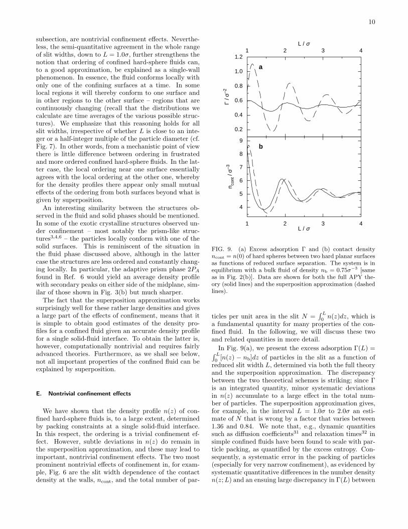
FIG. 9. (a) Excess adsorption Γ and (b) contact densityncont = n(0) of hard spheres between two hard planar surfacesas functions of reduced surface separation. The system is inequilibrium with a bulk fluid of density nb = 0.75σ−3 [sameas in Fig. 2(b)]. Data are shown for both the full APY the-ory (solid lines) and the superposition approximation (dashedlines).

ticles per unit area in the slit N =∫ L

0n(z)dz, which is

a fundamental quantity for many properties of the con-fined fluid. In the following, we will discuss these twoand related quantities in more detail.

In Fig. 9(a), we present the excess adsorption Γ(L) =∫ L

0[n(z) − nb]dz of particles in the slit as a function of

reduced slit width L, determined via both the full theoryand the superposition approximation. The discrepancybetween the two theoretical schemes is striking; since Γis an integrated quantity, minor systematic deviationsin n(z) accumulate to a large effect in the total num-ber of particles. The superposition approximation gives,for example, in the interval L = 1.0σ to 2.0σ an esti-mate of N that is wrong by a factor that varies between1.36 and 0.84. We note that, e.g., dynamic quantitiessuch as diffusion coefficients31 and relaxation times32 insimple confined fluids have been found to scale with par-ticle packing, as quantified by the excess entropy. Con-sequently, a systematic error in the packing of particles(especially for very narrow confinement), as evidenced bysystematic quantitative differences in the number densityn(z;L) and an ensuing large discrepancy in Γ(L) between

11

the full theory and the superposition approximation, willhave a substantial impact on many properties of the con-fined fluid obtained theoretically.Fig. 9(b) shows the contact density ncont = n(0) as

a function of L, again obtained both via the full theoryand the superposition approximation. This is an impor-tant quantity, because it yields the pressure between thewalls, Pin = kBTn(0), according to the contact theorem.Consequently, ncont is related to the net pressure actingon the confining surfaces, Π(L) = Pin(L) − Pb with Pb

denoting the bulk pressure, and hence to the extensivelystudied oscillatory surface forces.33,34 While the superpo-sition approximation explains reasonably well the magni-tude of ncont, there is a nontrivial systematic phase shiftwith respect to L of about 0.1σ. This effect has beenobserved by one of us (S.S.) already earlier,30 and in thefollowing we will provide a mechanistic explanation of thephenomenon. A similar phase shift can also be seen inΓ(L), Fig. 9(a).In the superposition approximation, Eq. (7) yields the

contact density for the wall at z = 0 as

nspcont(L) = nsp(0;L) =

n∞(0)n∞(L)

nb. (9)

Thus, the contact density for a reduced slit width L is inthis approximation proportional to the density at z = Loutside a single surface. To analyze the L dependencefurther we will need the following equation that is equiv-alent to Eq. (1),

d[lnn(z1) + βv(z1)]

dz1=

− β

∫

n(z2)h(z1, z2, R12)dv(z2)

dz2dz2dR12. (10)

[The two equations can be transformed into each otherby the Ornstein-Zernike equation (2).] For a single hardwall-fluid interface located at z = 0, Eq. (10) yields

dn∞(z1)

dz1= n∞(z1)n∞(0)

∫

h∞(z1, 0, R12)dR12, (11)

where h∞ is the total pair correlation function for thefluid outside the single surface. By inserting z1 = L, thisequation together with Eq. (9) imply that

dnspcont(L)

dL= nsp

cont(L)n∞(0)

∫

h∞(z1, 0, R12)dR12

∣

∣

∣

∣

z1=L

.

(12)For the exact case, the corresponding equation can beobtained from Eq. (5), which yields

dncont(L)

dL= [ncont(L)]

2

∫

h(z1, 0, R12)dR12

∣

∣

∣

∣

z1=L

. (13)

Apart from the factors in front of the integral, we see thatthe main difference is that in the superposition approx-imation the total pair correlation function for a single

wall is evaluated at coordinate z1 = L outside the wall,while for the exact case the correlation function for thefluid in the slit is evaluated at the opposite surface (alsoat z1 = L). The oscillatory behavior of the contact den-sity as a function of L implies that its derivative changessign with the same periodicity. Since the prefactors arepositive, the phase shift for nsp

cont relative to ncont mustoriginate from the integrals.

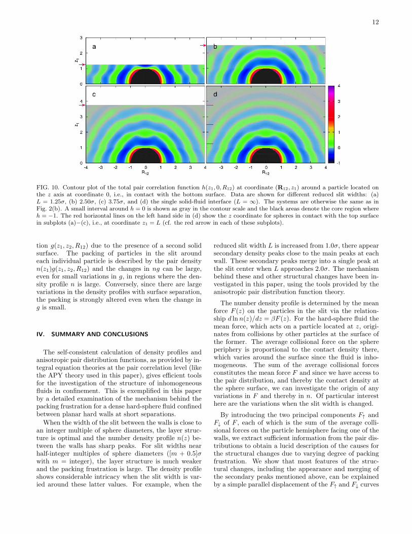
In Fig. 10 we have plotted the total pair correlationfunction h(z1, 0, R12) in the slit when the central particleis in contact with the lower surface (i.e., at coordinate 0)for the cases L = 1.25σ, 2.50σ, and 3.75σ together withthe corresponding function for a single hard wall-fluidinterface. The first impression is a striking similarity ofthese plots, despite that there is an upper surface presentin the first three cases. There are only small differences inthe entire slit compared to the single surface case for thecorresponding z1 values. When looking closely, one can,however, see some systematic differences in the h func-tion induced by the presence of the upper surface. Mostimportantly, we will investigate h for z1 = L, which oc-curs in the integral in Eq. (13), and compare this with thevalues at the same z1 coordinates for the single surfacecase, occurring in Eq. (12). These z1 values are markedwith red arrows in the left hand side of Figs. 10(a)–(c)and with red lines in Fig. 10(d).

Fig. 11 shows R12 × h(z1, 0, R12) with z1 = L for thecases in Figs. 10(a)–(c) and these curves are compared toR12 × h∞(z1, 0, R12) for the same z1 coordinates (shownas blue dotted lines in the figure). The factor R12 isincluded so the areas under the curves in Fig. 11 areproportional to the values of the integrals of Eqs. (12)and (13); this factor originates from the area differentialdR12 = 2πR12dR12. The L values in Figs. 10 and 11 areselected such that we cover cases where dncont(L)/dL anddnsp

cont(L)/dL in Fig. 9(b) are negative (L = 1.25σ) andpositive (L = 3.75σ). There is also one case (L = 2.50σ)with dnsp

cont(L)/dL ≈ 0. These signs can be verified byinspection of the areas under the curves in Fig. 11 (thecontributions around R12 = 0 are most important for thesign; there are substantial cancellations in the tail regiondue to the oscillations).

We can see in the figure that the full curves and theblue dotted ones do not agree, which means that thevalues of the integrals and hence of dncont(L)/dL aredifferent, as expected. If we instead plot the values ofR12 × h∞(z1, 0, R12) for z1 = L + 0.1σ (red dotted linesin the figure) we obtain better agreement. Thus thepresence of the upper surface makes h(z1, 0, R12) “com-pressed” in the z direction by about 0.1σ compared toh∞(z1, 0, R12). This compression gives rise to the phaseshift observed in Fig. 9. There are also some other smalldifferences between h and h∞ and, in addition, there aredifferent prefactors in Eqs. (12) and (13). This gives theremaining differences in ncont(L) and nsp

cont(L) seen inFig. 9(b).

The nontrivial confinement effects are accordingly dueto rather delicate changes in the pair distribution func-

12

FIG. 10. Contour plot of the total pair correlation function h(z1, 0, R12) at coordinate (R12, z1) around a particle located onthe z axis at coordinate 0, i.e., in contact with the bottom surface. Data are shown for different reduced slit widths: (a)L = 1.25σ, (b) 2.50σ, (c) 3.75σ, and (d) the single solid-fluid interface (L = ∞). The systems are otherwise the same as inFig. 2(b). A small interval around h = 0 is shown as gray in the contour scale and the black areas denote the core region whereh = −1. The red horizontal lines on the left hand side in (d) show the z coordinate for spheres in contact with the top surfacein subplots (a)−(c), i.e., at coordinate z1 = L (cf. the red arrow in each of these subplots).

tion g(z1, z2, R12) due to the presence of a second solidsurface. The packing of particles in the slit aroundeach individual particle is described by the pair densityn(z1)g(z1, z2, R12) and the changes in ng can be large,even for small variations in g, in regions where the den-sity profile n is large. Conversely, since there are largevariations in the density profiles with surface separation,the packing is strongly altered even when the change ing is small.

IV. SUMMARY AND CONCLUSIONS

The self-consistent calculation of density profiles andanisotropic pair distribution functions, as provided by in-tegral equation theories at the pair correlation level (likethe APY theory used in this paper), gives efficient toolsfor the investigation of the structure of inhomogeneousfluids in confinement. This is exemplified in this paperby a detailed examination of the mechanism behind thepacking frustration for a dense hard-sphere fluid confinedbetween planar hard walls at short separations.

When the width of the slit between the walls is close toan integer multiple of sphere diameters, the layer struc-ture is optimal and the number density profile n(z) be-tween the walls has sharp peaks. For slit widths nearhalf-integer multiples of sphere diameters ([m + 0.5]σwith m = integer), the layer structure is much weakerand the packing frustration is large. The density profileshows considerable intricacy when the slit width is var-ied around these latter values. For example, when the

reduced slit width L is increased from 1.0σ, there appearsecondary density peaks close to the main peaks at eachwall. These secondary peaks merge into a single peak atthe slit center when L approaches 2.0σ. The mechanismbehind these and other structural changes have been in-vestigated in this paper, using the tools provided by theanisotropic pair distribution function theory.

The number density profile is determined by the meanforce F (z) on the particles in the slit via the relation-ship d lnn(z)/dz = βF (z). For the hard-sphere fluid themean force, which acts on a particle located at z, origi-nates from collisions by other particles at the surface ofthe former. The average collisional force on the sphereperiphery is proportional to the contact density there,which varies around the surface since the fluid is inho-mogeneous. The sum of the average collisional forcesconstitutes the mean force F and since we have access tothe pair distribution, and thereby the contact density atthe sphere surface, we can investigate the origin of anyvariations in F and thereby in n. Of particular interesthere are the variations when the slit width is changed.

By introducing the two principal components F↑ andF↓ of F , each of which is the sum of the average colli-sional forces on the particle hemisphere facing one of thewalls, we extract sufficient information from the pair dis-tributions to obtain a lucid description of the causes forthe structural changes due to varying degree of packingfrustration. We show that most features of the struc-tural changes, including the appearance and merging ofthe secondary peaks mentioned above, can be explainedby a simple parallel displacement of the F↑ and F↓ curves

13

0 2 4 6 8 10

-0.2

-0.1

0.0

0.1

0.2

0.3

R12

/ σ

h⋅R

12 / σ

L = 1.25

L = 2.50

L = 3.75

-0.06

-0.04

-0.02

0.00

0.02

0.04

0.06

h⋅R

12 / σ

0 2 4 6 8 10

-0.015

-0.010

-0.005

0.000

0.005

0.010

0.015

R12

/ σ

h⋅R

12 / σ

FIG. 11. R12×h(L, 0, R12) as function of R12 for the systemsin Fig. 10(a)-(c) with reduced surface separations L = 1.25σ,L = 2.50σ, and L = 3.75σ. The data are obtained via fullAPY theory (solid line), superposition approximation (bluedotted line), and shifted superposition approximation (L →

L + 0.1σ, red dotted line). In the latter two cases, R12 ×

h∞(z1, 0, R12) is plotted for the appropriate z1 values (seetext). Note the different scales on the y axis in the subplots.The curves go to zero at R12 = 0 because of the factor R12.

when the slit width is varied around half-integer σ val-ues. The underlying reasons for this simple behavior isrevealed via a detailed investigation of the pair distri-bution, that gives information about how the contactdensities around the sphere periphery varies for differ-ent positions z of a particle in the slit.

It is found that the components F↑ and F↓, and therebythe ordering of the fluid, are essentially governed by thepacking conditions at each single solid-fluid interface.The fluid in the slit thereby conforms locally with onlyone of the confining surfaces at a time. In some localregions it will conform to one surface and in other re-gions to the other surface – regions that are constantlychanging (the calculated distributions are averages of thevarious possible structures). This picture holds for all slitwidths, irrespective of whether L is close to an integer or

a half-integer multiple of the particle diameter.As a consequence of these local packing conditions, the

force components F↑ and F↓, and thereby the total meanforce F = F↑ − F↓ acting on a particle in the slit, canto a surprisingly good approximation be written as a su-perposition of contributions due to the presence of eachindividual solid-fluid interface at the walls. When theslit width is varied, this superposition can be expressedin terms of a parallel displacement of force curves due toeither surface.There are, however, some important properties of the

inhomogeneous fluid that cannot be described by a simplesuperposition, but are instead determined by nontrivialconfinement effects. In this paper, we exemplify suchquantities by the number of particles per unit area in theslit N , the excess adsorption Γ, the contact density ofthe fluid at the wall surfaces n(0), and the net interac-tion pressure between the walls Π. In the superpositionapproximation, N and Γ disagree to a large extent com-pared to the accurate values, while n(0) and Π are mainlyoff by a phase shift in their oscillations. The analysisshow that these nontrivial confinement effects are due torather delicate changes in the anisotropic pair distribu-tion function g(z1, z2, R12) when the wall separation ischanged.

ACKNOWLEDGMENTS

We thank Tom Truskett for providing the simulationdata in Fig. 2(a). K.N. and R.K. acknowledge supportfrom the Swedish Research Council (Grant nos. 621-2012-3897 and 621-2009-2908, respectively). The com-putations were supported by the Swedish National In-frastructure for Computing (SNIC 001-09-152) via PDC.

Appendix A: Force subdivision in superposition

approximation

For a hard sphere fluid in the slit between two hardwalls, the force on, for example, the lower hemisphere of ahard sphere, F↑, can in the superposition approximationbe divided into contributions due to either wall surface.The contribution FL

↑ from the lower surface is given by

[cf. Eq. (6)]

βFL↑ (z2) = 2π

∫ z2

z2−σ

dz1n∞(z1)gcont∞ (z1, z2)(z2 − z1),

(A1)where gcont∞ is the contact value of the pair distributionfor the fluid outside a single surface. Likewise, the con-tribution FU

↑ from the upper surface is given by

βFU↑ (z2;L) = 2π

∫ z2

z2−σ

dz1n∞(L − z1)

× gcont∞ (L− z1, L− z2)(z2 − z1). (A2)

14

In the total F sp↑ there is a further contribution. From

Eq. (7) we see that the total βF sp is equal to the deriva-tive of lnnsp(z;L) = lnn∞(z) + lnn∞(L − z) − lnnb.While the last term gives zero for βF sp, i.e., the meanforce in bulk is zero, this is not the case for βF sp

↑ . The

mean force on one half of the sphere surface in bulk, F b↑ ,

is non-zero; it is only the sum of the forces on both halvesthat are zero. Thus we have

F sp↑ (z2;L) = FL

↑ (z2) + FU↑ (z2;L)− F b

↑ (A3)

with βF b↑ = πσ2nbg

contb , where gcontb is the contact value

for the pair distribution in bulk. When L → ∞, the pres-ence of the last term makes F sp

↑ go to the single surface

force FL↑ , as it should in this limit.

1P. Pieranski, L. Strzelecki, and B. Pansu, Phys. Rev. Lett. 50,900 (1983).

2M. Schmidt and H. Lowen, Phys. Rev. Lett. 76, 4552 (1996).3S. Neser, C. Bechinger, P. Leiderer, and T. Palberg, Phys. Rev.Lett. 79, 2348 (1997).

4A. Fortini and M. Dijkstra, J. Phys.: Condens. Matter 18, L371(2006).

5A. B. Fontecha and H. J. Schope, Phys. Rev. E 77, 061401 (2008).6E. C. Oguz, M. Marechal, F. Ramiro-Manzano, I. Rodriguez,R. Messina, F. J. Meseguer, and H. Lowen, Phys. Rev. Lett.109, 218301 (2012).

7P. N. Pusey and W. van Megen, Nature 320, 340 (1986).8K. Nygard, S. Sarman, and R. Kjellander, J. Chem. Phys. 139,164701 (2013).

9J. Mittal, J. R. Errington, and T. M. Truskett, J. Chem. Phys.126, 244708 (2007).

10J. Mittal, T. M. Truskett, J. R. Errington, and G. Hummer,Phys. Rev. Lett. 100, 145901 (2008).

11S. Lang, V. Botan, M. Oettel, D. Hajnal, T. Franosch, andR. Schilling, Phys. Rev. Lett. 105, 125701 (2010).

12S. Lang, R. Schilling, V. Krakoviack, and T. Franosch, Phys.Rev. E 86, 021502 (2012).

13J.-P. Hansen and I. R. McDonald, Theory of Simple Liquids, 3rded. (Academic Press, Amsterdam, 2006).

14R. Kjellander and S. Marcelja, J. Chem. Phys. 88, 7138 (1988).15R. Kjellander and S. Sarman, J. Chem. Soc. Faraday Trans. 87,1869 (1991).

16R. Kjellander and S. Sarman, Mol. Phys. 74, 665 (1991).17B. Gotzelmann and S. Dietrich, Phys. Rev. E 55, 2993 (1997).18V. Botan, F. Pesth, T. Schilling, and M. Oettel, Phys. Rev. E79, 061402 (2009).

19D. Henderson, S. Sokolowski, and D. Wasan, J. Stat. Phys. 89,233 (1997).

20J. W. Zwanikken and M. Olvera de la Cruz, Proc. Natl. Acad.Sci. USA 110, 5301 (2013).

21R. Kjellander and S. Sarman, Chem. Phys. Lett. 149, 102 (1988).22H. Greberg, R. Kjellander, and T. Akesson, Molec. Phys. 92, 35(1997).

23R. Roth, J. Phys.: Condens. Matter 22, 063102 (2010).24K. Nygard, R. Kjellander, S. Sarman, S. Chodankar, E. Perret,J. Buitenhuis, and J. F. van der Veen, Phys. Rev. Lett. 108,037802 (2012).

25For videos of the density profile as a function of slit width,see the Supplementary material of Ref. 8, Video 2, atftp://ftp.aip.org/epaps/journ_chem_phys/E-JCPSA6-139-037340.Videos of pair distributions and anisotropic structure factors forthe system can also be found there.

26R. Kjellander, J. Phys.: Condens. Matter 21, 424101 (2009).27J. K. Percus, J. Stat. Phys. 23, 657 (1980).28I. K. Snook and W. van Megen, J. Chem. Soc. Faraday Trans. 277, 181 (1981).

29M. S. Wertheim, L. Blum, and D. Bratko, in Micellar Solutions

and Microemulsions, edited by S.-H. Chen and R. Rajagopalan(Springer-Verlag, New York, 1990) p. 99.

30S. Sarman, in Liquids at Interfaces, edited by J. Charvolin, J. F.Joanny, and J. Zinn-Justin (Elsevier, Amsterdam, 1990) p. 169.

31J. Mittal, J. R. Errington, and T. M. Truskett, Phys. Rev. Lett.96, 177804 (2006).

32T. S. Ingebrigtsen, J. R. Errington, T. M. Truskett, and J. C.Dyre, Phys. Rev. Lett. 111, 235901 (2013).

33R. G. Horn and J. N. Israelachvili, J. Chem. Phys. 75, 1400(1981).

34J. N. Israelachvili, Intermolecular and Surface Forces, 2nd ed.(Academic Press, London, 1991).