arX

iv:1

105.

1300

v1 [

astr

o-ph

.GA

] 6

May

201

1

Infrared and optical polarimetry around the low-mass star-forming regionNGC 1333 IRAS 4A

F. O. Alves1, J. A. Acosta-Pulido2,3, J. M. Girart1, G. A. P. Franco4, and R. Lopez5

1Institut de Ciencies de l’Espai (IEEC–CSIC), Campus UAB, Facultat de Ciencies, C5 par 2a,

08193 Bellaterra, Catalunya, Spain

[oliveira;girart]@ice.cat

2Instituto de Astrofısica de Canarias, Vıa Lactea s/n, E-38200 La Laguna, Tenerife, Spain

jap@iac.es

3Departamento de Astrofısica, Universidad de La Laguna, E-38205 La Laguna, Tenerife, Spain

4Departamento de Fısica – ICEx – UFMG, Caixa Postal 702, 30.123-970 Belo Horizonte, Brazil

franco@fisica.ufmg.br

5Departament d’Astronomia i Meteorologia (IEEC-UB), Institut de Ciencies del Cosmos,

Universitat de Barcelona, Martı i Franques 1, E-08028 Barcelona, Spain

rosario@am.ub.es

Received ; accepted

Based on observations collected with the 4.2 m William Herschel Telescope, at La Palma, Ca-

nary Islands (Spain) and the 1.6 m Telescope of the Observat´orio do Pico dos Dias, operated by

Laboratorio Nacional de Astrofısica (LNA/MCT, Brazil) .

– 2 –

ABSTRACT

We performedJ- andR-band linear polarimetry with the 4.2 m William Herschel

Telescope at the Observatorio del Roque de los Muchachos andwith the 1.6 m tele-

scope at the Observatorio do Pico dos Dias, respectively, to derive the magnetic field

geometry of the diffuse molecular cloud surrounding the embedded protostellarsystem

NGC 1333 IRAS 4A. We obtained interstellar polarization data for about two dozen

stars. The distribution of polarization position angles has low dispersion and suggests

the existence of an ordered magnetic field component at physical scales larger than the

protostar. Some of the observed stars present intrinsic polarization and evidence of be-

ing young stellar objects. The estimated mean orientation of the interstellar magnetic

field as derived from these data is almost perpendicular to the main direction of the

magnetic field associated with the dense molecular envelopearound IRAS 4A. Since

the distribution of the CO emission in NGC 1333 indicates that the diffuse molecular

gas has a multi-layered structure, we suggest that the observed polarization position

angles are caused by the superposed projection along the line of sight of different

magnetic field components.

Subject headings: ISM: clouds – ISM: individual objects: NGC 1333 – ISM: magnetic fields

– Polarization – Stars: Individual: 2MASS – Techniques: polarimetric

– 3 –

1. Introduction

Infrared and optical polarimetry is a suitable tool for observing magnetic fields within

molecular clouds at large scales. At these wavelengths polarization can be produced by dichroic

extinction of background starlight. Davis & Greenstein (1951) proposed that a fraction of

non-spherical interstellar dust grains become aligned perpendicular to the local magnetic field due

to paramagnetic relaxation. Although this mechanism is commonly invoked in the literature, it

seems to be inefficient within molecular clouds (e.g., Lazarian 2007). However, a more realistic

scenario was proposed by several authors who have successfully modeled the perpendicular

alignment between grains and magnetic fields by radiative torques propelled by anisotropic

radiation (Draine & Weingartner 1996; Lazarian & Hoang 2007; Hoang & Lazarian 2008, 2009).

Aligned dust grains behave like a polarizer to any incoming radiation, absorbing and

scattering the component of the electric field (E-vectors) parallel to their longest axis. Therefore,

the observed radiation will carry some degree of linear polarization. The resulting polarization

map outlines the geometry of the magnetic field lines projected onto the plane of sky (POS).

Near-infrared (near-IR) polarimetric observations tracevisual extinctions of a few tens of

magnitudes, providing deeper photometry than optical wavelengths. However, the increase in

interstellar extinction is not usually accompanied by a linear increase in the degree of polarization.

This has been interpreted as a decrease in the polarization efficiency, or depolarization, with

increasing visual extinction (Goodman et al. 1992, 1995; Gerakines et al. 1995; Arce et al. 1998).

Nevertheless, this depolarization at optical wavelengthsis not observed in the Pipe Nebula

(Franco et al. 2010) and submillimeter polarization observations show that there is unequivocal

evidence that grains do align in dense environments with high visual extinction (e.g., Whittet et al.

2008; Vaillancourt et al. 2008). Additionally, the scattering of stellar light by dust grains also

generates linear polarization in the optical and near-IR. This type of polarization is found in

reflection nebulae associated with disks and envelopes of young stars.

– 4 –

NGC 1333 is the most active star-forming site in the Perseus molecular cloud (Lada et al.

1996). A large portion of the NGC 1333 young stellar cluster is composed by low-mass stars

younger than 1 Myr (Wilking et al. 2004). In addition, there are numerous embedded protostars

powering molecular and Herbig-Haro outflows (Knee & Sandell2000). There is evidence that

the molecular cloud in NGC 1333 is being disturbed by the large amount of outflow (Warin et al.

1996; Sandell & Knee 2001; Quillen et al. 2005).

The first polarimetric observations toward NGC 1333 were carried out by Vrba et al. (1976)

and Turnshek et al. (1980). Tamura et al. (1988) conductedK-band polarimetric observations

towards the center of the NGC 1333 reflection nebula. A largerpolarimetric survey covering

the full Perseus complex was carried out by Goodman et al. (1990). These observations show

that there is a bimodal distribution of polarization P.A., indicating that there are two large scale

magnetic field components along the line of sight.

NGC 1333 IRAS 4A (hereafter IRAS 4A), a low-mass protostellar system, has become the

textbook case of a collapsing magnetized core: high angularsubmm polarimetric observations

have revealed that the magnetic field has an hourglass morphology at scales of few hundred AUs

(Girart et al. 1999, 2006). This is the magnetic field morphology predicted by theoretical models

based on magnetically controlled molecular core collapse (e.g., Shu et al. 1987; Mouschovias

2001). Indeed, the synthetic polarization maps constructed using models of collapsing magnetized

cores (Galli & Shu 1993; Shu et al. 2006) reproduced quite well the observations in IRAS 4A

(Goncalves et al. 2008). In this context, it is worth mentioning that it is still a question of ongoing

debate whether magnetic fields or interstellar turbulence plays a major role in the dynamical

evolution of a molecular cloud (e. g., Crutcher et al. 2009; Mouschovias & Tassis 2010).

In this paper, we report on one of the first scientific results obtained with the near-IR camera

LIRIS (Long-slit Intermediate Resolution Infrared Spectrograph: Acosta-Pulido et al. 2003;

Manchado et al. 2004) in its polarimetric mode. The observations were done using theJ-band

– 5 –

filter toward stars located relatively close to IRAS 4A (∼ 4′–8′). The fields were selected to avoid

the most active star-forming portion of the NGC 1333 cloud, so the measured polarized light is

mainly due to dichroic absorption. In order to ascertain thequality of the near-IR data, we also

provide complementaryR-band linear polarimetry obtained with the Observatorio do Pico dos

Dias toward the same region. The scientific goal of this work is to compare the magnetic field

observed in the IRAS 4A molecular core with the larger scale field associated with the cloud

surrounding IRAS 4A. Girart et al. (2006) have already done this comparison but using very few

distant stars (∼ 14′–20′) retrieved from the Goodman et al. (1990) survey.

2. Observations

2.1. Near-infrared observations

The near-infrared observations were carried out in December 2006 and December 2007 at

the Observatorio del Roque de los Muchachos (La Palma, Canary Islands, Spain). The LIRIS

camera, attached to the Cassegrain focus of the 4.2 m WilliamHerschel Telescope, is equipped by

a Hawaii detector of 1024× 1024 pixels optimized for the 0.8 to 2.5µm range.

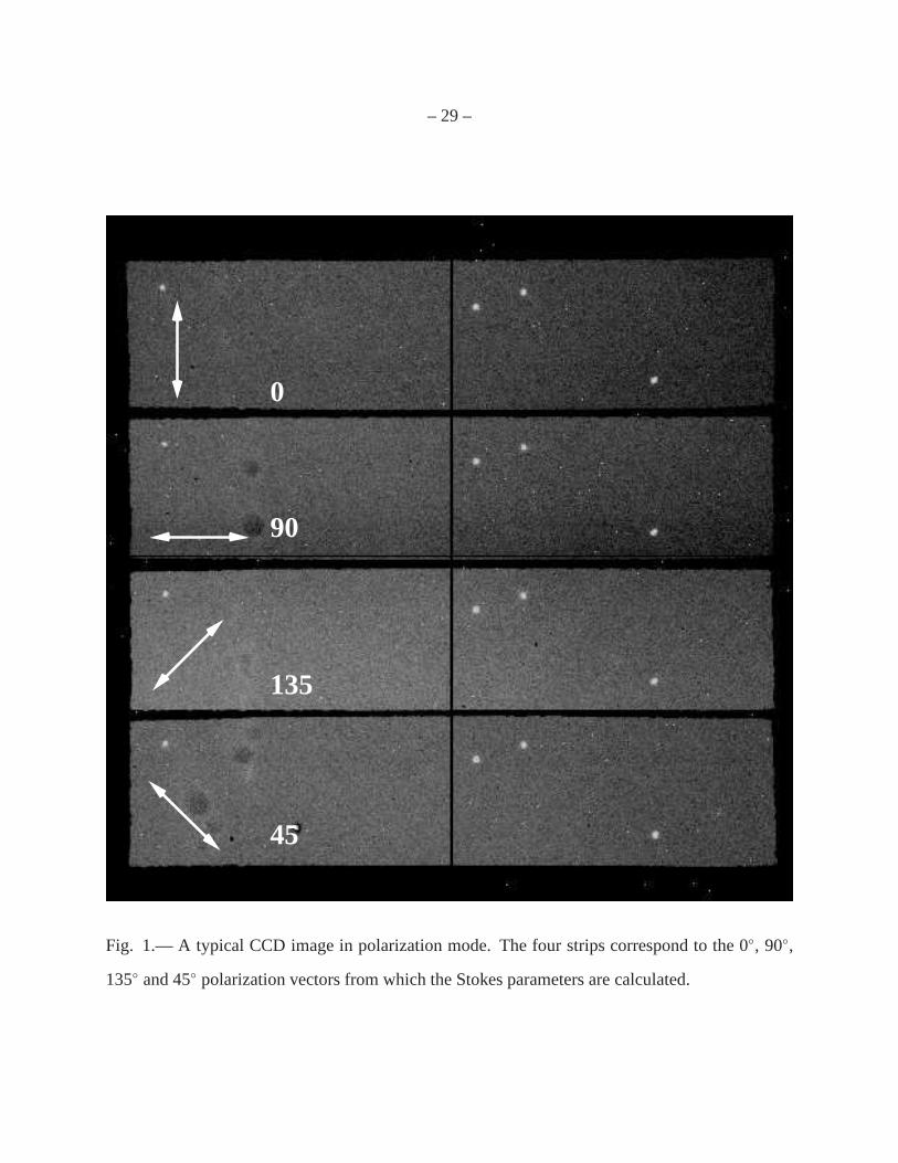
LIRIS is capable of performing polarization observations by using a wedged double

Wollaston device, WeDoWo, which is composed by a combination of two Wollaston prisms and

two wedges (see Oliva 1997, for detailed description). In this observing mode, the polarized flux

is measured simultaneously at four different angles (0◦, 45◦, 90◦ and 135◦). An aperture mask of

4′ × 1′ is used in order to avoid overlapping between the different polarization images. Figure 1

shows a typical LIRIS image in polarimetric mode. The degreeof linear polarization can thus be

determined from data taken at the same time and with the same observing conditions. In order

to achieve accurate sky subtraction, a 5-point dither pattern was used. Offsets of about 20′′ were

adopted along the horizontal, long mask direction. During the 2006 and 2007 campaigns, we took

– 6 –

seven and six exposures, respectively, of 20 s per dither position. The 5-point dither cycle was

repeated several times until completion of the observation. The total observing time for each field

was 2800 s in 2006 and 2400 s in 2007.

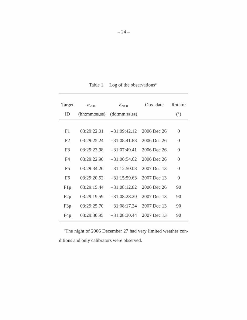
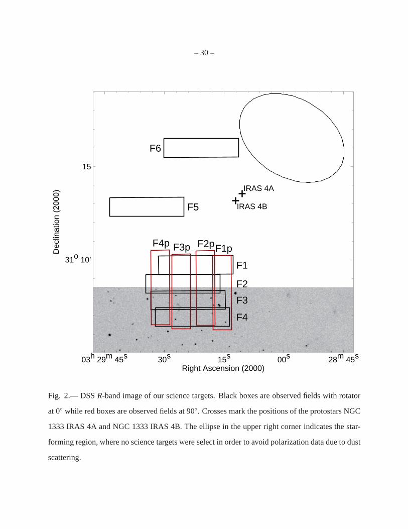
We carried outJ-band polarization observations of ten fields, six of them with the telescope

rotator at 0◦ and four with the rotator at 90◦ (see Table 1). Figure 2 indicates the observed fields

as black and red rectangles, corresponding to observationswith rotator at 0◦ and 90◦, respectively.

We covered the area surveyed by observing with the rotator at0◦ and 90◦, except for the two upper

fields. This procedure allows us to compare both data sets and, consequently, to achieve higher

precision in the estimated polarization parameters.

2.2. Optical observations

The opticalR-band linear polarimetry was performed using the 1.6 m telescope of the

Observatorio do Pico dos Dias (LNA/MCT, Brazil) during observing runs conducted in 2007

and 2008. A specially adapted CCD camera composed by a half-wave rotating retarder followed

by a calcite Savart plate and a filter wheel was attached to thefocal plane of the telescope. The

half-wave retarder can be rotated in steps of 22.◦5 and one polarization modulation cycle is fully

covered after a complete 90◦ rotation. The birefringence property of the Savart plate divides

the incoming light beam into two perpendicularly polarizedcomponents: the ordinary and the

extra-ordinary beams. From the difference in the measured flux for each beam one estimates the

degree of polarization and its orientation in the plane of the sky. For a technical description of

this polarimetric unit, we refer the interested reader to the work by Magalhaes et al. (1996). The

obtained optical data is part of an ongoing large scale (∼ 1 square degree) survey whose results

will be discussed in a forthcoming paper (Franco et al., in preparation). The area covered by

the optical survey overlaps the portion of the sky observed in near-IR, and in order to make a

comparative analysis of the results obtained at both wavelengths, we included the optical results

– 7 –

gathered for stars lying in the overlapped area in the discussion.

3. LIRIS data reduction and calibration

The near-IR data reduction was performed using thelirisdr package developed by the LIRIS

team in the IRAF environment.1 Given the particular geometry of the frames (see Fig. 1), the

first procedure was to slice the image into four frames. Each set of frames corresponding to a

given polarization stage is processed independently. The data reduction process comprises sky

subtraction, flat-fielding, geometrical distortion correction, and finally co-addition of images after

registering. A second background subtraction was performed upon flat-fielded images in order to

avoid the residuals introduced by the vertical gradient dueto the reset anomaly effect associated

with the Hawaii arrays (e.g., Acosta-Pulido et al. 2006). Anapproximate astrometric solution was

determined based on the image header parameters.

3.1. Photometry

Aperture photometry of the field stars in each slice was obtained using the task Object

Detection, available within Starlink Gaia software.2 The aperture radius used was∼ 4′′, which

corresponds to 3 times the median seeing of the night. The background was extracted from an

annulus with an inner radius of 6′′ and an outer radius of 8′′. The astrometric solution of each

1IRAF is distributed by the National Optical Astronomy Observatories, which are operated by

the Association of Universities for Research in Astronomy,Inc., under cooperative agreement with

the National Science Foundation.

2GAIA is a derivative of the Skycat catalogue and image display tool, developed as a part of

the VLT project at ESO.

– 8 –

slice was tweaked using the astrometric tools available within the Starlink Gaia software. We used

the 2MASS catalogue to perform the photometric and astrometric calibrations. In our sample, we

reachedJ magnitudes as faint as∼17. As a final step, we identified the counterparts of each object

in the four slices in order to compute the polarization properties. In some cases, matching of stars

observed with rotator at 0◦ and 90◦ was also necessary since some objects were present in both

sets of observations.

3.2. Polarimetric analysis

Using the WeDoWo, we measured simultaneously four polarization states in each of the

strips as,

i0[PA = 0] =12

t0 (I∗ +Q∗) (1)

i90[PA = 0] =12

t90 (I∗ −Q∗) (2)

i45[PA = 0] =12

t45 (I∗ + U∗) (3)

i135[PA = 0] =12

t135(I∗ − U∗) (4)

whereI∗, Q∗ andU∗ are the Stokes parameters of the object to be measured, and the factors

t[0,90,45,135] represent the transmission for each polarization state. Inthis case, the normalized

Stokes parameters can be determined by,

q∗ =i0 − i90 t0/90

i0 + i90 t0/90(5)

u∗ =i45− i135 t45/135

i45+ i135 t45/135(6)

where the factorst0/90 and t45/135 measure the relative transmission of the ordinary and

extraordinary rays for each Wollaston. These factors were calibrated using non-polarized

– 9 –

standards and resulted in the valuest0/90 = 0.997 andt45/135 = 1.030, with an uncertainty of about

0.002 in both cases.

The rotation of the whole instrument by 90◦ causes the exchange of the optical paths for the

orthogonal polarization vectors. Now, the resulting polarization states are given by

i0[PA = 90] =12

t0(I∗ − Q∗) (7)

i90[PA = 90] =12

t90(I∗ + Q∗) (8)

i45[PA = 90] =12

t45(I∗ − U∗) (9)

i135[PA = 90] =12

t135(I∗ + U∗) (10)

This effect can be used in order to get a more accurate estimate of the Stokes parameters

because the combination of both measurements, PA=0◦ and 90◦, results in the cancelation of the

transmission factors and reduces flat-field uncertainties.The normalized Stokes parameters are

then computed by

q∗ =RQ − 1

RQ + 1, beingR2

Q =i0[PA = 0]/i90[PA = 0]

i0[PA = 90]/i90[PA = 90](11)

u∗ =RU − 1RU + 1

, beingR2U =

i45[PA = 0]/i135[PA = 0]i45[PA = 90]/i135[PA = 90]

(12)

Finally, after estimation of theq andu Stokes parameter, the degree of linear polarization and

the position of polarization angle (measured eastwards with respect to the North Celestial Pole)

are calculated as

p =

√

q2∗ + u2

∗ (13)

θ =12

tan−1

(

u∗q∗

)

.

– 10 –

Flux errors ini0, i90, i45 andi135 are dominated by photon shot noise while the theoretical

error in polarization fraction was estimated performing error propagation through the previous

equations. In addition, we calculated the errors inp using a Monte Carlo method, which returned

values similar to those estimated from error propagation. The 1σ uncertainty inθ was estimated

(i) by applying the relation derived by Serkowski (1974) usingstandard error propagation, that

is,σθ = 28◦.65σp/p, whenp/σp ≥ 5; or (ii) graphically with the aid of the curve proposed by

Naghizadeh-Khouei & Clarke (1993) whenp/σp < 5.

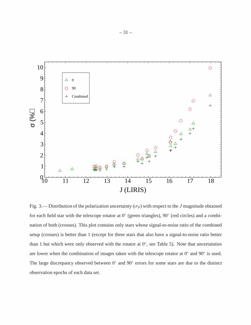
Figure 3 shows the polarization uncertainty as a function ofthe J-band magnitude achieved

with our LIRIS observations. The observed distribution suggests that the uncertainties are

dominated by photon shot noise, as expected for a sample collected with fixed exposure time. As

expected, the uncertainties decrease when the data taken at0◦ and 90◦ are combined. There is

a natural limit which is due to the uncertainty bias when measuring low levels of polarization.

Bias in the degree of linear polarization (p) comes from the fact that this quantity is defined

as a quadratic sum ofq andu, which produces a non-zero polarization estimate due to the

uncertainties in their measurement (for a detailed discussion see for instance, Simmons & Stewart

1985; Wardle & Kronberg 1974). In order to remove the polarization bias and compute the

true polarization, we used the prescription proposed by Simmons & Stewart (1985) for low

polarization stars. The true polarization degree can be approximated by the expressionsptrue = 0

if pobs/σp < Ka, otherwiseptrue = (p2obs − σ

2p · K

2a )1/2. We adoptedKa = 1, which corresponds to

the estimator defined by Wardle & Kronberg (1974).

3.3. Standard stars

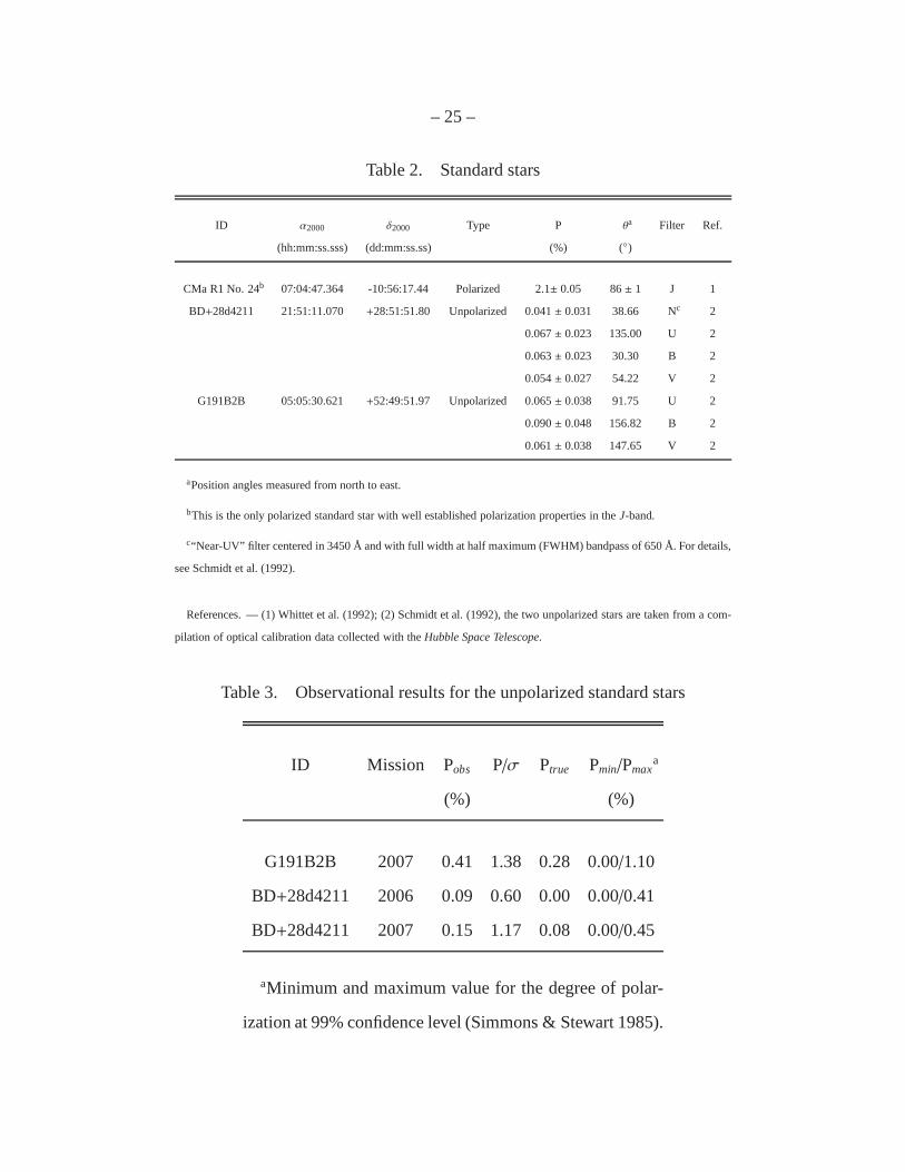
Observations of polarized and unpolarized standard stars were taken in order to calibrate

the instrumental characteristics of LIRIS in its polarimetric mode. Table 2 summarizes the

general information for these stars: columns 1 to 8 indicatetheir name, equatorial coordinates,

– 11 –

type, polarization degree and position angle, the filter used for the polarization measurements

and the reference, respectively. Unpolarized standard stars were observed to check for any

possible instrumental polarization and for systematic errors in our polarimetry. The unpolarized

stars G191B2B and BD+28d4211 were observed with rotator at 0◦ and 90◦. The polarized

intensity measured for the two unpolarized standards was very small (see Table 3): The measured

normalized Stokesq andu were 0.051% and 0.226%, respectively, with the rotator at 0◦,

and−0.117% and 0.119%, respectively, with the rotator at 90◦. Table 3 shows the observed

polarization degree before and after bias correction for the two unpolarized standards. The

measurements taken in the two epochs for BD+28d4211 give consistent values. We applied the

method proposed by Simmons & Stewart (1985) for a 99% confidence level for the observed

unpolarized standards. This resulted in a small, if any, instrumental polarization.

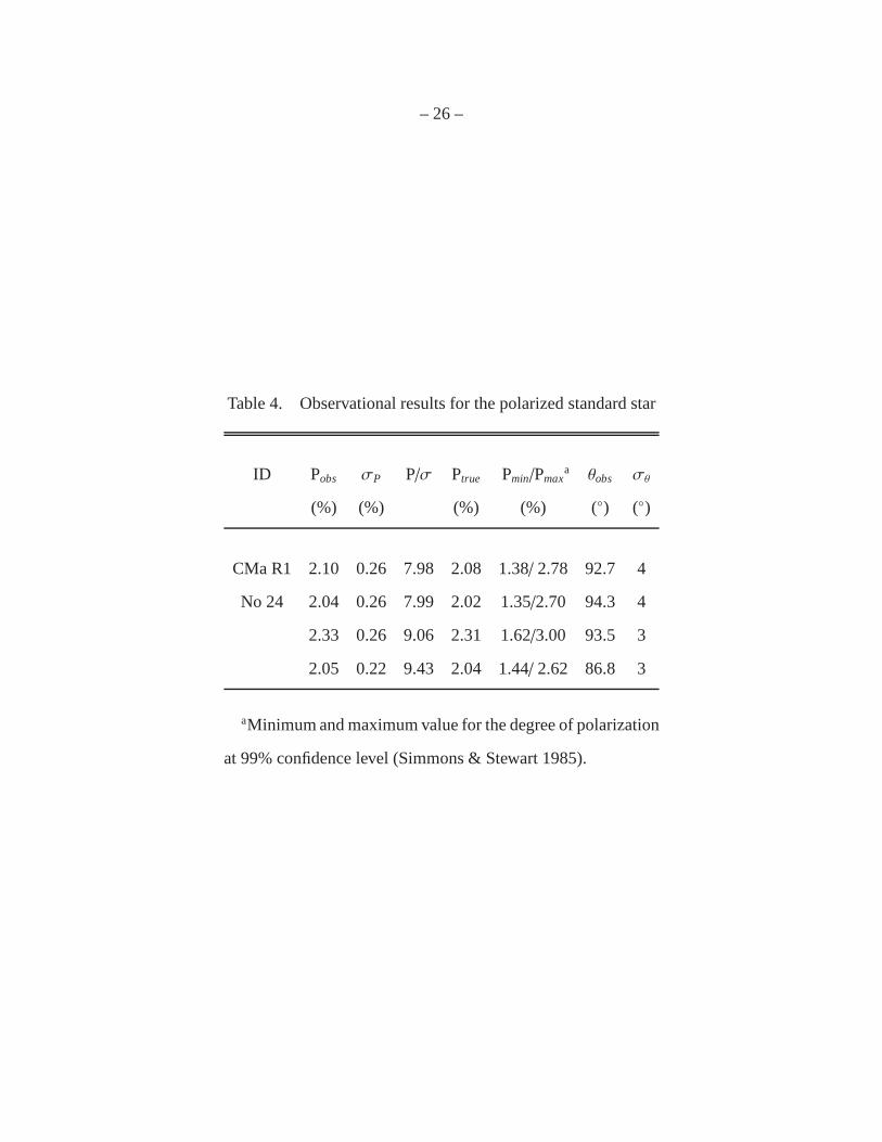
The polarized standard star CMa R1 No. 24 was observed in order to verify the zero

point of the polarization position angles. Table 4 summarizes the results obtained for the four

measurements conducted for this object. As expected, high quality data are less sensitive to

biasing, and the unbiased polarization has basically the same values of the observed polarization.

Taking into account the uncertainties, we see that ourJ-band data match the result obtained

by Whittet et al. (1992). The difference between the average P.A. obtained for these four

measurements and that obtained by Whittet et al. (1992) is∼ 6◦, which is very close to the

statistical deviation of our measurements thus discardingany further correction for the zero angle

calibration.

– 12 –

4. Polarization properties

4.1. Infrared data

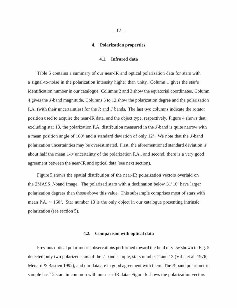
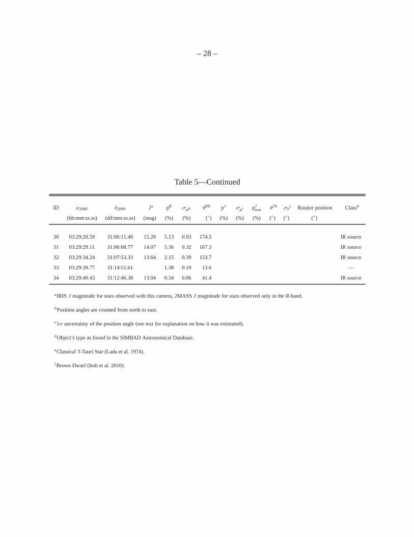
Table 5 contains a summary of our near-IR and optical polarization data for stars with

a signal-to-noise in the polarization intensity higher than unity. Column 1 gives the star’s

identification number in our catalogue. Columns 2 and 3 show the equatorial coordinates. Column

4 gives theJ-band magnitude. Columns 5 to 12 show the polarization degree and the polarization

P.A. (with their uncertainties) for theR andJ bands. The last two columns indicate the rotator

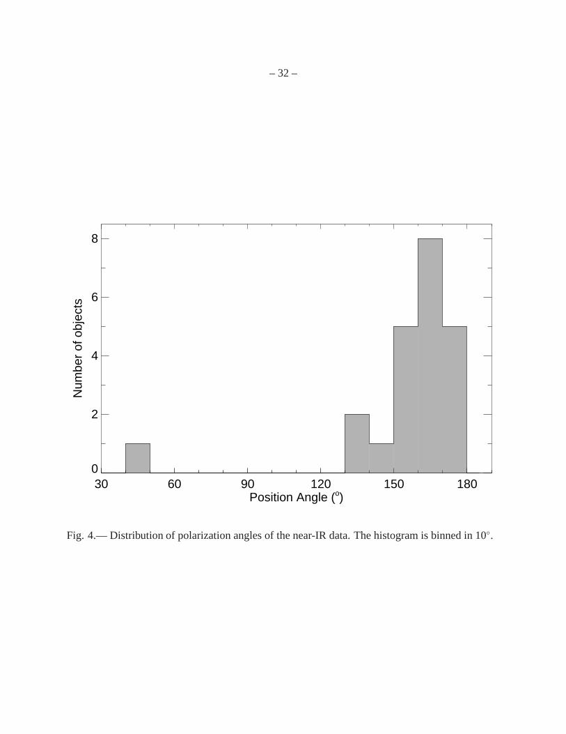
position used to acquire the near-IR data, and the object type, respectively. Figure 4 shows that,

excluding star 13, the polarization P.A. distribution measured in theJ-band is quite narrow with

a mean position angle of 160◦ and a standard deviation of only 12◦. We note that theJ-band

polarization uncertainties may be overestimated. First, the aforementioned standard deviation is

about half the mean 1-σ uncertainty of the polarization P.A., and second, there is avery good

agreement between the near-IR and optical data (see next section).

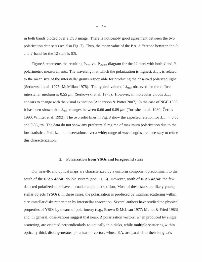
Figure 5 shows the spatial distribution of the near-IR polarization vectors overlaid on

the 2MASSJ-band image. The polarized stars with a declination below 31◦10′ have larger

polarization degrees than those above this value. This subsample comprises most of stars with

mean P.A.≃ 160◦. Star number 13 is the only object in our catalogue presenting intrinsic

polarization (see section 5).

4.2. Comparison with optical data

Previous optical polarimetric observations performed toward the field of view shown in Fig. 5

detected only two polarized stars of theJ-band sample, stars number 2 and 13 (Vrba et al. 1976;

Menard & Bastien 1992), and our data are in good agreement with them. TheR-band polarimetric

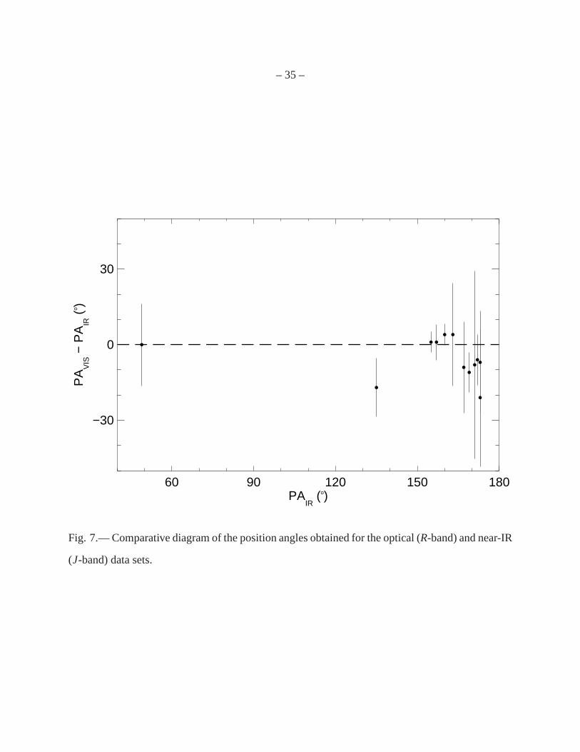
sample has 12 stars in common with our near-IR data. Figure 6 shows the polarization vectors

– 13 –

in both bands plotted over a DSS image. There is noticeably good agreement between the two

polarization data sets (see also Fig. 7). Thus, the mean value of the P.A. difference between theR

andJ-band for the 12 stars is 6.◦5.

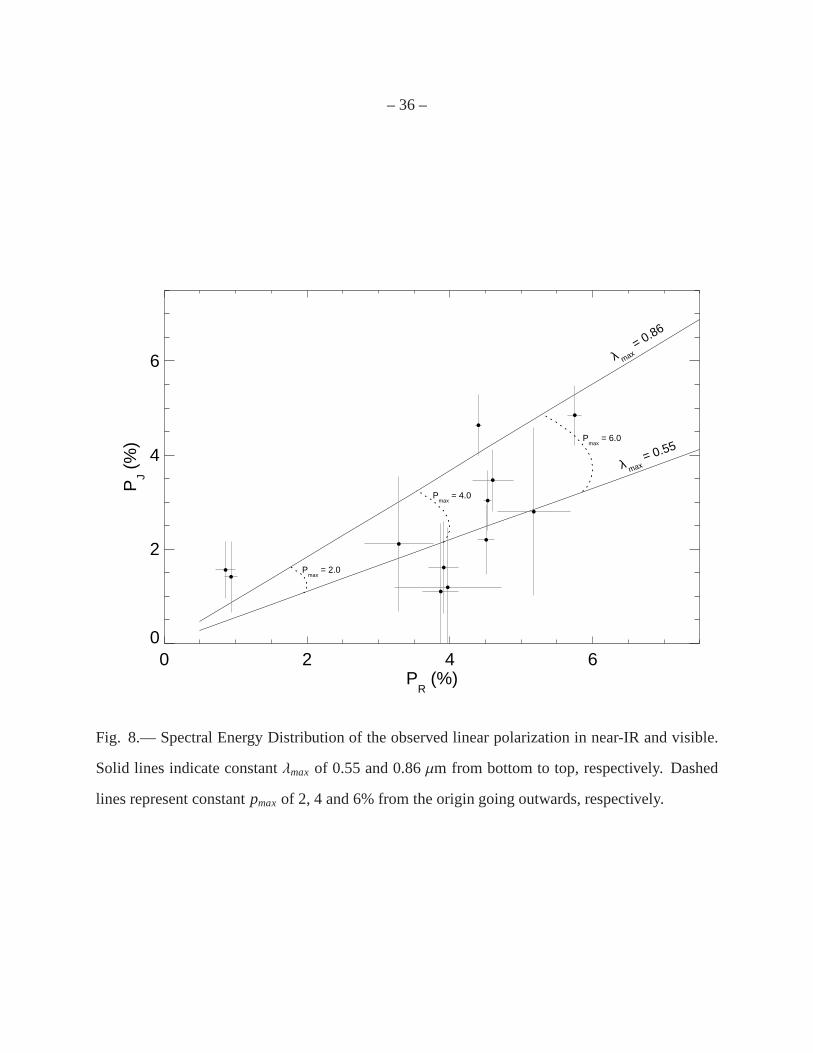
Figure 8 represents the resulting PNIR vs. Pvisible diagram for the 12 stars with bothJ andR

polarimetric measurements. The wavelength at which the polarization is highest,λmax, is related

to the mean size of the interstellar grains responsible for producing the observed polarized light

(Serkowski et al. 1975; McMillan 1978). The typical value ofλmax observed for the diffuse

interstellar medium is 0.55µm (Serkowski et al. 1975). However, in molecular cloudsλmax

appears to change with the visual extinction (Andersson & Potter 2007). In the case of NGC 1333,

it has been shown thatλmax changes between 0.66 and 0.89µm (Turnshek et al. 1980;Cernis

1990; Whittet et al. 1992). The two solid lines in Fig. 8 show the expected relation forλmax = 0.55

and 0.86µm. The data do not show any preferential regime of maximum polarization due to the

low statistics. Polarization observations over a wider range of wavelengths are necessary to refine

this characterization.

5. Polarization from YSOs and foreground stars

Our near-IR and optical maps are characterized by a uniform component predominant to the

south of the IRAS 4A/4B double system (see Fig. 6). However, north of IRAS 4A/4B the few

detected polarized stars have a broader angle distribution. Most of these stars are likely young

stellar objects (YSOs). In these cases, the polarization isproduced by intrinsic scattering within

circumstellar disks rather than by interstellar absorption. Several authors have studied the physical

properties of YSOs by means of polarimetry (e.g., Brown & McLean 1977; Mundt & Fried 1983)

and, in general, observations suggest that near-IR polarization vectors, when produced by single

scattering, are oriented perpendicularly to optically thin disks, while multiple scattering within

optically thick disks generates polarization vectors whose P.A. are parallel to their long axis

– 14 –

(Angel 1969; Bastien & Menard 1990; Pereyra et al. 2009).

The YSOs possibly showing intrinsic polarization in the near-IR and/or R-band are listed

below:

• LkHα 271 (star n. 13 of Table 5) is a Classical T Tauri star (Lada et al. 1974). The near-IR

polarization angle and degree are in excellent agreement with theR-band data. Previous

observations showed that the polarization varies considerably, which has being interpreted

as arising from outbursts or inhomogeneities in a circumstellar shell within an optically

thick circumstellar disk (Tamura et al. 1988; Menard & Bastien 1992).

• SVS 13A (star n. 24) was observed only in theR-band. The obtained polarization is in

excellent agreement with the value previously measured in theK-band (PK = 7.2± 0.9% and

P.A.= 56± 4◦, Tamura et al. 1988). This object is a well-studied source (Rodrıguez et al.

2002; Anglada et al. 2004; Chen et al. 2009) which powers a bipolar and collimated outflow

associated with the well-known Herbig-Haro objects HH 7-11(Herbig 1974; Strom et al.

1974). The orientation of the outflow is roughly perpendicular to the polarization P.A.,

which suggests that the disk is optically thick.

• 2MASS J03290289+3116010 (star n. 23) is close to SVS 13A and has a very low degree of

polarization. According to the SIMBAD Astronomical Database, this is a bright (J ≃ 12.8)

K-type star and it is possibly a foreground star. In fact, previous spectral analysis and

photometric studies place this star at a distance of only∼50 pc from the Sun (Aspin et al.

1994; Aspin 2003).

• ASR 8 (star n. 25) is classified as a brown dwarf by SIMBAD. However, an extensive

survey on the evolutionary state of stars in NGC 1333 identifies this object as a T Tauri star

with a mass of 0.7 M⊙ (Aspin 2003), which is reinforced by the presence of X-ray emission

(Getman et al. 2002). We therefore attribute the optical polarization measured for this star

– 15 –

due to intrinsic scattering.

In addition, there are two bright infrared stars (J . 13.0) with low polarization (stars n. 28

and 34 in Table 5) that are apparently not associated with YSOs, as no star formation or nebulosity

signs has been reported in the literature. Their 2MASS colorindices suggest that they may be

unreddened M-type dwarf stars, which is also corroborated by the low degree of polarization. We

therefore consider these objects to be foreground stars.

6. The magnetic field in NGC 1333

6.1. The distribution of dust and molecular gas in NGC 1333

The most detailed picture of the distribution of gas and dustin the Perseus cloud has

been provided by the COMPLETE project (Ridge et al. 2006a; Pineda et al. 2008), a survey of

near/far-infrared extinction data, and of atomic, molecular, and thermal dust continuum emission

obtained over a large area. These data show a wide range of visual magnitudes for NGC 1333,

and a non-Gaussian CO spectral profile consistent with multi-velocity components. These results

are consistent and likely related to a layered cloud structure along the line of sight, which was first

proposed by Ungerechts & Thaddeus (1987). Interstellar extinction studies of field stars toward

NGC 1333 also suggest at least two components in the line of sight at different distances toward

NGC 1333 (Cernis 1990).

According to column density maps of the Perseus cloud (Ridgeet al. 2006b), the region

studied here lies in the lower density envelope of NGC 1333. Maps of high density molecular

tracers (N2H+, HCO+) as well as of the 870µm dust emission, show that around IRAS 4A the

dense gas has a filamentary distribution oriented in the NW–SE direction, with the long axis

positioned at≃142◦(Sandell & Knee 2001; Olmi et al. 2005; Walsh et al. 2007).

– 16 –

6.2. The field morphology as traced by the diffuse gas

The near-IR and optical polarization vectors of the background stars shown in Fig. 6 trace

the POS component of the magnetic field associated with the lower density envelope around

IRAS 4A/4B. South of these sources, where we have most of the polarization sample, the

magnetic field has a direction of≃ 160◦. The observed configuration is consistent with the results

obtained at much larger scale by Goodman et al. (1990) and Tamura et al. (1988). According to

the COMPLETE survey (Ridge et al. 2006a) the polarization was measured toward regions with a

visual extinction of 4 to 5 mag.

The magnetic field orientation derived from our data is roughly parallel to the dense

filamentary structure associated with IRAS 4A (Walsh et al. 2007; Sandell & Knee 2001).

However, the submm polarization maps towards IRAS 4A and IRAS 4B show that the magnetic

field within the filament is approximately perpendicular to the filament’s major axis (Girart et al.

1999, 2006; Attard et al. 2009), and is therefore perpendicular to the magnetic field direction

traced by our optical and near-IR data. The single-dish submm polarization map from Attard et al.

(2009) around IRAS 4A is associated with visual extinctionsas low as∼10 magnitudes, which is

a typical value for near-IR extinction data. Therefore, thesubmm and near-IR/optical data seem

to reveal substantial changes in the magnetic field topologybetween the dense filament and the

diffuse molecular envelope that surrounds it. Such a sharp twistin the field is hard to explain

by means of structural changes in the magnetic field only, because within the observed field, the

position angle of the optical and near-IR polarimetric datais quite uniform (see Fig. 4). Instead,

the two data sets may be simply tracing distinct gas components. As explained in§ 6.1, there

is observational evidence of a multi-component structure for the NGC 1333 molecular cloud.

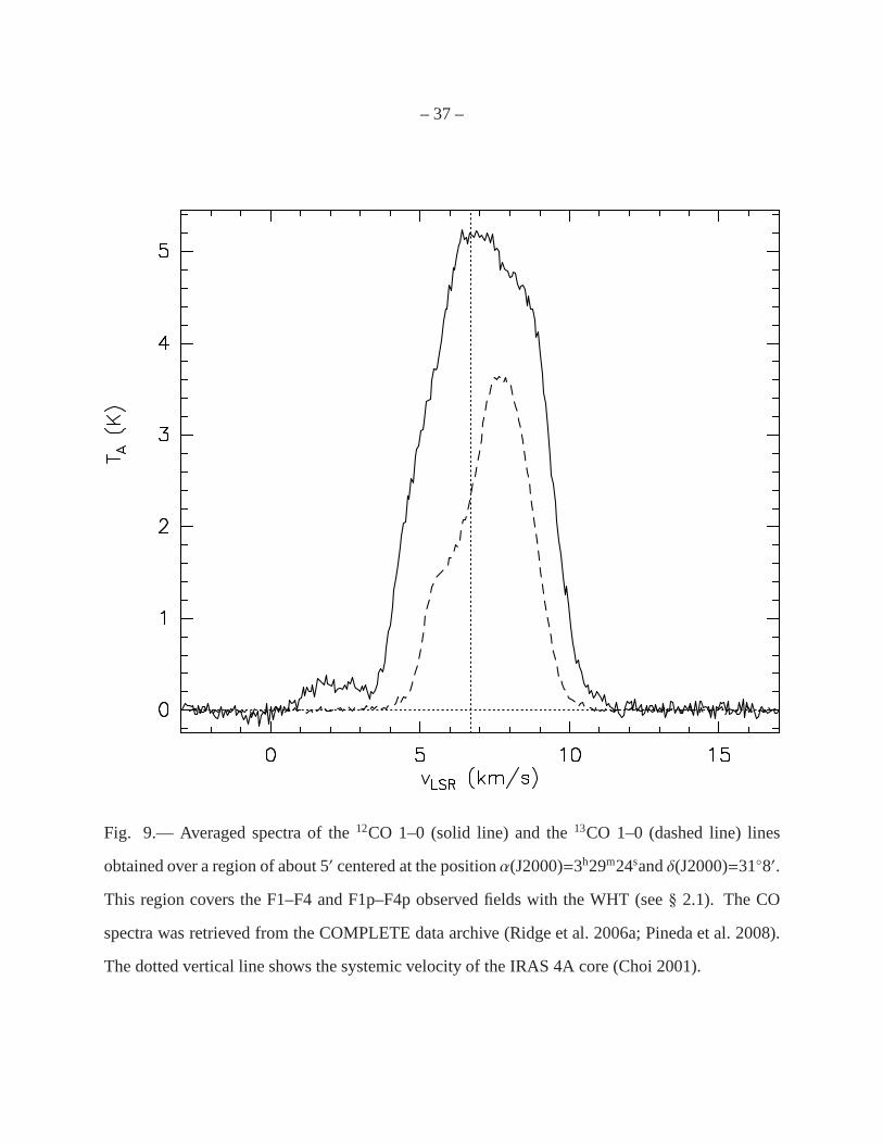
Figure 9 shows the12CO and13CO spectra extracted from a box containing the region studied

here. These spectra show at least three distinguishable velocity components: a faint emission

centered atvLSR ≃ 2 km s−1 (seen more clearly in the12CO data), the peak of the13CO data

– 17 –

centered at∼7.6 km s−1 and the peak of the12CO data at∼6.7 km s−1. This last component has the

samevLSR of the IRAS 4A dense core (Choi 2001). Therefore, whereas thesubmm polarization

measurements trace only the molecular cloud component associated with the IRAS 4A dense

core, the near-IR and optical polarimetric data are probably tracing the mean magnetic field of the

different velocity molecular cloud components observed in the CO maps. Nevertheless, further

observations are needed in order to obtain a more complete description of the magnetic field in

this region.

7. Conclusions

We have carried out one of the first polarimetric observations in theJ-band collected

with the WHT/LIRIS infrared camera. We also presentR-band linear polarimetry obtained at

the Observatorio do Pico dos Dias. We observed an area of∼ 6′ × 4′ around the NGC 1333

IRAS 4A/4B protostellar system. The main conclusions of this work are:

• The infrared polarization map derived for the surveyed areais highly consistent with the

optical map obtained with a different telescope and observational technique. Therefore,

the near-IR polarimetric capabilities of LIRIS have provedto be scientifically trustworthy

for the astronomical community, and assure this mode will beuseful for gathering

measurements of objects experiencing high interstellar extinction inaccessible to optical

instruments.

• The polarization map obtained for the surveyed area is dominated by a well-ordered

component produced by dichroic interstellar absorption. However, there are objects, some

of them catalogued as YSOs, that show a transversal component which may be generated

by internal scattering within circumstellar disks.

• The magnetic field morphology traced by the near-IR/optical map is almost perpendicular

– 18 –

with respect to the field morphology obtained with the submillimeter data toward the dense

molecular core around IRAS 4A/4B. The near-IR/optical polarimetric data trace the field

morphology of the diffuse molecular gas, which is known to have a multi-velocity structure.

That is, the observed resulting magnetic field direction is probably the averaged magnetic

field over several distinct velocity components of the cloud. CO molecular data obtained for

this line of sight show non-Gaussian line profiles that are consistent with this hypothesis.

FOA acknowledges the hospitality of the Instituto de Astrofısica de Canarias, where part

of this work was developed. The authors thank the staffs of the Observatorio del Roque de

los Muchachos and Observatorio do Pico dos Dias for their hospitality and invaluable help

during the observing runs. We also appreciate Terry Mahoney’s help with the manuscript. We

made extensive use of NASA’s Astrophysics Data System (NASA/ADS) and the SIMBAD

database, operated at CDS, Strasbourg, France. CO spectra were retrieved from the COMPLETE

Survey of Star-forming Regions (Goodman 2004; Ridge et al. 2006a). This publication makes

use of data products from the Two Micron All Sky Survey, whichis a joint project of the

University of Massachusetts and the Infrared Processing and Analysis Center/California Institute

of Technology, funded by the National Aeronautics and SpaceAdministration and the National

Science Foundation. GAPF acknowledges a grant from Fundacion Carolina (Spain). This

research has been partially supported by AYA2008-06189-C03 and AYA2004-03136 (Ministerio

de Ciencia e Innovacion, Spain), CEX APQ-1130-5.01/07 (FAPEMIG, Brazil), CNPq (Ministerio

da Ciencia e Tecnologia, Brazil) and 2009SGR1172 (AGAUR, Generalitat de Catalunya).

– 19 –

REFERENCES

Acosta-Pulido, J. A., Barrena-Delgado, R., Ramos-Almeida, C., & Manchado-Torres, A. 2006, in

Scientific Detectors for Astronomy 2005, ed. J. E. Beletic, J. W. Beletic, & P. Amico, 521

Acosta-Pulido, J. A., Ballesteros, E., Barreto, M., et al. 2003, The Newsletter of the Isaac Newton

Group of Telescopes, 7, 15

Andersson, B.-G., & Potter, S. B. 2007, ApJ, 665, 369

Angel, J. R. P. 1969, ApJ, 158, 219

Anglada, G., Rodrıguez, L. F., Osorio, M., et al. 2004, ApJ,605, L137

Arce, H. G., Goodman, A. A., Bastien, P., Manset, N., & Sumner, M. 1998, ApJ, 499, L93

Aspin, C. 2003, AJ, 125, 1480

Aspin, C., Sandell, G., & Russell, A. P. G. 1994, A&AS, 106, 165

Attard, M., Houde, M., Novak, G., et al. 2009, ApJ, 702, 1584

Bastien, P. & Menard, F. 1990, ApJ, 364, 232

Brown, J. C. & McLean, I. S. 1977, A&A, 57, 141

Cernis, K. 1990, Ap&SS, 166, 315

Chen, X., Launhardt, R., & Henning, T. 2009, ApJ, 691, 1729

Choi, M. 2001, ApJ, 553, 219

Crutcher, R. M., Hakobian, N., & Troland, T. H. 2009, ApJ, 692, 844

Davis, L. J. & Greenstein, J. L. 1951, ApJ, 114, 206

– 20 –

Draine, B. T. & Weingartner, J. C. 1996, ApJ, 470, 551

Franco, G. A. P., Alves, F. O., & Girart, J. M. 2010, ApJ, 723, 146

Galli, D. & Shu, F. H. 1993, ApJ, 417, 243

Gerakines, P. A., Whittet, D. C. B., & Lazarian, A. 1995, ApJ,455, L171

Getman, K. V., Feigelson, E. D., Townsley, L., et al. 2002, ApJ, 575, 354

Girart, J. M., Crutcher, R. M., & Rao, R. 1999, ApJ, 525, L109

Girart, J. M., Rao, R., & Marrone, D. P. 2006, Science, 313, 812

Goncalves, J., Galli, D., & Girart, J. M. 2008, A&A, 490, L39

Goodman, A. A. 2004, in Astronomical Society of the Pacific Conference Series, Vol. 323, Star

Formation in the Interstellar Medium: In Honor of David Hollenbach, ed. D. Johnstone,

F. C. Adams, D. N. C. Lin, D. A. Neufeeld, & E. C. Ostriker , 171

Goodman, A. A., Bastien, P., Menard, F., & Myers, P. C. 1990, ApJ, 359, 363

Goodman, A. A., Jones, T. J., Lada, E. A., & Myers, P. C. 1992, ApJ, 399, 108

Goodman, A. A., Jones, T. J., Lada, E. A., & Myers, P. C. 1995, ApJ, 448, 748

Herbig, G. H. 1974, Lick Observatory Bulletin, 658, 1

Hoang, T. & Lazarian, A. 2008, MNRAS, 388, 117

Hoang, T. & Lazarian, A. 2009, ApJ, 697, 1316

Itoh, Y., Gupta, R., Oasa, Y., et al. 2010, PASJ, 62, 1149

Knee, L. B. G. & Sandell, G. 2000, A&A, 361, 671

– 21 –

Lada, C. J., Alves, J., & Lada, E. A. 1996, AJ, 111, 1964

Lada, C. J., Gottlieb, C. A., Litvak, M. M., & Lilley, A. E. 1974, ApJ, 194, 609

Lazarian, A. 2007, Journal of Quantitative Spectroscopy and Radiative Transfer, 106, 225

Lazarian, A. & Hoang, T. 2007, MNRAS, 378, 910

Magalhaes, A. M., Rodrigues, C. V., Margoniner, V. E., Pereyra, A., & Heathcote, S. 1996, in

ASP Conf. Ser. 97: Polarimetry of the Interstellar Medium, 118

Manchado, A., Barreto, M., Acosta-Pulido, J., et al. 2004, in Presented at the Society of Photo-

Optical Instrumentation Engineers (SPIE) Conference, Vol. 5492, Society of Photo-Optical

Instrumentation Engineers (SPIE) Conference Series, ed. A. F. M. Moorwood & M. Iye,

1094–1104

McMillan, R. S. 1978, ApJ, 225, 880

Menard, F. & Bastien, P. 1992, AJ, 103, 564

Mouschovias, T. 2001, in ASP Conf. Ser. 248: Magnetic FieldsAcross the Hertzsprung-Russell

Diagram, 515

Mouschovias, T. C. & Tassis, K. 2010, MNRAS, 409, 801

Mundt, R. & Fried, J. W. 1983, ApJ, 274, L83

Naghizadeh-Khouei, J. & Clarke, D. 1993, A&A, 274, 968

Oliva, E. 1997, A&AS, 123, 589

Olmi, L., Testi, L., & Sargent, A. I. 2005, A&A, 431, 253

Pereyra, A., Girart, J. M., Magalhaes, A. M., Rodrigues, C.V., & de Araujo, F. X. 2009, A&A,

501, 595

– 22 –

Pineda, J. E., Caselli, P., & Goodman, A. A. 2008, ApJ, 679, 481

Quillen, A. C., Thorndike, S. L., Cunningham, A., et al. 2005, ApJ, 632, 941

Ridge, N. A., Di Francesco, J., Kirk, H., et al. 2006a, AJ, 131, 2921

Ridge, N. A., Schnee, S. L., Goodman, A. A., & Foster, J. B. 2006b, ApJ, 643, 932

Rodrıguez, L. F., Anglada, G., Torrelles, J. M., et al. 2002, A&A, 389, 572

Sandell, G. & Knee, L. B. G. 2001, ApJ, 546, L49

Schmidt, G. D., Elston, R., & Lupie, O. L. 1992, AJ, 104, 1563

Serkowski, K. 1974, in Methods Exper. Phys. Vol. 12A, ed. N. Carleton (Academic, New York),

361

Serkowski, K., Mathewson, D. S., & Ford, V. L. 1975, ApJ, 196,261

Shu, F. H., Galli, D., Lizano, S., & Cai, M. 2006, ApJ, 647, 382

Shu, F. H., Adams, F. C., & Lizano, S. 1987, ARA&A, 25, 23

Simmons, J. F. L. & Stewart, B. G. 1985, A&A, 142, 100

Strom, S. E., Grasdalen, G. L., & Strom, K. M. 1974, ApJ, 191, 111

Tamura, M., Yamashita, T., Sato, S., Nagata, T., & Gatley, I.1988, MNRAS, 231, 445

Turnshek, D. A., Turnshek, D. E., & Craine, E. R. 1980, AJ, 85,1638

Ungerechts, H. & Thaddeus, P. 1987, ApJS, 63, 645

Vaillancourt, J. E., et al. 2008, ApJ, 679, L25

Vrba, F. J., Strom, S. E., & Strom, K. M. 1976, AJ, 81, 958

– 23 –

Walsh, A. J., Myers, P. C., Di Francesco, J., et al. 2007, ApJ,655, 958

Wardle, J. F. C. & Kronberg, P. P. 1974, ApJ, 194, 249

Warin, S., Castets, A., Langer, W. D., Wilson, R. W., & Pagani, L. 1996, A&A, 306, 935

Whittet, D. C. B., Hough, J. H., Lazarian, A., & Hoang, T. 2008, ApJ, 674, 304

Whittet, D. C. B., Martin, P. G., Hough, J. H., et al. 1992, ApJ, 386, 562

Wilking, B. A., Meyer, M. R., Greene, T. P., Mikhail, A., & Carlson, G. 2004, AJ, 127, 1131

This manuscript was prepared with the AAS LATEX macros v5.2.

– 24 –

Table 1. Log of the observationsa

Target α2000 δ2000 Obs. date Rotator

ID (hh:mm:ss.ss) (dd:mm:ss.ss) (◦)

F1 03:29:22.01 +31:09:42.12 2006 Dec 26 0

F2 03:29:25.24 +31:08:41.88 2006 Dec 26 0

F3 03:29:23.98 +31:07:49.41 2006 Dec 26 0

F4 03:29:22.90 +31:06:54.62 2006 Dec 26 0

F5 03:29:34.26 +31:12:50.08 2007 Dec 13 0

F6 03:29:20.52 +31:15:59.63 2007 Dec 13 0

F1p 03:29:15.44 +31:08:12.82 2006 Dec 26 90

F2p 03:29:19.59 +31:08:28.20 2007 Dec 13 90

F3p 03:29:25.70 +31:08:17.24 2007 Dec 13 90

F4p 03:29:30.95 +31:08:30.44 2007 Dec 13 90

aThe night of 2006 December 27 had very limited weather con-

ditions and only calibrators were observed.

– 25 –

Table 2. Standard stars

ID α2000 δ2000 Type P θa Filter Ref.

(hh:mm:ss.sss) (dd:mm:ss.ss) (%) (◦)

CMa R1 No. 24b 07:04:47.364 -10:56:17.44 Polarized 2.1± 0.05 86± 1 J 1

BD+28d4211 21:51:11.070 +28:51:51.80 Unpolarized 0.041± 0.031 38.66 Nc 2

0.067± 0.023 135.00 U 2

0.063± 0.023 30.30 B 2

0.054± 0.027 54.22 V 2

G191B2B 05:05:30.621 +52:49:51.97 Unpolarized 0.065± 0.038 91.75 U 2

0.090± 0.048 156.82 B 2

0.061± 0.038 147.65 V 2

aPosition angles measured from north to east.

bThis is the only polarized standard star with well established polarization properties in theJ-band.

c“Near-UV” filter centered in 3450 Å and with full width at halfmaximum (FWHM) bandpass of 650 Å. For details,

see Schmidt et al. (1992).

References. — (1) Whittet et al. (1992); (2) Schmidt et al. (1992), the two unpolarized stars are taken from a com-

pilation of optical calibration data collected with theHubble Space Telescope.

Table 3. Observational results for the unpolarized standard stars

ID Mission Pobs P/σ Ptrue Pmin/Pmaxa

(%) (%)

G191B2B 2007 0.41 1.38 0.28 0.00/1.10

BD+28d4211 2006 0.09 0.60 0.00 0.00/0.41

BD+28d4211 2007 0.15 1.17 0.08 0.00/0.45

aMinimum and maximum value for the degree of polar-

ization at 99% confidence level (Simmons & Stewart 1985).

– 26 –

Table 4. Observational results for the polarized standard star

ID Pobs σP P/σ Ptrue Pmin/Pmaxa θobs σθ

(%) (%) (%) (%) (◦) (◦)

CMa R1 2.10 0.26 7.98 2.08 1.38/ 2.78 92.7 4

No 24 2.04 0.26 7.99 2.02 1.35/2.70 94.3 4

2.33 0.26 9.06 2.31 1.62/3.00 93.5 3

2.05 0.22 9.43 2.04 1.44/ 2.62 86.8 3

aMinimum and maximum value for the degree of polarization

at 99% confidence level (Simmons & Stewart 1985).

– 27 –

Table 5. Polarization data

ID α2000 δ2000 Ja pR σpR θRb pJ σpJ pJtrue θJ b σθ

c Rotator position Classd

(hh:mm:ss.ss) (dd:mm:ss.ss) (mag) (%) (%) (◦) (%) (%) (%) (◦) (◦) (◦)

1 03:29:14.58 31:06:38.20 14.70 4.04 0.75 151.5 1.74 1.27 1.41 173 27 0,90 IR source

2 03:29:14.89 31:09:27.50 12.67 4.53 0.06 157.8 3.10 0.64 3.03 157 7 0,90 Star

3 03:29:15.05 31:08:06.90 16.06 3.16 2.43 2.02 160 33 0,90 IRsource

4 03:29:16.08 31:07:31.40 12.99 4.51 0.12 166.2 2.32 0.74 2.20 172 10 0,90 IR source

5 03:29:16.20 31:07:34.00 13.83 3.92 0.21 157.6 1.88 0.97 1.61 167 18 0,90 —

6 03:29:16.68 31:16:18.30 10.74 0.87 0.14 117.5 1.67 0.60 1.56 135 11 0 IR source

7 03:29:17.52 31:07:33.20 15.04 3.88 0.25 163.3 1.82 1.45 1.10 171 37 0,90 IR source

8 03:29:17.91 31:07:07.70 15.34 2.70 1.91 1.90 169 29 0,90 IRsource

9 03:29:18.21 31:07:55.70 14.50 3.32 0.48 167.2 2.55 1.43 2.11 163 20 0,90 IR source

10 03:29:18.64 31:09:59.60 12.50 4.40 0.04 156.4 4.68 0.65 4.63 155 4 0,90 Star

11 03:29:20.01 31:09:54.30 12.45 5.75 0.10 164.0 4.89 0.64 4.85 160 4 0,90 Star

12 03:29:20.10 31:08:54.00 16.08 3.15 2.44 1.99 155 33 0,90 —

13 03:29:21.87 31:15:36.30 11.33 0.94 0.09 49.4 1.60 0.75 1.41 49 16 0 CTTSe

14 03:29:23.50 31:07:25.00 16.57 4.54 3.46 2.94 167 33 0,90 —

15 03:29:24.70 31.07:27.00 17.16 4.56 4.42 1.12 167 24 0,90 —

16 03:29:25.60 31:08:43.00 17.00 4.90 3.99 2.85 172 23 0,90 IR source

17 03:29:27.04 31:08:04.60 12.39 4.61 0.29 157.6 3.53 0.66 3.47 169 6 0,90 IR source

18 03:29:27.16 31:06:48.20 14.92 5.20 0.51 166.1 3.32 1.79 2.80 173 20 0,90 IR source

19 03:29:28.99 31:10:00.30 13.36 4.01 0.93 3.90 142 7 0,90 IRsource

20 03:29:29.60 31:08:47.90 16.30 3.17 2.71 1.64 156 42 0,90 IR source

21 03:29:30.80 31.06:33.00 17.97 7.01 6.51 2.61 160 25 0,90 IR source

22 03:29:32.41 31:13:01.10 13.34 1.90 1.21 1.47 135 24 0 IR source

stars withR-band data only

23 03:29:02.87 31:16:00.82 12.84 0.68 0.15 66.4 YSOC

24 03:29:03.74 31:16:03.60 11.74 7.58 0.54 57.7 V512 Per

25 03:29:04.04 31:17:06.66 13.31 1.38 0.52 86.3 BDf

26 03:29:07.39 31:10:49.02 13.10 3.11 0.17 167.0 Star

27 03:29:09.57 31:09:08.68 14.94 4.61 0.61 161.1 Star

28 03:29:12.16 31:08:10.91 12.99 0.39 0.08 71.8 IR source

29 03:29:17.84 31:05:37.40 14.04 4.35 0.45 164.4 IR source

– 28 –

Table 5—Continued

ID α2000 δ2000 Ja pR σpR θRb pJ σpJ pJtrue θJ b σθ

c Rotator position Classd

(hh:mm:ss.ss) (dd:mm:ss.ss) (mag) (%) (%) (◦) (%) (%) (%) (◦) (◦) (◦)

30 03:29:20.59 31:06:11.48 15.28 5.13 0.93 174.5 IR source

31 03:29:29.11 31:06:08.77 14.07 5.36 0.32 167.3 IR source

32 03:29:34.24 31:07:53.33 13.64 2.15 0.39 153.7 IR source

33 03:29:39.77 31:14:51.61 1.38 0.19 13.6 —

34 03:29:40.43 31:12:46.38 13.04 0.34 0.06 41.4 IR source

aIRIS J magnitude for stars observed with this camera, 2MASSJ magnitude for stars observed only in theR-band.

bPosition angles are counted from north to east.

c1σ uncertainty of the position angle (see text for explanationon how it was estimated).

dObject’s type as found in the SIMBAD Astronomical Database.

eClassical T-Tauri Star (Lada et al. 1974).

f Brown Dwarf (Itoh et al. 2010).

– 29 –

0

90

135

45

Fig. 1.— A typical CCD image in polarization mode. The four strips correspond to the 0◦, 90◦,

135◦ and 45◦ polarization vectors from which the Stokes parameters are calculated.

– 30 –

03h 29m 45s 30s 15s 00s 28m 45s

Right Ascension (2000)

31o 10’

15

Dec

linat

ion

(200

0)

F1

F2

F3

F4

F5

F6

F1pF2pF3pF4p

IRAS 4A

IRAS 4B

Fig. 2.— DSSR-band image of our science targets. Black boxes are observedfields with rotator

at 0◦ while red boxes are observed fields at 90◦. Crosses mark the positions of the protostars NGC

1333 IRAS 4A and NGC 1333 IRAS 4B. The ellipse in the upper right corner indicates the star-

forming region, where no science targets were select in order to avoid polarization data due to dust

scattering.

– 31 –

10 11 12 13 14 15 16 17 18

J (LIRIS)

0

1

2

3

4

5

6

7

8

9

10

σ (%

)

0

90

Combined

Fig. 3.— Distribution of the polarization uncertainty (σP) with respect to theJ magnitude obtained

for each field star with the telescope rotator at 0◦ (green triangles), 90◦ (red circles) and a combi-

nation of both (crosses). This plot contains only stars whose signal-to-noise ratio of the combined

setup (crosses) is better than 1 (except for three stars thatalso have a signal-to-noise ratio better

than 1 but which were only observed with the rotator at 0◦, see Table 5). Note that uncertainties

are lower when the combination of images taken with the telescope rotator at 0◦ and 90◦ is used.

The large discrepancy observed between 0◦ and 90◦ errors for some stars are due to the distinct

observation epochs of each data set.

– 32 –

30 60 90 120 150 180Position Angle (o)

0

2

4

6

8

Num

ber

of o

bjec

ts

Fig. 4.— Distribution of polarization angles of the near-IRdata. The histogram is binned in 10◦.

– 33 –

03h 29m 40s 30s 20s 10s

Right Ascension (2000)

31o 05’

10

15

Dec

linat

ion

(200

0)

5%

Fig. 5.— J-band polarization vectors in NGC 1333 plotted over a 2MASSJ-band image. Vector

length scale is shown on the upper left corner. Green vectorsindicate stars with P/σP > 3 while

red vectors have 1< P/σP < 3. Open circles indicate positions of observed objects withP/σP < 1.

Some of the detected polarized stars in theJ-band does not have a 2MASS counterpart, indicating

that the obtained LIRIS data probe deeper visual extinctions in the cloud than the 2MASS.

– 34 –

03h 29m 45s 30s 15s 00s 28m 45s

Right Ascension (2000)

31o 10’

15

Dec

linat

ion

(200

0)

IRAS 4A

IRAS 4B

5%

Fig. 6.— Comparison between optical (blue vectors) and near-IR (red vectors) data. The polari-

metric map is plotted over a DSSR-band image. The vector length scale is shown on the upper

left corner. Orange vectors represent the averaged magnetic field of IRAS 4A and IRAS 4B, as

obtained by submillimeter observations of Attard et al. (2009).

– 35 –

60 90 120 150 180PA

IR (o)

−30

0

30

PA

VIS

− P

AIR

(o )

Fig. 7.— Comparative diagram of the position angles obtained for the optical (R-band) and near-IR

(J-band) data sets.

– 36 –

0 2 4 6P

R (%)

0

2

4

6

PJ (

%)

λ max = 0.55

λ max = 0.86

Pmax

= 2.0

Pmax

= 4.0

Pmax

= 6.0

Fig. 8.— Spectral Energy Distribution of the observed linear polarization in near-IR and visible.

Solid lines indicate constantλmax of 0.55 and 0.86µm from bottom to top, respectively. Dashed

lines represent constantpmax of 2, 4 and 6% from the origin going outwards, respectively.

– 37 –

Fig. 9.— Averaged spectra of the12CO 1–0 (solid line) and the13CO 1–0 (dashed line) lines

obtained over a region of about 5′ centered at the positionα(J2000)=3h29m24sandδ(J2000)=31◦8′.

This region covers the F1–F4 and F1p–F4p observed fields withthe WHT (see§ 2.1). The CO

spectra was retrieved from the COMPLETE data archive (Ridgeet al. 2006a; Pineda et al. 2008).

The dotted vertical line shows the systemic velocity of the IRAS 4A core (Choi 2001).