Water deuterium fractionation in the high-mass star-forming region G34.26+0.15 based on...
21
Mon. Not. R. Astron. Soc. 000, 000–000 (0000) Printed 4 September 2014 (MN L A T E X style file v2.2) Water deuterium fractionation in the high-mass star-forming region G34.26+0.15 based on Herschel/HIFI data A. Coutens 1,2? , C. Vastel 3,4 , U. Hincelin 5 , E. Herbst 5 , D. C. Lis 6,7 , L. Chavarr´ ıa 8 , M. G´ erin 9 , F. F. S. van der Tak 10,11 , C. M. Persson 12 , P. F. Goldsmith 13 , E. Caux 3,4 1 Niels Bohr Institute, University of Copenhagen, Juliane Maries Vej 30, DK-2100 Copenhagen Ø, Denmark 2 Centre for Star and Planet Formation, Natural History Museum of Denmark, University of Copenhagen, Øster Voldgade 5-7, DK-1350 Copenhagen K, Denmark 3 Universit´ e de Toulouse, UPS-OMP, IRAP, Toulouse, France 4 CNRS, Institut de Recherche en Astrophysique et Plan´ etologie, 9 Av. Colonel Roche, BP 44346, 31028 Toulouse Cedex 4, France 5 Department of Chemistry, University of Virginia, McCormick Road, Charlottesville, VA 22904, USA 6 California Institute of Technology, Cahill Center for Astronomy and Astrophysics 301-17, Pasadena, CA 91125, USA 7 Sorbonne Universit´ es, Universit´ e Pierre et Marie Curie, Paris 6, CNRS, Observatoire de Paris, UMR 8112, LERMA, Paris, France 8 Universidad de Chile - CONICYT, Camino del Observatorio 1515, Las Condes, Santiago 9 LERMA-LRA, UMR 8112 du CNRS, Observatoire de Paris, Ecole Normale Sup´ erieure, UPMC & UCP, 24 rue Lhomond, 75231 Paris Cedex 05, France 10 SRON Netherlands Institute for Space Research, Landleven 12, 9747 AD Groningen, The Netherlands 11 Kapteyn Astronomical Institute, University of Groningen, 9700 AV Groningen, The Netherlands 12 Chalmers University of Technology, Department of Earth and Space Sciences, Onsala Space Observatory, 43992 Onsala, Sweden 13 Jet Propulsion Laboratory, California Institute of Technology, Pasadena, CA 91125, USA Accepted xxx. Received xxx; in original form xxx ABSTRACT Understanding water deuterium fractionation is important for constraining the mechanisms of water formation in interstellar clouds. Observations of HDO and H 18 2 O transitions were carried out towards the high-mass star-forming region G34.26+0.15 with the HIFI instrument onboard the Herschel Space Observatory, as well as with ground-based single-dish telescopes. Ten HDO lines and three H 18 2 O lines covering a broad range of upper energy levels (22– 204K) were detected. We used a non-LTE 1D analysis to determine the HDO/H 2 O ratio as a function of radius in the envelope. Models with different water abundance distributions were considered in order to reproduce the observed line profiles. The HDO/H 2 O ratio is found to be lower in the hot core (∼3.5 × 10 -4 –7.5 × 10 -4 ) than in the colder envelope (∼1.0 × 10 -3 – 2.2 × 10 -3 ). This is the first time that a radial variation of the HDO/H 2 O ratio has been found to occur in a high-mass source. The chemical evolution of this source was modeled as a function of its radius and the observations are relatively well reproduced. The comparison between the chemical model and the observations leads to an age of ∼10 5 years after the infrared dark cloud stage. Key words: astrochemistry – ISM: individual object: G34.26+0.15 – ISM: molecules – ISM: abundances 1 INTRODUCTION Water, being necessary for the emergence of life, is one of the most important molecules found in space. As a dominant form of oxygen (the most abundant element in the Universe after hydrogen and he- lium), water controls the chemistry of many other species, whether in the gas phase or in the solid phase (see for example the review by van Dishoeck et al. 2013). Water is a unique diagnostic of the warmer gas and the energetic processes taking place close to star- forming regions. Water is also a contributor to maintaining the low ? E-mail: [email protected] temperature of the gas by spectral line radiative cooling. Low tem- peratures are a requisite for cloud collapse and star formation. Wa- ter is mainly in its solid form (as ice on the surface of dust grains) in the cold regions of the interstellar medium as well as in asteroids and comets that likely delivered water to the Earth’s oceans (e.g., Hartogh et al. 2011; Alexander et al. 2012). Therefore, constrain- ing the distribution of water vapor and ice during the entire star and planet formation phase is mandatory to understand our own origins. Because of its high abundance in our own atmosphere, obser- vations of interstellar water have been primarily carried out from space observatories including ISO, Spitzer, ODIN, SWAS, and re- cently Herschel. Indeed, water has been detected toward the cold prestellar core L1544 (Caselli et al. 2012), many low-mass proto- arXiv:1409.1092v1 [astro-ph.SR] 3 Sep 2014
Transcript of Water deuterium fractionation in the high-mass star-forming region G34.26+0.15 based on...
Mon. Not. R. Astron. Soc. 000, 000–000 (0000) Printed 4 September 2014 (MN LATEX style file v2.2)
Water deuterium fractionation in the high-mass star-forming regionG34.26+0.15 based on Herschel/HIFI data
A. Coutens1,2?, C. Vastel3,4, U. Hincelin5, E. Herbst5, D. C. Lis6,7, L. Chavarrıa8,M. Gerin9, F. F. S. van der Tak10,11, C. M. Persson12, P. F. Goldsmith13, E. Caux3,41 Niels Bohr Institute, University of Copenhagen, Juliane Maries Vej 30, DK-2100 Copenhagen Ø, Denmark2 Centre for Star and Planet Formation, Natural History Museum of Denmark, University of Copenhagen, Øster Voldgade 5-7,DK-1350 Copenhagen K, Denmark3 Universite de Toulouse, UPS-OMP, IRAP, Toulouse, France4 CNRS, Institut de Recherche en Astrophysique et Planetologie, 9 Av. Colonel Roche, BP 44346, 31028 Toulouse Cedex 4, France5 Department of Chemistry, University of Virginia, McCormick Road, Charlottesville, VA 22904, USA6 California Institute of Technology, Cahill Center for Astronomy and Astrophysics 301-17, Pasadena, CA 91125, USA7 Sorbonne Universites, Universite Pierre et Marie Curie, Paris 6, CNRS, Observatoire de Paris, UMR 8112, LERMA, Paris, France8 Universidad de Chile - CONICYT, Camino del Observatorio 1515, Las Condes, Santiago9 LERMA-LRA, UMR 8112 du CNRS, Observatoire de Paris, Ecole Normale Superieure, UPMC & UCP, 24 rue Lhomond, 75231 Paris Cedex 05, France10 SRON Netherlands Institute for Space Research, Landleven 12, 9747 AD Groningen, The Netherlands11 Kapteyn Astronomical Institute, University of Groningen, 9700 AV Groningen, The Netherlands12 Chalmers University of Technology, Department of Earth and Space Sciences, Onsala Space Observatory, 43992 Onsala, Sweden13 Jet Propulsion Laboratory, California Institute of Technology, Pasadena, CA 91125, USA
Accepted xxx. Received xxx; in original form xxx
ABSTRACTUnderstanding water deuterium fractionation is important for constraining the mechanismsof water formation in interstellar clouds. Observations of HDO and H18
2 O transitions werecarried out towards the high-mass star-forming region G34.26+0.15 with the HIFI instrumentonboard the Herschel Space Observatory, as well as with ground-based single-dish telescopes.Ten HDO lines and three H18
2 O lines covering a broad range of upper energy levels (22–204 K) were detected. We used a non-LTE 1D analysis to determine the HDO/H2O ratio as afunction of radius in the envelope. Models with different water abundance distributions wereconsidered in order to reproduce the observed line profiles. The HDO/H2O ratio is found tobe lower in the hot core (∼3.5× 10⁻⁴–7.5× 10⁻⁴) than in the colder envelope (∼1.0× 10⁻³–2.2× 10⁻³). This is the first time that a radial variation of the HDO/H2O ratio has been found tooccur in a high-mass source. The chemical evolution of this source was modeled as a functionof its radius and the observations are relatively well reproduced. The comparison between thechemical model and the observations leads to an age of ∼105 years after the infrared darkcloud stage.
Key words: astrochemistry – ISM: individual object: G34.26+0.15 – ISM: molecules – ISM:abundances
1 INTRODUCTION
Water, being necessary for the emergence of life, is one of the mostimportant molecules found in space. As a dominant form of oxygen(the most abundant element in the Universe after hydrogen and he-lium), water controls the chemistry of many other species, whetherin the gas phase or in the solid phase (see for example the reviewby van Dishoeck et al. 2013). Water is a unique diagnostic of thewarmer gas and the energetic processes taking place close to star-forming regions. Water is also a contributor to maintaining the low
? E-mail: [email protected]
temperature of the gas by spectral line radiative cooling. Low tem-peratures are a requisite for cloud collapse and star formation. Wa-ter is mainly in its solid form (as ice on the surface of dust grains)in the cold regions of the interstellar medium as well as in asteroidsand comets that likely delivered water to the Earth’s oceans (e.g.,Hartogh et al. 2011; Alexander et al. 2012). Therefore, constrain-ing the distribution of water vapor and ice during the entire star andplanet formation phase is mandatory to understand our own origins.
Because of its high abundance in our own atmosphere, obser-vations of interstellar water have been primarily carried out fromspace observatories including ISO, Spitzer, ODIN, SWAS, and re-cently Herschel. Indeed, water has been detected toward the coldprestellar core L1544 (Caselli et al. 2012), many low-mass proto-
c© 0000 RAS
arX
iv:1
409.
1092
v1 [
astr
o-ph
.SR
] 3
Sep
201
4

2 A. Coutens, C. Vastel, U. Hincelin et al.
stars (e.g., Coutens et al. 2012; Kristensen et al. 2010, 2012), high-mass protostars (e.g., van der Tak et al. 2013; Emprechtinger et al.2013), in the disk of a young star TW Hydrae (Hogerheijde et al.2011), as well as in many comets (e.g., 103P/Hartley 2: Hartoghet al. 2011, C/2009 P1 (Garradd): Bockelee-Morvan et al. 2012,45P/Honda-Mrkos-Pajdusakova: Lis et al. 2013) and in asteroids(24 Themis: Campins et al. 2010, Ceres: Kuppers et al. 2014). Thewater abundance shows a very large variation from one source cate-gory to another, as well as within each type of sources. The questionthen arises: how is water produced and why are its abundance vari-ations so large? Although production in the gas phase followed bydirect condensation onto dust grains is possible (Bergin et al. 1999),observations favor formation through chemical reactions on the sur-face of cold dust grains. Indeed, in comparison to gas-phase waterabundance, the observed water ice abundance is too high to be en-tirely explained by direct accretion from the gas-phase (Roberts &Herbst 2002). Consequently surface reactions on cold dust grainsto form water molecules have been investigated with modern sur-face science techniques (e.g. Watanabe & Kouchi 2008). Consider-ing the large reservoir of oxygen and hydrogen atoms in molecularclouds, large amounts of water ice might be produced (Dulieu et al.2010) following the successive hydrogenation of oxygen on grainsurfaces:
OH−→ OH
H−→ H2O. (1)
Tielens & Hagen (1982) proposed that water ice might also be pro-duced through the successive hydrogenation of molecular oxygen:
O2H−→ HO2
H−→ H2O2
H−→ H2O + OH, (2)
demonstrated by Miyauchi et al. (2008), Ioppolo et al. (2008) andOba et al. (2009), or by hydrogenation of ozone:
O3H−→ O2 + OH, OH
H2−−→ H2O + H, (3)
demonstrated by Mokrane et al. (2009).Deuterated water is likely to be formed through the same pro-
cesses. Many rotational transitions have been detected from theground, as well as with Herschel/HIFI, for example in low-massprotostars (Parise et al. 2005; Liu et al. 2011; Coutens et al. 2012,2013; Persson et al. 2013, 2014), high-mass star forming regions(e.g., Jacq et al. 1990; Gensheimer et al. 1996), and comets (e.g.,Bockelee-Morvan et al. 1998; Hartogh et al. 2011; Lis et al. 2013).The HDO/H2O ratio is an interesting diagnostic tool to help un-derstand the origin of water in the interstellar medium, with adirect comparison with the D/H ratio observed in comets and inthe Earth’s oceans. It is also helpful to constrain the water for-mation conditions. In star-forming regions, observations of bothhigh- and low-excitation water lines with a high spectral reso-lution are needed to disentangle the contributions from the hotcores (or hot corinos in the case of low-mass protostars) and thecolder external envelope, that can be linked to the parental cloud,in which stars form. Near protostars, the grain temperature risesabove ∼100 K, leading to rapid water ice desorption that increasesthe gas-phase H2O (and its deuterated counterparts) abundance inthe inner parts of the envelope. In order to interpret the observedspectra in terms of local physical conditions and relative abun-dances, radiative transfer modeling is necessary. This is illustratedwith the modeling performed by Coutens et al. (2012, 2013) towardthe low-mass protostar IRAS 16293-2422, where numerous HDO,H18
2 O, and D2O transitions have been used simultaneously to con-strain the abundances in the hot corino, in the cold envelope, and ina water-rich absorbing layer surrounding the envelope.
This paper reports full statistical equilibrium and radia-tive transfer calculations towards the ultra compact HII regionG34.26+0.15 (hereafter G34) using both ground-based observa-tions and Herschel/HIFI observations of HDO and the less abun-dant H18
2 O water isotopologue. The paper is organized as follows.In Sections 2 and 3, we describe the source and the observationsrespectively. In Section 4, we present results obtained both with asimple local thermal equilibrium modeling (LTE) and with the 1Dnon-LTE modeling. In Section 5, we compare them with a chemicalmodel. Finally, we present our conclusions in Section 6.
2 SOURCE DESCRIPTION
Located at a distance of ∼3.3 kpc (Kuchar & Bania 1994), G34 hasbeen widely studied in radio continuum (Turner et al. 1974; Reid& Ho 1985; Wood & Churchwell 1989; Sewiło et al. 2011) andradio recombination lines (Garay et al. 1985, 1986; Gaume et al.1994; Sewiło et al. 2004, 2011). Several components have beenidentified in radio continuum observations: two ultra compact HIIregions called A and B, a more evolved HII region with a cometaryshape (component C), and an extended (1′) HII region (componentD) in the south-east. Chemical surveys were carried out towards theA, B and C components using single-dish telescopes (MacDonaldet al. 1996; Hatchell et al. 1998) and interferometric observations(Mookerjea et al. 2007). Many complex species, characteristic ofhot cores, have been detected. From molecular line observations,the emission peak does not coincide with the HII components (Watt& Mundy 1999; De Buizer et al. 2003), but is shifted to the East ofthe component C by ∼1′′ (Mookerjea et al. 2007: Figure 3). Thisdifference may arise due to the external influence of the nearby HIIregions, or may reveal separate regions of chemical enrichment.The hot core is likely externally heated by stellar photons ratherthan by shocks, as SiO was not detected at the position of the hotcore (Hatchell et al. 2001). This source is also characterized byinfall motions as suggested by observations of absorption compo-nents of NH3, CN, HCN and HCO+ (Wyrowski et al. 2012; Liuet al. 2013, Hajigholi et al. in prep.).
The hot core of G34 has been the target of many Her-schel/HIFI observations for the past four years, including waterline emission (Flagey et al. 2013) and its deuterated couterparts.We present in Section 3 the H18
2 O and HDO transitions observedfrom the ground as well as the Herschel/HIFI observations. Notethat the Half-Power Beam Width (HPBW) of those telescopes en-compasses the components A and B and the molecular peak fromcomponent C for all observations.
3 OBSERVATIONS
3.1 Observations and data reduction
This source is part of the PRISMAS Key Program (PRobing Inter-Stellar Molecules with Absorption line Studies; Gerin et al. 2010)which was followed by an Open Time Program led by C. Vastel.The targeted coordinates are α(J2000) = 18h53m18.7s, δ(J2000) =
01◦14′58′′. The observations were performed in the pointed dualbeam switch (DBS) mode using the double sideband (DSB) HIFIinstrument (de Graauw et al. 2010; Roelfsema et al. 2012) onboardthe Herschel Space Observatory (Pilbratt et al. 2010). The DBSreference positions were situated approximately 3′ east and westof the source. The HIFI Wide Band Spectrometer (WBS) was used
c© 0000 RAS, MNRAS 000, 000–000
Water deuterium fractionation in the high-mass star-forming region G34.26+0.15 3
Table 1. HDO and H182 O transitions observed towards the ultra-compact HII region G34(1).
Species Frequency JKa,Kc Eup/k Aij Telescope HPBW Feff Beff d3 rms(2)∫
Tmbd3 FWHM(GHz) (K) (s−1) (′′) (km s−1) (mK) (K km s−1) (km s−1)
HDO 80.5783 11,0–11,1 47 1.32 × 10⁻⁶ IRAM-30m 31.2 0.95 0.81 0.182 56 2.36 5.9225.8967 31,2–22,1 168 1.32 × 10⁻⁵ IRAM-30m 11.1 0.92 0.61 0.064 101 10.45 6.7241.5616 21,1–21,2 95 1.19 × 10⁻⁵ IRAM-30m 10.4 0.90 0.56 0.061 84 12.27 6.6464.9245 10,1–00,0 22 1.69 × 10⁻⁴ CSO 16.5 - 0.35(3) 0.078 304 7.48 5.2490.5966 20,2-11,1 66 5.25 × 10⁻⁴ HIFI 1a 43.9 0.96 0.76 0.305 10 2.13 7.6509.2924 11,0–10,1 47 2.32 × 10⁻³ HIFI 1a 42.3 0.96 0.76 0.294 44 1.76 9.0599.9267 21,1-20,2 95 3.45 × 10⁻³ HIFI 1b 35.9 0.96 0.75 0.250 12 2.63 7.7848.9618 21,2-11,1 84 9.27 × 10⁻⁴ HIFI 3a 25.4 0.96 0.75 0.176 10 3.92 10.3893.6387 11,1–00,0 43 8.35 × 10⁻³ HIFI 3b 24.1 0.96 0.74 0.167 63 −2.38(4) 5.9(5)
919.3109 20,2-10,1 66 1.56 × 10⁻³ HIFI 3b 23.4 0.96 0.74 0.163 20 2.01 6.1
p–H182 O 203.4075 31,3–22,0 204 4.81 × 10⁻⁶ IRAM-30m 12.1 0.93 0.62 0.074 121 8.38(6) 5.6(6)
p–H182 O(7) 1101.6983 11,1–00,0 53 1.79 × 10⁻² HIFI 4b 19.2 0.96 0.74 0.136 110 −1.97(8) 6.4 (9)
o–H182 O(7) 547.6764 11,0–10,1 60 3.29 × 10⁻³ HIFI 1a 38.7 0.96 0.75 0.274 12 1.77(10) 7.5(11)
(1) The frequencies, upper energy levels (Eup) and Einstein coefficients (Aij) come from the spectroscopic catalog JPL (Pickett et al. 1998).(2) The rms is calculated at the spectral resolution of the observations, which is indicated in the column d3.(3) This value corresponds to the ratio between the main beam efficiency Beff and the forward efficiency Feff .(4) The integrated flux of the emission component is ∼ 0.87 K.km s−1, whereas it is ∼ −3.25 K.km s−1 for the absorbing component.(5) The Full Width at Half Maximum (FWHM) of the fundamental line at 894 GHz is estimated to be 5.9 km s−1 for the emission component (vLS R =
58.0 km s−1) and 3.9 km s−1 for the absorption component (vLS R = 60.6 km s−1).(6) After subtraction of the CH3OCH3 line contaminating the para–H18
2 O line profile.(7) Observations from Flagey et al. (2013).(8) The integrated flux of the emission component is ∼ 1.80 K km s−1, whereas it is ∼ −0.13 K km s−1 for the absorbing component.(9) The Full Width at Half Maximum (FWHM) of the fundamental H18
2 O line at 1101 GHz is estimated to be 6.4 km s−1 for the emission component (vLS R =
57.5 km s−1) and 3.5 km s−1 for the absorption component (vLS R = 61.2 km s−1).(10) The integrated flux of the emission component is ∼ 1.39 K km s−1, whereas it is ∼ −3.36 K km s−1 for the absorbing component.(11) The Full Width at Half Maximum (FWHM) of the fundamental H18
2 O line at 547 GHz is estimated to be 7.5 km s−1 for the emission component (vLS R =
57.3 km s−1) and 3.3 km s−1 for the absorption component (vLS R = 60.6 km s−1).
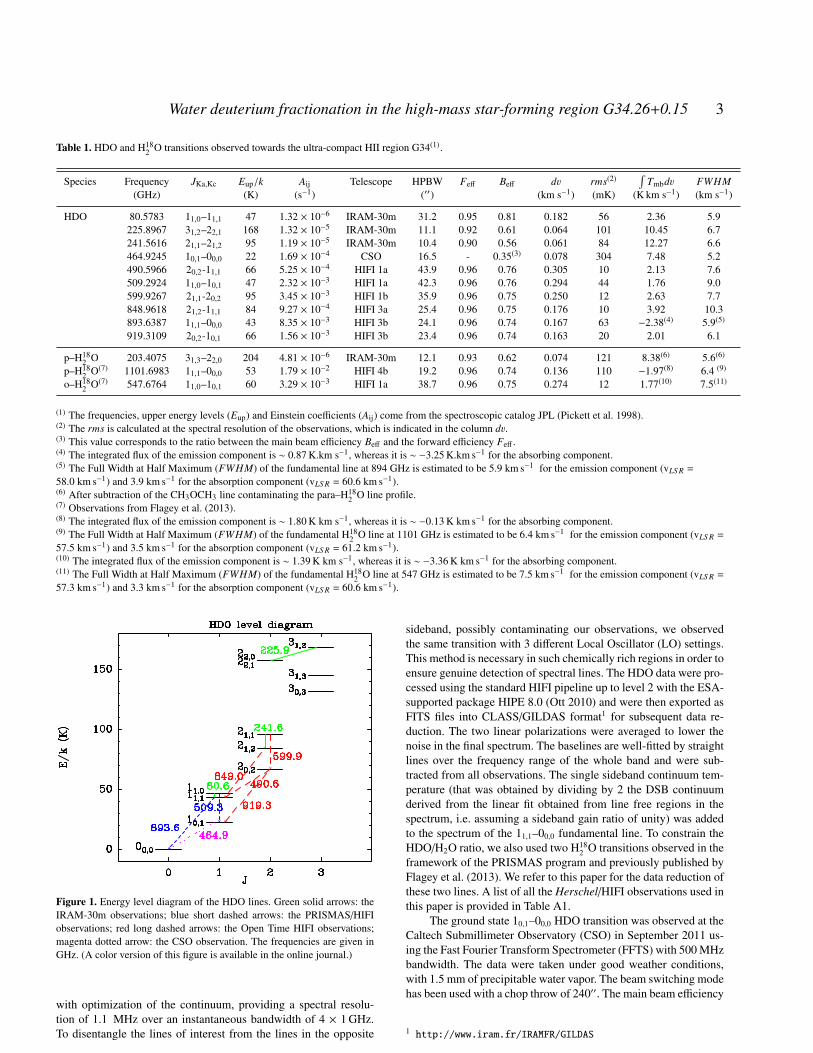
Figure 1. Energy level diagram of the HDO lines. Green solid arrows: theIRAM-30m observations; blue short dashed arrows: the PRISMAS/HIFIobservations; red long dashed arrows: the Open Time HIFI observations;magenta dotted arrow: the CSO observation. The frequencies are given inGHz. (A color version of this figure is available in the online journal.)
with optimization of the continuum, providing a spectral resolu-tion of 1.1 MHz over an instantaneous bandwidth of 4 × 1 GHz.To disentangle the lines of interest from the lines in the opposite
sideband, possibly contaminating our observations, we observedthe same transition with 3 different Local Oscillator (LO) settings.This method is necessary in such chemically rich regions in order toensure genuine detection of spectral lines. The HDO data were pro-cessed using the standard HIFI pipeline up to level 2 with the ESA-supported package HIPE 8.0 (Ott 2010) and were then exported asFITS files into CLASS/GILDAS format1 for subsequent data re-duction. The two linear polarizations were averaged to lower thenoise in the final spectrum. The baselines are well-fitted by straightlines over the frequency range of the whole band and were sub-tracted from all observations. The single sideband continuum tem-perature (that was obtained by dividing by 2 the DSB continuumderived from the linear fit obtained from line free regions in thespectrum, i.e. assuming a sideband gain ratio of unity) was addedto the spectrum of the 11,1–00,0 fundamental line. To constrain theHDO/H2O ratio, we also used two H18
2 O transitions observed in theframework of the PRISMAS program and previously published byFlagey et al. (2013). We refer to this paper for the data reduction ofthese two lines. A list of all the Herschel/HIFI observations used inthis paper is provided in Table A1.
The ground state 10,1–00,0 HDO transition was observed at theCaltech Submillimeter Observatory (CSO) in September 2011 us-ing the Fast Fourier Transform Spectrometer (FFTS) with 500 MHzbandwidth. The data were taken under good weather conditions,with 1.5 mm of precipitable water vapor. The beam switching modehas been used with a chop throw of 240′′. The main beam efficiency
1 http://www.iram.fr/IRAMFR/GILDAS
c© 0000 RAS, MNRAS 000, 000–000

4 A. Coutens, C. Vastel, U. Hincelin et al.
was determined from total power observations of Mars. The systemtemperature was about 3500 K during the run. The single sidebandcontinuum temperature (∼ 2.2 K) was added to the final baseline-subtracted spectrum.
Three additional HDO transitions at 81 (11,0–11,1), 226 (31,2–22,1) and 242 GHz (21,1–21,2) as well as the ortho–H18
2 O transition at203 GHz (31,3–22,0) were observed with the IRAM-30m telescope.The observations were carried out in December 2011 using the FastFourier Transform Spectrometer (FTS) at a 50 kHz resolution. Thespectral resolution was 0.19, 0.07 and 0.06 km s−1 for the 81, 226and 242 GHz transitions, respectively. All the observations wereperformed using the Wobbler Switching mode. The 30m beam sizesat the observing frequencies are given in Table 1. During this run,weather conditions were good for winter, with 2 mm of precipitablewater vapor. System temperatures were always less than 200 K.
Figure 1 presents the energy level diagram of the HDO transi-tions used for the modeling. Table 1 summarizes the observations.
3.2 Description of the observations
Most of the observed HDO lines show a Gaussian-like profile (seefor example Fig. 4). Only the HDO 11,1–00,0 fundamental transi-tion observed with Herschel/HIFI shows an inverse P-Cygni pro-file, i.e a profile showing a red-shifted absorption component anda blue-shifted emission component. A similar profile has alreadybeen observed for this transition in low-mass protostars (Coutenset al. 2012, 2013). The Gaussian FWHM (Full Width at Half-Maximum) was derived for each line with the CASSIS2 software(see Table 1). Using the available spectroscopic databases CDMS(Cologne Database Molecular Spectroscopy; Muller et al. 2011,2005) and JPL (Jet Propulsion Laboratory; Pickett et al. 1998), wealso checked that the different lines are not contaminated by otherspecies. The HDO 21,1–21,2 transition at 242 GHz could be slightlyblended with the CH3COCH3 1310,4–129,3 line. However a simpleLTE (Local Thermal Equilibrium) modeling of CH3COCH3 linesobserved in the spectra, shows that the contribution of CH3COCH3
is negligible. With a column density of 4× 1016 cm−2, an excitationtemperature of 100 K, a FWHM of 6 km s−1 and a source size of1.7′′, the predicted intensity of the CH3COCH3 line at 241.6 GHzis 0.06 K, to be compared with the observed line intensity 1.75 K.The HDO 21,2–11,1 line at 849 GHz is very probably blended withthree 13CH3OH lines (183,15–173,14 A-, 184,14–174,13 A+, and 184,15–174,14 A-) lying in the red-shifted portion of the line profile. Thiscould explain why this line is broader than the others (see Table 1).As the 13CH3OH contribution could be non-negligible, we do notuse this HDO line to constrain the abundances. We present howeverthe modeling of this line for completeness. The other HDO lines donot show any potential blending. The portion of the 600 GHz lineobserved at 3 > 72 km s−1 is produced by the CH3OH 73,5–62,4 3=0A+ line from the image band (ν = 590.3 GHz).
The para–H182 O 31,3–22,0 line is blended with the CH3OCH3
33,1,1–22,1,1 and 33,0,3–22,1,3 transitions at 203.4101 and203.4114 GHz (Eup = 18 K). We can reproduce, with a LTEmodeling approach, the CH3OCH3 lines observed nearby in thespectra (see Figure 2) as well as in the other bands. The CH3OCH3
lines are well-fitted with a column density of 7× 1017 cm−2, anexcitation temperature of 100 K, a FWHM of 6 km s−1 and asource size of 1.7′′. The predicted line profiles of the CH3OCH3
transitions blended with H182 O are then subtracted from the
2 http://cassis.irap.omp.eu
Figure 2. IRAM-30m observations (in black) of the para–H182 O 31,3–22,0
transition at 203.4 GHz. The frequency of the H182 O line is indicated by a
blue dotted line (3 = 58 km s−1). The other lines observed in this spectra arethe SO2 3=0 120,12–111,11 line at 81.5 km s−1 (green long dashed line), theC2H5CN 3=0 232,22–222,21 line at 74.1 km s−1 (yellow short dashed line)and several CH3OCH3 lines (magenta solid lines). A LTE modeling of theCH3OCH3 lines (in magenta) was carried out to estimate the contaminationof the para–H18
2 O line by the CH3OCH3 33,1,1–22,1,1 transition. (A colorversion of this figure is available in the online journal.)
observed line profile to extract the proper H182 O spectrum. Due to
the high number of CH3OCH3 lines considered in the analysis andthe presence of CH3OCH3 lines with similar upper energy levels(18 K) around the H18
2 O feature (see Figure 2), the uncertaintyproduced by this subtraction is negligible with respect to thecalibration uncertainty (≤20%).
4 RADIATIVE TRANSFER MODELING
4.1 Rotational diagram analysis
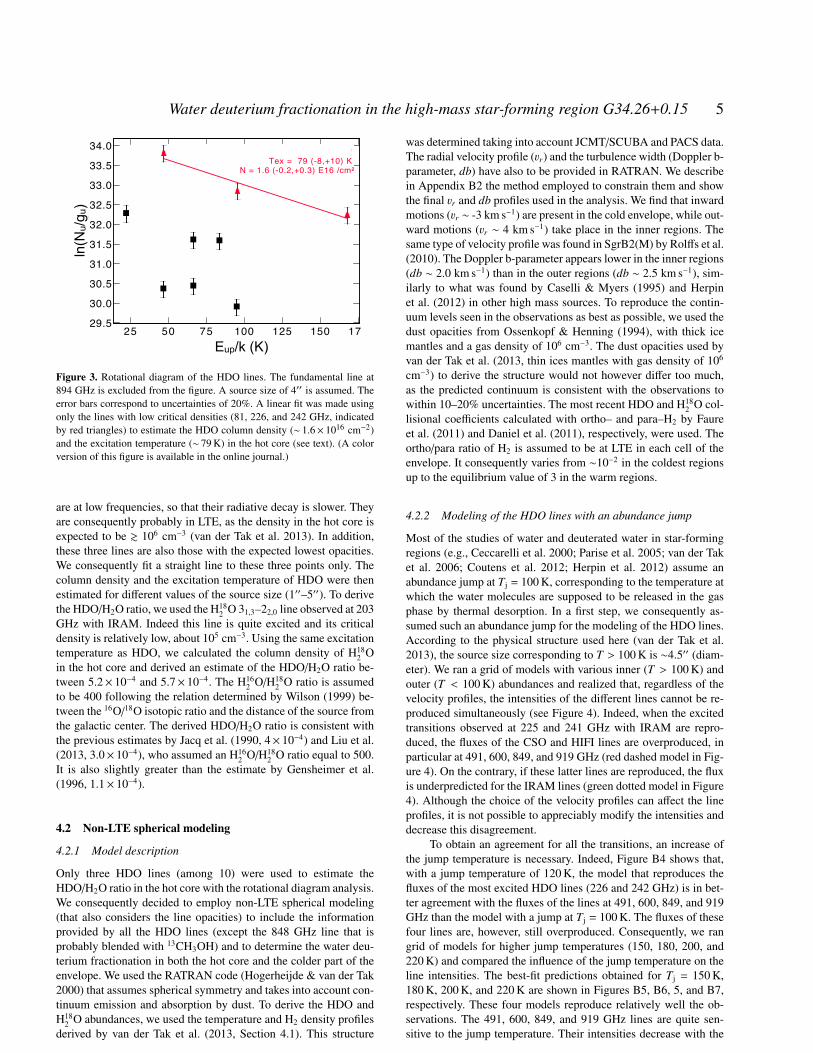
A simple LTE modeling was first employed to estimate theHDO/H2O ratio in the hot core. We plot in Figure 3 the rotationdiagram (Goldsmith & Langer 1999) of the HDO lines shown inTable 1. We exclude the fundamental transition at 894 GHz, whichshows absorption and probably probes colder regions outside of thehot core. We take into account beam dilution and consider differentsource sizes between 1′′ and 5′′, as the exact size of the hot coreis unknown. Indeed, the structure determined by van der Tak et al.(2013) predicts a size of 4.5′′ for T > 100 K, whereas the interfer-ometric observations of two HDO lines by Liu et al. (2013) favora smaller source size which, however, is not well constrained. Nolinear curve is in reasonable agreement with the complete dataset.Plausible explanations are that the lines are optically thick or thatthey do not all have the same excitation temperature. We estimatethe critical densities of these species using the HDO collisionalcoefficients with ortho– and para–H2 of Faure et al. (2011). At∼100 K, the critical densities are about 5× 10⁶ – 5× 107 cm−3 forall lines, except for the lines at 80, 226, and 242 GHz that have crit-ical densities between 3× 10⁴ and 3× 105 cm−3. These latter lines
c© 0000 RAS, MNRAS 000, 000–000
Water deuterium fractionation in the high-mass star-forming region G34.26+0.15 5
25 50 75 100 125 150 175Eup/k[K]
29.5
30.0
30.5
31.0
31.5
32.0
32.5
33.0
33.5
34.0
ln(N
u/gu
)
HDO 19002Tex = 79 (-8,+10) K
N = 1.6 (-0.2,+0.3) E16 /cm²
25 50 75 100 125 150 175Eup/k[K]
29.5
30.0
30.5
31.0
31.5
32.0
32.5
33.0
33.5
34.0
ln(N
u/gu
)
HDO 19002Tex = 79 (-8,+10) K
N = 1.6 (-0.2,+0.3) E16 /cm²
Texte Texte
ln(N
u/gu)
Eup/k (K)
Figure 3. Rotational diagram of the HDO lines. The fundamental line at894 GHz is excluded from the figure. A source size of 4′′ is assumed. Theerror bars correspond to uncertainties of 20%. A linear fit was made usingonly the lines with low critical densities (81, 226, and 242 GHz, indicatedby red triangles) to estimate the HDO column density (∼ 1.6× 1016 cm−2)and the excitation temperature (∼ 79 K) in the hot core (see text). (A colorversion of this figure is available in the online journal.)
are at low frequencies, so that their radiative decay is slower. Theyare consequently probably in LTE, as the density in the hot core isexpected to be & 106 cm−3 (van der Tak et al. 2013). In addition,these three lines are also those with the expected lowest opacities.We consequently fit a straight line to these three points only. Thecolumn density and the excitation temperature of HDO were thenestimated for different values of the source size (1′′–5′′). To derivethe HDO/H2O ratio, we used the H18
2 O 31,3–22,0 line observed at 203GHz with IRAM. Indeed this line is quite excited and its criticaldensity is relatively low, about 105 cm−3. Using the same excitationtemperature as HDO, we calculated the column density of H18
2 Oin the hot core and derived an estimate of the HDO/H2O ratio be-tween 5.2× 10⁻⁴ and 5.7× 10⁻⁴. The H16
2 O/H182 O ratio is assumed
to be 400 following the relation determined by Wilson (1999) be-tween the 16O/18O isotopic ratio and the distance of the source fromthe galactic center. The derived HDO/H2O ratio is consistent withthe previous estimates by Jacq et al. (1990, 4× 10⁻⁴) and Liu et al.(2013, 3.0× 10⁻⁴), who assumed an H16
2 O/H182 O ratio equal to 500.
It is also slightly greater than the estimate by Gensheimer et al.(1996, 1.1× 10⁻⁴).
4.2 Non-LTE spherical modeling
4.2.1 Model description
Only three HDO lines (among 10) were used to estimate theHDO/H2O ratio in the hot core with the rotational diagram analysis.We consequently decided to employ non-LTE spherical modeling(that also considers the line opacities) to include the informationprovided by all the HDO lines (except the 848 GHz line that isprobably blended with 13CH3OH) and to determine the water deu-terium fractionation in both the hot core and the colder part of theenvelope. We used the RATRAN code (Hogerheijde & van der Tak2000) that assumes spherical symmetry and takes into account con-tinuum emission and absorption by dust. To derive the HDO andH18
2 O abundances, we used the temperature and H2 density profilesderived by van der Tak et al. (2013, Section 4.1). This structure
was determined taking into account JCMT/SCUBA and PACS data.The radial velocity profile (3r) and the turbulence width (Doppler b-parameter, db) have also to be provided in RATRAN. We describein Appendix B2 the method employed to constrain them and showthe final 3r and db profiles used in the analysis. We find that inwardmotions (3r ∼ -3 km s−1) are present in the cold envelope, while out-ward motions (3r ∼ 4 km s−1) take place in the inner regions. Thesame type of velocity profile was found in SgrB2(M) by Rolffs et al.(2010). The Doppler b-parameter appears lower in the inner regions(db ∼ 2.0 km s−1) than in the outer regions (db ∼ 2.5 km s−1), sim-ilarly to what was found by Caselli & Myers (1995) and Herpinet al. (2012) in other high mass sources. To reproduce the contin-uum levels seen in the observations as best as possible, we used thedust opacities from Ossenkopf & Henning (1994), with thick icemantles and a gas density of 106 cm−3. The dust opacities used byvan der Tak et al. (2013, thin ices mantles with gas density of 106
cm−3) to derive the structure would not however differ too much,as the predicted continuum is consistent with the observations towithin 10–20% uncertainties. The most recent HDO and H18
2 O col-lisional coefficients calculated with ortho– and para–H2 by Faureet al. (2011) and Daniel et al. (2011), respectively, were used. Theortho/para ratio of H2 is assumed to be at LTE in each cell of theenvelope. It consequently varies from ∼10−2 in the coldest regionsup to the equilibrium value of 3 in the warm regions.
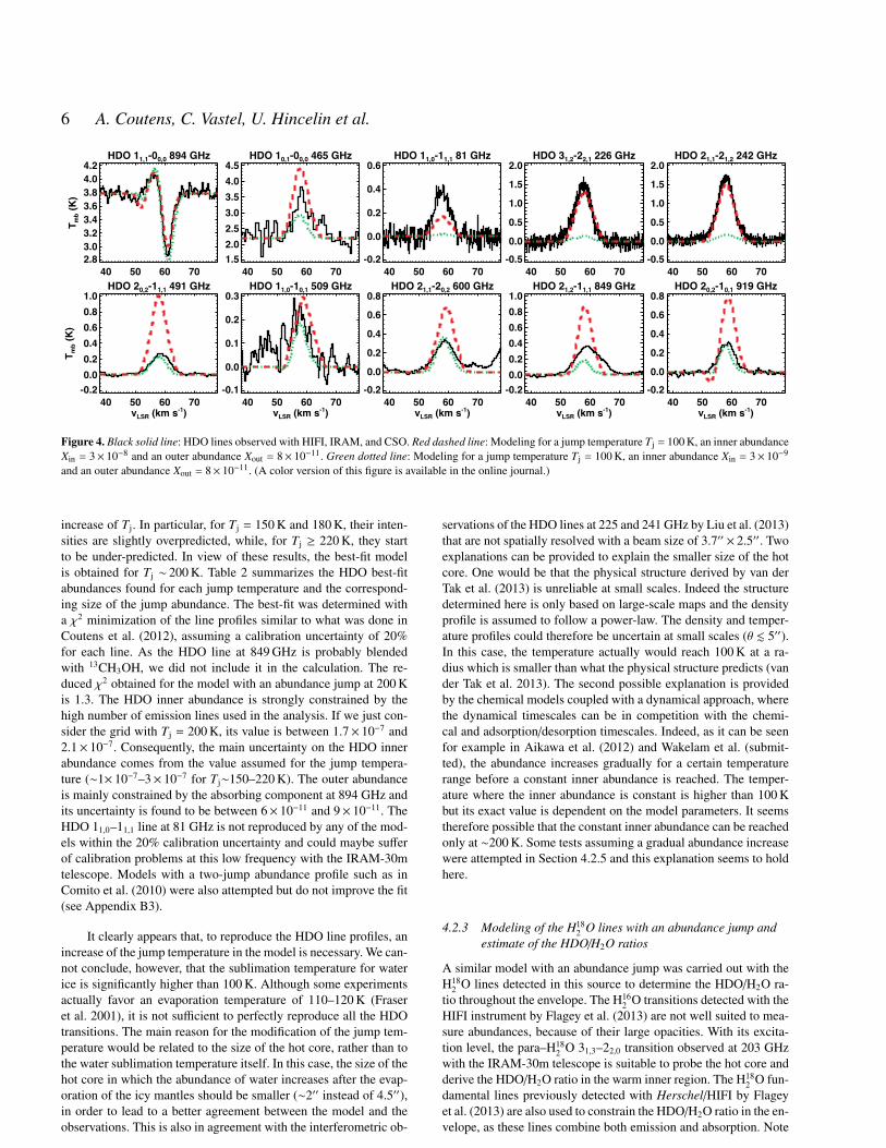
4.2.2 Modeling of the HDO lines with an abundance jump
Most of the studies of water and deuterated water in star-formingregions (e.g., Ceccarelli et al. 2000; Parise et al. 2005; van der Taket al. 2006; Coutens et al. 2012; Herpin et al. 2012) assume anabundance jump at Tj = 100 K, corresponding to the temperature atwhich the water molecules are supposed to be released in the gasphase by thermal desorption. In a first step, we consequently as-sumed such an abundance jump for the modeling of the HDO lines.According to the physical structure used here (van der Tak et al.2013), the source size corresponding to T > 100 K is ∼4.5′′ (diam-eter). We ran a grid of models with various inner (T > 100 K) andouter (T < 100 K) abundances and realized that, regardless of thevelocity profiles, the intensities of the different lines cannot be re-produced simultaneously (see Figure 4). Indeed, when the excitedtransitions observed at 225 and 241 GHz with IRAM are repro-duced, the fluxes of the CSO and HIFI lines are overproduced, inparticular at 491, 600, 849, and 919 GHz (red dashed model in Fig-ure 4). On the contrary, if these latter lines are reproduced, the fluxis underpredicted for the IRAM lines (green dotted model in Figure4). Although the choice of the velocity profiles can affect the lineprofiles, it is not possible to appreciably modify the intensities anddecrease this disagreement.
To obtain an agreement for all the transitions, an increase ofthe jump temperature is necessary. Indeed, Figure B4 shows that,with a jump temperature of 120 K, the model that reproduces thefluxes of the most excited HDO lines (226 and 242 GHz) is in bet-ter agreement with the fluxes of the lines at 491, 600, 849, and 919GHz than the model with a jump at Tj = 100 K. The fluxes of thesefour lines are, however, still overproduced. Consequently, we rangrid of models for higher jump temperatures (150, 180, 200, and220 K) and compared the influence of the jump temperature on theline intensities. The best-fit predictions obtained for Tj = 150 K,180 K, 200 K, and 220 K are shown in Figures B5, B6, 5, and B7,respectively. These four models reproduce relatively well the ob-servations. The 491, 600, 849, and 919 GHz lines are quite sen-sitive to the jump temperature. Their intensities decrease with the
c© 0000 RAS, MNRAS 000, 000–000
6 A. Coutens, C. Vastel, U. Hincelin et al.
HDO 11,1-00,0 894 GHz
40 50 60 702.83.03.23.43.63.84.04.2
T mb (
K)
HDO 10,1-00,0 465 GHz
40 50 60 701.52.02.53.03.54.04.5
HDO 11,0-11,1 81 GHz
40 50 60 70-0.2
0.0
0.2
0.4
0.6HDO 31,2-22,1 226 GHz
40 50 60 70-0.5
0.0
0.5
1.0
1.5
2.0HDO 21,1-21,2 242 GHz
40 50 60 70-0.5
0.0
0.5
1.0
1.5
2.0
HDO 20,2-11,1 491 GHz
40 50 60 70vLSR (km s-1)
-0.20.00.20.40.60.81.0
T mb (
K)
HDO 11,0-10,1 509 GHz
40 50 60 70vLSR (km s-1)
-0.1
0.0
0.1
0.2
0.3HDO 21,1-20,2 600 GHz
40 50 60 70vLSR (km s-1)
-0.2
0.0
0.2
0.4
0.6
0.8HDO 21,2-11,1 849 GHz
40 50 60 70vLSR (km s-1)
-0.20.00.20.40.60.81.0
HDO 20,2-10,1 919 GHz
40 50 60 70vLSR (km s-1)
-0.2
0.0
0.2
0.4
0.6
0.8
Figure 4. Black solid line: HDO lines observed with HIFI, IRAM, and CSO. Red dashed line: Modeling for a jump temperature Tj = 100 K, an inner abundanceXin = 3× 10⁻⁸ and an outer abundance Xout = 8× 10⁻¹¹. Green dotted line: Modeling for a jump temperature Tj = 100 K, an inner abundance Xin = 3× 10⁻⁹
and an outer abundance Xout = 8× 10⁻¹¹. (A color version of this figure is available in the online journal.)
increase of Tj. In particular, for Tj = 150 K and 180 K, their inten-sities are slightly overpredicted, while, for Tj ≥ 220 K, they startto be under-predicted. In view of these results, the best-fit modelis obtained for Tj ∼ 200 K. Table 2 summarizes the HDO best-fitabundances found for each jump temperature and the correspond-ing size of the jump abundance. The best-fit was determined witha χ2 minimization of the line profiles similar to what was done inCoutens et al. (2012), assuming a calibration uncertainty of 20%for each line. As the HDO line at 849 GHz is probably blendedwith 13CH3OH, we did not include it in the calculation. The re-duced χ2 obtained for the model with an abundance jump at 200 Kis 1.3. The HDO inner abundance is strongly constrained by thehigh number of emission lines used in the analysis. If we just con-sider the grid with Tj = 200 K, its value is between 1.7× 10⁻⁷ and2.1× 10−7. Consequently, the main uncertainty on the HDO innerabundance comes from the value assumed for the jump tempera-ture (∼1× 10⁻⁷–3× 10⁻⁷ for Tj∼150–220 K). The outer abundanceis mainly constrained by the absorbing component at 894 GHz andits uncertainty is found to be between 6× 10⁻¹¹ and 9× 10⁻¹¹. TheHDO 11,0–11,1 line at 81 GHz is not reproduced by any of the mod-els within the 20% calibration uncertainty and could maybe sufferof calibration problems at this low frequency with the IRAM-30mtelescope. Models with a two-jump abundance profile such as inComito et al. (2010) were also attempted but do not improve the fit(see Appendix B3).
It clearly appears that, to reproduce the HDO line profiles, anincrease of the jump temperature in the model is necessary. We can-not conclude, however, that the sublimation temperature for waterice is significantly higher than 100 K. Although some experimentsactually favor an evaporation temperature of 110–120 K (Fraseret al. 2001), it is not sufficient to perfectly reproduce all the HDOtransitions. The main reason for the modification of the jump tem-perature would be related to the size of the hot core, rather than tothe water sublimation temperature itself. In this case, the size of thehot core in which the abundance of water increases after the evap-oration of the icy mantles should be smaller (∼2′′ instead of 4.5′′),in order to lead to a better agreement between the model and theobservations. This is also in agreement with the interferometric ob-
servations of the HDO lines at 225 and 241 GHz by Liu et al. (2013)that are not spatially resolved with a beam size of 3.7′′ × 2.5′′. Twoexplanations can be provided to explain the smaller size of the hotcore. One would be that the physical structure derived by van derTak et al. (2013) is unreliable at small scales. Indeed the structuredetermined here is only based on large-scale maps and the densityprofile is assumed to follow a power-law. The density and temper-ature profiles could therefore be uncertain at small scales (θ . 5′′).In this case, the temperature actually would reach 100 K at a ra-dius which is smaller than what the physical structure predicts (vander Tak et al. 2013). The second possible explanation is providedby the chemical models coupled with a dynamical approach, wherethe dynamical timescales can be in competition with the chemi-cal and adsorption/desorption timescales. Indeed, as it can be seenfor example in Aikawa et al. (2012) and Wakelam et al. (submit-ted), the abundance increases gradually for a certain temperaturerange before a constant inner abundance is reached. The temper-ature where the inner abundance is constant is higher than 100 Kbut its exact value is dependent on the model parameters. It seemstherefore possible that the constant inner abundance can be reachedonly at ∼200 K. Some tests assuming a gradual abundance increasewere attempted in Section 4.2.5 and this explanation seems to holdhere.
4.2.3 Modeling of the H182 O lines with an abundance jump and
estimate of the HDO/H2O ratios
A similar model with an abundance jump was carried out with theH18
2 O lines detected in this source to determine the HDO/H2O ra-tio throughout the envelope. The H16
2 O transitions detected with theHIFI instrument by Flagey et al. (2013) are not well suited to mea-sure abundances, because of their large opacities. With its excita-tion level, the para–H18
2 O 31,3–22,0 transition observed at 203 GHzwith the IRAM-30m telescope is suitable to probe the hot core andderive the HDO/H2O ratio in the warm inner region. The H18
2 O fun-damental lines previously detected with Herschel/HIFI by Flageyet al. (2013) are also used to constrain the HDO/H2O ratio in the en-velope, as these lines combine both emission and absorption. Note
c© 0000 RAS, MNRAS 000, 000–000

Water deuterium fractionation in the high-mass star-forming region G34.26+0.15 7
HDO 11,1-00,0 894 GHz
40 50 60 702.5
3.0
3.5
4.0
4.5
T mb (
K)
HDO 10,1-00,0 465 GHz
40 50 60 701.5
2.0
2.5
3.0
3.5
4.0HDO 11,0-11,1 81 GHz
40 50 60 70-0.2
0.0
0.2
0.4
0.6HDO 31,2-22,1 226 GHz
40 50 60 70-0.5
0.0
0.5
1.0
1.5
2.0HDO 21,1-21,2 242 GHz
40 50 60 70-0.5
0.0
0.5
1.0
1.5
2.0
HDO 20,2-11,1 491 GHz
40 50 60 70vLSR (km s-1)
-0.1
0.0
0.1
0.2
0.3
T mb (
K)
HDO 11,0-10,1 509 GHz
40 50 60 70vLSR (km s-1)
-0.1
0.0
0.1
0.2
0.3HDO 21,1-20,2 600 GHz
40 50 60 70vLSR (km s-1)
-0.1
0.0
0.1
0.2
0.3
0.4HDO 21,2-11,1 849 GHz
40 50 60 70vLSR (km s-1)
-0.1
0.0
0.1
0.2
0.3
0.4HDO 20,2-10,1 919 GHz
40 50 60 70vLSR (km s-1)
-0.1
0.0
0.1
0.2
0.3
0.4
Figure 5. Black solid line: HDO lines observed with HIFI, IRAM, and CSO. Red dashed line: Modeling for a jump temperature Tj = 200 K, an inner abundanceXin = 2× 10⁻⁷ and an outer abundance Xout = 8× 10⁻¹¹. (A color version of this figure is available in the online journal.)
p-H218O 31,3-22,0 203 GHz
40 50 60 70vLSR (km s-1)
-0.5
0.0
0.5
1.0
1.5
2.0
T mb (
K)
p-H218O 11,1-00,0 1102 GHz
40 50 60 70vLSR (km s-1)
4.5
5.0
5.5
6.0
6.5o-H2
18O 11,0-10,1 548 GHz
40 50 60 70vLSR (km s-1)
0.80.91.01.11.21.31.4
Figure 6. Black solid line: H182 O lines observed with HIFI and IRAM. Red dashed line: Modeling for a jump temperature Tj = 200 K, an inner abundance
Xin = 9× 10⁻⁷ and an outer abundance Xout = 1.3× 10⁻¹⁰. (A color version of this figure is available in the online journal.)
that we only use here the ortho 11,0–10,1 transition at 548 GHz andthe para 11,1–00,0 transition at 1102 GHz. The fundamental ortho21,2–10,1 transition, which is observed at 1656 GHz in absorption,was not taken into account because of pointing problems affectingthe observations. The source being fairly peaked on the continuum,an offset could lead to a significant loss of flux.
All the physical parameters are kept similar to those of thestudy of HDO. Figures B8, B9, 6, and B10 show the best-fit modelsobtained for these three lines for the jump temperatures previouslyassumed for deuterated water, Tj = 150, 180, 200, and 220 K re-spectively. We assumed an ortho-to-para ratio of water equal to 3,corresponding to the thermal equilibrium value at high-temperature(> 50 K). This value is also consistent with the ratio determined inmost of the foreground clouds on the line of sight towards brightcontinuum sources (Lis et al. 2010; Flagey et al. 2013). The best-fitinner and outer H18
2 O abundances are summarized in Table 2. Thereduced χ2 is about 1.5 for the case Tj = 200 K. Assuming an obser-vational uncertainty of 20% for the excited para–H18
2 O line at 203GHz, the inner abundance cannot be higher than 1.2× 10⁻⁶ or lowerthan 7× 10⁻⁷ for the model with Tj = 200 K. The outer abundanceis estimated to be between 1.0× 10⁻¹⁰ and 1.5× 10⁻¹⁰, based onan observational uncertainty of 20% for the absorbing componentof the para–H18
2 O transition at 1102 GHz. The H162 O abundances
in Table 2 are estimated using an H162 O/H18
2 O ratio of 400 (Wilson1999).
The best-fit HDO/H2O ratios are then equal to ∼(5–6)× 10−4
in the hot core and ∼1.5× 10⁻³ in the outer envelope. Even whenconsidering the HDO and H18
2 O results with a 20% calibration un-certainty, the outer HDO/H2O ratio (1.0× 10⁻³–2.2× 10⁻³) is stillhigher than the inner HDO/H2O ratio (3.5× 10⁻⁴–7.5× 10⁻⁴ for Tj
= 200 K). We ran models with a constant ortho/para H2 ratio equalto 3 to check that the ortho/para H2 ratio assumed in the model doesnot affect the results. The HDO and H18
2 O line profiles are exactlythe same as with an LTE ortho/para ratio, confirming the variationof the HDO/H2O ratio from the cold to the warm regions.
4.2.4 Gradual decrease of the outer abundance from the cold tothe warm regions
Although we used a constant abundance of HDO and H182 O in the
cold envelope of G34, it is very probable that the water abun-dance shows variations in this region due to non-thermal desorp-tion mechanisms. In particular, Mottram et al. (2013) showed thatthe desorption by the cosmic ray-induced UV field leads to an outerabundance of water decreasing gradually from the cold to the warmregions of low-mass protostars. To confirm that the presence of agradual abundance decrease in the cold envelope does not affect thederived value of the HDO/H2O ratio in this region, we ran a mod-eling considering an equilibrium state between the desorption bythe cosmic ray-induced UV field and the re-depletion on the grains.
c© 0000 RAS, MNRAS 000, 000–000

8 A. Coutens, C. Vastel, U. Hincelin et al.
Table 2. HDO and H2O abundances obtained for different jump temperatures Tj
Tj (K) (a) θ (′′) (a) Xin(HDO) Xout(HDO) Xin(H182 O) Xout(H18
2 O) Xin(H2O)(b) Xout(H2O)(b) (HDO/H2O)in(b) (HDO/H2O)out
(b)
100(c) 4.5 – – – – – – – –120(c) 3.5 – – – – – – – –150 2.5 1 × 10⁻⁷ 8 × 10⁻¹¹ 4 × 10⁻⁷ 1.3 × 10⁻¹⁰ 1.6 × 10⁻⁴ 5.2 × 10⁻⁸ 6 × 10⁻⁴ 1.5 × 10⁻³
180 1.9 1.5 × 10⁻⁷ 8 × 10⁻¹¹ 7 × 10⁻⁷ 1.3 × 10⁻¹⁰ 2.8 × 10⁻⁴ 5.2 × 10⁻⁸ 5 × 10⁻⁴ 1.5 × 10⁻³
200(d) 1.7 2 × 10⁻⁷ 8 × 10⁻¹¹ 9 × 10⁻⁷ 1.3 × 10⁻¹⁰ 3.6 × 10⁻⁴ 5.2 × 10⁻⁸ 6 × 10⁻⁴ 1.5 × 10⁻³
220 1.5 3 × 10⁻⁷ 8 × 10⁻¹¹ 1.2 × 10⁻⁶ 1.3 × 10⁻¹⁰ 4.8 × 10⁻⁴ 5.2 × 10⁻⁸ 6 × 10⁻⁴ 1.5 × 10⁻³
Notes: (a) Size of the region where the temperature is higher than Tj (diameter). It is derived from the structure determined by van der Tak et al. (2013). (b)
Assuming H162 O/H18
2 O = 400. (c) Fit is not good enough to determine the HDO abundances. (d) Best-fit.
102 103 104 105
radius (AU)
10-13
10-12
10-11
10-10
10-9
10-8
10-7
10-6
HD
O a
bund
ance
0.1 1.0 10.0radius (’’)
Figure 7. Best-fit abundance profiles obtained for HDO when the outerabundance (region at T < 200 K) is constant (black solid line, Section 4.2.2),when it decreases from the cold regions to the region at T = 200 K (reddashed line, Section 4.2.4), and when it decreases from the cold regions tothe region at T = 100 K and increases from T = 100 K to T = 200 K (greendotted line, see Section 4.2.5). The temperature reaches 200 K at a radius of2700 AU (∼0.9′′, see Figure B1). (A color version of this figure is availablein the online journal.)
Using similar equations to those in Hollenbach et al. (2009) andMottram et al. (2013), we get by equating desorption to depletion:
GcrF0Yx fs,xngrσgr = n(x)ngrσgr3th,x (4)
with F0 the local interstellar flux of 6–13.6 eV photons assumedto be equal to 108 photons cm−2 s−1, Gcr the scaling factor of theUV flux, Yx the photodesorption yield for the molecule x (∼ 10−3
for H2O, Oberg et al. 2009), fs,x the fraction of the molecule x ongrains, ngr the grain density, σgr the cross sectional area of the grainand 3th,x the thermal velocity. The thermal velocity is calculatedaccording to the following formalism:
3th,x =
√8kbTk
πmx, (5)
where kb is the Boltzmann constant, Tk the gas temperature andmx the mass of the molecule x. The outer abundance of H2O withrespect to H2 is then equal to:
Xout(H2O) =GcrF0YH2O fs,H2O
3th,H2O nH2
, (6)
with nH2 the H2 density. Similarly we obtain for HDO:
Xout(HDO) =GcrF0YHDO fs,H2O
3th,HDO nH2
(HDOH2O
), (7)
and for H182 O:
Xout(H182 O) =
GcrF0YH182 O fs,H2O
3th,H182 O nH2
(H18
2 OH2O
). (8)
The photodesorption yields for HDO and H182 O are assumed simi-
lar to those for H2O (Oberg et al. 2009). The thermal velocity isapproximatively the same due to their relatively similar masses.All the other parameters are independent of the molecules exceptthe fraction fs,x of these molecules contained in the grain mantleswhich reflects the isotopic ratios, HDO/H2O and H18
2 O/H162 O, on
the grains. The external UV field should also affect the externalpart of the outer envelope. But, due to the very small constraints onthese different mechanisms, we only considered the desorption bythe cosmic ray-induced UV field.
We ran a grid of models for the case Tj = 200 K, keep-ing the inner abundances determined previously (Xin(HDO) =
2× 10⁻⁷ and Xin(H182 O) = 9× 10⁻⁷). Different values were then as-
sumed for the factors WHDO = Gcr fs,H2O HDO/H2O and WH182 O =
Gcr fs,H2O H182 O/H16
2 O. Assuming H182 O/H16
2 O = 400 (Wilson 1999)and fs,H2O = 1 (the icy grain mantles are constituted entirely ofH2O), the best-fit model of the H18
2 O lines gives a scaling factorGcr of about 1.6× 10⁻³. If water represents only 50% of the grainmantles, Gcr is then equal to 3.2× 10⁻³ leading to a cosmic ray-induced UV field of ∼3× 10⁵ photons cm−2 s−1. These values rep-resent, however, only upper limits, since the desorption by the ex-ternal UV field is not taken into account in the analysis. The typicalvalue of the cosmic-ray induced UV flux (Gcr ∼ 10−4; e.g., Prasad& Tarafdar 1983; Shen et al. 2004) is then consistent with the upperlimit derived here (Gcr . 3× 10⁻³).
The best-fit abundance profile determined for HDO when theouter abundance decreases from the cold to the warm regions ispresented in Figure 7 (red dashed line). The HDO/H2O ratio in theouter envelope is equal to 1.3× 10⁻³. It is then, once again, higherthan in the hot core (∼(5–6)× 10−4). The HDO and H18
2 O line pro-files predicted with the RATRAN code (see red dashed lines in Fig-ures 8 and 9) are relatively similar to those in Figures 5 and 6 thatassume a two-step abundance profile with a jump at 200 K. Thefit is even better for the H18
2 O and HDO fundamental transitions(HDO: 894 GHz; H18
2 O: 548 and 1102 GHz), as the predicted in-tensity of their emission is now in agreement with the observations.Some of the HDO lines (509, 600, and 919 GHz) show small self-absorptions on their blue-shifted side. However, these defects couldprobably disappear with slightly different velocity profiles. Indeed,
c© 0000 RAS, MNRAS 000, 000–000
Water deuterium fractionation in the high-mass star-forming region G34.26+0.15 9
HDO 11,1-00,0 894 GHz
40 50 60 702.83.03.23.43.63.84.04.2
T mb (
K)
HDO 10,1-00,0 465 GHz
40 50 60 701.5
2.0
2.5
3.0
3.5
4.0HDO 11,0-11,1 81 GHz
40 50 60 70-0.2
0.0
0.2
0.4
0.6HDO 31,2-22,1 226 GHz
40 50 60 70-0.5
0.0
0.5
1.0
1.5
2.0HDO 21,1-21,2 242 GHz
40 50 60 70-0.5
0.0
0.5
1.0
1.5
2.0
HDO 20,2-11,1 491 GHz
40 50 60 70vLSR (km s-1)
-0.1
0.0
0.1
0.2
0.3
T mb (
K)
HDO 11,0-10,1 509 GHz
40 50 60 70vLSR (km s-1)
-0.1
0.0
0.1
0.2
0.3HDO 21,1-20,2 600 GHz
40 50 60 70vLSR (km s-1)
-0.1
0.0
0.1
0.2
0.3
0.4HDO 21,2-11,1 849 GHz
40 50 60 70vLSR (km s-1)
-0.1
0.0
0.1
0.2
0.3
0.4HDO 20,2-10,1 919 GHz
40 50 60 70vLSR (km s-1)
-0.1
0.0
0.1
0.2
0.3
0.4
Figure 8. Black solid line: HDO lines observed with HIFI, IRAM, and CSO. Red dashed line: Modeling for a constant inner abundance Xin = 2× 10⁻⁷ (T ≥200 K) and an outer abundance (T < 200 K) decreasing from the cold to the warm regions (see Section 4.2.4). Green dotted line: Modeling for a constant innerabundance Xin = 2× 10⁻⁷ (T ≥ 200 K), an abundance gradually increasing from 100 to 200 K, and an outer abundance (T < 100 K) decreasing from the coldto the warm regions (see Section 4.2.5). (A color version of this figure is available in the online journal.)
p-H218O 31,3-22,0 203 GHz
40 50 60 70vLSR (km s-1)
-0.5
0.0
0.5
1.0
1.5
2.0
T mb (
K)
p-H218O 11,1-00,0 1102 GHz
40 50 60 70vLSR (km s-1)
4.5
5.0
5.5
6.0
6.5o-H2
18O 11,0-10,1 548 GHz
40 50 60 70vLSR (km s-1)
0.8
0.9
1.0
1.1
1.2
1.3
Figure 9. Black solid line: H182 O lines observed with HIFI and IRAM. Red dashed line: Modeling for a constant inner abundance Xin = 9× 10⁻⁷ (T ≥ 200 K)
and an outer abundance (T < 200 K) decreasing from the cold to the warm regions (see Section 4.2.4). Green dotted line: Modeling for a constant innerabundance Xin = 9× 10⁻⁷ (T ≥ 200 K), an abundance gradually increasing from 100 to 200 K, and an outer abundance (T < 100 K) decreasing from the coldto the warm regions (see Section 4.2.5). (A color version of this figure is available in the online journal.)
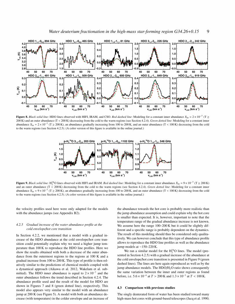
the velocity profiles used here were only adapted for the modelswith the abundance jumps (see Appendix B2).
4.2.5 Gradual increase of the water abundance profile at thecold envelope/hot core transition
In Section 4.2.2, we mentioned that a model with a gradual in-crease of the HDO abundance at the cold envelope/hot core tran-sition could potentially explain why we need a higher jump tem-perature than 100 K to reproduce the HDO line profiles. Here weshow the results obtained with both a decrease of the outer abun-dance from the outermost regions to the regions at 100 K and agradual increase from 100 to 200 K. This type of profile is then rel-atively similar to the predictions of chemical models coupled witha dynamical approach (Aikawa et al. 2012, Wakelam et al. sub-mitted). The HDO inner abundance is equal to 2× 10⁻⁷ and theouter abundance follows the trend described in Section 4.2.4. Theabundance profile used and the result of the model for HDO areshown in Figures 7 and 8 (green dotted line), respectively. Thismodel also appears very similar to the model with an abundancejump at 200 K (see Figure 5). A model with both an abundance de-crease (with temperature) in the colder envelope and an increase of
the abundance towards the hot core is probably more realistic thanthe jump abundance assumption and could explain why the hot coreis smaller than expected. It is, however, important to note that thetemperature range of the gradual abundance increase is not known.We assume here the range 100–200 K but it could be slightly dif-ferent and a specific range is probably dependent on the dynamics.The result of this modeling should thus be considered only qualita-tively. We can however conclude that this type of abundance profileallows to reproduce the HDO line profiles as well as the abundancejump models at ∼150–220 K.
We ran a similar model for the H182 O lines. The model (pre-
sented in Section 4.2.5) with a gradual increase of the abundance atthe cold envelope/hot core transition is presented in Figure 9 (greendashed lines). The lines are here again reproduced as well as by thejump abundance models. The HDO/H2O ratio shows consequentlythe same variation between the inner and outer regions as foundbefore, i.e. 5.6× 10⁻⁴ at T > 200 K and 1.3× 10⁻³ at T < 100 K.
4.3 Comparison with previous studies
The singly deuterated form of water has been studied toward manyhigh-mass hot cores with ground-based telescopes (Jacq et al. 1990;
c© 0000 RAS, MNRAS 000, 000–000
10 A. Coutens, C. Vastel, U. Hincelin et al.
Gensheimer et al. 1996; Pardo et al. 2001; van der Tak et al. 2006).These studies are relevant for the hot core study but do not directlyaddress for the cold external envelope, since the observations ofthe ground HDO transition at 894 GHz with a very good signal-to-noise ratio are necessary in order to disentangle the contribu-tion from the hot core to the contribution of the cold envelope. Thelaunch of the Herschel Space Observatory dramatically changedthe situation, with the access to the high frequency range with manyHDO transitions available in addition to the ground-state transi-tion. The D/H ratio in water remained for a long time very poorlyknown since the study of water was based on observations sufferingfrom dilution in the large beams of the Infrared Space Observatory(ISO), the Submillimeter Wave Astronomy Satellite (SWAS) andthe ODIN satellite as well as from large opacities. The only way tostudy water from the ground was to use the H18
2 O transition avail-able with some telescopes at 203 GHz (Jacq et al. 1988; van derTak et al. 2006; Jørgensen & van Dishoeck 2010; Persson et al.2012, 2013). With the help of this line, the water deuterium frac-tionation was previously estimated in the high-mass star-formingregion G34 by Jacq et al. (1990), Gensheimer et al. (1996), and Liuet al. (2013). They found, in its hot core, HDO/H2O ratios rangingbetween 1× 10⁻⁴ and 4× 10⁻⁴. Since our modeling in the hot coreregion is mostly dominated by the 81, 226 and 241 GHz transitionsaccessible from the ground, these values are relatively consistentwith our estimate of (5–6)× 10−4 both with the rotational diagramapproach and the non-LTE 1D analysis. Note that we assumed anH2
16O/H218O ratio of 400, whereas the previous studies assumed
500. In addition, the HDO/H2O ratio found in this hot core is con-sistent with the average HDO/H2O ratio (a few 10−4) found in otherhigh-mass sources (Jacq et al. 1990; Gensheimer et al. 1996; Pardoet al. 2001; van der Tak et al. 2006; Emprechtinger et al. 2013).
In the hot core, we also determined the water abundance (rel-ative to H2) to be a few× 10−4. Similar values were estimated inother high-mass hot cores (Chavarrıa et al. 2010; Herpin et al. 2012;Neill et al. 2013), although lower values were also found, for ex-ample, in NGC 6334 I (∼10−6, Emprechtinger et al. 2013). Thevalue of 10−4 is comparable to the observed abundance of solid wa-ter and together with the derived HDO/H2O abundance ratios of10−4 − 10−3 suggests that the origin of the observed water is evap-oration of grain mantles.
Recently, Liu et al. (2013) also attempted to constrain the D/Hratio for water in the outer envelope of G34 using the 894 GHztransition observed from the ground with APEX. From a RATRANmodeling using an abundance jump profile at 100 K, they failedto reproduce the profile of this ground state transition leading toa very uncertain value for the D/H ratio in the outer region of theenvelope of (1.9–4.9)× 10−4. With the sensitivity of Herschel/HIFIobservations of the 894 GHz transition, it became possible to mea-sure accurately the D/H ratio of water in low-mass (Coutens et al.2012, 2013) and high-mass protostars, from the hot core region tothe cold external envelope. We showed here that, with a value of(1.0–2.2)× 10−3 in the colder envelope, the HDO/H2O ratio is in-deed higher than the estimate by Liu et al. (2013). It is also higherthan in the hot core. A similar behavior was discovered in the low-mass sources IRAS16293 and NGC1333 IRAS4A (Coutens et al.2013a, 2013b). But this is the first time that a radial variation ofthe D/H ratio has been observed towards a high-mass star-formingregion. The HDO/H2O ratio derived in the colder envelope of G34is among the highest values found in high-mass sources. It is closeto the high value of (2–4)× 10−3 found in Orion KL (Persson et al.2007; Neill et al. 2013) but lower by more than a factor 10 than
in the absorbing layer of low-mass protostars (Coutens et al. 2012,2013).
5 CHEMICAL MODELING
In order to study the chemical pathways that could lead to the ob-served HDO and H2O abundances and their corresponding ratio,we modeled the chemical evolution of the source as a function ofits radius, using the full gas-grain chemical model Nautilus (Her-sant et al. 2009).
5.1 Model
Nautilus is a gas grain chemical code adapted from the originalcode developed by the Herbst group (Hasegawa & Herbst 1993).It solves the kinetic equations of gas-phase chemistry, takes intoaccount grain surface chemistry, and interactions between bothphases (adsorption, thermal and non-thermal desorption). The rateequations follow Hasegawa et al. (1992) and Caselli et al. (1998).More details on the processes included in the code are presentedby Semenov et al. (2010). The chemical network is adapted fromAikawa et al. (2012) and Furuya et al. (2012). As pointed out byPagani et al. (1992), Flower et al. (2004, 2006a,b), Walmsley et al.(2004), and Pagani et al. (2009), considering ortho and para spinmodifications of various H and D bearing species is important dueto some reactions which are much faster with ortho–H2 than para–H2, and can change the entire chemistry of deuterium fractionation.Thus, we extended the network including the ortho, para, and metastates of H2, D2, H+
3 , H2D+, D2H+, and D+3 . For the reactions in-
volving these species, we have applied spin selection rules to knowwhich reactions are allowed, and have determined branching ra-tios assuming a total scrambling and a pure nuclear spin statisticalweight. Some of the rate coefficients of these reactions have beentheoretically or experimentally determined (Marquette et al. 1988;Jensen et al. 2000; McCall et al. 2004; Dos Santos et al. 2007; Hugoet al. 2009; Honvault et al. 2011a,b; Dislaire et al. 2012) and forthese we used the calculated or measured values. We have bench-marked our model against some previous work that includes spin-state chemistry, using the same conditions as described in Figure 8of Pagani et al. (2009) and Figure 4 of Sipila et al. (2013): a tem-perature of ∼10 K and a density from ∼105 to ∼106 cm−3. Minordifferences in abundances do exist, since the networks, the models,and the input parameters can be slightly different, but the result isglobally similar. A notable difference is however seen for HD af-ter 105 yrs as compared with Sipila et al. (2013). They predict adecrease of its gas phase abundance by one order of magnitude at106 yr. Under the same conditions, we predict a decrease in the gasphase HD abundance of only a factor ≈ 2, similar to the modelof Albertsson et al. (2013, 2014, priv. com.). The inclusion in ourmodel of photodesorption and reactive desorption may have someeffect on HD depletion. Photodesorption due to direct interstellarUV photons and secondary photons generated by cosmic rays, aswell as the exothermic association between the surface species Hand D, may both release enough HD molecules to the gas phaseto lower the HD depletion. The network and a benchmark will bepresented in more detail in a forthcoming paper (U. Hincelin et al.,in preparation).
In our model, elemental and initial abundances followHincelin et al. (2011). Initially, the ortho-to-para H2 ratio is set toits statistical value of 3, and deuterium is assumed to be entirely
c© 0000 RAS, MNRAS 000, 000–000

Water deuterium fractionation in the high-mass star-forming region G34.26+0.15 11
in HD form with an abundance of 1.5 × 10⁻⁵ relative to total hy-drogen, following Kong et al. (2013). Note that the timescale forconversion to a thermal ortho-to-para H2 ratio is a few times 105 toa few times 106 yr at 10 K depending on the density, as in Paganiet al. (2009). In the evolutionary sequence of high-mass star for-mation proposed by Beuther et al. (2007) and Zinnecker & Yorke(2007), infrared dark clouds (IRDCs) are expected to be the firststage. Comparing observations of high-mass star-forming regionswith advanced gas-grain chemical modeling, Gerner et al. (2014)derived a chemical age for this stage of around 104 yrs. The meandensity and temperature of IRDCs are respectively 105 cm−3 and16 K (Sridharan et al. 2005). From the initial elemental and chem-ical abundances, we have computed the chemical evolution overa period of 104 yrs, corresponding to tIRDC in Figure 10, with atemperature of 16 K, a proton density of 2× 105 cm−3, and a visualextinction of 30. In our standard model, we use a cosmic ray ioniza-tion rate of 1.3× 10⁻¹⁷ s−1, but also use a value ten times higher, asdiscussed in Section 5.2. Following this first phase, we switched toa time-independent one-dimensional physical structure of G34 de-rived by van der Tak et al. (2013) as seen in Figure B1, and allowedthe time-dependent chemistry to continue to evolve independentlyat each value of the radius of the source.
5.2 Results
Figure 10 shows the computed fractional abundances for gaseousHDO and H2O relative to the total proton density and their ratio as afunction of the radius of the source, at different times following theIRDC stage. The computed values can be compared with the valuesthat best fit the observations, as listed in Table 2. The observationalvalues are given for two points in the table, the inner hot core andthe colder envelope, but these values are represented as areas in thefigures with their height referring to uncertainty and their length tothe length of the inner and outer regions. Note that observationalresults may not be constant as a function of radius, as shown forthe abundances in Sections 4.2.4 and 4.2.5.
During the IRDC phase, water and HDO are present mainly onthe grain surfaces, with the water abundance ≈ 10−4. Once we applythe physical profile of the source, the temperature in the inner re-gion, greater than ∼100 K, is high enough to allow the rapid desorp-tion of H2O and HDO, and a transition region is observed around6 × 103 AU, which corresponds to ∼100 K. Beyond 6 × 10³ AU,the reverse effect is observed: molecules are slowly adsorbed ontograin surfaces depending on the radius, because the density of thesource is now higher than during the IRDC phase. The rate of ad-sorption is directly proportional to the density, and since the densityis higher for small radii, the gaseous molecules are adsorbed morequickly closer to the transition region. This effect is clearly seen attimes of 103 yrs and longer. While the gas-phase water fractionalabundance predicted by the chemical model in the inner core (ra-dius ≤ 5000 AU) is almost constant, at 10−4 to 10−5 relative to thetotal proton density, in the colder envelope, the water abundanceslie between a few× 10−7 and 10−9 depending on the radius and thetime. This dependence also holds for HDO, which possesses aninner-core abundance between 10−8 and 10−9, and an outer abun-dance between a few× 10−9 and 10−12.
In addition to these gas-grain interactions, chemical reactionsare also occurring. In the inner core, gaseous water is mainly de-stroyed by reactions with atomic hydrogen: H + H2O −→ OH +
ortho-H2, and H + H2O −→ OH + para-H2. However, water is effi-ciently reformed by the reverse reactions, so its abundance does notchange significantly. In the same region, HDO is also mainly de-
tIRDC + 1 yrtIRDC + 103 yrtIRDC + 104 yrtIRDC + 105 yrtIRDC + 1.8x10⁵ yrtIRDC + 5.6x10⁵ yr
H2O
HDO
Figure 10. Top and center: calculated gas-phase abundances of H2O andHDO relative to the total density of protons. Gray areas show observationalvalues and uncertainties of H2O and HDO, observed in the hot inner coreand the colder envelope. Bottom: HDO/H2O gas-phase abundance ratio.Gray areas show observational values and uncertainties of HDO/H2O gas-phase abundance ratio observed in the hot inner core and the colder enve-lope (see Sections 4.2.2 and 4.2.3 for information about uncertainties). Bothabundances are plotted as a function of the radius of the source. The resultsare time dependent, and the colors and types of lines correspond to differentvalues after the first initial phase: black solid lines (t = tIRDC +1 yr), red dot-ted lines (t = tIRDC + 103 yr), green short dashed lines (t = tIRDC + 104 yr),blue dashed dotted (1 dot) lines (t = tIRDC + 105 yr), orange dashed dot-ted (3 dots) lines (t = tIRDC + 1.8 × 10⁵ yr), and purple long dashed lines(t = tIRDC + 5.6 × 10⁵ yr). (A color version of this figure is available in theonline journal.)
c© 0000 RAS, MNRAS 000, 000–000

12 A. Coutens, C. Vastel, U. Hincelin et al.
stroyed by reactions with atomic hydrogen: H+HDO −→ OH+HD,H + HDO −→ OD + ortho-H2, and H + HDO −→ OD + para-H2.Although HDO is also reformed by the reverse reactions, these pro-cesses are sufficiently slower than the destruction reactions that theHDO abundance decreases, with an efficiency depending on the lo-cal temperature. This is indicated by the dashed lines in the upperpanel of Figure 10, particularly within a radius of 1000 AU. Thus,we observe a general decrease of the HDO/H2O ratio in the hotinner core as a function of time.
In the colder envelope, at larger radii, the H2O gas phase abun-dance is reduced due to adsorption, as discussed above, and ion-molecule reactions, particularly the reaction with HCO+, whichforms H3O+ and CO. Before t = tIRDC + 104 yrs, HCO+ mainlyreacts with carbon atoms, and after this time, the carbon atom abun-dance is low enough to allow an increase of the HCO+ abundancethrough ion-molecule reactions involving CO. Although HDO alsoreacts with HCO+, it is partially reformed by ion-molecule reac-tions involving H2DO+, and dissociative recombination of H2DO+
with an electron. H2O is also reformed by reactions involvingH3O+, but not as efficiently as HDO. At later times, the abundancesof HDO+ and H2DO+ are increased, while the ones of H2O+ andH3O+ are decreased, so that the HDO/H2O abundance ratio in-creases.
At 104 AU, next to the transition region, the temperature anddensity are respectively equal to 80 K and 106 cm−3. Here, there isa complex competition between the formation of HDO and H2O inthe gas phase and the adsorption and desorption of these molecules.For this reason, we get temporarily a peak in the HDO/H2O ra-tio around 104 and 105 yrs (respectively the green and blue peak).The main gas phase reactions involved are the following: H3O+ andH2DO+ react with DCN, DNC, HCN, and HNC, which form HDOand H2O. Besides, after 104 yrs, H2CO plays also a role: it is slowlyreleased from the grain surface, and reacts efficiently with OH andOD to form respectively H2O and HDO. However, at this tempera-ture and density, adsorption of HDO and H2O is still quite efficient,and removes a part of these molecules from the gas phase.
If we compare the computed abundances of water and HDOwith the observational values, seen as gray areas in Figure 10, theH2O abundances are in good agreement in both the hot inner coreand the colder outer envelope. This also holds true for HDO inthe colder envelope; however, our model does not produce enoughHDO in the hot inner core at all times. Specifically, our values arefive to fifty times less than those indicated by the observations, de-pending on the time and the radius. Given the low abundance ofHDO in the hot inner core, our calculated gaseous HDO/H2O ra-tio is lower than the observed one throughout this region, whilein the colder outer envelope, our ratio lies within the range of theobservational values at selected times. Note that the observationalabundances and ratio may not be constant as a function of radius inthe two regions, so more constraints are necessary to compare withthe model results.
The HDO abundance profiles in the cold outer region fromFigure 10 favor the best-fit abundance profile for water from Figure7, which increases with radius in the cold envelope. A comparisonbetween the HDO profiles of these two figures leads to the bestagreement around t = tIRDC + 105 yrs. This time corresponds tothe best-fit chemical age of Gerner et al. (2014): their high massprotostellar object stage, the stage just after the IRDC stage, lasts∼ 6×10⁴ yrs, and the following stage, the hot molecular core stage,lasts ∼ 4 × 10⁴ yrs, which give a total similar to ours.
We have tested the sensitivity of H2O and HDO to the cosmic-ray ionization rate, using a value of 1.3 × 10⁻¹⁶ s−1, which is ten
times higher than the standard rate. This value is close to the up-per limit derived in this source (see Section 4.2.4). Cosmic rays arethe main source of ions in clouds, and formation and destruction ofneutral species involve mainly reactions with charged species. As aconsequence, most of the molecules are sensitive to the cosmic-rayionization rate (Wakelam et al. 2010). Compared with our standardmodel, in the cold envelope, the gas phase H2O abundance is de-creased by one order of magnitude at early times after the IRDCphase. Then, H2O is reformed quite efficiently so that the finalabundance is one order of magnitude higher than with our stan-dard model. In the same region, the HDO abundance is increasedby a factor 10 to 100 depending on the time. The HDO/H2O ratio isthen enhanced, and higher than the observational value by a factorof ∼100 and <2 respectively at early and later times. In the innercore, the H2O abundance is slightly increased to a value ≥ 10−4 atall times. The HDO abundance is more sensitive at early times tothe cosmic ionization rate: it is firstly increased by a factor of 100,but then the value tends to decrease to the same one as in our stan-dard model. The HDO/H2O ratio is also enhanced, up to a factor of100 at early times, but tends to decrease to the same value as in ourstandard model. In the IRDC phase and the cold envelope, gaseousH2O is mainly formed by reactions involving H3O+ and destroyedby reactions with HCO+ and C+, while H2DO+ is the main reac-tant involved in the formation of HDO. In the inner hot core, theabundances of H2O and HDO are mainly changed due to OH andOD which are sensitive to the cosmic ray ionization rate (Wakelamet al. 2010).
We have also tested the sensitivity of our modeling to the in-clusion of spin-state chemistry, and provide in Appendix C the re-sults of a simulation using our chemical network without consider-ing the spin states. Our main conclusion is that the gas phase HDOabundance is not only sensitive to the inclusion of spin-state chem-istry at low temperature, but also at high temperature, although thedifference is less strong. In addition, the H2O abundance is slightlysensitive at longer times to the spin-state chemistry in the cold en-velope region, but not in the hot inner core region. The overall ratioHDO/H2O decreases if we take into account spin state chemistry,as it can be predicted based simply on the thermodynamics of pro-tonated ion-HD exchange reactions.
5.3 Comparison with other studies
Below we compare our results for water and HDO both in the gasand on ice mantles with those of earlier studies. We first considerice mantles. Some of these studies include spin-state chemistrywhile others do not.
Several groups theoretically studied deuteration of water instar forming regions (i.e. Cazaux et al. 2011; Aikawa et al. 2012;Sipila et al. 2013; Taquet et al. 2013, 2014). These studies focuson low mass star-formation regions or cold conditions, and as aconsequence generally deal with lower temperatures and densitiesthan ours. However, considering the external region of the cold en-velope of our source, where the conditions are the closest to thesestudies (30 K and 105 cm−3), it is worth making some comparisonswith our ice results. Our HDO/H2O ice ratio in the cold envelopevaries between 10−4 and 10−3 depending on the time. The largerthe time, the larger the ratio. We can compare our values to thosein Figures 11 and 12 in Sipila et al. (2013) and Figure 8 in Taquetet al. (2013). These studies also include spin state chemistry. Ingeneral, we predict a lower HDO/H2O ice ratio than these studies.Despite our slightly higher temperature, and multiple differencesbetween our models, the initial ortho-to-para H2 ratio may be the
c© 0000 RAS, MNRAS 000, 000–000

Water deuterium fractionation in the high-mass star-forming region G34.26+0.15 13
main reason, since a higher value tends to decrease the deuteriumfractionation. Cazaux et al. (2011) and Aikawa et al. (2012), whodid not consider the spin state chemistry, predicted an HDO/H2Oice ratio of ∼ 0.01, which then can be considered as an upper limit.
Aikawa et al. (2012) and Taquet et al. (2014) studied thedeuteration of molecules as a function of the radius of a formingprotostellar core. Here we can compare calculated HDO/H2O ra-tios in the gas phase. Their temperature and density gradient alongthe radius is quite important, from ∼ 10 K and ∼ 104 cm−3 to sev-eral hundred Kelvin and 1012 cm−3, close to the range of condi-tions of our source. Note that these studies include a dynamicalphysical structure instead of a static structure. Despite the differ-ences between our model and these earlier studies, we obtain thesame qualitative pattern, in which the gas phase water abundance ishigher in the inner and hot region, while it is lower in the outer andcold region. In the outer region, the abundance is governed mainlyby the density, and as a consequence, tends to be lower when thedensity gets higher. Their HDO/H2O ratio changes by one to twoorders of magnitude between the cold region and the hot region,and is higher in the colder region.
6 CONCLUSIONS
Ten lines of HDO and three lines of H182 O covering a broad range
of upper energy levels (22–204 K) were detected with the Her-schel/HIFI instrument, the IRAM-30m telescope, and the CSO to-wards the high-mass star-forming region G34.26+0.15. Using a1D non-LTE radiative transfer code, we constrained the abundancedistribution of HDO and H18
2 O throughout the envelope from thehot core to the colder regions. To reproduce the HDO line pro-files, it is necessary to assume an abundance jump at a temperaturehigher than 100 K (∼150–220 K), which suggests that the hot coreis smaller than expected. This could be explained by the fact that thewater abundance increases gradually within a certain temperaturerange between the cold envelope and the hot core, as suggested bysome chemical models considering dynamics (Aikawa et al. 2012,Wakelam et al. submitted). Another explanation would be that thestructure is relatively uncertain at small scales. Similar studies (in-cluding observations of the HDO lines at 226 and 242 GHz, as wellas some HIFI lines at 491, 600, or 919 GHz) should be carried outtowards other high-mass sources to know if this higher jump tem-perature is specific to G34 or common to other objects. Using dif-ferent types of water abundance profiles, we showed that the waterdeuterium fractionation in the hot core and in the colder envelopeis strongly constrained. Assuming calibration uncertainties of 20%,the HDO/H2O ratio is estimated to be about (3.5–7.5)× 10−4 in thehot core. It is in agreement with the value derived with the rota-tional diagram analysis of the IRAM-30m lines as well as with pre-vious studies (Jacq et al. 1990; Liu et al. 2013). In the colder gas,we determined the HDO/H2O ratio to be about (1.0–2.2)× 10−3,including the uncertainties. Although radial variations of the waterdeuterium fractionation have already been observed in low-massprotostars (Coutens et al. 2012, 2013a, 2013b), this is the first timethat a decrease of the water deuterium fractionation in the warmerregions has been measured in a high-mass star-forming region. Fi-nally, we modeled the chemical evolution of G34 as a function ofits radius and showed that our model reproduces relatively well theobservational results that assumed an increase of the water abun-dance with radius in the cold regions (see Figures 7 and 10). Thecomparison of the chemical model and the observations favors an
age of 105 years after the IRDC stage, which is consistent with theage derived for hot molecular cores by Gerner et al. (2014).
ACKNOWLEDGMENTS
The authors are grateful to the anonymous referee for his/her use-ful and pertinent comments and suggestions. They thank K. Furuyaand Y. Aikawa for providing the initial chemical network of deuter-ated species and N. Flagey for providing the reduced HIFI dataof H18
2 O. They would also like to thank M. Hajigholi for fruitfuldiscussions regarding the source modeling. A. C. and C. V. thankPCMI for support of the Herschel HIFI project on deuterated wa-ter. C. M. P. acknowledges generous support from the Swedish Na-tional Space Board. Support for this work was also provided byNASA through an award issued by JPL/Caltech.
This work is based on observations carried out with the HIFIinstrument onboard the Herschel Space Observatory, the Institutde RadioAstronomie Millimetrique (IRAM) 30m Telescope andthe Caltech Submillimeter Telescope (CSO). Herschel is an ESAspace observatory with science instruments provided by European-led principal Investigator consortia and with important participationfrom NASA. HIFI has been designed and built by a consortium ofinstitutes and university departments from across Europe, Canadaand the United States under the leadership of SRON NetherlandsInstitute for Space Research, Groningen, The Netherlands and withmajor contributions from Germany, France and the US. Consor-tium members are: Canada: CSA, U.Waterloo; France: IRAP (for-merly CESR), LAB, LERMA, IRAM; Germany: KOSMA, MPIfR,MPS; Ireland, NUI Maynooth; Italy: ASI, IFSI-INAF, OsservatorioAstrofisico di Arcetri-INAF; Netherlands: SRON, TUD; Poland:CAMK, CBK; Spain: Observatorio Astronomico Nacional (IGN),Centro de Astrobiologıa (CSIC-INTA). Sweden: Chalmers Uni-versity of Technology - MC2, RSS & GARD; Onsala Space Ob-servatory; Swedish National Space Board, Stockholm University -Stockholm Observatory; Switzerland: ETH Zurich, FHNW; USA:Caltech, JPL, NHSC. IRAM is supported by INSU/CNRS (France),MPG (Germany) and IGN (Spain). The CSO is operated by the Cal-ifornia Institute of Technology under cooperative agreement withthe National Science Foundation (AST-0838261).
REFERENCES
Aikawa Y., Wakelam V., Hersant F., Garrod R. T., Herbst E., 2012,ApJ, 760, 40
Albertsson T., Indriolo N., Kreckel H., Semenov D., CrabtreeK. N., Henning T., 2014, ApJ, 787, 44
Albertsson T., Semenov D. A., Vasyunin A. I., Henning T., HerbstE., 2013, ApJS, 207, 27
Alexander C. M. O. D., Bowden R., Fogel M. L., Howard K. T.,Herd C. D. K., Nittler L. R., 2012, Science, 337, 721
Bergin E. A., Neufeld D. A., Melnick G. J., 1999, ApJL, 510,L145
Beuther H., Churchwell E. B., McKee C. F., Tan J. C., 2007, Pro-tostars and Planets V, pp 165–180
Bockelee-Morvan D., Biver N., Swinyard B., de Val-Borro M.,Crovisier J., Hartogh P., Lis D. C., Moreno R., Szutowicz S.,Lellouch E., Emprechtinger M., Blake G. A., Courtin R., et al.2012, A&A, 544, L15
c© 0000 RAS, MNRAS 000, 000–000

14 A. Coutens, C. Vastel, U. Hincelin et al.
Bockelee-Morvan D., Gautier D., Lis D. C., Young K., Keene J.,Phillips T., Owen T., Crovisier J., Goldsmith P. F., Bergin E. A.,Despois D., Wootten A., 1998, Icarus, 133, 147
Campins H., Hargrove K., Pinilla-Alonso N., Howell E. S., KelleyM. S., Licandro J., Mothe-Diniz T., Fernandez Y., Ziffer J., 2010,Nature, 464, 1320
Caselli P., Hasegawa T. I., Herbst E., 1998, ApJ, 495, 309Caselli P., Keto E., Bergin E. A., Tafalla M., Aikawa Y., Douglas
T., Pagani L., Yıldız U. A., van der Tak F. F. S., Walmsley C. M.,Codella C., Nisini B., Kristensen L. E., van Dishoeck E. F., 2012,ApJL, 759, L37
Caselli P., Myers P. C., 1995, ApJ, 446, 665Cazaux S., Caselli P., Spaans M., 2011, ApJL, 741, L34Ceccarelli C., Castets A., Caux E., Hollenbach D., Loinard L.,
Molinari S., Tielens A. G. G. M., 2000, A&A, 355, 1129Chavarrıa L., Herpin F., Jacq T., Braine J., Bontemps S., Baudry
A., Marseille M., van der Tak F., et al. 2010, A&A, 521, L37Comito C., Schilke P., Rolffs R., Lis D. C., Belloche A., Bergin
E. A., Phillips T. G., Bell T. A., Crockett N. R., et al. 2010, A&A,521, L38+
Coutens A., Vastel C., Cabrit S., Codella C., Kristensen L. E.,Ceccarelli C., van Dishoeck E. F., Boogert A. C. A., BottinelliS., Castets A., et al. 2013, A&A, 560, A39
Coutens A., Vastel C., Caux E., Ceccarelli C., Bottinelli S.,Wiesenfeld L., Faure A., Scribano Y., Kahane C., 2012, A&A,539, A132
Coutens A., Vastel C., Cazaux S., Bottinelli S., Caux E., Cecca-relli C., Demyk K., Taquet V., Wakelam V., 2013, A&A, 553,A75
Daniel F., Dubernet M.-L., Grosjean A., 2011, A&A, 536, A76De Buizer J. M., Radomski J. T., Telesco C. M., Pina R. K., 2003,
ApJ, 598, 1127de Graauw T., Helmich F. P., Phillips T. G., Stutzki J., Caux E.,
Whyborn N. D., Dieleman P., Roelfsema P. R., Aarts H., As-sendorp R., Bachiller R., Baechtold W., et al. 2010, A&A, 518,L6+
Dislaire V., Hily-Blant P., Faure A., Maret S., Bacmann A., PineauDes Forets G., 2012, A&A, 537, A20
Dos Santos S. F., Kokoouline V., Greene C. H., 2007,J. Chem. Phys., 127, 124309
Dulieu F., Amiaud L., Congiu E., Fillion J.-H., Matar E., MomeniA., Pirronello V., Lemaire J. L., 2010, A&A, 512, A30+
Emprechtinger M., Lis D. C., Rolffs R., Schilke P., Monje R. R.,Comito C., Ceccarelli C., Neufeld D. A., van der Tak F. F. S.,2013, ApJ, 765, 61
Faure A., Wiesenfeld L., Scribano Y., Ceccarelli C., 2011, MN-RAS, p. 2015
Flagey N., Goldsmith P. F., Lis D. C., Gerin M., Neufeld D., Son-nentrucker P., De Luca M., Godard B., Goicoechea J. R., MonjeR., Phillips T. G., 2013, ApJ, 762, 11
Flower D. R., Pineau des Forets G., Walmsley C. M., 2004, A&A,427, 887
Flower D. R., Pineau Des Forets G., Walmsley C. M., 2006a,A&A, 456, 215
Flower D. R., Pineau Des Forets G., Walmsley C. M., 2006b,A&A, 449, 621
Fraser H. J., Collings M. P., McCoustra M. R. S., Williams D. A.,2001, MNRAS, 327, 1165
Furuya K., Aikawa Y., Tomida K., Matsumoto T., Saigo K.,Tomisaka K., Hersant F., Wakelam V., 2012, ApJ, 758, 86
Garay G., Reid M. J., Moran J. M., 1985, ApJ, 289, 681Garay G., Rodriguez L. F., van Gorkom J. H., 1986, ApJ, 309, 553
Gaume R. A., Fey A. L., Claussen M. J., 1994, ApJ, 432, 648Gensheimer P. D., Mauersberger R., Wilson T. L., 1996, A&A,
314, 281Gerin M., de Luca M., Goicoechea J. R., Herbst E., Falgarone E.,
Godard B., Bell T. A., Coutens A., Kazmierczak M., Sonnen-trucker P., Black J. H., et al. 2010, A&A, 521, L16
Gerner T., Beuther H., Semenov D., Linz H., Vasyunina T., BihrS., Shirley Y. L., Henning T., 2014, A&A, 563, A97
Goldsmith P. F., Langer W. D., 1999, ApJ, 517, 209Hartogh P., Lis D. C., Bockelee-Morvan D., de Val-Borro M.,
Biver N., Kuppers M., Emprechtinger M., Bergin E. A., Cro-visier J., Rengel M., Moreno R., Szutowicz S., Blake G. A.,2011, Nature, 478, 218
Hasegawa T. I., Herbst E., 1993, MNRAS, 261, 83Hasegawa T. I., Herbst E., Leung C. M., 1992, ApJS, 82, 167Hatchell J., Fuller G. A., Millar T. J., 2001, A&A, 372, 281Hatchell J., Thompson M. A., Millar T. J., MacDonald G. H.,
1998, A&AS, 133, 29Herpin F., Chavarrıa L., van der Tak F., Wyrowski F., van
Dishoeck E. F., Jacq T., Braine J., Baudry A., Bontemps S., Kris-tensen L., 2012, A&A, 542, A76
Hersant F., Wakelam V., Dutrey A., Guilloteau S., Herbst E., 2009,A&A, 493, L49
Hincelin U., Wakelam V., Hersant F., Guilloteau S., Loison J. C.,Honvault P., Troe J., 2011, A&A, 530, A61
Hogerheijde M. R., Bergin E. A., Brinch C., Cleeves L. I., Fo-gel J. K. J., Blake G. A., Dominik C., Lis D. C., Melnick G.,Neufeld D., Panic O., Pearson J. C., Kristensen L., Yıldız U. A.,van Dishoeck E. F., 2011, Science, 334, 338
Hogerheijde M. R., van der Tak F. F. S., 2000, A&A, 362, 697Hollenbach D., Kaufman M. J., Bergin E. A., Melnick G. J., 2009,
ApJ, 690, 1497Honvault P., Jorfi M., Gonzalez-Lezana T., Faure A., Pagani L.,
2011a, Physical Review Letters, 107, 023201Honvault P., Jorfi M., Gonzalez-Lezana T., Faure A., Pagani
L., 2011b, Physical Chemistry Chemical Physics (IncorporatingFaraday Transactions), 13, 19089
Hugo E., Asvany O., Schlemmer S., 2009, J. Chem. Phys., 130,164302
Ioppolo S., Cuppen H. M., Romanzin C., van Dishoeck E. F., Lin-nartz H., 2008, ApJ, 686, 1474
Jacq T., Henkel C., Walmsley C. M., Jewell P. R., Baudry A.,1988, A&A, 199, L5
Jacq T., Walmsley C. M., Henkel C., Baudry A., Mauersberger R.,Jewell P. R., 1990, A&A, 228, 447
Jensen M. J., Bilodeau R. C., Safvan C. P., Seiersen K., AndersenL. H., Pedersen H. B., Heber O., 2000, ApJ, 543, 764
Jørgensen J. K., van Dishoeck E. F., 2010, ApJL, 710, L72Kong S., Caselli P., Tan J. C., Wakelam V., 2013, ArXiv
1312.0971Kristensen L. E., van Dishoeck E. F., Bergin E. A., Visser R.,
Yıldız U. A., San Jose-Garcia I., Jørgensen J. K., Herczeg G. J.,Johnstone D., Wampfler S. F., et al. 2012, A&A, 542, A8
Kristensen L. E., Visser R., van Dishoeck E. F., Yıldız U. A., DotyS. D., Herczeg G. J., Liu F.-C., Parise B., Jørgensen J. K., et al.2010, A&A, 521, L30+
Kuchar T. A., Bania T. M., 1994, ApJ, 436, 117Kuppers M., O’Rourke L., Bockelee-Morvan D., Zakharov V.,
Lee S., von Allmen P., Carry B., Teyssier D., Marston A., MullerT., Crovisier J., Barucci M. A., Moreno R., 2014, Nature, 505,525
Lis D. C., Biver N., Bockelee-Morvan D., Hartogh P., Bergin
c© 0000 RAS, MNRAS 000, 000–000

Water deuterium fractionation in the high-mass star-forming region G34.26+0.15 15
E. A., Blake G. A., Crovisier J., de Val-Borro M., Jehin E.,Kuppers M., Manfroid J., Moreno R., Rengel M., Szutowicz S.,2013, ApJL, 774, L3
Lis D. C., Phillips T. G., Goldsmith P. F., Neufeld D. A., HerbstE., Comito C., Schilke P., Muller H. S. P., Bergin E. A., GerinM., Bell T. A., Emprechtinger M., et al. 2010, A&A, 521, L26
Liu F., Parise B., Kristensen L., Visser R., van Dishoeck E. F.,Gusten R., 2011, A&A, 527, A19+
Liu F.-C., Parise B., Wyrowski F., Zhang Q., Gusten R., 2013,A&A, 550, A37
Liu T., Wu Y., Zhang H., 2013, ApJ, 776, 29MacDonald G. H., Gibb A. G., Habing R. J., Millar T. J., 1996,
A&AS, 119, 333Marquette J. B., Rebrion C., Rowe B. R., 1988, J. Chem. Phys.,
89, 2041McCall B. J., Huneycutt A. J., Saykally R. J., Djuric N., Dunn
G. H., Semaniak J., Novotny O., Al-Khalili A., Ehlerding A.,Hellberg F., Kalhori S., Neau A., Thomas R. D., Paal A.,Osterdahl F., Larsson M., 2004, Phys. Rev. A, 70, 052716
Miyauchi N., Hidaka H., Chigai T., Nagaoka A., Watanabe N.,Kouchi A., 2008, Chemical Physics Letters, 456, 27
Mokrane H., Chaabouni H., Accolla M., Congiu E., Dulieu F.,Chehrouri M., Lemaire J. L., 2009, ApJL, 705, L195
Mookerjea B., Casper E., Mundy L. G., Looney L. W., 2007, ApJ,659, 447
Mottram J. C., van Dishoeck E. F., Schmalzl M., Kristensen L. E.,Visser R., Hogerheijde M. R., Bruderer S., 2013, A&A, 558,A126
Muller H. S. P., Coutens A., Walters A., Grabow J.-U., SchlemmerS., 2011, Journal of Molecular Spectroscopy, 267, 100
Muller H. S. P., Schloder F., Stutzki J., Winnewisser G., 2005,Journal of Molecular Structure, 742, 215
Neill J. L., Wang S., Bergin E. A., Crockett N. R., Favre C., PlumeR., Melnick G. J., 2013, ApJ, 770, 142
Oba Y., Miyauchi N., Hidaka H., Chigai T., Watanabe N., KouchiA., 2009, ApJ, 701, 464
Oberg K. I., Linnartz H., Visser R., van Dishoeck E. F., 2009, ApJ,693, 1209
Ossenkopf V., Henning T., 1994, A&A, 291, 943Ott S., 2010, in Astronomical Data Analysis Software and Sys-
tems XIX Vol. 434 of Astronomical Society of the Pacific Con-ference Series, The Herschel Data Processing System HIPE andPipelines Up and Running Since the Start of the Mission. p. 139
Pagani L., Salez M., Wannier P. G., 1992, A&A, 258, 479Pagani L., Vastel C., Hugo E., Kokoouline V., Greene C. H., Bac-
mann A., Bayet E., Ceccarelli C., Peng R., Schlemmer S., 2009,A&A, 494, 623
Pardo J. R., Cernicharo J., Herpin F., Kawamura J., Kooi J.,Phillips T. G., 2001, ApJ, 562, 799
Parise B., Caux E., Castets A., Ceccarelli C., Loinard L., TielensA. G. G. M., Bacmann A., Cazaux S., Comito C., Helmich F.,Kahane C., Schilke P., van Dishoeck E., Wakelam V., WaltersA., 2005, A&A, 431, 547
Persson C. M., Olofsson A. O. H., Koning N., Bergman P.,Bernath P., Black J. H., Frisk U., Geppert W., Hasegawa T. I.,Hjalmarson Å., Kwok S., Larsson B., Lecacheux A., NummelinA., Olberg M., Sandqvist A., Wirstrom E. S., 2007, A&A, 476,807
Persson M. V., Jørgensen J. K., van Dishoeck E. F., 2012, A&A,541, A39
Persson M. V., Jørgensen J. K., van Dishoeck E. F., 2013, A&A,549, L3
Persson M. V., Jørgensen J. K., van Dishoeck E. F., Harsono D.,2014, A&A, 563, A74
Pickett H. M., Poynter R. L., Cohen E. A., Delitsky M. L., PearsonJ. C., Muller H. S. P., 1998, J. Quant. Spec. Radiat. Transf., 60,883
Pilbratt G. L., Riedinger J. R., Passvogel T., Crone G., Doyle D.,Gageur U., Heras A. M., Jewell C., Metcalfe L., Ott S., SchmidtM., 2010, A&A, 518, L1+
Prasad S. S., Tarafdar S. P., 1983, ApJ, 267, 603Reid M. J., Ho P. T. P., 1985, ApJL, 288, L17Roberts H., Herbst E., 2002, A&A, 395, 233Roelfsema P. R., Helmich F. P., Teyssier D., Ossenkopf V., Mor-
ris P., Olberg M., Shipman R., Risacher C., Akyilmaz M., As-sendorp R., Avruch I. M., Beintema D., Biver N., Boogert A.,Borys C., Braine J., et al. 2012, A&A, 537, A17
Rolffs R., Schilke P., Comito C., Bergin E. A., van der Tak F. F. S.,Lis D. C., Qin S.-L., Menten K. M., Gusten R., et al. 2010, A&A,521, L46
Semenov D., Hersant F., Wakelam V., Dutrey A., Chapillon E.,Guilloteau S., Henning T., Launhardt R., Pietu V., Schreyer K.,2010, A&A, 522, A42
Sewiło M., Churchwell E., Kurtz S., Goss W. M., Hofner P., 2004,ApJ, 605, 285
Sewiło M., Churchwell E., Kurtz S., Goss W. M., Hofner P., 2011,ApJS, 194, 44
Shen C. J., Greenberg J. M., Schutte W. A., van Dishoeck E. F.,2004, A&A, 415, 203
Sipila O., Caselli P., Harju J., 2013, A&A, 554, A92Sridharan T. K., Beuther H., Saito M., Wyrowski F., Schilke P.,
2005, ApJL, 634, L57Taquet V., Charnley S. B., Sipila O., 2014, ApJ, 791, 1Taquet V., Peters P. S., Kahane C., Ceccarelli C., Lopez-Sepulcre
A., Toubin C., Duflot D., Wiesenfeld L., 2013, A&A, 550, A127Tielens A. G. G. M., Hagen W., 1982, A&A, 114, 245Turner B. E., Balick B., Cudaback D. D., Heiles C., Boyle R. J.,
1974, ApJ, 194, 279van der Tak F. F. S., Chavarrıa L., Herpin F., Wyrowski F., Walm-
sley C. M., van Dishoeck E. F., Benz A. O., Bergin E. A., CaselliP., Hogerheijde M. R., Johnstone D., Kristensen L. E., Liseau R.,Nisini B., Tafalla M., 2013, A&A, 554, A83
van der Tak F. F. S., Walmsley C. M., Herpin F., Ceccarelli C.,2006, A&A, 447, 1011
van Dishoeck E. F., Herbst E., Neufeld D. A., 2013, ChemicalReviews, 113, 9043
Wakelam V., Herbst E., Le Bourlot J., Hersant F., Selsis F., Guil-loteau S., 2010, A&A, 517, A21
Walmsley C. M., Flower D. R., Pineau des Forets G., 2004, A&A,418, 1035
Watanabe N., Kouchi A., 2008, Progress In Surface Science, 83,439
Watt S., Mundy L. G., 1999, ApJS, 125, 143Wilson T. L., 1999, Reports on Progress in Physics, 62, 143Wood D. O. S., Churchwell E., 1989, ApJS, 69, 831Wyrowski F., Gusten R., Menten K. M., Wiesemeyer H., Klein B.,
2012, A&A, 542, L15Zinnecker H., Yorke H. W., 2007, ARA&A, 45, 481
c© 0000 RAS, MNRAS 000, 000–000
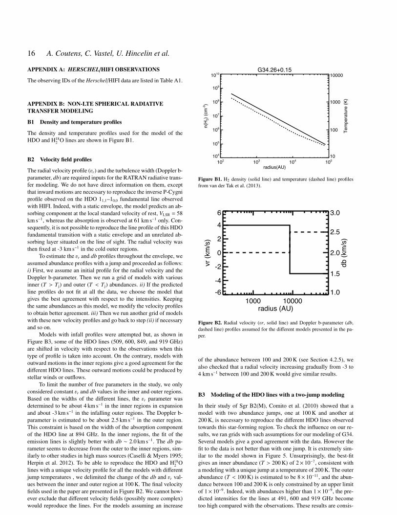
16 A. Coutens, C. Vastel, U. Hincelin et al.
APPENDIX A: HERSCHEL/HIFI OBSERVATIONS
The observing IDs of the Herschel/HIFI data are listed in Table A1.
APPENDIX B: NON-LTE SPHERICAL RADIATIVETRANSFER MODELING
B1 Density and temperature profiles
The density and temperature profiles used for the model of theHDO and H18
2 O lines are shown in Figure B1.
B2 Velocity field profiles
The radial velocity profile (3r) and the turbulence width (Doppler b-parameter, db) are required inputs for the RATRAN radiative trans-fer modeling. We do not have direct information on them, exceptthat inward motions are necessary to reproduce the inverse P-Cygniprofile observed on the HDO 11,1–10,0 fundamental line observedwith HIFI. Indeed, with a static envelope, the model predicts an ab-sorbing component at the local standard velocity of rest, VLSR = 58km s−1, whereas the absorption is observed at 61 km s−1 only. Con-sequently, it is not possible to reproduce the line profile of this HDOfundamental transition with a static envelope and an unrelated ab-sorbing layer situated on the line of sight. The radial velocity wasthen fixed at -3 km s−1 in the cold outer regions.
To estimate the 3r and db profiles throughout the envelope, weassumed abundance profiles with a jump and proceeded as follows:i) First, we assume an initial profile for the radial velocity and theDoppler b-parameter. Then we run a grid of models with variousinner (T > Tj) and outer (T < Tj) abundances. ii) If the predictedline profiles do not fit at all the data, we choose the model thatgives the best agreement with respect to the intensities. Keepingthe same abundances as this model, we modify the velocity profilesto obtain better agreement. iii) Then we run another grid of modelswith these new velocity profiles and go back to step (ii) if necessaryand so on.
Models with infall profiles were attempted but, as shown inFigure B3, some of the HDO lines (509, 600, 849, and 919 GHz)are shifted in velocity with respect to the observations when thistype of profile is taken into account. On the contrary, models withoutward motions in the inner regions give a good agreement for thedifferent HDO lines. These outward motions could be produced bystellar winds or outflows.
To limit the number of free parameters in the study, we onlyconsidered constant 3r and db values in the inner and outer regions.Based on the widths of the different lines, the 3r parameter wasdetermined to be about 4 km s−1 in the inner regions in expansionand about -3 km s−1 in the infalling outer regions. The Doppler b-parameter is estimated to be about 2.5 km s−1 in the outer region.This constraint is based on the width of the absorption componentof the HDO line at 894 GHz. In the inner regions, the fit of theemission lines is slightly better with db ∼ 2.0 km s−1. The db pa-rameter seems to decrease from the outer to the inner regions, sim-ilarly to other studies in high mass sources (Caselli & Myers 1995;Herpin et al. 2012). To be able to reproduce the HDO and H18
2 Olines with a unique velocity profile for all the models with differentjump temperatures , we delimited the change of the db and 3r val-ues between the inner and outer region at 100 K. The final velocityfields used in the paper are presented in Figure B2. We cannot how-ever exclude that different velocity fields (possibly more complex)would reproduce the lines. For the models assuming an increase
G34.26+0.15
102 103 104 105
radius(AU)
104
105
106
107
108
109
1010
n(H
2) (c
m-3)
10
100
1000
10000
Tem
pera
ture
(K)
Figure B1. H2 density (solid line) and temperature (dashed line) profilesfrom van der Tak et al. (2013).
1000 10000radius (AU)
-6-4
-2
0
2
46
vr (k
m/s
)
1.0
1.5
2.0
2.5
3.0
db (k
m/s
)
Figure B2. Radial velocity (3r, solid line) and Doppler b-parameter (db,dashed line) profiles assumed for the different models presented in the pa-per.
of the abundance between 100 and 200 K (see Section 4.2.5), wealso checked that a radial velocity increasing gradually from -3 to4 km s−1 between 100 and 200 K would give similar results.
B3 Modeling of the HDO lines with a two-jump modeling
In their study of Sgr B2(M), Comito et al. (2010) showed that amodel with two abundance jumps, one at 100 K and another at200 K, is necessary to reproduce the different HDO lines observedtowards this star-forming region. To check the influence on our re-sults, we ran grids with such assumptions for our modeling of G34.Several models give a good agreement with the data. However thefit to the data is not better than with one jump. It is extremely sim-ilar to the model shown in Figure 5. Unsurprisingly, the best-fitgives an inner abundance (T > 200 K) of 2× 10⁻⁷, consistent witha modeling with a unique jump at a temperature of 200 K. The outerabundance (T < 100 K) is estimated to be 8× 10⁻¹¹, and the abun-dance between 100 and 200 K is only constrained by an upper limitof 1× 10⁻⁹. Indeed, with abundances higher than 1× 10⁻⁹, the pre-dicted intensities for the lines at 491, 600 and 919 GHz becometoo high compared with the observations. These results are consis-
c© 0000 RAS, MNRAS 000, 000–000
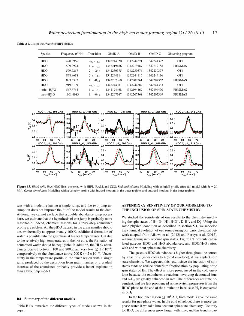
Water deuterium fractionation in the high-mass star-forming region G34.26+0.15 17
Table A1. List of the Herschel/HIFI obsIDs
Species Frequency (GHz) Transition ObsID-A ObsID-B ObsID-C Observing program
HDO 490.5966 20,2–11,1 1342244320 1342244321 1342244322 OT1HDO 509.2924 11,0–10,1 1342219186 1342219187 1342219188 PRISMASHDO 599.9267 21,1–20,2 1342230375 1342230376 1342230377 OT1HDO 848.9618 21,2–11,1 1342244114 1342244115 1342244116 OT1HDO 893.6387 11,1–00,0 1342207360 1342207361 1342207362 PRISMASHDO 919.3109 20,2–10,1 1342244381 1342244382 1342244383 OT1ortho–H18
2 O 547.6764 11,0–10,1 1342194468 1342194469 1342194470 PRISMASpara–H18
2 O 1101.6983 11,1–00,0 1342207367 1342207368 1342207369 PRISMAS
HDO 11,1-00,0 894 GHz
40 50 60 702.5
3.0
3.5
4.0
4.5
T mb (
K)
HDO 10,1-00,0 465 GHz
40 50 60 701.5
2.0
2.5
3.0
3.5
4.0HDO 11,0-11,1 81 GHz
40 50 60 70-0.2
0.0
0.2
0.4
0.6HDO 31,2-22,1 226 GHz
40 50 60 70-0.5
0.0
0.5
1.0
1.5
2.0HDO 21,1-21,2 242 GHz
40 50 60 70-0.5
0.0
0.5
1.0
1.5
2.0
HDO 20,2-11,1 491 GHz
40 50 60 70vLSR (km s-1)
-0.1
0.0
0.1
0.2
0.3
T mb (
K)
HDO 11,0-10,1 509 GHz
40 50 60 70vLSR (km s-1)
-0.1
0.0
0.1
0.2
0.3HDO 21,1-20,2 600 GHz
40 50 60 70vLSR (km s-1)
-0.1
0.0
0.1
0.2
0.3
0.4HDO 21,2-11,1 849 GHz
40 50 60 70vLSR (km s-1)
-0.1
0.0
0.1
0.2
0.3
0.4HDO 20,2-10,1 919 GHz
40 50 60 70vLSR (km s-1)
-0.1
0.0
0.1
0.2
0.3
0.4
Figure B3. Black solid line: HDO lines observed with HIFI, IRAM, and CSO. Red dashed line: Modeling with an infall profile (free-fall model with M = 20M�). Green dotted line: Modeling with a velocity profile with inward motions in the outer regions and outward motions in the inner regions.
tent with a modeling having a single jump, and the two-jump as-sumption does not improve the fit of the model results to the data.Although we cannot exclude that a double abundance jump occurshere, we estimate that the hypothesis of one jump is probably morereasonable. Indeed, chemical reasons for a three-step abundanceprofile are unclear. All the HDO trapped in the grain mantles shoulddesorb thermally at approximately 100 K. Additional formation ofwater is possible into the gas phase at higher temperatures. But dueto the relatively high temperatures in the hot core, the formation ofdeuterated water should be negligible. In addition, the HDO abun-dances derived between 100 and 200 K are very low (≤ 1× 10⁻⁹)comparatively to the abundance above 200 K (∼ 2× 10⁻⁷). Uncer-tainty in the temperature profile in the inner region with a singlejump produced by the desorption from grain mantles or a gradualincrease of the abundance probably provide a better explanationthan a two jump model.
B4 Summary of the different models
Table B1 summarizes the different types of models shown in thepaper.
APPENDIX C: SENSITIVITY OF OUR MODELING TOTHE INCLUSION OF SPIN-STATE CHEMISTRY
We studied the sensitivity of our results to the chemistry involv-ing the spin states of H2, D2, H+
3 , H2D+, D2H+, and D+3 . Using the
same physical condition as described in section 5.1, we modeledthe chemical evolution of our source using our basic chemical net-work adapted from Aikawa et al. (2012) and Furuya et al. (2012),without taking into account spin states. Figure C1 presents calcu-lated gaseous HDO and H2O abundances, and HDO/H2O ratios,with and without spin-state chemistry.
The gaseous HDO abundance is higher throughout the sourceby a factor 2 (inner core) to 4 (cold envelope), if we neglect spinstate chemistry. We expected this result since the inclusion of spinstates tends to reduce deuterium fractionation by populating orthospin states of H2. The effect is more pronounced in the cold enve-lope because the endothermic reactions involving deuterated ionsand o-H2 are greatly enhanced in rate. The differences are time de-pendent, and are less pronounced as the system progresses from theIRDC phase to the end of the simulation because o-H2 is convertedin p-H2.
In the hot inner region (≤ 104 AU) both models give the sameresults for gas-phase water. In the cold envelope, there is more gasphase water if we take into account spin-state chemistry. Contraryto HDO, the differences grow larger with time, and this trend is par-
c© 0000 RAS, MNRAS 000, 000–000
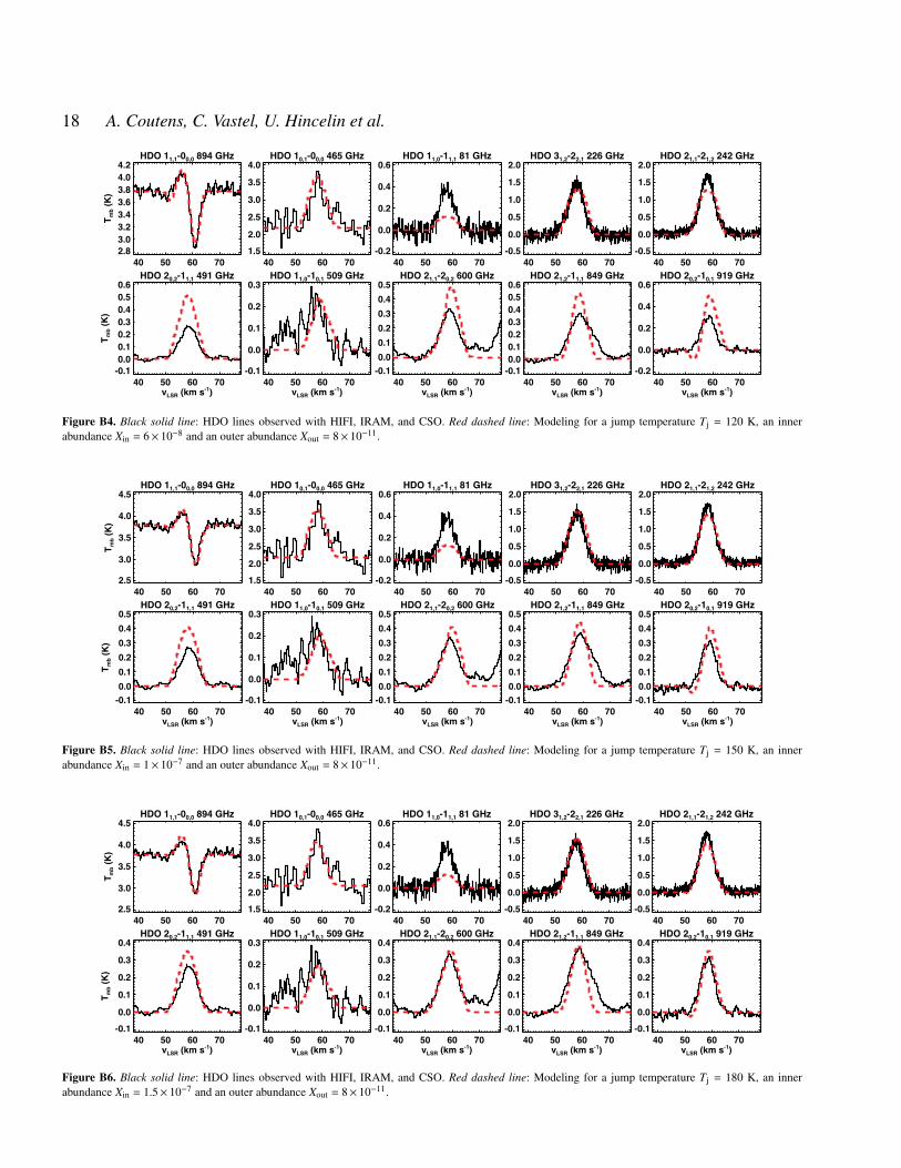
18 A. Coutens, C. Vastel, U. Hincelin et al.
HDO 11,1-00,0 894 GHz
40 50 60 702.83.03.23.43.63.84.04.2
T mb (
K)
HDO 10,1-00,0 465 GHz
40 50 60 701.5
2.0
2.5
3.0
3.5
4.0HDO 11,0-11,1 81 GHz
40 50 60 70-0.2
0.0
0.2
0.4
0.6HDO 31,2-22,1 226 GHz
40 50 60 70-0.5
0.0
0.5
1.0
1.5
2.0HDO 21,1-21,2 242 GHz
40 50 60 70-0.5
0.0
0.5
1.0
1.5
2.0
HDO 20,2-11,1 491 GHz
40 50 60 70vLSR (km s-1)
-0.10.00.10.20.30.40.50.6
T mb (
K)
HDO 11,0-10,1 509 GHz
40 50 60 70vLSR (km s-1)
-0.1
0.0
0.1
0.2
0.3HDO 21,1-20,2 600 GHz
40 50 60 70vLSR (km s-1)
-0.10.00.10.20.30.40.5
HDO 21,2-11,1 849 GHz
40 50 60 70vLSR (km s-1)
-0.10.00.10.20.30.40.50.6
HDO 20,2-10,1 919 GHz
40 50 60 70vLSR (km s-1)
-0.2
0.0
0.2
0.4
0.6
Figure B4. Black solid line: HDO lines observed with HIFI, IRAM, and CSO. Red dashed line: Modeling for a jump temperature Tj = 120 K, an innerabundance Xin = 6× 10⁻⁸ and an outer abundance Xout = 8× 10⁻¹¹.
HDO 11,1-00,0 894 GHz
40 50 60 702.5
3.0
3.5
4.0
4.5
T mb (
K)
HDO 10,1-00,0 465 GHz
40 50 60 701.52.0
2.5
3.0
3.5
4.0HDO 11,0-11,1 81 GHz
40 50 60 70-0.2
0.0
0.2
0.4
0.6HDO 31,2-22,1 226 GHz
40 50 60 70-0.50.0
0.5
1.0
1.5
2.0HDO 21,1-21,2 242 GHz
40 50 60 70-0.50.0
0.5
1.0
1.5
2.0
HDO 20,2-11,1 491 GHz
40 50 60 70vLSR (km s-1)
-0.10.00.10.20.30.40.5
T mb (
K)
HDO 11,0-10,1 509 GHz
40 50 60 70vLSR (km s-1)
-0.1
0.0
0.1
0.2
0.3HDO 21,1-20,2 600 GHz
40 50 60 70vLSR (km s-1)
-0.10.00.10.20.30.40.5
HDO 21,2-11,1 849 GHz
40 50 60 70vLSR (km s-1)
-0.10.00.10.20.30.40.5
HDO 20,2-10,1 919 GHz
40 50 60 70vLSR (km s-1)
-0.10.00.10.20.30.40.5
Figure B5. Black solid line: HDO lines observed with HIFI, IRAM, and CSO. Red dashed line: Modeling for a jump temperature Tj = 150 K, an innerabundance Xin = 1× 10⁻⁷ and an outer abundance Xout = 8× 10⁻¹¹.
HDO 11,1-00,0 894 GHz
40 50 60 702.5
3.0
3.5
4.0
4.5
T mb (
K)
HDO 10,1-00,0 465 GHz
40 50 60 701.52.0
2.5
3.0
3.5
4.0HDO 11,0-11,1 81 GHz
40 50 60 70-0.2
0.0
0.2
0.4
0.6HDO 31,2-22,1 226 GHz
40 50 60 70-0.50.0
0.5
1.0
1.5
2.0HDO 21,1-21,2 242 GHz
40 50 60 70-0.50.0
0.5
1.0
1.5
2.0
HDO 20,2-11,1 491 GHz
40 50 60 70vLSR (km s-1)
-0.10.0
0.1
0.2
0.3
0.4
T mb (
K)
HDO 11,0-10,1 509 GHz
40 50 60 70vLSR (km s-1)
-0.1
0.0
0.1
0.2
0.3HDO 21,1-20,2 600 GHz
40 50 60 70vLSR (km s-1)
-0.10.0
0.1
0.2
0.3
0.4HDO 21,2-11,1 849 GHz
40 50 60 70vLSR (km s-1)
-0.10.0
0.1
0.2
0.3
0.4HDO 20,2-10,1 919 GHz
40 50 60 70vLSR (km s-1)
-0.10.0
0.1
0.2
0.3
0.4
Figure B6. Black solid line: HDO lines observed with HIFI, IRAM, and CSO. Red dashed line: Modeling for a jump temperature Tj = 180 K, an innerabundance Xin = 1.5× 10⁻⁷ and an outer abundance Xout = 8× 10⁻¹¹.
c© 0000 RAS, MNRAS 000, 000–000
Water deuterium fractionation in the high-mass star-forming region G34.26+0.15 19
Table B1. List of the models presented in the paper.
Model Abundance profile Sections & Figures
1 1 jump Tj = 100 K HDO : Sect. 4.2.2, Fig. 4
2 1 jump Tj = 120 K HDO : Sect. 4.2.2, Fig. B4
3 1 jump Tj = 150 K HDO : Sect. 4.2.2, Fig. B5H18
2 O : Sect. 4.2.3, Fig. B8
4 1 jump Tj = 180 K HDO : Sect. 4.2.2, Fig. B6H18
2 O : Sect. 4.2.3, Fig. B9
5 1 jump Tj = 200 K HDO : Sect. 4.2.2, Fig. 5H18
2 O : Sect. 4.2.3, Fig. 6
5 1 jump Tj = 220 K HDO : Sect. 4.2.2, Fig. B7H18
2 O : Sect. 4.2.3, Fig. B10
6 2 jumps Tj1 = 100 K, Tj2 = 200 K HDO : Appx. B3
7 Constant inner abundance (T ≥ 200 K) and HDO : Sect. 4.2.4, Fig. 8decrease of the outer abundance from the H18
2 O : Sect. 4.2.4, Fig. 9cold to the warm regions (see Fig. 7)
8 Constant inner abundance, gradual HDO : Sect. 4.2.5, Fig. 8increase of the abundance at the transition H18
2 O : Sect. 4.2.5, Fig. 9hot core/cold envelope (100–200 K) and decreaseof the outer abundance from the cold regionsto the regions at 100 K (see Fig. 7)
HDO 11,1-00,0 894 GHz
40 50 60 702.5
3.0
3.5
4.0
4.5
T mb (
K)
HDO 10,1-00,0 465 GHz
40 50 60 701.52.0
2.5
3.0
3.5
4.0HDO 11,0-11,1 81 GHz
40 50 60 70-0.2
0.0
0.2
0.4
0.6HDO 31,2-22,1 226 GHz
40 50 60 70-0.50.0
0.5
1.0
1.5
2.0HDO 21,1-21,2 242 GHz
40 50 60 70-0.50.0
0.5
1.0
1.5
2.0
HDO 20,2-11,1 491 GHz
40 50 60 70vLSR (km s-1)
-0.1
0.0
0.1
0.2
0.3
T mb (
K)
HDO 11,0-10,1 509 GHz
40 50 60 70vLSR (km s-1)
-0.1
0.0
0.1
0.2
0.3HDO 21,1-20,2 600 GHz
40 50 60 70vLSR (km s-1)
-0.10.0
0.1
0.2
0.3
0.4HDO 21,2-11,1 849 GHz
40 50 60 70vLSR (km s-1)
-0.10.0
0.1
0.2
0.3
0.4HDO 20,2-10,1 919 GHz
40 50 60 70vLSR (km s-1)
-0.10.0
0.1
0.2
0.3
0.4
Figure B7. Black solid line: HDO lines observed with HIFI, IRAM, and CSO. Red dashed line: Modeling for a jump temperature Tj = 220 K, an innerabundance Xin = 3× 10⁻⁷ and an outer abundance Xout = 8× 10⁻¹¹.
p-H218O 31,3-22,0 203 GHz
40 50 60 70vLSR (km s-1)
-0.5
0.0
0.5
1.0
1.5
2.0
T mb (
K)
p-H218O 11,1-00,0 1102 GHz
40 50 60 70vLSR (km s-1)
4.5
5.0
5.5
6.0
6.5o-H2
18O 11,0-10,1 548 GHz
40 50 60 70vLSR (km s-1)
0.80.91.01.11.21.31.4
Figure B8. Black solid line: H182 O lines observed with HIFI and IRAM. Red dashed line: Modeling for a jump temperature Tj = 150 K, an inner abundance
Xin = 4× 10⁻⁷ and an outer abundance Xout = 1.3× 10⁻¹⁰.
c© 0000 RAS, MNRAS 000, 000–000
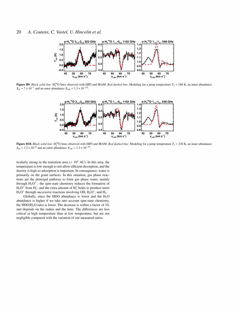
20 A. Coutens, C. Vastel, U. Hincelin et al.
p-H218O 31,3-22,0 203 GHz
40 50 60 70vLSR (km s-1)
-0.5
0.0
0.5
1.0
1.5
2.0
T mb (
K)
p-H218O 11,1-00,0 1102 GHz
40 50 60 70vLSR (km s-1)
4.5
5.0
5.5
6.0
6.5o-H2
18O 11,0-10,1 548 GHz
40 50 60 70vLSR (km s-1)
0.80.91.01.11.21.31.4
Figure B9. Black solid line: H182 O lines observed with HIFI and IRAM. Red dashed line: Modeling for a jump temperature Tj = 180 K, an inner abundance
Xin = 7× 10⁻⁷ and an outer abundance Xout = 1.3× 10⁻¹⁰.
p-H218O 31,3-22,0 203 GHz
40 50 60 70vLSR (km s-1)
-0.5
0.0
0.5
1.0
1.5
2.0
T mb (
K)
p-H218O 11,1-00,0 1102 GHz
40 50 60 70vLSR (km s-1)
4.5
5.0
5.5
6.0
6.5o-H2
18O 11,0-10,1 548 GHz
40 50 60 70vLSR (km s-1)
0.80.91.01.11.21.31.4
Figure B10. Black solid line: H182 O lines observed with HIFI and IRAM. Red dashed line: Modeling for a jump temperature Tj = 220 K, an inner abundance
Xin = 1.2× 10⁻⁶ and an outer abundance Xout = 1.3× 10⁻¹⁰.
ticularly strong in the transition area (' 104 AU). In this area, thetemperature is low enough to not allow efficient desorption, and thedensity is high so adsorption is important. In consequence, water isprimarily on the grain surfaces. In this situation, gas phase reac-tions are the principal pathway to form gas phase water, mainlythrough H3O+ : the spin-state chemistry reduces the formation ofH2D+ from H+
3 , and the extra amount of H+3 helps to produce more
H3O+ through successive reactions involving OH, H2O+, and H2.Globally, since the HDO abundance is lower and the H2O
abundance is higher if we take into account spin-state chemistry,the HDO/H2O ratio is lower. The decrease is within a factor of 10,and depends on the radius and the time. The differences are lesscritical at high temperature than at low temperature, but are notnegligible compared with the variation of our measured ratios.
c© 0000 RAS, MNRAS 000, 000–000
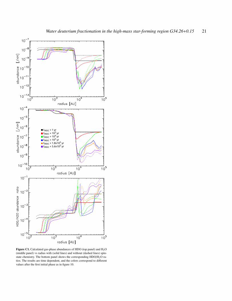
Water deuterium fractionation in the high-mass star-forming region G34.26+0.15 21
tIRDC + 1 yrtIRDC + 103 yrtIRDC + 104 yrtIRDC + 105 yrtIRDC + 1.8x10⁵ yrtIRDC + 5.6x10⁵ yr
Figure C1. Calculated gas-phase abundances of HDO (top panel) and H2O(middle panel) vs radius with (solid lines) and without (dashed lines) spin-state chemistry. The bottom panel shows the corresponding HDO/H2O ra-tios. The results are time dependent, and the colors correspond to differentvalues after the first initial phase as in figure 10.
c© 0000 RAS, MNRAS 000, 000–000