The data processing pipeline for the Herschel/SPIRE Imaging Fourier Transform Spectrometer

Trevor R. Fultona*, David A. Naylorb, Jean-Paul Baluteauc, Matt Griffind, Peter Davis-Imhofa, Bruce

M. Swinyarde, Tanya L. Lime, Christian Suracec, Dave Clementsf, Pasquale Panuzzog, Rene Gastaudg, Edward Polehamptonb,e, Steve Gueste, Nanyao Luh, Arnold Schwartzh, Kevin Xuh

aBlue Sky Spectroscopy Inc., 403 - 740 4 Avenue South, Lethbridge, T1J 0N9, Canada;

bDepartment of Physics, University of Lethbridge, Lethbridge, Canada, T1K 3M4; cLaboratoire d'Astrophysique de Marseille, Marseille, France, 13388;

dSchool of Physics and Astronomy, Cardiff University, Cardiff, United Kingdom, CF24 3AA; eSpace Science and Technology Department, Rutherford Appleton Laboratory, Didcot, United

Kingdom, OX11 0QX; fAstrophysics Group, Imperial College, London, United Kingdom, SW7 2AZ;

gLaboratoire AIM, CEA-Saclay, France, 91191; hInfrared Processing and Analysis Center, California Institute of Technology, Pasadena, USA, 91125

ABSTRACT

We present the data processing pipeline to generate calibrated data products from the Spectral and Photometric Imaging Receiver (SPIRE) imaging Fourier Transform Spectrometer. The pipeline processes telemetry from SPIRE point source, jiggle- and raster-map observations, producing calibrated spectra in low-, medium-, high-, and mixed low- and high-resolution modes. The spectrometer pipeline shares some elements with the SPIRE photometer pipeline, including the conversion of telemetry packets into data timelines and the calculation of bolometer voltages from the raw telemetry. We present the following fundamental processing steps unique to the spectrometer: temporal and spatial interpolation of the stage mechanism and detector data to create interferograms; apodization; Fourier transform, and creation of a hyperspectral data cube. We also describe the corrections for various instrumental effects including first- and second-level glitch identification and removal, correction of the effects due to the Herschel primary mirror and the spectrometer calibrator, interferogram baseline correction, channel fringe correction, temporal and spatial phase correction, non-linear response of the bolometers, variation of instrument performance across the focal plane arrays, and variation of spectral efficiency. Astronomical calibration is based on combinations of observations of standard astronomical sources and regions of space known to contain minimal emission.

Keywords: Herschel, SPIRE, Imaging Fourier transform spectroscopy, Data processing, Pipeline

1. INTRODUCTION The data processing pipeline for the Spectral and Photometric Imaging Receiver[1],[2] (SPIRE) Fourier Transform spectrometer (FTS) contains processing modules commonly used to process FTS data, such as phase correction and the Fourier transform. The SPIRE FTS pipeline also contains processing steps unique to SPIRE, such as the correction for the Herschel Telescope and Spectrometer Calibrator (SCAL).

The SPIRE FTS pipeline has been designed to be consistent with the astronomical observation templates[3] (AOTs) that are available to the users of the SPIRE spectrometer. The final data products generated by the Spectrometer pipelines will in all cases consist of hyperspectral data; two spatial dimensions representing the astronomical region under study and one spectral dimension. The degree to which the hyperspectral data product is sampled both spatially and spectrally depends on the type of observation chosen.

*Email: trevor.fulton@blueskyinc.ca; Telephone: (403) 317-1273; Fax: (403) 317-1273; www.blueskyinc.ca

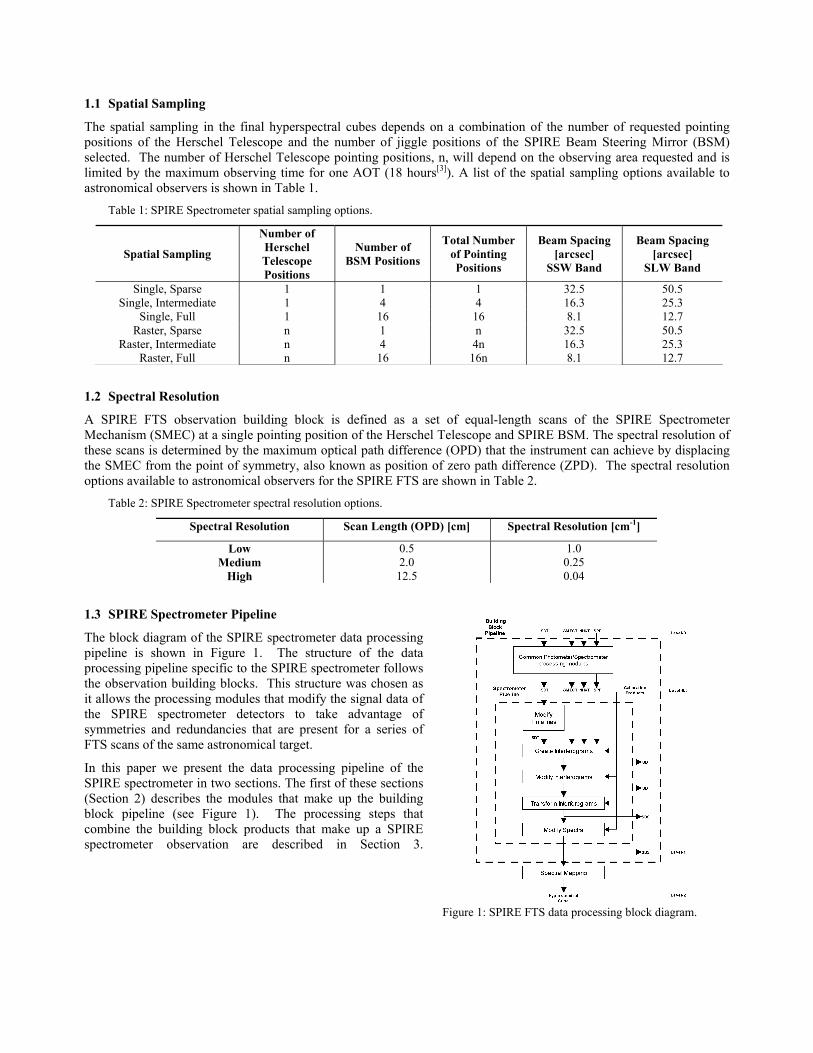
1.1 Spatial Sampling

The spatial sampling in the final hyperspectral cubes depends on a combination of the number of requested pointing positions of the Herschel Telescope and the number of jiggle positions of the SPIRE Beam Steering Mirror (BSM) selected. The number of Herschel Telescope pointing positions, n, will depend on the observing area requested and is limited by the maximum observing time for one AOT (18 hours[3]). A list of the spatial sampling options available to astronomical observers is shown in Table 1.

Table 1: SPIRE Spectrometer spatial sampling options.

Spatial Sampling

Number of Herschel Telescope Positions

Number of BSM Positions

Total Number of Pointing Positions

Beam Spacing [arcsec]

SSW Band

Beam Spacing [arcsec]

SLW Band

Single, Sparse 1 1 1 32.5 50.5 Single, Intermediate 1 4 4 16.3 25.3

Single, Full 1 16 16 8.1 12.7 Raster, Sparse n 1 n 32.5 50.5

Raster, Intermediate n 4 4n 16.3 25.3 Raster, Full n 16 16n 8.1 12.7

1.2 Spectral Resolution

A SPIRE FTS observation building block is defined as a set of equal-length scans of the SPIRE Spectrometer Mechanism (SMEC) at a single pointing position of the Herschel Telescope and SPIRE BSM. The spectral resolution of these scans is determined by the maximum optical path difference (OPD) that the instrument can achieve by displacing the SMEC from the point of symmetry, also known as position of zero path difference (ZPD). The spectral resolution options available to astronomical observers for the SPIRE FTS are shown in Table 2.

Table 2: SPIRE Spectrometer spectral resolution options.

Spectral Resolution Scan Length (OPD) [cm] Spectral Resolution [cm-1]

Low 0.5 1.0 Medium 2.0 0.25

High 12.5 0.04

1.3 SPIRE Spectrometer Pipeline

Figure 1: SPIRE FTS data processing block diagram.

The block diagram of the SPIRE spectrometer data processing pipeline is shown in Figure 1. The structure of the data processing pipeline specific to the SPIRE spectrometer follows the observation building blocks. This structure was chosen as it allows the processing modules that modify the signal data of the SPIRE spectrometer detectors to take advantage of symmetries and redundancies that are present for a series of FTS scans of the same astronomical target.

In this paper we present the data processing pipeline of the SPIRE spectrometer in two sections. The first of these sections (Section 2) describes the modules that make up the building block pipeline (see Figure 1). The processing steps that combine the building block products that make up a SPIRE spectrometer observation are described in Section 3.

2. SPIRE SPECTROMETER BUILDING BLOCK PIPELINE The SPIRE spectrometer data processing pipeline described here operates on one observation building block. The building block pipeline consists of six major processing groups (see Figure 1).

1. Common Photometer/Spectrometer Processing modules. These processing steps are common to both the SPIRE spectrometer and photometer pipelines[4].

2. Modify Timelines. These processing modules perform operations on detector signals that are time-dependent. The descriptions of the modules in this category are presented in Section 2.1.

3. Create Interferograms. This processing step merges the timelines of the spectrometer detectors and spectrometer mechanism into interferograms. This step produces a Level-0.5 Spectrometer Detector Interferogram product and is described in Section 2.2.

4. Modify Interferograms. The processing modules in this group perform operations on the spectrometer detector interferograms. These operations differ from those in the "Modify Timelines" group in that they are designed to act on signals that are a function of mirror position rather than signals that are a function of sample time. These processing modules are described in Section 2.3.

5. Transform Interferograms. This processing step transforms the interferograms into a set of spectra. This step produces a Level-0.5 Spectrometer Detector Spectrum product and is detailed in Section 2.4.

6. Modify Spectra. The processing modules in this group perform operations on spectra. The steps in this category combine to produce a Level-1 Spectrometer Detector Spectrum product and are described in Section 2.5.

2.1 Detector Timeline Modifications

After application of the processing steps common to both the photometer and spectrometer detectors[4], the raw samples for each one of the 66 spectrometer detectors, labeled i, will have been converted into RMS voltage timelines, VRMS-i(t). These quantities are contained in the Level 0.5 Spectrometer Detector Timeline Product (SDT).

The processing modules described in the following sections are applied to the timelines for each spectrometer detector. Each of the processing steps contained in this processing block (see Figure 2) accepts a Level-0.5 SDT product as input and delivers an SDT product as output.

Figure 2: Timeline modification section of the SPIRE Spectrometer building block pipeline.

2.1.1 First level deglitching

Glitches due to cosmic ray hits or other events in the detectors will be removed using an algorithm based on a wavelet-based local regularity analysis[5]. This process is composed of two steps: the first step detects glitch signatures over the measured signal; the second step locally reconstructs a signal free of such glitch signatures.

1. Glitch Identification. Glitches are detected in the input SDT product by continuous wavelet analysis and a subsequent analysis of the modulus maxima lines, assuming that the glitch signature is similar to the signature of a Dirac delta function.

2. Glitch Removal. Each glitch flagged by the preceding step contains localized wavelet coefficients specific to the glitch. These coefficients are removed and a local, inverse wavelet transform is performed to create an SDT product that is free of glitches.

The output of this module is the deglitched voltage timeline, V1-i(t) for detector i.

2.1.2 Electrical Crosstalk

The detector timelines may contain contributions that depend on the signals from other detectors due to electrical crosstalk. Electrical crosstalk is removed from the SPIRE spectrometer detector timelines by multiplication of a crosstalk matrix in a manner equivalent to that for the SPIRE photometer detectors[4].

2.1.3 Time Domain Phase Correction

The SPIRE spectrometer detector chain contains a 6-pole Bessel low pass filter (LPF) as well as single-pole RC LPF[6]. In addition to the electronic LPFs, the thermal behavior of the SPIRE bolometers can be modeled as a simple RC LPF with a detector-specific time constant, τ.

These two effects may be combined into a single detector transfer function:

)()()( ωωω iThermaliLPFiTotal HHH −−− ×= . (1)

The overall transfer function shown above will affect both the magnitude and the phase of the signal recorded by the SPIRE detectors. The phase imparted onto the detectors is given by:

( )( )⎥⎦

⎤⎢⎣

⎡=

−

−−− )(Re

)(Imtan)(1

11

ωωωφ

Total

TotaliTotal H

H. (2)

The phase shown above manifests itself, to first order, as a time delay of the recorded signal. This effect is particularly problematic for the scanning mode of the SPIRE spectrometer, where the delay induced by the electronic and thermal phase can lead to errors in the interpolation of the detector signals (see Section 2.1.1).

The phase per detector is characterized and its negative is used to derive the time domain phase correction function (PCF) given by,

[ ])(1 1)( ωφ −−−= Totalii eFTtPCF . (3)

The measured detector timelines are corrected by a convolution with the derived PCF,

)()()( 134 tPCFtVtV ii ⊗= −− . (4)

2.1.4 Detector non-linearity

Even though bolometric detectors are commonly fabricated with highly linear response characteristics, the detectors of the SPIRE spectrometer will be subject to a wide dynamic range which makes a non-linear response likely. A dedicated non-linearity correction is designed to account for changes in the response of the detectors to strong signals. The form of this correction will be a function that is dependent on the amplitude of the recorded signal as follows:

dVVfVftV

V

V ri ∫

−

=−

14

0)()()(5 . (5)

where f(V), the real detector responsivity, Vr is a reference voltage, and V0 is a fixed bolometer voltage. The normalized value of f(V) is derived as:

3

21)(

)(KV

KKVfVf

r −+= . (6)

The values for V0, K1, K2, and K3 (and their uncertainties) for each detector will be stored in calibration tables. Distinct calibration tables will be used for each detector bias configuration and for each value of V0 and Vr. Initially, the quantities in these calibration tables will be based on model predictions.

2.1.5 Bath Temperature Drift

To first order, bath temperature fluctuations will influence, coherently, all detectors in an array; the temperature and corresponding output voltages will vary in synchronism. A set of timelines, Vth-i(t), is generated to correct for this coherent drift.

Each of the two detector arrays of the SPIRE spectrometer contains several bolometers dedicated to measuring the temperature of the detector array. These thermometers are used to create a correction timeline for each detector, Vth-i(t). This timeline is then subtracted from that detector's signal timeline, V5-i(t).

The output of this module is a set of spectrometer detector voltage timelines corrected for correlated low-frequency thermal drifts.

2.2 Interferogram Creation

The pipeline modules listed to this point describe the operations on the Level 0.5 timelines of the spectrometer detectors. Three additional Level 0.5 timelines are required for the next step in the common spectrometer data processing pipeline. These are: the Spectrometer Mechanism timeline product (SMECT); the Nominal Housekeeping timeline product (NHKT); and the SPIRE Pointing timeline product (SPP) (see Figure 1).

2.2.1 Interferogram Creation

A Fourier transform spectrometer measures interferograms, i.e. detector signals as a function of OPD. In the case of the SPIRE FTS, the sampling of the SPIRE spectrometer detectors and the spectrometer mechanism is decoupled; the two subsystems are sampled at different rates and at different times. A step is required that links the timelines of the Spectrometer Mechanism with the Spectrometer Detector timelines. In addition, the SMEC positions to which the spectrometer detector signal samples are to be linked should be regularly spaced in terms of OPD in order to ensure accurate transformation of the interferogram with the Discrete Fourier Transform. The interferogram creation module of the SPIRE spectrometer pipeline performs these tasks in two steps: interpolation of the SMEC timeline; and merging of the Spectrometer Detector and SMEC timelines.

1. Interpolation of the SMEC timeline. This step converts the spectrometer mechanism timeline from one that is non-uniform in position to one that is uniform in position.

Establish a common OPD position vector. This step creates a common vector of OPD positions that will be the basis of the interferograms for all of the spectrometer detectors and for all of the scans in the building block. This common position vector contains samples that are uniformly spaced in terms of OPD position and a sample at the position of ZPD.

The step size of the common OPD vector is chosen to match the sampling rate of the spectrometer detector signal samples. For an SDT sampling rate s [Hz] and a SMEC scanning speed vSMEC [cm/s MPD], the position step size, ΔMPD, in units of cm; is given by:

svMPD SMEC=Δ . (7)

This step is then converted such that it is in terms of OPD by the following relation,

[ ]MPDFLOOROPD Δ=Δ 4 , (8)

where FLOOR[] denotes that the step size is rounded down to the nearest integer in units of μm OPD and the factor of four is the nominal conversion between MPD and OPD for a Mach-Zehnder FTS.

Map the common OPD position vector to a SMEC position vector for each spectrometer detector. This step maps, for each spectrometer detector, the common OPD positions, established in the preceding step, onto physical positions in units of mechanical path difference. This step involves: a scaling factor, f, that takes into account the step size for a Mach-Zehnder FTS; and a shifting factor, ZPD, which establishes the position of zero optical path difference. In order to take into account variations due to slight misalignments of the interferometer components, each of these quantities are unique to each spectrometer detector, i,

ii

i ZPDf

OPDMPD += . (9)

Parse the measured SMEC timeline into discrete scans. The full SMEC timeline, z(tSMEC) is split into a series of discrete timelines, zn(tSMEC). Each of the discrete timelines, zn(tSMEC), represents one spectrometer scan. The delineation of the SMEC timeline is accomplished by comparing consecutive SMEC position samples and finding those samples where the motion of mirror mechanism changes direction.

Interpolate the measured SMEC timelines onto the mapped SMEC timelines. On a detector-by-detector and scan-by-scan basis, the sample times when the spectrometer mechanism reached the mapped SMEC positions are determined through cubic spline interpolation. Since, for each detector, there is a 1:1 relationship between the mapped SMEC positions and the regularly spaced OPD positions, this step effectively determines the times when the SMEC reached the regularly spaced OPD positions for each detector,

. (10) )()( iMPDinSMECn tMPDtz −−→

2. Merge the spectrometer detector and the mapped SMEC timelines. This step combines the signal samples from the timeline of a given spectrometer detector, V5-i(ti), with the mapped SMEC timelines.

Interpolation of the spectrometer detector timelines. The spectrometer detector signal samples are mapped onto the times corresponding to the regular MPD positions, tMPD-i, by way of cubic spline interpolation. Since there is a 1:1 relationship between these time samples, tMPD-i, and the regular MPD positions, MPDi, this interpolation effectively maps, for each detector, the signal samples to the regularly spaced MPD positions. Moreover, since there is a 1:1 relationship between the regular MPD positions for each detector and the common OPD positions, this step accomplishes the mapping of the signal samples for each detector to the common OPD positions, which is the desired, equidistantly sampled interferogram,

)()()()()( 66665 xVOPDVtVtVtV iiOPDiiMPDiii −−−−−− ≡→→→ . (11)

The process outlined above is repeated for all spectrometer detectors for each scan of the observation building block. In addition, the mean value of the pointing, P(t), as derived from the input SPP for the observation building block is assigned to the output SDI product.

The data product that results from this processing step is a Level-0.5 Spectrometer Detector Interferogram (SDI) product that will be made available to observers.

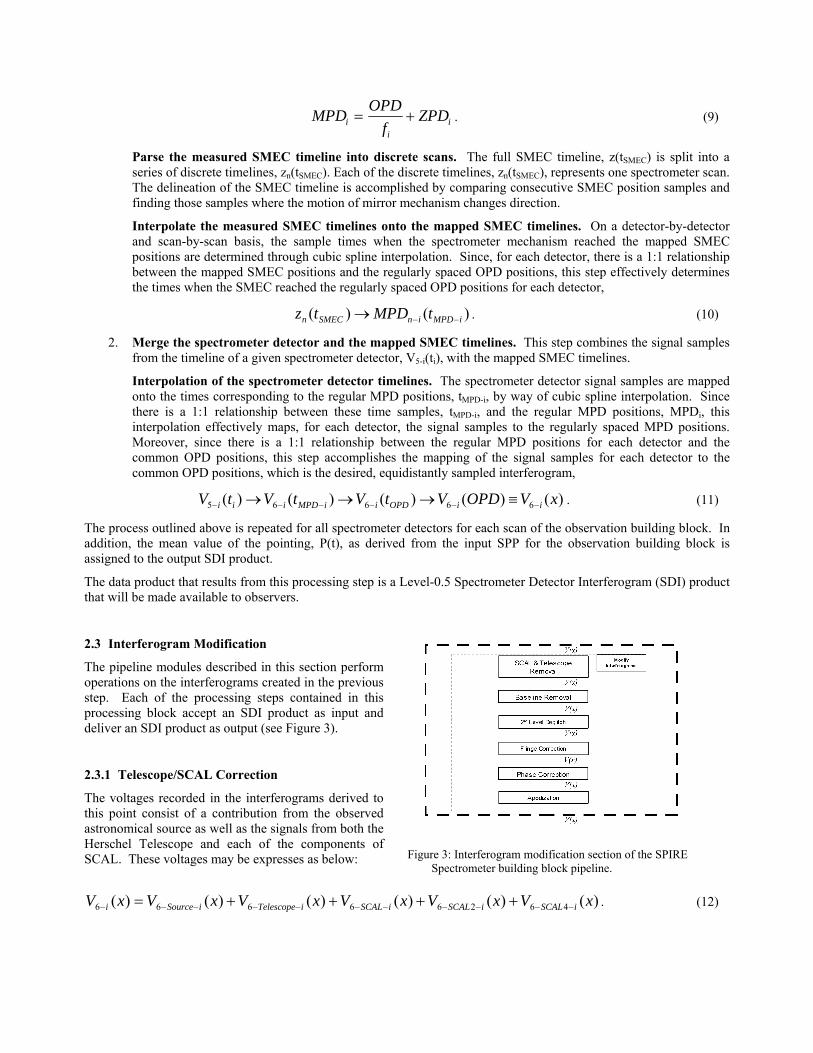
2.3 Interferogram Modification

The pipeline modules described in this section perform operations on the interferograms created in the previous step. Each of the processing steps contained in this processing block accept an SDI product as input and deliver an SDI product as output (see Figure 3).

2.3.1 Telescope/SCAL Correction

The voltages recorded in the interferograms derived to this point consist of a contribution from the observed astronomical source as well as the signals from both the Herschel Telescope and each of the components of SCAL. These voltages may be expresses as below:

)()()()()()( 46266666 xVxVxVxVxVxV iSCALiSCALiSCALiTelescopeiSourcei −−−−−−−−−−− ++++= . (12)

Figure 3: Interferogram modification section of the SPIRE Spectrometer building block pipeline.

A calibration observation will be performed by observing a region of space known to have little emission as the target source. The Herschel Telescope and SCAL components in the calibration observation will be maintained at the same temperatures as is the case for the on-source observation. The reference Level-0.5 interferograms, V6-ref-i(x), derived from the calibration observation may be expressed as below:

)()()()()( 4626666 xVxVxVxVxV irefSCALirefSCALirefSCALirefTelescopeiref −−−−−−−−−−−−−− +++= . (13)

The contributions from the Herschel Telescope and the SCAL components are removed from the input detector timelines by subtraction of the reference interferograms,

)(

)()()(

6

667

xV

xVxVxV

iSource

irefii

−−

−−−−

=

+=. (14)

2.3.2 Baseline Correction

Even after the removal of correlated drifts (see Section 2.1.5) the measured interferograms may still display a varying baseline due to perturbations which did not occur uniformly across the detector array. The baseline correction algorithm evaluates and removes, on a detector-by-detector and scan-by-scan basis, the offset portion of the measured interferograms, V7-i(x). The baseline of each interferogram is characterized by a fourth-order polynomial fit,

. (15) 432)( xexdxcxbaxV iiiiiiBaseline ++++=−

The fitted baseline polynomial is then subtracted from the input interferogram to derive the corrected interferogram,

)()()( 78 xVxVxV iBaselineii −−− −= . (16)

2.3.3 Second level deglitching

Repeated FTS measurements of the same astronomical source should not deviate from one another beyond random noise. This principle is be used to identify and remove glitches without having to make any assumptions about the shape of the glitches. Glitches are identified for each spectrometer detector by comparing, on an OPD-position-by-OPD-position basis, the samples from one scan to those from all other scans in the same building block. The samples that deviate more than a prescribed amount from the median are flagged as glitches.

The samples that are identified as glitches are then replaced. The value of the replacement sample for a glitch identified at a given position for a given spectrometer detector is determined by the average of the samples from the other observed interferograms at that position,

∑≠=

−−−− −=

ScansN

jnnkn

Scanskij xV

NxV

,1189 )(

11)( . (17)

This deglitching method relies on a statistical analysis of the measured interferograms and requires at least six interferograms (three forward and three reverse spectrometer scans) per building block.

2.3.4 Channel Fringe Correction

The SPIRE spectrometer suffers from channel fringes which are due to resonant cavities set up by the detector unit and a filter and lens assembly in front of the detector feedhorns. The effect of channel fringes on spectrometer data is similar to that of glitches[7] (Section 2.1.1, Section 2.3.3). If left uncorrected the channel fringes will contaminate the measured spectrum with unwanted artifacts. The current baseline-method of channel fringe removal is to multiply the interferograms with an apodization function (Section 2.3.6).

While apodization is effective at reducing at least some of the spectral artifacts due to the channel fringes, its application will result in a reduction of the spectral resolution. Given that the fringe features appear at the extreme high-resolution OPD end for the Spectrometer Long Wavelength (SLW) array and at the extreme medium-resolution OPD end for the Spectrometer Short Wavelength (SSW) array, however, the reduced resolution is expected to be acceptable for those cases.

2.3.5 Phase Correction

The phase correction module is separated into two components: the first step identifies any phase present in the input interferograms; the second step corrects the input interferograms by removing this phase.

1. Phase Identification. In order to determine the amount of phase present in the input interferograms, a spectrum is first derived from that portion of the measured interferogram that is sampled symmetrically about the position of ZPD,

, (18) [ ] dxexVxVFTBL

L

xii

LLiDSi ∫

−

−−−−−− == πσσ 2

101010 )()()(

where L represents the extent of the interferogram about the ZPD position. The phase for each spectral component is computed from the measured spectrum as:

( )( )⎥⎦

⎤⎢⎣

⎡=

−−

−−−−− )(Re

)(Imtan)(

10

10110 σ

σσϕ

DSi

DSiDSi B

B. (19)

2. Phase Removal. After the characterization of the phase from the double-sided portion of the measured interferograms, the next step in the process is phase removal. A fourth-order polynomial is fitted to the measured in-band phase,

High

Lowiiiiiifit edcba

σ

σσσσσσϕ 432)( ++++=− . (20)

Using the fitted phase rather than the calculated phase will keep the noise associated with the imaginary portion of the computed spectrum in the imaginary domain. If the phase is stable and the noise is due primarily to random sources, using a fitting function can lead to an increase in the resultant signal-to-noise ratio by a factor of √2.

A phase correction function (PCF) is then derived from the fitted phase for each interferogram as:

. (21) )()( σϕσ ifitii ePCF −−=

The derived PCFs for each scan for each spectrometer detector are then applied to spectra computed from each of the interferograms in the input SDI product by way of multiplication,

)()()( 1011 σσσ iii PCFBB ×= −− . (22)

If the observing mode is low- or medium-resolution, the above represents the final step in the phase correction process; high-resolution observations require an additional step. In that case, a convolution of the measured interferogram with the inverse FT of the PCF is performed,

[ ])()()( 11011 σiii PCFFTxVxV −−− ⊗= . (23)

2.3.6 Apodization

The natural instrument line shape (ILS) for a Fourier Transform spectrometer is a cardinal sine, or Sinc function. If the source signal contains features at or near the resolution of the spectrometer, the ILS can introduce secondary maxima in the spectra. The apodization functions available within this module may be used to reduce these secondary maxima at the cost of reducing the resolution of the resultant spectrum. The apodization module in the SPIRE spectrometer data processing pipeline offers a number of apodizing functions that to allow for an optimal trade-off between reduction in the secondary maxima and reduced resolution[8].

Apodization is performed by multiplying the input interferograms, Vn-11-i(x), on a detector-by-detector and on a scan-by-scan basis with a tapering or apodizing function,

)()()( 1112 xApodxVxV iii ×= −− . (24)

2.4 Spectrum Creation

At this point in the spectrometer pipeline, the interferograms have been subject to comprehensive corrections. The Fourier transform is now applied to the interferograms for each detector, Vn-m-i(x), into spectra, Bn-m-i(σ), and further corrections take place in the spectral domain.

2.4.1 Fourier Transform

The Fourier Transform module transforms the set of corrected interferograms into a set of spectra.

Double-sided Transform. The low- and medium-resolution AOTs[3] lead to double-sided interferograms. In these cases, each interferogram in the SDI is examined and the entire recorded interferogram is used to compute the resultant spectrum.

[ ] ∫−

−−−−− ==

L

L

xii

L

Lii dxexVxVFTB πσσ 2121212 )()()( . (25)

The Discrete Fourier transform that is used to compute the spectral components takes the form shown below:

∑−

=

−

−− =1

0

2

1212 )()(N

n

Nkni

ii enVkBπ

. (26)

Single-sided Transform. The high-resolution AOT[3] leads to single-sided interferograms, whose samples are asymmetric with respect to the position of ZPD. The spectra computed from the high-resolution observations are derived from the interferogram samples whose positions are greater than or equal to the position of ZPD,

[ ] ∫ −−− ==L

iL

ii dxxxVxVFTB0

1201212 )2cos()()()( πσσ . (27)

The Discrete Fourier transform that is used to compute the spectral components for single-sided interferograms takes the following form:

∑−

=−− ⎟

⎠⎞

⎜⎝⎛=

1

01212

2cos)()(N

nii N

knnVkB π. (28)

Wavenumber Grid. In the case of both the single-sided and double-sided transforms the wavenumber grid onto which the spectrum is registered is calculated from the interferogram sampling rate (ΔOPD) and the maximum OPD, L.

The Nyquist frequency (σNyquist), the maximum independent frequency in the output spectrum, is given by:

OPDNyquist 2

1=σ . (29)

The spacing between independent spectral samples (Δσ) is given by:

L2

1=Δσ . (30)

Interferogram Padding. The spacing between spectral samples can be modified by padding the interferogram with zeros. This procedure allows for an easier comparison of the spectra derived from observations at different spectral resolutions. In this case, a zero-padded interferogram, V12-ZP-i, is given by:

ZPL

L

LiiZP xVxV 0,)()(

01212 −−− = . (31)

The corresponding spectral sampling interval is given by:

ZP

ZP L21

=Δσ , (32)

and the resultant spectrum of the zero-padded interferogram is given by:

∑−

=

−

−−−− =1

0

2

1212 )()(ZP

ZP

N

n

Nkni

iZPiZP enVkBπ

. (33)

The SPIRE spectrometer AOTs[3] provide three spectral resolution options to astronomical observers. The lengths to which the interferograms are padded and the resultant spectral sampling intervals for each of the options are shown in Table 3.

Table 3: Spectral sampling intervals for three SPIRE spectral resolution observing options.

Padded scan length (OPD) [cm]

Spectral Sampling Interval [cm-1]

Sampling Interval (OPD) [μm]

Nyquist Wavenumber [cm-1] Spectral Resolution

Low 25 200 2.0 0.25 Medium 25 200 10.0 0.05

High 25 200 50.0 0.01 This processing step will create a Level-0.5 Spectrometer Detector Spectrum (SDS) product (see Figure 1) which will be available to observers.

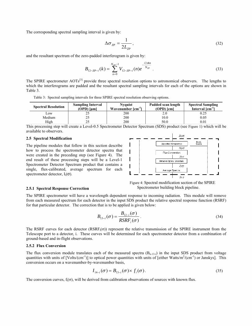
2.5 Spectral Modification

The pipeline modules that follow in this section describe how to process the spectrometer detector spectra that were created in the preceding step (see Figure 4). The end result of these processing steps will be a Level-1 Spectrometer Detector Spectrum product that contains a single, flux-calibrated, average spectrum for each spectrometer detector, Ii(σ).

Figure 4: Spectral modification section of the SPIRE Spectrometer building block pipeline. 2.5.1 Spectral Response Correction

The SPIRE spectrometer will have a wavelength dependent response to incoming radiation. This module will remove from each measured spectrum for each detector in the input SDS product the relative spectral response function (RSRF) for that particular detector. The correction that is to be applied is given below:

)()(

)( 1213 σ

σσ

i

ii RSRF

BB −

− = . (34)

The RSRF curves for each detector (RSRFi(σ)) represent the relative transmission of the SPIRE instrument from the Telescope port to a detector, i. These curves will be determined for each spectrometer detector from a combination of ground-based and in-flight observations.

2.5.2 Flux Conversion

The flux conversion module translates each of the measured spectra (BBn-13-i) in the input SDS product from voltage quantities with units of [Volts/(cm )] to optical power quantities with units of [either Watts/m /(cm ) or Janskys]. This conversion occurs on a wavenumber-by-wavenumber basis,

-1 2 -1

)()()( 1314 σσσ iii fBI ×= −− . (35)

The conversion curves, fi(σ), will be derived from calibration observations of sources with known flux.

2.5.3 Removal of Optical Crosstalk

Optical crosstalk is defined as power from the astronomical source that should be incident on one detector but is actually received by another. In the case of SPIRE, neighboring detectors are separated by approximately twice the full width at half maximum (FWHM) of the incident beam. Thus, even if a source is on-axis for a given detector, a small fraction of the source power will be incident on the neighboring detectors due to telescope diffraction. Non-neighboring detectors are sufficiently far apart that they should not receive significant power from an on-axis source.

The procedure to remove optical crosstalk from the SPIRE spectrometer detectors is functionally equivalent to that for the SPIRE photometer detectors[2].

2.5.4 Spectral Averaging

The final step of the spectrometer building block pipeline computes, on a wavenumber-by-wavenumber basis for each spectrometer detector, the average of the spectral intensities across the scans, n,

∑=

−−− =ScansN

nkin

Scanski I

NI

11616 )(1)( σσ . (36)

Tthe uncertainty in the average spectral intensity is estimated as the standard deviation of the spectral components,

( )∑=

−−−− −−

=ScansN

nkikin

Scanski II

NI

1

2

161616 )()(1

1)( σσσδ . (37)

The data product that results from this processing step will be made available to observers as a Level-1 Spectrometer Detector Spectrum (SDS) product.

3. SPECTRAL MAPPING The pipeline modules that follow in this section describe the operations on the Level-1 spectrometer detector spectra created in the preceding step. The end result of these spectral modifying processing steps will be a Level-2 Spectrum Cube product.

3.1 Spatial Regridding

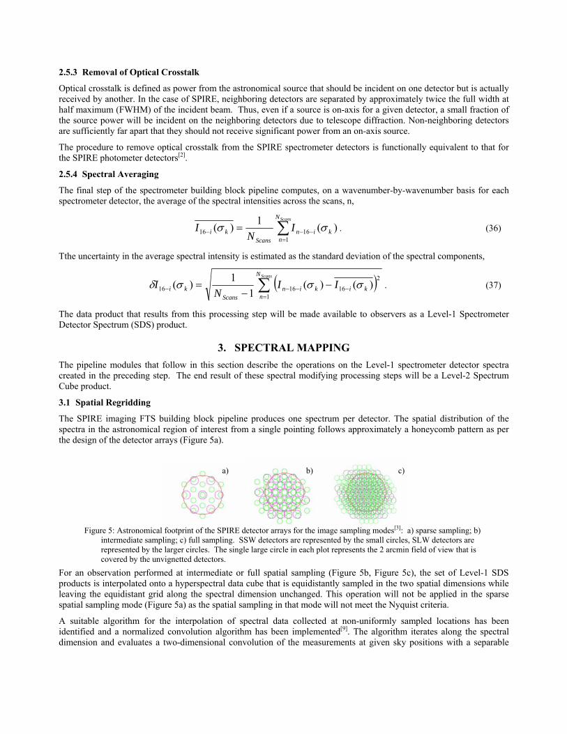
The SPIRE imaging FTS building block pipeline produces one spectrum per detector. The spatial distribution of the spectra in the astronomical region of interest from a single pointing follows approximately a honeycomb pattern as per the design of the detector arrays (Figure 5a).

a) b) c)

Figure 5: Astronomical footprint of the SPIRE detector arrays for the image sampling modes[3]: a) sparse sampling; b) intermediate sampling; c) full sampling. SSW detectors are represented by the small circles, SLW detectors are represented by the larger circles. The single large circle in each plot represents the 2 arcmin field of view that is covered by the unvignetted detectors.

For an observation performed at intermediate or full spatial sampling (Figure 5b, Figure 5c), the set of Level-1 SDS products is interpolated onto a hyperspectral data cube that is equidistantly sampled in the two spatial dimensions while leaving the equidistant grid along the spectral dimension unchanged. This operation will not be applied in the sparse spatial sampling mode (Figure 5a) as the spatial sampling in that mode will not meet the Nyquist criteria.

A suitable algorithm for the interpolation of spectral data collected at non-uniformly sampled locations has been identified and a normalized convolution algorithm has been implemented[9]. The algorithm iterates along the spectral dimension and evaluates a two-dimensional convolution of the measurements at given sky positions with a separable

two-dimensional kernel describing the field of view of the detectors. Ground-based measurements have shown that the FWHM of the beam of the SPIRE spectrometer detectors vary in a non-linear fashion with frequency between 15.5-17.5 arcsec for SSW and 31-41 arcsec for SLW[10]. This algorithm is well set up to take such a frequency-dependent beam size into account. It does, however, assume that the beam sizes of all detectors are identical. The suitability of this procedure remains to be verified.

4. CONCLUSIONS We have presented an overview of the data processing pipeline for the SPIRE Imaging Fourier transform spectrometer. The data processing modules that are and the manned by which they are combined within the pipeline have been described. The Level-0.5 and Level-1building block data products as well as the Level-2 spectral cube observation products for the SPIRE astronomical observation templates have been presented.

The current baseline of the SPIRE FTS processing pipeline is to employ algorithms that rely on empirical observations. As more detailed knowledge of the behavior of the SPIRE FTS is gained through in-flight observations, these modules may be modified to follow a model-based approach.

ACKNOWLEDGEMENTS

The authors wish to acknowledge Andres Rebolledo, Peter Kennedy, Zhaohan Weng, Yan He, Karim Ali, Yu Wai Wong, and Alim Harji for their contributions to the development of the SPIRE spectrometer data processing modules. The authors would also like to thank Christophe Ordenovic and Dominique Benielli for their contributions to the first level deglitching and Telescope/SCAL corrections. The figures that show the SPIRE astronomical footprint for the different spatial sampling modes were provided by Ivan Valtchanov. The funding for the Canadian contribution to SPIRE was provided by the Canadian Space Agency and NSERC.

REFERENCES [1] Griffin, M. J., et. al., “Herschel-SPIRE: design, ground test results, and predicted performance,” in Space

Telescopes and Instrumentation I: Optical, Infrared, and Millimeter Wave (this volume), 7010, Proc. SPIE, (2008). [2] Pilbratt, G. L., “Herschel mission overview and key programmes,” in Space Telescopes and Instrumentation I:

Optical, Infrared, and Millimeter Wave (this volume), 7010, Proc. SPIE, (2008). [3] Herschel Science Centre, “SPIRE Observer's Manual,” HERSCHEL-HSC-DOC-0789, version 1.2 (2007). [4] Griffin, M. J., Lim, T. L., Bendo, G., Bock, J. J., Castro-Rodriguez, N., Clements, D. , Chanial, P., Dowell, D.,

Gastaud, R., Glenn, J., King, K. J., Laurent, G., Lu, N., Mainetti, G., Morris, H., Nguyen, H. T., Panuzzo, P., Rizzo, D., Schulz, B., Schwartz, A., Swinyard, B. M., Xu, K. and Zhang, L., “The SPIRE photometer data-processing pipeline,” in Space Telescopes and Instrumentation I: Optical, Infrared, and Millimeter Wave (this volume), 7010, Proc. SPIE, (2008).

[5] Ordenovic, C., Surace, C., Torresani, B. and Llebaria, A., "Glitches detection and signal reconstruction using Holder and wavelet analysis," ADAIV preprint, (2007).

[6] Cara, C., “Herschel SPIRE Detector Control Unit Design Document,”, SPIRE-SAP-PRJ-001243, Tech. Rep., (2005).

[7] Naylor, D. A., Schultz A. A. and Clark, T. A., “Eliminating channel spectra in Fourier transform spectroscopy,” Appl. Opt., 27, 2603 (1988).

[8] Naylor, D. A. and Tahic, M. K., "Apodizing functions for Fourier transform spectroscopy," J. Opt. Soc. Am. A 24, 3644-3648 (2007).

[9] Knutsson, H. and Westin, C. F., “Normalized and Differential Convolution Methods for Interpolation and Filtering of Incomplete and Uncertain Data,” Proc. Computer Vision and Pattern Recognition, 512-523, (1993).

[10] Spencer, L. D., Naylor, D. A., Zhang, B., Davis-Imhof, P., Fulton, T. R., Baluteau, J.-P., Ferlet, M. J., Lim, T. L., Polehampton, E. T. and Swinyard, B. M., “Performance evaluation of the Herschel/SPIRE instrument flight model-imaging Fourier transform spectrometer,” in Space Telescopes and Instrumentation I: Optical, Infrared, and Millimeter Wave (this volume) , 7010, Proc. SPIE, (2008).