Florida International UniversityFIU Digital Commons

FIU Electronic Theses and Dissertations University Graduate School

2-8-2019

Numerical Simulation of Flushing Deposits inPipelinesJoseph S. CoverstonFlorida International University, jcove010@fiu.edu

Follow this and additional works at: https://digitalcommons.fiu.edu/etdPart of the Aerodynamics and Fluid Mechanics Commons

This work is brought to you for free and open access by the University Graduate School at FIU Digital Commons. It has been accepted for inclusion inFIU Electronic Theses and Dissertations by an authorized administrator of FIU Digital Commons. For more information, please contact dcc@fiu.edu.

Recommended CitationCoverston, Joseph S., "Numerical Simulation of Flushing Deposits in Pipelines" (2019). FIU Electronic Theses and Dissertations. 3951.https://digitalcommons.fiu.edu/etd/3951

FLORIDA INTERNATIONAL UNIVERSITY

Miami, Florida

NUMERICAL SIMULATION OF FLUSHING DEPOSITS IN PIPELINES

requirements for the degree of

MASTER OF SCIENCE

In

MECHANICAL ENGINEERING

by

Joseph Stanley Coverston

2019

A thesis submitted in partial fulfillment of the

ii

To: John L. Volakis College of Engineering and Computing

We have read this thesis and recommend that it be approved.

___________________________________________ Dwayne McDaniel

___________________________________________

Seung Jae Lee

___________________________________________ Cheng-Xian Lin

___________________________________________ George S. Dulikravich, Major Professor

___________________________________________ Dean John L. Volakis

College of Engineering and Computing

___________________________________________ Andrés G. Gil

Vice President for Research and Economic Development and Dean of the University Graduate School

Florida International University, 2019

This thesis, written by Joseph Stanley Coverston, and entitled Numerical Simulation of Flushing Deposits in Pipelines, having been approved in respect to style and intellectual content, is referred to you for judgment.

Date of Defense: February 8, 2019

The thesis of Joseph Stanley Coverston is approved.

iii

DEDICATION

I dedicate this thesis to my loving wife. Without her support, patience, and

encouragement, this thesis would not have been possible.

iv

ACKNOWLEDGMENTS

This work was supported by the United States Department of Energy.

I would like to acknowledge and thank Professor George S. Dulikravich for the

excellent advice and resources that he has provided throughout my

undergraduate and graduate careers at FIU and for arranging for my summer

internship at PennState’s ARL. I appreciate his personal and professional

support throughout the five years that I have been at FIU. Special thanks goes

out to Dr. Ahmadreza Abbasi Baharanchi, for his amazing technical knowledge in

the area of this thesis, and extremely helpful and insightful comments on the

subject matter. I cannot thank him enough for being my mentor with the DOE

Fellows program, and for taking the time to critically review any and all results I

generated for this thesis. I would also like to thank Dr. Leonel E. Lagos for his

support through the Department of Energy Fellowship program. This program

has been an amazing opportunity to work directly with the DOE and United

States National Labs, especially over the summer months where I, and many

others, were supported as interns working full time at the National Labs.

To my committee members, Dr. Cheng-Xian Lin, Dr. Seung Jae Lee, and Dr.

Dwayne McDaniel, thank you for your advice and support on this thesis. Dr.

McDaniel, thank you for your extra assistance making sure I stayed on track both

for this thesis and for my professional aspirations. Lastly, I would like to thank

anyone who is not specifically mentioned here, such as my peers in the DOE

Fellows program, who have assisted and encouraged this thesis, and my

supervisors at PennState’s ARL, Dr. Robert Kunz and Dr. Norman Foster.

v

ABSTRACT OF THE THESIS

NUMERICAL SIMULATION OF

FLUSHING DEPOSITS IN PIPELINES

by

Florida International University, 2019

Miami, Florida

Professor George S. Dulikravich, Major Professor

The purpose of this research is to reduce the amount of waste generated in

Department of Energy nuclear cleanup efforts currently underway. Due to the

highly radioactive nature of the waste, any fluid that contacts the waste must then

be treated and processed as waste. To minimize the fluids contaminated during

flushing, this research aims to provide a basis for the flushing of High Level

Waste (HLW) pipelines. Edgar Plastic Kaolin (EPK) with solid particles of a

nominal diameter of 1 micron was used as a simulacrum for HLW. An Eulerian-

Eulerian simulation built in StarCCM+ software, with a k-𝜔 turbulence model, and

a drag coefficient to connect the solid EPK phase with the liquid phase, was used

to simulate the flushing of pipelines. Velocities from 3 ft/s to 10 ft/s were

investigated to find the highest volumetric efficiency, and it was determined that

10 ft/s was the optimal flushing velocity.

Joseph Stanley Coverston

vi

CONTENTS

CHAPTER PAGE

Introduction ........................................................................................................... 1

Motivation .......................................................................................................... 1

Background ....................................................................................................... 2

Research Objectives ............................................................................................ 7

Methods ................................................................................................................ 9

Governing Equations - Eulerian-Eulerian approach.............................................. 9

Navier Stokes transport equations for k-𝜔 ...................................................... 13

Turbulent kinetic energy, k .............................................................................. 13

Specific dissipation rate, 𝜔 .............................................................................. 13

Turbulence production terms in the k-𝜔 equations: ......................................... 13

Dissipation in the k-𝜔 equations: ..................................................................... 14

Summary of model constants for the k-𝜔 model: ............................................ 15

Boundary Conditions ....................................................................................... 15

Y+ Calculation ................................................................................................. 15

Solver Algorithm .............................................................................................. 16

vii

StarCCM+ Solution ............................................................................................. 16

Initialization ......................................................................................................... 19

Simulation Results .............................................................................................. 21

Discussion .......................................................................................................... 23

Mesh Convergence Study .................................................................................. 26

Verification Case ................................................................................................ 28

Conclusion .......................................................................................................... 30

Suggestions for Future Work .............................................................................. 31

References ......................................................................................................... 33

Appendix ............................................................................................................ 36

viii

LIST OF TABLES

PAGETABLE

Table 1 - Pipe volume flushed vs velocity ........................................................... 18

Table 2 - Solids detection vs flow rate ................................................................ 24

Table 3 - Tabulated flush results ........................................................................ 26

ix

LIST OF FIGURES

FIGURE

Figure 1 - PNNL test loop [7] ................................................................................ 3

Figure 12 - Solid mobilization vs flush volumes.................................................. 22

Figure 13 - 10 ft/s, Typical Kaolin mobilization and suspension ......................... 22

Figure 14 - High rates of shear drive the increase in apparent viscosity ............ 23

Figure 15 - RCT1000 Coriolis meter................................................................... 24

Figure 16 - Flush velocity vs pipe volumes to flush ............................................ 25

Figure 17 - High mesh overlaid on original mesh result...................................... 27

Figure 18 - Error percent of converged mesh..................................................... 28

Figure 2 - First flushing test utilizing 10-micron glass bead simulant [7] ............... 5

Figure 3 - Second flushing test of 10-micron glass bead simulant [7]................... 6

Figure 4 - Non-Newtonian Fluids [17] ................................................................. 12

Figure 5 - 55% Kaolin in water rheological properties [16] [17] .......................... 12

Figure 6 - Geometry model of pipeline to be flushed.......................................... 16

Figure 11 - Volume fraction of solid initialization (top) and steady state solution (below)................................................................................................................ 21

Figure 10 - Initialization of Kaolin bed in the long section of the pipeline (left) steady state solution (right) ................................................................ ................ 20

Figure 8 - Initialization function........................................................................... 19

Figure 9 - Initialization of Kaolin bed in the pipe bend (left) steady state solution (right) .................. 20................................................................................................

Figure 7 – Unstructured dual prismatic/polyhedral mesh generated in StarCCM+, Mesh size exaggerated for clarity ....... 17.............................................

PAGE

x

Figure 19 - StarCCM+ model on left, ANSYS CFX on right [20] ......................... 29

Figure 20 - Experimental results vs CFX and StarCCM+ [20] ............................ 30

Figure 21 - 3 ft/s ................................................................................................. 36

Figure 22 - 5 ft/s ................................................................................................. 36

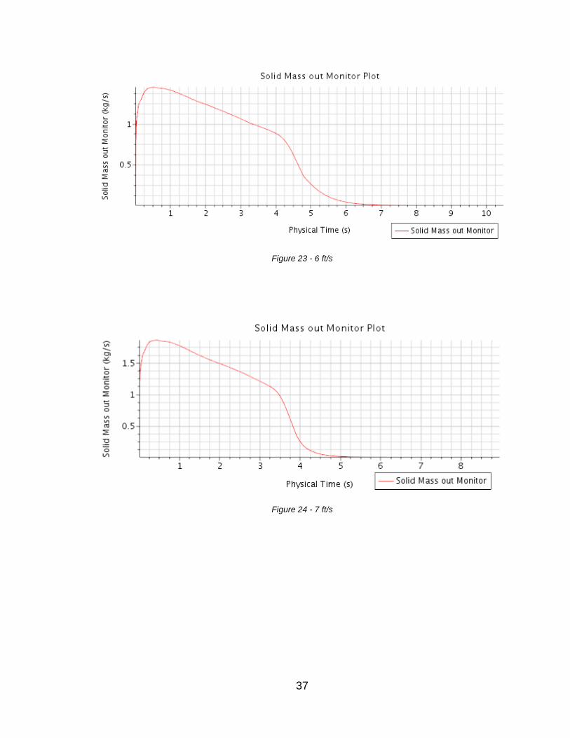
Figure 23 - 6 ft/s ................................................................................................. 37

Figure 24 - 7 ft/s ................................................................................................. 37

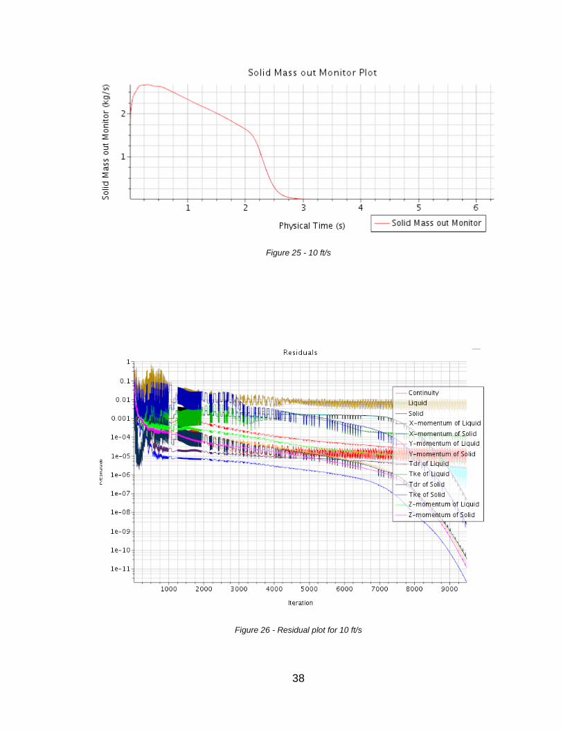
Figure 25 - 10 ft/s ............................................................................................... 38

Figure 26 - Residual plot for 10 ft/s ..................................................................... 38

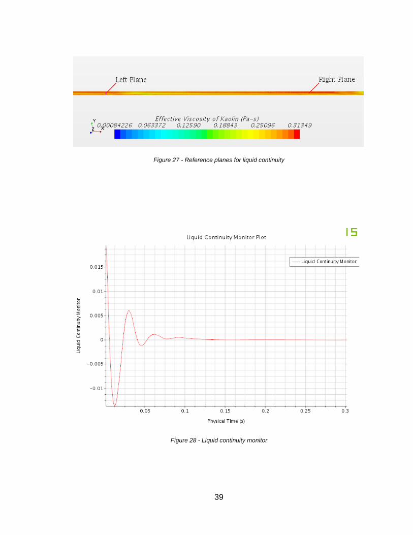
Figure 27 - Reference planes for liquid continuity............................................... 39

Figure 28 - Liquid continuity monitor ................................................................... 39

Figure 29 - Overview 5 ft/s upper section Kaolin suspension ............................. 40

Figure 30 - 5 ft/s detailed view of Kaolin suspension .......................................... 40

Figure 31 - Apparent viscosity at the boundary layer of Kaolin to water (5 ft/s) .. 41

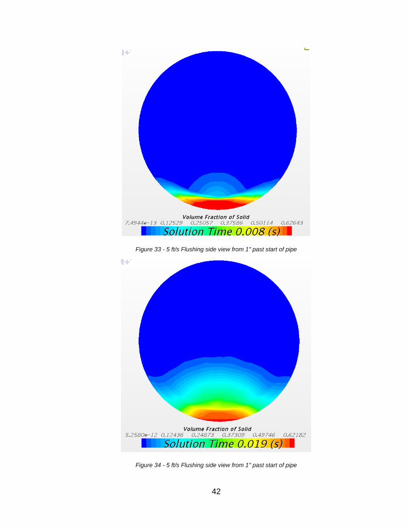
Figure 33 - 5 ft/s Flushing side view from 1" past start of pipe ........................... 42

Figure 34 - 5 ft/s Flushing side view from 1" past start of pipe ........................... 42

Figure 35 – Steady state pressure in system start section (5 ft/s) ...................... 43

Figure 36 - Steady state pressure in system full view (5 ft/s) ............................. 43

Figure 37 - Steady state pressure in system end (5 ft/s) .................................... 44

Figure 38 - Streamlines of velocity at inlet to system .......................................... 44

Figure 32 - Volume fraction of Kaolin, for comparison to the apparent viscosity (Figure 31).......................................................................................................... 41

PNNL Pacific Northwest National Laboratory

HLW High Level Waste

EPK Edgar Plastic Kaolin

𝐴𝑑 Linearized drag factor

𝐶𝑑 Coefficient of drag

d Diameter of particle

𝐹𝑖 Internal solid pressure force

k Kinetic energy

�̇� Mass transfer rate

𝑀𝑝 Interphase momentum transfer

p Pressure

v Velocity

∆𝑠 Wall spacing

Greek Symbols

𝛼𝑝 Volume fraction of phase

𝛤 Turbulent stresses

𝜇 Dynamic viscosity

𝜌𝑝 Density of phase

𝜔 Specific dissipation rate

Subscripts

c continuous phase

d dispersed phase

r relative velocity

xi

NOMENCLATURE

1

INTRODUCTION

Motivation

Pacific Northwest National Laboratory (PNNL) is investigating techniques that will

enable the safe and efficient transfer of High Level Waste (HLW) slurries from

existing holding tanks, into processing facilities that will enable the long term safe

storage of radioactive particles. To complete this process, the slurry must

conform to rheological standards for both acceptance at the final immobilization

facility, and for the transfer of the slurry either across a 5-mile-long cross-site

transfer line, or a shorter, less than 2000 ft transfer line for inter-site transfers. To

meet the rheological standards, water is usually introduced into the slurries to

control the concentration of particles. The addition of water allows for reasonable

velocities when transporting the particulate waste, and also allows for a specific

concentration of particles to be achieved for the transport, such as a 5% by

weight transfer. However, due to the radioactive nature of HLW, any fluid that

comes into contact with waste must then be treated and processed as waste,

adding to the overall cost of processing and disposing of HLW. While a singular

addition of waste to the holding tanks may not pose a long-term problem, the

majority of processes that occur at the Hanford facilities immobilize the majority

of solid waste but generate a diffuse return slurry. In addition, the process and

transfer lines must be flushed after a transfer, to either reduce cross

contamination of different waste batches, or to reduce the amount of salt

crystallization that occurs with certain waste types.

2

Currently, PNNL is investigating the transport of 28 million gallons of waste from

the current storage tanks into the processing facilities at the Hanford,

Washington site. Due to the limited amount of volume available for the storage

and processing of waste there is a strong need to control the amount of water

used to flush piping systems used to transfer waste across the site, and within

the site. Currently there are guidelines for the safe transport of HLW solids, but

there is no technical basis for the flushing volume used to clear the lines after a

transfer.

Background

Previous studies have focused on critical velocities for the suspension of such

particles, to reduce or eliminate deposits in piping systems. Two commonly used

models are the Oroskar and Turian model and the Gilles and Shook model [1],

which may not accurately estimate the correct critical velocity, depending on the

diameter of the particles of the slurry being transported [2]. However, particulate

deposits can still occur in piping systems that operate at the critical velocity, due

to pipe discontinuities, rheological changes due to temperature, or an

unanticipated yield stress present in the slurry transported [3]. The current

practice to estimate the flushing velocity and volume required to maintain a low

concentration of particles in a transfer line has no technical basis, but has been

shown to be effective for some HLW transfers [4]. Current practices relate the

flushing velocity to the critical velocity, but it has been shown that a re-

suspension velocity required for flushing is not adequately satisfied by a simple

linear correlation to critical velocity. As particles settle into a bed at the bottom of

3

a pipe system, they become harder to re-suspend into the flush water due to the

development of non-zero yield stresses from particle-particle interaction [5].

When a bed of particles has formed, it is also necessary to control the velocity of

the flow so that the particles re-suspend into the flow, instead of forming a sliding

bed of particles, or ‘pile up’ and cause the pipe to clog. In addition, the current

standard for flushing of HLW, TFC-ENG-STD-26, does not specify the same

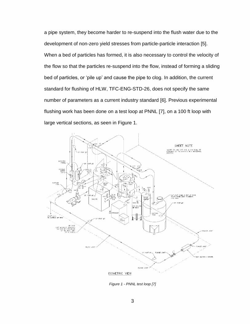
number of parameters as a current industry standard [6]. Previous experimental

flushing work has been done on a test loop at PNNL [7], on a 100 ft loop with

large vertical sections, as seen in Figure 1.

Figure 1 - PNNL test loop [7]

4

As Figure 1 shows, the system has many vertical segments that are not

representative of the pipe conditions at Hanford, and utilizes straight sections

parallel to the floor. The pipe sections also terminate into a capture tank after

they are lifted vertically 10 feet into the air, which would cause an uneven settling

of particles in the main section of the pipeline, and also not be comparable to

conditions out at the Hanford site. The experimental setup was created in order

to test critical velocity of various simulants, so many of the features of the test

loop render the results inapplicable to the majority of transfer pipelines that are

the focus of this thesis.

The flushes conducted on the system are meant to mirror procedures at the

Hanford Immobilization plant, called WTP, and are presented here for reference.

The simulant used are 10-micron glass beads, and the flush system uses

pressurized air charges to drive flushing to a velocity of 20 ft/s in order to clear

simulants between tests.

5

Figure 2 - First flushing test utilizing 10-micron glass bead simulant [7]

As can be seen from Figure 2, a complete flush occurs at around 1.8 pipe

volumes. An interesting feature of this tests is the spike in velocity at the

beginning of the flush, and a fairly slow ramp up of velocity to 20 ft/s afterwards.

Of note is that the peak pressure point occurs after the majority of the solid mass

has been ejected from the system, indicating that the pressure spike is not a

result of partial pipe blockage.

6

Figure 3 - Second flushing test of 10-micron glass bead simulant [7]

Figure 3 shows a more typical flush, with a pressure spike occurring at .5 pipe

volumes, indicating that the solid particles partially blocked the pipe flow leading

to an increase in pressure. The second test also shows that the system ramped

up to 20 ft/s within .5 pipe volumes, but within this ramp up time about 50% of the

particles had already been flushed from the system.

The two previous tests show that a flush volume of 1.5-1.8 would be adequate for

complete flushing, but this value may be obscured by other differences with the

experimental setup, and the pipe flush velocity that is above the guidelines for

pipes currently installed at Hanford.

7

RESEARCH OBJECTIVES

Currently, there have been no detailed experimentation or simulation that

attempts to estimate the amount of flushing required to re-suspend and mobilize

slurry particles in a tilted pipe system. All previous test loops did not incorporate

a gravity draining system which is present in the pipe systems at Hanford. The

current drop rate of the tank farms is given as 1-inch for every 100ft of horizontal

pipe. Previous test loops, such as Yokunda et al. [8], did not incorporate the

gravity draining feature of the existing tank pipe system, due to focusing on the

critical velocity, which would not be significantly affected by a gravity drain.

Due to the presence of the gravity draining system, the amount of slurry and

water in a given pipe system may vary significantly from a flat system, especially

in cases where the slurry particles are very small and easily suspended into the

main fluid. As one of the main functions of flushing a pipe system is the

resuspension of particles, not simply the continued suspension of particles, the

concentration and shape of the solids bed that forms on the lower part of the pipe

is of great interest and has not been previously studied for this specific waste.

A constraint that is unique to the Hanford system, which is not present in

commercial systems, is the presence of toxic organic vapors inside of the waste

tanks, which has limited the options for flushing to only water or other pure liquids

[9]. Currently facilities exist to process some additional water that may be

generated in the flushing of HLW transfer lines, but there are not large-scale

facilities which allow for the processing of vapors that come into contact with the

waste. Due to the nuclear, and often chemically hazardous nature of the waste, it

8

is not reasonable to develop such gas handling systems simply for the flushing of

waste in pipelines, thus, this alternative has not been considered for research

[10]. The toxic nature of the materials also has prevented direct experimentation

and observation of the waste to be transported; instead waste simulants are used

to mimic the physical properties of the waste that will be transported. The

majority of the problematic waste contains aluminum in the form of gibbsite and

boehmite, so the initial testing of the pipe flushing systems will use the simulant

EPK (Kaolin), which has been established to mimic the behavior of various

aluminum compounds. The particle size chosen for the initial testing is a nominal

1 micron, which is the smallest particle size of concern for the transport of waste.

In addition, the smaller particle size allows for the non-newtonian slurry behavior

to be observed, as beds of settled Kaolin can have large shear forces applied

before significant movement of the slurry can be seen.

The primary objective of this research is thus to characterize the re-suspension

velocity and volume required to fully or partially mobilize Kaolin particles

nominally 1 micron, that are present in a piping system that is a simulacrum of

the existing pipe system at Hanford [11].

A second objective is to characterize the initial slurry bed that can form in a given

pipe system, so that proper flushing guidelines can be created. Without an

understanding of the initial bed created after a HLW transfer, it may not be

possible to develop an accurate flushing guide.

9

METHODS

StarCCM+ commercial software was used to computationally determine the initial

bed of Kaolin particles, using an Eulerian-Eulerian approach, with a drag force

used to couple the suspended solids to the liquid phase. The simulation was

initialized as a completely suspended 17% by weight Kaolin particle solution, and

then the solution was run without any input velocity to allow for the Kaolin to

settle in the system.

This approach allows for the initial solids to be dispersed in the pipe system in a

semi-physical manner and will offer some insight into the potential settling of

solids in a gravity draining system.

A StarCCM+ simulation will then be started to determine the optimal velocity and

volume required to remove 17% by weight solids from the system. An initial test

of 5 different velocities will be used, 3, 5, 6, 7 and 10 ft/s, and for each velocity,

measurements will be taken of the total solid mass present in the system at 1, 2

and 3 pipe volumes of flush. From the 15 data points, a response surface will be

created using radial basis functions.

GOVERNING EQUATIONS - EULERIAN-EULERIAN APPROACH

In the Eulerian-Eulerian system, we assume that the two phases are completely

continuous, comingled continua, or “Interpenetrating continua”. This assumption

allows us to solve for the mass, momentum, energy and turbulence for each

phase separately, and then relate the two phases through the usage of coupling

equation systems that model physical phenomena such as drag [12].

10

For each phase, the conservation equation is

𝜕

𝜕𝑡(𝛼𝑝𝜌𝑝) + 𝛻 ⋅ (𝛼𝑝𝜌𝑝𝑣𝑝) = 0 (1)

The Eulerian-Eulerian system is modeled as

𝜕

𝜕𝑡(𝛼𝑝𝜌𝑝) + 𝛻 ⋅ (𝛼𝑝𝜌𝑝𝑣𝑝) =∑(�̇�𝑗𝑝 − �̇�𝑝𝑗)

𝑁

𝐽=1

+ 𝑆𝑝 (2)

where 𝛼𝑝 is the volume fraction of the phase, 𝜌𝑝 is the density, 𝑣𝑝 is the velocity,

N is the number of phases, (�̇�𝑗𝑝 − �̇�𝑝𝑗) is the mass transfer rate of the system,

and 𝑆𝑝 is the source term for the phase.

Conservation of momentum for each phase is thus

𝜕

𝜕𝑡(𝛼𝑝𝜌𝑝𝑣𝑝) + 𝛻 ⋅ (𝛼𝑝𝜌𝑝𝑣𝑝

2) = −𝛼𝑝𝛻𝑝 + 𝛼𝑝𝜌𝑝𝑔 + 𝛻 ⋅ (𝛼𝑝𝛤) +𝑀𝑝 + 𝐹𝑖 (3)

Here, Mp is the interphase momentum transfer and for each phase is defined as

𝑀𝑐 = −𝑀𝑑, and includes drag and turbulent dispersion forces. 𝐹𝑖 is the internal

solid pressure force, which occurs when particles reach the packing limit of 0.624

and is only present in the momentum equation for the solid phase.

Linearized Drag Factor

The linearized drag factor is calculated using the Gidaspow formula [13], with

𝐶𝐷 = 0.44, and vr as the relative velocity between phases.

𝐴𝐷 =

{

150𝛼𝑑

2𝜇𝑐𝛼𝑐𝑑2

+1.75𝛼𝑑𝜌𝑐|𝑣𝑟|

𝑑, 𝛼𝑑 ≥ 0.2

3

4(.44)

𝛼𝑑𝜌𝑐|𝑣𝑟|

𝑑𝛼𝑐−1.65, 𝛼𝑑 < 0.2

(4)

11

The force of drag per unit volume is then

𝐹𝐷 = 𝐴𝐷(𝑣𝑐 − 𝑣𝑑) (5)

To accurately model the interactions between particles in the dispersed phase

and the small, localized eddies in the continuous phase, a turbulent dispersion

force is added [14]. The dispersion force for the dispersed phase is calculated as

𝐹𝐷𝑇 = 𝐴𝐷𝑣𝑐𝜎𝛼(𝛼𝑐𝛼𝑐−𝛼𝑑𝛼𝑑) (6)

where 𝜎𝛼 through the Reynolds analogy yields turbulent Prandtl number of 1.

Solid pressure force is used when the particles reach a predetermined volume

fraction of 0.624 and is only used in the simulation when the volume fraction

approaches this limit. The value of 0.624 is used as this is representative of

small, spherical particles.

𝐹𝑖 = (𝑒𝐴(𝛼𝑝,𝑚𝑎𝑥−𝛼𝑑))∇(𝛼𝑑) (7)

where A is the model constant, set to a value of -600, 𝛼𝑝,𝑚𝑎𝑥 is the maximum

packing limit, and 𝛼𝑑 is the volume fraction of the dispersed phase.

For the second phase that contains particles, non-Newtonian fluid behavior is

expected, due to the tendency of particle suspensions in Newtonian fluids to

cause non-Newtonian behaviors, which correlates to the volume fraction of the

particle phase.

For the solid particle phase, the viscosity is replaced by an apparent viscosity of

μ = μ(γ), where the viscosity is a function of the shear rate [15]. Experimental

12

data was used to create the apparent viscosity function for the solid phase, using

data from Balmforth et al. [16], and Huang and Garcia [17].

Figure 4 - Non-Newtonian Fluids [17]

Figure 5 - 55% Kaolin in water rheological properties [16] [17]

13

Navier-Stokes transport equations for k-𝝎

To solve the turbulent flow, we must first use the Boussinesq hypothesis, which

is that the Reynolds Stress tensor is proportional to the mean strain rate tensor.

This allows for the resolution of large eddies, and the modeling of smaller

turbulence fluctuations. The turbulence scales are solved in two transport

equations, one for kinetic energy, k, and the other for 𝜔, the specific dissipation

rate. The k- 𝜔 model was chosen as it has a high level of accuracy for wall

bounded flows.

Turbulent kinetic energy, k, [18]

𝜕

𝜕𝑡(𝜌𝑘) +

𝜕

𝜕𝑥𝑖(𝜌𝑘𝑢𝑖) =

𝜕

𝜕𝑥𝑗(𝛤𝑘

𝜕𝑘

𝜕𝑥𝑗) + �̃�𝑘 − 𝑌𝑘 (8)

Specific dissipation rate, 𝜔

𝜕

𝜕𝑡(𝜌𝜔) +

𝜕

𝜕𝑥𝑖(𝜌𝑤𝑢𝑖) =

𝜕

𝜕𝑥𝑗(𝛤𝑤

𝜕𝑤

𝜕𝑥𝑗)+𝐺𝑤 − 𝑌𝑤 + 𝐷𝑤 (9)

Turbulence production terms in the k-𝜔 equations:

𝛤𝑘 = 𝜇 +𝜇𝑡

𝜎𝑘 and

𝛤𝑤 = 𝜇+𝜇𝑡𝜎𝑤

(10)

Turbulent viscosity is calculated as

𝜇𝑡 = 𝛼∞∗ (𝜌𝑘

𝜔) (11)

where 𝛼∞∗ becomes 1 in a high Reynolds number flow.

Gk is given as

𝐺𝑘 = 𝜇𝑡𝑆2 (12)

14

with S defined as the modulus of the mean rate-of-strain tensor:

𝑆 = √2𝑆𝑖𝑗𝑆𝑗𝑖 (13)

and Gw is

𝐺𝑤 = 𝛼𝜔

𝑘𝐺𝑘 (14)

where 𝛼 becomes 1 in a high Reynolds number form.

Dissipation in the k-𝝎 equations:

Dissipation of k:

𝑌𝑘 = 𝜌𝛽∗𝑓𝛽∗𝑘𝜔 (15)

where

𝑓𝛽∗ = 1 (16)

𝛽∗ = 𝛽𝑖∗[𝜁∗𝐹(𝑀𝑇)] (17)

𝛽𝑖∗ = 𝛽∞

∗

415+ (

𝑅𝑒𝑡𝑅𝛽)4

1 + (𝑅𝑒𝑡𝑅𝛽)4

(18)

Dissipation of ω:

𝑌𝑤 = 𝜌𝛽𝑓𝛽𝑤2 (19)

where

𝑓𝛽 =1 + 7𝑂𝑥𝜔1 + 80𝑥𝜔

(20)

𝑥𝑤 = |𝛺𝑖𝑗 ⋅ 𝛺𝑗𝑘𝑆𝑘𝑖(𝛽∞∗ 𝜔)3

| (21)

Vorticity is defined as:

15

𝛺𝑖𝑗 =1

2(𝜕𝑢𝑖𝜕𝑥𝑖

−𝜕𝑢𝑗

𝜕𝑥𝑖) (22)

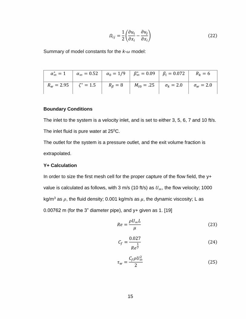
Summary of model constants for the k-𝜔 model:

Boundary Conditions

The inlet to the system is a velocity inlet, and is set to either 3, 5, 6, 7 and 10 ft/s.

The inlet fluid is pure water at 250C.

The outlet for the system is a pressure outlet, and the exit volume fraction is

extrapolated.

Y+ Calculation

In order to size the first mesh cell for the proper capture of the flow field, the y+

value is calculated as follows, with 3 m/s (10 ft/s) as 𝑈∞, the flow velocity; 1000

kg/m3 as 𝜌, the fluid density; 0.001 kg/m/s as 𝜇, the dynamic viscosity; L as

0.00762 m (for the 3” diameter pipe), and y+ given as 1. [19]

𝑅𝑒 =𝜌𝑈∞𝐿

𝜇 (23)

𝐶𝑓 =0.027

𝑅𝑒17

(24)

𝜏𝑤 =𝐶𝑓𝜌𝑈∞

2

2(25)

𝛼∞∗ = 1 𝛼∞ = 0.52 𝛼0 = 1/9 𝛽∞

∗ = 0.09 𝛽𝑖 = 0.072 𝑅𝑘 = 6

𝑅𝑤 = 2.95 𝜁∗ = 1.5 𝑅𝛽 = 8 𝑀𝑡0 = .25 𝜎𝑘 = 2.0 𝜎𝑤 = 2.0

16

𝑈𝑓𝑟𝑖𝑐 = √𝜏𝑤𝜌

(26)

𝛥𝑠 =𝑦+𝜇

𝑈𝑓𝑟𝑖𝑐𝜌(27)

The resulting initial grid cell height from the wall is then 0.0001m, or 0.1mm.

Solver Algorithm

The solver used for the simulations was the Eulerian-Eulerian Multiphase solver.

The simulations were run as implicit unsteady, with a time step of 0.001s, and 25

inner iterations per time step.

STARCCM+ SOLUTION

Figure 6 - Geometry model of pipeline to be flushed

The inlet is the red section on the left side of Figure 6, and the outlet is the

orange section on the right.

17

The CFD model is made from the first 22 feet of an experimental test loop,

starting from the proposed location of a slurry pump.

Figure 7 – Unstructured dual prismatic/polyhedral mesh generated in StarCCM+, Mesh size exaggerated for

clarity

The following details were used to create the mesh and domain for the

simulation:

• 3-in diameter pipe, 22 feet long

• 1-foot rise in height from the inlet

• Slope of horizontal pipe sections is 1-in drop for every 100 feet.

• 25,067,563 polyhedral cells used for the mesh (equivalent to 75,000,000

tetrahedral cells)

• Maximum skewness angle is 0.521 degrees

• Base size of polyhedral mesh is 1 cm

• 15 Prism layers, starting at .01mm and expanding by a 1.5 ratio each layer

18

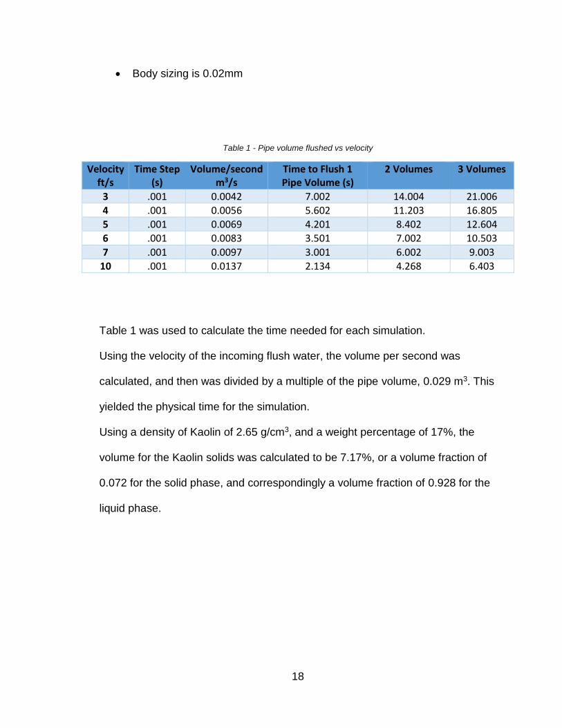
• Body sizing is 0.02mm

Table 1 - Pipe volume flushed vs velocity

Velocity ft/s

Time Step (s)

Volume/second m3/s

Time to Flush 1 Pipe Volume (s)

2 Volumes 3 Volumes

3 .001 0.0042 7.002 14.004 21.006

4 .001 0.0056 5.602 11.203 16.805

5 .001 0.0069 4.201 8.402 12.604

6 .001 0.0083 3.501 7.002 10.503

7 .001 0.0097 3.001 6.002 9.003

10 .001 0.0137 2.134 4.268 6.403

Table 1 was used to calculate the time needed for each simulation.

Using the velocity of the incoming flush water, the volume per second was

calculated, and then was divided by a multiple of the pipe volume, 0.029 m3. This

yielded the physical time for the simulation.

Using a density of Kaolin of 2.65 g/cm3, and a weight percentage of 17%, the

volume for the Kaolin solids was calculated to be 7.17%, or a volume fraction of

0.072 for the solid phase, and correspondingly a volume fraction of 0.928 for the

liquid phase.

19

INITIALIZATION

To create a repeatable bed for the flushing simulation, the system was initialized

to 7.17% Kaolin by volume and allowed to settle. A steady state simulation was

run to determine the shape of the bed, and then from this solution a function-

based initialization was created, to allow for quicker implementation in the event

the geometry or mesh is changed.

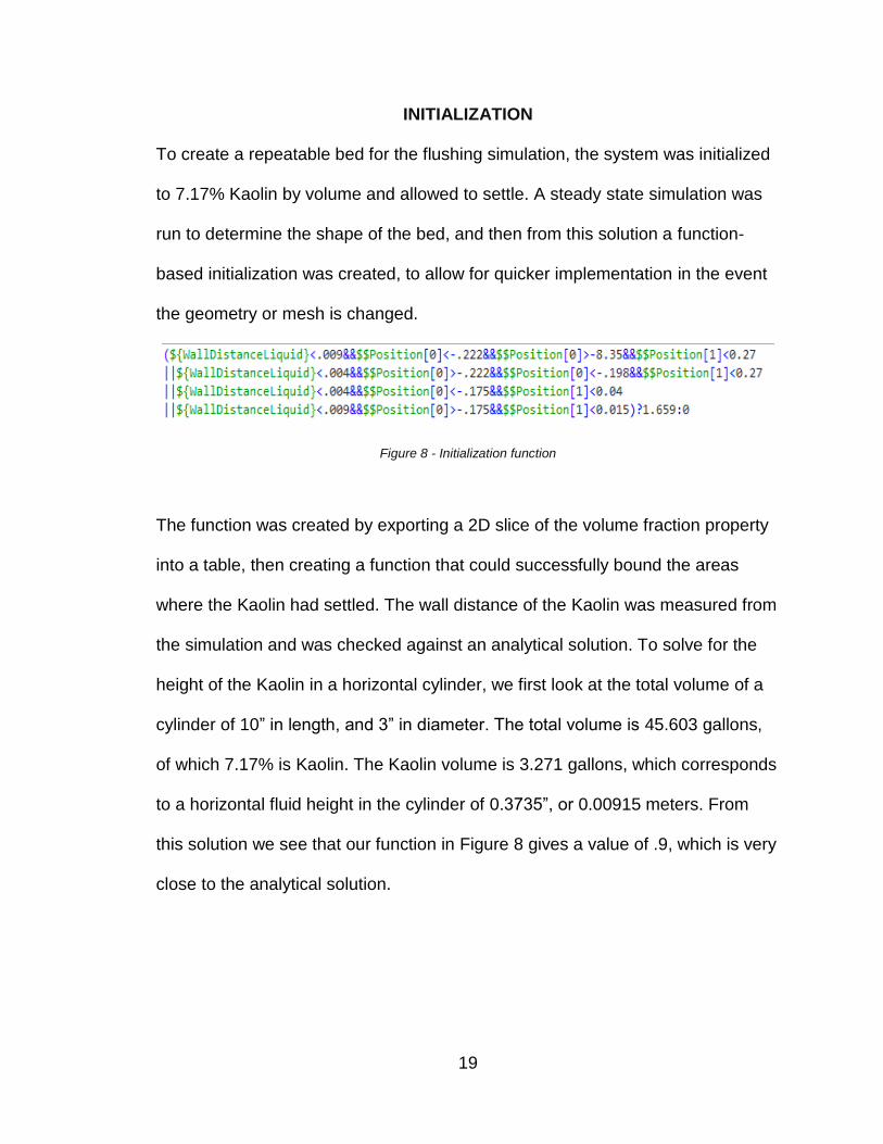
Figure 8 - Initialization function

The function was created by exporting a 2D slice of the volume fraction property

into a table, then creating a function that could successfully bound the areas

where the Kaolin had settled. The wall distance of the Kaolin was measured from

the simulation and was checked against an analytical solution. To solve for the

height of the Kaolin in a horizontal cylinder, we first look at the total volume of a

cylinder of 10” in length, and 3” in diameter. The total volume is 45.603 gallons,

of which 7.17% is Kaolin. The Kaolin volume is 3.271 gallons, which corresponds

to a horizontal fluid height in the cylinder of 0.3735”, or 0.00915 meters. From

this solution we see that our function in Figure 8 gives a value of .9, which is very

close to the analytical solution.

20

Figure 9 - Initialization of Kaolin bed in the pipe bend (left) steady state solution (right)

It can be seen from Figure 9 that the initialization function does a fairly close job

of characterizing the settled solid bed, and thus can be used as the initial state

for flushing of the system in subsequent tests.

Figure 10 - Initialization of Kaolin bed in the long section of the pipeline (left) steady state solution (right)

Figure 10 shows the characterization of the settled slurry in the long section of

the pipe. It should be noted from Figure 10 that the pipe system is slightly tilted,

so it will always appear nearly parallel to the X-axis when viewed up close. The

tilt is also fairly slight, but discernable in longer views of the system, as can be

seen in Figure 11, although the tile is only viewed as a few pixels of tilt in this

view.

21

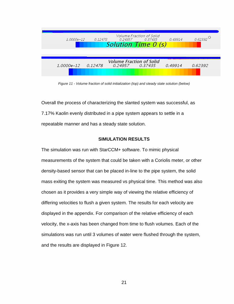
Figure 11 - Volume fraction of solid initialization (top) and steady state solution (below)

Overall the process of characterizing the slanted system was successful, as

7.17% Kaolin evenly distributed in a pipe system appears to settle in a

repeatable manner and has a steady state solution.

SIMULATION RESULTS

The simulation was run with StarCCM+ software. To mimic physical

measurements of the system that could be taken with a Coriolis meter, or other

density-based sensor that can be placed in-line to the pipe system, the solid

mass exiting the system was measured vs physical time. This method was also

chosen as it provides a very simple way of viewing the relative efficiency of

differing velocities to flush a given system. The results for each velocity are

displayed in the appendix. For comparison of the relative efficiency of each

velocity, the x-axis has been changed from time to flush volumes. Each of the

simulations was run until 3 volumes of water were flushed through the system,

and the results are displayed in Figure 12.

22

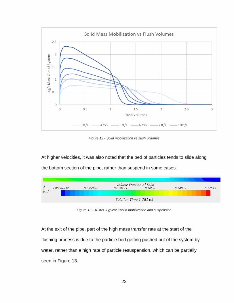
Figure 12 - Solid mobilization vs flush volumes

At higher velocities, it was also noted that the bed of particles tends to slide along

the bottom section of the pipe, rather than suspend in some cases.

Figure 13 - 10 ft/s, Typical Kaolin mobilization and suspension

At the exit of the pipe, part of the high mass transfer rate at the start of the

flushing process is due to the particle bed getting pushed out of the system by

water, rather than a high rate of particle resuspension, which can be partially

seen in Figure 13.

23

Figure 14 - High rates of shear drive the increase in apparent viscosity

Figure 14 shows the increase in the apparent viscosity of Kaolin that is observed

in a 10 ft/s flush. It was also noted for all cases that the 90 degree bend tends to

quickly clear of particles, which is believed to be caused by relatively larger

turbulent forces that are generated by the acceleration of fluid through the

change in direction that occurs in this region. For larger particle mass loadings, it

has been proven that changes in direction of flow are an area of concern for

pipeline plugging, but this has not proven to be the case for this simulation, which

utilizes relatively simple bends.

DISCUSSION

For the analysis of the flushed system, the completeness of a flush is quantified

as the smallest amount of Kaolin leaving the system that could be measured by

experimental verification using a Coriolis meter. A standard Coriolis meter is

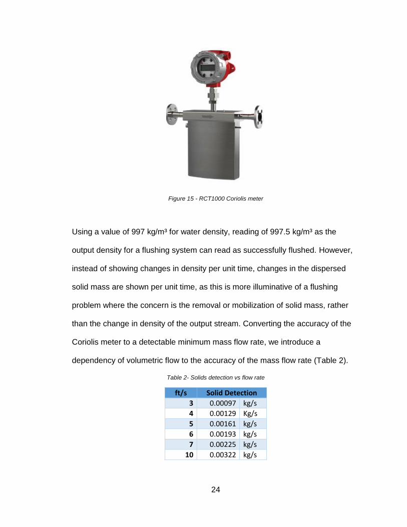
shown in Figure 15, which has an accuracy of +/- 0.5 kg/m³.

24

Figure 15 - RCT1000 Coriolis meter

Using a value of 997 kg/m³ for water density, reading of 997.5 kg/m³ as the

output density for a flushing system can read as successfully flushed. However,

instead of showing changes in density per unit time, changes in the dispersed

solid mass are shown per unit time, as this is more illuminative of a flushing

problem where the concern is the removal or mobilization of solid mass, rather

than the change in density of the output stream. Converting the accuracy of the

Coriolis meter to a detectable minimum mass flow rate, we introduce a

dependency of volumetric flow to the accuracy of the mass flow rate (Table 2).

Table 2- Solids detection vs flow rate

ft/s Solid Detection

3 0.00097 kg/s

4 0.00129 Kg/s

5 0.00161 kg/s

6 0.00193 kg/s

7 0.00225 kg/s

10 0.00322 kg/s

25

In an experimental setup, this dependency would mean that at higher flow rates,

the Coriolis meter is less accurate. The difference between the lowest and

highest rate of mass flow rate detection is close to 0.002 kg/s, which translates

into a density error of .11%. As this error rate is very low, 0.001 kg/s of solid

mass flow was chosen as the flushed condition.

With this criteria for a “flushed” system, the overall efficiency of each velocity can

be calculated from the mass out data. To gauge the volume efficiency of each

velocity, pipe volumes were used to show how each velocity compare, shown in

Figure 16, and tabulated in Table 3.

Figure 16 - Flush velocity vs pipe volumes to flush

It can be seen from the final results that there is a linear correlation between

velocity and volumetric efficiency of flush. The largest increase in efficiency

26

comes from the jump from 4 ft/s to 5 ft/s, which is a nearly 20% decrease in

volume used to flush.

Table 3 - Tabulated flush results

Velocity ft/s

Volume/second m3/s

Time to Complete Flush (s)

Volumes to Complete Flush

Volume of Flush Water

% of 3 Volumes

3 0.0042 +21.006 >3 Volumes 23.14 +100%

4 0.0056 15.754 2.812 23.13 100%

5 0.0069 7.023 2.428 12.89 81%

6 0.0083 7.666 2.190 16.89 73%

7 0.0097 6.211 2.070 15.96 69%

10 0.0137 3.144 1.496 11.54 50%

From the results in Table 3 it can be concluded that for very light and small

particles like 1-micron EPK, higher flush velocities will give significant increases

to volumetric efficiency. While velocities higher than 10 ft/s may yield further

increases to volumetric efficiency, due to safety, pressure, and material

constraints of the Hanford site, 10 ft/s is considered to be a maximum velocity for

flushing.

MESH CONVERGENCE STUDY

In order to prove grid independence of the simulation, a higher mesh was run on

the test case of 10ft/s. 10 ft/s was chosen for the convergence study as the

velocity of the fluid and sold phases are the highest out of any of the other

simulations, which causes a higher dependence on grid size.

To generate the higher mesh, the base size of the polyhedral mesh was reduced

to .8cm, and the prismatic mesh was lowered to 0.0075mm, which resulted in a

mesh of around 30 million cells, which is a 20% increase in mesh density from

27

the original mesh. The simulation was run again, and the mass flow results were

then compared to the previous results.

Figure 17 - High mesh overlaid on original mesh result

In Figure 17, we see the relative differences between the mass out on a higher

resolution mesh is very similar to the mass out on the original mesh, which

confirms that the solution is grid independent.

Figure 18 shows the difference between the original mesh and the higher mesh.

From the very low percent differences, we can see that the simulation has

converged at the original mesh size, and that increasing the mesh density further

will only result in a change of 0.5% or less to the final results.

28

Figure 18 - Error percent of converged mesh

VERIFICATION CASE

To verify the computational model used in the flushing simulations, a known

validated model for Kaolin suspensions in centrifugal pumps was used [20]. A 3”

centrifugal pump was created in StarCCM and was run using the same physics

models as the flushing simulation. The comparison CFD model was created in

ANSYS CFX 15.0, and was experimentally validated and contained a maximum

error of 6% [20] . The simulation used a 35% Kaolin mixture that is completely

dispersed within water, with the pump impeller spinning at 2900 RPM and a flow

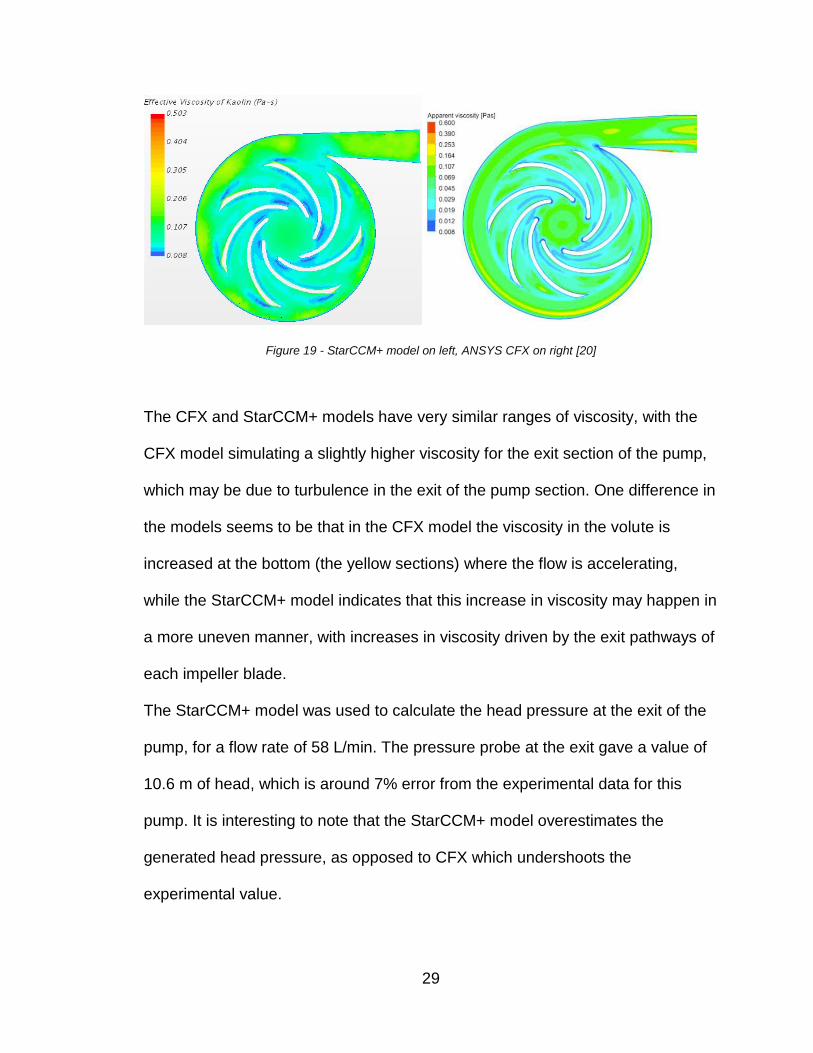
rate of 58 Liters/min. As can be seen by inspection of Figure 19 , effective

viscosity for the StarCCM+ physics model correlates very well to the effective

viscosity in the CFX model.

29

Figure 19 - StarCCM+ model on left, ANSYS CFX on right [20]

The CFX and StarCCM+ models have very similar ranges of viscosity, with the

CFX model simulating a slightly higher viscosity for the exit section of the pump,

which may be due to turbulence in the exit of the pump section. One difference in

the models seems to be that in the CFX model the viscosity in the volute is

increased at the bottom (the yellow sections) where the flow is accelerating,

while the StarCCM+ model indicates that this increase in viscosity may happen in

a more uneven manner, with increases in viscosity driven by the exit pathways of

each impeller blade.

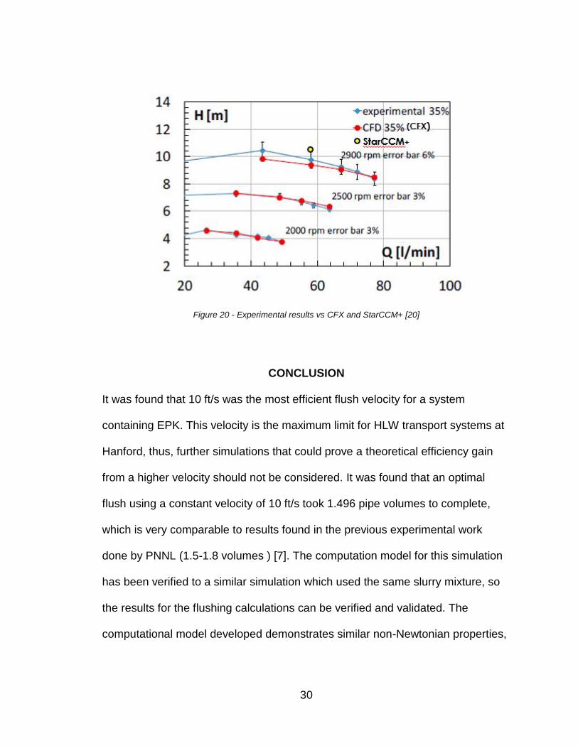
The StarCCM+ model was used to calculate the head pressure at the exit of the

pump, for a flow rate of 58 L/min. The pressure probe at the exit gave a value of

10.6 m of head, which is around 7% error from the experimental data for this

pump. It is interesting to note that the StarCCM+ model overestimates the

generated head pressure, as opposed to CFX which undershoots the

experimental value.

30

Figure 20 - Experimental results vs CFX and StarCCM+ [20]

CONCLUSION

It was found that 10 ft/s was the most efficient flush velocity for a system

containing EPK. This velocity is the maximum limit for HLW transport systems at

Hanford, thus, further simulations that could prove a theoretical efficiency gain

from a higher velocity should not be considered. It was found that an optimal

flush using a constant velocity of 10 ft/s took 1.496 pipe volumes to complete,

which is very comparable to results found in the previous experimental work

done by PNNL (1.5-1.8 volumes ) [7]. The computation model for this simulation

has been verified to a similar simulation which used the same slurry mixture, so

the results for the flushing calculations can be verified and validated. The

computational model developed demonstrates similar non-Newtonian properties,

31

such as an increase in apparent viscosity upon application of a shear force, to a

previously verified and validated model. The simulation was shown to have an

error rate of ~7% when compared to experimental data, which indicates that the

simulation has a fairly high degree of accuracy and should be comparable to

experimental results of the same geometry as those modeled here. The

characterization of the initial bed of Kaolin was also successful, and the

simulation of a 7.17% by volume Kaolin pipe system converged successfully to a

steady state solution. Due to the low angle of tilt of the pipe, the settled bed of

Kaolin was observed to form a bed of a height of .009m above the center of the

internal pipe surface.

SUGGESTIONS FOR FUTURE WORK

As the simulation did not utilize a pipe roughness coefficient, the Kaolin bed was

partially pushed out of the domain in many of the high velocity cases, as can be

seen in Figure 13. The inclusion of a surface roughness coefficient would

possibly change the volumetric efficiency results to be even more favorable to

higher velocities, as surface roughness would limit sliding of a particle bed

against the bottom of the pipe at low velocities.

Future work should include a ramping function for the velocities of the flush

volumes. In real pipe systems, flushing operations cannot be started and stopped

suddenly through the use of a valve, so a more realistic flush scenario would

32

include a ramp up and ramp down velocity for the flush water. The overall

volumetric efficiency of the system is highly dependent on the time spent at each

velocity, so it is possible that any ramping of velocities could shift the efficiency of

flushing towards a lower velocity. This transiting of slower velocities might negate

some of the efficiency benefits seen with constant velocity flushing.

Further work could be done to expand the computational model to include non-

spherical particles, with a particle size distribution heavily centered around 1

micron. This higher degree of physical simulation for the particles might enable a

more accurate prediction of the slurry characteristics, which is the main source of

error for the simulation.

Another addition that would be possible for this simulation would be the addition

of probes that mimic an experimental setup. Points measuring for pressure could

be added and recorded during the simulation. Flow meters could also be

incorporated into the system as well.

The geometry of the system could also be updated to include a more detailed

model of the fittings used to join pipes together. This is of special concern in the

bending sections of the test loop, as the most pipe discontinuities are located

there.

33

[1] D. Lidell and K. a. Burnett, "Critical Transport Velocity: A Review of

Correlations and Models. RPP-7185, Rev-0,," CH2M Hill Hanford Group,,

Richland, Washington, 2000.

REFERENCES

[2] A. Poloski, A. Etchells, J. Chun, H. Adkins, A. Casella, M. Minette and S.

Yokuda, "A Pipeline Transport Correlation for Slurries with Small But Dense

Particles," The Canadian Journal Of Chemical Engineering, vol. 88, pp.

182-189, April 2010.

[3] A. Poloski, "Deposition Velocities of Non Newtonian Slurries in Pipelines:

Complex Simulant Testing," Pacific Northwest National Laboratory ,

Richland, Washington, 2009.

[4] R. Gillies, R. Sun, R. Sanders and J. Schaan, "Lowered Expectations: The

Impact of Yield Stress on Sand Transport in Laminar, Non-Newtonian

Flows," Hydrotransport, vol. 1, p. 1–14, May 2007.

[5] C. Litzenberger, "Rheological Study of Kaolin Clay Slurries," M.Sc. Thesis

University of Saskatchewan, Saskatoon, Canada,, 2003.

[6] Washington River Protection Solutions, "WASTE TRANSFER, DILUTION,

AND FLUSHING REQUIREMENTS," Washington River Protection

Solutions, Richland, Washington, 2015.

[7] A. Poloski, H. Adkins, J. Abrefah, A. Casella, R. Hohimer, F. Nigl, M.

Minette, J. Toth, J. Tingey and S. Yokuda, "Deposition Velocities of

34

Newtonian and Non-Newtonian Slurries in Pipelines," Pacific Northwest

National Laboratory, Richland, Washington, 2009.

[8] S. T. Yokuda, "A Qualitative Investigation of Deposition Velocities of a Non-

Newtonian Slurry in Complex Pipeline Geometries," PNNL, RIchland,

Washington, 2009.

[9] C.L.Wua, A. Berroukb and K. Nandakumarb, "Three-dimensional discrete

particle model for gas–solid fluidized beds on unstructured mesh," Chemical

Engineering Journal, no. 152, p. 16, 2009.

[10] V. Nguyen, M. S. Fountain, C. Enderlin, A. Fuher and L. Pease, "One

System River Protection Project Integrated Flowsheet – Slurry Waste

Transfer Line Flushing Study," Washington River Protection Solutions LLC,

One System, Richland, WA, 2016.

[11] M. A. Knight and B. E. Wells, "Estimate of Hanford Waste Insoluble Solid

Particle Size and Density Distribution," Battelle - Pacific Northwest Division,

Richland, Washington, 2007.

[12] P. Mineva, B. Chen and K. Nandakumar, "A finite element technique for

multifluid incompressible flow using Eulerian grids," Journal of

Computational Physics, vol. 187, p. 255–273, 2003.

[13] D. Gidaspow and J. Ding, "A bubbling fluidisation model using kinetic theory

of granular flow," American Institute of Chemical Engineers, vol. 36, no. 4,

pp. 523-538, 1990.

35

[14] K. Ekambara, R. S. Sanders, K. Nandakumar and J. H. Masliyah,

"Hydrodynamic Simulation of Horizontal Slurry Pipeline Flow Using ANSYS-

CFX," Industrial Engineering Chemistry Research, vol. 48, no. 17, pp. 8159-

8171, 2009.

[15] R. Sumner, J. Munkler, S. Carriere and C. Shook, "Rheology of Kaolin

Slurries Containing Large Silica Particles,," J. Hydrology and

Hydromechanics, vol. 48, p. 117–119, 2000.

[16] N. Balmforth, A. Burbidge, R. Craster, J. Salzig and A. Shen, "Visco-plastic

models of isothermal lava domes," Journal of Fluid Mechanics, vol. 403, pp.

37-65, 2000.

[17] X. Huang and M. H. Garcia, "A Herschel–Bulkley model for mud flow down

a slope," Journal of Fluid Mechanics, vol. 374, pp. 305-333, 1998.

[18] SHARCNET, "ANSYS FLUENT K-w model," SHARCNET, 1 12 2012.

[Online]. Available:

https://www.sharcnet.ca/Software/Fluent6/html/ug/node486.htm. [Accessed

22 JULY 2018].

[19] F. M. White, Fluid Mechanics, 7th Edition, New York: McGraw Hill, 2011.

[20] N. Aldi, C. Buratto, N. Casari, D. Dainese, V. Mazzanti, F. Mollica, E.

Munari, M. Occari, M. Pinelli, S. Randi, P. R. Spina and A. Suman,

"Experimental and Numerical Analysis of a Non-Newtonian Fluids

Processing Pump," in 72nd Conference of the Italian Thermal Machines

Engineering Association,, Lecce, Italy, 2017.

36

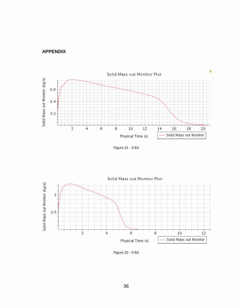
APPENDIX

Figure 21 - 3 ft/s

Figure 22 - 5 ft/s

37

Figure 23 - 6 ft/s

Figure 24 - 7 ft/s

38

Figure 25 - 10 ft/s

Figure 26 - Residual plot for 10 ft/s

39

Figure 27 - Reference planes for liquid continuity

Figure 28 - Liquid continuity monitor

40

Figure 29 - Overview 5 ft/s upper section Kaolin suspension

Figure 30 - 5 ft/s detailed view of Kaolin suspension

41

Figure 31 - Apparent viscosity at the boundary layer of Kaolin to water (5 ft/s)

Figure 32 - Volume fraction of Kaolin, for comparison to the apparent viscosity (Figure 31)

42

Figure 33 - 5 ft/s Flushing side view from 1" past start of pipe

Figure 34 - 5 ft/s Flushing side view from 1" past start of pipe

43

Figure 35 – Steady state pressure in system start section (5 ft/s)

Figure 36 - Steady state pressure in system full view (5 ft/s)

44

Figure 37 - Steady state pressure in system end (5 ft/s)

Figure 38 - Streamlines of velocity at inlet to system