1249

Advances in River Sediment Research – Fukuoka et al. (eds)© 2013 Taylor & Francis Group, London, ISBN 978-1-138-00062-9

Numerical study of flushing half-cone formation due to pressurized sediment flushing

W.J. Pringle & M.E. Meshkati ShahmirzadiUrban Management & Environmental Engineering Department, Kyoto University, Kyoto, Japan

N. Yoneyama & T. SumiDisaster Prevention Research Institute, Kyoto University, Kyoto, Japan

S. EmamgholizadehDepartment of Water and Soil, Agriculture College, Shahrood University of Technology, Iran

ABSTRACT: Pressure flushing cleans up the hydropower plant entrance from the sediment deposition. This technique results in localized scouring, that is called flushing cone. In this study, the flushing cone formation is simulated by implementing a RANS based 3D numerical model that consists of two suc-cessive stages: hydraulic flow and sediment erosion simulation. The velocity distribution profiles and the final geometry of the flushing cone were used to verify the numerical model outcomes. The results obtained by the hydraulic flow simulation revealed that the calculated velocity distribution profiles were comparable with the experimental data and the universal wall equations with roughness, ks = 10 mm as a sediment boundary condition was adequate for the application. However, when considering the simula-tion of the sediment erosion process using the moving boundary method the model should be improved for better accuracy in predicting flushing cone geometry.

level which causes large scale scouring in the form of a channel along the reservoir. Whereas, in pres-sure flushing the water level is maintained at a near constant level high above the bottom outlet such that the loss of water, an important dam resource, is conserved. Here, the scour formation shape is similar to that of a half-cone, often simply referred to as a flushing cone. This paper is concerned with pressure flushing and the formation of the cone.

Previously a few studies have experimentally investigated the flushing cone formation and pro-posed empirical equations to estimate the final volume and length of flushing cone (Scheuerlein et al., 2004, Emamgholizadeh, 2005, Meshkati et al., 2010, and Fathi-Moghadam et al., 2010). While empirical regression-based relations can allow for a quick and simple estimate of final cone geometry, these equations are often flawed because of the high nonlinearity between the cone geom-etry and the significant parameters.

Instead of using experimental and analytical methods, a less costly and potentially more accu-rate alternative is to use a numerical model (Olsen, 1999). A number of numerical studies have been conducted to simulate the flushing operation in dam reservoirs. Most of these studies are devoted to either 1D or 2D numerical models. Holly and

1 INTRODuCTION

One of most pressing problems of river and dam management in current times is the excess depo-sition of sediment. Severe sediment deposition which occurs in dam reservoirs decreases the water storage capacity and thus reduces the efficiency of the dam operation related to flood control and flow regulation (Graf, 1984). On top of the issues directly related to sedimentation in dam reservoirs, including intake clogging and machinery abrasion, a number of environmental problems also arise downstream of the dam. These include riverbed and bank erosion, armouring of the river bed, and a reduction in the quality of habitat for aquatic species, thereby threatening reductions in river sys-tem biodiversity (Kondolof, 1997).

To negate the issues related to sedimentation, a number of techniques have been proposed such as density current venting, flushing, by passing, dredging and sluicing (Brandt, 2000). However, flushing has proven to be one of the most effec-tive and efficient in removing reservoir sediment through the bottom outlet (Shen and Lai, 1996). This technique can be categorized into two types; free flushing and pressure flushing. In free flushing the water level is drawn down to a relatively low

1250

Rahuel (1990); Lai and Shen (1996) and Basson and Rooseboom (1997), individually developed a 1-D model to simulate the bed topography change during the drawdown phase in free flushing. These models may only be used to study flushing proc-esses in long and narrow reservoirs. Ruland and Rouve (1992) utilized a 2D finite element model to simulate the erosion process in the reservoir. Olsen (1999) solved the depth-averaged Navier-Stokes equation on a 2D mesh and extrapolated the corresponding flow field onto a 3D mesh to solve sediment concentration in flushing processes. Although, in addition to its difficult analytical characterization, the formation of the flushing cone is a complex three-dimensional phenomenon (Scheuerlein et al., 2004), where turbulent eddies, secondary currents and vertical velocities are sig-nificant, particularly in the vicinity of the bottom outlet. However, as can be found in the literature only a few studies have considered a 3D numeri-cal model and the majority of these are devoted to only free flushing phenomena, e.g.: Haun and Olsen (2012a, b) where a RANS model that solves the transient-convection equation for suspended sediment transport and Van Rijn’s (1984) empirical formula for bed load transport was utilized.

In this study, the formation of the flushing cone is simulated utilizing a RANS based 3D numerical model verified by Yoneyama (2010) and Yoneyama et al. (2012a, b) and adapted for this analysis. The simulation process consists of two stages. In the first stage the velocity distribution and equilib-rium bed topography (final shape) of the flush-ing half-cone, from the experimental investigation conducted by Emamgholizadeh (2005), were used for verification and calibration of the hydraulic model. In the second stage the numerical model commences from the initial sediment condition incorporating the moving boundary method to simulate the sediment erosion process. The mov-ing boundary method, while primitive, was cho-sen because of its simplicity and since only the final bed shape is of interest in this analysis. The results of the simulation in the second phase are compared to the geometry of the flushing cone as found experimentally.

2 EXPERIMENTATION

2.1 Experimental setup

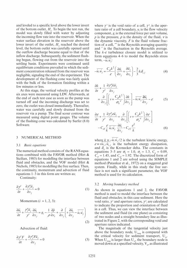
A hexahedral shallow basin of size 3.0 m length, 1.5 m width and 1.5 m height was used as the reservoir model. A schematic side and plan view of the model as well as the scoured flushing cone in the vicinity of bottom outlet are shown in Figure 1. A gate valve was installed in the center

Figure 1. Schematic side and plan view of the reser-voir model, the flushing cone and its relevant hydraulic parameters.

of the front wall of the model (dam wall) as a representation of the bottom outlet. A 50.8 mm diameter gate valve was employed. Inside the reservoir, sediment was placed and paved in the reach covering the entire width and 2.0 m of the length from the dam wall. The sediment thickness was 0.32 m, measured from the lower invert of the outlet to the sediment surface. Sand particles with a uniform size distribution were used as sediment. The particles had a median diameter, d50 of 1.2 mm and specific gravity, Gs of 2.65. Inflow discharges of 1.0, 3.0, 4.5, 6.0 and 8.0 L/s were used at the upstream end. The discharge at the outlet was kept the same as that of the inflow so that the reservoir water level was maintained constant at the required elevation. Three constant water levels of 0.425, 0.825 and 1.125 m were examined.

A digital point gauge device was utilized to meas-ure the scour cone configuration after each experi-ment. The vertical velocity profile was measured along six different axis locations by Laser-Doppler (LDV). The axis locations were selected along the x-axis (centerline of the bottom outlet), separated by equal 0.1 m intervals and numbered I–VI in Figure 1.

2.2 Experimental procedure and design

The following general procedure was enacted for all tests conducted in the experimental study. Before each test the sediment was wetted, flattened

1251

and leveled to a specific level above the lower invert of the bottom outlet, Hs. To begin the test run, the model was slowly filled with water by adjusting the incoming flow rate into the reservoir. When the water surface elevation in the reservoir above the lower invert of the outlet, Hw reached the desired level, the bottom outlet was carefully opened until the outflow discharge became equal to that of the inflow discharge. Subsequently, the sediment flush-ing began, flowing out from the reservoir into the settling basin. Experiments were continued until equilibrium conditions prevailed in which the sedi-ment concentration released from the reservoir was negligible, signaling the end of the experiment. The development of the flushing cone was fairly quick with the bulk of the formation finishing within a few minutes or less.

At this stage, the vertical velocity profiles at the six axes were measured using LDV. Afterwards, at the end of each test case as soon as the pump was turned off and the incoming discharge was set to zero, the outlet was closed immediately. Thereafter, water was carefully and slowly drained from the reservoir via a pump. The final scour contour was measured using digital point gauges. The volume of the flushing cone was calculated by Surfer (8.0) Software.

3 NuMERICAL METHOD

3.1 Basic equations

The numerical method consists of the RANS equa-tions combined with the FAVOR method (Hirt & Sicilian, 1985) for modelling the interface between fluid and obstacles, and the VOF model (Hirt & Nichols, 1985) for modelling the free surface. Then, the continuity, momentum and advection of fluid equations 1–3 in this form are written as;

Continuity:

∂∂

+∂∂

=γ γv

ja

j

jtu

x0 (1)

Momentum (i = 1, 2, 3):

∂∂

+∂∂

= −∂∂

+∂

∂∂∂

−

ut

u ux

gpx x

vux

u ui ja

jv

i

ji

i j

i

ji j

γγ ρ

1 ′ ′

(2)

Advection of fluid:

∂∂

+∂

∂=

γ γvja

j

j

Ft

Fux

0 (3)

where γ v is the void ratio of a cell, γ ai is the aper-

ture ratio of a cell boundary, ui is the flow velocity component, gi is the external force per unit volume, p is the pressure, ρ is the density of the fluid, ν is the dynamic viscosity, F is the fluid volume frac-tion of a cell, ¯ is the Reynolds averaging quantity and ′ is the fluctuation in the Reynolds average. The k-ε turbulence closure model is utilized to form equations 4–6 to model the Reynolds stress term, −u ui j

′ ′ :

− =∂∂

+∂∂

−u u

C k ux

ux

ki ji

j

j

ii j

′ ′ µ

εδ

2 23 , (4)

∂∂

+∂

∂

=∂

∂+

∂∂

−

kt

kux

xv

C k kx

u u

vja

j

j

j k ji j

1

2γ

γ

σµ

ε′ ′ ∂∂

∂−

ux

i

jε (5)

∂∂

+∂

∂=

∂∂

+

∂∂

−

εγ

γ εσ

ε

ε

µ

εε

ε

tu

x xv

C kx

Ck

u

vja

j

j j j

1 2

1′′ ′

i ji

ju

ux

Ck

∂∂

− εε

2

2

(6)

where k u ui j≡ − ′ ′ / 2 is the turbulent kinetic energy, ε ≡ vu ui j i j

′ ′, , is the turbulent energy dissipation, and δi,j is the Kronecker delta. The constants in equations 3–5 are σk = 1.0, σε = 1.3, Cµ = 0.09, Cε1 = 1.45, and Cε2 = 1.92. The discretized form of equations 1 and 2 are solved using the SIMPLE method (Patankar et al., 1972) on a staggered grid system. Finally, while in this study the free sur-face is not such a significant parameter, the VOF method is used for its calculation.

3.2 Moving boundary method

As shown in equations 1 and 2, the FAVOR method is used to model the interface between the fluid and obstacles; in this case sediment. Here the void ratio, γ v and aperture ratios, γ ai are calculated to indicate the proportion and orientation of fluid in a cell. Thus, we can view the interface between the sediment and fluid (in one plane) as consisting of two nodes and a straight boundary line as illus-trated in Figure 2, with the corresponding void and aperture ratios indicated.

The magnitude of the tangential velocity just above the boundary node, utang is compared with the critical velocity for sediment transport, ucr. When utang is larger than ucr, the boundary node is moved down at a specified velocity, Vd, as illustrated

1252

The length is 3.0 m, width 1.5 m and maxi-mum domain height of 1.0 m. The cell size in the x-direction ranges from 0.05 m at the inlet end, to 0.02 m in the area close to the outlet. The size of the cell in the y-direction is 0.025 m at the sides and as small as 0.01 m at the outlet. Similarly the cell size in the vertical direction is 0.01 m near the outlet and up to 0.02 m elsewhere. A total of around 390,000 cells are used to make up the domain but approximately 220,000 cells are used in calculation. Figure 5 pro-vides a snapshot of the calculation domain with an illustration of the parameters Q, Hw and Hs.

4.2 Bottom outlet representation

The bottom outlet was represented as a polygon made up of the rectangular cells of the numerical mesh as illustrated in Figure 6. The maximum cross-sectional width of the numerical outlet was 50 mm (compared with a diameter of 50.8 mm for the experiments) and had a total cross-sectional area of 2.0 × 10−3 m2 (compared with 2.03 × 10−3 m2 for the experiments). The bottom outlet was modeled by manipulating the streamwise aperture ratio, γ a

x into the last cell in the calculation domain as indicated in Figure 6.

Figure 2. Calculation cell containing both fluid and sediment, with its corresponding void ratio, γ v and aper-ture ratios, γ a

x.

Figure 3. Movement of the boundary node when the critical velocity for sediment transport is exceeded near the node.

Figure 4. Movement of the boundary node towards the angle of repose in submerged conditions, αs.

Figure 5. Side-view snapshot of the velocity profile in experiment Case D (1st stage) with parameters Q, Hw and Hs shown.

Figure 6. Diagram of the bottom outlet representation in the YZ plane, and its aperture ratios, γ a

x.

in Figure 3. Furthermore, the angle of the bound-ary line cannot exceed the angle of repose in sub-merged conditions, αs. In this case the higher of the two boundary nodes are lowered at the velocity, Vd, until the angle of repose is reached (Fig. 4).

4 NuMERICAL CONDITIONS

4.1 Domain

The domain size and conditions are the same as the experiments conducted by Emamgholizadeh (2005).

1253

4.3 Boundary conditions

Both the upstream inlet boundary and the down-stream bottom outlet boundary were subjected to Dirichlet boundary conditions.

At the inlet, both the constant water elevation, Hw, and the resulting ux velocity component calcu-lated from the input flow-rate, Q, over the cross-sectional area were specified. Since a single cell contains two cell boundaries in the x-direction, the velocity, ux was specified for both cell boundaries. The velocity distribution was uniform.

The ux velocity component at the bottom outlet was specified by the setting the outflow equal to the inlet flow rate, Q. This flow rate was divided by the cross-sectional area of the bottom outlet, found in section 4.2, to calculate and set the same ux velocity component at each cell in the bottom outlet. In addi-tion, since the inflow takes some time to reach and affect the area downstream, a “warming-up period” of 2.5s was specified to avoid imparting an initial rapid outflow velocity with no inflow into the con-trol volume. Within this period, the outflow velocity was linearly increased from zero at 0s, to the calcu-lated velocity based on the inflow, Q at 2.5s.

4.4 Numerical cases

Table 1 shows the experimental conditions that were used for simulation.

Each case was made up of two stages. The first stage consisted of solely a hydraulic study with the sediment, represented as a rigid bed, at the final stage as measured from the experiments. The resulting velocity profile was compared with that of the experiments. The simulation was calibrated by adjusting the boundary condition at the bed. The second stage took the calibrated hydraulic model and incorporated the moving boundary method. The initial condition was that of the sediment placed flat at a uniform depth throughout the entire domain. The simulation was run until the model predicted no further change in scour shape, and compared with the measured experimental scour shape (the flushing cone).

5 NuMERICAL RESuLTS

5.1 Rigid bed analysis

In this stage of the study various sediment bound-ary conditions were tried to identify the best repre-sentation of the experimental work. The simplest boundary conditions to apply are the no-slip, half-slip or free-slip conditions. The other sediment boundary conditions applied were the universal wall equations. These were applied in empirical form and as suggested by Le Roux (2004) which gives equations for all three hydrodynamic stages (rough, smooth and transitional). These equations were adjusted by changing the roughness of the rigid bed, ks. The sediment boundary conditions are shown in Table 2.

The selection of ks = 1.0 mm is because it is very close to the mean sediment diameter while ks = 10 mm represents a much rougher condition as a comparison. Figures 7–10 show velocity profiles at axis 1 and axis 2 for Cases B and D.

Typically, the velocities at low heights above the sediment surface were either; overestimated near the bottom outlet (axis 1) except for the free-slip case or underestimated further from the bottom outlet (axis 2) in the calculation. For larger heights above the sediment surface better agreement was

Table 1. Experimental conditions applied to numerical study.

CaseQ (L/s)

Hw (m)

Hs (m)

D (cm)

d50 (mm)

A 6.0 0.425 0.32 5.08 1.2B 8.0 0.425 0.32 5.08 1.2C 6.0 0.825 0.32 5.08 1.2D 8.0 0.825 0.32 5.08 1.2E 6.0 1.125 0.32 5.08 1.2F 8.0 1.125 0.32 5.08 1.2

Table 2. Sediment boundary conditions applied.

Condition Type ks (mm)

I Free-slip –II No-slip –III Half-slip –IV Wall equation 1.0V Wall equation 10.0

Figure 7. Velocity profile comparison at axis 1 for Case B.

1254

condition that sets the pressure of the outflow equal to atmospheric the outflow will depend on the hydrostatic pressure in the reservoir rather than the numerically stipulated outflow velocity calcu-lated using Q. Here, as the outflow increases so that it exceeds Q, the opening of the bottom outlet, as defined by the aperture ratios, can be decreased so that the outflow is equivalent to Q.

It was found that by comparing RMSE and R2 curve fit values between the experimental data and the numerical data for all axes, considering only boundary conditions I–III, the no slip sediment boundary condition (II) produced more favourable results overall. When comparing with the wall equa-tions (IV and V), only very tiny differences were evi-dent between each other and the no-slip condition. This is because the flow is generally hydrodynami-cally smooth everywhere. Here, the roughness, ks does not influence on the calculation of the velocity at the boundary. In fact only at the peak velocities of flow near the bottom outlet where the flow could be in a hydrodynamically transitional or rough stage are any notable differences detected between the wall equations and the no slip condition. But as noted above, the peak velocities at axis 1 are over-estimated and can be reduced slightly by imposing the wall equations and a higher value of ks. More investigation is required to determine the optimum value of ks for this study but ks = 10 mm produced slightly improved results from ks = 1 mm.

5.2 Movable bed analysis

In this stage the calculation is conducted with an initially uniform sediment bed level (0.32 m for all cases). The wall equations are applied as the sedi-ment boundary condition determined from stage 1. The calculation is run until no notable change was evident between a sufficient time gap. Similar to the experiment this generally occurs after about 60–120s depending on the calculation case.

Figures 11 and 12 show the final bed topography for Cases B and D respectively. As can be seen a cone

Figure 8. Velocity profile comparison at axis 1 for Case D.

Figure 9. Velocity profile comparison at axis 2 for Case B.

Figure 10. Velocity profile comparison at axis 2 for Case D.

Figure 11. Final flushing cone geometry for Case B.

found between the experimental and calculation data, however slightly underestimated in general. To obtain better results the boundary condition at the bottom outlet may need to be modelled differ-ently. For example, by using a pressure boundary

1255

Emamgholizadeh, S. 2005. Pressure flushing of sedi-ment through storage reservoir: Laboratory testing. Journal of the Institution of Eng. (India), CE Div. 89(5): 23–27.

Fathi-Moghadam, M. Emamgholizadeh, S. Bina, M. & Ghomeshi, M. 2010. Physical modeling of pressure flushing for de-silting of non-cohesive sediment. Journal of Hydraulic Research. 48(4): 509–514.

Graf, W.H. 1984. Storage losses in reservoirs. Inter-national Water Power & Dams Construction. 36(4): 37–40.

Haun, S. & Olsen, N.R.B. 2012a. Three-dimensional numerical modelling of reservoir flushing in a proto-type scale. International Journal of River Basin Man-agement. 10(4): 341–349.

Haun, S. & Olsen, N.R.B. 2012b. Three-dimensional numerical modelling of the flushing process of the Kali Gandaki hydropower reservoir. Lakes and Reser-voirs: Research and Management. 17(1): 25–33.

Hirt, C.W. & Sicilian, J.M. 1985. A Porosity Technique for the Definition of Obstacles in Rectangular Cell Meshes. Proc. 4th Int. Conf. Ship Hydro. National Academy of Science. Washington, D.C. 1–19.

Holly, F.M. & Rahuel, J.L. 1990. New numerical/physi-cal framework for mobile-bed modeling. Journal of Hydraulic Research. 27(4): 401–416.

Kondolf, G.M. 1997. Hungry water: effects of dams and gravel mining on river channels. Environmental Management. 21: 533–551.

Lai, J.S. & Shen, H.W. 1996. Flushing sediment through reservoirs. Journal of Hydraulic Research. 34(2): 237–255.

Le Roux, J.P. 2004. An integrated law of the wall for hydrodynamically transitional flow over plane beds. Sedimentary Geology. 163(3–4): 311–321.

Meshkati Shahmirzadi, M.E. Dehghani, A.A. Sumi, T. Naser, Gh. & Ahadpour, A. 2010. Experimental inves-tigation of local half-cone scouring against dam. Proc. Int. Conf. on Fluvial Hydraulics River. Braunschweig. Germany. 1267–1273.

Olsen, N.R.B. 1999. Two-dimensional numerical mod-eling of flushing processes in water reservoirs. Journal of Hydraulic Research. 37(1): 3–13.

Patanker, S.V. & Spalding, D.B. 1972. A Calculation Pro-cedure for Heat, Mass and Momentum Transfer in Three-Dimensional Parabolic Flow. Journal of Heat Mass Transfer. 15: 1787–1806.

Ruland, P. & Rouve, G. 1992. Risk assessment of sedi-ment erosion in river basins. Proc. of the Fifth Interna-tional Symposium on River Sedimentation. Karlsruhe. Germany. 357–364.

Scheuerlein, H. Tritthart, M. & Nunez Gonzalez, F. 2004. Numerical and physical modeling concerning the removal of sediment deposits from reservoirs. Proc. of Hydraulic of Dams and River Structures. Tehran. Iran. 245–254.

Shen, H.W. & Lai, J.S. 1996. Sustain reservoir useful life by flushing sediment. International Journal of sedi-ment Research, IRTCES (International Research and Training Center on Erosion and Sedimentation). 11(3): 10–17.

Van Rijn L.C. 1984. Sediment transport. Part I: bed load transport. Journal of Hydraulic Engineering. 110(10): 1431–1456.

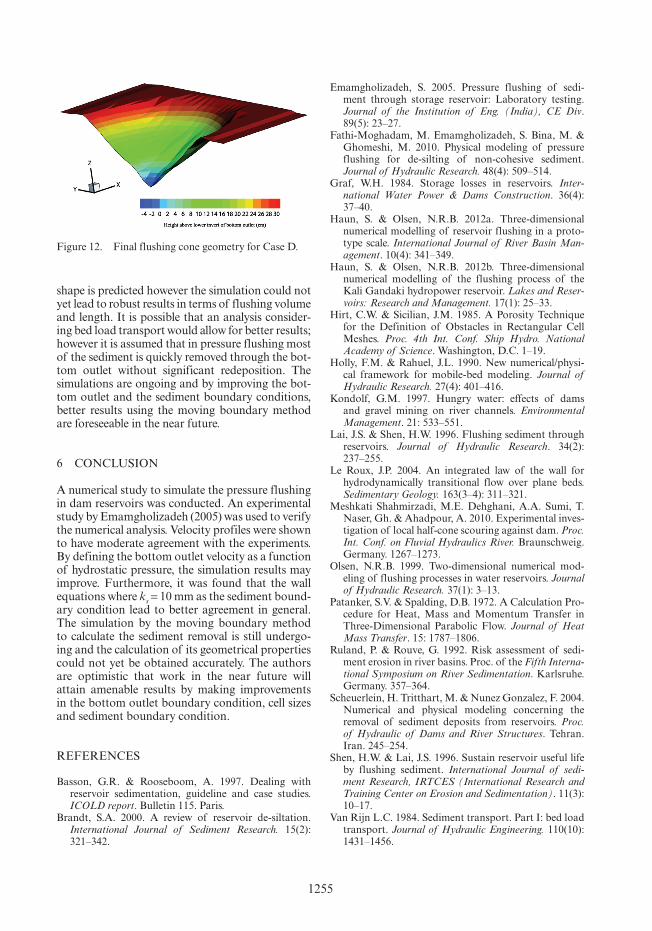
Figure 12. Final flushing cone geometry for Case D.

shape is predicted however the simulation could not yet lead to robust results in terms of flushing volume and length. It is possible that an analysis consider-ing bed load transport would allow for better results; however it is assumed that in pressure flushing most of the sediment is quickly removed through the bot-tom outlet without significant redeposition. The simulations are ongoing and by improving the bot-tom outlet and the sediment boundary conditions, better results using the moving boundary method are foreseeable in the near future.

6 CONCLuSION

A numerical study to simulate the pressure flushing in dam reservoirs was conducted. An experimental study by Emamgholizadeh (2005) was used to verify the numerical analysis. Velocity profiles were shown to have moderate agreement with the experiments. By defining the bottom outlet velocity as a function of hydrostatic pressure, the simulation results may improve. Furthermore, it was found that the wall equations where ks = 10 mm as the sediment bound-ary condition lead to better agreement in general. The simulation by the moving boundary method to calculate the sediment removal is still undergo-ing and the calculation of its geometrical properties could not yet be obtained accurately. The authors are optimistic that work in the near future will attain amenable results by making improvements in the bottom outlet boundary condition, cell sizes and sediment boundary condition.

REFERENCES

Basson, G.R. & Rooseboom, A. 1997. Dealing with reservoir sedimentation, guideline and case studies. ICOLD report. Bulletin 115. Paris.

Brandt, S.A. 2000. A review of reservoir de-siltation. International Journal of Sediment Research. 15(2): 321–342.

1256

Yoneyama, N. 2010. Optimal design of a sand discharge pipe determined by fluid analysis using the moving boundary method. Proc. of the 11th International Symposium on River Sedimentation. Stellenbosch, South Africa. CD-ROM.

Yoneyama, N. Saito, A. & Iguchi, K. 2012. Development of numerical analysis code for predicting behavior of removal sediment from reservoir bed by using dis-charge pipe based on siphon principle. Proc. of Inter-national Symposium on Dams for A Changing World. 24th ICOLD congress. Kyoto, Japan. CD-ROM.

Yoneyama, N. Nagashima, H. & Toda, K. 2012. Three-dimensional numerical analysis to predict behavior of driftage carried by tsunami. Earth Planets Space. 64: 965–972.