
Modernizing irrigation operations: spatially differentiated resource allocations
Upload
khangminh22Category
view
0download
0
DESIGN AND OPERATIONS MANUAL PRESSURIZED IRRIGATION SYSTEMS
VOLUME I
Shehzad Ahmad1, Ali Ajaz2
1 Design Engineer (HEIS) 2 Assistant Design Engineer (HEIS)
Document type: Technical Report
Volume: I
Publisher: Project- Implementation Supervision Consultants (PSC)
Month Published: December, 2013
DOI: 10.13140/RG.2.2.14110.18244
SEE NEXT PAGE
DESIGN AND OPERATIONS MANUAL
PRESSURIZED IRRIGATION SYSTEMS
VOLUME I
Technical Team
Shehzad Ahmad
Design Engineer (HEIS)
Ali Ajaz
Assistant Design Engineer (HEIS)
Principal Editor
Project Manager
December 2013,
Lahore, Pakistan
Project- Implementation Supervision Consultants (PSC)
A Joint Venture of NESPAK and NDC

PREFACE
This manual covers the technical design and operational aspects of high efficiency (pressurized) irrigation
system in a brief and comprehensive way. The first volume covers a detail discussion of pressurized
irrigation systems including their classifications, selection criteria and components followed by basics of
design. Design proforma for design of drip and sprinkler irrigation system has been discussed in detail
covering the procedure for collection of necessary field data required for proper system design. Hydraulic
principles have also been covered in detail for proper selection of pipe network and pumping unit. Design
procedure has been elaborated with solved examples. Second volume of this manual covers the
operational part of pressurized irrigation systems, which includes general maintenance and tips for
durability and sustainability of high efficiency irrigation system equipments. It also covers the vigilance
and checking during system operation, care after completing a crop season, care of prime movers, system
re-adjustments, clogging and its remedies, chemigation including acid treatment and chlorination,
maintenance tips of water storage tanks, general trouble shooting and remedies. A list of tables and
diagrams is also provided for the ease of users. This manual will provide a general guideline to project
technical staff and contractors for proper design and smooth field operations of high efficiency irrigation
system sites and it will also be helpful for effective post installation services and getting the desired results
from high efficiency irrigation systems.


XXXXXXXXXXXXXXXXXXXXXXXX Design and Operations Manual
Project – Implementation Supervision Consultants (PSC) 69
5. BASICS OF HEIS DESIGN
The basic information required for design of micro irrigation system is described in following sections.
5.1 GENERAL INFORMATION
5.1.1 Water Source
It is very essential to confirm the source and quantum of water available before designing of any irrigation system. There are mainly three types of water sources used for irrigation in Pakistan namely Canal water, Tube wells and Dug wells. The location of the water source on the layout map should be demarcated which ultimately helps to locate the best possible location for head unit installation.
Using different methods as given below, the volume of available water can be determined for three types of available water sources.
5.1.1.1 Canal Water
Volume of water available can be calculated as under:
V = (B X C X K)
V = Volume of water available (litres) B = Time of water availability (hrs) C = Discharge of canal outlet (LPS) K = Constant, 3600
If the discharge of the canal outlet is not known, then rough estimation can be made using the float method.
5.1.1.2 Tubewell Water
The discharge of the tubewell water can be estimated by the trajectory method as follows:
The Discharge in LPS can be found as
Example: Determine volume of available water for 1.5 cfs (42.5 lps) canal outlet discharge. Total time of water availability is 5 hours.
B = 5 hrs C = 42.5 lps Volume of available water = (5 x 42.5 x 3600) = 765450 liters (765.450 M3)

XXXXXXXXXXXXXXXXXXXXXXXX Design and Operations Manual
Project – Implementation Supervision Consultants (PSC) 70
Q = 0.0174 X (D)2 / √Y D = Diameter of delivery pipe, cm X = X value of trajectory, cm Y = Y value of trajectory, cm
Fig. 5.1 Trajectory of Water Flow from the Tubewell
Example:
Determine the discharge of a tubewell with pipe diameter 11 cm, X & Y values of trajectory are 55 cm & 25 cm, respectively
Solution: By using equation 3.5 the discharge of tubewell can be calculated as:
Q = 0.0174 X (D)2 / √Y
Q = 0.0174 X (11)2 X 55 / √25
= 23.2 LPS
5.1.1.3 Dug Well
The volume of water in a dugwell can be determined using following relationship.
Available volume of water in m3 can be found as:
V = 3.14 (D)2 (B) / 4

XXXXXXXXXXXXXXXXXXXXXXXX Design and Operations Manual
Project – Implementation Supervision Consultants (PSC) 71
V = Volume of water, m3 D = Diameter of Well, m B = Depth of water column, m
Example:
Calculate water availability for 5 meter diameter dug well, the depth of water column in the dug well is 2m.
Using equation 3.4, volume of available water in the dug well can be calculated as:
V = 3.14 x (5 x 5) x 2 / 4 = 39.25 m3
5.2 FIELD LAYOUT AND TOPOGRAPHY
The first step to proceed for the design is to determine the area of the field layout for which the system is to be designed. This may be done measuring directly the lengths and the widths of the field. A particular farmer field will be of specific geometrical shape such as square and rectangular. Sometimes it may be of irregular shape. Measurements for such area will not be easy with conventional systems using measuring tapes; it may require use of Global Positioning System (GPS) for establishing plot boundaries and directly measuring the area. Particular geometrical shapes and formulae for calculating area are given below:
A = (L1 X W1) + (L2 X W2)
Where; L1, L2 = Length, m (ft) W1, W2 = Width, m (ft)
A = L X W )
A = Area, m2 (ft2) L = Length, m (ft) W = Width, m (ft)
W2
L2
W1 L1

XXXXXXXXXXXXXXXXXXXXXXXX Design and Operations Manual
Project – Implementation Supervision Consultants (PSC) 72
A = ½ X b X h
A = Area, m2 (ft2) b = Width, m (ft) h = Height of triangle, m (ft)
In case the area to be irrigated is fairly large and visibly having topography uneven, a topographic survey of the area is carried out in order to determine the general slope and contours are drawn. If practically possible, the main line is laid along contours and sub-mains are laid along the slope. Accordingly, a field layout is drawn showing the dimensions (length and width) of the area, location of water source/pump-set, location and lengths of main, sub-mains, laterals according to the plant or row spacing
5.3 CROPS
Information regarding crops should be entered in “crop information” section of the design proforma as given in Table 5.1
Table 5.1 Crop Information Proforma
Parameters Crop Area
(acres)
Plant spacing
(m)
Row spacing
(m)
Age of crop
(years)
Sowing Date
Harvesting Date
Block-I Row crops Proposed Rotation
Sub-Total: I
Block-II Orchards Type-I Type-II
Sub-Total: II Block-III Annual Crops
Sub-Total: III
Block-IV Field Crops Type-I Type-II
Sub-Total: IV
Total / Design Value

XXXXXXXXXXXXXXXXXXXXXXXX Design and Operations Manual
Project – Implementation Supervision Consultants (PSC) 73
5.3.1 Row Crops
Line source drip systems are generally suitable for row crops such as cotton, maize, cucumber, chilli, capsicum, melons, tomatoes, onions, sunflower and sugarcane etc. Sprinklers can also be used on most of these crops with certain care. Generally distance between two plant rows is kept 0.76 m (2.5 ft) under conventional planting practice (Furrow), whereas under drip irrigation system it will cost more. An appropriate technique may be to place on drip line at 1.52 m (5 ft) spacing (depending upon soil characteristics) and planting two plant rows on each side of the lateral. A single drip line may be provided for two or more crop rows or for a single crop row depending upon growth behavior. The information needed for designing a system includes distance between rows of crop and the time of sowing and harvesting etc. Similar information regarding rotational crop is very important for selecting and designing a suitable system that will be suitable for both the crops.
5.3.2 Orchards
Orchards comprise of fruits or nut producing trees grown for commercial production. Point source drip line, mini sprinklers, spray jets or bubblers can be used for irrigation of orchard depending upon plant stage. Most of the orchard crops grown in Pakistan include Banana, Coconut, Guava, Mango, Citrus, Date Palm, Lychee, Apple, Apricot, Chikku, Ber, Peach and Plum. The information regarding time of sowing, age of crop, canopy diameter and spacing between plants and rows of matured/new orchard is required to be collected for designing purpose. It is also important to note whether farmer plans to go for intercultural practices in the orchard or not. This should be decided at the planning stage and will effect the selection of particular emitting devices/high efficiency irrigation system.
5.3.3 Annual Crops
This category particularly covers sugarcane which remains standing for whole of the year.
5.3.4 Field Crops
It comprises a particular group of crops which are not cultivated in geometrical shapes (beds, furrow) but are broadcasted like wheat, fodders, oilseeds etc. sprinkler system is suited for such kind of crops.
5.4 IRRIGATION SYSTEM EFFICIENCY
Irrigation system efficiency is that part of the water pumped or diverted through the conveyance system which is used effectively by the plants. It is the product of two types of efficiencies i.e., conveyance efficiency and field application efficiency. Conveyance efficiency represents the efficiency of water transported in canals, watercourses and field application efficiency represents the efficiency of water application in the field. For pressurized irrigation systems, conveyance efficiency is almost 100% and thus design engineers are only concerned with field application efficiency. Conventional irrigation system is the lowest efficient method. Among pressurized irrigation systems, drip is the most efficient irrigation method as shown in Fig. 5.2

XXXXXXXXXXXXXXXXXXXXXXXX Design and Operational Manual
Project – Implementation Supervision Consultants (PSC) 74
Fig. 5.2 Least to Most Efficient Irrigation Systems
Field application efficiency mainly depends on the irrigation method and the level of farmer discipline. Some indicative values of the average field application efficiency are given in following Table 3.4.
Table 5.2 Values of Field Application Efficiency
Water Application Method Water Use Efficiency (%)
Surface 40-70
Sprinkler (Center Pivot) 85-90
Sprinkler (Linear Move) 80-88
Fixed Sprinkler (Solid set) 60-85
Trickle/ Drip (Point Source) 65-92
Trickle/ Drip (Line Source) 60-85
5.5 WATER QUALITY
Quality of water is very important for prevention of clogging in micro irrigation system especially for drip irrigation system. Potential contributors towards emitter clogging are shown in Table 5.3
Least Efficient
Most Efficient
Flood Irrigation
Furrow Irrigation
Bubbler Irrigation
Sprinkler Irrigation
Drip Irrigation

XXXXXXXXXXXXXXXXXXXXXXXX Design and Operational Manual
Project – Implementation Supervision Consultants (PSC) 75
Table 5.3 Major Contributors of Emitter Clogging PHYSICAL
(Suspended Solids)
CHEMICAL (Precipitation)
BIOLOGICAL (Bacteria and algae)
1. Sand 1. Calcium or magnesium carbonate 1. Filaments
2. Silt 2. Calcium sulphate 2. Slimes
3. Clay 3. Heavy metal hydroxides, oxides, carbonates, silicates and sulphides
3. Microbial depositions:
(a) Iron
(b) Sulphur
(c) Manganese
4. Organic matter 4. Fertilizers 4.Bacteria
(a) Phosphate
(b) Aqueous ammonia
(c) Iron, zinc, copper, manganese
5.Small aquatic organisms
(a) Snail eggs
(b) Larva
(Source: FAO, 1994)
Prevention requires an understanding of the potential problems associated with a particular water source. Water quality information should be obtained and made available to the designer and irrigation manager in the early stages of the planning so that suitable system components especially the filtration system and management and maintenance plans can be selected. Water quality refers to the characteristics of a water supply that will influence its suitability for a specific use, i.e. how well the quality meets the needs of the user. Quality is defined by certain physical, chemical and biological characteristics (FAO) and may impose long term impacts on soil as well as result in clogging of micro irrigation system. Type and quantity of dissolved salts will determine the severity of water quality. Standard water quality tests are shown in Table 5.4.
Table 5.4 Standard quality tests for Micro Irrigation System Major Inorganic Salts Micro-organisms
Hardness1 Iron
Suspended Solids Dissolved Oxygen
Total Dissolved Solids (TDS)1 Hydrogen Sulphide
BOD (Biological Oxygen Demand) Iron Bacteria
COD (Chemical Oxygen Demand) Sulphate Reducing Bacteria
Organics and Organic Matter (Source: FAO, 1994)

XXXXXXXXXXXXXXXXXXXXXXXX Design and Operational Manual
Project – Implementation Supervision Consultants (PSC) 76
The analysis needed will vary with each situation. It is to keep in mind that cost of the micro irrigation system is very high and it is advisable to bear some additional cost which is very nominal to perform these tests so as the system can be run effectively. The presence of elements (Table 5.6) in irrigation water will determine the degree of clogging and restriction of water use.
Table 5.6 Influence of water quality on emitter clogging
Potential Problem Units Degree of Restriction on Use
None Slight to Moderate Severe Physical Suspended Solids mg/l < 50 50 – 100 > 100 Chemical pH < 7.0 7.0 – 8.0 > 8.0 Dissolved Solids mg/l < 500 500 – 2000 > 2000 Manganese2 mg/l < 0.1 0.1 – 1.5 > 1.5 Iron3 mg/l < 0.1 0.1 – 1.5 > 1.5 Hydrogen Sulphide mg/l < 0.5 0.5 – 2.0 > 2.0 Biological Bacterial populations maximum
number/ml <10 000 10 000 – 50 000 >50 000
(Source: FAO, 1994)
5.6 LEACHING REQUIREMENT
Presence of salts in irrigation water and in the soil affects the crop yield. Under micro irrigation system, salts are usually repelled away from the wetting front of the emitter; therefore, marginally saline water can be used efficiently for crop production. For sprinkler irrigation system, irrigation frequency may be more than one day especially under rain-guns; there is a need to account for leaching requirements to leach the salts down from root zone of the plant. It is important to keep the salinity level within permissible limits by applying additional quantity of water to soil/plants so that yield may not be reduced more than 10%.
Leaching requirement (LR) can be estimated using following equation (Rhoades and Merrill 1976):
LR = minimum leaching requirement (Fraction) needed to control salts within the tolerance (ECe) ECw = salinity of the applied irrigation water in dS/m which can be determined by laboratory analysis
ECe = Average soil salinity tolerated by the crop as measured on a soil saturation extract which is depicted in Table 5.7

XXXXXXXXXXXXXXXXXXXXXXXX Design and Operational Manual
Project – Implementation Supervision Consultants (PSC) 77
Table 5.7 Values of ECe with 10% yield reduction Crop ECe – dS/m
Cotton 9.6 Sorghum 5.1 Wheat 7.4 Corn (maize) 2.5 Tomato 3.5 Cucumber 3.3 Spinach 3.3 Potato 2.5 Onion 1.8 Date palm 6.8 Orange 2.3 Apple 2.3 Peach 2.2 Apricot 2.0 Grape 2.5 Almond 2.0
Example: Calculate Leaching Requirement for sprinkler system
Given data: Crop: Wheat ECw: 2.1 dS/m
Solution: Select ECe of wheat from Table 3.8. ECe = 7.4 and solving equation 3.8.
LR = 2.1/(5x7.4 - 2.1) = 0.06 (fraction)
5.7 WETTED AREA
Wetted area is important for micro irrigation system as only portion of the plant’s area is wetted as shown in Fig. 5.2. The first criterion, wetting a sufficient portion of the plant's root volume, must be achieved for a plant to efficiently utilize the water that is delivered.
When drip devices are used, the area or volume of the soil that is wetted depends on the soil type and emitter flow rate. At least 33 percent and up to 67 percent of the plant root zone should be wetted to get the maximum benefit from micro-irrigation. On sandy soils, micro- spray or sprinkler emitters rather than drip emitters may be needed to wet sufficient root volume.

XXXXXXXXXXXXXXXXXXXXXXXX Design and Operational Manual
Project – Implementation Supervision Consultants (PSC) 78
Fig. 5.2 Partial wetting of soil under micro irrigation system (Source: FAO,)
While published guidelines for drip emitter wetted diameters on typical sand, loam and clay soils can be used, it is much better to field test by actually wetting one or more selected typical locations in the field. This can be done easily by setting up a small portable pump (or connecting to a house or barn water system) and running a suitable line with drip emitters attached to the selected sites (adjust pressure according to emitters used). The wetting patterns which develop from dripping water onto the soil depend on discharge and soil type. Fig. 5.5 & 5.6 shows the effect of changes in discharge on two different soil types, namely sand and clay.
Fig. 5.3 Wetting patterns for Sandy soils with high and low discharge (Source: FAO,)

XXXXXXXXXXXXXXXXXXXXXXXX Design and Operational Manual
Project – Implementation Supervision Consultants (PSC) 79
Fig. 5.4 Wetting patterns for Clay soils with high and low discharge rates
On sandy soils, the maximum wetted width may be reached in as little as two hours, but on clay soils this may take 12 to 15 hours (caution: do not allow surface runoff to occur). For safety, the emitter should be operated the same number of hours that is planned for the zone set time, according to soil type. Measurement of wetted diameter is done by trenching across the visible wetted edge to see how far from the emitter water has moved. The wetted area will be wider beneath the soil surface, but it is impossible to know how far it extends without digging. Estimated wetted area by 4LPH dripper is given in Table 5.7a.
Table 5.7a Estimated are wetted by 4 L/hr emitter (m x m)
Soil depth (m) Soil Texture Degree of soil stratification
Homogeneous Stratified Layered
0.75
Coarse 0.4 x 0.5 0.6 x 0.8 0.9 x 1.1
Medium 0.7 x 0.9 1.0 x 1.2 1.2 x 1.5 Fine 0.9 x 1.1 1.2 x 1.5 1.5 x 1.8
1.5
Coarse 0.6 x 0.8 1.1 x 1.4 1.4 x 1.8
Medium 1.0 x 1.2 1.7 x 2.1 2.2 x 2.7 Fine 1.2 x 1.5 1.6 x 2.0 2.0 x 2.4
(Source: Jack Keller and Ron D.Bliesner- 1990)
Table 5.8 can also be used if none of the information regarding wetted diameter or area of soil available. To be on safer side lower values may preferably to used.

XXXXXXXXXXXXXXXXXXXXXXXX Design and Operational Manual
Project – Implementation Supervision Consultants (PSC) 80
Table 5.8 Estimated area wetted
Soil Type
Diameter (m) Area (m2) Min Max Average min max Average
Sandy (coarse soil) 0.8 1.5 1.1 0.46 1.82 1.14
Loam (medium soil) 1.5 2.7 2.1 1.82 5.91 3.87
Clay (fine soil) 2.7 4.3 3.5 5.91 14.30 10.11
5.8 POWER SOURCE
All sprinkler and drip irrigation systems require energy to move water through pipe distribution network and deliver it through the emitting devices. In some instances, this energy is provided by gravity as water flows downhill through the delivery system which is most likely possible in Balochistan, NWFP and Northern areas of Pakistan. However, in most irrigation systems, energy is provided by a pump that in turn receives its energy from either an electric motor or an internal combustion engine. The combination of pump and engine is central to the performance of most irrigation systems. The most common power source/drive units for pumps are electric motors, diesel or petrol engines and PTO of tractors.
5.8.1 Electric Motors
Electric motors are more efficient, cheaper to maintain and where they needed to be run continuously, the fuel costs are lower than for other types of power source. On drip irrigation system, mostly Three Phase Motors are installed. Before designing a system, a transformer of required capacity must be ensured to operate the system. The electricity supply in Pakistan is 50 cycles and the standard motor operating speeds are 2900 rpm, 1450 rpm and 960 rpm. Ideally the pump unit should couple direct to the motor shaft so the speeds of the two units are identical. However, where a different pump speed is required, V-belts and pulleys will be required. Efforts should be made to select an efficient electric motor to keep the operational cost low.
5.8.2 Petrol Engines
Petrol engines can be used for intermittent operation such as supplementary irrigation, where the operating time per day does not exceed two or three hours. The use of CNG fuel is becoming more widespread in Pakistan which can be a good replacement of petrol to be used.
5.8.3 3. Diesel Engines
Compact high speed diesel engines should be used as energy source where electricity is not available. Diesel engines offer the most efficient form of drive for

XXXXXXXXXXXXXXXXXXXXXXXX Design and Operational Manual
Project – Implementation Supervision Consultants (PSC) 81
pumps. They are particularly suited for use on portable installations. Care should be taken to select a suitable drive unit otherwise operational cost will become much higher as compared to the electricity.
5.8.4 Tractors
Tractor can also be used as power source for high pressure system such as Rain Gun sprinkler system which requires high energy or to drive pumps as a stand-by measure in the event of the primary unit breaking down or where the scheme is primarily for supplementary irrigation and is only operated for a few hours every day.

XXXXXXXXXXXXXXXXXXXXXXXX Design and Operational Manual
Project – Implementation Supervision Consultants (PSC) 82
6. DRIP DESIGN STEPS
The main objective of an irrigation system design is to supply adequate and timely water to plants and to help farmer to get best out of his fields. The following considerations may help achieve this objective:
1. Planning proper irrigation zones and system layout2. Properly engineered system components
Properly engineered system components are secondary to a good system layout and it has a little value if the system has not been properly zoned and planned. It may include the following objectives:
Optimum selection of the system components Ease in operation and maintenance of the system Low system cost with high efficiency
6.1 OBJECTIVE OF DESIGN
• Selection of Optimum Components• Easy Management and Maintenance of System Parts• Low System Cost Vs High Efficiency• To help farmer get best out of his field• To maintain higher system and irrigation efficiency by means of higher
emission uniformity.• To maintain optimum moisture level in soil for optimization of crop yield.• To maintain both initial investment and annual cost at minimum level.• To design suitable type of system which last and perform well.• To design a manageable system which can be easily operated and maintained.• To satisfy and fulfill the requirements of crops and farmers.

XXXXXXXXXXXXXXXXXXXXXXXX Design and Operational Manual
Project – Implementation Supervision Consultants (PSC) 83
6.2 DRIP DESIGN PROCEDURE-STEP BY STEP (ORCHARD)
Under the on-going project, drip systems are being installed on orchard and at row crops/vegetables. In this section, steps for designing a drip system for orchard will be discussed. The following are the design steps.
1. Collection of Basic Information2. Estimation of Peak Water Requirement PWR3. Drawing of project area, selection of zone area and No. of Operations4. Selection of emitter/dripper, and flow rat5. No. of emitters per plant, No. of drip lines per row, optimal distance between
two laterals6. Calculation of plant area, total number of plants and minimum number of
emitters per plant7. Calculation of total length of lateral and total No. of emitters8. Calculation of Total Flow rate requirement (Q)9. Calculation of Application Rate10. Total Operational Time11. Pipe Hydraulics12. Selection and Design of Lateral Line13. Design of Sub-mainline14. Design of Mainline15. Selection of Filters and other equipment and head loss16. Calculation of total dynamic head (H)17. Calculation of required horsepower (HP)18. Selection of Pumps and Motor19. Preparation of Drawing20. Preparation of Bill of Quantities

XXXXXXXXXXXXXXXXXXXXXXXX Design and Operational Manual
Project – Implementation Supervision Consultants (PSC) 84
Step 1. Collection of Basic Information
The following basic information be available before designing a drip irrigation system.
• General information: Name of farmer, village/chak No., tehsil, district, phoneNo.
• Land holding and Area spared for the project• Engineering survey: GPS coordinates, Field measurement, Elevation
difference/slope. After field measurement, a map showing all dimensions andlocation of water source be drawn
• Agricultural details: crops (orchard, row/field crop), spacing, type, age,reference evapotranspiration of the area and water requirement of crop
• Crop Spacing (Row to Row, Plant to Plant), sowing and harvesting date• Soil Type/texture• Soil and water analysis reports: water quality, presence of iron, pH,
suspended particles, soil type, Ec, pH• Water Source, quantity, availability, location• Power Source:Electric motor, diesel engine, tractor, solar system• Climatologically data: temperature, humidity, rainfall, wind speed • Peak Water Requirement: (ETo, Kc, Cf)• Water source and Total Available Time of water• System capacity: The system should have capacity adequate to fulfill daily crop
water requirements of the area within a stipulated time or not more than 12hours of operation per day (only for Pakistan circumferences, otherwise may be22 hrs).
The basic information can be categorized as under.

XXXXXXXXXXXXXXXXXXXXXXXX Design and Operational Manual
Project – Implementation Supervision Consultants (PSC) 85
6.2.1 General Information
Name of beneficiary Town/Village/City Tehsil District Province Phone No. Land holding (Acre) Scheme area (acres) Topography (Flat/Undulated)
6.2.2 Crop Information
Parameters Crop Area
(acres)
Plant spacig (m)
Row spacing (m)
Age of crop(year
s)
Sowing date
Harvesting date
Block-I
Orchard
Proposed Citrus 7.04 3.10 6.1 2 Rotation
Sub total: I
Block-I
Orchard Proposed Citrus 6.07 4.57 4.57 New Rotation
Sub total: II
Block-I
Orchard Proposed
Mango 1.2 6.10 6.1 1
Rotation Sub total: III
Block-I
Sub total: IV

XXXXXXXXXXXXXXXXXXXXXXXX Design and Operational Manual
Project – Implementation Supervision Consultants (PSC) 86
6.2.3 Soil Type/Soil Test/Water Supply/Water Quality
Soil type/Texture
Soil limitation (soil analysis report attached)
Soil EC , PH , N , P , K , SAR
WATER SUPPLY
Available water sources
1) Canal
Sanctioned discharge (LPS)
Perennial/non-perennial
Warabandi Days
Hours per Warabandi
Total Volume (m3) of water for 7 days
2) Groundwater
a) Dug well
Depth of well
Diameter of well
Recharge rate
b) Tube well/bore well
Discharge capacity (LPS)
Diameter of bore (inches)
Depth of water table from ground (m)
3) Storage/reservoir capacity (m3)
Water quality (detailed report attached)
Iron
Ph
EC(mmohs/cm)
Distance of water source from field (m)

XXXXXXXXXXXXXXXXXXXXXXXX Design and Operational Manual
Project – Implementation Supervision Consultants (PSC) 87
6.2.4 POWER SOURCE AND PUMP
POWER SOURCE Type of power to be used For electric Motor,
ELECTRICITY NOT AVAILABLE
Type of connection (single/3-phase) Make/model HP of Motor RPM of Motor
For diesel engine Make HP Condition) For Tractor Make/model HP Condition Any other power source, if any PUMP SET Type Make/Model Pressure (ft/psi/bar) Flow(lps) Inlet/outlet size RPM Pulley size

XXXXXXXXXXXXXXXXXXXXXXXX Design and Operational Manual
Project – Implementation Supervision Consultants (PSC) 88
6.2.5 Water Analysis Report Farmer Name : Abbass Qureshi Water Source Tube Well Address :Muzaffar garh Sampling Date 10/5/2010
Ph :0345-8644888 Sp Receive Date : 13/05/2010
Agronomist: Ather Mehmood Khursheed Report Date : 31/05/2010 Ref.Sample # 372
Parameters Degree of Presence / Problem Lab
Result Unit Noma
l Higher Extrem
e pH 7 <7 Acidic >7 A 7.37 Electrical Conductivity (Salinity)
microsemens/cm - - - 2240
Total dissolved solids ppm <500 500 - 600 >600 1290 Hardness ppm <200 200 - 300 >300 312 Calcium ppm <60 60 - 100 >100 78.4 Magnesium Ppm <25 25 - 40 >40 28.21 Carbonate Ppm <200 200 - 600 >600 72 Bicarbonate Ppm <200 200 - 600 >600 176 Chloride (Toxic) Ppm <140 140 - 350 >350 198.5 Sulphates Ppm <20 20 - 50 >50 23.4 Sodium Ppm <100 100 - 200 >200 235 SAR - <3 3-9 >9 2 Potassium Ppm <10 10 - 20 >20 12 Sulphides Ppm <15 15-25 >25 - Iron Ppm <0.1 0.1 - 0.4 >0.4 0.1 Manganese Ppm <0.2 0.2 - 0.4 >0.4 - Suspended solids Ppm <10 10 - 100 >100 7.1 Boron Ppm <0.5 0.5 - 2.0 >2.0 -

XXXXXXXXXXXXXXXXXXXXXXXX Design and Operational Manual
Project – Implementation Supervision Consultants (PSC) 89
Figure 6.1. Sample Report

XXXX
XXXX
XXXX
XXXX
XXXX
XXXX
C
rop
Wat
er R
equi
rem
ent &
Irrig
atio
n Sc
hedu
ling
Proj
ect –
Impl
emen
tatio
n Su
perv
isio
n C
onsu
ltant
s (P
SC)
9
0
6.2.
6 So
il An
alys
is R
epor
t
Farm
er N
ame
: Ab
bas
Qur
eshi
B
lock
Siz
e
: Ad
dres
s
:
M
uzaf
farg
arh
Sam
plin
g D
ate
:
11
/5/2
010
Ph
:
3458
6448
8 Sp
Rec
eive
Dat
e :
13/0
5/20
10
Agro
nom
ist
:
Athe
r Meh
moo
d Sh
eikh
R
epor
t Dat
e
:
26
/04/
2010
C
ode
:
AMK
-S00
1
Ref
.Soi
l Sa
mpl
e #
Blo
ck
# D
epth
(inch
es)
Text
ure
Org
anic
M
atte
r %
pH
Elec
tric
al
cond
uctiv
ity
(mic
/cm
)
Avai
labl
e Ph
osph
orus
(P)
(ppm
)
Avai
labl
e Po
tass
ium
(K)
(ppm
) So
lubl
e &
Ex
ch. N
a (m
eq/L
)
Solu
ble
&
Ca
+Mg
(meq
/L)
SAR
Neu
tral
6.5-
7.5
Al
kalin
e >8
.5
Poor
<7.
0
Med
ium
7-1
3 Sa
tisfa
ctor
ty >
13
Poor
<12
5
Med
ium
125
-25
0 Sa
tisfa
ctor
ty
>250
Nor
mal
<1
0.0
Sodi
c >1
0.0
2835
1
0 - 6
'' Sa
nd,C
lay
0.24
5 8.
44
411
- 11
0 6.
52
3.2
4 28
36
6 - 1
2''
Sand
,Cla
y 0.
582
7.74
46
8 -
120
6.95
3.
2 4.
3 28
37
2 0
- 6''
Sand
,Cla
y 0.
827
8.15
57
2 -
110
11.7
3 3.
1 7.
5 28
38
6 - 1
2''
Sand
,Cla
y 0.
612
8.26
55
0 -
110
10.4
3 2.
7 7.
7 28
39
3 0
- 6''
Sand
,Cla
y 0.
612
8.29
31
6 -
90
6.52
3.
4 3.
8 28
40
6 - 1
2''
Sand
,Cla
y 0.
735
8.39
30
4 -
90
6.95
3.
7 3.
7 28
41
4 0
- 6''
Sand
,Cla
y 0.
821
8.21
38
4 -
100
6.08
3.
2 3.
8 28
42
6 - 1
2''
Sand
,Cla
y 0.
735
8.25
35
8 -
100
6.52
3.
2 4
2843
0
- 6''
Sand
,Cla
y 1.
01
8.02
50
6 -
150
4.34
5.
1 1.
7 28
44
6 - 1
2''
Sand
,Cla
y 0.
98
8.02
49
4 -
160
4.34
4.
2 2
2845
6
0 - 6
'' Sa
nd,C
lay
1.04
1 8.
05
412
- 12
0 4.
34
4.2
2 28
46
6 - 1
2''
Sand
,Cla
y 0.
919
8.11
35
6 -
100
4.34
4.
2 2
2847
7
0 - 6
'' Sa
nd,C
lay
0.91
9 7.
97
1080
-
80
10.8
6 6.
6 3.
2 28
48
6 - 1
2''
Sand
,Cla
y 0.
549
8.02
11
23
- 80
11
.73
5.8
4

XXXXXXXXXXXXXXXXXXXXXXXX Design and Operational Manual
Project – Implementation Supervision Consultants (PSC) 91
It is advisable to make rough map of the area and mark salient features, divide the drawn map into different blocks and number the same for soil and water sampling. This map will be finalized during designing of drip irrigation system and will show all necessary details including drippers, dia, length and location of laterals, submain and main, location of water source, power source etc.,

XXXXXXXXXXXXXXXXXXXXXXXX Design and Operational Manual
Project – Implementation Supervision Consultants (PSC) 92
6.2.7 Estimation of Peak Crop Water Requirement
Estimating the reference crop evapotranspiration (ETo), using the Penman-Monteith method, and the crop evapotranspiration (ETc), through the use of the appropriate crop factor Kc, have been covered in Chapter-4 of this Manual. Evapo-transpiration is composed of the evaporation from the soil and the transpiration of the plant. Since under localized irrigation only a portion of the soil is wetted, the evaporation component of evapotranspiration can be reduced accordingly, using the appropriate ground cover reduction factor Kr.
For the design of surface and sprinkler irrigation systems: ETc = ETo x Kc
For the design of Drip irrigation systems:
Water Requirements for Orchard ETc= ETo x Kc x Canopy Factor/ Efficiency Percent area wetted, 100% for closely spaced crops with rows and emitter lines less than 1.8m.
Peak Crop Water Requirement can be tabulated as under. Month J F M A M J J A S O N D
Eto (mm/d) 2.1 2.7 4.2 5.6 7 7.9 7.3 6.8 5.9 4.8 3.3 2.3 Kc (citrus) 0.7 0.7 0.7 0.7 0.7 0.7 0.7 0.7 0.7 0.7 0.7 0.7 Crop factor at mat. 0.57 0.57 0.57 0.57 0.57 0.6 0.57 0.57 0.57 0.57 0.6 0.57 Efficiency 0.9 0.9 0.9 0.9 0.9 0.9 0.9 0.9 0.9 0.9 0.9 0.9 PCWR (citrus) 0.93 1.20 1.86 2.48 3.10 3.50 3.24 3.01 2.62 2.13 1.46 1.02 Kc (mango) 1.1 1.1 1.1 1.1 1.1 1.1 1.1 1.1 1.1 1.1 1.1 1.1 Crop factor at mat. 0.55 0.55 0.55 0.55 0.55 0.6 0.55 0.55 0.55 0.55 0.6 0.55 PCWR (mango) 1.41 1.82 2.82 3.76 4.71 5.31 4.91 4.57 3.97 3.23 2.22 1.55 Kc (field crops) CWR (field crops)
6.2.8 Drawing of Project Area, Selection of zone area and No. of Operations
A map of the scheme area be drawn and tentative number of zones having equal area of the project be selected to estimate number of operations. It is advisable that area of each of each zone must be equal so that all the discharge coming out from the pump be fully utilized in each zone area. In case all zones are not equal, some additional water has to be sent back to the water storage tank through bypass valve during irrigation of small area zones.
6.2.9 Step 4. SELECTION OF EMITTER/DRIPPER AND FLOW RATE
Varieties of drippers/drip tubing are available with different discharge rates, dripper spacing, characteristics and suitability for different crops. The emitter selected for the drip system:

XXXXXXXXXXXXXXXXXXXXXXXX Design and Operational Manual
Project – Implementation Supervision Consultants (PSC) 93
• Should be Inexpensive, durable and serviceable• Should have relatively low discharge rate to keep the system cost low• Should have higher emission uniformity (90%) and low coefficient of variation (CV
5%) • Should have emission discharge exponent in the range of 0.4-0.7.• Should have relatively large cross sectional area and flow path to avoid clogging• Should have turbulent flow path and pressure compensation action• Should not create runoff within the immediate application area
Drippers are available for 2, 4, 8 and 12 LPH discharge. Emitter operating pressure is usually 10m.
E/
The shape of the wetted zone of the emitter depends on the physical properties
In sandy and light soil, the water will tend to go straight down, and there will be less lateral movement as compared to downward movement. In light soils, the distribution of the water will be narrow and deeper
(close spaced low discharged emitters/Closer emitter spacing)
In loamy soil, the water will move slowly and will spread evenly
(average discharged emitter &/or Spacing)
In clay soil, the water will be absorbed very slowly and there will be more lateral movement as compared to downward movement. In heavy soil, the distribution of the water will be relatively spherical shape, wider and less depth.
wider emitter spacing

XXXXXXXXXXXXXXXXXXXXXXXX Design and Operational Manual
Project – Implementation Supervision Consultants (PSC) 94
Recommended emitter spacing (cm) for various Discharge Rates (LPH) in different soils

XXXXXXXXXXXXXXXXXXXXXXXX Design and Operational Manual
Project – Implementation Supervision Consultants (PSC) 95
Soil Type Discharge Rates (LPH) 2 LPH 4 LPH 8 LPH
Light 40 80 120
Medium 80 120 160
Heavy 120 160 200
• Heavy soil recommended distance: 0.50 to 1.00 meter*• Medium soil recommended distance: 0.40 to 0.75 meter*• Light soil recommended distance: 0.20 to 0.50 meter*• *The spacing between drippers depend on the root depth of the crop.
Emitter spacing should be maximum 0.5m, 0.4-0.6 and 0.5-0.8m in light, medium and heavy soil respectively.

XXXXXXXXXXXXXXXXXXXXXXXX Design and Operational Manual
Project – Implementation Supervision Consultants (PSC) 96

XXXXXXXXXXXXXXXXXXXXXXXX Design and Operational Manual
Project – Implementation Supervision Consultants (PSC) 97
Calculation of X value for a 4 LPH discharge emitter
Most of the water emitter flow regime is fully turbulent with an exponent value equal to 0.5. In order to ensure a high uniformity of water application over the field, the differences in the discharge of the emitters should be kept to the minimum possible and in no case exceed 10 percent. These criteria were established by J. Christiansen for sprinklers and are now applied in all pressurized systems. As a general rule, the maximum permissible difference in pressure between any two emitters in operation should be no more than 20 percent. The lateral lines with emitters must be of a size that does not allow a loss of head (pressure) due to friction of more than 20 percent. In case emitter operating pressure is 01 bar or 10 meter, the head loss in the selected lateral must not be more than 02 meter.

XXXXXXXXXXXXXXXXXXXXXXXX Design and Operational Manual
Project – Implementation Supervision Consultants (PSC) 98
Coefficient of Variation (Cv) of Emitter
Coefficient of Variation is a measure of consistency in the flow. If we randomly select several emitters and measure the discharge of each at nominal pressure, the consistency in the results will reveal Cv of the product.
Cv = Standard Deviation of Discharge Rate Average Discharge Rate of Sample
6.2.10 No. of Emitters per Plant, No. of Drip Lines per Row and optimal Distance between two Laterals
No. of emitters/drippers per plant can be 2, 4 or 6. No. of drip lines per row can be 02. Optimal distance between two laterals can be 20 feet (6.1 m)
6.2.11 Step 6. Calculation of Plant Area and Total Number of Plants and Minimum No. of Emitters per plant
Plant Area
Individual plant such as orchards will be irrigated by individual emitters. Area of each plant will be required for estimation of number of plants in scheme as well as for calculation of water requirements. Area for individual plant can be determined by using following relationship.
Ap = SP x SR Where
Ap = Plant area (m2) SP = Plant spacing (m) SR = Row spacing (m)
No. of Plants
Np = A / Ap Where
Np = Number of plants A = Scheme area (m2)
Example: Scheme area = 8.1 ha (20 acre) Plant spacing = 5 m Row Spacing = 5 m Plant area = 5 x 5 = 25 m2 No. of plants = 20 x 4047 m2 ÷ (25 m2)
= 3,238 Nos.

XXXXXXXXXXXXXXXXXXXXXXXX Design and Operational Manual
Project – Implementation Supervision Consultants (PSC) 99
For row crops, almost entire field will be covered by the crops and hence number of plants is not important as their water requirements will be calculated based on the shaded area which is usually taken as 100%.
Note: Number of plant is not important for sprinkler system
6.2.12 Emitter Placement Geometry
In drip irrigation systems, the lateral lines are the pipes on which the emitters are attached. Water flows from the manifold into the laterals, which are usually made of plastic tubing ranging from 10 mm to 25 mm in diameter. Continuous-size tubing provides better flushing. The layout of lateral lines should be such that it provides the required emission points for the crop to be irrigated. Sometimes two laterals per row of trees are needed. Other methods of obtaining more emission points per tree are zigzag and "snake" layouts and use of pigtail lines looped around or between the trees. Figs 6.1 to 6.4 show various lateral layouts for widely spaced permanent crops.
Single line for each row of tree
For a drip system with straight laterals of single drip emitters and emitter spacing (Se) equal to or less than optimum emitter spacing (Se’) then percent area wetted Pw, can be computed by following equation
Where: Pw = Percent area wetted e = number of emission points per plant. Se = spacing between emitters on a lateral, m or feet. Sw = width of the strip that would be wetted by emitters on a lateral at Se’: or closer, m/feet. Sp = plant spacing in the row, m/feet. Sr = plant row spacing, m/feet.
Fig. 4.1 Single lateral line for each row of plants

XXXXXXXXXXXXXXXXXXXXXXXX Design and Operational Manual
Project – Implementation Supervision Consultants (PSC) 100
Double line for each row of tree
For drip systems with double laterals or zigzag, pigtail, or multi exit layout, wetted area Pw, can be computed by following equation.
For double laterals, the two laterals should be placed apart at a distance equal to Se’. This spacing gives the greatest Aw, and leaves no extensive dry areas between he double lateral lines. For the greatest Aw, with zigzag, pigtail, and multi exit layouts, the emission points should be placed at a distance equal to Se’ in each direction.
Fig. 6.2 Two lateral lines for each row of plants
Fig. 6.3 Zigzag style of lateral placement along plant stem
Fig. 6.4 Pig tail style of lateral placement along plant stem

XXXXXXXXXXXXXXXXXXXXXXXX Design and Operational Manual
Project – Implementation Supervision Consultants (PSC) 101
Spray System
For a drip system with spray emitters, Pw, can be computed by following equation.
Where; As = estimate of the soil surface area wetted per sprayer from field tests with a few sprayers, square meters/ square feet/. PS = perimeter of the area directly wetted by the test sprayers, feet/m. 1/2Se’ = one-half the Se’ values for homogeneous soils, m/feet
Minimum No. of Emitters
For micro irrigation system (drip, bubbler, micro jets) type and numbers of emitters are selected based on the soil, crop and area to be wetted. The number of emitters is based on the volume of wetting for each plant. The number of emitters required at each plant or tree to wet sufficient root zone can be calculated by the formula:
e = SP x SR x Pw / Aw
e = Minimum number of emitters SP = Plant spacing SR = Row spacing Pw = % area to be wetted area wetted by each emitter Aw = Area wetted by a single emitter
This will give the number of emitters per plant. If the number is a fraction, the next larger number should be used.
Example:
Number of emitters = (5 m X 5 m X 40% wetted area) ÷ (1.8 m2 wetted by each emitter)
= 5.5 say 6 Emitters.
Six emitters must be used to wet sufficient root zone. No. of drip lines can be selected as 02.
6.2.13 Calculation Of Total Length Of Lateral, Number Of Emitters In One Zone And Total Number Of Emitters
The length of lateral required for the scheme area under micro irrigation system can be calculated as follows:
XXXXXXXXXXXXXXXXXXXXXXXX Design and Operational Manual
Project – Implementation Supervision Consultants (PSC) 102
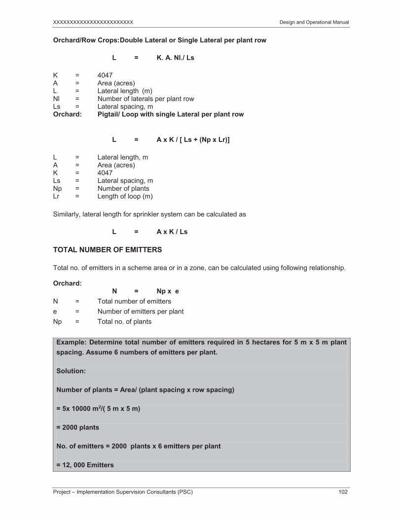
Orchard/Row Crops: Double Lateral or Single Lateral per plant row
L = K. A. Nl./ Ls
K = 4047 A = Area (acres) L = Lateral length (m) Nl = Number of laterals per plant row Ls = Lateral spacing, m Orchard: Pigtail/ Loop with single Lateral per plant row
L = A x K / [ Ls + (Np x Lr)]
L = Lateral length, m A = Area (acres) K = 4047 Ls = Lateral spacing, m Np = Number of plants Lr = Length of loop (m)
Similarly, lateral length for sprinkler system can be calculated as
L = A x K / Ls
TOTAL NUMBER OF EMITTERS
Total no. of emitters in a scheme area or in a zone, can be calculated using following relationship.
Orchard: N = Np x e
N = Total number of emitters e = Number of emitters per plant Np = Total no. of plants
Example: Determine total number of emitters required in 5 hectares for 5 m x 5 m plant spacing. Assume 6 numbers of emitters per plant.
Solution:
Number of plants = Area/ (plant spacing x row spacing)
= 5x 10000 m2/( 5 m x 5 m)
= 2000 plants
No. of emitters = 2000 plants x 6 emitters per plant
= 12, 000 Emitters

XXXXXXXXXXXXXXXXXXXXXXXX Design and Operational Manual
Project – Implementation Supervision Consultants (PSC) 103
Row crops:
Total number of emitters = Total lateral length / Emitter spacing
Similarly, the numbers of sprinklers are calculated based on the following pattern using relationship:
Number of sprinklers = A/(S x L)
A = Area, Acres (hectares) L = Sprinkler spacing between lateral or Lateral spacing S = Sprinkler spacing at lateral or sprinkler spacing
6.2.14 Calculation of Total Flow Rate Requirements (lph)
For micro irrigation system, total flow rate required for the hydro-zone and/or scheme area can be calculated using the following relationships.
For Orchard: Q = Np x e x q
Q = Total Flow Rate, lph q = emitter flow rate, lph
Example: Orchard
Total flow rate = 3238 x 6 x 8 lph = 155,424 LPH = 43.2 LPS = 155.424 m3/hr
For Row Crops: Q = e x q
Q = L x q x Se
Where,
Se = Emitter spacing
Similarly for sprinkler irrigation system, total flow will be calculated based on the following relationship.
Q = Ns x Qs

XXXXXXXXXXXXXXXXXXXXXXXX Design and Operational Manual
Project – Implementation Supervision Consultants (PSC) 104
Ns = Number of sprinklers operating in a zone Qs = Sprinkler flow rate, lph
6.2.15 Calculation of Application Rate (Mm/Hr)
Application rate is the depth of water uniformly distributed over the entire scheme area and can be estimated using following relationship.
I = Q / A
I = Application Rate (mm/hr) Q = Total flow rate, Lph A = Area, m2
For Orchard:
Application rate = 155.424 m3/hr x 1000 / (20 * 4047 m2) = 1.92 mm/hr
For Row crops:
Application rate = m3/hr x 1000 / (20 * 4047 m2) = mm/hr
Application rate for sprinkler system can be calculated using above relationship. Average application rate can also be calculated as:
I = K x q/(S x L)
I = Application rate, mm/hr (in/hr) K = Conversion constant, 60 for metric unit (96.3 for English unit) Q = Sprinkler discharge, L/min (gpm) S = Sprinkler spacing along lateral, m (ft) L = Lateral spacing, m (ft)
6.2.16 Total Operation Time (Hrs)
Operation time required to provide irrigation depth to meet daily consumptive use can be estimated using following relationship. The same relationship can be applied for both the Micro Irrigation system and sprinkler irrigation system.

XXXXXXXXXXXXXXXXXXXXXXXX Design and Operational Manual
Project – Implementation Supervision Consultants (PSC) 105
T = Cu / I
T = Daily Operation time, hrs
Example: Orchard
Daily operation hours = 2.4 ÷ 1.92 = 1.25 hrs
Operation time can also be calculated using following equation.
Ta = IR/ (Np x q) ) Where
Ta = Daily Operation Time, hrs IR = Gross irrigation requirement, mm Np = No. of emitters per plant q = Emitter flow rate, LPH
Example orchard:
Total area under HEIS : 4.5 Acres ETo mm/day : 7.9 Kc : 0.7 Plant spacing m : 6.1 Row Spacing m : 6.1 Canopy Diameter : 5.18 Emitter Flow Rate : 8 LPH
Calculate Design Steps from 1-10
Solution:

XXXXXXXXXXXXXXXXXXXXXXXX Design and Operational Manual
Project – Implementation Supervision Consultants (PSC) 106
Calculation of Design Parameters of HEIS Design Sr. No Parameters Formula Description Units Zone I
1 Total area under HEIS A Acres 4.5
2 Reference Evapotranspiration (ET) mm/d 7.9
3 Crop Factor (Kc) 0.70
4 Plant spacing m 6.10
5 Row spacing/ Lateral spacing m 6.10
6 Canopy Diameter Cd m 5.18
7 Canopy Area Ca=3.1416 x Canopy diameter ^2/4 m2 21.1
8 Canopy factor at maturity Cf=Canopy Area/Plant Spacing x Lateral Spacing Fraction 0.57
9 Irrigation system efficiency % 90
10 8.0
11 Emitter flow rate LPH 8.0
12
Optimal wetted width of each emitter (30 cm) below soil surface at peak water demand)
13 No. of emitter/dripper per plant Nos. 6.0
14 Emitter spacing along plant canopy
15 No. of drip lines per row Nos. 2.0
16 Optimal distance between two Laterals m 6.10
17 Irrigation cycle (assume one day) Days 1.0
18 Peak daily consumptive use per day
Reference ET x crop factor x Canopy factor/Efficiency mm/d 3.50
19 Total no. of plants Area x 4047/Plant Spacing x Lateral Spacing Nos. 489
20 Total drip line length Area x 4047/Lateral Spacing x No. of drip lines per row m 5971
21 Total no. of emitters/drippers
Total no. of plants x drippers per plant Nos. 2937
22 Average emitter spacing Total drip line length/Total no. of emitters m 2.03
23 Total flow rate Total no. of emitters x emitter flow rate LPH 23492
24 Application rate (Total flow rate/1000)/(Area x 4047) x 1000 mm/hr 1.29
25 Operation time* Peak daily consumptive use per day/Application rate Hrs 2.72

XXXXXXXXXXXXXXXXXXXXXXXX Design and Operations Manual
Project – Implementation Supervision Consultants (PSC) 107
6.3 PIPES
As a rule, pressurized irrigation schemes are composed of water lifting devices, piped networks, water delivery devices, and pressure and water control devices. Sometimes water gravitates in the system and no water lifting devices required in the system.
Some of the systems require less pressure for operation and other require more to operate. Keeping in view all the limitations which may technical, economical and on ground demand, the type and size of the pipe is decided for the irrigation schemes to be installed.
In case where water is lifted at higher elevations the material and equipment used in the start of the schemes withstands higher pressure. The reverse is true when water is flowing from higher elevation to lower elevation the material used at the end of the scheme withstand higher pressure. The design engineers must be careful in selection of materials for such types of schemes.
6.3.1 Selection of Pipes
The most common pipes used for pressurized irrigations systems are;
Fiber- cements pipes known as Asbestos cement pipes Un plasticized polyvinyl chloride pipes (uPvc) Polyethylene pipes Hoses Aluminum pipes Steel pipes
Very often design engineer is confronted with the question of which type of pipe should be used for what diameter, their life expectancy and the installation cost.
For the sizing of economic pipe diameter the Smit (1993) proposed the following combination of pipe sizes and types of pipes for south African conditions.
For size up to 50 mm = Polyethylene pipes For size from 50 mm- 110 mm = u Pvc Pipes For Sizes from 110 mm- 350 mm = Fiber cement pipes For sizes larger than 350mm = steel pipes
However, these norms vary from country to country because of combined effect of pipes prices, transportation and installation cost. There is large fluctuation in rates of pipes as derivative of petroleum product.
In our conditions sizing and selection of pipes for pressurized irrigations schemes is based on pressurized non bursting velocity, financial limits and water demands.

XXXXXXXXXXXXXXXXXXXXXXXX Design and Operations Manual
Project – Implementation Supervision Consultants (PSC) 108
D = 63.25 (Q /3.141x v)1/2
Where D = Dia of pipe in inches Q = Discharge in lps V = velocity in m/sec (assumed 1.0-1.5m)
6.3.2 Fiber Cement Pipes
Fiber cement pipes or Asbestos pipes are made from port land cement reinforced by fibers, the formulation of which contains chrysotile Asbestos. The pipe is very smooth internally and thus friction coefficient is very low. It can easily be damaged if poorly handled. At times, cracks occurring during transports and installation only become noticeable later on during testing. The yet an other disadvantage of this pipe is its poor fitting. Diverse kind of specials is used for jointing of pipes.
The standards available for AC pipe are;
ISO 160:1980, ISO 390,ISO 7337, SAZS 113:2000
NOMINAL AND OUT SIDE DIAMETER AT FINISHED ENDS OF FIBER- CEMENTS PRESSURE PIPES SAZS -113: 2000
Nominal dia (mm) Class Outside dia (mm) Tolerance at outside dia (+/-)
50 A II 69.1 0.6 75 A II 95.6 0.6 100 A II 121.9 0.6 125 A II 149.9 0.6 150 A II 177.3 0.6
CLASSIFICATION OF FIBER CEMENT PRESSURE PIPES ISO-160: 1980
CLASS Work hydraulic test pressure Bar Mpa
5 5 0.5 6 6 0.6 10 10 1.0 12 12 1.2

XXXXXXXXXXXXXXXXXXXXXXXX Design and Operations Manual
Project – Implementation Supervision Consultants (PSC) 109
6.3.3 Un-plasticized Polyvinyl Chloride Pipes (UPVC)
uPVC pipes and fittings are made by PVC- U polymer, to which some additives are incorporated in order to facilitate manufacture. ISO – 1620 provides for the testing of this polymer. These pipes are cheaper, light in weight, resistant to corrosion, long life and offer less resistance to flow. The only limitation is that these are to be protected from sunlight and always laid underground.
In Pakistan these are manufactured according to BS 3505,1991 standard for PVC pipes.
The class of pipe is selected according to the total head (pressure) which pipe has to withstand.
6.3.4 CLASSIFICATION OF PIPES
CLASS WORKING PRESSURE TEST PRESSURE Bar Kgf/ cm2 Lbf / in2 Bar Kgf/ cm2 Lbf / in2
B 6 6.12 87 9 9.18 130 C 9 9.18 130 14 13.77 195 D 12 12.25 173 18 18.38 259 E 15 15.3 217 23 22.95 325
Nor
mal
Siz
e
Out
side
D
iam
eter
(m
m)
Class B pipe Class C pipe Class D pipe Class E Pipe
Min
imum
th
ickn
ess
(mm
) 6
Bar
Wei
ght
Kgs
/ M
Min
imum
th
ickn
ess
(mm
) 9
Bar
Wei
ght
Kgs
/ M
Min
imum
th
ickn
ess
(mm
) 12
Bar
Wei
ght
Kgs
/ M
Min
imum
th
ickn
ess
(mm
) 15
Bar
Wei
ght
Kgs
/ M
3’’ 88.7 2.9 1.17 3.5 4.14 4.6 1.82 - - 4’’ 114.1 3.4 1.78 4.5 2.32 6.0 3.03 - - 5’’ 140.0 3.8 2.44 5.5 3.49 - - - - 6’’ 188.0 4.5 3.46 6.6 5.01 - - - - 8’’ 218.8 5.3 5.30 7.8 7.72 - - - - 10’’ 272.6 6.6 8.26 - - - - - - 12’’ 323.4 7.8 11.55 - - - - - -
TESTS
Physical and chemical characteristics
Appearance
The pipe should be reasonably round. The external and internal surface of the pipe should be smooth, clean, and reasonably free from grooving and other effects that would impair its performance in service. The ends should be cleanly cut and square with the axis of the pipe.

XXXXXXXXXXXXXXXXXXXXXXXX Design and Operations Manual
Project – Implementation Supervision Consultants (PSC) 110
Heat Revision Test
Pipe should be tested at the temperature of 150 0 c for at least 15 minutes. After testing, the pipe shall show no faults, for example cracks, cavities, or blisters and pipe length should not change more than 5%.
Acetone Test:
A short length of pipe shall be immersed vertically to depth of at least 25 mm in acetone complying with BS 509 at room temperature. The effect of the acetone on the pipe surface shall be noted after 2 hours. After testing, sample should not show any delaminating or disintegration. Flattering and/or swelling of the pipe shall not be deemed to the constitute failure.
Test for resistance to sulphuric acid
The test specimen should be cut from the pipe and must have a surface area of 45+/-3 sq.cm or (7 +/- 0.5 sq inches). The test specimen should be cleaned, wiped and weighed then totally immersed in 93 +/- 0.5% sulphuric acid for 14 days at 55 (+/- 2) centigrade. Care should be taken to avoid gradual connection of the acid during the test due to evaporation losses etc. After rhe specified time the specimen should be removed, washed in running water for 5 minutes, wiped dry with clean cloth and re-weighed immediately.
When tested by the method, the mass of the specimen shall neither increase more than 0.32 grams nor decrease by more than 0.013g. The effect of the acid on the surface appearance of the specimen should be ignored.
Test for opacity:
The following apparatus will be used in this test
a) Source of lightb) Photoelectric cellc) Spot light galvanometer
The light source and photoelectric cell shall be set up at convenient distance of daylight. The galvanometer shall be connected to the photoelectric cell and the maximum deflection registered shall be noted. A piece of pipe shall then be placed over the photoelectric cell so that one wall is interposed between the light source and cell being kept constant. The maximum deflection of the galvanometer shall again be noted. The second deflection expressed as percentage of the first shall give a measure of the visible light transmitted. When tested by this method the wall of the pipe should not transmit more than 0.2% of the visible light falling on to it.

XXXXXXXXXXXXXXXXXXXXXXXX Design and Operations Manual
Project – Implementation Supervision Consultants (PSC) 111
6.3.5 MECHANICAL CHARACTERISTICS
Short term hydrostatic test
A sample pipe collected from the field is checked in the laboratory at 20o c. The sample pipe is fitted in the apparatus and appropriate internal pressure is applied within 30-40 seconds. The pipe should withstand the appropriate internal pressure for at least one hour without failure.
MINIMUM ONE HOUR INTERNAL PRESSURE
CLASS OF PIPE Minimum one hour internal hydrostatic pressure Bar Psi
B all sizes 21.8 310 C all sizes 32.4 470 D all sizes 43.2 620 E all sizes 54.0 780
Long term hydrostatic test
The specimen collected as explained under procedure for short term and fitted in the same way is admitted to maintain a pressure within accuracy of (+/-) 2 % throughout the test at 200 c. For each test specimen stress shall be so chosen that first piece of pipe should expected to burst with in period of 1-10 hours and the second piece of pipe should be expected to burst with in period of 100-1000 hours. Both pieces of pipes should be tested to failure.
Stress limits
Size of pipe Minimum one hour stress Minimum 50 years stress
Bar Psi Bar Psi Below 1’’ 353 5124 206 2988 1’’- 7’’ 366 5700 230 3340 8’’ and above 443 6430 360 3770
After testing, the extrapolated 1 hour and 50 year circumferential stress levels should not be less than the appropriate values given above.
Falling weight or impact test
Falling weight or impact test is conducted at 20oc (room temperature). Test pieces are placed in the apparatus to sustain particular number of strokes with respective weights from height of 2 meters.

XXXXXXXXXXXXXXXXXXXXXXXX Design and Operations Manual
Project – Implementation Supervision Consultants (PSC) 112
Dia Size No of strokes Size of test piece Falling weight 3// 4 0.75 inch 2.25 kg 4// 6 1 inch 2.75 kg 5// 8 1.25 inch 3.25 kg
6.3.6 GALVANIZED IRON PIPES (G.I Pipes)
Galvanized pipes are made from steel sheets and coated through chemical process of galvanization. These pipes are very costly, shorter in life. Susceptible to corrosion, heavy in weight and offer more resistance to flow.
These pipes are only used in specific conditions where pvc pipes cannot buried or where higher pressures are to be sustained and liable to be kept on the surface.
The GI pipes are prepared according to the international standards BS and ASTM. The PSI has developed PS 1851/1987 standard for GI pipes in Pakistan.
The GI pipes are generally classified as light, medium and heavy according to BS 1387/1967 standards.
Dimensions of Pipes (Light) BSS 1387/1967
SIZE (INCHES)
OUT SIDE DIAMETER ( in) WALL THICKNESS
(inches) WEIGHT
Kg/ft Maximum Minimum
2 2.370 2.347 0.116 1.25
2.5 2.991 2.960 0.128 1.77
3 3.491 3.460 0.128 2.08
4 4.481 4.450 0.144 3.01
Dimensions of pipes (Medium) BSS 1387/1967
SIZE ( INCHES)
OUT SIDE DIAMETER ( inches) WALL THICKNESS
(inches) WEIGHT
Kg/ft Maximum Minimum
2 2.394 2.354 0.144 1.55 2.5 3.014 2.969 0.144 1.99 3 3.524 3.469 0.160 2.58 4 4.525 4.459 0.176 3.69 5 5.534 5.459 0.192 4.94 6 6.539 6.459 0.192 5.85

XXXXXXXXXXXXXXXXXXXXXXXX Design and Operations Manual
Project – Implementation Supervision Consultants (PSC) 113
Dimensions of pipes (Heavy) BSS 1387/1967
SIZE (INCHES)
OUT SIDE DIAMETER ( in) WALL THICKNESS
(inches) WEIGHT
Kg/ft Maximum Minimum
2 2.394 2.354 0.176 1.89 2.5 3.014 2.969 0.176 2.41 3 3.524 3.469 0.192 3.07 4 4.525 4.459 0.212 4.40 5 5.534 5.459 0.212 5.44 6 6.539 6.459 0.212 6.49
Tests
Pipes should be physically checked for appearance, smoothness, seeming line, and galvanization by making abrasions on the surface.
Permissible variation in thickness
Light Quality - 8 % + no limit
Light Quality - 10 % + no limit
Light Quality - 10 % + no limit
Permissible variation in Weight
Single tube 20 ft - 8 % + 10 %
Lot of 1000 ft & over - 4 % + 4 %
Hydrostatic pressure test
Light 700 Psi
Medium 700 psi
Heavy 700 Psi

XXXXXXXXXXXXXXXXXXXXXXXX Design and Operations Manual
Project – Implementation Supervision Consultants (PSC) 114
6.3.7 POLYETHYLENE PIPES
The extrusion compound used for the PE pipe is manufactured from mixture of polyethylene which may include copolymers of ethylene and higher olefins. It also includes antioxidants and carbon black uniformly dispersed.
There are several ISO standards defining the material and are as given below.
ISO 12162 / 1995, ISO 8779/ 2001and ISO 8796/ 1989
Two types of polyethylene pipes are available in the market the low density polyethylene pipe (LDPE) and high density polyethylene pipe (HDPE). The LDPE pipe is used for drip irrigation schemes and is specified by SABS 533 Part 1:1982. It is used both on ground and underground installations. In some countries, HDPE pipe is used as secondary and manifold lines for drip irrigation systems.
There are several types of LDPE and HDPE pipes confirming the SABS standards.
6.3.8 DRIP TAPE
One of the most interesting development with localized irrigation is the introduction of what is commonly known as drip tape. The ANSI/ASAE S553 MAROI standard provide the specifications.
6.4 PIPE HYDRAULICS
6.4.1 Friction Loss
Head loss results from friction between the pipe walls and water as it flows through the system. Various fittings such as turns, bends, expansions and contractions, etc. along the way, will increase the head loss.
Head loss in a pipe system is affected by the following: Length Type of material Inside diameter Flow rate through pipe Type of liquid flowing through the pipe
There are two types of friction losses that will occur while water will be flowing through the pipe system of the pressurized irrigation system namely major losses and minor losses. Major head losses result as water moves through straight pipes. Minor losses are created when water flows through bends and transitions.

XXXXXXXXXXXXXXXXXXXXXXXX Design and Operations Manual
Project – Implementation Supervision Consultants (PSC) 115
6.4.2 Calculation of Friction Loss
Different methods and equations developed i.e., Hazen-Williams, Darcy-Weisbach, and Watters & Keller can be used for the calculation of head losses through the pipes and fittings. This manual will cover only two of these methods namely; Hazen-Williams and Watters & Kellers due to their simplicity.
6.4.3 Hazen-Williams Equation
Empirical formulae are sometimes used to calculate the approximate head loss in a pipe when water is flowing and the flow is turbulent. Prior to the availability of personal computers, Hazen-Williams formula was very popular with engineers because of the relatively simple calculations required. Unfortunately, the results depend upon the value of the Friction Factor “C” which must be used with the formula and this can vary from around 80 up to 130 and higher, depending on the pipe type, pipe size and the water velocity. The empirical form of the Hazen Williams formula is:
J = hf/ L/100 = K (Q/C)1.852 x D-4.8655 Where: hf = Head loss due to pipe friction, m (ft) J = Head loss gradient, m/100 m (ft/100 ft)
K = Conversion constant, 1.212 x 10 12 for metric units (1050 for English units) L = Length of pipe, m (ft) C = Friction coefficient, which is a function of pipe material characteristics Q = Flow rate in the pipe, L/s (gpm) D = Inside diameter of the pipe, mm (in)
The empirical nature of the friction factor C makes the ‘Hazen-Williams’ formula unsuitable for accurate prediction of head loss. The results are only valid for fluids which have a kinematics viscosity of 1.13 centistokes, where the fluid velocity is less than 10 feet per sec and the pipe size is greater than 2” diameter. Water at 60º F (15.5º C) has a kinematics viscosity of 1.13 centistokes.
Table 5.1 Typical values of C for various types of pipe
Hazen-Williams formula provides more accurate results for pipe diameters 75mm (3 inches) or larger, however, for small diameter pipes this equation underestimates the results.
Asbestos Cement 140 Plastic pipe 140 PVC pipe 150 General smooth pipes 140 Galvanized Steel pipe 135 Aluminum 130

XXXXXXXXXXXXXXXXXXXXXXXX Design and Operations Manual
Project – Implementation Supervision Consultants (PSC) 116
Example: Determine head loss through 100 mm (inside diameter 99 mm) Aluminum pipe, 396 m long pipe with 990 litre/minute (16.5 L/s).
Select C value from Table 6.1 and enter values in the equation.
J = 1.21 x 10¹² (16.5/130)1.852 x (99)-4.8655
J = 5.06 m/100 m Hf = 5.06/100x396= 20 m
6.4.4 Watters & Keller Equation
Watters & Kellers developed a simplified equation for use with smooth plastic pipes and hoses less than 125 mm (5 inches).
J = 100 hf/ L = K Q1.75/ D1.75
Where K = Conversion constant, 7.89 x 10⁷ for metric units (0.133 for English units)
For large plastic pipe, where diameter is greater than 125 mm (5 in), the friction head loss gradient can be approximated by:
J = 100 hf/ L = K Q1.83/ D4.83 )
Where K = Conversion constant, 9.58 x 10⁷ for metric units (0.133 for English units)
6.4.5 VELOCITY OF FLOW
Velocity of water flowing through pipes can be calculated using the following equation
V = K Q/(D2)
Where
V = velocity of flow in pipe, m/s (ft/s) Q = Flow rate, L/s (gpm) K = Conversion factor, 1273 for metric unit (0.4085 for English units) D = Inside diameter of pipe, mm (in)
Example: Determine velocity of water through pipe (inside diameter 10.226 in) flowing at1200 gpm

XXXXXXXXXXXXXXXXXXXXXXXX Design and Operations Manual
Project – Implementation Supervision Consultants (PSC) 117
Using Equation No. 5.4
V = 0.4085 x 1200/ (10.226)2 ] V = 4.7 ft/s Velocity in sub-mainlines may be kept under 2.5 m/s.
6.4.6 Selection and Design of Lateral Line
Laterals are available in different sizes i.e. 12 mm, 16 mm and 20 mm. Head loss in the lateral length between the first and last emitter should not exceed by 20% of the head available at the first emitter to keep flow variation within 10% so as 90% of application uniformity can be achieved.
The design of lateral pipe involves selection of required pipe size for a given length which can require quantity of water to the plant. This is the most important component of the system as large amount of pipe per unit of land is required and the pipe cost is such that system is economically viable.
In designing the lateral, the discharge and operating pressure at emitters are required to be known and accordingly, the allowable pressure drop can be determined by the same formula as the main line. The total friction head loss in lateral can be calculated by multiplying the head loss over the total length by a factor F given in Table 6.2.
Lateral Head loss = hf x F

XXXXXXXXXXXXXXXXXXXXXXXX Design and Operations Manual
Project – Implementation Supervision Consultants (PSC) 118
Criteria: Allowable pressure drop in sub-mainline and laterals depends upon the operating pressure required at emitters. The pressure difference between the proximate and distant point along the supply line should not exceed 20% which will keep the variation of discharge within 10% of its value at the first emitter. The emitter operating pressure is usually 10 m, therefore, the maximum allowable head loss in a lateral should be less than 20% of emitter operating pressure i.e. 2m.
Table 6.2 Reduction Coefficient 'F' for Multiple Outlet Pipeline Friction Loss No. of outlets F No. of outlets F
1 1 8 0.42 2 0.65 10 to 11 0.41 3 0.55 12 to 15 0.40 4 0.50 16 to 20 0.39 5 0.47 21 to 30 0.38 6 0.45 21 to 37 0.37 7 0.44 38 to 70 0.36
Example Lateral Design:
Assume:
Flow per dripper = 8 LPH Dripper to dripper spacing (average) =2.30 m Lateral diameter = 16mm (inside diameter= 14.2m) What should be maximum permissible length of lateral to have a head loss of 2m= ?
Solution: Particulars Unit H.Zone1 Lateral Length m 56 Inside diameter mm 10.2 Pipe material PE Pipe friction coefficient 150 Emitter spacing m 2.0 No. of emitters Nos. 27 Emitter flow rate LPH 8 Lateral flow rate LPH 216 Factor for multiple outlet - 0.36 Fittings loss for emitters m 0 Head loss (Watter & Keller) m/100m 3.3 Head loss (Hazzen Willam) m/100m 2.7 Total lateral head loss, hf m 1.87 Velocity m/sec 0.73
Emitter operating pressure= 10 Required lateral head loss (20%)= 2 Calculated lateral head loss = 1.87
OK

XXXXXXXXXXXXXXXXXXXXXXXX Design and Operations Manual
Project – Implementation Supervision Consultants (PSC) 119
Lateral is selected
Example Lateral Design:
Assume:
Flow per dripper = 8 LPH Dripper to dripper spacing (average) =2.30 m Lateral diameter = 16mm (inside diameter= 14.2m) What should be maximum permissible length of lateral to have a head loss of 2m= ?
Solution: Lateral Length M 109 Inside diameter Mm 14.2 Pipe material PE Pipe friction coefficient 150 Emitter spacing M 2.3 No. of emitters Nos. 47 Emitter flow rate LPH 8 Lateral flow rate LPH 376 Factor for multiple outlet - 0.36 Fittings loss for emitters M 0 Head loss (Watter & Keller) m/100m 1.8 Head loss (Hazzen Willam) m/100m 1.5 Total lateral head loss, hf M 2.00 Velocity m/sec 0.66
Emitter operating pressure= 10 Required lateral head loss (20%)= 2 Calculated lateral head loss = 2.00
OK
Lateral is selected
6.4.7 DESIGN OF SUB-MAIN LINE
On the manifolds, whether these pipelines are the sub-main or the mains as well, a number of laterals are fed simultaneously. The flow of the line is distributed en route, as in the laterals with the emitters. Consequently, when computing the friction losses.
The mains, sub-main and all hydrants are selected in such sizes that the friction losses do not exceed approximately 15 percent of the total dynamic head required at the beginning of the system’s piped network. On level ground, these friction losses amount to about 20 percent of the emitter’s fixed operating pressure. This is a practical rule for all pressurized systems to achieve uniform pressure conditions and water distribution at any point of the systems. The above figure

XXXXXXXXXXXXXXXXXXXXXXXX Design and Operations Manual
Project – Implementation Supervision Consultants (PSC) 120
should not be confused with or related in any way to the maximum permissible friction losses along the laterals.
Criteria:
• Maximum Water Velocity in sub-main and mainline= 1.5 m/s• Maximum Frictional Losses in sub-main = 2m• Maximum Frictional Losses in mainline = 20m per 1000m length• Hazen Williams Equation for Frictional Losses
Assume:
Flow per dripper = 4 LPH Dripper to dripper spacing= 0.5 m Lateral to lateral spacing = 1.5 m Sub-main diameter = 2 inch= 63 mm (inside diameter= 59.8 mm) What should be sub-main maximum permissible length to have a head loss of 2m= ?
Particulars Unit H.Zone1 Sub-Mainline Length m 41 Inside diameter mm 75 Pipe material PVC Pipe friction coefficient 150 Lateral spacing m 0.75 No. of laterals operating Nos. 55 Lateral flow rate LPH 368 Sub-mainline flow rate LPH 20117 Factor for multiple outlet - 0.36 Head loss gradient (Watter & Keller) m/100m 0.72 Head loss gradient (Hazzen Willam) m/100m 0.73 Total head loss, hf m 0.3 Velocity m/s 1.27
Sub-main is selected
Assume:
Flow per dripper = 8 LPH Dripper to dripper spacing= 0.5 m Lateral to lateral spacing = 1.5 m Sub-main diameter = 2 inch= 63 mm (inside diameter= 59.8 mm) What should be sub-main maximum permissible length to have a head loss of 2m= ?

XXXXXXXXXXXXXXXXXXXXXXXX Design and Operations Manual
Project – Implementation Supervision Consultants (PSC) 121
Particulars Unit H.Zone1 Sub-Mainline Length m 95 Inside diameter mm 71.4 Pipe material PVC Pipe friction coefficient 150 Lateral spacing m 2.29 No. of laterals operating Nos. 83 Lateral flow rate LPH 256 Sub-mainline flow rate LPH 21240 Factor for multiple outlet - 0.36 Head loss gradient (Watter & Keller) m/100m 0.99 Head loss gradient (Hazzen Willam) m/100m 1.02 Total head loss, hf m 1.0 Velocity m/s 1.47
6.4.8 Selection and Design of mainline
Criteria:
• Should be selected based on the quantity of water, length, elevation of ground, velocity,cost etc.
• Permissible velocity : Less than 1.5 m/s • Frictional losses : Less than 2 m/100 m • Economics: Less initial and annual operating cost • Elevation and Class of Pipe: Pipe class affects the system cost, use appropriate pressure
class pipe and try to lay the pipe at same elevation • Control measures: Pressure relief valves at appropriate location i.e.,
where elevation changes
Example
Assume
Mainline length = 156 m Diameter = 4 inch= 150 mm (inside diameter= 85.6 mm) Designed discharge= 23492 lps Material is PVC (C=150)

XXXXXXXXXXXXXXXXXXXXXXXX Design and Operations Manual
Project – Implementation Supervision Consultants (PSC) 122
Calculate friction loss and check velocity
Particular Unit Section 1
Length m 156 Inside diameter mm 85.6 Pipe material PVC Pipe friction coefficient 150 Design capacity LPH 23492 Head loss gradient (Watter & Keller) m/100 m 1.39 Head loss gradient (Hazzen Willam) m/100m 1.42 Mainline fittings losses m 0 Flow velocity m/s 1.13 Total mainline head loss m 2.21
Main line is selected
Example 2
Particular Unit Section 1
Length m 213 Inside diameter mm 84.4 Pipe material PVC Pipe friction coefficient 150 Design capacity LPH 23253
Head loss gradient (Watter & Keller) m/100 m 1.46
Head loss gradient (Hazzen Willam) m/100m 1.49
Mainline fittings losses m 0 Flow velocity m/s 1.16 Total mainline head loss m 3.17
6.4.9 HEAD LOSS THROUGH FITTINGS
The three conventional methods for computing the additional pressure-head losses from special equipment, valves, pipe and fittings are: (1) graphing friction loss vs. flow rate, (2) expressing the added pressure head loss as the length of pipe (of the same diameter) that would give the same loss, and (3) expressing the loss in terms of a velocity head coefficient. Following Equation 5.5 can be used for computing friction head loss caused by a specific fitting (he), feet.

XXXXXXXXXXXXXXXXXXXXXXXX Design and Operations Manual
Project – Implementation Supervision Consultants (PSC) 123
Where;
Kf = friction head-loss coefficient for a specific fitting. V2/2g = velocity head, which is the energy head from the velocity of flow, feet or m. Kf values should be supplied by manufacturers or taken from handbooks on hydraulics. Usually the losses attributed to standard pipe fittings are small and can be grouped in a miscellaneous friction-loss or safety factor.
6.4.10 SELECTION OF FILTERS AND THEIR HEAD LOSS
There are four kinds of filters used in different combination depending upon source of water
Hydrocylone Filter (H) Sand Media (S) Disc Filter (D) Screen filters
Application: H+S+D = When Water quality is very bad, contains silt particles S+D = Open Well, Tank, Pond, Reservoir, Canal H+D = Borewell D (only) = When water is very clean
To prevent solid particles in the water from penetrating the irrigation system and clogging the drippers
Source of water Type, size and concentration of physical impurities Type of irrigation system Ease of handling, cleaning, maintenance and repairing Filtration media and frictional losses Economical investment, maintenance and power cost

XXXXXXXXXXXXXXXXXXXXXXXX Design and Operations Manual
Project – Implementation Supervision Consultants (PSC) 124
Sand Media Filter
Hydrocyclone Filter
Disc Filter

XXXXXXXXXXXXXXXXXXXXXXXX Design and Operations Manual
Project – Implementation Supervision Consultants (PSC) 125
WATER QUALITY
(Factor for drip irrigation)
Physical (Suspended solids) Chemical (Precipitation) Biological (Bacteria & Algae)
Inorganic particles Sand Silt
Clay Plastics
Calcium or Magnesium carbonates, Calcium Sulphates
Filaments Slime
Organic Particles Aquatic plants
Aquatic animals Bacteria
Heavy metals, oxides, hydrocides, carobonates,
silicates and sulphides
Microbial decomposition Iron
Sulphur Manganese
Oil or other lubricant fertilizers Phosphate
Aqueous Ammonia Iron, Copper, Zinc, Manganese
WATER QUALITY CRITERIA FOR EMITTER CLOGGING
Type of Problem Clogging Hazard
Minor Moderate Severe
Physical (Suspended solidsa
50 50 - 100 100
Chemical pH
Dissolved Solidsa Manganesea Total Irona
Hydrogen Sulphides a
7.0 500 0.1 0.2 0.2
7.0 – 8.0 500 – 2000 0.1 – 1.5 0.2 – 1.5 0.2 – 2.0
8.020001.51.52.0
Biological Bacterial Population b 10,000 10,000 – 50,000 50, 000
(a: ppm b: number/mL)
Selection of Valves
• The Valve can take upto 40% more flow than the pipe flow rate. Hence the Valve size canbe one size less than the Pipeline Size
• The Friction loss in the Valve will be upto 2m approx.

XXXXXXXXXXXXXXXXXXXXXXXX Design and Operations Manual
Project – Implementation Supervision Consultants (PSC) 126
6.4.11 Total Dynamic Head
Total Dynamic head is the total pressure required to provide the required pressure at the end of the last emitter. It is calculated as follows
Total Dynamic Head = suction head + delivery head + filter losses + mainline losses + sub-mainline losses + lateral loss + Fertigation system loss + fitting loss + - elevation difference + operating pressure
Emitter operating pressure M 10 Elevation difference M 0 Headloss in lateral M 0.7 Headloss in Submain M 1.1 1.1 Head Loss (Main) M 3.17 3.17 Headloss in valves M 2 2 Fitting loss Lateral M 1.1 1.1 Fitting loss Mainline M 2 2 Fitting loss Sub-mainline M 0 Fitting loss Head unit M 0 Head loss in filters(Primary) M 4 Head loss in filters(secondry) M 4 Head loss in fertigation system M 5 Head loss in flow meter M 0 Field fitting losses M 0 Safty equipment headloss M 2 Miscellaneous head loss M 0 Suction head M 1 Delivery head M 1 Pumping lift M 0 Total Dynamic Head M 37.07 9.37
Emitter operating pressure m 10 Elevation difference m 0 Total Head Loss (Pipe network) m 4.18 Fitting loss Lateral m 0.1 Fitting loss Mainline m 0.6 Fitting loss Sub-mainline m 0.6 Fitting loss Head unit m 0.7 Head loss in filters m 12 Head loss in fertigation system m 4 Head loss in flow meter m 1 Field fitting losses m 0 Miscellaneous head loss m 2 Pumping lift m 2 Total Dynamic Head m 37.18
Total pipe network HL < 25% of Total Dynamic Head
Main line and sub mainline head loss may be less than 1m/100m

XXXXXXXXXXXXXXXXXXXXXXXX Design and Operations Manual
Project – Implementation Supervision Consultants (PSC) 127
Total pipe network headloss/Total Dynamic Head (%)= 25 % Total pipe network HL < 25% of Total Dynamic Head
Lateral head loss may be less than 20% of the emitter operating pressure Flow velocity less than 1.5 m/sec Main line and sub mainline head loss may be less than 1m/100m
6.4.12 Calculation of Required Horsepower
Pumps and lifting/propelling devices are often classified on the basis of the mechanical principle used to lift the water: direct lift, displacement, creating a velocity head, using the buoyancy of a gas or gravity. Most categories sub-divide into further classifications “reciprocating/cyclic” and “rotary”. Virtually all water lifting devices can best be characterized for practical purposes by measuring their output at different heads and speeds. Normally the performance of a pump is presented on a graph of head versus flow (an H-Q graph) and in most cases curves can be defined for the relationship between H and Q at different speeds of operation. Invariably there is a certain head, flow and speed of operation that represents the optimum efficiency of the device, i.e. where the output is maximized in relation to the power input. Some devices and pumps are more sensitive to variations in these factors than others; i.e. some only function well close to a certain design condition of speed, flow and head, while others can tolerate a wide range of operating conditions with little loss of efficiency.
• Selection of Pump and Motor depends on Flow and pressure required for system.• Pressure is calculated after adding all the losses of the system and pressure required at
emitters.• An approximate HP for motor is calculated as follows:
HP = Q x H_____ 75 x E1 x E2
where:
Q is discharge, LPS H is the total head, m; E1 is the pump efficiency (fraction in the order of 0.5-0.8); and E2 is the driving efficiency (fraction of 0.7-0.9 for electric motors and 0.5-0.75 for diesel engines).
The overall pumping efficiency under field conditions ranges accordingly from 0.35 in engine driven units to 0.50 in motor driven pumps. Higher efficiencies are not realistic. (Always rely on manufacturer chart to know the actual horse power)
PUMP REQUIREMENT Unit Capacity (LPS) 6.46 Head (m) 37.1 Motor effciency (%) 0.9 Pump Efficiency (%) 0.65 Pump H.P required H.P 5

XXXXXXXXXXXXXXXXXXXXXXXX Design and Operations Manual
Project – Implementation Supervision Consultants (PSC) 128
Curves for pump selectionKSB - ETA 65-200
222.82 GPM
42 m
187mm imp. dia16hp
6.4.13 Selection of Pump and Motor

XXXXXXXXXXXXXXXXXXXXXXXX Design and Operations Manual
Project – Implementation Supervision Consultants (PSC) 129
6.4.14 Preparation of Drawing
6.4.15 Preparation of Bill of Quantities BOQ
Bill of Quantities is divided into following subsets:
• Pump Set, Head Unit, Valves, PVC Pipes and Fittings, Emitting System• Safety and Monitoring Equipments

XXXXXXXXXXXXXXXXXXXXXXXX Design and Operations Manual
Project – Implementation Supervision Consultants (PSC) 130
•

XXXXXXXXXXXXXXXXXXXXXXXX Design and Operations Manual
Project – Implementation Supervision Consultants (PSC) 131

XXXXXXXXXXXXXXXXXXXXXXXX Design and Operations Manual
Project – Implementation Supervision Consultants (PSC) 132
Example Orchard - 1
Design a drip irrigation system for citrus using following data:
Size of the field = 1 ha Shape = assume square plot of 100m X 100m Type of drippers = on-line Plant spacing = 6.09 m Row spacing (Lateral spacing) = 6.09 m Discharge of dripper = 8 LPH at 1 Kg/cm2 Maximum ETo = 8 mm/day Kc for citrus = 0.70 Area to be wetted as a Percentage of total area = 60 % Soil type = clay loam Availability of electricity per day = 12 hours Topography of field = level Application efficiency = 90 % Hazen-William constant = 150 for PVC pipe and 140 for LDPE pipes
Assume water source is at the corner of the field.
Solution:
A) Computation of water requirement of the area
Consumptive use can be calculated using equation - 4.6 CU = Eto x Kc x Kf ÷ efficiency
= 8 X 0.70 X 0.60 / (90 / 100) = 3.73 mm/day
B) Calculation of number of plants
Total no. of plants can be calculated by using equation Np = A / Ap
= 10000 / (6.09 X 6.09) = 269 plants
C) Selection of emitters
Numbers of emitters are selected based on the equation. e = SP x SR x Pw / Aw
The value of Aw is selected from Table-3.10 for loam (medium) soil and is used in the above equation to find the no. of emitters per plant.

XXXXXXXXXXXXXXXXXXXXXXXX Design and Operations Manual
Project – Implementation Supervision Consultants (PSC) 133
e = 6.09 x 6.09 x 0.60 / 3.87 = 5.8 = 6 (Approx.)
Total no. of drippers required for the area can be calculated using equation N = Np x e
= 269 X 6 = 1614
D) Computation of Flow Rate
Total flow rate can be calculated by using equation Q = Np x e x q
= 269 x 6 X 8 = 12912 LPH
E) Lateral Requirement
Two no. of drip line for one row of plants is suggested and the total drip line length for the area can be calculated by using equation
L = K. A. Nl./ Ls = 4047 x 2.471 X 2 / 6.09 = 3284 m
F) Application Rate
Application rate can be calculated using equation – 4.29 I = Q / A
= 12912 / 10000 = 1.29 mm/hr
G) Total Operation Time
Operation time can be calculated using equation – 4.31 T = Cu / I
= 3.73 / 1.29 = 2.89 hrs
Here it comes the decisive moment to prepare layout for pipe network. The entire system can be irrigated in one operation requiring larger sized head unit components and pipe networks resulting higher initial investments but less operation hours. The same system can further be economized by diving the area into zones (may be four) that will result in approximately 12 hours of operations but smaller sized head unit components and pipe diameters. To make design calculations easier, the entire system is to irrigate in a single operation.

XXXXXXXXXXXXXXXXXXXXXXXX Design and Operations Manual
Project – Implementation Supervision Consultants (PSC) 134
H) Selection and Design of Lateral
For economy, divide the flow into two sections and give the submain at the center of plot.
i) Length of lateral on one side of sub-main= 50 mNo. of plants on one lateral = Lateral length / plant spacing
= 50/6.09 = 8
ii) Two no. of laterals for one crop row are suggested @ 3 no. of drippers on each lateral per plant, so the total no. of drippers on each lateral can be calculated as:
= No. of plants on each lateral X no. of dripper per plant per lateral = 8 X 3
= 24 no.
iii) Flow rate of the lateral can be calculated by using equation as:= Total no. of dripper on each lateral X Flow rate of each emitter = 24 X 8 = 192 LPH
Select 12 mm diameter lateral (thickness of the lateral is 1.1 mm), inside diameter of lateral =12 – (1.1+1.1)
= 9.8 mm
Using equation – 5.2 (Watter and Keller)
J = 100 hf/ L = K Q1.75/ D4.75
= 100 hf/ (50 m) = 7.89 x 107 x (192/3600)1.75 / 9.81.75
= 9.14 m Hf = 9.14 x 50/100 = 4.57 m
Multiplying by outlet factor for multiple outlets i.e., 0.36 taken from Table 6.2. Total head loss in lateral = 4.57 x 0.36 = 1.65 m Head loss due to friction for 50m lateral length = 1.65 m
Emitter operating pressure is 10 m and calculated head loss 1.65 m is less than 20%, which means flow variation is less than 10%. Lateral of 12 mm size is sufficient to carry the flow.
I) Selection and Design of Sub-main
i) Length of sub-main = 100 m ii) No. of lateral on one side of submain
= 2 X (Submain length / Lateral spacing) = 2 X (100 / 6.09) = 33

XXXXXXXXXXXXXXXXXXXXXXXX Design and Operations Manual
Project – Implementation Supervision Consultants (PSC) 135
iii) No. of laterals on submain = 33 X 2 = 66
iv) Flow rate in submain= flow rate in one lateral X No. of laterals on submain = 192 X 66 = 12672 LPH
Which is approximately the same as calculated total flow of area considering total plants in the area i.e 12912 LPH
v) Outlet factor (66 outlet) for sub main = 0.36
Select 60.5 mm diameter of sub main, inside diameter of sub main = 55.5 mm
Using equation – 5.2 (Water and Keller) as described in lateral size calculation
Head loss due to friction for 100m sub main length = 1.53 m
J) Calculation of Flow Velocity
Flow velocity can be calculated using equation 5.4. V = K Q / D2
= 1273 (12912/3600) / (55.5)2
= 1.48 m/s
As the calculated head loss is less than 2 m, also the velocity is also less than the maximum permissible limit of 2.5 m/s, the sub-main of 60.5 mm size is sufficient to carry the flow. Therefore, the design of sub-main is acceptable.
K) Selection and design of mainline
i) Length of main line = 50 m ii) Flow rate of main line = Flow rate of submain
= 12912 LPH Select 60.5 mm diameter of submain, inside diameter of submain = 55.5 mm
Using equation – 6.2 (Watter and Keller)
Head loss due to friction for 100m lateral length = 3.82 m Head loss due to friction for 50m main line length = 1.91 m
Velocity = 1.48 m/s
The calculated velocity for mainline is less than the maximum permissible limit of 1.5 m/s, the mainline of 60.5 mm size is sufficient to carry the flow. Therefore, the design of mainline is acceptable.

XXXXXXXXXXXXXXXXXXXXXXXX Design and Operations Manual
Project – Implementation Supervision Consultants (PSC) 136
The head loss for suction and delivery pipe for pump be calculated using the same equation (Water & Keller)
Suction and delivery head loss = 0.09 m
Total head losses in piping network = 1.65 + 1.53 + 0.09 = 5.18m
Fitting losses
(may be taken 20% of the pipe losses) = 1.04 m Emitter operating pressure in form of water head = 10 m
Head losses for fittings, filters, fertigation system and other flow control and monitoring devices shall be added as given by the vendors.
Assume, Head loss in fertigation = 5 m Head losses in filters = 8 m Head loss in flow meter = 1 m Misc. head losses = 2 m
The total dynamic head can be calculated by adding all the head losses occurring in the system and can be presented as follow:
Total Dynamic Head = 30.22 m Pump flow rate = 12912 (LPH) / 3600 (Sec.)
= 3.59 LPS
L) Horse Power Requirement
Horse Power Requirement can be calculated using equation
H.P = Q. H / [75 X Em x Ep]
The efficiencies for pump and electric motor are assumed as 60% and 80% respectively.
= 3.59 x 30.22 / [75 x 0.6 x 0.8]
Required Horse Power = 3.0 (appx.)

XXXXXXXXXXXXXXXXXXXXXXXX Design and Operations Manual
Project – Implementation Supervision Consultants (PSC) 137
LATERAL LAYOUT PATTERNS FOR ORCHARDS
2Cont …..
Fig. 6.2 Design layout for drip irrigation system
Example Orchard - 2

XXXXXXXXXXXXXXXXXXXXXXXX Design and Operations Manual
Project – Implementation Supervision Consultants (PSC) 138
3Cont …..
4

XXXXXXXXXXXXXXXXXXXXXXXX Design and Operations Manual
Project – Implementation Supervision Consultants (PSC) 139
AREA WETTED BY ONE EMITTER
Soil Type Area wetted by one emitter (m2)
Sandy soils 0.5-2
Loamy soils 2-6
Clay 6-15
Rain Bird, 1980
Percent Wetted Area
• The percentage area wetted Pw is the average horizontal area wetted within the top 30cmof the crop root zone depth in relation to the total cropped area.
• For largely spaced crops such as orchards is to wet at least one third and as much as twothird (33%-66%) of potential horizontal area of the plant root system.
• In closely spaced crops with rows and emitter laterals spaced less than 1.8 m apart oftenreaches 100%.
Example
Percentage Wetted Area Pw= no. of emitters x area wetted by single emitter Row to Row x Plant-Plant distance
No. of emitters = 4 Area wetted by single emitter = 4 m2 Row to Row distance = 4.57 m Plant-Plant distance = 4.57 m
Pw =4 x 4/4.57 x 4.57 = 77%

XXXXXXXXXXXXXXXXXXXXXXXX Design and Operations Manual
Project – Implementation Supervision Consultants (PSC) 140
10
302
m
201 m
38 m
1
Crop Information
Parameters Crop Area (acres)
Plant spacing
(m)
Row spacing
(m)
Age of crop
(years)
Sowing Date
Harvesting Date
Block-I Row cropsProposed Citrus 15 4.57 4.57 1 year
Rotation
Sub-Total: I
Block-II OrchardsType-I
Type-II
Sub-Total: II
Block-III Annual Crops
Sub-Total: III
Block-IV Field CropsType-I
Type-II
Sub-Total: IV
Total / Design Value 15 4.57 4.57
Design a drip irrigation system for Citrus Orchard in Okara District.

XXXXXXXXXXXXXXXXXXXXXXXX Design and Operations Manual
Project – Implementation Supervision Consultants (PSC) 141
12
EVAPOTRANSPIRATION AND CROP COEFFICIENTS (ETo & Kc)
Month J F M A M J J A S O N D
Eto (mm/d) 1.4 2.2 3.6 5.0 6.3 6.5 5.2 4.7 4.5 3.2 1.8 1.3
Kc (row crop) 0.65 0.65 0.65 0.65 0.65 0.65 0.65 0.65 0.65 0.65 0.65 0.65CWR (row crop) 0.9 1.4 2.3 3.3 4.1 4.2 3.4 3.1 2.9 2.1 1.2 0.8Kc (orchards)
CWR (orchards)
Kc (annual crop)
CWR (annual crop)
Kc (field crops)
CWR (field crops)
13
Water SourcesSoil type Loamy Sand
Water Sources
1) Canal
Sanctioned Discharge (LPS) 56
Perennial / Non Perennial Perennial
Warabandi (Days) 7
Water Availability Hrs/Warabandi 8
Volume (m3) 1612

XXXXXXXXXXXXXXXXXXXXXXXX Design and Operations Manual
Project – Implementation Supervision Consultants (PSC) 142
14
1. Total area under HEIS Acres 15
2. Design reference evapotranspiration, ETo mm/day 6.5
3. Design Crop factor at maturity, Kc - 0.65
4. Plant spacing m 4.57
5. Row spacing m 4.57
Canopy Area m2 14.62
6. Canopy Factor % 70
7. Irrigation system efficiency % 90
Optimum wetted width of each emitter m
8. Emitter flow rate LPH 8
No. of emitters per plant Nos. 4
10. No. of drip lines per plant rows Nos. 2
11. Irrigation cycle (assume one day) Days 1
15
S.N.
Parameters Unit Calculations
13 Peak daily consumptive use per day
Mm = ETo * Kc * canopy factor/ efficiency=6.5 * 0.65 * 0.7/0.9 = 3.29 mm
14 Total no. of plants Nos = Area x 4047 /(R-R * P-P)= 15*4047/(4.57*4.57) = 2,908
15 Total drip line length M = Area*4047x no of lines per plant row/L-L= 15*4047x2/(4.57) = 26,566
16 Total no. of emitters Nos = Total no. of plants x no. of emitters per plant= 2908x4 = 11,632
17 Average emitter spacing M 2.3
18 Total flow rate Lph = total no. of emitters x emitter flow rate= 11632 * 8 = 93,056
19 Application rate Mm/hr Total flow rate / area= (93,056/1000)/(15*4047*1000)= 1.53
20 Operation time* hrs = Peak daily consumptive use/ Application rate= 3.29/1.53= 2.15 hrs

XXXXXXXXXXXXXXXXXXXXXXXX Design and Operations Manual
Project – Implementation Supervision Consultants (PSC) 143
Drip design sheet-orchard Sr. No Parameters Formula
Description Units Zone I Total
1 Total area under HEIS A Acres 3.75 15.00
2 Reference Evapotranspiration (ET) Mm/d 6.50
3 Crop Factor (Kc) 0.65
4 Plant spacing M 4.57
5 Row spacing/ Lateral spacing M 4.57
6 Canopy Diameter Cd M 4.31
7 Canopy Area Ca=3.1416 x Canopy diameter ^2/4
m2 14.6
8 Canopy factor at maturity Cf=Canopy Area/Plant Spacing x Lateral Spacing
Fraction 0.70
9 Irrigation system efficiency % 0.9 10 Emitter flow rate LPH 8
11 Optimal wetted width of each emitter (30 cm) below soil surface at peak water demand)
12 No. of emitter/dripper per plant Nos. 4 13 Emitter spacing along plant canopy 14 No. of drip lines per plant row Nos. 2
15 Optimal distance between two Laterals M
16 Irrigation cycle (assume one day) Days 1.0
17 Peak daily consumptive use per day
Reference ET x crop factor x
Canopy factor/Efficiency
Mm/d 3.28
18 Total no. of plants Area x 4047/Plant Spacing x Lateral Spacing
Nos. 727 2907
19 Total drip line length
Area x 4047 x No. of drip lines per plant row/Lateral Spacing
M 6642 26,567
20 Total no. of emitters/drippers Total no. of plants x drippers per plant Nos. 2907 11,627
21 Average emitter spacing Total drip line length/Total no. of emitters
M 2.29
22 Total flow rate Total no. of emitters x emitter flow rate LPH 23,253 93,013
23 LPS 6.46 25.84 24 m3/hr 23.25 93.01
25 Application rate (Total flow rate/1000)/(Area x 4047) x 1000
Mm/hr 1.53 0.00
26 Operation time*
Peak daily consumptive use per day/Application rate
Hrs 2.14 8.56
27 Vol. of water req./operation/day Flow x operational time m3 50 199

XXXXXXXXXXXXXXXXXXXXXXXX Design and Operations Manual
Project – Implementation Supervision Consultants (PSC) 144
16
302
m
201 m
75 m
150
m
37 m27 m37 m
63 m
75 m
Darcy- Weisbach and Blasius Equation can be combined to give accurate prediction of friction head loss for smooth plastic pipes of less than 125 mm (5 in.) diameter.
J = 100 hf/L = k * [(Q^1.75)/(D^4.75 )] * F J = Head loss gradient, m/100 m Hf = pipe friction head loss, m K = Constant, 7.89 * 10 ^7 for metric units Q = Flow Rate, LPS L = Pipe length, m D = Inside Diameter of Pipe, mm
Lateral Design:
Lateral length = 73 m No. of emitters = 73/2.3= 32 Lateral flow rate = 32*8=256 lph Assume 16 mm lateral line Inside diameter = 14.2 mm
J = 7.89*10^7 * [(256/3600)^1.75)/(14.2^4.75)] * 0.36 J= 0.93 m/100 m For 73 m length Hf = 0.68m

XXXXXXXXXXXXXXXXXXXXXXXX Design and Operations Manual
Project – Implementation Supervision Consultants (PSC) 145
Particulars Unit H.Zone1 Lateral Length m 73 Inside diameter mm 14.2 Pipe material PE Pipe friction coefficient 150 Emitter spacing m 2.29 No. of emitters Nos. 32.00 Emitter flow rate LPH 8 Lateral flow rate LPH 256 Factor for multiple outlet - 0.36 Fittings loss for emitters m 0 Head loss (Watter & Keller) m/100m 0.9 Head loss (Hazzen Willam) m/100m 0.7 Total lateral head loss, hf m 0.68 Velocity m/sec 0.45
Sub-Mainline Design:
Length = 100 m Sub-main flow rate = 93056/4 =23,264 lph Assume 71.4 mm ID
Sub-Mainline
J = 7.89*10^7 * [(23264/3600)^1.75)/(71.4^4.75)] * 0.36 J= 1.21m/100 m For 100 m length Hf = 1.21 m
Darcy- Weisbach and Blasius Equation can be combined to give accurate prediction of friction head loss for smooth plastic pipes of less than 125 mm (5 in.) diameter.
J = 100 hf/L = k * [(Q^1.75)/(D^4.75 )] J = Head loss gradient, m/100 m Hf = pipe friction head loss, m K = Constant, 7.89 * 10 ^7 for metric units Q = Flow Rate, LPS L = Pipe length, m D = Inside Diameter of Pipe, mm

XXXXXXXXXXXXXXXXXXXXXXXX Design and Operations Manual
Project – Implementation Supervision Consultants (PSC) 146
Particulars Unit H.Zone1 Sub-Mainline Length m 100 Inside diameter mm 71.4 Pipe material PVC Pipe friction coefficient 150 Lateral spacing m 2.29 No. of laterals operating Nos. 91 Lateral flow rate LPH 256 Sub-mainline flow rate LPH 23296 Factor for multiple outlet - 0.36 Head loss gradient (Watter & Keller) m/100m 1.17 Head loss gradient (Hazzen Willam) m/100m 1.21 Total head loss, hf m 1.21 Velocity m/s 1.62
Mainline Design:
Length = 213 m Main-line flow rate = 23264 LPH Assume 84.4 ID Mainline J = 7.89*10^7 * [(23264/3600)^1.75)/(84.4^4.75)] J= 1.46 m/100 m For 213 m length Hf = 3.17 m
V = 1.274 x [(23264/(1000*3600)]/ [(84.4/1000)^2] = 1.16 m/s
Particular Unit Section 1
Length m 213 Inside diameter mm 84.4 Pipe material PVC Pipe friction coefficient 150 Design capacity LPH 23253 Head loss gradient (Watter & Keller) m/100 m 1.46 Head loss gradient (Hazzen Willam) m/100m 1.49 Mainline fittings losses M 0 Flow velocity m/s 1.16 Total mainline head loss M 3.17
TOTAL DYNAMIC HEAD • Emitter operating pressure = 10 m • Head loss in lateral = 0.68 m • Lateral Elevation = 0 m • Head loss in submains = 1.16 m

XXXXXXXXXXXXXXXXXXXXXXXX Design and Operations Manual
Project – Implementation Supervision Consultants (PSC) 147
• Head loss in Valve (assume 2 m) = 2.0 m • Field fitting head loss = 2.0 m • Head Loss in Main line = 3.12 m • Primary filter head loss (Gravel 20 m3) = 1.5 m • Secondary filter head loss (Disc 20 m3) = 1.3 m • Fertigation equipment head loss (5 m for ventury) = 5 m• Water source depth = 0 m • Suction head = 1 m • Delivery head = 1 m • Safety equipment head loss = 2 m • Elevation difference = 0 m • Other losses = 0 m • Total Head Required = 30.76 m
Say 31 m
Total Flow Required = 23,264 m3/hr = 6.46 lps
Pump H.P = Q (LPS) * H (m)/ (75 x pump efficiency x motor efficiency) = 6.46 * 30.76 /(75 * 0.65 * 0.9) = 4.56
Say 5 H.P
Sample Bill Of Quantities
23
S.N Description Standard/specification
Unit Quantity Rate (Rs.) Cost (Rs.)
1 Pump set ( 20 HP) KSB/MECO/X No 01 80,000 80,000
2 Gravel Filter 40 M3/Hr 40 M3/hr, Jain 02 40,000 80,000
3 Disc filters 40 M3/hr, Netafim
02 25,000 50,000
4 Ventury with assembly 01 7,500 7,500
5 Flow Meter 80 M3/hr , Kitz 01 65,000 65,000
6 Pressure Gauges 05 1,100 5,500
7 Air Release valves 02 1500 3,000
8 NRV 01 15,000 1,500
9 Foot valve 01 10,000 10,000
10 Flush valves (sub-main) 02 3,000 6,000
11 GI Pipe 110 mm m 5 2,000 10,000
12 GI Fittings 110 mm L/s 1 10,000 10,000
13 PVC Pipe , B Class 160 mm m 60 700 42,000
14 PVC Pipe, B Class 110 mm m 225 370 83,250
15 Plain Lateral 16mm m 500 20 10,000
16 Lateral line 2lph x 0.4 m spacing, wt 1.5 mm 16 mm m 18,000 25 450,000
17 GTO Nos. 290 15 4,350
18 Lateral End Stop Nos. 290 10 2,900
Sub-Total 921,000Service charges (Design, Installation, Service) 8% of total 73,680
Grand Total 994,680

XXXXXXXXXXXXXXXXXXXXXXXX Design and Operations Manual
Project – Implementation Supervision Consultants (PSC) 148
Example Orchard-3
Given InformationCrop CitrusSpacing 6m x 6m Area 20 AcEto 7 mm/dKc 0.7Time available 12 Hours Water available 18m3/hr Open well 6m dia x 8m deep Soil Loam
LimitationsButton Dripper 8 lph X 4 per Plant Lateral 12mm Plot size 180m x 450m
Total Area = 450 x 180 = 81000 m2 PWR = Eto x Kc x canopy factor /efficiency
= 6 x 0.7 x 0.6 / 0.9 = 2.8 mm/d Total drip line length = Area x no. of drip lines per plant row / (lateral spacing)
= 81000 x 1 /6 = 13500 m Total number of plants = Area / ( plant spacing x row spacing)
= (81000/ (6 x 6) = 2250 Total number of emitters = No. of plants x Dripper per plant
= 2250 x 4 = 9000
Total number of emitters = No. of plants x Dripper per plant = 2250 x 4 = 9000
Average emitter spacing = 13500/9000 = 1.5 m Total flow rate = no. of emitters x emitter flow rate
= 9000 x 8 lph = 72,000 lph Application Rate = Flow rate/ area
= 72000/81000 = 0.89 mm/h Operation time per day = PWR/ Application Rate
= 2.8/0.89 = 3.15 hours Capacity of the water source is 18000 lph, we will divide the area into shifts No. of shifts/hydro-zone = 72000 lph/ 18000 lph = 4
Wetted percentage =

XXXXXXXXXXXXXXXXXXXXXXXX Design and Operations Manual
Project – Implementation Supervision Consultants (PSC) 149
no. of emitters x Area wetterd by single emitter/plant Area = 4 x 4/(6 x 6) = 44%
If we go with 6 drippers per plant, then percent wetted area will result about 66%.
14
180
m
450 m Water Source
15
180
m
450 m Water Source
DESIGN LAYOUT

XXXXXXXXXXXXXXXXXXXXXXXX Design and Operations Manual
Project – Implementation Supervision Consultants (PSC) 150
A) Lateral Selection
(12 mm OD WT = 0.9 mm) Length, m = 90 m Inside diameter, mm = 10.2 mm Flow rate, lph = (90/1.5)* 8 = 480 lph Head loss using Hazzen-William Equation: (6.1 m/100 m = 3.4 meters) PLZ CHECK CALCULATION
B) Sub-Mainline Selection
Length, m = 112.5 m Inside diameter, mm = 60.0 mm Flow rate, lph = 18,000 lph Head loss using Hazzen-William Equation: 2.1 m/100 m = 2.34 meters
C. Mainline Selection
Length, m = 517.5 m Inside diameter, mm = 68.0 mm Flow rate, lph = 18,000 lph Head loss using Hazzen-William Equation: 2.61 m/100 m = 11.72 meters Velocity = 1.38 m/seconds
18
180
m
450 m Water Source
ALTERNATE DESIGN LAYOUT (PTION -II)

XXXXXXXXXXXXXXXXXXXXXXXX Design and Operations Manual
Project – Implementation Supervision Consultants (PSC) 151
A) Lateral Selection
(12 mm OD WT = 0.9 mm) Length, m = 45 m Inside diameter, mm = 10.2 mm Flow rate, lph = (45/1.5)* 8 = 240 lph Head loss using Hazzen-William Equation: 3.1 m/100 m = 1.4 meters
B) Sub-Mainline Selection
Length, m = 112.5 m Inside diameter, mm = 60.0 mm Flow rate, lph = 18,000 lph Head loss using Hazzen-William Equation: 2.1 m/100 m = 2.34 meters
C. Mainline Selection
Length, m = 337.5 m Inside diameter, mm = 68.0 mm Flow rate, lph = 18,000 lph Head loss using Hazzen-William Equation: 2.61 m/100 m = 11.72 meters Velocity = 1.38 m/seconds
TDH = 45 m Q = 18000 lph H.P ?
6.5 DRIP DESIGN PROCEDURE-STEP BY STEP (ROW CROP)
Under the on-going project, drip systems are being installed on orchard and at row crops/vegetables. In this section, steps for designing a drip system for row crop will be discussed. The following are the design steps.
1. Collection of Basic Information2. Estimation of Peak Water Requirement PWR3. Drawing of project area, selection of zone area and No. of Operations4. Selection of emitter/dripper, and flow rate5. Calculation of total length of lateral No. of emitters in one zone and total No. of emitters6. Calculation of Total Flow rate requirement (Q)7. Calculation of Application Rate8. Total Operational Time9. Selection and Design of Lateral Line10. Design of Sub-mainline11. Design of Mainline12. Head Loss through fittings13. Selection of Filters and other equipment and head loss14. Calculation of total dynamic head (H)15. Calculation of required horsepower (HP)16. Selection of Pumps and Motor17. Preparation of Drawing18. Preparation of Bill of Quantities

XXXXXXXXXXXXXXXXXXXXXXXX Design and Operations Manual
Project – Implementation Supervision Consultants (PSC) 152
Step 1. Collection of Basic Information
The following basic information be available before designing a drip irrigation system.
• General information: Name of farmer, village/chak No., tehsil, district, phone No.• Land holding and Area spared for the project• Engineering survey: GPS coordinates, Field measurement, Elevation difference/slope.
After field measurement, a map showing all dimensions and location of water source bedrawn
• Agricultural details: crops (orchard, row/field crop), spacing, type, age, referenceevapotranspiration of the area and water requirement of crop
• Crop Spacing (Row to Row, Plant to Plant), sowing and harvesting date• Soil Type/texture• Soil and water analysis reports water quality, presence of iron, pH, suspended particles,
soil type, Ec, pH• Water Source, quantity, availability, location• Power Source: Electric motor, diesel engine, tractor, solar system• Climatologically data: temperature, humidity, rainfall, wind speed• Peak Water Requirement: (ETo, Kc, Cf)• Water source and Total Available Time of water• System capacity: The system should have capacity adequate to fulfill daily crop water
requirements of the area within a stipulated time or not more than 12 hours of operationper day (only for Pakistan circumferences, otherwise may be 22 hrs).
The basic information can be categorized as under.
I. GENERAL INFORMATION Name of beneficiary Town/Village/City Tehsil District Province Phone No. Land holding (Acre) Scheme area (acres) Topography (Flat/Undulated)
II. CROP INFORMATION
Parameters Crop
Area
(a
cres )
Plan
t sp
acig
(m
)R
ow
spac
ing
(m)
Age
of
crop
(yea
rs)
Sow
ing
date
Har
vest
ing
date
Block-I Row Crop
Proposed COTTON 20 0.5 1.52 MARCH NOV.
III. EVAPOTRANSPIRATION AND CROP COEFFICIENTS (Etc & Kc) Month J F M A M J J A S O N D Eto (mm/d) 1.8 2.7 4 6.4 8.6 9.2 7.6 6.5 5.8 4.5 2.7 1.9 Kc (cotton) 0.5 0.8 1 1.29 1.2 0.9 0.7 0.7 Crop factor at mat. 0.4 0.7 1 1 1.1 1 1 0.7 Efficiency 0.9 0.9 0.9 0.9 0.9 0.9 0.9 0.9 PCWR (cotton) 1.42 5.35 10.2 10.89 9.53 5.80 3.50 1.37 Kc () Crop factor at mat. PCWR () Kc (field crops) CWR (field crops)

XXXXXXXXXXXXXXXXXXXXXXXX Design and Operations Manual
Project – Implementation Supervision Consultants (PSC) 153
IV. SOIL TYPE/SOIL TEST/WATER SUPPLY/WATER QUALITY
SOIL TEST
Soil type/Texture LOAMY
Soil limitation (soil analysis report attached)
Soil EC , PH , N , P , K , SAR
WATER SUPPLY
Available water sources
1) Canal WATER SOURCE IS CANAL AND TUBEWELL
Sanctioned discharge (LPS) 42.46 LPS
Perennial/non-perennial NON-PERENNIAL
Warabandi (days) Hrs/Warabandi 48 HOURS PER WEEK
Water availability Volume (m3) 7337 (1048 CUBIC METERS PER DAY)
2) Groundwater
a) Dug well
Depth of well
Diameter of well
Recharge rate
b) Tube well/bore well
Discharge capacity (LPS) 42.46
Diameter of bore (inches) 8
Depth of water table from ground (m) 9.15
3) Storage/reservoir capacity (m3) 827(20.3x20.3x2m) for 1 day
Water quality (detailed report attached)
Iron
Ph
EC(mmohs/cm)
Distance of water source from field (m)

XXXXXXXXXXXXXXXXXXXXXXXX Design and Operations Manual
Project – Implementation Supervision Consultants (PSC) 154
V. POWER SOURCE AND PUMP POWER SOURCE
Type of power to be usedFor electric Motor, Type of connection (single/3-phase) Make/model HP of Motor RPM of Motor
ELECTRICITY NOT AVAILABLE For diesel engine Make HP Condition)For Tractor Make/model HP Condition
Any other power source, if any
PUMP SETType Make/Model Pressure (ft/psi/bar) Flow(lps) Inlet/outlet size RPM Pulley size

XXXXXXXXXXXXXXXXXXXXXXXX Design and Operations Manual
Project – Implementation Supervision Consultants (PSC) 155
Water Analysis Report
Farmer Name : Abbass Qureshi Water Source Tube Well Address :Muzaffar garh Sampling Date 10/5/2010
Ph :0345-8644888 Sp Receive Date : 13/05/2010
Agronomist: Ather Mehmood Khursheed Report Date : 31/05/2010
Ref.Sample # 372
Parameters Degree of Presence / Problem Lab
Result Unit Noma
l Higher Extrem
e pH 7 <7 Acidic >7 A 7.37 Electrical Conductivity (Salinity) microsemens/cm - - - 2240 Total dissolved solids ppm <500 500 - 600 >600 1290 Hardness ppm <200 200 - 300 >300 312 Calcium ppm <60 60 - 100 >100 78.4 Magnesium ppm <25 25 - 40 >40 28.21 Carbonate ppm <200 200 - 600 >600 72 Bicarbonate ppm <200 200 - 600 >600 176 Chloride (Toxic) ppm <140 140 - 350 >350 198.5 Sulphates ppm <20 20 - 50 >50 23.4 Sodium ppm <100 100 - 200 >200 235 SAR - <3 3-9 >9 2 Potassium ppm <10 10 - 20 >20 12 Sulphides ppm <15 15-25 >25 - Iron ppm <0.1 0.1 - 0.4 >0.4 0.1 Manganese ppm <0.2 0.2 - 0.4 >0.4 - Suspended solids ppm <10 10 - 100 >100 7.1 Boron ppm <0.5 0.5 - 2.0 >2.0 -

XXXXXXXXXXXXXXXXXXXXXXXX Design and Operations Manual
Project – Implementation Supervision Consultants (PSC) 156
Soil Analysis Report
Farmer Name :
Abbas Qureshi Block Size
: Address :
Muzaffargarh Sampling Date :
11/5/2010
Ph :
345864488 Sp Receive Date :
13/05/2010
Agronomist :
Ather Mehmood Sheikh
Report Date :
26/04/2010
Code : AMK-S001
Ref.Soil
Sample #
Block #
Depth (inche
s) Texture
Organic
Matter %
pH
ivity
(m
ic/c
m)
Phos
phor
us(P
) (p
pm)
Pota
ssi
um(K
) (p
pm)
Soluble & Exch. Na (meq
/L)
Soluble &
Ca +Mg (meq
/L)
SAR
Neutral
6.5- 7.5
Alkaline
>8.5
Poor <7.0
Medium 7-13
Satisfactorty >13
Poor <125
Medium 125-250 Satisfac
torty >250
Normal <10.
0 Sodi
c >10.
0
2835 1
0 - 6'' Sand,Cl
ay 0.245 8.44
411
- 110 6.52 3.2 4
2836 6 - 12'' Sand,Cl
ay 0.582 7.74
468
- 120 6.95 3.2 4.3
2837 2
0 - 6'' Sand,Cl
ay 0.827 8.15
572
- 110 11.7
3 3.1 7.5
2838 6 - 12'' Sand,Cl
ay 0.612 8.26
550
- 110 10.4
3 2.7 7.7
2839 3
0 - 6'' Sand,Cl
ay 0.612 8.29
316
- 90 6.52 3.4 3.8
2840 6 - 12'' Sand,Cl
ay 0.735 8.39
304
- 90 6.95 3.7 3.7
2841 4
0 - 6'' Sand,Cl
ay 0.821 8.21
384
- 100 6.08 3.2 3.8
2842 6 - 12'' Sand,Cl
ay 0.735 8.25
358
- 100 6.52 3.2 4
2843 0 - 6'' Sand,Cl
ay 1.01 8.02
506
- 150 4.34 5.1 1.7
2844 6 - 12'' Sand,Cl
ay 0.98 8.02
494
- 160 4.34 4.2 2

XXXXXXXXXXXXXXXXXXXXXXXX Design and Operations Manual
Project – Implementation Supervision Consultants (PSC) 157
2845 6
0 - 6'' Sand,Cl
ay 1.041 8.05
412
- 120 4.34 4.2 2
2846 6 - 12'' Sand,Cl
ay 0.919 8.11
356
- 100 4.34 4.2 2
2847 7
0 - 6'' Sand,Cl
ay 0.919 7.97
1080
- 80 10.8
6 6.6 3.2
2848 6 - 12'' Sand,Cl
ay 0.549 8.02
1123
- 80 11.7
3 5.8 4
It is advisable to make rough map of the area and mark salient features, divide the drawn map into different blocks and number the same for soil and water sampling. This map will be finalized during designing of drip irrigation system and will show all necessary details including drippers, dia, length and location of laterals, submain and main, location of water source, power source etc.,

XXXXXXXXXXXXXXXXXXXXXXXX Design and Operations Manual
Project – Implementation Supervision Consultants (PSC) 158
Step 2. Estimation of Peak Crop Water Requirement
Estimating the reference crop evapotranspiration (ETo), using the Penman-Monteith method, and the crop evapotranspiration (ETc), through the use of the appropriate crop factor Kc, have been covered in Module 4 Chapter______ of this Manual. Evapo-transpiration is composed of the evaporation from the soil and the transpiration of the plant. Since under localized irrigation only a portion of the soil is wetted, the evaporation component of evapotranspiration can be reduced accordingly, using the appropriate ground cover reduction factor Kr.
For the design of surface and sprinkler irrigation systems:
ETc = ETo x Kc
For the design of Drip irrigation systems: Water Requirements for Orchard ETc= ETo x Kc x Canopy Factor/ Efficiency Percent area wetted, 100% for closely spaced crops with rows and emitter lines less than 1.8m.
Peak Crop Water Requirement can be tabulated as under.
Month J F M A M J J A S O N D Eto (mm/d) 2.1 2.7 4.2 5.6 7 7.9 7.3 6.8 5.9 4.8 3.3 2.3 Kc (citrus) 0.7 0.7 0.7 0.7 0.7 0.7 0.7 0.7 0.7 0.7 0.7 0.7
Crop factor at mat. 0.57 0.5
7 0.5
7 0.5
7 0.5
7 0.6 0.5
7 0.5
7 0.5
7 0.5
7 0.6 0.57 Efficiency 0.9 0.9 0.9 0.9 0.9 0.9 0.9 0.9 0.9 0.9 0.9 0.9
PCWR (citrus) 0.93 1.2
0 1.8
6 2.4
8 3.1
0 3.5
0 3.2
4 3.0
1 2.6
2 2.1
3 1.4
6 1.02 Kc (mango) 1.1 1.1 1.1 1.1 1.1 1.1 1.1 1.1 1.1 1.1 1.1 1.1
Crop factor at mat. 0.55 0.5
5 0.5
5 0.5
5 0.5
5 0.6 0.5
5 0.5
5 0.5
5 0.5
5 0.6 0.55
PCWR (mango) 1.41 1.8
2 2.8
2 3.7
6 4.7
1 5.3
1 4.9
1 4.5
7 3.9
7 3.2
3 2.2
2 1.55 Kc (field crops) CWR (field crops)
Step 3. Drawing of Project Area, Selection of zone area and No. of Operations
A map of the scheme area be drawn and tentative number of zones having equal area of the project be selected to estimate number of operations. It is advisable that area of each of each zone must be equal so that all the discharge coming out from the pump be fully utilized in each zone area. In case all zones are not equal, some additional water has to be sent back to the water storage tank through bypass valve during irrigation of small area zones.

XXXXXXXXXXXXXXXXXXXXXXXX Design and Operations Manual
Project – Implementation Supervision Consultants (PSC) 159

XXXXXXXXXXXXXXXXXXXXXXXX Design and Operations Manual
Project – Implementation Supervision Consultants (PSC) 160

XXXXXXXXXXXXXXXXXXXXXXXX Design and Operations Manual
Project – Implementation Supervision Consultants (PSC) 161
Step 4. Selection of Emitter/Dripper and Flow Rate
Varieties of drippers/drip tubing are available with different discharge rates, dripper spacing, characteristics and suitability for different crops. The emitter selected for the drip system:
• Should be Inexpensive, durable and serviceable• Should have relatively low discharge rate to keep the system cost low• Should have higher emission uniformity (90%) and low coefficient of variation (CV 5%)• Should have emission discharge exponent in the range of 0.4-0.7.• Should have relatively large cross sectional area and flow path to avoid clogging• Should have turbulent flow path and pressure compensation action• Should not create runoff within the immediate application area
Drippers are available for 2, 4, 8 and 12 LPH discharge. Emitter operating pressure is usually 10m. The shape of the wetted zone of the emitter depends on the physical properties
In sandy and light soil, the water will tend to go straight down, and there will be less lateral movement as compared to downward movement. In light soils, the distribution of the water will be narrow and deeper
(close spaced low discharged emitters/Closer emitter spacing)
In loamy soil, the water will move slowly and will spread evenly
(average discharged emitter &/or Spacing)
In clay soil, the water will be absorbed very slowly and there will be more lateral movement as compared to downward movement. In heavy soil, the distribution of the water will be relatively spherical shape, wider and less depth.
wider emitter spacing

XXXXXXXXXXXXXXXXXXXXXXXX Design and Operations Manual
Project – Implementation Supervision Consultants (PSC) 162
• Heavy soil recommended distance: 0.50 to 1.00 meter*• Medium soil recommended distance: 0.40 to 0.75 meter*• Light soil recommended distance:• 0.20 to 0.50 meter*• *The spacing between drippers depend on the root depth of the crop.
Emitter spacing should be maximum 0.5m, 0.4-0.6 and 0.5-0.8m in light, medium and heavy soil respectively.
Most of the water emitter flow regime is fully turbulent with an exponent value equal to 0.5. In order to ensure a high uniformity of water application over the field, the differences in the discharge of the emitters should be kept to the minimum possible and in no case exceed 10 percent. These criteria were established by J. Christiansen for sprinklers and are now applied in all pressurized systems. As a general rule, the maximum permissible difference in pressure between any two emitters in operation should be no more than 20 percent. The lateral lines with emitters must be of a size that does not allow a loss of head (pressure) due to friction of more than 20 percent. In case emitter operating pressure is 01 bar or 10 meter, the head loss in the selected lateral must not be more than 02 meter.
Step 7. Calculation Of Total Length Of Lateral, Number Of Emitters In One Zone And Total Number Of Emitters
The length of lateral required for the scheme area under micro irrigation system can be calculated as follows:

XXXXXXXXXXXXXXXXXXXXXXXX Design and Operations Manual
Project – Implementation Supervision Consultants (PSC) 163
Row Crops: Single Lateral per plant row
L = K. A./ Ls (4.19)
K = 4047
A = Area (acres)
L = Lateral length (m)
Ls = Lateral spacing, m
Similarly, lateral length for sprinkler system can be calculated as
L = A x K / Ls (4.21)
TOTAL NUMBER OF EMITTERS
Total no. of emitters in a scheme area or in a zone, can be calculated using following relationship.
Row crops:
Total number of emitters e = Total lateral length / Emitter spacing (4.23)
Step 8. Calculation of total flow rate requirements (lph)
For micro irrigation system, total flow rate required for the hydro-zone and/or scheme area can be calculated using the following relationships.
For Row Crops: Q = e x q (4.26)
Q = L x q x Se (4.27)
Where, e = Total number of emitters q = Emitter flow rate L = Lateral length Se = Emitter spacing Q = Total flow rate
Step 9. Calculation of application rate (mm/hr)
Application rate is the depth of water uniformly distributed over the entire scheme area and can be estimated using following relationship.

XXXXXXXXXXXXXXXXXXXXXXXX Design and Operations Manual
Project – Implementation Supervision Consultants (PSC) 164
I = Q / A
I = Application Rate (mm/hr) Q = Total flow rate, Lph A = Area, m2
Step 10. Total operation time (hrs)
Operation time required to provide irrigation depth to meet daily consumptive use can be estimated using following relationship. The same relationship can be applied for both the Micro Irrigation system and sprinkler irrigation system.
T = Cu / I
T = Daily Operation time, hrs
EXAMPLE ROW CROP:
Total area under HEIS : 20 Acres ETo mm/day : 7.6 Kc : 1.29 Canopy factor : 1 Plant spacing m : 0.5 Row Spacing m : 0.5 Emitter Flow Rate : 4 LPH
Calculate Design Steps from 1-8
Solution:

XXXXXXXXXXXXXXXXXXXXXXXX Design and Operations Manual
Project – Implementation Supervision Consultants (PSC) 165
Table _______ indicates calculation of all parameters.
Sr. No. Description Formulas Unit Zone I to VII
Total
1 Area A m2 80940 80940 2 Total Area under HEIS ac 20.00 20.00 3 Avg. Sectional Area ac 2.86
Avg. Sectional Area m2 11563 No. of zones Nos. 7 7.00
4 Lateral dia B mm 12 12 5 Emitter flow rate C lph 4 4 6 Emitter Spacing D m 0.5 0.5 7 Lat-Lat Spacing H m 1.52 1.52
No. of crop rows per drip line 2 Irrigation cycle 1 Allowable HL in Lateral m 2 2 Internal Diameter of lateral mm 10.7 10.7 Max. Permissible Length m 38 38
8 Design reference evapo-transpiration (Eto) Eo mm/day 7.6
9 Design crop factor at maturity (Kc) F ratio 1.29
10 Canopy factor Cf G ratio 1 1 Shaded area 100%
11 Irrigation Efficiency Ef % 90% 90% 12 Peak Water Requirement
PWR(peak daily consumptive use per day)
I=Eo*Kc*Cf/Ef I=Eo*F*G/Ef mm/day 10.89

XXXXXXXXXXXXXXXXXXXXXXXX Design and Operations Manual
Project – Implementation Supervision Consultants (PSC) 166
Sr. No. Description Formulas Unit Zone I
to VII Total
14 Total No. of Emitters
=Area/lat-lateral spacing*Emitter
spacing M=L/D Nos. 15214 10650
0
15 Total Flow
=Area*emitter flow rate/lat-lateral
spacing*Emitter spacing N=M*C lph 60857
lps 16.90 Application
Rate(method-1) Total flow/total area mm/hr 5.26
16 Application
Rate(method-2)
=Emitter flow rate/(lat-lat spacing * emitter
spacing) O=C/(H*D
) mm/hr 5.26 5.26
17 Duration per operation
=Peak water requirement/applicatio
n rate) P=I/O hrs 2.07 0.00 No. of zones/operations Nos. 7 7
18 Total Irrigation Time Q=P*J hrs 14.49 0.00
19 Flow Per Operation =Total flow/# of zones R=N/J m3/hr 8.69 60.86 20 Flow Per Operation lps 2.41 16.90 21 Flow Per Operation IGPM 31.92 223.41
22 Vol. of water req./operation/day m3
125.96 882
Questions: 1. Is total irrigation time per day is less than 12 hours 2. Do we have required volume of water per day
If yes OK If no Reduce area and repeat the design process
6.6 Selection and Design of Lateral Line
Laterals are available in different sizes i.e. 12 mm, 16 mm and 20 mm. Head loss in the lateral length between the first and last emitter should not exceed by 20% of the head available at the first emitter to keep flow variation within 10% so as 90% of application uniformity can be achieved.
The design of lateral pipe involves selection of required pipe size for a given length which can require quantity of water to the plant. This is the most important component of the system as large amount of pipe per unit of land is required and the pipe cost is such that system is economically viable.
In designing the lateral, the discharge and operating pressure at emitters are required to be known and accordingly, the allowable pressure drop can be determined by the same formula as the main line. The total friction head loss in lateral can be calculated by multiplying the head loss over the total length by a factor F given in Table 5.2.

XXXXXXXXXXXXXXXXXXXXXXXX Design and Operations Manual
Project – Implementation Supervision Consultants (PSC) 167
Lateral Head loss = hf x F
Criteria: Allowable pressure drop in sub-mainline and laterals depends upon the operating pressure required at emitters. The pressure difference between the proximate and distant point along the supply line should not exceed 20% which will keep the variation of discharge within 10% of its value at the first emitter. The emitter operating pressure is usually 10 m, therefore, the maximum allowable head loss in a lateral should be less than 20% of emitter operating pressure i.e. 2m.
Table 5.2 Reduction Coefficient 'F' for Multiple Outlet Pipeline Friction Loss No. of outlets F No. of outlets F
1 1 8 0.42 2 0.65 10 to 11 0.41 3 0.55 12 to 15 0.40 4 0.50 16 to 20 0.39 5 0.47 21 to 30 0.38 6 0.45 21 to 37 0.37 7 0.44 38 to 70 0.36
EXAMPLE LATERAL DESIGN:
Assume:
Flow per dripper = 4 LPH Dripper to dripper spacing = 0.5 m Lateral diameter = 12mm (inside diameter= 10.7 m) What should be maximum permissible length of lateral to have a head loss of 2m= ?
Solution: Particulars Unit H.Zone1 Lateral Length m 29 Inside diameter mm 10.8 Pipe material PE Pipe friction coefficient 150 Emitter spacing m 0.5 No. of emitters Nos. 58 Emitter flow rate LPH 4 Lateral flow rate LPH 232 Factor for multiple outlet - 0.36 Fittings loss for emitters m 0 Head loss (Watter & Keller) m/100m 2.9 Head loss (Hazzen Willam) m/100m 2.4 Total lateral head loss, hf m 0.84 Velocity m/sec 0.70

XXXXXXXXXXXXXXXXXXXXXXXX Design and Operations Manual
Project – Implementation Supervision Consultants (PSC) 168
Emitter operating pressure= 10 Required lateral head loss (20%)= 2 Calculated lateral head loss = 0.84
OK
Lateral is Selected
Step 13. Design of sub-main line
On the manifolds, whether these pipelines are the sub-main or the mains as well, a number of laterals are fed simultaneously. The flow of the line is distributed en route, as in the laterals with the emitters. Consequently, when computing the friction losses.
The mains, sub-main and all hydrants are selected in such sizes that the friction losses do not exceed approximately 15 percent of the total dynamic head required at the beginning of the system’s piped network. On level ground, these friction losses amount to about 20 percent of the emitter’s fixed operating pressure. This is a practical rule for all pressurized systems to achieve uniform pressure conditions and water distribution at any point of the systems. The above figure should not be confused with or related in any way to the maximum permissible friction losses along the laterals.
Criteria
• Maximum Water Velocity in sub-main and mainline= 1.5 m/s• Maximum Frictional Losses in sub-main = 2m• Maximum Frictional Losses in mainline = 20m per 1000m length• Hazen Williams Equation for Frictional Losses
Assume:
Flow per dripper = 4 LPH Dripper to dripper spacing= 0.5 m Lateral to lateral spacing = 1.52 m Sub-main diameter = 3 inch= 75 mm (inside diameter= 71.2 mm) What should be sub-main maximum permissible length to have a head loss of 2m= ?
Particulars Unit H.Zone1 Sub-Mainline Length m 50 Inside diameter mm 71.2 Pipe material PVC Pipe friction coefficient 150 Lateral spacing m 1.52 No. of laterals operating Nos. Lateral flow rate LPH Sub-mainline flow rate LPH 30000 Factor for multiple outlet - 0.36 Head loss gradient (Watter & Keller) m/100m 1.84 Head loss gradient (Hazzen Willam) m/100m 1.97 Total head loss, hf m 1.0 Velocity m/s 2.09

XXXXXXXXXXXXXXXXXXXXXXXX Design and Operations Manual
Project – Implementation Supervision Consultants (PSC) 169
Sub-main is selected
STEP 14: Selection and Design of Mainline
CRITERIA:
• Should be selected based on the quantity of water, length, elevation of ground, velocity,cost etc.
• Permissible velocity : Less than 1.5 m/s • Frictional losses : Less than 2 m/100 m • Economics: Less initial and annual operating cost • Elevation and Class of Pipe: Pipe class affects the system cost, use
appropriate pressure class pipe and try to lay the pipe at same elevation
• Control measures: Pressure relief valves at appropriate location i.e., where elevation changes
EXAMPLE
Assume Mainline length = 418 m Diameter = 6 inch= 150 mm (inside diameter= 133 mm) Designed discharge= 60700 lps Material is PVC (C=150)
Calculate friction loss and check velocity
Particular Unit Section 1
Length m 418 Inside diameter mm 133 Pipe material PVC Pipe friction coefficient 150 Design capacity LPH 60700 Head loss gradient (Watter & Keller) m/100 m 0.90 Head loss gradient (Hazzen Willam) m/100m 0.96 Mainline fittings losses m 0 Flow velocity m/s 1.21 Total mainline head loss m 4.01
Main line is selected
6.7 Head Loss Through Fittings
The three conventional methods for computing the additional pressure-head losses from special equipment, valves, pipe and fittings are: (1) graphing friction loss vs. flow rate, (2) expressing the added pressure head loss as the length of pipe (of the same diameter) that would give the same loss, and (3) expressing the loss in terms of a velocity head coefficient. Following Equation 5.5 can be used for computing friction head loss caused by a specific fitting (he), feet.

XXXXXXXXXXXXXXXXXXXXXXXX Design and Operations Manual
Project – Implementation Supervision Consultants (PSC) 170
Where;
Kf = friction head-loss coefficient for a specific fitting. V2/2g = velocity head, which is the energy head from the velocity of flow, feet or m. Kf values should be supplied by manufacturers or taken from handbooks on hydraulics. Usually the losses attributed to standard pipe fittings are small and can be grouped in a miscellaneous friction-loss or safety factor.
Step 15. Selection of Filters and their Head Loss
There are four kinds of filters used in different combination depending upon source of water
– Hydrocylone Filter (H)– Sand Media (S)– Disc Filter (D)– Screen filters
Application:
• H+S+D = When Water quality is very bad, contains silt particles• S+D = Open Well, Tank, Pond, Reservoir, Canal• H+D = Borewell• D (only) = When water is very clean
To prevent solid particles in the water from penetrating the irrigation system and clogging the drippers
• Source of water• Type, size and concentration of physical impurities• Type of irrigation system• Ease of handling, cleaning, maintenance and repairing• Filtration media and frictional losses• Economical investment, maintenance and power cost

XXXXXXXXXXXXXXXXXXXXXXXX Design and Operations Manual
Project – Implementation Supervision Consultants (PSC) 171
Sand Media Filter
Hydrocyclone Filter

XXXXXXXXXXXXXXXXXXXXXXXX Design and Operations Manual
Project – Implementation Supervision Consultants (PSC) 172
Disc Filter
Selection of Valves • The Valve can take upto 40% more flow than the pipe flow rate. Hence the Valve size can
be one size less than the Pipeline Size • The Friction loss in the Valve will be upto 2m approx.
6.8 TOTAL DYNAMIC HEAD
Total Dynamic head is the total pressure required to provide the required pressure at the end of the last emitter. It is calculated as follows
Total Dynamic Head = suction head + delivery head + filter losses + mainline losses + sub-mainline losses + lateral loss + Fertigation system loss + fitting loss + - elevation difference + operating pressure
Emitter operating pressure m 10 Elevation difference m 0 Total Head Loss (Pipe network) m 9 Fitting loss Lateral m 0.1 Fitting loss Mainline m 0.6 Fitting loss Sub-mainline m 0.6 Fitting loss Head unit m 0.7 Head loss in filters m 12 Head loss in fertigation system m 4 Head loss in flow meter m 1 Field fitting losses m 0 Miscellaneous head loss m 2 Pumping lift m 2 Total Dynamic Head m 42

XXXXXXXXXXXXXXXXXXXXXXXX Design and Operations Manual
Project – Implementation Supervision Consultants (PSC) 173
Total pipe network headloss/Total Dynamic Head (%)= 25 % Total pipe network HL < 25% of Total Dynamic Head
Lateral head loss may be less than 20% of the emitter operating pressure Flow velocity less than 1.5 m/sec Main line and submainline head loss may be less than 1m/100m
Step 17. Calculation of Required Horse Power
Pumps and lifting/propelling devices are often classified on the basis of the mechanical principle used to lift the water: direct lift, displacement, creating a velocity head, using the buoyancy of a gas or gravity. Most categories sub-divide into further classifications “reciprocating/cyclic” and “rotary”. Virtually all water lifting devices can best be characterized for practical purposes by measuring their output at different heads and speeds. Normally the performance of a pump is presented on a graph of head versus flow (an H-Q graph) and in most cases curves can be defined for the relationship between H and Q at different speeds of operation. Invariably there is a certain head, flow and speed of operation that represents the optimum efficiency of the device, i.e. where the output is maximized in relation to the power input. Some devices and pumps are more sensitive to variations in these factors than others; i.e. some only function well close to a certain design condition of speed, flow and head, while others can tolerate a wide range of operating conditions with little loss of efficiency.
• Selection of Pump and Motor depends on Flow and pressure required for system.• Pressure is calculated after adding all the losses of the system and pressure required at
emitters.• An approximate HP for motor is calculated as follows:•
HP = Q x H_____ 75 x E1 x E2
where:
Q is discharge, LPS H is the total head, m; E1 is the pump efficiency (fraction in the order of 0.5-0.8); and E2 is the driving efficiency (fraction of 0.7-0.9 for electric motors and 0.5-0.75 for diesel engines). The overall pumping efficiency under field conditions ranges accordingly from 0.35 in engine driven units to 0.50 in motor driven pumps. Higher efficiencies are not realistic. (Always rely on manufacturer chart to know the actual horse power)
VIII) Pump & Motor Requirement PUMP REQUIREMENT Unit Capacity (LPH) 60840 Head (m) 42.0 Motor effciency (%) 0.5 Pump Efficiency (%) (%) 0.6 Pump H.P required H.P 32

XXXXXXXXXXXXXXXXXXXXXXXX Design and Operations Manual
Project – Implementation Supervision Consultants (PSC) 174
Step 18. Selection of Pump and Motor
Curves for pump selectionKSB - ETA 65-200
222.82 GPM
42 m
187mm imp. dia16hp

XXXXXXXXXXXXXXXXXXXXXXXX Design and Operations Manual
Project – Implementation Supervision Consultants (PSC) 175
Step 19. Preparation of drawing

XXXXXXXXXXXXXXXXXXXXXXXX Design and Operations Manual
Project – Implementation Supervision Consultants (PSC) 176
Step 20. Preparation of bill of quantities BOQ
Bill of Quantities is divided into following subsets:
• Pump Set, Head Unit, Valves, PVC Pipes and Fittings, Emitting System
• Safety and Monitoring Equipments

XXXXXXXXXXXXXXXXXXXXXXXX Design and Operations Manual
Project – Implementation Supervision Consultants (PSC) 177
4
Crop Information
Parameters Crop Area (acres)
Plant spacing
(m)
Row spacing
(m)
Age of crop
(years)
Sowing Date
Harvesting Date
Block-I Row cropsProposed Cotton 6.5 0.3 1.52 new 15 May 15 Nov
Rotation
Sub-Total: I
Block-II OrchardsType-I
Type-II
Sub-Total: II
Block-III Annual Crops
Sub-Total: III
Block-IV Field CropsType-I
Type-II
Sub-Total: IV
Total / Design Value 6.5 0.3 1.52 15 May 15 Nov
6.9 DESIGN OF DRIP IRRIGATION SYSTEM (ROW CROP)
To design a drip irrigation system for 6.5 acres of cotton crop in Bhakkar. Soil is sandy loam. System should be farmer friendly.
Canal water is available for 2 hours and discharge is 28 lps. Farmer is interested to use canal water only but he can manage, ground water also.
3
220 m
120 m
Pump

XXXXXXXXXXXXXXXXXXXXXXXX Design and Operations Manual
Project – Implementation Supervision Consultants (PSC) 178
5
EVAPOTRANSPIRATION AND CROP COEFFICIENTS (ETo & Kc)
Month J F M A M J J A S O N D
Eto (mm/d) 1.8 2.7 4.0 6.4 8.6 9.2 7.6 6.5 5.8 4.5 2.7 1.9
Kc (row crop) 0.4 0.6 0.8 1.2 1.1 0.4 0.4CWR (row crop) 3.4 5.5 6.1 7.8 6.4 2.1 1.1Kc (orchards)
CWR (orchards)
Kc (annual crop)
CWR (annual crop)
Kc (field crops)
CWR (field crops)
6
Water SourcesSoil type Loamy Sand
Water Sources
1) Canal
Sanctioned Discharge (LPS) 28
Perennial / Non Perennial Non-Perennial
Warabandi (Days) 7
Water Availability Hrs/Warabandi 2
Volume (m3)
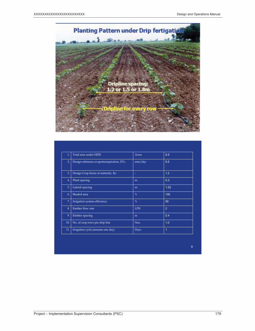
XXXXXXXXXXXXXXXXXXXXXXXX Design and Operations Manual
Project – Implementation Supervision Consultants (PSC) 179
7
9
1. Total area under HEIS Acres 6.5
2. Design reference evapotranspiration, ETo mm/day 6.5
3. Design Crop factor at maturity, Kc - 1.2
4. Plant spacing m 0.3
5. Lateral spacing m 1.52
6. Shaded area % 100
7. Irrigation system efficiency % 90
8. Emitter flow rate LPH 2
9. Emitter spacing m 0.4
10. No. of crop rows per drip line Nos. 1.0
11. Irrigation cycle (assume one day) Days 1

XXXXXXXXXXXXXXXXXXXXXXXX Design and Operations Manual
Project – Implementation Supervision Consultants (PSC) 180
10
S.N.
Parameters Unit Calculations
13 Peak daily consumptive use per day
Mm = ETo * Kc * shaded area/ efficiency=6.5 * 1.2 * 1 /0.9 = 8.7 mm
14 Total no. of plants Nos = Area x 4047 /(R-R * P-P)= 6.5*4047/(1.52*0.3) = 57,688
15 Total drip line length M = Area*4047/L-L= 6.5*4047/(1.52) = 17,306
16 Total no. of emitters Nos = Total drip length/ emitter spacing= 17306/0.4 = 43,266
17 Average emitter spacing M 0.4
18 Total flow rate Lph = total no. of emitters x emitter flow rate= 43266 * 2 = 86,531
19 Application rate Mm/hr Total flow rate / area= (86,531/1000)/(6.5*4047) *1000= 3.29
20 Operation time* hrs = Peak daily consumptive use/ Application rate= 8.7/3.29= 2.64 hrs
Do We Have Sufficient Water?
Peak Water Requirement = 8.7 mm/day (calculated previously) Volume of water required (m3/d)
= PWR x Area (m2) = 8.7/1000 * 6.5*4047 = 229 cubic meters per day
Water Availability
a) For Canal Water
Outlet discharge = 28 lps Warabandi period = 2 hrs
Total water availability = 28/1000*3600 * 2 = 202 cubic meters for seven days
NO
Water is not sufficient to design a drip irrigation system for 6.5 acres. Options: a) Reduce areaOr b) Arrange alternate water sourceGo for option b) as farmer has arranged water source i.e., tubewell water: Proceed further

XXXXXXXXXXXXXXXXXXXXXXXX Design and Operations Manual
Project – Implementation Supervision Consultants (PSC) 181
14
220 m
120 m
Pump
Option-I (Irrigate entire area at a time)
mainline
Sub-mainline
Lateral
110 m
60 m
60 m
Darcy- Weisbach and Blasius Equation can be combined to give accurate prediction of friction head loss for smooth plastic pipes of less than 125 mm (5 in.) diameter.
J = 100 hf/L = k * [(Q1.75)/(D4.75 )]
J = Head loss gradient, m/100 m Hf = pipe friction head loss, m K = Constant, 7.89 * 10 ^7 for metric units Q = Flow Rate, LPS L = Pipe length, m D = Inside Diameter of Pipe, mm
Darcy- Weisbach and Blasius Equation can be combined to give accurate prediction of friction head loss for smooth plastic pipes of less than 125 mm (5 in.) diameter.
J = 100 hf/L = k * [(Q^1.75)/(D^4.75 )] * F
J = Head loss gradient, m/100 m Hf = pipe friction head loss, m K = Constant, 7.89 * 10 ^7 for metric units Q = Flow Rate, LPS L = Pipe length, m D = Inside Diameter of Pipe, mm

XXXXXXXXXXXXXXXXXXXXXXXX Design and Operations Manual
Project – Implementation Supervision Consultants (PSC) 182
Lateral Design: Lateral length = 60 m No. of emitters = 60/0.4= 150 Lateral flow rate = 300 lph Assume 13 mm lateral line Inside diameter = 10 mm
J = 7.89*10^7 * [(300/3600)^1.75)/(10^4.75)] * 0.36 J= 6.53 m/100 m For 60 m length Hf = 3.92m
Lateral Design: Lateral length = 60 m No. of emitters = 60/0.4= 150 Lateral flow rate = 300 lph Assume 16 mm lateral line Inside diameter = 13 mm
J = 7.89*10^7 * [(300/3600)^1.75)/(13^4.75)] * 0.36 J= 1.9 m/100 m For 60 m length Hf = 1.1m
Sub-Mainline Design: Length = 120 m No. of laterals = 120/1.52= 79 Sub-main flow rate = 86531/2 =43265lph Assume 70 mm lateral line Inside diameter = 63 mm
J = 7.89*10^7 * [(43265/3600)^1.75)/(63^4.75)] * 0.36 J= 6.3 m/100 m For 120 m length Hf = 7.5 m
Sub-Mainline Design: Length = 120 m No. of laterals = 120/1.52= 79 Sub-main flow rate = 86531/2 =43265lph

XXXXXXXXXXXXXXXXXXXXXXXX Design and Operations Manual
Project – Implementation Supervision Consultants (PSC) 183
Assume 110 mm Sub-Mainline Inside diameter = 104 mm
J = 7.89*10^7 * [(43265/3600)^1.75)/(104^4.75)] * 0.36 J= 0.6 m/100 m For 120 m length Hf = 0.7 m
Darcy- Weisbach and Blasius Equation can be combined to give accurate prediction of friction head loss for smooth plastic pipes of less than 125 mm (5 in.) diameter.
J = 100 hf/L = k * [(Q^1.75)/(D^4.75 )]
J = Head loss gradient, m/100 m Hf = pipe friction head loss, m K = Constant, 7.89 * 10 ^7 for metric units Q = Flow Rate, LPS L = Pipe length, m D = Inside Diameter of Pipe, mm
Mainline Design: Length = 60 m Sub-main flow rate = 86531 LPH Assume 110 mm Sub-Mainline Inside diameter = 104 mm
J = 7.89*10^7 * [(86531/3600)^1.75)/(104^4.75)] J= 5.4 m/100 m For 60 m length Hf = 3.2 m
V = 1.274 q / d2
Where
V = velocity (m/s)
Q = volume flow (m3/s)
D = pipe inside diameter (m)
V = 1.274 x [(86531/(1000*3600)]/ [(104/1000)^2] = 3.68 m/s Darcy- Weisbach and Blasius Equation can be combined to give accurate prediction of friction head loss for smooth plastic pipes of less than 125 mm (5 in.) diameter.

XXXXXXXXXXXXXXXXXXXXXXXX Design and Operations Manual
Project – Implementation Supervision Consultants (PSC) 184
J = 100 hf/L = k * [(Q^1.75)/(D^4.75 )]
J = Head loss gradient, m/100 m Hf = pipe friction head loss, m K = Constant, 7.89 * 10 ^7 for metric units Q = Flow Rate, LPS L = Pipe length, m D = Inside Diameter of Pipe, mm
Mainline Design: Length = 60 m Sub-main flow rate = 86531 LPH Assume 170 mm Sub-Mainline Inside diameter = 160 mm
J = 7.89*10^7 * [(86531/3600)^1.75)/(160^4.75)] J= 0.7 m/100 m For 60 m length Hf = 0.4 m
23
Velocity of Mainlinev = 1.274 q / d2
where
v = velocity (m/s)
q = volume flow (m3/s)
d = pipe inside diameter (m)
V = 1.274 x [(86531/(1000*3600)]/ [(104/1000)^2]
= 1.20 m/sOK

XXXXXXXXXXXXXXXXXXXXXXXX Design and Operations Manual
Project – Implementation Supervision Consultants (PSC) 185
24
Velocity Formula to Determine Pipe Size for Mainline
v = 1.274 q / d2
d2 = V / (1.274 q)d = SQRT [V / (1.274 q)]
v = velocity (m/s)
q = volume flow (m3/s)
d = pipe inside diameter (m)
25
Filters: Head Loss
Source: Jain Disc Filter

XXXXXXXXXXXXXXXXXXXXXXXX Design and Operations Manual
Project – Implementation Supervision Consultants (PSC) 186
26Source: Jain Hydro-cyclone Filter
Filters: Head Loss
27Source: Jain Media Filter
Filters: Head Loss
TOTAL DYNAMIC HEAD
• Emitter operating pressure = 10 m • Head loss in lateral = 1.1 m • Lateral Elevation = 0 m • Head loss in submains = 0.7 m • Head loss in Valve (assume 2 m) = 2.0 m

XXXXXXXXXXXXXXXXXXXXXXXX Design and Operations Manual
Project – Implementation Supervision Consultants (PSC) 187
• Field fitting head loss = 2.0 m • Head Loss in Main line = 0.4 m • Primary filter head loss (Gravel 2 x40 M3) .2x2 =4m = 4 m • Secondary filter head loss (Disc 2 x 40 M3) .2x2 = 4m = 4 m • Fertigation equipment head loss (5 m for ventury) = 5 m• Water source depth = 0 m • Suction head = 1 m • Delivery head = 1 m • Safety equipment head loss = 2 m • Elevation difference = 0 m • Other losses = m • Total Head Required = 33.2 m
Say 35 m
PUMP REQUIREMENT
Total Flow Required = 85.531m3/hr = 23.8 lps Pump H.P = Q (LPS) * H (m)/ (75 x pump efficiency x motor efficiency)
= 23.8 * 35 /(75 * 0.65 * 0.9) = 19
Say 20 H.P
30
220 m
120 m
Pump
Option-II (Irrigate area into Zones: Say 2 Zones)
mainline
SM-2SM-1

XXXXXXXXXXXXXXXXXXXXXXXX Design and Operations Manual
Project – Implementation Supervision Consultants (PSC) 188
30
220 m
120 m
Pump
Option-II (Irrigate area into Zones: Say 2 Zones)
mainline
SM-2SM-1
31
220 m
120 m
Pump
Option-III (Irrigate area into Zones: Say 4 Zones)
mainline
SM-4
Lateral
SM-2SM-1
SM-3

XXXXXXXXXXXXXXXXXXXXXXXX Design and Operations Manual
Project – Implementation Supervision Consultants (PSC) 189
Parameters Unit HZ-1 HZ-2 HZ-3 HZ-4 Total
Area Acres 1.625 1.625 1.625 1.625 6.5
Peak daily consumptive use per day Mm 8.7 8.7 8.7 8.7 8.7
Total no. of plants Nos 14,422 14,422 14,422 14,422 57,688
Total drip line length M 4,327 4,327 4,327 4,327 17,306
Total no. of emitters Nos 10,816 10,816 10,816 10,816 43,266
Average emitter spacing M 0.4 0.4 0.4 0.4 0.4
Total flow rate Lph 21,633 21,633 21,633 21,633 21,633
Application rate Mm/hr 3.3 3.3 3.3 3.3 0.8
Operation time* hrs 2.6 2.6 2.6 2.6 10.532
Darcy- Weisbach and Blasius Equation can be combined to give accurate prediction of friction head loss for smooth plastic pipes of less than 125 mm (5 in.) diameter.
J = 100 hf/L = k * [(Q1.75)/(D4.75 )]
J = Head loss gradient, m/100 m Hf = pipe friction head loss, m K = Constant, 7.89 * 10 ^7 for metric units Q = Flow Rate, LPS L = Pipe length, m D = Inside Diameter of Pipe, mm
Darcy- Weisbach and Blasius Equation can be combined to give accurate prediction of friction head loss for smooth plastic pipes of less than 125 mm (5 in.) diameter.
J = 100 hf/L = k * [(Q^1.75)/(D^4.75 )] * F
J = Head loss gradient, m/100 m Hf = pipe friction head loss, m K = Constant, 7.89 * 10 ^7 for metric units Q = Flow Rate, LPS L = Pipe length, m D = Inside Diameter of Pipe, mm

XXXXXXXXXXXXXXXXXXXXXXXX Design and Operations Manual
Project – Implementation Supervision Consultants (PSC) 190
Lateral Design: Lateral length = 60 m No. of emitters = 60/0.4= 150 Lateral flow rate = 300 lph Assume 13 mm lateral line Inside diameter = 10 mm
J = 7.89*10^7 * [(300/3600)^1.75)/(10^4.75)] * 0.36 J= 6.53 m/100 m For 60 m length Hf = 3.92m
Lateral Design: Lateral length = 60 m No. of emitters = 60/0.4= 150 Lateral flow rate = 300 lph Assume 16 mm lateral line Inside diameter = 13 mm J = 7.89*10^7 * [(300/3600)^1.75)/(13^4.75)] * 0.36 J= 1.9 m/100 m For 60 m length Hf = 1.1m
Sub-Mainline Design: Length = 120 m No. of laterals = 120/1.52= 79 Sub-main flow rate = 86531/4 =21,633 lph Assume 70 mm lateral line Inside diameter = 63 mm J = 7.89*10^7 * [(21,633/3600)^1.75)/(63^4.75)] * 0.36 J= 1.9 m/100 m For 120 m length Hf = 2.2 m
Darcy- Weisbach and Blasius Equation can be combined to give accurate prediction of friction head loss for smooth plastic pipes of less than 125 mm (5 in.) diameter.
J = 100 hf/L = k * [(Q^1.75)/(D^4.75 )]
J = Head loss gradient, m/100 m Hf = pipe friction head loss, m K = Constant, 7.89 * 10 ^7 for metric units Q = Flow Rate, LPS

XXXXXXXXXXXXXXXXXXXXXXXX Design and Operations Manual
Project – Implementation Supervision Consultants (PSC) 191
L = Pipe length, m D = Inside Diameter of Pipe, mm
Mainline Design: Length = 60 m Sub-main flow rate = 86531 LPH Assume 90 mm Sub-Mainline Inside diameter = 87 mm
J = 7.89*10^7 * [(21633/3600)^1.75)/(87^4.75)] J= 1.1 m/100 m For 60 m length Hf = 0.7 m
38
Velocity of Mainlinev = 1.274 q / d2
where
v = velocity (m/s)
q = volume flow (m3/s)
d = pipe inside diameter (m)
V = 1.274 x [(21633/(1000*3600)]/ [(87/1000)^2]
= 1.01 m/s

XXXXXXXXXXXXXXXXXXXXXXXX Design and Operations Manual
Project – Implementation Supervision Consultants (PSC) 192
40Source: Jain Hydro-cyclone Filter
Filters: Head Loss
41Source: Jain Media Filter
Filters: Head Loss

XXXXXXXXXXXXXXXXXXXXXXXX Design and Operations Manual
Project – Implementation Supervision Consultants (PSC) 193
41Source: Jain Media Filter
Filters: Head Loss
• Emitter operating pressure = 10 m • Head loss in lateral = 1.1 m • Lateral Elevation = 0 m • Head loss in submains = 2.2 m • Head loss in Valve (assume 2 m) = 2.0 m • Field fitting head loss = 2.0 m • Head Loss in Main line = 0.7 m • Primary filter head loss (Gravel 20 m3) = 1.5 m • Secondary filter head loss (Disc 20 m3) = 1.3 m • Fertigation equipment head loss (5 m for ventury) = 5 m • Water source depth = 0 m • Suction head = 1 m • Delivery head = 1 m • Safety equipment head loss = 2 m • Elevation difference = 0 m • Other losses = m • Total Head Required = 29.8 m
Say 30 m
Total Flow Required = 21.382 m3/hr = 5.94 lps Pump H.P = Q (LPS) * H (m)/ (75 x pump efficiency x motor efficiency)
= 5.94 * 30 /(75 * 0.65 * 0.9) = 4.1
Say 5 H.P

XXXXXXXXXXXXXXXXXXXXXXXX Design and Operations Manual
Project – Implementation Supervision Consultants (PSC) 194
6.10 DESIGN OF SPRINKLER IRRIGATION SYSTEM
A pressurized irrigation system is a network of installation consisting of pipes, fittings and other devices properly designed and installed to supply water under pressure from the source of the water to the irrigable area.
Two main classification:
Sprinkler Irrigation Micro/Drip Irrigation
Typical Sprinkler Irrigation System Layout
Piped irrigation systems are classified according to the pressure required for operation, the method of delivering water to plants, and the type of installation
PRESSURE: it is the maximum water pressure required for normal system operation

XXXXXXXXXXXXXXXXXXXXXXXX Design and Operations Manual
Project – Implementation Supervision Consultants (PSC) 195
Low Pressure System: 2.0 to 3.5 bars Medium Pressure System: 3.5 to 5.0 bars High Pressure System: > 5.0 bars
TYPE OF INSTALLATION
Solid Installation (all components are installed at fixed positions) Semi- solid installation (Main and submain are permanent, lateral are portable,
hand move or mechanical move) Portable (all component parts are portable)
WATER DELIVERY METHOD
Sprinkler (Over head irrigation) Micro-irrigation (Localized irrigation) by dripper, bubblers, micro jets etc
Sprinkler irrigation is the method where water is sprayed through the air and it falls to the ground like rain. The spray is obtained by the flow of water under pressure through small orifices or nozzles known as sprinklers. Water is conveyed from the pump and distributed through a network of pipes called mainline, sub-mainlines, laterals and sprinklers.
Advantages
Sprinkler irrigation is suitable for all crops except rice as it requires standing water. Water can be spread over row crops and under canopy of tree crops. Large sprinklers are not suitable for delicate flowering and fruiting plants because larger
water drops may damage the crop.
• Suitable to complete range of topography• Land leveling not required• Light textured soil which cannot be irrigated properly by surface irrigation can be effectively
irrigated.• Higher irrigation efficiency can be achieved through proper designing• Soluble fertilizers can be applied through foliar application• Easy to operate• Less sensitive to clogging.• High efficiency can be achieved with a proper design
Disadvantages
Very sensitive to wind conditions Higher evaporation rate Fine textured soil having very low infiltration rates cannot be irrigated efficiently Few crops with delicate flowering cannot be irrigated with sprinkler system Use of low quality water may cause leaf burn Must work under pressure, according to the manufacturer’s recommendations to obtain
good results

XXXXXXXXXXXXXXXXXXXXXXXX Design and Operations Manual
Project – Implementation Supervision Consultants (PSC) 196
Two Basic Groups Set System
Periodic move systems Hand move lateral, End-Tow Lateral, Rain Gun system, Boom
sprinklers etc. Fixed system
Lateral lines and sprinkler heads are fixed Continuous move systems
Center Pivot system Linear Move system
Agriculture sprinklers Operating pressure (bars)
Flow rate(m3/h)
Diameter coverage (m)
Low pressureMedium pressure
High pressure
1.5-2.52.5-3.54.0-9.0
0.3-1.51.5-3.05.0-45.0
12-2124.3560-80
Classification of sprinkler heads based on operating pressure
The initial cost and the labor required are both directly related to the portability of a sprinkler system. The more portable a system, the lower the initial cost and the higher the labor requirements to operate it Conversely, the permanent system has the highest initial cost and lowest labor requirements. Each person selecting a sprinkler system has his own set of circumstances and economic conditions to consider.
The selection of a system is an economic compromise of these individual conditions. and no two may be exactly alike However, after the type of system has been selected, there is a basic common guideline to follow in developing the details of the system

XXXXXXXXXXXXXXXXXXXXXXXX Design and Operations Manual
Project – Implementation Supervision Consultants (PSC) 197

XXXXXXXXXXXXXXXXXXXXXXXX Design and Operations Manual
Project – Implementation Supervision Consultants (PSC) 198

XXXXXXXXXXXXXXXXXXXXXXXX Design and Operations Manual
Project – Implementation Supervision Consultants (PSC) 199
6.10.1 Components of Sprinkler System
A. PUMP SET
Centrifugal/deep-well turbine pumps may be used. May be powered by electric motors or internal combustion engines using diesel, gasoline
or natural gas.
B. Main pipeline, Sub-mains & Laterals
To convey water from the pumping unit to the laterals. Laterals may be directly connected to the main line without any sub-main line. Generally made of uPVC and HDPE Generally made of uPVC and HDPE
C. Laterals
receive water from the main pipeline or sub-main to the sprinklers.Usually made of uPVC, HDPE
D. Riser/Hydrants
To connect sprinkler head to the lateral pipe. Height of riser pipe depends upon the height of crop to be irrigated and sprinkler flow rate..

XXXXXXXXXXXXXXXXXXXXXXXX Design and Operations Manual
Project – Implementation Supervision Consultants (PSC) 200
Generally made of Aluminum, GI
E. Valves & Safety Equipment
Flow control valve: To divert flow from mainline to sub-mainline Check/NRV valves: on the discharge side of the pump so that if the pump is shut off it
should maintain water in the pipeline above the pump. Foot-valve: on the bottom of the suction pipe Pressure Gauges: To monitor system pressure Flow Meter: to record amount of water passing
6.11 SPRINKLER SYSTEM TECHNICAL ASPECT
i. Discharge from Sprinkler Nozzle
Theoretical discharge from sprinkler nozzle can be computed from orifice flow equation:
ghcdaq 2
q = nozzle discharge, m3/sec a = x- sectional area of sprinkler nozzle, m2 h = pressure head at the nozzle, m Cd = coefficient of discharge as a function of friction and contraction (ranges from 0.8 to 0.98: larger the nozzle, lower the coefficient) g =acceleration due to gravity, m/sec2
ii. Wetted Area of Sprinkler
RAdhR 35.1
A = Area covered by the sprinkler, m2 R = Radius of weter area, m d = Diameter of sprinkler nozzle, mm h = Pressure head at nozzle, m
iii. Distribution Uniformity
100.1dyEd
Indicates the extent to which water is uniformly distributed.

XXXXXXXXXXXXXXXXXXXXXXXX Design and Operations Manual
Project – Implementation Supervision Consultants (PSC) 201
Ed = Water distribution efficiency, % d = Average depth of water stored y = Average numerical deviation from d
iv. Application Rate of Sprinkler
The rate at which sprinkler apply water on soil surface. Application rate depends on:
• Size of sprinkler nozzle• Operating pressure• Spacing between sprinklers
SlxSmqI
I = Application rate, mm/hr q = Discharge, lph Sm = Sprinkler spacing along sub-mainline, m Sl = Sprinkler spacing on lateral, m
v. Capacity Requirement
fTAdQ 78.2
Q = System Discharge Capacity, lps A = design area (ha) D = gross depth of application (mm) f = Time allowed for completion of irrigation (days) T = Actual operating time (hrs/day)
vi. Minimum Number of Sprinklers Operating
qQNn
Nn = Minimum average number of sprinkler operating q = average sprinkler discharge
vii. Wind Effect on the Diameter of Throw
For 0-3 mph wind:
reduce manufacturer's listed diameter of throw by 10% for an effective value (i.e. the diameter where the application of water is significant) over 3 mph wind:

XXXXXXXXXXXXXXXXXXXXXXXX Design and Operations Manual
Project – Implementation Supervision Consultants (PSC) 202
reduce manufacturer's listed diameter of throw by an additional 2.5% for every 1 mph above 3 mph (5.6% for every 1 m/s over 1.34 m/s)
viii. Wind Effect on The Diameter of Throw
For 0-3 mph (0-1.34 m/s): diam = 0.9diammanuf
For > 3 mph (> 1.34 m/s): diam = diammanuf [0.9 - 0.025 (windmph - 3)]
Example: a manufacturer gives an 80-ft diameter of throw for a certain sprinkler and operating pressure. For a 5 mph wind, what is the effective diameter? 80 ft - (0.10)(0.80) = 72 ft diam = 80(0.9-0.025(5-3))=68 ft
ix. Overlapping
Distribution pattern of a single sprinkler is not uniform throughout the radius and also affects drastically by wind. To minimize the effect of wind and provide uniform depth of water on the area under sprinkler irrigation system, distance between the sprinklers is reduced in such a way that water from one sprinkler reaches approximately to the adjacent sprinkler.

XXXXXXXXXXXXXXXXXXXXXXXX Design and Operations Manual
Project – Implementation Supervision Consultants (PSC) 203
Dry zone
Water distribution patterns for individual and overlapped sprinklers (Source: USDA, SCS Handbook, 1960).
SPRAY PATTERN AS A RESULT OF OVERLAPPING

XXXXXXXXXXXXXXXXXXXXXXXX Design and Operations Manual
Project – Implementation Supervision Consultants (PSC) 204
1. RECTANGULAR SPACING
Sprinkler spacing at lateral40% of effective diameter
Lateral Spacing67% of the effective diameter
(For big volume Rain Gun lateral spacingshould not exceed 65% of effective diameterand sprinkler spacing at lateral should be 50%of effective wetted diameter)
40% of Deff
67% of Deff
DIFFERENT PATTERN OF SPRINKLER PLACEMENT
Sprinkler spacing at lateral50% of effective diameterLateral Spacing50% of the effective diameter 50% of Deff
50% of Deff

XXXXXXXXXXXXXXXXXXXXXXXX Design and Operations Manual
Project – Implementation Supervision Consultants (PSC) 205
Sprinkler spacing at lateral62% of effective diameterLateral Spacing54% of the effective diameter
Rectangular: 40% x 67%
Square: 50% x 50%
Triangular: 62% x 54%
OVERLAPPING PATTERNSDIFFERENT SPACING OF LATERALS

XXXXXXXXXXXXXXXXXXXXXXXX Design and Operations Manual
Project – Implementation Supervision Consultants (PSC) 206
Sprinkler Discharge(lps)
Minimum Riser height (cm)
< 0.6 15
0.6 to 1.6 23
1.6 to 3.2 30
3.2 to 7.6 45
>7.6 90
Riser pipes elevate and support the sprinklers above the cropProvide connecting link to the lateral.
Soil texture
Maximum application rate (mm/hr)
0 to 5% 5 to 8% 8 to 12% 12 to 16%Coarse sandy soil
50 38 25 13
Light sandy loam
25 20 15 10
Silty loam 13 10 8 5Heavy textured clay
4 2.5 2 1.5

XXXXXXXXXXXXXXXXXXXXXXXX Design and Operations Manual
Project – Implementation Supervision Consultants (PSC) 207

XXXXXXXXXXXXXXXXXXXXXXXX Design and Operations Manual
Project – Implementation Supervision Consultants (PSC) 208
S.No Crop Ece (dS/m)
1 Cotton 9.62 Sorghum 5.13 Wheat 7.44 Maize 2.5
68
The criteria for selection of sprinkler spacing are based on uniformity of water distribution within the limitation of wind velocity. Higher the wind velocity will result in lower spacing between the sprinklers and vice versa. Fig 6.5 below shows water distribution pattern of a particular sprinkler system. This depicts that area under the first 60% of the sprinkler’s radius is generally sufficiently irrigated for growing crop without any overlapping. Beyond this, quantum of water will be reducing and thus will not be sufficient to grow crop. To overcome this problem, overlapping between the sprinklers is suggested with following recommendations.

XXXXXXXXXXXXXXXXXXXXXXXX Design and Operations Manual
Project – Implementation Supervision Consultants (PSC) 209
Fig. 6.5 Wetting Pattern Without and with Overlapping
At the same time wind badly affects the distribution pattern of a sprinkler system. Fig. 6.6 shows the effect of wind over the distribution pattern of a particular sprinkler system.
Fig 6.6 Distribution Pattern Distorted by Wind (10.7 MPH)
Volume of water delivered from the sprinkler varies from sprinkler to the edge of the wetted radius as shown in Fig. below. More water will be available near the sprinkler and will be reduced gradually as we move away from sprinkler. Finally, where the sprinkler radius came to an end there will be no water. Sprinkler water distribution graph is shown in Fig 6.7.
Wat
er d
epth
Distance from sprinkler

XXXXXXXXXXXXXXXXXXXXXXXX Design and Operations Manual
Project – Implementation Supervision Consultants (PSC) 210
Fig 6.7 Sprinkler water distribution graph (Courtesy: Rain Bird)
It is noted that 60% radius of the sprinkler will be well irrigated to meet the crop water demands and remaining 40% will be under irrigated. To overcome this problem, the flow from other sprinkler should fall in this 40% radius of the first sprinkler so as sum of flows from both sprinklers in this area would approximately match the flow depth in the 60% radius of the first sprinkler as shown in the Fig 6.8.
Fig 6.8 60% of diameter sprinkler spacing (Courtesy: Rain Bird)
Another layout showing head-to-head sprinkler spacing is shown in following Fig 4.9 to match the flow in each part of the area under sprinkler system.
Fig 6.9 Head To Head Sprinkler Spacing For Uniform Water Distribution

XXXXXXXXXXXXXXXXXXXXXXXX Design and Operations Manual
Project – Implementation Supervision Consultants (PSC) 211
6.11.1.1 Effect of pressure on Sprinkler
Sprinkler wetting pattern is affected by pressure and nozzle size. For a particular combination of nozzle size and at manufacturer’s recommended operating pressure, precipitation profile seems like Fig 6.10-b. When pressure is much lower than the manufacturer’s recommended pressure, large sized drops fall near the sprinkler in a ring as shown in Fig. 6.10-a. When pressure is much higher than manufacturers recommended pressure, then very small sized drops results and can be distorted easily and precipitation profile results like Fig. 6.10-c.
Fig 6.10-a. Pressure is too low
Fig 6.10-b. Pressure is satisfactory
Fig 6.10-c. Pressure is too high
6.11.1.2 Sprinkler Pattern
There are three different ways for placing sprinklers to achieve uniform application of water namely square, triangle and rectangular pattern.
The detail of sprinkler patterns is explained in the following sections.

XXXXXXXXXXXXXXXXXXXXXXXX Design and Operations Manual
Project – Implementation Supervision Consultants (PSC) 212
Square Spacing
The distance between sprinkler along the laterals and between the lateral is kept same under square pattern of sprinkler spacing as shown in Fig.6.11. This pattern is suitable to sites which are square in geometry. The spacing between sprinklers is decided based on the wind conditions as given below:
For wind velocity 0 to 3 mph (0 to 5 km/h), the spacing should be 55% of diameter For wind velocity 4 to 7 mph (6 to 11 km/h), the spacing should be 50% of diameter For wind velocity 8 to 12 mph (13 to 19 km/h), the spacing should be 45% of diameter
Fig 6.11 Square sprinkler pattern
The limitation of square pattern is that diagonal distance increases to approximately 70% of wetted diameter (for 50% sprinkler spacing).
Triangular Spacing
Triangular spacing is generally adopted for irregular field boundaries, over spray is permitted and no part circle sprinklers are needed. The geometrical view of triangular spacing is shown in Fig 6.12. The recommended spacing for this pattern as suggested by Rain Bird is given below:
Fig 6.12 Triangular Sprinkler Pattern
The distance between sprinklers is usually labeled S, and the distance between rows is labeled L.

XXXXXXXXXXXXXXXXXXXXXXXX Design and Operations Manual
Project – Implementation Supervision Consultants (PSC) 213
Sprinkler spacing should be selected based on the following relationship.
L= S x 0.866
Where; L = sprinkler spacing between lateral S = sprinkler spacing at lateral
Recommends triangular spacing (Source Rain Bird):
60% if wind velocities are 0-3 mph on site. 55% if wind velocities are 4-7 mph on site. 50% if wind velocities are 8-12 mph on site.
Rectangular Spacing
The spacing between lateral (L) is usually kept more than the sprinkler spacing (S) forming a rectangular pattern. The recommended spacing for rectangular pattern is given below.
Recommended triangular spacing (Source Rain Bird):
L=60% of wetted diameter, S=50% wetted diameter if wind velocities are 0-3 mph on site. L=60% of wetted diameter, S=45% wetted diameter if wind velocities are 4-7 mph on site. L=60% of wetted diameter, S=40% wetted diameter if wind velocities are 8-12 mph on site.
CONSUMPTIVE USE
For the design of surface and sprinkler irrigation systems: ETcrop = ETo x Kc/(1-LR) Potential Water Requirement = ETcrop/(Efficiency)
LEACHING REQUIREMENT
ECwECeECwLR
)(5
LR = leaching requirement (Fraction) Ecw = Salinity of applied irrigation water in dS/m Ece = Average soil salinity tolerated by crop taken from literature
IRRIGATION DEPTH
dx = MAD (Wa . Z)/100 dx = Maximum depth of water to be applied per irrigation (mm)

XXXXXXXXXXXXXXXXXXXXXXXX Design and Operations Manual
Project – Implementation Supervision Consultants (PSC) 214
MAD =Management Allowed Deficit (%) Wa =Water holding capacity of soil, mm/m Z =Effective root depth, m
IRRIGATION INTERVAL
Fx = dx/Cu = MAD (Wa . Z)/(cu . 100) Fx = Irrigation interval, days dx = Maximum depth of water to be applied per irrigation (mm) MAD =Management Allowed Deficit (%) Wa =Water holding capacity of soil, mm/m Z =Effective root depth, mm Cu = Consumptive use, mm
OPERTIONAL TIME
Operation time depends upon various factors including;
• Weather conditions• Crop stage,• Root depth etc.
Daily operation time = Daily consumptive use/ Application Rate
SYSTEM HYDRAULICS
Determining the pressure distribution in the system Selection of pipe sizes and fittings to convey and regulate water delivery Determining the power and energy requirements
WAYS OF CALCULATING FRICTION LOSS
Equations Hazen-Williams Darcy-Weisbach Watters and Keller Tables/Charts for any given pipe material, pipe diameter, and flow rate, look up values for friction loss in
meter per hundred meters of pipe Software: Based on equations
FACTORS AFFECTING FRICTION LOSS
Flow rate Pipe diameter Pipe length Pipe roughness Type of fluid

XXXXXXXXXXXXXXXXXXXXXXXX Design and Operations Manual
Project – Implementation Supervision Consultants (PSC) 215
HAZEN- WILLIAM EQUATION
J = hf/ (L/100) = K (Q/C)1.852 * D - 4.87 J = head loss gradient, m/100m K = Conversion constant, 1.212 * 10^12 for metric units Hf = Head loss due to pipe friction, m L = Length of pipe, m Q = Flow rate in pipe, L/S C = Friction Factor, for PVC pipe C=150 D = Inside diameter of pipe, mm
Typical values of C for use in the Hazen-Williams equation are:
Pipe Material C Plastic 150 Epoxy-coated steel 145 Cement asbestos 140 Galvanized steel 135 Aluminum (with couplers every 30 ft) 130 Steel (new) 130 Steel (15 years old) or concrete 100 Source: (Keller and Blisner, 1988, page 135)
For smooth plastic pipes, Watters and Keller (1978) proposed the following equations as discussed by Keller and Bliesner (1988, page 138):
WATERS AND KELLER FORMULA
For small Pipe less than 125 mm J = 100 * hf/ L = K (Q)1.852 x D -4.75 J = head loss gradient, m/100m K = Conversion constant, 7.89 * 10^7 for metric units Hf = Head loss due to pipe friction, m L = Length of pipe, m Q = Flow rate in pipe, L/S D = Inside diameter of pipe, mm
WATERS AND KELLER FORMULA
For Pipe Greater than 125 mm J = 100 * hf/ L = K (Q)1.83 / D 4.83 J = head loss gradient, m/100m K = Conversion constant, 9.58 * 107 for metric units Hf = Head loss due to pipe friction, m L = Length of pipe in, m Q = Flow rate in pipe, L/S D = Inside diameter of pipe , mm
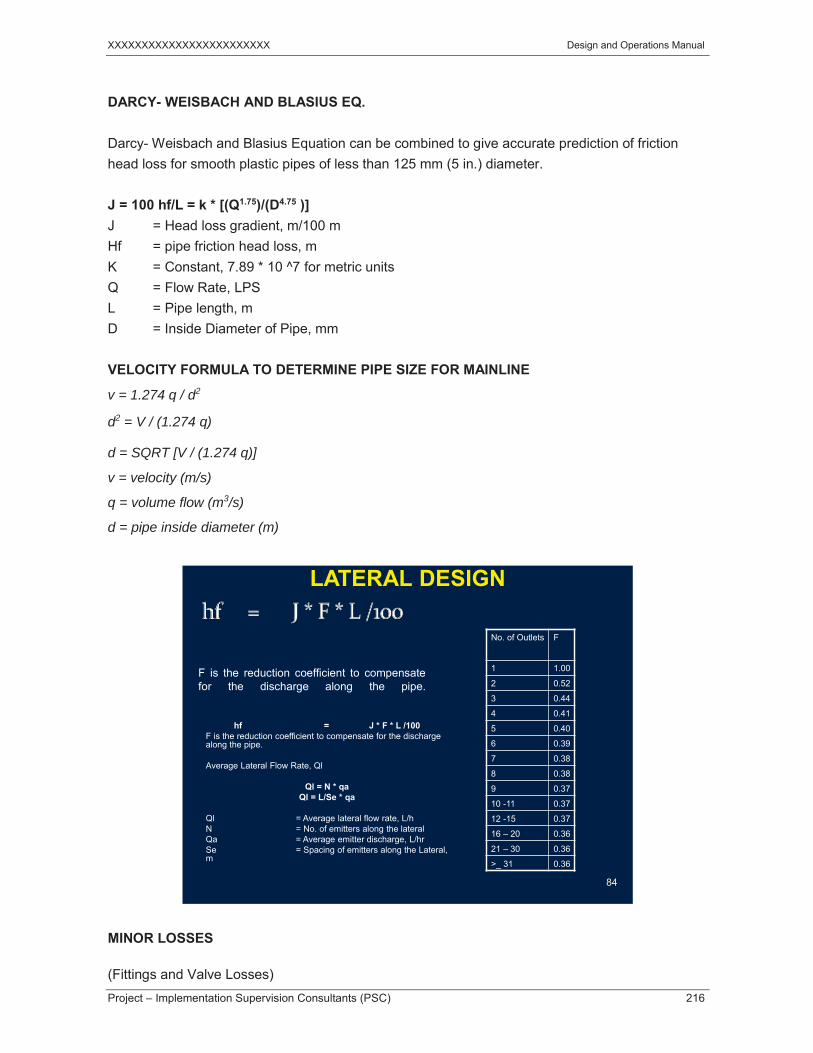
XXXXXXXXXXXXXXXXXXXXXXXX Design and Operations Manual
Project – Implementation Supervision Consultants (PSC) 216
DARCY- WEISBACH AND BLASIUS EQ.
Darcy- Weisbach and Blasius Equation can be combined to give accurate prediction of friction head loss for smooth plastic pipes of less than 125 mm (5 in.) diameter.
J = 100 hf/L = k * [(Q1.75)/(D4.75 )] J = Head loss gradient, m/100 m Hf = pipe friction head loss, m K = Constant, 7.89 * 10 ^7 for metric units Q = Flow Rate, LPS L = Pipe length, m D = Inside Diameter of Pipe, mm
VELOCITY FORMULA TO DETERMINE PIPE SIZE FOR MAINLINE
v = 1.274 q / d2
d2 = V / (1.274 q)
d = SQRT [V / (1.274 q)]
v = velocity (m/s)
q = volume flow (m3/s)
d = pipe inside diameter (m)
No. of Outlets F
1 1.00
2 0.52
3 0.44
4 0.41
5 0.40
6 0.39
7 0.38
8 0.38
9 0.37
10 -11 0.37
12 -15 0.37
16 – 20 0.36
21 – 30 0.36
>_ 31 0.36
84
F is the reduction coefficient to compensatefor the discharge along the pipe.
LATERAL DESIGN
hf = J * F * L /100F is the reduction coefficient to compensate for the discharge along the pipe.
Average Lateral Flow Rate, Ql
Ql = N * qaQl = L/Se * qa
Ql = Average lateral flow rate, L/hN = No. of emitters along the lateralQa = Average emitter discharge, L/hr Se = Spacing of emitters along the Lateral, m
MINOR LOSSES
(Fittings and Valve Losses)

XXXXXXXXXXXXXXXXXXXXXXXX Design and Operations Manual
Project – Implementation Supervision Consultants (PSC) 217
Hf = Kr [ V2/ 2g] Hf = Friction head loss due to pipe fittings, m (ft) Kr = Resistance coefficient for the fitting or valve V2/2g = Velocity head for given discharge, m (ft) g = Acceleration due to gravity, 9.81 m/s (32.2 ft/sec)
V2/2g = K Q2/D4
K is constant 8.26 x 10⁴ for metric unit, 2.59 x10⁻³ for English unit)
SizeODID
Wall Thk
Flow GPM
Velocity FPS
PSI Loss
Velocity FPS
PSI Loss
Velocity FPS
PSI Loss
2 0.56 0.06 0.26 0.01 0.16 04 1.11 0.22 0.51 0.03 0.33 0.026 1.67 0.46 0.77 0.07 0.49 0.038 2.23 0.79 1.03 0.12 0.66 0.05
10 2.78 1.19 1.28 0.18 0.82 0.0712 3.34 1.67 1.54 0.25 0.99 0.1116 4.45 2.85 2.05 0.43 1.31 0.1818 5.01 3.54 2.31 0.54 1.48 0.2220 5.56 4.31 2.56 0.65 1.64 0.2622 6.12 5.14 2.82 0.78 1.81 0.3124 6.68 6.03 3.08 0.92 1.97 0.3626 7.23 7 3.33 1.06 2.14 0.4128 7.79 8.03 3.59 1.22 2.3 0.4730 8.35 9.12 3.85 1.38 2.46 0.6235 9.74 12.14 4.49 1.84 2.87 0.840 11.13 15.54 5.13 2.36 3.28 0.9945 12.52 19.33 5.77 2.93 3.7 1.2150 13.91 23.49 6.41 3.57 4.11 1.4455 15.3 28.03 7.05 4.26 4.52 1.6960 16.69 32.93 7.69 5 4.93 1.9665 18.08 38.19 8.33 6.65 5.34 2.2570 19.47 43.81 8.97 7.56 5.75 2.5675 - - 9.61 8.52 6.16 2.88
0.052 0.058 0.073
1.211 1.784 2.2291.315 1.9 2.375
1" 1 1/2" 2"Charts
Example

XXXXXXXXXXXXXXXXXXXXXXXX Design and Operations Manual
Project – Implementation Supervision Consultants (PSC) 218
Total head required (H)
Total dynamic head should be capable of supplying required pressure and discharge for efficient functioning of the system.
Total head required (H) = suction head + Delivery head + Filtration losses+ Fertigation system losses+ Friction loss in pipes (main, sub-main and lateral) + Emitter operating pressure+ Fitting losses + Elevation (if any) Suction = Vertical distance between water level to center of pump Delivery = Vertical distance between center of pump to ground level Filtration losses = Filtration head losses in different types of filters Fertigation losses = Certain pressure is required to operate fertigation
system, generally 5 m for manually operated ventury.
Friction losses in pipe = sum of pressure loss calculated for main, sub-main and lateral lines Emitter operating pressure = Recommended emitter operating pressure given by the manufacturer Fitting Losses = Generally 20% of pipe network lossess Elevation = Vertical distance b/w ground level near to water source
to the highest or lowest level
HORSE POWER REQUIRED
Q x H H.P = ----------------
75 x e1 x e2
where:
Q is discharge, l/s H is the total head, m; e1 is the pump efficiency (fraction in the order of 0.5-0.8); and e2 is the driving efficiency (fraction of 0.7-0.9 for electric motors and 0.5-0.75 for diesel engines). The overall pumping efficiency under field conditions ranges accordingly from 0.35 in engine driven units to 0.50 in motor driven pumps. Higher efficiencies are not realistic. (Always rely on manufacturer chart to know the actual horse power)
6.12 Design Process Sprinkler
6.12.1 Factors Affecting the Layout of Sprinkler System
Availability of water, quality, and source of power Soil factors Crop factors and uniformity required Purpose of the system and amount and frequency of water application

XXXXXXXXXXXXXXXXXXXXXXXX Design and Operations Manual
Project – Implementation Supervision Consultants (PSC) 219
Sprinkler spacing, nozzle size, and operating pressure Relative land elevations and pressure requirements. Layout of main and lateral lines Sizing of main and lateral lines for proper operation. Plans for proper operation of system Economic analysis
6.12.2 Design Procedure-Step by Step (Sprinkler)
Under the on-going project, sprinkler systems are being installed on field crops. In this section, steps for designing a sprinkler irrigation system will be discussed. The following are the design steps.
Collection of Basic Information Selection of Sprinkler Heads Place sprinkler heads Design map Calculation of total flow Estimation of PWR Calculation of Application rate Running time per operation No. of operations Calculation of sectional flow Calculation of total dynamic head (H) Calculation of required horsepower (HP) Selection of Pumps and Motor Preparation of Drawing Preparation of Bill of Quantities
Step 1. Collection of Basic Information
The following basic information be available before designing a sprinkler irrigation system.
• General information: Name of farmer, village/chak No., tehsil, district, phone No.• Land holding and Area of the project• Engineering survey: GPS coordinates, Field measurement, Elevation difference/slope.
After field measurement, a map showing all dimensions and location of water source bedrawn
• Agricultural details: crops (orchard, row/field crop), spacing, type, age, Effective CropRoot Depth, Reference Evapo-transpiration of the area (ETo), and water requirementof crop, Management Allowable Deficit (MAD)
• Crop Spacing (Row to Row, Plant to Plant), sowing and harvesting date• Soil Type/texture, Water Holding Capacity• Soil and water analysis reports: water quality, presence of iron, pH, suspended
particles, soil type, Electrical Conductivity of Irrigation water (Eciw), pH• Water Source, quantity, availability, location• Power Source:Electric motor, diesel engine, tractor, solar system• Climatologically data: temperature, humidity, rainfall, wind speed• Peak Water Requirement: (ETo, Kc, Cf)• Water source and Total Available Time of water• System capacity: The system should have capacity adequate to fulfill daily crop water
requirements of the area within a stipulated time or not more than 12 hours of operationper day (only for Pakistan circumferences, otherwise may be 22 hrs).
The basic information can be categorized as under.

XXXXXXXXXXXXXXXXXXXXXXXX Design and Operations Manual
Project – Implementation Supervision Consultants (PSC) 220
I. GENERAL INFORMATION Name of beneficiary Town/Village/City Tehsil District Province Phone No. Land holding (Acre) Scheme area (acres) 16.06 Topography (Flat/Undulated)
II. CROP INFORMATION
Parameters Crop Area (acres)
Plant spacig
(m)
Row spacing
(m) Age of
crop(years) Sowing
date Harvesting
date
Block-I Orchard Proposed Citrus 7.04 3.10 6.1 2
Rotation Sub total: I
Block-I Orchard Proposed Citrus 6.07 4.57 4.57 New
Rotation Sub total: II
Block-I Orchard Proposed Mango 1.2 6.10 6.1 1
Rotation Sub total: III
Block-I Sub total: IV

XXXXXXXXXXXXXXXXXXXXXXXX Design and Operations Manual
Project – Implementation Supervision Consultants (PSC) 221
III. SOIL TYPE/SOIL TEST/WATER SUPPY/WATER QUALITY
Soil type/Texture
Soil limitation (soil analysis report attached)
Soil EC , PH , N , P , K , SAR
WATER SUPPLY
Available water sources
1) Canal
Sanctioned discharge (LPS)
Perennial/non-perennial
Warabandi Days
Hours per Warabandi
Total Volume (m3) of water for 7 days
2) Groundwater
a) Dug well
Depth of well
Diameter of well
Recharge rate
b) Tube well/bore well
Discharge capacity (LPS)
Diameter of bore (inches)
Depth of water table from ground (m)
3) Storage/reservoir capacity (m3)
Water quality (detailed report attached) Iron
Ph
EC(mmohs/cm)
Distance of water source from field (m)

XXXXXXXXXXXXXXXXXXXXXXXX Design and Operations Manual
Project – Implementation Supervision Consultants (PSC) 222
IV. POWER SOURCE AND PUMP
POWER SOURCE
Type of power to be used For electric Motor, Type of connection (single/3-phase) Make/model HP of Motor RPM of Motor
For diesel engine Make HP Condition) For Tractor Make/model HP Condition Any other power source, if any PUMP SET Type Make/Model Pressure (ft/psi/bar) Flow(lps) Inlet/outlet size RPM Pulley size

XXXXXXXXXXXXXXXXXXXXXXXX Design and Operations Manual
Project – Implementation Supervision Consultants (PSC) 223
Water Analysis Report
Farmer Name : Abbass Qureshi Water Source Address :Muzaffar garh Sampling Date
Ph :0345-8644888 Sp Receive Date : Agronomist: Ather Mehmood Khursheed Report Date :
Ref.Sample #
Parameters Degree of Presence / Problem Unit Nomal Higher Extreme
pH 7 <7 Acidic >7 A Electrical Conductivity (Salinity) microsemens/cm - - - Total dissolved solids ppm <500 500 - 600 >600 Hardness ppm <200 200 - 300 >300 Calcium ppm <60 60 - 100 >100 Magnesium Ppm <25 25 - 40 >40 Carbonate Ppm <200 200 - 600 >600 Bicarbonate Ppm <200 200 - 600 >600 Chloride (Toxic) Ppm <140 140 - 350 >350 Sulphates Ppm <20 20 - 50 >50 Sodium Ppm <100 100 - 200 >200 SAR - <3 3-9 >9 Potassium Ppm <10 10 - 20 >20 Sulphides Ppm <15 15-25 >25 Iron Ppm <0.1 0.1 - 0.4 >0.4 Manganese Ppm <0.2 0.2 - 0.4 >0.4 Suspended solids Ppm <10 10 - 100 >100 Boron Ppm <0.5 0.5 - 2.0 >2.0

XXXXXXXXXXXXXXXXXXXXXXXX Design and Operations Manual
Project – Implementation Supervision Consultants (PSC) 224
Soil Analysis Report
Farmer Name : Abbas Qureshi Block Size :
Address : Muzaffargarh Sampling Date : 11/5/2010
Ph : 345864488 Sp Receive Date : 13/05/2010
Agronomist : Ather Mehmood Sheikh Report Date : 26/04/2010
Code : AMK-S001
Ref.Soil Sample
#
Block #
Depth (inches)
Texture Organic Matter
%
pH Electrical
conductivity (mic/cm)
Available Phosphorus(P)
(ppm)
Available Potassium(K)
(ppm) Soluble & Exch.
Na (meq/L)
Soluble & Ca +Mg
(meq/L)
SAR
Neutral 6.5- 7.5 Alkaline
>8.5
Poor <7.0 Medium 7-13
Satisfactorty >13
Poor <125 Medium 125-
250 Satisfactorty
>250
Normal <10.0 Sodic
>10.0
2835 1
0 - 6'' Sand,Clay 0.245 8.44 411 - 110 6.52 3.2 4
2836 6 - 12'' Sand,Clay 0.582 7.74 468 - 120 6.95 3.2 4.3
2837 2
0 - 6'' Sand,Clay 0.827 8.15 572 - 110 11.73 3.1 7.5
2838 6 - 12'' Sand,Clay 0.612 8.26 550 - 110 10.43 2.7 7.7
2839 3
0 - 6'' Sand,Clay 0.612 8.29 316 - 90 6.52 3.4 3.8
2840 6 - 12'' Sand,Clay 0.735 8.39 304 - 90 6.95 3.7 3.7
2841 4
0 - 6'' Sand,Clay 0.821 8.21 384 - 100 6.08 3.2 3.8
2842 6 - 12'' Sand,Clay 0.735 8.25 358 - 100 6.52 3.2 4
2843 0 - 6'' Sand,Clay 1.01 8.02 506 - 150 4.34 5.1 1.7
2844 6 - 12'' Sand,Clay 0.98 8.02 494 - 160 4.34 4.2 2
2845 6
0 - 6'' Sand,Clay 1.041 8.05 412 - 120 4.34 4.2 2
2846 6 - 12'' Sand,Clay 0.919 8.11 356 - 100 4.34 4.2 2
2847 7
0 - 6'' Sand,Clay 0.919 7.97 1080 - 80 10.86 6.6 3.2
2848 6 - 12'' Sand,Clay 0.549 8.02 1123 - 80 11.73 5.8 4
It is advisable to make rough map of the area and mark salient features, divide the drawn map into different blocks and number the same for soil and water sampling. This map will be finalized during designing of drip irrigation system and will show all necessary details including drippers, dia, length and location of laterals, submain and main, location of water source, power source etc.,

XXXXXXXXXXXXXXXXXXXXXXXX Design and Operations Manual
Project – Implementation Supervision Consultants (PSC) 225
Step 2. Estimation of Leaching Requirement
All irrigation water contains some dissolved salts that are pushed downward by sprinkling and rainfall. By applying more water than the plants consume, most of the salts can be pushed or leached below the root zone. The first step in computing bye additional water required for leaching is to determine the leaching requirement by:

XXXXXXXXXXXXXXXXXXXXXXXX Design and Operations Manual
Project – Implementation Supervision Consultants (PSC) 226
Where
LR = leaching requirement ratio for sprinkle or surface irrigation ECw = electrical conductivity of the irrigation water, Ds/M (MMHOS/CM)
ECe = estimated electrical conductivity of the average saturation extract of the soil root zone profile for an appropriate yield reduction, ds/m ( mmhos /cm)
It is recommended that the ECe values presented in Table 3.5 be used in Eq. 3.3. These are values that will give an approximate 10% yield reduction, as

XXXXXXXXXXXXXXXXXXXXXXXX Design and Operations Manual
Project – Implementation Supervision Consultants (PSC) 227
Step 2. Estimation of Peak Crop Water
Requirement
Estimating the reference crop evapo-transpiration (ETo), using the Penman-Monteith method, and the crop evapo-transpiration (ETc), through the use of the appropriate crop factor Kc, have been covered in Module 4 Chapter______ of this Manual. Evapo-transpiration is composed of the evaporation from the soil and the transpiration of the plant. Since under localized irrigation only a portion of the soil is wetted, the evaporation component of evapotranspiration can be reduced accordingly, using the appropriate ground cover reduction factor Kr.
For the design of sprinkler irrigation systems: ETc = ETo x Kc

XXXXXXXXXXXXXXXXXXXXXXXX Design and Operations Manual
Project – Implementation Supervision Consultants (PSC) 228
III. CROP WATER REQUIREMENTMonth J F M A M J J A S O N D Eto (mm/d) 1.4 2.2 3.6 5 6.3 6.5 5.2 4.7 4.5 3.2 1.8 1.3
Kc Carrot 1.05
1.05
1.05
1.05
1.05
1.05 1.05
1.05
1.05
1.05
1.05
1.05
Crop factor cp 1 1 1 1 1 1 1 1 1
CWR (row crop) 1.47
2.31 3.785.25 6.62
6.83 5.46 4.94 4.73
3.36 1.89 1.37
Kc (annual crop) CWR (annual crop) Kc (field crops) CWR (field crops)
Step 3. Drawing of Project Area, Selection of zone area and No. of Operations
A map of the scheme area be drawn and tentative number of zones having equal area of the project be selected to estimate number of operations. It is advisable that area of each of each zone must be equal so that all the discharge coming out from the pump be fully utilized in each zone area. In case all zones are not equal, some additional water has to be sent back to the water storage tank through bypass valve during irrigation of small area zones.
Example:
Crop = carrot Area = 0.67 acre ETo = 6.5 mm/day kc = 1.05 Irrigation system efficiency = 0.75 ECiw = 0.2 ECe = 7.4
Calculate leaching requirement. Calculate peak daily consumptive use

XXXXXXXXXXXXXXXXXXXXXXXX Design and Operations Manual
Project – Implementation Supervision Consultants (PSC) 229
SolutionCalculated data can be tabulated as under.
No. Parameters Notation/Formula Zone 1 Units
1 Total area under HEIS A 0.67 Acres
2 Reference Evapo-transpiration ETo 6.5 mm/d
3 Crop Factor Kc 1.05 5 Irrigation system efficiency N 75.0 % 6 Quality of Irrigation Water ECiw 0.2 dS/m
7 Estimated water quality of root zone that will cause 10% yield reduction
ECe 7.4 dS/m
8 Leaching Requirements LR=ECiw/(5ECe-ECiw) 0.01 Fraction
9 Peak daily consumptive use per day
Etc=ETo x kc/(n) x (1-LR) 9.15 mm/day
Step 4. SELECTION OF SPRINKLER HEAD
As an example, select a sprinkler rain gun Twin 101 with operating pressure of 60 psi, 24 mm (0.94 inch) nozzle diameter with a discharge of 198 gpm and sprinkler wetted diameter of 315 feet. Assume a sprinkler overlapping along lateral 100% and sprinkler overlapping between laterals 65%. Lateral spacing and sprinkler spacing at lateral can be calculated as under.
System is to be designed with KOMET Rain-Gun 101
Selection of Rain-Gun
Radius = 41.6 m at 4.0 bars with 24 mm Nozzle
Wetted Diameter of sprinkler = 96 mEffective diameter = 96- 10/100 (96)
= 96-9.6= 86.4 m
Effect of wind = Nil as wind velocity is taken as zero
For Rectangular Pattern:
Sprinkler spacing between lateral/sub-mainline=0.65 x 86.4 = 56 m
Sprinkler spacing at lateral/sub-mainline = 0.5 x 86.4 = 43 m

XXXXXXXXXXXXXXXXXXXXXXXX Design and Operations Manual
Project – Implementation Supervision Consultants (PSC) 230
No. Parameters Zone 1 Units
1 Sprnkler flow rate 198.0 gpm 2 Sprinkler Flow Rate 44906 LPH 12.474 lps 3 Nozzle size 24 mm 0.94 Inch 4 Nozzle operating pressure PSI 41.60 m 60 psi 5 Nozzle operating pressure Bars 4 bar 6 Wetted diameter of sprinkler 96.0 m 315.0 ft 7 Wetted radius of sprinkler 48.0 m 157.5 ft 8 Maximum wind velocity 6.0 km/hr 9 Sprinkler overlapping along lateral 100.0 %
10 Sprinkler overlapping between lateral 65.0 % 11 Lateral spacing 56 m 12 Sprinkler spacing at lateral 43 13 Irrigation cycle (assume one day) 1.0 Days 14 Total No. of Sprinkler 1 Nos.
Step 4. Calculation of maximum irrigation interval
As an example, Water holding capacity = 167 mm/m MAD = 50% Effective crop root depth = 0.9 m Peak daily consumptive use = 9.15 mm/day
Calculate maximum irrigation interval

XXXXXXXXXXXXXXXXXXXXXXXX Design and Operations Manual
Project – Implementation Supervision Consultants (PSC) 231
Solution
The same is given in following table
No. Parameters Notation/Formula Zone 1 to 24
Units
1 No. of zones 24 2 Effective crop Root depth D 0.9 M 3 Management Allowed Deficit MAD 50.0 % 4 Water holding capacity of soil WHC 167.0 mm/m
5 Peak daily consumptive use per day Etc=ETo x kc/(n) x (1-LR) 9.15 mm/d
6 Max. depth of irrigation water that can be applied
Dmax=D x MAD x WHC/100 75 Mm
7 Max. irrigation interval Ii=Dmax/ETc 8.2 Days
Step 4. Calculation of Lateral Length and number of sprinklers
As an example, Area = 0.67 acre Lateral spacing = 56 m Sprinkler spacing 45 meter = 45 m
Calculate length of lateral and No. of sprinklers
Length of Lateral and No. of Sprinklers/hydrants
Length of laterals can be calculated using Equation (4.21) as follows L = A x K / Ls
Total lateral line length = Area in acres X 4047 / Lateral spacing = 0.67 X 4047 / 56 = 48 m
Total number of sprinklers/ hydrants required can be calculated using Equation (4.24)
Number of sprinklers = A / (S x L) = 0.67 X 4047 / (56 x 45) = 1 No.
XXXXXXXXXXXXXXXXXXXXXXXX Design and Operations Manual
Project – Implementation Supervision Consultants (PSC) 232
A) Total Flow Rate
Total flow rate for sprinkler system depends upon the number of sprinkler to be operated simultaneously and can be calculated using Equation (4.28).
Total flow rate = No. of sprinkler X Sprinkler flow rate = 1 X 44906 = 44906 LPH = 12.47 lps
B) Application Rate
Using equation (4.29) application rate can be calculated as:
Application rate = Total flow rate / (Area in acres X 4047) = 44906 / (0.67 X 4047) = 16.56 mm/hr
C) Operation Time (hr)D) Total operation time can be calculated using Equation (4.31)
Operation time = DCU / Application rate = 9.15 / 16.56 = 0.55 hrs
In case the area is 16 acres, 26 no. of sprinklers will be required for which the total flow rate to irrigate 16 acres is 1167556 LPH (324 lps) which is much higher. To deliver this flow rate to the system, larger diameter pipe is required accordingly; high energy will be required, which is economically not feasible. Depending upon the farmer’s ease and economics and available power source for the system it is suggested to operate only one rain gun at a time, such that the total area of 16 acres is irrigated in 26 shifts.
Area irrigated in one shift/zone = total area / No. of shifts = 16 / 26 = 0.62 acres
Sprinkler Design Example
Design a rain-gun sprinkler system for 43 acres to provide supplemental Irrigation.

XXXXXXXXXXXXXXXXXXXXXXXX Design and Operations Manual
Project – Implementation Supervision Consultants (PSC) 233
Crop: Wheat Soil type : Sandy
Water source: canal + Tubewll Energy source: Tractor Engine
530 m
328 m
Important: System is to be designed with KOMET Rain-Gun 101 Selection of Rain-Gun
Radius = 45 m at 4.0 bars with 24 mm Nozzle
Wetted Diameter of sprinkler = 90 m Effective diameter = 90- 10/100 (90)
= 90-9= 81 m Effect of wind = Nil as wind velocity is taken as zero
For Rectangular Pattern: Sprinkler spacing between lateral/sub-mainline =0.65 x 81= 53 m
Sprinkler spacing at lateral/sub-mainline = 0.5 x 81= 41 m

XXXXXXXXXXXXXXXXXXXXXXXX Design and Operations Manual
Project – Implementation Supervision Consultants (PSC) 234
Total area under HEIS , 43.0 Acres
Design reference evapotranspiration, ETo , 4.2 mm/day
Design Crop factor at maturity, Kc , 0.75 -
Plant spacing , 0.1 mRow spacing , 0.1 m
Irrigation system efficiency , 75 %Quality of irrigation water , 4.5 dS/m
Estimated water quality of root zone that will cause 10% yield reduction , 7.5
dS/m
Effective crop root depth , 1.0 mManagement allowed deficit , 50.0 %Water holding capacity of soil , 83.0 mm/mSprinkler flow rate , 44300 lphNozzle size , 24 mmNozzle operating pressure , 40 mWetted diameter of sprinkler/nozzle , 81 mMaximum wind velocity , 0.0 km/hr
Leaching requirement
= Ecw / [ 5 Ece – Ecw ] = 4.5 / [ 5 x 7.5 – 4.5] = 0.136
Peak Daily Consumptive use per day = Eto x Kc /[(1-LR) x efficiency ] = 4.2 x 0.75 / [(1- 0.136) x 0.75]
= 4.86 mm
XXXXXXXXXXXXXXXXXXXXXXXX Design and Operations Manual
Project – Implementation Supervision Consultants (PSC) 235
Lateral Length = Area x 4047/ Lateral spacing
= 43 x 4047 /53 = 3283 m Minimum Sprinkler/Hydrants
= Area x 4047/[ lateral spacing x sprinkler spacing] = 43 x 4047/[53 x 41]
= 80
Total Flow Rate, LPH = No. of sprinklers x sprinkler flow rate
= 80 x 44300 = 3,544,000 lph
Application Rate, mm/hr = Total flow rate/total area
= 3,544,000/[43x4047] = 20.36
= SPRINKLER FLOW RATE/ (SL X Sm) = 44300/(53 X 41) = 20.38 mm/hr
Operation Time (when all sprinklers operating together) = Peak daily consumptive use/ Application Rate
= 4.86/20.38 = 0.24 hrs
No. of operations/hydro-zones = total no. of sprinklers or hydrants / no. of sprinklers operating
= 80 / 2 = 40
Total operation time = No. of operation x operation time for one setting
= 40 x 0.24 = 9.60 hours

XXXXXXXXXXXXXXXXXXXXXXXX Design and Operations Manual
Project – Implementation Supervision Consultants (PSC) 236
328
m SM-3
28 m
530 m
328
m SM-3
28 m
530 m

XXXXXXXXXXXXXXXXXXXXXXXX Design and Operations Manual
Project – Implementation Supervision Consultants (PSC) 237
328
m
530 m
530 m

XXXXXXXXXXXXXXXXXXXXXXXX Design and Operations Manual
Project – Implementation Supervision Consultants (PSC) 238
WATERS AND KELLER FORMULA
For small Pipe less than 125 mm J = 100 * hf/ L = K (Q)1.852 x D -4.75 J = head loss gradient, m/100m
K = Conversion constant, 7.89 * 10^7 for metric units Hf = Head loss due to pipe friction, m
L = Length of pipe, m Q = Flow rate in pipe, L/S
D = Inside diameter of pipe , mm For Pipe Greater than 125 mm
J = 100 * hf/ L = K (Q)1.83 / D 4.83 J = head loss gradient, m/100m
K = Conversion constant, 9.58 * 107 for metric units Hf = Head loss due to pipe friction, m
L = Length of pipe in, m Q = Flow rate in pipe, L/S
D = Inside diameter of pipe , mm
Velocity Formula to Determine Pipe Size for Mainline
v = 1.274 q / d2
d2 = V / (1.274 q)
d = SQRT [V / (1.274 q)]
v = velocity (m/s)
q = volume flow (m3/s)
d = pipe inside diameter (m)
Hydraulic Calculation
Mainline Head Loss (6” pipe, ID = 154 mm, L= 530 m, Q= 88600 lph) Using Watters and Keller Eq.
J = 9.58 x 10⁷ x Q1.83/D4.83 J = 9.58 x 107 x (24.6)1.83/(154)4.83
=0.91 m/100m =0.91 / 100 x 530 =4.823 m
v = 1.274 q / d2 = 1.274 x (0.0246)/(0.154x0.154)
v = velocity (m/s)
q = volume flow (m3/s)
d = pipe inside diameter (m)

XXXXXXXXXXXXXXXXXXXXXXXX Design and Operations Manual
Project – Implementation Supervision Consultants (PSC) 239
Sprinkler operating pressure 40.0Elevation difference 0.0Head loss in lateral 0.0Head loss in sub-mainline 3.3Head loss in mainline 6.6Head loss in filter 0.0Head loss in hydrant 1.0Head loss in fertigation system 0.0Head loss in flow meter 1Field fitting losses 2.0Miscellaneous head loss, if anyPumping lift 0Total Head Requirement (Approximately) 53.0
Velocity = 1.32 m/s
Using Watters and Keller Eq. Sub-Mainline Head Loss (4”, ID = 105 mm, L= 328m, Q= 44300 lph)
J = 7.89 x 10⁷ x Q1.852/D4.75 J = 7.89 x 107 x (12.3)1.852/(105)4.75
=2.06 m/100m =2.0/100 x 328 = 6.56 m
Velocity = 1.42 m/s
Pump Requirement
Q = 88600 lph = 24.6 lps
H = 53 m HP = 24.6 x 53/ (75 x 0.7 x 0.5)
50

XXXXXXXXXXXXXXXXXXXXXXXX Design and Operations Manual
Project – Implementation Supervision Consultants (PSC) 240
S.N Description Standard/specification
Unit Quantity Rate (Rs.) Cost (Rs.)
1 Pump set 25 LPS , 51 M No 01
2 Flow Meter 100 M3/hr 01
3 Pressure Gauges 03
4 Air Release valves 02
5 NRV 01
6 Foot valve 01
7 GI Hydrants with brass valves 2 inches, 2m Nos. 80
8 Flow control valves 4 inches Nos. 11
9 GI Fittings 160 mm L/s 1
10 PVC Pipe , B Class 160 mm m 530
11 PVC Pipe, B Class 110 mm m 3280
12 Rain Guns Twin 101 Nos. 03
13 Trenching
14 Civil works for head unit & Hydrants reinforcement
LS.
Sub-TotalService charges (Design, Installation, Service) 8% of total
Grand Total
6.13 SELECTION OF PUMP
Pump is selected based on the discharge and total dynamic head. The selection process involves finding an economic pumping plant that will provide required discharge and head and also operate at high efficiency. Pump characteristic curves developed by the manufacturers provide the ready reference for selection of most efficient pumping unit.
Horse power requirement can be calculated as
H.P = Q. H / [75 X Em x Ep] (5.6)
Q = Flow rate, lps H = Total dynamic head, m Em = Motor efficiency (fraction) Ep = Pump efficiency (fraction)
Electric motor efficiency is generally taken as 80%. Diesel engine efficiency is generally take as 40-50% Pump efficiency is generally taken as 50-75%.
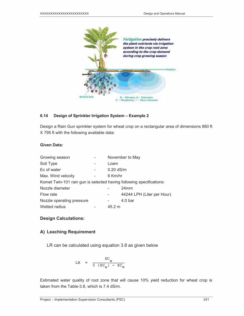
XXXXXXXXXXXXXXXXXXXXXXXX Design and Operations Manual
Project – Implementation Supervision Consultants (PSC) 241
6.14 Design of Sprinkler Irrigation System – Example 2
Design a Rain Gun sprinkler system for wheat crop on a rectangular area of dimensions 880 ft X 795 ft with the following available data:
Given Data:
Growing season - November to May Soil Type - Loam Ec of water - 0.20 dS/m Max. Wind velocity - 6 Km/hr Komet Twin-101 rain gun is selected having following specifications: Nozzle diameter - 24mm Flow rate - 44244 LPH (Liter per Hour) Nozzle operating pressure - 4.0 bar Wetted radius - 45.2 m
Design Calculations:
A) Leaching Requirement
LR can be calculated using equation 3.8 as given below
Estimated water quality of root zone that will cause 10% yield reduction for wheat crop is taken from the Table-3.8, which is 7.4 dS/m.

XXXXXXXXXXXXXXXXXXXXXXXX Design and Operations Manual
Project – Implementation Supervision Consultants (PSC) 242
= 0.2 / 5 [ 7.4 – 0.2] = 0.01
B) Crop Water Requirement
Crop water requirement is calculated by multiplying ETo and Kc values for each month of the growing season of the wheat crop. ETo values in mm per day for each month of the year and Kc values of the growing season of the selected area can be selected from Tables given in Crop Water Requirement Manual. For designing purpose select the maximum crop water requirement (CWR) value. For wheat the maximum CWR value comes in the month of February so the ETo and Kc values of this month are incorporated in the design sheet.
Peak daily consumptive use (CU) per day is calculated using equation as follows:
CU = ETo X Kc X Kf / [efficiency x (1-LR)] = 2.2 X 1.2 X 1 / (0.75 x (1- 0.01) = 3.56 mm/day
Irrigation system efficiency for sprinkler system is taken from the Table-3.4 giving range (60-85%) the average value 75% is generally used for high pressure sprinkler system such as Rain-Gun.
C) Sprinkler Pattern/ Spacing
100% of sprinkler overlapping is selected along lateral while 65% overlapping is selected between laterals. Using this type of overlapping the sprinkler to sprinkler and lateral to lateral spacing is calculated as below:
Sprinkler Spacing = 0.50 X Wetted dia. of sprinkler = 0.50 X (2 X 45.2) = 45.2 m
Lateral Spacing = 0.65 X Wetted dia. of sprinkler = 0.65 X (2 X 45.2) = 58.76 m
D) Length of Lateral and No. of Sprinklers/hydrants
Length of laterals can be calculated using Equation (4.21) as follows L = A x K / Ls
Total lateral line length = Area in acres X 4047 / Lateral spacing = 16 X 4047 / 58.76 = 1102 m

XXXXXXXXXXXXXXXXXXXXXXXX Design and Operations Manual
Project – Implementation Supervision Consultants (PSC) 243
Total number of sprinklers/ hydrants required can be calculated using Equation (4.24)
Number of sprinklers = A / (S x L) = 16 X 4047 / (58.76 x 45.2) = 24.4 say 25 Nos.
E) Total Flow Rate
Total flow rate for sprinkler system depends upon the number of sprinkler to be operated simultaneously and can be calculated using Equation.
Total flow rate = No. of sprinkler X Sprinkler flow rate = 25 X 44244 = 1106100 LPH
F) Application Rate
Using equation application rate can be calculated as:
Application rate = Total flow rate / (Area in acres X 4047) = 1106100 / (16 X 4047) = 17.08 mm/hr
G) Operation Time (hr)
Total operation time can be calculated using Equation.
Operation time = DCU / Application rate = 3.56 / 17.08 = 0.21 hrs
As 25 no. of sprinklers are required for which the total flow rate to irrigate 16 acres is 1106100 LPH which is much higher. To deliver this flow rate to the system, larger diameter pipe is required accordingly; high energy will be required, which is economically not feasible. Depending upon the farmer’s ease and economics and available power source for the system it is suggested to operate only one rain gun at a time, such that the total area of 16 acres is irrigated in 25 shifts.
Area irrigated in one shift/zone = total area / No. of shifts = 16 / 25 = 0.64 acres
H) Maximum irrigation Depth
Maximum irrigation depth (dx) can be calculated using Equation (4.12)
dx = MAD (Wa x Z)/100

XXXXXXXXXXXXXXXXXXXXXXXX Design and Operations Manual
Project – Implementation Supervision Consultants (PSC) 244
Effective rooting depth of wheat crop is taken from Table-4.4 which is 1.2 m. Management Allowed Deficit is taken from the Table-3.2 which is 25% Water holding capacity for loam soil is taken from Table-3.1 which is 170 mm/m
= 25 x (170 x 1.2) / 100 = 51 mm
I) Maximum Irrigation Interval
Maximum irrigation interval can be calculated using Equation 4.13.
Fx = dx / Cu Fx = 51 / 3.56 = 14 days
Design layout for sprinkler irrigation system

XXXXXXXXXXXXXXXXXXXXXXXX Design and Operations Manual
Project – Implementation Supervision Consultants (PSC) 245
All the above calculated values are arranged in the form of table for design as flows: Sr. No.
Parameters Units Zone
(1 to 24) Total
1 Total Area Acres 0.64 16 2 Design Reference Evapotranspiration, ETo mm/day 2.2 3 Design crop factor at maturity, Kc - 1.2 4 Irrigation system efficiency % 75 5 Quality of irrigation water dS/m 0.20 6 Estimated water quality of root zone that will
cause 10% yield reduction dS/m 7.4
7 Effective crop root depth m 1.2 8 Management Allowed Deficit % 25 9 Water holding capacity of soil mm/m 170 10 Leaching requirement fraction 0.01 11 Maximum wind velocity Km/hr 6 12 Sprinkler flow rate LPH 44244 44244 13 Nozzle size mm 24 14 Nozzle operating pressure m 40 15 Wetted radius of sprinkler m 45.2 16 Sprinkler overlapping along lateral % 100 17 Sprinkler overlapping between lateral % 65 18 Sprinkler spacing at lateral m 45.2 19 Lateral spacing m 58.76 20 Irrigation Cycle days 1 21 Peak daily consumptive use per day mm/day 3.52 22 Total no. of sprinklers No. 1 23 Total flow rate LPH 44244 24 Application rate mm/hr 17.08 25 Operation time hrs 0.21 5.04
J) Head Loss Calculations
The maximum lateral line length to be laid at site is 180 m (see layout) while only one number of sprinkler is to be operate on a lateral for which the flow rate is 44244 LPH. The diameter of pipe required to deliver this amount of water shall be selected such that the head loss may be less than 20% of the sprinkler operating pressure or the velocity shall not exceed 1.5 m/s. A 4” pipe diameter is selected for which the head loss can be calculated by using equations as illustrated in Exapmle-1.
Lateral Head Loss for 100m length using Watter & Keller’s equation = 1.42 m Lateral Head Loss for 180m length using Watter & Keller’s equation = 2.56 m
XXXXXXXXXXXXXXXXXXXXXXXX Design and Operations Manual
Project – Implementation Supervision Consultants (PSC) 246
Lateral Head Loss for 100m length using Hazzen William’s equation= 1.49 m Lateral Head Loss for 180m length using Hazzen William’s equation= 2.68 m
Average lateral head loss for 180 m of length = 2.62 m
The total length of main line pipe to deliver water to the remotest lateral is 325m (see layout) which will also be used to carry water flow rate of 44244 LPH to each outlet point in the pipe network, so similar sized pipe can be used for lateral and mainline.
As the flow rate and diameter of pipe is same and only the length is changed so that the head loss for 325 m of length can be given as:
Main line head loss for 325 m of length = 4.90 m
The head loss for suction and delivery pipe for pump be calculated using the same equation.
Suction and delivery head loss = 0.09 m Total head losses in piping network = 2.62 + 4.90 + 0.09
= 7.61m Fitting losses (may be taken 20% of the pipe losses) = 1.52 m Sprinkler operating pressure in form of water head = 40 m
Head losses for fittings, filters, fertigation system and other flow control and monitoring devices shall be included as given by the manufacturers. For example
Head loss in fertigation = 5 m Head loss in flow meter = 1 m Misc. head losses = 2 m
The total dynamic head can be calculated by adding all the head losses occurring in the system and can be presented as follow:
Total Dynamic Head = 57.13 m
K) Power requirements
Horse Power Requirement can be calculated using equation – 5.6
Pump flow rate = 44244 (LPH) / 3600 (Sec.) = 12.29 LPS
The efficiencies for pump and electric motor are assumed as 60% and 80% respectively.
H.P = Q. H / [75 X Em x Ep] = 12.29 x 57.13 / [75 x 0.55 x 0.8]
Required Horse Power = 20 (appx.)

XXXXXXXXXXXXXXXXXXXXXXXX Design and Operations Manual
Project – Implementation Supervision Consultants (PSC)
References
Consultants will furnish references on request.
Copyright © 2022 FDOKUMEN