Scholars' Mine Scholars' Mine

Doctoral Dissertations Student Theses and Dissertations

Spring 2016

Thorium-based mixed oxide fuel in a pressurized water reactor: A Thorium-based mixed oxide fuel in a pressurized water reactor: A

feasibility analysis with MCNP feasibility analysis with MCNP

Lucas Powelson Tucker

Follow this and additional works at: https://scholarsmine.mst.edu/doctoral_dissertations

Part of the Nuclear Engineering Commons

Department: Nuclear Engineering and Radiation Science Department: Nuclear Engineering and Radiation Science

Recommended Citation Recommended Citation Tucker, Lucas Powelson, "Thorium-based mixed oxide fuel in a pressurized water reactor: A feasibility analysis with MCNP" (2016). Doctoral Dissertations. 2492. https://scholarsmine.mst.edu/doctoral_dissertations/2492

This thesis is brought to you by Scholars' Mine, a service of the Missouri S&T Library and Learning Resources. This work is protected by U. S. Copyright Law. Unauthorized use including reproduction for redistribution requires the permission of the copyright holder. For more information, please contact scholarsmine@mst.edu.

THORIUM-BASED MIXED OXIDE FUEL

IN A PRESSURIZED WATER REACTOR:

A FEASIBILITY ANALYSIS WITH MCNP

by

LUCAS POWELSON TUCKER

A DISSERTATION

Presented to the Graduate Faculty of the

MISSOURI UNIVERSITY OF SCIENCE AND TECHNOLOGY

In Partial Fulfillment of the Requirements for the Degree

DOCTOR OF PHILOSOPHY

in

NUCLEAR ENGINEERING

2016

Approved by:

Shoaib Usman, Advisor

Ayodeji Alajo

Carlos Castaño

Hyoung Koo Lee

G. Ivan Maldonado

iii

PUBLICATION DISSERTATION OPTION

This dissertation consists of the following four articles, which either have been

published, have been submitted for publication, or will be submitted for publication:

Paper I, entitled “Portable Spectroscopic Fast Neutron Probe and 3He Detector

Dead-time Measurements” and presented from page 10 to 29 in this dissertation, was

submitted to Progress in Nuclear Energy on 23 January 2016 and is under review.

Paper II, entitled “Characterization of Best Candidate Isotopes for Burnup Analysis

and Monitoring of Irradiated Fuel” and presented from page 30 to 64 in this dissertation,

was published in Annals of Nuclear Energy Volume 69, pages 278-291, in 2014.

Paper III, entitled “Thorium-based Mixed Oxide Fuel in a Pressurized Water

Reactor: A Beginning of Life Feasibility Analysis with MCNP” and presented from page

65 to 92 in this dissertation, was published in Annals of Nuclear Energy Volume 76, pages

323-334, in 2015.

Paper IV, entitled “Thorium-based Mixed Oxide Fuel in a Pressurized Water

Reactor: A Burnup Analysis with MCNP” and presented from page 93 to 123 in this

dissertation, will be submitted to Annals of Nuclear Energy for publication.

iv

ABSTRACT

This dissertation investigates techniques for spent fuel monitoring, and assesses the

feasibility of using a thorium-based mixed oxide fuel in a conventional pressurized water

reactor for plutonium disposition. Both non-paralyzing and paralyzing dead-time

calculations were performed for the Portable Spectroscopic Fast Neutron Probe (N-Probe),

which can be used for spent fuel interrogation. Also, a Canberra 3He neutron detector’s

dead-time was estimated using a combination of subcritical assembly measurements and

MCNP simulations. Next, a multitude of fission products were identified as candidates for

burnup and spent fuel analysis of irradiated mixed oxide fuel. The best isotopes for these

applications were identified by investigating half-life, photon energy, fission yield,

branching ratios, production modes, thermal neutron absorption cross section and fuel

matrix diffusivity. 132I and 97Nb were identified as good candidates for MOX fuel on-line

burnup analysis. In the second, and most important, part of this work, the feasibility of

utilizing ThMOX fuel in a pressurized water reactor (PWR) was first examined under

steady-state, beginning of life conditions. Using a three-dimensional MCNP model of a

Westinghouse-type 17x17 PWR, several fuel compositions and configurations of a one-

third ThMOX core were compared to a 100% UO2 core. A blanket-type arrangement of

5.5 wt% PuO2 was determined to be the best candidate for further analysis. Next, the safety

of the ThMOX configuration was evaluated through three cycles of burnup at several using

the following metrics: axial and radial nuclear hot channel factors, moderator and fuel

temperature coefficients, delayed neutron fraction, and shutdown margin. Additionally, the

performance of the ThMOX configuration was assessed by tracking cycle length,

plutonium destroyed, and fission product poison concentration.

v

ACKNOWLEDGMENTS

I could not have completed this project without the tremendous support I received

from faculty, staff, family, and friends. My advisor, Dr. Shoaib Usman, guided me through

the process of choosing a project, executing it, presenting it, and staying funded. His help

was invaluable.

I also need to thank Dr. Ayodeji Alajo and Dr. Ivan Maldonado, whose insights

added depth and breadth to my results. And the remaining members of my thesis

committee, Dr. Hyoung Lee and Dr. Carlos H. Castaño, also deserve thanks for their

interest. Dr. Arvind Kumar, the former chair of the Nuclear Engineering Department, and

after him, Dr. Lee, were instrumental in maintaining support for me and my project with

teaching and research assistantships throughout my many years at Missouri S&T. The

Missouri University of Science and Technology Reactor staff also must be acknowledged

for their contribution. Bill Bonzer, the reactor manager, and Craig Reisner, the assistant

reactor manager helped complete the N-Probe detector dead time measurements. I must

acknowledge the sources of my funding: the U.S. Nuclear Regulatory Commission and the

Missouri University of Science and Technology Chancellor’s Fellowship.

My friends and family have also contributed a great deal. Dr. Tayfun Akyurek was

my frequent collaborator. Without him, the first two papers in this dissertation would not

exist. I have shared many late night discussions and pots of coffee with Dr. Edwin Grant

and Dr. Chrystian Posada, and I appreciated their encouragement, assistance, and opinions.

After Dr. Grant and Dr. Posada graduated and moved on, a new crop of graduate students

moved in to Fulton 230 with me. Ashish Avachat, Manish Sharma, and Edward Norris

made my last years in Rolla much more enjoyable.

Last, and far from least, I thank my family. My wife, Erica, encouraged, listened,

edited, typed, and provided the love and companionship I needed to complete my doctorate.

Her contribution to this work is greater than I have words for. I can only imagine how much

I’ll enjoy spending the rest of my life with her. I also owe her an apology (she knows why).

My parents, Tim and Dr. Stephanie Powelson, provided a place for Erica and I to live while

I completed my dissertation. They have supported me in every endeavor I have undertaken

throughout my life, and I would have accomplished very little without them.

vi

TABLE OF CONTENTS

Page

PUBLICATION DISSERTATION OPTION ................................................................. iii

ABSTRACT .................................................................................................................. iv

ACKNOWLEDGMENTS ...............................................................................................v

LIST OF ILLUSTRATIONS ......................................................................................... ix

LIST OF TABLES ....................................................................................................... xii

SECTION

1. INTRODUCTION ....................................................................................1

1.1 SPENT FUEL INTERROGATION USING PHOTONS AND

NEUTRONS ................................................................................. 1

1.2 THORIUM AS A NUCLEAR FUEL ............................................ 2

1.3 RESEARCH OBJECTIVES .......................................................... 4

1.4 DISSERTATION ORGANIZATION............................................ 5

REFERENCES ....................................................................................................7

PAPER

I. PORTABLE SPECTROSCOPIC FAST NEUTRON PROBE AND 3HE DETECTOR DEAD-TIME MESUREMENTS ............................... 10

Abstract .................................................................................................. 10

1. Introduction ................................................................................ 11

2. Experimental Design ................................................................... 14

2.1 Dead-time Experiment for N-Probe Fast Neutron

Detector........................................................................... 14

2.2 Dead-time Experiment for Canberra 3He Detector ........... 19

3. Results ........................................................................................ 21

4. Conclusion .................................................................................. 26

References .............................................................................................. 27

II. CHARACTERIZATION OF BEST CANDIDATE ISOTOPES FOR

BURNUP ANALYSIS AND MONITORING OF IRRADIATED

FUEL ..................................................................................................... 29

Abstract .................................................................................................. 29

1. Introduction ................................................................................ 29

2. Traditional Tools, Techniques and Conventional Isotopes for

Burnup Analysis ......................................................................... 31

vii

3. Important Indicators for Burnup Analysis and Spent Fuel

Monitoring .................................................................................. 32

4. Candidate Isotopes ...................................................................... 33

a) Online burnup analysis – Candidate Isotopes ................... 36

b) Interim Storage (short term monitoring) – Candidate

Isotopes ........................................................................... 43

c) Long-term storage/Historic data – Candidate Isotopes ..... 50

d) Suitable Isotopes of Burnup Monitoring .......................... 54

5. Conclusions and Recommendations ............................................ 55

References .............................................................................................. 57

III. THORIUM-BASED MIXED OXIDE FUEL IN A PRESSURIZED

WATER REACTOR: A BEGINNING OF LIFE FEASIBILITY

ANALYSIS WITH MCNP ..................................................................... 63

Abstract .................................................................................................. 63

1. Introduction ................................................................................ 64

2. Description of Reference Case: 100% UO2 ................................. 66

3. Th-MOX Fuel Composition and Core Configuration Selection ... 67

3.1. Core Configuration Analysis ........................................... 68

3.2. Fuel Composition Analysis .............................................. 71

4. One-Third Th-MOX Core Reactor Safety Metrics ....................... 73

4.1. Delayed Neutron Fraction ................................................ 73

4.2. Temperature Coefficients of Reactivity ........................... 74

4.3. Control Rod Worth and Shutdown Margin....................... 77

4.4. Nuclear Hot Channel Factors ........................................... 80

5. Conclusions and Future Work ..................................................... 85

References .............................................................................................. 88

IV. THORIUM-BASED MIXED OXIDE FUEL IN A PRESSURIZED

WATER REACTOR: A BURNUP ANALYSIS WITH MCNP .............. 91

Abstract .................................................................................................. 91

1. Introduction ................................................................................ 92

2. Description of Reactor Configurations ........................................ 94

3. Burnup Procedure ....................................................................... 97

4. Cycle Lengths ............................................................................. 98

4.1. Cycle 1 .......................................................................... 100

4.2. Cycle 2 .......................................................................... 101

viii

4.3. Cycle 3 .......................................................................... 102

5. Plutonium Destruction .............................................................. 103

6. Fission Product Poisons ............................................................ 107

7. Nuclear Hot Channel Factors .................................................... 109

8. Delayed Neutron Fraction ......................................................... 114

9. Temperature Coefficients .......................................................... 115

9.1. Moderator Temperature Coefficient ............................... 116

9.2. Fuel Temperature Coefficient ........................................ 118

10. Shutdown Margin ..................................................................... 118

11. Conclusions .............................................................................. 120

References ............................................................................................ 122

SECTION

2. CONCLUSIONS .................................................................................. 125

VITA ........................................................................................................................... 128

ix

LIST OF ILLUSTRATIONS

PAPER I Page

Fig. 1. N-Probe fast and thermal neutron spectrometer [9]. ....................................... 12

Fig. 2. Illustration of experimental setup ................................................................... 14

Fig. 3. Neutron capture and scrattering interaction probabilities ................................ 16

Fig. 4. Picture of 3He detector neutron measurements in subcritical assembly ........... 19

Fig. 5. MCNP simulation layout. The Pu-Be neutron source (S) was placed in the

center-most position of the subcritical assembly. Nine MCNP simulations

and nine measurements were performed in the numbered locations on axis

A. Five more sets of measurements, repeating those made on axis A, were

made on the five remaining axes. ................................................................... 20

Fig. 6. Fast neutron count rates with different thickness of Plexiglass at 5 kw power. 22

Fig. 7. Fast neutron count rates with different thickness of Plexiglass at 5 kw power. 24

Fig. 8. The results of the measurements and simulations, normalized to their lowest

values for comparison. ................................................................................... 26

PAPER III

Fig. 1. Radial cross-section of core geometry showing many of the included core

components.................................................................................................... 67

Fig. 2. Core loading schemes analyzed to compare a PWR fueled only with UO2 to

a PWR fueled with some Th-MOX. ■ 3.1% enriched UO2, ■ 2.6% enriched

UO2, ■ 2.1% enriched UO2, ■ Th-MOX. (a) 100% UO2, (b) Th-MOX

blanket, (c) Th-MOX ring. ............................................................................. 69

Fig. 3. The effective multiplication factor of a 17x17 PWR core as a function of 10B concentration for the 100% UO2, Th-MOX blanket, and Th-MOX ring

fuel configurations detailed in Fig. 2. ............................................................. 70

Fig. 4. Flux profile comparisons of 5% to 7% PuO2 Th-MOX blanketed core and

100% UO2 core. (a) Radial. (b) Axial. ............................................................ 71

Fig. 5. Flux profile comparison of 5.5% PuO2 Th-MOX blanketed core and 100%

UO2 core. (a) Radial. (b) Axial. ...................................................................... 72

Fig. 6. Total temperature coefficient data for the 100% UO2 core and the 5.5%

PuO2 Th-MOX blanketed core ....................................................................... 76

Fig. 7. Fuel temperature coefficient data for the 100% UO2 core and the 5.5%

PuO2 Th-MOX blanketed core ....................................................................... 76

Fig. 8. Map of assemblies analyzed for control rod worth and shutdown margin

simulations. The various fuel enrichments are distinguished by their color,

while the part-length and full-length control assemblies are distinguished

with shading. These assemblies are in the northeast quadrant of the core. ...... 78

x

Fig. 9. Heat maps of the assembly-by-assembly thermal flux tally results for one

quarter of each core from vertical sections 1 and 9. Results from the 100%

UO2 core are in the left column, and results from the 1/3 Th-MOX core are

on the right. ................................................................................................... 83

Fig. 10. Heat maps of the total assembly-by-assembly thermal flux tally results

summed over all 16 vertical sections for one quarter of the core in each

fuel configuration. For both configurations the peak assembly is H4, the

midpoint of which is located at (x = 0 cm, y = 86.0 cm). (a) 100% UO2

(b) 1/3 Th-MOX ............................................................................................ 84

Fig. 11. Heat maps of the pin-by-pin thermal flux tally results for assembly H4 from

each core from vertical sections 1 and 9. Results from the 100% UO2 core

are in the left column, and results from the 1/3 Th-MOX core are on the

right. Water-filled channels are shown in gray. .............................................. 85

Fig. 12. Heat maps of the total pin-by-pin thermal flux tally results summed over

all 17 vertical sections in assembly H4 for each fuel configuration. Water-

filled channels are gray. (a) 100% UO2, peak assembly midpoint located at

(x = 3.8 cm, y = 83.5 cm) (b) 1/3 Th-MOX, peak assembly midpoint located

at (x = 3.8 cm, y = 91.1 cm) ........................................................................... 86

PAPER IV

Fig. 1. Beginning of Cycle 1 fuel configurations. (a) UO2. (b) ThMOX. 3.1%

enriched UO2 in dark blue, 2.6% enriched UO2, in medium blue, 2.1%

enriched UO2 in light blue, Th-MOX in green. ............................................... 94

Fig. 2. Cycle 1 burnable absorber arrangement for both the UO2 and the ThMOX

cores. Assemblies with burnable absorber rods are indicated by the number

of rods in the assembly. ................................................................................. 95

Fig. 3. PWR control assembly layout. Full-length control assemblies are marked

with an “F”. Part-length control assemblies are marked with a “P”................. 96

Fig. 4. Map of materials used for burnup analysis ..................................................... 98

Fig. 5. Visualization of fuel shuffling procedure for the 100% UO2 configuration

from Cycle 1 to Cycle 2. .............................................................................. 100

Fig. 6. Multiplication factor plotted against time for both core configurations for

Cycle 1. ....................................................................................................... 101

Fig. 7. Multiplication factor plotted against time for both core configurations for

Cycle 2. ....................................................................................................... 102

Fig. 8. Multiplication factor plotted against time for both core configurations for

Cycle 3. ....................................................................................................... 103

Fig. 9. Whole-core plutonium mass in kilograms during Cycle 1. ........................... 105

Fig. 10. Whole-core plutonium mass in kilograms during Cycle 2. ........................... 105

Fig. 11. Whole-core plutonium mass in kilograms during Cycle 3. ........................... 105

xi

Fig. 12. Lifetime 233U production of the ThMOX configuration. ............................... 106

Fig. 13. Lifetime whole-core mass of 135Xe for both the UO2 and ThMOX

configurations. ............................................................................................. 108

Fig. 14. Lifetime whole-core mass of 149Sm for both the UO2 and ThMOX

configurations. The ThMOX configuration’s 149Sm concentration is plotted

on the secondary axis. .................................................................................. 108

Fig. 15. Whole-core approximation of the nuclear radial hot channel factor at each

time step for both the UO2 and ThMOX configurations. The worst-case

scenario for each configuration has been flagged. ........................................ 111

Fig. 16. Assembly-by-assembly power distribution for each configuration at the

time step with the highest whole-core approximation of the radial nuclear

hot channel factor. Colors are scaled from the lowest value across all three

cycles to the highest value across all three cycles. ........................................ 111

Fig. 17. Pin-by-pin thermal neutron flux distribution for each configuration’s

hottest assembly at the time step with the highest whole-core

approximation of the nuclear radial hot channel factor. The hot channel is

bordered in green. Non-fuel channels are shaded gray. ................................. 113

Fig. 18. Flux per vertical section (VS) for each configuration’s hot channel (HC).

Each configuration’s average hot channel flux is also included as a

horizontal line. These values were used to calculate the axial nuclear hot

channel factor. The ThMOX configuration’s values are plotted on the

secondary axis. ............................................................................................ 114

xii

LIST OF TABLES

PAPER I Page

Table 1. The fast neutron measurements using N-Probe at 5 kW power ....................... 21

Table 2. Total macroscopic cross section (ƩTOT) for Plexiglas using all counts ............ 23

Table 3. Dead-time calculations of N-Probe for two ideal models ................................ 23

Table 4. Neutron measurements from the Canberra 3He Detector in the Subcritical

Assembly ....................................................................................................... 25

Table 5. Results of MCNP simulations of Canberra 3He neutron detector in the

Subcritical Assembly ..................................................................................... 25

PAPER II

Table 1. Reference isotopes for burnup analysis and spent fuel monitoring [6] ............ 34

Table 2. Candidate isotopes grouped by half-life for burnup analysis [19] ................... 37

Table 3. Group 1 fission product and decay characteristics [20, 21, 22, 23] ................. 38

Table 4. Group 1 candidate isotopes thermal absorption cross section and production

mode for online burnup analysis [24] ............................................................. 40

Table 5. Diffusion coefficients of candidate isotopes for online burnup analysis .......... 42

Table 6. Group 2 fission product and decay data [20,21,22,23] .................................... 44

Table 7. Group 2 candidate isotopes thermal absorption cross section and production

mode for storage fuel burnup analysis [24]..................................................... 47

Table 8. Diffusion coefficients of candidate isotopes for spent fuel monitoring ........... 48

Table 9. Group 3 fission product and decay data [20,21,22,23] .................................... 51

Table 10. Group 3 candidate isotopes thermal absorption cross section and production

modes for online burnup analysis [24] ........................................................... 52

Table 11. Diffusion coefficients of candidate isotopes for historical data ....................... 52

Table 12. Candidate isotopes comparison for three burnup applications......................... 53

Table 13. Best candidate isotopes for three burnup applications with characteristic data 54

PAPER III

Table 1. Isotopic composition of plutonium used for Th-MOX feasibility analysis.

Adapted from Shwageraus, Hejzlar, and Kazimi [19]. .................................... 68

Table 2. Excess reactivity in pcm and critical boron concentration in ppm for all

simulated core configurations and fuel compositions ..................................... 73

Table 3. Reactor fuel parameters for 100% UO2 core, one-third 5.5% PuO2 Th-MOX

blanketed core, and one-third 7% PuO2 Th-MOX blanketed core ................... 74

xiii

Table 4. This table provides the control rod worths for the control assemblies that

were analyzed in both the 100% UO2 configuration and the Th-MOX

blanket configuration and each configuration’s SDM. The reactivity of the

highest worth rod is shaded. ........................................................................... 79

PAPER IV

Table 1. Isotopic composition of plutonium used for ThMOX. Adapted from

Shwageraus, Hejzlar, and Kazimi [9]. ............................................................ 95

Table 2. Attributes of full-length and part-length control assemblies in a PWR. ........... 96

Table 3. Excess reactivity and critical boron concentration. ....................................... 100

Table 4. Total core plutonium mass in kilograms at the beginning of each cycle for

both configurations. ..................................................................................... 104

Table 5. Net change in core plutonium mass (kg) for each configuration at the end

of each cycle and totaled across all three cycles. .......................................... 104

Table 6. Total discharge activity of thrice-burned, Group 1 Assemblies at EOC 3. .... 107

Table 7. Axial and radial nuclear hot channel factors at the time step with the

highest whole-core approximation of the radial nuclear hot channel factor

for each configuration. ................................................................................. 113

Table 8. Delayed neutron fraction at times of interest for both configurations. ........... 115

Table 9. Moderator temperature coefficient at each time step of interest for both

configurations. ............................................................................................. 117

Table 10. Fuel temperature coefficient at each time step of interest for both

configurations. ............................................................................................. 118

Table 11. Shutdown margin and highest worth rod at each time step of interest for

both configurations. ..................................................................................... 119

1

SECTION

1. INTRODUCTION

1.1 SPENT FUEL INTERROGATION USING PHOTONS AND NEUTRONS

Non-destructive analysis (NDA) techniques have long been used for monitoring

spent uranium dioxide (UO2) fuel. There are two groups of NDA techniques available:

passive techniques measure delayed neutrons and gamma rays emitted after radioactive

decay, while active techniques interrogate fuel by first bombarding it with a neutron source

and then monitoring gamma and/or neutron emissions [1]. With the resurgence of interest

in mixed oxide (MOX) in the United States, NDA techniques for monitoring spent MOX

fuel need to be investigated.

Commercial nuclear fuel reprocessing was banned by the United States

government, interrupting the U.S. reprocessing industry between 1977 and 1981, but

France embraced reprocessing technology and incorporated mixed oxide (MOX) fuel into

their nuclear fuel cycle. France has demonstrated that MOX fuel can be integrated into a

Uranium fueled core without risking the safety of the plant or the proliferation of nuclear

weapons. Recently, the U.S. nuclear power industry has been reconsidering MOX fuel. The

successful disposition of Russian highly enriched uranium through the Megatons to

Megawatts program has encouraged interest in a similar program for plutonium disposition

in MOX fuel [2]. Therefore, better tools and techniques are necessary for burnup analysis

and spent fuel monitoring of MOX fuel.

Using the NDA technique of passive gamma measurement, photons emitted by

irradiated fuel assemblies can be analyzed to determine parameters such as burnup, cooling

time, and irradiation history [3]. Willman et al., have discriminated MOX fuel from LEU

fuel using 134Cs, 137Cs, and 154Eu isotopes as cooling time and irradiation history indicators

[4]. Dennis and Usman reported on 106Ru as another potential burnup indicator [5].

Another NDA technique for spent fuel interrogation is neutron measurement. When

238U is exposed to substantial neutron fluence (as with reactor fuel), 244Cm is produced.

Spontaneous fission of 244Cm provides a source of delayed neutrons. Since the half-life of

244Cm is 18.1 years – much longer than the amount of time fuel spends in a power reactor

2

– neutron intensity from 244Cm can be used as a measure of burnup [6]. However, this

technique is highly sensitive to cooling time, and initial enrichment.

Destructive techniques, such as chemical assay with a mass spectrometer, have

historically been applied to determine isotopic composition of spent nuclear fuel. But these

techniques require fuel sample destruction and can take a long time for sample analysis

and results [7].

The Missouri University of Science and Technology research reactor (MSTR) is a

pool-type reactor licensed by the NRC to operate up to 200 kW thermal power. The

research reactor was the first nuclear reactor in Missouri and its core contains low enriched

uranium (LEU) fuel. Facilities at the reactor allow for non-destructive burnup analysis and

discrimination of fuel elements based on plutonium and uranium content using gamma and

delayed neutron measurements. All radiation measurements need to be corrected using

either non-paralyzing dead-time or paralyzing dead-time model depending on detector

behavior.

1.2 THORIUM AS A NUCLEAR FUEL

Thorium represents a vast, largely untapped source of nuclear energy. Its abundance

in the earth’s crust is roughly three times greater than uranium [8]. Though 232Th – the only

naturally occurring isotope of thorium – is not fissile, it is fertile. After absorbing a neutron

to become 233Th and decaying to 233Pa, it ultimately decays to 233U [9]. Thorium-based

fuels offer several potential advantages over uranium fuels: higher fissile conversion rate,

higher thermal fission factor (η), lower capture-to-fission ratio, low actinide production,

plutonium reduction, chemical stability, proliferation resistance [10, 11, 12, 13]. Because

of these advantages, several methods for utilizing thorium fuels have been explored.

Most thorium utilization schemes require the development of advanced reactor

designs. In a molten salt reactor (MSR) thorium and uranium fluorides are dissolved with

the fluorides of beryllium and lithium [14]. MSRs offer some distinct advantages: they

have a strongly negative temperature coefficient and allow for online refueling [14]. Also,

two MSRs were designed, built, and operated at Oak Ridge National Laboratory, proving

the concept and providing valuable experimental data [15, 16].

3

High temperature gas cooled reactors (HTGRs) are another option for thorium

utilization. HTGRs would use TRISO fuel composed of pellets of thorium oxide or carbide

blended with pellets of uranium oxide or carbide and coated with several layers of carbon

and silicon carbide; the TRISO particles are combined in a graphite matrix and formed into

either prisms or pebbles 10. Several countries (Germany, Japan, the Russian Federation,

the United Kingdom, and the United States) have built HTGRs and loaded them with

thorium fuel 10; and Tsinghua University in China is currently designing a 500 MW(th)

pebble bed reactor demonstration plant [17]. HTGRs could be adapted to several fuel

cycles without modification of the core or plant, but several technical hurdles remain before

the technology is commercially viable 10.

An accelerator driven system is a unique reactor design in which a proton

accelerator is used to produce enough spallation neutrons to bring an otherwise subcritical

core to criticality 12. Such a system would use only natural uranium and thorium fuels,

eliminating the need for enrichment technology, and reducing proliferation concerns, while

also achieving high burnup [18]. India has been pursuing this technology, but the design is

still in the conceptual stages, and the amount of power required to operate the accelerator

casts doubt on the economic viability of such a system [18, 13].

Perhaps the most expedient scheme for exploiting the world’s thorium resources is

incorporating it into the current reactor fuel supply. Numerous publications have

demonstrated a number of ways thorium could enhance the operation of boiling water

reactors (BWRs), pressurized water reactors (PWRs), and heavy water reactors (HWRs)

[10, 11, 19, 20, 21].

Thor Energy, a Norwegian company, is developing and testing thorium-plutonium

BWR fuel pellets and assemblies for plutonium destruction [22, 23]. Xu, Downar,

Takahashi, and Rohatgi are also studying the potential for plutonium disposition in BWRs

[24] as are Mac Donald and Kazimi [25]. Francois et al. have investigated replacing all of

the uranium fuel in a BWR with a thorium-uranium fuel blend [26].

Similar research on Th-Pu and Th-U fuels has been conducted for PWRs as well.

Shwageraus, Hejzlar, and Kazimi have investigated the use of Th-Pu fuel in PWRs for both

the destruction of plutonium [27] and improved economics [28]. Bjork et al. studied the

use of Th-Pu fuel for extending the operating cycle of a PWR [29]. Trellue, Bathke, and

4

Sadasivan have used MCNP and MCNPX to compare the reactivity safety characteristics

and Pu destruction capabilities of conventional MOX fuel to those of Th-MOX fuel [30].

Their work is complemented by that of Tsige-Tamirat, who also used Monte Carlo

techniques to study the effect of Th-MOX fuel on a PWR’s reactivity safety characteristics

[31]. Burnup analyses of Th-MOX fuel for Pu disposition in PWRs have been performed

by others: Fridman and Kliem [32].

Research on thorium utilization in HWRs has focused on both incorporating

thorium rods into existing CANDU reactors [33], and, in India, developing advanced heavy

water reactors specifically designed to burn thorium fuel [34].

1.3 RESEARCH OBJECTIVES

The primary objective of this work was to investigate the feasibility of

incorporating a Th-Pu MOX fuel into the fuel supply of a conventional PWR for plutonium

disposition. In pursuit of this objective, it was helpful to identify the best candidate isotopes

for online burnup analysis and spent fuel monitoring of MOX fuel, and develop a non-

destructive technique for discriminating plutonium and uranium. Therefore, the following

tasks were accomplished:

Investigate the half-lives, decay photon energies, fission yields, branching ratios,

production modes, thermal neutron absorption cross sections, and fuel matrix diffusivities

of fission products to determine the best isotopes for online burnup analysis, spent fuel

monitoring, and historical fuel monitoring of MOX fuel.

Use non-destructive techniques to interrogate the MSTR’s spent fuel elements and

calculate the uranium fuel burnup values. Record fast delayed neutron energy spectra for

spent and fresh fuel elements. Measure delayed neutron emission rates to calculate

plutonium conversion.

Use MCNP to model a conventional UO2-fueled PWR at beginning of life. Identify

the ThMOX fuel configuration which best matches the neutronic characteristics of the

conventional UO2-fueled PWR configuration. Simulate three cycles of burnup for both

configurations. Compare the ThMOX configuration to the UO2 configuration using the

following safety metrics: axial and radial nuclear hot channel factor, moderator and fuel

temperature coefficient, delayed neutron fraction, fission product poison concentration,

5

and shutdown margin. Assess the plutonium destruction capability of the ThMOX

configuration.

1.4 DISSERTATION ORGANIZATION

This dissertation is organized into three sections: the first section is an introduction

to the areas under investigation; the second section is comprised of four papers which either

have been published, have been submitted for publication, or will be submitted for

publication; the third section summarizes the conclusions drawn from the papers presented

in the second section and proposes future work.

In Paper I, both non-paralyzing and paralyzing dead-time calculations were

obtained for a fast neutron detector used for spent fuel interrogations. The dead-time for

another neutron detector (3He) was also calculated using measurements collected in a

subcritical assembly. An MCNP model of the subcritical assembly experiment was

developed for comparison.

In Paper II, a multitude of fission products identified as candidates for burnup and

spent fuel analysis were scrutinized for their suitability. From this list of candidates, the

best isotopes for analysis were identified by investigating half-life, fission yield, branching

ratios, production modes, thermal neutron absorption cross section and fuel matrix

diffusivity.

In Paper III, the feasibility of utilizing ThMOX fuel in a pressurized water reactor

was examined under steady-state, beginning of life conditions. With a three-dimensional

MCNP model of a Westinghouse-type 17x17 PWR, many possibilities for replacing one-

third of the UO2 assemblies with ThMOX assemblies were considered. The excess

reactivity, critical boron concentration, and centerline axial and radial flux profiles for

several configurations and compositions of a one-third ThMOX core were compared to a

100% UO2 core. A blanket-type arrangement of 5.5 wt% PuO2 was determined to be the

best candidate for further analysis. Therefore, this configuration was compared to a 100%

UO2 core using the following parameters: delayed neutron fraction, temperature

coefficient, shutdown margin, and axial and radial nuclear hot channel factors.

In Paper IV, a burnup analysis was performed using the UO2 configuration and the

ThMOX configuration identified and examined in Paper III. The safety of the ThMOX

6

configuration was compared to that of the UO2 configuration at several time steps of

interest within each cycle (beginning of cycle, peak excess reactivity of cycle, and end of

cycle) with the following metrics: axial and radial nuclear hot channel factors, moderator

and fuel temperature coefficients, delayed neutron fraction, and shutdown margin.

Additionally, the performance of the ThMOX configuration was assessed by tracking cycle

lengths, the amount of plutonium destroyed, and fission product poison concentration.

7

REFERENCES

[1] T. Akyurek et al. “Characterization of Best Candidate Isotopes for Burnup Analysis

and Monitoring of Irradiated Fuel” Annals of Nuclear Energy, 69, 278-291. 2014.

[2] United States Enrichment Corporation. “Megatons to Megawatts Program”

http://www.usec.com/news/megatons-megawatts-program-recycles-450-metric-

tons-weapons-grade-uranium-commercial-nuclear-fu, accessed on 13 April, 2013,

created on 9 July 2012.

[3] A. Håkansson, et al. “Results of spent-fuel NDA with HRGS” Proceedings of the

15th Annual Esarda Meeting. Rome, Italy. 1993.

[4] C. Willman, et al. “A nondestructive method for discriminating MOX fuel from

LEU fuel for safeguards purpose” Annals of Nuclear Energy, 33, 766-773. 2006.

[5] M.L. Dennis, S. Usman. “Feasibility of 106Ru peak measurement for MOX fuel

burnup analysis” Nuclear Engineering and Design, 240, 3687-3696. 2010.

[6] K.A. Jordan, G. Perret. “A delayed neutron technique for measuring induced fission

rates in fresh and burnt LWR fuel” Nuclear Instruments and Methods in Physics

Research A, 634, 91-100. 2011.

[7] K. Inoue et al. “Burnup determination of Nuclear Fuel” Mass Spectroscopy, 17,

830-842. 1969.

[8] B.S. Van Gosen, V.S. Gillerman, T.J. Armbrustmacher. “Thorium Deposits of the

United States—Energy Resources for the Future?” U.S. Geological Survey Circular

1336. 2009.

[9] E.M. Baum, H.D. Knox, T.R. Miller. “Nuclides and Isotopes: Chart of Nuclides,

16th Ed.” Lockheed Martin Distribution Services. 2002.

[10] F. Sokolov, K. Fukuda, H.P. Nawada. “Thorium Fuel Cycle – Potential Benefits

and Challenges” IAEA-TECDOC-1450. IAEA. Vienna, 2005.

[11] “Role of Thorium to Supplement Fuel Cycles of Future Nuclear Energy Systems”

IAEA Nuclear Energy Series No. NF-T-2.4. IAEA. Vienna, 2012.

[12] S. Peggs, W. Horak, T. Roser, et al. “Thorium Energy Futures” Proceedings of

IPAC2012. New Orleans, 2012.

[13] K. Hesketh, A. Worrall. “The Thorium Fuel Cycle: An independent assessment by

the UK National Nuclear Laboratory” National Nuclear Laboratory Position Paper.

2010.

[14] J.A. Lane “Fluid Fuel Reactors” Addison-Wesley Pub. Co. 1958.

8

[15] P.N. Haubenreich, J.R. Engel. “Experience with the Molten-Salt Reactor

Experiment” Nuclear Applications and Technology. 1970.

[16] D.E. Holcomb, G.F. Flanagan, B.W. Patton, J.C. Gehin, R.L. Howard, T.J.

Harrison, “Fast Spectrum Molten Salt Reactor Options” ORNL Report ORNL/TM-

2011/105. 2011.

[17] Zuoyi Zhang, Zongxin Wu, Dazhong Wang, Yuanhui Xu, Yuliang Sun, Fu Li,

Yujie Dong. “Current Status and Technical Description of Chinese 2 x 250 MWth

HTR-PM Demonstration Plant” Nuclear Engineering and Design, 239, 1212-1219.

July 2009.

[18] S. Banerjee. “Towards a Sustainable Nuclear Energy Future” 35th World Nuclear

Association Symposium. London, 2010.

[19] P. Bromley, et al. “LWR-Based Transmutation of Nuclear Waste An Evaluation of

Feasibility of Light Water Reactor (LWR) Based Actinide Transmutation

Concepts-Thorium-Based Fuel Cycle Options” BNL-AAA-2002-001. 2002.

[20] K.D. Weaver, J.S. Herring. “Performance of Thorium-Based Mixed Oxide Fuels

for the Consumption of Plutonium in Current and Advanced Reactors” Nucl. Tech.,

143, 22-36. 2002.

[21] M. Todosow, G. Raitses. “Thorium Based Fuel Cycle Options for PWRs”

Proceedings of ICAPP ’10, 1891-1900. June 13-17, 2010.

[22] K.I. Bjork. “A BWR Fuel Assembly Design for Efficient Use of Plutonium in

Thorium-Plutonium Fuel” Progress in Nuclear Energy, 65, 56-63. 2013.

[23] K.I. Bjork, V. Fhager, C. Demaziere. “Comparison of Thorium-Based Fuels with

Different Fissile Components in Existing Boiling Water Reactors” Progress in

Nuclear Energy, 53, 618-625. 2011.

[24] Yunlin Xu, T.J. Downar, H. Takahashi, U.S. Rohatgi. “Neutronics Design and Fuel

Cycle Analysis of a High Conversion BWR with Pu-Th Fuel” ICAPP. Florida,

2002.

[25] P. Mac Donald, M.S. Kazimi. “Advanced Proliferation Resistant, Lower Cost,

Uranium-Thorium Dioxide Fuels for Light Water Reactors” NERI Annual Report,

INEEL/EXT-2000-01217. 2000.

[26] J.L. Francois, A. Nun͂ez-Carrera, G. Espinosa-Paredes, C. Martin-del-Campo.

“Design of a Boiling Water Reactor Equilibrium Core Using Thorium-Uranium

Fuel” Americas Nuclear Energy Sumposium 2004. Miami Beach, FL, 2004.

[27] E. Shwageraus, P. Hejzlar, M.S. Kazimi. “Use of Thorium for Transmutation of

Plutonium and Minor Actinides in PWRs” Nucl. Tech., 147, 53-68. 2004.

9

[28] E. Shwageraus, P. Hejzlar, M.J. Driscoll, M.S. Kazimi. “Optimization of Micro-

Heterogeneous Uranium-Thorium Dioxide PWR Fuels for Economics and

Enhanced Proliferation Resistance”, MIT-NFC-TR-046, MIT, Nucl. Eng. Dep,

2002.

[29] K.I. Bjork, C.W. Lau, H. Nylen, U. Sandberg. “Study of Thorium-Plutonium Fuel

for Possible Operating Cycle Extension in PWRs” Science and Technology of

Nuclear Installations. 2013.

[30] H.R. Trellue, C.G. Bathke, P. Sadasivan. “Neutronics and Material Attractiveness

for PWR Thorium Systems Using Monte Carlo Techniques” Progress in Nuclear

Energy, 53, 698-707. 2011.

[31] H. Tsige-Tamirat. “Neutronics Assessment of the Use of Thorium Fuels in Current

Pressurized Water Reactors” Progress in Nuclear Energy, 53, 717-721. 2011.

[32] E. Fridman, S. Kliem. “Pu Recycling in a full Th-MOX PWR Core. Part I: Steady

State Analysis” Nucl. Eng. and Design, 241, 193-202. 2011.

[33] P.G. Boczar, G.R. Dyck, P.S.W. Chan, D.B. Buss. “Recent Advances in Thorium

Fuel Cycles for CANDU Reactors” Thorium Fuel Utilization: Options and Trends,

IAEA-TECDOC-1319, 104-122. IAEA, Vienna, 2002.

[34] R.K. Sinha, A. Kakodar. “Design and Development of the AHWR – the Indain

Thorium Fuelled Innovative Nuclear Reactor” Nucl. Eng. and Design, 236, 683-

700. 2006.

10

PAPER

I. PORTABLE SPECTROSCOPIC FAST NEUTRON PROBE AND 3HE

DETECTOR DEAD-TIME MESUREMENTS

T. Akyureka, b,1, L. P. Tuckerb, X. Liub, S. Usmanb

a Department of Physics, Faculty of Art and Science, Marmara University,

34722, Kadikoy, Istanbul, TURKEY

b Department of Mining and Nuclear Engineering, Missouri University of Science &

Technology, Rolla, MO, 65401, USA

Abstract

This paper presents dead-time calculations for the Portable Spectroscopic Fast

Neutron Probe (N-Probe) using a combination of the attenuation law, MCNP (Monte Carlo

N-particle Code) simulations and the assumption of ideal paralyzing and non-paralyzing

dead-time models. The N-Probe contains an NE-213 liquid scintillator detector and a

spherical 3He detector. For the fast neutron probe, non-paralyzing dead-time values were

higher than paralyzing dead-time values, as expected. Paralyzing dead-time was calculated

to be 37.6 µs and non-paralyzing dead-time was calculated to be 43.7 µs for the N-Probe

liquid scintillator detector. A Canberra 3He neutron detector (0.5NH1/1K) dead-time value

was also estimated using a combination of subcritical assembly measurements and MCNP

simulations. The paralyzing dead-time was estimated to be 14.5 μs, and the non-paralyzing

dead-time was estimated to be 16.4 μs for 3He gas filled detector. These results are

consistent with the dead-time values reported for helium detectors.

1 Marmara Üniversitesi Fen Edebiyat Fakültesi Fizik Bolumu, Göztepe Kampüsü, Istanbul, TURKEY, 34722,

Email: tayfun.akyurek@marmara.edu.tr, Phone: +90 216 345 1186- Ext:1175

11

1. Introduction

Many techniques have been developed for detecting and measuring the uncharged

neutron since its discovery in 1932. One of the most prevalent neutron detectors is the

organic liquid scintillation detector (e.g., NE-213). These detectors are frequently used in

nuclear experiments for their good energy resolution and high detection efficiency for

neutrons and photons [1, 2]. Using pulse shape discrimination (PSD) techniques, liquid

scintillation detectors allow for the separation of the neutron and photon signals. The

techniques are based on the difference in scintillator response to neutron and photon events

[1]. Since the neutron is not a charged particle, it does not ionize the scintillation material

directly. It can be generally detected through nuclear interactions that produce energetic

charged particles. Fast neutron detection relies on the production and detection of protons

from (n,p) reactions within the detector. Therefore, hydrogen-rich materials are typically

used as the detector material [1]. The most commonly used scintillator for fast neutron

detection and spectroscopy is the NE-213 liquid scintillator produced by Nuclear

Enterprises Limited. The most significant advantage of this scintillator is its excellent

pulse-shape discrimination properties compared to other scintillators [1].

3He gas proportional counters are common neutron detectors best suited for the

detection of thermal neutrons since the 3He(n, p) reaction is attractive for thermal neutron

detection. 3He counters are not suitable for operation in the Geiger-Müller region since

there is no capability to discriminate the pulses produced by photon interactions [1]. The

neutrons are captured by the 3He(n, p)3H reaction, producing a proton and a triton with a

reaction Q-value of 764 keV. The energy dependent cross section of this reaction is one of

the well-known standards in neutron measurements. Since the proton and triton are charged

ions, both will usually be registered by the proportional counter [1]. Another widely used

detector for thermal neutrons is the BF3 proportional detector. Boron trifluoride behaves as

a proportional gas and the target for thermal neutron conversion into secondary particles.

Enriching the 10B in the gas can make the detector up to five times more efficient [1].

Bubble Technology Industries (BTI) has manufactured a portable neutron

scintillation spectrometer (N-Probe) with potential applications at nuclear reactor facilities,

spent fuel storage areas, and waste processing operations [1]. Fig. (1) shows the N-Probe

12

spectrometer which contains a 5 cm by 5 cm NE-213 liquid scintillator detector to measure

fast neutrons between 800 keV and 20 MeV, as well as a spherical 3He detector to measure

low energy neutrons from 0 to 1.5 MeV [1]. Sophisticated proprietary pulse-shape

discrimination is used to remove undesirable photon counts for the NE-213 liquid

scintillator detector. These two detectors work simultaneously and pulse-height

distributions from both are shown during the measurements. The detector’s software

merges information from the two detectors to generate a single neutron energy spectrum.

One of the significant advantages of the N-Probe is that it provides both the neutron energy

spectrum and the total neutron counts for fast neutrons and thermal neutrons.

Scientists have been working on dead-time problems for radiation detectors since

the 1940s. In any detector system, a minimum amount of time must separate two events

before they can be measured independently. This minimum time separation is referred to

as the counting system’s dead-time [1]. The intrinsic properties of the detector and the

pulse processing circuitry’s characteristics are the sources of dead-time. Researchers have

been working on improving a detector dead-time model that can implicitly characterize a

detection system’s behavior while reducing counting errors [1, 2].

Fig. 1. N-Probe fast and thermal neutron spectrometer [9].

There are two commonly known dead-time models: the “Paralyzing” and the “Non-

paralyzing” models. In reality, detection systems fit neither of these idealized models

perfectly, instead falling somewhere between the two models [1]. The paralyzing model is

mathematically expressed by Eq. (1), where m is the measured count rate, n is the true

13

count rate and τ is dead-time. This model assumes that each event during the dead-time

will reset it to a fixed duration, thus extending the dead-time. The dead-time extension

depends on the count rate.

nnem (1)

According to the non-paralyzing model, dead-time is fixed after each detected

event, and all events occurring during dead-time are lost. The fraction of time during which

an apparatus is sensitive is 1-mτ. Therefore, the fraction of the true number of events can

be recorded as seen in Eq. (2) [14].

n

nm

1 (2)

The dead-time of the N-Probe detector is not provided by the manufacturer; BTI,

and there is no other dead-time study published on the N-Probe detector. In this study, the

dead-time of the BTI N-Probe (NE-213 Liquid scintillation) was examined using different

thicknesses of Plexiglas at the Missouri University of Science and Technology Research

Reactor (MSTR). Furthermore, the dead-time of the Canberra 10 mm diameter 3He tube

detector [1] was calculated by comparing measured counts from different locations in the

subcritical assembly at MSTR with MCNP simulations. The dead-time calculations are

provided for both the paralyzing and non-paralyzing models for the fast neutron detector

(N-Probe) and the Canberra 10 mm diameter 3He tube detector.

During all experiments, the reactor operated at 5 kW power for a standardized

neutron flux from the beam port. The macroscopic cross section of Plexiglas was calculated

for fast neutrons using the fast neutron detector (N-Probe). For the total macroscopic cross

section measurements, the flux was low, and hence the effect of the detector dead-time can

have assumed to be negligible at 5 kW reactor power. The neutrons were attenuated by

different thicknesses of Plexiglas and counted by the detector in front of MSTR beam port.

For 3He detector dead-time calculations, the MSTR Subcritical Assembly was filled

with water and its plutonium-beryllium (PuBe) neutron source was used for measurements.

14

The MSTR Subcritical Assembly was also simulated using MCNP code for all positions.

Using the combination of measurement and simulation results, the dead-time of 3He

detector was calculated.

2. Experimental Design

2.1 Dead-time Experiment for N-Probe Fast Neutron Detector

The MSTR is a swimming pool type reactor licensed to operate at 200 kW. The

beam port, which is 15.24 cm in diameter and 6.45 m long, was used to take fast neutron

measurements [1]. A special 2-cm-diameter collimator was used for the neutron beam

from the beam port to the Plexiglas. During the experiment, the operation of the detector

and measurement was controlled remotely by a computer to avoid any radiation exposure.

Fig. (2) shows the experimental set-up of the system to measure fast neutrons with N-Probe

detector in the beam port room of the MSTR. This set-up allowed for a beam of neutron

with post moderation energy distribution to be available for measurement.

Fig. 2. Illustration of experimental setup

Fast neutron measurements were first taken with no plexiglass. A 0.5-cm-thick

layer of plexiglass was then placed between the detector and collimator. The neutron

measurements were taken from 0 to 3.0-cm-thick layers of plexiglass using thickness

15

intervals of 0.5 cm. Measurements with and without plexiglass were taken for ten minutes

with a constant flux/beam intensity at 5 kW power. With the reactor still at 5 kW, the beam

port was closed to replace the plexiglass after each measurement.

Since neutrons are neutral particles, they interact weakly with matter; it is for this

reason that they have the potential to penetrate deeper. Light atoms (e.g, hydrogen, oxygen)

can interact with neutrons with a high interaction probability. If a narrow beam attenuation

experiment is implimented for neutrons, as shown in Fig. (2), the number of neutrons will

decrease exponentially with absorber thickness. The relationship between incoming

neutron beam and transmitted beam is given as

xTOTeII.

0 .

(3)

where ƩTOT is the total macroscopic cross section -- the probability per unit path length that

an interaction will take place -- and x is the thickness of the absorber [1]. The above

equation is valid for thin shielding thicknesses; when there is no build-up. The total

macroscopic cross section is given as

.. saTOT (4)

where Ʃa is the absorption cross section and Ʃs is the scattering cross section. So, under the

assumption of thin shield all neutron going through either absorption or scattering

interaction with the shielding are lost from the beam. Fig. (3) illustrates the neutron capture

and scattering interaction probabilities and assumes that only those neutrons which do not

interact with matter will arrive at the detector.

Assuming the incident number of true neutrons (n0) is equal to the intensity of

incident neutrons (I0), then the transmitted number of true neutrons (n1) can be expressed

as

xTOTenn.

01 .

(5)

16

The total neutron macroscopic cross section under thin shield assumption can be

calculated as

)ln(1

0

1

n

n

xTOT (6)

Fig. 3. Neutron capture and scrattering interaction probabilities

With no Plexiglas between the detector and collimator, the non-paralyzing

measured count rate can be written as the following:

0

00

1 n

nm

(7)

where m0 is the measured count rate and n0 is the true count rate with no shielding or

absorber between the detector and collimator. With the addition of shielding and/or

absorber between the detector and collimator, the non-paralyzing model becomes;

17

1

11

1 n

nm

(8)

If another layer of shielding and/or absorber were added between the detector and

collimator, then m1 and n1 would become m2 and n2, respectively. The ratio between m0 and

m1 is given as

)1

).(1

(1

1

0

0

1

0

n

n

n

n

m

m

(9)

where n1 is shown in Eq. (5). Substituting this into Eq. (9) provides the following ratio:

x

x

TOT

TOT

en

en

m

m.

0

.

0

1

0

.1

1

(10)

If there were a second shielding layer, Eq. (10) would become

x

x

TOT

TOT

en

en

m

m2.

0

2.

0

2

0

.1

1

(11)

From Eqs. (10) and (11), it is evident that the 0n parameters are the same for both

equations. The 0n parameter from Eq. (10) is;

xx

x

TOTTOT

TOT

em

me

em

m

n.

1

0.

.

1

0

0

1

(12)

18

The only unknown in Eq. (12) is the total macroscopic cross section (Σ𝑇𝑂𝑇) of

Plexiglas. Plugging all known parameters into Eq. (12) will give the total macroscopic

cross section. It is important to recognize that during the experiment the beam of neutron

available from the reactor was not mono-energetic. Hence, one would expect macroscopic

cross section dependence on energy. However, since the detector only see fast neutron

(800 keV to 20 MeV) and cross section variability with energy is minimum for such high

energy neutron [1], use of a single cross section for this beam with a spectrum of fast

neutron is a reasonable approximation. With this approximation of a single cross section

for high energy neutrons one can make use of Eq. (12) to calculate 0n . Once the total

macroscopic cross section is found, Eq. (12) can be used to find the 0n parameter, which

in turn can be used in Eq. (7) to find the true count rate ( 0n ) for the non-paralyzing model.

Using the true count rate ( 0n ) and measured count rate ( 0m ) in Eq. (7) will give the

detector’s dead-time for the non-paralyzing model.

Using the same ratio technique demonstrated with the non-paralyzing method

equations, the ratio of m0 and m1 can be calculated for the paralyzing model. This ratio is

shown in Eq. (13).

x

TOTTOTenxn

m

m .

00

1

0 ..ln

(13)

If there were a second shielding layer, Eq. (13) would become the following:

x

TOTTOTenxn

m

m 2.

00

2

0 .2.ln

(14)

As evidenced by Eqs. (13) and (14), the 0n parameters are the same for both equations.

The 0n from Eq. (13) is

19

1

.ln

.

1

0

0

x

TOT

TOTe

xm

m

n (15)

Once total macroscopic cross section is available for non-paralyzing model one can use the

same in these equations to obtain the 0n factor using Eq. (15) which can subsequently be

used to calculate the dead-time using Eq. (16).

000

nenm

(16)

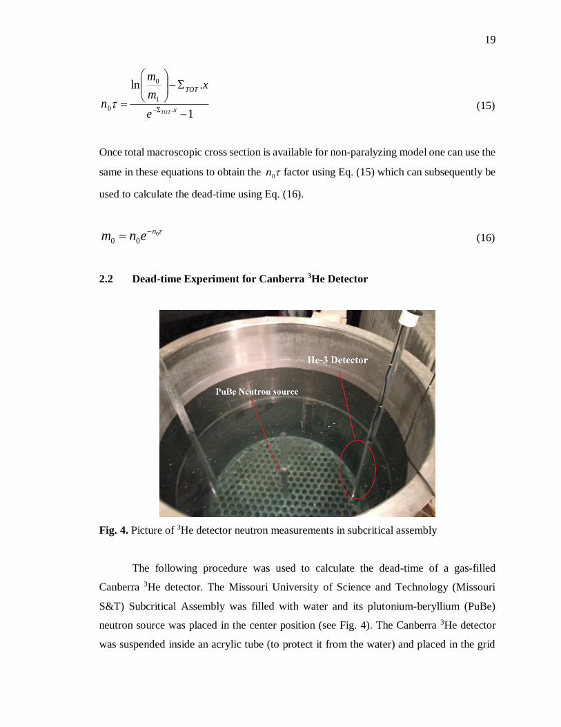
2.2 Dead-time Experiment for Canberra 3He Detector

Fig. 4. Picture of 3He detector neutron measurements in subcritical assembly

The following procedure was used to calculate the dead-time of a gas-filled

Canberra 3He detector. The Missouri University of Science and Technology (Missouri

S&T) Subcritical Assembly was filled with water and its plutonium-beryllium (PuBe)

neutron source was placed in the center position (see Fig. 4). The Canberra 3He detector

was suspended inside an acrylic tube (to protect it from the water) and placed in the grid

20

plate position A1 (5.08 cm center-to-center). A five-minute count was taken and the

detector was moved to the second position, A2, 10.16 cm from the source. This process

was repeated for the remaining seven positions on the A axis and again along each of the

five other axes – B, C, D, E, and F. This layout, which was also used for the MCNP

simulations, can be seen in Fig. (5).

Fig. 5. MCNP simulation layout. The Pu-Be neutron source (S) was placed in the center-

most position of the subcritical assembly. Nine MCNP simulations and nine measurements

were performed in the numbered locations on axis A. Five more sets of measurements,

repeating those made on axis A, were made on the five remaining axes.

The Canberra Lynx Digital Signal Analyzer was used to supply power to the

detector and record counts [18]. An MCNP model of the Missouri S&T Subcritical

Assembly was used to simulate the measurements. The model was developed by Tucker

[15] and it was experimentally validated. Nine simulations were performed with the

21

detector modeled in each of the nine detector locations along axis A. The water-filled cells

between the source and the detector were given higher importance to ensure usable

statistics. One hundred million histories were used for detector locations A1 through A6.

One hundred fifty million histories were used for locations A7 through A9. Cell-averaged

neutron flux (neutrons per square centimeter per source particle) was tallied over the

detector gas portion of the modeled detector.

Measurements of a plutonium-beryllium (Pu-Be) neutron source were taken from

nine distances with the Canberra 3He Detector in the Missouri S&T Subcritical Assembly.

These measurements were compared to the results from MCNP simulations. The difference

between the measured and simulated values were attributed to dead-time losses and was

used to estimate the detector’s dead time.

3. Results

The dead time measurement for N-Probe was conducted using the beam port of

MSTR and only fast neutron probe was used for this set of measurements. The fast neutron

measurements were first taken without a Plexiglas layer, and then with six different

thicknesses of Plexiglas layers. Data collection for each step was 10 minutes. The Plexiglas

thickness changed from 0 cm to 3 cm with increments of 0.5 cm. The measurements are

tabulated in Table 1 at 5 kW constant power for each thickness.

Table 1. The fast neutron measurements using N-Probe at 5 kW power

Plexiglas

thickness

(cm)

N-Probe

Fast Neutrons

counts

Count rates

0.0 2077857 3463.09 ± 58.85

0.5 2035029

3391.71 ± 58.24

1.0 1986735 3311.22 ± 57.54

1.5 1938566 3230.94 ± 56.84

2.0 1893107 3155.17 ± 56.17

2.5 1842570 3070.95 ± 55.42

3.0 1797494 2995.82 ± 54.73

22

Fig. (6) shows the plot of the neutron count rate with different thicknesses of

Plexiglas. Errors were propagated based on one standard deviation (1σ) and are included

on the graphs. The first count without any Plexiglas for fast neutrons using the N-Probe

spectrometer was 3463.09 per second and the counts decreased with increments of

Plexiglas thickness. The last count for fast neutron measurement with 3 cm thickness of

Plexiglas was 2995.82 per second.

Fig. 6. Fast neutron count rates with different thickness of Plexiglass at 5 kw power.

Exponential trend line in Fig. (6) provides the total macroscopic cross section,

0.049 cm-1, needed for both non-paralyzing and paralyzing dead-time calculations. The

total macroscopic cross section for average neutrons are tabulated in Table 2. The total

macroscopic cross sections were calculated based on total counts of fast neutrons (fast

neutrons vary from 800 keV to 20 MeV) for the N-Probe. The total absorption cross section

of Plexiglas can be calculated for a specific neutron energy using the same method.

The average macroscopic cross section of Plexiglas using the N-Probe liquid

scintillator (Fast probe) was calculated to be 0.049 cm-1 for the non-paralyzing model using

0.5 cm and 1 cm thicknesses. Same macroscopic cross section can be used for the

paralyzing model since the same Plexiglas thicknesses were used for dead-time

calculations for paralyzing dead-time model.

y = 3472.1e-0.049x

R² = 0.999

2500

2700

2900

3100

3300

3500

3700

0 0.5 1 1.5 2 2.5 3

Cou

nts

Thickness (cm)

at 5 kw Power Expon. (at 5 kw Power)

23

Table 2. Total macroscopic cross section (ƩTOT) for Plexiglas using all counts

Plexiglas

Thickness

(cm)

ƩTOT (1/cm)

Non-Paralyzing

Method

ƩTOT (1/cm)

Paralyzing Method

0.5 0.049 0.049

1 0.049 0.049

Based on a combination of the attenuation law and non-paralyzing and paralyzing

dead-time models, the dead-time of the fast probe (N-Probe detector) was calculated. Eqs.

(7), (10) and (12) were used to calculate dead-time for the non-paralyzing model while

Eqs. (13), (15) and (16) were used to calculate dead-time for the paralyzing model. Table

3 shows the dead-time calculations for the N-Probe detector. Non-paralyzing dead-time of

the detector was found to be 43.7 µs with an error of ± 5.24 and paralyzing dead-time of

the detector was found to be 37.6 µs with an error of ± 5.33. As was expected, dead-time

based on non-paralyzing assumption for the detector was higher than paralyzing dead-time.

Error propagations ( S ) of dead-time measurements for both idealized models were

calculated using Eq. (17). sm and sn are individual errors of measured counts and true

counts.

222 )()(n

sm

sS nm

(17)

Table 3. Dead-time calculations of N-Probe for two ideal models

Plexiglas

thickness

(cm)

Non-Paralyzing

Dead-time (µs) Errors

Paralyzing

Dead-time (µs) Errors

0.5 43.7 ± 5.24 37.6 ± 5.34

1 43.7 ± 5.22 37.6 ± 5.33

It is important to notice that the above technique assumes that the build-up of

neutron flux is insignificant for the geometry with half and one cm Plexiglas.

After calculating the dead-time of the detector, a high count rate experiment was

conducted and the count rates were corrected using non-paralyzing and paralyzing dead-

24

times (see Fig. 7). As count rate increases, the dead-time effect of the detector increases.

The dead-time effect is almost negligible at low count rates. In the experiment, fast neutron

counts were high at around 900 keV and the dead-time effect is observable and the two

model seems to be separating the predictions significantly.

Fig. 7. Fast neutron count rates with different thickness of Plexiglass at 5 kw power.

For the Canberra 3He detector (0.5NH1/1K) subcritical assembly was used to

calculate the detector dead time. Measurements of a plutonium-beryllium (PuBe) neutron

source were taken from nine distances with the Canberra 3He detector in the Missouri S&T

Subcritical Assembly. These measurements were compared to results from well calibrated

MCNP model simulation results. The difference between the measured and simulated

values was attributed to dead time losses. Using this difference dead time was estimated

for the detector. The results of the measurements are provided in Table 4.

The results of the measurements (counts per second) and simulations (n cm-2 sp-1)

cannot be directly compared so both sets of data were normalized to their smallest value

(see Fig. 8) for which dead time effects were considered to be negligible. In order to

calculate detector dead time, the true and measured count rates must be known. The

collection of the measured count rate has already been discussed. The MCNP results were

used to generate the true count rate. To do this, each tally result generated by MCNP was

0

200

400

600

800

1000

1200

0 500 1000 1500 2000 2500 3000

Cou

nt ra

te

Energy (keV)

Measured counts

Non-Paralayzable correction

Paralayzable correction

25

divided by the tally result for the ninth detector position (45.72 cm from the source) and

multiplied by the measured value at the ninth detector position as seen in Eq. (18).

𝑇𝑟𝑢𝑒 𝐶𝑜𝑢𝑛𝑡 𝑅𝑎𝑡𝑒 =𝑆𝑖

𝑆9𝑀9 (18)

Table 4. Neutron measurements from the Canberra 3He Detector in the Subcritical

Assembly

Distance from

PuBe neutron source (cm) Count rate (counts s-1)

5.08 12661.98 ± 156.32

10.16 7522.19 ± 53.33

15.24 2935.79 ± 56.30

20.32 1101.94 ± 26.70

25.40 439.10 ± 30.23

30.48 174.85 ± 5.29

35.56 74.17 ± 2.06

40.64 33.18 ± 0.68

45.72 15.44 ± 0.52

Table 5. Results of MCNP simulations of Canberra 3He neutron detector in the Subcritical

Assembly

Distance from

PuBe neutron source (cm)

Cell-averaged Flux Tally

Result (n cm-2 sp-1)

5.08 2.40851E-03 ± 4.09447E-

06 10.16 1.43884E-03 ± 3.02156E-

06 15.24 5.57542E-04 ± 1.95140E-

06 20.32 2.01799E-04 ± 1.10989E-

06 25.40 7.43707E-05 ± 6.76773E-

07 30.48 2.98034E-05 ± 4.26189E-

07 35.56 1.21184E-05 ± 2.13284E-

07 40.64 5.59834E-06 ± 1.45557E-

07 45.72 2.32741E-06 ± 9.12345E-

08

26

Where S represents the tally result from MCNP and M represents the

measured value. Eq. (18) was applied to the results for the eight closest detector distances

and the dead-time at each location was calculated according to both the paralyzing and

non-paralyzing models. The ninth location was excluded because this position was used

for normalization process and cannot be used to calculate a dead-time using Eq. (18). The

results of the simulations are provided in Table 5. The paralyzing dead-time was calculated

to be 14.5 μs, and the non-paralyzing dead-time was calculated to be 16.4 μs.

Fig. 8. The results of the measurements and simulations, normalized to their lowest values

for comparison.

4. Conclusion

The N-Probe utilizes two different spectroscopic techniques for providing neutron

spectrum. From 800 keV to 20 MeV, the fast neutron energy region is measured by a liquid

scintillator combined with a photon discriminator (fast probe). From 0 to 800 keV, the

thermal neutron energy region is measured by a spherical 3He detector. The dead-time of

the fast probe was determined via the combination of the attenuation law and idealized

dead-time models. All measurements were taken in front of the beam port at the Missouri

S&T Research Reactor (MSTR) while at 5 kW constant power. The paralyzing dead-time

value of N-Probe Liquid scintillator detector was found to be 37.6 ± 5.34 µs, while the non-

0

2000

4000

6000

8000

10000

12000

14000

16000

0 5 10 15 20 25 30 35 40 45 50

Co

un

t R

ate

(n s

-1)

Distance from Source (cm)

MeasurementsSimulations

27

paralyzing dead-time value was found to be 43.7 ± 5.24 µs. At this point we were not able

to compare the dead-time value of N-Probe liquid scintillator detector with BTI N-Probe

detector manual since the company strictly protecting this information. Dead-time values

for the fast probe were higher than expected since average liquid scintillator dead-time is

1 to 10 µs [6]. The same method was used to calculate the dead-time of the N-Probe thermal

neutron probe at 5 kW power (constant flux). However, some fast neutrons thermalized

when the layers of Plexiglas was placed in front of detector. These thermalized neutrons

affect the dead-time calculations and result in negative dead-time values.

The dead-time of a tube-type Canberra 3He gas-filled detector was calculated for

both non-paralyzing and paralyzing dead-time models using subcritical assembly

measurements and MCNP simulations. The paralyzing dead-time was calculated to be 14.5

μs, and the non-paralyzing dead-time was calculated to be 16.4 μs for 3He gas filled

detector. The dead-time of gas-filled proportional (especially GM counters) detectors

generally lies between 100 and 300 µs [6]. However, Hashimoto and Ohya [20] used a

variance to mean method to calculate the dead-time of a 3He proportional counter and its

dead-time was found to be approximately 10 µs. Calculated dead-time value of 3He gas

filled detector is agreed with their result in the order of magnitude.

References

[1] V. V. Verbinski, et al., Calibration of an organic scintillator for neutron

spectrometry. Nucl. Instrum. Methods 65, 8–25, (1968).

[2] J. A. Harvey, and N. W/ Hill, Scintillation detectors for fast neutron physics, Nucl.

Instrum. Meth. 162, 507, (1979).

[3] I. Yousuke, et al., "Deterioration of pulse-shape discrimination in liquid organic

scintillator at high energies". Nuclear Science Symposium Conference Record,

1,219–221, (2000).

[4] G. F. Knoll, Radiation Detection and Measurement. 4th Edition, p.573, 2010, John

Willey & Sons Inc, USA.

[5] M. Karlsson, Absolute efficiency calibration of NE-213 liquid scintillator using a

252Cf source, Department of Nuclear Physics in Lund University, Sweden, 1997.

28

[6] N. Tsoulfanidis, S. Landsberger, Measurement and Detection of Radiation. 3th

Edition, 2011, CRC Press. Taylor & Francis Group. New York.

[7] T. W. Krane, and M. N. Baker, Neutron Detectors Chapter 13,

http://www.lanl.gov/orgs/n/n1/panda/00326408.pdf (Accessed, September 2014).

[8] G. F. Knoll, Radiation Detection and Measurement. 4th Edition, p.523, 2010, John

Willey & Sons Inc, USA.

[9] H. Ing, et al., Portable Spectroscopic Neutron Probe, Radiation Protection

Dosimetry, 126, 238-243, (2007).

[10] Mobile Microspec Operational Manual, Bubble Technology Industries Inc (BTI),

Revised: October 30, 2009.

[11] J.W. Muller, Dead-time problems. Nuclear Instruments and Methods. 112, 47-57,

(1973).

[12] J.W. Muller, Generalized Dead Times, Nuclear Instruments and Methods, 301,543-

551, (1991).

[13] H. G. Stever, The discharge mechanism of fast G-M counters from the dead-time

experiment, Phys. Rev. 61, 38-52, (1942).

[14] W. Feller, On probability problems in the theory of counters, in R. Courant

Anniversary volume, Studies and Essays. Interscience. New York. 105-115,

(1948).

[15] L. P. Tucker, Upgrade and simulation of the subcritical assembly at Missouri

University of Science and Technology, Master’s Thesis, Missouri University of

Science and Technology. Rolla, MO. 2011.

[16] “Missouri S&T Nuclear Reactor” Missouri University of Science and Technology

Nuclear Engineering Department. http://nuclear.mst.edu/research/reactor/ (2016).

[17] J. R. Lamarsh, Introduction to Nuclear Engineering, 3rd Edition, p. 57, 2001,

Prentice Hall, New Jersey, USA.

[18] Canberra Industries, Inc., Lynx Digital Signal Analyzer Data Sheet, Meriden,

Conn., 2012.

[19] D. J. Loaiza, High-efficiency 3He proportional counter for detection of delayed

neutrons, Nuclear Instuments and Methods in Physics Research A, 422, (1999), 43-

46.

[20] K. Hashimoto and K. Ohya, Dead-time measurement for radiation counters by

variance to mean method, Journal of Nuclear Science and Technology, 33, 863-

868, (1996).

29

II. CHARACTERIZATION OF BEST CANDIDATE ISOTOPES FOR BURNUP

ANALYSIS AND MONITORING OF IRRADIATED FUEL

T. Akyurek, L.P. Tucker, and S. Usman

Department of Mining and Nuclear Engineering, Missouri University of

Science & Technology, Rolla, MO 65409, USA

Abstract

This research is an extension of feasibility study of MOX fuel online burnup

analysis. A multitude of fission products identified as candidates have been scrutinized for

their suitability of burnup analysis and spent fuel analysis. Best isotopes obtained for

analysis by investigating half-life, fission yield, branching ratios, production modes,

thermal neutron absorption cross section and fuel matrix diffusivity. 132I and 97Nb are

identified as good isotope candidates for on-line burnup analysis. 132I is also a good

candidate for plutonium/uranium discrimination due to the large difference in the fission

yield of the isotope. For interim storage monitoring the well-established cesium isotopes

appears to be the best choices unless the data gaps are addressed. Only alternate for cesium

for interim monitoring is 131I at the present time. For the long-term storage monitoring 94Nb

is the most attractive candidate. It has a low diffusion rate of ~10-11 cm2/s, an almost zero

neutron absorption cross section making it burnup history independent and decent gamma

yield of 1.44E-09. In addition, the paper also identifies the data gaps for developing a robust

burnup analysis tool using gamma spectroscopy.

1. Introduction

Between 1977 and 1981 commercial reprocessing was banned by the United States

government, interrupting the U.S. reprocessing industry. The U.S. moratorium on 88

reprocessing did not, however, discourage European countries such as France from

developing the technology and incorporating Mixed OXide (MOX) fuel into their nuclear

30

fuel cycle. While other nations pursued reprocessing, the U.S. chose to invest in the Yucca

Mountain Nuclear Waste Repository. However, with Yucca Mountain no longer under

consideration, the U.S. is reconsidering its fuel cycle options, and taking a second look at

reprocessing and MOX fuel [1, 2].

Decades of operation in France have demonstrated that MOX fuel can be

incorporated into a UO2 fueled core without risking the safety of the plant or increasing the

risk of proliferation [3]. Now the U.S. power industry is investigating the fuel. In 2005,

Duke Energy commissioned AREVA to build four MOX fuel assemblies for the Catawba

Nuclear Station. The Megatons to Megawatts program is another major commitment by

the U.S to incorporate MOX into the fuel cycle. This program is an agreement between the

United States and Russia to dispose of approximately 35 metric tons (MT) of weapons-

grade plutonium by converting it into MOX fuel to be burned in commercial nuclear power

plants. The MOX fuel assemblies will be manufactured at the Department of Energy’s

Savannah River Site through a contract with Duke COGEMA Stone & Webster. As of July

2012, this program has converted 450 MT of weapons-grade uranium to low-enriched fuel

for power reactors [4].

Thorium fueled reactors are also under consideration because of the advantages of

the thorium fuel cycle. Thorium is abundant in the earth’s crust. With roughly four times

the concentration of uranium, it can be found across the globe. And because 238U is not

usually present in thorium fuel there are fewer transuranic elements in the spent fuel [5].

Thorium-based fuels can also be used for plutonium destruction. As there is no plutonium

created during use all the plutonium burned is gone for good. The only downside is that

fissile 233U is produced, which has many of the same proliferation concerns.

Regardless of how the U.S. fuel cycle changes, better tools and techniques for

measuring burnup and monitoring spent fuel will be required. One attractive option for

non-destructively examining spent fuel is gamma spectroscopy. In this work, a multitude

of fission products identified as candidates for burnup analysis and spent fuel monitoring,

as proposed by Dennis and Usman [6], are scrutinized for their suitability for such a

program. Consideration is given to half-life, fission yield, branching ratios, thermal neutron

absorption cross section, production modes and fuel matrix diffusivity. Based on these

31

parameters, the best isotopes for non-destructive burnup analysis and spent fuel monitoring

have been identified.

2. Traditional Tools, Techniques and Conventional Isotopes for Burnup Analysis

A report was published by US Nuclear Regulatory Commission [7] discussing

various aspects of spent fuel monitoring and the requirements of the measurements system.

There are two broad groups of techniques available; “passive” measurement of delayed

neutrons and gamma and “active” interrogation by either a pulsed neutron source or a weak

steady state source and subsequently monitoring the gamma and/or neutron emissions. For

safe transportation of spent nuclear fuel it is critical to have a reliable and efficient

monitoring system capable of on-site, accurate measurement of the spent fuel to ensure

compliance with the safety criteria. Gamma measurement is one non-destructive technique

(NDA) for spent fuel monitoring, analyzing the radiation emitted by irradiated nuclear fuel

assemblies to determine parameters such as burnup, cooling time, and a qualitative

verification of the irradiation history [8]. These parameters can be calculated with the help

of flux measurements in the core and following the path of the fuel assembly as it proceeds

with its burnup cycle. These calculations can be experimentally verified by the above

mentioned techniques. Willman and co-workers [9] have investigated 137Cs (T1/2 = 30.1

years), 134Cs (T1/2 = 2.1 years) and 154Eu (T1/2 = 8.6 years) as indictors of cooling time and

irradiation history since these isotopes dominate the gamma spectrum of spent fuel after

five years of cooling time [7]. Moreover, the isotope has very small neutron absorption

cross sections and hence negligible burnup history dependence and its fission yields from

235U and 239Pu is approximately the same. Willman and co-worker [10] has reported the

success of using 154Eu while Dennis and Usman [11] reported the potential of using 106Ru.

Because of their relatively long half-lives, these isotopes are most useful for analyzing used

fuel after about 10 years of cooling. Focus of this manuscript is to analyze new isotopes

for their suitability as a burnup indicator. The conventional fission isotopes (137Cs, 154Eu,

106Ru etc.) already considered for burnup analysis are not included in this discussion with

the exception of 134Cs which is included for comparison. Interested reader may refer to

literature [8-11] for discussion on the conventional burnup isotopes.

32

Another NDA technique for power reactor released spent fuel is based on neutron

measurements. A series of neutron absorptions in 238U leads to the production of 244Cm.

Spontaneous fission of 244Cm provides a source of “delayed neutron”. Since the half-life

of 244Cm is 18.1 years, neutrons from 244Cm are a measure of burnup. This technique is

sensitive to cooling time, and initial enrichment for the spent fuel. Additional information

on neutron measurement based burnup calculation is available in the literature [12].

Additionally, chemical assay with mass spectroscopic techniques [13] have

historically been applied to determine isotopic composition of spent nuclear fuel but these

techniques requires fuel sample destruction and can take a long time for sample analysis

91 and results. Recent new attempts for spent nuclear fuel analysis include use of digital

measurement of Cherenkov [14]. A patent is also been filed by Dowdy and co-workers

[15] on the application of Cherenkov radiation for irradiated fuel monitoring.

Focus of this manuscript is to compare the advantages of various isotopes for

gamma emission based spent fuel measurement. While other techniques are available

gamma measurement based spent fuel monitoring is the most commonly used technique.

3. Important Indicators for Burnup Analysis and Spent Fuel Monitoring

Burnup measurement are useful for a number of applications including; pre-

transportation compliance certification, monitoring of spent fuel for Special Nuclear

Material (SNM) accountability and proliferation deterrence, monitoring during storage for

historic burnup analysis and online burnup measurement for next generation reactors for

fuel cycle optimization. Additional spent fuel monitoring is required during reprocessing

operation. For each of these application one or more of the techniques described in the

previous section is better suited than others.

Half-life of the burnup indicator isotope is one characteristic that can dramatically

impact its suitability for different applications; online applications, interim storage and

long-term storage. A nuclide with a half-life between minutes and days is ideal for online

burnup determination but useless for historical data collection. For interim storage-pool

monitoring, the indicator’s half-life should be between a few days and a few years. Burnup

indicators for long-term storage applications should have half-lives greater than few years.

33

Another desirable characteristic for burnup and used fuel monitoring indicators is

a simple production mode and a simple decay chain. Generally, it is significantly more

complicated to track the decay of a candidate isotope with multiple decay modes and

multiple production modes, which via direct fission and by decay of several fission

products. However, in certain situations this can be an advantage. A single production path

(production from single parent nuclide or direct production from fission) coupled with a

high fission yield ensures that a detectable amount of the isotope would be present. Since

the emitted gamma rays must potentially penetrate several layers of fuel, cladding, and

moderator, a high energy gamma ray (on the order of MeV) with a high branching ratio is

also necessary for detectability.

It is also important for the indicator isotope to remain in the fuel where it was

created after it is produced. Therefore, the neutron capture cross-section must be as low as

possible and must not exceed more than a few barns so that product atoms density is

independent of burnup history. Small neutron absorption cross section also ensures that

burnup indicator isotope generated from fission is not subsequently consumed by parasitic

neutron absorption. Low fission product migration at high temperatures is another desirable

characteristic. The fission product must ideally remain where it was created. Any migration

of fission products will skew the burnup profile of the assembly [16].

4. Candidate Isotopes

137Cs, 134Cs and 154Eu are commonly used isotopes for burnup analysis and fuel

monitoring. Recently Willman et al. investigated two correlations between burnup and the

intensity of these isotopes. They proposed a linear correlation between burnup and the

intensity of the 661.7 keV 137Cs peak while they found that 154Eu and 134Cs is related to the

93 square of burnup [9]. Hawari and co-workers [17] have considered gamma spectrometry

of Cs-137 and Eu-154 for online burnup monitoring of pebble bed reactors. Jansson and

co-workers [18] provide corroborating evidence that there is a correlation between 137Cs

intensity and burnup for Pressurized Water Reactor (PWR) assemblies [18]. Dennis and

Usman [11] proposed 106Ru isotope for MOX fuel burnup analysis. They studied the

feasibility of using 106Ru as a burnup indicator for UO2 fuel and as a means for

34

discriminating between MOX and UO2 fuel. Their ORIGEN-ARP (Oak Ridge Isotope

Generation and Depletion Code – Automatic Rapid Processing) simulations showed a

linear correlation between primary photopeak intensity and MOX fuel assembly burnup

for 137Cs and 106Ru. They relied on using peak ratios rather than raw peak counts to

normalize and remove the burnup history dependence.

This paper analyzes the list of candidate isotopes proposed by Dennis and Usman

[6] for their suitability for burnup analysis application. These isotopes are listed in Table

1. To complete the analysis, data was collected on the half-life, fission yield, branching

ratios, diffusivity, and neutron absorption cross section for each of the candidate isotope.

Some nuclides lacked data for some of these characteristics, leaving room for additional

research. However, based on an analysis of the data that was available, the best isotopes

for burnup analysis and irradiated fuel monitoring have been identified.

There are some isotopes in Table 1 that decay with virtually identical photon

energies. For example, 137mBa, 98Tc, and 132Cs have almost same photon energy and

emission probability values. It would be difficult to distinguish these isotopes based on

gamma spectroscopy alone. However, their half-lives differ by orders of magnitude. 137mBa

has a half-life of 2.55 min, which will decay quickly. The half-life of 98Tc is 4.2 million

years, making it practically stable. 132Cs has half-life of 6.48 days. For these situations one

may consider using an unfolding technique to determine correct apportionment of summed

peak and separating say 137mBa from 98Tc.

Table 1. Reference isotopes for burnup analysis and spent fuel monitoring [6]

Simulation

Energy

(keV)

Potential

Isotope

Energy

(MeV)

Photon

Emission

Probablity

Simulation

Energy

(keV)

Potential

Isotope

Energy

(MeV)

Photon

Emission

Probablity

76.6110 243Am 0.07467 0.66 617.82 108mAg 0.61437 0.90393

206Bi 0.074969 0.54146 43K 0.61749 0.80514

61Co 0.067412 0.85 190mOs 0.61608 0.9862

73Se 0.067 0.7729601 144Pm 0.61801 0.98597

44Ti 0.07838 0.97619 626.15 43K 0.61749 0.80514

93.2640 49Cr 0.090639 0.532 144Pm 0.61801 0.98597

101.5900 67Ga 0.93311 0.357 148mPm 0.62997 0.88998

134.9000 99mTc 0.14051 0.8907 659.46 137mBa 0.66165 0.8998

143.2200 99mTc 0.14051 0.8907 132Cs 0.66769 0.97423

85mKr 0.15118 0.75278 130I 0.66854 0.96129

159.8700 52Fe 0.016868 0.966 132I 0.66769 0.987

35

Table 1 continued. 56Ni 0.15838 0.98795 97Nb 0.6579 0.9809

176.5300 52Fe 0.016868 0.966 126Sb 0.66633 0.99619

111Ln 0.17128 0.9024 667.78 137mBa 0.66165 0.8998

193.1800 90Y 0.20251 0.96631 98Tc 0.65241 0.99745

166mHo 0.18442 0.726 132Cs 0.66799 0.97423

190mOs 0.18673 0.702 130I 0.66854 0.96129

226.4900 85mSr 0.23169 0.84725 132I 0.66769 0.987

132Te 0.22816 0.88 692.76 97Nb 0.6579 0.9809

276.4400 203Hg 0.27919 0.773 126Sb 0.66633 0.99619

203Pb 0.27919 0.768 94Nb 0.70293 1

318.0800 192Ir 0.31651 0.82853 717.74 144Pm 0.69649 0.99492

51Ti 0.32008 0.929 126Sb 0.695 0.99619

157Dy 0.32616 0.938 108mAg 0.72295 0.90499

326.4000 194mIr 0.32845 0.929 751.05 166mHo 0.71169 0.54087

51Ti 0.32008 0.929 126Sb 0.7205 0.53794

157Dy 0.32616 09.38 244Am 0.746 0.67

359.71 73Se 0.3611 0.965 52Mn 0.74421 0.9

190mOs 0.36109 0.9488 97mNb 0.74336 0.9796

131I 0.36448 0.81164 759.37 98Tc 0.74535 0.99819

376.36 43K 0.37276 0.87273 95Zr 0.75671 0.55345

204mPb 0.89915 0.99164 95Nb 0.76579 0.99808

200Tl 0.36794 0.873 767.7 95Tc 0.76579 0.9382

434.64 108mAg 0.43393 0.89881 95Zr 0.75671 0.55345

202Tl 0.43956 0.915 82Br 0.77649 0.8331

69mZn 0.43863 0.94889 132I1 0.77261 0.76196

484.6 181Hf 0.48203 0.825 792.68 95Nb 0.76579 0.99808

194mIr 0.48286 0.97 95Tc 0.76579 0.9382

87Y 0.4847 0.9394 809.33 134Cs 0.79584 0.854

90mY 0.47953 0.9099 210Tl 0.7997 0.9896

492.93 190Os 0.50255 0.9778 206Bi 0.8031 0.9889

103Ru 0.49708 0.889 58Co 0.81076 0.9943

87Y 0.4847 0.9394 136Cs 0.8185 0.997

534.56 130I 0.53609 0.99 166mHo 0.81031 0.57136

133I 0.52987 0.8632 56Ni 0.81185 0.85996

135mXe 0.52656 0.80997 1592 96Tc 0.81254 0.81803

601.17 134Cs 0.6047 0.976 210Tl 0.7997 0.9896

124Sb 0.60271 0.978001 140La 1.5965 0.9549

Table 2 lists the candidate isotopes from Table 1 with their half-lives and divides

them into groups based on their usefulness for online burnup analysis, interim storage

monitoring, and long-term or historical data applications. A cut off of ten minutes was used

as the lower limit for online measurement system. This choice is based on the fact that at

least 2-3 minutes would be required to transport the irradiated fuel to location where it can

be measured. And a minimum of one minute count might be necessary for good statistics

of the peak counts. However, if there is a slight uncertainty in the cooling/transport time

the quality of measurement can be adversely impacted for a short lived isotope. Therefore,

36

a ten minute lower limit is set for half-life for online burnup application. Hence,

radioisotopes with half-lives less than ten minutes are not considered useful for any of these

applications. This choice of ten minutes is also to ensure that during the measurement time

(that is one min count) the activity is only going to reduce by less than 7%. Four isotopes

are placed in Group 0 with half-lives less than 10 minutes and therefore minimum to no

usefulness. There are 21 isotopes in Group 1 having half-lives between 10 minutes and 24

hours. Nuclides in Group 1 are suitable for online burnup analysis. For online measurement

too long half-life is not useful either. The upper limit for online burnup applications half

live is set at 24 hours. These choices are somewhat arbitrary. There are 30 isotopes in

Group 2 with half-lives between 24 hours and 5 years. Group 2 nuclides are ideal for

interim-storage pool monitoring applications. Group 3 encompasses potential tracers for

long-term storage applications. There are six isotopes in Group 3 with half-life of 5 years

or more. These isotopes are possibly best suited for historical data validations and long-

term spent fuel monitoring.

a) Online burnup analysis – Candidate Isotopes

For the three applications in mind, next step is to evaluate the best isotopes for each

application in regards to their physical properties; fission yield, branching ratio and gamma

energies, neutron absorption cross section and diffusion parameters. Group 1 is candidate

isotopes for online monitoring. Table 3 provides half-lives, emission probabilities

(branching ratio), the corresponding gamma energies and fission yields (thermal neutron

fission yield from uranium and plutonium) for all candidate isotopes for group 1. The last

column in the table lists gamma yield (PxFY) which is the product of fission yield and

emission probability and can be used as a figure of merits for an isotope’s suitability as a

burnup indicator. PxFY is in fact number of discrete energy gammas released per fission.

Higher the PxFY is better suited the isotope would be for burnup applications. Table 3 also

lists the ratio of the fission yield for 235U and 239Pu. This ratio is an indicator of the isotope’s

usefulness to be used as a discriminator between 235U and 239Pu.

37

Table 2. Candidate isotopes grouped by half-life for burnup analysis [19]

NOT USEFUL

(GROUP 0)

ONLINE

ANALYSIS

(GROUP 1)

INTERIM STORAGE

ANALYSIS

(GROUP 2)

LONG-TERM

STORAGE

(GROUP 3)

Less than

9 min

(T1/2)

(min)

10 min –

24 hours

(T1/2)

(min)

24 hours-

5 years

(T1/2)

(days)

5 years-

more

(T1/2)

(year)

1 97mNb 0.9683 190mOs 9.9 200Tl 1.088 44Ti 58.9

2 210Tl 1.3 49Cr 42.3 82Br 1.47 108mAg 418

3 137mBa 2.55 204mPb 67.2 140La 1.6785 166mHo 1200

4 51Ti 5.77 85mSr 67.63 203Pb 2.163 243Am 7390

5 97Nb 72.1 90Y 2.67 94Nb 20300

6 61Co 99 111In 2.8 98Tc 4200000

7 132I 137.7 132Te 3.20

8 90mY 191.4 67Ga 3.26

9 85mKr 268.8 87Y 3.35

10 99mTc 360 96Tc 4.28

11 73Se 429 52Mn 5.59

12 157Dy 488.4 56Ni 6.075

13 52Fe 496.5 206Bi 6.243

14 244Am 606 132Cs 6.48

15 130I 741.6 131I 8.0252

16 69mZn 825.6 202Tl 12.31

17 135mXe 917.4 126Sb 12.35

18 95Tc 1200 136Cs 13.16

19 133I 1248 95Nb 34.985

20 43K 1338 103Ru 39.247

21 200Tl 1566 148mPm 41.3

22 181Hf 42.38

23 203Hg 46.594

24 124Sb 60.2

25 95Zr 64.032

26 58Co 70.86

27 192Ir 73.828

28 194mIr 170

29 144Pm 363

30 134Cs 753.725

38

Table 3. Group 1 fission product and decay characteristics [20, 21, 22, 23]

(Potential candidates for online measurements)

Isot

ope

Half-life

(mins)

Emission

Probability

(%)

Energy

(keV)

235U Th.

Fiss.

Yield

239Pu Th.

Fiss. Yield

FY Ratio

(235U/239Pu)

PxFY (235U)

Gamma yield

43K 1338 86.8 79.16

11.85

372.76 617.49

396.86

N/A N/A N/A N/A

49Cr 42.3 53.2 30.32 16.39

90.64 152.93 62.29

N/A N/A N/A N/A

52Fe 496.5 99.18 1.64 0.21

168.69 377.75 1727.57

N/A N/A N/A N/A

61Co 99 84.67 0.79 3.62

67.42 841.7 909.2

N/A N/A N/A N/A

69mZn

825.6 94.8 100.0

438.63 573.9

1.0604E-11 7.0227E-10 0.01509976 1.0053E-11 1.0604E-11

73Se 429

69.84

97.0 0.27

67.07

361.2 510

5.1100E-17 2.0330E-19 251.352680

3.5688E-17

4.9567E-17 1.3797E-19

85mKr

268.8

75

0.300 0.01 14

151.195

129.81 451.0

304.87

5.8987E-05 2.3275E-05 2.53440460

4.424E-05

1.7696E-07 5.8987E-09 8.2582E-06

85mSr 67.63

96.0 97.49 1.12 0.11 0.32

151.19 231.86 129.82 731.80 238.78

1.4735E-13 2.1241E-11 0.00693691

1.4145E-13 1.4365E-13 1.6503E-15 1.6208E-16 4.7150E-16

90mY 191.4

100. 97.25 90.74 0.32

2318.97 202.53 479.51 681.8

5.2570E-08 1.1327E-06 0.04641017

5.2570E-08 5.1125E-08 4.7702E-08 1.6822E-10

95Tc 1200 1.95 3.74 93.82

947.67 1073.71 765.79

8.2435E-17 2.6280E-16 0.31367960 1.6075E-18 3.0831E-18 7.7341E-17

97Nb 72.1 1.09 0.15 98.23

1024.4 1268.62 657.94

1.0704E-04 6.5215E-04 0.16413044 1.1667E-06 1.5056E-07 1.0514E-04

99mTc

360 88.5 0.023 140.511 142.683

2.8512E-10 2.7839E-08 0.010241823 2.5233E-10 6.5577E-14

130I 741.6

99.

96.03 82.17

536.07

668.54 739.51

1.5510E-06 3.2879E-05 0.04717187

1.5354E-06

1.4894E-06 1.2744E-06

132I 137.7 98.7 75.6

17.57

667.71 772.60

954.55

1.0393E-04 1.5148E-03 0.068611905 1.0258E-04 7.8574E-05

1.8261E-05

39

Table 3 continued.

133I 1248

0.356 0.309

1.81 0.539 0.645 1.49 0.457 1.23 4.47 0.551 1.49

2.33 86.3

262.70 422.903 510.530 617.978

680.252 706.575 768.360 856.278 875.328 1052.39 1236.44 1298.22

529.870

1.0232E-03 6.8765E-03 0.14880330

3.6427E-06 3.1618E-06 1.8521E-05 5.5153E-06

6.5999E-06 1.5246E-05 4.6762E-06 1.2586E-05 4.5739E-05 5.6381E-06 1.5246E-05 2.3841E-05

8.8306E-04

135mXe 917.4

1.47 0.1 0.07 80.8

786.9 1133.0 1358.0 526.56

1.8117E-03 7.5384E-03 0.24032192

2.6631E-05 1.8117E-06 1.2682E-06 1.4638E-03

157Dy 488.4 93

0.26 1.33

326.34 83.04 182.42

2.6950E-18 1.6595E-15 0.0016239 2.5064E-18 7.0070E-21 3.5844E-20

190mOs 9.9 94.88 97.79 98.62

361.2 502.5 616.5

N/A N/A N/A N/A N/A N/A

200Tl 1566 87.0 13.75

29.93

367.94 579.30 1205.75

N/A N/A N/A N/A

204mPb 67.2 94.2

99.17

91.5

374.76 899.15

911.74

N/A N/A N/A N/A

244Am 606 66. 28

16.4

743.97 897.85 153.86

N/A N/A N/A N/A

We have somewhat arbitrarily selected a lower limit of gamma yield per fission of

10-6 to identify the most attractive isotopes for burnup interrogation. For online application

since the cooling time is small isotopes an isotope with lower than 10-6 gamma yield may

still be useful, therefore we have set the gamma yield usefulness limit to 10-8. At this point

it is important to notice the data gaps, for many isotopes (marked as N/A – not available).

For these isotopes fission yield information is either not available at all or is available with

large discrepancies between the sources of information. Therefore additional work is

required to evaluate the effectiveness of these isotopes as burnup indicator.

Some of the isotopes, such as 73Se, 85mSr are not suited for burnup analysis because

their low gamma yields (PxFY). Some of the isotopes such as 190mOs have no fission yield

(and hence gamma yield) available in the literature. Candidate isotopes without gamma

yield values or with values below 10-8 are not considered suitable for online burnup

40

analysis. 130I emits a 668.54 keV photon with an emission probability of 96.03%, while 132I

emits a 667.1 keV photon with an emission probability of 98.7%. Because of their similar

photon emission energies, distinguishing them from one another would be difficult even

with high resolution spectroscopy. However, the fission yield for 132I is two orders of

magnitude higher than that of 130I, therefore most of the gamma in this case would come

from for 132I (note that the emission yields of the gammas of interest are very similar). In

cases where the fission yield difference is not as large, but there is significant difference in

the half-lives (for example, half-life of 130I is almost five times longer than 132I) one would

rely on standard unfolding techniques to separate the contribution from the individual

peaks.

Table 4 lists thermal neutron absorption cross sections and number of production

paths for group 1 candidate isotopes. Thermal neutron cross section is an important

parameter for a candidate burnup analysis isotope. A large neutron cross section would

mean that the isotope will exhibit large burnup history dependence. Therefore a low

thermal neutron absorption cross section is desired. Moreover, any burnup indicator with

large thermal neutron cross section will be lost by neutron absorption. Therefore at

2.65E+06 b, the thermal absorption cross section of 135mXe is much too high to be used as

a tracer for online burnup analyses. On the other hand, 97Nb and 132I have an absorption

cross section of 0 b; the lowest of the isotopes in Group 1 therefore making them a very

attractive candidate for burnup analysis.

Table 4. Group 1 candidate isotopes thermal absorption cross section and production mode

for online burnup analysis [24]

Isotope

Thermal Absorption

Cross Section

(barns)

Number of

Production

Modes

132I 0.00E+00 1

97Nb 0.00E+00 1

49Cr 1.72E-02 2

61Co 1.73E-02 1

85mKr 2.35E-02 1

41

Table 4 continued. 43K 1.18E+00 1

52Fe 1.74E+00 2

190mOs 3.90E+00 1

90mY 6.50E+00 1

69mZn 7.24E+00 1

133I 9.69E+00 1

95Tc 1.41E+01 1

130I 1.80E+01 1

85mSr 1.91E+01 1

200Tl 1.95E+01 1

73Se 2.18E+01 1

99mTc 2.29E+01 1

157Dy 1.17E+02 1

244Am 6.00E+02 1

204mPb 7.03E+02 1

135mXe 2.65E+06 1

The ideal online burnup tracer would only be produced by fission. However, two

isotopes in Group 1, 49Cr and 52Fe, are also produced by the decay of other fission products,

making them less than ideal candidates. Any burnup analysis algorithm based on an isotope

with multiple production modes will show cooling time and burnup history dependence

and therefore should be avoided.

Table 5 shows the diffusion properties of the Group 1 isotopes. Where possible the

diffusion coefficient in UO2 is provided, but for many candidates this information is not

readily available. High diffusion rates would lead to significant migration of the isotope

from its original location of birth to other areas. This migration will skew the measurement

results, and will make certain sections of high burnup fuel not to be recorded appropriately.

Therefore, high diffusion rates are not desirable for isotopes being considered for burnup

analysis. There are significant knowledge gaps in regards to diffusion coefficients of fission

isotopes. Ideally these diffusion coefficients must be measured in MOX and UO2 fuel

matrix separately at the elevated temperature comparable to fuel operating temperatures.

Much of this information is missing. There is limited data on uranium diffusion and none

42

on MOX. When UO2 diffusion data was missing, to provide predictive data as a helpful

tool diffusion coefficient in other materials is listed in table 5. For example, there is no

diffusion coefficient for Os in fuel material is available, however diffusion coefficient of

1.07x10-9 cm2/s (at 1100 0C) is reported in pyrrhotite (OsPO5) which too varies with

temperatures [25]. Reference cited in the table may be a good starting point for an interested

reader to explore additional information. Needless to say that more work is needed in the

area of isotope diffusion rates for many isotopes of interest. It is also difficult to predict the

diffusive characteristics of MOX fuel without experimental data and how it would compare

with UO2.

Table 5. Diffusion coefficients of candidate isotopes for online burnup analysis

Isotopes DIFFUSION Isotopes DIFFUSION

43K

K in melilite :

D=1.22x10-16 cm2/s at 900 0C

[26]

99mTc

Tc in dense Bentonite :

D=8x10-7 cm2/s

Tc in dense metalic Molybdenum :

D=5.1x10-13 cm2/s at 600 0C [44,27]

49Cr

Cr in β-Uranium :

D=3.6x10-10 cm2/s at 670 0C

D=6.45x10-11 cm2/s at 680 0C

D=3.80x10-10 cm2/s at 695.8 0C D=5.36x10-10 cm2/s at 712.7 0C

[30]

130I

Iodine in UO2 :

D=5.0x10-14 cm2/s at 1650 0C

D=3.0x10-15 cm2/s at 1400 0C [28]

52Fe

Fe in Fe3O4:

D=1.63x10-8 cm2/s at 1199 0C

D=1.59x10-9 cm2/s at 1200 0C

[29]

132I

Iodine in UO2 :

D=5.0x10-14 cm2/s at 1650 0C

D=3.0x10-15 cm2/s at 1400 0C

[28]

61Co

Co in β-Uranium :

D=9.3x10-9 cm2/s at 691.5 0C

D=1.16x10-8 cm2/s at 706.3 0C

D=1.33x10-8 cm2/s at 717.0 0C

D=1.90x10-8 cm2/s at 741.0 0C

[30]

133I

Iodine in UO2 :

D=5.0x10-14 cm2/s at 1650 0C

D=3.0x10-15 cm2/s at 1400 0C

[28]

69mZn

Zn in LiTaO3 :

D=3.055x10-14 cm2/s at 900 0C

Zn in CuInSe2 bulk crystal:

D=5.0x10-11 cm2/s at 550 0C

[31,32]

135mXe

Xe in UO2:

D=2.5x10-14 cm2/s at 1400 0C

[33]

43

Table 5 continued.

73Se

Se in PbSe :

D=0.5x10-13 cm2/s at 400 0C

D=1x10-12 cm2/s at 500 0C

D=0.8x10-10 cm2/s at 800 0C

Se in Carbon steel :

D=2x10-32 cm2/s

[34,35]

157Dy

Dy on the W(111) facet :

D=5.0x10-8 cm2/s at 827 0C

[36]

85mSr

Sr in Bi2Sr2CuO4:

D=3.4x10-13 cm2/s at 775 0C

D=1.1x10-11 cm2/s at 800 0C

Sr in Carbon steel :

D=9.7x10-8 cm2/s

[34,37]

190mOs

Os in Pyrrhotite(OsPO5) :

D=1.07x10-9 cm2/s at 1100 0C

[25]

85mKr

Kr in crushed UO2 :

D=6.7x10-17 cm2/s at 900 0C

D=8.3x10-15 cm2/s at 1100 0C [38]

200Tl

Tl in KCl:

D=0.8x10-11 m2/s at 300 0C

Tl in Tl Amalgam : D=0.98x105 cm2/s at 1200 0C

[39,40]

90mY

Y in UO2 :

D=6.8x10-8 cm2/s at 1150-1450 0C

[41]

204mPb

Pb in Zircon :

D=1.77x10-16 m2/s at 1251 0C

Pb in solid PbTl 50%Pb :

D=1.86x10-12 cm2/s at 206 0C

[42,43]

95Tc

Tc in dense Bentonite :

D=8x10-7 cm2/s

Tc in dense metallic Molybdenum :

D=5.1x10-17 m2/s at 600 0C

[35,44]

244Am

Am in UO2:

D=4.5x10-11 cm2/s for high O potential

D=6.0x10-10 cm2/s for low O potential

[45]

97Nb

Nb in UO2:

D=7.99x10-11 cm2/s at 1096 0C

D=4.82x10-11 cm2/s at 1380 0C [41]

b) Interim Storage (short term monitoring) – Candidate Isotopes

For interim storage analysis isotopes from third column of table 2 were selected for

further analysis. Table 6 displays half-lives, emission probabilities (branching ratio), the

corresponding gamma energies for all candidate isotopes for group 2. Similar to group 1,

the last column in the table lists gamma yield which is the product of fission yield and

44

emission probability and the other two columns list the ratio of the fission yield for 235U

and 239Pu and fission yields (thermal neutron fission yield from uranium and plutonium).

The data in Table 6 is used in conjunction with the data in Tables 7 and 8 to evaluate

usefulness of these isotopes for spent fuel monitoring program. The criteria for isotopes in

Group 2 are similar to those used for Group 1. If a candidate’s gamma yield (PxFY) value

is less than 10-8, it is considered as unsuitable tracer for spent fuel monitoring. Several

candidates were eliminated from Group 2 because of their low gamma yield (PxFY) values

for example, 67Ga, 111In, and 148mPm. Candidate isotopes were also excluded if their gamma

yield could not be determined due to lack of data, for example; 56Ni and 203Hg.

Table 6. Group 2 fission product and decay data [20,21,22,23]

Isotope

Half-

life

(days)

Emission

Prob.

(%)

Energy

(keV)

235U Th.

Fiss. Yield

239Pu Th.

Fiss. Yield

FY Ratio

(235U/239Pu)

PxFY

(235U)

52Mn 5.59

90.0

94.5 100.0

744.23

935.54 1434.09

N/A N/A N/A N/A

56Ni 6.075

98.8

49.5 86. 0

158.38

749.95 811.85

N/A N/A N/A N/A

58Co 70.86

30.0 99.45 0.69 0.52

511.0 810.759 863.00

1674.72

N/A N/A N/A N/A

67Ga 3.26 38.81 21.41 16.64

93.31 184.58 300.22

1.1934E-17 2.91553E-16 0.040932523 4.6316E-18 2.5551E-18 1.9858E-18

82Br 1.470 71.06 43.53 83.4

554.35 619.11 776.52

3.82137E-07 8.99942E-06 4.24624E-02 2.7155E-07 1.6634E-07 3.1870E-07

87Y 3.35 82.2

89.84

388.53

484.81 3.52878E-15 1.01775E-12 0.003467237

2.9007E-15

3.1738E-15

90Y 2.67 N/A

0.000001 1760.70 2186.24

3.69872E-08 7.96964E-07 0.046410126 N/A

3.6987E-16

95Zr 64.032 0.27 44.27 54.38

235.69 724.193 756.729

1.27051E-03 1.25467E-03 1.01262E+00 3.4304E-06 5.6245E-04 6.9090E-04

95Nb 34.985 0.03 0.01

99.808

204.12 561.88

765.803 1.06041E-06 5.65875E-06 1.87393E-01

3.1812E-10 1.0604E-10 1.0584E-06

45

Table 6 continued.

96Tc 4.28 99.76 82.00 97.57

778.22 812.54 849.86

N/A N/A N/A N/A

103Ru 39.247

0.071 0.384

0.289 0.344 91.31 0.855 5.78

39.76 53.275

294.98 443.80 497.08 557.04 610.33

2.35624E-07 1.26480E-05 0.018629349

1.6729E-10 9.0480E-10

6.8095E-10 8.1055E-10 2.1515E-07 2.0146E-09 1.3619E-08

111In 2.8 0.003 90.65

94.09

150.81 171.28

245.35

2.9712E-15 1.6524E-12 0.001798112 8.9136E-20 2.6934E-15

2.7956E-15

124Sb 60.2

98.3 7.46 1.360

2.287 10.81 0.743 1.892 1.841 1.588 1.043 2.623

1.222 0.675 47.79 5.51

602.727 645.853 709.320

713.781 722.784 790.711 968.199 1045.128 1325.508 1355.175 1368.160

1436.561 1488.88 1690.975 2090.936

2.70379E-08 2.69957E-07 1.00156E-01

2.6578E-08 2.0170E-09 3.6772E-10

6.1836E-10 2.9228E-09 2.0089E-10 5.1156E-10 4.9777E-10 4.2936E-10 2.8201E-10 7.0920E-10

3.3040E-10 1.8251E-10 1.2921E-08 1.4898E-19

126Sb 12.35 83.27 99.6 99.6

414.7 666.5 695.0

8.75506E-06 1.37397E-05 0.637208964 7.2903E-06 8.7200E-06 8.7200E-06

131I 8.0252

2.607 6.06 81.2 7.26 1.796

80.185 284.305 364.48

636.989 722.911

3.90977E-05 2.29304E-04 0.170505966

1.0193E-06 2.3693E-06 3.1747E-05 2.8385E-06 7.0219E-07

132Te 3.20375 14.96 1.96 88.0

49.72 116.30 228.16

1.52851E-02 2.25318E-02 0.678379002 2.2867E-03 2.9959E-04 1.3451E-02

132Cs 6.48

0.75 0.96 99.45 84.48 11.94 6.88

505.79 630.19 667.71 464.47 567.16

1031.66

7.36827E-10 2.97953E-09 0.247296386

5.5262E-12 7.0735E-12 7.3277E-10 6.2247E-10 8.7977E-11 5.0694E-11

134Cs 753.725

8.37 15.38 97.65 85.5

8.7 3.017

563.243 569.32 604.72 795.83

801.945 1365.186

4.43390E-08 3.85859E-06 1.14910E-02

3.7112E-09 6.8193E-09 4.3297E-08 3.7910E-08

3.8575E-09 1.3377E-09

46

Table 6 continued.

136Cs 13.16 42.17 99.7 79.76

340.55 818.51

1048.07 3.48339E-05 6.13750E-04 5.67558E-02

1.4689E-05 3.4729E-05 2.7784E-05

140La 1.6785

20.8 2.995 46.1 4.392 23.72 5.58

2.73 7.04 0.531 95.40 0.845 3.412

328.761 432.513 487.022 751.653 815.781 867.839

919.533 925.198 950.988 1596.203 2347.847 2521.30

5.20771E-05 1.01954E-04 5.10790E-01

1.0832E-05 1.5597E-06 2.4008E-05 2.2872E-06 1.2353E-05 2.9059E-06

1.4217E-06 3.6662E-06 2.7653E-07 4.9682E-05 4.4005E-07 1.7769E-06

144Pm 363 43.78 98.5

99.49

476.78 618.01

696.49

4.6662E-14 1.2900E-12 0.036172093 2.0429E-14 4.5962E-14

4.6424E-14

148mPm 41.3

22.2 2.47 1.10

12.56 3.92 18.66 5.35 6.75 94.9 12.54 5.48

89.0 32.8 17.17 20.3

75.8 98.48 189.63

288.11 311.63 414.07 432.78 501.26 550.27 599.74 611.26

629.97 725.70 915.33

1013.81

8.78357E-11 4.03712E-08 0.002175702

1.9500E-11 2.1695E-12 9.6619E-13

1.1032E-11 3.4432E-12 1.6390E-11 4.6992E-12 5.9289E-12 8.3356E-11 1.1015E-11 4.8134E-12

7.8174E-11 2.8810E-11 1.5081E-11 1.7831E-11

181Hf 42.38

43.3 5.85 0.86 15.12

0.703 80.5 0.233

133.021 136.26 136.86 345.93

475.99 482.18 615.17

N/A N/A N/A N/A

192Ir 73.828 31.2 86.94 50.26

308.46 316.51 468.07

N/A N/A N/A N/A

194mIr 170 93 97 62

328.5 482.6 600.5

N/A N/A N/A N/A

200Tl 1.088 87.0 13.75 29.93

367.94 579.30

1205.75 N/A N/A N/A N/A

202Tl 12.31 91.5 0.59 0.07

439.51 520.3 960.1

N/A N/A N/A N/A

47

Table 6 continued.

203Pb 2.163 80.9 3.35 0.75

279.2 401.32 680.51

N/A N/A N/A N/A

203Hg 46.594 81.48 279.2 N/A N/A N/A N/A

206Bi 6.243 40.79

99

66.23

516.18 803.10

881.01

N/A N/A N/A N/A

Table 7 lists thermal neutron absorption cross sections and number of production

paths for group 2 candidate isotopes. In this table 192Ir has the highest value of absorption

cross section. Similar to group 1, for storage-pool monitoring applications (group 2) low

thermal neutron absorption cross section is desired. Any burnup indicator with large

thermal neutron cross section will be highly dependent on burnup history. Therefore at

1.42E+03 b, the thermal absorption cross section of 192Ir is much too high to be used as a

tracer for online burnup analyses. On the other hand, 56Ni, 206Bi, and 203Pb having multiple

modes of production is not suitable for interim-storage monitoring applications.

Table 8 shows the diffusion properties for group 2 isotopes. Where possible the

diffusion coefficient in UO2 is provided, but for most candidates this information is not

readily available. As discussed earlier, high diffusion rates are not desirable for isotopes

being considered for burnup analysis. Diffusion coefficients data is provided for many of

these isotopes in other materials due to limited information available in the literature. For

instance, there is no diffusion coefficient within the fuel element for Ni isotope; however,

data is available for Ni diffusion in copper and aluminum. The available data also shows

significant temperature dependence. Diffusion coefficients in the table 8 are not sufficient

and need for further research on diffusion coefficients in UO2 and MOX fuels is obvious.

Table 7. Group 2 candidate isotopes thermal absorption cross section and production mode

for storage fuel burnup analysis [24]

Isotope Thermal Absorption

Cross Section (barns)

Number of

Production Modes

134Cs 0.0000E+00 1

103Ru 0.0000E+00 1

148mPm 0.0000E+00 1

48

Table 7 continued.

132Te 2.0000E-03 1

95Zr 1.2000E+00 1

140La 2.7000E+00 1

90Y 3.5000E+00 1

203Hg 4.9480E+00 1

56Ni 5.0230E+00 3

126Sb 5.8000E+00 1

95Nb 7.0000E+00 1

203Pb 9.8709E+00 2

206Bi 1.0400E+01 2

67Ga 1.0760E+01 1

202Tl 1.1402E+01 1

136Cs 1.30000E+1 1

82Br 1.6630E+01 1

124Sb 1.7400E+01 1

194mIr 1.7600E+01 1

87Y 1.8361E+01 1

200Tl 1.9500E+01 1

96Tc 2.35440E+1 1

144Pm 3.5380E+01 1

132Cs 3.7035E+01 1

111In 4.3100E+01 1

52Mn 5.3366E+01 1

181Hf 8.0000E+01 1

131I 8.0000E+01 1

58Co 1.6508E+02 1

192Ir 1.4212E+03 1

Table 8. Diffusion coefficients of candidate isotopes for spent fuel monitoring

Isotopes DIFFUSION Isotopes DIFFUSION

52Mn

Mn in CdTe: D=9.72x10-11 cm2/s at 800 0C

D=8.70x10-14 cm2/s at 600 0C

[46]

132Te

Te in UO2 :

D=1.7x10-12 cm2/s at 1400 0C

[47]

49

Table 8 continued.

56Ni

Ni in copper : D=4.67x10-24 m2/s at 340 0C

Ni in aluminum:

D: 5.12x10-13 cm2/s at 450 0C

[48,49]

132Cs

Cs in UO2:

D=1.14x10-18 cm2/s at 1227 0C

D=1.0x10-17 cm2/s at 1327 0C

[50]

58Co

Co in β-Uranium :

D=9.3x10-9 cm2/s at 691.5 0C

D=1.16x10-8 cm2/s at 706.3 0C

D=1.33x10-8 cm2/s at 717.0 0C

D=1.90x10-8 cm2/s at 741.0 0C

[30]

134Cs

Cs in UO2:

D=1.14x10-18 cm2/s at 1227 0C

D=1.0x10-17 cm2/s at 1327 0C

[50]

67Ga

Ga in GaSb : D=3.83x10-18 cm2/s at 551 0C

D: 9.33x10-16 cm2/s at 640 0C

[51]

136Cs

Cs in UO2: D=1.14x10-18 cm2/s at 1227 0C

D=1.0x10-17 cm2/s at 1327 0C

[50]

82Br

Br in NaCl:

D=2.27x10-16 cm2/s at 20 0C

D=1.52x10-13 cm2/s at 500 0C

[52]

140La

La in molten Uranium:

D=4.2x10-7 cm2/s at 1200 0C

[53]

87Y

Y in UO2 :

D=6.8x10-8 cm2/s at 1150-1450 0C

[41]

144Pm

Pm in Silicon:

D=1x10-13 cm2/s at 1100 0C

D=1.5x10-12 cm2/s at 1250 0C

[54]

90Y

Y in UO2 :

D=6.8x10-8 cm2/s at 1150-1450 0C

[41]

148mPm

Pm in Silicon:

D=1x10-13 cm2/s at 1100 0C

D=1.5x10-12 cm2/s at 1250 0C

[54]

95Nb

Nb in UO2:

D=7.99x10-11 cm2/s at 1096 0C

D=4.82x10-11 cm2/s at 1380 0C

[41]

181Hf

Hf in α-Zr:

D=4.0x10-24 m2/s at 500 0C

D=1.5x10-20 cm2/s at 842 0C

[55]

95Zr

Zr in Titanite:

D=3.46x10-19 cm2/s at 753 0C

D=1.21x10-15 cm2/s at 1050 0C

[56]

192Ir

Ir in Silicon :

D=3.1x10-20 cm2/s at 550 0C

[57]

96Tc

Tc in dense Bentonite :

D=8x10-11 m2/s

Tc in dense metalic

Molybolenum :

D=5.1x10-14 cm2/s at 600 0C

[44,27]

194mIr

Ir in Silicon :

D=3.1x10-20 cm2/s at 550 0C

[57]

50

Table 8 continued.

103Ru

Ru in SiC: D=55x10-12 cm2/s at 1850 0C

D=8x10-12 cm2/s at 1650 0C

Ru in Aluminum:

D= 5.1x10-10 cm2/s at 600 0C

[58,59]

200Tl

Tl in KCl: D=0.8x10-7 cm2/s at 300 0C

Tl in Tl Amalgam :

D=0.98x105 cm2/s at 1200 0C

[39,40]

111In

In in In-Sn alloy :

D=2.29x10-18 cm2/s at 25 0C

[60]

202Tl

Tl in KCl :

D=0.8x10-10 cm2/s at 300 0C

D=1.2x10-6 cm2/s at 350 0C

[39,40]

124Sb

Sb in TiSi2:

D=3x10-14 cm2/s at 550 0C

D=1.3x10-13 cm2/s at 600 0C

D=1.5x10-12 cm2/s at 700 0C

[61]

203Pb

Pb in Zircon : D=1.77x10-16 cm2/s at 1251 0C

Pb in solid PbTl 50%Pb :

D=1.86x10-12 cm2/s at 206 0C

[42,43]

126Sb

Sb in TiSi2:

D=3x10-14 cm2/s at 550 0C

D=1.3x10-13 cm2/s at 600 0C

D=1.5x10-12 cm2/s at 700 0C

[61]

203Hg

Hg in Ag3Sn :

D=6.04x10-11 cm2/s at 50 0C

Hg in Ag2Hg3 :

D=1.53x10-9 cm2/s at 50 0C

[62,63]

131I

Iodine in UO2

D=5.0x10-14 cm2/s at 1700 0C

D=3.0x10-15 cm2/s at 1400 0C

[28]

206Bi

Bi in nanocrystalline copper :

D=2.3x10-15 cm2/s at 100 0C

[64]

c) Long-term storage/Historic data – Candidate Isotopes

For long-term storage monitoring application (group 3) only six isotopes were

identified in table 2. Table 9 lists data aggregated from the literature to identify the best

isotopes from Group 3 (5 years < T1/2) for historical data burnup analysis. The data

presented here includes the thermal fission yields from 235U and 239Pu, important photon

emission probabilities, and corresponding gamma ray energies. Similar to the previous

groups the product of fission yields and gamma emission is also listed as the figure of merit

for the isotope’s suitability for tracer applications. Isotopes with a gamma yield of less than

10-8 were not consideration useful. Unfortunately, the highest gamma yield in Table 9

(from 94Nb) is still an order of magnitude below this criterion. For group 3 application

long-term storage historic burnup data reconstruction it is possible to count for extended

51

period of data and therefore lower gamma yield are acceptable. Moreover, due to long

cooling time many of the interfering short lived gamma emitter would decay away making

low intensity measurements possible. With this possibility in mind, thermal absorption

cross sections, number of production modes and diffusion coefficients of group 3 isotopes

are presented in Tables 10 and 11 respectively.

Table 9. Group 3 fission product and decay data [20,21,22,23]

Isotope

Half-

life

(years)

Emission

Probability

(%)

Energy

(keV)

235U Th.

Fiss. Yield

239Pu Th.

Fiss. Yield

FY Ratio

(235U/239Pu)

PxFY

(235U)

44Ti 58.9 69.84 97.0

0.27

67.07 361.2

510.0

N/A N/A N/A N/A

94Nb 20300 99.815 99.892

702.639 871.114

1.44759E-09 9.51964E-08 1.5206E-02 1.4449E-09 1.4460E-09

98Tc 4200000 100 102

652.41 745.35

8.87586E-09 4.16934E-09 2.1288E+00 8.8758E-09 9.0533E-09

108mAg 418

99.1 98.41 99.5

76.2

433.94 614.28 722.91

79.13

2.9300E-10 9.4100E-06 3.1137E-05

2.9036E-10 2.8834E-10 2.9153E-10

2.2326E-10

166mHo 1200 72 .0 54.14 56.88

184.41 711.68 810.29

9.40646E-13 1.32047E-09 7.1236E-04 6.7726E-13 5.0926E-13 5.3503E-13

243Am 7390

5.89

67.20.346 0.115 0.56

43.53 74.66 86.71 141.90 117.60

N/A N/A N/A N/A

The thermal absorption cross sections and number of production modes for Group

3 candidates are listed in Table 10. Several of the isotopes listed in the table have rather

convoluted production path with multiple modes. For example, 243Am is produced in a

thermal reactor through three different paths. This makes it an unattractive candidate for

burnup analysis. The same is true for 44Ti which has four production paths.

Table 11 shows diffusion properties of candidate isotopes. Only Am and Nb

diffusion coefficients are available in UO2 fuel for other isotopes diffusion coefficient in

other materials are reported as reference information. Ideally diffusion coefficient should

52

be available in UO2 or MOX fuel material at elevated temperature comparable to the fuel

temperature in the reactor. In the absence of the desired information available data is

reported as starting point. For example, diffusion coefficient for Ti is 79x10-14 m2/s at 1010

0C and 0.25x10-14 m2/s at 700 0C in pure copper. Significant variation with temperature is

obvious from the data [65]. Data gaps are obvious stressing the need for collection of

diffusion coefficient values for these isotopes in UO2 and MOX fuel at high temperatures.

Table 10. Group 3 candidate isotopes thermal absorption cross section and production

modes for online burnup analysis [24]

Isotopes Thermal Absorption

Cross Section (barns)

Number of

Production Modes

243Am 0.000000E+0 3

94Nb 0.000000E+0 1

98Tc 9.300000E-1 1

44Ti 9.726000E-1 4

108mAg 5.070600E+1 1

166mHo 2.838660E+3 1

Table 11. Diffusion coefficients of candidate isotopes for historical data

Isotopes DIFFUSION Isotopes DIFFUSION

44Ti

Ti in pure copper :

D=79x10-10 cm2/s at 1010 0C

D: 0.25x10-10 cm2/s at 700 0C

[65]

108mAg

Ag in SiC :

D=1.0x10-14 cm2/s at 1200 0C

Ag in Cadmium :

D=2.63x10-11 cm2/s at 220 0C

D=2.29x10-10 cm2/s at 280 0C

[66,67]

94Nb

Nb in UO2:

D=7.99x10-11 cm2/s at 1096 0C

D=4.82x10-11 cm2/s at 1380 0C

[41]

166mHo

Ho in barium titanate :

D=4.3x10-14 cm2/s at 1200 0C

D: 4.7x10-13 cm2/s at 1400 0C

[68]

98Tc

Tc in dense Bentonite :

D=8x10-7 cm2/s

Tc in dense metalic Molybolenum :

D=5.1x10-13 cm2/s at 600 0C

[44,27]

243Am

Am in UO2:

D=4.5x10-11 cm2/s for high O

potential

D=6.0x10-10 cm2/s for low O

potential

[45]

53

Table 12. Candidate isotopes comparison for three burnup applications

ONLINE ANALYSIS

(GROUP 1)

INTERIM STORAGE

ANALYSIS

(GROUP 2)

LONG-TERM

STORAGE

(GROUP 3)

Isotope Remarks Isotope Remarks Isotope Remarks

1 190Os

(m) 1 200Tl 1,4 44Ti 1,3,4

2 49Cr 1,3,4 82Br 5 108mAg 5*

3 204mPb 1,2 140La 4* 166mHo 1,2

4 85mSr 1,4 203Pb 1,3 243Am 1,3

5 97Nb 5 90Y 1,4 94Nb 5

6 61Co 1,4 111In 1 98Tc 5*

7 132I 5 132Te 5

8 90mY 4* 67Ga 1

9 85mKr 5* 87Y 1,4

10 99mTc 1 96Tc 1

11 73Se 1 52Mn 1

12 157Dy 1,2,4 56Ni 1,3

13 52Fe 1,3,4 206Bi 1,3

14 244Am 1,2 132Cs 1

15 130I 5 131I 5

16 69mZn 1 202Tl 1,4

17 135mXe 2 126Sb 5*

18 95Tc 1 136Cs 5

19 133I 5 95Nb 5

20 43K 1 103Ru 5

21 200Tl 1,4 148mPm 1

22 181Hf 1

23 203Hg 1,4

24 124Sb 5*

25 95Zr 5*

26 58Co 1,2,4

27 192Ir 1,2

28 194mIr 1

29 144Pm 1

30 134Cs 5

54

Remarks – 1) Not Suitable due to low or missing gamma yield 2) Not Suitable due to high

neutron x-section 3) Not Suitable due to multiple production 4) Not Suitable due to high

diffusion rate 5) Suitable based on available data *) Perhaps acceptable

d) Suitable Isotopes of Burnup Monitoring

Based on the available information the three lists of candidate isotopes for the three

applications; online burnup analysis, interim-storage and long-term storage were evaluated

and the results is shown in table 12. The list is not in any specific order, however, the

remarks may be helpful in narrowing down the choice for a certain application to a single

or small group of isotopes.

Best suited candidate isotopes for three applications are listed in table 13 with

gamma energies and yields. Based on the available measurement resources and the

application users would have to select the gamma peaks of interest to be measured for

analysis. For example, for on-line burnup analysis 97Nb is identified as a good candidate

with 657.94 keV (yield of 1.05E-04) and 1268.62 keV (yield of 1.50E-07). If the available

measurement system does not offer good energy resolution at low energies one may have

to rely on 1268.62 keV low yield peak while if high resolution system is available one

could measure 657.94 keV.

Table 13. Best candidate isotopes for three burnup applications with characteristic data

*) Diffusion Data not available to UO2

ONLINE ANALYSIS

(GROUP 1)

INTERIM STORAGE

ANALYSIS

(GROUP 2)

LONG-TERM STORAGE

(GROUP 3)

Isotope

(T1/2)

(min)

Gamma

Energy

(keV)

Gamma

Yields

Isotope

(T1/2)

(days)

Gamma

Energy

(keV)

Gamma

Yields

Isotope

(T1/2)

(years)

Gamma

Energy

(keV)

Gamma

Yields

1 97Nb

(72.1) 1268.62 657.94

1.50E-07 1.05E-04

82

Br* (1.47)

554.35

619.11 776.52

2.71E-07

1.66E-07 3.18E-07

108mAg* (418)

433.94 614.28 722.91 79.13

2.90E-10 2.88E-10 2.91E-10 2.23E-10

2 132I

(137.7)

667.71 772.60 954.55

1.02E-04 7.86E-05 1.83E-05

13

2Te (3.20)

49.72 116.30 228.16

2.28E-03 2.99E-04 1.34E-02

94Nb (20300)

702.639 871.114

1.44E-09 1.44E-09

3 85mKr

(268.8)

75

0.300 0.01 14

151.195

129.81 451.0

304.87

13

1I (8.025)

80.185 284.30 364.48 636.98 722.91

98Tc* (42E+5)

652.41 745.35

8.87E-09 9.05E-09

55

Table 13 continued.

4 130I

(741.6)

536.07 668.54 739.51

1.54E-06 1.49E-06 1.27E-06

12

6Sb* (12.35)

414.7 666.5 695.0

7.29E-06 8.72E-06 8.72E-06

5 133I

(1248)

262.70 422.903 510.530 617.978 680.252

706.575 768.360 856.278 875.328 1052.39 1236.44 1298.22 529.870

3.64E-06 3.16E-06 1.85E-05 5.51E-06 6.59E-06

1.52E-05 4.67E-06 1.25E-05 4.57E-05 5.63E-06 1.52E-05 2.38E-05 8.83E-04

1136Cs

(13.16)

340.55 818.51 1048.07

1.46E-05 3.47E-05 2.77E-05

6 9

95Nb (34.98)

204.12 561.88 765.803

3.18E-10 1.06E-10 1.05E-06

7

1103Ru* (39.24)

39.76 53.275 294.98

443.80 497.08 557.04 610.33

1.67E-10 9.04E-10 6.80E-10

8.10E-10 2.15E-07 2.01E-09 1.36E-08

8

11

24Sb* (60.2)

602.727 645.853 709.320 713.781

722.784 790.711 968.199

1045.128 1325.508 1355.175 1368.160 1436.561

1488.88 1690.975 2090.936

2.65E-08 2.01E-09 3.67E-10 6.18E-10

2.92E-09 2.00E-10 5.11E-10 4.97E-10 4.29E-10 2.82E-10 7.09E-10 3.30E-10

1.82E-10 1.29E-08 1.48E-19

9

99

5Zr* (64.03)

235.69 724.193 756.729

3.43E-06 5.62E-04 6.90E-04

10

11

34Cs (753.7)

563.243 569.32 604.72 795.83 801.945

1365.186

3.71E-09 6.81E-09 4.32E-08 3.79E-08 3.85E-09 1.33E-09

5. Conclusions and Recommendations

The best isotopes for online burnup analysis, interim storage monitoring, and long-

term storage monitoring have been investigated. Considering group 1 isotopes in table 2

56

and all the burnup indicator parameters that discussed before, 130I, 132I, 133I for all

corresponding energy levels are better candidate for the online burnup analysis while 97Nb

is also a good candidate. 132I has a small (0.0686) fission yield ratio making it a good

candidate for plutonium identification. But the low gamma energies from 132I is would

make it a bit challenging to separate the peak out from the possible noise from Compton

from higher energies and other sources. The possibility of relying on 1024.4 keV from 97Nb

is not as attractive because of the low gamma yield of only 1.1667E-06. Therefore 132I

seems to be a better candidate. Because of the small difference between the emission

energy from 130I (668.54 keV) 132I (667.71 keV) the two peaks will be practically

inseparable but due to the low gamma yield of 130I (1.4894E-06) as compared to 132I

(1.0258E-04) one can assume that the entire peak is from 132I.

In short, 132I seems to be a good candidate for on-line burnup analysis. Other

isotopes like 85Kr(m) is not as attractive due to its low emission energy (151.195 keV and

304.87 keV) and hence being prone interference. Iodine is also an attractive candidate for

burnup analysis due to its low diffusion rate (~10-14 cm2/s) in UO2 at the elevated

temperature. Another good candidate is 97Nb at the energy level of 1024.4 keV and 657.94

keV. Even though 135Xe(m) looks very good candidate given the circumstances, it has very

large thermal neutron absorption cross section (2.65x106 barn) it will not be considered a

good candidate for the analysis.

For the interim storage (short-term) monitoring there are several candidate isotopes.

However, the list reduces to only a few once consideration is given to gamma yield and

emission energies. The good candidate isotopes include; 140La, 136Cs, 134Cs, 131I, 95Zr and

103Ru. From the list 140La is of particular interest due to its high emission energy (2521.30

keV) and significantly large gamma yield of (1.7769E-06). However it has a large diffusion

rate (4.2E-07 cm2/s) in molten uranium making it not so attractive. The two isotopes of

cesium are well known for their usefulness as a burnup indicator and need not to be

discussed. From the remaining choices, 131I is an attractive option. The two energies of

interest from 131I are 636.98 keV and 722.91 keV with the respective yields of 2.8385E-06

and 7.0219E-07. 131I also have a nonzero neutron absorption cross section make its use

somewhat history dependent. 95Zr is also a good candidate but it has two drawbacks. Firstly

while the gamma yields are high, the emission energies are relatively low in the 700 keV

57

range. The other issue with 95Zr is the unavailability of its diffusion rate information in the

fuel matrix. This knowledge gap must be filled to make use of this very attractive candidate.

103Ru is potentially a good candidate for plutonium identification because of the large

difference in the fission yield from uranium vs. plutonium. However, it has the same issue

of missing information on the diffusion rate in UO2. The other issue with the possible use

of 103Ru is the low emission energies with the maximum being 610.33keV. In short the

only alternate to the use of cesium is 131I isotopes for interim storage monitoring unless the

data gaps are addressed for other isotopes.

There are only six isotopes for long term storage monitoring. From those six only

108mAg*, 94Nb and 98Tc* are viable options. 98Tc has a very long half live (42E+05 yrs)

which will result very low count rates. Moreover, the emission energies are also low

(652.41 keV and 745.35 keV). 108mAg has a large difference in the fission yield from

uranium vs. plutonium (fission yield ratio of 3.1137E-05) but its diffusion rate in UO2 is

not known and it has a nonzero absorption cross section. Therefore the only good candidate

for long term storage monitoring is 94Nb. It has a half-life of 20300 years with a low

diffusion rate of ~10-11 cm2/s. It has almost zero neutron absorption cross section making

it burnup history independent and decent gamma yield of 1.44E-09. Based on this analysis

94Nb is the only good candidate for long-term storage monitoring.

References

[1] Nuclear waste repository safe for future generations, 1663 LANL Sci/Tech

Magazine. December 2008. Retrieved September 19, 2010.

[2] Nuclear Energy Institute, Plutonium and Uranium Reprocessing,

http://www.nei.org/resourcesandstats/documentlibrary/nuclearwastedisposal/polic

ybrief/advancedfuelcycle, Accessed on 13, April, 2013, Created on March 2010.

[3] Shaw Areva MOX Services, LLC, 2008, September 27. MOX Project [Online].

Available: http://www.moxproject.com/.

[4] United States Enrichment Corporation, Megatons to Megawatts Program,

http://www.usec.com/news/megatons-megawatts-program-recycles-450-metric-

tons-weapons-grade-uranium-commercial-nuclear-fu, Accessed on 13 April, 2013,

Created on 9 July 2012.

58

[5] International Atomic Energy Agency, Thorium Fuel cycle-Potential benefits and

challenges, IAEA-TECDOC-1450, page 1-2, May 2005, Austria.

[6] M. L. Dennis, S. Usman, “Feasibility Study of MOX Fuel Online Burnup

Analysis”, Proceedings of ICAPP ’06. Reno, NV. June 2006.

[7] B.B. Bevard, J.C. Wagner, C.V. Parks, and M. Aissa, “Review of Information for

Spent Nuclear Fuel Burnup Confirmation”, NUREG/CR-6998, 2009.

[8] Håkansson, A., Bäcklin, A., Hildingson, L., Danielson, N. 1993. Results of spent-

fuel NDA with HRGS. In: Proceedings of the 15th Annual Esarda meeting, Rome,

Italy.

[9] C. Willman, et al., “Nondestructive assay of spent nuclear fuel with gamma-ray

spectroscopy”, Annals of Nuclear Energy 33, (2006), 427-438.

[10] C. Willman, et al., “A nondestructive method for discriminating MOX fuel from

LEU fuel for safeguards purpose”, Annals of Nuclear Energy 33, (2006), 766-773.

[11] M. L. Dennis, S. Usman, Feasibility of 106Ru peak measurement for MOX fuel

burnup analysis. Nuclear Engineering and Design, 240 (2010), 3687-3696.

[12] K.A. Jordan, G. Perret, “A delayed neutron technique for measuring induced fission

rates in fresh and burnt LWR fuel”, Nuclear Instruments and Methods in Physics

Research A 634, 91-100, (2011).

[13] Kiyoshi Inoue et al., “Burnup determination of Nuclear Fuel”, Mass Spectroscopy,

17, (1969), 830-842.

[14] S. Grape, et al., “Modeling Cherenkov light from irradiated nuclear fuel assemblies

using GEANT4”, IAEA-CN-184/88, The IAEA Symposium on International

Safeguards, Vienna, Austria, November 1-5, 2010.

[15] E. Dowdy, et al., “Method of monitoring irradiated nuclear fuel using Cerenkov

radiation”, US Patent No. 4,389,568, Jun. 21, 1983.

[16] Crane, T.W., Hsue, S.T., Lee, J.C., Talbert Jr., W.L., 1978. Nondestructive assay

methods for irradiated nuclear fuels. Los Alamos National Lab., Los Alamos, NM,

LA-6923, pp. 2-8.

[17] A. Hawari, et.al., Assessment of Online Burnup Monitoring of Pebble Bed Reactor

Fuel Using Passive Gamma Ray Spectrometry, IEEE Transaction of Nuclear

Science, Vol. 49, 1249 (2002).

[18] P. Jansson, A. Håkansson, and A. Backlin, Gamma-ray Measurements of Spent

PWR Fuel and Determination of Residual Power,

http://jansson.net/publications/isv_7_1997.pdf, Accessed on April 2013, Created

on October 1997, p.12.

59

[19] J. R. Parrington, et al., Nuclides and Isotopes Chart of the Nuclides Fifteenth

Edition, Lockheed Martin Company, NY, 1996.

[20] “Nuclear Data Center” Japan Atomic Energy Agency, wwwndc.jaea.go.jp,

Accessed April 2013, Created 1995.

[21] “Nuclear Data Services” International Atomic Energy Agency, www-nds.iaea.org,

Accessed April 2013, Created 2007.

[22] “Fission Data” The Isotopes Project – Lawrence Berkeley National Laboratory,

http://ie.lbl.gov/fission.html, Accessed April 2013.

[23] K. Tasaka, et al., JNDC Nuclear Data Library of Fission Products, Japan Atomic

Energy Research Institute, JAERI 1287, June 3, 1983.

[24] “Evaluated Nuclear Data File (ENDF) Database” International Atomic Energy

Agency, http://www-nds.iaea.org/exfor/endf.htm#1, Accessed April 2013.

[25] James M. Brenan, et al., Diffusion of Osmium in pyrrhotite and pyrite: implications

for closure of the Re-Os isotopic system, Earth and Planetary Science Letters, 180,

(2000), 399-413.

[26] M. Ito and J. Ganguly, Potassium diffusion in melilite; Experimental studies and

constraints on the thermal history and size of planetesimals hosting CAIs,

Meteoritics & Planetary Science 39, (2004), 1911-1919.

[27] I. E. Alekseev and A. E. Antropov, Accelerated Transfer of 99mTc impurity atoms

at polymorphic transition in irradiated molybdenum metal, Radiochemistry, 44,

(2002), 336-369.

[28] G. Stankunas, et al., Modeling the influence of nuclear fuel microstructure on

fission product release, Lithuanian Journal of Physics, 46, (2006), 271-275.

[29] N. L. Peterson, W.K Chen and D. Wolf, Correlation and isotope effects for cation

diffusion in magnetite, J. Phys Chem Solids, 41, (1980) 709-719.

[30] M.P Dariel, M. Blumenfeld, and G. Kimmel, Diffusion of Cobalt in BetaUranium,

J. Applied Physics, 41, (1970) 1480-1483.

[31] I. Song, et al., Diffusion of Zn in stoichiometric LiTaO3, Journal of Crystal Growth,

270, (2004), 568-572.

[32] M. Benabdeslem, et al., Diffusion of Zn in CuInSe2 bulk crystals, Journal of Crystal

Growth, 274, (2005), 144-148.

[33] W. Miekeley and F.W. Felix, Effect of stoichiometry on diffusion of xenon in UO2,

Journal of Nuclear Materials, 42, (1972), 297-306.

60

[34] T.B. Caldwell, Ancillary Equipment Residual Radioactivity Estimate to support

tank closure activities for F-tank farm, CBU-PIT-2005-00120, June 16, 2005.

[35] R. L. Guldi, et al., Difusion of lead and selenium in lead selenide, J. Applied

Physics, 44, (1973), 4896-4907.

[36] T. Biernat, R. Blaszczyszyn, Surface diffusion of dysprosium on the W(111) facet,

Applied surface science, 230, (2004), 81-87.

[37] N. Chen, et al., Diffusion of Sr in Bi2Sr2Can-1Cu2n+4, J. Mater. Res., Vol. 8, No.

10, (1993), 2465-2470.

[38] A. B. Auskern, The diffusion of krypton-85 from uranium dioxide powder,

Metallurgy and ceramics, 1960.

[39] K. Gaswami, et al., Determination of the diffusion coefficient of thallium in KCl

crystal by electron irradiation, Solid-state science and technology, (1980), 1855-

1856.

[40] W. T. Foley, M.T.H. Liu, Tracer diffusion of thallium in thallium amalgams,

Canadian Journal of Chemistry, 42, (1964), 2607-2609.

[41] J.I Federer and R.A. Padgett, Jr., Diffusion studies of 95Nb in polycrystalline UO2

between 1100 and 2100 0C, Journal of Nuclear Material, 17, (1965), 294-304.

[42] D.J. Cherniak, E.B. Watson, Pb diffusion in zircon, Chemical geology, 172, (2000),

5-24.

[43] H.A. Resing and N. H. Nachtrieb, Self-diffusion of lead, thallium and bismuth in

the solid lead-thallium system, J. Phys. Chem. Solids, 21, (1961), 40-56.

[44] N.G. Sawatsky and D.V. Oscarson, Diffusion of Technetium in dense bentonite,

Water, air, and soil pollution, 57-58, (1991), 449-456.

[45] I. Sato, K. Tanaka, and T. Arima, Diffusion behaviors of plutonium and americium

in polycrystalline urania, Materials Science and Engineering, 9, (2010), 012005.

[46] N. Y. Jamil and D. Shaw, The diffusion of Mn in CdTe, Semicond. Science

Technology, 10, (1995), 952-958.

[47] Dominique Bayen, Release of Volatile Fission Products from Uranium Dioxide-

MS Thesis, University of California, Nuclear Engineering Department, 1983.

[48] A. Almazouzi, et al., Diffusion of iron and nickel in single-crystalline copper,

Physical Review B, 54, (1996), 857-863.

[49] Ken-Ichi Hirano, R.P. Agarwala and Morris Cohen, Diffusion of Iron, Nickel and

Cobalt in Aluminum, Acta Metallurgica, 10, (1962), 857-863.

61

[50] G. Busker, R.W. Grimes, M. R. Bradford, The diffusion of Iodine and caesium in

the UO2±x lattice, Journal of Nuclear Materials, 279, (2000), 46-50.

[51] K. Sunder, et al., Zinc and Gallium diffusion in gallium antimonide, Physical

Review B, 75, (2007), 245210-1 - 245210-9.

[52] M. Hess, et al., Diffusion constants of Br in NaCl measured by Rutherford

backscattering spectroscopy, Journal of Applied Physics, 105, (2009), 124910-

124915.

[53] J. Hovingh, Diffusion of Lanthanum in Molten Uranium, Department of Nuclear

Engineering, University of California, Berkeley, California.

[54] D. E. Nazyrov, G. S. Kulikov, R. Sh. Malkovich, Diffusion of Promethium in

Silicon, Tech. Physics Letter, 23, (1997), 68-69.

[55] F. Dyment, et al., Diffusion of Hf in α-Zr, Applied Physics A, 51, (1990), 29-33.

[56] D. J. Cherniak, Zr diffusion in titanite, Contrib Mineral Petrol, 152, (2006), 639-

647.

[57] A. Rodriguez, et al., RBS characterization of the iridium diffusion in silicon,

Nuclear Instruments and Methods in Physics Research B, 161-163, (2000), 663-

667.

[58] K. Fukuda and K. Iwamoto, Diffusion Behavior of Fission Product in Pyrolytic

Silicon Carbide, Journal of Nuclear Materials, 75, (1978), 131-144.

[59] F. Dyment, et al., Ru Self-diffusion and Ru diffusion in Al, Defect and Diffusion

Forum, 237-240, (2005), 402-407.

[60] Masaharu Komiyama, et al., Diffusion coefficients of indium and tin in In-Sn alloys

determined by Auger electron spectroscopy using xenon ion bombardment, Journal

of Materials Science Letters, 5, (1986), 673-674.

[61] P. Gas, et al., Diffusion of Sb, Ga, Ge, and (As) in TiSi2, Journal of Applied

Physics, 63, (1988), 5335-5345.

[62] T. Okabe, A. L. Hines, R.F Hochman, Diffusion of mercury in Ag3Sn, Journal of

Applied Physics, 47, (1976), 49-52.

[63] P. J. Shires, A.L. Hines, and T. Okabe, Diffusion of mercury in Ag2Hg3, Journal

of Applied Physics, 48, (1977), 1734-1735.

[64] H. J. Höfler, et al., Diffusion of bismuth and gold in nanocrystalline copper, Journal

of Applied Physics, 74, (1993), 3832.

62

[65] Y. Iijima, K. Hoshino, and K. Hirano, Diffusion of Titanium in Copper,

Metallurgical Transactions A, 8A, (1997), 997-1001.

[66] E. López-Honorato, et al., Silver Diffusion in Silicon Carbide Coatings, Journal of

the American Ceramic Society, 94, (2011), 3064-3071.

[67] A. K. Jha, et al., Diffusion of Silver in Cadmium, Scripta Metallurgica, 6, (1972),

495-500.

[68] J. Itoh, et al., Diffusion and solubility of holmium ions in barium titanate ceramics,

Journal of Materials Research, 19, (2004), 3512-3520.

63

III. THORIUM-BASED MIXED OXIDE FUEL IN A PRESSURIZED WATER

REACTOR: A BEGINNING OF LIFE FEASIBILITY ANALYSIS WITH

MCNP

Lucas P. Tucker, Ayodeji Alajo and Shoaib Usman2

Abstract

Thorium is an asset the nuclear industry does not use, and plutonium is a liability

that much of the world would like to be rid of. By incorporating a thorium-plutonium mixed

oxide fuel (Th-MOX) into the fuel cycle, pressurized water reactors could provide a means

for the United States to address both of these issues – but only if key reactor safety

parameters are not affected.

The feasibility of utilizing Th-MOX fuel in a pressurized water reactor is examined

under steady-state, beginning of life conditions. With a three-dimensional MCNP model

of a Westinghouse-type 17x17 PWR, many possibilities for replacing one-third of the UO2

assemblies with Th-MOX assemblies were considered. The excess reactivity, critical boron

concentration, and centerline axial and radial flux profiles for several configurations and

compositions of a one-third Th-MOX core were compared to a 100% UO2 core. A blanket-

type arrangement of 5.5 wt% PuO2 was determined to be the best candidate for further

analysis. Therefore, this configuration was compared to a 100% UO2 core using the

following parameters: delayed neutron fraction (βeff), temperature coefficient, shutdown

margin (SDM), and axial and radial nuclear hot channel factors (𝐹𝑍𝑁 and 𝐹𝑅

𝑁).

The one-third Th-MOX configuration showed an undesirable reduction in βeff from

0.00716 ± 4.60E-07 for the 100% UO2 configuration to 0.00607 ± 4.30E-07. The reduction

in βeff would perhaps be ameliorated by the one-third Th-MOX configuration’s temperature

coefficient of reactivity, which at -2.05 0.02 pcm oF-1 is more favorable than the

corresponding value of -1.42 0.02 pcm oF-1 for the 100% UO2 configuration. The SDM

of the one-third Th-MOX configuration is estimated to be 8134 ± 47 pcm, which is lower

2 Correspondence to usmans@mst.edu, 225 Fulton Hall, 301 W. 14th Street Rolla, MO 65409.

64

than SDM of the 100% UO2 configuration. The 𝐹𝑍𝑁 for the two cores were virtually

identical. However, 𝐹𝑅𝑁 for the one-third Th-MOX configuration (1.67 0.28) was 20%

higher than the corresponding value for the 100% UO2 configuration (1.39 0.23).

These preliminary results are encouraging. However, additional investigations are

required to study the impact of thermal fluid feedback and the effect of burnup and poison

buildup.

1. Introduction

Thorium represents a vast, largely untapped source of nuclear energy. Its abundance

in the earth’s crust is roughly three times greater than uranium [1]. Though 232Th – the only

naturally occurring isotope of thorium – is not fissile, it is fertile. After absorbing a neutron

to become 233Th and decaying to 233Pa, it ultimately decays to 233U [2]. Thorium-based

fuels offer several potential advantages over uranium fuels: higher fissile conversion rate,

higher thermal fission factor (η), lower capture-to-fission ratio, low actinide production,

plutonium reduction, chemical stability, proliferation resistance [3, 4, 5, 32]. Because of

these advantages, several methods for utilizing thorium fuels have been explored.

Most thorium utilization schemes require the development of advanced reactor

designs. In a molten salt reactor (MSR) thorium and uranium fluorides are dissolved with

the fluorides of beryllium and lithium [6]. MSRs offer some distinct advantages: they have

a strongly negative temperature coefficient and allow for online refueling [6]. Also, two

MSRs were designed, built, and operated at Oak Ridge National Laboratory, proving the

concept and providing valuable experimental data [7, 8].

High temperature gas cooled reactors (HTGRs) are another option for thorium

utilization. HTGRs would use TRISO fuel composed of pellets of thorium oxide or carbide

blended with pellets of uranium oxide or carbide and coated with several layers of carbon

and silicon carbide; the TRISO particles are combined in a graphite matrix and formed into

either prisms or pebbles [3]. Several countries (Germany, Japan, the Russian Federation,

the United Kingdom, and the United States) have built HTGRs and loaded them with

thorium fuel [3]; and Tsinghua University in China is currently designing a 500 MW(th)

pebble bed reactor demonstration plant [9]. HTGRs could be adapted to several fuel cycles

65

without modification of the core or plant, but several technical hurdles remain before the

technology is commercially viable [3].

An accelerator driven system is a unique reactor design in which a proton

accelerator is used to produce enough spallation neutrons to bring an otherwise subcritical

core to criticality [5]. Such a system would use only natural uranium and thorium fuels,

eliminating the need for enrichment technology, and reducing proliferation concerns, while

also achieving high burnup [10]. India has been pursuing this technology, but the design is

still in the conceptual stages, and the amount of power required to operate the accelerator

casts doubt on the economic viability of such a system [10, 32].

Perhaps the most expedient scheme for exploiting the world’s thorium resources is

incorporating it into the current reactor fuel supply. Numerous publications have

demonstrated a number of ways thorium could enhance the operation of boiling water

reactors (BWRs), pressurized water reactors (PWRs), and heavy water reactors (HWRs)

[3, 4, 11, 12, 13].

Thor Energy, a Norwegian company, is developing and testing thorium-plutonium

BWR fuel pellets and assemblies for plutonium destruction [14, 15]. Xu, Downar,

Takahashi, and Rohatgi are also studying the potential for plutonium disposition in BWRs

[16] as are Mac Donald and Kazimi [17]. Francois et al. have investigated replacing all of

the uranium fuel in a BWR with a thorium-uranium fuel blend [18].

Similar research on Th-Pu and Th-U fuels has been conducted for PWRs as well.

Shwageraus, Hejzlar, and Kazimi have investigated the use of Th-Pu fuel in PWRs for both

the destruction of plutonium [19] and improved economics [20]. Bjork et al. studied the

use of Th-Pu fuel for extending the operating cycle of a PWR [21]. Trellue, Bathke, and

Sadasivan have used MCNP and MCNPX to compare the reactivity safety characteristics

and Pu destruction capabilities of conventional MOX fuel to those of Th-MOX fuel [22].

Their work is complemented by that of Tsige-Tamirat, who also used Monte Carlo

techniques to study the effect of Th-MOX fuel on a PWR’s reactivity safety characteristics

[23]. Burnup analyses of Th-MOX fuel for Pu disposition in PWRs have been performed

by others: Fridman and Kliem [24].

66

Research on thorium utilization in HWRs has focused on both incorporating

thorium rods into existing CANDU reactors [25], and, in India, developing advanced heavy

water reactors specifically designed to burn thorium fuel [26].

This work focuses on incorporating thorium-plutonium mixed oxide fuel (Th-

MOX) into the fleet of currently operating reactors for the purpose of plutonium

disposition. The goal was to incorporate Th-MOX without changing the geometry of the

core or fuel assemblies or the reactor’s operational and safety characteristics. The Monte

Carlo code MCNP was used to develop a three dimensional neutronic model of a 17x17

Westinghouse pressurized water reactor. For reference, a conventional cold, clean, UO2-

fueled core was modeled. Several Th-MOX fuel compositions and arrangements were

considered. A core arrangement in which the outer third of the UO2 assemblies were

replaced with Th-MOX assemblies composed of 5.5% PuO2 and 94.5% ThO2 was

identified as the most promising scenario. The following reactor characteristics were used

for the analysis: excess reactivity, critical boron concentration, axial and radial flux

profiles, delayed neutron fraction, temperature coefficient, shutdown margin, and axial and

radial nuclear hot channel factors. These hot channel factors are routinely used in the

industry to perform safety analysis.

2. Description of Reference Case: 100% UO2

To understand the effects of incorporating Th-MOX fuel into a PWR core a

conventional, UO2 fueled reference model was developed in MCNP, and all simulations

performed for characterization of the Th-MOX model were first performed on the UO2

model. As seen in Figure 1, virtually all core structures were included. However, the upper

and lower coolant nozzle on each assembly was homogenized and the grid spacers were

not included. Another noteworthy approximation is that the control rods were modeled as

fully withdrawn except for the shutdown margin simulation. Since the control rods were

modeled as fully withdrawn, boric acid (with natural boron) was incorporated into the

coolant as the control material. All other contributions to primary coolant chemistry

(hydrogen, lithium, oxygen, chloride, sulfate) were ignored in this study.

67

Fig. 1. Radial cross-section of core geometry showing many of the included core

components.

Three fuel mixtures make up the beginning of life (BOL) core. The outer ring of

fuel is enriched to 3.1% 235U by weight. The inner assemblies are enriched to 2.6% or 2.1%

and arranged in a checkerboard pattern. Figure 2 (a) shows the distribution of each fuel

assembly type in the core. These enrichments were meant to maintain a relatively flat radial

power profile and emulate depletion as fuel is burned and shuffled during its lifetime.

However, the buildup of fission products and actinides was ignored.

All simulations were performed with MNCP5 Version 1.51. The ENDF-VII cross

section libraries were used (unless unavailable for a particular isotope). For most problems,

Two hundred million histories (2,000 KCODE cycles of 100,000 histories) were sufficient

to obtain a relative error of less than 5%. All simulations were performed on a machine

with eight 3 GHz processors and 8 GB of RAM.

3. Th-MOX Fuel Composition and Core Configuration Selection

During the first stage of the analysis, the fuel arrangement and fuel composition

were selected. Three Th-MOX fuel arrangements were compared to each other and to the

68

100% UO2 core based on their excess reactivity and critical boron concentration. Several

fuel compositions were compared based on the reactor’s centerline axial and radial flux

profiles. However, an initial Th-MOX fuel composition was needed to examine the effect

of core configuration. With this initial fuel composition the core could be configured with

all of the Th-MOX fuel in the center, with a ring of Th-MOX fuel, and finally with a blanket

of Th-MOX fuel replacing the 3.1% enriched UO2 assemblies and surrounding the LEU

core.

3.1. Core Configuration Analysis

Since an initial fuel composition was needed to begin the core configuration

analysis, a literature review was performed, and a Th-MOX fuel composition of 7 wt%

PuO2 and 93 wt% ThO2 was selected from the work of Shwageraus, Hejzlar, and Kazimi

[19]. The isotopic composition for plutonium used in this work and shown in Table 1 was

also adopted from their work.

Table 1. Isotopic composition of plutonium used for Th-MOX feasibility analysis.

Adapted from Shwageraus, Hejzlar, and Kazimi [19].

Isotope Weight Percent 238Pu 3.18 239Pu 56.35 240Pu 26.62 241Pu 8.02 242Pu 5.83

The first task was to quantify the change in excess reactivity and critical boron

concentration when Th-MOX fuel is incorporated into the core. To do this, the reference

MCNP model of a Westinghouse PWR described in Section 2 was modified to include Th-

MOX fuel and several KCODE calculations were performed while the boron concentration

was varied. Two arrangements of Th-MOX fuel were compared to the 100% UO2-fueled

core. Figure 2 shows all three simulated core configurations. As previously discussed, the

100% UO2 fueled core utilized the typical BOL loading pattern of a high enrichment (3.1%)

69

ring with an alternating checker board pattern of low enrichment (2.6% and 2.1%) as shown

in Figure 2 (a). Figure 2 (b) demonstrates the blanket configuration of the Th-MOX fuel in

which all 3.1% enriched UO2 fuel is replaced with Th-MOX fuel. Figure 2 (c) shows the

ring geometry in which some of the lower enrichment assemblies with 2.6% or 2.1%

enriched UO2 fuel are replaced, creating a ring of Th-MOX fuel in the core. For both the

blanket and the ring configuration, 64 of the UO2 assemblies (one third of the core) were

replaced with Th-MOX assemblies to simulate the introduction of MOX into the current

fuel cycle.

(a) (b) (c)

Fig. 2. Core loading schemes analyzed to compare a PWR fueled only with UO2 to a PWR

fueled with some Th-MOX. ■ 3.1% enriched UO2, ■ 2.6% enriched UO2, ■ 2.1% enriched

UO2, ■ Th-MOX. (a) 100% UO2, (b) Th-MOX blanket, (c) Th-MOX ring.

Figure 3 shows the results of the KCODE simulations to determine excess reactivity

and critical boron concentration for the 100% UO2 core, the Th-MOX blanket

configuration, and the Th-MOX ring configuration. All three configurations yielded similar

excess reactivity, but the critical boron concentration of the Th-MOX ring configuration is

almost twice that of the 100% UO2 fueled core. On the other hand, the critical boron

concentration curve for the Th-MOX blanket configuration is very similar to that of the

100% UO2-fueled core with a critical boron concentration (CBC) that is only about 100

ppm higher. The differences in excess reactivity and CBC between the 100% UO2

configuration and the Th-MOX blanket configuration are due to the higher thermal neutron

capture cross section of 232Th (7.37 b [2]) compared to 238U (2.68 b [2]) and higher fast

fission factor of 239Pu compared to 235U. Though determining the fast fission factor would

require considerable analysis, the relative difference between the fission factors of the two

3.1 3.1 3.1 3.1 3.1 3.1 3.1

3.1 3.1 3.1 2.1 3.1 2.1 3.1 2.1 3.1 3.1 3.1

3.1 3.1 2.6 2.1 2.6 2.1 2.6 2.1 2.6 2.1 2.6 3.1 3.1

3.1 2.6 2.6 2.6 2.1 2.6 2.1 2.6 2.1 2.6 2.6 2.6 3.1

3.1 3.1 2.1 2.6 2.1 2.6 2.1 2.6 2.1 2.6 2.1 2.6 2.1 3.1 3.1

3.1 2.1 2.6 2.1 2.6 2.1 2.6 2.1 2.6 2.1 2.6 2.1 2.6 2.1 3.1

3.1 3.1 2.1 2.6 2.1 2.6 2.1 2.6 2.1 2.6 2.1 2.6 2.1 3.1 3.1

3.1 2.1 2.6 2.1 2.6 2.1 2.6 2.1 2.6 2.1 2.6 2.1 2.6 2.1 3.1

3.1 3.1 2.1 2.6 2.1 2.6 2.1 2.6 2.1 2.6 2.1 2.6 2.1 3.1 3.1

3.1 2.1 2.6 2.1 2.6 2.1 2.6 2.1 2.6 2.1 2.6 2.1 2.6 2.1 3.1

3.1 3.1 2.1 2.6 2.1 2.6 2.1 2.6 2.1 2.6 2.1 2.6 2.1 3.1 3.1

3.1 2.6 2.6 2.6 2.1 2.6 2.1 2.6 2.1 2.6 2.6 2.6 3.1

3.1 3.1 2.6 2.1 2.6 2.1 2.6 2.1 2.6 2.1 2.6 3.1 3.1

3.1 3.1 3.1 2.1 3.1 2.1 3.1 2.1 3.1 3.1 3.1

3.1 3.1 3.1 3.1 3.1 3.1 3.1

70

fissile isotopes can be estimated by calculating the ratio of fast fission cross section over

thermal fission cross section as in Equation 1.

[𝜎𝑓

𝐹

𝜎𝑓𝑇]

𝑃𝑢−239

[𝜎𝑓

𝐹

𝜎𝑓𝑇]

𝑈−235

(1)

This ratio is 1.035; meaning that for a given flux one would expect a higher fast

fission factor for Pu. The Th-MOX blanket configuration was selected for all future

analysis in order to match the performance of the 100% UO2 core as closely as possible.

The last configuration of Th-MOX considered was an annulus of UO2 fuel surrounding 64

Th-MOX assemblies in the center of the core. However, based on the results from the

blanket and ring configurations it was concluded that the UO2 annulus would require much

higher initial boron concentration making it undesirable for any transition to Th-MOX fuel.

Fig. 3. The effective multiplication factor of a 17x17 PWR core as a function of 10B

concentration for the 100% UO2, Th-MOX blanket, and Th-MOX ring fuel configurations

detailed in Fig. 2.

1.00

1.05

1.10

1.15

1.20

0 500 1000 1500 2000 2500 3000

k eff

ppm Boron

100% UO2

Th-MOX Blanket

Th-MOX Ring

71

3.2. Fuel Composition Analysis

After selecting the Th-MOX blanket configuration, the optimum fuel composition

was determined. Centerline radial and axial flux profiles were generated for a range of

PuO2 contents between 5% and 7% by weight as seen in Figure 4. Based on error analysis,

5.5 wt% PuO2 had the smallest percent difference relative to the 100% UO2 configuration

for both the radial and axial flux profiles.

In Figure 5 the radial and axial flux profiles of the 100% UO2 and 5.5 wt% PuO2

Th-MOX blanket configurations are compared. The axial flux profiles are almost identical.

Though similar, the radial flux profile of the Th-MOX configuration slightly deviates from

the 100% UO2 configuration approximately 130 cm from the center of the core, which is

the beginning of the Th-MOX assemblies.

(a) (b)

Fig. 4. Flux profile comparisons of 5% to 7% PuO2 Th-MOX blanketed core and 100%

UO2 core. (a) Radial. (b) Axial.

After 5.5 wt% PuO2 was found to be the best fuel composition, the analysis of

excess reactivity and critical boron concentration was repeated to ensure the blanket

0.0E+00

5.0E-07

1.0E-06

1.5E-06

2.0E-06

2.5E-06

3.0E-06

3.5E-06

0 50 100 150

Flu

ence

(n

cm

-2sp

-1)

Radial Position (cm)

UO2

5% Th-MOX

5.5% Th-MOX

6% Th-MOX

7% Th-MOX0

50

100

150

200

250

300

350

0.0E+00 1.0E-06 2.0E-06 3.0E-06

Axi

al P

osi

tio

n (c

m)

Fluence (n cm-2 sp-1)

72

configuration with 5.5 wt% remained the configuration most similar to the 100% UO2

configuration. Table 2 shows the results of this analysis. Though the excess reactivity of

the Th-MOX Ring configuration with 5.5 wt% PuO2 was actually closer to that of 100%

UO2, the CBC remains substantially (680 ppm) higher. The CBC of the 5.5 wt% PuO2 Th-

MOX blanket configuration was only 15 ppm higher than that of the 100% UO2

configuration. Therefore, the blanket configuration remained the recommended

configuration.

Based on the results of the simulations to determine excess reactivity, critical boron

concentration, and the radial and axial flux profiles, it can be concluded that if Th-MOX

assemblies were to be introduced into the existing fleet of PWRs the blanket configuration

with fuel composed of 5.5 wt% PuO2 would most closely match the performance of the

100% UO2 core. For all subsequent analyses in this work, this configuration and

composition was used.

(a) (b)

Fig. 5. Flux profile comparison of 5.5% PuO2 Th-MOX blanketed core and 100% UO2

core. (a) Radial. (b) Axial.

0.0E+00

5.0E-07

1.0E-06

1.5E-06

2.0E-06

2.5E-06

3.0E-06

0 20 40 60 80 100 120 140 160

Flu

ence

(n/c

m2/s

p)

Radius (cm)

Uranium

Th-MOX

0

50

100

150

200

250

300

350

0.0E+00 1.0E-06 2.0E-06

Hei

ght

Fro

m B

ott

om

(cm

)

Fluence (n/cm2/sp)

Uranium

Th-MOX

Midplane

73

Table 2. Excess reactivity in pcm and critical boron concentration in ppm for all simulated

core configurations and fuel compositions

Configuration Excess Reactivity

(pcm)

Critical Boron

Concentration

(ppm B)

100% UO2 14785 ± 20 1290

7% Th-MOX Blanket 14381 ± 28 1452

5.5% Th-MOX Blanket 14200 ± 30 1305

7% Th-MOX Ring 17425 ± 21 2798

5.5% Th-MOX Ring 14912 ± 29 1970

4. One-Third Th-MOX Core Reactor Safety Metrics

With the least disruptive Th-MOX fuel composition and configuration identified

by determining the excess reactivity, critical boron concentration, and radial and axial flux

profiles, several reactor safety parameters were investigated for the Th-MOX blanket

configuration with 5.5 wt% PuO2. The safety parameters investigated here were delayed

neutron fraction, temperature coefficient of reactivity, control rod worth and shutdown

margin, and the axial and radial nuclear hot channel factors.

4.1. Delayed Neutron Fraction

Since a smaller delayed neutron fraction (βeff) reduces the reactor’s controllability,

βeff is an important parameter to investigate. To determine the delayed neutron fraction,

two KCODE simulations were performed at 600 K for each configuration and fuel

composition. In the first simulation, both delayed neutrons and prompt neutrons were

generated and tracked yielding the total multiplication factor. In the second simulation,

only prompt neutrons were generated and tracked, yielding the prompt multiplication

factor. Using results of these two simulations the effective delayed neutron fraction could

be determined from Equation 2 [27]:

𝛽𝑒𝑓𝑓 ≅ 1 −𝑘𝑝

𝑘 (2)

74

These simulations were performed for the 100% UO2 and Th-MOX blanket

configuration. For the Th-MOX blanket configuration two fuel compositions were used:

5.5 wt% PuO2 and 7 wt% PuO2. Results are shown in Table 3 with each configuration’s

values for excess reactivity and critical boron concentration. For a core with one third 5.5

wt% PuO2 Th-MOX assemblies βeff is slightly lower than the corresponding value for the

100% UO2 core but it is higher than the βeff for 7 wt% Th-MOX. This finding, together

with its lower excess reactivity and CBC, indicates that 5.5 wt% Th-MOX fuel in blanket

configuration is the better choice than 7 wt% PuO2 Th-MOX. In both cases, βeff is lower

for the Th-MOX configuration than the 100% UO2 configuration suggesting that Th-MOX

core will be slightly more difficult to control than the 100% LEU core.

Table 3. Reactor fuel parameters for 100% UO2 core, one-third 5.5% PuO2 Th-MOX

blanketed core, and one-third 7% PuO2 Th-MOX blanketed core

Fuel Arrangement βeff Excess Reactivity

(pcm)

Critical Boron

Concentration

(ppm)

100% UO2 0.00716 ± 4.60E-07 14785 ± 20 1290

5.5% PuO2 Th-MOX 0.00607 ± 4.30E-07 14200 ± 30 1305

7% PuO2 Th-MOX 0.00545 ± 1.65E-06 14381 ± 28 1452

4.2. Temperature Coefficients of Reactivity

Another important reactor safety parameter is the temperature coefficient (αT),

which quantifies the effects of temperature changes on reactivity. Equation 3 shows how

the temperature coefficient is calculated [28].

𝛼𝑇 =1

𝑘2

𝑑𝑘

𝑑𝑇 (3)

Typically, a negative αT is both desired and required by the Nuclear Regulatory

Commission (NRC). However, at beginning of life the NRC does allow most plants to have

75

a slightly positive αT. For the Westinghouse PWR simulated for this project an αT up to 5

pcm/ºF is allowed [29].

To determine the temperature coefficient of each core configuration three MCNP

simulations were performed. The first simulation was performed with room-temperature

cross sections for coolant and fuel (293.6 K, typically the 70c ENDF-VII libraries). Water

density was 1 g cm-3, and the critical boron concentration for each configuration was used.

A KCODE with 5,000 active cycles of 40,000 particles was run under these conditions to

determine the effective multiplication factor (keff) as an initial point for calculating both

the overall coefficient of reactivity and the fuel coefficient of reactivity. The second

simulation was performed with cross sections at the PWR operating temperature for both

the coolant and fuel (600 K, typically the 71c ENDF-VII libraries). A reduced coolant

density of 0.711 g cm-3 was applied, which automatically resulted in reduced boron number

density. A KCODE with 5,000 active cycles of 40,000 particles was run under these

conditions to determine the overall coefficient of reactivity. The final simulation was

performed with elevated fuel temperature (600 K) cross sections and room temperature

(293.6 K) coolant cross sections and density. The purpose of this last simulation was to

separately determine the fuel coefficient of reactivity.

All three simulations were performed for the 100% UO2 configuration and the 5.5

wt% PuO2 Th-MOX blanket configuration. The results of these simulations are plotted in

Figures 6 and 7. As shown in Figure 6, the overall temperature coefficient of reactivity for

the 100% UO2 configuration is approximately 1.5094E-05 ± 2.2857E-07 Δk/K (or 0.83863

± 0.02286 pcm/ºF), while the 5.5 wt% PuO2 Th-MOX blanket configuration is

approximately -3.4051E-05 ± 2.3355E-07 Δk/K (-1.8917 ± 0.02335 pcm/ºF).

For various safety reasons NRC pays particular attention to the fuel temperature

coefficient of reactivity [30]. Therefore, the fuel coefficient of reactivity was estimated by

running a simulation with room temperature moderator but with fuel cross sections at

elevated temperature. These results for both 100% UO2 and 5.5 wt% PuO2 fuel are shown

in Figure 7. It is important to note that for both fuels, these coefficients were negative as

required by NRC. As shown in Figure 7, the fuel temperature coefficient of reactivity for

the 100% UO2 configuration was -2.5648E-05 ± 2.3432E-07 Δk/K (or -1.42491 ± 0.02343

pcm/ºF), while it was -3.6922E-05 ± 2.3395 Δk/K (-2.05122 ± 0.02339 pcm/ºF) for the 5.5

76

wt% PuO2 Th-MOX blanket configuration. These results suggest that introducing Th-

MOX fuel into a PWR fuel cycle would not negatively impact the reactor’s temperature

coefficient.

Fig. 6. Total temperature coefficient data for the 100% UO2 core and the 5.5% PuO2 Th-

MOX blanketed core

Fig. 7. Fuel temperature coefficient data for the 100% UO2 core and the 5.5% PuO2 Th-

MOX blanketed core

0.990

0.995

1.000

1.005

1.010

200 250 300 350 400 450 500 550 600 650

k eff

Temperature (K)

Uranium

Th-MOX

0.990

0.995

1.000

1.005

1.010

200 250 300 350 400 450 500 550 600 650

k eff

Temperature (K)

Uranium

Th-MOX

77

4.3. Control Rod Worth and Shutdown Margin

A safety analysis of any reactor will invariably include determination of the control

rod worth and shutdown margins. In order to comply with regulatory requirements, the

shutdown margin of a reactor with Th-MOX fuel must be comparable to that of a 100%

UO2 fueled core. A reactor core’s reactivity is the algebraic sum of many contributing

factors, and so its control rod worth depends on many factors as well. Control rod

calibrations are part of routine operation; each time fuel is shuffled or fresh fuel is added,

the control rods must be calibrated. However, the calibration is dynamic in that as fuel is

consumed and fission products build up during operation, the neutron flux at the location

of a rod may have changed significantly, and, consequently, the rod worth will have

changed as well. Likewise, boron concentration in the coolant and the thermal feedback of

the moderator will also have a profound effect on rod worth. In general, rod worth can be

expressed as:

𝜌𝑅𝑜𝑑 = 𝜌𝐹𝑢𝑒𝑙 − 𝜌𝐵𝑜𝑟𝑜𝑛 − 𝜌𝑋𝑒 − 𝜌𝑆𝑚 − 𝜌𝑀𝑜𝑑 (4)

Where Fuel is the excess reactivity of the fuel, Boron is the negative reactivity of

the boron in the coolant and Mod is the negative reactivity feedback from density changes

of the moderator. The remaining two terms, Xe and Sm, represent the negative reactivity

introduced by xenon and samarium buildup – the two dominant fission product poisons.

The process of determining control rod worths began with a KCODE simulation

with all control rods fully inserted. To determine the worth of each rod a separate KCODE

simulation would have to be performed with each rod withdrawn, one-by-one. However,

taking advantage of the symmetry of a PWR, control rod worth only needed to be

determined for one quarter of the reactor’s rods. Therefore, KCODE simulations were

performed with each full-length control rod in the northeast quadrant of the core fully

withdrawn, one-by-one, to identify the highest worth rod. Figure 8 provides a map of the

control rods that were analyzed.

78

H I J K L M N O

1

2

3

4

5

6

7

8

3.1% Enriched

UO2 Fuel

Assembly

2.6% Enriched

UO2 Fuel

Assembly

2.1% Enriched

UO2 Fuel

Assembly

Full-Length

Control

Assembly

Part-Length

Control

Assembly

Fig. 8. Map of assemblies analyzed for control rod worth and shutdown margin

simulations. The various fuel enrichments are distinguished by their color, while the part-

length and full-length control assemblies are distinguished with shading. These assemblies

are in the northeast quadrant of the core.

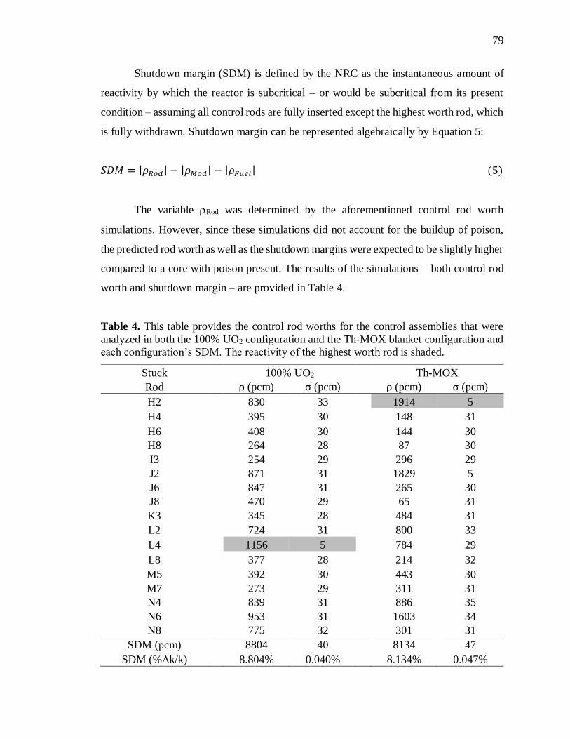
79

Shutdown margin (SDM) is defined by the NRC as the instantaneous amount of

reactivity by which the reactor is subcritical – or would be subcritical from its present

condition – assuming all control rods are fully inserted except the highest worth rod, which

is fully withdrawn. Shutdown margin can be represented algebraically by Equation 5:

𝑆𝐷𝑀 = |𝜌𝑅𝑜𝑑| − |𝜌𝑀𝑜𝑑| − |𝜌𝐹𝑢𝑒𝑙| (5)

The variable Rod was determined by the aforementioned control rod worth

simulations. However, since these simulations did not account for the buildup of poison,

the predicted rod worth as well as the shutdown margins were expected to be slightly higher

compared to a core with poison present. The results of the simulations – both control rod

worth and shutdown margin – are provided in Table 4.

Table 4. This table provides the control rod worths for the control assemblies that were

analyzed in both the 100% UO2 configuration and the Th-MOX blanket configuration and

each configuration’s SDM. The reactivity of the highest worth rod is shaded.

Stuck 100% UO2 Th-MOX

Rod ρ (pcm) σ (pcm) ρ (pcm) σ (pcm)

H2 830 33 1914 5

H4 395 30 148 31

H6 408 30 144 30

H8 264 28 87 30

I3 254 29 296 29

J2 871 31 1829 5

J6 847 31 265 30

J8 470 29 65 31

K3 345 28 484 31

L2 724 31 800 33

L4 1156 5 784 29

L8 377 28 214 32

M5 392 30 443 30

M7 273 29 311 31

N4 839 31 886 35

N6 953 31 1603 34

N8 775 32 301 31

SDM (pcm) 8804 40 8134 47

SDM (%Δk/k) 8.804% 0.040% 8.134% 0.047%

80

SDM was calculated to be 8804 ± 40 pcm for the 100% UO2 configuration and

8134 ± 47 pcm for the Th-MOX configuration. Both values are well above the 1300 pcm

required by the NRC, but the reduction in SDM for the one-third Th-MOX configuration

is concerning. It would be possible to ameliorate this deficit by increasing the worth of the

control rods (e.g. increasing boron-10 content). Again, burnup and fission product buildup

have been ignored for these simulations; therefore, the actual SDM would be higher than

what was predicted here.

4.4. Nuclear Hot Channel Factors

It is important that replacing the outer third of a PWR’s UO2 assemblies with Th-

MOX assemblies does not dramatically change the core’s power distribution or induce hot

channel factors beyond prescribed limits. There are strict regulatory requirements

concerning flux and power distributions in power reactors. Likewise, to ensure that there

is no risk of fuel melting, the fuel centerline temperature must be kept well within the

melting temperature of the fuel. This requirement is met by ensuring the critical heat flux

is never reached. In order to find the critical heat flux, two hot channel factors are required:

the nuclear axial hot channel factor (FZN) and the enthalpy rise hot channel factor (FΔh) as

seen in Equation 6.

𝑞𝑐′′ = 𝑞𝑎𝑣

′′ 𝐹𝑍𝑁 𝐹∆ℎ (6)

FZN is defined as the ratio of the maximum heat flux in the hot channel to the average

heat flux in the hot channel (see Equation 7).

𝐹𝑍𝑁 =

𝐸𝑠𝑡𝑖𝑚𝑎𝑡𝑒𝑑 𝑚𝑎𝑥𝑖𝑚𝑢𝑚 ℎ𝑒𝑎𝑡 𝑓𝑙𝑢𝑥 𝑖𝑛 ℎ𝑜𝑡 𝑐ℎ𝑎𝑛𝑛𝑒𝑙

𝑀𝑒𝑎𝑛 ℎ𝑒𝑎𝑡 𝑓𝑙𝑢𝑥 𝑖𝑛 ℎ𝑜𝑡 𝑐ℎ𝑎𝑛𝑛𝑒𝑙 (7)

FΔh is the enthalpy rise in the hottest channel over the enthalpy rise in the average

channel [31]. FΔh accounts for both the radial nuclear hot channel factor (FRN) and the

engineering enthalpy rise hot channel factor (F∆hE );

81

𝐹∆ℎ = 𝐹𝑅𝑁𝐹∆ℎ

𝐸 (8)

The radial nuclear hot channel factor (FRN) is the mean heat flux in the hot channel

over the mean heat flux in the average channel of the core (see Equation 9).

𝐹𝑅𝑁 =

𝑀𝑒𝑎𝑛 ℎ𝑒𝑎𝑡 𝑓𝑙𝑢𝑥 𝑖𝑛 ℎ𝑜𝑡 𝑐ℎ𝑎𝑛𝑛𝑒𝑙

𝑀𝑒𝑎𝑛 ℎ𝑒𝑎𝑡 𝑓𝑙𝑢𝑥 𝑖𝑛 𝑎𝑣𝑒𝑟𝑎𝑔𝑒 𝑐ℎ𝑎𝑛𝑛𝑒𝑙 𝑜𝑓 𝑡ℎ𝑒 𝑐𝑜𝑟𝑒 (9)

However, one would be required to perform a detailed thermal hydraulic analysis

of the core to determine the engineering enthalpy rise hot channel factor which would

include the core flow subfactor and core mixing subfactor. Additionally, there are fuel

fabrication uncertainties associated with the enrichment, density and geometry of the fuel,

all of which are accounted for in the engineering hot channel factor, 𝐹𝑄𝐸. In the absence of

information regarding engineering enthalpy rise hot channel factor (𝐹∆ℎ𝐸 ) and the

engineering hot channel factor (𝐹𝑄𝐸), only nuclear hot channel factors can be compared to

assess the relative safety of incorporating Th-MOX fuel into a PWR core.

Though calculating the engineering enthalpy rise hot channel factor (F∆hE ) was

outside the scope of this work, it was possible to estimate the axial and radial nuclear hot

channel factors by approximating heat flux with thermal neutron flux. Thermal neutron

flux can be used to approximate heat flux in a thermal reactor because the rate of fission

and hence energy production is directly related to the thermal neutron population.

However, a portion of the thermal reactor’s power is produced by fast fission (typically

about 8%), which will introduce some error to the nuclear hot channel factor results

presented here – particularly for the Th-MOX core which, as previously mentioned, has a

higher fast fission factor.

To find the axial and radial nuclear hot channel factors, several thermal neutron

flux tallies were generated with MCNP for both the 100% UO2 configuration and the 5.5

wt% PuO2 Th-MOX blanket configuration. First, taking advantage of the symmetry of the

PWR core, the northeast quadrant (56 assemblies) was tallied on an assembly-by-assembly

basis in sixteen vertical sections. This data was used to generate sixteen flux maps of the

core, examples of which can be seen in Figure 9. The thermal neutron flux per source

82

particle for each vertical section of each assembly was recorded according to its location

in the core and color coded according to its magnitude. The data from these sixteen flux

maps were totaled to determine which assembly had the highest neutron flux and thus the

highest power production (hottest assembly). These results are shown in Figure 10. For

both the 100% UO2 configuration and the 5.5 wt% PuO2 Th-MOX blanket configuration,

assembly H4 (midpoint at x = 0 cm, y = 86.0 cm) was the hottest assembly.

Subsequently, a pin-by-pin analysis of assembly H4 was then performed for both

fuel configurations. The assembly was divided into seventeen vertical sections and thermal

neutron flux was tallied in the fueled channels. Water-filled channels were ignored. The

results of this analysis were used to generate seventeen flux maps of assembly H4.

Examples of these results can be seen in Figure 11. Each channel’s flux was summed across

each vertical section to determine the hot channel. Figure 12 displays the results. For the

100% UO2 configuration the channel centered at (x = 3.8 cm, y = 83.5 cm) was hottest,

while the channel centered at (x = 3.8 cm, y = 91.1 cm) was the hottest channel in the 5.5

wt% PuO2 Th-MOX blanket configuration.

The neutron tally results for each of the seventeen vertical sections in the hot

assembly were averaged to obtain the mean heat flux in the hot channel. The highest

neutron flux was observed in the middle section as expected. This value was divided by

the mean neutron flux of the entire hot channel to obtain the nuclear hot channel factors for

each configuration: [𝐹𝑍𝑁]𝑈𝑂2 and [𝐹𝑍

𝑁]𝑇ℎ−𝑀𝑂𝑋 , respectively.

𝐹𝑍𝑁 =

𝜙𝑚𝑎𝑥

𝜙𝑎𝑣𝑒≈

𝜙9

117

∑ 𝜙𝑖17𝑖=1

(10)

[𝐹𝑍𝑁]𝑈𝑂2 was found to be 1.47 0.24 and [𝐹𝑍

𝑁]𝑇ℎ−𝑀𝑂𝑋 was 1.49 0.25. The relative

difference between these two values is small and within one standard deviation suggesting

the difference is statistically insignificant, and, hence, adopting the 5.5 wt% PuO2 Th-MOX

blanket configuration would not cause significantly higher vertical heat flux peaking.

Subsequently, the nuclear radial hot channel factor was considered. To determine

the radial hot channel factor, thermal neutrons were tallied and averaged for each assembly

in the northeast quadrant of the core, and the assembly with the maximum thermal neutron

83

flux was identified. Dividing the maximum flux by the average provided the initial

approximation of 𝐹𝑅𝑁.

[𝐹𝑅𝑁]𝑖𝑛𝑖𝑡𝑖𝑎𝑙 =

117

∑ 𝜙𝑖ℎ𝑜𝑡17

𝑖=1

117

∑ 𝜙𝑖𝑎𝑣𝑔17

𝑖=1

(11)

100% UO2 1/3 Th-MOX

Fig. 9. Heat maps of the assembly-by-assembly thermal flux tally results for one quarter of

each core from vertical sections 1 and 9. Results from the 100% UO2 core are in the left

column, and results from the 1/3 Th-MOX core are on the right.

150.5

129.0

107.5

86.0

64.5

43.0

21.5

0

0 21.5 43.0 64.5 86.0 107.5 129.0 150.5

Y-A

xis

Tall

y M

idp

oin

t (c

m)

X-Axis Tally Midpoint (cm)

150.5

129.0

107.5

86.0

64.5

43.0

21.5

0

0 21.5 43.0 64.5 86.0 107.5 129.0 150.5

Y-A

xis

Tall

y M

idp

oin

t (c

m)

X-Axis Tally Midpoint (cm)

150.5

129.0

107.5

86.0

64.5

43.0

21.5

0

0 21.5 43.0 64.5 86.0 107.5 129.0 150.5

Y-A

xis

Tall

y M

idp

oin

t (c

m)

X-Axis Tally Midpoint (cm)

150.5

129.0

107.5

86.0

64.5

43.0

21.5

0

0 21.5 43.0 64.5 86.0 107.5 129.0 150.5

Y-A

xis

Tall

y M

idp

oin

t (c

m)

X-Axis Tally Midpoint (cm)

11.43 cm 11.43 cm

194.31 cm 194.31 cm

2.003E-07

1.812E-07

1.621E-07

1.430E-07

1.239E-07

1.048E-07

8.569E-08

6.659E-08

4.749E-08

2.839E-08

9.295E-09

2.575E-06

2.333E-06

2.091E-06

1.849E-06

1.607E-06

1.364E-06

1.122E-06

8.800E-07

6.378E-07

3.956E-07

1.535E-07

84

However, the estimated value needed additional correction to account for the fact

that within the hottest assembly neutron flux – and consequently heat flux – varies by

channel. Therefore, additional simulations were performed to acquire pin-by-pin tallies for

the hot assembly. The ratio of the flux of the hottest pin divided by the mean pin flux was

used as a correction factor. This ratio was multiplied by the result of Equation 10 to arrive

at the final value for 𝐹𝑅𝑁 as seen in Equation 11.

𝐹𝑅𝑁 ≈

𝜙𝑝𝑖𝑛𝑚𝑎𝑥

𝜙𝑝𝑖𝑛𝑎𝑣𝑔 [𝐹𝑅

𝑁]𝑖𝑛𝑖𝑡𝑖𝑎𝑙 (12)

The radial nuclear hot channel factor for the 100% UO2 configuration ([𝐹𝑅𝑁]𝑈𝑂2)

was found to be 1.39 0.23, whereas for the 5.5 wt% PuO2 Th-MOX blanket configuration

the corresponding value ([𝐹𝑅𝑁]𝑇ℎ−𝑀𝑂𝑋) was found to be 1.67 0.28. Because [𝐹𝑅

𝑁]𝑇ℎ−𝑀𝑂𝑋

is slightly higher, additional safety analysis may be required to ensure that all safety

requirements are fulfilled before Th-MOX can be introduced into an existing PWR.

(a) (b)

Fig. 10. Heat maps of the total assembly-by-assembly thermal flux tally results summed

over all 16 vertical sections for one quarter of the core in each fuel configuration. For both

configurations the peak assembly is H4, the midpoint of which is located at (x = 0 cm, y =

86.0 cm). (a) 100% UO2 (b) 1/3 Th-MOX

150.5

129.0

107.5

86.0

64.5

43.0

21.5

0

0 21.5 43.0 64.5 86.0 107.5 129.0 150.5

X-Axis Tally Midpoint (cm)

Y-A

xis

Tall

y M

idp

oin

t (c

m)

150.5

129.0

107.5

86.0

64.5

43.0

21.5

0

0 21.5 43.0 64.5 86.0 107.5 129.0 150.5

Y-A

xis

Tall

y M

idp

oin

t (c

m)

X-Axis Tally Midpoint (cm)

2.1544E-06

1.9957E-06

1.8369E-06

1.6782E-06

1.5195E-06

1.3608E-06

1.202E-06

1.0433E-06

8.8457E-07

7.2585E-07

5.6712E-07

2.726E-05

2.558E-05

2.389E-05

2.221E-05

2.053E-05

1.884E-05

1.716E-05

1.548E-05

1.379E-05

1.211E-05

1.042E-05

85

100% UO2 1/3 Th-MOX

Fig. 11. Heat maps of the pin-by-pin thermal flux tally results for assembly H4 from each

core from vertical sections 1 and 9. Results from the 100% UO2 core are in the left column,

and results from the 1/3 Th-MOX core are on the right. Water-filled channels are shown in

gray.

5. Conclusions and Future Work

Based on the initial investigation presented here, it appears feasible to introduce

Th-MOX fuel into the current fleet of PWRs. However, care is warranted in that many of

the one-third Th-MOX configuration’s safety parameters, while within the prescribed

safety limits, are less favorable than those of the 100% UO2 configuration.

96.1

94.9

93.6

92.3

91.1

89.8

88.5

87.3

86.0

84.8

83.5

82.2

81.0

79.7

78.4

77.2

75.9

-10

.1

-8.9

-7.6

-6.3

-5.1

-3.8

-2.5

-1.3

0.0

1.3

2.5

3.8

5.1

6.3

7.6

8.9

10

.1

Y-A

xis

Tal

ly M

idp

oin

t (c

m)

X-Axis Tally Midpoint (cm)

96.1

94.9

93.6

92.3

91.1

89.8

88.5

87.3

86.0

84.8

83.5

82.2

81.0

79.7

78.4

77.2

75.9

-10

.1

-8.9

-7.6

-6.3

-5.1

-3.8

-2.5

-1.3

0.0

1.3

2.5

3.8

5.1

6.3

7.6

8.9

10

.1

Y-A

xis

Tal

ly M

idp

oin

t (c

m)

X-Axis Tally Midpoint (cm)

96.1

94.9

93.6

92.3

91.1

89.8

88.5

87.3

86.0

84.8

83.5

82.2

81.0

79.7

78.4

77.2

75.9

-10

.1

-8.9

-7.6

-6.3

-5.1

-3.8

-2.5

-1.3

0.0

1.3

2.5

3.8

5.1

6.3

7.6

8.9

10

.1

Y-A

xis

Tal

ly M

idp

oin

t (c

m)

X-Axis Tally Midpoint (cm)

96.1

94.9

93.6

92.3

91.1

89.8

88.5

87.3

86.0

84.8

83.5

82.2

81.0

79.7

78.4

77.2

75.9

-10.

1

-8.9

-7.6

-6.3

-5.1

-3.8

-2.5

-1.3

0.0

1.3

2.5

3.8

5.1

6.3

7.6

8.9

10.1

Y-A

xis

Tally

Mid

po

int

(cm

)

X-Axis Tally Midpoint (cm)

2.3003E-07

2.0936E-07

1.8869E-07

1.6802E-07

1.4735E-07

1.2668E-07

1.0601E-07

8.5344E-08

6.4675E-08

4.4006E-08

2.3337E-08

2.1939E-07

1.9967E-07

1.7995E-07

1.6023E-07

1.4052E-07

1.208E-07

1.0108E-07

8.1358E-08

6.1639E-08

4.192E-08

2.2202E-08

10.758 cm 10.758 cm

182.88 cm 182.88 cm

86

(a) (b)

Fig. 12. Heat maps of the total pin-by-pin thermal flux tally results summed over all 17

vertical sections in assembly H4 for each fuel configuration. Water-filled channels are

gray. (a) 100% UO2, peak assembly midpoint located at (x = 3.8 cm, y = 83.5 cm) (b) 1/3

Th-MOX, peak assembly midpoint located at (x = 3.8 cm, y = 91.1 cm)

Several configurations for replacing one-third of the UO2 assemblies in a PWR with

Th-MOX fuel were considered. It was found that replacing the blanket of higher

enrichment (3.1%) UO2 with Th-MOX had the smallest effect on excess reactivity and

critical boron concentration, making this configuration most suitable for further study.

Centerline axial and radial flux profiles were compared for several Th-MOX fuel

compositions. A composition of 5.5 wt% PuO2 in ThO2 (94.5 wt%) resulted in the smallest

flux difference relative to the 100% UO2 configuration. Therefore, a blanket configuration

of 5.5 wt% PuO2 Th-MOX fuel was examined for all future safety analysis.

The delayed neutron fraction (βeff) is a good indicator of a reactor’s temporal

response. For the 100% UO2 configuration, βeff was found to be 0.00716 ± 4.60E-07

compared to the 5.5 wt% PuO2 Th-MOX blanket configuration’s value of 0.00607 ± 4.30E-

07. This 15% decrease in the delayed neutron fraction may not be significant enough to

cause any safety related problems; however, the decrease in βeff must be carefully examined

for its impact on the reactor’s safety.

Thermal reactivity feedback is another parameter of interest for operational safety.

In this regard, the one-third Th-MOX configuration seemed to out-perform the 100% UO2

96.1

94.9

93.6

92.3

91.1

89.8

88.5

87.3

86.0

84.8

83.5

82.2

81.0

79.7

78.4

77.2

75.9

-10

.1

-8.9

-7.6

-6.3

-5.1

-3.8

-2.5

-1.3

0.0

1.3

2.5

3.8

5.1

6.3

7.6

8.9

10

.1

Y-A

xis

Tal

ly M

idp

oin

t (c

m)

X-Axis Tally Midpoint (cm)

96.1

94.9

93.6

92.3

91.1

89.8

88.5

87.3

86.0

84.8

83.5

82.2

81.0

79.7

78.4

77.2

75.9

-10

.1

-8.9

-7.6

-6.3

-5.1

-3.8

-2.5

-1.3

0.0

1.3

2.5

3.8

5.1

6.3

7.6

8.9

10

.1

Y-A

xis

Tal

ly M

idp

oin

t (c

m)

X-Axis Tally Midpoint (cm)

2.5379E-06

2.4808E-06

2.4238E-06

2.3667E-06

2.3097E-06

2.2526E-06

2.1955E-06

2.1385E-06

2.0814E-06

2.0244E-06

1.9673E-06

2.4255E-06

2.3628E-06

2.3001E-06

2.2373E-06

2.1746E-06

2.1119E-06

2.0492E-06

1.9865E-06

1.9238E-06

1.8611E-06

1.7984E-06

87

configuration. The fuel temperature coefficient of reactivity for the one-third Th-MOX

configuration was found to be -2.05 0.02 pcm oF-1, which is lower than -1.42 0.02 pcm

oF-1, the value for the 100% UO2 configuration. Likewise, the overall temperature

coefficient of reactivity (moderator plus fuel) for the Th-MOX configuration was -1.89

0.02 pcm oF-1, which was more favorable than the positive value of 0.84 0.02 pcm oF-1

for the 100% UO2 configuration. This favorable temperature feedback of reactivity may

help compensate for reduced controllability via the lower βeff of Th-MOX.

Shutdown margin (SDM) was the next safety parameter used to analyze the

feasibility of the one-third Th-MOX configuration. To calculate shutdown margin, the rod

worth of each control rod cluster in the northeast quadrant of the core was determined. It

was found that the SDM for the 100% UO2 configuration was 8804 ± 40 pcm, which was

higher than the SDM of the Th-MOX configuration, 8134 ± 47 pcm. This aspect of the

one-third Th-MOX configuration’s behavior would require additional safety analysis

before incorporating Th-MOX into the fuel cycle of a PWR could be recommended. While

the estimated SDM was well within the NRC’s prescribed limits, the reduction in SDM of

the Th-MOX configuration could reduce its controllability. Increasing the boron-10

content of the control rods could ameliorate this issue. Nevertheless, this is an area of

concern based on the present study.

Finally, nuclear hot channel factors were estimated to analyze any potential power

peaking issues. The axial nuclear hot channel factor comparison showed no statistically

significant difference between the 100% UO2 configuration (1.47 0.24) and the one-third

Th-MOX configuration (1.49 0.25). Though this result was promising, the results for the

radial nuclear hot channel factor were less encouraging. The radial nuclear hot channel

factor for the one-third Th-MOX configuration was found to be 1.67 0.28 – 20% higher

than the corresponding value of 1.39 0.23 for the 100% UO2 configuration. Therefore,

additional studies are required.

It is important to reiterate that all analyses presented here were performed without

any thermal fluid considerations. However, because of the identical core and assembly

geometry, the assumption that the two cores will exhibit similar thermal fluid behavior

during normal and off-normal operating conditions makes these comparisons relevant.

Nevertheless, it would be beneficial to couple a detailed thermal analysis with this study to

88

provide comprehensive answers to all safety concerns (i.e. hot channel factors, control rod

worth and shutdown margin). Additionally, the analysis presented here was limited to the

beginning-of-life condition. Burnup and fission product buildup were not included in the

neutronic simulations. Burnup and buildup will be considered in a follow-up study.

References

[1] B.S. Van Gosen, V.S. Gillerman, T.J. Armbrustmacher. “Thorium Deposits of the

United States—Energy Resources for the Future?” U.S. Geological Survey Circular

1336. 2009.

[2] E.M. Baum, H.D. Knox, T.R. Miller. “Nuclides and Isotopes: Chart of Nuclides,

16th Ed.” Lockheed Martin Distribution Services. 2002.

[3] F. Sokolov, K. Fukuda, H.P. Nawada. “Thorium Fuel Cycle – Potential Benefits

and Challenges” IAEA-TECDOC-1450. IAEA. Vienna, 2005.

[4] “Role of Thorium to Supplement Fuel Cycles of Future Nuclear Energy Systems”

IAEA Nuclear Energy Series No. NF-T-2.4. IAEA. Vienna, 2012.

[5] S. Peggs, W. Horak, T. Roser, et al. “Thorium Energy Futures” Proceedings of

IPAC2012. New Orleans, 2012.

[6] J.A. Lane “Fluid Fuel Reactors” Addison-Wesley Pub. Co. 1958.

[7] P.N. Haubenreich, J.R. Engel. “Experience with the Molten-Salt Reactor

Experiment” Nuclear Applications and Technology. 1970.

[8] D.E. Holcomb, G.F. Flanagan, B.W. Patton, J.C. Gehin, R.L. Howard, T.J.

Harrison, “Fast Spectrum Molten Salt Reactor Options” ORNL Report ORNL/TM-

2011/105. 2011.

[9] Zuoyi Zhang, Zongxin Wu, Dazhong Wang, Yuanhui Xu, Yuliang Sun, Fu Li,

Yujie Dong. “Current Status and Technical Description of Chinese 2 x 250 MWth

HTR-PM Demonstration Plant” Nuclear Engineering and Design, 239, 1212-1219.

July 2009.

[10] S. Banerjee. “Towards a Sustainable Nuclear Energy Future” 35th World Nuclear

Association Symposium. London, 2010.

[11] P. Bromley, et al. “LWR-Based Transmutation of Nuclear Waste An Evaluation of

Feasibility of Light Water Reactor (LWR) Based Actinide Transmutation

Concepts-Thorium-Based Fuel Cycle Options” BNL-AAA-2002-001. 2002.

89

[12] K.D. Weaver, J.S. Herring. “Performance of Thorium-Based Mixed Oxide Fuels

for the Consumption of Plutonium in Current and Advanced Reactors” Nucl. Tech.,

143, 22-36. 2002.

[13] M. Todosow, G. Raitses. “Thorium Based Fuel Cycle Options for PWRs”

Proceedings of ICAPP ’10, 1891-1900. June 13-17, 2010.

[14] K.I. Bjork. “A BWR Fuel Assembly Design for Efficient Use of Plutonium in

Thorium-Plutonium Fuel” Progress in Nuclear Energy, 65, 56-63. 2013.

[15] K.I. Bjork, V. Fhager, C. Demaziere. “Comparison of Thorium-Based Fuels with

Different Fissile Components in Existing Boiling Water Reactors” Progress in

Nuclear Energy, 53, 618-625. 2011.

[16] Yunlin Xu, T.J. Downar, H. Takahashi, U.S. Rohatgi. “Neutronics Design and Fuel

Cycle Analysis of a High Conversion BWR with Pu-Th Fuel” ICAPP. Florida,

2002.

[17] P. Mac Donald, M.S. Kazimi. “Advanced Proliferation Resistant, Lower Cost,

Uranium-Thorium Dioxide Fuels for Light Water Reactors” NERI Annual Report,

INEEL/EXT-2000-01217. 2000.

[18] J.L. Francois, A. Nun͂ez-Carrera, G. Espinosa-Paredes, C. Martin-del-Campo.

“Design of a Boiling Water Reactor Equilibrium Core Using Thorium-Uranium

Fuel” Americas Nuclear Energy Sumposium 2004. Miami Beach, FL, 2004.

[19] E. Shwageraus, P. Hejzlar, M.S. Kazimi. “Use of Thorium for Transmutation of

Plutonium and Minor Actinides in PWRs” Nucl. Tech., 147, 53-68. 2004.

[20] E. Shwageraus, P. Hejzlar, M.J. Driscoll, M.S. Kazimi. “Optimization of Micro-

Heterogeneous Uranium-Thorium Dioxide PWR Fuels for Economics and

Enhanced Proliferation Resistance”, MIT-NFC-TR-046, MIT, Nucl. Eng. Dep,

2002.

[21] K.I. Bjork, C.W. Lau, H. Nylen, U. Sandberg. “Study of Thorium-Plutonium Fuel

for Possible Operating Cycle Extension in PWRs” Science and Technology of

Nuclear Installations. 2013.

[22] H.R. Trellue, C.G. Bathke, P. Sadasivan. “Neutronics and Material Attractiveness

for PWR Thorium Systems Using Monte Carlo Techniques” Progress in Nuclear

Energy, 53, 698-707. 2011.

[23] H. Tsige-Tamirat. “Neutronics Assessment of the Use of Thorium Fuels in Current

Pressurized Water Reactors” Progress in Nuclear Energy, 53, 717-721. 2011.

[24] E. Fridman, S. Kliem. “Pu Recycling in a full Th-MOX PWR Core. Part I: Steady

State Analysis” Nucl. Eng. and Design, 241, 193-202. 2011.

90

[25] P.G. Boczar, G.R. Dyck, P.S.W. Chan, D.B. Buss. “Recent Advances in Thorium

Fuel Cycles for CANDU Reactors” Thorium Fuel Utilization: Options and Trends,

IAEA-TECDOC-1319, 104-122. IAEA, Vienna, 2002.

[26] R.K. Sinha, A. Kakodar. “Design and Development of the AHWR – the Indain

Thorium Fuelled Innovative Nuclear Reactor” Nucl. Eng. and Design, 236, 683-

700. 2006.

[27] S. Michalek, J. Hascik, G. Farkas. “MCNP5 Delayed Neutron Fraction (βeff)

Calculation in Training Reactor VR-1” Jour. of Elec. Eng., 59, 221-224, 2008.

[28] J.R. Lamarsh. “Introduction to Nuclear Reactor Theory” American Nuclear

Society, Inc. LaGrange Park, Ill. 2002.

[29] “Callaway cycle 15 core operating limits report (Revision 1)” ULNRC-05335. U.S.

Nuclear Regulatory Commission. 28 September 2006.

[30] “Inspection Procedure 61708: Isothermal and moderator temperature coefficient

determinations” NRC Inspection Manual. 11 October 1985.

[31] J. Weisman. Elements of Nuclear Reactor Design. 2nd Ed. Robert E. Kriegler

Publishing Company. Malabar, Florida. 1983.

[32] K. Hesketh, A. Worrall. “The Thorium Fuel Cycle: An independent assessment by

the UK National Nuclear Laboratory” National Nuclear Laboratory Position Paper.

2010.

91

IV. THORIUM-BASED MIXED OXIDE FUEL IN A PRESSURIZED WATER

REACTOR: A BURNUP ANALYSIS WITH MCNP

Lucas P. Tucker and Shoaib Usman3

Abstract

A three-dimensional MCNP model of a Westinghouse-type 17x17 PWR was used

to assess the feasibility of enhancing the current fuel supply with a thorium-plutonium

mixed oxide fuel (ThMOX). A conventional UO2-fueled configuration was compared to a

configuration which incorporated ThMOX fuel. The safety of the ThMOX configuration

was compared to that of the UO2 configuration at several time steps of interest within all

three cycles (beginning of cycle, peak excess reactivity of cycle, and end of cycle) using

the following metrics: axial and radial nuclear hot channel factors (FZN and FR

N), moderator

and fuel temperature coefficients (MTC and FTC), delayed neutron fraction (βeff), and

shutdown margin (SDM). Additionally, the performance of the ThMOX configuration was

assessed by tracking cycle lengths, the amount of plutonium destroyed, and fission product

poison concentration.

The ThMOX configuration’s FZN (1.839 ± 0.951) was less favorable than that of the

UO2 configuration (1.515 ± 0.246), as was its FRN (3.820 ± 0.232 compared to 3.430 ± 0.066

for UO2). The delayed neutron fraction was another problem area for the ThMOX

configuration. It was lower than that of the UO2 configuration, but the lowest βeff occurred

at the beginning of Cycle 3 (3.324E-03 ± 8.919E-07). The βeff of the UO2 configuration

was 46% higher (6.177E-03 ± 1.510E-06) at this time step. Similarly, the ThMOX

configuration’s SDMs were less favorable than those of the UO2 configuration, though

even the lowest (3971 ± 43 pcm) remained well within the NRC prescribed limit of 1300

pcm. However, the MTC of the ThMOX configuration was more favorable for all time

steps except the beginning of Cycle 3, and even then it was negative as required by the

NRC (-2.325 ± 0.00098 pcm/oF). The FTC results were also more favorable for the

3 Correspondence to usmans@mst.edu, 225 Fulton Hall, 301 W. 14th Street Rolla, MO 65409.

92

ThMOX configuration. Its highest FTC value (-6.132 ± 0.00186 pcm/oF at the peak of

Cycle 1) was more negative than the lowest FTC of the UO2 configuration (-4.391 ±

0.00156 pcm/oF at the beginning of Cycle 2).

Overall, incorporating ThMOX fuel into the fuel supply for a conventional PWR

seems feasible from a neutronics standpoint. However, a full thermal hydraulic analysis is

required. Also, this analysis would benefit from a more detailed burnup simulation and

optimization of the ThMOX fuel composition.

1. Introduction

Thorium represents a vast, largely untapped source of nuclear energy. Its abundance

in the earth’s crust is roughly three times greater than uranium [1]. Though 232Th – the only

naturally occurring isotope of thorium – is not fissile, it is fertile. After absorbing a neutron

to become 233Th and decaying to 233Pa, it ultimately decays to 233U [2]. Thorium-based

fuels offer several potential advantages over uranium fuels: higher fissile conversion rate,

higher thermal fission factor (η), lower capture-to-fission ratio, low actinide production,

plutonium reduction, and chemical stability [3, 4, 5, 6].

Perhaps the most expedient scheme for exploiting the world’s thorium resources is

by incorporating it into the current light water reactor (LWR) fuel supply. As the reactor

type with the greatest install base, the pressurized water reactor (PWR) warrants the

greatest attention. Since it is fertile, a fissile isotope must be included with thorium if it is

to be used in a conventional reactor. In this way, a thorium-plutonium mixed oxide

(ThMOX) fuel can be used for the disposition of plutonium.

The concept of destroying plutonium in current-gen LWRs with ThMOX fuel has

been researched by many – mostly with computer simulations. Throughout the literature

studies can be found with a variety of fuel compositions, core configurations, burnup

histories, design objectives, and modeling methodologies. Sometimes the focus is on safety

characteristics: Mittag et al. focused on changes in coefficients of reactivity when one-third

of the core was replaced with ThMOX [19], while Bjork et al. considered a wider variety

of parameters, including control rod worths and decay heat for several fuel compositions

[20]. Other times the focus is on performance: Trellue et al. analyzed the improvement in

93

plutonium destruction ThMOX fuel provides over conventional MOX fuel for a one-third

MOX core [21], Fridman and Kliem also looked at the plutonium destruction capability of

ThMOX [22] and Bjork et al. and Weaver et al. considered improvements in cycle length

[23, 24]. More exotic applications are receiving attention as well. Baldova et al. have

considered ThMOX fuel for breeding 233U [25]. Todosow et al. considered the impact

ThMOX would have at the fuel cycle level rather than at the level of an individual reactor

[26]. It is also worth noting that the analysis of ThMOX fuel has moved out of the realm

of simulations and into experimentation [27]. However, none of these studies focus on the

transition from a UO2 fueled core to a one-third ThMOX core to a full ThMOX core.

The feasibility of the use of ThMOX fuel in a PWR was examined by Tucker, Alajo,

and Usman for beginning of life (BOL) conditions [7]. A three-dimensional MCNP model

of a Westinghouse-type 17x17 PWR was used to examine various possibilities for

replacing one-third of the UO2 assemblies with ThMOX assemblies. The excess reactivity,

critical boron concentration, and centerline axial and radial flux profiles for several

configurations and compositions of a one-third ThMOX core were compared to a 100%

UO2 core. A blanket-type arrangement of 5.5% PuO2 by weight was determined to be the

best candidate for further analysis. Therefore, this configuration was compared to a 100%

UO2 core using the following parameters: delayed neutron fraction (βeff), temperature

coefficient, shutdown margin (SDM), and axial and radial nuclear hot channel factors (FZN

and FRN). The one-third ThMOX core compared favorably, and a burnup analysis was

recommended.

This work is a continuation of Tucker et al.’s BOL feasibility analysis [7]. Starting

with the configuration that was identified as most favorable in the earlier study (one-third

5.5% PuO2 in the blanket configuration), a three cycle burnup analysis was performed

using MCNP [8]. After the end of the first and second cycles, the discarded UO2 fuel was

replaced with fresh ThMOX fuel. The third cycle was fueled entirely with ThMOX. The

results of the ThMOX burnup analysis were compared to a similar analysis of an

unmodified 100% UO2 fueled core. Several characteristics of each configuration were

monitored throughout the burnup analysis: excess reactivity (ρex), critical boron

concentration (CBC), cycle length, plutonium destruction, and fission product poison

concentration. Additionally, the performance of the ThMOX configuration was evaluated

94

against that of the UO2 configuration by comparing delayed neutron fraction (βeff), overall

temperature coefficient, fuel temperature coefficient, shutdown margin, axial and radial

nuclear hot channel factors. All of these characteristics and criteria were evaluated at the

beginning and end of each cycle unless unnecessary (e.g. excess reactivity at end of cycle).

2. Description of Reactor Configurations

The beginning of cycle (BOC) 1 core configurations are based on the work

performed for the BOL feasibility analysis. As seen in Figure 1a the 100% UO2 core is

composed of assemblies of three different fuel enrichments: 3.1% (Group 1), 2.6% (Group

2), and 2.1% (Group 3). For the ThMOX core, the 3.1% enriched fuel in Group 1 was

replaced with 5.5% PuO2 ThMOX as seen in Figure 1b. Replacing the 3.1% enriched UO2

assemblies with ThMOX assemblies is consistent with the goal of destroying the maximum

amount of plutonium. The BOL composition of the plutonium in the ThMOX fuel can be

seen in Table 1.

(a) (b)

Fig. 1. Beginning of Cycle 1 fuel configurations. (a) UO2. (b) ThMOX. 3.1% enriched UO2

in dark blue, 2.6% enriched UO2, in medium blue, 2.1% enriched UO2 in light blue, Th-

MOX in green.

3.1 3.1 3.1 3.1 3.1 3.1 3.1

3.1 3.1 3.1 2.1 3.1 2.1 3.1 2.1 3.1 3.1 3.1

3.1 3.1 2.6 2.1 2.6 2.1 2.6 2.1 2.6 2.1 2.6 3.1 3.1

3.1 2.6 2.6 2.6 2.1 2.6 2.1 2.6 2.1 2.6 2.6 2.6 3.1

3.1 3.1 2.1 2.6 2.1 2.6 2.1 2.6 2.1 2.6 2.1 2.6 2.1 3.1 3.1

3.1 2.1 2.6 2.1 2.6 2.1 2.6 2.1 2.6 2.1 2.6 2.1 2.6 2.1 3.1

3.1 3.1 2.1 2.6 2.1 2.6 2.1 2.6 2.1 2.6 2.1 2.6 2.1 3.1 3.1

3.1 2.1 2.6 2.1 2.6 2.1 2.6 2.1 2.6 2.1 2.6 2.1 2.6 2.1 3.1

3.1 3.1 2.1 2.6 2.1 2.6 2.1 2.6 2.1 2.6 2.1 2.6 2.1 3.1 3.1

3.1 2.1 2.6 2.1 2.6 2.1 2.6 2.1 2.6 2.1 2.6 2.1 2.6 2.1 3.1

3.1 3.1 2.1 2.6 2.1 2.6 2.1 2.6 2.1 2.6 2.1 2.6 2.1 3.1 3.1

3.1 2.6 2.6 2.6 2.1 2.6 2.1 2.6 2.1 2.6 2.6 2.6 3.1

3.1 3.1 2.6 2.1 2.6 2.1 2.6 2.1 2.6 2.1 2.6 3.1 3.1

3.1 3.1 3.1 2.1 3.1 2.1 3.1 2.1 3.1 3.1 3.1

3.1 3.1 3.1 3.1 3.1 3.1 3.1

95

Table 1. Isotopic composition of plutonium used for ThMOX. Adapted from Shwageraus,

Hejzlar, and Kazimi [9].

Isotope Weight Percent 238Pu 3.18 239Pu 56.35 240Pu 26.62 241Pu 8.02 242Pu 5.83

For Cycle 1, which is the BOL cycle, both cores were loaded with borosilicate glass

tube burnable absorbers to compensate for the lack of fission product poisons. Burnable

absorbers are located within fuel assembly guide tubes. The arrangement that was used for

both cores can be seen in Figure 2. Burnable absorbers were not used for Cycles 2 or 3.

Fig. 2. Cycle 1 burnable absorber arrangement for both the UO2 and the ThMOX cores.

Assemblies with burnable absorber rods are indicated by the number of rods in the

assembly.

Nearly all simulations were run with all control rods fully withdrawn. The

exceptions were those simulations performed to calculate shutdown margin. Two types of

control rods were used: full-length and part-length. Dimensions and composition of each

control rod type can be found in Table 2, and the distribution of control assemblies can be

seen in Figure 3.

10 10 10

9 12 20 20 12 9

9 20 16 16 16 20 9

20 20 16 16 20 20

12 20 16 16 16 20 12

10 16 16 20 20 16 16 10

20 16 20 20 20 16 20

10 16 16 20 20 16 16 10

20 16 20 20 20 16 20

10 16 16 20 20 16 16 10

12 20 16 16 16 20 12

20 20 16 16 20 20

9 20 16 16 16 20 9

9 12 20 20 12 9

10 10 10

96

Table 2. Attributes of full-length and part-length control assemblies in a PWR.

Full-Length Control Assembly Part-Length Control Assembly

Active length 360.68 cm 91.44 cm

Composition 80% Silver 80% Silver

15% Indium 15% Indium

5% Cadmium 5% Cadmium

Number in Core 53 8

Fig. 3. PWR control assembly layout. Full-length control assemblies are marked with an

“F”. Part-length control assemblies are marked with a “P”.

There are many possible configurations for PWRs – various enrichments, fuel

assembly arrangements, burnable absorber and control assembly compositions and

distributions, etc. The configuration selected for this work was chosen based on the

information available to the authors regarding fuel assembly dimensions, material

compositions, etc. The purpose of this work is to assess the feasibility of incorporating

ThMOX fuel into the PWR fuel supply. While this work does suggest the feasibility of

incorporating ThMOX fuel into the PWR fuel supply, further analysis and optimization as

well as experimental validation would have to be performed before implementation of such

a drastic change in the fuel cycle.

A B C D E F G H I J K L M N O

1

2 F F F F F3 F F F F4 F F P F P F F5 F F6 F P F F F P F7 F F8 F F F F F F F9 F F

10 F P F F F P F11 F F12 F F P F P F F13 F F F F14 F F F F F15

97

3. Burnup Procedure

The burnup analysis presented here was completed using MCNP6. The MCNP6

burnup capability is based on the utility developed for MCNPX [8]. First, a steady-state

neutron transport calculation is performed to determine keff, the energy-dependent flux

distribution and reaction rates, fission multiplicity (ν), and the recoverable energy per

fission [10]. This information is passed to CINDER90 to perform depletion calculations

and generate new number densities which correspond to the end of a prescribed time step

[10]. The new number densities are passed back to MCNP for the next neutron transport

calculation. This process is repeated for as many time steps as are requested by the user. It

is important to take time steps small enough to ensure minimal change in flux shape, as

large flux shape changes between time steps will produce unreliable results.

When setting up the BURN card, the user must specify which fission products

MCNP should track. There are three tiers of fission products that can be tracked. There are

twelve isotopes in Tier 1 [10]. Tier 2 asks MCNP to track all fission products for which

there are neutron cross sections in the cross section directory [10]. Tier 3 contains all fission

products for which CINDER90 has fission yield data [10]. For this work the Tier 2 fission

products were used.

It is possible for CINDER90 to generate fission product isotopes for which cross

section data does not exist in MCNP. Therefore, MCNP’s BURN card allows the user to

provide a list of isotopes to be omitted from neutron transport calculations and from the

output file [10]. Ultimately, 177 isotopes had to be omitted from this work. The inclusion

of these isotopes could affect both the neutron transport characteristics of either reactor and

the discharge activity of each material. However, the isotopes omitted had very low

concentrations (on the order of 10-10 atom percent) with either short half-lives and/or small

neutron cross sections.

A burnup run outputs an abundance of data. At the system level, MCNP reports the

multiplication factor, the total flux, the average ν, the average Q, the total burnup, and the

source strength. For each material tracked by the burnup calculation, values are returned

for the fraction of the power produced and burnup in GWd/MTHM for each time step. It is

also returns the mass and activity of each materials’ isotopes at each time step.

98

In this analysis, burnup calculations were performed for 31 materials, each of which

corresponded to a fuel assembly location as seen in Figure 4. Using 31 materials made it

possible to take advantage of a PWR’s one-eighth symmetry while accounting for

differences in flux at each location. However, this forced burnup to be uniform across each

assembly both axially and radially. Additionally, all burnup calculations were performed

without boric acid in the coolant. This simplified the calculations and reduced run time,

but it likely also reduced cycle length.

Fig. 4. Map of materials used for burnup analysis

All simulations were performed with MNCP6 Version 1.0. The ENDF-VII cross

section libraries were used (unless unavailable for a particular isotope). For most problems,

ten million histories (500 active KCODE cycles of 20,000 histories) were sufficient to

obtain a relative error of less than 10%. All burnup simulations were performed on a

machine with an Intel Core i7 CPU and 32 GB of RAM.

4. Cycle Lengths

This analysis was run for three cycles. The goal for the ThMOX configuration was

to destroy plutonium and match the performance of the UO2 configuration – in that order.

Shorter burnup steps were used at the beginning of each cycle as fission product poison

H I J K L M N O

1

2

3 66 67

4 55 56 57

5 44 45 46 47 48

6 33 34 35 36 37 38

7 22 23 24 25 26 27 28

8 11 12 13 14 15 16 17 18

99

equilibrium values are reached and, in the case of Cycle 1, as burnable absorber rods are

consumed. Longer burnup steps (100 days each) were used once roughly linear burnup

began. Shorter burnup steps (20 to 50 days) were used towards the end of each cycle in an

attempt to capture the day keff reached unity within 100 pcm. After the end of Cycles 1 and

2 a thirty-day decay was performed to approximate a refueling shutdown. Following the

decay step, Group 3 fuel assemblies were removed and replaced with Group 2 assemblies;

Group 2 fuel assemblies were replaced with Group 1 fuel assemblies; and Group 1

assemblies were replaced with fresh fuel assemblies.

As can be seen in Figure 4, some assemblies have one-eighth symmetry (they are

one of eight assemblies with identical neutronic and material characteristics, such as

Assembly 67), while others (such as Assembly 18) have one-fourth symmetry, and

Assembly 11 has no symmetry. Assembly 11 was not shuffled between cycles, but was

instead replaced with fresh 2.1% enriched fuel at the beginning of each cycle. For all other

assemblies, the following fuel shuffling procedure was used for both configurations before

Cycles 2 and 3. First, the assemblies from each group were sorted by burnup in descending

order. The one-eighth symmetry assembly with the lowest burnup in Group 2 was used to

fill the two one-fourth symmetry assembly locations with the highest burnup in Group 3.

The one-fourth symmetry assembly with the lowest burnup in Group 2 was used to fill the

third lowest one-fourth symmetry assembly location in Group 3, and so on and so forth for

the rest of the one-fourth symmetry assemblies from Group 2. The one-eighth symmetry

assembly from Group 2 with the second lowest burnup was then used to fill the one-eighth

symmetry assembly location with the highest burnup in Group 3. The one-eighth symmetry

assembly from Group 2 with the third lowest burnup was then used to fill the one-eighth

symmetry assembly location with the second highest burnup in Group 3, and so on and so

forth for the remaining one-eighth symmetry assemblies in Group 2. The same procedure

was used to shuffle assemblies from Group 1 to Group 2. A visualization of this procedure

can be seen in Figure 5.

For Cycles 2 and 3 the plutonium content of the fresh ThMOX fuel was increased

to match the BOC excess reactivity of the UO2 configuration. The BOC critical boron

concentration (CBC) was also determined. See Table 3 for each cycle’s excess reactivity

and CBC. A more detailed discussion of each cycle is found in Sections 4.1, 4.2, and 4.3.

100

Fig. 5. Visualization of fuel shuffling procedure for the 100% UO2 configuration from

Cycle 1 to Cycle 2.

Table 3. Excess reactivity and critical boron concentration.

UO2 ThMOX

ρex (% Δk/k) CBC (ppm B) ρex (% Δk/k) CBC (ppm B)

BOC 1 14.793 ± 0.019 1290 ± 7 14.183 ± 0.020 1322 ± 19

POC 1 19.109 ± 0.019 1690 ± 6 17.866 ± 0.020 1678 ± 18

BOC 2 12.507 ± 0.005 1156 ± 10 12.541 ± 0.022 3997 ± 14

BOC 3 16.069 ± 0.020 1540 ± 11 16.086 ± 0.023 8504 ± 21

4.1. Cycle 1

Both the 100% UO2 and the ThMOX configurations began Cycle 1 composed

entirely of fresh fuel (Figure 1) and with burnable absorbers (Figure 2). In Figure 6 each

configuration’s multiplication factor is plotted against cycle time. There is an initial drop

in keff during the first ten days as fission product poisons (FPP) reach equilibrium followed

by an upswing as the burnable absorbers are consumed until each configuration reaches its

peak multiplication factor after forty days. This time step (40 days after the beginning of

Cycle 1) will be referred to as peak of cycle (POC). The ThMOX curve closely follows the

UO2 curve, but with slightly less excess reactivity at BOC its cycle length is shorter. This

is understandable as the fissile content of the ThMOX fuel is less than that of the UO2 fuel

it replaced.

101

Fig. 6. Multiplication factor plotted against time for both core configurations for Cycle 1.

4.2. Cycle 2

The 100% UO2 configuration began Cycle 2 with 64 fresh 3.1% enriched UO2

assemblies (Group 1), 64 once-burned, 3.1% enriched UO2 assemblies (Group 2); 64 once-

burned, 2.6% enriched UO2 assemblies (Group 3); and one fresh, 2.1% enriched UO2

assembly at the center of the reactor (position H8). No burnable absorbers were used. The

multiplication factor for the UO2 configuration reached unity after two hundred days. The

multiplication factor trend for both configurations are plotted in Figure 7.

At the beginning of Cycle 2 the plutonium content of the Group 1 fuel assemblies

in the ThMOX configuration was increased from 5.5% PuO2 to 15.8% PuO2. This higher

plutonium concentration was used to maximize plutonium destruction without exceeding

the BOC excess reactivity of the UO2 configuration. Group 2 assemblies contained once-

burned, 5.5% ThMOX; Group 3 assemblies contained once-burned, 2.6% UO2; and the

center-most assembly (position H8) contained fresh, 2.1% UO2. No burnable absorbers

were used. The increase in plutonium concentration of the Group 1 fuel resulted in a 470

day cycle – 270 days longer than Cycle 2 for the UO2 configuration and only 30 days

shorter than Cycle 1 for the ThMOX configuration. However, as seen in Table 3, the higher

fissile content increases the BOC CBC substantially when compared to ThMOX Cycle 1,

0.95

1.00

1.05

1.10

1.15

1.20

0 100 200 300 400 500 600

k eff

Time since BOC 1 (days)

UO2

ThMOX

102

UO2 Cycle 1 or UO2 Cycle 2. The increase in CBC made temperature coefficient and

shutdown margin calculations vital. See Section 9 and Section 10 for those results.

Fig. 7. Multiplication factor plotted against time for both core configurations for Cycle 2.

4.3. Cycle 3

The 100% UO2 configuration began Cycle 3 with 64 fresh 3.1% enriched UO2

assemblies (Group 1), 64 once-burned, 3.1% enriched UO2 assemblies (Group 2); 64 twice-

burned, 3.1% enriched UO2 assemblies (Group 3); and one fresh, 2.1% enriched UO2

assembly at the center of the reactor (position H8). No burnable absorbers were used. The

cycle lasted 320 days. The multiplication factor trend for both configurations are plotted in

Figure 8.

At the beginning of Cycle 3 the plutonium content of the Group 1 fuel assemblies

in the ThMOX configuration was increased from 15.8% PuO2 to 19.2% PuO2. This was

done to maximize plutonium destruction without exceeding the BOC excess reactivity of

the UO2 configuration. Group 2 assemblies contained once-burned, 15.8% ThMOX; Group

3 assemblies contained twice-burned, 5.5% PuO2 ThMOX; and the center-most assembly

(position H8) contained fresh, 2.1% UO2. No burnable absorbers were used. The increase

in plutonium concentration of the Group 1 fuel combined with the increase that had been

0.95

1.00

1.05

1.10

1.15

0 50 100 150 200 250 300 350 400 450 500

k eff

Time since BOC 2 (days)

UO2

ThMOX

103

made for Cycle 2 resulted in a 975 day cycle. It is unlikely that a commercial power reactor

would run for 975 days given the host of non-neutronic problems such a long cycle would

likely cause. However, such a run would destroy (or make unavailable) a substantial

quantity of plutonium. See Section 5 for discussion of the changes in plutonium

concentration for each cycle and fuel configuration. Additionally, as for the ThMOX Cycle

2 configuration, the higher fissile content increases the BOC CBC substantially. See

Section 9 and Section 10 for a discussion of the impact on temperature coefficient and

shutdown margin.

Fig. 8. Multiplication factor plotted against time for both core configurations for Cycle 3.

5. Plutonium Destruction

The purpose of this work was to assess the feasibility of using a ThMOX fuel in a

conventional PWR for plutonium destruction. Therefore, it was vital to examine the

amount of plutonium destroyed by the ThMOX fuel cycle. Table 4 provides the mass in

kilograms of plutonium in the whole core at the beginning of each cycle for each

configuration, while Table 5 provides the net change in plutonium mass. The change in

plutonium mass during Cycles 1, 2, and 3 are plotted in Figures 9, 10, and 11, respectively.

0.95

1.00

1.05

1.10

1.15

1.20

0 100 200 300 400 500 600 700 800 900 1000

k eff

Time since BOC 3 (days)

UO2

ThMOX

104

Table 4. Total core plutonium mass in kilograms at the beginning of each cycle for both

configurations.

UO2 ThMOX

239Pu 240Pu 241Pu 239Pu 240Pu 241Pu

Cycle 1 0 0 0 727 282 204

Cycle 2 279 105 52 3192 1394 976

Cycle 3 248 78 38 5083 2501 1717

Table 5. Net change in core plutonium mass (kg) for each configuration at the end of each

cycle and totaled across all three cycles.

UO2 ThMOX

239Pu 240Pu 241Pu 239Pu 240Pu 241Pu

Cycle 1 397 146 70 -17 111 37

Cycle 2 102 42 22 -1094 -42 -99

Cycle 3 150 72 39 -2430 -307 -366

Total 649 260 131 -3541 -238 -427

During Cycle 1, the net loss of 239Pu for the ThMOX configuration was only 17 kg

(2.4% of BOC mass). Cycle 1 illustrates why increasing the concentration of plutonium in

the fuel and the number of ThMOX assemblies in the core is necessary for efficient

plutonium destruction. Two-thirds of the fuel assemblies in the ThMOX configuration

were conventional UO2 assemblies comprised mostly of 238U. As the cycle progressed these

assemblies produced almost enough plutonium to completely negate the loss of plutonium

in the ThMOX assemblies, which comprised one-third of the core. To maximize plutonium

destruction during Cycle 2 without exceeding the BOC excess reactivity of the UO2

configuration, an additional one-third of the UO2 assemblies were replaced with ThMOX

assemblies and the amount of PuO2 was increased from 5.5% to 15.8% as described in

Section 4.2.

During Cycle 1, the net loss of 239Pu for the ThMOX configuration was only 17 kg

(2.4% of BOC mass). Cycle 1 illustrates why increasing the concentration of plutonium in

the fuel and the number of ThMOX assemblies in the core is necessary for efficient

plutonium destruction. Two-thirds of the fuel assemblies in the ThMOX configuration

were conventional UO2 assemblies comprised mostly of 238U. As the cycle progressed these

105

Fig. 9. Whole-core plutonium mass in kilograms during Cycle 1.

Fig. 10. Whole-core plutonium mass in kilograms during Cycle 2.

Fig. 11. Whole-core plutonium mass in kilograms during Cycle 3.

0

100

200

300

400

500

600

700

800

900

0 100 200 300 400 500 600

Mas

s o

f P

luto

niu

m (k

g)

Time since BOC 1 (days)

UO2-Pu239UO2-Pu240UO2-Pu241ThMOX-Pu239ThMOX-Pu240ThMOX-Pu241

0

500

1,000

1,500

2,000

2,500

3,000

3,500

0 50 100 150 200 250 300 350 400 450 500

Mas

s o

f P

luto

niu

m (k

g)

Time since BOC 2 (d)

UO2-Pu239UO2-Pu240UO2-Pu241ThMOX-Pu239ThMOX-Pu240

0

500

1,000

1,500

2,000

2,500

3,000

3,500

4,000

4,500

5,000

5,500

0 100 200 300 400 500 600 700 800 900 1000

Mas

s o

f P

luto

niu

m (k

g)

Time since BOC 3 (days)

UO2-Pu239UO2-Pu240

UO2-Pu241

ThMOX-Pu239ThMOX-Pu240ThMOX-Pu241

106

assemblies produced almost enough plutonium to completely negate the loss of plutonium

in the ThMOX assemblies, which comprised one-third of the core. To maximize plutonium

destruction during Cycle 2 without exceeding the BOC excess reactivity of the UO2

configuration, an additional one-third of the UO2 assemblies were replaced with ThMOX

assemblies and the amount of PuO2 was increased from 5.5% to 15.8% as described in

Section 4.2.

With an additional 2,465 kg of 239Pu present in the ThMOX configuration at BOC

2, the net loss of 239Pu during Cycle 2 was a more substantial 1,094 kg (34% of BOC mass).

For Cycle 3, the plutonium content of the fresh ThMOX fuel was further increased to

19.2% PuO2 to maximize plutonium destruction while maintaining the UO2

configuration’s BOC excess reactivity, and all but one UO2 assembly was replaced with

ThMOX. It is no surprise, therefore, that the net loss of 239Pu increased to 2,430 kg (48%

of BOC mass).

At the end of Cycle 3, the UO2 configuration had produced 649 kg of 239Pu, while

the ThMOX configuration netted 3,541 kg of 239Pu destroyed. However, the 239Pu

destroyed by the ThMOX configuration must be balanced with the 1,188 kg of 233U it

produced. In Figure 12, the cumulative production of 233U is plotted.

Fig. 12. Lifetime 233U production of the ThMOX configuration.

0

200

400

600

800

1,000

1,200

0 500 1000 1500 2000

Mas

s 23

3U

(kg

)

Time since BOL (days)

107

Table 6. Total discharge activity of thrice-burned, Group 1 Assemblies at EOC 3.

UO2 ThMOX

Material

No. of

Assys

Total

Activity

(Ci)

Activity

per Assy

(Ci)

Total

Activity

(Ci)

Activity

per Assy

(Ci)

13 4 1.138E+08 2.845E+07 8.218E+07 2.055E+07

15 4 1.181E+08 2.953E+07 8.934E+07 2.234E+07

17 4 1.247E+08 3.117E+07 1.230E+08 3.074E+07

22 4 1.162E+08 2.904E+07 8.501E+07 2.125E+07

24 8 2.098E+08 2.623E+07 1.666E+08 2.082E+07

26 8 2.340E+08 2.926E+07 2.073E+08 2.591E+07

33 4 1.140E+08 2.851E+07 8.005E+07 2.001E+07

35 8 2.173E+08 2.717E+07 1.804E+08 2.255E+07

37 8 2.397E+08 2.996E+07 2.367E+08 2.958E+07

44 4 1.172E+08 2.929E+07 9.055E+07 2.264E+07

46 8 2.431E+08 3.039E+07 2.243E+08 2.804E+07

Of course, any fissile material remaining in a used fuel assembly would be well

protected by the highly radioactive material with which it resides. Table 6 shows that the

discharge activity of the thrice-burned fuel from the ThMOX configuration, while less than

that of the UO2 configuration, is sufficient to deter diversion.

6. Fission Product Poisons

In addition to monitoring fissile isotope mass, it is also prudent to monitor the

buildup of fission product poisons (FPP). The FPP of greatest concern is 135Xe; its lifetime

mass in each configuration is shown in Figure 13. By Cycle 3 the equilibrium concentration

of 135Xe is much higher for the ThMOX configuration than the UO2 configuration. Two

factors contribute to this difference: first, the amount of fissile material is much higher in

the ThMOX configuration; second, the fission yield of 135Xe from 239Pu (0.0105) is several

times higher than that from 235U (0.00237) [11]. The primary impact lies with an unplanned

shutdown: potentially dozens of additional hours would be required to accommodate the

decay of the additional 135Xe present in the ThMOX configuration.

108

Fig. 13. Lifetime whole-core mass of 135Xe for both the UO2 and ThMOX configurations.

Fig. 14. Lifetime whole-core mass of 149Sm for both the UO2 and ThMOX configurations.

The ThMOX configuration’s 149Sm concentration is plotted on the secondary axis.

The other FPP worth monitoring is 149Sm. Its lifetime whole-core mass for each

configuration is plotted in Figure 14. Much like 135Xe, the equilibrium concentration of

149Sm is much higher for the ThMOX configuration. However, the difference in 149Sm

concentration is caused solely by the difference in fissile content, as the fission yield from

239Pu (0.0121) is virtually identical to that of 235U (0.01071) [11]. The additional 149Sm

0

10

20

30

40

50

60

0 500 1000 1500 2000

Xe-

135

Mas

s (g

)

Time (d)

UO2-Xe135

ThMOX-Xe135

0

200

400

600

800

1000

1200

1400

1600

1800

2000

0

20

40

60

80

100

120

140

160

180

0 500 1000 1500 2000Sm

-149

Mas

s in

Th

MO

X C

ore

(g)

Sm-1

49 M

ass

in U

O2

Co

re (

g)

Time (d)

UO2-Sm149

ThMOX-Sm149

109

mass present in the ThMOX configuration has the potential to shorten the lifetime of the

fuel. If an unplanned shutdown occurs and there is too little excess reactivity to overcome

the negative reactivity represented by the mass of 149Sm, the reactor must be refueled. With

so much more 149Sm present, a cycle-ending unplanned shutdown could occur earlier –

reducing total burnup.

7. Nuclear Hot Channel Factors

There are strict regulatory requirements concerning flux and power distributions in

power reactors. Likewise, to ensure that there is no risk of fuel melting, the fuel centerline

temperature must be kept below the melting temperature of the fuel. This requirement is

met by ensuring the critical heat flux is never reached. In order to find the critical heat flux,

two hot channel factors are required: the nuclear axial hot channel factor (FZN) and the

enthalpy rise hot channel factor (FΔh) as seen in Equation 1.

𝑞𝑐′′ = 𝑞𝑎𝑣

′′ 𝐹𝑍𝑁 𝐹∆ℎ (1)

FZN is defined as the ratio of the maximum heat flux in the hot channel to the average

heat flux in the hot channel (see Equation 2).

𝐹𝑍𝑁 =

𝐸𝑠𝑡𝑖𝑚𝑎𝑡𝑒𝑑 𝑚𝑎𝑥𝑖𝑚𝑢𝑚 ℎ𝑒𝑎𝑡 𝑓𝑙𝑢𝑥 𝑖𝑛 ℎ𝑜𝑡 𝑐ℎ𝑎𝑛𝑛𝑒𝑙

𝑀𝑒𝑎𝑛 ℎ𝑒𝑎𝑡 𝑓𝑙𝑢𝑥 𝑖𝑛 ℎ𝑜𝑡 𝑐ℎ𝑎𝑛𝑛𝑒𝑙 (2)

FΔh is the enthalpy rise in the hottest channel over the enthalpy rise in the average

channel [12]. FΔh accounts for both the radial nuclear hot channel factor (FRN) and the

engineering enthalpy rise hot channel factor (F∆hE ):

𝐹∆ℎ = 𝐹𝑅𝑁𝐹∆ℎ

𝐸 (3)

The radial nuclear hot channel factor (FRN) is the mean heat flux in the hot channel

over the mean heat flux in the average channel of the core (see Equation 4).

110

𝐹𝑅𝑁 =

𝑀𝑒𝑎𝑛 ℎ𝑒𝑎𝑡 𝑓𝑙𝑢𝑥 𝑖𝑛 ℎ𝑜𝑡 𝑐ℎ𝑎𝑛𝑛𝑒𝑙

𝑀𝑒𝑎𝑛 ℎ𝑒𝑎𝑡 𝑓𝑙𝑢𝑥 𝑖𝑛 𝑎𝑣𝑒𝑟𝑎𝑔𝑒 𝑐ℎ𝑎𝑛𝑛𝑒𝑙 𝑜𝑓 𝑡ℎ𝑒 𝑐𝑜𝑟𝑒 (4)

However, one would be required to perform a detailed thermal hydraulic analysis

of the core to determine the engineering enthalpy rise hot channel factor which would

include the core flow subfactor and core mixing subfactor. Additionally, there are fuel

fabrication uncertainties associated with the enrichment, density and geometry of the fuel,

all of which are accounted for in the engineering hot channel factor, FQE. In the absence of

information regarding engineering enthalpy rise hot channel factor (F∆hE ) and the

engineering hot channel factor (FQE), only nuclear hot channel factors can be compared to

assess the relative safety of incorporating Th-MOX fuel into a PWR core. Though

calculating the engineering enthalpy rise hot channel factor (F∆hE ) was outside the scope of

this work, it was possible to estimate the axial and radial nuclear hot channel factors with

assembly-level power generation data from the burnup runs and thermal neutron flux tallies

performed after the burnup runs were completed.

As stated in Section 3, an MCNP burnup run outputs the fraction of the total power

generated by each material. Since a different fuel material was assigned to each assembly

necessary given the one-eighth symmetry of a PWR (as seen in Figure 4), the power

fraction for each material could be multiplied by the total thermal reactor power (3,411

MW) and the symmetry of the assembly represented by that material (e.g. one-fourth for

material 22, one-eighth for material 23) to determine the power produced by each assembly

for each time step. Then, the assembly with the maximum thermal output was found. The

power produced by this assembly was divided by the average power produced per assembly

for its time step to generate a whole-core approximation of FRN as seen in Equation 5. The

results of the calculations for each time step for both configurations are plotted in Figure

15. These results were also used to create a heat map of each time step’s power distribution

with each assembly color coded according to the maximum and minimum power producer

across all time steps for each configuration. Examples of these plots are provided in Figure

16 at the time step with the highest [𝐹𝑅𝑁]𝑐𝑜𝑟𝑒 for each configuration.

111

[𝐹𝑅𝑁]𝑐𝑜𝑟𝑒 =

𝑃𝑚𝑎𝑥

𝑃𝑎𝑣𝑒𝑟𝑎𝑔𝑒 (5)

Fig. 15. Whole-core approximation of the nuclear radial hot channel factor at each time

step for both the UO2 and ThMOX configurations. The worst-case scenario for each

configuration has been flagged.

UO2 BOC 2 ThMOX BOC 3

Fig. 16. Assembly-by-assembly power distribution for each configuration at the time step

with the highest whole-core approximation of the radial nuclear hot channel factor. Colors

are scaled from the lowest value across all three cycles to the highest value across all three

cycles.

580, 2.76 1030, 2.79

1.0

1.2

1.4

1.6

1.8

2.0

2.2

2.4

2.6

2.8

3.0

0 500 1000 1500 2000

Init

ial N

ucl

ear

Rad

ial H

ot

Ch

ann

el F

acto

r

Time since BOL (days)

UO2

ThMOX

8 46.65

7 40.62

6 34.60

5 28.58

4 22.56

3 16.54

2 10.52

1 4.50

1 2 3 4 5 6 7 8 MW(t)

8 45.84

7 39.61

6 33.37

5 27.13

4 20.89

3 14.65

2 8.41

1 2.17

1 2 3 4 5 6 7 8 MW(t)

112

For the UO2 configuration, the initial approximation for FRN peaks at the beginning

of Cycle 2, while it peaks at the beginning of Cycle 3 for the ThMOX configuration. The

highest power producing assemblies are Assembly 27 and Assembly 66, respectively. If

the nuclear hot channel factors are acceptable for these assemblies at these time steps – the

worst case scenarios – then it can be reasoned that they will be acceptable for all other

assemblies at all other time steps. Therefore, each of these assemblies were examined in

greater detail.

A pin-by-pin thermal neutron flux tally in seventeen vertical sections was

performed on UO2 BOC 2 Assembly 27 and ThMOX BOC 3 Assembly 66. Water-filled

channels were ignored. Thermal neutron flux can be used to approximate heat flux in a

thermal reactor because the rate of fission and hence energy production is directly related

to the thermal neutron population. However, a portion of a thermal reactor’s power is

produced by fast fission (typically about 8%), which will introduce some error to the

nuclear hot channel factor results presented here. The results of this analysis were used to

generate seventeen flux maps of each configuration’s hottest assembly. Then the results

for each pin were summed across all seventeen vertical sections to reveal each

configuration’s hot channel. These plots are shown in Figure 17. For UO2 BOC 2 the hot

channel is located at (x = 135.3 cm, y = 16.5 cm). For ThMOX BOC 3 the hot channel is

located at (x = 101.2 cm, y = 112.6 cm). In both cases the origin is in the center of the core

at the bottom of the fuel.

To complete the approximation of the radial nuclear hot channel factor, the initial

approximation for FRN is multiplied by the ratio of the total flux in the hot channel (ϕHC

HA)

divided by the average channel flux in the hot assembly (ϕaveHA ). See Equation 6. The results

of these calculations are presented in Table 3.

𝐹𝑅𝑁 ≈

𝜙𝐻𝐶𝐻𝐴

𝜙𝑎𝑣𝑒𝐻𝐴

[𝐹𝑅𝑁]𝑐𝑜𝑟𝑒 (6)

The results from the thermal neutron flux tallies performed on each configuration’s

hot assembly were also used to calculate the axial nuclear hot channel factors. No

additional simulations were required. In the hot channel, the flux from the vertical section

113

with the highest flux (ϕmax HC ) was divided by the average flux in the hot channel (ϕave

HC ) as

seen in Equation 7. The results of these calculations are presented in Table 3.

𝐹𝑍𝑁 ≈

𝜙𝑚𝑎𝑥 𝐻𝐶

𝜙𝑎𝑣𝑒𝐻𝐶 (7)

UO2 BOC 2 Assembly 27 ThMOX BOC 3 Assembly 66

Fig. 17. Pin-by-pin thermal neutron flux distribution for each configuration’s hottest

assembly at the time step with the highest whole-core approximation of the nuclear radial

hot channel factor. The hot channel is bordered in green. Non-fuel channels are shaded

gray.

Table 7. Axial and radial nuclear hot channel factors at the time step with the highest

whole-core approximation of the radial nuclear hot channel factor for each configuration.

FZN FR

N

UO2 BOC 2 1.515 ± 0.246 3.430 ± 0.066

ThMOX BOC 3 1.839 ± 0.951 3.820 ± 0.232

For both the axial and the radial nuclear hot channel factors the ThMOX results are

less favorable than the UO2 results. The difference in FRN can be explained by the significant

increase in plutonium content made for cycles 2 and 3, which increases the fraction of the

power produced in the outer assemblies. Even with the 19.2% PuO2 assemblies in the core

the FRN of the worst-case scenario for the ThMOX configuration is only 11% worse than

the FRN for the UO2 configuration’s worst-case scenario.

31.6 5.2E-06

30.3 4.9E-06

29.1 4.7E-06

27.8 4.4E-06

26.5 4.2E-06

25.3 3.9E-06

24.0 3.7E-06

22.8 3.4E-06

21.5 3.1E-06

20.2 2.9E-06

19.0 2.6E-06

17.7 __n__

16.5 cm2 sp

15.2

13.9

12.7

11.4

11

8.9

12

0.2

12

1.5

12

2.7

12

4.0

12

5.2

12

6.5

12

7.8

12

9.0

13

0.3

13

1.5

13

2.8

13

4.1

13

5.3

13

6.6

13

7.8

13

9.1

117.6 3.4E-07

116.3 3.2E-07

115.1 3.0E-07

113.8 2.8E-07

112.6 2.6E-07

111.3 2.5E-07

110.0 2.3E-07

108.8 2.1E-07

107.5 1.9E-07

106.3 1.7E-07

105.0 1.5E-07

103.7 __n__

102.5 cm2 sp

101.2100.0

98.797.4

97

.49

8.7

10

0.0

10

1.2

10

2.5

10

3.7

10

5.0

10

6.3

10

7.5

10

8.8

11

0.0

11

1.3

11

2.6

11

3.8

11

5.1

11

6.3

11

7.6

114

The 21% difference in FZN can also be explained mostly by the increase in plutonium

composition. There is no axial variation in fuel composition because of approximations

necessary for the burnup simulations. However, flux shape changes axially with differences

in leakage and power production. With more fuel added to the Group 1 assemblies in the

ThMOX configuration (Assembly 66 included), more power will be produced on the core’s

periphery, and higher axial power peaking will occur. A 21% difference is still within the

statistical uncertainty of the simulations, so further investigation might reveal a much

smaller difference between each configuration’s FZN. In Figure 18, the values used to

calculate FZN are plotted for each configuration.

Fig. 18. Flux per vertical section (VS) for each configuration’s hot channel (HC). Each

configuration’s average hot channel flux is also included as a horizontal line. These values

were used to calculate the axial nuclear hot channel factor. The ThMOX configuration’s

values are plotted on the secondary axis.

8. Delayed Neutron Fraction

Since the delayed neutron fraction (βeff) influences a reactor’s controllability, βeff is

an important parameter to investigate. Two KCODE simulations are necessary to

determine βeff with MCNP. In the first simulation, both delayed neutrons and prompt

neutrons are generated and tracked yielding the total multiplication factor (k). In the second

simulation, only prompt neutrons were generated and tracked, yielding the prompt

0.0E+00

5.0E-09

1.0E-08

1.5E-08

2.0E-08

2.5E-08

3.0E-08

3.5E-08

4.0E-08

4.5E-08

5.0E-08

0.0E+00

5.0E-08

1.0E-07

1.5E-07

2.0E-07

2.5E-07

3.0E-07

3.5E-07

4.0E-07

4.5E-07

5.0E-07

0 50 100 150 200 250 300 350

ThM

OX

HC

Flu

x p

er V

S (n

cm

-2sp

-1)

UO

2H

C F

lux

per

VS

(n c

m-2

sp-1

)

Distance from Fuel Bottom to VS Centroid (cm)

UO2

UO2-ave

ThMOX

ThMOX-ave

115

multiplication factor (kp). Using the results of these two simulations the effective delayed

neutron fraction could be approximated with Equation 8 [13]:

𝛽𝑒𝑓𝑓 ≅ 1 −𝑘𝑝

𝑘 (8)

KCODE simulations were performed at each time step of interest (BOC, POC,

EOC) for both configurations. Results are presented in Table 7. At every time step the

ThMOX configuration’s βeff is less than the UO2 configuration’s, with the greatest

difference occurring at BOC 3. These results are not surprising as there is a great deal more

plutonium in the ThMOX configuration, and the βeff of 239Pu (0.0021) is lower than that of

235U (0.0065) [14]. Greater care will have to be taken during the operation of a reactor

fueled with ThMOX as it is likely to be more difficult to control unless the lower βeff of the

ThMOX configuration is balanced by some other difference. For instance, positive

reactivity would have to be added more slowly to ensure reactor safety margins are

maintained.

Table 8. Delayed neutron fraction at times of interest for both configurations.

UO2 ThMOX

BOC 1 7.288E-03 ± 1.630E-06 4.325E-03 ± 1.274E-06

POC 1 6.607E-03 ± 1.456E-06 5.888E-03 ± 1.417E-06

EOC 1 5.105E-03 ± 2.881E-07 4.614E-03 ± 2.642E-07

BOC 2 6.320E-03 ± 3.985E-07 3.750E-03 ± 1.039E-06

EOC 2 5.327E-03 ± 1.507E-06 4.073E-03 ± 1.152E-06

BOC 3 6.177E-03 ± 1.510E-06 3.324E-03 ± 8.919E-07

EOC 3 4.457E-03 ± 1.226E-06 3.603E-03 ± 9.969E-07

9. Temperature Coefficients

Another important reactor safety parameter is the temperature coefficient (αT),

which quantifies the effects of temperature changes on reactivity. Equation 9 shows how

the temperature coefficient is calculated [15].

116

𝛼𝑇 =1

𝑘2

𝑑𝑘

𝑑𝑇 (9)

Separate components such as the moderator and the fuel have their own temperature

coefficients. This study considered the moderator temperature coefficient (MTC) and the

fuel temperature coefficient (FTC).

Finding both of the temperature coefficients for one of the configurations at one of

the time steps required three MCNP KCODE simulations. The first simulation was

performed with operating temperature cross sections for moderator and fuel (600 K,

typically the 71c ENDF-VII libraries). Water density was 0.711 g cm-3, and the

configuration’s critical boron concentration was used. The second simulation used

operating temperature (600 K) cross sections for the fuel, and room temperature cross

sections and density (1 g cm-3) for the moderator (the 70c ENDF-VII libraries at 293 K).

Increasing the mass density of the moderator automatically increased the number density

of boron in the moderator. Finally, a simulation was performed with room temperature fuel

and room temperature moderator.

The MTC is calculated from the results of the first simulation (operating

temperature moderator and operating temperature fuel) and the third simulation (room

temperature moderator and room temperature fuel). The FTC is calculated from the results

of the second simulation (room temperature moderator and operating temperature fuel) and

the third simulation (room temperature moderator and room temperature fuel).

9.1. Moderator Temperature Coefficient

Each configuration’s MTC results for all time steps of interest are presented in

Table 9. Three of the MTC results are positive. Typically, a negative MTC is required by

the Nuclear Regulatory Commission (NRC). However, at BOL the NRC does allow most

plants to have a slightly positive MTC. For the Callaway Plant an MTC of up to 5 pcm/ºF

is allowed [16]. Under this exception the positive MTC value for UO2 BOC 1 is not only

allowed, but expected. However, the positive MTC values both configurations exhibit at

117

POC 1 (40 days after BOC) do not meet the NRC’s criteria for exception – namely,

operating at less than 100% of rated thermal power (RTP).

Table 9. Moderator temperature coefficient at each time step of interest for both

configurations.

UO2 (pcm/oF) ThMOX (pcm/oF)

BOC 1 2.743 ± 0.00024 -6.004 ± 0.00052

POC 1 15.311 ± 0.00513 3.453 ± 0.00104

EOC 1 -25.409 ± 0.00440 -25.467 ± 0.00849

BOC 2 -15.208 ± 0.00553 -22.564 ± 0.00889

EOC 2 -32.487 ± 0.01078 -35.736 ± 0.01279

BOC 3 -4.992 ± 0.00183 -2.325 ± 0.00098

EOC 3 -30.324 ± 0.01007 -32.805 ± 0.01093

It should not be possible for either configuration to produce a positive MTC value

at any point other than BOL. The buildup of FPP should prevent this; and before sufficient

FPP concentration has been achieved the burnable absorbers should prevent it. The most

likely cause for the positive MTC values at POC 1 is the omission of a power ramp at BOC.

When real-world PWRs are brought online, control assemblies are slowly withdrawn over

the course of several days, allowing the system to gradually warm up to operating

temperature as it approaches full power. During the burnup simulation both configurations

were run at 100% of RTP, which accelerated the burnout of the burnable absorber rods.

Since the BAs burned out faster than designed, the systems were unable to maintain a

negative MTC.

At all time steps except BOC 3, the MTC of the ThMOX configuration is lower

than that of the UO2 configuration. This indicates that even with the positive MTC values

at POC 1, the ThMOX configuration should not be precluded from consideration.

Furthermore, it is possible that the more favorable MTC values of the ThMOX

configuration could ameliorate the controllability issues suggested by its lower delayed

neutron fractions. However, since the favorability of the ThMOX configuration’s MTC is

lost after the fissile content is substantially increased for Cycle 3 the decision to increase

fissile content – or, at the very least, the magnitude of the increase – should be reevaluated.

118

9.2. Fuel Temperature Coefficient

For various safety reasons NRC pays particular attention to the FTC [17]. These

values are reported in Table 10 for both configurations at all time steps of interest. First, it

is important to note that all values for both configurations are negative. Second, at every

time step the FTC of the ThMOX configuration is more negative than that of the UO2

configuration. This is likely caused by greater thermal conductivity of the ThMOX fuel.

Initial experimental data for fuel designed by Thor Energy suggests as much [27]. At any

rate, the improved FTC could further reduce the impact on controllability of the ThMOX

configuration’s lower βeff values.

Table 10. Fuel temperature coefficient at each time step of interest for both configurations.

UO2 (pcm/oF) ThMOX (pcm/oF)

BOC 1 -4.546 ± 0.00039 -6.499 ± 0.00056

POC 1 -4.486 ± 0.00152 -6.132 ± 0.00186

EOC 1 -5.443 ± 0.00093 -6.223 ± 0.00205

BOC 2 -4.391 ± 0.00156 -7.130 ± 0.00282

EOC 2 -4.478 ± 0.00144 -7.235 ± 0.00254

BOC 3 -4.530 ± 0.00169 -6.527 ± 0.00283

EOC 3 -5.534 ± 0.00181 -7.596 ± 0.00249

10. Shutdown Margin

A safety analysis of any reactor will invariably include determination of the control

rod worth and shutdown margins. In order to comply with regulatory requirements, the

shutdown margin the ThMOX configuration should be comparable to that of the UO2

configuration and must be greater than 1300 pcm as prescribed by the NRC. A reactor

core’s reactivity is the algebraic sum of many contributing factors, and so its control rod

worth (ρrods) depends on many factors as well. To calculate ρrods two MCNP simulations

were necessary: one with all control assemblies (CA) fully inserted (kin) according to

Figure 3, and another with all CAs fully withdrawn (kout). Then finding ρrods is simply a

matter of subtracting kin from kout as in Equation 10:

119

𝜌𝑟𝑜𝑑𝑠 = 𝑘𝑜𝑢𝑡 − 𝑘𝑖𝑛 (10)

Shutdown margin (SDM) is defined by the NRC as the instantaneous amount of

reactivity by which the reactor is subcritical – or would be subcritical from its present

condition – assuming all control rods are fully inserted except the highest worth rod

(HWR), which is fully withdrawn [18]. Shutdown margin can be represented algebraically

by Equation 11:

𝑆𝐷𝑀 = 𝜌𝑟𝑜𝑑𝑠 − 𝜌𝐻𝑊𝑅 (11)

It is necessary, therefore, to determine which assembly is the HWR. To find the

HWR with MCNP a KCODE simulation is performed with all assemblies except the CA

of interest inserted (kouti ). From this, kin is subtracted to find the worth of that rod (ρrod

i )

as in Equation 12:

𝜌𝑟𝑜𝑑𝑖 = 𝑘𝑜𝑢𝑡

𝑖 − 𝑘𝑖𝑛 (12)

Fortunately, one can capitalize on the symmetry of a PWR, omitting most CAs from

the analysis. The only CAs considered for this work were those above Row 8 and to the

right of Column H (inclusive) as defined in Figure 3. The results of these calculations for

both configurations at the time steps of interest are collected in Table 11.

Table 11. Shutdown margin and highest worth rod at each time step of interest for both

configurations.

UO2 ThMOX

HWR SDM (pcm) HWR SDM (pcm)

BOC 1 J6 8804 ± 40 J6 8134 ± 47

POC 1 J6 8297 ± 40 J6 7559 ± 39

EOC 1 H8 6701 ± 33 L4 6827 ± 33

BOC 2 H2 4407 ± 40 N8 4281 ± 41

EOC 2 H2 5975 ± 35 H2 4314 ± 37

BOC 3 N4 7275 ± 41 N4 3971 ± 43

EOC 3 H2 6958 ± 34 H4 4608 ± 35

120

While the ThMOX configuration’s SDMs are lower than those of the UO2

configuration for all time steps of interest, they all substantially exceed the NRC limit of

1,300 pcm [18].

11. Conclusions

It is feasible not only to incorporate ThMOX fuel into a conventional PWR, but

also to replace the entire core with ThMOX assemblies. The work presented here supports

this statement – with a few caveats.

The results produced for this work relied on comparing a conventional UO2-fueled

PWR configuration to a novel ThMOX configuration. At BOL the UO2 configuration was

stocked with 3.1%, 2.6%, and 2.1% enriched fuel, while in the ThMOX configuration the

3.1% UO2 fuel was replaced 5.5% PuO2 ThMOX fuel. Burnable absorbers were distributed

throughout, and Ag-In-Cd CAs and soluble boron were the available control materials.

Both configurations were run through three cycles of burnup simulations while

fresh fuel was added and used fuel was either shuffled or replaced. The fresh fuel

incorporated into the UO2 configuration for Cycles 2 and 3 was kept at 3.1% enrichment,

resulting in cycle lengths of 550 days, 200 days, and 320 days, respectively. In an effort to

destroy as much plutonium as safely possible with the ThMOX configuration, the

plutonium content of the fresh fuel was increased to 15.8% PuO2 for Cycle 2 and 19.2%

PuO2 for Cycle 3 to maximize plutonium destruction without exceeding the BOC excess

reactivity of the UO2 configuration. The increase in fissile content resulted in a

substantially longer third cycle: from 500 days for Cycle 1 and 470 days for Cycle 2 to 975

days for Cycle 3.

The increase in the plutonium content of the ThMOX configuration’s fresh fuel,

coupled with the shuffling out of used UO2 fuel, created the necessary conditions for

significant plutonium destruction. While Cycle 1 saw a net destruction of only 17 kg of

239Pu, the ThMOX configuration destroyed 1,094 kg of 239Pu during Cycle 2 and 2,430 kg

during Cycle 3 for a total net destruction of 3,541 kg across all three cycles. This means

the ThMOX configuration could destroy all of the 239Pu produced by three cycles of

operation (649 kg) for more than five UO2-fueled PWRs. However, the 1,188 kg of fissile

121

233U that were produced by the ThMOX configuration during three cycles of operation

must not be forgotten. Of course, the highly radioactive fission products which accompany

both the 233U that was produced and the 239Pu that was not destroyed would provide a

significant deterrent for diversion.

The first notable caveat to the ThMOX configuration is the sizeable increase in

fission product poison concentration. The masses of both 135Xe and 149Sm in the ThMOX

configuration dramatically outpaced those in the UO2 configuration. The increase in 135Xe

mass would increase the duration of an unplanned outage. And the increase in 149Sm mass

could increase the likelihood that an unplanned outage would force a refueling.

Axial and radial nuclear hot channel factor results are also less favorable for the

ThMOX configuration. However, neither the 21% increase in FNZ nor the 11% increase in

FN𝑅 preclude it from consideration. Furthermore, a thermal hydraulic analysis is required to

fully understand the impact of the fuel change.

The delayed neutron fraction results are another area of concern. At all time steps

of interest the ThMOX configuration’s βeff is lower than that of the UO2 configuration. A

lower βeff could make the reactor more difficult to control. However, all fuel temperature

coefficients for the ThMOX configuration are lower than those of the UO2 configuration,

and (with the exception of BOC 3) the ThMOX configuration’s moderator temperature

results are also more favorable. The more favorable temperature coefficients could

ameliorate the impact of βeff on the controllability of the ThMOX configuration, however,

they also call into question the magnitude of the increase in plutonium content for Cycle 3.

And finally, though the ThMOX configuration’s shutdown margins were lower

than those of the UO2 configuration, they were well above the NRC-required 1,300 pcm.

It is important to reiterate that all analyses presented here were performed without

any thermal fluid considerations. However, because of the identical core and assembly

geometry, the assumption that the two cores will exhibit similar thermal fluid behavior

during normal and off-normal operating conditions makes these comparisons relevant.

Nevertheless, it would be beneficial to couple a detailed thermal analysis with this study to

provide comprehensive assessments of all safety parameters. Additionally, an optimization

of the ThMOX configuration for plutonium destruction would be interesting. And an

122

improvement to the burnup procedure to include more accurate modeling of the initial

power ramp up would further refine the results.

References

[1] B.S. Van Gosen, V.S. Gillerman, T.J. Armbrustmacher. “Thorium Deposits of the

United States—Energy Resources for the Future?” U.S. Geological Survey Circular

1336. 2009.

[2] E.M. Baum, H.D. Knox, T.R. Miller. “Nuclides and Isotopes: Chart of Nuclides,

16th Ed.” Lockheed Martin Distribution Services. 2002.

[3] F. Sokolov, K. Fukuda, H.P. Nawada. “Thorium Fuel Cycle – Potential Benefits

and Challenges” IAEA-TECDOC-1450. IAEA. Vienna. 2005.

[4] “Role of Thorium to Supplement Fuel Cycles of Future Nuclear Energy Systems”

IAEA Nuclear Energy Series No. NF-T-2.4. IAEA. Vienna. 2012.

[5] S. Peggs, W. Horak, T. Roser, et al. “Thorium Energy Futures” Proceedings of

IPAC2012. New Orleans. 2012.

[6] K. Hesketh, A. Worrall. “The Thorium Fuel Cycle: An independent assessment by

the UK National Nuclear Laboratory” National Nuclear Laboratory Position Paper.

2010.

[7] L.P. Tucker, A. Alajo, S. Usman. “Thorium-based mixed oxide fuel in a pressurized

water reactor: A beginning of life feasibility analysis with MCNP” Annals of

Nuclear Energy, 76, 323-334. 2015.

[8] J.T. Goorley, M.R. James, T.E. Booth, et al. “Initial MCNP6 Release Overview

MCNP6 Version 1.0” Los Alamos National Laboratory report, LA-UR-13-22934.

2013.

[9] E. Shwageraus, P. Hejzlar, M.S. Kazimi. “Use of Thorium for Transmutation of

Plutonium and Minor Actinides in PWRs” Nucl. Tech., 147, 53-68. 2004.

[10] J.S. Hendricks, G.W. McKinney, M.L. Fensin, et al. “MCNPX 2.6.0 Extensions”

Los Alamos National Laboratory report, LA-UR-08-2216. 2008.

[11] M.E. Meek, B.F. Rider. “Compilation of Fission Product Yields” General Electric

Company Report NEDO-12154. 1972.

123

[12] J. Weisman. Elements of Nuclear Reactor Design. 2nd Ed. Robert E. Kriegler

Publishing Company. Malabar, Florida. 1983.

[13] S. Michalek, J. Hascik, G. Farkas. “MCNP5 Delayed Neutron Fraction (βeff)

Calculation in Training Reactor VR-1” Jour. of Elec. Eng., 59, 221-224. 2008.

[14] J.R. Lamarsh, A.J. Baratta. Introduction to Nuclear Engineering. 3rd Ed. Prentice

Hall, Inc. Upper Saddle River, New Jersey. 2001.

[15] J.R. Lamarsh. Introduction to Nuclear Reactor Theory. American Nuclear Society,

Inc. LaGrange Park, Ill. 2002.

[16] “Callaway cycle 15 core operating limits report (Revision 1)” ULNRC-05335. U.S.

Nuclear Regulatory Commission. 28 September 2006.

[17] “Inspection Procedure 61708: Isothermal and moderator temperature coefficient

determinations” NRC Inspection Manual. 11 October 1985.

[18] Union Electric Company. “Callaway Plant Unit No. 1 Facility Operating License”

Docket No. STN 50-483, U.S. Nuclear Regulatory Commission, License No. NPF-

30, Amendment No. 120. 13 February 1998.

[19] S. Mittag, S. Kliem. “Burning plutonium and minimizing waste in existing PWRs”

Annals of Nuclear Energy, 38, 98-102. 2011.

[20] K.I. Bjork, V. Fhager, C. Demaziere. “Comparison of thorium-based fuels with

different fissile components in existing boiling water reactors” Progress in Nuclear

Energy, 53, 618-625. 2011.

[21] H.R. Trellue, C.G. Bathke, P. Sadasivan. “Neutronics and material attractiveness

for PWR thorium systems using monte carlo techniques” Progress in Nuclear

Energy, 53, 698-707. 2011.

[22] E. Fridman, S. Kliem. “Pu recycling in a full Th-MOX PWR core. Part I: Steady

state analysis” Nuclear Engineering and Design, 241, 193-202. 2011.

[23] K.I. Bjork, C.W. Lau, H. Nylen, U. Sandberg. “Study of thorium-plutonium fuel

for possible operating cycle extension in PWRs” Science and Technology of

Nuclear Installations. 2013.

[24] K.D. Weaver, J.S. Herring. “Performance of thorium-based mixed oxide fuels for

the consumption of plutonium in current and advanced reactors” International

Congress on Advanced Nuclear Power Plants 2002. Hollywood, FL. 2002.

124

[25] D. Baldova, E. Fridman, E. Shwageraus. “High Conversion Th-U233 fuel for

current generation of PWRs: Part III – Fuel availability and utilization

considerations” Annals of Nuclear Energy, 87, 517-526. 2016.

[26] M. Todosow, G. Raitses. “Thorium based fuel cycle options for PWRs”

Proceedings of ICAPP ’10. San Diego. 13-17 June 2010.

[27] K.I. Bjork, S.S. Drera, J.F. Kelly, et al. “Commercial thorium fuel manufacture and

irradiation: Testing (Th, Pu)O2 and (Th, U)O2 in the ‘Seven-Thirty’ program”

Annals of Nuclear Energy, 75, 79-86. 2015.

125

SECTION

2. CONCLUSIONS

The primary objective of this work was to investigate the feasibility of

incorporating a Th-Pu MOX fuel into the fuel supply of a conventional PWR for plutonium

disposition. In pursuit of this objective, it was helpful to investigate the dead-time of two

neutron detectors and identify the best candidate isotopes for online burnup analysis and

spent fuel monitoring of MOX fuel.

Both non-paralyzing and paralyzing dead-time calculations were performed for the

Portable Spectroscopic Fast Neutron Probe (N-Probe), which can be used for spent fuel

interrogation. The dead-time for another neutron detector (3He) was also calculated using

measurements collected in a subcritical assembly. An MCNP model of the subcritical

assembly experiment was developed for comparison. The calculations relied on a

combination of the attenuation law and paralyzing and non-paralyzing dead-time models.

The N-Probe contains an NE-213 liquid scintillator detector and a spherical 3He detector.

For the spherical 3He fast neutron probe, non-paralyzing dead-time values were higher than

paralyzing dead-time values, as expected. Average paralyzing dead-time was calculated to

be 101.2 µs and non-paralyzing dead-time was calculated to be 254.8 µs for the N-Probe

liquid scintillator detector. A Canberra 3He neutron detector’s dead-time was estimated

using a combination of subcritical assembly measurements and MCNP simulations. The

paralyzing dead-time was estimated to be 14.5 μs, and the non-paralyzing dead-time was

estimated to be 16.4 μs for 3He gas filled detector.

A multitude of fission products identified previously identified with ORIGEN ARP

computer simulations were scrutinized for their suitability for burnup and spent fuel

analysis. The best candidate isotopes were identified by investigating half-life, fission

yield, branching ratios, production modes, thermal neutron absorption cross section, and

fuel matrix diffusivity. 132I and 97Nb were identified as good isotope candidates for on-line

burnup analysis. 132I is also a good candidate for plutonium/uranium discrimination due to

the large difference between its fission yields. Cesium isotopes appear to be the best

choices for interim storage monitoring. For long-term storage monitoring 94Nb is the most

126

attractive candidate. It has a low diffusion rate of about 10 to 11 cm2/s, an almost zero

neutron absorption cross section (making it burnup history independent), and a gamma

yield of 1.44E-09.

After investigating spent fuel monitoring techniques, the feasibility of utilizing

ThMOX fuel in a pressurized water reactor was examined under steady-state, beginning of

life conditions. With a three-dimensional MCNP model of a Westinghouse-type 17x17

PWR, many possibilities for replacing one-third of the UO2 assemblies with ThMOX

assemblies were considered. The excess reactivity, critical boron concentration, and

centerline axial and radial flux profiles for several configurations and compositions of a

one-third ThMOX core were compared to a 100% UO2 core. A blanket-type arrangement

of 5.5 wt% PuO2 was determined to be the best candidate for further analysis. Therefore,

this configuration was compared to a 100% UO2 core using the following parameters:

delayed neutron fraction, temperature coefficient, shutdown margin, and axial and radial

nuclear hot channel factors.

Following the initial beginning of life analysis, the effect of burnup on the ThMOX

configuration was compared to the UO2 configuration. The safety of the ThMOX

configuration was compared to that of the UO2 configuration at several time steps of

interest within each cycle (beginning of cycle, peak excess reactivity of cycle, and end of

cycle) with the following metrics: axial and radial nuclear hot channel factors, moderator

and fuel temperature coefficients, delayed neutron fraction, and shutdown margin.

Additionally, the performance of the ThMOX configuration was assessed by tracking cycle

lengths, the amount of plutonium destroyed, and fission product poison concentration. The

ThMOX configuration’s axial and radial nuclear hot channel factors, and delayed neutron

fraction were less favorable than their UO2 configuration counterparts at all time steps of

interest. However, the moderator temperature coefficients, fuel temperature coefficients,

and shutdown margins of the ThMOX configuration were more favorable at all time steps

of interest. Overall, incorporating ThMOX fuel into the fuel supply for a conventional

PWR seems feasible from a neutronics standpoint.

In the future, it would be beneficial to couple a detailed thermal analysis with this

study to provide comprehensive assessments of all safety parameters. Additionally, an

optimization of the ThMOX configuration for plutonium destruction would be interesting.

127

And an improvement to the burnup procedure to include more accurate modeling of the

initial power ramp up would further refine the results.

128

VITA

Lucas Tucker was born in Louisville, Kentucky in 1987. He earned a B.S. in

Nuclear Engineering from Missouri University of Science and Technology in May 2009,

and an M.S. in Nuclear Engineering from the same school in July 2011. He was a U.S.

Nuclear Regulatory Commission Fellow and a Missouri S&T Chancellor’s Fellow. He

interned at Los Alamos National Laboratory in 2012 and Oak Ridge National Laboratory

in 2013. He has produced several journal articles and conference presentations. His

teaching experience includes Introduction to Nuclear Engineering, Nuclear Radiation

Measurements, and Reactor Laboratory I. He is a student member of the American Nuclear

Society and Alpha Nu Sigma. In May 2016, he received his Ph.D. in Nuclear Engineering

from Missouri University of Science and Technology.