interpretation of the discontinuous mechanical cone ... - CORE
287
INTERPRETATION OF THE DISCONTINUOUS MECHANICAL CONE PENETRATION TEST IN NORTHEASTERN OKLAHOMA ALLUVIAL SOILS By JAMES B. JR., P.E. Bachelor of Science University of Oklahoma Norman, Oklahoma 1967 Master of Science University of Oklahoma Norman, Oklahoma 1977 Submitted to the Faculty of the Graduate College of the Oklahoma State University in partial fulfillment of the requirements for the Degree of DOCTOR OF PHILOSOPHY May, 1989
-
Upload
khangminh22 -
Category
Documents
-
view
5 -
download
0
Transcript of interpretation of the discontinuous mechanical cone ... - CORE

INTERPRETATION OF THE DISCONTINUOUS MECHANICAL
CONE PENETRATION TEST IN NORTHEASTERN
OKLAHOMA ALLUVIAL SOILS
By
JAMES B. ~EVELS, JR., P.E.
Bachelor of Science University of Oklahoma
Norman, Oklahoma 1967
Master of Science University of Oklahoma
Norman, Oklahoma 1977
Submitted to the Faculty of the Graduate College of the Oklahoma State University
in partial fulfillment of the requirements for the Degree of
DOCTOR OF PHILOSOPHY May, 1989

INTERPRETATION OF THE DISCONTINUOUS MECHANICAL
CONE PENETRATION TEST IN NORTHEASTERN
OKLAHOMA ALLUVIAL SOILS
Thesis Approved:
Thesis Adviser
ii

To my mother
Agatha Nevels
for her love and encouragement
and
To my professor and adviser
Dr. Joakim Laguros
University of Oklahoma
for his teaching, inspiration, guidance,
and friendship
ACKNOWLEDGMENTS
The author wishes to express his sincere appreciation and grati
;tude to Dr. D. R. Snethen, Thesis Adviser and Chairman of the Advisory
Committee for his invaluable counsel, guidance, encouragement, and
friendship during this research program.
The author is grateful to Ors. P. G. Manke, Mete Oner, and D. G.
Kent for their excellent instruction, advice, and interest during this
research study.
Sincere appreciation is extended to Messrs. John Clack, Joe
Davis, and Miss Deborah Nutter of the Oklahoma Department of Trans
portation, Materials Division, for assistance in data reduction; and
to Miss Alana Rose for initial typing and collating this research.
The author expresses his gratitude to the Oklahoma Department of
Transportation for financial support and assistance throughout his
Ph.D. program.
The author is exceptionally grateful to his wife, Sherry Ann, for
her love and patience during this study; and to his daughter, Rachel,
and son, ,James, for their understanding.
; ; ;

Chapter
I.
II.
III.
IV.
v.
TABLE OF CONTENTS
INTRODUCTION ............................................. LITERATURE REVIEW ••••••••••••••••••••••••••••••••••••••••
Mechanical Cone OevelopJTJent ......................... Historical Review •••••••••••••••••••••••••••••• Role of the Cone Penetration Test •••••••••••••• Test Standardization ••••••••••••••••••••••••••• Equipment •••••••••••••••••••••••••••••••••••••• CPT Procedure •••••••••••••••••••••••••••••••••• CPT Soil Classification •••••••••••••••••••••••• SPT-CPT Correlation ............................ Estimation of Undrained Shear Strength ••••••••• CoJTJpressibility of Clay, Oversonsolid-
ation Ratio, Sensitivity •••••••••••••••••••••
RESEARCH PROGRAM •••••••••••••••••••••••••••••••••••••••••
Introduction •••••••••••••••••••••••••••••••••••••••• CPT Test Equipment and Procedure .................... .......................................... Test Sites Testing Program .....................................
PRESENTATION OF RESULTS . ................................ . Introduction ........................................ Roring Logs and Physical Properties ................. In Situ Tests .......................................
ANALYSIS ANO DISCUSSION OF RESULTS . ..................... . Introduction •••••••••••••••••••••••••••••••••••••••• Soil Classification With CPT •••••••••••••••••••••••• CPT Correlation With Atterberg
Limits and Clay Consistency ••••••••••••••••••••••• Cone Resistance Comparison Betwee~
Different Cone Tips ••••••••••••••••••••••••••••••• SPT-CPT Correlation .................................
iv
Page
1
3
3
3 6 8
10 21 31 35 37
43
47
47 47 48 54
61
61 61 61
93
93 95
125
132 133

Chapter Page
Correlation of CPT and Undrained Shear Strength •••••••••••••••••••••••••••••••••••• 140
VI. CONCLUSIONS AND RECOMMENDATIONS •••••••••••••••••••••••••• 147
REFERENCES
Conclusions ••••••••••••••••••••••••••••••••••••••••• 147 Recommendations ••••••••••••••••••••••••••••••••••••• 151
...................................................... 152
APPENDIX A - EUROPEAN RECOMMENDED STANDARD, 1977 •••••••••••••••• 157
APPENDIX B - ASTM D 3441-86 SPECIFICATIONS •••••••••••••••••••••• 164
APPENDIX C - EXCERPTS FROM HOGENTOGLER OPERATION PROCEDURES MANUAL •••••••••••••••••••••••••••••••••• 168
APPENDIX D - BORING LOGS AND PHYSICAL PROPERTY DATA ••••••••••••• 195
APPENDIX E - CPT DATA ••••••••••••••••••••••••••••••••••••••••••• 217
APPENDIX F - COMPARATIVE CPT DATA ••••••••••••••••••••••••••••••• 243
APPENDIX G - CONE RESISTANCE COMPARISON BETWEEN DUTCH MANTLE ANO FRICTION SLEEVE MECHANICAL CONES ••••••••••••••••••••••••••••••••••• 265
APPENDIX H - CONE RESISTANCE COMPARISON BETWEEN FRICTION SLEEVE MECHANICAL CONE AND ELECTRICAL CONE •••••••••••••••••••••••••••••••• 269
v
LIST OF TABLES
Table Page
I. In Situ Test Methods and Their Perceived Applicability, 1986 •••••••••••••••••••••••••••••••••••• 9
II. Friction Ratios--Soil Type ••••••••••••••••••••••••••••••• 36
III. SPT 11 N11 Resistance and Unconfined Com-pressive Strength in Clayey Soils •••••••••••••••••••••• 38
IV. Some Variables That Influence Nk ••••••••••••••••••••••••• 42
V. Number of In Situ Test Locations ......................... 55
VI. Undrained Shear Strength Based on PMT Data From Wagoner and Tulsa Sites •••••••••••••••••••••• 69
VII. Summary for qc Mantle/qc Friction •••••••••••••••••••••••• 78
VIII. Summary for qc Friction/qc Electric •••••••••••••••••••••• 79
IX. Overconsolidation Ratio Versus Depth for Boring Tl at Tulsa Site •••••••••••••••••••••••••••• 80
X. Summary of Unconsolidated Undrained (Ull) Triaxial Test Data •••••••••••••••••••••••••••••••• 83
XI. Detailed Boring Log Description (ASTM D 2488-84) for W2, Wagoner Site •••••••••••••••••••••••• 92
XII. Comparison of Direct Application of the Begemann Classification Scheme and Logged Boring Description for CPT .
·No. 13/Boring No. 2, Wagoner Site •••••••••••••••••••••• 100
XIII. Comparison of Direct Application of the Searle Classification Scheme and Logged Boring Description for CPT No. 13/ Roring No. 2, Wagoner Site ••••••••••••••••••••••••••••• 104
vi

LIST OF FIGURES
Figure Page
1. Three Types of the New Friction Jacket-Cone ................ 5
2. Hogentogler Model No. E5301 Hand-Operated 2.75-Ton Dutch Cone Penetrometer ••••••••••••••••••••••••• 11
3. Hogentogler Model No. E5401 Dutch Cone Penetrometer, 11-Ton Capacity •••••••••••••••••••••••••••• 13
4. Special Sounding Truck . ................................... . 5. Hogentogler Model No. E5501 Dutch Cone
Penetrometer, 20-Ton Capacity, Trailer
14
Mounted •••••••••••••••••••••••••••••••••••••••••••••••••• 15
6. Hogentogler Model No. E5701 Dutch Cone Conversion Package •••••••••••••••••••••••••••••••••••••••
7. Spacer-Ring Connection to Reduce the Effects of Side Friction •••••••••••••••••••••••••••••••••
8. Begemann Friction Sleeve Penetrometer Tip and Cam Friction Reducer •••••••••••••••••••••••••••••••••
9. Penetrometer Rods ••••••••••••••••••••••••••••••••••••••••••
10. Possible Arrange111ents for Recording and
16
18
19
20
Processing CPT Data •••••••••••••••••••••••••••••••••••••• 25
11. Penetrometer Tests With Friction Measurement ••••••••••••••• 26
12. Readings of Resistance in 10 cm Measuring Steps . .......... . 29
13. Graph Showing Relationship Between Cone Resis-tance, Local Frictio11, and Soil Type • • • • • • ••• • • • • • • • • • ••• 32
14. Guide for Estimating Soil Type From Dutch Friction-Cone Ratio •••••••••••••••••••••••••••••••••••••• 33
vii
Figure Page
15. Identification of Soils Using the Dutch Mechanical Friction-Sleeve Penetrometer ••••••••••••••••••••••••••••• 34
16.
17.
Variation of qc/N Ratio With Mean Grain Size
Fissure Patterns in Overconsolidate9 Clays Related to Scale of Cone Penetrometer Tip
. ............. . ................
18. Effect of Sample Size on Undrained Shear Strength
39
44
of London Clay ••••••••••••••••••••••••••••••••••••••••••• 45
19.
20.
Mechanical and Electrical
Rods and Friction Reducer
Cones ••••••••••••••••••••••••••••
. ................................ . 49
50
21. Hydraulic Load Cell and Gauges ••••••••••••••••••••••••••••• 51
22. CME Model 75 Drill Rig ••••••••••••••••••••••••••••••••••••• 52
23. Test Site Locations •••••••••••••••••••••••••••••••••••••••• 53
24. Plan Layout of SPT and CPT Locations at Wagoner Site •••••••••••••••••••••••••••••••••••••••••• 57
25. Plan Layout of CPT Locations Used for Cone Resistance Comparison and PMT Locations at Wagoner Site •••••••••••••••••••••••••••••••••••••••••• 58
26. Plan Layout of SPT, CPT, and PMT Locations at Tulsa Site •••••••••••••••••••••••••••••••••••••••••••• 59
27 •· Baring 142 at Wagoner Site .................................. 62
28. Boring Tl at Tulsa Site . ................................... 63
29. Baring Rl at Roland Site ................................... 64
30. Cone Resistance Versus Depth, W22 Wagoner Site ••••••••••••• 66
31. Local Friction, W22 Wagoner Site ........................... 67
32. Friction Ratio, W22 Wagoner Site . ......................... . 68
33. Volume Versus Pressure at Depth of 8.1 Feet Near SPT 1 at Wagoner Site ••••••••••••••••••••••••••••••• 70
34. Composite SPT 11 N11 Resistance Versus Depth, Wagoner Site ••••••••••••••••••••••••••••••••••••••••••••• 72
viii

Figure Page
35. Variation of Cone Resistance With Depth at Wagoner Site.......................................... 73
36. Variation of Local Friction With Depth at Wagoner Site •••••••••••••••••••••••••••••••••••••••••• 74
37. Cone Resistance Versus Depth, Tulsa Site . ................. . 75
38. Comparison of Cone Resistance Between CPT 5 and 6 at Tulsa Site •••••••••••••••••••••••••••••••• 76
Electric Cone Data for W201 77
40. Consolidation Test, Tulsa Site ••••••••••••••••••••••••••••• 82
41. UU Triaxial Test Data •••••••••••••••••••••••••••••••••••••• 84
42. Secondary Clay Structure, Fissures, Sam-ple BA at Boring W4, Wagoner Site •••••••••••••••••••••••• 85
43. Secondary Clay Structure, Fissures, Sam-ple SB at Boring W4, Wagoner Site •••••••••••••••••••••••• 86
44. Secondary Clay Structure, Fissures and Slickenside, Sample BC at Boring W4, Wagoner Site ••••••••••••••••••••••••••••••••••••••••••••• 87
45. Secondary Clay Structure, Slickenside, Sample 80 at Boring W4, Wagoner Site ••••••••••••••••••••• 88
46. Secondary Clay Structure, Fissures, Sam-ple 8( at Boring W4, Wagoner Site •••••••••••••••••••••••• 89
47. Secondary Clay Structure, Slickenside, Sample Depth 13-15 Feet at Boring W4, Wagoner Site ••••••••••••••••••••••••••••••••••••••••••••• 90
48. Secondary Clay Structure, Blocky, Sample 8H at Boring W4, Wagoner Site •••••••••••••••••••••••••••• 91
49. Variation of Cone Resistance With Soil Type in Descending Order ••••••••••••••••••••••••••••••••• 96
50. Cone Resistance Versus Soil Type ••••••••••••••••••••••••••• 97
51. Local Friction Versus Soil Type ............................ 52. Friction Ratio Versus Soil Type . .......................... . 53. Log of Cone Resistance Versus Log of
98
99
Friction Ratio for CH Soils •••••••••••••••••••••••••••••• 108
ix
Figure Page
54. Log of Cone Resistance Versus Log of Friction Ratio for CL Soils •••••••••••••••••••••••••••••• 109
55. Histogram for Cone Resistance of Lean Clay From All Sites ••••••••••••••••••••••••••••••••• 111
56. Histogram for Local Friction of Lean Clay From All Sites ••••••••••••••••••••••••••••••••• 112
57. Histogram for Friction Ratio of Lean 'Cl ay From A 11 Sit es • • • • • • • • • • • • • • • • • • • • • • • • • • • • • • • • • 113
58. Histogram for Cone Resistance of Fat Clay From All Sites •••••••••••••••••••••••••••••••••• 114
59. Histogram for Local Friction of Fat Clay From All Site ••••••••••••••••••••••••••••••••••• 115
60. Histogram for Friction Ratio of Fat Clay From All Sites •••••••••••••••••••••••••••••••••• 116
61. Cumulative Frequency Diagram for Friction Ratio of Fat Clay From All Sites • • • •• • • • • • • •.• • • •• • • • •• • • • 117
62. Cumulative Frequency Diagram for Friction Ratio of Fat Clay From All Sites Plotted on Normal Probability Paper •••••••••••••••••••••••••••••• 118
63. Histogram for Cone Resistance of Lean Clay From Wagoner Site •••••••••••••••••••••••••••••••••••••••• 119
64. Histogram for Local Friction of Lean Clay Frorn Wagoner Site •••••••••••••••••••••••••••••••••••••••• 120
65. Histogram for Friction Ratio of Lean Clay From Wagoner Site •••••••••••••••••••••••••••••••••••••••• 121
66. Histogram for Cone Resistance of Fat Clay F ro111 Wagoner Site ••••••••••••••••••••••••••••••••••••••••
67. Histogram of Local Friction for Fat Clay From \1agoner Site .••••••••••.•••••••••.•••••••••••••••••.
68. Histogram for Friction Ratio of Fat Clay From Wagoner Site ••••••••••••••••••••••••••••••••••••••••
69. Relatio~ship Between Cone Resistance and Lo ca 1 :Friction for Lean Clay Data From
122
123
124
A 1 l Si! t es • • • • • • • • • • • • • • • • • • • • • • • • • • • • • • • • • • • • • • • • • • • • • • • • 12 6
x

Figure Page
70. Relationship Between Cone Resistance and Local Friction for Fat Clay Data From All Sites •••••••••••••••••••••••••••••••••••••••••••••••• 127
71. Relationship Between Cone Resistance and Local Friction for All Wagoner Lean Clay Data •••••••••••••••••••••••••••••••••••••••••••••••• 128
72. Relationship Between Cone Resistance and Local Friction for All Wagoner Fat Clay Data • • • • • • • • • • • • • • • . • • • • • • • • • • • • • •.• • • • • • • • • • • • • • 129
73. Cone Resistance Versus Liquidity Index for Wagoner Lean and Fat Clays ••••••••••••••••••••••••••• 130
74. Cone Resistance Versus Clay Consistency Based on SPT Correlation From Table 3 .................... 131
75. Histogram for qc/N of Lean and Fat Clay From All Sites ••••••••••••••••••••••••••••••••••••••••••• 134
76. Histogram for qc/N of Lean and Fat Clay From Wagoner ••••••••••••••••••••••••••••••••••••••••••••• 135
77. Histogram for qc/N of Wagoner Lean Clay •••••••••••••••••••• 136
78. Histogram for qc/N of Wagoner Fat Clay ••••••••••••••••••••• 137
79. Cumulative Frequency Diagram for qc/N of Wagoner Lean Clay ••••••••••••••••••••••••••••••••••••• 138
80. Cumulative Frequency Diagram for qc/N of Wagoner Lean Clay ••••••••••••••••••••••••••••••••••••• 139
81. Relationship Between Cone Resistance and SPT N Value for Wagoner Lean and Fat Clay •••••••••••• ~ •••••••••••••••••••••••••••••••• 141
82. Relationship Between Cone Resistance and SPT N Value for Wagoner Lean Clay •••••••••••••••••••••••• 142
83. Relationship Between Cone Resistance anrl SPT N Value for Wagoner Fat Clay ••••••••••••••••••••••••• 143
84. Relationship Between Undrained Shear Strength and Cone Resistance ••••••••••••••••••••••••••••• 145
85. Relationship Between Undrained Shear Strength and Cone Resistances All Data •••••••••••.•••••••.•••••..••••••.••••••••••...•..••• 146
xi
CHAPTER I
INTROOLJCTI ON
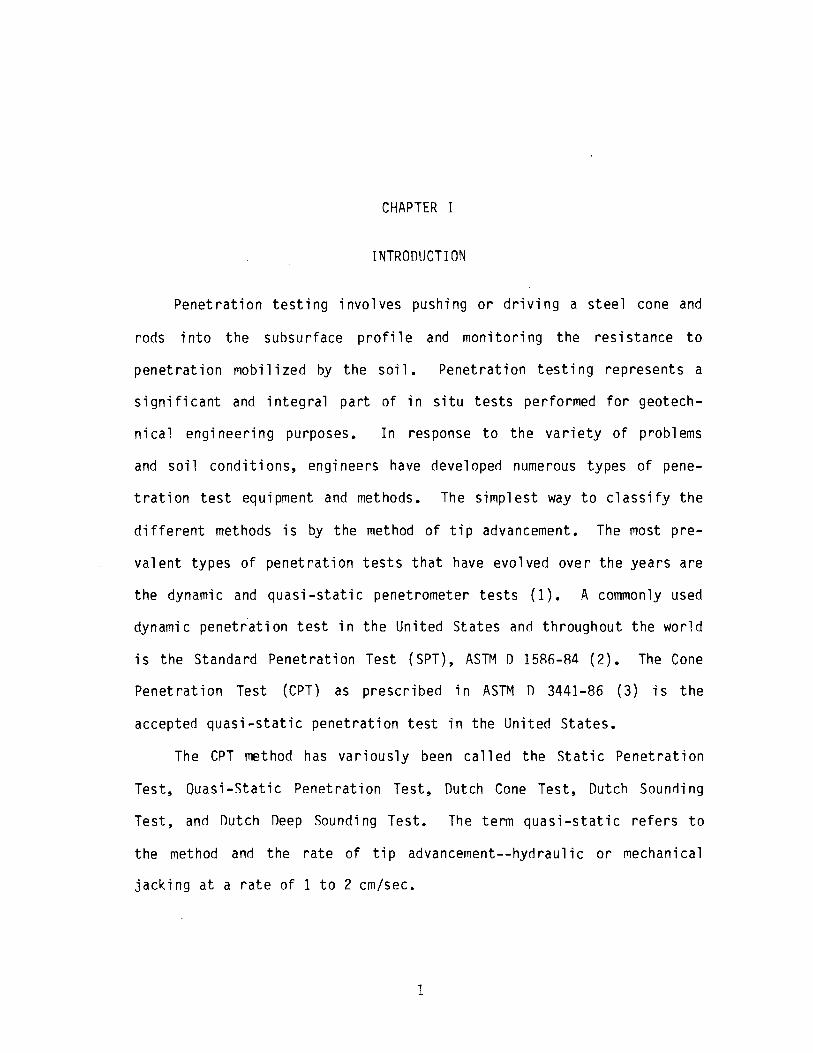
Penetration testing involves pushing or driving a steel cone and
rods into the subsurface profile and monitoring the resistance to
penetration mobilized by the soil. Penetration testing represents a
significant and integral part of in situ tests performed for geotech
ni cal engineering purposes. In response to the variety of problems
and soil conditions, engineers have developed numerous types of pene
tration test equipment and methods. The simplest way to classify the
different methods is by the method of tip advancement. The J11ost pre
valent types of penetration tests that have evolved over the years are
the dynamic and quasi-static penetrometer tests (1). A commonly used
dynamic penetr.ation test in the United States and throughout the world
is the Standard Penetration Test (SPT), ASTM D 1586-84 (2). The Cone
Penetration Test (CPT) as prescribed in ASTM D 3441-86 (3) is the
accepted quasi-static penetration test in the United States.
The CPT method has variously been called the Static Penetration
Test, Quasi-Static Penetration Test, Dutch Cone Test, Dutch Sounding
Test, and Dutch Deep Sounding Test. The term quasi-static refers to
the method and the rate of tip advancement--hydraulic or mechanical
jacking at a rate of 1 to 2 cm/sec.
1

2
The Cone Penetration Test as defined in AASHTO D 3441-86 is a
test method that covers the determination of end bearing and side
friction, the components of penetration resistance which are developed
during the steady, slow penetration of a rod into the soil. This test
method includes the use of both cone and friction-cone penetrometers
of both the mechanical and electrical types. These are the most
widely userl types of cone penetrometers. Various other options in
recent years have been added to produce pi ezometri c, thermal conduc
tivity, nuclear, seismic acoustic, and permeability cones. Most nota
ble of the newer cone options is the piezocone; however, there are
currently no American test standards for these cone variations.
The objective of this research is to evaluate possible relation
ships between the cone penetration test (CPT) of the mechanical cone
~and typical alluvial clay soils of northeastern Oklahoma. In
particular, this research will consirler the following: the adapta
bility, in general, of the mechanical cone penetration test (MCPT) in
Oklahoma soils and geologic formations, development of localized cor
relations between soil cl~ssification and cone data, evaluation of
lithological and stratigraphical interpretations of cone resistance
diagrams, development of SPT-N value and cone resistance relation
ships, evaluation of potential correlation between soil shear strength
and consolidation properties with cone data, and finally review
results of some case histories.
CHAPTER II
LITERATURE REVIEW
Mechanical Cone Development
Historical Review
The idea of determining soil parameters by pushing rods into the
ground is a very old one. The method developed by Collin in France in
1846 used a Vicat-type needle of 1 mm in diameter and weighing 1 kg to
estimate the cohesion of different types of clay of various consis
tency (4). From that date until 1932, numerous variations in the cone
penetration method were developed in Europe, especially in Sweden,
Norway, and the Netherlands. In 1917, for example, the Swedish Rail
roads standardized a method of sounding which is still in use today.
It consisted of pushing a metal rod, 19 mm in diameter, with loads of
5, 15, 25, 50, 75, and 100 kg. When refusal was encountered with a
load of 100 kg, the rods were rotated, either manually or by machine,
in order to advance the rods further. Sanglerat (4) gives an exten
sive accounting of the early development stages of the mechanical cone
penetrometer.
Between 1932-1937, Barentsen (5) in the Netherlands, while asso
ciated with N. V. Goudsche Machinefabriek, developed and patented a
sleeve-type apparatus--the first quasi-static cone penetrometer in a
3
4
form recog~izable today (see Appendix A). Initially, the apparatus I I
consisted df a simple cone where the 1 oad on the cone was measured as
it was advanced ahead of outer tubes. Then the total load was mea-
sured as the cone and outer tubes were advanced together. Following
the development of this simple cone, Vermeiden (6) of the Delft Soil
Mechanics Laboratory <lesigned a mantle cone in 1948 (see Appendix A)
to prevent soil particles from entering the space between the cone and
the push rods. Accuracy in penetration resistance was immensely im-
proved over that of the simple cone described in Appendix A. Similar
ideas on the improvement of Barentsen 1 s simple cone were made by
Plantema (7) using a slightly different cone configuration at about
the same time. A friction sleeve to measure local skin friction over
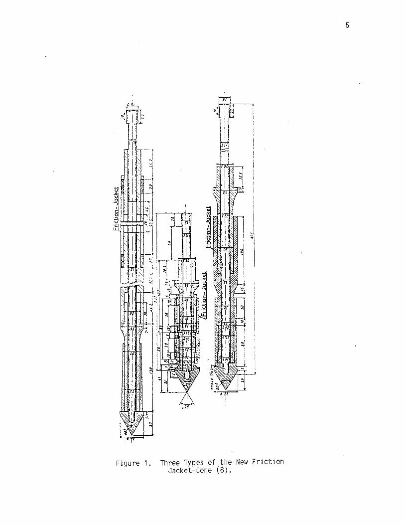
a short length above the con~ was introduced by Begemann (8) in Inda-
.nesia in 1953. At that time, Begemann 1 s research was being conducted
on three variants of what was called the 11 adhesi on jacket cone11 to
determine the most effective location of adhesion jacket relative to
the cone tip (see Figure 1). Further refinements continued by
Machi nefabri ek of Gouda, Netherlands, in conjunction with the Soil
Mechanics Laboratory of the Technical llniversity at Delft in the
Netherlands, in developing what was now termed the 11 friction 11 jacket
cone. The ~chani cal cone development culminated with the improve
ments by Machinefabriek to conform with Regemann 1 s 1965 recommendation
(9) (see Appendix B). The Hogentogler & Co., Inc. (10) reports that
Machinefabriek started supplying mechanical cones that met the speci
fication NEN: 3680 of the Delft Ground mechanics (LGM) of Holland in i
1976. nue t\o this new specification, the shape of the mantle in the
friction-sle~ve cone was changed to conform to the Dutch mantle cone.
). ,' ..
009
Figure 1. Three Types of the New Friction Jacket-Cone ( 8).
5
6
There have been numerous mechanical cones developed and used by
many countries throughout the world. Sanglerat (4) presents a compre
hensive review of cone penetrometer testing and various cone develop
ments throughout the world. However, when one considers the more
recent cone development, it is the Dutch apparatus manufactured by
Machi nefabri 1ek and ·patented in the Netherlands by the Soi 1 Mechanics
Laboratory of nel ft that are the most widely used and popular mechan
ical cone penetrometers. Its use has spread worldwide. Schmertmann
(11) is credited with introducing the MCPT into the United States in
the middle 1960s.
Beginning with the work of Geuze in 1948, as noted by Sanglerat
(4), the electric cone development has shadowed that of the mechanical
cone. The electrical cone came into more general use in the late
1960s. Only limited discussion will be addressed to the electric cone
in this research study.
Role of the Cone Penetration Test
The CPT has three main applications:
1. Determine the soil profile and identify soils present
2. Interpolate ground conditions between control boreholes
3. Evaluate thP engineering properties of the soils and to assess
bearing capacity and settlement.
Its value must be seen within the framework of the overal 1 geotechni
cal investigation. The role of the CPT is one of enhanced definition
of site conditions.
The qualitative use of the CPT in the first two roles is of tre
mendous value and has been described by numerous researchers and

7
practitioners (4, 11, 12). The CPT is the only investigative tech
nique that provides an accurate continuous or virtually continuous
profile of soil strati fi cation. Ry performing a number of cone pene
tration tests (sounrlings) over a site, a picture can be obtained of
the uniformity of soil conditions. Based on that information, a de
tailed soil exploration program can then be designed, including samp
ling of specific critical layers and possibly other in situ testing.
The identification of soils is achieved by means of empirical correla
tion between soil type and the ratio of the local side friction to
cone resistance (skin friction ratio) considered "in relation to the
cone resistance.
With regard to the third application, the assessment of engi
neering properties is more complicated in view of the many soil para
meters that determine the cone resistance. However, much success has
been achieved with the correlation of the CPT and some important soil
parameters such as undrained shear strength of clay (11, 12). Assess
ment of engineering properties of soils has been based on empirical
correlations. The important soil engineering parameters are: angle
of internal friction and deformation characteristics in cohesionless
soils, and undrained shear strength and modulus in cohesive soils.
Practical applications of the CPT include the assessment of ultimate
bearing capacity and settlement of footings and piles (11, 12).
Again, these are based on empirical correlation with the CPT.
The use of mechanical cone penetration testing in light of these
three applications has great potential for cost and time savings.
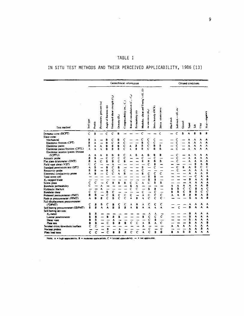
Robertson (13) reviewed the perceived applicability of the major types
of in situ test methods, which includes the mechanical cone penetro-

8
meter (see Table I). It is evident from Table I that the mechanical
cone penetrometer can make a significant contribution to a geotech
nical study.
Test Standardization
Standardization of test procedures for CPT has been an on-going
process. Two of the currently used test stanrlards for cone penetra
tion testing are the European Recommended Standard (ERS) and the
American Society of Testing of Materials ASTM D 3441-86 (see Appen
dices A and B, respectively).
Efforts to stanrlardize methods of penetration testing date back
to the 4th Conference of the International Society of Soil Mechanics
and Foundation Engineering (ISSMFE) in London in 1957. At that time
an ISSMFE subcommittee on static and dynamic penetration testing meth
ods was established to sturly the various test methods with the intent
of achieving standardization. Recommendations from this subcommittee
led to the publication of the European Recommended Standard (ERS) in
1977. Of significance, this standard recommended what is called the
standard tip geometry as shown in Figure 1 of Appendix A. The ERS
recognized the continued use of mechanical cones and allowed the use
of nonstandard cones as referenced in Section 10. It is further
required by ERS that a rleviation from the standard tip geometry and
test procedure should be staterl when presenting CPT results. The
ISSMFE is continuing to work on an internationally acceptable refer
ence test.
The ASTM n 3441 standard was tentatively adopted in 1975 and
approved as a test standard in 1979. The current standard was reap
proved in 1986 as ASTM D 3441-86 (see Appendix B). Of significance,
9
TABLE I
IN SITU TEST METHODS AND THEIR PERCEIVED APPLICABILITY, 1986 (13)
Geo1echn1cal 1nfonnauon Ground cond111ons
z ;.:i
, .~ ~
"' " "' "i -= .. ""'
= ;. " '..J ~ .. ~
= = >-
~ ~ e 2 .,, ~ .. .... ; = ~ g " ;; ~ i:i
~ !; ~ "ii! ... ;; " ~
-4 ~ ~ .... ~
.... :: ~ :a .! n
~ = i = .:::: = n ;; " 5 .,, ~ a .. .... 5 l!.. ~ 1! :.Q :.; :;; :;; ... ll
-~ " ..;; ~ = ;; ~ '" I ~ I ::- ..!! ..!! ll = ~ n il '§ z ... ~ = e l:!
= 1 n ::: .,, -= > .,, >. ;
~ .. = ~
:> '" .. l! l! ;; ~ ~ ; " ..
Tes1 me!hod :!: :!: < ::i u ¥ =- ~ .:: :;; :;; :c "' Vi :i "'" Dynanuc cone (0Cm c B c c B c c c B A B B B Siatic cone:
Meclwucal B A B c B c c c c c A A A A Elec!rOftlC friclion (cm B A B c B c B c c c A A A A Elec!ronic p1ezo B A A B B B c A B B c B B c A A A A Elecaoruc p1ezo/fric1ion 1CPTUl A A A B B B c A B B c B B c A A A A Elecaonic se1sm1c/p1ezo1 fric1ion
!SCPTUl A A A B B B c A B A B B B c A A A A Acous1ic probe B B c c c c c c c A A A A Flat plate dila1ometer 1 DMTl B A c B B c B B B B B c A A A A
Field vane shear l VSTI c c A c B B A 8 S1andard peneuauon lest ( SPTl A 8 8 c 8 8 c c 8 A 8 c c Res1s11vi1y probe B B B c A c c c A A A A
Elecaon1c conducti vi1y probe A B c c A B B c c c A A A B T ol&I stress cell B B c A A Ko siepped blade B B B A A B Screw plate c c c B B B c c A c B B A A A A Borehole penneability c A B A A A A A A A B Hydraulic fracture A c c B B B B c c B A c Borehole shear c c B c c c B B c B B c c Prcbored prcssurcmeter ( PMTI B B c B c c c A c c c A A B B B A B Push-in prcssurcmeier ( PPMTl A B B c B c c A B A c c c B A A B Full·displac:ement pressurcmcter
iFDPMTl c B B c B c c A B A c c c A A A A Sclf·bonng pressurcmeter (SBPMTl B B A A B B B A B A A A A c B A A A Sclf·bonn1 dev1cn:
Ko meter B B A A B A A A
l..alCtal penctrometcr B B B B B B c c c B A A A
Shear vane B B A c B B A A A
Plate iest B B c B B 8 c c A B A c B A A B ScismJC cross/downhole/surfac:c c c A A A A A A A A
Nuclear probes B A c c A A B A Plate 111..t iests c c c B B B c c A c B B B A B B A A A
Non: A •hip lfllllicabdiry. B • moclenlc applicabdity, C • hmlled •pphcabih1y. - • noc ;opphc•ble.

10
this test :standard allows the use of both cone and friction-cone
penetrometers of both the mechanical and electrical type and acknow
ledges that test results will differ depending on which devices and
procedures are used. Mechanical cones, h~rein, generally refer to the
Dutch mantle and Regemann friction sleeve cones shown, respectively,
in Figures 1 and 2, Appendix B.
There has been interest by some groups to bring the ASTM standard
in line with the recommended European Standard (14). The main argument
is that ASTM in effect recognizes two separate standards. Several
investigations (1, 15, 16) have recognized that the mechanical cone
pen et rometers wi 11 continue to have a significant useful l ness because
of their relative ruggedness, simplicity, and initial cost--very much
similar to the continued use of the Standard Penetration Test, ASTM D
1586-84.
Equipment
CPT Apparatus: The mechanical cone penetration test apparatus
generally consists of a thrust machine and a reaction system (rig) and
a penetrometer with measuring and recording equipment.
Machines available generally have a thrust in the range of 2-3/4
to 20 tons. They are discussed under three categories: light, medium,
and heavy. A light rig is used in the exploration of weak soil layers
and generally is one rated up to a capacity of 2-3/4 tons. Penetration
is limited to a short distance into medium-dense sands or stiff clays.
They are oft!en light, portable, and hand operated through a chain
drive (see Figure 2). A medium size rig is one rated to a capacity of
11 tons, and reasonable penetration can be obtained in stiff clays and

Figure 2. Hogentogler Model No. E5301 HandOperated 2.75-Ton Dutch Cone Penetrometer (10)
11
12
'
medium-dense sands for depths up to 65 feet. They can be mounted on a
trailer with screw anchors or in a specially designed truck or tractor I
ballasted with sufficient weight or with screw anchors. Penetration
is usually achieved by a hydraulic jacking system (see Figure 3). A
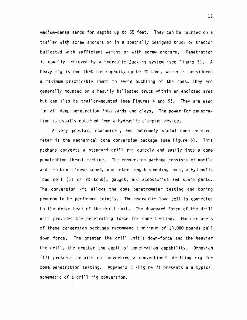
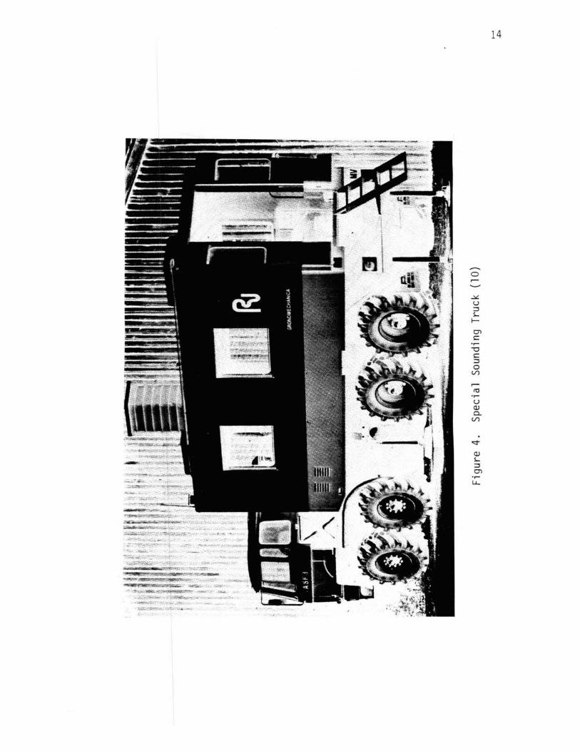
heavy rig is one that has capacity up to 20 tons, which is considered
a maximum practicable limit to avoid buckling of the rods. They are
generally mounted on a heavily ballasted truck within an enclosed area
but can also be trailor-mounted (see Figures 4 and 5). They are used
for all deep penetration into sands and clays. The power for penetra-
tion is usually obtained from a hydraulic clamping device.
A very popular, economical, and extremely useful cone penetro-
meter is the mechanical cone conversion package (see Figure 6). This
package converts a standard drill rig quickly and easily into a cone
penetration thrust machine. The conversion package consists of mantle
and friction sleeve cones, one meter length sounding rods, a hydraulic
load cell (11 or 20 tons), gauges, and accessories and spare parts.
The conversion kit allows the cone penetrometer testing and boring
program to be performed jointly. The hydraulic load cell is connected
to the drive head of the drill unit. The downward force of the drill
unit provides the penetrating force for cone testing. Manufacturers
of these conversion packages recommend a minimu~ of 10,000 pounds pull
down force. ·The greater the dri 11 unit's down-force and the heavier
the drill, the greater the depth of penetration capability. Drnevich
(17) presents details on converting a conventional drilling rig for
cone penetrat~on testing. Appendix C (Figure 7) presents a a typical
schematic of a d ri 11 rig conversion.

Figure 3. Hogentogler Model No. E540l Dutch Cone Penetrometer, 11-Ton Capacity (10)
13
?~':tt:JPfmt:z;;.~•~.1..-.:.:1;.?~-- .;z;-:t:'.1¥":'(';'.~"'."·ll':·'. ~~~.w::.-..;~.;!i;.·;'t.:.,,.;:. .... #,',. .• :~ • .: ••. ,:1._l,.
~.,.., :fll.Mo>J'.;.. ,',."'.t.r• ·",;.. ·,-;_"..;.(·.,;, .• ; •. ;.•. ~. ,,~,.,
... ~.,.,.,~j:,..."J',:;-1--, .. ~':"":7~i;t;"fJ!P.-~-··o- ·.,.
.. ~ . ....... ~·---:·
..,c;;,:;.*:-z;.:,"':"'::_-.·.-..o;,"'-'"Jr~."'
f°<'t/~~;_';.'.J-"".'?/>:f't:r_tt~ .• ·.-..:..- •· ',' t}J~·,",....,I~.•,..., H
55""'"~';""""=··~, ,,.,..,.,._ ~ "~.·;~-.wrw~· ~ "•'./· ~~.;·.-.:r·.-r,:np,.,,,,
'·,,,-,.Y~-~~'~:;,-.. ;1.-',.r"""'-.-"-'' ,..},;;l:/;W~;w,~ .. ,~..,~~.~-··--.~ •. ~ .... ,.., .• ,..;-Jrl, • .,,,..J'~'."':'+;.•.1.-r,..,;.Qf;; ·.~. ·"···•~....,.; .. ~-g,;..~~!',tp.,kl'J;.v:'.
.t ~
0
......
...... u Q) c... ll1
<:t"
Q) s... ::J 0) ......
LL..
14
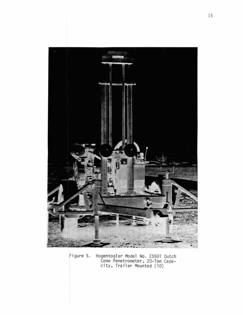
Figure 5. Hogentogler Model No. E5501 Dutch Cone Penetrometer, 20-Ton Capacity, Trailer Mounted (10)
15
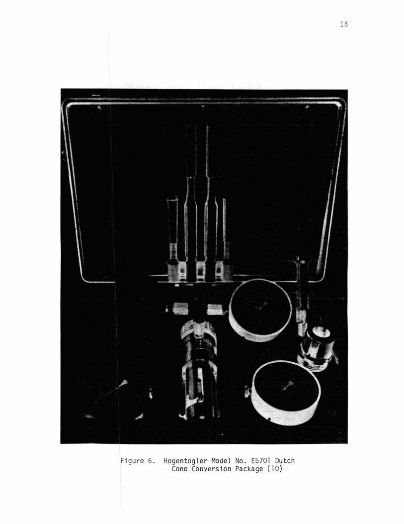
Figure 6. Hogentogler Model No. E5701 Dutch Cone Conversion Package (10)
16

17
The A$TM makes no stringent requirement on the thrust machine
other than \that the machine shall provide a continuous stroke prefer-
ably over a distance of one push rod length. Advancement of the tip
must also be at a constant rate.
The standard push rod is made of high tensile steel and has a
length of one meter. ASTM requires the rods to be smooth and have
flush fitting joints. The diameter of standard inner rods is speci-
fied as between 0.5 and 1.0 mm less than the internal diameter of the
push rods, and it is usually made of polished steel so as to reduce
friction between the push rod and inner rod. To increase the depth of
penetration and not reduce any differences between the resistance com-
ponents, a special rod called a "friction reducer" is introduced into
the string of push rods. The friction reducer is a rod (usually a
short section of rod) which has an enlarged rtiameter or special pro-
jection. A friction reducer that has been found to be very effective
in clayey soils is shown in Figure 7 (4). One that has been found to
work well in sandy soils is the "cam friction reducer" shown in Figure
8 (18). ASTM D 3441-86 allows the use of such rods in the push rod
string no closer than 1.3 feet above the base of the mantle mechanical
cone or 1.0 feet above the top of the friction sleeve for the friction
sleeve cone mechanical cone. Nominal dimensions for push rods used in
mechanical cone testing are given in Figure 9.
Penetrometer Tips: Penetrometers are of two main types, mechan-
ical and ele~trical. They can further be subdivided into those for
measurement df cone resistance only and those for measurement of both I
cone resistarlce and local side friction. In mechanical penetrometers, I
the forces r¢quirerl to mohilize cone resistance and local side fric-

E E
Q
°'
E E 0 0 N
E e
0 0 C"t
Figur¢ 7. Spacer-Ring Connection to Reduce the Effects of Side Friction (4).
18

cone
ll t~O H
t 11ct1on sleeve
mantle
1
cam
10.0 11.0 weld~
@ ~~mrn rn 5'1
2
Figure 8. Begemann Friction Sleeve Penetrometer Tip (1) and Cam Friction Reducer (2, 18)
19

I I
I
lOOOmm
i 1 • I I
I '
I '
I I
/ , I
I I
I '
I
1 (a) Push rod with friction reducer
I
16mm
36mm
I
I I I
( b) Push rod
15mm
(cl Inner rod
Figure 9. Penetrometer Rods (12)
20

21
' tion are applied to the tip through the interaction of push rods and I
inner rods:1
and measurerl at the surface. With electric penetrometers,
penetration is achieved by the application of force to the push rods.
Forces are measured by electrical resistance strain gauges built into
the tip, and measurements are transmitted to the surface through an
electrical cable. Dimensions and specifications of the mechanical and
electrical cones (tips) are given in ASTM 3441-86.
Similarities in the basic dimensions between mechanical and elec-
trical cones are the following: the cone tip has a 60° point angle, a
2 projected cone surface area of 10 cm , cone base diameter of 35.7 mm,
and a friction-sleeve surface area of 150 crn2• Differences are the
tip geometry and method of operation as discussed in Appendix B. Rol
(19) conducted research comparing cone resistance in sand with -three
CPT-tips, two of which were the standard electric cone and mechanical
f ri ct ion-sleeve of the Begemann type. Results indicate that di ff er-
ences do exist and can be attributed mainly to friction between push
rods and inner rods of mechanical cones. Differing cone geometrics
also affect cone resistance and interpretation in normally and over-
consolidated clays; however, there are other factors involved (12).
CPT Procedure
Extent of CPT Use: Early use of the mechanical cone was applied
to extensive studies of soft or weak soils in Holland and Belgium (4).
Application of the mechanical CPT has spread from principally recent
alluvial normally consolidated clays and sands to overconsolidated
alluvial cla{s and sands, residual clays, and older geologic forma
tions. The \mechanical cone is not used generally for rock explora-

22
tion, although very soft and/or weathered rock have been investigated.
Searle (20), for example, has studied the interpretation of the
mechanical cone in chalk (carbonate siltstone). Schmertmann (11)
i nrli cat es as a rough guide to the pen et ration limit is that 10-ton
equipment can just penetrate a 5-foot layer of Standard Penetration
Test (SPT) N = 100 sand at a depth of 25 feet. Ramage and Williams
(21) report that, depending upon the machine used, the CPT is re
stricted to material with a SPT hlowcount of less than 70 to 90 blows
per foot. The CPT is rather restricted in penetrating gravel. Ramage
anrl Williams also inrlicate that the ability of the mechanical cone to
penetrate is limited to material that contains less than 45 percent of
1/2-inch or smaller gravel. Based on this literature review, it does
appear that the applicability of the mechanical cone test has increas
ed substantially in the material types now being investigated as com
pared to its original use in Holland.
Operation of Equipment: Detailed operational procedure for the
mechanical cone is presented in Appendices A, B, and C. Basically,
the procedural steps as outlined by de Ruiter (15) for the mantle and
friction-sleeve mechanical cones are as follows:
Mantle Cone:
(a) The cone can be advanced 7 cm by means of the inner rods and
a representative cone resistance value is recorded for that
interval •
b) After advancing the cone, the outer rods are generally
pu~hed down 20 cm, over the last 12 cm of which cone and
rod[s move together. The procedure is then repeated so that·
intiermittent readings are obtained at intervals of 20 cm.
23
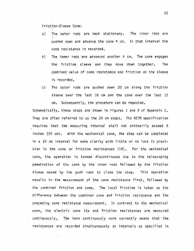
Friction-Sleeve Cone:
a) The outer rods are kept stationary. The ·inner rods are
pushed down and advance the cone 4 cm. In that interval the
cone resistance is recorded.
b) The inner rods are advanced another 4 cm. The cone engages
the friction. sleeve and they move down together. The
I • combined value of cone resistance and friction on the sleeve
is recorded.
c) The outer rods are pushed down 20 cm along the friction
sleeve over the last 16 cm and the cone over the last 12
cm. Subsequently, the procedure can be repeated.
Schematically, these steps are shown in Figures 1 and 2 of Appendix C.
They are often referred to as the 20 cm steps. The ASTM specification
requires that the measuring interval shall not ordinarily exceed 8
inches (20 cm). With the mechanical cone, the step can be completed
in a 10 cm interval for more clarity with little or no loss in preci-
sion in the cone or friction resistances (18). For the mechanical
cone, the operation is termed discontinuous due to the telescoping
penetration of the cone by the inner rods followed by the friction
sleeve moved by the push rods to close the step. This operation
results in the measurement of the cone resistance first, followed by
the combined friction and cone. The local friction is taken as the
difference between the combined cone and friction resistance and the
preceding cone resistance measurement. In contrast to the mechanical
cone, the electric cone tip and friction resistances are measured
continuously. The term continuously more correctly means that the ! I
resistances are recorded simultaneously at intervals as specified in
24
the ASTM standard. For light penetrometer rigs the mechanical cone is
advanced by hand operation of a chain drive; in the medium and heavy
penetrometer rigs penetration is obtained by the use of a hydraulic
rafTl.
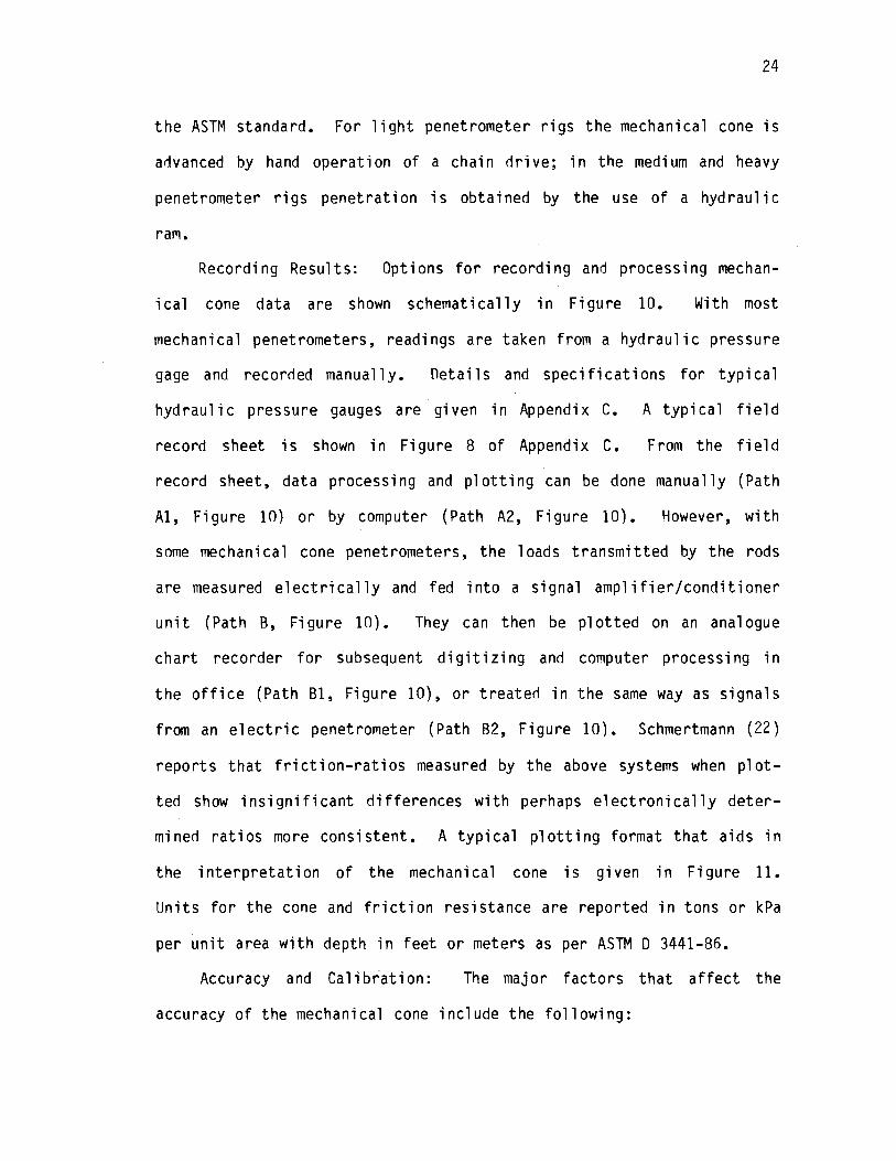
Recording Results: Options for recording and processing mechan-
ical cone data are shown schematically in Figure 10. With most
mechanical penetrometers, readings are taken from a hydraulic pressure
gage and recorded manually. Details and specifications for typical
hydraulic pressure gauges are given in Appendix C. A typical field
record sheet is shown in Figure 8 of Appendix C. From the field
record sheet, data processing and plotting can be done manually (Path
Al, Figure 10) or by computer {Path A2, Figure 10). However, with
some mechanical cone penetrometers, the 1 oads transmitted by the rods
are measured electrically and fed into a signal amplifier/conditioner
unit (Path B, Figure 10). They can then be plotted on an analogue
chart recorder for subsequent digitizing and computer processing in
the office (Path Bl, Figure 10), or treated in the same way as signals
from an e 1 ect ri c pen et rometer (Path 82, Figure 10). Schmertmann ( 22)
reports that friction-ratios measured by the above systems when plot
ted show insignificant differences with perhaps electronically deter
mined ratios more consistent. A typical plotting format that aids in
the interpretation of the mechanical cone is given in Figure 11.
Units for the cone and friction resistance are reported in tons or kPa
per unit area with depth in feet or meters as per ASTM D 3441-86.
Accuracy and Calibration: The major factors that affect the
accuracy of the mechanical cone include the following:

------------------------------------- r o"Ns1'Te ___ 1 -,'NoF"Fice __ _
Hydr1ulic lold cell
Ind g1uges
Reldings hind-recorded
Electrie1I OePth lold encoder cell
Sivn11 1mplifi1r/
A
M1gnet1c tape
recorder (e1ssenel
or floppy disc
I I I
Electric conditioner
I I 1· I I I I I I I
tip
I Gr1phic1I I I recorder I I (1nlloguel I L.: ____ _J
Figure 10. Possible Arrangements for Recording and Processing CPT Data (12)
25

FRICTION IN FRICTION IN KG/CM2 CONE BEARING IN KG/CM2 KG/CM 2 CONE BEARING IN KG/CM2
2.5 0 100 200
A. MECHANICAL CONE
2,5 0
A. MECHANICAL CONE , DISCONTINUOUS READINGS
I. ELECTRIC CONE , CONTINUOUSLY RECORDED
100
ELECTRIC CONE
200
Figure 11. Penetrometer Tests With Friction Measurement (15)
26

27
Rate of penetration
Inner rod friction
Weight of inner rod
Jamming
Wear of cone dimensions
Distance between cone and friction sleeve
Drift of tip
Research indicates that the cone resistance tends to increase
with the penetration rate for both clays and sands (12, 23). Small
variations in the speed relative to the standard rate of 2 cm/sec have
no si gni fi cant influence on cone resistance. ASTM D 3441 standard
which allows a variation of ±25 percent appears fully acceptable
(23). Inner rod friction is a much discussed topic in mechanical cone
testing. Care must be taken that the inner rods are free of soil par-
ticles and corrosion and lubricated before insertion into the push
rods. A procedure for estimating the inner rod friction in a homo-
geneous is presented in Figure 9 of Appendix c. Additional inner rod
friction develops due to penetrating hard layers and at great depths,
because of elastic compression, causes shortening of the inner rod
(15). This elastic compression further shortens and eliminates the
free stroke for the cone measurement. Appendix C, Figures Cl and C2,
contains a procedure for compensation of elastic compression rod
shortening. Mei gh (12) suggests the mechanical cone should not be
used for depths greater than 20 m in order to avoid inner rod fri c-
ti on. Van den Berg (16) reports some manufacturers are now producing I
a highly poliished surface on inner rods and the inner surface of the
push rods which they claim virtually eliminates inner rod friction.
28
For improved accuracy at low cone resistance values, a correction
of the cone data is required to account for the accumulated weight of
the inner rod from the cone tip to the topmost rod. For very soft
clays, Schmertmann (1) indicates the practice of using aluminum inner
rods. Soil particles between sliding surfaces or bending of the tip
may jam the mechanism during many extensions and collapses of the
telescoping mechanical tip. The sounding has to be stopped as soon as
uncorrectable jamming occurs.
Measurements become 1 ess accurate if the dimensions of the cone
depart appreciably from the ASTM n 3441-86 standard due to wear or by
damage. Of particular importance is the surface roughness of the cone
and the friction sleeve. Parez (24) and Durgunoglu and Mitchell (25)
have conducted research showing the effect of shape .and base roughness
of the cone tip upon penetration resistances.
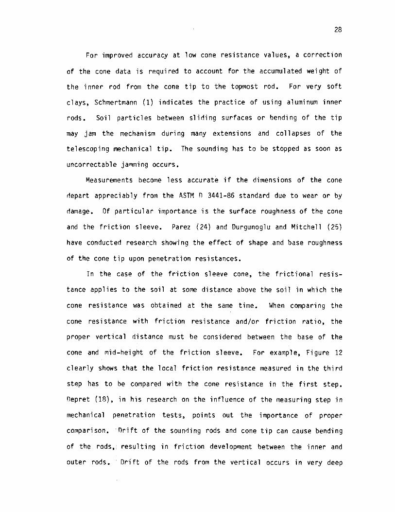
In the case of the friction sleeve cone, the frictional resis
tance applies to the soil at some distance above the soil in which the
cone resistance was obtained at the same time. When comparing the
cone resistance with friction resistance and/or friction ratio, the
proper vertical di stance must be considered between the base of the
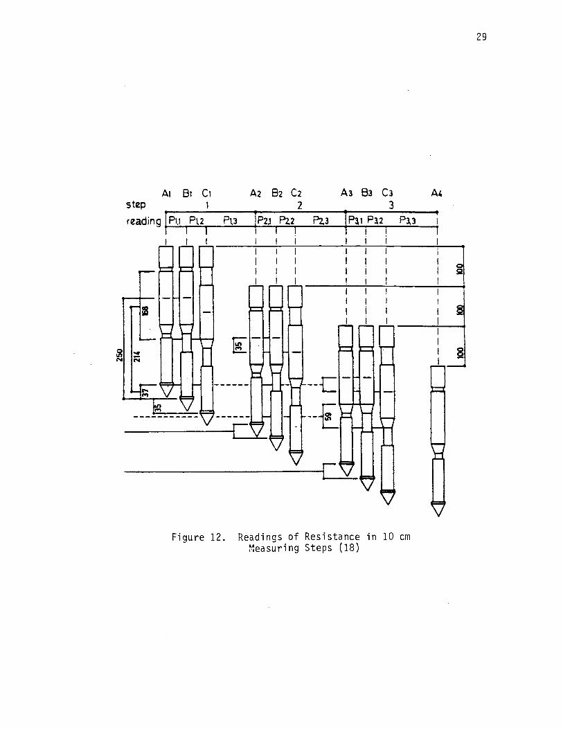
cone and mid-height of the friction sleeve. For example, Figure 12
clearly shows that the local friction resistance measured in the third
step has to be compared with the cone resistance in the first step.
Depret (18), in his research on the influence of the measuring step in
mechanical penetration tests, points out the importance of proper
comparison. · Orift of the sounding rods and cone tip can cause bending
of the rods,: resulting in friction development between the inner and
outer rods. Drift of the rods from the vertical occurs in very deep
At Bt C1 step 1
reading { P1.1 P\2 I 1
I I I
2 I P2.1 P2.2 P2,3 1 I I
I I I I I I I i i I
r.:- - -~.
Al 83 Cl 3
f Pl1 Pl2 Pl3 1 I I I i
.I I i I I i i I I I I I I I I I
---c ---£
Figure 12. Readings of Resistance in 10 cm Measuring Steps (18)
29
A4
30
soundings and when passing through or alongside obstructions such as
boulders, soil concretions, thin rock layers, and inclined dense
strata. For penetration depths exceeding about 40 feet, the tip will
probably drift away from a vertical alignment (3).
The traditional method of measuring cone resistance is rather
simple, but it does require a double string of rods which can intro
duce a number of errors. However, if used in a careful and competent
manner, and if attention is paid to specification detail and calibra
tion, the method can be fully adequate. Experience of a great number
of investigators over many years has shown that reliable results are
obtained provided that tests are executed with proper care (15).
A comparison of the difference in the values of the cone and
friction resistances between those measured with the mechanical and
those measured with the electrical penetrometers is to be expected for
two reasons: first is the influence of the penetrometer shape; second
is the difference in the method of advancement of the cone {15).
However, de Ruiter (15) and Van den Berg (16) can find no systematic
difference hetween the cone resistance values from the mechanical and
electrical penetrometers, as noted in Figure 11. In contrast to the
cone resistance, marked differences are found in the magnitude of the
friction resistance as measured with the Begemann mechanical
pen et rometer anrl with the electric penet romete r. A comparison of the
two friction graphs in Figure 11 indicates that on average the
friction resistance of the electric cone is only about half of the
mechanical cone. Numerous other comparisons found the same approxi -
mate ratio (2o, 27). The large difference in friction can be explain
ed mainly by, the end resistance on the lower edge of the friction
31
sleeve. In clays this will be of minor importance, but in cohesionless
soils it may affect the result appreciably.
CPT Soil Classification
Soil classification from CPT data has been traditionally obtained
from the magnitude of cone resistance and more specifically from their
friction ratio (the ratio of local side friction to cone resistance,
f s/qc).
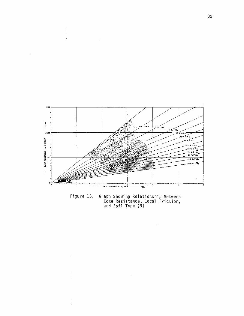
A soil classification scheme using mechanical cones was first
formulated by Begemann (9). Begemann developed his scheme from
approximately 250 comparative friction cone penetration soundings and
accompanying borings which cone resistance is compared to local side
friction (see Figure 13). The graph with lines that relate to the
percentage of soil particles less than 16 u is the basic figure.
Figure 13 shows the names of soil types used by the Delft Soil
Mechanics Laboratory on the basic graph. Schmertmann (11) extended
Begemann's work to include an interpretation of density or stiffness
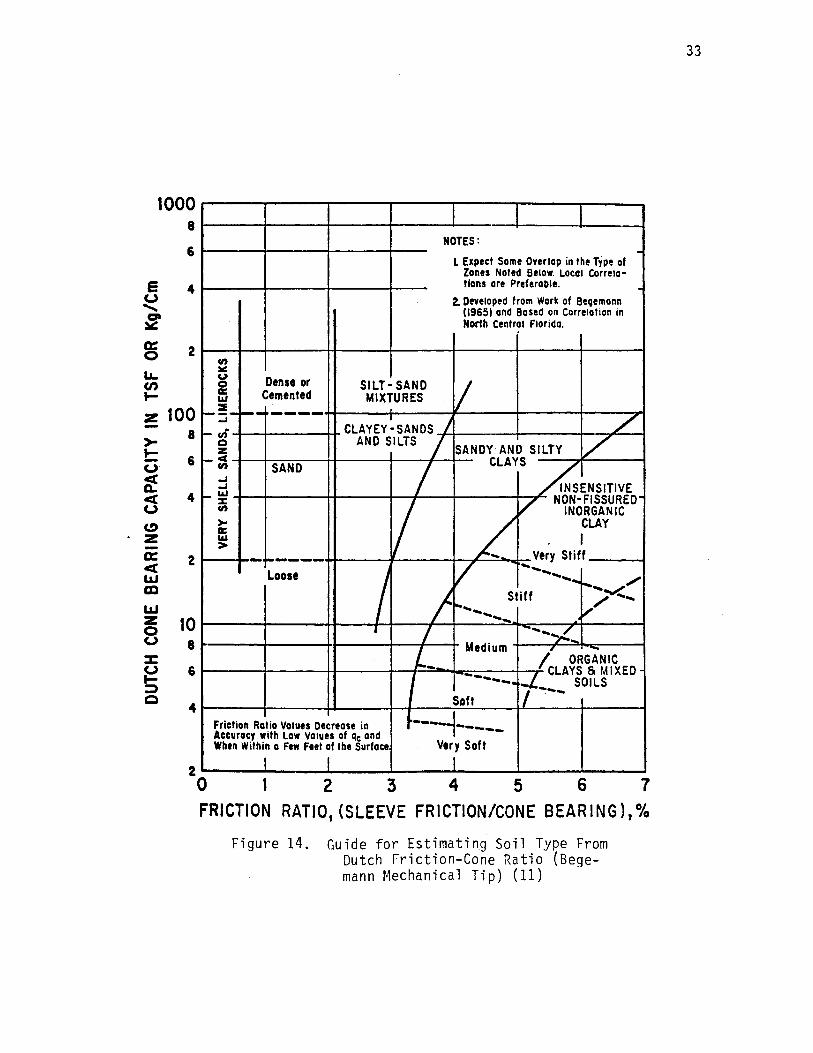
(see Figure 14) in terms of cone resistance and friction ratio.
Searle (20) included the results of further field measurements and
expanded the Begemann and Schmertmann charts (see Figure 15). This
approach differed from the previous ones in that soil type was
directly related to friction ratio.
The basis for soil cl assifi cation by a cone penetrometer is the
analogy that it models a rlriven pile. The ratio of skin friction to
tip resistance has been found to be approximately 5 percent for clay
and 1 percent for sand. This analogy is applied to a cone penetro
meter and termed the friction ratio. The friction ratio (FR) is a
. " ~ ~ ;!
I 1ool---------l---,L:.:_~,i4~4'~~~~~~~""'~~~ II!
5 .. I
' ' ----L.OCALFJllCTIOH IN KG/Cll2----~=-=-
Figure 13. Graph Showing Relationship Between Cone Resistance, Local Friction, and Soil Type (9)
32
1000
e <.J ....... at ¥
0: 0
..... en ~
z >-t::: <.J
~ ct <.J (,!) z 0: ct LLI m LLI z 0 <.J
:c ~ ~ c
8 NOTES:
6 -L Expect Some Overlap in the Type of
Zones Noted Below. Local Correla·
4 tlons ore Preferable. . 2. Developed from Work of Be9emann
(19651 and Based on Correlation in North Central Florida.
2 en :ill:
100 8
6
4
2
10 8
6
4
u Dense or SILT· SAND I 0 a:: Cemented MIXTURES w :& -----i----- / ..J
CLAYEY~SANDS ) .... en 0 AND SILTS I SANDYAND SILTY v z .... "" CLAYS en SAND I hsENSITIVE ..J ..J
I- w :c
I v NON-FISSURED"
en INORGANIC >- ~ CLAY a::
VMy sm1f w > - ~---- v ........ Loose
I .............. /
I !"'" .... ~
Stiff / ....... "'"........... ~ .........
I I -... .,.! ... ...... L __ Medium ·' ~ I ORGANIC
I --- .L. CLAYS S MIXED --.. - SOILS Soft I ~----
Friction Ratio Values Decrease in ----1 ----..... Accuracy with Low Values of Qc and Very Soft When Within a Few Feet of the Surface
2 0
I
1 I 2 3
I 4 5 6 7
FRICTION RATIO, (SLEEVE FRICTION/CONE BEARING),%
Figure 14. Guide for Estimating Soil Type From Dutch Friction-Cone Ratio (Begemann Mechanical Tip) (11)
33

..... e -z:
:IE
10
10
Figure 15. Identification of Soils Using the Dutch Mechanical Friction-Sleeve Pcnetrometer (20)
34
100
35
characteristic of the soi 1 type but can vary depending on the cone
configuration used (4). In general, it has been found that the higher
the FR, the greater the percentage of fines in the soil--particularly
cohesive fines. As reported by Sanglerat (4), extensive correlation
between various investigators has 1 ed to genera 1 acceptance of fri c
t ion ratios for different soil types (see Table II).
Most investigators (4, 11, 12) point out that the above listed
classification schemes are guidelines and recommend deriving corre
lations based on local conditions by direct comparison with one or
more test borings, preferably by continuous sampling.
Cone resistance responds to soil changes with 5 to 10 diameters
above and below the cone, the distance increasing with increasing
stiffness. This leads to some inaccuracies in locating soil inter
faces as noted earlier. Very thin layers can be missed. A thin layer
of sand within a clay stratum may not be detected if it is less than 4
inches thick and a clay layer within sand may not be detected if it is
1 ess than 6 to 8 inches thick. However, the accuracy of CPT 1 oggi ng
is considered better than conventional boring and sampling (5 foot
interval sampling).
SPT-CPT Correlation
Because of the extensive use of the standard pen et ration test
(SPT) in the United states, it is of interest to develop a correlation
between the SPT blow count (N-values) and the cone resistance. Sang
lerat (4) discusses these correlations· in detail. The correlations
generally take the form:

36
TABLE II
FRICTION RATIOS--SOIL TYPE (4)
FR Soil Type
0.0-0.5% Ordinarily indicates soft rock, shells, or loose gravel
0.5-2.0% Ordinarily indicates sands or gravels
2.0-5.03 Clay-sand mixtures and silts
>5.0% Clays
37
qc = nN (1)
where n varies from 2 for clays to 10 for sands. Schmertmann ( 28)
presented some theoretical carrel at ion between SPT and cone sounding
data and indicated a decreasing qc/N ratio with increasing cohesive-
ness of the soi 1. He also has found that the ratios of (N06 _12
in"/N12-18 in.) correlate well with the FR. Further research by
Schmertmann resulted in the development of an equation giving the N
value as a function of cone resistance (qc) and friction ratio (FR)
that is applicable in any type of soil. This equation can be formul
ated as fo 11 ows:
N (SPT) = (A + B x FR %) qc'
where A and B are constants.
(2)
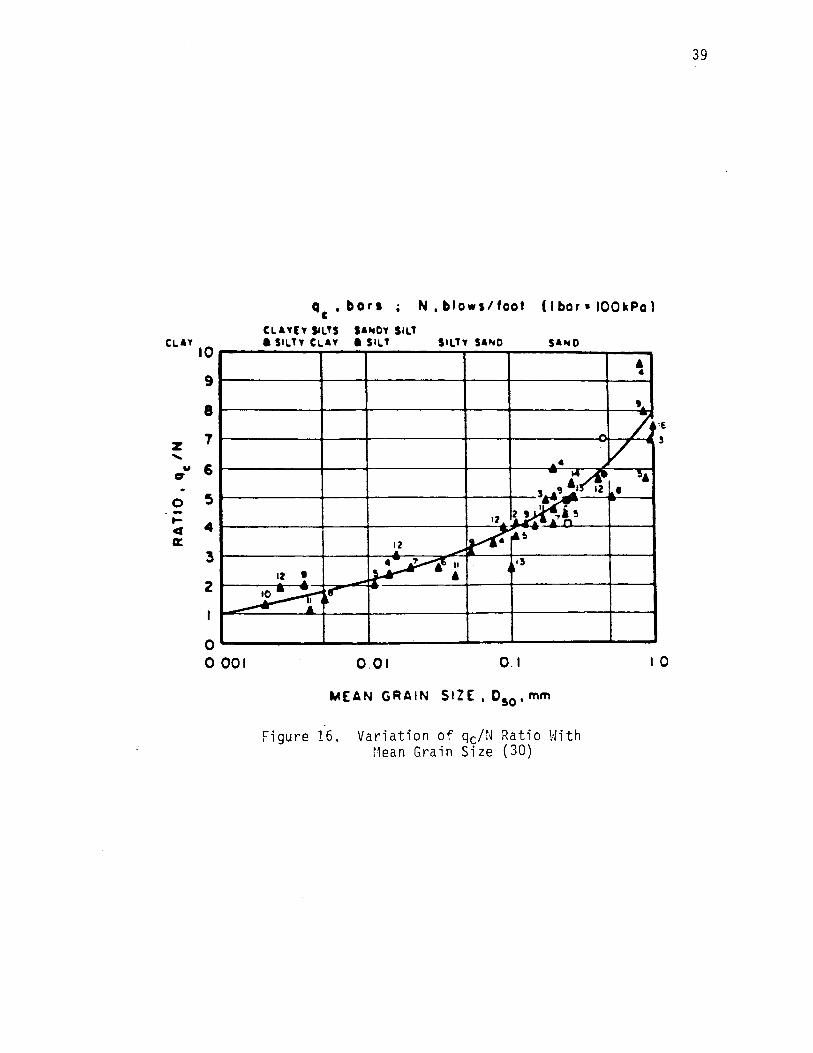
Begemann, as reported by Schmertmann (29), has found closer
correlation between local friction (fs) and SPT resistance N, than
between cone resistance, qc and N. For insensitive clay, the qc/N
ratio is potentially very useful to correlate between clay consistency
and estimated undrained shear strength from local correlations with N
or from generalized correlations. The correlations in Table III by
Terzaghi and Peck were reported by Sanglerat (4). In more recent
research Robertson and Campanella (30) show that qc/N ratios are a
function of the mean grain size (D50 ) (see Figure 16). Here again,
one can see that qc/N is generally low for clays and higher for sands.
Estimation of Undrained Shear Strength
An early application of the cone penetration test was in the
evaluation of undrained shear strength (cu) of clays {31). The esti-

N
2 2-4
4-8 8-15
15-30 Over 30
TABLE II I
SPT "N" RESISTANCE AND UNCONFINED COMPRESSIVE STRENGTH IN CLAYEY SOILS
Unconfined Compressive Strength in Clayey Soils
Consistency (qu in tsf)
Very Soft 0.25 Soft 0.25-0.50
Medium Soft 0.5-1.0
Stiff l . 0-2. 0 Very Stiff 2.0-4.0
Hard 4.0-8.0
38
CLAY
z .... u
fr
0 .... Cl a::
10
9
8
q ,bars i N,blows/foot (lbar•IOOkPa) c CL&Y(Y SILTS IAHDY SILT a SILTY CLAY a SILT SILTY SAND SAND
A •
•£
7 t-~~~~-+~~+-~~~~-+~~-+-~~~~-o.--~s
6
5
4
3
2
O'----------.r....--..J...--_... ____ _._ __ _. ________ _. __ ..-
0 001 0.01 0.1
MEAN GRAIN SIZE, 0~0 , mm
Figure 16. Variation of qc/N Ratio With Mean Grain Size (30)
10
39

40
mation of the undrained shear strength in clays using mechanical cones
is based on the classical bearing capacity equation
q = cN + n DN + 21 Cl RN u c q - (l
(3)
where c equals cohesion of the soil; B equals the width of the foot
ing; n equals depth of embedment of footing; n equals density of soil;
and Nc, Nq, N are dimensionless coefficients. From Equation (3) for
frictionless soil (<I>= O) the equation reduces to
(4)
For the mechanical cone resistance (qc) and undrained shear strength
(su) of a cohesive soil, Equation (4) can be rewritten as
(5)
where <lZ is the total vertical stress, and Nk is the cone factor
analogous to the bearing capacity factor, Nc. In terms of undrained
strength, Equation (5) is then
q - <lZ c (6)
Due to the difficulty of measuring piezometric levels in clays, many
researchers (32, 33, 34) neglect <lZ, thereby giving a much simplified
formula for undrained shear strength as
(7)
However, Nk is not a constant. Some of the main factors affecting Nk
according to Meigh (12) are as follows:
1. Method and reliability of measurement of cu
2. Shape of the penetrometer
41
3. R te of penetration
4. Strength anisotropy
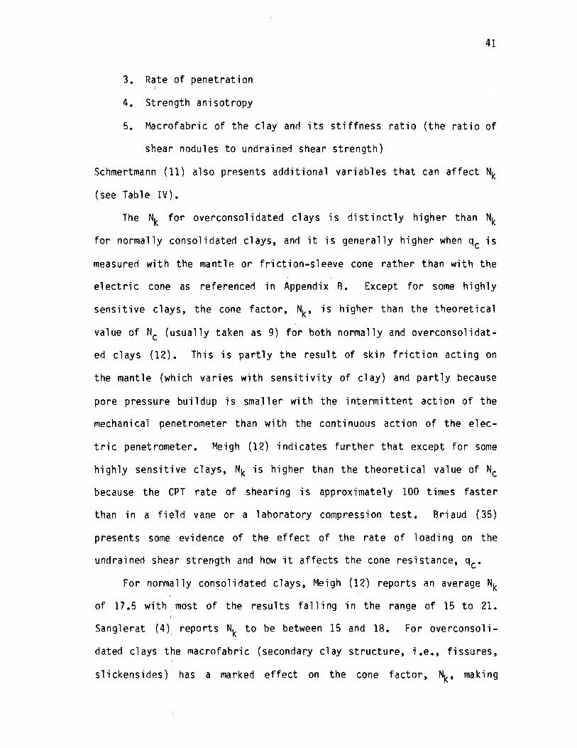
5. Macrofabric of the clay and its stiffness ratio (the ratio of
shear nodules to undrained shear strength)
Schmertmann (11) also presents additional variables that can affect Nk
(see Table IV).
The Nk for overconsolidated clays is distinctly higher than Nk
for normally consolidated clays, and it is generally higher when qc is
measured with the mantle or friction-sleeve cone rather than with the
electric cone as referenced in Appendix R. Except for some highly
sensitive clays, the cone factor, Nk, is higher than the theoretical
value of Nc (usually taken as 9) for both normally and overconsolidat
ed clays (12). This is partly the result of skin friction acting on
the mantle (which varies with sensitivity of clay) and partly because
pore pressure buildup is smaller with the intermittent action of the
mechanical penetrometer than with the continuous action of the elec
tric penetrometer. Meigh (12) indicates further that except for some
highly sensitive clays, Nk is higher than the theoretical value of Ne
because the CPT rate of shearing is approximately 100 times faster
than in a field vane or a laboratory compression test. Briaud (35)
presents some evi de nee of the effect of the rate of 1 oadi ng on the
undrained shear strength and how it affects the cone resistance, qc.
For norm~lly consolidated clays, Meigh (12) reports an average Nk
of 17.5 with most of the results falling in the range of 15 to 21.
Sanglerat (4) reports Nk to be between 15 and 18. For overconsoli
dated clays the macrofabric (secondary clay structure, i.e., fissures,
slickensides). has a marked effect on the cone factor, Nk, making

42
TABLE IV
SOME VARIABLES THAT INFLUENCE Nk ( 11)
Approx. Nc Factor
Variable Potential
1. Changing the test 2 to 3 method fQr obtain-; ng reference su
2. Clay stiffness 3.0 ratio = G/su
3. Ratio increasing/ 3.0 decreasing modu-lus (E+/E-) at peak Su
4. Effective fric- 2 to 3 tion, tancJ>
5. K0 or OCR 3.0
6. Shape of pene- 2.0 trometer tip
1.5
7. Rate of pene- 1.2 tration
8. Method of penetration
1.2
Oi rect ion
Better sampling, thinner vanes, use of suJ>MT all decrease Nc
Increases with increasing stiffness
Decreases with decreasing ratio
Increases with increasing cJ>
Increases with increasing K0 or OCR .
Clay adhesion on mantle of mechanical tips increases NC--
Reduced diameter above cone can decrease N in very sensitive clays
Increasing rate increases Nc
Notes
See Eq. ( 4)
Vesic (1972)
Ladanyi ( 1967)
Janbu (1974)
Jan bu (1974)
Example in Amar et al. (1975, Figure 2)
Schmertmann (1972b)
Viscous, no pore pressure effects
Continuous (electrical tips) . penetration decreases Nc compared to incremental (mechanical tips) because of higher pore pressures

43
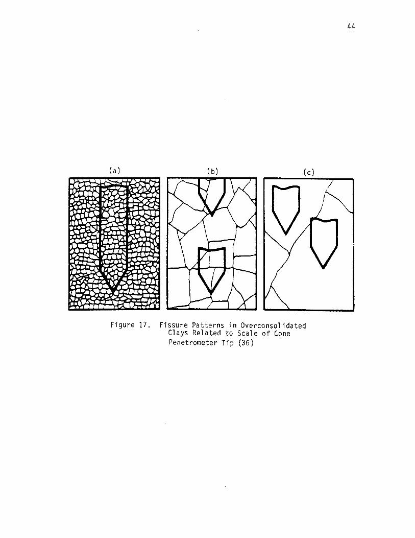
interpretation of shear strength more difficult and uncertain than in
normally consolidated clays. Marsland and Ouaterman (36) present in
their research three fissure and/or discontinuity patterns (see Figure
17). As observed in this figure, for case (a), the cone resistance
reflects the effect of fissures on the strength of the clay mass. For
case (b), the cone resistance only partly reflects the effect of fi s
sures. Case (c) indicates widely spaced fissures. In other research,
Marsland ( 37) further shows the influence of fissures by comparing
vane shear test results with various sized triaxial specimens (see
Figure 18). Other researchers ( 38, 39) indicate good correlation
between qc and pressuremeter results. The Nk range reported by Meigh
(12) for stiff fissured overconsolidated clays is 27±3. Sanglerat (4)
shows Nk values ranging from 22 to 26 for stiff clays.
Compressibility of Clay, Overconsolid
ation Ratio, Sensitivity
The conventional cone penetrometer, measuring qc and f s, does not
lend itself to reliable estimates of clay compressibility. Only in
direct methods have been developed by Schmertmann (11) and Sanglerat
(4). Schmertmann 1 s approach is based on estimating the overconsoli
dation ratio (OCR) to predict clay compressibility. In Sanglerat's
approach, an empirical relationship was developed mainly for the
mantle cone between the coefficient of constrained modulus (mv) and
tip resistance (qc) to estimate clay compressibility.
Some recent research by Tavenas and Lerouei 1 ( 40) and by Mayne
(41) used the cone penetration test to index the in-situ overconsol
idation ratio which affects clay settlement predictions. Schmertmann
(a)
Figure 17.
( b) ( c)
Fissure Patterns in Overconsolidated Clays Related to Scale of Cone Penetrometer Tio (36)
44

45
1. 2 ....._ ___ ..t.--___ ..__ __ __._ ___ __._ ___ .....
1.0
J:= -g' 0-8 QI .... -en - 0·6 u ,. -c:: ·-......
.s:: 0·4 -c:::.t c:: QI .... -= 0·2 QI -Cl. e ,.
0 en
T' Average vP.rtical strength:
\ \ \
• Glasgow boulder ciay • Blue London Clay
\ \ \ \ \ \ Boulder
clay London ', ~ fissure Clay ',, ... I: strength slide, ---- ·--.-~--'----·----· --- -----.I. -
/"///////////////.
102 io3 104 I 105 106 107
13 mm 38 mm J02 152 230 304,· 606 x 606 mm Hand Triaxial Triaxial tests Field shear box vane tests (mm)
Area of potential failure plane ( mm2)
Figure 18. Effect of Sample Size on Undrained Shear Strength of London Clay (37)
46
(11) and Robertson and CaPlpenella (31) report correlations between
clay sensitivity and FR and qc.

CHAPTER I I I
RESEARCH PROGRAM
Introduction
As indicated, the purpose of this research is to characterize
typical Eastern Oklahoma alluvial soils and develop localized rela
tionships between mechanical cone penetrometer parameters, qc and f s,
and the following: soil classification, SPT, undrained shear strength,
and clay compressibility through the estimate of OCR. There is need
for conducting research of this nature in order to expand the data
base on the merits and limitations of the mechanical cone penetro
meter. This equipment is simple in operation and has significant
practical use in many geotechnical engineering applications under
various geologic conditions. Cone penetrometer equipment and methods
have become increasingly more sophisticated (15, 30, 31). However, it
is believed that a proper perspective of the increased technological
advances in the cone penetrometer should be one of enhancement and not
total replacement of the mechanical cone with more advanced types.
CPT Test Equipment and Procedure
The cone equipment used in this research was the mantle and
friction-sleeve mechanical (Model No. E5705) and the electric cone
47

48
(Model No. 57035) supplied by the Hogentogler & Co., Inc. The
friction-sleeve used has the tapered mantle conforming to the LGM
specification NEN 3680 which was referenced earlier. The hydraulic
system of a CME 75 conventional drilling rig was used along with the
necessary conversion kit to advance the cones. A cam friction reducer
was used in all soundings. Recording of qc and fs was done by manu
ally reading hydraulic pressure gauges (direct reading of tip force in
Newtons). The actual equipment--cones, rods, and friction reducer,
hydraulic load cell and gauges, and CME 75 rig--used in this research
are shown in Figures 19, 20, 21, and 22, respectively.
The cone equipment and procedure followed ASTM O 3441-86. Care
ful. attention was paid to Section 6 of ASTM D 3441-86 at all sounding
locations.
Test Sites
The test sites for this research were selected to study typical
alluvial clays formed on broad floodplains in the northeastern quarter
of Oklahoma. Generally, the streams and rivers in this region are low
gradient tributaries of the Arkansas River. Typically, these alluvial
clays are found to occur to depths of 50 feet. They are highly pl as
ti c, desiccated, firm to stiff clays that tend to become soft and non
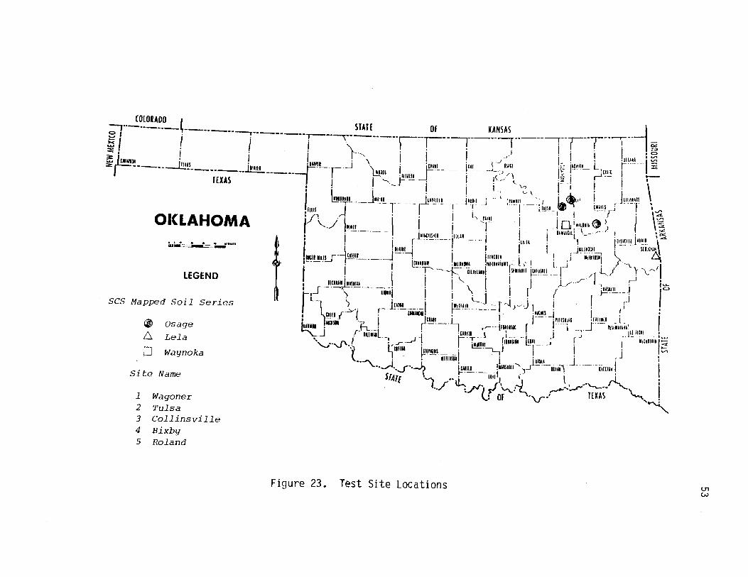
structed with depth. Three sites were mapped according to the USDA
Soil Conservation Service as Osage soil series, one as a Lela, and one
as a Waynoka soil series (see Figure 23). The sites are named for the
closest community within the vicinity (see Figure 23 for general loca
tions).

49
Figure 19. Mechanical and Electrical Cones

50
Figure 20 . Rods and Friction Reducer

51
Figure 21. Hydraulic Load Cell and Gauges

52
Figure 22. CME Model 75 Drill Rig
COlORADO I STATE Of KANSAS __ -·-.--·_] -.,--------~--------:--------.---,-------·r---r---.------r··----r---r T i I ~ C>f I . . I I I I . . I 1C> ~I I ! '\ ·1. i _)I. I ! ·Ulll!! .... ,. ~ ~ · · r ' I . · .../ ~. ·ma11 L I == : ' I I !1un1 _j \. · ·~•!_._ .. 111! __ -L.»111' 1 ·I~ !--· - 'E!~ _J ..-~,lc•111oa •um •11111 -r·- r 'auaas I j · ~· ./\ ~ I r1 ·
1 •
z -------"'--------'=------ , r~_i"'"" . 1 1 .- L'"' j'·; , . \ TEXAS : ! . . ! ! ' - : ' '- \' . ~L•' ! .J~l!!!•H - ,
I llllltlll J11111 _h1~1_1!. . __ jl~lt! _ _; ,r1w1.1l1 ___ !1' II L~ {Miii! j I '</' ~-T--- ·-,----, . ! ~ ~-t• I -I ' \~ OICLAHOMA
I 1. • a • • •llitll .. -----.-LEGEND
SCS Mapped Soil Series
@
£::.
0
Osage
Lela
Waynoka
Site Name
1 2
Wagoner Tulsa
3 Collinsville 4 Bixby 5 Roland
:f1 _). ·, ·. ! t..._ ~·,·!!_ -- ! ,. j 0 :t!~m ~-) l .~ I ....... ./ \11111 I I I . lll~ICllL -~· I 1' '.4 • .- ---·- - • i11~1~!• ___ ·1u~11_ -· __ j ·lllll ! 1 . jc"ucu!.. au~~- • \
' ' ' r I i 1-· --- -·-1 j~U!•~Cll_, . !IM•·a.\ I ~ ·~!~I ·1 '11m1• . - ! .l •111111i I.._. ~ ~ · CISlll , . . - , . , /" '\. .~ .. 11~!.J · ·------l ~11111 ·!!!!•'~~ . .1111111111111- I., ! L 1 __ J , J r '-~'I .- . ! -T' --..---K. curiull! .11111111 !~~I'!! __ . .r ,rt-....... ,.i , I ! I ·1 . \... I I J ,l_r-- l, . 10 1 . .Jl_CIUl1 Ir•!!!!! . _ __ c• • I \ , j j ( · _ft.Ill!!__ - ! I '- J \. 1• 111 I I i J · • · [ r-' , I l • • ..._ .,.~ J I . J
l. ) _h1111 1111~!!...._ _ ..:._· . .:_ , J ~. 1 · j I :
l r..::.--'(. : ·-tliiiclil ~ j J·~U~S -!,llllibiC ·_II!~' _ i. I , t,,c1111 J I lm11 L. · I- ---. J M11M111K1' ~• liiaiii .. ? • r-·-· I ,~--Lr~llllC r . L.-!. - i'!~l!ll - : ...... 111111 J' rn...·-t . ·m111 ~ ,_ -i.. ,I r J 11ui111•1-
. . IAllll . .., r _J r . T . ·- f11us111 ~"-. _j • I ~ •• •. I . , .r- . ...r ! I ~~· . ! I . V"I
'-' -...I'·.:~ t' ctn11 ~1.r~s _ __1. -..., I ! . , J I \. 1 · , KllllSll i 11111 . _ _j ____ --- -""""\.. •. _..i .... r·4 µ•~!!!...·-,.,i[li1111ii~y-1~---,i11l mmw! !
s141£ l.J~·-~ . s11·"'-rl ,..-.,.;._r-·'""'--l'"-.~ I ./' {., Of -v-' TUAI ''°'\
Figure 23. Test Site Locations U1 w
54
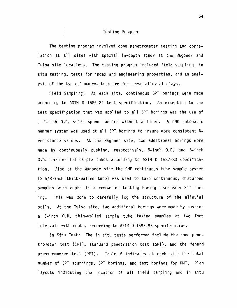
Testing Program
The testing program involved cone penetrorneter testing and corre-
1 ati on at all sites with special in-depth _study at the Wagoner and
Tulsa site locations. The testing program included field sampling, in
situ testing, tests for index and engineering properties, and an anal
ysis of the typical macro-structure for these alluvial clays.
Field Sampling: At each site, continuous SPT borings were made
according to ASTM D 1586-84 test specification. An exception to the
test specification that was applied to all SPT borings was the use of
a 2-inch o.o. split spoon sampler without a liner. A CME automatic
hammer system was used at all SPT borings to insure more consistent N
resistance values. At the Wagoner site, two additional borings were
made by continuously pushing, respectively, 5-inch o.o.· and 3-inch
O.D. thin-walled sample tubes according to ASTM D 1587-83 specifica
tion. Also at the Wagoner site the CME continuous tube sample system
(2-5/8-inch thick-walled tube) was used to take continuous, disturbed
samples with depth in a companion testing boring near each SPT bor
ing. This was done to carefully 1 og the structure of the alluvial
soils. At the Tulsa site, two additional borings were made by pushing
a 3-inch o.o. thin-walled sample tube taking samples at two foot
intervals with depth, according to ASTM D 1587-83 specification.
In Situ Test: The in situ tests performed include the cone pene
trometer test (CPT), standard penetration test (SPT), and the Menard
pressuremeter test ( PMT). Table V indicates at each site the total
number of CPT · soundings, SPT borings, and test borings for PMT. Pl an
layouts indicating the location of all field sampling and in situ
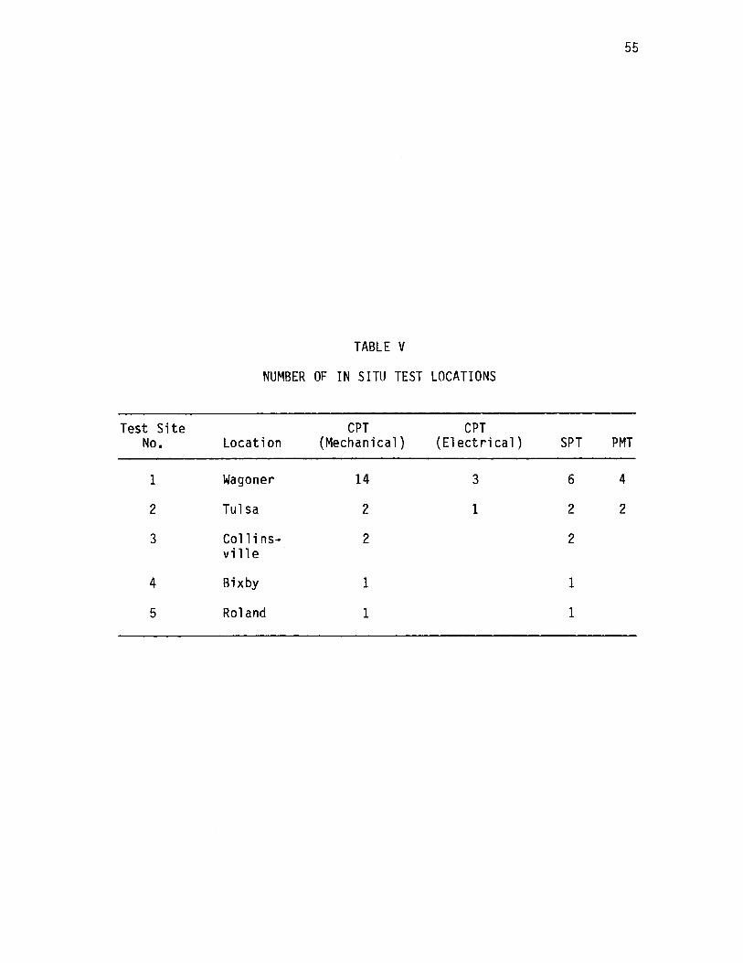
55
TABLE V
NUMBER OF IN SITU TEST LOCATIONS
Test Site CPT CPT No. Location (Mechanical) (Elect ri cal ) SPT PMT
1 Wagoner 14 3 6 4
2 Tulsa 2 1 2 2
3 Collins- 2 2 ville
4 Bixby 1 1
5 Roland 1 1

56
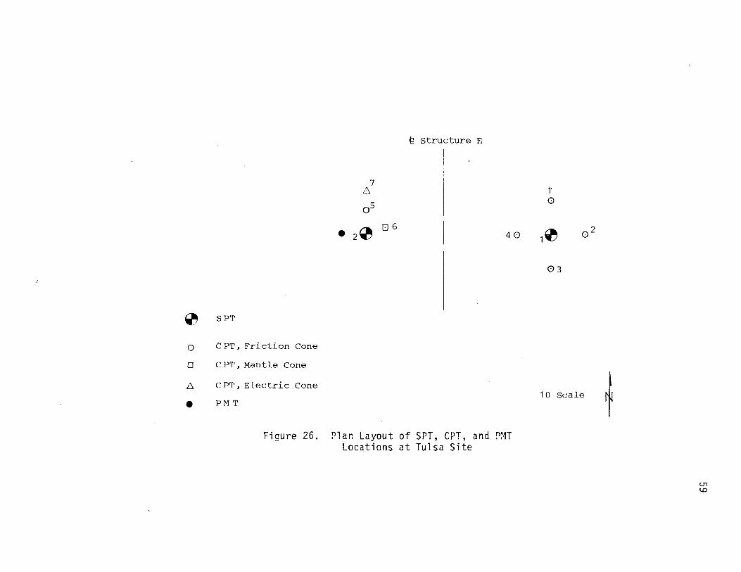
tests for ~he Wagoner and Tulsa sites are presented in Figures 24, 25, i I
and 26, re~pectively. The location of SPT borings and mechanical CPT
soundings are noted on the boring logs.
The CPT soundings were made at all sites adjacent to completed
test borings according to ASTM D 3441-86 test procedure. Additionally,
three mechanical Dutch mantle and four electric cone soundings were
made according to ASTM D 3441-86 test procedure at the Wagoner and
Tulsa sites for comparison with the mechanical friction sleeve cone.
The SPT 11 N11 resistance values were as noted earlier conducted contin-
uously according to ASTM n 1586-84 at all sites. The Menard pressure
meter test ( PMT) was made at four borings at the Wagoner and Tulsa
sites to measure the in situ undrained shear strength. The test was
conducted at three-foot intervals in each boring according to ASTM 0
4719-87. To insure as precise a measurement of undrained shear
strength as possible, the borings were made with a hand auger.
Test for Engineering Properties: Atterberg Limits (LL, PL) were
conducted according to ASTM D 4318-84 specification. All specimens
were seasoned 24 hours before running tests. Particle size analysis
of all samples was made according to ASTM D 422-63 (Reapproved 1972)
specification. A measure of the consistency of these alluvial soils
is represented by the liquidity index (42) and by correlation with the
SPT 11 N11 resistance values (see Table III). One-dimensional consolid
ation tests were conducted according to ASTM D 2435-80 specification
to quantify the typical stress history of these alluvial clays. Cor
relation of lthe undrained shear strength based on 1 aboratory tests I
with total lone resistance values from CPT soundings was made by
undrained uncpnsolidated (lllJ) triaxial tests. Tests were performed on

I tf 5H51
-~} 7., 897' I 538.0 I
-1 15.0 1· f\i •., _j_ 12 13
0 1 T• \ • • 16'
<i •s3 on I· I
14- 1.5 /H.5 10~ +,, ----- ---- ------
0 s4- 1i···· ~ l---aq.1 I i 8't7 1 {.I.~ _LZL 110
•s • • 695 ( 5 I I :J II 2..
---------·- ----------- -
• CPT
S SPT
Teat ait• layout referenced to CPT Locations.
Hean Blevation 522.25 feet with maximum differential bet-en SPT and CPT of 0.85 feet.
60 Scale·
Borrow Pit
1
Figure 24. P Ian Layout of SPT and CPT (Friction Sleeve) Locations at Wagoner Site. (J1
-...J

11207.
Ill 0
0 114 11109•• 11108
r--89.67'--1 • • 11113 11112
E SH 51
112 0 11106
11201 • : 11107
~ (
LEGEND BORROW PIT SPT0 CPT •
FRICTION CONE - 107,109,110,112,113 MANTLE CONE - 106,108,111 ELECTRIC CONE - 201,202,207
f 60 SCALE
Figure 25. Plan Layout of CPT Locations Used for Cone Resistance Comparison and PMT Locations at Wagoner Site
0113 • 11202
<.Tl CX>
~
0
0
~
•
{'. Structure E
7 6
I 05
• 2 ~ [] 6 I 40
SPT
C PT, Friction Cone
C PT 1 Mantle Cone
C PT, Electric Cone
PM T
Figure 26. Plan Layout of SPT, CPT, and P~T Locations at Tulsa Site
1' 0
1~ 02
03
10 Scale ~
U1 ~
60
1.4-inch diameter specimens according to ASTM D 2850-87 specification.
Tests were also conducted on single 2.8-inch diameter specimens in a
multi-stage loading (43).
Clay Structure Analysis: Detailed field and laboratory obser-
vations were made on all samples for structure according to ASTM D
2488-84. In addition, typical structural patterns were photographed
with depth on partially air-dried samples.
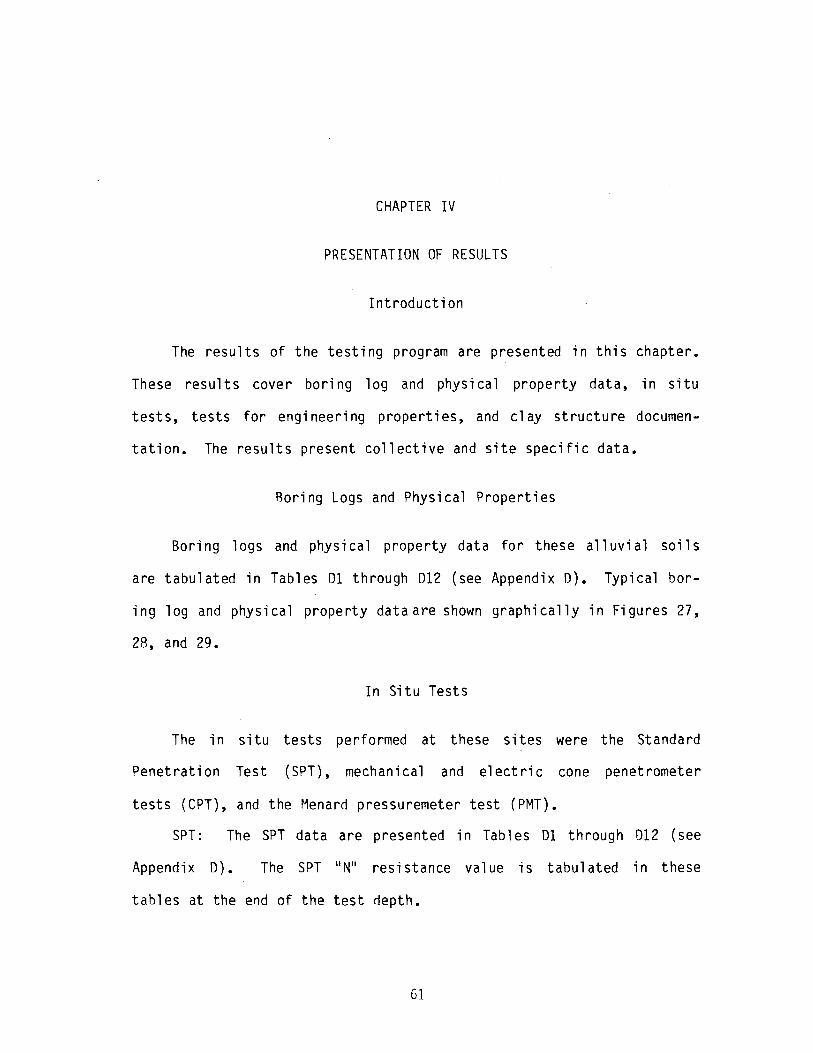
CHAPTER IV
PRESENTATION OF RESULTS
Introduction
The results of the testing program are presented in this chapter.
These results cover boring log and physical property data, in situ
tests, tests for engineering properties, and clay structure documen
tation. The results present collective and site specific data.
Roring Logs and Physical Properties
Boring logs and physical property data for these alluvial soils
are tabulated in Tables 01 through 012 (see Appendix 0). Typical bor
ing log and physical property dataare shown graphically in Figures 27,
28, and 29.
In Si tu Tests
The in situ tests performed at these sites were the Standard
Penetration Test (SPT), mechanical and electric cone penetrometer
tests (CPT), and the Menard pressuremeter test (PMT).
SPT: The SPT data are presented in Tab 1 es 01 through 012 (see
Appendix D). The SPT 11 N11 resistance value is tabulated in these
tables at the end of the test depth.
61

62
w~ Mo1sTute " ~ . I .o .. "l'e.r- l 0 1-:.
20 40 60 o.+ 'N'
l/J.~. ::i-
24 "''"' 2.1o' 7 Fa.+ C/o.'f
4 -~.7
4 Faf C!.?'f
h.3 4-I
4 I
Fat Ci"') 5' ~
9.7 t---6 7 IA
r. Fc.t C\o't
8
6 14 I to I
/~.+ B 1---6 I Fo.+ c ':._'( IA
II i-...c. IS.S ~ .. ., Cla'{ /'/.I.
IA
Ci<>.y ~ L.eari 10 14 I
1--.6 I
4- lean Cl"'f 1-.t. I
C.l°"I w/ So net ..........0. I
l.eo11 r66f' 3 l.ec.P) C.loy 1---<!1 I \.eo.- Cloy w/ S~ncl.. 1, ~I
l-5oncly Le""' Cioy I L.e.on C,o.~
~ 1---1 c..
I
2.-- Si I~~ 5,. <I. I I
s,.,..d:'I 5;1+y c1 .. y 1--1 c.. 1· SiJ+'I Clo'{B'f so~ci
,___, c.. I "' lo-IA
5, H''I So.not· -~P-
5 5c;i .,CJ,1 s·, !+y Cla'I 1--lL I 5.lfy -;;~ ..... -/IP- PL LL
llo 5ilty S••d. w/ G•o·,d --NP- I A I I
31.J PooP I~ G~o.d1:l 5,,,.,.;; ..,/-;,., ,, --ttP- M.C. I 17
Sil+~ so. .. d, w/ Gro .,1 I -II?- ! -II().-
I 17 t---i Clc..~e~ So."~ w/ ~'""~I 1---i
Leo 11 Clay< ~eofl.ered ;b/L) ! ; .
Figure 27. Boring W2 at Wagoner Site

Tl
STATION 440+78,LT. 33 FT. ELEVATION 596.54 FT.
0·.2 0.8
8. 3
11.1
12.0
14. 3
15.0
16. 5
21.9
24.0
25.5
26.3
28.5
31.5
33.0
33.9 34. 5
36.8
39.7
40.5
42.6
44.1 44.6 45.1
46.4 47.1 47,7
Ma6
LEAN CLAY WITH SA.'ID LEAN CLAY
LEAN CLAY
FAT CLAY
FAT CLAY
FAT CLAY
LEAN CLAY
W.L. 12.7' AT 48 HRS. ---LEAN CLAY WITH SAND
LEAN CLAY
LEAN CLAY WITH SA.'ID
LEAN CLAY
LEAN CLAY
LEAN CLAY WITH SAND
LEAN CLAY
LEAN CLAY
LEAN CLAY WITH SAND
SANDY LEAN CLAY SANDY LEAN CLAY.
SANDY LEAN CLAY
LEAll CLAY WITH SAND
SANDY LEAN CLAY
SIL TY CLAYEY SAND
SANDY LEAN CLAY SILTY SAND SANDY LEA!! CLAY
SILTY j;..:;c
SILTY SAND WITH GRAVEL SILTY CLAYEY SAND Witll GRAVEL
LEAll CLAY (WEAtllERED SHALE!
MOISTURE CONTENT,, 10 20 30 40 50 60
PL MC
Figure 28. Boring Tl at Tulsa Site
63

64
Rl MOISTURE CONTENT,% 10 30 50 70 90 110
1.0 FAT CLAY FAT CLAY A
1. 5 FAT CLAY A
2.0 A A
A n
FAT CLAY A A
AA 6.5 A
A 7.5
FAT CLAY 6. FAT CLAY 6.
8.5 6.A A
6. FAT CLAY A
A A
12.5 A A
FAT CLAY 14.0 6. 14.5
FAT CLAY A A FAT CLAY A
16.0 A A
A 6. t---1
A A A A
A A
A A
FAT CLAY t:. A A " -
t:. ""'' A 28.2
0
29.8 LEAN CLAY A FAT CLAY 6.
31.0 LEAN CLAY It!;
31.5 A FAT CLAY A
32.0 POORLY GRADED 33.5 SAND WITH SILT NP
EOB PL MC LL
Figure 29. Boring RI at Roland Site

65
CPT: The CPT data are tabulated in Tables El through E12 (see
Appendix E). Typical graphical presentation of these data is present
ed for sounding W22 at the Wagoner site in Figures 30, 31, and 32.
PMT: Undrained shear strength based on PMT test data is given in
Table VI. A typical graphical presentation of a typical PMT test
parameter is shown in Figures 33a, h, and c.
Comparative Data: The variation in the SPT 11 N11 resistance value
for all SPT borings at the Wagoner site is given in a composite 11 N"
versus depth profile in Figure 34. Variations in the cone resistance
and local friction with depth at the Wagoner site is shown in Figures
35 and 36. Additional comparative cone data indicating the relative
uniformity of the suhsoil at the Wagoner site are presented in Tables
Fl through F7 (see Appendix F). A comparison made between the cone
resistance of the Dutch mantle and the friction sleeve mechanical
cones for 1 ean and fat clays at the Wagoner and Tulsa sites is pre
sented in Tables Gl through G3 (see Appendix G). Typical graphical
presentations of the cone resistance comparison are shown in Figures
37 and 38 for the Tulsa site. A comparison of the cone resistance
between the friction sleeve mechanical cone and electrical cone for
the Wagoner anrl Tulsa sites is given in Tables Hl through H4 (see
Appendix H). Graphically, the electric cone data are shown in Figure
39 for W201 at the Wagoner site. A summary of these qc ratios is
presented in Tables VII and VIII, respectively.
The stress history, specifically the overconsolidation ratio
(OCR) typical of these alluvial clays, is shown in Table IX with depth
for boring, Tl at the Tulsa site (see also Figure 28). A typical con
solidation test showing the calculation for the preconsolidation pres-
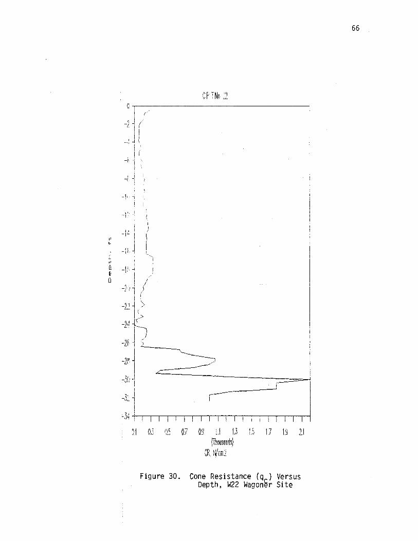
-J)
r: p· T~.1. :n .. 1~C ...... 1::1 ~--------------------,
. --2 I
<. _II,•
~ ,l ! -1't -1
i
< i -if: 1
I
.r
! ·'.:1j ()j 1:,1_~ {)] IJ~J J.1 1j 1_5. 1.7 JJ 2.1 \fbr.~sana3}
1"f:· Ui.- 'I '..f•., I'~' Lilli
Figure 30. Cone Resistance (qc) Versus Depth, W22 Wagoner Site
66

.f.' ~
[ ;.•
~ (' LI
C'
-21 -4 ~
I I
-H I
,n, ~ ...
j -1{:1 ·1
I
I i'"I I
-IL 1 ! I
'I I -j't I
i -H,~
I -J.r· ~ .. I -,;_',} 'I'' i -n ~
-24 j -26
-18
i"PTN '.1'.1 '•' ~. ""-
-·- -·
"'-~-----
? (
___ ) L __ _
----=--
-Yt1 --=============-_,, j '''-
-J4
-f~}
-==-----....... --==:::::-::,. ------~
-(:1
lF, N/rm1
Figure 31. Local Friction (f 5 ), W22 Wagoner Site
67
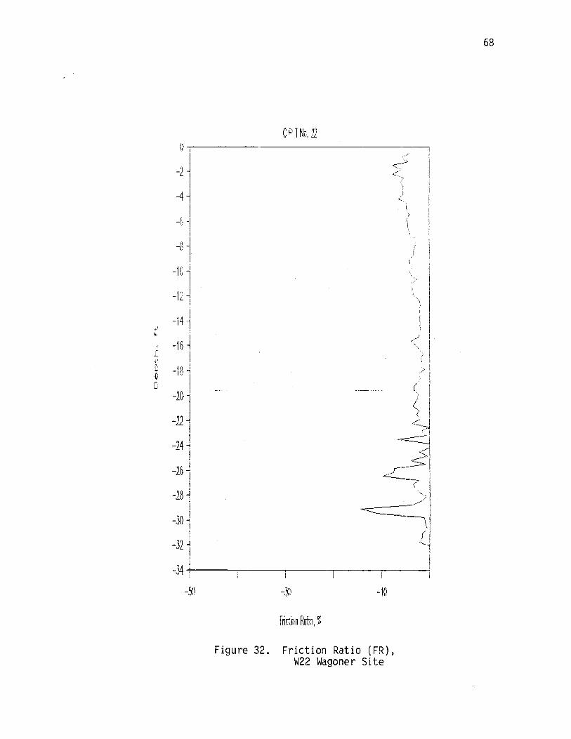
(} I
_., J L I
:1 I
-s ~ I
-ji'\ ~ " I
-rd "- I I
4 I +'
-i 1 \- I
-1H [ I +' fJ. -18 ~ (1
0 -20
-21
-14
-26
-28
-J-0
-31
-J.4 I
-JI)
f'PTN '!'.! ... I},""'-
<\ .I
·~-
·-i..
\
/ i
·~··
1
·,_ -.,. ________ ... ..... _____ '
-10
- ... \ t "·--
Figure 32. Friction Ratio (FR)t W22 Wagoner Site
68

TARLE VI
UNDRAINEO SHEAR STRENGTH BASED ON PMT OATA FROM WAGONER AND TULSA SITES
Sample nepth ac PL Po Su Nka Nkb
Location No. (ft) (ts f) (tsf) (tsf) (1) (2) (1) (2) (1) (2)
Wagoner, SPT No. 1 1 2 .1 36.0 3.33 0.20 0.50 o. 77 71.8 46.6 72.0 46.8 Wagoner, SPT No. 1 2 5.1 27.2 3.75 0.20 0.57 1.16 47.4 23.3 47.7 23.4 Wagoner, SPT No. 1 3 8.1 20.9 4.05 0.33 0.60 1.00 34.3 20.6 34.8 20.9 Wagoner, SPT No. 2 1 2.1 11.0 2.40 0.33 0.33 0.68 33.0 16.0 33.3 16.2 Wagoner, SPT No. 2 2 5.0 14.6 3.25 0.30 0.48 0.90 30.0 16.0 30.4 16.2 Wagoner, SPT No. 2 3 8.0 17.8 4.15 0.28 0.62 1.24 28.2 14.1 28.5 14.3 Wagoner, SPT No. 2 4 11.0 20.4 5.13 0.43 0.76 1.64 26.3 12.2 26.7 12.4 Wagoner, SPT No. 2 5 13.8 20.4 5.50 0.78 0.76 1.83 26.2 10.9 26.7 11.1 Wagoner, SPT No. 2 6 16.7 21.4 5.88 0.79 0.82 1.58 25.4 13.2 26.1 13.5 Tulsa, SPT No. 1 1 3.7 18.8 4.30 0.60 0.60 1.23 31.0 15.1 31.3 15.2 Tulsa, SPT No. 2 2 6.8 17.8 5.01 0.80 0.68 1.28 25.6 13.6 26.2 13.9 Tulsa, SPT No. 3 3 9.8 24.0 7.16 1.10 0.98 1.59 23.9 14.7 24.5 15.1
Averages 33.6 18.0 34.0 18.3
Notes: Su (!)--Undrained shear strength based on PMT limiting pressure. Su (2)--Undrained shear strength based on Gibson and Anderson (44).
aNk (!)--Factor based on using Su (1) in Equation (6).
(2)--Factor based on using Su (2) in Equation (6).
bNk (!)--Factor based on using Su (1) in Equation (7).
(2)--Factor based on using Su (2) in Equation (7).
O"I l.D

a} L1ait1ng Pressure Method oE Bst11m11tln~ b} Gibson and Anderson Method of Estimating Su plots p-loge Aviv
u u
Su ls based on P0 and P ('l'aken frot1 plots oE V-P and Inverse V-P}.
from the Plastic Phase. s Eound u
IQ!)
SOD
-
as the slope of the line •(7}.
Pseudo-Blastic Phase? 1
Plastic Phase)
I I I I
I I I
·-·------·-----.
// ,/
-<{"
~/~/ ~-
~ _,~__.\.--___,,------· .J---· .
..... g
ltlO
o ....... ~~-'-_,_~~~~~~~-'-~~~-'-~~~-l~~~--'~~~--''---~~--''--~~~.1-.~~~.._~~~_,_~--''--' 0 .soo ,000 /400 ,!!IOOO ~300 .:/000 ~ 4000 4'°"' ~ ssoo .:.ooo
~ ~ ~ Pressure, Psf
Figure 33. Volume Versus Pressure at Depth of 8.1 Feet Near SPT 1 at Wagoner Site. -....i
0

71
2000 (c)
-7
/ 1000 /
900 / 800 / .~
700 ("')
::;: u 600
/ ..... / ~
/ '-.!
~ c-
0 z H 500 0 < IJ:l CG
IJ:l ::;: :::> ...J 0 400 >
Vo c::i
- - - - - - _,.... - 7 - - - - - __ ,_ - -- - - -
- - - - -7 V-__ - - - - - - -1- - -- - --
0 IJ:l ~ u IJ:l CG CG - - - - - - -- - -- - - - ...__ - - -- - -- - - -0 u ::... 0
IJ:l Ul 300 CG IJ:l > z H
- - - .__ - - _,_ - -- - - - .._ - - --- - -- - - -
200 3000 4000 5000 oi>OOO '1000 sooo
CORRECTED PRESSURE (POUNDS/FT2 )
Figure 33. Continued
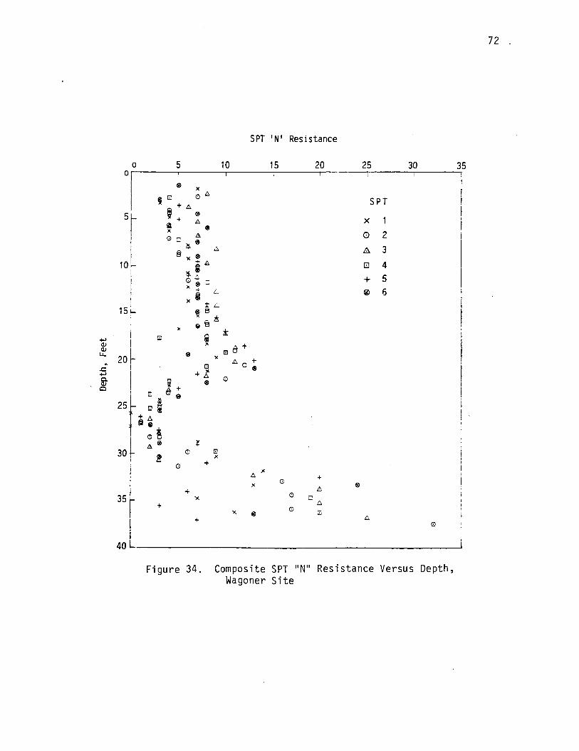
I I I
0
15 f-
5
+
+
G
+l e
+
+
8 )(
10
0
x
SPT 'N' Resistance
15
0
0
0
20
+
25
SPT
x 1
0 2
.8 3
0 4 + 5 ® 6
30
Figure 34. Composite SPT "N" Resistance Versus Depth, Wagoner Site
72 .
35
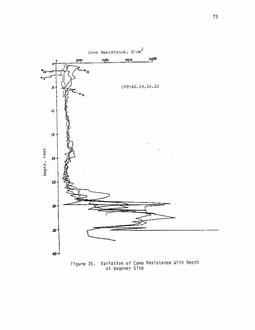
5
10
15
zo
2S
. I 2 Cone Resistance, N cm
CPT-10,13,16,22
Figure 35. Variation of Cone Resistance With Depth at Wagoner Site
73

..c
.µ 0. Q) 0
. . I 2 Local Friction, N cm
c I LJ
-- '
' C,PT ~~ ID, 1:i, lu ... 22.) -
- - - ------+------+ - t
__ ·--:.._ ~ t::: :-~_-::_ ~~+~~- ----E-- ~~ ==-===-::t..--=--=:-=;;:-~-- - --+--1
~---+-----+---~--+-~---+------+
Figure 36: Variation of Local Friction With Depth at Wagoner Site
74
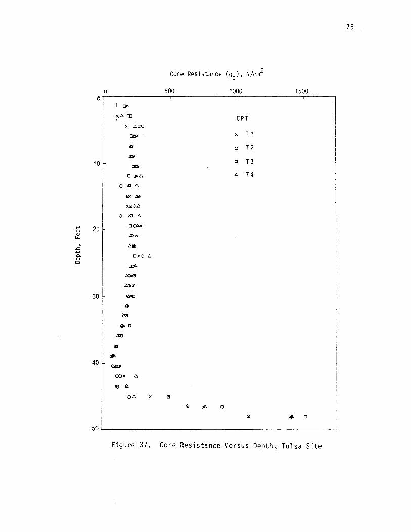
75
Cone Resistance (qc), N/cm2
0 500 1000 1500
01 1 alt>
X A Gl::J CPT x il.00
00< x T 1
10 f O' 0 T2 0
T3 0 m
0 ();Ll. A T4
0 :e:J 8
i:x ~
XG08
0 >C:J A
-+-' 20 8~ CL> CL> $X LL.
..r:::::. 811)
-+-' Cl.. O><O 8 CL>
0 ~
COlC:J
4lQ(C3
30 e>O
0
as (ti C3
Ll:.tl
a [!It.
40 003(
OOK A
'l€l 0
oA x 13
0 )tt> a Gl ~ Cl
50
Fii gure 37. Cone Resistance Versus Depth, Tulsa Site

.µ Q) Q) µ,,
£ 0. Q)
0
Figure 38.
. I 2 Cone Resistance, N cm
.. ·~·~·~ ~-0 d ~-Fr.c.'4--ion. C.or'l~
+-4-o&- Ma.n+1~ c:.or; ...
·-~--- -----+---- --~ --- - -- -- -l----- - - -
. - -·--·----- --- --------·-- ----- -----··· --- ·- -·--- ... ----- ---- . - . -----i-------
·-=-===--=====:~--~=-_:__==:==:.-~-=~-i_-~~~ ·:--------------- . ---·-----
--------+-------- ---.l..-- -- ·- --
Comparison of Cone Resistance Between CPT 5 and 6 at Tulsa Site
76
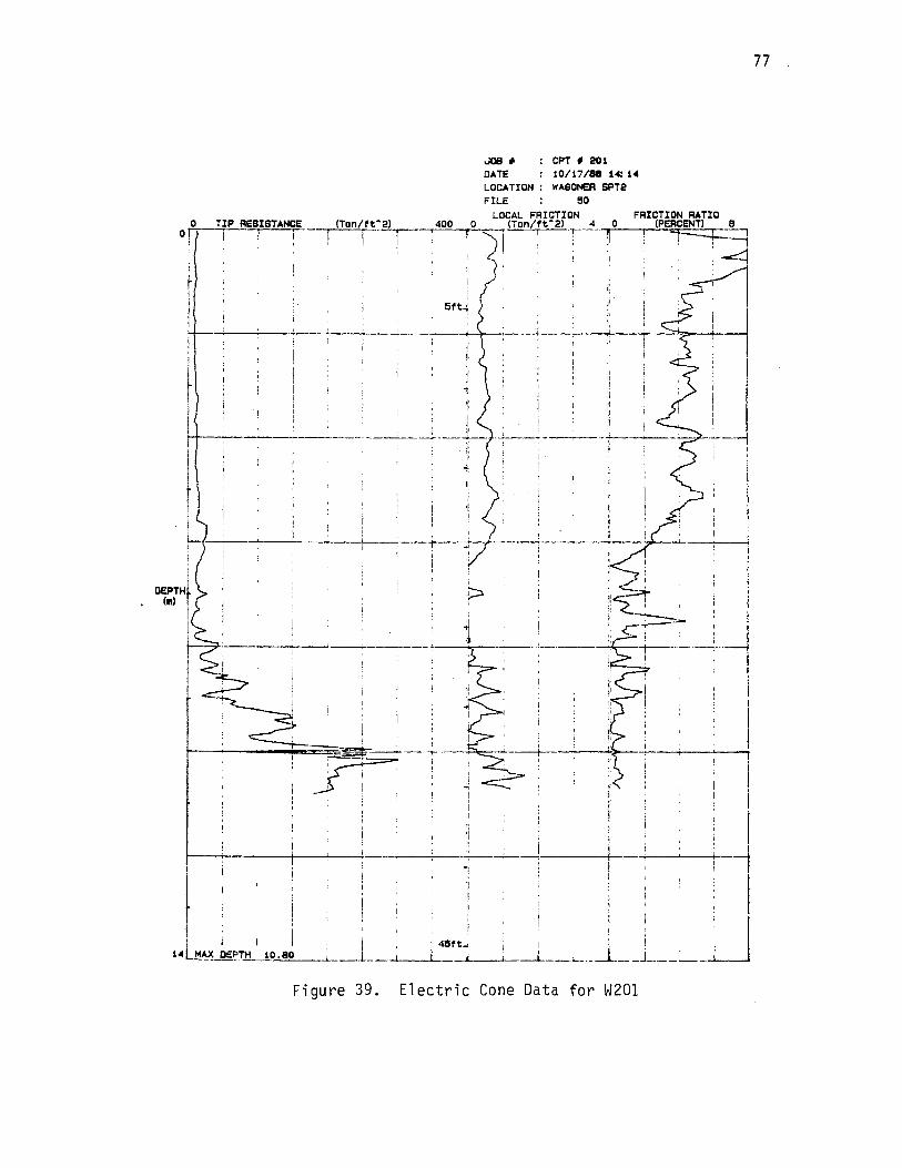
0 01
I
TIP RESISTANCE ! --
.JOB,. DATE
CPT • 201 10/17/88 1.C: 1.C
LOCATION : WA60NER SPT2 FILE 50
LOCAL FRICTION FRICTION RATIO (Ton/ft•21 400 0 (Ton/ft.21 4 0 (PERCENT) 8
-·-r-~~~ r. ·---~. . -~-i
I ! I ; j ' ' : I
5f t~
.-+-------<---_;_- ·-' --· --' -- ---+-----+-----+--
--.-----;----·-----··---·---~-----t---
p
i --...-----···--·---
~ . i I
t l ;: ! lJ; , _J. . L' 4!1ft.... : 1 :
...._ _-1__ ----''---~-~--~- _ _l ___ J_. ___ ' --·
---t----'.---· -
f I . I I I
1.C~AX DEPTH 10.80
Figure 39. Electric Cone Data for W201
77

TABLE VII
SUMMARY FOR qc MANTLE/qc FRICTION
From For CH Soils Table Range Average Std. Dev. Range
8-A 1.7222-0.8333 1.1535 0.2516 2.3000-0.8462
8-B 1.4000-0.8750 1.1194 1.1194 1.9000-0.8750
8-C 1.2400-0.7500 1.0862 0.1363 3.7692-0.8400 1.1197
For CL Soils Average
1.2510
1.1189
1.2473 1.2057
Std. -Dev.
0.4274
0.3275
0.5019
...... 00

TABLE VIII
SUMMARY FOR qc FRICTION/qc ELECTRIC
From For CH Soils Table Range Average Std. Dev. Range
8-0 3.7778-1.0952 1.9917 0.7059 2.3000-1.3000
8-E 2.4444-1.1000 1.5969 0.3241 2.2500-0.5926
8-F 3.1667-1.1111 1.4668 0.4621 1.6111-1.1250
8-Ci 1.7857-1.1250 1.3253 0.1961 2.3846-0.3059 1.5959
For CL Soils Average
1.6377
1.2043
1.3628
1.2542 1.3648
Std. Dev.
0.3189
0.5013
0.1845
0.4402
......, I.()
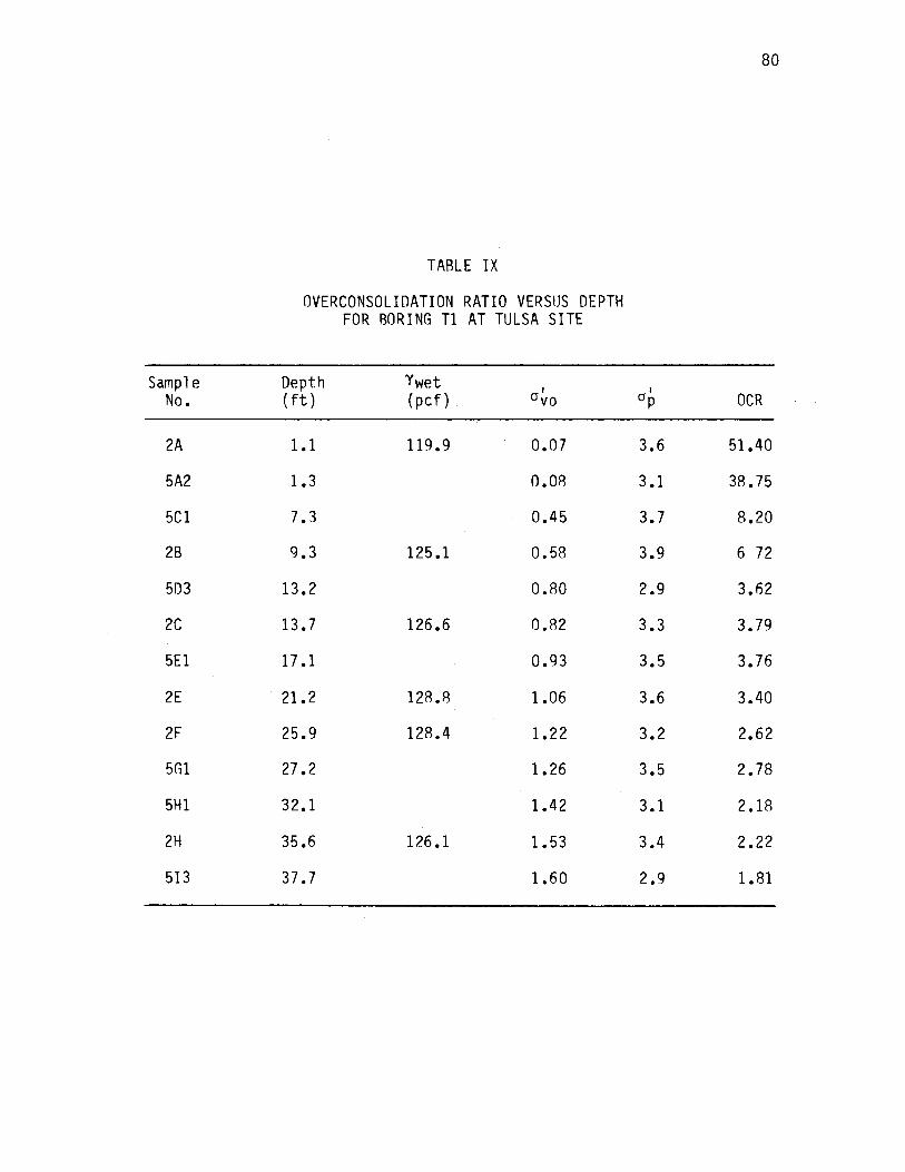
Sample No.
2A
5A2
5Cl
2B
503
2C
5El
2E
2F
5Gl
5Hl
2H
513
TABLE IX
OVERCONSOLIDATION RATIO VERSUS DEPTH FOR BORING Tl AT TULSA SITE
Depth Ywet I
(ft) ( pcf) . 0 vo
1.1 119.9 0.07
1.3 0.08
7.3 0.45
9.3 125.1 0.58
13.2 0.80
13.7 126.6 0.82
17.1 0.93
. 21.2 128.8 1.06
25.9 128.4 1.22
27.2 1.26
32.1 1.42
35.6 126.1 1.53
37.7 1.60
80
I Op OCR
3.6 51.40
3.1 38.75
3.7 8.20
3.9 6 72
2.9 3.62
3.3 3.79
3.5 3.76
3.6 3.40
3.2 2.62
3.5 2.78
3.1 2.18
3.4 2.22
2.9 1.81
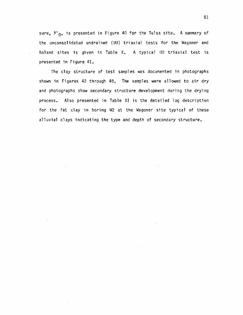
81
sure, P1 0, is presented in Figure 40 for the Tulsa site. A summary of
the unconsolidated undrained {UU) triaxial tests for the Wagoner and
Roland sites is given in Table X. A typical UU triaxial test is
presented in Figure 41.
The clay structure of test samples was documented in photographs
shown in Figures 42 through 48. The samples were allowed to air dry
and photographs show secondary structure development during the drying
process. Also presented in Table XI is the detailed log description
for the fat clay in boring W2 at the Wagoner site typical of these
alluvial clays indicating the type and depth of secondary structure.

Q)
+-' ....... V1
<O Vl
+-' Vl Q) I-
c 0
+-' <O
"O
0 Vl c 0 u
0 o:::j"
Q) S::i c::n
LL.
82
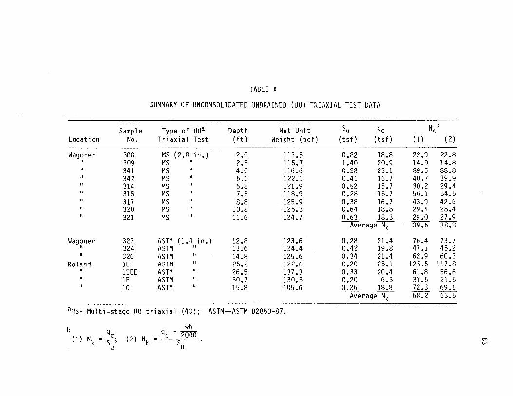
TABLE X
SUMMARY OF UNCONSOLIDATED UNDRAINED (UU) TRIAXIAL TEST DATA
Sample Type of uua nepth Wet Unit Su qc Nkb
Location No. Tri axial Test (ft) Weight ( pcf) (tsf) (tsf) (1) ( 2)
Wagoner 308 MS { 2. 8 in.) 2.0 113.5 0.82 18.8 22.9 22.8 309 MS 2.8 115. 7 1.40 20.9 14.9 14.8 341 MS 4.0 116.6 0.28 25.1 89.6 88.8 342 MS 6.0 122.1 0.41 16.7 40.7 39.9 314 MS 6.8 121.9 0.52 15.7 30.2 29.4 315 MS 7.6 118.9 0.28 15.7 56.1 54.5 317 MS 8.8 125.9 0.38 16.7 43.9 42.6 320 MS 10.8 125.3 0.64 18.8 29.4 28.4 321 MS 11.6 124.7 0.63 18.3 29.0 27.9
-rverage~ 39.6 38.8
Wagoner 323 ASTM (1. 4 i n. ) 12.8 123.6 0.28 21.4 76.4 73.7 II 324 ASTM 13.6 124.4 0.42 19.8 47.1 45.2 II 326 ASTM 14.8 125.6 0.34 21.4 62.9 60.3
Roland lE ASTM 25.2 122.6 0.20 25.1 125.5 117 .8 II lEEE ASTM 26.5 137.3 0.33 20.4 61.8 56.6 II 1F ASTM 30.7 130.3 0.20 6.3 31.5 21.5 II lC ASTM 15.8 105.6 0.26 18.8 72.3 69.1
--;\VerageT 68.2 63.5
aMS--Multi-stage UU triaxial (43); ASTM--ASTM D2850-87.
b qc yh
qc - 2000 (1) N =-· (2) Nk =
Su . (X)
k s ' w u
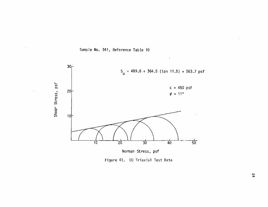
4-VJ 0.. .. VJ VJ
~ ~ s...
"' Q) ..c I.I)
30
20
Sample No. 341, Reference Table 10
S = 489.6 + 364.5 (tan 11.5) = 563.7 psf u
Norman Stress, psf
c = 450 psf !6 = 11°
Figure 41. UU Triaxial Test Data
50
ex:> .i::=.

Figure 42. Secondary Clay Structure, Fissures, Sample BA at Boring W4, Wagoner Site
85

Figure 43. Secondary Clay Structure, Fissures, Sample BB at Boring W4, Wagoner Site
86
Figure 44. Secondary Clay Structure, Fissures and Slickenside, Sample 8C at Boring W4, Wagoner Site
87
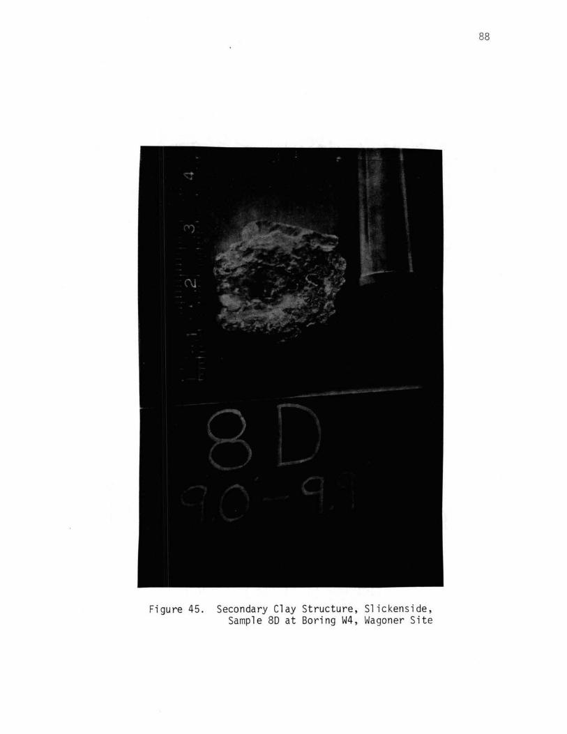
Figure 45. Secondary Clay Structure, Slickenside, Sample 80 at Boring W4, Wagoner Site
88
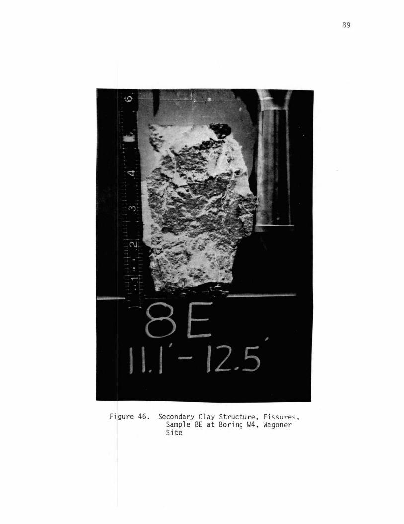
Figure 46. Secondary Clay Structure, Fissures, Sample 8E at Boring W4, Wagoner Site
89
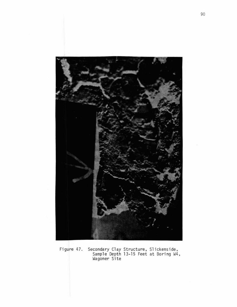
Figure 47. Secondary Clay Structure, Slickenside, Sample Depth 13-15 Feet at Boring W4, Wagoner Site
90
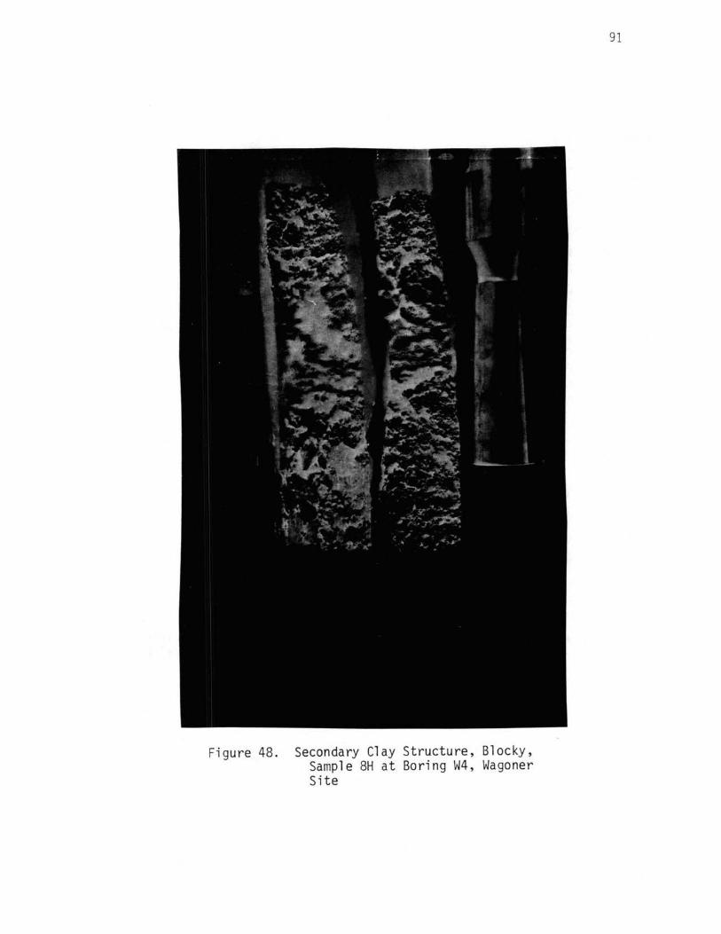
Figure 48. Secondary Clay Structure, Blocky, Sample 8H at Boring W4, Wagoner Site
91

TABLE XI
DETAILED BORING LOG OESCRIPTION (ASTM D 2488-84) FOR W2, WAGONER SITE
Depth (ft) Description
o.n-3.7 Fat Clay, very dark gray (10YR3/1) mottled with dark yellowish brown (IOYR3/6) maximum particle size 3/8 inch subrounded chert gravel, trace of gravel, approximately 3% in the top 0.0-0.4 feet, approximately 2% sand predominately fine, 98% highly plastic fines, dry to moist, medium stiff to soft, blocky with black (10YR2/1) iron concretions and roots, no HCL reaction, alluvial clay (CH).
3.7-6.3 Fat Clay, mottlerl very dark gray (10YR3/l), very dark grayish brown (IOYR3/2) and with few specks dark yellowish brown (10YR3/6), maximum particle size, coarse sand size, approximately 2% sand prerlominately fine, 98% highly plastic fines, moist with wet joints, soft, blocky with black (10YR2/l) iron concretions and roots, no HCL reaction, alluvial clay (CH).
6.3-9.7 Fat Clay, mottled dark gray (10YR4/l), dark grayish brown (IOYR4/2), and dark yellowish brown (10YR3/6), maximum particle size 3/8 inch subrounded chert gravel, trace of gravel, approximately 2% at 7.5-8.2 and 8.9-9.2 feet, approximately 5% sand, 95% highly plastic fines, moist with wet joints, soft to medium stiff, blocky with few black (10YR2/l) iron and pale brown (10YR6/3) calcium carbonate concretions and some decayerl roots anrl slickensides, no HCL reaction in clay matrix, strong reaction in calcium carbonate concretions, alluvial clay (CH).
9.7-16.4 Fat Clay, mottled dark gray (IOYR4/l) brown (IOYR4/3) and dark yellowish brown (IOYR4/6), maximum particle size, coarse size, approximately 2% sand predominately fine size, 98% highly plastic fines, moist with wet joints, medium stiff, blocky with slickensides, with few black (10YR2/1) iron and soft pale brown (10YR6/3) calcium carbonate concretions, no HCL reaction in clay matrix, strong reaction in clay matrix, strong reaction in calcium carbonate concretions, alluvial clay (CH).
16.8-17.8 Fat Clay, mottled gray (10YR5/4) dark gray (10YR4/l) and brown (10YR4/3) same as in 9.7-16.4 feet. Note: Colors into the clay below.
17.8-18.5 Fat Clay, mottled light gray (5YR6/l), brown (IOYR5/3) and dark yellowish brown (IOYR4/6) same as in 9.7-16.4 feet. \.0
N

CHAPTER V
ANALYSIS AND DISCUSSION OF RESULTS
Introduction
The purpose of this research was to add to the knowledge con
cerned with interpretation of the mechanical cone penetration test
data by studying potential correlations with the basic cone para
meters, cone resistance (qc) and local friction {fs), and engineering
parameters of northeastern Oklahoma alluvial soils. The alluvial soil
sites chosen were representative of soils that have experienced sta
bility and settlement problems due to highway embankment loads. The
selection of the mechanical cone for use in this research study as
opposed to other more advanced cone types was due to the simplicity of
equipment and operation. In addition, it is felt that Oklahoma allu
vial soil types preclude the use of more sop hi st i cated cones such as
the piezocone.
The major emphasis was placed on the evaluation of cone para
meters of the clay soils found at these sites. There is limited
inference to other soil types due to the small number of sampling
sites. The correlations and analysis include the following:
1. Soil classification using the CPT
a. A comparison between coarse and fine grain soils.
93
94
b. Applicability of the Begemann, Schmertmann, and Searle
classification schemes.
c. A comparison of cone resistance, local friction, and
friction ratio for the lean and fat clays studied.
2. Correlation of CPT with Atterberg limits and clay consis
tency.
3. Comparison of the friction sleeve cone, Dutch mantle cone,
and electric cone.
4. Correlation between the SPT 11 N11 value and CPT 11 qc" value for
lean and fat clays in the study area.
5. Correlation of the CPT cone factor Nk and undrained shear
strength, su.
a. Analysis using small diameter UU triaxial data and large
diameter multi-stage triaxial data.
b. Analysis using pressuremeter test data (PMT).
c. Analysis using backcalculated undrained shear strength
from embankment slope failures.
The analysis of the data for these correlations was based on com
paring a 11 cone resistance and 1oca1 friction va 1 ues for each soi 1
type as 1 ogged in the companion test borings and averaged cone resi s
tance and local friction within a test or sample length. For the case
of qc/N ratio comparison, the cone resistance values were averaged
over the length of the SPT test. Also in the shear strength-cone
resistance analysis, the cone resistance was averaged over the labora
tory test sample length or length of the PMT test probe.
Appendix F presents the cone data as compiled in the field and
shows the adjustments made to correlate cone resistance and local
95
friction at the same depth interval. Analysis and graphical presen
tation of all data were accomplished by an IBM main frame computer
through a statistically oriented program language called SAS and SAS
graph.
Soil Classification With CPT
A comparison between coarse and fine grained soils for this study
is presented in Figures 49, 50, 51, and 52. Figure 49 presents cone
resistance in descending order for Unified Soil Classification System
soil types. This confirms material presented in the literature, that
in general, coarse grained soils have substantially higher cone resis-
tances than fine grained soils. Lower friction ratios for coarse
grained soils as compared to fine grained soils are also reported in
the literature. Figure 52 indicates this general trend for the soils
in this research study.
The Begemann, Schmertmann, and Searle CPT soil classification
schemes were applied to a 11 test borings and corresponding mechanical
cone soundings (reference Appendices D and E, respectively). Poor
agreement was found in all cases in the direct application of both the
Begemann and Schmertmann soil classification schemes. For example,
note the contrasts in Table XII for the Begemann classification scheme
as compared to actual logged data. The Searle classification scheme,
however, appears somewhat more consistent as compared to actual logged
boring descriptions (see Table XIII). The Searle classification method
does delineate between coarse grained and fine grained soils around a
friction ratio of 2.4 (see Figures 53 and 54).

14000
13000
12000
11000
10000
9000
8000 ... ~
...... ~ 7000 ,_ .,. .,. ...... ""' .... 2§ 6000 ....
5000
4000
3000
2000
1000
2 4 s & 1 a
SOIL TYPE 1. SILTT SAND llTH eRAVEL 2. CLATET SAND llTH GRUEL J. SILTT SAND 4. CLAYEY SAND 5. SILTT CLATET SAND 6 • SANDT SI LTY Q.Af 7. SILTY CLAY 8. SILTY CLAY llTH SAllD 9. SANDT SILT 1G. LEAN CLAY 11. SILT U. FAT CLAT WITH SAND ll. FAT CLAY 14. SANDY LEAN a.AT 15. LEAN CLAY WITH SAND
10 11 12 13 14 15
SOIL TYPE
Figure 49. Variation of Cone Resistance With Soil Type (Unified Soil Classification) in Descending Order
96

c Q... ....,
r...J u z < I-(/)
(/)
r...J ~
r...J z 0 u
9000 1
8000
7000
6000
5000
4000
JOOO
2000
1000
0 SC-SM ML
NOTE: SC-SM on Figures 50, 51 and 52 represent the summation of all coarse grained soils.
CL-ML CL CH
SOIL TYPE (UNIFIED SOIL CLASSIFICATtON)
Figure 50. Cone Resistance Versus Soil Type (Unified Soil Classification)
97
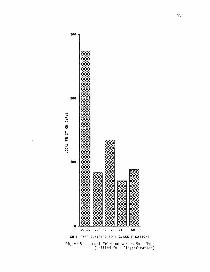
c ~ ~
z 0
~
u ~ ~
~
< u 0 ~
100
SC-SM ML. ·CL-ML CL CH
SOIL TYPE (UNIFIED SOIL CLASSIFICATION)
Figure 51. Local Friction Versus Soil Type (Unified Soil Classification)
98
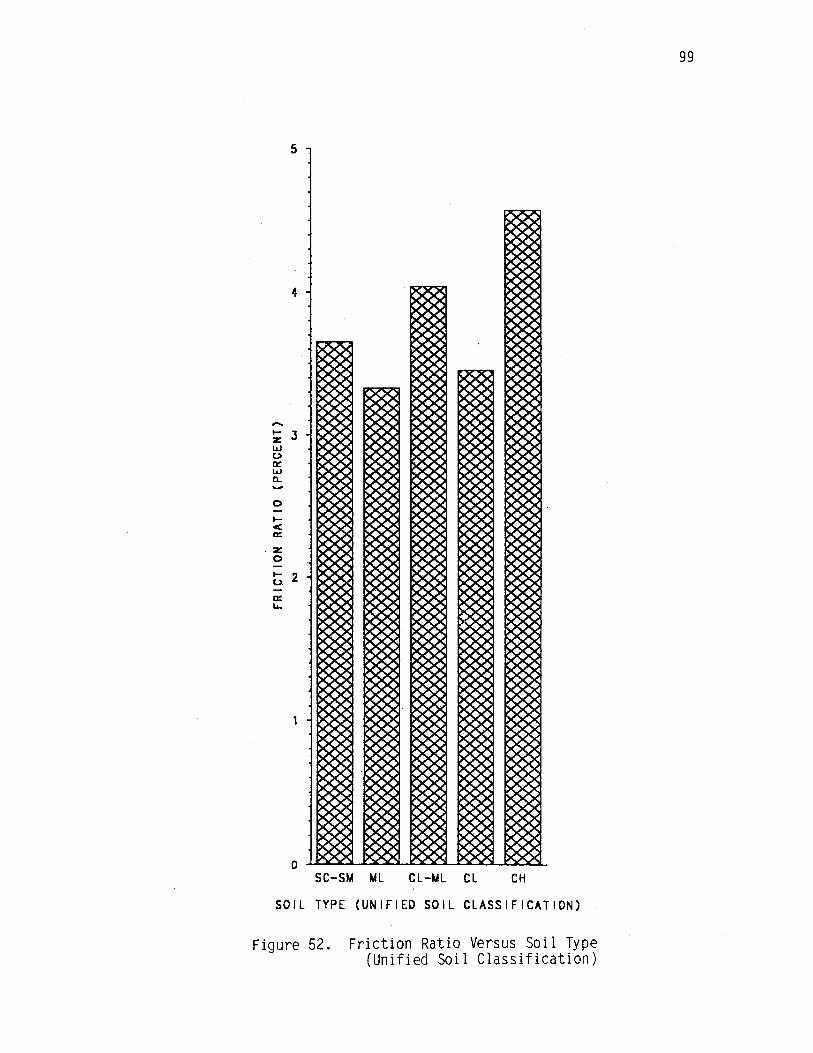
5
4
..... ~ 3 w u a:: w a..
0
I< a::
. z 0
t>. 2
SC-SM ML CL-ML CL CH
SOIL TYPE (UNIFIED SOIL CLASSIFICATION)
Figure 52. Friction Ratio Versus Soi 1 Type (Unified Soil Classification)
99
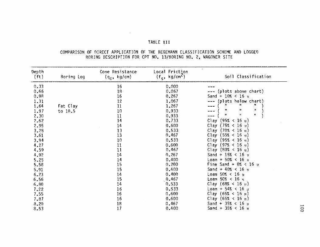
TABLE XII
COMPARISON OF OIRECT APPLICATION OF THE BEGEMANN CLASSIFICATION SCHEME AND LOGGED RORING DESCRIPTION FOR CPT NO. 13/BORING NO. 2, WAGONER SITE
Depth Cone Resistance Local Frict~on (ft) Boring Log (qc, kg/cm) (f S' kg/cm ) Soil Classification
0.33 16 o.ooo 0.66 18 0.067 --- (plots above chart) 0.98 16 0.267 Sand + 10% < 16 u 1.31 12 1.067 --- (plots helow chart) 1.64 Fat Clay 11 1.267 --- ( II II II ) 1.97 to 18.5 10 0.933 --- ( II II II ) 2.30 11 0.933 --- ( II II II ) 2.62 14 0.733 Clay (95% < 16 u) 2.95 14 0.600 Clay (75% < 16 1t) 3.28 13 0.533 Clay (70% < 16 11) 3.61 13 0.467 Clay (55% < 16 11) 3.94 10 0.533 Clay (95% < 16 11) 4.27 11 0.600 Clay (97% < 16 u) 4.59 11 0.467 Clay (80% < 16 u) 4.92 14 0.267 Sand + 15% < 16 u 5.25 14 0.400 Loam + 50% < 16 u 5.58 15 0.200 Fine Sand + 0% < 16 u 5.91 15 0.400 Sand + 40% < 16 u 6.23 14 0.400 Loam 50% < 16 u 6.56 15 0.467 Loam 50% < 16 11
6.80 14 0.533 Clay (68% < 16 1t) 7.22 16 0.533 Loam + 54% < 16 u 7.55 16 0.600 Clay (65% < 16 id 7.87 16 0.600 Clay (65% < 16 u) 8.20 18 0.467 Sand + 35% < 16 u 8.53 17 0.400 Sand + 35% < 16 11
f-1 0 0

TABLE XII (Continued)
nepth Cone Resistance Local Frict~on (ft) Boring Log (qc) kg/cm (f s, kg/cm ) Soil Classification
8.86 18 0.600 Clay (55% < 16 u 9.19 19 0.467 Sand + 20% < 16 u 9. 51 18 0.600 Clay ( 55% < 16 1i) 9.84 18 0.600 Clay ( 55% < 16 u)
10.17 18 0.667 Sand + 24% < 16 11
10.50 19 0.733 Sand + 27% < 16 u 10.83 19 0.733 Sand + 27% < 16 u 11.15 20 0.667 Sand + 15% < 16 u ll.48 21 0.600 Sand + 7% < 16 u 11.81 20 0.667 Sand + 15% < 16 u 12.14 22 0.667 Sand + 40% < 16 11
12.47 23 0.600 Sand + 30% < 16 u 12.80 22 0.667 Sand + 40% < 16 u 13.12 23 0.667 Sand + 30% < 16 11
13.45 22 0.533 Sand + 22% < 16 11
13.78 20 0.600 Sand + 45% < 16 u 14.11 19 0.667 Clay (70% < 16 u 14.44 20 0.533 Sand + 37% < 16 u 14.76 19 0.600 Loam + 52% < 16 u 15.09 20 0.533 Sand + 37% < 16 u 15.42 19 0.667 Clay (70% < 16 11) 15.75 21 0.467 Sand + 17% < 16 u 16.08 20 0.600 Sand + 45% < 16 u 16.40 20 0.667 Sand + 15% < 16 u 16.73 21 0.600 Sand + 7% < 16 u 17.06 22 0.533 Sand + 22% < 16 11
17.39 21 0.667 Sand + 45% < 16 u 17. 72 22 1.000 Clay (753 < 16 u) ...... 18.04 28 0.867 Sand + 47% < 16 u) C> ......
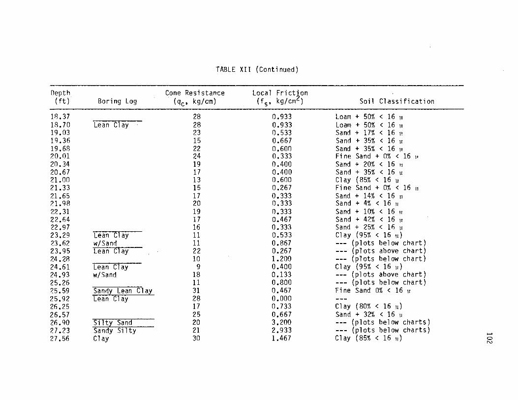
TABLE XII (Continued)
Depth Cone Resistance Local Frict~on (ft) Boring Log (qc, kg/cm) ( f s , kg I cm ) Soil Classification
18.37 28 0.933 Loam + 50% < 16 11
18. 70 Lean Clay 28 0.933 Loam + 50% < 16 u 19.03 23 0.533 Sand + 17% < 16 11 1q.36 15 0.667 Sand + 35% < 16 u 19.68 22 0.600 Sand + 35% < 16 u 20.01 24 0.333 Fine Sand + 0% < 16 JI
20. 34 19 0.400 Sand + 20% < 16 11
20.67 17 0.400 Sand + 35% < 16 u 21.00 13 0.600 Clay (85% < 16 u 21.33 15 0.267 Fine Sand + 0% < 16 u 21.65 17 0.333 Sand + 14% < 16 u 21. qg 20 0.333 Sand + 4% < 16 u 22.31 19 0.333 Sand + 10% < 16 11
22.64 17 0.467 Sand + 42% < 16 u 22.97 16 0.333 Sand + 25% < 16 ll
23.29 Lean Clay 11 0.533 Clay ( 9 5% < 16 11) 23.n2 w/Sand 11 0.867 --- (plots below chart) 23.95 Lean Clay 22 0.267 --- {plots above chart) 24.28 10 1.200 --- (plots below chart) 24.61 Lean Clay 9 0.400 Clay (95% < 16 11) 24.93 w/Sand 18 0.133 --- (plots above chart) 25.26 11 0.800 --- {plots below chart) 25.59 Sandy Lean Cla,x: 31 0.467 Fine Sand 0% < 16 u 25.92 Lean Clay 28 0.000 2n.25 17 0.733 Clay (80% < 16 u) 26.57 25 0.667 Sand + 32% < 16 11
26.90 Si it,x: Sand 20 3.200 --- {plots below charts) 27.23 Sandy Si 1 ty 21 2.933 --- (plots below charts) ...... 27.56 Clay 30 1.467 Clay (85% < 16 11) 0
N
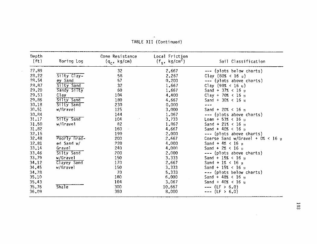
TABLE XII (Continued)
Depth Cone Resistance Local Frict~on (ft) Boring Log (qc, kg/cm) (f s, kg/cm ) Soil Classification
27.89 32 2.667 --- (plots below charts) 28.22 Silty Clay- 58 2.267 Clay (80% < 16 u) 28.54 ey_ Sand 57 0.200 --- (plots above charts) 28.87 Silty Sand 32 1.667 Clay (90% < 16 u) 29.20 Sandy Silty 60 1.667 Sand + 37% < 16 u 29.53 Clay_ 104 4.400 Clay+ 70% < 16 11
29.86 Silty_ Sand 180 4.667 Sand + 30% < 16 11 30.18 Silty Sand 230 o.ooo 30. 51 w/Gravel 125 3.000 Sand + 20% < 16 u 30.84 144 1.067 --- (plots above charts) 31.17 Silty Sand 104 3.733 Loam + 53% < 16 u 31.50 w/Gravel 82 1.R67 Sand + 21% < 16 u 31.82 160 4.667 Sand + 40% < 16 ii 32.15 190 2.000 --- (plots above charts) 32.48 Poorly Grad- 200 2.667 Coarse Sand w/Gravel + 0% < 16 u 32.81 erl Sanrl w/ 220 4.000 Sand + 4% < 16 u 33.14 Gravel 240 4.000 Sand + 2% < 16 u 33.46 Silty Sand 200 2.000 --- (plots above charts) 33.79 w/Gravel 150 3.333 Sand + 15% < 16 u 34.12 Clayey Sand 170 2.667 Sand + 1% < 16 u 34.45 w/f1ravel 150 3.333 Sand + 15% < 16 u 34.78 70 5.333 --- (plots below charts) 35.10 180 6.000 Sand + 48% < 16 ii
35.43 104 3.067 Sand + 40% < 16 u 35.76 Shale 300 10.667 --- (LF > 6.0) 36.09 380 8.000 --- (LF > 6.0)
...... 0 w

Oepth (ft)
o.33 0.66 0.98 l. 31 1.64 1.97 2.30 2.62 2.95 3.28 3.61 3.94 4.27 4.59 4.92 5.25 5.58 5.91 6.23 6.56 6.89 7.22 7.55 7.87 8.20 R.53
TABLE XI II
COMPARISON OF DIRECT APPLICATION OF THE SEARLE CLASSIFICATION SCHEME AND LOGGED BORING DESCRIPTION FOR CPT NO. 13/BORING NO. 2, WAGONER SITE
Cone Resistance Local Friction Boring Log (qc, MPa) (f s, kg/cm2) Soil Classification
Fat Clay to 1.6 o.oo 18.5 1.8 0.37 Very Sensitive Soils
1.6 1.67 Loose F.M.C. Sand 1.2 8.89 Fi rm Heavy Clay 1.1 11.52 II II II
1.0 9.33 II II II
1.1 8.48 II II II
1.4 5.24 Fi rm Clayey Silt 1.4 4.29 Med. Dense Clayey Sandy Silt 1.3 4 .10 II II II II II
1.3 3.59 II II II II II
1.0 5.33 Soft Clayey Silt 1.1 5.45 Fi rm Clayey Silt 1.1 4.24 Loose Clayey Sanrly Silt 1.4 1.90 Loose Silty Sanrl 1.4 2.86 Loose Clayey Silty Sand 1.5 1.33 Loose F.M.C. Sand 1.5 2.67 Loose Clayey Silty Sand 1.4 2.86 II II II II
1.5 3.11 II II II II
1.4 3.81 Med. Dense Clayey Sanrly Silt 1.6 3.33 II II II II II
1.6 3.75 II II II II II
1.6 3.75 II II II II II
1.8 2.59 Loose Clayey Silty Sand 1. 7 2.35 II II II II
....... 0
"""

TABLE XIII (Continued)
nepth Cone Resistance Local Frict~on (ft) Boring Log (qc, MPa) (f s, kg/cm ) Soil Classification
8.86 1.8 3.33 Med. Dense Clayey Sandy Silt 9.lg 1.9 2.46 Loose Clayey Silty Sand 9.51 1.8 3.33 Med. Dense Clayey Sandy Silt 9.84 1.8 3.33 II II II II II
10 .17 1.8 3.70 II II II II II
10.50 1.9 3.86 II II II II II
10.83 1.9 3.86 II II II II II
11.15 2.0 3.33 II II II II II
11.48 2.1 2.86 Med. Dense Clayey Silty Sand 11.81 2.0 3.33 Med. Dense Clayey Sandy Silt 12 .14 2.2 3.03 Med. Dense Clayey Silty Sand 12.47 2.3 2.61 II II II II II
12.80 2.2 3.03 II II II II II
13.12 2.3 2.90 II II II II II
12 .45 2.2 2.42 II II II II II
13. 78 2.0 3.00 II II II II II
14.11 1.9 3.51 Med. Dense Clayey Sandy Silt 14.44 2.0 2.67 Med. Dense Clayey Silty Sand 14.76 1.9 3.16 II II II II II
15.09 2.0 2.67 II II II II II
15.42 1.9 3.51 II II II II II
15.75 2.1 2.22 Med. Dense Silty Sand 16.08 2.0 3.00 Med. Dense Clayey Silty Sand 16.40 2.0 3.33 Med. Dense Clayey Sandy Silt 16.73 Fat Clay 2.1 2.86 Med. Dense Clayey Silty Sand 17.06 2.2 2.42 II II II II II
17.39 2.1 3.17 II II II II II
17. 72 2.2 4.55 Fi rm Clayey Si 1t 18.04 2.8 3.10 Med. Dense Clayey Silty Sand ........
0 (.]1
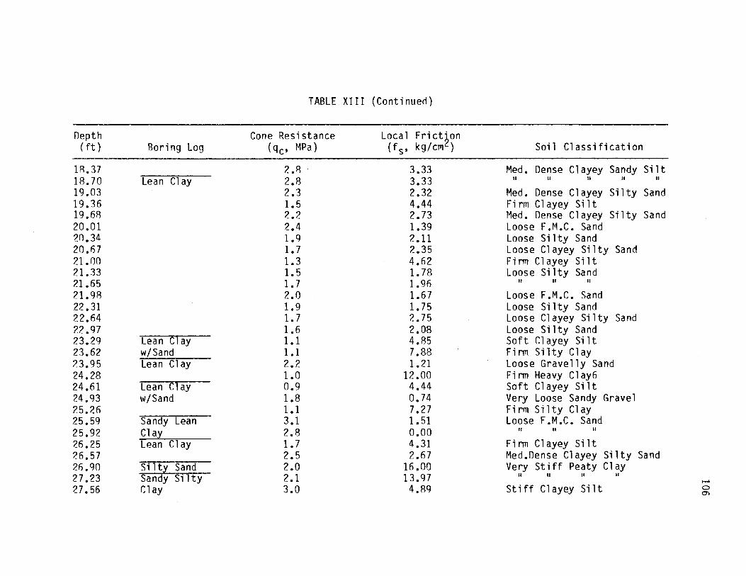
TABLE XIII {Continued)
Depth Cone Resistance Local Frict~on (ft) Boring Log (qc, MPa) (f s, kg/cm ) Soi 1 Cl ass ifi cation
IR.37 2 .8 . 3.33 Med. Dense Clayey Sandy Silt I8.70 Lean Clay 2.8 3.33 II II II II II
I9.03 2.3 2.32 Med. Dense Clayey Silty Sand I9.36 1.5 4.44 Fi rm Cl ay'ey Si 1 t I9.68 2.2 2.73 Med. Dense Clayey Silty Sand 20.0I 2.4 1.39 Loose F.M.C. Sand 20.34 1.9 2.11 Loose Si 1 ty Sand 20.67 I.7 2.35 Loose Clayey Silty Sand 2I.OO 1.3 4.62 Fi rm Clayey Si 1t 21.33 I.5 1. 78 Loose Si 1 ty Sand 2I.65 1. 7 1.96 II II II
21.98 2.0 1.67 Loose F.M.C. Sand 22 .3I 1.9 1. 75 Loose Si 1 ty Sand 22.64 I. 7 2.75 Loose Clayey Silty Sand 22.97 1.6 2.08 Loose Silty Sand 23.29 Lean Clay 1.1 4.85 Soft Clayey Silt 23.62 w/Sand I.I 7.88 Fi n11 Silty Clay 23.95 Lean Clay 2.2 1.2I Loose Gravelly Sand 24.28 1.0 12.00 Fi rm Heavy Cl ay6 24.6I Lean Clay 0.9 4.44 Soft Clayey Si l t 24.93 w/Sand 1.8 0.74 Very Loose Sandy Gravel 25.26 I. I 7.27 Firm Silty Clay 25.59 Sandy Lean 3.I 1.5I Loose F.M.C. Sand 25.92 c1ax 2.8 o.oo II II II
26.25 Lean Clay 1.7 4.31 Fi rm Clayey Silt 26.57 2.5 2.67 Med.Dense Clayey Silty Sand 26.90 Sil tx Sand 2.0 I6.00 Very Stiff Peaty Clay 27.23 Sandy Silty 2.I I3.97 II II II II
....... 27 .56 Clay 3.0 4.89 Stiff Clayey Silt 0
O"I

TABLE XIII (Continued)
nepth Cone Resistance Local Frict~on (ft) Raring Log (qc, MPa) (f s, kg/cm ) Soil Classification
27.89. 3.2 8.33 Very Stiff Silty Clay 28.22 Silty Clayey 5.8 3.91 Med. Dense Clayey Sandy Silt 28.54 Sand 5.7 0.35 Loose Gravel 28.87 Si 1 ty Sand 3.2 5.21 Stiff Clayey Silt 29.20 Sandy s.; 1 ty 6.0 2.78 Med. Dense Clayey Silty Sand 29.53 Cl at 10.4 4.23 Dense Clayey Sandy Silt ?Q.86 Silty Sand 18.0 2.59 Dense Clayey Silty Sand 30.18 Si 1 ty Sand 23.0 o.oo 30.51 w/Gravel 12.5 2.40 Dense Clayey Silty Sand 30.84 14.4 0.74 Med. Dense Sandy Gravel 31.17 Si 1 ty Sand 10.4 3.59 Dense Clayey Sandy Silt 31.50 w/Gravel 8.2 2.28 Med. Dense Silty Sand 31. 8?. 16.0 2.92 Dense Clayey Silty Sand 32.15 19.0 1.05 Med. Oense Gravelly Sand 32.48 Poorly Grad- 20.0 1.33 Dense F.M.C. Sand 32.81 ed Sand w/ 22.0 1.82 Dense Silty Sand 33.14 Gravel 24.0 1.67 Dense F.M.C. Sand 33.46 Silty Sand 20.0 1.00 Med. Dense Gravelly Sand 33.79 w/Gravel 15.0 2.22 Dense Silty Sand 34.12 Clayey Sand 17.0 1.57 Dense F~M.C. Sand 34.45 w/Gravel 15.0 2.22 Dense Silty Sand 34.78 7.0 7.62 Ha rd Silty Clay 35.10 18.0 3.33 Dense Clayey Sandy Silt 35.43 10.4 2.95 Oense Clayey Silty Sand 35.76 Shale 30.0 3.56 Very Dense Clayey Sandy Silt 36.09 38.0 2.11 Very Dense Silty Sand
....... 0 '.J
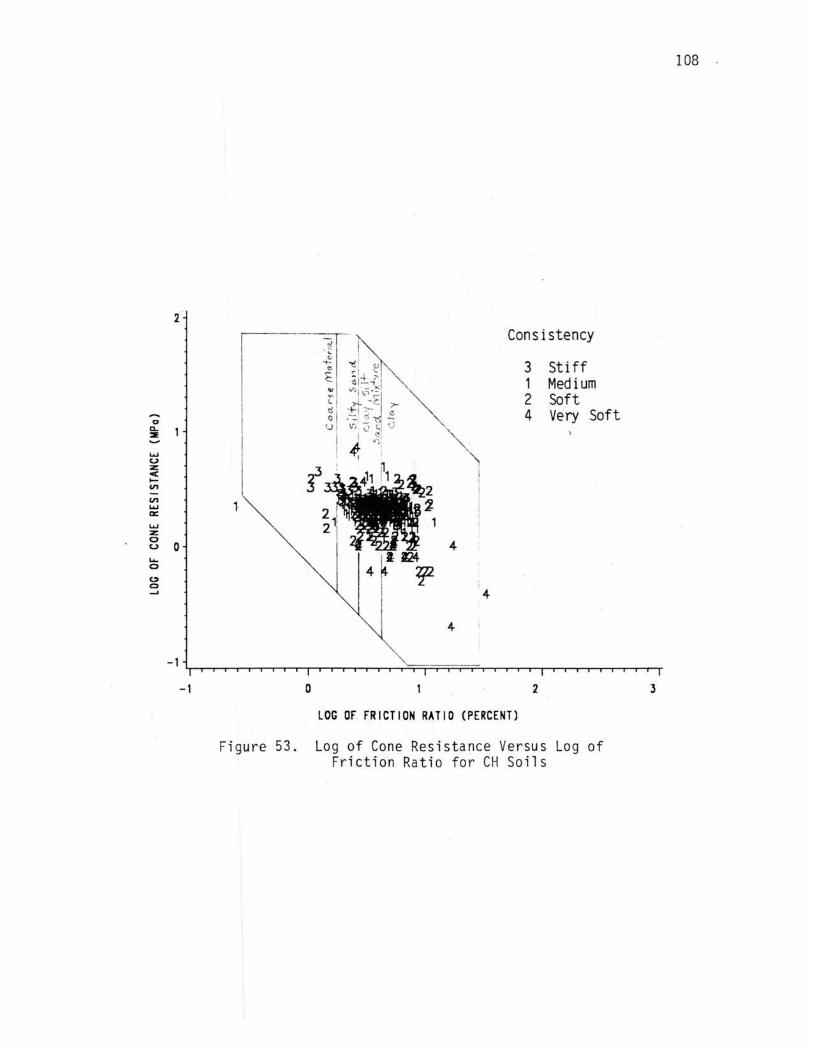
108
2
~ I Consistency
· ;;: I
~
~ ! ~~ 3 Stiff d
~ d!±-i 1 Medium .. °'i "~ -~ "' 2 Soft L ,..L ->-
t! . ._I >-- >-4 Very Soft ....... 0 .-:.: 0 ~
D Ir. ;:> '-I v a.. <..)
:::E I ~· ....... #. ; u
n z: j3 < .f 1 i 1 ..... "' "' 1-....... a:: ....... z: 0
4 u 0 .... ~1124 0
4 ' ¥2 ~ ; 0
I ...... 4
I 4
-1
-1 D 2 3
LOG Of FRICTI ON RATI O (PERCENT)
Fi gure 53 . Log of Cone Resistance Versus Log of Friction Ratio for CH Soils

2
D c.. ::IE
..... u :z: cC I-en
en ..... a:: ..... :z: 0 u 0 ~ 0
Cl 0 -'
_,
Consistency "' • <:;' ~
3 Stiff d
~ 1 Medium 2 Soft 4 Very Soft
2
·4 32. 3
4 44
0 2
LOG OF FRICTION RATIO (PERCENT)
Fi gure 54. Log of Cone Resistance Versus Log of Friction Ratio for CL Soils
109
3

110
A comparison of the histograms of cone resistance, local fric
tion, and friction ratios for all lean and fat clay data indicates the
mean and standard deviation (see Figures 55 through 60). All clay
data appear to follow a normal distribution based on plotting percent
cumulative frequency from the histogram data of Figures 55 through 60
on normal probability paper. Figures 61 and 62 present a percent
cu111ulative frequency versus friction ratio diagrams for all fat clay
data, as an example. All other histogram data showed similar results.
The friction ratios for lean and fat clay, from all sites were found
to be the following:
~ Mean Standard nevi at ion
Lean
Fat
x = 3.5
x = 4.6
CJ' = ±6 .1
CJ' = ±2.4
A similar comparison was made by the use of histograms of cone res is
tance, local friction, and friction ratios for all lean and fat clay
at the Wagoner site (see Figures 63 through 68). The data again
appear to follow a normal distribution based on plotting percent
cumulative frequency from the histogram data of Figures 63 through 68
on nonnal probability paper. The friction ratios for all lean and fat
clay at this specific site were found to be the following:
~ Mean Standard Deviation
Lean
Fat
x = 2.9
x = 4.5
CJ' = 2.0
CJ' = 1. 9
The friction ratios reported here for these fissured lean and fat
clays are somewhat lower than reported by Sanglerat (reference Table
II) and considerably lower than indicated by Searle's chart (reference
Figure 15). Results found in this study tend to agree with the fric-

-...,. -...... =-""" ...... ... .......
50
40
JO
20
10
0
Note: Last bar on following histograms are SAS
Graph computer summations.
x = 2205 kPa
a = 1436 kPa
SAS Graph computer summation of cone resistance exceeding 4200 kPa.
0 1 J 4 I 7 9 1 1 1 1 1 1 2 2 2 2 2 J J J J J J J 4 4 5 0 5 0 5 0 0 2 J & II 9 1 4 5 7 II D 1 J 4 & 1 9 D 2 0 0 0 0 0 D 5 D 5 5 D 5 0 D 5 a 5 D 5 D 5 a 5 D 5 0
0 D 0 0 0 D 0 D 0 0 D D 0 D D 0 D 0 D 0
CONE R£SISTAICE (kP1)
Figure 55. Histogram for Cone Resistance of Lean Clay From All Sites
111
4 l 5 D
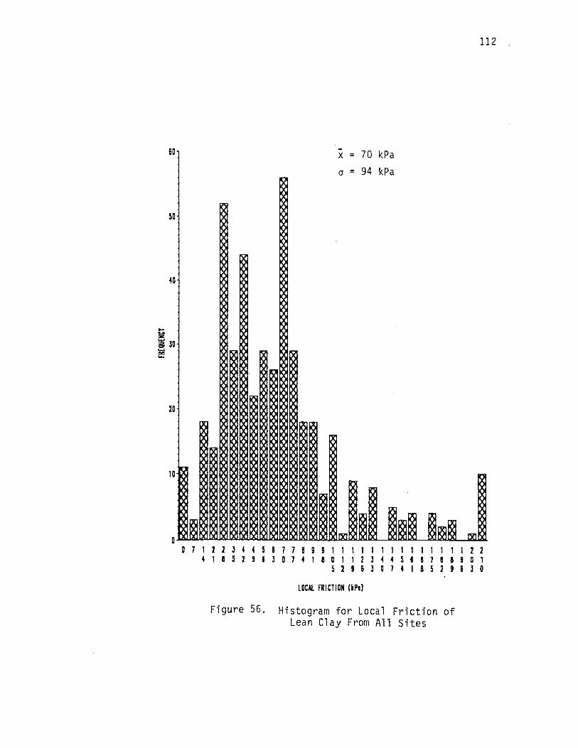
112
60 -x = 70 kPa a = 94 kPa
50
20
to
0 0 7 I 2 2 J 4 4 5 & 1 7 I 9 9 I I 1 t I 1 I t 1 I I t t I 2 2
4 I a 5 z 9 I J D 7 4 I a D I 1 z J 4 4 5 I I 1 a a 9 D 1 5 2 9 & l 0 1 4 1 8 5 2 9 & l 0
LOCAL FRICTION (kPal
Figure 56. Histogram for Local Friction of Lean Clay From All Sites

113
ao -x = 3.5%
70
60
SD
30
20
10
0 0 D I 2 2 J J 4 4 5 5 6 6 7 1 a 8 9 1 1 1 1 1 I 1
D 0 2 2 J 3 4 0 s 0 5 0 5 D 5 D 5 D 5 D 5 D 5 0 5 D 5
D 5 0 5 D 5 0 5 D
FRICTION RATIO (PERCENT)
Figure 57. Histogram for Friction Ratio of Lean Clay From Al 1 Si~es.
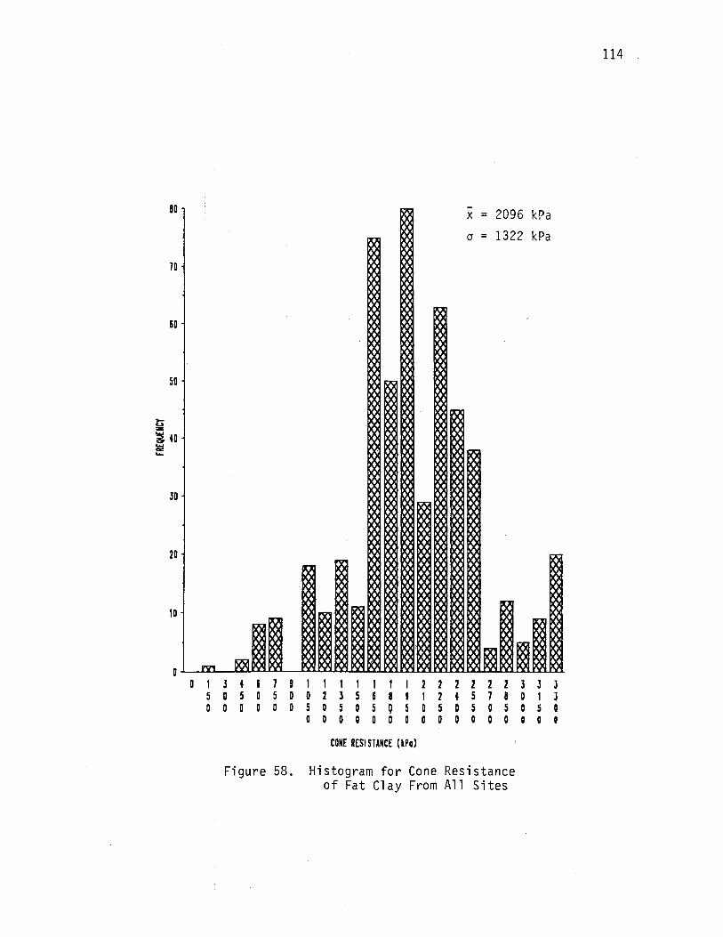
114 .
0 1 J ~ 7 9 1 1 1 1 1 1 2 2 2 2 2 2 J J J 5 a 5 5 0 0 2 3 5 6 8 1 2 ~ 5 7 8 0 1 J 0 0 0 0 0 5 0 5 0 5 Q 0 5 D 5 0 5 0 5 0
0 0 0 0 0 0 0 0 0 0 0 0 0 0 0
CONE RESISTANCE (kPa)
Figure 58. Histogram for Cone Resistance of Fat Clay From All Sites

115
70
-x = 88 kPa (J = 45 kPa
llt
50
I 40
"I
~
30
l'i
20 0
~.
'\ . < 'II'
ID ' .
<
~ ~
.,
I i . ) ~~ ~ <; ~ ~ PJ ~ ~~~ ~IQ! pj1 <: 0
D 7 I 2 2 J 4 4 5 I 7 7 I 9 ' I I I I I 1 I I 1 I I I 1 4 1 a 5 2 9 & l D t 4 1 I D 1 1 2 l 4 4 5 I & 7 I a
5 2 I & 3 0 1 4 1 I 5' 1 I
LOCAL FRICTION CkPtJ
Figure 59. Histogram for Local Friction of Fat Clay From All Sites
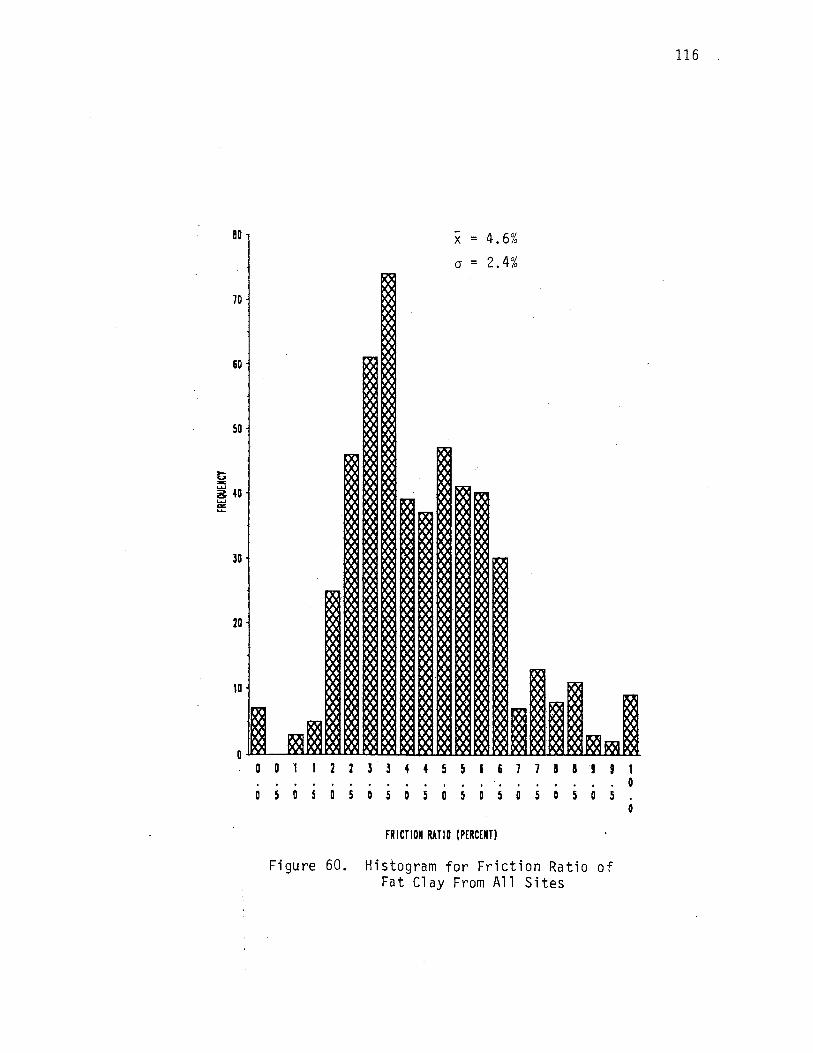
80
70
60
50
lD
20
f.O
0 0 0 I 2 2
0 5 D D 5
Figure 60.
3
D
3 4 4 5
5 0 5 0
x = 4.6%
(J = 2.4%
5 & 1
5 0 5 0
FRICTION RATIO (PERCENT)
1 I I
5 D 5
Histogram for Friction Ratio Fat Clay From All Sites
116
9 9 I D
D 5 0
of

117

I
• ....... _.__:;: = Q , .. ~
11----=2 ....... ,, c
'' -11' ! . ... 'i' ' I . I i I' ',, I I
I I i I I I II . I I
I i i ! I ! i ! !
t+t"'+t+H-!+IH+H++++++++H+H-!+H+H++++++++H+H-!+IH+H+++tttt+tt+H-!+IH+H++++ttt+HH+H-1~
I !
Friction Ratio, %
Figure 62. Cumulative Frequency Diagram for Friction Ratio of Fat Clay From All Sites Plotted on Norma 1 Prob ab i 1 i ty Paper
118
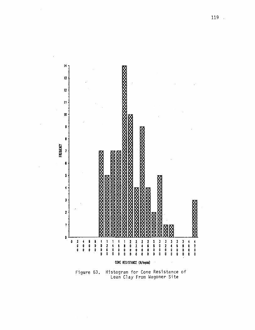
119 .
14
13
12
11
10
9
a >-~ -.... 7 ~ ..... "" ....
&
5
4
3
2
0 0 2 4 6 8 1 1 1 1 1 2 2 2 2 2 J 3 3 3 3 4 4
0 0 0 0 D 2 4 & 8 0 2 4 6 8 0 z 4 & 8 0 2 0 0 0 0 0 0 D 0 D 0 0 0 0 0 0 0 0 D 0 0 0
0 D D D D 0 0 0 0 D 0 0 0 0 0 D 0
CONE RES I STANCE (N/1~e1)
Figure 63. Histogram for Cone Resistance of Lean Clay From Wagoner Site

14
13
12
11
10
g
I ..... c..> z: .....
7 :::> ~ ..... a: ......
6
5
D ID 20 30 40 50 60 70 BO 90 100 110 no 130 140 150 160 170 180 190 200
LOCAL FRICTION (N/1~c1)
Figure 64. Histogram for Local Friction of Lean Clay From Wagoner Site
120 .

.... IU -
20
~ID ...... -.....
0 D
D
D 2 2 l l 4 4 5 5 & 7 7 B a 9 9
5 D s D s 0 s 0 s D s D 5 D 5 0 s 0 s
FRICTION RATIO (PERCENT)
Figure 65. Histogram for Friction Ratio of Lean Clay From Wagoner Site
121
1 0
0

40
JO
t; -~ 20 ...... ""' ...
10
0 0 2 4 6 8 I
0 0 0 0 D 0 0 0 0 0
D
Figure 66.
122
I I 1 I 2 2 2 2 2 J J J J J 4 4 2 4 & 8 0 2 4 & B 0 2 4 & 8 D 2 0 0 0 0 0 0 0 Q 0 0 0 0 0 0 0 D D D D D 0 0 0 0 D D D D D D D D
CONE RESISTANCE 0/1qc1)
Histogram for Cone Resistance of Fat Clay From Wagoner Site

0 10! 20 30 40 50 &O 70 BO 90 !OD 110 120 130 140 150 160 170 180 190 200
LOCAL FRICTION (l/1~c1)
Figure 67. Histogram of Local Friction for Fat Clay From Wagoner Site
123

po 22334455111111111 0
a s a 5 a s o s o s a s a s a s o s o s 0
FRICTION RATIO (PERCENT)
Figure 68. Histogram for Friction Ratio of Fat Clay From Wagoner Site
124

125
ti on ratios reported by Cancell i (34) for overconsol idated alluvial
clays.
Begemann's research (9) indicated that the slope of an arithmetic
plot of cone resistance versus local friction remains approximately
constant with soil type. The results in the form of a regression line
and equation from a method of least squares analysis of lean and fat
clay from all sites and the Wagoner site are given in Figures 69
through 72. It can be observed that the slopes from these regression
1 i nes do not correspond to the slope of clay soi 1 s indicated in the
Begemann's soil classification scheme. This would help explain the
poor correlation indicated in Table XII.
CPT Correlation With Atterberg Limits
and Clay Consistency
An attempt was made to carrel ate the cone resistance with the
Atterberg limits (LL and PL) and clay consistency as referenced by the
liquidity index (Ly). There· has been some research indicating linear
relationships between cone resistance and relative consistency which
is the reciprocal of the liquidity index (45·). Liquidity index has
replaced the older term, relative consistency, as a measure of clay
consistency. However, only a vague trend was noted; see typical rela
tionship in Figure 73 for the cone resistance versus liquidity index
for Wagoner lean and fat clays. No correlations were believed possi
ble without a more sophisticated statistical analysis. An indication
of some possible general relationship between the cone parameters and
clay consistency is shown in Figure 74. This figure relates cone
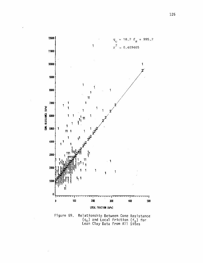
!2000
11000
10000
9000
8000
7000 ';;" :r.... --...... ~ &000 :n :n ...... =-.... ~ 5000
4000
3000
2000
1000
q = 18.2 f + 995.2 c s 2
r = 0 .409465
1
1 / 1
I 11
2 1
1 ./ 2/ 1 11 11 2'
i . 1/ 1 11
1 11 #
11 i
1, 1
0 100 200 300 400 SOD
LOCAL FRICTION (kPal
Figure 69. Relationship Between Cone Resistance (qc) and Local Friction (f s) for Lean Clay Data From All Sites
126
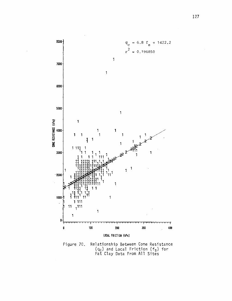
-.. .... -....
8000
7000
&DOD
5000
!i 4000 -"" "" .... ""' i
lDOO
. 2000
1000
q = 6.8 f + 1422.2 c s
r 2 = 0.196850
1
1
D 100 200 JOO 400
LOCAL FRICTION (kPal
Figure 70. Relationship Between Cone Resistance (qc) and Local Friction (fs) for Fat Clay Data From All Sites
127

.... ~ ,_ "" ~ -i
&ODD
50DD
40DD
JODD
1
ZODD
1
1 1
1 1 1
1
1 1
q = 14.1 f + 1251.7 c s 2
r = 0.385507
1
1
!ODD 1 1
0 10 20 JD 40 50 60 70 80 90 100 110 120 IJD 140 150 160 170 180 190
LOCAL FRICTION (l/sqc1)
Figure 71. Relationship Between Cone Resistance (qc) and Local Friction (f s) for All Wagoner Lean Clay Data
128
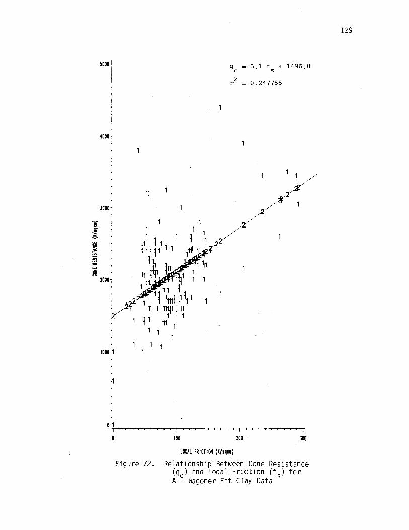
5000
4000
JOOO
'ii' ~ -...... -=
...... "-" ~ -~ .,, ...... -...... ~ "-"
2000
1000
0
q = 6.1 f + 1496.0 c s
r 2 = 0.247755
100 200 300
LOCAL fRICTION (l/1qc1)
Figure 72. Relationship Between Cone Resistance (qc) and Local Friction (f s) for All Wagoner Fat Clay Data
129

600
1 SOD
1
400 1 1
a 1~
c:. 1 .,. ........ 1 :z: ~ 300 ~ ~ 1
1 ..... Yo :z: c ..... .,. .... ... .... :z: 0 ~
1 1 11 1
1 1 ,lm 1 1
lt 11 1
~1, 11 11 1 1
200
0 111 1 1 1 11
1 1 1
1 111 1
,1 1 1 1 ,~ 11 1
11i 1 1 11 1
100 1 1
1
-1 0 2
LIQUIDITY INDEX
Figure 73. Cone Resistance Versus Liquidity Index for Wagoner Lean and Fat Clays
130
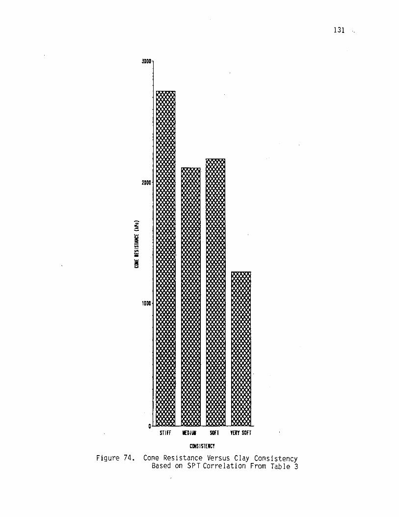
-.. ~ -~ "' "' .... -i
3000
2000
1000
0
" K K 0
~ ~~'I ~ ~ ~
Q ~ ,.. IV
0 It ~
~
~ ~ ~ i! ~ ~~
1; .J 'I
~ ~ >J ~
" y
'I ~
JI
"' " y
""' y
~
";: \I ~ y y
~
w
w w
w
w w
w
w
" JI y
y
w w . •• y
w
STIFF l(D 111 SOFT VERY SOH
CONS I STENCl
Figure 74. Cone Resistance Versus Clay Consistency Based on SPT Correlation From Table 3
131
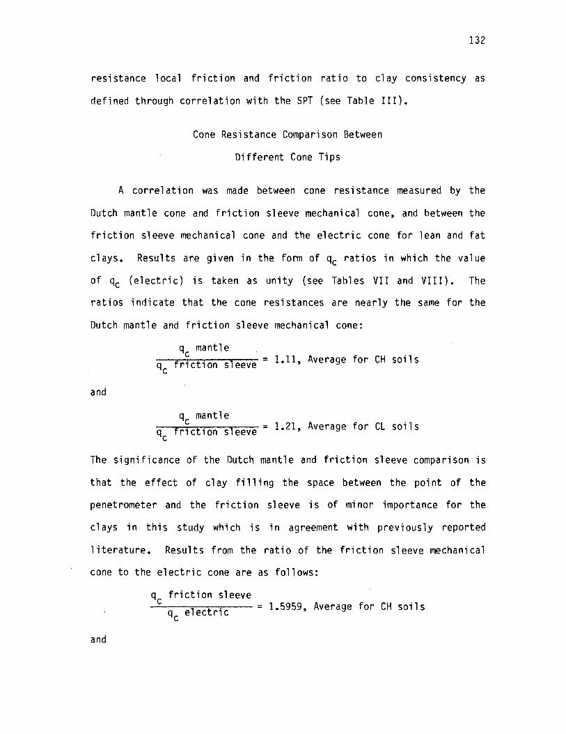
132
resistance local friction and friction ratio to clay consistency as
defined through correlation with the SPT (see Table III).
Cone Resistance Comparison Between
Different Cone Tips
A carrel ati on was made between cone resistance measured by the
Dutch mantle cone and friction sleeve mechanical cone, and between the
friction sleeve mechanical cone and the electric cone for lean and fat
clays. Results are given in the form of qc ratios in which the value
of qc (electric) is taken as unity (see Tables VII and VIII). The
ratios indicate that the cone resistances are nearly the same for the
Dutch mantle and friction sleeve mechanical cone:
and
qc friction sleeve = 1.11, Average for CH soils q mantle c
qc mantle friction sleeve = 1.21, Average for CL soils
qc
The significance of the Dutch mantle and friction sleeve comparison is
that the effect of clay fi 11 i ng the space between the point of the
penetrometer and the friction sleeve is of mi nor importance for the
clays in this study which is in agreement with previously reported
literature. Results from the ratio of the friction sleeve mechanical
cone to the electric cone are as follows:
and
qc friction sleeve ----=------ = 1. 5959, Average for CH soi 1 s
qc electric
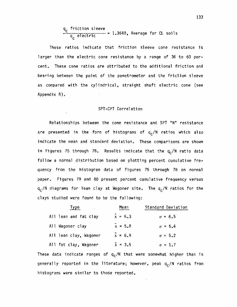
qc friction sleeve ----=--__,....-- = 1.3648, Average for CL soils
qc electric
133
These ratios indicate that friction sleeve cone resistance is
1 arger than the electric cone resistance by a range of 36 to 60 per
cent. These cone ratios are attributed to the additional friction and
bearing between the point of the penetrometer and the friction sleeve
as compared with the cylindrical, straight shaft electric cone (see
Appendix B).
SPT-CPT Correlation
Relationships between the cone resistance and SPT 11 N11 resistance
are presented in the form of histograms of qc/N ratios which also
indicate the mean and standard deviation. These comparisons are shown
in Figures 75 through 78. Results indicate that the qc/N ratio data
follow a normal distribution based on plotting percent cumulative fre
quency from the histogram data of Figures 75 through 78 on normal
paper. Figures 79 and 80 present percent cumulative frequency versus
qc/N diagrams for 1 ean clay at Wagoner site. The qc/N ratios for the
clays studied were found to be the fo 11 owing:
~ Mean Standard Deviation
All lean and fat clay x = 6.3 (j = 6.5
All Wagoner clay x = 5.8 (j = 5.4
All lean clay, Wagoner x = 6.9 (j = 5.2
All fat clay, Wagoner - 3.5 1. 7 x = (j =
These data indicate ranges of qc/N that were somewhat higher than is
generally reported in the literature; however, peak qc/N ratios from
histograms were similar to those reported.

Mean 6.3 Tsf Standard Deviation 6.5 Tsf
0 1 2 l 4 5 I 1 B 9 10 ti 12 tJ 14 15 16 17 18 19 20 21 22 2l 24·25 26 q /N, Tsf
c
Figure 75. Histogram for qc/N of Lean and Fat Clay From All Sites
134
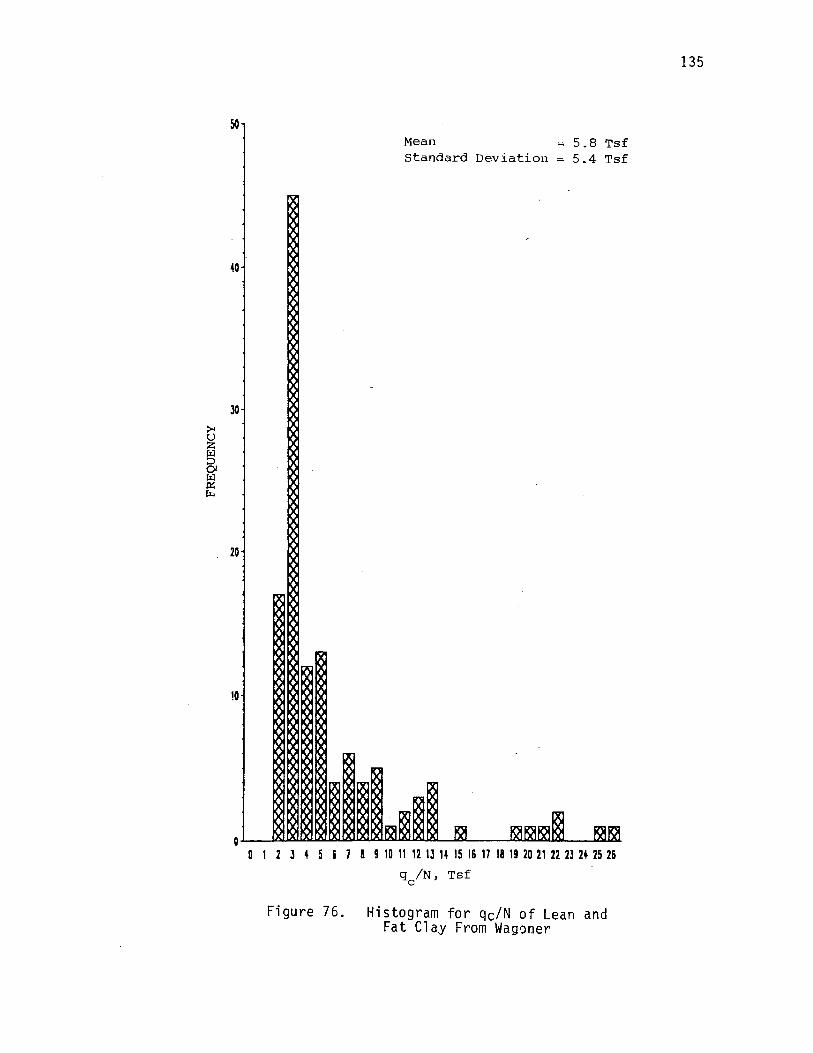
50
40
30
20
Mean 5.8 Tsf Standard Deviation 5.4 Tsf
O 1 2 J 4 5 5 1 B 9 10 11 12 1J 14 15 16 17 18 19 20 21 22 23 24 25 26
q /N, Tsf c
Figure 76. Histogram for qc/N of Lean and Fat Clay From Wagoner
135

7
5
Mean 6.9 Tsf Standard Deviation 5.2 Tsf
D 1 2 l 4 5 6 1 B 9 10 11 12 1J 14 15 18 17 18 19 20 21 22 2J 24
q /N, Tsf c
Figure 77. Histogram for qc/N of Wagoner Lean Clay
136
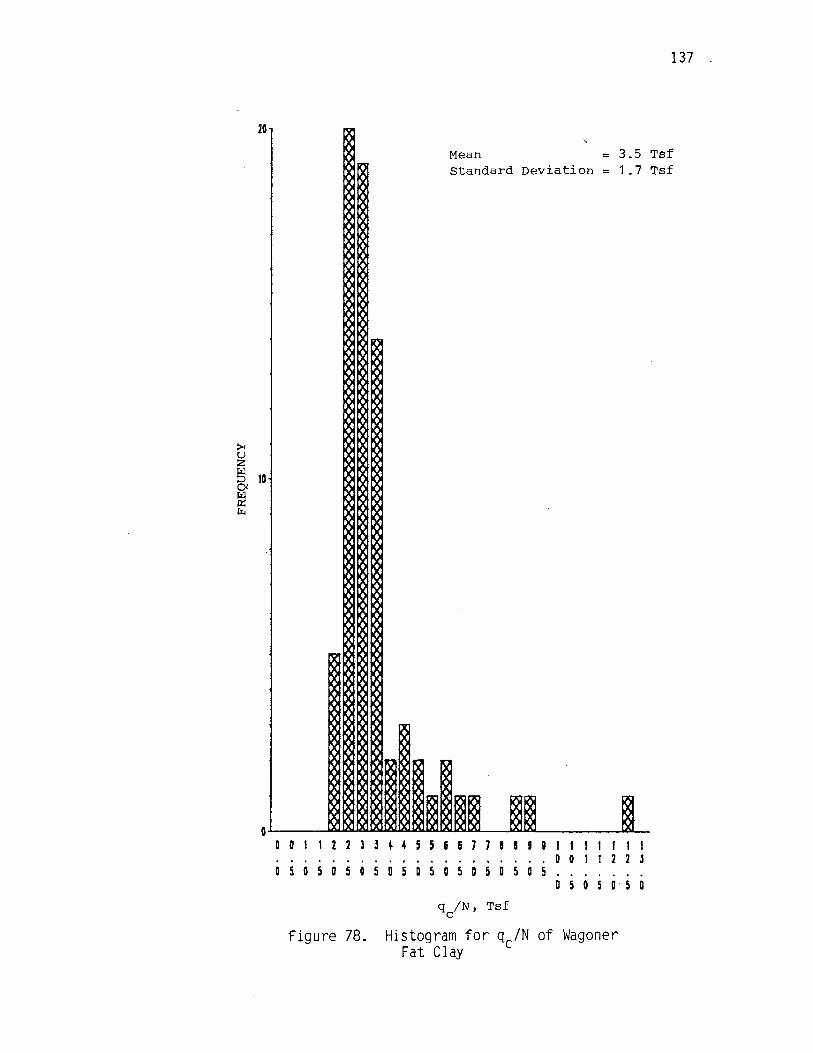
20
0 0 D 2 2 J
0 5 0 5 0 5 0 5
figure 78.
Mean Standard Deviation
4 4 5 5 6 6 7 7 8 8 9 I 1 I 0 0 2
0 5 5 0 5 0 s 0 a 5 D s 0 0
q /N, Tsf c
Histogram for qc/N of Wagoner Fat Clay
137 .
3.5 Tsf 1 .7 Tsf
1 I 2 l
s 0

30
20
10
D
ll:
~ ~ R R ~
~ ~ ~
~ ~
O~~u r~~ 0 0 ~
~~I x ~ ~ '
"' "' "' UI
~ ~ ~"' ~ !!,
WI : 'J 11 -- v "'~ . '.J WI
~ .. ~ ~ ~"' .. '·
"' ~ ~ u '
II
" .0
~ " ~
WI ) ~
~ I\ ;
R > ~ -J',
"' "' "' .w ~ B Pl
II II ,. ,.
~ ·.:., ~ ~ r1 R ~ "' ~ II\ .~ ~
~-~ ~ ~ II 11. II II V ~
u
R Pl
~ II ~
0 ~
w ~- ~ .. 0 1 2 3 4 5 & 1 a 9 10 11 12 13 14 15 16 17 18 19 20 21 22 23 24
q /N, Tsf c
Figure 79. Cumulative Frequency Diagram for qc/N of Wagoner Lean Clay
138 .
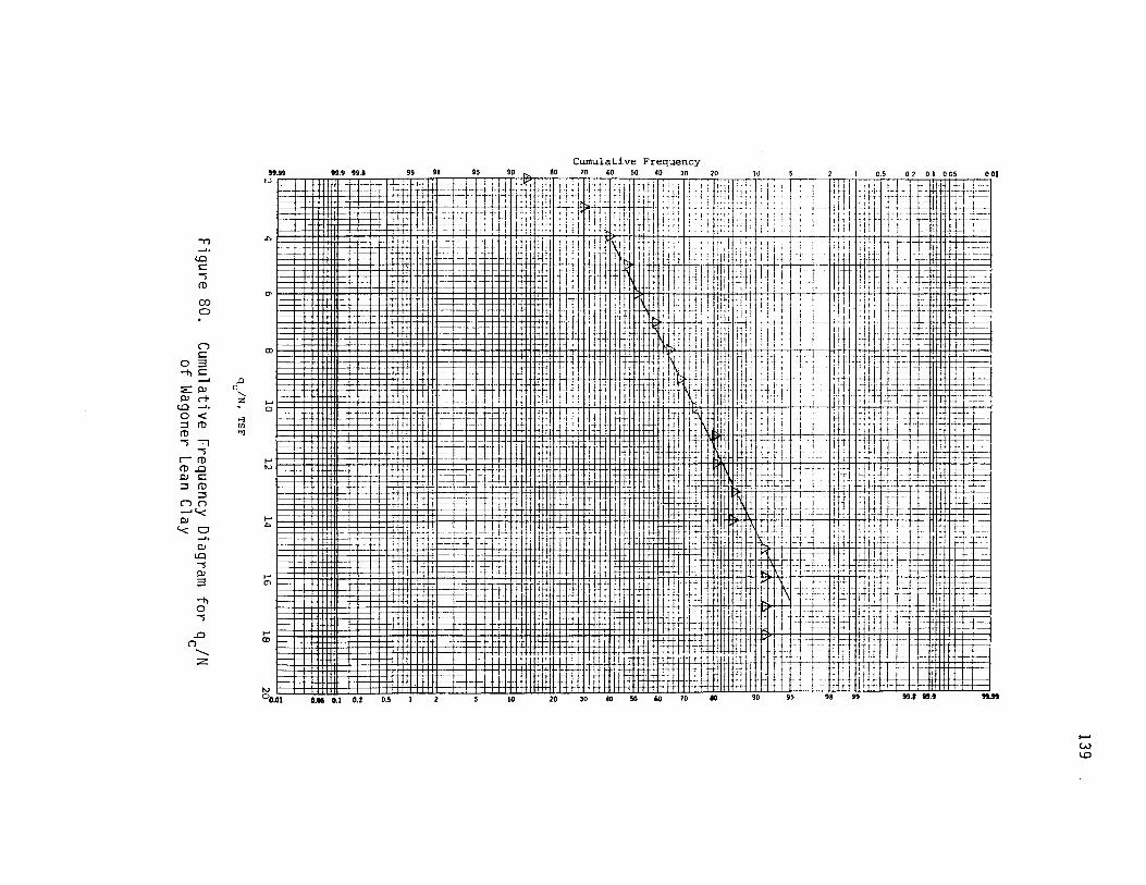
.,, -'·
lQ s::::: '"'S ro 00 0
n s:::::
0 3 -t, s:::::
--' ::0: Ill Ill c-1-
lQ -'· O< ::i ro ro '"'S "Tl
'"'S rro ro ..o Ill s::::: ::i ro
::i n (") --''< Ill '< Cl
-'• Ill lQ '"'S Ill 3
-t, 0 '"'S
..0 (") -:z:
.0 n
"' z
~ "l
co
,_. 0
I I I 1111111 I I 1+
,_. "' I I 111111 I I I I 1 I llll-!-
r: ---i-
--d-t·+-H:1ti1·i-i1Jrmrm1·'l1 tiif4a'm!frrTlf~uf1' 11rr·1'1·1 1 '-i I' --1 1f'l-1 1''il++-t·~-t==rrt.1 - llil1~11i r;m i~ T+!HN~li!Witi Iii-! i fr --;;;1 r~~l-: 1
11 ft1Tirrnrnttt+mnn111tr11Tl 1ili111-1 tttil : __ ! --l!_-1H Jr_ l1tjt1 :·1 ·.r:.-_ 1l-tlili1llr+1-htltfH.HHh qr 1- ! ' In-~· -,-,--i+:-
!:± ·-·=t= --+--.i--
~
~~HmffiWEffiR=•m••aB#!Ji=RH#W#P.~~
,_.
~ l=±±ttll I I I I l±tit±t=tl 111111 :::ttttm:tl 11 ltttt:::::t=tl I ll±:t:t:ttlti1 00.01 0.05 0.1 0.2 0.5 I 2 S 10 20
-tt•iutr•· i T • trm+ttt-, -_ ,:, : -:~.t~~tb -- -A 11 !it I f- i nmTin: lJkidJJOOttl@ 95 98 99 99.1 99.t 9Ut 90 30 40 so '° 10 IO
I-' w l.O
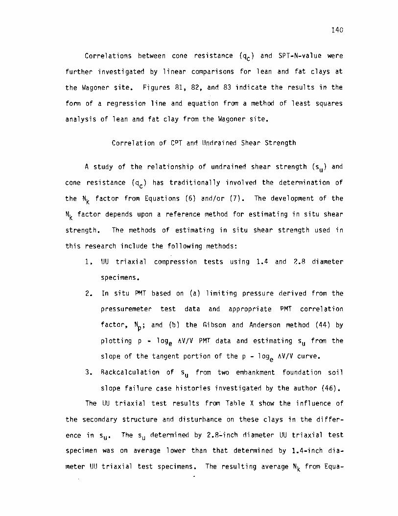
140
Correlations between cone resistance (qc) and SPT-N-value were
further investigated by linear comparisons for lean and fat clays at
the Wagoner site. Figures 81, 82, and 83 indicate the results in the
form of a regression line and equation from a method of least squares
analysis of lean and fat clay from the Wagoner site.
Correlation of CPT and Undrained Shear Strength
A study of the relationship of undrained shear strength (su) and
cone resistance (qc) has traditionally involved the determination of
the Nk factor from Equations (6) and/or (7). The development of the
Nk factor depends upon a reference method for estimating in situ shear
strength. The methods of estimating in situ shear strength used in
this research include the following methods:
1. UU triaxial compression tests using 1.4 and 2.8 diameter
specimens.
2. In situ PMT based on (a) limiting pressure derived from the
pressuremeter test data and appropriate PMT correlation
factor, NP; and (b) the '1i bson and Anderson method ( 44) by
plotting p - loge AV /V PMT data and estimating su from the
slope of the tangent portion of the p - loge AV/V curve.
3. Backcalculation of su from two embankment foundation soil
slope failure case histories investigated by the author (46).
The UU triaxial test results from Table X show the influence of
the secondary structure and disturbance on these clays in the differ
ence in Su· The Su determined by 2.8~inch rliameter UU triaxial test
specimen was on average lower than that determined by 1.4-i nch di a
meter UlJ triaxial test specimens. The resulting average Nk from Equa-
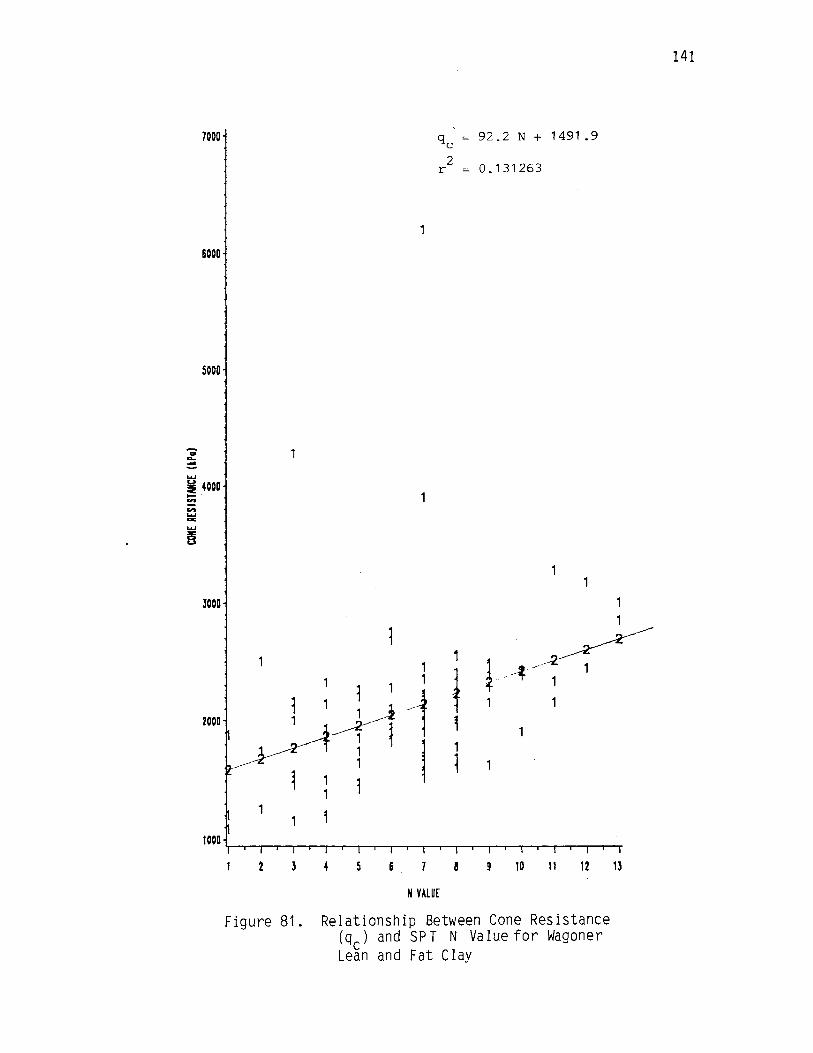
7000
6000
5000
~ 4000 ..... .,. ..,, ..... ...
JOOO
2000
1
2 J 4 5
q = 92.2 N + 1491 .9 c 2
r = 0.131263
8 9 10 11 12 1J
N VALUE
Figure 81. Relationship Between Cone Resistance (qc) and SPT N Value for Wagoner Lean and Fat Clay
141
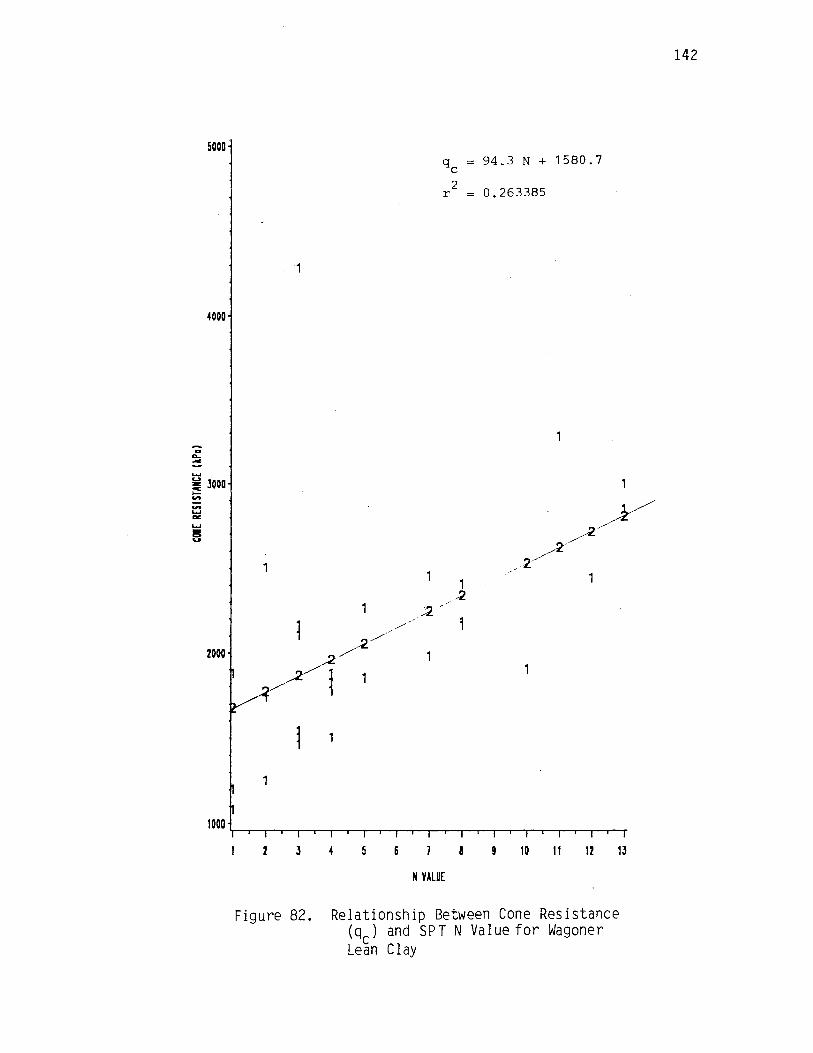
.. a... ...
SOOD,
4000
~ 3000 .__ .,. .,. ~ a:: ~ -8
2000
94.3 N + 1580.7
0.263385
1
1
2 4 5 6 1 a 9 10 11 12 13
N VALUE
Figure 82. Relationship Between Cone Resistance (qc) and SPT N Value for Wagoner Lean Clay
142

7000
6000
5000
q = 107.9 N + 1341 .5 c 2
r == 0.091888
~ 4000 ,_ ""' .,. ..... ""' ~
3000
2000
1000 i.-~----~-~~-~~-------J 4 5 7 ID 11 12
N VALUE
Figure 83. Relationship Between Cone Resistance (qc) and SPT N Value for Wagoner Fat Clay
143

144
tions (6) and (7) for the larger 2.8-inch diameter test specimens is
closer to the values reported in the literature for fissured clays
than the average Nk for 1.4-inch test specimens. Also indicated in
Table X is that Equations (6) and (7) show essentially the same Nk
values.
The su estimated from pressuremeter tests with depth indicate
similar Nk values to those obtained from 2.8-inch diameter UU triaxial
test specimens (see Table VI) •. However, Marsland and Randolph (47)
point out that su determined by the Gibson and Anderson method over-
estimates su for stiff fissured clays. They recommend using the
limiting pressure approach and an appropriate PMT Np correlation
factor in the su equation (see Table VI). The value of Np correlated
with large plate bearing tests and applicable to fissured clays is
6.2. Substituting su (PMT) based on limiting pressure into Equation
(7) gives values of Nk that are compatible with those reported in the
literature (see Table VI). A plot of undrained shear strength (su)
and cone resistance (qc) shows the variation in Nk with regard to the
reference su used (see Figures 84 and 85). It appears that the wide
scatter is influenced by inappropriate reference Su·
Backcalculated undrained shear strength from two failed slopes
was used to estimate the Su based on a <!> = o approach for arriving at
an average mobilized shear strength along the slippage plane. Exten
sive details were applied to define a failure surface for embankment
/foundation slope failures at the Wagoner and Roland sites. Backcal
cul ated shear strength from these slides was used to estimate the Nk
from Equations (6) and (7). Results indicate an Nk = 34 for the
Wagoner slide and NBk = 42 for the Roland slide.

2.0
..... VI I-. - 1.5 ::I VI ....
..c: ..... Cl c: cu I-..... V)
1.0 I-ra cu ..c: V)
"'C cu c: ·-ra 0.5 I-
"'C c:
:::::>
. Nk = 22.4
// f, /// /I\. 30.0
:// /~ (J ,p ~
(J _y------------Nk = 80.0
/:...
~ -· - ·----L---·"· 10 20 30 40 50
Cone Resistance (qc), Tsf
o PMT (Limiting Pressure), Wagoner Site
• PMT (Limiting Pressure), Wagoner Site, SPT 2
e PMT (Limiting Pressure), Tulsa Site, SPT 2
,'\ Triaxial Data (2.8-inch Diameter), Wagoner Site
60 70
Figure 84. Relationship Between Undrained Shear Strength and Cone Resistance
....... ..i:::. C.T1
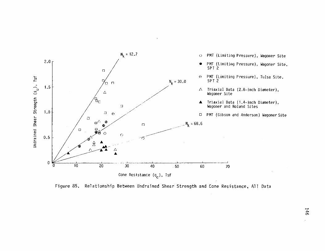
4--1/)
I-
::J (/)
.s= +-' Ol c: ~ +-' U)
s.... <O QJ
.s= U)
"O QJ c: ..... <O s.... "O c: =>
2.0
1.5
1.0
0.5
Nk = 12 .7
0
/Nk=30.0 D n
.6.
o PMT (Limiting Pressure), Wagoner Site
• PMT (Limiting Pressure), Wagoner Site, SPT 2
8
.6.
PMT (Limiting Pressure), Tulsa Site, SPT 2
Triaxial Data (2.8-inch Diameter), Wagoner Site
~D lJ /_// .A Triaxial Data (1.4-inch Diameter),
Wagoner and Roland Sites
o y/o e // e.6. @
D @
fa9 0
/al'~ 0
/~ .6.
o PMT (Gibson and Anderson) WagonerSite
-- Nk = 68 6 ---------- .~---. .
--0---------D
.A
"1--- /", ...
0 -·-· . --- _ _J_
0 10 20 30 I I ___1___ I
40 50 60 70
Cone Resistance (qc), Tsf
Figure 85. Relationship Between Undrained Shear Strength and Cone Resistance, All Data
f--' +:>
°'

CHAPTER VI
CONCLUSIONS AND RECOMMENDATIONS
The objectives of this investigation were to determine possible
rel at i ons'1i ps between the cone penetration test results and typi ca 1
engineering parameters for alluvial soils. Basic considerations were
correlations between CPT data and soil classification, relationships
with CPT data and Atterberg 1 imits and clay consistency, a comparison
of CPT tip geometry with regard to cone resistance, development of a
qc/N ratio for lean and fat. clays, and development of relationships
between undrained shear strength and cone resistance.
Conclusions
The results of the testing program and analysis of data obtained
indicate the following conclusions:
1. Sufficient data were analyzed to characterize the alluvial
soils as, typically, highly plastic desiccated firm to stiff
clay that tends to become soft and nonstructed with depth.
The stress history as indicated by the OCR from Table IX is
typical of the alluvial cla,xs with depth. All clays were
found to have a secondary structure consisting of cracks,
joints, fissures, and slickensides. The depth of the secon
dary structure influence decreases, slowing with depth.
147
148
2. The direct application of the Begernann and Schmertmann CPT
soil classification schemes gives generally inconsistent log
descriptions when compared to detailed boring logs. However,
they can qualitatively separate fine and coarse grai n·ed
soils. The Searle classification appears to be most suitable
for the study area soils. An examination of Figures 53 and
54 shows a tendency to fall to the 1 eft side with respect of
the vertical limits traced on the chart for clay soils. This
means that the measured values of the local friction are -
relatively low in comparison with cone resistance. Also, the
fact that these clays are overconsol i dated, which results in
less possible deformation, can increase cone resistance
without any appreciable increase of the local friction. The
friction ratios for lean anrl fat clays tend to match those
reported in the literature. The dispersion· of the data
within one standard deviation is fairly well defined. The
data for lean and fat clays appear to follow a normal
di stri but ion. For a 95 percent confidence 1 evel, the fri c-
tion ratios have a narrow range. This suggests that the
friction ratios for lean and fat clays overlap. This is
evident also by Figures 53 and 54.
3. A correlation between CPT cone resistance and Atterberg
limits and clay consistency was not possible with this sample
population. The dispersion of the data was considered the
reason for a lack of correlation; however, there were some
vague trenrls suggested in some of the CPT-SPT boring and
sampling combinations.
149
4. A comparison of cone resistance measured by different cone
types supports expected trends. The Dutch mantle and fric
tion sleeve cones gave essentially the same cone resis
tance. Internal friction of the inner rods nor that asso
ciated with friction sleeve did not appear to be signifi-
cant. The friction sleeve and electric cone comparison
followed the trend reported in the literature but by a higher
percentage.
5. The relationship between CPT and SPT, based on the mean and
standard deviations in this study, indicate higher qc/N
ratios for lean and fat clays than reported in the litera-
tu re. However, peak values of qc/N are nearly identical.
Some moderately good linear carrel at i ans were found between
cone resistance and N resistance (reference Figures 81, 82,
and 83). Comparison between .local friction and SPT N resis-
tance showed no significant correlation. These findings
appear to contradict Begemann's conclusion (29) in that he
showed the correlation to be much better between local fric
tion and SPT N resistance. One might cone l ude that CPT cone
resistance is more proportional during driving to the end
resistance of the SPT sampler. Note that the horizontally
projected area of the SPT sampler equals 10.7 cm2--nearly the
same as the 10.0 cm2 of the CPT cone. The linear correlation
between cone resistance and SPT N resistance would appear
attributable to the preconsolidation state of the soils which
results in less possible deformation as noted in item 2.

150
6. A relationship between CPT cone resistance and undrained
shear strength, Nk factor, was found to be influenced by the
following:
a. Sample size, based on the 1.4- and 2.8-inch diameter com
parisons, affects the estimate of Nk. The 1.4-inch size
sample size does take into account secondary clay struc
ture.
h. The scale effect of these clays' secondary structure
relative to the size of the cone resistance was estimated
to range between scales (a), (b), and (c) of Figure 17.
The (a) scale could be observed in the upper four feet of
the soil profile (B-horizon). The (b) scale was predomi
nately found in the majority of the soil profile. Below
approximately 18 to 20 feet the scale was found to tran
sition from (b) to (c) scale. These observations were
based on intensive logging detail.
c. Estimated Nk values based on Equations (6) and (7) were
essentially the same, based on results shown in Tables VI
and X.
d. The Nk factor for the Wagoner site based on 2.8-inch dia
meter triaxial test specimens averaged 39. The Nk factor
based on PMT ave raged 34. By using backca l cul ated un
drained shear strength data from a slope failure at the
Wagoner site, the Nk factor was estimated at 34. These
Nk values are slightly higher than what has been reported
in the literature (12). However, based on three separate
approaches, the Nk values fall into a narrow range.
151
e. The clay stiffness and structure within the top 4.0 to
5 .o feet apparently influenced these average Nk values.
However, neglecting the top three Nk values (Equation 2)
did not significantly lower the Nk average.
Recommendations
1. The data base should be expanded to refine the correlations
for more northeastern quarter alluvial clays that have the
physical property and engineering characteristics of the
study area soils.
2. There appears to be a significant impact of preconsolidation
on the cone parameters. In any future studies, correlation
of OCR with cone parameter should be investigated.
3. With a larger data base more sophisticated statistical proce
dures may in future studies indicate relationships between
cone parameters and Atterberg limits and clay consistency.
4. The correlation between Nk and undrained shear strength
should be further studied to delineate ranges for fissured
clays.
REFERENCES
(1) "Measurement of In Situ Shear Strength. 11
on In Si tu Measurement of Soil Pro erti es.
(2) Standard Method for Penetration Test and Split-Barrel Sampling of Soils. ASTM D 1586"'.'84. Vol. 04.08. Philadelphia: American Society for Testing and Materials, 1988.
(3) Standard Test Method for Deep, Quasi-Static, Cone and FrictionCone Penetration Test of Soil. ASTM D 3441-86. Vol. 04.08. Philadelphia: American Society for Testing and Materials, 1988.
(4) Sanglerat, G. The Penetrometer and Soil Exploration. Amsterdam: Elsevier Publishing Co., 1972.
(5) Barentsen, P. "Short Description of a Field Testing Method With a Cone Shaped Sounding Apparatus. 11 Proc., 1st Int. Conf. on Soi 1 Mechanics and Foundation Engineering. Vol. 2. Harvaril University, Boston, MA, 1936, pp. 7-10.
(6) Vermeiden, J. "Improved Soundings Apparatus, As Developed in Holland Since 1936. 11 Proc., 2nd Int. Conf. on Soil Mechanics and Foundation Engineering. Vol. 1. Amsterdam, 1948, pp. 280-287.
(7) Plantema, I. G. "Construction and Method of Working of a New Deep-Sounding Apparatus. 11 Proc., 2nd. Int. Conf. on Soil Mechanics and Foundation Engineering. Vol. 1. Amsterdam, 1948, pp. 277-279.
(8) Begemann, H.K. "Improved Method for Determining Resistance to Adhesion by Sounding Through a Loose Sleeve Placed Behind the Cone. 11 Proc., 3rd Int. Conf. on Soil Mechanics and Foundation Engineering. Vol. 1. Zurich, 1953, pp. 213-217.
(9) Regemann, H.K. 11 The Friction Jacket Cone as an Aid in Deter-mining the Soil Profile. 11 Proc., 6th Int. Conf. on Soil Mechanics and Foundation Engineering. Vol. 1. Montreal, 1965, pp. 17-20.
(10) Hogentogler & Co., Inc., P.O. Box 370, Gaithersburg, MD.
152

153
(11) Schmertmann, J. H. Guidelines for Cone Penetration Test:
(12)
Performance and Design. Report No. FHWA-TS-78-209. Washington, o.c.: U.S. Department of Transportation, Federal Highways Administration, Offices of Research and Development, July 1978.
Meigh, A. C. tat ion.
Cone Pen et ration Testing, Methods and InterpreLondon: Butt~rworths, 1987.
{13) Robertson, P. K. 11 In Situ Testing and Its Application to Foun-dation Engineering. 11 Soil Mechanics. Series No. 91. University of British Columbia, Vancouver, B.C., 1985.
(14) Shields, o. H. 11 Should ASTM Adopt the European Standard? 11
Symposium on Cone Penetrometer Testing and Experience. Geotechnical Division, ASCE. St. Louis, MO,· 1981, pp. 383-393.
(15) de Ruiter, J. 11 Electric Penetrometer for Site Investigations. 11
Journal of the Soil Mechanics and Foundations Division, ASCE, Vol. 97, No. SM2 (February 1971), pp. 457-472.
(16) Van den Berg, A. P. 11 Latest Developments in Cone Penetrometers and Other Soil Testing Equipment. 11 Proc., 2nd European Symposium on Penetration Testing. Vol. 2. Amsterdam, 1982, pp. 447-455.
(17) Ornevich, V. P. 11 1Jse of Conventional Boring Rigs for Cone Penetration Testing. 11 Proc., 1st Euro)ean Symposium on Penetration Testing. Vol. 2.1. Stockho m, 1974, pp. 125-128.
(18) Depret, M. U. A. 11 Influence of the Measuring Step in Discontinuous Mechanical Penetration Tests. 11 Proc., 2nd. Euroaean Symposium on Penetration Testing. Vol. 2. Amster am, 1982, pp. 551-555.
(19) Rol, A. H. 11 Comparative Study on Cone Resistance Measured With Types of CPT Tips. 11 Proc., 2nd European Symposium on Penetration Testing. Vol. 2. Amsterdam, 1982, pp. 813-819.
(20) Searle, I. w. 11 The Interpretation of Cone Results to Give Soil Types Proc., 7th Euro ean Conf. on Soil ng1neer1ng. r1g ton,
270.
Begemann Friction Jacket and Design Parameters. 11
Mechanics and Foundation
(21) Ramage, J., and S. s. Williams, Jr. Sensing Systems for Measuring Mechanical Properties in Ground Masses: Vol. 4, Static Penetrometer. Report No. FHWA/RD-81/112. Washington, D.C.: Office of Research, Federal Highway Administration, October 1982.

( 22)
(23)
(24)
154
Schmertmann, J. H. nutch Friction-Cone Penetration Exploration of Research Area at Field 5. Contract Report No. S-69-4. Eglin Air Force Base, Florida; and U.S.A.E. Waterways Experiment Station, Vicksburg, MS, 1969.
de Ruiter, J. 11 The Static Cone Penetration Test, State of the Art. 11 Proc., 2nd. European Symposium on Penetration Test-~· Vol. 2. Amsterdam, 1982, pp. 389-405.
Parez, L. A. 11 Static Penetrometer: The Importance Friction Associated With the Point Resistance." European Symposium on Penetration Testing. Stockholm, 1974, pp. 293-299.
of the Skin Proc., 1st Vol. 2.2.
(25) nurgunoglu, H. T., and J. K. Mitchell. 11 Static Penetration Resistance of Soils. 11 Proc., Conf. on In Situ Measurement of Soil Properties. Vol 1. Raleigh, N.C., .June 1975, pp. 151-188.
(26) Smits, J. V. "Cone Penetration Tests in Dry Sand. 11 Proc. 2nd. European Symposium on Penetration Testing. Vol. 2. Amsterdam, 1982, pp. 877-881.
(27) Krajicek, P. V. E., and J. Kruizinga. 11 CPT 1 s, An Excellent Aid
( 28)
to Determine Soil Parameters and Deviations in the Soil Profile of the Proposed Motorway-River Crossing Near Amsterdam." Proc. 2nd. European Symposium on Penetration Testing. Vol 2. Amsterdam, 1982, pp. 651-654.
Schmertmann, tl. H. "Oiscussion to neMell 's SOA paper, The Stan-dard Penetration Test." Proc., 4th PanAm Conf. of Soil Mech an i cs and Found at i on E~n-g~i -n e~e-r__,i_n_g-. --,.v.-o"Tl-.--,,I~I-=-1-. --=-P-u-e r"""'t,....._o Rico, 1971, pp. 90-98.
(29) Schmertmann, J. H. "CPT to Help Understand SPT. 11 Proc., 1st, Vol. 2.1. European Symposium on Penetration Testing.
Stockholm, 1974, p. 146.
(30) Robertson, P. K., and R. G. Campanella. "Interpretation of Cone Penetration Tests: Part I, Sand. 11 Canadian Geotechnical Journal, Vol. 20, No. 4 (1983), pp. 718-733.
(31) Robertson, P. K., and R. G. Campenella. 11 Interpretation of Cone Penetration Tests: Part II, Clay. 11 Canadian Geotechnical Journal, Vol. 20, No. 4 (1983), pp. 734-745.
(32) Drnevich, V. P., C. T. Gorman, and T. C. Hopkins. 11 Shear Strength of Cohesive Soils and Friction Sleeve Resistance. 11
Proc., 1st Euro ean Sm osium on Penetration Testin • Vol. • • toe o m, , pp.
155
(33) Cancelli, A., R. Guadagnini, and M. Pellegrini. 11 Friction-Cone Penetration Testing in Alluvial Clays. 11 Proc., 2nd European Symposium on Penetration Testing. Vol. 2. Amsterdam, 1982, pp. 513-518.
(34) Cancelli, A. "Penetration Tests on Cohesive Soils in Northern Italy." Proc., Intl. Symposium on Soil and Rock Investi-gations by In Situ Testing. Vol. 2. Paris, 1983, pp. 241-245 •.
(35) Briaud, J., and E. Garland. "Loading Rate Method for Pile Re-sponse in Clay. 11 ASCE, Journal of Geotechni cal En i nee r-ing, Vol. 3, No. 3 March 1985 , pp. 319-335.
(36) Marslan<i, A., anrl R. s. Quaterman. "Factors Affecting the Mea-surements and Interpretation of Quasi-Static Penetration Tests in Clays. 11 Proc., 2nd. European Symposium on Penetration Testing. Vol. 2. Amsterdam, 1982, pp. 697-702.
(37) Marsland, A. 11 Discussion, Session 4. 11 Proc., 7th European Conf. on Soil. Mechanics and Foundation Engineering. Vol. 4. Brighton, England, 1979, pp. 137-139.
(38) Dayal, IJ. "Oetermination of Shear Strength and Soil Modulus from CPT and Other In Situ Tests." Proc., 2nd. European Symposium on Penetration Testing. Vol. 2. Amsterdam, 1982, pp. 529-534.
(39) Ramaswamy, S. O., I. IJ. Daulan, and Z. Hasan. "Pressuremeter Correlations With Standard Penetration and Cone Penetration Tests." Proc., 1st European Srimposium on Penetration Testing. Vol. 2.1. Amsterdam, 19 4, pp. 137-142.
(40) Tavenas, F., and Leroueil, s. "Clay Behavior and the Selection of Design Parameters." Proc., 7th European Conf. on Soil Mechanics. Vol. 2. Brighton, England, 1979, pp. 281-291.
(41) Mayne, P. W. "CPT Indexing of In Situ OCR in Clays. "Proc., Conf. on Use of In Situ Testing in Geotechnical Engineering, ASCE. New York, 1986, pp. 780-793.
(42) Terzaghi, Karl, and Ralph B. Peck. Soil Mechanics in Engineering Practice. New York: John Wiley and Sons, Inc., 1967.
(43) Haliburton, T. Allan, and Robert M. Macnonald. Shear Strength Testing. Tech. Pub. No. 27. School of Civil Engineering, Oklahoma State University, Stillwater, Oklahoma, 1980.
(44) Gibson, R. E., and W. F. Anderson. "In-Situ Measurement of Soil Properties With the Pressuremeter. 11 Civil Engineering and Public Works Review, Vol. 56 (1961), pp. 615-618.
156
{45) Melzer, K. J. 11 llse of the WES Cone Penetrometer in Cohesive Soils. 11 Proc., 1st European SyMposium on Penetration Test~· Vol. 21. Amsterdam, 1974, pp. 263-268.
{46) Nevels, J. Foundation Investigation. Report No. 20023. Oklahoma City: Oklahoma Department of Transportation, Materials Division, 1qs7.
{47) Marsland, A., and J. Randolph. 11 In Situ Testing. 11 Geotech-nigue, Vol. 27 {1984), pp. 440-458.
APPENDIX A
EUROPEAN RECOMMENDED STANDARD, 1977
157

~ 5 E.
='I ::1 u
I . !i1 . -.. . " .. ~= § .. . ii = ·d ... . . . := ~ ::: :
.. 0 :; .. .. ? i :s "' ... 0
• • :: j ,X .. "' ! ... 0 .. .. & • •
I e .. ... ! !' .. .. • .... " : .. .. .. .. • " • ... ... 0
"' u
I ~ .. i i ! 1:1 ... i u
15 -... ... ! , II u -.. • I ;:: a I ... .. ~
:; ...
•C . . c ... •: . " 1; t~ . . -=: . -c .. . .. "
158

n " " ·< • .. . t; ~
·• '· . . . " .. .... .. .,,,1
... < ' '. ~~
.. . .. •• ~· :I'" ... .... .: . '· I •I• ...... ... .. .. ' ••n ,, .. ,, ... cu i.; . . . n •"
. " . .. '·" r.u
. " .. u . ~" .. . , ... .. .. .. . .. ~ ..
·•.. . , .t: at. .. . ..... ... i:. 'J cc
-~~ H
•U
'"
m ~~~ :: ~: r.1.•
m~
. L
m ~~! 1111" ... •cc . c • n O> .. .. . .. ... - , nr: rr I; i1 ..
~--··.. ;~~?.
I )
. .. . •C . ~n • 1; ... :ri f;!·
'o~ L • .. . " .. ~a
:: l i
; ~
cc ... C·,.. .. ... u r. c .. . .. .. ....
14 ....
! ~ ri ~ . ~)>4 •1;;.• ............ ~4
. ··- -- .........
!! _i .. ~~ ........ . ..... 1i
i ~
~--I • J
. .
.,
h ... !~ .. f.~
5;
H i~
@) I~ • !• • a
:: I: 1:: f!! :: r· ::.~
..; .
~[[[>
! . . . , ... ~~
:1 : CN . -· .. !i
' 2
. . . :
.. ..
159

. t, !I!
:ilf.:~ . "'.., . 0 ... 0 u ...
-;: ~ ~ .. ~ .. . . ... . 8"'~~!: .. &. • 1.-0 . ·"'cc. ..i
1~::~::~ C • • • L ~~.li:o ~ .. ;: ~:.; "'!:t;! • 0 0
g ~t:: r~ 1.U .. I.
"0 •• ,, Cl .. 0 1 .... 0 D
0 • .. " ... c v t!C 0.,., • .... ... -..... c .... t ... "&. ••.
.. • .. cc u ........ :I
I • l, It 0 I II :f u ...... ,..
f"! ti .. .. ...... '"c" ,, ..... I. . ...... "' •• > 0 0 t: LI • I... • I. ..... :I t.. p. a. ••• c
cu 0. • .., .. t:
~:~E~
_ HH~ · 1!j\j • f- ,. <I ......
"I ~ \ I
:
I'
. .. .. . "~· .. c
•• ' C' - .. 0
" { £(··
"c' .. ,. ~ .J .. " Q.
•• .. :J •••
"•· r • c
I ' '- ... ""~ •• 'I .... .,.,.-W• ,., C> •'
• 4.. ~ L .o 1 1-c ... •C•
• >- ......
' • 0
" ll/ .... , .... , .. , ..
i i < ~ i ~
! !
\ ~ . 0
\ J J
-~ ~:
w •<-. ao> . " c -• u . ' . " .. . ..
0
0 . ~ . . .
c . c
c
"· ~ - .. .. -
!
~ i .i ..;
~
. c •• . .....
- -c . . .... u • c. . - . ••• c: .. c - 0 .. .. . . . ....... u.. • . ;:-;: ~o ~ - ..
0 Co . c. -· .
I . c . i -
c . c
: I ~ ~!
0
I !! ' s~
c • 0. . .. .
'Ou. \.I -· a..t. •• ... : ~-~ ~ ; .. ~! lt'O .. .C • r.,., . . . . . . "' • c ...
• 0 -... 0 c. .........
c -..... :I ... • 0. .
... i"I ;zi:: • u-i" ~E~;! ~-==! ~~~;E
. - . .~::'O! r:e c
. ~~
,. .. . -.. EE~ 'ct:: ,~ . c.
ii~ ro:
C• ·-· >c.
~&; ··-W•O
E I
:··~-~-~-~~ !'O·:.~~:o!::; ... :~c.--e:c~o c: u. ...... . ....
~i:!;~gi~; ~:g~~~~i~~! .. !;t·~,,~~'1:1&"'
•t: "''"' :! 5 ~:;::: E ~ c. .. 0 . ., "'ooo .. - c • ~~ ... ~t;~ ... =~e1 C> ........
•o•C·UJ:ll..
Hn: 0 ................
•"'•:J•C•· .. G -· u-•uc•"'• c:•c ~ ~ : ~ • t• c; ~ ~ :. &. &. ....... c .. .: ;::~:t:~=~ t iS:~~~£;'o ~ ~
.. • c
"" ... : i;; ~; ~~~~~·~
;;~~i~ .. . ~;,,"' 0 i.. ...... '" . .. .. ..... ... ... :I. z • .. 1.- 0 E C_..., -·· j8~~::
.. 0" ~ . .....
l 0 .c . ,, .....
~!:! :i:: . 0 .... ,,. 1 • c •• ,.
~ .. ~~I ""'".IC m • •'Cl c: u ...
..; t: &. 0. c Cl Q. I.. g,. c
. t !j HS ~ :al :~~~·= " ~r 0 ,,_
~;~1; :~i.r .... co •.C:C: c: . ...... o ~ c • 0 u ... .. . ... .. ...
~;~~~ L
..... ! • ~
e:: :.,; : "
. .. ·.. -· H
. . ' c 0
~
-
.. •C .. 00
~r
·-C• 0 •.
Ez& .. -·· oc ·-· -·~ •~ ID 0
. , .
... c: ...... ! :: Z! ....
c -· .
i·~g ... z Ci.. t.C.CI u. ..... .. c. • t! ! u
; ~ ~ ~; ~ ~ i: ... i:::~: ~ ~~=•'U•g '·.. .c.. c. ~
~~i~~!z
mm
... " . u . ,. , .. 0 , 0 c c
~ c . u
~ -
c >C •
it~. c•o .. u c -.. •<• ~-· .... :..e> ... ". ...
•c .. -f ~! c• .. n
c-• •OC - .
0 ~=a. .... r:"-:! 'i Io ... t.-··· ...... u. . ·-. ~ ~~ ~ ~~:; .!; ~ 1 ~ .. :~~:
~ :; ' t g Ii: • :I. c
:~!: e. 0. c. u'"
.. . ·-.. c c.
·-c-0. u . . ' .. 0" . .. ., D• -·
e . .. ·. . . .. .. . . c
• 0 ·.. ·c. ·-:t H ;~ . ~= . .
..;...c ... .,. • u c . . ~c-
•• c
t~· .;
!
I . . £
c . . 0
. " . . c 0 .
.. ...
:::
160

~~ ~ .., u .. ,., . ·.. cu • .. .. 0 .. t.. ,_,. .. . . . ,
•r.u "c ... u .. . . .. .: t.. ... U'll:Jt:.t..
<• ,. n ''., .. c - .... O·• 1, at ••• 0 ..
II Oil C 1 • .. . . •C • .... " . ..... .. Ii
n :~~I
:~ .~~H
. '· ' .. .. .
~· 0 . .. .. i ~: .. r" •.. . . .. . au . .. . .. .. .. .. ·-· .. •·.
·~. CO•
~:t a•U . cua .... c •n • • c c • . .. ... ... uoa . .. ~·· ••c ...
161
.. ~ ~
----------~~~~~.!- ..

i r g
~ .!
i e• ~~
t!
' c ~ . i
u u . . c ' . . >
I ~ • o >
· ~ .. --.. .
c c L C 0 . , _ .
c ·-" 0 0 •
• 0 u
' c .. ' . , . .. ~
·· ~ . .. .. F " ' ~ . .. •
c c .... ~;- ~~~ ~~ i! U • u D ·
:: ~ ... l ... l :JL ::I••
" .
.&;~ n . o
~~?t~~ c ..
uc . ... . t: • . r ·« !: t::.t: ·-·•· ... •·
, ; ; .. - ;;; ~
. . ~
~
.. . -· · ~. c:
... 0
~ ' , . j c -. i . & -· L , _ ,
' . c ..... .. ..
~~~~ t. ... , . . .. 0
~ ,
'o
. '
~
' , c
l
. c
~
... ~ f < r.
' . ' ' 0. c ..
• 0 ~
'u -· ' . .. ! ~
. ,
., <• -· .. ~ i ; i oc
~ ~~ .
162
. :
! !~
-.~
~' H H H ~; J : lf
t
.. ~? cl r.
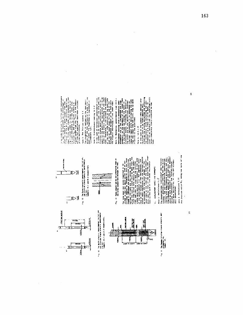
163
; i
_...._"_·_II> JI
?. l ~
~j - r
-
r~J a ! ~ ~
IE i il r
"¥ ! ,_ .., • K" ~ gj
::;
L !
-~~ !! ~ i~ci F:;.: '· zia zH ~ = . .::
APPENDIX B
ASTM D 3441-86 SPECIFICATIONS
164

165
., :;
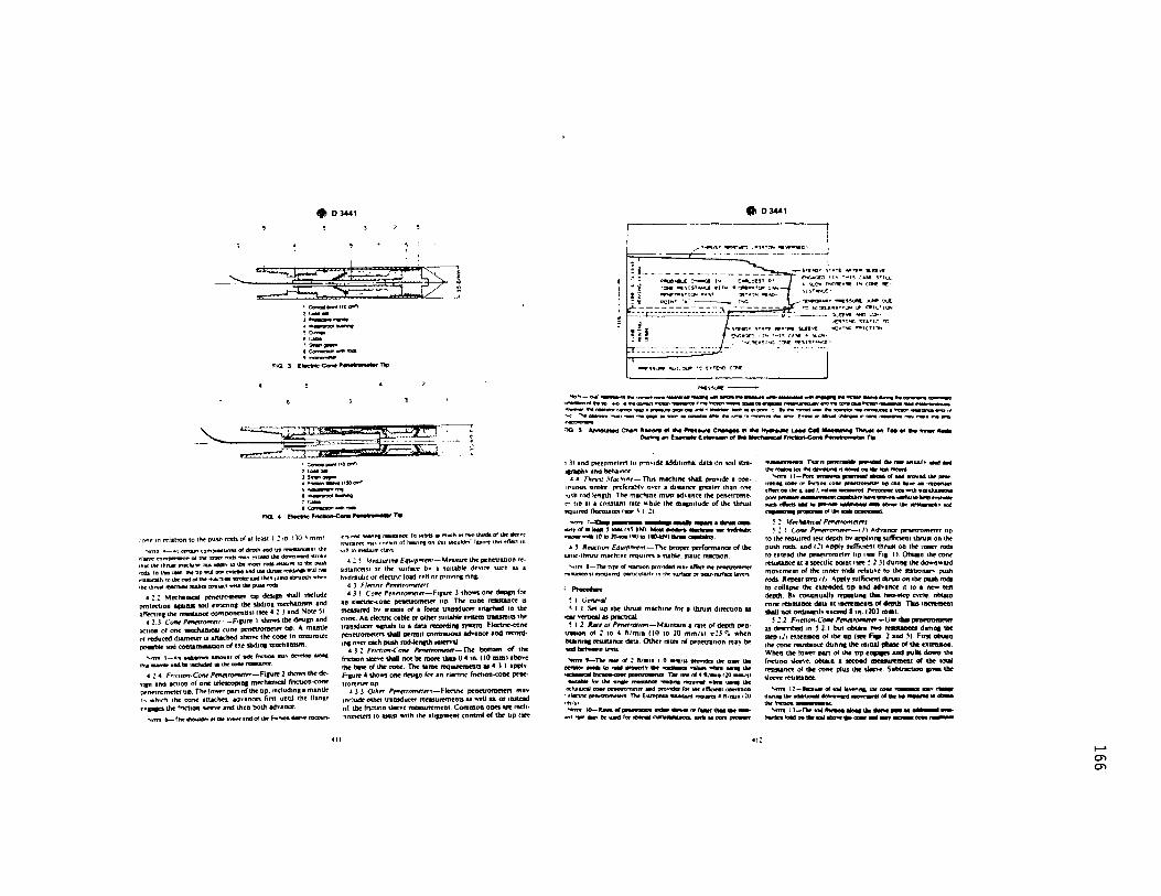
0 03441
-~ ::;:@1: ~:-~ 'c....._.11ocrro"I ,,_"" , __ JW.....,,.,,~
'"""' oc-•s .... Gllfl'll
·~-"* ·-FK;. 3 !lectnc:-CaN ~Tip
-~ :::::3§§B:EE---liS&s ~ -~ ~
1 ec.-Oll""•10crro"I ,,_"" 1s ... .... .. -.._.. ..... ,150Cl""I , __ ..., IW~~
''-!IC-........
'lQ .• l!i.c.te ,~~1\111
·()nt m rt'lation 10 tht push rods of a1 lust I :: in.! JO~ mm!
..,.mr ....._.,, C!r'Wn comblubOm of dc'tlth ind UP ,_..naf11 tllt ~lnuc romC!ft'90n of llw 111Drf mi:b m•~ neftd W ~-.rd ttrollc 11111 lM 1hn&ll mKtlllle 128 .... lO U. 11\Dn' Jodi ~1"t to lbr ~ •odl lo 11111 ca.. llW no wtU not nv.d and lbr lhtWl ,_,ftll W\U "" tluuc:Mh 10 the~ of tlw mKbtDf tUt*t ud Wu 1ump abrupt.I" wMn itw lftru.i mtcbl• ma.kn coUK'I wtW lbr puMi rodL
4 .: . .: MecharucaJ pmttrometer up lkslp shall 1ncluck prot«Uon lplml mtl entcnq the Wctin1 mecba111sm 1nd aff«t1n1 lhf resauncr comoone11as1uer4 2 J 1nd Notr 51
4 2.l COM Pnwt.NJlf/'ln' -Fisurr I ~ 1be deup and K110ft of one rnecharucal ~one pcnctromrter llP ~ mantle nl re:luced dlamelft IS anached above the CODf 10 n11mmue po19blc "1 co1na11unauon of 1he sbdJDI mechanism
.._"" ,_,n •• .,.. amo .. 1 ol tldl' l'ncbo. mav ~ .,_. 11u1!9M'lllf111d bt 1Kludied im tM com~
4 2 4 F,1won·COM'"""'°'"""'-Fiptt2thowitheck· ""' and anion of OM ll'~bl mechanttal fncuon-conr P'f'netrom~tt tip. TM I~ pan of the tJp. 1ncluc:hn1 a manlk 1,, which !ht cone attaches.. Mh"antt!. fil"'Jt uuuJ th' nan1t ""PifS the fnctJou tJttvt and then both ildv.aDCe.
..,on 6---llie~•tbr~~oftlwrnctlotltklnT~n·
t"!"I "nd·hdn"I l'C!UU!rK'e la u.ndl u much u ,....., tlwdJ of tM *"'"" ~'IUUnn' ma~ conllJ! of tanrtt on 11\n lbouldtr" llftl>IT th.It tffcr:i '"
'l<ll"I 10 medium dart
.a::..~ \fnuurm.t Equ1pm111r-'4easutttM oenetnuon rt• ~1st.1na:H1 l1 the •urtaa: bv a \U1t.1bk' d'vtct 'uch ll a h\·drauhc or 'lcctnc load cell or provm1 nn1.
4 J Elmric P111nromnrrf
41 I
4 3 I Co"r Pr"ffromfftr-Fi1urt 3th~ orw deslp for an eiennc<one pcneuomtter up. The cone telllUIK'f: 15 measured ~ means of a fottt uamducrr 1nached to th' cone. An elcanc c:::abte or <Khn •U1labte s.-m nnsnnts the tnolducn sapals 10 a data recordint Jy'!lnll. Eleanc-cone ptneuome'len VWJ perm11 conbnuous advancc and rtcord-1n1 o•er each push rocMeftllh 1nltrVal.
.. J ~ F r"/CflO'l·C OM Pnll'lromntr- Tbe bottom of lhf' fncuon sleeve lb.II.I oot be~ tlwl o.• 1n.110 mml abo•e the bur of the cone. The time ftlQUU'mlOb as •.l.I •PPI~ F1prt 4 1howt one dtstp for an dectnc fncoon<OM pnle·
trom~up
4 J 3 01h~ Prnnromn'1'.r-E&ennc peneuomctm ma• 1ncludt other tramdUttf measun:ments u wtU u. or 1nSteld of. the fncuon lletve measu~eat. Common ones are inch· nometen to U11J1 W'llh the ahpment control of tbr tJP lire
• 03441
/T'411,J!,T ~~ 1•!<;T!".h <W\lfflWC'• h= ="= -- - - --- --- -- -f_ ___ _
: Dtl09..._IE C .. ANC.1! ...
-'ST"EIO" ~tAY@ ..,.T"E• t.El!'Jf ~G(:l f ["' •w15 :ASI: '!>TIU. I 51..C'W l~A!i( I., C:>E IW:·
~- .. ~55'.JW~Ol...I:
.~:_=~if •:: IC:E\.E:~~ '~~~~I~ ~'l"«i 5THI.: ~C
~·~o t I"' •~15 (l'iE ' <;i.~w
:•.o:ll!E•51'<. 77* 1:1£5ISU...:£•
'""'!55,__ !lu!:..~ •:: E•~'<I C7*
~5~---..., •• _.l).'9 • ........,, ..... alf"WIE'I _____ ....,,.,.~ .. -..-_....-.......... --. .......... __..,....._
,..__1111 ... ID .M.•"--~----~"'9"""-'-.muiit•......,--....,- ... _OllJI~------- ..... --~-•-QllQl'IM-~- ..,. .... _...~ ..,-~-- .. ~._.__.~--'11 -.....:: ..,.......,..._.,._,.,.~•-•--....,-"""'ID ......... .,...., ~ncar_.,......,c:o._....,....,•---:io. 5 ~ Cftelt ltecot'll ............... c-... ..... ~ l.eMll C4'I .... euMI ""'* Oft , ....... ""*' ._..... Durtrlt9"IE1.,...IE.......,.of ... ~,~~n.
1 J 1 .and praomrttn 10 prov1d,. adcb11onal data on .ad Hra-111"1C*v .and behavtor
.S .S Tltrv11 .\(11</mrr- flus mKh1ne '1'1all prov1<k a COri• 1nuous urok,. ~frnr.hl\. ovrr 1 cbstlntt p·ea1itr than onr ·u~h rod ~nllh T~ mach1n' muS1 adv1_n~ Ute prnenomel"r 1111 11 a constant nit -. bde the masnnude of the lhrust -rqwrtd OUC1u.a1es flltl! ~-1 ;1.
"'7fll...0., ............ ...., ................
""" ol• ... ' iam••, llNl. Mam ..... ---- - ~ ..--wtflll 10ta20-to91901a llD-tJ'IO*-:~.
.s ' lf.rtKt1on £q111rmrn1- TM proper perl'oi'inance of the u11c-1hnut mach1neo ~u1rn a ttable. st.auc reacuon
,,,,. l-T'biit~ofruruonpro.-.ded111a•alfecttM~ ..,.'IUIK!l'lll mruuttd. CMtrUcutarl~ '" 1Plt •urlaa: °' MU-IWfaa: laven ;
~ I tirrwral ~ I I Set: up the thrus1 machine for a thrust d1rect1oa u
IC:W Vn1ial U pracucat ' I 2 If.air 01 Pmn,at1on-Mauu11n a nte of Mpth pra.
UallOfl of ~ 10 • fttmin 110 to 20 mm/SI :t~S t-;. w~ ·bUlln1 .. rtSISlan« data. Other rat.ts of prnttrabon mav be .iedbmt«nlnts
~ "-Tlw ~of! fttm1• flO .... 111 ciroWlda tM a• tW ~--~--proprrtyt.Wr.-or .............. .. 1-----~~ ~1t1tol•ftl•••:0••1tl ~larllw••reltlUllm' rmilllllrwa"'* ... u.111t11e
a-fl.l..m cow cinnmmritt ud proVldls fm tM ~l'l'iant ooenuoo · riennc ~ ~ Eurnpeu Qfldud l'eq111ta4 1111.i•llO 1m111
"'kn'I 10-ltae ol~ fttMf ........ !JIJ,.... dlM - -w ........ ~,Of---~IUCti•OOft~
<II~
mQlllftftHU ftus·q &Wmllfmtlko ~tile f9W K'luall¥ 1.-:f ... IMnmot1fortM....,__1S~Oll--rwcord
-..cm 1t-~l"W'!ra_.,..,a-so1-.c1.,,.,•w ... UMllll COM °' fncuom COM ~ ao CUI -~ .. ·~ rrr., om tM ._ ud I ........ __,..,, PwlDmM U111 wtdt •• ......,_ P«t"...-we~t~lllll .. '""'"lllrf'l&jll)lwto...WllMr tw;lt dfctl .. IO"°""'* .......... -.,. lat .,.......,... &Dd
~~of·--~ 5 ~ .\fft"lw,.r<ol Pnrttmmnf'f"'f ~: I Conr p,.,,,,,.om,,rr--111 A.dvanct pmeiro~rr 11p
10 tht l'C!IQu1ttd 1ts1 depth ~ apph1n1 wffiaeo1 thrust on lbr pusll'rods. oiltd 111 Apoply suffiotnt 1hrus1 oa ttw •DMT rods to e1tend the prMrometer up 1wie F11. I). Obuln the COM ~•ta speclf1e pointlK"e 5.2.Jldunns the~want movement of the 1nMT rods "'lau"e 10 the muonarv Ptllh rods. Repeat s1ep 1 / J. ~Pl'l'f suffiaent 1hni11 on tbr P'Uh rods 10 collapte 1tw e•~ up ind adv•ntt 11 to a new 1et1 depth. Bv conbnu•HY repau111 lbls two-lltp ~cle. obuan cone l'ftlSUntt data 11 1IK'ftmnts of depth. 1ms tncftlM'bt
shill not ordlunl~ e1.ceed I tn. t20J mm». 5 :.2 FnctlOl'l·COMPrnftl"OlfVfrt-Utrtbll.~
u de!mbed an ' 2.1 but obwa rwo l'f'SaDClS d111n111 1llr sirp 1}1 t•1tntt0a of tbt op lter f"•. 2 ud S). Finl obulln 1hr cone n:sraance dunns the tnlbat .,..._of the nlmllOll. When the lower CIU1. of the op e..-.. and puUs down the fnc:uou sltt•e. obtain a Sf'COOd lltalUlftllelll of tbe 11XA1
rnullntt of the cone plus the Wrvr. Subuw:boa 11¥8 the •ltt~ rnlSUftee
"'°" I i-a.c. .. o1..- illwnn& die cow~ IBll• dlUlll dwuetktd*UCMt.,.....,.,~o1•-.,...... .. ~ ... ...__
"'°"' 1J-n..•rne.o.-... ..................... . bWdNk..so.dlit• ..... CDM ... _,. ~CDM,_.
-Ol Ol
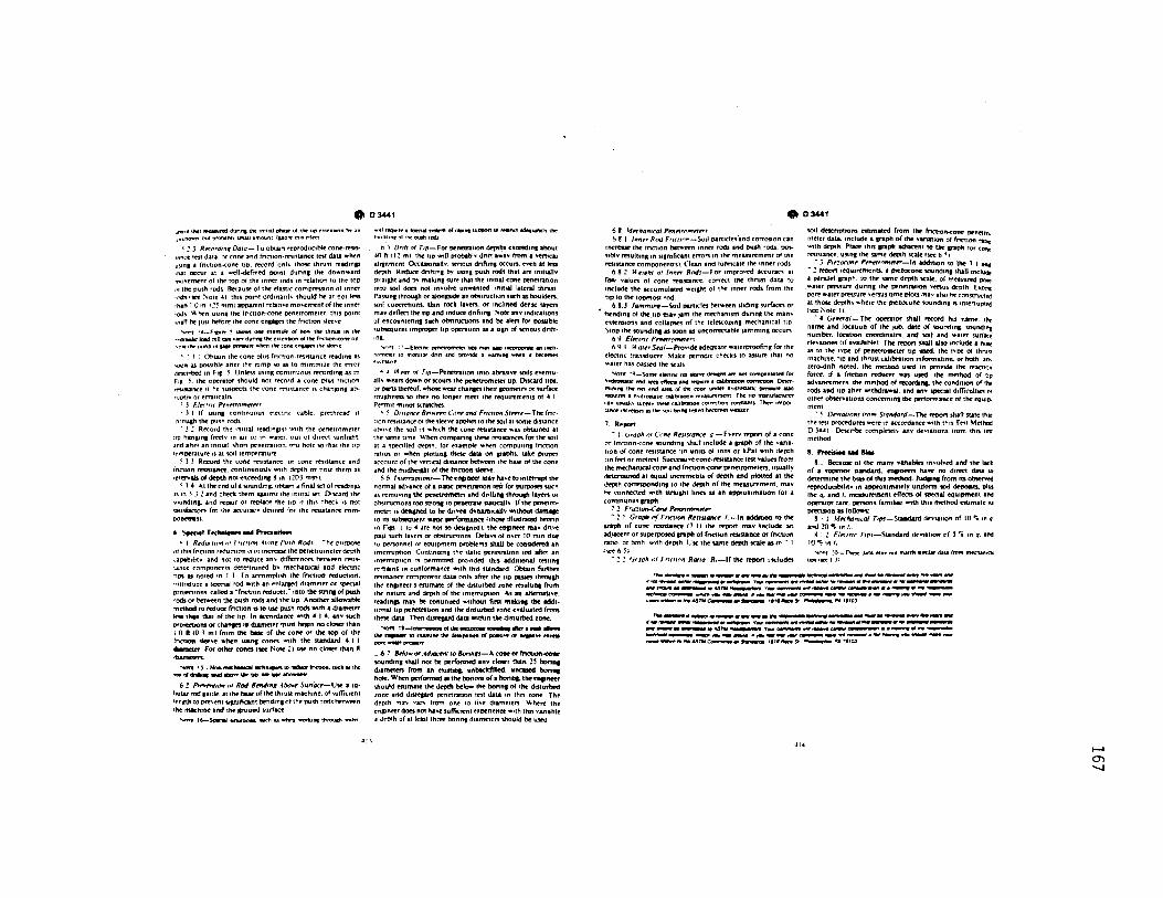
0 D:M41
aMl•C dlll 11ta111ral dun111die1ft111al DhuP of the 11111 f'Ol'fttHti• b\t •n J"1nown bin """'9:bh atLltl •moun1 llftOtT 1ft11 r1lm
~ ~ J Rnnrd111r Daro-lo obwn rrproduc1~ CDM·fftl5•
r:1nl·e 1n1 data. or cone .and rnct1on-rn.Ulrta' lnl d.llta when 11s1n1 a lncllon-conc UD. record onh. 1hosr 1hrust rrad1np 1hal occur 11 a ...ell-drlined pcnn1 dunn1 lhe downward ino•e~n1 ol tht IOP ot 1he inner rods in ~la1ton 10 lhe 1op ,•! 1be push rods Because or 1ht elu11c comprn51on ot 1nntt •r.OS fttt So1e .&1 1h1s po1n1 ord1n.nh 1hould t'lt 11 no1 less rhan I O 1n 1 ~~ mml apparenl rela11"e mo"'rmen1 of1he' inner rods Whtn u11n1111he fncuon-cone prnruometn. 1h1s omni ,11111 he 1ust trfore the cone enpen lhe rnd1on sltt"e
"1Tf 1&-F1prT ' lhowl onr u1mplc of tto. 11.e 1tma. 11!1 '"' ·~drmallC lmd rdl c .. .,.,. dunftl thr ctrrnllOft of 1hl fncucm<OM 11111
"""''"" rump1n ptr.,.._rT •l'll'n IM coftl' 'npen 1M~
• ~ J I Otitain 1he C"One plu1 rne11on-""11tan« rrad1n,: as "°'"' as poU1b~ .ar'lrr thr rump "° u to m1mm1u lhe trTor JnCnbed an F11. S Unlns usrn1 con1inuou1 rrcord1n1 as 1n Fr1 ~- 1he oper111or should no1 rttord .a cone Olus 1ne110n '"'9Uncc 1( ht swpec:u the' cone rM11t1.n«> is ch1n11n1- .ab-ruPIJv or emucaU\>
c J F.ltrmc P~rtnrn"'n~1 ~ J I If us1n1 cont1nuou1 tltttnc c1ble. pttthrtad 11
·nrnqh 1he push rods : J :. Record 1he 1n111aJ rtad1n1n1 '"'1th the prnetrometer
110 l't1n11n1 f~lv 1n an or m w11er. ou1 l11 d1rttt \unhJht. Jnd .after an 1n111aJ. 1hon prMl~t1on tf'"\1 hole 10 rh11 the 11p Tf'ml)C~IUrt IS II !all 1emper11ture
~ J J Record thr cone resmance. or cone re!ISUnct .and t"ncuon resutlnc:t'. conunuolUJv wi1h ckpth or note lhtm a1 1111en.is ol drDtl'I no1·e1cecdlna 8 1n 120J mm1.
' J .t -.1 the end of 1 'IOunding. ottwn 1 final srt of rnchnllS 1.\ 1n 5 J ;;!, .and chtck lhem Jp1n11tht1nmal set Discard the \l•und1n1- .and rer.wr or rf'Olace rhc UP II lh1\ chrd1 is not \IURtQMI for lht accunc~ ~ired for 1he rrsutanC"C com· ponnru~
•- s,.rill T«M"9n _, Pnaim.t
"' I Rrdumn" m f"r1wn" 41nnr Putli Rod.1-Tht PUl'1JIOV tll lhl!I rnc1IOO reduC110Q IS ID llKTCUC' the penttromeltr l'.kJ>th ~af9b1htv and no1 ro reduce anw d1fTtrl'nces betwren rn1,.. ancc compantnts detemnned bv mechamcal and eleanc "°' n notf'd 1n I ) To aL"'C'omphsh 1hc fnct1on reduction. •ntmdUCC' a llW'Clal rod Wllh .an enl.,.ed d11nm:er or ,.,eaal prOtft:tlOM. called • ""fnctJon reduttr .• IDIO the nnn1 of push rods or ~n the push rod!I and the tip. Another .UOW.ble mnhod 10 reducr (net.Ion is 10 !di!! push rods with • diameter "'9 Wn tha1 of thf' trc-. In IC"C'Oftbnc:e .,th • I •. anv such ttrOMICUOlll or chl.fllS 1• daameltr mun besrn no clotrr than I o tl 10 J m I from the bml' of dtt conr or the lop of the fnctlOa sAeeve •hen u.111 cones with the nandard •. I I ~ For othrr cones ltee NOie 21 UR no ctmer 1han I ...........
'limt 1 '-No..l9lldlmlmi .tl&lllMl IO ....... fncboa. tucll M IM .. ~drlli .. 11111d~lllt11P.•...,..._..,.,
6 2 ~"'" ol Rod IN•"' .4bo., Suttdcr-Uw a IU· hulu"rod1uK1e.a11heburoftht1hrua machine. of"'uffiettn1 lf'nJth to Prfven1 •P11fican1 btndln1 of 1he oush rods betwttn 1ttt m11eh1ne .and lite pound surface
""' 1&-s.-.r •hllluom. -.ch ..... -.ort1111 tll'°""" -'"
-11~11T1Wlfttal..-mofca111tuPllllWllO!ftlnct9dal1119lly1M touckJn11 of 11\f DU .. rndt.
: tt J Drrtr nl Tip-for prnctrauon ~hi e~_ceed11t1 abou1 .ui ft f I~ ml. lhe llP .,11 prot.blY dhfl 1..:1v fr0m • YftttCll aJ11nment On:lllOnallv. wnous dnfun1 occun. '"'n al less Gkpttl. Reduct dnfhnc b,.. usina push rods 1hat are 1n11ia11~ i1n11stn and b'W malun1 sure 1ba1 the 1n111ll COM pme1~11on in10 toil don not involve unwan1ed. 1nmal a.tttm lhl"USl. Pu.11na throuth or llonpdt 1n obstrucuon wc:h • boulden. soil concret1on1. thin rack la"en. or 1nchned dtmt la,cn mav ddlttt 1ht 11p •nd induce dnfilna. ~ote anv 1ncha11ons of encoun1enna such obnrvcuom and be aim for poa1ble 1ubtequent 1mproprr tip open.non u a sip of wnous dnft.
"'
inc.
'lrinn I• -EIK'tnr prllftnlllMWr UD1 MIY a11o lllCDflllDftW an IM'fl· no~r 10 moa11or dnfl 111d oro"'1dr J ..,,.1111 •Mii 11 betofl!ln
"'.& "rar nt Tio-Prnnmron 1n10 .abrulve sods eventu· .alh wean dcJwon or "°"" lht peneuom~ up. Discard ups. or puts lite~. •hole wear c:halllft 1heir ltOIHlrt or surface roughness so the,.. no lonlff mft'I lhe requ1rtments ol .a I Pcnnn minor 'Kfttchrs.
" ~ Dma•1u 8#1'4ttn Ccmr anti Frrct1ort Sl~-The fnc:· non rn111.1.nce ol ttle \lttvt apphcs to the sod 11 mme d1stan« aro~e 1he ..,11 1n which 1he cone rninana was obtained 11 1h~ \llmt t1mr When companns \Mir f't'tlSUnccs for the 'IOll
at 1 \Pttllied depth_ for eumolc •l'ttn com1nmns lnc:uon r.mos QI" when plott1q these data on paphs. take proper accounl of 1he vertical dlsu"" betYtftn lhe bur of dw cone and 1he mldbalbt of tM fncaoa slePe.
I; 6 '"''"""''mu-The cftpnftr may have to 1ntem1p1 the nonnal adv•ntt of a abC" pennnuon tftl for pul'POltS such u removin1 the PtftCUOIM1n and dnlh111 lhl'OUlh a.,en or 0M1ruct1on1 too IUODl •o pennnllt aatica.llY. Ir the pmftl'O
mettr IS drllped tO bl: dnftll dvumtclUY wttlKJUI dim.et 10 Ill tublequent Ube perfOl1IWICt' llhow lllllSlnHed hemD 1n Fip I 10 •.are no1 to desaanfdJ. the fnllnt'tt mav dnve past 1Uth lnen or obstructrons. Dtlavi of over 10 min dbf 10 prf"IOnM"I nr equipment Pl'Qbtems shall bt COftlldcftd In
1nte1TUp11on Con11nu1n1 1he su11c penftn.Hon 1rst after an 1n1enup11on 11 oenn111ed providtid this addmonal tnt1n1 rrm .. ns 1n confonnantt •llh 1his standard Oblasn runhtt rn1stantt component dala onlv .after the tip .,._,, throuah 1hr en11neer"1 esuma1e or the cbsturbtd zoM mult1n1 from lhr nature and dtpth of the 1ntenupuon. A.s an lhemau~. rncbnp ma,.. bl: continued •llhou• fira m&bns die addl· non&I tlP penftl'l.bon and the d1S1urbed rone evaluated from thne data. Thm ~ data "Mtlun the datumed ione.
~ ,,_,..........,. .. ,..__ .................... IJle~..,1Deum1111'thrdlla11MJ011olpaauwwor_.wwnmm
CIOl'l .... "'9111T
_ -6 7 lrloworAdlGllflrtallon11rs-Aeontorrl"ICbOll<Olll' 10undnt1 shall no1 bl: perfonned anv dOll'r than 2' bonr11 cbaintetcn from • na111ns. unbeckftlled. •ftCaled bonna hate. When performed at the bonom of• bonna. Ille enpnttr Vloukl esttmalr the depth below the bonn1 of the d111urtled 1one and d1lttllf'd pennr.1uon int data 1n this zone Tht dcpch m.a... ,...,.... from one to five d1•me1tn. Whe~ 1ht entpnerr dOt'S noc hlive sufficient e1pem:ntt With nus v.nable ;ii Jf'Olh or 11 leut lhrft' bonn1 dia~1rn shoukl bt utrd
• 03441
6 I \frrhanrc-al PrrrrtrtlllMrr• 6.8 I fr111rr Rod F"W""-Suil oan1cln°1nd corTOS1on can
1M:rcae the fnct1011 be'lween inner rods. and .push rocb. pm-11btv rnull1r11 1n sip11r1c:11n1 mon m the mtuurtment of 1he f't'tlSl.lfla' comDOnenuti. CICln and lubnc:ate lht inner rods
61 . .:? ""''"' ,,, '""" /fod1-For 1moroved IC'Cunci.· 11 l"cllit values of cone f't'tlstance. co1Teet thr 1hru11 data to include the xcumulatl'd we11h1 of tht inner rods from tht np to 1hr topmost md
..c 6 l.J Ja,.,minw-Sotl P9f11c:IH ~'Wern slldtnt surfaca or 1"nd1n1 of 1hr 11p m•y Jim thr mtthlnnm dun:ns lhr man' n1enwns .and collaP!Ct of 1hr ielncoP1n1 mechanical tip
S100 the sound1111 as IOOft a uncortKU1bte ,amm1n1 ~un 6 9 Efrrmc- Pntnromnr~1 ti 9 I JI ortr SHl-ProVKk ldeau11r watervroolins for thr
~lectnc: 1r11n'ICluCt'r. Make rxnod1c checks 10 murt 1ha1 no wa1er h~ paged the teaJS
""'ort 10-SoFM ellnnc rnr *""' *""".., riat C'OllQlll'n•IN ror h"*-IMlc end ... effKu and~. c:allbntlon C'OfftalOll Dnnm1111 .. t1't M1 tnd uaolthrC'Oflt' under h~ ~mllD 1111uim • h~ron.rruc ca&ibnuoft masurentn11 lhr no 1111.aulanurtt can utuall" 'UDO!.., 11tnr cahbnmon cont'CtlOn mtisu.nu fhf'ir 1mD01"-1.1nce 1ncra..s u '"" 1011 btr1111nied bf'coTfln -aer
7. R•"°" .. I <irapli ,,, Cr1nr Rrsmancr "-E,,ttV re-pon or 1 cone
or (nc110n<Ortt' 10UllChRI shaJI include I pph O( lhe Vlnl·
uon of cone rntStantt 11n un1u of tons or II.Pal "Mth dcplh 11n feet or mtlrnl Succemve cone-restaanc:r lest vllun from 1hr mechlrual conr •nd rnc:uon-coae prneuome1en. USU&ll~ dmmuned •t equa1 11Kft1M111S or deiKh and plotted •• 1tte
depth correspond1111 10 lht dtplh of the meuu"m""'- ma~ ~ c:onncded With llJ'allhl hnrs u an appro11mauon IOr a continuous ...,ti.
~.? Fr1e11art-COM Pttwtrom11.tr -Y .:?. I GrorJlt tr/ Fr1t.1101t lfrrm1111tt. 1,-ln addition to thr
p;1ph of COM t'edlante f 7 11 t.hr rrpon: 1118'1 1nc:ludr an adJac:en1 or 1UCll'f1IOlftl sraph of fncuon nsaance or rncuon ra1ro. or hoth. W"llh dePlh l:tt 1he Kmr depth tc2k u in • I Htt 6 ~I
.. ~ ~ Urapli "' F'1ct1t1n Raua /f,_lf Ille' RllOf1 1ncludr\
'IOd dnc:np11ons es11mated from the' f'nct.1on-cone prftftrn. meltt dala.. Include I lf'lph of the YlnallOft of fnc:t1on ~llO wnh ~h. Pt.ct- this paph _.,K'ellt to tht lr.lph for COflt rn1nancc. us1ns the 1i1me drplh ~ 11ee 6.~ 1
.. J P1r.oc""' P"""""""'"-ln mckbuon to thf' 7 t ill(! .. : ~ l'l'Qu1remenu. • peczoconr 1DUnchn1 1lwll 1nc:IQdr a parallrl snph. 10 lhe 'lolme drSMh scale. of meaiured PDff •11er preuure dunn11he penetratMH1 vmus dtpth. E~ pare water prnsu" ,,enus nnie plou ma~ 1IVJ ~ con11ructe.i 11 lhDlt' depths •hrrr 1heo prcrocone sound1n1 11 1ntenvpre.i t'lot:e Note 11.
.. .a Grrtrral- fhr opnator shall f'ttOfd his IUllM. lht name and locauon of thr }Ob. due of toundlq. sounc11na number. location c:oon:hna1e1. and DI and •atcr surtar:r eltvauons 11r av .. lable1 The~ shall <a 1nchade a~ as 10 the IV1JC of Pt'netro!Hltt HP llSfd. tht '"Pl' of thru!I m.ach1nc. llP and 1hn111cal1brauon1nfonnat1on. or bO'lh . .an' zero-dnft: noted. thr mnhod ultd to iirovidr 1he 1nt11011 fort:e. If a fnction rtducer •• used. lhe method of llD
adva~mmt. the mtthod ot m:ord1111- the condmon of thr rods and up aft:rr w11hd,...a_ ind anv special dlfficulllt" or otner obvf\'att0ns conttn11n1 thr pertonn•nce ol the equ1Dmen1
.. ~ lJ#iY1at1on1 riomn Srortdard-Thr wpon tttall 1ta1e 1h11 the int OfOt'fdurcs ~re 1n accordantt 'llllth 1h11 T"'1 Mnhad 0 J.W I Ot<Jcnbt compfelel) .an~ dtviauons rrom this lest me1hod. .. ..._... ... _
I. I BeaUll: of the manv vanabln 1nvol"nl net the •• or 1 supmor standard. eGpneen ~ no d1rai u .. io
de'lemune the bt• of tlul mrtltod. Judit .. from 111 oblervel reproductbtlilv 1n appro1.11nately uruform to1I drpamts. plw the q, •nd 1, meuu~n• efTccu of 'IDft'lal equipment .and operator catt. penons fam1hu 'lllllh tJt11 mt1hod esum•w 1u pn!t"UIOtl • rotiow.: - ·
8 I I .Wtcltaruco/ TIP!-Sl&Bdard dev1•oon of 10 c;, 1n t1
and 20'° 1n I •. IJ I = El«mc Tlt'J-Standllrd devtlUon of 5 ~ tn q, Ind
10~ 1n I, "loTI :0- T1Mw daLI "'"' not lftlllrit •111•lllr dll..I fnMll mecM111C11
UOllW.: I JI
,.,.__.._. ................ ,_....,... __ ...... ___ ~- .... ... .,_ ...... .._.._.... . ......_. ,., .......... --........ - ....... __.. .... _ ....... .. .,... .. _._.. .. ,.,.._.... .. ,.,.._.. ____ ~··-..-----...~--- .-.eft,....,_ ..... ,.-~ .... - ........ - ................. ,.,, __ ,.,..ASrvc:-.. - 11rt-.s .,_..,N1trOJ
,.. _____ ..._ .......... .-...-c.---.................... -, .. ---.._.... • ......_. y_._...,.. .. ....., .... _ ... __ .... _ ...... ---·--··"'----~---..... _..,_......., ............... ._ _,.....,._ .,..,,....., ........... ...,,_.. ........ _ ... ......,,., ......... _ ._._,..,.AS1VC--•9-dl •lllllleeiesr ....._.,,..,,,OJ
... ....... en .......
APPENDIX C
EXCERPTS FROM HOGENTOGLER OPERATION
PROCEDURES MANUAL
168

OPERATION PROCEDURES FOR THE DUTCH CONE PENETROMETER
CONVERSION KIT
I. INTRODUCTION:
The Dutch Cone ·Penetrometer or quaaistallc cone penetrometer 1s a device for
obtaining Jn-situ 1ub1urface data Jn a variety or soUS. Useful design datil can he obtained
In most type• of •oil the equipment can penetrate. The chief advanl•Ke of the Dutch Cone
Penetrometer ts Its ability to retrieve large quantities or useful data :rt an economical
cost.
A few apeclCic applicatJons for the Dutch Cone Penetrometcr are:
1. Determination of the uniformity and continuity of soil depusil~: i .1! ••
stratia:raphy.
Definition or soil type; e.g •• sand, clayey silt. etc.
3. Obtaining in-situ engineering soil parameters.
~. Design of pile foundations.
5. Compaction control where soils :ue compacted hy a \':iriety tJf m•~thocl~.
The followinK procedures are applicable to the operaUon or the Dutch Cone Pene-
trometer Conversion Kit sold by Hogentogler and Company. The procedures are also
applicable to the trailer and skid m·Junted penetrometers sold by Hogentogler and Co.
with the exception of the operation of their hydraulic loading systems; reference should
be made to the respective operators• handbooks for proper use or these other types or
penetrometer sy 1tem1.
The Dutch Cone Penetration Test con1i1t11 of the measurement or the resistance to
penetration of a hardened steel device of standard dimensions as it is forced into
the subsurface at a fixed, predetermined rate.
All penetrometer teat1 should be conducted in accordance wnh ASTM D :J-141-751'
"Deep Quasi-Static Cone and Friction-Cone Penetration Tests of Soil." :\ 1•opy of thts
' speciflcaUon is contained in Appendix A.
II. CONVERSION EQUIPMENT AND ITS FUNCTION,
The conversion kit converts a standard core or auger drill quickly and easily to
a Dutch Cone Penetrometer tester. To perform the penctrom~ter conversion lhe
following pieces or equipment are supplied with the Dutch Cone Penetrometer Conversion
Kil:
2 - mande cones
2 - friction Jackel cones
25 - one meter sounding tubes and rods
I - 11 ton hydr•uUc load cell and gauges
I - pulling device
l - 75 mm inner nxl extensfon
2 - 15 mm Inner rod e'"en&ions
1 - continuous sounding ring
l - dt!pth indicator gauge
1 - friction reducing section or sounding tube
2 • spare gauges
1 - carrying caae
Nole: A mounlln1 bracket I• used lo attach lhe load cell lo the drill riK. The
hro.cket ia fabrtcated by the customer because its configuration depende on the customer's
drill ril model.
The above component• are interchangeable with those component& found on the trailer
...... O'I l..O
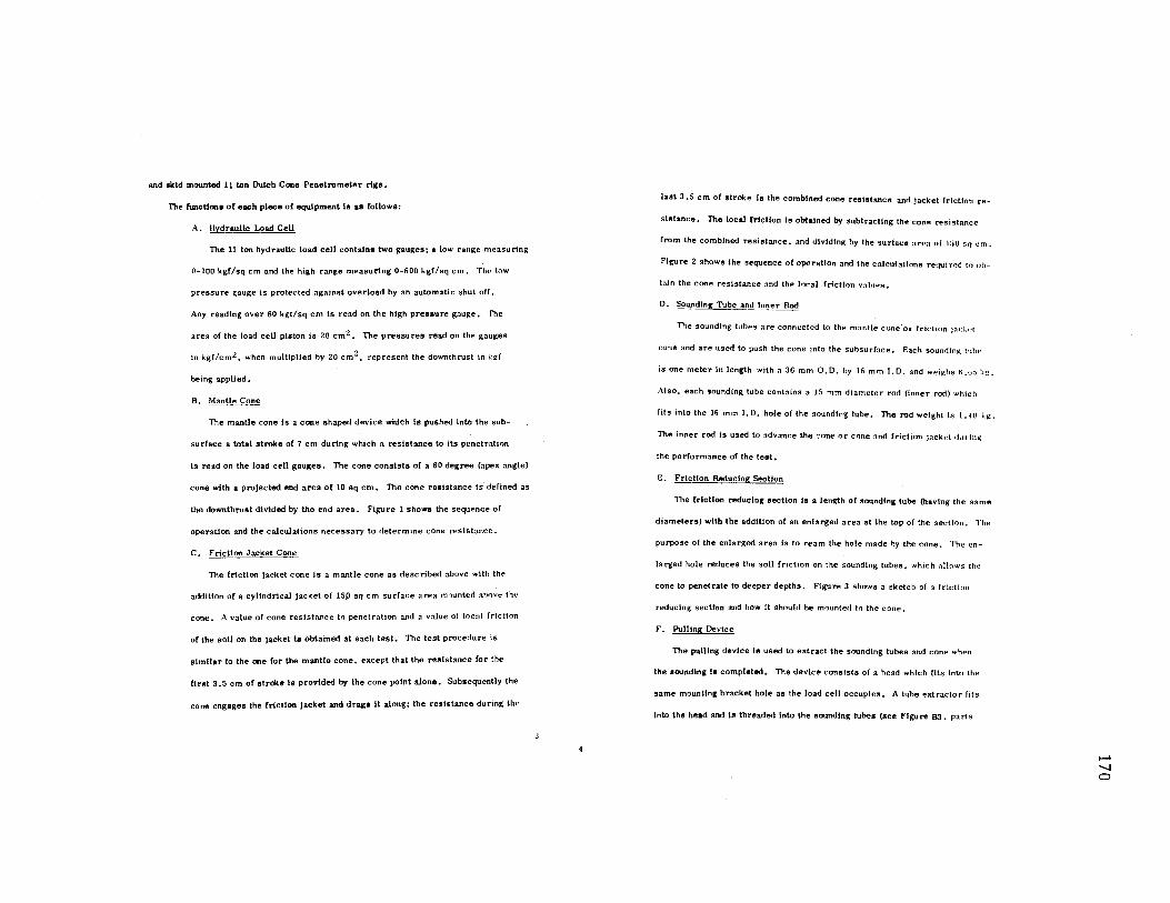
and skid mounted 11 ton Dutch Cone Penelrometer rig•,
The functlona or each piece or equipment lo ao follows:
A. Hvdraullc Load Cell
The 11 ton hydraulic load cell contains two gauges; a low range measuring
0-100 kgf/sq cm and the high range measuring 0-600 kgf/sq cm. The low
pressure gauge is protected a"aJnst overload by an automatic shut off.
Any reading over 80 kg(/ sq cm is read on the high pre111ure gau1te. The
area of the load cell pJston is 20 cm2. The pressures read on the gauges
in kgf/cm2, when multiplied by 20 cm 2, represent the downthrust in kd
being appUed.
B. Mantle Cone
The mantle cone ts a cone shaped device which is pushed into the sub
surface a total stroke of 7 cm during which a resistance to its penctr:wlion
ls read on the load cell gauges. The cone consists of a 60 degree (apex angle)
cone wllh a projected end area or 10 sq cm. The cone resistance Is defined as
the downthruot divided by lhe end area. Figure I shows lhe sequence or
operation and the calculations necessary to determine cont! resistance.
C. Friction Jacket Cone
The friction jacket cone ls a mantle cone as described above with thE"
addition of a cylindrical jacket or 15j) aq cm surface area m?unterl ahf)ve tht.•
cone. A value of cone resistance to penetration and a value or local friction
or the soil on lhe jacket Is obtained at each test. The test procedure is
stmllar to the one for the mantle cone. except that the resistance for the
Drat 3.5 cm or stroke la provided by the cone point alone. Subsequently the
cone engages lhe rr1ct1on jacket and drag1 it along; the reolstance during the
la11t 3 .5 cm of stroke ts the combined cone resistance and Jacket friction re-
slatance. The local friction is obtained by subtracting the cone resistance
from the combined resistance. and dividing by the surface area of 1;,o sq cm.
Figure 2 shows the sequence of operation and the calcu:laUons required to ob-
ta.in the cone resistance and the local friction valutc""s.
D. Sounding Tube and lnne r Rod
The sounding tuhes are connected to the mantle cone.or rrtction 1ac1.~1
cone and are used to push the cone into the subsurface. F:ach sounding IUhf"
is one meter tn length with a 36 mm O.D. hy 16 mm 1.D. and weighs 6.65 kg.
Also. each sounding tube contains a 15 mm diameter rod (Inner rod) which
fits into the 16 mm l.D. hole of the sounding tube. The rod weight is 1.-10 l..it.
The inner rod le used to advance the cone or cone and friction jack1~t 1111 rin~
the performance of the teat.
E. Frtctton Reducing Section
The friction reduclnr section ta a length of sounding tube (having the Same
diameters) with the addition of an enlarged area at the top of the section~ The
purpoee of the enlarged area Is to ream the hole made by the cone. The en
larged hole reduces the soil friction on the sounding tubes. which allows the
cone to penetrate to deeper depths. Figure 3 shows a sketch of a friction
reducing sectton and how it should be m?unted to the cone.
F. Pulling Device
The pulling device fe used to extract the sounding tubes and cone when
the 1oundln1 I• completed. The device consists of a head which fits into the
same mounting bracket hole as the load cell occupies. A tube extractor fits
Into the head and I• threaded Into the sounding tubes (see Figure 83. parts
.......
" 0
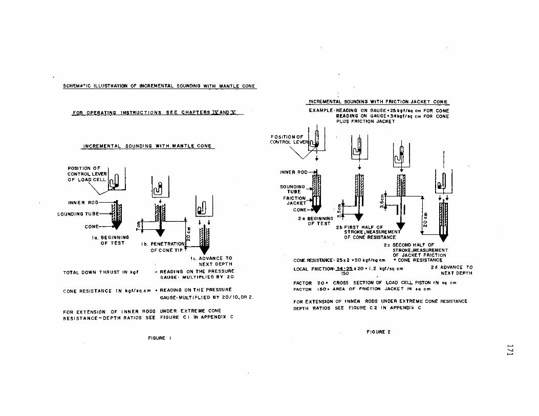
SCHS::MA .. IC ILLIJSTRATION OF INCREMENTAL SOUNDING WITH MANTLE CONE
FOR OPERATING INSTRUCTIONS SEE CHAPTERS .nz:ANDY
INCREMENTAL SOUNDING WITH.MANTLE CONE
OF LOAD CELL
POSITION~F CONTROL LEVER w INNER ROD:)
SOUNDING TUBE
CONE
la. BEGINNING OF TEST
Ji ~ ~ TOTAL DOWN THRUST IN kQf
N I b. PENETRATION'!---{llYll
OF CONE TIP
I c. ADVANCE TO NEXT DEPTH
READING ON THE PRESSURE GAUGE• MULTIPLIED BY 20.
CONE RESISTANCE IN koflsq.cm. •READING ON THE PRESSURE
GAUGE• MULTI PU ED BY 20110, OR 2.
FOR EXTENSION OF INNER RODS UNDER EXTREME CONE RESISTANCE-DEPTH RATIOS SEE FIGURE CI IN APPENDIX C.
FIGURE I
INCREMENTAL SOUNDING WITH FRICTION JACKET CONE
EXAMPLE•READING ON GAUGE•25kof/1q cm FOR CONE READING ON GAUGE• 34kof/sq cm FOR CONE PLUS FRICTION JACKET
'o'"'~ CONTROL LEV
+ INNER ROD
SOUNDING TUBE
FRICTION JACKET
...
CONE 9
2 a BEGINNING OF TEST
~ ~ ~
2b FIRST HALF OF STROKE;MEASUREMENT OF CONE RESISTANCE
E u 0 N
I
l4J +.+
2c SECOND HALF OF STROKE;MEASUREMENT OF JACKET FRICTION
CONE RESISTANCE• 25 x 2 = 50 kof/sq cm -t CONE RESISTANCE
LOCAL FRICTION•~• 20 • I. 2 kof/sq cm 150
2 d ADVANCE TO NEXT DEPTH
FACTOR 20 • CROSS SECTION OF LOAD CELL PISTON IN sq cm FACTOR 150 • AREA OF FRICTION JACK.ET IN oq cm
FOR EXTENSION OF INNER ROOS UNDER EXTREME CONE RESISTANCE DEPTH RATIOS SEE FIGURE C 2 IN APPENDIX C
FIGURE 2
...... -..J .........

A
NOTE: ENLARGED SECTION PLACED AWAY FROM CONE
B
A FRICTION REDUCING TUBE MAY BE USED( FIG.84) FOR REDUCING LATERAL FRICTION ON THE SOUNDING TUBES.
CONTINUOUS SOUNDING WITH JACKET CONE I . FIT CONTINUOUS SOUNDING RING TO THE
MEASURING DEVICE.
2. EXTEND IJRESSURE ROD BY MEANS OF THE EXTENDING ROD.( 75 mm).
3. ADVANCE CONE INTO GROUND AT FIXED RATE AND OBSERVE GAUGE READINGS AT
INTERVALS, SUCH AS 20 cm.
FIGURE 3
Number 18 and 19. Appendix 8). The hydraulic system o( the drill is used to
extract the soundtn1 tubes.
G. Contlnuouo Sounding Ring Plate
The contlnu.01.1.• llOWldlng ring plate Is attached to the bottom of the load
cell (See Figure 831. The ring Is used when continuous sounding using the
m1111Ue oone Is desired (See Section V). Continuous ooundlng Is a procedure
whereby cone reolatance lo oboenred periodically ao the cone lo puohed Into
the soil without Interruption.
H. 75 mm Inner Rod Extenolon
Continuous sounding with the mantle cone requires the use of a 75 mm
long by 15 mm diameter inner rod eKtens10n which is used in conjunction with
the continuous sounding ring (described above). The purpose of the rod
exteneion ls to extend the inner rod (See D above) so 1t contacts the actuating
mechanism of' the load cell.
I. 15 mm Inner Rod Extension
Under extreme cone resistance the inner rods are subjected to forces
which will cause them to. shorten elastically. The 15 mm rod extensions are
u•ed to compensate for the elastic shortening (See Appendix C). Alternatively.
a single overlength sounding rod may be used for the same purpo1e.
J. Depth Indicator Gauge
The depth lndlca&or 1aup i• a 1 + meter long slender rod containing depth
tndtcattn11roove• machined Into lt every 10 cm •. A heavy base 111 nlso provided
to keep the gauge from Upping over. The gauge ls located next to the soundinat
tubes 10 the operator can visually determine how rar the sounding tubes should
be pu•hed into the 1ub1urface between teat• (test ta normally performed every
........ -....J N
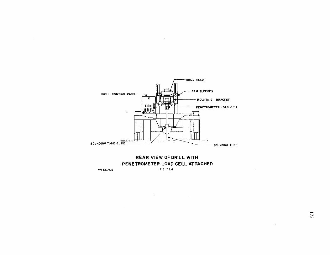
~DRILL HEAD
DRILL CONTROL PANEL
_A~ MOUNTING BRACKET
M -1 I PENETROMETER LOAD CELL
SOUNDING TUBE GUIDE------_,. -----SOUNDING TUBE
REAR VIEW OF DRILL WITH
PENETROMETER LOAD CELL ATTACHED Wl SCALf; FIGl'~E.4
.......
" w
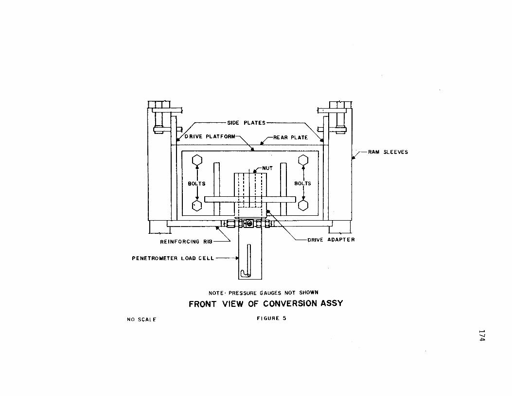
----SIDE PLATES-----
REAR PLATE
9 9 eors eors 0 0
REINFORCING RIB DRIVE ADAPTER
PENETROMETER LOAD CELL---
NOTE: PRESSURE GAUGES NOT SHOWN
FRONT VIEW OF CONVERSION ASSY
NO SCAL f FIGURE 5
RAM SLEEVES
I-' "-J
*'"

REAR PLATE
DRIVE
GAUGE
PENETROMETER LOAD CELL
RAM SLEEVES
SIDE PLATE
DRILL BRACE BRACKET
REINFORCING RIB
-DRIVE ADAPTER
SIDE VIEW OF CONVERSION ASSY
Flf E 6
f-'
" U1
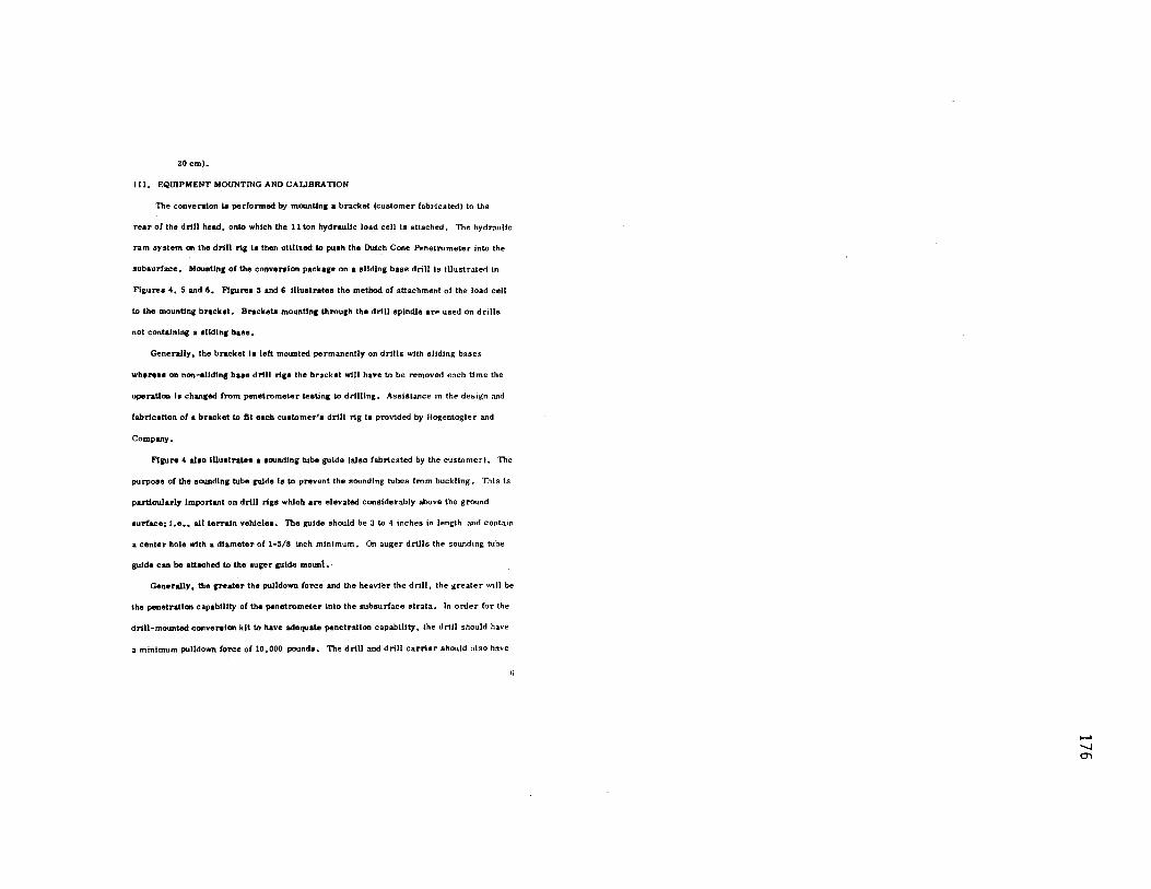
20 cmj.
I II. EQ!nPMENT MOUNTING AND CALIBRATION
The convenlon I• performed by mounttn1 a bracket (cul!ltomer fabricated) to the
rear of the drlU head, onto which the 11 ton hydraulic load cell Is attached. The hydraulic
ram system on the drill ri& i• then ullUzed to pu•h the Dutc::h Cone Penetrometer into the
subaurface. Maunt1n1 of the conver•ion package on a sliding base drill Is lllustratect in
Figures 4. 5 and 6. F11111ro• 5 and 6 Illustrates tho method of attachment of the load cell
to the mounUng bracket. Bracketl mounttnc throu1h the drill spindle are used on drilll!I
not containing a alldlnc baae.
Generally, the bracket 11 left mounted permanently on drills with sliding bases
wherea1 on non-sliding base drtll rigs the bracket will have to be removed each ti me the
operation la changed from penetrometer teeting to drilling. Assistance in the design and
fabrlc•tlon of a bracket to flt each customer'• drill rig I• provided by Hogentogler and
Comp1111y.
Fl1111re 4 al•o llluotrat•• a •oundln11 tube guide (also fabricated by the customer). The
purpose of the sounding tube guide 111 to prevent the sounding tubes from buckUng. This is
particularly lmport1111I on drill rigs which are elevated considerably above the ground
surface: i.e., all terrain vehicle•. The guide should be 3 to 4 inches in length and contain
a center hole with a diameter of 1-5/8 Inch minimum. On auger drills the sounding tube
guide can be alhched to Ibo au11or 11Ulde mount.·
Generally, the .rreater the pulldown force and the heavier the drill. the greater will be
the penetration capablllty of the penetrometer into the subsurface strata. In order for the
drill-mounted convenlon kit lo have adequate penetration capability. the drill should have
a minimum puJldown force of 10,000 pound•. The drill and drill carrier should also have
...... -....J O'l
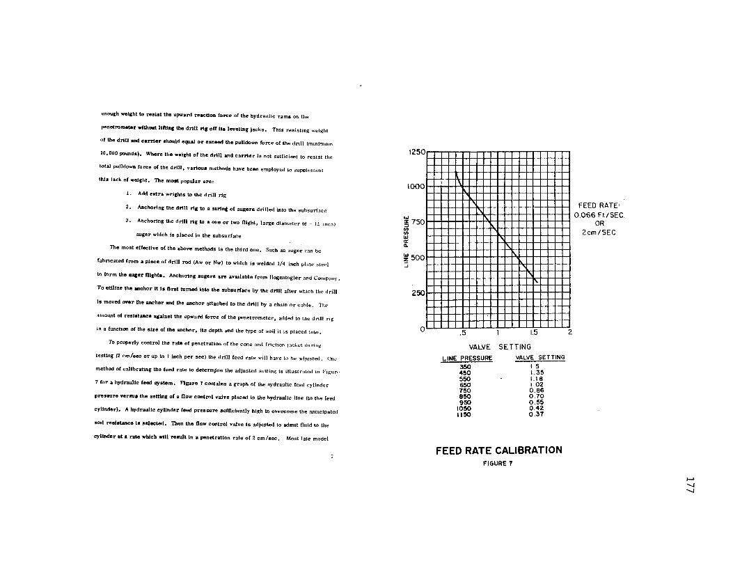
enough wet1ht to resist the upward reaction force of the hydraulic rams on the
penetrometer without liftfnc the drill rig off ita leveling jacks. This resisting Wl!ight
of the drill and carrier •hould equal or exceed the pulldown force of the drill (minimum
10,000 powid•). Where the weight of the drill and c::irrier is not sufficient to resist the
total puJldown force of the drill, various methods h3ve been employed to supplt!nwnl
this lack of weight. The most popular are:
I. Add extra w~tghts to the drill rig
2. Anchoring the drill rig to a string of augers drilled into the subsurface
3. Anchoring the drill rig to Rone or two flight, large diameter (8 - I:! inch)
auger which is placed In the subsurface
The most effective of the above methods is the third one. Such an auger c:m he
fabricated from a piece of drill rod {Aw or Nw) to which is welded 1/4 inch pbte stet•I
to form the :weer Ot1hta. Anchoring augers are available from llogentogler :ind Company.
To utilize the anchor It Is first turned Into the subsurface by the drill after which the drill
Is moved over the anchor and the anchor attached to the drill by a. chain or c;ible. Tht•
amount of real1tance against the upward force of the penetrometer 1 added to the drill rig
is a function of the atze of the anchor. tts depth and the type or soil it is placed into,
To properly control the rate of penetration or the cone and [riction pchct durin~
testing (2 cm/sec or up to 1 inch per sec) the drill feed rate will have to he adjusted. One
method of calibrating the feed rate to determjne the adjusted setting is illustrated in Fi1.:11ri·
7 for a hydraulic feed system. Figure 7 contains a graph of the hydraulic feed cylinder
pressure versua the setting of a flow control valve placed in the hydraulic line (to the feed
cylinder). A hydraullc cylinder feed pressure sufficiently high to overcome the anticipated
soil resiltance ls selected. Then the flow control valve ts adjusted to admit fluid to the
cylinder at a rate which wtll result in a penetration rate of 2 cm/sec. Most late model
1250
1000
~ 750 ::> U) U) UJ a: Q.
~ 500 :::i
250
0
I ' '
I"\ ....
"
.5
VALVE
LINE PRESSURE 350 450 550 650 750 850 950
1050 II !50
' " .... ' I'
....
1.5
SETTING VALVE SETTING
I. 5 I. 35 I. I 8 I 02 0.86 0.70 0.55 0.42 0.37
FEED RATE CALIBRATION FIGURE 7
2
FEED RATE 0.066 Fl./SEC.
OR 2cm/SEC.
I-'
" "
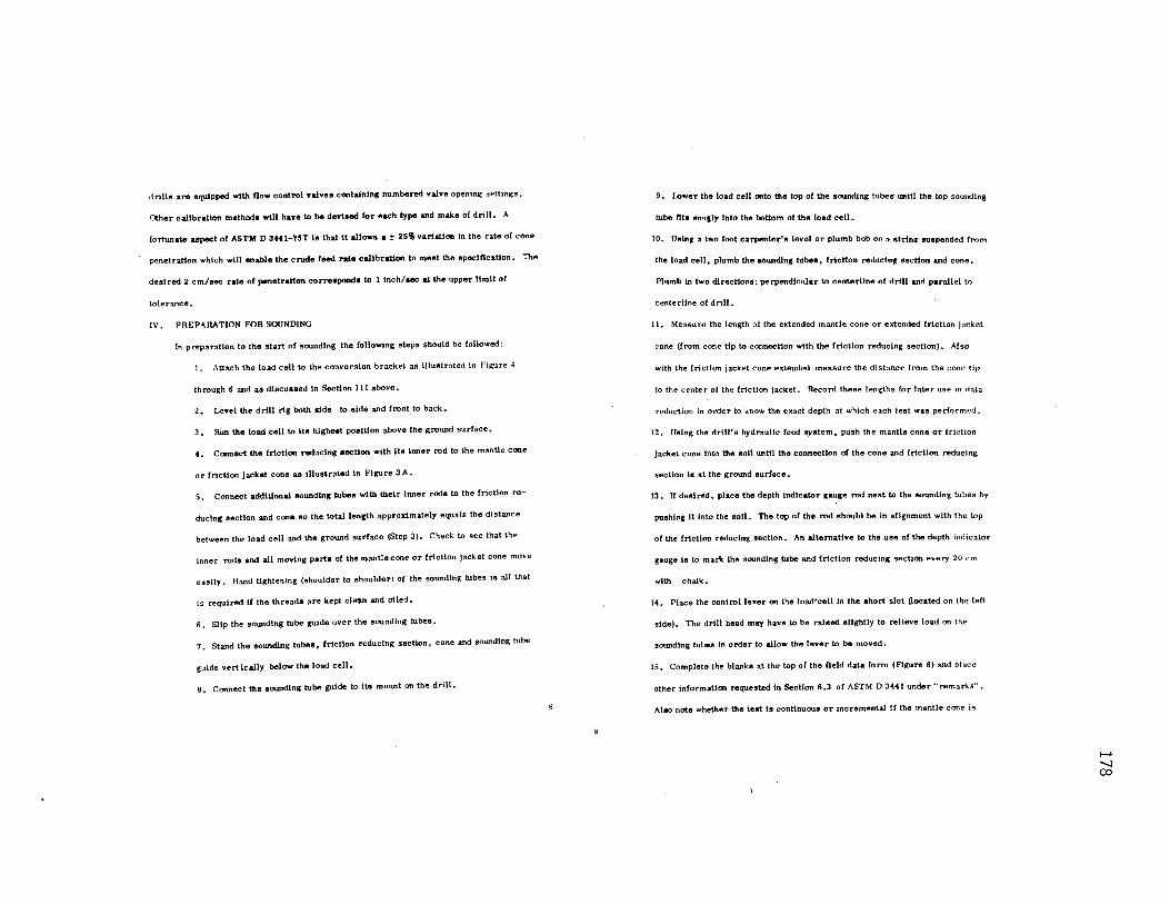
drll111 are equipped with ftow control valves containin1 numbered valve openinl{ settings.
other calibration method• will haY8 to be devl1ed for eoch type and make ol drill. A
fortunate upect of ASTM D 3441-75T la that It allows a t 25'{, variation in the rate ol cone
penetration which will enable the crude feed ralfi i>allbrdlon to meet the specification. The
desired 2 cm/eec rate of penetration correopond1 to 1 lnch/oec al the upper limit ol
tolerance.
IV. PREPARATION FOR SOUNDING
In preparation to the start of sounding the following •teps should be followed:
l. Attach the load cell to the conversion bracket as illustrated in Figure 4
th rough 6 and •• dlacuaaed In Section 111 above.
2. Level the drill rig both aide ro side and lront to back.
3. Run the load cell to Its highe•t position above the ground surface.
4. Connect the fricUon reducing section with Its Inner rod b> the mantle cone
or friction jacket cone as Illustrated in Figure 3A.
5. Connect additional sounding tubes with their Inner rods to the lrictlon re-
duclng aection and cone ao the total length approximately equals the distance
between the load cell and the ground surface (Step 3). Check to see that the
inner rod• and all moving part• of the mantle" cone or friction jacket cone move
easUy. Hand Ughtenlng (shoulder to shoulder) of the sounding tubes is aJI that
is required If the threads are kept clt!M and oiled.
6, Slip the sounding tube KUlde over the sounding tubes.
7 • Stand the soundlnl( tube1 , lrictlon reducing secUon , cone and sounding tube
guide vertically below the load cell.
8. Connect the 1oundlng tube guide to 111 mount on the drill.
9. Lawer the load cell onto the top of the •oundlng tubes until the top sounding
tube ftt• on•11ly Into the boUom of the load cell.
10. Using a two root carpenter's level or plumb bob on :l string suapendP.d rrnm
the load cell, plumb the moundln1 tube•, friction reducin1 section and cone.
Plumb In two directions: perpendicular to centerline of drill and parnllel b>
centerline or drill.
11. Measure the length of the extended mantle cone or extended friction jacket
cone (from cone tip to connection with the friction reducing section). Also
with the friction jacket cone extended measure the distance from the cone tip
to the center of the friction jacket. Record these lengths for later use in data
reduction in order to know the exact depth at which each test wa11 performed.
12. Using the drill's hydraulic reed syatem, push the mantle cone or friction
J~cket cone into the 11011 .mttl the connection of the cone and friction reducing
section Ja at the ground surface.
13. If deal red, place the depth Indicator gauge rod next ro the sounding tubes by
puahlng It Into the soil. The top of the rod should be In alignment with the b>p
ol the friction reducing section. An alternative to the uoe of the depth lndlcab>r
gauge la to mark the sounding tube and friction reducing section every 20 cm
with chalk.
14. Place the control lever on the load"cell In the ahort slot (located on the left
side). The drlll head may have to be raised slightly to relieve load on the
sounding tubes In order to allow the lever t.o be moved.
15. Complete the blank• at the top of the lleld data form (Figure 8) and place
other information requested In SecHon 6.3 of ASTM D 3441 under "remarks".
Also note whether the test la contlnuou1 or incremental If the mantle cone is
....... ....... 00
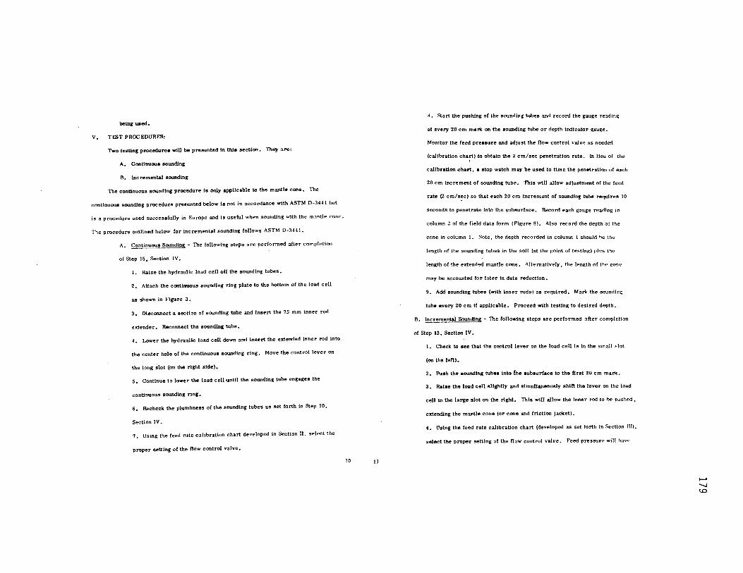
being uaed.
V. TEST PROCEDURF.S:
Two teattn1 procedure• will be presented In thl• section. They are:
A. Continuous aowidln&:
B. Incremental sounding
The continuous sounding procedure 11 only applicable to the mantle cone. The
contlnuou• sounding procedure presented below la not in accordance with ASTM D-3441 but
is a procedure used successfully in Europe and ls useful when sounding with the m:111tlt• <"om•.
The procedure outlined below for incremental sounding follows ASTM D-3441.
A,. Continuous Sounding - The following steps are performed after complrtion
0£ Step 15, Section IV.
I. Raise lhe hydraulic load cell off the sounding tubes.
2. Attach lhe continuous aoundln11 ring plate to the bottom of the loarl cell
as shown in Flgu re 3 •
3. Disconnect a •ectlon of sounding tube and Insert the 75 mm Inner rod
extender. Reconnect the sounding tube.
4. Lower the hydraulic load cell down and Insert the extended Inner rod Into
the center hole of the continuous sounding ring. Move the control lever on
the long slol (on the right side).
5. Continue to lower the load cell 41.nlll the sounding tube engages the
continuoua soundinl ring.
6. Recheck the plumbneas of the sounding tubes as set forth In Step 10.
Section IV.
7. Using the feed rate calibration chart developed in Section II. select the
proper setting of the Row control valve.
10 11
iL Start the pushJng of the 1ounding tubes and record the gauge readinK
at every 20 cm mark on the aoundtng tube or depth lndtcat.or gauge.
Monitor the feed presaure and adjust the now control valve as needed
(calibration chart) to obtain the 2 cm/sec penell"atlon rate. In Heu of the '
calibration chart. 1 atop watch may be used to time the penetration of each
20 cm increment of sounding lube. This will allow a.djuatment of the feed
rate (2 cm/s~c) so that each 20 cm Increment of sounding tube requires 10
seconds to penetrate Into. the subsurface. Record each gauge rearlfnfit in
column ;? of the field data form (Figure 8). Also record the depth of the
cone in column I . Note, the depth re('onled in column l shoulrl he the
length of the sounding tubes in the soil (at the point of t~sting) plus the
length of the extended mantle cone. Altematlvely, the lenJtth of tht~ cone
may be accounted for later In data reduction.
9·. Add sounding tubes (with Inner rods) as required. Mark ·the sounding
tube every 20 cm If applicable. Proceed with testing to desired depth.
B. lncrementai Sounding - The following steps are performed after completion
of Step 15. Section IV.
1. Check to 1ee that the control lever on the load cell Is tn the small slot
(on the left).
2. Pu•h the •oundlng tube• Into fhe subsurface to the ft rat 20 cm mark.
3. Raise the load cell slightly and almultaneouoly shift the lever on the load
cell to the large slot on the right. This will allow the Inner rod to he pushed,
extending the mantle cone (or cone and friction jacket).
4. Using the feed rate calibration chart (developed as set forth In Section 111).
select the proper setting of the Dow control valve. Feed pressure will h:1Vc
...... ......, \0

Old Gauges - Kgf/cm:z
New Gauges - I 000 ~
Load Cell Gauges
The old gauges were confusing (or two reasons. First. a kilogram (Kg) ls a unit of mass, not (orce. Therefor, the '1"' subscript (ICgO was used. since force is what l• really de1ired. Secondly. that pressure reading or Kgf/cm1 was a mea•urement of oil pressure in the load cell, not cone pressure at the lip or sleeve.
'!11.e new gauges are calibrated ln units of force. newtons (N), and are aleo calibrated to give a direct 1'eadln1 or Up force. For example, a reading or 34. 000 N mellll• a Carce of 3-1, 000 N is applted. Multiplying by :?O Is no longer necass:1ry. To get Up pressure or friction sleeve pressure in N/cm1 , simply div1tle by the tip are:. (10 .~m 1 l nr {r1ctlo·n sl1~eve 3rea (ViO cm.i) re!=pl''. -
tively.
It is recommended that newtons be used to In~ c<Jnt· d:it:t. A . s:tmple log sheet is provided on the bac\(.
However, to continue using l\:~f/cm 2 tip pressure 1!ll re:illy 4u1te
~1mple~ 1-:x:Jmple: Old gauge reads 25Kgf/cm:1.
2SKgC/cm' x 20cm2 (piston area) + lOcmJ (tip :-.rea) = SO Kg(/cm 1
F.:xample: New gauge reads 5000 N 5000 N • 10 N/Kgf • • 10 cm1 (tip area) = 50 Kgf/cm'
•approximation within the acc~racy of the gauges
IJUT('H CONE l'E,.,.ETRcJMETER , ..... o. ... , .. , ...
··-··· r.,,,., .... ,,.,., :f.111.olf'Hol ::i..111Co1•--1•U.l1•1Mc :1,..,.,.,, ..... :oc.;'.,•t1,.••l• ... 11n
.(,.,., F •Inell•• ll-R11o1unn
:11 • .,;.,,., "'''''~"u Lf •L.,.11 '""'o"" ···~"' .. r ""•' ""' • • .. / .....
" : - o • - !liO ,.,,. ... -..,,c.,.·
----------~------
I -i I i --, I - - --:
~r r 1 1 1 i
--.. -.. ~-·-· --------.................
I !
I --'------~
: ! 1 i I : : ; .. , , ! ' !
' ' r ! '
,-:--.-,--
:.;;-;;,;;;.:.-;;;.;-;; ,_,. ... .,, ......... 1 ... •-t lnuoa" .,,...11. m~ ~;;,;; •• " ........... :or ... -., .. ;.. ... . u.,,1,,c,.•"•"''"I'"'"''"'"'"'""
...... 00 0

I
I I
I I
F11ure 8
DUTCH CONE PENETROMETER field 0.la Fom1
o ...
'ro1ec1. ---------------------- Tesl No
lll-.llUR ---------------------
fnrcd b)': ---------- ........ , ---------------------rn1 ProcedMN:
fb1e or Fee4: laa/IK ar • IMle lbM I i•lttt Rwa 1n1 "8)' 20 a. or •ppro•. I i111tlm
C-c- F-Frtc-. R-CR-c--... LF-ladlfrlcl._ Weipl of-rra4 -0.14 K,/.,.1/ro<l le ... h
lleprb c F+C F CR Lf @-Ci> (j) KI @ ••. t:U
Kl;/cMJ K11c11111J IC11C•J Ks/CMJ ""'"'J ! .. j) 1) @ @ @
THE CC MPUTA" i'IONIN :OLUMI 5 IS NO LONGER
AS A LGAUC ES ARE NOWD RECT R ADING.
PLE SE Oil REGAR! 1 nas COMPIT ATION.
frklioa Ra1io•
@/@ .!)
NECESSA I• :Y
Fnc11on Raisunce
Cone Resina;na
Fric:tion R.alio
= ,_I I I I I I I I I I I
Q -+--+----<l-+--+--+----<~+--+--+-----<1--
•Nate: Tht fricciam rali9 ii com ..... '1 dhi6111M local frlctioft by rhc cone raistuc:e .......-eel 20 c• •bow: 1he local frictioa •llrilll •llc sn._ 1 ... 12
to be e•tlmated Initially and the now control valve adjusted after the initial
test and thereafter .. the reed pressure changes during the pushing or the
cone and friction sleeve. A better method of selecting Che proper r<'cd
rate (2 cm/sec) Is during the pushing of the sounding tubes. The proper
Ceed rate Is selected ae set forth under Step 8 of the continuous s0&mdlng
procedure (above).
5. At the calibrated rate of penetration. push the Inner rod taking reading
on lbe 1au1e• at:
ManUe Cone -After approximately 1 inch of relative movement of Inner
rod. Read gauge and record In column 2 of the lleld data form. (Figure HI
Friction Jacket Cone -The cone reading should be taken before the cone
engqea the frlcUon sleeve which wtll be noted by a jump (lncreasel of
the gauge reading. Record this Hrst reading in column :! of the field data
form (ngure 8). After the cone engages the friction sleeve, obtain a
reading on the gauge•. 'lbla second reading represents the cone plus
friction sleeve reslstance11. Record this reading In column 3 of tht> field
data form (Figure 8). Aleo record In column I the depth Oength of sound-
ID& tube• lD the eoll at the time of the teat plWI the average length of the
extended frlcUon Jacket cone) at whlc.h the cone and friction jacket gauge
readinga were obtained. Altet'naUvely, the length of the extended ·friction
jacket cone may be accounted for later In data reduction. In non-homo-
1eneoua 1011 deposit• or for more rellned data the exact depths of the
cone and frtcUon Jacket will have to be recorded In column t. The exact
deptha are the l•lllh of sounding tube• In the soil at the time of the test
plu:
........ 00 ........
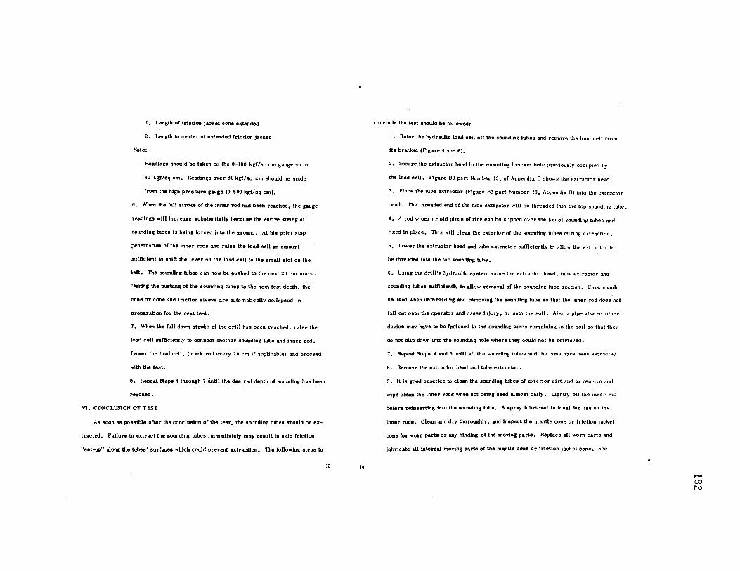
I. Length of friction jacket cone extended
2. Length to center of extended friction jacket
Note:
Reading• should be taken on the 0-100 kgf/oq cm gauge up to
80 kgf/oq cm. ReadlnKS over 80 kgf/sq cm should be made
from the high pressure gauge (0-600 kgf/sq cm).
6. When the run stroke of the inner rod hu been reached, the gauge
readings wUJ lncrea11e substantially because the entire string of
sounding tubes is being forced Into lhe ground. At his point stop
penetration of the inner rods and raJse the load cell an amount
sufficient to shift the lever on the load cell to the small slot on -the
left. The soundlnA" tubes can now be pushed to the neJrt 20 cm mark.
Durtnr the pushing of the sounding tubes to the next teat deptb 1 the
cone or cone and friction sleeve are automatically collapsed In
preparation for the neJrt test.
7. When the full down stroke of the drill has been reached, raise the
load cell sufficiently to connect another sounding tube and Inner rod.
Lower the load cell, (mark rod every 20 cm if applJcable) and proceed
with the test.
8. Repeat step• 4 through 7 Un_til the deatred depth or sounding ha• been
reached.
VI. CONCLUSION OF TEST
Ae soon a11 possible after the conclusion of the test, the sounding tubes should be ex-
tracted. Failure to extract the sounding tubes lmmedlstely may result In skin friction
"set-up" alone the tubes' surface• which could prevent extraction. The following ateps to
13 14
conclude the teat should be followed:
1. RaJse the hydraulic load cell off the sounding tubes and remove the load cell rrom
its bracket (Figure 4 and 6).
2. Secure the extractor head In the mounting bracket hole previously occupled by
the load cell. Ftgure 83 part Num~er 19 1 of Appendix B shows the extr~ctor head.
3. Place the tube extractor (Figure B3 part Number 18. Appendix 13) into the extractor
head. The threaded end of the tube extractor will be threaded Into the top sounding tuhe.
4. A rod wi~r or old piece of tire can be eUpped over the top or soundin~ tubes anrl
fixed In place. This will clean the exterior of the sounding tubes during extraction.
5. Lower the extractor head and tube extrnctor sufficiently to allow the extrnctor to
be threaded tnto the top soundJng tube.
6. Using the drill's hydrnullc system raise the extractor head, tube extractor and
SO\lllding tubea aufflt:tently to allow removal of the sounding b.Jbe section. Care should
be used when unthreadtng and removing the eound.Jng tube so that the Inner rod does not
fall out onto the operator and cause injury, or onto the soil. Also a pipe vise or other
device may have-to be fastened to the sounding b.Jb~s remaining In the soil so that they
do not slip down Into the so1.D1ding hole where they could not be retrieved.
7. Repeat Steps 4 and 5 until all the sounding tubes and the cone have been extrncte<l.
8. Remove the extractor head ancl tube extractor.
9. Jt Is goOO practice to clean the sounding tubea of exterior dirt.and to rern'Jve and
wipe clean the inner rods when not being used almost daily. Lightly oil the inner rod
before reln•erttnc Into the 11<>undlng tube. A spray lubricant ta Ideal for use on the
Inner rod•. Clean and dry thoroughly, and lnepect the mantle cone or h1ctton Jacket
cone for wom parts or any binding of the movtng parts. Replace all worn parts and
lubrlcote oil lntemol moving parts of the manUe cone or friction jacket cone. See
...... 00 N

Fipre1 84, B5 and 88 1 Appendix B, for views and part•s names of the mantle
cone and frlctl<11 jocket cone.
VII. CALCULATIONS AND REPORTING
Figure 8 I• a copy of a oelf explanatory field data form. By progressing from
column 1 to 7 and followtnc the calculatl.on1 at the top of each column the cone resistance,
local fr1ctl<11 and friction ratio are computed. Further brief explanations of the
calculatlono wUI be pven below.
The data collected durin& the field operatl.on1 Include 1auge readings for the cone,
and cone plus friction jacket, resistances. This data is placed in columns ~ and 3 of
figure 8, respectively and ts 1n the unite of kllo1ram1 force per square centimeter
(kgf/aq cm) .. U a mantle cone ts used, data le entered in column 2 oniy.
The area of the measurin1 plunger in ~e hydraulic load cell is 20 square centimeters.
The area of the cone 11 10 square centimeters. Thus to compute the pressure on the cone,
maltlply the gau1e r111dlng pressure (column 2) by two (20/IO) to yield the cone pressure
(column 5) in kilogram• per oquare centimeter (kgf/sq cm).
When a friction Jacket cone ls used, a gauge value wtll also be obtained for the
combined cone plus the frJctton jacket resistance (column 3). To determine the ~::1Uge
readJn1 for the friction jacket only. subtract the cone gauge reading (column 2) rrom rhe
gauge rt:adJng obtaJned for the cone plus friction jacket (column 3). This value is recorded
in column 4 of Figure 8. Since the measuring plunger in the hydraullc load cell is 20 s(ruare
centimeters, the total force (kgf) required to move the friction jacket is obtained by
mllitiplylnc the gauie reading for the friction jacket by 20. Dividing this result lry 150
square centimeter area of the friction Jacket yielde the local friction In kilograms per squ:1r~
centimeter (kgf/sq cm). The above computattona are combined into the factor O. 133 which is
multiplied by column 4 to obtain the local friction value In column 6 of Figure 8. Another
15 16
important computation ls the ratio of the cone resistance (column 5) to the local friction
(column 6), which I• referred to aa the friction ratio (column 7). Remember that the
friction ratio mu1t be determined from values of cone realetance and local friction
meuured at the 1ame depth in the soil stratum.
Superfmpo•ed plot• of the cone resistance, local friction and friction ratio versus
depth shculd be Included In the final reporting of the field data. Figure B provide• a graph
for the1e plot• although a more refined graph may be required for further office analysta.
For non-homo1enous soil depOl!llts It Will probably be necessary to use exact depths for the
cone and friction jacket rather than using an average depth for OOth readings. (See Section
V, Incremental Sounding) Thia is particularly lrnportant In computing the friction ratio
for non-homogenoua sotla. For an accurate friction ratio in non-homogenous soil deposits,
the cone re1lstance and local friction values should be as close to the same depth as possible.
VIII. SPECIAL PROCEDURES
The following •peclal procodure1 are applicable under unusual circumstances and are
not generally required:
A. Drift of the 1oundlng tube1 may become a problem in very deep soundings and when
paa•tng through or alongside of obstructtone such as boulders, soil concretions, thin
rock layers and inclined dense strata. Drift of the sounding tubes results in benrltng
of the tubes and the development of friction between the Inner wall of the sounding tube
and the Inner rod. The magnitude of this 'inner wall fMctton could have a significant
effect on the gauge readings obtained for cone resistance and local friction values.
Generally drift of the sounding tubes should be minimized hut if ci('t!umstance dictate
otherw1se and the sounding cannot be terminated and reinittated, Figure 9 should be
consulted to determine the magnitude of the inner rod friction.
...... co w
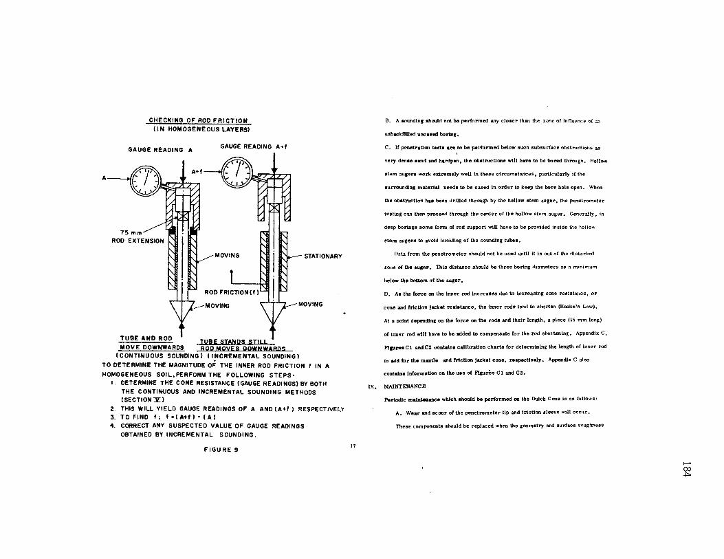
A
CHECKING OF ROD FRICTION (IN HOMOGENEOUS LAYERS)
GAUGE READING A GAUGE READING A .. f
TUBE AND ROD TUBE STANDS STILL MOVE DOWNWARDS ROD MOYES QOWNWAAQS
(CONTINUOUS SOUNDING I (INCREMENTAL SOUNDING)
STATIONARY
TO DETERMINE THE MAGNITUDE OF THE INNER ROD FRICTION f IN A
HOMOGENEOUS SOIL.PERFORM THE FOLLOWING STEPS• I. DETERMINE THE CONE RESISTANCE (GAUGE READINGS) BY BOTH
THE CONTINUOUS AND INCREMENTAL SOUNDING METHODS (SECTION Ji: I
2. THIS WILL YIELD GAUGE READINGS OF A AND (A+f I RESPECTIVELY 3. TO FIND f; f •(A-tf)- (Al 4. CORRECT ANY SUSPECTED VALUE OF GAUGE READINGS
OBTAINED BY INCREMENTAL SOUNDING.
FIGURE 9 17
B. A soundin1 ahollld not be performed any closer than the zone of tnnuence or an
unbockftlled unc11ed boring.
C. If penetraUon test• are to be performed below 11ucb subsurface obstructions as
very dense Hnd llld hardp111, the obotnictlons will have to be bon!d through. Hollow
stem augers work extremely well ln these circumstances, p:n1lcularly I( the
surrounding material needs to be cased In order to keep the bore hole open. When
the obotnictlon bu been drilled through by the hollow stem auger, the penetrometer
testing can then proceed through the center of the hollow stem auger. Generally, in
deep borings some form of rod suppnrt will have to be provided Inside the hollow
stem augers to avoid buckling of the sounding tubes.
Dat:l from the penetrometer should not be used until it is out of the diAturhed
zone of the au1er. This distance should be three boring diameters as a minimum
below the bottom of the auger,
D. A• the force on the IMer rod increase11 due to increasing cone resistance, or
cone and frlctton Jacket resistance, the IMer rods tend to soorten (Hooke's Law).
At a pnln& depending on the force on the rods and their length, a piece (15 mm long)
of Inner rod will have to be lidded to compensate for the rod shortening. Appendix C,
n111re•Cl llldC2 .:nntaln• ollllhratlon charts for determining the length of Inner rod
to ldd for the mMtle ond frlcltcm J1eket cone, reopectlvoly. Appendix C al!o
contain• tnformotlon OD the UH of ngures c 1 llld C2.
IX. MAINTENANCE
Periodic maintenance which should be performed on the Dutch Cone I• as follows:
A. ·Wear and 1cour of the penetrometer ttp and friction sleeve will occur.
These components should be replaced when the geometry and surface roughness
....... 00 ~
no longer meet the requJ rement or Section 3. l or ASTM D 344 J-75T (Appendix A).
n. The mantle cone and friction Jacket cone should be cleaned, drierl and oih.•ct
after each l!loundlng. AU moving ports should move freely.
C. The cut-off pressure at which the 0-100 kgf/eq cm p:auge should no longer
register and the 0-600 kgf/sq cm gauge should be read Is :lpproxim:i.tely RO kd/sq cm.
Adjusting screw 7 (Figure Bl. Appendix B) regulates this cut-off pre"sure. lllis cut-
orf pressure should he adjusted as required.
D. After each test all sounding b.lbes should be cleaned and checked for str:lii.thtnt>~s
and fractures (around threads). llt•pl:lce any sounriin~ tubes whkh arr- ht~nt nr
fracture<L Keep the threads cleanrd and Wf.>ll oilcrt so threading :met unthrt!:1ding c;m
be performed easily.
E. Keep the inner rods dean :md luhrir.ah•.f. ·\ spr:iv luhric:mt :ll1Plit·rl rn11·1· :i d:1\
wil1 assure relatively frictionlesfl movement or the inn,~r rods.
F. The oil level In the hydraulic load cell should he d1eck1?d periodically. To m:-.k1•
this check:
1. Place lever C, (See Figure 10) in th<' left h:-.nd slot.
~. Exert a force on the load cell hy pushing the penetrometer and somuling
tubes into the soil.
3. During the force exertion, measure the distance that lever C mo\'es upward.
Tiiis distance should be no more tha11 10 mtllimeters. If this distance is more
than 10 millimeters, add oil to the cell.
Oil is added to the cell by:
1. Release all pressure on the loarl cf'll.
-· Unscrew fill plug B (See FiglJrt• 10 or screw :J, Fi~ure 83, ,\ppendh B).
3. Push down the plunger. using the :J mm pin provided (until it stops).
IS
4. Open vent A to allow trapped aJr to eecape.
5, F'lll the cell with oil of grade through plu~ B.
6. Close vent A and plug B when the cell Is full.
19 ,__. co U'1
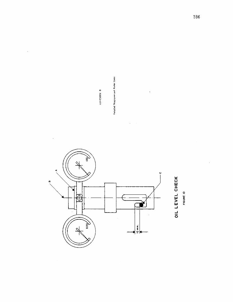
186
~
m :i
t ~
"' "' "C
>: ~
e c z
E "' ~ "' "- iS <
~ ;: c::
u
~ ID (.)
UJ :::c (.)
Q ..J LI.I UJ a:
::> > I!)
UJ ii: ..J
..J
0
e E

BY TWISTING THE ADJUSTING SCREW "7:• THE MAX PRESSURE ON
THE RIGHT GAUGE IS REGULATED. (MAX. 80 kQ/cm2)
,._, 115 c
,...._, 200cm
FIGURE Bl
ADJUSTING SCREW
A
FIGURE B 2
...... o::> -....,J
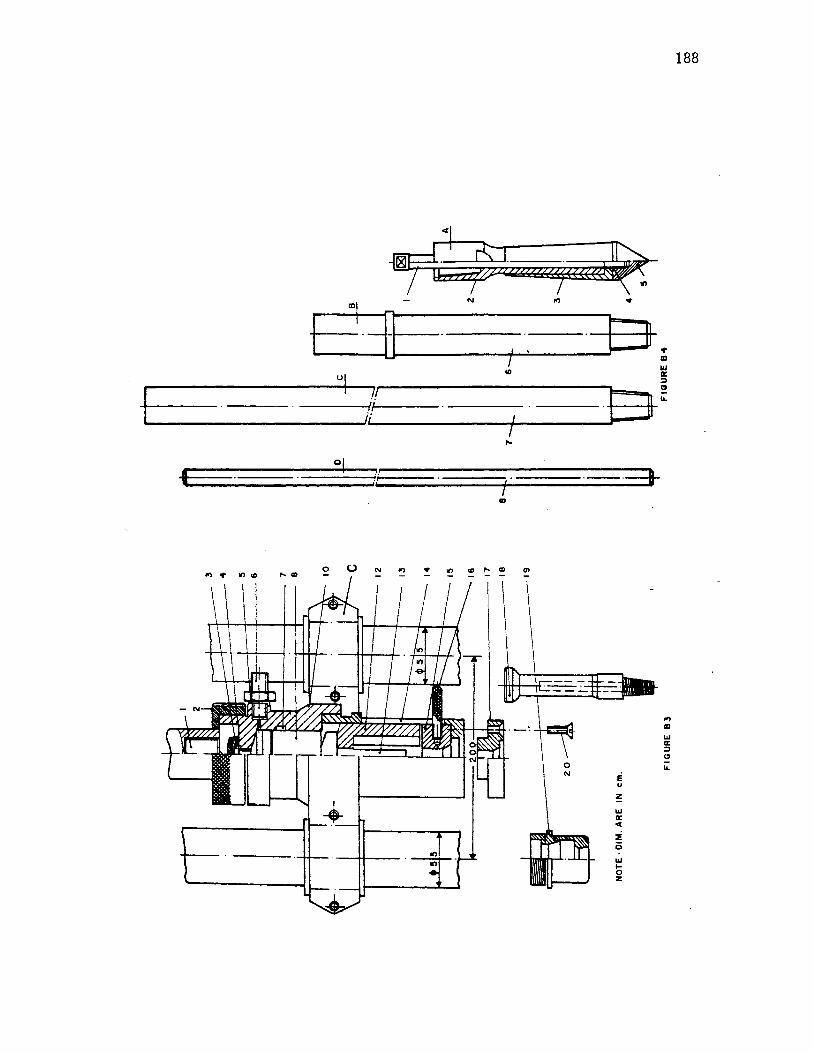
188
ul "' !!
ij I
I ,..
I al
d it I -----·--·=+
Ill
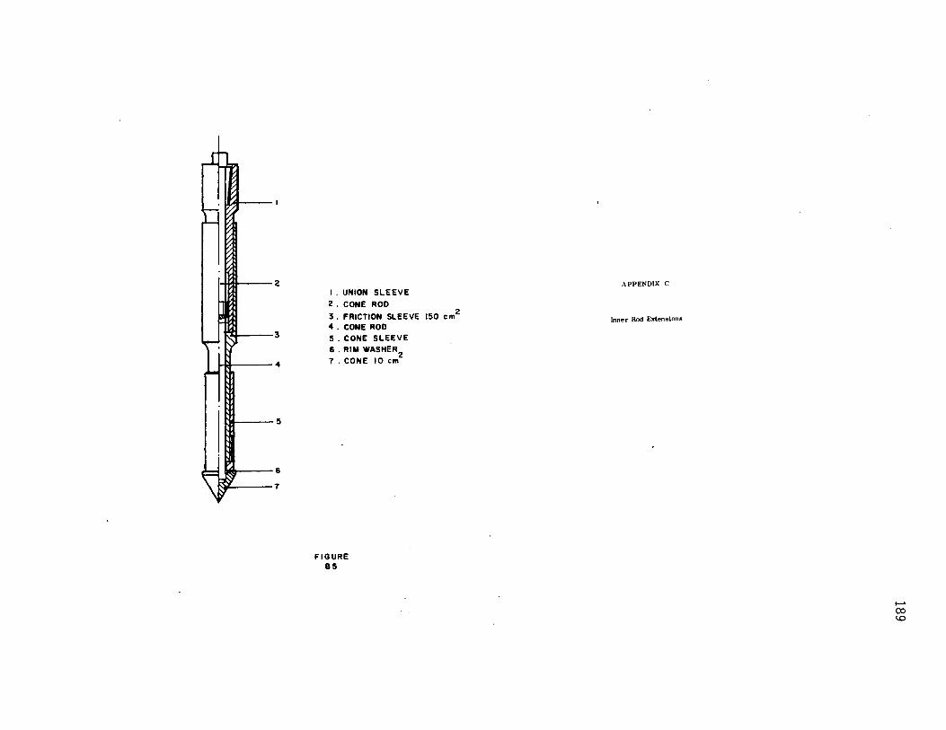
l..tm 2
m 3
HI 4
[:14 5
~ ;
I . UNION SLEEVE
2. CONE ROD
3. FRICTION SLEEVE 150 cm2
4. CONE ROD 5 . CONE SLEEVE 6 . RIM WASHER2 7 . CONE 10 cm
FIGURE 85
APPENDIX C
lnn"r Rod Extensions
I-' CX> l.O

ln1tnJCtion For U11e or
Ftaurea Cl and C2
Increaain1 cone re1i1t11DCe re1ult1 in the shortening of the inner rods. To compensate for
this 1hortenin11 15 mm lenphentn1 rod• are added to the inner rods. To determine the number
or lencthC,ning rod1 which mu1t be used, the force on the inner rods muat be found. To determine
the rod force 1t 11 neceaeary to obtain the gauce pressure readings for the cont! {mantle coneJ
~>r cone plus friction jacket (friction jacket cone). ·n.ese are the values recorded in columns :.!
and 3, respectively on Fi&Ure 8. To convert the gauge pressure readings to tons:
Rod force (ton1)
Ax 20
1000
A • Gause pre1sure u denned above for the mantle cone or friction
Jacklt cone, whichever I• u1ed f<c/cm2)
To determine th• added lenph of inner rod required, find the zone on Fl.gure C 1 or C2 where
the lnter1ect of the rod rorce (ton) and len(th of rod (m) [alls. The figures are:
Mantle cone ~See Figure Cl
Friction jacket cone • See Figure C2
Figure• are used a1 foUows:
Area A - penetration is made w1thout lengthening rod
Area 8 - penetration is made using one J!f mm piece or lengthening rod
Area C - penetration is made using two 15 mm pieces or lengthening rods
...... l..O 0
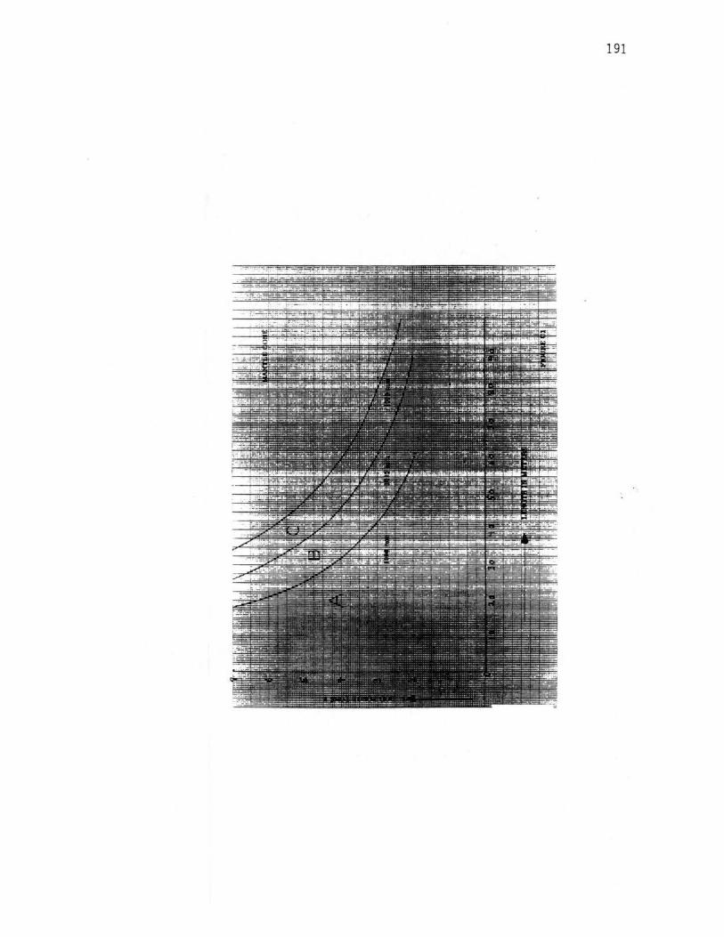
191
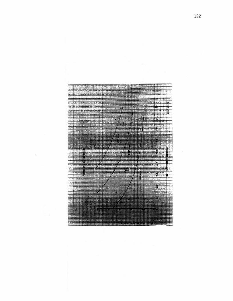
192
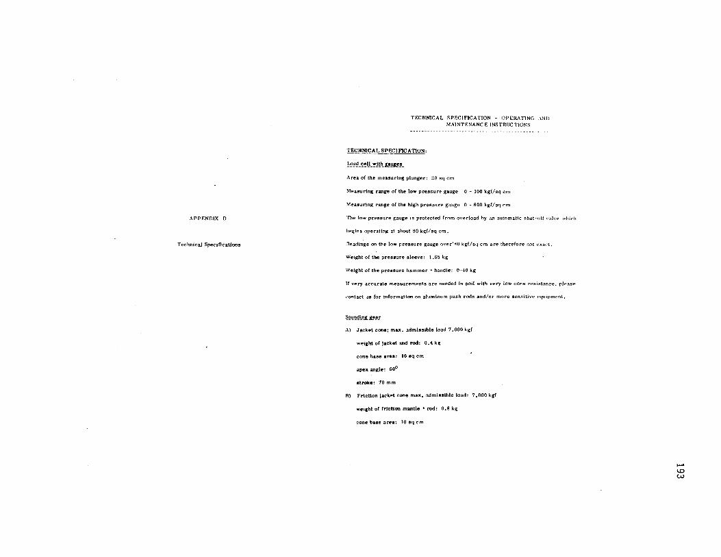
APPENDIX D
Technical Spec!Hcatlons
·.
TECHNlCAL SPECIFICATION - OPERATING .\Nil MAINTF.NANC E INSTRUCTIONS
TECHNICAL SPECIFICATION:
~l'~-~!!L~!!LK!.!!&!'.!'_
. Area of the measuring plunger: 20 sq cm
~eaeuring range of the low pressure gauge O - 100 kgf/sq cm
Meaeuring range of the high pressure gauge O - 600 kgf/sq cm
The low pressure gauge is protected from overload hy an automatic shut-ore \';ih·e whkh
hegina operating at ahoot 80 kgf/sq cm.
ReadinR;s on the low pressure gauge over'liO kgf/sq cm are therefore not t.':<m:t.
Weight of the pres1ure sleeve: 1.65 kg
Weight of the pre11sure hammer +handle: 0-40 kg
Ir very accurate measurements are needed in soil with very low cone resistance, -pleasP
l'Ontact us for Information on aluminum push rods and/or more sensitive equipment.
§~!!~l'!l..1.!1~!
Al Jacket cone: max, admlHlble load 7 ,000 kg!
weight of Jackel and rod: 0,4 kg
cone ba•e area: 10 sq crn
apex ongle: &o0
1troke: 70 mm
BJ FricUon Jackel cone max. admioslble load: 7 ,000 kg!
weight of friction mantle + rod: 0,8 kg
cone hue area: 10 sq cm
....... ID w

•pex anKle: 60°
atroke of • ..,., 35 mm
1troke of cone plua mantle: 35 mm
total 1troke: 10 mm
1urf11Ce of frlcUon Joeket: 150 1q cm
C) Friction reducln1 1ectlon tube
D) Saundln1 tubeo:
seamle••: f 36/16 mm x 1000 mm Joni:;:
weight: 6.65 kg
El Inner rod•:
' 15 mm x 1000 mm long
weight: 1.40 kl
Your spare part• order can be correctly earned out only tf you quote all of the fol lowing reference•:
No. of the Machine Pase Number Part Number
f!1<..r:!2, Bl
82
83
114
PA1'TS LIST
Pll.!:L.!'!.'!.o:..
la
11 II 15 lfi
IO 12 13 .. '' 16 17 IH 19
L! 13 ..
!?!'!IP!'~~".l!.t!~
Usltrlng Union nut Va.Ive 0-ring llolt Spring cup Spring Spring cup holt l)-Mng
House ITnion hnlt Union bolt Rin~ Bolt
Pressure Pre21sure
Collar holt Union nuts Sealing nipple Usilring Usitrfng trnion holt Cuppe1• washt!r Plunger Plunge re as int( Pressul"t" sleeve Pressure rod Pressure casing Pressure plate Lever
100 kgf/cm: 600 kgf/cm-
Ring for continuous sounding Tube extractor l·:xtractor head
Cone rod Unum slecvt•
Cone sleeve Sprmg wa.she r Cone (10 sq cm.!)
Friction reducinK section tube Sounding tube Inner rod -c..o
.i:>o
APPENDIX D
BORING LOGS AND PHYSICAL PROPERTY DATA
195
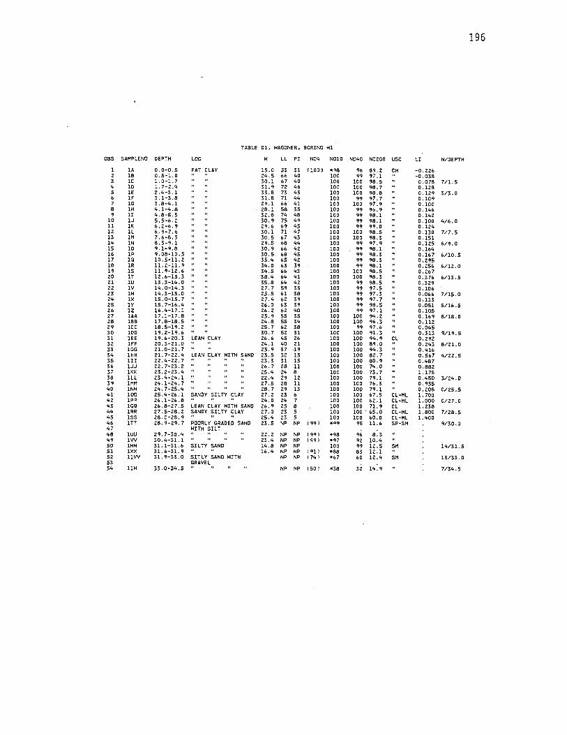
196
TABLE Dl, HAGONER, BORING Hl
OBS SAHPLENO DEPTH LOG H LL PI N04 NOlO N040 N0200 USC LI N/OEPTH
l lA o.o-o.s FAT CLAY 15.0 53 31 I 100 I •98 96 89.2 CH -0. 226 2 lB 0.5-1.0 " 24.5 66 40 100 99 97.l -o. 038 3 lC l.0-1.7 30.l 67 40 100 100 98.5 0.078 7/1.5 4 lD 1.7-2.4 31. 9 7Z 46 100 100 9B. 7 0.1Z8 5 lE 2.4-3.l 33.8 73 45 100 100 98.8 0.129 3/3.0 6 lF 3.1-3.8 31.8 71 44 100 99 97.7 0.109 7 lG 3.8-4.1 29.1 66 41 100 100 97.9 0.100 8 lH 4.1-4.8 28.1 58 3.5 100 99 96. 9 0.146 9 lI 4.8-5.5 32.8 74 48 100 99 98.l 0.142
10 lJ 5.5-6.2 30.9 75 49 100 99 98.1 0.100 4/6.0 11 lK 6.2-6.9 29.6 69 45 100 99 99.0 0.124 12 ll 6·.9-7.6 30. l 71 47 100 100 98.5 0.130 7/7.5 13 lf't 7.6-8.3 30.5 67 43 100 100 98.3 0.151 14 lN 8.3-9.l 29.5 68 44 100 99 97.9 0.125 6/9.0 15 10 9.1-9.8 30. 9 66 42 100 99 98.l 0.164 16 lP 9·.08-10.s 30.5 68 45 100 99 98.3 0.167 6/10.5 17 lQ 10.5-11.Z 35.4 65 42 100 99 98.3 0.295 18 lR 11. Z-11. 9 34.0 63 39 100 99 98.1 0.256 6/lZ.O 19 lS 11.9-lZ.6 34.5 66 43 100 100 98.5 0.267 zo lT 12.6-13.3 38.4 64 41 100 100 98.3 0.376 6/13.5 Zl lU 13.3-14.0 35.8 64 42 100 99 98.5 0.329 zz lV 14.0-14.3 27.7 59 35 100 99 97.5 0.106 23 lH 14.3-15.0 25.5 61 38 100 99 97.3 0.066 7/15.0 24 lX 15.0-15.7 27.4 62 39 100 99 97. 7 0.113 ZS lY 15.7-16.4 26.0 63 39 100 99 98.5 0.051 5/16.5 26 lZ 16 .4-17 .1 26. 2 62 40 100 99 97.1 0.105 27 lAA 17.1-17.8 25. 9 55 35 100 100 94.Z 0.169 8/18.0 28 lBB 17.8-18.5 24.8 55 34 100 100 96.3 0.112 29 lCC 18.5-19.Z 25. 7 62 38 100 99 97.6 0.045 30 lDD 19.2-19.6 30.7 sz 31 100 100 91.3 0.313 9/19.5 31 lEE 19.6-20. 3 EAN CLAY 26.6 45 26 100 100 94.9 Cl 0.292 32 lFF Z0.3-21. 0 24.1 40 21 100 100 89.0 o. 243 8/Zl.O 33 lGG Zl. 0-Zl. 7 .. 25. 9 37 .19 100 100 94.3 0.416 34 lHH 21. 7-ZZ.4 LEAN CLAY HITH SAND 25.5 32 15 100 100 82.7 0.567 4/ZZ.5 35 lII ZZ.4-22.7 .. 23.3 31 15 100 100 80.9 0.487 36 lJJ ZZ. 7-23.Z 26. 7 28 11 100 100 74.0 0.882 37 lKK Z3.2-Z3.4 25.4 24 8 100 100 73. 7 l.175 38 lll 23.4-24.1 22.4 29 12 100 100 79.l 0.450 3/24.0 39 lHH 24.1-24.7 " 27.5 28 11 100 100 76.3 0.955 40 lNN .24. 7-25.4 28. 7 29 13. 100 100 79. l 0.208 0/ZS.5 41 100 ZS.4-26.1 SANDY SILTY CLAY 27. 2 23 6 100 100 67.5 Cl-Hl l. 700 42 lPP 26.1-26.8 .. 24.0 24 7 100 100 62. l Cl-Hl l.000 0/27.0 43 lQQ 26.8-27.5 LEAN CLAY HITH SAND 26.9 25 8 100 100 71. 9 Cl l.238 44 lRR 27.5-28.2 SANDY SILTY CLAY 27. 0 23 5 100 100 . 65.0 Cl-Hl l.8DO 7/28.5 45 lSS 28.2-28.9 II II 25.4 23 5 100 100 60.0 Cl-Hl l.400 46 lTT 28.9-29.7 POORLY GRADED SAND 23.5 NP NP I 99 l •99 95 ll.6 SP-SH 9/30.0 47 HITH SILT 48 lUU 29.7-30.4 22.2 NP NP I 9• I •98 96 8.3 49 lVV 30.4-31. l 23.4 NP NP I 991 •97 qz 10.4 50 lHH 31.1-31.6 SILTY SAND 14.8 NP NP 100 99 12.5 SH 14/31.5 51 lXX 31.6-31.9 16.4 NP NP 1 •11 •88 83 12 .1 52 llW 31.9-33.D SITLY SAND HITH NP NP 174 I *67 60 12.4 SH 13/33.0 53 GRAVEL 54 llH 33.0-34.5 NP NP 150 I •38 32 14.9 7/34.5

197
TABLE Dl, HAGONER, BORING Hl (CONTINUED l
OBS SAMPLE NO DEPTH LOG H LL PI N04 NOlO N040 N0200 USC LI N/DEPTH
55 llX 34 .5-35. 0 SILTY SAND NP NP 100 95 12. 3 56 llXX 35. 0-36. 5 SIL TY SAND HITH NP NP ( 571 •46 37 13. 6 11/3&.5 57 GRAVEL 58 llZZ 36.5-37.2 LEAN CLAY HITH SANO 38 12 100 95 82.4 CL 59 !SHALE I
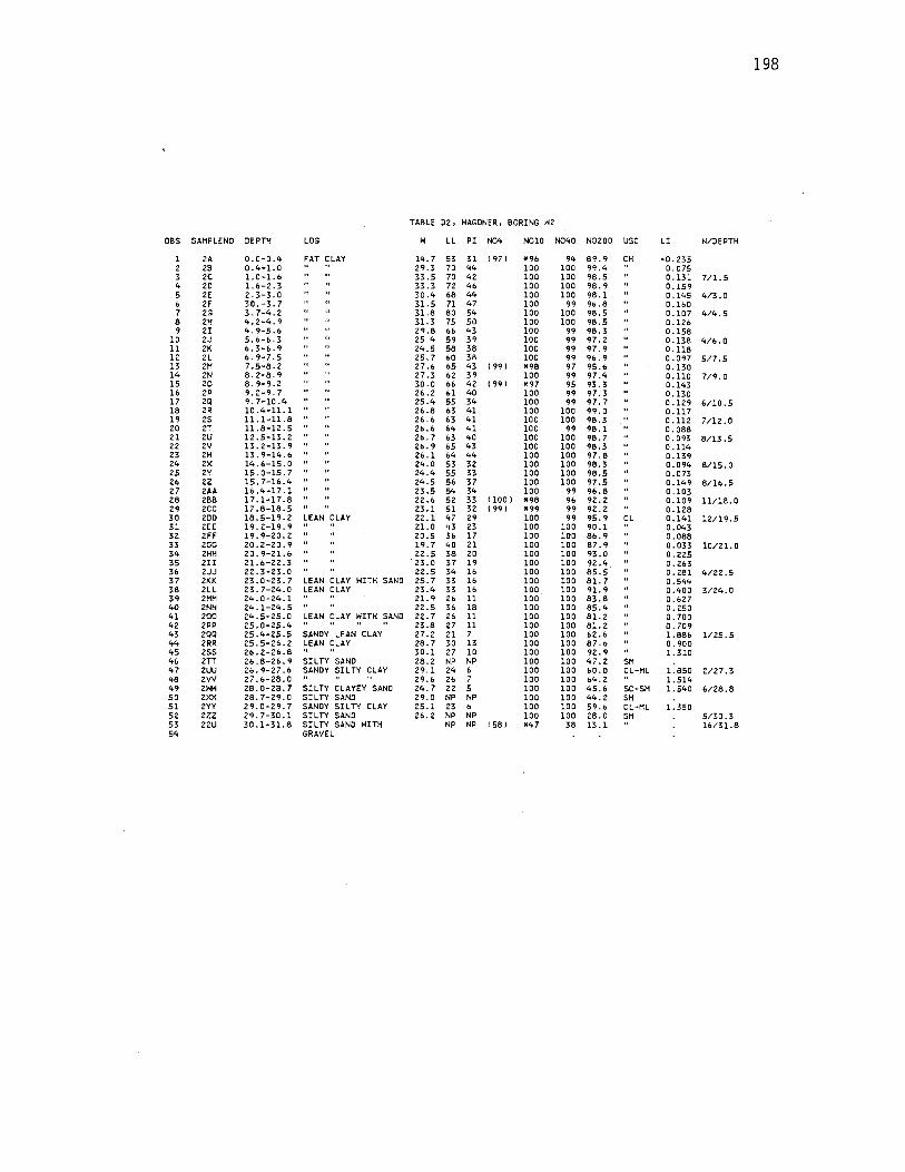
198
TABLE 02, HAGONER, BORING H2
OBS SAMPLENO DEPTH LOG H LL PI N04 NOlO N040 N0200 USC LI N/DEPTH
l 2A 0.0-0.4 FAT CLAY 14. 7 53 31 197 I *96 94 89.9 CH -o. 235 2 2B 0.4-1.0 29.3 70 44 100 100 99.4 0.075 3 2C l.0-1.6 33.5 70 42 100 100 98.5 0.131 7/1.5 4 20 1.6-2.3 33.3 72 46 100 100 98.9 0.159 5 ZE 2.3-3.0 30.4 68 44 100 100 98.l 0.145 4/3.0 6 2F 30.-3.7 31.5 71 47 100 99 96.8 0.1&0 7 ZG 3.7-4.2 31.8 80 54 100 100 98.5 0.107 4/4.5 8 ZH 4.Z-4.9 31.3 75 50 100 100 98.5 0.126 9 2I 4.9-5.6 29.8 66 43 100 99 98.3 0.158
10 2J 5.6-6.3 25.4 59 39 100 99 97.Z 0.138 4/6.0 11 2K 6.3-6.9 24.5 58 38 100 99 97.9 0.118 12 2L 6. 9-7.5 Z5. 7 60 38 100 99 96.9 0.097 5/7.5 13 2M 7.5-8.Z Z7 .& 65 43 199 I *98 97 95.6 0.130 14 ZN 8.2-8.9 Z7.3 62 39 100 99 97.4 0.110 7/9.0 15 20 8.9-9.Z 30.0 66 4Z 1991 ,.97 95 93.3 0.143 16 zp 9.2-9.7 Z&. Z 61 40 100 99 97.3 0.130 17 2Q 9.7-10.4 Z5.4 55 34 100 99 97.7 0.129 6/10.5 18 ZR 10 .4-11. l Z6.8 63 41 100 100 99.0 0.117 19 ZS 11.1-11.8 Z6.6 63 41 100 100 98.3 0.112 7/lZ. 0 20 ZT ll.8-lZ.5 Z6. 6 64 41 100 99 98.l 0.088 21 zu 12.5-13.Z Z6. 7. 63 40 100 100 98.7 0.093 8/13.5 zz zv 13.2-13.9 26. 9 65 43 100 100 98.3 0.114 23 ZH 13. 9-14. 6 26. l 64 44 100 100 97.8 0.139 24 zx 14.6-15.0 24.0 53 32 100 100 98.3 0.094 8/15.0 25 2Y lS.0-15.7 Z4.4 55 33 100 100 98.5 0.073 26 2Z 15.7-16.4 24.5 56 37 100 100 97.5 0.149 8/16.5 27 2AA 16.4-17.l 23.5 54 34 100 99 96.8 0.103 28 288 17.1-17.B Z2.6 52 33 1100 l *98 96 92. z 0.109 11/18.0 29 zcc 17.8-18.5 23. l 51 32 199 I ,.99 99 92. 2 0.128 30 zoo 18.5-19.2 LEAN CLAY Z2. l 47 29 100 99 95.9 L 0.141 12/19.5 31 ZEE 19.Z-19.9 Zl.O 43 Z3 100 100 90.l 0.043 32 ZFF 19.9-20.2 Z0.5 36 17 100 100 86.9 0.088 33 ZGG 20.2-20.9 " 19. 7 40 21 100 100 87.9 0.033 10/21. 0 34 2HH 20.9-21.6 22.5 38 20 100 100 93.0 0.2Z5 35 2II Zl.6-22.3 . 23.0 37 19 100 100 92.4 0.263 36 2JJ 22.3-23.0 2Z.5 34 16 100 100 85.5 o. 281 4/22.5 37 ZKK Z3.0-23.7 LEAN CLAY HITH SANO 25. 7 33 16 100 100 Bl. 7 0.544 38 2LL 23.7-24.0 LEAN CLAY 23.4 33 16 100 100 91. 9 0.400 3/24.0 39 2MH 24.0-24.l 21. 9 26 11 100 100 83.8 0.627 40 2NN 24.1-24.5. " 22.5 36 18 100 100 85.4 0.250 41 zoo 24.5-25.0 LEAN CLAY HITH SAND zz. 7 26 11 100 100 81.2 o. 700 42 2PP 25.0-Z5.4 " Z3.B 27 11 100 100 81.2 o. 709 43 2QQ 25.4-Z5.5 SANDY LEAN CLAY Z7 .z 21 7 100 100 62.6 l.886 l/Z5.5 44 ZRR 25.5-26.2 LEAN CLAY 28. 7 30 13 100 100 87.6 0.900 45 zss Z6.Z-Z6.8 " 30. l Z7 10 100 100 92. 9 1.310 46 2TT 26.8-26.9 SILTY SAND ZB.Z NP NP 100 100 47.2 SM 47 2UU Z&.9-Z7.6 SANDY SILTY CLAY Z9.l 24 6 100 100 &O.O CL-ML 1.850 2/27.3 48 2W 27.6-28.0 Z9.6 26 7 100 100 64.Z 1.514 49 2HH 28.0-28.7 SILTY CLAYEY SAND 24. 7 22 5 100 100 45.6 SC-SH 1.540 6/28.8 50 zxx 28. 7-29.0 SILTY SAND 29.0 NP NP 100 100 44.2 SM 51 2YY 29.0-29.7 SANDY SIL TY CLAY 25.l 23 6 100 100 59.6 CL-ML 1.350 52 zzz 29.7-30.l SILTY SAND 26.2 NP NP 100 100 28.D SM 5/30.3 53 22U 30.1-31.8 SIL TY SAND HITH NP NP 1581 *47 38 13.l 16/31.8 54 GRAVEL
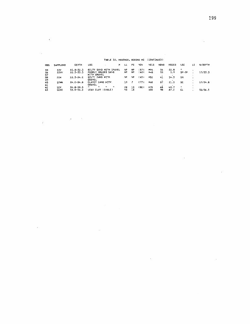
199
TABLE DZ, HAGONER, BORING HZ I CONTINUED I
OBS SAHPLENO DEPTH LOG H LL PI N04 NOlO N040 NO ZOO USC LI NIDEPTH
SS zzv 3l.8-3Z.3 SIL TY SAND HITH GRAVEL NP NP 1571 •44 34 ZZ.8 56 zzw 32.3-33.3 POORLY GRADED SAND NP NP (60) *48 35 l.9 SP-SH 17133.3 57 HITH GRAVEL 58 ZZH 33.3-34.0 SILTY SAND HITH NP NP ( 63) *5Z 41 14.3 SH 59 GRAVEL 60 ZZHH 34.0-34.8 CLAYEY SAND HITH 19 (77) •68 57 21.3 SC 17134.8 61 GRAVEL 6Z zzx 34.8-35.5 ZS 10 IBZ) *75 68 40.7 63 zzxx 35.5-36.3 LEAN CLAY ISHALEl 40 15 100 98 87.Z CL 3Zl36.3

200
TABLE D3, HAGONER, BORING H3
OBS SAHPLENO DEPTH LOG H LL PI N04 NOlO N040 N0200 USC LI N/DEPTH
l 3A 0.0-0.3 FAT CLAY 15. 7 52 27 100 100 95. 9 CH -0. 344 2 3B 0.3-0.8 24.8 59 33 100 100 97. 7 -o. 036 3 3C 0 .8-1.5 29.5 61 36 100 100 97. 9 0.125 8/1.5 4 3D l.5-2.2 30.0 60 36 100 100 97. 7 0 .167 5 3E 2.2-2.9 30. l 62 37 100 100 97. 9 0.105 6/3.0 6 3F 2.9-3.6 LEAN CLAY 27. 0 47 26 100 98 95. l CL 0. 231 7 3G 3.6-4.0 .. 25. 2 42 22 100 97 94. l 0. 236 8 3H 4.0-4.7 FAT CLAY 26 .4 51 31 100 100 95.3 CH 0. 206 7/4.5 9 3I 4.7-5.4 25.2 54 34 100 99 96.9 0.153
10 3J 5.4-6.l 25.8 59 39 100 99 97 .3 0.149 7/6.0 11 3K 6.1-6.8 25.8 56 35 100 99 97.l 0.137 12 3L 6.8-7.5 27. 2 56 35 100 99 97 .3 0.177 9/7.5 13 3H 7.5-8.2 28.4 58 36 100 99 97. 7 0.192 14 3N 8.2-8.9 26 .o 56 35 100 99 97. 3 0.143 8/9.0 15 30 8.9-9.2 26.5 57 35 100 99 96.9 0.129 16 3P 9.2-9.9 26. 7 62 39 100 100 97. 7 0.095 17 3Q 9.9-10.6 26. 2 62 38 100 99 97.7 0.058 7/10 .5 18 3R 10.6-11.3 25.3 62 40 100 100 98.8 0.083 19 3S 11.3-12.0 25. 3 60 38 100 99 97.7 0.087 9/12. 0 20 3T 12.0-12.7 24. 9 60 38 100 100 97. 9 0.076 21 3U 12. 7-13. 4 25. 2 62 39 100 100 97. 9 0.056 9/13.5 22 3V 13 .4-14. l 24. 7 65 42 100 100 97 .9 0.040 23 3H 14.1-14.3 24.6 59 37 100 100 97. 7 0.070 24 3X 14. 3-15. 0 24.8 59 37 100 99 97 .l 0.076 9/15.0 25 3Y 15.0-15. 7 25.5 59 37 100 99 97 .1 0.089 26 3Z 15. 7-16 .4 24. l 58 37 100 99 96. 7 0.084 10/16.5 27 3AA 16.4-17.l 24.4 57 36 I 99 I *99 98 94.6 0.094 28 3BB 17.1-17.8 24.0 54 33 100 100 96.5 0.091 11/18. 0 29 3CC 17.8-18.5 23. 2 50 30 100 99 91. 9 0.107 30 300 18.5-19.2 LEAN CLAY 23. 0 49 28 100 99 as.a CL 0.071 31 3EE 19.2-19.5 LEAN CLAY HITH SANO 19. 7 40 22 100 100 82.3 0.077 11/19.5 32 3FF 19.5-20.2 21. 2 36 19 100 99 79. 7 0. 221 33 3GG 20.2-20.9 20. l 34 17 100 100 79. 7 0.182 8/21.0 34 3HH 20. 9-21. 6 SANDY LEAN CLAY 22. l 27 11 100 100 70. l 0.555 35 3II 21. 6-22. 3 LEAN CLAY HITH SANO 23. l 28 12 100 100 78.8 0.592 4/22 .5 36 3JJ 22.3-23.0 24.8 28 11 100 100 75. l o. 709 37 3KK 23.0-23.4 22. 2 28 11 100 100 78.0 0 .473 38 3LL 23.4-23.8 22.4 28 13 100 100 78.3 0.569 39 3HH 23.8-24.0 22.9 30 13 100 100 82.3 0.454 3/24.0 40 3NN 24.0-24.5 SANDY LEAN CLAY . 23. 2 25 9 100 lDO 67 .o 0.800 41 300 24.5-25.3 SILT HITH SAND 32. 7 NP NP 100 100 79.4 HL 2125.5 42 3PP 25.3-25.8 SANDY SIL TY CLAY 24.5 23 7 100 100 61.0 CL-ML l. 214 43 3QQ 25.8-26.2 SILTY SAND 31. 6 NP NP 100 100 32 .5 SH 44 3RR 26.2-27.0 SANDY LEAN CLAY 29. 7 25 a 100 100 69.4 CL l.588 3127. 0 45 3SS 27 .0-27 .4 SANDY SILTY CLAY 25. 7 20 4 100 lDO 49.4 CL-ML 2.425 46 3TT 27.4-28.l SILTY SAND 24 .4 NP NP lDO 100 40.6 SH 47 3UU 28.1-28.7 24.6 NP NP 100 100 31.8 2128.5 48 3VV 26.7-29.l 24.4 NP NP 180) *89 89 27. 6 49 3HH 29.1-29.8 POORLY GRADED SAND 22.4 NP NP 100 100 10. 2 SP-SH 3/30. 0 50 HITH SILT 51 3XX 29 .. 8-30.5 zo. 6 NP NP 100 97 b.6 52 3YY 30.5-31.2 zo .1 NP NP 100 OS 5.6 53 3ZZ 31.2-31.5 SILTY SAND 19. 6 NP NP 199 I *98 91 18.8 SH 13/31.5 54 3-1 31.5-31.9 16. 2 NP NP I q6 J *91 80 18.6
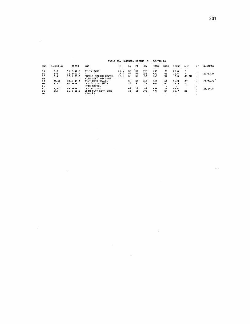
201
TABLE 03' HAGONER, BORING H3 I CONTINUED J
OBS SAHPLENO DEPTH LOG H LL PI N04 NOlO N040 NOZOO use LI N/OEPTH
55 3-2 31.9-32.4 SILTY SANO 14.6 NP NP ( 9S J *93 78 2S.8 56 3-3 32. 4-32. 9 14.3 NP NP 158 J *SO 46 16.4 20/33.0 S7 3-4 32.9-33.5 POORLY GRADED GRAVEL 12 .5 NP NP IS31 *46 37 9. 8 GP-GM 58 HITH SILT ANO SANO 59 33HH 33.5-34.5 SILT HITH GRAVEL NP NP I 62 I *S3 42 16. 3 SH 20/34 .s 60 33X 34.5-35.4 CLAYEY SANO HITH 25 9 I 71 I *bl so 25.8 SC 61 HITH GRAVEL 62 33XX 3S.4-36.0 CLAYEY SANO 42 17 I qs I *93 71 38.4 2S/36.0 63 33Y 36.0-36.8 LEAN CLAY HITH SANO 3S 13 I 9S I *94 84 71. 7 CL 64 I SHALE I

202
TABLE 04, WAGONER, BORING W4
OBS SAMPLENO DEPTH LOG H LL PI N04 NOlO N040 N0200 use LI N/DEPTH
l 4A 0.0-0.3 FAT CLAY 19. 3 67 43 100 99 97. 9 CH -o .109 2 4B 0.3-0.7 23.l 62 37 100 100 98.3 -0.051 3 4C 0.7-1.4 32.7 67 4.1 100 100 97. 7 0 .163 4/1.5 4 4D l.4-2.l ELASTIC SILT 30 .5 66 30 100 100 97. 7 MH -0 .183 s 4E 2.1-2.8 FAT CLAY 27. l 58 36 100 99 96.4 CH 0.142 4/3.0 6 4F 2.8-3.5 29.5 63 41 100 99 97. 0 0.183 7 4G 3.5-4.2 29.5 66 46 100 99 97. l 0.206 8 4H 4.2-4.7 28.l 60 38 100 99 97. 7 0.161 4/4.5 9 41 4.7-5.l 27 .3 62 41" 100 99 97.5 0.154
10 4J 5.1-5.5 27. 6 62 40 100 99 97 .1 0.140 11 4K 5.5-6.2 29.4 64 41 100 100 98. 7 0.156 5/6.0 12 4L 6.2-6.9 29. 7 67 44 100 99 98.1 0.152 13 4M 6.9-7.6 25. 9 65 42 100 99 97 .3 o. 069 517.5 14 4N 7.6-8.3 27.5 68 46 100 98 96.9 0.120 15 40 8.3-9.0 26. 9 63 41 100 99 97.7 0 .120 7/9.0 16 4P 9.0-9.7 26 .8 61 38 100 98 96.8 0.100 17 4Q 9.7-10.0 26 .1 61 40 100 99 97. 7 0.128 18 4R 10.0-10.7 26 .6 58 38 100 99 96.8 0.174 8/10. 5 19 4S 10.7-11.4 26. 6 62 40 100 99 98.5 0.115 20 4T 11.4-12.l 26. 3 62 40 100 100 98.3 0.108 7/12. 0 21 4U 12.1-12.8 25. 7 61 39 100 100 98.3 0.095 22 4V 12.8-13.5 26 .4 62 40 100 99 97. 9 0.110 8/13.5 23 4H 13 .5-13. 9 26.0 61 39 100 99 96.6 0.103 24 4X 13.9-14.6 24.8 59 36 100 99 97. 9 0.050 25 4Y 14.6-15.2 25.6 57 35 100 99 95.8 0.103 8/15.0 26 4Z 15.2-15.9 27 .1 59 37 100 98 94.9 0.138 27 4AA 15.9-16.6 27 .4 56 33 100 98 95.3 0.133 3/16.5 28 4BB 16. 6-17. 3 27. 9 55 33 100 99 96.4 0.179 .29 4CC 17.3-17.6 26.7 56 35 100 99 96.9 0.163 30 40D 17.6-18.3 25. 2 56 34 I 99 I *99 98 95.1 0.094 10/18.0 31 4EE 18.3-19.0 AT LAY HITH SAND 23. 6 50 30 100 100 84.4 0 .120 32 4FF 19.0-19. 7 FAT CLAY 23.1 53 31 100 98 9?>. 9 0.035 8/19.5 33 4GG 19.7-20.l 24.5 58 35 100 99 96.6 0.043 34 4HH 20.1-20.5 LEAN CLAY 22.7 46 28 I 99 I *qq 97 87 .3 CL 0.108 35 4II 20 .5-21. 2 23. 0 43 24 100 98 85.l 0.167 4/21. 0 36 4JJ 21. 2-21. 9 29. 0 45 25 100 99 90. 7 0.360 37 4KK 21. 9-22. 6 29.4 45 27 100 100 91.5 0.422 2/22. 2 38 4LL 22. 6-23. 3 26.7 43 25 100 100 90. 9 0.348 39 4HM 23.3-24.0 27. 7 42 23 100 100 90 .1 0.378 2/24.0 40 4NN 24.0-24 .5 LEAN CLAY HITH SAND 23.2 30 13 100 100 82.5 0.477 41 400 24.5-25.l 24. 3 26 10 100 100 80.6 0 .830 42 4PP 25.1-25.8 29.7 25 8 100 100 81. 2 l.588 1/25.5 43 4QQ 25.8-26.2 LEAN CLAY 31.0 27 10 100 100 98.3 l.400 44 4RR 26. 2-26 .5 LEAN CLAY HITH SAND3 . 9 28 10 100 100 84.8 1. 290 45 4SS 26 .5-26. 7 29.5 28 10 100 100 71. 2 l.150 46 4TT 26.7-27.l SILTY CLAY 27 .1 22 4 100 100 88.1 CL-ML 2. 275 3/27. 0 47 4UU 27.1-27.5 SANDY SILT 25.8 20 3 100 100 57.4 ML 2.933 48 4VV 27.5-28.2 SILTY SAND 21. 6 NP NP 100 100 31.1 SM 9/28.5 49 4HH 28. 2-28. 9 23.3 NP NP 100 100 39.5 50 4XX 28. 9-29. 6 21.8 NP NP 100 100 17 .8 51 4YY 29. 6-30. 0 23.3 NP NP 100 9• 15.4 49/30. 0 52 4ZZ 30.0-30.4 23 .5 NP NP f qq I *"7 93 18.8 53 44G 30.4-31.2 SILTY SAND HITH NP NP 1501 *40 29 13 .6 54 GRAVEL
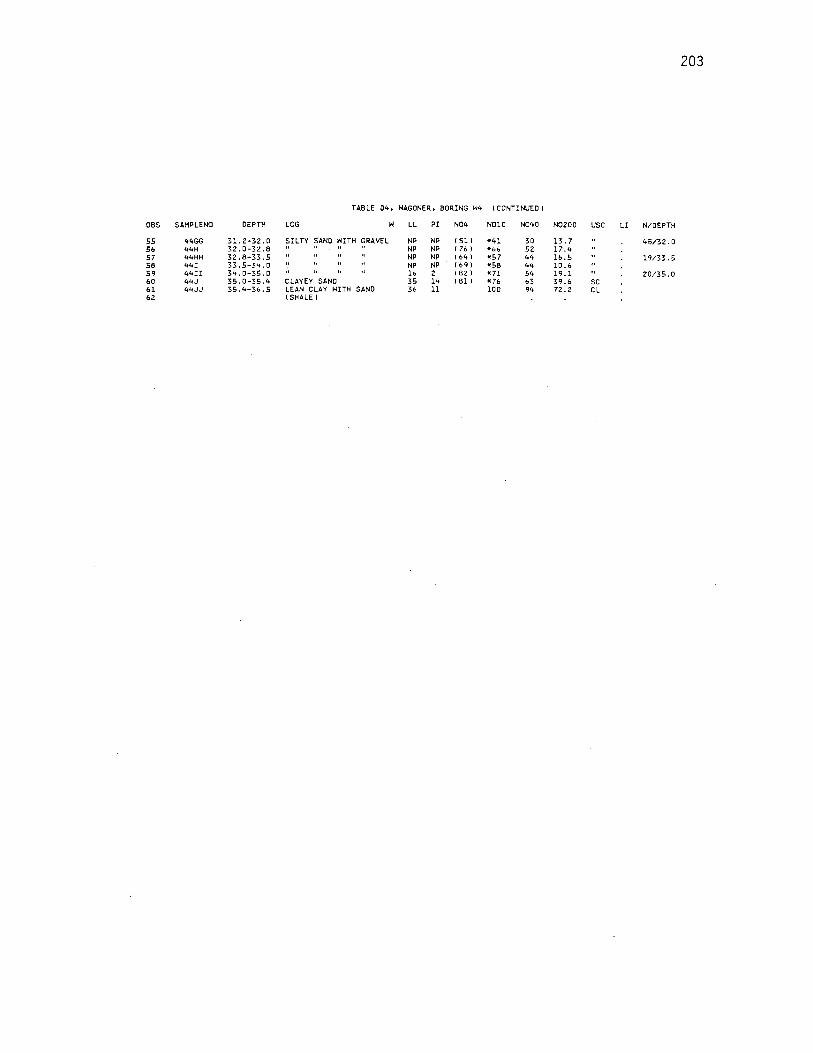
203
TABLE 04, HAGONER, BORING H4 I CONTINUED I
OBS SAHPLENO DEPTH LOG H LL PI N04 NOlO N040 N0200 use LI N/OEPTH
55 44GG 31. 2-32 .0 SILTY SANO HITH GRAVEL NP NP 1511 *41 30 13. 7 45/32.0 56 44H 32.0-32.8 NP NP I 76 I *66 52 17 .4 57 44HH 32.8-33.5 NP NP 164 I *57 44 16.5 19/33.5 58 44I 33.5-34.0 NP NP 1691 *58 44 10.6 59 44!! 34.0-35.0 16 2 1821 *71 54 19.l 20/35.0 60 44J 35.0-35.4 CLAYEY SANO 35 14 1811 *76 63 39.6 SC 61 44JJ 35.4-36.5 LEAN CLAY HITH SAND 36 11 100 94 72.2 Cl 62 I SHALE I
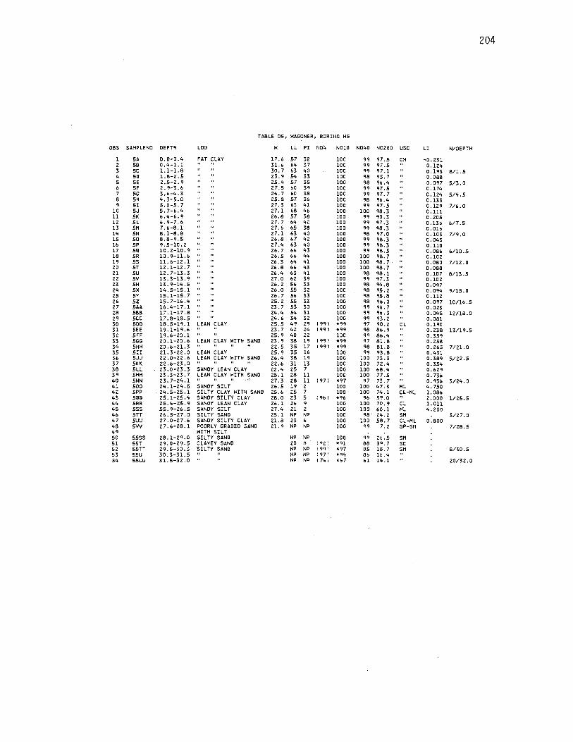
204
TABLE DS, HAGONER, BORING HS
OBS SAMPLENO DEPTH LOG H LL PI N04 NOlD N040 NO ZOO USC LI N/DEPTH
l SA D.D-0.4 FAT CLAY 17 .6 S7 3Z 100 99 97.S CH -0. Z3l z SB 0.4-l.l " 31.6 64 37 100 99 97.S O. lZ4 3 5C l.l-l.8 30. 7 63 40 100 99 97 .1 0 .193 8/l.S 4 SD l.8-Z.S Z3. 9 S4 33 100 98 9S. 7 0.088 s SE 2.S-Z.9 2S.4 S7 3S 100 98 96.4 o. 097 S/3.0 6 SF Z.9-3.6 Z7.8 60 39 100 99 97.S 0.174 7 SG 3.6-4.3 Z6. 7 60 38 100 99 97.7 O.lZ4 S/4.S 8 SH 4.3-S.O ZS.8 S7 36 100 98 96.4 0.133 9 SI s.o-s.7 Z7 .3 63 41 100 99 97.S 0 .129 7/6.0
10 SJ S.7-6.4 Z7 .l 68 46 100 100 98.3 O.lll ll SK 6.4-6.9 Z6.8 S7 38 100 99 90.3 o.zos lZ SL 6.9-7.6 Z7. 7 64 42 100 99 97 .3 0.136 617.5 13 511 7.6-8.l Z7.6 6S 38 100 99 98.3 0.016 14 SN 8.1-8.8 27.l 63 40 100 98 97 .o 0.103 7/9.0 lS so 8.8-9.s Z6.8 67 42 100 99 98.3 0.043 16 SP 9.S-10.Z Z7.4 63 40 100 99 98.3 0.110 17 SQ 10.Z-10.9 Z6. 7 66 43 100 99 98.S 0.086 6/10.S 18 SR 10.9-ll.6 26.S 66 44 100 100 98. 7 0.102 19 SS ll.6-12.l Z6.3 64 41 100 lOD 98. 7 0.080 7/lZ.0 zo ST lZ.1-lZ. 7 Z6.8 66 43 100 100 98. 7 0.088 21 SU 1.2. 7-13. 3 26.4 63 41 100 98 98. l 0.107 8/13.S Z2 SY 1:3.3-13.9 27 .0 62 39 100 99 97.3 0.102 23 SH 13.9-14.S 26~ z S6 33 100 98 94.8 0.097 24 SX 14.S-lS.l 26.0 SS 32 100 98 9S.Z 0.094 9/lS.O 2S SY lS.1-lS.7 26. 7 S6 33 100 98 9S.8 O.llz 26 sz lS.7-16.4 2S. z SS 33 100 98 96.0 0.097 10/16.S Z7 SAA 16.4-17.l Z3. 7 S3 30 100 99 96. 7 0.023 28 SBB 17.1-17.8 24.4 S4 3l 100 99 96.3 0.04S 12118.0 29 sec 17.8-18.S 24.6 54 32 100 99 93.2 0.081 30 SOD 18.S-19.l EAN CLAY 2S.S 49 29 I 99 I *99 97 90.2 CL 0.190 31 SEE 19.1-19.6 23. 7 42 24 1991 •99 98 86.9 O.Z38 13/19.S 3Z SFF 19.6-ZO.l 2S.9 40 22 100 99 86.4 0.3S9 33 SGG 20.1-20.6 LEAN CLAY HITH SAND 23. 9 38 19 1991 *99 97 81.8 o. 2S8 34 SHH 20.6-Zl.3 22.S 3S 17 1991 *99 98 81.8 0.26S 7121. 0 3S SII 21. 3-22. 0 LEAN CLAY 2S.9 3S 16 100 99 93.8 0.431 36 SJJ 2z.o-22.6 LEAN CLAY HITH SAND 26.4 38 19 100 100 73.3 0.389 S/22.S 37 SKK 22.6-23.0 22.6 31 13 100 100 72.4 0.3S4 38 SLL 23.0-23.3 SANDY LEAN CLAY ZZ.4 2S 7 100 100 68.4 0.629 39 SHH 23.3-23.7 LEAN CLAY HITH SAND 2S. l 28 ll 100 100 77.S o. 736 40 SNN 23. 7-24. l 27. 3 28 11 1971 *97 97 73. 7 0.936 3/24.0 41 soo 24.1-24.S SANDY SILT 26.S 19 2 100 100 47.3 HL 4. 7SO 42 SPP . Z4.S-2S. l SILTY CLAY HITH SAND 2S.6 2S 7 100 100 74.1 CL-HL l.086 43 SQQ 2S.l-2S.4 SANDY SILTY CLAY 28.0 23 s I 961 •96 96 S9.0 2.000 l/2S.S 44 SRR 2S.4-2S.9 SANDY LEAN CLAY 26 .l 26 9 100 100 70. 9 CL l.Oll 4S SSS SS.9-26.S SANDY SILT 27 .4 21 2 100 100 60. l HL 4. 200 46 STT 26 .S-27. D SILTY SAND 2S. l NP NP 100 98" 24.2 SH 3127 .0 47 suu 27.0-27.6 SANDY SIL TY CLAY 21.8 23 6 100 100 S8. 7 CL-HL 0.800 48 SYY 27.6-28.l POORLY GRADED SAND 21. 9 NP NP 100 99 7. z SP-SM 7/Z8.S 4• HITH SILT so ssss ZS.1-29.0 SILTY SAND NP NP, 100 99 Z6.5 SH Sl SST 29.0-29.S CLAYEY SAND 20 8 I •2 I *•l 88 39. 7 SC S2 S5TT 29.S-30.3 SILTY SAND NP NP I qq I •97 as 18. 7 SH 8/30.S S3 SSU 30. 3-31. s NP NP I 971 •94 Bo l&.4 S4 SSUU 31.S-3Z.O NP NP I 74 I *&7 &l 14. l Z0/3Z.O

205
TABLE OS, HAGONER, BORING HS I CONTINUED I
OBS SAHPLENO DEPTH LOG H LL PI N04 NOlO N040 N0200 USC LI N/OEPTH
SS SSH 32.0-33.S SIL TY SAND HITH NP NP IS6 I *SO 42 14.0 6/33.S S6 GRAVEL S7 SSY 33.S-3S.O " NP NP 1531 *4S 32 13.0 3/3S.O S8 ssx 3S.0-3S.6 CLAYEY SAND HITH 26 8 162) *S4 42 21.2 SC S9 GRAVEL 60 ssxx 3S.6-3S.9 LEAN CLAY I SHALE I so 22 100 98 9<t.O CL
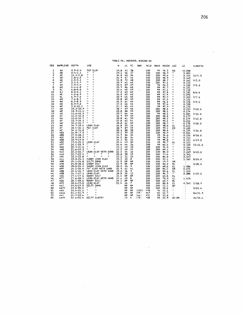
206
TABLE D6, HAGONER, BORING H6
OBS SAMPLENO DEPTH LOG H LL PI N04 NOlD N040 NO ZOO use LI N/DEPTH
l 6A 0.0-0.4 FAT CLAY Z0.8 61 38 100 99 96. 3 CH -o. 058 z 6B 0.4-1.l Z9 .1 66 37 100 100 98. 9 0. 003 3 6C 11.1-1.8 34.8 65 36 100 100 99.4 0.161 lZ/l. 5 4 6D 1.8-Z.5 3Z. 9 67 41 100 100 98. 9 o. loa 5 6E Z.5-3.Z 31. a 72 48 100 100 98. 7 0 .163 313. 0 6 6F 3.Z-3.9 ZS. 9 61 40 100 100 97 .3 0. lZ3 7 6G 3.9-4.4 ZS.4 59 39 100 98 96.3 0.138 7/4.S 8 6H 4.4-4.8 2S. 9 56 4S 100 99 97. 7 0 .131 9 6I 4.8-5.S 2S. 6 60 39 100 99 97 .1 0.118
10 6J 5.S-6.2 Z7. 3 60 40 100 99 97 .5 0.183 8/6,0 11 6K 6.2-6.9 ZS. 0 63 4Z 100 99 97. 9 0.095 lZ 6L 6.9-7.6 ZS. 9 66 45 100 99 97. 7 0.109 711.5 13 6M 7.6-8.3 ZS.8 60 39 100 99 97.3 0. lZ3 14 6N 8.3-8.9 Z6. 0 61 40 100 99 96.6 O. lZS 7/9.0 lS 60 8.9-9.5 Z7. 3 66 44 100 99 97.4 0 .120 16 6P 9.S-10.Z 27.7 6S 43 100 99 97. 9 0.133 17 6Q 10.Z-l0.9 Z8. 7 69 46 100 100 98.5 0.119 7/10.S 18 6R 10. 9-11.6 25.8 58 39 100 100 98.3 0.174 19 6S 11. 6-lZ. 3 ZS. 7 66 44 100 99 98.3 0.084 7/lZ. 0 zo 6T lZ.3-13.0 26.9 59 39 100 100 98.5 0.177 Zl 6U 13.0-13. 7 Z8.8 61 39 100 100 98.3 0.174 7113 .s zz 6V 13.7-14.Z 33.8 6Z 41 100 100 99.Z O.ZlS Z3 6H 14.2-14.7 Z8.8 61 40 100 100 98. 7 0.19S 7115. 0 Z4 6X 14. 7-lS.4 LEAN CLAY Z6.8 33 16 100 100 98.S CL 0.613 25 6Y 15 .4-16 .1 FAT CLAY Z5. 9 59 37 100 100 99. 2 CH 0.105 26 6Z 16.1-16.8 Z5.l 58 38 100 100 98.0 0.134 7/16. 5 27 6AA 16.8-17.5 ZS. 2 S9 33 100 100 96.9 -0.024 26 &BB 17.5-18.2 24. 9 56 36 100 99 96.5 0.136 8/lB.O 29 6CC lB.Z-lB.9 24.0 S6 36 100 99 96.3 0.111 30 6DO lB.9-19.5 23. l 52 33 100 99 94.8 0.124 6/19. 5 31 6EE 19.5-20.2 LEAN CLAY 22 .4 49 30 100 99 90. 7 CL 0.113 32 6FF 20. Z-ZO. 9 26. 6 44 Z6 100 99 86.6 0.100 13/Zl. 0 33 6GG 20. 9-Zl. 6 zz. l 43 25 100 100 91.0 0.164 34 6HH 21.6-22. 3 22. 3 40 Z2 100 100 69. l 0.195 35 6II 22.3-22.7 LEAN CLAY HITH SANO zz .3 34 16 100 100 64.0 0. Z69 8/ZZ. 5 36 6JJ ZZ.7-Z3.3 ZS.5 38 19 100 100 77.4 0.34Z 37 &KK Z3.3-Z3.B 22 .1 31 lS 100 100 84.S 0.407 38 &LL Z3.8-Z4.l SANDY LEAN CLAY Z4. 3 23 8 100 100 57.l 1.163 5/Z4. 0 39 6MM Z4. l-Z4.8 SILTY SANO zz. 5 NP NP 100 100 19. 7 SM 40 &NN Z4.8-Z5.5 SANOY SILT Z3. 9 NP NP 100 100 50.Z ML 3/Z5. 5 41 600 ZS.5-Z6.Z SANDY LEAN CLAY zs.s ZS 9 100 100 68.6 CL 1.0S6 4Z 6PP Z6.Z-Z6.4 FAT CLAY HITH SAND 2Z. 9 61 41 100 100 84.l CH 0.071 43 6QQ Z6.4-Z6.7 LEAN CLAY HITH SAND Z9. 0 Z6 9 100 100 80.6 CL 1.333 44 6RR Z6.7-Z7.l LEAN CLAY Z8.S 30 l3 100 100 94. 7 0.885 2127. 0 45 6SS Z7.l-Z7.6 SANDY SILT Z4.4 NP NP 100 100 63.5 ML 46 6TT Z7.6-Z8.l LEAN CLAY HITH SAND 25.o ZS 8 100 100 70. 9 CL l.07S 47 6UU Z8.l-Z8.6 SANDY SILT 24.3 NP NP 100 100 60.7 ML 48 6VV 28.6-29.0 LEAN CLAY Zl.4 26 7 100 100 85.5 CL 0.343 3/Z8. 9 49 66T Z9.0-29.5 SILTY SANO NP NP 100 100 Zl. l SM 50 66TT Z9.5-30.4 NP NP 100 100 35.6 3/30 .4 51 o6U 30. 4-31. z NP NP I 100 l *96 % 3Z.l 5Z ooUU 31. 2-31. 9 NP NP I 59 I *47 40 14. 9 56/31. 9 53 OoV 3l.9-Z3.6 NP NP ( 66) *51 38 13.5 54 ooVV 32.6-33.4 SILTY CLAYEY 23 4 I 70 J *SB 48 25. 9 SC-SM 24/33. 4

207
TABLE D6, WAGONER, BORING H6 I CONTINUED J
OBS SAHPLENO DEPTH LOG H LL PI N04 NOlO N040 N0200 USC LI N/DEPTH
55 66H 33.4-34.9 SIL TY SAND HITH NP NP ( 70) *63 49 17.9 SH 19/34.9 56 GRAVEL 57 66X 34. 9-35 .5 SILTY CLAYEY SAND 19 5 1791 *71 57 19. 0 SC-SH 58 HITH GRAVEL 59 66XX 35.5-36.4 SANDY LEAN CLAY HITH 31 21 ( 91) *86 86 67.4 CL 13/36.4 60 GRAVEL 61 66Y 36 .4-36 .8 SIL TY SAND HITH NP NP ( 75) *62 58 42. 7 SH 62 GRAVEL 63 66YY 36.8-37.2 LEAN CLAY ISHALEJ 34 10 100 98 88.1 CL 64 66YYY 37.2-37.9 CLAVEY SAND I SANDY 33 13 ( 92) *90 87 48.5 SC 65 SHALE I
HATER LEVEL AT 24 HOURS: 2.6 FEET
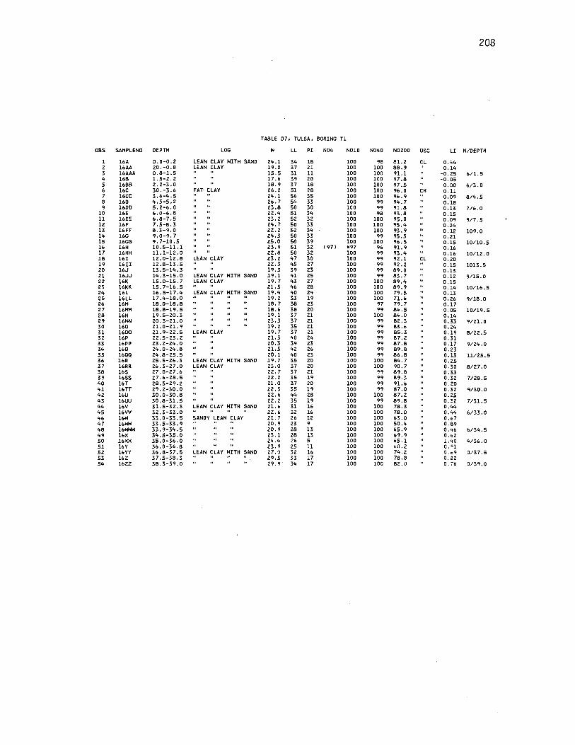
208
TABLE D7, TULSA, BORING Tl
OBS SAMPLENO DEPTH LOG H LL PI N04 NOlO N040 N0200 use LI N/OEPTH
l l6A 0.0-0.2 LEAN CLAY HITH SAND 24.l 34 18 100 98 Bl. 2 CL 0.44 2 l6AA 20.-0.s LEAN CLAY l 9. 2 37 21 lOO 100 88.9 0.14 3 l6AAA 0.8-l.5 15.5 31 ll 100 100 9l. l -o. 25 6/l.5 4 16B 1.5-2.2 17 .6 39 26 100 100 97 .s -0.05 5 l6BB 2.2-3.0 18. 9 37 18 100 100 97 .5 0. 00 6/3 .o 6 16C 30.-3.6 FAT- CLAY 26. 2 51 28 100 100 96.0 CH O.ll 7 l6CC 3.6-4.5 24. l 56 35 100 100 96.9 0.09 B/4.5 B 160 4.5-5.2 26. 7 54 33 100 99 94.7 O. lB 9 1600 5.2-6.0 23.B 50 30 100 99 91.B O.l3 7/6.0
10 16E 6.0-6.S 22.4 51 34 100 98 93.B 0.15 11 l6EE 6.B-7.5 23. 2 52 32 100 100 95.0 0.09 9/7.5 12 l6F 7.5-B.3 24. 7 50 33 lOO 100 95.4 0.24 13 l6FF B.3-9.0 22 .2 52 34 100 100 93. 9 0 .12 109. 0 14 166 9.0-9.7 24.3 50 33 100 99 95.5 0. 21 15 16GG 9. 7-10.5 25.0 SB 39 100 100 96.5 0.15 10/10 .5 16 l6H 10.5-11. l 23.9 51 32 ( 97) •97 96 9l. 9 0 .16 17 16HH ll.1-12. 0 22.B 50 32 100 99 93.4 0 .16 10/12. 0 18 16I 12.0-12.S LEAN CLAY 23. 2 47 30 100 99 92. l o. 20 19 16II 12.8-13.5 22.3 45 27 100 99 92. 2 0.15 1013.5 20 16J 13.5-14.3 19.3 39 23 100 99 89.0 a.13 21 16JJ 14.3-15.0 LEAN CLAY HITH SANO 19. l 41 25 100 99 83.7 0 .12 9/15.0 22 16K 15.0-15.7 LEAN CLAY 19. 7 43 27 100 100 89.4 0.15 23 l6KK 15. 7-16.5 2l.5 46 28 100 100 89. 9 0.14 10/16.5 24 l6L 16.5-17.4 LEAN CLAY HITH SANO 19.4 40 24 100 100 79.5 O.l3 25 16LL 17.4-18.0 19. 2 33 19 100 100 71.6 o. 26 9/18.0 26 l6M 18.0-18.B 18. 7 38 23 100 97 79. 7 0.17 27 16MH 18.8-19.5 18.6 38 20 100 99 84.5 a.as 10/19.5 28 l6N 19.5-20.3 19.1 37 21 100 100 84.0 0.14 29 l6NN 20. 3-21. 0 23.3 37 21 lao 99 82.3 0. 33 9/Zl. 0 30 160 2l.0-2l. 9 19. 2 35 21 100 99 83 .6 0.24 31 1600 21. 9-22 .5 LEAN CLAY 19.7 37 21 100 99 85.3 0 .19 8/22.5 32 16P 22.5-23.2 2l. 3 40 24 100 99 87. 2 a.31 33 16PP 23.2-24.0 20.3 39 23 100 99 87.B a .17 9/24.0 34 l6Q 24.0-24.8 2l.5 42 26 100 99 89.B 0. 23 35 l6QQ 24.8-25.5 20 .1 40 23 lOO 99 86.B 0.13 ll/ZS.5 36 16R 25.5-26.3 LEAN CLAY HITH SANO 19. 7 35 20 100 100 84. 7 0.25 37 16RR 26.3-27.0 LEAN CLAY 23.0 37 20 100 100 90. 7 0.30 B/27. 0 38 165 27.0-27.6 22. 7 37 21 100 99 89.B 0.33 39 l6SS 27.6-28.5 22. 2 35 19 100 99 89.3 0.32 7/28.5 40 16T 28.5-29.2 2l.O 37 20 100 99 9l.6 o. 20 41 16TT 29. 2-30.0 22 .3 35 19 100 99 87.0 0.32 9/30. 0 42 l6U 30.0-30.B 22. 6 44 28 100 100 87.2 0.25 43 16UU 30.8-31.5 22. 2 35 19 100 99 89.B 0. 32 7/3l.5 44 l6V 31.5-32.3 LEAN CLAY HITH SAND 2l. b 31 16 100 100 78.3 0.44 45 l6W 32.3-33.0 22. 6 32 16 100 100 78.0 0.44 6/33. 0 46 l6H 33.0-33.5 SANDY LEAN CLAY 2l. 7 2& 12 100 100 63.0 o. •7 47 l6HH 33.5-33.9 20. 9 23 9 100 100 50.4 0.89 48 l6HHH 33.9-34.5 20. q 28 13 100 100 65.9 0.46 6/34.5 49 l6X 34.5-35.0 23. l 28 13 100 100 69.9 0. •2 50 l&XX 35.0-3·6.0 24.4 26 5 laa lOa 65. l l. 40 4/36. 0 51 l&Y 36.0-36.B 23 .9 25 ll lao 100 &0.2 0. 0 1 52 l&YY 36.B-37.5 LEAN CLAY HITH SAND 27. 0 32 l& 100 100 74. 2 0. o9 0/37. 5 53 l6Z 37.5-38.3 29.5 33 17 100 lOa 78.B 0. 82 54 l6ZZ 38.3-39.0 29. 9 34 17 100 100 s2. a 0. 76 a/39. 0

209
TABLE D7, TULSA, .BORING Tl I CONTINUED J
OBS SAMPLENO DEPTH LOG H LL PI N04 NOlO N040 N0200 use LI N/DEPTH
55 16-1 39.0-39.7 29.8 29 13 100 100 77.l 1.08 56 16-11 39.7-40.5 SANDY LEAN CLAY 25.l 24 10 100 100 63.5 1.10 0/40.5 57 16-2 40.5-41.3 SILTY CLAYEY SAND 28.0 20 5 100 100 43.9 SC-SM 2. 60 58 16-22 41. 3-42. l " It 23.3 19 6 100 100 38.5 l.67 59 16-22 42.1-42.6 25.5 19 5 100 100 40.7 2.40 0/42.6 60 16-3 42.6-43.4 SANDY LEAN CLAY 26.8 26 11 100 100 58.7 CL l.09 61 16-33 43.4-44.l 29.5 26 11 100 100 61.2 1.36 l/44. l 62 16-4 44.1-44.6 SILTY SAND 25.3 19 3 100 100 36.3 SM 3.00 63 16-44 44.6-45.l SANDY LEAN CLAY 31.0 36 16 100 98 69.4 CL 0. 74 64 16-44 45.1-45.6 SILTY SANO 21.2 17 l 100 86 29.2 SM 5.00 6/45.6 65 16-5 45.6-46.4 " 19.6 20 2 100 80 32.4 l. 00 66 16-55 46.4-47.l SIL TY SAND HITH 19.0 20 2P !80 I •69 60 27.2 0.50 13/47 .1 67 GRAVEL 68 16-6 47.1-47.7 SILTY CLAYEY SAND 17.4 21 5 !B2·l •65 57 31.2 SC-SM 0.20 69 HITH GRAVEL 70 16-66 47.7-48.6 LEAN CLAY 12.l 29 11 100 99 94.8 CL -0.55 99/48.6

210
TABLE D8, TULSA, BORING T2
OBS SAHPLENO DEPTH LOG H LL PI N04 NOlO N040 N0200 USC: LI N/DEPTH'
1 17A D.o-o.5 LEAN CLAY 9.7 40 23 1991 *98 96 87.2 CL 2 17AA 0.5-0.7 CLAYEY GRAVEL 3.2 39 21 ( 351 *28 27 26.5 GC: 3 17AAA o. 7-1.2 LEAN CLAY n.o 38 20 100 97 87.8 CL 4 17-4A 1. 2-1.5 LEAN CLAY HITH SAND 15.1 32 14 100 98 75.0 17/1.5 5 17B 1.5-2.4 18.4 33 16 I 93 I *92 90 71.6 6 17BB 2.4-3.0 LEAN CLAY 28.8 41 23 100 99 93.6 10/3.0 7 17C: 3.0-3.7 24.4 49 29 100 99 96.3 8 17C:C: 3.7-4.5 FAT CLAY 31.Z 54 33 100 99 97.5 CH 3/4.5 9 170 4.5-5.2 Z5. l 53 34 100 99 95.4
10 17DD 5.2-6.0 28. 7 52 34 100 98 94.4 6/6.0 11 17E 6.0-6.7 Z2.D 53 36 100 99 94.8 lZ 17EE 6.7-7.5 2B. 7 54 36 100 99 93.8 7/7.5 13 17F 7.5-8.2 22.8 52 35 100 " 95.2 14 17FF 8.2-9.0 27. 2 51 33 100 98 93.0 7/9.0 15 17G 9.0-9. 7 LEAN CLAY 20. 7 49 22 100 99 94.8 C:L 16 17GG 9.7-10.5 FAT CLAY 32.8 53 34 100 99 94.6 CH 7/10.5 17 17H 10.5-11.2 23.1 54 35 100 " 95.0 18 17HH 11.2-12.0 24.2 56 38 lDO 99 96.5 7/12.D 19 17I lZ.0-12.7 22.5 53 35 lOD '' 96.5 20 17II 12.7-13.5 21.0 50 32 100 99 97. 7 8/13.5 21 17J 13.5-14.2 LEAN CLAY 21. 7 44 26 100 99 93.7 C:L 22 17JJ 14.Z-15.0 24.6 45 28 100 99 92.8 10/15.0 23 17K 15.0-15.7 17.8 48 31 100 99 90.8 24 17KK 15. 7-16.5 22.8 48 30 100 100 91.6 14/16.5 25 17L 16.5-17.Z 19.7 46 29 100 100 88.7 26 17U 17.2-18.0 LEAN CLAY HITH SAND 18.5 35 2D 100 100 73.9 9/lB.O 27 17H 18.0-18.7 II II II 18.6 37 18 100 100 75.5 28 17HH 18.7-19.5 18.9 37 22 100 100 80.3 7/19.5 29 17N 19.5-20.2 18. 7 39 23 100 100 84.5 30 17NN 20.2-21.0 25.3 36 19 100 99 82.3 7/21.0 31. 170 21. 0-21. 7 LEAN CLAY 20. 3 37 21 100 " 85.5 32 1700 21. 7-22 .5 LEAN CLAY HITH SAND 18.0 34· 18 100 100 80.0 7/22.5 33 17P 22.5-23.2 LEAN CLAY 21.l 38 23 100 100 86.7 34 17PP 23,Z-24.0 20.7 38 24 100 100 87.6 5/24.0 35 17!l 24.0-24.7 21.8 39 22 100 99 84.8 36 17!l!l 24.7-25.5 27 .o 38 20 100 99 86.Z 7/25.5 37 17R z5.5-Z6.2 20. 9 36 18 100 99 86.9 38 17RR 26.Z-Z7.D LEAN CLAY HITH SAND 31.5 34 18 100 99 8Z.4 5/27.0
HATER LEVEL AT Z4 HOURS: 12.7 FEET

211
TABLE D9, COLLINSVILLE, BORING Cl
OBS SAHPLENO DEPTH LOG H LL PI N04 NOlO N040 NOZOD USC LI N/DEPTH
l lA o.o-o.5 FAT CLAY 16.4 60 34 100 100 96.3 CH z lAA 0.5-l.l " 16.3 50 z5· 100 100 93. 9 " 3 lAAA l.l-l.5 36.l 56 32 100 100 95.0 14/l.5 4 lB l.5-Z.2 23.0 50 29 ( 99 I •99 99 88.l 5 lBB Z.2-3.0 36.4 57 36 100 100 88.l 4/3.0 6 lC 3.0-3.7 FAT CLAY HITH SANO 23.6 61 42 !lOOl •99 9B 82.7 7 lCC 3.7-4.5 30.5 57 39 100 99 B0.4 5/4.5 B 10 4.5-5.2 SANDY LEAN CLAY lB.7 42 26 100 99 63.0 CL 9 lDO 5.2-6.0 II II Tl 24.9 34 20 100 100 55.2 7/6.0
10 lE 6.0-6.7 17.5 3Z lB 100 100 53.2 ll lEE 6.7-7.0 CLAYEY SAND lB.5 24 9 100 100 49.4 SC 12 lEEE 7.0-7.5 23 B ( 100 I •99 99 45.2 3/7.5 l3 lF 7 .5-B.o 24 9 ( 92 I •BB B6 43.5 14 lFF 8.0-B.5 SILTY CLAYEY SANO 2Z 7 ( 93 I •90 89 37.2 SC-SH 15 lFFF 8.5-9.0 CLAYEY SANO 23 B !BBi •B4 BO 37.l SC 5/9.0 16 lG 9.0-9.6 SIL TY CLAYEY SAND 22 7 ( 72 I •65 60 29.6 SC-SH 17 HITH GRAVEL 18 lGG 9.6-10.3 SILTY SAND HITH 21 1741 •69 61 27.6 SH 19 GRAVEL 20 lGGG 10.3-10.5 SILTY CLAYEY SAND 21 5 ( 91 I •79 69 33.4 SC-SH 23/10.5 Zl lH 10.5-10.7 II II 11 22 5 (651 •63 60 43.0 " 22 lHH 10. 7-11.4 LEAN CLAY 3B 16 100 96 87.7 CL 23 lHHH 11.4-11.6 LEAN CLAY !HEATHERED 33 14 lllO 95 70.5 10, 20,10 24 SHALE I R 3 3/16"
HATER TABLE AT 24 HOURS: 7.3 FEET

212
TABLE 010' COLLINSVILLE, BORING CZ
OBS SAMPLENO DEPTH LOG H LL PI N04 NOlO N040 NOZOO use LI N/DEPTH
1 2A 0.0-0.7 LEAN CLAY 14.0 47 24 100 100 97 .1 CL 2 2AA 0.7-1.5 29.8 49 25 100 100 97. l 8/1.5 3 2B 1.5-Z.Z 18.5 45 24 lOO 100 97. 7 4 2BB 2.2-3.0 33.9 45 26 100 100 96.1 ll/3. 0 5 zc 3.0-3.9 11.0 31 lZ 100 100 90.6 6 zcc 3.9-4.5 27 .3 3Z 14 100 100 92.4 13/4.5 7 zo 4.S-S.O 19. 7 33 16 100 100 87. z 8 SOD 5.0-S.Z 15. 6 43 Z4 100 100 96.0 9 ZODD 5.2-6.0 34.6 38 18 100 99 95. 9 10/6. 0
10 ZE 6.0-6.7 18.6 44 ZS 100 99 94.6 ll ZEE 6. 7-7 .5 27.5 47 Z7 100 99 94.4 10/7.5 12 ZF 7 .5-8. z FAT CLAY ZS. l 53 3Z 100 99 94.5 CH 13 2FF 8.2-9.0 38.4 Sl 32 100 99 93. 9 10/9. 0 14 2G 9.0-9.7 GRAVELLY FAT CLAY Z9.Z 58 38 C 78 I *S9 S8 S6.l 15 HITH SANO 16 2GG 9.7-10.S FAT CLAY 32.6 54 35 100 99 94.9 9/10.5 17 2H 10.5-11.2 Z2. 9 52 33 100 99 9S.6 18 ZHH ll. 2-12. O LEAN CLAY 3Z.O 41 Z4 100 98 9S.4 CL 9/10 .5 19 ZI 12.0-12.7 Z3 .8 4Z Z4 100 99 94.8 zo 2II lz,7-13.s 31. 9 38 24 100 99 94.6 4/13. s 21 2J 13.5-14.Z Z7.7 36 19 100 100 93.8 22 2JJ 14. 2-15. 0 31. 9 38 zo 100 99 95.4 3/lS.0 23 ZK lS.0-15. 7 24.9 34 16 100 100 94.0 24 ZKK 15. 7-16.5 32.4 34 16 100 99 9Z.8 0/16.5 2S 2L 16.5-17.2 26.0 35 16 100 100 96. 7 26 ZLL 17.2-18.0 33.6 41 23 100 100 96.2 0/18.0 27 2M 18.0-18.7 40.2 42 24 100 100 97.7 28 ZMM 18.7-19.l 28. 9 41 24 100 100 9S.9 Z9 ZMMtl 19.1-19.S 28.6 31 13 100 99 89.9 0/19.5 30 ZN 19.5-Z0.2 Z5. 9 30 12 100 100 91.0 31 2NN ZO. Z-Zl. 0 Z7.9 28 10 100 100 91.8 l/Zl. 0 32 20 21. 0-21. 7 26.6 30 11 199 I *93 92 87.3 33 200 21. 7-22 .s 28. 9 29 10 100 100 92. z 1/22.5 34 2P 22.5-23. 2 LEAN LAY HITH SAND 28.S 27 10 100 100 78.1 35 2PP 23.Z-Z4.0 LEAN CLAY 28.0 28 11 100 99 88.l O/Z4.0 36 2Q 24.0-Z4.8 LEAN CLAY HITH SAND 25.5 26 9 100 100 77.l 37 2QQ 24.8-25.5 29.S Z9 13 100 100 80.5 l/2S.S 38 ZR Z5.S-Z6.l 3Z. 9 Z8 12 100 100 74.4 39 ZRR 26. l-26 .4 27 .6 27 11 100 100 78.9 40 2RRR Z6.4-Z7.0 LEAN CLAY 30.6 3Z 15 100 100 91.8 0/27.0 41 ZS Z7. O-Z7. 7 LEAN CLAY HITH SAND 31.8 ZS 11 100 lOO 79.4 42 zss 27. 7-28.5 30. 9 28 10 lOO lOO 77. 9 0/28.5 43 2T 28 .5-29. 2 SANDY LEAN CLAY ZS.3 ZS 8 100 100 68.4 44 ZTT Z9.2-30.0 LEAN CLAY HITH SAND 3Z. z Z6 9 100 100 73.8 l/30.0 45 zu 30.0-30.7 30. l Z9 11 100 99 82.4 46 zuu 30. 7-31.5 39. 9 28 9 100 100 78. 0 0/31.S 47 zv 31. 5-3Z. 2 SANDY LEAN CLAY 26.4 2& 10 100 98 62.0 48 zvv 3Z. Z-33. 0 LEAN CLAY HITH SAND 3Z. 9 Zb 11 100 100 71. 9 0/33.0 49 ZH 33. 0-33. 6 Z9.4 Z8 lZ 100 lOO 7S.8 50 ZHH 33. 6-33. 9 SILTY SAND Z9.l NP NP 100 qq 27. 7 SM Sl ZHHH 33. 9-34.4 Z9. z NP NP 100 .. Z9. 6 52 2HHHW 34 .4-34. 9 SANDY LEAN CLAY Z8.6 ZS 10 100 lOO 66.9 CL 2/34. 9 53 zx 34. 9-35. 7 SIL TY CLAYEY SAND Zl.o 20 4 196 I *88 8S 41. 2 SC-SM 54 zxx 35.7-36.4 CLAYEY SANO 18.4 ZS 8 I 871 *73 68 4S.8 SC 3/36. 4

213
TABLE DlO, COLLINSVILLE, BORING C2 I CONTINUED J
OBS SAHPLENO DEPTH LOG H LL PI N04 NOlO N040 N0200 use LI N/DEPTH'
55 2Y 36.4-37.2 SANDY LEAN CLAY 23.8 26 9 I 100) •99 97 66.9 CL 56 2YY 37.2-37.9 LEAN CLAY l'UTH SAND 22.6 29 12 100 99 71.5 3/37. 9 57 2Z 37. 9-38.5 SANDY LEAN CLAY 21.4 28 10 I 97J •94 92 64. 7 58 2ZZ 38.5-39.2 SANDY SILTY CLAY 22.4 22 6 100 100 56.5 CL-HL 59 2ZZZ 39.2-40.0 24.0 24 7 100 92 66.9 4/40. 0 60 2-l 40. 0-40. 3 24.4 22 5 100 100 57.l 61 2-ll 40. 8-41. 5 SILTY SAND 26.2 NP NP 100 100 36. 3 SH 9/41. 5 62 2-2 41.5-42. l SANDY SILT 22.l 19 3 100 99 52.0 ML 63 2-22 42.1-42.5 SILTY SAND 20 .4 NP NP 100 99 35.2 SH 64 2-222 42.5-43.0 SIL TY SAND HITH 12.8 NP NP I 76) *66 62 18.4 35/43. 0 65 GRAVEL 66 2-3 43.0-43.7 13.4 NP NP 168) •54 38 19.4 67 2-33 43.7-44.5 13.0 NP NP 1851 *Bl 65 24. l 74/44.5 68 2-4 44.5-45.3 SILTY GRAVEL HITH 14.6 NP NP I 53 J *40 36 22.l GM 69 SAND 70 2-44 45.3-46.0 SILTY SAND 15. q NP NP I 60 J •45 39 17. 9 SH 27/46.0 7l 2-5 46.0-46.4 13.0 NP NP 1651 •51 38 29. l 72 2-55 46.4-47.5 LEAN CLAY I SHALE J 15. 7 31 9 100 96 89. 9 CL 42/47. 5 73 2-6 47 .5-48. 2 I" J 10.5 32 12 I 100 I •99 96 88.9 5, 38' 50 74 R 2 l/8"
LOCATION: N.H. l/4, N.E. l/4, N.E. l/4, SEC 15, T 22 N,R 14 E ROGERS COUNTY
HATER LEVEL AT 24 HOURS: 17.8 FEET
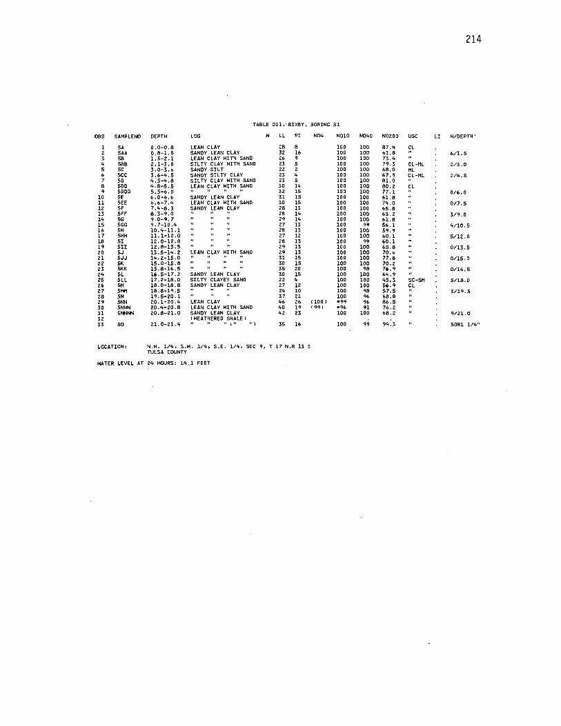
214
TABLE 011, ·BIXBY, BORING Bl
OBS SAHPLENO DEPTH LOG H LL PI N04 NOlO N040 N0200 use LI N/OEPTH'
l SA o.0-0.B LEAN CLAY 2B B 100 100 B7 .4 CL 2 SAA O.B-1.S SANDY LEAN CLAY 32 16 100 100 61.8 6/1.5 3 SB 1.5-2 .1 LEAN CLAY HITH SAND 26 9 100 100 73.4 4 SBB 2.1-3.0 SILTY CLAY HITH SAND 23 5 100 100 79. 3 CL-ML 213 .o 5 SC 3.0-3.6 SANDY SILT 22 2 100 100 68.0 ML 6 sec 3.6-4.S SANDY SILTY CLAY 23 4 100 .100 67.9 CL-ML 214.S 7 SD 4.S-4.8 SIL TY CLAY HITH SAND 23 s 100 100 81.0 8 500 4.8-S.S LEAN CLAY HITH SAND 30 14 100 100 80.2 CL 9 SODO S.S-6.0 32 lS 100 100 77.l 0/6.0
10 SE 6.D-6.6 SANDY LEAN CLAY 31 lS 100 100 61.8 11 SEE 6.6-7.4 LEAN CLAY HITH SAND 30 lS 100 100 74 .0 0/7.S 12 SF 7.4-8.3 SANDY LEAN CLAY 28 13 100 100 6S.8 13 SFF 8.3-9.0 28 14 100 100 63. 2 3/9.0 14 SG 9.0-9.7 29 14 100 100 61.8 lS SGG 9.7-10.4 27 13 100 99 S6.l 4/10 .s 16 SH 10. 4-11. l 28 13 100 100 S9.9 17 SHH 11.1-12. 0 27 12 100 100 60. l S/12.0 18 SI 12.0-12.8 28 13 100 99 60.l 19 SII 12.8-13.S 29 13 100 100 6S.8 0/13.S 20 5.J 13 .S-14. 2 LEAN CLAY HITH SANO 29 13 100 100 70.6 21 SJJ 14.2-lS.O 31 lS 100 100 77.8 O/lS.O 22 5K lS.O-lS.8 30 lS 100 100 70. 2 23 5KK lS.8-16.S 3S 20 100 98 76. 9 0/16.S 24 SL 16.S-17.2 SANDY LEAN CLAY 30 lS 100 100 64.9 2S SLL 17.2-18.0 SILTY CLAYEY SANO 22 4 100 100 4S.3 SC-SH S/18.0 26 SH 18.0-18.8 SANDY LEAN CLAY 27 12 100 100 S6.9 CL 27 SHH 18.8-19.S 24 10 100 98 S7.S 3/19.S 28 SN 19.S-20.l 37 21 100 96 68.8 29 5NN 20.1-20.4 LEAN CLAY 46 26 1100 I •99 96 86.S 30 SNNN 20.4-20.8 LEAN CLAY HITH SANO 40 19 I 99 I •96 91 76. 2 31 Sl*INN 20 .8-21. 0 SANDY LEAN CLAY 42 23 100 100 68.2 9/21. 0 32 IHEATHERED SHALEI 33 50 21.0-21.4 I" ") 35 16 100 99 94.3 SORl 1/4"
LOCATION: N.H. 1/4, S.H. 1/4, S.E. 1/4, SEC 9, T 17 N,R 13 E TULSA COUNTY
HATER LEVEL AT 24 HOURS: 14.l FEET

215
TABLE Dl2, ROLAND, BORING Rl
OBS SAMPLENO DEPTH LOG H LL PI N04 NOlO N040 N0200 use LI N/DEPTH
l 3A 5.7-6.l FAT CLAY 50.B Bl 51 100 100 99.6 CH 0.41 2 3AA 6.l-6.8 50. 6 77 53 100 100 99.4 0.50 3 3AAA 6.8-7.2 41.3 75 51 100 100 99.8 0. 34 0/7.2 4 3B 7.2-7.9 48.0 87 59 100 100 98.5 0 .34 5 3BB 7. 9-8. 7 42.5 82 54 100 100 99.6 0.27 2/8. 7 6 3C 8.7-9.2 41.6 81 54 100 100 98. 7 0. 27 7 3CC 9.2-9.7 42.5 87 59 100 100 99.6 o. 25 8 3CCC 9. 7-10.2 43.7 73 46 100 100 99.8 0 .36 3/10. 2 9 30 10.2-10.7 47 .l 96 63 100 100 99.6 0.22
10 300 10. 7-ll. 2 43.3 98 63 100 100 99.8 0.13 ll 3000 ll.2-ll.7 45.4 91 60 100 100 99.4 o.z'4 3/ll. 7 12 3E ll. 7-12. 2 49.0 100 75 100 100 99.6 0.32 13 3EE 12.2-12.7 38.8 87 55 100 100 99.6 0.12 14 3EEE 12. 7-13. 2 37.8 92 58 100 100 99. 6 0.07 3/13.2 15 3F 13.2-13.7 39.6 88 59 100 100 99.8 0.18 16 3FF 13. 7-14. 2 39.3 83 53 100 100 99.6 0.18 17 3FFF 14.2-14. 7 40.7 90 59 100 100 99.6 0 .16 3/14. 7 18 3G 14. 7-15.4 45.l 87 56 100 100 99.3 0.69 19 3GG 15. 4-16. 2 42.1 86 54 100 99 98.7 0. 23 4/16.2 20 3H 16.2-16.7 39.8 93 64 100 100 99.6 0.17 21 3HH 16.7-17.2 40.0 91 63 100 100 99.6 0 .19 22 3HHH 17.2-17.7 43.4 98 70 100 100 99.3 0.22 3/17.7 23 3I 17.7-17.9 43.9 89 62 100 100 99. l 0.27 24 3II 17.9-18.7 43.3 77 48 100 100 99.3 0.30 25 3III 18. 7-19. 2 44.2 72 44 100 100 97 .0 0.37 4/19. 2 26 3.1 19. 2-19. 7 35. 7 72 47 100 99 95.0 0.23 27 3.1.I 19.7-20.2 40.3 79 50 100 100 99.3 0.23 28 3.1.1.I 20.2-20.7 40.1 83 56 100 100 99.6 0. 23 3/20.7 29 3K 20. 7-21. 2 38.8 82 53 100 99 98. 7 0.18 30 3KK 21. 2-21. 7 38.4 90 63 1100) *99 99 98.6 0.18 31 3KKK 21.7-22.2 42. 2 84 56 100 100 99.3 0.25 3/22. 2 32 3L 22. 2-22. 7 38.6 91 62 100 100 91.l 0.15 33 3LL 22.7-23.2 36.5 84 73 100 99 98. 9 0.35 34 3LLL 23.2-23.7 40.6 91 63 100 100 99.8 0. 20 4/23.7 35 3M 23.7-24.2 41.6 93 66 100 100 99.7 0. 22 36 3MM 24.2-24.7 41.5 92 63 100 100 99.6 0.20 37 3M1111 24.7-25.2 43.3 92 65 100 100 98.8 o. 25 5/25.2 3B 3N 25.2-25.7 45.9 98 68 100 100 100.0 0.23 39 3NN 25.7-26.2 38.3 91 62 100 100 99.8 0.15 40 3NNN 26.2-26.7 45.3 94 64 100 100 100.0 0.24 5/26.7
• 41 30 26. 7-27. 2 44.0 92 63 100 100 100.0 0.24 42 300 27. 2-27. 7 38. 9 86 59 100 100 100.0 0.20 43 3000 27.7-28.2 47 .6 92 62 100 100 99. 9 o. 28 4/Z8, 2 44 3P 28.2-28.7 47.4 89 01 100 100 99.8 0.32 45 3PP 28.7-29.2 58.9 96 66 100 100 99.8 0.44 46 3PPP 29.2-29.7 59. 7 100 66 100 100 99.8 0.39 3/29.7 47 3Q 29.7-30.2 62.8 90 59 100 100 100.0 0.54 48 3QQ 30.2-30.7 59.7 84 56 100 100 99.7 0.57 49 3QQQ 30.7-31.2 62.4 85 57 100 100 99.8 o. 60 50 3QQQQ 31.2-31.7 64.6 86 58 100 100 lDO .D 0.63 0/31. 7 51 3R 31.7-32.2 66.7 82 54 I 100 I *•3 93 92.5 o. 7Z 52 3RR 32.2-32.7 52.3 54 36 100 100 94. 7 0. 95 53 3RRR 32.7-33.2 31.2 55 36 100 100 97. 9 o. 34 l/33. 2 54 3S 33.2-33.9 26. 0 54 37 1100 I *98 96 92. 7 0. 24
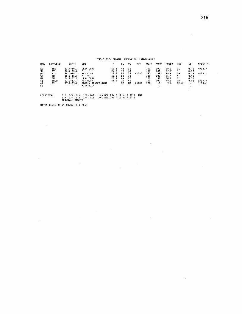
216
TABLE DlZ, ROLAND, BORING Rl I CONTINUED l
OBS SAHPLENO DEPTH LOG N LL PI N04 NOlO N040 N02DO USC LI N/DEPTH'
55 3SS 33.9-34.7 LEAN CLAY 39. 2 48 3D 100 100 98.1 CL 0. 71 4/34. 7 56 3T 34. 7-35.4 24.2 49 30 100 100 97. 7 0 .17 57 3TT 35.4-36.2 FAT CLAY 27. 7 51 33 I 100 I *97 95 89.6 CH 0. 29 4/36. 2 58 3U 36.2-36.7 32. 2 50 30 100 100 96.4 0.41 59 3UU 36.7-37.2 LEAN CLAY 25.3 44 27 100 97 90. 2 CL 0. 31 60 3UUU 37.2-37.7 FAT CLAY 51.5 70 46 100 100 99.0 CH 0.60 5/37.7 61 3V 37.7-39.2 POORLY GRADED SAND NP NP ( 100) *95 15 9.4 SP-SH 1/39. 2 62 HITH SILT
LOCATION: S.E. l/4, S.N. l/4, S.E. l/4, SEC 19, T 11 N, R 27 E AND S.H. 1/4, S.E. 1/4, S.E. 1/4, SEC 19, T 11 N, R 27 E SEQUOYAH COUNTY
NATER LEVEL AT 24 HOURS: 6.3 FEET
APPENDIX E
CPT DATA
217

218
TABLE El, HAGONER, BORING Hl
OBS LOCATION SOIL TYPE USC CR LF FR
l 7 FAT CLAY CH 2300 73.3 3.1870 2 7 FAT CLAY CH 4000 126.7 3.1675 3 7 FAT CLAY CH 4800 213.3 4.4437 4 7 FAT CLAY CH 4000 193.3 4.8325 5 7 FAT CLAY CH 3800 220.0 5.7895 6 7 FAT CLAY CH 3500 260.0 7.4286 7 7 FAT CLAY CH 3400 213.3 6.2735 8 7 FAT CLAY CH 3300 266.7 8.0818 9 7 FAT CLAY CH 3700 286.7 7.7486
10 7 FAT CLAY CH . 3800 306.7 8.0711 11 7 FAT CLAY CH 3100 273.3 8.8161 12 7 FAT CLAY CH 3100 266.7 8.6032 13 7 FAT CLAY CH 3000 326.7 10.8900 14 7 FAT CLAY CH 3100' 260.0 8.3871 15 7 FAT CLAY CH 2900 273.3 9.4241 16 7 FAT CLAY CH 2300 253.3 11.0130 17 7 FAT CLAY CH 2200 233.3 10.6045 18 7 FAT CLAY CH 2100 180.0 8.5714 19 7 FAT CLAY CH 2400 160.0 6.6667 20 7 FAT CLAY CH 2200 126.7 5. 7591 21 7 FAT CLAY CH 2100 140.0 6.6667 22 7 FAT CLAY CH 2400 146.7 6.1125 23 7 FAT CLAY CH 2300 140.0 6.0870 24 7 FAT CLAY CH 2100 146.7 6.9857 25 7 FAT CLAY CH 1900 140.0 7.3684 26 7 FAT CLAY CH 1700 146.7 8.6294 27 7 FAT CLAY CH 1700 146.7 8.6294 28 7 FAT CLAY CH 1800 106.7 5.9278 29 7 FAT CLAY CH 1600 40.0 2.5000 30 7 FAT CLAY CH 1900 40.0 2.1053 31 7 'FAT CLAY CH 1900 40.0 2.1053 32 7 FAT CLAY CH 1900 53.3 2.8053 33 7 FAT CLAY CH 1900 60.0 3.1579 34 7 FAT CLAY CH 1900 73.3 3.8579 35 7 FAT CLAY CH 1900 66.7 3.5105 36 7 FAT CLAY CH 1900 66.7 3.5105 37 7 FAT CLAY CH 2100 80.0 3.8095 38 7 FAT CLAY CH 2000 93.3 4.6650 39 7 FAT CLAY CH 2000 73.3 3.6650 40 7 FAT CLAY CH 1900 73.3 3.8579 41 7 FAT CLAY CH 2200 60.0 2. 7273 42 7 FAT CLAY CH 2200 73.3 3.3318 43 7 FAT CLAY CH 2100 60.0 2.8571 44 7 FAT CLAY CH 2100 60.0 2.8571 45 7 FAT CLAY CH 2000 60.0 3.0000. 46 7 FAT CLAY CH 2100 60.0 2.8571 47 7 FAT CLAY CH 2000 40.0 2.0000 48 7 FAT CLAY CH 2100 60.0 2.8571 49 7 FAT CLAY CH 2100 46.7 2.2238 50 7 FAT CLAY CH 2000 53.3 2.6650 51 7 FAT CLAY CH 2100 60.0 2.8571 52 7 FAT CLAY CH 2100 66.7 3.1762 53 7 FAT CLAY CH 2100 93.3 4.4429 54 7 FAT CLAY CH 2100 73.3 3.4905

219
TABLE El, HAGONER, BORING Hl (CONTINUED J
OBS LOCATION SOIL TYPE USC CR LF FR
55 7 FAT CLAY CH 2400 80.0 3.33333 56 7 FAT CLAY CH 2700 53.3 1.97407 57 7 FAT CLAY CH 2500 53.3 2.13200 58 7 FAT CLAY CH 2300 53.3 2.31739 59 7 FAT CLAY CH 2400 66.7 2.77917 60 7 LEAN CLAY CL 2400 80.0 3.33333 61 7 LEAN Cl:AY CL 2400 53.3 2.22083 62 7 LEAN CLAY CL 2400 66.7 2.77917 63 7 LEAN CLAY CL 2700 66.7 2.47037 64 7 LEAN CLAY CL 2100 60.0 2.85714 65 7 LEAN CLAY CL 1800 73.3 4.07222 66 7 LEAN CLAY CL 1500 40.0 2.66667 67 7 LEAN CLAY H/SAND CL 1300 ~o.o 3.07692 68 7 LEAN CLAY H/SAND CL 1400 46.7 3.33571 69 7 LEAN CLAY H/SAND :CL 1800 40.0 2.22222 70 7 LEAN.CLAY H/SAND CL 1300 26.7 2.05385 71 7 LEAN CLAY H/SAND CL 1200 20.0 1.66667 72 7 LEAN CLAY H/SAND CL 1500 33.3 2.22000 73 7 LEAN CLAY H/SAND CL 1500 40.0 2.66667 74 7 LEAN CLAY H/SAND CL- 1600 53.3 3.33125 75 7 LEAN CLAY H/SAND CL 1900 26.7 1.40526 76 7 LEAN CLAY H/SAND .CL 2300 20.0 0.86957 77 7 LEAN CLAY H/SAND CL 1700 26.7 1.57059 78 7 SANDY SILTY CLAY CL-ML 1700 40.0 2.35294 79 7 SANDY SILTY CLAY CL-ML 1800 60.0 3.33333 80 7 SANDY SILTY CLAY CL-ML 1400 o.o 0.00000 81 7 SANDY SILTY CLAY CL-ML 3200 153.3 4.79062 82 7 LEAN CLAY H/SAND CL 1900 80.0 4.21053 83 7 LEAN CLAY H/SAND CL 170.0 13.3 0.78235 84 7 SANDY SILTY CLAY CL-ML 3100 73.3 2.36452 85 7 SANDY SILTY CLAY CL-ML 4500 126.7 2.81556 86 7 SANDY SILTY CLAY CL-ML 4300 113.3 2.63488 87 7 SANDY SILTY CLAY CL-ML 4000 66.7 1.66750 88 7 SANDY SILTY CLAY CL-ML 6000 340.0 5.66667 89 7 SILTY SAND SH 18000 500.0 2. 77778 90 7 SILTY SAND SH 18000 466.7 2.59278 91 7 SILTY SAND SH 18000 366.7 2.03722

220
TABLE E2, HAGONER, BORING H2
OBS LOCATION SOIL TYPE USC CR LF FR
1 8 FAT CLAY CH 1600 26.7 1.66875 2 8 FAT CLAY CH 1800 106.7 5.92778 3 8 FAT CLAY CH 1600 126.7 7.91875 4 8 FAT CLAY CH 1200 93.3 7.77500 5 8 FAT CLAY CH 1100 93.3 8.48182 6 8 FAT CLAY CH 1000 73.3 7.33000 7 8 FAT CLAY CH 1100 60.0 5.45455 8 8 FAT CLAY CH 1400 53.3 3.80714 9 8 FAT CLAY CH 1400 46.7 3. 33571
10 8 FAT CLAY CH 1300 53.3 4.10000 11 8 FAT CLAY CH 1300 60.0 4.61538 12 8 FAT CLAY CH 1000 46.7 4.67000 13 8 FAT CLAY CH 1100 26. 7 2.42727 14 8 FAT CLAY CH 1100 40.0 3.63636 15 8 FAT CLAY CH 1400 20.0 1.42857 16 8 FAT CLAY CH 1400 40.0 2.85714 17 '8 FAT CLAY CH 1500 40.0 2.66667 18 8 FAT CLAY CH 1500 46.7 3.11333 19 8 FAT CLAY CH 1400 53.3 3.80714 20 8 FAT CLAY CH 1500 53.3 3.55333 21 8 FAT CLAY CH 1400 60.0 4.28571 22 8 FAT CLAY CH 1600 60.0 3.75000 23 8 FAT CLAY CH 1600 46.7 2.91875 24 8 FAT CLAY CH 1600 40.0 2.50000 25 8 FAT CLAY CH 1800 60.0 3.33333 26 8 FAT CLAY CH 1700 46.7 2.74706 27 8 FAT CLAY CH 1800 60.0 3.33333 28 8 FAT CLAY CH 1900 60.0 3.15789 29 8 FAT CLAY CH 1800 66.7 3.70556 30 8 FAT CLAY CH 1800 73.3 4.07222 31 8 FAT CLAY CH 1800 73.3 4.07222 32 8 FAT CLAY CH 1900 66.7 3.51053 33 8 FAT CLAY CH 1900 60.0 3.15789 34 8 FAT CLAY CH 2000 66.7 3.33500 35 8 FAT CLAY CH 2100 66.7 3.17619 36 8 FAT CLAY CH 2000 60.0 3.00000 37 8 FAT CLAY CH 2200 66.7 3.03182 38 8 FAT CLAY CH 2300 66.7 2.90000 39 8 FAT CLAY CH 2200 53.3 2.42273 40 8 FAT CLAY CH 2300 60.0 2.60870 41 8 FAT CLAY CH 2200 66.7 3.03182 42 8 FAT CLAY CH 2000 53.3 2.66500 43 8 FAT CLAY CH 1900 60.0 3.15789 44 8 FAT CLAY CH 2000 53.3 2.66500 45 8 FAT CLAY CH 1900 66.7 3.51053 46 8 FAT CLAY CH 2000 46.7 2.33500 47 8 FAT CLAY CH 1900 60.0 3.15789 48 8 FAT CLAY CH 2100 66.7 3.17619 49 8 FAT CLAY CH 2000 60.0 3.00000 50 8 FAT CLAY CH 2000 53.3 2.66500 51 8 FAT CLAY CH 2100 66.7 3.17619 52 8 FAT CLAY CH 2200 100.0 4.54545 53 8 FAT CLAY CH 2100 86.7 4.12857 54 8 FAT CLAY CH 2200 93.3 4.24091
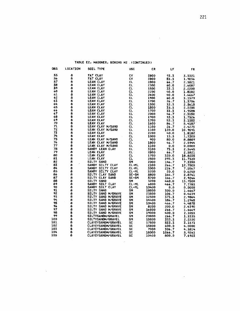
221
TABLE E2, HAGONER, BORING H2 . f CONTINUED J
OBS LOCATION SOIL TYPE USC CR LF FR
55 8 FAT CLAY CH 28DO 93.3 3.3321 56 8 FAT CLAY CH 2800 53.3 1.9036 57 8 LEAN CLAY CL 2800 66.7 2.3821 58 8 LEAN CLAY CL 2300 60.0 2.6087 59 8 LEAN CLAY CL 1500 33.3 2.2200 60 8 LEAN CLAY CL 2200 40.0 1.8182 61 8 LEAN CLAY CL 2400 40.0 1.6667 62 8 LEAN CLAY CL 1900 60.0 3.1579 63 8 LEAN CLAY CL 1700 26.7 1.5706 64 8 LEAN CLAY CL 1300 33.3 2.5615 65 8 LEAN CLAY CL 1500 33.3 2.2200 66 8 LEAN CLAY CL 1700 33.3 1.9588 67 8 LEAN CLAY CL 2000 46.7 2.3350 68 8 LEAN CLAY CL 1900 33.3 1.7526-69 8 LEAN CLAY CL 1700 53.3 3.1353 70 8 LEAN CLAY CL 1600 86.7 5.4187 71 8 LEAN CLAY H/SAND CL 1100 26.7 2.4273 72 8 LEAN CLAY H/SAND CL 1100 120.0 10.9091 73 8 LEAN CLAY CL 2200 40.0 1.8182 74 8 LEAN CLAY CL 1000 13.3 1.3300 75 8 LEAN CLAY H/SAND CL 900 80.0 8.8889 76 8 LEAN CLAY H/SAND CL 1800 46.7 2.5944 77 8 LEAN CLAY H/SAND CL 1100 0.0 0.0000 78 8 SANDY LEAN CLAY CL 3100 73.3 2.3645 79 8 LEAN CLAY CL 2800 66.7 2.3821 80 8 LEAN CLAY CL 1700 320.0 18.8235 81 8 LEAN CLAY CL 2500 293.3 11. 7320 82 8 SILTY SAND SM 2000 146.7 7.3350 83 8 SANDY SILTY CLAY CL-ML 2100 266.7 12.7000 84 8 SANDY SILTY CLAY CL-ML 3000 226.7 7.5567 85 8 SANDY SILTY CLAY CL-ML 3200 20.0 0.6250 86 8 SILTY CLAY SAND sC-SM 5800 166.7 2.8741 87 8 SILTY CLAY SAND SC-SM 5700 166.7 2.9246 88 8 SILTY SAND SM 3200 440.0 13.7500 89 8 SANDY SILT CLAY CL-ML 6000 466.7 7.7783 90 8 SANDY SILT CLAY CL-ML 10400 o.o 0.0000 91 8 SILTY SAND SM 18000 300.0 1.6667 92 8 SILTY SAND H/GRAVE SM 23000 106.7 0.4639 93 8 SILTY SAND H/GRAVE SM 12500 373.3 2.9864 94 8 SILTY SAND H/GRAVE SM 14400 186.7 1. 2965 95 8 SILTY SAND H/GRAVE SM 10400 466.7 4.4875 96 8 SILTY SAND H/GRAVE SM 8200 200.0 2 .4390 97 8 SILTY SAND H/GRAVE SM 16000 266.7 1.6669 98 8 SILTY SAND H/GRAVE SM 19000 400.0 2.1053 99 8 SILTYSANDH/GRAVEL SM 20000 266.7 1.3335
100 8 SILTYSANDH/GRAVEL SM 15000 333.3 2.2220 101 8 CLAYEYSANDH/GRAVEL SC 17000 533.3 3.1371 102 8 CLAYEYSANDH/GRAVEL SC 15000 600.0 4.0000 103 8 CLAYEYSANDH/GRAVEL SC 7000 306.7 4.3814 104 8 CLAYEYSANDH/GRAVEL SC 18000 1066.7 5.9261 105 8 CLAYEYSANDH/GRAVEL SC 10400 800.0 7.6923

222
TABLE E3, HAGONER, BORING H3
OBS LOCATION SOIL TYPE USC CR LF FR
1 9 FAT CLAY CH 2000 106.7 5.33500 2 9 FAT CLAY CH 2400 146.7 6.11250 3 9 FAT CLAY CH 2200 120.0 5.45455 4 9 FAT CLAY CH 2200 166.7 7 .57727 5 9 FAT CLAY CH 2700 166.7 6.17407 6 9 FAT CLAY CH 2300 160.0 6.95652 7 9 FAT CLAY CH 2500 140.0 5.60000 8 9 FAT CLAY CH 2800 146.7 5.23929 9 9 LEAN CLAY CL 3100 180.0 5.80645
10 9 LEAN CLAY CL 2900 173.3 5.97586 11 9 LEAN CLAY CL 2600 160.0 6.15385 12 9 LEAN CLAY CL 2300 146. 7 6.37826 13 9 FAT CLAY CH 2000 166.7 8.33500
-14 9 FAT CLAY CH 2000 40.0 2.00000 15 9 FAT CLAY CH 1800 140.0 7.77778 16 9 FAT CLAY CH 3800 133.3 3.50789 17 9 FAT CLAY CH 1800 126.7 7.03889 18 9 FAT CLAY CH 1700 120.0 7.05882 19 9 FAT CLAY CH 1600 93.3 5.83125 20 9 FAT CLAY CH 1500 86.7 5.78000 21 9 FAT CLAY CH 1700 73.3 4.31176 22 9 FAT CLAY CH 1700 73.3 4.31176 23 9 FAT CLAY CH 1700 80.0 4.70588 24 9 FAT CLAY CH 1800 80.0 4.44444 25 9 FAT CLAY CH 1700 60.0 3.52941 26 9 FAT CLAY CH 1600 53.3 3.33125 27 9 FAT CLAY CH 1600 60.0 3.75000 28 9 FAT CLAY CH 1700 86.7 5.10000 29 9 FAT CLAY CH 1600 93.3 5.83125 30 9 FAT CLAY CH 1800 86.7 4.81667 31 9 FAT CLAY CH 1900 60.0 3.15789 32 9 FAT CLAY CH 2000 46.7 2.33500 33 9 FAT CLAY CH 2300 60.0 2.60870 34 9 FAT CLAY CH 2300 53.3 2.31739 35 9 FAT CLAY CH 2100 53.3 2.53810 36 9 FAT CLAY CH 2400 60.0 2.50000 37 9 FAT CLAY CH 2500 66.7 2.66800 38 9 FAT CLAY CH 2500 86.7 3.46800 39 9 FAT CLAY CH 2500 66.7 2.66800 40 9 FAT CLAY CH 2200 66.7 3.03182 41 9 FAT CLAY CH 2200 66.7 3.03182 42 9 FAT CLAY CH 2100 60.0 2.85714 43 9 FAT CLAY CH 2000 80.0 4.00000 44 9 FAT CLAY CH 2200 60.0 2. 72727 45 9 FAT CLAY CH 2300 66.7 2.90000 46 9 FAT CLAY CH 2500 80.0 3.20000 47 9 FAT CLAY CH 2500 73.3 2.93200 48 9 FAT CLAY CH 2300 53.3 2. 31739 49 9 FAT CLAY CH 2300 60.0 2.60870 50 9 FAT CLAY CH 2500 66.7 2.66800 51 9 FAT CLAY CH 2200 80.0 3.63636 52 9 FAT CLAY CH 2000 60.0 3.00000 53 9 FAT CLAY CH 2200 86.7 3.94091 54 9 FAT CLAY CH 2900 160.0 5.51724
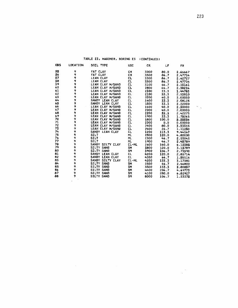
223
TABLE E3, HAGONER, BORING E3 (CONTINUED l
OBS LOCATION SOIL TYPE USC CR LF FR
55 9 FAT CLAY CH 3000 80.0 2.66667 56 9 FAT CLAY CH 3500 86.7 2.47714 57 9 LEAN CLAY CL 3300 86.7 2.62727 58 9 LEAN CLAY CL 3500 86.7 2.47714 59 9 LEAN CLAY H/SAND CL 3100 66.7 2.15161 60 9 LEAN CLAY H/SAND CL 2800 66.7 2.38214 61 9 LEAN CLAY H/SAND CL 2300 33.3 1.44783 62 9 LEAN CLAY H/SAND CL 2100 53.3 2.53810 63 9 LEAN CLAY H/SAND CL 2000 60.0 3.00000 64 9 SANDY LEAN CLAY CL 1600 33.3 2.08125 65 9 SANDY LEAN CLAY CL 1500 33.3 2.22000 66 9 LEAN CLAY H/SAND CL 1600 40.0 2.50000 67 9 LEAN CLAY H/SAND CL 2000 40.0 2.00000 68 9 LEAN CLAY H/SAND CL 2200 53.3 2.42273 69 9 LEAN CLAY H/SAND CL 1900 33.3 1.75263 70 9 LEAN CLAY H/SAND CL 1800 100.0 5.55556 71 9 LEAN CLAY H/SAND CL 2000 0.0 0.00000 72 9 LEAN CLAY H/SAND CL 2400 80.0 3.33333 73 9 LEAN CLAY H/SAND CL 2400 26.7 1.11250 74 9 SANDY LEAN CLAY CL 1200 113.3 9.44167 75 9 SILT ML 2500 120.0 4.80000 76 9 SILT ML 2300 46.7 2.03043 77 9 SILT ML 1900 46.7 2.45789 78 9 SANDY SILTY CLAY CL-ML 2600 160.0 6.15385 79 9 SILTY SAND SM 3800 120.0 3.15789 80 9 SILTY SAND SM 3900 106.7 2. 73590 81 9 SANDY LEAN CLAY CL 4200 120.0 2.85714 82 9 SANDY LEAN CLAY CL 4300 66.7 1.55116 83 9 SANDY SILTY CLAY CL-ML 4200 133.3 3.17381 84 9 SILTY SAND SM 2500 66.7 2.66800 85 9 SILTY SAND SM 3500 133.3 3.80857 86 9 SILTY SAND SM 4400 206.7 4.69773 87 9 SILTY SAND SM 4100 280.0 6.82927 88 9 SILTY SAND SM 8000 106.7 1.33375

224
TABLE E4, HAGONER, BORING H4
OBS LOCATION SOIL TYPE USC CR LF FR
1 14 FAT CLAY CH 1000 0.0' 0.0000 2 14 FAT CLAY CH 2500 66.7 2.6680 3 14 FAT CLAY CH 3000 133.3 4.4433 4 14 FAT CLAY CH 2200 113.3 5.1500 5 14 FAT CLAY CH 2000 133.3 6.6650 6 14 FAT CLAY CH 2000 120.0 6.0000 7 14 FAT CLAY CH 2200 120.0 5.4545 8 14 FAT CLAY CH 2200 146.7 6.6682 9 14 FAT CLAY CH 2300 140.0 6.0870
10 14 FAT CLAY CH 2400 146.7 6.1125 11 14 FAT-CLAY CH 2500 160.0 6.4000 12 14 FAT CLAY CH 2600 133.3 5.1269 13 14 FAT CLAY CH 2400 133.3 5.5542 14 14 FAT CLAY CH 2400 153.3 6.3875 15 14 FAT CLAY CH 2000 146.7 7.3350 1€> 14 FAT CLAY CH 1600 193.3 12.0812 17 14 FAT CLAY CH 1400 120.0 8.5714 18 14 FAT CLAY CH 1600 100.0 6.2500 19 14 FAT CLAY CH 1400 106.7 7.6214 20 14 FAT CLAY CH 1300 86.7 6.6692 21 14 FAT CLAY CH 1400 106.7 7.6214 22 14 FAT CLAY CH 1600 93.3 5.8312 23 14 FAT CLAY CH 1600 100.0 6.2500 24 14 FAT CLAY CH 1600 106.7 6.6687 25 14 FAT CLAY CH 1600 113.3 7.0812 26 14 FAT CLAY CH 1800 120.0 6.6667 27 14 FAT CLAY CH 1700 106.7 6.2765 28 14 FAT CLAY CH 1800 113.3 6.2944 29 14 FAT CLAY CH 1800 100.0 5.5556 30 14 FAT CLAY CH 1700 113.3 6.6647 31 14 FAT CLAY CH 1900 113.3 5.9632 32 14 FAT CLAY CH 1800 93.3 5.1833 33 14 FAT CLAY CH 1800 93.3 5.1833 34 14 FAT CLAY CH 1700 ioo.o 5.8824 35 14 FAT CLAY CH 2000 100.0 5.0000 36 14 FAT CLAY CH 2000 113.3 5.6650 37 14 FAT CLAY CH 2100 100.0 4.7619 38 14 FAT CLAY CH 1800 113.3 6.2944 39 14 FAT CLAY CH 1800 100.0 5.5556 40 14 FAT CLAY CH 2000 106.7 5.3350 41 14 FAT CLAY CH 2100 113.3 5.3952 42 14 FAT CLAY CH 2000 106.7 5.3350 43 14 FAT CLAY CH 2100 106.7 5.0810 44 14 FAT CLAY CH 2000 100.0 5.0000 45 14 FAT CLAY CH 2000 80.0 4.0000 46 14 FAT CLAY CH 2000 106.7 5.3350 47 14 FAT CLAY CH 2000 100.0 5.0000 48 14 FAT CLAY CH 2000 .100.0 5.0000 49 14 FAT CLAY CH 2200 120.0 5.4545 50 14 FAT CLAY CH 2300 106.7 4.6391 51 14 FAT CLAY CH 2400 120.0 5.0000 52 14 FAT CLAY CH 2600 133.3 5.1269 53 14 FAT CLAY CH 2600 113.3 4.3577 54 14 FAT CLAY H/SAND CH 2600 106.7 4.1038
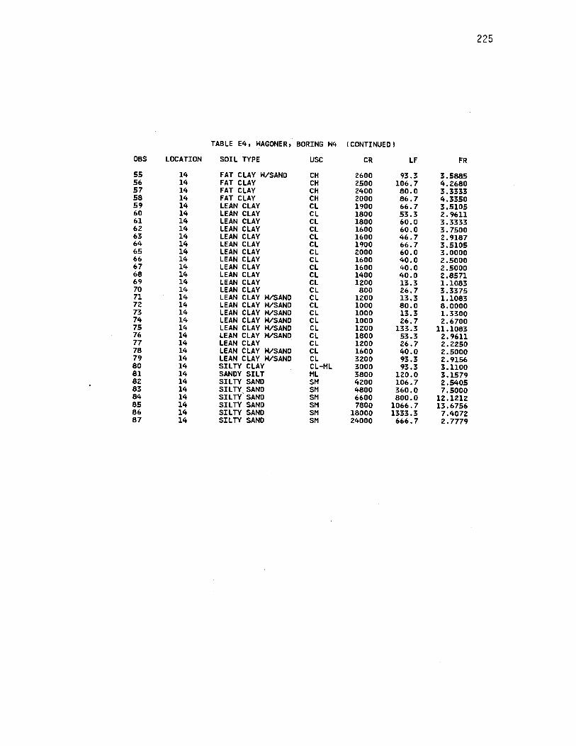
225
TABLE E4, NAGONER, BORING N4 l CONTINUED l
OBS LOCATION SOIL TYPE USC CR LF FR
55 14 FAT CLAY N/SAND CH 2600 93.3 3.5885 56 14 FAT CLAY CH 2500 106.7 4.2680 57 14 FAT CLAY CH 2400 80.0 3.3333 58 14 FAT CLAY CH 2000 86.7 4.3350 59 14 LEAN CLAY CL 1900 66.7 3.5105 60 14 LEAN CLAY CL 1800 53.3 2.9611 61 14 LEAN CLAY CL 1800 60.0 3.3333 62 14 LEAN CLAY CL 1600 60.0 3.7500 63 14 LEAN CLAY CL 1600 46.7 2.9187 64 14 LEAN CLAY CL 1900 66.7 3.5105 65 14 LEAN CLAY CL 2000 60.0 3.0000 66 14 LEAN CLAY CL 1600 40.0 2.5000 67 14 LEAN CLAY CL 1600 40.0 2.5000 68 14 LEAN CLAY CL 1400 40.0 2.8571 69 14 LEAN CLAY CL 1200 13.3 1.1083 70 14 LEAN CLAY CL 800 26.7 3.3375 71 14 LEAN CLAY N/SAND CL 1200 13.3 1.1083 72 14 LEAN CLAY N/SAND CL 1000 80.0 8.0000 73 14 LEAN CLAY N/SAND CL 1000 13.3 1.3300 74 14 LEAN CLAY N/SAND CL 1000 26.7 2.6700 75 14 LEAN CLAY N/SAND CL 1200 133.3 11.1083 76 14 LEAN CLAY N/SAND CL 1800 53.3 2.9611 77 14 LEAN CLAY CL 1200 26.7 2.2250 78 14 LEAN CLAY N/SAND CL 1600 40.0 2.5000 79 14 LEAN CLAY N/SAND CL 3200 93.3 2.9156 80 14 SILTY CLAY CL-ML 3000 93.3 3.1100 81 14 SANDY SILT ML 3800 120.0 3.1579 82 14 SILTY SAND SM 4200 106.7 2.5405 83 14 SILTY, SAND SM 4800 360.0 7.5000 84 14 SILTY SAND SM 6600 800.0 12.1212 85 14 SILTY SAND SM 7800 1066.7 13.6756 86 14 SILTY SAND SM 18000 1333.3 7.4072 87 14 SILTY SAND SM 24000 666.7 2.7779
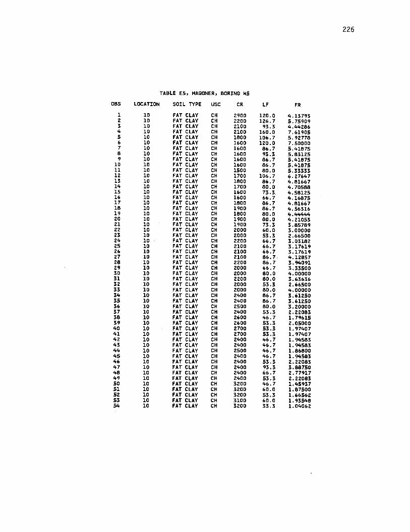
226
TABLE ES, HAGONER, BORING HS
OBS LOCATION SOIL TYPE USC CR LF FR
l 10 FAT CLAY CH 2900 120.0 4.13793 2 10 FAT CLAY CH 2200 126.7 S.7S909 3 10 FAT CLAY CH 2100 93.3 4.44286 4 10 FAT CLAY CH 2100 160.0 7.6190S s 10 FAT CLAY CH 1800 106.7 S.92778 6 10 FAT CLAY CH 1600 120.0 7.SOOOO 7 10 FAT CLAY CH 1600 86.7 S.4187S 8 10 FAT CLAY CH 1600 93.3 S.83125 9 10 FAT CLAY CH 1600 86.7 S.4187S
10 10 FAT CLAY CH 1600 86.7 S.4187S 11 10 FAT CLAY CH 1500 80.0 S.33333 12 10 FAT CLAY CH 1700 106.7 6.27647 13 10 FAT CLAY CH 1800 86.7 4.81667 14 10 FAT CLAY CH 1700 80.0 4.70588 15 10 FAT CLAY CH 1600 73.3. 4.58125 16 10 FAT CLAY CH 1600 66.7 4.16875 17 10 FAT CLAY CH 1800 86.7 4.81667 18 10 FAT CLAY CH 1900 86.7 4.S6316 19 10 FAT CLAY CH 1800 80.0 4.44444 20 10 FAT CLAY CH 1900 80.0 4.21053 21 10 FAT CLAY CH 1900 73.3 3.8S789 22 10 FAT CLAY CH 2000 60.0 3.00000 23 10 FAT CLAY CH 2000 S3.3 2.66500 24 10 FAT CLAY CH 2200 66.7 3.03182 25 10 FAT CLAY CH 2100 66.7 3.17619 26 10 FAT CLAY CH 2100 66.7 3.17619 27 10 FAT CLAY CH 2100 86.7. 4.12857 28 10 FAT CLAY CH 2200 86.7 3.94091 29 10 FAT CLAY CH 2000 66.7 3.33SOO 30 10 FAT CLAY CH 2000 80.0 4.00000 31 10 FAT CLAY CH 2200 80.0 3.63636 32 10 FAT CLAY CH 2000 S3.3 2.66SOO 33 10 FAT CLAY CH 2000 80.0 4.00000 34 10 FAT CLAY CH 2400 86.7 3.612SO 3S 10 FAT CLAY CH 2400 86.7 3.612SO 36 10 FAT CLAY CH 2SOO 80.0 3.20000 37 10 FAT CLAY CH 2400 S3.3 2.22083 38 10 FAT CLAY CH 2600 46.7 l.7961S 39 10 FAT CLAY CH 2600 S3.3 2.0SOOO 40 10 FAT CLAY CH 2700 53.3 1.97407 41 10 FAT CLAY CH 2700 S3.3 1.97407 42 10 FAT CLAY CH 2400 46.7 1.94583 43 10 FAT CLAY CH 2400 46.7 1.94583 44 10 FAT CLAY CH 2SOO 46.7 1.86800 4S 10 FAT CLAY CH 2400 46.7 1.94583 46 10 FAT CLAY CH 2400 S3.3 2.22083 47 10 FAT CLAY CH 2400 93.3 3.88750 48 10 FAT CLAY CH 2400 66.7 2. 77917 49 10 FAT CLAY CH 2400 S3.3 2.22083 so 10 FAT CLAY CH 3200 46.7 l.4S937 Sl 10 FAT CLAY CH 3200 60.0 l.87SOO S2 10 FAT CLAY CH 3200 S3.3 l.66S62 S3 10 FAT CLAY CH 3100 60.0 1.93548 S4 10 FAT CLAY CH 3200 33.3 1.04062

227
TABLE E5, HAGONER, BORING H5 (CONTINUED J
OBS LOCATION SOIL TYPE USC CR LF FR
55 10 FAT CLAY CH 3200 80.0 2.50000 56 10 LEAN CLAY CL 3100 60.0 1.93548 57 10 LEAN CLAY CL 2600 60.0 2.30769 58 10 LEAN CLAY CL 2500 80.0 3.20000 59 10 LEAN CLAY CL 2300 73.3 3.18696 60 10 LEAN CLAY CL 2000 46.7 2.33500 61 10 LEAN CLAY H/SAND CL 2100 53.3 2.53810 62 10 LEAN CLAY H/SAND CL 1800 53.3 2. 96111 63 10 LEAN CLAY H/SAND CL 1700 60.0 3.52941 64 10 LEAN CLAY H/SANO CL 1700 33.3 1.95882 65 10 LEAN CLAY CL 1800 46.7 2.59444 66 10 LEAN CLAY CL 2200 40.0 1.81818 67 10 LEAN CLAY H/SAND CL 1700 60.0 3.52941 68 10 LEAN CLAY H/SAND CL 1400 o.o 0.00000 69 10 LEAN CLAY H/SAND CL 1500 26.7 1.78000 70 10 SANDY LEAN CLAY CL 2000 13.3 0.66500 71 10 LEAN CLAY H/SAND CL 1200 80.0 6.66667 72 10 LEAN CLAY H/SAND CL 1400 0.0 0.00000 73 10 SANDY SILT ML 1000 0.0 0.00000 74 10 SANDY SILT ML 2400 53.3 2.22083 75 10 SILTY CLAY H/SAND CL-ML 2500 13.3 0.53200 76 10 SILTY CLAY H/SAND CL-ML 2400 26.7 1.11250 77 10 SANDY SILTY CLAY CL-ML 2300 20.0 0.86957 78 10 SANDY LEAN CLAY CL 1800 133.3 7.40556 79 10 SANDY SILT ML 2100 160.0 7.61905 80 10 SANDY SILT ML 1800 173.3 ·9.62778 81 10 SILTY SAND SM 6400 146.7 2.29219 82 10 SANDY SILTY CLAY CL-ML 6600 226.7 3.43485 83 10 SANDY SILTY CLAY CL-ML 8200 240.0 2.92683
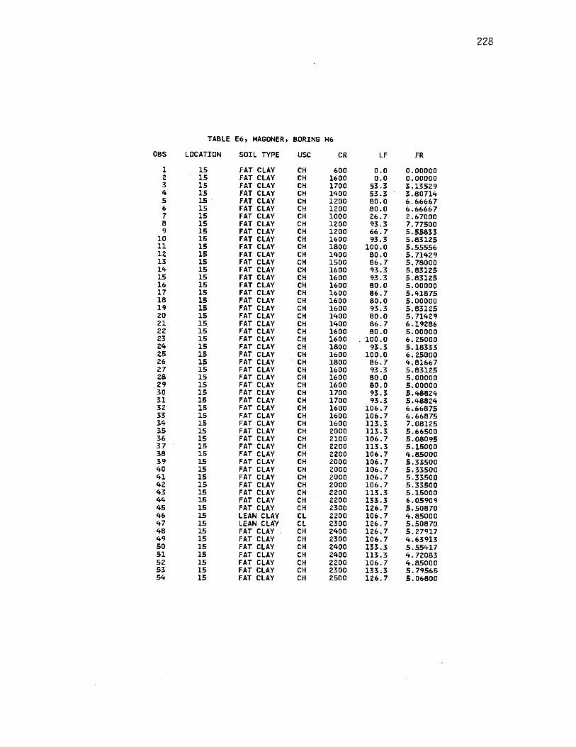
228
TABLE E6, HAGONER, BORING H6
OBS LOCATION SOIL TYPE use CR LF FR
1 15 FAT CLAY CH 600 o.o 0.00000 2 15 FAT CLAY CH 1600 0.0 0.00000 3 15 FAT CLAY CH 1700 53.3 3.13529 4 15 FAT CLAY CH 1400 53.3 3.80714 5 15 FAT CLAY CH 1200 80.0 6.66667 6 15 FAT CLAY CH 1200 80.0 6.66667 7 15 FAT CLAY CH 1000 26.7 2.67000 8 15 FAT CLAY CH 1200 93.3 7.77500 9 15 FAT CLAY CH 1200 66.7 5.55833
10 15 FAT CLAY CH 1600 93.3 5.83125 11 15 FAT CLAY CH 1800 100.0 5.55556 12 15 FAT CLAY CH 1400 80.0 5. 71429 13 15 FAT CLAY CH 1500 86.7 5.78000 14 15 FAT CLAY CH 1600 93.3 5.83125 15 15 FAT CLAY CH 1600 93.3 5.83125 16 15 FAT CLAY CH 1600 80.0 5.00000 17 15 FAT CLAY CH 1600 86.7 5.41875 18 15 FAT CLAY CH 1600 80.0 5.00000 19 15 FAT CLAY CH 1600 93.3 5.83125 20 15 FAT CLAY CH 1400 80.0 5. 71429 21 15 FAT CLAY CH 1400 86.7 6.19286 22 15 FAT CLAY CH 1600 80.0 5.00000 23 15 FAT CLAY CH 1600 100.0 6.25000 24 15 FAT CLAY CH 1800 93.3 5.18333 25 15 FAT CLAY CH 1600 100.0 6.25000 26 15 FAT CLAY CH 1800 86.7 4.81667 27 1.5 FAT CLAY CH 1600 93.3 5.83125 28 15 FAT CLAY CH 1600 80.0 5.00000 29 15 FAT CLAY CH 1600 80.0 5.00000 30 15 FAT CLAY CH 1700 93.3 5.48824 31 15 FAT CLAY CH 1700 93.3 5.48824 32 15 FAT CLAY CH 1600 106.7 6.66875 33 15 FAT CLAY CH 1600 106.7 6.66875 34 15 FAT CLAY CH 1600 113.3 7.08125 35 15 FAT CLAY CH 2000 113.3 5.66500 36 15 FAT CLAY CH 2100 106.7 5.08095 37 15 FAT CLAY CH 2200 113.3 5.15000 38 15 FAT CLAY CH 2200 106.7 4.85000 39 15 FAT CLAY CH 2000 106.7 5.33500 40 15 FAT CLAY CH 2000 106.7 5.33500 41 15 FAT CLAY CH 2000 106. 7 5.33500 42 15 FAT CLAY CH 2000 106.7 5.33500 43 15 FAT CLAY CH 2200 113.3 5.15000 44 15 FAT CLAY CH 2200 133.3 6.05909 45 15 FAT CLAY CH 2300 126.7 5.50870 46 15 LEAN CLAY CL 2200 106.7 4.85000 47 15 LEAN CLAY CL 2300 126. 7 5.50870 48 15 FAT CLAY CH 2400 126.7 5.27917 49 15 FAT CLAY CH 2300 106.7 4.63913 50 15 FAT CLAY CH 2400 133.3 5.55417 51 15 FAT CLAY CH 2400 113.3 4. 72083 52 15 FAT CLAY CH 2200 106.7 4.85000 53 15 FAT CLAY CH 2300 133.3 5.79565 54 15 FAT CLAY CH 2500 126.7 5.06800

229
TABLE E6, HAGONER, BORING H6 (CONTINUED l
OBS LOCATION SOIL TYPE USC CR LF FR
55 15 FAT CLAY CH 2200 126. 7 5. 75909 56 15 FAT CLAY CH 2600 120.0 4.61538 57 15 FAT CLAY CH 2600 146.7 5.64231 58 15 FAT CLAY CH 2800 106. 7 3.81071 59 15 FAT CLAY CH 3000 106.7 3.55667 60 15 LEAN CLAY CL 3200 120.0 3.75000 61 15 LEAN CLAY CL 3200 106. 7 3.33437 62 15 LEAN CLAY CL 2800 100.0 3.57143 63 15 LEAN CLAY CL 2900 106.7 3.67931 64 15 LEAN CLAY CL 2900 46.7 1.61034 65 15 LEAN CLAY CL 2400 80.0 3.33333 66 15 LEAN CLAY CL 2300 53.3 2.31739 67 15 LEAN CLAY CL 1800 80.0 4.44444 68 15 LEAN CLAY CL 2000 53.3 2.66500 69 15 LEAN CLAY H/SAND CL 2400 93.3 3.88750 70 15 LEAN CLAY H/SAND CL 2400 53.3 2.22083 71 15 LEAN CLAY H/SAND CL 2100 60.0 2.85714 72 15 LEAN CLAY H/SAND CL 2400 40.0 1.66667 73 15 LEAN CLAY H/SAND CL 2000 60.0 3.00000 74 15 SANDY LEAN CLAY CL 1800 40.0 2.22222 75 15 SILTY SAND SM 1500 53.3 3.55333 76 15 SILTY SAND SM 1200 80.0 6.66667 77 15 SANDY SILT ML 1600 26.7 1.66875 78 15 SANDY SILT ML 1600 40.0 2.50000 79 15 SANDY LEAN CLAY CL 2000 26.7 1.33500 80 15 SANDY LEAN CLAY CL 1600 0.0 0.00000 81 15 FAT CLAY H/SAND CH 3800 40.0 1.05263 82 15 LEAN CLAY H/SAND CL 2600 120.0 4.61538 83 15 LEAN CLAY CL 2600 0.0 0.00000 84 15 SANDY SILT ML 2400 120.0 5.00000 85 15 LEAN CLAY H/SAND CL 3800 26.7 0.70263 86 15 LEAN CLAY H/SAND CL 6400 146.7 2.29219 87 15 SANDY SILT ML 6200 160.0 2.58065 88 15 LEAN CLAY CL 5000 186.7 3.73400 89 15 LEAN CLAY CL 4300 126.7 2.94651

230
TABLE E7, TULSA, BORING Tl
OBS LOCATION SOIL TYPE USC CR LF FR
l 3 LEAN CLAY CL 1800 13.3 o. 73889 2 3 LEAN CLAY CL 2200 44.4 2.01818 3 3 LEAN CLAY CL 1900 66.7 3.51053 4 3 LEAN CLAY CL 1600 73.3 4.58125 5 3 LEAN CLAY CL 1200 66.7 5.55833 6 3 LEAN CLAY CL 900 40.0 4.44444 7 3 LEAN CLAY CL 800 6.7 0.83750 8 3 LEAN CLAY CL 1400 13.3 0.95000 9 3 FAT CLAY CH 1800 . 53.3 2.96111
10 3 FAT CLAY CH 1800 66.7 3.70556 11 3 FAT CLAY CH 1600 66.7 4.16875 12 3 FAT CLAY CH 1800 100.0 5.55556 13 3 FAT CLAY CH 1800 93.3 5.18333 14 3 FAT CLAY CH 1900 106.7 5.61579 15 3 FAT CLAY CH 2800 133.3 4.76071 16 3 FAT CLAY CH 2800 133.3 4.76071 17 3 FAT CLAY CH 2800 140.0 5.00000 18 3 FAT CLAY CH 2400 133.3 5.55417 19 3 FAT CLAY CH 2200 100.0 4.54545 20 3 FAT CLAY CH 2200 100.0 4.54545 21 3 FAT CLAY CH 2400 93.3 3.88750 22 3 FAT CLAY CH 2200 80.0 3.63636 23 3 FAT CLAY CH 2200 86.7 3.94091 24 3 FAT CLAY CH 2300 86.7 3.76957 25 3 FAT CLAY CH 2400 93.3 3.88750 26 3 FAT CLAY CH 2400 86.7 3.61250 27 3 FAT CLAY CH 2400 73.3 3.05417 28 3 FAT CLAY CH 2200 80.0 3.63636 29 3 FAT CLAY CH 2500 93.3 3.73200 30 3 FAT CLAY CH 2600 86.7 3.33462 31 3 FAT CLAY CH 2500 93.3 3.73200 32 3 FAT CLAY CH 2600 86.7 3.33462 33 3 FAT CLAY CH 2500 86.7 3.46800 34 3 FAT CLAY CH 2600 93.3 3.58846 35 3 FAT CLAY CH 2500 86.7 3.46800 36 3 FAT CLAY CH 2400 93.3 3.88750" 37 3 LEAN CLAY CL 2200 73.3 3.33182 38 3 LEAN CLAY CL 2000 93.3 4.66500 39 3 LEAN CLAY CL 1700 60.0 3.52941 40 3 LEAN CLAY CL 2000 60.0 3.00000 41 3 LEAN CLAY CL 1900 66.7 3.51053 42 3 LEAN CLAY CL 1900 73.3 3.85789 43 3 LEAN CLAY CL 2200 93.3 4.24091 44 3 LEAN CLAY l'VSAND CL 2000 100.0 5.00000 45 3 LEAN CLAY H/SAND CL 2000 66.7 3.33500 46 3 LEAN CLAY CL 1900 93.3 4.91053 47 3 LEAN CLAY CL 1800 53.3 2.96111 48 3 LEAN CLAY CL 1800 46.7 2.59444 49 3 LEAN CLAY CL 1800 53.3 2.96111 so 3 LEAN CLAY CL 1800 60.0 3.33333 51 3 LEAN CLAY H/SAND CL 1600 66.7 4.16875 52 3 LEAN CLAY H/SAND CL 1600 80.0 s.00000 53 3 LEAN CLAY l'VSAND CL 2400 86.7 3.61250 54 3 LEAN CLAY H/SAND CL 2600 93.3 3.58846

231
TABLE E7, TULSA, BORING Tl I CONTINUED l
OBS LOCATION SOIL TYPE USC CR LF FR
55 3 LEAN CLAY H/SAND CL 2500 73.3 2.93200 56 3 LEAN CLAY H/SAND CL 2500 73.3 2.93200 57 3 LEAN CLAY H/SAND CL 2800 73.3 2.61786 58 3 LEAN CLAY H/SAND CL 2800 80.0 2.85714 59 3 LEAN CLAY H/SAND CL 2800 73.3 2.61786 60 3 LEAN CLAY H/SAND CL 2800 80.0 2.85714 61 3 LEAN CLAY H/SAND CL 2800 80.0 2.85714 62 3 LEAN CLAY H/SAND , CL 2400 73.3 3.05417 63 3 LEAN CLAY H/SAND CL 2300 73.3 3.18696 64 3 LEAN CLAY H/SAND CL 2400 73.3 3.05417 65 3 LEAN CLAY H/SAND CL 2500 73.3 2.93200 66 3 LEAN CLAY H/SAND CL 2400 53.3 2.22083 67 3 LEAN CLAY CL 2300 53.3 2.31739 68 3 LEAN CLAY CL 2200 73.3 3.33182 69 3 LEAN CLAY CL 2200 66.7 3.03182 70 3 LEAN CLAY CL 2200 73.3 3.33182 71 3 LEAN CLAY CL 2500 33.3 1.33200 72 3 LEAN CLAY CL 2800 80.0 2.85714 73 3 LEAN CLAY CL 3800 80.0 2.10526 74 3 LEAN CLAY CL 2800 100.0 3.57143 75 3 LEAN CLAY CL 2800 93.3 3.33214 76 3 LEAN CLAY CL 2200 93.3 4.24091 77 3 LEAN CLAY CL 2000 80.0 4.00000 78 3 LEAN CLAY H/SAND CL 2000 80.0 4.00000 79 3 LEAN CLAY H/SAND CL 2200 80.0 3.63636 80 3 LEAN CLAY- CL 2400 73.3 3.05417 81 3 LEAN CLAY CL 2400 80.0 3.33333 82 3 LEAN CLAY CL 2400 80.0 3.33333 83 3 LEAN CLAY CL 2200 73.3 3.33182 84 3 LEAN CLAY CL 2200 60.0 2.72727 85 3· LEAN CLAY CL 2200 86.7 3.94091 86 3 LEAN CLAY CL 1900 73.3 3.85789 87 3 LEAN CLAY CL 2100 80.0 3.80952 88 3 LEAN CLAY CL 2400 86.7 3.61250 89 3 LEAN CLAY CL 2200 86.7 3.94091 90 3 LEAN CLAY CL 2200 93.3 4.24091 91 3 LEAN CLAY CL 2200 66.7 3.03182 92 3 LEAN CLAY CL 2000 53.3 2.66500 93 3 LEAN CLAY CL 1900 26.7 1.40526 94 3 LEAN CLAY CL 2000 46.7 2.33500 95 3 LEAN CLAY CL 1900 40.0 2.10526 96 3 LEAN CLAY H/SAND CL 1800 40.0 2.22222 97 3 LEAN CLAY H/SAND CL 1800 46.7 2.59444 98 3 LEAN CLAY H/SAND CL 1800 73.3 4.07222 99 3 LEAN CLAY H/SAND CL 1800 40.0 2.22222
100 3 LEAN CLAY H/SAND CL 1900 26.7 1.40526 101 3 SANDY LEAN CLAY CL 1900 53.3 2.80526 102 3 SANDY LEAN CLAY CL 1800 26.7 1.48333 103 3 SANDY LEAN CLAY CL 1400 26.7 1.90714 104 3 SANDY LEAN CLAY CL 1500 26.7 1.78000 105 3 SANDY LEAN CLAY CL 1800 40.0 2.22222 106 3 SANDY LEAN CLAY CL 1700 60.0 3.52941 107 3 SANDY LEAN CLAY CL 1400 46.7 3.33571 108 3 SANDY LEAN CLAY CL 1000 53.3 5.33000

232
TABLE E7, TULSA, BORING T7 !CONTINUED)
OBS LOCATION SOIL TYPE use CR LF FR
109 3 SANDY LEAN CLAY CL 1100 53.3 4.8455 110 3 SANDY LEAN CLAY CL 1000 46.7 4.6700 111 3 SANDY LEAN CLAY CL 1000 46.7 4.6700 112 3 LEAN CLAY H/SAND CL 1000 53.3 5.3300 113 3 LEAN CLAY H/SAND CL 1000 46.7 4.6700 114 3 LEAN CLAY H/SAND CL 1000 46.7 4.6700 115 3 LEAN CLAY H/SAND CL 1000 40.0 4.0000 116 3 LEAN CLAY H/SAND CL 800 33.3 4.1625 117 3 LEAN CLAY H/SAND CL 700 20.0 2.8571 118 3 LEAN CLAY H/SAND CL 600 53.3 8.8833 119 3 LEAN CLAY H/SAND CL 600 13.3 2.2167 120 3 LEAN CLAY H/SAND CL 1000 13.3 1.3300 121 3 SANDY LEAN CLAY CL 2400 80.0 3.3333 122 - 3 SANDY LEAN CLAY CL 1000 33.3 3.3300 123 3 SANDY LEAN CLAY CL 1800 26.7 1.4833 124 3 SILTY, CLAYEY SAND SC-SH 1000 66.7 6.6700 125 3 SILTY, CLAYEY SAND SC-SH 1400 26.7 1. 9071 126 3 SILTY, CLAYEY SAND SC-SH 1800 20.0 1.1111 127 3 SILTY, CLAYEY SAND SC-SH 2000 53.3 2.6650 128 3 SILTY, CLAYEY SAND SC-SH 1900 60.0 3.1579 129 3 SILTY, CLAYEY SAND SC-SH 1000 53.3 5.3300 130 3 SANDY LEAN CLAY CL 900 40.0 4.4444 131 3 SANDY LEAN CLAY CL 1000 40.0 4.0000 132 3 SANDY LEAN CLAY CL 1200 26.7 2.2250 133 3 SANDY LEAN CLAY CL 900 66.7 7.4111 134 3 SANDY LEAN CLAY CL 1400 26.7 1.9071 135 3 SILTY SAND SH 4800 66.7 1.3896 136 3 SANDY LEAN CLAY CL 6000 93.3 1.5550 137 3 SANDY LEAN CLAY CL 5000 13.3 0.2660 138 3 SILTY SAND SH 8400 106.7 1.2702 139 3 SILTY SAND SH 7000 120.0 1.7143 140 3 SILTY SAND SH 6400 240.0 3.7500 141 3 SILTY SAND SH 8400 106.7 1.2702 142 3 SILTY SAND H/GRAVE SH 10400 200.0 1.9231 143 3 SILTY SAN H/GRAVEL SH 4800 533.3 11.1104
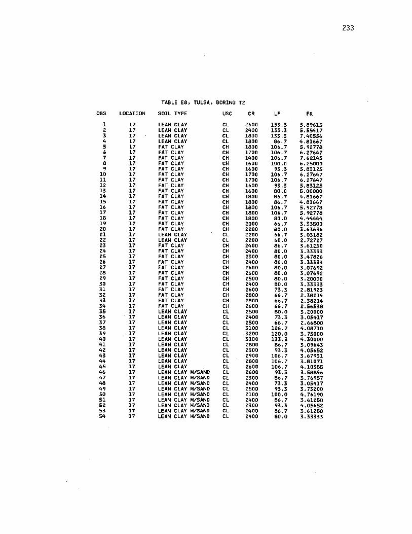
233
TABLE ES, TULSA, BORING T2
OBS LOCATION SOIL TYPE use CR LF FR
1 17 LEAN CLAY CL 2600 153.3 5.89615 2 17 LEAN CLAY CL 2400 133.3 5.55417 3 17 LEAN CLAY CL 1800 133.3 7.40556 4 17 LEAN CLAY CL 1800 86.7 4.81667 5 17 FAT CLAY CH 1800 106.7 5.92778 6 17 FAT CLAY CH 1700 106.7 6.27647 7 17 FAT CLAY CH 1400 106.7 7.62143 8 17 FAT CLAY CH 1600 100.0 6.25000 9 17 FAT CLAY CH 1600 93.3 5.83125
10 17 FAT CLAY CH 1700 106.7 6.27647 11 17 FAT CLAY CH 1700 106.7 6.27647 12 17 FAT CLAY CH 1600 93.3 5.83125 13 17 FAT CLAY CH 1600 80.0 5.00000 14 17 FAT CLAY CH 1800 86.7 4.81667 15 17 FAT CLAY CH 1800 86.7 4.81667 16 17 FAT CLAY CH 1800 106.7 5.92778 17 17 FAT CLAY CH 1800 106.7 5.92778 18 17 FAT CLAY CH 1800 80.0 4.44444 19 17 FAT CLAY CH 2000 66.7 3.33500 20 17 FAT CLAY CH 2200 80.0 3.63636 21 17 LEAN CLAY CL 2200 66.7 3.03182 22 17 LEAN CLAY CL 2200 60.0 2.72727 23 17 FAT CLAY CH 2400 86.7 3.61250 24 17 FAT CLAY CH 2400 80.0 3.33333 25 17 FAT CLAY CH 2300 80.0 3.47826 26 17 FAT CLAY CH 2400 80.0 3.33333 27 17 FAT CLAY CH 2600 80.0 3.07692 28 17 FAT CLAY CH 2600 80.0 3.07692 29 17 FAT CLAY CH 2500 80.0 3.20000 30 17 FAT CLAY CH 2400 80.0 3.33333 31 17 FAT CLAY CH 2600 73.3 2.81923 32 17 FAT CLAY CH 2800 66.7 2.38214 33 17 FAT CLAY CH 2800 66.7 2.38214 34 17 FAT CLAY CH 2600 66.7 2.56538 35 17 LEAN CLAY CL 2500 80.0 3.20000 36 17 LEAN CLAY CL 2400 73.3 3.05417 37 17 LEAN CLAY CL 2500 66.7 2.66800 38 17 LEAN CLAY CL 3100 126.7 4.08710 39 17 LEAN CLAY CL 3200 120.0 3.75000 40 17 LEAN CLAY CL 3100 133.3 4.30000 41 17 LEAN CLAY CL 2800 86.7 3.09643 42 17 LEAN CLAY CL 2300 93.3 4.05652 43 17 LEAN CLAY CL 2900 106. 7 3.67931 44 17 LEAN CLAY CL 2800 106.7 3.81071 45 17 LEAN CLAY CL 2600 106.7 4.10385 46 17 LEAN CLAY H/SAND CL 2600 93.3 3.58846 47 17 LEAN CLAY H/SAND CL 2300 86.7 3.76957 48 17 LEAN CLAY H/SAND CL 2400 73.3 3.05417 49 17 LEAN CLAY H/SAND CL 2500 93.3 3.73200 50 17 LEAN CLAY H/SAND CL 2100 100.0 4.76190 51 17 LEAN CLAY H/SAND CL 2400 86.7 3.61250 52 17 LEAN CLAY H/SAND CL 2300 93.3 4.05652 53 17 LEAN CLAY H/SAND CL 2400 86.7 3.61250 54 17 LEAN CLAY H/SAND CL 2400 80.0 3.33333

234
TABLE E8, TULSA, BORING T2 I CONTINUED l
OBS LOCATION SOIL TYPE USC CR LF FR
55 17 LEAN CLAY H/SAND CL 2400 106.7 4.44583 56 17 LEAN CLAY H/SAND CL 2200 106.7 4.85000 57 17 LEAN CLAY CL 2000 106.7 5.33500 58 17 LEAN CLAY CL 2000 93.3 4.66500 59 17 LEAN CLAY CL 2200 73.3 3.33182 60 17 LEAN CLAY H/SAND CL 2200 93.3 4.24091 61 17 LEAN CLAY H/SAND CL 2300 120.0 5.21739 62 17 LEAN CLAY CL 2200 93.3 4.24091 63 17 LEAN CLAY CL 2200 106.7 4.85000 64 17 LEAN CLAY CL 2800 86.7 3.09643 65 17 LEAN CLAY CL 3000 106.7 3.55667 66 17 LEAN CLAY CL 3300 106.7 3.23333 67 17 LEAN CLAY CL 3100 100.0 3.22581 68 17 LEAN CLAY CL 3200 100.D 3.12500 69 17 LEAN CLAY CL 3200 93.3 2.91562 70 17 LEAN CLAY CL 3300 106.7 3.23333 71 17 LEAN CLAY CL 3200 106.7 3.33437 72 17 LEAN CLAY CL 2400 66.7 2. 77917 73 17 LEAN CLAY H/SAND CL 2200 80.0 3.63636 74 17 LEAN CLAY H/SAND CL 2200 66.7 3.03182 75 17 LEAN CLAY H/SAND CL 2000 53.3 2.66500
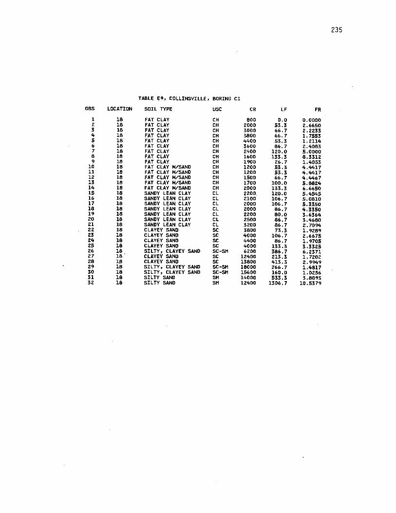
235
TABLE E9, COLLINSVILLE, BORING Cl
OBS LOCATION SOIL TYPE USC CR LF FR
l 18 FAT CLAY CH 800 o.o 0.0000 2 18 FAT CLAY CH 2000 53.3 2.6650 3 18 FAT CLAY CH 3000 66.7 2.2233 4 18 FAT CLAY CH 3800 66.7 1.7553 5 18 FAT CLAY CH 4400 53.3 1. 2114 6 18 FAT CLAY CH 3600 86.7 2.4083 7 18 FAT CLAY CH 2400 120.0 5.0000 8 18 FAT CLAY CH 1600 133.3 8.3312 9 18 FAT CLAY CH 1900 26.7 1.4053
10 18 FAT CLAY H/SAND CH 1200 53.3 4.4417 11 18 FAT CLAY H/SAND CH 1200 53.3 4.4417 12 18 FAT CLAY H/SAND CH 1500 66.7 4.4467 13 18 FAT CLAY H/SAND CH 1700 100.0 5.8824 14 18 FAT CLAY H/SAND CH 2000 133.3 6.6650 15 18 SANDY LEAN CLAY CL 2200. 120·.0 5.4545 16 18 SANDY LEAN CLAY CL 2100 106.7 5.0810 17 18 SANDY LEAN CLAY CL 2000 106.7 5.3350 18 18 SANDY LEAN CLAY CL 2000 86.7 4.3350 19 18 SANDY LEAN CLAY CL 2200 80.0 3.6364 20 18 SANDY LEAN CLAY CL 2500 86.7 3.4680 21 18 SANDY LEAN CLAY CL 3200 86.7 2. 7094 22 18 C.LAYEY SAND SC 3800 73.3 1.9289 23 18 CLAYEY SAND SC 4000 106.7 2.6675 24 18 CLAYEY SAND SC 4400 86.7 1.9705 25 18 CLAYEY SAND SC 4000 133.3 3.3325 26 18 SILTY, CLAYEY SAND SC-SM 6200 386.7 6.2371 27 18 CLAYEY SAND SC 12400 213.3 1.7202 28 l~ CLAYEY SAND SC 13800 413.3 2.9949 29 18 SILTY, CLAYEY SAND SC-SM 18000 266.7 1.4817 30 18 SILTY, CLAYEY SAND SC-SM 15600 160.0 1.0256 31 18 SILTY SAND SM 14000 533.3 3.8093 32 18 SILTY SAND SM 12400 1306. 7 10.5379
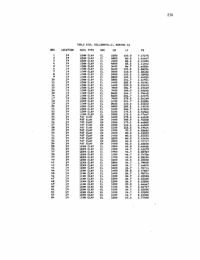
236
TABLE ElO, COLLINSVILLE, BORING C2
OBS LOCATION SOIL TYPE use CR LF FR
1 19 LEAN CLAY Cl 2200 160.0 7. 27273 2 19 LEAN CLAY Cl 4800 80.0 1.66667 3 19 LEAN CLAY Cl 2400 53.3 2.22083 4 19 LEAN CLAY Cl 4800 53.3 1.11042 5 19 LEAN CLAY Cl 5400 86.7 1.60556 6 19 LEAN CLAY Cl 5600 133.3 2.38036 7 19 LEAN CLAY Cl 5500 120.0 2.18182 8 19 LEAN CLAY CL 5900 133.3 2.25932 9 19 LEAN CLAY CL 5800 153.3 2.64310
10 19 LEAN CLAY Cl 5800 146.7 2.52931 11 19 LEAN CLAY Cl 6400 253.3 3.95781 12 19 LEAN CLAY Cl 6600 220.0 3.33333 13 19 LEAN CLAY Cl 7800 186.7 2.39359 14 19 LEAN CLAY CL 7400 180.0 2.43243 15 19 LEAN CLAY CL 8400 146.7 1.74643 16 19 LEAN CLAY Cl 8200 206.7 2.52073 17 19 LEAN CLAY CL 7400 173.3 2.34189 18 19 LEAN CLAY CL 5700 12'6. 7 - 2.22281 19 19 LEAN CLAY CL 5400 120.0 2.22222 20 19 LEAN CLAY CL 4800 153.3 3.19375 21 19 LEAN CLAY CL 3600 146.7 4.07500 22 19 LEAN CLAY Cl 3200 173.3 5.41562 23 19 LEAN CLAY CL 3000 173.3 5.77667 24 19 FAT CLAY CH 2600 173.3 6.66538 25 19 FAT CLAY CH 2600 180.0 6.92308 26 19 FAT CLAY CH 2000 173.3 8.66500 27 19 FAT CLAY CH 2000 133.3 6.66500 28 19 FAT CLAY CH 2100 113.3 5.39524 29 19 FAT CLAY CH 2300 93.3 4.05652 30 19 FAT CLAY CH 2400 80.0 3.33333 31 19 FAT CLAY CH 2400 80.0 3.33333 32 19 FAT CLAY CH 2200 80.0 3.63636 33 19 FAT CLAY CH 2200 60.0 2.72727 34 19 FAT CLAY CH 2400 60.0 2.50000 35 19 LEAN CLAY CL 2500 60.0 2.40000 36 19 LEAN CLAY Cl 2200 46.7 2.12273 37 19 LEAN CLAY CL 1900 46.7 2.45789 38 19 LEAN CLAY CL 1700 46.7 2. 74706 39 19 LEAN CLAY CL 1700 40.0 2.35294 40 19 LEAN CLAY CL 1500 33.3 2.22000 41 19 LEAN CLAY CL 1500 26.7 1.78000 42 19 LEAN CLAY CL 1600 26.7 1.66875 43 19 LEAN CLAY CL 1400 26.7 1.90714 44 19 LEAN CLAY CL 1400 33.3 2.37857 45 19 LEAN CLAY CL 1400 26.7 1. 90714 46 19 LEAN CLAY CL 1300 26.7 2.05385 47 19 LEAN CLAY CL 1200 26.7 2.22500 48 19 LEAN CLAY CL 1200 26.7 2.22500 49 19 LEAN CLAY CL 1200 20.0 1.66667 50 19 LEAN CLAY CL 1100 26.7 2.42727 51 19 LEAN CLAY Cl 1200 26.7 2.22500 52 19 LEAN CLAY CL 1200 26.7 2.22500 53 19 LEAN CLAY CL 1200 26.7 2.22500 54 19 LEAN CLAY Cl 1200 33.3 2.77500
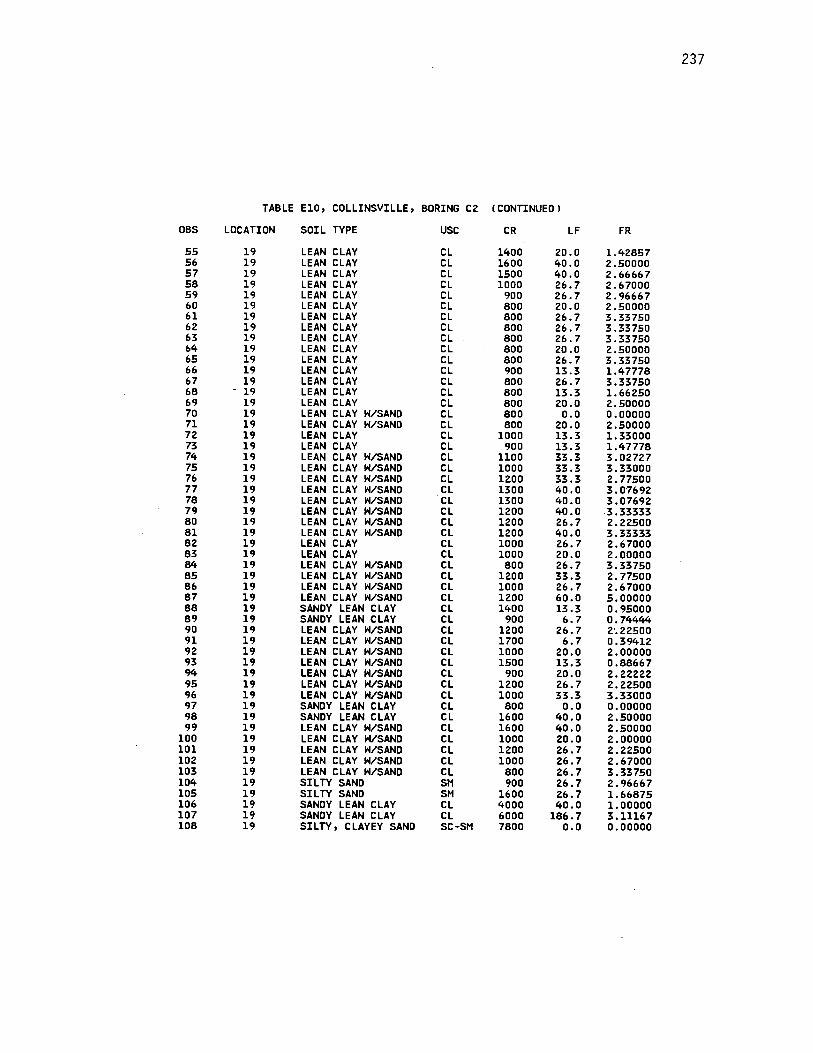
237
TABLE ElO, COLLINSVILLE, BORING CZ (CONTINUED l
OBS LOCATION SOIL TYPE USC CR LF FR
55 19 LEAN CLAY CL 1400 20.0 1.42857 56 19 LEAN CLAY CL 1600 40.0 2.50000 57 19 LEAN CLAY CL 1500 40.0 2.66667 58 19 LEAN CLAY CL 1000 26.7 2.67000 59 19 LEAN CLAY CL 900 26.7 2.96667 60 19 LEAN CLAY CL 800 20.0 2.50000 61 19 LEAN CLAY CL 800 26.7 3.33750 62 19 LEAN CLAY CL 800 26.7 3.33750 63 19 LEAN CLAY CL 800 26.7 3.33750 64 19 LEAN CLAY CL 800 20.0 2.50000 65 19 LEAN CLAY CL 800 26.7 3.33750 66 19 LEAN CLAY CL 900 13.3 1.47778 67 19 LEAN CLAY CL 800 26.7 3.33750 68 - 19 LEAN CLAY CL 800 13.3 1.66250 69 19 LEAN CLAY CL 800 20.0 2.50000 70 19 LEAN CLAY H/SAND CL 800 o.o 0.00000 71 19 LEAN CLAY H/SAND CL 800 20.0 2.50000 72 19 LEAN CLAY CL 1000 13.3 1.33000 73 19 LEAN CLAY CL 900 13.3 l.47778 74 19 LEAN CLAY H/SAND CL 1100 33.3 3.02727 75 19 LEAN CLAY H/SAND CL 1000 33.3 3.33000 76 19 LEAN CLAY H/SAND CL 12.00 33.3 2.77500 77 19 LEAN CLAY H/SAND CL 1300 40.0 3.07692 78 19 LEAN CLAY H/SAND CL 1300 40.0 3.07692 79 19 LEAN CLAY H/SAND CL 1200 40.0 -3.33333 80 19 LEAN CLAY H/SAND CL 1200 26.7 2.22500 81 19 LEAN CLAY H/SAND CL 1200 40.0 3.33333 82 19 LEAN CLAY CL 1000 26.7 2.67000 83 19 LEAN CLAY CL 1000 20.0 2.000DO 84 19 LEAN CLAY H/SAND CL 800 26.7 3.33750 85 19 LEAN CLAY H/SAND CL 1200 33.3 2.77500 86 19 LEAN CLAY H/SAND CL 1000 26.7 2.67000 87 19 LEAN CLAY H/SAND CL 1200 60.0 5.00000 88 19 SANDY LEAN CLAY CL 1400 13.3 0.95000 89 19 SANDY LEAN CLAY CL 900 6.7 0.74444 90 19 LEAN CLAY H/SAND CL 1200 26.7 2·. 22500 91 19 LEAN CLAY H/SAND CL 1700 6.7 0.39412 92 19 LEAN CLAY H/SAND CL 1000 20.0 2.00000 93 19 LEAN CLAY H/SAND CL 1500 13.3 0.88667 94 19 LEAN CLAY H/SAND CL 900 20.0 2.22222 95 19 LEAN CLAY H/SAND CL 1200 26.7 2.22500 96 19 LEAN CLAY H/SAND CL 1000 33.3 3.33000 97 19 SANDY LEAN CLAY CL 800 o.o 0.00000 98 19 SANDY LEAN CLAY CL 1600 40.0 2.50000 99 19 LEAN CLAY H/SAND CL 1600 40.0 2.50000
100 19 LEAN CLAY H/SAND CL 1000 20.0 2.00000 101 19 LEAN CLAY H/SAND CL 1200 26.7 2.22500 102 19 LEAN CLAY H/SAND CL 1000 26.7 2.67000 103 19 LEAN CLAY H/SAND CL 800 26.7 3.33750 104 19 SILTY SAND SM 900 26.7 2.96667 105 19 SILTY SAND SM 1600 26.7 1.66875 106 19 SANDY LEAN CLAY CL 4000 40.0 1.00000 107 19 SANDY LEAN CLAY CL 6000 186.7 3.11167 108 19 SILTY, CLAYEY SAND SC-SM 7800 o.o 0.00000

238
TABLE ElO, COLLINSVILLE, BORING C2 I CONTINUED I
OBS LOCATION SOIL TYPE USC CR LF FR
109 19 SILTY, CLAYEY SAND SC-SM 3600 60.0 1.66667 110 19 CLAYEY SAND SC 5200 33.3 0.64038 111 19 CLAYEY SAND SC 1600 6.7 0.41875 112 19 SANDY LEAN CLAY CL 1800 o.o 0.00000 113 19 SANDY LEAN CLAY CL 2000 0.0 0.00000 114 19 SANDY LEAN CLAY CL 2200 40.0 1.81818 115 19 LEAN CLAY H/SAND CL 2600 20.0 0.76923 116 19 LEAN CLAY H/SAND CL 2000 40.0 2.00000 117 19 SANDY LEAN CLAY CL 2000 40.0 2.00000 118 19 SANDY LEAN CLAY CL 1800 160.0 8.88889 119 19 SANDY SILTY CLAY CL-ML 2200 53.3 2.42273 120 19 SANDY SILTY CLAY CL-ML 3600 0.0 0.00000 121 19 SANDY SILTY CLAY CL-ML 5200 26.7 0.51346 122 19 SANDY SILTY CLAY CL-ML 8200 226.7 2.76463 123 19 SANDY SILTY CLAY CL-ML 4400 o.o 0.00000

239
TABLE Ell, BIXBY, BORING Bl
OBS LOCATION SOIL TYPE USC CR LF FR
1 16 LEAN CLAY CL 1800 0.0 0.0000 2 16 LEAN CLAY CL 6800 40.0 0.5882 3 16 LEAN CLAY CL 7000 66.7 0.9529 4 16 SANDY LEAN CLAY CL 6600 66.7 1.0106 5 16 SANDY LEAN CLAY CL 6000 66.7 1.1117 6 16 LEAN CLAY H/SAND. CL 5200 60.0 1.1538 7 16 LEAN CLAY H/SAND CL 4800 60.0 1.2500 8 16 SILTY CLAY H/ SAND ·CL-ML 4600 66.7 1.4500 9 16 SILTY CLAY H/SAND CL-ML 3900 40.0 1.0256
10 16 SILTY CLAY H/SAND CL-ML 3600 60.0 1.6667 11 16 SANDY SILT ML 3800 46.7 1.2289 12 16 SANDY SILT ML 2800 46.7 1.6679 13 16 SILTYCLAY H/SAND CL-ML 2600 46.7 1.7962 14 16 SILTY CLAY H/SAND CL-ML 2000 66.7 3.3350 15 16 SILTYCLAY H/SAND CL-ML 1600 73.3 4.5812 16 16 LEAN CLAY H/SAND CL 1200 26.7 2.2250 17 16 LEAN CLAY H/SAND CL 1200 6.7 0.5583 18 16 LEAN CLAY H/SAND CL 1400 80.0 5.7143 19 16 LEAN CLAY H/SAND CL 1600 86.7 5.4187 20 16 SANDY LEAN CLAY CL 400 46.7 11.6750 21 16 SANDY LEAN CLAY CL 400 53.3 13.3250 22 16 LEAN CLAY H/SAND CL 1200 53.3 4.4417 23 16 LEAN CLAY H/SAND CL 1200 40.0 3.3333 24 16 SANDY LEAN CLAY CL 1600 60.0 3.7500 25 16 SANDY LEAN CLAY CL lSOO 73.3 4.0722 26 16 SANDY LEAN CLAY CL 1800 60.0 3.3333 27 16 SANDY LEAN.CLAY CL 2100 .73.3 3.4905 28 16 SANDY LEAN CLAY CL 2200 66.7 3.0318 29 16 SANDY LEAN CLAY CL 2000 73.3 3.6650 30 16 SANDY LEAN CLAY CL 2000 66.7 3.3350 31 16 SANDY LEAN CLAY CL 1900 66.7 3.5105 32 16 SANDY LEAN CLAY CL 2100 73.3 3.4905 33 16 SANDY LEAN CLAY CL 2000 66.7 3.3350 34 16 SANDY LEAN CLAY CL 2000 60.0 3.0000 35 16 SANDY LEAN CLAY CL 1800 46.7 2.5944 36 16 SANDY LEAN CLAY CL 1500 40.0 2.6667 37 16 SANDY LEAN CLAY CL 1300 40.0 3.0769 38 16 SANDY LEAN CLAY CL 1000 33.3 3.3300 39 16 SANDY LEAN CLAY CL 1000 40.0 4.0000 40 16 SANDY LEAN CLAY CL 1000 26.7 2.6700 41 16 SANDY LEAN CLAY CL 1000 33.3 3.3300 42 16 SANDY LEAN CLAY CL 1200 33.3 2.7750 43 16 LEAN CLAY H/SAND CL 1200 33.3 2.7750 44 16 LEAN CLAY H/SAND CL 1300 26.7 2.0538 45 16 LEAN CLAY H/SAND CL 1200 26.7 2.2250 46 16 LEAN CLAY H/SAND CL 1200 26.7 2.2250 47 16 LEAN CLAY H/SAND CL 1000 46.7 4.6700 48 16 LEAN CLAY H/SAND CL 1000 66.7 6.6700 49 16 LEAN CLAY H/SAND CL 900 13.3 1.4778 50 16 LEAN CLAY H/SAND CL 1200 40.0 3.3333 51 16 LEAN CLAY H/SAND CL 1500 53.3 3.5533 52 16 SANDY LEAN CLAY CL 1100 33.3 3.0273 53 16 SANDY LEAN CLAY CL 1500 53.3 3.5533 54 16 SANDY SILTY CLAY CL-ML 1700 40.0 2.3529

240
TABLE Ell, BIXBY, BORING Bl ICONTINUEDJ
OBS LOCATION SOIL TYPE USC CR LF FR
55 16 SANDY SILTY CLAY CL-ML 1500 80.0 5.333 56 16 SANDY LEAN CLAY CL 1400 33.3 Z.379 57 16 SANDY LEAN CLAY CL 1600 46.7 Z.919 58 16 SANDY LEAN CLAY CL 1900 33.3 1.753 59 16 SANDY LEAN CLAY CL 1700 80.0 4.706 60 16 SANDY LEAN CLAY CL 1800 Zl3.3 11.850 61 16 SANDY LEAN CLAY CL 1600 Z66.7 16.669 6Z 16 SANDY LEAN CLAY CL 3ZOO 133.3 4.166 63 16 LEAN CLAY CL 1400 1733.3 1Z3.807
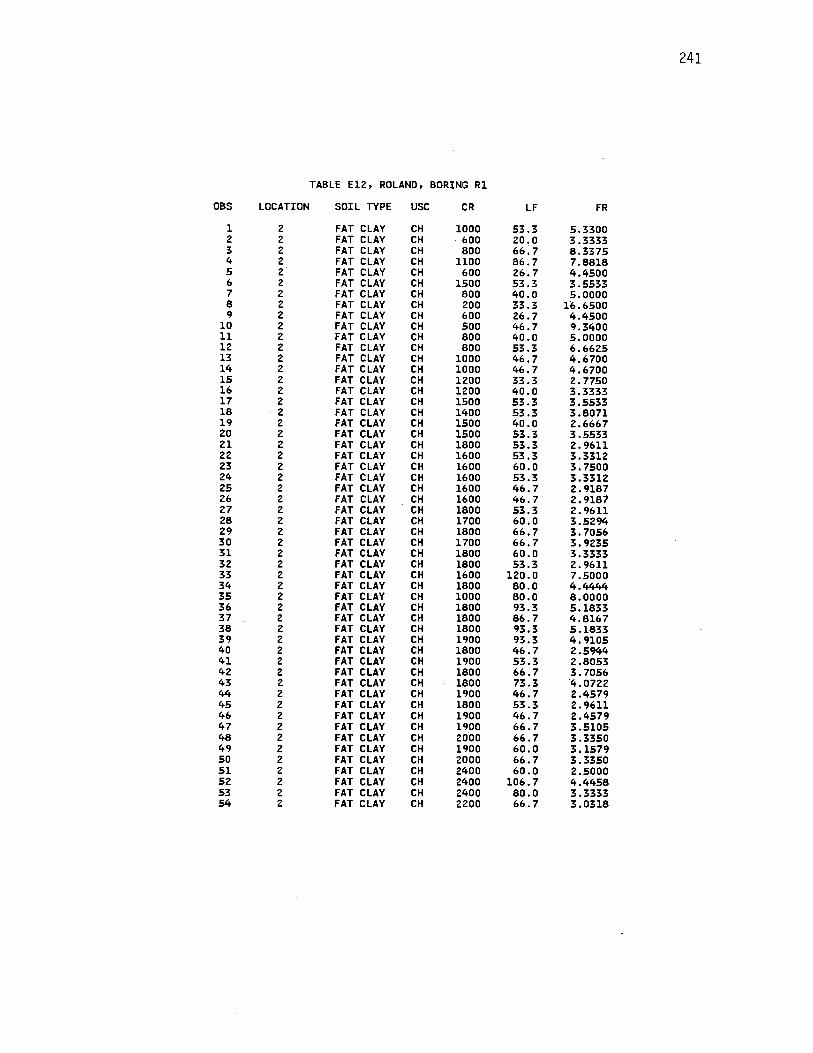
241
TABLE ElZ, ROLAND, BORING Rl
OBS LOCATION SOIL TYPE USC CR LF FR
1 z FAT CLAY CH 1000 53.3 5.3300 z z FAT CLAY CH 600 zo.o 3.3333 3 z FAT CLAY CH 800 66;7 8.3375 4 z FAT CLAY CH 1100 86.7 7.8818 5 z FAT CLAY CH 600 Z6.7 4.4500 6 z FAT CLAY CH 1500 53.3 3.5533 7 z FAT CLAY CH 800 40.0 5.0000 8 z FAT CLAY CH zoo 33.3 16.6500 9 z FAT CLAY CH 600 Z6.7 4.4500
10 z FAT CLAY CH 500 46.7 9.3400 11 z FAT CLAY CH 800 40.0 5.0000 lZ z FAT CLAY CH 800 53.3 6.66Z5 13 z FAT CLAY CH 1000 46.7 4.6700 14 z FAT CLAY CH 1000 46.7 4.6700 15 z FAT CLAY CH lZOO 33.3 Z.7750 16 z FAT CLAY CH lZOO 40.0 3.3333 17 z FAT CLAY CH 1500 53.3 3.5533 18 ·Z FAT CLAY CH 1400 53.3 3.8071 19 z FAT CLAY CH 1500 40.0 Z.6667 zo z FAT CLAY CH 1500 53.3 3.5533 Zl z FAT CLAY CH 1800 53.3 Z;96ll zz z FAT CLAY CH 1600 53.3 3.331Z Z3 z FAT CLAY CH 1600 60.0 3.7500 Z4 z FAT CLAY CH 1600 53.3 3.331Z ZS z FAT CLAY CH 1600 46.7 Z.9187 Z6 z FAT CLAY CH 1600 46.7 Z.9181 Z7 z FAT CLAY CH 1800 53.3 Z.9611 ZS z FAT CLAY CH 1700 60.0 3.5294 Z9 z FAT CLAY CH 1800 66.7 3.7056 30 z FAT CLAY CH 1700 66.7 3.9235 31 z FAT CLAY CH 1800 60.0 3.3333 3Z z FAT CLAY CH 1800 53.3 2.9611 33 2 FAT CLAY CH 1600 lZO.O 7.5000 34 z FAT CLAY CH 1800 80.0 4.4444 35 2 FAT CLAY CH 1000 80.0 8.0000 36 2 FAT CLAY CH 1800 93.3 5.1833 37 2 FAT CLAY CH 1800 86.7 4.8167 38 z FAT CLAY CH 1800 93.3 5.1833 39 2 FAT CLAY CH 1900 93.3 4.9105 40 z FAT CLAY CH 1800 46.7 2.5944 41 2 FAT CLAY CH 1900 53.3 Z.8053 4Z 2 FAT CLAY CH 1800 66.7 3.7056 43 z FAT CLAY CH 1800 73.3 4.0722 44 z FAT CLAY CH 1900 46.7 Z.4579 45 z FAT CLAY CH 1800 53.3 Z.9611 46 2 FAT CLAY CH 1900 46.7 2.4579 47 z FAT CLAY CH 1900 66.7 3.5105 48 z FAT CLAY CH 2000 66.7 3.3350 49 z FAT CLAY CH 1900 60.0 3.1579 50 2 FAT CLAY CH zooo 66.7 3.3350 51 z FAT CLAY CH 2400 60.0 Z.5000 52 z FAT CLAY CH 2400 106.7 4.4458 53 z FAT CLAY CH Z400 80.0 3.3333 54 z FAT CLAY CH zzoo 66.7 3.0318

242
TABLE El2, ROLAND, BORING Rl I CONTINUED l
OBS LOCATION SOIL TYPE USC CR LF FR
55 2 FAT CLAY CH 2400 93.3 3.8875 56 2 FAT CLAY CH 2500 93.3 3.7320 57 2 FAT CLAY CH 2200 66.7 3.0318 58 2 FAT CLAY CH 2200 80.0 3.6364 59 2 FAT CLAY CH 2300 80.0 3.4783 60 2 FAT CLAY CH 2400 73.3 3.0542 61 2 FAT CLAY CH 2400 100.0 4.1667 62 2 FAT CLAY CH 2200 80.0 3.6364 63 2 FAT CLAY CH 1900 93.3 4.9105 64 2 FAT CLAY CH 2000 66.7 3.3350 65 2 FAT CLAY· CH 1900 66.7 3.5105 66 2 FAT CLAY CH 1800 40.0 2.2222 67 2 FAT CLAY CH 1800 40.0 2.2222 68 2 FAT CLAY CH 1400 53.3 3.8071 69 2 FAT CLAY CH 1200 40.0 3.3333 70 2 FAT CLAY CH 1000 40.0 4.0000 71 2 FAT CLAY CH 1000 46.7 4.6700 72 2 FAT CLAY CH 1000 53.3 5.3300 73 2 FAT CLAY CH 800 60.0 7.5000 74 2 FAT CLAY CH 800 40.0 5.0000 75 2 FAT CLAY CH 600 53.3 8.8833 76 2 FAT CLAY CH 600 60.0 10.0000 77 2 FAT CLAY CH 600 53.3 8.8833 78 2 FAT CLAY CH 600 66.7 11.1167 79 2 FAT CLAY CH 800 53.3 6.6625 80 2 FAT CLAY CH 800 53.3 6.6625 81 2 FAT CLAY CH 1000 173.3 17.3300 82 2 FAT CLAY CH 1000 26.7 2.6700 83 2 FAT CLAY CH 2400 153.3 6.3875 84 2 FAT CLAY CH 3800 126.7 3.3342 85 2 FAT CLAY CH 3600 106.7 2. 9639 86 2 FAT CLAY CH 6600 160.0 2.4242 87 2 FAT CLAY CH 7200 186.7 2.5931 88 2 LEAN CLAY CL 7000 160.0 2.2857 89 2 LEAN CLAY CL 8000 293.3 3.6662 90 2 LEAN CLAY CL 10000 466.7 4.6670 91 2 LEAN CLAY CL 11400 200.0 1.7544
APPENDIX F
COMPARATIVE CPT DATA
243
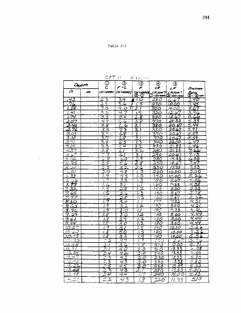
244
Table F-1
ro..-.._,I I
I/ , , i'i .'.< .')::. '. ~ ,·
a.pm © @ © @ c r- c.<- ~r- r;.,.c;,.,,
/'I. ,,,,,
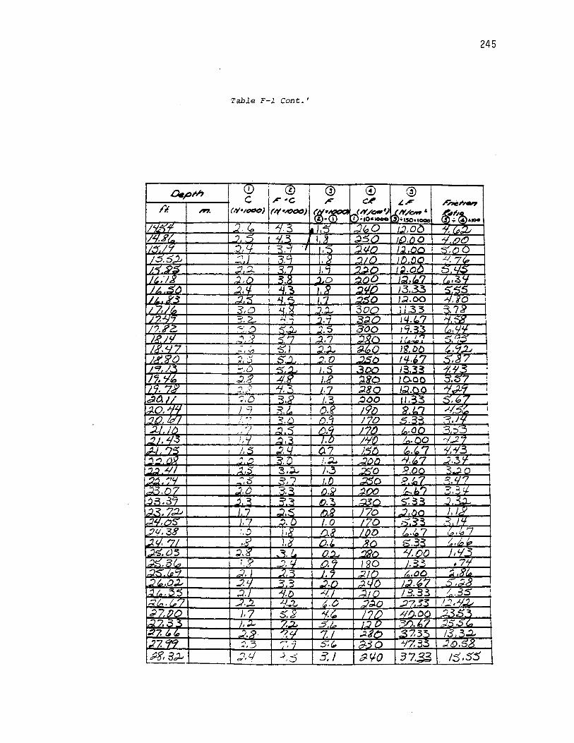
245
Table F-1 Cont. '
© @ C , .. c r ©
c-<-(1(•1#0) f/t•IOOO) (i •·.::ii::--•,_.
• I
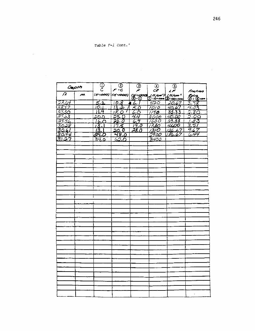
246
Table F-1 Cont.'
' (!.) © Q) © @ 0.pl'h c r•C r- c, ~r- r"nc;,,_, /'I. '"' (/'(•/«ID) f/t•ICJCO) ~:~ (N/-') .J.,l'f/ow' ~"'~ ri'>•10·- 3 ~150a1oao .. ,,._
;))?,/,,!./ ~.· . l~.8 t., I f:::JO ,.JQ,(;, 7 3-, '1,,S. 1~~7·7 J(). 13 • .i. J _4J(.Q /t?IO .l.//'"J, ~7 -v,o~
4 'j, ~"" l I ( IX{) I ln,f\ I J'f t!J ~;;:,3 ~ :J. iin c.¢7,,{,3 l~n.1) :;J~. D 8.l.j. . :J. ()l)ri J,//),11 j .:::i.oo ,.;2 '7. 'j/,,.. II. .n :;;i~.o ,.,,. '1 /600 ::J.'1.3. I ,t!f'-~ Bt"J,;J.J( J_ . l 17.'5 JC.,,O /,::<,,//) ,l./~f)O :=?.SI ~O.lol I=',. ~/') D .:li.n i.~10 J,:J/... L 7 9.t. 7 '; (),q"' 1...9 ... f') '""~ n '2t:JOO Ji'l-,k.7 (,..,'fJf :
1.:: 1.:J.? 31.J D (~,() 3~DO
I
! i
I
I I
I
I I
I
-....
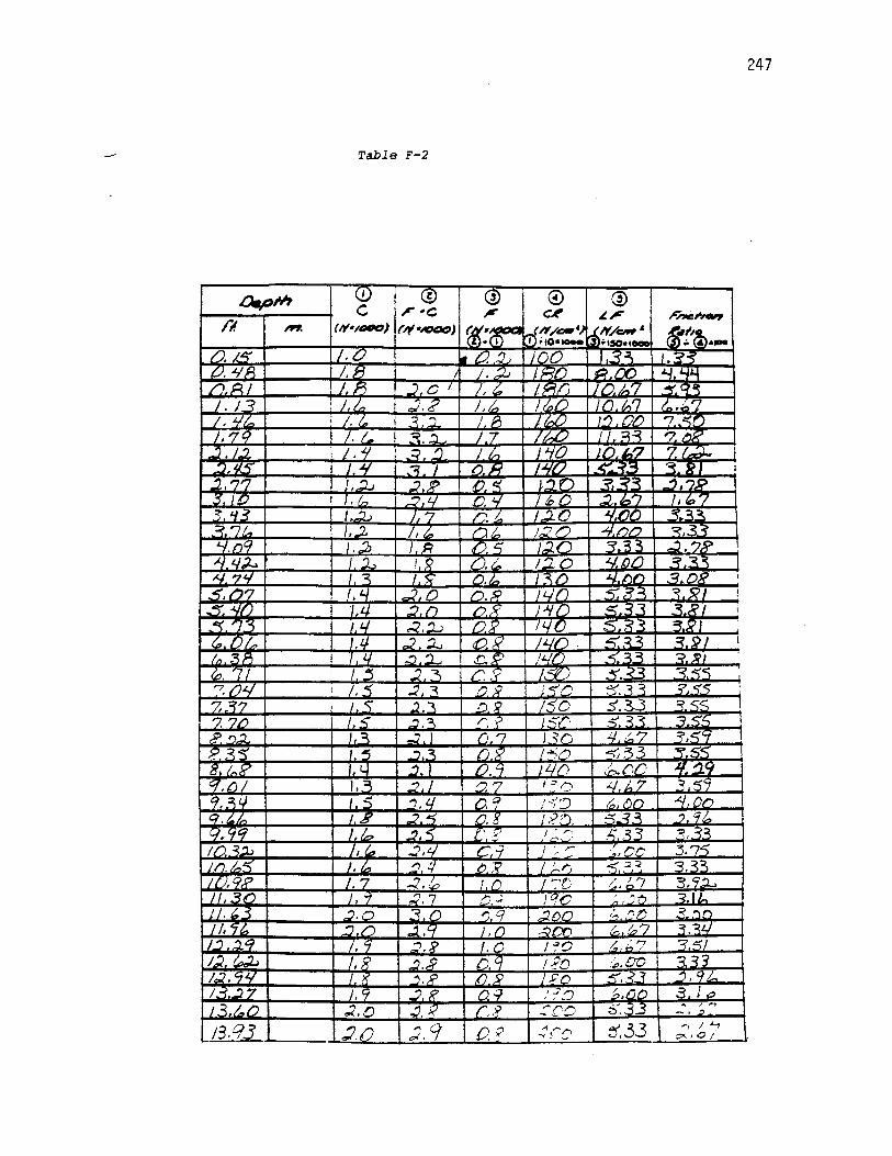
247
Table F-2
a.plh (.!) © @ © @ c , -c: ,ir C.t' ~, ,-,.;,.,, it! ,.,,. (1(•1t#IO) (/f•IOOO) ~ .. -..-. tN,/09•J .JiN/ow' ~,,~ .{i' ITT•t0•- .;.150 • .- .p , ....
/J, 14' /,(.) i. 0. ~, 100 3~ I.~ .. 0. -'lfi I ~ /, .2, HD .o_rn '-'· ~ /').~/ /, ~ - ,0 I /, t, ,'9111 "/" ,,1.,,7 ~.q•
I. J3 /,/,,, ,.,7, /? J, I '1.,n '/ ' ,,,7 (,...b' I, 1./1, I. I. .
'J J ~ . /.,/) '' nn ? .. ::)O I./_ ~."'I I or /1. .£./ I - .~ ~ "JX' /, '7' ..
~. 1:. /. I -=< ') /. ,_, ·O JJ) :a , ,.;;J-~.11..· I •I ~~ I /) .. /,,/,, r/ ~ .... .. '1! ;
..1, '7~ ·- J .:; J' "Ci -~n .. ~ ':I 'J " •I I,.
;'$ 10 J. /,., ~ IJ a~ "{) ~ .~ ~'7 I '
I' 7
~ ". I.~. I 'i /J, I. .:10 • (.J 'tJ ~~ - ~
.=?. '71 ... ,.1 j, "· r.l 1-. ,,.='!") ,,I. 1'1n ~ ... ".fJ"/ • -21 I .J I': 15 1- rJ ..3~ _:') I I " , 1./- .... ~" ! ) I' .~ 1:. 0 , 'n/J 3_•
"' ~L/ -: c. .~ .. : r.. . L'r .::-..o I
~. /')'J • L. 1'J .ri,R !..., ,. ..., ; :, -:; ~ ! --_ .. .c, 'l u .:'. ("l /"'_ ~- J "I 5. -: ~ i
.c, ,. _"j L ,.:) . ., ' r, ~ 14t.,; ~.;• ::; s ,,. I '/,,, .~ ,;) :i... tr. R JL/O. ~ - : I I
"' ::: p, ' _.., ') r"~ ~ /L/rJ < - : ':: 'I
jl:i, , 7/ I I .'._) 2~ /". ;' /::::'j' I _"';',<· -:; .~ I"\
'7,/ 7"/ /, c .:( ~ ,I') 'it i.50 '"5. -~ . - ~ ~.., '
7,.1'7 .s .:2 ' ri R 150 s.3.3 =i' SS 1 7. 7LJ .:: :J. - r< 5C" ::::. ~ <: 3. <:;"'-.
,p_~ ; _:; /" '7 J ~{) l.J. ~7 ·.~...,
8. ,)• • _., ~ f '>i {.a)("') ~~~ -=~s....,
" -I> I ,.,7 I.«.. _j L.' JL/{) .~(",/) " . , ~q c .{J/ I• :1 .:2, I a.'/ ' .:> t:i ..:./ J..7 ~ :'7 I>, .3 ( t <:i ~.4 • .,, Q !1'D t:.. Ar .. , /t/'i
(~. L . .K .2 .., D, ~ :??1 . ..::: <::. ...:.' '1 t,,. C!.9"1 I./.... .:J .... l' y I . r-,
~ .· ,J; .~: ~'' :; ~~
/rJ.· ~~ ,,,.,, ~,. J c-~ ' . ,... I ~ :,.,OC 3,1.r::,
1n.1. .ii:\' I, ~., ::::> ·' n~ }-. lj < =<=< 3.~ ... /{),• N? ~, ..:; , '..., I f / '":'C /., t,. '7 3.'1."1
I • • ' I') •, 1 .., IJ . .J ''fO ;, . , ;") 3. '-«•
J /. "~ .:;. CJ .:1 r'J 'l.' ~r\rJ ,;.,, l".1') < .')f'l
/, ~ t. ...,,/') ,.j .'-I , /l --1,;Cf) (,.. 1,..,'7 3,"::J.U ) . , . ~q ', 17 ~. '"' ' /, c. I '?0 ~ J.7 -:z. :=I 1:. &,..b ' ..!) • r: ' 1-?o ~.00 ::?. _=1 , 1.:. .~"'! . ~. ;;> /, ~J I /i'O :"'(, <1 ~. 9/_ I: ~7 ' .:J . .,, I ,J /-?'O ~.l"JtJ .3 lo
~. ;( I' ' .:c~ ;S~ ~ 3 ... , 13.1-0 .).. CJ .. ~' ~
_13,q3 :l.IJ ~.9 OP .-( (,,,....r'I ~.33 -, I ,_,
...... - 0<10 /
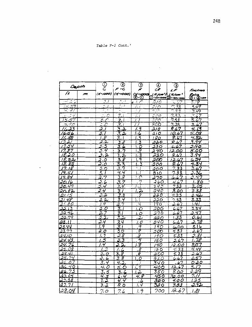
Table F-2 Cont. '
© @ c ,. .. c r-<N•1M10J f/f•IOOO)
. _".', J
,, I
~ -_, ....... :;
248
© CA'

249
Table F-2 Cont.
a.p;h i (!) © @ © @ c ,r -c ;r c~ ~, .rnie;,.,, /I. '"' (,/(•/MIO) (/f•IOCO) ff·-- (N/o'•) .S,N/orr" ~,,,~ ·CD n.:1o•iooo •150•1000 .;. ,._
'_"l.237 S-:.2.. ""' /.,., .3.ID 5d.o :1</.~0 .q.12 "'J9_t{,'t ,,/ i?.O 1t~.o /,.,/() 10~.~? J' ~ ,s: ~7 .29, ,#'),:/_ f'), S' "1, '/ //. 0 ~80 n3.~3 /,;;. I o'f :l'i, '3</ 1-R. {) 3r.f.O s.O /JUu; 3.:5.,<~ /,5.:5 ,), ?. 1,,9 3<1. (J 41.C::,{) ~"aCJ 30.CJ/ .1./0 D ~:£,_,") 1-/000
:
I
! ;
I
I !
I
I I I
._ __ -
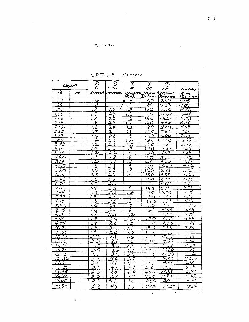
250
Table F-3
I (.!) © @ © @ .a.p;n c , .. c , c~ ~, -'ne~,.,, ti. '"" (/(•/«JO) f/(•IOOO) f«:~ .<N/-') .J.,N/0#' ~{'@.,.. i -m 11•10•-o " ~150•1000
,;~5 '·~ 1111 • l.f lnO 2. fr, 7 ~q.s
,.R9 ~ J J. 1~0 7.3.3 4.o? I ,-=i I I.: 2.:l I I<. 1~0 /t'J,00 ~Sl. J :'\3 /, 7 ~.~ 1.l- 170 l/0.<;'..7 ...; . .;.p J. 91- - ) J' 3.: /, t,, I~ "O , .... 1~? 5'. ~ ~ :; 1'7 ' .::!.' I..., n >O '1:33 :-=\', J, .:2. S-2 I. )
~-" I •1, I ~0 rl.DO Jo/., 'l'I -'.R5 /, 7 3 I 17D ? . .?.3 41.~~J ;
~ /7 , {,,, .:;, ~ ' I ~0 1...00 3.75 < 'i'O /, :i, ~ I.~ ... 1;;i.o 9,0u <~.~7 3 ?3 !. , ~.l ! '.'J )~0
~ ,/ .' -s.:=5 r... .. , ,, ... '4 It,.,, I." ~. {.
,.., I t./ 0 I . , * .I , <" I
~ °")( ....... ~,1.Jq /, ;JJ :i. ,;J.I .7 I .:JD "-/.~? -:r.8' 1-/.9-:J., '. I J. l ,g I\ 0 <:;"33 -4.8'"' ~.14 '.~ '· '. ,\( l..:l (') .:;-.3 3 -~.i./~ ' <:,1../7 ·-~ ~ • Cj 1~0 -~ae .i..J I .
. '"" J.J !
.:z. ~/'l .s ..., 3 .8 \SO S:33 :=? .55 i
... · '-~ I. '!5 :<.<I "'.) !5(") ~.33 l~,lAla ,..,.c./(,., /. s :<3 .9 !5C !...co ,...; .:>O I
,,.,,7R I J. <::' _J,0 ! ,,
'. --: '._) 4.1:,7 _--:•/I
7.11 '/,~ .:2.3 ,,;., I tJ () 5.33 ? .. ~ l ' "7, l./t/ I I ~ .:';,() ).;).J l~O ~ OQ -~ .5 '
'7.77 J. 3 ,,j ! ,...
1~0 - =' '::"· ,,..,_JC r'\' '":::i. ;,.....,..
<.:?,I?'! /,3 ...;i,5 ·:J !'SO : .; .. -=: ,.!./,/D -~. f../ ';L /. t.- ~.4 ,7 I!,,., 0 . I . -· ~. :j,, -'·'JS' /, / ,2,!/ .8 't-0 :" .. -~~ 3 . .=?3
' Dl? I. ~ - --·.::::> ·'· :;._, ·".':"' ,-:i,.:; b ..:./.Lf'f
c ,1./1 /_ ' -"· i&> /, 1 1RO -'I~ ,j 0 -4, l../l/ c;, ?I./ /_)' .1, 0 I ;i.., I.; ..) ·/_oo .:..: :.; lJ
10,/JI'.. I. ~ .::• I I I .;:; :J ,....,3~ 7 Sl-/D.3'7 /.? 3,D I. /,.., I .
., ID.~~' .·-·.:.:::.·
·-'' ·- -
//)_ h"J ,2,Q 3.1 ), IA :co 10.b 7 0::3 'f J /. ;i< ~.D 3.1- J.~ 'JOO l{).~7 ·::'.~I.) I/. ~~ ··l ~
:~.I.~ /. 7 ~ . \ . ., ~.::. · .. ·.35 -- ~? -. , ...._
I ,, I ..J,O 3.1... _.., I ·: -~ 0 ll.f. ~o -,!)0 -, . • D~ I ...
3 '- "J. 0 - 1.-5 -~ 3 -~_:,_ --. . , . ,.~/A J, c; ~o "'.0 1 ,.; '.J 1:;, ~ 3 ,...,, ~ ~.J
I 'i, .~ 9 '· I ~,/ "' " - /3.33 :~,~~ ..... .,,...- - -. ~. ,,..,., -' J -"I /, 7 ~10 ... ~, ;,') (o.03
J ~.-~~ ) . /) - .., /') ..:;, 0 .:i 6 0 /d .. ~3 (D.I.? 13.t:.'7 ..:::.o ?', 9 /. 7 ~00 //. 3 .5 :5.~7 /'-/. 00 ;?. 0 ~.D I.~ ::J (J 0 /~.C> () ~ • .'Jo
JL./. 3 3 . .,?, .3 L/.{) /. (,, :'....30 1.:i . .,;, 7 '"l~et

251
Table F-3 Cont.'
CWp;h i ' (!) @ @ © @ c _r .. c ,,,,: c.e .t.F ,r,,.c;,,.,, /I. ,,,,, (/(•ttJOO) fl(•IQCC)
~--- (h/ow') ~IY/ow" ~,,,~ .(j) m.:10•-o 3 .; 150• •0CIO .;. ,._ IL/./.. I~ .2, 3 • '/-. I /. l.11 ..230 !Oln7 "'!, ~· I IL/. ...J-J ;i . .1 ' 3.1? J.i,, ..,;>~O !(),/,..,~ J..{,47£
/5.31 .:;, I I 3.7 J. 7 :JI 0 I/ . .3 '3 I _.::;,' l ~.>! ')/) < ,_ /.8 ~QO /,:;l/11"'1 · ... 4 (1
1~.:17 /,CJ "2 /_ /,.., ICfD //, 33 6, ~' /1-.::: 0 _,,,3 -;ij 1 J, '] ;l.c3 0 //.~';I,. "f I '
,; _:, /ti. /, .. ~ ,: 140 "' ~ /, ' -.:2~0 12.~7 J.. .~ .. , //,.,. 'f/,,..
: I =' J./. Cj ~. "J80 /'l.N"I ~ .oo :
/7 ::29 ~y LJ,., J. 'I ~J-6 9. 3~ :~.? ;c
1/7./,/ .:..7 '4.,51 /,1. ;J?D >?.,J(") .::<. 'fb /?, Ot/ 0 <.LJ. }, ~ 300 '.'?. t. '7 ,.,..,11·1
k£_.-"' I 3.D - ., --~I .300 /'i.{)0 -':I'.~· .!!.;.-- ::-,,-J
·,:, .. ~/) ~ '1 S.i, .:J,J :;qo JL/.()0 '-f.~ :5 JR, 'l~ 2.8 "'1,9 I, <, .;;.20 10.00 3.S7 / 'i . ., "' ~.i -i.J~ '·:;... ,;J.70 ~Ji{) ,;; 'it.. ' I 'i. <5) ;J,? .1../,1., /, ~ ;J. 7() 9,t,7 .:5..;L/ !
1'7. 9/ ~.~ ~..., /, ~ ~50 R.b7 :5. ''7 !
-:.in,).<./ J,R R.-l ),;) 1;;' 0 .~.Q{) ':'-,' I•./
- ~ _c(t.. I, ti .:J. 7 .~ ! ; J ,") 5 .. 3~ ·:s. '(!I I
-' ,'] >?'7 I .', ~ ...... ~ I '1 ; '\ · ... '..., -· ,:;) 7 ..:l /, 'l ') ' 15 _JI:;; /, I I .,,- ."I
'-' -~ ... ~.,.., ~ .4/. (!{/ I
_J/ ~,:; i /5 ~.r.J .s ./--_?; "'"'1 .· - ~.;;i.:;i... : ~1.J?R J, /.,, ") '7 • <:;' ; .,_.,.i - -- ,;(.OJ I . ' -~ • ..'.)!') --1. ~ ~.R a ' ., , , ;}, 1,,J I
' . .... .,, ~ J
..:J;)., 53 I. 7 :J,t./ .7 ; ·'I .. -, . .,.(,.'il,o I ....,., , .>I ·~ !, 7 .::J.~ .7 ;J ',,., .;;. . 'f~ -t /!" /
,;:.,~ l'i /. ~ 3.~ l,O ! .? ~ ' ,_, ~.17 .~lc.L!I ·
.:J~ 5.~ 1.3 ::J, 0 3 130 ;), :JD J.ts'i :J~.~5 I. J' 3.-~ • i.J 180 j_,/,..,? I. 4~ ldq/7 I.&, 1.9 '" lbO :;', ~ ~ -'Di?
_..,<-/. _..,-0 I.I I 5 .::; un -~ ~-~ .3.L>-3 ~
(.j .R ~ J, I./ !5? ·" 140 "{, {:.'"} .._'";. ~ (.j. --'<,IL. !. 'j ~. t./ 7 / 'jlJ .I../.!...') :.:.:.fl. :;z -") '-' q ~-~ ..=.7 ,.J, (/. ;ca ){,;,.00 ·\.CC :2""".x1 /, 7 '·" ..; l?D ;;).t..7 J,57 ~t:.. It/ ::.'. r.,t "/..$? ), 0 :)'In /_,~7 .. -:;,r.W .:u .... i./7 .9.R '-!.~ I. 5 380 l."'i, QD ..:.'4~ i,.,,~.f?{) .3" 4 . .; I. I../ 340 q,3_~ ~.7tl ~7.IS 3 s: 3 s. 7 380 :;;r.;._,:~ (o.4'1 ~ 7, 'l.5 3_, 5'.;J... .:;. ::L 3S'D /.!../,/,.,? -<:. 8(.o _,~ ,....,,;? .:..: ~ Si.n !.... " ""/'3CJ .J:/..:../, JO •:!:.~ 3
l-'R. !J 10.~ J 'J. Tj. 4/,0 10;).0 ::(~. ~7 "1. ~I
-c~g I 't''./ /~.'/ / 1. 0 d.0 !dl <./ tJ ·.:< ~:;. I "8 -. u,._;~ • I _,

.Qe,ol'h
/'I. '"" ~J".'Y7 :.. 'I. tJ'i ~a,l/:L
,:,"l."75 F:ll, /JO
tf) .4// 7•'J' ~ 'O. •
.: I )1.1.i
• I. 3' 31.7.!L 3~.l"J<. 3,j 3~ .'3:1. '70 5'~. DS 3~ 3b
~
I Table F-3 Cont.
i (!) © c ,. -c ( 1'(•1tHH:J) f/t•IOOO)
~11.D ~~.o i~9.0 ai. o .~/.[) R3.ll
i I&,,/) .;Jj, CJ i 1.;l,1' I 3,t'J
ln,11 /~, i ~./> /().~
I IP. ' ,~ ~ao 1~.t., '::T,7,; ~.1. l~.:z.,
I c!),}, I 4/. "l
ID.'~ 1-'··~ J~.·" -yq.n ~-,., ....//, () :JR. f\ ~1.0
I
I
0 r
~·Mll'2'll l .(j)
~.o t.., l'l I. I' t., ' :'(, }
q., .!J, .!. 3,~7
3.t.,' _"),.:.. 1 ... 4. I~.()
13.n
252
© @ c-<- ~r r-ne;,.,,
fN/-') ~NA:-' ~t'& .... i1•10•-o 3 •t50•10C0 -~f'J('J I~ 3.3 1')1., 7
~,00 'ID.tln /. _;;,;
3/tJO l../-7 ~.--,-/,.. :J (J J../~ s~ J,) 3 1.-:.;.Ja 3~. /.7 .3.~
,.,, ')('.) h:::::.33 JO.R~
-<a~ J'/,t,7 .:;,• ;'.,3 J~!J. a ~$.~ ~ ..:1.' /Jr' :
I~ ti() ~.~? I·• .3 'SIU I) /~.t>O }, . a
N'J 5}(') N<l.tJO .J/.07 JcJ(/0 ,0/ tf] 9:1!~
1"1.t.10 ~1-.1,.? l...'i~ ' ~JltJO
.:J3otJ I
! i
' I
I
'
l I

253
Table F-4
.:.PT !Z
© © c..e c
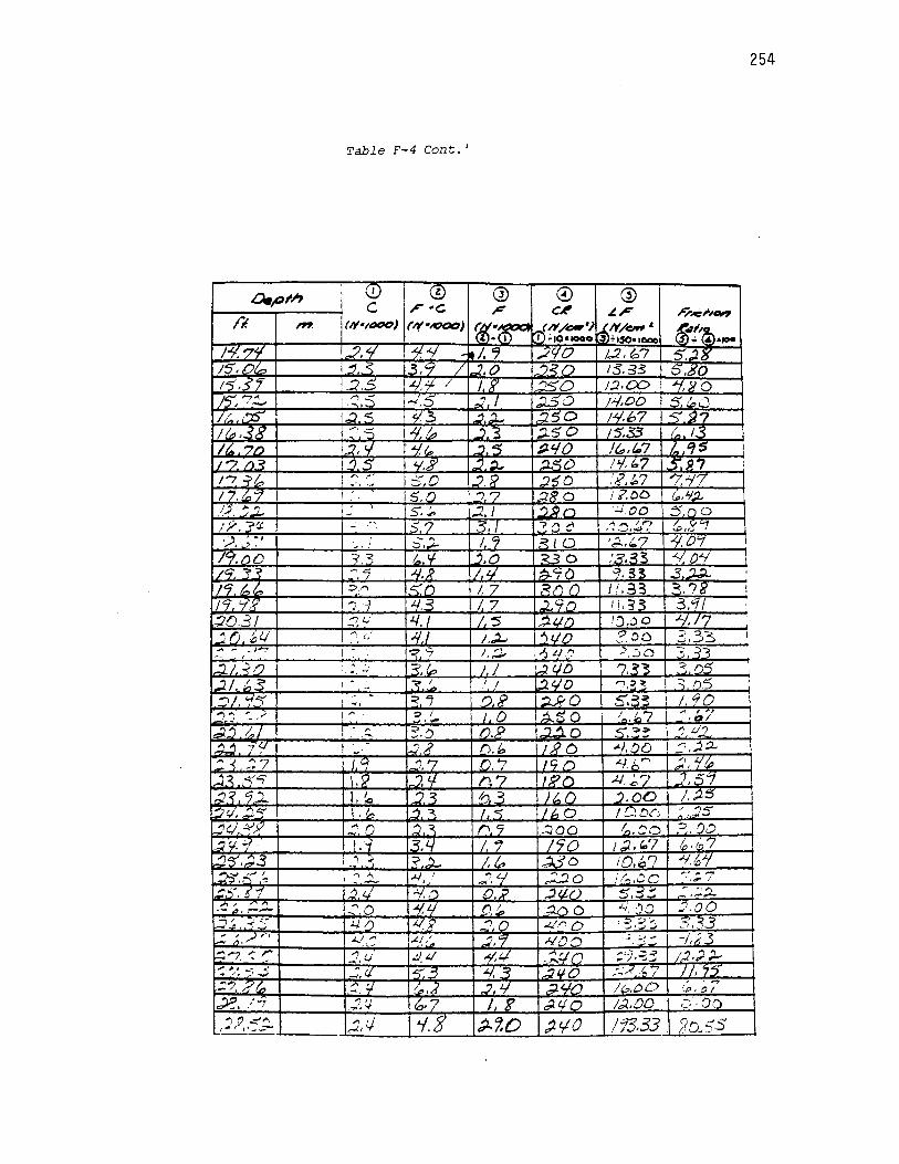
254
Table F-4 Cont.'
0.plh (!) © 0 © @ c .r-c .!=" c~ ~F "~''°"' ii. /n. (1(•1«'0) (/f•IOCO) ar:."~ (/t/-·) rJiN/ow' ~"'~ -m 1J;1o•iooo ~ •t50•1000 .. ,._
Fl. 7·',f -2.~ ~ "-! r .,.;, '7 ,,:.;c.;o /..2.(:;? 5'.:i }5 15', n,~ I~.<) 3. '1' / u.o '?<O 1;5. :B 5.lfO 15',?"' :J . .5 ..£1,Jf / I g' 'J.::::Q ;:i.co >(, >! 0 /5', "7~ i:~ 5 -".5 ,,: I ~Q !;./,OD s:.:::.u I/,, ,.,.., .:JS ~3 -1.i ;;zso /.</.67 .::; 'X7 11~ • .sg :' -s .L/, ~ -' 3 :;.50 15',$3
, 13 1~
It. 7n 2,<./ "i l. ., "5 ::;J.'/ 0 /(,,,,~7 tn qs 17. !"I~ :J5 "/,,,$" .2i !l..t:<O /J./, (:.7 5.~7 :
/'7 .:;>/,., ,... ,...
5,0 I./. 2 ;)$0 .'P..!o7 '7.77 .. ·. -I 7.t,.,"1 I IS'J) ~7 ::iR 0 !?.DO (,,.'-!~ P. ,.. 1.. ... s.~ .:2. I "')$:; ("") ·:.J.oo 5no /?. -:S<t - " :5 7 3. J '7 ,., ,..\ ........ f""\. I r'J ~,,~'-'! .._, - '° ~ .__,I..:.) I
·;>, . ; ~ 1 f ~.J.. I 9 ,;;;;;e,10 '~,,? ~0'1
J •I
I'-!. /lO ':?, 3 t.. c j,Q <30 .'3.35 -4./. 041 /C.,". ~ ~7 ,!./,}' /,i/ !. 'i 0 q, 33 3 '1.!l ' /7 /,...,~ .:;>/') l<o /, 7 -;!,{) 0 / 1,33 3."18 !
17. ';<',\ ") ~1 lf.3 I. 7 - .'10 I/, 33 3.'11 ' l~0.31 ~I .. : 4. J I "5 .~ .{j(J ':).;) 0 ,;_;,17 ~f) o!.I :1. l/ 4.1 J.,:J... -')l./D ?oo 3.33. I
.... r ..... }~ I l"Z 9 /,;;., ~ /./,':' -' . .)O :;: ~~ . , '. . . ::u. ~/) ' ... " ~. &,, JI I~ f./D ?.5~ < ()<:) · . .,·, '"'f'
:J/. £3 I " ... .<\ .'... / J l.!lJ./0 h/S3 :; n.5 -i/ 4-')
~ - =s ~ (),;? ~o S.33 /,Cf() 1 I .,,
.-;i~ ~- /~ .... - :>. (.. I 0 ~.50 )~.t,,7 " I . ,Q/ ' dj.~ ~/
,.. :'.~ D.R ~o S'. -;..;. .., t./j --- . -
~ i<f - id2 n.b 'J? () -<l,()O .., ,;i:;... ~
~ ~ ~7 I '1 .7 0.7 /9 0 "-/.;.., r-, ~,'/~ _)_~ .. ~'7 U? "l, 1./- /"), 7 /XJ()
;}.../ , ,...., ·<::> / .J, 5'1
;j':{ '7'1 I. lo 2. ~ t13 )t,0 _j.00 /.~5
2c/, ~""' 1.~ ..., ~ I ")' /{,0 I C:D<! :: , .. :15 ..:cJ. 4-'x _~. r j ~ ri. 7 ~00 I,,, ~O ::;>. ')D
l~r./. --1 '.1 3.4 /. ., 170 Id.., C..? fa,07 -~s'.~3 -'\ ;i <~ /{., ~5D 10."'7 -'l.~71 ~--<;
,.., A
""· ,
~"'.9' ;::.:;;. 0 //.-..,CC ,_. .., ....,
-·~ ·'·e' I
,~,.:.,-, t "1 21./ ""I.,') 0.9 .;lU.O 5.:S~ ~ ,~:;._ ,.,.. I "
~,O ..I./. L.j tJ to ~(') 0 "-1, JQ J.oo ... -~ .. -,-~ .. ~ .( •-:- ,!./. /) ~9 _"'l {) -</"".(> ; ::.> :;> ., 3,~3 ....J '-' _,
::. -~',.,..; ,., ""'1.(; ..:~ :~ .), '7 ,t../{)Q ; :, ... .,. -/,!J .3 . ._:._
~ '/. -: r. ,., ' . ....,/,:...;. .!.!,ti -'/,ti _;...c;o :.'} .~:; /J,))..., -:: ":-: ':i ..j .]. ct .:(.3 4.3 ~"fO :->< -·~ 7 I/, 76>
.:?. ?,(,,, ::. :,t 1,,.,d ~. l.f ,.;2 '10 /&.DO .......
i'.p' !) I
~. /-: ~~~ 0.7 /, F ,;.. <I() /;J..OD ,; . On
(-:J /', ."5:;. .... ;J., i./ 'l.Z :)..'J.0 )t./0 /1333 l0~5S
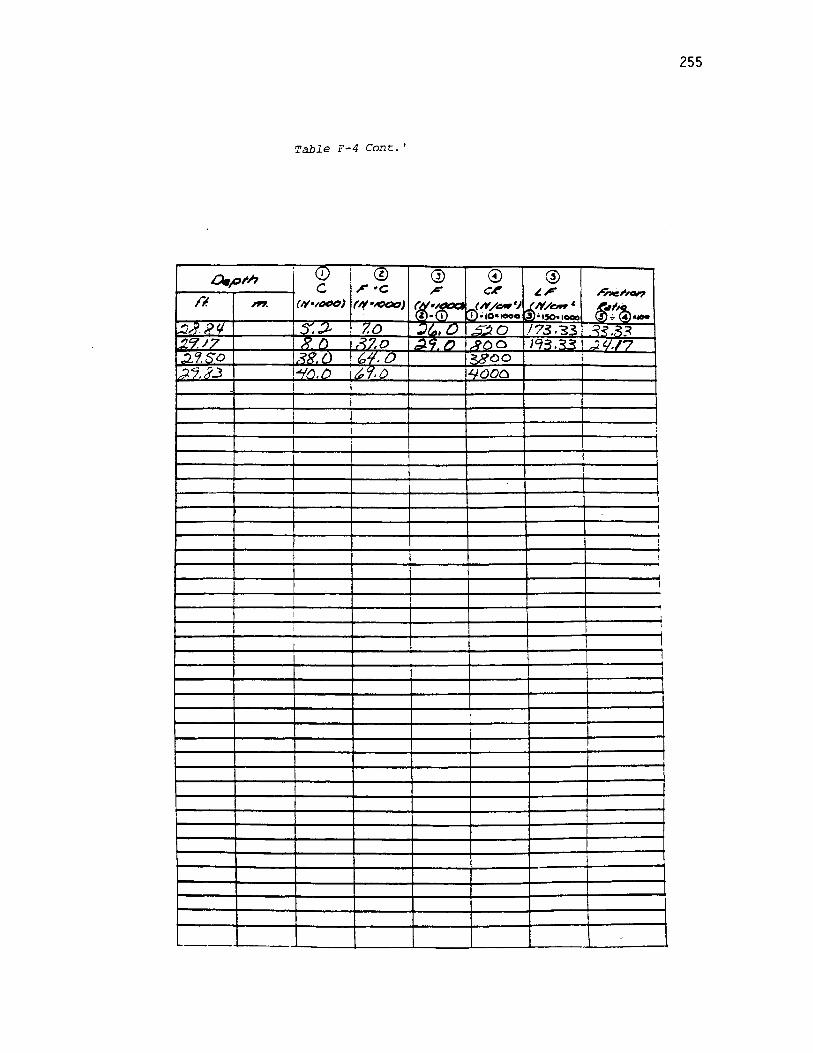
255
Table F-4 Cont. '
: (!) © @ © @ LA.p;.h c ;-c , C.<' ~, ,.:;._.c;,°'7 /"I. '"" (/(•/"°°) (/(•/COO) f«·-- (N/&1W') ~N/ow' (~t'~.'" -ti'I ri'i.;.10•-o 3 ••50•1000
.::; /f, R 'I :5'.:;., 7.o :J~. ?J 5.20 /73 .3~ ::.·~ .,• 3 "'/~17 l? f) r~ ~o ,:J.Cf. /') ~CJO 193.~':<! ~ '/,,•7 ~ '1. so .~R.f) 6" 'E, 0 ~00
..'.:27,J'-3 i~().IJ /j, ff.() 14()00 I
:
I
i I
' !
'
I
I I
i '
l I
-~

256
Table F-5
-. ,o T / 4·- ~'\/:'a. .. "i ~ ... r~ .-·.· , ...
: (!) © @ © @ a.,01h c ,. -c r CA' .t.F ;nit:;,.,, /I. '"" (/(•/t>OO) ft;•IOCJO) r«.·~ (N/t:M•) rf>N/ow' ~,,,~ 1.-m i)•10·- ••50•1000
.;. , __ _ :•(':l., I. '1 :2,0 11 0.$! !'10 S.~:5 :;i., ti I • J;l.. ~-~ ~.'I , -' Cl ::J.30 13. ~ ~ .:5 ,,)!0 I I J? .J.D "J..2 I :J ld00 .!4.00 7,00 /.~/ i /, 7 < ....., -. I !
,J'1 '-' I '7 0 )~,DD q "'-/I ) £'4/ ' 1, 7 ~g .:; ..,
'_; , ,., 0 /5:,3~ 4,at. . 17 /, 5 3,, :J,3 J '5 0 /5 ~'t, //). '2 z:.
J .-<o J,'-/ 3. ·1 ~. 14V ,, .oo }(), () (:)
~ .5?.:L I _, ~ '5' i, ...,
I~() l .s.3 •• 'I'! : I
~ :.c:: I~ 3.~ -7 ! '.' ') 1;' '53 a. L/'I • ::;>. J_J ::! 1,3 ~o . "' ·- ..... :o.~7 ~7 ;J_/
~ -~' I, 3 3.0 . : 'or.'.:.:; :-;;},00 ...., ..:2~ ..
.L.:. '~I /. ~ .., q ! r, ; ... 'l I ' -5 .:s > '/:;l-.<./, 4'7 I 3 3.J / . - ) ::J.00 ~ . .;.3 .. "'/.77 I, '7 -.;;,4 0 PO /:1.00 7. or.,., :') /~ I. _;. ~.4 ' ,,, ''..-.0 JO. ~·J (,,,.fo7 I
.-r: 45 /, .t:: -~.3 .+ I -·~ -""\ '~.~3 /,,, :;;~ !
5.7.R I, -5 3. 14 ... ''! '7-33 /,,, 22... ' 1:....11 I ~ ~.Q '. 'l. ) J...:J p (]0 5,00 ·~.~..'.._~ I, ~ :3. 0 . I ) t.. 0 ,....,,~3 ,1...J 5c I
I I .... J .o '.' -... ',' ~· - ~ . ~ ,,- I-~ ,,.., ·'"" ..
,., ') -1 'I,;;;., "J,3 .(1 /_ I:;() '·.'.'JO ~ .3'3 ' "':-: .ii 1 ' ' . .:../ "'l,4 !!'), '7 I LJ ,.-.._ N,(...7 --· :, I../ : ?.
__ ,~ I I, 7 .:>. ~ ().7 ''~· ;./. ,;.7 _'1,7:5 I
;: ,, 7 J, '7 ~.4 0,'; ... --. ; _5 ~,,7
'? .J./D I 9 1..1 • .::; !.~ ' -: 0 ::',JO ,J._ '· i../ :./ >< 7::r J,Jl "1 I /.I
,., "J ':J ·~ ;..,. :;'7 --·~ - • ..J ~
7. {)(,,, l, R 3.0 /,I . ".'..-; -: 3~ -/.0'? -1 .• ~7 J q 3.() /.D ! _, ') IA.b7 3,-:)J q,7/ 1.R ~.°I !J,5( I "; (' a- .,jJ.; :; 7 i. ..... '-' ...J
//) ,/)J.f ~.o ~.o /1;7 ,,.·, .•. ,~) I • ' ' I. ~' : . 3 cf
If;', 37 :: I ~."j /J.9 'JI r; 5,33 ':!' -;'(/ 1n "7-~ ' -~
.] I ~ .17 rJ. '7 ~I~> -?'-~'/ "" ,.., //
"""""'~---I I."'<. -:J () .!>',.: Q,"j -. ~ " !,.,.CJO -;.~U -! I. ~"°
.., ., ..., :.. ,.., '7 ' .... ' ' ,. -1c"- -· .-4, ·.C' I - . -
JI, /Al) :J, 0 ~.' l'J. 7 A~ -'"/. (_ 7 :J,5<J 1->.DI "" "' ~.<; tJk - ' .. ,.i.J,t){) I I ,}' .2.. ··-1.:1 •. ~LI ,, .... /J7
. 7 ~- ,,;.::;_ ; ...• .:,.'{ """'-",?" J~ •. .:.7 "' ;:;,7 /') ./,, -'(,()() ..; :')
~.
13, D ':' .: I I ~? a.~ - 3', 5~ J,59 "' . '~ /.~.3~ '1, I) .:; . Jr a. 7
.. , "'\ ~.?.'7 J,}:.L
13./ ... 5 ~. j ~.~ l'.A ~., , - .:..;.oo /I -1 :::; '•
.'~.ii! _') n ~.'/ Cl8 :/(' 0 ~.3~ :;:.,~7
I~ 3/ .:.3 ..:2. '1 cJ),~ ........ ,;? ., 5.13 j,3z... .. -~.>-
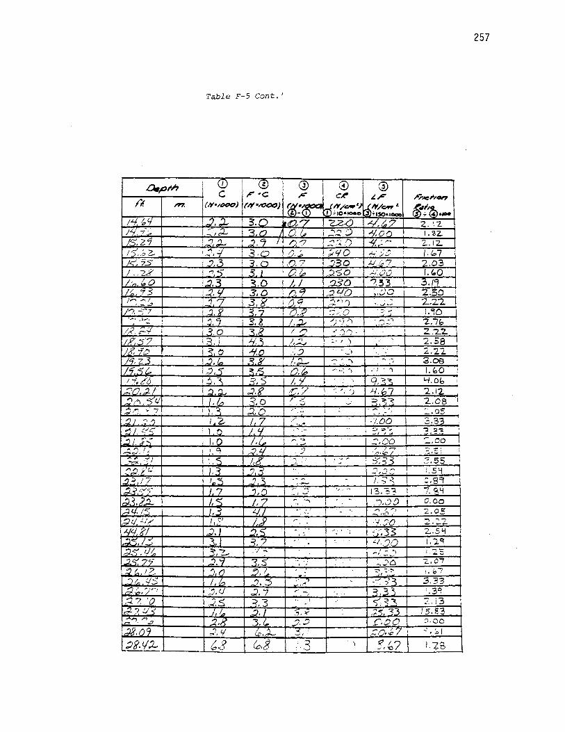
Ff. -i~
;,.,, ~ 0 /!':., 'i 3
/"!, "";/
;-:;,z 3
;,:;_,--:'I
::.' . .::::', tJI,.,
:: l. .17 •.
,'.'.1?. 'O 1.;z 7 :J<
!.:JX.09
Table F-5 Cont. '
i (!) © @ © @ C r ~c ,,,: c.t' ~F
(lt•ttf>OO) ftr•l'CCJO) (/Y•h!2t:lt':A (N/.:M') 1N/aw' m-m 0;1o•to00 [.j);.,50.1000
' .:J, .2...
l~.3 2, 'I
,_:] 7 I ~.9 'j, '7 ~.o ::-, j .> b
. /,,., I , '<,
I '2.-iO
I ),D I t:;
\ '<; .3 I,,~
'7
I I<:'
~.I ,, I
::J. '1
/, (,..., ;), 1./
~.5
~.o a.(~
~- (")
~ I 3.0 3,0
:;:,7
_:r, s
~.o
/, 7 !. 'I /,L,
ur
..2.3 :J,O /,7
.:::S. '? . ·: ...,
~.s
..:2. I
,,f), 7
J. I
!J.R J. ::i, I (:! /,.2,,
.< :J /.~ /'), (,,,
/.'I :C./ I, :5 ,,, ..... ...
' A
., ..... ),
,. ~
- : -
.. ., _,,."'(
.... 'l
-~ I ._I.'
.'.3
~30
,; ) -' ,.., .. .r. -...·
~- , .) - __ .,
, '
~- '; ')
1 • • 4 ....
,,,,,..., _.1-·
,:./OO '?33
~ -. '
,·I 'I
1-U~7
- ..... ~ I .. "" ,'
·l.00
:::,oo / /,...,
'/'J•lo I
1'3. '3?
.·'!·, :;o
.;."5' ··n
257
Z. I "2. I. '82.
2.. 12. /. (.,, 7 2.03 I. <..o
3./Cj 2.SO :
1.90 '2.7b ., .., ., -·'-~
2.58 2.22 3.oe I
1.~o !
'-I.Ob I
'2.12 2.08 I
_.as
-:..oo .,,.._, f :
:.gcr
o.oo 2.05
2.::..2 2.s~
2.07 1, C7 3.33
I ";2Q •-''
.: .. i 3 15.83
:J. 00
l.-Z8

258
Table F-5 Cont. '
0.,ol'h (!) © Q) © @ c ;:- "C r- c, "'' ,r.ne;.,.,,
/"I. ,,,.,, (1'(•1"4:10) (/(•IOCO) ~•H--.i (N/ow') ~.IY/Cll'P' ~11~ -(1 j);IO•IOOO ••50•1000 .;. 4•-_:u ,,7c/ I (,,,0 'i, I ..._:), .. J - ~.]0 ~/. "?<.. 3.Sh '-~· •.07 -'/. 7 fc,.LJ ~.c: ./../";'() :JL,no .5.53 :...; " ·~I.In ~,11 .~. /,, ~· ....... ~:..... -~) :J.tJ.7.71 IQ.29 ~7.7~ i ~/ 11.0 /"l, ~J ""' _, ..:./.~7 (). (o(,,
l..S0.01- '7,q I/.(,, ~::>.D ,,,..,_._:;; I /,;;:....t,..U/ :?./. 10
7,7 !?. /_ d1 ... :n -· ~
" I ,8,~~ 21.9 4 .':?l'l < 5( ,_,
~f"I, 7/ I //('/) ~:s.o /yQ()
-"<-I ,Of.I ~.n Hl?,D ·: ~ ·~, ') ;
I
.,___.,__,,_, I
I
! I
I
! !
'
I ' I
I I I
I !
....

259
Table F-6
C P! !5 ' I .Alac;nc/" . .Qeplh (!) © G) © @ c , .. c r- Gt' ~r- r-ne;_,,
/I. '"' (1(•1000) r;t·~J ~·~ .fN/ow'J ~N/ow" '='~~ z .m 1).:10•-o • ISO. IOCIO ~ ~ ... '·-,03 ;:<,L/ :JJ./ it I.~ 'J~O ;;}, 00 . 33 . '1 t,, 3.0 ~.5 ' 1,1- ~00 ll'J.t.7 • . 5fb /,:;))/ -::!.,7 3.'1 I /,~ ~?() /0,/,..,7 ;; rtS J /,./ ~.t/ -'/,0 /,:5 -:J.'10 JIJ,oo .: 17 J 9'1 ...:!-2 3.8' 15 "12 0 JO,£Y'!J " • :::>.J . !J.7 .~./ ~,l. J.~ ~10 In .l'J~ ....., ' . '" -: ,r.o ;J,/ ~~ /,jJ ~ID 11~.0t'> ~, ' 7/ ~.'12,. :J,O ~."5' .'J I "vio J,t.J,tJo , J l 0 :
-
~.~5 ~.:J 3.8 I ;r !JOO 1~.co l,.')tf') ~ ~Jil ,., ' "I,:;... ~.I ::J/li /.t./ (. 10 (,.,' l ,7 ... . ..
=< q I ..., ·' ~.'7 ,,), 0 ::J.J 0 /~. 3 /,. ~5 -·. ~'f .. :2JI ') ~,7 ;;.o lf:D /.~ •. : 3 7. 4 ~I
-'1,:-<7 J ~? 3.7 !7 170 JI. - 3 (,,,. ,,., l,,. ... •'.l,9'7 /. 6 : ,. (. ~:;.; 1;.o /,. ~ I' ~~) ~ ~".! /, 7 ,<J /. (j /"70 7;. >3 .. , './~ . ~S'S .~.~· . /, '-! ~7.") 7·- -~ • . .;l~ ! f"\ >()( . -~ ,,.. ' J.~ J.~O 9.3~ 'J:J •..;i .;l.. i . :::i ..... /.. ~/ r ) ,, -. /.~ ISO 'X.t. 7 S.7e! L 5=? ( -'" ... /, :i.. /40 2.~0 :5' -, , I
t.: . 5(/,,., I ' ~J . /,"/ 15/' -·~~ ~ ,:J..2 . -7,J~ ! '
~ . "' ,2,)( J. I /·~{) "'? '3 3 "'IS ..st ' ? 5..1. I /,, 3,0 /,I./ /1 c -.'.~~ 5 ;;i3 ?. P;l. I /, ..:i. '7 J,3 I. 'Q >? • .b 7 ~~;i_
ii'/7 !, .... .:: i,3 l :>C ~·,.L;, 7 ..:..J ";')I -·· I?, 51'"') !, ..,. -~ I /, 3 1RO '9. t-.7 ..L./ J".;l..
'? p- ~ /.~ ~.z. ,,5 /'7·"1 10.00 ~~,;{., •1.11 ... I. c 3,?_ I. 3 i e;;'> )?.(,.,/ "'/,s't.o '~ '/9 ;J,j'.) 3.5 15 .:JCj JC,00 ~.DO
'1. JJ I I, ~ 3.1 J,5 r ,...., ·~ ...... I :J, 00 ::;""',5'~ J(').)t./ I. ' .. • <../ .s , ... ,~/'""""\ IC Da ---~-~ ~ !/'),.;; '? /J - 3 .s . "" I,< '- i().00 .·-' 5 ~
J l'J YD "7 '2.. 1,5 J?:J 10.00 -~88 //, I ~ 1, j,, .. , I /~ ,') 1DJ~? :..,:,,7 I,_
/), (./~ ,.1 ~.' ',3 1~r; 5(, t,7 : . / 'i Jl ? ... ~ JI '( 3. 'I ', .:J. /SC j'i.A")/) .:./,"/¥ /,..:)' J ..:J.;;... ?.~ /').~ ... , ... J-.. "''.()0
i - ..,
,, .... ... /
/:J.(/l/ ~.I ~3 I, 5 ~ • "'I Ill .oo .L..., - -- .. / ::). ;"? /,~ .., "" /'\g'
...... ~--- ·, :::-,3 i .,.,_ -·.J
·~. /.!J .),t/ 3 ..... /,-: -.. , •) ·- -.... ..,, //, -. ..:..,1.-~
I ;i, '-I?- 5 2, /, 7 ., .:) J ::J, j ,-7 9.'15 I~, 7S - ,:J,.. .3', • ;.s ..uo /O,tJ'D ,.,_J.S5 F-/. Olf - . () 3: 7 /, => ."JOO 1tJ,O o .:'.),00
.!.!LiL .2,3 J,2 /, t./ ~j·.') 'J. 33 ~~b
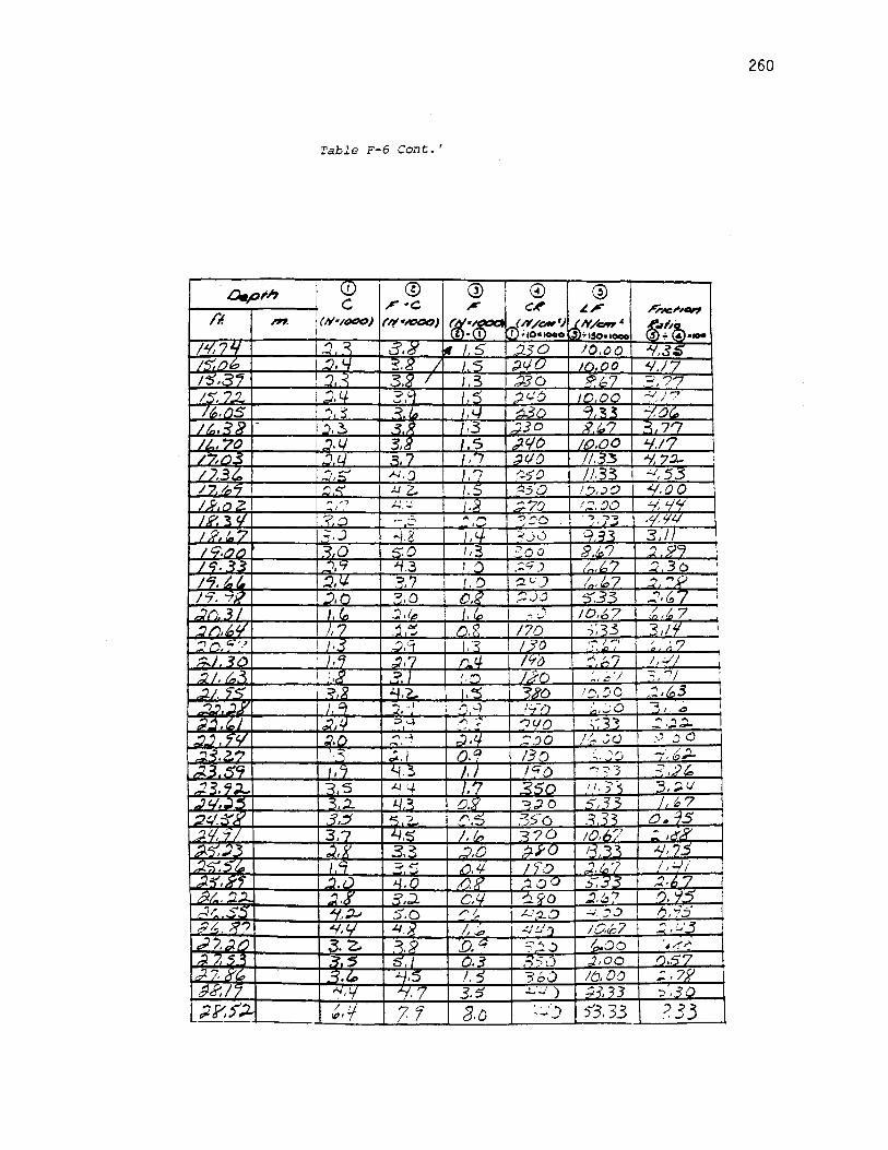
260
Table F-6 Cont. '
a.prh I (!) © @ © @ c ;-c ,,,:- c.<- ~,#' F"nW:;,,°'7 II. ,,,.,. (/(•/000) r.tt•KJDOJ ffi'.·~ (/'l/e.-') rf> /'I /ow ' ~"'t'~--.(i) i);10•.-o •150•1000
/~?"I ~' ";(. 3.~ .ft I 5 'HO 10.00 .4/,s~ /5°',/')b ~1, '-I ~ .. / 15 ;;!../ u J(},00 "-/,/7 /~,3i ~ ~ 3.: I 13 :;J..30 >J.b7 ~' ')?
/_"{, /..? :J. l.J. ":;:> I ~ '") ::) c,: 6 1n oo .-:../, ! '7 ....,, , ·" .
/ti,.IJS "l,5 .~ ... /,'-I -;..30 ~ 33 ·.oG. J /-., ~ 5l - .), 3i .~. ,3 .:;Jo x.~7 3, 7'7 Jt., 70 :J. I./ '3.; .s d-'10 /IJ,00 'i.17 /'7,/'J ~ ! .:J. LI .~. J ,7 ~f.)0 //.33 "'/, '7:;... ;
//,3~ 'l,t:;:' ,L.J, :J ,.., ~5'0 1133 .:./, 55
' I
17. /,,"'1 ~.<!:' /.J z.. 1.5 .Q5Q .rf),:;O 4.00 J:il.l"J ~ " ,, fl •I .:x .::.i'o ! ::. :JO "-/, "f'-1 _, ..... -19.":a:f.I ?,o ,, ~- --. "' ,.... '? .'.'.)('.;) . ~ -,Ji ·~'fl./ ,......, .J
J p, 1-7 ~ . .) .... , g t.J. ?c.Ju 9.~~ 3,/1 I q,t'J,, :;',Q 5.0 1,3 :coo 2.~7 ~.51/ I<::;, ~ :;,,9 "1.3 I :'.) .-:.<:;) (,.,,t.7 ;J' 3 0 ' /'?, t.1. :J, /,/. .":?.7 I'() -:J,t.:J /,.,, 4:, 7 ~ '."'y !
/7. 7f..> :), t"J 7,0 OJ< ;,.. .) o) 5:33 ..... ""·~-/ ;
..:Jli. ~I . :... ::J ,f~ ' "
., J0,b7 I~"~ 7 ~ '_.'
!:) /'), ;/, t/ /, '? .:l.~ {),; 170 .;;33 3,J'f I
".:' ""' .:;- ',1 ! I, :;i, ''.i ~ I 50 ,--, / '7 .~ ;.,7 ,_ .:.~I --
:::;..J,30 ' ~.7 fl. ' /'to ,;, ;., 7 /,.;// I ' .:; /, /... ~ I :,)' :? '.{") 120 , :. , )
~1 ~ ; , "1/ ;
..::1.1. ']c; ~. '4.2. I.~ ~A"O li\{)0 ~.t,3 .., ., ').Y ' ~, .. J .•J, '-1 1:..-/) .:;.,,.:_~o : I, r0 i
~'j.t../ .:J, 4 ::> ·-l :~· '_,,... '?C/Q :: 33 ~ .... ~ '""""·-al-.. .,,"JV :;),{') ~ -~ ;:,; ,4 :: :JO /",,. ,.)cJ _..,,;) () ,..., .
-< • .2.. '7 . <; .;,, I (),a 130 ~. ·'~ -'-'', &;.;i.. ...; ~ 59 ,7 l.1. 3 ,/ /'i() "'"':; 3 =<,:;, .23.7.:J - s .Li 4 I 'J <:5o I /, 3' :s 3, .:;l(/ ~
..J (./, :J 4., ~ ,:i., LJ ':i, CJ.2 "=?~ 0 .~ 13 /, 67 2:1.~J.. ' ,::f <:; ?_ rl,:=) :~S6 .~ 33 o.~s ;). </, '7 / 3.7 L/,5 /, fLJ 370 10.h'? ~ ,;rJ( ,;;l..~..J.3 ~.K 3.~ ;),Q ;;.;.-u lj ~~ /..), 75 ,;2-S-:5~ I '1 ~5 ,('), 'J. 170 ,.},(,.,? I I;,..{/
:J.~, JiJ'1 !J,iJ J.J.O /J,K :'.200 S'.~5 ::;.1J7 ~~ . .'.'.2.1 :J .lf .=?.;:;.. CJ./ ~¥0 ~.~i l), '15 ..:Ir_ .<:5 /.f, ;;_, s.o ,,...,~ ~~a ..:..;, ,,.:> h, ..;::;-
;; /,, ?f7 ~,l./ .J./. J /, ~ .:..,' !./_·') IC.rb? ,; I LJ'-5 d,,d_I) $. z. .1. ;> !), '1" ::;:· 1,J ~oa ·-~~ ~ 7. s ~ ~.5 5. ().3 =:..:;o ,J,OO t'),:5 '/ ,..;i.7, X'=' 3.t.o .:...J,5 /, 5 3b.J /{:),DO ;_,79 CJ.ef. 11 "'.',I./ ""/. 7 3.5 .:_;:..;) :).3, 3 3 ::-,~o
).?,$').. ~
/ 1 IQ I 77 3.o ·,-._·) 53,33 ?33
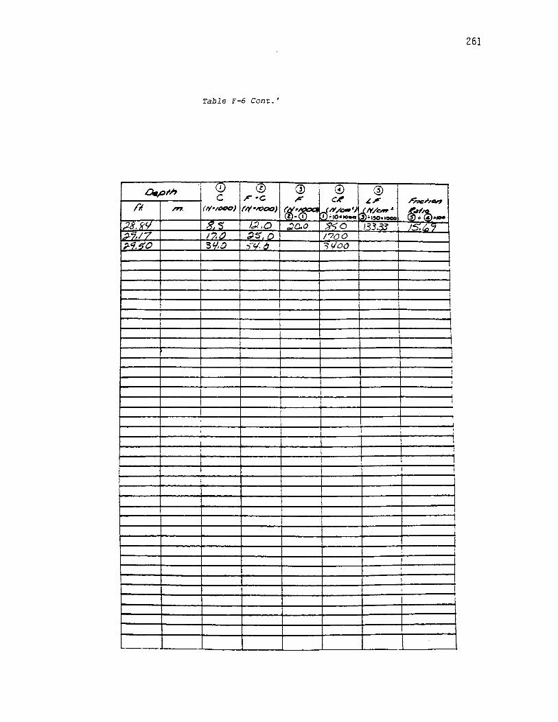
261
Table F-6 Cont. '
.Qe,DJ'h i Q) © @ © @ c r"C r- c-<- ~, n-..c;,.,, /i! '"' (/(•/MIO) (/f•IOOO) f«·- '~/-') riN/ow" ~"'(!) .ti) ITT•ro·-• ~ ••50•1000 ~ '.,..
.)8. f('I 11~ l,;l .o ~(J.O s.:;o 1~3.~~ 1'5,t, 7 ~~/7 1?.7i ~~. /') /?00 ;.'i . .f!i'O 5'l0 j""e/. b 5c/OO
I
:
I I
I
! I
I
I .
I
I I I I
-...
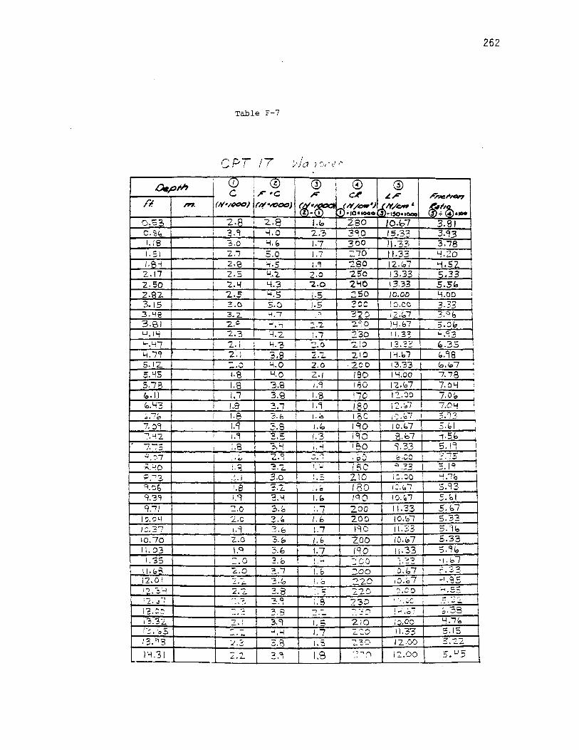
!
.GW,ol'h /"I. ,,,,,,
o.s3 o. 'Sb I 1.18 I. s 1 I
/.BY 2..17 z.so 2.Q2 3.15 I 3-'Hl 3.BI ~.\Y
'-l.Y/ 4.79 s.12 5.YS 5.7B fo .1.1 ~.Y3
~.7(., I 7.09 :.~'2. I
7-;5 I
~.'J7 I
.;;.~o
~.~i
"'1.~Ei
'i. '39 'ti/
I ~.OL!
/C.37 I0.70
11.03 : I, '35 11.1o!I. l:Z. 0 ! l 2, !.LI !?..~l
i '3. =~ i'°;.'32. , ..... I .,..
....... o.:>
13."'3
l'-\.31 -
Table F-7
CPT/7 (!) © c ,. -c
(1(•1«10) ,,, •,!000)
2.8 2.8 3.9 ~.o
2:.o '-1.~
2.i 5.0 2.9 f.f,5
2.s Y:l. 2.4 4.3 '2..S '"i.S 3.0 s.o 3. 2. Y.7 2.~ ...;
o"'\
'2.3 Y.2. '2.. I "i."3 2.1 3.8 -:.o Y.O 1.a Y.O 1.8 3.9 1.7 3.9 1.8 3.7 j. 8 3.b I.~ 3.8 1."1 ':I::.
-·~ l.8 "3. 'i :.~
.., 0 <.•I
:.~ ..... -~·'-
:::.1 3.0 1.e -s.2 1.9 3.Y ::.o 3.'=o 2..0 ":I I
~·" 1 . ..::i 3.h 2..0 3.b 1.9 3.b ~ .0 ';i I
-·O
~.o 3.7 2.:. 3,"' 2.'2.. 3.\3 ~: .?, "2,Q -· · - -::. 3.3 -· .... .-, I '., 3,9 ~ - ,.j.~ . -:.t.3 3.e. ..., ..., .t. ..... 3."1
I' / n ~)~·
@ r-
f«.·~ -m f .(o
2.3 /,7 /.7 1."1 2.0 "2.o 1.5 J.5
...
::2 l.'1 :z.o 2.'l. 2.0 z.1 1.9 1.8 I. 9 i.c 1.'-!.3 i.~ - .... ~.I
I '.J I• I :: ··-I.a I."' 1.7 I. b J.7 I.{:,
1.7 !.~
I. b :.o ... i.8 .., ·-I,:;
1.7 l.S
1.9
262
© @ C.(# ~, ,#',..,c;,.,,
(N/-•.J .J,N/ow' ~t'~•IH 0•1o•tooo ••50•1000 280 fO.b7 3.81 390 /5.33 3.93 300 lt.33 3.78 270 fl.33 !.f.Zo '280 12.G;.7 '-f,52 '2.So 13.33 S.33 '21.10 13.33 5.S'=i ::so /O.OD Lf.00 :
300 Jo.co :2 ':l2 _._.,._,I 32~ i z.ro / 3.% 2.90 )t./.b7 5.0/, :?.30 11. 33 Y.93 2~0 17 7';1 ....,._,_ f,.35 210 111.bl '--98 I
·200 13.'33 (c,.fo7 I
180 I 'i.oo 7.78 !
180 l'Z.~7 7.0Lf !
110 l~.00 7.01o 180 12.~7 7.0Lf I
loC ,-;;.67 5,93 ICfO /0.b7 ;.c.1 I
190 11..b7 -i. 5 lo !BO 9.33 5.19 •oO b,CO ~ -,:; .... ·-ISC "'.33 3. IC! Z.10 I :.~D ~."?b
180 1:.r.,, 7 5.93 lqO IO.~ l 5.bl 200 11.33 5.67 2.00 10.~1 s.33 190 I t.33 5. 16 200 /O.lo7 .S.33 l~O 11.33 s."16 -·co ' "'j"j •1.b 7 I'"""'...,..
:::oo 1O.fo7 -: ":::! -::- . -·-' ""'20 :o.1o 7 - 1.s.s 720 ~.~c ~.=~
1-.:.-:·c - ...... 23:? :; . '"',_ ;·.:.~ ! ~ .0 j ;.38 210 1:i.oo Y.l'-2:.0 I 1.33' 5.IS ..., ";!,.""\ ........ - 12.00 5'. "'2.'2.
-:.:'..., :l 12.00 5.45

263
Table F-7 Cont.'
lM,o#I <.!) © 0 © @ c r"'C ,lift' C.t' "'' .r.ne;,.,, Ii! ,,,,, (/t•1«10) (/Y•IOOO) f«:~ (~/oW·) ~l'l/0#' ~1.· 1-m ll•10•-o ••50•1000 "":~.-
14.(..4 z.s 4.3 2.1 '2.50 /Y.b7 5.87 IY.91o 2.5 Y.3 2.2 250 IY." 7 5.87 rs.zc:i 2.Y 1..j, (o 2.Y '2.1.\0 lb.00 "· fo 7 I 5.(,2 2.'-1 4.C. 2.3 2LJO 15.33 !0.39 15.'tl5' 2.11 y,9 2.1 2YO 14.0C S.93 llo."28 2.s 11.s l."f 250 12.'-7 5.07
''""o '2.C:, 11.7 2.0 2"0 13.33 5.13 I (,.'13 2.b Y.5 1.8 2(,,0 12.00 1.1.1..2 :
17.2b 2.Y '-i.Y l.Y 2'-ID "l.33 3.89 !7.5<=t 2.~ '-1.b l.C: "2.80 12.1.. "7 '"L52 11.er2 2.8 l../."Z. J.S 280 ;2.00 Y.Z9 18."2.Y ?..~ ~.s !.b 2(..0 10.C,7 l...f.10 18.57 2.7 '-1.S l.'-1 270 9,33 3.Yb l~.90 "Z.5 Y.I l.G:, 250 IO.b7 Lj, '2.7 I ct."2.3 '2.5 3.9 1.2 2.50 s.oo 3.20 ' 19.Sb 2.3 3.9 1.1 230 7,33 3. lei !
19.SB 2.3 3.5 1.0 230 b.t,7 2."10 i
zo:z.1 2.1 3. '2. 0.9 2.10 b.00 z.~t..
'20.51.j 2.0 3.0 0.'1 z.oo b.Oo '3.oo I
?Q.8i I 1.9 '2.8 o.a /C,O 5.33 2.RI '21-20 ' /.b 2.s O.(Q 160 '1.00 2.-50 I
'21.53 l,S 2.3 1.1 150 7,33 Y.8C\ '
21.85 I I. lo 2:2 0.5 I G.O 3,33 2.os 2z.:s i. '3 2.y 0.2 i30 ; . :;3 j .0.3 2'2.51 2.0 2.5 c.e 200 5,33 2.{o7 '2'2..~l-1 1.s '2.0 0.Y IBO 2.~7 I.YB 23.17 l.b 2.'-1 2.2. /G,D 1'1."-7 ~.17
2'3."19 l.b 2.0 1.Y lbO 9.'33 5.83 2.3.92 o.e 3.0 0.3 80 2.00 2. • .50 2Y.15 o." :z.o 0.b "'o "i,00 (,,.f,7
2.'-1. 'i8 1.0 1.3 I. 3 100 c;.~7 8.~7 2.Y.81 o.8 /. '1 o.s 80 3,33 Y.17 25.13 l.b 2.9 o.s lbO 3.33 2.oB 25,1.j~ ::'."2. 2.7 1.0 220 /:;.(,7 ,?.03 25.79 1.8 2.3 0.3 180 2.00 1. IJ z~.12 !.5 2.s 1.3 150 8.b7 5.78 ?(.,,'·i.5 3,y ?.7 O.Y 3uo "2.. lo7 0.78 2.lo.77 2.3 3.b 1.S '230 \Z.00 5, 2.2 ~7. IQ 3.o 3,1...1 1.7 300 ll.33 3.78 ~/. 43 5. '2. 7.0 o.c:i 5'2.0 ".oo 1.15 27. "7"' ~-5 s:i.. 3,2 bSO "2.l.'33 3.2.9 2.8.0'=t 7. f.c 8.5 3.2 '"o '2.1. 3'3 2.81 28.Y2. /O.Q 13 .. "2.. I. 6 rooo /O.<o7 1.07 ,_

264
Table F-7 Cont.'
.0.plh (!) © @ © @ c .r•c r- c~ ~r- r;.~;.,.,,
/I. ,,..,_ (#•tC-00) (l(•K:JCC) ar.·~ (N/cw') ~N/ow 4 &-11~ .(j) m•tO•IOOO 3 ••50•1000 .. , __
29.7Y c:i:z .. /2.'i 3.7 920 21.f.<..7 2.bt) Z.9. 07 /0.8 12. Lj 2.0 1080 13.'33 '. '2. 3 2.9.YO S.Y 1 2. I 5.0 8110 33.3'3 3,97 29.73 i 8.Y 10. y 3.0 8Lf0 Z.0.00 ::.39 lo.Ob f,.2 11.2 1.0 620 (a.fc 7 I.OB 30.38 18.0 21.0 lo.2. 1800 l.jf.33 2..30 30.I I 1.5.0 Jb.0 s.o /SOO 33.'33 z. 2.1. 31.04 9.0 15:2.. 2.7 900 18.00 2.00 :
31.37 3.Cl f S.O '-i.5 /300 so.oo '2. 3 l 3\.70 15,3 1s.o 3.2 1530 '2.. \.33 1.39 3'2.02 12.s /7.0 .5.9 1250 3<=J.3.3 3, l.S 32.35 10.8 11.\.0 2.Y 1 oer:::. 11::.00 '.'"!8 32.C:.B 3.1 IY.O 2.0 8\0 13.33 1. i::.s 33.0I 8.Y I0.8 2.Y gyo lb.00 f.90 -:i~."3Y 7.lc '=/. b r.B 7'a0 12..00 f.58 ' 33.(:.b 5.0 7.'-1 4.0 soo ?...fc.(,, 7 5.33 ! 33. CJ9 ~.~ 8.b 4.0 "80 2t...I07 3.92. i
3"1. 3 '2. 8.0 12.0 0.8 goo 5.33 o.r.:.7 31.i.~5 11.0 15.0 1.9 1100 12.r.. '7 1.15 I
3Y.'111 ! ~. 'O '7."' 7. 9 C:.80 :2.1..7 -7,75 35.'30 b.4 8.3 '-l.9 b"iO 32.'-7 ..5. /0 3S.b3 i ~.I IY.0 7.t:i blO so.t:.7 ~.3J
35. 9!o I ~.7 11.b Go.O b70 L.J0.00 5,9; I 3r..2i:i I =·~ ~.'-] -l,Q ~80 zr...~7 er. 52.. 36.1:,2. "2.0 '2.tl "2000 31..'=!5 3~ 3e 3'-!00
-

APPENDIX G
CONE RESISTANCE COMPARISON BETWEEN DUTCH
MANTLE AND FRICTION SLEEVE
MECHANICAL CONES
265
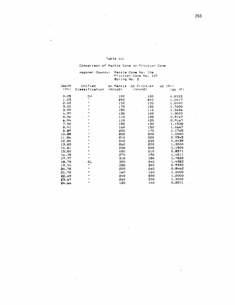
266
Table G-1
Comparison of Mantle Cone to Friction Cone
Wagoner County- Mantle Cone No. 106 Friction Cone No. 107 Boring No. 2
Depth Unified qc Mantle QC Friction QC (M >I (ft) Classification <Nlcm2> (N/cm2> /qc <F>
0.05 CH 100 120 0.8333 1.03 250 240 1. 04 1 7 2.02 130 130 1. 0000 3.00 170 100 l. 7000 3.99 150 110 l. 3636 4.97 130 100 l. 3000 5.96 110 120 0.9167 6.94 110 120 0.9167 7.92 150 130 l • 1538 8.91 160 150 1.0667 8.89 200 170 1.1765
10.88 200 200 l .0000 11.86 210 220 0.9545 12.84 240 230 1 .0435 13.83 260 200 1.3000 14.81 230 200 1. 1500 15.80 180 210 0.8571 16.78 270 190 l • 4211 17.77 310 180 l. 7222 18.75 CL 350 240 1.4583 19.74 280 300 0.9333 20.72 220 260 0.8462 21. 70 160 160 l. 0000 22.69 240 200 1.2000 23.67 260 200 1.3000 24.66 120 140 0.8571

267
Table G-2
Comparison of Mantle Cone to Friction Cone
Wagoner County- Mantle Cone No. 108 Friction Cone No. 109 Boring No. 4
Depth Unified qc Mantle qc Friction qc <Ml/ (ft) Classification CN/cm2l <N/cm2> /qc CF)
0.10 CH 140 100 1 .4000 l.08 CH 230 220 l. 0455 2.07 MH 240 180 l. 3333 3.05 CH 220 220 l .0000 4.04 260 240 1.0833 5.02 220 240 0.9167 6.00 140 160 0.8750 6.99 160 140 1.1429 7.97 150 160 0.9375 8.96 180 160 1.1250 9.94 180 180 1.0000
10.93 220 190 1.1579 11. 91 230 170 1.3529 12.90 240 210 1.1429 13.88 240 200 1.2000 14.86 210 210 1.0000 15.85 240 200 1.2000 16.83 290 220 1. 3182 17.82 270 260 1.0385 18.80 CL 250 260 0.9615 19.79 200 200 1.0000 20.77 160 180 0.8889 21.75 190 190 1. 0000 22.74 140 160 0.8750 23.72 120 80 1.5000 24.71 190 100 1.9000 25.69 170 180 0.9444 26.68 320 320 1.0000
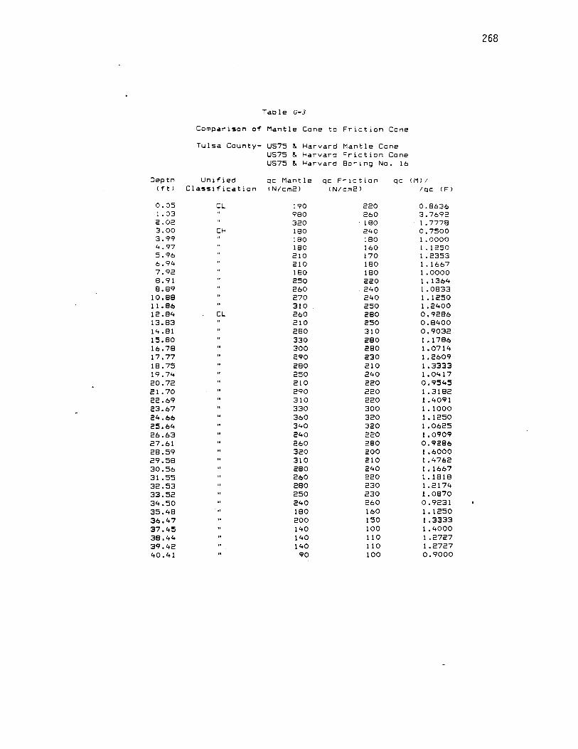
268
Table G-3
Comparison of Mantle Cone to Friction Cone
Tulsa County- US75 g, Harvard Mantle Cone US75 g, Harvard Friction Cone US75 g, Harvard Boring No. 16
Depth Unified qc Mantle qc Friction qc <M> I (ft) Classification <Nlcm2> <Nlcm2> /qc <F>
0.05 CL 190 220 0.8636 l .03 980 260 3.7692 2.02 320 180 1. 7778 3.00 CH 180 240 0.7500 3.99 180 180 1.0000 4.97 180 160 1.1250 5.96 210 170 1. 2353 6.94 210 180 1.1667 7.92 180 180 l. 0000 8.91 250 220 1.1364 8.89 260 240 1. 0833
10.88 270 240 1.1250 11. 86 310 250 1 .2400 12.84 CL 260 280 0.9286 13.83 210 250 0.8400 14.81 280 310 0.9032 15.80 330 280 1.1786 16.78 300 280 1.0714 17.77 290 230 1 .2609 18.75 280 210 1.3333 19.74 250 240 1. 0417 20.72 210 220 0.9545 21. 70 290 220 1. 3182 22.69 310 220 1.4091 23.67 330 300 1.1000 24.66 360 320 1.1250 25.64 340 320 1.0625 26.63 240 220 1.0909 27.61 260 280 0.9286 28.59 320 200 1.6000 29.58 310 210 1.4762 30.56 280 240 1.1667 31.55 260 220 1.1818 32.53 280 230 1 . 21 74 33.52 250 230 l. 0870 34.50 240 260 0.9231 35.48 180 160 1. 1250 36.47 200 150 1.3333 37.45 140 100 1.4000 38.44 140 110 1.2727 39.42 140 110 1.2727 40.41 90 100 0.9000
APPENDIX H
CONE RESISTANCE COMPARISON BETWEEN FRIC
TION SLEEVE MECHANICAL CONE
AND ELECTRICAL CONE
269
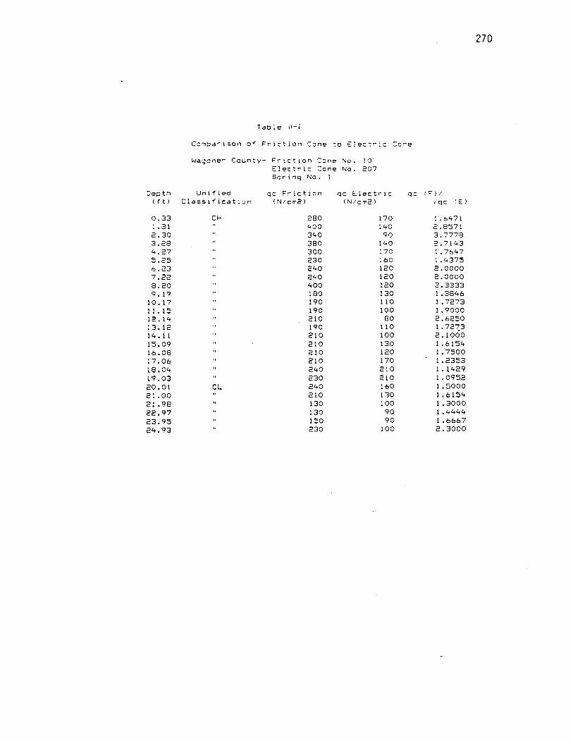
270
Table 11-1
Comparison of Friction Cone to Electric Cone
Wagoner County- Friction Cone No. 10 Electric Cone No. 207 Boring No. 1
Depth Unified qc Friction qc Electri.c qc < F >I (ft) Classification <Nlcm2) CN/cm2> /qc <E>
0.33 CH 280 170 1. 6471 1. 31 400 140 2.8571 2.30 340 90 3.7778 3.28 380 140 2.7143 4.27 300 170 1. 7647 5.25 230 160 1. 4375 6.23 240 120 2.0000 7.<":!2 240 120 2.0000 8.20 400 120 3.3333 9.19 180 130 1. 3846
10. 17 190 110 1.7273 11 • 15 190 100 1. 9000 12. 14 210 80 2.6250 13.12 190 110 1. 72~3 14. 11 210 100 2 .1000 15.09 210 130 1 • 6154 16.08 210 120 1. 7500 17.06 210 170 1. 2353 18.04 240 210 1.1429 19.03 230 210 1. 0952 20.01 CL 240 160 1.5000 21.00 210 130 1 • 6154 21.98 130 100 1.3000 22.97 130 90 1. 4444 23.95 150 90 1.6667 24.93 230 100 2.3000

271
Table 11-2
Comparison of Friction Cone to Electric Cone
Wagoner County- Friction Cone No. l""l Electric Cone No. 201 Soring No. 2
Depth Unified qc Friction qc Electric qc ( F 'I (ft) Classification <Nlcm2l (N/cm2> ,qc (El
0.33 CH 160 130 1.2308 l . 31 120 100 1 .2000 2.30 11 0 100 1 . 1 000 3.28 130 110 1 . 1818 4.27 110 80 1.3750 5.25 140 80 1. 7500 6.23 140 90 1.5556 7.22 160 90 1.7778 8.20 180 90 2.0000 9. 19 190 110 1. 7273
l 0. 17 180 110 1. 6364 11 • 15 200 130 1. 5385 12. 14 220 90 2.4444 13. 12 230 130 1. 7692 14. 11 190 120 1 . 583".3 15.09 200 120 l. 6667 16.08 200 140 1.4286 17.06 220 160 1.3750 18.04 280 140 2.0000 19.03 CL 230 270 O.S519 20.01 240 240 1. 0000 21.00 130 160 0.8125 21 .98 200 120 1.6667 22.97 160 270 0.5926 23.95 220 170 l . 2941 24.93 180 80 2.2500 25.92 280 240 1.1667
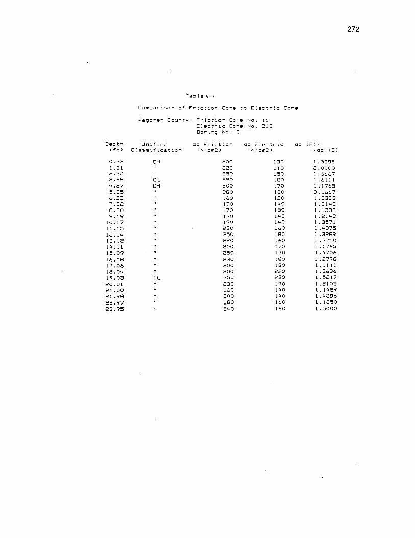
272
TableH-J
Comparison of Friction Cone to Electric Co,-,e
Wagoner County- Friction Cone No. 16 Electric Cone No. 202 Boring No. 3
Depth Unified qc Friction qc Electric qc < F) I (ft) Classification <Nlcm2) <Nlcm2) /qc <E>
0.33 CH 200 1 30 1. 5385 l . 31 220 1 10 2.0000 2.30 250 150 1.6667 3.28 CL 290 180 l.6111 4.27 CH 200 170 l . 1 765 5.25 380 120 3.1667 6.23 160 120 1.3333 7.22 170 140 l .2143 8.20 170 150 1 . 1333 9. 19 170 140 1 .2143
10. 17 190 140 1.3571 1 1 • 15 230 160 1.4375 12. 14 250 180 1.3889 13. 12 220 160 1.3750 14. 11 200 170 1.1765 15.09 250 170 1. 4706 16.08 230 180 1.2778 17.06 200 180 l.1111 18.04 300 220 1. 3636 19.03 CL 350 230 1.5217 20.01 230 190 1 . 2105 21.00 160 140 1.1429 21. 98 200 140 1.4286 22.97 180 . 160 1. 1250 23.95 240 160 1. 5000

273
Tablell-4
Comparison of Friction Cone to Electric Corie
Tulsa County- US75 & Harvard Friction Cone US75 & Harvard Electric Cone US75 & Harvard Boring No. 16
Depth Unified qc Friction qc Electric oc ( F > / (ft) Classification CN/cm2> CN/cm2> /qc <El
0.05 CL 220 220 1.0000 1.03 260 850 0.3059 2.02 180 550 0.3273 3.00 CH 240 190 l. 2632 3.99 180 130 1. 3846 4.97 160 130 1. 2308 5.96 170 150 1.1333 6.94 180 160 l.1250 7.92 180 160 1. 1250 8.91 220 170 1. 2941 8.89 240 160 1. 5000
10.88 240 170 1 .4118 11. 86 250 140 1. 7857 12.84 CL 280 130 2. 1538 13.83 250 110 2.2727 14.81 310 130 2.3846 15.80 280 200 1.4000 16.78 280 220 1.2727 17.77 230 200 1.1500 18.75 210 200 1.0500 19.74 240 200 1.2000 20.72 220 180 1. 2222 21. 70 220 180 l. 2222 22.69 220 170 l. 2941 23.67 300 180 1. 6667 24.66 320 200 1.6000 25.64 320 220 l. 4545 26.63 220 190 1.1579 27.61 280 180 1.5556 28.59 200 190 1.0526 29.58 210 190 1.1053 30.56 240 190 1 .2632 31.55 220 190 1.1579 32.53 230 170 1.3529 33.52 230 170 1.3529 34.50 260 180 1.4444 35.48 160 180 0.8889 36.47 150 170 0.8824 37.45 100 120 0.8333 38.44 110 100 l. 1000 39.42 110 100 1.1000 40.41 100 110 0.9091

/f'l',1
VITA
James B. Nevels, Jr.
Candidate for the Degree of
Doctor of Philosophy
Thesis: INTERPRETATION OF THE OISCONTI NUOUS MECHANICAL CONE PENETRATION TEST IN NORTHEASTERN OKLAHOMA ALLUVIAL SOILS
Major Field: Civil Engineering
Biographical:
Personal Data: Born in Norman, Oklahoma, September 25, 1942, the son of James B. and Agatha E. Nevels.
Education: Graduated from Norman High Schoo 1, Norman, Ok 1 ahoma, in 1961; received the Bachelor of Science degree from the University of Oklahoma, Norman, Oklahoma, in 1967; received the Master of Science degree from the University of Oklahoma in 1977; completed requirements for the Doctor of Philosophy degree at Oklahoma State University in May, 1989.
Professional Experience: Civil Engineer with the Oklahoma Department of Transportation since 1967, with the last fifteen years in the field of geotechnical engineering.