Room acoustic modeling with the time-domain discontinuous ...

Room acoustic modeling with the time-domain discontinuousGalerkin methodCitation for published version (APA):Wang, H. (2021). Room acoustic modeling with the time-domain discontinuous Galerkin method. EindhovenUniversity of Technology.

Document status and date:Published: 06/10/2021

Document Version:Publisher’s PDF, also known as Version of Record (includes final page, issue and volume numbers)

Please check the document version of this publication:

• A submitted manuscript is the version of the article upon submission and before peer-review. There can beimportant differences between the submitted version and the official published version of record. Peopleinterested in the research are advised to contact the author for the final version of the publication, or visit theDOI to the publisher's website.• The final author version and the galley proof are versions of the publication after peer review.• The final published version features the final layout of the paper including the volume, issue and pagenumbers.Link to publication

General rightsCopyright and moral rights for the publications made accessible in the public portal are retained by the authors and/or other copyright ownersand it is a condition of accessing publications that users recognise and abide by the legal requirements associated with these rights.

• Users may download and print one copy of any publication from the public portal for the purpose of private study or research. • You may not further distribute the material or use it for any profit-making activity or commercial gain • You may freely distribute the URL identifying the publication in the public portal.

If the publication is distributed under the terms of Article 25fa of the Dutch Copyright Act, indicated by the “Taverne” license above, pleasefollow below link for the End User Agreement:www.tue.nl/taverne

Take down policyIf you believe that this document breaches copyright please contact us at:[email protected] details and we will investigate your claim.

Download date: 27. Mar. 2022

https://research.tue.nl/en/publications/105efc05-0bd2-4b4f-ae5a-de3b8919153b

Bouwstenen 321

321

Room acoustic modeling with the time-domain discontinuous Galerkin method

Huiqing Wang

Ro

om

acou

stic mo

delin

g w

ith th

e time-d

om

ain d

iscontin

uo

us G

alerkin m

etho

d

Room acoustic modeling with the time-domaindiscontinuous Galerkin method

PROEFSCHRIFT

ter verkrijging van de graad van doctor aan de Technische UniversiteitEindhoven, op gezag van de rector magnificus prof.dr.ir. F.P.T. Baaijens,voor een commissie aangewezen door het College voor Promoties, in het

openbaar te verdedigenop woensdag 06 oktober 2021 om 16:00 uur

door

Huiqing Wang

geboren te Yantai, China

Dit proefschrift is goedgekeurd door de promotoren en de samenstellingvan de promotiecommissie is als volgt:

voorzitter: prof.dr.ir. T.A.M. Salet1e promotor: prof.dr.ir. M.C.J. Hornikxco-promotor: dr. M. Cosnefroyleden: prof.dr.ir. E.H. van Brummelen

prof.dr. S. Bilbao (The University of Edinburgh)dr. C-H. Jeong (Technical University of Denmark)dr.ir. H. Hofmeyer

Het onderzoek dat in dit proefschrift wordt beschreven is uitgevoerd inovereenstemming met de TU/e Gedragscode Wetenschapsbeoefening.

Room acoustic modelingwith the time-domain

discontinuous Galerkinmethod

Huiqing Wang

Department of the Built EnvironmentEindhoven University of Technology

July 2021

The work in this dissertation was performed within the unit of Building Physics andServices (BPS) at the Department of the Built Environment of the Eindhoven Univer-sity of Technology (the Netherlands), and was financially supported by the EuropeanCommission within the ITN Marie Skłodowska-Curie Action project ACOUTECTunder the 7th Framework Programme (EC grant agreement Nr. 721536).Project website: http://www.acoutect.eu/

Copyright © 2021, Huiqing WangAll rights are reserved. No part of this publication may be reproduced, stored in aretrieval system, or transmitted, in any form or by any means, including electronic,mechanical, photocopying, recording or otherwise, without the prior permission ofthe author.

A catalogue record is available from the Eindhoven University of Technology Library.

ISBN: 978-90-386-5357-0Bouwstenen: 321NUR: 955Cover design: Huiqing WangPrinted by: ADC-Nederland

http://www.acoutect.eu

Dedicated to my parents and grandparents献给我的父母, 姥姥和姥爷

Abstract

The acoustic properties of indoor spaces significantly impact our com-fort, well-being and productivity. Room acoustic simulations have been apractical tool for acoustic consultants in the design phase of buildings toensure pleasant and functional acoustic environments. More recently, ad-vancements of modern computing hardware make room acoustic model-ing applicable to more computationally intensive real-time systems suchas virtual reality applications.

Over the past 50 years, numerous room acoustic modeling techniqueshave been developed, which are typically classified as geometrical acous-tics methods or wave-based methods. Compared to geometrical acousticsmethods, which treat sound waves as rays and thus suffer from the lossof accuracy in the low-frequency range, wave-based methods simulatewave propagation by directly solving its governing equations based onadvanced numerical modeling techniques, and are able to more accu-rately predict complex wave phenomena, such as scattering, diffractionand interference effects, at the cost of more computational efforts.

This PhD project aims at contributing to the room acoustic modelingcommunity via the development and validation of an efficient, robust andaccurate wave-based method. Reflecting on the state of the art numeri-cal modeling techniques, the time-domain discontinuous Galerkin (DG)method is chosen as the focus of this thesis, due to its inherent favorableproperties of high-order accuracy, geometric flexibility, and potential formassive parallel computing. The DG method derives discrete represen-tations of the spatial derivatives of the governing equations based onelementwise approximations of unknown solutions using a local polyno-mial basis, and uses the so-called numerical flux to communicate acrosselement interfaces and to impose boundary conditions. The resultingsemi-discrete formulation is integrated in time by an explicit scheme.

Although the DG method has been widely used for numerical simu-lations of varieties of physical processes, its application to room acous-

Page i

tic modeling has not been explored. Therefore, the positioning of themethod is addressed first, which involves a presentation of its mathe-matical formulation for solving the linear wave equations, a formulationof real-valued impedance boundary conditions, a semi-discrete stabilityanalysis and numerical verifications. Numerical tests quantify the propa-gation error and demonstrate the convergence of the scheme. To simulatethe locally reacting behavior of sound wave reflection and transmission inthe vicinity of boundaries, a time-domain frequency-dependent bound-ary condition formulation, which is based on multi-pole model repre-sentations of the plane wave reflection and transmission coefficients, isproposed, and is incorporated into the framework of the DG methodby reformulating the upwind numerical fluxes near acoustic boundaries.It is shown that the boundary formulation can maintain the high-orderaccuracy of the scheme. Numerical examples of practical boundary sce-narios are presented as evidence of its applicability. To enhance thecomputational efficiency in the presence of constraints that limit timestep sizes, a local time-stepping strategy based on the arbitrary high-order derivatives methodology is proposed and numerically verified. Apreliminary application to the acoustic field analysis of an open plan of-fice examines the reliability and limitations of the developed scheme forreal-world problems.

Page ii

Publications

Thesis publicationsThe thesis is based on the research work contained in the following publications,which are appended to the thesis. The contributions of individual author for eachpublication, which are based on CRediT (Contributor Roles Taxonomy), are describedbelow.

• Paper IH. Wang, I. Sihar, R. Pagán Muñoz, M. Hornikx. (2019). Room acousticsmodelling in the time-domain with the nodal discontinuous Galerkin method.The Journal of the Acoustical Society of America, 145(4), 2650-2663.H. Wang: Conceptualization, Methodology, Software, Validation, Visualiza-tion, Formal analysis, Writing (whole paper except for Section I, IV.D andIV.C). I. Sihar: Software, Validation, Writing (Section IV.C). R. PagánMuñoz: Software, Validation, Investigation, Writing (Section I and IV.D).M. Hornikx: Supervision, Writing-Reviewing and Editing.

• Paper IIH. Wang, M. Hornikx. (2020). Time-domain impedance boundary conditionmodeling with the discontinuous Galerkin method for room acoustics simula-tions. The Journal of the Acoustical Society of America, 147 (4), 2534-2546.

H. Wang: Conceptualization, Methodology, Software, Validation, Visualiza-tion, Formal analysis, Writing. M. Hornikx: Supervision, Writing-Reviewingand Editing.

• Paper IIIH. Wang, J. Yang, M. Hornikx. (2020). Frequency-dependent transmissionboundary condition in the acoustic time-domain nodal discontinuous Galerkinmodel. Applied Acoustics 164, 107280.

H. Wang: Conceptualization, Methodology, Software, Validation, Visualiza-tion, Formal analysis, Writing. J. Yang: Software, Visualization, Writing-Reviewing and Editing. M. Hornikx: Supervision, Writing-Reviewing andEditing.

Page iii

https://www.elsevier.com/authors/policies-and-guidelines/credit-author-statement

• Paper IVH. Wang, M. Cosnefroy, M. Hornikx. (2021). An arbitrary high-order dis-continuous Galerkin method with local time-stepping for linear acoustic wavepropagation. The Journal of the Acoustical Society of America, 147 (4), 2534-2546.

H. Wang: Conceptualization, Methodology, Software, Validation, Visualiza-tion, Formal analysis, Writing. M. Cosnefroy: Formal analysis, Writing-Reviewing and Editing. M. Hornikx: Supervision, Writing-Reviewing andEditing.

• Paper VH. Wang, W. Wittebol, M. Cosnefroy, M. Hornikx, R. Wenmaekers (2021).Wave-based room acoustic simulations of an open plan office. In Proceedings ofEuronoise 2021(Madeira, Portugal, 2021).H. Wang: Conceptualization, Methodology, Software, Validation, Visualiza-tion, Writing. W. Wittebol: Software, Validation, Writing-Reviewing andEditing. M. Cosnefroy: Software, Writing-Reviewing and Editing. M. Hornikx:Conceptualization, Writing-Reviewing and Editing. R. Wenmaekers: Inves-tigation.

Other publicationsThe following academic publications were produced during this PhD project, someof which are collaborative work. Due to the less relevance or overlapping contents,these publications are not appended to this thesis.

Proceedings and conference contributions• H. Wang, M. Hornikx (2019). Broadband time-domain impedance boundary

modeling with the discontinuous Galerkin method for room acoustics simula-tions. In Proceedings of the 23rd International Congress on Acoustics (Aachen,Germany, 2019).

• B. Briere de la Hosseraye, H. Wang, F. Georgiou, M. Hornikx, P. W.Robinson(2019). Derivation of time-domain impedance boundary conditions based onin-situ surface measurement and model fitting. In Proceedings of the 23rd In-ternational Congress on Acoustics (Aachen, Germany, 2019).

• B. Briere de la Hosseraye, F. Egner, G. Diapoulis, H. Wang (2020). A casestudy on workstation-dependent acoustic characterization of open-plan offices.Poster in Forum Acusticum 2020 (Lyon, France, 2020).

Booklet chapter• B. Briere de la Hosseraye, G. Diapoulis, F. Egner, H. Wang (2020). A case

study on workstation-dependent acoustic characterization of open-plan offices.ACOUTECT project. (Link to download)

Page iv

http://www.acoutect.eu/images/Demonstrators/Acoutect_booklet_OPred.pdf

Table of contents

Abstract i

Publications iii

Table of contents v

List of acronyms and abbreviations vii

1 General introduction 1

1.1 Background on room acoustic modeling . . . . . . . . . . . . . . . . . 1

1.2 State-of-the-art room acoustic modeling techniques . . . . . . . . . . . 9

1.3 Thesis objective and main contributions . . . . . . . . . . . . . . . . . 20

1.4 Thesis structure and related publications . . . . . . . . . . . . . . . . . 21

2 Room acoustic modeling with the time-domain nodal discontinuousGalerkin method 23

2.1 A conceptual introduction of the DG method . . . . . . . . . . . . . . 23

2.2 Overview of Paper I . . . . . . . . . . . . . . . . . . . . . . . . . . . . 25

3 Time-domain locally reacting impedance boundary conditions 29

3.1 Extendedly and locally reacting sound absorption modeling . . . . . . 29

3.2 Overview of Paper II . . . . . . . . . . . . . . . . . . . . . . . . . . . . 33

4 Time-domain locally reacting transmission boundary conditions 35

4.1 Sound transmission modeling . . . . . . . . . . . . . . . . . . . . . . . 35

4.2 Overview of Paper III . . . . . . . . . . . . . . . . . . . . . . . . . . . 36

4.3 Application to modeling limp permeable membranes . . . . . . . . . . 37

Page v

5 ADER-DG with local time-stepping 415.1 Context . . . . . . . . . . . . . . . . . . . . . . . . . . . . . . . . . . . 415.2 Overview of Paper IV . . . . . . . . . . . . . . . . . . . . . . . . . . . 42

6 Application study: wave-based simulations of an open plan office 456.1 Reference measurements . . . . . . . . . . . . . . . . . . . . . . . . . . 456.2 Boundary characterization . . . . . . . . . . . . . . . . . . . . . . . . . 466.3 Mesh generation . . . . . . . . . . . . . . . . . . . . . . . . . . . . . . 506.4 Summary of findings . . . . . . . . . . . . . . . . . . . . . . . . . . . . 51

7 Conclusions and prospects 557.1 Concluding remarks . . . . . . . . . . . . . . . . . . . . . . . . . . . . 557.2 Future work . . . . . . . . . . . . . . . . . . . . . . . . . . . . . . . . . 56

Bibliography 59

Paper I 91

Paper II 107

Paper III 123

Paper IV 139

Paper V 153

Acknowledgements 165

Curriculum Vitae 167

Page vi

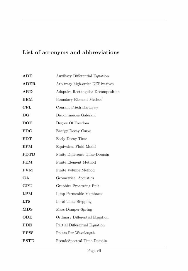
List of acronyms and abbreviations

ADE Auxiliary Differential Equation

ADER Arbitrary high-order DERivatives

ARD Adaptive Rectangular Decomposition

BEM Boundary Element Method

CFL Courant-Friedrichs-Lewy

DG Discontinuous Galerkin

DOF Degree Of Freedom

EDC Energy Decay Curve

EDT Early Decay Time

EFM Equivalent Fluid Model

FDTD Finite Difference Time-Domain

FEM Finite Element Method

FVM Finite Volume Method

GA Geometrical Acoustics

GPU Graphics Processing Pnit

LPM Limp Permeable Membrane

LTS Local Time-Stepping

MDS Mass-Damper-Spring

ODE Ordinary Differential Equation

PDE Partial Differential Equation

PPW Points Per Wavelength

PSTD PseudoSpectral Time-Domain

Page vii

List of abbreviationsRIR Room Impulse Response

RT Reverberation Time

SPL Sound Pressure Level

TDIBC Time-Domain Impedance Boundary Condition

VF Vector Fitting

Page viii

1 General introduction

1.1 Background on room acoustic modelingPeople of modern days spend the main part of their lives in offices, homes,factories, cars, lecture rooms and many other kinds of closed spaces.Meanwhile, sound is all around us, which can be in the form of speech,music and noise. With such daily exposure to indoor sounds 1, satis-factory acoustical environment is of vital importance to our comfort [1],health and well-being [2, 3, 4], work productivity [5, 6, 7, 8] and studyperformance [9, 10]. The need for a pleasant, functional and healthyacoustic environment calls for appropriate guidelines and designs fromacoustical scientists and engineers.

1.1.1 Room acoustics fundamentalsRoom acoustics deals with the study of the behavior of sound wavesin indoor spaces. From a scientific point of view, it aims to understandinfluencing factors on the sound experienced in rooms and thereby to im-prove the acoustical environment of indoor spaces. Generally speaking,a room acoustician needs to take two aspects into account: the physicalprocess of sound generation and propagation in closed spaces, and thepsychological factors related with humans’ perception of sounds [11]. Asstandardized by the international standard ISO 3382 [12, 13, 14], thesetwo aspects are connected through a set of objective and perceptuallyrelevant room acoustic parameters, such as the source-independent re-verberation time and the speech transmission index. These acousticalparameters can serve as guidelines for design purposes to fulfill certainfunctions of the space, and as a reference frame for the comparison andevaluation of room acoustic qualities. They will be discussed in section1.1.3.

1The sources of sound can potentially originate from external locations, e.g., neighbor noise andoutdoor traffic noise.

Page 1

1 General introductionThe fundamental quantities associated with room acoustics include

the acoustic pressure p, the particle velocity vector v = [u, v, w]T , thestatic density of air ρ0 is and the adiabatic sound speed c0; these acous-tical quantities are connected through the mass, momentum and energyconservation laws [15], from which we can derive a linearized set of gov-erning partial differential equations (PDEs), to describe sound propa-gation in free space. For typical room acoustic problems, it is furtherassumed that the propagation medium has zero mean velocity. Underthese assumptions, the following homogeneous (without source term)coupled system of linear equations can be derived

∂v

∂t+

1

ρ0∇p = 0,

∂p

∂t+ ρ0c

20∇ · v = 0, (1.1)

which is equivalent to second-order wave equation,

c20∇2p =∂2p

∂t2. (1.2)

These equations describe the variations in time and space of the acousticvariables p and v. The speed of sound can be calculated from the formulac0 = (331 + 0.6Tr) [m/s], where Tr is the room temperature in Celsius[12]. In this work, Tr is set to 20C and c0 is 343 m/s. Assuming thatthe convention eiωt is used for the harmonic time variation and insertingthe following single frequency ansatz of the form

p(t) = P (ω)eiωt (1.3)

into the wave equation, we obtain the Helmholtz equation

∇2P + k2P = 0, (1.4)

where k is the wavenumber as k = ω/c0.Besides the governing equations describing sound wave propagation,

a complete quantification of a sound field inside a closed space mathe-matically requires a geometrical model of the interested space, boundaryconditions that characterize acoustic properties of surface materials byrelating the acoustic pressure p to the normal component of the parti-cle velocity on the boundaries (treated in Chapter 3 and 4) and soundsources. In this work, sound sources are introduced via the initial condi-tions (see, e.g., Eq. (29) in the appended Paper I); it is thus sufficient to

Page 2


Cha

pter

1

consider homogeneous propagation equations. Even though the physicsof sound generation and free field propagation is well understood fun-damentally, solutions in analytical forms only exists for certain caseswith simple boundary conditions and geometries. For real problems ofinterest, accurate predictions call for advanced numerical techniques.

1.1.2 Room impulse responseRoom acoustic modeling aims to describe sound fields in complex enclo-sures by numerically calculating impulse responses of the space of inter-est. A room impulse response (RIR) is a (pressure) signal as a functionof time at a discrete point in space in response to an acoustic excita-tion. When a room is acoustically considered as a linear time-invariant(LTI) system, the RIR is mathematically defined as the point-to-pointtime-domain transfer function h(t) between a point source q(t) and a spe-cific receiver. The impulse response fully characterizes the propagationbetween the source and the receiver, in terms of both phase and magni-tude, as the acoustic pressure recorded at the receiver for an arbitrarymonopole source signal can be obtained from the convolution theorem

p(t) =

∫ t

−∞h(t− τ)q(τ)dτ, (1.5)

under the assumption of linearity, time-invariance, and limited spatialsupport of the source. This is also the principle behind auralization,which will be elaborated upon in Sec. 1.1.4. Practical measurements ofthe RIR follow the guidelines and procedures documented in ISO 3382[12, 13, 14], which also specify detailed requirements on the equipmentand the source signal. However, the measured RIR is fundamentallyinexact since it is hard to obtain point sources and receivers in practice.

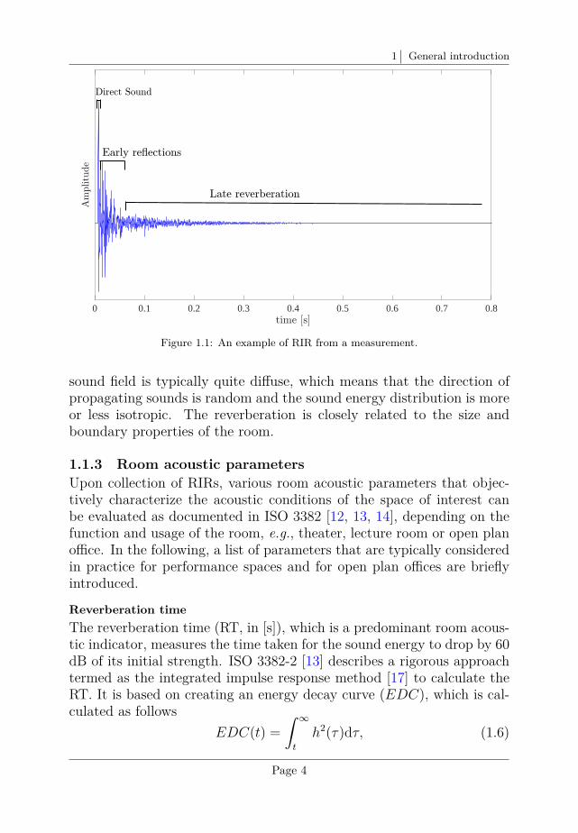
Generally, an RIR consists of three separate parts as shown in Fig.1.1: direct sound, early reflections, and late reverberation. If there isa line of sight between the source and receiver, the direct sound is thesound that arrives at the receiver along the shortest path from the sourcewithout any reflections and is usually perceived as the loudest. Theearly reflections are the sounds that arrive at the receiver undergoingat least one reflection from the walls, ceiling, floor and other potentialindoor objects. The direct sound and the early reflections together aremainly responsible for sound localization by the human brain [16]. Thelate reverberation is the sound that reaches the receiver after the earlyreflections; as a result of the large amount of repetitive reflections, the

Page 3


0 0.1 0.2 0.3 0.4 0.5 0.6 0.7 0.8

Figure 1.1: An example of RIR from a measurement.

sound field is typically quite diffuse, which means that the direction ofpropagating sounds is random and the sound energy distribution is moreor less isotropic. The reverberation is closely related to the size andboundary properties of the room.

1.1.3 Room acoustic parametersUpon collection of RIRs, various room acoustic parameters that objec-tively characterize the acoustic conditions of the space of interest canbe evaluated as documented in ISO 3382 [12, 13, 14], depending on thefunction and usage of the room, e.g., theater, lecture room or open planoffice. In the following, a list of parameters that are typically consideredin practice for performance spaces and for open plan offices are brieflyintroduced.

Reverberation timeThe reverberation time (RT, in [s]), which is a predominant room acous-tic indicator, measures the time taken for the sound energy to drop by 60dB of its initial strength. ISO 3382-2 [13] describes a rigorous approachtermed as the integrated impulse response method [17] to calculate theRT. It is based on creating an energy decay curve (EDC), which is cal-culated as follows

EDC(t) =

∫ ∞

t

h2(τ)dτ, (1.6)

Page 4


Cha

pter

1

where ∞ denotes the time when the sound field reaches the equilibriumstate. If the background noise level is known, ∞ is calculated as the in-tersection between a horizontal line through the background noise and asloping line through a representative part of the squared impulse responsedisplayed using a logarithmic scale [13]. Actually, EDC(t) measures theamount of sound energy that has yet to arrive at the receiver.

The reverberation time is calculated by fitting a linear regression lineto the EDC(t), which is first normalized by the maximum energy leveland plotted in the logarithmic scale, starting from -5 dB. Based on theslope of the fitting line, which specifies the decay rate dr [dB·/s], thereverberation time is the time it takes to reach a 60 dB drop of the soundenergy and amounts to 60/dr. To overcome the issue associated with thebackground noise and the power of the source, the regression range thatis used to calculate the slope can be shortened, for example between -5dB and -25 (or -35) dB. The reverberation time is then labelled as T20

(or T30) accordingly.

It should be noted that reverberation time and every other parameterdescribed in the following are normally evaluated in either octave orone-third octave bands, which require the band-pass filtering of RIRs.A single number also can be retrieved by averaging the RT values inthe 500 Hz and 1000 Hz octave bands. In figure 1.2, the energy decaycurve evaluated for the 500 Hz octave band of the RIR in Fig. 1.1 isshown, along with the linear regression obtained using the evaluationrange [-5,-35] dB.

Early decay time

The early decay time (in [s]), denoted as EDT , measures the initial partof the sound energy decay. Its calculation is similar to the reverberationtime, which involves a linear regression based on the fixed range of 0dB to -10 dB and an extrapolation to a decay time of 60 dB. Sinceboth the direct sound and the early reflection components are coveredin the [-10,0] dB range of EDC(t), EDT is more important subjectivelyand more related to perceived reverberance than T20 or T30 [18]. Foran ideally diffuse sound field with an exponential decay in energy, EDTequals the reverberation time.

Early-to-late index

The early-to-late index (Cte , in [dB]), represents the logarithmic ratiobetween the early arriving and late arriving sound energy. Cte is formally

Page 5


0 0.2 0.4 0.6 0.8-100

-80

-60

-40

-20

0

Figure 1.2: Energy decay curve example and fitting to calculate T30.

calculated as:

Cte = 10 log10

(∫ te0h2(t)dt∫∞

teh2(t)dt

), (1.7)

where te is the early time limit of either 50 ms (suitable for speech con-ditions) or 80 ms (suitable for music conditions). A high value of Cte

indicates that the perceived sound is clear and distinguishable whereas alow value of Cte implies that the audio information is perceptually fuzzyand unclear at the listening position. For this reason, Cte is also referredto as ‘clarity’. Typical values of Cte fall into the range of [-5,5] dB. Foran intelligible speech, C50 should be higher than -2 dB [12].

Center time

The center time (TS, in [ms]), is the time of the center of gravity of thesquared impulse response:

TS = 10 log10

(∫∞0

th2(t)dt∫∞0

h2(t)dt

). (1.8)

The subscript S of TS stands for “Schwerpunktzeit”in German. TS spec-ifies the balance between clarity and reverberance [12]. To be specific,low values of TS allude to a clear sound whereas high values indicate areverberant sound environment. Similar to the clarity, TS is valuable inacoustic evaluations of the speech and music conditions.

Page 6


Cha

pter

1

A-weighted sound pressure level of speech and its spatial decay rate

The A-weighted sound pressure level (SPL) of speech (Lp,A,S) and its spa-tial decay rate (D2,S), as specified in ISO 3382-3 [14], are single numberacoustic parameters indicating the acoustic performances of open planoffices with furnishing, the principal aims of which being to ensure goodspeech privacy and to weaken distractions between workstations. Thesequantities are measured or simulated by placing a single omnidirectionalloudspeaker at one selected working position and by recording the soundpressure signal in other working positions, mimicking the situation wherea single person is talking and others are silent.

The following steps need to be conducted to obtain these parameters.First of all, the SPL at measurement point n (with a distance rn from thesource) in i-th octave band (from 125 Hz to 8000 Hz), which is denotedas Lp,Ls,n,i (index Ls refers to loudspeaker), is calculated by processingmeasured or simulated impulse responses. Then, the corresponding at-tenuation Dn,i in decibels compared to the SPL at a distance of 1 m inthe free field condition (Lp,Ls,1m,i) is determined by

Dn,i = Lp,Ls,1m,i − Lp,Ls,n,i. (1.9)

Given the sound power level of the loudspeaker in octave bands LW,Ls,i,Lp,Ls,1m,i is approximately equal to LW,Ls,i − 11 dB. Upon collections ofDn,i, the SPL of normal speech Lp,S,n,i are calculated as

Lp,S,n,i = Lp,S,1m,i −Dn,i, (1.10)

where Lp,S,1m,i is the SPL of normal speech standardized for normal voiceeffort [14]. Finally, the A-weighted SPL of speech Lp,A,S,n is obtained byadding the A-weighting values Ai in each octave band and the logarithmicsummation:

Lp,A,S,n = 10lg( 7∑

i=1

10Lp,S,n,i+Ai

10

). (1.11)

The spatial decay rate D2,S is calculated by performing a linear regressionof Lp,A,S,n with respect to the receiver distances rn within the range 2 mto 16 m in a logarithmic scale to base 2. Therefore, it indicates the SPLreduction when the distance is doubled. Furthermore, the A-weightedSPL of speech at 4 m (Lp,A,S,4m), which is evaluated in practice as a singlenumber target quantity, is determined based on the linear regression. Forbetter clarification, an example taken from ISO 3382-3 [14] is shown inFig. 1.3.

Page 7


ISO 3382-3:2012(E)

a) The determination of D2,S and Lp,A,S,4 m b) The determination of distraction distance rD

Key KeyLp,A A-weighted sound pressure level y speech transmission indexr distance to the speaker r distance to the speakerD2,S spatial decay rate of speech rD

rP

distraction distance

privacy distanceLp,A,B A-weighted sound pressure level of background noise

Lp,A,S A-weighted sound pressure level of speechLp,A,S,4 m A-weighted sound pressure level of speech at

4 m from the sound source

Figure 3 — Examples of the determination of single number quantities from spatial distribution curves

Table 2 — Reporting single number quantities

Line 1 Line 2STI in the nearest workstation

Distraction distance, rD, in m

Privacy distance, rP, in m (if measured)

Spatial decay rate of A-weighted SPL of speech, D2,S, in dB

A-weighted SPL of speech at 4 metres, Lp,A,S,4 m, in dB

Average A-weighted background noise, Lp,A,B, in dB

10 © ISO 2012 – All rights reserved

NEN-EN-ISO 3382-3:2012

Dit document is door NEN onder licentie verstrekt aan: / This document has been supplied under license by NEN to:Avans Hogeschool Breda 7-11-2014 16:41:01

Figure 1.3: Example of the determination of D2,S and Lp,A,S,4m from Ref. [14]. The whitedots denote the A-weighted SPL of the background noise while the black dots stand for theA-weighted SPL of speech.

1.1.4 ApplicationsWith its ability to accurately reproduce indoor sound behavior, roomacoustic modeling plays an important role in the following applications:

• One application is associated with the realization and improvementof certain acoustic conditions, which are prevalent in many fields,such as architecture design [19, 11, 20]; the acoustic properties ofvarious design or renovation options can be evaluated and furtheroptimized. In such applications, the physical accuracy of the simu-lated sound field is of primary concern. Such modeling proceduresbecome a key step in the early design phase and act as an economi-cal substitute to the traditional acoustic research method using thescaled physical models of spaces.

• The second application category is more inclined to synthesizing acertain spatial immersion or to conveying an aesthetically pleasing

Page 8


Cha

pter

1

auditory feeling, while preserving a desired level of realism. Typ-ical examples are observed in the areas of computer games [21],where artificial reverberation effects [22] are added to mimic re-alistic environments. Here, real-time interaction, which involvesdynamic model attributes such as time-dependent geometry andmoving source/receiver locations, is a priority whereas the accuracyof the detailed physical model is of less concern.

• The last category of application is concerned with the concept ofauralization, which by definition is the process of rendering audible,by physical or mathematical modeling, the sound field of a source ina space, in such a way as to simulate the binaural listening experi-ence at a given position in the modeled space. [23]. In other words,it focuses on creating a virtual auditory environment where the au-ral experience can be as close to reality as possible [24, 25, 26]. Ina technical sense, auralization requires an (binaural) RIR as accu-rate as possible with limited computational resources, and thereforeis more challenging compared to the previous two types of applica-tions. Driven by the vast potential of application needs, recent yearshave witnessed great advancements of auralization in various sce-narios, for example building design [27, 28] and cognitive training[29].

1.2 State-of-the-art room acoustic modelingtechniques

The concept of room acoustic simulation was conceived by Schroeder[30] in the early 1960s. Since then, numerous modeling techniques havebeen developed along with the advancement of ever-increasing comput-ing power. Depending on their fundamental assumptions, room acous-tic modeling approaches fall in general into two categories: geometricalacoustics (GA) methods and wave-based methods.

It should be mentioned that in literature there exists another type ofenergy-based method called the diffusion equation method, which is effi-cient in modeling the reverberation tail of impulse responses. Comparedto traditional statistical models of a perfectly diffuse sound field withlimited applicability and accuracy [11], it allows for local variations ofenergy densities [31] and is considered more accurate for practical roomscenarios. One influencing factor on the accuracy in practice is related tothe difficulty to obtain the controlling parameters of the diffusion process

Page 9

1 General introductionfor complex geometries. Further details of the diffusion equation methodcan be found in Refs. [32, 33, 34].

Besides, data driven techniques and machine learning have spurredrejuvenated interest in the field of acoustics [35]. Recent related de-velopments include machine learning methods for the simulating wavepropagation [36], artificial/convolutional neural network techniques forfast auralization [37, 38] and estimation of sound scattering [39], unsuper-vised machine learning algorithm for reduced-order modeling of travelingwaves [40]. More kinds of techniques for room acoustic modeling, whichare not established enough yet, could be expected in the future.

1.2.1 Geometrical acousticsGeometrical room acoustic modeling techniques treat sound waves asrays without fully considering the wave nature of sound. Generally, thisfundamental assumption is valid at high frequencies, where the largestwavelength of interest is supposed to be at least one order of magnitudesmaller than the relevant geometry details [41]. The main approachesare the image source method and the ray tracing method.Image source methodsThe concept of image source was applied to room acoustics by Eyring in1930 [42] to predict the reverberation time. In 1972, Gibbs and Jonesapplied the image source method for calculating the variation in soundpressure level in a rectangular room with various absorption configura-tions [43]. The first open source code of the algorithm was published byAllen and Berkeley in 1979 [44]. Extension of the image source methodto arbitrary polyhedra was described by Borish [45], where the first ex-tensive attempt to check the validity and visibility of reflection pathswas made.

In the image source method, a sound propagation path originatesfrom the source and then reflects on the boundary surface specularly.Each reflection is represented using a secondary source, the intensity ofwhich depends on the traveling distance and absorption properties of thesurface. One deterministically considers all specular reflection paths froma source to a receiver by mirroring the image sources at each reflectionsurface recursively. During this process, the sound field is collected. Therecursion process continues until a given reflection order is achieved orthe reflected component has lost a certain percentage of its initial energylevel.

The computational cost of the image source method increases dra-matically with the order of reflections. Furthermore, it is generally able

Page 10


Cha

pter

1

to obtain an accurate approximation of the early reflections in an RIR.However, only specular reflections are taken into account naturally andsound diffusion is neglected. Also, handling non-trivial geometries re-quires significant implementation efforts.Ray tracing methodsOne of the earliest application of ray tracing method in room acousticmodeling was proposed by Krokstad et al. [46] in 1968. In ray tracing, agiven number of rays carrying a finite amount of energy is emitted fromthe source location in directions that follow the desired source directivity.For each ray, the energy remains constant during the free propagation[47] and its reflection on the boundary surfaces follows the geometriclaw of specular reflection. After each reflection, a certain amount of en-ergy is deducted from the previous energy level. A ray terminates itspath upon hitting the volume surrounding the receiver or experiencinga sufficient energy decay. The elapsed time since the source excitationis recorded. Main drawbacks of ray tracing include the accuracy degra-dation in modeling diffraction, negligence of important early reflectionpaths and inclusion of duplicated or invalid recorded ray paths [48].

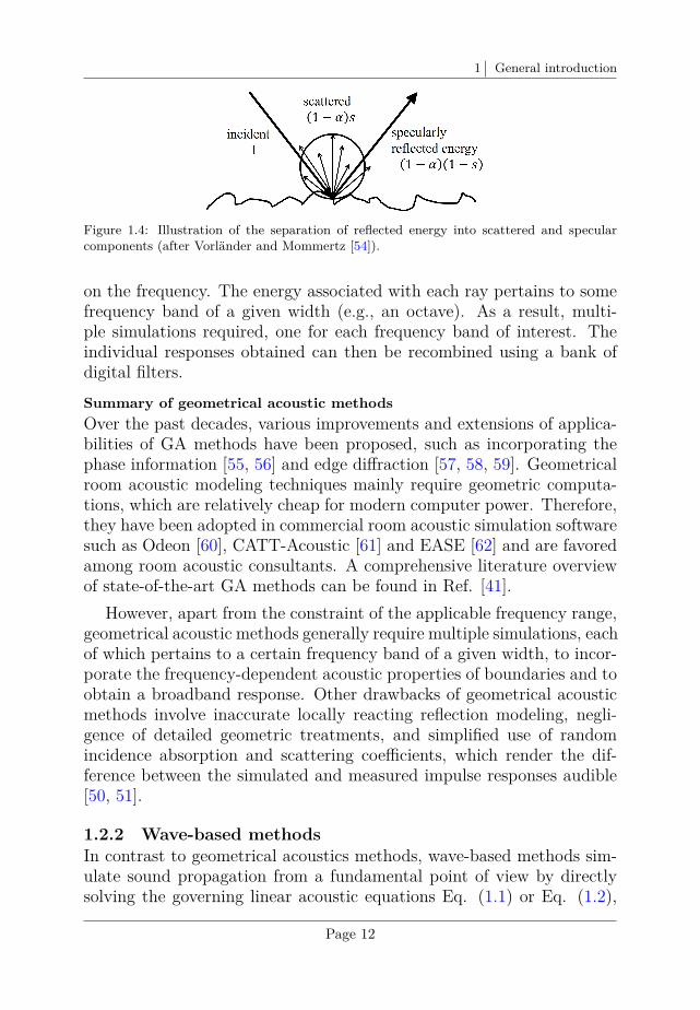
When sound rays hit surfaces in a room, a portion of the sound energyis absorbed as characterized by the absorption coefficient α, while theremaining parts are reflected either specularly or non-specularly (scat-tered). The ratio of the non-specularly reflected sound energy to thetotal reflected energy defines the scattering coefficient s [49] as illus-trated in Fig. 1.4. It is found that the inclusion of scattering effectsgenerated by edges and surface roughness is effective in improving theaccuracy of room acoustic parameters that hinge on early reflections,such as early decay time and clarity [50, 51, 52]. The scattering coef-ficient alone is inadequate at describing the complex acoustic behaviorof scattering surfaces. In order to describe the spatial distribution ofthe scattered sound, the diffusion coefficient is defined to quantify thedegree of uniformity of the polar response of a surface. If the energyis scattered uniformly in all directions, then the diffusion coefficient 2

is equal to one. If all the energy is scattered in one direction, then thediffusion coefficient is equal to zero [11]. It was demonstrated that theincorporation of the diffuse surface reflections into the ray tracing modelleads to better prediction accuracy[53].

Frequency dependency can be added by splitting the energy spectruminto frequency bands and making the absorption coefficients dependent

2Here, diffusion refers to the diffuse reflection, not volume diffusion.

Page 11


Figure 1.4: Illustration of the separation of reflected energy into scattered and specularcomponents (after Vorländer and Mommertz [54]).

on the frequency. The energy associated with each ray pertains to somefrequency band of a given width (e.g., an octave). As a result, multi-ple simulations required, one for each frequency band of interest. Theindividual responses obtained can then be recombined using a bank ofdigital filters.Summary of geometrical acoustic methodsOver the past decades, various improvements and extensions of applica-bilities of GA methods have been proposed, such as incorporating thephase information [55, 56] and edge diffraction [57, 58, 59]. Geometricalroom acoustic modeling techniques mainly require geometric computa-tions, which are relatively cheap for modern computer power. Therefore,they have been adopted in commercial room acoustic simulation softwaresuch as Odeon [60], CATT-Acoustic [61] and EASE [62] and are favoredamong room acoustic consultants. A comprehensive literature overviewof state-of-the-art GA methods can be found in Ref. [41].

However, apart from the constraint of the applicable frequency range,geometrical acoustic methods generally require multiple simulations, eachof which pertains to a certain frequency band of a given width, to incor-porate the frequency-dependent acoustic properties of boundaries and toobtain a broadband response. Other drawbacks of geometrical acousticmethods involve inaccurate locally reacting reflection modeling, negli-gence of detailed geometric treatments, and simplified use of randomincidence absorption and scattering coefficients, which render the dif-ference between the simulated and measured impulse responses audible[50, 51].

1.2.2 Wave-based methodsIn contrast to geometrical acoustics methods, wave-based methods sim-ulate sound propagation from a fundamental point of view by directlysolving the governing linear acoustic equations Eq. (1.1) or Eq. (1.2),

Page 12


Cha

pter

1

based on numerical approximation techniques. Therefore, wave-basedmethods are able to capture wave phenomena such as scattering, diffrac-tion and interference effects with no/fewer inherent constraints on thefrequency range.

Wave-based methods can be classified into two types: time-domainmethods and frequency-domain methods. Particularly, time-domain ap-proaches, which are in line with the physical nature of sound propaga-tion, have the benefits of calculating the solution over a broad frequencyrange. Furthermore, they are capable of handling room acoustic scenar-ios involving moving sources. However, frequency-domain approachesare preferred by certain methods due to their nature of numerical for-mulations. Time-domain methods generally follow the methodology ofthe method of lines, where spatial derivatives are treated first and thentime integration is performed at each time step. In the following, an ab-stract and not-exhaustive overview of a variety of wave-based methodsis presented as they are the main focus of this thesis, including the finitedifference time-domain method, the spectral method, the finite volumemethod, the finite element method and the boundary element method.Finite Difference Time-Domain methodsAmong the wave-based methods, the finite difference time-domain (FDTD)methods, which originated from the computational electromagnetics com-munity [63, 64] in the middle of 1960s, are so far the most establishedand popular numerical techniques for room acoustic simulation purposes.Due to their simplicity and relative ease of implementation, finite differ-ence methods have been widely used in many engineering applications,including computational acoustics [65, 66, 67, 68, 69]. Their applicabilityto time-domain room acoustic modeling were firstly and independentlyinvestigated by Chiba et al. [70], Savioja et al. [71] and Botteldooren[72, 73] in the 1990’s.

As a class of numerical techniques for solving PDEs, the finite differ-ence methods discretize both the spatial domain and time interval intodiscrete points. The PDEs are converted into algebraic equations by ap-proximating derivatives with finite differences from nearby points basedon polynomial interpolants. The solution values at these discrete pointsare calculated approximately by solving the resulting algebraic equations.To date, considerable research efforts have been devoted to improveFDTD methods for room acoustic simulations in various aspects, includ-ing high-order accuracy schemes [74, 75, 76, 77, 78, 79, 80, 81], soundsource modeling [82, 83, 84, 85, 86], high-performance-computing imple-mentations with the graphics processing unit (GPU) and parallelization

Page 13

1 General introduction[87, 88, 89, 90], real-time applications [91] and impedance boundary mod-eling [92, 93, 94, 95, 96, 97].

However, despite their remarkable features, FDTD methods are plaguedwith its inherent lack of geometric flexibility due to their use of struc-tured meshes. Consequently, their application is mostly restricted toproblems with simple geometries. If the Cartesian grid discretization isemployed, curved geometries have to be represented with a staircase ap-proximation, which is only accurate for cases where the shape variationsare relatively large compared to the smallest wavelength of interest [98];otherwise, significant errors arise in estimating sound scattering and re-flection [98, 99]. Another strategy to deal with practical geometries is touse a multi-block approach or curvilinear meshes [100, 101], where thephysical domain is mapped onto several Cartesian grid blocks through(non-)linear geometric transformations.

It is worth mentioning that there is another class of closely-relatedtechniques referred to as the digital waveguide mesh methods [102, 103,104, 105, 84] that share similar formulations with FDTD methods. Asystematic elaboration of the functional equivalence of these two ap-proaches and the conditions for building mixed models are presented inRef. [106]. Since FDTD methods are not the main focus of this the-sis, interested readers can refer to the PhD thesis of Hamilton [98] andvan Mourik [107] for an in-depth discussion of uses and developments ofFDTD methods in room acoustic simulations; their applications withinthe context of auralization can be found in the PhD thesis of Saarelma[108].

Spectral methodsAnother broad class of methods that rely on structured grids for theapproximation of spatial derivatives are the (pseudo) spectral methods[109, 110, 111, 112]. In contrast to finite difference methods, whichapproximate the solutions at any given point with a local polynomial in-terpolant based on information at neighboring points, spectral methodsexpand the unknown solutions with a global orthogonal polynomial basis.Depending on the type of global basis employed, spectral methods canbe further classified, e.g., Fourier spectral methods (for periodic prob-lems) and Chebyshev spectral methods (for non-periodic cases). Furtherdistinguishment arises from the different ways to calculate the expan-sion coefficients of the global basis, e.g., the Tau approach, the Galerkinapproach and the collocation approach [113, 114].

In the general context of solving time-dependent PDEs, spectral meth-

Page 14


Cha

pter

1

ods exhibit several appealing properties. First of all, as a result of thespectral expansion, evaluations of the spatial derivative are transformedfrom the physical space to the space of the polynomial basis (wavenumberspace in the case of Fourier basis), and hence can be performed pseudo-analytically. It implies that for periodic problems, there is no dispersionerror from the spatial discretization and exponential convergence rate isachieved [114]. The efficient implementations of pseudospectral methodsbenefit greatly from the fast Fourier transform (FFT) algorithm devel-oped by Cooley and Tukey [115]. Theoretically, Fourier spectral methodsneed only two points per wavelength (PPW) while Chebyshev methodsneed π PPW on condition that the approximated solutions are suffi-ciently smooth and periodic. However, periodic boundary conditions arehardly met in practice and a larger number of PPW is needed to capturethe geometrical details of the physical space. Furthermore, compared toFDTD, the advantage of higher convergence rate comes at a cost of themore stringent Courant-Friedrichs-Lewy (CFL) condition [116].

In the specific field of room acoustics modeling, adaptive rectangu-lar decomposition (ARD) methods [117, 118] and pseudospectral time-domain methods (PSTD) [119, 120, 121] have been applied based on theFourier basis. Combined with domain decomposition techniques, theydemonstrate attractive computational efficiency for problems with rela-tively simple geometries and boundary conditions. However, like FDTDmethods, several factors result in difficulties or inefficiencies for roomacoustics when using spectral methods. For example, an extra errorarises from communication across the interface between sub-domains.Another challenging issue that remains to be addressed is the accurateand efficient modeling of frequency-dependent impedance boundary con-ditions.Finite Volume methodsFinite volume methods (FVM) overcome the geometric flexibility issuesof methods based on structured grids by utilizing an unstructured tes-sellation of the computational domain in the form of polygonal or poly-hedral elements (cells in the nomenclature of FVM). In contrast to finitedifference and spectral methods, FVM operates on the integral form ofthe governing PDEs, where the divergence term is converted to a sur-face integral using the divergence theorem. Specifically, the integral ofunknown solutions over each grid cell at one time instant, also known asthe cell average, is approximated and tracked. In each time step, thesecell averages are updated using approximations to the fluxes through thecell edges. A high-order accuracy is achieved by using local polynomial

Page 15

1 General introductionreconstructions with nearby cell averages in the construction of numeri-cal flux functions. A popular choice is the upwind flux [122] and it relieson the solutions to the Riemann problem, which is simply the govern-ing equation with piecewise constant initial data that has a single jumpdiscontinuity [123].

FVM has undergone decades of developments in various fields of en-gineering, especially for computational fluid dynamics. Its application inroom acoustic simulation started from the work of Botteldooren [72]. Re-cent developments include locally reacting frequency dependent bound-aries [124, 125] and air absorption [126]. However, the main limitation ofFVM lies in its difficulty to achieve high-order accuracy (beyond second-order) on general multi-dimensional unstructured meshes in an efficientway.

Finite Element methodsThe continuous finite element methods (FEM), which first appearedin wave-based analysis of room acoustic modes in 1965 [127], consti-tute another class of methods that operate on unstructured meshes, andtherefore are suitable for problems with complex geometries. The dis-cretization strategy is characterized by the variational (weak) formula-tion. Usually, the Bubnov-Galerkin approach is followed, which meansthat the function space for both test functions and solution functions arethe same.

In contrast to FVM, FEM uses piecewise polynomial interpolationsinside each element, ensuring high-order approximations locally withoutthe need of large stencils across neighboring elements. Since the nodesalong the faces of neighboring elements are shared, the basis functionsare continuous across elements and essentially globally defined. As aresult, the discretized system is implicitly coupled between the elements,implying that a large sparse linear system is needed to be solved using adirect or an iterative approach. This poses computational challenges forlarge scale 3D problems. Generally speaking, FEM is a natural choice forelliptic boundary value problems, such as the Helmholtz equation (1.4)and therefore it is mainly used for modeling room acoustic problems inthe frequency domain [128, 129, 130, 131, 132, 133].

Applications of FEM to time-domain room acoustic modeling havebeen investigated by Okuzono et al., using the implicit Newmark timeintegration scheme with preconditioned iterative solver [134, 135, 136]or the explicit time integration scheme with the mass lumping tech-nique [137]. Recently, a high-order variant of FEM, the so-called spec-

Page 16


Cha

pter

1

tral element method (SEM) [138, 139] was applied to time-domain roomacoustic modeling by Pind et al. [140], where the mass lumping tech-nique [141] is adopted to increase the efficiency and a formulation offrequency-dependent impedance boundary condition is presented.Boundary Element methodsBoundary element methods (BEM) are established numerical techniquesto solve boundary-value problems based on a discretization of the bound-aries of the space of interest, different from the aforementioned methodsthat employ a spatial (volumetric) discretization. In the field of acous-tics, pioneering work began in 1960s [142], which predicted sound ra-diation from an arbitrary vibrating body immersed in an infinite fluidmedium. The governing equation to be numerically solved in the timedomain is the integral form of the wave equation known as the Kirchhoffintegral equation, whereas in the frequency domain, it is the integralform of the Helmholtz equation, i.e., the Kirchhoff-Helmholtz integralequation, both of which are derived based on the divergence theorem.These integral equations fundamentally state that the acoustic pressureat an arbitrary location is determined by the distribution of the acousticpressure and its normal derivative (normal velocity) on the boundarysurface [143].

Depending on the way to solve the unknown pressure along the bound-aries and to fulfill the integral equation, BEM can be classified into thecollocation approach [144, 145] and the variational approach [146]. To ad-dress the inherent non-uniqueness problem of the frequency domain for-mulation at certain frequencies, the Burton-Miller formulation [147] andthe combined Helmholtz integral equation formulation (CHIEF) [148]were proposed. To predict the extended reaction in a cavity containingsound absorbing materials, a multi-domain method, which enforces thecontinuity condition of the normal velocity and acoustic pressure at theinterface, can be employed [149]. To overcome the difficulty of model-ing thin objects for conventional BEM, indirect BEM using degenerateboundary formulation is introduced [150, 151].

Since only the boundaries need to be discretized in the form of un-structured elements, the number of degrees of freedom (DOFs) is signifi-cantly reduced compared to volumetric discretization methods discussedso far. In general, BEM is considered efficient for exterior problemsinvolving sound radiation and scattering phenomena in homogeneousmedia [152]. However, the benefit of dimension reduction comes at acost of solving dense discretization matrices, making it difficult to ap-ply the BEM to large-scale problems. Remedies using the fast-multipole

Page 17

1 General introductionmethods [153, 154] are used to speed up the analysis of sound fields[155, 156, 157]. Applications of time-domain BEM to room acousticanalysis are presented in Refs. [158, 159].

1.2.3 Hybrid methodsEach of the above mentioned room acoustic modeling methods has itsown merits and limitations. It can therefore be beneficial to adopt ahybrid methodology, thus exploiting the advantage of each contributingmethod and achieving a decent balance in terms of the accuracy, com-putational cost and applicable frequency range. There are various kindsof hybridizations. For example, hybrid GA models tend to utilize theimage source method to simulate the early specular reflection paths andray tracing or radiosity-based techniques for the late reverberation partof the impulse response [160].

Hybridizing of GA and wave-based methods can be a feasible solutionto addressing the issue of the wide audible frequency range. Wave-basedmethods are used for the low frequencies, where the wavelengths areclose to the characteristic dimensions of rooms (and objects) and wavephenomena dominate the acoustics, while GA methods are employedfor high frequencies [161, 162, 163, 164, 165, 166, 167]. The crossoverfrequency is generally case-dependent based on acoustic characteristicsof rooms. The Schroeder frequency [11], which approximately indicatesthe boundary between overlapping and distinguishable resonant roommodes, is usually used as a rough estimate of the upper limit of thelow-frequency range.

Hybrid methods that spatially couple different wave-based methodsalso exist, the fundamental principle behind which is the spatial domaindecomposition. A popular strategy is to utilize more efficient methodsto treat the interior domain with relatively simple geometries and largevolumes, and to use more accurate but time-consuming methods nearthe boundaries. Examples include the hybrid of the ARD method withFDTD [117, 118], the hybrid of the PSTD method with FEM [168], andthe hybrid of the FVM with FDTD [124, 126].

1.2.4 Summary and discussionTo the best of the author’s knowledge, the properties and capabilitiesof each wave-based method discussed so far is summarized in terms ofentries listed in Table 1.1. The entry of “explicit semi-discrete form” isrelevant for time-domain approaches, and the explicit formulation savesthe trouble of using an iterative solver to solve large linear systems of

Page 18


Cha

pter

1

equations. It should be noted that some of the issues and restrictionscould be addressed and overcome with on-going active research efforts.Nevertheless, this comparison does highlight the most obvious shortcom-ings of each method that need to be resolved for room acoustic modeling.

Table 1.1: A summary of generic properties of the state-of-the-art wave-based methods forroom acoustic modeling. The numbers represent to what extent the properties are addressedin the respective method. 1 means it can be well handled; 2 indicates efforts are needed toresolve the issue; 3 implies even more efforts are needed.

FDTD Spectral M. FVM FEM BEMGeometric flexibility 3 3 1 1 2High-order accuracy 1 1 3 1 1

Impedance boundary conditions 1 3 1 1 1Explicit semi-discrete form 1 1 1 2 3

Parallel computing 1 1 1 2 2

Generally speaking, wave-based methods, which are built upon nu-merically solving the fundamental physical laws governing sound prop-agation, have relatively higher accuracy compared to geometrical roomacoustic modeling techniques and energy-based methods for both thefree propagation and the interaction with boundaries, especially in thelow-frequency range. Furthermore, compared to other approaches, it ismore natural and straightforward to integrate wave-based sound propa-gation modeling with other fields of modeling that are relevant to roomacoustics. For example, direct modeling of (multiple) directional sourceby coupling sound emitting physical objects with the propagation media[169, 170, 171] can be realized more easily with wave-based methods. Onthis account, the framework of sound synthesis can be connected withroom acoustic modeling. More than that, binaural sound localisationcan be realized naturally by incorporating head and torso models intothe simulated space [172, 173].

However, a general criticism of wave-based methods is that the com-putational cost can become prohibitive. As a general rule of thumb,state-of-the-art wave-based methods typically require spatial discretiza-tion resolution of 6 up to 10 PPW for the sake of the dispersion and dis-sipation error [174] arising from the numerical approximation. In 3D, thedegrees of freedoms for volumetric discretization techniques scale withthe maximum frequency of interest fmax as O(f 3

max). Therefore, it isgenerally acknowledged that acoustic simulations of large rooms at highfrequencies remain a challenging issue for the foreseen future. However,

Page 19

1 General introductionlow- and mid-frequency calculations are becoming more and more feasi-ble, and the upper limit of the applicable frequency range is expandedthanks to the ever-growing computing power with parallel architectures[87, 88, 89, 90].

1.3 Thesis objective and main contributionsThis PhD project is motivated towards an efficient, robust and accuratewave-based room acoustic modeling technique. Following the discussionspresented in the previous section and reflecting on the state-of-the-artnumerical modeling techniques, the time-domain discontinuous Galerkin(DG) method is chosen as the focus of this thesis, since it possesses eachof the attractive properties listed in Table 1.1. As will be discussed inChapter 2, the DG method is a well-established numerical approximationtechnique for solving partial differential equations that govern variousphysical processes. However, its applications to room acoustic modelingwas far less developed at the outset of this PhD project. Therefore, itis the goal of this work to develop the necessary formulations of the DGmethod for room acoustic modeling purposes, and to perform validationsagainst analytical, numerical and measurement results.

The main contributions of this thesis are as follows:

• For room acoustic modeling purposes, the performance of the time-domain nodal DG method is evaluated. A comprehensive derivationof the nodal DG scheme for solving the linear acoustic equations ispresented. A formulation of real-valued impedance boundary con-dition is proposed as a preliminary attempt to simulate the soundabsorption phenomena along the boundaries. The semi-discrete sta-bility of the scheme is analyzed using the energy method. Verifi-cations are performed against analytical solutions, demonstratingthe convergence of the scheme. As a collaborative work, simulationresults for a real empty room are compared with measured resultsand a good match is observed in 1/3 octave bands.

• A high-order accurate and generic time-domain impedance bound-ary condition formulation for locally reacting materials is devel-oped and validated, aiming at a further step towards a fully-fledgedtime-domain DG solver for realistic room acoustic simulations. Thebenefits of using a high-order basis in terms of cost-efficiency andmemory-efficiency is demonstrated with numerical experiments. Theapplicability of the proposed formulation for modeling real-world

Page 20


Cha

pter

1

materials is demonstrated through an example of a rigidly-backedglass-wool baffle.

• Following the impedance boundary formulation, a formulation ofbroadband time-domain transmission boundary conditions for lo-cally reacting surfaces is proposed and validated. A few examplesof sound transmissive boundaries are presented to illustrate the ap-plicability of the scheme to handle practical scenarios.

• A numerical scheme of arbitrary order of accuracy in both spaceand time, based on the arbitrary high-order derivatives (ADER)methodology, for linear acoustic wave propagation is developed andvalidated. The scheme combines the nodal DG method for the spa-tial discretization and Taylor series integrator for the time integra-tion. A novel local time-stepping approach is proposed to increasethe simulation efficiency for realistic problems containing geometricor parametric constraints without losing high-order accuracy.

• A preliminary application to the room acoustic simulations of areal open plan office in the low-frequency range is explored, with thepurpose of assessing the accuracy and applicability of the developedtime-domain nodal DG method for a realistic sound field analysis bycomparing simulation results with the results from measurements.

1.4 Thesis structure and related publicationsThe thesis is mainly based on work presented in the appended JournalPapers. Each of the following chapter summarizes the main findingsand contributions of each paper respectively. Additional comments arepresented where necessary. The rest of the thesis is structured as follows.

• Chapter 2 is mainly based on the appended Paper I.This chapter lays the foundation of this thesis, where the position-ing of time-domain DG method as a wave-based method for roomacoustic modeling purposes has been addressed. It introduces themain ingredients of the DG method and reviews its development inthe general context of the computational physics community. Then,a brief overview of the content of Paper I follows.

• Chapter 3 is mainly based on the appended Paper II.This chapter is devoted to the accurate modeling of sound reflec-tion and absorption along locally reacting impedance boundarieswithin the time-domain DG framework. An introduction of acoustic

Page 21

1 General introductionboundary conditions under the extendedly and locally reacting as-sumption is presented first, followed by the discussion on the poroussound absorber. A brief review of time-domain impedance bound-ary condition formulation is presented. Lastly, the main content ofPaper II are summarized.

• Chapter 4 is mainly based on the appended Paper III.This chapter presents a formulation of broadband time-domain trans-mission boundary conditions for locally reacting surfaces in theframework of the time-domain DG method. It begins with a shortliterature review on sound transmission modeling in the context ofroom acoustics. Then, a summary of the main contributions ofPaper III is given. Additionally, the formulation of simulatingan acoustic boundary modeled by a limp permeable membrane ispresented.

• Chapter 5 is mainly based on the appended Paper IV.This chapter aiming at accelerating realistic room acoustic simula-tions with the time-domain DG method. To achieve this goal, wefirst explore the challenges associated with time integration schemesand identify the need for a more efficient scheme, in the presenceof geometric or parametric constraints that limit time step sizes. Ashort review of publications produced in this context is summarized.Then, the main contributions of Paper IV are presented.

• Chapter 6 is mainly based on the appended Paper V.This chapter is related to validating the developed time-domain DGwave-based solver by means of a realistic case study. The simulationresults are compared against measurements for a real open-planoffice. As complements to the content of Paper V, a discussion onretrieving accurate acoustical boundary conditions from measuredabsorption coefficients data is introduced first, followed by moredetails on the mesh generation.

• Chapter 7 contains concluding remarks and insights for futurework.

Page 22

2 Room acoustic modeling with the time-domainnodal discontinuous Galerkin method

The purpose of this chapter is to introduce the time-domain discon-tinuous Galerkin (DG) method for room acoustics modeling purposes.It begins with a brief discussion and with the development of the DGmethod in the general context of the computational physics community.Then, a brief overview of the content of Paper I and a summary of itsmain contributions are presented.

2.1 A conceptual introduction of the DG methodThe discontinuous Galerkin (DG) method, as a subtype of the finite el-ement method (FEM), is based on locally piecewise polynomial approx-imations to represent the unknown solutions. It supports both struc-tured and unstructured mesh elements of various shapes as the genericFEM. Different from the (classical) FEM that utilizes continuous ba-sis functions, DG method uses basis functions that can be completelydiscontinuous across the interface of neighboring mesh elements to ap-proximate the unknown variables, where duplicated solutions exist at allnodes, as shown in Fig. 2.1. As a result of this discontinuity, the weakformulation can be obtained by performing the Galerkin projection lo-cally, i.e., by setting the local residual of the approximated governingequation orthogonal to all test functions. Following the same idea asFVM, the divergence term inside the weak formulation is converted intoa surface flux using Gauss’ theorem. The surface flux, which is referredto as the numerical flux, is a single valued function that depends on thesolution values at the element surfaces from both sides of the interface.The numerical flux serves not only to couple the elements, but also toenforce boundary conditions, which is also illustrated in Fig. 2.1.

The construction of local polynomial approximations and subsequent

Page 23

2 Room acoustic modeling with the time-domain nodal discontinuous Galerkin method

Figure 2.1: Illustration of the difference between the continuous Galerkin (CG) and thediscontinuous Galerkin (DG) FEM in a 2D domain. Dk denotes the space elements and qk

is the corresponding local approximation. The height of the vertical dotted line denotes thesolution values. For the DG-FEM, there are steps, denoted as dq, between the approxima-tions of neighboring elements, which introduce the need for the numerical fluxes f∗, e.g.,f∗21 and f∗

23 for the element Dk2 . The boundary conditions are imposed weakly through thenumerical flux f∗

2b as well.

evaluations of volume and surface integrals can be conducted in variousways, which further classify different approaches, e.g., the modal andnodal approaches. The calculation of the numerical flux, which is theonly non-local operation involving different elements, involves only thesolution nodes on the element surfaces, whereas the volume integrationdepends on all interior nodes inside the element.

Following the method of lines, the semi-discrete formulation obtainedfrom the spatial discretization of the DG method can be marched intime with general ordinary differential equation (ODE) solvers, e.g., theRunge-Kutta method [81]. It should be noted that the semi-discreteformulation can be easily rewritten in ODE form due to the fact thatthe spatial matrices can be easily inverted.

Similar to FVM, the DG method exhibits strong stability and ro-bustness when dealing with sharp gradients or even jumps in materialproperties that are aligned with the mesh, making it suitable for nu-merically solving time-dependent hyperbolic PDEs, such as the linearacoustic equations under consideration here. However, the high-orderrepresentation of the solutions in each cell of FVM, which involves thepolynomial reconstruction procedure using a large stencil of cells on gen-eral multi-dimensional unstructured grids, is not necessary for the DGmethod, since the solutions within each element are approximated lo-cally using high-order polynomials. Therefore, the DG method may beconsidered as a favorable combination of FVM and FEM. Furthermore,

Page 24


Cha

pter

2

the DG method offers great flexibility in local mesh and order adaptivity.Because most operations are performed elementwise, it allows for easyparallelization with a significant acceleration potential [175, 176].

Historically, the DG method was firstly introduced in 1973 by Reedand Hill [177] in the framework of neutron transport problems and waslater analyzed by Lesaint and Raviart [178]. The stability and errorestimates for the DG method applied to a linear hyperbolic equationwere first proved by Johnson and Pitkäranta [179] in 1986. Eigensolutionanalysis to the linear wave equations can be found in Refs. [180, 181,182, 183]. Developments of the DG method for non-linear hyperbolicconservation laws were carried out by Cockburn et al. in a series of papers[184, 185, 186, 187]. In related work, Atkins and Shu [188] proposed aquadrature-free implementation that achieves a significant reduction incomputational cost and storage requirements. Interested readers canrefer to more extensive literature [189, 190, 191], which contains moredetailed discussions and references concerning the development of DGin all aspects including algorithm design, implementations, analysis andapplications.

The DG method has enjoyed substantial development in recent yearsin diverse fields such as electromagnetics [192, 193], seismology [194],poroelastic wave modeling [195], elastic-acoustic wave propagation [196,197, 171], aeroacoustics [198, 199, 200, 201, 202], shallow water modeling[203], coastal ocean modeling [204], computational fluid dynamics [139].However, it has never been used for room acoustic modeling by the timePaper I was published.

2.2 Overview of Paper IPaper I aims to address the positioning of time-domain DG as a wave-based method for room acoustics. This paper begins with a brief reviewof the state-of-the-art room acoustic modeling techniques, highlightingthe necessity of using wave-based methods for low-frequency problems.Then, general features of the DG method are introduced, demonstratingits strong potential for room acoustic problems. Meanwhile, develop-ments needed to achieve a fully-fledged DG method for room acousticmodeling, such as a proper formulation of impedance boundary condi-tions, are identified.

The equations governing wave propagation in the context of roomacoustics are the linear acoustic equations introduced in Eq. (1.1), whichare derived from the general conservation laws [15]. To numerically solve

Page 25

2 Room acoustic modeling with the time-domain nodal discontinuous Galerkin methodthe governing equations, the nodal DG method is used for the evaluationof the spatial derivatives, and for the time-integration an explicit multi-stage Runge-Kutta method [200] is adopted. The main ingredients forthe spatial discretization are adopted directly from the nodal formulationpresented by Hesthaven and Warburton [190], including the constructionof local approximations using a multi-dimensional Lagrange polynomialbasis with an α-optimized node distribution [205], and efficient calcula-tions of mass, stiffness, and surface integral matrices. The derivation ofthe upwind numerical flux associated with the linear acoustic equationsis presented, which completes the semi-discrete formulation for free-fieldpropagation. To provide insight into the numerical dissipation and dis-persion properties of the DG scheme, relevant literature is referred toand major findings are summarized.

To deal with sound absorption on the boundaries, a frequency-independent real-valued impedance boundary formulation is proposed,and is incorporated into the scheme via the upwind flux along theboundaries. The principle behind the formulation is that the charac-teristic waves [206, 207] of the linear acoustic equations, which appearin the definition of the upwind numerical flux and are thus evaluatednodally, act as plane waves locally along the normal direction to theboundary surfaces. Therefore, incoming (reflected) characteristic wavescan be calculated as a product of the plane wave reflection coefficientand the outgoing (incident) characteristic waves. The semi-discretestability of the spatial DG operator together with the proposedimpedance boundary conditions is analyzed using the energy method.It is proven that the semi-discrete system resulting from the DGdiscretization is unconditionally stable for passive boundary conditionswith a real-valued impedance. It is worth mentioning that the reflectioncoefficient also enables the use of all real-valued impedance boundaryconditions regardless of the imposed impedance values, sparing theneed for exceptional treatments even for singular cases such as aninfinitely hard wall and soft wall. A discussion on the discrete stabilityof the scheme is presented and a criterion for choosing the time step ispresented.

To evaluate the performance of the time-domain DG method for roomacoustics problems, various 3D numerical tests are presented.

• The first test is a free field propagation of a single frequency planewave with periodic boundary conditions. In this case, the dissipa-tion errors and the dispersion errors are quantified with respect to

Page 26


Cha

pter

2

the number of PPW and the propagation distance.

• The second configuration is a sound source over an impedanceplane. The convergence of the spherical wave reflection coefficientunder two different angles of incidence is verified for frequency-independent impedance boundary conditions. It is also found thatthe accuracy is rather independent from the incidence angle.

• As a third scenario, a cuboid room with rigid boundaries is used, forwhich a long-time (10 seconds) simulation is run. By comparing thenumerical results against the analytical solution, it can be concludedagain that with increasing spatial resolution, the dispersion anddissipation errors become monotonously small, i.e., convergence isachieved.

• Finally, the comparison in terms of the narrow and 1/3 octave bandssound pressure level between numerical and experimental solutionsshows that DG is a suitable tool for acoustic predictions in rooms.Taking into account that only one uniform real-valued impedancehas been used for the whole frequency range of interest, the compar-ison against the measurement is quite satisfactory. In this case, theincorporation of frequency dependent boundary conditions woulddefinitely help to produce a better match with the real measure-ments. This topic will be addressed in the following chapter.

Page 27

3 Time-domain locally reacting impedanceboundary conditions

While the fundamental recipe of the nodal DG method to solve the lin-ear acoustic equations has been described, the efficacy of the introducedreal-valued impedance boundary condition is quite limited in terms ofbandwidth, since most of realistic materials absorb sound waves in afrequency-dependent way. The purpose of this chapter is to introduce thetime-domain frequency-dependent impedance boundary condition for-mulation, which is an indispensable part of a fully-fledged room acousticmodeling solver. This chapter begins with a discussion and literaturereview of the extendedly and locally reacting assumption for impedanceboundary modeling. Then, a brief overview that outlines the content ofPaper P2 and a summary of its main contributions are presented.

3.1 Extendedly and locally reacting soundabsorption modeling

Sound absorption along surfaces of various objects inside a room hasa major influence on the acoustics of the room. Therefore, accuratemodeling of the behaviour of sound waves in the immediate vicinity ofboundaries is of primary concern. In various room acoustic modelingtechniques, the boundary conditions that represent the sound absorptionproperties of materials can be characterized in terms of either the acous-tic surface impedance, the sound absorption coefficient or the plane-wavereflection coefficient. These quantities in general vary with the frequencyand the angle of incidence. The absorption coefficient is usually usedin geometrical acoustics models, while the acoustic surface impedancecomes into play in wave-based methods (e.g., FEM, BEM, FDTD, DG,etc.) through the imposition of boundary conditions.

Suppose the outward normal vector to the boundary surface is denoted

Page 29

3 Time-domain locally reacting impedance boundary conditionsas n. At a given angular frequency ω, the normalized surface impedanceZs, is defined as the ratio of the complex sound pressure P (ω) and theparticle velocity component normal to the surface Vn(ω) = V (ω) · n,divided by the characteristic impedance of air, i.e.,

Zs(ω) =1

ρ0c0

P (ω)

Vn(ω). (3.1)

In the time domain, relation (3.1) can be expressed as:

p(t) = ρ0c0

∫ ∞

−∞zs(t− τ)vn(τ)dτ, (3.2)

where zs(t) is the inverse Fourier transform of Zs(ω), and the same holdsfor p(t) and vn(t).

The impedance model has to satisfy three necessary conditions in thefrequency domain in order to be physically admissible, as proposed byRienstra [208]:

• Causality condition: the present states must be time-updated basedon the past and present states. In other words, the response of thesystem is supposed to be zero before it is simulated. Mathemati-cally, it indicates that Zs(ω) is analytic and non-zero in Im(ω) < 0;

• Reality condition: p(t), vn(t) and z(t) must be real-valued quan-tities. In other words, Z∗

s (ω) = Zs(−ω), where the superscript ∗denotes the complex conjugate;

• Passivity condition: the reflecting surfaces absorb energy ratherthan generate it. Consequently, Re

(Zs(ω)

)≥ 0 must hold for all

frequencies.

The physical admissibility of some popular semi-empirical impedancemodels are discussed in [209, 210].

The physics behind the reflection of sound waves is well describedby Snell’s law. However, the fact that surface impedance values varywith the incidence angle of the impinging sound wave, which is referredto as extendedly reacting behavior, poses great challenges to numericalmodeling. To deal with this issue, a general approach based on a wave-splitting technique [211] was proposed to extract the incidence angle,which makes it feasible to adapt the impedance value to the incidentacoustic field on the run [212]. However, this method can only detect

Page 30

3 Time-domain locally reacting impedance boundary conditions

Cha

pter

3

the incidence angle accurately on the condition that a sparse sound fieldis present, which is not typical for room acoustics. Another approach tocope with the extendedly reacting behavior is to couple the sound propa-gation between the boundary materials and the air, by explicitly solvingthe governing equations inside the materials. However, this coupling ap-proach, which requires problem-dependent treatments, suffers from theextra computational cost of modeling the boundary materials.

3.1.1 Porous sound absorberThe porous material, which might exhibit a strong extended reaction,is the most widely used type of acoustic treatments in architectural de-sign. Acoustic wave propagation inside porous materials with elastic solidframes is most systematically described by the Biot poroelastic theory[213, 214, 215, 216], which accounts for structure-born waves as well.However, the high complexity of the Biot model necessitates a numberof material parameters that are difficult to measure, such as the frameshear modulus, thus limiting its practical applicability.

For cases where the frame is motionless or the structural waves arehighly damped, simplified (semi-) empirical equivalent fluid models(EFM) prove to be realistically adequate for porous absorbers. Inits most general formulation, EFM can involve up to six materialparameters, i.e., flow resistivity σ0 [Pa·s·m−2], material porosity ϕ0 ,material tortuosity α∞, viscous characteristic length Λ [m], thermalcharacteristic length Λ′ [m], static thermal permeability k′

0 [m2]. Basedon these parameters, the frequency-dependent complex quantitiesdescribing wave propagation inside the materials, i.e. the propagationconstant and the characteristic impedance, or the effective density andthe effective bulk modulus, can be obtained. Examples of well-knownempirical EFMs are the Zwikker and Kosten model [217], Delany andBazley model [218], and Miki model [219].

Sound propagation based on EFM has been studied quite extensively,including theoretical analysis [220, 221, 222, 223, 224], time-domain for-mulations [225, 226, 227, 228] and numerical modeling in the frequencydomain using FEM [229, 133] and BEM [230]. The time-domain nu-merical modeling of acoustic wave propagation based on EFM have beenperformed in various wave-based frameworks, including the PSTD frame-work [231], the FDTD framework [232, 233] and the DG framework [234],to name a few recent developments.

It should be noted that other common materials used for room acous-tic treatments also exhibit extendedly reacting behavior, such as thin

Page 31

3 Time-domain locally reacting impedance boundary conditionssolid panels [235, 236], permeable membranes [237], suspended ceilings[238, 239], especially when they are backed by a large air cavity [240, 241].

3.1.2 Local reaction modelingIn the literature, most of the wave-based room acoustic modeling tech-niques employ the locally reacting assumption due to its simplicity. Itindicates that responses (velocity, displacement, acceleration, etc.) ata certain point on the surface are related to the sound pressure andacoustic velocity of that specific point alone. In other words, the sur-face impedance is constant with respect to the incidence angle, and isset to be the same as for normal incidence [242]. The locally reactingassumption is appropriate for: (1) single layer isotropic porous absorp-tive materials with a high flow resistivity or large losses, especially whenthe speed of longitudinal waves in such materials is much lower thanthe speed of sound [240]; (2) anisotropic solids, such as plates with lowstiffness, perforated structures or honeycomb core structures, where thelateral wave is rapidly attenuated or blocked.

Various formulations of locally reacting time-domain impedanceboundary conditions (TDIBC) that have been developed in computa-tional acoustics communities differ mainly in terms of the followingthree aspects:

• The acoustic quantities that characterize the acoustic propertiesof reflecting surfaces or materials. Besides the acoustic surfaceimpedance, TDIBCs based on the acoustic admittance [243, 124,125, 244] and the plane-wave reflection coefficient [245, 246, 247,248, 249, 250] have been developed. Compared to others, the for-mulation using the plane-wave reflection coefficient has more easedealing with (asymptotically) singular boundaries of both the hard-wall and pressure-release boundaries.

• The broadband approximations (including the parameter fitting ap-proach) in the numerical impedance (admittance/reflection coeffi-cient) models to the measurement data or specific (semi-) empiricalimpedance models in the frequency-domain. One early attempt toincorporate the frequency-dependency was to model the impedanceboundary as a mass-damper-spring (MDS) system, which is analo-gous to the resistance-inductance-capacitance (RLC) system in anelectrical circuit. Tam and Auriault [251] first used it for aeroacous-tic applications and at the same time, Botteldooren [73] applied it

Page 32

3 Time-domain locally reacting impedance boundary conditions

Cha

pter

3

for FDTD room acoustic modeling. Other examples that use se-ries of MDS can be found in Refs. [245, 246, 93, 124, 125, 97].Later on, as a generalization of the MDS model, the multi-polemodel, which approximates the frequency response of the impedance(admittance/reflection coefficient) using a sum of first order (realpoles) and second order (complex conjugate poles) rational func-tions, gained popularity [252, 253, 254, 250, 255, 136], due to itsextended range of representation of generic impedance models andmore flexibility in the parameter fitting. Therefore, the multi-polemodel is considered in this thesis.

• The time-domain implementations. The follow-up time-domain im-plementations, which are usually tailored to the specific spatialdiscretization method, are quite diverse. Here, it is not intendedto present an exhaustive overview of all the developed TDIBCs,which are discussed more systematically in Ref. [256]. Among theapproaches to the computation of the convolution integral of Eq.(3.2), the auxiliary differential equation (ADE) method [257, 258,231, 136] is widely used because of its high-order accuracy and low-storage benefit.

3.2 Overview of Paper IIPaper II aims to develop a robust and efficient time-domain imple-mentation of a generic broadband impedance boundary condition forlocally reacting boundary materials, as a further step towards a time-domain DG solver for realistic room acoustic simulations. The formu-lation of the numerical flux along the impedance boundary is derivedstraightforwardly based on the plane wave reflection coefficient and thecharacteristic acoustic waves, and its detailed implementation in theDG method is presented. The extension of the previous frequency-independent impedance boundary formulation presented in Paper I toaccount for a frequency dependence is achieved through the multi-polerepresentation of the reflection coefficient in the frequency domain. Com-bined with the ADE method [258, 231], the whole computation can beperformed in a low-storage and high-order accuracy manner.

The multi-pole model is essentially a linear summation of rationalfunctions plus a constant term. Properties of rational functions arediscussed, and requirements for the parameters to satisfy the above-mentioned physical admissibility conditions are presented. The fittingof the multi-pole model to a given empirical impedance model or mea-surement data is of concern from the following three aspects. Firstly,

Page 33

3 Time-domain locally reacting impedance boundary conditionscomputational costs associated with the boundary modeling alone arelinearly proportional to the number of poles/rational functions resultingfrom the fitting procedure. Secondly, the maximum value of the pa-rameters determines the stiffness of the auxiliary differential equations,which might affect the maximum allowable time step size of the explicittime-integration scheme. Last, the accuracy of the complex-valued fit-ting procedure has a direct impact on the accuracy of the boundaryabsorption modeling.

In this study, the optimization technique firstly presented by Cottéet al. [252] is chosen to fit the parameters in the multi-pole model forthe following reasons. Firstly, the optimization technique is capable ofensuring causality and reality conditions by enforcing the positivity ofthe fitting parameters values. Secondly, the number of poles can be pre-defined and the maximum values of parameters can be confined such thatthe stiffness of auxiliary differential equations falls below the thresholdas determined by the discrete stability condition. It should be notedthat the fitting solution is not unique, and there exist other methods tofit the parameters such as the well-known vector fitting (VF) methodwith pole relocations [259, 260]. Both the optimization technique andthe VF method are based on an iterative procedure and the resultingapproximation depends heavily on the choice of the starting poles. Inpractice, some degree of expertise is needed to obtain an accurate fitting,especially when multiple local extrema of the reflection coefficients thatcorrespond to resonances are present within the frequency range of in-terest. The optimization-based method is chosen because of its controlover the range of the fitting parameters and the number of poles.

In Paper II, a typical room acoustic treatment using a glass-woolbaffle mounted on a rigid backing is considered, the acoustic propertyof which can be represented by the Johnson-Champoux-Allard-Lafarge(JCAL) model [223, 224]. To validate this formulation, numerical simu-lations of a single reflection scenario are performed. Both the amplitudeand the phase error from the reflection, which are important for roomacoustics modeling featuring successive multiple reflections, are investi-gated and quantified for both the plane wave reflection in a 1D settingand the spherical wave reflection in 3D. The convergence rates of differ-ent spatial orders are verified. Cost-efficiency and memory-efficiency ofhigh-order basis functions are demonstrated. To sum up, the proposedTDIBC formulation further strengthens the potential of the time-domaindiscontinuous Galerkin method as a wave-based method for room acous-tics modeling.

Page 34

4 Time-domain locally reacting transmissionboundary conditions

This chapter is based on Paper III, which presents a framework tomodel the sound transmission behavior across boundaries for room acous-tic modeling purposes. Sound transmission is an acoustic phenomenonrelating how a sound wave travels from one medium into another. Asbefore, this chapter begins with a short literature review. Then, a sum-mary of the main contributions of Paper III is presented. Last, thepossibility of simulating a limp permeable membrane is discussed.

4.1 Sound transmission modelingAs reviewed in Sec. 3.1, many efforts in the field of room acoustic mod-eling have been devoted to model the reflection and absorption behaviorof sound impinging on boundary materials, which are generally backedby acoustically rigid walls, by imposing an acoustic boundary condition.However, in certain practical scenarios with sound transmissive bound-aries, e.g., a suspended ceiling or a sound barrier made of permeablematerials, the acoustics of the space hinges on not only the boundarymaterial, but also the space or cavity behind, which boils down to anacoustic problem involving three propagation media.

There are mainly two types of approaches to simulate sound trans-mission phenomena. One type is to simulate the sound propagationinside the boundary material explicitly, such as in porous materials aspreviously discussed in Sec. 3.1.1, by coupling it with the neighboringpropagation media. The other type of approaches is to formulate adhoc internally locally reacting boundary conditions at both sides of theboundary materials that fit their acoustic properties.

For modeling permeable panels/plates, formulations of boundary con-ditions within the framework of FDTD can be found in Refs. [235, 236],

Page 35

4 Time-domain locally reacting transmission boundary conditionswhereas the formulations using FEM are presented in Refs. [261, 262,237]. Aiming for a more general formulation, Toyoda and Ishikawa [97]have proposed a locally reacting boundary condition within the FDTDframework using the mass-damper-spring (MDS) system inserted be-tween propagation media to simulate the frequency-dependent absorp-tion and transmission characteristics. The MDS boundary has in totalseven parameters to fit the frequency characteristics of materials in termsof the impedance, including three masses, two damping and two springconstants. To the best of authors’ knowledge, no formulation regard-ing the sound transmission boundary condition has been presented sofar for the time-domain DG method in the context of room acoustics.Therefore, it would be desirable to develop a general acoustic bound-ary condition that could take both the sound reflection and transmissionphenomena into account.

4.2 Overview of Paper IIIThe purpose of Paper III is to present a general formulation of thetransmission boundary condition within the time-domain DG framewrokfor locally reacting materials. Similar to the TDIBC presented in Pa-per II, the formulation is derived based on the plane wave theory. Theplane wave reflection and transmission coefficients at normal incidenceconforming to the frequency-dependent reflection and transmission char-acteristics of the considered materials are represented with the multi-polemodel and then incorporated into the upwind numerical flux of DG. Fol-lowing the same steps as for the impedance boundary condition, thefitting of parameters in this representation for a target transmissioncharacteristic is achieved by the optimization technique and the time-domain implementations based on the auxiliary differential equations(ADE) method [258, 231] are presented. It should be noted that theformulation also applies to cases where the simulated boundary materialhas anisotropic physical attributes and consequent asymmetrical reflec-tion and transmission properties, under the local reaction assumption.

As a demonstration of its applicability, three scenarios, i.e., the limpwall, the MDS partition (e.g., fiberglass) and the single layer of porousmaterial based on the equivalent fluid model (EFM), are discussed andnumerically tested. Numerical verifications of the proposed boundaryformulation in 1D against analytical solutions are presented, and 2Dverifications are performed against the frequency-domain FEM solver ofCOMSOL Multiphysics ® [263]. A good match in terms of the magnitudeand the phase of the reflected/transmitted sound pressure is observed.

Page 36

4 Time-domain locally reacting transmission boundary conditions

Cha

pter

4

4.3 Application to modeling limp permeablemembranes

Paper III considers the sound transmission across three different bound-ary materials. The purpose of this section is to demonstrate that thetransmission boundary formulation is also applicable to materials thatcan be categorized as a limp permeable membrane (LPM), e.g., curtainsmade of woven fabric and suspended ceilings.

The acoustic properties of acoustic treatments made of LPM havebeen investigated by analytical approaches for a single-leaf structure [264,265] and a double-leaf structure [266, 267, 268]. It is found that theacoustic characteristics of a LPM absorber are mainly governed by twoproperties, namely the inertia due to its mass and the flow resistancefrom its air permeability.

Suppose the surface mass density of the LPM is given by m (kg·m−2).Then, from Newton’s second law, the equation of motion for the LPM is

m∂vm∂t

= pa − pb, (4.1)

where vm denotes the vibration velocity of the membrane, pa and pbdenote the acoustic pressure on both sides of LPM, as illustrated in Fig.4.1. When the membrane is not permeable, the local average of acousticparticle velocity on the membrane, denoted as vf , is equal to vm followingthe velocity continuity condition. The transfer impedance, also referredto as wall impedance or partition impedance, is defined as the ratio of thepressure difference on the two sides of the limp material and the acousticparticle velocity, and is identified as iωm according to Eq. (4.1).

For the case of a permeable membrane, vf is not equal to vm anymoresince there is a net flow of air through the LPM. However, it is still rea-sonable to assume the local average velocities on both sides of the LPMare equal on the condition that the pore volume per unit surface areaof LPM is substantially less than a quarter of a wavelength [242]. Theeffect of air permeability of materials is described by the flow resistancerf [Pa·s·m−1] as

rf =pa − pbvf − vm

, (4.2)

which is usually assumed independent of frequency. rf is linearly propor-tional to the thickness of the membrane and its value per unit thicknessis the flow resistivity σ0. By considering Eq. (4.1) and Eq. (4.2), the

Page 37


Figure 4.1: Schematic diagram of a LPM absorber under a normal incidence of a plane wave.

transfer impedance of a LPM is obtained as

ZLPM (ω) =( 1

rf+

1

iωm)−1 (4.3)

which is analogous to the electric impedance of two circuit elements inparallel, namely the inertia iωm and the flow resistance rf . When theLPM is surrounded by air, its surface acoustic impedance is Zsur(ω) =ZLPM (ω) + Zc, where Zc = ρ0c0 is the characteristic impedance of air.Again, in terms of an electric-circuit analogy, the surface impedanceconsists of ZLPM and Zc in series.

With the surface impedance Zsur(ω), both the reflection coefficientR(ω) and the transmission coefficient T (ω) can be derived in the follow-

Page 38


Cha

pter

4

ing multi-pole model form

R(ω) =Zsur(ω)− Zc

Zsur(ω) + Zc

=ZLPM (ω)

ZLPM (ω) + 2Zc

= ALPM − ALPMζ

iω + ζ(4.4)

T (ω) = 1−R

= 1− ALPM +ALPMζ

iω + ζ, (4.5)

with a constant ALPM = rf/(rf + 2Zc) and a single real pole ζ =2rfZc/(rfm+ 2Zcm). Fig. 4.2 shows an example of the magnitude andphase information of R(ω) and T (ω) for a LPM with rf = 196 Pa·s·m−1

and m = 0.065 kg·m−2, which is representative of air-permeable thin(woven) fabrics [237].

0 200 400 600 800 1000

0

0.2

0.4

0.6

0.8

1

0 200 400 600 800 1000

-3

-2

-1

0

1

2

3

Figure 4.2: Example of the plane wave reflection coefficient R(ω) and transmission coefficientT (ω) of a LPM.

Since the numerical formulation of the transmission boundary con-dition has been verified, repetitive numerical verifications are not per-formed here. In the future, it would be interesting to apply this formu-lation to model the extended reaction inside the air cavity behind theLPM.

Page 39

5 ADER-DG with local time-stepping

The chapter is based on Paper IV, which presents an efficient numericalscheme of arbitrary order of accuracy in both space and time based on thearbitrary high-order derivatives (ADER) methodology, and a novel localtime-stepping (LTS) strategy for transient acoustic simulations, includ-ing room acoustic modeling. In this chapter, we explore the challengesassociated with time integration schemes that are combined with the DGmethod, with the aim of boosting simulation efficiency. This chapter be-gins with a short review of publications produced in this context. Then,a summary of the main contributions of Paper IV is presented.

5.1 ContextAs mentioned in Sec. 2.1, following the method of lines, the semi-discreteformulation obtained from the spatial discretization of the DG methodcan be integrated in time with computationally efficient ODE solvers.Explicit low-storage Runge-Kutta methods [269, 270, 271, 200], whichinvolve only a linear combination of the evaluations of the semi-discreteformulation, were used in Paper I, Paper II and Paper III, becausethey are easy to implement, and each unknown solution only needs oneextra memory unit to store its intermediate stage values. Furthermore,their accuracy and stability properties [189, 272, 81, 273] have been wellunderstood from the scientific computing community. However, the in-efficiency issue due to a restrictive maximum allowable time step ac-companying explicit time integration schemes, which is imposed by thewell-known Courant-Friedrichs-Lewy (CFL) conditional stability condi-tion, makes industrial applications of the wave-based solver infeasiblefor long-time simulations. In the context of room acoustic modeling, theuniformly defined time step might be mainly constrained by two factors.One is the geometric constraint resulting from some elements in the meshthat are considerably smaller than the rest. The other is the so-called

Page 41

5 ADER-DG with local time-steppingparametric constraint. For example, the wave speed inside the couplingmedium (e.g. vibrating plate) might be larger than the speed of sound.Besides, as mentioned in Sec. 3.2, the pole values of the multi-pole modelare another potential parametric constraint.

The existing methods devoted to addressing the issue of restrictivetime step sizes can be generally classified into three kinds: implicit-explicit schemes [274, 275, 276], exponential-based time integrators [277,278] and explicit LTS methods. LTS methods, also called multiple ormulti-rate time-stepping, are preferred in practice due to their high com-patibility with modern parallel computing techniques. The essential ideais to advance elements locally in time with their maximum allowable timesteps. Various LTS methods have been developed in the scientific com-puting community targeting either general ODEs containing couplingcomponents of various time scales [279, 280, 281] or specific spatially dis-cretized governing equations of physical systems, e.g., the shallow-waterequations [203, 204], the linearized Euler equations [202], the second-order wave equation [282, 283, 284, 285, 286], the Maxwell equations[287, 288, 289, 290, 193], the linear elastic wave equations [291, 194, 292]and the non-linear conservation laws [293].

Among the above mentioned methods, the modal form of the ADER-DG method [291, 194] has exhibited strong potential for acceleratingthe solutions of linear first-order wave equations containing geometric orparametric constraints. However, it has the drawback that the high-orderspatial derivatives of the polynomial basis are rather tedious to deriveand to implement. The purpose of this study is to develop the nodalformulation of the ADER-DG method with LTS capability, in order toenhance the simulation efficiency of the wave-based solver for realisticproblems containing geometric or parametric constraints without losinghigh-order accuracy.

5.2 Overview of Paper IVPaper IV first present a nodal form of the ADER-DG approach withan arbitrary order of accuracy in time and space. Following the samemethodology used in paper P1, the governing acoustic equations are firstspatially discretized with the nodal DG method by projection onto thespace-dependent polynomial basis functions, and the semi-discrete for-mulation in terms of time-dependent expansion coefficients are obtained.Then, these coefficients are integrated in time by the Taylor series inte-grator. The needed time derivatives are replaced with the numerically

Page 42

5 ADER-DG with local time-stepping

Cha

pter

5

approximated spatial derivatives by recursively using the semi-discreteformulation. The whole procedure can be seen as a discrete version ofthe conventional Cauchy-Kovalewski procedure [294] or the Lax–Wen-droff scheme [295].

Secondly, this paper presents a novel LTS algorithm accompanyingthe ADER-DG scheme to overcome the inefficiency issue occurring instiff systems. Without involving any overlapping subdomains or extrap-olation of neighboring spatial points across the interface, the proposedcoupling procedure between domains with different time steps maintainsthe same high-order accuracy as that of the usual global time-steppingscheme, and is valid for arbitrary ratios of time steps. The CFL stabilitycondition is investigated numerically, with the aim of providing guidanceon the choice of time step sizes in practical simulations. Numerical testsdemonstrate that the LTS scheme maintains the same order of accuracyas that of the global time-stepping scheme, and the stability is ensuredlocally without a huge compromise on the time steps. An application tothe sound propagation across a transmissive noise barrier exhibits thecomputational benefits of the proposed LTS strategy.

Page 43

6 Application study: wave-based simulations of anopen plan office

This chapter is concerned with a preliminary application study of a realopen plan office, as presented in the appended conference proceedingPaper V. The purpose of this work is to assess the accuracy and appli-cability of the developed wave-based time-domain DG method for realis-tic sound field analysis in the low-frequency range (up to 500 Hz octaveband). The reference data to be compared against are measurement re-sults, which were previously published in a study on how room acousticparameters are affected by varying configurations of furniture and soundabsorbing barriers [296]. In this chapter, the measurement setups arerecapitulated first. Then, additional results on top of the content ofPaper V are presented to give more details about the following topics:boundary characterization and mesh generation. Lastly, the comparisonfindings are summarized.

6.1 Reference measurementsAs shown in Fig. 6.1, the open plan office under study has a long andnarrow floor plan with windows along the walls. Small closed roomsindicated by the blue areas are present to subdivide the long space.The office has a volume of 962 m3. The 2.9 m tall sound absorbingsuspended ceiling is made of 20 mm thick Rockfon panels with an aircavity of at least 200 mm. The floor is covered with a carpet. Duringthe measurements, the room was completely empty except for the 5workstation islands. Within each group of 4 workstations, two variationsof the setup are considered:

• V1: only tables in the room,

• V2: tables with dividing panels and side panels.

Page 45

6 Application study: wave-based simulations of an open plan office

Figure 6.1: Picture of the measured open plan office and its floor plan in top view.

Dividing and side panels, which are made of 25 mm chipboard, standon the floor and have a height of 1.5 m. To increase sound absorption,30 mm thick melamine foam is applied to both sides of the upper 1.3 mpart of the table dividing panels that are along the y-direction.

The source location and the 9 receiver locations are denoted by thered and yellow circles respectively, with the exact position of the sourceand of one receiver (R9) provided. The table depth for each sitting posi-tion is 0.8 m and the source and microphones are positioned 0.3 m awayfrom the tables. More geometrical details can be found in Ref. [296].The measurements have been performed following ISO 3382-3 [14]. Anomnidirectional sound source (B&K 4292) and omnidirectional micro-phones were connected to a laptop with measurement software Dirac 6(B&K 7841) via a triton USB device (AE) and an amplifier (B&K 2734).

6.2 Boundary characterization

Acoustic properties of the room surface materials in the considered of-fice, which are represented with Sabine absorption coefficients, were mea-sured in a reverberation chamber according to ISO 354, which specifies amethod of measuring the sound absorption coefficient of acoustical mate-rials used as wall or ceiling treatments, or the equivalent sound absorptionarea of objects, such as furniture, persons or space absorbers, in a rever-beration room [297]. The Sabine absorption coefficient measured by the

Page 46


Cha

pter

6

reverberation chamber method is defined as follows:

αSab =55.3V

Sc0

( 1

T2

− 1

T1

), (6.1)

where V is the volume of the reverberation chamber, S is the area of thematerial sample, T1 is the reverberation time for an empty condition,and T2 is the reverberation time with the test sample.

However, it is debatable to directly use the Sabine absorption coeffi-cients measured in a specific chamber as boundary conditions in roomacoustic simulations for the following reasons. First of all, any rever-beration chamber is non-diffuse in different ways, resulting in a poorreproducibility of the Sabine absorption coefficients from laboratory tolaboratory [298, 299]. Moreover, test samples have finite sizes, whichincurs a size effect due to the diffraction from edges of the test sam-ples. As a consequence, overestimated measured absorption coefficients,which in some cases exceed unity, are observed. Other reasons includethe finite volume of a reverberation chamber, the locations of the sam-ple/source/microphones and the mounting methods [300].

In practice, the measured Sabine absorption coefficients should notbe confused with the theoretical random incidence absorption coefficient,which is calculated using Paris’ law [301]:

αrand =

∫ π/2

0

αinf (θ) sin(2θ)dθ, (6.2)

where αinf (θ) is the oblique incidence absorption coefficient for planewaves at an incidence angle θ on an infinitely large surface. It is definedas

αinf (θ) =4Re(Zs(θ)) cos(θ)

(Zs(θ) cos θ)2 + 2Re(Zs(θ)) cos θ + 1, (6.3)

with Zs being the normalized surface impedance. The theoretical randomincidence absorption coefficient is defined based on the assumption of aperfectly diffuse field, where the intensity of the incident sound is uni-formly distributed over all possible directions and the phases of incidentwaves are randomly distributed. It has been found that using the the-oretical random incidence absorption coefficient as boundary conditionsfor a phased beam tracing model achieves reasonably accurate results[302].

Large discrepancies between the measured Sabine absorption coeffi-cients αSab and the theoretical random incidence absorption coefficients

Page 47

6 Application study: wave-based simulations of an open plan officeαrand have already been reported in the literature. Corrections to themeasured Sabine absorption coefficients are needed in order to providereliable input data for room acoustic simulations. Thomasson [303] orig-inally suggested corrections of measured absorption coefficients underthe locally reacting assumption, with respect to the two main factors,i.e., the non-uniform sound intensity distributions in terms of incidenceangles and the size effect associated with the radiation impedance of afinite-sized absorber. To obtain correction (angular weighting) functionsconcerning the first factor, Jeong [304, 305] investigated sound intensitydistributions on an absorber under measurement conditions using phasedbeam tracing simulations. It was found that the frequency-dependentsound intensity distributions on absorbers depend on the geometry anddimensions of reverberation chambers, the absorption capability of thetest sample, and the placement of the test sample. Furthermore, at highfrequencies above 1 kHz for all studied cases, intensity distributions ex-hibit similar patterns of downturn with respect to increasing incidenceangles, and better agreements between measured and corrected absorp-tion coefficients are observed when the angular weighting is incorporated.By contrast, at low frequencies, intensity distributions are rather uniformacross the range of incidence angle.

Subsequent study [300] on converting αSab to αrand based on Miki’smodel has emphasized the fact that the size correction should be takeninto account for frequencies below 1 kHz [303], while the non-uniformintensity distributions are of primary importance at frequencies higherthan 1 kHz. Therefore, given the low frequency range of interest in thecurrent work, only the size correction is considered and the size correctedabsorption coefficient is calculated as

αsize(θ) = 8

∫ π/2

0

Re(Zs(θ)) sin θ

|Zs(θ) + Zr(θ)|2dθ. (6.4)

Zr is the averaged radiation impedance over azimuthal angles ϕ expressedas Zr =

∫ 2π

0Zrdϕ/2π. For the case of an infinitely large plate, the

radiation impedance is known to be a constant equal to 1/ cos(θ), andthe size corrected absorption coefficient Eq. (6.4) becomes equivalent tothe oblique incidence absorption coefficient as in Eq. (6.3). The averagedradiation impedance of a finite absorber can be calculated with numericalintegrations in an accurate way, based on tabulated values provided inRef. [306, 300].

The assumptions and details of the parameter fitting needed for the

Page 48


Cha

pter

6

0 100 200 300 400 500 600 700 800 900 10000

0.1

0.2

0.3

0.4

0.5

0.6

0.7

0.8

0.9

1

(a) ceiling

0 100 200 300 400 500 600 700 800 900 10000

0.1

0.2

0.3

0.4

0.5

0.6

0.7

0.8

0.9

1

(b) foam

0 100 200 300 400 500 600 700 800 900 10000

0.1

0.2

0.3

0.4

0.5

0.6

0.7

0.8

0.9

1

(c) carpet

Figure 6.2: Measured and estimated absorption coefficients.

TDIBC are presented in Sec. 3.3 of Paper V. It should be noted that the

Page 49

6 Application study: wave-based simulations of an open plan officestrategies on converting absorption coefficients into surface impedancesas proposed in Refs. [307] are considered but not followed exactly. Inthis work, the pressure reflection coefficient at normal incidence in themulti-pole form, which uniquely defines the surface impedance as in Eq.(6.4), is used directly in the optimization procedure of the parameterfitting, whereas Ref. [307] considers the surface impedance expressed interms of fractional integrals and derivative. In addition to the measuredSabine absorption coefficients, Fig. 6.2 displays both the theoretical ran-dom incidence absorption coefficients and the size-corrected absorptioncoefficients that are based on the multi-pole approximation of the reflec-tion coefficients; the size-corrected ones are used as input for the DGsimulations.

Sound absorption measurement is an on-going research topic. Besidesthe reverberation chamber method, there are other options such as theimpedance tube method [308, 309] and the in situ acoustic impedancemeasurement technique [310, 311, 312]. However, large discrepancies ofmeasured absorption properties are observed with different measurementtechniques [162]. Such uncertainties pertaining to the input parameterscan have an influential impact on the correctness of room acoustic sim-ulations [313, 160].

6.3 Mesh generationOne key step in a simulation with the time-domain DG method is thegeneration of an unstructured mesh. In this work, the tetrahedral meshesgenerated by the widely used open access meshing software Gmsh [314]is considered. Although Gmsh proposes several automatic meshing algo-rithms for 3D applications, the 3D Delaunay algorithm is the only onethat supports generating conformal meshes with 2D infinitely thin sur-faces embedded in a 3D volume. Therefore, it is used in this study inorder to mesh these “floating” surfaces such as the tables and panels.

It is well known that the element size and the mesh quality have apivotal influence on the maximum allowable time step size and the sim-ulation accuracy. In Gmsh, mesh element sizes are usually prescribed byadjusting the so-called characteristic lengths (denoted as Lc), which aremore or less equal to the length of the element edges. There are varietiesof measures proposed to characterize the size of an unstructured meshto fulfill the CFL stability condition. Here, for tetrahedral elements, atypical size measure, which is the radius of the largest inscribed sphererin within each element, is used. As for the mesh quality (denoted as

Page 50


Cha

pter

6

rq), various measures that characterize distortion of mesh elements havebeen tested in Ref. [315]. Based on the comparison, the triple of theratio between rin and the radius of the smallest circumscribed spherercir, i.e. rq = 3rin/rcir, is chosen as the mesh quality measure. As areference, a regular tetrahedron has rq = 1 (optimal mesh quality), anda degenerate tetrahedron (zero volume) has rq = 0.

Figure 6.3: Interior view of the mesh around the height of the desks. Coarse and fineelements have cyan and purple face color respectively.

To gain insights into the effects of the characteristic length Lc onthe mesh quality and the element sizes, meshes with five differentLc = [0.3, 0.35, 0.4, 0.45, 0.5] m values are generated for the two furni-ture setups. The distributions of the mesh quality measure rq and theelement size measure rin are shown in Figure 6.4 and 6.5 for the V1 andV2 setups, respectively. K# denotes the total number of tetrahedral el-ements. It can be seen that decreasing the characteristic lengths of themesh elements (increasing the number of elements) does not necessar-ily yield larger values of rq (better mesh quality). For both setups, themeshes with Lc = 0.45 m, which have an optimal balance between K#and rin, are adopted in the simulations.

To accelerate the simulations, all elements are divided into two groups.All elements with rin ≤ 3min(rin) are marked as fine elements, and therest are considered as coarse elements, as shown in Fig. 6.3. The localtime-stepping scheme presented in Paper IV is used to integrate the fineand coarse elements in time with their corresponding time step sizes.

6.4 Summary of findingsThis study first compares four room acoustic parameters in three octavebands defined in ISO 3382-1 [12], including reverberation time (T30),

Page 51

6 Application study: wave-based simulations of an open plan officeearly decay time (EDT ), clarity (C50) and center of gravity (TS). Then,the spatial decay rate of speech D2,S (level reduction when doubling thedistance) and A-weighted sound pressure level of speech at a distance of4m from the sound source (Lp,A,S,4m) as described in ISO 3382-3 [14] areinvestigated. It is found there are discrepancies between the simulationand measurement results for all considered parameters. The mismatchcould result from three aspects, namely, the inherent uncertainties in thereal measurements, imprecise input of acoustic boundary properties andthe incapability of modeling extended reaction of boundaries.

Page 52


Cha

pter

6

(a) Lc=0.3, K#=161889 (b) Lc=0.35, K#=109438

(c) Lc=0.4, K#=71730 (d) Lc=0.45, K#=50379

(e) Lc=0.5, K#=37175

Figure 6.4: Distribution of the mesh quality measure rq and the mesh size measure rin forthe V1 setup. The color indicates the number of elements in each bin.

Page 53


(a) Lc=0.3, K#=171215 (b) Lc=0.35, K#=123575

(c) Lc=0.4, K#=86050 (d) Lc=0.45, K#=57489

(e) Lc=0.5, K#=43480

Figure 6.5: Distribution of the mesh quality measure rq and the mesh size measure rin forthe V2 setup. The color indicates the number of elements in each bin.

Page 54

7 Conclusions and prospects

7.1 Concluding remarksThe past decades have witnessed fruitful advancements in room acousticmodeling techniques and ever expanding applications. This PhD projectaims to further contribute to the room acoustic simulation community bydeveloping an efficient, robust and accurate wave-based modeling tech-nique. In Chapter 1, state-of-the-art room acoustic modeling techniquesare reviewed, pros and cons of each numerical methodology are discussed.As a well-established numerical approximation technique, the discontin-uous Galerkin method combines favorable properties of high-order accu-racy, geometric flexibility, and potential for massive parallel computing.It is the goal of this work to develop and validate the necessary for-mulations of the time-domain discontinuous Galerkin method for roomacoustic modeling purposes.

Chapter 2 (Paper I) addresses the positioning of time-domain DGmethod as a wave-based for room acoustic modeling purposes. Nu-merical verifications demonstrate its appealing properties such as high-order accuracy, long-time simulation stability and capability of handlingcomplex-shaped rooms.

Chapter 3 (Paper II) and Chapter 4 (Paper III) present the time-domain boundary formulations that simulate the local reaction of soundreflection and sound transmission, respectively. Albeit fundamentallyimprecise, locally reacting assumptions have prevailed in the room acous-tic modeling community due to their simplicity and ease of implemen-tation. For boundary materials that do not exhibit significant discrep-ancies between extended and local reactions, the proposed time-domainboundary condition formulations are efficient and general.

Chapter 5 (Paper IV) focuses on improving simulation efficiency forrealistic problems that contain geometric and parametric constraints,

Page 55

7 Conclusions and prospectswhich can compromise stability in the case of explicit time integration.It has been demonstrated that the proposed local time-stepping approachmaintains the original high-order precision of the scheme.

Finally, Chapter 6 (Paper V) applies the developed time-domain DGmethod to the room acoustic modeling of a real open office. Measure-ment results serve as the reference solution. In order to further reducethe computational cost, only the low-to-middle frequency range (125 Hzto 500 Hz octave bands) is considered. The available information onthe acoustic properties of the materials in the room are in the form ofSabine absorption coefficients measured in full octave bands. Therefore,the required impedance values for the boundary modeling are retrievedby solving a constrained optimization problem. During this process, theacoustic properties of the materials are respected. However, partly dueto the lack of high-resolution and to the inacurracy of the sound ab-sorption characterization, large discrepancies in terms of the consideredroom acoustic parameters between the simulation and measurement re-sults are observed. The lack of extended reaction in the simulations alsocontributes to the deviation with the measurements

7.2 Future workThe work presented in this thesis highlights the strong potential of thetime-domain DG method for room acoustic modeling applications. How-ever, there are still some challenging issues to be tackled and interestingtopics worth investigating in the future, which include:

• Further developments of time-domain boundary conditions for sim-ulating extendedly-reacting behavior are needed to further extendthe applicability of the time-domain DG method to more practicalproblems. A general formulation may be difficult to achieve, butad hoc formulations for certain realistic examples, such as poroussound absorbers backed by an air cavity and permeable vibratingthin panels, could yield more accurate results.

• A quantitative accuracy analysis of the time-domain DG methodfor the determination of room acoustics parameters, such the rever-beration time and clarity, is still missing. As is common with time-domain methods, both dissipation and dispersion errors increasegradually with the simulation duration. Therefore, a rigorous erroranalysis is needed, in order to provide a more detailed guideline onthe efficient combination of meshing resolution, polynomial order

Page 56

7 Conclusions and prospects

Cha

pter

7

and time step sizes, that guarantees room acoustics parameters inaccordance with the just noticeable differences.

• The sound sources in this work are omni-directional. To be ableto simulate more realistic sound sources, sound source directivity[316, 86, 317] can be incorporated into the current time-domain DGframework.

• Only specular reflection is considered in the current model, whichworks well for the low frequency range. However, as the simulationmoves towards higher frequency ranges, surface roughness and airabsorption comes into play. It is necessary to develop a computa-tionally efficient model that takes those effects into account.

• Advancements in terms of computational performance are needed atthe implementation level. It would be beneficial to incorporate thepresent developments into an existing open source toolkit [176, 318,319] that involves outstanding parallelization executed on GraphicsProcessing Units.

• Further comparisons with regards to measurements with increasinglevels of complexity should be performed in order to appraise the ef-fects of input data, particularly boundary properties, on the overallaccuracy.

Page 57

Bibliography

[1] T. Lokki, “Tasting music like wine: Sensory evaluation of concerthalls,” Physics Today, vol. 67, no. 1, p. 27, 2014.

[2] G. Tiesler, R. Machner, and H. Brokmann, “Classroom acous-tics and impact on health and social behaviour,” Energy Procedia,vol. 78, pp. 3108–3113, 2015.

[3] K. Persson Waye, E. Ryherd, B. Lindahl, and I. Bergbom, “Relat-ing the hospital sound environment to occupant psychological andphysiological response,” The Journal of the Acoustical Society ofAmerica, vol. 123, no. 5, pp. 3193–3193, 2008.

[4] M. Basner, W. Babisch, A. Davis, M. Brink, C. Clark, S. Janssen,and S. Stansfeld, “Auditory and non-auditory effects of noise onhealth,” The lancet, vol. 383, no. 9925, pp. 1325–1332, 2014.

[5] A. Haapakangas, V. Hongisto, J. Hyönä, J. Kokko, and J. Keränen,“Effects of unattended speech on performance and subjective dis-traction: The role of acoustic design in open-plan offices,” AppliedAcoustics, vol. 86, pp. 1–16, 2014.

[6] L. Brocolini, E. Parizet, and P. Chevret, “Effect of masking noise oncognitive performance and annoyance in open plan offices,” AppliedAcoustics, vol. 114, pp. 44–55, 2016.

[7] V. Hongisto, J. Varjo, H. Leppämäki, D. Oliva, and J. Hyönä,“Work performance in private office rooms: The effects of sound in-sulation and sound masking,” Building and Environment, vol. 104,pp. 263–274, 2016.

[8] J. Reinten, P. E. Braat-Eggen, M. Hornikx, H. S. Kort, andA. Kohlrausch, “The indoor sound environment and human taskperformance: A literature review on the role of room acoustics,”Building and Environment, vol. 123, pp. 315–332, 2017.

Page 59

[9] E. Braat-Eggen, M. K. vd Poll, M. Hornikx, and A. Kohlrausch,“Auditory distraction in open-plan study environments: Effects ofbackground speech and reverberation time on a collaboration task,”Applied Acoustics, vol. 154, pp. 148–160, 2019.

[10] E. Braat-Eggen, J. Reinten, M. Hornikx, and A. Kohlrausch, “Theinfluence of background speech on a writing task in an open-plan study environment,” Building and Environment, vol. 169,p. 106586, 2020.

[11] H. Kuttruff, Room acoustics. New York: CRC Press, 2019.[12] ISO 3382-1, “Acoustics - Measurement of room acoustic parameters

- Part 1: Performance spaces,” standard, International Organiza-tion for Standardization, Geneva, CH, Mar. 2015.

[13] ISO 3382-2, “Acoustics - Measurement of room acoustic parame-ters - Part 2: Reverberation time in ordinary rooms,” standard,International Organization for Standardization, Geneva, CH, Mar.2016.

[14] ISO 3382-3, “Acoustics - Measurement of room acoustic parameters- Part 3: Open plan offices,” standard, International Organizationfor Standardization, Geneva, CH, 2017.

[15] V. E. Ostashev, D. K. Wilson, L. Liu, D. F. Aldridge, N. P.Symons, and D. Marlin, “Equations for finite-difference, time-domain simulation of sound propagation in moving inhomogeneousmedia and numerical implementation,” The Journal of the Acous-tical Society of America, vol. 117, no. 2, pp. 503–517, 2005.

[16] W. M. Hartmann, “Localization of sound in rooms,” The Journalof the Acoustical Society of America, vol. 74, no. 5, pp. 1380–1391,1983.

[17] M. R. Schroeder, “New method of measuring reverberation time,”The Journal of the Acoustical Society of America, vol. 37, no. 6,pp. 1187–1188, 1965.

[18] D. Howard and J. Angus, Acoustics and psychoacoustics. NewYork: Taylor & Francis Group, 2009.

[19] S. Pelzer, L. Aspöck, D. Schröder, and M. Vorländer, “Integrat-ing real-time room acoustics simulation into a CAD modeling soft-ware to enhance the architectural design process,” Buildings, vol. 4,no. 2, pp. 113–138, 2014.

Page 60

[20] T. Sakuma, S. Sakamoto, and T. Otsuru, Computational simula-tion in architectural and environmental acoustics. Springer, 2014.

[21] N. Moustakas, A. Floros, and N. Kanellopoulos, “Eidola: An in-teractive augmented reality audio-game prototype,” in Audio Engi-neering Society Convention 127, Audio Engineering Society, 2009.

[22] V. Valimaki, J. D. Parker, L. Savioja, J. O. Smith, and J. S. Abel,“Fifty years of artificial reverberation,” IEEE Transactions on Au-dio, Speech, and Language Processing, vol. 20, no. 5, pp. 1421–1448,2012.

[23] M. Kleiner, B.-I. Dalenbäck, and P. Svensson, “Auralization-anoverview,” Journal of the Audio Engineering Society, vol. 41, no. 11,pp. 861–875, 1993.

[24] M. Vorländer, Auralization: fundamentals of acoustics, modelling,simulation, algorithms and acoustic virtual reality. Springer Science& Business Media, 2007.

[25] L. Savioja, J. Huopaniemi, T. Lokki, and R. Väänänen, “Creatinginteractive virtual acoustic environments,” Journal of the AudioEngineering Society, vol. 47, no. 9, pp. 675–705, 1999.

[26] R. Mehra, A. Rungta, A. Golas, M. Lin, and D. Manocha, “Wave:Interactive wave-based sound propagation for virtual environ-ments,” IEEE transactions on visualization and computer graphics,vol. 21, no. 4, pp. 434–442, 2015.

[27] M. Vorländer, D. Schröder, S. Pelzer, and F. Wefers, “Virtual re-ality for architectural acoustics,” Journal of Building PerformanceSimulation, vol. 8, no. 1, pp. 15–25, 2015.

[28] H. S. Llopis, F. Pind, and C.-H. Jeong, “Development of an au-ditory virtual reality system based on pre-computed B-format im-pulse responses for building design evaluation,” Building and En-vironment, vol. 169, p. 106553, 2020.

[29] K. Allain, B. Dado, M. Van Gelderen, O. Hokke, M. Oliveira,R. Bidarra, N. D. Gaubitch, R. C. Hendriks, and B. Kybartas,“An audio game for training navigation skills of blind children,”in 2015 IEEE 2nd VR workshop on sonic interactions for virtualenvironments (SIVE), pp. 1–4, IEEE, 2015.

Page 61

[30] M. R. Schroeder, “Novel uses of digital computers in room acous-tics,” The Journal of the Acoustical Society of America, vol. 33,p. 1669, nov 1961.

[31] J. Picaut, L. Simon, and J.-D. Polack, “A mathematical model ofdiffuse sound field based on a diffusion equation,” ACTA Acusticaunited with Acustica, vol. 83, no. 4, pp. 614–621, 1997.

[32] V. Valeau, J. Picaut, and M. Hodgson, “On the use of a diffusionequation for room-acoustic prediction,” The Journal of the Acous-tical Society of America, vol. 119, pp. 1504–1513, mar 2006.

[33] J. M. Navarro, J. Escolano, and J. J. López, “Implementation andevaluation of a diffusion equation model based on finite differenceschemes for sound field prediction in rooms,” Applied Acoustics,vol. 73, pp. 659–665, jun 2012.

[34] Y. Jing and N. Xiang, “A modified diffusion equation for room-acoustic prediction,” The Journal of the Acoustical Society ofAmerica, vol. 121, no. 6, pp. 3284–3287, 2007.

[35] M. J. Bianco, P. Gerstoft, J. Traer, E. Ozanich, M. A. Roch,S. Gannot, and C.-A. Deledalle, “Machine learning in acoustics:Theory and applications,” The Journal of the Acoustical Society ofAmerica, vol. 146, no. 5, pp. 3590–3628, 2019.

[36] B. Moseley, T. Nissen-Meyer, and A. Markham, “Deep learning forfast simulation of seismic waves in complex media,” Solid Earth,vol. 11, no. 4, pp. 1527–1549, 2020.

[37] R. A. Tenenbaum, F. O. Taminato, and V. S. Melo, “Fast aural-ization using radial basis functions type of artificial neural networktechniques,” Applied Acoustics, vol. 157, p. 106993, 2020.

[38] Z. Fan, V. Vineet, H. Gamper, and N. Raghuvanshi, “Fast acousticscattering using convolutional neural networks,” in ICASSP 2020-2020 IEEE International Conference on Acoustics, Speech and Sig-nal Processing (ICASSP), pp. 171–175, IEEE, 2020.

[39] V. Pulkki and U. P. Svensson, “Machine-learning-based estimationand rendering of scattering in virtual reality,” The Journal of theAcoustical Society of America, vol. 145, no. 4, pp. 2664–2676, 2019.

[40] A. Mendible, S. L. Brunton, A. Y. Aravkin, W. Lowrie, and J. N.Kutz, “Dimensionality reduction and reduced-order modeling for

Page 62

traveling wave physics,” Theoretical and Computational Fluid Dy-namics, vol. 34, no. 4, pp. 385–400, 2020.

[41] L. Savioja and U. P. Svensson, “Overview of geometrical roomacoustic modeling techniques,” The Journal of the Acoustical So-ciety of America, vol. 138, pp. 708–730, aug 2015.

[42] C. F. Eyring, “Reverberation time in“dead”rooms,” The Journalof the Acoustical Society of America, vol. 1, no. 2A, pp. 217–241,1930.

[43] B. M. Gibbs and D. Jones, “A simple image method for calculatingthe distribution of sound pressure levels within an enclosure,” ActaAcustica united with Acustica, vol. 26, no. 1, pp. 24–32, 1972.

[44] J. B. Allen and D. A. Berkley, “Image method for efficiently simu-lating small-room acoustics,” The Journal of the Acoustical Societyof America, vol. 65, no. 4, pp. 943–950, 1979.

[45] J. Borish, “Extension of the image model to arbitrary polyhedra,”The Journal of the Acoustical Society of America, vol. 75, no. 6,pp. 1827–1836, 1984.

[46] A. Krokstad, S. Strøm, and S. Sørsdal, “Calculating the acousticalroom response by the use of a ray tracing technique,” Journal ofSound and Vibration, vol. 8, no. 1, pp. 118–125, 1968.

[47] A. Kulowski, “Algorithmic representation of the ray tracing tech-nique,” Applied Acoustics, vol. 18, no. 6, pp. 449–469, 1985.

[48] H. Lehnert, “Systematic errors of the ray-tracing algorithm,” Ap-plied Acoustics, vol. 38, no. 2-4, pp. 207–221, 1993.

[49] T. J. Cox, B.-I. Dalenback, P. D’Antonio, J.-J. Embrechts, J. Y.Jeon, E. Mommertz, and M. Vorländer, “A tutorial on scatteringand diffusion coefficients for room acoustic surfaces,” Acta Acusticaunited with ACUSTICA, vol. 92, no. 1, pp. 1–15, 2006.

[50] I. Bork, “Report on the 3rd round robin on room acoustical com-puter simulation–part i: Measurements,” Acta Acustica united withAcustica, vol. 91, no. 4, pp. 740–752, 2005.

[51] I. Bork, “Report on the 3rd round robin on room acoustical com-puter simulation–part ii: Calculations,” Acta Acustica united withAcustica, vol. 91, no. 4, pp. 753–763, 2005.

Page 63

[52] F. Brinkmann, L. Aspöck, D. Ackermann, S. Lepa, M. Vorländer,and S. Weinzierl, “A round robin on room acoustical simulation andauralization,” The Journal of the Acoustical Society of America,vol. 145, no. 4, pp. 2746–2760, 2019.

[53] M. Hodgson, “Evidence of diffuse surface reflections in rooms,”The Journal of the Acoustical Society of America, vol. 89, no. 2,pp. 765–771, 1991.

[54] M. Vorländer and E. Mommertz, “Definition and measurementof random-incidence scattering coefficients,” Applied acoustics,vol. 60, no. 2, pp. 187–199, 2000.

[55] G. Marbjerg, J. Brunskog, C.-H. Jeong, and E. Nilsson, “Develop-ment and validation of a combined phased acoustical radiosity andimage source model for predicting sound fields in rooms,” The Jour-nal of the Acoustical Society of America, vol. 138, no. 3, pp. 1457–1468, 2015.

[56] C.-H. Jeong, J.-G. Ih, and J. H. Rindel, “An approximate treat-ment of reflection coefficient in the phased beam tracing methodfor the simulation of enclosed sound fields at medium frequencies,”Applied Acoustics, vol. 69, no. 7, pp. 601–613, 2008.

[57] L. Antani, A. Chandak, M. Taylor, and D. Manocha, “Efficientfinite-edge diffraction using conservative from-region visibility,”Applied Acoustics, vol. 73, no. 3, pp. 218–233, 2012.

[58] P. T. Calamia, Advances in edge-diffraction modeling for virtual-acoustic simulations. Ph.D. dissertation, The University of Edin-burgh, 2009.

[59] R. R. Torres, U. P. Svensson, and M. Kleiner, “Computation ofedge diffraction for more accurate room acoustics auralization,”The Journal of the Acoustical Society of America, vol. 109, no. 2,pp. 600–610, 2001.

[60] G. M. Naylor, “ODEON–Another hybrid room acoustical model,”Applied Acoustics, vol. 38, no. 2-4, pp. 131–143, 1993.

[61] B.-I. Dalenbäck, A new model for room acoustic prediction andauralization. PhD thesis, Chalmers University of Technology, 1995.

[62] W. Ahnert and R. Feistel, “EARS auralization software,” Journalof the Audio Engineering Society, vol. 41, no. 11, pp. 894–904, 1993.

Page 64

[63] K. Yee, “Numerical solution of initial boundary value problemsinvolving maxwell’s equations in isotropic media,” IEEE Transac-tions on antennas and propagation, vol. 14, no. 3, pp. 302–307,1966.

[64] K. S. Kunz and R. J. Luebbers, The finite difference time domainmethod for electromagnetics. CRC press, 1993.

[65] R. Alford, K. Kelly, and D. M. Boore, “Accuracy of finite-differencemodeling of the acoustic wave equation,” Geophysics, vol. 39, no. 6,pp. 834–842, 1974.

[66] S. K. Lele, “Compact finite difference schemes with spectral-likeresolution,” Journal of Computational Physics, vol. 103, no. 1,pp. 16–42, 1992.

[67] C. K. Tam, “Computational aeroacoustics-issues and methods,”AIAA journal, vol. 33, no. 10, pp. 1788–1796, 1995.

[68] D. W. Zingg, “Comparison of high-accuracy finite-difference meth-ods for linear wave propagation,” SIAM Journal on Scientific Com-puting, vol. 22, no. 2, pp. 476–502, 2000.

[69] V. Thomée, “From finite differences to finite elements: A short his-tory of numerical analysis of partial differential equations,” Journalof Computational and Applied Mathematics, vol. 128, no. 1, pp. 1– 54, 2001. Numerical Analysis 2000. Vol. VII: Partial DifferentialEquations.

[70] O. Chiba, “Analysis of sound field in three-dimensional space bythe time-dependent finite-difference method based on the leap-frogalgorithm,” JJAP, vol. 49, pp. 551–562, 1993.

[71] L. Savioja, T. Rinne, and T. Takala, “Simulation of Room Acous-tics with a 3-D Finite Difference Mesh,” in Proc. Int. Comp. MusicConf. (ICMC), pp. 463–466, 1994.

[72] D. Botteldooren, “Acoustical finite-difference time-domain simu-lation in a quasi-cartesian grid,” The Journal of the AcousticalSociety of America, vol. 95, no. 5, pp. 2313–2319, 1994.

[73] D. Botteldooren, “Finite-difference time-domain simulation of low-frequency room acoustic problems,” The Journal of the AcousticalSociety of America, vol. 98, no. 6, pp. 3302–3308, 1995.

Page 65

[74] C. K. Tam and J. C. Webb, “Dispersion-relation-preserving finitedifference schemes for computational acoustics,” Journal of Com-putational Physics, vol. 107, no. 2, pp. 262–281, 1993.

[75] S. Sakamoto, “Phase-error analysis of high-order finite differencetime domain scheme and its influence on calculation results of im-pulse response in closed sound field,” Acoustical science and tech-nology, vol. 28, no. 5, pp. 295–309, 2007.

[76] S. Sakamoto, H. Nagatomo, A. Ushiyama, and H. Tachibana, “Cal-culation of impulse responses and acoustic parameters in a hall bythe finite-difference time-domain method,” Acoustical science andtechnology, vol. 29, no. 4, pp. 256–265, 2008.

[77] K. Kowalczyk and M. Van Walstijn, “Room acoustics simulationusing 3-D compact explicit FDTD schemes,” IEEE Transactions onAudio, Speech, and Language Processing, vol. 19, no. 1, pp. 34–46,2010.

[78] S. Bilbao and B. Hamilton, “Higher-order accurate two-step finitedifference schemes for the many-dimensional wave equation,” Jour-nal of Computational Physics, vol. 367, pp. 134–165, 2018.

[79] B. Hamilton and S. Bilbao, “FDTD Methods for 3-D Room Acous-tics Simulation With High-Order Accuracy in Space and Time,”IEEE/ACM Transactions on Audio, Speech, and Language Pro-cessing, vol. 25, pp. 2112–2124, nov 2017.

[80] J. Van Mourik and D. Murphy, “Explicit higher-order FDTDschemes for 3D room acoustic simulation,” IEEE/ACM Transac-tions on Audio, Speech, and Language Processing, vol. 22, no. 12,pp. 2003–2011, 2014.

[81] C. Bogey and C. Bailly, “A family of low dispersive and low dissi-pative explicit schemes for flow and noise computations,” Journalof Computational Physics, vol. 194, no. 1, pp. 194–214, 2004.

[82] J. Sheaffer, M. van Walstijn, and B. Fazenda, “Physical and numer-ical constraints in source modeling for finite difference simulation ofroom acoustics,” The Journal of the Acoustical Society of America,vol. 135, pp. 251–261, jan 2014.

[83] H. Jeong and Y. W. Lam, “Source implementation to eliminatelow-frequency artifacts in finite difference time domain room acous-

Page 66

tic simulation,” The Journal of the Acoustical Society of America,vol. 131, no. 1, pp. 258–268, 2012.

[84] D. T. Murphy, A. Southern, and L. Savioja, “Source excitationstrategies for obtaining impulse responses in finite difference timedomain room acoustics simulation,” Applied Acoustics, vol. 82,pp. 6–14, 2014.

[85] S. Bilbao, J. Ahrens, and B. Hamilton, “Incorporating source di-rectivity in wave-based virtual acoustics: Time-domain models andfitting to measured data,” The Journal of the Acoustical Society ofAmerica, vol. 146, no. 4, pp. 2692–2703, 2019.

[86] D. Takeuchi, K. Yatabe, and Y. Oikawa, “Source directivity ap-proximation for finite-difference time-domain simulation by esti-mating initial value,” The Journal of the Acoustical Society ofAmerica, vol. 145, no. 4, pp. 2638–2649, 2019.

[87] C. Spa, A. Rey, and E. Hernandez, “A GPU Implementation ofan Explicit Compact FDTD Algorithm with a Digital ImpedanceFilter for Room Acoustics Applications,” IEEE/ACM Transactionson Audio, Speech, and Language Processing, vol. 23, pp. 1368–1380,aug 2015.

[88] C. J. Webb, Parallel computation techniques for virtual acousticsand physical modelling synthesis. Ph.D. dissertation, The Univer-sity of Edinburgh, 2014.

[89] J. Sheaffer, B. Fazenda, et al., “FDTD/K-DWM simulation of 3Droom acoustics on general purpose graphics hardware using com-pute unified device architecture (CUDA),” Proc. Institute of Acous-tics, vol. 32, no. 5, 2010.

[90] J. Saarelma and L. Savioja, “An open source finite-difference time-domain solver for room acoustics using graphics processing units,”in Forum Acusticum, Krakow, Poland, p. SS11.8, 2014.

[91] L. Savioja, “Real-time 3D finite-difference time-domain simulationof low-and mid-frequency room acoustics,” in 13th Int. Conf onDigital Audio Effects, vol. 1, p. 75, 2010.

[92] J. Escolano, F. Jacobsen, and J. J. López, “An efficient realizationof frequency dependent boundary conditions in an acoustic finite-difference time-domain model,” Journal of Sound and Vibration,vol. 316, no. 1-5, pp. 234–247, 2008.

Page 67

[93] K. Kowalczyk and M. van Walstijn, “Formulation of locally react-ing surfaces in FDTD/K-DWM modelling of acoustic spaces,” ActaAcustica united with Acustica, vol. 94, no. 6, pp. 891–906, 2008.

[94] K. Kowalczyk and M. v. Walstijn, “Modeling frequency-dependentboundaries as digital impedance filters in FDTD and K-DWMroom acoustics simulations,” Journal of the Audio Engineering So-ciety, vol. 56, no. 7/8, pp. 569–583, 2008.

[95] J. Huopaniemi, L. Savioja, and M. Karjalainen, “Modeling of re-flections and air absorption in acoustical spaces — a digital filterdesign approach,” in Applications of Signal Processing to Audioand Acoustics, 1997. 1997 IEEE ASSP Workshop on, pp. 4–pp,IEEE, 1997.

[96] S. Oxnard, “Investigating the stability of frequency-dependent lo-cally reacting surface boundary conditions in numerical acousticmodels,” The Journal of the Acoustical Society of America, vol. 143,pp. EL266–EL270, apr 2018.

[97] M. Toyoda and S. Ishikawa, “Frequency-dependent absorptionand transmission boundary for the finite-difference time-domainmethod,” Applied Acoustics, vol. 145, pp. 159–166, 2019.

[98] B. Hamilton, Finite Difference and Finite Volume Methods forWave-based Modelling of Room Acoustics. PhD thesis, The Uni-versity of Edinburgh, 2016.

[99] J. De Poorter and D. Botteldooren, “Acoustical finite-differencetime-domain simulations of subwavelength geometries,” The Jour-nal of the Acoustical Society of America, vol. 104, no. 3, pp. 1171–1177, 1998.

[100] J. Nordström and M. H. Carpenter, “High-order finite differencemethods, multidimensional linear problems, and curvilinear coordi-nates,” Journal of Computational Physics, vol. 173, no. 1, pp. 149–174, 2001.

[101] M. R. Visbal and D. V. Gaitonde, “On the use of higher-orderfinite-difference schemes on curvilinear and deforming meshes,”Journal of Computational Physics, vol. 181, no. 1, pp. 155–185,2002.

[102] J. O. Smith, “Physical modeling using digital waveguides,” Com-puter music journal, vol. 16, no. 4, pp. 74–91, 1992.

Page 68

[103] S. A. van Duyne and J. O. Smith, “Physical modeling with the 2-Ddigital waveguide mesh,” in Proceedings of the International Com-puter Music Conference, pp. 40–40, INTERNATIONAL COM-PUTER MUSIC ACCOCIATION, 1993.

[104] D. Murphy, A. Kelloniemi, J. Mullen, and S. Shelley, “Acousticmodeling using the digital waveguide mesh,” IEEE Signal Process-ing Magazine, vol. 24, no. 2, pp. 55–66, 2007.

[105] D. T. Murphy and M. Beeson, “The KW-boundary hybrid digitalwaveguide mesh for room acoustics applications,” IEEE Transac-tions on Audio, Speech, and Language Processing, vol. 15, no. 2,pp. 552–564, 2007.

[106] M. Karjalainen and C. Erkut, “Digital waveguides versus finite dif-ference structures: Equivalence and mixed modeling,” EURASIPJournal on Advances in Signal Processing, vol. 2004, no. 7,p. 561060, 2004.

[107] J. van Mourik, Higher-order Finite Difference Time Domain Al-gorithms for Room Acoustic Modelling. PhD thesis, University ofYork, 2016.

[108] J. Saarelma, Finite-difference time-domain method for room acous-tic simulation-auralization and applications. PhD thesis, Aalto Uni-versity, 2019.

[109] B. Fornberg, “On a Fourier method for the integration of hyperbolicequations,” SIAM Journal on Numerical Analysis, vol. 12, no. 4,pp. 509–528, 1975.

[110] D. Gottlieb and S. A. Orszag, Numerical analysis of spectral meth-ods: theory and applications. SIAM, 1977.

[111] Q. H. Liu, “The PSTD algorithm: A time-domain method requir-ing only two cells per wavelength,” Microwave and optical technol-ogy letters, vol. 15, no. 3, pp. 158–165, 1997.

[112] L. N. Trefethen, Spectral methods in MATLAB. SIAM, 2000.

[113] J. S. Hesthaven, S. Gottlieb, and D. Gottlieb, Spectral methodsfor time-dependent problems, vol. 21. Cambridge University Press,2007.

[114] B. Fornberg, A practical guide to pseudospectral methods, vol. 1.Cambridge university press, 1998.

Page 69

[115] J. W. Cooley and J. W. Tukey, “An algorithm for the machine cal-culation of complex Fourier series,” Mathematics of computation,vol. 19, no. 90, pp. 297–301, 1965.

[116] D. Gottlieb and E. Tadmor, “The CFL condition for spectralapproximations to hyperbolic initial-boundary value problems,”Mathematics of Computation, vol. 56, no. 194, pp. 565–588, 1991.

[117] N. Raghuvanshi, R. Narain, and M. C. Lin, “Efficient and ac-curate sound propagation using adaptive rectangular decomposi-tion,” IEEE Transactions on Visualization and Computer Graph-ics, vol. 15, no. 5, pp. 789–801, 2009.

[118] R. Mehra, N. Raghuvanshi, L. Savioja, M. C. Lin, and D. Manocha,“An efficient GPU-based time domain solver for the acoustic waveequation,” Applied Acoustics, vol. 73, no. 2, pp. 83–94, 2012.

[119] C. Spa, A. Garriga, and J. Escolano, “Impedance boundary condi-tions for pseudo-spectral time-domain methods in room acoustics,”Applied Acoustics, vol. 71, no. 5, pp. 402–410, 2010.

[120] M. Hornikx, T. Krijnen, and L. van Harten, “openPSTD: The opensource pseudospectral time-domain method for acoustic propaga-tion,” Computer Physics Communications, vol. 203, pp. 298–308,2016.

[121] M. Hornikx, W. De Roeck, and W. Desmet, “A multi-domainFourier pseudospectral time-domain method for the linearized Eu-ler equations,” Journal of Computational Physics, vol. 231, no. 14,pp. 4759–4774, 2012.

[122] S. K. Godunov, “Finite difference method for numerical computa-tion of discontinuous solutions of the equations of fluid dynamics,”Matematičeskij sbornik, vol. 47, no. 3, pp. 271–306, 1959.

[123] R. J. LeVeque, Finite Volume Methods for Hyperbolic Problems.Cambridge: Cambridge University Press, 2002.

[124] S. Bilbao, “Modeling of Complex Geometries and Boundary Con-ditions in Finite Difference/Finite Volume Time Domain RoomAcoustics Simulation,” IEEE Transactions on Audio, Speech, andLanguage Processing, vol. 21, pp. 1524–1533, jul 2013.

[125] S. Bilbao, B. Hamilton, J. Botts, and L. Savioja, “Finite volumetime domain room acoustics simulation under general impedance

Page 70

boundary conditions,” IEEE/ACM Transactions on Audio, Speechand Language Processing (TASLP), vol. 24, no. 1, pp. 161–173,2016.

[126] S. Bilbao and B. Hamilton, “Wave-based room acoustics simu-lation: Explicit/implicit finite volume modeling of viscothermallosses and frequency-dependent boundaries,” Journal of the AudioEngineering Society, vol. 65, no. 1/2, pp. 78–89, 2017.

[127] G. M. Gladwell, “A finite element method for acoustics,” in 5thInternational Congress on Acoustics, pp. 2437–2444, 1965.

[128] M. Petyt, J. Lea, and G. Koopmann, “A finite element methodfor determining the acoustic modes of irregular shaped cavities,”Journal of Sound and Vibration, vol. 45, no. 4, pp. 495–502, 1976.

[129] A. Craggs, “A finite element method for the free vibration of airin ducts and rooms with absorbing walls,” Journal of sound andvibration, vol. 173, no. 4, pp. 568–576, 1994.

[130] V. Easwaran and A. Craggs, “An application of acoustic finite ele-ment models to finding the reverberation times of irregular rooms,”Acta Acustica united with Acustica, vol. 82, no. 1, pp. 54–64, 1996.

[131] L. L. Thompson, “A review of finite-element methods for time-harmonic acoustics,” The Journal of the Acoustical Society ofAmerica, vol. 119, no. 3, pp. 1315–1330, 2006.

[132] F. Ihlenburg, Finite element analysis of acoustic scattering,vol. 132. Springer Science & Business Media, 2006.

[133] M. Aretz and M. Vorländer, “Efficient modelling of absorbingboundaries in room acoustic FE simulations,” Acta Acustica unitedwith Acustica, vol. 96, no. 6, pp. 1042–1050, 2010.

[134] T. Okuzono, T. Otsuru, R. Tomiku, and N. Okamoto, “Fundamen-tal accuracy of time domain finite element method for sound-fieldanalysis of rooms,” Applied Acoustics, vol. 71, no. 10, pp. 940–946,2010.

[135] T. Okuzono, T. Otsuru, R. Tomiku, and N. Okamoto, “Applicationof modified integration rule to time-domain finite-element acous-tic simulation of rooms,” The Journal of the Acoustical Society ofAmerica, vol. 132, no. 2, pp. 804–813, 2012.

Page 71

[136] T. Okuzono, T. Yoshida, and K. Sakagami, “Efficiency of roomacoustic simulations with time-domain FEM including frequency-dependent absorbing boundary conditions: Comparison withfrequency-domain FEM,” Applied Acoustics, vol. 182, p. 108212,2021.

[137] T. Okuzono, T. Yoshida, K. Sakagami, and T. Otsuru, “An explicittime-domain finite element method for room acoustics simulations:Comparison of the performance with implicit methods,” AppliedAcoustics, pp. 76–84, 2016.

[138] A. T. Patera, “A spectral element method for fluid dynamics:laminar flow in a channel expansion,” Journal of ComputationalPhysics, vol. 54, no. 3, pp. 468–488, 1984.

[139] G. Karniadakis and S. Sherwin, Spectral/hp Element Methods forComputational Fluid Dynamics. Oxford University Press, 2nd ed.,2005.

[140] F. Pind, A. P. Engsig-Karup, C.-H. Jeong, J. S. Hesthaven, M. S.Mejling, and J. Strømann-Andersen, “Time domain room acousticsimulations using the spectral element method,” The Journal ofthe Acoustical Society of America, vol. 145, no. 6, pp. 3299–3310,2019.

[141] G. Cohen, Higher-Order Numerical Methods for Transient WaveEquations. Springer-Verlag Berlin Heidelberg, 2002.

[142] L. Chen and D. Schweikert, “Sound radiation from an arbitrarybody,” The Journal of the Acoustical society of America, vol. 35,no. 10, pp. 1626–1632, 1963.

[143] Y. Yasuda and T. Sakuma, “Boundary element method,” in Com-putational Simulation in Architectural and Environmental Acous-tics, pp. 79–115, Springer, 2014.

[144] S. Marburg and B. Nolte, Computational acoustics of noise prop-agation in fluids: finite and boundary element methods, vol. 578.Springer, 2008.

[145] V. C. Henriquez and P. M. Juhl, “OpenBEM-An open sourceBoundary Element Method software in acoustics,” Internoise 2010,vol. 7, pp. 13–16, 2010.

Page 72

[146] Z. Chen, G. Hofstetter, and H. Mang, “A symmetric Galerkin for-mulation of the boundary element method for acoustic radiationand scattering,” Journal of Computational Acoustics, vol. 5, no. 02,pp. 219–241, 1997.

[147] A. Burton and G. Miller, “The application of integral equationmethods to the numerical solution of some exterior boundary-valueproblems,” Proceedings of the Royal Society of London. A. Math-ematical and Physical Sciences, vol. 323, no. 1553, pp. 201–210,1971.

[148] H. A. Schenck, “Improved integral formulation for acoustic radia-tion problems,” The journal of the acoustical society of America,vol. 44, no. 1, pp. 41–58, 1968.

[149] H. Utsuno, T. W. Wu, A. F. Seybert, and T. Tanaka, “Predictionof sound fields in cavities with sound absorbing materials,” AIAAjournal, vol. 28, no. 11, pp. 1870–1876, 1990.

[150] T. Terai, “On calculation of sound fields around three dimensionalobjects by integral equation methods,” Journal of Sound and Vi-bration, vol. 69, no. 1, pp. 71–100, 1980.

[151] R. Martinez, “The thin-shape breakdown (TSB) of the Helmholtzintegral equation,” The Journal of the Acoustical Society of Amer-ica, vol. 90, no. 5, pp. 2728–2738, 1991.

[152] S. Kirkup, “The boundary element method in acoustics: A survey,”Applied Sciences, vol. 9, no. 8, p. 1642, 2019.

[153] V. Rokhlin, “Rapid solution of integral equations of classical po-tential theory,” Journal of Computational Physics, vol. 60, no. 2,pp. 187–207, 1985.

[154] V. Rokhlin, “Rapid solution of integral equations of scattering the-ory in two dimensions,” Journal of Computational Physics, vol. 86,no. 2, pp. 414–439, 1990.

[155] T. Sakuma and Y. Yasuda, “Fast multipole boundary elementmethod for large-scale steady-state sound field analysis. Part I:setup and validation,” Acta Acustica united with Acustica, vol. 88,no. 4, pp. 513–525, 2002.

[156] Y. Yasuda and T. Sakuma, “Fast multipole boundary elementmethod for large-scale steady-state sound field analysis. Part II:

Page 73

Examination of numerical items,” Acta Acustica united with Acus-tica, vol. 89, no. 1, pp. 28–38, 2003.

[157] Y. Yasuda, T. Oshima, T. Sakuma, A. Gunawan, and T. Ma-sumoto, “Fast multipole boundary element method for low-frequency acoustic problems based on a variety of formulations,”Journal of Computational Acoustics, vol. 18, no. 04, pp. 363–395,2010.

[158] J. A. Hargreaves and T. J. Cox, “A transient boundary elementmethod model of Schroeder diffuser scattering using well mouthimpedance,” The Journal of the Acoustical Society of America,vol. 124, no. 5, pp. 2942–2951, 2008.

[159] J. A. Hargreaves, L. R. Rendell, and Y. W. Lam, “A frameworkfor auralization of boundary element method simulations includ-ing source and receiver directivity,” The Journal of the AcousticalSociety of America, vol. 145, no. 4, pp. 2625–2637, 2019.

[160] M. Vorländer, “Performance of computer simulations for architec-tural acoustics,” in Proceedings of 20th International Congress onAcoustics, 2010.

[161] M. Aretz and M. Vorländer, “Combined wave and ray based roomacoustic simulations of audio systems in car passenger compart-ments, Part I: Boundary and source data,” Applied acoustics,vol. 76, pp. 82–99, 2014.

[162] M. Aretz, Combined wave and ray based room acoustic simulationsof small rooms. PhD thesis, RWTH Aachen, 2012.

[163] M. Aretz, R. Nöthen, M. Vorländer, and D. Schröder, “Combinedbroadband impulse responses using FEM and hybrid ray-basedmethods,” in Proc. EAA Symp. Auralization, pp. 201–206, 2009.

[164] J. E. Summers, K. Takahashi, Y. Shimizu, and T. Yamakawa,“Assessing the accuracy of auralizations computed using a hybridgeometrical-acoustics and wave-acoustics method,” The Journal ofthe Acoustical Society of America, vol. 115, no. 5, pp. 2514–2515,2004.

[165] A. Southern, S. Siltanen, D. T. Murphy, and L. Savioja, “Roomimpulse response synthesis and validation using a hybrid acousticmodel,” IEEE transactions on audio, speech, and language process-ing, vol. 21, no. 9, pp. 1940–1952, 2013.

Page 74

[166] M. Vorländer, “Computer simulations in room acoustics: Conceptsand uncertainties,” The Journal of the Acoustical Society of Amer-ica, vol. 133, pp. 1203–1213, mar 2013.

[167] S. Siltanen, T. Lokki, and L. Savioja, “Rays or waves? understand-ing the strengths and weaknesses of computational room acousticsmodeling techniques,” in Proc. Int. Symposium on Room Acoustics,2010.

[168] R. P. Muñoz and M. Hornikx, “Hybrid Fourier pseudospec-tral/discontinuous Galerkin time-domain method for wave prop-agation,” Journal of Computational Physics, vol. 348, pp. 416–432,2017.

[169] L. Rhaouti, A. Chaigne, and P. Joly, “Time-domain modeling andnumerical simulation of a kettledrum,” The Journal of the Acous-tical Society of America, vol. 105, no. 6, pp. 3545–3562, 1999.

[170] S. Bilbao, “Time domain simulation and sound synthesis for thesnare drum,” The Journal of the Acoustical Society of America,vol. 131, no. 1, pp. 914–925, 2012.

[171] S.-P. Simonaho, T. Lähivaara, and T. Huttunen, “Modeling ofacoustic wave propagation in time-domain using the discontinu-ous Galerkin method–A comparison with measurements,” AppliedAcoustics, vol. 73, no. 2, pp. 173–183, 2012.

[172] T. Xiao and Q. Huo Liu, “Finite difference computation of head-related transfer function for human hearing,” The Journal of theAcoustical Society of America, vol. 113, no. 5, pp. 2434–2441, 2003.

[173] C. J. Webb and S. Bilbao, “Binaural simulations using audio rateFDTD schemes and CUDA,” in Proc. 15th Int. Conf. Digital AudioEffects (DAFx-12), 2012.

[174] J. Saarelma, J. Botts, B. Hamilton, and L. Savioja, “Audibilityof dispersion error in room acoustic finite-difference time-domainsimulation as a function of simulation distance,” The Journal ofthe Acoustical Society of America, vol. 139, no. 4, pp. 1822–1832,2016.

[175] A. Modave, A. St-Cyr, and T. Warburton, “GPU performanceanalysis of a nodal discontinuous Galerkin method for acoustic andelastic models,” Computers & Geosciences, vol. 91, pp. 64–76, 2016.

Page 75

[176] S. Schoeder, W. Wall, and M. Kronbichler, “ExWave: A high per-formance discontinuous Galerkin solver for the acoustic wave equa-tion,” SoftwareX, vol. 9, pp. 49–54, 2019.

[177] W. H. Reed and T. Hill, “Triangular mesh methods for the neu-tron transport equation,” tech. rep., Los Alamos Scientific Lab.,N. Mex.(USA), 1973.

[178] P. Lasaint and P.-A. Raviart, “On a finite element method for solv-ing the neutron transport equation,” in Mathematical aspects of fi-nite elements in partial differential equations, pp. 89–123, Elsevier,1974.

[179] C. Johnson and J. Pitkäranta, “An analysis of the discontinuousGalerkin method for a scalar hyperbolic equation,” Mathematics ofcomputation, vol. 46, no. 173, pp. 1–26, 1986.

[180] F. Q. Hu, M. Hussaini, and P. Rasetarinera, “An analysis of thediscontinuous Galerkin method for wave propagation problems,”Journal of Computational Physics, vol. 151, no. 2, pp. 921–946,1999.

[181] F. Hu and H. Atkins, “Two-dimensional wave analysis of the dis-continuous Galerkin method with non-uniform grids and boundaryconditions,” in 8th AIAA/CEAS Aeroacoustics Conference & Ex-hibit, p. 2514, 2002.

[182] F. Q. Hu and H. Atkins, “Eigensolution analysis of the discontin-uous Galerkin method with nonuniform grids: I. one space dimen-sion,” Journal of Computational Physics, vol. 182, no. 2, pp. 516–545, 2002.

[183] M. Ainsworth, “Dispersive and dissipative behaviour of high orderdiscontinuous Galerkin finite element methods,” Journal of Com-putational Physics, vol. 198, no. 1, pp. 106–130, 2004.

[184] B. Cockburn and C.-W. Shu, “TVB Runge-Kutta local projec-tion discontinuous Galerkin finite element method for conservationlaws. II. General framework,” Mathematics of computation, vol. 52,no. 186, pp. 411–435, 1989.

[185] B. Cockburn, S.-Y. Lin, and C.-W. Shu, “TVB Runge-Kutta localprojection discontinuous Galerkin finite element method for con-servation laws III: one-dimensional systems,” Journal of Computa-tional Physics, vol. 84, no. 1, pp. 90–113, 1989.

Page 76

[186] B. Cockburn, S. Hou, and C.-W. Shu, “The Runge-Kutta localprojection discontinuous Galerkin finite element method for con-servation laws. IV. The multidimensional case,” Mathematics ofComputation, vol. 54, no. 190, pp. 545–581, 1990.

[187] B. Cockburn and C.-W. Shu, “The Runge-Kutta discontinuousGalerkin method for conservation laws V: multidimensional sys-tems,” Journal of Computational Physics, vol. 141, no. 2, pp. 199–224, 1998.

[188] H. L. Atkins and C.-W. Shu, “Quadrature-free implementation ofdiscontinuous Galerkin method for hyperbolic equations,” AIAAjournal, vol. 36, no. 5, pp. 775–782, 1998.

[189] B. Cockburn and C.-W. Shu, “Runge-Kutta discontinuous Galerkinmethods for convection-dominated problems,” Journal of ScientificComputing, vol. 16, no. 3, pp. 173–261, 2001.

[190] J. S. Hesthaven and T. Warburton, Nodal discontinuous Galerkinmethods: Algorithms, Analysis and Applications. New York:Springer-Verlag, 2007.

[191] B. Cockburn, G. E. Karniadakis, and C.-W. Shu, DiscontinuousGalerkin methods: theory, computation and applications, vol. 11.Berlin Heidelberg: Springer-Verlag, 2000.

[192] J. S. Hesthaven and T. Warburton, “Nodal high-order methods onunstructured grids: I. Time-domain solution of Maxwell’s equa-tions,” Journal of Computational Physics, vol. 181, no. 1, pp. 186–221, 2002.

[193] H. Qi, X. Wang, J. Zhang, and J. Wang, “An ADER discontinuousGalerkin method with local time-stepping for transient electromag-netics,” Computer Physics Communications, vol. 229, pp. 106–115,2018.

[194] M. Dumbser, M. Käser, and E. F. Toro, “An arbitrary high-order Discontinuous Galerkin method for elastic waves on unstruc-tured meshes-V. Local time stepping and p-adaptivity,” Geophys-ical Journal International, vol. 171, no. 2, pp. 695–717, 2007.

[195] Q. Zhan, M. Zhuang, Y. Fang, Y. Hu, Y. Mao, W.-F. Huang,R. Zhang, D. Wang, and Q. H. Liu, “Full-anisotropic poroelastic

Page 77

wave modeling: A discontinuous Galerkin algorithm with a gener-alized wave impedance,” Computer Methods in Applied Mechanicsand Engineering, vol. 346, pp. 288–311, 2019.

[196] T. Lähivaara and T. Huttunen, “A non-uniform basis order for thediscontinuous Galerkin method of the 3D dissipative wave equationwith perfectly matched layer,” Journal of Computational Physics,vol. 229, no. 13, pp. 5144–5160, 2010.

[197] L. C. Wilcox, G. Stadler, C. Burstedde, and O. Ghattas, “Ahigh-order discontinuous Galerkin method for wave propagationthrough coupled elastic–acoustic media,” Journal of ComputationalPhysics, vol. 229, no. 24, pp. 9373–9396, 2010.

[198] H. Atkins, “Continued development of the discontinuous Galerkinmethod for computational aeroacoustic applications,” in 3rdAIAA/CEAS Aeroacoustics Conference, p. 1581, 1997.

[199] I. Toulopoulos and J. A. Ekaterinaris, “High-order discontinuousGalerkin discretizations for computational aeroacoustics in com-plex domains,” AIAA journal, vol. 44, no. 3, pp. 502–511, 2006.

[200] T. Toulorge and W. Desmet, “Optimal Runge-Kutta schemes fordiscontinuous Galerkin space discretizations applied to wave prop-agation problems,” Journal of Computational Physics, vol. 231,no. 4, pp. 2067–2091, 2012.

[201] R. Della Ratta Rinaldi, A. Iob, and R. Arina, “An efficient discon-tinuous Galerkin method for aeroacoustic propagation,” Interna-tional Journal for Numerical Methods in Fluids, vol. 69, pp. 1473–1495, jul 2012.

[202] L. Liu, X. Li, and F. Q. Hu, “Nonuniform time-step Runge-Kuttadiscontinuous Galerkin method for computational aeroacoustics,”Journal of Computational Physics, vol. 229, no. 19, pp. 6874–6897,2010.

[203] C. J. Trahan and C. Dawson, “Local time-stepping in Runge-Kutta discontinuous Galerkin finite element methods applied tothe shallow-water equations,” Computer Methods in Applied Me-chanics and Engineering, vol. 217, pp. 139–152, 2012.

[204] C. Dawson, C. J. Trahan, E. J. Kubatko, and J. J. Westerink,“A parallel local timestepping Runge-Kutta discontinuous Galerkinmethod with applications to coastal ocean modeling,” Computer

Page 78

Methods in Applied Mechanics and Engineering, vol. 259, pp. 154–165, 2013.

[205] J. S. Hesthaven and C.-H. Teng, “Stable spectral methods on tetra-hedral elements,” SIAM Journal on Scientific Computing, vol. 21,no. 6, pp. 2352–2380, 2000.

[206] B.-T. Chu and L. S. Kovásznay, “Non-linear interactions in a vis-cous heat-conducting compressible gas,” Journal of Fluid Mechan-ics, vol. 3, no. 5, pp. 494–514, 1958.

[207] K. W. Thompson, “Time dependent boundary conditions for hy-perbolic systems,” Journal of Computational Physics, vol. 68, no. 1,pp. 1–24, 1987.

[208] S. Rienstra, “Impedance models in time domain, including theextended Helmholtz resonator model,” in 12th AIAA/CEASAeroacoustics Conference (27th AIAA Aeroacoustics Conference),p. 2686, 2006.

[209] D. Dragna and P. Blanc-Benon, “Physically admissible impedancemodels for time-domain computations of outdoor sound propaga-tion,” Acta Acustica united with Acustica, vol. 100, no. 3, pp. 401–410, 2014.

[210] D. Dragna, K. Attenborough, and P. Blanc-Benon, “On the inad-visability of using single parameter impedance models for repre-senting the acoustical properties of ground surfaces,” The Journalof the Acoustical Society of America, vol. 138, no. 4, pp. 2399–2413,2015.

[211] M. J. Grote, M. Kray, F. Nataf, and F. Assous, “Time-dependentwave splitting and source separation,” Journal of ComputationalPhysics, vol. 330, pp. 981–996, 2017.

[212] F. Pind, C.-H. Jeong, J. S. Hesthaven, A. P. Engsig-Karup, andJ. Strømann-Andersen, “A phenomenological extended-reactionboundary model for time-domain wave-based acoustic simulationsunder sparse reflection conditions using a wave splitting method,”Applied Acoustics, vol. 172, p. 107596, 2021.

[213] M. A. Biot, “Theory of propagation of elastic waves in a fluid-saturated porous solid. i. low‐frequency range,” The Journal of theAcoustical Society of America, vol. 28, no. 2, pp. 168–178, 1956.

Page 79

[214] M. A. Biot, “Theory of propagation of elastic waves in a fluid-saturated porous solid. ii. higher frequency range,” The Journal ofthe Acoustical Society of America, vol. 28, no. 2, pp. 179–191, 1956.

[215] M. A. Biot, “Mechanics of deformation and acoustic propagation inporous media,” Journal of Applied Physics, vol. 33, no. 4, pp. 1482–1498, 1962.

[216] M. A. Biot, “Generalized theory of acoustic propagation in porousdissipative media,” The Journal of the Acoustical Society of Amer-ica, vol. 34, no. 9, pp. 1254–1264, 1962.

[217] C. Zwikker and C. Kosten, Sound absorbing materials. New York:Elsevier, 1949.

[218] M. Delany and E. Bazley, “Acoustical properties of fibrous ab-sorbent materials,” Applied acoustics, vol. 3, no. 2, pp. 105–116,1970.

[219] Y. Miki, “Acoustical properties of porous materials-modificationsof delany-bazley models,” Journal of the Acoustical Society of Japan(E), vol. 11, no. 1, pp. 19–24, 1990.

[220] D. L. Johnson, J. Koplik, and R. Dashen, “Theory of dynamic per-meability and tortuosity in fluid-saturated porous media,” Journalof fluid mechanics, vol. 176, pp. 379–402, 1987.

[221] J. Allard and N. Atalla, Propagation of sound in porous media:modelling sound absorbing materials. John Wiley & Sons, 2009.

[222] N. Atalla, R. Panneton, and P. Debergue, “A mixed displacement-pressure formulation for poroelastic materials,” The Journal of theAcoustical Society of America, vol. 104, no. 3, pp. 1444–1452, 1998.

[223] J.-F. Allard and Y. Champoux, “New empirical equations for soundpropagation in rigid frame fibrous materials,” The Journal of theAcoustical Society of America, vol. 91, no. 6, pp. 3346–3353, 1992.

[224] D. Lafarge, P. Lemarinier, J. F. Allard, and V. Tarnow, “Dynamiccompressibility of air in porous structures at audible frequencies,”The Journal of the Acoustical Society of America, vol. 102, no. 4,pp. 1995–2006, 1997.

[225] Z. Fellah and C. Depollier, “Transient acoustic wave propagation inrigid porous media: A time-domain approach,” The Journal of theAcoustical Society of America, vol. 107, no. 2, pp. 683–688, 2000.

Page 80

[226] Z. E. A. Fellah, M. Fellah, W. Lauriks, and C. Depollier, “Directand inverse scattering of transient acoustic waves by a slab of rigidporous material,” The Journal of the Acoustical Society of America,vol. 113, no. 1, pp. 61–72, 2003.

[227] D. K. Wilson, V. E. Ostashev, and S. L. Collier, “Time-domainequations for sound propagation in rigid-frame porous media,”The Journal of the Acoustical Society of America, vol. 116, no. 4,pp. 1889–1892, 2004.

[228] O. Umnova and D. Turo, “Time domain formulation of the equiva-lent fluid model for rigid porous media,” The Journal of the Acous-tical Society of America, vol. 125, no. 4, pp. 1860–1863, 2009.

[229] R. Panneton and N. Atalla, “An efficient finite element scheme forsolving the three-dimensional poroelasticity problem in acoustics,”The Journal of the Acoustical Society of America, vol. 101, no. 6,pp. 3287–3298, 1997.

[230] Y. Yasuda, S. Ueno, M. Kadota, and H. Sekine, “Applicabilityof locally reacting boundary conditions to porous material layerbacked by rigid wall: Wave-based numerical study in non-diffusesound field with unevenly distributed sound absorbing surfaces,”Applied Acoustics, vol. 113, pp. 45–57, 2016.

[231] D. Dragna, P. Pineau, and P. Blanc-Benon, “A generalized recur-sive convolution method for time-domain propagation in porousmedia,” The Journal of the Acoustical Society of America, vol. 138,no. 2, pp. 1030–1042, 2015.

[232] J. Zhao, M. Bao, X. Wang, H. Lee, and S. Sakamoto, “An equiva-lent fluid model based finite-difference time-domain algorithm forsound propagation in porous material with rigid frame,” The Jour-nal of the Acoustical Society of America, vol. 143, no. 1, pp. 130–138, 2018.

[233] J. Zhao, Z. Chen, M. Bao, H. Lee, and S. Sakamoto, “Two-dimensional finite-difference time-domain analysis of sound prop-agation in rigid-frame porous material based on equivalent fluidmodel,” Applied Acoustics, vol. 146, pp. 204–212, 2019.

[234] F. Pind, C.-H. Jeong, A. P. Engsig-Karup, J. S. Hesthaven, andJ. Strømann-Andersen, “Time-domain room acoustic simulationswith extended-reacting porous absorbers using the discontinuous

Page 81

Galerkin method,” The Journal of the Acoustical Society of Amer-ica, vol. 148, no. 5, pp. 2851–2863, 2020.

[235] M. Toyoda and J. Motooka, “Prediction of permeable thin ab-sorbers using the finite-difference time-domain method,” The Jour-nal of the Acoustical Society of America, vol. 143, no. 5, pp. 2870–2877, 2018.

[236] M. Toyoda and D. Eto, “Prediction of microperforated panel ab-sorbers using the finite-difference time-domain method,” Wave Mo-tion, vol. 86, pp. 110–124, 2019.

[237] T. Okuzono, N. Shimizu, and K. Sakagami, “Predicting absorp-tion characteristics of single-leaf permeable membrane absorbersusing finite element method in a time domain,” Applied Acoustics,vol. 151, pp. 172–182, 2019.

[238] K. Gunnarsdóttir, C.-H. Jeong, and G. Marbjerg, “Acoustic behav-ior of porous ceiling absorbers based on local and extended reac-tion,” The Journal of the Acoustical Society of America, vol. 137,no. 1, pp. 509–512, 2015.

[239] E. Nilsson, “Decay processes in rooms with non-diffuse sound fieldspart i: ceiling treatment with absorbing material,” Building Acous-tics, vol. 11, no. 1, pp. 39–60, 2004.

[240] C.-H. Jeong, “Guideline for adopting the local reaction assump-tion for porous absorbers in terms of random incidence absorptioncoefficients,” Acta Acustica united with Acustica, vol. 97, no. 5,pp. 779–790, 2011.

[241] B. Yousefzadeh and M. Hodgson, “Energy-and wave-based beam-tracing prediction of room-acoustical parameters using differentboundary conditions,” The Journal of the Acoustical Society ofAmerica, vol. 132, no. 3, pp. 1450–1461, 2012.

[242] A. D. Pierce, Acoustics: An Introduction to Its Physical Princi-ples and Applications. Springer Nature Switzerland AG: SpringerInternational Publishing, 2019.

[243] Y. Reymen, M. Baelmans, and W. Desmet, “Efficient implemen-tation of Tam and Auriault’s time-domain impedance boundarycondition,” AIAA journal, vol. 46, no. 9, pp. 2368–2376, 2008.

Page 82

[244] S. Zhong, X. Zhang, and X. Huang, “A controllable canonical formimplementation of time domain impedance boundary conditions forbroadband aeroacoustic computation,” Journal of ComputationalPhysics, vol. 313, pp. 713–725, 2016.

[245] K.-Y. Fung and H. Ju, “Broadband time-domain impedance mod-els,” AIAA journal, vol. 39, no. 8, pp. 1449–1454, 2001.

[246] H. Ju and K.-Y. Fung, “Time-domain simulation of acoustic sourcesover an impedance plane,” Journal of Computational Acoustics,vol. 10, no. 03, pp. 311–329, 2002.

[247] K.-Y. Fung and H. Ju, “Time-domain impedance boundary condi-tions for computational acoustics and aeroacoustics,” InternationalJournal of Computational Fluid Dynamics, vol. 18, no. 6, pp. 503–511, 2004.

[248] S. Jaensch, C. Sovardi, and W. Polifke, “On the robust, flexibleand consistent implementation of time domain impedance bound-ary conditions for compressible flow simulations,” Journal of Com-putational Physics, vol. 314, pp. 145–159, 2016.

[249] J. Lin, C. Scalo, and L. Hesselink, “High-fidelity simulation ofa standing-wave thermoacoustic-piezoelectric engine,” Journal ofFluid Mechanics, vol. 808, pp. 19–60, 2016.

[250] Q. Douasbin, C. Scalo, L. Selle, and T. Poinsot, “Delayed-timedomain impedance boundary conditions (D-TDIBC),” Journal ofComputational Physics, vol. 371, pp. 50–66, 2018.

[251] C. K. Tam and L. Auriault, “Time-domain impedance boundaryconditions for computational aeroacoustics,” AIAA journal, vol. 34,no. 5, pp. 917–923, 1996.

[252] B. Cotté, P. Blanc-Benon, C. Bogey, and F. Poisson, “Time-domainimpedance boundary conditions for simulations of outdoor soundpropagation,” AIAA journal, vol. 47, no. 10, pp. 2391–2403, 2009.

[253] X. Li, X. Li, and C. K. W. Tam, “Improved multipole broad-band time-domain impedance boundary condition,” AIAA journal,vol. 50, no. 4, pp. 980–984, 2012.

[254] D. Dragna, P. Blanc-Benon, and F. Poisson, “Time-domain solverin curvilinear coordinates for outdoor sound propagation over com-plex terrain,” The Journal of the Acoustical Society of America,vol. 133, no. 6, pp. 3751–3763, 2013.

Page 83

[255] D. Dragna, B. Cotté, P. Blanc-Benon, and F. Poisson, “Time-domain simulations of outdoor sound propagation with suitableimpedance boundary conditions,” AIAA journal, vol. 49, no. 7,pp. 1420–1428, 2011.

[256] C. Richter, J. A. Hay, N. Schönwald, S. Busse, F. Thiele, et al.,“A review of time-domain impedance modelling and applications,”Journal of Sound and Vibration, vol. 330, no. 16, pp. 3859–3873,2011.

[257] R. Troian, D. Dragna, C. Bailly, and M.-A. Galland, “Broadbandliner impedance eduction for multimodal acoustic propagation inthe presence of a mean flow,” Journal of Sound and Vibration,vol. 392, pp. 200–216, 2017.

[258] R. M. Joseph, S. C. Hagness, and A. Taflove, “Direct time in-tegration of Maxwell’s equations in linear dispersive media withabsorption for scattering and propagation of femtosecond electro-magnetic pulses,” Optics Letters, vol. 16, no. 18, pp. 1412–1414,1991.

[259] B. Gustavsen and A. Semlyen, “Rational approximation of fre-quency domain responses by vector fitting,” IEEE Transactions onpower delivery, vol. 14, no. 3, pp. 1052–1061, 1999.

[260] B. Gustavsen, “Improving the pole relocating properties of vec-tor fitting,” IEEE Transactions on Power Delivery, vol. 21, no. 3,pp. 1587–1592, 2006.

[261] T. Okuzono and K. Sakagami, “A time-domain finite elementmodel of permeable membrane absorbers,” Acoustical Science andTechnology, vol. 37, no. 1, pp. 46–49, 2016.

[262] T. Okuzono and K. Sakagami, “A frequency domain finite elementsolver for acoustic simulations of 3D rooms with microperforatedpanel absorbers,” Applied Acoustics, vol. 129, pp. 1–12, 2018.

[263] COMSOL AB, Stockholm, Sweden, COMSOL Multiphysics® v.5.4.

[264] D. Takahashi, K. Sakagami, and M. Morimoto, “Acoustic prop-erties of permeable membranes,” The Journal of the AcousticalSociety of America, vol. 99, no. 5, pp. 3003–3009, 1996.

Page 84

[265] K. Sakagami, M. Kiyama, M. Morimoto, and D. Takahashi, “De-tailed analysis of the acoustic properties of a permeable mem-brane,” Applied Acoustics, vol. 54, no. 2, pp. 93–111, 1998.

[266] K. Sakagami, M. Kiyama, and M. Morimoto, “Acoustic propertiesof double-leaf membranes with a permeable leaf on sound incidenceside,” Applied Acoustics, vol. 63, no. 8, pp. 911–926, 2002.

[267] R. Pieren, “Sound absorption modeling of thin woven fabricsbacked by an air cavity,” Textile Research Journal, vol. 82, no. 9,pp. 864–874, 2012.

[268] K. Sakagami, Y. Fukutani, M. Yairi, and M. Morimoto, “Soundabsorption characteristics of a double-leaf structure with an MPPand a permeable membrane,” Applied Acoustics, vol. 76, pp. 28–34,2014.

[269] J. Williamson, “Low-storage Runge-Kutta schemes,” Journal ofComputational Physics, vol. 35, no. 1, pp. 48–56, 1980.

[270] M. H. Carpenter and C. A. Kennedy, “Fourth-order 2N-storageRunge-Kutta schemes,” in NASA-TM-109112, 1994.

[271] F. Hu, M. Y. Hussaini, and J. Manthey, “Low-dissipation andlow-dispersion Runge-Kutta schemes for computational acoustics,”Journal of Computational Physics, vol. 124, no. 1, pp. 177–191,1996.

[272] D. Stanescu and W. Habashi, “2N-storage low dissipation and dis-persion Runge-Kutta schemes for computational acoustics,” Jour-nal of Computational Physics, vol. 143, no. 2, pp. 674–681, 1998.

[273] J. Berland, C. Bogey, and C. Bailly, “Low-dissipation and low-dispersion fourth-order Runge-Kutta algorithm,” Computers &Fluids, vol. 35, no. 10, pp. 1459–1463, 2006.

[274] A. Kanevsky, M. H. Carpenter, D. Gottlieb, and J. S. Hesthaven,“Application of implicit-explicit high order Runge-Kutta meth-ods to discontinuous-Galerkin schemes,” Journal of ComputationalPhysics, vol. 225, no. 2, pp. 1753–1781, 2007.

[275] V. Dolean, H. Fahs, L. Fezoui, and S. Lanteri, “Locally implicitdiscontinuous Galerkin method for time domain electromagnetics,”Journal of Computational Physics, vol. 229, no. 2, pp. 512–526,2010.

Page 85

[276] S. Descombes, S. Lanteri, and L. Moya, “Locally implicit time inte-gration strategies in a discontinuous Galerkin method for Maxwell’sequations,” Journal of Scientific Computing, vol. 56, no. 1, pp. 190–218, 2013.

[277] M. Hochbruck and A. Ostermann, “Exponential multistep meth-ods of Adams-type,” BIT Numerical Mathematics, vol. 51, no. 4,pp. 889–908, 2011.

[278] H. Wang, L. Xu, B. Li, S. Descombes, and S. Lanteri, “A new fam-ily of exponential-based high-order DGTD methods for modeling3-D transient multiscale electromagnetic problems,” IEEE Trans-actions on Antennas and Propagation, vol. 65, no. 11, pp. 5960–5974, 2017.

[279] C. W. Gear and D. Wells, “Multirate linear multistep methods,”BIT Numerical Mathematics, vol. 24, no. 4, pp. 484–502, 1984.

[280] M. Günther, A. Kvaernø, and P. Rentrop, “Multirate partitionedRunge-Kutta methods,” BIT Numerical Mathematics, vol. 41,no. 3, pp. 504–514, 2001.

[281] V. Savcenco, W. Hundsdorfer, and J. Verwer, “A multirate timestepping strategy for stiff ordinary differential equations,” BIT Nu-merical Mathematics, vol. 47, no. 1, pp. 137–155, 2007.

[282] J. Diaz and M. J. Grote, “Energy conserving explicit local timestepping for second-order wave equations,” SIAM Journal on Sci-entific Computing, vol. 31, no. 3, pp. 1985–2014, 2009.

[283] J. Diaz and M. J. Grote, “Multi-level explicit local time-steppingmethods for second-order wave equations,” Computer Methods inApplied Mechanics and Engineering, vol. 291, pp. 240–265, 2015.

[284] M. Almquist and M. Mehlin, “MultiLevel Local Time-SteppingMethods of Runge-Kutta-type for Wave Equations,” SIAM Journalon Scientific Computing, vol. 39, no. 5, pp. A2020–A2048, 2017.

[285] M. J. Grote, M. Mehlin, and T. Mitkova, “Runge-Kutta-based ex-plicit local time-stepping methods for wave propagation,” SIAMJournal on Scientific Computing, vol. 37, no. 2, pp. A747–A775,2015.

[286] S. Schoeder, M. Kronbichler, and W. A. Wall, “Arbitrary high-order explicit hybridizable discontinuous Galerkin methods for the

Page 86

acoustic wave equation,” Journal of Scientific Computing, vol. 76,no. 2, pp. 969–1006, 2018.

[287] S. Piperno, “Symplectic local time-stepping in non-dissipativeDGTD methods applied to wave propagation problems,” ESAIM:Mathematical Modelling and Numerical Analysis-ModélisationMathématique et Analyse Numérique, vol. 40, no. 5, pp. 815–841,2006.

[288] E. Montseny, S. Pernet, X. Ferrières, and G. Cohen, “Dissipativeterms and local time-stepping improvements in a spatial high or-der Discontinuous Galerkin scheme for the time-domain Maxwell’sequations,” Journal of Computational Physics, vol. 227, no. 14,pp. 6795–6820, 2008.

[289] A. Taube, M. Dumbser, C.-D. Munz, and R. Schneider, “A high-order discontinuous Galerkin method with time-accurate local timestepping for the Maxwell equations,” International Journal ofNumerical Modelling: Electronic Networks, Devices and Fields,vol. 22, no. 1, pp. 77–103, 2009.

[290] S. Schomann, N. Godel, T. Warburton, and M. Clemens, “Localtimestepping techniques using Taylor expansion for modeling elec-tromagnetic wave propagation with discontinuous Galerkin-FEM,”IEEE transactions on magnetics, vol. 46, no. 8, pp. 3504–3507,2010.

[291] M. Käser and M. Dumbser, “An arbitrary high-order discontinu-ous Galerkin method for elastic waves on unstructured meshes-I.The two-dimensional isotropic case with external source terms,”Geophysical Journal International, vol. 166, no. 2, pp. 855–877,2006.

[292] M. Käser, M. Dumbser, J. De La Puente, and H. Igel, “An arbi-trary high-order discontinuous Galerkin method for elastic waveson unstructured meshes-III. Viscoelastic attenuation,” GeophysicalJournal International, vol. 168, no. 1, pp. 224–242, 2007.

[293] L. Krivodonova, “An efficient local time-stepping scheme for so-lution of nonlinear conservation laws,” Journal of ComputationalPhysics, vol. 229, no. 22, pp. 8537–8551, 2010.

[294] M. Taylor, Partial Differential Equations I: Basic Theory. Springer-Verlag New York, 1996.

Page 87

[295] P. Lax and B. Wendroff, “Systems of conservation laws,” Commu-nications on Pure and Applied Mathematics, vol. 13, no. 2, pp. 217–237, 1960.

[296] R. Wenmaekers and N. van Hout, “How ISO 3382-3 acoustic pa-rameter values are affected by furniture, barriers and sound absorp-tion in a typical open plan office,” in 23rd International Congresson Acoustics, pp. 2437–2444, 2019.

[297] ISO354: 2003, “Acoustics - Measurement of sound absorption ina reverberation room,” standard, International Organization forStandardization, Geneva, CH, 2003.

[298] M. Vercammen, “On the revision of ISO 354, measurement of thesound absorption in the reverberation room,” in 23rd InternationalCongress on Acoustics, pp. 3991–3997, 2019.

[299] C.-H. Jeong and J.-H. Chang, “Reproducibility of the random inci-dence absorption coefficient converted from the sabine absorptioncoefficient,” Acta Acustica united with Acustica, vol. 101, no. 1,pp. 99–112, 2015.

[300] C.-H. Jeong, “Converting sabine absorption coefficients to randomincidence absorption coefficients,” The Journal of the AcousticalSociety of America, vol. 133, no. 6, pp. 3951–3962, 2013.

[301] E. Paris, “L. on the coefficient of sound-absorption measured by thereverberation method,” The London, Edinburgh, and Dublin Philo-sophical Magazine and Journal of Science, vol. 5, no. 29, pp. 489–497, 1928.

[302] C.-H. Jeong, “Absorption and impedance boundary conditions forphased geometrical-acoustics methods,” The Journal of the Acous-tical Society of America, vol. 132, no. 4, pp. 2347–2358, 2012.

[303] S.-I. Thomasson, “On the absorption coefficient,” Acta Acusticaunited with Acustica, vol. 44, no. 4, pp. 265–273, 1980.

[304] C.-H. Jeong, “A correction of random incidence absorption coeffi-cients for the angular distribution of acoustic energy under mea-surement conditions,” The Journal of the Acoustical Society ofAmerica, vol. 125, no. 4, pp. 2064–2071, 2009.

[305] C.-H. Jeong, “Non-uniform sound intensity distributions whenmeasuring absorption coefficients in reverberation chambers using

Page 88

a phased beam tracing,” The Journal of the Acoustical Society ofAmerica, vol. 127, no. 6, pp. 3560–3568, 2010.

[306] S.-I. Thomasson, “Theory and experiments on the sound absorp-tion as a function of area,” Royal Institute of Technology, Stock-holm, 1982.

[307] B. Mondet, J. Brunskog, C.-H. Jeong, and J. H. Rindel, “Fromabsorption to impedance: Enhancing boundary conditions in roomacoustic simulations,” Applied Acoustics, vol. 157, p. 106884, 2020.

[308] ISO 10534-1, “Acoustics-Determination of sound absorption coef-ficient and impedance in impedance tubes - Part 1: Method us-ing standing wave ratio,” standard, International Organization forStandardization, Geneva, CH, 1996.

[309] ISO 10534-2, “Acoustics-Determination of sound absorption co-efficient and impedance in impedance tubes - Part 2: Transfer-function method,” standard, International Organization for Stan-dardization, Geneva, CH, 1998.

[310] E. Tijs, Study and development of an in situ acoustic absorptionmeasurement method. PhD thesis, University of Twente, 2013.

[311] E. Brandão, A. Lenzi, and S. Paul, “A review of the in situimpedance and sound absorption measurement techniques,” ActaAcustica united with Acustica, vol. 101, no. 3, pp. 443–463, 2015.

[312] M. Ottink, J. Brunskog, C.-H. Jeong, E. Fernandez-Grande, P. Tro-jgaard, and E. Tiana-Roig, “In situ measurements of the obliqueincidence sound absorption coefficient for finite sized absorbers,”The Journal of the Acoustical Society of America, vol. 139, no. 1,pp. 41–52, 2016.

[313] T. Thydal, F. Pind, C.-H. Jeong, and A. P. Engsig-Karup,“Experimental validation and uncertainty quantification in wave-based computational room acoustics,” Applied Acoustics, vol. 178,p. 107939, 2021.

[314] C. Geuzaine and J.-F. Remacle, “Gmsh: A 3-D finite element meshgenerator with built-in pre-and post-processing facilities,” Inter-national Journal for Numerical Methods in Engineering, vol. 79,no. 11, pp. 1309–1331, 2009.

Page 89

[315] V. Parthasarathy, C. Graichen, and A. Hathaway, “A comparisonof tetrahedron quality measures,” Finite Elements in Analysis andDesign, vol. 15, no. 3, pp. 255–261, 1994.

[316] S. Bilbao and B. Hamilton, “Directional sources in wave-basedacoustic simulation,” IEEE/ACM Transactions on Audio, Speech,and Language Processing, vol. 27, no. 2, pp. 415–428, 2018.

[317] F. Georgiou and M. Hornikx, “Incorporating directivity in thefourier pseudospectral time-domain method using spherical har-monics,” The Journal of the Acoustical Society of America, vol. 140,no. 2, pp. 855–865, 2016.

[318] S. Balay, S. Abhyankar, M. F. Adams, J. Brown, P. Brune,K. Buschelman, L. Dalcin, A. Dener, V. Eijkhout, W. D. Gropp,D. Karpeyev, D. Kaushik, M. G. Knepley, D. A. May, L. C.McInnes, R. T. Mills, T. Munson, K. Rupp, P. Sanan, B. F.Smith, S. Zampini, H. Zhang, and H. Zhang, “PETSc Web page.”https://www.mcs.anl.gov/petsc, 2021.

[319] S. Balay, S. Abhyankar, M. F. Adams, J. Brown, P. Brune,K. Buschelman, L. Dalcin, A. Dener, V. Eijkhout, W. D. Gropp,D. Karpeyev, D. Kaushik, M. G. Knepley, D. A. May, L. C.McInnes, R. T. Mills, T. Munson, K. Rupp, P. Sanan, B. F. Smith,S. Zampini, H. Zhang, and H. Zhang, “PETSc users manual,” Tech.Rep. ANL-95/11 - Revision 3.15, Argonne National Laboratory,2021.

Page 90

https://www.mcs.anl.gov/petsc

Paper I

Page 91

Room acoustics modelling in the time-domain with the nodaldiscontinuous Galerkin method

Huiqing Wang,a) Indra Sihar, Raul Pagan Mu~noz, and Maarten HornikxDepartment of the Built Environment, Eindhoven University of Technology, P.O. Box 513,5600 MB Eindhoven, The Netherlands

(Received 9 August 2018; revised 9 January 2019; accepted 10 January 2019; published online 30April 2019)

To solve the linear acoustic equations for room acoustic purposes, the performance of the time-

domain nodal discontinuous Galerkin (DG) method is evaluated. A nodal DG method is used for

the evaluation of the spatial derivatives, and for the time-integration an explicit multi-stage Runge-

Kutta method is adopted. The scheme supports a high order approximation on unstructured meshes.

To model frequency-independent real-valued impedance boundary conditions, a formulation based

on the plane wave reflection coefficient is proposed. Semi-discrete stability of the scheme is ana-

lyzed using the energy method. The performance of the DG method is evaluated for four three-

dimensional configurations. The first two cases concern sound propagations in free field and over a

flat impedance ground surface. Results show that the solution converges with increasing DG poly-

nomial order and the accuracy of the impedance boundary condition is independent on the inci-

dence angle. The third configuration is a cuboid room with rigid boundaries, for which an

analytical solution serves as the reference solution. Finally, DG results for a real room scenario are

compared with experimental results. For both room scenarios, results show good agreements.VC 2019 Acoustical Society of America. https://doi.org/10.1121/1.5096154

[LS] Pages: 2650–2663

I. INTRODUCTION

Computer simulation of the sound field in indoor envi-

ronments has been investigated back in time since the publi-

cation of Manfred Robert Schroeder.1 After all these years,

prediction methods for room acoustic applications are still

under development trying to improve efficiency of the calcu-

lations and accuracy and realism of the results, hand in hand

with the advances in computer power. In acoustics, the com-

putational techniques are mainly separated between wave-

based, geometrical and diffuse field methods. Each of these

methodologies has been amply presented in literature.

Concepts, implementations and applications of room simula-

tion methods are reviewed by Vorl€ander,2 Savioja et al.,3

and Hamilton4 for geometrical and wave-based methods,

while diffuse field methods are described for instance by

Valeau5 or Navarro et al.6

In contrast with the high-frequency simplifications

assumed in the geometrical and diffuse field methods, wave-

based methodologies solve the governing physical equations,

implicitly including all wave effects such as diffraction and

interference. Among these methods, time-domain approaches

to model wave problems have attracted significant attention in

the last few decades, since they are favoured for auralization

purposes over frequency-domain methods. The main wave-

based time-domain numerical techniques employed in room

acoustics problems are the finite-differences time-domain

method (FDTD),7–10 finite-element (FEM)11 and finite-

volume (FVM) methods,12 and Fourier spectral methods such

as the adaptive rectangular decomposition method (ARD)13

and the pseudospectral time-domain method (PSTD).14–16

In the last few years, the discontinuous Galerkin time-

domain method (DG)17 is another approach gaining impor-

tance, mainly in the aero-acoustic community.18,19 DG

discretizes the spatial domain into non-overlapping mesh

elements, in which the governing equations are solved ele-

mentwise, and uses the so-called numerical flux at adjacent

elements interfaces to communicate the information between

them. DG combines the favourable properties of existing

wave-based time domain methods for room acoustics as it

preserves high order accuracy, allows for local refinement

by a variable polynomial order and element size, and there-

fore can deal with complex geometries. Also, because equa-

tions are solved elementwise, it allows for easy

parallelization and massive calculation acceleration opportu-

nities,20 like other methods such as FDTD and FVM. DG

can be seen as an extension to FV by using a polynomial

basis for evaluating the spatial derivatives, leading to a

higher order method. Also, DG can be seen as an extended

FEM version by decoupling the elements without imposing

continuity of the variables, thereby creating local matrices.

Therefore, DG is a very suitable numerical method for

acoustic propagation problems including, definitely, room

acoustics. However, some developments towards room

acoustic applications are still missing: although results for

impedance boundary conditions with the DG method have

been presented,21 a proper formulation of these boundary

conditions in the framework of DG have not been published.

In contrast, frequency-dependent impedance conditions have

been extensively developed in other methodologies (FDTD,

FVTD).12 In the present work, a frequency-independenta)Electronic mail: [email protected]

2650 J. Acoust. Soc. Am. 145 (4), April 2019 VC 2019 Acoustical Society of America0001-4966/2019/145(4)/2650/14/$30.00

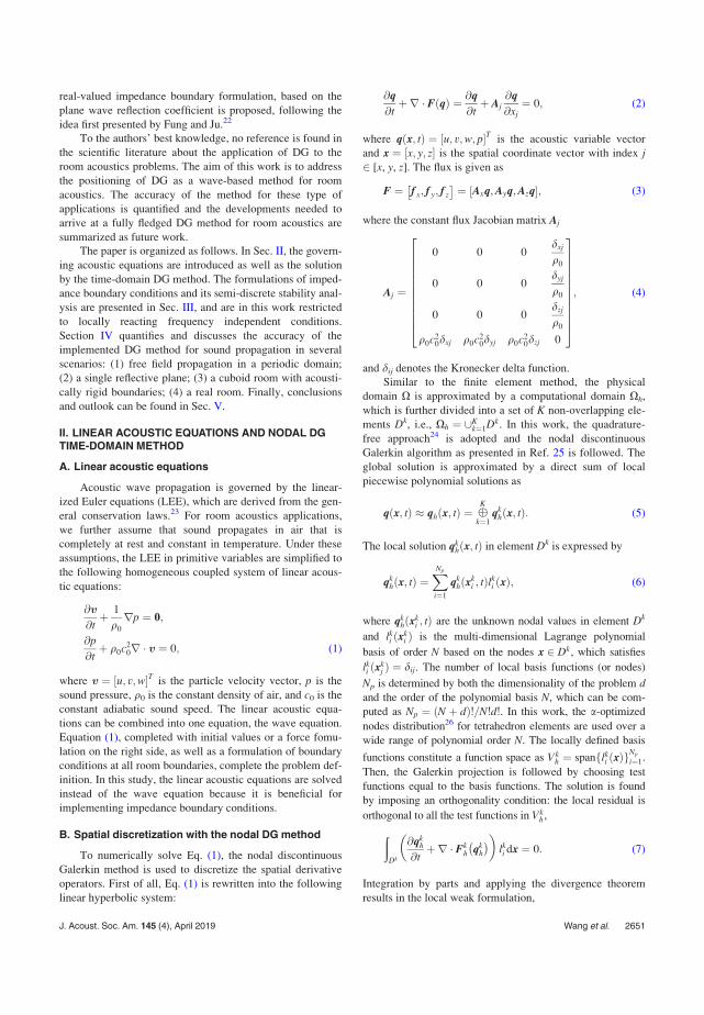
real-valued impedance boundary formulation, based on the

plane wave reflection coefficient is proposed, following the

idea first presented by Fung and Ju.22

To the authors’ best knowledge, no reference is found in

the scientific literature about the application of DG to the

room acoustics problems. The aim of this work is to address

the positioning of DG as a wave-based method for room

acoustics. The accuracy of the method for these type of

applications is quantified and the developments needed to

arrive at a fully fledged DG method for room acoustics are

summarized as future work.

The paper is organized as follows. In Sec. II, the govern-

ing acoustic equations are introduced as well as the solution

by the time-domain DG method. The formulations of imped-

ance boundary conditions and its semi-discrete stability anal-

ysis are presented in Sec. III, and are in this work restricted

to locally reacting frequency independent conditions.

Section IV quantifies and discusses the accuracy of the

implemented DG method for sound propagation in several

scenarios: (1) free field propagation in a periodic domain;

(2) a single reflective plane; (3) a cuboid room with acousti-

cally rigid boundaries; (4) a real room. Finally, conclusions

and outlook can be found in Sec. V.

II. LINEAR ACOUSTIC EQUATIONS AND NODAL DGTIME-DOMAIN METHOD

A. Linear acoustic equations

Acoustic wave propagation is governed by the linear-

ized Euler equations (LEE), which are derived from the gen-

eral conservation laws.23 For room acoustics applications,

we further assume that sound propagates in air that is

completely at rest and constant in temperature. Under these

assumptions, the LEE in primitive variables are simplified to

the following homogeneous coupled system of linear acous-

tic equations:

@v

@tþ 1

q0

rp ¼ 0;

@p

@tþ q0c2

0r v ¼ 0; (1)

where v ¼ ½u; v;wT is the particle velocity vector, p is the

sound pressure, q0 is the constant density of air, and c0 is the

constant adiabatic sound speed. The linear acoustic equa-

tions can be combined into one equation, the wave equation.

Equation (1), completed with initial values or a force fomu-

lation on the right side, as well as a formulation of boundary

conditions at all room boundaries, complete the problem def-

inition. In this study, the linear acoustic equations are solved

instead of the wave equation because it is beneficial for

implementing impedance boundary conditions.

B. Spatial discretization with the nodal DG method

To numerically solve Eq. (1), the nodal discontinuous

Galerkin method is used to discretize the spatial derivative

operators. First of all, Eq. (1) is rewritten into the following

linear hyperbolic system:

@q

@tþr FðqÞ ¼ @q

@tþ Aj

@q

@xj¼ 0; (2)

where qðx; tÞ ¼ ½u; v;w; pT is the acoustic variable vector

and x ¼ ½x; y; z is the spatial coordinate vector with index j2 [x, y, z]. The flux is given as

F ¼ f x; f y; f z

¼ Axq;Ayq;Azq½ ; (3)

where the constant flux Jacobian matrix Aj

Aj ¼

0 0 0dxj

q0

0 0 0dyj

q0

0 0 0dzj

q0

q0c20dxj q0c2

0dyj q0c20dzj 0

266666666664

377777777775; (4)

and dij denotes the Kronecker delta function.

Similar to the finite element method, the physical

domain X is approximated by a computational domain Xh,

which is further divided into a set of K non-overlapping ele-

ments Dk, i.e., Xh ¼ [Kk¼1Dk. In this work, the quadrature-

free approach24 is adopted and the nodal discontinuous

Galerkin algorithm as presented in Ref. 25 is followed. The

global solution is approximated by a direct sum of local

piecewise polynomial solutions as

qðx; tÞ qhðx; tÞ ¼ K

k¼1qk

hðx; tÞ: (5)

The local solution qkhðx; tÞ in element Dk is expressed by

qkhðx; tÞ ¼

XNp

i¼1

qkhðxk

i ; tÞlki ðxÞ; (6)

where qkhðxk

i ; tÞ are the unknown nodal values in element Dk

and lki ðxki Þ is the multi-dimensional Lagrange polynomial

basis of order N based on the nodes x 2 Dk, which satisfies

lki ðxk

j Þ ¼ dij. The number of local basis functions (or nodes)

Np is determined by both the dimensionality of the problem dand the order of the polynomial basis N, which can be com-

puted as Np ¼ ðN þ dÞ!=N!d!. In this work, the a-optimized

nodes distribution26 for tetrahedron elements are used over a

wide range of polynomial order N. The locally defined basis

functions constitute a function space as Vkh ¼ spanflk

i ðxÞgNp

i¼1.

Then, the Galerkin projection is followed by choosing test

functions equal to the basis functions. The solution is found

by imposing an orthogonality condition: the local residual is

orthogonal to all the test functions in Vkh ,

ðDk

@qkh

@tþr Fk

h qkh

lki dx ¼ 0: (7)

Integration by parts and applying the divergence theorem

results in the local weak formulation,

J. Acoust. Soc. Am. 145 (4), April 2019 Wang et al. 2651

ðDk

@qkh

@tlki Fk

h qkh

rlk

i

dx ¼

ð@Dk

n Flki dx; (8)

where n ¼ ½nx; ny; nz is the outward normal vector of the ele-

ment surface @Dk and Fðqh ; qþh Þ is the so-called numerical

flux from element Dk to its neighboring elements through their

intersection @Dk. In contrast to the classical continuous

Galerkin method, the discontinuous Galerkin method uses

local basis functions and test functions that are smooth within

each element and discontinuous across the element intersec-

tions. As a result, the solutions are multiply defined on the

intersections @Dk, where the numerical flux Fðqh ; qþh Þshould be defined properly as a function of both the interior

and exterior (or neighboring) solution. In the remainder, the

solution value from the interior side of the intersection is

denoted by a superscript “” and the exterior value by “þ.”

Applying integration by parts once again to the spatial deriva-

tive term in Eq. (8) yields the strong formulation

ðDk

@qkh

@tþr Fk

h qkh

lki dx

¼ð@Dk

n Fkh qk

h

F

lki dx: (9)

In this study, the flux-splitting approach27 is followed and the

upwind numerical flux is derived as follows. Let us first con-

sider the case where the element Dk lies in the interior of the

computational domain. As is shown in Eq. (9), the formula-

tion of a flux along the surface normal direction n, i.e.,

n F ¼ ðnxf x þ nyf y þ nzf zÞ is of interest. To derive the

upwind flux, we utilize the hyperbolic property of the system

and decompose the normal flux on the interface @Dk into out-

going and incoming waves. Mathematically, an eigendecom-

position applied to the normally projected flux Jacobian yields

An ¼ nxAx þ nyAy þ nzAzð Þ

¼

0 0 0nx

q0

0 0 0ny

q0

0 0 0nz

q0

q0c20nx q0c2

0ny q0c20nz 0

26666666664

37777777775

¼ LKL1; (10)

where

L ¼

nz ny nx=2 nx=2

nz nx ny=2 ny=2

ny nx nz=2 nz=2

0 0 q0c0=2 q0c0=2

266664

377775;

K ¼

0 0 0 0

0 0 0 0

0 0 c0 0

0 0 0 c0

266664

377775: (11)

The upwind numerical flux is defined by considering the

direction of the characteristic speed, i.e.,

ðn FÞ ¼ LðKþL1qh þ KL1qþh Þ; (12)

where Kþ and K contain the positive and negative entries

of K, respectively. Physically, Kþ (K) corresponds to the

characteristic waves propagating along (opposite to) the nor-

mal direction n, which are referred to as outgoing waves out

of Dk (incoming waves into Dk). Therefore, the outgoing

waves are associated with the interior solution qh whereas

the incoming waves are dependent on the exterior (neighbor-

ing) solution qþh . The expression of the numerical flux on the

impedance boundary will be discussed in Sec. III. Finally,

the semi-discrete formulation is obtained by substituting the

nodal basis expansion Eq. (6) and the upwind flux Eq. (12)

into the strong formulation Eq. (9), which can be further

recast into the following matrix form:

Mk @ukh

@tþ 1

qSk

xpkh ¼

Xf

r¼1

MkrFkr

u ; (13a)

Mk @vkh

@tþ 1

qSk

ypkh ¼

Xf

r¼1

MkrFkr

v ; (13b)

Mk @wkh

@tþ 1

qSk

z pkh ¼

Xf

r¼1

MkrFkr

w ; (13c)

Mk @pkh

@tþ qc2Sk

xukh þ qc2Sk

yvkh þ qc2Sk

z wkh ¼

Xf

r¼1

MkrFkr

p ;

(13d)

where the second superscript r denotes the rth faces @Dkr of

the element Dk and f is the total number of faces of the ele-

ment Dk, which is equal to 4 for tetrahedra elements. For

brevity, the subscript 0 in q0 and c0 are omitted from here.

ukh; v

kh; wk

h; and pkh are vectors representing all the unknown

nodal values ukhðxk

i ; tÞ; vkhðxk

i ; tÞ; and pkhðxk

i ; tÞ respectively,

e.g., ukh ¼ ½uk

hðxk1; tÞ; uk

hðxk2; tÞ;…; uk

hðxkNp; tÞT . F

kr

u ; Fkr

v ; Fkr

w ;

and Fkr

p are flux terms associated with the integrand

n ðFkhðqk

hÞ FÞ over the element surface @Dkr in the strong

formulation Eq. (9). The element mass matrix Mk, the ele-

ment stiffness matrices Skj and the element face matrices Mkr

are defined as

Mkmn ¼

ðDk

lkmðxÞlknðxÞdx 2 RNpNp ; (14a)

Skj

mn¼ð

Dk

lkm xð Þ @lkn xð Þ

@xjdx 2 RNpNp ; (14b)

Mkrmn ¼

ð@Dkr

lkrm ðxÞlkr

n ðxÞdx 2 RNpNf p ; (14c)

where j is the jth Cartesian coordinates and Nfp is the number

of nodes along one element face. When the upwind flux is

used, the flux terms for each acoustic variable read as

2652 J. Acoust. Soc. Am. 145 (4), April 2019 Wang et al.

Fkr

u ¼ cnkr2

x

2½ukr

h cnkr

x nkry

2½vkr

h cnkr

x nkrz

2½wkr

h

þ nkrx

2q½pkr

h ; (15a)

Fkr

v ¼ cnkr2

y

2½vkr

h cnkr

x nkry

2½ukr

h cnkr

y nkrz

2½wkr

h

þnkr

y

2q½pkr

h ; (15b)

Fkr

w ¼ cnkr2

z

2½wkr

h cnkr

x nkrz

2½ukr

h cnkr

y nkrz

2½vkr

h

þ nkrz

2q½pkr

h ; (15c)

Fkr

p ¼c2qnkr

x

2½ukr

h þc2qnkr

y

2½vkr

h þc2qnkr

z

2½wkr

h c

2½pkr

h ;

(15d)

where ½ukrh :¼ ukr

h uls; ½vkrh :¼ vkr

h vlsh ; ½wkr

h :¼wkrh wls

h ;

and ½pkrh :¼ pkr

h plsh are the jump differences across the

shared intersection face @Dkr or, equivalently, @Dls, between

neighboring elements Dk and Dl, ukrh ; etc:, are the nodal

value vectors, over the element surface @Dkr.

In this work, flat-faced tetrahedra elements are used so

that each tetrahedron can be mapped into a reference tetrahe-

dron by a linear transformation with a constant Jacobian

matrix. As a consequence, the integrals in the above element

matrices, i.e., Mk; Skj ; and Mkr, need to be evaluated only

once. The reader is referred to Ref. 25 for more details on

how to compute the matrices locally and efficiently.

1. Numerical dissipation and dispersion properties

For a discontinuous Galerkin scheme that uses polyno-

mial basis up to order N, it is well known that generally the

rate of convergence in terms of the global L2 error is hNþ 1/2

(h being the element size).28 The dominant error comes from

the representations of the initial conditions, while the addi-

tional dispersive and dissipative errors from the wave propa-

gations are relatively small and only visible after a very long

time integration.25 The one-dimensional eigenvalue problem

for the spatially propagating waves is studied in Ref. 29

and it is reported that the dispersion relation is accurate to

(jh)2Nþ2 locally, where j is the wavenumber. Actually,

when the upwind flux is used, the dissipation error has been

proved to be of order (jh)2Nþ2 while the dispersion error is

of order (jh)2Nþ3.30 When the centered numerical flux is

used, the dissipation rate is exactly zero, but the discrete dis-

persion relation can only approximate the exact one for a

smaller range of the wavenumber.31 Extensions to the two-

dimensional hyperbolic system on triangle and quadrilateral

mesh are studied in Ref. 32 and the same numerical disper-

sion relation as the one-dimensional case are reported. In

Ref. 30, a rigorous mathematical proof of the above numeri-

cal dispersion relation and error behavior is provided for a

general multi-dimensional setting (including 3D).

C. Time integration with the optimal Runge-Kuttamethod

After the spatial discretization by the nodal DG method,

the semi-discrete system can be expressed in a general form

of ordinary differential equations (ODE) as

dqh

dt¼ LðqhðtÞ; tÞ; (16)

where qh is the vector of all discrete nodal solutions and Lthe spatial discretization operator of DG. Here, a low-storage

explicit Runge-Kutta method is used to integrate Eq. (16),

which reads

qð0Þh ¼qn

h;

kðiÞ ¼aikði1ÞþDtLðtnþciDt;q

ði1Þh Þ;

qðiÞh ¼q

ði1Þh þbik

ðiÞ;for i¼1;…;s;

8<:qnþ1

h ¼qðsÞh ; (17)

where Dt¼ tnþ 1 tn is the time step, qnþ1h and qn

h are the

solution vectors at time tnþ1 and tn, respectively, s is

the number of stages of a particular scheme. In this work,

the coefficients ai, bi, and ci are chosen from the optimal

Runge-Kutta scheme reported in Ref. 33.

III. IMPEDANCE BOUNDARY CONDITIONS ANDNUMERICAL STABILITY

A. Numerical flux for frequency-independentimpedance boundary conditions

The numerical flux F plays a key role in the DG

scheme. Apart from linking neighboring interior elements, it

serves to impose the boundary conditions and to guarantee

stability of the formulation. Boundary conditions can be

enforced weakly through the numerical flux either by refor-

mulating the flux subject to specific boundary conditions or

by providing the exterior solution qþh .34 In both cases, the

solutions from the interior side of the element face (equiva-

lent to boundary surface) qh are readily used, whereas, for

the second case, the exterior solutions qþh need to be suitably

defined as a function of interior solution qh based on the

imposed conditions. In the following, the impedance bound-

ary condition is prescribed by reformulating the numerical

flux. It should be noted that throughout this study, only

plane-shaped reflecting boundary surfaces are considered.

Furthermore, only locally reacting surfaces are considered,

whose surface impedance is independent of the incident

angle. This assumption is in accordance with the nodal DG

scheme, since the unknown acoustic particle velocities on

the boundary surface nodes depend on the pressure at exactly

the same positions.

To reformulate the numerical flux at an impedance

boundary, we take advantage of the characteristics of the

underlying hyperbolic system and utilize the reflection coef-

ficient R for plane waves at normal incidence. First, the same

eigendecomposition procedure is performed for the projected

flux Jacobian on the boundary as is shown in Eq. (10).


Second, by pre-multiplying the acoustic variables q with the

left eigenmatrix L1, the characteristics corresponding to the

acoustic waves35,36 read

xo

xi

¼ p=qcþ unx þ vny þ wnz

p=qc unx vny wnz

; (18)

where xo corresponds to the outgoing characteristic variable

that leaves the computational domain and xi is the incoming

characteristic variable.

The general principle for imposing boundary conditions

of hyperbolic systems is that the outgoing characteristic vari-

able should be computed with the upwind scheme using the

interior values, while the incoming characteristic variable

are specified conforming with the prescribed behaviour

across the boundary. The proposed real-valued impedance

boundary formulation is accomplished by setting the incom-

ing characteristic variable as the product of the reflection

coefficient and the outgoing characteristic variable, i.e.,

xi¼Rxo. Finally, the numerical flux on the impedance

boundary surface can be expressed in terms of the interior

values qh as follows:

ðn FÞ ¼ LK

0

0

ph =qcþ uh nx þ vh ny þ wh nz

R ðph =qcþ uh nx þ vh ny þ wh nzÞ

266664

377775:

(19)

For given constant values of the normalized surface imped-

ance Zs, the reflection coefficient can be calculated from

R ¼ ðZs 1Þ=ðZs þ 1Þ, which is consistent with the fact that

the numerical flux from the nodal DG scheme is always nor-

mal to the boundary surface. When the reflection coefficient

is set to zero it can be easily verified that the proposed for-

mulation reduces to the characteristic non-reflective bound-

ary condition, which is equivalent to the first-order

Engquist-Majda absorbing boundary condition.37

B. Numerical stability of the DG scheme

In this section, the stability properties of the DG scheme

are discussed. First, the semi-boundedness of the spatial DG

operator together with the proposed impedance boundary

conditions is analyzed using the energy method. Second, the

fully discrete stability is discussed and the criterion for

choosing the discrete time step is presented.

1. Stability of the semi-discrete formulation

Under a certain initial condition and impedance bound-

ary condition, the governing linear acoustic equations (1)

constitute a general initial-boundary value problem. For

real-valued impedance boundary conditions, the classical

von Neumann (or Fourier) stability analysis can no longer be

applied, because the necessary periodic boundary conditions

for the Fourier components do not exist. To analyze the sta-

bility or boundedness of the semi-discrete system, the energy

method38 is adopted here. The principle is to construct a

norm and to demonstrate it does not grow with increasing

time. This technique has also been applied in other acoustic

simulation methods,4,39 even in the fully discrete case.

For the numerical solution of the acoustic variables,

e.g., uhðx; tÞ, the local inner product and its associated L2

norm in function space Vkh are defined as

ðukh; u

khÞDk ¼

ðDk

ukhðx; tÞuk

hðx; tÞdx ¼ kukhk

2Dk : (20)

Similarly, over the element surface @Dkr, define

ðukrh ; u

krh Þ@Dkr ¼

ð@Dkr

ukrh ðx; tÞukr

h ðx; tÞdx ¼ kukrh k

2@Dkr ;

(21)

where ukrh is the numerical solution on the element surface

@Dkr. Now, the discrete acoustic energy norm inside single

element Dk can be defined

Ekh ¼

1

2qkuk

hk2Dk þ

1

2qkvk

hk2Dk þ

1

2qkwk

hk2Dk

þ 1

2qc2kpk

hk2Dk : (22)

This definition is in complete analogy with the continuous

acoustic energy, denoted as E, throughout the whole domain

X, i.e., E ¼ÐXð1=2qc2Þp2 þ ðq=2Þjv2jdx.

By summing all the local discrete acoustic energies over

the volume and the boundaries, it can be proved in the

Appendix that the total discrete acoustic energy, which is

denoted as Eh ¼ RKk¼1Ek

h, is governed by

d

dtEh ¼

X@Dmt2FB

1 Rmt

2qckpmt

h k2@Dmt

þ qc

21þ Rmtð Þkvmt

hnk2@Dmt

X

@Dkr2F I

1

2qck½pkr

h k2@Dkr þ

qc

2knkr

x k½ukrh

þ nkry ½vkr

h þ nkrz ½wkr

h k2@Dkr

; (23)

where F I and FB denote the union set of interior elements

and elements with at least one surface collocated with a

physical boundary. [] denotes the jump differences across

the element surfaces. vmthn ¼ nmt

x umth þ nmt

y vmth þ nmt

z wmth denotes

the outward velocity component normal to the impedance

boundary. Rmt is the normal incidence plane-wave reflection

coefficient along the tth boundary surface of element @Dm.

@Dkr and @Dls refers to the same element intersection surface

between neighboring elements Dk and Dl. Since each norm

is non-negative and R 2 [1, 1] holds for a passive imped-

ance boundary,40 it is proved that the semi-discrete acoustic

system resulting from the DG discretization is uncondition-

ally stable for passive boundary conditions with a real-

valued impedance.

It is worth mentioning that the second sum term of Eq.

(23) is related to the energy dissipation inside the


computational domain due to the use of the upwind scheme.

This dissipation will converge to zero when the jump differ-

ences across the shared element interfaces converge to zero

at a rate corresponding to the approximation polynomial

order. The first sum of Eq. (23) is associated with the energy

flow through the impedance boundary. One advantage of

using the reflection coefficient to impose the impedance

boundary condition is that the following singular cases can

be considered without the need for exceptional treatments.

• Hard wall case. As Zs ! 1 or R ! 1, vhn ! 0, then the

boundary energy term converges to 0, meaning that the

energy is conserved.• Pressure-release condition. As Zs ! 0 or R ! 1, ph !

0, then the boundary energy term once again converges to

0, and the energy is conserved as well.

2. Stability of the fully discrete formulation and timestep choices

The above analysis is devoted to the stability analysis of the

semi-discrete formulation Eq. (16), which in matrix form reads

dqh

dt¼ Lhqh; (24)

where Lh is the matrix representation of the spatial operator

L. Ideally, the fully discrete approximation should be stable,

at least under a reasonable upper bound on the time step

size. Unfortunately, the theoretical ground for stability of a

discretized PDE system is not very complete,38 particularly

for high order time integration methods. A commonly used

approach based on the von Neumann analysis is to choose

the time step size Dt small enough so that the product of Dtwith the full eigenvalue spectrum of Lh falls inside the sta-

bility region of the time integration scheme. It should be

noted that this is only a necessary condition for a general

initial-boundary value problem, with the sufficient condition

being more restrictive and complex.41,42 However, for real

world problems, this necessary condition serves as a useful

guideline.

It is computationally infeasible to compute the eigen-

value of Lh before the simulation is started for various

unstructured mesh, polynomial order and boundary condi-

tions. For the DG method, it is found that for the first order

system Eq. (16), the gradients of the normalized Nth order

polynomial basis are of order OðN2=hÞ near the boundary

part of the element,25 consequently the magnitude of the

maximum eigenvalue kN scales with the polynomial order Nas: max(kN) / N2, indicating that Dt / N2. This severe

time step size restriction limits the computational efficiency

of high polynomial order approximations. In all the numeri-

cal experiments presented in this work, the temporal time

steps are determined in the following way:33

Dt ¼ CCFLmin rDð Þ1

c; (25)

where rD is the radius of the inscribed sphere of the tetrahe-

dral elements. As a reference, the tabulated maximum allow-

able Courant number CCFL of the current used RKF84

scheme for each polynomial order N can be found in Ref.

33. In each of the following numerical tests, the exact value

of CCFL are explicitly stated for completeness.

IV. APPLICATIONS

To investigate the applicability of the nodal DG time-

domain method as described in Sec. II and Sec. III for room

acoustics problems, various 3-D numerical tests are designed

and compared in this section. The first test is a free field propa-

gation of a single frequency plane wave under periodic bound-

ary conditions. In this case, the dissipation error in terms of the

wave amplitude and the dispersion error are investigated. The

second configuration is a sound source over an impedance

plane. The accuracy of the proposed DG formulation to simu-

late frequency-independent impedance boundary conditions is

verified. The third configuration is a sound source in a cuboid

room with rigid boundary conditions, embodying an approxi-

mation to a real room including multiple reflections. The modal

behaviour of the space is investigated for different polynomial

order N of the basis functions when compared with the analyti-

cal solution, together with an analysis of the sound energy con-

servation inside the room to quantify the numerical dissipation.

Finally, the fourth configuration is adopted to demonstrate the

applicability of the method to a real room. The configuration is

a room with complex geometry and a real-valued impedance

boundary condition. In this configuration, the pressure response

functions in the frequency domain are compared with the mea-

sured results at several receiver locations. For the acoustic

speed and the air density, c¼ 343 m/s and q¼ 1.2 kg/m3 are

used in all calculations. Due to the fact that there are duplicated

nodes along the element interfaces, in this work, the number of

degrees of freedom per wavelength k (DPW) is used to give a

practical indication of the computational cost. It is computed as

DPW ¼ k

ffiffiffiffiffiffiffiffiffiffiffiffiffiffiffiNp K

V

3

r; (26)

where NpK is the number of degrees of freedom for a sin-

gle physical variable in the computational domain, V is the

volume of the whole domain.

A. Free field propagation in periodic domain

To verify the accuracy of the free field propagation, we

consider a cubic computational domain of size [0, 1]3 in meters,

which is discretized with six congruent tetrahedral elements.

10 10 10 receivers are evenly spaced in all directions

throughout the domain. The domain is initialized with a single

frequency plane wave propagating in the x-direction only,

pðx; t ¼ 0Þ ¼ sinð2pxÞ; (27a)

u x; t ¼ 0ð Þ ¼ 1

qcsin 2pxð Þ; (27b)

vðx; t ¼ 0Þ ¼ 0; wðx; t ¼ 0Þ ¼ 0: (27c)

The wavelength k is chosen to be equal to 1 m such that peri-

odic boundary conditions can be applied in all directions. As

mentioned in Sec. II B, when an initial value problem is


simulated, the approximation error associated with the repre-

sentations of the initial conditions is a dominant component.

In order to rule out this approximation error and to assess the

dissipation and dispersion error accumulated from the wave

propagation alone, the solution values at receiver locations

recorded during the first wave period T of propagation are

taken as the reference values. The solutions sampled during

later time period inverval t¼ [(n 1)T, nT] are compared

with these reference values, where n¼ 10, 20, 30,…, 100.

The amplitude and phase values of the single frequency

wave at each of the receiver locations are obtained from a

Fourier transform of the recorded time signals without win-

dowing. The dissipation error amp in dB and the phase error

/ in % are calculated as follows:

amp ¼ max 20 log10

jPref xð ÞjjPnT xð Þj

!; (28a)

/ ¼ maxj/ PnT xð Þð Þ / Pref xð Þ

j

p 100%

; (28b)

where Pref ðxÞ and PnTðxÞ are the Fourier transform of the

recorded pressure values at different locations, during the

first time period and the nth period, respectively. /()extracts the phase angle of a complex number.

Simulations for N¼ 5, 6, 7 corresponding to

DPW¼ 6.9, 7.9, 8.9 have been carried out and a single time

step size Dt¼ T/100¼ 1/(100 343) is used for all simula-

tions to make sure the time integration error is much smaller

than the spatial error.

The dissipation and the phase error from the explicit

Runge-Kutta time integration is calculated based on the

descriptions presented in Ref. 43 and shown as dashed lines

in Fig. 1. As can be seen, both the dissipation error and the

phase error grow linearly with respect to the propagation dis-

tance. For the 5th order polynomial basis (DPW¼ 6.9), the

averaged dissipation error is approximately 0.035 dB when

the wave travels one wavelength distance while the phase

error is 0.095%. Both error drop to 0.002 dB and 0.005%,

respectively, when the DPW increases to 8. When the DPW

is equal to 8.9, the dissipation error is 1.1 104 dB per

wavelength of propagation and the phase error is less than

3 104%.

B. Single reflective plane

To verify the performance of the proposed frequency-

independent impedance boundary condition, a single reflec-

tion scenario is considered and the reflection coefficient

obtained from the numerical tests is compared with the analyt-

ical one based on a locally reacting impedance. The experi-

ment consists of two simulations. In the first simulation, we

consider a cubic domain of size [8, 8]3 in meters, where the

source is located at the center [0, 0, 0] m, and two receivers

are placed at xr1 ¼ ½0; 0;1m and xr2 ¼ ½0; 4;1m. In this

case, the free field propagation of a sound source is simulated,

and sound pressure signals are recorded at both receiver loca-

tions. In the second simulation, a plane reflecting surface is

placed 2 m away from the source at z¼2 m. The measured

sound pressure signals not only contain the direct sound but

also the sound reflected from the impedance surface. In both

cases, initial pressure conditions are used to initiate the

simulations:

pðx; t ¼ 0Þ ¼ elnð2Þ=b2ððxxsÞ2þðyysÞ2þðzzsÞ2Þ; (29a)

vðx; t ¼ 0Þ ¼ 0; (29b)

which is a Gaussian pulse centered at the source coordinates

[xs, ys, zs]¼ [0, 0, 0] The half-bandwidth of this Gaussian

pulse is chosen as b¼ 0.25 m. Simulations are stopped at

around 0.0321 s in order to avoid the waves reflected from

the exterior boundaries of the whole domain. In order to

eliminate the effects of the unstructured mesh quality on the

accuracy, structured tetrahedra meshes are used for this

study, which are generated with the meshing software

GMSH.44 The whole cuboid domain is made up of structured

cubes of the same size, then each cube is split into six tetra-

hedra elements. The length of each cube is 0.5 m.

Let pd denote the direct sound signal measured from the

first simulation, then the reflected sound signal pr(t) is

FIG. 1. (Color online) Amplitude error amp (a) and phase error / (b) for the periodic propagation of a single frequency plane wave Eq. (27).


obtained by eliminating pd(t) from the solution of the second

simulation. Let R1 denote the distance between the source

and the receiver and R2 is the distance between the receiver

and the image source (located at [0, 0, 4] m) mirrored by

the reflecting impedance surface. The spectra of the direct

sound and the reflected sound, denoted as Pd(f) and Pr(f)respectively, are obtained by Fourier transforming pd and pr

without windowing. The numerical reflection coefficient

Qnum is calculated as follows:

Qnumðf Þ ¼Pr fð Þ G jR1ð ÞPd fð Þ G jR2ð Þ ; (30)

where

GðjRÞ ¼ eijR=R (31)

is the Green function in 3D free space. j is the wavenumber.

The analytical spherical wave reflection coefficient Qreads45

Q ¼ 1 2jR2

ZseijR2

ð10

eqj=Zse

ijffiffiffiffiffiffiffiffiffiffiffiffiffiffiffiffiffiffiffiffiffiffir2

pþ zþzsþiqð Þ2p

ffiffiffiffiffiffiffiffiffiffiffiffiffiffiffiffiffiffiffiffiffiffiffiffiffiffiffiffiffiffiffiffiffiffiffiffiffir2

p þ zþ zs þ iqð Þ2q dq;

(32)

where Zs is the normalized surface impedance, z¼ 1 is the

distance between the receiver and the reflecting surface,

zs¼ 2 is the distance between the source and the surface, rp

is the distance between the source and the receiver projected

on the reflecting surface.

Simulations with polynomial order N¼ 5 up to N¼ 8

are carried out with the corresponding CCFL and time step Dtpresented in Table I.

The results of the numerical tests for Zs¼ 3 are illus-

trated in Fig. 2. The DPW is calculated based on the fre-

quency of 500 Hz. The comparison of the magnitudes of the

spherical wave reflection coefficient for both the normal

incidence angle h¼ 0 and the oblique incidence (h¼ 53)are shown in Figs. 2(a) and 2(b), respectively. The phase

angle comparison is presented in Figs. 2(c) and 2(d). It can

be seen that with increasing polynomial order N (or DPW),

the numerical reflection coefficient converges to the analyti-

cal one in terms of the magnitude and the phase angle. Also,

the accuracy is rather independent on the two angles of inci-

dence h. In order to achieve a satisfactory accuracy, at least

12 DPW are needed. Many tests are performed with different

impedances (Zs 2 [1,1]) and receiver locations (h 2 [0, 90]),the same conclusion can be reached.

C. Cuboid room with rigid boundaries

In this section, the nodal DG method is applied to sound

propagation in a 3-D room with rigid boundaries (R¼ 1). In

contrast to the previous applications, sound propagation

inside the room is characterized by multiple reflections and

sound energy is conserved. The domain of the room is

[0, Lx] [0, Ly] [0, Lz] m, with Lx¼ 1.8, Ly¼ 1.5, Lz¼ 2.

Initial conditions are given as in Eqs. (29), with b¼ 0.2 m.

The source is positioned at [0.9, 0.75, 1] m, and a receiver

is positioned at [1.7, 1.45, 1.9] m. Similar as in the previ-

ous test case, the room is discretized using structured tet-

rahedral elements of size 0.4 m. The analytical pressure

response in a cuboid domain can be obtained by the modal

summation method, and can in the 3-D Cartesian coordi-

nate system be written as46

pðx; tÞ ¼X1l¼0

X1m¼0

X1n¼0

plmnðtÞwlmnðxÞ cos ðxlmntÞ; (33a)

wlmn xð Þ ¼ coslpx

Lx

cos

mpy

Ly

cos

npz

Lz

; (33b)

xlmn ¼ c

ffiffiffiffiffiffiffiffiffiffiffiffiffiffiffiffiffiffiffiffiffiffiffiffiffiffiffiffiffiffiffiffiffiffiffiffiffiffiffiffiffiffiffiffiffiffiffiffiffiffiffiffiffiffilpLx

2

þ mpLy

2

þ npLz

2s

; (33c)

with wlmn the modal shape function; plmn the modal partici-

pation factor; xlmn the natural angular frequency; and l,m, n the mode indices. Since reflections from the room

boundaries occur without energy loss, the modal participa-

tion factors are constant over time. To obtain plmnð0Þ, the

initial pressure distribution is projected onto each modal

shape as

plmn 0ð Þ ¼ 1

Klmn

ðX

p x; t ¼ 0ð Þwlmn xð Þdx; (34a)

Klmn ¼ð

Xw2

lmnðxÞdx: (34b)

The integration in Eq. (34a) can be calculated separately for

each coordinate. For example, in the x coordinate, the indefinite

integration can be expressed in terms of the error function asðe a0 xxsð Þ2ð Þcos b0xð Þdx

¼ffiffiffipp

4ffiffiffiffiffia0p e b2

0=4a0ð Þib0xsð Þ erf Bð Þþe i2b0xsð Þerf Bð Þ

þC;

(35)

with B¼ ffiffiffiffiffia0p ðxx0Þþ ib0=2

ffiffiffiffiffia0p

; a0¼ lnð2Þ=b2; b0¼ lp=Lx,

and C is a constant. Equation (33a) is used as the reference

solution with modal frequencies up to 8 kHz. Furthermore,

to show the applicability of the nodal DG method for a long

time simulation, 10 s is taken as the simulation duration.

To solve for this configuration, the CCFL numbers and

time steps for the approximating polynomial orders of N¼ 3

up to N¼ 7 are presented in Table II.

The sound pressure level is computed as

TABLE I. CCFL number and time step Dt for single reflection case

(h¼ 0.5 m).

N CCFL Dt [s]

5 0.185 9.721 105

6 0.144 7.550 105

7 0.114 5.993 105

8 0.094 4.908 105


Lp ¼ 20 log10

P fð Þffiffiffi2p

P0

; (36)

with P0¼ 2 105 Pa, and P(f) the spectrum of recorded

pressure time signal p(t) at the receiver location. The end of

the time signal is tapered using a Gaussian window with a

length of 3.5 s to avoid the Gibbs effect.

Figure 3 shows the sound pressure level at the receiver

location. The numerical solutions show an excellent agree-

ment with the reference solution, with the accuracy of the

numerical solution increasing as the approximating polyno-

mial order increases.

Figure 4 displays the results for f¼ 950–1000 Hz. From

this figure, we can see that the resonance frequencies are not

well represented for N 5, for which DPW varies between

4.5 and 6.6 in this frequency range. On the other hand, the

resonance frequencies are correctly represented for N 6,

where the minimum number of DPW is 7.2. The correct rep-

resentation of the room resonance frequencies indicates that

the numerical dispersion is low in the DG solution. The

numerical dispersion aspect is essential with regards to aur-

alization as shown by Saarelma et al.,47 where the audibility

of the numerical dispersion error from the finite difference

time domain simulation is investigated. Furthermore, Fig. 4

clearly shows that the DG results have reduced peak ampli-

tudes when the approximating polynomial orders are low.

D. Real room with real-valued impedance boundaryconditions

The final scenario is a comparison between experimen-

tal and numerical results of a real room. The room is located

in the Acoustics Laboratory building (ECHO building) at the

campus of the Eindhoven University of Technology.

Geometrical data of the room, including the dimensions and

FIG. 2. (Color online) Numerical reflection coefficient calculated by Eq. (30) with different polynomial orders, compared with the theoretical result according

to Eq. (32) (black dashed line): (a) magnitude for receiver 1, h¼ 0, (b) magnitude for receiver 2, h¼ 53, (c) phase angle for receiver 1, h¼ 0, (d) phase

angle for receiver 2, h¼ 53.

TABLE II. CCFL number and time step Dt for a rigid cuboid room

(h¼ 0.4 m).

N CCFL Dt [s]

3 0.355 1.400 104

4 0.248 9.810 105

5 0.185 7.322 105

6 0.144 5.687 105

7 0.114 4.514 105


the location of the source and microphone positions are pre-

sented in Fig. 5. The room has a volume of V¼ 89.54 m3

and a boundary surface area of S¼ 125.08 m2.

The source is located at [1.7, 2.92, 1.77] m and micro-

phones (M) are located at [3.8, 1.82, 1.66] m for M1 and

[4.75, 3.87, 1.63] m for M2. The height (z-coordinate) of the

sound source location is measured at the opening (highest

point) of the used sound source (B&K type 4295,

OmniSource Sound Source). The measurements were per-

formed using one free-field microphone B&K type 4189

connected to a Triton USB Audio Interface. The impulse

responses were acquired with a sampling frequency of 48

KHz with a laptop using the room acoustics software

DIRAC (B&K type 7841). The input channel is calibrated

before starting the measurements using a calibrator (B&K

type 4230). The sound signal used for the excitation of the

room is the DIRAC built-in e-Sweep signal with a duration

of 87.4 s connected to an Amphion measurement amplifier.

At each microphone position, three measurement repetitions

were performed. The results presented in this section for M1

and M2 represent the average of the three repetitions.

The room is discretized in 9524 tetrahedral elements by

using GMSH and the largest element size is 0.5 m. A detail of

the mesh is shown in Fig. 5(b). The same initial pressure

distribution as for the 3-D cuboid room of Sec. IV C is used.

The polynomial order used in the calculations is N¼ 4 with

a CFL number of CCFL¼ 0.25. The computed impulse

responses have a duration of 15 s. The model uses a DPW of

13 for the frequency of 400 Hz. All the boundaries of the

model are computed using a uniform real-valued reflection

coefficient of R¼ 0.991. The coefficient is calculated from

the experimental results at M1 by computing the Q-value of

the resonance at f0¼ 97.9 Hz, using R ¼ 1 dr8V=cS with,

dr ¼ 2pf0=2Q the decay constant of the room’s resonance.

Both impulse responses from the measurements and

simulations were transformed to the frequency domain by

using a forward Fourier transform. The end of the time sig-

nals is tapered by a single-sided Gaussian window with a

length of 500 samples (approximately, 5.6 ms) to avoid the

Gibbs effect. Furthermore, the time function of the numeri-

cal source is obtained from the following analytical expres-

sion: ps;anaðtÞ¼ ½ðrsrctÞ=2rsreðlnð2Þ=b2ÞðrsrctÞ2 þ½ðrsrþ ctÞ=2rsreðlnð2Þ=b2ÞðrsrþctÞ2 (with rsr the source-receiver distance).

This function is transformed to the frequency domain to nor-

malize the calculated impulse responses in DG by the source

power spectrum. Likewise, the experimental results have

been normalized by the B&K 4295 sound power spectra.

The source spectra of an equivalent source B&K 4295 has

FIG. 3. (Color online) Sound pressure

level at receiver position in the config-

uration of the 3-D rigid cuboid room.

FIG. 4. (Color online) Receiver sound

pressure response level between 950

and 1000 Hz.


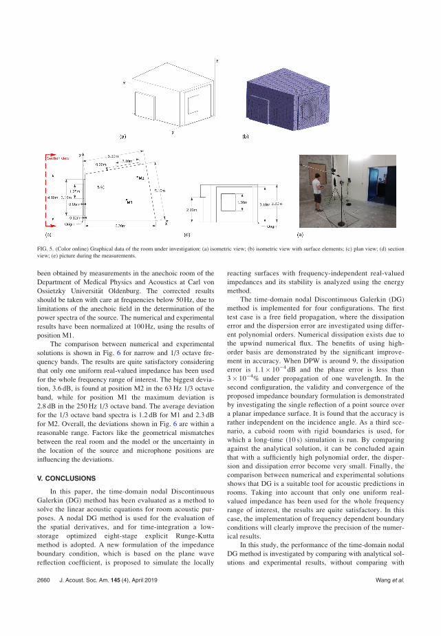
been obtained by measurements in the anechoic room of the

Department of Medical Physics and Acoustics at Carl von

Ossietzky Universit€at Oldenburg. The corrected results

should be taken with care at frequencies below 50Hz, due to

limitations of the anechoic field in the determination of the

power spectra of the source. The numerical and experimental

results have been normalized at 100Hz, using the results of

position M1.

The comparison between numerical and experimental

solutions is shown in Fig. 6 for narrow and 1/3 octave fre-

quency bands. The results are quite satisfactory considering

that only one uniform real-valued impedance has been used

for the whole frequency range of interest. The biggest devia-

tion, 3.6 dB, is found at position M2 in the 63 Hz 1/3 octave

band, while for position M1 the maximum deviation is

2.8 dB in the 250 Hz 1/3 octave band. The average deviation

for the 1/3 octave band spectra is 1.2 dB for M1 and 2.3 dB

for M2. Overall, the deviations shown in Fig. 6 are within a

reasonable range. Factors like the geometrical mismatches

between the real room and the model or the uncertainty in

the location of the source and microphone positions are

influencing the deviations.

V. CONCLUSIONS

In this paper, the time-domain nodal Discontinuous

Galerkin (DG) method has been evaluated as a method to

solve the linear acoustic equations for room acoustic pur-

poses. A nodal DG method is used for the evaluation of

the spatial derivatives, and for time-integration a low-

storage optimized eight-stage explicit Runge-Kutta

method is adopted. A new formulation of the impedance

boundary condition, which is based on the plane wave

reflection coefficient, is proposed to simulate the locally

reacting surfaces with frequency-independent real-valued

impedances and its stability is analyzed using the energy

method.

The time-domain nodal Discontinuous Galerkin (DG)

method is implemented for four configurations. The first

test case is a free field propagation, where the dissipation

error and the dispersion error are investigated using differ-

ent polynomial orders. Numerical dissipation exists due to

the upwind numerical flux. The benefits of using high-

order basis are demonstrated by the significant improve-

ment in accuracy. When DPW is around 9, the dissipation

error is 1.1 104 dB and the phase error is less than

3 104% under propagation of one wavelength. In the

second configuration, the validity and convergence of the

proposed impedance boundary formulation is demonstrated

by investigating the single reflection of a point source over

a planar impedance surface. It is found that the accuracy is

rather independent on the incidence angle. As a third sce-

nario, a cuboid room with rigid boundaries is used, for

which a long-time (10 s) simulation is run. By comparing

against the analytical solution, it can be concluded again

that with a sufficiently high polynomial order, the disper-

sion and dissipation error become very small. Finally, the

comparison between numerical and experimental solutions

shows that DG is a suitable tool for acoustic predictions in

rooms. Taking into account that only one uniform real-

valued impedance has been used for the whole frequency

range of interest, the results are quite satisfactory. In this

case, the implementation of frequency dependent boundary

conditions will clearly improve the precision of the numer-

ical results.

In this study, the performance of the time-domain nodal

DG method is investigated by comparing with analytical sol-

utions and experimental results, without comparing with

FIG. 5. (Color online) Graphical data of the room under investigation: (a) isometric view; (b) isometric view with surface elements; (c) plan view; (d) section

view; (e) picture during the measurements.


other commonly used room acoustics modelling techniques

such as FDTD and FEM. The aim of this work is to demon-

strate the viability of the DG method to room acoustics

modelling, where high-order accuracy and geometrical flexi-

bility are of key importance. With the opportunity to mas-

sively parallelize the DG method, it has great potential as a

wave-based method for room acoustic purposes. Whereas

the results show that high accuracy can be achieved with

DG, some issues remain to be addressed. The improvements

in accuracy using high-order schemes come at a cost of

smaller time step size for the sake of stability. There is a

trade-off between a high-order scheme with a small time

step and fewer spatial points and low-order methods, where

a larger time step is allowed but a higher number of spatial

points are needed to achieve the same accuracy. Further

investigations are needed to find out the most cost-efficient

combination of the polynomial order and the mesh size

under a given accuracy requirement. Also, when the mesh

configuration is fixed by the geometry, the local adaptivity

of polynomial orders and time step sizes could be a feasible

approach to improve the computational efficiency of DG

for room acoustics applications. Furthermore, general

frequency-dependent impedance boundary conditions as

well as extended reacting boundary conditions are still to

be rigorously developed in DG.

ACKNOWLEDGMENTS

This project has received funding from the European

Union’s Horizon 2020 research and innovation programme

under Grant Agreement No. 721536. The second author is

supported by the ministry of finance of the Republic of

Indonesia under framework of endowment fund for

education (LPDP). Additionally, we would like to thank the

Department of Medical Physics and Acoustics at Carl von

Ossietzky Universit€at Oldenburg for their help in the

estimation of the sound power spectra of the sound source.

APPENDIX: DERIVATIONS OF THE TOTAL DISCRETEACOUSTIC ENERGY OF THE SEMI-DISCRETESYSTEM

It can be seen that the local energy can be recovered

from the product of the element mass matrix Mk and the

nodal vectors ukh as follows:

FIG. 6. (Color online) Sound pressure

level Lp in the real room configuration

for the experimental and the DG

results in narrow frequency bands

(black broken line and red solid line,

respectively) and 1/3 octave bands

(black dot and red dot, respectively)

for the microphone positions (a) M1

and (b) M2.


ðukhÞ

TMkukh ¼

ðDk

XNp

i¼1

ukhðxk

i ; tÞlki ðxÞ

XNp

j¼1

ukhðxk

j ; tÞlkj ðxÞdx

¼ kukhk

2Dk : (A1)

Furthermore, it can be verified that

ukh

TSk

xpkh ¼

ðDk

XNp

i¼1

pkh xk

i ; t

lki xð Þ

XNp

j¼1

ukh xk

j ; t @lk

j xð Þ@x

dx

¼ð

Dk

pkh x; tð Þ

@ukh x; tð Þ@x

dx ¼ pkh;@uk

h

@x

Dk

(A2)

and

ðukhÞ

TMkrpkrh ¼ð@Dkr

XNp

i¼1

ukhðxk

i ;tÞlki ðxÞXNf p

j¼1

pkrh ðxkr

j ;tÞlkrj ðxÞdx

¼ð@Dkr

XNf p

i¼1

ukrh ðxkr

i ;tÞlki ðxÞXNf p

j¼1

pkrh ðxkr

j ;tÞlkrj ðxÞdx

¼ð@Dkr

ukrh ðx;tÞpkr

h ðx;tÞdx¼ðukrh ;p

krh Þ@Dkr :

(A3)

Now, the total discrete acoustic energy Eh of the semi-

discrete formulation Eq. (13) can be calculated. By pre-

multiplying Eq. (13a) with qðukhÞ

T, pre-multiplying Eq. (13b)

with qðvkhÞ

T, pre-multiplying Eq. (13c) with qðwk

hÞT, pre-

multiplying Eq. (13d) with ð1=qc2ÞðpkhÞ

Tand sum them

together, using the relations mentioned in Eqs. (A1), (A2),

yields

d

dtEk

h ¼ Xf

r¼1

nkrx ukr

h ; pkrh

@Dkr þ nkr

y vkrh ; p

krh

@Dkr

þnkrz wkr

h ; pkrh

@Dkr

… þq uk

h

TXf

r¼1

MkrFkr

u

þ q vkh

TXf

r¼1

MkrFkr

v þ q wkh

TXf

r¼1

MkrFkr

w

þ 1

qc2pk

h

TXf

r¼1

MkrFkr

p ; (A4)

where the divergence theorem is used to obtain the surface

integral term, that is

ukh;@pk

h

@x

Dkþ vk

h;@pk

h

@y

!Dk

þ wkh;@pk

h

@z

Dk

þ pkh;@uk

h

@x

Dkþ pk

h;@vk

h

@y

!Dk

þ pkh;@wk

h

@z

Dk

¼Xf

r¼1

nkr

x ukrh ; p

krh

@Dkr þ nkr

y vkrh ; p

krh

@Dkr

þ nkrz wkr

h ; pkrh

@Dkr

: (A5)

Substitute the numerical flux Eqs. (15) into Eq. (A4) and use

Eq. (A3), after some simple algebraic manipulations, the

semi-discrete acoustic energy balance on element yields

d

dtEk

h ¼Xf

r¼1

Rkrh ; (A6)

where

Rkrh ¼ pkr

h ; vkrhn

@Dkr

1

2xkr

o ; pkrh þ qcvkr

hn

@Dkr

þ 1

2xls

i ; pkrh qcvkr

hn

@Dkr (A7)

is the discrete energy flux through the shared surface @Dkr or

equivalently @Dls between the neighboring elements Dk and

Dl in the interior of the computation domain. x0 and xi are

the characteristic waves defined in Eq. (18). By using the

condition that the outward normal vector of neighboring ele-

ments are opposite, the final form of energy contribution

from the coupling across one shared interface reads

Rkrh þRls

h ¼

1

2qck½pkr

h k2@Dkr þ

qc

2knkr

x ½ukrh

þ nkry ½vkr

h þ nkrz ½wkr

h k2@Dkr

; (A8)

which is non-positive. This ends the discussion for the inte-

rior elements. Now, for elements that have at least one sur-

face lying on the real-valued impedance boundary, e.g.,

element Dm with surface @Dmt 2 @Xh, the numerical flux is

calculated using Eq. (19). After some algebraic operations,

the energy flux through the reflective boundary surface

becomes

Rmth ¼

1 Rmt

2qckpmt

h k2@Dmt þ

qc

21þ Rmtð Þkvmt

hnk2@Dmt

:

(A9)

Finally, by summing the energy flux through all of the faces

of the mesh, we get the total acoustic energy of the whole

semi-discrete system as in Eq. (23).

1M. R. Schroeder, “Novel uses of digital computers in room acoustics,”

J. Acoust. Soc. Am. 33(11), 1669–1669 (1961).2M. Vorl€ander, “Computer simulations in room acoustics: Concepts and

uncertainties,” J. Acoust. Soc. Am. 133(3), 1203–1213 (2013).3L. Savioja and U. P. Svensson, “Overview of geometrical room acoustic

modeling techniques,” J. Acoust. Soc. Am. 138(2), 708–730 (2015).4B. Hamilton, “Finite difference and finite volume methods for wave-based

modelling of room acoustics,” Ph.D. dissertation, The University of

Edinburgh, Edinburgh, Scotland, 2016.5V. Valeau, J. Picaut, and M. Hodgson, “On the use of a diffusion equation

for room-acoustic prediction,” J. Acoust. Soc. Am. 119(3), 1504–1513

(2006).6J. M. Navarro, J. Escolano, and J. J. Lopez, “Implementation and evalua-

tion of a diffusion equation model based on finite difference schemes for

sound field prediction in rooms,” Appl. Acoust. 73(6-7), 659–665 (2012).7D. Botteldooren, “Finite-difference time-domain simulation of low-

frequency room acoustic problems,” J. Acoust. Soc. Am. 98(6),

3302–3308 (1995).


8J. Sheaffer, M. van Walstijn, and B. Fazenda, “Physical and numerical

constraints in source modeling for finite difference simulation of room

acoustics,” J. Acoust. Soc. Am. 135(1), 251–261 (2014).9C. Spa, A. Rey, and E. Hernandez, “A GPU implementation of an explicit

compact FDTD algorithm with a digital impedance filter for room acous-

tics applications,” IEEE/ACM Trans. Audio Speech Lang. Process. 23(8),

1368–1380 (2015).10B. Hamilton and S. Bilbao, “FDTD methods for 3-D room acoustics simu-

lation with high-order accuracy in space and time,” IEEE/ACM Trans.

Audio Speech Lang. Process. 25(11), 2112–2124 (2017).11T. Okuzono, T. Yoshida, K. Sakagami, and T. Otsuru, “An explicit time-

domain finite element method for room acoustics simulations:

Comparison of the performance with implicit methods,” Appl. Acoust.

104, 76–84 (2016).12S. Bilbao, “Modeling of complex geometries and boundary conditions in

finite difference/finite volume time domain room acoustics simulation,”

IEEE Trans. Audio Speech Lang. Process. 21(7), 1524–1533 (2013).13R. Mehra, N. Raghuvanshi, L. Savioja, M. C. Lin, and D. Manocha, “An

efficient GPU-based time domain solver for the acoustic wave equation,”

Appl. Acoust. 73(2), 83–94 (2012).14C. Spa, A. Garriga, and J. Escolano, “Impedance boundary conditions for

pseudo-spectral time-domain methods in room acoustics,” Appl. Acoust.

71(5), 402–410 (2010).15M. Hornikx, W. De Roeck, and W. Desmet, “A multi-domain Fourier

pseudospectral time-domain method for the linearized Euler equations,”

J. Comput. Phys. 231(14), 4759–4774 (2012).16M. Hornikx, C. Hak, and R. Wenmaekers, “Acoustic modelling of sports

halls, two case studies,” J. Build. Perform. Simul. 8(1), 26–38 (2015).17B. Cockburn and C.-W. Shu, “TVB Runge-Kutta local projection discon-

tinuous Galerkin finite element method for conservation laws II: General

framework,” Math. Comput. 52(186), 411 (1989).18Y. Reymen, W. De Roeck, G. Rubio, M. Baelmans, and W. Desmet, “A

3D discontinuous Galerkin method for aeroacoustic propagation,” in

Twelfth International Congress on Sound and Vibration, Lisbon, Portugal

(2005).19J. Nytra, L. Cermak, and M. Jıcha, “Applications of the discontinuous

Galerkin method to propagating acoustic wave problems,” Adv. Mech.

Eng. 9(6), 168781401770363 (2017).20A. Modave, A. St-Cyr, and T. Warburton, “GPU performance analysis of

a nodal discontinuous Galerkin method for acoustic and elastic models,”

Comput. Geosci. 91, 64–76 (2016).21Y. Reymen, M. Baelmans, and W. Desmet, “Efficient implementation of

Tam and Auriault’s time-domain impedance boundary condition,” AIAA

J. 46(9), 2368–2376 (2008).22K.-Y. Fung and H. Ju, “Broadband time-domain impedance models,”

AIAA J. 39(8), 1449–1454 (2001).23V. E. Ostashev, D. K. Wilson, L. Liu, D. F. Aldridge, N. P. Symons, and

D. Marlin, “Equations for finite-difference, time-domain simulation of

sound propagation in moving inhomogeneous media and numerical

implementation,” J. Acoust. Soc. Am. 117(2), 503–517 (2005).24H. L. Atkins and C.-W. Shu, “Quadrature-free implementation of discon-

tinuous Galerkin method for hyperbolic equations,” AIAA J. 36(5),

775–782 (1998).25J. S. Hesthaven and T. Warburton, Nodal Discontinuous Galerkin

Methods: Algorithms, Analysis and Applications (Springer-Verlag, New

York, 2007), Chaps. 2,3,4,6,10.26J. S. Hesthaven and C.-H. Teng, “Stable spectral methods on tetrahedral

elements,” SIAM J. Sci. Comput. 21(6), 2352–2380 (2000).

27R. J. LeVeque, Finite Volume Methods for Hyperbolic Problems(Cambridge University Press, Cambridge, 2002), Chap. 2.

28P. Lasaint and P.-A. Raviart, “On a finite element method for solving the

neutron transport equation,” in Mathematical Aspects of Finite Elementsin Partial Differential Equations (Elsevier, Amsterdam, 1974), pp.

89–123.29F. Q. Hu and H. Atkins, “Eigensolution analysis of the discontinuous

Galerkin method with nonuniform grids: I. One space dimension,”

J. Comput. Phys. 182(2), 516–545 (2002).30M. Ainsworth, “Dispersive and dissipative behaviour of high order discon-

tinuous Galerkin finite element methods,” J. Comput. Phys. 198(1),

106–130 (2004).31F. Q. Hu, M. Hussaini, and P. Rasetarinera, “An analysis of the discontinu-

ous Galerkin method for wave propagation problems,” J. Comput. Phys.

151(2), 921–946 (1999).32F. Hu and H. Atkins, “Two-dimensional wave analysis of the discontinu-

ous Galerkin method with non-uniform grids and boundary conditions,” in

8th AIAA/CEAS Aeroacoustics Conference & Exhibit (2002), p. 2514.33T. Toulorge and W. Desmet, “Optimal Runge-Kutta schemes for discon-

tinuous Galerkin space discretizations applied to wave propagation prob-

lems,” J. Comput. Phys. 231(4), 2067–2091 (2012).34H. Atkins, “Continued development of the discontinuous Galerkin method

for computational aeroacoustic applications,” in 3rd AIAA/CEASAeroacoustics Conference (1997), p. 1581.

35B.-T. Chu and L. S. Kovasznay, “Non-linear interactions in a viscous

heat-conducting compressible gas,” J. Fluid Mech. 3(5), 494–514 (1958).36K. W. Thompson, “Time dependent boundary conditions for hyperbolic

systems,” J. Comput. Phys. 68(1), 1–24 (1987).37B. Engquist and A. Majda, “Absorbing boundary conditions for numerical

simulation of waves,” Proc. Natl. Acad. Sci. 74(5), 1765–1766 (1977).38B. Gustafsson, High Order Difference Methods for Time Dependent PDE

(Springer-Verlag, Berlin, 2007), Chap. 2.39S. Bilbao, B. Hamilton, J. Botts, and L. Savioja, “Finite volume time

domain room acoustics simulation under general impedance boundary

conditions,” IEEE/ACM Trans. Audio Speech Lang. Process. 24(1),

161–173 (2016).40D. Dragna, K. Attenborough, and P. Blanc-Benon, “On the inadvisability

of using single parameter impedance models for representing the acousti-

cal properties of ground surfaces,” J. Acoust. Soc. Am. 138(4), 2399–2413

(2015).41S. C. Reddy and L. N. Trefethen, “Stability of the method of lines,”

Numer. Math. 62(1), 235–267 (1992).42H. O. Kreiss and L. Wu, “On the stability definition of difference approxi-

mations for the initial boundary value problem,” Appl. Numer. Math.

12(1-3), 213–227 (1993).43C. Bogey and C. Bailly, “A family of low dispersive and low dissipative

explicit schemes for flow and noise computations,” J. Comput. Phys.

194(1), 194–214 (2004).44C. Geuzaine and J.-F. Remacle, “GMSH: A 3-D finite element mesh gen-

erator with built-in pre- and post-processing facilities,” Int. J. Numer.

Meth. Eng. 79(11), 1309–1331 (2009).45X. Di and K. E. Gilbert, “An exact Laplace transform formulation for a point

source above a ground surface,” J. Acoust. Soc. Am. 93(2), 714–720 (1993).46H. Kuttruff, Acoustics: An Introduction (CRC Press, Boca Raton, FL,

2006), Chap. 9.47J. Saarelma, J. Botts, B. Hamilton, and L. Savioja, “Audibility of dispersion

error in room acoustic finite-difference time-domain simulation as a function

of simulation distance,” J. Acoust. Soc. Am. 139(4), 1822–1832 (2016).


Errata of Paper I

• Eq. (11)

L =

−nz ny nx/2 −nx/2nz −nx ny/2 −ny/2−ny nx nz/2 −nz/20 0 ρ0c0/2 ρ0c0/2

, Λ =

0 0 0 00 0 0 00 0 c0 00 0 0 −c0

.

should be replaced by

L =

−ny −nz nx/2 −nx/2nx 0 ny/2 −ny/20 nx nz/2 −nz/20 0 ρ0c0/2 ρ0c0/2

, Λ =

0 0 0 00 0 0 00 0 c0 00 0 0 −c0

.

Page 106

Paper II

Page 107

Time-domain impedance boundary condition modeling with thediscontinuous Galerkin method for room acoustics simulations

Huiqing Wanga) and Maarten Hornikxb)

Building Physics and Services, Department of the Built Environment, Eindhoven University of Technology, P.O. Box 513,5600 MB Eindhoven, The Netherlands

ABSTRACT:The time-domain nodal discontinuous Galerkin (TD-DG) method is emerging as a potential wave-based method for

three-dimensional (3D) room acoustics modeling, where high-order accuracy in the low frequency range, geometri-

cal flexibility, and accurate modeling of boundary conditions are of critical importance. This paper presents a formu-

lation of broadband time-domain impedance boundary conditions (TDIBCs) of locally-reacting surfaces in the

framework of the TD-DG method. The formulation is based on the approximation of the plane-wave reflection coef-

ficient at normal incidence in the frequency domain using a sum of template rational functions, which can be directly

transformed to the time-domain. The coupling of the TDIBCs with the discontinuous Galerkin discretization is

achieved through the characteristic waves of the upwind flux along the boundary, where a series of first-order auxil-

iary differential equations is time-integrated in a high-order way. To verify the performance of the formulation,

various numerical tests of single reflection scenarios are shown to demonstrate the cost efficiency and memory-

efficiency of high-order basis functions, among which a 3D application to an impedance boundary of rigidly backed

glass-wool baffle for room acoustic purposes is presented. VC 2020 Acoustical Society of America.

https://doi.org/10.1121/10.0001128

(Received 31 August 2019; revised 2 April 2020; accepted 3 April 2020; published online 23 April 2020)

[Editor: Lauri Savioja] Pages: 2534–2546

I. INTRODUCTION

Sound propagation in a room is a complicated process

due to the geometry of the room and the objects inside it.

Furthermore, a variety of surface natures and surface impe-

dances, which are typically frequency-dependent, make it

extremely hard to achieve analytical representations of the

acoustic field. Therefore, computer simulation of the sound

field in indoor environments has become a common tool for

the analysis of sound in rooms.1

In general, room acoustic modeling techniques can be

divided into two categories, namely, geometrical acoustics

methods and wave-based methods. Thanks to the steady

increase in computing power, wave-based methods have

become more mature during the past decades.2 Compared to

frequency-domain wave-based methods, time-domain

modeling allows single run broadband calculations with

moving sources and time-varying domains and generates

directly the impulse response of the room. After applications

to fields as aeroacoustics,3 the time-domain discontinuous

Galerkin (TD-DG) method has for the first time been evalu-

ated as a potential wave-based method for room acoustics

modeling purposes.4 Its high accuracy and ability to handle

complex boundary geometries were demonstrated through

verifications by analytical solutions and by comparison

against measurement results of a real room. Since the

acoustic wave equation is solved element-wise, highly effi-

cient parallel-computing solvers that exploit modern hard-

ware have been developed.5,6 The applicability of the

discontinuous Galerkin (DG) solver to a large scale room

acoustics simulation is demonstrated in Ref. 7, in analogy

to the example of a cathedral-like geometry presented in

Ref. 8. However, in order to provide physical simulation

results that match real materials, a time-domain impedance

boundary condition (TDIBC) formulation that handles

frequency-dependent acoustic properties is needed.

The acoustic behavior of a locally reactive reflecting sur-

face can be characterized by the surface impedance,9 the

admittance,10–12 or the plane-wave reflection coefficient.13–16

Although these quantities are mathematically equivalent, the

implementations of their respective TDIBC models differ at a

discrete level. Furthermore, for time-domain computations,

the impedance models defined in the frequency domain

should satisfy the causality, reality, and passivity conditions

in order to be physically admissible.9,17,18 One approach to

incorporate the frequency-dependency is to model the imped-

ance boundary based on the mass-spring-damper sys-

tem.10,11,19–22 Besides, approaches based on well-chosen

basis functions or digital filters in the frequency domain have

been developed. Zhong et al.12 proposed to transform the fre-

quency domain transfer function of the impedance model in

the form of rational polynomials to an equivalent time-

domain representation using the state-space canonical form.

Approaches based on digital filter design have been proposed

in Refs. 23 and 24. Another popular family of impedance

a)Electronic mail: [email protected], ORCID: 0000-0003-3465-3555.b)ORCID: 0000-0002-8343-6613.

2534 J. Acoust. Soc. Am. 147 (4), April 2020 VC 2020 Acoustical Society of America0001-4966/2020/147(4)/2534/13/$30.00

ARTICLE...................................

models is the so-called multi-pole model,10,13,14,16,25–28

which offers great flexibility for fitting impedance values

while ensuring physical admissibility conditions.

The aforementioned various TDIBC formulations and the

corresponding stability analysis are usually tailored to the spe-

cific discretization methods that are used to simulate acoustic

wave propagation. For example, a formulation based on the

admittance in the framework of the finite volume method and

its fully-discrete stability analysis using the trapezoid rule

approximation to the time derivative is presented in Ref. 29.

For the TD-DG method, an early attempt to implement the

impedance boundary condition was made by Reymen et al.,10

where the three-parameter impedance model20 was reformu-

lated in the form of a complex conjugate pole. The normal

velocity on the impedance boundary was updated based on the

convolution of the pressure from previous time steps with the

impulse response of the admittance and the convolution is cal-

culated in a piecewise-linear recursive way. Recently, two for-

mulations based on the reflection coefficient instead of the

impedance or admittance were proposed in Ref. 30 and Ref. 4

at the same time. Compared to the TDIBC formulations based

on either the impedance or the admittance, the formulation

using the reflection coefficient is computationally desirable as

it is capable of handling singular cases of both the hard-wall

and pressure-release boundaries without the need for excep-

tional treatments, where the impedance and the admittance

value approaches infinity, respectively. Reference 4 adopts the

upwind flux based on the characteristics of the hyperbolic law

throughout the whole computational domain while Ref. 30 uses

the centered flux along the impedance boundary and the upwind

flux on the interior of the domain. From the analysis of disper-

sive properties,31,32 the central flux has zero dissipation error.

However, it could exhibit unphysical waves. Compared to the

upwind flux, it is less accurate in terms of the dispersion error,

which is of vital importance for the room acoustic auralization

applications as shown by Saarelma et al.34

The main objective of this work is to develop a robust,

efficient and generic TDIBC for locally-reacting materials,

aiming at a further step towards a fully-fledged TD-DG

solver for realistic room acoustic simulations. The formula-

tion of the numerical flux along the impedance boundary is

derived straightforwardly based on the plane-wave reflection

coefficient and the characteristic acoustic waves, and its

detailed implementations in the DG method are presented.

The extension of previous frequency-independent imped-

ance boundary formulation4 to the frequency-dependent one

is achieved through the multi-pole representation of the

reflection coefficient in the frequency domain. The fitting of

parameters of this representation for an empirical impedance

model or measurement data is achieved by solving an opti-

mization problem. Combined with the auxiliary differential

equations (ADE) method, the whole computation can be

performed in a low-storage and high-order accuracy manner.

To validate this formulation, numerical simulations of a sin-

gle reflection scenario are performed. The convergence rates

are verified and the benefits of using the high-order polyno-

mial basis are highlighted. Both the amplitude and the phase

error from the reflection, which are important for room

acoustics modeling featuring multiple reflections, are inves-

tigated and quantified for both the plane-wave reflection in a

one-dimensional (1D) setting and the spherical-wave reflec-

tion in a three-dimensional (3D) case. Application to a typi-

cal impedance model of a rigid-frame porous material for

room acoustic uses is used to demonstrate the feasibility of

the proposed approach.

The paper is organized as follows. The formulations of

impedance boundary conditions within the TD-DG method

are presented in Sec. II. Section III discusses and quantifies

the accuracy of the implemented formulation by comparison

with analytical solutions. Finally, the conclusions and out-

look can be found in Sec. IV.

II. TDIBC IN DG METHOD

A. Governing equations and spatial discretization

In this work, the governing equations are the linear

acoustic equations for a motionless propagation medium

@v

@tþ 1

qrp ¼ 0;

@p

@tþ qc2r v ¼ 0; (1)

where v ¼ ½u; v;wT is the particle velocity vector, p is the

sound pressure, q is the constant density of air, and c is the

constant speed of sound. Equivalently, Eq. (1) reads

@q

@tþr FðqÞ ¼ @q

@tþ Aj

@q

@xj¼ 0; (2)

where qðx; tÞ ¼ ½u; v;w; pT is the acoustic variable vector

and Aj is the constant flux Jacobian matrix with coordinate

index j 2 ½x; y; z. Let Dk be a set of simplex and geometri-

cally conformal elements that discretize the computational

domain Xh, i.e., Xh ¼ [Kk¼1Dk. The local solution qk

hðx; tÞ in

element Dk, where subscript h denotes the numerical

approximation, is given by

qkhðx; tÞ ¼

XNp

i¼1

qkhðxk


where qkhðxk

i ; tÞ are the unknown nodal values, lki ðxki Þ is the

multi-dimensional Lagrange polynomial basis of order N,

which satisfies lki ðxk

j Þ ¼ dij, and indices i, j denote the order-

ing of nodes. Np is the number of local basis functions (or

nodes) inside a single element and equal to ðN þ dÞ!=ðN!d!Þfor simplex elements, where d is the dimensionality. The

basis (shape) function lki ðxÞ is determined by the nodal dis-

tribution xki , and in this study, the Legendre-Gauss-Lobatto

(LGL) quadrature points are used for 1D problems and the

a-optimized nodes distribution35 is used for 3D tetrahedron

elements due to its low Lebesque constants. After the

Galerkin projection and integration by parts twice, the semi-

discrete nodal DG formulation of Eq. (2) reads,

J. Acoust. Soc. Am. 147 (4), April 2020 Huiqing Wang and Maarten Hornikx 2535

https://doi.org/10.1121/10.0001128

ðDk

@qkh

@tþr Fk

hðqkhÞ

lki dx ¼

ð@Dk

n ðFkhðqk

hÞ FÞlki dx;

(4)

where n ¼ ½nx; ny; nz is the outward normal vector of the

element surface @Dk. F, the so-called numerical flux across

element intersection @Dk, is a function of both the solution

value from the interior side of the intersection, i.e., qh and

the exterior value qþh . In this study, the upwind numerical

flux is used throughout the whole domain because of its low

dispersive and dissipation error.33,36 It is defined by consid-

ering the direction of the characteristic speed, i.e.,

n Fðqh ; qþh Þ ¼ LðKþL1qh þ KL1qþh Þ; (5)

where K is a diagonal matrix with diagonal entries

½0; 0; c;c. Kþ and K contain the positive and negative

entries of K, respectively. L is the eigenmatrix of the nor-

mally projected flux Jacobian, i.e.,

An ¼ ðnxAx þ nyAy þ nzAzÞ¼ LKL1: (6)

Physically, Kþ (K, respectively) corresponds to the charac-

teristic waves propagating along (opposite to respectively)

the outward normal direction n, which is referred to as outgo-

ing waves out of Dk (incoming waves into Dk, respectively).

Therefore, the outgoing waves are associated with the interior

solution qh , whereas the incoming waves are dependent on

the exterior (neighboring) solution qþh . Finally, the semi-

discrete formulation is obtained by substituting the nodal

basis expansion Eq. (3) and the upwind flux Eq. (5) into the

strong formulation Eq. (4). The resulting vector-matrix form

of the formulation and more descriptions of implementations

can be found in Ref. 4.

It is well known that generally, the rate of convergence

of the DG scheme in terms of the global L2 error is hNþ1=2 (hbeing the element size).37 When solving initial value prob-

lems such as calculating the room impulse response consid-

ered here, the dominant error comes from the spatial

representations of the initial conditions, while the additional

dispersive and dissipative errors from the wave propagation

are relatively small and only visible after a very long time

integration.31 When the upwind flux is used, the dissipation

error is of order ðjhÞ2Nþ2while the dispersion error is of

order ðjhÞ2Nþ3,33,36 where j is the wavenumber. It should

be noted that the audibility of the numerical error on the per-

ceptual level is important for practical room acoustic simu-

lations. Future studies are needed to investigate the

modeling requirements and error constraints of the TD-DG

scheme for the auralization purposes.

B. Numerical flux formulation of TDIBC

Previously, a frequency-independent impedance bound-

ary formulation was proposed to simulate a locally-reacting

surface within the DG method and its semi-discrete stability

was proved using the energy method.4 The essential idea is

to reformulate the numerical flux along the normal direction

to the impedance boundary surface by utilizing the charac-

teristic waves of the linear acoustic equations and the reflec-

tion coefficient R. The incoming and outgoing characteristic

acoustic waves, which are denoted as -inn and -out

n , and ori-

ented in the opposite and the same direction of the outward

normal n along the boundary surface, respectively, are

defined as

-inn ðxÞ ¼

pðxÞqc vnðxÞ; (7)

-outn ðxÞ ¼

pðxÞqcþ vnðxÞ; (8)

where vnðxÞ ¼ vðxÞ n denotes the particle velocity com-

ponent normal to the surface at a given angular frequency

x. Let Zs denote the normalized surface impedance, i.e.,

ZsðxÞ ¼1

qc

pðxÞvnðxÞ

; (9)

and the plane-wave reflection coefficient RðxÞ at normal

incidence angle satisfies1

RðxÞ ¼ ZsðxÞ 1

ZsðxÞ þ 1: (10)

Inserting Eq. (9) into Eq. (10) directly yields the following

condition concerning the reflection coefficient and charac-

teristic waves

RðxÞ ¼ -inn ðxÞ

-outn ðxÞ

: (11)

The time-domain implementation of the impedance bound-

ary condition is realized by coupling the above condition

Eq. (11) with the DG discretization through the reformula-

tion of the upwind flux near the boundaries. The use of the

plane-wave reflection coefficient at normal incidence is con-

sistent with the fact that the numerical flux from the nodal

DG scheme is always normal to the boundary surface.

Furthermore, the impedance surface is assumed to be locally

reacting, which holds true when the sound speed in the

reflecting material is much lower than that of the incident

wave, especially for porous materials with a high flow resis-

tivity.38 However, it should be noted that many common

materials used in room acoustics such as solid panels and

membranes are extendedly-reacting.

In this work, the real-valued frequency-independent reflec-

tion coefficient R1 is extended to the frequency-dependent

one RðxÞ through the use of the multi-pole model. The whole

TDIBC formulation consists of three steps. The first step is to

transform the impedance values ZsðxÞ, which can be obtained

from either a continuous semi-empirical impedance model

or measured discrete impedance values, within the interested

frequency range, to the corresponding normal reflection

2536 J. Acoust. Soc. Am. 147 (4), April 2020 Huiqing Wang and Maarten Hornikx

https://doi.org/10.1121/10.0001128

coefficient RðxÞ using Eq. (10). Second, the target reflection

coefficient RðxÞ is approximated with a sum of rational

functions39

RðxÞ R1 þXS

k¼1

Ak

fk þ ix

þXT

l¼1

1

2

Bl iCl

al ibl þ ixþ Bl þ iCl

al þ ibl þ ix

¼ R1 þXS

k¼1

Ak

fk þ ixþXT

l¼1

Blixþ Clbl þ alBl

ðal þ ixÞ2 þ b2l

;

(12)

where ½R1;Ak;Bl;Cl; fk; al; bl 2 R are all real numerical

parameters. R1 is the limit value of RðxÞ as the frequency

approaches infinity. fk and al6ibl are the real poles and

complex conjugate pole pairs respectively. To satisfy the

causality and reality conditions fk; al; bl need to be positive,

and the passivity condition is fulfilled when jRnðxÞj 1.16

By applying the inverse Fourier transform to Eq. (12),

the so-called reflection impulse response function in the

time-domain is obtained as

RðtÞ R1dðtÞ þXS

k¼1

AkefktHðtÞ

þXT

l¼1

eal tðBl cosðbltÞ þ Cl sinðbltÞÞHðtÞ; (13)

where dðtÞ and H(t) are the Dirac delta and Heaviside func-

tion, respectively. As shown in Ref. 39, each term in R(t)can be interpreted as follows. The first term of Eq. (13)

stands for the instantaneous response since R1 is the fre-

quency independent value or high-frequency limit of RðxÞ.The second term is an exponentially decaying relaxation

function, which mimics the absorption behavior of porous

materials. The last group of terms is the so-called damped

multi-oscillators that can be linked to resonator-type absorb-

ers, where the imaginary part of the pole bl determines the

oscillation period and the real part al governs the decaying

rate.

The third and last step of the proposed TDIBC formula-

tion is to enforce the multi-pole impedance model into the

numerical flux along the impedance boundary surface. The

time-domain counterpart of the characteristic acoustic

waves as defined in Eqs. (7) and (8) can be obtained by pre-

multiplying the acoustic variables q with the left eigenma-

trix L1, i.e.,

L1q ¼

0

0

-outn ðtÞ

-inn ðtÞ

266664

377775 ¼

0

0pðtÞqcþ vnðtÞ

pðtÞqc vnðtÞ

2666666664

3777777775: (14)

It should be noted that the first two characteristic terms in

Eq. (14) are numerically irrelevant in the whole boundary

formulation since their characteristic speeds (the first two

diagonal values in K) are zero. Finally, the numerical flux

formulation of the TDIBC reads

n Fðqh Þ ¼ LK 0; 0;-outn ðtÞ;-in

n ðtÞ T

; (15)

where -outn ðtÞ can be first calculated with the interior solu-

tion values at each of discrete nodes along the boundary as

-outn ðtÞ ¼

pðtÞqcþ vn ðtÞ; (16)

and then based on the condition of Eq. (11), the time-

domain incoming wave -inn ðtÞ is obtained from the convolu-

tion of -outn ðtÞ with R(t) of Eq. (13),

-inn ðtÞ ¼

ðt

1-out

n ðsÞRðt sÞds: (17)

To compute the convolution Eq. (17), the ADE method39,40

is used. Substitution of the reflection impulse response R(t)Eq. (13) into Eq. (17) yields

-inn ðtÞ ¼ R1-out

n ðtÞ þXS

k¼1

Ak/kðtÞ

þXT

l¼1

Blwð1Þl ðtÞ þ Clw

ð2Þl ðtÞ

h i; (18)

where the so-called accumulators or auxiliary variables

/kðtÞ;wð1Þl ðtÞ;w

ð2Þl ðtÞ, are given by

/kðtÞ ¼ðt

0

-outn ðsÞefkðtsÞds; (19a)

wð1Þl ðtÞ ¼ðt

0

-outn ðsÞealðtsÞ cos ðblðt sÞÞds; (19b)

wð2Þl ðtÞ ¼ðt

0

-outn ðsÞealðtsÞ sin ðblðt sÞÞds: (19c)

The first term in Eq. (18) corresponds to the real-valued

impedance boundary formulation. The bounds of the integrals

in Eq. (19) are reduced to ½0; t due to the causality constraint

indicated in the Heaviside function H(t). The accumulators are

calculated by solving the following first-order ordinary differ-

ential equations (ODEs) with zero initial values, which result

from the differentiation of Eqs. (19) with respect to time

@/k

@tþ fk/kðtÞ ¼ -out

n ðtÞ; (20a)

@wð1Þl

@tþ alw

ð1Þl ðtÞ þ blw

ð2Þl ðtÞ ¼ -out

n ðtÞ; (20b)

@wð2Þl

@tþ alw

ð2Þl ðtÞ blw

ð1Þl ðtÞ ¼ 0: (20c)


https://doi.org/10.1121/10.0001128

As shown by Dragna et al.,39 the ADE method keeps the

same order accuracy of a general multi-stage time integra-

tion scheme. Furthermore, since these accumulators only

exist on the boundary nodes and only one time stage history

of their values need to be stored, this approach has the bene-

fit of low memory requirements.

C. Discussions on time stepping and stability

In this work, the basic idea of method of lines (MOL) is

followed. After the spatial discretization with the DG

method, a five-stage, fourth-order explicit Runge-Kutta

(RK) scheme41 is used to integrate all the time-derivatives

of the discretized system. An explicit time-stepping method

comes with the conditional stability, which necessitates an

upper bound on the time step size Dt. From the classical sta-

bility analysis of the MOL,42,43 it is required that the time

step size Dt is small enough so that the product of Dt with

the full eigenvalue spectrum of the spatially-discretized sys-

tem falls inside the stability region of the time integration

scheme.42,43 However, for the proposed scheme, the spatial

discretization with the DG method is no longer completely

decoupled from the time integration. To be more specific,

the spatially-dependent upwind flux along the impedance

boundary involves the time-integrated auxiliary variables,

which are in turn stated explicitly in terms of the spatial

dependent variables as shown in Eqs. (18) and (20). As a

result, the stability analysis for the coupled system as con-

sidered here is not as straightforward as the well-established

von Neumann analysis, which is typically applied to an

initial-valued system of ODEs as in Ref. 29. Instead of pro-

viding a solid proof of discrete stability, the preliminary sta-

bility analysis for coupled systems from Refs. 39 and 44 are

adopted for reference. It was claimed that the maximum

allowable time step is determined by two factors: (1) the

usual Courant-Friedrichs-Lewy (CFL) condition for the spa-

tial discretization with DG method, which requires that

Dt C1=maxjkNj, where kN represents the eigenvalues of

the spatial discretization by DG method and C1 is a constant

depending on the stability region of the time-stepping

method; (2) the stiffness of the ADEs as shown in Eq. (20),

which is influenced by the maximum possible value of the

parameters f; a, b in the multi-pole approximation. In this

work, as will be presented in the following section, the stiff-

ness is restricted so that the stability of the ADEs is auto-

matically satisfied given a time-step size resulting from the

first factor. For the first factor, it is known that for the linear

system with first order of spatial differentiation, the gra-

dients of the normalized Nth order polynomial basis are of

order OðN2=hÞ near the boundary part of the element,31 con-

sequently, the magnitude of the maximum eigenvalue kN

scales with the polynomial order N as: max ðkNÞ / N2, indi-

cating that Dt / N2. This severe time step size restriction

greatly limits the computational efficiency of high polyno-

mial order approximations.44 The temporal time steps are

determined in the following way:31

Dt ¼ CCFL minðDxlÞ 1

c 1

N2; (21)

where Dxl is the smallest edge length of mesh elements and

CCFL is a constant of order Oð1Þ.

D. Properties of rational functions and parametersidentification

When fitting a generic broadband impedance model

with Eq. (12), the fitted solutions are not unique. The three

admissibility conditions need to be verified for each set of

parameters as, otherwise, unphysical instabilities arise.

Also, the additional computational work is proportional to

the number of poles used. Furthermore, each term in the

reflection impulse response R(t) may vary drastically even

though the corresponding frequency domain model RðxÞ as

a whole approximates the same impedance models or data

equally well. Consequently, for the sake of numerical stabil-

ity and computational efficiency, restrictions on the parame-

ter values and number of poles are needed.

Each rational function with single real pole has two

degrees of freedom (DoF). It is a monotonically decreasing

function over frequency in terms of magnitude, which resem-

bles a low-pass filter. At zero frequency, the maximum value

is A=f obtained from Eq. (12) and the rate at which the mag-

nitude decreases becomes smaller with increasing value of f.

The rational function with complex conjugate pole pair

has four parameters (DoFs). Recall that the mass-spring-

damper three-parameter impedance model is expressed as

ZsðxÞ ¼ R0 þ X1ixþ X1

ix; (22)

with the resistance R0, the stiffness X1, and the mass X1

being positive. Inserting above Eq. (22) into Eq. (10) yields

RðxÞ ¼ 1 2ix=X1

x2 þ R0 þ 1

X1

ixþ X1

X1

: (23)

By comparing Eq. (23) with the complex-pole rational func-

tion, it can be seen that they differ in the constant term 1, the

sign of the complex part in the numerator, and the number of

parameters. In an attempt to mimic the physical behavior of a

mass-spring-damper system, we define Cbþ Ba ¼ 0, i.e.,

C ¼ aB=b. Consequently, the DoFs are reduced to three

and the magnitude of each rational function Bix=ðx2

þ2aixþ a2 þ b2Þ now increases from 0 at zero frequency to

the maximum value of B=2a at the resonance frequency

x0 ¼ffiffiffiffiffiffiffiffiffiffiffiffiffiffiffia2 þ b2

p, and then approaches 0 asymptotically.

To give an example of how to obtain the parameters of

the multi-pole approximation for a specific impedance

model, we consider a glass-wool baffle mounted on a rigid

backing that is typical for room acoustic purposes. The sur-

face impedance is modeled by the Johnson-Champoux-

Allard-Lafarge (JCAL) model,45 which is a phenomenologi-

cal model considering wave propagation in porous materials


https://doi.org/10.1121/10.0001128

on a microscopic scale. The characteristic impedance Zc

reads Zc ¼ffiffiffiffiffiffiffiffiffiffiffiffiffiffiqeff Beff

p, where the effective density qeff and

the effective bulk modulus Beff are described by

qeff ¼qa1u

1þ ruixa1q

1þ 4ia21gq

r2K2u2

!1=224

35; (24)

Beff ¼cP0

uc c1

1þ ugixk00qPr

1þ4ixk020 qPr

gK02u2

!1=224

35

0BBB@

1CCCA1

:

(25)

The descriptions of physical parameters and their values for a

typical glass wool material measured from experiments46 are

given in Table IV in the Appendix. The surface impedance of

rigidly backed porous layer with thickness of d reads

Zs ¼ iZccotðjeff dÞ; (26)

where the wavenumber of the porous material is given as

jeff ¼ xffiffiffiffiffiffiffiffiffiffiffiffiffiffiffiffiffiqeff =Beff

q. In this study, the parameters in the

multi-pole fit are obtained by the optimization technique

first presented by Cotte et al.25 It is shown25 that the opti-

mization technique is capable of ensuring the positivity of

the fitting parameters in order to meet the causality and

reality conditions. Furthermore, the number of poles can

be pre-defined and the maximum values of parameters can

be confined such that the stiffness of ADEs falls below the

threshold as determined by the discrete stability condition.

However, different from the general impedance boundary

formulations using admittance as described in Refs. 11

and 29, where the condition for passivity is framed in

terms of the positivity of real-valued fitting coefficients of

the impedance model, the passivity condition of the cur-

rent impedance boundary formulation is fulfilled when

jRnðxÞj 1.16 Consequently, a posterior check jRnðxÞj 1 is needed.

For the JCAL model under consideration, it is sufficient

to use real poles alone since the absorption coefficient

increases monotonously with frequency. Since RðxÞ is a

complex value, both the real parts and the imaginary parts

should be fitted simultaneously instead of the amplitude and

the phase in order to avoid wrap around ambiguity.11 The

real-pole approximation can be rearranged to

RðxÞ XS

k¼1

Ak

fk þ ix¼XS

k¼1

Akfk

f2k þ x2

iXS

k¼1

Akx

f2k þ x2

:

(27)

Following the approach as in Ref. 25, the optimization is

performed considering 100 frequencies logarithmically sam-

pled between 20 and 1000 Hz, and the Euclidean norm of

the deviation of real parts are minimized while keeping the

difference of imaginary parts at each of the sampled fre-

quency under a tolerance value , i.e.,

minAk ;fk

ffiffiffiffiffiffiffiffiffiffiffiffiffiffiffiffiffiffiffiffiffiffiffiffiffiffiffiffiffiffiffiffiffiffiffiffiffiffiffiffiffiffiffiffiffiffiffiffiffiffiffiffiffiffiffiffiffiffiffiffiffiffiffiffiffiffiffiffiX100

i¼1

Re RðxðiÞÞ½ XS

k¼1

Akfk

f2k þ xðiÞ2

vuut0B@

1CA

such that

0 fk fmax

8i; Im RðxðiÞÞ½ þXS

k¼1

AkxðiÞf2

k þ xðiÞ2

;

8>><>>:

(28)

where fmax is the threshold value for f due to the discrete

stability condition and is chosen as 5 104 in this work con-

sidering the CFL condition and the interested frequency

range up to 1000 Hz. To solve this minimization problem,

the interior-point algorithm47 of the non-linear minimization

function fmincon from the MATLAB optimization toolbox48 is

used. A series of optimizations is run to get a good fit. In the

first run, the initial values of Ak and fk are chosen randomly

between 0 and fmax and a relatively large value of is used,

e.g., ¼ 1 101. Then, the obtained set of coefficients is

TABLE I. Coefficients Ak and fk of the real pole approximation for the

rigidly backed layer of JCAL model.

Coefficients Ak fk

k¼ 1 3:4454 102 1:2967 103

k¼ 2 1:1999 104 4:3215 104

k¼ 3 4:9999 104 2:8108 103

k¼ 4 2:9954 103 1:4546 104

k¼ 5 4:9298 104 2:8111 103

FIG. 1. (Color online) Real and imaginary part of the normal reflection

coefficient of rigidly backed layer of JCAL model (red solid line), real pole

fitting with the set of coefficients in Table IV (dashed blue line) in fre-

quency band 20–1000 Hz.


https://doi.org/10.1121/10.0001128

used as the initial value for the next optimization with a smaller

value of . The process continues until a good approximation is

obtained. Numerical experiments show that there is a compro-

mise between the number of poles and the fitting accuracy. One

set of coefficients is given in Table I, and the fitted reflection

coefficient is plotted in Fig. 1. The maximum absolute value

error at the sampled frequencies are 6:1513 104 and

3:6357 105 for the real and imaginary parts, respectively.

III. NUMERICAL VERIFICATIONS

In this work, all the simulations are initiated with the

same Gaussian-shaped pressure conditions

pðx; t ¼ 0Þ ¼ eðln 2=b2ÞðxxsÞ2 ; (29a)

vðx; t ¼ 0Þ ¼ 0; (29b)

where xs represents the source coordinates and b the half-

bandwidth of this Gaussian pulse. A smaller value of b indi-

cates a source spectrum up to a higher frequency.

A. Numerical properties and error in 1D

To verify the convergence property of the proposed for-

mulation of the TDIBC and to quantify both the dissipation

and dispersion error, a 1D single reflection scenario is con-

sidered. Each of the following experiment consists of two

simulations. In the first simulation, the direct sound signal,

denoted as pdðtÞ, is recorded. In the second simulation, a

reflecting surface is present and the measured sound pres-

sure signals contain both the direct sound and the sound

reflected from the impedance surface. The reflected sound

signal prðtÞ can obtained by subtracting pdðtÞ. The spectra

of the direct sound and the reflected sound, denoted as

Pdðf Þ and Prðf Þ, respectively, are obtained by Fourier

transforming pd and pr without windowing. Let R1 denote

the distance between the source and the receiver and R2 is

the distance between the receiver and the image source

mirrored by the reflecting impedance surface. The numeri-

cal plane-wave reflection coefficient Rnum is calculated as

follows:

Rnumðf Þ ¼Prðf Þ GðjR1ÞPdðf Þ GðjR2Þ

; (30)

where GðjRÞ is the 1D Green’s function for the free field

propagation and j is the wavenumber. For room acoustic

modeling, where multiple reflections happen inside an

enclosure, it is important to quantify the error arising from

each reflection. The dissipation error amp in dB and the

phase error # in % from a single reflection are calculated as

follows:

ampðf Þ ¼ 20 log10

Ranaðf ÞRnumðf Þ

; (31a)

#ðf Þ ¼1

pj#ðRanaðf ÞÞ #ðRnumðf ÞÞj 100%; (31b)

where Ranaðf Þ is the analytical plane-wave reflection coeffi-

cient and #ðÞ extracts the phase angle of a complex number.

For a given broadband incident acoustic wave of arbitrary

amplitude, the loss of sound pressure level (SPL) and the

distortion of the phase across the frequency range of interest

can be quantified.

Consider an 1D test case with an impedance boundary

condition on the left (x¼ 0 m) and a non-reflecting boundary

condition on the right (x¼ 10 m). The Gaussian pressure

pulse is located xs¼ 6 m while the receiver location is at

xr¼ 3 m. b is chosen as 0.15 such that the pulse has a signifi-

cant frequency content up to 1000 Hz. The simulation is run

for a non-dimensional time of t ¼ t=ðlref =cÞ ¼ 15, where t is

physical time and lref¼ 1 m is used as the reference length,

to make sure that the rightward-traveling wave has left the

domain while the reflected leftward-traveling wave has

passed the receiver location to a sufficient extent. The real-

valued, single real pole, and single complex conjugate pole

cases are considered separately. Without loss of generality,

the real-valued specific impedance is chosen as Zs¼ 19, the

real pole coefficients are chosen as ½A; f ¼ ½6:4 103;8 103. The complex conjugate pole pair has coefficient

½B;C; a; b ¼ ½1:3195 103;7:6179 102; 9:4247 102;1:6324 103, which corresponds to a maximum value of

reflection coefficient 0.7 at the resonance frequency 300 Hz.

FIG. 2. (Color online) Convergence rate test of L2 with CCFL¼ 1 and N ¼ 3; 4; 5; 6: (a) real-valued impedance, (b) single real pole, (c) single complex con-

jugate pole.


https://doi.org/10.1121/10.0001128

1. Convergence rate verification

The numerical errors originate from the spatial and tem-

poral discretization of the interior domain, as well as from

the impedance boundary formulation, where an extra recur-

sive convolution error may be involved. Before quantifying

the error magnitudes, first, the convergence rate, denoted by

kc with respect to the mesh sizes, is verified. The physical

domain is discretized with ½20; 40; 60; 80; 100 uniform ele-

ments (Dx ¼ ½0:5; 0:25; 0:167; 0:125; 0:1 m). Two error

measures are used. The first one is the standard L2 error

defined as L2 ¼ jjpanaðt ¼ 15Þ pnumðt ¼ 15ÞjjL2 , where

panaðt ¼ 15Þ and pnumðt ¼ 15Þ denote the analytical solu-

tion49 and the numerical solution at the final time across the

whole domain. jj jjL2 denotes the L2 integration, which is

carried out numerically and accurately up to the order of

polynomial approximation. The second error measure is

defined as the absolute-valued deviation of magnitude of the

reflection coefficient at discrete sampling frequencies, i.e.,

Rðf Þ ¼ jRanaðf Þ Rnumðf Þj.In practice, it is desirable to set CCFL very close to the

stability limit to save computational time. In order to get

insights into the effects of the temporal errors on the conver-

gence rate from both the time derivative approximation and

the convolution, all test are performed using relatively large

time steps that correspond to CCFL¼ 1 in Eq. (21) for each

set of the polynomial basis order and the mesh size. The

global L2 error is shown in Fig. 2, where a first-order fit is

used to calculate the convergence rate. The expected con-

vergence rate hNþ1=2 with different polynomial orders is

observed for all kinds of boundaries considered. Figure 3

shows the convergence rate kc of the reflection coefficient

magnitude at some frequencies with a polynomial basis of

order N¼ 4. It can be seen that for all types of boundaries,

the convergence rate lies between 4 and 5 as expected across

the frequency range of interest. Furthermore, by comparing

the real-valued impedance boundaries with the other two

frequency-dependent boundaries in both Figs. 2 and 3, it can

be seen that the magnitudes of error of all types of bound-

aries are almost the same, indicating that the extra time inte-

gration error from the coupled ADEs are negligible.

Numerical tests with a smaller time step of CCFL¼ 0.1 have

been carried out and it is found that the numerical error

remains the same. In other words, the spatial error from the

DG discretization dominates over the time integration error

arising from the time partial derivative approximation of the

wave equation and the coupled ADEs.

2. Cost efficiency and memory efficiency of high orderbasis functions

One benefit of the DG scheme is its low dissipation and

dispersion error for a given mesh resolution with the usage

FIG. 3. (Color online) Convergence rate test of Rðf Þ with CCFL¼ 1. (a) Real-valued impedance, (b) single real pole, (c) single complex conjugate pole.

FIG. 4. (Color online) The dissipation error amp in dB, the phase error # in % and the amplitude of the plane-wave reflection coefficient from a single

reflection for a single real pole model.


https://doi.org/10.1121/10.0001128

of high-order polynomial basis function results. However,

a small time step size is needed to satisfy the conditional

stability of the explicit time-integration scheme. Another

concern is related to the computational memory space to

store all the acoustic variables and the geometry informa-

tion of the mesh. For room acoustic simulations, the

desired length of the impulse response determines the sim-

ulation time, while the highest frequency of interest

decides the required memory space under a given mesh

resolution.

To investigate whether the high-order basis function is

a good choice for modeling frequency-dependent impedance

boundary in terms of the cost efficiency the following mea-

sure as a function of basis function order N is used to give a

general estimate of the computational cost under a required

simulation time44

WcðNÞ ¼ Ntimesteps NDOF; (32)

where Ntimesteps is the number of time steps and NDOF is the

total number of DOF. This simplified computational cost

measure assumes serial computations and excludes the

effects of advanced parallel computing and matrix

operations on the computational time. For 1D problems,

NDOF ¼ ðN þ 1Þ K (K being the number of elements), and

under the explicit time-stepping stability condition as in Eq.

(21), the computational cost can be re-written as

WcðNÞ ¼ C K N2 ðN þ 1Þ K; (33)

where the constant factor C is determined by the CFL num-

ber and the number of acoustic variables. Now, suppose the

computational budget is set by restricting K N2 ðNþ1Þ K2:4105, then, for polynomial basis function of order

N¼½2;3;6;7, the number of mesh elements K¼½141;81;31;25. Simulations with a practically large time step that

corresponds to CCFL¼1 in Eq. (21) are performed for each

combined set of the polynomial basis order and mesh.

Figure 4 shows the dissipation error amp and the phase

error # as defined in Eq. (31), as well as the amplitude of

the plane-wave reflection coefficient from a single reflection

corresponding to a single real pole model, while Fig. 5

presents the results for a single complex conjugate pole

model. It can be seen that the numerical errors using high-

order polynomial basis functions such as N¼ 6, 7, are much

smaller than those with low-order basis functions like N¼ 2,

3, indicating that high-order basis functions achieve a better

accuracy under a given computational complexity. In other

words, under a given threshold value for dissipation and dis-

persion error, high-order basis functions use less computa-

tional power. However, it should be noted that the cost

efficiency benefits of using high-order basis concluded

above are based on the simplified measure of the computa-

tional cost as in Eq. (32), while in practice, other factors

such as the parallel implementations could affect the compu-

tational time as well.

To check the memory efficiency of high-order basis

functions, similar numerical experiments as described above

are performed with the polynomial basis function of order

N ¼ ½3; 5; 7 and the time step size resulting from CCFL¼ 1

FIG. 5. (Color online) The dissipation error amp in dB, the phase error # in % and the amplitude of the plane-wave reflection coefficient from a single

reflection for a single complex conjugate pole model.

TABLE II. The dissipation error amp in dB as a function of DPW for various polynomial order N ¼ ½3; 5; 7.

Single real pole Single complex conjugate pole

DPW N¼ 3 N¼ 5 N¼ 7 N¼ 3 N¼ 5 N¼ 7

8 1:4786 100 1:1201 101 5:4273 102 1.4789 100 1:1199 101 5:4275 102

10 1:4626 101 1:5818 102 6:7342 103 1:4639 101 1:5808 102 6:7357 103

12 3:1635 102 1:7270 103 1:4177 103 3:1596 102 1:7212 103 1:4185 103


https://doi.org/10.1121/10.0001128

in Eq. (21). The corresponding number of mesh elements

are chosen as K ¼ ½60; 40; 30 in order to have almost the

same number of DOF, i.e., NDOF¼ 240. The dissipation and

dispersion error is quantified with respect to the DOF per

wavelength (DPW), which is defined as4

DPW ¼ c

f

Np KV

1=d

: (34)

Here, f is the frequency of interest, Np ¼ N þ 1 is the num-

ber of points inside single 1D element, d is the physical

dimension, and V is the volume of the whole domain. For

the considered 1D test, DPW ½8; 10; 12 when f ½1000;800; 680 Hz. Table II shows the dissipation error amp for

both the single real pole case and the single complex conju-

gate pole case, while the results of the phase error # are dis-

played in Table III. Almost the same error magnitudes are

obtained for both types of poles. Furthermore, it can be

observed that given the same spatial resolution, high-order

basis functions achieve better accuracy compared to low-

order basis functions.

B. 3D single reflection from an impedance surfacemodeled by JCAL

To verify the impedance boundary condition formulation

in 3D, a large 3D domain with a reflecting impedance bound-

ary on the bottom is now considered. The impedance of the

reflecting boundary is the surface impedance of the rigidly

backed glass-wool panel as in Eq. (26). This test case mimics

the reflection scenarios that happen multiple times in a real

room acoustic simulation. The Gaussian pressure pulse is cen-

tered at xs ¼ ½0; 0; 0 m, a plane reflecting surface is placed

2 m away from the source at z¼ – 2 m and two receivers are

placed at xr1 ¼ ½0; 0;1 m and xr2 ¼ ½4; 4;1 m, which

corresponds to the normal incidence and the oblique incidence

with an incidence angle of 63, respectively. The value of b as

in Eq. (29) is chosen as 0.17 so that the pulse has a significant

frequency content up to 700 Hz. In this work, the hard wall

boundary conditions are imposed on exterior boundaries of the

whole computational domain, and the simulations are stopped

as soon as the pulse has passed the receivers’ location to a suf-

ficient extent, but before the reflected waves from the exterior

boundaries reach the receivers. For the normal incidence case,

Fig. 6 shows the configuration diagram to obtain the reflected

sound at the first receiver xr1 with a reflecting surface on the

bottom. For the oblique incidence case, a cubic domain of

dimension ½5:5; 9:5 ½5:5; 9:5 ½2; 7:5 in meters is

used to obtain the reflected sound at xr2. The simulations are

run for a non-dimensional time of t ¼ t=ðlref=cÞ ¼ 10.

Uniform structured tetrahedra meshes generated with the

meshing software GMSH50 are used for this study. In order to

have sufficient spatial resolution at the highest frequency of

interest 700 Hz, the mesh size is chosen as 0.5 m and simula-

tions with polynomial basis of order N ¼ ½7; 9 are performed,

resulting in DPW of ½8:8; 10:8. The time step sizes used cor-

respond to CCFL¼ 1 as in Eq. (21).

The analytical solutions of the total pressure, which

includes both the direct sound and the reflected sound, for

the considered test case exist in the frequency domain.51 For

the Gaussian pulse as described in Eq. (29), the direct sound

reaching the receivers can be calculated analytically as

pd;anaðtÞ ¼ ½ðrsr ctÞ=2rsreðln 2=b2ÞðrsrctÞ2 þ ½ðrsr þ ctÞ=2rsreðln 2=b2ÞðrsrþctÞ2 (with rsr being the source-receiver dis-

tance).4 Figure 7 shows the comparison of the simulated

pressure and the analytical solutions for both cases in terms

of the amplitude and the phase. A good match between

these results is observed, demonstrating the correct imple-

mentation and high precision of the proposed boundary

scheme.

However, the comparison of the pressure field alone

hardly reveals detailed information regarding the error

behaviour. To investigate that, the error measures of Eq.

(31) defined in the 1D tests are considered. The analytical

spherical-wave reflection coefficient Rana52 corresponding to

the rigidly backed glass-wool as in Eq. (26) and the numeri-

cal reflection coefficient Rnum is calculated as shown in

TABLE III. The phase error # % as a function of DPW for various polynomial order N ¼ ½3; 5; 7.

Single real pole Single complex conjugate pole

DPW N¼ 3 N¼ 5 N¼ 7 N¼ 3 N¼ 5 N¼ 7

8 1.2155 100 4:9461 101 3:5896 102 1.2113 100 4:9467 101 3:5932 102

10 9:2882 101 1:6612 101 1:6333 102 9:2877 101 1:6613 102 1:6323 102

12 5:4287 102 7:1990 102 7:4670 103 5:4289 101 7:1992 102 7:4616 103

FIG. 6. (Color online) 3D computational domain to obtain reflected sound

at normal incidence.


https://doi.org/10.1121/10.0001128

Ref. 4. It should be noted that the observed numerical errors

could arise from several potential mechanisms, including

the dissipation and dispersion during the wave propagation,

the reflection from the impedance boundary. In particular,

early truncation of the recorded time signal has a large effect

on the low frequency error. In order to focus on the error

arising from the boundary condition alone and to rule out

the effects of other mechanisms, the well-established hard

FIG. 7. (Color online) Complex pressure of a single reflection from a locally reacting, frequency dependent impedance boundary, compared with the ana-

lytic solution. (a) Amplitude. (b) Phase in degree.

FIG. 8. (Color online) The dissipation error amp, the phase error # in and the amplitude of the spherical-wave reflection coefficient for the rigidly backed

JCAL layer and the rigid wall. (a) Normal incidence. (b) Oblique incidence.


https://doi.org/10.1121/10.0001128

wall boundary condition31,53 and its associated error is used

as a reference bound for the reflecting surface. Its imple-

mentation has been verified in previous work4 by compari-

son against the analytical solution for a 3D cuboid room

with rigid walls. Figure 8 shows the results of both the nor-

mal incidence and the oblique incidence cases. It is observed

that the error behaviour of the proposed impedance bound-

ary condition more or less follows the hard wall case. The

small deviation can be partly attributed to the approximation

error of the JCAL model using the multi-pole models.

Furthermore, reduction of error in the high frequency range

with a higher polynomial order illustrates the convergence.

IV. CONCLUSIONS

In this work, a numerical formulation for the TDIBC

implementations in the framework of the TD-DG method is

developed for the simulation of broadband sound propaga-

tion problems, specially targeting at the room acoustic appli-

cations. The essential idea is to model the acoustic reflection

behaviour of a locally-reacting surface using the reflection

coefficient RðxÞ in the form of a multi-pole model and then

reformulate the corresponding time-domain upwind flux.

This work is an extension of previous frequency-

independent impedance boundary formulation to a generic

broadband one. The properties of the multi-pole model are

discussed, followed by a straightforward and effective

parameter identification strategy to ensure the fully-discrete

stability of the whole formulation. An application example

of a typical impedance boundary of a rigidly-backed glass-

wool baffle for room acoustic purposes is presented.

To verify the performance of the formulation, the

reflection coefficients obtained from numerical tests are

compared with the analytical ones. The 1D tests verify the

high-order convergence property of the proposed formula-

tion for accurately representing the reflection behavior of

the plane wave. Meanwhile, the benefits of using high-order

polynomial basis functions are demonstrated through the

single reflection scenario, indicating a significant improve-

ment in both cost efficiency and memory efficiency. The 3D

tests further demonstrate the capacity of the proposed meth-

odology for representing practical locally-reacting imped-

ance boundary in the multi-dimensional case. To sum up,

the proposed method further strengthens the potential of the

TD-DG method as a wave-based method for room acoustics

modeling.

ACKNOWLEDGMENTS

This project has received funding from the European

Union’s Horizon 2020 research and innovation programme

under Grant No. 721536. Additionally, we would like to

thank Mr. Finnur Pind from the Department of Electrical

Engineering at Technical University of Denmark for his

kind help with the analytical solution of the 3D reflecting

surface test case. Last but not least, the constructive

comments and suggestions from the anonymous reviewers

are greatly appreciated.

APPENDIX

1H. Kuttruff, Room Acoustics (CRC Press, Boca Raton, FL, 2016).2T. Sakuma, S. Sakamoto, and T. Otsuru, Computational Simulation inArchitectural and Environmental Acoustics (Springer, New York, 2014).

3I. Toulopoulos and J. A. Ekaterinaris, “High-order discontinuous galerkin

discretizations for computational aeroacoustics in complex domains,”

AIAA J. 44(3), 502–511 (2006).4H. Wang, I. Sihar, R. Pagan Mu~noz, and M. Hornikx, “Room acoustics

modelling in the time-domain with the nodal discontinuous galerkin

method,” J. Acoust. Soc. Am. 145(4), 2650–2663 (2019).5A. Modave, A. St-Cyr, and T. Warburton, “GPU performance analysis of


Comput. Geosci. 91, 64–76 (2016).6S. Schoeder, W. Wall, and M. Kronbichler, “Exwave: A high performance

discontinuous galerkin solver for the acoustic wave equation,” SoftwareX

9, 49–54 (2019).7S. M. Schoeder, “Efficient discontinuous Galerkin methods for wave

propagation and iterative optoacoustic image reconstruction,” Ph.D. the-

sis, Technische Universit€at M€unchen, M€unchen, Germany, 2019.8S. Bilbao, “Modeling of complex geometries and boundary conditions in

finite difference/finite volume time domain room acoustics simulation,”

IEEE Trans. Audio Speech Lang. Process. 21(7), 1524–1533 (2013).9S. Rienstra, “Impedance models in time domain, including the extended

helmholtz resonator model,” in Proceedings of the 12th AIAA/CEASAeroacoustics Conference (27th AIAA Aeroacoustics Conference),Cambridge, MA (May 8–10, 2006), p. 2686.

10Y. Reymen, M. Baelmans, and W. Desmet, “Efficient implementation of

Tam and Auriault’s time-domain impedance boundary condition,” AIAA

J. 46(9), 2368–2376 (2008).11S. Bilbao, B. Hamilton, J. Botts, and L. Savioja, “Finite volume time

domain room acoustics simulation under general impedance boundary

conditions,” IEEE/ACM Trans. Audio Speech Lang. Process. (TASLP)

24(1), 161–173 (2016).12S. Zhong, X. Zhang, and X. Huang, “A controllable canonical form

implementation of time domain impedance boundary conditions for

broadband aeroacoustic computation,” J. Comput. Phys. 313, 713–725

(2016).13K.-Y. Fung and H. Ju, “Broadband time-domain impedance models,”

AIAA J. 39(8), 1449–1454 (2001).14H. Ju and K.-Y. Fung, “Time-domain simulation of acoustic sources over

an impedance plane,” J. Comput. Acoust. 10(03), 311–329 (2002).15K.-Y. Fung and H. Ju, “Time-domain impedance boundary conditions for

computational acoustics and aeroacoustics,” Int. J. Comput. Fluid Dyn.

18(6), 503–511 (2004).16Q. Douasbin, C. Scalo, L. Selle, and T. Poinsot, “Delayed-time domain

impedance boundary conditions (d-tdibc),” J. Comput. Phys. 371, 50–66

(2018).

TABLE IV. Overview of the JCAL impedance model.

Property Value

Atmospheric pressure P0 (Pa) 1:01 105

Speed of sound c (m s1) 343

Density q (kg m3) 1.2

Airflow resistivity r (Pa s m2) 70821

Porosity u 0.967

Tortuosity a1 1.049

Viscous characteristic length K (m) 6 105

Thermal characteristic length K0 (m) 1:4 104

Static thermal permeability k00 (m2) 6:345 109

Dynamic viscosity g (N m2) 1:82 105

Prandtl number Pr 0.71

Layer thickness d (m) 0.04

Specific heat ratio c 1.4


https://doi.org/10.1121/10.0001128

17D. Dragna and P. Blanc-Benon, “Physically admissible impedance models

for time-domain computations of outdoor sound propagation,” Acta

Acust. united Ac. 100(3), 113 (2014).18D. Dragna, K. Attenborough, and P. Blanc-Benon, “On the inadvisability

of using single parameter impedance models for representing the acousti-

cal properties of ground surfaces,” J. Acoust. Soc. Am. 138(4),

2399–2413 (2015).19D. Botteldooren, “Finite-difference time–domain simulation of low–fre-

quency room acoustic problems,” J. Acoust. Soc. Am. 98(6), 3302–3308

(1995).20C. K. Tam and L. Auriault, “Time-domain impedance boundary condi-

tions for computational aeroacoustics,” AIAA J. 34(5), 917–923 (1996).21K. Kowalczyk and M. van Walstijn, “Formulation of locally reacting sur-

faces in FDTD/K-DWM modelling of acoustic spaces,” Acta Acust.

united Ac. 94(6), 891–906 (2008).22S. Sakamoto, H. Nagatomo, A. Ushiyama, and H. Tachibana,

“Calculation of impulse responses and acoustic parameters in a hall by

the finite-difference time-domain method,” Acoust. Sci. Technol. 29(4),

256–265 (2008).23K. Kowalczyk and M. V. Walstijn, “Modeling frequency-dependent

boundaries as digital impedance filters in FDTD and K-DWM room

acoustics simulations,” J. Audio Eng. Soc. 56(7/8), 569–583 (2008).24J. Escolano, F. Jacobsen, and J. J. Lopez, “An efficient realization of fre-

quency dependent boundary conditions in an acoustic finite-difference

time-domain model,” J. Sound Vib. 316(1–5), 234–247 (2008).25B. Cotte, P. Blanc-Benon, C. Bogey, and F. Poisson, “Time-domain

impedance boundary conditions for simulations of outdoor sound prop-

agation,” AIAA J. 47(10), 2391–2403 (2009).26D. Dragna, B. Cotte, P. Blanc-Benon, and F. Poisson, “Time-domain sim-

ulations of outdoor sound propagation with suitable impedance boundary

conditions,” AIAA J. 49(7), 1420–1428 (2011).27D. Dragna, P. Blanc-Benon, and F. Poisson, “Time-domain solver in cur-

vilinear coordinates for outdoor sound propagation over complex terrain,”

J. Acoust. Soc. Am. 133(6), 3751–3763 (2013).28R. Troian, D. Dragna, C. Bailly, and M.-A. Galland, “Broadband liner

impedance eduction for multimodal acoustic propagation in the presence

of a mean flow,” J. Sound Vib. 392, 200–216 (2017).29S. Bilbao and B. Hamilton, “Passive volumetric time domain simulation

for room acoustics applications,” J. Acoust. Soc. Am. 145(4), 2613–2624

(2019).30F. Monteghetti, D. Matignon, and E. Piot, “Energy analysis and discreti-

zation of nonlinear impedance boundary conditions for the time-domain

linearized Euler equations,” J. Comput. Phys. 375, 393–426 (2018).31J. S. Hesthaven and T. Warburton, Nodal Discontinuous Galerkin

Methods: Algorithms, Analysis and Applications (Springer-Verlag, New

York, 2007).32F. Q. Hu, M. Hussaini, and P. Rasetarinera, “An analysis of the discontin-

uous Galerkin method for wave propagation problems,” J. Comput. Phys.

151(2), 921–946 (1999).33F. Hu and H. Atkins, “Two-dimensional wave analysis of the discontinu-

ous Galerkin method with non-uniform grids and boundary conditions,”

in Proceedings of the 8th AIAA/CEAS Aeroacoustics Conference &Exhibit, Breckenridge, CO (June 17–20, 2002), p. 2514.

34J. Saarelma, J. Botts, B. Hamilton, and L. Savioja, “Audibility of dispersion

error in room acoustic finite-difference time-domain simulation as a function

of simulation distance,” J. Acoust. Soc. Am. 139(4), 1822–1832 (2016).

35J. S. Hesthaven and C.-H. Teng, “Stable spectral methods on tetrahedral

elements,” SIAM J. Sci. Comput. 21(6), 2352–2380 (2000).36M. Ainsworth, “Dispersive and dissipative behaviour of high order dis-

continuous Galerkin finite element methods,” J. Comput. Phys. 198(1),

106–130 (2004).37P. Lasaint and P.-A. Raviart, “On a finite element method for solving the

neutron transport equation,” in Mathematical Aspects of Finite Elementsin Partial Differential Equations (Elsevier, Amsterdam, the Netherlands,

1974), pp. 89–123.38K. Gunnarsdottir, C.-H. Jeong, and G. Marbjerg, “Acoustic behavior of

porous ceiling absorbers based on local and extended reaction,” J. Acoust.

Soc. Am. 137(1), 509–512 (2015).39D. Dragna, P. Pineau, and P. Blanc-Benon, “A generalized recursive con-

volution method for time-domain propagation in porous media,”

J. Acoust. Soc. Am. 138(2), 1030–1042 (2015).40R. M. Joseph, S. C. Hagness, and A. Taflove, “Direct time integration of

maxwell’s equations in linear dispersive media with absorption for scat-

tering and propagation of femtosecond electromagnetic pulses,” Opt. Lett.

16(18), 1412–1414 (1991).41M. H. Carpenter and C. A. Kennedy, “Fourth-order 2N-storage Runge-Kutta

schemes,” Report No. NASA-TM-109112 (NASA, Washington, DC, 1994).42S. C. Reddy and L. N. Trefethen, “Stability of the method of lines,”

Numer. Math. 62(1), 235–267 (1992).43B. Gustafsson, High Order Difference Methods for Time Dependent PDE

(Springer-Verlag, Berlin, Germany, 2007).44F. Pind, A. P. Engsig-Karup, C.-H. Jeong, J. S. Hesthaven, M. S. Mejling,

and J. Strømann-Andersen, “Time domain room acoustic simulations

using the spectral element method,” J. Acoust. Soc. Am. 145(6),

3299–3310 (2019).45D. Lafarge, P. Lemarinier, J. F. Allard, and V. Tarnow, “Dynamic com-

pressibility of air in porous structures at audible frequencies,” J. Acoust.

Soc. Am. 102(4), 1995–2006 (1997).46N. Hoeskstra, “Sound absorption of periodically spaced baffles,” M.S.

thesis, Eindhoven University of Techonology, Eindhoven, the

Netherlands, 2016.47R. H. Byrd, M. E. Hribar, and J. Nocedal, “An interior point algorithm for

large-scale nonlinear programming,” SIAM J. Optim. 9(4), 877–900

(1999).48Mathworks Inc., MATLAB Optimization Toolbox (R2018b) (The

MathWorks, Inc., Natick, MA 2018).49Y. €Ozy€or€uk and L. N. Long, “A time-domain implementation of surface

acoustic impedance condition with and without flow,” J. Comput. Acoust.

5(03), 277–296 (1997).50C. Geuzaine and J.-F. Remacle, “Gmsh: A 3-D finite element mesh gener-

ator with built-in pre- and post-processing facilities,” Int. J. Numer.

Methods Eng. 79(11), 1309–1331 (2009).51K. W. Thompson, “Time dependent boundary conditions for hyperbolic

systems,” J. Comput. Phys. 68(1), 1–24 (1987).52X. Di and K. E. Gilbert, “An exact Laplace transform formulation for a

point source above a ground surface,” J. Acoust. Soc. Am. 93(2),

714–720 (1993).53H. Atkins, “Continued development of the discontinuous Galerkin method

for computational aeroacoustic applications,” in Proceedings of the 3rdAIAA/CEAS Aeroacoustics Conference, Atlanta, GA (May 12–14, 1997),

p. 1581.


https://doi.org/10.1121/10.0001128

Errata of Paper II

• Reference 51. K. W. Thompson, “Time dependent boundary conditions forhyperbolic systems,”J. Comput. Phys. 68(1), 1–24 (1987).should be replaced byS.I. Thomasson, ”Reflection of waves from a point source by an impedanceboundary.” The Journal of the Acoustical Society of America 59(4), 780-785(1976).

Page 121

Paper III

Page 123

Frequency-dependent transmission boundary condition in the acoustictime-domain nodal discontinuous Galerkin model

Huiqing Wang ⇑, Jieun Yang, Maarten HornikxBuilding Physics and Services, Department of the Built Environment, Eindhoven University of Technology, P.O. Box 513, 5600 MB Eindhoven, The Netherlands

a r t i c l e i n f o

Article history:Received 14 November 2019Received in revised form 13 February 2020Accepted 18 February 2020

a b s t r a c t

Accurate modeling of boundary conditions is of critical importance for acoustic simulations. Recently, thetime-domain nodal discontinuous Galerkin (TD-DG) method has emerged as a potential wave-basedmethod for acoustic modeling. Although the acoustic reflection behavior of various time-domain impe-dance boundaries has been studied extensively, the modeling of the sound transmission across alocally-reacting layer of impedance discontinuity is far less developed. This paper presents a formulationof broadband time-domain transmission boundary conditions for locally-reacting surfaces in the frame-work of the TD-DG method. The formulation simulates the acoustic wave behavior at each of the bound-ary nodes using the plane-wave theory. Through the multi-pole model representation of the transmissioncoefficient, various types of transmission layers can be simulated. One-dimensional numerical examplesdemonstrate the capability of the proposed formulation to accurately simulate the reflection and trans-mission characteristics of the limp wall and the porous layer, where quantitative error behavior againstanalytical results is presented. Furthermore, to demonstrate the applicability, two scenarios of two-dimensional acoustic environment are considered. One is the sound transmission between two roomspartitioned by a limp panel and the other is the sound propagation through a transmissive noise barrier.Comparison of the predicted results from the proposed method against the results from the frequency-domain finite element simulations further verifies the formulation. 2020 The Authors. Published by Elsevier Ltd. This is an open access articleunder the CCBY-NC-ND license

(http://creativecommons.org/licenses/by-nc-nd/4.0/).

1. Introduction

Numerical simulation of sound fields in complex enclosures is aresearch subject of continuing interest and has been applied inmany fields, for example, architecture design [1–3], automotivedesign [4], virtual reality [5], aircraft cabin noise control [6]. In gen-eral, there are mainly two groups of acoustic modeling approaches,namely geometrical acoustic methods [7] and wave-based meth-ods. For the geometrical acoustic methods, simplifying assump-tions regarding sound propagation and reflection are being made,which directly deteriorate the simulation accuracy of complexwave phenomena such as interferences, scattering and diffraction,especially in the low-frequency range. Besides that, geometricalacoustic methods often use simplified 3D models, where neglectedgeometrical details of the configurations are replaced by equiva-lent scattering coefficients [8]. By contrast, wave-based methodsaddress sound propagation in complex scenarios from a morephysical point of view and solve the governing partial differentialequations based on numerical methods. The acoustic field over

the whole enclosure is captured completely. Compared tofrequency-domain wave-based methods, time-domain modelingallows single run broadband calculations with moving sourcesand time-varying domains and generates the impulse response ofthe room. Therefore, they are favored for the purpose of auralisa-tion. There are various methodologies, including finite-differencetime-domain method (FDTD) [9], finite-element (FEM) [10],finite-volume (FVM) methods [11] and pseudospectral time-domain method (PSTD) [12]. These methods differ in terms ofthe fundamental formulation, the implementation complexity,the computational cost, the accuracy in representing realistic andgeometrically complicated boundary conditions, and the abilityto suppress the dissipation and dispersion error.

After decades of developments in various areas of computa-tional engineering, the time-domain discontinuous Galerkin (DG)method [13–16] has for the first time been evaluated as a potentialwave-based method for room acoustic modeling purposes [17].The DG method is known to be weakly dissipative and dispersivefor wave propagation due to its high-order polynomial basis dis-cretization [18] and thus well suitable for cost-efficient simula-tions over a long time duration. Since it operates on unstructured(curvilinear) mesh and allows for local refinement in terms of

https://doi.org/10.1016/j.apacoust.2020.1072800003-682X/ 2020 The Authors. Published by Elsevier Ltd.This is an open access article under the CC BY-NC-ND license (http://creativecommons.org/licenses/by-nc-nd/4.0/).

⇑ Corresponding author.E-mail address: [email protected] (H. Wang).

Applied Acoustics 164 (2020) 107280

Contents lists available at ScienceDirect

Applied Acoustics

journal homepage: www.elsevier .com/locate /apacoust

the polynomial order and the mesh size, the DG method is capableof simulating arbitrary complex geometries without geometricalsimplifications. Though computationally intensive, the DG methodsolves governing equations elementwise and uses the so-callednumerical flux at adjacent element interfaces to communicatethe information between them, thus it is well suited to parallelcomputation [19,20], particularly when explicit time-integrationmethods are used. Recently, it has become possible to apply theDG method to large scale wave propagation problems [21].

A major concern for realistic acoustic simulations is the accuratemodeling of boundary interfaces, where more physical mechanismsapart from free propagation come into play, such as diffusion, diffrac-tion, scattering, absorption, transmission, and coupling with anothermedium [22]. For time-domain simulations, many efforts have beendevoted tomodel the reflection and absorption behavior ofmaterialsusing the frequency-dependent impedanceboundaryconditionswithvarious of the above-mentioned methodologies, which can be foundin Refs. [23,24]. In the specific framework of the time-domain DGmethod, the formulations for the locally-reacting impedance bound-ary condition have been presented in Refs. [25–27]. However, whenthe propagating acoustic wave experiences a locally-reacting bound-ary, part of it is reflected while the other part is transmitted, and thedistribution depends on the degree of the impedancemismatch [28].Therefore, in theareaof thegeneral linear acoustics, itwouldbedesir-able todevelopauniformacousticboundarycondition that could takeboth the sound reflection and transmission into account. To addressthis issue, Toyoda and Ishikawa [22] have proposed a locally-reacting boundary condition within the FDTD framework using themass-damper-spring (MDS) system inserted between propagationmedia to simulate the frequency-dependent absorption and trans-mission characteristics. TheMDS boundary has in total seven param-eters to fit the frequency characteristics of materials in terms of theimpedance, including threemasses, twodampingand twospringcon-stants. To the best of authors’ knowledge, no formulation regardingthe sound transmission boundary condition has been presented sofar for the time-domain DGmethod.

In this work, a formulation of the transmission boundary condi-tion for locally-reacting materials is derived based on the planewave theory. The frequency-dependent transmission characteris-tics are incorporated into the formulation through the multi-polerepresentation of the plane wave transmission coefficient in thefrequency domain. This multi-pole model defined from rationalfunctions has been widely used in time-domain impedance bound-ary conditions [29,25,30–33]. The fitting of parameters in this rep-resentation for a target transmission characteristic is achieved bythe optimization technique as firstly presented by Cotté et al.[30]. The time-domain implementation based on the auxiliary dif-ferential equations (ADE) method [34,35] is used.

The paper is organized as follows. The formulations of thereflection and transmission boundary conditions within the time-domain DG method are derived in Section 2. The formulation ofmulti-pole models for three practical cases, i.e., limp wall partition,mass-damper-spring partition, and locally-reacting porous layer, isillustrated in Section 3. Section 4 presents several 1D and 2Dnumerical examples to demonstrate the validity and accuracy ofthe implemented formulation. Finally, the conclusions and outlookcan be found in Section 5.

2. Reflection and transmission boundary condition in the time-domain DG scheme

2.1. Spatial discretization of a sound field

In this work, the governing equations are the linear acousticequations for a motionless propagation medium

@v@t þ 1

qrp ¼ 0;@p@t þ qc2r v ¼ 0;

ð1Þ

where v ¼ ½u;v ;wT is the particle velocity vector, p is the soundpressure, q is the constant density and c is the constant speed ofsound. Also, Eq. (1) can be written as

@q@t

þr FðqÞ ¼ @q@t

þ Aj@q@xj

¼ 0; ð2Þ

where qðx; tÞ ¼ ½u;v;w;pTis the acoustic variable vector and Aj isthe constant flux Jacobian matrix with coordinate index j 2 ½x; y; z.Let Dk be a set of simplex and geometrically conformal elements

that discretize the computational domain Xh, i.e., Xh ¼ SKk¼1D

k.

The local solution qkhðx; tÞ in element Dk, where subscript h denotes

the numerical approximation, is given by:

qkhðx; tÞ ¼

XNp

i¼1

qkhðxki ; tÞlki ðxÞ; ð3Þ

where qkhðxki ; tÞ are the unknown nodal values and lki ðxÞ is the multi-

dimensional Lagrange polynomial basis of order N, which satisfies

lki ðxkj Þ ¼ dij. Np is the number of local basis functions (or nodes)inside a single element and equal to ðN þ dÞ!=ðN!d!Þ for simplex ele-ments, where d is the dimensionality. In this study, the Legendre-Gauss–Lobatto (LGL) quadrature points are used for the 1D casesand the a-optimized node distribution [36] is used for the 2D casesdue to its low Lebesque constants. After the Galerkin projection andintegration by parts twice, the semi-discrete nodal DG formulationof Eq. (2) reads:ZDk

@qkh

@tþr Fk

hðqkhÞ

lki dx ¼

Z@Dk

n Fkhðqk

hÞ F

lki dx; ð4Þ

where n ¼ ½nx;ny;nz is the outward normal vector of the element

surface @Dk. F, the so-called numerical flux across element inter-

section @Dk, is a function of both the solution value from the interiorside of the intersection, i.e., q

h and the exterior value qþh . In this

study, the upwind numerical flux is used throughout the wholedomain because of its low dispersive and dissipation error[18,37]. To derive the upwind flux, we utilize the hyperbolic prop-erty of the system and decompose the normal flux on the interface

@Dk into outgoing and incoming waves, the so-called characteristicmodes. Mathematically, an eigendecomposition conducted to thenormally projected flux Jacobian yields:

An ¼ ðnxAx þ nyAy þ nzAzÞ

¼

0 0 0 nxq

0 0 0 nyq

0 0 0 nzq

qc2nx qc2ny qc2nz 0

266664

377775

¼ LKL1;

ð5Þ

where

L ¼

nz ny nx=2 nx=2nz nx ny=2 ny=2ny nx nz=2 nz=20 0 qc=2 qc=2

26664

37775; K ¼

0 0 0 00 0 0 00 0 c 00 0 0 c

26664

37775 ð6Þ

The numerical upwind flux is defined by considering the directionof the characteristic speed, i.e.,

2 H. Wang et al. / Applied Acoustics 164 (2020) 107280

n Fðqh ;q

þh Þ ¼ LðKþL1q

h þ KL1qþh Þ; ð7Þ

where Kþ and K contain the positive and negative parts of K. Phys-ically, Kþ (K, respectively) corresponds to the characteristic wavespropagating along (opposite to, respectively) the outward normal

direction n, which are referred to as outgoing waves out of Dk (in-

coming waves into Dk, respectively). Therefore, the outgoing wavesare associated with the interior solution q

h whereas the incomingwaves are dependent on the exterior (neighboring) solution qþ

h .Finally, the semi-discrete formulation is obtained by substitutingthe nodal basis expansion Eq. (3) and the upwind flux Eq. (7) intothe strong formulation Eq. (4). The resulting vector–matrix formof the formulation and more details of the implementation can befound in Ref. [17].

2.2. Formulation of the reflection and transmission boundaryconditions

The prescription of the numerical flux plays a key role in the DGscheme. Apart from linking neighboring interior elements, it servesto impose the boundary condition and to guarantee thestability of the formulation. In the following, we will first presentthe formulation of frequency-independent reflection and transmis-sion boundary conditions of locally reacting type. Then, the exten-sion of the formulation to the frequency-dependent case will beshown.

For the DG method, boundary conditions are enforced weaklythrough the numerical flux on the boundary surfaces either byreformulating the flux subject to specific boundary conditions orby providing the exterior values of the solution qþ

h [38] neededfor the numerical flux. In both cases, the interior values q

h areneeded. In this work, the reflection and transmission boundaryconditions are enforced by providing the exterior values of thesolution qþ

h that conform with the acoustic characteristics of theboundary. As illustrated in Fig. 1, the reflection and transmissionboundary that takes the form of a flat surface/layer of an impe-dance discontinuity separates two propagation media 1 and 3. Inthe DG modeling framework, this boundary is considered as aninternal interface connecting the neighboring interior elements in

media 1 and 3, which are denoted as Dk1 and Dk3, respectively.To set the correct exterior values of the solution needed for theupwind flux Eq. (7), the classical plane wave theory is used. With-out loss of generality, suppose that a plane wave propagates per-pendicular to the interface in the positive x-direction, whichintersects the x-axis at x ¼ 0. According to the plane wave theory[2], the pressure and the particle velocity of the incident wave inmedium 1 satisfy

pi1ðx; tÞ ¼ p0 exp½iðxt kxÞ ð8aÞ

ui1ðx; tÞ ¼ p0

qcexp½iðxt kxÞ; ð8bÞ

where p0 is the amplitude, x is the angular frequency and k is thewavenumber. The corresponding reflected wave at the interface is

pr1ðx; tÞ ¼ R p0 exp½iðxt þ kxÞ ð9aÞ

ur1ðx; tÞ ¼ R p0

qcexp½iðxt þ kxÞ; ð9bÞ

while the transmitted wave from medium 1 to medium 3 reads

pt13ðx; tÞ ¼ T p0 exp½iðxt kxÞ ð10aÞ

ut13ðx; tÞ ¼ T p0

qcexp½iðxt kxÞ; ð10bÞ

where R and T are the plane wave reflection coefficient and trans-mission coefficient, respectively. By setting x ¼ 0 in the above Eqs.(8)–(10), the following explicit relations between the incident, thereflected and the transmitted waves on the flat discontinuity sur-face are obtained

pr1ð0; tÞ ¼ R pi1ð0; tÞ ð11aÞur1ð0; tÞ ¼ R ui1ð0; tÞ ð11bÞpt13ð0; tÞ ¼ T pi1ð0; tÞ ð11cÞut13ð0; tÞ ¼ T ui1ð0; tÞ: ð11dÞ

Similarly, for the plane wave traveling in the negative x-direction perpendicular to the interface from medium 3 towardsmedium 1, we yield the following relations

pr3ð0; tÞ ¼ R0 pi3ð0; tÞ ð12aÞur3ð0; tÞ ¼ R0 ui3ð0; tÞ ð12bÞpt31ð0; tÞ ¼ T 0 pi3ð0; tÞ ð12cÞut31ð0; tÞ ¼ T 0 ui3ð0; tÞ: ð12dÞHere, R0 and T 0 are the plane wave reflection coefficient and trans-mission coefficient for the wave propagating from medium 3towards medium 1, which can be different values from R and T inEq. (11). For more general cases where the discontinuity surface isin arbitrary direction, the same relations as shown in Eqs. (11)and (12) hold for the incident, reflected and transmitted pressure,as well as the corresponding acoustic particle velocity vector com-ponent in each direction, i.e., v ¼ ½u;v ;w due to Eq. (1).

To impose the upwind flux as stated in Eq. (7), we regard thelocal reflected wave and transmitted wave as the exterior informa-tion coming from neighboring element and let the local incidentwave govern the interior value. Therefore, for the boundary nodeslying on the medium 1 side, which are denoted with superscript 1,we set p1 ¼ pi1;u

1 ¼ ui1;v1 ¼ v i1;w1 ¼ wi1 andp1þ ¼ pr1 þ pt31;u

1þ ¼ ur1 þ ut31;v1þ ¼ vr1 þ v t31;w1þ ¼ wr1 þwt31.Due to the relations prescribed in Eqs. (11) and (12), the exteriorvalues as a function of interior values are determined in the follow-ing way:

p1þ ¼ R p1 þ T p3 ð13aÞu1þ ¼ R u1 þ T u3 ð13bÞv1þ ¼ R v1 þ T v3 ð13cÞw1þ ¼ R w1 þ T w3: ð13dÞSubstitute above exterior values into Eq. (7), the upwind flux for the

boundary element Dk1 in medium 1 isFig. 1. Upwind numerical flux for interior triangular elements and plane wavebehavior across the transmission boundary.

H. Wang et al. / Applied Acoustics 164 (2020) 107280 3

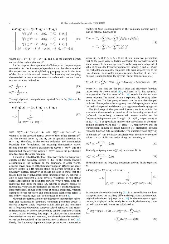
n Fðq1h ;q1þ

h Þ ¼ LðKþL1q1h þ KL1q1þ

h Þ

¼

nxc2

1þRqc p1 þ ð1þ RÞv1

n1 þ T p3qc T v3n1

nyc2


n1 þ T p3qc T v3n1

nzc2


n1 þ T p3qc T v3n1

c2 p1 R p1 T p3 þ qcðv1

n1 R v1n1 þ T v3

n1 Þ

266666664

377777775;ð14Þ

where v1n1 ¼ v1 n1;v3

n1 ¼ v3 n1 and n1 is the outward normal

vector of the surface element Dk1.For the purpose of computational efficiency and compact imple-

mentation for the frequency-dependent case, the above upwindflux expression can be simplified by grouping terms in the formof the characteristic acoustic waves. The incoming and outgoingcharacteristic acoustic waves across a surface with outward nor-mal vector n are defined as

-inn ¼ p

qc v n ð15Þ

-outn ¼ p

qcþ v n: ð16Þ

Through algebraic manipulations, upwind flux in Eq. (14) can bereformulated as

n Fðq1h ;q1þ

h Þ ¼ LðKþL1q1h þ KL1q1þ

h Þ

¼ LK

00

-out1n1

R -out1n1 þ T -out3

n3

26664

37775; ð17Þ

with -out1n1 ¼ p1=qc þ v1 n1 and -out3

n3 ¼ p3=qc þ v3 n3,

where n3 is the outward normal vector of the surface element Dk3

and the normal vector n1 and n3 are in opposite direction, i.e.,n1 ¼ n3. Therefore, in the current reflection and transmissionboundary flux formulation, the incoming characteristic wavesinclude both the reflected characteristic waves R -out1

n1 and thetransmitted characteristic waves T -out3

n3 across the partitioninginterface from the other medium.

It should be noted that the local plane wave behavior happeningexactly on the boundary surface is due to the locally-reactingassumption of the medium on the boundary. In other words,acoustic waves on each of the boundary nodes in 3D physical spacebehave locally in a 1D manner along the normal direction of theboundary surface. However, it should be kept in mind that thelocally high-order polynomial basis function of the DG scheme isable to well represent a local physical wavefront of non-planarshape approaching the boundary surface. What’s more, since thenumerical flux from the nodal DG scheme is always normal tothe boundary surface, the reflection coefficient R and the transmis-sion coefficient T should be the ones at normal incidence. Practicalexamples of the reflection and transmission coefficients across aflat locally-reacting layer will be discussed in Section 3.

Although the formulation for the frequency-independent reflec-tion and transmission boundary condition presented above isderived at a given single frequencyx, it in principle also holds truefor a frequency-dependent complex-valued reflection and trans-mission boundary, where a phase delay can be taken into accountas well. In the following, key steps to calculate the transmittedcharacteristic waves are presented, and the reflected characteristicwaves can be obtained in the same manner as shown in Ref. [27].Firstly, the frequency-dependent target plane wave transmission

coefficient TðxÞ is approximated in the frequency domain with asum of rational functions as

TðxÞ T1 þXSk¼1

Akfkþixþ

XTl¼1

12

BliClaliblþixþ BlþiCl

alþiblþix

¼ T1 þXSk¼1

Akfkþixþ

XTl¼1

Bl ixþClblþalBlðalþixÞ2þb2l

;

ð18Þ

where ½T1;Ak; Bl;Cl; fk;al; bl 2 R are all real numerical parametersthat fit the plane wave reflection coefficient for normally incidentsound waves. To be more specific, T1 is the frequency independentvalue of TðxÞ as the frequency approaches infinity. fk and al iblarethe real poles and complex conjugate pole pairs, respectively. In thetime-domain, the so-called impulse response function of the trans-mission is obtained from the inverse Fourier transform of TðxÞ

TðtÞ T1dðtÞ þXSk¼1

Akefk tHðtÞ þXTl¼1

eal t Bl cosðbltÞ þ Cl sinðbltÞð ÞHðtÞ; ð19Þ

where dðtÞ and HðtÞ are the Dirac delta and Heaviside function,respectively. As shown in Ref. [35], each term in TðtÞ has a physicalinterpretation. The first term of Eq. (19) stands for the instanta-neous response. The second term is a exponentially decaying relax-ation function. The last group of terms are the so-called dampedmulti-oscillators, where the imaginary part of the pole bldeterminesthe oscillation period and the real part al governs the decaying rate.

The final step of the proposed formulation is to obtain theequivalent time-domain expression of the incoming transmitted(reflected, respectively) characteristic waves similar to thefrequency-independent one T -out3

n3 (R -out1n1 , respectively) as

in Eq. (17). To be specific, it involves the convolution of the time-domain outgoing wave -out3

n3 ðtÞ (-out1n1 ðtÞ, respectively) and the

transmission impulse response function TðtÞ (reflection impulseresponse function RðtÞ, respectively). The outgoing wave -out1

n1 ðtÞin element Dk1 can be firstly calculated with the interior solutionvalues at each of discrete nodes along the boundary as

-out1n1 ðtÞ ¼ p1ðtÞ

qcþ v1

n1 ðtÞ: ð20Þ

Similarly, outgoing wave -out3n3 ðtÞ in element Dk3 is

-out3n3 ðtÞ ¼ p3ðtÞ

qcþ v3

n3 ðtÞ: ð21Þ

The final form of the frequency-dependent upwind flux is expressedas

n Fðq1h ;q1þ

h Þ¼ LðKþL1q1h þKL1q1þ

h Þ

¼ LK

00

-out1n1R t

1-out1n1 ðsÞRðtsÞdsþR t

1-out3n3 ðsÞTðtsÞds

266664

377775:

ð22Þ

To compute the convolution in Eq. (22) in a time efficient and low-storage manner, the auxiliary differential equations (ADE) method,originally developed by Joseph et al. [34] for electromagnetic appli-cations, is employed in this study. For example, the incoming trans-mitted characteristic waves are calculated asZ t

1-out3

n3 ðsÞTðt sÞds ¼ T1-out3n3 ðtÞ þ

XSk¼1

Ak/kðtÞ

þXTl¼1

½Blw1l ðtÞ þ Clw

2l ðtÞ; ð23Þ


where the new terms /kðtÞ;w1l ðtÞ;w2

l ðtÞ, referred to as accumulatorsor auxiliary variables, are given by:

/kðtÞ ¼Z t

0-out3

n3 ðsÞefkðtsÞds; ð24aÞ

w1l ðtÞ ¼

Z t

0-out3

n3 ðsÞealðtsÞ cos blðt sÞð Þds; ð24bÞ

w2l ðtÞ ¼

Z t

0-out3

n3 ðsÞealðtsÞ sin blðt sÞð Þds: ð24cÞ

The first term in Eq. (23) corresponds to the frequency-independentreflected wave as presented in Eq. (17). The bounds of the integralsin above Eq. (24) are reduced to ½0; t due to the causality constraintindicated in the Heaviside function HðtÞ. Instead of computing accu-mulators based on the integral of Eq. (24), the accumulators are cal-culated by solving the following first-order ordinary differentialequations, which result from the differentiation of Eq. (24) withrespect to time,

@/k

@tþ fk/kðtÞ ¼ -out3

n3 ðtÞ; ð25Þ@w1

l

@tþ alw

1l ðtÞ þ blw

2l ðtÞ ¼ -out3

n3 ðtÞ; ð26Þ@w2

l

@tþ alw

2l ðtÞ blw

1l ðtÞ ¼ 0: ð27Þ

The above system is numerically integrated from zero initial valuesusing the same time-integration scheme as for the semi-discrete DGformulation in Eq. (4), which will be shown in the following. There-fore, as shown by Dragna et al. [35], the ADE method keeps thesame order of accuracy of a general multi-stage time integrationscheme. It should be noted that these accumulators only exist onthe boundary nodes.

2.3. Time stepping and stability

After the spatial discretization by the nodal DG method, thesemi-discrete system can be expressed in a general form of ordi-nary differential equations (ODE) as:

dqh

dt¼ L qhðtÞ; tð Þ; ð28Þ

where qh is the vector of all discrete nodal solutions and L the spa-tial discretization operator of the DG method. A five-stage, fourth-order explicit Runge–Kutta (RK) scheme [39] is used to integrateEq. (28), i.e.,

qð0Þh ¼ qn

h;

kðiÞ ¼ aikði1Þ þDtL tn þ ciDt;q

ði1Þh

;

qðiÞh ¼ qði1Þ

h þ bikðiÞ;

8<: for i ¼ 1; . . . ;5

qnþ1h ¼ qð5Þ

h ;

ð29Þ

where Dt ¼ tnþ1 tn is the time step, qnþ1h and qn

h are the solutionvectors at time tnþ1 and tn, respectively. The coefficients ai; bi, andci of the Runge–Kutta method can be found in Ref. [39].

The explicit time-stepping method comes with the conditionalstability, which requires that the time step size Dt is small enoughso that the product of Dt with the full eigenvalue spectrum of ODEsystem falls inside the stability region of the time integrationscheme [40,41]. The whole ODE system under considerationincludes both the spatially-discretized linear acoustic equationsand the ADEs, which are coupled together along the impedanceboundary. Therefore, as shown in Refs. [35,42], the maximumallowable time step is determined by two factors: (1) the usual

Courant-Friedrichs-Lewy (CFL) condition for the spatial discretiza-tion with the DG scheme, which requires that Dt 6 C1=maxjkNj,where kN represents the eigenvalues of the spatial discretizationby the DG scheme and C1 is a constant depending on the stabilityregion of the time-stepping method; (2) the stiffness of the ADEs.As shown in Eqs. (25)–(27), the stiffness of the ADEs is influencedby the maximum possible value of the parameters f;a and b in themulti-pole approximation. In this work, the stiffness is restrictedso that the stability of the ADEs is automatically satisfied given atime-step size resulting from the first factor. The measures forrestrictions will be presented in Section 3.4. For the first factor, itis known that for the linear system with the first order of spatialdifferentiation, the gradients of the normalized N-th order polyno-mial basis are of order OðN2=hÞ near the boundary part of the ele-ment [16], consequently, the magnitude of the maximumeigenvalue kN scales with the polynomial order N as: maxðkNÞ / N2,indicating that Dt / N2. The temporal time steps are determinedin the following way [16]:

Dt ¼ CCFL minðDxlÞ 1c 1N2 ;

where Dxl is the smallest edge length of mesh elements and CCFL is aconstant of order Oð1Þ.

3. Multi-pole modeling of practical locally-reacting boundaries

The presented formulation of the reflection and transmissionboundary condition needs the plane wave reflection and transmis-sion coefficients at normal incidence conforming to the reflectionand transmission characteristics of the boundary considered. Asshown in Eqs. (11) and (12), the formulation also applies to caseswhere the simulated boundary has asymmetrical reflection andtransmission properties. The purpose of this section is to presenta few practical scenarios where sound reflection and transmissionhappen over a flat surface of the impedance discontinuity, and toillustrate how the multi-pole modeling approach can be appliedin practice to simulate the sound reflection and transmission onthe boundaries of locally-reacting media. The locally-reactingassumption, which indicates that reactions (velocity, displacement,acceleration, etc.) at a certain point on the surface are related to thesound pressure of only that point, holds true for: (a) isotropic por-ous absorptive materials with a high flow resistivity or large losses,especially when the speed of longitudinal wave in such materials ismuch lower than that of the adjacent propagation media [43]; (b)anisotropic solids, such as plates with low stiffness, perforatedstructure or honeycomb core structure, where the lateral wave israpidly attenuated or blocked.

3.1. Transmission through a limp wall (mass law)

A simple case of the impedance discontinuity that has practicalimportance in architectural acoustics is a limp wall, where only themass effect is considered and the interior stiffness or damping isignored. It can be seen as a simplified model of a thin partitionbetween two enclosures, whose thickness is much smaller thanthe wavelength in the frequency range of interest [44]. Due tothe continuum assumption, the wall vibrates with the same fre-quency and magnitude of the fluid particle that it is in direct con-tact with, and the normal component of velocity is continuous.Different from the classical elastic plate theory [45], the flexuralrigidity of the wall is ignored, and therefore the wall acts in alocally-reacting way and the corresponding reflection coefficientRðxÞ and the transmission coefficient TðxÞ are derived based onthe Newton’s second law and the continuity assumption of the nor-


mal velocity, as shown in Ref. [28]. They can be further re-writtenin the following multi-pole model form

RðxÞ ¼ 1 2Zc=mixþ 2Zc=m

; ð31Þ

TðxÞ ¼ 2Zc=mixþ 2Zc=m

; ð32Þ

where Zc is the characteristic impedance of the propagation mediaand m (kg/m2) is the surface density of the wall.

3.2. Transmission through a mass-damper-spring (MDS) partition

A more general case of locally-reacting partition is to incorpo-rate the damper and the spring effects into the surface partitionbetween two media, which results in a mass-damper-spring(MDS) system as illustrated in Fig. 2. The flexible partition of massper unit area m is mounted upon a viscously damped, elastic sus-pension, with the linear damping constant rd per unit area andthe spring constant s per unit area, respectively. This simplifiedmodel could approximate the fundamental mode of a large vibrat-ing panel [46]. Unlike the FDTD approach presented in Ref. [22],where the governing motion equations of the MDS system are dis-cretized explicitly by the central difference scheme, in this study,the MDS partition is treated as a whole system of the impedancediscontinuity, and the transmission and reflection coefficientsrequired for the upwind flux formulation are derived. As shownin Ref. [28], the wall impedance becomes ixmþ rd is=x. Apply-ing the same Newton’s second law and the continuity assumptionof the normal velocity as for the limp wall case, the correspondingreflection coefficient RðxÞ and the transmission coefficient TðxÞare obtained as

RðxÞ ¼ 1 2Zc

iðxm s=xÞ þ 2Zc þ rd; ð33Þ

TðxÞ ¼ 2Zc

iðxm s=xÞ þ 2Zc þ rd: ð34Þ

However, compared to the limp wall case, there is an extrafrequency-dependent term s=x in the denominators of above twoEqs. (33) and (34) due to spring effect. Consequently, both thereflection coefficient RðxÞ and the transmission coefficient TðxÞcannot be re-written in the multi-pole model form as shown inEq. (18). Consequently, a further approximation is needed toexpress RðxÞ and TðxÞ using the rational functions as basis func-tions. The approximation procedure will be discussed in Section 3.4.

3.3. Transmission through of a locally-reacting porous layer

Another practical scenario where the sound transmission mat-ters would be the noise barriers that are made of porous materials.As illustrated in Fig. 3, suppose that the locally-reacting porouslayer has a thickness of d, the transmission and reflection behavioroccurring in three different regions with respective characteristicimpedance values Z1; Z2, and Z3 are governed by the continuitycondition of both the pressure and the normal velocity on the dis-continuity interfaces. The corresponding plane wave reflectioncoefficient RðxÞ and the transmission coefficient TðxÞ are derivedas [47]

RðxÞ ¼ ðZ2 þ Z3ÞðZ2 Z1Þei2k2d þ ðZ3 Z2ÞðZ2 þ Z1ÞðZ2 þ Z3ÞðZ2 þ Z1Þei2k2d þ ðZ3 Z2ÞðZ2 Z1Þ ; ð35Þ

TðxÞ ¼ 4Z2Z3

ðZ3 Z2ÞðZ2 Z1Þeik2d þ ðZ2 þ Z3ÞðZ2 þ Z1Þeik2d ; ð36Þ

where k2 is the wavenumber and Z2 is the characteristic impedanceof the locally-reacting layer. In this study, Z1 and Z3 are chosen asthe characteristic impedance of air, i.e., Z1 ¼ Z3 ¼ qc. Like the caseof the MDS system, a parameter fitting procedure is needed toapproximate RðxÞ and TðxÞ with the multi-pole model.

3.4. Parameter fitting of the multi-pole model

In order to fit the multi-pole representation of the target reflec-tion coefficient and the target transmission coefficient, denoted byRtarðxÞ and TtarðxÞ, respectively, there are several parameter iden-tification methods available, e.g., the vector fitting technique [48]and the optimization technique [30]. A comparative study by Cottéet al. [30] shows that the optimization technique is preferred overthe vector fitting technique since it is straightforward to confinethe values of parameters and the number of poles to satisfy admis-sibility and stability conditions. Therefore, in this study, the opti-mization technique as in Ref. [30] is used. Since RtarðxÞ andTtarðxÞ can be complex values, both the real parts and the imagi-nary parts should be fitted simultaneously, instead of the ampli-tude and the phase, in order to avoid wraparound ambiguity[49]. In the following, the fitting procedure for the target transmis-sion coefficient TtarðxÞ is presented and the same procedure can beapplied to the target reflection coefficient RtarðxÞ. Let TfitðxÞ denotethe fitting multi-pole approximation as in Eq. (18) of TtarðxÞ, theoptimization is performed considering f s discrete frequencies sam-pled within the interested frequency range in a certain manner,e.g., logarithmically or linearly spaced. Then, the Euclidean normof the deviation of real parts are minimized while keeping the dif-ference of imaginary parts at each of the sampled frequency undera tolerance value , i.e.,

Fig. 2. Simplified model of reflection and transmission through a single-leafpartition under normal incidence sound waves. Fig. 3. Reflection and transmission through of a locally-reacting porous layer.


minAk ;fk ;al ;bl ;Bl ;Cl

ffiffiffiffiffiffiffiffiffiffiffiffiffiffiffiffiffiffiffiffiffiffiffiffiffiffiffiffiffiffiffiffiffiffiffiffiffiffiffiffiffiffiffiffiffiffiffiffiffiffiffiffiffiffiffiXf si¼1

jRe½TtarðxiÞ TfitðxiÞjvuut

0@

1A ð37Þ

suchthat

0 6 fk 6 fmax

0 6 al 6 amax

0 6 bl 6 bmax

8i; jIm½TtarðxiÞ TfitðxiÞj 6 :

8>>><>>>:

where fmax;amax, and bmax are the threshold values for f;a, and b forthe sake of the time-stepping stability. To solve this minimizationproblem, the interior-point algorithm [50] of the non-linear mini-mization function fmincon from the MATLAB optimization toolbox[51] is used. A series of optimizations are run to get a good fit. Inthe first run, the initial values of (Ak; fk;al;bl; Bl;Cl) are chosen ran-domly between 0 and fmax;amax;bmax, respectively, and a relativelylarge value of is used, e.g., ¼ 1 101. Then, the obtained setof coefficients are used as the initial values for the next optimiza-tion with a smaller value of . The process continues until thethreshold value of meets the accuracy requirement. An exampleof parameter fitting will be shown in the following numerical test.

4. Numerical examples and discussions

This section presents both one-dimensional and two-dimensional numerical examples to verify the proposed formula-tion of the time-domain reflection and transmission boundary con-dition. Depending on whether a multi-pole approximation isneeded, two types of locally-reacting boundaries are consideredin this study. One is the limp wall boundary, the reflection andtransmission coefficients of which can be represented exactly withthe real pole model as shown in Eqs. (31) and (32). The other one isthe locally-reacting porous layer, which needs a further level ofapproximation of the reflection and transmission coefficients usingthe multi-pole model in Eq. (18). It should be noted that the mass-damper-spring (MDS) partition could be tackled with the samemethodology as the porous layer. All of the following numericalexperiments are initiated with the Gaussian-shaped pressure con-ditions as

pðx; t ¼ 0Þ ¼ e ln 2b2

ðxxsÞ2 ; ð38aÞvðx; t ¼ 0Þ ¼ 0; ð38bÞ

with xs being the source coordinates and b being the half-bandwidth of this Gaussian pulse.

4.1. One-dimensional cases

As illustrated in Fig. 4, the sound field has a single monopolesource at xs ¼ 3 m and two receivers at xr1 ¼ 0:5 m andxr2 ¼ 1:5 m, respectively. The transmissive boundary is placed atx ¼ 0 m. The computational domain are terminated at both endsx ¼ 5 m with the perfectly absorbing boundary condition, which

is achieved by discarding the incoming wave component in thenumerical upwind flux [38]. b is chosen as 0.15 such that the initialGaussian pulse has a significant frequency content up to 1000 Hz.

For the one-dimensional test case, the analytical values of thefrequency-dependent plane wave reflection and transmission coef-ficients are available. In order to obtain the numerical reflectioncoefficient Rnum and the transmission coefficient Tnum, two simula-tions are conducted. In the first simulation, the transmissiveboundary is removed and the direct sound signal, denoted aspdðtÞ, at each of two receivers is recorded. In the second simulation,the transmissive boundary is present, the measured sound pres-sure signal at first receiver xr1 contains both the direct sound andthe sound reflected from the transmissive boundary while the sig-nal at second receiver xr2 contains the transmitted signal aloneptðtÞ. The reflected sound signal prðtÞ can be obtained by subtract-ing pdðtÞ. The spectra of the direct sound, the reflected sound, andthe transmitted sound, denoted as Pdðf Þ; Prðf Þ, and Ptðf Þ, respec-tively, are obtained by Fourier transformation of pd; pr , and pt with-out windowing. Let R1 denote the distance between the source andthe receiver and R2 be the distance between the receiver and theimage source mirrored by the reflecting surface. The numericalreflection coefficient Rnum is calculated as follows:

Rnumðf Þ ¼ Prðf Þ GðkR1ÞPdðf Þ GðkR2Þ ; ð39Þ

where GðkRÞ ¼ eikR=ð2ikÞ is the 1D Green’s function for the soundpropagation in free field. Similarly, the numerical transmissioncoefficient Tnum results from the ratio of the transmitted soundand the direct sound. As shown in Ref. [17], it is desirable to havearound 10 points per wavelength (PPW) to achieve a satisfactoryaccuracy. Therefore, we discretize the computational domain withK ¼ 30 elements, corresponding to Dx ¼ 1=3 m, and inside each ele-ment, a polynomial basis of order N ¼ 8 is used, resulting into aPPW value of 9.2 at the frequency of 1000 Hz. According to Eq.(30), the time step size used is Dt ¼ 4:871 105 s, correspondingto CCFL ¼ 1. The simulations are run for t ¼ 0:5 s so that the pulsehas passed the receiver locations to a sufficient extent.

To quantify the error arising from each reflection and transmis-sion, the dissipation error amp in dB and the phase error # in %

from a single transmission are calculated as follows

ampðf Þ ¼ 20log10Tanaðf ÞTnumðf Þ

; ð40aÞ

#ðf Þ ¼ 1pj# Tanaðf Þð Þ # Tnumðf Þð Þj 100%; ð40bÞ

where # ð Þ extracts the phase angle of a complex number. Similarly,the error from a single reflection can be calculated by replacing Twith R in above two equations. Therefore, for a given broadbandincident acoustic wave of arbitrary amplitude, the loss of SPL andthe distortion of the phase across the frequency range of interestcan be quantified.

Fig. 4. 1D computational configuration with a transmissive boundary.


The first type of the transmissive boundary to be investigated isthe limp wall case that is governed by the mass law. As discussedin Section 3.1, the surface mass density m of the thin partitionmaterial is the only parameter that affects the reflection and trans-mission characteristics. Here, two values of m ¼ 10 kg/m2 andm ¼ 20 kg/m2 are considered, corresponding to 3 cm thick materi-als of typical wood panels and light concrete, respectively. The ana-lytical reflection coefficient Rana and the transmission coefficientTana are calculated as shown in Eqs. (31) and (32). Fig. 5 presentsthe comparison of the results obtained by the numerical simula-tions and by the analytical solution. Both of the amplitudes ofthe reflection and the transmission coefficients match quite wellwith the analytical ones. As expected, all error increases graduallywith increasing frequency due to the decreased PPW. Concretely,the dissipation error falls onto the order of magnitude Oð104Þand the phase error is below 0:02%.

As for the locally-reacting porous layer, we consider a glasswool that is typically used as baffles for room acoustic purposes.Supposed its characteristic impedance Zc is governed by theJohnson-Champoux-Allard-Lafarge (JCAL) model [52], which is aphenomenological model describing wave propagation in porousmaterials on a macroscopic scale and is expressed as

Zc ¼ffiffiffiffiffiffiffiffiffiffiffiffiffiffiffiqeff Beff

q. The effective density qeff and the effective bulk mod-

ulus Beff are described by

qeff ¼qa1u

1þ ruixa1q

1þ 4ia21gq

r2K2u2

!1=224

35; ð41Þ

Beff ¼ cP0

uc c 1

1þ ugixk00qPr

ð1þ 4ixk020 qPrgK02u2 Þ

1=2

0BB@

1CCA

1

: ð42Þ

The wavenumber of the porous material is given as

keff ¼ xffiffiffiffiffiffiffiffiffiffiffiffiffiffiffiffiffiqeff =Beff

q. The descriptions of physical parameters are given

in Table A.3 in Appendix A and their values for the considered glasswool were measured by experiments [53]. In order to model thereflection and transmission properties of the porous layer, firstly,the characteristic impedance Zc is inserted into the plane wavereflection coefficient RðxÞ as in Eq. (35) and the transmission coef-ficient TðxÞ as in Eq. (36). Then, the resulting target RtarðxÞ andTtarðxÞ are approximated with rational functions in the multi-poleform using the optimization techniques presented in Section 3.4.For the considered JCAL model, it is easy to verify that the magni-tude of both RtarðxÞ and TtarðxÞ are monotonic decreasing functionof frequency, which allows us to use real-poles alone for theapproximation. The optimization is performed considering 100 fre-quencies logarithmically sampled between 20 and 1000 Hz, and thetolerance value for the deviation of the imaginary part is chosen as1 104. Numerical tests show that there is a compromise betweenthe number of poles and the fitting accuracy. Sets of fitting param-eters for RðxÞ and TðxÞ are given in Table 1 and Table 2, respec-tively. The maximum absolute value error at the sampledfrequencies are 2:362 103 and 6:118 105 for the real andimaginary part of the reflection coefficient, respectively, and theerror for the transmission coefficient are 2:636 103 and5:418 105. The dissipation error amp, the phase error # asdefined in Eq. (40) of the fitted coefficients are shown in Fig. 6,including the magnitude of both target and fitted coefficients aswell.

The numerically simulated frequency-dependent characteris-tics of the porous layer are compared against the analytical onesin Fig. 7. Similar to the limp wall test case, the amplitudes of boththe reflection and the transmission coefficients agree well with theanalytical ones. However, the amplitudes and the frequency-

0 500 10000

2

4

6

8

10 10-4

0 500 10000

0.005

0.01

0.015

0.02

0 500 10000

0.2

0.4

0.6

0.8

1

0 500 10000

2

4

6

8

10 10-4

0 500 10000

0.005

0.01

0.015

0.02

0 500 10000

0.2

0.4

0.6

0.8

1

Fig. 5. The dissipation error amp , the phase error # and the magnitude of transmission and reflection coefficients for the 1D limp wall.


dependency of the quantified errors, especially the dissipationerror, are quite different from the limp wall case. Through compar-ison of Figs. 6 and 7, it can be observed that the approximationerror of R and T using the multi-pole model dominates over theDG discretization error for the overall error. This implies that thefitting quality of the multi-pole model plays a crucial role in theoverall accuracy.

4.2. Two-dimensional cases

This section is devoted to the verification of the transmissionboundary condition in a two-dimensional sound field. Differentfrom the one-dimensional test case, where the analytical valuesof the reflection and transmission coefficients are available, here,the numerical results obtained from the time-domain DG simula-tions are firstly transformed into the frequency-domain and thencompared against the results obtained by the frequency-domainfinite element (FE) analysis with the commercial software COMSOLMultiphysics [54]. For each of the following numerical tests, the

free field responses at receivers are calculated firstly for bothtime-domain DG and frequency-domain FE simulations, in orderto normalize the difference of the source power spectra betweenthe DG simulations and frequency-domain FE simulations.

The first test case involves a rectangular domain evenly sepa-rated by a limp panel in the middle as shown in Fig. 8, which mim-ics a typical building acoustic scenario of sound transmissionbetween two rooms partitioned by a thin structure. Here, thereflection and transmission characteristics of the limp panel aregoverned by the mass law as discussed in Section 3.1. Without lossof generality, two values of surface mass densitym ¼ 30 kg/m2 andm ¼ 65 kg/m2 are used for the limp panel, representing light andmoderately heavy room partitions, respectively. All the otherboundaries are assigned as a uniform real-valued absorption coef-ficient of 0.36, which corresponds to the reflection coefficient ofR ¼ 0:8. The locations of the sound source and receivers are illus-trated in Fig. 8. The half-bandwidth of Gaussian pulse is chosenas b ¼ 0:25 such that the source has a sufficient power up to600 Hz. The computational domain for the DG simulation is

Table 1Fitting parameters Ak and fk of the real pole approximation for the reflection coefficient RðxÞ of the glass wool.

Coefficients k ¼ 1 k ¼ 2 k ¼ 3 k ¼ 4

Ak 3:124 103 6:956 101 8:175 103 2:459 103

fk 4:771 104 1:747 103 2:735 104 6:641 103

Table 2Fitting parameters Ak and fk of the real pole approximation for the transmission coefficient TðxÞ of the glass wool.

Coefficients k ¼ 1 k ¼ 2 k ¼ 3 k ¼ 4 k ¼ 5

Ak 9:751 103 1:087 103 1:703 103 6:401 103 5:397 101

fk 3:117 104 6:121 103 7:807 103 5:773 104 1:738 103

0 500 1000-0.03

-0.02

-0.01

0

0.01

0.02

0 500 10000

0.1

0.2

0.3

0.4

0.5

0.6

0 500 10000

0.2

0.4

0.6

0.8

1

Fig. 6. The dissipation error amp , the phase error # and the magnitude of the fitted transmission and reflection coefficients for the 1D porous layer.

0 500 1000-0.03

-0.02

-0.01

0

0.01

0.02

0 500 10000

0.1

0.2

0.3

0.4

0.5

0.6

0 500 10000

0.2

0.4

0.6

0.8

1

Fig. 7. The dissipation error amp , the phase error # and the magnitude of the numerically simulated transmission and reflection coefficient for the 1D porous layer.


discretized with right angled isosceles triangles of equal leg lengthof 0.5 m, resulting into K ¼ 96 triangle elements. A local polyno-mial basis of order N ¼ 8 is used in order to have PPW = 10.8 up-to frequency of 600 Hz. The time step size is Dt ¼ 2:278 105 s,corresponding to CCFL ¼ 1 as described in Eq. (30). The simulationsare run for t ¼ 0:45 s and the time signal at each of the receiverlocations approaches zero eventually due to the wall absorptions.For the frequency-domain FE analysis, the model was built in pres-sure acoustic module of the COMSOL Multiphysics [54]. Themonopole point source with a volume flow rate per unit length 1m2=s is applied at the source position. On the boundary corre-sponding to the limp panel, an interior impedance boundary con-dition with a frequency dependent impedance value ixm isimposed. On all the other boundaries, impedance boundary condi-tions with the surface impedance of Zs ¼ ð1þ RÞ=ð1 RÞ areimposed. The meshes are discretized so that there are at least 6 ele-ments per the shortest wavelength in the frequency range of inter-est, which is the wavelength of the time-harmonic acoustic wavesat 600 Hz in this case, in order to ensure accuracy of the analysis.

The relative sound pressure level, which is obtained by calculat-ing the amplitude of ratio of the pressure spectra with respect tothe free field, is used for the comparison between the time-domain DG method and the frequency-domain FEM. As shown inFig. 9, both numerical results agree well with each other at threereceiver locations for two different surface mass density values.To demonstrate the comparison in terms of the phase shift, thephase angles of the ratio of the pressure spectra with respect tothe free field spectra are compared in Fig. 10. For the sake of clarity,the phase angles at different receivers are shifted by a constant inthe plot. A very good match between the time-domain simulationsand the frequency-domain simulations can be observed.

The second test case considered is the sound propagation acrossa finite-height noise barrier made of the same porous glass-woolmaterial as used in the one-dimensional test case. The schematicdiagrams for both the DG and FE simulations are shown inFig. 11. The source is located at ðxs; ysÞ ¼ ð2;0Þ m and four recei-vers at ðxr1 ; yr1 Þ ¼ ð1;0Þ; ðxr2 ; yr2 Þ ¼ ð1;3Þ; ðxr3 ; yr3 Þ ¼ ð1;0Þ, andðxr4 ; yr4 Þ ¼ ð1;3Þ m are distributed symmetrically with respect tothe barrier, which is attached to the hard ground and has a heightof H ¼ 4 m and width of W ¼ 4 cm. To mimic a real noise barriermounted on a hard ground surface, the top edge of the barrier isa rigid boundary, whereas both side edges are treated as a trans-missive porous layer. The other boundaries are assumed to be rigid.

In order to capture the diffraction effects from the top edge of thebarrier, the full geometry details of the barrier are meshed andmodeled. For this test case, unstructured triangle meshes are gen-erated with the meshing software GMSH [55]. As illustrated inFig. 12, the mesh is locally refined near the top edge of the soundbarrier and mesh elements far away from the sound barrier havean edge length of approximately 0.5 m. A local polynomial basisof order N ¼ 8 is adopted. The global uniform time step size isDt ¼ 1:391 106 s, corresponding to CCFL ¼ 1 as described in Eq.(30). The impulse response from the DG simulation is recordeduntil the reflected waves from the exterior boundaries reach thereceivers while ensuring that the pulse has passed the receivers’location to a sufficient extent.

In FE simulation, the barrier is modelled as an anisotropic med-ium with different acoustic densities in x and y directions to imi-tate the locally reacting wave behavior inside the porous layer,as it is described in Section 3.3. Therefore, the acoustic density inthe x direction of the medium is represented as same as the effec-tive density of the porous material in Eq. (41) but an infinite valueis imposed for the acoustic density in the y direction to prohibit thewave propagation along the y direction. In addition, to truncatecomputational regions of an inifnitely open space, perfectlymatched layers (PMLs) are added on the top as well as at the leftand right ends of the domain as shown in Fig. 11(b). Again, thereare at least 6 elements per wavelength corresponding to thetime-harmonic acoustic waves at 600 Hz, in order to ensure accu-racy of the analysis.

Fig. 8. Computational configuration of a two-dimensional sound field with a limpwall partition.

0 100 200 300 400 500 600-80

-60

-40

-20

0

20

0 100 200 300 400 500 600-80

-60

-40

-20

0

20

Fig. 9. Comparison of the relative sound pressure level between the DG simulationand the FE simulation for the limp wall case with two different surface mass densitym.


Similar to the previous test case, the comparison of the relativesound pressure level and the phase angles of the pressure spectraratio at different receiver locations are shown in Figs. 13 and 14,respectively. Again, a good match between the time-domain DGsimulations and the frequency-domain FE simulations is found. Itshould be noted that the pressure waves arriving at the receiversacross the barrier include not only the transmission components,but also the components diffracted over the hard barrier top, sincethe geometry details are fully resolved by both simulations. How-ever, the discrepancies between two simulations in terms of thehigh order diffraction components, which should have existeddue to the early truncated DG simulation, are mitigated due tothe absorption effect of the noise barrier.0 100 200 300 400 500 600

-10

-5

0

5

10

15

0 100 200 300 400 500 600-10

-5

0

5

10

15

Fig. 10. Comparison of the phase angle of ratio between the DG simulation and theFE simulation for the limp wall case with two different surface mass density m.

Fig. 11. Schematic diagram of a two-dimensional configuration with a noise barrier.

Fig. 12. 2D mesh around the noise barrier for the DG simulation.

0 100 200 300 400 500 600-25

-20

-15

-10

-5

0

5

Fig. 13. Comparison of the relative sound pressure level between the DG simulationand the FE simulation for the noise barrier case.


5. Conclusion

In this study, a general time-domain transmission boundarycondition in the framework of the time-domain DG method isdeveloped for the broadband simulations of general linear acous-tics, with potential applications to the areas of room acoustics,building acoustics, urban acoustics to name a few. The proposednumerical formulation is able to simulate frequency-dependentreflection and transmission characteristics of a locally-reactingboundary. The essential idea is to model the acoustic characteris-tics of a locally-reacting surface using the plane wave reflectioncoefficient and transmission coefficients in the form of a multi-pole model and then reformulate the corresponding time-domainupwind flux. Practical examples of the boundary modeling withthe multi-pole model approach are presented.

To verify the performance of the formulation, one-dimensionalnumerical tests are performed and convergence of the numericalresults to the analytical ones are demonstrated. Furthermore, ithas been shown that the both dissipation and dispersion errorsdepend largely on the accuracy of parameters fitting of themulti-pole models. In this work, an optimization-based methodis employed to obtain the fitting parameters. Although it is suffi-cient to verify the formulation for the locally-reacting boundarieswith one-dimensional examples, two-dimensional numerical testsare conducted to further demonstrate the general practicability ofthe boundary formulation within the time-domain DG framework.Excellent agreement of numerical results obtained by the proposedtime-domain method and the frequency-domain FEM areobserved. However, for acoustic boundaries where non-negligibleinteractions happen, the locally-reacting assumption may lead toinaccurate representation of the acoustic behavior. Therefore, fur-ther developments of modeling extendedly-reacting boundarieswill be undertaken in future works.

Declaration of Competing Interest

The authors declare that they have no known competing finan-cial interests or personal relationships that could have appearedto influence the work reported in this paper.

Acknowledgements

This project has received funding from the European Union’sHorizon 2020 research and innovation programme under grantagreement No. 721536.

Appendix A

References

[1] Pelzer S, Aspöck L, Schröder D, Vorländer M. Integrating real-time roomacoustics simulation into a cad modeling software to enhance the architecturaldesign process. Buildings 2014;4(2):113–38.

[2] Kuttruff H. Room acoustics. New York: CRC Press; 2016.[3] Sakuma T, Sakamoto S, Otsuru T. Computational simulation in architectural

and environmental acoustics. Springer; 2014.[4] Aretz M, Vorländer M. Combined wave and ray based room acoustic

simulations of audio systems in car passenger compartments, part i:Boundary and source data. Appl Acoust 2014;76:82–99.

[5] Mehra R, Rungta A, Golas A, Lin M, Manocha D. Wave: Interactive wave-basedsound propagation for virtual environments. IEEE Trans Visualization ComputGraphics 2015;21(4):434–42.

[6] Mallardo V, Aliabadi M, Brancati A, Marant V. An accelerated bem forsimulation of noise control in the aircraft cabin. Aerospace Sci Technol2012;23(1):418–28.

[7] Savioja L, Svensson UP. Overview of geometrical room acoustic modelingtechniques. J Acoust Soc Am 2015;138(2):708–30.

[8] Cox T, D’Antonio P. Acoustic absorbers and diffusers: theory, design andapplication. CRC Press; 2016.

[9] Botteldooren D. Finite-difference time-domain simulation of low-frequencyroom acoustic problems. J Acoust Soc Am 1995;98(6):3302–8.

[10] Okuzono T, Yoshida T, Sakagami K, Otsuru T. An explicit time-domain finiteelement method for room acoustics simulations: Comparison of theperformance with implicit methods. Appl Acoust 2016:76–84.

[11] Bilbao S. Modeling of complex geometries and boundary conditions in finitedifference/finite volume time domain room acoustics simulation. IEEE TransAudio, Speech, Language Process 2013;21(7):1524–33.

[12] Hornikx M, Krijnen T, van Harten L. openPSTD: The open sourcepseudospectral time-domain method for acoustic propagation. Comput PhysCommun 2016;203:298–308.

[13] Atkins HL, Shu C-W. Quadrature-free implementation of discontinuousGalerkin method for hyperbolic equations. AIAA J 1998;36(5):775–82.

[14] Delorme P, Mazet P, Peyret C, Ventribout Y. Computational aeroacousticsapplications based on a discontinuous galerkin method. Comptes RendusMécanique 2005;333(9):676–82.

[15] Cockburn B, Karniadakis GE, Shu C-W. Discontinuous Galerkin methods:theory, computation and applications, vol. 11. Springer Science & BusinessMedia; 2012.

[16] Hesthaven JS, Warburton T. Nodal discontinuous Galerkin methods:Algorithms Analysis and Applications. New York: Springer-Verlag; 2007.

[17] Wang H, Sihar I, Pagán Muñoz R, Hornikx M. Room acoustics modelling in thetime-domain with the nodal discontinuous galerkin method. J Acoust Soc Am2019;145(4):2650–63.

[18] Hu F, Atkins H. Two-dimensional wave analysis of the discontinuous Galerkinmethod with non-uniform grids and boundary conditions. In: 8th AIAA/CEASAeroacoustics Conference & Exhibit. p. 2514.

[19] Modave A, St-Cyr A, Warburton T. GPU performance analysis of a nodaldiscontinuous Galerkin method for acoustic and elastic models. ComputGeosci 2016;91:64–76.

[20] Schoeder S, Wall W, Kronbichler M. Exwave: A high performancediscontinuous galerkin solver for the acoustic wave equation. SoftwareX2019;9:49–54.

[21] Schoeder SM. Efficient Discontinuous Galerkin Methods for Wave Propagationand Iterative Optoacoustic Image Reconstruction Ph.D.dissertation. Technische Universität München; 2019.

[22] Toyoda M, Ishikawa S. Frequency-dependent absorption and transmissionboundary for the finite-difference time-domain method. Appl Acoust2019;145:159–66.

Table A.3Overview of the JCAL impedance model parameters for the glass wool.

Property Value

Atmospheric pressure P0 [Pa] 1:01 105

Speed of sound c [ms1] 343

Density q [kgm3] 1.2

Airflow resistivity r [Pasm2] 70821Porosity u 0.967

Tortuosity a1 1.049Viscous characteristic length K [m] 6 105

Thermal characteristic length K0 [m] 1:4 104

Static thermal permeability k00 [m2] 6:345 109

Dynamic viscosity g [Nm2] 1:82 105

Prandtl number Pr 0.71Layer thickness d [m] 0.04Specific heat ratio c 1.4

0 100 200 300 400 500 600-8

-6

-4

-2

0

2

4

6

8

Fig. 14. Comparison of the phase angle of ratio between the DG simulation and theFE simulation for the noise barrier case.


[23] Richter C, Hay JA, Schönwald N, Busse S, Thiele F. A review of time-domain impedance modelling and applications. J Sound Vib 2011;330(16):3859–73.

[24] Fung K-Y, Ju H. Time-domain impedance boundary conditions forcomputational acoustics and aeroacoustics. Int J Comput Fluid Dyn 2004;18(6):503–11.

[25] Reymen Y, Baelmans M, Desmet W. Efficient implementation of Tam andAuriault’s time-domain impedance boundary condition. AIAA J 2008;46(9):2368–76.

[26] Monteghetti F, Matignon D, Piot E. Energy analysis and discretization ofnonlinear impedance boundary conditions for the time-domain linearizedeuler equations. J Comput Phys 2018;375:393–426.

[27] Wang H, Hornikx M. Broadband time-domain impedance boundary modelingwith the discontinuous galerkin method for room acoustics simulations. In:23rd International Congress on Acoustics. p. 779–86.

[28] Kim Y-H. Sound propagation: an impedance based approach. John Wiley &Sons; 2010.

[29] Fung K-Y, Ju H. Broadband time-domain impedance models. AIAA J 2001;39(8):1449–54.

[30] Cotté B, Blanc-Benon P, Bogey C, Poisson F. Time-domain impedance boundaryconditions for simulations of outdoor sound propagation. AIAA J 2009;47(10):2391–403.

[31] Dragna D, Cotté B, Blanc-Benon P, Poisson F. Time-domain simulations ofoutdoor sound propagation with suitable impedance boundary conditions.AIAA J 2011;49(7):1420–8.

[32] Troian R, Dragna D, Bailly C, Galland M-A. Broadband liner impedanceeduction for multimodal acoustic propagation in the presence of a meanflow. J Sound Vib 2017;392:200–16.

[33] Douasbin Q, Scalo C, Selle L, Poinsot T. Delayed-time domain impedanceboundary conditions (d-tdibc). J Comput Phys 2018;371:50–66.

[34] Joseph RM, Hagness SC, Taflove A. Direct time integration of maxwell’sequations in linear dispersive media with absorption for scattering andpropagation of femtosecond electromagnetic pulses. Opt Lett 1991;16(18):1412–4.

[35] Dragna D, Pineau P, Blanc-Benon P. A generalized recursive convolutionmethod for time-domain propagation in porous media. J Acoust Soc Am2015;138(2):1030–42.

[36] Hesthaven JS, Teng C-H. Stable spectral methods on tetrahedral elements.SIAM J Sci Comput 2000;21(6):2352–80.

[37] Ainsworth M. Dispersive and dissipative behaviour of high orderdiscontinuous Galerkin finite element methods. J Comput Phys 2004;198(1):106–30.

[38] Atkins H. Continued development of the discontinuous Galerkin method forcomputational aeroacoustic applications. In: 3rd AIAA/CEAS AeroacousticsConference. p. 1581.

[39] M.H. Carpenter, C.A. Kennedy, Fourth-order 2n-storage runge-kutta schemes,in: NASA-TM-109112, 1994..

[40] Reddy SC, Trefethen LN. Stability of the method of lines. Numer Math 1992;62(1):235–67.

[41] Gustafsson B. High order difference methods for time dependentPDE. Berlin: Springer-Verlag; 2007.

[42] Pind F, Engsig-Karup AP, Jeong C-H, Hesthaven JS, Mejling MS, Strømann-Andersen J. Time domain room acoustic simulations using the spectralelement method. J Acoust Soc Am 2019;145(6):3299–310.

[43] Gunnarsdóttir K, Jeong C-H, Marbjerg G. Acoustic behavior of porous ceilingabsorbers based on local and extended reaction. J Acoust Soc Am 2015;137(1):509–12.

[44] Kinsler LE, Frey AR, Coppens AB, Sanders JV, Fundamentals of acoustics,Fundamentals of Acoustics, 4th Edition, by Lawrence E. Kinsler, Austin R. Frey,Alan B. Coppens, James V. Sanders, pp. 560. ISBN 0-471-84789-5. Wiley-VCH,December 1999. (1999) 560..

[45] Reddy JN. Theory and analysis of elastic plates and shells. CRC Press; 2006.[46] Fahy F, Gardonio P. Sound and structural vibration – radiation, transmission

and response. Elsevier; 2007.[47] Brekhovskikh LM, Godin OA. Acoustics of layered media I: Plane and quasi-

plane waves, vol. 5. Springer Science & Business Media; 2012.[48] Gustavsen B, Semlyen A. Rational approximation of frequency domain

responses by vector fitting. IEEE Trans Power Delivery 1999;14(3):1052–61.[49] Bilbao S, Hamilton B, Botts J, Savioja L. Finite volume time domain room

acoustics simulation under general impedance boundary conditions. IEEE/ACM Trans Audio Speech Language Processing (TASLP) 2016;24(1):161–73.

[50] Byrd RH, Hribar ME, Nocedal J. An interior point algorithm for large-scalenonlinear programming. SIAM J Optim 1999;9(4):877–900.

[51] MATLAB Optimization Toolbox (R2018b), The MathWorks, Inc., Natick,Massachusetts, USA, 2018..

[52] Lafarge D, Lemarinier P, Allard JF, Tarnow V. Dynamic compressibility of air inporous structures at audible frequencies. J Acoust Soc Am 1997;102(4):1995–2006.

[53] Hoeskstra N. Sound absorption of periodically spaced baffles Masterthesis. Eindhoven University of Techonology; 2016.

[54] COMSOL AB, Stockholm, Sweden, COMSOL Multiphysics v. 5.4..[55] Geuzaine C, Remacle J-F. Gmsh: A 3-D finite element mesh generator with

built-in pre-and post-processing facilities. Int J Numer Meth Eng 2009;79(11):1309–31.


Errata of Paper IIIIt should be noted that the statement following Eqs. (33) and (34) in section

3.2, which is “However, compared to the limp wall case, there is an extra frequency-dependent term s/ω in the denominators of above two equations (33) and (34) due tospring effect. Consequently both the reflection coefficient R(ω) and the transmissioncoefficient T (ω) cannot be re-written in the multi-pole model form as shown in Eq.(18). Consequently, a further approximation is needed to express R(ω) and T (ω)using the rational functions as basis functions. The approximation procedure will bediscussed in Sec. 3.4. ”, is incorrect.

As shown in the following, both the plane wave reflection coefficient R(ω) andtransmission coefficient T (ω) can be re-cast in a multi-pole form with complex polesand therefore, no further approximation is needed for R(ω) and T (ω). Recall thatthe multi-pole model approximation is (taking T (ω) for example),

T (ω) ≈ T∞ +

S∑k=1

Ak

ζk + iω +

K∑l=1

1

2

( Bl − iCl

αl − iβl + iω +Bl + iCl

αl + iβl + iω

)= T∞ +

S∑k=1

Ak

ζk + iω +

K∑l=1

Bliω + Clβl + αlBl

α2l + β2

l + 2αliω − ω2.

As shown in Eq. (34) of Paper III, the transmission coefficient T (ω) for the mass-damper-spring (MDS) partition is

T (ω) =2Zc

i(ωm− s/ω) + 2Zc + rd

=2Zciω/m

s/m+ iω(2Zc + rd)/m− ω2.

By comparing above two equations, it is straightforward to obtain the relations be-tween the multi-pole model parameters and the MDS parameters as B = 2Zc/m,α =(2Zc + rd)/(2m), β =

√s/m− α2, C = −αB/β.

Therefore, the texts following Eqs. (33) and (34) in section 3.2 should be correctedto: “Through derivations, it is straightforward to express the transmission coefficientT (ω) in terms of the multi-pole model parameters with B = 2Zc/m,α = (2Zc +rd)/(2m), β =

√s/m− α2, C = −αB/β, whereas the reflection coefficient R(ω) only

differs by the constant 1 and the sign of B.”

Page 137

Paper IV

Page 139

An arbitrary high-order discontinuous Galerkin method withlocal time-stepping for linear acoustic wave propagation

Huiqing Wang,a) Matthias Cosnefroy, and Maarten Hornikxb)

Building Physics and Services, Department of the Built Environment, Eindhoven University of Technology, P.O. Box 513, Eindhoven,5600 MB, The Netherlands

ABSTRACT:This paper presents a numerical scheme of arbitrary order of accuracy in both space and time, based on the arbitrary

high-order derivatives methodology, for transient acoustic simulations. The scheme combines the nodal discontinu-

ous Galerkin method for the spatial discretization and the Taylor series integrator (TSI) for the time integration. The

main idea of the TSI is a temporal Taylor series expansion of all unknown acoustic variables in which the time deriv-

atives are replaced by spatial derivatives via the Cauchy-Kovalewski procedure. The computational cost for the time

integration is linearly proportional to the order of accuracy. To increase the computational efficiency for simulations

involving strongly varying mesh sizes or material properties, a local time-stepping (LTS) algorithm accompanying

the arbitrary high-order derivatives discontinuous Galerkin (ADER-DG) scheme, which ensures correct communica-

tions between domains with different time step sizes, is proposed. A numerical stability analysis in terms of the max-

imum allowable time step sizes is performed. Based on numerical convergence analysis, we demonstrate that for

nonuniform meshes, a consistent high-order accuracy in space and time is achieved using ADER-DG with LTS. An

application to the sound propagation across a transmissive noise barrier validates the potential of the proposed

method for practical problems demanding high accuracy. VC 2021 Acoustical Society of America.

https://doi.org/10.1121/10.0003340

(Received 2 October 2020; revised 3 December 2020; accepted 21 December 2020; published online 25 January 2021)

[Editor: Nickolas Vlahopoulos] Pages: 569–580

I. INTRODUCTION

Recent years have witnessed rapid developments and

applications of the time-domain discontinuous Galerkin

(TD-DG) method for modeling wave propagation phenom-

ena,1–8 which possesses many favorable properties, such as

high-order accuracy, geometric flexibility, and its capability

of handling inhomogeneous media and physically absorbing

media.9–11 It first discretizes the volumetric space into non-

overlapping mesh elements that can be locally refined to

meet the geometrical constraints. Then, solutions of govern-

ing acoustic equations are approximated spatially with a

polynomial basis. Because the locally defined basis func-

tions can be discontinuous across element interfaces, the

resulting mass matrix is block diagonal, which favors a fully

explicit time-marching scheme with intrinsic parallel com-

putations.12,13 Last, following the numerical methodology

of the method of lines, the resulting semi-discrete formula-

tions in the form of coupled ordinary differential equations

(ODEs) are integrated in time by an ODE solver. Explicit

Runge-Kutta (RK) methods, which involve only a linear

combination of the right-hand-side evaluations of the semi-

discrete formulation, are usually used because they are easy

to implement, and each unknown solution only needs one

extra memory unit to store its intermediate stage values with

low-storage RK methods.14–20

However, despite the abovementioned advantages,

industrial applications of the TD-DG method for computa-

tional acoustics remain hindered by the high computational

cost for longtime simulations, and advancements to improve

the computational efficiency are needed. One major

criticism arises from the severely restrictive maximum

allowable time step imposed by the well-known Courant-

Friedrichs-Lewy (CFL) conditional stability condition

accompanying explicit time integration schemes. As far as

practical acoustic simulations are concerned, local mesh

refinement is usually needed to capture complex geometry

features, such as abruptly varying surfaces, resulting in stiff

terms in ODEs that necessitate a much smaller time step.

When global time-stepping (GTS) is used, as is often the

practice with the method of lines, the uniformly defined

time step is constrained by the smallest element in the mesh,

excessively slowing down the time-marching over the whole

domain. Apart from the mesh-induced stiffness, the model-

ing of physically absorbing media9,10 is a potential source of

stiffness as well. A natural solution to the restrictive time

steps required for stability of explicit GTS methods is to

switch to unconditionally stable implicit methods. However,

for three-dimensional problems with a large number of

unknowns, the computational efficiency of such an approach

is debatable because solving a large linear system at every

time step is time consuming.21 An alternative is to use

implicit-explicit (IMEX) schemes,22–24 which applies an

explicit integrator to the non-stiff/coarse part and an implicit

a)Electronic mail: [email protected], ORCID: 0000-0003-3465-3555.b)ORCID: 0000-0002-8343-6613.

J. Acoust. Soc. Am. 149 (1), January 2021 VC 2021 Acoustical Society of America 5690001-4966/2021/149(1)/569/12/$30.00

ARTICLE...................................

integrator to the stiff/refined part such that the same time

step is used everywhere. Additionally, exponential-based

time integrators25,26 alleviate the stability restrictions by

removing the stiffness on the explicit time integration

through transforming the differential equations. However,

pitfalls, such as lower-order coupling errors, coupling stabil-

ity problems, ill-conditioning issues for highly disparate

meshes, and cumbersome implementations, may occur. An

alternative approach to mitigate the time step restriction is

to use explicit local time-stepping (LTS) methods, also

called multiple or multi-rate time-stepping (MTS) in the lit-

erature, which use smaller time steps where necessary while

remaining fully explicit in the entire mesh. This increases

the efficiency drastically as larger elements can be advanced

with large local time steps. Over the past decades, various

LTS methods have been developed in the scientific com-

puting community targeting either general ODEs27–29 or

specific spatial discretization methods.30 As far as the DG

method is concerned, LTS schemes based on the second-

order leap-frog (LF2) method,31–34 pth-order Runge-Kutta

(RKp, p 4) methods,35–40 pth-order Adams-Bashforth

multistep schemes (ABp, p 4),41 and the causal-path

concept, combining LF2 and RK4 (Ref. 42), have been

proposed for wave propagation problems. Recently, the

arbitrary high-order derivatives discontinuous Galerkin

(ADER-DG) method with the LTS scheme was used to

model transient electromagnetic,43 elastic,44,45 and acous-

tic46 wave propagation. The arbitrary high-order deriva-

tives (ADER) time integration approach follows the Taylor

series method and expands the unknown solutions directly

into a temporal Taylor series in which all of the time deriv-

atives are converted into spatial derivatives by repeatedly

using the governing partial differential equations (the so-

called Cauchy-Kovalewski procedure). The high-order spa-

tial derivatives are approximated with the DG method. The

ADER approach is a one-step explicit scheme that does not

require intermediate stages while maintaining the same

approximation order in space and time. Despite such

attractive properties, it has a drawback that the high-order

spatial derivatives of the polynomial basis are rather

tedious to derive and implement, especially when non-

affine (curved) elements with varying Jacobians are

involved.

This work aims to further develop the TD-DG method

to be more robust and efficient in simulating transient

acoustic wave propagation from the following two aspects.

First, inspired by a new class of high-order scheme recently

introduced for seismic47 and electromagnetic48,49 wave

modeling, we present a variant of the ADER-DG approach

to solve the time-dependent linear acoustic equations with

an arbitrary order of accuracy in time and space and incor-

porate necessary formulations of time-domain impedance

and transmission boundary conditions for indoor-outdoor

acoustic simulation purposes. The governing acoustic

equations are first spatially discretized with the DG method

by projection onto the space-dependent polynomial basis

functions to obtain the semi-discrete formulation in terms

of time-dependent expansion coefficients. Then, these

coefficients are time integrated by the Taylor series inte-

grator (TSI). The needed time derivatives are replaced with

the numerically approximated spatial derivatives by recur-

sively using the semi-discrete formulation. These consti-

tute a discrete version of the Cauchy-Kovalewski

procedure. Second, we propose a new LTS algorithm to

accompany the ADER-DG scheme to overcome the ineffi-

ciency and stability issues occurring in stiff systems.

Without any overlapping subdomains or extrapolation

involved, the proposed coupling procedure between

domains with different time steps maintains the same high-

order accuracy as that of the GTS scheme by using the

underlying TSI in a straightforward and efficient manner

and is valid for arbitrary ratios of time steps. Furthermore,

the computational cost grows linearly with respect to tem-

poral orders of accuracy. The CFL stability conditions are

investigated numerically with the aim of providing guid-

ance on time step sizes in practical simulations. An appli-

cation to the sound propagation across a transmissive noise

barrier exhibits the computational benefits of the proposed

LTS schemes.

The paper is organized as follows. In Sec. II, spatial dis-

cretization of linear acoustic equations with impedance and

transmission boundary conditions by the DG method is

briefly reviewed. A detailed description of the proposed

time-stepping scheme follows in Sec. III. Numerical stabil-

ity analysis and convergence rate tests are presented in Sec.

IV. Application to the sound propagation across a transmis-

sive noise barrier is shown in Sec. V. Finally, concluding

remarks can be found in Sec. VI.

II. SPATIAL DISCRETIZATION OF LINEAR ACOUSTICEQUATIONS WITH THE NODAL DG METHOD

To avoid redundant repetitions with previous works50

while introducing necessary notations for the convenience

of discussion, first, we briefly review the main ingredients

of the nodal DG method, which is used for the spatial dis-

cretization. Acoustic wave propagation can be described

by the following coupled system of linear acoustic

equations:

@v

@tþ 1

qrp ¼ 0;

@p

@tþ qc2r v ¼ 0; in X 0; t½ ; (1)

where vðx; tÞ ¼ ½u; v;wT is the particle velocity vector, pðx; tÞis the sound pressure, x is the position in the spatial domain of

interest X, q is the constant density of air, and c is the constant

speed of sound (c¼ 343 m/s and q ¼ 1:2 kg/m3 in this work).

Equivalently, Eq. (1) reads

@q

@tþr FðqÞ ¼ @q

@tþ Aj

@q

@xj¼ 0; (2)

570 J. Acoust. Soc. Am. 149 (1), January 2021 Wang et al.

https://doi.org/10.1121/10.0003340

where qðx; tÞ ¼ ½u; v;w; pT is the unknown acoustic variable

vector and Aj is the constant flux Jacobian matrix with spa-

tial coordinate index j 2 f1; 2; 3g and x1 ¼ x; x2 ¼ y;x3 ¼ z. The computational domain X is divided into non-

overlapping simplex elements Dk, i.e., X ¼ [Kk¼1Dk. In this

work, the quadrature-free approach1 is adopted and the

nodal discontinuous Galerkin algorithm as presented in Ref.

4 is followed. The local solution qkhðx; tÞ in element Dk,

where subscript h denotes the numerically approximated

variable, is given by

qkhðx; tÞ ¼

XNp

i¼1

qkhðxk


where qkhðxk

i ; tÞ are the unknown nodal values, lki ðxk

i Þ is the

multidimensional Lagrange polynomial basis of order N,

which satisfies lki ðxk

j Þ ¼ dij, and indices i, j denote the

ordering of the nodes. Np is the number of local basis

functions (or nodes) inside a single element and is equal to

ðN þ dÞ!=ðN!d!Þ for simplex elements, where d is the dimen-

sionality. The basis (shape) function lki ðxÞ is determined by

the nodal distribution xki , and in this study, the Legendre-

Gauss-Lobatto (LGL) quadrature points are used for one-

dimensional (1D) problems and the a-optimized nodal dis-

tribution51 is used for multidimensional elements due to its

low Lebesque constants. Also, the test function space is

spanned by the same basis polynomials lki ðxÞ. After the

Galerkin projection of Eq. (2) and twice integrations by

parts, the strong formulation reads

ðDk

@qkh

@tþr Fk

hðqkhÞ

lki dx

¼ð@Dk

n Fkhðqk

hÞ Fðqh ; qþh Þ

lki dx; (4)

where n ¼ ½nx; ny; nz is the outward normal vector of the

element surface @Dk. Fðqh ; qþh Þ, the so-called numerical

flux across element intersection @Dk, is a function of

both the solution value from the interior side of the

intersection, i.e., qh and the neighboring exterior value

qþh . In this study, the upwind numerical flux is used

throughout the whole domain because of its low disper-

sion and dissipation errors.52,53 It is defined by consider-

ing the direction of propagating characteristic waves,

i.e.,

n Fðqh ; qþh Þ ¼ LðKþL1qh þ KL1q1h Þ; (5)

where K is a diagonal matrix with diagonal entries

½0; 0; c;c, corresponding to the speed of each characteris-

tic wave. Kþ and K contain the positive and negative

entries of K respectively. L is the eigenmatrix of the nor-

mally projected flux Jacobian, i.e.,

An ¼ ðnxAx þ nyAy þ nzAzÞ ¼ LKL1; (6)

where

L ¼

ny nz nx=2 nx=2

nx 0 ny=2 ny=2

0 nx nz=2 nz=2

0 0 qc=2 qc=2

266666664

377777775;

K ¼

0 0 0 0

0 0 0 0

0 0 c 0

0 0 0 c

266666664

377777775: (7)

Physically, Kþ (K, respectively) corresponds to the

characteristic waves propagating along (opposite to) the

outward normal direction n, which are referred to as out-

going waves out of Dk (incoming waves into Dk).

Therefore, the outgoing waves are associated with the

interior solution qh , whereas the incoming waves are

dependent on the exterior (neighboring) solution qþh .

Finally, the semi-discrete formulation is obtained by

substituting the nodal basis expansion [Eq. (3)] and the

upwind flux [Eq. (5)] into the strong formulation [Eq.

(4)]. The resulting vector-matrix form of the formulation

and additional descriptions of implementations can be

found in Ref. 50.

Besides the spatial discretization inside the computa-

tional domain, proper formulations of the boundary con-

ditions are of critical importance because boundaries of

various shapes introduce a considerable amount of com-

plexities into the wave patterns over a long time, such as

absorption, transmission, and coupling with structural

vibrations.9–11,54,55 For the DG method, boundary condi-

tions are enforced weakly through the numerical flux. In

this work, the formulations of broadband time-domain

impedance and transmission boundary conditions for

locally reacting surfaces are considered.10,11 The essential

idea is to reformulate the numerical flux based on the

characteristic waves of the linear acoustic equations,

together with the plane wave reflection coefficient R and

transmission coefficient T at normal incidence. The use

of coefficients at normal incidence is consistent with the

fact that only the normal component of the numerical

flux to the boundary surface contributes to the surface

integral in Eq. (4). As shown in Refs. 10 and 11, the

inputs required for the boundary formulation are the

complex-valued plane wave reflection coefficient RðxÞand transmission coefficient TðxÞ as a function of the

angular frequency x in the frequency domain, which may

be obtained from (semi-) analytical impedance models or

measured discrete impedance values. Then, both coeffi-

cients are approximated within the frequency range of

interest using multipole models.56–58 For example, RðxÞis approximated as

J. Acoust. Soc. Am. 149 (1), January 2021 Wang et al. 571

https://doi.org/10.1121/10.0003340

RðxÞ R1 þXS

k¼1

Ak

fk þ ix

þXT

l¼1

1

2

Bl iCl

al ibl þ ixþ Bl þ iCl

al þ ibl þ ix

¼ R1 þXS

k¼1

Ak

fk þ ixþXT

l¼1

Blixþ Clbl þ alBl

ðal þ ixÞ2 þ b2l

;

(8)

where ½R1;Ak;Bl;Cl; fk; al; bl 2 R are all real numerical

fitting parameters. R1 is the frequency-independent value,

e.g., R1 ¼ 1 for the hard wall boundary. fk and al 6 ibl are

the real poles and complex conjugate pole pairs, S and T are

their numbers, respectively. The numerical properties of the

multipole model and parameter fitting procedures can be

found in Ref. 10 while a few examples of practical locally

reacting boundaries are discussed in Ref. 11. By applying

the inverse Fourier transform to Eq. (8), the so-called reflec-

tion impulse response function in the time-domain is

obtained as

RðtÞ R1dðtÞ þXS

k¼1

AkefktHðtÞ

þXT

l¼1

eal t Bl cosðbltÞ þ Cl sinðbltÞð ÞHðtÞ; (9)

where dðtÞ and H(t) are the Dirac delta and Heaviside func-

tions, respectively. The transmission impulse response func-

tion T(t) can be calculated similarly. As derived in Ref. 11,

the general form of upwind flux along the boundary is

expressed as

nFðqh ;qþh Þ

¼LK

0

0

-outnðt

1-out

n ðsÞRðtsÞdsþðt

1-out

n ðsÞTðtsÞds

26666664

37777775:

(10)

Here, -outn ðtÞ is the outgoing characteristic wave that is cal-

culated with the interior solution values qh at each of the

discrete nodes along the boundary as

-outn ðtÞ ¼

pðtÞqcþ vðtÞ n; (11)

where n is the outward normal vector of the boundary ele-

ment surface. Similarly, -outn is the outgoing wave coming

from the neighboring element that lies on the other side of

the transmissive boundary surface and is calculated using

exterior solution values as -outn ¼ pþðtÞ=qc vþðtÞ n. It

should be noted that when transmission is not considered,

T(t) becomes zero and Eq. (10) reduces to the flux for the

general impedance boundary.

To compute the convolution terms in Eq. (10), the aux-

iliary differential equations (ADEs) method59,60 is used. For

example, substitution of the reflection impulse response R(t)[Eq. (9)] into

Ð t1 -out

n ðsÞRðt sÞds yields

-inn ðtÞ ¼ R1-out

n ðtÞ þXS

k¼1

Ak/kðtÞ

þXT

l¼1

Blwð1Þl ðtÞ þ Clw

ð2Þl ðtÞ

h i; (12)

where /kðtÞ;wð1Þl ðtÞ;w

ð2Þl ðtÞ are the so-called accumulators

or auxiliary variables and are given, respectively, by the fol-

lowing ODEs:

d/k

dtþ fk/kðtÞ ¼ -out

n ðtÞ; (13a)

dwð1Þl

dtþ alw

ð1Þl ðtÞ þ blw

ð2Þl ðtÞ ¼ -out

n ðtÞ; (13b)

dwð2Þl

dtþ alw

ð2Þl ðtÞ blw

ð1Þl ðtÞ ¼ 0: (13c)

The above system is numerically integrated from zero initial

values using the same time integration scheme as for the

semi-discrete DG formulation in Eq. (4), which will be

shown in the following.

III. THE ADER-DG SCHEME AND LTS

A. The ADER Taylor Series time integrator

After the spatial discretization by the nodal DG method,

the total semi-discrete system can be expressed in a general

form of ODEs as

@~qh

@t¼ Lð~qhðtÞ; tÞ; (14)

where ~qh denotes the union of all unknown solutions,

including acoustic variables qh as in Eq. (4) and auxiliary

variables from the boundary conditions. Here, L considers

both the spatial discretization operator of DG in Eq. (4) and

the ADEs of Eqs. (13a)–(13c). To introduce the Taylor

Series time integrator scheme, we expand ~qh into a truncated

Taylor series with respect to time and omit the time deriva-

tive terms of order higher than Nt, obtaining

~qhðtþ DtÞ ¼ ~qhðtÞ þXNt

i¼1

Dti

i!

@i~qhðtÞ@ti

: (15)

Then, the discrete Cauchy-Kovalewski procedure is used

to replace the time derivatives in the above Taylor series

by spatial derivatives through the repeated use of Eq. (14),

i.e.,

@i~qh

@ti¼ @

@t

@i1~qh

@ti1¼ L @i1~qh

@ti1

¼ Li~qh: (16)


https://doi.org/10.1121/10.0003340

This yields the final time-discrete formulation

~qhðtþ DtÞ ¼ ~qhðtÞ þXNt

i¼1

ciDtiLi~qhðtÞ; (17)

where ci ¼ 1=i! are coefficients of the Taylor series. For this

conceptually simple scheme, the order of accuracy Nt

becomes merely a numerical parameter that can be flexibly

fixed. Thanks to the iterative nature of the high-order deriva-

tive construction, the computational cost is linearly propor-

tional to the order Nt, i.e., an Ntth-order approximation

needs only Nt times the right-hand-side evaluations of

Eq. (14). Furthermore, the algorithm can be implemented

efficiently in the 2N-storage format, which means that for

each variable, only one additional storage is needed to store

the derivative value besides its solution value at the same

time. Within each time step, the solutions are updated itera-

tively by adding one specific Taylor series term, which is

updated from a lower-order derivative to the next higher-

order derivative by evaluating the right-hand-side of

Eq. (14). It should be noted that the closed-form solution to

any explicit RK method14–20 can be written in a form similar

to that of Eq. (17). The TSI method can, therefore, be readily

generalized to an arbitrary set of optimized coefficients and is

not limited to the standard coefficients of the Taylor series.

The TSI scheme, as an explicit time-stepping method,

features the CFL conditional stability that sets an upper

bound on the time step size. The stability and accuracy of an

explicit scheme is characterized by applying it to the model

equation,

@u

@t¼ ku; k 2 C; (18)

with a time step Dt ¼ tnþ1 tn. This yields the relation

unþ1 ¼ RðzÞun, where z ¼ kDt. R is the complex amplifica-

tion polynomial61 given by

RðzÞ ¼XNt

i¼0

cizi: (19)

Besides accuracy, the amplification polynomial R(z) also

determines the absolute stability region S of the scheme as

S ¼ fz : jRðzÞj 1g: (20)

To evaluate the fully discrete stability of the ADER-DG

scheme with a given time step Dt, the eigenvalues kNðLÞ of

the semi-discrete operator L are substituted into Eq. (18).

Then, the stability condition becomes

kDt S; 8k 2 kNðLÞ: (21)

Equation (21) is a necessary condition for the absolute sta-

bility in a general sense.62,63 It can also serve as an excellent

guideline for the time step choice.4 In this work, we follow

this guideline and determine the time step in the following

way:4

Dt ¼ CCFL

1

N2minðDxlÞ

1

c; (22)

where Dxl is a measure of the element size and CCFL is a

constant of order Oð1Þ. Recall that N is the spatial approxi-

mation order. Here, we split the conventionally defined CFL

number, which is, in practice, set to 1=ð2N þ 1Þ for a discre-

tization combination of the Nth-order DG method and an

ðN þ 1Þ th-order explicit RK method,2 as a product of CCFL

and 1=N2. The factor 1=N2 is attributed to the fact4,64 that

the eigenvalue spectrum of the spatial operator of DG grows

at a rate slightly slower than does OðN2Þ, whereas CCFL

accounts for the effect of the size of the absolute stability

region of time integration schemes of various orders.

Because both the eigenvalue spectrum of the DG operator

and the absolute stability region of the TSI schemes are

defined implicitly, the exact values of CCFL will be deter-

mined numerically in Sec. IV A.

B. LTS strategy

Practical simulations typically use meshes of different

sizes for regions of various dimensions to capture the neces-

sary geometrical details while maintaining the computa-

tional efficiency. In addition, spatial variations in the sound

speed c across elements influence the stiffness or the eigen-

value spectrum of the semi-discrete system (14).

Furthermore, the fitting parameters of the multipole model

for the impedance boundary condition as in Eq. (8) may

introduce extra stiffness. To satisfy the CFL stability condi-

tion (21), the global time step is dictated by the most

demanding factor, e.g., the smallest element. To overcome

this inefficiency, an explicit LTS strategy accompanying the

TSI scheme is introduced.

For a convenient demonstration but without loss of gen-

erality, consider a 1D computational domain with two sub-

domains that are composed of coarse and fine meshes and

denoted as Xc and Xf, respectively, with their local time

steps Dtc and Dtf , as illustrated in Fig. 1. Suppose the local

time steps follow the relation Dtc ¼ rDtf , where the ratio of

time step sizes r is determined based on mesh partitioning

and efficiency considerations. As we will see, the proposed

LTS strategy can be extended to a ratio of an arbitrary value.

However, for ease of explanation, the case with an integer r

FIG. 1. Illustration of the LTS algorithm in the 1D space.


https://doi.org/10.1121/10.0003340

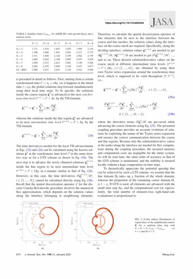
is presented in detail as follows. First, starting from a certain

synchronized time tn ¼ t0 þ nDtc (as it happens at the initial

time t¼ t0), the global solutions step forward simultaneously

using their local time steps. To be specific, the solutions

inside the coarse region ~qnc is advanced to the next synchro-

nous time level tnþ1 ¼ tn þ Dtc by the TSI formula

~qnþ1c ¼ ~qn

c þXNt

i¼1

ciDtic

@i~qnc

@ti; (23)

whereas the solutions inside the fine region ~qnf are advanced

to its next intermediate time level tnþ1=r ¼ tn þ Dtf by the

TSI formula

~qnþ1=rf ¼ ~qn

f þXNt

i¼1

ciDtif

@i~qnf

@ti: (24)

The time derivatives needed for the local TSI advancements

in Eqs. (23) and (24) can be calculated using the known sol-

utions ~qn at the synchronous time level tn in the same itera-

tive way as for a GTS scheme as shown in Eq. (16). The

next step is to advance the newly obtained solutions ~qnþ1=rf

inside the fine region to its next intermediate time level

tnþ2=r ¼ tn þ 2Dtf in a manner similar to that of Eq. (24).

However, in this case, the time derivatives @i~qnþ1=rf =@ti;

i 2 f1;…;Ntg cannot be calculated directly using Eq. (16).

Recall that the spatial discretization operator L for the dis-

crete Cauchy-Kovalewski procedure involves the numerical

flux approximation, which depends on the solution values

along the interface belonging to neighboring elements.

Therefore, to calculate the spatial discretization operator of

fine elements that lie next to the interface between the

coarse and fine meshes, the solution values along the inter-

face on the coarse mesh are required. Specifically, along the

dividing interface, solution values ~qnþ1=rc are needed to get

@~qnþ1=rf =@t; @~qnþ1=r

c =@t are needed to get @2~qnþ1=rf =@t2; …,

and so on. These desired solution/derivative values on the

coarse mesh at different intermediate time levels ðtnþj=r

¼ tn þ jDtf ; j 2 f1;…; rgÞ, are obtained by using their

own Taylor series expansions around the synchronous time

level, which is supposed to be valid throughout ½tn; tnþ1,i.e.,

~qnþj=rc ¼ ~qn

c þXNt

i¼1

ciðjDtf Þi@i~qn

c

@ti; j 2 1;…; rf g;

(25a)

@k~qnþj=rc

@tk¼ @

k~qnc

@tkþXNt

i¼kþ1

cikðjDtf Þik @i~qn

c

@ti;

k 2 1;…;Nt 1f g; (25b)

where the derivative terms @i~qnc=@ti are pre-saved while

advancing the coarse elements using Eq. (23). The presented

coupling procedure provides an accurate evolution of solu-

tions by exploiting the nature of the Taylor series expansion

and ensures the correct communication between the coarse

and fine regions. Because only the solution/derivative values

at the nodes along the interface are needed for flux computa-

tions during the coupling procedure, the incurred memory

and computation costs are negligible for the entire system.

As will be seen later, the same order of accuracy as that of

the GTS scheme is maintained, and the stability is ensured

locally without a huge compromise on time steps.

To theoretically appreciate the potential speedup that

can be achieved by such a LTS scheme, we assume that the

fine domain Xf takes up v fraction of the whole domain,

whereas the proportion of the remaining coarse domain Xc

is 1 v. If GTS is used, all elements are advanced with the

small time step Dtf , and the computational cost (or, equiva-

lently, the total number of element-wise right-hand-side

evaluations) is proportional to

TABLE I. Stability limits CCFLmaxfor ADER-DG with upwind fluxes and a

uniform mesh.

N¼ 3 N¼ 4 N¼ 5 N¼ 6 N¼ 7 N¼ 8

Nt¼ 3 1.171 1.434 1.653 1.835 1.994 2.134

Nt¼ 4 1.308 1.600 1.841 2.043 2.217 2.372

Nt¼ 5 1.511 1.848 2.126 2.359 2.562 2.739

Nt¼ 6 1.669 2.042 2.348 2.605 2.832 3.028

Nt¼ 7 1.858 2.272 2.612 2.901 3.150 3.368

Nt¼ 8 2.026 2.478 2.849 3.164 3.437 3.677

LS – RK5 1.980 2.437 2.815 3.135 3.412 3.656

FIG. 2. (Color online) Distribution of

eigenvalues of the amplification matrix

R for a uniform time step with

N ¼ Nt ¼ 6; CCFL ¼ CCFLmax. (a)

r¼ 1 and (b) r¼ 5.


https://doi.org/10.1121/10.0003340

NGTS ¼ 1

Dtf:

In contrast, if LTS is used, the computational cost scales as

NLTS ¼ vDtfþ 1 v

Dtc:

Therefore, the theoretical speedup is obtained as the ratio

¼ NGTS

NLTS¼ r

1 vþ rv 1: (26)

Two extreme cases are noteworthy to understand Eq. (26).

One case is that the two time steps are extremely disparate,

i.e., r 1, then we obtain

limr!1

¼ 1

v;

indicating that a dramatic speedup is achieved if a small

fraction of elements need a very small time step. The other

case is when there are a small number of fine elements, i.e.,

v! 0, and then the speedup is determined by the ratio of

time steps as

limv!0

¼ r:

The above two-level formulation with integer-valued ratios

can be extended to general real-valued time step ratios of

arbitrarily many levels of local time steps to accommodate

the needs arising from practical simulations, e.g., mesh par-

titioning. It should be mentioned that the cost of the cou-

pling procedure [Eqs. (25a) and (25b)], which can be

performed efficiently with matrix-vector multiplication,

together with accompanying storage needs, is negligible

compared to the overall computational work. A common

approach to save the memory cost is to group elements with

similar maximum allowable time steps together and, then, to

adopt one uniform time step for each group.

IV. NUMERICAL STUDIES OF THE ADER-DG SCHEMEWITH LTS

In this section, numerical experiments are performed to

investigate the numerical properties of the ADER-DG

scheme with both GTS and LTS.

A. Numerical stability analysis

The stability properties are studied by applying the

ADER-DG scheme to the 1D linear acoustic equation (1)

with periodic boundary conditions. Consider a computa-

tional domain of size x 2 ½0; 4m, where ½0; 2m is discre-

tized with an equidistant mesh of size Dxc, whereas ½2; 4mis discretized with an equidistant mesh of size Dxf ¼ Dxc=r.

First, the stability with a uniform time step is evaluated. To

that end, we assemble the DG spatial discretization operator

TABLE II. The ratio of stability limits CCFLmaxof a nonuniform mesh with

r¼ 5 and LTS to the CCFLmaxwith a uniform mesh with GTS as in Table I.

N¼ 3 N¼ 4 N¼ 5 N¼ 6 N¼ 7 N¼ 8

Nt¼ 3 1.000 1.000 1.000 1.000 1.000 1.000

Nt¼ 4 0.999 0.999 0.997 0.998 0.999 0.999

Nt¼ 5 0.994 0.993 0.996 0.995 0.994 0.996

Nt¼ 6 0.990 0.990 0.990 0.992 0.991 0.991

Nt¼ 7 0.985 0.988 0.986 0.987 0.990 0.988

Nt¼ 8 0.982 0.981 0.983 0.984 0.983 0.983

FIG. 3. (Color online) Distribution of

eigenvalues of the amplification matrix

R for a nonuniform time step r¼ 5,

CCFL ¼ CCFLmax. (a) N ¼ Nt ¼ 4 and

(b) N ¼ Nt ¼ 6.

FIG. 4. (Color online) Convergence rate test with periodic boundary condi-

tions, CCFL ¼ CCFLmaxand N ¼ Nt ¼ 4; 5; 6.


https://doi.org/10.1121/10.0003340

L and insert it into an Ntth-order TSI time integration [Eq.

(17)]. Then, it is straightforward to obtain the amplification

matrix R that relates the solutions between two time levels

as qnþ1h ¼ Rqn

h, where

R ¼ I þXNt

i¼1

ciDtiLi; (27)

and I is the identity matrix. The fully discrete formulation is

stable if all eigenvalues of matrix R, denoted as kNðRÞ, have

a modulus less or equal to unity, i.e.,

max jkNðRÞjð Þ 1: (28)

For the uniform time step case, eigenvalues of matrix R are

related to the product of eigenvalues of the spatial operator

L and the time step as kNðRÞ ¼ RðkNðLÞDtÞ, and the condi-

tion of Eq. (28) is equivalent to the stability condition of Eq.

(21). The eigenvalues based on a uniform mesh with

Dxc ¼ Dxf ¼ 0:1 m are calculated, and a simple bisection

method is used to find the maximum allowable time step by

iteratively reducing the time step subject to the stability con-

dition of Eq. (28). Table I presents the maximum allowable

CCFL values as in Eq. (22) for different combinations of

time and space discretization orders, which match exactly

the corresponding CFL number limit for the standard RK

method as reported in Ref. 2. For each fixed spatial order N,

CCFLmaxincreases with the time integration order Nt as the

absolute stability region grows. Furthermore, since the

eigenvalue spectrum of the DG discretization operator

grows at a rate slightly slower than OðN2Þ, a slight increase

in CCFLmaxwith respect to N is observed as well. As a com-

parison, the low-storage five-stage fourth-order RK (LS-

RK5) scheme,15 which is devised and optimized to enhance

stability, has a much larger stability region than the fifth-

order TSI scheme at the cost of a compromising accuracy.

The stability limit also applies to the nonuniform mesh case,

where CCFL is determined by the finer mesh. Figure 2 dis-

plays the distribution of eigenvalues of the amplification

matrix R for a uniform mesh with Dxc ¼ Dxf ¼ 0:1 m as

well as a nonuniform mesh with Dxc ¼ 5Dxf ¼ 0:1 m.

Next, the stability of the proposed LTS scheme is evalu-

ated, and we now consider the domain with a nonuniform

mesh of ratio r¼ 5. To obtain the amplification matrix R,

the TSI for both the coarse and fine regions [Eqs. (23) and

(24), respectively], together with the coupling procedure

[Eqs. (25a) and (25b)], are applied to the semi-discrete for-

mulation [Eq. (14)]. Clearly, the eigenvalues of RðDtc;Dtf Þ,arising from the LTS scheme, are different from those for a

GTS scheme. Ideally, the LTS scheme would introduce no

further constraint on the time step size and, therefore, the

same CFL condition as in the GTS case would be obtained.

However, it is found that the maximum allowable CFL-like

constants CCFLmaxfor the LTS scheme are slightly smaller

than the maximum allowable CFL-like constants for the

GTS case, which is typical for a spatially nonoverlapping

coupling procedure.33,36 Their ratios are shown in Table II.

Figure 3 shows two examples of distributions of the eigen-

values. Similar numerical experiments with different values

of r have been performed to test the CFL stability condi-

tions for the LTS scheme. It is found that a ratio value of

0.95 would yield a stable scheme in all of the tests, indicat-

ing that the developed coupling procedure does not have a

significant negative impact on the stability limit of the TSI,

in general.

FIG. 5. (Color online) Convergence

rate test of ADER-DG with Nt¼ 5 and

periodic boundary conditions. (a)

CCFL ¼ CCFLmax> 1 and (b) CCFL¼ 1.

FIG. 6. A 1D configuration with impedance and transmissive boundaries.FIG. 7. (Color online) Convergence rate test with impedance and transmis-

sion boundaries, CCFL ¼ CCFLmaxand N ¼ Nt ¼ 4; 5; 6.


https://doi.org/10.1121/10.0003340

B. Convergence rate of ADER-DG

1. Periodic boundary with GTS

To investigate the convergence rate of the proposed

ADER-DG method for free field propagation, the 1D linear

acoustic equation [Eq. (1)] on the interval x 2 ½0; 4m with

uniform meshes are solved. Periodic boundary conditions

are prescribed on both ends, and the initial condition is a

sine wave of wavelength kw ¼ 4 m,

pðx; t ¼ 0Þ ¼ sinð0:5pxÞ; (29a)

uðx; t ¼ 0Þ ¼ 1

qcsinð0:5pxÞ: (29b)

First, numerical tests are conducted for various orders of

accuracy in space and time with a uniform maximum allow-

able CFL number on a sequence of mesh sizes Dx. The L2

space-time error defined as L2 ¼ jjpanaðTf Þ pnumðTf ÞjjL2 is

used to evaluate the accuracy, where panaðTf Þ and pnumðTf Þdenote the analytical solution and the numerical solution,

respectively, at the final time Tf ¼ ð16 m)/c across the whole

domain. jj jjL2 denotes the L2 norm, which is carried out

numerically and accuratly up to the order of the polynomial

approximation. As shown in Fig. 4, the observed conver-

gence rates kc, which are calculated by linear fitting with the

least square method, are as expected.

Next, to investigate the effects of temporal error on the

spatial convergence rate, we repeat previous tests with a

fixed time integration order of Nt¼ 5 and different time step

sizes. Figure 5(a) displays the results obtained using the

maximum allowable time step for ADER-DG as prescribed

from Table I. It can be seen that above a certain spatial reso-

lution, the time integration error becomes dominant over the

spatial error, and the spatial convergence rate is deteriorated.

As shown in Fig. 5(b), a smaller time step reduces the tem-

poral error and the expected spatial convergence rate of

ADER-DG scheme is recovered.

2. Impedance and transmission boundary with GTS

Now, convergence rates of the ADER-DG scheme for

wave propagation involving time-domain impedance and

transmission boundary conditions are verified, where the

ADEs [Eqs. (13a)–(13c)] are integrated using the same time

integration scheme. As illustrated in Fig. 6, the transmission

and impedance boundary is located at x¼ 0 m, and the

source at xs ¼ 2:5 m initiates the simulation with the

Gaussian-shaped pressure conditions

pðx; t ¼ 0Þ ¼ eðln 2=b2ÞðxxsÞ2 ; (30a)

vðx; t ¼ 0Þ ¼ 0; (30b)

where b¼ 0.15 m is the half-bandwidth of the Gaussian

pulse. Convergence tests similar to those in the periodic

boundary case are performed. The numerical solutions at the

final time Tf ¼ 4=c s, when both the reflected and transmit-

ted waves are present in the domain, are compared against

the analytical solutions.65 Without loss of generality, one

single real pole ½A; fR ¼ ½6:4 103; 8 103 is used for fit-

ting the reflection coefficient R as in Eq. (8) while the trans-

mission coefficient T is defined by ½A; fT ¼ ½5 103;9 103. The L2 error with conforming spatial and temporal

approximation order is plotted in Fig. 7. The expected con-

vergence rates are yielded.

C. Convergence of ADER-DG with LTS and compari-son against GTS

To verify the convergence rate of ADER-DG with the

proposed LTS scheme, we repeat the above numerical tests

using nonuniform meshes. For the periodic boundary case,

the original computational domain x 2 ½0; 4m is split into

two parts with different mesh sizes. The coarse part

x 2 ½0; 2m is discretized with an equidistant mesh of size

Dxc, whereas the fine part x 2 ½2; 4m has a mesh of size

Dxf ¼ Dxc=r. For the impedance and transmission boundary

case, the interface between the coarse region x 2 ½4; 0mand the fine region x 2 ½0; 2m coincides with the reflective

and transmissive boundary. With a uniform CFL value, the

time step sizes are different between the two regions. The

L2 error for different values of mesh size ratio r and a fixed

order of accuracy is presented in Fig. 8 for both boundary

cases. As a comparison, the results obtained from the GTS

scheme are shown as well. It can be seen that for all of the

tested time step ratios r, the expected convergence rates kc

are observed for LTS, and the scheme introduces no extra

error compared to the GTS scheme.

FIG. 8. (Color online) Convergence

rate of LTS and its comparison with

GTS with CCFL ¼ 0:95CCFLmax; N ¼

Nt ¼ 5 and r ¼ 1; 2; 3; 4; 8. (a)

Periodic and (b) impedance and trans-

mission boundaries.


https://doi.org/10.1121/10.0003340

V. APPLICATION

To demonstrate the functionality and speedup potential

of the proposed ADER-DG scheme with LTS for practical

applications, wave propagation across a finite-height noise

barrier made of porous glass-wool material is simulated,

which is a configuration pertaining to outdoor sound propa-

gation. The schematic diagram is shown in Fig. 9(a) with

the outer boundaries far away from the barrier to prevent

spurious reflected waves from influencing the pressure

response. The source is located at ðxs; ysÞ ¼ ð2; 0Þ and

four receivers are located at ð1; 0Þ; ð1; 3Þ, (1,0), and

(1,3) are distributed symmetrically with respect to the bar-

rier, which has a height of H¼ 4 m and a width of

W¼ 0.04 m. To mimic a real noise barrier mounted on a

hard ground surface, the rigid boundary condition is

imposed on the top edge of the barrier, whereas both side

edges are modeled with the reflective and transmissive

boundary conditions. The characteristic impedance of the

locally reacting glass-wool layer is assumed to follow the

phenomenological Johnson-Champoux-Allard-Lafarge

(JCAL) model66 with its physical parameters measured

experimentally.11 To model the reflection and transmission

properties of the layer, four and five real poles are used to fit

the reflection and transmission coefficients from the time-

domain boundary conditions, respectively, as shown in

Ref. 11. The other boundaries are assumed to be rigid.

The two-dimensional domain is discretized with 13 427

unstructured triangles.67 As illustrated in Fig. 9(b), the mesh

is locally refined near the top edge of the sound barrier in

order to capture the geometry features and diffraction

effects. A relatively simple mesh size measure, which is the

shortest edge length h, is chosen for determining the time

step size based on the CFL condition (22). In-depth discus-

sions on appropriate triangular mesh measures can be found

in Refs. 68 and 69. Mesh elements far away from the sound

barrier have an edge length of approximately 0.5 m. Here,

suppose the shortest edge length is denoted by hmin, we treat

all of the elements with the shortest length that satisfies h 6hmin as the fine mesh elements, i.e., the green triangles in

Fig. 9(c). There are, in total, 2729 fine triangles scattered

around the barrier, which suggests a speedup ratio of 3

with the LTS scheme according to Eq. (26).

To evaluate the accuracy of the LTS scheme, we use

the numerical solutions obtained by the RK-DG method

with the GTS scheme and the same mesh, which have been

verified against the finite element solutions in the frequency

domain,11 as the reference solutions. Following the same

numerical setup of the reference solution, a uniform CFL-

like constant CCFL¼ 1 is used, as well as a spatial polyno-

mial basis of order N¼ 8, together with a fifth-order TSI,

which shares the same computational cost as the LS-RK5

scheme, are used. The time steps in two regions follow the

relation Dtc ¼ 6Dtf . The Gaussian distribution with

b¼ 0.25 m as in Eqs. (30a) and (30b) acts as the source and

initiates the simulation. The comparison of pressure signals

at two receiver locations obtained from both the GTS

scheme and LTS scheme are shown in Fig. 10, where a high

level of agreement is observed. For receiver 2, the main

components are the direct sound and the reflected sound

from the barrier, whereas receiver 4 experiences the pres-

sure signal diffracted over the hard barrier top as well as the

faint pressure signal transmitted through the barrier.

Besides the time-domain comparisons, the relative sound

pressure level, which is obtained by normalizing the total

spectrum against the spectrum of the free field solution, and

its phase angle at different receiver locations are shown in

Figs. 11(a) and 11(b), respectively. Again, a perfect match

of the frequency-domain results between the GTS scheme

and the LTS scheme is found.

VI. CONCLUSION

In this work, we present an ADER-DG approach with

the LTS scheme to solve the time-dependent linear acoustic

equations with an arbitrary order of accuracy in time and

FIG. 9. (Color online) Geometry and mesh of the noise barrier. (a) Schematic diagram, (b) overall mesh, and (c) zoomed-in view of the fine mesh near the

top edge.

FIG. 10. (Color online) Time history of the pressure signal at receivers r2

and r4.


https://doi.org/10.1121/10.0003340

space. Built upon the well-known nodal DG method for the

spatial discretization, it performs the time integration using

TSI in an efficient and accurate manner. Necessary formula-

tions of time-domain acoustic boundary conditions are

included for indoor-outdoor acoustic simulation purposes.

Numerical experiments and applications are performed to

validate the stability and convergence properties. It is shown

that the proposed LTS scheme enables a significant reduc-

tion in computational cost while maintaining the desired

high-order accuracy. Applications to more practical sound

propagation problems involving complex geometries and

material properties will be addressed in future work.

1H. L. Atkins and C.-W. Shu, “Quadrature-free implementation of discon-

tinuous Galerkin method for hyperbolic equations,” AIAA J. 36(5),

775–782 (1998).2B. Cockburn and C.-W. Shu, “Runge-Kutta discontinuous Galerkin meth-

ods for convection-dominated problems,” J. Sci. Comput. 16(3), 173–261

(2001).3B. Cockburn, G. E. Karniadakis, and C.-W. Shu, Discontinuous GalerkinMethods: Theory, Computation and Applications (Springer-Verlag, Berlin

Heidelberg, 2000), Vol. 11.4J. S. Hesthaven and T. Warburton, Nodal Discontinuous GalerkinMethods: Algorithms, Analysis and Applications (Springer, New York,

2007).5T. L€ahivaara and T. Huttunen, “A non-uniform basis order for the discon-

tinuous Galerkin method of the 3D dissipative wave equation with per-

fectly matched layer,” J. Comput. Phys. 229(13), 5144–5160 (2010).6L. C. Wilcox, G. Stadler, C. Burstedde, and O. Ghattas, “A high-order dis-

continuous Galerkin method for wave propagation through coupled

elastic-acoustic media,” J. Comput. Phys. 229(24), 9373–9396 (2010).7M. Kronbichler, S. Schoeder, C. M€uller, and W. A. Wall, “Comparison of

implicit and explicit hybridizable discontinuous Galerkin methods for the

acoustic wave equation,” Int. J. Numer. Methods Eng. 106(9), 712–739

(2016).8N. C. Nguyen, J. Peraire, and B. Cockburn, “High-order implicit hybridiz-

able discontinuous Galerkin methods for acoustics and elastodynamics,”

J. Comput. Phys. 230(10), 3695–3718 (2011).9F. Monteghetti, D. Matignon, and E. Piot, “Energy analysis and discreti-

zation of nonlinear impedance boundary conditions for the time-domain

linearized Euler equations,” J. Comput. Phys. 375, 393–426 (2018).10H. Wang and M. Hornikx, “Time-domain impedance boundary condition

modeling with the discontinuous Galerkin method for room acoustics sim-

ulations,” J. Acoust. Soc. Am. 147(4), 2534–2546 (2020).11H. Wang, J. Yang, and M. Hornikx, “Frequency-dependent transmission

boundary condition in the acoustic time-domain nodal discontinuous

Galerkin model,” Appl. Acoust. 164, 107280 (2020).12A. Modave, A. St-Cyr, and T. Warburton, “GPU performance analysis of


Comput. Geosci. 91, 64–76 (2016).13S. Schoeder, W. Wall, and M. Kronbichler, “ExWave: A high perfor-

mance discontinuous Galerkin solver for the acoustic wave equation,”

SoftwareX 9, 49–54 (2019).

14J. Williamson, “Low-storage Runge-Kutta schemes,” J. Comput. Phys.

35(1), 48–56 (1980).15M. H. Carpenter and C. A. Kennedy, “Fourth-order 2N-storage Runge-

Kutta schemes,” in NASA-TM-109112 (1994).).16F. Hu, M. Y. Hussaini, and J. Manthey, “Low-dissipation and low-

dispersion Runge-Kutta schemes for computational acoustics,”

J. Comput. Phys. 124(1), 177–191 (1996).17D. Stanescu and W. Habashi, “2N-storage low dissipation and dispersion

Runge-Kutta schemes for computational acoustics,” J. Comput. Phys.

143(2), 674–681 (1998).18C. Bogey and C. Bailly, “A family of low dispersive and low dissipative

explicit schemes for flow and noise computations,” J. Comput. Phys.

194(1), 194–214 (2004).19J. Berland, C. Bogey, and C. Bailly, “Low-dissipation and low-dispersion

fourth-order Runge–Kutta algorithm,” Comput. Fluids 35(10), 1459–1463

(2006).20T. Toulorge and W. Desmet, “Optimal Runge-Kutta schemes for discon-

tinuous Galerkin space discretizations applied to wave propagation prob-

lems,” J. Comput. Phys. 231(4), 2067–2091 (2012).21D. A. Kopriva and E. Jimenez, “An assessment of the efficiency of nodal

discontinuous Galerkin spectral element methods,” in RecentDevelopments in the Numerics of Nonlinear Hyperbolic ConservationLaws (Springer, Berlin, Heidelberg, 2013), pp. 223–235.

22A. Kanevsky, M. H. Carpenter, D. Gottlieb, and J. S. Hesthaven, “Application

of implicit-explicit high order Runge-Kutta methods to discontinuous-

Galerkin schemes,” J. Comput. Phys. 225(2), 1753–1781 (2007).23V. Dolean, H. Fahs, L. Fezoui, and S. Lanteri, “Locally implicit discontin-

uous Galerkin method for time domain electromagnetics,” J. Comput.

Phys. 229(2), 512–526 (2010).24S. Descombes, S. Lanteri, and L. Moya, “Locally implicit time integration

strategies in a discontinuous Galerkin method for Maxwell’s equations,”

J. Sci. Comput. 56(1), 190–218 (2013).25M. Hochbruck and A. Ostermann, “Exponential multistep methods of

Adams-type,” BIT Numer. Math. 51(4), 889–908 (2011).26H. Wang, L. Xu, B. Li, S. Descombes, and S. Lanteri, “A new family of

exponential-based high-order DGTD methods for modeling 3-D transient

multiscale electromagnetic problems,” IEEE Trans. Antennas Propag.

65(11), 5960–5974 (2017).27C. W. Gear and D. Wells, “Multirate linear multistep methods,” BIT

Numer. Math. 24(4), 484–502 (1984).28M. G€unther, A. Kvaernø, and P. Rentrop, “Multirate partitioned Runge-

Kutta methods,” BIT Numer. Math. 41(3), 504–514 (2001).29V. Savcenco, W. Hundsdorfer, and J. Verwer, “A multirate time stepping

strategy for stiff ordinary differential equations,” BIT Numer. Math.

47(1), 137–155 (2007).30M. J. Berger and J. Oliger, “Adaptive mesh refinement for hyperbolic par-

tial differential equations,” J. Comput. Phys. 53(3), 484–512 (1984).31S. Piperno, “Symplectic local time-stepping in non-dissipative DGTD

methods applied to wave propagation problems,” ESAIM: Math. Modell.

Numer. Anal. 40(5), 815–841 (2006).32E. Montseny, S. Pernet, X. Ferrieres, and G. Cohen, “Dissipative terms

and local time-stepping improvements in a spatial high order discontinu-

ous Galerkin scheme for the time-domain Maxwell’s equations,”

J. Comput. Phys. 227(14), 6795–6820 (2008).33J. Diaz and M. J. Grote, “Energy conserving explicit local time stepping

for second-order wave equations,” SIAM J. Sci. Comput. 31(3),

1985–2014 (2009).

FIG. 11. (Color online) Comparison

between the GTS and LTS for the

noise barrier case. (a) Relative sound

pressure level and (b) phase angle.


https://doi.org/10.1121/10.0003340

34J. Diaz and M. J. Grote, “Multi-level explicit local time-stepping methods

for second-order wave equations,” Comput. Methods Appl. Mech. Eng.

291, 240–265 (2015).35M. J. Grote, M. Mehlin, and T. Mitkova, “Runge-Kutta-based explicit

local time-stepping methods for wave propagation,” SIAM J. Sci.

Comput. 37(2), A747–A775 (2015).36M. Almquist and M. Mehlin, “Multilevel local time-stepping methods of

Runge-Kutta-type for wave equations,” SIAM J. Sci. Comput. 39(5),

A2020–A2048 (2017).37C. J. Trahan and C. Dawson, “Local time-stepping in Runge-Kutta discontin-

uous Galerkin finite element methods applied to the shallow-water equa-

tions,” Comput. Methods Appl. Mech. Eng. 217-220, 139–152 (2012).38L. Liu, X. Li, and F. Q. Hu, “Nonuniform time-step Runge-Kutta discon-

tinuous Galerkin method for computational aeroacoustics,” J. Comput.

Phys. 229(19), 6874–6897 (2010).39C. Dawson, C. J. Trahan, E. J. Kubatko, and J. J. Westerink, “A parallel

local timestepping Runge-Kutta discontinuous Galerkin method with

applications to coastal ocean modeling,” Comput. Methods Appl. Mech.

Eng. 259, 154–165 (2013).40L. Krivodonova, “An efficient local time-stepping scheme for solution of

nonlinear conservation laws,” J. Comput. Phys. 229(22), 8537–8551 (2010).41M. J. Grote and T. Mitkova, “High-order explicit local time-stepping

methods for damped wave equations,” J. Comput. Appl. Math. 239,

270–289 (2013).42L. Angulo, J. Alvarez, F. L. Teixeira, M. F. Pantoja, and S. G. Garcia,

“Causal-path local time-stepping in the discontinuous Galerkin method

for Maxwell’s equations,” J. Comput. Phys. 256, 678–695 (2014).43A. Taube, M. Dumbser, C.-D. Munz, and R. Schneider, “A high-order dis-

continuous Galerkin method with time-accurate local time stepping for

the Maxwell equations,” Int. J. Numer. Modell.: Electron. Networks,

Devices Fields 22(1), 77–103 (2009).44M. K€aser and M. Dumbser, “An arbitrary high-order discontinuous

Galerkin method for elastic waves on unstructured meshes—I. The two-

dimensional isotropic case with external source terms,” Geophys. J. Int.

166(2), 855–877 (2006).45M. Dumbser, M. K€aser, and E. F. Toro, “An arbitrary high-order discontinu-

ous Galerkin method for elastic waves on unstructured meshes—V. Local

time stepping and p-adaptivity,” Geophys. J. Int. 171(2), 695–717 (2007).46S. Schoeder, M. Kronbichler, and W. A. Wall, “Arbitrary high-order

explicit hybridizable discontinuous Galerkin methods for the acoustic

wave equation,” J. Sci. Comput. 76(2), 969–1006 (2018).47M. K€aser, M. Dumbser, J. De La Puente, and H. Igel, “An arbitrary high-

order discontinuous Galerkin method for elastic waves on unstructured

meshes—III. Viscoelastic attenuation,” Geophys. J. Int. 168(1), 224–242

(2007).48S. Schomann, N. Godel, T. Warburton, and M. Clemens, “Local timestep-

ping techniques using Taylor expansion for modeling electromagnetic

wave propagation with discontinuous Galerkin-FEM,” IEEE Trans.

Magn. 46(8), 3504–3507 (2010).49H. Qi, X. Wang, J. Zhang, and J. Wang, “An ADER discontinuous

Galerkin method with local time-stepping for transient electromagnetics,”

Comput. Phys. Commun. 229, 106–115 (2018).50H. Wang, I. Sihar, R. P. Mu~noz, and M. Hornikx, “Room acoustics

modelling in the time-domain with the nodal discontinuous Galerkin

method,” J. Acoust. Soc. Am. 145(4), 2650–2663 (2019).

51J. S. Hesthaven and C.-H. Teng, “Stable spectral methods on tetrahedral

elements,” SIAM J. Sci. Comput. 21(6), 2352–2380 (2000).52F. Hu and H. Atkins, “Two-dimensional wave analysis of the discontin-

uous Galerkin method with non-uniform grids and boundary con-

ditions,” in 8th AIAA/CEAS Aeroacoustics Conference and Exhibit(2002), p. 2514.

53M. Ainsworth, “Dispersive and dissipative behaviour of high order dis-

continuous Galerkin finite element methods,” J. Comput. Phys. 198(1),

106–130 (2004).54M. Toyoda and J. Motooka, “Prediction of permeable thin absorbers using

the finite-difference time-domain method,” J. Acoust. Soc. Am. 143(5),

2870–2877 (2018).55M. Toyoda and S. Ishikawa, “Frequency-dependent absorption and trans-

mission boundary for the finite-difference time-domain method,” Appl.

Acoust. 145, 159–166 (2019).56H. Ju and K.-Y. Fung, “Time-domain simulation of acoustic sources over

an impedance plane,” J. Comput. Acoust. 10(03), 311–329 (2002).57B. Cotte, P. Blanc-Benon, C. Bogey, and F. Poisson, “Time-domain

impedance boundary conditions for simulations of outdoor sound prop-

agation,” AIAA J. 47(10), 2391–2403 (2009).58D. Dragna, P. Blanc-Benon, and F. Poisson, “Time-domain solver in cur-

vilinear coordinates for outdoor sound propagation over complex terrain,”

J. Acoust. Soc. Am. 133(6), 3751–3763 (2013).59R. M. Joseph, S. C. Hagness, and A. Taflove, “Direct time integration of

Maxwell’s equations in linear dispersive media with absorption for scat-

tering and propagation of femtosecond electromagnetic pulses,” Opt. Lett.

16(18), 1412–1414 (1991).60D. Dragna, P. Pineau, and P. Blanc-Benon, “A generalized recursive con-

volution method for time-domain propagation in porous media,”

J. Acoust. Soc. Am. 138(2), 1030–1042 (2015).61J. C. Butcher, The Numerical Analysis of Ordinary Differential

Equations: Runge-Kutta and General Linear Methods (Wiley-

Interscience, New York, 1987).62S. C. Reddy and L. N. Trefethen, “Stability of the method of lines,”

Numerische Mathematik 62(1), 235–267 (1992).63H. O. Kreiss and L. Wu, “On the stability definition of difference approxi-

mations for the initial boundary value problem,” Appl. Numer. Math.

12(1-3), 213–227 (1993).64L. Krivodonova and R. Qin, “An analysis of the spectrum of the discon-

tinuous Galerkin method,” Appl. Numer. Math. 64, 1–18 (2013).65Y. €Ozy€or€uk and L. N. Long, “A time-domain implementation of surface

acoustic impedance condition with and without flow,” J. Comput. Acoust.

05(03), 277–296 (1997).66D. Lafarge, P. Lemarinier, J. F. Allard, and V. Tarnow, “Dynamic com-

pressibility of air in porous structures at audible frequencies,” J. Acoust.

Soc. Am. 102(4), 1995–2006 (1997).67C. Geuzaine and J.-F. Remacle, “Gmsh: A 3-D finite element mesh gener-

ator with built-in pre-and post-processing facilities,” Int. J. Numer.

Methods Eng. 79(11), 1309–1331 (2009).68N. Chalmers and L. Krivodonova, “A robust CFL condition for the dis-

continuous Galerkin method on triangular meshes,” J. Comput. Phys. 403,

109095 (2020).69T. Toulorge and W. Desmet, “CFL conditions for Runge-Kutta discontin-

uous Galerkin methods on triangular grids,” J. Comput. Phys. 230(12),

4657–4678 (2011).


https://doi.org/10.1121/10.0003340

Paper V

Page 153

Wave-based room acoustic simulations of an open plan office

Huiqing Wang1,∗, Wouter Wittebol1, Matthias Cosnefroy1, Maarten Hornikx1, Remy Wenmaekers2

1Building Physics and Services, Department of the Built Environment, Eindhoven University of Technology,P.O. Box 513, 5600 MB Eindhoven, The Netherlands

2Level Acoustics & Vibration, De Rondom 10, 5612 AP Eindhoven, The Netherlands

*[email protected]

AbstractIn this study, room acoustic simulations of a real open plan office using the time-domain discontinuous Galerkin(TD-DG) method are performed, as a preliminary attempt to assess the accuracy and applicability of this wave-based method for realistic sound field analysis in the low-frequency range. This TD-DG simulation involvesthe developed techniques of locally-reacting frequency-dependent impedance boundary conditions and thelocal-time stepping scheme. The required input for the boundary modeling of relevant absorption materials isobtained from the absorption coefficients measured in a reverberation room based on the international standardISO 354. Observed discrepancies, in terms of the room acoustic parameters, between the measurements andsimulation results indicate the limitation of the detailed wave-based modeling in the absence of a preciseboundary characterization.

Keywords: wave-based simulation, time-domain discontinuous Galerkin method, open-plan office.

1 Introduction

Wave-based room acoustic simulation methods simulate sound propagation by directly solving the waveequation based on numerical approximation techniques. Compared to the well-established geometrical acoustic(GA) simulation techniques [1], which are built upon the assumption that sound acts as rays, wave-basedmethods are able to accurately capture inherent complex wave-phenomena such as scattering, diffractionand phase effects. Despite their superior accuracy, wave-based methods suffer from a heavy computationalcost. Therefore, GA simulation methods have been the prevailing approach for acoustic practitioners andresearchers for simulating the acoustic fields of large rooms like concert halls and theaters; while it isgenerally acknowledged that wave-based methods serve as preferred alternatives to GA models for rooms withsmall volumes below the Schroeder frequency, where the modal overlap is low. Recently, the time-domaindiscontinuous Galerkin (TD-DG) wave-based method has been investigated for room acoustic modelingpurposes [2, 3] and efforts have been made to enhance its performance in terms of acoustic boundary modeling[2, 4, 5], efficiency [6] and high-performance computing [2].A comprehensive evaluation of the accuracy of room acoustic simulations typically involves a comparisonwith measurements. For state-of-the-art of room acoustic modeling software that are based on GA models,round robin experiments have been performed using acoustic scenes of different levels of complexity [7]and benchmark databases have been established [8]. Audible deviations are observed, and it proves tobe a challenging task to guarantee an exact match of model input parameters between simulations andmeasurements. Sources of input data uncertainties include room geometries, absorption and scatteringproperties of room surfaces and the source and receiver characteristics [9].For wave-based methods, there have been on-going research activities trying to close the gap betweenreal-world measurements and simulations as well. Experimental validation of room acoustic simulationsinside a reverberation room with a time-domain finite element method (FEM) is reported by Okuzono et al.

1

[10], and a decent agreement of band-limited room impulse responses is observed in three separate octavebands. Comparisons of different boundary representations of porous absorbers in small rooms are performedrespectively within the framework of the frequency-domain FEM model [11] and the TD-DG model [12],highlighting the effects of extended reaction of boundary materials for room acoustics. For the TD-DG method,previous validation work [3] has been done inside an empty reverberation room, where the walls are modeledwith a uniform real-valued impedance. Later on, benchmark tests with various furniture inside were conducted[13] and the good match with measurements indicate the strong potential for more challenging and larger roomscenarios. Another recent study compares measurements with simulation results from the TD-DG methodin a small rectangular room with porous absorbers, with a focus on establishing a comprehensive validationand uncertainty quantification framework in wave-based room acoustic simulations [14]. It was found thatthe input uncertainties associated with the absorption properties makes it intractable to predict common roomacoustic parameters within just noticeable difference (JND) thresholds.In this study, the TD-DG method is applied to simulate the acoustics of a large real open plan office in thelow-to-middle frequency range (125 Hz to 500 Hz octave bands), with the aim of assessing the accuracy andapplicability of this wave-based method for realistic sound field analysis. The ground truth references to becompared with are measurement results, which were previously published in a study on how room acousticparameters are affected with varying configurations of furniture and sound absorbing barriers [15]. Theacoustic properties of involved boundary surfaces are characterized based on standardized reverberation roommeasurements [16]. The required specifications of complex-valued reflection coefficients for the wave-basedcalculations are obtained by transforming the measured Sabine absorption coefficients. The comparisonbetween the simulation and measurement results are conducted in terms of six room acoustic parameters thatare derived from the room impulse response.The paper is organized as follows. The description of the reference room measurements is presented inSec. 2. Sec. 3 describes the setup of the wave-based simulation model and the approach used for retrievingcomplex-valued impedance boundary data. Section 4 presents the comparison of simulation results withmeasurements, as well as discussions on the potential limitations of the current wave-based model.

2 Reference measurement

2.1. Measurement room and proceduresAs shown in Fig. 1, the open plan office under study has a long and narrow floor plan with windows along

the walls. Small closed rooms indicated by the blue areas are present to subdivide the long space. The roomhas a volume of 962 m3 and the ceiling is 2.9 m tall. During the measurements, the room was completelyempty except for the 5 workstation islands. Within each group of 4 workstations, two variations of the setupare considered:

– V1: only tables in the room,

– V2: tables with dividing panels and side panels.

The source location and the 9 receiver locations are denoted by the red and yellow circles respectively, with theexact position of the source and of one receiver (R9) provided. The table depth for each sitting position is 0.8m and the source and microphones are positioned 0.3 m away from the tables. More geometrical details can befound in Ref. [15]. The measurements have been performed following ISO 3382-3 [17]. An omnidirectionalsound source (B&K 4292) and omnidirectional microphones were connected to a laptop with measurementsoftware Dirac 6 (B&K 7841) via a triton USB device (AE) and an amplifier (B&K 2734).

2.2. Acoustic properties of room materialsThe room has a sound absorbing suspended ceiling of 20 mm thick Rockfon panels with an air cavity of at

least 200 mm. The floor is covered with carpet. Dividing and side panels, which are made of 25 mm chipboard,

2

Figure 1: Pictures of the measured open plan office and its floor plan in top view.

stand on the floor and have a height of 1.5 m. To increase sound absorption, 30 mm thick melamine foam isapplied to both sides of the upper 1.3 m part of the dividing panels that are along the y-direction.The acoustic properties of the room surface materials, which are represented with the Sabine absorptioncoefficients in this work, are measured in a reverberation chamber according to ISO354 [16] and are availablein octave bands as shown in Table 1. The Sabine absorption coefficients are measured by the reverberationchamber method as follows:

αS ab =55.3VS c0

( 1T2−

1T1

), (1)

where V is the volume of the reverberation chamber, S is the area of the material sample, T1 is the reverberation

Table 1: Measured Sabine absorption coefficients αS ab of materials in octave bands. The values in parenthesesare the estimated size-corrected ones used in simulations, as described in Sec. 3

Frequency [Hz]/Materials Ceiling Foam Carpet

125 0.45 (0.45) 0.10 (0.11) 0.02 (0.01)

250 0.70 (0.72) 0.35 (0.33) 0.03 (0.03)

500 0.90 (0.87) 0.60 (0.62) 0.07 (0.08)

time for an empty condition, and T2 is the reverberation time with the test sample. It should be mentionedthat due to the limited volume of the reverberation chamber, the measurements for the suspended ceiling areperformed with the mounting type E-200 of ISO 354 [16], i.e., placing the test sample with a 200 mm cavitybehind it.

3 Wave-based modeling

3.1. Brief description of the time-domain DG methodThe simulations are performed using an in-house simulation tool based on the TD-DG method. This

section presents the main formulations whereas additional details can be found in Refs. [3, 4, 6]. Underthe assumption of lossless propagation medium, the sound propagation is governed by the following partialdifferential equations

∂q

∂t+ ∇ · F (q) =

∂q

∂t+ A j

∂q

∂x j= 0, (2)

3

where q(x, t) = [u, v,w, p]T is the acoustic variable vector, containing the particle velocity component [u, v,w]and the sound pressure p. ρ is the constant air density and c is the constant speed of sound. The constant fluxJacobian matrix A j reads

A j =

0 0 0 δx j

ρ

0 0 0 δy jρ

0 0 0 δz jρ

ρc2δx j ρc2δy j ρc2δz j 0

, (3)

with coordinate index j ∈ [x, y, z]. Let Dk be a set of simplex and geometrically conformal elements thatdiscretize the computational domain Ωh, i.e., Ωh =

⋃Kk=1 Dk. The local solution qk

h(x, t) in element Dk, wheresubscript h denotes the numerical approximation, is given by:

qkh(x, t) =

Np∑i=1

qkh(xk

i , t)lki (x), (4)

where qkh(xk

i , t) are the unknown nodal values and lki (x) is the multi-dimensional Lagrange polynomial basisof order N, which satisfies lki (xk

j) = δi j. Np is the number of local basis functions (or nodes) inside a singleelement and is equal to (N + d)!/(N!d!) for simplex elements, where d is the dimensionality. After the Galerkinprojection and integrating by parts twice, the semi-discrete nodal DG formulation of Eq. (2) reads:∫

Dk

(∂qkh

∂t+ ∇ · F k

h (qkh))lki dx =

∫∂Dk

n ·(F k

h (qkh) − F ∗

)lki dx, (5)

where n = [nx, ny, nz] is the outward normal vector of the element surface ∂Dk. F ∗ is the numerical flux acrosselement intersection ∂Dk and in this study, the upwind numerical flux is used throughout the whole domainbecause of its low dispersive and dissipation error. The semi-discrete formulation is obtained by substitutingthe nodal basis expansion Eq. (4) into the strong formulation Eq. (5). The resulting vector-matrix form of theformulation and more details of the implementation can be found in Ref. [3].Locally reacting time-domain impedance boundary conditions (TDIBC) are weakly enforced through thenumerical flux terms, where the reflected characteristic wave is expressed as the convolution between thereflection coefficient at normal incidence and the incident characteristic wave. The method of auxiliarydifferential equations is used to calculate the convolution. The reflection coefficient is represented by themulti-pole model as described in Ref. [4].The semi-discrete system with a 6th order spatial approximation is integrated in time using a 5th order explicitTaylor series integrator based on the arbitrary high-order derivatives (ADER) methodology, with a localtime-stepping scheme incorporated as presented in[6].

3.2. Mesh generationThe model geometry is imported into the meshing software Gmsh [18] to generate the unstructured

tetrahedral mesh, as shown in Fig. 2 for the V2 setup. The geometrical model contains all details whosedimensions are comparable to the shortest wavelength resolved, which is around 0.5 m. The absorbing foam,dividing panels and desks are modeled as “floating” surfaces with their thicknesses neglected.

It is known that the mesh quality has a pivotal influence on the maximum allowable time step size and thenumerical error. In Gmsh, mesh element sizes are usually prescribed by adjusting the so-called characteristiclengths (denoted as Lc), which are more or less equal to the length of the element edges. Here, the radiusof the largest inscribed sphere rin is used as the element size measure. The chosen quality measure rq istriple of the ratio between rin and the radius of the smallest circumscribed sphere rcir, i.e. rq = 3rin/rcir.As a reference, a regular tetrahedron has rq = 1 (optimal mesh quality), and a degenerate tetrahedron (zerovolume) has rq = 0. Considering the maximum frequency of interest of 500 Hz, meshes with five different

4

Figure 2: Geometry model in Gmsh.

Figure 3: Distribution of the mesh quality measure rq and the mesh size measure rin. V1 and V2 are displayedin the left and right plot respectively. The color indicates the number of elements in each bin.

Lc = [0.3, 0.35, 0.4, 0.45, 0.5] m values are generated for both setups. It is found that decreasing the meshelement size (increasing the number of elements) does not necessarily yield larger values of rq (better meshquality). By comparing the distributions of the mesh quality measure rq and the element size measure rin, themeshes with Lc = 0.45 m are chosen for both setups, with their distributions of rq and rin are shown in Fig. 3.The number of elements are 50379 and 57489 for V1 and V2, respectively. The points per wavelength is 11.2(11.8) at the center frequency and 7.9 (8.3) at the upper limit of 500 Hz octave band for the V1 (V2) mesh.In this work, considering the CFL stability condition of the explicit time integration scheme, the time step sizeis determined by

∆t = CCFL ·min(rin) ·1c·

1(2N + 1)

. (6)

In this study, CCFL is set to 0.9, and min(rin) = 0.074 m for V1 and min(rin) = 0.042 m for V2. To accelerate thesimulation for the V2 setup, where small elements exist around the corner of table dividers due to the geometryconstraint, a local time-stepping scheme [6] is used and all elements are divided into two groups. All elementsthat have rin ≤ 3 min(rin) are marked as fine elements, accounting for 8.4% of total elements, and are timeintegrated with ∆t of Eq. (6). The rest are considered as coarse elements and have a time step size of 3∆t.

3.3. Acoustic boundary modelingThe measured Sabine absorption coefficients αS ab are energy parameters that do not carry phase information.

They approximately represent the theoretical random incidence absorption coefficient αrand for plane waveincidence on an infinitely large surface. However, for wave-based room acoustic simulations, such as the TD-DG method herein, the complex-valued surface impedances or equivalent reflection coefficients are neededfor the boundary modeling. In general, it is considered intractable to retrieve the correct complex-valuedsurface impedance from a real-valued absorption coefficient when there is no more information on the material

5

available, because there are an infinite number of surface impedance values that yield the same absorptioncoefficient. To address this issue, a common strategy is to add some assumptions and constraints [19, 20].First of all, local reaction is assumed, meaning that the surface impedance Zs(θ) is independent of the angle ofincidence θ (and thus the surface impedance for normal incidence is assumed representative of all incidenceangles). Secondly, as proposed in Refs. [21, 20], we assume that the measured Sabine absorption coefficientcorresponds to the size-corrected absorption coefficient for the low frequency range of interest, which isproposed by Thomasson [22] as follows:

αsize(θ) = 8∫ π/2

0

Re(Zs(θ)) sin θ|Zs(θ) + Zr(θ)|2

dθ, (7)

where Zr is the averaged radiation impedance over azimuthal angles φ and expressed as Zr =∫ 2π

0 Zrdφ/2π.The average radiation impedance can be calculated with numerical integrations in an accurate way, based ontabulated values provided in Table I of Ref. [21].From the rudimentary assessment of the limited absorption coefficients data, the rigidly-backed foam and carpetcorrespond to the cases “soft porous” and “hard porous” as discussed in Ref. [20]. It has been shown thereinthat the surface impedance of rigidly-backing porous materials, which exhibits a monotonic behavior, can bewell captured by approximations with fractional derivatives, similar to the multi-pole model representation asused in the TDIBC here. By contrast, the suspended ceiling with a large air cavity is quite difficult to simulate inpractice [20], because the cotangent term in the surface impedance produces oscillating behavior. Therefore, theresulting narrow-band frequency variations are impossible to be reasonably captured from the coarse frequency-averaged octave band data. In this work, restricted by the availability of input data, we preliminarily assume thatstrong oscillations are not present in the current frequency range of interest. The multi-pole parameters neededfor the TDIBC are determined by solving an optimization problem. The idea is to optimize the parameters inthe multi-pole approximations of the reflection coefficient at normal incidence (denoted as Rnor), which can belinearly transformed into the surface impedance in Eq. (7), that produces the best match between the measuredand the estimated size-corrected absorption coefficient. The magnitude and the phase angle of fitted reflectioncoefficients Rnor are shown in Fig. 4. The corresponding size-corrected absorption coefficients are the valuesinside the parenthesis of Table 1.

Besides the considered ceiling, foam and carpet, there are other materials in the room absorbing sound in

0 100 200 300 400 500 600 700 8000.2

0.3

0.4

0.5

0.6

0.7

0.8

0.9

1

0 100 200 300 400 500 600 700 800-1.4

-1.2

-1

-0.8

-0.6

-0.4

-0.2

0

Figure 4: Estimated reflection coefficient at normal incidence. ϑ(·)

extracts the phase angle of a complexnumber.

the considered frequency range, for example the window glass and gypsum board. However, the detailedinformation on their sizes and acoustic properties are missing. Here, real-valued impedances in octave bandsare assigned to all other surfaces in the room guided by the typical values of absorption coefficients providedin Ref. [23], i.e., 0.15, 0.15 and 0.1 for the octave bands 125 Hz, 250 Hz and 500 Hz respectively.

6

Table 2: Spatial average of the considered room acoustic parameters and their standard deviation for bothsetups. The values before the slash are the measured ones and after the slash are the simulated ones.

Para. Oct. Space aver. V1 Std. V1 Space aver. V2 Std. V2

T30 [s]125 0.83/0.70 0.06/0.08 0.78/0.61 0.09/0.08

250 0.80/1.14 0.07/0.20 0.76/0.82 0.14/0.12

500 0.64/1.13 0.07/0.26 0.61/0.79 0.10/0.08

EDT [s]125 0.70/0.79 0.26/0.31 0.94/0.92 0.33/0.33

250 0.57/0.78 0.18/0.21 0.77/0.68 0.22/0.25

500 0.55/0.83 0.20/0.29 0.61/0.69 0.21/0.28

C50 [dB]125 4.70/3.0 3.10/4.94 -0.47/0.34 5.24/2.98

250 6.50/4.75 2.54/1.66 2.02/5.65 2.89/4.71

500 6.80/3.31 3.26/3.00 6.25/4.23 3.32/2.71

TS [ms]125 77.5/79.0 25.9/33.7 100.9/99.1 35.4/33.7

250 66.2/77.8 23.6/28.2 88.7/75.5 28.5/29.0

500 59.2/80.6 25.3/32.8 70.9/76.0 24.7/28.3

4 Results

The results from the measurements and the simulations are first evaluated in terms of standard roomacoustic parameters as stated in ISO 3382–1 [24], including reverberation time (T30), early decay time (EDT ),clarity (C50) and center of gravity (TS ). In the DG simulation, the dodecahedron source is modeled by a pointsource that has a Gaussian shaped time signal with a non-flat spectrum. Therefore, the simulated responsesare deconvolved by the spectral division approach with the water level regularization technique [25] applied inorder to get the room impulse responses.In order to evaluate room acoustic parameters that are representative of the whole room, the spatial averaging

values, which are obtained from the arithmetic average for all nine receiver locations, are presented in Table 2.The standard deviations provide insights into the spatial variance of the parameters across various locations.The first impression of the comparison results is that none of the simulation results match the measured onesvery well, except for the center time TS at 125 Hz, which is the center of gravity of the squared impulseresponse and indicates the balance between clarity and reverberance. Larger deviations are observed for spatialmean values of both T30 and EDT , which are directly calculated from the energy decay curve. For T30, lowervalues are predicted compared to the measurements for both setups in the 125 Hz octave band, whereas highervalues are found in the simulations for the 250 Hz and 500 Hz octave bands. For the clarity C50, the simulatedvalues are lower than the measured ones, except for setup V2 at 125 Hz, implying that the simulated soundfield is more perceptually blurred.The reverberation time of a room is usually regarded as the predominant indicator of its acoustical properties.However, for the open plan office, good speech privacy between workstations is of primary concern. Therefore,the spatial decay rate of speech D2,S (level reduction when doubling the distance) and A-weighted soundpressure level (SPL) of speech at a distance of 4 m from the sound source (Lp,A,S ,4m) as described in ISO3382-3 [17] are investigated. The sound power level of the loud speaker and simulation impulse source arenormalized based on the SPL at a distance of 1 m in the free-field condition. Due to the limited frequencyrange of the wave-based simulations, the logarithm summation of the A-weighted SPL is calculated only upto the 500 Hz octave band instead of 8000 Hz for both simulation and measurements. It should be noted thatdue to the SPL spectrum of normal speech and the A-weighting, the A-weighted SPL of speech almost fullydepends on the 500 Hz octave band.

7

The comparisons for the V1 setup (with empty tables alone) and the V2 setup (with table dividers and sidepanels ) are shown in Fig. 5, where the linear regression is performed to determine D2,S according to ISO3382-3 [17]. It can be seen that the simulations have a lower predicted SPL of normal speech for all receiverlocations except the eighth receiver. The discrepancies get smaller at further distance. Furthermore, thesimulated spatial decay rates of speech D2,S are smaller than the measured ones in both cases. For the V1setup, the monotonic decrease of Lp,A,S is well predicted, while a fairly good agreement of the zigzag shape interms of Lp,A,S is observed for the V2 setup, implying the effects of the table dividers and side panels are takeninto account in the simulations.The considered comparison has proven to be quite challenging. While it is intractable to pin down the exact

2 4 6 8 10 12 14 16 1830

35

40

45

50

55

60

2 4 6 8 10 12 14 16 1830

35

40

45

50

55

60

Figure 5: Comparison of D2,S and Lp,A,S ,4m. V1 and V2 are displayed in the left and right plot respectively.

deficiency of the numerical model, the discrepancies between the simulation and measurement results can beelucidated mainly from the following three aspects. First of all, there are inevitable uncertainties and inherentrandomness in both the measurements and the simulation inputs, including boundary material properties,geometry and the source/receiver locations. In this study, the lack of knowledge about the exact size of thewindows and their acoustic properties could also affects the accuracy of simulated T30 and EDT .Secondly, the measured absorption coefficients of three major absorbing materials according to ISO 354 [16]may not truly represent the acoustic properties of the materials due to the limitation of the standard [26, 27].Furthermore, octave band data does not provide a sufficient frequency resolution for simulation purposes.The acoustic properties of the considered materials might not be monotonic in the interested frequency range,as assumed. Also, the accurate phase information about the surface impedance is missing, which has beenshown quite influential in capturing the frequency shift [28] and the reverberation time [29]. This argument issupported by the fact that the standard deviation of EDT is slightly larger than that of T30, since EDT is moresensitive to the relatively sparse early reflections.Last but not least, the current wave-based simulation models all surfaces as locally reacting. In manyapplications, this assumption has prevailed due to its simplicity. However, previous studies showed that forgrazing incidence waves, considerable discrepancies between locally and extendedly reacting absorbers exist[30]. For the studied office, the distance between the floor and the absorbing ceiling is rather low. As aconsequence, grazing incidence might be more pronounced in the early reflections for certain source-receiverpositions, resulting in a serious degradation of the accuracy in EDT . Furthermore, extended reaction mostlikely arises in the suspended ceiling treatment, which has an air gap larger than 200 mm. It has been shownthat absorbers with an air gap exhibit strong extendedly reacting behavior and that a better agreement at largerincidence angles at lower frequencies is observed for extended reaction models [31].

8

5 Conclusion

Wave-based room simulation of a real open plan office in the low-frequency range has been performed withthe time-domain discontinuous Galerkin method. The acoustic properties of materials are represented with theenergy-based absorption coefficients in octave bands measured with the reverberation chamber method. Fromthis input data, the needed complex-valued surface impedance data is retrieved by fitting the size-correctedSabine absorption coefficients, assuming monotonic absorption behavior within the interested frequency range.To assess the validity of the whole framework, the simulation results are compared with the measurements interms of room acoustic parameters.Noticeable discrepancies between the simulation and measurement results are observed, especially for thereverberation time and early decay time. While it is generally difficult to determine which influencing factorscontribute the most to the overall simulation deviations, the potential limitations of the current numerical modelare summarized. It should be noted that this work is a preliminary attempt to investigate the applicability forchallenging practical cases, where a high level of complexity and uncertainty in model inputs is involved. Asfuture work, experimental validations with increasing level of complexity of room scenarios will be performed.Furthermore, the formulation of extendedly reacting boundary conditions should help to achieve satisfactoryimprovements in the simulation accuracy.

References

[1] Lauri Savioja and U. Peter Svensson. Overview of geometrical room acoustic modeling techniques. TheJournal of the Acoustical Society of America, 138(2):708–730, aug 2015.

[2] Finnur Pind. Wave-Based Virtual Acoustics. PhD thesis, Technical University of Denmark, 2020.[3] Huiqing Wang, Indra Sihar, Raúl Pagán Muñoz, and Maarten Hornikx. Room acoustics modelling in the

time-domain with the nodal discontinuous Galerkin method. The Journal of the Acoustical Society ofAmerica, 145(4):2650–2663, 2019.

[4] Huiqing Wang and Maarten Hornikx. Time-domain impedance boundary condition modeling with thediscontinuous Galerkin method for room acoustics simulations. The Journal of the Acoustical Society ofAmerica, 147(4):2534–2546, 2020.

[5] Huiqing Wang, Jieun Yang, and Maarten Hornikx. Frequency-dependent transmission boundary conditionin the acoustic time-domain nodal discontinuous Galerkin model. Applied Acoustics, 164:107280, 2020.

[6] Huiqing Wang, Matthias Cosnefroy, and Maarten Hornikx. An arbitrary high-order discontinuousGalerkin method with local time-stepping for linear acoustic wave propagation. The Journal of theAcoustical Society of America, 149(1):569–580, 2021.

[7] Fabian Brinkmann, Lukas Aspöck, David Ackermann, Steffen Lepa, Michael Vorländer, and StefanWeinzierl. A round robin on room acoustical simulation and auralization. The Journal of the AcousticalSociety of America, 145(4):2746–2760, 2019.

[8] Fabian Brinkmann, Lukas Aspöck, David Ackermann, Rob Opdam, Michael Vorländer, and StefanWeinzierl. A benchmark for room acoustical simulation. concept and database. Applied Acoustics,176:107867, 2021.

[9] Michael Vorländer. Computer simulations in room acoustics: Concepts and uncertainties. The Journal ofthe Acoustical Society of America, 133(3):1203–1213, mar 2013.

[10] Takeshi Okuzono, Toru Otsuru, Reiji Tomiku, and Noriko Okamoto. Fundamental accuracy of timedomain finite element method for sound-field analysis of rooms. Applied Acoustics, 71(10):940–946,2010.

[11] Marc Aretz and Michael Vorländer. Efficient modelling of absorbing boundaries in room acoustic FEsimulations. Acta Acustica united with Acustica, 96(6):1042–1050, 2010.

9

[12] Finnur Pind, Cheol-Ho Jeong, Allan P Engsig-Karup, Jan S Hesthaven, and Jakob Strømann-Andersen.Time-domain room acoustic simulations with extended-reacting porous absorbers using the discontinuousGalerkin method. The Journal of the Acoustical Society of America, 148(5):2851–2863, 2020.

[13] Fotis Georgiou, Baltazar Briere de la Hosseraye, Maarten Hornikx, and Philip W Robinson. Design andsimulation of a benchmark room for room acoustic auralizations. In 23rd International Congress onAcoustics, pages 723–730, 2019.

[14] Tobias Thydal, Finnur Pind, Cheol-Ho Jeong, and Allan P Engsig-Karup. Experimental validation anduncertainty quantification in wave-based computational room acoustics. Applied Acoustics, 178:107939,2021.

[15] Remy Wenmaekers and Nicole van Hout. How ISO 3382-3 acoustic parameter values are affected byfurniture, barriers and sound absorption in a typical open plan office. In 23rd International Congress onAcoustics, pages 2437–2444, 2019.

[16] ISO354: 2003. Acoustics - Measurement of sound absorption in a reverberation room. Standard,International Organization for Standardization, Geneva, CH, 2003.

[17] ISO 3382-3. Acoustics - Measurement of room acoustic parameters - Part 3: Open plan offices. Standard,International Organization for Standardization, Geneva, CH, 2017.

[18] Christophe Geuzaine and Jean-François Remacle. Gmsh: A 3-D finite element mesh generator withbuilt-in pre-and post-processing facilities. International Journal for Numerical Methods in Engineering,79(11):1309–1331, 2009.

[19] Jens Holger Rindel. An impedance model for estimating the complex pressure reflection factor. In ForumAcusticum, volume 2011, 2011.

[20] Boris Mondet, Jonas Brunskog, Cheol-Ho Jeong, and Jens Holger Rindel. From absorption to impedance:Enhancing boundary conditions in room acoustic simulations. Applied Acoustics, 157:106884, 2020.

[21] Cheol-Ho Jeong. Converting sabine absorption coefficients to random incidence absorption coefficients.The Journal of the Acoustical Society of America, 133(6):3951–3962, 2013.

[22] Sven-Ingvar Thomasson. On the absorption coefficient. Acta Acustica united with Acustica, 44(4):265–273, 1980.

[23] H. Kuttruff. Acoustics: An Introduction. CRC Press, New York, 2006.[24] ISO 3382-1. Acoustics - Measurement of room acoustic parameters - Part 1: Performance spaces.

Standard, International Organization for Standardization, Geneva, CH, March 2015.[25] Deconvolution, a glimpse ahead, pages 103–107. Springer Berlin Heidelberg, Berlin, Heidelberg, 1994.[26] Martijn Vercammen. On the revision of ISO 354, measurement of the sound absorption in the

reverberation room. In 23rd International Congress on Acoustics, pages 3991–3997, 2019.[27] Cheol-Ho Jeong and Ji-Ho Chang. Reproducibility of the random incidence absorption coefficient

converted from the sabine absorption coefficient. Acta Acustica united with Acustica, 101(1):99–112,2015.

[28] Diego M Murillo, Filippo M Fazi, and Jeremy Astley. Room acoustic simulations using the finite elementmethod and diffuse absorption coefficients. Acta Acustica united with Acustica, 105(1):231–239, 2019.

[29] Cheol-Ho Jeong, Doheon Lee, Sébastien Santurette, and Jeong-Guon Ih. Influence of impedance phaseangle on sound pressures and reverberation times in a rectangular room. The Journal of the AcousticalSociety of America, 135(2):712–723, 2014.

[30] Behrooz Yousefzadeh and Murray Hodgson. Energy-and wave-based beam-tracing prediction of room-acoustical parameters using different boundary conditions. The Journal of the Acoustical Society ofAmerica, 132(3):1450–1461, 2012.

[31] Kristrún Gunnarsdóttir, Cheol-Ho Jeong, and Gerd Marbjerg. Acoustic behavior of porous ceilingabsorbers based on local and extended reaction. The Journal of the Acoustical Society of America,137(1):509–512, 2015.

10

Acknowledgements

Recollecting my past four-year adventure as a PhD candidate, I feel very lucky toget motivated and inspired by many kind people directly or indirectly. Without theirsupport and help, the work presented in this thesis could not be achieved.

First and foremost, my sincere gratitude goes to my supervisor Prof. MaartenHornikx. It has been such a rewarding PhD study experience with him. I appreciatehim offering this project on room acoustics to me, who even had no idea of whatreverberation time is in the beginning. I am grateful for his consistent trust, end-less support, profound guidance, in addition to encouraging me to explore my pathfollowing my own passion. Many thanks to his time and patience on reading mymanuscripts. His scrupulous attitude, critical questions and insightful feedbacks helpme to stay on track towards a scientific researcher. More than that, his profession-alism and diligence have significantly motivated me, and will continuously motivateme to move on.

I would like to express my gratitude to my co-promotor Dr. Matthias Cosnefroy forsupporting the final year of my PhD with his dedicated efforts. All those constructivecomments and intelligent suggestions to my thesis are greatly appreciated.

I am also grateful to my supervisory committee members, Prof. Harald van Brum-melen, Prof. Stefan Bilbao, Dr. Cheol-Ho Jeong, Dr. Hèrm Hofmeyer, for their in-terest in my research and time on reviewing my thesis. I appreciate their instructiveremarks and positive feedbacks towards my work.

I appreciate all the collaborations from co-authors, Indra, Raúl, Baltazar, Fotis,Jieun, Wouter, Matthias, Dr. Remy Wenmaekers, Felix and Georgios. Thanks for allyour intelligible input, stimulating debates and critical reviews.

Great thanks to the funding support of the ACOUTECT project, through whichI had the honor to get to know many nice (future) acousticians. All those enjoyableactivities will always be precious memories to me. Also, I appreciate all the effortsfrom the consortium in organizing those wonderful training schools that considerablybroaden my knowledge and horizons. Special thanks go to Dr. Onur Atak and Dr.Jacques Cuenca from Siemens Industry Software for their warm welcome and supportto our demonstrator secondment.

I would like to thank my friends and colleagues in the building acoustics groupfor creating a cheerful working morale. Fotis, Raúl, Indra, Chang, Qin, Sai, Jikke,Ella, Fanyu, Antonio, Baltazar, Jieun, JinJack, Wouter, Tanmayee, Maud, Lingge,Matthias, Alessia and Michalis, thank you all for the fruitful conversations, count-less discussions, sharing your knowledge, and above all, those occasional relaxingdrinkings. I wish to thank the HR personnel/secretary of the department for their

Page 165

Acknowledgementstimely support and help whenever I am in need. Furthermore, I would like to thankIndra and Raúl for offering patient assistance, and sharing valuable experience andadvice (not only in research), especially during the first few months of my PhD whenMaarten was on sabbatical leave. Many thanks go to Wouter and Jieun for all thosejoyful moments during the pandemic lockdown.

I am blessed with indispensable distractions and care from all my friends thatcarry me through stressful and difficult times. Thank you! Particularly, a debt ofgratitude is owed to Dr. Feng for all your kind support. Special thanks go to Jessiefor your warm-hearted help and all delightful moments together. Also thanks to myold friend Dr. Teng Zhou for all those great and cherished time in Delft, Hong Kong,etc..

Lastly, my deepest gratitude to my dear parents and family. Thanks for your un-conditional love, solid support throughout my education and firm belief in me. To mymother for teaching me patience and kindness. To my father for your encouragementand standing by my side as always.

Page 166

Curriculum Vitae

Huiqing Wang was born in August 1989 in Yantai, which is a charming city south tothe Bohai Strait along the east coast of mainland China. He finished his pre-collegeeducation at Yantai No. 2 High school in 2008. In 2012, he obtained his bachelor de-gree in Aircraft Design and Engineering from Nanjing University of Aeronautics andAstronautics, with specialization in helicopter design. In 2013, he came to the Nether-lands for his master study and obtained his MSc degree in Aerospace Engineeringwith a track on aerodynamics from Delft University of Technology. His master thesistopic is Stochastic Collocation with CFD robustness concepts for multi-dimensionalstochastic space. From 2015 to 2016, he worked as a research engineer on the topic ofreduced order modeling at Multibody & Mechatronic Systems Lab at University ofLiège, Belgium. From 2016 to 2017, he worked as a research and teaching assistant atAdvanced Aircraft Noise Technology Center of Hong Kong University of Science andTechnology, Hong Kong SAR. Since November of 2017, Huiqing joined the Build-ing Acoustics group chaired by prof.dr.ir. Maarten Hornikx at the Department ofthe Built Environment at Eindhoven University of Technology, and started his PhDproject within the ITN Marie Skłodowska-Curie Action project ACOUTECT underthe 7th Framework Programme of the European Union.

Page 167

Bouwstenen is een publicatiereeksvan de Faculteit Bouwkunde,Technische Universiteit Eindhoven.Zij presenteert resultaten vanonderzoek en andere activiteiten ophet vakgebied der Bouwkunde,uitgevoerd in het kader van dezeFaculteit.

Bouwstenen en andere proefschriften van de TU/e zijn online beschikbaar via: https://research.tue.nl/

Reeds verschenen in de serieBouwstenen

nr 1Elan: A Computer Model for Building Energy Design: Theory and ValidationMartin H. de WitH.H. DriessenR.M.M. van der Velden

nr 2Kwaliteit, Keuzevrijheid en Kosten: Evaluatie van Experiment Klarendal, ArnhemJ. SmeetsC. le NobelM. Broos J. FrenkenA. v.d. Sanden

nr 3Crooswijk: Van ‘Bijzonder’ naar ‘Gewoon’Vincent SmitKees Noort

nr 4Staal in de WoningbouwEdwin J.F. Delsing

nr 5Mathematical Theory of Stressed Skin Action in Profiled Sheeting with Various Edge ConditionsAndre W.A.M.J. van den Bogaard

nr 6Hoe Berekenbaar en Betrouwbaar is de Coëfficiënt k in x-ksigma en x-ks? K.B. LubA.J. Bosch

nr 7Het Typologisch Gereedschap: Een Verkennende Studie Omtrent Typologie en Omtrent de Aanpak van Typologisch OnderzoekJ.H. Luiten nr 8Informatievoorziening en BeheerprocessenA. NautaJos Smeets (red.)Helga Fassbinder (projectleider)Adrie ProveniersJ. v.d. Moosdijk

nr 9Strukturering en Verwerking van Tijdgegevens voor de Uitvoering van Bouwwerkenir. W.F. SchaeferP.A. Erkelens

nr 10Stedebouw en de Vorming van een Speciale WetenschapK. Doevendans

nr 11Informatica en Ondersteuning van Ruimtelijke BesluitvormingG.G. van der Meulen

nr 12Staal in de Woningbouw, Korrosie-Bescherming van de Begane GrondvloerEdwin J.F. Delsing

nr 13Een Thermisch Model voor de Berekening van Staalplaatbetonvloeren onder BrandomstandighedenA.F. Hamerlinck

nr 14De Wijkgedachte in Nederland: Gemeenschapsstreven in een Stedebouwkundige ContextK. DoevendansR. Stolzenburg

nr 15Diaphragm Effect of Trapezoidally Profiled Steel Sheets: Experimental Research into the Influence of Force ApplicationAndre W.A.M.J. van den Bogaard

nr 16Versterken met Spuit-Ferrocement: Het Mechanische Gedrag van met Spuit-Ferrocement Versterkte Gewapend BetonbalkenK.B. LubirM.C.G. van Wanroy

nr 17De Tractaten van Jean Nicolas Louis DurandG. van Zeyl

nr 18Wonen onder een Plat Dak: Drie Opstellen over Enkele Vooronderstellingen van de StedebouwK. Doevendans

nr 19Supporting Decision Making Processes: A Graphical and Interactive Analysis of Multivariate DataW. Adams

nr 20Self-Help Building Productivity: A Method for Improving House Building by Low-Income Groups Applied to Kenya 1990-2000P. A. Erkelens

nr 21De Verdeling van Woningen: Een Kwestie van OnderhandelenVincent Smit

nr 22Flexibiliteit en Kosten in het Ontwerpproces: Een Besluitvormingondersteunend ModelM. Prins

nr 23Spontane Nederzettingen Begeleid: Voorwaarden en Criteria in Sri LankaPo Hin Thung

nr 24Fundamentals of the Design of Bamboo StructuresOscar Arce-Villalobos

nr 25Concepten van de BouwkundeM.F.Th. Bax (red.)H.M.G.J. Trum (red.)

nr 26Meaning of the SiteXiaodong Li

nr 27Het Woonmilieu op Begrip Gebracht: Een Speurtocht naar de Betekenis van het Begrip 'Woonmilieu'Jaap Ketelaar

nr 28Urban Environment in Developing Countrieseditors: Peter A. Erkelens George G. van der Meulen (red.)

nr 29Stategische Plannen voor de Stad: Onderzoek en Planning in Drie Stedenprof.dr. H. Fassbinder (red.)H. Rikhof (red.)

nr 30Stedebouwkunde en StadsbestuurPiet Beekman

nr 31De Architectuur van Djenné: Een Onderzoek naar de Historische StadP.C.M. Maas

nr 32Conjoint Experiments and Retail PlanningHarmen Oppewal

nr 33Strukturformen Indonesischer Bautechnik: Entwicklung Methodischer Grundlagen für eine ‘Konstruktive Pattern Language’ in IndonesienHeinz Frick arch. SIA

nr 34Styles of Architectural Designing: Empirical Research on Working Styles and Personality DispositionsAnton P.M. van Bakel

nr 35Conjoint Choice Models for Urban Tourism Planning and MarketingBenedict Dellaert

nr 36Stedelijke Planvorming als Co-ProduktieHelga Fassbinder (red.)

nr 37 Design Research in the Netherlandseditors: R.M. Oxman M.F.Th. Bax H.H. Achten

nr 38 Communication in the Building IndustryBauke de Vries

nr 39 Optimaal Dimensioneren van Gelaste PlaatliggersJ.B.W. StarkF. van PeltL.F.M. van GorpB.W.E.M. van Hove

nr 40 Huisvesting en Overwinning van ArmoedeP.H. Thung P. Beekman (red.)

nr 41 Urban Habitat: The Environment of TomorrowGeorge G. van der Meulen Peter A. Erkelens

nr 42A Typology of JointsJohn C.M. Olie

nr 43Modeling Constraints-Based Choices for Leisure Mobility PlanningMarcus P. Stemerding

nr 44Activity-Based Travel Demand ModelingDick Ettema

nr 45Wind-Induced Pressure Fluctuations on Building FacadesChris Geurts

nr 46Generic RepresentationsHenri Achten

nr 47Johann Santini Aichel: Architectuur en AmbiguiteitDirk De Meyer

nr 48Concrete Behaviour in Multiaxial CompressionErik van Geel

nr 49Modelling Site SelectionFrank Witlox

nr 50Ecolemma ModelFerdinand Beetstra

nr 51Conjoint Approaches to Developing Activity-Based ModelsDonggen Wang

nr 52On the Effectiveness of VentilationAd Roos

nr 53Conjoint Modeling Approaches for Residential Group preferencesEric Molin

nr 54Modelling Architectural Design Information by FeaturesJos van Leeuwen

nr 55A Spatial Decision Support System for the Planning of Retail and Service FacilitiesTheo Arentze

nr 56Integrated Lighting System AssistantEllie de Groot

nr 57Ontwerpend Leren, Leren OntwerpenJ.T. Boekholt

nr 58Temporal Aspects of Theme Park Choice BehaviorAstrid Kemperman

nr 59Ontwerp van een Geïndustrialiseerde FunderingswijzeFaas Moonen

nr 60Merlin: A Decision Support System for Outdoor Leisure PlanningManon van Middelkoop

nr 61The Aura of ModernityJos Bosman

nr 62Urban Form and Activity-Travel PatternsDaniëlle Snellen

nr 63Design Research in the Netherlands 2000Henri Achten

nr 64Computer Aided Dimensional Control in Building ConstructionRui Wu

nr 65Beyond Sustainable Buildingeditors: Peter A. Erkelens Sander de Jonge August A.M. van Vlietco-editor: Ruth J.G. Verhagen

nr 66Das Globalrecyclingfähige HausHans Löfflad

nr 67Cool Schools for Hot SuburbsRené J. Dierkx

nr 68A Bamboo Building Design Decision Support ToolFitri Mardjono

nr 69Driving Rain on Building EnvelopesFabien van Mook

nr 70Heating Monumental ChurchesHenk Schellen

nr 71Van Woningverhuurder naar Aanbieder van WoongenotPatrick Dogge

nr 72Moisture Transfer Properties of Coated GypsumEmile Goossens

nr 73Plybamboo Wall-Panels for HousingGuillermo E. González-Beltrán

nr 74The Future Site-ProceedingsGer MaasFrans van Gassel

nr 75Radon transport in Autoclaved Aerated ConcreteMichel van der Pal

nr 76The Reliability and Validity of Interactive Virtual Reality Computer ExperimentsAmy Tan

nr 77Measuring Housing Preferences Using Virtual Reality and Belief NetworksMaciej A. Orzechowski

nr 78Computational Representations of Words and Associations in Architectural DesignNicole Segers

nr 79Measuring and Predicting Adaptation in Multidimensional Activity-Travel PatternsChang-Hyeon Joh

nr 80Strategic BriefingFayez Al Hassan

nr 81Well Being in HospitalsSimona Di Cicco

nr 82Solares Bauen:Implementierungs- und Umsetzungs-Aspekte in der Hochschulausbildung in ÖsterreichGerhard Schuster

nr 83Supporting Strategic Design of Workplace Environments with Case-Based ReasoningShauna Mallory-Hill

nr 84ACCEL: A Tool for Supporting Concept Generation in the Early Design Phase Maxim Ivashkov

nr 85Brick-Mortar Interaction in Masonry under CompressionAd Vermeltfoort

nr 86 Zelfredzaam WonenGuus van Vliet

nr 87Een Ensemble met Grootstedelijke AllureJos BosmanHans Schippers

nr 88On the Computation of Well-Structured Graphic Representations in Architectural Design Henri Achten

nr 89De Evolutie van een West-Afrikaanse Vernaculaire ArchitectuurWolf Schijns

nr 90ROMBO TactiekChristoph Maria Ravesloot

nr 91External Coupling between Building Energy Simulation and Computational Fluid DynamicsEry Djunaedy

nr 92Design Research in the Netherlands 2005editors: Henri Achten Kees Dorst Pieter Jan Stappers Bauke de Vries

nr 93Ein Modell zur Baulichen TransformationJalil H. Saber Zaimian

nr 94Human Lighting Demands: Healthy Lighting in an Office EnvironmentMyriam Aries

nr 95A Spatial Decision Support System for the Provision and Monitoring of Urban GreenspaceClaudia Pelizaro

nr 96Leren CreërenAdri Proveniers

nr 97SimlandscapeRob de Waard

nr 98Design Team CommunicationAd den Otter

nr 99Humaan-Ecologisch Georiënteerde WoningbouwJuri Czabanowski

nr 100HambaseMartin de Wit

nr 101Sound Transmission through Pipe Systems and into Building StructuresSusanne Bron-van der Jagt

nr 102Het Bouwkundig ContrapuntJan Francis Boelen

nr 103A Framework for a Multi-Agent Planning Support SystemDick Saarloos

nr 104Bracing Steel Frames with Calcium Silicate Element WallsBright Mweene Ng’andu

nr 105Naar een Nieuwe HoutskeletbouwF.N.G. De Medts

nr 106 and 107Niet gepubliceerd

nr 108GeborgenheidT.E.L. van Pinxteren

nr 109Modelling Strategic Behaviour in Anticipation of CongestionQi Han

nr 110Reflecties op het WoondomeinFred Sanders

nr 111On Assessment of Wind Comfort by Sand ErosionGábor Dezsö

nr 112Bench Heating in Monumental Churches Dionne Limpens-Neilen

nr 113RE. ArchitectureAna Pereira Roders

nr 114Toward Applicable Green ArchitectureUsama El Fiky

nr 115Knowledge Representation under Inherent Uncertainty in a Multi-Agent System for Land Use PlanningLiying Ma

nr 116Integrated Heat Air and Moisture Modeling and SimulationJos van Schijndel

nr 117Concrete Behaviour in Multiaxial CompressionJ.P.W. Bongers

nr 118The Image of the Urban LandscapeAna Moya Pellitero

nr 119The Self-Organizing City in VietnamStephanie Geertman

nr 120A Multi-Agent Planning Support System for Assessing Externalities of Urban Form ScenariosRachel Katoshevski-Cavari

nr 121Den Schulbau Neu Denken, Fühlen und WollenUrs Christian Maurer-Dietrich

nr 122Peter Eisenman Theories and PracticesBernhard Kormoss

nr 123User Simulation of Space UtilisationVincent Tabak

nr 125In Search of a Complex System ModelOswald Devisch

nr 126Lighting at Work:Environmental Study of Direct Effects of Lighting Level and Spectrum onPsycho-Physiological VariablesGrazyna Górnicka

nr 127Flanking Sound Transmission through Lightweight Framed Double Leaf WallsStefan Schoenwald

nr 128Bounded Rationality and Spatio-Temporal Pedestrian Shopping BehaviorWei Zhu

nr 129Travel Information:Impact on Activity Travel PatternZhongwei Sun

nr 130Co-Simulation for Performance Prediction of Innovative Integrated Mechanical Energy Systems in BuildingsMarija Trcka

nr 131Niet gepubliceerd

˙

nr 132Architectural Cue Model in Evacuation Simulation for Underground Space DesignChengyu Sun

nr 133Uncertainty and Sensitivity Analysis in Building Performance Simulation for Decision Support and Design OptimizationChristina Hopfe

nr 134Facilitating Distributed Collaboration in the AEC/FM Sector Using Semantic Web TechnologiesJacob Beetz

nr 135Circumferentially Adhesive Bonded Glass Panes for Bracing Steel Frame in FaçadesEdwin Huveners

nr 136Influence of Temperature on Concrete Beams Strengthened in Flexure with CFRPErnst-Lucas Klamer

nr 137Sturen op KlantwaardeJos Smeets

nr 139Lateral Behavior of Steel Frames with Discretely Connected Precast Concrete Infill PanelsPaul Teewen

nr 140Integral Design Method in the Context of Sustainable Building DesignPerica Savanovic

nr 141Household Activity-Travel Behavior: Implementation of Within-Household InteractionsRenni Anggraini

nr 142Design Research in the Netherlands 2010Henri Achten

nr 143Modelling Life Trajectories and Transport Mode Choice Using Bayesian Belief NetworksMarloes Verhoeven

nr 144Assessing Construction Project Performance in GhanaWilliam Gyadu-Asiedu

nr 145Empowering Seniors through Domotic HomesMasi Mohammadi

nr 146An Integral Design Concept forEcological Self-Compacting ConcreteMartin Hunger

nr 147Governing Multi-Actor Decision Processes in Dutch Industrial Area RedevelopmentErik Blokhuis

nr 148A Multifunctional Design Approach for Sustainable ConcreteGötz Hüsken

nr 149Quality Monitoring in Infrastructural Design-Build ProjectsRuben Favié

nr 150Assessment Matrix for Conservation of Valuable Timber StructuresMichael Abels

nr 151Co-simulation of Building Energy Simulation and Computational Fluid Dynamics for Whole-Building Heat, Air and Moisture EngineeringMohammad Mirsadeghi

nr 152External Coupling of Building Energy Simulation and Building Element Heat, Air and Moisture SimulationDaniel Cóstola

´

nr 153Adaptive Decision Making In Multi-Stakeholder Retail Planning Ingrid Janssen

nr 154Landscape GeneratorKymo Slager

nr 155Constraint Specification in ArchitectureRemco Niemeijer

nr 156A Need-Based Approach to Dynamic Activity GenerationLinda Nijland

nr 157Modeling Office Firm Dynamics in an Agent-Based Micro Simulation FrameworkGustavo Garcia Manzato

nr 158Lightweight Floor System for Vibration ComfortSander Zegers

nr 159Aanpasbaarheid van de DraagstructuurRoel Gijsbers

nr 160'Village in the City' in Guangzhou, ChinaYanliu Lin

nr 161Climate Risk Assessment in MuseumsMarco Martens

nr 162Social Activity-Travel PatternsPauline van den Berg

nr 163Sound Concentration Caused by Curved SurfacesMartijn Vercammen

nr 164Design of Environmentally Friendly Calcium Sulfate-Based Building Materials: Towards an Improved Indoor Air QualityQingliang Yu

nr 165Beyond Uniform Thermal Comfort on the Effects of Non-Uniformity and Individual PhysiologyLisje Schellen

nr 166Sustainable Residential DistrictsGaby Abdalla

nr 167Towards a Performance Assessment Methodology using Computational Simulation for Air Distribution System Designs in Operating RoomsMônica do Amaral Melhado

nr 168Strategic Decision Modeling in Brownfield RedevelopmentBrano Glumac

nr 169Pamela: A Parking Analysis Model for Predicting Effects in Local AreasPeter van der Waerden

nr 170A Vision Driven Wayfinding Simulation-System Based on the Architectural Features Perceived in the Office EnvironmentQunli Chen

nr 171Measuring Mental Representations Underlying Activity-Travel ChoicesOliver Horeni

nr 172Modelling the Effects of Social Networks on Activity and Travel BehaviourNicole Ronald

nr 173Uncertainty Propagation and Sensitivity Analysis Techniques in Building Performance Simulation to Support Conceptual Building and System DesignChristian Struck

nr 174Numerical Modeling of Micro-Scale Wind-Induced Pollutant Dispersion in the Built EnvironmentPierre Gousseau

nr 175Modeling Recreation Choices over the Family LifecycleAnna Beatriz Grigolon

nr 176Experimental and Numerical Analysis of Mixing Ventilation at Laminar, Transitional and Turbulent Slot Reynolds NumbersTwan van Hooff

nr 177Collaborative Design Support:Workshops to Stimulate Interaction and Knowledge Exchange Between PractitionersEmile M.C.J. Quanjel

nr 178Future-Proof Platforms for Aging-in-PlaceMichiel Brink

nr 179Motivate: A Context-Aware Mobile Application forPhysical Activity PromotionYuzhong Lin

nr 180Experience the City:Analysis of Space-Time Behaviour and Spatial Learning Anastasia Moiseeva

nr 181Unbonded Post-Tensioned Shear Walls of Calcium Silicate Element MasonryLex van der Meer

nr 182Construction and Demolition Waste Recycling into Innovative Building Materials for Sustainable Construction in TanzaniaMwita M. Sabai

nr 183Durability of Concretewith Emphasis on Chloride MigrationPrzemysaw Spiesz

nr 184Computational Modeling of Urban Wind Flow and Natural Ventilation Potential of Buildings Rubina Ramponi

nr 185A Distributed Dynamic Simulation Mechanism for Buildings Automation and Control SystemsAzzedine Yahiaoui

nr 186Modeling Cognitive Learning of UrbanNetworks in Daily Activity-Travel BehaviorSehnaz Cenani Durmazoglu

nr 187Functionality and Adaptability of Design Solutions for Public Apartment Buildingsin GhanaStephen Agyefi-Mensah

nr 188A Construction Waste Generation Model for Developing CountriesLilliana Abarca-Guerrero

nr 189Synchronizing Networks:The Modeling of Supernetworks for Activity-Travel BehaviorFeixiong Liao

nr 190Time and Money Allocation Decisions in Out-of-Home Leisure Activity Choices Gamze Zeynep Dane

nr 191How to Measure Added Value of CRE and Building Design Rianne Appel-Meulenbroek

nr 192Secondary Materials in Cement-Based Products:Treatment, Modeling and Environmental InteractionMiruna Florea

nr 193Concepts for the Robustness Improvement of Self-Compacting Concrete: Effects of Admixtures and Mixture Components on the Rheology and Early Hydration at Varying TemperaturesWolfram Schmidt

¸

nr 194Modelling and Simulation of Virtual Natural Lighting Solutions in BuildingsRizki A. Mangkuto

nr 195Nano-Silica Production at Low Temperatures from the Dissolution of Olivine - Synthesis, Tailoring and ModellingAlberto Lazaro Garcia

nr 196Building Energy Simulation Based Assessment of Industrial Halls for Design SupportBruno Lee

nr 197Computational Performance Prediction of the Potential of Hybrid Adaptable Thermal Storage Concepts for Lightweight Low-Energy Houses Pieter-Jan Hoes

nr 198Application of Nano-Silica in Concrete George Quercia Bianchi

nr 199Dynamics of Social Networks and Activity Travel BehaviourFariya Sharmeen

nr 200Building Structural Design Generation and Optimisation including Spatial ModificationJuan Manuel Davila Delgado

nr 201Hydration and Thermal Decomposition of Cement/Calcium-Sulphate Based MaterialsAriën de Korte

nr 202Republiek van Beelden:De Politieke Werkingen van het Ontwerp in Regionale PlanvormingBart de Zwart

nr 203Effects of Energy Price Increases on Individual Activity-Travel Repertoires and Energy ConsumptionDujuan Yang

nr 204Geometry and Ventilation:Evaluation of the Leeward Sawtooth Roof Potential in the Natural Ventilation of BuildingsJorge Isaac Perén Montero

nr 205Computational Modelling of Evaporative Cooling as a Climate Change Adaptation Measure at the Spatial Scale of Buildings and StreetsHamid Montazeri

nr 206Local Buckling of Aluminium Beams in Fire ConditionsRonald van der Meulen

nr 207Historic Urban Landscapes:Framing the Integration of Urban and Heritage Planning in Multilevel GovernanceLoes Veldpaus

nr 208Sustainable Transformation of the Cities:Urban Design Pragmatics to Achieve a Sustainable CityErnesto Antonio Zumelzu Scheel

nr 209Development of Sustainable Protective Ultra-High Performance Fibre Reinforced Concrete (UHPFRC):Design, Assessment and ModelingRui Yu

nr 210Uncertainty in Modeling Activity-Travel Demand in Complex Uban SystemsSoora Rasouli

nr 211Simulation-based Performance Assessment of Climate Adaptive Greenhouse ShellsChul-sung Lee

nr 212Green Cities:Modelling the Spatial Transformation of the Urban Environment using Renewable Energy TechnologiesSaleh Mohammadi

nr 213A Bounded Rationality Model of Short and Long-Term Dynamics of Activity-Travel BehaviorIfigeneia Psarra

nr 214Effects of Pricing Strategies on Dynamic Repertoires of Activity-Travel BehaviourElaheh Khademi

nr 215Handstorm Principles for Creative and Collaborative WorkingFrans van Gassel

nr 216Light Conditions in Nursing Homes:Visual Comfort and Visual Functioning of Residents Marianne M. Sinoo

nr 217Woonsporen:De Sociale en Ruimtelijke Biografie van een Stedelijk Bouwblok in de Amsterdamse Transvaalbuurt Hüseyin Hüsnü Yegenoglu

nr 218Studies on User Control in Ambient Intelligent SystemsBerent Willem Meerbeek

nr 219Daily Livings in a Smart Home:Users’ Living Preference Modeling of Smart HomesErfaneh Allameh

nr 220Smart Home Design:Spatial Preference Modeling of Smart HomesMohammadali Heidari Jozam

nr 221Wonen:Discoursen, Praktijken, PerspectievenJos Smeets

nr 222Personal Control over Indoor Climate in Offices:Impact on Comfort, Health and ProductivityAtze Christiaan Boerstra

nr 223Personalized Route Finding in Multimodal Transportation NetworksJianwe Zhang

nr 224The Design of an Adaptive Healing Room for Stroke PatientsElke Daemen

nr 225Experimental and Numerical Analysis of Climate Change Induced Risks to Historic Buildings and CollectionsZara Huijbregts

nr 226Wind Flow Modeling in Urban Areas Through Experimental and Numerical TechniquesAlessio Ricci

nr 227Clever Climate Control for Culture:Energy Efficient Indoor Climate Control Strategies for Museums Respecting Collection Preservation and Thermal Comfort of VisitorsRick Kramer

nr 228Fatigue Life Estimation of Metal Structures Based on Damage ModelingSarmediran Silitonga

nr 229A multi-agents and occupancy based strategy for energy management and process control on the room-levelTimilehin Moses Labeodan

nr 230Environmental assessment of Building Integrated Photovoltaics:Numerical and Experimental Carrying Capacity Based ApproachMichiel Ritzen

nr 231Performance of Admixture and Secondary Minerals in Alkali Activated Concrete:Sustaining a Concrete Future Arno Keulen

nr 232World Heritage Cities and Sustainable Urban Development: Bridging Global and Local Levels in Monitor-ing the Sustainable Urban Development of World Heritage Cities Paloma C. Guzman Molina

nr 233 Stage Acoustics and Sound Exposure in Performance and Rehearsal Spaces for Orchestras: Methods for Physical MeasurementsRemy Wenmaekers

nr 234Municipal Solid Waste Incineration (MSWI) Bottom Ash:From Waste to Value Characterization, Treatments and ApplicationPei Tang

nr 235Large Eddy Simulations Applied to Wind Loading and Pollutant DispersionMattia Ricci

nr 236Alkali Activated Slag-Fly Ash Binders: Design, Modeling and ApplicationXu Gao

nr 237Sodium Carbonate Activated Slag: Reaction Analysis, Microstructural Modification & Engineering ApplicationBo Yuan

nr 238Shopping Behavior in MallsWidiyani

nr 239Smart Grid-Building Energy Interactions:Demand Side Power Flexibility in Office BuildingsKennedy Otieno Aduda

nr 240Modeling Taxis Dynamic Behavior in Uncertain Urban EnvironmentsZheng Zhong

nr 241Gap-Theoretical Analyses of Residential Satisfaction and Intention to Move Wen Jiang

nr 242Travel Satisfaction and Subjective Well-Being: A Behavioral Modeling Perspective Yanan Gao

nr 243Building Energy Modelling to Support the Commissioning of Holistic Data Centre OperationVojtech Zavrel

nr 244Regret-Based Travel Behavior Modeling:An Extended FrameworkSunghoon Jang

nr 245Towards Robust Low-Energy Houses: A Computational Approach for Performance Robustness Assessment using Scenario AnalysisRajesh Reddy Kotireddy

nr 246Development of sustainable and functionalized inorganic binder-biofiber compositesGuillaume Doudart de la Grée

nr 247A Multiscale Analysis of the Urban Heat Island Effect: From City Averaged Temperatures to the Energy Demand of Individual BuildingsYasin Toparlar

nr 248Design Method for Adaptive Daylight Systems for buildings covered by large (span) roofsFlorian Heinzelmann

nr 249Hardening, high-temperature resistance and acid resistance of one-part geopolymersPatrick Sturm

nr 250Effects of the built environment on dynamic repertoires of activity-travel behaviourAida Pontes de Aquino

nr 251Modeling for auralization of urban environments: Incorporation of directivity in sound propagation and analysis of a frame-work for auralizing a car pass-byFotis Georgiou

nr 252Wind Loads on Heliostats and Photovoltaic TrackersAndreas Pfahl

nr 253Approaches for computational performance optimization of innovative adaptive façade conceptsRoel Loonen

nr 254Multi-scale FEM-DEM Model for Granular Materials: Micro-scale boundary conditions, Statics, and DynamicsJiadun Liu

nr 255Bending Moment - Shear Force Interaction of Rolled I-Shaped Steel SectionsRianne Willie Adriana Dekker

nr 256Paralympic tandem cycling and hand-cycling: Computational and wind tunnel analysis of aerodynamic performancePaul Fionn Mannion

nr 257Experimental characterization and nu-merical modelling of 3D printed concrete: Controlling structural behaviour in the fresh and hardened stateRobert Johannes Maria Wolfs

nr 258Requirement checking in the building indus-try: Enabling modularized and extensible requirement checking systems based on semantic web technologiesChi Zhang

nr 259A Sustainable Industrial Site Redevelop-ment Planning Support SystemTong Wang

nr 260Efficient storage and retrieval of detailed building models: Multi-disciplinary and long-term use of geometric and semantic construction informationThomas Ferdinand Krijnen

nr 261The users’ value of business center concepts for knowledge sharing and networking be-havior within and between organizationsMinou Weijs-Perrée

nr 262Characterization and improvement of aero-dynamic performance of vertical axis wind turbines using computational fluid dynamics (CFD)Abdolrahim Rezaeiha

nr 263In-situ characterization of the acoustic impedance of vegetated roofsChang Liu

nr 264Occupancy-based lighting control: Develop-ing an energy saving strategy that ensures office workers’ comfortChristel de Bakker

nr 265Stakeholders-Oriented Spatial Decision Support SystemCahyono Susetyo

nr 266Climate-induced damage in oak museum objectsRianne Aleida Luimes

nr 267Towards individual thermal comfort:Model predictive personalized control of heating systemsKatarina Katic

nr 268Modelling and Measuring Quality of Urban Life: Housing, Neighborhood, Transport and JobLida Aminian

nr 269Optimization of an aquifer thermal energy storage system through integrated model-ling of aquifer, HVAC systems and buildingBasar Bozkaya

nr 270Numerical modeling for urban sound propagation: developments in wave-based and energy-based methodsRaúl Pagán Muñoz

nr 271Lighting in multi-user office environments: improving employee wellbeing through personal controlSanae van der Vleuten-Chraibi

nr 272A strategy for fit-for-purpose occupant behavior modelling in building energy and comfort performance simulationIsabella I. Gaetani dell’Aquila d’Aragona

nr 273Een architectuurhistorische waardestelling van naoorlogse woonwijken in Nederland: Het voorbeeld van de Westelijke Tuinsteden in AmsterdamEleonore Henriette Marie Mens

nr 274Job-Housing Co-Dependent Mobility Decisions in Life TrajectoriesJia Guo

nr 275A user-oriented focus to create healthcare facilities: decision making on strategic valuesEmilia Rosalia Catharina Maria Huisman

nr 276Dynamics of plane impinging jets at moderate Reynolds numbers – with applications to air curtainsAdelya Khayrullina

nr 277Valorization of Municipal Solid Waste Incineration Bottom Ash - Chemical Nature, Leachability and Treatments of Hazardous ElementsQadeer Alam

nr 278Treatments and valorization of MSWI bottom ash - application in cement-based materialsVeronica Caprai

nr 279Personal lighting conditions of office workers - input for intelligent systems to optimize subjective alertnessJuliëtte van Duijnhoven

nr 280Social influence effects in tourism travel: air trip itinerary and destination choicesXiaofeng Pan

nr 281Advancing Post-War Housing: Integrating Heritage Impact, Environmental Impact, Hygrothermal Risk and Costs in Renovation Design DecisionsLisanne Claartje Havinga

nr 282Impact resistant ultra-high performance fibre reinforced concrete: materials, compo-nents and propertiesPeipeng Li

nr 283Demand-driven Science Parks: The Per-ceived Benefits and Trade-offs of Tenant Firms with regard to Science Park AttributesWei Keat Benny Ng

nr 284Raise the lantern; how light can help to maintain a healthy and safe hospital environment focusing on nursesMaria Petronella Johanna Aarts

nr 285Modelling Learning and Dynamic Route and Parking Choice Behaviour under UncertaintyElaine Cristina Schneider de Carvalho

nr 286Identifying indoor local microclimates for safekeeping of cultural heritageKarin Kompatscher

nr 287Probabilistic modeling of fatigue resistance for welded and riveted bridge details. Resistance models and estimation of uncertainty.Davide Leonetti

nr 288Performance of Layered UHPFRC under Static and Dynamic Loads: Effects of steel fibers, coarse aggregates and layered structuresYangyueye Cao

nr 289Photocatalytic abatement of the nitrogen oxide pollution: synthesis, application and long-term evaluation of titania-silica compositesYuri Hendrix

nr 290Assessing knowledge adoption in post-disaster reconstruction: Understanding the impact of hazard-resistant construction knowledge on reconstruction processes of self-recovering communities in Nepal and the PhilippinesEefje Hendriks

nr 291Locating electric vehicle charging stations: A multi-agent based dynamic simulationSeheon Kim

nr 292De invloed van Lean Management op de beheersing van het bouwprocesWim van den Bouwhuijsen

nr 293Neighborhood Environment and Physical Activity of Older AdultsZhengying Liu

nr 294Practical and continuous luminance distribution measurements for lighting qualityThijs Willem Kruisselbrink

nr 295Auditory Distraction in Open-Plan Study Environments in Higher EducationPieternella Elizabeth Braat-Eggen

nr 296Exploring the effect of the sound environ-ment on nurses' task performance: an applied approach focusing on prospective memoryJikke Reinten

nr 297Design and performance of water resist-ant cementitious materials– Mechanisms, evaluation and applicationsZhengyao Qu

nr 298Design Optimization of Seasonal Thermal Energy Storage Integrated District Heating and Cooling System: A Modeling and Simu-lation ApproachLuyi Xu

nr 299Land use and transport: Integrated ap-proaches for planning and managementZhongqi Wang

nr 300Multi-disciplinary optimization of building spatial designs: co-evolutionary design process simulations, evolutionary algorithms, hybrid approachesSjonnie Boonstra

nr 301Modeling the spatial and temporal relation between urban land use, temperature, and energy demandHung-Chu Chen

nr 302Seismic retrofitting of masonry walls with flexible deep mounted CFRP stripsÖmer Serhat Türkmen

nr 303Coupled Aerostructural Shape and Topology Optimization of Horizontal-Axis Wind Turbine Rotor BladesZhijun Wang

nr 304Valorization of Recycled Waste Glass and Converter Steel Slag as Ingredients for Building Materials: Hydration and Carbona-tion StudiesGang Liu

nr 305Low-Carbon City Development based on Land Use PlanningGengzhe Wang

nr 306Sustainable energy transition scenario analysis for buildings and neighborhoods - Data driven optimizationShalika Saubhagya Wickramarachchi Walker

nr 307In-between living and manufactured: an exploratory study on biobuilding components for building designBerrak Kirbas Akyurek

nr 308Development of alternative cementitious binders and functionalized materials: design, performance and durabilityAnna Monika Kaja

nr 309Development a morphological approach for interactive kinetic façade design: Improving multiple occupants’ visual comfortSeyed Morteza Hosseini

nr 310PV in urban context: modeling and simula-tion strategies for analyzing the perfor-mance of shaded PV systemsÁdám Bognár

nr 311Life Trajectory, Household Car Ownership Dynamics and Home Renewable Energy Equipment AdoptionGaofeng Gu

nr 312Impact of Street-Scale Built Environment on Walking/Cycling around Metro StationsYanan Liu

nr 313Advances in Urban Traffic Network Equilibrium Models and AlgorithmsDong Wang

nr 314Development of an uncertainty analysis framework for model-based consequen-tial life cycle assessment: application to activity-based modelling and life cycle as-sessment of multimodal mobilityPaul Martin Baustert

nr 315Variable stiffness and damping structural joints for semi-active vibration controlQinyu Wang

nr 316Understanding Carsharing-Facilitating Neighborhood PreferencesJuan Wang

nr 317Dynamic alignment of Corporate Real Estate to business strategies: An empirical analysis using historical data and in-depth modelling of decision makingHoward Cooke

nr 318Local People Matter: Towards participatory governance of cultural heritage in ChinaJi Li

nr 319Walkability and Walkable Healthy NeighborhoodsBojing Liao

nr 320On the role of light directionality in design of healthy officesParisa Khademagha

DEPARTMENT OF THE BUILT ENVIRONMENT

321

The acoustic properties of indoor spaces significantly impact our comfort, well-being and productivity. Room acoustic simulations have been a practical tool for acoustic consultants in the design phase of buildings to ensure pleasant and functional acoustic environments. More recently, advancements of modern computing hardware make room acoustic modeling applicable to more computationally intensive real-time systems such as virtual reality applications.

This PhD project aims at contributing to the room acoustic modeling community via the development and validation of an efficient, robust and accurate wave-based method. Reflecting on the state of the art numerical modeling techniques, the time-domain discontinuous Galerkin method is chosen as the focus of this thesis, due to its inherent favorable properties of high-order accuracy, geometric flexibility, and potential for massive parallel computing. The positioning of the method is addressed first, which involves a presentation of its mathematical formulation for solving the linear wave equations, a formulation of real-valued impedance boundary conditions, a semi-discrete stability analysis and numerical verifications. To simulate the locally reacting behavior of sound wave reflection and transmission in the vicinity of boundaries, a time-domain frequency-dependent boundary condition formulation is proposed. Furthermore, a local time-stepping strategy based on the arbitrary high-order derivatives methodology is proposed and numerically verified. A preliminary application to the acoustic field analysis of an open plan office examines the reliability and limitations of the developed scheme for real-world problems.

Ro

om

acou

stic mo

delin

g w

ith th

e time-d

om

ain d

iscontin

uo

us G

alerkin m

etho

d

Room acoustic modeling with the time-domain discontinuous ...

Documents

Transcript of Room acoustic modeling with the time-domain discontinuous ...