Stabilized Time-Discontinuous Galerkin Methods ... - CiteSeerX

Dow

STABILIZED TIME-DISCONTINUOUS GALERKIN METHODS WITH APPLICATIONSTO STRUCTURAL ACOUSTICS

Lonny L. Thompson∗

Department of Mechanical EngineeringClemson University

Clemson, South Carolina, 29634-0921Email: [email protected]

Prapot KunthongDepartment of Mechanical Engineering

Kasetsart UniversityBangkok, Thailand, 10900Email: [email protected]

Proceedings of IMECE2006 2006 ASME International Mechanical Engineering Congress and Exposition

November 5-10, 2006, Chicago, Illinois, USA

IMECE2006-15753

ABSTRACTThe time-discontinuous Galerkin (TDG) method possesses

high-order accuracy and desirable C- and L-stability for second-order hyperbolic systems including structural acoustics.C- andL-stability provide asymptotic annihilation of high frequency re-sponse due to spurious resolution of small scales. These non-physical responses are due to limitations in spatial discretizationlevel for large-complex systems. In order to retain the high-orderaccuracy of the parent TDG method for high temporal approxi-mation orders within an efficient multi-pass iterative solution al-gorithm which maintains stability, generalized gradientsof resid-uals of the equations of motion expressed in state-space form areadded to the TDG variational formulation. The resultant algo-rithm is shown to belong to a family of Pade approximationsfor the exponential solution to the spatially discrete hyperbolicequation system. The final form of the algorithm uses only afew iteration passes to reach the order of accuracy of the par-ent solution. Analysis of the multi-pass algorithm shows that thefirst iteration pass belongs to the family of (p+1)-stage stiff ac-curate Singly-Diagonal-Implicit-Runge-Kutta (SDIRK) method.The methods developed can be viewed as a generalization to theSDIRK method, retaining the desirable features of efficiency andstability, now extended to high-order accuracy. An exampleofa transient solution to the scalar wave equation demonstratesthe efficiency and accuracy of the multi-pass algorithms overstandard second-order accurate single-step/single-solve (SS/SS)methods.

∗Corresponding Author

nloaded From: https://proceedings.asmedigitalcollection.asme.org on 06/18/2019 Terms o

INTRODUCTIONFinite element spatial discretization for second-order hyper-

bolic equation systems arising from applications such as struc-tural dynamics or acoustics governed by the scalar wave equationleads to a coupled system of second-order ordinary differentialequations in time which can be expressed as

MMMuuu(t)+CCCuuu(t)+KKKuuu(t) = fff (t), t ∈ (0,t f ], (1a)

uuu(0) = uuu0, (1b)

uuu(0) = vvv0, (1c)

whereMMM is symmetric positive-definite mass matrix;CCC andKKKare symmetric semi-positive-definite damping and stiffness ma-trices, respectively;fff (t) is the prescribed source vector;uuu(t) isthe unknown nodal displacement vector of dimensionneq; uuu0 andvvv0 are the initial displacement and velocity vectors, respectively.A superdot denotes differentiation with respect to time. Usingvvv(t) = uuu(t), the equation system (1) may be written in first-orderform as

AAAyyy(t)+BBByyy(t) = qqq(t), t ∈ (0,t f ], (2a)

yyy(0) = yyy0, (2b)

where

AAA =

[

MMM 00 KKK

]

, BBB =

[

CCC KKK−KKK 0

]

,

yyy(t) =

vvv(t)uuu(t)

, yyy0 =

vvv0

uuu0

, qqq(t) =

fff (t)0

. (3)

1 Copyright c© 2006 by ASME

f Use: http://www.asme.org/about-asme/terms-of-use

s

e

o

ri

,

u

d

h

Copyright c© 2006 by ASME

This system of ordinary differential equations in time can besolved using a time-integration method which advances theo-lution in steps. Perhaps the most widely used time integrationtechniques may be classified as single-step/single-solve (SS/SS)methods which involve a single equation system of sizeneq

with no more than a single solve at each time step [1]. Timintegration methods are called explicit if their algorithms do notrequire coupled equation solving in order to advance the solutionat discrete time-steps. Although explicit methods are compu-tationally efficient, their solutions are only conditionally stableby a restriction on the maximum time step size [2]. Uncondtionally stable algorithms have no stability restrictionswhen ap-plied to linear problems but require the solution of an implicitmatrix equation at each time step. From a Taylor-series anay-sis of the numerical solution, the highest accuracy achieved byunconditionally stable implicit SS/SS methods is second-order.The trapezoidal rule has the smallest leading error constant of theSS/SS methods and preserves energy for linear systems. The-fore, it exhibits relatively good phase accuracy and no numericaldamping.

For stiff systems, spatial discretization leads to a broad fre-quency response. However, only the first few modes are appr-imated with sufficient accuracy to represent physical behavior.The high frequency responses are poorly approximated and iisdesirable to filter these modes using numerical dissipation. Typ-ically, at least 10 to 12 linear finite elements per wavelength areneeded to accurately represent a physical mode. Second-oeraccurate SS/SS methods with controllable numerical dampgare contained in the generalized-α family [3], which can be spe-cialized to the HHT-α [4] and WBZ-α [5] methods. While thesesecond-order accurate SS/SS algorithms are commonly usedev-idence indicates that these algorithms may be unsatisfactory inmany applications, especially for long-term simulations wherethe second-order accuracy may introduce excessive accuma-tion error over long time intervals with many small time steps[6]. For problems with sufficient regularity, high-order accuratealgorithms allow a larger time step size without compromisingaccuracy.

The time-discontinuous Galerkin (TDG) method [7] applieto second-order hyperbolic systems possesses the desirable prop-erties of high-order approximation with polynomial orderp, un-conditional stability, asymptotic annihilation of spectral radiusproviding numerical damping to dissipate any spurious hig-frequency oscillations, and naturala posteriori error estimatesfor adaptive time-stepping and approximation order [8, 9].In[10, 11] an efficient multi-pass iterative method is developed forthe TDG method which retains the accuracy and stability proper-ties of the parent algorithm in only a few iteration passes. Onlyone matrix factorization is required for each time step of sizeequal to the number of spatial unknownsneq. A careful analy-sis of operation counts show that the computational cost of themulti-pass TDG algorithm is highly competitive with second-

2

Downloaded From: https://proceedings.asmedigitalcollection.asme.org on 06/18/2019 Terms of Us

-

i-

l

er

x

t

dn

l

order time-integration methods which share the same factoriza-tion cost, but require significantly smaller time steps to achievethe same accuracy as the TDG with high polynomial orders. Nu-merical results verify that for comparable accuracy, theP2-TDGmethod with 3 iteration passes is more efficient than second-order time-integration methods, particularly for long term sim-ulation, or simulations which require adaptive time-steps, andthus multiple factorizations. For theP3-TDG method, solutionsobtained by 4 iteration passes of the predictor/multi-corrector al-gorithm match the 7th-order accuracy and asymptotic stability ofthe parent algorithm but are only conditionally stable.

In this work, we extend the TDG variational formulationto include the addition ofp-th order gradients acting on resid-uals of the matrix equations in a least-squares form. The useofresiduals in the variational formulation provides consistency ofthe method, and together with the unconditional stability prop-erties, ensures convergence. Using this approach, we are ableto obtain an efficientP3-TDG/GLS multi-pass algorithm whichis 6-th order accurate after only 2 iterations, and retains all thedesirable stability properties of the parent algorithm. After 3 it-eration passes, the algorithm is 6-th order accurate and matchesthe leading coefficient of the parent TDG/GLS solution. Analysisof the multi-pass algorithm shows that the first iteration pass be-longs to the family of (p+1)-stage stiff accurate Singly-Diagonal-Implicit-Runge-Kutta (SDIRK) methods [11]. The methods de-veloped can be viewed as a generalization to the SDIRK method,retaining the desirable features of efficiency and stability, nowextended to high-order accuracy. In the following, we refertothis method as the time-discontinuous Galerkin/gradient least-squares (TDG/GLS) method. The use of gradients of residu-als in least-squares form as been used to stabilize the spatialdiscretization of the Galerkin finite element method in applica-tions of convection-diffusion problems [12] and time-harmonicwaves governed by the Helmholtz equation [13], including time-harmonic structural acoustics [14]. The use of residuals inleast-squares form (without gradients) has been used for the TDGmethod in [7, 15] in order to formally prove convergence at op-timal rates. Attempts at formulating an efficient multi-correctoralgorithm which retains high-order accuracy using least-squaresstabilizing terms without gradients for the time-discontinuousGalerkin/least-squares method produced algorithms whichlackmonotone spectral response (loss ofC-stability) and exhibit sig-nificant algorithmic damping and frequency error relative to theparent TDG method [16].

TDG/GLS METHODThe idea behind the time-discontinuous Galerkin time-

stepping method is to consider a partition of the time domain,t ∈ I = (0,t f ] into N time intervalsInN−1

n=0 : 0 = t0 < t1 < · · · <tN = t f , whereIn = (tn,tn+1). The length of variable time stepsize is given by∆tn = tn+1 − tn. The approximations for the

e: http://www.asme.org/about-asme/terms-of-use

Do

tn

tn+1

uh( )t

tn -1

uh( )t

n -1

-

uh( )t

n -1

+

uh( )t

n

-

uh( )t

n

+

uh( )t

n+1

-

uh( )t

n+1

+

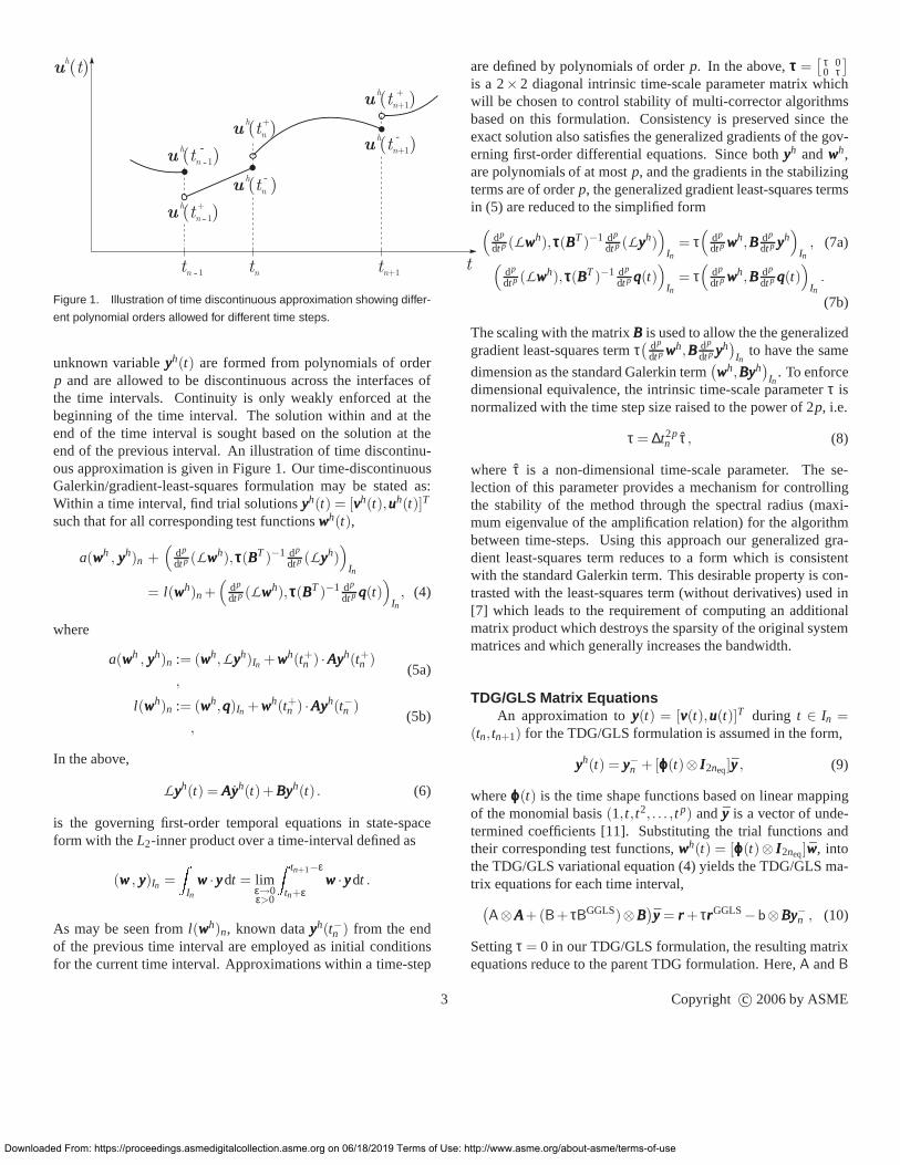
Figure 1. Illustration of time discontinuous approximation showing differ-

ent polynomial orders allowed for different time steps.

unknown variableyyyh(t) are formed from polynomials of orderp and are allowed to be discontinuous across the interfacesthe time intervals. Continuity is only weakly enforced at thebeginning of the time interval. The solution within and at theend of the time interval is sought based on the solution at tend of the previous interval. An illustration of time discontinu-ous approximation is given in Figure 1. Our time-discontinuousGalerkin/gradient-least-squares formulation may be stated as:Within a time interval, find trial solutionsyyyh(t) = [vvvh(t),uuuh(t)]T

such that for all corresponding test functionswwwh(t),

a(wwwh , yyyh)n +(

dp

dt p (Lwwwh),τττ(BBBT)−1 dp

dt p (Lyyyh))

In

= l(wwwh)n +(

dp


dt p qqq(t))

In, (4)

where

a(wwwh , yyyh)n := (wwwh,Lyyyh)In +wwwh(t+n ) ·AAAyyyh(t+n )

,(5a)

l(wwwh)n := (wwwh,qqq)In +wwwh(t+n ) ·AAAyyyh(t−n )

,(5b)

In the above,

Lyyyh(t) = AAAyyyh(t)+BBByyyh(t) . (6)

is the governing first-order temporal equations in state-spaceform with theL2-inner product over a time-interval defined as

(www, yyy)In =Z

Inwww ·yyydt = lim

ε→0ε>0

Z tn+1−ε

tn+εwww ·yyydt .

As may be seen froml(wwwh)n, known datayyyh(t−n ) from the endof the previous time interval are employed as initial conditionsfor the current time interval. Approximations within a time-step

3

wnloaded From: https://proceedings.asmedigitalcollection.asme.org on 06/18/2019 Terms of U

t

of

he

are defined by polynomials of orderp. In the above,τττ =[ τ 0

0 τ]

is a 2× 2 diagonal intrinsic time-scale parameter matrix whichwill be chosen to control stability of multi-corrector algorithmsbased on this formulation. Consistency is preserved since theexact solution also satisfies the generalized gradients of the gov-erning first-order differential equations. Since bothyyyh andwwwh,are polynomials of at mostp, and the gradients in the stabilizingterms are of orderp, the generalized gradient least-squares termsin (5) are reduced to the simplified form

(

dp


dt p (Lyyyh))

In= τ

(

dp

dt p wwwh,BBB dp

dt p yyyh)

In, (7a)

(

dp


dt p qqq(t))

In= τ

(

dp

dt p wwwh,BBB dp

dt p qqq(t))

In.

(7b)

The scaling with the matrixBBB is used to allow the the generalizedgradient least-squares termτ

( dp

dt p wwwh,BBB dp

dt p yyyh)

Into have the same

dimension as the standard Galerkin term(

wwwh,BBByyyh)

In. To enforce

dimensional equivalence, the intrinsic time-scale parameter τ isnormalized with the time step size raised to the power of 2p, i.e.

τ = ∆t2pn τ , (8)

where τ is a non-dimensional time-scale parameter. The se-lection of this parameter provides a mechanism for controllingthe stability of the method through the spectral radius (maxi-mum eigenvalue of the amplification relation) for the algorithmbetween time-steps. Using this approach our generalized gra-dient least-squares term reduces to a form which is consistentwith the standard Galerkin term. This desirable property iscon-trasted with the least-squares term (without derivatives)used in[7] which leads to the requirement of computing an additionalmatrix product which destroys the sparsity of the original systemmatrices and which generally increases the bandwidth.

TDG/GLS Matrix EquationsAn approximation toyyy(t) = [vvv(t),uuu(t)]T during t ∈ In =

(tn,tn+1) for the TDG/GLS formulation is assumed in the form,

yyyh(t) = yyy−n +[ϕϕϕ(t)⊗ III2neq]yyy, (9)

whereϕϕϕ(t) is the time shape functions based on linear mappingof the monomial basis(1,t,t2, . . . ,t p) andyyy is a vector of unde-termined coefficients [11]. Substituting the trial functions andtheir corresponding test functions,wwwh(t) = [ϕϕϕ(t)⊗ III2neq]www, intothe TDG/GLS variational equation (4) yields the TDG/GLS ma-trix equations for each time interval,

(

A⊗AAA+(B+ τBGGLS)⊗BBB)

yyy = rrr + τrrrGGLS−b⊗BBByyy−n , (10)

Settingτ = 0 in our TDG/GLS formulation, the resulting matrixequations reduce to the parent TDG formulation. Here,A andB


se: http://www.asme.org/about-asme/terms-of-use

are(p+1)× (p+1) matrices defined by integration over a timeintervalIn ∈ (tn,tn+1):

A =Z

InϕϕϕT(t) ϕϕϕ(t) dt + ϕϕϕT(t+n )ϕϕϕ(t+n ) , (11a)

B = BT =

ZIn

ϕϕϕT(t)ϕϕϕ(t) dt , (11b)

and right-hand-side vectors:

b =Z

InϕϕϕT(t) dt , (11c)

rrr =Z

InϕϕϕT(t)⊗qqq(t) dt . (11d)

From (7), the matrixBGGLS and vectorrrrGGLS can be written as

BGGLS =

ZIn

dp

dt p ϕϕϕT(t) dp

dt p ϕϕϕ(t) dt , (12a)

rrrGGLS =

ZIn

dp

dt p ϕϕϕT(t)⊗ dp

dt p qqq(t) dt . (12b)

It is shown in [11] that in the absence of external forcesfff = 0, the total energy at the end of a time step is boundedby the total energy at the end of the previous time step. As aconsequence, the total energy at the end of a time intervalt f , isbounded by the initial total energy which implies stabilityfor anytime step size. A similar result was found for the standard TDGmethod [7]. Accuracy and stability properties obtained fromanalysis of a representative single-degree-of-freedom (SDOF)modal equation shows that specific values for the intrinsic time-scale parameterτ in the proposed TDG/GLS algorithms matchesoptimal families of Pade approximations to the exact exponen-tial solution to the model equation expressed in first-orderform.Pade approximations [17] are a particular type of rationalfractionapproximation to the exponential solution. The idea is to matchthe Taylor’s series expansion of the exact and numerical approxi-mation as far as possible in rational form. Since Pade approxima-tions have the lowest relative error, these algorithms are optimalin term of accuracy, dissipation, dispersion and overshootchar-acteristics. Comparing the eigenvalues of the amplification ma-trices relating the solution at the beginning and end of a time-stepfor the TDG method to the Pade approximations, it can be shownthat the TDG method is equivalent to the first sub-diagonal Padeapproximations to the exponential function [18]. For the gener-alized TDG/GLS algorithms (denoted byPp-TDG/GLS, with pthe polynomial order used), it can be shown that selectingτ = τ0

defined in Table 1 yields diagonal Pade approximations whichare energy conservingA-stable and achieve accuracy of order2p [11]. With τ0 ≤ τ ≤ 0, the algorithms possess desirableL-stability (asymptotic annihilation of high-frequency oscillations)and achieve accuracy of order 2p. Likewise, selectingτ = τ1,yields the second sub-diagonal Pade approximations [11].Thesecond sub-diagonal Pade approximations also exhibitL-stability
and achieve accuracy of order 2p.
4

Downloaded From: https://proceedings.asmedigitalcollection.asme.org on 06/18/2019 Terms of Use

MULTI-PASS TDG/GLS ALGORITHMThe system of algebraic equations given in (10) resulting

from space and time discretization of the TDG formulation is2(p+ 1) times larger than the size of the originalKKK andMMM sys-tem matrices. Direct solution of this large system of coupledequations for the unknown coefficient vectorsyyyi is computation-ally expensive. To address this problem a multi-pass iterative al-gorithm is proposed to solve (10) efficiently while retaining theaccuracy and stability of the direct solution. Multiplyingbothside of (10) with(A−1⊗ III2neq) results in

(

Ip+1⊗AAA+[

G+ τGGGLS]

⊗BBB)

yyy = sss+ τsssGGLS−d⊗BBByyy−n ,

(13)whereIp+1 is the identity matrix of orderp+1, and

G = A−1

B = ∆tn

Z 1

0ψψψT(t)ϕϕϕ(t) dt , (14a)

GGGLS = A

−1B

GGLS = ∆tn

Z 1

0

dp

dt p ψψψT(t) dp

dt p ϕϕϕ(t) dt , (14b)

and the right-hand-side vectors,

d = A−1

b = ∆tn

Z 1

0ψψψT(t) dt , (14c)

sss = A−1rrr = ∆tn

Z 1

0ψψψT(t)⊗qqq(t) dt , (14d)

sssGGLS = A−1rrrGGLS = ∆tn

Z 1

0

dp

dt p ψψψT(t)⊗ dp

dt p qqq(t) dt , (14e)

In the above,ψψψT(t), are defined by

ψψψT(t) = A−1ϕϕϕT(t). (15)

and 0< t < 1 is a scaled reference interval within a time-stepsuch thatt = t+n +(∆tn) t. From an accuracy study of multi-passalgorithms based on the TDG method given in [10], the timeshape functions in (9) are defined to be: Fori = 0,1,2, . . . , p ,

ϕi(t) =i

∑k=0

(−1)k k! γk(

ik

)2

t i−k = (−1)i i! γi Li (t/γ) , (16)

where( i

k

)

is the binomial coefficient [19] andLi is theLaguerrepolynomial of degreei [20]. Unlike the multi-pass algorithm forthe TDG method developed in [10] whereγ is pre-specified to beγ = 1

2p+1, the choice ofγ for the TDG/GLS is arbitrary and is se-lected to provide stability to high-order accurate multi-pass itera-tive algorithms with polynomial orderp > 2. The correspondingweighting functions can also be expressed by

ψψψT(t) = A−1ϕϕϕT(t) = W tttT(t) . (17)


: http://www.asme.org/about-asme/terms-of-use

Downlo

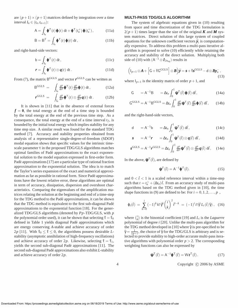
Table 1. Accuracy and stability properties of TDG/GLS method with approximation orders p = 1,2,3 and different values of τ.

τ Error rate StabilityAlgorithm

τ0 τ1 τ 6= 0 τ = 0 τ = τ0 τ > τ0

(p = 1) Linear - 112

16 ∆t2 ∆t3 A-stable C- & L-stable

(p = 2) Quadratic - 1720


(p = 3) Cubic - 1100800


wherettt(t) =[

1, t, t2, · · · , t p]

are monomials in time, andW =[wi j ] are coefficients defined by

w00 = 1,

wi j = (−1)i+ j (p+ j)!( j!)2(p− j)!

p

∑q=i

(

(p+q)!(q!)2(p−q)!

)(

jj +q

)

cqi ,

(18)

where

ci j =

0 if i < j ,

1 if i = j ,

(−1)m

m! γmm−1∏

k=0(i −k)2 if i > j ,

. (19)

In the above,m= i − j, andγ is arbitrary.

To obtain an efficient block iterative solution method, thediagonal components of the matrixG = G + τGGGLS are con-strained to have the same values. This singly diagonal require-ment can be obtained by selecting

τ =p! (p−1)!

(2p)! (2p−1)!(p+1)

(

γ− 12p+1

)

∆t2pn , (20)

wherep is the order of polynomial approximations. The abovecondition leads to

diag(G) = D = ∆tnγ Ip+1 = γ Ip+1 , (21)

whereγ is an arbitrary parameter. Selectingγ = 12p+1 in (20) re-

sults inτ = 0 and hence reduces to our previous implementatiofor the TDG formulation in [10]. Choice of the free parameterγis selected to enhance stability of the predictor/multi-correctoral-gorithm as discussed in the following Section. LetE =E+EGGLS

denote the off-diagonal part of theG matrix, i.e. G = γIp+1 + E.Using the time shape functions (16) and the time-scale parame-

5

aded From: https://proceedings.asmedigitalcollection.asme.org on 06/18/2019 Terms of Us

n

ter (20), the components of the off-diagonal part are definedby

Ei j =

1i

∆tn , for j = i −1, andi = 1,2, . . . , p,

∆tnp∑

r=0wir

p∑

s=0

1r+s+1 cps, for j = p, andi = 0,1, . . . , p−1,

0, otherwise,(22a)

EGGLSi j =

∆tnap(

γ− 12p+1

)

wip , for j = p , andi = 0,1, . . . , p−1,

0, otherwise,

(22b)

whereap =(p!)3 (p−1)!(2p)! (2p−1)! (p+1) and the vectord is given by,

di = ∆tn(δi0γ+ δi1) , for i = 0,1, . . . , p. (23)

To facilitate the block matrix Gauss-Seidel iterative algorithm,the off-diagonal part is split into the lower and upper triangularmatrices, i.e.E = L+U. The TDG/GLS matrix equations (13) isthen written as an addition of the diagonal and off-diagonalparts,

(Ip+1⊗ [AAA+ γBBB]+ (L+U)⊗BBB) yyy = sss+ τsssGGLS−d⊗BBByyy−n .(24)

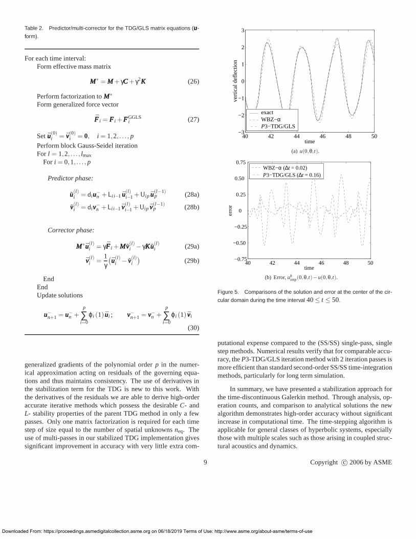
After permutation, the upper triangular part is moved to theright-hand-side to obtain a block matrix Gauss-Seidel iterationtype method. The algorithm can be written in the efficientpredictor/multi-corrector form given in Table 2 in terms ofthesmaller vector sizeuuui . An alternative form in terms of velocityvvvi is given in [11]. The explicit expressions for the generalizedforce vectorsFFF i andFFFGGLS

i in the tables are given as follows,

FFF i = ∆tnp

∑r=0

wir

Z 1

0tr fff (t)dt , (25a)

FFFGGLSi = ∆tn

(p!)2 (p−1)!(2p)! (2p−1)! (p+1)

(

γ− 12p+1

)

wip

Z 1

0

dp

dt p fff (t)dt ,

(25b)

for i = 0,1, . . . , p. Settingγ = 12p+1 corresponding to the parent

TDG method givesEGGLS= 0 andFFFGGLS= 0. From an analysis



Downloaded From: https:

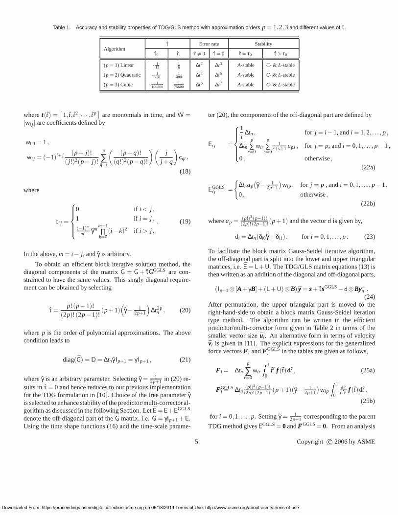
Table 3. L-stability region and accuracy-order of multi-pass TDG/GLS algorithms.

Super-convergence

Algorithm # of pass L-stability Error rateL-stability Error rate

1 (2−√

2)/2≤ γ ≤ (2+√

2)/2 1 γ = (2±√

2)/2 2

P1 2 0.27160681≤ γ ≤ 3.14260677 2 γ = 1/3 3

3 0.26525866≤ γ ≤ 4.34603336 2 γ = 1/3 3

1 0.18042531≤ γ ≤ 2.18560010 2 γ = 0.43586652 3

P2 2 0.19873253≤ γ ≤ 0.55560395 4 γ = 0.26378983 5

3 0.17112822≤ γ ≤ 0.77164994 4 γ = 1/5 5

1 0.22364780≤ γ ≤ 0.57281606 3 γ = 0.57281606 4

P3 2 0.22042841≤ γ ≤ (6+√

6)/30 5 γ =

0.22042841(6+

√6)/30 6

3 0.22184316≤ γ ≤ 0.34083315 6 − −


of the eigenvalues for the amplification matrix relating thesolu-tion at the beginning and end of a time-step for the iterationpassl , the range of values forγ providingL-stability for the multi-passP1-, P2- andP3-TDG/GLS algorithms are determined [11] andsummarized in Table 3.

The value ofγ should be kept unchanged during each iteration pass to minimize the computational effort of refactorization.For the P3-TDG/GLS algorithm, settingγ = 6+

√6

30 (0.28164966)providesL-stability for all iteration passes and achieves sixthorder accuracy in only two passes; see Table 4. The spectradii for the multi-passP3-TDG/GLS algorithm withγ = 6+

√6

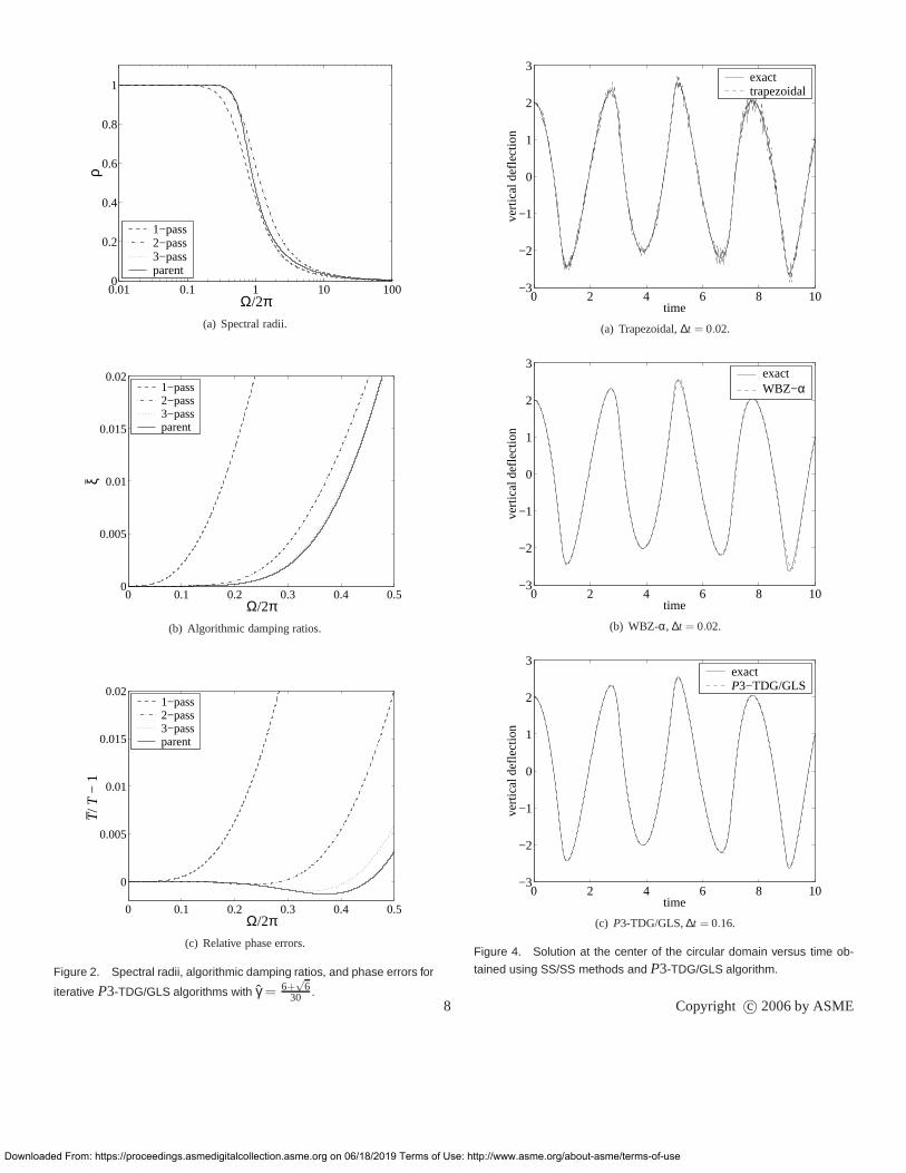
30is shown in Figure 2(a). The spectral radii retain the desirableC-andL-stability of the parent algorithm for all iteration passes. For3 or more iteration passes, the spectral radius closely follows theparent algorithm over the entire frequency range. Figures 2(b)and 2(c) depict the algorithmic damping ratios and phase errorsof the multi-pass algorithm, respectively. As predicted from theanalysis in Table 4 only 2 or 3 iteration passes are neededmatch the same 6th order accuracy of the parent solution. Afteronly 2 or 3 iteration passes, both algorithmic damping and phaseerror nearly match those of the parent solution. Results for4 ormore iteration passes are identical over the frequency range up to0.5∗Ω/(2π).

The final form of the algorithm uses only a few iterationpasses to reach the order of accuracy of the parent solutioAnalysis of the multi-pass algorithm shows that the first iter-ation pass belongs to the family of (p+1)-stage stiff accurateSingly-Diagonal-Implicit-Runge-Kutta (SDIRK) method [21].The methods developed can be viewed as a generalization toe

6

//proceedings.asmedigitalcollection.asme.org on 06/18/2019 Terms of Us

-

ral

to

n.

th

SDIRK method, retaining the desirable features of efficiency andstability, now extended to high-order accuracy. A detailedanal-ysis of the operation counts for the algorithm in Table 2 showsthat the obtained high-order algorithms have the same factoriza-tion cost and after amortized over time steps, the right-hand-sidematrix-vector updates are comparable to single-step, single-solve(SS/SS) methods such as HHT-α and WBZ-α. In practice, forsufficiently regular solutions, the high-order algorithmsderivedare more efficient than the second-order SS/SS methods for thesame error tolerance, since larger time-step sizes can be used,especially over long-time simulations.

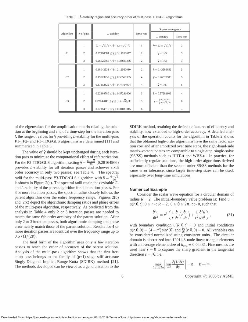
Numerical ExampleConsider the scalar wave equation for a circular domain of

radiusR= 2. The initial-boundary value problem is: Findu =u(r,θ,t), 0≤ r < R= 2, 0≤ θ ≤ 2π , t > 0, such that

∂2u∂t2 = c2

(

1r

∂∂r

(

r∂u∂r

)

+1r2

∂2u∂θ2

)

, (31)

with boundary conditionu(R,θ,t) = 0 and initial conditionsu(r,θ,0) =

(

4− r2)

sin2(θ) and ∂u∂t (r,θ,0) = 0. All variables can

be considered normalized using consistent units. The circulardomain is discretized into 12014 3-node linear triangle elementswith an average element size ofhavg= 0.04431. Fine meshes areused nearr = 0 to capture the sharp gradient in the tangentialdirections= rθ, i.e.

max0≤θ≤2π

∣

∣

∣

∣

limr→0

∂ f (r,θ)

∂s

∣

∣

∣

∣

= ε , ε → ∞.


Downloaded From:

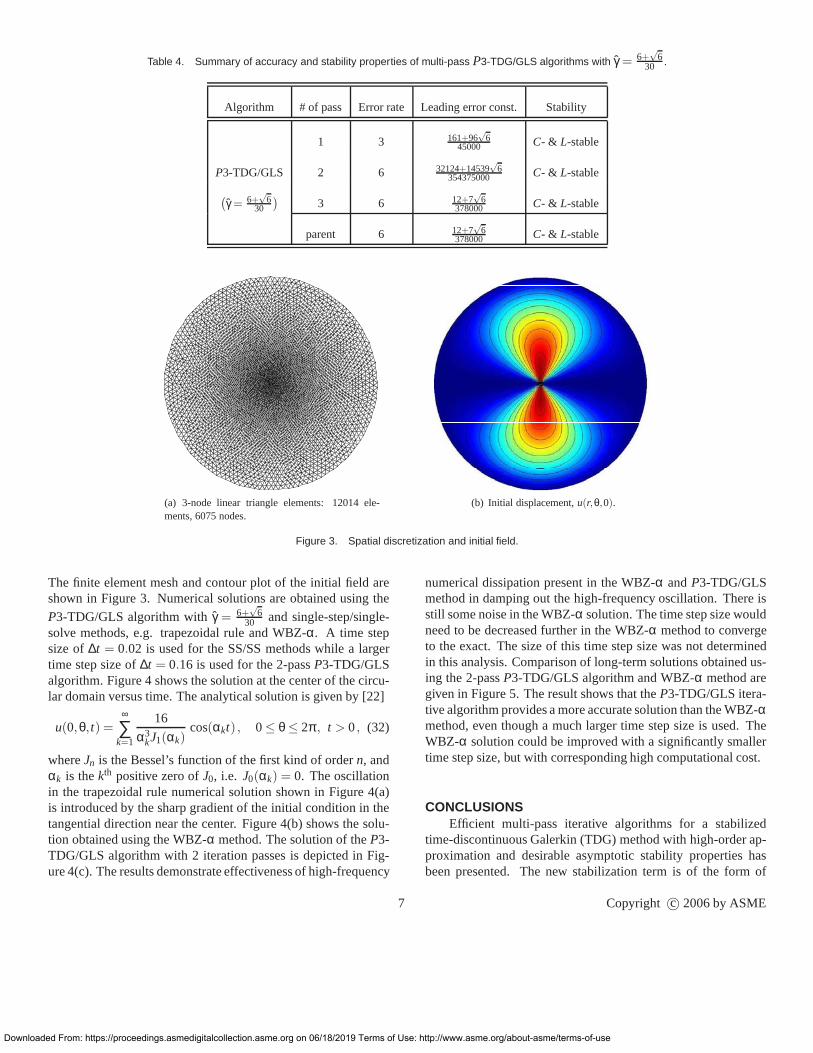
Table 4. Summary of accuracy and stability properties of multi-pass P3-TDG/GLS algorithms with γ = 6+√

630 .

Algorithm # of pass Error rate Leading error const. Stability

1 3 161+96√

645000 C- & L-stable

P3-TDG/GLS 2 6 32124+14539√

6354375000 C- & L-stable

(

γ = 6+√

630

)

3 6 12+7√

6378000 C- & L-stable

parent 6 12+7√

6378000 C- & L-stable

(a) 3-node linear triangle elements: 12014 ele-ments, 6075 nodes.

(b) Initial displacement,u(r,θ,0).

Figure 3. Spatial discretization and initial field.

r

The finite element mesh and contour plot of the initial field areshown in Figure 3. Numerical solutions are obtained using the

P3-TDG/GLS algorithm withγ = 6+√

630 and single-step/single-

solve methods, e.g. trapezoidal rule and WBZ-α. A time stepsize of∆t = 0.02 is used for the SS/SS methods while a largetime step size of∆t = 0.16 is used for the 2-passP3-TDG/GLSalgorithm. Figure 4 shows the solution at the center of the circu-lar domain versus time. The analytical solution is given by [22]

u(0,θ,t) =∞

∑k=1

16

α3kJ1(αk)

cos(αkt) , 0≤ θ ≤ 2π , t > 0, (32)

whereJn is the Bessel’s function of the first kind of ordern, andαk is thekth positive zero ofJ0, i.e. J0(αk) = 0. The oscillationin the trapezoidal rule numerical solution shown in Figure 4(a)is introduced by the sharp gradient of the initial conditionin thetangential direction near the center. Figure 4(b) shows thesolu-tion obtained using the WBZ-α method. The solution of theP3-TDG/GLS algorithm with 2 iteration passes is depicted in Fig-ure 4(c). The results demonstrate effectiveness of high-frequency

7

https://proceedings.asmedigitalcollection.asme.org on 06/18/2019 Terms of Use:

numerical dissipation present in the WBZ-α andP3-TDG/GLSmethod in damping out the high-frequency oscillation. There isstill some noise in the WBZ-α solution. The time step size wouldneed to be decreased further in the WBZ-α method to convergeto the exact. The size of this time step size was not determinedin this analysis. Comparison of long-term solutions obtained us-ing the 2-passP3-TDG/GLS algorithm and WBZ-α method aregiven in Figure 5. The result shows that theP3-TDG/GLS itera-tive algorithm provides a more accurate solution than the WBZ-αmethod, even though a much larger time step size is used. TheWBZ-α solution could be improved with a significantly smallertime step size, but with corresponding high computational cost.

CONCLUSIONSEfficient multi-pass iterative algorithms for a stabilized

time-discontinuous Galerkin (TDG) method with high-orderap-proximation and desirable asymptotic stability properties hasbeen presented. The new stabilization term is of the form of


http://www.asme.org/about-asme/terms-of-use

Do

0.01 0.1 1 10 1000

0.2

0.4

0.6

0.8

1

Ω/2π

ρ

1−pass2−pass3−passparent

(a) Spectral radii.

0 0.1 0.2 0.3 0.4 0.50

0.005

0.01

0.015

0.02

Ω/2π

ξ


(b) Algorithmic damping ratios.

0 0.1 0.2 0.3 0.4 0.5

0

0.005

0.01

0.015

0.02

Ω/2π

T/ T

− 1


(c) Relative phase errors.

Figure 2. Spectral radii, algorithmic damping ratios, and phase errors for

ˆ 6+√

6
iterative P3-TDG/GLS algorithms with γ = 30 .8
wnloaded From: https://proceedings.asmedigitalcollection.asme.org on 06/18/2019 Terms of Us

0 2 4 6 8 10−3

−2

−1

0

1

2

3

time

vert

ical

def

lect

ion

exacttrapezoidal

(a) Trapezoidal,∆t = 0.02.

0 2 4 6 8 10−3

−2

−1

0

1

2

3

time

vert

ical

def

lect

ion

exactWBZ−α

(b) WBZ-α, ∆t = 0.02.

0 2 4 6 8 10−3

−2

−1

0

1

2

3

time

vert

ical

def

lect

ion

exactP3−TDG/GLS

(c) P3-TDG/GLS,∆t = 0.16.

Figure 4. Solution at the center of the circular domain versus time ob-

tained using SS/SS methods and P3-TDG/GLS algorithm.



Dow

Table 2. Predictor/multi-corrector for the TDG/GLS matrix equations (uuu-

form).

For each time interval:Form effective mass matrix

MMM∗ = MMM + γCCC+ γ2KKK (26)

Perform factorization toMMM∗

Form generalized force vector

FFF i = FFF i +FFFGGLSi (27)

Setuuu(0)i = vvv(0)

i = 0, i = 1,2, . . . , p

Perform block Gauss-Seidel iterationFor l = 1,2, . . . , lmax

For i = 0,1, . . . , p

Predictor phase:

uuu(l)i = diuuu

−n +Li i−1 uuu(l)

i−1 +Uip uuu(l−1)p (28a)

vvv(l)i = divvv

−n +Li i−1 vvv(l)

i−1 +Uip vvv(l−1)p (28b)

Corrector phase:

MMM∗uuu(l)i = γFFF i +MMMvvv(l)

i − γKKKuuu(l)i (29a)

vvv(l)i =

1γ(

uuu(l)i − vvv(l)

i

)

(29b)

EndEndUpdate solutions

uuu−n+1 = uuu−n +p

∑i=0

ϕi (1) uuui ; vvv−n+1 = vvv−n +p

∑i=0

ϕi (1) vvvi

(30)

generalized gradients of the polynomial orderp in the numer-ical approximation acting on residuals of the governing equa-tions and thus maintains consistency. The use of derivatives inthe stabilization term for the TDG is new to this work. Withthe derivatives of the residuals we are able to derive high-orderaccurate iterative methods which possess the desirableC- andL- stability properties of the parent TDG method in only a fewpasses. Only one matrix factorization is required for each timestep of size equal to the number of spatial unknownsneq. Theuse of multi-passes in our stabilized TDG implementation givessignificant improvement in accuracy with very little extra com-

9

nloaded From: https://proceedings.asmedigitalcollection.asme.org on 06/18/2019 Terms of Us

40 42 44 46 48 50−3

−2

−1

0

1

2

3

time

vert

ical

def

lect

ion

exactWBZ−αP3−TDG/GLS

(a) u(0,θ,t).

40 42 44 46 48 50−0.75

−0.50

−0.25

0

0.25

0.50

0.75

time

erro

r

WBZ−α (∆t = 0.02)P3−TDG/GLS (∆t = 0.16)

(b) Error,uhintp(0,θ,t)−u(0,θ,t).

Figure 5. Comparisons of the solution and error at the center of the cir-

cular domain during the time interval 40≤ t ≤ 50.

putational expense compared to the (SS/SS) single-pass, singlestep methods. Numerical results verify that for comparableaccu-racy, theP3-TDG/GLS iteration method with 2 iteration passes ismore efficient than standard second-order SS/SS time-integrationmethods, particularly for long term simulation.

In summary, we have presented a stabilization approach forthe time-discontinuous Galerkin method. Through analysis, op-eration counts, and comparison to analytical solutions thenewalgorithm demonstrates high-order accuracy without significantincrease in computational time. The time-stepping algorithm isapplicable for general classes of hyperbolic systems, especiallythose with multiple scales such as those arising in coupled struc-tural acoustics and dynamics.



,

-

ss-

Dow

ACKNOWLEDGMENTSupport for L.Thompson was provided by the National Sc

ence Foundation under Grant CMS-9702082 in conjunction wiha Presidential Early Career Award for Scientists and Engineers(PECASE), and is gratefully acknowledged. We also thank thanonymous reviewers for their comments.

REFERENCES[1] Hughes, T. J., 2000.The Finite Element Method: Linear

Static and Dynamic Finite Element Analysis. Dover Publi-cation, Inc.

[2] Dahlquist, G. G., 1963. “A special stability problem forlinear multistep methods”.BIT, 3 [], pp. 27–43.

[3] Chung, J., and Hulbert, G. M., 1993. “A time integrationalgorithm for structural dynamics with improved numericadissipation: The Generalized-α method”. Journal of Ap-plied Mechanics,TRANS. ASME, 60 [], pp. 371–375.

[4] Hilber, H. M., Hughes, T. J. R., and Taylor, R. L., 1977“Improved numerical dissipation for time integration algo-rithms in structural dynamics”.Earthquake Engineeringand Structural Dynamics,5 [], pp. 283–292.

[5] Wood, W. L., Bossak, M., and Zienkiewicz, O. C., 1981“An alpha modification of Newmark’s method”.Interna-tional Journal for Numerical Methods in Engineering,15[], pp. 1562–1566.

[6] Austin, M., 1993. “High-order integration of smooth dy-namical systems: Theory and numerical experiments”.In-ternational Journal for Numerical Methods in Engineering36 [], pp. 2107–2122.

[7] Hulbert, G. M., 1992. “Time finite element methods forstructural dynamics”.International Journal for NumericalMethods in Engineering,33 [], pp. 307–331.

[8] Thompson, L. L., and He, D., 2005. “Adaptive space-timfinite element methods for the wave equation on unbounddomains”. Computer Methods in Applied Mechanics andEngineering,194 [], pp. 1947–2000.

[9] Subbarayalu, S., and Thompson, L. L., 2004.hp-adaptivetime-discontinuous Galerkin finite element methods fotime-dependent waves. Proceedings of 2004 ASME Intenational Mechanical Engineering Congress & ExpositionNov. 2004, Anaheim, CA., Paper IMECE 2004-60403.

[10] Kunthong, P., and Thompson, L. L., 2005. “An effi-cient solver for the high-order accurate time-discontinuousgalerkin (TDG) method for second-order hyperbolic systems”. Finite Elements in Analysis & Design,141 (7-8) [],pp. 729–762.

[11] Kunthong, P., 2005.Efficient Predictor/Multi-corrector al-gorithms based on high-order accurate time-discontinuouGalerkin methods for second-order Hyperbolic system.PhD thesis, Clemson University, Department of Civil Engineering, Clemson, South Carolina.

nloaded From: https://proceedings.asmedigitalcollection.asme.org on 06/18/2019 Terms o

i-t

e

l

.

.

,

eed

rr-

[12] Franca, L. P., and Carmo, E. G. D. D., 1989. “The Galerkingradient least-squares method”.Computer Methods in Ap-plied Mechanics and Engineering,74 [], pp. 41–54.

[13] Thompson, L. L., and Kunthong, P., 2005. “A residualbased variational method for reducing dispersion error in fi-nite element methods”. In Paper IMECE2005-80551, Pro-ceedings IMECE’05, The American Society of Mechani-cal Engineers. 2005 International Mechanical EngineeringConference & Exposition by the Noise Control & Acous-tics Division.

[14] Thompson, L. L., and Sankar, S., 2001. “Dispersion anal-ysis of stabilized finite element methods for acoustic fluidinteraction with Reissner-Mindlin plates”. Int. J. Numer.Meth. Engng,50 (11) [], pp. 2521–2545.

[15] Thompson, L. L., and Pinsky, P. M., 1996. “A space-timefinite element method for structural acoustics in infinitedomains, Part I: Formulation, stability, and convergence”.Comput. Methods in Appl. Mech. Engrg,132 [], pp. 195–227.

[16] Hulbert, G. M., 1989. Space-Time Finite Element Meth-ods for Second-Order Hyperbolic Equations. PhD thesis,Stanford University, Stanford, California.

[17] Baker, Jr., G. A., 1975.Essesntials of Pade Approximants.Academic Press, Inc., 111 Fifth Avenue, New York, NewYork 10003.

[18] Hulbert, G. M., 1994. “A unified set of single-stepasymptotic annihilation algorithms for structural dynam-ics”. Computer Methods in Applied Mechanics and En-gineering.,113 [], pp. 1–9.

[19] Burington, R. S., 1972.Handbook of Mathematical Tableand Formulas, fifth ed. McGraw-Hill Book Company.

[20] Rainville, E. D., 1960.Special Functions. The MacmillanCompany, New York, USA.

[21] Hairer, E., and Wanner, G., 1991.Solving Ordinary Differ-ential Equations II: Stiff and Differential-Algebraic Prob-lems. Springer, Berlin.

[22] ONeil, P. V., 1995. Advanced Engineering Mathematics,forth ed. Brooks/Cole Publishing Company, Pacific Grove,CA, USA.

10 Copyright c© 2006 by ASME

f Use: http://www.asme.org/about-asme/terms-of-use

Stabilized Time-Discontinuous Galerkin Methods ... - CiteSeerX

Documents

Transcript of Stabilized Time-Discontinuous Galerkin Methods ... - CiteSeerX