ESAIM: PROCEEDINGS, Vol. ?, 2009, 1-10

Editors: Will be set by the publisher

A HIGH-ORDER DISCONTINUOUS GALERKIN METHOD FOR THE SEISMIC

WAVE PROPAGATION

Sarah Delcourte1, Loula Fezoui1 and Nathalie Glinsky-Olivier2

Abstract. We are interested in the simulation of P-SV seismic wave propagation by a high-orderDiscontinuous Galerkin method based on centered fluxes at the interfaces combined with a leap-frogtime-integration. This non-diffusive method, previously developed for the Maxwell equations [4,9,20],is particularly well adapted to complex topographies and fault discontinuities in the medium. We provethat the scheme is stable under a CFL type condition and that a discrete energy is preserved on aninfinite domain. Convergence properties and efficiency of the method are studied through numericalsimulations in two and three dimensions of space.

Resume. Nous nous interessons a la propagation d’ondes sismiques de types P et SV par une methodede Galerkin Discontinue d’ordre eleve basee sur des flux centres aux interfaces combines a un schemasaute-mouton en temps. Cette methode non-dissipative, precedemment developpee pour les equationsde Maxwell [4, 9, 20], est particulierement bien adaptee a des milieux presentant une topographiecomplexe ou contenant des failles. On prouve la stabilite du schema sous une condition de type CFLainsi que la conservation d’une energie discrete dans un domaine infini. L’efficacite de la methode estillustree par des simulations numeriques en deux et trois dimensions d’espace.

1. Introduction

During an Earthquake, two types of waves are generated: body waves which travel through the interior ofthe Earth and surface waves which propagate just at the surface. In what follows, we focus on the body waveswhich can be distinguished into two types of waves: the P-waves (as primary waves because they arrive at firston a seismogram) and the S-waves (as secondary waves; their speed is lower than for the P-waves, so they appearlater on a seismogram). The P-waves are longitudinal and compressive waves which alternatively compress ordistend the ground in the direction of propagation. The S-waves are transverse and shear waves which displacethe ground perpendicularly to the direction of propagation. More, their amplitude is often higher than thoseof the P-waves making them more destructive and we can note that fluids do not support shear stresses. Thedifference in the arrival time of the P and S-waves allows to specify the distance of an event.

The P-SV wave propagation in an isotropic, linearly elastic medium is modelised by the elastodynamicequations, which write initially in displacement-stress formulation; let be U = (Uα), α = x, y, z, the displacement

1 INRIA, NACHOS project-team, 2004 route des Lucioles, BP 93, 06902 Sophia Antipolis.2 CERMICS and INRIA, NACHOS project-team, 2004 route des Lucioles, BP 93, 06902 Sophia Antipolis.Sarah.Delcourte, Loula.Fezoui, Nathalie.Glinsky@inria.fr

c© EDP Sciences, SMAI 2009

2 ESAIM: PROCEEDINGS

vector and σ = (σα,β), α, β = x, y, z, the stress tensor, then the system reads

ρ∂2U

∂t2= ∇ · σ ,

σ = λ (∇ · U) I + µ (∇U + (∇U)T ) ,

(1)

where I is the identity matrix, ρ is the density of the medium and λ and µ are the Lame constants.

Using the Helmholtz decomposition of U = ∇φ+ ∇× ψ = Up + Us and properties of the operators, we canestablish the following identity:

∇

(∂2φ

∂t2− v2

p ∆φ

)+ ∇ ×

(∂2ψ

∂t2− v2

s ∆ψ

)= 0 , (2)

where vp =√

λ+2µρ and vs =

√µρ are the velocities of the P and S-waves respectively, and vp > vs. One solution

of (2) can be obtained by setting both bracketed terms to zero. This yields two wave equations, one for eachpotential φ and ψ, which correspond to the P and S-waves:

∂2φ

∂t2− v2

p ∆φ = 0 and∂2ψ

∂t2− v2

s ∆ψ = 0 . (3)

In order to solve the problem (1), we introduce the velocity vector V =∂U

∂tin (1) and we obtain the velocity-

stress formulation, which allows to take into account more easily the boundary conditions:

ρ∂V

∂t= ∇ · σ ,

∂σ

∂t= λ (∇ · V ) I + µ (∇V + (∇V )T ) .

(4)

The most famous method to solve this problem is the finite difference scheme of Virieux [22] which can beviewed as an adaptation to elastodynamic equations of the Yee’s scheme [23], very popular in electromagnetism.This method is very easy to implement, second order accurate, not too costly in CPU time and weakly disper-sive, but the major drawback is the restriction to rectangular grids, not suited for geometrical irregularities.This method has known later many extensions in three dimensions, to anisotropic media or to higher order ofaccuracy for example. Some other methods have been further developed such as the finite element methodswhich have allowed to deal with meshes adapted to complex geometries. However, they are very costly because,at each time-step, one needs to invert a N-diagonal mass matrix with N depending on the order of the methodand the dimension of the space. This difficulty was overcome by the use of Gauss-Lobatto Legendre quadratureformulae and these methods applied to quadrangular or hexahedral meshes are referenced as spectral elementmethods [14].

In what follows, we focus on Discontinuous Galerkin methods which are finite element methods with discon-tinuities at the interfaces, well adapted to take into account cracks in the medium. They are non-conformingmethods (in the sense of finite elements), so that we can note a greater flexibility (compared to spectral elementmethods) in the choice of the local degree p of the polynomial interpolation. They require in general the use ofnumerical fluxes, as for the finite volume methods. These methods have been introduced in 1973 by Reed & Hillto simulate neutron transport. The first analysis of the method for hyperbolic equations has been presentedby Lesaint & Raviart [16, 17] in 1974. Their result has been further improved and the analysis substantially

ESAIM: PROCEEDINGS 3

broadened by Johnson, Pitkaranta & Navert [11,12], who have established that the optimal order of convergencein the L2-norm is p+ 1

2 if polynomials of degree p are used. These methods have only become popular since the90s with several remarkable contributions as Cockburn et al. [5] who studied the non-linear hyperbolic equationscombined to a Discontinuous Galerkin discretization in space with an explicit Runge-Kutta method in time.This renewed interest can be explained by the capability of the Discontinuous Galerkin methods to adapt tomost meshes such as unstructured and non-conforming meshes. Moreover, we can note their flexibility in the useof high-order hp-adaptive finite element methods which consist in techniques of mesh refinement (h-adaptivity)and in the variation of the degree p of the polynomial interpolation (p-adaptivity); see, for example, Suli etal. [21] or Demkowicz et al. [7].

For the seismic wave propagation, Kaser et al. [8, 13] have been recently interested in the development ofhigh-order Discontinuous Galerkin method. They combine upwind fluxes through the interfaces with the ADERscheme in time, so that they get the same order of accuracy in space and in time. However, their scheme isdiffusive. It is the reason why we propose here centered fluxes through the interfaces with a leap-frog time-discretization, which leads to a non-dissipative combination. The extension to higher order in space is realizedby Lagrange interpolants, locally on triangles (in two dimensions) or on tetraedra (in three dimensions), whichdo not necessitate the inversion of a global mass matrix. This method can be viewed as a generalization ofthe finite volume method developed in [1] and allows the use of unstructured and non-conforming meshes, welladapted to heterogeneities of the medium and to complex topographies.

This article is organized as follows. In section 2, we state the velocity-stress formulation in a symmetricalpseudo-conservative form. Then, in section 3, we detail the discretization of the equations system by the Discon-tinuous Galerkin method based on centered fluxes in space and a leap-frog scheme in time. The approximationof the boundary conditions is also presented. After, we study, in section 4, some properties of the scheme andfinally, in section 5, we illustrate this study by some numerical results in two and three dimensions in space ontwo types of meshes. Convergence and efficiency of the method are addressed.

2. Velocity-stress formulation in pseudo-conservative form

We note W =(V , σ

)Tthe vector composed by the velocity components V = (Vx, Vy , Vz)

T and the stress

components σ = (σxx, σyy, σzz , σxy, σxz, σyz)T . Then, the system (4) can be rewritten as

∂W

∂t+

∑

α∈x,y,z

Aα (ρ, λ, µ) ∂αW = 0 . (5)

Moreover, for any real vector n = (nx, ny, nz)T , we define the matrix

An(ρ, λ, µ) =∑

α∈x,y,z

Aα(ρ, λ, µ) nα , (6)

which reads:

An(ρ, λ, µ) = −

0 0 0 nx

ρ0 0

ny

ρnz

ρ0

0 0 0 0ny

ρ0 nx

ρ0 nz

ρ

0 0 0 0 0 nz

ρ0 nx

ρ

ny

ρ

(λ + 2µ)nx λny λnz 0 0 0 0 0 0λnx (λ + 2µ)ny λnz 0 0 0 0 0 0λnx λny (λ + 2µ)nz 0 0 0 0 0 0µny µnx 0 0 0 0 0 0 0µnz 0 µnx 0 0 0 0 0 00 µnz µny 0 0 0 0 0 0

(7)

4 ESAIM: PROCEEDINGS

Remark that the matrices Aα (ρ, λ, µ), for α ∈ x, y, z, are easily deduced from the expression of An(ρ, λ, µ)by keeping only one component nα equal to 1 while the two other are equal to zero. We choose here not todetail these matrices.

In order to express the system (5) in pseudo conservative form, we introduce the following change of variables

σ = Rσ on the stress components. For example in 3D

R =

13

13

13 0 0 0

23 − 1

3 − 13 0 0 0

− 13

23 − 1

3 0 0 00 0 0 1 0 00 0 0 0 1 00 0 0 0 0 1

. So, the system reads

Λ (ρ, λ, µ)∂W

∂t+

∑

α∈x,y,z

Aα ∂αW = 0 , (8)

where W =(V , σ

)Tand Λ = diag

(ρ, ρ, ρ,

3

3λ+ 2µ,

3

2µ,

3

2µ,1

µ,1

µ,1

µ

)is a diagonal matrix containing the char-

acteristics of the medium. We can notice that now the matrices Aα are constant and do not depend anymoreon the material properties.

At last, we multiply the previous system by the following matrix S0 =

1 0 0 0 0 0 0 0 00 1 0 0 0 0 0 0 00 0 1 0 0 0 0 0 00 0 0 1 0 0 0 0 00 0 0 0 2

313 0 0 0

0 0 0 0 13

23 0 0 0

0 0 0 0 0 0 1 0 00 0 0 0 0 0 0 1 00 0 0 0 0 0 0 0 1

in order to obtain a symmetrical system. Therefore, we finally get the symmetrical pseudo-conservative formu-lation:

Λ0 (ρ, λ, µ)∂W

∂t+

∑

α∈x,y,z

Sα ∂αW = 0 , (9)

where Λ0 = S0Λ and Sα = S0Aα (α = x, y, z) are symmetric. This formulation will be very useful to establishthe energy conservation. For the numerical simulations, we add boundary conditions on the free surface σ n = 0or absorbing conditions to approximate an infinite domain.

3. Discretization

We consider a polygonal domain Ω, discretized in NT symplectic elements Ti (triangles in 2D and tetrahedrain 3D), which form a partition of the domain. We denote by V(i) the set of indices of the neighboring elementsof Ti and we note Sik each internal face common to both elements Ti and Tk i.e. Sik = Ti ∩ Tk. Finally, someelements Ti have one or more faces common to the boundary of the domain. The set of the indices k of suchfaces Sbi

k = Ti ∩ ∂Ω is denoted by E(i). Remark that this set is empty for most elements.

ESAIM: PROCEEDINGS 5

We multiply each equation of the problem (4) by a scalar test function φTi

l and we integrate them on eachelement Ti:

∫

Ti

∂W

∂t+

∑

α∈x,y,z

Aα(ρ, λ, µ) ∂αW

φTi

l dxdydz = 0 . (10)

Then, we assume that the characteristics of the medium (ρ, λ, µ) are constant over each element Ti and we applythe Green formula to the second term of (10):

∫

Ti

∂W

∂tφTi

l dxdydz −∑

α∈x,y,z

ATi

α

∫

Ti

W ∂αφTi

l dxdydz +ATi

n

∫

∂Ti

W φTi

l ds = 0 , (11)

where ATi

n is the restriction of An to the element Ti and n represents the outwards unit normal vector to Ti.

Now, we take as test function the Lagrange nodal interpolants φTi

l of Pm(Ti), set of polynomials with a degree

m. Then, each component W of the vector W is approximated on Ti by:

W|Ti(x, y, z, t) =

ndof∑

j=1

W Ti

j (t) φTi

j (x, y, z) , (12)

where ndof is the number of degrees of freedom on the element Ti and φTi

j (j = 1, ..., ndof) are the associated

basis functions. The first term of (11) can be expressed by:

∀l = 1, ..., ndof ,

∫

Ti

∂

∂tW φTi

l dxdydz =

ndof∑

j=1

MTi

lj

d

dtWj

Ti, (13)

where MTi

=

(∫

Ti

φTi

j φTi

l dxdydz

)

1≤j,l≤ndof

denotes the mass matrix on the element Ti.

The second integral of (11) is approximated in the following way:

∀l = 1, ..., ndof ,∑

α∈x,y,z

ATi

α

∫

Ti

W ∂αφTi

l dxdydz =∑

α∈x,y,z

ATi

α

ndof∑

j=1

GTi

α,lj WTi

j , (14)

with GTi

α =

(∫

Ti

φTi

j ∂αφTi

l dxdydz

)

1≤j,l≤ndof

. Then, to calculate the integral on ∂Ti, we split this boundary

in internal and boundary faces:

∀l = 1, ..., ndof , ATi

n

∑

k∈V(i)

∫

Sik

W φTi

l ds+ATi

n

∑

k∈E(i)

∫

Sbik

W φTi

l ds. (15)

For the interior faces Sik, we apply centered fluxes by introducing the mean value on this face:

W|Sik=

1

2

(W

Ti+ W

Tk

). (16)

Therefore, this integral writes

∀l = 1, ..., ndof , ATi

n

∑

k∈V(i)

∫

Sik

W φTi

l ds =1

2A

Ti

n

∑

k∈V(i)

ndof∑

j=1

[(R

Ti

|Sik

)

lj

WTi

j +

(R

Tk

|Sik

)

lj

WTk

j

], (17)

6 ESAIM: PROCEEDINGS

where we have set RTi

|Sik=

(∫

Sik

φTi

j φTi

l ds

)

1≤j,l≤ndof

and RTk

|Sik=

(∫

Sik

φTk

j φTi

l ds

)

1≤j,l≤ndof

.

For the boundary integrals, two type of boundary conditions have been considered : a free surface conditionat the physical interface between air and the medium, and an absorbing condition on the artificial boundariesof an infinite domain.Free surfaces: On these faces, we compute the fluxes by introducing weakly the condition σ n = 0 in thesecond term of (15). No special condition is applied on the velocity. So, for a boundary face Sbi

k of Ti, thisintegral reduces to

∀l = 1, ..., ndof , ATi

n

∫

Sbik

W φTi

l ds = ATi

n

ndof∑

j=1

(R

Ti

|S

bik

)

lj

(W

Ti

|S

bik

)

j

, (18)

where WTi

|S

bik

= (V Tix , V Ti

y , V Tiz , 0, 0, 0, 0, 0, 0)T and R

Ti

|S

bik

=

(∫

Sbik

φTi

j φTi

l ds

)

1≤j,l≤ndof

.

Absorbing surfaces: To simulate infinite domains, we introduce artificial boundaries, chosen such that thesolution is inside the computational domain and sufficiently far of the frontier, and we impose absorbing condi-tions.For any real unit vector n = (nx, ny, nz)

T 6= 0R3 , the matrix An of (6) is diagonalizable in R, ie all its eigenvaluesλk (k=1,...,9) are real:

λ1 = −vp, λ2 = λ3 = −vs, λ4 = λ5 = λ6 = 0, λ7 = λ8 = vs, λ9 = vp ,

and we note P the matrix whose column k is the right eigenvector associated to the eigenvalue λk. Theabsorbing boundary conditions are then dealt with an upwind technique where we consider only the outgoing

waves. For that, we write An = A+

n + A−

n where we set A+

n = P Λ+ P−1

and A−

n = P Λ− P−1

with Λ+ =

diag(λ+k )1≤k≤9 and Λ− = diag(λ−k )1≤k≤9 the diagonal matrices composed by the positive λ+

k = max(λk, 0)

and the negative λ−k = min(λk, 0) eigenvalues of An. Then, for a boundary face Sbi

k of Ti, the second integralof (15) is approximated by:

∀l = 1, ..., ndof , ATi

n

∫

Sbik

W φTi

l ds = ATi

n

+ ndof∑

j=1

(R

Ti

|S

bik

)

lj

WjTi. (19)

It is a first-order approximation, efficient for waves with a normal incidence to the artificial boundaries.

At last, we apply a leap-frog time-integration scheme. It is a two step explicit scheme which allows, combinedto the centered fluxes defined at (16)-(17), to get a non-diffusive scheme. We note ∆t the time-step and we

can view the final scheme on each element Ti by introducing discrete operators FTiα (α = x, y, z) and GTi

α,β

(α, β = x, y, z) which collect the integrals on Ti and ∂Ti :

MTi Wn+1

Vα−Wn

Vα

∆t= FTi

α

(V

n, σn+ 1

2

), (20)

MTi Wn+ 3

2

σαβ−Wn+ 1

2

σαβ

∆t= GTi

α,β

(V

n+1, σn+ 1

2

), (21)

where WVαand Wσαβ

are respectively the vectors composed by the ndof values of Vα (α = x, y, z) and σαβ

(α, β = x, y, z) in the element Ti, Vn+1

represents the velocity at (n + 1)∆t and σn+ 1

2 the stress tensor at

ESAIM: PROCEEDINGS 7

(n+ 12 )∆t.

Note that the initialisation is realized at t = t0 for the velocity and at t = t0 + ∆t2 for the stress tensor.

4. Properties of the scheme

4.1. VF scheme on cubic elementary volumes

Thanks to standard techniques, the following properties for the P0 scheme (finite volumes: VF) on a domaindiscretized by parallelepipedic elementary volumes are easy to state:

• First, the scheme is second order consistant in space and in time.

• Then, applying Fourier analysis, we can prove that the scheme is stable under the following optimalCFL condition:

vp ∆t

√1

∆x2+

1

∆y2+

1

∆z2≤ 2 , (22)

where ∆x,∆y and ∆z are the standard notations for the lengths of the parallelepipeds in the threedirections.

• Using the Lax theorem, the scheme converges with a second order accuracy to the solution of the elas-todynamics problem on meshes composed of parallelepipeds when (22) is satisfied.

• For the longitudinal or compressional wave, the dispersion relation ω2 = |kp|2 v2p is deduced from the

scalar wave equation of (3), whereas for transverse or shear waves, it is deduced from the vectorial waveequation of (3) and we have ω2 = |ks|2 v2

s , where ω is the pulsation and, kp = (kxp, kyp

, kzp)T and

ks = (kxs, kys

, kzs)T are the wave number vectors associated to the P and SV-waves respectively (by

convention, |k|2 = k2x + k2

y + k2z).

The numerical dispersion relations for the P and SV-waves are given with an order two:

ω2

»

1 −w2∆t2

12+ O

`

w4∆t

4´

–

= |kp|2v2p

"

1 −k4

xp∆x2 + k4

yp∆y2 + k4

zp∆z2

3 |kp|2 + O

k6xp

∆x4 + k6yp

∆y4 + k6zp

∆z4

|kp|2

!#

,

ω2

»

1 −w2∆t2

12+ O

`

w4∆t

4´

–

= |ks|2

v2s

»

1 −k4

xs∆x2 + k4

ys∆y2 + k4

zs∆z2

3 |ks|2 + O

„

k6xs

∆x4 + k6ys

∆y4 + k6zs

∆z4

|ks|2

«–

.

Remark 4.1. : on a twice as fine grid(

∆x2 ,

∆y2 ,

∆z2

), the optimal CFL condition and the numerical dispersion

error of the VF scheme are the same that those obtained with the finite difference scheme of Virieux [22] on agrid (∆x,∆y,∆z). These results are similar to those described by Remaki in [19,20] for the Maxwell equationsdiscretized by centered fluxes through the interfaces combined with a leap-frog time-integration.

4.2. Discrete energy

In order to keep the proof simple, we choose to study the discrete energy only in the 2D case, but it can beeasily extended to the 3D equations. Such a study in both 2D and 3D cases, but leading to a very restrictivestability condition can be found in [2]. We define the discrete energy En at time n∆t by:

En =1

2

NT∑

i=1

∫

Ti

[ρ (Vx

ni )2 + ρ (Vy

ni )2 +

1

λ+ µσxx

n+1/2i σxx

n−1/2i

+1

µσyy

n+1/2i σyy

n−1/2i +

1

µσzz

n+1/2i σzz

n−1/2i

]. (23)

8 ESAIM: PROCEEDINGS

Theorem 4.2. On an infinite domain, the discrete elastodynamic energy is preserved through one time-step:

∀n ∈ N∗, En+1 = En ,

which means the scheme is non-diffusive.

Proof. In the two dimensional case, Eq. (9) can be rewritten as:

ρ∂V

∂t=

∑

α∈x,y

∂αMασ ,

Λσ(λ, µ)∂σ

∂t=

∑

α∈x,y

∂αNαV ,

(24)

with Mx = NT

x =

(1 1 00 0 1

), My = N

T

y =

(0 0 11 −1 0

)and Λσ = diag

(1

λ+ µ,1

µ,1

µ

)is a diagonal ma-

trix containing the Lame constants λ and µ associated to the stress vector σ =

(σxx + σyy

2,σxx − σyy

2, σxy

)T

.

In what follows, we calculate the variation of the discrete energy during one time-step ∆t:

En+1 − En =

NT∑

i=1

[ρ

∫

Ti

Vn+1

i + Vn

i

2·(V n+1

i − V ni

)+

∫

Ti

σn+ 1

2

i

2Λσ

(σ

n+ 3

2

i − σn− 1

2

i

)]. (25)

We define V[n+ 1

2 ]i =

Vn+1

i + Vn

i

2and the previous equation becomes:

En+1 − E

n = ∆t

NTX

i=1

2

4−X

α∈x,y

Z

Ti

„

∂αV[n+ 1

2]

i

«T

Mα σn+ 1

2

i +1

2

X

k∈V(i)

Z

Sik

„

V[n+ 1

2]

i

«T

Mα

„

σn+ 1

2

i + σn+ 1

2

k

«

nαik

−X

α∈x,y

Z

Ti

„

∂ασn+ 1

2

i

«T

Nα V[n+ 1

2]

i +1

2

X

k∈V(i)

Z

Sik

„

σn+ 1

2

i

«T

Nα

„

V[n+ 1

2]

i + V[n+ 1

2]

k

«

nαik

3

5 , (26)

where nαik(α = x, y) are the components of the unit normal vector oriented from Ti to Tk.

As Mα = NT

α (α = x, y), we easily check that

(V

[n+ 1

2 ]i

)T

Mα ∂ασn+ 1

2

i =(∂ασ

n+ 1

2

i

)T

Nα V[n+ 1

2 ]i and

then, the Green formula implies that:

∫

Ti

(∂αV

[n+ 1

2 ]i

)T

Mα σn+ 1

2

i +

∫

Ti

(∂ασ

n+ 1

2

i

)T

Nα V[n+ 1

2 ]i =

∑

k∈V(i)

∫

Sik

(V

[n+ 1

2 ]i

)T

Mα σn+ 1

2

i nαik. (27)

Therefore, introducing the previous equation in (26), the variation of the discrete energy can be rewritten as:

En+1 − En =∆t

2

NT∑

i=1

∑

k∈V(i)

∫

Sik

(V

[n+ 1

2 ]i

)T

Mα σn+ 1

2

k nαik+∑

k∈V(i)

∫

Sik

(σ

n+ 1

2

i

)T

Nα V[n+ 1

2 ]k nαik

. (28)

Finally, the two terms of En+1 − En vanish on the internal edges thanks to the orientation of nαikfrom Ti to

Tk, which means that the discrete elastodynamic energy is preserved in an infinite domain.

ESAIM: PROCEEDINGS 9

In what follows, we note ‖W‖Tiand ‖W‖Sik

the L2-norms of a component W of W over the element Ti andthe face Sik respectively.

Moreover, for any element Ti, we assume that there exists two constants ai and bik (k ∈ V(i)) such that:

∀W ∈ Pm(Ti),

∀α ∈ x, y, z, ‖∂αW‖Ti≤ ai|Si|

|Ti|‖W‖Ti

,

∀k ∈ V(i), ‖W‖Sik≤

√bik |Sik|

|Ti|‖W‖Ti

,

(29)

where |Sik| is the length of the edge Sik and |Si| =∑

k∈V(i)

|Sik| (resp. |Ti|) is the perimeter (resp. the area) of

the element Ti.

On the other hand, there exist two integers C1 and C2 such that:

NT∑

i=1

∑

k∈V(i)

‖Vαknxik

‖2Tk

≤ C1

NT∑

i=1

‖Vαi‖2

Ti, (30)

NT∑

i=1

∑

k∈V(i)

‖Vαknyik

‖2Tk

≤ C2

NT∑

i=1

‖Vαi‖2

Ti. (31)

Remark that C1 and C2 are bounded by the number of faces of the element Ti (ie three for triangles, in 2D).

In the case of a reference triangle T = ((0, 0), (1, 0), (0, 1)), thanks to the orientation of the normal vector n tothe edges, nx or ny can vanish and then C1 = C2 = 2.

Theorem 4.3. On an infinite domain, using the scheme described in section 3, under the assumptions (29),the discrete elastodynamic energy (23) is preserved through iterations and is a positive definite quadratic formfor all the unknowns of W. Therefore, the scheme is L2-stable under the CFL conditions:

∀i = 1, ..., NT , ρ− (λ + 3µ) ∆t2a2

i |Si|2|Ti|2

− ∆t2

4

maxi=1,...,NT

∑

k∈V(i)

b2ik|Sik|2|Ti||Tk|

(C1(λ+ µ) + C2µ) ≥ 0 , (32)

∀i = 1, ..., NT , ρ− (λ + 3µ) ∆t2a2

i |Si|2|Ti|2

− ∆t2

4

maxi=1,...,NT

∑

k∈V(i)

b2ik|Sik|2|Ti||Tk|

(C2(λ+ µ) + C1µ) ≥ 0 , (33)

where C1 and C2 are the two integers defined in (30) and (31) respectively.

Proof. At first, we integrate on an element Ti the third equation of (24) multiplied by a function test φ inPm(Ti). Applying the procedures of discretization described in section 3, we get:

1

λ+ µ

∫

Ti

σxxn+1/2i − σxx

n−1/2i

∆tφ dxdydz = −

∫

Ti

(V n

x

∂φ

∂x+ V n

y

∂φ

∂y

)dxdydz

+1

2

∑

k∈V(i)

∫

Sik

[(V n

xi+ V n

xk

)nxik

+(V n

yi+ V n

yk

)nyik

]φ ds .(34)

10 ESAIM: PROCEEDINGS

We can split the boundary integrals into two integrals by respect to the indices i and k. Then, we apply theGreen formula to those dealing with the couple (Vxi

, Vyi):

1

2

∑

k∈V(i)

∫

Sik

[V n

xinxik

+ V nyinyik

]φ ds =

1

2

∫

Ti

[∂V n

xi

∂xφ+ V n

xi

∂φ

∂x+∂V n

yi

∂yφ+ V n

yi

∂φ

∂y

]dxdydz .

So, substituting the previous line in (34) with φ = σxxn−1/2i and applying the Cauchy-Schwarz inequality, we

get for T3 =1

λ+ µ

∫

Ti

σxxn+1/2i σxx

n−1/2i :

T3 ≥ 1

λ+ µ

∥∥∥ σxxn−1/2i

∥∥∥2

Ti

− ∆t

2

∑

k∈V(i)

∥∥V nxknxik

+ V nyknyik

∥∥Sik

∥∥∥ σxxn−1/2i

∥∥∥Sik

− ∆t

2

[∥∥∥∥∂V n

xi

∂x

∥∥∥∥Ti

∥∥∥ σxxn−1/2i

∥∥∥Ti

+

∥∥∥∥∂V n

yi

∂y

∥∥∥∥Ti

∥∥∥ σxxn−1/2i

∥∥∥Ti

+∥∥V n

xi

∥∥Ti

∥∥∥∥∥∂ σxx

n−1/2i

∂x

∥∥∥∥∥Ti

+∥∥V n

yi

∥∥Ti

∥∥∥∥∥∂ σxx

n−1/2i

∂y

∥∥∥∥∥Ti

].

Then, applying the assumptions (29) and expressing the previous line as a sum of square terms, we obtain:

T3 ≥ 1

λ+ µ

[∥∥∥ σxxn−1/2i

∥∥∥Ti

−∆t

2(λ+ µ)

ai|Si||Ti|

(∥∥V nxi

∥∥Ti

+∥∥V n

yi

∥∥Ti

)+

1

2

∑

k∈V(i)

bik |Sik|√|Ti||Tk|

∥∥V nxknxik

+ V nyknyik

∥∥Tk

2

− (λ+ µ)∆t2

4

ai|Si||Ti|

(∥∥V nxi

∥∥Ti

+∥∥V n

yi

∥∥Ti

)+

1

2

∑

k∈V(i)

bik |Sik|√|Ti||Tk|

∥∥V nxknxik

+ V nyknyik

∥∥Tk

2

.

We focus on the second term of T3 and we apply twice an inequality of type (a + b)2 ≤ 2 (a2 + b2) and theCauchy-Schwarz inequality, so that we obtain:

T3 ≥ 1

λ+ µ

[∥∥∥ σxxn−1/2i

∥∥∥Ti

−∆t

2(λ+ µ)

ai|Si||Ti|

(∥∥V nxi

∥∥Ti

+∥∥V n

yi

∥∥Ti

)+

1

2

∑

k∈V(i)

bik |Sik|√|Ti||Tk|

∥∥V nxknxik

+ V nyknyik

∥∥Tk

2

− (λ+ µ)∆t2

2

2a2

i |Si|2|Ti|2

(∥∥V nxi

∥∥2

Ti+∥∥V n

yi

∥∥2

Ti

)+

1

4

∑

k∈V(i)

b2ik |Sik|2|Ti||Tk|

∑

k∈V(i)

∥∥V nxknxik

+ V nyknyik

∥∥2

Tk

.

ESAIM: PROCEEDINGS 11

Proceeding in the very same way for the fourth term T4 =1

µ

∫

Ti

σyyn+1/2i σyy

n−1/2i of the discrete energy (23),

we find:

T4 ≥ 1

µ

[∥∥∥ σyyn−1/2i

∥∥∥Ti

−∆t

2µ

ai|Si||Ti|

(∥∥V nxi

∥∥Ti

+∥∥V n

yi

∥∥Ti

)+

1

2

∑

k∈V(i)

bik |Sik|√|Ti||Tk|

∥∥V nxknxik

− V nyknyik

∥∥Tk

2

− µ∆t2

2

2a2

i |Si|2|Ti|2

(∥∥V nxi

∥∥2

Ti+∥∥V n

yi

∥∥2

Ti

)+

1

4

∑

k∈V(i)

b2ik |Sik|2|Ti||Tk|

∑

k∈V(i)

∥∥V nxknxik

− V nyknyik

∥∥2

Tk

,

and for the fifth term T5 =1

µ

∫

Ti

σxyn+1/2i σxy

n−1/2i , we get:

T5 ≥ 1

µ

[∥∥∥ σxyn−1/2i

∥∥∥Ti

−∆t

2µ

ai|Si||Ti|

(∥∥V nxi

∥∥Ti

+∥∥V n

yi

∥∥Ti

)+

1

2

∑

k∈V(i)

bik |Sik|√|Ti||Tk|

∥∥V nyknxik

+ V nxknyik

∥∥Tk

2

− µ∆t2

2

2a2

i |Si|2|Ti|2

(∥∥V nxi

∥∥2

Ti+∥∥V n

yi

∥∥2

Ti

)+

1

4

∑

k∈V(i)

b2ik |Sik|2|Ti||Tk|

∑

k∈V(i)

∥∥V nyknxik

+ V nxknyik

∥∥2

Tk

.

When we sum T3, T4 and T5, we are lead to add three terms containing the real number bik. Therefore, applying(30) and (31), we remark that

NT∑

i=1

∑

k∈V(i)

[(λ+ µ)

∥∥V nxknxik

+ V nyknyik

∥∥2

Tk+ µ

∥∥V nxknxik

− V nyknyik

∥∥2

Tk+ µ

∥∥V nyknxik

+ V nxknyik

∥∥2

Tk

]

≤NT∑

i=1

[2(λ+ µ)

(C1

NT∑

i=1

∥∥V nxi

∥∥2

Ti+ C2

NT∑

i=1

∥∥V nyi

∥∥2

Ti

)+ 2µ

(C2

NT∑

i=1

∥∥V nxi

∥∥2

Ti+ C1

NT∑

i=1

∥∥V nyi

∥∥2

Ti

)].

12 ESAIM: PROCEEDINGS

Finally, the discrete elastodynamic energy at n∆t is bounded lower in the following way:

En ≥ 1

2

NT∑

i=1

1

λ+ µ

[∥∥∥ σxxn−1/2i

∥∥∥Ti

−∆t

2(λ + µ)

ai|Si||Ti|

(∥∥V nxi

∥∥Ti

+∥∥V n

yi

∥∥Ti

)+

1

2

∑

k∈V(i)

bik |Sik|√|Ti||Tk|

∥∥V nxknxik

+ V nyknyik

∥∥Tk

2

+1

2

NT∑

i=1

1

µ

[∥∥∥ σyyn−1/2i

∥∥∥Ti

−∆t

2µ

ai|Si||Ti|

(∥∥V nxi

∥∥Ti

+∥∥V n

yi

∥∥Ti

)+

1

2

∑

k∈V(i)

bik |Sik|√|Ti||Tk|

∥∥V nxknxik

− V nyknyik

∥∥Tk

2

+1

2

NT∑

i=1

1

µ

[∥∥∥ σxyn−1/2i

∥∥∥Ti

−∆t

2µ

ai|Si||Ti|

(∥∥V nxi

∥∥Ti

+∥∥V n

yi

∥∥Ti

)+

1

2

∑

k∈V(i)

bik |Sik|√|Ti||Tk|

∥∥V nyknxik

+ V nxknyik

∥∥Tk

2

+1

2

NT∑

i=1

ρ− (λ + 3µ) ∆t2a2

i |Si|2|Ti|2

− ∆t2

8

maxi=1,...,NT

∑

k∈V(i)

b2ik |Sik|2|Ti||Tk|

(2C1(λ+ µ) + 2C2µ)

∥∥V nxi

∥∥2

Ti

+1

2

NT∑

i=1

ρ− (λ + 3µ) ∆t2a2

i |Si|2|Ti|2

− ∆t2

8

maxi=1,...,NT

∑

k∈V(i)

b2ik |Sik|2|Ti||Tk|

(2C2(λ+ µ) + 2C1µ)

∥∥V nyi

∥∥2

Ti,

and we can conclude that En is a positive quadratic form of all the unknowns V nα and σ

n− 1

2

α,β if (32) and (33)are satisfied ∀i = 1, ..., NT .

Remark 4.4. The stability conditions (32) and (33) on ∆t are sufficient conditions and may be suboptimal.Indeed, in the particular case of the finite volumes (P0 polynomial approximation), we have clearly ∀i, ai = 0and ∀i, ∀k ∈ V(i), bik = 1. For domains partitioned with reference triangles (where h is the smallest altitude)or squares (where h is the longest edge), we have C1 = C2 = 2 and we obtain from (32) and (33) the followingCFL conditions:

vp∆t

h≤ 1√

2for squares and vp

∆t

h≤ 1

2for reference triangles.

However, the Cauchy-Schwarz inequalities are strong majorations and using exclusively the finite volume scheme,i.e. without integral, we are able, with similar ideas to the previous proof, to obtain the optimal CFL conditions:

vp∆t

h≤

√2 for squares and vp

∆t

h≤ 1 for reference triangles.

5. Numerical results

5.1. Limit of stability

In order to check numerically the stability of the method, we apply the numerical scheme (20)-(21) in the twodimensional case. The domain of computation is the unit square and we introduce an explosive point source atthe center (xs, ys) = (0.5, 0.5) of Ω. This source is added as a right-hand side of the system (4), only for the

ESAIM: PROCEEDINGS 13

diagonal components of the stress tensor σxx and σyy and this source term is δ (xs, ys) s (t) where δ is the Dirac

measure and s (t) is a Ricker function whose expression is s (t) =[−1 + 2α (t− t0)

2]exp−α(t−t0)2 with t0 = 0.3

and α = 1.0. We impose free surface boundary conditions on all sides of domain and we set adimensional valuesfor the medium properties ρ = 1.0, λ = 0.5 and µ = 0.25, which implies that vp = 1 and vs = 0.5.

The Dirac measure has the nice property to group together all the frequences, so that we are ensured to getthe more restrictive CFL condition in this case. (To prove this affirmation, we can check that the support ofthe Fourier transform of a Dirac measure is R whereas the support of the Fourier transform of an harmoniceix is reduced to a singleton). Initial conditions for the system are V = 0 and σ = 0. Energy is broughtonly by the source for t ∈ [0; 2.5]. For times greater than 2.5s, the source does not provide energy anymore tothe system, so that it is preserved if the scheme is stable. The time-step used for the calculation depends ongeometrical properties of the mesh and is proportional to a cfl value which is a data of the simulation. Anoptimal formula for the time-step would provide a stable scheme until the value cfl = 1 in the finite volumecase. For unstructured meshes, such a formula is not easily established. To test the stability of the scheme, twodifferent meshes have been used : an uniform mesh composed of 800 right triangles and an unstructured meshconstructed via a mesher depending on the number of points on each side of the domain (here 21 points). Amesh step h is defined, it is the length of the smallest altitude of the mesh.

On figures 1 and 2, we display the limit of stability of the scheme for both meshes that is the evolution ofenergy as a function of time for different values of cfl. Different methods have been tested ; the notation Pkrefers to a method based on polynomials of degree k. When studying the figure 1 for the structured mesh,we notice than for the P0 method, the scheme is stable until a value of cfl = 1.0. For higher order methods,the scheme is stable for lower time-steps. The value of cfl is about 0.37 for the P1 method, 0.2 for the P2method, 0.13 for the P3 method and 0.09 for the P4 method. In all cases, when the scheme is stable, theenergy is preserved for times greater than 2.5s. For the unstructured mesh, figure 2, we remark than P0 schemeallows cfl values until 1.376 which proves that the time-step formula is non optimal and too restrictive in thiscase. For this mesh, the cfl value allowing stability is also decreasing as the order of the method increases andconservation of the energy is verified.

5.2. Monodimensional pulse

The second problem we have studied is the propagation of a monodimensional pulse. Although this is a onedimensional problem, it is possible to solve it using the two-dimensional solver. The initial condition for theimpulsion is:

Vx(x, t0 = 0) = exp−50(x−x0)

2

,

σxx(x, t0 = 0) = − exp−50(x−x0)2

,(35)

and for all t, we assume Vy = 0 and σyy = σxy = 0. The analytical solution in 1D is calculated using thecharacteristic method according to the initial condition at t0 = 0. Its expression is:

Vx(t, x) =1

2

[Vx(0, x− vp t) −

σxx(0, x− vp t)

ρ vp

]

+1

2

[Vx(0, x+ vp t) +

σxx(0, x+ vp t)

ρ vp

],

σxx(t, x) =1

2ρ vp

[Vx(0, x+ vp t) +

σxx(0, x+ vp t)

ρ vp

]

− 1

2ρ vp

[Vx(0, x− vp t) −

σxx(0, x− vp t)

ρ vp

].

(36)

14 ESAIM: PROCEEDINGS

0 1 2 3 4 5 6 7 8 9 100

5

10

15

20

25

30

35

40P0

t (s)

Ene

rgy

cfl=1.0cfl=1.001

0 1 2 3 4 5 6 7 8 9 100

5

10

15

20

25

30

35

40

45

50P1

t (s)

Ene

rgy

cfl=0.371cfl=0.372

0 1 2 3 4 5 6 7 8 9 100

20

40

60

80

100

120P2

t (s)

Ene

rgy

cfl=0.205cfl=0.206

0 1 2 3 4 5 6 7 8 9 100

50

100

150P3

t (s)

Ene

rgy

cfl=0.132cfl=0.133

0 1 2 3 4 5 6 7 8 9 100

50

100

150

200

250

300P4

t (s)E

nerg

y

cfl=0.091cfl=0.092

Figure 1. Evolution of the energy by respect to the time for the uniform mesh.

0 2 4 6 8 10 12 14 16 18 200

5

10

15

20

25

30P0

t (s)

Ene

rgy

cfl=1.376cfl=1.377

0 1 2 3 4 5 6 7 8 9 100

5

10

15

20

25

30

35

40

45

50P1

t (s)

Ene

rgy

cfl=0.465cfl=0.466

0 1 2 3 4 5 6 7 8 9 100

20

40

60

80

100

120P2

t (s)

Ene

rgy

cfl=0.254cfl=0.255

0 1 2 3 4 5 6 7 8 9 100

50

100

150

200

250P3

t (s)

Ene

rgy

cfl=0.160cfl=0.161

0 1 2 3 4 5 6 7 8 9 100

50

100

150

200

250P4

t (s)

Ene

rgy

cfl=0.108cfl=0.109

Figure 2. Evolution of the energy by respect to the time for the unstructured mesh.

The domain of computation is [0, 2]2 on which we apply absorbing boundary conditions. As previously, weset dimensionless values for ρ = 1.0, λ = 0.5 and µ = 0.25, then the P and S-wave velocities are respectively

ESAIM: PROCEEDINGS 15

vp = 1 and vs = 1/2. The pulse is placed in the middle of the domain (x0 = 1.) and the initialisation of the

leap-frog scheme is realized by taking the values at t = 0 for the velocity components and at t = ∆t2 for the

stress components. Note that in 2D, the matrix

An(ρ, λ, µ) =∑

α∈x,y

Aα(ρ, λ, µ) nα , (37)

is diagonalizable in R, ie all its eigenvalues are real:

λ1 = −vp, λ2 = −vs, λ3 = 0, λ4 = vs, λ5 = vp ,

and the associated eigenvectors form a basis of R5 and are the columns of the following matrix:

P =

vp nx −vs ny 0 vs ny −vp nx

vp ny vs nx 0 −vs nx −vp ny

λ+ 2µ n2x −2µ nx ny n2

y −2µ nx ny λ+ 2µ n2x

λ+ 2µ n2y 2µ nx ny n2

x 2µ nx ny λ+ 2µ n2y

2µ nx ny µ (n2x − n2

y) −nx ny µ (n2x − n2

y) 2µ nx ny

.

We remind the boundary condition on the absorbing edges

ATi

n

∫

Sbik

W φTi

l ds = ATi

n

+ ndof∑

j=1

(RTi

|S

bik

)

lj

WTi

j = P |S

bik

Λ+Ti

P−1

|S

bik

ndof∑

j=1

(RTi

|S

bik

)

lj

WTi

j . (38)

The L2-error at the step n between the exact solution and the approximated solution is computed from valuesof Vx at n∆t and σxx at (n+ 1

2 )∆t :

errnL2 =

√√√√N∑

i=1

dxi

[(Vx(n∆t, xi) − (Vx)n

i )2 +

(σxx

((n+

1

2

)∆t, xi

)− (σxx)

n+1/2i

)2],

where N is the number of points on the line y = 1.0 and dxi is the length of the i-th edge.

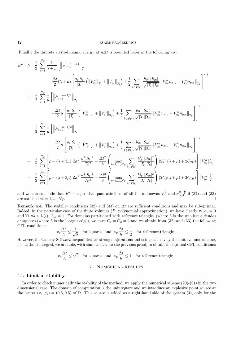
On the figures 3, 4, 5 and 6, we have displayed, firstly on the left, the numerical error in the L2-norm inlogarithmic scale by respect to the mesh step h, and secondly on the right, the numerical error in the L2-normin logarithmic scale as a function of the CPU time. The meshes are the same as those presented in the previoussection except that unstructured meshes are composed of four Delaunay meshes of the unit square gatheredtogether. This has been done to explicitly identify in the mesh the lines x = 1 and y = 1 in order to be able to cal-culate here the L2-error on the line y = 1 without interpolation. The mesh step h is the longest edge of the mesh.

For solutions at times lower than 0.8 s, when the pulse is still completely inside the domain, as on the figures3 and 4, we observe a second-order convergence on uniform meshes. On unstructured meshes, the order ofaccuracy depends of the choice of the degree of the polynomials since a third order convergence is observed forboth P3 and P4 methods. Concerning the efficiency, if a given L2-error is sought, the corresponding CPU timeis always lower for the high order polynomials and for both type of meshes despite the fact that high-ordermethods necessitate lower time-steps and more degrees of freedom on each element. So, we can conclude thatthe high order approximation method is more accurate and more efficient.

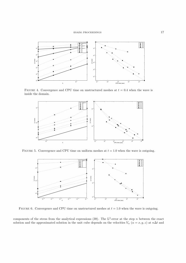
On the other hand, for solutions at times greater than 0.8 s, when the pulse reaches the boundary and goesout of the domain, as on figures 5 and 6 presenting solutions at time t = 1.0 s, we observe that the order of

16 ESAIM: PROCEEDINGS

convergence is one for all the methods except the finite volume (P0) method when structured meshes are used.On the other hand, for unstructured meshes, we remark a second-order convergence. These differences betweensolutions, at times t = 0.4 s and t = 1. s, come from the absorbing condition which is not accurate enough,especially when high degree polynomials are employed. The properties of such absorbing conditions are quiteknown : results are not very accurate in presence of grazing waves and for too small numerical domains forwhich the boundaries are rapidly reached by the waves. Extension of such absorbing conditions to high orderis not obvious, particularly in three dimensions of space. A way to improve the results consists in surroundingthe domain by Perfectly Matched Layers (PML), initially developed for the Maxwell equations by Berenger [3].Many variations of this method have been proposed. Among them, we can quote the convolutional PerfectlyMatched Layer (C-PML) proposed by Komatitsch and Martin [15] for three-dimensional elastodynamic equa-tions which, compared to other methods, do not necessitate any splitting of the unknowns. We are interestednow in the implementation of such conditions.

Lastly, we remark than the results obtained using unstructured meshes are very satisfactory even betteras those of structured meshes. It is probably due to the choice of Delaunay meshes which have well knownproperties. Indeed, each Delaunay mesh has, for example, local orthogonality properties with its dual mesh,called Voronoı mesh, whereas the only characteristic of structured meshes is periodicity.

10−2

10−7

10−6

10−5

10−4

10−3

10−2

h

L2−

erro

r

Slope=2P0P1P2P3P4

10−1

100

101

102

103

10−6

10−5

10−4

10−3

10−2

CPU time (sec)

L2−

erro

r

P0P1P2P3P4

Figure 3. Convergence and CPU time on uniform meshes at t = 0.4 when the wave is inside the domain.

5.3. Propagation of an eigenmode in 3D

The last test case concerns the propagation of an eigenmode in three dimensions of space. The domain ofcomputation is the unit cubic cavity on which we apply free surface boundary conditions. We are interested inthe (1, 1, 1) mode whose exact solution is given by:

Vx = cos(πx) (sin(πy) − sin(πz)) cos(Ωt) ,Vy = cos(πy) (sin(πz) − sin(πx)) cos(Ωt) ,Vz = cos(πz) (sin(πx) − sin(πy)) cos(Ωt) ,σxx = −A sin(πx) (sin(πy) − sin(πz)) sin(Ωt) ,σyy = −A sin(πy) (sin(πz) − sin(πx)) sin(Ωt) ,σzz = −A sin(πz) (sin(πx) − sin(πy)) sin(Ωt) ,σxy = σxz = σxz = 0 ,

(39)

with A =√

2 ρ µ and Ω = π√

2µρ . As previously, we set ρ = 1.0, λ = 0.5 and µ = 0.25, and the initialisation of

the leap-frog scheme is realized by taking the values at t = 0 for the velocity components and at t = ∆t2 for the

ESAIM: PROCEEDINGS 17

10−1

10−7

10−6

10−5

10−4

10−3

10−2

h

L2−

erro

r

Slope=0.5P0Slope=2P1Slope=3P2P3P4

10−1

100

101

102

103

10−6

10−5

10−4

10−3

10−2

CPU time (sec)

L2−

erro

r

P1P2P3P4

Figure 4. Convergence and CPU time on unstructured meshes at t = 0.4 when the wave isinside the domain.

10−2

10−4

10−3

10−2

h

L2−

erro

r

Slope=1P0P1P2P3P4

10−1

100

101

102

103

104

10−3

10−2

CPU time (sec)

L2−

erro

r

P0P1P2P3P4

Figure 5. Convergence and CPU time on uniform meshes at t = 1.0 when the wave is outgoing.

10−1.6

10−1.5

10−1.4

10−1.3

10−1.2

10−1.1

10−4

10−3

10−2

h

L2−

erro

r

Slope=2P0P1P2P3P4

10−1

100

101

102

103

10−4

10−3

10−2

CPU time (sec)

L2−

erro

r

P0P1P2P3P4

Figure 6. Convergence and CPU time on unstructured meshes at t = 1.0 when the wave is outgoing.

components of the stress from the analytical expressions (39). The L2-error at the step n between the exactsolution and the approximated solution in the unit cube depends on the velocities Vα (α = x, y, z) at n∆t and

18 ESAIM: PROCEEDINGS

the stress σαβ (α, β = x, y, z) at (n+ 12 )∆t :

errnL2 =

√√√√√NT∑

i=1

∫

Ti

∑

α∈x,y,z

(Vα(n∆t, xi) − (Vα)ni )2 +

∑

α,β∈x,y,z

(σαβ

((n+

1

2

)∆t, xi

)− (σαβ)

n+1/2i

)2

.

As in 2D, structured and unstructured meshes have been used. Structured meshes are obtained by dividingthe domain in cubic cells which are split in six tetraedra. The unstructured meshes are Delaunay meshes con-structed by a mesher from 2D surfacic Delaunay meshes of the boundaries of the domain. The mesh step h ishere also the length of the longest edge of the mesh.

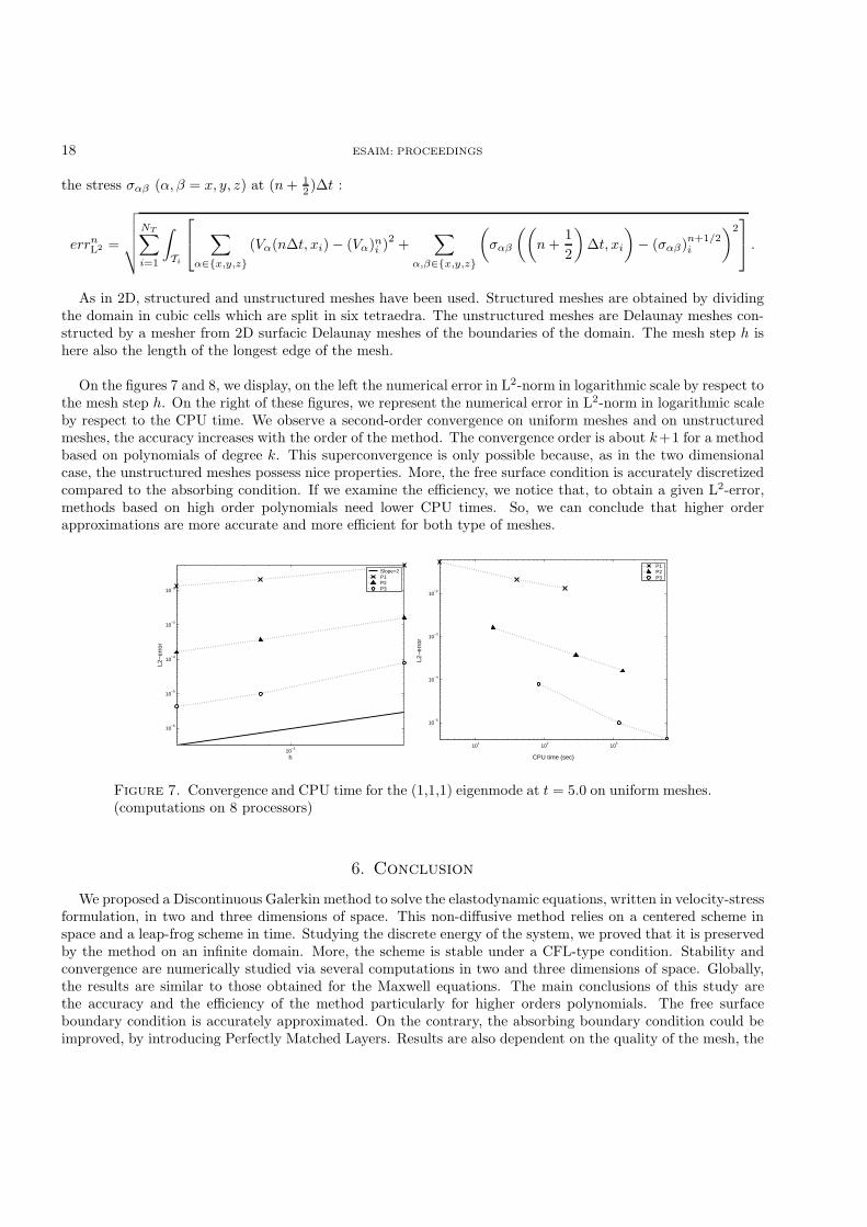
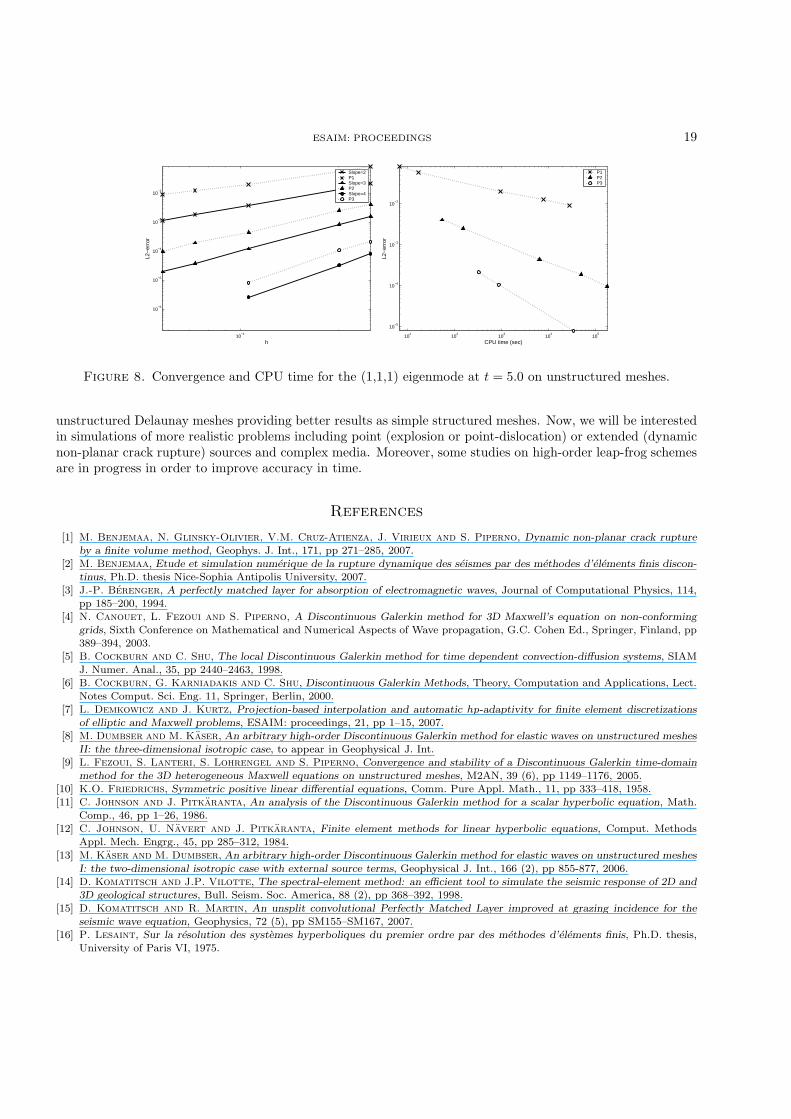
On the figures 7 and 8, we display, on the left the numerical error in L2-norm in logarithmic scale by respect tothe mesh step h. On the right of these figures, we represent the numerical error in L2-norm in logarithmic scaleby respect to the CPU time. We observe a second-order convergence on uniform meshes and on unstructuredmeshes, the accuracy increases with the order of the method. The convergence order is about k+1 for a methodbased on polynomials of degree k. This superconvergence is only possible because, as in the two dimensionalcase, the unstructured meshes possess nice properties. More, the free surface condition is accurately discretizedcompared to the absorbing condition. If we examine the efficiency, we notice that, to obtain a given L2-error,methods based on high order polynomials need lower CPU times. So, we can conclude that higher orderapproximations are more accurate and more efficient for both type of meshes.

10−1

10−6

10−5

10−4

10−3

10−2

h

L2−

erro

r

Slope=2P1P2P3

101

102

103

10−5

10−4

10−3

10−2

CPU time (sec)

L2−

erro

r

P1P2P3

Figure 7. Convergence and CPU time for the (1,1,1) eigenmode at t = 5.0 on uniform meshes.(computations on 8 processors)

6. Conclusion

We proposed a Discontinuous Galerkin method to solve the elastodynamic equations, written in velocity-stressformulation, in two and three dimensions of space. This non-diffusive method relies on a centered scheme inspace and a leap-frog scheme in time. Studying the discrete energy of the system, we proved that it is preservedby the method on an infinite domain. More, the scheme is stable under a CFL-type condition. Stability andconvergence are numerically studied via several computations in two and three dimensions of space. Globally,the results are similar to those obtained for the Maxwell equations. The main conclusions of this study arethe accuracy and the efficiency of the method particularly for higher orders polynomials. The free surfaceboundary condition is accurately approximated. On the contrary, the absorbing boundary condition could beimproved, by introducing Perfectly Matched Layers. Results are also dependent on the quality of the mesh, the

ESAIM: PROCEEDINGS 19

10−1

10−6

10−5

10−4

10−3

10−2

h

L2−

erro

r

Slope=2P1Slope=3P2Slope=4P3

101

102

103

104

105

10−5

10−4

10−3

10−2

CPU time (sec)

L2−

erro

r

P1P2P3

Figure 8. Convergence and CPU time for the (1,1,1) eigenmode at t = 5.0 on unstructured meshes.

unstructured Delaunay meshes providing better results as simple structured meshes. Now, we will be interestedin simulations of more realistic problems including point (explosion or point-dislocation) or extended (dynamicnon-planar crack rupture) sources and complex media. Moreover, some studies on high-order leap-frog schemesare in progress in order to improve accuracy in time.

References

[1] M. Benjemaa, N. Glinsky-Olivier, V.M. Cruz-Atienza, J. Virieux and S. Piperno, Dynamic non-planar crack rupture

by a finite volume method, Geophys. J. Int., 171, pp 271–285, 2007.[2] M. Benjemaa, Etude et simulation numerique de la rupture dynamique des seismes par des methodes d’elements finis discon-

tinus, Ph.D. thesis Nice-Sophia Antipolis University, 2007.[3] J.-P. Berenger, A perfectly matched layer for absorption of electromagnetic waves, Journal of Computational Physics, 114,

pp 185–200, 1994.[4] N. Canouet, L. Fezoui and S. Piperno, A Discontinuous Galerkin method for 3D Maxwell’s equation on non-conforming

grids, Sixth Conference on Mathematical and Numerical Aspects of Wave propagation, G.C. Cohen Ed., Springer, Finland, pp389–394, 2003.

[5] B. Cockburn and C. Shu, The local Discontinuous Galerkin method for time dependent convection-diffusion systems, SIAMJ. Numer. Anal., 35, pp 2440–2463, 1998.

[6] B. Cockburn, G. Karniadakis and C. Shu, Discontinuous Galerkin Methods, Theory, Computation and Applications, Lect.Notes Comput. Sci. Eng. 11, Springer, Berlin, 2000.

[7] L. Demkowicz and J. Kurtz, Projection-based interpolation and automatic hp-adaptivity for finite element discretizations

of elliptic and Maxwell problems, ESAIM: proceedings, 21, pp 1–15, 2007.[8] M. Dumbser and M. Kaser, An arbitrary high-order Discontinuous Galerkin method for elastic waves on unstructured meshes

II: the three-dimensional isotropic case, to appear in Geophysical J. Int.[9] L. Fezoui, S. Lanteri, S. Lohrengel and S. Piperno, Convergence and stability of a Discontinuous Galerkin time-domain

method for the 3D heterogeneous Maxwell equations on unstructured meshes, M2AN, 39 (6), pp 1149–1176, 2005.[10] K.O. Friedrichs, Symmetric positive linear differential equations, Comm. Pure Appl. Math., 11, pp 333–418, 1958.[11] C. Johnson and J. Pitkaranta, An analysis of the Discontinuous Galerkin method for a scalar hyperbolic equation, Math.

Comp., 46, pp 1–26, 1986.[12] C. Johnson, U. Navert and J. Pitkaranta, Finite element methods for linear hyperbolic equations, Comput. Methods

Appl. Mech. Engrg., 45, pp 285–312, 1984.

[13] M. Kaser and M. Dumbser, An arbitrary high-order Discontinuous Galerkin method for elastic waves on unstructured meshes

I: the two-dimensional isotropic case with external source terms, Geophysical J. Int., 166 (2), pp 855-877, 2006.[14] D. Komatitsch and J.P. Vilotte, The spectral-element method: an efficient tool to simulate the seismic response of 2D and

3D geological structures, Bull. Seism. Soc. America, 88 (2), pp 368–392, 1998.[15] D. Komatitsch and R. Martin, An unsplit convolutional Perfectly Matched Layer improved at grazing incidence for the

seismic wave equation, Geophysics, 72 (5), pp SM155–SM167, 2007.[16] P. Lesaint, Sur la resolution des systemes hyperboliques du premier ordre par des methodes d’elements finis, Ph.D. thesis,

University of Paris VI, 1975.

20 ESAIM: PROCEEDINGS

[17] P. Lesaint and P.-A. Raviart, On a finite element method for solving the neutron transport equation, in MathematicalAspects of Finite Element Methods in Partial Differential Equations, C.A. deBoor, ed., Academic Press, New York, pp 89–123,1974.

[18] W. Reed and T. Hill, Triangular mesh methods for the neutron transport equation, Technical Report LA-UR-73-479, LosAlamos Scientific Laboratory, Los Alamos, NM, 1973.

[19] M. Remaki, Methodes numeriques pour les equations de Maxwell instationnaires en milieu heterogene, Ph.D. thesis ENPCCERMICS, France, 1999.

[20] S. Piperno, M. Remaki and L. Fezoui, A non-diffusive finite volume scheme for the 3D Maxwell equations on unstructured

meshes, SIAM J. Numer. Anal., 39, pp 2089–2108, 2002.[21] E. Suli, C. Schwab and P. Houston, hp-DGFEM for partial differential equations with non-negative characteristic form,

in Discontinuous Galerkin Methods Theory, Computation and Applications, Lect. Notes Comput. Sci. Eng. 11, B. Cockburn,G.E. Karniadakis and C.-W. Shu eds., Springer, Berlin, pp 221–230, 2000.

[22] J. Virieux, P-SV wave propagation in heterogeneous media, velocity-stress finite difference method, Geophysics, 51, pp 889–901, 1986.

[23] K.S. Yee, Numerical solution of initial boundary value problems involving Maxwell’s equations in isotropic media, IEEE Trans.Antennas and Propagat., 14 (3), pp 302–307, 1966.