Central WENO Schemes for Hamilton–Jacobi Equations on Triangular Meshes

SIAM J. SCI. COMPUT. c© 2006 Society for Industrial and Applied MathematicsVol. 28, No. 6, pp. 2229–2247

CENTRAL WENO SCHEMES FOR HAMILTON–JACOBIEQUATIONS ON TRIANGULAR MESHES∗

DORON LEVY† , SUHAS NAYAK† , CHI-WANG SHU‡ , AND YONG-TAO ZHANG§

Abstract. We derive Godunov-type semidiscrete central schemes for Hamilton–Jacobi equa-tions on triangular meshes. High-order schemes are then obtained by combining our new numericalfluxes with high-order WENO reconstructions on triangular meshes. The numerical fluxes are shownto be monotone in certain cases. The accuracy and high-resolution properties of our scheme aredemonstrated in a variety of numerical examples.

Key words. Hamilton–Jacobi equations, central schemes, unstructured grids

AMS subject classifications. Primary, 65M06; Secondary, 35L99

DOI. 10.1137/040612002

1. Introduction. We consider Cauchy problems for Hamilton–Jacobi (HJ) equa-tions of the form{

φt(x, t) + H(x, φ(x, t),∇φ(x, t)) = 0, x ∈ Ω ⊂ R2,

φ(x, t = 0) = φ0(x).(1.1)

HJ equations are being used in a variety of applications, such as optimal controlproblems, differential games, geometric optics, and the calculus of variations.

It is well known that solutions of (1.1) may develop discontinuous derivatives infinite time, and hence it is necessary to interpret solutions of (1.1) in an appropriateweak sense. Such a formulation in terms of the so-called viscosity solutions is dueto Crandall, Evans, Ishii, Lions, among others (see [10, 11, 25] and the referencestherein).

We are interested in approximating solutions of (1.1) on a given conforming trian-gulation of the domain Ω. While general theory for approximating solutions of (1.1)can be found in the works of Barles, Lions, and Souganidis [4, 33, 26], in this workwe focus on Godunov-type schemes for approximating such problems. Godunov-typeschemes are based on a global reconstruction which is evolved exactly in time andsampled at the grid nodes at the next time step. A subclass of these schemes are cen-tral schemes in which the evolution stage is carried out at points that are located awayfrom the discontinuities. Such a procedure eliminates the necessity of dealing with(generalized) Riemann problems on the cell-interfaces. In addition, systems can besolved componentwise without a characteristic decomposition. These features makecentral schemes particularly suitable for multidimensional problems and complicatedgeometries.

∗Received by the editors July 20, 2004; accepted for publication (in revised form) June 22, 2006;published electronically December 11, 2006.

http://www.siam.org/journals/sisc/28-6/61200.html†Department of Mathematics, Stanford University, Stanford, CA 94305-2125 (dlevy@math.

stanford.edu, [email protected]). The work of the first author was supported in part bythe National Science Foundation under Career grant DMS-0133511.

‡Division of Applied Mathematics, Brown University, Providence, RI 02912 ([email protected]). The work of this author was supported in part by ARO grant DAAD19-00-1-0405, NSF grantDMS-0207451, and AFOSR grant F49620-02-1-0113.

§Department of Mathematics, University of California, Irvine, CA 92697 ([email protected]).

2229

2230 D. LEVY, S. NAYAK, C.-W. SHU, AND Y.-T. ZHANG

First- and second-order fully discrete central schemes were introduced by Lin andTadmor [23, 24] (see also [7]). Their schemes were based on the first-order Lax–Friedrichs scheme [12] and its second-order extension, the Nessyahu–Tadmor scheme[28], for approximating solutions of hyperbolic conservation laws.

Semidiscrete central schemes (on Cartesian meshes) were derived by Kurganovand Tadmor [21]. The main goal there was to reduce the numerical dissipation byestimating the local speeds of propagation of information from the interfaces betweenneighboring computational cells. The numerical dissipation in these schemes was fur-ther reduced by keeping an even more accurate account of the different local speeds[20]. Semidiscrete schemes have a lower numerical dissipation when compared withfully discrete schemes, which make them particularly suitable for long-time simula-tions, steady-state calculations, and approximating solutions of viscous problems.

The fully discrete schemes of [7, 23, 24] were extended to high-order in [8].Such extensions were obtained by using suitable weighted essentially nonoscillatory(WENO) reconstructions that were designed following the WENO schemes of Liu,Osher, and Chan [27] and Jiang and Shu [17]. It is important to note that these ideasextend the essentially nonoscillatory (ENO) schemes of Harten et al. [14]. High-orderversions of the semidiscrete scheme [21] were obtained by combining the semidiscretenumerical fluxes with WENO reconstructions [9]. This work also provided the the-oretical foundation for the monotonicity of the fluxes of [20, 21]. A version of theseschemes with reduced numerical dissipation was recently derived in [6].

It is important to note that the progress with central schemes for HJ equationsparallels the advances made with upwind schemes for HJ equations. These include theENO schemes of Osher, Sethian, and Shu [30, 31] and the WENO schemes of Jiangand Peng [16]. Similar methods on triangular meshes include the pioneering works ofAbgrall [1, 2], Augoula and Abgrall [3], Barth and Sethian [5], Kossioris, Makridakis,and Souganidis [19], and the recent work of Zhang and Shu [35] on WENO schemesfor HJ equations on triangular meshes. The high-order WENO reconstructions ontriangular meshes that were used in [35] were based on the results of Hu and Shu [15].

In this paper we present the first semidiscrete central scheme for approximatingsolutions of (1.1) on triangular meshes. Our scheme combines a new numerical flux(that was announced in [22]) with the high-order WENO reconstructions of [35].

We would like to emphasize that the main benefit of the new scheme is in itsdevelopment as a Godunov-type scheme, in which a global reconstruction is evolvedexactly according to the equation. This probably also means that one can expectto obtain for this scheme convergence results in the spirit of the works of Lin andTadmor [23, 24].

The structure of this paper is as follows: We start in section 2 with the derivationof the numerical flux for HJ equations on triangular meshes. A couple of examplesof high-order reconstructions on triangular meshes are then discussed in section 3.Numerical examples that verify the expected order of accuracy of the schemes aswell as the high-resolution properties of the resulting solutions are given in section 4.Concluding remarks summarize this work in section 5.

2. Central schemes for Hamilton–Jacobi equations.

2.1. The scheme. To simplify the discussion and the notation, we considerequations of type (1.1) with a Hamiltonian that depends only on ∇φ, i.e.,{

φt(x, t) + H(∇φ(x, t)) = 0, x ∈ Ω ⊂ R2,

φ(x, t = 0) = φ0(x).(2.1)

CENTRAL WENO SCHEMES FOR HJ EQUATIONS 2231

xα

dl

xlα

θl

Tl

a+l Δt

a−l Δt

Fig. 2.1. The evolution point xlα that is derived from the maximal local speeds of propagation

into Tl, a+l , and a−

l .

We assume a given triangulation, T, of Ω, denote the grid points by xα, and as-sume that every such point is surrounded by mα angular sectors Tα

l that are orderedcounterclockwise. For simplicity we use the simpler notation Tl = Tα

l (see Figure 2.1).Given a time-step Δt, we denote the approximate value at time tn = nΔt of

φ(xα, tn) by ϕn

α. Assuming that the values of ϕnα at the grid points xα are known, we

reconstruct a piecewise-polynomial interpolant ϕ̃α. This interpolant has discontinuousgradients along the cell-interfaces. We denote the approximation of the gradient atxα that is obtained from the reconstruction in the cell Tl by ∇ϕ̃α,l. For the purpose ofdeveloping the numerical flux there is no need to assume any particular reconstruction.A WENO reconstruction will be described in section 3.

The reconstruction ϕ̃α can now be used to estimate the maximal speeds of prop-agation of information from the cell-interfaces in a direction that is perpendicular tothe interfaces. In every sector, Tl, we denote the counterclockwise speed of propa-gation by a+

l and the speed of propagation on the other interface by a−l (see Figure2.1). These speeds can be estimated by

a+l = max

{maxTl

{|∇H(∇ϕ̃α(x)) · �nl−1,l|} , maxTl−1{|∇H(∇ϕ̃α(x)) · �nl−1,l|}

},

a−l = max{maxTl

{|∇H(∇ϕ̃α(x)) · �nl+1,l|} , maxTl+1{|∇H(∇ϕ̃α(x)) · �nl+1,l|}

}.

(2.2)

Here, �nj,l is the normal vector on the interface between Tj and Tl pointing into Tl.The evolution stage of Godunov-type schemes will be carried out at points xl

α

that are located away from the interfaces, assuming that the time-step is sufficientlysmall (see Figure 2.1). The distance of the evolution point xl

α from xα is denoted bydl. Clearly, dl depends on the local speeds of propagation a±l and on the angle θl. Astraightforward computation allows us to define dl as

dl = Δtd̂l,(2.3)

where

d̂2l =

(a−l )2 + 2a−l a+l cos θl + (a+

l )2

sin2 θl.(2.4)


We now evolve the interpolant ϕ̃(�x, tn) to the next time-step tn+1 at the points xlα

according to (2.1). Since the evolution points are located away from the propagatingdiscontinuities, the value at the next time-step can be approximated with a first-orderTaylor expansion in time, i.e.,

ϕ(xlα, t

n+1) = ϕ̃(xlα, t

n) − ΔtH(∇ϕ̃(xlα, t

n)) + O(Δt2).(2.5)

Here, the value of the gradient, ∇ϕ̃(xlα, t

n), is obtained from the reconstruction, ϕ̃.Expressions of the form (2.5) hold for every evolution point, xl

α, around xα.In order to combine all these values of ϕ into one value ϕn+1

α , we write a convexcombination of the values from the different sectors with weights sl ≥ 0 that are yetto be determined:

ϕn+1α =

∑mα

l=1 slϕ(xlα, t

n+1)∑mα

l=1 sl=

∑mα

l=1 sl[ϕ̃(xl

α, tn) − ΔtH(∇ϕ̃(xl

α, tn)]∑mα

l=1 sl.(2.6)

We now define ρl to be the unit vector in the direction of xlα from xα and write

a Taylor expansion in space:

ϕ̃(xlα, t

n) = ϕ̃(xα, tn) + dlρl · ∇ϕ̃(xl

α, tn) + O(Δt2).

Here by ∇ϕ̃(xlα, t

n) we refer to the value of the gradient at xα that is associated withthe reconstruction in sector Tl at xl

α. We may therefore rewrite (2.6) as the fullydiscrete scheme

ϕn+1α = ϕ̃n

α +Δt∑mα

l=1 sl

mα∑l=1

sl

[d̂lρl · ∇ϕ̃(xl

α, tn) −H(∇ϕ̃(xl

α, tn))

].(2.7)

A semidiscrete scheme can now be obtained in the limit Δt → 0,

d

dtϕα(t) = lim

Δt→0

ϕn+1α − ϕn

α

Δt=

1∑mα

l=1 sl

mα∑l=1

sl

[d̂lρl · ∇ϕ̃l

α(t) −H(∇ϕ̃lα(t))

],(2.8)

where for each l, ∇ϕ̃lα(t) denotes limΔt→0 ∇ϕ̃(xl

α, tn). All that remains is to deter-

mine the coefficients sl in (2.8). The consistency of the scheme implies that if thevalue of the gradient is identical in every sector that surrounds xα, then the numer-ical Hamiltonian should become the differential Hamiltonian. Hence, we are seekingcoefficients sl, such that

mα∑l=1

sld̂lρl = 0.(2.9)

These coefficients can be determined using the results of Abgrall [2]. We denote byμl+1/2 a unit vector in a direction that is aligned with the interface between thesectors Tl and Tl+1, and we assume that θl < π (which is indeed the case with atriangulation). It was shown in [2] that

mα∑l=1

ξl+ 12μl+ 1

2= 0,(2.10)


xlα

θ−la+

l Δt

a−l Δt

θ+l

ρl

a+l+1Δt

ρl+1

Tl+1a−

l+1Δt

θ+l+1

θ−l+1

Tl

xα

Fig. 2.2. The angles around xα.

provided that

ξl+ 12

=

[tan

(θl2

)+ tan

(θl+1

2

)].(2.11)

In order to incorporate (2.10)–(2.11) into our framework, we split each angle θl intotwo parts, θ±l , that are defined as

θ±l = arcsina±ld̂l

(2.12)

(see Figure 2.2). The consistency condition (2.9) is then satisfied if the weights sl are

taken as sl = βl/d̂l, where

βl = tan

(θ+l + θ−l−1

2

)+ tan

(θ−l + θ+

l+1

2

).

We note that if ∀l, θ+l + θ−l−1 ≤ π, then βl are guaranteed to be positive. With this

notation, a consistent, semidiscrete scheme is given by

d

dtϕα(t) =

1∑mα

l=1βl

d̂l

mα∑l=1

βl

[ρl · ∇ϕ̃l

α(t) − H(∇ϕ̃lα(t))

d̂l

].(2.13)

Remarks.1. It is straightforward to extend scheme (2.13) to more general problems, such

as general Hamiltonians of the form present in (1.1) or viscous HJ problems.Examples of these obvious generalizations in the Cartesian case can be found,e.g., in [7, 8, 9, 20, 21].

2. The order of accuracy of the scheme (2.13) is determined by the order ofaccuracy of the reconstruction ϕ̃α, and the order of the ODE solver. Due tothe known properties of viscosity solutions of HJ equations and the structureof Godunov-type schemes, we assume a global underlying piecewise-smoothreconstruction. We note that, in practice, the final semidiscrete scheme (2.13)uses only values of the gradient computed in the different cells around eachgrid point xα. This means that all that we need from the reconstructionare the values of these gradients. High-order reconstructions on triangularmeshes are discussed in section 3.


3. There are several ways to simplify the scheme (2.13). One possibility is toreplace the different speeds of propagation at every grid point by their max-imum, i.e., aα = maxl{a+

l , a−l }. This implies that d̂l = aα/ sin(θl/2). In this

case (2.13) becomes

d

dtϕα(t) =

aα∑mα

l=1 βl sinθl2

mα∑l=1

βl

[ρl · ∇ϕ̃l

α(t) −sin θl

2

aH(∇ϕ̃l

α(t))

].(2.14)

If, in addition, the triangulation of the domain is such that the angles areidentical around each point, i.e., θ = θl ∀ l, then (2.14) takes the simpler form

d

dtϕα(t) =

1

mα

mα∑l=1

[aα

sin θ2

ρl · ∇ϕ̃lα(t) −H(∇ϕ̃l

α(t))

].(2.15)

In the special case of a Cartesian grid with equal spacing in the x- and y-directions, the number of angular sectors at each point is mα = 4, and sin(θ/2)= sin(π/4) =

√2/2. If we assume that the velocities are identical in both

directions, then (2.15) becomes

(2.16)

d

dtϕα(t) =

aα2

(ϕ+x − ϕ−

x + ϕ+y − ϕ−

y

)−1

4

[H

(ϕ+x , ϕ

+y

)+ H

(ϕ−x , ϕ

+y

)+ H

(ϕ+x , ϕ

−y

)+ H

(ϕ−x , ϕ

−y

)],

with the obvious notation; e.g., H(ϕ+x , ϕ

+y ) is the Hamiltonian evaluated at

the gradient at xα that is taken from the first quadrant. The scheme (2.16)is identical to the semidiscrete central scheme for Cartesian grids [9, 21].

4. The following Lax–Friedrichs-type scheme on triangular meshes was derivedby Abgrall [2]:

d

dtϕα(t) =

a

π

mα∑l=1

βl+ 12μl+ 1

2·(∇ϕ̃l

α(t) + ∇ϕ̃l+1α (t)

2

)−H

(∑mα

l=1 θl∇ϕ̃lα

2π

).

(2.17)

Here μl+1/2 is the unit vector in the direction of the interface between thesectors Tl and Tl+1, and βl+1/2 = tan(θl/2) + tan(θl+1/2). The derivation of(2.17) involved evolution points that were located on the interfaces betweenthe sectors. This resulted in the form of the dissipative term in (2.17) thatcontains averages of gradients in adjacent sectors. Also, the scheme (2.17)involves a Hamiltonian that is evaluated at the average of the derivativesthat are computed in different sectors (with weights that are proportional tothe angles). This Hamiltonian term was postulated to be in this form, butcould have had other forms. In our case (2.13), this term takes the form ofan average over the Hamiltonian that is evaluated in different sectors and isdictated by the derivation of the scheme.

5. We would like to emphasize that the main benefit of the new scheme is inits development as a Godunov-type scheme, in which a global reconstructionis evolved exactly according to the equation. It is a different approach tothe “standard” line of schemes for HJ equations in which a monotone flux is


ϕα

vl,l+1

vl+1,l+2

vl−1,l

ϕl,l+1α

Tl+1

Tl

Fig. 2.3. Grid value at xα and two triangles containing xα and grid vectors v.

combined with a high-order reconstruction. This probably also means thatone can expect to obtain for this scheme convergence results in the spirit ofthe works of Lin and Tadmor [23, 24]. For this purpose, such a constructionof a scheme is probably more favorable than traditional constructions.

2.2. Monotonicity. In this section we provide a partial result regarding themonotonicity of our scheme (2.13). Monotonicity is one of the main ingredients inthe convergence theory of Barles and Souganidis [4]. Roughly speaking, a stable,consistent, and monotone approximation for an equation that satisfies an underlyingcomparison principle converges to the viscosity solution.

For simplicity we consider the monotonicity of the scheme in the case where thespeeds of propagation do not depend on the gradients of the reconstruction, i.e., theyare all equal to a constant that is determined based on a priori bounds. Hence, weassume a = maxl,± a±l , which also implies that θ+

l = θ−l = θl/2.Monotonicity means that if we rewrite our scheme (2.13) in terms of grid differ-

ences,

d

dtϕα(t) = F (ϕα, ϕα − ϕ′),(2.18)

where ϕα − ϕ′ is a vector of grid differences that involve the central node, then F isnonincreasing in all arguments (see, e.g., [4, 11, 29, 31]).

We assume that the gradient of ϕ in the triangle Tl is constant in that triangle.The normal to the plane connecting the three corners of Tl is given by

(vxl,l+1, vyl,l+1, ϕ

l,l+1α − ϕα) × (vxl−1,l, v

yl−1,l, ϕ

l−1,lα − ϕα),

where × denotes the cross-product between the vectors. Hence, the gradient of ϕ inthe sector Tl, ∇ϕl

α is given by (see Figure 2.3)

1

C

((ϕα − ϕl−1,l

α )vyl,l+1 − (ϕα − ϕl,l+1α )vyl−1,l, (ϕα − ϕl,l+1

α )vxl−1,l − (ϕα − ϕl−1,lα )vxl,l+1

).

Here, C = (vl,l+1 × vl−1,l) · k and k is the unit vector pointing out of the plane. Thesuperscripts x and y denote the x- and y-components of the various vectors. We notethat C is a negative quantity. Letting u1 = ϕα−ϕl,l+1

α , the derivative of the gradientof ϕl

α with respect to u1 is given by

∂

∂u1∇ϕl

α =1

C(−vyl−1,l, v

xl−1,l).


This means that

ρl ·∂

∂u1∇ϕl

α =1

Cρl · nl−1,l||vl−1,l|| =

1

Csin

(θl2

)||vl−1,l||,

where nl−1,l is the unit normal vector pointing into Tl (and is in the plane defined byTl). Similarly

∂

∂u1∇ϕl+1

α =1

C ′ (vyl+1,l+2,−vxl+1,l+2) =

1

C ′ ||vl+1,l+2||nl+2,l+1,

where C ′ = (vl+1,l+2 × vl,l+1) · k and nl+2,l+1 is the normal vector from Tl+2 pointinginto Tl+1.

Since these are the only two quantities in F that involve u1, we may evaluate thepartial derivative of F with respect to u1. Letting K = 1/

∑mα

l=1βl

d̂l(which we note is

a positive quantity) we have

∂F

∂u1=

1

K

βl||vl−1,l||Cd̂l

(d̂lρl · nl−1,l −∇H(∇ϕl

α) · nl−1,l

)(2.19)

+1

K

βl+1||vl+1,l+2||C ′d̂l+1

(d̂l+1ρl+1 · nl+2,l+1 −∇H(∇ϕl+1

α ) · nl+2,l+1

)

=1

K

βl||vl−1,l||Cd̂l

(d̂l sin

(θl2

)−∇H(∇ϕl

α) · nl−1,l

)

+1

K

βl+1||vl+1,l+2||C ′d̂l+1

(d̂l+1 sin

(θl+1

2

)−∇H(∇ϕl+1

α ) · nl+2,l+1

).

We consider only the first term, as an analogous argument holds for the secondterm. Equation (2.12) implies that sin(θl/2) = a/d̂l. Also, from (2.2) we know that∇H(∇ϕl

α) · nl−1,l ≤ a, which means that

d̂l sin

(θl2

)−∇H(∇ϕl

α) · nl−1,l ≥ 0.

Since C < 0 and since we assume that the triangulation is such that the βl’s arepositive, we can conclude that the first term in (2.19) is nonpositive. By similar argu-ments the second term in (2.19) is nonpositive, which means that F is nonincreasingin u1. The same is true for all the variables of F and hence the scheme is monotone.

3. High-order reconstructions on triangular meshes. In this section wereview two third-order reconstructions from [35] (see also [15]). We start with alinear-weights reconstruction. First, we solve an interpolation problem on a largestencil. We then split the large stencil into smaller pieces, obtaining a (low-order)interpolant on each. We conclude with a convex combination of the low-order in-terpolants that provides the desired (formal) accuracy. The second reconstruction isof WENO type. Here, we replace the linear weights in the convex combination bynonlinear weights. This procedure reduces the spurious oscillations that otherwisedevelop at singularities. We would like to emphasize that the scheme developed insection 2, i.e., (2.13), does not depend on any particular reconstruction, and the re-constructions described here are provided for the sake of completeness. Extensions tofourth-order are described in [35].


i1

i3

lT

i2

��

��

��

��

��

��

��

��

��

��

��

��

��

9

57

1

48

2

3

6

G

Fig. 3.1. The nodes used for the large stencil of the third-order reconstruction around Tl. Thepoint G is the barycenter of the cell Tl.

3.1. A linear-weights reconstruction. We provide an overview of the linear-weights third-order reconstruction from [35]. The problem can be formulated as aninterpolation problem, in which the main question is how to choose the interpolationpoints. The solution is not so obvious, in particular since the geometry of the meshmight not be uniform, which means that stability considerations might imply that itmight be better to use different stencils around different triangular sectors.

Assuming a given triangular sector, Tl, the procedure for approximating the com-ponents of the derivatives at its three nodes is composed of two steps. First, welook for a large stencil that will provide a stable, third-order approximation of thederivative. There are many ways for choosing such a stencil around any given sector,and we are interested in a compact stencil and a stable reconstruction. In the secondstep we break the large stencil into several small stencils (all of which are based ongrid points that are in the large stencil). Each small stencil provides a second-orderapproximation of the derivative. These stencils are chosen following compactness andstability considerations. We take sufficiently many such stencils (which will amountto five) such that they can be linearly combined to achieve the desired accuracy ofthe derivative.

We start by considering an angular sector, Tl, with its three nodes denoted byi1, i2, i3. To obtain a third-order approximation of the derivative at these points,(∇ϕ)i1 , (∇ϕ)i2 , (∇ϕ)i3 , we first construct a cubic polynomial. Since we are solving atwo-dimensional problem, there are ten free parameters that we have to determine.These will be given by interpolation requirements on a stencil that is yet to be deter-mined. In our numerical interpolation we use normalized coordinates, (x−xG)/

√|Tl|,

where xG is the coordinate of the barycenter G and |Tl| is the area of the triangle Tl

(see Figure 3.1).With this in mind, we number the nodes in the neighboring mesh points as

{1, . . . , 9} (in the way that is portrayed in Figure 3.1) and consider the ordered setW = {1, . . . , 9}. The nodes are numbered as in Figure 3.1 in order to avoid biasingthe stencil in any particular direction. We note that the geometry of the mesh might


imply that some of these points can be identical. If this is the case, more remotepoints are added to the list. We omit the details and refer to [35]. We now set athreshold δ and use the following algorithm:

1. Set the interpolation points as S0 = {i1, i2, i3, 1, . . . , 7}.2. Form the 10×10 interpolation coefficients matrix A and compute its reciprocal

condition number, c(A).3. While c(A) < δ, add the next node in W to S0 and compute the least squares

interpolation coefficients matrix A from the nodes in S0. Compute c(A).4. The final S0 is the large stencil.

Remark. The numerical simulations of [35] showed that at most 12 nodes areneeded in order to satisfy the condition c(A) ≥ δ when the threshold is set as δ = 10−3.This is the value that was used in our simulations in section 4.

We denote the interpolation polynomial that is obtained from the stencil S0 byp3(x, y). This polynomial, p3(x, y), can be used to estimate a third-order approxima-tion of the derivatives at the three nodes of Tl. Our goal now is to split the stencil S0

into several small stencils in such a way that we will be able to recover the third-orderaccuracy with a convex combination of these smaller stencils. In this case, we willgenerate five quadratic polynomials, ps, s = 1, . . . , 5, such that a third-order approx-imation to the derivatives in the x- and y-directions at {i1, i2, i3} will be given by

∂

∂xϕ(xij , yij ) ≈

∂

∂xp3(xij , yij ) =

5∑s=1

γs,x,ij∂

∂xps(xij , yij ), j = 1, 2, 3,

∂

∂yϕ(xij , yij ) ≈

∂

∂yp3(xij , yij ) =

5∑s=1

γs,y,ij∂

∂yps(xij , yij ), j = 1, 2, 3.

(3.1)

Here, γs,x,ij and γs,y,ij are the linear weights for the derivatives in the x- and y-directions, respectively. They depend only on the local geometry of the mesh andshould satisfy the normalization constraints,

∑5s=1 γs,x,ij = 1 and

∑5s=1 γs,y,ij = 1.

Under these additional conditions, a simple calculation shows that the number ofquadratic interpolants has to be greater than or equal to five, which is the reason weset it as five [15, 35].

We are now seeking five small stencils Γs, s = 1, . . . , 5, for the target triangle Tl

such that S0 = ∪5s=1Γs. We associate with each such stencil a quadratic polynomial

ps. We note that while the stencils are going to be identical for all the nodes in agiven angular sector and in both directions, the linear weights γs,x,ij and γs,y,ij canbe different for each node and for each direction. We summarize the stages given in[35, Procedure 2.2] as follows (for further details see [35]):

1. Obtain a large stencil S0.

2. For each s = 1, . . . , 5 find a set of candidate small stencils Ws = {Γ(r)s , r =

1, . . . , ns} in the following way. The nodes i1, i2, i3 are included in every Γ(r)s .

Let A(r)s denote the center of Γ

(r)s , where A

(r)s is given in Table 3.1. Find

at least three additional nodes other than i1, i2, i3 such that they have the

shortest distance from A(r)s and the points in Γ

(r)s induce an interpolation

coefficient matrix A with a good reciprocal condition number (c(A) ≥ δ).Based on the experiments in [35] a maximum number of 8 nodes is requiredto reach the threshold δ = 10−3.

3. Obtain n1 × · · ·×n5 groups of small stencils by taking one small stencil Γ(rs)s

from each Ws, s = 1, . . . , 5. Eliminate the groups that contain the same small

stencils and those that do not satisfy the condition ∪5s=1Γ

(rs)s = S0.


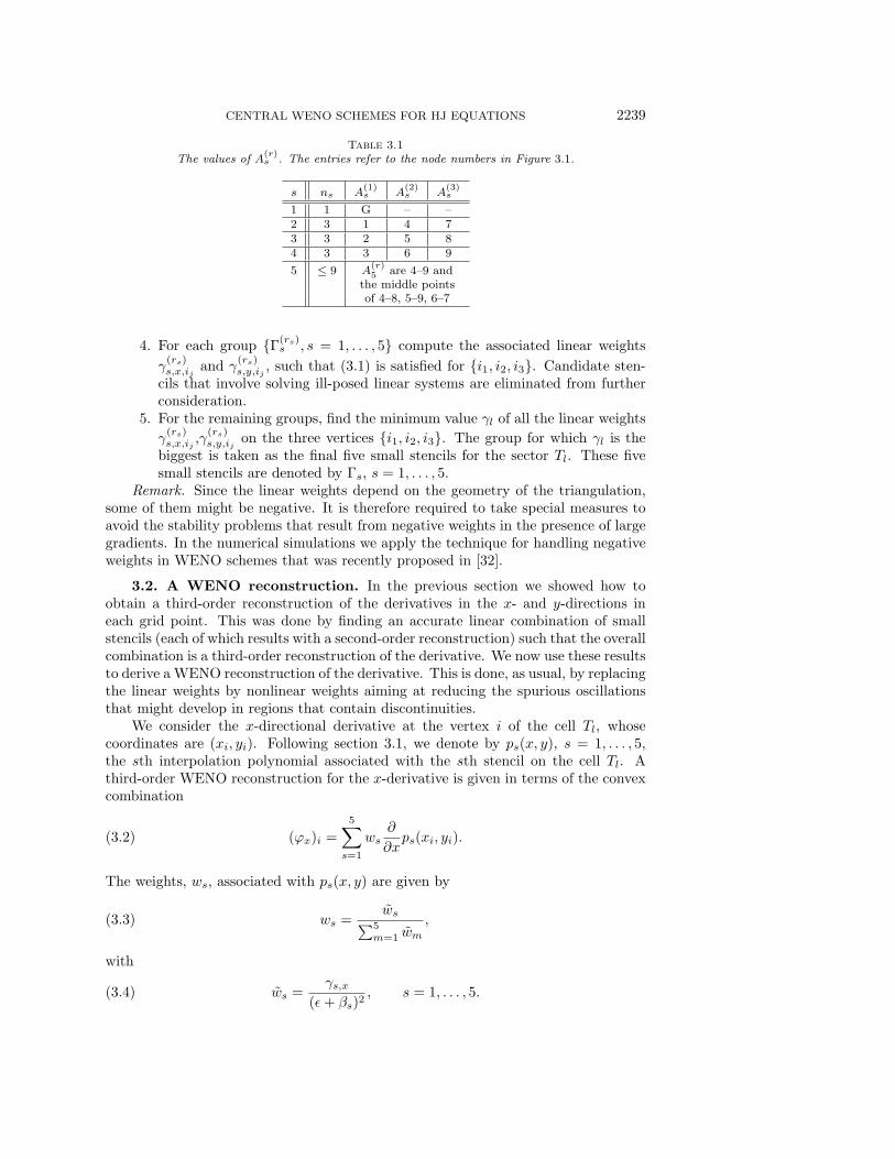
Table 3.1

The values of A(r)s . The entries refer to the node numbers in Figure 3.1.

s ns A(1)s A

(2)s A

(3)s

1 1 G – –2 3 1 4 73 3 2 5 84 3 3 6 9

5 ≤ 9 A(r)5 are 4–9 and

the middle pointsof 4–8, 5–9, 6–7

4. For each group {Γ(rs)s , s = 1, . . . , 5} compute the associated linear weights

γ(rs)s,x,ij

and γ(rs)s,y,ij

, such that (3.1) is satisfied for {i1, i2, i3}. Candidate sten-cils that involve solving ill-posed linear systems are eliminated from furtherconsideration.

5. For the remaining groups, find the minimum value γl of all the linear weights

γ(rs)s,x,ij

,γ(rs)s,y,ij

on the three vertices {i1, i2, i3}. The group for which γl is thebiggest is taken as the final five small stencils for the sector Tl. These fivesmall stencils are denoted by Γs, s = 1, . . . , 5.

Remark. Since the linear weights depend on the geometry of the triangulation,some of them might be negative. It is therefore required to take special measures toavoid the stability problems that result from negative weights in the presence of largegradients. In the numerical simulations we apply the technique for handling negativeweights in WENO schemes that was recently proposed in [32].

3.2. A WENO reconstruction. In the previous section we showed how toobtain a third-order reconstruction of the derivatives in the x- and y-directions ineach grid point. This was done by finding an accurate linear combination of smallstencils (each of which results with a second-order reconstruction) such that the overallcombination is a third-order reconstruction of the derivative. We now use these resultsto derive a WENO reconstruction of the derivative. This is done, as usual, by replacingthe linear weights by nonlinear weights aiming at reducing the spurious oscillationsthat might develop in regions that contain discontinuities.

We consider the x-directional derivative at the vertex i of the cell Tl, whosecoordinates are (xi, yi). Following section 3.1, we denote by ps(x, y), s = 1, . . . , 5,the sth interpolation polynomial associated with the sth stencil on the cell Tl. Athird-order WENO reconstruction for the x-derivative is given in terms of the convexcombination

(ϕx)i =

5∑s=1

ws∂

∂xps(xi, yi).(3.2)

The weights, ws, associated with ps(x, y) are given by

ws =w̃s∑5

m=1 w̃m

,(3.3)

with

w̃s =γs,x

(ε + βs)2, s = 1, . . . , 5.(3.4)


Here, γs,x is the linear weight associated with stencil s for computing the x-derivativeat (xi, yi), ε is set as a small number to prevent the denominator from vanishing, andβs is the oscillation indicator associated with the sth stencil.

The oscillatory indicator, βs, is given by

βs =∑|η|=2

∫Tl

(Dηps(x, y))2dxdy.(3.5)

An expression analogous to (3.2) holds for the derivative in the y-direction.

4. Numerical examples. In the numerical examples we use two kinds of trian-gular meshes. Both are shown in Figure 4.1. The first kind is a “uniform triangularmesh” shown in Figure 4.1 (left). The particular mesh in Figure 4.1 (left) is a coarsemesh with h = 2/5, where h is the length of the right-angled side. The second mesh isa “nonuniform triangular mesh” such as the one shown in Figure 4.1 (right). The meshin the figure is a coarse mesh with N = 105 nodes. Refinements of nonuniform meshesare done by splitting each triangle into four similar triangles. The reconstructions weuse in all the simulations are the third-order linear and WENO reconstructions fromsection 3. We refer to the flux (2.13) together with the linear-weights reconstructionof section 3.1 as the “linear scheme.” We refer to (2.13) together with the WENOreconstruction of section 3.2 as the “WENO scheme.” The ODE solver we used is thethird-order strong stability preserving Runge–Kutta (SSP-RK) method [13].

Example 1. A two-dimensional linear equation. Consider the two-dimen-sional (2D) linear equation{

φt + φx + φy = 0, −2 ≤ x < 2,−2 ≤ y < 2,

φ(x, y, 0) = sin(π2 (x + y)),(4.1)

with periodic boundary conditions.We solve (4.1) with the linear-weights and the WENO schemes on nonuniform

meshes up to time t = 2. Since this is a linear problem with constant coefficients,the flux with the local speeds and the flux with the global speeds are identical. TheL1- and L∞-errors and orders of accuracy, shown in Table 4.1, confirm the expectedthird-order accuracy.

X

Y

-2 -1 0 1 2-2

-1.5

-1

-0.5

0

0.5

1

1.5

2

X

Y

-2 -1 0 1 2-2

-1.5

-1

-0.5

0

0.5

1

1.5

2

Fig. 4.1. Left: coarsest uniform mesh with h = 2/5. Right: coarsest nonuniform mesh withN = 105 nodes.


Table 4.1

Accuracy test for the 2D linear equation (4.1) on nonuniform meshes with the third-order linearand WENO schemes at t = 2.

Linear scheme WENO scheme

N L1-error Order L∞-error Order L1-error Order L∞-error Order105 2.03E-01 — 3.50E-01 — 4.63E-01 — 7.24E-01 —385 3.16E-02 2.68 6.12E-02 2.51 1.69E-01 1.46 2.62E-01 1.47

1473 4.17E-03 2.92 9.02E-03 2.76 3.32E-02 2.34 7.10E-02 1.885761 5.30E-04 2.97 1.20E-03 2.91 5.09E-03 2.70 1.70E-02 2.07

22785 6.68E-05 2.99 1.54E-04 2.96 5.84E-04 3.12 2.53E-03 2.74

Table 4.2

Accuracy for the 2D Burgers equation (4.2) on nonuniform meshes with third-order linear andWENO schemes at t = 0.5/π2. A global constant speed.



1473 5.32E-04 2.83 3.90E-03 2.22 3.50E-03 2.23 1.66E-02 1.845761 6.99E-05 2.93 6.99E-04 2.48 5.98E-04 2.55 3.63E-03 2.19

22785 8.96E-06 2.96 8.87E-05 2.98 7.26E-05 3.04 4.95E-04 2.87

Table 4.3

Accuracy for the 2D Burgers equation (4.2) on nonuniform meshes with third-order linear andWENO schemes at t = 0.5/π2. Local speeds of propagation.



1473 2.49E-04 2.91 1.56E-03 1.95 2.24E-03 2.14 1.48E-02 1.745761 3.20E-05 2.96 2.23E-04 2.81 3.97E-04 2.50 3.49E-03 2.09

22785 4.05E-06 2.98 3.21E-05 2.80 4.70E-05 3.08 4.88E-04 2.84

Example 2. A 2D Burgers equation. Consider the 2D Burgers equation{φt + 1

2 (φx + φy + 1)2 = 0, −2 ≤ x < 2,−2 ≤ y < 2,

φ(x, y, 0) = − cos(π2 (x + y)

),

(4.2)

augmented with periodic boundary conditions.We use this example to investigate the difference between fluxes that use a global

constant speed and those that use local speeds. A scheme with a global constantspeed is obtained from (2.14) when we replace aα by a = maxα aα. We solve (4.2) onnonuniform meshes up to time t = 0.5/π2. This is before the solution develops anysingularities. Table 4.2 shows the L1- and L∞-accuracy results that are obtained withthe scheme that used a global constant speed. Table 4.3 shows the L1- and L∞-errorsand orders of accuracy that are obtained when local speeds are taken into account inthe numerical flux. In both cases we use linear and WENO schemes. In all cases weverify the expected third-order of accuracy. Indeed, the errors obtained when usinga global speed are larger than the error obtained when accounting for local speeds.These results are comparable to those obtained using Abgrall’s scheme [2].


-1

-0.5

0

0.5

φ

-2-1.5-1-0.500.511.52

X

-2

-1

0

1

2

Y

3rd-order WENO Scheme, h=1/10

Fig. 4.2. The 2D Burgers equation (4.2) at t = 1.5/π2 on a uniform mesh with h = 1/10. Thesolution is obtained with a third-order WENO scheme and a local speeds flux.

X

Y

-2 -1 0 1 2-2

-1.5

-1

-0.5

0

0.5

1

1.5

2

Local refinement ratio: 5

X

Y

-2 -1 0 1 2-2

-1.5

-1

-0.5

0

0.5

1

1.5

2

Fig. 4.3. Left: coarsest very nonuniform mesh with N = 353 nodes. Right: the refinement ofleft mesh, with N = 1377 nodes.

In Figure 4.2 we plot the solution of (4.2) at time t = 1.5/π2, after the solu-tion developed discontinuous derivatives. The solution is obtained with a third-orderWENO scheme and a uniform mesh with mesh spacing h = 1/10.

We repeat the convergence study, this time using very nonuniform meshes thatare shown in Figure 4.3. These meshes are obtained by adding more points in themiddle region [−0.5, 0.5] × [−0.5, 0.5] of the domain [−2, 2] × [−2, 2].

Table 4.4 includes the accuracy and the minimum and maximum values of localspeeds a−l for those meshes as shown in Figure 4.3. The same ranges hold for a+

l .The range of local speeds is from ≈ 10−3 to ≈ 6.0, which is a relatively large range ofsuch local speeds.


Table 4.4

Accuracy and the range of local speeds for the 2D Burgers equation (4.2) on very nonuniformmeshes of Figure 4.3 with third-order Linear and WENO schemes at t = 0.5/π2. Using the fluxwith local speeds of propagation.


N L1-error Order Min Max L1-error Order Min Maxspeed speed speed speed

353 7.85E-03 — 1.91E-03 6.04 2.75E-02 — 1.91E-03 5.881377 1.11E-03 2.82 1.40E-03 5.93 6.70E-03 2.04 1.40E-03 5.855441 1.48E-04 2.90 1.14E-03 5.87 1.48E-03 2.18 1.14E-03 5.85

21633 1.96E-05 2.92 1.01E-03 5.86 2.54E-04 2.54 1.01E-03 5.85

-1

-0.5

0

0.5

1

φ

-2-1.5-1-0.500.511.52

X

-2

-1

0

1

2

Y

3rd-order WENO Scheme, 1473 nodes

Fig. 4.4. A 2D HJ equation with a nonconvex flux (4.3) at t = 1.5/π2. The solution is obtainedwith a third-order WENO scheme on a nonuniform mesh with N = 1473 nodes and a local speedsflux.

Example 3. A nonconvex flux. Consider the following HJ equation with anonconvex flux:{

φt − cos(φx + φy + 1) = 0, −2 ≤ x < 2,−2 ≤ y < 2,

φ(x, y, 0) = − cos(π(x+y)2 ),

(4.3)

augmented with periodic boundary conditions.In this example we use a nonuniform mesh with N = 1473 nodes. At t = 1.5/π2

the solution develops a discontinuous derivative. In Figure 4.4 we show the resultsobtained using the third-order WENO scheme with the local speeds flux.

Example 4. A 2D Riemann problem. Consider the following 2D Riemannproblem: {

φt + sin(φx + φy) = 0, −1 < x < 1,−1 < y < 1,

φ(x, y, 0) = π(|y| − |x|).(4.4)

We solve (4.4) on a uniform triangular mesh with 40 × 40 × 2 elements. The schemewe use is a third-order WENO scheme with a local speeds flux. Figure 4.5 shows theresults obtained at time t = 1.


-2

0

2

φ

-1

-0.5

0

0.5

1

X

-1-0.5

00.5

1

Y

3rd order WENO, h=1/20

Fig. 4.5. The 2D Riemann problem (4.4) at t = 1. The solution is obtained with a third-orderWENO scheme and a local speeds flux on a uniform triangular mesh with h = 1/20.

Example 5. An optimal control problem. Consider the optimal controlproblem

{φt+(sin y)φx+(sinx+sgn(φy))φy− 1

2 sin2 y−(1−cosx) = 0, −π < x < π,−π < y < π,

φ(x, y, 0) = 0,

(4.5)

with periodic boundary conditions; see [31]. This problem captures some of themain features and difficulties of control problems, such as the nonsmoothness of theHamiltonian.

We approximate solutions of (4.5) on a uniform triangular mesh with 40× 40× 2elements using a third-order WENO scheme with a local speeds flux. The solution att = 1 is shown in Figure 4.6 (left). The corresponding optimal control ω = sgn(φy) isshown in Figure 4.6 (right).

Example 6. A 2D eikonal equation. Consider the following 2D eikonal equa-tion which arises in geometric optics [18]:{

φt +√φ2x + φ2

y + 1 = 0, 0 ≤ x < 1, 0 ≤ y < 1,

φ(x, y, 0) = 0.25(cos(2πx) − 1)(cos(2πy) − 1) − 1.(4.6)

We approximate solutions of (4.6) using the third-order WENO scheme with a localspeeds flux. We use the nonuniform mesh that is shown in Figure 4.7 (left). Thesolution at t = 0.6 is shown in Figure 4.7 (right).

Example 7. A level set equation in a ring. Consider the evolution of thelevel set function in a ring, as modeled by{

φt + sign(φ0)(√φ2x + φ2

y − 1) = 0, 12 <

√x2 + y2 < 1,

φ(x, y, 0) = φ0(x, y).(4.7)


0

1

2

φ

-3-2-10123

X

-2

0

2Y

3rd-order WENO scheme, h=2π/40

-1

-0.5

0

0.5

1

ω

-20

2

X

-2

0

2Y

3rd-order WENO scheme, h=2π/40

Fig. 4.6. An optimal control problem (4.5) at t = 1 solved on a uniform triangular mesh withh = 2π/40. The solution is obtained with a third-order WENO scheme and a local speeds flux. Left:the solution. Right: the optimal control ω = sgn(φy).

X

Y

0 0.25 0.5 0.75 10

0.1

0.2

0.3

0.4

0.5

0.6

0.7

0.8

0.9

1

7438 elements, 3820 nodes

-1.6

-1.55

-1.5

-1.45

-1.4

φ

0

0.2

0.4

0.6

0.8

1

X

00.2

0.40.6

0.81

Y

3rd-order WENO, 7438 elements, 3820 nodes

Fig. 4.7. The 2D eikonal equation (4.6). Left: the nonuniform mesh used in this example.Right: the solution at t = 0.6 obtained with the third-order WENO scheme with a local speeds flux.

This problem is from [34]. The solution φ to (4.7) has the same zero level set as φ0,and the steady-state solution is the distance function to that zero level curve. In thisexample, the exact steady-state solution is the distance function to the inner boundaryof the domain. We compute the time-dependent problem to reach the steady-statesolution. The exact solution of the steady state is the boundary condition. The meshwith 1420 triangles is shown in Figure 4.8 (left), and the numerical result on thatmesh using our third-order scheme is shown in Figure 4.8 (right).


X

Y

-1 -0.5 0 0.5 1-1

-0.75

-0.5

-0.25

0

0.25

0.5

0.75

1

1420 triangles

0

0.2

0.4

φ

-1

-0.5

0

0.5

1

X-1

-0.5

0

0.5

1

Y

3rd-order WENO, steady state solution

Fig. 4.8. Solving the level set equation (4.7) in a ring. Left: the mesh with 1420 triangles.Right: the steady-state solution obtained with our third-order scheme.

5. Conclusion. In this paper we derived the first central scheme for Hamilton–Jacobi equations on unstructured grids. Similarly to any other Godunov-type method,this scheme is obtained by an exact evolution of a reconstruction which is then pro-jected back onto the mesh points. The order of accuracy of the scheme is determinedby the accuracy of the reconstruction and the accuracy of the ODE solver. Thereconstructions we used were the third-order linear and WENO reconstructions ontriangular meshes [35].

While we have proved the monotonicity of the scheme (with a piecewise-linearreconstruction) in the special case of a global constant local speeds of propagation,we believe that the scheme is monotone in the general case (for a proper choice of thespeeds where some global bounds are taken into consideration, see [31]). This pointremains as an open problem which we hope to address in the future.

Acknowledgment. We would like to thank Adam Oberman for helpful discus-sions.

REFERENCES

[1] R. Abgrall, On essentially nonoscillatory schemes on unstructured meshes: Analysis andimplementation, J. Comput. Phys., 114 (1994), pp. 45–54.

[2] R. Abgrall, Numerical discretization of the first-order Hamilton–Jacobi equation on triangu-lar meshes, Commun. Pure Appl. Math., 49 (1996), pp. 1339–1373.

[3] S. Augoula and R. Abgrall, High order numerical discretization for Hamilton–Jacobi equa-tions on triangular meshes, J. Sci. Comput., 15 (2000), pp. 197–229.

[4] G. Barles and P. E. Souganidis, Convergence of approximation schemes for fully nonlinearsecond order equations, Asymptot. Anal., 4 (1991), pp. 271–283.

[5] T. Barth and J. Sethian, Numerical schemes for the Hamilton–Jacobi and level set equationson triangulated domains, J. Comput. Phys., 145 (1998), pp. 1–40.

[6] S. Bryson, A. Kurganov, D. Levy, and G. Petrova, Semi-discrete central-upwind schemeswith reduced dissipation for Hamilton–Jacobi equations, IMA J. Numer. Anal., 25 (2005),pp. 87–112.

[7] S. Bryson and D. Levy, Central schemes for multidimensional Hamilton–Jacobi equations,SIAM J. Sci. Comput., 25 (2003), pp. 767–791.

[8] S. Bryson and D. Levy, High-order central WENO schemes for multidimensional Hamilton–Jacobi equations, SIAM J. Numer. Anal., 41 (2003), pp. 1339–1369.

[9] S. Bryson and D. Levy, High-order semi-discrete central-upwind schemes for multidimen-sional Hamilton–Jacobi equations, J. Comput. Phys., 189 (2003), pp. 63–87.


[10] M. G. Crandall, H. Ishii, and P.-L. Lions, User’s guide to viscosity solutions of second orderpartial differential equations, Bull. Amer. Math. Soc., 27 (1992), pp. 1–67.

[11] M. G. Crandall and P.-L. Lions, Two approximations of solutions of Hamilton–Jacobi equa-tions, Math. Comp., 43 (1984), pp. 1–19.

[12] K. O. Friedrichs and P. D. Lax, Systems of conservation equations with a convex extension,Proc. Nat. Acad. Sci., 68 (1971), pp. 1686–1688.

[13] S. Gottlieb, C.-W. Shu, and E. Tadmor, Strong stability-preserving high-order time dis-cretization methods, SIAM Rev., 43 (2001), pp. 89–112.

[14] A. Harten, B. Engquist, S. Osher, and S. Chakravarthy, Uniformly high order accurateessentially nonoscillatory schemes III, J. Comput. Phys., 71 (1987), pp. 231–303.

[15] C. Hu and C.-W. Shu, Weighted essentially nonoscillatory schemes on triangular meshes, J.Comput. Phys., 150 (1999), pp. 97–127.

[16] G.-S. Jiang and D. Peng, Weighted ENO schemes for Hamilton–Jacobi equations, SIAM J.Sci. Comput., 21 (2000), pp. 2126–2143.

[17] G.-S. Jiang and C.-W. Shu, Efficient implementation of weighted ENO schemes, J. Comput.Phys., 126 (1996), pp. 202–228.

[18] S. Jin and Z. Xin, Numerical passage from systems of conservation laws to Hamilton–Jacobiequations, and relaxation schemes, SIAM J. Numer. Anal., 35 (1998), pp. 2385–2404.

[19] G. Kossioris, Ch. Makridakis, and P. E. Souganidis, Finite volume schemes for Hamilton–Jacobi equations, Numer. Math., 83 (1999), pp. 427–442.

[20] A. Kurganov, S. Noelle, and G. Petrova, Semidiscrete central-upwind schemes for hyper-bolic conservation laws and Hamilton–Jacobi equations, SIAM J. Sci. Comput., 23 (2001),pp. 707–740.

[21] A. Kurganov and E. Tadmor, New high-resolution semi-discrete schemes for Hamilton–Jacobi equations, J. Comput. Phys., 160 (2000), pp. 241–282.

[22] D. Levy and S. Nayak, Central schemes for Hamilton–Jacobi on unstructured grids, in Pro-ceedings of the 5th European Conference on Numerical Mathematics and Advanced Ap-plications (ENUMATH 2003), Prague, Czech Republic, Springer-Verlag, Berlin, 2004, pp.623–630.

[23] C.-T. Lin and E. Tadmor, L1-stability and error estimates for approximate Hamilton–Jacobisolutions, Numer. Math., 87 (2001), pp. 701–735.

[24] C.-T. Lin and E. Tadmor, High-resolution nonoscillatory central schemes for Hamilton–Jacobi Equations, SIAM J. Sci. Comput., 21 (2000), pp. 2163–2186.

[25] P. L. Lions, Generalized Solutions of Hamilton–Jacobi Equations, Pitman, London, 1982.[26] P. L. Lions and P. E. Souganidis, Convergence of MUSCL and filtered schemes for scalar

conservation laws and Hamilton–Jacobi equations, Numer. Math., 69 (1995), pp. 441–470.[27] X.-D. Liu, S. Osher, and T. Chan, Weighted essentially nonoscillatory schemes, J. Comput.

Phys., 115 (1994), pp. 200–212.[28] H. Nessyahu and E. Tadmor, Nonoscillatory central differencing for hyperbolic conservation

laws, J. Comput. Phys., 87 (1990), pp. 408–463.[29] A. M. Oberman, Convergent difference schemes for degenerate elliptic and parabolic equations:

Hamilton–Jacobi equations and free boundary problems, SIAM J. Numer. Anal., 44 (2006),pp. 879–895.

[30] S. Osher and J. Sethian, Fronts propagating with curvature dependent speed: Algorithmsbased on Hamilton–Jacobi formulations, J. Comput. Phys., 79 (1988), pp. 12–49.

[31] S. Osher and C.-W. Shu, High-order essentially nonoscillatory schemes for Hamilton–Jacobiequations, SIAM J. Numer. Anal., 28 (1991), pp. 907–922.

[32] J. Shi, C. Hu, and C.-W. Shu, A technique of treating negative weights in WENO schemes,J. Comput. Phys., 175 (2002), pp. 108–127.

[33] P. E. Souganidis, Approximation schemes for viscosity solutions of Hamilton–Jacobi equa-tions, J. Differential Equations, 59 (1985), pp. 1–43.

[34] M. Sussman, P. Smereka, and S. Osher, A level set approach for computing solution toincompressible two-phase flow, J. Comput. Phys., 114 (1994), pp. 146–159.

[35] Y.-T. Zhang and C.-W. Shu, High-order WENO schemes for Hamilton–Jacobi equations ontriangular meshes, SIAM J. Sci. Comput., 24 (2003), pp. 1005–1030.

Central WENO Schemes for Hamilton–Jacobi Equations on Triangular Meshes

Documents

Transcript of Central WENO Schemes for Hamilton–Jacobi Equations on Triangular Meshes