QUARTERLY OF APPLIED MATHEMATICS

VOLUME , NUMBER 0

XXXX XXXX, PAGES 000–000

S 0033-569X(XX)0000-0

JACOBI FIELDS IN GROUPS OF DIFFEOMORPHISMS AND

APPLICATIONS.

By

LAURENT YOUNES

Department of Applied Mathematics and Statistics and Center for Imaging ScienceJohns Hopkins University

3400 N. Charles St.Baltimore MD 21218

Abstract. This paper presents a series of applications of the Jacobi evolution equa-

tions along geodesics in groups of diffeomorphisms. We describe, in particular, how they

can be used to perform implementable gradient descent algorithms for image matching,

in several situations, and illustrate this with 2D and 3D experiments. We also discuss

parallel translation in the group, and its projection on shape manifolds, and focus in

particular on an implementation of these equations using iterated Jacobi fields.

1. Introduction. This paper derives new algorithms for the analysis of image defor-

mations generated by geodesics in groups of diffeomorphisms. The general framework is

the one of large deformation diffeomorphisms, developed in particular in [10, 25, 6, 4].

A primary application of this framework is the research of correspondences between two

images. Matching in this context is parametrized by a diffeomorphism, say ϕ, and the

optimal ϕ is given by the minimizer of an energy of the form [10, 25, 6] (letting id be

the identity function)

E(ϕ) = D(id , ϕ)2 +1

σ2‖I0 ϕ

−1 − I1‖22. (1)

In this energy, I0 and I1 are the images being compared. I0ϕ−1 is the image deformed

by the diffeomorphism ϕ, which is therefore required to be close to I1. The closeness is

measured by the squared L2 norm between functions, that we have denoted ‖.‖22, and

weighted by the parameter 1/σ2. All images and diffeomorphisms are assumed to be

defined on an open subset Ω of Rd, and space integrals are taken over Ω. The first

term, D(id , ϕ)2, is a squared distance between the identity transformation and ϕ. This

distance is obtained by placing a Riemannian structure on the group of diffeomorphisms

[24, 19, 17, 18, 26]. This will be summarized later in this section.

Key words and phrases. Groups of Diffeomorphisms; Jacobi Fields; Image Registration; Shape Analysis;Deformable Templates.This work is partially supported by NSF DMS-0456253 .E-mail address: laurent.younes@jhu.edu

c©XXXX Brown University

1

2AND LAURENT YOUNES

Such an approach has the big advantage to always provide diffeomorphic (non-ambiguous)

correspondences, while conserving a notable degree of smoothness, even for very large de-

formations. The counterpart is an increase of the computational complexity compared to

other “static” methods used in this context [5, 22, 23]. The framework is also somewhat

more demanding mathematically. We now take a little time introducing it.

As introduced by [9], we build diffeomorphisms as flows associated to non-homogeneous

ordinary differential equations (ODE’s), of the form yt = v(t, y). (Here and in the rest

of the paper derivatives and partial derivatives are indicated by subscripts: yt = dy/dt.)

The function v is a time dependent vector field which becomes an auxilliary variable for

the matching problem. It is assumed to vanish on the boundary of Ω (or at infinity if

Ω is not bounded). It generates a time-dependent diffeomorphism (the associated flow),

defined by

ϕvt (t, x) = v(t, x), ϕv(0, x) = x

(again, ϕvt is the partial derivative of ϕv with respect to time). Diffeomorphisms gener-

ated in this way have been shown to form a group that we shall denote GV . This leads

to formulate the inexact matching problem as the search for the minimum of the energy

E(v) =

∫ 1

0

‖v(t)‖2V +

1

σ2‖I0 ϕ

v(1)−1 − I1‖22 (2)

where v(t) and ϕ(t) are the function x 7→ v(t, x) and x 7→ ϕ(t, x) and ‖.‖V refers to a

norm over vector fields that will be discussed later. This problem, formulated in [10, 25],

has been numerically solved in [6], with an alternative procedure provided in [4].

This problem is equivalent to (1) if the minimum there is searched over ϕ in GV . This

is because

D(ϕ, ϕ) := min

√

∫ 1

0

‖v(t)‖2V dt : ϕ = ϕv(1) ϕ

is a distance between diffeomorphisms, and minv E(v) = minϕE(ϕ) with

E(ϕ) = minv:ϕv(1)=ϕ

E(v) = D(id , ϕ)2 +1

σ2‖I0 ϕ

−1 − I1‖22.

The distance D is in fact a Riemannian metric on GV . Metrics that are written

under this form are such that the optimal v satisfies an evolution equation, which has

been described in abstract form by Arnold [3, 2]. This equation also derives from an

application of the Euler-Poincare principle, as described in [12, 15], and has been called

EPDiff. It coincides with the Euler equation for compressible fluids in the case when

‖v(t)‖V = ‖v(t)‖2, the L2 norm. Another type of norm on V (called the H1α norm)

relates to models of waves in shallow water, and provides the Camassa-Holm equation

[7]. A discussion of EPDiff in the particular case of template matching is provided in [18],

and a parallel with the soliton emerging from the Camassa-Holm equation is discussed in

[13]. For us, the interest of this equation is that it makes possible specifying the optimal

v by the initial condition v(0); therefore minimizing E can be rewritten in a problem

involving v(0) only. However, because the dependency of ϕv in v(0) is quite complex,

the algorithms provided in [6, 4] do not use this property, and instead directly minimize

GROUPS OF DIFFEOMORPHISMS 3

E in terms of the time-dependent vector field v(t). One of the goals of this paper is to

provide an alternative procedure addressing the problem uniquely in terms of v(0).

The main ingredient for this purpose is the computation of the differential of ϕv with

respect to the initial condition v(0). That such a computation is relevant is clear from the

dependency of E on ϕv(1). These derivatives correspond to a well known geometric object

for the underlying Riemannian structure, the Jacobi fields [8, 14]. After introducing these

fields, and in particular, the evolution equations they satisfy, we will be able to provide

a new matching algorithm for images. We will also describe how Jacobi fields can also

be used to implement parallel translation in GV .

In the following, Ω will be an open subset of Rd, assumed to be bounded for simplicity;

V will be a Hilbert space of square integrable vector fields on Ω. Elements of V will be

assumed to have enough partial derivatives, and to vanish on ∂Ω. We will denote the

dot product on V by (v, w) 7→ 〈v | w〉V and the value of a linear form m ∈ V ∗ at v ∈ V

by (m | v). The duality operators K : V ∗ → V and L = K−1 : V → V ∗ are defined by

(m | v) = 〈Km | v〉V and 〈v | w〉V = (Lv | w). They are symmetric in the sense that

(m | Kp) = (p | Km) and (Lv | w) = (Lw | v).

IfA is a linear operator from V to V , its dual, A∗ : V ∗ → V ∗, is defined by (A∗m | v) =

(m | Av).

2. Jacobi Fields for diffeomorphisms. The group of diffeomorphismsGV is equipped

with a right invariant metric coinciding with 〈 | 〉V at the identity, as described in

[2, 25, 12, 18] for example. A geodesic in this group (starting from the identity in the

direction v(0)) is given by the equation ϕt = v(t, ϕ) where v satisfies the conservation of

momentum: for all w ∈ V

(Lv(t), w) = (Lv(0), (dϕ(t))−1w ϕ(t)).

This equation uniquely specifies Lv(t) as a linear form on V , given the initial momentum

and the evolving diffeomorphism ϕ(t).

For a diffeomorphism, ϕ, the transformation w 7→ (dϕ ϕ−1)w ϕ−1 is called the

Adjoint of ϕ and denoted Adϕw. The conservation of momentum can therefore be written

(Lv(t), w) = (Lv(0), Adϕ(t)−1w) or Lv(t) = (Adϕ(t)−1)∗(Lv(0)). When m(0) = Lv(0) is

a function (in which case (m(0), w) is simply given by∫

Ω〈m(0) | w〉

Rddx), a change of

variables provides the expression of (Adψ)∗m(0) which is

(Adψ)∗m(0) = (dψ)Tm(0) ψ| det dψ|

where ψ is a diffeomorphism (note that Lv(0) being a function is a rather particular case;

in general, Lv(0) belongs to the dual, V ∗, which contains functions, but also measures

and more general distributions). Under some assumptions on the operator L, the system

of equations

ϕt = v(t, ϕ)

Lv(t) = (Adϕ(t)−1)∗(Lv(0))

has a unique solution over all times with the initial condition ϕ(0) = id , providing a

time-dependent diffeomorphism that we will denote ϕv(0)(t). A proof of this statement

is provided in [26], theorem 7 (which needs to be applied, using notation of [26], in the

4AND LAURENT YOUNES

particular case σ2 = 0). This is the exponential map on GV , for its right invariant

Riemannian structure.

A Jacobi field (starting at 0) is a time-dependent vector-field along this geodesic given

by the differential at ε = 0 of ε 7→ ϕv(0)+εw(0)(t), for some w(0) in V . Our first task

is to derive the equations that it satisfies, in a form that will be useful for our further

computations.

2.1. Evolution equation for Jacobi fields. We consider a geodesic given by the initial

condition v(0) ∈ V , and denote ϕ(t) = ϕv(0)(t), ψ(t) = ϕ(t)−1. Given w(0) ∈ V , δϕ and

δψ are the derivatives, with respect to ε and at ε = 0, of ϕv(0)+εw(0) and of its inverse.

We also introduce the vector fields α and β defined by

δϕ = α ϕ, δψ = β ψ.

The Lie group bracket on diffeomorphisms is defined by advα = [v, α] = dv α− dα v.

The bracket is related to Ad by (Adϕ(ε)w)ε = advAdϕ(0)w with v given by ϕε(0) =

v ϕ(0).

We have the following result

Theorem 1. The time dependent vector fields α and β satisfy the equations

αt = K(Ad∗ϕLw(0)) −K(ad∗αAd∗ψ(Lv(0))) + advα, (3)

βt = −AdψKAd∗ψ(Lw(0) + ad∗β(Lv(0))) (4)

with α(0) = β(0) = 0.

Also, the variation of the momentum Lv is given by

δLv = Ad∗ψLw(0) − ad∗αAd∗ψ(Lv(0)) = Ad∗ψ(Lw(0) + ad∗β(Lv(0))). (5)

Like the big adjoint, ad∗βm can be computed, at least when m is a C1 function, and

is given by

ad∗βm = (dβTm+ dmβ +mdivβ).

Proof. This result is proved (in a different form) in [16]. We make only a formal

proof by identifying the equations satisfied by α and β. We therefore work under the

assumptions that the derivative in ε exists.

The inverse diffeomorphism, ψ, is governed by the equation ψt = −dψv. Taking the

variation in ε yields

βt ψ + dβ ψ(−dψv) = −d(β ψ)v − dψ(δv)

which yields

βt = −dψ ϕ(δv) ϕ = −Adψ(δv) (6)

The expression of δv in terms of β can be computed from the conservation equation,

which yields

(δ(Lv), w) = (δ(Lv(0)), Adψw) + (Lv0, δ(Adψ)w)

= (Lw(0), Adψw) − (Lv(0), adβAdψw)

so that

δLv = Ad∗ψLw(0) −Ad∗ψad∗β(Lv(0)).

GROUPS OF DIFFEOMORPHISMS 5

which is the second part of (5). Plugging this expression, with δv = Kδ(Lv), into (6)

yields equation (4).

To prove (3), it suffices to notice that, since δψ = −dψα, we have α = −Adϕβ so that

αt = −advα − Adϕβt. This directly yields (3), while the first part of (5) comes from

adα = −AdϕadβAdψ which yields ad∗αAd∗ψ = −Ad∗ψad

∗β . ut

3. Application: gradient descent in the group. We now consider, as a first

application, the issue of minimizing with gradient descent a function that depends on

a diffeomorphism ϕ in GV . We will consider functions of the form D(id , ϕ)2 + E(ϕ−1)

where D is the geodesic distance on GV . When ϕ = ϕv(0)(1) for some v(0) ∈ V , we have

D(id , ϕ)2 = ‖v(0)‖2V = (Lv(0) | v(0)). Since this representation can always be achieved

(geodesics exist between any pair of points in GV , [24]), there is no loss of generality in

working directly with v(0) and minimizing

J(v(0)) = (Lv(0) | v(0)) +E(ϕ(1)−1).

This is the problem we consider now.

3.1. Derivative of J . With our previous notation, the derivative of J(v(0) + εw(0))

(in ε at ε = 0) is given by

2(Lv(0) | w(0)) +(

dE(ϕ(1)−1) | β(1) ϕ(1)−1)

where β(1) is given by (4). We now assume that dE(ϕ(1)−1) can be expressed as a

function, which will be the case in the applications we are discussing here. Making a

change of variable in the second term yields

2(Lv(0) | w(0)) +(

| det dϕ(1)|dE(ϕ(1)−1) ϕ(1) | β(1))

(7)

Note that the assumption that dE is a function will not apply to situations like landmark,

curve or surface matching, for which it will typically be a measure. While computation

is still possible in such cases, the change of variable will take another form.

We now want to express (7) in a “gradient form”, (∇J(v(0)) | w(0)). This will provide

a gradient descent algorithm for J , under the form

v(n+1)(0) = v(n)(0) − γK∇J(v(n)(0)).

This requires the computation of the dual of the operation w(0) 7→ β(1), which is ad-

dressed in the next section.

3.2. Dual of the Jacobi evolution. Since (4) is linear in w(0) and β, we introduce a

time-dependent operator, Q(t), such that

β(t) = Q(t)w(0) (8)

We already now that Q(0) = 0, since (4) is initialized at β = 0. Similarly, we let

α(t) = R(t)w(0). (9)

We will prove the following theorem:

6AND LAURENT YOUNES

Theorem 2. We have

Q∗(t)w = −

∫ t

0

LAdψ(t−s)KAd∗ψ(t−s)H(s, t)ds (10)

with

Hs(s, t) = ad∗Adψ(t−s)KAd∗

ψ(t−s)H(Lv(0)). (11)

and H(0, t) = w. We also have

R(t)∗w = −Q(t)∗Ad∗ϕw. (12)

Proof. Introduce the operators V (t)w = −Adψ(t)KAd∗ψ(t)Lw and

U(t)β = −(Adψ(t)KAd∗ψ(t)ad

∗β)(Lv(0)).

With this notation, Q is solution of the linear equation Qt = V + UQ with Q(0) = 0.

Let W (s, t) be the solution of the homogeneous equation, Wt = UW , with the initial

condition W (s, s) = Id. The solution of the general equation is then given by

Q(t) =

∫ t

0

W (s, t)V (s)ds

so that

Q∗(t) =

∫ t

0

V ∗(s)W ∗(s, t)ds.

From W (s, t)W (t, s) = Id, we have

(d

dsW (s, t))W (t, s)+W (s, t)(

d

dsW (t, s)) = (

d

dsW (s, t))W (t, s)+W (s, t)U(s)W (t, s) = 0

so that (d/ds)W (s, t) = −W (s, t)U(s) and, passing to the dual :

d

dsW (s, t)∗ = −U(s)∗W (s, t)∗.

To summarize Q∗(t) is given by

Q∗(t) =

∫ t

0

V ∗(t− s)W ∗(t− s, t)ds

with (d/ds)W (t − s, t)∗ = U(t − s)∗W (t − s, t)∗. So, fixing w and letting H(s, t) =

W ∗(t− s, t)w, we have

Q∗(t)w =

∫ 1

0

V ∗(t− s)H(s, t)ds

with Hs(s, t) = U∗(t − s)H(s, t), H(0, t) = w. We now proceed to the computation of

U∗ and V ∗.

Since V = −AdψKAd∗ψL, we have V ∗ = −LAdψKAd

∗ψ. Write

Uβ = −(AdψKAd∗ψL)(Kad∗β)(Lv(0)).

We first compute B∗ for Bβ = K(adβ)∗(Lv(0)). We have

(m | K(adβ)∗(Lv(0))) = ((adβ)

∗(Lv(0)) | Km)

= −(Lv(0) | adKmβ)

= −((adKm)∗Lv(0) | β)

GROUPS OF DIFFEOMORPHISMS 7

so that B∗m = −(adKm)∗Lv(0). Finally,

U∗m = −B∗(LAdψKAd∗ψm) = ad∗AdψKAd∗ψm(Lv(0))

Putting everything together yields equation (10). Equation (12) is a consequence of

the identity α = −Adϕβ. ut

3.3. Image matching. We illustrate this with an algorithm for image matching. Here,

we assume that I0 and I1 are smooth images. We minimize:

(Lv(0), v(0)) + (1/σ2)‖I0 ϕ(1)−1 − I1‖22

In this case, | det dϕ|∇E(ϕ−1) ϕ = (2/σ2)| det dϕ|(I0 − I1 ϕ)∇I0, and the gradient is

given by

J(v(0)) = 2Lv(0) + (2/σ2)Q∗(1)(| det dϕ|(I0 − I1 ϕ)∇I0). (13)

One can also add the constraint that Lv(0) = Z∇I0 for some Z (normality constraint,

see [18]) and write a gradient descent algorithm directly in Z. In this case, making

Z 7→ Z + εz, the first variation is

2(Lv(0) | K(z∇I0)) + (2/σ2)(Q∗(1)(| det dϕ|(I0 − I1 ϕ)∇I0) | K(z∇I0))

which can be written

2(

z |⟨

∇I0 | v(0) + (2/σ2)Q∗(1)(| det dϕ|(I0 − I1 ϕ)∇I0)⟩)

.

This gives the gradient descent algorithm on Z:

Z(n+ 1) = Z(n) − γ⟨

∇I0 | v(0) + (2/σ2)Q∗(1)(| det dϕ|(I0 − I1 ϕ)∇I0)⟩

. (14)

Recall that ϕ = ϕ(1) itself is given by the evolution equations

ϕt = v(t) ϕ, with Lv(t) = Ad∗ψ(t)(Z∇I). (15)

3.4. Experiments. Before providing experimental results using this algorithm, we pro-

vide a few details on our implementation. The computation of the gradient requires

solving equation (14), together with (15) and (10). The gradient descent equation

(14) is combined with a line search procedure (Golden Section [21]). The vector field

| det dϕ|(I0 − I1 ϕ)∇I0 is approximated by finite differences.

Solving (15) is done with a standard Euler scheme:

ϕ(t+ δt) = ϕ(t) + δt v(t, ϕ(t))

with linear interpolation for the last term. We also solve simultaneously for ψ(t) = ϕ(t)−1

using ψ(t + δt) = ψ(t, id − δtv(t)). The time step δt is taken proportional to the norm

of the initial momentum Lv(0) = Z∇I(0), i.e. proportional to (Lv(0) | v(0))1/2

. The

solution of (10) proceeds similarly, combining a Euler scheme with finite differences and

linear interpolation.

An important issue concerns dealing with the kernel and its inverse. We use a censored

Gaussian kernel with null boundary conditions on the image domain Ω. This kernel is

defined, in the continuum, by

K(x, y) = µ(x)e−‖x−y‖2/(2σ2)µ(y)

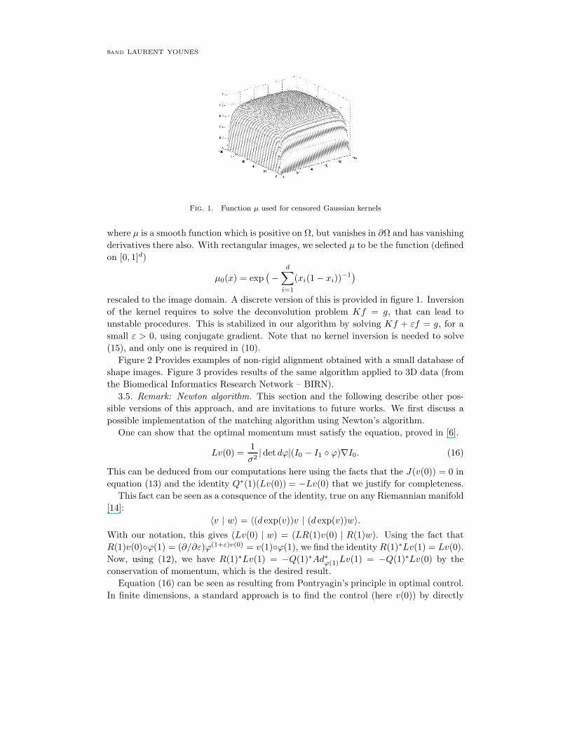
8AND LAURENT YOUNES

Fig. 1. Function µ used for censored Gaussian kernels

where µ is a smooth function which is positive on Ω, but vanishes in ∂Ω and has vanishing

derivatives there also. With rectangular images, we selected µ to be the function (defined

on [0, 1]d)

µ0(x) = exp(

−

d∑

i=1

(xi(1 − xi))−1

)

rescaled to the image domain. A discrete version of this is provided in figure 1. Inversion

of the kernel requires to solve the deconvolution problem Kf = g, that can lead to

unstable procedures. This is stabilized in our algorithm by solving Kf + εf = g, for a

small ε > 0, using conjugate gradient. Note that no kernel inversion is needed to solve

(15), and only one is required in (10).

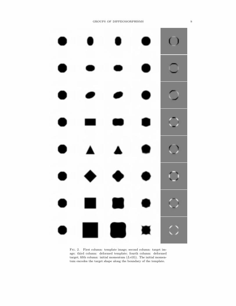
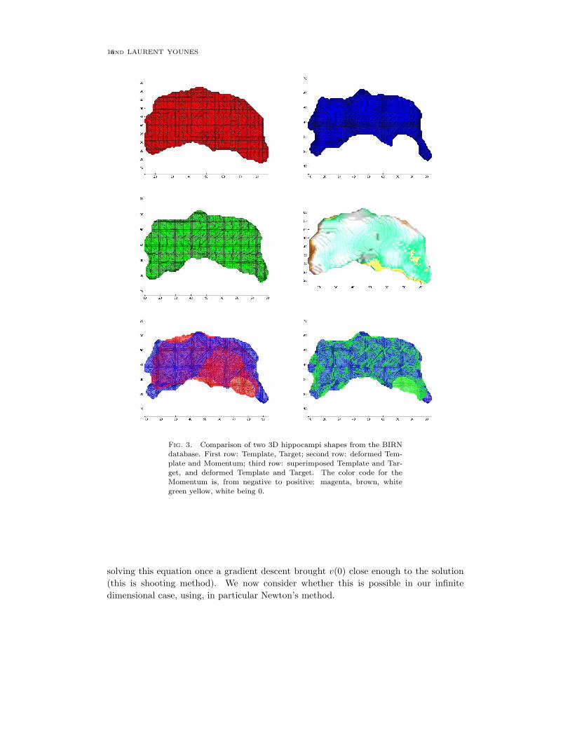
Figure 2 Provides examples of non-rigid alignment obtained with a small database of

shape images. Figure 3 provides results of the same algorithm applied to 3D data (from

the Biomedical Informatics Research Network – BIRN).

3.5. Remark: Newton algorithm. This section and the following describe other pos-

sible versions of this approach, and are invitations to future works. We first discuss a

possible implementation of the matching algorithm using Newton’s algorithm.

One can show that the optimal momentum must satisfy the equation, proved in [6].

Lv(0) =1

σ2| det dϕ|(I0 − I1 ϕ)∇I0. (16)

This can be deduced from our computations here using the facts that the J(v(0)) = 0 in

equation (13) and the identity Q∗(1)(Lv(0)) = −Lv(0) that we justify for completeness.

This fact can be seen as a consquence of the identity, true on any Riemannian manifold

[14]:

〈v | w〉 = 〈(d exp(v))v | (d exp(v))w〉.

With our notation, this gives (Lv(0) | w) = (LR(1)v(0) | R(1)w). Using the fact that

R(1)v(0)ϕ(1) = (∂/∂ε)ϕ(1+ε)v(0) = v(1)ϕ(1), we find the identity R(1)∗Lv(1) = Lv(0).

Now, using (12), we have R(1)∗Lv(1) = −Q(1)∗Ad∗ϕ(1)Lv(1) = −Q(1)∗Lv(0) by the

conservation of momentum, which is the desired result.

Equation (16) can be seen as resulting from Pontryagin’s principle in optimal control.

In finite dimensions, a standard approach is to find the control (here v(0)) by directly

GROUPS OF DIFFEOMORPHISMS 9

Fig. 2. First column: template image; second column: target im-age; third column: deformed template; fourth column: deformedtarget; fifth column: initial momentum (Lv(0)). The initial momen-tum encodes the target shape along the boundary of the template.

10AND LAURENT YOUNES

Fig. 3. Comparison of two 3D hippocampi shapes from the BIRNdatabase. First row: Template, Target; second row: deformed Tem-plate and Momentum; third row: superimposed Template and Tar-get, and deformed Template and Target. The color code for theMomentum is, from negative to positive: magenta, brown, whitegreen yellow, white being 0.

solving this equation once a gradient descent brought v(0) close enough to the solution

(this is shooting method). We now consider whether this is possible in our infinite

dimensional case, using, in particular Newton’s method.

GROUPS OF DIFFEOMORPHISMS 11

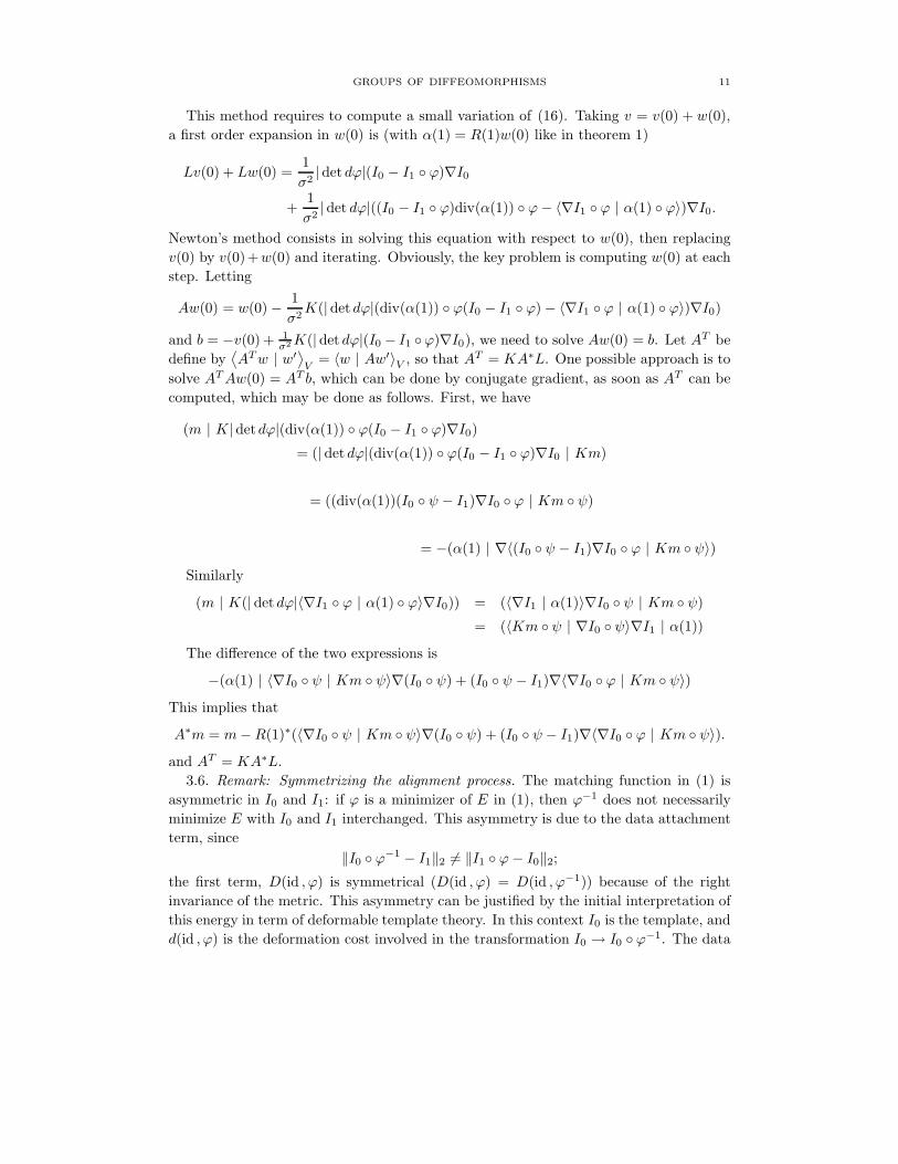
This method requires to compute a small variation of (16). Taking v = v(0) + w(0),

a first order expansion in w(0) is (with α(1) = R(1)w(0) like in theorem 1)

Lv(0) + Lw(0) =1

σ2| det dϕ|(I0 − I1 ϕ)∇I0

+1

σ2| det dϕ|((I0 − I1 ϕ)div(α(1)) ϕ− 〈∇I1 ϕ | α(1) ϕ〉)∇I0.

Newton’s method consists in solving this equation with respect to w(0), then replacing

v(0) by v(0)+w(0) and iterating. Obviously, the key problem is computing w(0) at each

step. Letting

Aw(0) = w(0) −1

σ2K(| det dϕ|(div(α(1)) ϕ(I0 − I1 ϕ) − 〈∇I1 ϕ | α(1) ϕ〉)∇I0)

and b = −v(0) + 1σ2K(| det dϕ|(I0 − I1 ϕ)∇I0), we need to solve Aw(0) = b. Let AT be

define by⟨

ATw | w′⟩

V= 〈w | Aw′〉V , so that AT = KA∗L. One possible approach is to

solve ATAw(0) = AT b, which can be done by conjugate gradient, as soon as AT can be

computed, which may be done as follows. First, we have

(m | K| detdϕ|(div(α(1)) ϕ(I0 − I1 ϕ)∇I0)

= (| det dϕ|(div(α(1)) ϕ(I0 − I1 ϕ)∇I0 | Km)

= ((div(α(1))(I0 ψ − I1)∇I0 ϕ | Km ψ)

= −(α(1) | ∇〈(I0 ψ − I1)∇I0 ϕ | Km ψ〉)

Similarly

(m | K(| det dϕ|〈∇I1 ϕ | α(1) ϕ〉∇I0)) = (〈∇I1 | α(1)〉∇I0 ψ | Km ψ)

= (〈Km ψ | ∇I0 ψ〉∇I1 | α(1))

The difference of the two expressions is

−(α(1) | 〈∇I0 ψ | Km ψ〉∇(I0 ψ) + (I0 ψ − I1)∇〈∇I0 ϕ | Km ψ〉)

This implies that

A∗m = m−R(1)∗(〈∇I0 ψ | Km ψ〉∇(I0 ψ) + (I0 ψ − I1)∇〈∇I0 ϕ | Km ψ〉).

and AT = KA∗L.

3.6. Remark: Symmetrizing the alignment process. The matching function in (1) is

asymmetric in I0 and I1: if ϕ is a minimizer of E in (1), then ϕ−1 does not necessarily

minimize E with I0 and I1 interchanged. This asymmetry is due to the data attachment

term, since

‖I0 ϕ−1 − I1‖2 6= ‖I1 ϕ− I0‖2;

the first term, D(id , ϕ) is symmetrical (D(id , ϕ) = D(id , ϕ−1)) because of the right

invariance of the metric. This asymmetry can be justified by the initial interpretation of

this energy in term of deformable template theory. In this context I0 is the template, and

d(id , ϕ) is the deformation cost involved in the transformation I0 → I0 ϕ−1. The data

12AND LAURENT YOUNES

attachment term then can be interpreted as observation noise, explaining the difference

between the ideal image (the deformed template) and the observed one, I1.

In situations when the asymetry template/target is not natural, it may be preferrable

to symmetrize the procedure. This can be easily done by slightly modifying the data

attachment term to be

U(I0, I1, ϕ) =

∫

| det dϕ ϕ−1|−1/2(I0 ϕ−1 − I1)

2dx =

∫

| det dψ|1/2(I0 ψ − I1)2dx.

with ψ = ϕ−1. Indeed, with this choice, we have

U(I0, I1, ϕ) =

∫

| det dψ|1/2(I0 ψ − I1)2dx

=

∫

| det dψ|1/2(I0 ψ − I1)2dx

=

∫

| det dψ ϕ|1/2| det dϕ|(I0 − I1 ϕ)2dx

= U(I1, I0, ψ).

With the previous notation ∂ψ = β ψ, we can compute the variation of U to be

∂U =

∫

| det dψ|1/2(I0 ψ − I1)〈∇I0 ψ | β ψ〉dx+1

2

∫

| det dψ|1/2(I0 ψ − I1)2(divβ) ψdx

=

∫

| det dϕ|1/2(I0 − I1 ϕ)〈∇I0 | β〉dx+1

2

∫

| det dϕ|1/2(I0 − I1 ϕ)2divβdx

=

∫

| det dϕ|1/2(I0 − I1 ϕ)〈∇I0 | β〉dx−1

2

∫

⟨

∇(| det dϕ|1/2(I0 − I1 ϕ)2) | β⟩

dx

Therefore, the new expression of the energy gradient (13) is

J(v(0)) = 2Lv(0) + (2/σ2)Q∗(1)(| det dϕ|1/2(I0 − I1 ϕ)∇I0)

− (1/σ2)Q∗(1)∇(| det dϕ|1/2(I0 − I1 ϕ)2) (17)

Another way to enforce symmetry, which is generalizable to other types of data at-

tachment terms, is to place the comparison at the midpoint of the geodesic t 7→ ϕ(t).

Indeed, consider the geodesic evolution in GV starting at id with velocity v(0), and let

w(0) = −v(1) where v(1) is the final velocity of the geodesic. Then, one can prove that

ϕw(0)(t) ϕv(0)(1) = ϕv(0)(1 − t)

and the final velocity of the geodesic starting from id with initial velocity w(0) is −v(0)

(this is just traveling along the same geodesic of GV in the reverse direction). Because

the velocities have constant norm along geodesics, we have

‖v(0)‖2V + λ‖I0 ψ

v(0)(1/2) − I1 ϕv(0)(1) ψv(0)(1/2)‖2

2 =

‖w(0)‖2V + λ‖I1 ψ

w(0)(1/2) − I0 ϕw(0)(1) ψw(0)(1/2)‖2

2.

This argument shows the symmetry of the matching method with the data attachment

term replaced by U = ‖I0 ψ(1/2)− I1 ϕ(1) ψ(1/2)‖22.

GROUPS OF DIFFEOMORPHISMS 13

In this case, the variation δU is (after computation)

δU = 2

∫

(I0 − I1 ϕ(1))| det dϕ(1/2)|(〈∇I0 | β(1)〉 − 〈∇(I1 ϕ(1)) | β(1/2) − β(1)〉)dx.

so that, the gradient is

2Q(1)∗((I0 − I1 ϕ(1))| det dϕ(1/2)|(∇I0 + ∇(I1 ϕ(1))))

− 2Q(1/2)∗((I0 − I1 ϕ(1))| det dϕ(1/2)|∇(I1 ϕ(1))).

3.7. Remark: Image Metamorphoses. The previous results can be formally applied to

image metamorphoses ([19, 27]). Image metamorphoses can be described via the action

of a larger group, which is the semidirect product of the group GV of diffeomorphisms

and the space L2. This is a special case. In general, metamorphoses (as defined in [27])

do not reduce to semi-direct products.

We consider the space GV n L2 which consists of all elements (ϕ, h) ∈ GV × L2,

equipped with the product

(ϕ, h)(ϕ, h) = (ϕ ϕ, h ϕ−1 + h).

GV nL2 is equipped with the right-invariant metric associated to the dot product on

V × L2:⟨

(v, δ) | (v, δ)⟩

= 〈v | v〉V +1

σ2

⟨

δ | δ⟩

L2.

This product can also be written⟨

(v, δ) | (v, δ)⟩

=(

L(v, δ) | (v, δ))

where L(v, δ) = (Lv, δ/σ2). In particular, K = L−1 is given by K(m, δ) = (Km,σ2δ).

The associated metric on GV nL2 induces a canonical metric on images via the projection

(ϕ, h) 7→ h. We associate curves in GV nL2 to time dependent pairs (v(t), δ(t)) ∈ V ×L2

via the equations (which are a generalization of ϕt = v ϕ)

ϕt = v ϕ, ht = δ − 〈∇h | v〉. (18)

The geodesic and Jacobi equations are formally the same on GV nL2 as they were for

GV . To explicit them, we only have to compute the adjoint maps and their conjugate

for this larger structure. First, write

(ϕ, h)(ϕ, h)(ϕ, h)−1 = (ϕ ϕ, h ϕ−1 + h)(ϕ−1,−h ϕ)

= (ϕ ϕ ϕ−1,−h ϕ ϕ−1 ϕ−1 + h ϕ−1 + h)

The Adjoint is obtained by taking (ϕ, h) = (id +εv, εδ) in the previous formula and take

the derivative with respect to ε, yielding (at ε = 0):

Ad(ϕ,h)(v, δ) = (Adϕv, δ ϕ−1 + 〈∇h | Adϕv〉)

where Adϕ refers to the Adjoint in the group of diffeomorphism as before. For the dual,

we have, for m ∈ V ∗ and µ ∈ L2:(

(m,µ) | Ad(ϕ,h)(v, δ))

= (m | Adϕv) +(

µ | δ ϕ−1 + 〈∇h | Adϕv〉)

=(

Ad∗ϕ(m+ µ∇h) | v)

+ (| det dϕ|µ ϕ | δ)

14AND LAURENT YOUNES

yielding

Ad∗(ϕ,h)(m,µ) = (Ad∗ϕ(m+ µ∇h), | det dϕ|µ ϕ).

In particular, the conservation of momentum that characterizes geodesics (specified by

(18)) in G n L2 is Ad∗(ϕ,h)(Lv, δ/σ2) = cst or (Lv, δ/σ2) = Ad(ψ,−hϕ)(Lv(0), δ(0)/σ2).

This gives

Lv = Ad∗ψ(Lv(0) −1

σ2δ(0)∇(h ϕ))

δ = | det dψ|δ(0) ψ

In the first equation, we have

Ad∗ψ(δ(0)∇(h ϕ)) = | det dψ|δ(0) ψdψT dϕT ϕ∇h = δ∇h

Therefore we have

Lv = Ad∗ϕLv(0) + δ∇h

δ = | det dψ|δ(0) ψ(19)

The expression of ad(v,δ)(w, η) comes by differentiating Ad(ϕ,h)(w, η) with respect to

ε, where ϕ = id + εv and h = εδ. This gives

ad(v,δ)(w, η) = (advw, 〈∇h | w〉 − 〈∇η | v〉).

The same operation on the dual yields

ad∗(v,δ)(m,µ) = (ad∗vm+ µ∇δ, 〈∇µ | v〉 + µdivv).

This provides, for example, the Jacobi evolution for a variation of the initial (v, δ) by

a perturbation in the direction of (w, η). Let, for example (β ϕt, ρ + 〈∇h ϕ | v〉) be

the perturbation of (ϕ, h)−1. We have, appying (4)

(β, ρ)t = −Ad(ψ,−hϕ)KAd∗(ψ,−hψ)((Lw(0), η/σ2) + ad∗(β,ρ)(Lv(0), δ/σ2))

Other quantities, including Q∗(1), adapt similarly. This opens the possibility of an

implementation of metamorphoses using Jacobi fields. Denoting (ϕv(0),z(0), hv(0),z(0)) the

solution of system (19), the problems consist in minimizing (Lv(0) | v(0)) + σ2‖z(0)‖22

under the constraint that hv(0),z(0) = I1 − I0 (ϕv(0),z(0))−1. This can be done by

minimizing

E(v, z) =∥

∥I1 − I0 (ϕv,z)−1 − hv,z∥

∥

2

2

using gradient descent. One can furthermore use the fact that optimal solutions satisfy

Lv(0) = ∇I0z(0) and work only with the initial z.

It is also possible (maybe not feasible) to try to solve the equation I1 − I0 (ϕv,z)−1−

hv,z = 0 using Newton’s algorithm, similarly to section 3.5.

Note that geodesic equations derived from the action of semi-direct products is related

(with some important differences) to evolution equations derived in finite and infinite

dimensional mechanics [12].

GROUPS OF DIFFEOMORPHISMS 15

4. Application: Parallel Translation. As a second application, we discuss an

implementation of parallel translation in the group of diffeomorphism and between images

using Jacobi fields, with he following motivation.

There are situations when the objects of study are not a shapes or images, but the

relative positions of pairs (orm-tuples) of them. The usual point of view in computational

anatomy [11] (and many other approaches in shape analysis) is template-based: before

analysis, all the observations are placed in a “common coordinate system” by registering

them to the template. This point of view is based on the expectation that objects with

different shapes will end up having different representations relative to the template, as

illustrated, for example, on our 2D simple shape database (Figure 2), where the target

shape could be read from its momentum representation in the disc-centered coordinate

system.

However, this representation is not adequate to easily address issues about the relative

positions of the shapes. For example, one would be willing to decide whether a rectangle,

relative to a square, is in some way in the same relation as an ellipse, relative to a disc.

The same is true for real applications, like studies of growth or other shape evolution.

A natural way to represent relative positions on a manifold is by using tangent vectors.

They are of course first order approximations of a variation, but can also represent large

variations as initial velocities of geodesics, at least in the presence of a Riemannian

structure. It is therefore natural to consider the issue of displacing a tangent vector at a

given shape toward the tangent space at another shape. On Riemannian manifolds, this

can be done using parallel translation.

In the following sections, we discuss parallel translation in the group of diffeomor-

phisms, then on shapes or images spaces, which are projections of the group obtained by

the action on a template.

We (formally) identify V to the set of right invariant vector fields on GV , via the

relation v ∈ V ↔ Xv : ϕ 7→ v.ϕ = v ϕ. The bracket on V is such that [v, w]ϕ =

−[Xv, Xw]ϕ where the last term is the Lie bracket between vector fields, [X,Y ] = XY −

Y X .

4.1. Parallel translation on G.

4.1.1. Covariant derivative. Parallel translation along a curve γ being characterized

by ∇γtX = 0, we need the expression of the covariant derivative on GV . If X is a vector

field on GV , we let vX be the function ϕ 7→ Xϕϕ−1 ∈ V . vX therefore is defined on GV

and takes values in V . We have the following proposition.

Proposition 1.

(∇YX)ϕ = (AvY vX + (Y vX))ϕ (20)

with

Avw =1

2

(

adTv w + adTwv − advw)

(21)

16AND LAURENT YOUNES

Proof. This is proved in [1], [16], and derives from an application of the general formula

for the Levi-Civita connection on a Riemannian manifold, namely

2〈∇YX | Z〉 = X〈Y | Z〉V + Y 〈X | Z〉V − Z〈X | Y 〉V

+ 〈[Y,X ] | Z〉 − 〈Y | [X,Z]〉 − 〈X | [Y, Z]〉. (22)

and on the identity (with notation from the proposition) v[X,Y ] = XvY −Y vX +[vX , vY ].

ut

4.1.2. Parallel translation. Let Y coincide with γ along a curve γ. If v(t) = vY (γ(t))

and w(t) = vX(γ(t)), we obtain the equation for the parallel translation along γ:

dw

dt+Avw = 0

ordw

dt+

1

2

(

adTv w + adTwv − advw)

= 0.

(In particular, for v = w, one retrieves the geodesic equation dv/dt+ adTv v = 0.)

The parallel translation in cotangent space can also be explicited. Denote, as usual,

by L the duality operator L : V → V ∗ and let K = L−1. Then, the covariant derivative

of 1-forms is characterized by:

Y (M | X) = (∇YM | X) + (M | ∇YX)

For ϕ ∈ G, Define m(ϕ) ∈ V ∗ by (m(ϕ) | v) = (M | vϕ): we will write M = mϕ. Then

one has (M | X) = (m | vX). This yields

(Ym | vX) + (m | Y vX) = (∇YM | X) + (m | Y vX +AvY vX).

Therefore

(∇YM | X) = (Y m | vX) − (m | AvY vX).

We have (m | advw) = (ad∗vm | w),

(

m | adTwv)

=⟨

Km | adTwv⟩

V= 〈v | [w,Km]〉 = −(ad∗

KmLv | w)

and(

m | adTv w)

= 〈w | adv(Km)]〉. This implies that

2(m | AvY vX) =(

−ad∗vYm | vX

)

− 〈ad∗Km(LvY ) | vX〉 + 〈advY (Km) | vX〉

which implies

(∇YM)g =

(

Ym+1

2(ad∗

vYm+ ad∗Km(LvY ) − LadvY (Km))

)

g

The equation for parallel translation along γ therefore is

dm

dt+

1

2(ad∗wp+ ad∗vm− Ladvw) = 0 (23)

with the notation γ = vγ, v = Kp and w = Km.

Again, for v = w, we retrieve the conservation equation

dm

dt+ ad∗vm = 0.

GROUPS OF DIFFEOMORPHISMS 17

4.1.3. Parallel translation along geodesics and Jacobi fields. When γ is a geodesic on

G, parallel translation along γ can be related to Jacobi fields. We indeed have the relation,

in a Riemannian manifold, Π(t) holding for parallel transport along the geodesic,

Π(t)w(0) = J(t)/t+ o(t).

Since Π(2t)w(0) = Π(t)Π(t)w(0), we see that we can implement parallel translation by

iterating the computation of normalized Jacobi fields over small periods of time. We

describe this in more details in the next section, first for a general manifold, then in the

case of the group G.

4.2. Discretization using Jacobi fields.

4.2.1. General algorithm. For a point ϕ on a Riemannian manifold M and a tangent

vector X at ϕ, denote γ(t, ϕ,X) the geodesic starting at ϕ in the direction X . If Y is

another vector tangent to M at ϕ, we want to compute the parallel translation of Y

along this geodesic. We will denote this by P (t, Y ).

We consider the Jacobi field measuring the variation of the geodesic when the initial

direction X is slightly perturbed by X 7→ X + εY , namely

J(t) = J(t, ϕ,X, Y ) =d

dεγ(t, ϕ,X + εY ).

Using

P (t, Y ) =1

tJ(t, g,X, Y ) + o(t),

we can use the following procedure to approximate P (1, Y ) [2]: let ∆ = 1/N and Y0 = Y ,

then iterate

Yk+1 =1

∆J(∆, ϕk, Xk, Yk)

until k = N (ϕk and Xk come from the discretization of the geodesic with step k).

This algorithm is described in the appendix of [2]. One can enforce the conservation of

norm and angles as follows. LetXk+1 be the velocity of the geodesic at time t = (k+1)/N .

The value of Yk+1 previously obtained can be replaced by

Yk+1 = αXk+1 + βYk+1

where α and β are computed by solving the equations ‖Yk+1‖2γk+1

= ‖Yk‖2γk

and⟨

Yk+1 | Xk+1

⟩

γk+1

=⟨

Yk | Xk

⟩

γk.

4.2.2. Groups of diffeomorphisms. We now adapt this algorithm to groups of diffeo-

morphisms, with our previously introduced notation. We consider a geodesic starting at

the identity, and a vector w(0) ∈ V . The parallel translation along the geodesic starting

in the direction v(0) can be computed as follows. Let α(t) = R(t, v(0))w(0) be such that

(d/dε)ϕv(0)+εw(0)(t) = α(t) ϕv(0)(t). For a small ∆ = 1/N , iterate

w(k + 1) = R(∆, v(k∆))w(k)/∆

until k = N . The parallel translation of w(0) is w(N) ϕ(1).

Conservation of the norm and of the dot product with v can be enforced as before,

keeping in mind that the norm which is used is ‖v‖2V = (Lv | v).

4.3. Parallel translation in an orbit.

18AND LAURENT YOUNES

4.3.1. General formulation. Objects of interest, like image and shapes, are not dif-

feomorphisms, but are acted upon by diffeomorphisms. To address this, we consider an

action (G,M) → M and the induced metric. The action is assumed to be transitive (or

restricted to an orbit), and we fix m0, a reference element in M (the template).

We define the projection π : G → M by π(ϕ) = ϕ.m0. For v ∈ V and m ∈ M , we

use the notation ρm(v) = v.m for the infinitesimal action on m (v.m ∈ TmM), and let

Vm = v : v.m = 0.

For m ∈ M , we let Gm = π−1(m) be the fiber over m. For ϕ ∈ Gm, TϕGm is the

vertical space over m: it is equal to the right translation of Vm, denoted Vmϕ. The

horizontal space is orthogonal to Vmϕ in Tϕ, and equal to V ⊥mϕ by right invariance.

Note that ρm restricted to V ⊥m is a bijection onto TmM . We will denote vξ for the

inverse image (lifting) of ξ ∈ TmM under this map: vξ ∈ V ⊥m and vξm = ξ. The metric

on M is defined by

‖δ‖m =∥

∥vδ∥

∥

V= inf ‖v‖V : v.m = δ . (24)

A vector field X on G is horizontal if Xg ∈ V ⊥g.m0

g for all g. Given a vector field ξ on

M , there is a unique “basic” horizontal lift to a vector field, denoted ξ on G defined by

ξg = vξm .g for m = π(g).

It can easily be proved (cf. [20] or directly from the formula for the covariant deriva-

tive) than, when ξ and η are vector fields on M ,

(∇ηξ) = dπ(∇η ξ).

This is therefore the projection of the covariant derivative of the lifted vector fields.

Letting vξ(ϕ) = vξπ(ϕ) and similarly for vη, we have

(∇η ξ)ϕ = (ηvξ + Avηvξ)ϕ.

Consider a curve t 7→ m(t) on M : this can be lifted in a unique way as a horizontal

curve ϕ(t) on G with

ϕt = vmtϕ(t).

In particular,mt = ϕtm0 = vmtm. Parallel translation alongm is therefore characterized

by (using dπ(ϕ)(v.ϕ) = v.m)(

vξt +Avmt vξ)

m = 0.

Since ξ = vξ.m, we have ξt = vξt .m+ vξ(vmtm). We therefore get the evolution equation

ξt + (Avmt vξ)m = vξ(vmtm).

4.3.2. Discretization using Jacobi fields. When parallel translation is computed along

a geodesic, we can use again Jacobi fields. Because the metric on M is the projection

of the metric on G, the geodesic on M starting at m in the direction ξ simply is the

projection of the geodesic on G starting at id in the direction vξ. In other terms, with

our previous notation:

γ(t,m, ξ) = ϕvξ(t)m

From this comes the fact that

J(t,m, ξ, η) =d

dεγ(t,m, ξ + εη) = (R(t, vξ).vη).(ϕ.m).

GROUPS OF DIFFEOMORPHISMS 19

In other terms, to compute the Jacobi field J(t,m, ξ, η) it suffices to lift ξ and η into vξ

and vη, then compute the corresponding Jacobi field w on G, and finally, to reproject it

on M .

4.3.3. Application to parallel transport with images. Diffeomorphisms act on images

by (ϕ, I) → m ϕ−1. This implies that the infinitesimal action of a vector field on an

image I is v.I = −〈∇I | v〉. If ξ is a scalar field, its lift vξ is defined by the constrained

minimization problem:

vξ = argmin(‖v‖V : 〈∇I | v〉 = −ξ).

Introduce a space discretization by reducing the constraints to a finite grid constituted

by points x1, . . . , xM . In this approximation, we therefore only require that, for all j:

ξ(xj) = −⟨

∇xjI | v(xj)⟩

. In such a case, we know that the solution takes the form

v(x) =

M∑

j=1

K(x, xj)αj∇xjI

with αj ∈ R. The coefficients α1, . . . , αM will be determined by the constraints which

yield (assuming that the kernel is scalar)

ξ(xj′ ) =

M∑

j=1

K(xj′ , xj)⟨

∇xj′ I | ∇xjI⟩

αj , j′ = 1, . . . ,M.

This is an M dimensional linear system, which can be solved, for example, by conjugate

gradient.

Another approach is possible when ξ is already given by −w.I for some vector field

w. In this case, the constraint can be written 〈v − w | ∇I〉 = 0. Define the vector

NI to be ∇I/|∇I| when ∇I 6= 0 and 0 is ∇I = 0. The constraint can be rewritten

〈v − w | NI〉 = 0. Define the operator PI by (PIh)(x) = h(x) − 〈h(x) | NI(x)〉NI(x).

The problem we need to solve is equivalent to the minimization of |PIh−w|2V with respect

to h ∈ V . We have

1

2|PIh− w|2V =

1

2(LPIh | PIh) − (Lw | PIh) + |w|2V

so that the problem is (formally) equivalent to minimizing (1/2)(h | Ah) − (b | h) with

A = PILPI and b = PILw (using the fact that PI is self adjoint for the L2 inner product).

This can again be implemented using conjugate gradient. This second approach seemed

more robust in our experiments.

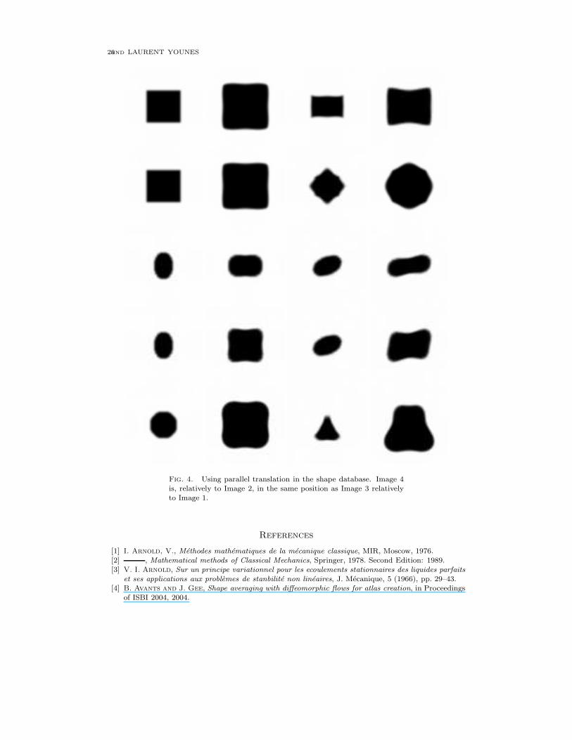
Figure 4 provides examples of transformations resulting from parallel translation using

our basis of simple shapes. The experiment answers the following question: given three

images, I1, I2, I3, which image I4 is in the same situation relative to I2 as I3 relative to

I1. This is done by computing the initial momentum of the geodesic between I1 and I3,

then parallel transporting it along the geodesic between I1 and I2, and finally shooting

from I2 with the obtained momentum.

20AND LAURENT YOUNES

Fig. 4. Using parallel translation in the shape database. Image 4is, relatively to Image 2, in the same position as Image 3 relativelyto Image 1.

References

[1] I. Arnold, V., Methodes mathematiques de la mecanique classique, MIR, Moscow, 1976.[2] , Mathematical methods of Classical Mechanics, Springer, 1978. Second Edition: 1989.[3] V. I. Arnold, Sur un principe variationnel pour les ecoulements stationnaires des liquides parfaits

et ses applications aux problemes de stanbilite non lineaires, J. Mecanique, 5 (1966), pp. 29–43.[4] B. Avants and J. Gee, Shape averaging with diffeomorphic flows for atlas creation, in Proceedings

of ISBI 2004, 2004.

GROUPS OF DIFFEOMORPHISMS 21

[5] R. Bajcsy and C. Broit, Matching of deformed images, in The 6th international conference inpattern recognition, 1982, pp. 351–353.

[6] M. F. Beg, M. I. Miller, A. Trouve, and L. Younes, Computing large deformation metricmappings via geodesic flows of diffeomorphisms, Int J. Comp. Vis., 61 (2005), pp. 139–157.

[7] R. Camassa and D. D. Holm, An integrable shallow water equation with peaked solitons, Phys.Rev. Lett., 71 (1993), pp. 1661–1664.

[8] M. P. D. Carmo, Riemannian geometry, Birkauser., 1992.[9] E. Christensen, G, D. Rabbitt, R, and I. Miller, M, Deformable templates using large defor-

mation kinematics, IEEE trans. Image Proc., (1996).[10] P. Dupuis, U. Grenander, and M. Miller, Variational problems on flows of diffeomorphisms for

image matching, Quaterly of Applied Math., (1998).[11] U. Grenander and I. Miller, M, Computational anatomy: An emerging discipline, Quarterly of

Applied Mathematics, LVI (1998), pp. 617–694.[12] D. D. Holm, J. E. Marsden, and T. S. Ratiu, The Euler–Poincar equations and semidirect

products with applications to continuum theories, Adv. in Math., 137 (1998), pp. 1–81.[13] R. Holm, D, T. Ratnanather, J, A. Trouve, and L. Younes, Soliton dynamics in computational

anatomy, Neuroimage, 23 (2004), pp. S170–S178.[14] S. Joshi, Large deformation diffeomorphisms and Gaussian random fields for statistical character-

ization of brain sub-manifolds, PhD thesis, Sever institute of technology, Washington University,1997.

[15] E. Marsden, J and S. Ratiu, T, Introduction to Mechanics and Symmetry, Springer, 1999.[16] P. Michor, Some geometric equations arising as geodesic equations on groups of diffeomorphisms

and spaces of plane curves including the hamiltonian approach. Lecture Course, University of Wien.[17] I. Miller, M, A. Trouve, and L. Younes, On the metrics and euler-lagrange equations of com-

putational anatomy, Annual Review of biomedical Engineering, 4 (2002), pp. 375–405.[18] , Geodesic shooting for computational anatomy, J. Math. Image and Vision, (2005).[19] I. Miller, M and L. Younes, Group action, diffeomorphism and matching: a general framework,

Int. J. Comp. Vis, 41 (2001), pp. 61–84. (Originally published in electronic form in: Proceeding ofSCTV 99, http://www.cis.ohio-state.edu/ szhu/SCTV99.html).

[20] B. O’Neill, The fundamental equations of a submersion, Michigan Math. J., (1966), pp. 459–469.[21] H. Press, W., A. Teukolsky, S., T. Vetterling, W., and P. Flannery, B., Numerical Recipes

in C, The Art of Scientific Computing, Cambridge University Press, second edition, 1992.[22] J.-P. Thirion, Image matching as a diffusion process: an analogy with maxwell’s demons, Medical

Image Analysis, 2 (1998), pp. 243–260.[23] , Diffusing models and applications, in Brain Warping, W. Toga, A, ed., 1999, pp. 144–155.[24] A. Trouve, Infinite dimensional group action and pattern recognition, tech. report, DMI, Ecole

Normale Suprieure, 1995.[25] , Diffeomorphism groups and pattern matching in image analysis, Int. J. of Comp. Vis., 28

(1998), pp. 213–221.[26] A. Trouve and L. Younes, Local geometry of deformable templates, SIAM J. Math. Anal., (2005).

To appear.[27] A. Trouve and L. Younes, Metamorphoses through lie group action, Found. Comp. Math., (2005),

pp. 173–198.