electromagnetic fields and waves - mrcet.ac.in

ELECTROMAGNETIC FIELDS AND WAVES

LECTURE NOTES

B.TECH (II YEAR – II SEM)

(2020-21)

Prepared by: Dr. K.Mallikarjuna Lingam, Associate Professor

Mrs.N.Saritha, Assistant Professor M.Sreedhar Reddy,Associate Professor

Department of Electronics and Communication Engineering

MALLA REDDY COLLEGE OF ENGINEERING & TECHNOLOGY

(Autonomous Institution – UGC, Govt. of India) Recognized under 2(f) and 12 (B) of UGC ACT 1956

(Affiliated to JNTUH, Hyderabad, Approved by AICTE - Accredited by NBA & NAAC – ‘A’ Grade - ISO 9001:2015 Certified) Maisammaguda, Dhulapally (Post Via. Kompally), Secunderabad – 500100, Telangana State, India

1

ELECTROMAGNETIC FIELDS&WAVES DEPT.ECE

MALLA REDDY COLLEGE OF ENGINEERING AND TECHNOLOGY II Year B.Tech. ECE-II Sem L T/P/D C

4 1/ - /- 4

(R18A0406) ELECTROMAGNETIC FIELDS & WAVES OBJECTIVES The course objectives are:

1. To introduce the student to the coordinate system and its implementation to electromagnetics.

2. To elaborate the concept of electromagnetic waves and their practical applications. 3. To study the propagation, reflection, and refraction of plane waves in different media.

UNIT - I: Vector Analysis & Co-ordinate system: Vector analysis- Representation, operations-Dot product and cross product, Basics of coordinate system- rectangular, cylindrical and spherical co-ordinate systems. Electrostatics-I: Coulomb’s Law, Electric Field Intensity - Fields due to Different Charge Distributions, Electric Flux Density; Illustrative Problems.

UNIT - II: Electrostatics-II: Gauss Law and Applications, Electric Potential, Relations Between E and V, Maxwell's Equations for Electrostatic Fields, Dielectric Constant, Isotropic and Homogeneous Dielectrics, Continuity Equation, Relaxation Time, Poisson's and Laplace's Equations, Boundary conditions-conductor- Dielectric and Dielectric-Dielectric; Illustrative Problems.

UNIT - III: Magnetostatics: Biot - Savart's Law , Ampere's Circuital Law and Applications, Magnetic Flux Density, Maxwell's Equations for Magnetostatic Fields, Magnetic Scalar and Vector Potentials, Ampere’s Force law , Faraday's Law, Displacement Current Density, Maxwell's Equations for time varying fields, Illustrative Problems.

UNIT - IV: EM Wave Characteristics-I : Wave Equations for Conducting and Perfect Dielectric Media, Uniform Plane Waves - Definition, Relation Between E & H, Wave Propagation in Lossless and Conducting Media, Wave Propagation in Good Conductors and Good Dielectrics, Illustrative Problems.

UNIT - V: EM Wave Characteristics – II: Reflection and Refraction of Plane Waves – Normal incidence for both perfect Conductors and perfect Dielectrics, Brewster Angle, Critical Angle and Total Internal Reflection, Surface Impedance, Poynting Vector and Poynting Theorem – Applications, Illustrative Problems.

2


TEXT BOOKS:

1. Elements of Electromagnetics - Matthew N. O. Sadiku, 4th., Oxford Univ. Press. 2. Electromagnetic Waves and Radiating Systems - E.C. Jordan and K. G. Balmain, 2nd Ed.,

2000, PHI. 3. Engineering Electromagnetic - William H. Hay Jr. and John A. Buck, 7thEd., 2006, TMH

REFERENCES BOOKS:

1. Engineering Electromagnetics - Nathan Ida, 2ndEd., 2005, Springer (India) Pvt. Ltd., New Delhi.

2. Electromagnetic Waves and Transmission Lines-Y Mallikarjuna Reddy, University Press. 3. Electromagnetic Fields Theory and Transmission Lines - G. Dashibhushana Rao, Wiley

India, 2013.

COURSE OUTCOMES:

Upon the successful completion of the course, students will be able to; 1. Study time varying Maxwell equations and their applications in electromagnetic

problems 2. Determine the relationship between time varying electric and magnetic field and

electromotive force 3. Use Maxwell equation to describe the propagation of electromagnetic waves 4. Demonstrate the reflection and refraction of waves at boundaries

3


UNIT – I

ELECTROSTATICS

Contents

Vector Analysis & Co-ordinate system

Vector analysis

Representation

Operations-Dot product and cross product

Basics of coordinate system

Rectangular coordinate system

Cylindrical coordinate system

Spherical coordinate system

Electrostatics-I:

Coulomb’s Law Electric Field Intensity

Fields due to Different Charge Distributions

Electric Flux Density

Problems.

4


Vector Analysis

Introduction:

Vector Algebra is a part of algebra that deals with the theory of vectors and vector spaces.

Most of the physical quantities are either scalar or vector quantities.

Scalar Quantity:

Scalar is a number that defines magnitude. Hence a scalar quantity is defined as a

quantity that has magnitude only. A scalar quantity does not point to any direction i.e. a

scalar quantity has no directional component.

For example when we say, the temperature of the room is 30o C, we don‘t specify the direction.

Hence examples of scalar quantities are mass, temperature, volume, speed etc.

A scalar quantity is represented simply by a letter – A, B, T, V, S.

Vector Quantity:

A Vector has both a magnitude and a direction. Hence a vector quantity is a

quantity that has both magnitude and direction.

Examples of vector quantities are force, displacement, velocity, etc.

A vector quantity is represented by a letter with an arrow over it or a bold letter.

Unit Vectors:

When a simple vector is divided by its own magnitude, a new vector is created known as

the unit vector. A unit vector has a magnitude of one. Hence the name - unit vector.

A unit vector is always used to describe the direction of respective vector.

Hence any vector can be written as the product of its magnitude and its unit vector. Unit Vectors

along the co-ordinate directions are referred to as the base vectors. For example unit vectors

along X, Y and Z directions are ax, ay and az respectively.

Position Vector / Radius Vector ( ):

A Position Vector / Radius vector define the position of a point(P) in space relative to

the origin(O).Hence Position vector is another way to denote a point in space.

= 𝑥𝑥 + 𝑦𝑦 + 𝑧𝑧

5


Displacement Vector

Displacement Vector is the displacement or the shortest distance from one point to another.

Vector Multiplication

When two vectors are multiplied the result is either a scalar or a vector depending on how

they are multiplied. The two important types of vector multiplication are:

Dot Product/Scalar Product (A.B)

Cross product (A x B)

1. DOT PRODUCT (A. B):

Dot product of two vectors A and B is defined as:

. = cos 𝜃𝐴𝐵

Where 𝜃𝐴𝐵 is the angle formed between A and B.

Also 𝜃𝐴𝐵 ranges from 0 to π i.e. 0 ≤ 𝜃𝐴𝐵 ≤ π

The result of A.B is a scalar, hence dot product is also known as Scalar Product.

Properties of Dot Product:

1. If A = (Ax, Ay, Az) and B = (Bx, By, Bz) then

. = AxBx + AyBy + AzBz

2. . = |A| |B|, if cos𝜃𝐴𝐵=1 which means θAB = 00

This shows that A and B are in the same direction or we can also say that A and B are

parallel to each other.

3. 𝐴. = - |A| |B|, if cos 𝜃𝐴𝐵=-1 which means 𝜃𝐴𝐵 = 1800.

This shows that A and B are in the opposite direction or we can also say that A and B are

antiparallel to each other.

45.. . = 0, if cos 𝜃𝐴𝐵=0 which means 𝜃𝐴𝐵 = 900.

This shows that A and B are orthogonal or perpendicular to each other.

5. Since we know the Cartesian base vectors are mutually perpendicular to each other, we have

𝑥 . 𝑥 = 𝑦. 𝑦 = 𝑧. 𝑧 = 1

𝑥 . 𝑦 = 𝑦. 𝑧 = 𝑧. 𝑥 = 0

6


2. Cross Product (A X B):

Cross Product of two vectors A and B is given as:

𝑋 = sin 𝜃𝐴𝐵 𝑁

Where 𝜃𝐴𝐵is the angle formed between A and B and 𝑁 is a unit vector normal to both A and B.

Also θ ranges from 0 to π i.e. 0 ≤ 𝜃𝐴𝐵≤ π

The cross product is an operation between two vectors and the output is also a vector.

Properties of Cross Product:

1. If A = (Ax, Ay, Az) and B = (Bx, By, Bz) then,

The resultant vector is always normal to both the vector A and B.

2. 𝑋 = 0, if sin 𝜃𝐴𝐵 = 0 which means 𝜃𝐴𝐵 = 00 or 1800;

This shows that A and B are either parallel or antiparallel to each other.

63. . 𝑋 =𝑁, if sin 𝜃𝐴𝐵 = 0 which means 𝜃𝐴𝐵 = 900.

This shows that A and B are orthogonal or perpendicular to each other.

4. Since we know the Cartesian base vectors are mutually perpendicular to each other, we have

𝑥𝑋 𝑥 = 𝑦 𝑋 𝑦 = 𝑧𝑋𝑧 = 0

𝑥𝑋 𝑦 = 𝑧 , 𝑦 𝑋 𝑧 = 𝑥 , 𝑧𝑋 𝑥 = 𝑦

7


CO-ORDINATE SYSTEMS:

Co-Ordinate system is a system of representing points in a space of given dimensions by

coordinates, such as the Cartesian coordinate system or the system of celestial longitude and

latitude.

In order to describe the spatial variations of the quantities, appropriate coordinate system is

required. A point or vector can be represented in a curvilinear coordinate system that may be

orthogonal or non-orthogonal. An orthogonal system is one in which the coordinates are mutually

perpendicular to each other.

The different co-ordinate system available are:

Cartesian or Rectangular co-ordinate system.(Example: Cube, Cuboid)

Circular Cylindrical co-ordinate system.(Example : Cylinder)

Spherical co-ordinate system. (Example: Sphere)

The choice depends on the geometry of the application.

A set of 3 scalar values that define position and a set of unit vectors that define direction form

a co-ordinate system. The 3 scalar values used to define position are called co-ordinates. All

coordinates are defined with respect to an arbitrary point called the origin.

1. Cartesian Co-ordinate System / Rectangular Co-ordinate System (x,y,z)

A Vector in Cartesian system is represented as (Ax, Ay, Az) Or

= 𝐴𝑥𝑥 + 𝐴𝑦𝑦 + 𝐴𝑧𝑧

Where𝑥,𝑦 and 𝑧are the unit vectors in x, y, z direction respectively.

8


= 𝑑𝑦𝑑𝑧𝑥

= 𝑑𝑥𝑑𝑧𝑦

Range of the variables:

It defines the minimum and the maximum value that x, y and z can have in Cartesian system.

-∞ ≤ x,y,z ≤ ∞

Differential Displacement / Differential Length (dl):

It is given as

𝑙 = 𝑑𝑥𝑥 + 𝑑𝑦𝑦 + 𝑑𝑧𝑧

Differential length for a line parallel to x, y and z axis are respectively given as:

dl = 𝑑𝑥𝑥---( For a line parallel to x-axis).

dl = 𝑑𝑦𝑦 ---( For a line Parallel to y-axis).

dl = 𝑑𝑧𝑧 ---( For a line parallel to z-axis).

If there is a wire of length L in z-axis, then the differential length is given as dl = dz az. Similarly

if the wire is in y-axis then the differential length is given as dl = dy ay.

Differential Normal Surface (ds):

Differential surface is basically a cross product between two parameters of the surface.

The differential surface (area element) is defined as = 𝑑𝑠𝑁

Where𝑁, is the unit vector perpendicular to the surface.

For the 1st figure,

2nd figure,

3rd figure,

Differential Volume:

= 𝑑𝑥𝑑𝑦𝑧

The differential volume element (dv) can be expressed in terms of the triple product.

𝑑𝑣 = 𝑑𝑥𝑑𝑦𝑑𝑧

9


2. Circular Cylindrical Co-ordinate System

A Vector in Cylindrical system is represented as (Ar, AǾ, Az) or

= 𝐴𝑟𝑟 + 𝐴∅∅ + 𝐴𝑧𝑧

Where𝑟, ∅ and 𝑧 are the unit vectors in r, Φ and z directions respectively.

The physical significance of each parameter of cylindrical coordinates:

1. The value r indicates the distance of the point from the z-axis. It is the radius of the

cylinder.

2. The value Φ, also called the azimuthal angle, indicates the rotation angle around the z-

axis. It is basically measured from the x axis in the x-y plane. It is measured anti

clockwise.

3. The value z indicates the distance of the point from z-axis. It is the same as in the

Cartesian system. In short, it is the height of the cylinder.

10



It defines the minimum and the maximum values of r, Φ and z.

0 ≤ r ≤ ∞

0 ≤ Φ ≤ 2π -∞ ≤ z ≤ ∞

Figure shows Point P and Unit vectors in Cylindrical Co-ordinate System.

Differential Displacement / Differential Length (dl):

It is given as

𝑙 = 𝑑𝑟𝑟 + 𝑟𝑑𝜑𝜑 + 𝑑𝑧𝑧

Differential length for a line parallel to r, Φ and z axis are respectively given as:

dl = 𝑑𝑟𝑟---( For a line parallel to r-direction).

dl = 𝑟𝑑𝜑𝜑 ---( For a line Parallel to Φ-direction).

dl = 𝑑𝑧𝑧 ---( For a line parallel to z-axis).





This surface describes a circular disc. Always remember- To define a circular disk we

need two parameter one distance measure and one angular measure. An angular parameter

will always give a curved line or an arc.

In this case dΦ is measured in terms of change in arc.

Arc is given as:

Arc= radius * angle

11



= 𝑟𝑑𝑟𝑑𝜑𝑧 = 𝑑𝑟𝑑𝑧𝜑

= 𝑟𝑑𝑟𝑑𝜑𝑟


𝑑𝑣 = 𝑟𝑑𝑟𝑑𝜑𝑑𝑧

3. Spherical coordinate System:

Spherical coordinates consist of one scalar value (r), with units of distance, while the other two

scalarvalues (θ, Φ) have angular units (degrees or radians).

A Vector in Spherical System is represented as (Ar ,AӨ, AΦ) or

= 𝐴𝑟𝑟 + 𝐴𝜃𝜃 + 𝐴𝜑𝜑

Where𝑟,𝜃 and 𝜑 are the unit vectors in r, θ and Φ direction respectively.

The physical significance of each parameter of spherical coordinates:

1. The value r expresses the distance of the point from origin (i.e. similar to

altitude). It is the radius of the sphere.

2. The angle θ is the angle formed with the z- axis (i.e. similar to latitude). It is also

called the co-latitude angle. It is measured clockwise.

3. The angle Φ, also called the azimuthal angle, indicates the rotation angle around the z-

axis (i.e. similar to longitude). It is basically measured from the x axis in the x-y plane.

It is measured counter-clockwise.


It defines the minimum and the maximum value that r, θ and υ can have in spherical co-ordinate

system.

0 ≤ r ≤ ∞ 0 ≤ θ ≤ π 0 ≤ Φ≤ 2π

12


Differential length: It is given as

𝑙 = 𝑑𝑟𝑟 + 𝑟𝑑𝜃𝜃 + 𝑟 sin 𝜃 𝑑𝜑𝜑

Differential length for a line parallel to r, θ and Φ axis are respectively given as:

dl = 𝑑𝑟𝑟--(For a line parallel to r axis)

dl = 𝑟𝑑𝜃𝜃---( For a line parallel to θ direction)

dl = 𝑟 sin 𝜃 𝑑𝜑𝜑 --(For a line parallel to Φ direction)





= 𝑟𝑑𝑟𝑑𝜃𝜑 = 𝑟2 sin 𝜃 𝑑𝜑𝑑𝜃𝑟 = 𝑟 sin 𝜃 𝑑𝑟𝑑𝜑𝜃



𝑑𝑣 = 𝑟2 sin 𝜃 𝑑𝑟𝑑𝜑𝑑𝜃

13


Coordinate transformations:

14


15


Del operator:

Del is a vector differential operator. The del operator will be used in for differential operations

throughout any course on field theory. The following equation is the del operator for different

coordinate systems.

Gradient of a Scalar:

• The gradient of a scalar field, V, is a vector that represents both the magnitude and the

direction of the maximum space rate of increase of V.

• To help visualize this concept, take for example a topographical map. Lines on the map

represent equal magnitudes of the scalar field. The gradient vector crosses map at the location

where the lines packed into the most dense space and perpendicular (or normal) to them. The

orientation (up or down) of the gradient vector is such that the field is increased in magnitude

along that direction.

-Fundamental properties of the gradient of a scalar field – The magnitude of gradient equals the maximum rate of change in V per unit distance

– Gradient points in the direction of the maximum rate of change in V

– Gradient at any point is perpendicular to the constant V surface that passes through that

point

– The projection of the gradient in the direction of the unit vector a, is

and is called the directional derivative of V along a. This is the rate of change of V

in the direction of a. – If A is the gradient of V, then V is said to be the scalar potential of A.

16


Divergence of a Vector:

• The divergence of a vector, A, at any given point P is the outward flux per unit volume as

volume shrinks about P.

Divergence Theorem:

• The divergence theorem states that the total outward flux of a vector field, A, through the

closed surface, S, is the same as the volume integral of the divergence of A.

• This theorem is easily shown from the equation for the divergence of a vector field.

Curl of a Vector:

The curl of a vector, A is an axial vector whose magnitude is the maximum circulation of A

per unit area as the area tends to zero and whose direction is the normal direction of the area

when the area is oriented to make the circulation maximum. -Curl of a vector in each of the three primary coordinate systems are,

17


Stokes Theorem:

• Stokes theorem states that the circulation of a vector field A, around a closed path, L is equal

to the surface integral of the curl of A over the open surface S bounded by L. This theorem has

been proven to hold as long as A and the curl of A are continuous along the closed surface S of

a closed path L

• This theorem is easily shown from the equation for the curl of a vector field.

Classification of vector field:

The vector field, A, is said to be divergenceless ( or solenoidal) if .

– Such fields have no source or sink of flux, thus all the vector field lines entering an enclosed

surface, S, must also leave it.

– Examples include magnetic fields, conduction current density under steady state, and imcompressible fluids

– The following equations are commonly utilized to solve divergenceless field problems

The vector field, A, is said to be potential (or irrotational) if

– Such fields are said to be conservative. Examples include gravity, and electrostatic fields.

– The following equations are commonly used to solve potential field problems;

18


Electrostatics-I

Introduction:

Electromagnetic theory is concerned with the study of charges at rest and in motion.

Electromagnetic principles are fundamental to the study of electrical engineering.

Electromagnetic theory is also required for the understanding, analysis and design of various

electrical, electromechanical and electronic systems.

Electromagnetic theory can be thought of as generalization of circuit theory. Electromagnetic

theory deals directly with the electric and magnetic field vectors where as circuit theory deals

with the voltages and currents. Voltages and currents are integrated effects of electric and

magnetic fields respectively.

Electromagnetic field problems involve three space variables along with the time variable and

hence the solution tends to become correspondingly complex. Vector analysis is the required

mathematical tool with which electromagnetic concepts can be conveniently expressed and best

comprehended. Since use of vector analysis in the study of electromagnetic field theory is

prerequisite, first we will go through vector algebra.

Applications of Electromagnetic theory:

This subject basically consist of static electric fields, static magnetic fields, time-varying fields &

it’ applications. One of the most common applications of electrostatic fields is the deflection of a

charged particle such as an electron or proton in order to control it’s trajectory. The deflection is

achieved by maintaining a potential difference between a pair of parallel plates. This principle is

used in CROs, ink-jet printer etc. Electrostatic fields are also used for sorting of minerals for

example in ore separation. Other applications are in electrostatic generator and electrostatic

voltmeter.

The most common applications of static magnetic fields are in dc machines. Other

applications include magnetic deflection, magnetic separator, cyclotron, hall effect sensors,

magneto hydrodynamic generator etc.

Electrostatics is a branch of science that involves the study of various phenomena caused by

electric charges that are slow-moving or even stationary. Electric charge is a fundamental

property of matter and charge exist in integral multiple of electronic charge. Electrostatics as the

study of electric charges at rest.

The two important laws of electrostatics are

Coulomb‘s Law.

Gauss‘s Law.

Both these laws are used to find the electric field due to different charge configurations.

19


Coulomb‘s law is applicable in finding electric field due to any charge configurations where as

Gauss‘s law is applicable only when the charge distribution is symmetrical.

Coulomb's Law

Coulomb's Law states that the force between two point charges Q1and Q2 is directly

proportional to the product of the charges and inversely proportional to the square of the distance

between them.

A point charge is a charge that occupies a region of space which is negligibly small compared to

the distance between the point charge and any other object.

Point charge is a hypothetical charge located at a single point in space. It is an idealized model of

a particle having an electric charge.

Mathematically, , where k is the proportionality constant.

In SI units, Q1 and Q2 are expressed in Coulombs(C) and R is in meters.

Force F is in Newtons (N) and , is called the permittivity of free space.

(We are assuming the charges are in free space. If the charges are any other dielectric medium,

we will use instead where is called the relative permittivity or the dielectric

constant of the medium).

Therefore ................................................ (1)

As shown in the Figure 1 let the position vectors of the point charges Q1and Q2 are given by

and . Let represent the force on Q1 due to charge Q2.

20


Fig 1: Coulomb's Law

The charges are separated by a distance of . We define the unit vectors as

and

can be defined as .

Similarly the force on Q1 due to charge Q2 can be calculated and if represents this force then

we can write

When we have a number of point charges, to determine the force on a particular charge due to all

other charges, we apply principle of superposition. If we have N number of charges

Q1,Q2,.........QN located respectively at the points represented by the position vectors , ,......

, the force experienced by a charge Q located at is given by,

Field:

A field is a function that specifies a particular physical quantity everywhere in a region.

Depending upon the nature of the quantity under consideration, the field may be a vector or a

scalar field. Example of scalar field is the electrostatic potential in a region while electric or

magnetic fields at any point is the example of vector field. Static Electric Fields:

Electrostatics can be defined as the study of electric charges at rest. Electric fields have their

sources in electric charges. The fundamental & experimentally proved laws of electrostatics

are Coulomb’s law & Gauss’s theorem.

21


Electric Field:

Electric field due to a charge is the space around the unit charge in which it experiences a force.

Electric field intensity or the electric field strength at a point is defined as the force per unit

charge.

Mathematically,

E = F / Q

OR

F = E Q

The force on charge Q is the product of a charge (which is a scalar) and the value of the

electric field (which is a vector) at the point where the charge is located. That is

or,

The electric field intensity E at a point r (observation point) due a point charge Q located at

(source point) is given by:

For a collection of N point charges Q1 ,Q2 ,.........QN located at , ,...... , the electric field

intensity at point is obtained as

The expression (6) can be modified suitably to compute the electric filed due to a continuous

distribution of charges.

In figure 2 we consider a continuous volume distribution of charge (t) in the region denoted as

the source region.

For an elementary charge , i.e. considering this charge as point charge, we can

write the field expression as:

22


Fig 2: Continuous Volume Distribution of Charge

When this expression is integrated over the source region, we get the electric field at the point P

due to this distribution of charges. Thus the expression for the electric field at P can be written

as:

...............volume charge...........................

Similar technique can be adopted when the charge distribution is in the form of a line charge

density or a surface charge density.

.....................line charge ................

..................surface charge......................

Electric Lines of Forces:

Electric line of force is a pictorial representation of the electric field.

Electric line of force (also called Electric Flux lines or Streamlines) is an imaginary straight or

curved path along which a unit positive charge tends to move in an electric field.

Properties Of Electric Lines Of Force:

1. Lines of force start from positive charge and terminate either at negative

charge or move to infinity.

2. Similarly lines of force due to a negative charge are assumed to start at

infinity and terminate at the negative charge.

23

DEPT.ECE

3. The number of lines per unit area, through a plane at right angles to the lines, is

proportional to the magnitude of E. This means that, where the lines of force are close

together, E is large and where they are far apart E is small.

4. If there is no charge in a volume, then each field line which enters it must also leave it.

5. If there is a positive charge in a volume then more field lines leave it than enter it.

6. If there is a negative charge in a volume then more field lines enter it than leave it.

7. Hence we say Positive charges are sources and Negative charges are sinks of the field.

8. These lines are independent on medium.

9. Lines of force never intersect i.e. they do not cross each other.

10. Tangent to a line of force at any point gives the direction of the electric field E at that

point.

Electricfluxdensity:

As stated earlier electric field intensity or simply ‘Electric field' gives the strength of the field at

a particular point. The electric field depends on the material media in which the field is being

considered. The flux density vector is defined to be independent of the material media (as we'll

see that it relates to the charge that is producing it).For a linear isotropic medium under

consideration; the flux density vector is defined as:

We define the electric flux as

ELECTROMAGNETIC FIELDS&WAVES

24


Solved problems:

Problem1:

Problem-2

Problem-3

Problem-4

25


Problem-5

Problem-6

Problem-7

26


Problem-8

27


UNIT - II:

Electrostatics-II

Gauss Law and Applications

Electric Potential

Relations between E and V

Maxwell’s Equations for Electrostatic Fields

Dielectric Constant

Isotropic and Homogeneous Dielectrics

Continuity Equation

Relaxation Time

Poisson's and Laplace's Equations

Boundary conditions-conductor-Dielectric and Dielectric-Dielectric

Problems.

28


Gauss's Law:

Gauss's law is one of the fundamental laws of electromagnetism and it states that the total

electric flux through a closed surface is equal to the total charge enclosed by the surface.

Fig 3: Gauss's Law

Let us consider a point charge Q located in an isotropic homogeneous medium of dielectric

constant . The flux density at a distance r on a surface enclosing the charge is given by

If we consider an elementary area ds, the amount of flux passing through the elementary area is

given by

But , is the elementary solid angle subtended by the area at the location of Q.

Therefore we can write

For a closed surface enclosing the charge, we can write

which can seen to be same as what we have stated in the definition of Gauss's Law.

29


This equation is called the 1st Maxwell's equation of electrostatics.

Application of Gauss's Law:

Gauss's law is particularly useful in computing or where the charge distribution has some

symmetry. We shall illustrate the application of Gauss's Law with some examples.

1. due to an infinite line charge

As the first example of illustration of use of Gauss's law, let consider the problem of

determination of the electric field produced by an infinite line charge of density LC/m. Let us

consider a line charge positioned along the z-axis as shown in Fig. 4(a) (next slide). Since the

line charge is assumed to be infinitely long, the electric field will be of the form as shown in Fig.

4(b) (next slide).

If we consider a close cylindrical surface as shown in Fig. 2.4(a), using Gauss's theorm we can

write,

Considering the fact that the unit normal vector to areas S1 and S3 are perpendicular to the

electric field, the surface integrals for the top and bottom surfaces evaluates to zero. Hence we

30


can write,

Fig 4: Infinite Line Charge

2. Infinite Sheet of Charge

As a second example of application of Gauss's theorem, we consider an infinite charged sheet

covering the x-z plane as shown in figure 5. Assuming a surface charge density of for the

infinite surface charge, if we consider a cylindrical volume having sides placed symmetrically

as shown in figure 5, we can write:

31


Fig 5: Infinite Sheet of Charge

It may be noted that the electric field strength is independent of distance. This is true for the

infinite plane of charge; electric lines of force on either side of the charge will be perpendicular

to the sheet and extend to infinity as parallel lines. As number of lines of force per unit area gives

the strength of the field, the field becomes independent of distance. For a finite charge sheet, the

field will be a function of distance.

3. Uniformly Charged Sphere

Let us consider a sphere of radius r0 having a uniform volume charge density of rv C/m3. To

determine everywhere, inside and outside the sphere, we construct Gaussian surfaces of

radius r < r0 and r > r0 as shown in Fig. 6 (a) and Fig. 6(b).

For the region ; the total enclosed charge will be

Fig 6: Uniformly Charged Sphere

32


By applying Gauss's theorem,

Therefore

For the region ; the total enclosed charge will be

By applying Gauss's theorem,

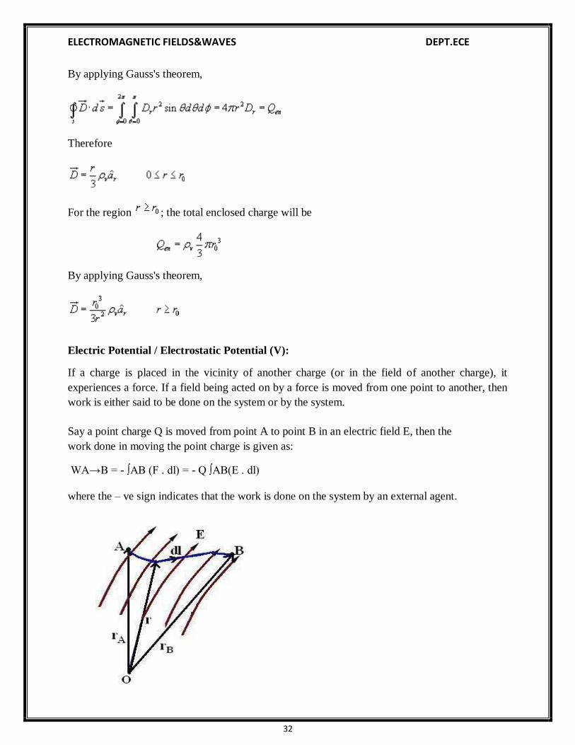
Electric Potential / Electrostatic Potential (V):

If a charge is placed in the vicinity of another charge (or in the field of another charge), it

experiences a force. If a field being acted on by a force is moved from one point to another, then

work is either said to be done on the system or by the system.

Say a point charge Q is moved from point A to point B in an electric field E, then the

work done in moving the point charge is given as:

WA→B = - ∫AB (F . dl) = - Q ∫AB(E . dl)

where the – ve sign indicates that the work is done on the system by an external agent.

33


The work done per unit charge in moving a test charge from point A to point B is the

electrostatic potential difference between the two points(VAB).

VAB = WA→B / Q

- ∫AB(E . dl)

- ∫InitialFinal (E . dl)

If the potential difference is positive, there is a gain in potential energy in the movement,

external agent performs the work against the field. If the sign of the potential difference is

negative, work is done by the field.

The electrostatic field is conservative i.e. the value of the line integral depends only on

end points and is independent of the path taken.

- Since the electrostatic field is conservative, the electric potential can also be written as:

𝐵

𝑉𝐴𝐵 = − ∫ 𝐸 . 𝑙 𝐴

𝑝0

𝑉𝐴𝐵 = − ∫ 𝐴

𝐵

𝐵

𝐸 . 𝑙 − ∫ 𝐸 . 𝑙 𝑝0

𝐴

𝑉𝐴𝐵 = − ∫ 𝐸 . 𝑙 + ∫ 𝐸 . 𝑙 𝑝0 𝑝0

𝑉𝐴𝐵 = 𝑉𝐵 − 𝑉𝐴

34

𝐴


Thus the potential difference between two points in an electrostatic field is a scalar field that

is defined at every point in space and is independent of the path taken.

- The work done in moving a point charge from point A to point B can be written as:

WA→B = - Q [VB – VA] = −𝑄 ∫𝐵

. 𝑙

- Consider a point charge Q at origin O.

Now if a unit test charge is moved from point A to Point B, then the potential difference between

them is given as:

- Electrostatic potential or Scalar Electric potential (V) at any point P is given by:

𝑃

𝑉 = − ∫ . 𝑙 𝑃0

35


The reference point Po is where the potential is zero (analogues to ground in a circuit).

The reference is often taken to be at infinity so that the potential of a point in space is

defined as

𝑃

𝑉 = − ∫ . 𝑙 ∞

Basically potential is considered to be zero at infinity. Thus potential at any point ( rB = r) due

to a point charge Q can be written as the amount of work done in bringing a unit positive

charge frominfinity to that point (i.e. rA → ∞)

Electric potential (V) at point r due to a point charge Q located at a point with position vector

r1 is given as:

Similarly for N point charges Q1, Q2 ….Qn located at points with position vectors r1,

r2, r3…..rn, theelectric potential (V) at point r is given as:

The charge element dQ and the total charge due to different charge distribution is given as:

dQ = ρldl → Q = ∫L (ρldl) → (Line Charge)

dQ = ρsds → Q = ∫S (ρsds) → (Surface Charge)

dQ = ρvdv → Q = ∫V (ρvdv) → (Volume Charge)

36


Second Maxwell’s Equation of Electrostatics:

The work done per unit charge in moving a test charge from point A to point B is the

electrostatic potential difference between the two points(VAB).

VAB = VB – VA

Similarly,

VBA = VA – VB

Hence it‘s clear that potential difference is independent of the path taken. Therefore

VAB = - VBA

VAB+ VBA = 0

∫AB (E . dl) + [ - ∫BA (E . dl) ] = 0

The above equation is called the second Maxwell‘s Equation of Electrostatics in integral form..

The above equation shows that the line integral of Electric field intensity (E) along a closed path

is equal to zero.

In simple words―No work is done in moving a charge along a closed path in an electrostatic

field.

Applying Stokes‘ Theorem to the above Equation, we have:

If the Curl of any vector field is equal to zero, then such a vector field is called an Irrotational or

Conservative Field. Hence an electrostatic field is also called a conservative field. The above equation is called the second Maxwell‘s Equation of Electrostatics in differential form.

37


Relationship Between Electric Field Intensity (E) and Electric Potential (V):

Since Electric potential is a scalar quantity, hence dV (as a function of x, y and z variables) can

be written as:

Hence the Electric field intensity (E) is the negative gradient of Electric potential (V).

The negative sign shows that E is directed from higher to lower values of V i.e. E is opposite to

the direction in which V increases.

Work Done To Assemble Charges:

In case, if we wish to assemble a number of charges in an empty system, work is required to do

so. Also electrostatic energy is said to be stored in such a collection.

Let us build up a system in which we position three point charges Q1, Q2 and Q3 at position r1,

r2 and r3 respectively in an initially empty system.

Consider a point charge Q1 transferred from infinity to position r1 in the system. It takes no

work to bring the first charge from infinity since there is no electric field to fight against (as the

system is empty i.e. charge free).

Hence, W1 = 0 J

Now bring in another point charge Q2 from infinity to position r2 in the system. In this case we

have to do work against the electric field generated by the first charge Q1.

Hence, W2 = Q2 V21

where V21 is the electrostatic potential at point r2 due to Q1.

- Work done W2 is also given as:

38


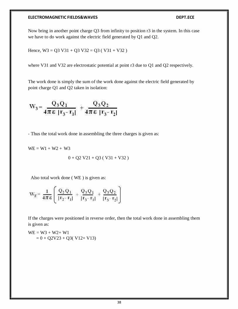
Now bring in another point charge Q3 from infinity to position r3 in the system. In this case

we have to do work against the electric field generated by Q1 and Q2.

Hence, W3 = Q3 V31 + Q3 V32 = Q3 ( V31 + V32 )

where V31 and V32 are electrostatic potential at point r3 due to Q1 and Q2 respectively.

The work done is simply the sum of the work done against the electric field generated by

point charge Q1 and Q2 taken in isolation:

- Thus the total work done in assembling the three charges is given as:

WE = W1 + W2 + W3

0 + Q2 V21 + Q3 ( V31 + V32 )

Also total work done ( WE ) is given as:

If the charges were positioned in reverse order, then the total work done in assembling them

is given as:

WE = W3 + W2+ W1

= 0 + Q2V23 + Q3( V12+ V13)

39


Where V23 is the electrostatic potential at point r2 due to Q3 and V12 and V13 are electrostatic

potential at point r1 due to Q2 and Q3 respectively.

- Adding the above two equations we have,

2WE = Q1 (V12 + V13) + Q2 (V21 + V23) + Q3 (V31 + V32)

= Q1 V1 + Q2 V2 + Q3 V3

Hence

WE =1 / 2 [Q1V1 + Q2V2 + Q3V3]

where V1, V2 and V3 are total potentials at position r1, r2 and r3 respectively.

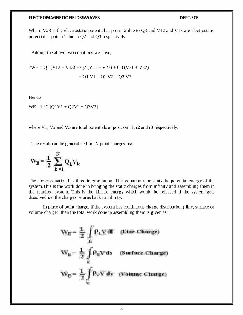
- The result can be generalized for N point charges as:

The above equation has three interpretation: This equation represents the potential energy of the

system.This is the work done in bringing the static charges from infinity and assembling them in

the required system. This is the kinetic energy which would be released if the system gets

dissolved i.e. the charges returns back to infinity.

In place of point charge, if the system has continuous charge distribution ( line, surface or

volume charge), then the total work done in assembling them is given as:

40


Since ρv = ∇ . D and E = - ∇ V,

Substituting the values in the above equation, work done in assembling a volume charge

distribution in terms of electric field and flux density is given as:

The above equation tells us that the potential energy of a continuous charge distribution

is stored in an electric field.

The electrostatic energy density wE is defined as:

Properties of Materials and Steady Electric Current:

Electric field can not only exist in free space and vacuum but also in any material medium. When

an electric field is applied to the material, the material will modify the electric field either by

strengthening it or weakening it, depending on what kind of material it is.

Materials are classified into 3 groups based on conductivity / electrical property:

Conductors (Metals like Copper, Aluminum, etc.) have high conductivity (σ >> 1).

Insulators / Dielectric (Vacuum, Glass, Rubber, etc.) have low conductivity (σ << 1).

Semiconductors (Silicon, Germanium, etc.) have intermediate conductivity.

Conductivity (σ) is a measure of the ability of the material to conduct electricity. It is

the reciprocal of resistivity (ρ). Units of conductivity are Siemens/meter and mho.

The basic difference between a conductor and an insulator lies in the amount of free electrons

available for conduction of current. Conductors have a large amount of free electrons where as

insulators have only a few number ofelectrons for conduction of current. Most of the conductors

obey ohm‘s law. Such conductors are also called ohmic conductors.

Due to the movement of free charges, several types of electric current can be caused.

The different types of electric current are:

Conduction Current.

Convection Current.

Displacement Current.

41

𝑆


Electric current:

Electric current (I) defines the rate at which the net charge passes through a wire of

cross sectional surface area S.

Mathematically,

If a net charge ΔQ moves across surface S in some small amount of time Δt, electric current(I)

is defined as:

How fast or how speed the charges will move depends on the nature of the material medium.

Current density:

Current density (J) is defined as current ΔI flowing through surface ΔS.

Imagine surface area ΔS inside a conductor at right angles to the flow of current. As the

area approaches zero, the current density at a point is defined as:

The above equation is applicable only when current density (J) is normal to the surface.

In case if current density(J) is not perpendicular to the surface, consider a small area ds of

the conductor at an angle θ to the flow of current as shown:

In this case current flowing through the area is given as:

dI = J dS cosθ = J . dS and 𝐼 = ∫ 𝐽.

42


Where angle θ is the angle between the normal to the area and direction of the current.

From the above equation it‘s clear that electric current is a scalar quantity.

CONVECTION CURRENT DENSITY:

Convection current occurs in insulators or dielectrics such as liquid, vacuum and rarified gas.

Convection current results from motion of electrons or ions in an insulating medium. Since

convection current doesn‘t involve conductors, hence it does not satisfy ohm‘s law. Consider a

filament where there is a flow of charge ρv at a velocity u = uy ay.

- Hence the current is given as:

43


Where uy is the velocity of the moving electron or ion and ρv is the free volume charge density.

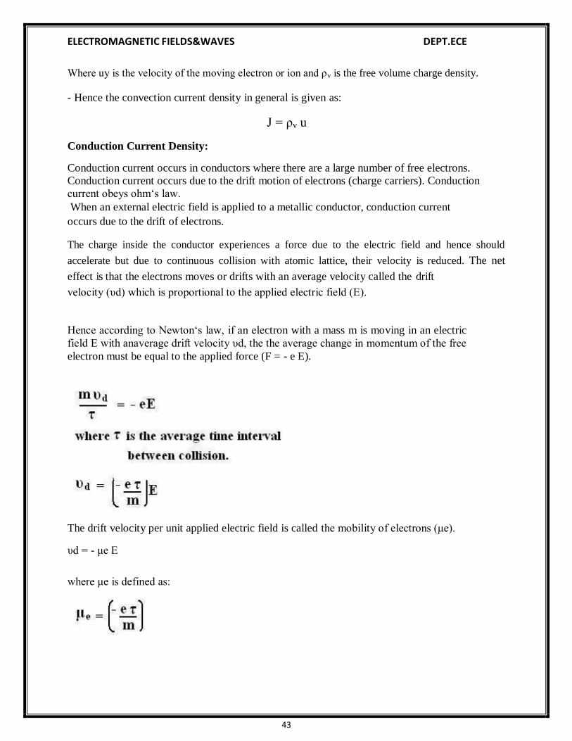
- Hence the convection current density in general is given as:

J = ρv u

Conduction Current Density:

Conduction current occurs in conductors where there are a large number of free electrons.

Conduction current occurs due to the drift motion of electrons (charge carriers). Conduction

current obeys ohm‘s law.

When an external electric field is applied to a metallic conductor, conduction current

occurs due to the drift of electrons.

The charge inside the conductor experiences a force due to the electric field and hence should

accelerate but due to continuous collision with atomic lattice, their velocity is reduced. The net

effect is that the electrons moves or drifts with an average velocity called the drift

velocity (υd) which is proportional to the applied electric field (E).

Hence according to Newton‘s law, if an electron with a mass m is moving in an electric

field E with anaverage drift velocity υd, the the average change in momentum of the free

electron must be equal to the applied force (F = - e E).

The drift velocity per unit applied electric field is called the mobility of electrons (μe).

υd = - μe E

where μe is defined as:

44


Consider a conducting wire in which charges subjected to an electric field are moving with

drift velocity υd.

Say there are Ne free electrons per cubic meter of conductor, then the free volume

charge density(ρv)within the wire is

ρv= - e Ne

The charge ΔQ is given as:

ΔQ = ρv ΔV = - e Ne ΔS Δl = - e Ne ΔS υd Δt

- The incremental current is thus given as:

The conduction current density is thus defined as:

where σ is the conductivity of the material.

The above equation is known as the Ohm‘s law in point form and is valid at every point

in space.

In a semiconductor, current flow is due to the movement of both electrons and

holes, hence conductivity is given as:

σ = ( Ne μe + Nh μh )e

45


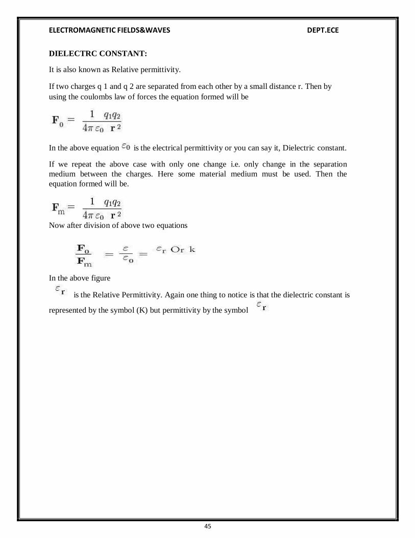
DIELECTRC CONSTANT:

It is also known as Relative permittivity.

If two charges q 1 and q 2 are separated from each other by a small distance r. Then by

using the coulombs law of forces the equation formed will be

In the above equation is the electrical permittivity or you can say it, Dielectric constant.

If we repeat the above case with only one change i.e. only change in the separation

medium between the charges. Here some material medium must be used. Then the

equation formed will be.

Now after division of above two equations

In the above figure

is the Relative Permittivity. Again one thing to notice is that the dielectric constant is

represented by the symbol (K) but permittivity by the symbol

46


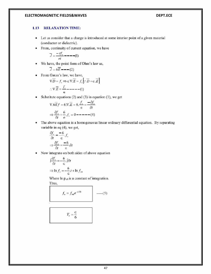
CONTINUITY EQUATION:

The continuity equation is derived from two of Maxwell's equations. It states that the

divergence of the current density is equal to the negative rate of change of the charge density,

Derivation

One of Maxwell's equations, Ampère's law, states that

Taking the divergence of both sides results in

but the divergence of a curl is zero, so that

Another one of Maxwell's equations, Gauss's law, states that

Substitute this into equation (1) to obtain

which is the continuity equation.

47


48


49


LAPLACE'S AND POISSON'S EQUATIONS:

A useful approach to the calculation of electric potentials is to relate that potential to the

charge density which gives rise to it. The electric field is related to the charge density by the

divergence relationship

and the electric field is related to the electric potential by a gradient relationship

Therefore the potential is related to the charge density by Poisson's equation

In a charge-free region of space, this becomes LaPlace's equation

This mathematical operation, the divergence of the gradient of a function, is called the

LaPlacian. Expressing the LaPlacian in different coordinate systems to take advantage of the

symmetry of a charge distribution helps in the solution for the electric potential V. For example,

if the charge distribution has spherical symmetry, you use the LaPlacian in spherical polar

coordinates.

Since the potential is a scalar function, this approach has advantages over trying to calculate the

electric field directly. Once the potential has been calculated, the electric field can be computed

by taking the gradient of the potential.

50


Polarization of Dielectric:

If a material contains polar molecules, they will generally be in random orientations when

no electric field is applied. An applied electric field will polarize the material by orienting

the dipole moments of polar molecules.

This decreases the effective electric

field between the plates and will

increase the capacitance of the parallel

plate structure. The dielectric must be

a good electric insulator so as to

minimize any DC leakage current

through a capacitor.

The presence of the dielectric decreases the electric field produced by a given charge density.

The factor k by which the effective field is decreased by the polarization of the

dielectric is called the dielectric constant of the material.

51


Solved problems:

Problem1:

Problem-2

Problem-3

Problem-4

Problem-5

52


Problem-6

53


Contents:

Biot - Savart's Law

UNIT-III

MAGNETOSTATICS

Ampere's Circuital Law and Applications

Magnetic Flux Density

Maxwell’s Equations for Magnetostatic Fields

Magnetic Scalar and Vector Potentials

Ampere's Force Law

Faraday's Law

Transformer EMF

Displacement Current Density

Maxwell's Equations for time varying fields

Illustrative Problems.

54


Introduction:

In previous chapters we have seen that an electrostatic field is produced by static or stationary charges.

The relationship of the steady magnetic field to its sources is much more complicated.

The source of steady magnetic field may be a permanent magnet, a direct current or an electric

field changing with time. In this chapter we shall mainly consider the magnetic field produced by

a direct current. The magnetic field produced due to time varying electric field will be discussed

later.

There are two major laws governing the magneto static fields are:

Biot-Savart Law

Ampere's Law

Usually, the magnetic field intensity is represented by the vector . It is customary to represent the

direction of the magnetic field intensity (or current) by a small circle with a dot or cross sign

depending on whether the field (or current) is out of or into the page as shown in Fig. 2.1.

(or l ) into the page

Fig. Representation of magnetic field (or current)

Biot- Savart’s Law:

This law relates the magnetic field intensity dH produced at a point due to a differential

current element as shown in Fig.

(or l ) out of the page

55


The magnetic field intensity at P can be written as,

where is the distance of the current element from the point P.

The value of the constant of proportionality 'K' depends upon a property called permeability of

the medium around the conductor. Permeability is represented by symbol 'm' and the constant 'K'

is expressed in terms of 'm' as

Magnetic field 'B' is a vector and unless we give the direction of 'dB', its description is not

complete. Its direction is found to be perpendicular to the plane of 'r' and 'dl'.

If we assign the direction of the current 'I' to the length element 'dl', the vector product dl x r has

magnitude r dl sinq and direction perpendicular to 'r' and 'dl'.

Hence, Biot–Savart law can be stated in vector form to give both the magnitude as well as

direction of magnetic field due to a current element as

56


Similar to different charge distributions, we can have different current distribution such as

line current, surface current and volume current. These different types of current densities are

shown in Fig. 2.3.

Line Current Surface Current Volume Current

Fig. 2.3: Different types of current distributions

By denoting the surface current density as K (in amp/m) and volume current density as J

(in amp/m2) we can write:

( It may be noted that )

Employing Biot -Savart Law, we can now express the magnetic field intensity H. In terms of

these current distributions as

............................. for line current............................

........................ for surface current ....................

....................... for volume current......................

57


Due to infinitely long straight conductor:

We consider a finite length of a conductor carrying a current placed along z-axis as shown in

the Fig 2.4. We determine the magnetic field at point P due to this current carrying conductor.

Fig. 2.4: Field at a point P due to a finite length current carrying conductor

With reference to Fig. 2.4, we find that

Applying Biot - Savart's law for the current element We can write,

Substituting we can write,

We find that, for an infinitely long conductor carrying a current I , and

Therefore

58


Ampere's Circuital Law:

Ampere's circuital law states that the line integral of the magnetic field (circulation of H )

around a closed path is the net current enclosed by this path. Mathematically,

The total current I enc can be written as,

By applying Stoke's theorem, we can write

Which is the Ampere's circuital law in the point form and Maxwell’s equation for magneto static

fields.

59


Applications of Ampere's circuital law:

1. It is used to find and due to any type of current distribution.

2. If or is known then it is also used to find current enclosed by any closed path.

We illustrate the application of Ampere's Law with some examples.

Due to infinitely long straight conductor :( using Ampere's circuital law)

We compute magnetic field due to an infinitely long thin current carrying conductor as

shown in Fig. 2.5. Using Ampere's Law, we consider the close path to be a circle of

radius as shown in the Fig. 4.5.

If we consider a small current element , is perpendicular to the plane

containing both and . Therefore only component of that will be present is

,i.e., .

By applying Ampere's law we can write,

Fig. Magnetic field due to an infinite thin current carrying conductor

60


Due to infinitely long coaxial conductor :( using Ampere's circuital law)

We consider the cross section of an infinitely long coaxial conductor, the inner conductor

carrying a current I and outer conductor carrying current - I as shown in figure 2.6. We

compute the magnetic field as a function of as follows:

In the region

In the region

Fig. 2.6: Coaxial conductor carrying equal and opposite currents in the region

In the region

61


Magnetic Flux Density:

In simple matter, the magnetic flux density related to the magnetic field intensity as

where called the permeability. In particular when we consider the free space

where H/m is the permeability of the free space. Magnetic flux density is

measured in terms of Wb/m 2 .

The magnetic flux density through a surface is given by:

Wb

In the case of electrostatic field, we have seen that if the surface is a closed surface, the net flux

passing through the surface is equal to the charge enclosed by the surface. In case of magnetic

field isolated magnetic charge (i. e. pole) does not exist. Magnetic poles always occur in pair (as

N-S). For example, if we desire to have an isolated magnetic pole by dividing the magnetic bar

successively into two, we end up with pieces each having north (N) and south (S) pole as shown

in Fig. 6 (a). This process could be continued until the magnets are of atomic dimensions; still

we will have N-S pair occurring together. This means that the magnetic poles cannot be isolated.

Fig. 6: (a) Subdivision of a magnet (b) Magnetic field/ flux lines of a straight current carrying

conductor

Maxwell’s 2nd equation for static magnetic fields:

Similarly if we consider the field/flux lines of a current carrying conductor as shown in Fig. 6

(b), we find that these lines are closed lines, that is, if we consider a closed surface, the number

of flux lines that would leave the surface would be same as the number of flux lines that would

enter the surface.

From our discussions above, it is evident that for magnetic field,

62


......................................in integral form

which is the Gauss's law for the magnetic field.

By applying divergence theorem, we can write:

Hence, ...................................................................................... in point/differential form

which is the Gauss's law for the magnetic field in point form.

Magnetic Scalar and Vector Potentials:

In studying electric field problems, we introduced the concept of electric potential that simplified

the computation of electric fields for certain types of problems. In the same manner let us relate

the magnetic field intensity to a scalar magnetic potential and write:

From Ampere's law , we know that

Therefore,

But using vector identity, we find that is valid only where .

Thus the scalar magnetic potential is defined only in the region where . Moreover, Vm in

general is not a single valued function of position. This point can be illustrated as follows. Let us

consider the cross section of a coaxial line as shown in fig 7.

In the region , and

63


Fig. 7: Cross Section of a Coaxial Line

If Vm is the magnetic potential then,

If we set Vm = 0 at then c=0 and

We observe that as we make a complete lap around the current carrying conductor , we reach

again but Vm this time becomes

We observe that value of Vm keeps changing as we complete additional laps to pass through the

same point. We introduced Vm analogous to electostatic potential V.

But for static electric fields,

and

whereas for steady magnetic field wherever but even if

along the path of integration.

We now introduce the vector magnetic potential which can be used in regions where

current density may be zero or nonzero and the same can be easily extended to time varying

cases. The use of vector magnetic potential provides elegant ways of solving EM field problems.

Since and we have the vector identity that for any vector , , we

can write .

Here, the vector field is called the vector magnetic potential. Its SI unit is Wb/m.

Thus if can find of a given current distribution, can be found from through a curl

operation. We have introduced the vector function and related its curl to . A vector

function is defined fully in terms of its curl as well as divergence. The choice of is made as

follows.

64


By using vector identity,

Great deal of simplification can be achieved if we choose .

Putting , we get which is vector poisson equation.

In Cartesian coordinates, the above equation can be written in terms of the components as

.

The form of all the above equation is same as that of

for which the solution is

In case of time varying fields we shall see that , which is known as Lorentz condition, V being

the electric potential. Here we are dealing with static magnetic field, so .

By comparison, we can write the solution for Ax as

Computing similar solutions for other two components of the vector potential, the vector

potential can be written as

This equation enables us to find the vector potential at a given point because of a volume current

density .

Similarly for line or surface current density we can write

65


.

The magnetic flux through a given area S is given by

Substituting

Vector potential thus have the physical significance that its integral around any closed path is

equal to the magnetic flux passing through that path.

66


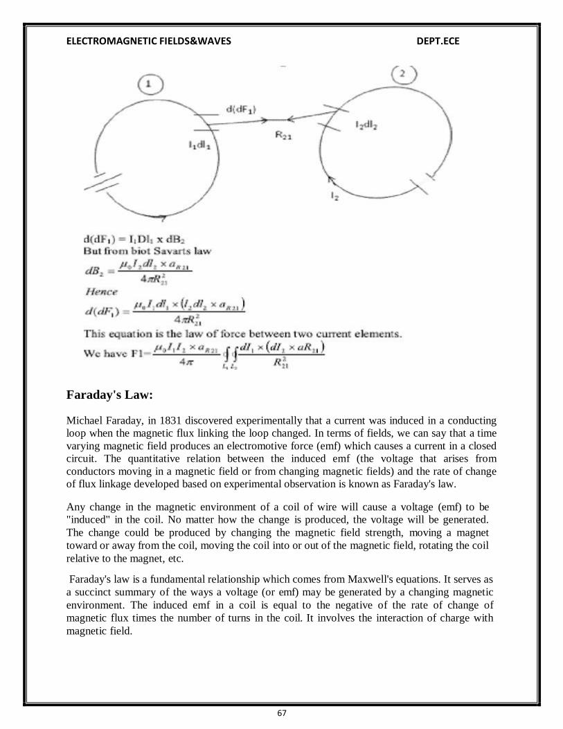
Forces due to magnetic fields

67


Faraday's Law:

Michael Faraday, in 1831 discovered experimentally that a current was induced in a conducting

loop when the magnetic flux linking the loop changed. In terms of fields, we can say that a time

varying magnetic field produces an electromotive force (emf) which causes a current in a closed

circuit. The quantitative relation between the induced emf (the voltage that arises from

conductors moving in a magnetic field or from changing magnetic fields) and the rate of change

of flux linkage developed based on experimental observation is known as Faraday's law.

Any change in the magnetic environment of a coil of wire will cause a voltage (emf) to be

"induced" in the coil. No matter how the change is produced, the voltage will be generated.

The change could be produced by changing the magnetic field strength, moving a magnet

toward or away from the coil, moving the coil into or out of the magnetic field, rotating the coil

relative to the magnet, etc.

Faraday's law is a fundamental relationship which comes from Maxwell's equations. It serves as

a succinct summary of the ways a voltage (or emf) may be generated by a changing magnetic

environment. The induced emf in a coil is equal to the negative of the rate of change of

magnetic flux times the number of turns in the coil. It involves the interaction of charge with

magnetic field.

68


When two current carrying conductors are placed next to each other, we notice that each induces

a force on the other. Each conductor produces a magnetic field around itself (Biot– Savart law)

and the second experiences a force that is given by the Lorentz force.

Mathematically, the induced emf can be written as

Emf = Volts

where is the flux linkage over the closed path.

A non zero may result due to any of the following:

(a) time changing flux linkage a stationary closed path.

(b) relative motion between a steady flux a closed path.

(c) a combination of the above two cases.

The negative sign in equation (7) was introduced by Lenz in order to comply with the

polarity of the induced emf. The negative sign implies that the induced emf will cause a current

flow in the closed loop in such a direction so as to oppose the change in the linking magnetic

flux which produces it. (It may be noted that as far as the induced emf is concerned, the closed

path forming a loop does not necessarily have to be conductive).

If the closed path is in the form of N tightly wound turns of a coil, the change in the

magnetic flux linking the coil induces an emf in each turn of the coil and total emf is the sum of

the induced emfs of the individual turns, i.e.,

Emf = Volts

By defining the total flux linkage as

69


The emf can be written as

Emf =

Continuing with equation (3), over a closed contour 'C' we can write

Emf =

where is the induced electric field on the conductor to sustain the current.

Further, total flux enclosed by the contour 'C ' is given by

Where S is the surface for which 'C' is the contour.

From (11) and using (12) in (3) we can write

By applying stokes theorem

Therefore, we can write

which is the Faraday's law in the point form

We have said that non zero can be produced in a several ways. One particular case is when a

time varying flux linking a stationary closed path induces an emf. The emf induced in a

stationary closed path by a time varying magnetic field is called a transformer emf .

70


71


MAXWELL’S EQUATIONS (Time varying Fields)

Introduction:

In our study of static fields so far, we have observed that static electric fields are produced by

electric charges, static magnetic fields are produced by charges in motion or by steady current.

Further, static electric field is a conservative field and has no curl, the static magnetic field is

continuous and its divergence is zero. The fundamental relationships for static electric fields

among the field quantities can be summarized as:

(1)

(2)

For a linear and isotropic medium,

(3)

Similarly for the magnetostatic case

(4)

(5)

(6)

It can be seen that for static case, the electric field vectors and and magnetic field

vectors and form separate pairs.

In this chapter we will consider the time varying scenario. In the time varying case we

will observe that a changing magnetic field will produce a changing electric field and vice versa.

We begin our discussion with Faraday's Law of electromagnetic induction and then

present the Maxwell's equations which form the foundation for the electromagnetic theory.

Maxwell's equations represent one of the most elegant and concise ways to state the

fundamentals of electricity and magnetism. From them one can develop most of the working

relationships in the field. Because of their concise statement, they embody a high level of

mathematical sophistication and are therefore not generally introduced in an introductory

treatment of the subject, except perhaps as summary relationships.

These basic equations of electricity and magnetism can be used as a starting point for advanced

courses, but are usually first encountered as unifying equations after the study of electrical and

magnetic phenomena.

72


Symbols Used

E = Electric field ρ = charge density i = electric current

B = Magnetic field ε0 = permittivity J = current density

D = Electric displacement μ0 = permeability c = speed of light

H = Magnetic field strength

M = Magnetization P = Polarization

Integral form in the absence of magnetic or polarizable media:

I. Gauss' law for electricity

Gauss' law for magnetism

III. Faraday's law of induction

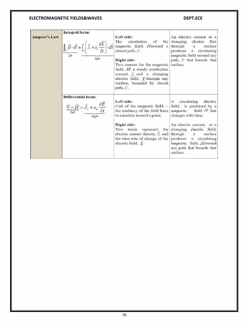
IV. Ampere's law

73


Differential form in the absence of magnetic or polarizable media:


Gauss' law for magnetism


IV. Ampere's law

Differential form with magnetic and/or polarizable media:


74



IV. Ampere's law

II. Gauss' law for magnetism

75


76


77


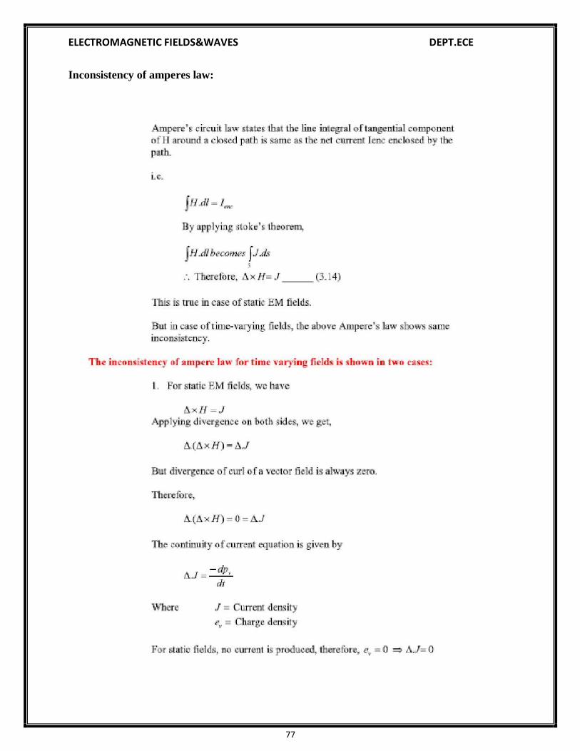
Inconsistency of amperes law:

78


79


80


Solved problems:

Problem1:

81


Problem2:

82


Problem3:

Problem4:

83


Problem5:

84


Problem6:

85


Problem7:

Problem8:

86


87


88


UNIT – IV

EM WAVE CHARACTERISTICS-I

Wave Equations for Conducting and Perfect Dielectric Media

Uniform Plane Waves - Definition, Relation between E & H

Wave Propagation in Lossless and Conducting Media

Wave Propagation in Good Conductors and Good Dielectrics


89

from 1


Wave equations:

The Maxwell's equations in the differential form are

Let us consider a source free uniform medium having dielectric constant , magnetic

permeability and conductivity . The above set of equations can be written as

Using the vector identity ,

We can write from 2

Substituting

But in source free(

In the same manner for equation eqn 1

Since from eqn 4, we can write

) medium (eq3)

90


These two equations

are known as wave equations.

Uniform plane waves:

A uniform plane wave is a particular solution of Maxwell's equation assuming electric

field (and magnetic field) has same magnitude and phase in infinite planes perpendicular to the

direction of propagation. It may be noted that in the strict sense a uniform plane wave doesn't

exist in practice as creation of such waves are possible with sources of infinite extent. However,

at large distances from the source, the wave front or the surface of the constant phase becomes

almost spherical and a small portion of this large sphere can be considered to plane. The

characteristics of plane waves are simple and useful for studying many practical scenarios

Let us consider a plane wave which has only Ex component and propagating along z .

Since the plane wave will have no variation along the plane perpendicular to z

i.e., xy plane, . The Helmholtz's equation reduces to,

The solution to this equation can be written as

are the amplitude constants (can be determined from boundary conditions).

In the time domain,

assuming are real constants.

Here, represents the forward traveling wave. The plot of

for several values of t is shown in the Figure below

91


Figure : Plane wave traveling in the + z direction

As can be seen from the figure, at successive times, the wave travels in the +z direction.

If we fix our attention on a particular point or phase on the wave (as shown by the dot) i.e. ,

= constant

Then we see that as t is increased to , z also should increase to so that

Or,

Or,

When ,

we write = phase velocity .

If the medium in which the wave is propagating is free space i.e.,

Then

Where 'C' is the speed of light. That is plane EM wave travels in free space with the speed of

light.

The wavelength is defined as the distance between two successive maxima (or minima or

any other reference points).

i.e.,

or,

or,

92


Substituting ,

or,

Thus wavelength also represents the distance covered in one oscillation of the wave.

Similarly, represents a plane wave traveling in the -z direction.

The associated magnetic field can be found as follows:

From (6.4),

=

=

where is the intrinsic impedance of the medium.

When the wave travels in free space

is the intrinsic impedance of the free space.

In the time domain,

Which represents the magnetic field of the wave traveling in the +z direction.

For the negative traveling wave,

For the plane waves described, both the E & H fields are perpendicular to the direction of

propagation, and these waves are called TEM (transverse electromagnetic) waves.

The E & H field components of a TEM wave is shown in Fig below

93


1

Figure : E & H fields of a particular plane wave at time t.

Solved Problems:

1. The vector amplitude of an electric field associated with a plane wave that propagates in

the negative z direction in free space is given by m 2 ax 3ay V

m

Find the magnetic field strength.

Solution:

The direction of propagation nβ is –az. The vector amplitude of the magnetic field is then given

n ax ay az 1

by m

0 0 1 377

3ax 2 ay A

m

2 3 0

*note 120π~377Ω (Appendix D – Table D.1)

2. The phasor electric field expression in a phase is given by

ax y a y 2

Find the following:

j5 az e j2.3(0.6x0.8 y)

1. y .

2. Vector magnetic field, assuming and .

3. Frequency and wavelength of this wave.

94


Solution:

1. The general expression for a uniform plane wave propagating in an arbitrary direction is given by

m e j r

where the amplitude vector m , in general, has components in the x, y, and z

directions. Comparing equation 6.3 with the general field equation for the plane wave propagating in an arbitrary direction, we obtain

β · r = βxx + βyy + βzz

= β (cos θxx + cos θyy + cos θzz) = 2.3(-0.6x + 0.8y + 0)

Hence, a unit vector in the direction of propagation nβ is given by nβ = -0.6ax + 0.8ay.

Because the electric field must be perpendicular to the direction of propagation nβ, it must

satisfy the following relations:

nβ · = 0

Therefore, (-0.6ax + 0.8ay) · ax y ay 2 j5 az 0

Or

-0.6 + 0.8 y = 0

Hence, y = 0.75. The electric field is given by

a x y a y 2 j5 az e j2.3(0.6x0.8 y)

2. The vector magnetic field is given by

1 1 ax ay az

n

377 0.6 0.8 0

1 0.75 2 j5

so that

x 0.8(2

377

j5) 4.24 j10.6103

95

y


0.6(2 j5)

3.18

377 j7.95103

z

0.60.75 0.8 3.31103

377

The vector magnetic field is then given by

x ax y ay z az e j2.3(0.6x0.8y)

3. The wavelength λ is given by

2

2

2.73 m

2.3

and the frequency

f c

3108

0.11GHz

2.73

10.3 WAVE PROPAGATION IN LOSSY DIELECTRICS 417

- 50 sin jix

Figure 10.3 For Example 10.1; wavetravels along — ax.

(c) t = Tl

PRACTICE EXERCISE 10.1 J

In free space, H = 0.1 cos (2 X 108/ - kx) ay A/m. Calculate

(a) k, A, and T(b) The time tx it takes the wave to travel A/8(c) Sketch the wave at time tx.

Answer: (a) 0.667 rad/m, 9.425 m, 31.42 ns, (b) 3.927 ns, (c) see Figure 10.4.

0.3 WAVE PROPAGATION IN LOSSY DIELECTRICS

As mentioned in Section 10.1, wave propagation in lossy dielectrics is a general case fromwhich wave propagation in other types of media can be derived as special cases. Therefore,this section is foundational to the next three sections.

418 • Electromagnetic Wave Propagation

0. 1 " >

Figure 10.4 For Practice Exercise 10.1(c).

A lossy dielectric is a medium in which an EM wave loses power as it propagatesdue to poor conduction.

In other words, a lossy dielectric is a partially conducting medium (imperfect dielectric orimperfect conductor) with a ¥= 0, as distinct from a lossless dielectric (perfect or good di-electric) in which a = 0.

Consider a linear, isotropic, homogeneous, lossy dielectric medium that is charge free(pv = 0). Assuming and suppressing the time factor ej"', Maxwell's equations (see Table9.2) become

V • E, = 0

V • Hs = 0

V X Es = -ju>nHs

Taking the curl of both sides of eq. (10.13) gives

V X V X Es = -join V X H S

Applying the vector identity

VX V X A = V(V-A) - V2A

(10.11)

(10.12)

(10.13)

(10.14)

(10.15)

(10.16)

to the left-hand side of eq. (10.15) and invoking eqs. (10.11) and (10.14), we obtain

V(V/E, ) - V2ES = -j

or

V2ES - 72ES = 0 (10.17)

where

7 = j'w/ Cff + j (10.18)

10.3 WAVE PROPAGATION IN LOSSY DIELECTRICS 419

and y is called the propagation constant (in per meter) of the medium. By a similar proce-dure, it can be shown that for the H field,

V2HS - y2Ks = 0 (10.19)

Equations (10.17) and (10.19) are known as homogeneous vector Helmholtz 's equations orsimply vector wave equations. In Cartesian coordinates, eq. (10.17), for example, is equiv-alent to three scalar wave equations, one for each component of E along ax, ay, and az.

Since y in eqs. (10.17) to (10.19) is a complex quantity, we may let

y = a + j/3

We obtain a and /3 from eqs. (10.18) and (10.20) by noting that

Re y2 = P2 - a2 = (f

and

\y2\ = 01 + a2 = ufi VV + co

From eqs. (10.21) and (10.22), we obtain

V

(10.20)

(10.21)

(10.22)

Oi =

6 =

V 2 [V

•°v 2 [V

acos

coe

J2 "I

J

(10.23)

(10.24)

Without loss of generality, if we assume that the wave propagates along +az and thatEs has only an x-component, then

Es = Exs(z)ax

Substituting this into eq. (10.17) yields

(V2 - y2)Exs(z)

Hence

d2Exs(z)

(10.25)

(10.26)

or,2

—2 - y2 \Exs(z) = 0dz

(10.27)

420 B Electromagnetic Wave Propagation

This is a scalar wave equation, a linear homogeneous differential equation, with solution(see Case 2 in Example 6.5)

EJx) = Eoe'yz + E'oeyz (10.28)

where Eo and E'o are constants. The fact that the field must be finite at infinity requires thatE'o = 0. Alternatively, because eiz denotes a wave traveling along —az whereas we assumewave propagation along az, E'o = 0. Whichever way we look at it, E'o = 0. Inserting thetime factor ejo" into eq. (10.28) and using eq. (10.20), we obtain

Efc t) = Re aJ = Re (Eoe-azeji"'-0z)ax)

or

Efo i) = Eoe~azcos(at - j3z)ax (10.29)

A sketch of |E| at times t = 0 and t = At is portrayed in Figure 10.5, where it is evidentthat E has only an x-component and it is traveling along the +z-direction. Having obtainedE(z, t), we obtain H(z, t) either by taking similar steps to solve eq. (10.19) or by using eq.(10.29) in conjunction with Maxwell's equations as we did in Example 9.8. We will even-tually arrive at

H(z, t) = Re (Hoe-ayM-ft) ) (10.30)

where

H - ^ (10.31)

and 77 is a complex quantity known as the intrinsic impedance (in ohms) of the medium. Itcan be shown by following the steps taken in Example 9.8 that

V = (10.32)

Figure 10.5 £-field with x-componenttraveling along +z-direction at timest = 0 and t = At; arrows indicate in-stantaneous values of E.

10.3 WAVE PROPAGATION IN LOSSY DIELECTRICS • 421

with

(10.33)

where 0 < 6V < 45°. Substituting eqs. (10.31) and (10.32) into eq. (10.30) gives

or

H = ~\ e~az cos(co? - pz- 0,) (10.34)

Notice from eqs. (10.29) and (10.34) that as the wave propagates along az, it decreases orattenuates in amplitude by a factor e~az, and hence a is known as the attenuation constantor attenuation factor of the medium. It is a measure of the spatial rate of decay of the wavein the medium, measured in nepers per meter (Np/m) or in decibels per meter (dB/m). Anattenuation of 1 neper denotes a reduction to e~l of the original value whereas an increaseof 1 neper indicates an increase by a factor of e. Hence, for voltages

1 Np = 20 log10 e = 8.686 dB (10.35)

From eq. (10.23), we notice that if a = 0, as is the case for a lossless medium and freespace, a = 0 and the wave is not attenuated as it propagates. The quantity (3 is a measureof the phase shift per length and is called the phase constant or wave number. In terms of/?, the wave velocity u and wavelength X are, respectively, given by [see eqs. (10.7b) and(10.8)]

COX = 2x

0(10.36)

We also notice from eqs. (10.29) and (10.34) that E and H are out of phase by 0, at anyinstant of time due to the complex intrinsic impedance of the medium. Thus at any time, Eleads H (or H lags E) by 6V. Finally, we notice that the ratio of the magnitude of the con-duction current density J to that of the displacement current density Jd in a lossy mediumis

IX* 0)8= tan I

or

tan 6 = —coe (10.37)

422 Electromagnetic Wave Propagation

where tan 6 is known as the loss tangent and d is the loss angle of the medium as illustratedin Figure 10.6. Although a line of demarcation between good conductors and lossy di-electrics is not easy to make, tan 6 or 6 may be used to determine how lossy a medium is.A medium is said to be a good (lossless or perfect) dielectric if tan d is very small(<j <SC we) or a good conductor if tan 0 is very large (a 5> we). From the viewpoint ofwave propagation, the characteristic behavior of a medium depends not only on its consti-tutive parameters a, e, and fx but also on the frequency of operation. A medium that is re-garded as a good conductor at low frequencies may be a good dielectric at high frequen-cies. Note from eqs. (10.33) and (10.37) that

From eq. (10.14)

V X Hs = (o + jue)Es = jws 1 - E,

(10.38)

(10.39)

where

(10.40a)

or

ec = e (10.40b)

and e' = e, s" = a/w; sc is called the complex permittivity of the medium. We observe thatthe ratio of e" to e' is the loss tangent of the medium; that is,

e atan d = — = —e we

(10.41)

In subsequent sections, we will consider wave propagation in other types of media,which may be regarded as special cases of what we have considered here. Thus we willsimply deduce the governing formulas from those obtained for the general case treated inthis section. The student is advised not just to memorize the formulas but to observe howthey are easily obtained from the formulas for the general case.

Jds = Figure 10.6 Loss angle of a lossy medium.

JJ5 = oEs

10.5 PLANE WAVES IN FREE SPACE • 423

10.4 PLANE WAVES IN LOSSLESS DIELECTRICS

In a lossless dielectric, a <$C we. It is a special case of that in Section 10.3 except that

a - 0, e = eosr, n = fiofir

Substituting these into eqs. (10.23) and (10.24) gives

a = 0, /3 = WV/JLE

1 - TJXS

Also

and thus E and H are in time phase with each other.

(10.42)

(10.43a)

(10.43b)

(10.44)

i 0.5 PLANE WAVES IN FREE SPACE

This is a special case of what we considered in Section 10.3. In this case,

a - 0, e - eo, (10.45)

This may also be regarded as a special case of Section 10.4. Thus we simply replace e byeo and \k by /xo in eq. (10.43) or we substitute eq. (10.45) directly into eqs. (10.23) and(10.24). Either way, we obtain

a = 0, /3 = wV/xoso = —

u = = c, X =

(10.46a)

(10.46b)

where c — 3 X 108 m/s, the speed of light in a vacuum. The fact that EM wave travels infree space at the speed of light is significant. It shows that light is the manifestation of anEM wave. In other words, light is characteristically electromagnetic.

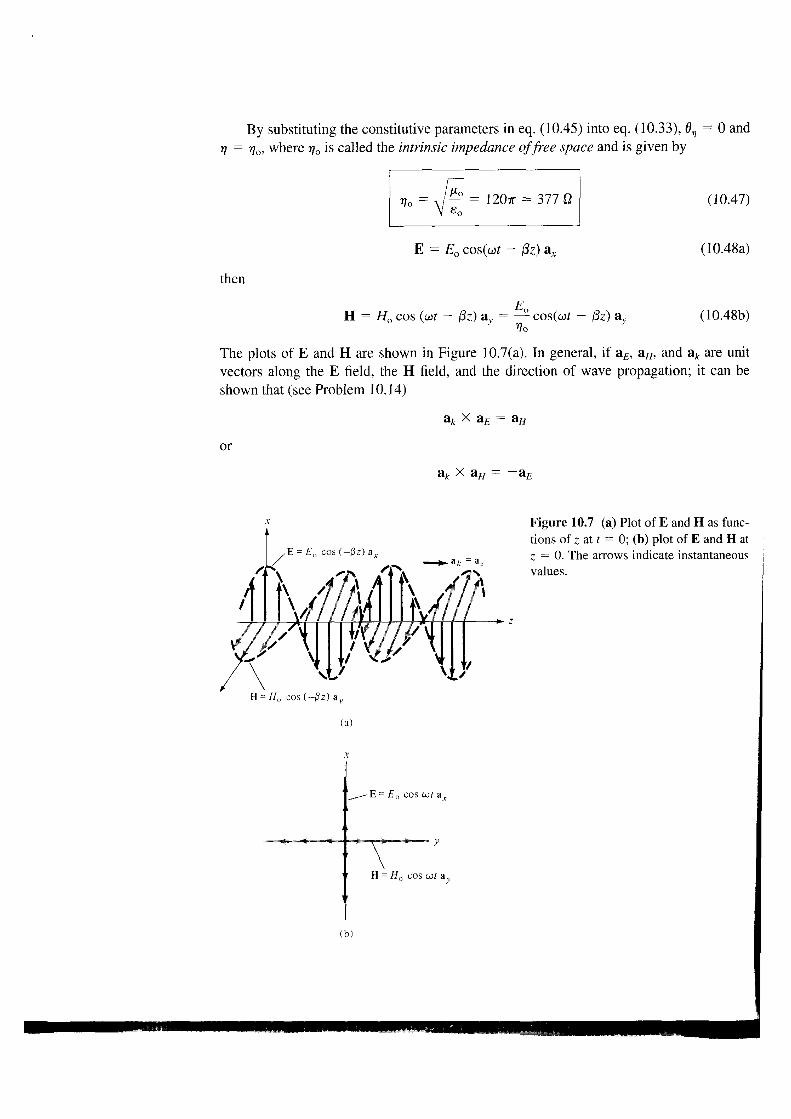
424 • Electromagnetic Wave Propagation

By substituting the constitutive parameters in eq. (10.45) into eq. (10.33), dv = 0 andV = ^oi where rjo is called the intrinsic impedance of free space and is given by

(10.47)

E = Eo - (3z)

then

H = Ho cos (ut - f3z) &y = —- cos(cof - (3z)

(10.48a)

(10.48b)

The plots of E and H are shown in Figure 10.7(a). In general, if a£, aH, and ak are unitvectors along the E field, the H field, and the direction of wave propagation; it can beshown that (see Problem 10.14)

ak X a£ = aH

orX aH = -

Figure 10.7 (a) Plot of E and H as func-tions of z at t = 0; (b) plot of E and H atz = 0. The arrows indicate instantaneousvalues.

(a)

-E = Eo cos oj/ ax

H = Ho cos ut ay

(b)

10.6 PLANE WAVES IN GOOD CONDUCTORS 425

or

aE X aH = ak (10.49)

Both E and H fields (or EM waves) are everywhere normal to the direction of wave prop-agation, ak. That means, the fields lie in a plane that is transverse or orthogonal to the di-rection of wave propagation. They form an EM wave that has no electric or magnetic fieldcomponents along the direction of propagation; such a wave is called a transverse electro-magnetic (TEM) wave. Each of E and H is called a uniform plane wave because E (or H)has the same magnitude throughout any transverse plane, defined by z = constant. The di-rection in which the electric field points is the polarization of a TEM wave.3 The wave ineq. (10.29), for example, is polarized in the ^-direction. This should be observed in Figure10.7(b), where an illustration of uniform plane waves is given. A uniform plane wavecannot exist physically because it stretches to infinity and would represent an infiniteenergy. However, such waves are characteristically simple but fundamentally important.They serve as approximations to practical waves, such as from a radio antenna, at distancessufficiently far from radiating sources. Although our discussion after eq. (10.48) deals withfree space, it also applies for any other isotropic medium.

0.6 PLANE WAVES IN GOOD CONDUCTORS

This is another special case of that considered in Section 10.3. A perfect, or good conduc-tor, is one in which a S> we so that a/we —> °o; that is,

a — °°, e = so, JX = fionr

Hence, eqs. (10.23) and (10.24) become

a = 13 =

Also,

and thus E leads H by 45°. If

E = Eoe~azcos(a)t - j8z) ax

(10.50)

(10.51a)

(10.51b)

(10.52)

(10.53a)

3Some texts define polarization differently.

426 P Electromagnetic Wave Propagation

then

H = az cos(co? — &z — 45°) a.. (10.53b)

Therefore, as E (or H) wave travels in a conducting medium, its amplitude is attenuated bythe factor e~az. The distance <5, shown in Figure 10.8, through which the wave amplitudedecreases by a factor e~l (about 37%) is called skin depth or penetration depth of themedium; that is,

or

a (10.54a)

The skin depth is a measure of the depth to which an EM wave can penetrate themedium.

Equation (10.54a) is generally valid for any material medium. For good conductors,eqs. (10.51a) and (10.54a) give

<5 = —^ (10.54b)

The illustration in Figure 10.8 for a good conductor is exaggerated. However, for apartially conducting medium, the skin depth can be considerably large. Note fromeqs. (10.51a), (10.52), and (10.54b) that for a good conductor.

ao a8(10.55)

Figure 10.8 Illustration of skin depth.


TABLE 10.2 Skin

Frequency (Hz)

Skin depth (mm)

Depth in

10 60

20.8 8.6

Copper*

100

6.6

500

2.99

104

0.66 6.6

108

X 10~3

1010

6.6 x 10"4

*For copper, a = 5.8 X IO7 mhos/m, fi = ft,,, <5 = 66.1/ vf (in mm).

Also for good conductors, eq. (10.53a) can be written as

E = Eae~dh cos o>t--)ax

showing that 5 measures the exponential damping of the wave as it travels through the con-ductor. The skin depth in copper at various frequencies is shown in Table 10.2. From thetable, we notice that the skin depth decreases with increase in frequency. Thus, E and Hcan hardly propagate through good conductors.

The phenomenon whereby field intensity in a conductor rapidly decreases is known asskin effect. The fields and associated currents are confined to a very thin layer (the skin) ofthe conductor surface. For a wire of radius a, for example, it is a good approximation athigh frequencies to assume that all of the current flows in the circular ring of thickness 5 asshown in Figure 10.9. Skin effect appears in different guises in such problems as attenua-tion in waveguides, effective or ac resistance of transmission lines, and electromagneticshielding. It is used to advantage in many applications. For example, because the skindepth in silver is very small, the difference in performance between a pure silver compo-nent and a silver-plated brass component is negligible, so silver plating is often used toreduce material cost of waveguide components. For the same reason, hollow tubular con-ductors are used instead of solid conductors in outdoor television antennas. Effective elec-tromagnetic shielding of electrical devices can be provided by conductive enclosures a fewskin depths in thickness.

The skin depth is useful in calculating the ac resistance due to skin effect. The resis-tance in eq. (5.16) is called the dc resistance, that is,

aS(5.16)

Figure 10.9 Skin depth at high frequencies, 5 <SC a.


We define the surface or skin resistance Rs (in fl/m2) as the real part of the 77 for a goodconductor. Thus from eq. (10.55)

(10.56)

This is the resistance of a unit width and unit length of the conductor. It is equivalent to thedc resistance for a unit length of the conductor having cross-sectional area 1 X 5 . Thus fora given width w and length €, the ac resistance is calculated using the familiar dc resistancerelation of eq. (5.16) and assuming a uniform current flow in the conductor of thickness 6,that is,

obw w(10.57)

where S 8w. For a conductor wire of radius a (see Figure 10.9), w = 2ira, so

_J__/?ac _ ff27ra6 afl^~~~^~26

(77ra2

Since 6 <3C a at high frequencies, this shows that /?ac is far greater than Rdc. In general, theratio of the ac to the dc resistance starts at 1.0 for dc and very low frequencies and in-creases as the frequency increases. Also, although the bulk of the current is nonuniformlydistributed over a thickness of 56 of the conductor, the power loss is the same as though itwere uniformly distributed over a thickness of 6 and zero elsewhere. This is one morereason why 5 is referred to as the skin depth.

EXAMPLE 10.2 A lossy dielectric has an intrinsic impedance of 200 /30° fi at a particular frequency. If, atthat frequency, the plane wave propagating through the dielectric has the magnetic fieldcomponent

H = 10e"°"cos(cof--xJa>,A/m

find E and a. Determine the skin depth and wave polarization.

Solution:

The given wave travels along ax so that ak = ax; aH = ay, so

- a £ = a* X aH = ax x ay = az

oraE = - a z

10.6 PLANE WAVES IN GOOD CONDUCTORS B 429

AlsoWo = 10, so

H,- = 77 = 200 rW = 200 eJ*16 -> Eo = 2000e"r/6

Except for the amplitude and phase difference, E and H always have the same form. Hence

E = Re (2000e;7rV7V"'a£)

or

E = - 2 e ~ M cosf cot - - + - ) az kV/mV 2 6 /

Knowing that /3 = 1/2, we need to determine a. Since

and

»-<*/¥ K H=1 +

CT

COS

1 +coe

+ 1

1/2

- 1

+ 1

But — = tan 2(L = tan 60° = V l Hence,we '

2 -2+ lJ V3

or

a = -4= = F = 0.2887 Np/m4= = FV3 2V3

and

m5 = - = 2 V 3 = 3.4641a

The wave has an Ez component; hence it is polarized along the z-direction.


PRACTICE EXERCISE 10.2

A plane wave propagating through a medium with er — 8, ixr - 2 has E = 0.5e~^3 sin(108f - @z) ax V/m. Determine

(a) 0(b) The loss tangent(c) Wave impedance(d) Wave velocity(e) H field

Answer: (a) 1.374 rad/m, (b) 0.5154, (c) 177.72 /13.63° 0, (d) 7.278 X 107 m/s,(e) 2.%\le~M sin(1081 - 0z - 13.63°)ay mA/m.

EXAMPLE 10.3 In a lossless medium for which -q = 60ir, ixr = 1, and H = —0.1 cos (cof — z) ax +0.5 sin (cor — z)&y A/m, calculate er, co, and E.

Solution:

In this case, a = 0, a = 0, and /3 = 1, so

/Xo 12O-7T

or

120TT 120xer = = ^ — = 2 -> er = 4

60TT

2coc

or

co =1 (3 X 108)

= 1.5 X 108rad/s

From the given H field, E can be calculated in two ways: using the techniques (based onMaxwell's equations) developed in this chapter or directly using Maxwell's equations as inthe last chapter.

Method 1: To use the techniques developed in this chapter, we let

E = H, + H2


where Hj = -0.1 cos (uf - z) ax and H2 = 0.5 sin (wt - z) ay and the correspondingelectric field

E = E, + E7

where Ej = Elo cos (cof - z) a£i and E2 = E2o sin (cof - z) aEi. Notice that although Hhas components along ax and ay, it has no component along the direction of propagation; itis therefore a TEM wave.ForE b

afi] = -(a* X aHl) = - ( a , X -ax) = a,

E\o = V Hlo = 60TT (0.1) = 6TT

Hence

ForE,

= 6x cos bit — z) av

aEl = ~akx aH) = -az X ay) = ax

E2o = V H2o = 60TT (0.5) = 30x

Hence

E2 = 30TT sin wt - z)ax

Adding E) and E2 gives E; that is,

E = 94.25 sin (1.5 X 108f - z) ax + 18.85 cos (1.5 X 108? - z) ay V/m

Method 2: We may apply Maxwell's equations directly.

1V X H = iE + s •

0

because a = 0. But

V X H =

dt

JL JL A.dx dy dzHx(z) Hv(z) 0

dHy dHx

= H2o cos bit - z) ax + Hlo sin (wf - z)ay

where Hlo = -0.1 and//2o = 0.5. Hence

i f W WE = - VxH(i ( = — sin (wf - z) a, cos (cor - z) a,,

e J eco eco '= 94.25 sin(cor - z)ax+ 18.85 cos(wf - z) a, V/m

as expected.

432 8 Electromagnetic Wave Propagation


A plane wave in a nonmagnetic medium has E = 50 sin (10 t + 2z) ay V/m. Find

(a) The direction of wave propagation(b) A,/, and sr

(c) H

Answer: (a) along -z direction, (b) 3.142 m, 15.92 MHz, 36, (c) 0.7958sin(108f + 2z) ax A/m.

EXAMPLE 10.4 A uniform plane wave propagating in a medium has

E = 2e'az sin (108f - /3z) ay V/m.

If the medium is characterized by er = 1, \ir = 20, and a = 3 mhos/m, find a, /3, and H.

Solution:We need to determine the loss tangent to be able to tell whether the medium is a lossy di-electric or a good conductor.

awe

108 X 1 X 10ro = 3393

36TT

showing that the medium may be regarded as a good conductor at the frequency of opera-tion. Hence,

a= (3 =4TT X 10~7 X 20(108)(3) 1/2

Also

= 61.4a = 61.4 Np/m, /3 = 61.4 rad/m

4TT X 10"' X 20(10s)a

8OO7T

1/2

tan 20 = — = 3393 = 45° = TT/4

Hence

H = Hoe~az sin [ at - &z


where

and

aH = ak X aE = az X ay = -ax

Thus

H -69.1 e"61'4zsin - 61.42z J ax mA/m


A plane wave traveling in the +)>-direction in a lossy medium (er = 4, \xr = 1,cr = 10"2 mhos/m) has E = 30 cos (109?r t + x/4) az V/m at y = 0. Find

(a) E at y = 1 m, / = 2 ns(b) The distance traveled by the wave to have a phase shift of 10°(c) The distance traveled by the wave to have its amplitude reduced by 40%(d) H at y = 2 m, t = 2 ns

Answer: (a) 2.787az V/m, (b) 8.325 mm, (c) 542 mm, (d) -4.71a, mA/m

XAMPLE10.5 A plane wave E = Eo cos (u>t - j3z) ax is incident on a good conductor at z = 0. Find thecurrent density in the conductor.

Solution:Since the current density J = CTE, we expect J to satisfy the wave equation in eq. (10.17),that is,

V2JS - T2JS = 0

Also the incident E has only an x-component and varies with z. Hence J = Jx(z, t) ax and

l _ _ 2, 2 5X ^ sx

UZ

which is an ordinary differential equation with solution (see Case 2 of Example 6.5)

7 = Ae~yz + Be+yz


The constant B must be zero because Jsx is finite as z~> °°. But in a good conductor,a ^> we so that a = /3 = 1/5. Hence

and

or

7 = a + jf3 = a(l + j) =

= Ae~*

(1 + j)

where Jsx (0) is the current density on the conductor surface.


Due to the current density of Example 10.5, find the magnitude of the total currentthrough a strip of the conductor of infinite depth along z and width w along y.

Answer: V~2

EXAMPLE 10.6 For the copper coaxial cable of Figure 7.12, let a = 2 mm, b = 6 mm, and t = 1 mm. Cal-culate the resistance of 2 m length of the cable at dc and at 100 MHz.

Solution:Let

R = Ro + Ri

where Ro and Rt are the resistances of the inner and outer conductors.Atdc,

/?„ = — =

aira2 5.8 X 107TT[2 X 10~3]2= 2.744 mfi

aS oir[[b + t]2 - b2] air[t2 + 2bt\2

~ 5.8 X 107TT [1 + 12] X 10"6

= 0.8429 mO

Hence Rdc = 2.744 + 0.8429 = 3.587 mfi

10.7 POWER AND THE POYNTING VECTOR 435

A t / = 100 MHz,

Rsl _ Iw o82ira 2-KO. V o

2

2-K X 2 X 10"3

= 0.41 fl

TT X 10s X 4?r X 10"5.8 X 107

Since 6 = 6.6 /xm <$C t = 1 mm, H1 = 2TT£ for the outer conductor. Hence,

w 2-Kb V a

2TT X 6 X 10= 0.1384 fi

- 3TT X 10s X 4TT X

5.8 X 107

Hence,

Rac = 0.41 + 0.1384 = 0.5484 U

which is about 150 times greater than Rdc. Thus, for the same effective current i, the ohmicloss (i2R) of the cable at 100 MHz is far greater than the dc power loss by a factor of 150.


For an aluminum wire having a diameter 2.6 mm, calculate the ratio of ac to dc re-sistance at

(a) 10 MHz(b) 2 GHz

Answer: (a) 24.16, (b) 341.7.

0.7 POWER AND THE POYNTING VECTOR

As mentioned before, energy can be transported from one point (where a transmitter islocated) to another point (with a receiver) by means of EM waves. The rate of such energytransportation can be obtained from Maxwell's equations:

V X E = -Jdt

dE—dt

(10.58a)

(10.58b)


96

UNIT - V

EM WAVE CHARACTERISTICS – II

Reflection and Refraction of Plane Waves –

Normal incidence for both perfect Conductors

perfect Dielectrics

Brewster Angle

Critical Angle

Total Internal Reflection S

Surface Impedance,

Poynting Vector and

Poynting Theorem – Applications



97

Plane Wave Propagation at Arbitrary Angle

Plane waves are not normally incident, so now we must consider the general problem of a plane

wave propagating along a specified axis that is arbitrarily relative to a rectangular coordinate

system. The most convenient way is in terms of the direction cosines of the uniform plane wave,

the equiphase surfaces are planes perpendicular to the direction of propagation.

Definitions:

uniform planes – a free space plane wave at an infinite distance from the generator,

having constant amplitude electric and magnetic field vectors over the equiphase surfaces.

equiphase surface – any surface in a wave over which the field vectors of a particular

instant have either 0° or 180° phase difference.

For a plane wave propagating along the +z axis

( ) z e amj z

x (6.1)

Equation (6.1) states that each z equal to a constant plane will represent an equiphase surface

with no spatial variation in the electric or magnetic fields. In other words,

x y

0 for a uniform plane wave

It will be necessary to replace z for a plane wave traveling in an arbitrary direction with an

expression when put equal to a constant (βz = constant), that will result in equiphase surfaces.

The equation of an equiphase plane is given by

r n r

The radial vector (r) from the origin to any point on the plane, and β is the vector normal to the plane is shown in Figure (6.1).

x y

z

P

W

r

x

y

z

O

M

n


98

As you can see from figure 6.1, the plane perpendicular to the vector β is seen from its side

appearing as a line P-W. The dot product nβ · r is the projection of the radial vector r along the

normal to the plane and will have the constant value OM for all points on the plane. The

equation β · r = constant is the characteristic property of a plane perpendicular to the direction

of propagation β.

The equiphase equation is

β · r = βxx + βyy + βzz

= β (cos θxx + cos θyy + cos θzz)

= constant

r = x a y a z ax y z

x x y y z za a a

θx, θy, θz, are the angles the β vector makes with x, y, and z axes, respectively.

Reflection and Refraction at Plane Interface between Two Media: Figure 6.7 shows two media with electrical properties 1and 1 in medium 1, and 2 and 2 in

medium 2. Here a plane wave incident anglei on a boundary between the two media will be

partially transmitted into and partially reflected at the dielectric surface. The transmitted wave is

reflected into the second medium, so its direction of propagation is different from the incidence

wave. The figure also shows two rays for each the incident, reflected, and transmitted waves. A

ray is a line drawn normal to the equiphase surfaces, and the line is along the direction of

propagation.


99

Figure 6.7

The incident ray 2 travels the distance CB, while on the contrary the reflected ray 1 travels the

distance AE. For both AC and BE to be the incident and reflected wave fronts or planes of

equiphase, the incident wave should take the same time to cover the distance AE. The reason

being that the incident and reflected wave rays are located in the same medium, therefore their

velocities will be equal,

CB

V

AE

V1 2

OR

AB ABi rsin sin

With this being the case then it follows that

i r

What is the relationship between the angles of incidence i and refraction r ?

It takes the incident ray the equal amount of time to cover distance CB as it takes the refracted

ray to cover distance AD –

CB

V

AD

V1 2

And the magnitude of the velocity V1 in medium 1 is:

1

2

Reflected rays

1

2

2 2,

1 1,

Incident rays

i

A B

t

r

C E

Reflected rays


100

1

1 1

1V

And in medium 2:

2

2 2

1V

Also,

CB AB

AD AB

i

i

sin

sin

Therefore,

CB

AD

V

V

i

t

sin

sin

1

2

2 2

1 1

For most dielectrics 2 1

Therefore, sin

sin

i

t

2

11 2

(6.12)

Equation 6.12 is known as Snell’s Law of Refraction.

Behaviour of Plane waves at the inteface of two media:

We have considered the propagation of uniform plane waves in an unbounded

homogeneous medium. In practice, the wave will propagate in bounded regions where several

values of will be present. When plane wave travelling in one medium meets a different

medium, it is partly reflected and partly transmitted. In this section, we consider wave reflection

and transmission at planar boundary between two media.


101

Fig 6 : Normal Incidence at a plane boundary

Case1: Let z = 0 plane represent the interface between two media. Medium 1 is characterised by

and medium 2 is characterized by .Let the subscripts 'i' denotes incident,

'r' denotes reflected and 't' denotes transmitted field components respectively.

The incident wave is assumed to be a plane wave polarized along x and travelling in medium 1

along direction. From equation (6.24) we can write

..................(1)

......................(2)

where and .

Because of the presence of the second medium at z =0, the incident wave will undergo partial

reflection and partial transmission.The reflected wave will travel along in medium 1.

The reflected field components are:

...............................................(3)

.........(4)

The transmitted wave will travel in medium 2 along for which the field components are

............................................(5)

............................................(6)

where and

In medium 1,

and

and in medium 2,

and

Applying boundary conditions at the interface z = 0, i.e., continuity of tangential field

components and noting that incident, reflected and transmitted field components are tangential at

the boundary, we can write


102

&

From equation 3to 6 we get,

................................................................(7)

..............................................................(8)

Eliminating Eto ,

or,

or,

...............(8)

is called the reflection coefficient.

From equation (8), we can write

or,

........................................(9)

is called the transmission coefficient.

We observe that,

........................................(10)

The following may be noted

(i) both and T are dimensionless and may be complex

(ii)

Let us now consider specific cases:

Case I: Normal incidence on a plane conducting boundary

The medium 1 is perfect dielectric and medium 2 is perfectly conducting .


103

From (9) and (10)

= -1

and T =0

Hence the wave is not transmitted to medium 2, it gets reflected entirely from the interface to the

medium 1.

& .................................(11)

Proceeding in the same manner for the magnetic field in region 1, we can show that,

...................................................................................(12)

The wave in medium 1 thus becomes a standing wave due to the super position of a forward

travelling wave and a backward travelling wave. For a given ' t', both and vary

sinusoidally with distance measured from z = 0. This is shown in figure 6.9.

Figure 7: Generation of standing wave

Zeroes of E1(z,t) and Maxima of H1(z,t).

Maxima of E1(z,t) and zeroes of H1(z,t).


104

Case2: Normal incidence on a plane dielectric boundary : If the medium 2 is not a perfect

conductor (i.e. ) partial reflection will result. There will be a reflected wave in the

medium 1 and a transmitted wave in the medium 2.Because of the reflected wave, standing wave

is formed in medium 1.

From equation (10) and equation (13) we can write

..................(14)

Let us consider the scenario when both the media are dissipation less i.e. perfect dielectrics (

)

..................(15)

In this case both and become real numbers.

..................(16)

From (6.61), we can see that, in medium 1 we have a traveling wave component with amplitude

TEio and a standing wave component with amplitude 2JEio. The location of the maximum and the

minimum of the electric and magnetic field components in the medium 1from the interface can

be found as follows. The electric field in medium 1 can be written as

..................(17)

If i.e. >0

The maximum value of the electric field is

..................(18)

and this occurs when


105

or , n = 0, 1, 2, 3.......................(19)

The minimum value of is

.................(20)

And this occurs when

or , n = 0, 1, 2, 3.............................(21)

For i.e. <0

The maximum value of is which occurs at the zmin locations and the minimum

value of is which occurs at zmax locations as given by the equations (6.64) and

(6.66).

From our discussions so far we observe that can be written as

.................(22)

The quantity S is called as the standing wave ratio.

As the range of S is given by

From (6.62), we can write the expression for the magnetic field in medium 1 as

.................(23)

From (6.68) we find that will be maximum at locations where is minimum and vice

versa.

In medium 2, the transmitted wave propagates in the + z direction.

Brewster Angle: Brewster angle is defined as the angle of incidence at which there will be no reflected wave. It

occurs when the incident wave is polarized such that the E field is parallel to the plane of

incidence.

Brewster Angle – (from Brewster’s Law), the polarizing angle of which (when light is

incident) the reflected and refracted index is equal to the tangent of the polarizing angle. In other

words, the angle of incidence of which there is no reflection.

From the reflection coefficient expression-


106

| |

2 1

2 1

cos cos

cos cos

t

t i

i

It can be seen that there is an angle of incidence at | | 0 . This angle can be obtained when

1 2 cos cosi t

Or

cos cosi t

2

1

The angle of incidencei , at which | | 0 , is known as the Brewster angle. The expression for

this angle in terms of the dielectric properties of media 1 & 2, considering Snell’s Law for the

special case 1 2 is

sin

sin

i

t

V

V

1

2

2

11 2

This condition is important, because it is usually satisfied by the materials often used in optical

applications.

Equation 6.19 will take the form –

i tcos cos

1

2

Square both sides of equation 6.20 and use Snell’s Law for the special case of 1 2 for

the following result:

2 1

2cos i

2 1 2

2

1cos sint t

1

2

1 2

sin i

The last substitution was based on Snell’s Law of refraction. Therefore,

1 2 sin i1

2

12

22

2

sin i


107

11

2

2sin i 1

12

22

And

2 2

2 1sin i

The Brewster angle of incidence is

sin i

2

2 1

A specific value of θi can be obtained from equation 6.21 -

1 2 2

2 1

cos i

Or

2 2

2 1

1cos i

1

2 1

cos i

1

2 1 (6.23)

From equations 6.22 & 6.23 –

tan i

2

1

This specific angle of incidence i is called the Brewster angle .

1 2

1tan

Critical angle:

In geometric optics, at a refractive boundary, the smallest angle of incidence at which total

internal reflection occurs. The critical angle is given by

https://www.its.bldrdoc.gov/fs-1037/dir-017/_2454.htm





108

Where Өc is the critical angle, n 1 is the refractive index of the less dense medium, and n 2 is the

refractive index of the denser medium.

Angle of incidence: The angle between an incident ray and the normal to a reflecting or

refracting surface

Total Reflection at Critical Angle of Incidence

In the previous section it was shown that for common dielectrics, the phenomenon of total

transmission exists only where the electric field is parallel to the plane of incidence known as

parallel polarization.

There is a second phenomenon existing for both polarizations:

Total reflection occurring at the interface between two dielectric media

A wave passing from a medium with a larger dielectric constant to a medium with

smaller value of ε

Snell’s Law of refraction shows –

sin

sin

i

t

2

1

or sinsin

it

2

1

(6.26)

Therefore, if 1 2 , and t i then a wave incident at an angle i will pass into medium 2

at a larger anglet .

Definition:

c , (critical angle of incidence) is the value of i that makes t = π/2, see Figure 6.13.

Substitute t = π/2 in equation 6.26 to get –





109

sin c

2

1, or c

1 2

1sin

Figure 6.13 illustrates the fact that t i if , 1 2 . The critical angle c is defined as the

value of i at which t = π/2.

Envision a beam of light impinging on an interface between two transparent media where

n ni t . At normal incidence (i = 0) most of the incoming light is transmitted into the less

dense medium. As i increases, more and more light is reflected back into the dense medium,

while t increases. When t = 90°, i is defined to be c and the transmittance becomes zero.

For i > c all of the light is totally internally reflected, remaining in the incident medium.

Poynting Vector and Power Flow in Electromagnetic Fields:

Electromagnetic waves can transport energy from one point to another point. The electric and

magnetic field intensities asscociated with a travelling electromagnetic wave can be related to the

rate of such energy transfer.

Let us consider Maxwell's Curl Equations:

Using vector identity

the above curl equations we can write

t 2

c

1

2

1 2

i

t


110

.............................................(1)

In simple medium where and are constant, we can write

and

Applying Divergence theorem we can write,

...........................(2)

The term represents the rate of change of energy stored in the electric

and magnetic fields and the term represents the power dissipation within the volume.

Hence right hand side of the equation (6.36) represents the total decrease in power within the

volume under consideration.

The left hand side of equation (6.36) can be written as where

(W/mt2) is called the Poynting vector and it represents the power density vector associated with

the electromagnetic field. The integration of the Poynting vector over any closed surface gives

the net power flowing out of the surface. Equation (6.36) is referred to as Poynting theorem and

it states that the net power flowing out of a given volume is equal to the time rate of decrease in

the energy stored within the volume minus the conduction losses.

Poynting vector for the time harmonic case:

For time harmonic case, the time variation is of the form , and we have seen that

instantaneous value of a quantity is the real part of the product of a phasor quantity and when

is used as reference. For example, if we consider the phasor

then we can write the instanteneous field as

.................................(1)


111

when E0 is real.

Let us consider two instanteneous quantities A and B such that

..................(2)

where A and B are the phasor quantities.

i.e,

Therefore,

..............................(3)

Since A and B are periodic with period , the time average value of the product form AB,

denoted by can be written as

.....................................(4)

Further, considering the phasor quantities A and B, we find that

and , where * denotes complex conjugate.

..............................................(5)

The poynting vector can be expressed as

...................................(6)

If we consider a plane electromagnetic wave propagating in +z direction and has only

component, from (6.42) we can write:

Using (6)


112

........................................(7)

where and , for the plane wave under consideration.

For a general case, we can write

.....................(8)

We can define a complex Poynting vector

and time average of the instantaneous Poynting vector is given by .

Polarization of plane wave:

The polarization of a plane wave can be defined as the orientation of the electric field

vector as a function of time at a fixed point in space. For an electromagnetic wave, the

specification of the orientation of the electric field is sufficient as the magnetic field components

are related to electric field vector by the Maxwell's equations.

Let us consider a plane wave travelling in the +z direction. The wave has both Ex and Ey

components.

The corresponding magnetic fields are given by,

Depending upon the values of Eox and Eoy we can have several possibilities:

1. If Eoy = 0, then the wave is linearly polarised in the x-direction.

2. If Eoy = 0, then the wave is linearly polarised in the y-direction.

3. If Eox and Eoy are both real (or complex with equal phase), once again we get a linearly

polarised wave with the axis of polarisation inclined at an angle , with respect to the x-

axis. This is shown in fig1 below


113

Fig1 : Linear Polarisation

4. If Eox and Eoy are complex with different phase angles, will not point to a single spatial

direction. This is explained as follows:

Let

Then,

and ....................................(2)

To keep the things simple, let us consider a =0 and . Further, let us study the nature of the

electric field on the z =0 plain.

From equation (2) we find that,

.....................................(3)

and the electric field vector at z = 0 can be written as

.............................................(4)

Assuming , the plot of for various values of t is hown in figure 2


114

Figure 2 : Plot of E(o,t)

From equation (6.47) and figure (6.5) we observe that the tip of the arrow representing electric

field vector traces qn ellipse and the field is said to be elliptically polarised.

Figure 3: Polarisation ellipse

The polarisation ellipse shown in figure 3 is defined by its axial ratio(M/N, the ratio of

semimajor to semiminor axis), tilt angle (orientation with respect to xaxis) and sense of

rotation(i.e., CW or CCW). Linear polarisation can be treated as a special case of elliptical

polarisation, for which the axial ratio is infinite.

In our example, if , from equation the tip of the arrow representing electric field

vector traces out a circle. Such a case is referred to as Circular Polarisation. For circular

polarisation the axial ratio is unity


115

Figure 5: Circular Polarisation (RHCP)

Further, the circular polarisation is aside to be right handed circular polarisation (RHCP) if the

electric field vector rotates in the direction of the fingers of the right hand when the thumb points

in the direction of propagation-(same and CCW). If the electric field vector rotates in the

opposite direction, the polarisation is asid to be left hand circular polarisation (LHCP) (same as

CW).In AM radio broadcast, the radiated electromagnetic wave is linearly polarised with the

field vertical to the ground( vertical polarisation) where as TV signals are horizontally polarised

waves. FM broadcast is usually carried out using circularly polarised waves.In radio

communication, different information signals can be transmitted at the same frequency at

orthogonal polarisation ( one signal as vertically polarised other horizontally polarised or one as

RHCP while the other as LHCP) to increase capacity. Otherwise, same signal can be transmitted

at orthogonal polarisation to obtain diversity gain to improve reliability of transmission.


116

Solved Problems:

1. Calculate the polarization angle (Brewster angle) for an air water r 81 interface at

which plane waves pass from the following:

(a) Air into water.

(b) Water into air.

SOLUTION

1. (a) Air into water:

r rand1 21 81

The Brewster angle is then given by

1 2

1tan = 6.34°

Therefore,

1 81tan = 83.7°

(b) Water into air:

r rand1 281 1

Hence,

11

81tan = 6.34°

To relate the Brewster angles in both cases, let us calculate the angle of

refraction.

sin

sin

i

t

2

1

Therefore, in case a,

sin

sin

t 81

Therefore,

tsinsin .

. 837

9011

Ort 6 34. , which is the same as the Brewster angle for case b. Also, the angle of refraction

in case b is given by Snell’s Law as:

sin

sin

t

81

1

81

Therefore,


117

tsinsin .

. 6 34

1

81

0 99

Or t 83 7. , which is the Brewster angle for case a.

2. The index of refraction of liquid is 1.9. What is the critical angle for a light ray travelling in

the liquid toward a flat layer of air?

Solution

The critical angle is determined by the following expression (Snell’s law, in which the angle of

refraction is ):

Here is the index of refraction of medium 1 (liquid), is the index of

refraction of medium 2 (air). We substitute the known values in the above expression and find

the critical angle

3. Find the critical angle for total internal reflection for light going from ice (index of refraction

= 1.31) into air.

Solution

The critical angle is defined as the angle of incidence for which the corresponding angle of

refraction is . Then the Snell’s law takes the following form

Here is the index of refraction of medium 1 (ice), is the unknown critical

angle, is the angle of refraction (angle in air), and is the index of refraction

of medium 2 (air). We substitute these values into above expression and obtain

Then

electromagnetic fields and waves - mrcet.ac.in

Documents

Transcript of electromagnetic fields and waves - mrcet.ac.in