
Probability and Statistics.pdf - mrcet.ac.in
98
MALLA REDDY COLLEGE OF ENGINEERING & TECHNOLOGY (An Autonomous Institution – UGC, Govt.of India) Recognizes under 2(f) and 12(B) of UGC ACT 1956 (Affiliated to JNTUH, Hyderabad, Approved by AICTE –Accredited by NBA & NAAC-“A” Grade-ISO 9001:2015 Certified) PROBABILITY AND STATISTICS B.Tech – II Year – I Semester DEPARTMENT OF HUMANITIES AND SCIENCES
-
Upload
khangminh22 -
Category
Documents
-
view
1 -
download
0
Transcript of Probability and Statistics.pdf - mrcet.ac.in

MALLA REDDY COLLEGE OF
ENGINEERING & TECHNOLOGY (An Autonomous Institution – UGC, Govt.of India)
Recognizes under 2(f) and 12(B) of UGC ACT 1956 (Affiliated to JNTUH, Hyderabad, Approved by AICTE –Accredited by NBA & NAAC-“A” Grade-ISO 9001:2015 Certified)
PROBABILITY AND STATISTICS
B.Tech – II Year – I Semester
DEPARTMENT OF HUMANITIES AND SCIENCES

CONTENTS
UNIT –I RANDOM VARIABLES 1- 15
UNIT –II PROBABILITY DISTRIBUTIONS 16-32
UNIT –III CORRELATION AND REGRESSION 33-47
UNIT –IV SAMPLING 48-61
UNIT –V STATISTICAL INFERENCES 62-94
(R18A0024) PROBABILTY AND STATISTICS
(Common to CSE, IT and MECH)
UNIT – I: Random Variables
Single and multiple Random variables -Discrete and Continuous. Probability distribution function,
mass function and density function of probability distribution. mathematical expectation and variance.
UNIT-II: Probability distributions
Binomial distribution – properties, mean and variance, Poisson distribution – properties, mean and
variance and Normal distribution – properties, mean and variance.
UNIT -III :Correlation and Regression
Correlation -Coefficient of correlation, Rank correlation, Regression- Regression Coefficients , Lines
of Regression.
UNIT –IV: Sampling
Sampling: Definitions of population, sampling, statistic, parameter - Types of sampling - Expected
values of sample mean and variance, Standard error - Sampling distribution of means and variance. Estimation - Point estimation and Interval estimation.
Testing of hypothesis: Null and Alternative hypothesis - Type I and Type II errors, Critical region - confidence interval - Level of significance, One tailed and Two tailed test.
Unit-V: Statistical Inference
Large sample Tests: Test of significance - Large sample test for single mean, difference of means,
single proportion, difference of proportions.
Small samples: Test for single mean, difference of means, test for ratio of variances (F-test) - Chi-square test for goodness of fit and independence of attributes.
Suggested Text Books:
i) Fundamental of Statistics by S.C. Gupta ,7th Edition,2016.
ii) Fundamentals of Mathematical Statistics by SC Gupta and V.K. Kapoor
iii) B.S. Grewal, Higher Engineering Mathematics, Khanna Publishers, 35th Edition, 2000.
References :
i) Probability and Statistics for Engineers and Scientists by Sheldon M.Ross,Academic
Press.
ii) Probability and Statistics by T.K..V Iyengar& B.Krishna Gandhi S.Ranganatham
,MVSSAN Prasad. S Chand Publishers

Course Outcomes:
Understand a random variable that describes randomness or an uncertainty in certain
realistic situation. It can be either discrete or continuous type.
In the discrete case, study of the binomial and the Poisson random variables and the
normal random variable for the continuous case predominantly describe important
probability distributions. Important statistical properties for these random variables
provide very good insight and are essential for industrial applications.
The types of sampling, Sampling distribution of means, Sampling distribution of
variance, Estimations of statistical parameters, Testing of hypothesis of few unknown
statistical parameters.
PROBABILITY AND STATISTICS RANDOM VARIABLES
DEPARTMENT OF HUMANITIES & SCIENCES ©MRCET (EAMCET CODE: MLRD) 1
UNIT – I
RANDOM VARIABLES
Random Variable
A Random Variable X is a real valued function from sample space S to a real number R.
(or)
A Random Variable X is a real number which is determined by the outcomes of the random
experiment.
Eg:1.Tosssing 2 coins simultaneously
Sample space ={HH,HT,TH,TT}
Let the random variable be getting number of heads then
X(S)={0,1,2}.
2.Sum of the two numbers on throwing 2 dice
X(S)={2,3,4,5,6,7,8,9,10,11,12}.
Types of Random Variables:
1.Discrete Random Variables : A Random Variable X is said to be discrete if it takes only
the values of the set {0,1,2…..n}.
Eg:1.Tosssing a coin, throwing a dice,number of defective items in a bag.
2.Continuous Random Variables: A Random Variable X which takes all possible values
in a given interval of domain.
Eg: Heights, weights of students in a class.
Discrete Probability Distribution:
Let x is a Discrete Random Variable with possible outcomes 𝑥1,𝑥2, 𝑥3 … . 𝑥𝑛 having
probabilities 𝑝(𝑥𝑖)𝑓𝑜𝑟 𝑖 = 1,2 … 𝑛 .If 𝑝(𝑥𝑖) > 0 𝑎𝑛𝑑 ∑ 𝑝(𝑥𝑖) = 1𝑛𝑖=1 then the function 𝑝(𝑥𝑖)
is called Probability mass function of a random variable X and { 𝑥𝑖, 𝑝(𝑥𝑖)} 𝑓𝑜𝑟 𝑖 = 1,2 … 𝑛
is called Discrete Probability Distribution.
Eg: Tossing 2 coins simultaneously
Sample space ={HH,HT,TH,TT}
Let the random variable be getting number of heads then
X(S)={0,1,2}.

PROBABILITY AND STATISTICS RANDOM VARIABLES
DEPARTMENT OF HUMANITIES & SCIENCES ©MRCET (EAMCET CODE: MLRD) 2
Probability of getting no heads = 1
4, Probability of getting 1 head =
1
2, Probability of getting 2
heads = 1
4
∴ Discrete Probability Distribution is
𝑥𝑖 0 1 2
𝑝(𝑥𝑖) 1
4
1
2
1
4
Cumulative Distribution function is given by 𝐹(𝑥) = 𝑝[𝑋 ≤ 𝑥] = ∑ 𝑝(𝑥𝑖)𝑥𝑖=0 .
Properties of Cumulative Distribution function:
1. 𝑃[𝑎 < 𝑥 < 𝑏] = 𝐹(𝑏) − 𝐹(𝑎) − 𝑃[𝑋 = 𝑏]
2. 𝑃[𝑎 ≤ 𝑥 ≤ 𝑏] = 𝐹(𝑏) − 𝐹(𝑎) − 𝑃[𝑋 = 𝑎]
3. 𝑃[𝑎 < 𝑥 ≤ 𝑏] = 𝐹(𝑏) − 𝐹(𝑎)
4. 𝑃[𝑎 ≤ 𝑥 < 𝑏] = 𝐹(𝑏) − 𝐹(𝑎) − 𝑃[𝑋 = 𝑏] + 𝑃[𝑋 = 𝑎]
Mean: The mean of the discrete Probability Distribution is defined as
𝜇 =∑ 𝑥𝑖𝑝(𝑥𝑖)𝑛
𝑖=1
∑ 𝑝(𝑥𝑖)𝑛𝑖=1
= ∑ 𝑥𝑖𝑝(𝑥𝑖)𝑛𝑖=1 since ∑ 𝑝(𝑥𝑖)
𝑛𝑖=1 = 1
Expectation: The Expectation of the discrete Probability Distribution is defined as
E(X) = ∑ 𝑥𝑖𝑝(𝑥𝑖)𝑛𝑖=1
In general, 𝐸(𝑔(𝑥)) = ∑ 𝑔(𝑥𝑖)𝑝(𝑥𝑖)𝑛𝑖=1
Properties:
1) 𝐸(𝑋) = 𝜇
2) 𝐸(𝑋) = 𝑘 𝐸(𝑋)
3) 𝐸(𝑋 + 𝑘) = 𝐸(𝑋) + 𝑘
4) ) 𝐸(𝑎𝑋 ± 𝑏) = 𝑎𝐸(𝑋) ± 𝑏
Variance: The variance of the discrete Probability Distribution is defined as
𝑉𝑎𝑟(𝑋) = 𝑉(𝑋) = 𝐸[𝑋 − 𝐸(𝑋)]2
∴ 𝑉(𝑋) = 𝐸[𝑋]2 − [𝐸(𝑋)]2
= ∑ 𝑥𝑖2𝑝𝑖 − 𝜇2

PROBABILITY AND STATISTICS RANDOM VARIABLES
DEPARTMENT OF HUMANITIES & SCIENCES ©MRCET (EAMCET CODE: MLRD) 3
Properties:
1) V(c) = 0 where c is a constant
2) V(kX) = k2 V(X)
3) V(X + k) = V(X)
4) V(aX ± b) = a2 V(X)
Problems
1.If 3 cars are selected randomly from 6 cars having 2 defective cars.
a)Find the Probability distribution of defective cars.
b)Find the Expected number of defective cars.
Sol: Number of ways to select 3 cars from 6 cars =6𝑐3
Let random variable X(S) = Number of defective cars = {0,1,2}
Probability of non defective cars = 4c32c0
6c3
= 1
5
Probability of one defective cars = 4𝑐22𝑐1
6𝑐3
= 3
5
Probability of two defective cars = 4c12c2
6c3
= 1
5
Clearly , p(xi) > 0 𝑎𝑛𝑑 ∑ p(xi)ni=1 = 1
Probability distribution of defective cars is
𝑥𝑖 0 1 2
𝑝(𝑥𝑖) 1
5
3
5
1
5
Expected number of defective cars = ∑ xip(xi)ni=1 = 0 (
1
5) + 1 (
3
5) + 2 (
1
5) = 1
2.Let X be a random variable of sum of two numbers in throwing two fair dice. Find the
probability distribution of X, mean ,variance.
Sol: Sample space of throwing two dices is
S ={(1,1),(1,2),(1,3),(1,4),(1,5),(1,6)
(2,1),(2,2),(2,3),(2,4),(2,5),(2,6)

PROBABILITY AND STATISTICS RANDOM VARIABLES
DEPARTMENT OF HUMANITIES & SCIENCES ©MRCET (EAMCET CODE: MLRD) 4
(3,1),(3,2),(3,3),(3,4),(3,5),(3,6)
(4,1),(4,2),(4,3),(4,4),(4,5),(4,6)
(5,1),(5,2),(5,3),(5,4),(5,5),(5,6)
(6,1),(6,2),(6,3),(6,4),(6,5),(6,6)}
∴ 𝑛(𝑆) = 36.
Let X = Sum of two numbers in throwing two dice = {2,3,4,5,6,7,8,9,10,11,12}
X Favorable cases No of Favorable
cases 𝑝(𝑥)
2
3
4
5
6
7
8
9
10
11
12
(1,1)
(2,1),)(1,2)
(3,1),(2,2),(1,3)
(4,1),(3,2),(2,3),(1,4)
(5,1),(4,2),(3,3),(2,4),(1,5)
(6,1),(5,2),(4,3),(3,4),(2,5),(1,6)
(6,2),(5,3),(4,4),(3,5),(2,6)
(6,3),(5,4),(4,5),(3,6)
(6,4),(5,5),(4,6)
(6,5),(5,6)
(6,6)
1
2
3
4
5
6
5
4
3
2
1
1
36
2
36
3
36
4
36
5
36
6
36
5
36
4
36
3
36
2
36
1
36
PROBABILITY AND STATISTICS RANDOM VARIABLES
DEPARTMENT OF HUMANITIES & SCIENCES ©MRCET (EAMCET CODE: MLRD) 5
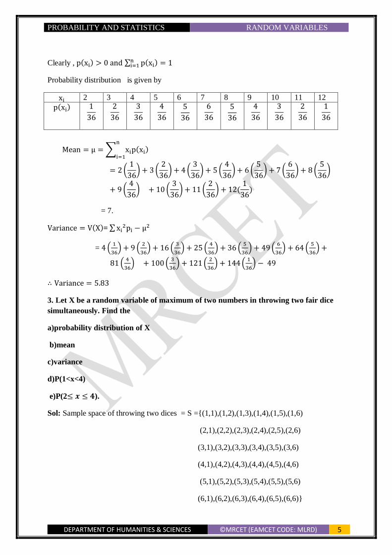
Clearly , p(xi) > 0 and ∑ p(xi)ni=1 = 1
Probability distribution is given by
xi 2 3 4 5 6 7 8 9 10 11 12
p(xi) 1
36
2
36
3
36
4
36
5
36
6
36
5
36
4
36
3
36
2
36
1
36
Mean = μ = ∑ xip(xi)n
i=1
= 2 (1
36) + 3 (
2
36) + 4 (
3
36) + 5 (
4
36) + 6 (
5
36) + 7 (
6
36) + 8 (
5
36)
+ 9 (4
36) + 10 (
3
36) + 11 (
2
36) + 12(
1
36)
= 7.
Variance = V(X)= ∑ xi2pi − μ2
= 4 (1
36) + 9 (
2
36) + 16 (
3
36) + 25 (
4
36) + 36 (
5
36) + 49 (
6
36) + 64 (
5
36) +
81 (4
36) + 100 (
3
36) + 121 (
2
36) + 144 (
1
36) − 49
∴ Variance = 5.83
3. Let X be a random variable of maximum of two numbers in throwing two fair dice
simultaneously. Find the
a)probability distribution of X
b)mean
c)variance
d)P(1<x<4)
e)P(2≤ 𝒙 ≤ 𝟒).
Sol: Sample space of throwing two dices = S ={(1,1),(1,2),(1,3),(1,4),(1,5),(1,6)
(2,1),(2,2),(2,3),(2,4),(2,5),(2,6)
(3,1),(3,2),(3,3),(3,4),(3,5),(3,6)
(4,1),(4,2),(4,3),(4,4),(4,5),(4,6)
(5,1),(5,2),(5,3),(5,4),(5,5),(5,6)
(6,1),(6,2),(6,3),(6,4),(6,5),(6,6)}

PROBABILITY AND STATISTICS RANDOM VARIABLES
DEPARTMENT OF HUMANITIES & SCIENCES ©MRCET (EAMCET CODE: MLRD) 6
∴ 𝑛(𝑆) = 36.
Let X = Maximum of two numbers in throwing two dice = {1,2,3,4,5,6,}
X Favorable cases No of
Favorable
cases
𝑝(𝑥)
1
2
3
4
5
6
(1,1)
(2,1),)(1,2),(2,2)
(3,1),(1,3),(2,3)(3,3),(3,2)
(1,4),(4,1),(4,2),(2,4)(4,3),(3,4),(4,4)
(1,5),(5,1),(2,5),(5,2)(3,5),(5,3),(5,4),(4,5),(5,5)
(1,6)(6,1),(6,2),(2,6),(6,3),(3,6),(4,6),(6,4),(6,5)(5,6),(6,6)
1
3
5
7
9
11
1
36
3
36
5
36
7
36
9
36
11
36
Clearly , p(xi) > 0 and ∑ p(xi)ni=1 = 1
Probability distribution is given by
𝑥𝑖 1 2 3 4 5 6
𝑝(𝑥𝑖) 1
36
3
36
5
36
7
36
9
36
11
36
Mean = μ = ∑ xip(xi)n
i=1= 1 (
1
36) + 2 (
3
36) + 3 (
5
36) + 4 (
7
36) + 5 (
9
36) + 6 (
11
36)
= 4.4 7.

PROBABILITY AND STATISTICS RANDOM VARIABLES
DEPARTMENT OF HUMANITIES & SCIENCES ©MRCET (EAMCET CODE: MLRD) 7
Variance = V(X)= ∑ xi2pi − μ2
= 1 (1
36) + 4 (
3
36) + 9 (
5
36) + 16 (
7
36) + 25 (
9
36) + 36 (
11
36)
∴ Variance = 1.99.
4.A random variable X has the following probability function
𝒙𝒊 -3 -2 -1 0 1 2 3
𝒑(𝒙𝒊) k 0.1 k 0.2 2k 0.4 2k
Find k ,mean, variance.
Sol: We know that ∑ p(xi) = 1ni=1
i.e k+0.1+k+0.2+2k+0.4+2k = 1
i.e 6k+0.7 = 1 ∴ 𝑘 = 0.05
Mean = μ = ∑ xip(xi)n
i=1= k(−3) + 0.1(−2) + k(−1) + 2k(1) + 2(0.4) + 3(2k)
= 0.8.
Variance = V(X)= ∑ xi2pi − μ2
= k(−3)2 + 0.12(−2) + k(−1)2 + 2k(1) + 4(0.4) + 9(2k)
∴ Variance = 2.86.
Continuous Probability distribution:
Let X be a continuous random variable taking values on the interval (a,b). A function f(x) is
said to be the Probability density function of x if
i) f(x) > 0 ∀ x ∈ (a, b)
ii) Total area under the probability curve is 1 i. e, ∫ f(x)dx = 1.b
a
iii) For two distinct numbers ‘c’ and ‘d’ in (𝑎, 𝑏) is given by P(c < x < d) =
Area under the probability curve between ordinates x = c and x = d i. e
∫ f(x)dx.d
c
Note: P(c < x < d) = P(c ≤ x ≤ d) = P(c ≤ x < d) = P(c < x ≤ d)
Cumulative distribution function of 𝑓(𝑥) is given by
∫ f(x)dxx
−∞ i.e, f(x) =
d
dxF(x)

PROBABILITY AND STATISTICS RANDOM VARIABLES
DEPARTMENT OF HUMANITIES & SCIENCES ©MRCET (EAMCET CODE: MLRD) 8
Mean: The mean of the continuous Probability Distribution is defined as
μ = ∫ x f(x)dx.∞
−∞
Expectation: The Expectation of the continuous Probability Distribution is defined as
E(X) = ∫ x f(x)dx.∞
−∞
In general, E(g(x)) = ∫ g(x) f(x)dx.∞
−∞
Properties:
1) E(X) = μ
2) E(X) = k E(X)
3) E(X + k) = E(X) + k
4) ) E(aX ± b) = aE(X) ± b
Variance: The variance of the Continuous Probability Distribution is defined as
Var(X) = V(X) = ∫ x2 f(x)dx − μ2.∞
−∞
Properties:
1) V(c) = 0 where c is a constant
2) V(kX) = k2 V(X)
3) V(X + k) = V(X)
4) V(aX ± b) = a2 V(X)
Mean Deviation: Mean deviation of continuous probability distribution function is
defined as
∫ |x − μ| f(x)dx.∞
−∞
Median: Median is the point which divides the entire distribution in to two equal parts. In
case of continuous distribution,median is the point which divides the total area in to two
equal parts i.e, ∫ f(x)dx = ∫ f(x)dx =1
2 ∀ x ∈ (a, b)
b
M.
M
a
Mode: Mode is the value of x for which f(x) is maximum.
i.e f ′(x) = 0 and f "(x) < 0 for x ∈ (a, b)
PROBABILITY AND STATISTICS RANDOM VARIABLES
DEPARTMENT OF HUMANITIES & SCIENCES ©MRCET (EAMCET CODE: MLRD) 9
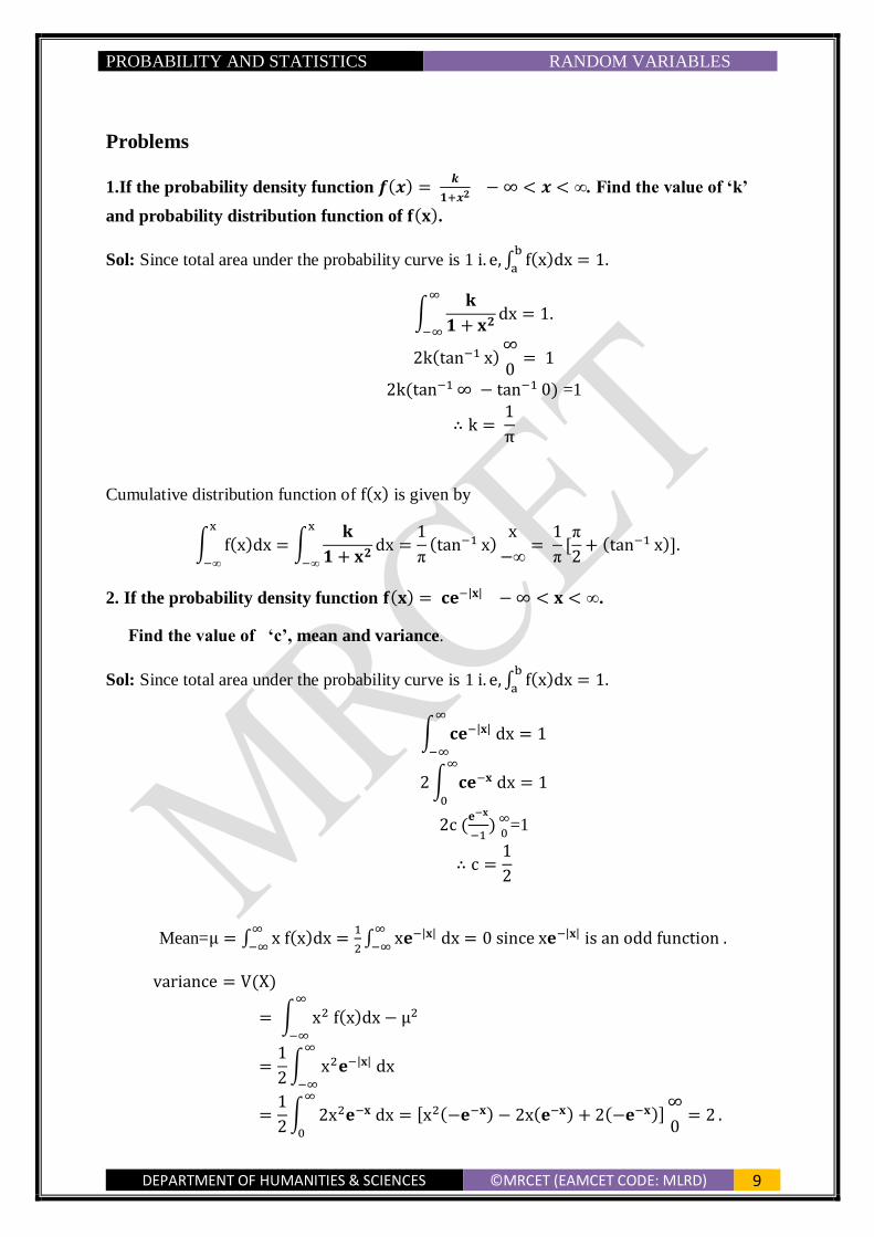
Problems
1.If the probability density function 𝒇(𝒙) = 𝒌
𝟏+𝒙𝟐 − ∞ < 𝒙 < ∞. Find the value of ‘k’
and probability distribution function of 𝐟(𝐱).
Sol: Since total area under the probability curve is 1 i. e, ∫ f(x)dx = 1.b
a
∫𝐤
𝟏 + 𝐱𝟐dx = 1.
∞
−∞
2k(tan−1 x)∞
0= 1
2k(tan−1 ∞ − tan−1 0) =1
∴ k = 1
π
Cumulative distribution function of f(x) is given by
∫ f(x)dx = ∫𝐤
𝟏 + 𝐱𝟐dx =
1
π(tan−1 x)
x
−∞=
1
π[π
2+ (tan−1 x)].
x
−∞
x
−∞
2. If the probability density function 𝐟(𝐱) = 𝐜𝐞−|𝐱| − ∞ < 𝐱 < ∞.
Find the value of ‘c’, mean and variance.
Sol: Since total area under the probability curve is 1 i. e, ∫ f(x)dx = 1.b
a
∫ 𝐜𝐞−|𝐱| dx = 1∞
−∞
2 ∫ 𝐜𝐞−𝐱 dx = 1∞
0
2c (𝐞−𝐱
−1) ∞
0=1
∴ c =1
2
Mean=μ = ∫ x f(x)dx =1
2∫ x𝐞−|𝐱| dx = 0 since x𝐞−|𝐱| is an odd function .
∞
−∞
∞
−∞
variance = V(X)
= ∫ x2 f(x)dx − μ2∞
−∞
=1
2∫ x2𝐞−|𝐱| dx
∞
−∞
=1
2∫ 2x2𝐞−𝐱 dx = [x2(−𝐞−𝐱) − 2x(𝐞−𝐱) + 2(−𝐞−𝐱)]
∞
0= 2
∞
0
.

PROBABILITY AND STATISTICS RANDOM VARIABLES
DEPARTMENT OF HUMANITIES & SCIENCES ©MRCET (EAMCET CODE: MLRD) 10
3. If the probability density function 𝐟(𝐱) = {𝐬𝐢𝐧𝐱
𝟐
𝟎 𝐨𝐭𝐡𝐞𝐫𝐰𝐢𝐬𝐞𝐢𝐟 𝟎 ≤ 𝐱 ≤ 𝛑 .
Find mean,median,mode and 𝐏(𝟎 < 𝐱 <𝛑
𝟐).
Sol: Mean = μ = ∫ x f(x)dx =1
2∫ x
𝐬𝐢𝐧𝐱
𝟐dx =
1
2[−xcosx + sinx] π
0=
π
2.
π
0
∞
−∞
Let M be the Median then
∫ f(x)dx = ∫ f(x)dx =1
2 ∀ x ∈ (−∞, ∞)
π
M
M
0
∫𝐬𝐢𝐧𝐱
𝟐dx = ∫
𝐬𝐢𝐧𝐱
𝟐dx =
1
2 ∀ x ∈ (−∞, ∞)
π
M
M
0
consider∫𝐬𝐢𝐧𝐱
𝟐dx =
1
2
π
M then (−cosx) π
M=1
∴ M =π
2
Since f(x) = {sinx
2
0 otherwiseif 0 ≤ x ≤ π
To find maximum, we have f ′(x) = 0
i.e, cosx = 0 implies that x =π
2
and f ′′(x) = −sinx
2 which is less than 0 at x =
π
2
∴ Mode =π
2.
4.If the distributed function is given by
𝐅(𝐱) = {𝟎 𝐢𝐟 𝐱 ≤ 𝟏𝐤(𝐱 − 𝟏)𝟒
𝟏 𝐢𝐟 𝐱 > 𝟑
𝐢𝐟 𝟏 ≤ 𝐱 ≤ 𝟑
Find 𝐤, 𝐟(𝐱), 𝐦𝐞𝐚𝐧.
Sol: Cumulative distribution function of f(x) is given by
∫ f(x)dxx
−∞ i.e, f(x) =
d
dxF(x)
i.e, f(x) = {40 if x ≤ 1k(x − 1)3
0 if x > 3
if 1 ≤ x ≤ 3

PROBABILITY AND STATISTICS RANDOM VARIABLES
DEPARTMENT OF HUMANITIES & SCIENCES ©MRCET (EAMCET CODE: MLRD) 11
Since total area under the probability curve is 1 i. e, ∫ f(x)dx = 1b
a
∫ 4k(x − 1)3dx = 13
1
[k(x − 1)4] 31 = 1
∴ k =1
16
∴ f(x) = {1
4
0 if x ≤ 1(x − 1)3
0 if x > 3
if 1 ≤ x ≤ 3
Mean=μ = ∫ x f(x)dx =1
4∫ x(x − 1)3dx = 19.6.
3
1
∞
−∞
Multiple Random variables
Discrete two dimensional random variable:
Joint probability mass function is defined as f(x, y) = P(X = xi , Y = yi)
Joint probability distribution function is defined as
𝐅𝐗𝐘(𝐱, 𝐲) = P(X < xi , Y < yi) =∑ ∑ p(xi , yi)<y<x
Marginal probability mass functions of X and Y are defined as
P(X = xi ) = p(xi ) = ∑ p(xi , yj)
j
P(Y = yj ) = p(yj ) = ∑ p(xi , yj)
i
Continuous two dimensional random variable:
Joint probability density function is defined as
fXY(x, y) = P(x ≤ X ≤ x + dx, y ≤ Y ≤ y + dy)
and ∫ ∫ fXY(x, y) dxdy = 1∞
−∞
∞
−∞
Joint probability distribution function is defined as
FXY(x, y) = P(X < xi , Y < yi) =∫ ∫ fXY(x, y) dxdyy
−∞
x
−∞
and fXY(x, y) =∂2
∂x ∂y[FXY(x, y) ]
PROBABILITY AND STATISTICS RANDOM VARIABLES
DEPARTMENT OF HUMANITIES & SCIENCES ©MRCET (EAMCET CODE: MLRD) 12
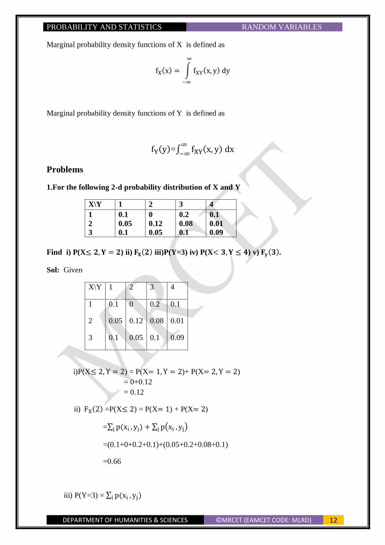
Marginal probability density functions of X is defined as
fX(x) = ∫ fXY(x, y) dy
∞
−∞
Marginal probability density functions of Y is defined as
fY(y)=∫ fXY(x, y) dx∞
−∞
Problems
1.For the following 2-d probability distribution of X and Y
X\Y 1 2 3 4
1
2
3
0.1
0.05
0.1
0
0.12
0.05
0.2
0.08
0.1
0.1
0.01
0.09
Find i) P(X≤ 𝟐, 𝐘 = 𝟐) ii) 𝐅𝐗(𝟐) iii)P(Y=3) iv) P(X< 𝟑, 𝐘 ≤ 𝟒) v) 𝐅𝐲(𝟑).
Sol: Given
X\Y 1 2 3 4
1
2
3
0.1
0.05
0.1
0
0.12
0.05
0.2
0.08
0.1
0.1
0.01
0.09
i)P(X≤ 2, Y = 2) = P(X= 1, Y = 2)+ P(X= 2, Y = 2)
= 0+0.12
= 0.12
ii) FX(2) =P(X≤ 2) = P(X= 1) + P(X= 2)
=∑ p(xi , yj)j + ∑ p(xi , yj)j
=(0.1+0+0.2+0.1)+(0.05+0.2+0.08+0.1)
=0.66
iii) P(Y=3) = ∑ p(xi , yj)i
PROBABILITY AND STATISTICS RANDOM VARIABLES
DEPARTMENT OF HUMANITIES & SCIENCES ©MRCET (EAMCET CODE: MLRD) 13
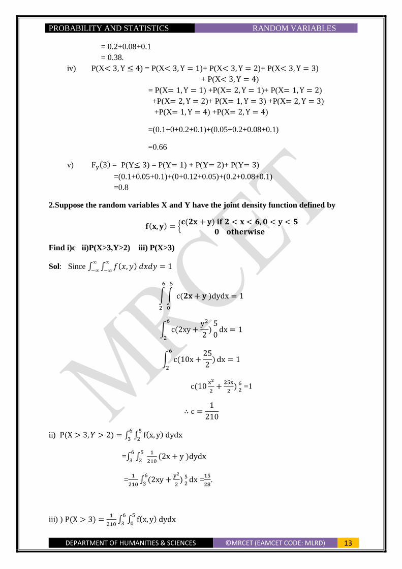
= 0.2+0.08+0.1
= 0.38.
iv) P(X< 3, Y ≤ 4) = P(X< 3, Y = 1)+ P(X< 3, Y = 2)+ P(X< 3, Y = 3)
+ P(X< 3, Y = 4)
= P(X= 1, Y = 1) +P(X= 2, Y = 1)+ P(X= 1, Y = 2)
+P(X= 2, Y = 2)+ P(X= 1, Y = 3) +P(X= 2, Y = 3)
+P(X= 1, Y = 4) +P(X= 2, Y = 4)
=(0.1+0+0.2+0.1)+(0.05+0.2+0.08+0.1)
=0.66
v) Fy(3) = P(Y≤ 3) = P(Y= 1) + P(Y= 2)+ P(Y= 3)
=(0.1+0.05+0.1)+(0+0.12+0.05)+(0.2+0.08+0.1)
=0.8
2.Suppose the random variables X and Y have the joint density function defined by
𝐟(𝐱, 𝐲) = {𝐜(𝟐𝐱 + 𝐲) 𝐢𝐟 𝟐 < 𝐱 < 𝟔, 𝟎 < 𝐲 < 𝟓
𝟎 𝐨𝐭𝐡𝐞𝐫𝐰𝐢𝐬𝐞
Find i)c ii)P(X>3,Y>2) iii) P(X>3)
Sol: Since ∫ ∫ 𝑓(𝑥, 𝑦) 𝑑𝑥𝑑𝑦 = 1∞
−∞
∞
−∞
∫ ∫ c(𝟐𝐱 + 𝐲 )dydx = 1
5
0
6
2
∫ c(2xy +y2
2)
5
0
6
2
dx = 1
∫ c(10x +25
2)
6
2
dx = 1
c(10x2
2+
25x
2) 6
2 =1
∴ c =1
210
ii) P(X > 3, 𝑌 > 2) = ∫ ∫ f(x, y) dydx5
2
6
3
=∫ ∫ 1
210(2x + y )dydx
5
2
6
3
=1
210∫ (2xy +
y2
2) 5
2
6
3dx =
15
28.
iii) ) P(X > 3) =1
210∫ ∫ f(x, y) dydx
5
0
6
3
PROBABILITY AND STATISTICS RANDOM VARIABLES
DEPARTMENT OF HUMANITIES & SCIENCES ©MRCET (EAMCET CODE: MLRD) 14
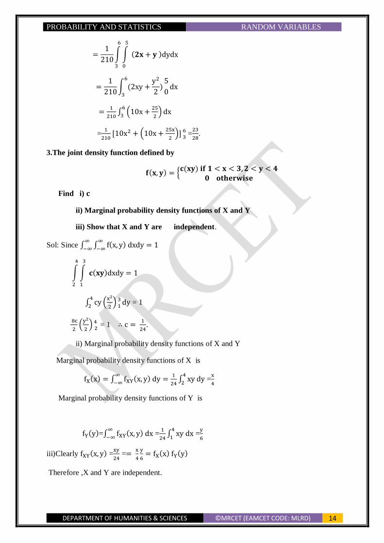
=1
210∫ ∫ (𝟐𝐱 + 𝐲 )dydx
5
0
6
3
=1
210∫ (2xy +
y2
2)
5
0
6
3
dx
=1
210∫ (10x +
25
2)
6
3dx
=1
210[10x2 + (10x +
25x
2)] 6
3 =
23
28.
3.The joint density function defined by
𝐟(𝐱, 𝐲) = {𝐜(𝐱𝐲) 𝐢𝐟 𝟏 < 𝐱 < 𝟑, 𝟐 < 𝐲 < 𝟒
𝟎 𝐨𝐭𝐡𝐞𝐫𝐰𝐢𝐬𝐞
Find i) 𝐜
ii) Marginal probability density functions of X and Y
iii) Show that X and Y are independent.
Sol: Since ∫ ∫ f(x, y) dxdy = 1∞
−∞
∞
−∞
∫ ∫ 𝐜(𝐱𝐲)dxdy = 1
3
1
4
2
∫ cy (x2
2) 3
1dy
4
2 = 1
8c
2(
y2
2) 4
2 = 1 ∴ c =
1
24.
ii) Marginal probability density functions of X and Y
Marginal probability density functions of X is
fX(x) = ∫ fXY(x, y) dy∞
−∞=
1
24∫ xy dy
4
2 =
x
4
Marginal probability density functions of Y is
fY(y)=∫ fXY(x, y) dx∞
−∞ =
1
24∫ xy dx
4
1 =
y
6
iii)Clearly fXY(x, y) =xy
24 ==
x
4
y
6= fX(x) fY(y)
Therefore ,X and Y are independent.

PROBABILITY AND STATISTICS RANDOM VARIABLES
DEPARTMENT OF HUMANITIES & SCIENCES ©MRCET (EAMCET CODE: MLRD) 15
Conditional probability density function :
Conditional probability density function of X on Y is
fXY(X/Y) = fXY(x, y)
fY(y)
Conditional probability density function of Y on X is
fXY(Y/X) = fXY(x, y)
fX(X)
4.The joint density function defined by
𝐟(𝐱, 𝐲) = {(𝐱𝟐 +
𝐱𝐲
𝟑) 𝐢𝐟 𝟎 < 𝐱 < 𝟏, 𝟎 < 𝐲 < 𝟐
𝟎 𝐨𝐭𝐡𝐞𝐫𝐰𝐢𝐬𝐞
Find
i) Conditional probability density functions.
ii) Marginal probability density functions
iii) Check whether the functions X and Y are independent or not
Sol: Given f(x, y) = {(x2 +
xy
3) if 0 < x < 1,0 < y < 2
0 otherwise
Marginal probability density functions of X is
fX(x) = ∫ fXY(x, y) dy∞
−∞= ∫ (𝐱𝟐 +
𝐱𝐲
𝟑) dy
2
0 = 2x(x +
1
3)
Marginal probability density functions of Y is
fY(y)=∫ fXY(x, y) dx∞
−∞ =∫ (𝐱𝟐 +
𝐱𝐲
𝟑) dx
1
0 =
1
3+
y
6
Here fY(y) fX(x) = 2x(x +1
3)(
1
3+
y
6)
Therefore, fXY(x, y) ≠ fX(x) fY(y)
Hence X and Y are not Independent.
Conditional probability density function of X on Y is
fXY(X/Y) = fXY(x,y)
fY(y) =
(𝐱𝟐+𝐱𝐲
𝟑)
(1
3+
y
6)
Conditional probability density function of Y on X is
fXY(Y/X) = fXY(x,y)
fX(X)=
(𝐱𝟐+𝐱𝐲
𝟑)
2x(x+1
3)
PROBABILITY AND STATISTICS PROBABILITY DISTRIBUTIONS
DEPARTMENT OF HUMANITIES & SCIENCES ©MRCET (EAMCET CODE: MLRD) 16
UNIT- II
PROBABILITY DISTRIBUTIONS
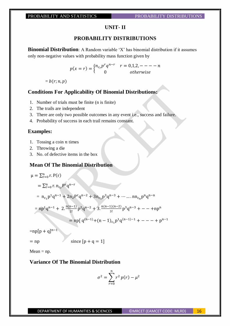
Binomial Distribution: A Random variable ‘X’ has binomial distribution if it assumes
only non-negative values with probability mass function given by
𝑝(𝑥 = 𝑟) = {𝑛𝑐𝑟
𝑝𝑟𝑞𝑛−𝑟 𝑟 = 0,1,2, − − − − 𝑛
0 𝑜𝑡ℎ𝑒𝑟𝑤𝑖𝑠𝑒
= 𝑏(𝑟; 𝑛, 𝑝)
Conditions For Applicability Of Binomial Distributions:
1. Number of trials must be finite (n is finite)
2. The trails are independent
3. There are only two possible outcomes in any event i.e., success and failure.
4. Probability of success in each trail remains constant.
Examples:
1. Tossing a coin 𝑛 times
2. Throwing a die
3. No. of defective items in the box
Mean Of The Binomial Distribution
μ = ∑ r. P(r)nr=0
= ∑ r.nr=0 ncr
Prqn−r
= nc1p1qn−1 + 2n2Prqn−2 + 3nc3
p3qn−3 + ⋯ … . nncnpnqn−n
= np1qn−1 + 2.n(n−1)
2!p2qn−2 + 3.
n(n−1)(n−2)
3!p3qn−3 + − − +npn
= np[ q(n−1)+(n − 1)c1p1q(n−1)−1 + − − − + pn−1
=np[p + q]n−1
= np since [p + q = 1]
Mean = np.
Variance Of The Binomial Distribution
𝜎2 = ∑ 𝑟2
𝑛
𝑟=0
𝑝(𝑟) − 𝜇2

PROBABILITY AND STATISTICS PROBABILITY DISTRIBUTIONS
DEPARTMENT OF HUMANITIES & SCIENCES ©MRCET (EAMCET CODE: MLRD) 17
= ∑[r(r − 1) + r]P(r) − μ2
n
r=0
= ∑ r(r − 1)P(r) +
n
r=0
∑ r. P(r) −
n
r=0
n2p2
= ∑ r(r − 1)ncrPrqn−r + np −
n
r=0
n2P2
let ∑ r(r − 1)P(r) =nr=0 ∑ r(r − 1)ncr
Prqn−r = 2nr=0 nc2r
P2q2nn−2 +
6nc3P3qn−3+12ncr
P4qn−4+---− + n(n − 1) Pn
= n(n − 1)P2⌈qn−2 + +(n − 2)c1p1q(n−2)−1 + − − − + p2⌉
= n(n − 1)P2(p + q)n−2
= n2P2 − nP2
σ2 = n2P2 − nP2 + np − n2P2
= np(1 − p)
= npq.
Problems
1.In tossing a coin 10 times simultaneously. Find the probability of getting
i)at least 7 heads ii) almost 3 heads iii)exactly 6 heads.
Sol: Given 𝑛 = 10
Probability of getting a head in tossing a coin = 1
2= 𝑝.
Probability of getting no head = 𝑞 = 1 −1
2 =
1
2.
The probability of getting 𝑟 heads in a throw of 10 coins is
𝑃(𝑋 = 𝑟) = 𝑝(𝑟) = 10𝐶𝑟(
1
2)
𝑟
(1
2)
10−𝑟
; 𝑟 = 0,1,2, … … . . ,10
(i) Probability of getting at least seven heads is given by
𝑃(𝑋 ≥ 7) = 𝑃(𝑋 = 7) + 𝑃(𝑋 = 8) + 𝑃(𝑋 = 9) + 𝑃(𝑋 = 10)
= 10𝐶7(
1
2)
7
(1
2)
10−7
+ 10𝐶8(
1
2)
8
(1
2)
10−8
+ 10𝐶9(
1
2)
9
(1
2)
10−9
+ 10𝐶10(
1
2)
10
=1
210[10𝐶7
+ 10𝐶8+ 10𝐶9
+ 10𝐶10]

PROBABILITY AND STATISTICS PROBABILITY DISTRIBUTIONS
DEPARTMENT OF HUMANITIES & SCIENCES ©MRCET (EAMCET CODE: MLRD) 18
=1
210[120 + 45 + 10 + 1]
=176
1024
= 0.1719
ii) Probability of getting at most 3 heads is given by
𝑃(𝑋 ≤ 3) = 𝑃(𝑋 = 0) + 𝑃(𝑋 = 1) + 𝑃(𝑋 = 2) + 𝑃(𝑋 = 3)
= 10𝑐1(
1
2)
1
(1
2)
10−1
+ 10𝑐2(
1
2)
2
(1
2)
10−2
+ 10𝐶3(
1
2)
3
(1
2)
10−3
+ 10𝐶0(
1
2)
10
=1
210[10𝐶0
+ 10𝐶1+ 10𝑐2
+ 10𝑐3]
=1
210[120 + 45 + 10 + 1]
=176
1024
= 0.1719
iii)Probability of getting exactly six heads is given by
𝑃(𝑋 = 6) =10𝑐6(
1
2)
6
(1
2)
10−6
=0.205.
2.In 𝟐𝟓𝟔 sets of 𝟏𝟐 tosses of a coin ,in how many cases one can expect 𝟖 Heads
and 𝟒 Tails.
Sol: The probability of getting a head, 𝑝 = 1
2
The probability of getting a tail,𝑞 = 1
2
Here 𝑛 = 12
The probability of getting 8heads and 4Tails in 12trials= 𝑃(𝑋 = 8) = 12𝐶8(
1
2)
8
(1
2)
4
= 12!
8! 4!(
1
2)
12
= 495
212
The expected number of getting 8 heads and 4 Tails in 12 trials of such cases in256 sets
= 256 × 𝑃(𝑋 = 8) = 28 ×495
212=
495
16= 30.9375 ~31

PROBABILITY AND STATISTICS PROBABILITY DISTRIBUTIONS
DEPARTMENT OF HUMANITIES & SCIENCES ©MRCET (EAMCET CODE: MLRD) 19
3.Find the probability of getting an even number 3 or 4 or 5 times in throwing a die 10
times
Sol: Probability of getting an even number in throwing a die = 3
6=
1
2 = 𝑝.
Probability of getting an odd number in throwing a die =𝑞 = 1
2.
∴Probability of getting an even number 3 or 4 or 5 times in throwing a die 10 times is
𝑃(𝑋 = 3) + 𝑃(𝑋 = 4) + 𝑃(𝑋 = 5)
= 10𝑐3(
1
2)
3
(1
2)
10−3
+ 10𝑐4(
1
2)
4
(1
2)
10−4
+ 10𝐶5(
1
2)
5
(1
2)
10−5
=1
210[10𝐶3
+ 10𝐶4+ 10𝑐5
]
=1
210[120 + 252 + 210]
=0.568.
4.Out of 800 families with 4 children each ,how many could you expect to have
a)three boys b)five girls c) 2 or 3 boys d)at least 1 boy.
Sol: : Given 𝑛 = 5, 𝑁 = 800
Let having boys be success
Probability of having a boy = 1
2= 𝑝.
Probability of having girl = 𝑞 = 1 −1
2 =
1
2.
The probability of having 𝑟 boyss in 5 children is
𝑃(𝑋 = 𝑟) = 𝑝(𝑟) = 5𝐶𝑟(
1
2)
𝑟
(1
2)
5−𝑟
; 𝑟 = 0,1,2 … … 5
a)Probability of having 3 boys is given by
𝑃(𝑋 = 3) = 5𝐶𝑟(
1
2)
3
(1
2)
5−3
=5
16
Expected number of families having 3 boys = 𝑁 𝑝(3) =800(5
16) =250 families.
b) Probability of having 5 girls = Probability of having no boys is given by
𝑃(𝑋 = 0) = 5𝐶0(
1
2)
0
(1
2)
5−0
=1
32
Expected number of families having 5 girls = 𝑁 𝑝(0) =800(1
32) =25 families.
c) Probability of having either 2 or 3 boys is given by
PROBABILITY AND STATISTICS PROBABILITY DISTRIBUTIONS
DEPARTMENT OF HUMANITIES & SCIENCES ©MRCET (EAMCET CODE: MLRD) 20
𝑃(𝑋 = 2) + 𝑃(𝑋 = 3) = 5𝐶2(
1
2)
2
(1
2)
5−2
+ 5𝐶3(
1
2)
3
(1
2)
5−3
=5
18
Expected number of families having 3 boys = 𝑁 𝑝(3) =800(5
8) =500 families.
d) Probability of having at least 1 boy is given by
𝑃(𝑋 ≥ 1) = 1 − 𝑃(𝑋 = 0)
= 1 − 5𝐶0(
1
2)
0
(1
2)
5−0
=31
32
Expected number of families having at least 1 boy =800(31
32) =775 families.
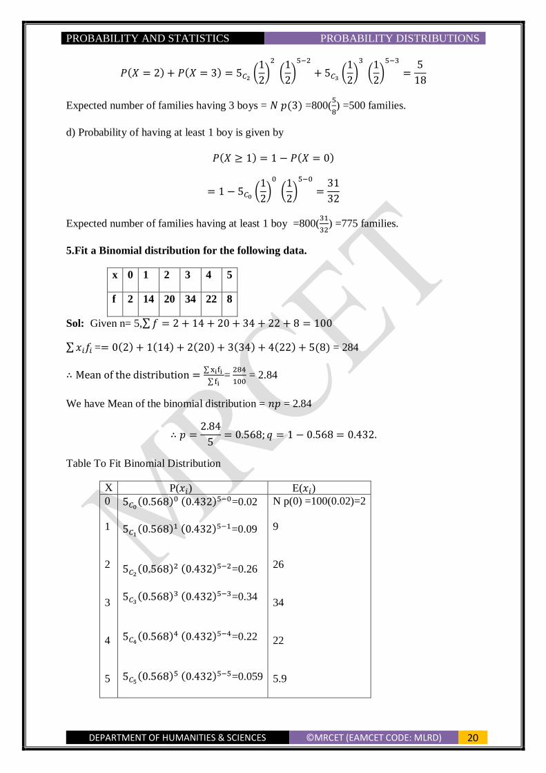
5.Fit a Binomial distribution for the following data.
x 0 1 2 3 4 5
f 2 14 20 34 22 8
Sol: Given n= 5,∑ 𝑓 = 2 + 14 + 20 + 34 + 22 + 8 = 100
∑ 𝑥𝑖𝑓𝑖 == 0(2) + 1(14) + 2(20) + 3(34) + 4(22) + 5(8) = 284
∴ Mean of the distribution =∑ xifi
∑ fi=
284
100 = 2.84
We have Mean of the binomial distribution = 𝑛𝑝 = 2.84
∴ 𝑝 =2.84
5= 0.568; 𝑞 = 1 − 0.568 = 0.432.
Table To Fit Binomial Distribution
X P(𝑥𝑖) E(𝑥𝑖)
0
1
2
3
4
5
5𝐶0(0.568)0 (0.432)5−0=0.02
5𝐶1(0.568)1 (0.432)5−1=0.09
5𝐶2(0.568)2 (0.432)5−2=0.26
5𝐶3(0.568)3 (0.432)5−3=0.34
5𝐶4(0.568)4 (0.432)5−4=0.22
5𝐶5(0.568)5 (0.432)5−5=0.059
N p(0) =100(0.02)=2
9
26
34
22
5.9
PROBABILITY AND STATISTICS PROBABILITY DISTRIBUTIONS
DEPARTMENT OF HUMANITIES & SCIENCES ©MRCET (EAMCET CODE: MLRD) 21
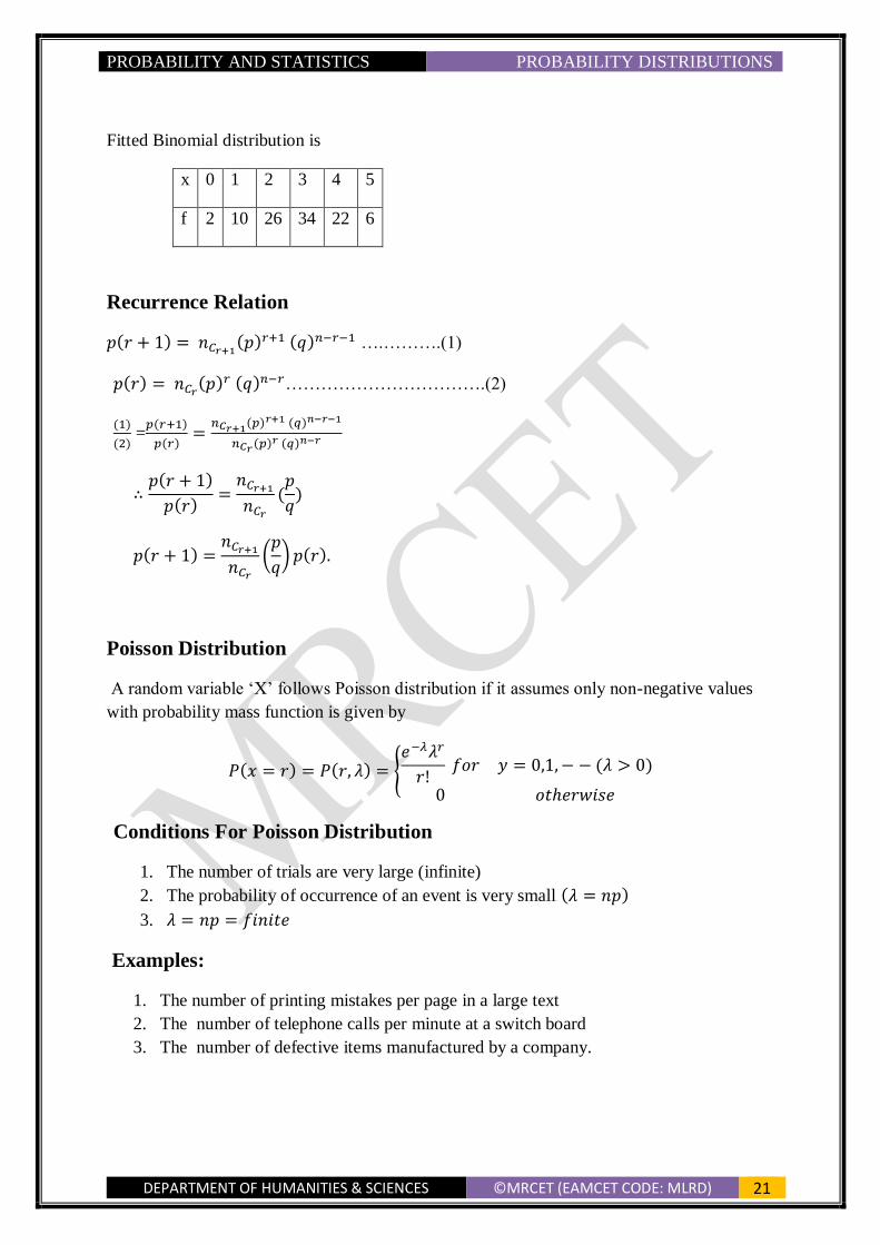
Fitted Binomial distribution is
x 0 1 2 3 4 5
f 2 10 26 34 22 6
Recurrence Relation
𝑝(𝑟 + 1) = 𝑛𝐶𝑟+1(𝑝)𝑟+1 (𝑞)𝑛−𝑟−1 ….……….(1)
𝑝(𝑟) = 𝑛𝐶𝑟(𝑝)𝑟 (𝑞)𝑛−𝑟…………………………….(2)
(1)
(2) =
𝑝(𝑟+1)
𝑝(𝑟)=
𝑛𝐶𝑟+1(𝑝)𝑟+1 (𝑞)𝑛−𝑟−1
𝑛𝐶𝑟 (𝑝)𝑟 (𝑞)𝑛−𝑟
∴𝑝(𝑟 + 1)
𝑝(𝑟)=
𝑛𝐶𝑟+1
𝑛𝐶𝑟
(𝑝
𝑞)
𝑝(𝑟 + 1) =𝑛𝐶𝑟+1
𝑛𝐶𝑟
(𝑝
𝑞) 𝑝(𝑟).
Poisson Distribution
A random variable ‘X’ follows Poisson distribution if it assumes only non-negative values
with probability mass function is given by
𝑃(𝑥 = 𝑟) = 𝑃(𝑟, 𝜆) = {𝑒−𝜆𝜆𝑟
𝑟! 𝑓𝑜𝑟 𝑦 = 0,1, − − (𝜆 > 0)
0 𝑜𝑡ℎ𝑒𝑟𝑤𝑖𝑠𝑒
Conditions For Poisson Distribution
1. The number of trials are very large (infinite)
2. The probability of occurrence of an event is very small (𝜆 = 𝑛𝑝)
3. 𝜆 = 𝑛𝑝 = 𝑓𝑖𝑛𝑖𝑡𝑒
Examples:
1. The number of printing mistakes per page in a large text
2. The number of telephone calls per minute at a switch board
3. The number of defective items manufactured by a company.
PROBABILITY AND STATISTICS PROBABILITY DISTRIBUTIONS
DEPARTMENT OF HUMANITIES & SCIENCES ©MRCET (EAMCET CODE: MLRD) 22
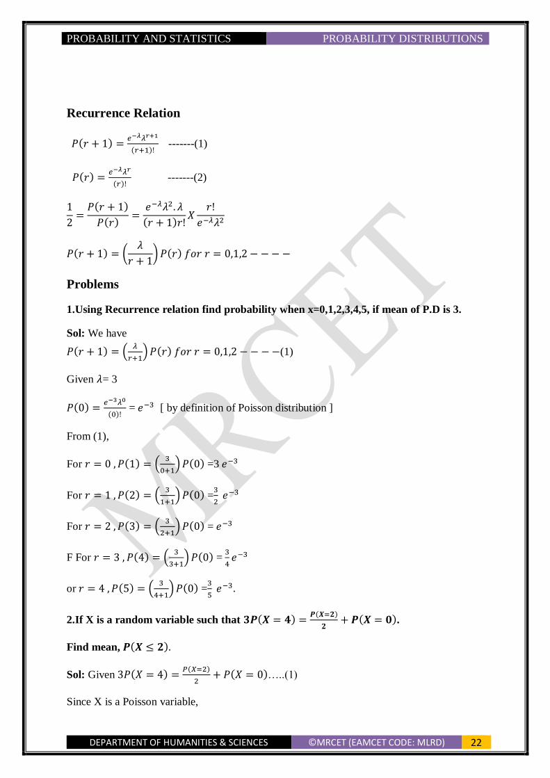
Recurrence Relation
𝑃(𝑟 + 1) =𝑒−𝜆𝜆𝑟+1
(𝑟+1)! -------(1)
𝑃(𝑟) =𝑒−𝜆𝜆𝑟
(𝑟)! -------(2)
1
2=
𝑃(𝑟 + 1)
𝑃(𝑟)=
𝑒−𝜆𝜆2. 𝜆
(𝑟 + 1)𝑟!𝑋
𝑟!
𝑒−𝜆𝜆2
𝑃(𝑟 + 1) = (𝜆
𝑟 + 1) 𝑃(𝑟) 𝑓𝑜𝑟 𝑟 = 0,1,2 − − − −
Problems
1.Using Recurrence relation find probability when x=0,1,2,3,4,5, if mean of P.D is 3.
Sol: We have
𝑃(𝑟 + 1) = (𝜆
𝑟+1) 𝑃(𝑟) 𝑓𝑜𝑟 𝑟 = 0,1,2 − − − −(1)
Given 𝜆= 3
𝑃(0) =𝑒−3𝜆0
(0)! = 𝑒−3 [ by definition of Poisson distribution ]
From (1),
For 𝑟 = 0 , 𝑃(1) = (3
0+1) 𝑃(0) =3 𝑒−3
For 𝑟 = 1 , 𝑃(2) = (3
1+1) 𝑃(0) =
3
2 𝑒−3
For 𝑟 = 2 , 𝑃(3) = (3
2+1) 𝑃(0) = 𝑒−3
F For 𝑟 = 3 , 𝑃(4) = (3
3+1) 𝑃(0) =
3
4𝑒−3
or 𝑟 = 4 , 𝑃(5) = (3
4+1) 𝑃(0) =
3
5 𝑒−3.
2.If X is a random variable such that 𝟑𝑷(𝑿 = 𝟒) =𝑷(𝑿=𝟐)
𝟐+ 𝑷(𝑿 = 𝟎).
Find mean, 𝑷(𝑿 ≤ 𝟐).
Sol: Given 3𝑃(𝑋 = 4) =𝑃(𝑋=2)
2+ 𝑃(𝑋 = 0)…..(1)
Since X is a Poisson variable,
PROBABILITY AND STATISTICS PROBABILITY DISTRIBUTIONS
DEPARTMENT OF HUMANITIES & SCIENCES ©MRCET (EAMCET CODE: MLRD) 23
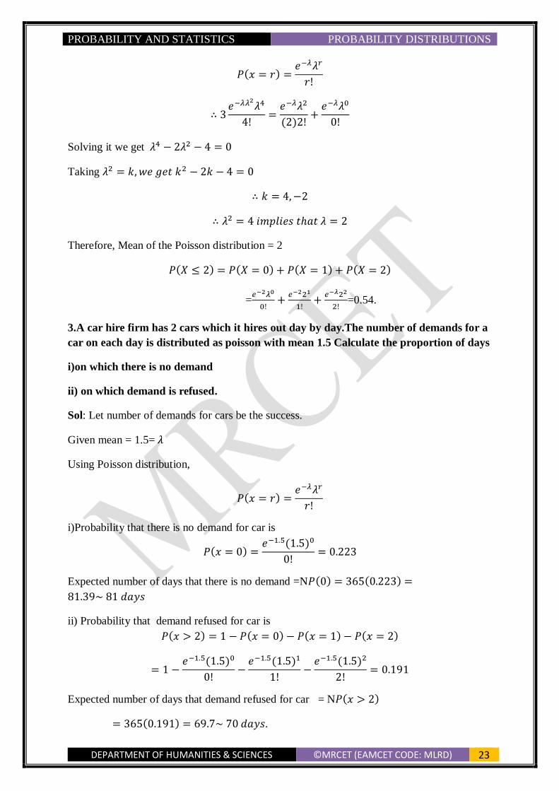
𝑃(𝑥 = 𝑟) =𝑒−𝜆𝜆𝑟
𝑟!
∴ 3𝑒−𝜆𝜆2
𝜆4
4!=
𝑒−𝜆𝜆2
(2)2!+
𝑒−𝜆𝜆0
0!
Solving it we get 𝜆4 − 2𝜆2 − 4 = 0
Taking 𝜆2 = 𝑘, 𝑤𝑒 𝑔𝑒𝑡 𝑘2 − 2𝑘 − 4 = 0
∴ 𝑘 = 4, −2
∴ 𝜆2 = 4 𝑖𝑚𝑝𝑙𝑖𝑒𝑠 𝑡ℎ𝑎𝑡 𝜆 = 2
Therefore, Mean of the Poisson distribution = 2
𝑃(𝑋 ≤ 2) = 𝑃(𝑋 = 0) + 𝑃(𝑋 = 1) + 𝑃(𝑋 = 2)
=𝑒−2𝜆0
0!+
𝑒−221
1!+
𝑒−𝜆22
2!=0.54.
3.A car hire firm has 2 cars which it hires out day by day.The number of demands for a
car on each day is distributed as poisson with mean 1.5 Calculate the proportion of days
i)on which there is no demand
ii) on which demand is refused.
Sol: Let number of demands for cars be the success.
Given mean = 1.5= 𝜆
Using Poisson distribution,
𝑃(𝑥 = 𝑟) =𝑒−𝜆𝜆𝑟
𝑟!
i)Probability that there is no demand for car is
𝑃(𝑥 = 0) =𝑒−1.5(1.5)0
0!= 0.223
Expected number of days that there is no demand =N𝑃(0) = 365(0.223) =
81.39~ 81 𝑑𝑎𝑦𝑠
ii) Probability that demand refused for car is
𝑃(𝑥 > 2) = 1 − 𝑃(𝑥 = 0) − 𝑃(𝑥 = 1) − 𝑃(𝑥 = 2)
= 1 −𝑒−1.5(1.5)0
0!−
𝑒−1.5(1.5)1
1!−
𝑒−1.5(1.5)2
2!= 0.191
Expected number of days that demand refused for car = N𝑃(𝑥 > 2)
= 365(0.191) = 69.7~ 70 𝑑𝑎𝑦𝑠.

PROBABILITY AND STATISTICS PROBABILITY DISTRIBUTIONS
DEPARTMENT OF HUMANITIES & SCIENCES ©MRCET (EAMCET CODE: MLRD) 24
4.The distribution of typing mistakes committed by typist is given below.
Fit a Poisson distribution for it.
Mistakes per page 0 1 2 3 4 5
Number of pages 142 156 69 27 5 1
Sol: Given n= 5,∑ 𝑓 = 142 + 156 + 69 + 27 + 5 + 1 = 400
∑ 𝑥𝑖𝑓𝑖 == 0(142) + 1(156) + 2(69) + 3(27) + 4(5) + 5(1) = 400
∴ Mean of the distribution =∑ xifi
∑ fi
= 400
400 = 1.
We have Mean of the Poisson distribution = 𝜆 = 1
Table To Fit Poisson Distribution
X P(𝑥𝑖) E(𝑥𝑖)
0
1
2
3
4
5
𝑒−1(1)0
0!=0.368
𝑒−1(1)1
1!=0.368
𝑒−1(1)2
2!=0.184
𝑒−1(1)3
3!=0.061
𝑒−1(1)4
4!= 0.015
𝑒−1(1)5
5!= 0.003
N p(0)
=400(0.368)=147.2~147
147
74
24
6
1
Fitted Poisson distribution is
Mistakes per page 0 1 2 3 4 5
Number of pages 147 147 74 24 6 1
PROBABILITY AND STATISTICS PROBABILITY DISTRIBUTIONS
DEPARTMENT OF HUMANITIES & SCIENCES ©MRCET (EAMCET CODE: MLRD) 25
Normal Distribution (Gaussian Distribution)
Let X be a continuous random variable, then it is said to follow normal distribution if its pdf
is given by
𝑓(𝑥, 𝜇, 𝜎) =1
𝜎√2𝜋𝑒−
12
(𝑥−𝜇
𝜎)
2
−∞ ≤ 𝑥 ≤ ∞, 𝜇, 𝜎>0
Here , 𝜎 are the mean & S.D of X.
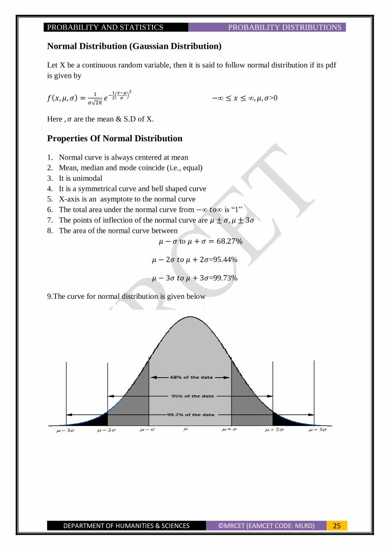
Properties Of Normal Distribution
1. Normal curve is always centered at mean
2. Mean, median and mode coincide (i.e., equal)
3. It is unimodal
4. It is a symmetrical curve and bell shaped curve
5. X-axis is an asymptote to the normal curve
6. The total area under the normal curve from −∞ 𝑡𝑜∞ is “1”
7. The points of inflection of the normal curve are 𝜇 ± 𝜎, 𝜇 ± 3𝜎
8. The area of the normal curve between
𝜇 − 𝜎 to 𝜇 + 𝜎 = 68.27%
𝜇 − 2𝜎 𝑡𝑜 𝜇 + 2𝜎=95.44%
𝜇 − 3𝜎 𝑡𝑜 𝜇 + 3𝜎=99.73%
9.The curve for normal distribution is given below

PROBABILITY AND STATISTICS PROBABILITY DISTRIBUTIONS
DEPARTMENT OF HUMANITIES & SCIENCES ©MRCET (EAMCET CODE: MLRD) 26
Standard Normal Variable
Let 𝑍 =𝑥−𝜇
𝜎 with mean ‘0’ and variance is ‘1’ then the normal variable is said to be standard
normal variable.
Standard Normal Distribution
The normal distribution with man ‘0’ and variance ‘1’ is said to be standard normal
distribution of its probability density function is defined by
𝑓(𝑥) =1
𝜎√2𝜋𝑒−
12
(𝑥−𝑢
𝜎)
2
−∞ < 𝑥 ≤ ∞
𝑓(𝑧) =1
√2𝜋𝑒−
𝑧2
2
−∞ ≤ 𝑥 ≤ ∞ (𝜇 = 0, 𝜎 = 1)
Mean Of The Normal Distribution
Consider Normal distribution with b,σ as parameters Then
f(x; b, σ)1
σ√2πe
−(x−b)2
2σ2
Mean of the continuous distribution is given by
μ = ∫ x f(x)dx = ∫ x 1
σ√2πe
−(x−b)2
2σ2 dx∞
−∞
∞
−∞
=1
√2π∫ (σz + b) e−
(z)2
2 dz∞
−∞ [Putting z =
x−b
σ so that dx = σ dz]
=σ
√2π∫ z e−
(z)2
2 dz∞
−∞+
b
√2π∫ e−
(z)2
2 dz∞
−∞
=2b
√2π∫ e−
(z)2
2 dz∞
−0
[ since z e−(z)2
2 is an odd function and e−(z)2
2 is an even function]
μ =2b
√2π√
π
2 = b
∴ Mean = b
σ2 = ∫ x2 f(x)dx − μ2.∞
−∞

PROBABILITY AND STATISTICS PROBABILITY DISTRIBUTIONS
DEPARTMENT OF HUMANITIES & SCIENCES ©MRCET (EAMCET CODE: MLRD) 27
Variance Of The Normal Distribution
Variance = ∫ x2∞
−∞f(x)dx − μ2
=1
σ√2π∫ x2
∞
−∞
e−1
2
(x−μ
σ)
2
dx − μ2
Let z =x−μ
σ⟹ dx = σdz
=1
σ√2π∫ (μ2
∞
−∞
+ σ2z2 + 2μσz) e−z2
2 σdz − μ2
=μ2
√2π∫ e−
z2
2
∞
−∞
dz +σ2
√2π∫ z2
∞
−∞
e−32
2
dz +2μσ
√2π∫ z2
∞
−∞
e−32
2
dz − μ2
=2μ2
√2π∫ e−
z2
2
∞
0
dz +2σ2
√2π∫ z2
∞
0
e−32
2
dz − μ2
=2σ2
√2π∫ z2e−
z2
2∞
0dz
∵z2
2= +⇒
2zdz
2= dt dz =
dt
√2t
=2σ2
√2π∫ (2 +)2et
∞
0
dt
√2t
=2σ2
√π∫ e−t∞
0+
32
−1.dt
=2σ2
√πΓ(
32
)
==2σ2
√π 1
2 Γ (
1
2)
=σ2
√π√π = σ2
PROBABILITY AND STATISTICS PROBABILITY DISTRIBUTIONS
DEPARTMENT OF HUMANITIES & SCIENCES ©MRCET (EAMCET CODE: MLRD) 28
Median Of The Normal Distribution
Let x=M be the median, then
∫ f(x)dx = ∫ f(x)dx =
∞
M
1
2
M
−∞
Let μϵ(−∞, M)
Let ∫ f(x)dx = ∫ f(x)dx + ∫ f(x)dx =1
2
M
μ
μ
−∞
∞
−∞
Consider ∫ f(x)dx =1
σ√2π∫ e−1
2(
x−μσ
)2μ
−∞dx
μ
−∞
Let z =x−μ
σ⇒ dx = σdz [∵ Limits of z − ∞ ⟶ 0]
∫ f(x)dx =1
σ√2π∫ e−
Z2
2
σdz0
−∞
μ
−∞
=1
√2π∫ e−
t2
2
(dt)0
∞ (by taking z=-t again)
=1
√2π√
π
2=
1
2
From (1)
∫ f(x)dx = 0 ⇒ μ = M
μ
μ
Mode Of The Normal Distribution
f(x) =1
σ√2πe−
12
(x−μ
σ)
2
− (x − μ
σ)
2
f`(x) = 0 ⇒1
σ√2πe−
12
(x−μ
σ)
2
(−1
2) 2 (
x − μ
σ)
1
σ= 0
⇒ x − μ = 0 ⇒ x = μ
⇒ x = μ
f 11(x) =−1
σ3√2π[e−
12
(x−μ
σ)
2
. 1 + (x − μ)e−12 (
x − μ
σ)
2
(−1
2) 2 (
x − μ
σ)
1
σ]
PROBABILITY AND STATISTICS PROBABILITY DISTRIBUTIONS
DEPARTMENT OF HUMANITIES & SCIENCES ©MRCET (EAMCET CODE: MLRD) 29
=−1
σ3√2π [e0 + 0]
=−1
σ3√2π<0
∵ x = μ is the mode of normal distribution.
Problems :
1.If X is a normal variate, find the area A
i) to the left of 𝒛 = 𝟏. 𝟕𝟖
ii) to the right of 𝒛 = −𝟏. 𝟒𝟓
iii) Corresponding to −𝟎. 𝟖 ≤ 𝒛 ≤ 𝟏. 𝟓𝟑
iv) to the left of 𝒛 = −𝟐. 𝟓𝟐 and to the right of 𝒛 = 𝟏. 𝟖𝟑.
Sol: i) 𝑃(𝑧 < −1.78) = 0.5 − 𝑃(−1.78 < 𝑧 < 0)
= 0.5 − 𝑃(0 < 𝑧 < 1.78)
= 0.5-0.4625 =0.0375.
ii) 𝑃(𝑧 > −1.45) = 0.5 + 𝑃(−1.45 < 𝑧 < 0)
= 0.5 + 𝑃(0 < 𝑧 < 1.45)
= 0.5+0.4625 =0.9265.
iii) 𝑃(−0.8 ≤ 𝑧 ≤ 1.53) = 𝑃(−0.8 ≤ 𝑧 ≤ 0) + 𝑃(0 ≤ 𝑧 ≤ 1.53)
= 0.2881+0.4370=0.7251.
iv ) 𝑃(𝑧 < −2.52) = 0.5 − 𝑃(0 < 𝑧 < 2.52)=0.0059
𝑃(𝑧 > 1.83) = 0.5 − 𝑃(0 < 𝑧 < 1.83)
=0.036
2.If the masses of 300 students are normally distributed with mean 68 kgs and standard
deviation 3kgs.How many students have masses
i)greater than 72kgs.
ii)less than or equal to 64 kgs
iii)between 65 and 71 kgs inclusive.
Sol: Given N=300,𝜇 = 68, 𝜎 = 3.Let X be the masses of the students.

PROBABILITY AND STATISTICS PROBABILITY DISTRIBUTIONS
DEPARTMENT OF HUMANITIES & SCIENCES ©MRCET (EAMCET CODE: MLRD) 30
i) Standard normal variate for X=72 is
𝑧 =𝑥 − 𝜇
𝜎=
72 − 68
3= 1.33
𝑃(𝑋 > 72)= 𝑃(𝑧 > 1.33)
== 0.5 − 𝑃(0 < 𝑧 < 1.33)
=0.5-0.4082
=0.092
Expected number of students greater than 72 = E(X>72)
=300(0.092)
=27.54~28 students
ii) Standard normal variate for X=64 is
𝑧 =𝑥 − 𝜇
𝜎=
64 − 68
3= −1.33
𝑃(𝑋 ≤ 64)= 𝑃(𝑧 ≤ −1.33)
== 0.5 − 𝑃(0 < 𝑧 < 1.33) (Using symmetry)
=0.5-0.4082
=0.092
Expected number of students less than or equal to 64 = E(X less than or equal to
64)
=300(0.092)
=27.54~28 students .
iii)Standard normal variate for X=65 is
𝑧1 =𝑥 − 𝜇
𝜎=
65 − 68
3= −1
Standard normal variate for X=71 is
𝑧2 =𝑥 − 𝜇
𝜎=
71 − 68
3= 1
𝑃(65 ≤ 𝑋 ≤ 71) = 𝑃(−1 ≤ 𝑧 ≤ 1)
= 𝑃(−1 ≤ 𝑧 ≤ 0) + 𝑃(−0 ≤ 𝑧 ≤ 1)
=2 𝑃(−0 ≤ 𝑧 ≤ 1)

PROBABILITY AND STATISTICS PROBABILITY DISTRIBUTIONS
DEPARTMENT OF HUMANITIES & SCIENCES ©MRCET (EAMCET CODE: MLRD) 31
=2(0.341)= 0.6826
𝐸(65 ≤ 𝑋 ≤ 71) = 300(0.6826) = 205 𝑆𝑡𝑢𝑑𝑒𝑛𝑡𝑠.
∴Expected number of students between 65 and 71 kgs inclusive = 205 students.
3.In a normal distribution 𝟑𝟏% of the items are under 45 and 𝟖% of the items are
over 64. Find mean and variance of the distribution.
Sol: Given 𝑃(𝑋 < 45)= 31% = 0.31
And 𝑃(𝑋 > 64)= 8% = 0.08
Let Mean and variances of the normal distributions are 𝜇, 𝜎2.
Standard normal variate for X is
𝑧 =𝑥 − 𝜇
𝜎
Standard normal variate for 𝑋1=45 is
𝑧1 =𝑋1 − 𝜇
𝜎=
45 − 𝜇
𝜎
⇒ 𝜇 + 𝜎𝑧1 = 45 … … … (1)
Standard normal variate for 𝑋2=64 is
𝑧2 =𝑋2 − 𝜇
𝜎=
64 − 𝜇
𝜎
⇒ 𝜇 + 𝜎𝑧2 = 64 … … … (2)
From normal curve ,we ℎ𝑎𝑣𝑒 𝑃(−𝑧1 ≤ 𝑧 ≤ 0) = 0.19
⇒ 𝑧1 = −0.5
𝑃(0 ≤ 𝑧 ≤ 𝑧2)=0.42
⇒ 𝑧2 = 1.41
𝑠𝑢𝑏𝑠𝑡𝑖𝑡𝑢𝑡𝑖𝑛𝑔 𝑡ℎ𝑒 𝑣𝑎𝑙𝑢𝑒𝑠 𝑜𝑓 𝑧1,𝑧2 in (1) and (2),we get
𝜇 = 50, 𝜎2 = 98.
4. In a normal distribution 𝟕% of the items are under 35 and 𝟖𝟗% of the items are
under 63. Find mean and variance of the distribution.
Sol: Given 𝑃(𝑋 < 35)= 7% = 0.07
And 𝑃(𝑋 < 63)= 89% = 0.89
Let Mean and variances of the normal distributions are 𝜇, 𝜎2.
Standard normal variate for X is
𝑧 =𝑥 − 𝜇
𝜎
PROBABILITY AND STATISTICS PROBABILITY DISTRIBUTIONS
DEPARTMENT OF HUMANITIES & SCIENCES ©MRCET (EAMCET CODE: MLRD) 32
Standard normal variate for 𝑋1=35 is
𝑧1 =𝑋1 − 𝜇
𝜎=
35 − 𝜇
𝜎
⇒ 𝜇 + 𝜎𝑧1 = 35 … … … (1)
Standard normal variate for 𝑋2=63 is
𝑧2 =𝑋2 − 𝜇
𝜎=
63 − 𝜇
𝜎
⇒ 𝜇 + 𝜎𝑧2 = 63 … … … (2)
Given 𝑃(𝑋 < 35) = 𝑃(𝑧 < 𝑧1)
0.07 = 0.5- 𝑃(−𝑧1 ≤ 𝑧 ≤ 0)
𝑃(0 ≤ 𝑧 ≤ 𝑧1) = 0.43
From normal curve ,we ℎ𝑎𝑣𝑒
⇒ 𝑧1 = 1.48
We have𝑃(𝑋 < 63) = 𝑃(𝑧 < 𝑧2)
0.89 = 0.5+𝑃(0 ≤ 𝑧 ≤ 𝑧2)
𝑃(0 ≤ 𝑧 ≤ 𝑧2) = 0.39
From normal curve ,we ℎ𝑎𝑣𝑒
⇒ 𝑧2 = 1.23
substituting the values of z1,z2 in (1) and (2),we get
μ = 50, σ2 = 100.

PROBABILITY AND STATISTICS CORRELATION AND REGRESSION
DEPARTMENT OF HUMANITIES & SCIENCES ©MRCET (EAMCET CODE: MLRD) 33
UNIT-III
CORRELATION AND REGRESSION
CORRELATION
Introduction
In a bivariate distribution and multivariate distribution we may be interested to find if there is
any relationship between the two variables under study. Correlation refers to the relationship
between two or more variables. The correlation expresses the relationship or interdependence
of two sets of variables upon each other.
Definition Correlation is a statistical tool which studies the relationship b/w 2 variables &
correlation analysis involves various methods & techniques used for studying & measuring
the extent of the relationship b/w them.
Two variables are said to be correlated if the change in one variable results in a
corresponding change in the other.
The Types of Correlation
1) Positive and Negative Correlation: If the values of the 2 variables deviate in the
same direction
i.e., if the increase in the values of one variable results in a corresponding increase in the
values of other variable (or) if the decrease in the values of one variable results in a
corresponding decrease in the values of other variable is called Positive Correlation.
e.g. Heights & weights of the individuals If the increase (decrease) in the values of one
variable results in a corresponding decrease (increase) in the values of other variable is called
Negative Correlation.
e.g, Price and demand of a commodity.
2) Linear and Non-linear Correlation: The correlation between two variables is said
to be Linear if the corresponding to a unit change in one variable there is a constant change
in the other variable over the entire range of the values (or) two variables 𝑥, 𝑦 are said to be
linearly related if there exists a relationship of the form y = a + bx.
PROBABILITY AND STATISTICS CORRELATION AND REGRESSION
DEPARTMENT OF HUMANITIES & SCIENCES ©MRCET (EAMCET CODE: MLRD) 34
e.g when the amount of output in a factory is doubled by doubling the number of workers.
Two variables are said to be Non linear or curvilinear if corresponding to a unit change
in one variable the other variable does not change at a constant rate but at fluctuating rate.
i.e Correlation is said to be non linear if the ratio of change is not constant. In other words,
when all the points on the scatter diagram tend to lie near a smooth curve, the correlation is
said to be non linear (curvilinear).
3) Partial and Total correlation: The study of two variables excluding some other
variables is called Partial correlation .
e.g. We study price and demand eliminating the supply.
In Total correlation all the facts are taken into account.
e.g Price, demand & supply ,all are taken into account.
4) Simple and Multiple correlation: When we study only two variables, the
relationship is described as Simple correlation.
E.g quantity of money and price level, demand and price.

PROBABILITY AND STATISTICS CORRELATION AND REGRESSION
DEPARTMENT OF HUMANITIES & SCIENCES ©MRCET (EAMCET CODE: MLRD) 35
The following are scatter diagrams of Correlation.
Karl Pearson’s Coefficient of Correlation
Karl Pearson suggested a mathematical method for measuring the magnitude of linear
relationship between 2 variables. This is known as Pearsonian Coefficient of correlation. It is
denoted by ‘𝑟’. This method is also known as Product-Moment correlation coefficient
r =Cov(xy)
σxσy
=∑ xy
Nσxσy
=∑ XY
√∑ X2 ∑ Y2
X = (x − X̅ ) , Y = (y − Y̅ ) where, X,̅ Y̅ are means of the series 𝑥 & 𝑦.
σx = standard deviation of series x
σy = standard deviation of series y

PROBABILITY AND STATISTICS CORRELATION AND REGRESSION
DEPARTMENT OF HUMANITIES & SCIENCES ©MRCET (EAMCET CODE: MLRD) 36
Properties
1. The Coefficient of correlation lies b/w −1 & +1 .
2. The Coefficient of correlation is independent of change of origin & scale of
measurements.
3. If X, Y are random variables and a, b, c, d are any numbers such that a ≠ 0, c ≠ 0 then
r(aX + b, cY + d) = ac
|ac|r(X, Y)
4. Two independent variables are uncorrelated. That is if X and Y are independent variables
then r(X, Y) = 0
Rank Correlation Coefficient
Charles Edward Spearman found out the method of finding the Coefficient of correlation by
ranks. This method is based on rank & is useful in dealing with qualitative characteristics
such as morality, character, intelligence and beauty. Rank correlation is applicable to only to
the individual observations.
formula: ρ = 6∑ D2
N(N2−1)
where : ρ - Rank Coefficient of correlation
D2- Sum of the squares of the differences of two ranks
N- Number of paired observations.
Properties
1. The value of ρ lies between +1 and − 1.
2. If ρ = 1, then there is complete agreement in the order of the ranks & the direction of the
rank is same.
3. If ρ = −1, then there is complete disagreement in the order of the ranks & they are in
opposite directions.

PROBABILITY AND STATISTICS CORRELATION AND REGRESSION
DEPARTMENT OF HUMANITIES & SCIENCES ©MRCET (EAMCET CODE: MLRD) 37
Equal or Repeated ranks
If any 2 or more items are with same value the in that case common ranks are given to
repeated items. The common rank is the average of the ranks which these items would have
assumed, if they were different from each other and the next item will get the rank next to
ranks already assumed.
Formula: ρ = 1 − 6{∑ D2+
1
12(m3−m)+
1
12(m3−m)….
N3−N}
where m = the number of items whose ranks are common.
N- Number of paired observations.
D2- Sum of the squares of the differences of two ranks

PROBABILITY AND STATISTICS CORRELATION AND REGRESSION
DEPARTMENT OF HUMANITIES & SCIENCES ©MRCET (EAMCET CODE: MLRD) 38
REGRESSION
In regression we can estimate value of one variable with the value of the other variable which
is known. The statistical method which helps us to estimate the unknown value of one
variable from the known value of the related variable is called ‘Regression’. The line
described in the average relationship b/w 2 variables is known as Line of Regression.
Regression Equation:
The standard form of the Regression equation is Y = a + b X where a, b are called constants.
‘a’ indicates value of Y when X = 0. It is called Y-intercept. ‘b’ indicates the value of slope
of the regression line & gives a measure of change of y for a unit change in X . it is also
called as regression coefficient of Y on X. The values of a, b are found with the help of
following Normal Equations.
Regression Equation of 𝐘 on 𝐗: ∑ 𝐘 = 𝐍𝐚 + 𝐛 ∑ 𝐗
∑ XY = a ∑ X + b ∑ X2
Regression Equation of 𝐗 on 𝐘 : ∑ 𝐗 = 𝐍𝐚 + b∑ 𝐘
∑ XY = a ∑ Y + b∑ Y2
Regression equations when deviations taken from the arithmetic mean :
Regression equation of Y on X : Y − Y̅ = byx(X − X̅ ) where byx =∑ XY
∑ X2

PROBABILITY AND STATISTICS CORRELATION AND REGRESSION
DEPARTMENT OF HUMANITIES & SCIENCES ©MRCET (EAMCET CODE: MLRD) 39
Regression equation of X on Y : X − X̅ = bxy(Y − Y̅ ) where bxy =∑ XY
∑ Y2
Angle b/w Two Regression lines : tanθ = m1−m2
1+m1m2
Note:
1. If θ is acute then tanθ =𝜎x𝜎y
𝜎2x+𝜎2
y(
1−𝑟2
𝑟)
2. If θ is obtuse then tanθ =𝜎x𝜎y
𝜎2x+𝜎2
y(
𝑟2−1
𝑟)
3. If r = 0 then tan θ = ∞ then θ = π
2. Thus if there is no relationship between the 2
variables (i.e, they are independent) then θ = π
2.
4. If 𝑟 = ±1 then tan θ = 0 then θ = 0 or π. Hence the 2 regression lines are parallel
or coincident. The correlation between 2 variables is perfect.

PROBABILITY AND STATISTICS CORRELATION AND REGRESSION
DEPARTMENT OF HUMANITIES & SCIENCES ©MRCET (EAMCET CODE: MLRD) 40
Problems
1. Find Karl Pearson’s coefficient of correlation from the following data.
Ht. in
inches
57 59 62 63 64 65 55 58 57
Weight
in lbs
113 117 126 126 130 129 111 116 112
Solution:
Ht. in
inches
X
Deviation
from mean
X = x-�̅�
𝑋2 Wt. in lbs
Y
Deviation
from mean
Y = y-�̅�
𝑌2 Product of
deviations
of X and Y
series (XY)
57 -3 9 113 -7 49 21
59 -1 1 117 -3 9 3
62 2 4 126 6 36 12
63 3 9 126 6 36 18
64 4 16 130 10 100 40
65 5 25 129 9 81 45
55 -5 25 111 -9 81 45
58 -2 4 116 -4 16 8
57 -3 9 112 -8 64 24
540 0 102 1080 0 472 216
Coefficient of correlation r = ∑ XY
√∑ X2 ∑ Y2 =
216
√(102)(471)= 0.98
PROBABILITY AND STATISTICS CORRELATION AND REGRESSION
DEPARTMENT OF HUMANITIES & SCIENCES ©MRCET (EAMCET CODE: MLRD) 41
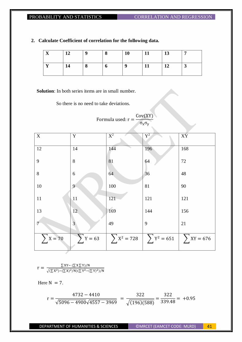
2. Calculate Coefficient of correlation for the following data.
X 12 9 8 10 11 13 7
Y 14 8 6 9 11 12 3
Solution: In both series items are in small number.
So there is no need to take deviations.
Formula used: r =Cov(XY)
σxσy
X Y X2 Y2 XY
12
9
8
10
11
13
7
14
8
6
9
11
12
3
144
81
64
100
121
169
49
196
64
36
81
121
144
9
168
72
48
90
121
156
21
∑ X = 70 ∑ Y = 63 ∑ X2 = 728 ∑ Y2 = 651 ∑ XY = 676
r = ∑ XY− (∑ X ∑ Y)/N
√(∑ X2)−(∑ X)2/N)(∑ Y2−(∑ Y)2)/N
Here N = 7.
r =4732 − 4410
√5096 − 4900√4557 − 3969 =
322
√(196)(588)=
322
339.48= +0.95

PROBABILITY AND STATISTICS CORRELATION AND REGRESSION
DEPARTMENT OF HUMANITIES & SCIENCES ©MRCET (EAMCET CODE: MLRD) 42
3. A sample of 𝟏𝟐 fathers and their elder sons gave the following data about their
elder sons. Calculate the rank correlation coefficient.
Fathers 65 63 67 64 68 62 70 66 68 67 69 71
Sons 68 66 68 65 69 66 68 65 71 67 68 70
Solution:
Fathers(x) Sons(y) Rank(x) Rank(y) di
= xi − yi
di2
65
63
67
64
68
62
70
66
68
67
69
71
68
66
68
65
69
66
68
65
71
67
68
70
9
11
6.5
10
4.5
12
2
8
4.5
6.5
3
1
5.5
9.5
5.5
11.5
3
9.5
5.5
11.5
1
8
5.5
2
3.5
1.5
1.0
-1.5
1.5
2.5
=3.5
3.5
=3.5
-1.5
-2.5
-1
12.25
2.25
1
2.25
2.25
6.25
12.25
12.25
12.25
2.25
6.25
1
∑ di2= 72.5
Repeated values are given common rank, which is the mean of the ranks .In X: 68 & 67
appear twice.

PROBABILITY AND STATISTICS CORRELATION AND REGRESSION
DEPARTMENT OF HUMANITIES & SCIENCES ©MRCET (EAMCET CODE: MLRD) 43
In Y : 68 appears 4 times , 66 appears twice & 65 appears twice. Here N = 12.
ρ = 1 − 6 {∑ D2+
1
12(m3−m)+
1
12(m3−m)
N3−N} = 1 −
6(72.5 + 7)
12(122−1)= 0.722
4. Given 𝐧 = 𝟏𝟎 , 𝛔𝐱= 5.4, 𝛔𝐲 = 𝟔. 𝟐 and sum of product of deviation from the mean of
𝐗 & 𝐘 is 𝟔𝟔. Find the correlation coefficient.
Solution: n = 10 , σx = 5.4, σy = 6.2
σx2 =
∑(x−x̅)2
n
σy2 =
∑(y−y̅)2
n
∑(x − x̅ )(y − y̅ ) = 66
r =∑(x − x̅ )(y − y̅ )
√∑(x − x̅)2 ∑(y − y̅)2 =
66
(5. )(6.2)= 0.1971
5. The heights of mothers & daughters are given in the following table. From the 2
tables of regression estimate the expected average height of daughter when the height
of the mother is 𝟔𝟒. 𝟓 inches.
Ht. of
Mother(inches)
62 63 64 64 65 66 68 70
Ht. of the
daughter(inches)
64 65 61 69 67 68 71 65
Solution:
Let X = heights of the mother
Y = heights of the daughter
Let dx = X − 65 , dy = Y – 67, ∑ x = 522, ∑ dx = 2, ∑ dx2 = 50, ∑ y = 530,
∑ dy = −6 ∑ dy2 = 74, ∑ dxdy = 20

PROBABILITY AND STATISTICS CORRELATION AND REGRESSION
DEPARTMENT OF HUMANITIES & SCIENCES ©MRCET (EAMCET CODE: MLRD) 44
X ̅ = ∑ X
N=
522
8= 66.25
Y ̅ = ∑ Y
N=
530
8= 65.25
byx =
∑ dxdy − ∑ dx ∑ dyN
∑ dx2 −(∑ dx)
2
N
= 20 −
2(−6)8
50 −28
= 0.434
Regression equation of Y on : Y − Y̅ = byx(X − X̅ )
Y = 37.93 + 0.434X
when X = 64.5 then Y = 69.923
6. The equations of two regression lines are 𝟕𝐱 − 𝟏𝟔𝐲 + 𝟗 = 𝟎 and 𝟓𝐲 − 𝟒𝐱 − 𝟑 = 𝟎.
Find the coefficient of correlation and the means of 𝐱& 𝑦 .
Solution: Given equations are 7x − 16y + 9 = 0……………….. (1)
5y − 4x − 3 = 0…………………. (2)
(1) × 4 gives 28x − 64y + 36 = 0
(2) × 7 gives -28𝑥 + 35𝑦 − 21 = 0
On adding we get −29𝑦 + 15 = 0
y = 0.5172
from(1) 7x = 16y − 9 which gives x = 0.1034
since regression line passes through (x,̅ y ̅) we have x̅ = 0.1034
y̅ = 0.5172
From(1) x =16
7y −
9
7
From (2) y =4
5x +
3
5,
rσx
σy=
16
7 and r
σy
σx=
4
5
Multiplying these 2 equations , we get r2 =16
7
4
5=
64
35
r =8
√35.
PROBABILITY AND STATISTICS CORRELATION AND REGRESSION
DEPARTMENT OF HUMANITIES & SCIENCES ©MRCET (EAMCET CODE: MLRD) 45
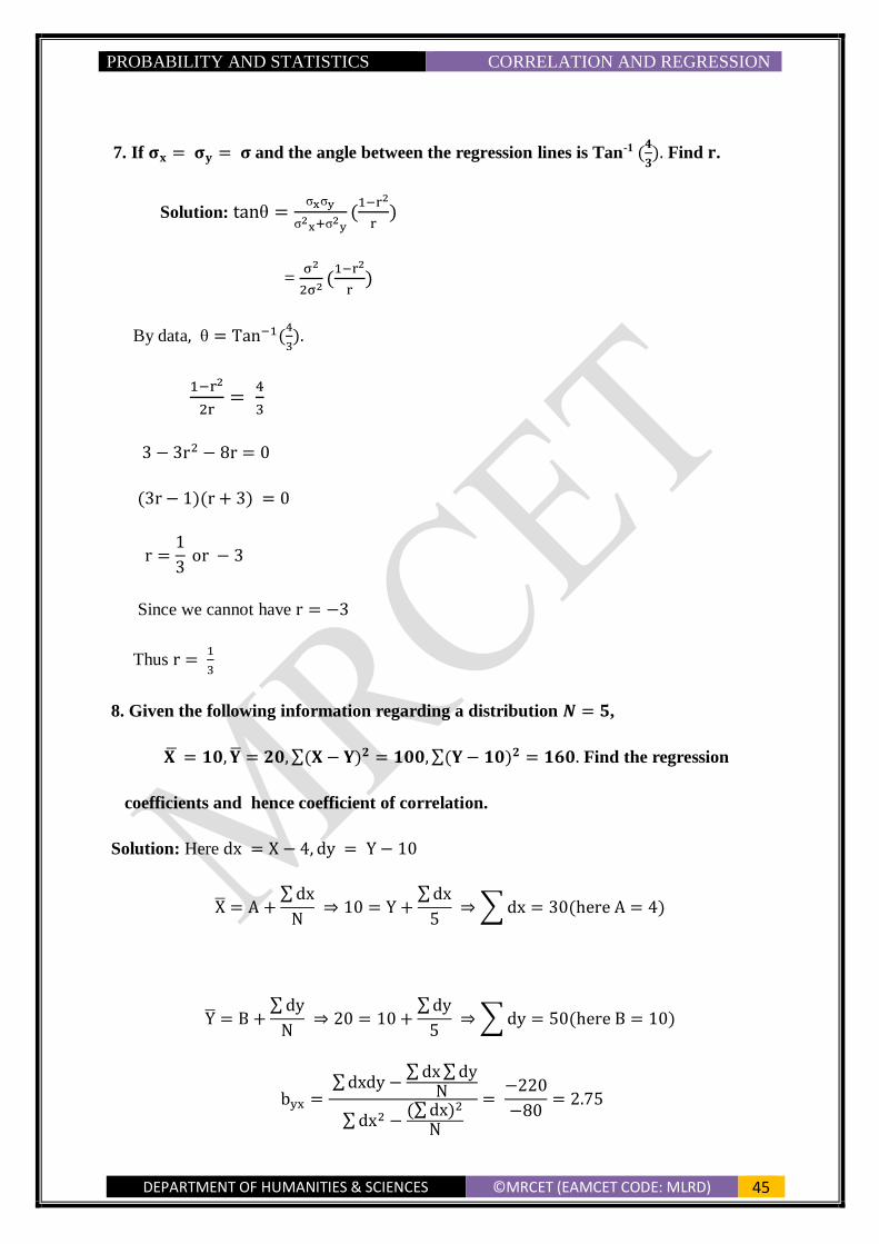
7. If 𝛔𝐱 = 𝛔𝐲 = 𝛔 and the angle between the regression lines is Tan-1 (𝟒
𝟑). Find 𝐫.
Solution: tanθ =σxσy
σ2x+σ2
y(
1−r2
r)
= σ2
2σ2(
1−r2
r)
By data, θ = Tan−1(4
3).
1−r2
2r=
4
3
3 − 3r2 − 8r = 0
(3r − 1)(r + 3) = 0
r =1
3 or − 3
Since we cannot have r = −3
Thus r = 1
3
8. Given the following information regarding a distribution 𝑵 = 𝟓,
𝐗 ̅ = 𝟏𝟎, 𝐘 = 𝟐𝟎, ∑(𝐗 − 𝐘)𝟐 = 𝟏𝟎𝟎, ∑(𝐘 − 𝟏𝟎)𝟐 = 𝟏𝟔𝟎. Find the regression
coefficients and hence coefficient of correlation.
Solution: Here dx = X − 4, dy = Y − 10
X̅ = A +∑ dx
N ⇒ 10 = Y +
∑ dx
5 ⇒ ∑ dx = 30(here A = 4)
Y̅ = B +∑ dy
N ⇒ 20 = 10 +
∑ dy
5 ⇒ ∑ dy = 50(here B = 10)
byx = ∑ dxdy −
∑ dx ∑ dyN
∑ dx2 −(∑ dx)2
N
= −220
−80= 2.75

PROBABILITY AND STATISTICS CORRELATION AND REGRESSION
DEPARTMENT OF HUMANITIES & SCIENCES ©MRCET (EAMCET CODE: MLRD) 46
bxy = ∑ dxdy −
∑ dx ∑ dyN
∑ dy2 −(∑ dy)2
N
= −220
−340= 0.65
Coefficient of correlation r = ±√bxy × byx = √(0.65)(2.75) = √1.7875 = 1.337
9. Given that 𝐗 = 𝟒𝐘 + 𝟓 and 𝐘 = 𝟒𝐗 + 𝟒 are the lines of regression of 𝐗 on 𝐘 and 𝐘 on
𝐗 respectively. Show that 𝟎 < 4𝒌 < 1. If 𝐤 =𝟏
𝟏𝟔find the means of the two variables
and coefficient of correlation between them.
Solution: Given lines are X= 4Y +5 …….(1)
Y = KX+4 ……….(2)
From (1) & (2), rσx
σy= 4 and r
σy
σx= K
Multiplying these two equations we get r2 = 4K
Since 0 ≤ r2 ≤ 1, we have 0 ≤ 4K ≤1
4
If K = 1
16 then we have X = 4Y + 5 and
Y = X/16 + 4
We get X − 4Y − 5 = 0
−X
44Y − 16 = 0
Adding we get 3X
4 − 21 = 0
X = 28
From(2), we get Y = 23
4
The regression lines pass through ( x,̅ y ̅)
We get means x̅ = 28 𝑎𝑛𝑑 y̅ =23
4
We have r2 = 4k =4
16=
1
4 ⇒ r = ±
1
2

PROBABILITY AND STATISTICS CORRELATION AND REGRESSION
DEPARTMENT OF HUMANITIES & SCIENCES ©MRCET (EAMCET CODE: MLRD) 47
We consider positive value and take r = 1
2
10.The difference between the ranks are 𝟎. 𝟓, −𝟔, −𝟒. 𝟓, −𝟑, −𝟓, −𝟏, 𝟑, 𝟎, 𝟓, 𝟓. 𝟓, 𝟎, −𝟎. 𝟓.
For refracted ranks 𝐱 𝐚𝐧𝐝 𝐲. ∑ 𝒎(𝒎𝟐−𝟏)
𝟏𝟐=3.5, 𝒓 = 𝟎. 𝟒𝟒. Find the number of terms.
Solution: Given difference (𝑑𝑖) 0.5, −6, −4.5, −3, −5, −1,3,0,5,5.5,0, −0.5
∑ di2 = 156
Here r = 1 − 6 {∑ di
2+∑ m(m2−1)
12
(N2−N)}
= 1 − (159.5)6
(N2 − N)
= 1 −957
N2−N
⇒ 0.44 = 1 −957
N2−N
⇒ N2 − N = 1708.92
⇒ N = 42
PROBABILITY AND STATISTICS SAMPLING
DEPARTMENT OF HUMANITIES & SCIENCES ©MRCET (EAMCET CODE: MLRD) 48
UNIT –IV
SAMPLING
Introduction: The totality of observations with which we are concerned , whether this
number be finite or infinite constitute population. In this chapter we focus on sampling from
distributions or populations and such important quantities as the sample mean and sample
variance.
Def: Population is defined as the aggregate or totality of statistical data forming a subject of
investigation .
EX. The population of the heights of Indian.
The number of observations in the population is defined to be the size of the population. It
may be finite or infinite .Size of the population is denoted by N.As the study of entire
population may not be possible to carry out and hence a part of the population alone is
selected.
Def: A portion of the population which is examined with a view to determining the
population characteristics is called a sample . In other words, sample is a subset of
population. Size of the sample is denoted by n.
The process of selection of a sample is called Sampling. There are different methods of
sampling
Probability Sampling Methods
Non-Probability Sampling Methods
Probability Sampling Methods:
a) Random Sampling (Probability Sampling):
It is the process of drawing a sample from a population in such a way that each
member of the population has an equal chance of being included in the sample.
Ex: A hand of cards from a well shuffled pack of cards is a random sample.
Note : If N is the size of the population and n is the size of the sample, then
The no. of samples with replacement = 𝑁𝑛
The no. of samples without replacement = 𝑁𝐶𝑛
b) Stratified Sampling :
In this , the population is first divided into several smaller groups called strata
according to some relevant characteristics . From each strata samples are selected at
random, all the samples are combined together to form the stratified sampling.
c) Systematic Sampling (Quasi Random Sampling):
In this method , all the units of the population are arranged in some order . If the
population size is N, and the sample size is n, then we first define sample interval
denoted by = 𝑁
𝑛 . then from first k items ,one unit is selected at random. Then from

PROBABILITY AND STATISTICS SAMPLING
DEPARTMENT OF HUMANITIES & SCIENCES ©MRCET (EAMCET CODE: MLRD) 49
first unit every kth unit is serially selected combining all the selected units constitute
a systematic sampling.
Non Probability Sampling Methods:
a) Purposive (Judgment ) Sampling :
In this method, the members constituting the sample are chosen not according to some
definite scientific procedure , but according to convenience and personal choice of the
individual who selects the sample . It is the choice of the individual items of a sample
entirely depends on the individual judgment of the investigator.
b) Sequential Sampling:
It consists of a sequence of sample drawn one after another from the population.
Depending on the results of previous samples if the result of the first sample is not
acceptable then second sample is drawn and the process continues to take proper
decision . But if the first sample is acceptable ,then no new sample is drawn.
Classification of Samples:
Large Samples : If the size of the sample n ≥
30 , then it is said to be large sample.
Small Samples : If the size of the sample n < 30 ,then it is said to be small sample or
exact sample.
Parameters and Statistics:
Parameter is a statistical measure based on all the units of a population. Statistic is a
statistical measure based on only the units selected in a sample.
Note :In this unit , Parameter refers to the population and Statistic refers to sample.
Central Limit Theorem: If �̅� be the mean of a random sample of size n drawn from
population having mean 𝜇 and standard deviation 𝜎 , then the sampling distribution of the
sample mean �̅� is approximately a normal distribution with mean 𝜇 and SD = S.E of �̅� = 𝜎
√𝑛
provided the sample size n is large.
Standard Error of a Statistic : The standard error of statistic ‘t’ is the standard
deviation of the sampling distribution of the statistic i.e, S.E of sample mean is the standard
deviation of the sampling distribution of sample mean.
Formulae for S.E:
S.E of Sample mean �̅� = 𝜎
√𝑛 i.e, S.E (�̅�) =
𝜎
√𝑛

PROBABILITY AND STATISTICS SAMPLING
DEPARTMENT OF HUMANITIES & SCIENCES ©MRCET (EAMCET CODE: MLRD) 50
S.E of sample proportion p=√𝑃𝑄
𝑛 i.e, S.E (p) = √
𝑃𝑄
𝑛 where Q=1-P
S.E of the difference of two sample means 𝑥1̅̅̅ and 𝑥2̅̅ ̅ i.e, S.E (𝑥1̅̅̅ − 𝑥2̅̅ ̅ ) = √𝜎1
2
𝑛1+
𝜎22
𝑛2
S.E of the difference of two proportions i.e, S.E(𝑝1 − 𝑝2) = √𝑃1𝑄1
𝑛1+
𝑃2𝑄2
𝑛2
Estimation :
To use the statistic obtained by the samples as an estimate to predict the unknown parameter
of the population from which the sample is drawn.
Estimate : An estimate is a statement made to find an unknown population parameter.
Estimator : The procedure or rule to determine an unknown population parameter is called
estimator.
Ex. Sample proportion is an estimate of population proportion , because with the help of
sample proportion value we can estimate the population proportion value.
Types of Estimation:
Point Estimation: If the estimate of the population parameter is given by a single
value , then the estimate is called a point estimation of the parameter.
Interval Estimation: If the estimate of the population parameter is given by two
different values between which the parameter may be considered to lie, then the
estimate is called an interval estimation of the parameter.
Confidence interval Estimation of parameters:
In an interval estimation of the population parameter 𝜃, if we can find two quantities 𝑡1 and
𝑡2 based on sample observations drawn from the population such that the unknown parameter
𝜃 is included in the interval [𝑡1,𝑡2] in a specified cases ,then this is called a confidence
interval for the parameter 𝜃.
Confidence Limits for Population mean 𝝁
95% confidence limits are �̅� ± 1.96 (𝑆. 𝐸. 𝑜𝑓 𝑥 ̅)
99% confidence limits are �̅� ± 2.58 (𝑆. 𝐸. 𝑜𝑓 𝑥 ̅)
99.73% confidence limits are �̅� ± 3 (𝑆. 𝐸. 𝑜𝑓 𝑥 ̅)
90% confidence limits are �̅� ± 1.645 (𝑆. 𝐸. 𝑜𝑓 𝑥 ̅)
Confidence limits for population proportion P
95% confidence limits are p ± 1.96(S.E.of p)
99% confidence limits are p ± 2.58(S.E. of p)

PROBABILITY AND STATISTICS SAMPLING
DEPARTMENT OF HUMANITIES & SCIENCES ©MRCET (EAMCET CODE: MLRD) 51
99.73% confidence limits are p ± 3(S.E.of p)
90% confidence limits are p ± 1.645(S.E.of p)
Confidence limits for the difference of two population means 𝝁𝟏 and 𝝁𝟐
95% confidence limits are ((𝑥1̅̅̅ − 𝑥2̅̅ ̅ )± 1.96 (S.E of ((𝑥1̅̅̅ − 𝑥2̅̅ ̅ ))
99% confidence limits are ((𝑥1̅̅̅ − 𝑥2̅̅ ̅ )± 2.58 (S.E of ((𝑥1̅̅̅ − 𝑥2̅̅ ̅ ))
99.73% confidence limits are ((𝑥1̅̅̅ − 𝑥2̅̅ ̅ )± 3 (S.E of ((𝑥1̅̅̅ − 𝑥2̅̅ ̅ ))
90% confidence limits are ((𝑥1̅̅̅ − 𝑥2̅̅ ̅ )± 2.58 (S.E of ((𝑥1̅̅̅ − 𝑥2̅̅ ̅ ))
Confidence limits for the difference of two population proportions
95% confidence limits are 𝑝1-𝑝2 ± 1.96 ( S.E. of 𝑝1-𝑝2)
99% confidence limits are 𝑝1-𝑝2 ± 2.58 ( S.E. of 𝑝1-𝑝2)
99.73% confidence limits are 𝑝1-𝑝2 ± 3 ( S.E. of 𝑝1-𝑝2)
90% confidence limits are 𝑝1-𝑝2 ± 1.645 ( S.E. of 𝑝1-𝑝2)
Determination of proper sample size
Sample size for estimating population mean :
n= (𝑧𝛼𝜎
𝐸)2
where 𝑧𝛼– Critical value of z at 𝛼 Level of significance
𝜎 − Standard deviation of population and
E – Maximum sampling Error = �̅� – 𝜇
Sample size for estimating population proportion :
𝑛 = 𝑧𝛼
2𝑃𝑄
𝐸2 where 𝑧𝛼 – Critical value of z at 𝛼 Level of significance
P − Population proportion
𝑄 − 1-P
𝐸 − Maximum Sampling error = p-P
Testing of Hypothesis :
It is an assumption or supposition and the decision making procedure about the assumption
whether to accept or reject is called hypothesis testing .
Def: Statistical Hypothesis : To arrive at decision about the population on the basis of
sample information we make assumptions about the population parameters involved such
assumption is called a statistical hypothesis .
Procedure for testing a hypothesis:

PROBABILITY AND STATISTICS SAMPLING
DEPARTMENT OF HUMANITIES & SCIENCES ©MRCET (EAMCET CODE: MLRD) 52
Test of Hypothesis involves the following steps:
Step1: Statement of hypothesis :
There are two types of hypothesis :
Null hypothesis: A definite statement about the population parameter. Usually a null
hypothesis is written as no difference , denoted by 𝐻0.
Ex. 𝐻0: 𝜇 = 𝜇0
Alternative hypothesis : A statement which contradicts the null hypothesis is called
alternative hypothesis. Usually an alternative hypothesis is written as some difference
, denoted by 𝐻1.
Setting of alternative hypothesis is very important to decide whether it is two-tailed or
one – tailed alternative , which depends upon the question it is dealing.
Ex.𝐻1: 𝜇 ≠ 𝜇0 (Two – Tailed test)
or
𝐻1: 𝜇 > 𝜇0 (Right one tailed test)
or
𝐻1: 𝜇 < 𝜇0 (Left one tailed test)
Step 2: Specification of level of significance :
The LOS denoted by 𝛼 is the confidence with which we reject or accept the null
hypothesis. It is generally specified before a test procedure ,which can be either 5%
(0.05) , 1% or 10% which means that thee are about 5 chances in 100 that we would
reject the null hypothesis 𝐻0 and the remaining 95% confident that we would accept
the null hypothesis 𝐻0 . Similarly , it is applicable for different level of significance.
Step 3 : Identification of the test Statistic :
There are several tests of significance like z,t, F etc .Depending upon the nature of the
information given in the problem we have to select the right test and construct the test
criterion and appropriate probability distribution.
Step 4: Critical Region:
It is the distribution of the statistic .
Two – Tailed Test : The critical region under the curve is equally distributed on
both sides of the mean.
If 𝐻1 has ≠ sign , the critical region is divided equally on both sides of the
distribution.

PROBABILITY AND STATISTICS SAMPLING
DEPARTMENT OF HUMANITIES & SCIENCES ©MRCET (EAMCET CODE: MLRD) 53
One Tailed Test: The critical region under the curve is distributed on one side of
the mean.
Left one tailed test: If 𝐻1 has < sign , the critical region is taken in the left side of the
distribution.
Right one tailed test : If 𝐻1 has > sign , the critical region is taken on right side of the
distribution.
Step 5 : Making decision:
By comparing the computed value and the critical value decision is taken for accepting or
rejecting 𝐻0
If calculated value ≤ critical value , we accept 𝐻0, otherwise reject 𝐻0.
PROBABILITY AND STATISTICS SAMPLING
DEPARTMENT OF HUMANITIES & SCIENCES ©MRCET (EAMCET CODE: MLRD) 54
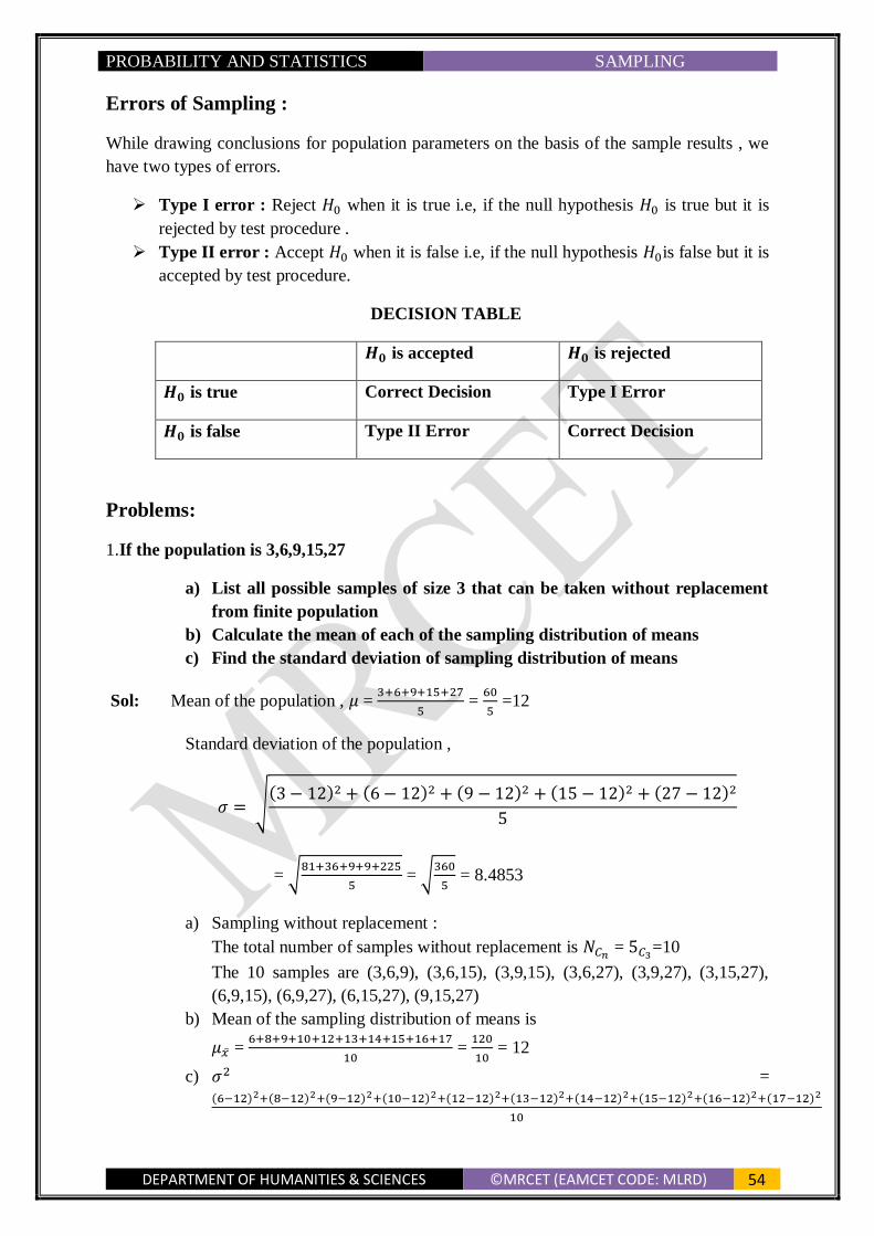
Errors of Sampling :
While drawing conclusions for population parameters on the basis of the sample results , we
have two types of errors.
Type I error : Reject 𝐻0 when it is true i.e, if the null hypothesis 𝐻0 is true but it is
rejected by test procedure .
Type II error : Accept 𝐻0 when it is false i.e, if the null hypothesis 𝐻0is false but it is
accepted by test procedure.
DECISION TABLE
𝑯𝟎 is accepted 𝑯𝟎 is rejected
𝑯𝟎 is true Correct Decision Type I Error
𝑯𝟎 is false Type II Error Correct Decision
Problems:
1.If the population is 3,6,9,15,27
a) List all possible samples of size 3 that can be taken without replacement
from finite population
b) Calculate the mean of each of the sampling distribution of means
c) Find the standard deviation of sampling distribution of means
Sol: Mean of the population , 𝜇 = 3+6+9+15+27
5 =
60
5 =12
Standard deviation of the population ,
𝜎 = √(3 − 12)2 + (6 − 12)2 + (9 − 12)2 + (15 − 12)2 + (27 − 12)2
5
= √81+36+9+9+225
5 = √
360
5 = 8.4853
a) Sampling without replacement :
The total number of samples without replacement is 𝑁𝐶𝑛 = 5𝐶3=10
The 10 samples are (3,6,9), (3,6,15), (3,9,15), (3,6,27), (3,9,27), (3,15,27),
(6,9,15), (6,9,27), (6,15,27), (9,15,27)
b) Mean of the sampling distribution of means is
𝜇�̅� = 6+8+9+10+12+13+14+15+16+17
10 =
120
10 = 12
c) 𝜎2 =
(6−12)2+(8−12)2+(9−12)2+(10−12)2+(12−12)2+(13−12)2+(14−12)2+(15−12)2+(16−12)2+(17−12)2
10
PROBABILITY AND STATISTICS SAMPLING
DEPARTMENT OF HUMANITIES & SCIENCES ©MRCET (EAMCET CODE: MLRD) 55
= 13.3
∴ 𝜎�̅� = √13.3 = 3.651
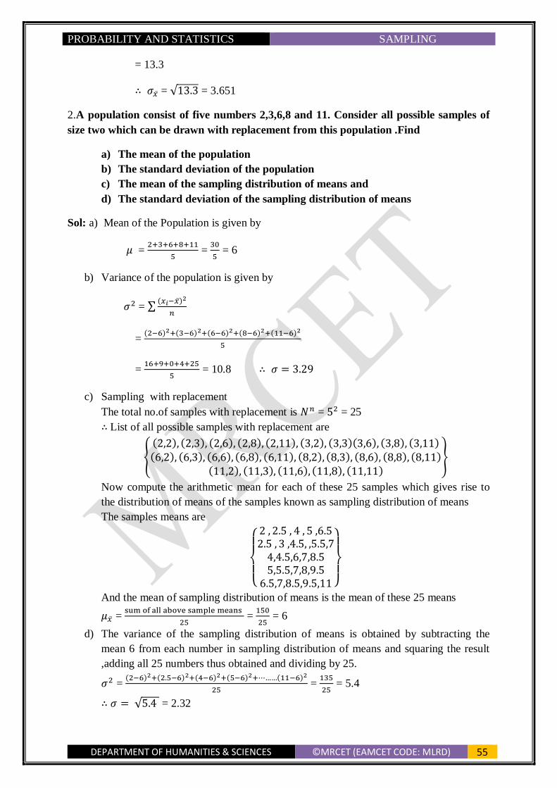
2.A population consist of five numbers 2,3,6,8 and 11. Consider all possible samples of
size two which can be drawn with replacement from this population .Find
a) The mean of the population
b) The standard deviation of the population
c) The mean of the sampling distribution of means and
d) The standard deviation of the sampling distribution of means
Sol: a) Mean of the Population is given by
𝜇 = 2+3+6+8+11
5 =
30
5 = 6
b) Variance of the population is given by
𝜎2 = ∑(𝑥𝑖−�̅�)
2
𝑛
= (2−6)2+(3−6)2+(6−6)2+(8−6)2+(11−6)2
5
= 16+9+0+4+25
5 = 10.8 ∴ 𝜎 = 3.29
c) Sampling with replacement
The total no.of samples with replacement is 𝑁𝑛 = 52 = 25
∴ List of all possible samples with replacement are
{
(2,2), (2,3), (2,6), (2,8), (2,11), (3,2), (3,3)(3,6), (3,8), (3,11)(6,2), (6,3), (6,6), (6,8), (6,11), (8,2), (8,3), (8,6), (8,8), (8,11)
(11,2), (11,3), (11,6), (11,8), (11,11)}
Now compute the arithmetic mean for each of these 25 samples which gives rise to
the distribution of means of the samples known as sampling distribution of means
The samples means are
{
2 , 2.5 , 4 , 5 ,6.52.5 , 3 ,4.5, ,5.5,74,4.5,6,7,8.55,5.5,7,8,9.56.5,7,8.5,9.5,11 }
And the mean of sampling distribution of means is the mean of these 25 means
𝜇�̅� = sum of all above sample means
25 =
150
25 = 6
d) The variance of the sampling distribution of means is obtained by subtracting the
mean 6 from each number in sampling distribution of means and squaring the result
,adding all 25 numbers thus obtained and dividing by 25.
𝜎2 = (2−6)2+(2.5−6)2+(4−6)2+(5−6)2+⋯……(11−6)2
25 =
135
25 = 5.4
∴ 𝜎 = √5.4 = 2.32
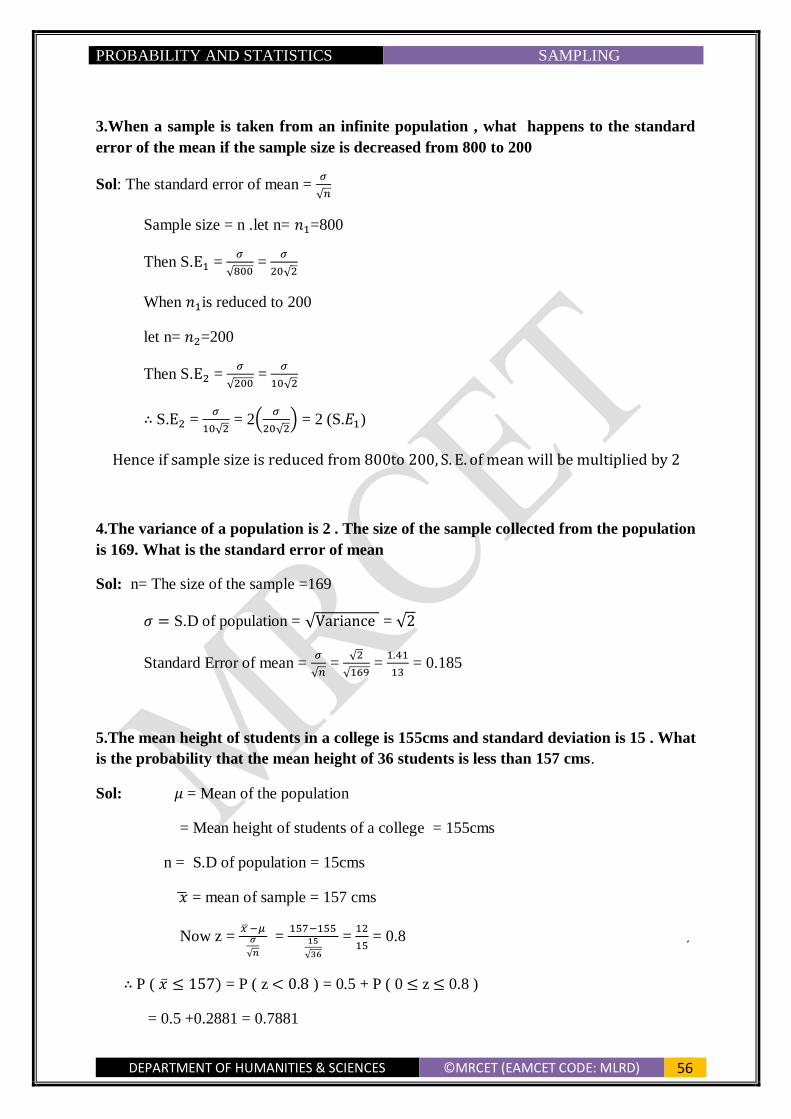
PROBABILITY AND STATISTICS SAMPLING
DEPARTMENT OF HUMANITIES & SCIENCES ©MRCET (EAMCET CODE: MLRD) 56
3.When a sample is taken from an infinite population , what happens to the standard
error of the mean if the sample size is decreased from 800 to 200
Sol: The standard error of mean = 𝜎
√𝑛
Sample size = n .let n= 𝑛1=800
Then S.E1 = 𝜎
√800 =
𝜎
20√2
When 𝑛1is reduced to 200
let n= 𝑛2=200
Then S.E2 = 𝜎
√200 =
𝜎
10√2
∴ S.E2 = 𝜎
10√2 = 2(
𝜎
20√2) = 2 (S.𝐸1)
Hence if sample size is reduced from 800to 200, S. E. of mean will be multiplied by 2
4.The variance of a population is 2 . The size of the sample collected from the population
is 169. What is the standard error of mean
Sol: n= The size of the sample =169
𝜎 = S.D of population = √Variance = √2
Standard Error of mean = 𝜎
√𝑛 =
√2
√169 =
1.41
13 = 0.185
5.The mean height of students in a college is 155cms and standard deviation is 15 . What
is the probability that the mean height of 36 students is less than 157 cms.
Sol: 𝜇 = Mean of the population
= Mean height of students of a college = 155cms
n = S.D of population = 15cms
�̅� = mean of sample = 157 cms
Now z = 𝑥 ̅−𝜇𝜎
√𝑛
= 157−155
15
√36
= 12
15 = 0.8
∴ P ( �̅� ≤ 157) = P ( z < 0.8 ) = 0.5 + P ( 0 ≤ z ≤ 0.8 )
= 0.5 +0.2881 = 0.7881

PROBABILITY AND STATISTICS SAMPLING
DEPARTMENT OF HUMANITIES & SCIENCES ©MRCET (EAMCET CODE: MLRD) 57
Thus the probability that the mean height of 36 students is less than 157 = 0.7881
6.A random sample of size 100 is taken from a population with 𝝈 = 5.1 . Given that the
sample mean is �̅� = 21.6 Construct a 95% confidence limits for the population mean .
Sol: Given �̅� = 21.6
𝑧𝛼2⁄ = 1.96, n = 100 , 𝜎 = 5.1
∴ Confidence interval = ( �̅� − 𝑧𝛼2⁄.𝜎
√𝑛 , �̅� + 𝑧𝛼
2⁄.𝜎
√𝑛 )
�̅� − 𝑧𝛼2⁄.𝜎
√𝑛 = 21.6 –
1.96 x 5.1
10 = 20.6
�̅� + 𝑧𝛼2⁄.𝜎
√𝑛 = 21.6 +
1.96 x 5.1
10 = 22.6
Hence (20.6,22.6) is the confidence interval for the population mean 𝜇
7.It is desired to estimate the mean time of continuous use until an answering machine
will first require service . If it can be assumed that 𝝈 = 60 days, how large a sample is
needed so that one will be able to assert with 90% confidence that the sample mean is
off by at most 10 days.
Sol: We have maximum error (E) = 10 days , 𝜎 = 60 days and 𝑧𝛼2⁄ = 1.645
∴ n = [𝑧𝛼
2⁄.𝜎
𝐸]2
= [1.645 x 60
10]2
= 97
8.A random sample of size 64 is taken from a normal population with 𝝁 = 𝟓𝟏. 𝟒 and 𝝈 =
6.8.What is the probability that the mean of the sample will a) exceed 52.9 b) fall
between 50.5 and 52.3 c) be less than 50.6
Sol: Given n = the size of the sample = 64
𝜇 = the mean of the population = 51.4
𝜎 = the S.D of the population = 6.8
a) P( 𝑥 ̅ exceed 52.9 ) = P(𝑥 ̅ > 52.9)
Z = �̅�−𝜇𝜎
√𝑛
= 52.9−51.4
6.8
√64
= 1.76
∴ P( 𝑥 ̅̅ ̅ > 52.9 ) = P(z > 1.76)
= 0.5 – P(0 < z < 1.76)
= 0.5 – 0.4608 = 0.0392
b) P( �̅� fall between 50.5 and 52.3)
i.e, P(50.5 < �̅� < 52.3) = P(𝑥1 ̅̅̅̅ < �̅� < 𝑥2 ̅̅̅̅ )
𝑧1= 𝑥1̅̅̅̅ −𝜇𝜎
√𝑛
= 50.5−51.4
0.85= −1.06
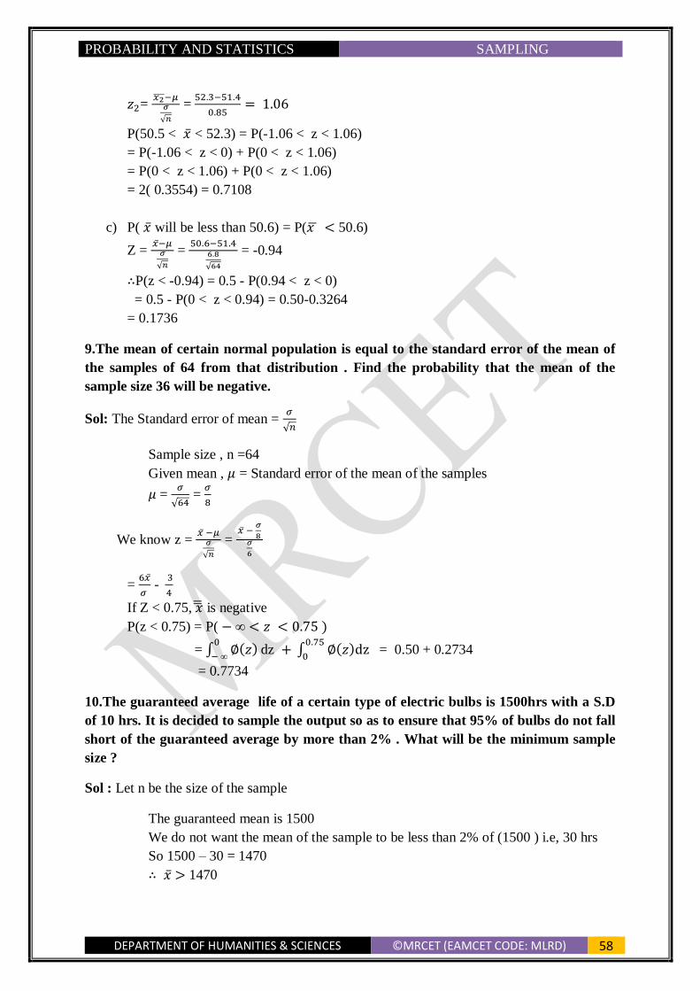
PROBABILITY AND STATISTICS SAMPLING
DEPARTMENT OF HUMANITIES & SCIENCES ©MRCET (EAMCET CODE: MLRD) 58
𝑧2= 𝑥2̅̅̅̅ −𝜇𝜎
√𝑛
= 52.3−51.4
0.85= 1.06
P(50.5 < �̅� < 52.3) = P(-1.06 < z < 1.06)
= P(-1.06 < z < 0) + P(0 < z < 1.06)
= P(0 < z < 1.06) + P(0 < z < 1.06)
= 2( 0.3554) = 0.7108
c) P( �̅� will be less than 50.6) = P(𝑥 ̅ < 50.6)
Z = �̅�−𝜇𝜎
√𝑛
= 50.6−51.4
6.8
√64
= -0.94
∴P(z < -0.94) = 0.5 - P(0.94 < z < 0)
= 0.5 - P(0 < z < 0.94) = 0.50-0.3264
= 0.1736
9.The mean of certain normal population is equal to the standard error of the mean of
the samples of 64 from that distribution . Find the probability that the mean of the
sample size 36 will be negative.
Sol: The Standard error of mean = 𝜎
√𝑛
Sample size , n =64
Given mean , 𝜇 = Standard error of the mean of the samples
𝜇 = 𝜎
√64 =
𝜎
8
We know z = �̅� −𝜇𝜎
√𝑛
= �̅� −
𝜎
8𝜎
6
= 6�̅�
𝜎 -
3
4
If Z < 0.75, �̅̅� is negative
P(z < 0.75) = P( − ∞ < 𝑧 < 0.75 )
= ∫ ∅(𝑧) 0
− ∞dz + ∫ ∅(𝑧)dz
0.75
0 = 0.50 + 0.2734
= 0.7734
10.The guaranteed average life of a certain type of electric bulbs is 1500hrs with a S.D
of 10 hrs. It is decided to sample the output so as to ensure that 95% of bulbs do not fall
short of the guaranteed average by more than 2% . What will be the minimum sample
size ?
Sol : Let n be the size of the sample
The guaranteed mean is 1500
We do not want the mean of the sample to be less than 2% of (1500 ) i.e, 30 hrs
So 1500 – 30 = 1470
∴ �̅� > 1470

PROBABILITY AND STATISTICS SAMPLING
DEPARTMENT OF HUMANITIES & SCIENCES ©MRCET (EAMCET CODE: MLRD) 59
∴ |𝑧| = |�̅�− 𝜇𝜎
√𝑛
| = |1470−1500
120
√𝑛
| = √𝑛
4
From the given condition , the area of the probability normal curve to the left of
√𝑛
4 should be 0.95
∴ The area between 0 and √n
4 is 0.45
We do not want to know about the bulbs which have life above the guranteed life .
∴ √𝑛
4 = 1.65 i.e., √𝑛 = 6.6
∴ n = 44
11.A normal population has a mean of 0.1 and standard deviation of 2.1 . Find the
probability that mean of a sample of size 900 will be negative .
Sol : Given 𝜇 = 0.1 , 𝜎 = 2.1 and n = 900
The Standard normal variate
Z = 𝑥 ̅− 𝜇𝜎
√𝑛
= �̅�− 𝜇2.1
√900
= �̅�− 0.1
0.07
∴ �̅� = 0.1 + 0.007 z where z ~ N ( 0 ,1)
∴ The required probability , that the sample mean is negative is given by
𝑃( 𝑥 ̅ < 0 ) = P ( 0.1 + 0.07 z < 0)
= P ( 0.07 z < - 0.1 )
= P ( z < (−0.1
0.07)
= P ( z < -1.43 )
= 0.50 – P ( 0 < z < 1.43 )
= 0.50 – 0.4236 = 0.0764
12.In a study of an automobile insurance a random sample of 80 body repair costs had a
mean of Rs 472.36 and the S.D of Rs 62.35. If �̅̅� is used as a point estimator to the true
average repair costs , with what confidence we can assert that the maximum error
doesn’t exceed Rs 10.
Sol : Size of a random sample , n = 80
The mean of random sample , �̅� = Rs 472.36
Standard deviation , 𝜎 = Rs 62.35
Maximum error of estimate , 𝐸 𝑚𝑎𝑥 = Rs 10
We have 𝐸 𝑚𝑎𝑥 =𝑍𝛼2⁄. 𝜎
√𝑛
i.e., 𝑍𝛼2⁄=
𝐸 𝑚𝑎𝑥 .√𝑛
𝜎 =
10 √80
62.35 =
89.4427
62.35 = 1.4345
∴ 𝑍𝛼2⁄= 1.43
The area when z = 1.43 from tables is 0.4236
∴ 𝛼
2 = 0.4236 i.e ., 𝛼 = 0.8472

PROBABILITY AND STATISTICS SAMPLING
DEPARTMENT OF HUMANITIES & SCIENCES ©MRCET (EAMCET CODE: MLRD) 60
∴ confidence = (1- 𝛼 ) 100% = 84.72 %
Hence we are 84.72% confidence that the maximum error is Rs. 10
13.If we can assert with 95% that the maximum error is 0.05 and P = 0.2 find the size of
the sample.
Sol : Given P =0.2 , E = 0.05
We have Q = 0.8 and 𝑍𝛼2⁄= 1.96 ( 5% LOS )
We know that maximum error , E = 𝑍𝛼2⁄ √
𝑃𝑄
𝑛
⇒ 0.05 = 1.96 √0.2 x 0.8
𝑛
⇒ Sample size , n = 0.2 x 0.8 x (1.96)2
(0.05)2 = 246
14.The mean and standard deviation of a population are 11,795 and 14,054 respectively
. What can one assert with 95 % confidence about the maximum error if �̅� = 11,795 and
n = 50. And also construct 95% confidence interval for true mean .
Sol: Here mean of population , 𝜇 = 11795
S.D of population , 𝜎 = 14054
�̅� = 11795
𝑛 = sample size = 50 , maximum error = 𝑍𝛼2⁄ . 𝜎
√𝑛
𝑍𝛼2⁄ for 95% confidence = 1.96
Max. error , 𝐸 = 𝑍𝛼2⁄ . 𝜎
√𝑛 = 1.96 .
14054
√50 = 3899
∴ Confidence interval = ( �̅� − 𝑍𝛼2⁄ . 𝜎
√𝑛 , �̅� + 𝑍𝛼
2⁄ . 𝜎
√𝑛 )
= (11795-3899, 11795+3899)
= (7896, 15694)
15.Find 95% confidence limits for the mean of a normally distributed population from
which the following sample was taken 15, 17 , 10 ,18 ,16 ,9, 7, 11, 13 ,14.
Sol: We have �̅� = 15+17+10+18+16+9+7+11+13+14
10 = 13
𝑆2 = ∑(𝑥𝑖−�̅�)
2
𝑛−1
= 1
9 [(15 − 13)2 + (15 − 13)2 + (15 − 13)2 + (15 − 13)2 + (15 − 13)2 +
(15 − 13)2 + (15 − 13)2 + (15 − 13)2 + (15 − 13)2 + (15 − 13)2]
= 40
3
Since 𝑍𝛼2⁄ = 1.96 , we have

PROBABILITY AND STATISTICS SAMPLING
DEPARTMENT OF HUMANITIES & SCIENCES ©MRCET (EAMCET CODE: MLRD) 61
𝑍𝛼2⁄ .
𝑠
√𝑛 = 1.96 .
√40
√10.√3 = 2.26
∴ Confidence limits are �̅� ± 𝑍𝛼2⁄ .
𝑠
√𝑛 = 13 ± 2.26 = ( 10.74 , 15.26 )
16.A random sample of 100 teachers in a large metropolitan area revealed mean weekly
salary of Rs. 487 with a standard deviation Rs.48. With what degree of confidence can
we assert that the average weekly of all teachers in the metropolitan area is between 472
to 502 ?
Sol: Given 𝜇 = 487 , 𝜎 = 48 , 𝑛 = 100
Z = �̅̅�− 𝜇𝜎
√𝑛
= �̅�− 487
48
√100
= �̅�− 487
4.8
Standard variable corresponding to Rs. 472 is
𝑍1 = 472− 487
4.8 = - 3.125
Standard vaiable corresponding to Rs. 502
𝑍2 = 502− 487
4.8 = 3.125
Let x ̅be the mean salary of teacher . Then
P ( 472 < x ̅ < 502 ) = P ( -3.125 < z < 3.125 )
= 2 ( 0 < z < 3.125 )
= 2 ∫ ∅(𝑧)𝑑𝑧3.125
0
= 2 ( 0.4991) = 0.9982
Thus we can ascertain with 99.82 % confidence

PROBABILITY AND STATISTICS STATISTICAL INFERENCES
DEPARTMENT OF HUMANITIES & SCIENCES ©MRCET (EAMCET CODE: MLRD) 62
UNIT-V
STATISTICAL INFERENCES
Large Samples: Let a random sample of size n >30 is defined as large sample.
Applications of Large Samples
Test of Significance of a Single Mean
Let a random sample of size n, x ̅be the mean of the sample and 𝜇 be the population mean.
1. Null hypothesis: 𝐻0: There is no significant difference in the given population mean
value say ‘𝜇0′ .
i.e 𝐻0:µ = 𝜇0
2. Alternative hypothesis: 𝐻1 :There is some significant difference in the given population
mean value.
i.e
a)𝐻1 : µ ≠ µ0 (Two –tailed)
b) 𝐻1 : µ > µ0 (Right one tailed)
c) 𝐻1 : µ > µ0 (Left one tailed)
3. Level of significance: Set the LOS α
4. Test Statistic: 𝑧𝑐𝑎𝑙 =�̅�−µ0
√𝑛𝜎/ (OR) 𝑧𝑐𝑎𝑙 =
�̅�−µ0
√𝑛𝑠/
5. Decision /conclusion : If zcalvalue < 𝑧∝value , accept 𝐻0 otherwise reject 𝐻0
CRITICAL VALUES OF Z
LOS ∝ 1% 5% 10%
µ≠ µ0 |𝑍|>2.58 |𝑍|>1.96 |𝑍|>1.645
µ> µ0 Z>2.33 z>1.645 Z>1.28
µ< µ0 Z<-2.33 Z<-1.645 Z<-1.28
NOTE: Confidence limits for the mean of the population corresponding to the given sample.
𝜇 = �̅� ± 𝑍∝2⁄ ( S.E of �̅�) i.e,
𝜇 = �̅� ± 𝑍∝2⁄ (
𝜎
√𝑛) (or) 𝜇 = �̅� ± 𝑍∝
2⁄ (휀
√𝑛)

PROBABILITY AND STATISTICS STATISTICAL INFERENCES
DEPARTMENT OF HUMANITIES & SCIENCES ©MRCET (EAMCET CODE: MLRD) 63
2. Test of Significance for Difference of Means of two Large Samples
Let 𝑥1̅̅ ̅ & 𝑥2̅̅ ̅ be the means of the samples of two ramdom sizes 𝓃1 & 𝓃2 drawn from two
populations having means 𝜇1&𝜇2 and SD’s 𝜎1&𝜎2
i) 𝐍𝐮𝐥𝐥 𝐡𝐲𝐨𝐩𝐨𝐭𝐡𝐞𝐬𝐢𝐬: 𝐻0: 𝜇1 = 𝜇2
ii) Alternative hypothesis :: a) H1 : 𝜇1 ≠ 𝜇2(Two Tailed)
b) H1: 𝜇1 < µ2 (Left one tailed)
c) H1: 𝜇1 > µ2 (Right one tailed)
iii) Level of Significance: Set the LOS α
iv) Test Statistic : 𝑍𝑐𝑎𝑙 =(×̅1−×̅2)−𝛿
𝑆𝐸 𝑜𝑓(×̅1−×̅2)= -
(×̅1−×̅2)−𝛿
√𝜎1
2
𝑛1+
𝜎22
𝑛2
Where 𝛿 = 𝜇1 − 𝜇2( where given constant)
Other wise 𝛿 = 𝜇1 − 𝜇2=0
𝑍𝑐𝑎𝑙 =×̅1−×̅2−𝛿
√𝜎1
2
𝑛1+
𝜎22
𝑛2
if 𝜎12 = 𝜎2
2 = 𝜎2 then 𝑍𝑐𝑎𝑙 =�̅�1−�̅�2
√1
𝑛1+
1𝑛2
𝜎
Critical value of Z from normal table at the LOS α
v) Decision: If |𝑍𝑐𝑎𝑙| < 𝑍𝑡𝑎𝑏, accept H0 otherwise reject H0
CRITICAL VALUES OF Z
LOS ∝ 1% 5% 10%
µ≠ µ0 /Z/>2.58 /Z/>1.96 /Z/>1.645
µ> µ0 Z>2.33 z>1.645 Z>1.28
µ< µ0 Z<-2.33 Z<-1.645 Z<-1.28
NOTE: Confidence limits for difference of means
𝜇1 − 𝜇2 = (�̅�1 − �̅�2) ± 𝑧∝ 2⁄ [𝑆. 𝐸 𝑜𝑓 (�̅�1 − �̅�2)]
= (�̅�1 − �̅�2) ± 𝑧∝ 2⁄ [√𝜎1
2
𝑛1+
𝜎22
𝑛1]

PROBABILITY AND STATISTICS STATISTICAL INFERENCES
DEPARTMENT OF HUMANITIES & SCIENCES ©MRCET (EAMCET CODE: MLRD) 64
3. Test of Significance for Single Proportions
Suppose a random sample of size n has a sample proportion p of members possessing
a certain attribute (proportion of successes). To test the hypothesis that the proportion
P in the population has a specified value P0 .
i) 𝐍𝐮𝐥𝐥 𝐡𝐲𝐨𝐩𝐨𝐭𝐡𝐞𝐬𝐢𝐬 : 𝐻0: 𝑃 = 𝑃0
ii) Alternative hypothesis : a) H1 : P≠ 𝑃0(Two Tailed test )
b) H1 ∶ 𝑃 < 𝑃0 (Left one- tailed)
c) H1 ∶ P > 𝑃0 (Right one tailed)
iii) Test statistic :𝑍𝑐𝑎𝑙 =𝑝−𝑃
√𝑃𝑄𝑛
when P is the Population proportion 𝑄 = 1 − 𝑃
iv) At specified LOS ∝, critical value of Z
v) Decision: If |𝑧𝑐𝑎𝑙| < 𝑍𝑡𝑎𝑏, accept H0 otherwise reject H0
CRITICAL VALUES OF Z
LOS ∝ 1% 5% 10%
µ≠ µ0 /Z/>2.58 /Z/>1.96 /Z/>1.645
µ> µ0 Z>2.33 z>1.645 Z>1.28
µ< µ0 Z<-2.33 Z<-1.645 Z<-1.28
NOTE : Confidence limits for population proportion
P = P ± Z∝2(S E of P)
= P ± Z∝2
(√pq
n)
4. Test for Equality of Two Proportions (Populations)
Let p1 and p2 be the sample proportions in two large random samples of sizes n1 & n2
drawn from two populations having proportions P1 & P2
i) 𝐍𝐮𝐥𝐥 𝐡𝐲𝐨𝐩𝐨𝐭𝐡𝐞𝐬𝐢𝐬 : 𝐻0: 𝑃1 = 𝑃2
ii) Alternative hypothesis : a) H1 : 𝑃1 ≠ 𝑃2(Two Tailed)
b) H1 : 𝑃1 < 𝑃2 (Left one tailed)
c) H1 : 𝑃1 > 𝑃2 (Right one tailed)
iii) Test statistic :𝑍𝑐𝑎𝑙 =(𝑃1−𝑃2)−(𝑃1−𝑃2)
√𝑃1𝑄1
𝑛1+
𝑃1𝑄1𝑛2
if (P1-P2) is given.

PROBABILITY AND STATISTICS STATISTICAL INFERENCES
DEPARTMENT OF HUMANITIES & SCIENCES ©MRCET (EAMCET CODE: MLRD) 65
If given only sample proportions then
𝑍𝑐𝑎𝑙 =𝑝1−𝑝2
√𝑃1𝑞1
𝑛1+
𝑃2𝑞1𝑛2
where p1
=x1
n1 & p
1=
x2
n2
OR
Zcal =p1 − p2
√pq(1
n1+
1
n2) Where p =
n1p1+n2p2
n1+n2 =
x1 +x2
n1+n2 and q = 1- p
iv) At specified LOS ∝ critical value of ‘Z’
v) Decision: If |𝑍𝑐𝑎𝑙| < 𝑍𝑇𝑎𝑏, accept H0 otherwise reject H0
CRITICAL VALUES OF Z
LOS ∝ 1% 5% 10%
µ≠ µ0 /Z/>2.58 /Z/>1.96 /Z/>1.645
µ> µ0 Z>2.33 z>1.645 Z>1.28
µ< µ0 Z<-2.33 Z<-1.645 Z<-1.28
NOTE: Confidence limits for difference of population proportions
𝑃1 − 𝑃2 = (𝑝1
− 𝑝2
) ± 𝑍∝ 2
(𝑆 . 𝐸 𝑜𝑓 𝑃1 − 𝑃2 )
Problems:
1. A sample of 64 students have a mean weight of 70 kgs . Can this be regarded as
asample mean from a population with mean weight 56 kgs and standard
deviation 25 kgs.
Sol : Given �̅� = mean of he sample = 70 kgs
𝝁 = Mean of the population = 56 kgs
𝝈 = S.D of population = 25 kgs
𝐚𝐧𝐝 𝒏 = 𝐒𝐚𝐦𝐩𝐥𝐞 𝐬𝐢𝐳𝐞 = 𝟔4
i) Sol: Null Hypothesis 𝐻0 : A Sample of 64 students with mean weight 70 kgs be
regarded as a sample from a population with mean weight 56 kgs and standard
deviation 25 kgs. i.e., 𝐻0 : 𝜇 = 70 kgs
ii) Alternative Hypothesis 𝐻1 : Sample cannot be regarded as one coming from the
population . i.e., 𝐻1 : 𝜇 ≠ 70 kgs ( Two –tailed test )
iii) Level of significance : 𝛼 = 0.05 (𝑍𝛼 = 1.96 )
iv) Test Statistic : 𝑍 𝑐𝑎𝑙= �̅�− 𝜇
𝜎
√𝑛
= 70−56
25
√64
= 4.48
v) Conclusion: Since |𝑍 𝑐𝑎𝑙| 𝑣𝑎𝑙𝑢𝑒 > 𝑍𝛼 value , we reject 𝐻0
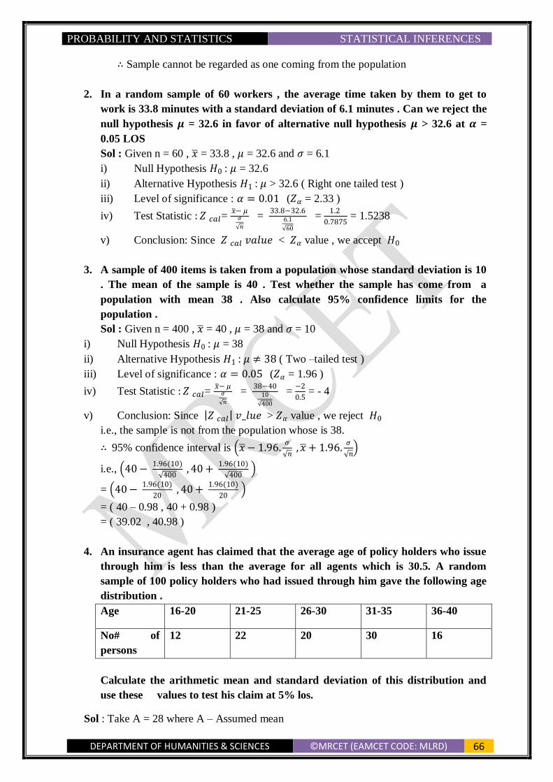
PROBABILITY AND STATISTICS STATISTICAL INFERENCES
DEPARTMENT OF HUMANITIES & SCIENCES ©MRCET (EAMCET CODE: MLRD) 66
∴ Sample cannot be regarded as one coming from the population
2. In a random sample of 60 workers , the average time taken by them to get to
work is 33.8 minutes with a standard deviation of 6.1 minutes . Can we reject the
null hypothesis 𝝁 = 32.6 in favor of alternative null hypothesis 𝝁 > 32.6 at 𝜶 =
0.05 LOS
Sol : Given n = 60 , �̅� = 33.8 , 𝜇 = 32.6 and 𝜎 = 6.1
i) Null Hypothesis 𝐻0 : 𝜇 = 32.6
ii) Alternative Hypothesis 𝐻1 : 𝜇 > 32.6 ( Right one tailed test )
iii) Level of significance : 𝛼 = 0.01 (𝑍𝛼 = 2.33 )
iv) Test Statistic : 𝑍 𝑐𝑎𝑙= �̅�− 𝜇
𝜎
√𝑛
= 33.8−32.6
6.1
√60
= 1.2
0.7875 = 1.5238
v) Conclusion: Since 𝑍 𝑐𝑎𝑙 𝑣𝑎𝑙𝑢𝑒 < 𝑍𝛼 value , we accept 𝐻0
3. A sample of 400 items is taken from a population whose standard deviation is 10
. The mean of the sample is 40 . Test whether the sample has come from a
population with mean 38 . Also calculate 95% confidence limits for the
population .
Sol : Given n = 400 , �̅� = 40 , 𝜇 = 38 and 𝜎 = 10
i) Null Hypothesis 𝐻0 : 𝜇 = 38
ii) Alternative Hypothesis 𝐻1 : 𝜇 ≠ 38 ( Two –tailed test )
iii) Level of significance : 𝛼 = 0.05 (𝑍𝛼 = 1.96 )
iv) Test Statistic : 𝑍 𝑐𝑎𝑙= �̅�− 𝜇
𝜎
√𝑛
= 38−40
10
√400
= −2
0.5 = - 4
v) Conclusion: Since |𝑍 𝑐𝑎𝑙| 𝑣_𝑙𝑢𝑒 > 𝑍𝛼 value , we reject 𝐻0
i.e., the sample is not from the population whose is 38.
∴ 95% confidence interval is (�̅� − 1.96.𝜎
√𝑛 , �̅� + 1.96.
𝜎
√𝑛)
i.e., (40 − 1.96(10)
√400 , 40 +
1.96(10)
√400 )
= (40 − 1.96(10)
20 , 40 +
1.96(10)
20 )
= ( 40 – 0.98 , 40 + 0.98 )
= ( 39.02 , 40.98 )
4. An insurance agent has claimed that the average age of policy holders who issue
through him is less than the average for all agents which is 30.5. A random
sample of 100 policy holders who had issued through him gave the following age
distribution .
Age 16-20 21-25 26-30 31-35 36-40
No# of
persons
12 22 20 30 16
Calculate the arithmetic mean and standard deviation of this distribution and
use these values to test his claim at 5% los.
Sol : Take A = 28 where A – Assumed mean

PROBABILITY AND STATISTICS STATISTICAL INFERENCES
DEPARTMENT OF HUMANITIES & SCIENCES ©MRCET (EAMCET CODE: MLRD) 67
𝑑𝑖 = 𝑥𝑖 – A
𝑥 ̅ = A + ℎ ∑ 𝑓𝑖𝑑𝑖
𝑁
= 28 + 5 x 16
100 = 28.8
S.D : S = h √∑ 𝑓𝑑2
𝑁− (
∑ 𝑓𝑑
𝑁)
2 = 5. √
164
100− (
16
100)
2 = 6.35
i) Null Hypothesis 𝐻0 : The sample is drawn from population with mean 𝜇
ii) i.e., 𝐻0 : 𝜇 = 30.5 years
iii) Alternative Hypothesis 𝐻1 : 𝜇 < 30.5 ( Left one –tailed test )
iv) Level of significance : 𝛼 = 0.05 (𝑍𝛼 = 1.645 )
v) Test Statistic : 𝑍 𝑐𝑎𝑙= �̅�− 𝜇
𝜎
√𝑛
= 28.8−30.5
6.35
√100
= − 2.677
vi) Conclusion: Since |𝑍 𝑐𝑎𝑙| 𝑣𝑎𝑙𝑢𝑒 > 𝑍𝛼 value , we reject 𝐻0
i.e., the sample is not drawn from the population with 𝜇 = 30.5 years .
5. An ambulance service claims that it takes on the average less than 10 minutes to
reach its destination in emergency calls . A sample of 36 calls has a mean of 11
minutes and the variance of 16 minutes .Test the claim at 0.05 los?
Sol : Given n = 36 , �̅� =11 , 𝜇 = 10 and 𝜎 = √16 = 4
i) Null Hypothesis 𝐻0 : 𝜇 = 10
ii) Alternative Hypothesis 𝐻1 : 𝜇 < 10 ( Left one –tailed test )
iii) Level of significance : 𝛼 = 0.05 (𝑍𝛼 = 1.645 )
iv) Test Statistic : 𝑍 𝑐𝑎𝑙= �̅�− 𝜇
𝜎
√𝑛
= 11−10
4
√36
= 6
4 = 1.5
v) Conclusion: Since |𝑍 𝑐𝑎𝑙| 𝑣𝑎𝑙𝑢𝑒 < 𝑍𝛼 value , we accept 𝐻0
6. The means of two large samples of sizes 1000 and 2000 members are 67.5 inches
and 68 inches respectively . Can the samples be regarded as drawn from the
same population of S.D 2.5 inches.
Sol: Let 𝜇1 and 𝜇2 be the means of the two populations
Given 𝑛1 = 1000 , 𝑛2 = 2000 and �̅�1 = 67.5 inches , �̅�2 = 68 inches
Population S.D, 𝜎 = 2.5 inches
i) Null Hypothesis 𝐻0 :The samples have been drawn from the same population of
S.D 2.5 inches
i.e., 𝐻0 : 𝜇1 = 𝜇2
ii) Alternative Hypothesis 𝐻1 : 𝜇1 ≠ 𝜇2 ( Two – Tailed test)
iii) Level of significance : 𝛼 = 0.05 (𝑍𝛼 = 1.96 )
iv) Test Statistic : 𝑍 𝑐𝑎𝑙= �̅�1−�̅�2
√1
𝑛1+
1𝑛2
𝜎 =
67.5−68
√(2.5)2(
11000
+1
2000)
= −0.5
0.0968 = -5.16
v) Conclusion: Since |𝑍 𝑐𝑎𝑙| 𝑣𝑎𝑙𝑢𝑒 > 𝑍𝛼 value , we reject 𝐻0
Hence , we conclude that the samples are not drawn from the same population of
S.D 2.5 inches.
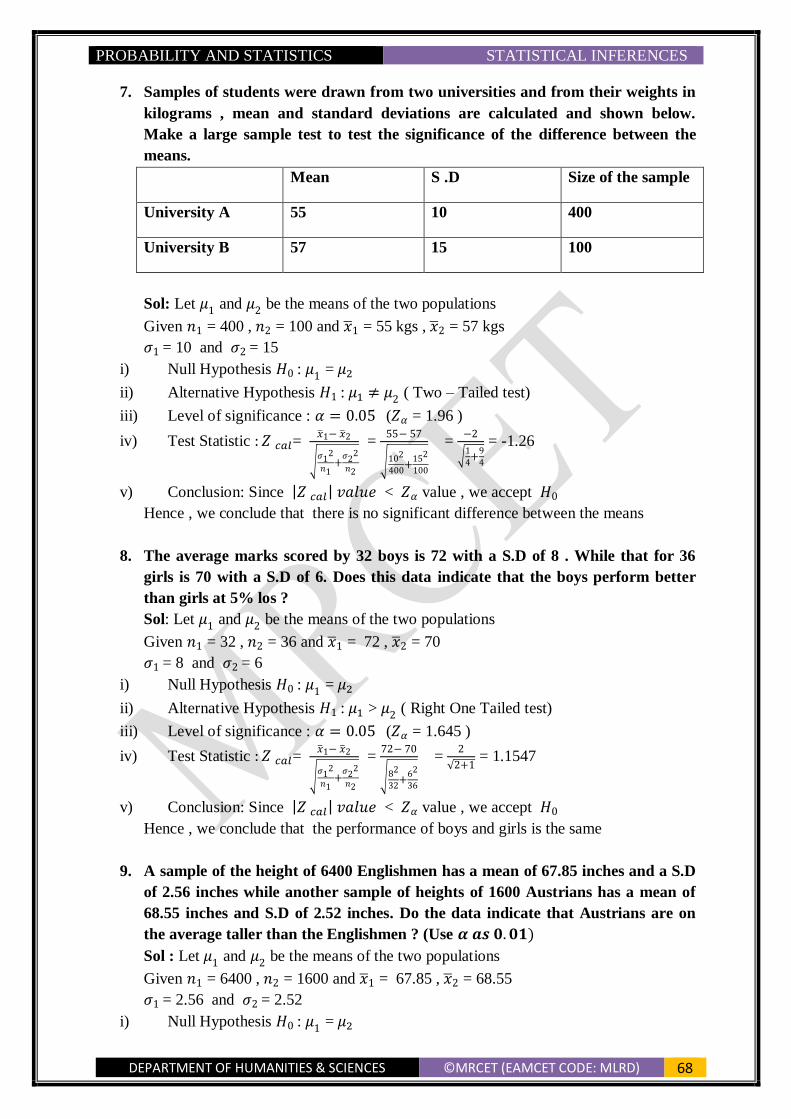
PROBABILITY AND STATISTICS STATISTICAL INFERENCES
DEPARTMENT OF HUMANITIES & SCIENCES ©MRCET (EAMCET CODE: MLRD) 68
7. Samples of students were drawn from two universities and from their weights in
kilograms , mean and standard deviations are calculated and shown below.
Make a large sample test to test the significance of the difference between the
means.
Mean S .D Size of the sample
University A 55 10 400
University B 57 15 100
Sol: Let 𝜇1 and 𝜇2 be the means of the two populations
Given 𝑛1 = 400 , 𝑛2 = 100 and �̅�1 = 55 kgs , �̅�2 = 57 kgs
𝜎1 = 10 and 𝜎2 = 15
i) Null Hypothesis 𝐻0 : 𝜇1 = 𝜇2
ii) Alternative Hypothesis 𝐻1 : 𝜇1 ≠ 𝜇2 ( Two – Tailed test)
iii) Level of significance : 𝛼 = 0.05 (𝑍𝛼 = 1.96 )
iv) Test Statistic : 𝑍 𝑐𝑎𝑙= �̅�1− �̅�2
√𝜎1
2
𝑛1+
𝜎22
𝑛2
= 55− 57
√102
400+
152
100
= −2
√1
4+
9
4
= -1.26
v) Conclusion: Since |𝑍 𝑐𝑎𝑙| 𝑣𝑎𝑙𝑢𝑒 < 𝑍𝛼 value , we accept 𝐻0
Hence , we conclude that there is no significant difference between the means
8. The average marks scored by 32 boys is 72 with a S.D of 8 . While that for 36
girls is 70 with a S.D of 6. Does this data indicate that the boys perform better
than girls at 5% los ?
Sol: Let 𝜇1 and 𝜇2 be the means of the two populations
Given 𝑛1 = 32 , 𝑛2 = 36 and �̅�1 = 72 , �̅�2 = 70
𝜎1 = 8 and 𝜎2 = 6
i) Null Hypothesis 𝐻0 : 𝜇1 = 𝜇2
ii) Alternative Hypothesis 𝐻1 : 𝜇1 > 𝜇2 ( Right One Tailed test)
iii) Level of significance : 𝛼 = 0.05 (𝑍𝛼 = 1.645 )
iv) Test Statistic : 𝑍 𝑐𝑎𝑙= �̅�1− �̅�2
√𝜎1
2
𝑛1+
𝜎22
𝑛2
= 72− 70
√82
32+
62
36
= 2
√2+1 = 1.1547
v) Conclusion: Since |𝑍 𝑐𝑎𝑙| 𝑣𝑎𝑙𝑢𝑒 < 𝑍𝛼 value , we accept 𝐻0
Hence , we conclude that the performance of boys and girls is the same
9. A sample of the height of 6400 Englishmen has a mean of 67.85 inches and a S.D
of 2.56 inches while another sample of heights of 1600 Austrians has a mean of
68.55 inches and S.D of 2.52 inches. Do the data indicate that Austrians are on
the average taller than the Englishmen ? (Use 𝜶 𝒂𝒔 𝟎. 𝟎𝟏)
Sol : Let 𝜇1 and 𝜇2 be the means of the two populations
Given 𝑛1 = 6400 , 𝑛2 = 1600 and �̅�1 = 67.85 , �̅�2 = 68.55
𝜎1 = 2.56 and 𝜎2 = 2.52
i) Null Hypothesis 𝐻0 : 𝜇1 = 𝜇2

PROBABILITY AND STATISTICS STATISTICAL INFERENCES
DEPARTMENT OF HUMANITIES & SCIENCES ©MRCET (EAMCET CODE: MLRD) 69
ii) Alternative Hypothesis 𝐻1 : 𝜇1 < 𝜇2 ( Left One Tailed test)
iii) Level of significance : 𝛼 = 0.01 (𝑍𝛼 = - 2.33 )
iv) Test Statistic : 𝑍 𝑐𝑎𝑙= �̅�1− �̅�2
√𝜎1
2
𝑛1+
𝜎22
𝑛2
= 67.85− 68.55
√2.562
6400+
2.522
1600
= 67.85 − 68.55
√6.55366400 +
6.351600
= − 0.7
√0.001+0.004 =
− 0.7
0.0707 - 9.9
v) Conclusion: Since |Z cal| value > Zα value , we reject 𝐻0
Hence , we conclude that Australians are taller than Englishmen.
10. At a certain large university a sociologist speculates that male students spend
considerably more money on junk food than female students. To test her
hypothesis the sociologist randomly selects from records the names of 200
students . Of thee , 125 are men and 75 are women . The mean of the average
amount spent on junk food per week by the men is Rs. 400 and S.D is 100. For
the women the sample mean is Rs. 450 and S.D is 150. Test the hypothesis at 5 %
los ?
Sol: Let 𝜇1 and 𝜇2 be the means of the two populations
Given 𝑛1 = 125 , 𝑛2 = 75 and �̅�1 = Mean of men = 400 , �̅�2 = Mean of women = 450
𝜎1 = 100 and 𝜎2 = 150
i) Null Hypothesis 𝐻0 : 𝜇1 = 𝜇2
ii) Alternative Hypothesis 𝐻1 : 𝜇1 > 𝜇2 ( Right One Tailed test)
iii) Level of significance : 𝛼 = 0.05 (𝑍𝛼 = 1.645 )
iv) Test Statistic : 𝑍 𝑐𝑎𝑙= �̅�1− �̅�2
√𝜎1
2
𝑛1+
𝜎22
𝑛2
= 400− 450
√1002
125+
1502
75
= − 50
√80 + 300
= − 50
√380 =
− 50
19.49 = - 2.5654
v) Conclusion: Since Zcalvalue < Zα value , we accept 𝐻0
Hence , we conclude that difference between the means are equal
11. The research investigator is interested in studying whether there is a significant
difference in the salaries of MBA grads in two cities. A random sample of size
100 from city A yields an average income of Rs. 20,150 . Another random sample
of size 60 from city B yields an average income of Rs. 20,250. If the variance are
given as 𝝈𝟏𝟐 = 40,000 and
𝝈𝟐𝟐 = 32,400 respectively . Test the equality of means and also construct 95%
confidence limits.
Sol: Let 𝜇1 and 𝜇2 be the means of the two populations
Given 𝑛1 = 100 , 𝑛2 = 60 and �̅�1 = Mean of city A = 20,150 , �̅�2 = Mean of city B =
20,250
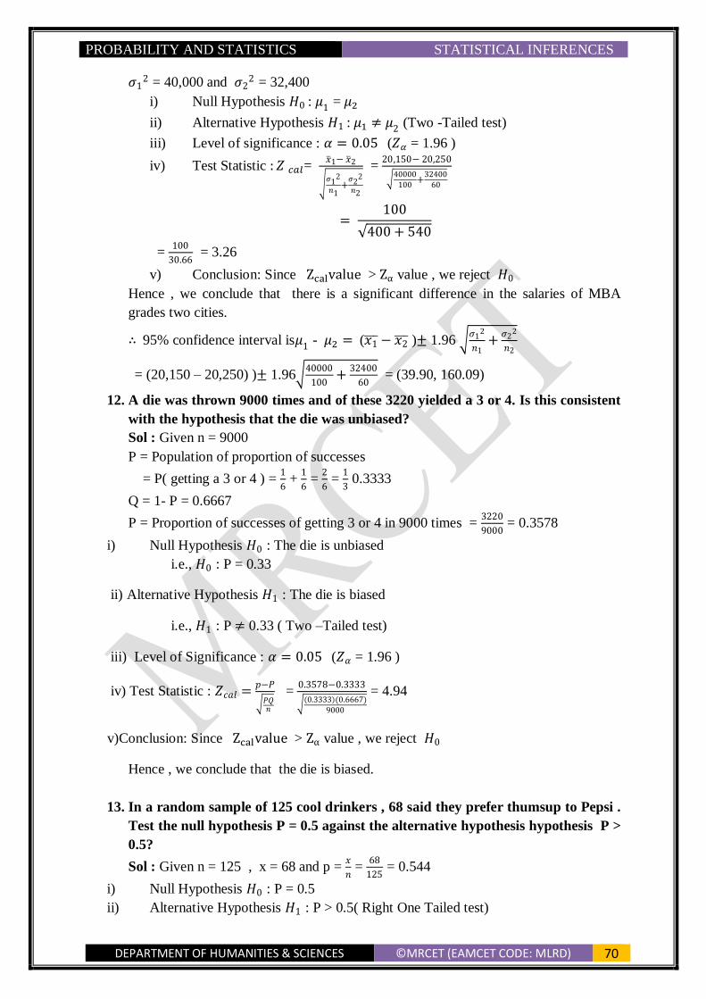
PROBABILITY AND STATISTICS STATISTICAL INFERENCES
DEPARTMENT OF HUMANITIES & SCIENCES ©MRCET (EAMCET CODE: MLRD) 70
𝜎12 = 40,000 and 𝜎2
2 = 32,400
i) Null Hypothesis 𝐻0 : 𝜇1 = 𝜇2
ii) Alternative Hypothesis 𝐻1 : 𝜇1 ≠ 𝜇2 (Two -Tailed test)
iii) Level of significance : 𝛼 = 0.05 (𝑍𝛼 = 1.96 )
iv) Test Statistic : 𝑍 𝑐𝑎𝑙= �̅�1− �̅�2
√𝜎1
2
𝑛1+
𝜎22
𝑛2
= 20,150− 20,250
√40000
100+
32400
60
= 100
√400 + 540
= 100
30.66 = 3.26
v) Conclusion: Since Zcalvalue > Zα value , we reject 𝐻0
Hence , we conclude that there is a significant difference in the salaries of MBA
grades two cities.
∴ 95% confidence interval is𝜇1 - 𝜇2 = (𝑥1̅̅ ̅ − 𝑥2̅̅ ̅ )± 1.96 √𝜎1
2
𝑛1+
𝜎22
𝑛2
= (20,150 – 20,250) )± 1.96√40000
100+
32400
60 = (39.90, 160.09)
12. A die was thrown 9000 times and of these 3220 yielded a 3 or 4. Is this consistent
with the hypothesis that the die was unbiased?
Sol : Given n = 9000
P = Population of proportion of successes
= P( getting a 3 or 4 ) = 1
6 +
1
6 =
2
6 =
1
3 0.3333
Q = 1- P = 0.6667
P = Proportion of successes of getting 3 or 4 in 9000 times = 3220
9000 = 0.3578
i) Null Hypothesis 𝐻0 : The die is unbiased
i.e., 𝐻0 : P = 0.33
ii) Alternative Hypothesis 𝐻1 : The die is biased
i.e., 𝐻1 : P ≠ 0.33 ( Two –Tailed test)
iii) Level of Significance : 𝛼 = 0.05 (𝑍𝛼 = 1.96 )
iv) Test Statistic : 𝑍𝑐𝑎𝑙 =𝑝−𝑃
√𝑃𝑄𝑛
= 0.3578−0.3333
√(0.3333)(0.6667)
9000
= 4.94
v)Conclusion: Since Zcalvalue > Zα value , we reject 𝐻0
Hence , we conclude that the die is biased.
13. In a random sample of 125 cool drinkers , 68 said they prefer thumsup to Pepsi .
Test the null hypothesis P = 0.5 against the alternative hypothesis hypothesis P >
0.5?
Sol : Given n = 125 , x = 68 and p = 𝑥
𝑛 =
68
125 = 0.544
i) Null Hypothesis 𝐻0 : P = 0.5
ii) Alternative Hypothesis 𝐻1 : P > 0.5( Right One Tailed test)

PROBABILITY AND STATISTICS STATISTICAL INFERENCES
DEPARTMENT OF HUMANITIES & SCIENCES ©MRCET (EAMCET CODE: MLRD) 71
iii) Level of Significance : 𝛼 = 0.05 (𝑍𝛼 = 1.645 )
iv) Test Statistic : 𝑍𝑐𝑎𝑙 =𝑝−𝑃
√𝑃𝑄𝑛
= 0.544−0.5
√(0.5)(0.5)
125
= 0.9839
v) Conclusion: Since Zcalvalue < Zα value , we accept 𝐻0
14. A manufacturer claimed that at least 95% of the equipment which he supplied to
a factory conformed to specifications . An experiment of a sample of 200 piece of
equipment revealed that 18 were faulty .Test the claim at 5% los ?
Sol : Given n = 200
Number of pieces confirming to specifications = 200-18 = 182
∴ p = Proportion of pieces confirming to specification = 182
200 = 0.91
P = Population proportion = 95
100 = 0.95
i) Null Hypothesis 𝐻0 : P = 0.95
ii) Alternative Hypothesis 𝐻1 : P < 0.95( Left One Tailed test)
iii) Level of Significance : 𝛼 = 0.05 (𝑍𝛼 = -1.645 )
iv) Test Statistic : 𝑍𝑐𝑎𝑙 =𝑝−𝑃
√𝑃𝑄𝑛
= 0.91−0.95
√0.95 x 0.05
200
= - 2.59
v) Conclusion: We reject 𝐻0
Hence , we conclude that the manufacturer’s claim is rejected.
15. Among 900 people in a state 90 are found to be chapatti eaters . Construct 99%
confidence interval for the true proportion and also test the hypothesis for single
proportion ?
Sol: Given x = 90 , n = 900
∴ p = 𝑥
𝑛 =
90
100 =
1
10 = 0.1
And q = 1- p= 0.9
Now √𝑝𝑞
𝑛 = √
(0.1)(0.9)
900 = 0.01
Confidence interval is 𝑃 = 𝑝 ± 𝑍∝2 (√𝑝𝑞
𝑛)
i.e., ( 0.1- 0.03 , 0.1 + 0.03 )
= ( 0.07 , 0.13 )
i) Null Hypothesis 𝐻0 : P = 0.5
ii) Alternative Hypothesis 𝐻1 : P ≠0.5( Two Tailed test)
iii) Level of Significance : 𝛼 = 0.01 (𝑍𝛼 = 2.58 )
iv) Test Statistic : 𝑍𝑐𝑎𝑙 =𝑝−𝑃
√𝑃𝑄𝑛
= 0.1−0.5
√0.5 x 0.5
900
= -24.39
v) Conclusion: Since |𝑍𝑐𝑎𝑙|𝑣𝑎𝑙𝑢𝑒 > 𝑍𝛼 value , we reject 𝐻0
16. Random samples of 400 men and 200 women in a locality were asked whether
they would like to have a bus stop a bus stop near their residence . 200 men and
40 women in favor of the proposal . Test the significance between the difference
of two proportions at 5% los ?
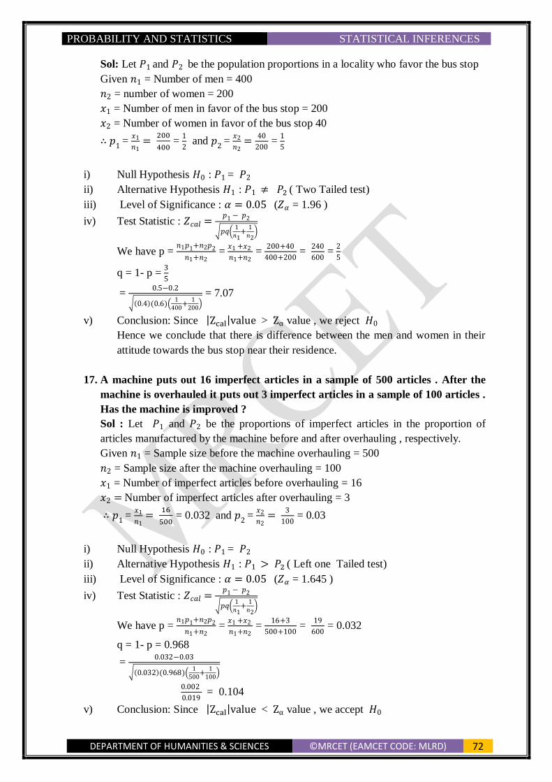
PROBABILITY AND STATISTICS STATISTICAL INFERENCES
DEPARTMENT OF HUMANITIES & SCIENCES ©MRCET (EAMCET CODE: MLRD) 72
Sol: Let 𝑃1 and 𝑃2 be the population proportions in a locality who favor the bus stop
Given 𝑛1 = Number of men = 400
𝑛2 = number of women = 200
𝑥1 = Number of men in favor of the bus stop = 200
𝑥2 = Number of women in favor of the bus stop 40
∴ 𝑝1
= 𝑥1
𝑛1 =
200
400 =
1
2 and 𝑝
2 =
𝑥2
𝑛2=
40
200 =
1
5
i) Null Hypothesis 𝐻0 : 𝑃1 = 𝑃2
ii) Alternative Hypothesis 𝐻1 : 𝑃1 ≠ 𝑃2 ( Two Tailed test)
iii) Level of Significance : 𝛼 = 0.05 (𝑍𝛼 = 1.96 )
iv) Test Statistic : 𝑍𝑐𝑎𝑙 =𝑝1 − 𝑝2
√𝑝𝑞(1
𝑛1+
1
𝑛2)
We have p = 𝑛1𝑝1+𝑛2𝑝2
𝑛1+𝑛2 =
𝑥1 +𝑥2
𝑛1+𝑛2 =
200+40
400+200 =
240
600 =
2
5
q = 1- p = 3
5
= 0.5−0.2
√(0.4)(0.6)(1
400+
1
200)
= 7.07
v) Conclusion: Since |Zcal|value > Zα value , we reject 𝐻0
Hence we conclude that there is difference between the men and women in their
attitude towards the bus stop near their residence.
17. A machine puts out 16 imperfect articles in a sample of 500 articles . After the
machine is overhauled it puts out 3 imperfect articles in a sample of 100 articles .
Has the machine is improved ?
Sol : Let 𝑃1 and 𝑃2 be the proportions of imperfect articles in the proportion of
articles manufactured by the machine before and after overhauling , respectively.
Given 𝑛1 = Sample size before the machine overhauling = 500
𝑛2 = Sample size after the machine overhauling = 100
𝑥1 = Number of imperfect articles before overhauling = 16
𝑥2 = Number of imperfect articles after overhauling = 3
∴ 𝑝1
= 𝑥1
𝑛1 =
16
500 = 0.032 and 𝑝
2 =
𝑥2
𝑛2=
3
100 = 0.03
i) Null Hypothesis 𝐻0 : 𝑃1 = 𝑃2
ii) Alternative Hypothesis 𝐻1 : 𝑃1 > 𝑃2 ( Left one Tailed test)
iii) Level of Significance : 𝛼 = 0.05 (𝑍𝛼 = 1.645 )
iv) Test Statistic : 𝑍𝑐𝑎𝑙 =𝑝1 − 𝑝2
√𝑝𝑞(1
𝑛1+
1
𝑛2)
We have p = 𝑛1𝑝1+𝑛2𝑝2
𝑛1+𝑛2 =
𝑥1 +𝑥2
𝑛1+𝑛2 =
16+3
500+100 =
19
600 = 0.032
q = 1- p = 0.968
= 0.032−0.03
√(0.032)(0.968)(1
500+
1
100)
0.002
0.019 = 0.104
v) Conclusion: Since |Zcal|value < Zα value , we accept 𝐻0
PROBABILITY AND STATISTICS STATISTICAL INFERENCES
DEPARTMENT OF HUMANITIES & SCIENCES ©MRCET (EAMCET CODE: MLRD) 73
Hence we conclude that the machine has improved.
18. In an investigation on the machine performance the following results are
obtained .
No# of units inspected No# of defectives
Machine 1 375 17
Machine 2 450 22
Test whether there is any significant performance of two machines at 𝜶 = 0.05
Sol: Let 𝑃1 and 𝑃2 be the proportions of defective units in the population of units inspected
in machine 1 and Machine 2 respectively.
Given 𝑛1 = Sample size of the Machine 1 = 375
𝑛2 = Sample size of the Machine 2 = 450
𝑥1 = Number of defectives of the Machine 1 = 17
𝑥2 = Number of defectives of the Machine 2 = 22
∴ 𝑝1
= 𝑥1
𝑛1 =
17
375 = 0.045 and 𝑝
2 =
𝑥2
𝑛2=
22
450 = 0.049
i) Null Hypothesis 𝐻0 : 𝑃1 = 𝑃2
ii) Alternative Hypothesis 𝐻1 : 𝑃1 ≠ 𝑃2 ( Two Tailed test)
iii) Level of Significance : 𝛼 = 0.05 (𝑍𝛼 = 1.96 )
iv) Test Statistic : 𝑍𝑐𝑎𝑙 =𝑝1 − 𝑝2
√𝑝𝑞(1
𝑛1+
1
𝑛2)
We have p = 𝑛1𝑝1+𝑛2𝑝2
𝑛1+𝑛2 =
𝑥1 +𝑥2
𝑛1+𝑛2 =
17+22
375+450 =
39
825 = 0.047
q = 1- p = 1- 0.047 = 0.953
= 0.045−0.049
√(0.047)(0.953)(1
375+
1
450)
= - 0.267
v) Conclusion: Since |Zcal|value < Zα value , we accept 𝐻0
Hence we conclude that there is no significant difference in performance of
machines.
19. A cigarette manufacturing firm claims that its brand A line of cigarettes outsells
its
brand B by 8% . If it is found that 42 out of 200 smokers prefer brand A and 18
out of another sample of 100 smokers prefer brand B . Test whether 8%
difference is a valid claim?
Sol: Given 𝑛1 = 200
𝑛2 = 100
𝑥1 = Number of smokers preferring brand A= 42
𝑥2 = Number of smokers preferring brand B = 18

PROBABILITY AND STATISTICS STATISTICAL INFERENCES
DEPARTMENT OF HUMANITIES & SCIENCES ©MRCET (EAMCET CODE: MLRD) 74
∴ 𝑝1
= 𝑥1
𝑛1 =
42
200 = 0.21 and 𝑝
2 =
𝑥2
𝑛2=
18
100 = 0.18
and 𝑃1 - 𝑃2 = 8% = 0.08
i) Null Hypothesis 𝐻0 : 𝑃1 - 𝑃2 = 0.08
ii) Alternative Hypothesis 𝐻1 : 𝑃1 - 𝑃2 ≠ 0.08 ( Two Tailed test)
iii) Level of Significance : 𝛼 = 0.05 (𝑍𝛼 = 1.96 )
iv) Test Statistic : 𝑍𝑐𝑎𝑙 =(𝑝1 − 𝑝2)−( 𝑃1 − 𝑃2)
√𝑝𝑞(1
𝑛1+
1
𝑛2)
We have p = 𝑛1𝑝1+𝑛2𝑝2
𝑛1+𝑛2 =
𝑥1 +𝑥2
𝑛1+𝑛2 =
42+18
200+100 =
60
300 = 0.2
q = 1- p = 1- 0.2 = 0.8
𝑍𝑐𝑎𝑙 = (0.21−0.18)−0.08
√(0.2)(0.8)(1
200+
1
100)
= −0.05
0.0489 = - 1.02
v) Conclusion: Since |𝑍𝑐𝑎𝑙|𝑣𝑎𝑙𝑢𝑒 < 𝑍𝛼 value , we accept 𝐻0
Hence we conclude that 8% difference in the sale of two brands of cigarettes is a
valid claim.
20. In a city A , 20% of a random sample of 900 schoolboys has a certain slight
physical defect . In another city B ,18.5% of a random sample of 1600 school
boys has the same defect . Is the difference between the proportions significant at
5% los?
Sol: Given 𝑛1 = 900
𝑛2 = 1600
𝑥1 = 20% of 900 = 180
𝑥2 = 18.5% of 1600 = 296
∴ 𝑝1
= 𝑥1
𝑛1 =
180
900 = 0.2 and 𝑝
2 =
𝑥2
𝑛2=
296
1600 = 0.185
i) Null Hypothesis 𝐻0 : 𝑃1 = 𝑃2
ii) Alternative Hypothesis 𝐻1 : 𝑃1 ≠ 𝑃2 ( Two Tailed test)
iii) Level of Significance : 𝛼 = 0.05 (𝑍𝛼 = 1.96 )
iv) Test Statistic : 𝑍𝑐𝑎𝑙 =(𝑝1 − 𝑝2)
√𝑝𝑞(1
𝑛1+
1
𝑛2)
We have p = 𝑛1𝑝1+𝑛2𝑝2
𝑛1+𝑛2 =
𝑥1 +𝑥2
𝑛1+𝑛2 =
180+296
900+1600 =
476
2500 = 0.19
q = 1- p = 1- 0.19 = 0.81
𝑍𝑐𝑎𝑙 = 0.2−0.185
√(0.19)(0.81)(1
900+
1
1600)
= −0.015
0.01634 = - 0.918
v) Conclusion: Since |𝑍𝑐𝑎𝑙|𝑣𝑎𝑙𝑢𝑒 < 𝑍𝛼 value , we accept 𝐻0
Hence we conclude that there is no significant difference between the proportions.
PROBABILITY AND STATISTICS STATISTICAL INFERENCES
DEPARTMENT OF HUMANITIES & SCIENCES ©MRCET (EAMCET CODE: MLRD) 75
SMALL SAMPLES
Introduction When the sample size n < 30, then if is referred to as small samples. In this
sampling distribution in many cases may not be normal ie., we will not be justified in
estimating the population parameters as equal to the corresponding sample values.
Degree Of Freedom The number of independent variates which make up the statistic is
known as the degrees of freedom (d.f) and it is denoted by 𝜗.
For Example: If 𝑥1 + 𝑥2 + 𝑥3 = 50 and we assign any values to two os the variables (say
x1,x2 ), then the values of x3 will be known. Thus, the two variables are free and independent
choices for finding the third.
In general, the number of degrees of freedom is equal to the total number of
observations less the number of independent constraints imposed on the observations.
For example: in a set of data of n observations, if K is the number of independent constraints
then 𝜗 = 𝑛 − 𝑘
Student’s t-Distribution Or t-Distribution
Let �̅� be the mean of a random sample of size n, taken from a normal population having the
mean 𝜇 and the variance 𝜎2, and sample variance 𝑆2=∑
(𝑋𝑖−�̅�)2
𝑛−1, then
𝑡 =�̅�−𝜇𝑆
√𝑛⁄
is a random variable having the 𝑡 − distribution with 𝜗 = 𝑛 − 1 degrees of freedom.
Properties of 𝒕 − Distribution
1. The shape of 𝑡 −distribution is bell shaped, which is similar to that of normal
distribution and is symmetrical about the mean.
2. The mean of the standard normal distribution as well as 𝑡 −distribution is zero, but
the variance of 𝑡 −distrubution depends upon the parometer 𝜗 which is called the
degrees of freedom.
3. The variance of 𝑡 −distribution exceeds 1, but approaches 1 as 𝑛 → ∞.
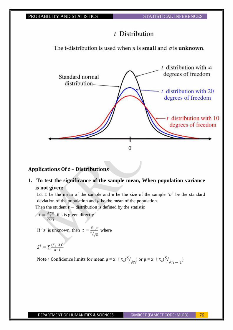
PROBABILITY AND STATISTICS STATISTICAL INFERENCES
DEPARTMENT OF HUMANITIES & SCIENCES ©MRCET (EAMCET CODE: MLRD) 76
Applications Of 𝒕 – Distributions
1. To test the significance of the sample mean, When population variance
is not given:
Let �̅� be the mean of the sample and n be the size of the sample ‘𝜎’ be the standard
deviation of the population and 𝜇 be the mean of the population.
Then the student 𝑡 − distribution is defined by the statistic
𝑡 =�̅�−𝜇
𝑠
√𝑛−1
if s is given directly
If ′𝜎′ is unknown, then 𝑡 =�̅�−𝜇𝑆
√𝑛⁄
where
𝑆2 = ∑(𝑋𝑖−�̅�)
2
𝑛−1
Note ∶ Confidence limits for mean µ = x̅ ± tα(S√n
⁄ ) or µ = x̅ ± tα(S√n − 1
⁄ )

PROBABILITY AND STATISTICS STATISTICAL INFERENCES
DEPARTMENT OF HUMANITIES & SCIENCES ©MRCET (EAMCET CODE: MLRD) 77
𝟐. To test the significance of the difference between means of the two
independent samples :
To test the significant difference between the sample means �̅�1 and �̅�2of two independent
samples of sizes n1 and n2, with the same variance .
We use statistic
𝑡 =�̅�1−�̅�2
√𝑆2( 1𝑛1
+ 1𝑛2
)-------(1) where
�̅�1 =∑ 𝑥1
𝑛1, �̅�2 =
∑ 𝑥2
𝑛2 and
𝑆2=
1
𝑛1+𝑛2−2 [∑(𝑥1 − 𝑥1̅̅ ̅)2 + ∑(𝑥2 − 𝑥2̅̅ ̅)2
OR 𝑆2=
1
𝑛1+𝑛2−2[(𝑛1𝑠1
2) + (𝑛2𝑠22)]
Where s1 and s2 are sample standard deviations.
Note: Confidence limits for difference of means : 𝜇1 − 𝜇2 = (�̅�1
− �̅�2)
± tα (√𝑆2 ( 1
𝑛1+ 1
𝑛2))
Paired t- test ( Test the significance of the difference between means of two
dependent samples ) :
Paired observations arise in many practical situations where each homogenous experimental
unit receives both population condition.
For Example: To test the effectiveness of ‘drug’ some // person’s blood pressure is measured
before and after the intake of certain drug. Here the individual person is the experimental unit
and the two populations are blood pressure “before” and “after” the drug is given
Paired t-test is applied for n paired observations by taking the differences d1,d2 ------dn of the
paired data. To test whether the differences di from a random sample of a population with
mean 𝜇.
𝑡 =𝑑
𝑠√𝑛⁄
𝑤ℎ𝑒𝑟𝑒 𝑑̅ =1
𝑛𝜖 𝑑𝑖 and 𝑠2 =
1
𝑛−1∑(𝑑 − �̅�)
2
Problems:
1. A sample of 26 bulbs gives a mean life of 990 hours with a S.D of 20 hours. The
manufacturer claims that the mean life of bulbs is 1000 hours . Is the sample not
upto the standard?
Sol: Given n = 26
�̅� = 990
𝜇 = 1000 and S.D i.e., s = 20
PROBABILITY AND STATISTICS STATISTICAL INFERENCES
DEPARTMENT OF HUMANITIES & SCIENCES ©MRCET (EAMCET CODE: MLRD) 78
i) Null Hypothesis : 𝐻0 : 𝜇 = 1000
ii) Alternative Hypothesis: 𝐻1 : 𝜇 < 1000( Left one tailed test )
(Since it is given below standard)
iii) Level of significance : 𝛼 = 0.05
t tabulated value with 25 degrees of freedom for left tailed test is 1.708
iv) Test Statistic : 𝑡 𝑐𝑎𝑙= �̅�− 𝜇
𝑠
√𝑛−1
= 990−1000
20
√25
= − 2.5
v) Conclusion: Since |𝑡 𝑐𝑎𝑙| value > 𝑡𝛼 value , we reject 𝐻0
Hence we conclude that the sample is not upto the standard.
2. A random sample of size 16 values from a normal population showed a mean of 53
and sum of squares of deviations from the mean equals to 150 . Can this sample be
regarded as taken from the population having 56 as mean ? Obtain 95% confidence
limits of the mean of the population.?
Sol: a) Given n = 16
�̅� = 53
𝜇 = 56 and ∑(𝑥𝑖 − �̅�)2 = 150
∴ 𝑆2 =
∑(𝑥𝑖−�̅�)2
𝑛−1 =
150
15 = 10 ⇒ S = √10
Degrees of freedom 𝜗 = n-1 = 16-1 =15
i) Null Hypothesis 𝐻0 : 𝜇 = 56
ii) Alternative Hypothesis 𝐻1 : 𝜇 ≠ 56 (Two tailed test )
iii) Level of significance : 𝛼 = 0.05
t tabulated value with 15 degrees of freedom for two tailed test is 2.13
iv) Test Statistic : 𝑡 𝑐𝑎𝑙= �̅�− 𝜇
𝑆
√𝑛
= 53−56
√10
√15
= − 3.79
v) Conclusion: Since |𝑡 𝑐𝑎𝑙| 𝑣𝑎𝑙𝑢𝑒 > 𝑡𝛼 value , we reject 𝐻0
Hence we conclude that the sample cannot be regarded as taken from population.
b) The 95% confidence limits of the mean of the population are given by
𝑥 ̅ ± 𝑡0.05𝑆
√𝑛 = 53 ± 2.13 × 0.79
= 53 ± 1.6827
= 54.68 and 51.31
∴ 95% confidence limits are( 51.31, 54.68 )
3. A random sample of 10 boys had the following I.Q’s : 70, 120 ,110, 101,88,
83,95,98,107 and 100.
a) Do these data support the assumption of a population mean I.Q of 100?
b) Find a reasonable range in which most of the mean I.Q values of samples of
10 boys lie
Sol: Since mean and s.d are not given
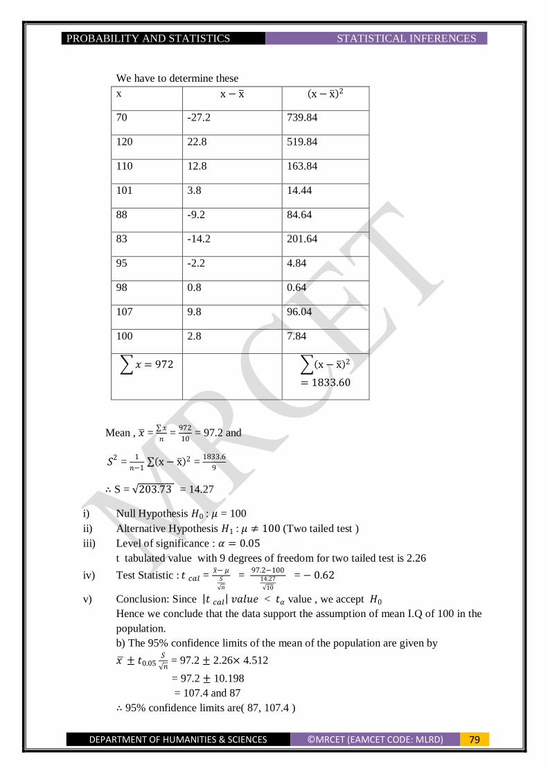
PROBABILITY AND STATISTICS STATISTICAL INFERENCES
DEPARTMENT OF HUMANITIES & SCIENCES ©MRCET (EAMCET CODE: MLRD) 79
We have to determine these
x x − x̅ (x − x̅)2
70 -27.2 739.84
120 22.8 519.84
110 12.8 163.84
101 3.8 14.44
88 -9.2 84.64
83 -14.2 201.64
95 -2.2 4.84
98 0.8 0.64
107 9.8 96.04
100 2.8 7.84
∑ 𝑥 = 972 ∑(x − x̅)2
= 1833.60
Mean , �̅� = ∑ 𝑥
𝑛 =
972
10 = 97.2 and
𝑆2 =
1
𝑛−1 ∑(x − x̅)2 =
1833.6
9
∴ S = √203.73 = 14.27
i) Null Hypothesis 𝐻0 : 𝜇 = 100
ii) Alternative Hypothesis 𝐻1 : 𝜇 ≠ 100 (Two tailed test )
iii) Level of significance : 𝛼 = 0.05
t tabulated value with 9 degrees of freedom for two tailed test is 2.26
iv) Test Statistic : 𝑡 𝑐𝑎𝑙 = �̅�− 𝜇
𝑆
√𝑛
= 97.2−100
14.27
√10
= − 0.62
v) Conclusion: Since |𝑡 𝑐𝑎𝑙| 𝑣𝑎𝑙𝑢𝑒 < 𝑡𝛼 value , we accept 𝐻0
Hence we conclude that the data support the assumption of mean I.Q of 100 in the
population.
b) The 95% confidence limits of the mean of the population are given by
𝑥 ̅ ± 𝑡0.05𝑆
√𝑛 = 97.2 ± 2.26× 4.512
= 97.2 ± 10.198
= 107.4 and 87
∴ 95% confidence limits are( 87, 107.4 )

PROBABILITY AND STATISTICS STATISTICAL INFERENCES
DEPARTMENT OF HUMANITIES & SCIENCES ©MRCET (EAMCET CODE: MLRD) 80
4. Samples of two types of electric bulbs were tested for length of life and following
data were obtained
Type 1 Type 2
Sample number , 𝒏𝟏 = 8 𝒏𝟐 = 7
Sample mean , 𝒙𝟏̅̅̅̅ = 1234 𝒙𝟐̅̅̅̅ = 1036
Sample S.D , 𝒔𝟏= 36 𝒔𝟐= 40
Is the difference in the mean sufficient to warrant that type 1 is superior to type
2 regarding length of life .
Sol: i) Null Hypothesis 𝐻0 : The two types of electric bulbs are identical
i.e., 𝐻0: 𝜇1 = 𝜇2
ii) Alternative Hypothesis 𝐻1 : 𝜇1 ≠ 𝜇2
iii)Test Statistic : 𝑡𝑐𝑎𝑙 = �̅�1− �̅�2
√𝑠(1
𝑛1+
1
𝑛2)
Where 𝑆2 =
𝑛1𝑠12+𝑛1𝑠1
2
𝑛1+𝑛2
= 1
8+7−2(8(36)2 + 7(40)2 ) = 1659.08
∴ t =1234− 1036
√1659.08(1
8+
1
7)
= 9.39
iv)Degrees of freedom = 8+7-2 =13 ,tabulated value of t for 13 d.f at 5% los is 2.16
v)Conclusion: Since |𝑡 𝑐𝑎𝑙| 𝑣𝑎𝑙𝑢𝑒 > 𝑡𝛼 value , we reject 𝐻0
Hence we conclude that the two types 1 and 2 of electric bulbs are not identical .
5. Two horses A and B were tested according to the time to run a particular track with
the following results .
Horse A 28 30 32 33 33 29 34
Horse B 29 30 30 24 27 29
Test whether the two horses have the same running capacity
Sol: Given 𝑛1 = 7 , 𝑛2 = 6
We first compute the sample means and standard deviations
�̅� = Mean of the first sample = 1
7 ( 28 + 30 + 32 + 33 + 33 + 29 + 34)
= 1
7(219) = 31.286
�̅� = Mean of the second sample = 1
6 ( 29 + 30 + 30 + 24 + 27 + 29 )
= 1
6(169) = 28.16

PROBABILITY AND STATISTICS STATISTICAL INFERENCES
DEPARTMENT OF HUMANITIES & SCIENCES ©MRCET (EAMCET CODE: MLRD) 81
𝑥 𝑥 − �̅� (𝑥 − �̅�)2 𝑦 𝑦 − �̅� (𝑦 − �̅�)2
28 -3.286 10.8 29 0.84 0.7056
30 -1.286 1.6538 30 1.84 3.3856
32 0.714 0.51 30 1.84 3.3856
33 1.714 2.94 24 -416 17.3056
33 1.714 2.94 27 -1.16 1.3456
29 -2.286 5.226 29 0.84 0.7056
34 2.714 7.366
∑ 𝑥
= 219
∑(𝑥 − �̅�)2
= 31.4358
∑ 𝑦
= 169
∑(𝑦 − �̅�)2
= 26.8336
Now 𝑆2 =
1
𝑛1+𝑛2−2[(∑(𝑥 − �̅�)2 + ∑(𝑦 − 𝑦)2]
= 1
11[31.4358 + 26.8336]
= 1
11(58.2694)
= 5.23
∴ S = √5.23 = 2.3
i) Null Hypothesis 𝐻0: 𝜇1 = 𝜇2
ii) Alternative Hypothesis 𝐻1 : 𝜇1 ≠ 𝜇2
iii) Test Statistic : 𝑡𝑐𝑎𝑙 = �̅�1− �̅�2
𝑆√(1
𝑛1+
1
𝑛2)
= 31.286 − 28.16
2.3 (√17 +
16)
= 2.443
∴ 𝑡𝑐𝑎𝑙 = 2.443
iv)Degrees of freedom = 7+6-2 =11
Tabulated value of t for 11 d.f at 5% los is 2.2
Conclusion: Since |t cal| value > tα value , we reject 𝐻0
Hence we conclude that both horses do not have the same running capacity.
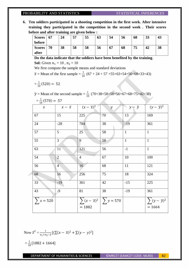
PROBABILITY AND STATISTICS STATISTICAL INFERENCES
DEPARTMENT OF HUMANITIES & SCIENCES ©MRCET (EAMCET CODE: MLRD) 82
6. Ten soldiers participated in a shooting competition in the first week. After intensive
training they participated in the competition in the second week . Their scores
before and after training are given below :
Scores
before
67 24 57 55 63 54 56 68 33 43
Scores
after
70 38 58 58 56 67 68 75 42 38
Do the data indicate that the soldiers have been benefited by the training.
Sol: Given 𝑛1 = 10 , 𝑛2 = 10
We first compute the sample means and standard deviations
�̅� = Mean of the first sample = 1
10 (67 + 24 + 57 +55+63+54+56+68+33+43)
= 1
10(520) = 52
�̅� = Mean of the second sample = 1
10 (70+38+58+58+56+67+68+75+42+38)
= 1
10(570) = 57
𝑥 𝑥 − �̅� (𝑥 − �̅�)2 𝑦 𝑦 − �̅� (𝑦 − �̅�)2
67 15 225 70 13 169
24 -28 784 38 -19 361
57 5 25 58 1 1
55 3 9 58 1 1
63 11 121 56 -1 1
54 2 4 67 10 100
56 4 16 68 11 121
68 16 256 75 18 324
33 -19 361 42 -15 225
43 -9 81 38 -19 361
∑ 𝑥 = 520 ∑(𝑥 − �̅�)2
= 1882
∑ 𝑦 = 570 ∑(𝑦 − �̅�)2
= 1664
Now 𝑆2 =
1
𝑛1+𝑛2−2[(∑(𝑥 − �̅�)2 + ∑(𝑦 − 𝑦)2]
= 1
18[1882 + 1664]
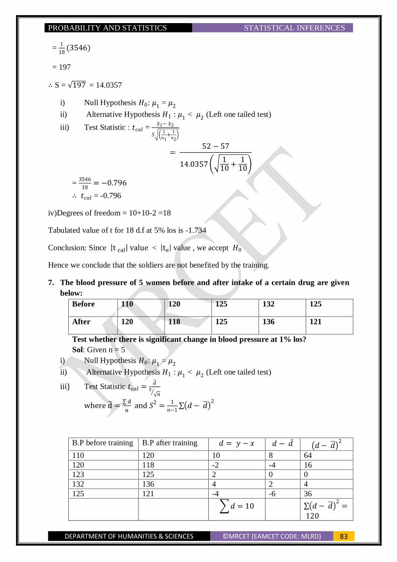
PROBABILITY AND STATISTICS STATISTICAL INFERENCES
DEPARTMENT OF HUMANITIES & SCIENCES ©MRCET (EAMCET CODE: MLRD) 83
= 1
18(3546)
= 197
∴ S = √197 = 14.0357
i) Null Hypothesis 𝐻0: 𝜇1 = 𝜇2
ii) Alternative Hypothesis 𝐻1 : 𝜇1 < 𝜇2 (Left one tailed test)
iii) Test Statistic : 𝑡𝑐𝑎𝑙 = �̅�1− �̅�2
𝑆√(1
𝑛1+
1
𝑛2)
= 52 − 57
14.0357 (√ 110 +
110)
= 3546
18= −0.796
∴ 𝑡𝑐𝑎𝑙 = -0.796
iv)Degrees of freedom = 10+10-2 =18
Tabulated value of t for 18 d.f at 5% los is -1.734
Conclusion: Since |t cal| value < |tα| value , we accept 𝐻0
Hence we conclude that the soldiers are not benefited by the training.
7. The blood pressure of 5 women before and after intake of a certain drug are given
below:
Before 110 120 125 132 125
After 120 118 125 136 121
Test whether there is significant change in blood pressure at 1% los?
Sol: Given n = 5
i) Null Hypothesis 𝐻0: 𝜇1 = 𝜇2
ii) Alternative Hypothesis 𝐻1 : 𝜇1 < 𝜇2 (Left one tailed test)
iii) Test Statistic 𝑡𝑐𝑎𝑙 =�̅�
𝑠√𝑛⁄
where d̅ =∑ d
n and 𝑆2 =
1
𝑛−1∑(𝑑 − �̅�)
2
B.P before training B.P after training 𝑑 = 𝑦 − 𝑥 𝑑 − 𝑑̅ (𝑑 − �̅�)2
110 120 10 8 64
120 118 -2 -4 16
123 125 2 0 0
132 136 4 2 4
125 121 -4 -6 36
∑ 𝑑 = 10 ∑(𝑑 − �̅�)2
=
120
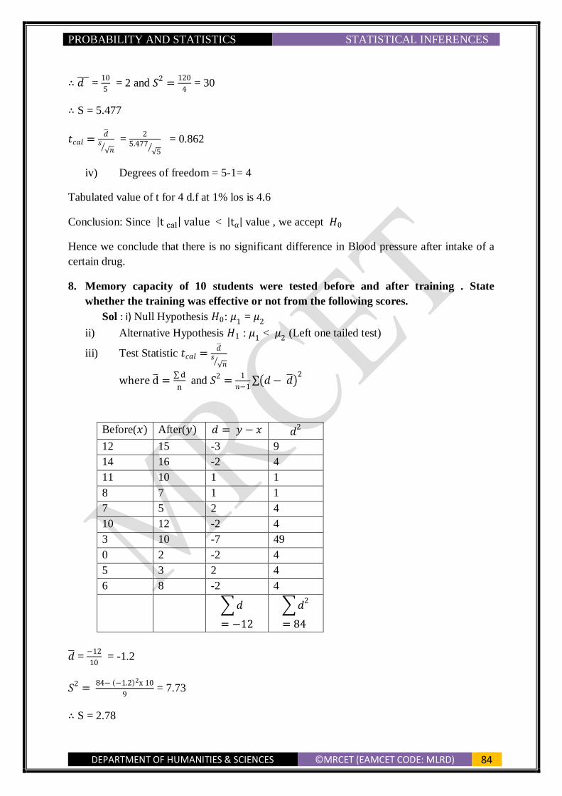
PROBABILITY AND STATISTICS STATISTICAL INFERENCES
DEPARTMENT OF HUMANITIES & SCIENCES ©MRCET (EAMCET CODE: MLRD) 84
∴ 𝑑 ̅̅̅̅ = 10
5 = 2 and 𝑆2 =
120
4 = 30
∴ S = 5.477
𝑡𝑐𝑎𝑙 =�̅�
𝑠√𝑛⁄
= 2
5.477√5
⁄ = 0.862
iv) Degrees of freedom = 5-1= 4
Tabulated value of t for 4 d.f at 1% los is 4.6
Conclusion: Since |t cal| value < |tα| value , we accept 𝐻0
Hence we conclude that there is no significant difference in Blood pressure after intake of a
certain drug.
8. Memory capacity of 10 students were tested before and after training . State
whether the training was effective or not from the following scores.
Sol : i) Null Hypothesis 𝐻0: 𝜇1 = 𝜇2
ii) Alternative Hypothesis 𝐻1 : 𝜇1 < 𝜇2 (Left one tailed test)
iii) Test Statistic 𝑡𝑐𝑎𝑙 =�̅�
𝑠√𝑛⁄
where d̅ =∑ d
n and 𝑆2 =
1
𝑛−1∑(𝑑 − �̅�)
2
Before(𝑥) After(𝑦) 𝑑 = 𝑦 − 𝑥 𝑑2
12 15 -3 9
14 16 -2 4
11 10 1 1
8 7 1 1
7 5 2 4
10 12 -2 4
3 10 -7 49
0 2 -2 4
5 3 2 4
6 8 -2 4
∑ 𝑑
= −12
∑ 𝑑2
= 84
�̅� = −12
10 = -1.2
𝑆2 = 84− (−1.2)2x 10
9 = 7.73
∴ S = 2.78

PROBABILITY AND STATISTICS STATISTICAL INFERENCES
DEPARTMENT OF HUMANITIES & SCIENCES ©MRCET (EAMCET CODE: MLRD) 85
𝑡𝑐𝑎𝑙 =�̅�
𝑠√𝑛⁄
= −1.2
2.78√10
⁄ = -1.365 and d.f = n-1 = 9
Tabulated value of t for 9 d.f at 5% los is 1.833
Conclusion: Since |t cal| value < |tα| value , we accept 𝐻0
Hence we conclude that there is no significant difference in memory capacity after the
training program.
Chi-Square (𝝌𝟐) Distribution
Chi square distribution is a type of cumulative probability distribution . probability
distributions provide the probability of every possible value that may occur . Distributions
that are cumulative give the probability of a random variable being less than or equal to a
particular value. Since the sum of the probabilities of every possible value must equal one ,
the total area under the curve is equal to one . Chi square distributions vary depending on the
degrees of freedom. The degrees of freedom is found by subtracting one from the number of
categories in the data .
.
Applications of Chi – Square Distribution:
Chi – Square test as a test of goodness of fit :
𝝌𝟐– test enables us to ascertain how well the theoretical distributions such as
binomial, Poisson, normal etc, fit the distributions obtained from sample data. If the
calculated value of 𝝌𝟐is less than the table value at a specified level of generally 5%
significance, the fit is considered to be good.
If the calculated value of 𝝌𝟐 is greater than the table value, the fit is considered to be poor.
i) Null hypothesis: H0 : There is no difference in given values and calculated values
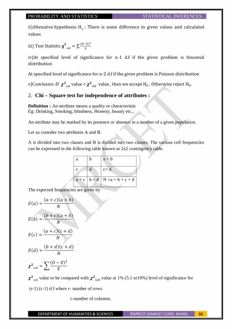
PROBABILITY AND STATISTICS STATISTICAL INFERENCES
DEPARTMENT OF HUMANITIES & SCIENCES ©MRCET (EAMCET CODE: MLRD) 86
ii)Altenative hypothesis: H1 : There is some difference in given values and calculated
values
iii) Test Statistic 𝛘𝟐cal
= ∑(O−E)2
E
iv)At specified level of significance for n-1 d.f if the given problem is binomial
distribution
At specified level of significance for n-2 d.f if the given problem is Poisson distribution
v)Conclusion :If 𝝌𝟐cal value < 𝝌𝟐
tab value , then we accept H0 , Otherwise reject H0.
2. Chi – Square test for independence of attributes :
Definition : An attribute means a quality or characteristic
Eg: Drinking, Smoking, blindness, Honesty, beauty etc.,
An attribute may be marked by its presence or absence in a number of a given population.
Let us consider two attributes A and B.
A is divided into two classes and B is divided into two classes. The various cell frequencies
can be expressed in the following table known as 2x2 contingency table.
a b a + b
c d c+ d
a + c b + d N =a + b + c + d
The expected frequencies are given by
𝐸(𝑎) =(𝑎 + 𝑐)(𝑎 + 𝑏)
𝑁
𝐸(𝑏) =(𝑏 + 𝑐)(𝑎 + 𝑏)
𝑁
𝐸(𝑐) =(𝑎 + 𝑐)(𝑐 + 𝑑)
𝑁
𝐸(𝑑) =(𝑏 + 𝑑)(𝑐 + 𝑑)
𝑁
𝝌𝟐𝑐𝑎𝑙 = ∑
(𝑂 − 𝐸)2
𝐸
𝝌𝟐𝑐𝑎𝑙 value to be compared with 𝝌𝟐
𝑡𝑎𝑏 value at 1% (5.1 or10%) level of significance for
(r-1) (c-1) d.f where r- number of rows
c-number of columns.

PROBABILITY AND STATISTICS STATISTICAL INFERENCES
DEPARTMENT OF HUMANITIES & SCIENCES ©MRCET (EAMCET CODE: MLRD) 87
Note: In 𝝌𝟐 distribution for independence of attributes, we test if two attributes A and B are
independent or not.
i)Null Hypothesis: H0 : The two attributes are independent
ii) Alternative hypothesis: H1 : The two attributes are not independent
iii) Test Statistic χ2cal
= ∑(O − E)2
E
where E = 𝐑𝐨𝐰 𝐭𝐨𝐭𝐚𝐥 𝐱 𝐂𝐨𝐥𝐮𝐦𝐧 𝐭𝐨𝐭𝐚𝐥
𝐆𝐫𝐚𝐧𝐝 𝐭𝐨𝐭𝐚𝐥
iv)At specified level of significance for (m-1) (n-1) d.f where m- no. of rows and n- no. of
columns
v)Conclusion : If 𝛘𝟐cal value < 𝛘𝟐
tab value , then we accept H0 , Otherwise reject H0.
Problems :
1. Fit a Poisson distribution to the following data and test for its goodness of fit at 5%
los
x 0 1 2 3 4
f 419 352 154 56 19
Sol:
X f fx
0 419 0
1 352 352
2 154 308
3 56 168
4 19 76
N=1000 ∑ 𝑓𝑥 = 904
Mean 𝜆 = ∑ 𝑓𝑥
N =
904
1000 = 0.904
Theoretical distribution is given by
= N x p(x) = 1000 x 𝑒−𝜆𝜆𝑥
𝑥!

PROBABILITY AND STATISTICS STATISTICAL INFERENCES
DEPARTMENT OF HUMANITIES & SCIENCES ©MRCET (EAMCET CODE: MLRD) 88
Hence the theoretical frequencies are given by
x 0 1 2 3 4 Total
f = 1000 x
𝑒−𝜆𝜆𝑥
𝑥!
406.2 366 165.4 49.8 12.6 1000
Since Given frequencies total is equal to Calculated frequencies total.
To test for goodness of fit:
i) H0 : There is no difference in given values and calculated values
ii) H1 : There is some difference in given values and calculated values
iii)𝝌𝟐𝑐𝑎𝑙
= ∑(𝑂−𝐸)2
𝐸
O E (𝑂 − 𝐸)2 (𝑂 − 𝐸)2
𝐸
419 406.2 (419 − 406.2)2 (419 − 406.2)2
406.2
352 366 (352 − 366)2 (352 − 366)2
366
154 165.4 (154 − 165.4)2 (154 − 165.4)2
165.4
56 49.8 (56 − 49.8)2 (56 − 49.8)2
49.8
19 12.6 (19 − 12.6)2 (19 − 12.6)2
12.6
∑(𝑂−𝐸)2
𝐸 = 5.748
Degrees of freedom = 5-2 = 3
𝝌𝟐𝑡𝑎𝑏 at 5% LOS = 7.82
Since 𝝌𝟐𝑐𝑎𝑙 value < 𝝌𝟐
𝑡𝑎𝑏 ,we accept 𝐻0 .
3. A die is thrown 264 times with following results. Show that the die is biased [ Given
𝝌𝟐𝟎.𝟎𝟓 = 11.07 for 5 d.f]
No. appeared
on the die
1 2 3 4 5 6
Frequency 40 32 28 58 54 52

PROBABILITY AND STATISTICS STATISTICAL INFERENCES
DEPARTMENT OF HUMANITIES & SCIENCES ©MRCET (EAMCET CODE: MLRD) 89
Sol: i) H0 : The die is unbiased
ii) H1 : The die is not unbiased
iii)𝛘𝟐cal
= ∑(𝑂−𝐸)2
𝐸
The expected frequency of each of the number 1,2,3,4,5,6 is 264
6= 44
Calculation of 𝝌𝟐:
O E (𝑂 − 𝐸)2 (𝑂 − 𝐸)2
𝐸
40 44 16 0.3636
32 44 144 3.2727
28 44 256 5.8181
58 44 196 4.4545
54 44 100 2.2727
52 44 64 1.4545
∑(𝑂−𝐸)2
𝐸 = 17.6362
𝝌𝟐𝑐𝑎𝑙 = 17.6362
The number of degrees of freedom = n-1 = 5
𝝌𝟐0.05 = 11.07 for 5 d.f
Since 𝝌𝟐𝑐𝑎𝑙 value > 𝝌𝟐
𝑡𝑎𝑏 value , we reject 𝐻0
Hence the die is biased
4. On the basis of information given below about the treatment of 200 patients
suffering from disease , state whether the new treatment is comparatively
Superior to the conventional treatment.
Treatment Favorable Not Favorable Total
New 60 30 90
Conventional 40 70 110
Sol: i) H0 : The two attributes are independent
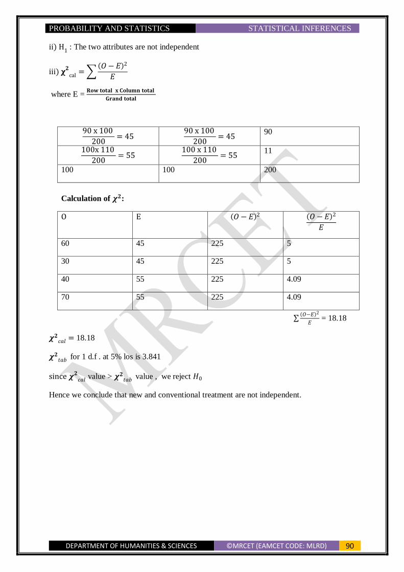
PROBABILITY AND STATISTICS STATISTICAL INFERENCES
DEPARTMENT OF HUMANITIES & SCIENCES ©MRCET (EAMCET CODE: MLRD) 90
ii) H1 : The two attributes are not independent
iii) 𝛘𝟐cal
= ∑(𝑂 − 𝐸)2
𝐸
where E = 𝐑𝐨𝐰 𝐭𝐨𝐭𝐚𝐥 𝐱 𝐂𝐨𝐥𝐮𝐦𝐧 𝐭𝐨𝐭𝐚𝐥
𝐆𝐫𝐚𝐧𝐝 𝐭𝐨𝐭𝐚𝐥
90 x 100
200= 45
90 x 100
200= 45
90
100x 110
200= 55
100 x 110
200= 55
11
100 100 200
Calculation of 𝝌𝟐:
O E (𝑂 − 𝐸)2 (𝑂 − 𝐸)2
𝐸
60 45 225 5
30 45 225 5
40 55 225 4.09
70 55 225 4.09
∑(𝑂−𝐸)2
𝐸 = 18.18
𝝌𝟐𝑐𝑎𝑙 = 18.18
𝝌𝟐𝑡𝑎𝑏 for 1 d.f . at 5% los is 3.841
since 𝝌𝟐𝑐𝑎𝑙 value > 𝝌𝟐
𝑡𝑎𝑏 value , we reject 𝐻0
Hence we conclude that new and conventional treatment are not independent.
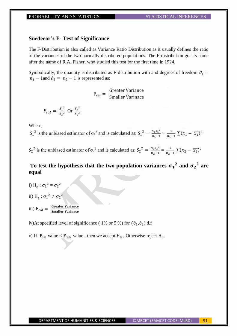
PROBABILITY AND STATISTICS STATISTICAL INFERENCES
DEPARTMENT OF HUMANITIES & SCIENCES ©MRCET (EAMCET CODE: MLRD) 91
Snedecor’s F- Test of Significance
The F-Distribution is also called as Variance Ratio Distribution as it usually defines the ratio
of the variances of the two normally distributed populations. The F-distribution got its name
after the name of R.A. Fisher, who studied this test for the first time in 1924.
Symbolically, the quantity is distributed as F-distribution with and degrees of freedom 𝜗1 = 𝑛1 − 1and 𝜗2 = 𝑛2 − 1 is represented as:
Fcal = Greater Variance
Smaller Varinace
𝐹𝑐𝑎𝑙 = 𝑆1
2
𝑆22 Or
𝑆22
𝑆12
Where,
𝑆12 is the unbiased estimator of σ1
2 and is calculated as: 𝑆12 =
𝑛1𝑠12
𝑛1−1=
1
𝑛1−1 ∑(𝑥1 − 𝑥1̅̅̅)2
𝑆22 is the unbiased estimator of σ2
2 and is calculated as: 𝑆22 =
𝑛2𝑠22
𝑛2−1=
1
𝑛2−1 ∑(𝑥2 − 𝑥2̅̅ ̅)2
To test the hypothesis that the two population variances 𝝈𝟏𝟐 and 𝝈𝟐
𝟐 are
equal
i) H0 : σ1
2 = σ22
ii) H1 : σ1
2 ≠ σ22
iii) Fcal = 𝐆𝐫𝐞𝐚𝐭𝐞𝐫 𝐕𝐚𝐫𝐢𝐚𝐧𝐜𝐞
𝐒𝐦𝐚𝐥𝐥𝐞𝐫 𝐕𝐚𝐫𝐢𝐧𝐚𝐜𝐞
iv)At specified level of significance ( 1% or 5 %) for (ϑ1,ϑ2) d.f
v) If 𝐅cal value < 𝐅tab value , then we accept H0 , Otherwise reject H0.

PROBABILITY AND STATISTICS STATISTICAL INFERENCES
DEPARTMENT OF HUMANITIES & SCIENCES ©MRCET (EAMCET CODE: MLRD) 92
𝐹𝑐𝑎𝑙(𝜗1, 𝜗2) is the value of F with 𝜗1 and 𝜗2 degrees of freedom such that the area under the
F – distribution to the right of 𝐹𝛼 is 𝛼.
Problems:
1. In one sample of 8 observations from a normal population, the sum of the squares of
deviations of the sample values from the sample mean is 84.4 and in another sample
of 10 observations it was 102.6. Test at 𝟓% level whether the populations have the
same varience.
Sol: Let 𝜎12 and 𝜎2
2 be the variances of the two normal populations from which the
samples are drawn.
Let the Null Hypothesis be 𝐻0: 𝜎12 = 𝜎2
2
Then the Alternative Hypothesis is 𝐻1: 𝜎12 ≠ 𝜎2
2
Here 𝑛1 = 8, 𝑛2 = 10
Also ∑(𝑥𝑖 − �̅�)2 = 84.4, ∑(𝑦𝑖− �̅�)
2= 102.6
If 𝑆12𝑎𝑛𝑑𝑆2
2 be the estimates of 𝜎1
2 and 𝜎22 then
𝑆12 =
1
𝑛1 − 1∑(𝑥𝑖 − �̅�)2 =
84.4
7= 12.057
and
𝑆22 =
1
𝑛2 − 1∑(𝑦
𝑖− �̅�)
2=
102.6
9= 11.4
Let 𝐻0 be true. Since 𝑆12 > 𝑆2
2, the test statistic is
𝐹 =𝑆1
2
𝑆22 =
12.057
11.4= 1.057
i.e., calculated F = 1.057.
Degrees of freedom are given by 𝑣1 = 𝑛1 − 1 = 8 − 1 = 7

PROBABILITY AND STATISTICS STATISTICAL INFERENCES
DEPARTMENT OF HUMANITIES & SCIENCES ©MRCET (EAMCET CODE: MLRD) 93
and 𝑣2 = 𝑛2 − 1 = 10 − 1 = 9
Tabulated value of 𝐹 at 5% level for (7,9) degrees of freedom is 3.29
i.e.,𝐹0.05(7,9) = 3.29
Since calculated 𝐹 < tabulated 𝐹, we accept the Null Hypothesis 𝐻0 and
conclude that the populations have the same variance.
2.The time taken by workers in performing a job by method I and method II is given
below
Do the data show that the variances of time distribution from population from which
these samples are drawn do not differ significantly?
Sol: Let the Null Hypothesis be 𝐻0: 𝜎12 = 𝜎2
2 where 𝜎12 and 𝜎2
2 are the variances of the
two populations from with the samples are drawn.
The Alternative Hypothesis is 𝐻1: 𝜎12 ≠ 𝜎2
2.
Calculation of sample variances.
𝑥 𝑥 − �̅� (𝑥 − �̅�)2 𝑦 𝑦 − �̅� (𝑦 − �̅�)2
20
16
26
27
23
22
-2.3
-6.3
3.7
4.7
0.7
-0.3
5.29
39.69
13.69
22.09
0.49
0.09
27
33
42
35
32
34
38
-7.4
-1.4
7.6
0.6
-2.4
-0.4
3.6
54.76
1.96
57.76
0.36
5.76
0.16
12.96
134 81.34 241 133.72
Given 𝑛1 = 6, 𝑛2 = 7
∴ �̅� =∑ 𝑥
𝑛1=
134
6= 22.3, �̅� =
∑ 𝑦
𝑛2=
241
67= 34.4
Method I 20 16 26 27 23 22 -
Method II 27 33 42 35 32 34 38

PROBABILITY AND STATISTICS STATISTICAL INFERENCES
DEPARTMENT OF HUMANITIES & SCIENCES ©MRCET (EAMCET CODE: MLRD) 94
And
∑(𝑥𝑖 − �̅�)2 = 81.34, ∑(𝑦𝑖
− �̅�)2
= 133.72
If 𝑆12𝑎𝑛𝑑𝑆2
2 be the estimates of 𝜎1
2 and 𝜎22, then
𝑆12 =
1
𝑛1 − 1∑(𝑥𝑖 − �̅�)2 =
81.34
5= 16.26
and
𝑆22 =
1
𝑛2 − 1∑(𝑦
𝑖− �̅�)
2=
133.72
6= 22.29
Let 𝐻0 be true
Since 𝑆22 > 𝑆1
2 , the statistic is
F = S2
2
S12 =
22.29
16.268 = 1.3699 = 1.37
F0.05(5,6) d. f = 4.39
Since calculated F < tabulated F , we accept the null hypothesis 𝐻0 at 5% los i.e., there is no
significant difference between the variances of the distribution by the workers.