PROBABILITY AND STATISTICS - Alagappa University
312
M.Sc. [Mathematics] IV-Semester 311 44 Directorate of Distance Education PROBABILITYANDSTATISTICS ALAGAPPAUNIVERSITY [Accreditedwith‘A+’GradebyNAAC(CGPA:3.64)intheThirdCycle and Gradedas Category–I University by MHRD-UGC] (AState University Established by the Government of Tamil Nadu) KARAIKUDI–630003
-
Upload
khangminh22 -
Category
Documents
-
view
0 -
download
0
Transcript of PROBABILITY AND STATISTICS - Alagappa University

M.Sc. [Mathematics]
IV - Semester
311 44
Directorate of Distance Education
PROBABILITY AND STATISTICS
ALAGAPPA UNIVERSITY[Accredited with ‘A+’ Grade by NAAC (CGPA:3.64) in the Third Cycle
and Graded as Category–I University by MHRD-UGC]
(A State University Established by the Government of Tamil Nadu)
KARAIKUDI – 630 003

All rights reserved. No part of this publication which is material protected by this copyright notice
may be reproduced or transmitted or utilized or stored in any form or by any means now known or
hereinafter invented, electronic, digital or mechanical, including photocopying, scanning, recording
or by any information storage or retrieval system, without prior written permission from the Alagappa
University, Karaikudi, Tamil Nadu.
Information contained in this book has been published by VIKAS® Publishing House Pvt. Ltd. and has
been obtained by its Authors from sources believed to be reliable and are correct to the best of their
knowledge. However, the Alagappa University, Publisher and its Authors shall in no event be liable for
any errors, omissions or damages arising out of use of this information and specifically disclaim any
implied warranties or merchantability or fitness for any particular use.
Authors:
J.S. Chandan, Prof. Medgar Evers College, City University of New York, New York
Units (1.2.4-1.2.6, 1.3.1, 1.4.1-1.9, 5.6, 8.3, 9.4-9.10, 13.3-13.8)
V K Khanna, Formerly Associate Professors, Department of Mathematics, Kirori Mal College, University of Delhi
S K Bhambri, Formerly Associate Professors, Department of Mathematics, Kirori Mal College, University of Delhi
Units (1.2.7-1.2.8, 1.3, 1.3.3, 1.4)
G.S Monga, Dean, Invertis Institute of Management Studies, Bareilly
Units (2, 3.3, 4.4-4.9, 5.5.3, 11.0-11.2)
Late C.R. Kothari, Former Principal, University Commerce College, Jaipur, and Associate Professor in the Department of Economic
Administration and Financial Management (EAFM), University of Rajasthan, Jaipur
Units (3.0-3.2, 4.3, 5.0-5.5.2, 5.7-5.11, 6.0-6.4, 6.6-6.10, 7.3-7.4, 8.0-8.2, 9.0-9.3, 10.3, 11.3)
Kalika Patrai, Senior Lecturer in Galgotia Institute of Management and Technology, Greater Noida
Units (3.4-3.9, 6.5, 7.5-7.10, 13.0-13.2, 14)
S Kalavathy, Dean, Department of Science and Humanities, K Ramakrishnan College of Technology, Samayapuram, Trichy
Units (8.4-8.9)
Vikas® Publishing House: Units (1.0-1.2.3, 1.3.2, 4.0-4.2, 7.0-7.2, 10.0-10.2, 10.4-10.8, 11.4-11.8, 12)
"The copyright shall be vested with Alagappa University"
Vikas® is the registered trademark of Vikas® Publishing House Pvt. Ltd.
VIKAS® PUBLISHING HOUSE PVT. LTD.
Phone: 0120-4078900 Fax: 0120-4078999
Website: www.vikaspublishing.com Email: [email protected]
Work Order No. AU/DDE/DE-12-02/Preparation and Printing of Course Materials/2020 Dated 30.01.2020 Copies - 1000

SYLLABI-BOOK MAPPING TABLEProbability and Statistics
BLOCK - I: PROBABILITY AND MULTIVARIATE DISTRIBUTIONSUNIT - I Probability and Distribution: Introduction - Set Theory - The ProbabilitySet Function - Conditional Probability and Independence.UNIT - II Random Variables of the Discrete Type - Random Variables of theContinuous Type.UNIT - III Properties of the Distribution Function - Expectation of Random Variable- Some Special Expectations - Chebyshev’s Inequality.UNIT - IV Multivariate Distributions: Distributions of Two Random Variables-Conditional Distributions and Expectations.
BLOCK - II: CORRELATION COEFFICIENT, SPECIAL DISTRIBUTIONSAND DISTRIBUTION
UNIT - V The Correlation Coefficient - Independent Random Variables - Extensionto Several Random Variables.UNIT - VI Some Special Distributions: The Binomial and Related Distributions- The Poisson Distribution.UNIT - VII The Gamma and Chi-Square Distributions - The Normal Distribution- The Bivariate Normal Distribution.UNIT-VIII Distributions of Functions of Random Variables: Sampling Theory -Transformations of Variables of the Discrete Type.
BLOCK - III: BETA, t, F, X AND ns2/σ2 DISTRIBUTIONSUNIT-IX Transformations of Variables of the Continuous Type - the Beta, t andF Distributions - Extensions of the Change - of - Variable Technique.UNIT-X Distributions of Order Statistics - The Moment Generating - Function,Techniques.UNIT-XI The Distributions of X and ns2/σ2 - Expectations of Functions of RandomVariables.
BLOCK - IV: LIMITING DISTRIBUTIONSUNIT-XII Limiting Distributions: Convergence in Distribution - Convergencein Probability.UNIT-XIII Limiting Moment Generating Functions - The Central Limit Theorem.UNIT-XIV Some Theorems on Limiting Distributions.
Syllabi Mapping in Book
Unit 1: Probability andSet Theory
(Pages 1-60);Unit 2: Random Variables
of Discrete andContinuous Type
(Pages 61-74);Unit 3: Expectation of
Random Variables(Pages 75-94);
Unit 4: Distribution ofRandom Variables
(Pages 95-114)
Unit 5: Correlation(Pages 115-132);
Unit 6: Distributions(Pages 133-157);
Unit 7: Special Distributions(Pages 158-191);
Unit 8: Distribution of Functionsof Random Variable and Sampling
(Pages 192-225)
Unit 9: Transformation of Variableof the Continuous Type
(Pages 226-256);Unit 10: Distributions of
Order Statistics(Pages 257-267);
Unit 11: Distributionof X and ns2/σ2
(Pages 268-276)
Unit 12: Limiting Distributionsand Convergence(Pages 277-287);
Unit 13: Limiting MomentGenerating Function and
Central Limit Theorem(Pages 288-296);
Unit 14: Some Theorems onLimiting Distributions
(Pages 297-302)

INTRODUCTION
BLOCK I: PROBABILITY AND MULTIVARIATE DISTRIBUTIONS
UNIT 1 PROBABILITY AND SET THEORY 1-601.0 Introduction1.1 Objectives1.2 Probability
1.2.1 Classical Theory of Probability1.2.2 Axiomatic Probability Theory1.2.3 Empirical Probability Theory1.2.4 Addition Rule1.2.5 Multiplication Rule1.2.6 Bayes’ Theorem1.2.7 Sample Space and Events1.2.8 Finite Probability Spaces
1.3 Set Theory1.3.1 Counting Principles1.3.2 Classes of Sets1.3.3 Power Sets
1.4 Conditional Probability and Independence1.4.1 Independent and Dependent Events
1.5 Answers to Check Your Progress Questions1.6 Summary1.7 Key Words1.8 Self-Assessment Questions and Exercises1.9 Further Readings
UNIT 2 RANDOM VARIABLES OF DISCRETE AND CONTINUOUS TYPE 61-74
2.0 Introduction2.1 Objectives2.2 Random Variables of the Discrete Type and Random Variables of the Continuous Type2.3 Answers to Check Your Progress Questions2.4 Summary2.5 Key Words2.6 Self-Assessment Questions and Exercises2.7 Further Readings
UNIT 3 EXPECTATION OF RANDOM VARIABLES 75-943.0 Introduction3.1 Objectives3.2 Properties of the Distribution Function
3.2.1 Function of a Random Variable3.2.2 Moment Generating Functions3.2.3 Probability Density Functions—Discrete and Continuous
CONTENTS

3.3 Expectation of Random Variable3.4 Chebyshev’s Inequality3.5 Answers to Check Your Progress Questions3.6 Summary3.7 Key Words3.8 Self-Assessment Questions and Exercises3.9 Further Reading
UNIT 4 DISTRIBUTION OF RANDOM VARIABLES 95-114
4.0 Introduction4.1 Objectives4.2 Multivariate Distribution4.3 Distribution of Two Random Variable4.4 Conditional Distribution and Expectation4.5 Answers to Check Your Progress Questions4.6 Summary4.7 Key Words4.8 Self-Assessment Questions and Exercises4.9 Further Readings
BLOCK II: CORRELATION COEFFICIENT, SPECIAL DISTRIBUTIONSAND DISTRIBUTION
UNIT 5 CORRELATION 115-1325.0 Introduction5.1 Objectives5.2 Correlation5.3 Types of Correlation5.4 Properties of Correlation Coefficient5.5 Methods of Studying Correlation
5.5.1 Scatter Diagram5.5.2 Karl Pearson’s Coefficient5.5.3 Rank Coefficient
5.6 Coefficient of Determination5.7 Answers to Check Your Progress Questions5.8 Summary5.9 Key Words
5.10 Self-Assessment Questions and Exercises5.11 Further Readings
UNIT 6 DISTRIBUTIONS 133-1576.0 Introduction6.1 Objectives6.2 Binomial Distribution6.3 The Poisson Distribution

6.4 Limiting Form of Binomial and Poisson Fitting6.5 Discrete Theoretical Distributions6.6 Answers to Check Your Progress Questions6.7 Summary6.8 Key Words6.9 Self-Assessment Questions and Exercises
6.10 Further ReadingsUNIT 7 SPECIAL DISTRIBUTIONS 158-191
7.0 Introduction7.1 Objectives7.2 The Gamma Distribution7.3 Chi-Square Distribution7.4 The Normal Distribution7.5 The Bivariate Normal Distribution7.6 Answers to Check Your Progress Questions7.7 Summary7.8 Key Words7.9 Self-Assessment Questions and Exercises
7.10 Further ReadingsUNIT 8 DISTRIBUTION OF FUNCTIONS OF RANDOM
VARIABLE AND SAMPLING 192-2258.0 Introduction8.1 Objectives8.2 Distribution of Functions of Random Variable8.3 Sampling Theory8.4 Transformation of Variable of the Discrete Type8.5 Answers to Check Your Progress Questions8.6 Summary8.7 Key Words8.8 Self-Assessment Questions and Exercises8.9 Further Readings
BLOCK III: BETA, t, F, X AND ns2/σ2 DISTRIBUTIONS
UNIT 9 TRANSFORMATION OF VARIABLE OFTHE CONTINUOUS TYPE 226-256
9.0 Introduction9.1 Objectives9.2 Transformation of Variable of the Continuous Type
9.2.1 The Beta Distribution9.2.2 t Distribution9.2.3 F Distribution

9.3 Answers to Check Your Progress Questions9.4 Summary9.5 Key Words9.6 Self-Assessment Questions and Exercises9.7 Further Readings
UNIT 10 DISTRIBUTIONS OF ORDER STATISTICS 257-26710.0 Introduction10.1 Objectives10.2 Distributions of Order Statistics
10.2.1 The Moment Generating Function10.3 Answers to Check Your Progress Questions10.4 Summary10.5 Key Words10.6 Self-Assessment Questions and Exercises10.7 Further Readings
UNIT 11 DISTRIBUTION OF X AND ns2/σ2 268-27611.0 Introduction11.1 Objectives11.2 The Distributions of X and ns2/σ2
11.3 Expectations of Functions of Random Variables11.4 Answers to Check Your Progress Questions11.5 Summary11.6 Key Words11.7 Self-Assessment Questions and Exercises11.8 Further Readings
BLOCK IV: LIMITING DISTRIBUTIONS
UNIT 12 LIMITING DISTRIBUTIONS AND CONVERGENCE 277-28712.0 Introduction12.1 Objectives12.2 Limiting Distributions
12.2.1 Convergence in Distribution12.2.2 Convergence in Probability
12.3 Answers to Check Your Progress Questions12.4 Summary12.5 Key Words12.6 Self-Assessment Questions and Exercises12.7 Further Readings
UNIT 13 LIMITING MOMENT GENERATING FUNCTIONAND CENTRAL LIMIT THEOREM 288-296
13.0 Introduction13.1 Objectives

13.2 Limiting Moment Generating Functions13.3 The Central Limit Theorem (CLT)13.4 Answers to Check Your Progress Questions13.5 Summary13.6 Key Words13.7 Self-Assessment Questions and Exercises13.8 Further Readings
UNIT 14 SOME THEOREMS ON LIMITING DISTRIBUTIONS 297-30214.0 Introduction14.1 Objectives14.2 Some Theorems on Limiting Distributions
14.2.1 Weak Law of Large Numbers14.2.2 Strong Law of Large Numbers
14.3 Answers to Check Your Progress Questions14.4 Summary14.5 Key Words14.6 Self-Assessment Questions and Exercises14.7 Further Readings

Introduction
NOTES
Self-Instructional10 Material
INTRODUCTION
Probability is the branch of mathematics concerning numerical descriptions of howlikely an event is to occur or how likely it is that a proposition is true. Probability issimply how likely something is to happen. The probability of an event is a numberbetween 0 and 1, where, roughly speaking, 0 indicates impossibility of the eventand 1 indicates certainty. The higher the probability of an event, the more likely itis that the event will occur. These concepts have been given an axiomaticmathematical formalization in probability theory, which is used widely in the areasof mathematics, statistics, finance, gambling, science (in particular physics), artificialintelligence/machine learning, computer science, game theory, and philosophy todraw inferences about the expected frequency of events. Probability theory is alsoused to describe the underlying mechanics and regularities of complex systems.
‘Probability’ and ‘Statistics’ are fundamentally related. The probability theorydescribes statistical phenomenon and analyses them to study correlation andregression, sampling methods, business decisions, statistical inferences, etc.Probability is considered as theory of chance whereas statistics is considered as amathematical science pertaining to the collection, analysis, interpretation orexplanation, and presentation of data. Statistical analysis is very important fortaking decisions and is widely used by academic institutions, the natural and socialsciences departments, the government and business organizations.
The word ‘Statistics’ is derived from the Latin word ‘status’ which meansa political state or government. It was originally applied in connection with kingsand monarchs collecting data on their citizenry which pertained to state wealth,collection of taxes, study of population, and so on. The subject of statistics isprimarily concerned with making decisions about various disciplines of marketand employment, such as stock market trends, unemployment rates in varioussectors of industry, demographic shifts, interest rate and inflation rate over theyears, and so on. To a layman, it often refers to a column of figures, or perhapstables, graphs and charts related to areas, such as population, national income,expenditures, production, consumption, supply, demand, sales, imports, exports,births, deaths and accidents.
Hence, the subject of statistics deals primarily with numerical data gatheredfrom surveys or collected using various statistical methods. Its objective is tosummarize such data, so that the summary gives us a good indication about certaincharacteristics of a population or phenomenon that we wish to study. To ensurethat our conclusions are meaningful, it is necessary to subject our data to scientificanalyses so that rational decisions can be made. Statistics is therefore concernedwith proper collection of data, organization of this data into a manageable andpresentable form, analysis and interpretation of the data into conclusions for usefulpurposes.

Introduction
NOTES
Self-InstructionalMaterial 11
The book ‘Probability and Statistics’ is divided into four blocks that arefurther divided into fourteen units which will help you understand how to solve theprobability and multivariate distributions, set theory, random variables of the discretetype, random variables of the continuous type, some special expectations,Chebyshev’s inequality, correlation coefficient, special distributions and distributionfunction of random variables, correlation coefficient, binomial and relateddistributions, Poisson distribution, Gamma and Chi-Square distributions, normaldistribution, bivariate normal distribution, sampling theory, transformations ofvariables of the continuous type (Beta, t and F distributions), distributions of orderstatistics, the moment generating function techniques, distributions of X andns2/ 2, expectations of functions of random variables, limiting distributions,convergence in distribution, convergence in probability, limiting moment generatingfunctions and some theorems on limiting distributions.
The book follows the Self-Instruction Mode or the SIM format whereineach unit begins with an ‘Introduction’ to the topic followed by an outline of the‘Objectives’. The content is presented in a simple, organized and comprehensiveform interspersed with ‘Check Your Progress’ questions and answers for betterunderstanding of the topics covered. A list of ‘Key Words’ along with a ‘Summary’and a set of ‘Self Assessment Questions and Exercises’ is provided at the end ofthe each unit for effective recapitulation.

NOTES
Self-InstructionalMaterial 1
Probability andSet TheoryBLOCK - I
PROBABILITY AND MULTIVARIATE DISTRIBUTIONS
UNIT 1 PROBABILITY AND SETTHEORY
Structure1.0 Introduction1.1 Objectives1.2 Probability
1.2.1 Classical Theory of Probability; 1.2.2 Axiomatic Probability Theory1.2.3 Empirical Probability Theory; 1.2.4 Addition Rule1.2.5 Multiplication Rule; 1.2.6 Bayes’ Theorem1.2.7 Sample Space and Events; 1.2.8 Finite Probability Spaces
1.3 Set Theory1.3.1 Counting Principles; 1.3.2 Classes of Sets; 1.3.3 Power Sets
1.4 Conditional Probability and Independence1.4.1 Independent and Dependent Events
1.5 Answers to Check Your Progress Questions1.6 Summary1.7 Key Words1.8 Self-Assessment Questions and Exercises1.9 Further Readings
1.0 INTRODUCTION
The subject of probability is in itself a vast one, hence only the basic concepts willbe discussed in this unit. The word probability or chance is very commonly usedin day-to-day conversation, and terms such as possible or probable or likely, allmean the same. Probability can be defined as a measure of the likelihood thata particular event will occur. It is a numerical measure with a value between 0and 1 of such likelihood where the probability of zero indicates that the givenevent cannot occur and the probability of one assures certainty of such anoccurrence. Probability theory helps a decision-maker to analyse a situation anddecide accordingly. The following are a few examples of such situations:
What is the chance that sales will increase if the price of the product isdecreased?What is the likelihood that a new machine will increase productivity?How likely is it that a given project will be completed on time?What are the possibilities that a competitor will introduce a cheaper substitutein the market?

Probability andSet Theory
NOTES
Self-Instructional2 Material
In set theory, the members of a set are called elements. Sets having a definitenumber of elements are termed as finite sets. You will also learn about singletonset, equality of sets, subsets, empty set or null set and power set. Union, intersectionand complement operations on sets are analogous to arithmetic operations suchas addition, multiplication and subtraction of numbers, respectively. You will learnto draw Venn diagrams to show all the possible mathematical or logical relationshipsbetween sets. Mathematical logic is the analysis of language that helps you toidentify valid arguments. You will learn about classes of sets, counting principleand duality.
In this unit, you will study about the probability, set theory, conditionalprobability and independence.
1.1 OBJECTIVES
After going through this unit, you will be able to:Explain about the probability, conditional probability and independenceDescribe the set theory
1.2 PROBABILITY
Probability theory is also called the theory of chance and can be mathematicallyderived using the standard formulas. A probability is expressed as a real number,p [0, 1]∈ and the probability number is expressed as a percentage (0 per cent
to 100 per cent) and not as a decimal. For example, a probability of 0.55 isexpressed as 55 per cent. When we say that the probability is 100 per cent, itmeans that the event is certain while the 0 per cent probability means that theevent is impossible. We can also express probability of an outcome in the ratioformat. For example, we have two probabilities, i.e., ‘chance of winning’ (1/4)and ‘chance of not winning’ (3/4), then using the mathematical formula of odds,we can say,
‘chance of winning’ : ‘chance of not winning’ = 1/4 : 3/4 = 1 : 3 or 1/3
We are using the probability in vague terms when we predict something for future.For example, we might say it will probably rain tomorrow or it will probably aholiday the day after. This is subjective probability to the person predicting, butimplies that the person believes the probability is greater than 50 per cent.Different types of probability theories are:
(i) Classical Theory of Probability(ii) Axiomatic Probability Theory(iii) Empirical Probability Theory
NOTES
Self-InstructionalMaterial 3
Probability andSet Theory
1.2.1 Classical Theory of Probability
The classical theory of probability is the theory based on the number of favourableoutcomes and the number of total outcomes. The probability is expressed as aratio of these two numbers. The term ‘favorable’ is not the subjective value givento the outcomes, but is rather the classical terminology used to indicate that anoutcome belongs to a given event of interest.Classical Definition of Probability: If the number of outcomes belonging to anevent E is NE , and the total number of outcomes is N, then the probability of event
E is defined as p NNE
E=
For example, a standard pack of cards (without jokers) has 52 cards. If werandomly draw a card from the pack, we can imagine about each card as a possibleoutcome. Therefore, there are 52 total outcomes. Calculating all the outcomeevents and their probabilities, we have the following possibilities:
Out of the 52 cards, there are 13 clubs. Therefore, if the event of interest isdrawing a club, there are 13 favourable outcomes, and the probability of
this event becomes: 13 152 4
There are 4 kings (one of each suit). The probability of drawing a king is:4 1
52 13What is the probability of drawing a king or a club? This example is slightlymore complicated. We cannot simply add together the number of outcomesfor each event separately (4 + 13 = 17) as this inadvertently counts one of
the outcomes twice (the king of clubs). The correct answer is: 1652 from
1352
452
152
+ −
We have this from the probability equation, p(club) + p(king) – p(king ofclubs).Classical probability has limitations, because this definition of probabilityimplicitly defines all outcomes to be equiprobable and this can be only usedfor conditions such as drawing cards, rolling dice, or pulling balls from urns.We cannot calculate the probability where the outcomes are unequalprobabilities.
It is not that the classical theory of probability is not useful because of theabove described limitations. We can use this as an important guiding factor tocalculate the probability of uncertain situations as mentioned above and to calculatethe axiomatic approach to probability.

Probability andSet Theory
NOTES
Self-Instructional4 Material
Frequency of Occurrence
This approach to probability is widely used to a wide range of scientific disciplines.It is based on the idea that the underlying probability of an event can be measuredby repeated trials.
Probability as a Measure of Frequency: Let nA be the number of timesevent A occurs after n trials. We define the probability of event A as,
Lim AA n
nPn→ ∞
=
It is not possible to conduct an infinite number of trials. However, it usuallysuffices to conduct a large number of trials, where the standard of large dependson the probability being measured and how accurate a measurement we need.
Definition of Probability: The sequence nnA in the limit that will converge to
the same result every time, or that it will not converge at all. To understand this, letus consider an experiment consisting of flipping a coin an infinite number of times.We want that the probability of heads must come up. The result may appear as thefollowing sequence:HTHHTTHHHHTTTTHHHHHHHHTTTTTTTTHHHHHHHHHHHHHHHHTTTTTTTTTTTTTTTT...
This shows that each run of k heads and k tails are being followed by another
run of the same probability. For this example, the sequence nnA oscillates between,
13 and
23 which does not converge. These sequences may be unlikely, and can
be right. The definition given above does not express convergence in the requiredway, but it shows some kind of convergence in probability. The problem offormulating exactly can be considered using axiomatic probability theory.
1.2.2 Axiomatic Probability Theory
The axiomatic probability theory is the most general approach to probability, andis used for more difficult problems in probability. We start with a set of axioms,which serve to define a probability space. These axioms are not immediately intuitiveand are developed using the classical probability theory.
1.2.3 Empirical Probability Theory
The empirical approach to determining probabilities relies on data from actualexperiments to determine approximate probabilities instead of the assumption ofequal likeliness. Probabilities in these experiments are defined as the ratio of thefrequency of the possibility of an event, f(E), to the number of trials in theexperiment, n, written symbolically as P(E) = f(E)/n. For example, while flipping

NOTES
Self-InstructionalMaterial 5
Probability andSet Theory
a coin, the empirical probability of heads is the number of heads divided by thetotal number of flips.
The relationship between these empirical probabilities and the theoreticalprobabilities is suggested by the (Law of Large Numbers). The law states that asthe number of trials of an experiment increases, the empirical probability approachesthe theoretical probability. Hence, if we roll a die a number of times, each numberwould come up approximately 1/6 of the time. The study of empirical probabilitiesis known as statistics.
1.2.4 Addition Rule
When two events are mutually exclusive, then the probability that either of theevents will occur is the sum of their separate probabilities. For example, if you rolla single die then the probability that it will come up with a face 5 or face 6, whereevent A refers to face 5 and event B refers to face 6, both events being mutuallyexclusive events, is given by,
P[A or B] = P[A] + P[B]Or P[5 or 6] = P[5] + P[6]
= 1/6 +1/6= 2/6 = 1/3
P [A or B] is written as [ ]P A B∪ and is known as P [A union B].However, if events A and B are not mutually exclusive, then the probability
of occurrence of either event A or event B or both is equal to the probabilitythat event A occurs plus the probability that event B occurs minus the probabilitythat events common to both A and B occur.
Symbolically, it can be written as,[ ]P A B∪ = P[A] + P[B] – P[A and B]
P[A and B] can also be written as [ ],P A B∩ known as P [A intersectionB] or simply P[AB].
Events [A and B] consist of all those events which are contained in bothA and B simultaneously. For example, in an experiment of taking cards out ofa pack of 52 playing cards, assume that:
Event A = An ace is drawn.Event B = A spade is drawn.Event [AB] = An ace of spade is drawn.
Hence, [ ]P A B P[A] + P[B] P[AB]∪ = −
= 4/52 + 13/52 – 1/52 = 16/52 = 4/13
This is because there are 4 aces, 13 cards of spades, including 1 ace ofspades out of a total of 52 cards in the pack. The logic behind subtracting

Probability andSet Theory
NOTES
Self-Instructional6 Material
P[AB] is that the ace of spades is counted twice—once in event A (4 aces) andonce again in event B (13 cards of spade including the ace).
Another example for [ ]P A B∪ , where event A and event B are not mutuallyexclusive is as follows:
Suppose a survey of 100 persons revealed that 50 persons read IndiaToday and 30 persons read Time magazine and 10 of these 100 persons readboth India Today and Time. Then:
Event [A] = 50Event [B] = 30
Event [AB] = 10Since event [AB] of 10 is included twice, both in event A as well as in
event B, event [AB] must be subtracted once in order to determine the event[ ]A B∪ which means that a person reads India Today or Time or both.Hence,
[ ]P A B∪ = P [A] + P [B] – P [AB]= 50/100 + 30/100 –10/100= 70/100 = 0.7
1.2.5 Multiplication RuleMultiplication rule is applied when it is necessary to compute the probability ifboth events A and B will occur at the same time. The multiplication rule isdifferent if the two events are independent as against the two events being notindependent.
If events A and B are independent events, then the probability that theyboth will occur is the product of their separate probabilities. This is a strictcondition so that events A and B are independent if, and only if,
P [AB] = P[A] × P[B] or= P[A]P[B]
For example, if we toss a coin twice, then the probability that the first tossresults in a head and the second toss results in a tail is given by,
P [HT] = P[H] × P[T]= 1/2 × 1/2 = 1/4
However, if events A and B are not independent, meaning that the probabilityof occurrence of an event is dependent or conditional upon the occurrence ornon-occurrence of the other event, then the probability that they will both occuris given by,
P[AB] = P[A] × P[B/given the outcome of A]This relationship is written as: P[AB] = P[A] × P[B/A] = P[A] P[B/A]

NOTES
Self-InstructionalMaterial 7
Probability andSet Theory
Where P[B/A] means the probability of event B on the condition that event Ahas occurred. As an example, assume that a bowl has 6 black balls and 4 whiteballs. A ball is drawn at random from the bowl. Then a second ball is drawnwithout replacement of the first ball back in the bowl. The probability of thesecond ball being black or white would depend upon the result of the first drawas to whether the first ball was black or white. The probability that both theseballs are black is given by,
P [two black balls] = P [black on 1st draw] × P [black on 2nd draw/black on 1st draw]
= 6/10 × 5/9 = 30/90 = 1/3This is so because, first there are 6 black balls out of a total of 10, but
if the first ball drawn is black then we are left with 5 black balls out of a totalof 9 balls.
1.2.6 Bayes’ Theorem
Reverend Thomas Bayes (1702–1761) introduced his theorem on probabilitywhich is concerned with a method for estimating the probability of causes whichare responsible for the outcome of an observed effect. Being a religious preacherhimself, as well as a mathematician, his motivation for the theorem came from hisdesire to prove the existence of God by looking at the evidence of the world thatGod created. He was interested in drawing conclusions about the causes byobserving the consequences. The theorem contributes to the statistical decisiontheory in revising prior probabilities of outcomes of events based upon theobservation and analysis of additional information.
Bayes’ theorem makes use of conditional probability formula where thecondition can be described in terms of the additional information which wouldresult in the revised probability of the outcome of an event.
Suppose that there are 50 students in our statistics class out of which 20 aremale students and 30 are female students. Out of the 30 females, 20 are Indianstudents and 10 are foreign students. Out of the 20 male students, 15 are Indiansand 5 are foreigners, so that out of all the 50 students, 35 are Indians and 15 areforeigners. This data can be presented in a tabular form as follows:
Indian Foreigner Total
Male 15 5 20
Female 20 10 30
Total 35 15 50
Based upon this information, the probability that a student picked up atrandom will be female is 30/50 or 0.6, since there are 30 females in the total classof 50 students. Now, suppose that we are given additional information that theperson picked up at random is Indian, then what is the probability that this person

Probability andSet Theory
NOTES
Self-Instructional8 Material
is a female? This additional information will result in revised probability or posteriorprobability in the sense that it is assigned to the outcome of the event after thisadditional information is made available.
Since we are interested in the revised probability of picking a female studentat random provided that we know that the student is Indian. Let A1 be the eventfemale, A2 be the event male and B the event Indian. Then based upon ourknowledge of conditional probability, Bayes’ theorem can be stated as follows,
P A B P A P B AP A P B A P A P B A
( ) = ( ( /( ( / + ( ( /1
1 1
1 1 2 2/ ) )
) ) )( )
In the example discussed here, there are 2 basic events which are A1 (female)and A2 (male). However, if there are n basic events, A1, A2, .....An, then Bayes’theorem can be generalized as,
1 11
1 1 2 2
( ) ( / )( / )( ) ( / ) ( )( ( / ) ... ( ) ( / )n n
P A P B AP A BP A P B A P A P B A P A P B A
=+ + +
Solving the case of 2 events we have,
P A B( / ) ( / )( / )( / )( / ) ( / )( / )
/ / .1 =+
= = =30 50 20 30
30 50 20 30 20 50 15 2020 35 4 7 0 57
This example shows that while the prior probability of picking up a femalestudent is 0.6, the posterior probability becomes 0.57 after the additionalinformation that the student is an American is incorporated in the problem.
Another example of application of Bayes’ theorem is as follows:Example 1. A businessman wants to construct a hotel in New Delhi. He generallybuilds three types of hotels. These are 50 rooms, 100 rooms and 150 rooms hotels,depending upon the demand for the rooms, which is a function of the area in whichthe hotel is located, and the traffic flow. The demand can be categorized as low,medium or high. Depending upon these various demands, the businessman has madesome preliminary assessment of his net profits and possible losses (in thousands ofdollars) for these various types of hotels. These pay-offs are shown in the followingtable.
States of Nature
Demand for Rooms Low (A1) Medium (A2) High (A3)
0.2 0.5 0.3 Demand ProbabilityNumber of Rooms R1 = (50) 25 35 50
R2 = (100) –10 40 70R3 = (150) –30 20 100

NOTES
Self-InstructionalMaterial 9
Probability andSet Theory
Solution. The businessman has also assigned ‘prior probabilities’ to the demandstructure or rooms. These probabilities reflect the initial judgement of thebusinessman based upon his intuition and his degree of belief regarding the outcomesof the states of nature.
Demand for rooms Probability of Demand
Low (A1) 0.2Medium (A2) 0.5High (A3) 0.3
Based upon these values, the expected pay-offs for various rooms can becomputed as follows,
EV (50) = ( 25 × 0.2) + (35 × 0.5) + (50 × 0.3) = 37.50EV (100) = (–10 × 0.2) + (40 × 0.5) + (70 × 0.3) = 39.00EV (150) = (–30 × 0.2) + (20 × 0.5) + (100 × 0.3) = 34.00
This gives us the maximum pay-off of $39,000 for building a 100 rooms hotel.Now the hotelier must decide whether to gather additional information
regarding the states of nature, so that these states can be predicted more accuratelythan the preliminary assessment. The basis of such a decision would be the cost ofobtaining additional information. If this cost is less than the increase in maximumexpected profit, then such additional information is justified.
Suppose that the businessman asks a consultant to study the market andpredict the states of nature more accurately. This study is going to cost thebusinessman $10,000. This cost would be justified if the maximum expected profitwith the new states of nature is at least $10,000 more than the expected pay-off withthe prior probabilities. The consultant made some studies and came up with theestimates of low demand (X1), medium demand (X2), and high demand (X3) witha degree of reliability in these estimates. This degree of reliability is expressed asconditional probability which is the probability that the consultant’s estimate of lowdemand will be correct and the demand will be actually low. Similarly, there will bea conditional probability of the consultant’s estimate of medium demand, when thedemand is actually low, and so on. These conditional probabilities are expressed inTable 1.1.
Table 1.1 Conditional Probabilities
X1 X2 X3
States of (A1) 0.5 0.3 0.2Nature (A2) 0.2 0.6 0.2(Demand) (A3) 51 0.3 0.6
The values in the preceding table are conditional probabilities and areinterpreted as follows:
The upper north-west value of 0.5 is the probability that the consultant’sprediction will be for low demand (X1) when the demand is actually low. Similarly,

Probability andSet Theory
NOTES
Self-Instructional10 Material
the probability is 0.3 that the consultant’s estimate will be for medium demand(X2) when in fact the demand is low, and so on. In other words, P(X1/ A1) = 0.5and P(X2/ A1) = 0.3. Similarly, P(X1 / A2) = 0.2 and P(X2 / A2) = 0.6, and so on.
Our objective is to obtain posteriors which are computed by taking theadditional information into consideration. One way to reach this objective is tofirst compute the joint probability which is the product of prior probability andconditional probability for each state of nature. Joint probabilities as computed isgiven as,
States Prior Joint Probabilities
of Nature Probability P(A1X1) P(A1X2) P(A1X3)
A1 0.2 0.2 × 0.5 = 0.1 0.2 × 0.3 = 0.06 0.2 × 0.2 = 0.04A2 0.5 0.5 × 0.2 = 0.1 0.5 × 0.6 = 0.3 0.5 × 0.2 = 0.1A3 0.3 0.3 × 0.1 = 0.03 0.3 × 0.3 = 0.09 0.3 × 0.6 = 0.18
Total marginal probabilities = 0.23 = 0.45 = 0.32
Now, the posterior probabilities for each state of nature Ai are calculated asfollows:
iJoint probability of and ( / )
Marginal probability of j
i jj
A XP A X
X
By using this formula, the joint probabilities are converted into posteriorprobabilities and the computed table for these posterior probabilities is given as,
States of Nature Posterior Probabilities
P(A1/X1) P(A1/X2) P(A1/X3)
A1 0.1/.023 = 0.435 0.06/0.45 = 0.133 0.04/0.32 = 0.125A2 0.1/.023 = 0.435 0.30/0.45 = 0.667 0.1/0.32 = 0.312A3 0.03/.023 = 0.130 0.09/0.45 = 0.200 0.18/0.32 = 0.563
Total = 1.0 = 1.0 = 1.0
Now, we have to compute the expected pay-offs for each course of actionwith the new posterior probabilities assigned to each state of nature. The netprofits for each course of action for a given state of nature is the same as beforeand is restated as follows. These net profits are expressed in thousands of dollars.
Low (A1) Medium (A2) High (A3)
Number of Rooms (R1) 25 35 50(R2) –10 40 70(R3) –30 20 100

NOTES
Self-InstructionalMaterial 11
Probability andSet Theory
Let Oij be the monetary outcome of course of action (i) when (j) is thecorresponding state of nature, so that in the above case Oi1 will be the outcome ofcourse of action R1 and state of nature A1, which in our case is $25,000. Similarly,Oi2 will be the outcome of action R2 and state of nature A2, which in our case is –$10,000, and so on. The expected value EV (in thousands of dollars) is calculatedon the basis of actual state of nature that prevails as well as the estimate of thestate of nature as provided by the consultant. These expected values are calculatedas follows,
Course of action = Ri
Estimate of consultant = Xi
Actual state of nature = Ai
where, i = 1, 2, 3Then
(A) Course of action = R1 = Build 50 rooms hotel
1
1
REVX
= 11
ii
AP OX
Σ
= 0.435(25) + 0.435 (–10) + 0.130 (–30)= 10.875 – 4.35 – 3.9 = 2.625
1
2
REVX
= 12
ii
AP OX
Σ
= 0.133(25) + 0.667 (–10) + 0.200 (–30)= 3.325 – 6.67 – 6.0 = –9.345
1
3
REVX
= 13
ii
AP OX
Σ
= 0.125(25) + 0.312(–10) + 0.563(–30)= 3.125 – 3.12 – 16.89= –16.885
(B) Course of action = R2 = Build 100 rooms hotel
2
1
REVX
= 21
ii
AP OX
Σ
= 0.435(35) + 0.435 (40) + 0.130 (20)= 15.225 + 17.4 + 2.6 = 35.225

Probability andSet Theory
NOTES
Self-Instructional12 Material
2
2
REVX
= 21
ii
AP OX
Σ
= 0.133(35) + 0.667 (40) + 0.200 (20)= 4.655 + 26.68 + 4.0 = 35.335
2
3
REVX
= 23
ii
AP OX
Σ
= 0.125(35) + 0.312(40) + 0.563(20)= 4.375 + 12.48 + 11.26 = 28.115
(C) Course of action = R3 = Build 150 room-hotel
3
1
REVX
= 31
ii
AP OX
Σ
= 0.435(50) + 0.435(70) + 0.130 (100)= 21.75 + 30.45 + 13 = 65.2
3
2
REVX
= 32
ii
AP OX
= 0.133(50) + 0.667 (70) + 0.200 (100)= 6.65 + 46.69 + 20 = 73.34
3
3
REVX
= 33
ii
AP OX
Σ
= 0.125(50) + 0.312(70) + 0.563(100)= 6.25 + 21.84 + 56.3 = 84.39
The calculated expected values in thousands of dollars, are presented in atabular form.
Expected Posterior Pay-Offs
Outcome EV (R1/Xi) EV (R2/Xi) EV (R3/Xi)
X1 2.625 35.225 65.2X2 –9.345 35.335 73.34
X3 –16.885 28.115 84.39
This table can now be analysed in the following manner.If the outcome is X1, it is desirable to build 150 rooms hotel, since the
expected pay-off for this course of action is maximum of $65,200. Similarly, if the

NOTES
Self-InstructionalMaterial 13
Probability andSet Theory
outcome is X2, the course of action should again be R3 since the maximum pay-offis $73,34. Finally, if the outcome is X3, the maximum pay-off is $84,390 for courseof action R3.
Accordingly, given these conditions and the pay-off, it would be advisableto build a hotel which has 150 rooms.
1.2.7 Sample Space and EventsSample SpaceA sample space is the collection of all possible events or outcomes of anexperiment. For example, there are two possible outcomes of a toss of a faircoin, which are a head and a tail. Then, the sample space for this experimentdenoted by S would be:
S = [H, T]This makes the probability of the sample space equals 1 or,
P[S] = P[H,T] =1This is so because in the toss of the coin, either a head or a tail must occur.
Similarly, when we roll a die, any of the six faces can come as a result of theroll, since there are a total of six faces. Hence, the sample space is S = [1, 2,3, 4, 5, 6], and P[S] = 1, since one of the six faces must occur.
EventsAn event is an outcome or a set of outcomes of an activity or a result of a trial.For example, getting two heads in the trial of tossing three fair coins simultaneouslywould be an event. The following are the various types of events:
Elementary Event. An elementary event, also known as a simple event, is asingle possible outcome of an experiment. For example, if we toss a fair coin, thenthe event of a head coming up is an elementary event. If the symbol for an elementaryevent is (E), then the probability of the event (E) is written as P[E].
Joint Event. A joint event, also known as compound event, has two ormore elementary events in it. For example, drawing a black ace from a pack ofcards would be a joint event, since it contains two elementary events of black andace.
Mutually Exclusive Events. Two events are said to be mutually exclusiveif the occurrence of one precludes the occurrence of another.
All simple events are mutually exclusive. Compound events are mutuallyexclusive only when they contain no simple event in common. Thus, in drawing ofa card from a normal pack, the events ‘a red card’ and ‘a spade’ are mutuallyexclusive as a card canot be red and a spade at the same time. But ‘a heart’ and ‘aking’ are not mutually exclusive as both the compound events include the elementaryevent ‘King of Heart’.

Probability andSet Theory
NOTES
Self-Instructional14 Material
Complementary Event. Two mutually exclusive events are said to becomplementary if they between themselves exhaust all possible outcomes. Thus,‘not Ace of Heart’ and ‘Ace of Heart’ are complementary events. So also are ‘nohead’ and ‘at least one head’ in repeated flipping of a coin. If one of them isdenoted by A, the other (complementary) event is denoted by A .
How is an Event Represented? It is a statement about one or more outcomesof an experiment. For example, ‘a number greater than 4 appears’ is an event forthe experiment of throwing a dice.
Consider an experiment of drawing a card from a pack containing just fourcards: Ace of Spades, Ace of Hearts, King of Spades and King of Hearts. Wedraw any one of these four cards. So there are four possible outcomes or events—drawing of SA, HA, SK, or HK. These events are called simple events becausethey cannot be decomposed further into two or more events.
Any set of simple events can be represented on diagram like Figure 1.1 Thecollection of all possible simple events in an experiment is called a sample spaceor a possibility space. Thus the sample space of drawing a card from the packdescribed earlier consists of four points.
HEARTACE
HEARTKING
SPADEACE
SPADEKING
Fig. 1.1 Simple Events
An event is termed compound if it represents two or more simple events. Thus,the event ‘Spade’ is a compound event as it represents two simple events SA andSK (Refer Figure 1.2).
HA HK
SA SK
Compound Event‘Spade’
Fig. 1.2 Compound Event

NOTES
Self-InstructionalMaterial 15
Probability andSet Theory
Similarly, ‘not HA’ is also a compound event made up of all event except HA,that is made up of SA, SK and HK (Refer Figure 1.3).
SK
Compound EventSA SK
Compound Event not HA
HA HK
Fig. 1.3 Compound Event
The sample may be discrete or continuous. If we are dealing with discretevariable, the sample space is discrete and if we are dealing with continuous variablesit is continuous. The sample space for rolling of two dices is a discrete one consistingof 36 points (Refer Figure 1.4) and that for the weights of individuals selected atrandom would be continuous.
6
5
4
3
2
1
1 2 3 4 5 6First Die
Seco
nd D
ie
Fig. 1.4 Discrete and Continuous Sample Space
Sum of Events. Sum of two events A1 and A2 is the compound event ‘eitherA1 or A2 or both’, i.e., at least one of A1 and A2 occurs. This is denoted by A1 +A2. In general, A1 + A2 + ... + An is the event which means the occurrence of atleast one of Ai’s.
Product of Events. Product of two events A1A2 is the compound event ‘A1and A2 both occur’. This is denoted by A1A2. Obviously, if A1 and A2 are twomutually exclusive events than A1A2 is impossible event.
Suppose a person is required to calculate the possibility of the occurence ofone outcome (simple or compound) of an experiment. One method to do this is totry the experiment a large number of times under exactly similar circumstances. If

Probability andSet Theory
NOTES
Self-Instructional16 Material
an outcome occurs m times in n trials, m/n is called is relative frequency. It isconventional to use the term success whenever the event under considerationtakes place and failure whenever it does not.
If the outcome of the experiment be represented by graph in which we havethe total number of trials n on the horizontal axis and the proportion of successesm/n on the vertical axis, we note the following points:
1. When n is small, the ratio m/n fluctuates considerably.2. When n becomes large, the ratio m/n becomes stable and tends to settle
down to a certain value, say P.From these, we conclude that when an experiment is repeated a large number
of times, the proportion of times the event occurs would be practically equal to thenumber P.
We call the number P the probability of occurrence of the given event.Thus, when we talk of the probability of an event, we simply refer to the
proportion of times that event occurs in a large number of trials or in a long run.This is called the relative frequency approach of defining probability.
So the probability of getting a six in a single rolling of a die is the proportion oftimes a six would show up in a large number of rollings of a single die underexactly similar circumstances.
Note carefully that P and the proportion of success m/n are not the samethings. The ratio m/n changes with n while P does not. It is a fixed number. However,when n is large and P is not known, m/n is taken as an estimate of P.
1.2.8 Finite Probability Spaces
A probability space is a measure of space such that the measure of the wholespace is equal to 1. A simple finite probability space is an ordered pair (S, p) suchthat S is set and p is a function with domain S. The range is a subset of [0,1] suchthat,
p(s) = 1s S
Suppose (S, p) be a simple finite probability space. Then,A = A : A S
Let, P(A) = p(s) = 1 for A As A
It can be easily verified that, (S, A,P) is a probability space.A simple and frequently used function p is obtained by letting p(s) equal one overthe number of elements of S for each s S.Definition: A finite probability space is a finite set 0 together with a function,Pr : R+ such that,

NOTES
Self-InstructionalMaterial 17
Probability andSet Theory
(i) Pr( ) > 0
(ii)ω∈Ω∑ Pr( ) = 1
Here, the set is the sample space and the function Pr is the probability distribution.The Elements are called atomic events or elementary events. An event is asubset of . The uniform distribution over the sample space is defined by settingPr( ) = 1 for every . This distribution defines the uniform probabilityspace over . In a uniform space, calculation of probabilities amounts to counting:Pr(A) = A /
Check Your Progress
1. Define the terms simple probability and joint probability.2. Explain the classical theory of probability.3. What is the addition rule?4. When is the law of multiplication applied?5. What is Bayes' theorem?6. What is a mutually exclusive event?
1.3 SET THEORY
Sets are one of the most fundamental concepts in mathematics. A set is a collectionof distinct object considered as a whole. Thus we say,
‘A set is any collection of objects such that given an object, it is possible todetermine whether that object belongs to the given collection or not.’
The members of a set are called elements. We use capital letters to denotesets and small letters to denote elements. We always use brackets to denote aset.Examples of Sets: (i) The set of all integers.
(ii) The set of all students of Delhi University.(iii) The set of all letters of the alphabet.(iv) The set of even integers 2, 4, 6, 8.
Example 2. Let M be the collection of all those men (only those men) in a villagewho do not shave themselves. Given that, (i) All men in the village must be cleanshaven, (ii) The village barber shaves all those men who do not shave themselves.Solution. Suppose b denotes the village barber. If b M, then b does not shavehimself. Then as per given statement (ii), b shaves himself, is a contradiction.
If b M, then b shaves himself. Then as per the given statement (i), b doesnot shave himself, again a contradiction.

Probability andSet Theory
NOTES
Self-Instructional18 Material
Since we cannot answer ‘Yes’ or ‘No’ to the question, ‘Is barber himselfa member of M ?’ We conclude that M is not a set.
Elements
The members of a set are called its elements. We use capital letters to denote setsand small letters to denote elements. If a is an element of the set A, we write it as,a A (read as ‘a belongs to A’) and if a is not an element of the set A, we writeit as, a A (read as ‘a does not belong to A’). There are different ways ofdescribing a set. For example, the set consisting of elements 1, 2, 3, 4, 5 could bewritten as 1, 2, 3, 4, 5 or 1, 2, . . . , 5 or x | x N, x 5,
Where, N = Set of natural numbers.We always use brackets to denote a set. A set which has finite number
of elements is called a finite set, else it is called an infinite set. For example, if Ais the set of all integers, then A is an infinite set denoted by . . . , – 2, – 1, 0, 1, 2,. . . or x| x is an integer.
SingletonA set having only one element is called singleton. If a is the element of the singletonA, then A is denoted by A = a. Note that a and a do not mean the same; astands for the set consisting of a single element a, while a is just the element ofa. It is the simplest example of a nonempty set.
Equality of SetsTwo sets A and B are said to be equal if every member of A is a member of B andevery member of B is a member of A. We express this by writing A = B, logicallyspeaking A = B means (x A) (x B) or the biconditional statement (x A)
(x B) is true for all x.Notes:1.The order of appearance of the elements of a set is of no consequence.
For example, the set 1, 2, 3 is same as 2, 3, 1 or 3, 2, 1, etc.2. Each element of a set is written only once. For example, 2, 2, 3 is
not a proper way of writing a set and it should be written as 2, 3.
Universal SetWhenever we talk of a set, we shall assume it to be a subset of a fixed set U. Thisfixed set U is called the universal set.
SubsetsLet A and B be two sets. If every element of A is an element of B, then A is calleda subset of B and we write A B or B A (read as ‘A is contained in B’ or ‘Bcontains A’).
Logically speaking, A B means (xm A) (x B) is true for every x.

NOTES
Self-InstructionalMaterial 19
Probability andSet Theory
Notes:1.If A B and A B, we write A B or B A (read as: A is a propersubset of B or B is a proper superset of A).
2. Every set is a subset and a superset of itself.3. If A is not a subset of B, we write A B.
Empty Set or Null SetA set which has no element is called the null set or empty set. It is denoted by thesymbol .
For example, each of the following is a null set:(i) The set of all real numbers whose square is –1.
(ii) The set of all those integers that are both even and odd.(iii)The set of all rational numbers whose square is 2.(iv)The set of all those integers x that satisfy the equation 2x = 5.
Example 3. The empty set is a subset of every set.Solution. Suppose is not a subset of the set A.This means there exists a such that a A. This is impossible as has no element. So, is a subset of everyset.
Aliter. Logically speaking, this can be proved that the conditional statement(x ) (x A) is true for every x. Since has no element, the statement ‘x
’ is false. Hence, the conditional statement (x ) (x A) is true, whichproves the result.
Example 4. List the following sets (here N denotes the set of natural numbers andZ, the set of integers).
(i) x | x N and x < 10(ii) x | x Z and x < 6(iii) x | x Z and 2 < x < 10
Solution. (i) We have to find the natural numbers which are less than 10. They are1, 2, 3, 4, 5, 6, 7, 8, 9. The set can be described as 1, 2, 3, 4, 5, 6, 7, 8, 9.
(ii) We have to find integers which are less than 6. They are all negativeintegers and the integers 0, 1, 2, 3, 4, 5. The set may be described as,
. . . , –3, –2, –1, 0, 1, 2, 3, 4, 5.(iii) We have to find integers that are between 2 and 10. They are 3, 4, 5,
6, 7, 8, 9. The set may be described as 3, 4, 5, 6, 7, 8, 9.
Example 5. Give the verbal translation of the following sets:(i) 2, 4, 6, 8
(ii) 1, 3, 5, 7, 9, . . .(iii) –1, 1
Solution. (i) It consists of all positive even integers less than 10.(ii) It consists of all positive odd integers.
(iii) It consists of those integers x which satisfy x2 – 1 = 0.

Probability andSet Theory
NOTES
Self-Instructional20 Material
Example 6. If a1 b1 and a1, b1 = a2, b2 then show that a2 b2.Solution. Let a2 = b2. Then a1 a1, b1 means a1 a2, b2 = a2. So a1= a2. Also b2 a1 b1 means b1 (a2, b2) = a2. So, b1 = a2. Therefore, a1= b1, which is wrong. Thus a2 b2.
Example 7. If A B and B C, then A C.Solution. Let a A be any element of A. Then as A B, a B.
Also B C a C.Thus every element of A belongs to C A C.
Aliter. Logically speaking, we want to prove that,[(x A) (x B)] [(x B) (x C)] [(x A) (x C)]
is true for every x. This follows the Transitive Law.
Example 8. If A B and B A, then A = B.Solution. Since A B, every element of A is an element of B. Also B A, meansevery element of B is also an element of A. This proves A = B.
Aliter. Logically speaking, this can be proved as,[(x A) (x B)] [ (x B) (x A)] [( x A) (x B)] is
true for every x. In other words, [(p q) (q p)] (p q) is true. Sincep q is true and q p is true, (p q) (q p) is also true. This also meansthat p q is true. So, [(p q) (q p)] (p q) is true. This proves theresult.
Example 9. If A B and B C, then A C.Solution. If A = C, then every element of B is also an element of A (as B A).But A B means every element of A is also an element of B. Combining thesefacts, we get A = B is a contradiction (as A is a proper subset of B). So, A C.Clearly, every element of A is also an element of C. Therefore, A is a propersubset of C.
Aliter. If A = C, then B A. This means (x B) (x A) is true for everyx.
Also A B means (x A) (x B) is true for all x. Therefore,(x A) (x B) is true for every x. So, A = B, is not possible as A is
proper subset of B. Hence, A C. A is subset of C.
Example 10. Find all possible solutions for x and y for each of the followingcases:
(i) 2x, y = 4, 6(ii) x, 2y = 1, 2(iii) 2x = 0
Solution. (i) Let A = 2x, y and B = 4, 6Now 2x A means 2x B. So, 2x = 4 or 2x = 6. If 2x = 4, then x = 2. Also
y A means y B. So, y = 4 or y = 6. However, y cannot be equal to 4. Then Awill have only element 4 while B will have elements 4 and 6. Therefore, one solution

NOTES
Self-InstructionalMaterial 21
Probability andSet Theory
is x = 2 and y = 6. If 2x = 6, then x = 3. But y cannot be 6. Then A will have onlyelement 6. Therefore,y must be 4. Another solution is x = 3 and y = 4.
(ii) Let , A = x, 2y and B = 1, 2x A means x BSo, x = 1 or x = 2If x = 1, then 2y = 2. So, one solution is x = 1 and y = 1
If x = 2, then 2y = 1. So, another solution is x = 2 and y = 12
(iii) Let, A = 2x, B = 02x A means 2x BSo, 2x = 0 which means x = 0
Therefore, the only solution is x = 0.
Example 11. Find at least one set A such that,(i) 1, 2 A 1, 2, 3, 4
(ii) 0, 1, 2 A 2, 3, 0, 1, 4Solution. (i) Since 1, 2 A, it means A must have 1, 2 as its elements andalso some other members. Again, A 1, 2, 3, 4 means that the extramember should be 3 or 4. So A = 1, 2, 3 or A = 1, 2, 4.
(ii) Considering the solution of above case (i), there are two possibilities.EitherA = 0, 1, 2, 3 or A = 0, 1, 2, 4.
Venn DiagramsVenn diagrams are used to illustrate various set operations. It is named after JohnVenn (1834–1883 ). You can represent the universal set by the points in and on arectangle and subsets A, B, C, . . .by points in and on the circles or ellipses drawninside the rectangle. In Figure 1.5, the shaded portion represents A B.
A B
UFig. 1.5
In Figure 1.6, the shaded portion represents A B.
A B
U
Fig. 1.6

Probability andSet Theory
NOTES
Self-Instructional22 Material
In Figure 1.7, the shaded portion represents A .
A
A' UFig. 1.7
In Figure 1.8, the shaded portion represents A – B.
A B
U
Fig. 1.8
In Figure 1.9, three sets A, B, C divide the universal set U into 8 parts. Eighthis part not numbered in the Venn diagram.
A B1 672 4
5
3 CU
Fig. 1.9
Example 12. Prove that A (B C) = (A B) (A C) using Venn diagrams.Solution. This can be proved with reference to Figure 1.9. B C is representedby areas 4 and 7, and A is represented by areas 1, 2, 6 and 7. So, A (B C)is represented by areas 1, 2, 4, 6 and 7. Again, areas 1, 2, 4, 5, 6, 7 represent A
B and areas 1, 2, 3, 4, 6, 7 represent A C. So, areas 1, 2, 4, 6, 7 represents(A B) (A C). This proves our assertion.
Example 13. Using Venn diagrams show that A – (B C) = (A – B) (A –C).Solution. To prove this see Figure 1.5, Areas 2, 3, 4, 5, 6, 7 represent B C.Therefore area 1 represents A – (B C). Now areas, 1, 2 represent A – B andareas 1, 6 represent A – C and area 1 represents (A – B) (A – C). This provesthe result.
Example 14. Using Venn diagrams show that for any two sets A and B,(A B) = A B
Solution. In Figure below, area 1 represents A B while areas 2, 3, 4 represent(A B) . Again areas 3, 4 represent A and areas 2, 4 represent B . Thereforeareas 2, 3, 4 represent A B .

NOTES
Self-InstructionalMaterial 23
Probability andSet Theory
A
B
2 1 3
4
Example 15. Use Venn diagrams to show that for any sets A and B,A B = A (B – A)
Solution. Refer Figure given in Example 14. Areas 1, 2, 3 represent A B. Alsoareas 1, 2 represent A and area 3 represents B – A. So, areas 1, 2, 3 representA (B – A). This proves the result.
Operations with SetsThe reader is familiar with the operations of addition and multiplication in Arithmetic.For any two given numbers, the operations of addition and multiplication associateanother number which is called sum or product of two numbers respectively. Inthis section, we will define three operations for associating any two given sets as athird set. These three operations namely, union, intersection and complement,analogous to the operations of addition, multiplications and subtraction of numbersrespectively.
UnionThe union of any two sets A and B is the set of all those elements x such that xbelongs to at least one of the two sets A and B. It is denoted by A B. Logicallyspeaking, if the biconditional statement (x C) (x A) (x B) is true for allx, then C = A B. In other words (x A B) (x A) (x B).
Example 16. Prove that for any sets A and B (i) A A B, (ii) B A B.Solution. (i) x A means x A B, by definition. Therefore, A A B.
(ii) x B means x A B, by definition. Therefore, B A B.Aliter. (i) We want to prove that the conditional statement,
(x A) (x A B) is trueBut this statement is false if (x A) is true and (x A B) is false. Such a
situation cannot occur, therefore for (x A) is true means that (x A) (x B)is true. Hence, (x A) (x B) is true and (x A B) is false. It means (x A) (x B) (x A B) is false. This is impossible by definition of A B.Similarly, we can prove case (ii).
Example 17. If A B, then A B = B and conversely, if A B = B, then A B.Solution. Suppose A B. Let x A B. Then x A, or x B or x (A andB). If x A, then x B (as A B). In any case, x A B means x B. So, A
B B. We have already proved A A B. Therefore, A B = B. Conversely,let A B=B. Let x A. Then x A B, which means x B. Hence, A B.

Probability andSet Theory
NOTES
Self-Instructional24 Material
Aliter. Suppose A B. This can be proved that the biconditional statement(x B) (x A) (x B) is true for every x. But this statement is false if andonly if (x B) is false and (x A) is true. Such a situation cannot occur as A B.
This proves A B = B.Conversely, if A B = B, then we want to show that the conditional statement
(x A) (x B) is true for every x. This is false if and only if (x A) is true and(x B) is false. Now (x A) is true means (x A) (x B) is true. Therefore,(x A) (x B) (x B) is false. This is impossible as B = A B. This provesA B.
Example 18. If A C and B C, then (A B) C.Solution. We want to show that (x A B) (x C) is true for every x. Thisis equivalent to say that (x A B) is true and (x C) is false cannot occurtogether. Suppose (x A B) is true. Then (x A) (x B) is true. This means(x A) is true or (x B) is true. If (x A) is true then (x C) is true as A C.If (x B) is true then (x C) is true as B C. In any case (x C) is true. So,when (x A B) is true, (x C) should also be true. This proves our assertion.
Aliter. Let x A B. This means x A or x B or x (A and B). If x A, then x C (as A C). If x B, then x C (as B C). In any case, x
C. So, x A B means x C.This proves A B C.
IntersectionThe intersection of two sets A and B is the set of all those elements x such that xbelongs to both A and B and is denoted by A B. If A B = , then A and B aresaid to be disjoint.
Logically speaking, if the biconditional statement (x C) (x A) (x B) is true for all x, then C = A B. Hence,
(x A B) (x A) (x B)
Example 19. Show that for any sets A and B (i) A B A (ii) A B BSolution. Let x A B. Then, by definition x A and x B. Therefore,A B A and A B B.
Aliter. (i) This can be proved that,(x A B) (x A) is true for all x.
Now, consider the case when (x A B) is true and (x A) is false. Here,(x A) is false means (x A) (x B) is false and so (x A B) (x A)
(x B) is also false which is impossible by definition of (A B). This proves theresult.
(ii) This can be proved that,(x A B) (x B) is true for all x.
The only doubtful case is when (x A B) is true and (x B) is false. Thisis not possible according to definition of A B. Hence proved.

NOTES
Self-InstructionalMaterial 25
Probability andSet Theory
Example 20. If A B and A C, then A (B C)Solution. Let x A. Then x B and x C (as A B and A C).So, x B C.
This proves that A B C.Aliter. This can be proved that,
(x A) (x B C) is true for all x.The only doubtful case is when (x A) is true and (x B C) is false.Now (x A) is true means (x B) is also true (as A B). Also (x C) is true
(as A C). This means (x B) (x C) is true and therefore (x B C) istrue. This proves the result.
Example 21. A B = A B if and only if A = B.Solution. Suppose A B = A B. Let x A. Then x A B and so x A B.Therefore, x B. This proves that A B. Similarly B A and hence A = B.
Aliter. Suppose A B = A BAccording to Adsorption law,
(x A) (x A) [(x A) (x B)] (x A) [x A B](x A) [x A B][(x A) (x A)] (x B)(x A) (x B)(x A B)(x A B)(x B) (x A)(x B) [(x A) (x A)](x B) [x B A](x B) [x A B](x B) [(x A) (x B)][(x B) (x A) (x B)(x B) Adsorption law
This proves that A = B.Conversely, if A = B, then
(x A B) (x A) (x B)(x B) (x B)(x B)(x B) (x B)(x A) (x B)(x A B)
Note: Adsorption law in logic means that,(i) p (p r) p (ii) p (p r) p

Probability andSet Theory
NOTES
Self-Instructional26 Material
ComplementsIf A and B are two sets then complement of B relative to A is the set of all thoseelements x A such that x B and is denoted by A – B. Logically speaking, if fora set C the biconditional statement (x C ) (x A) (x B) is true for all x,thenC = A – B. In other words, if (x C) (x A) (x B) then C is called thecomplement of B relative to A.
Notes:1.It is proved from the above definition that A – B is a subset of A.2. Whenever we say complement of B we mean complement of B
relative to the universal set U. In such cases, we denote complementof B by B .So, B = U – B.
Example 22. Show that A – B = A B .Solution. Let x A – B. This means x A and x B. By definition of theuniversal set A – B U. So, x U. Therefore x U, x B, implies that x B .This proves that A – B A B . Again if x A B , then x A and x B .Now x B implies that x B. So x A – B. This proves that A B A – B.
Therefore A – B = A B .Aliter.(x A – B) (x A) (x B)
(x A U) (x B) as A U = A[(x A) (x U)] (x B)[(x A) [(x U) (x B)][(x A) (x B )]
This proves that A – B = A B .
Example 23. Prove that A B if and only if B A .Solution. Suppose A B. Let x B . Then x U and x B. Now x Bimplies that x A (as A B). Therefore x U and x A implies that x A .This proves that B A . Conversely, let B A . Let B A. Then x A . Nowx A implies thatx B (as B A ). This means that x B. Hence, A B.
Aliter. Now (x A) (x B)~ (x B) ~ (x A) (by Contrapositive law in logic)(x B) (x A)(x B ) (x A )
Suppose A B. Then (x A) (x B) is true for all x. This is proved that,(x B ) (x A ) is true for all x. This means B A . Conversely, supposeB A . Then (x B ) (x A ) is true for all x. This is proved that (x A) (x B) is true for all x. This implies that A B. Hence proved.

NOTES
Self-InstructionalMaterial 27
Probability andSet Theory
Algebra of SetsThe following are some of the important laws of sets.
1. Law of Idempotence. For any set A,A A = A and A A = A
2. Commutative Law. For any sets A and B,A B = B A, A B = B A
3. Associative Law. For any three sets A, B, C,(i) A (B C) = (A B) C
(ii) A (B C) = (A B) CProof. (i) It can be proved that,
[x A (B C)] [x (A B) C] is true for all x.Now by definition,
[x A (B C)] [(x A) (x B) (x C)]and [x (A B) C] [(x A) (x B) (x C)]Hence, as per the associative law in logic, the result of case (i) follows.Similarly, you can prove case (ii). The proof (ii) is left as an exercise.
Distributive LawsFor any three sets A, B, C,
(i) A (B C) = (A B) (A C)(ii) A (B C) = (A B) (A C)
Proof. (i) Let x A (B C). This implies that x A and x B C. Now,x B C implies that x B or x C or x both B and C. If x B, then x A B. If x C, then x A C. In any case x (A B) (A C).
So, A (B C) (A B) (A C).Similarly (A B) (A C) A (B C). This proves case (i).Similarly, we can prove case (ii).Aliter.x [A (B C)] [(x A) (x B C)]
[(x A) (x B) (x C)][(x A) (x B)] [(x A) (x C)](by Distributive Law of logic)[x (A B)] [x (A C)][ x (A B) (A C)]
So, A (B C) = (A B) (A C)Similarly, we can prove case (ii) by laws of logic.

Probability andSet Theory
NOTES
Self-Instructional28 Material
De Morgan’s LawsFor any two sets A and B,
(i) (A B) = A B(ii) (A B) = A B
Proof. (i) Let x (A B) . This implies that x A B and x U. Nowx A B implies that x A and x B. But x A and x U implies that x A and x B and x U implies that x B . Therefore, x A B and so (A
B) A B . Similarly (A B ) ( A B) .This proves that (A B) = A BAlternative proof of case (i) using logic:Now x (A B) ~[(x (A B)]
~ [(x A) (x B)] ~ (x A) ~ (x B) (x A ) (x B) (x A ) (x B ) (x A B )
Therefore, (A B) = A BThe proof of case (ii) is left as an exercise.
Example 24. Let A, B, C be any three sets. Prove that,A (B – C) = ( A B) – (A C)
Solution. (A B) – (A C) = (A B) (A C)= (A B) (A C )
by De Morgan’s law= [(A B) A ] [(A B) C ] by Distributive law
[(A A ) B] [(A B) C ] by Associative law[ B] [A (B C )]
[A (B C )]A (B C )A (B – C)
Example 25. For any sets A and B, show that,(A – B) (B – A) = (A B) – (A B)
Solution. (A B) – (A B) = (A B) (A B)= (A B) (A B )
By De Morgan’s law,= [(A B) A ] [(A B) B ]
By Distributive law,= [(A A ) (B A )] [(A B ) (B B )]= [ (B A )] [(A B ) ]

NOTES
Self-InstructionalMaterial 29
Probability andSet Theory
= (B A ) (A B )= (B – A) (A – B)= (A – B) (B – A)
By Commutative law,
Finite SetsIf A is a finite set, then we shall denote the number of elements in A by n(A). If Aand B are two finite sets, then it is very clear from the Venn diagram of A – B that,
n(A – B) = n(A) – n(B A)Suppose A and B are two finite sets such that A B = . Then, the number ofelements in A B is the sum of number of elements in A and B the number ofelements in B.i.e., n(A B) = n(A) + n(B) if A B = For example, to find the number of elements in A B, in case A B , can beproved as follows:For any two sets A and B,
A B = A (B – A)Here, A (B – A) =Therefore, n(A B) = n(A) + n(B – A)
= n(A) + n(B) –n(A B)Note: According to the definition of empty set it follows that n( ) = 0.Therefore, if A and B are two finite sets, then,
n(A B) = n(A) + n (B) – n(A B)Similarly, if A, B, C are three finite sets, then,n(A B C) = n(A B) + n(C) – n[(A B) C]
= n(A) + n(B) – n(A B) + n(C) – n[(A B) C]= n(A) + n(B) + n (C) – n(A B) –n[(A C) (B C)]= n(A) + n(B) + n(C) – n(A B) – [n(A C)]
+ n(B C) – n[(A C) (B C )]= n(A) + n(B) + n(C) – n(A B) –n(A C) – n(B C)
+ n(A B C) as A C B C = A B CThese two results are used in the following problems.
Example 26. In a recent survey of 400 students in a school, 100 were listed assmokers and 150 as chewers of gum; 75 were listed as both smokers and gumchewers. Find out how many students are neither smokers nor gum chewers.Solution. Let U be the set of students questioned. Let A be the set of smokers,and B the set of gum chewers.
Then, n(U) = 400, n(A) = 100, n(B) = 150, n(A B) = 75We have to find out n(A B )

Probability andSet Theory
NOTES
Self-Instructional30 Material
Now, A B = (A B) = U – (A B)Therefore,
n(A B ) = n [U – (A B)]= n(U) – n[(A B) U]= n(U) – n(A B)= n(U) – n(A) – n(B) + n(A B)= 400 – 100 – 150 + 75= 225
Example 27. Out of 500 car owners investigated, 400 owned Fiat cars and 200owned Ambassador cars; 50 owned both Fiat and Ambassador cars. Is this datacorrect?Solution. Let U be the set of car owners investigated. Let A be the set of thosepersons who own Fiat cars and B the set of persons who own Ambassador cars;then A B is the set of persons who own both Fiat and Ambassador cars.
n(U) = 500, n(A) = 400, n(B) = 200, n(A B) = 50Therefore, n(A B) = n(A) + n(B) – n(A B)
= 400 + 200 – 50 = 550This exceeds the total number of car owners investigated.So, the given data is not correct.
Example 28. A market research group conducted a survey of 1000 consumersand reported that 720 consumers liked product A and 450 consumers liked productB. What is the least number that must have liked both the products?Solution. Let, U = Set of consumers questioned
S = Set of consumers who liked product AT = Set of consumers who liked product B
Then, S T = Set of consumers who liked both the products A and BNow, n(U) = 1000, n(S) = 720, n(T) = 450Therefore, n(S T) = n(S) + n(T) – n(S T)
= 1170 – n(S T)So, n(S T) = 1170 – n(S T)Now, n(S T) is least when n(S T) is maximum. But S T U implies thatn(S T) n(U).This implies that maximum value of n( S T) is 1000.So, least value of n(S T) = 170Hence, the least number of consumers who liked both the products A and B is170.
Example 29. Out of 1000 students who appeared for C.A. IntermediateExamination, 750 failed in Maths, 600 failed in Accounts and 600 failed in Costing,450 failed in both Maths and Accounts, 400 failed in both Maths and Costing,
NOTES
Self-InstructionalMaterial 31
Probability andSet Theory
150 failed in both Accounts and Costing. The students who failed in all the threesubjects were 75. Prove that the above data is not correct.Solution.
Let, U = Set of students who appeared in the examination.A = Set of students who failed in Maths.B = Set of students who failed in Accounts.C = Set of students who failed in Costing.
Then, A B = Set of students who failed in both Maths and Accounts.B C = Set of students who failed in both Accounts and Costing.A C = Set of students who failed in both Maths and Costing.
A B C = Set of students who failed in all the three subjects.Now, n(U) = 1000, n(A) = 750, n(B) = 600, n(C) = 600, n(A B) = 450,
n(B C) = 150, n(A C) = 400, n(A B C) = 75Therefore, n(A B C) = 750 + 600 + 600 – 450 – 150 – 400 + 75
= 1025This exceeds the total number of students who appeared in the examination.Hence, the given data is not correct.
Example 30. A factory inspector examined the defects in hardness, finish anddimensions of an item. After examining 100 items he gave the following report:
All three defects 5, defects in hardness and finish 10, defects in dimension andfinish 8, defects in dimension and hardness 20. Defects in finish 30, in hardness23, in dimension 50. The inspector was fined. Why?Solution. Suppose H represents the set of items which have defect in hardness, Frepresents the set of items which have defect in finish and D represents the set ofitems which have defect in dimension.
Then, n(H F D) = 5, n(H F) = 10, n(D F) = 8n( D H) = 20, n(F) = 30, n(H) = 23, n(D) = 50
So, n(H F D) = 30 + 23 + 50 –20 – 10 – 8 + 5 = 70Now, n(D F) = n(D) + n(F) – n(D F)
= 50 + 30 – 8 = 72D F D F H implies that n(D F) n(D F H), i.e., 72 70Hence, there is an error in the report and for this reason inspector was fined.
Example 31. In a survey of 100 families the numbers that read the most recentissues of various magazines were found to be as follows:
Readers Digest 28Readers Digest and Science Today 8Science Today 30Readers Digest and Caravan 10

Probability andSet Theory
NOTES
Self-Instructional32 Material
Caravan 42Science Today and Caravan 5All the three Magazines 3
Using set theory, find(i) How many read none of the three magazines?(ii) How many read Caravan as their only magazine?
(iii) How many read Science Today if and only if they read Caravan?Solution. Let, S = Set of those families who read Science Today
R = Set of those families who read Readers DigestC = Set of those families who read Caravan
(i) Find n(S R C )Let U = Set of the families questioned.
Now, S R C = (S R C)= U – (S R C)
Therefore,n(S R C ) = n(U) – n(S R C)= 100 – n(S R C)
Now, n(S R C) = 30 + 28 + 42 – 8 – 10 –5 + 3 = 80So, n(S R C ) = 100 – 80 = 20(ii) Find n[C – (R S)]Now, n[C – (R S)] = n(C) – n[C (R S)]
= n(C) – n[(C R) (C S)]= n(C) – n(C R) – n(C S) + n(C R S)= 42 – 10 – 5 + 3= 30
(iii) Find n[(S C) – R]Now, n[(S C) – R] = n(S C) – n(S C R)
= 5 – 3 = 2
Example 32. In a survey conducted of women it was found that,(i) There are more single than married women in South Delhi.(ii) There are more married women who own cars than unmarried women.(iii) There are fewer single women who own cars and homes than married
women who are without cars but own homes.Is the number of single women who own cars and do not own homes greater
than number of married women who do not own cars but own homes?Solution. Let, A = Set of married women
B = Set of women who own carsC = Set of women who own homes

NOTES
Self-InstructionalMaterial 33
Probability andSet Theory
Then, the given conditions are,(i) n(A ) > n (A)
(ii) n(A B) > n(A B )(iii)n(A B C ) > n( A B C)Find n(A B C ) and n(A B C)Let, U = Set of all women questioned.Now, A = A U = A (B B ) = (A B) (A B )
A = A U = A (B B ) = (A B) (A B )So, n(A ) = n(A B) + n(A B )
n(A) = n(A B) + n(A B )According to case (i), we have,
n(A B) + n(A B ) > n(A B) + n (A B )Also, by case (ii) we have,
n(A B) + n (A B ) > n(A B) + n(A B ) > n(A B ) + n(A B )Therefore,
n(A B) > n (A B )Also, A B = (A B) (C C )
= (A B C) (A B C )And A B = (A B ) ( C C )
= (A B C) (A B C )So, n(A B) = n(A B C) + n(A B C )
n(A B ) = n(A B C) + n(A B C )Using case (iii) we get,n(A B C) + n(A B C ) > n(A B C ) + n(A B C)i.e., n(A B C ) > n(A B C)So, the number of single women who own cars and do not own a home is
greater than the number of married women who do not own cars but own homes.
1.3.1 Counting PrinciplesThe probability of a successful outcome is calculated as the number of successfuloutcomes divided by the total number of possible outcomes. When the numberof total outcomes is comparatively small we can list them all and this constitutesthe entire sample space. This task becomes cumbersome when the number ofpossible outcomes is large. For such situations some counting methods havebeen developed, and this makes it easier to calculate the number of all possibleoutcomes of all events. For example, if we roll a die, we know that there are6 possible outcomes, namely, 1, 2, 3, 4, 5, 6. When a second die is rolled, thenumber of possible outcomes for both dice together increases to 6 × 6 = 36.If the die is rolled four times, the number of possible outcomes becomes 6 ×6 × 6 × 6 = 1296. To solve such probability problems, the counting rule canbe stated as follows:

Probability andSet Theory
NOTES
Self-Instructional34 Material
If an event A can occur in n1 ways and after its occurrence, event Bcan occur in n2 ways, then both events can occur in a total of n1 × n2different ways in a given order of occurrences.
For example, if we toss a coin 3 times, there are two possible outcomesfor each toss. Hence the total number of possible outcomes in 2 × 2 × 2 = 8.This can be illustrated as follows:
Outcome1 HHH2 HHT3 HTH4 HTT5 TTT6 THH7 THT8 TTH
Accordingly, the fundamental counting principle can be expanded as follows:If there are k separate parts of an experiment, and the first part can
he done in n1 ways, second successive part in n2 ways .... and kth successivepart in nk ways, then the total number of possible outcomes is given by thefollowing product:
n1 × n2 ×........ × nk
1.3.2 Classes of SetsSets are fundamental objects aimed at defining all other concepts in mathematics.Sets are taken as something self-understood. It is a kind of standard concept withformal axioms. In earlier days ‘class and set’ were not considered different, as it isdone now.
In set theory, a collection of set or some mathematical objects having similarityin property among members is said to form a class. A class in modern set theoryspeaks of an arbitrary collection of elements of the universe. Thus all sets areclasses since these are collections of elements of the universe, but not all classesare sets. A proper class is not a set.
Set theory has its own language that defines the concept of membership. Inreal world, we deal with different kinds of sets. These may be sets composed ofnumbers, points, functions, or other sets.
Concept of class became more important after advent of computer scienceand various programming languages. Object oriented programming languages useclasses and objects while defining functions that perform a particular task. Theygive a set of inputs that goes under a set of processes and gives a set of outputs.
Sets fall into two classes, basic sets which are typically simple sets whichform a base for the topology, and denotable sets which are unions of basic sets.

NOTES
Self-InstructionalMaterial 35
Probability andSet Theory
All geometrical shapes represent classes of sets. Like, a circle denotes a setthat contains points in a plane or in three dimensional spaces whose distance froma fixed point is constant. A parabola is also a set containing points in a plane or inthree dimensional spaces in which its distance from a fixed point known as focus issame as its distance from a line known as directrix. Similarily, other geometricalshapes like, ellipse, hyperbola, sphere, ellipsoid, paraboloid, etc., are defined inthe language of sets. But here the set is not finite as it is not definite as how manypoints lie on these plane curves or three dimensional bodies.
The fundamental geometric operations are – contains (Set, State), disjoint(Set,Set) and subset(Set,Set). Fuzzy basic sets, which are sets of sets, definedusing interval data, to store intermediate results if these cannot be computed exactly.These sets can be converted to ordinary basic sets by over or under approximation.Alternatively, the fundamental binary predicates can be computed directly for thefuzzy set types. Denotable sets are never fuzzy.
Basic sets are so-called because they form a base for the topology of thespace. Typically, basic sets are (a subclass of) convex polytopes or ellipsoids.Basic sets must support the fundamental geometric predicates, both within theclass and with the Rectangle class. Additionally, basic sets may support the optionalgeometric operations, but only if the class of set under consideration is closedunder that operation. The result may be exactly computable if it involves noarithmetic (for example, intersection of two rectangles) or may need to berepresented by a fuzzy set (for example, Minkowski sum of two rectangles).Denotable Sets: A denotable set implements a set as a union of basic sets. Thespecification of the denotable set concept is given by the class followed by a ::and name of the set that it contains.
Predicates and Operations on SetsPredicates on Sets
The fundamental geometric predicates are:contains(): test whether a set contains a point.disjoint(): test whether two sets are disjoint.subset(): test whether a set is a subset of another.intersects(): test whether two sets intersect.superset(): test whether the second set is a subset of the first.
All these predicates return a fuzzy logic value, since the result of the test maybe impossible to determine at the given precision.
1.3.3 Power Sets
Power set is a class of sets which is a collection all the subsets that is formed bymember of a set denoted by A or any other letter. Number of power sets that canbe formed is given by 2n where n is the cardinality of the set, i.e., number of
Probability andSet Theory
NOTES
Self-Instructional36 Material
members of the set. For example if a set contains three members then number ofsubsets that it can form is 23 = 8 subsets. There are 8 subsets in a power set of setA when #(A), n(A) or |A| = 3.
For example, let there be a set A = 1,2,3 then the power set containssubsets 1,2,3, 3,1, 2,1, 1,3, 1,2, 1, 2, 3, . Here, null setin which there is no element and its universal set in which all the elements arepresent, both are present.Fuzzy Sets: This kind of set has varying degree of membership. It was proposedin 1965 by L.A. Zadeh and it is an extension of the conventional notation of set. Inconventional set theory an element is either in a set or not in a set, but in a fuzzy setthere is a grade of association.
If there is a set S = x1, ………, xn, the fuzzy set (S, m) is shown asm(x1)/x1, ………, m(xn)/xn.If m(x) = 0 for any x then it means that the member is not in the set and ifm(x) = 1, shows full membership in the fuzzy set. Any value in-between 0 to
1 shows varying degree of association of members of the fuzzy set.
Operation on Fuzzy Sets
Union: Union of two fuzzy sets S1 and S2 having membership function (S1) and(S2) is given by max((S1), (S2)). This operation resembles OR operation in Booleanalgebra.Intersection: Intersection of two fuzzy sets S1 and S2 having membership function(S1) and (S2) is given by min((S1), (S2)). This operation resembles AND operationin Boolean algebra.Complement: This operation is the negation of the specified membership functionand shows the negation criterion. This operation is like NOT operation in Booleanalgebra.
Rules which are common in classical set theory also apply to fuzzy set theory.
Important Terms associated with Fuzzy Set
Universe of Disclosure: It is the range of input values for a fuzzy logic.Fuzzy Set: A set that allows degree of association from 0 to 1. Zero (0) showsno association and 1 shows full association.Fuzzy Singleton: It is a fuzzy logic having single point with membership of 1.Example 33. Classification of dwelling units.Problem Statement. A builder wants to classify the flats that he is building andintending to sell to home seekers. Level of comfort is given by number of bedroomsin a flat. If U represent the set of those available flats and is given as:
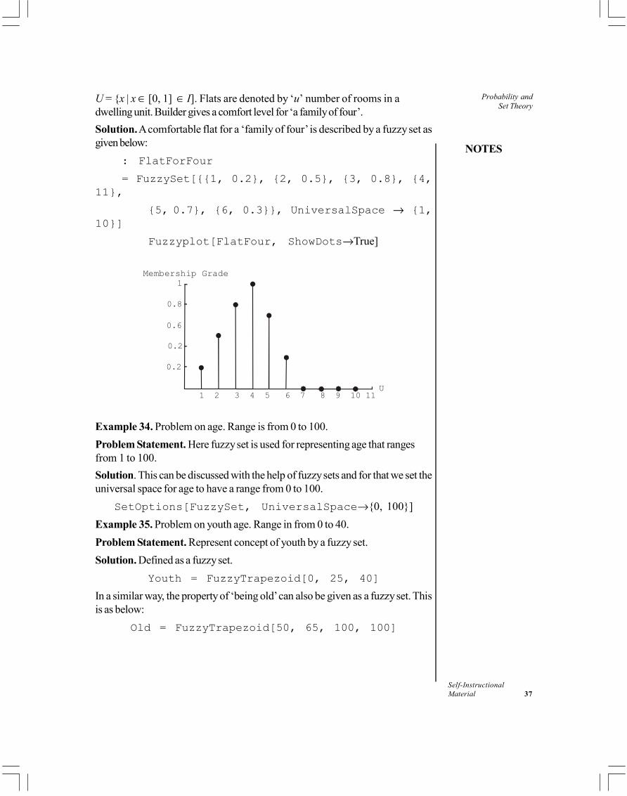
NOTES
Self-InstructionalMaterial 37
Probability andSet Theory
U = x | x ∈ [0, 1] ∈ I]. Flats are denoted by ‘u’ number of rooms in adwelling unit. Builder gives a comfort level for ‘a family of four’.Solution. A comfortable flat for a ‘family of four’ is described by a fuzzy set asgiven below:
: FlatForFour
= FuzzySet[1, 0.2, 2, 0.5, 3, 0.8, 4,11,
5, 0.7, 6, 0.3, UniversalSpace 1,10]
Fuzzyplot[FlatFour, ShowDots True]
Membership Grade1
0.8
0.6
0.2
0.2
1 2 3 4 5 6 7 8 9 10 11 U
Example 34. Problem on age. Range is from 0 to 100.Problem Statement. Here fuzzy set is used for representing age that rangesfrom 1 to 100.Solution. This can be discussed with the help of fuzzy sets and for that we set theuniversal space for age to have a range from 0 to 100.
SetOptions[FuzzySet, UniversalSpace 0, 100]Example 35. Problem on youth age. Range in from 0 to 40.Problem Statement. Represent concept of youth by a fuzzy set.Solution. Defined as a fuzzy set.
Youth = FuzzyTrapezoid[0, 25, 40]
In a similar way, the property of ‘being old’ can also be given as a fuzzy set. Thisis as below:
Old = FuzzyTrapezoid[50, 65, 100, 100]

Probability andSet Theory
NOTES
Self-Instructional38 Material
Example 36. This example shows the operation ‘intersection’ on fuzzy sets.Problem Statement. Define the concept of ‘middle-aged’ using fuzzy set.Solution. A middle age means ‘not old’ OR ‘not young’. This requires use ofoperators NOT, OR. Thus a middle age is found by ‘not old’ (Complement ofold) OR (Disjunction) ‘not young’ (Complement of youth) as in example 33(a)and 33(b).Middle-Aged = Intersection[Complement[Young],
Complement[Old]];
We can also define and operation FuzzyPlot to find a graphical presentation ofage, performing an operation which named as FuzzyPlot.
FuzzyPlot[Young, Middle-Aged, Old,
PlotJoined True];
0.8
0.5
0.4
0.2
Membership Grade1
0 20 40 60 80 100U
The graph shows that the intersection of ‘not young’ and ‘not old’ gives a reasonabledefinition for the concept of ‘middle-aged.’Example 37. Fuzzy set with natural numbers.Problem Statement. To define a set of natural numbers in the neighbourhood of6. This can be done in different ways.Solution. Define a fuzzy set of number adjacent to 6.SetOptions[FuzzySet, UniversalSpace 0, 20];
Six1 =
FuzzySet[3, 0.1, 4, 0.1 4, 0.3 5, 0.6,6,1.0, Number’s closeness to 6.7, 0.6, 8, 0.3, 9, 0.1]
FuzzyPlot[Six1];

NOTES
Self-InstructionalMaterial 39
Probability andSet Theory
Membership Grade1
c-8
c-6
c-2
c-4
1 3 5 7 9 11 13 15 17 19 21U
Solution. We use a function FuzzyTrapazoid and create a fuzzy set. If we thinkthat triangular fuzzy set is perhaps a better choice then we have to set two parametersin the middle of the set as 6 which would tell about the closeness to number 6. Wealso define a set Six2 which shows a set of,
Six2=FuzzyTrapezoid[2, 6, 6, 10];
FuzzyPlot[Six2]; This shows a set of points according this definition.
Membership Grade1
0.8
0.6
0.2
0.4
1 3 5 7 9 11 13 15 17 19 21U
Solution. There may be a third solution which creates a fuzzy set defining nearnessto 6.
2
1CloseTo[x]: =
1+(1-x)
We name it Six3.Six3 = CreateFuzzySet[CloseTo[6]];
FuzzyPlot[Six3];
Membership Grade

Probability andSet Theory
NOTES
Self-Instructional40 Material
Solution. There may be a fourth solution which uses a ‘piece-wise definedfunction’.
= == > <NearSix[x]: which[x 6,1,x 6 & &x 12,
< >− −2 2
1 1,x 6 & & 0, ,True, 0]
(x 5) (7 x)
Six4 = CreateFuzzySet [NearSix];
FuzzyPlot [Six4];
Example 38. Problem on disjunctive sum.Problem. To find,
RMat = .8, .3, .5, .2, .4, 0, .7, .3, .6, .2, .8, .6
This shows a one membership matrix.
SMat = .9,.5,.8, 1, .4,.6,.7, .5,.7,.8,.8,.7
This shows another membership matrix.
R = FromMembershipMatrix[Rmat]; This defines relation inRMatS = FromMembershipMatrix[SMat]; This defines relation in
SMat.FuxxyPlot 3D[R,S, ShowDots True] This shows location of
point.
Grade

NOTES
Self-InstructionalMaterial 41
Probability andSet Theory
Let there be two fuzzy relationships R and S in the universal space V × W.The disjunctive sum is given by: DisSum = (R S’) ∪ (R’ S), which is a relationin V × W, with the following property:
v, w V×W, andDisSum(v, w)= Maximum of (Min(R(v, w), 1 - S(v,
w)),Min(1 - R(v, w), S(v, w)))DisSum = Union[Intersection[R, Complement[s]], Intersection[Complement[R],S]];FuzzyPlot3D[DisSum];
ToMembershipMatrix[DisSum] // MatrixForm
Example 39. Problem on distance.Problem Statement. We take a fuzzy relation R on sets X, Y. We define thesesets as: X = Delhi, Moscow and Y = Dacca, Delhi, London). The relation R isrepresenting the idea of being ‘far’. The relation may be shown as R(X,Y) = 1.0/Delhi, Dacca + 0/Delhi, Toronto + 0.6/Delhi, London + 0.9/Moscow, Delhi +Dacca + 0.9/London, Dacca + 0.7/London, Delhi + 0.3/London.Solution. Representation of such a fuzzy relation is as below: A membership matrixis to be created to depict the relationship. For this we represent by number foreach city in the set. For X we keep 1 for Delhi and 2 for Moscow. In Y we set 1 forDacca, 2 for Delhi and 3 for London.
After this, we are in a position to create relation using a function by name frommemebrship matrix and the relationship can be plotted using a function that isnamed FuzzyPlot3D.DistMat = 1,0,0,6, 0.9,0.7,0.3
1,0,0.6, 0.9,0.7,0.3

Probability andSet Theory
NOTES
Self-Instructional42 Material
DistRel = FromMembershipMatrix[DistMat,
1,2, 1,3]
FuzzyRelation[
1,1,1,1,2,01,3,0.6
2,1,0.9,2,2,0.7,2,30.3,
UniversalSpace 1,2,1,1,3,1]
This relation can be plotted using the FuzzyPlot3D function.Fuzzy Plot3D[DistRel,
Axes Label “ X”, “Y”, “Grade”],
View Point 2, 0, 1,
Axxes Edge -1, -1, 1, -1, 1, 1];
ToMembershipMatrix[DisRel] // MatrixForm
Example 40. To choose a job, Fuzzy sets can help to choose between four givenjobs. Let this job be numbered as 1 to 4.Problem Statement. We have to make selection such that the job provides bestsalary and at the same time it should be near to place of stay.Solution. The first part of selection criteria is given by following definition of fuzzysets. From this selection criterion Job 3 looks most attractive out of all these fourjobs and Job 1 is least attractive. Similarly, a fuzzy set can be created for thesecond part of the selection criteria. We create a set named drive for the distancefrom the working place. Here membership has varying grade depending on distance.Here, least is desired.

NOTES
Self-InstructionalMaterial 43
Probability andSet Theory
From analysis we find that from the second criterion Job 4 is most attractive asit is nearest among the given four and Job 1 is the farthest.
As the goal is to get a good salary, we find that Job 1 has highest and Job 4 isthe lowest.
We have examined all criteria one-by-one using fuzzy sets, but have madeanything to make a final decision. So a decision function is being defined usingintersection. By applying intersection operation betwen the constraints and goalswould give best decision. Plotting the fuzzy set for decision we can visualize theresult graphically. Considering all these the decision function says that Job 2 is thebest.
We can plot the decision fuzzy set to see the results graphically.
Membership Grade
1 2 3 4 5

Probability andSet Theory
NOTES
Self-Instructional44 Material
Power SetThe set of all subsets of a given set A is called the power set of A and is denotedby P(A). The name power set is motivated by the fact that ‘if A has n elementsthen its power set P(A) contains exactly 2n elements.’
Example 41. If A = 1, 2, find P(A).Solution. Now is a subset of A. A is also a subset of A.1 and 2 are alsosubsets of A. Therefore, these are all subsets of A. So, P(A) = [ , 1, 2, A].Therefore P(A) has 22 = 4 elements.
Example 42. Let A = 1, 2, 3. Find P(A).Solution. Now subsets consisting of one element only are 1, 2, 3. Subsetsconsisting of two elements only are, 1, 2, 2, 3, 1, 3. Also and A aresubsets of A.
So P(A) = [ , 1, 2, 3, 1, 2, 2, 3, 1, 3, A] and the number ofelements in P(A) is 23 = 8.
Example 43. Let B be a subset of A. Let P(A : B) = X P(A) | B X. If B =1,2 and A = 1, 2, 3, 4, 5, list all the elements of P(A : B).Solution. Clearly B 1, 2, B 1, 2, 3, B 1, 2, 3, 4, B 1, 2, 3,4, 5, B 1, 2, 4, B 1, 2, 5, B 1, 2, 3, 5, B 1, 2, 4, 5. Thesegive all the elements of P (A : B).
DualityUnion and Intersection of sets are termed as dual operations.If the validity of a law involving are of the two, or is established, then the dualobtained by replacing by and by is also established.
Partition of a SetThe partition of a set A is written as,
A = A1, A2, ..., AnWhere Aj A j = 1, 2, ..., n or Aj’s are inclusive.Thus, (i) A1, A2, ..., An are subsets of A
(ii) Aj Ak = j = 1, 2, ..., n, k = 1,2, ..., n i.e., Any Aj , Ak are disjoints.
(iii) A1 A2 ... An = A, i.e., A1, A2, ..., An are exhaustive.Thus every elements of A is a member of one and only one of the subsets in thepartition.Any sample S can be written as,
S = A, —A
= — —
, , , A B A B A B A B

NOTES
Self-InstructionalMaterial 45
Probability andSet Theory
In any exercise, if (i), (ii), (iii) are all satisfied for a set A = A1, A2, ..., An thenthis represents the partition of A.
Check Your Progress
7. Define the terms set and element.8. Differentiate between finite set and infinite set.9. What is singleton set?
10. Define the term subset.11. What do you mean by null set?12. What are Venn diagrams? Why are they called so?13. What is union of sets?14. Define intersection of sets.15. What does complement of sets mean?16. What is a power set?
1.4 CONDITIONAL PROBABILITY ANDINDEPENDENCE
In many situations, a manager may know the outcome of an event that hasalready occurred and may want to know the chances of a second event occurringbased upon the knowledge of the outcome of the earlier event. We are interestedin finding out as to how additional information obtained as a result of theknowledge about the outcome of an event affects the probability of the occurrenceof the second event. For example, let us assume that a new brand of toothpasteis being introduced in the market. Based on the study of competitive markets,the manufacturer has some idea about the chances of its success. Now, heintroduces the product in a few selected stores in a few selected areas beforemarketing it nationally. A highly positive response from the test-market area willimprove his confidence about the success of his brand nationally. Accordingly,the manufacturer’s assessment of high probability of sales for his brand wouldbe conditional upon the positive response from the test-market.
Let there be two events A and B. Then the probability of event A giventhe outcome of event B is given by:
P[AB]P[A/B]=P[B]
Where P[A/B] is interpreted as the probability of event A on the condition thatevent B has occurred and P [AB] is the joint probability of event A and eventB, and P[B] is not equal to zero.

Probability andSet Theory
NOTES
Self-Instructional46 Material
As an example, let us suppose that we roll a die and we know that thenumber that came up is larger than 4. We want to find out the probability thatthe outcome is an even number given that it is larger than 4.Let, event A = EvenAnd event B = Larger than 4
Then, P[Even / Larger than 4] = P[Even and larger than 4]
P[Larger than 4]
Or, ( )( )
16 1 2
26
P[AB]P[A/B] = /P[B]
= =
But for independent events, P[AB] = P[A]P[B]. Thus substituting thisrelationship in the formula for conditional probability, we get:
P[AB] P[A]P[B]P[A/B] = = =P[A]P[B] P[B]
This means that P[A] will remain the same no matter what the outcomeof event B is. For example, if we want to find out the probability of a head onthe second toss of a fair coin, given that the outcome of the first toss was ahead, this probability would still be 1/2 because the two events are independentevents and the outcome of the first toss does not affect the outcome of thesecond toss.
1.4.1 Independent and Dependent EventsTwo events A and B are said to be independent events, if the occurrence of oneevent is not influenced at all by the occurrence of the other. For example, if twofair coins are tossed, then the result of one toss is totally independent of theresult of the other toss. The probability that a head will be the outcome of anyone toss will always be 1/2, irrespective of whatever the outcome is of the othertoss. Hence, these two events are independent.
Let us assume that one fair coin is tossed 10 times and it happens that thefirst nine tosses resulted in heads. What is the probability that the outcome ofthe tenth toss will also be a head? There is always a psychological tendency tothink that a tail would be more likely in the tenth toss since the first nine tossesresulted in heads. However, since the events of tossing a coin 10 times are allindependent events, the earlier outcomes have no influence whatsoever on theresult of the tenth toss. Hence the probability that the outcome will be a headon the tenth toss is still 1/2.
On the other hand, consider drawing two cards from a pack of 52 playingcards. The probability that the second card will be an ace would depend uponwhether the first card was an ace or not. Hence these two events are notindependent events.

NOTES
Self-InstructionalMaterial 47
Probability andSet Theory
Independent Repeated Trials
Probability is a measure of relative frequency. According to definition, theprobability of an event E is equal to the number of equally likely ways E canoccur divided by the total number of equally likely things which can occur.
For studying independent repeated trials, combinatorics is considered importantwhen we consider that an event is consisting of repeated trials. Tossing a fair coinmany times is an example of it. Suppose that a fair coin is tossed 10 times. Nowthe probability of the coin landing on heads for each toss is 1/2, since there aretwo possible equally-likely outcomes (heads or tails) and just one way it can comeup heads. Furthermore, each toss of the coin is independent of every other toss.Basically this defines that the coin has no memory and the probability of the coinlanding on heads for any given toss will be always 1/2. It has no relation with theoutcome history of the previous tosses. Suppose the coin had just landed on heads8 times in a row. Is it possible that the coin is more likely to land on tails on the nexttoss? The probability of it landing on heads is always 1/2, since the coin has nomemory. It is true that in the long run, 50 per cent of the tosses will be heads and50 per cent tails, but this is not achieved by the coin making up for any deficit ofheads or tails but rather by turning up heads roughly half the time in all futuretosses.
The fraction of successes depends on the probability of success in each trial,as the number of trials increases in repeated independent trials with the sameprobability of success. This is also known as the (Law of Large Numbers).According to this law if a discrete random variable is observed repeatedly inindependent experiments then the fraction of experiments for which the randomvariable equals any of its possible values has the probability that the random variableequals that value.
Check Your Progress
17. Explain the concept of independent events.18. Define binomial distribution.19. What is a random variable?
1.5 ANSWERS TO CHECK YOUR PROGRESSQUESTIONS
1. The term simple probability refers to a phenomenon where only a simpleor an elementary event occurs. For example, assume that event (E), thedrawing of a diamond card from a pack of 52 cards, is a simple event.Since there are 13 diamond cards in the pack and each card is equally likelyto be drawn, the probability of event (E) or P[E] = 13/52 or 1/4.

Probability andSet Theory
NOTES
Self-Instructional48 Material
The term joint probability refers to the phenomenon of occurrence of twoor more simple events. For example, assume that event (E) is a joint event(or compound event) of drawing a black ace from a pack of cards. Thereare two simple events involved in the compound event, which are: the cardbeing black and the card being an ace. Hence, P[Black ace] or P[E] = 2/52 since there are two black aces in the pack.
2. The classical theory of probability is the theory based on the number offavourable outcomes and the number of total outcomes. The probability isexpressed as a ratio of these two numbers. The term ‘favourable’ is not thesubjective value given to the outcomes, but is rather the classical terminologyused to indicate that an outcome belongs to a given event of interest.
3. The addition rule states that when two events are mutually exclusive, thenthe probability that either of the events will occur is the sum of their separateprobabilities. For example, if you roll a single dice then the probability thatit will come up with a face 5 or face 6, where event A refers to face 5 andevent B refers to face 6, both events being mutually exclusive events, isgiven by,
P[A or B] = P[A] + P[B]Or, P[5 or 6] = P[5] + P[6]
= 1/6 +1/6= 2/6 = 1/3
4. Multiplication rule is applied when it is necessary to compute the probabilityin case two events occur at the same time.
5. Bayes’ theorem on probability is concerned with a method for estimatingthe probability of causes which are responsible for the outcome of anobserved effect. The theorem contributes to the statistical decision theoryin revising prior probabilities of outcomes of events based upon theobservation and analysis of additional information.
6. Two events are said to be mutually exclusive, if both events cannot occur atthe same time as the outcome of a single experiment. For example, if wetoss a coin, then either event head or event tail would occur, but not both.Hence, these are mutually exclusive events.
7. ‘A set is any collection of objects such that given an object, it is possible todetermine whether that object belongs to the given collection or not.’The members of a set are called elements. We use capital letters to denotesets and small letters to denote elements. We always use brackets todenote a set.
8. A set which has finite number of elements is called a finite set, else it is calledan infinite set.

NOTES
Self-InstructionalMaterial 49
Probability andSet Theory
9. A set having only one element is called Singleton. If a is the element of thesingleton A, then A is denoted by A = a.
10. Let A and B be two sets. If every element of A is an element of B, then A iscalled a subset of B and we write A B or B A (read as ‘A is contained inB’ or ‘B contains A’).
11. A set which has no element is called the null set or empty set. It is denotedby the symbol .
12. Venn diagrams are used to illustrate various set operations. It is named afterJohn Venn (1834–1883 ).
13. The union of any two sets A and B is the set of all those elements x such thatx belongs to at least one of the two sets A and B. It is denoted by A B.Logically speaking, if the biconditional statement (x C) (x A) (x B)is true for all x, then C = A B. In other words (x A B) (x A) (x B).
14. The intersection of two sets A and B is the set of all those elements x suchthat x belongs to both A and B and is denoted by A B. If A B = , then Aand B are said to be disjoint.Logically speaking, if the biconditional statement (x C) (x A) (x B)is true for all x, then C = A B. Hence,
(x A B) (x A) (x B)
15. If A and B are two sets then complement of B relative to A is the set of allthose elements x A such that x B and is denoted by A – B. Logicallyspeaking, if for a set C the biconditional statement (x C ) (x A) (x B) is true for all x, then C = A – B. In other words, if (x C) (x A)
(x B) then C is called the complement of B relative to A.16. The set of all subsets of a given set A is called the power set of A and is
denoted by P(A). The name power set is motivated by the fact that ‘if A hasn elements then its power set P(A) contains exactly 2n elements.’
17. Two events A and B are said to be independent events, if the occurrence ofone event is not at all influenced by the occurrence of the other. For example,if two fair coins are tossed, then the result of one toss is totally independentof the result of the other toss. The probability that a head will be the outcomeof any one toss will always be 1/2, irrespective of whatever the outcome isof the other toss. Hence, these two events are independent.
18. Binomial distribution is one of the simplest and most frequently used discreteprobability distribution and is very useful in many practical situations involvingeither/or types of events.
19. A random variable is a phenomenon of interest in which the observedoutcomes of an activity are entirely by chance, are absolutely unpredictableand may differ from response to response.

Probability andSet Theory
NOTES
Self-Instructional50 Material
1.6 SUMMARY
A probability is expressed as a real number, p [0, 1]∈ and the probabilitynumber is expressed as a percentage (0 per cent to 100 per cent) and notas a decimal.The classical theory of probability is the theory based on the number offavourable outcomes and the number of total outcomes.If the number of outcomes belonging to an event E is NE , and the totalnumber of outcomes is N, then the probability of event E is defined as
p NNE
E=
We cannot calculate the probability where the outcomes are unequalprobabilities.
The sequence nnA in the limit that will converge to the same result every
time, or that it will not converge at all.The axiomatic probability theory is the most general approach to probability,and is used for more difficult problems in probability.The empirical approach to determining probabilities relies on data fromactual experiments to determine approximate probabilities instead of theassumption of equal likeliness.The relationship between these empirical probabilities and the theoreticalprobabilities is suggested by the (Law of Large Numbers). The law statesthat as the number of trials of an experiment increases, the empiricalprobability approaches the theoretical probability.Multiplication rule is applied when it is necessary to compute the probabilityif both events A and B will occur at the same time.Bayes’ theorem makes use of conditional probability formula where thecondition can be described in terms of the additional information whichwould result in the revised probability of the outcome of an event.A sample space is the collection of all possible events or outcomes of anexperiment.An event is an outcome or a set of outcomes of an activity or a result of atrial.Two mutually exclusive events are said to be complementary if they betweenthemselves exhaust all possible outcomes.A probability space is a measure of space such that the measure of thewhole space is equal to 1. A simple finite probability space is an orderedpair (S, p) such that S is set and p is a function with domain S.
NOTES
Self-InstructionalMaterial 51
Probability andSet Theory
The members of a set are called its elements. We use capital letters todenote sets and small letters to denote elements.A set having only one element is called singleton. If a is the element of thesingleton A, then A is denoted by A = a.Whenever we talk of a set, we shall assume it to be a subset of a fixed setU. This fixed set U is called the universal set.A set which has no element is called the null set or empty set. It is denotedby the symbol f.The union of any two sets A and B is the set of all those elements x such thatx belongs to at least one of the two sets A and B.The intersection of two sets A and B is the set of all those elements x suchthat x belongs to both A and B and is denoted by A B. If A B = , thenA and B are said to be disjoint.If A and B are two sets then complement of B relative to A is the set of allthose elements x A such that x B and is denoted by A – B.Two events A and B are said to be independent events, if the occurrence ofone event is not influenced at all by the occurrence of the other.The fraction of successes depends on the probability of success in eachtrial, as the number of trials increases in repeated independent trials with thesame probability of success.
1.7 KEY WORDS
Classical theory of probability: It is the theory of probability based onthe number of favourable outcomes and the number of total outcomes.Event: It is an outcome or a set of outcomes of an activity or the result ofa trial.Elementary event: It is the single possible outcome of an experiment. It isalso known as a simple event.Joint event: It is also known as compound event and has two or moreelementary events in it.Sample space: It is the collection of all possible events or outcomes of anexperiment.Addition rule: It states that when two events are mutually exclusive, thenthe probability that either of the events will occur is the sum of their separateprobabilities.Multiplication rule: It is applied when it is necessary to compute theprobability, if both events A and B occur at the same time. Different rulesare applied for different conditions.

Probability andSet Theory
NOTES
Self-Instructional52 Material
Set: It is a collection of objects, such that given an object, it is possible todetermine whether that object belongs to the given collection or not.Element: The members of a set are called its elements.Singleton: It is a set having only one or single element.Null set: It is a set with no elements.
1.8 SELF-ASSESSMENT QUESTIONS ANDEXERCISES
Short-Answer Questions
1. Explain the concept of probability.2. What are the different theories of probability? Explain briefly.3. What do you understand by simple probability?4. Explain the axiomatic approach to probability.5. Explain the concept of multiplication rule.6. What is Bayes’ theorem? What is its importance in statistical calculations?7. Define sample space.8. Explain event and its types with the help of examples.9. What is a mutually exclusive event?
10. Explain the terms, ‘Sum of Events’ and ‘Product of Events’.11. What is finite probability space?12. Define set with the help of examples.13. How will you define a universal set?14. When are two sets termed equal?15. Explain power set.16. Describe union, intersection and complement set operations.17. Explain the importance of Venn diagrams.18. What do you understand by finite sets and counting principle?19. Explain distributive laws and De Morgan’s laws of set theory.20. What are the important applications of set theory?21. Explain duality.22. What is mathematical induction?23. Describe the importance of conditional probability.24. When are independent repeated trials used?25. Explain the properties of binomial distribution.

NOTES
Self-InstructionalMaterial 53
Probability andSet Theory
26. What is a random variable? Differentiate between qualitative and quantitativerandom variables.
Long-Answer Questions1. A family plans to have two children. What is the probability that both
children will be boys? (List all the possibilities and then select the one whichwould be two boys.)
2. A family plans to have three children. List all the possible combinations andfind the probability that all the three children will be boys.
3. A card is selected at random from an ordinary well-shuffled pack of 52cards. What is the probability of getting:(i) A king(ii) A spade(iii) A king or an ace(iv) A picture card
4. A wheel of fortune has numbers 1 to 40 painted on it, each number beingat equal distance from the other so that when the wheel is rotated, thereis the same chance that the pointer will point at any of these numbers.Tickets have been issued to contestants numbering 1 to 40. The number atwhich the wheel stops after being rotated would be the winning number.What is the probability that:(i) Ticket number 29 wins.(ii) One person who bought 5 tickets numbered 18 to 22 inclusive wins the
prize.5. In a computer course, the probability that a student will get an A is 0.09.
The probability that he will get a B grade is 0.15 and the probability thathe will get a C grade is 0.45. What is the probability that the student willget either a D or an F grade?
6. The Dean of the School of Business has two secretaries, Mary and Jane.The probability that Mary will be absent on any given day is 0.08. Theprobability that Jane will be absent on any given day is 0.06. The probabilitythat both the secretaries will be absent on any given day is 0.02. Find theprobability that either one of them will be absent on any given day.
7. A fair die is rolled once. What is the probability of getting:(i) An odd number.(ii) A number greater than 3.
8. Two fair dice are rolled. What is the probability of getting:(i) A sum of 10 or more.(ii) A pair of which atleast one number is 3.(iii) A sum of 8, 9, or 10.(iv) One number less than 4.

Probability andSet Theory
NOTES
Self-Instructional54 Material
9. An urn contains 12 white balls and 8 red balls. Two balls are to be selectedin succession, at random and without replacement. What is the probabilitythat:(i) Both balls are white.(ii) The first ball is white and the second ball is red.(iii) One white ball and one red ball are selected.(iv) Would the probabilities change if the first ball after being identified is
put back in the urn before the second ball is selected?10. In a statistics class, the probability that a student picked up at random
comes from a two parent family is 0.65, and the probability that he will failthe exam is 0.20. What is the probability that such a randomly selectedstudent will be a low achiever given that he comes from a two parentfamily?
11. The following is a breakdown of faculty members in various ranks at thecollege.Rank Number of Males Number of FemalesProfessor 20 12Assoc. Professor 18 20Asst. Professor 25 30What is the probability that a faculty member selected at random is:(i) A female.(ii) A female professor.(iii) A female given that the person is a professor.(iv) A female or a professor.(v) A professor or an assistant professor.(vi) Are the events of being a male and being an associate professor
statistically independent events?12. A movie house is filled with 700 people and 60 per cent of these people
are females. 70 per cent of these people are seated in the no smoking areaincluding 300 females. What is the probability that a person picked up atrandom in the movie house is:(i) A male.(ii) A female smoker.(iii) A male or a non-smoker.(iv) A smoker if we knew that the person is a male.(v) Are the events sex and smoking statistically independent?
13. A part-time student is taking two courses, namely, Statistics and Finance.The probability that the student will pass the Statistics course is 0.60 andthe probability of passing the Finance course is 0.70. The probability thatthe student will pass both courses is 0.50. Find the probability that thestudent:

NOTES
Self-InstructionalMaterial 55
Probability andSet Theory
(i) will pass at least one course.(ii) will pass either or both courses.(iii) will fail both courses.
14. 200 students from the college were surveyed to find out if they were takingany of the Management, Marketing or Finance courses. It was found that80 of them were taking Management courses, 70 of them were takingMarketing courses and 50 of them were taking Finance courses. It wasalso found that 30 of them were taking Management and Marketing courses,30 of them were taking Management and Finance courses and 25 of themwere taking Marketing and Finance courses. It was further determined that20 of these students were taking courses in all the three areas. What is theprobability that a particular student is not taking any course in any of theseareas?
15. Out of 20 students in a Statistics class, 3 students are failing in the course.If 4 students from the class are picked up at random, what is the probabilitythat one of the failing students will be among them.
16. The New York Pick Five lottery drawing draws five numbers at random outof 39 numbers labelled 1 to 39. How many different outcomes are possible?
17. A company has 18 senior executives. Six of these executives are womenincluding four blacks and two Indians. Six of these executives are to beselected at random for a Christmas cruise. What is the probability that theselection will include:(i) All the black and Indian women.(ii) At least one Indian woman.(iii) Not more than two women.(iv) Half men and half women.
18. The probability that a management trainee will remain with the companyafter the training programme is completed is 0.70. The records indicate that60 per cent of all managers earn over $60,000 per year. The probability thatan employee is a management trainee or who earns more than $60,000 peryear is 0.80. What is the probability that an employee earns more than$60,000 per year, given that he is a management trainee who stayed withthe company after completing the training programme.
19. A manufacturer of laptop computer monitors has determined that on anaverage, 3 per cent of screens produced are defective. A sample of onedozen monitors from a production lot was taken at random. What is theprobability that in this sample fewer than 2 defectives will be found?
20. A fair coin is tossed 16 times. What is the probability of getting no morethan 2 heads?
21. A student is given 4 True or False questions. The student does not knowthe answer to any of the questions. He tosses a fair coin. Each time he getsa head, he selects True. What is the probability that he will get:

Probability andSet Theory
NOTES
Self-Instructional56 Material
(i) Only one correct answer(ii) At most 2 correct answers(iii) At least 3 correct answers(iv) All correct answers
22. A newly married couple plans to have 5 children. An astrologist tells themthat based on astrological reading, they have an 80 per cent chance ofhaving a baby boy on any particular birth. The couple would like to have3 boys and 2 girls. Find the probability of this event.
23. An automatic machine makes paper clips from coils of wire. On an average,one in 400 paper clips is defective. If the paper clips are packed in smallboxes of 100 clips each, what is the probability that any given box of clipscontains.(i) No defectives(ii) One or more defectives(iii) Less than two defectives(iv) Two or less defectives
24. Because of recycling campaigns, a number of empty glass soda bottles arebeing returned for refilling It has been found that 10 per cent of theincoming bottles are chipped and hence are discarded. In the next batch of20 bottles, what is the probability that:(i) None will be chipped.(ii) Two or fewer will be chipped.(iii) Three or more will be chipped.(iv) What is the expected number of chipped bottles in a batch of 20?
25. The customers arrive at a drive-in window of Apple bank at an averagerate of one customer per minute.(i) What is the probability that exactly two customers arrive in a given
minute?(ii) What is the probability of no arrivals in a particular minute?
26. Write the following sets by listing elements enclosed in brackets :(i) A is the set whose elements are first five letters of the alphabet.(ii) B is the set of all odd integers.(iii) X is the set of all two digit positive numbers which are divisible by 15.
27. Write the following sets using a statement to designate each:(i) A = 3, 6, 12, 15, 18(ii) B = s, t, u, v, w, x, y, z(iii) C = 1, 3, 5, 7, . . . ., 2n –1, . . .
(iv) D = 1 1 1 1 1, , , , . . . , . . .1 2 3 4 n

NOTES
Self-InstructionalMaterial 57
Probability andSet Theory
28. Indicate which of the following sets are finite:(i) A = x | x is a positive integer(ii) B = x | x is an even integer lying between 2 and 10(iii) C = x | x is a letter of the alphabet(iv) E = x | x is an integter less than 10
29. Let A be the set 1, 3, 5, 7, 9, 11, 13, 15, 17, 19. Now, list the following sets:(i) x | x is an element of A and x + 1 is even(ii) x | x is an element of A and 2x is an element of A(iii) x | x is an element of A and 2x < 20(iv) x | x is not an element of A and 0 < x < 21
30. Find all possible solutions for x and y in each of the following cases:(i) 2, 3 = 2x, y(ii) x, y = 1, 2(iii) x, x2 = 9, 3
31. Show that if a1 b1, a1 a2 and a1, b1 = a2, b2, then b1 = b2.32. Show that a = b, c if and only if a = b = c.33. State the relation if any, between sets A and B in the following:
(i) A = 1, 3, 5, 7, 9, . . . B = 3, 9, 15, 21, . . . . , 3(2n – 1), . . .
(ii) A = 2, 4, 7, 12, 18, 24B = 1, 3, 7, 11, 16, 22, 29
(iii) A = x | x is an even natural number less than 20B = x | x is natural number less than 20 which is divisible by 2
(iv) A = x | x is an even integerB = x | x is an integer divisible by 3
34. Prove that A B and B C implies A C.35. Prove that A implies A = .36. If a set A has 101 elements, find the number of subsets of A having odd
number of elements.37. What are the elements of the power set of the set [1, 2, 3]?38. If A = 1, 2, 3, 4, 5, B = 2, 4, 6, 8, 10, C = 3, 6, 9, 12, 15. Find that,
(i) (A B) C (ii) A (B C)(iii) (A C) B
39. If A = 1, 2, 3, 4, B = 3, 4, 5, 6, C = 4, 5, 6, 7. Find that,(i) A – B (ii) (A B) – C(iii) A – (B C) (iv) (A B) – (B U C)

Probability andSet Theory
NOTES
Self-Instructional58 Material
40. If U = 1, 2, 3, 4, 5, 6, 7, 8, 9, 10A = 1, 4, 7, 10B = 2, 5, 8Find (i) A (ii) B (iii) A B (iv) A B (v) A B
41. Prove that (A B) C = A (B C) if and only if C A.42. Prove that if A B then P (A) P (B).43. For any sets A and B, prove or disprove that,
P(A) P(B) = P(A B)P(A) P(B) = P(A B)
44. In a survey of 100 students, the numbers studying various languages werefound to be: Spanish 28; German 30; French 42; Spanish and French 10;Spanish and German 8; German and French 5; all the three languages 3.(i) How many students were studying no language?(ii) How many students had French as their only language?(iii) How many students studied German if and only if they studied French?
45. In each of the following sentences, determine which is a statement (S), ornot (N):(i) Every rectangle is a square.(ii) The sum of three angles of a triangle is 180°.(iii) How are you?(iv) 2 + 1 = 3.
(v) 2 is a rational number..46. In a latter survey of the 100 students, the numbers studying the various
languages were found to be:German only 18; German but not Spanish 23; German and French 8; German26; French 48; French and Spanish 8; studying no language 24.(i) How many students took Spanish?(ii) How many took German and Spanish but not French?(iii) How many took French if and only if they did not take Spanish?
47. If A and B are two sets, prove that number of elements in A B is equal to:(Number of elements in A – Number of elements in A B).
48. The report of one survey of 100 students stated that the numbers studyingthe various languages were; all three languages 5; German and Spanish 10;French and Spanish 8; German and French 20; Spanish 30; German 23; French50. The surveyor who turned in this report was fired. Why?
49. In a recent survey of 5000 people, it was found that 2800 read Indian Expressand 2300 read Statesman while 400 read both the papers. How many readneither Indian Express nor Statesman?

NOTES
Self-InstructionalMaterial 59
Probability andSet Theory
50. In a survey of 30 students, it was found that 19 take Mathematics, 17 takeMusic, 11 take History, 7 take Mathematics and History, 12 take Mathematicsand Music, 5 take Music and History and 2 take all three courses. Find(i) The number of students that take Mathematics but do not take History(ii) The number that take exactly two of the three courses.
51. In a Chemistry class there are 20 students, and in a Psychology class thereare 30 students. Find the number either in a Psychology class or Chemistryclass if,(i) The two classes meet at the same hour.(ii) The two classes meet at different hours and 10 students are enrolled in
both courses.52. On an Air India flight, there are 9 boys, 5 Indian children, 9 men, 7 foreign
boys, 14 Indian, 6 Indian males and 7 foreign females. What is the number ofpeople in this plane?
53. A college awarded 38 medals in Football, 15 in Basket ball and 20 in Cricket.If these medals went to a total of 58 men and only three of these men gotmedals in all the three sports, how many men received medals in exactly twoof the three sports?
54. Suppose that in survey concerning the reading habits of students it is foundthat:60 per cent read magazine A,50 per cent read magazine B,50 per cent read magazine C,30 per cent read magazines A and B,20 per cent read magazines B and C,30 per cent read magazines A and C,10 per cent read all three magazines.(i) What per cent read exactly two magazines?(ii) What per cent do not read any of the magazines?
55. In a survey of 500 consumers, it was found that 425 liked product A and 375liked product B. What is the least number of consumers that must have likedboth products assuming that there may be consumers of products differentfrom A and B.
56. Explain how a class is different from a set.57. How many power sets are formed from vowels of English language?58. Give a brief description of basic sets and denotable sets.59. Explain how a fuzzy set is different from a generally defined set.60. Give your comments on ‘operations on fuzzy sets’. Explain three operations.61. What are the areas of application of fuzzy set? Explain with three examples.

Probability andSet Theory
NOTES
Self-Instructional60 Material
1.9 FURTHER READINGS
Hogg, Robert. V., Allen T. Craig and Joseph W. McKean. 2005. Introduction toMathematical Statistics. New Delhi: Pearson Education.
Fisz, Marek. 1963. Probability Theory and Mathematical Statistics, 3rd Edition.New York: John Wiley & Sons, Inc.
Rohatgi, Vijay K. 1985. An Introduction to Probability Theory andMathematical Statistics. New Delhi: Wiley Eastern Limited.
Gupta, C.B. and Vijay Gupta. 2004. An Introduction to Statistical Methods,23rd Edition. New Delhi: Vikas Publishing House.
Levin, Richard I. and David S. Rubin. 1998. Statistics for Management. NewJersey: Prentice Hall.
Chandan, J. S. 1998. Statistics for Business and Economics. New Delhi: VikasPublishing House Pvt. Ltd.
Campbell, Stephen K. 1987. Applied Statistics. New York: Harper & Row.Chance, William A. 1969. Statistical Methods for Decision Making. Illinois:
Richard D Irwin.Hooda, R. P. 2013. Statistics for Business and Economics, 5th Edition. New
Delhi: Vikas Publishing House Pvt. Ltd.

NOTES
Self-InstructionalMaterial 61
Random Variables ofDiscrete and
Continuous TypeUNIT 2 RANDOM VARIABLES OFDISCRETE ANDCONTINUOUS TYPE
Structure2.0 Introduction2.1 Objectives2.2 Random Variables of the Discrete Type and Random Variables of the
Continuous Type2.3 Answers to Check Your Progress Questions2.4 Summary2.5 Key Words2.6 Self-Assessment Questions and Exercises2.7 Further Readings
2.0 INTRODUCTION
Randomness means each possible entity has the same chance of being considered.A random variable may be qualitative or quantitative in nature. You will studyprobability distribution, which means listing of all possible outcomes of an experimenttogether with their probabilities. It may be discrete or continuous.
In this unit, you will study about the random variables of the discrete typeand random variables of the continuous type.
2.1 OBJECTIVES
After going through this unit, you will be able to:Understand the random variables of the discrete typeAnalyse the random variables of the continuous type
2.2 RANDOM VARIABLES OF THE DISCRETETYPE AND RANDOM VARIABLES OF THECONTINUOUS TYPE
Discrete Probability Distributions
When a random variable x takes discrete values x1, x2,...., xn with probabilitiesp1, p2,...,pn, we have a discrete probability distribution of X.

Random Variables ofDiscrete andContinuous Type
NOTES
Self-Instructional62 Material
The function p(x) for which X = x1, x2,..., xn takes values p1, p2,....,pn, isthe probability function of X.
The variable is discrete because it does not assume all values. Its propertiesare:
p(xi) = Probability that X assumes the value x.= Prob (x = xi) = pi
p(x) 0, p(x) = 1For example, four coins are tossed and the number of heads X noted. X can takevalue 0, 1, 2, 3, 4 heads.
p(X = 0) = 41 1
2 16 =
p(X = 1) = 3
41
1 1 42 2 16
C =
p(X = 2) = 2 2
42
1 1 62 2 16
C =
p(X = 3) = 3
43
1 1 42 2 16
C =
p(X = 4) = 4 0
44
1 1 12 2 16
C =
O0 1 2 3 4
616
516
416
316
216
116
4
2
1 4 6 4 1( ) 116 16 16 16 16x
p x=
= + + + + =∑This is a discrete probability distribution.
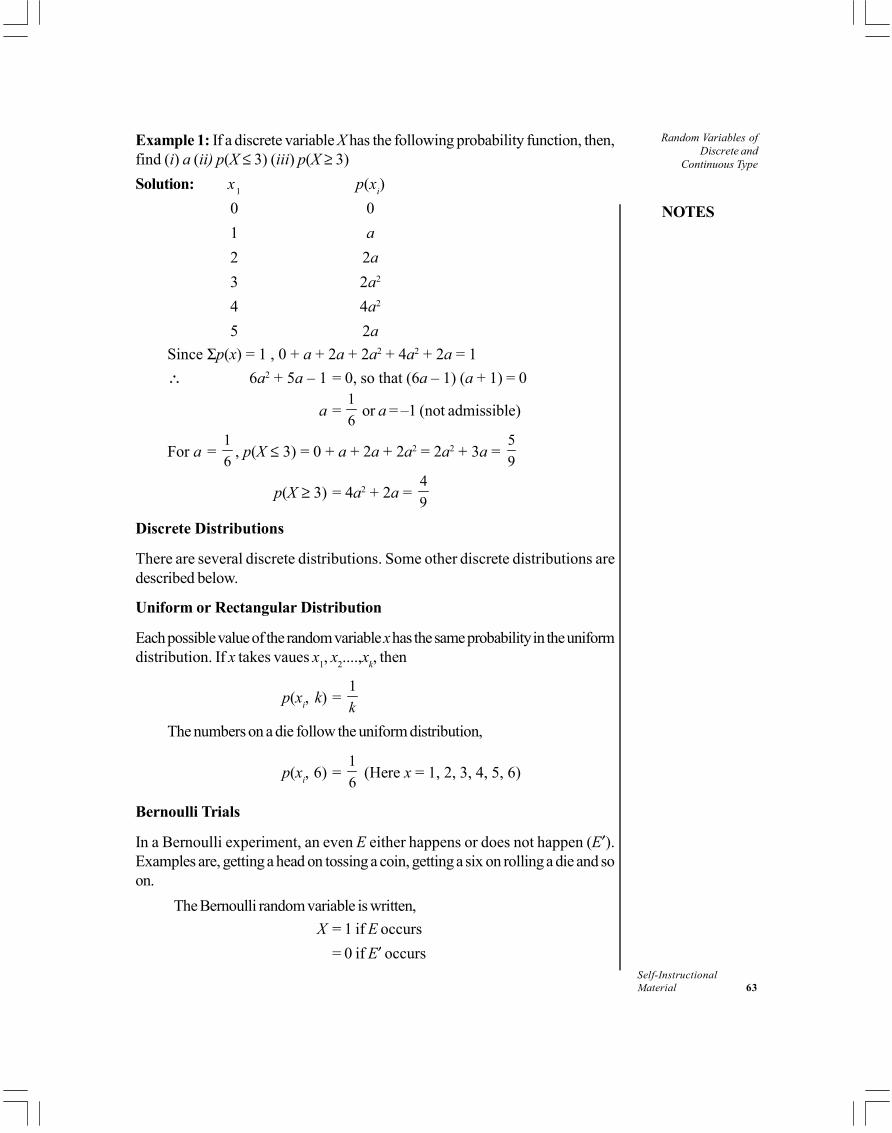
NOTES
Self-InstructionalMaterial 63
Random Variables ofDiscrete and
Continuous Type
Example 1: If a discrete variable X has the following probability function, then,find (i) a (ii) p(X 3) (iii) p(X 3)Solution: x1 p(xi)
0 01 a2 2a3 2a2
4 4a2
5 2aSince p(x) = 1 , 0 + a + 2a + 2a2 + 4a2 + 2a = 1
6a2 + 5a – 1 = 0, so that (6a – 1) (a + 1) = 0
a = 16 or a = –1 (not admissible)
For a = 16 , p(X 3) = 0 + a + 2a + 2a2 = 2a2 + 3a =
59
p(X 3) = 4a2 + 2a = 49
Discrete Distributions
There are several discrete distributions. Some other discrete distributions aredescribed below.
Uniform or Rectangular Distribution
Each possible value of the random variable x has the same probability in the uniformdistribution. If x takes vaues x1, x2....,xk, then
p(xi, k) = 1k
The numbers on a die follow the uniform distribution,
p(xi, 6) = 16 (Here x = 1, 2, 3, 4, 5, 6)
Bernoulli Trials
In a Bernoulli experiment, an even E either happens or does not happen (E ).Examples are, getting a head on tossing a coin, getting a six on rolling a die and soon.
The Bernoulli random variable is written,X = 1 if E occurs
= 0 if E occurs

Random Variables ofDiscrete andContinuous Type
NOTES
Self-Instructional64 Material
Since there are two possible value it is a case of a discrete variablewhere,
Probability of success = p = p(E)Profitability of failure = 1 – p = q = p(E )
We can write,For k = 1, f(k) = pFor k = 0, f(k) = qFor k = 0 or 1, f(k) = pkq1–k
Negative Binomial
In this distribution the variance is larger than the mean.Suppose, the probability of success p in a series of independent Bernoulli
trials remains constant.Suppose the rth success occurs after x failures in x + r trials.1. The probability of the success of the last trial is p.2. The number of remaining trials is x + r – 1 in which there should be r –
1 successes. The probability of r – 1 successes is given by,–1 –1
–1x r r x
rC p q+
The combined pobability of cases (1) and (2) happening together is,
p(x) = –1 –1–1
x r r xrpx C p q+ x = 0, 1, 2,....
This is the Negative Binomial distribution. We can write it in an alternativeform,
p(x) = – ( )r r xxC p q− x = 0, 1, 2,....
This can be summed up as follows:In an infinite series of Bernoulli trials the probability that x + r trials will be
required to get r successes is the Negative Binomial,
p(x) = –1 –1–1
x r r xrC p q+ r 0
If r = 1, it becomes the Geometric distribution.If p 0, , rp = m a constant, then the negative binomial tends tothe Poisson distribution.
Geometric Distribution
Suppose the probability of success p in a series of independent trials remainsconstant.
Suppose, the first success occurs after x failures, i.e., there are x failurespreceding the first success. The probability of this event will be given by p(x) =qxp (x = 0, 1, 2,.....)

NOTES
Self-InstructionalMaterial 65
Random Variables ofDiscrete and
Continuous Type
This is the Geometric distribution and can be derived from the NegativeBinomial. If we put r = 1 in the Negative Binomial distribution:
p(x) = –1 –1–1
x r r xrC p q+
We get the Geometric distribution,
p(x) = 10
x x xC p q pq=
p(x) = 0
11
px
n
pq pq=
= =−∑
E(x) = Mean = pq
Variance = 2
pq
Mode = 12
x
Example 2: Find the expectation of the number of failures preceding the firstsuccess in an infinite series of independent trials with constant probability p ofsuccess.Solution: The probability of success in,
1st trial = p (Success at once)2nd trial = qp (One failure then success and so on)3rd trial = q2p (Two failures then success and so
on)The expected number of failures preceding the success,
E(x) = 0 . p + 1. pq + 2p2p + ............= pq(1 + 2q + 3q2 + .........)
= 2 2
1 1(1– )
qpq qpq p p
= =
Since p = 1 – q.
Hypergeometic Distribution
From a finite population of size N, a sample of size n is drawn without replacement.Let there be N1 successes out of N.The number of failures is N2 = N – N1
The disribution of the random variable X, which is the number of successesobtained in the above case, is called the Hypergeometic distribution.
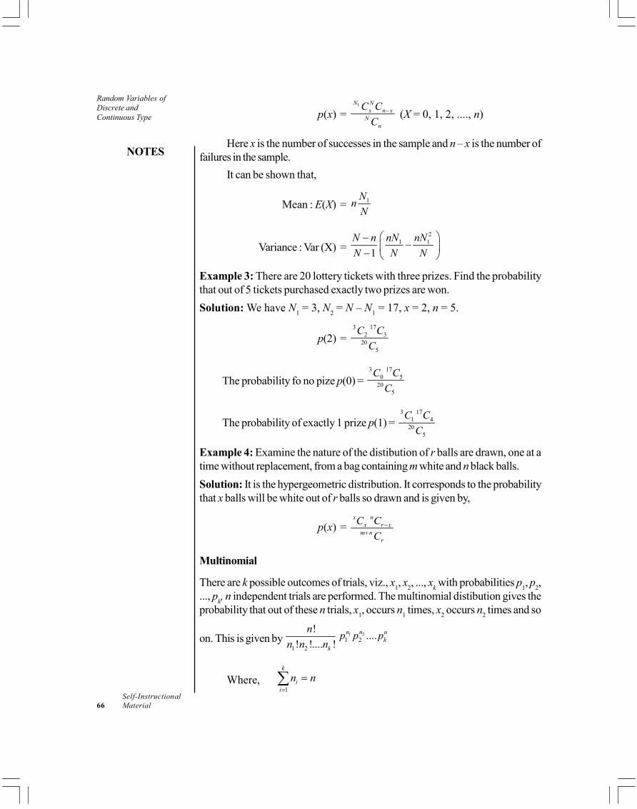
Random Variables ofDiscrete andContinuous Type
NOTES
Self-Instructional66 Material
p(x) = 1N N
x n xN
n
C CC
− (X = 0, 1, 2, ...., n)
Here x is the number of successes in the sample and n – x is the number offailures in the sample.
It can be shown that,
Mean : E(X) = 1NnN
Variance : Var (X) = 2
1 1–1
N n nN nNN N N
− −
Example 3: There are 20 lottery tickets with three prizes. Find the probabilitythat out of 5 tickets purchased exactly two prizes are won.Solution: We have N1 = 3, N2 = N – N1 = 17, x = 2, n = 5.
p(2) = 3 17
2 320
5
C CC
The probability fo no pize p(0) = 3 17
0 520
5
C CC
The probability of exactly 1 prize p(1) = 3 17
1 420
5
C CC
Example 4: Examine the nature of the distibution of r balls are drawn, one at atime without replacement, from a bag containing m white and n black balls.Solution: It is the hypergeometric distribution. It corresponds to the probabilitythat x balls will be white out of r balls so drawn and is given by,
p(x) = x n
x r xm n
r
C CC
−+
Multinomial
There are k possible outcomes of trials, viz., x1, x2, ..., xk with probabilities p1, p2,..., pk, n independent trials are performed. The multinomial distibution gives theprobability that out of these n trials, x1, occurs n1 times, x2 occurs n2 times and so
on. This is given by 1 21 2
1 2
! ....! !.... !
n n nk
k
n p p pn n n
Where, 1
k
ii
n n=
=∑

NOTES
Self-InstructionalMaterial 67
Random Variables ofDiscrete and
Continuous Type
Characteristic Features of the Binomial Distribution
The following are the characteristics of Binomial distribution:1. It is a discrete distribution.2. It gives the probability of x successes and n – x failures in a specific order.3. The experiment consists of n repeated trials.4. Each trial results in a success or a failure.5. The probability of success remains constant from trial to trial.6. The trials are independent.7. The success probability p of any outcome remains constant over time. This
condition is usually not fully satisfied in situations involving management andeconomics, for example, the probability of response from successiveinformants is not the same. However, it may be assumed that the conditionis reasonably well satisfied in many cases and that the outcome of one trialdoes not depend on the outcome of another. This condition too, may not befully satisfied in many cases. An investigator may not approach a secondinformant with the same set-up of mind as used for the first informant.
8. The binomial distribution depends on two parameters n and p. Each set ofdifferent values of n, p has a different binomial distribution.
9. If p = 0.5, the distribution is symmetrical. For a symmetrical distribution, in nProb. (X = 0) = Prob (X = n)
i.e., the probabilities of 0 or n successes in n trials will be the same. Similarly,Prob (X = 1) = Prob(X = n – 1) and so on.
If p > 0.5, the distribution is not symmetrical. The probabilities on the rightare larger than those on the left. The reverse case is when p < 0.5.When n becomes large the distribution becomes bell shaped. Even when nis not very large but p 0.5, it is fairly bell shaped.
10. The binomial distribution can be approximated by the normal. As n becomeslarge and p is close to 0.5, the approximation becomes better.
Example 5: If the ratio n/N, i.e., sample size to population size is small, the resultgiven by the Binomial may not be reliable. Comment.Solution: When the distribution is binomial, each successive trial, being independentof other trials, has constant probability of success. If he sampling of n items iswithout replacement from a population of size N, the probability of success of anyevent depends upon what happened in the previous events. In this case the Bionomialcannot be used unless the ratio n/N is small. Even then there is no guarantee ofgetting accurate results.
The Binomial should be used only if the ratio nN is very small, say less that 0.05.

Random Variables ofDiscrete andContinuous Type
NOTES
Self-Instructional68 Material
Example 6: Explain the concept of a discrete probability distribution.Solution: If a random variable x assumes n discrete values x1, x2, ........xn, withrespective probabilities p1, p2,...........pn(p1 + p2 + .......+ pn = 1) then, thedistribution of values xi with probabilities pi (= 1, 2,.....n), is called the discreteprobability distribution of x.
The frequency function or frequency distribution of x is defined by p(x)which for different values x1, x2, ........xn of x, gives the corresponding probabilities:
p(xi) = pi where, p(x) 0 p(x) = 1Example 7: For the following probability distribution, find p(x > 4) andp(x 4):
0 1 2 3 4 5( ) 0 /2 /2 /4 /4x
p x a a a a a
Solution:
Since, p(x) = 1,0 12 2 4 4a a a aa+ + + + + =
52
a = 1 or a = 25
p(x > 4) = p(x = 5) = 9 14 10=
p(x 4) = 0 + a + 9 9
2 2 4 4 10a a a a+ + + =
Example 8: A fair coin is tossed 400 times. Find the mean number of heads andthe corresponding standard deviation.
Solution: This is a case of Binomial distribution with p = q = 12
, n = 400
The mean number of heads is given by = np = 14002
× = 200
and S. D. = 1 1400 102 2
npq = × × =
Example 9: A manager has thought of 4 planning strategies each of which has anequal chance of being successful. What is the probability that at least one of his
strategies will work if he tries them in 4 situations? Here p = 14
, q = 34
.
Solution: The probability that none of the strategies will work is given by,
p(0) = 0 4 4
40
1 3 34 4 4
C =
The probability that at least one will work is given by 43 1751
4 256 − =

NOTES
Self-InstructionalMaterial 69
Random Variables ofDiscrete and
Continuous Type
Example 10: Suppose the proportion of people preferring a car C is 0.5. Let Xdenote the number of people out of a set of 3 who prefer C. The probabilities of0, 1, 2, 3 of them preferring C are,
Solution: p(X = 0) = 3 0 30
1(0.5) (0.5)8
C =
p(X = 1) = 3 1 21
3(0.5) (0.5)8
C =
p(X = 2) = 3 2 12
3(0.5) (0.5)8
C =
p(X = 3) = 3 3 03
1(0.5) (0.5)8
C =
= E(X) = 21 3 3 3 10 1 2 2 3 1.58 8 8 8 8i ix pΣ = × + × + + × + × =
2 = 2( – μ)E X = 2 2 2 2( ) – μ – μi iE X x p= Σ
= 2 2 2 2 21 3 3 10 1 2 3 –1.58 8 8 8
× + × + × + ×
= 0.75Example 11: For the Poisson distribution, write the probabilities of 0, 1, 2, ....successes.Solution:
–
– 0
–
( )!
0 (0) / 0!
1 (1) (0).1!
xm
m
m
mx p x ex
p e mmp e p m
=
=
= =
2–
3–
2 (2) (1).2! 2
3 (3) (2).3! 3
m
m
m me p p
m me p p
= =
= =
and so on.Total of all probabilities p(x) = 1
Example 12: What are the raw moments of Poisson distribution?Solution: First raw moment 1 = m
Second raw moment 2 = m2 + mThird raw moment 3 = m3 + 3m2 + m

Random Variables ofDiscrete andContinuous Type
NOTES
Self-Instructional70 Material
Example 13: For a Poisson distribution p(0) = p(1), find p(x > 0).Solution: We have e–m m0/0! = e–m m0/1! so that m = 1
p(0) = e–1 = 1/2.718 = 0.37 p(x > 0) = 1 – p(0) = 0.63
Example 14: It is claimed that the TV branded M is demanded by 70% ofcustomers. If X is the number of TVs demanded, find the probability distributionof X when there are four customers.Solution: If all the four demand M then p(4) = 0.74 = 0.2401. The probabilitydistribution is
X 4 3 2 1 0p 0.2401 0.4116 0.2646 0.0756 0.0081
These values may be plotted.Note: Poisson Approximation to the Binomial. When the number of trials n
is large and the probability p of a success is small, the binomial distribution can beapproximated by the Poisson. This approximation is useful is practice.
If p = 0.002, n = 1000, m = np = 2The probability of 2 successes in 1000 trials is,
p(X = 2) = – 100 2 9982 (0.002) (0.998)n x n x
xC p q C=
Similarly, p(X = 3) = 100 3 9973 (0.002) (0.998)C , etc.
These terms are difficult to calculate. If we employ the Poisson, we have amuch easier task before us.
m = np = 100 × 0.002 = 2
p(X = 2) = – –2 22 0.1353 20.2706
! 2!
m xe m ex
= = ×
p(X = 3) = – –2 32 0.1804
! 3!
m xe m ex
= =
Example 15: One in every 100 items made on a machine is defective. Out of 25items picked, find the probability of 1 item being defective.
p = 0.01, q = 0.99, n = 25, np = 0.25
Binomial : p(1) = 25 1 241(0.1) (0.99) 0.1964C =
Poisson : p(1) = –25 1(0.25) 0.1947
1!e
=
Continuous Probability Distributions
When a random variate can take any value in the given interval a x b, it is acontinuous variate and its distribution is a Continuous Probability Distribution.

NOTES
Self-InstructionalMaterial 71
Random Variables ofDiscrete and
Continuous Type
Theoretical distributions are often continuous. They are useful in practice becausethey are convenient to handle mathematically. They can serve as goodapproximations to discrete distributions.
The range of the variate may be finite or infinite.A continuous random variable can take all values in a given interval.A continuous probability distribution is represented by a smooth curve.The total area under the curve for a probability distribution is necessarily
unity. The curve is always above the x axis because the area under the curve forany interval represents probability and probabilities cannot be negative.
If X is a continous variable, the probability of X falling in an interval with endpoints z1, z2 may be written p(z1 X z2).
This probability corresponds to the shaded area under the curve.
z1 z2
A function is a probability density function if,
–( ) 1, ( ) 0, – ,
∞
∞= > ∞ < < ∞∫ p x dx p x x i.e., the area under the curve p(x) is
‘1’ and the probability of x lying between two values a, b, i.e., p(a < x < b) ispositive. The most prominent example of a continuous probability function is thenormal distribution.
Cumulative Probability Function (CPF)The Cumulative probability function (CPF) shows the probability that x takes avalue less than or equal to, say, z and corresponds to the area under the curve upto z:
–( ) ( )
zp x z p x dx
∞≤ = ∫
This is denoted by F(x).
Check Your Progress
1. Explain the moment generating function with reference to probability theory.2. Explain discrete probability distribution.3. What is a hypergeometric distribution?4. Explain continuous probability distribution.

Random Variables ofDiscrete andContinuous Type
NOTES
Self-Instructional72 Material
2.3 ANSWERS TO CHECK YOUR PROGRESSQUESTIONS
1. According to probability theory, moment generating function generates themoments for the probability distribution of a random variable X, and can bedefined as:
MX(t) = E (etX), t R+
∈
2. When a random variable x takes discrete values x1, x2,...., xn with probabilitiesp1, p2,...,pn we have a discrete probability distribution of X.
3. The disribution of the random variable X which is the number of successesobtained is called the hypergeometic distribution.
4. When a random variate can take any value in the given interval a x b, itis a continuous variate and its distribution is a Continuous ProbabilityDistribution.
2.4 SUMMARY
When a random variable x takes discrete values x1, x2,...., xn withprobabilities p1, p2,...,pn, we have a discrete probability distribution of X.Each possible value of the random variable x has the same probability inthe uniform distribution. If x takes vaues x1, x2....,xk, then
p(xi, k) = 1k
In a Bernoulli experiment, an even E either happens or does not happen(E ).Suppose, the probability of success p in a series of independent Bernoullitrials remains constant.Suppose, the first success occurs after x failures, i.e., there are x failurespreceding the first success. The probability of this event will be given byp(x) = qxp (x = 0, 1, 2,.....)The multinomial distibution gives the probability that out of these n trials, x1,occurs n1 times, x2 occurs n2 times and so on. This is given by
1 21 2
1 2
! ....! !.... !
n n nk
k
n p p pn n n
When a random variate can take any value in the given interval a x b, itis a continuous variate and its distribution is a Continuous ProbabilityDistribution.

NOTES
Self-InstructionalMaterial 73
Random Variables ofDiscrete and
Continuous Type
The Cumulative probability function (CPF) shows the probability that xtakes a value less than or equal to, say, z and corresponds to the area underthe curve up to z:
–( ) ( )
zp x z p x dx
∞≤ = ∫
2.5 KEY WORDS
Hypergeometic distribution: The disribution of the random variable X,which is the number of successes obtained in the above case, is called theHypergeometic distribution.Random variablele: It is a variable which takes on different values as aresult of the outcomes of a random experiment. It can be either discrete orcontinuous.
2.6 SELF-ASSESSMENT QUESTIONS ANDEXERCISES
Short-Answer Questions
1. Why is random variable considered important in statistics?2. Explain the techniques of assigning probability.3. What is moment generating function?4. Explain briefly the probability distribution and its types.
Long-Answer Questions
1. Differentiate between a discrete and a continuous variable.2. A continuous variable is an uninterrupted motion like the fall of a rain drop.
Comment on it.3. There are 3 tickets numbered 0, 2, 3. One ticket is selected and replaced;
another ticket is selected and replaced. A third ticket is selected and replacedonce again. If X stands for the sum of the 3 ticket numbers, construct theprobability distribution of X and find m and 2σ .
4. A car insurance policy offers Rs. 1000 after an accident the probability ofwhose occurrence is 0.04. If the expected gain is to be zero what should bethe premium?
5. For the probability distribution,x – 1 – 2 3 7.5 8p 0.2 0.15 0.3 0.1 0.05
E(x) = 2.15 V(x) = 9.5

Random Variables ofDiscrete andContinuous Type
NOTES
Self-Instructional74 Material
6. In a queue the probability of the number of people joining per minute givenbelow.Number of persons 0 1 2 3Joining the queueProbability 0.4 0.3 0.2 0.1
7. From an urn containing 20 black and 30 red balls, 6 balls are drawn atrandom. Find the probability that no red ball is selected.
8. Examine the nature of the distribution of r balls are drawn, one at a time,without replacement, from a bag containing m white and n black balls.
9. 20 per cent of bolts in a factory are defective. Deduce the probabilitydistribution of the number of defectives in a sample of 5.
2.7 FURTHER READINGS
Hogg, Robert. V., Allen T. Craig and Joseph W. McKean. 2005. Introduction toMathematical Statistics. New Delhi: Pearson Education.
Fisz, Marek. 1963. Probability Theory and Mathematical Statistics, 3rd Edition.New York: John Wiley & Sons, Inc.
Rohatgi, Vijay K. 1985. An Introduction to Probability Theory andMathematical Statistics. New Delhi: Wiley Eastern Limited.
Gupta, C.B. and Vijay Gupta. 2004. An Introduction to Statistical Methods,23rd Edition. New Delhi: Vikas Publishing House.
Levin, Richard I. and David S. Rubin. 1998. Statistics for Management. NewJersey: Prentice Hall.
Chandan, J. S. 1998. Statistics for Business and Economics. New Delhi: VikasPublishing House Pvt. Ltd.
Campbell, Stephen K. 1987. Applied Statistics. New York: Harper & Row.Chance, William A. 1969. Statistical Methods for Decision Making. Illinois:
Richard D Irwin.Hooda, R. P. 2013. Statistics for Business and Economics, 5th Edition. New
Delhi: Vikas Publishing House Pvt. Ltd.

NOTES
Self-InstructionalMaterial 75
Expectation ofRandom VariablesUNIT 3 EXPECTATION OF
RANDOM VARIABLES
Structure3.0 Introduction3.1 Objectives3.2 Properties of the Distribution Function
3.2.1 Function of a Random Variable3.2.2 Moment Generating Functions3.2.3 Probability Density Functions—Discrete and Continuous
3.3 Expectation of Random Variable3.4 Chebyshev’s Inequality3.5 Answers to Check Your Progress Questions3.6 Summary3.7 Key Words3.8 Self-Assessment Questions and Exercises3.9 Further Readings
3.0 INTRODUCTION
An expected value is the sum of each possible outcome and the probability ofoccurrence of outcome. Expectation may be conditional or iterated. You will studythe moment generating function (MGF), which generates the moments for theprobability distribution of a random variable. The subject of probability in itself isa cumbersome one, hence, only the basic concepts will be discussed here.
Since the outcomes of most decisions cannot be accurately predicted becauseof the impact of many uncontrollable and unpredictable variables, it is necessarythat all the known risks be scientifically evaluated. Probability theory, sometimesreferred to as the science of uncertainty, is very helpful in such evaluations. It helpsthe decision-maker with only limited information to analyse the risks and select thestrategy of minimum risk.
In this unit, you will study about the properties of the distribution function,expectation of random variable, Chebyshev’s inequality.
3.1 OBJECTIVES
After going through this unit, you will be able to:Describe the properties of the distribution functionAnalyse the expectation of random variableUnderstand about the Chebyshev’s inequality

Expectation ofRandom Variables
NOTES
Self-Instructional76 Material
3.2 PROPERTIES OF THE DISTRIBUTION FUNCTION
Distribution function can be related to any random variable which refers to thefunction that assigns a probability to each number in an organized and well-arrangedmethod such that the value of the random variable is equal to or less than the givennumber.
The distribution function is also known as cumulative frequency distributionor cumulative distribution function. Fundamentally, it defines the probability that isthe value related to the variable X tend to be equal to or less than number ‘x’.
Probability distributions indicate the likelihood of an event or outcome, i.e.,a probability distribution is a function that describes the likelihood of obtaining thepossible values that a random variable can assume. In other words, the values ofthe variable vary based on the underlying probability distribution. This type ofdistribution is very useful when you want to know which outcomes are most likely,the spread of potential values, and the likelihood of different results. The sum of allprobabilities for all possible values must equal 1. Furthermore, the probability fora particular value or range of values must be between 0 and 1. Probabilitydistributions, therefore, describe the dispersion of the values of a random variable.
A random variable is a real valued function from the probability space. Wecan compute the probability that a random variable takes values in an interval bysubtracting the distribution function evaluated at the endpoints of the intervals.
3.2.1 Function of a Random Variable
A random variable is a variable that takes on different values as a result ofthe outcomes of a random experiment. In other words, a function which assignsnumerical values to each element of the set of events that may occur (i.e., everyelement in the sample space) is termed a random variable. The value of a randomvariable is the general outcome of the random experiment. One should alwaysmake a distinction between the random variable and the values that it can take on.All this can be illustrated by a few examples shown in the Table 3.1.
Table 3.1 Random Variable
Random Variable Values of the Description of the Values ofRandom Variable the Random Variable
X 0, 1, 2, 3, 4 Possible number of headsin four tosses of a fair coin
Y 1, 2, 3, 4, 5, 6 Possible outcomes in asingle throw of a die
Z 2, 3, 4, 5, 6, 7, 8, 9, 10, 11, 12 Possible outcomes fromthrowing a pair of dice
M 0, 1, 2, 3, . . . . . . . . . . . S Possible sales ofnewspapers by anewspaper boy,S representing his stock

NOTES
Self-InstructionalMaterial 77
Expectation ofRandom Variables
All these above stated random variable assignments cover every possibleoutcome and each numerical value represents a unique set of outcomes. A randomvariable can be either discrete or continuous. If a random variable is allowedto take on only a limited number of values, it is a discrete random variable but if itis allowed to assume any value within a given range, it is a continuous randomvariable. Random variables presented in the above table are examples of discreterandom variables. We can have continuous random variables if they can take onany value within a range of values, for example, within 2 and 5, in that case wewrite the values of a random variable x as follows:
2 x 5
Techniques of Assigning Probabilities
We can assign probability values to the random variables. Since the assignment ofprobabilities is not an easy task, we should observe certain rules in this context asgiven below:
(i) A probability cannot be less than zero or greater than one, i.e., 0 pr 1,where pr represents probability.
(ii) The sum of all the probabilities assigned to each value of the random variablemust be exactly one.
There are three techniques of assignment of probabilities to the values of the randomvariable:
(a) Subjective Probability Assignment. It is the technique of assigningprobabilities on the basis of personal judgement. Such assignment may differfrom individual to individual and depends upon the expertise of the personassigning the probabilities. It cannot be termed as a rational way of assigningprobabilities but is used when the objective methods cannot be used forone reason or the other.
(b) A-Priori Probability Assignment. It is the technique under which theprobability is assigned by calculating the ratio of the number of ways inwhich a given outcome can occur to the total number of possible outcomes.The basic underlying assumption in using this procedure is that every possibleoutcome is likely to occur equally. But at times the use of this techniquegives ridiculous conclusions. For example, we have to assign probability tothe event that a person of age 35 will live upto age 36. There are twopossible outcomes, he lives or he dies. If the probability assigned inaccordance with a-priori probability assignment is half then the same maynot represent reality. In such a situation, probability can be assigned bysome other techniques.
(c) Empirical Probability Assignment. It is an objective method of assigningprobabilities and is used by the decision-makers. Using this technique theprobability is assigned by calculating the relative frequency of occurrence

Expectation ofRandom Variables
NOTES
Self-Instructional78 Material
of a given event over an infinite number of occurrences. However, in practiceonly a finite (perhaps very large) number of cases are observed and relativefrequency of the event is calculated. The probability assignment throughthis technique may as well be unrealistic, if future conditions do not happento be a reflection of the past.Thus, what constitutes the ‘best’ method of probability assignment can onlybe judged in the light of what seems best to depict reality. It depends uponthe nature of the problem and also on the circumstances under which theproblem is being studied.
Variance and Standard Deviation of Random VariableThe mean or the expected value of random variable may not be adequateenough at times to study the problem as to how random variable actuallybehaves and we may as well be interested in knowing something about how thevalues of random variable are dispersed about the mean. In other words, wewant to measure the dispersion of random variable (X) about its expectedvalue, i.e., E(X). The variance and the standard deviation provide measures ofthis dispersion.
The variance of random variable is defined as the sum of the squareddeviations of the values of random variable from the expected value weightedby their probability. Mathematically, we can write it as follows:
22
1Var . .
n
X i ii
X X E X pr X
Alternatively, it can also be written as,222Var .X i iX X pr X E X
Where, E (X) is the expected value of random variable. Xi is the ith value of random variable. pr. (Xi) is the probability of the ith value.
The standard deviation of random variable is the square root of thevariance of random variable and is denoted as,
2 =X Xσ σ
The variance of a constant time random variable is the constant squaredtimes the variance of random variable. This can be symbolically written as,
Var (cX ) = c2 Var (X)
The variance of a sum of independent random variables equals the sumof the variances.

NOTES
Self-InstructionalMaterial 79
Expectation ofRandom Variables
Thus,Var (X + Y + Z ) = Var(X) + Var(Y ) + Var(Z)
If X, Y and Z are independent of each other.The following examples will illustrate the method of calculation of these
measures of a random variable.Example 1: Calculate the mean, the variance and the standard deviation forrandom variable sales from the following information provided by a sales managerof a certain business unit for a new product:
Monthly Sales (in units) Probability
50 0.10100 0.30150 0.30200 0.15250 0.10300 0.05
Solution:The given information may be developed as shown in the following table forcalculating mean, variance and the standard deviation for random variable sales:
Monthly Sales Probability (Xi) pr (Xi) (Xi – E (X))2 Xi – E (X)2
(in units)1 Xi pr (Xi) pr (Xi)
X1 50 0.10 5.00 (50 – 150)2 1000.00= 10000
X2 100 0.30 30.00 (100 – 150)2 750.00= 2500
X3 150 0.30 45.00 (150 – 150)2 0.00= 0
X4 200 0.15 30.00 (200 – 150)2 375.00= 2500
X5 250 0.10 25.00 (250 – 150)2 1000.00= 10000
X6 300 0.5 15.00 (300 – 150)2 1125.00= 22500
(Xi) pr (Xi) [Xi – E (X)2]= 150.00 pr (Xi) = 4250.00
Mean of random variable sales = X_
or, E (X) = (Xi).pr(Xi) = 150Variance of random variable sales,

Expectation ofRandom Variables
NOTES
Self-Instructional80 Material
Or,22
1. 4250
n
X i ii
X E X pr X
Standard deviation of random variable sales,
Or, 2 4250 65.2 approx.X X
The mean value calculated above indicates that in the long run the average saleswill be 150 units per month. The variance and the standard deviations measurethe variation or dispersion of random variable values about the mean or theexpected value of random variable.Example 2: Given are the mean values of four different random variables viz.,A, B, C, and D.
20, 40, 10, 5A B C D
Find the mean value of the random variable (A + B + C + D)Solution: E(A + B + C + D) = E(A) + E(B) + E(C) + E(D)
= A B C D= 20 + 40 + 10 + 5= 75
Hence, the mean value of random variable (A + B + C + D) is 75.Example 3: If X represents the number of heads that appear when one coinis tossed and Y the number of heads that appear when two coins are tossed,compare the variances of the random variables X and Y. The probabilitydistributions of X and Y are as follows:
Xi pr (Xi) Yi pr (Yi)
0 1/2 0 1/41 1/2
1 1/2 2 1/4
Total = 1 Total = 1
Solution:
Variance of 2XX =
2 21 1 1 10 . 1 .2 2 2 2
=1 1 1 0.258 8 4
Variance of 2YY =
2 21 10 1 . (1 1)
4 2
+ ( )2 1 1 12 1 . 0 0.504 4 4
− = + + =

NOTES
Self-InstructionalMaterial 81
Expectation ofRandom Variables
The variance of the number of heads for two coins is double the varianceof the number of heads for one coin.
3.2.2 Moment Generating FunctionsAccording to probability theory, moment generating function generates the momentsfor the probability distribution of a random variable X, and can be defined as:
MX(t) = E (etX), t R+
∈
When the moment generating function exists with an interval t = 0, the nth momentbecomes,
E(Xn) = MX(n) (0) = [dn MX (t) / dtn] t=0
The moment generating function, for probability distribution condition beingcontinuous or not, can also be given by Riemann-Stieltjes integral,
( ) ( )tXXM t e dF x
∞
−∞= ∫
Where F is the cumulative distribution function.The probability density function f(x), for X having continuous moment generatingfunction becomes,
( ) ( )
= ( / ! ....) ( )
tXX
2 2
M t e f x dx
1 tx t x 2 f x dx
∞
−∞
∞
−∞
=
+ + +
∫∫
Note: The moment generating function of X always exists, when the exponentialfunction is positive and is either a real number or a positive infinity.
1. Prove that when X shows a discrete distribution having density function f,then,
( ) ( )txX
x SM t e f x
∈
=∑
2. When X is continuous with density function f, then,
( ) ( )txX
S
M t e f x dx= ∫
3. Consider that X and Y are independent. Show that,
MX + Y(t) = MX(t) MY(t)
3.2.3 Probability Density Functions—Discrete and Continuous
Probability density may be defined as a measure of existence. Logic can be analysedwith the help of a graph. In graphical representation, a probability density functions

Expectation ofRandom Variables
NOTES
Self-Instructional82 Material
gives information about the existence of samples at various locations and the entiregraph area can be considered as a sample space.
A mathematical description of samples in regions can be given under acoordinate system. The regions and the existence of samples at various locationscan be described in this coordinate system by mathematical functions. For example,to locate a point in a sample space it is expressed as a pair of (x,y) coordinatesand a mathematical function describes a location for each sample.
The function that shows the location of each sample is called a ‘densityfunction’. By showing locations of each sample, density of the samples can beunderstood. If we assume that the odds of selecting any one sample is the same asfor any other, then the PDF (probability density function), p(x,y), gives theprobability of a point in sample space to lie between two given limits of the variables.
Thus, in case of a discrete variable x, the probability function, PDF(x), is theprobability of occurrence of x, variable of continuous nature, PDF(x) showsprobability density of a variable x. Thus, probability of a value between x and x+dxis PDF(x) × dx.
A ‘cumulative density function’, CDF(x), shows the probability that thesaid variable assumes a value <= x .
The mean or the average value is available in majority of cases. This MEANis taken as sum of products x × PDF(x). In case of continuous variables, MEANis given by an integral of X × PDF(x), integrated in the range.Let f be a non-negative fucntion mapped R R then the probability distribu-tion has density f probability in the interval [a, b] is given as,
( )b
af x dx∫ in case of any two numbers a and b
Total integral of f must be 1. It converse is also true which tells that a functionf with total integral is equal to 1 then, f represents the probability density for someprobability distribution.
A probability density function is in fact, a refined version of a histogram withvery small or infinitesimal interval. Due to this, the curve is smooth. If sampling isdone, taking many values of a random variable which is of continuous nature, ahistogram is produced that depicts a histogram showing probability density, in avery narrow output range. This can be termed a probability density function if andonly if it is non-negative and the area under the graph is 1. Putting mathematicallywith logical connective showing ‘conjunction’, it is given as:
( ) 0 ( ) 1f x x f x dx∞
−∞≥ ∀ ∧ =∫
All distributions are not showing density function. It is said to have a densityfunction f(x) only if its CDF, denoted as F(x), is continuous.

NOTES
Self-InstructionalMaterial 83
Expectation ofRandom Variables
This is expressed mathematically as:
( ) ( )d F x f xdx
=
Link between Discrete and Continuous Distributions
A PDF describes association of variable in a distribution that is continuous: takinga set of two state variable in the interval [a, b].
Discrete random variables may be represented probability distribution usinga delta function. If we consider a binary discrete random variable by taking twodistinct value, say 1 which are equally likely, probability density of such a variableis given by:
1( ) ( ( 1) ( 1))2
f t t tδ δ= + + −
We may generalize this as follows: If a discrete variable assumes ‘n’ differentvalues in the set of real numbers, then the associated probability density function isgiven by:
1( ) ( )
=
= −∑n
i ii
f t P t xδ
Where i = 1, 2,3....., n, and x1, ......,. xn stand for discrete values for thevariables and SPi (where i = 1, 2, …., n) are probabilities associated with thesevalues.
The method is used for knowing the characteristics the mean, its varianceand kurtosis.
The method is used to show mathematically the characteristic of Brownianmovement and deciding on its initial configuration.
Probability Functions Associated with Multiple Variables
In case of random variables, of continuous nature, SXi, where i = 1, 2,3, 4, …..,n, one can define a PDF for the whole set. This is a term coined as joint PDFwhich is defined as a function with n variables. This is known by a different nameMDF which means marginal density function.
Independence
Random variables X1, …,…, Xn of continuous nature are independent of eachother if and only if fX1, ...., Xn (x1, ..., xn) = fX1(x1) ... fXn(xn).
Corollary
If a JPDF (joint probability distribution function) of a vector of n random variablesshown as a product of n functions of one variable fX1, ...., Xn (x1, ..., xn) = f1(x1)

Expectation ofRandom Variables
NOTES
Self-Instructional84 Material
· fn(xn), then all these variables are independent of each other. MPDF (marginalprobability density function) for each is expressed as:
( )( )( )
i ii i
i
f xfX xf x dx
=∫
For example, this illustrates the definition of a MDPF (multidimensional probabilitydensity functions) as stated above. This condition is considered for function with aset of two variables. This condition is considered in case of a function of a set oftwo variables. Let us call R
a 2-dimensional random vector of coordinates (X,Y):
the probability to obtain R in the quarter plane of positive x and y is
0 0Pr( 0, 0) , ( , )X Y fX Y x y dx dy
∞ ∞> > = ∫ ∫
Sums of Independent Random Variables
Let there be two random variables, u and v. Here each of which has a PDF; thenthe sum of these two PDFs, is taken as convolution of these two and is theconvolution of their separate density functions. This is given mathematically, asbelow:
( ) ( ) ( )∞
−∞+ = −∫fu v x fu y fv x y dy
Check Your Progress
1. Define variance of random variable.2. Explain discrete and continuous random variables.3. Define variance of random variable.4. Explain the moment generating function with reference to probability theory.5. What is a density function?6. What is meant by independence of a random variable?
3.3 EXPECTATION OF RANDOM VARIABLE
The expected value (or mean) of X is the weighted average of the possiblevalues that X can take. Here X is a discrete random variable and each value isbeing weighted according to the probability of the possibility of the occurrence ofthe event. The expected value of X is usually written as E(X) or .
E(X) = × P(X = x)
Hence, the expected value is the sum of:

NOTES
Self-InstructionalMaterial 85
Expectation ofRandom Variables
Each of the possible outcomes + The probability of the outcome occurringTherefore, the expectation is the outcome you expect of an experiment.Let us consider the following example,What is the expected value when we roll a fair die?There are six possible outcomes 1, 2, 3, 4, 5, 6. Each one of these has a probabilityof 1/6 of occurring. Let X be the outcome of the experiment.Then,
P(X =1) = 1/6 (this shows that the probability that the outcome of theexperiment is 1 is 1/6)P(X = 2) = 1/6 (the probability that you throw a 2 is 1/6)P(X = 3) = 1/6 (the probability that you throw a 3 is 1/6)P(X = 4) = 1/6 (the probability that you throw a 4 is 1/6)P(X = 5) = 1/6 (the probability that you throw a 5 is 1/6)P(X = 6) = 1/6 (the probability that you throw a 6 is 1/6)E(X) = 1×P(X = 1) + 2×P(X = 2) + 3×P(X = 3) + 4×P(X=4) +5×P(X=5) + 6 × P (X = 6)
Therefore,
E(X) = 1/6 + 2/6 + 3/6 + 4/6 + 5/6 + 6/6 = 7/2 or 3.5
Hence, the expectation is 3.5, which is also the halfway between the possiblevalues the die can take, and so this is what you should have expected.
Expected Value of a Function of X
To find E[ f(X) ], where f(X) is a function of X, we use the following formula:
E[ f(X) ] = f(x)P(X = x)
Let us consider the above example of die, and calculate E(X2)Using the notation above, f(x) = x2
f(1) = 1, f(2) = 4, f(3) = 9, f(4) = 16, f(5) = 25, f(6) = 36P(X = 1) = 1/6, P(X = 2) = 1/6, etc.
Hence, E(X2) = 1/6 + 4/6 + 9/6 + 16/6 + 25/6 + 36/6 = 91/6 = 15.167The expected value of a constant is just the constant, as for example E(1) = 1.Multiplying a random variable by a constant multiplies the expected value by thatconstant.Therefore, E[2X] = 2E[X]

Expectation ofRandom Variables
NOTES
Self-Instructional86 Material
An important formula, where a and b are constants, is:
E[aX + b] = aE[X] + b
Hence, we can say that the expectation is a linear operator.
Variance
The variance of a random variable tells us something about the spread of thepossible values of the variable. For a discrete random variable X, the variance ofX is written as Var(X).
Var(X) = E[(X – )2]
Where, is the expected value E(X)This can also be written as:
Var(X) = E(X2) – 2
The standard deviation of X is the square root of Var(X). Note: The variance does not behave in the same way as expectation, when wemultiply and add constants to random variables.
Var[aX + b] = a2Var(X)
Because, Var[aX + b] = E[ (aX + b)2 ] – (E [aX + b])2
= E[ a2X2 + 2abX + b2] – (aE(X) + b)2
= a2E(X2) + 2abE(X) + b2 – a2E2(X) – 2abE(X) – b2
= a2E(X2) – a2E2(X) = a2Var(X)
3.4 CHEBYSHEV’S INEQUALITY
The Chebyshev polynomials Tn(x) are orthogonal on (–1, 1) with respect tothe weight function w(x) = (1 – x2)–1/2. The Chebyshev polynomial is defined bythe following relation:
For x [–1, 1], defineTn(x) = cos (n cos–1 (x)) for each n 0.
It is not obvious from this definition that Tn(x) is an nth degree polynomial inx, but now it will be proved that it is. First note that
T0(x) = cos 0 = 1 and T1(x) = cos (cos–1(x)) = x.For n 1, introduce the substitution = cos–1x to change this
equation to
Tn(x) = ( ( )) ( ) cos( ),n nT x T nθ ≡ θ = θ where | 0, | .θ∈ π

NOTES
Self-InstructionalMaterial 87
Expectation ofRandom Variables
A recurrence relation is derived by noting that:
1( )nT + θ = cos( ) cos( ) cos sin( ) sinn n nθ + θ = θ θ − θ θ
And 1( )nT − θ = cos( ) cos( ) cos sin( ) sin .n n nθ − θ = θ θ + θ θ
Adding these equations gives the following:
1 1( ) ( )n nT T+ −θ + θ = 2 cos( ) cos .nθ θ
Returning to the variable x and solving for 1( )nT x+ you have, for each n 1,
1( )nT + θ = 1 12cos( arccos ). ( ) 2 ( ) ( ).n n nn x x T x T x x T x− −− = −
Since 0 ( )T x and 1( )T x are both polynomials in x, 1( )nT x+ will be apolynomial in x for each n.
[Chebyshev Polynomials] 0 ( )T x = 1, 1( ) ,T x x=
and, for n 1, 1( )nT x+ is the polynomial of degree n + 1 given by
1( )nT x+ = 12 ( ) ( ).n nxT x T x−−
The recurrence relation implies that Tn(x) is a polynomial of degree n, andit has leading coefficient 2n – 1, when n 1. The next three Chebyshev polynomialstherefore are as follows:
2 ( )T x = 21 02 ( ) ( ) 2 1.xT x T x x− = −
3( )T x = 32 12 ( ) ( ) 4 3 .xT x T x x x− = −
And 4 ( )T x = 4 23 22 ( ) ( ) 8 8 1.xT x T x x x− = − +
The graphs of 1 2 3 4, , , andT T T T are shown in Figure 3.1. Notice that eachof the graphs is symmetric to either the origin or the y-axis, and that each assumesa maximum value of 1 and a minimum value of –1 on the interval [–1, 1].
T (x)1
T (x)4T (x)3
T (x)n
1
–1 1x
T (x)2–1
Fig. 3.1 Graph of Chebyshev Polynomials

Expectation ofRandom Variables
NOTES
Self-Instructional88 Material
The first few Chebyshev polynomials are summarized as follows:
0( )T x = 1
1( )T x = x
2 ( )T x = 2x2 – 1
3( )T x = 4x3 – 3x
4 ( )T x = 8x4 – 8x2 + 1
5( )T x = 16x5 – 20x3 + 5x
6( )T x = 32x6 – 48x4 + 18x2 – 1Note: The coefficients of xn in Tn(x) is always 2n – 1.
By using the Chebyshev polynomials, you can express 1, x, x2, ... x6 asfollows:
1 = 0( )T x
x = 1( )T x
x2 = 2 01 [ ( ) ( )]2
T x T x+
x3 = 1 31 [3 ( ) ( )]4
T x T x+
x4 = 0 2 41 [3 ( ) 4 ( ) ( )]8
T x T x T x+ +
x5 = 1 3 51 [10 ( ) 5 ( ) ( )]
16T x T x T x+ +
and x6 = 0 2 4 61 [10 ( ) 15 ( ) 6 ( ) ( )]
32T x T x T x T x+ + +
These expressions are useful in the economization of power series.Thus, after omitting T5(x) you have, sin x 1 3– 0.8802 ( ) 0.03906 ( )T x T x−
substituting 31 3( ) and ( ) 4 3T x x T x x x= = − you have,
sin x = 0.9974x – 0.1562x3
which gives sin x correctly upto three significant digits with only two terms for anyvalue of x.
Chebychev Inequality
If X is a random variable having as expected value and 2 as finite variance,then for a positive real number k

NOTES
Self-Instructional
Material 89
Expectation of
Random VariablesPr (|X – | ) 2
1
k.
Only when, k > 1, we can get useful information. This is equivalent to
Pr (|X – | ) .
k = 2, at least half of these values lie in the open
interval ( – , + 2 ).
The theorem provides loose bounds. However, bounds provided as per
k > 1,
following example having = 1/k, meets such bounds exactly.
Pr(X = – 1) = 1/(2k2),
Pr(X = 0) = 1 – 2k2,
k2),
Pr(|X – | ) = 1/k2,
Equality holds exactly in case of a linear transformation whereas inequality
holds for distribution which is non-linear transformation.
Theorem is useful as it applies to random variables for any distribution and
these bounds can be computed by knowing only mean and variance.
Any observation, howsoever accurate it may be, is never more than few
standard deviations away from the mean. Chebyshev’s inequality gives following
bounds that apply to all distributions in which it is possible to define standard
deviation.
At least:
50% of these values lie within standard deviations = 2
75% of the values lie within standard deviations = 2
89% lie within standard deviations = 3
94% lie within standard deviations = 4
96% lie within standard deviations = 5
97% lie within standard deviations = 6
Standard deviations are always taken from the mean.
Generally:
Minimum (1 – 1/k2) × 100% lie with standard deviations = k.
Example 4: Represent sin x = ...x by using Chebyshev polynomial
to obtain three significant digits accuracy in the computation of sin x.

Expectation ofRandom Variables
NOTES
Self-Instructional90 Material
Solution: Using Chebyshev polynomial, sin x is approximated as:
sin x = 1 1 3 1 3 51 1( ) [3 ( ) ( )] [10 ( ) 5 ( ) ( )]24 1920
T x T x T x T x T x T x− + + + +
~ 1 3 50.8802 ( ) 0.03906 ( ) 0.00052 ( )T x T x T x− +
As the coefficient of T5(x) is 0.00052 and as | T5(x) | 1 for all x, thereforethe truncation error if we omit the last term above still gives three significant digitaccuracy.Example 5: Express the Taylor series expansion of
xe− = 2 3 4
1 ....2! 3! 4!x x xx− + − + +
in terms of Chebyshev polynomials.Solution: The Chebyshev polynomial representation of
xe− = 2 3
1 ....2! 3!x xx− + − +
as xe− = 0 1 2 0 1 31 1( ) ( ) [ ( ) ( )] [3 ( ) ( )]4 24
T x T x T x T x T x T x− + + − +
0 2 4 1 3 51 1[3 ( ) 4 ( ) ( )] [10 ( ) 5 ( ) ( )] ...
195 1920T x T x T x T x T x T x+ + + − + + +
Thus,xe− = 0 1 21.26606 ( ) 1.13021 ( ) 0.27148 ( )T x T x T x− +
3 40.04427 ( ) 0.0054687 ( )T x T x− + 50.0005208 ( ) ...T x− + .
Now, if you expand 0 1 2 3 4( ), ( ), ( ), ( ), ( )T x T x T x T x T x and 5( )T x usingtheir polynomial equivalents and truncate after six terms, than you have,
xe− = 1.00045 – 1.000022x + 0.4991992x2 – 0.166488x3
+ 0.043794x4 – 0.008687x5
Comparing this representation with the Taylor series representation, youobserve that there is a slight difference in the coefficients of different powers of x.The main advantage of this representation as a sum of Chebyshev polynomials isthat, for a given error bound, you can truncate the series with a smaller number ofterms compared to the Taylor series. Also, the error is more uniformly distributedfor various arguments. The possibility of a series with a lower number of terms iscalled economization of power series. The maximum error in the six terms ofChebyshev representation of xe− is 0.00045 whereas the error in the six terms ofTaylor series representation of xe− is 0.0014. Thus, you have to add one more

NOTES
Self-InstructionalMaterial 91
Expectation ofRandom Variables
term in Taylor series to ensure that the error is less than that in the Chebyshevapproximation.
Check Your Progress
7. What is an expected value?8. Define variance with respect to discrete random variable.9. Summarize the first few Chebyshev polynomials.
3.5 ANSWERS TO CHECK YOUR PROGRESSQUESTIONS
1. A random variable is a variable that takes on different values as a result of theoutcomes of a random experiment.
2. A random variable can be either discrete or continuous. If a random variableis allowed to take on only a limited number of values, it is a discrete randomvariable but if it is allowed to assume any value within a given range, it is acontinuous random variable.
(i) A probability cannot be less than zero or greater than one, i.e., 0 < pr< 1, where, pr represents probability.
(ii) The sum of all the probabilities assigned to each value of the randomvariable must be exactly one.
3. The variance of random variable is defined as the sum of the squared deviationsof the values of random variable from the expected value weighted by theirprobability.
4. According to probability theory, moment generating function generates themoments for the probability distribution of a random variable X, and can bedefined as:
MX(t) = E (etX), t R+
∈
5. The function that shows the location of each sample is called a ‘densityfunction’. By showing locations of each sample, density of the samples canbe understood.
6. Random variables X1, ……, Xn of continuous nature are independent ofeach other if and only if fX1, ...., Xn (x1, ..., xn) = fX1(x1) · · · fXn(xn).
7. The expected value (or mean) of X is the weighted average of the possiblevalues that X can take. Here X is a discrete random variable and each valueis being weighted according to the probability of the possibility of the

Expectation ofRandom Variables
NOTES
Self-Instructional92 Material
occurrence of the event. The expected value of X is usually written as E(X)or .
8. The variance of a random variable tells us something about the spread of thepossible values of the variable. For a discrete random variable X, the varianceof X is written as Var(X).Var(X) = E[(X – )2]
Where, is the expected value E(X).9. The first few Chebyshev polynomials can be summarized as follows:
0( )T x = 1
1( )T x = x
3.6 SUMMARY
A function which assigns numerical values to each element of the set ofevents that may occur (i.e., every element in the sample space) is termed arandom variable.If a random variable is allowed to take on only a limited number of values,it is a discrete random variable but if it is allowed to assume any value withina given range, it is a continuous random variable.The sum of all the probabilities assigned to each value of the random variablemust be exactly one.we want to measure the dispersion of random variable (X) about its expectedvalue, i.e., E(X). The variance and the standard deviation provide measuresof this dispersion.The variance of random variable is defined as the sum of the squareddeviations of the values of random variable from the expected value weightedby their probability.According to probability theory, moment generating function generates themoments for the probability distribution of a random variable X, and can bedefined as:
MX(t) = E (etX), t R+
∈
In graphical representation, a probability density functions gives informationabout the existence of samples at various locations and the entire grapharea can be considered as a sample space.

NOTES
Self-InstructionalMaterial 93
Expectation ofRandom Variables
The mean or the average value is available in majority of cases. This MEANis taken as sum of products x × PDF(x). In case of continuous variables,MEAN is given by an integral of X × PDF(x), integrated in the range.If a JPDF (joint probability distribution function) of a vector of n randomvariables shown as a product of n functions of one variable fX1, ...., Xn (x1,..., xn) = f1(x1) · fn(xn), then all these variables are independent of eachother.
The maximum error in the six terms of Chebyshev representation of xe− is0.00045 whereas the error in the six terms of Taylor series representationof xe− is 0.0014.
3.7 KEY WORDS
Expected value: The expected value (or mean) of X is the weightedaverage of the possible values that X can take.Variance: The variance of a random variable tells us something about thespread of the possible values of the variable.Chebyshev polynomials: The Chebyshev polynomials Tn(x) areorthogonal on (–1, 1) with respect to the weight function w(x) = (1 – x2)–1/2.
3.8 SELF-ASSESSMENT QUESTIONS ANDEXERCISES
Short-Answer Questions
1. Explain the techniques of assigning probability.2. What is moment generating function?3. Explain the concept of expectation of a random variable.4. Explain briefly the terms ‘expectation’ and ‘expected value’.5. Define variance.
Long-Answer Questions
1. Discuss the techniques of assigning probabilities.2. Give the mathematically representation of the variance of random variable.3. Define the various theories of moment generating function with syntax and
example.4. Explain the probability density functions of discrete and continuous type.5. Drive the relation of expected value of a function of X.6. Briefly describe about the Chebyshev inequality.

Expectation ofRandom Variables
NOTES
Self-Instructional94 Material
3.9 FURTHER READINGS
Hogg, Robert. V., Allen T. Craig and Joseph W. McKean. 2005. Introduction toMathematical Statistics. New Delhi: Pearson Education.
Fisz, Marek. 1963. Probability Theory and Mathematical Statistics, 3rd Edition.New York: John Wiley & Sons, Inc.
Rohatgi, Vijay K. 1985. An Introduction to Probability Theory andMathematical Statistics. New Delhi: Wiley Eastern Limited.
Gupta, C.B. and Vijay Gupta. 2004. An Introduction to Statistical Methods,23rd Edition. New Delhi: Vikas Publishing House.
Levin, Richard I. and David S. Rubin. 1998. Statistics for Management. NewJersey: Prentice Hall.
Chandan, J. S. 1998. Statistics for Business and Economics. New Delhi: VikasPublishing House Pvt. Ltd.
Campbell, Stephen K. 1987. Applied Statistics. New York: Harper & Row.Chance, William A. 1969. Statistical Methods for Decision Making. Illinois:
Richard D Irwin.Hooda, R. P. 2013. Statistics for Business and Economics, 5th Edition. New
Delhi: Vikas Publishing House Pvt. Ltd.

NOTES
Self-InstructionalMaterial 95
Distribution ofRandom VariablesUNIT 4 DISTRIBUTION OF
RANDOM VARIABLES
Structure4.0 Introduction4.1 Objectives4.2 Multivariate Distribution4.3 Distribution of Two Random Variable4.4 Conditional Distribution and Expectation4.5 Answers to Check Your Progress Questions4.6 Summary4.7 Key Words4.8 Self-Assessment Questions and Exercises4.9 Further Readings
4.0 INTRODUCTION
A random variable is a phenomenon of interest in which the observed outcomes ofan activity are entirely by chance, are absolutely unpredictable and may differfrom response to response. By definition of randomness, each possible entity hasthe same chance of being considered. For instance, lottery drawings are consideredto be random drawings so that each number has exactly the same chance of beingpicked up. Similarly, the value of the outcome of a toss of a fair coin is random,since a head or a tail has the same chance of occurring. A random variable may bequalitative or quantitative in nature. The qualitative random variables yieldcategorical responses so that the responses fit into one category or another. Forexample, a response to a question such as ‘Are you currently unemployed?’ wouldfit in the category of either ‘Yes’ or ‘No’. On the other hand, quantitative randomvariables yield numerical responses.
In this unit, you will study about the multivariate distribution, distribution oftwo random variable, conditional distribution and expectation.
4.1 OBJECTIVES
After going through this unit, you will be able to:Analyse the multivariate distributionsExplain the distribution of two random variableDiscuss about the conditional distribution and expectation

Distribution ofRandom Variables
NOTES
Self-Instructional96 Material
4.2 MULTIVARIATE DISTRIBUTION
Uniform or Rectangular Distribution
Each possible value of the random variable x has the same probability in theuniform distribution. If x takes vaues x1, x2....,xk, then,
p(xi, k) = 1k
The numbers on a die follow the uniform distribution,
p(xi, 6) = 16 (Here x = 1, 2, 3, 4, 5, 6)
Bernoulli Trials
In a Bernoulli experiment, an Event E either happens or does not happen (E ).Examples are, getting a head on tossing a coin, getting a six on rolling a die, and soon.
The Bernoulli random variable is written,X = 1 if E occurs
= 0 if E occursSince there are two possible value it is a case of a discrete variablewhere,
Probability of success = p = p(E)Profitability of failure = 1 – p = q = p(E )
We can write,For k = 1, f(k) = pFor k = 0, f(k) = qFor k = 0 or 1, f(k) = pkq1–k
Geometric Distribution
Suppose the probability of success p in a series of independent trials remainsconstant.
Suppose, the first success occurs after x failures, i.e., there are x failurespreceding the first success. The probability of this event will be given by p(x) =qxp (x = 0, 1, 2,.....)
This is the geometric distribution and can be derived from the negativebinomial. If we put r = 1 in the Negative Binomial distribution:
p(x) = –1 –1–1
x r r xrC p q+
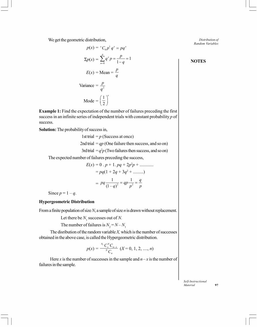
NOTES
Self-InstructionalMaterial 97
Distribution ofRandom Variables
We get the geometric distribution,
p(x) = 10
x x xC p q pq=
p(x) = 0
11
px
n
pq pq=
= =−∑
E(x) = Mean = pq
Variance = 2
pq
Mode = 12
x
Example 1: Find the expectation of the number of failures preceding the firstsuccess in an infinite series of independent trials with constant probability p ofsuccess.Solution: The probability of success in,
1st trial = p (Success at once)2nd trial = qp (One failure then success, and so on)3rd trial = q2p (Two failures then success, and so on)
The expected number of failures preceding the success,E(x) = 0 . p + 1. pq + 2p2p + ............
= pq(1 + 2q + 3q2 + .........)
= 2 2
1 1(1– )
qpq qpq p p
= =
Since p = 1 – q.
Hypergeometric Distribution
From a finite population of size N, a sample of size n is drawn without replacement.Let there be N1 successes out of N.The number of failures is N2 = N – N1
The disribution of the random variable X, which is the number of successesobtained in the above case, is called the Hypergeometric distribution.
p(x) = 1N N
x n xN
n
C CC
− (X = 0, 1, 2, ...., n)
Here x is the number of successes in the sample and n – x is the number offailures in the sample.

Distribution ofRandom Variables
NOTES
Self-Instructional98 Material
It can be shown that,
Mean : E(X) = 1NnN
Variance : Var (X) = 2
1 1–1
N n nN nNN N N
− −
Example 2: There are 20 lottery tickets with three prizes. Find the probabilitythat out of 5 tickets purchased exactly two prizes are won.Solution: We have N1 = 3, N2 = N – N1 = 17, x = 2, n = 5.
p(2) = 3 17
2 320
5
C CC
The probability of getting no prize p(0) = 3 17
0 520
5
C CC
The probability of getting exactly 1 prize p(1) = 3 17
1 420
5
C CC
Example 3: Examine the nature of the distibution of r balls are drawn, one at atime without replacement, from a bag containing m white and n black balls.Solution: It is the hypergeometric distribution. It corresponds to the probabilitythat x balls will be white out of r balls so drawn and is given by,
p(x) = x n
x r xm n
r
C CC
−+
Multinomial
There are k possible outcomes of trials, viz., x1, x2, ..., xk with probabilities p1, p2,..., pk, n independent trials are performed. The multinomial distibution gives theprobability that out of these n trials, x1 occurs n1 times, x2 occurs n2 times, and so
on. This is given by the following equation: 1 21 2
1 2
! ....! !.... !
n n nk
k
n p p pn n n
Where, 1
k
ii
n n=
=∑
Characteristic Features of the Binomial Distribution
The following are the characteristics of Binomial distribution:1. It is a discrete distribution.2. It gives the probability of x successes and n – x failures in a specific order.3. The experiment consists of n repeated trials.

NOTES
Self-InstructionalMaterial 99
Distribution ofRandom Variables
4. Each trial results in a success or a failure.5. The probability of success remains constant from trial to trial.6. The trials are independent.7. The success probability p of any outcome remains constant over time. This
condition is usually not fully satisfied in situations involving management andeconomics, for example, the probability of response from successiveinformants is not the same. However, it may be assumed that the conditionis reasonably well satisfied in many cases and that the outcome of one trialdoes not depend on the outcome of another. This condition too, may not befully satisfied in many cases. An investigator may not approach a secondinformant with the same set-up of mind as used for the first informant.
8. The Binomial distribution depends on two parameters n and p. Each set ofdifferent values of n, p has a different Binomial distribution.
9. If p = 0.5, the distribution is symmetrical. For a symmetrical distribution,in n
Prob (X = 0) = Prob (X = n)i.e., the probabilities of 0 or n successes in n trials will be the same. Similarly,
Prob (X = 1) = Prob(X = n – 1), and so on.If p > 0.5, the distribution is not symmetrical. The probabilities on the rightare larger than those on the left. The reverse case is when p < 0.5.When n becomes large, the distribution becomes bell shaped. Even when nis not very large but p 0.5, it is fairly bell shaped.
10. The Binomial distribution can be approximated by the normal. As n becomeslarge and p is close to 0.5, the approximation becomes better.
Example 4: If the ratio n/N, i.e., sample size to population size is small, the resultgiven by the Binomial may not be reliable. Comment.Solution: When the distribution is Binomial, each successive trial, being independentof other trials, has constant probability of success. If he sampling of n items iswithout replacement from a population of size N, the probability of success of anyevent depends upon what happened in the previous events. In this case the Bionomialcannot be used unless the ratio n/N is small. Even then there is no guarantee ofgetting accurate results.
The Binomial should be used only if the ratio nN is very small, say less that
0.05.Example 5: Explain the concept of a discrete probability distribution.Solution: If a random variable x assumes n discrete values x1, x2, .......,xn, withrespective probabilities p1, p2,..........,pn(p1 + p2 + .......+ pn = 1) then, the

Distribution ofRandom Variables
NOTES
Self-Instructional100 Material
distribution of values xi with probabilities pi (= 1, 2,....,n), is called the discreteprobability distribution of x.
The frequency function or frequency distribution of x is defined by p(x)which for different values x1, x2, .......,xn of x, gives the corresponding probabilities:
p(xi) = pi where, p(x) 0 p(x) = 1Example 6: For the following probability distribution, find p(x > 4) andp(x 4):
0 1 2 3 4 5( ) 0 /2 /2 /4 /4x
p x a a a a a
Solution: The solution is obtained as follows:
Since, p(x) = 1,0 12 2 4 4a a a aa+ + + + + =
52
a = 1 or a = 25
p(x > 4) = p(x = 5) = 9 14 10=
p(x 4) = 0 + a + 9 9
2 2 4 4 10a a a a+ + + =
Example 7: A fair coin is tossed 400 times. Find the mean number of heads andthe corresponding standard deviation.
Solution: This is a case of Binomial distribution with p = q = 12
, n = 400
The mean number of heads is given by = np = 14002
× = 200
And S. D. = 1 1400 102 2
npq = × × =
Example 8: A manager has thought of 4 planning strategies each of which has anequal chance of being successful. What is the probability that at least one of his
strategies will work if he tries them in 4 situations? Here p = 14
, q = 34
.
Solution: The probability that none of the strategies will work is given by,
p(0) = 0 4 4
40
1 3 34 4 4
C =
The probability that at least one will work is given by 43 1751
4 256 − =

NOTES
Self-InstructionalMaterial 101
Distribution ofRandom Variables
Example 9: Suppose the proportion of people preferring a car C is 0.5. Let Xdenote the number of people out of a set of 3 who prefer C. The probabilities of0, 1, 2, 3 of them preferring C are,Solution: The solution is obtained as follows:
p(X = 0) = 3 0 30
1(0.5) (0.5)8
C =
p(X = 1) = 3 1 21
3(0.5) (0.5)8
C =
p(X = 2) = 3 2 12
3(0.5) (0.5)8
C =
p(X = 3) = 3 3 03
1(0.5) (0.5)8
C =
= E(X) = 21 3 3 3 10 1 2 2 3 1.58 8 8 8 8i ix pΣ = × + × + + × + × =
2 = 2( – μ)E X = 2 2 2 2( ) – μ – μi iE X x p= Σ
= 2 2 2 2 21 3 3 10 1 2 3 –1.58 8 8 8
× + × + × + ×
= 0.75Example 10: For the Poisson distribution, write the probabilities of 0, 1, 2, ....successes.Solution: The solution is obtained as follows:
–
– 0
–
( )!
0 (0) / 0!
1 (1) (0).1!
xm
m
m
mx p x ex
p e mmp e p m
=
=
= =
2–
3–
2 (2) (1).2! 2
3 (3) (2).3! 3
m
m
m me p p
m me p p
= =
= =
, and so on.Total of all probabilities p(x) = 1

Distribution ofRandom Variables
NOTES
Self-Instructional102 Material
Example 11 What are the raw moments of Poisson distribution?Solution: First raw moment 1 = m
Second raw moment 2 = m2 + mThird raw moment 3 = m3 + 3m2 + m
Example 12: For a Poisson distribution p(0) = p(1), find p(x > 0).Solution: We have e–m m0/0! = e–m m0/1! so that m = 1
p(0) = e–1 = 1/2.718 = 0.37 p(x > 0) = 1 – p(0) = 0.63
Example 13: It is claimed that the TV branded M is demanded by 70% ofcustomers. If X is the number of TVs demanded, find the probability distributionof X when there are four customers.Solution: If all the four demand M then p(4) = 0.74 = 0.2401. The probabilitydistribution is:
X 4 3 2 1 0p 0.2401 0.4116 0.2646 0.0756 0.0081
These values may be plotted.Note: Poisson Approximation to the Binomial is given by when the number of trials n is largeand the probability p of a success is small, the Binomial distribution can be approximated bythe Poisson. This approximation is useful is practice.
If p = 0.002, n = 1000, m = np = 2The probability of 2 successes in 1000 trials is,
p(X = 2) = – 100 2 9982 (0.002) (0.998)n x n x
xC p q C=
Similarly, p(X = 3) = 100 3 9973 (0.002) (0.998)C , etc.
These terms are difficult to calculate. If we employ the Poisson, we have amuch easier task before us.
m = np = 100 × 0.002 = 2
p(X = 2) = – –2 22 0.1353 20.2706
! 2!
m xe m ex
= = ×
p(X = 3) = – –2 32 0.1804
! 3!
m xe m ex
= =
Example 14: One in every 100 items made on a machine is defective. Out of 25items picked, find the probability of 1 item being defective.Solution: p = 0.01, q = 0.99, n = 25, np = 0.25
Binomial : p(1) = 25 1 241(0.1) (0.99) 0.1964C =
Poisson : p(1) = –25 1(0.25) 0.1947
1!e
=

NOTES
Self-InstructionalMaterial 103
Distribution ofRandom Variables
Exponential Distribution
In probability theory and statistics, the exponential distributions, also known asnegative exponential distributions, are a set of continuous probability distributions.They describe the times between events in a Poisson process, i.e., a process inwhich events occur continuously and independently at a constant average rate.
Probability Density Function
The Probability Density Function (PDF) of an exponential distribution is definedas,
– 0,,;
0.0,
x xef x
x
Here λ > 0 is the parameter of the distribution and is frequently termed as the rateparameter, . The distribution is based on the interval (0, •). When a randomvariable X has exponential distribution, then it is written as X ~ Exp(λ).
Cumulative Distribution Function
The cumulative distribution function is defined as,– 0,1– ,
;0.0,
x xeF x
x
Alternative Parameterization
The Probability Density Function (PDF) of an exponential distribution can also bedefined using alternative parameterization as,
/–1 , 0,;
0.0,
x xef x
x
Here β > 0 is a scale parameter of the distribution. It is the reciprocal of the rateparameter, λ. In this specific notation, β is considered as a survival parameter ifa random variable X which is the duration of time that manages system to surviveand X ~ Exponential(β) then E[X] = β. Thus, the expected duration of survival ofthe system is β units of time. The parameterization involves the ‘rate parameter’that arises in the context of events arriving at a rate λ, when the time betweenevents has a mean of β = λ–1.
Occurrence and Uses
The exponential distribution occurs automatically while the lengths of the inter-arrival times are described in a homogeneous Poisson process. It can be analysed

Distribution ofRandom Variables
NOTES
Self-Instructional104 Material
as a continuous counterpart of the geometric distribution for describing the numberof Bernoulli trials necessary for a discrete process to change state. Thus, theexponential distribution describes the time for a continuous process to changestate.
Exponential variables can be used to model situations where specific eventsoccur with a constant probability per unit length. In queuing theory, the servicetimes of agents in a system are frequently modeled as exponentially distributedvariables, for example the time taken by a bank teller to serve a customer. Thelength of a process can be considered as a sequence of several independent eventsand is modeled using a variable following the Erlang distribution, which is thedistribution of the sum of several independent exponentially distributed variables.
The exponential distribution is also used in reliability theory and reliabilityengineering. Because this distribution has the memoryless property, hence it isquite compatible to model the constant hazard rate portion of the bathtub curve inreliability theory. In physics, when a gas is observed at a fixed temperature andpressure in a uniform gravitational field, then the altitudes of the various moleculesalso adhere to an approximate exponential distribution.
Properties of Exponential Distribution
Mean: The mean or expected value of an exponentially distributed random variableX with rate parameter is given as,
1[ ] .E X =λ
Variance: The variance of X is given as,
2
1Var[ ] .X =λ
Median: The median of X is given as,
n 2[ ] [ ],lm X E X= <λ
Here, ln refers to the natural logarithm. Hence, the absolute difference betweenthe mean and median is given as shown below in accordance with the median-mean inequality.
1 – n 2 1| [ ] [ ] | Standard deviationlE X m X− = < =λ λ
Memorylessness: It is an important property of the exponential distribution.This explains that when a random variable T is exponentially distributed, then itsconditional probability follows the following notation:
Pr[ | ] Pr[ ] for all , 0.T s t T s T t s t> + > = > ≥
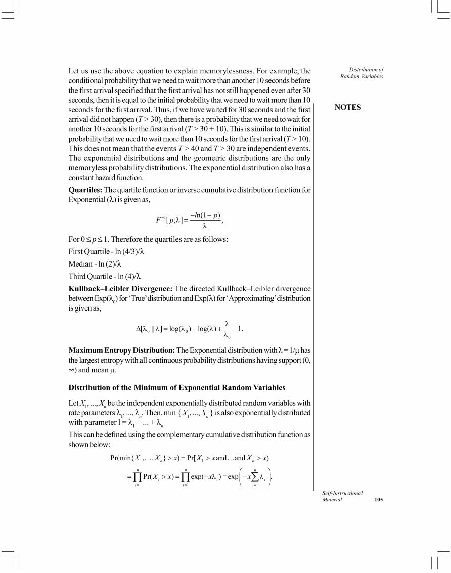
NOTES
Self-InstructionalMaterial 105
Distribution ofRandom Variables
Let us use the above equation to explain memorylessness. For example, theconditional probability that we need to wait more than another 10 seconds beforethe first arrival specified that the first arrival has not still happened even after 30seconds, then it is equal to the initial probability that we need to wait more than 10seconds for the first arrival. Thus, if we have waited for 30 seconds and the firstarrival did not happen (T > 30), then there is a probability that we need to wait foranother 10 seconds for the first arrival (T > 30 + 10). This is similar to the initialprobability that we need to wait more than 10 seconds for the first arrival (T > 10).This does not mean that the events T > 40 and T > 30 are independent events.The exponential distributions and the geometric distributions are the onlymemoryless probability distributions. The exponential distribution also has aconstant hazard function.Quartiles: The quartile function or inverse cumulative distribution function forExponential ( ) is given as,
1 – n(1 – )[ ; ] ,l pF p− λ =λ
For 0 p 1. Therefore the quartiles are as follows:First Quartile - ln (4/3)/Median - ln (2)/Third Quartile - ln (4)/Kullback–Leibler Divergence: The directed Kullback–Leibler divergencebetween Exp( 0) for ‘True’ distribution and Exp( ) for ‘Approximating’ distributionis given as,
0 00
[ || ] log( ) log( ) 1.λ∆ λ λ = λ − λ + −
λ
Maximum Entropy Distribution: The Exponential distribution with λ = 1/μ hasthe largest entropy with all continuous probability distributions having support (0,
) and mean μ.
Distribution of the Minimum of Exponential Random Variables
Let X1, ..., Xn be the independent exponentially distributed random variables withrate parameters 1, ..., n. Then, min X1, ..., Xn is also exponentially distributedwith parameter l = 1 + ... + n
This can be defined using the complementary cumulative distribution function asshown below:
1 1Pr(min , , ) Pr[ and and )n nX X x X x X x> = > >
11 1
Pr( ) exp( ) = exp .n n n
i i iii i
X x x x== =
= > = − λ − λ ∑∏ ∏

Distribution ofRandom Variables
NOTES
Self-Instructional106 Material
The index of the variable which achieves the minimum is distributed according tothe law,
1Pr( min , , ) .kk n
i n
X X X λ= =
λ + + λ
Remember that min X1, ..., Xn is not exponentially distributed.
Check Your Progress
1. What are the Bernoulli trials?2. Define the term hypergeometric distribution.3. Give some characteristics features of the binomial distribution.4. What is exponential distribution?
4.3 DISTRIBUTION OF TWO RANDOMVARIABLE
Mean of Random Variable or The Expected Value ofRandom Variable
Mean of random variable is the sum of the values of the random variable weightedby the probability that the random variable will take on the value. In other words,it is the sum of the product of the different values of the random variable and theirrespective probabilities. Symbolically, we write the mean of a random variable,say X, as X . The Expected value of the random variable is the average valuethat would occur if we have to average an infinite number of outcomes of therandom variable. In other words, it is the average value of the random variable inthe long run. The expected value of a random variable is calculated by weightingeach value of a random variable by its probability and summing over all values.The symbol for the expected value of a random variable is E (X). Mathematically,we can write the mean and the expected value of a random variable, X, as follows:
1. .
n
i ii
X X pr X
And,
1. .
n
i ii
E X X pr X
Thus, the mean and expected value of a random variable are conceptuallyand numerically the same but usually denoted by different symbols and as suchthe two symbols, viz., X
_ and E (X) are completely interchangeable. We can,
therefore, express the two as follows:

NOTES
Self-InstructionalMaterial 107
Distribution ofRandom Variables
1. .
n
i ii
E X X pr X X
Where Xi is the ith value X can take.
Sum of Random Variables
If we are given the means or the expected values of different random variables,say X, Y, and Z to obtain the mean of the random variable (X + Y + Z), then it canbe obtained as under:
E X Y Z E X E Y E Z X Y Z
Similarly, the expectation of a constant time a random variable is theconstant time the expectation of the random variable. Symbolically, we canwrite this as under:
E cX cE X c X
Where cX is the constant time random variable.
4.4 CONDITIONAL DISTRIBUTION ANDEXPECTATION
Expectation (Conditional)
The expectation of a random variable X with probability density function (PDF) p(x) is theoretically defined as:
E X xp x dx[ ] ( )= zIf we consider two random variables X and Y (not necessarily independent), thentheir combined behaviour is described by their joint probability density functionp(x, y) and is defined as:
p x X x dx y Y y dy p x y dx dy , ( , ). .≤ < + ≤ < + =
The marginal probability density of X is defined as,
p x p x y dyX ( ) ( , )= z
For any fixed value y of Y, the distribution of X is the conditional distribution of X,where Y = y , and it is denoted by p(x , y).
Expectation (Iterated)
The expectation of the random variable is expressed as:
E[X] = E[E[X | Y]]

Distribution ofRandom Variables
NOTES
Self-Instructional108 Material
This expression is known as the ‘Theorem of Iterated Expectation’ or‘Theorem of Double Expectation’. Symbolically, it can be expressed as:(i) For the discrete case:
E[X] = y E[X | Y = y].PY = y
(ii) For the continuous case:
E X E X Y y f y dy[ ] [ | ]. ( ).= =−∞+∞z
Expectation: Continuous Variables
If x is a continuous random variable we define that,
E(x) = –
( )x P x dx u∞
∞
=∫
The expectation of a function h(x) is,
Eh(x) = –
( ) ( )h x P x dx∞
∞∫
The rth moment about the mean is,
E(x – )r = –
( –μ) ( )rx P x dx∞
∞∫
Example 15: A newspaper earns Rs. 100 a day if there is suspense in the news.He loses Rs. 10 a day if it is an eventless newspaper. What is the expectation ofhis earnings if the probability of suspense news is 0.4?Solution: E(x) = p1x1 + p2x2
= 0.4 × 100 – 0.6 × 10= 40 – 6 = 34
Example 16: A player tossing three coins, earns Rs. 10 for 3 heads, Rs. 6 for 2heads and Re. 1 for 1 head. He loses Rs. 25, if 3 tails appear. Find his expectation.
Solution: p(HHH) = 11 1 1 1.. say2 2 2 8
p= = 3 heads
p(HHT) = 32 2
1 1 1 3... say2 2 2 8
C p= = 2 heads, 1 tail
p(HTT) = 31 3
1 1 1 3... say2 2 2 8
C p= = 1 head, 2 tails

NOTES
Self-InstructionalMaterial 109
Distribution ofRandom Variablesp(TTT) = 4
1 1 1 3.. say2 2 2 8
p= = 3 tails
E(x) = p1x1 + p2x2 + p3x3 – p4x4
= 1 3 3 110 6 2 – 258 8 8 8× + × + × ×
= 9 Rs 1.1258=
Example 17: A and B roll a die. Whoever gets a 6, first wins Rs. 550. Find theirindividual expectations if A makes a start. What will be the answer if B makes astart?
Solution: A may not get 6 in 1st trial, p1 = 16
A may not get in 1st, B may not get in 2nd and A may get in 3rd,
p3 = 25 5 1 5 1
6 6 6 6 6 × × =
and so on.
A’s winning chance = 25 5 1 5 1
6 6 6 6 6 × × =
+...........
Where p(x) is the density function x,
= 2
1 1 66 1151–
6
=
25Geometric progression with common ratio6
B’s winning chance = 6 51–
11 11=
A wins Rs. 550 with probability p = 6
11
A gets nothing if he loses with probability q = 5
11

Distribution ofRandom Variables
NOTES
Self-Instructional110 Material
Expectation of A = p . x + q . 0
= 6 5550 0 300
11 11× + × =
Similarly B wins with p = 5
11
B gets nothing if he loses with q = 6
11
Expectation of B = 5 6550 0 200
11 11× + × =
If B starts first his expectation would be 300 and A’s would be 250.Example 18: Calculate the standard deviation (S.D.) when x takes the values 0,1, 2 and 9 with probability, 0.4, 0 – 0.1.Solution: x takes the values 0, 1, 2, 9 with probability 0.4, 0.2, 0.3, 0.1.
= E(x) = (xi pi) = 0 × 0.4 + 12 × 0.2 + 3 × 0.3 + 9 × 0.1 = 2.0E(x2) = xi
2pi = 02 × 0.4 + 12 × 0.2 + 3 × 0.3 + 92 × 0.1 = 11.0V(x) = E(x2) – 2 = 11 – 2 = 9
S.D.(x) = 9 3=
Example 19: The purchase of some shares can give a profit of Rs. 400 withprobability 1/100 and Rs. 300 with probability 1/20. Comment on a fair price ofthe share.
Solution: Expected value E(x) = xi pi = 1 1400 300 19100 20
× + × =
Example 20: Find the variance and standard deviation (S.D.) of the followingprobability distribution:
1
1
1 2 3 40.1 0.3 0.2 0.4
xp
Solution: E(x)= pixi = 0.1 × 1 + 0.3 × 2 + 0.2 × 3 + 0.4 × 4 = 2.9
Variance (x) = V(x) = E(x2) – 2x=
2 2 2 2 2 2 2– 0.1 1 0.3 2 0.2 3 0.4 4 – 2.9i ip x xΣ = × + × + × + ×
= 0.1 + 1.2 + 1.8 + 6.4 – 8.41 = 1.0.9
S.D.(x) = ( ) 1.091.044V x =

NOTES
Self-InstructionalMaterial 111
Distribution ofRandom Variables
Example 21: Prove that the variance of a constant is zero.Solution: If k is a constant, it has no variability.
V(k) = 0If the constant k is attached to a variable x then,
V(kx) = k2V(x)V(2x) = 4V(x)
V(2 + 3x) = V(3x) = 9 V(x)Example 22: A box contains 2n tickets of which nCi tickets bear the number i(i =1, 2, 3, ...., n). If a set of m tickets is drawn, find the expected value of the sum oftheir numbers.Solution: To find E(A), where A = x1 + x2 + ...+ xm. Here xi can take values 0, 1,2,...., n with probabilities,
0 1, ,....2 2 2
n nnn
n n n
C CC
E(xi) = 0 1 2.0 .1 .2 .... . 2 2 2 2
n nn nn
i i n n n n
C CC Cp x nΣ = + + + +
= 1 21 [ 2 .... ]2
n n nnn C C n C+ + +
= –1 –1 –11 2 –1[1 .... ]
2n n n
nnn C C C+ + + + (By taking n common)
= –1(1 1)2 2
nn
n n+ = [Expand (1 + 1)n – 1 and check]
E(A) = 1
( )2
m
ii
mnE x=
=∑
Check Your Progress
5. Explain the mean of random variable.6. What is conditional expectation?
4.5 ANSWERS TO CHECK YOUR PROGRESSQUESTIONS
1. In a Bernoulli experiment, an Event E either happens or does not happen(E ). Examples are, getting a head on tossing a coin, getting a six on rollinga die, and so on.

Distribution ofRandom Variables
NOTES
Self-Instructional112 Material
2. The disribution of the random variable X, which is the number of successesobtained in the above case, is called the Hypergeometric distribution.
p(x) = 1N N
x n xN
n
C CC
− (X = 0, 1, 2, ...., n)
3. The following are the characteristics of Binomial distribution:(a) It is a discrete distribution.(b) It gives the probability of x successes and n – x failures in a specific
order.(c) The experiment consists of n repeated trials.(d) Each trial results in a success or a failure.
4. In probability theory and statistics, the exponential distributions, also knownas negative exponential distributions, are a set of continuous probabilitydistributions.
5. Mean of random variable is the sum of the values of the random variableweighted by the probability that the random variable will take on the value.
6. The expectation of a random variable X with probability density function(PDF) p(x) is theoretically defined as:
E X xp x dx[ ] ( )= zIf we consider two random variables X and Y (not necessarily independent),then their combined behaviour is described by their joint probability densityfunction p(x, y) and is defined as:
p x X x dx y Y y dy p x y dx dy , ( , ). .≤ < + ≤ < + =
The marginal probability density of X is defined as,
p x p x y dyX ( ) ( , )= z
For any fixed value y of Y, the distribution of X is the conditional distributionof X, where Y = y , and it is denoted by p(x , y).
4.6 SUMMARY
Each possible value of the random variable x has the same probability in theuniform distribution. If x takes vaues x1, x2....,xk, then,
p(xi, k) = 1k
The multinomial distibution gives the probability that out of these n trials, x1occurs n1 times, x2 occurs n2 times, and so on. This is given by the following
equation: 1 21 2
1 2
! ....! !.... !
n n nk
k
n p p pn n n

NOTES
Self-InstructionalMaterial 113
Distribution ofRandom Variables
The Binomial distribution depends on two parameters n and p. Each set ofdifferent values of n, p has a different Binomial distribution.The Binomial distribution can be approximated by the normal. As n becomeslarge and p is close to 0.5, the approximation becomes better.The Probability Density Function (PDF) of an exponential distribution canalso be defined using alternative parameterization as,
/–1 , 0,;
0.0,
x xef x
x
The Expected value of the random variable is the average value that wouldoccur if we have to average an infinite number of outcomes of the randomvariable.
4.7 KEY WORDS
Cumulative distribution function: The cumulative distribution function isdefined as,
– 0,1– ,;
0.0,
x xeF x
x
Quartiles: The quartile function or inverse cumulative distribution functionfor Exponential ( ) is given as,
1 – n(1 – )[ ; ] ,l pF p− λ =λ
Maximum entropy distribution: The Exponential distribution with λ = 1/μ has the largest entropy with all continuous probability distributions havingsupport (0, ) and mean μ.
4.8 SELF-ASSESSMENT QUESTIONS ANDEXERCISES
Short-Answer Questions
1. Explain about the uniform or rectangular distribution.2. What is geometric distribution?3. What is meant by multinomial?4. Explain the sum of random variables.5. What is iterated expectation?

Distribution ofRandom Variables
NOTES
Self-Instructional114 Material
Long-Answer Questions
1. Briefly describe the probability density function.2. Discuss the properties of exponential distribution.3. Describe the expected value of random variables.4. Explain the continuous variables expectation.
4.9 FURTHER READINGS
Hogg, Robert. V., Allen T. Craig and Joseph W. McKean. 2005. Introduction toMathematical Statistics. New Delhi: Pearson Education.
Fisz, Marek. 1963. Probability Theory and Mathematical Statistics, 3rd Edition.New York: John Wiley & Sons, Inc.
Rohatgi, Vijay K. 1985. An Introduction to Probability Theory andMathematical Statistics. New Delhi: Wiley Eastern Limited.
Gupta, C.B. and Vijay Gupta. 2004. An Introduction to Statistical Methods,23rd Edition. New Delhi: Vikas Publishing House.
Levin, Richard I. and David S. Rubin. 1998. Statistics for Management. NewJersey: Prentice Hall.
Chandan, J. S. 1998. Statistics for Business and Economics. New Delhi: VikasPublishing House Pvt. Ltd.
Campbell, Stephen K. 1987. Applied Statistics. New York: Harper & Row.Chance, William A. 1969. Statistical Methods for Decision Making. Illinois:
Richard D Irwin.Hooda, R. P. 2013. Statistics for Business and Economics, 5th Edition. New
Delhi: Vikas Publishing House Pvt. Ltd.

NOTES
Self-InstructionalMaterial 115
CorrelationBLOCK - II
CORRELATION COEFFICIENT, SPECIALDISTRIBUTIONS AND DISTRIBUTIONFUNCTION OF RANDOM VARIABLES
UNIT 5 CORRELATION
Structure5.0 Introduction5.1 Objectives5.2 Correlation5.3 Types of Correlation5.4 Properties of Correlation Coefficient5.5 Methods of Studying Correlation
5.5.1 Scatter Diagram5.5.2 Karl Pearson’s Coefficient5.5.3 Rank Coefficient
5.6 Coefficient of Determination5.7 Answers to Check Your Progress Questions5.8 Summary5.9 Key Words
5.10 Self-Assessment Questions and Exercises5.11 Further Readings
5.0 INTRODUCTION
Correlation analysis looks at the indirect relationships in sample survey data andestablishes the variables which are most closely associated with a given action ormind-set. It is the process of finding how accurately the line fits using theobservations. Correlation analysis can be referred as the statistical tool used todescribe the degree to which one variable is related to another. The relationship, ifany, is usually assumed to be a linear one. In fact, the word correlation refers tothe relationship or interdependence between two variables. There are variousphenomena which have relation to each other. The theory by means of whichquantitative connections between two sets of phenomena are determined is calledthe ‘Theory of Correlation’. On the basis of the theory of correlation you canstudy the comparative changes occurring in two related phenomena and their cause-effect relation can also be examined. Thus, correlation is concerned with relationshipbetween two related and quantifiable variables and can be positive or negative.
In this unit you will study about the correlation, types of correlation andproperties of correlation coefficient, methods of studying correlation, scatter diagram,Karl Pearson’s coefficient, rank coefficient and coefficient of determination.
Correlation
NOTES
Self-Instructional116 Material
5.1 OBJECTIVES
After going through this unit, you will be able to:Define correlationExplain the different types of correlationUnderstand the function of correlation coefficientUnderstand the different methods of studying correlation
5.2 CORRELATION
Correlation analysis is the statistical tool generally used to describe the degree towhich one variable is related to another. The relationship, if any, is usually assumedto be a linear one. This analysis is used quite frequently in conjunction with regressionanalysis to measure how well the regression line explains the variations of thedependent variable. In fact, the word correlation refers to the relationship orinterdependence between two variables. There are various phenomena which haverelation to each other. For instance, when demand of a certain commodityincreases, then its price goes up and when its demand decreases then its pricecomes down. Similarly, with age the height of the children increases; with heightthe weight of the children increases, with money supply the general level of pricesgo up. Such sort of relationship can as well be noticed for several other phenomena.The theory by means of which quantitative connections between two sets ofphenomena are determined is called the Theory of Correlation.
On the basis of the theory of correlation one can study the comparativechanges occurring in two related phenomena and their cause-effect relation canbe examined. It should, however, be borne in mind that relationship like ‘black catcauses bad luck’, ‘filled-up pitchers result in good fortune’ and similar other beliefsof the people cannot be explained by the theory of correlation since they are allimaginary and are incapable of being justified mathematically. Thus, correlation isconcerned with the relationship between two related and quantifiable variables. Iftwo quantities vary in sympathy so that a movement (an increase or decrease) inthe one tends to be accompanied by a movement in the same or opposite directionin the other and the greater the change in the one, the greater is the change in theother, the quantities are said to be correlated. This type of relationship is known ascorrelation or what is sometimes called, in statistics, co-variation.
For correlation it is essential that the two phenomena, should have cause-effect relationship. If such relationship does not exist then one should not talk ofcorrelation. For example, if the height of the students as well as the height of thetrees increases, then one should not call it a case of correlation because the twophenomena, viz., the height of students and the height of trees are not causallyrelated. But the relationship between the price of a commodity and its demand,the price of a commodity and its supply, the rate of interest and savings, etc., are

NOTES
Self-InstructionalMaterial 117
Correlationexamples of correlation since in all such cases the change in one phenomenon isexplained by a change in the other phenomenon.
Check Your Progress
1. What are the different types of correlations?2. Explain the meaning of correlation analysis.3. What is the scatter diagram method?4. What is the least-squares method?
5.3 TYPES OF CORRELATION
It is appropriate here to mention that correlation in case of phenomena pertainingto natural sciences can be reduced to absolute mathematical terms, for example,heat always increases with light. But in phenomena pertaining to social sciences, itis often difficult to establish any absolute relationship between two phenomena.Hence, in social sciences we must take the fact of correlation being established ifin a large number of cases, two variables always tend to move in the same or theopposite direction.
Correlation can either be positive or it can be negative. Whethercorrelation is positive or negative would depend upon the direction in which thevariables are moving. If both variables are changing in the same direction, thencorrelation is said to be positive but when the variations in the two variables takeplace in opposite direction, the correlation is termed as negative. This can beexplained as follows:
Changes in Independent Changes in Dependent Nature ofVariable Variable Correlation
Increase (+) Increase (+) Positive (+)Decrease (–) Decrease (–) Positive (+)Increase (+) Decrease (–) Negative (–)Decrease (–) Increase (+) Negative (–)
Correlation can either be linear or it can be non-linear. Non-linearcorrelation is also known as curvilinear correlation. The distinction is based uponthe constancy of the ratio of change between the variables. When the amount ofchange in one variable tends to bear a constant ratio to the amount of change in theother variable then the correlation is said to be linear. In such a case, if the valuesof the variables are plotted on a graph paper, then a straight line is obtained. Thisis why the correlation is known as linear correlation. But when the amount ofchange in one variable does not bear a constant ratio to the amount of change inthe other variable, i.e., the ratio happens to be variable instead of constant, thenthe correlation is said to be non-linear or curvilinear. In such a situation we shallobtain a curve if the values of the variables are plotted on a graph paper.

Correlation
NOTES
Self-Instructional118 Material
Correlation can either be simple correlation or it can be partialcorrelation or it can be multiple correlation. The study of correlation for twovariables (of which one is independent and the other is dependent) involvesapplication of simple correlation. When more than two variables are involved in astudy relating to correlation then it can either be as of multiple correlation or ofpartial correlation. Multiple correlation studies the relationship between a dependentvariable and two or more independent variables. In partial correlation, we measurethe correlation between a dependent variable and one particular independent variableassuming that all other independent variables remain constant.
Statisticians have developed two measures for describing the correlationbetween two variables viz., the coefficient of determination and the coefficient ofcorrelation.
5.4 PROPERTIES OF CORRELATIONCOEFFICIENT
The coefficient of correlation symbolically denoted by ‘r’ is an important measure todescribe how well one variable is explained by another. It measures the degree ofrelationship between the two causally-related variables. The value of this coefficientcan never be more than + 1 or less than –1. Thus, + 1 and –1 are the limits of thiscoefficient. For a unit change in independent variable, if there happens to be a constantchange in the dependent variable in the same direction then the value of the coefficientwill be + 1 indicative of the perfect positive correlation; but if such a change occursin the opposite direction, the value of the coefficient will be –1, indicating perfectnegative correlation. In practical life the possibility of obtaining either a perfect positiveor perfect negative correlation is very remote, particularly in respect of phenomenaconcerning social sciences. If the coefficient of correlation has a zero value then itmeans that there exists no correlation between the variables under study.
There are several methods of finding the coefficient of correlation but thefollowing ones are considered important:1
(i) Coefficient of correlation by the method of least squares(ii) Coefficient of correlation through product moment method or Karl
Pearson’s coefficient of correlation(iii) Coefficient of correlation using simple regression coefficients
Whichever of these three methods, we adopt we get the same value of r.Now, we explain in brief each one of these three methods of finding ‘r’.
5.5 METHODS OF STUDYING CORRELATION
5.5.1 Scatter Diagram
Least squares method of fitting a line (the line of best fit or the regression line)through the scatter diagram is a method which minimizes the sum of the squared

NOTES
Self-InstructionalMaterial 119
Correlationvertical deviations from the fitted line. In other words, the line to be fitted will passthrough the points of the scatter diagram in such a fashion that the sum of thesquares of the vertical deviations of these points from the line will be a minimum.
Fig 5.1 Scatter Diagram
The meaning of the least squares criterion can be better understood moreeasily through reference to the following Figure 5.2 where the Scatter diagram hasbeen reproduced along with a line which represents the least squares fit to thedata.
Fig 5.2 Scatter Diagram, Regression Line and Short Vertical Lines Representing ‘e’
In Figure 5.2, the vertical deviations of the individual points from the line areshown as the short vertical lines joining the points to the least squares line. Thesedeviations are denoted by the symbol ‘e’. The value ‘e’ varies from one point toanother. In some cases it is positive, in others it is negative. If the line drawnhappens to be the least squares line then the values of o
ie∑ is the least possible. Itis because of this feature the method is known as Least Squares Method.
Why we insist on minimizing the sum of squared deviations is a question thatneeds explanation. If we denote the deviations from the actual value Y to the

Correlation
NOTES
Self-Instructional120 Material
estimated value as ˆ( – )Y Y or ei, it is logical that we want the 1
ˆ( – ) or ,n
iY Y e to
be as small as possible. However, mere examining 1
ˆ( – ) or ,n
iY Y e is inappropriate
since any ei can be positive or negative and large positive values and large negativevalues would cancel one another.
But large values of ei regardless of their sign, indicate a poor prediction. Even
if we ignore the signs while working out 1
| |n
ii
e=∑ , the difficulties may continue to be
there. Hence, the standard procedure is to eliminate the effect of signs by squaringeach observation. Squaring each term accomplishes two purposes viz., (i) It magnifies(or penalizes) the larger errors, and (ii) It cancels the effect of the positive andnegative values (since a negative error squared becomes positive). The choice ofminimizing the squared sum of errors rather than the sum of the absolute valuesimplies that we would make many small errors rather than a few large errors. Hence,in obtaining the regression line we follow the approach that the sum of the squareddeviations be minimum and on this basis work out the values of its constants viz., ‘a’and ‘b’ or what is known as the intercept and the slope of the line. This is done withthe help of the following two normal equations:3
Y = na + b XXY = a X + b X2
In these two equations, ‘a’ and ‘b’ are unknowns and all other values viz.,X, Y, X2, XY are the sum of the products and the cross products to be
calculated from the sample data and ‘n’ means the number of observations in thesample. Hence, one can solve these two equations for finding the unknown values.Once these values are found, the regression line is said to have been defined forthe given problem. Statisticians have also derived a short cut method throughwhich these two equations can be rewritten so that the values of ‘a’ and ‘b’ can bedirectly obtained as follows:
( )22
.n XY X Ybn X X∑ −∑ ∑
=∑ − ∑
Y Xa bn n
5.5.2 Karl Pearson’s Coefficient
Karl Pearson’s method is the most widely used method for measuring therelationship between two variables. This coefficient is based on the followingassumptions:

NOTES
Self-InstructionalMaterial 121
Correlation(i) There is a linear relationship between the two variables which means that astraight line would be obtained if the observed data is plotted on a graph.
(ii) The two variables are causally related which means that one of the variablesis independent and the other one is dependent.
(iii) A large number of independent causes operates in both the variables so asto produce a normal distribution.According to Karl Pearson, ‘r’ can be worked out as follows:
r =x y
xyn
Here, x = (x – x)y = (y – y)
x = Standard deviation of
X series and is equal to 2x
n∑
y = Standard deviation of
Y series and is equal to2y
n∑
n = Number of pairs of X and Y observed
A short cut formula known as the Product Moment Formula can be derivedfrom the earlier formula:
r =x y
xyn
=2 2
xy
x yn n
=2 2
n xy
x y
These formulae are based on obtaining the true means (viz., and x y ) firstand then performing all other calculations.
5.5.3 Rank CoefficientIf observations on two variables are given in the form of ranks and not as numericalvalues, it is possible to compute what is known as rank correlation between thetwo series.
The rank correlation, written , is a descriptive index of agreement betweenranks over individuals. It is the same as the ordinary coefficient of correlationcomputed on ranks, but its formula is simpler.

Correlation
NOTES
Self-Instructional122 Material
2
2
6ρ 1( 1)
iDn n
Here, n is the number of observations and Di the positive difference betweenranks associated with the individuals i.
Like r, the rank correlation lies between –1 and +1.Example 1: The ranks given by two judges to 10 individuals are as follows:
Rank given byIndividual Judge I Judge II D D2
x y = x – y1 1 7 6 362 2 5 3 93 7 8 1 14 9 10 1 15 8 9 1 16 6 4 2 47 4 1 3 98 3 6 3 99 10 3 7 4910 5 2 3 9
D2 = 128Solution: The rank correlation is given by,
2
3 3
6 6 1281 1 1 0.776 0.22410 10
Dn n
The value of = 0.224 shows that the agreement between the judges is nothigh.Example 2: In the previous case, compute r and compare.Solution: The simple coefficient of correlation r for the previous data is calculatedas follows:
x y x2 y2 xy1 7 1 49 72 5 4 25 107 8 49 64 569 10 81 100 908 9 64 81 726 4 36 16 244 1 16 1 43 6 9 36 18
10 3 100 9 305 2 25 4 10
x = 55 y = 55 x2 = 385 y2 = 385 xy = 321

NOTES
Self-InstructionalMaterial 123
Correlation
r =
55 55321 1010 10
2 255 55385 10 385 1010 10
− × ×
− × − ×
= 18.5
82.5 82.5× =
18.582.5
= 0.224This shows that the Spearman for any two sets of ranks is the same as
the Pearson r for the set of ranks. But it is much easier to compute .Often, the ranks are not given. Instead, the numerical values of observations
are given. In such a case, we must attach the ranks to these values to calculate.
Example 3:Marks in Marks in Rank in Rank in
Maths Stats Maths Stats D D2
45 60 4 2 2 447 61 3 1 2 460 58 1 3 2 438 48 5 4 1 150 46 2 5 3 9
D2 = 222
3
6 6 221 1 0.1125 5
Dn n
Solution: This shows a negative, though small, correlation between the ranks.If two or more observations have the same value, their ranks are equal and
obtained by calculating the means of the various ranks.If in this data, marks in maths, are 45 for each of the first two students, the
rank of each would be 3 42+ = 3.5. Similarly, if the marks of each of the last
two students in statistics are 48, their ranks would be 4 52+ = 4.5
The problem takes the following shape:Rank
Marks in Marks in x y DD2 Maths Stats
45 60 3.5 2 1.5 2.2545 61 3.5 1 2.5 6.2560 58 1 3 2 4.0038 48 5 4.5 1.5 2.2550 48 2 4.5 2.5 6.25

Correlation
NOTES
Self-Instructional124 Material
2
36 6 211 1 0.05
120D
n nAn elaborate formula which can be used in case of equal ranks is
2 336 11
12D m m
n n .
Here, 3112
m mΣ( − ) is to be added to D2 for each group of equal ranks, m
being the number of equal ranks each time.For the given data, we haveFor series x, the number of equal ranks m = 2.For series y, also, m = 2; so that,
= 3 33
6 1 11 21 (2 2) (2 2)12 125 5
= 6 6 61 21
120 12 12
= 6 221120×
− = –0.1
Example 4: Show by means of diagrams various cases of scatter expressingcorrelation between x, y.Solution:
(a) Y
XO Negative slopeInverse linear relationship
High scatter low, negativer
(b) Y
XO Positive slopeDirect linear relationship
High scatter low, positiver
(c) Y
XO Slope = 0= 0r
(d) Y
XO No relationship – ~ 0r
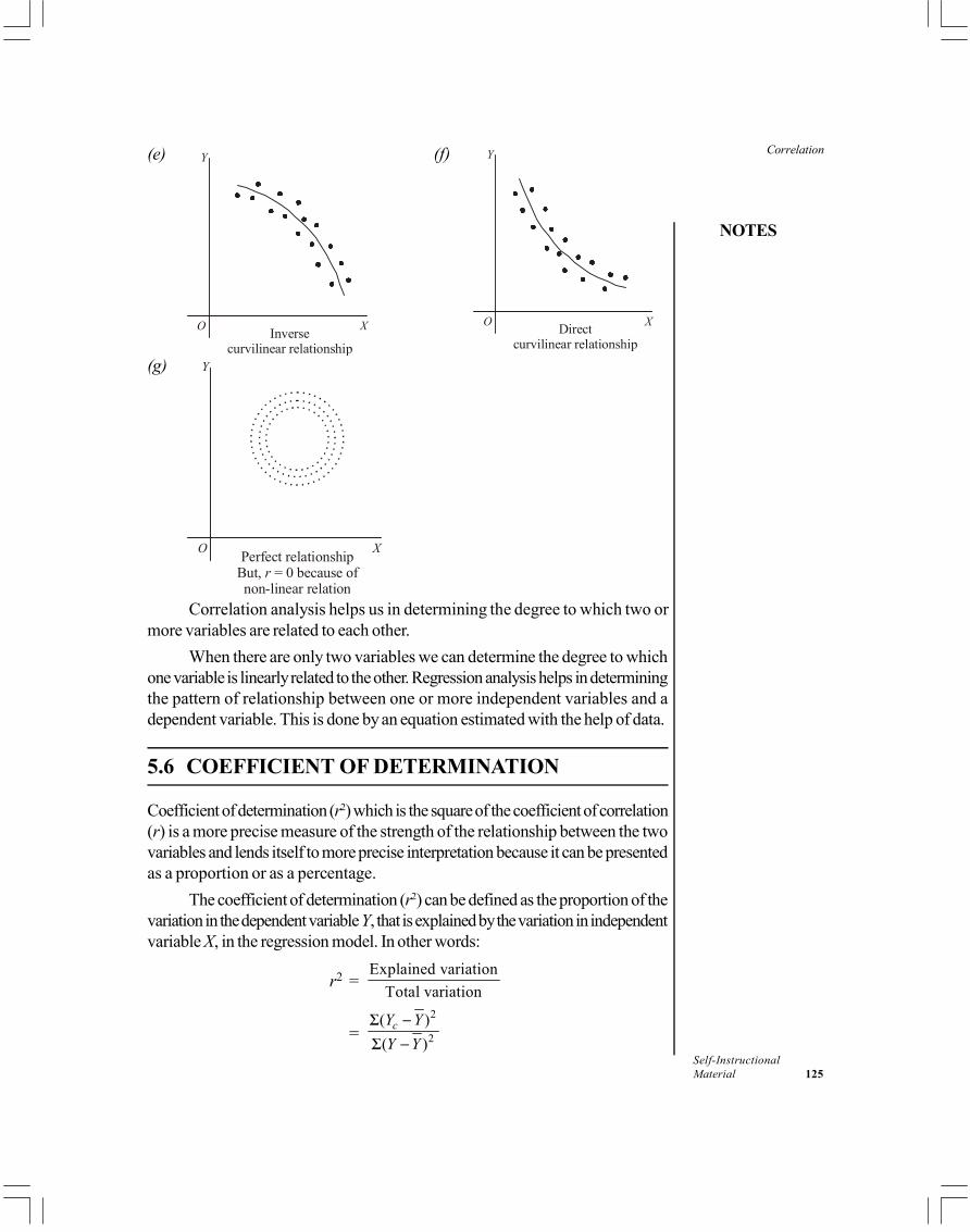
NOTES
Self-InstructionalMaterial 125
Correlation(e) Y
XO Inversecurvilinear relationship
(f) Y
XO Directcurvilinear relationship
(g) Y
XO Perfect relationshipBut, = 0 because of non-linear relation
r
Correlation analysis helps us in determining the degree to which two ormore variables are related to each other.
When there are only two variables we can determine the degree to whichone variable is linearly related to the other. Regression analysis helps in determiningthe pattern of relationship between one or more independent variables and adependent variable. This is done by an equation estimated with the help of data.
5.6 COEFFICIENT OF DETERMINATION
Coefficient of determination (r2) which is the square of the coefficient of correlation(r) is a more precise measure of the strength of the relationship between the twovariables and lends itself to more precise interpretation because it can be presentedas a proportion or as a percentage.
The coefficient of determination (r2) can be defined as the proportion of thevariation in the dependent variable Y, that is explained by the variation in independentvariable X, in the regression model. In other words:
r2 =Explained variation
Total variation
=2
2( )( )
cY YY Y
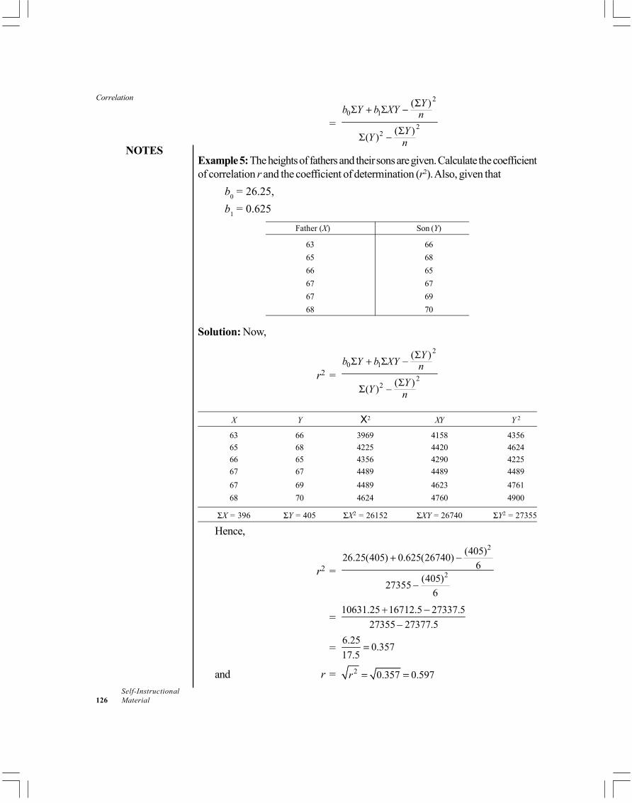
Correlation
NOTES
Self-Instructional126 Material
=
2
0 1
22
( )
( )( )
Yb Y b XY nYY n
Example 5: The heights of fathers and their sons are given. Calculate the coefficientof correlation r and the coefficient of determination (r2). Also, given that
b0 = 26.25,b1 = 0.625
Father (X) Son (Y)
63 6665 6866 6567 6767 6968 70
Solution: Now,
r2 =
2
0 1
22
( )
( )( )
Yb Y b XY nYY n
X Y X2 XY Y 2
63 66 3969 4158 435665 68 4225 4420 462466 65 4356 4290 422567 67 4489 4489 448967 69 4489 4623 476168 70 4624 4760 4900
X = 396 Y = 405 X2 = 26152 XY = 26740 Y2 = 27355
Hence,
r2 =
2
2
(405)26.25(405) 0.625(26740)6
(405)273556
=10631.25 16712.5 27337.5
27355 27377.5
=6.25 0.35717.5
and r = 2 0.357 0.597r

NOTES
Self-InstructionalMaterial 127
CorrelationWhile the value of r = 0.597 is more of an abstract figure, the value of r2 =0.357 tells us that 35.7% of the variation in Y is explained by the variation in X.This indicates a weak relationship since the value of r2 = 0, means no relationshipat all and the value of r = 1 or 100% means perfect relationship. In general, for ahigh degree of correlation which leads to better estimates and prediction, thecoefficient of determination r2 must have a high value.
Check Your Progress
5. What do you mean by coefficient of correlation?6. State the assumptions for finding the coefficient of correlation by Karl
Pearson’s method.7. Define coefficient of determination, r2.
5.7 ANSWERS TO CHECK YOUR PROGRESSQUESTIONS
1. There are several types of correlations. They are:(a) Positive or negative correlations(b) Linear or non-linear correlations(c) Simple, partial or multiple correlations
2. Correlation analysis is the statistical tool that is generally used to describethe degree to which one variable is related to another. The relationship, ifany, is usually assumed to be a linear one. This analysis is used quite frequentlyin conjunction with regression analysis to measure how well the regressionline explains the variations of the dependent variable. In fact, the wordcorrelation refers to the relationship or interdependence between twovariables. There are various phenomena, which are related to each other.For instance, when demand of a certain commodity increases, then its pricegoes up and when its demand decreases then its price comes down.
3. Scatter diagram is the method to calculate the constants in regression modelsthat makes use of scatter diagram or dot diagram. A scatter diagram is adiagram that represents two series with the known variables, i.e., independentvariable plotted on the X-axis and the variable to be estimated, i.e., dependentvariable to be plotted on the Y-axis.
4. The least squares method is a method to calculate the constants in regressionmodels for fitting a line through the scatter diagram that minimizes the sumof the squared vertical deviations from the fitted line. In other words, theline to be fitted will pass through the points of the scatter diagram in such afashion that the sum of the squares of the vertical deviations of these pointsfrom the line will be a minimum.

Correlation
NOTES
Self-Instructional128 Material
5. The coefficient of correlation, which is symbolically denoted by r, is anotherimportant measure to describe how well one variable explains another. Itmeasures the degree of relationship between two casually related variables.The value of this coefficient can never be more than +1 or –1. Thus, +1 and–1 are the limits of this coefficient.
6. Karl Pearson’s method is most widely used method of measuring therelationship between two variables. This coefficient is based on the followingassumptions:(i) There is a linear relationship between the two variables which means
that a straight line would be obtained if the observed data is plotted ona graph.
(ii) The two variables are casually related which means that one of thevariables is independent and the other is dependent.
(iii) A large number of independent causes are operating in both the variablesso as to produce a normal distribution.
7. The coefficient of determination (r2), the square of the coefficient ofcorrelation (r), is a more precise measure of the strength of the relationshipbetween the two variables and lends itself to more precise interpretationbecause it can be presented as a proportion or as a percentage.
5.8 SUMMARY
Correlation analysis is the statistical tool generally used to describe the degreeto which one variable is related to another. The relationship, if any, is usuallyassumed to be a linear one. This analysis is used quite frequently inconjunction with regression analysis to measure how well the regressionline explains the variations of the dependent variable.Correlation can either be positive or it can be negative. Whether correlationis positive or negative would depend upon the direction in which the variablesare moving.Non-linear correlation is also known as curvilinear correlation. The distinctionis based upon the constancy of the ratio of change between the variables.Least squares method of fitting a line (the line of best fit or the regressionline) through the scatter diagram is a method which minimizes the sum of thesquared vertical deviations from the fitted line.There is a linear relationship between the two variables which means that astraight line would be obtained if the observed data is plotted on a graph.The two variables are causally related which means that one of the variablesis independent and the other one is dependent.If observations on two variables are given in the form of ranks and not asnumerical values, it is possible to compute what is known as rank correlationbetween the two series.

NOTES
Self-InstructionalMaterial 129
CorrelationCoefficient of determination (r2) which is the square of the coefficient ofcorrelation (r) is a more precise measure of the strength of the relationshipbetween the two variables and lends itself to more precise interpretationbecause it can be presented as a proportion or as a percentage.
5.9 KEY WORDS
Correlation analysis: It is the statistical tool to describe the degree towhich one variable is related to another.Scatter diagram: It is a graph of observed plotted points where eachpoint represents the values of X and Y as a coordinate.Coefficient of determination: It can be defined as the proportion of thevariation in the dependent variable Y that is explained by the variation inindependent variable X.Rank correlation: In this type of correlation, observations on two variablesare given in the form of ranks instead of numerical values. Rank correlationis a descriptive index of agreement between ranks over individuals.
5.10 SELF-ASSESSMENT QUESTIONS ANDEXERCISES
Short-Answer Questions
1. What is a scatter diagram?2. Under what conditions will you say that a correlation is linear?3. How does a scatter diagram help in studying the correlation between two
variables?4. List the different types of correlation.5. Define correlation analysis.
Long-Answer Questions
1. Obtain the estimating equation by the method of least squares from thefollowing information:
X Y(Independent variable) (Dependent variable)
2 184 125 106 88 711 5

Correlation
NOTES
Self-Instructional130 Material
2. Find out the coefficient of correlation between the two kinds of assessmentof M.A. students’ performance.
(i) By adopting Karl Pearson’s method(ii) By the method of least squares
S.N. of Internal assessment External assessmentStudents (Marks obtained (Marks obtained
out of 100) out of 100)
1 51 492 63 723 73 744 46 445 50 586 60 667 47 508 36 309 60 35
Also, work out r2 and interpret the same.3. Calculate correlation coefficient from the following results:
n = 10; X = 140; Y = 150(X – 10)2 = 180; (Y – 15)2 = 215
(X – 10) (Y – 15) = 604. Given is the following information:
Observation Test score Sales (,000 Rs)X Y
1 73 4502 78 4903 92 5704 61 3805 87 5406 81 5007 77 4808 70 4309 65 41010 82 490
Total 766 4740
You are required to:(i) Graph the scatter diagram for the given data.(ii) Find the regression equation and draw the line corresponding to the
equation on the scatter diagram.(iii) Make an estimate of sales if the test score happens to be 75.

NOTES
Self-InstructionalMaterial 131
Correlation5. Calculate correlation coefficient and the two regression lines for the followinginformation:
Ages of Wives (in years)
10–20 20–30 30–40 40–50 Total
Ages of 10–20 20 26 — — 46
Husbands 20–30 8 14 37 — 59
(in 30–40 — 4 18 3 25
years) 40–50 — — 4 6 10
Total 28 44 59 9 140
6. To know what relationship exists between unemployment and suicideattempts, a sociologist surveyed twelve cities and obtained the followingdata:
S.N. of the Unemployment rate Number of suicide attemptscity per cent per 1000 residents
1 7.3 22
2 6.4 17
3 6.2 9
4 5.5 8
5 6.4 12
6 4.7 5
7 5.8 7
8 7.9 19
9 6.7 13
10 9.6 29
11 10.3 33
12 7.2 18
(i) Develop the estimating equation that best describes the givenrelationship.
(ii) Find a prediction interval (with 95% confidence level) for the attemptedsuicide rate when unemployment rate happens to be 6%.

Correlation
NOTES
Self-Instructional132 Material
5.11 FURTHER READINGS
Hogg, Robert. V., Allen T. Craig and Joseph W. McKean. 2005. Introduction toMathematical Statistics. New Delhi: Pearson Education.
Fisz, Marek. 1963. Probability Theory and Mathematical Statistics, 3rd Edition.New York: John Wiley & Sons, Inc.
Rohatgi, Vijay K. 1985. An Introduction to Probability Theory andMathematical Statistics. New Delhi: Wiley Eastern Limited.
Gupta, C.B. and Vijay Gupta. 2004. An Introduction to Statistical Methods,23rd Edition. New Delhi: Vikas Publishing House.
Levin, Richard I. and David S. Rubin. 1998. Statistics for Management. NewJersey: Prentice Hall.
Chandan, J. S. 1998. Statistics for Business and Economics. New Delhi: VikasPublishing House Pvt. Ltd.
Campbell, Stephen K. 1987. Applied Statistics. New York: Harper & Row.Chance, William A. 1969. Statistical Methods for Decision Making. Illinois:
Richard D Irwin.Hooda, R. P. 2013. Statistics for Business and Economics, 5th Edition. New
Delhi: Vikas Publishing House Pvt. Ltd.

NOTES
Self-InstructionalMaterial 133
Distributions
UNIT 6 DISTRIBUTIONS
Structure6.0 Introduction6.1 Objectives6.2 Binomial Distribution6.3 The Poisson Distribution6.4 Limiting Form of Binomial and Poisson Fitting6.5 Discrete Theoretical Distributions6.6 Answers to Check Your Progress Questions6.7 Summary6.8 Key Words6.9 Self-Assessment Questions and Exercises
6.10 Further Readings
6.0 INTRODUCTION
Binomial distribution is used in finite sampling problems where each observation isone of two possible outcomes (‘success’ or ‘failure’). Poisson distribution is usedfor modelling rates of occurrence. Exponential distribution is used to describeunits that have a constant failure rate. The term ‘normal distribution’ refers to aparticular way in which observations will tend to pile up around a particular valuerather than be spread evenly across a range of values, i.e., the Central Limit Theorem(CLT). It is generally most applicable to continuous data and is intrinsicallyassociated with parametric statistics (For example, ANOVA, t-test, regressionanalysis). Graphically, the normal distribution is best described by a bell-shapedcurve. This curve is described in terms of the point at which its height is maximum,i.e., its mean and its width or standard deviation.
In this unit, you will study about the binomial distribution, Poisson distribution,limiting form of binomial and Poisson fitting and discrete theoretical distributions.
6.1 UNIT OBJECTIVES
After going through this unit, you will be able to:Understand about the binomial distributionAnalyse the Poisson distributionDiscuss the limiting form of binomial and Poisson fittingExplain the discrete theoretical distributions

Distributions
NOTES
Self-Instructional134 Material
6.2 BINOMIAL DISTRIBUTION
Binomial distribution (or the Binomial probability distribution) is a widely usedprobability distribution concerned with a discrete random variable and as such isan example of a discrete probability distribution. The binomial distribution describesdiscrete data resulting from what is often called as the Bernoulli process. Thetossing of a fair coin a fixed number of times is a Bernoulli process and the outcomeof such tosses can be represented by the binomial distribution. The name of Swissmathematician Jacob Bernoulli is associated with this distribution. This distributionapplies in situations where there are repeated trials of any experiment for whichonly one of two mutually exclusive outcomes (often denoted as ‘success’ and‘failure’) can result on each trial.
Bernoulli Process
Binomial distribution is considered appropriate in a Bernoulli process which hasthe following characteristics:
(a) Dichotomy. This means that each trial has only two mutually exclusivepossible outcomes, for example, ‘Success’ or ‘failure’, ‘Yes’ or ‘No’,‘Heads’ or ‘Tails’ and the like.
(b) Stability. This means that the probability of the outcome of any trial isknown (or given) and remains fixed over time, i.e., remains the same for allthe trials.
(c) Independence. This means that the trials are statistically independent, i.e.,to say the happening of an outcome or the event in any particular trial isindependent of its happening in any other trial or trials.
Probability Function of Binomial Distribution
The random variable, say X, in the Binomial distribution is the number of ‘successes’in n trials. The probability function of the binomial distribution is written as under:
f (X = r) = nCr prqn–r
r = 0, 1, 2…nWhere, n = Numbers of trials.
p = Probability of success in a single trial.q = (1 – p) = Probability of ‘failure’ in a single trial.r = Number of successes in ‘n’ trials.
Parameters of Binomial Distribution
This distribution depends upon the values of p and n which in fact are its parameters.Knowledge of p truly defines the probability of X since n is known by definition of

NOTES
Self-InstructionalMaterial 135
Distributionsthe problem. The probability of the happening of exactly r events in n trials can befound out using the above stated binomial function.
The value of p also determines the general appearance of the binomialdistribution, if shown graphically. In this context the usual generalizations are:
(a) When p is small (say 0.1), the binomial distribution is skewed to the right,i.e., the graph takes the form shown in Figure 6.1.
Prob
abili
ty
No. of Successes0 1 2 3 4 5 6 7 8
Fig. 6.1
(b) When p is equal to 0.5, the binomial distribution is symmetrical and thegraph takes the form as shown in Figure 6.2.
No. of Successes
Prob
abili
ty
0 1 2 3 4 5 6 7 8
Fig. 6.2
(c) When p is larger than 0.5, the binomial distribution is skewed to the left andthe graph takes the form as shown in Figure 6.3.
Prob
abili
ty
No. of Successes0 1 2 3 4 5 6 7 8
Fig. 6.3
But if ‘p’ stays constant and ‘n’ increases, then as ‘n’ increases the verticallines become not only numerous but also tend to bunch up together to form a bellshape, i.e., the binomial distribution tends to become symmetrical and the graphtakes the shape as shown in Figure 6.4.

Distributions
NOTES
Self-Instructional136 Material
Prob
abili
ty
No. of Successes0, 1, 2, ..........
Fig. 6.4
Important Measures of Binomial DistributionThe expected value of random variable [i.e., E(X)] or mean of random variable(i.e., X
_) of the binomial distribution is equal to n.p and the variance of random
variable is equal to n. p. q or n. p. (1 – p). Accordingly the standard deviationof binomial distribution is equal to . . .n p q The other important measures relatingto binomial distribution are as under:
Skewness =1 2
. .p
n p q
Kurtosis =21 6 63
. .p q
n p q
When to Use Binomial Distribution
The use of binomial distribution is most appropriate in situations fulfilling theconditions outlined above. Two such situations, for example, can be described asfollows.
(a) When we have to find the probability of 6 heads in 10 throws of a fair coin.(b) When we have to find the probability that 3 out of 10 items produced by a
machine, which produces 8 per cent defective items on an average, will bedefective.
Example 1: A fair coin is thrown 10 times. The random variable X is the numberof head(s) coming upwards. Using the binomial probability function, find theprobabilities of all possible values which X can take and then verify that binomialdistribution has a mean: X = n.p. and variance: 2σ = n.p.q
Solution: Since the coin is fair and so, when thrown, can come either with head
upward or tail upward. Hence, p (head) 12 and q (no head) 1 .
2 The required
probability function is,f(X = r) = nCr prqn–r
r = 0, 1, 2…10

NOTES
Self-InstructionalMaterial 137
DistributionsThe following table of binomial probability distribution is constructed using thisfunction.
Xi (Number Probability pri Xi pri (Xi – X_
) (Xi – X_
)2 (Xi – X_
)2.piof Heads)
0 10C0 p0
q10 = 1/1024 0/1024 –5 25 25/1024
1 10C1 p1
q9 = 10/1024 10/1024 –4 16 160/1024
2 10C2 p2
q8 = 45/1024 90/1024 –3 9 405/1024
3 10C3 p3
q7 = 120/1024 360/1024 –2 4 480/1024
4 10C4 p4
q6 = 210/1024 840/1024 –1 1 210/1024
5 10C5 p5
q5 = 252/1024 1260/1024 0 0 0/1024
6 10C6 p6
q4 = 210/1024 1260/1024 1 1 210/1024
7 10C7 p7
q3 = 120/1024 840/1024 2 4 480/1024
8 10C8 p8
q2 = 45/1024 360/1024 3 9 405/1024
9 10C9 p9
q1 = 10/1024 90/1024 4 16 160/1024
10 10C10 p10
q0 = 1/1024 10/1024 5 25 25/1024
X_
= 5120/1024 Variance = 2 =X_
= 5 (Xi– X_
)2.pri =2560/1024 = 2.5
The mean of the binomial distribution1 is given by n. p. = 10 × 12 = 5 and the
variance of this distribution is equal to n. p. q. = 10 × 12 × 1
2 = 2.5
These values are exactly the same as we have found them in the above table.Hence, these values stand verified with the calculated values of the two
measures as shown in the table.
Check Your Progress
1. Explain the Bernoulli process.2. Write the probability function of binomial distribution.3. Explain the different parameters of binomial distributions.4. Explain the important measures of binomial distribution.5. Under what circumstances will you use binomial distribution?
6.3 THE POISSON DISTRIBUTION
Poisson distribution is also a discrete probability distribution with which is associatedthe name of a Frenchman, Simeon Denis Poisson who developed this distribution.This distribution is frequently used in context of Operations Research and for thisreason has a great significance for management people. This distribution plays animportant role in Queuing theory, Inventory control problems and also in Riskmodels.

Distributions
NOTES
Self-Instructional138 Material
Unlike binomial distribution, Poisson distribution cannot be deducted onpurely theoretical grounds based on the conditions of the experiment. In fact, itmust be based on experience, i.e., on the empirical results of past experimentsrelating to the problem under study. Poisson distribution is appropriate speciallywhen probability of happening of an event is very small (so that q or (1– p) isalmost equal to unity) and n is very large such that the average of series (viz., n. p.)is a finite number. Experience has shown that this distribution is good for calculatingthe probabilities associated with X occurrences in a given time period or specifiedarea.
The random variable of interest in Poisson distribution is number ofoccurrences of a given event during a given interval (interval may be time, distance,area, etc.). We use capital X to represent the discrete random variable and lowercase x to represent a specific value that capital X can take. The probability functionof this distribution is generally written as under:
( )!
−
= =x
ief X x
x
λλ
x = 0, 1, 2…
Where, = Average number of occurrences per specified interval.2 In otherwords, it is the mean of the distribution.
e = 2.7183 being the basis of natural logarithms.x = Number of occurrences of a given event.
Poisson ProcessThe distribution applies in case of Poisson process which has followingcharacteristics.
Concerning a given random variable, the mean relating to a given intervalcan be estimated on the basis of past data concerning the variable understudy.If we divide the given interval into very very small intervals we will find:(a) The probability that exactly one event will happen during the very very
small interval is a very small number and is constant for every othervery small interval.
(b) The probability that two or more events will happen within a very smallinterval is so small that we can assign it a zero value.
(c) The event that happens in a given very small interval is independent,when the very small interval falls during a given interval.
(d) The number of events in any small interval is not dependent on thenumber of events in any other small interval.

NOTES
Self-InstructionalMaterial 139
DistributionsParameter and Important Measures of Poisson DistributionPoisson distribution depends upon the value of , the average number ofoccurrences per specified interval which is its only parameter. The probabilityof exactly x occurrences can be found out using Poisson probability functionstated above. The expected value or the mean of Poisson random variable is
and its variance is also . The standard deviation of Poisson distributionis, λ .
Underlying the Poisson model is the assumption that if there are on theaverage occurrences per interval t, then there are on the average k occurrences per interval kt. For example, if the number of arrivals at a servicecounted in a given hour, has a Poisson distribution with = 4, then y, thenumber of arrivals at a service counter in a given 6 hour day, has the Poissondistribution = 24, i.e., 6×4.
When to Use Poisson DistributionThe use of Poisson distribution is resorted to those cases when we do not knowthe value of ‘n’ or when ‘n’ can not be estimated with any degree of accuracy.In fact, in certain cases it does not make any sense in asking the value of ‘n’.For example, the goals scored by one team in a football match are given, itcannot be stated how many goals could not be scored. Similarly, if one watchescarefully one may find out how many times the lightning flashed but it is notpossible to state how many times it did not flash. It is in such cases we usePoisson distribution. The number of death per day in a district in one year dueto a disease, the number of scooters passing through a road per minute duringa certain part of the day for a few months, the number of printing mistakes perpage in a book containing many pages, are a few other examples where Poissonprobability distribution is generally used.Example 2: Suppose that a manufactured product has 2 defects per unit ofproduct inspected. Use Poisson distribution and calculate the probabilities offinding a product without any defect, with 3 defects and with four defects.Solution: If the product has 2 defects per unit of product inspected. Hence,
= 2.Poisson probability function is as follows:
( ) .!
−
= = −x
ief X xx
λλ
x = 0, 1, 2,…Using the above probability function, we find the required probabilities as under:
P(without any defects, i.e., x = 0) =0 22 .0e

Distributions
NOTES
Self-Instructional140 Material
=1. 0.13534
0.135341
P(with 3 defects, i.e., x = 3) =3 22 .3e =
2 2 2 .1353403 2 1
=0.54136 0.18045
3
P(with 4 defects, i.e., x = 4) = 242 .
4e =
2 2 2 2 0.135344 3 2 1
= 0.27068 0.09023
3
Example 3: How would you use a Poisson distribution to find approximatelythe probability of exactly 5 successes in 100 trials the probability of success ineach trial being p = 0.1?Solution: In the question we have been given,
n = 100 and p = 0.1= n.p = 100 × 0.1 = 10
To find the required probability, we can use Poisson probability function as anapproximation to Binomial probability function as shown below:
( ) ( ) ( ).. ..! !
−−
= = =x n px
in p eef X x
x x
λλ
or P(5)7 =5 10 100000 0.0000510 . 5.000005 5 4 3 2 1 5 4 3 2 1e
=124 = 0.042
Check Your Progress
6. What is Poisson distribution?7. Where and when will you use Poisson distribution?
6.4 LIMITING FORM OF BINOMIAL ANDPOISSON FITTING
Fitting a Binomial DistributionWhen a binomial distribution is to be fitted to the given data, then the followingprocedure is adopted:
NOTES
Self-InstructionalMaterial 141
Distributions(a) Determine the values of ‘p’ and ‘q’ keeping in view that X = n. p. andq = (1 p).
(b) Find the probabilities for all possible values of the given random variableapplying the binomial probability function, viz.,
f (Xi = r) = nCr prqn–r
r = 0, 1, 2,…n(c) Work out the expected frequencies for all values of random variable by
multiplying N (the total frequency) with the corresponding probability.(d) The expected frequencies, so calculated, constitute the fitted binomial
distribution to the given data.
Fitting a Poisson DistributionWhen a Poisson distribution is to be fitted to the given data, then the followingprocedure is adopted:(a) Determine the value of , the mean of the distribution.(b) Find the probabilities for all possible values of the given random variable
using the Poisson probability function, viz.,
.x
ief X xx
x = 0, 1, 2,…(c) Work out the expected frequencies as follows:
n.p.(Xi = x)(d) The result of case (c) above is the fitted Poisson distribution to the given
data.
Poisson Distribution as an Approximation of Binomial DistributionUnder certain circumstances Poisson distribution can be considered as areasonable approximation of Binomial distribution and can be used accordingly.The circumstances which permit all this, are when ‘n’ is large approaching toinfinity and p is small approaching to zero (n = Number of Trials, p = Probabilityof ‘Success’). Statisticians usually take the meaning of large n, for this purpose,when n 20 and by small ‘p’ they mean when p 0.05. In cases where thesetwo conditions are fulfilled, we can use mean of the binomial distribution (viz.,n.p.) in place of the mean of Poisson distribution (viz., ) so that the probabilityfunction of Poisson distribution becomes as stated below:
. .x np
in p e
f X xx
We can explain Poisson distribution as an approximation of the Binomialdistribution with the help of following example.

Distributions
NOTES
Self-Instructional142 Material
Example 4: Given is the following information:(a) There are 20 machines in a certain factory, i.e., n = 20.(b) The probability of machine going out of order during any day is 0.02.
What is the probability that exactly 3 machines will be out of order on the sameday? Calculate the required probability using both Binomial and PoissonsDistributions and state whether Poisson distribution is a good approximation ofthe Binomial distribution in this case.Solution: Probability, as per Poisson probability function (using n.p in placeof )
(since n 20 and p 0.05)
( ) ( ). .!
−
= =x np
in p e
f X xx
Where, x means number of machines becoming out of order on the same day.
P(Xi = 3) =3 20 0.0220 0.02 .3
e
=30.4 . 0.67032 (0.064)(0.67032)3 2 1 6
= 0.00715Probability, as per Binomial probability function,
f(Xi = r) = nCr prqn–r
Where, n = 20, r = 3, p = 0.02 and hence q = 0.98f(Xi = 3) = 20C3(0.02)3 (0.98)17
= 0.00650The difference between the probability of 3 machines becoming out of order onthe same day calculated using probability function and binomial probabilityfunction is just 0.00065. The difference being very very small, we can state thatin the given case Poisson distribution appears to be a good approximation ofBinomial distribution.Example 5: How would you use a Poisson distribution to find approximatelythe probability of exactly 5 successes in 100 trials the probability of success ineach trial being p = 0.1?Solution: In the question we have been given,
n = 100 and p = 0.1= n.p = 100 × 0.1 = 10
To find the required probability, we can use Poisson probability function as anapproximation to Binomial probability function, as shown below:

NOTES
Self-InstructionalMaterial 143
Distributions
( ) ( ) ( ).. ..! !
−−
= = =x n px
in p eef X x
x x
λλ
Or, P(5)7 =5 10 100000 0.0000510 . 5.000005 5 4 3 2 1 5 4 3 2 1e
=124 = 0.042
Check Your Progress
8. How can we measure the area under the curve?9. Under what circumstances, is a Poisson distribution considered as an
approximation of binomial distribution?
6.5 DISCRETE THEORETICAL DISTRIBUTIONS
Theoretical Distributions: If a certain hypothesis is assumed, it is sometimespossible to derive mathematically, what the frequency distributions of certainuniverses should be. Such distributions are called theoretical distributions.
Binomial Distribution
Binomial distribution was discovered by James Bernoulli in the year 1700.Let there be an event the probability of its success* is P and the probability
of its failure is Q is one trial, so P + Q = 1Consider a set of n independent trials and the probability P of success is the
same in every trial, then Q = 1 – P is the probability of failure in any trial.Let the set of n trials be repeated N times, where N is a very large number.
Out of these N, there will be sets with few success and also with number ofsuccesses and so on.
Now the probability that the first k trials are successes and the remaining(n – k) trial are failures is PkQ(n–k).
Since k can be chosen out of n-trials in nck ways, the probability ofk-successes, P(k) in a series of n-independent trials is given by,
P(k) = nck. Pk.Q(n – k)
The probability distribution of the number of successes, so obtained is calledthe ‘Binomial probability distribution’.
The probabilities of 0, 1, 2, ... n successes are nC0P0Qn, nC1P1Qn–1,...nCnPnQ0, are the successive terms of binomial expansion (Q + P)n.

Distributions
NOTES
Self-Instructional144 Material
Definition: A random variable X is said to follow binomial distribution if it assumesonly non-negative values and its probability mass function is given by,
P(X = k) = P(k) = ( ). . ; 0,1, 2, ... 1
0 ; Otherwise
n k n kkc P Q k Q P
Usually we use the notation X ~ B(n, P) to denote that the random variable Xfollows binomial distribution with parameters n and P.Notes: 1. Since n and P are independent constants in the binomial distribution ,they are called the parameters of distribution.
2. 0
( )n
kP k
=∑ =
0. .
nn k n k
kk
C P Q −
=∑ = (Q + P)n = 1
3. If the experiment consisting of n-trials is repeated n times, then thefrequency function of the binomial distribution is given by,
f(k) = N.P(k) = N. [nCk.Pk.Q(n–k)]; k = 0, 1, 2, ...and the expected frequencies of 0, 1, 2, ...n successes are the successive terms ofthe binomial expansion, N(Q + P)n; (Q + P = 1)
Moments
The first four moments about origin of binomial distribution are obtained as follows:(i) Mean or First Moment about Origin
1 = E(X) = 0
. . .n
n x n xx
xx C P Q −
=∑
= nP1 1
11
. .n
n x n xx
xC P Q− − −
−=∑
= nP[Qn–1 + n–1C1P.Qn–2 + ... + Pn–1]= nP(Q + P)n–1 = nP as P + Q = 1
So, mean or 1 = nP.
(ii) Second Moment about Origin
2= E(X2) = 2
0. . .
nn x n x
xk
x C P Q −
=∑
= 0
( ( 1)) . .n
n x n xx
xx x x C P Q −
=
+ − ∑
NOTES
Self-InstructionalMaterial 145
Distributions
= 0
. . .n
n x n xx
xx C P Q −
=∑ +
0( 1). . .
nn x n x
xx
x x C P Q −
=−∑
= nP + n(n – 1)P2.2 2
22
. .n
n x n xx
xC P Q− − −
−=∑
= nP + n(n – 1)P2.(Q – P)n–2
2 = nPQ + n2P2.(iii) Third Moment about Origin
3= E(X 3) = 3
0. . .
nn x n x
xk
x C P Q −
=∑
On simplifying, we get,3 = n(n – 1)(n – 2)P3 + 3n(n – 1)P2 + nP.
(iv) Fourth Moment about Origin
4= E(X4) = 4
0. . .
nn x n x
xk
x C P Q −
=∑
And on simplifying, we get,
4 = n(n – 1) (n – 2) (n – 3)P4 + 6n(n – 1)(n – 2)P3
+ 7n(n – 1)P2 + nP.Now, the moment about ‘Mean of Binomial Distribution will be Discussed’.(i) First Moment about Mean
0 = 0 (always)(ii) Second Moment about Mean
2 = 2 – ( 1)2 = E(X2) – [E(x)]2
= nPQ + n2P2 – n2P2 = nPQThus, Var (X) = 2 = nPQ and standard deviation (X) = nPQ
(iii) Third and Fourth Moment about Mean(a) 3 = 3 – 3 2 1 + 2( 1)
3
= nPQ (Q – P) (On simplification)(b) 4 = 4 – 4 3 1 + 6 2( 1)
2 – 2( 1)4
= 3n2P2Q2 – 6nP2Q2 + nPQ= nPQ[1 + 3(n – 2)PQ]
Hence, 1 = 2 2 2 2 2 2
33 3 3 3
2
( ) (1 2 )n P Q Q P PnPQn P Q
µ − −= =
µ
2 = 42 2 2 2
2
[1 3( 2) ] 1 63nPQ n PQ PQnPQn P Q
µ + − −= = +
µ

Distributions
NOTES
Self-Instructional146 Material
1 = 1β = Q P
nPQ−
and 2 = 2 – 3 = 1 6PQ
nPQ−
Moment Generating Function of Binomial Distribution: Let x have a binomialdistribution with probability function,
P(x) = nCx PxQn–x ; x = 0, 1, 2, ... nThe moment generating function about the origin is given as
M0(t) = E(etx) = –
0
. .n
tx n x n xx
xe C P Q
=∑
= –
0
( ) .n
n t x n xx
xC Pe Q
=∑
M0(t) = (Q + Pet)n
Moment generating function about mean nP is given by,MnP(t) = E[et(x–nP)] = E(etx.e–nPt)
= e–nPt.E(etx) = e–nPt.M0(t)= e–nPt(Q + et.P)n
= (Q.e–Pt + P.e(1 – P)t)n
MnP(t) = (Q.e–Pt + P.eQt)n
Poisson Distribution with Mean and Variance
The Poisson distribution is a limiting case of binomial distribution when the probabilityof success or failure (i.e., P or Q) is vary small and the number of trial n is verylarge (i.e. n ) enough so that nP is a finite constant say i.e. nP = . Underthese conditions, P(x) the probability of x success in the binomial distribution,
P(x) = P(X – x) = nCx PxQn–x can be written as,
P(x) = ! . . 1!.( )!
x n xnx n x n n
−λ λ − −
= !1
!( )! 1
nx
xx
nx n
n n xn
λ λ − λ − −
Using Lim n , we have,
P(x) = !Lim 1 Lim
!( )! 1 .
nx
xn n x
nx n
n x nn
→∞ →∞
λ λ − λ − −
...(6.1)

NOTES
Self-InstructionalMaterial 147
Distributions
We know that Lim 1n
n n→∞
λ −
= e– and Lim 1x
n n→∞
λ −
= 1
And using Stirling’s formula for n!, we have,
n! = 1/ 22 . n nn e+ −π
!( )!
nn x−
= 1/ 2
1/ 22 . .
2 .( ) .
n n
n x n xn e
n x e
+ −
− + − +π
π −
So, !( )!
nn x−
= 1/ 2
1/ 2.
( ) . .
n n
n x n x xn e
n x e n
+ −
− + − +−
Thus, Equation (6.1) becomes,
P(x) = 1/ 2
1/ 2.. .Lim
! ( ) . .
x n n
n x n x xn
n eex n x e n
+ −−λ
− + − +→∞
λ−
= 1/ 2
1/ 2. ..L im!. ( ) . .
x n n
x n x n xn
e n ex e n x e n
−λ + −
− + −→∞
λ−
= 1/ 2
121/ 2
. .L im!.
1
x n x
x n n xn x
e nx e xn
n
−λ − +
→∞ − +− +
λ
−
= 12
. 1.Lim!.
1 . 1
x
x n n x
ex e x x
n n
−λ
→∞ − +
λ − −
= . 1.!. .1
x
x xe
x e e
−λ
−λ = .
!
x ex
−λλ
Thus,
P(X = x) = P(x) = .!
x ex
−λλ ; x = 0, 1, 2, ...
When n , nP = and P 0Here, is known as the parameter of Poisson distribution.
Definition: A random variable X is said to follow a Poisson distribution ifi t assumes only non-negative values and i ts probabi l i ty mass function isgiven by,

Distributions
NOTES
Self-Instructional148 Material
P(x, ) = P(X = x) = .!
x ex
−λλ ; x = 0, 1, 2, ...; > 0.
Constants of the Poisson Distribution: (i) Mean, 1 = = E(X).(ii) 2 = E(X2) = .(iii) 3 = E(X3) = .(iv) 4 = E(X4) = (v) First moment about mean 1 = 0.(vi) V(X) = 2 = E(X2) – [E(X)]2 = 2 – 1
2
= + 2 – 2 = Note that, Mean = Variance = .
(vii) Standard deviation (X) = λ .(viii) 3, i.e. the third moment about mean
3 = 3 – 2 1 + 2 13
= ( ) – 3 ( ) + = (ix) 4 = 4 – 4 3 1 + 6 2 1
2 – 3 14 =
Thus, coefficients of skewness and kurtosis are given by,
1 = 2 2
33 3
2
1µ λ= =
λµ λ and 1 = 1β = 1
λ
Also, 2 = 42
2
13µ= +
λµ and 2 = 2 – 3 = 1
λ
Hence, the Poisson distribution is always a skewed distribution if Limλ→∞
, we get,
1 = 0, 2 = 3.Negative Binomial Distribution: Suppose there are n-trials of an event. Weassume that
(i) The n-trials are independent.(ii) P is the probability of success which remains constant from trial to trial.Let f (x; r, P) denote the probability that there are x failures preceeding the
rth success in (x + r) trials.Now, in (x + r) trials the last trial must be a success with probability P. Then
in the remaining (x + r – 1) trials, we must have (r – 1) successes whose probabilityis given by
x+r–1Cr–1. Pr–1. Qx.Therefore, the compound probability theorem f(x; r, P) is given by the
product of these two probabilities.

NOTES
Self-InstructionalMaterial 149
DistributionsSo f(x; r, P) = x+r–1Cr–i. Pr–1. Qx.P= x+r–1Cr–i. Pr. Qx.
Moment Generating Function of Poisson Distribution
Let P(X = x) = .
!
xe
x−λ λ ; x = 0, 1, 2, ... ; > 0 be a Poisson distribution.
Then the moment generating function is given by,
M(t) = E(etx) = 0
..!
xtx
x
eex
−λ∞
=
λ∑
= 0
( . ).!
t x
x
eex
∞−λ
=
λ∑
= ( 1).t te ee e e−λ λ λ −=
and moment generating function about mean is,M (t) = E(et(x– )) = e– t. E(etx)
= e– t.e (et –1)
So, M (t) = ( )tt ee −λ + λ − λ
Definition: A random variable X is said to follow a negative binomial distribution,if its probability mass function is given by,
P(X = x) = P(x) = x+r–1Cr–1. Pr. Qx; x = 0, 1, 2, ...0; otherwise.
Also, we know that nCr = nCn–r
So x+r–1Cr–1 = x+r–1Cx
= ( 1) ( 2) ... ( 1).
!x r x r r r
x+ − + − +
= ( 1) ( ) ( 1) ... ( 2) ( 1)!
x r r r x r xx
− − − − − + + − + + = (–1)x. – rCx
So p(x) = . ( ) ; 0,1, 2, ...
0 ; otherwise
r r xrC p q x− − =
which is the (x + 1)th term in the expansion of Pr(1 – Q)–r, a binomial expansionwith a negative index. Hence, the distribution is called a negative binomialdistribution. Also,
0( )
xP x
∞
=∑ =
0( )r r x
xx
P C Q∞
−
=−∑ = Pr × (1 – Q)–r = 1
Therefore, P(x) represents the probability function and the discrete variablewhich follows this probability function is called the negative binomial variable.

Distributions
NOTES
Self-Instructional150 Material
Example 6: A continuous random variable X has a probability distribution functionf(x) = 3x2, 0 x 1.
Find a and b such that (i) pX a = pX a, and(ii) pX b = 0.05
Solution: (i) Since PX a = PX a
each must be equal to 12
, because total probability is always 1.
PX a = 12
0
( )a
f x dx∫ = 12
Or, 3 2
0
ax dx∫ = 1
2
3
03
3
ax
= 12
Or, a3 = 12
a = 1/ 31
2
(ii) pX b = 0.05.1
( )b
f x dx∫ = 0.05 1
23b
x dx∫ = 0.05
133
3 b
x
= 0.05 1 – b3 = 120
b = 1/ 319
20
Example 7: A probability curve y = f(x) has a range from 0 to . Iff(x) = e–x find the mean and variance and the third moment about mean.Solution: We know that, the rth moment about origin,
r = 0
( )rx f x dx∞
∫ = 0
.r xx e dx∞
−∫
= ( 1)rΓ + = r! (Using Gamma Integral)
Substituting, r = 1, 2, and 3, we have,Mean, 1
2 = 2! = 2 and 3 = 3! = 6Thus, variance = 2 = 2 – ( 1)
2 = 2 – 1 = 1And 3 = 3 – 2. 1 + 2( 1)
3 = 6 – 3 × 2 + 2 = 2 is the required thirdmoment about mean.

NOTES
Self-InstructionalMaterial 151
DistributionsUniform Distribution
A random variable X is said to have a continuous uniform distribution over aninterval (a, b) if its probability density function is constant say k, over the entirerange of X.
That is, f(x) = ;
0; otherwisek a X b< <
Since total probability is always unity, we have,
( )b
af x dx∫ = 1 k = 1
b
adx =∫
Or, k = 1b a−
Thus, f(x) = 1 ;
0 ; otherwise
a X bb a
< <−
This is also known as rectangular distribution as the curve y = f(x) describes
a rectangle over the x-axis and between the ordinates at x = a and x = b.The distribution function F(x) is given by,
F(x) =
0 ; if
;
1 ;
x ax a a x bb a
b x
−∞ < < − ≤ ≤ −
< < ∞Since F(x) is not continuous at x = a and x = b, it is not differentiable at
these points. Thus, 1( ) ( ) 0,d F x f xdx b a
= = ≠−
exists everywhere except at
the points x = a and x = b and consequently probability distribution function f(x)is given by,
f(x) = 1 ;
0 ; otherwise
a x bb a
< <−
Fig. 6.5 Uniform Distribution

Distributions
NOTES
Self-Instructional152 Material
Moments of Uniform Distribution:
'rµ = 1 11( )
( ) 1
r ra rb
b ax f x dxb a r
+ + −= − +
∫ .
In particular,
mean, 1'µ = 2 21
2 2b a b a
b a − + = −
And 2'µ = 3 3
2 21 1 ( )3 3
b a b ab ab a
−= + + −
Variance = µ2 = 22 1' ( ' )µ − µ
= 2
2 21 ( )3 2
b ab ab a + + + −
= 21 ( )12
b a−
Moment generating function is given by,
MX(t) = ( )( )
bt atb ta
e ee f x dxt b a
−=
−∫And the characteristic function is given by,
( )x tφ = ( )( )
ibt iatb itxa
e ee f x dxt b a
−=
−∫
Check Your Progress
10. Who discovered binomial distribution?11. When is a random variable X said to follow binomial distribution?12. What is Poisson distribution?
6.6 ANSWERS TO ‘CHECK YOUR PROGRESS’
1. Bernoulli process or Binomial distribution is considered appropriate and hasthe following characteristics;(a) Dichotomy: This means that each trial has only two mutually exclusive
possible outcomes. For example, success or failure, yes or no, heads ortail, etc.
(b) Stability: This means that the probability of the outcome of any trial isknown and remains fixed over time, i.e., remains the same for all thetrials.

NOTES
Self-InstructionalMaterial 153
Distributions(c) Independence: This means that the trials are statistically independent,i.e., to say the happening of an outcome or the event in any particular trialis independent of its happening in any other trial or trials.
2. The probability function of binomial distribution is written as under:
( ) 0,1, 2,...
= ==
n r n-rrf X r C p q
r n
Where,n = Numbers of trials.p = Probability of success in a single trial.q = (1 – p) = Probability of failure in a single trial.r = Number of successes in n trials.
3. The parameters of binomial distribution are p and n, where p specifies theprobability of success in a single trial and n specifies the number of trials.
4. The important measures of binomial distribution are:
2
1 2Skewness
1 6 6Kurtosis 3
pn.p.q
p qn.p.q
5. We need to use binomial distribution under the following circumstances:(a) When we have to find the probability of heads in 10 throws of a fair coin.(b) When we have to find the probability that 3 out of 10 items produced by
a machine, which produces 8% defective items on an average, will bedefective.
6. Poisson distribution is a discrete probability distribution that is frequently usedin the context of Operations Research. Unlike binomial distribution, Poissondistribution cannot be deduced on purely theoretical grounds based on theconditions of the experiment. In fact, it must be based on the experience, i.e.,on the empirical results of past experiments relating to the problem understudy.
7. Poisson distribution is used when probability of happening of an event is verysmall and n is very large such that the average of series is a finite number. Thisdistribution is good for calculating the probabilities associated with Xoccurrences in a given time period or specified area.
8. For measuring the area under a curve, we make use of the statistical tablesconstructed by mathematicians. Using these tables, we can find the area thatthe normally distributed random variable will lie within certain distances fromthe mean. These distances are defined in terms of standard deviations. Whileusing the tables showing the area under the normal curve, it is considered in

Distributions
NOTES
Self-Instructional154 Material
terms of standard variate, which means standard deviations without units ofmeasurement and it is calculated as:
XZ
Where, Z = The standard variate or number of standard deviations from Xto the mean of the distribution.
X = Value of the random variable under consideration.= Mean of the distribution of the random variable.= Standard deviation of the distribution.
9. When n is large approaching to infinity and p is small approaching to zero,Poisson distribution is considered as an approximation of binomial distribution.
10. Binomial distribution was discovered by James Bernoulli.11. A random variable X is said to follow binomial distribution if it assumes only
non-negative values and its probability mass function is given by,
P(X = k) = P(k) = ( ). . ; 0,1, 2, ... 1
0 ; otherwise
n k n kkc P Q k Q P− = = −
12. Poisson distribution is a limiting case of binomial distribution when theprobability of success or failure is very small and the number of trial n is verylarge.
6.7 SUMMARY
The binomial distribution describes discrete data resulting from what is oftencalled as the Bernoulli process. The tossing of a fair coin a fixed number oftimes is a Bernoulli process and the outcome of such tosses can berepresented by the binomial distribution. The name of Swiss mathematicianJacob Bernoulli is associated with this distribution.The expected value of random variable [i.e., E(X)] or mean of randomvariable (i.e., X
_) of the binomial distribution is equal to n.p and the variance
of random variable is equal to n. p. q or n. p. (1 – p).Unlike binomial distribution, Poisson distribution cannot be deducted onpurely theoretical grounds based on the conditions of the experiment. Infact, it must be based on experience, i.e., on the empirical results of pastexperiments relating to the problem under study.Poisson distribution is appropriate specially when probability of happeningof an event is very small (so that q or (1– p) is almost equal to unity) and nis very large such that the average of series (viz., n. p.) is a finite number.

NOTES
Self-InstructionalMaterial 155
DistributionsPoisson distribution depends upon the value of , the average number ofoccurrences per specified interval which is its only parameter.If a certain hypothesis is assumed, it is sometimes possible to derivemathematically, what the frequency distributions of certain universes shouldbe. Such distributions are called theoretical distributions.A random variable X is said to follow binomial distribution if it assumes onlynon-negative values and its probability mass function is given by,
P(X = k) = P(k) = ( ). . ; 0,1, 2, ... 1
0 ; Otherwise
n k n kkc P Q k Q P
The Poisson distribution is a limiting case of binomial distribution when theprobability of success or failure (i.e., P or Q) is vary small and the numberof trial n is very large (i.e. n ) enough so that nP is a finite constant say
, i.e., nP = .A random variable X is said to follow a Poisson distribution if itassumes only non-negative values and its probability mass functionis given by
P(x, ) = P(X = x) = .!
x ex
−λλ ; x = 0, 1, 2, ...; > 0.
A random variable X is said to have a continuous uniform distribution overan interval (a, b) if its probability density function is constant say k, over theentire range of X.
6.8 KEY WORDS
Binomial distribution: It is also called as Bernoulli process and is used todescribe discrete random variable.Poisson distribution: It is used to describe the empirical results of pastexperiments relating to the problem and plays important role in queuingtheory, inventory control problems and risk models.
6.9 SELF-ASSESSMENT QUESTIONS ANDEXERCISES
Short-Answer Questions1. Define probability distribution and probability functions.2. Describe binomial distribution and its measures.3. How a binomial distribution can be fitted to a given data?

Distributions
NOTES
Self-Instructional156 Material
4. Describe Poisson distribution and its important measures.5. Poisson distribution can be an approximation of binomial distribution.
Explain.6. When is the Poisson distribution used?7. Write the formula for measuring the area under the curve.8. Explain the circumstances when the normal probability distribution can be
used.
Long-Answer Questions1. Given is the following probability distribution:
Xi pr(Xi)0 1/81 2/82 3/83 2/8
Calculate the expected value of Xi, its variance, and standard deviation.2. A coin is tossed 3 times. Let X be the number of runs in the sequence of
outcomes: first toss, second toss, third toss. Find the probability distributionof X. What values of X are most probable?
3. (a) Explain the meaning of Bernoulli process pointing out its maincharacteristics.
(b) Give a few examples narrating some situations wherein binomial pr.distribution can be used.
4. State the distinctive features of the Binomial, Poisson and Normal probabilitydistributions. When does a Binomial distribution tend to become a Normaland a Poisson distribution? Explain.
5. Explain the circumstances when the following probability distributions areused:(a) Binomial distribution(b) Poisson distribution(c) Normal distribution
6. Certain articles were produced of which 0.5 per cent are defective, arepacked in cartons, each containing 130 articles. When proportion of cartonsare free from defective articles? What proportion of cartons contain 2 ormore defective?(Given e–0.5=0.6065).

NOTES
Self-InstructionalMaterial 157
Distributions7. The following mistakes per page were observed in a book:No. of Mistakes No. of Times the Mistake
Per Page Occurred0 2111 902 193 54 0
Total 345Fit a Poisson distribution to the data given above and test the goodness offit.
8. In a distribution exactly normal, 7 per cent of the items are under 35 and 89per cent are under 63. What are the mean and standard deviation of thedistribution?
9. Assume the mean height of soldiers to be 68.22 inches with a variance of10.8 inches. How many soldiers in a regiment of 1000 would you expect tobe over six feet tall?.
6.10 FURTHER READINGS
Hogg, Robert. V., Allen T. Craig and Joseph W. McKean. 2005. Introduction toMathematical Statistics. New Delhi: Pearson Education.
Fisz, Marek. 1963. Probability Theory and Mathematical Statistics, 3rd Edition.New York: John Wiley & Sons, Inc.
Rohatgi, Vijay K. 1985. An Introduction to Probability Theory andMathematical Statistics. New Delhi: Wiley Eastern Limited.
Gupta, C.B. and Vijay Gupta. 2004. An Introduction to Statistical Methods,23rd Edition. New Delhi: Vikas Publishing House.
Levin, Richard I. and David S. Rubin. 1998. Statistics for Management. NewJersey: Prentice Hall.
Chandan, J. S. 1998. Statistics for Business and Economics. New Delhi: VikasPublishing House Pvt. Ltd.
Campbell, Stephen K. 1987. Applied Statistics. New York: Harper & Row.Chance, William A. 1969. Statistical Methods for Decision Making. Illinois:
Richard D Irwin.Hooda, R. P. 2013. Statistics for Business and Economics, 5th Edition. New
Delhi: Vikas Publishing House Pvt. Ltd.

Special Distributions
NOTES
Self-Instructional158 Material
UNIT 7 SPECIAL DISTRIBUTIONS
Structure7.0 Introduction7.1 Objectives7.2 The Gamma Distribution7.3 Chi-Square Distribution7.4 The Normal Distribution7.5 The Bivariate Normal Distribution7.6 Answers to Check Your Progress Questions7.7 Summary7.8 Key Words7.9 Self-Assessment Questions and Exercises
7.10 Further Readings
7.0 INTRODUCTION
Any statistical hypothesis test, in which the test statistic has a Chi-square distribution,when the null hypothesis is true, is termed as Chi-square test. Chi-square test is anon-parametric test of statistical significance for bivariate tabular analysis, alsoknown as cross-breaks. Amongst the several tests used in statistics for judging thesignificance of the sampling data, Chi-square test, developed by Prof. Fisher, isconsidered an important test. Chi-square, symbolically written as 2 (pronouncedas Ki-square), is a statistical measure with the help of which it is possible to assessthe significance of the difference between the observed frequencies and the expectedfrequencies obtained from some hypothetical universe. Chi-square tests enable usto test and compare whether more than two population proportions can beconsidered equal. Hence, it is a statistical test commonly used to compare observeddata with expected data and testing the null hypothesis, which states that there isno significant difference between the expected and the observed result.
In this unit, you will study about the Gamma distribution, Chi-squaredistribution, the normal distribution and the bivariate normal distribution.
7.1 OBJECTIVES
After going through this unit, you will be able to:Understand about the Gamma distributionExplain various Chi-square distributionDescribe the normal distributionAnalyse the bivariate normal distribution

NOTES
Self-InstructionalMaterial 159
Special Distributions7.2 THE GAMMA DISTRIBUTION
The Erlang distribution is a continuous probability distribution with wideapplicability primarily due to its relation to the Exponential and Gamma distributions.The Erlang distribution was developed by A. K. Erlang. He developed the Erlangdistribution to examine the number of telephone calls which might be made at thesame time to the operators of the switching stations. This work on telephone trafficengineering has been expanded to consider waiting times in queuing systems ingeneral. Erlang distribution is now used in the fields of stochastic processes andbiomathematics.
Given a Poisson distribution with a rate of change , the Distribution FunctionD (x) giving the waiting times until the hth Poisson event is:
1
0
( )( ) 1!
khx
k
xD x ek
−−λ
=
λ= −∑
=( , )1
( )h x
h
For x (0, ), where (x) is a complete gamma function, and (a, x) anincomplete gamma function. With h explicitly an integer, this distribution is knownas the Erlang distribution and has the following probability function:
1( )( )( 1)!
hxxP x e
h
−−λλ λ
=−
It is closely related to the gamma distribution, which is obtained by letting a h (not necessarily an integer) and defining 1/ . When h = 1, it simplifies to
the exponential distribution.The probability density function of the Erlang distribution is given below:
1
( ; , ) for , 0,( )
k k xx ef x k xk
− −λλλ = λ ≥
Γ
Where, (k) is the gamma function evaluated at k, the parameter k is calledthe shape parameter and the parameter is called the rate parameter.
An alternative but equivalent parameterization (Gamma distribution) usesthe scale parameter , which is the reciprocal of the rate parameter (i.e., ):
1
( ; , ) for , 0.( )
xk
k
x ef x k xk
−− µ
µ = µ ≥µ Γ
When the scale parameter equals to 2, the distribution simplifies the Chi-square distribution with 2k degrees of freedom. It can, therefore, be regarded asa generalized Chi-squared distribution for even numbers of degrees of freedom.

Special Distributions
NOTES
Self-Instructional160 Material
Because of the factorial function in the denominator, the Erlang distributionis only defined when the parameter k is a positive integer. In fact, this distributionis sometimes called the Erlang-k distribution (for example, an Erlang-2 distributionis an Erlang distribution with k = 2). The Gamma distribution generalizes the Erlangdistribution by allowing k to be any real number, using the Gamma function insteadof the factorial function.
The Cumulative Distribution Function (CDF) of the Erlang distribution isgiven below:
( , )( ; , ) ,( 1)!
k xF x kkγ λ
λ =−
Where, is the lower incomplete gamma function. The CDF may alsobe expressed as follows:
1
0
1( ; , ) 1 ( ) .!
kx n
nF x k e x
n
−−λ
=
λ = − λ∑
An asymptotic expansion is known for the median of an Erlang distribution,for which coefficients can be computed and bounds are known.
Generating Erlang Distributed Random Numbers
Erlang distributed random numbers can be generated from uniform distributionrandom numbers (U (0, 1)) using the following formula:
1
1( , ) lnk
ii
E k U=
λ ≈ −λ ∏
Waiting Times
Events that occur independently with some average rate are modeled with a Poissonprocess. The waiting times between k occurrences of the event are Erlangdistributed.
The Erlang distribution, which measures the time between incoming calls,can be used in conjunction with the expected duration of incoming calls to produceinformation about the traffic load measured in Erlang units. This can be used todetermine the probability of packet loss or delay, according to various assumptionsmade about whether blocked calls are aborted (Erlang B formula) or queued untilserved (Erlang C formula). The Erlang B and C formulae are still in everyday usefor traffic modelling for applications, such as the design of call centers.
A.K. Erlang worked a lot in traffic modelling. Thus, there are two otherErlang distributions which used in modelling traffic. They are given below:
Erlang B Distribution: This is the easier of the two distributions and canbe used in a call centre to calculate the number of trunks one need to carrya certain amount of phone traffic with a certain ‘target service’.

NOTES
Self-InstructionalMaterial 161
Special DistributionsErlang C Distribution: This formula is much more difficult and is oftenused to calculate how long callers will have to wait before being connectedto a human in a call centre or similar situation.
Stochastic Processes
The Erlang distribution is the distribution of the sum of k independent and identicallydistributed random variables each having an exponential distribution. The long-runrate at which events occur is the reciprocal of the expectation of X, that is, l/k. The(age specific event) rate of the Erlang distribution is, for k > 1, monotonic in x,increasing from zero at x = 0, to l as x tends to infinity.
Check Your Progress
1. Define Erlang-k distribution.2. What is Erlang C distribution?
7.3 CHI-SQUARE DISTRIBUTION
Chi-square test is a non-parametric test of statistical significance for bivariate tabularanalysis (also known as cross-breaks). Any appropriate test of statistical significancelets you know the degree of confidence you can have in accepting or rejecting ahypothesis. Typically, the Chi-square test is any statistical hypothesis test, in whichthe test statistics has a chi-square distribution when the null hypothesis is true. It isperformed on different samples (of people) who are different enough in somecharacteristic or aspect of their behaviour that we can generalize from the samplesselected. The population from which our samples are drawn should also be differentin the behaviour or characteristic. Amongst the several tests used in statistics forjudging the significance of the sampling data, Chi-square test, developed by Prof.Fisher, is considered as an important test. Chi-square, symbolically written as 2
(pronounced as Ki-square), is a statistical measure with the help of which, it ispossible to assess the significance of the difference between the observedfrequencies and the expected frequencies obtained from some hypothetical universe.Chi-square tests enable us to test whether more than two population proportionscan be considered equal. In order that Chi-square test may be applicable, boththe frequencies must be grouped in the same way and the theoretical distributionmust be adjusted to give the same total frequency which is equal to that of observedfrequencies. c2 is calculated with the help of the following formula:
22 0( )e
e
f ff
Where, f0 means the observed frequency; andfe means the expected frequency.

Special Distributions
NOTES
Self-Instructional162 Material
Whether or not a calculated value of 2 is significant, it can be ascertained bylooking at the tabulated values of 2 (given at the end of this book in appendixpart) for given degrees of freedom at a certain level of confidence (generally a5% level is taken). If the calculated value of 2 exceeds the table value, thedifference between the observed and expected frequencies is taken assignificant but if the table value is more than the calculated value of 2, then thedifference between the observed and expected frequencies is considered asinsignificant, i.e., considered to have arisen as a result of chance and as suchcan be ignored.
Degrees of FreedomAs already stated in the earlier unit, the number of independent constraintsdetermines the number of degrees of freedom2 (or df). If there are 10 frequencyclasses and there is one independent constraint, then there are (10 – 1) = 9degrees of freedom. Thus, if n is the number of groups and one constraint isplaced by making the totals of observed and expected frequencies equal, df =(n – 1); when two constraints are placed by making the totals as well as thearithmetic means equal then df = (n – 2) and so on. In the case of a contingencytable (i.e., a table with two columns and more than two rows or table with tworows but more than two columns or a table with more than two rows and morethan two columns) or in the case of a 2 × 2 table the degrees of freedom isworked out as follows:
df = (c – 1)(r – 1)Where, c = Number of columns
r = Number of rows
Conditions for the Application of Test
The following conditions should be satisfied before the test can be applied:(i) Observations recorded and used are collected on a random basis.(ii) All the members (or items) in the sample must be independent.(iii) No group should contain very few items say less than 10. In cases
where the frequencies are less than 10, regrouping is done by combiningthe frequencies of adjoining groups so that the new frequencies becomegreater than 10. Some statisticians take this number as 5, but 10 isregarded as better by most of the statisticians.
(iv) The overall number of items (i.e., N) must be reasonably large. Itshould at least be 50, howsoever small the number of groups may be.
(v) The constraints must be linear. Constraints which involve linear equationsin the cell frequencies of a contingency table (i.e., equations containingno squares or higher powers of the frequencies) are known as linearconstraints.

NOTES
Self-InstructionalMaterial 163
Special DistributionsAreas of Application of Chi-Square TestChi-square test is applicable in large number of problems. The test is, in fact,a technique through the use of which it is possible for us to (a) Test thegoodness of fit; (b) Test the homogeneity of a number of frequency distributions;and (c) Test the significance of association between two attributes. In otherwords, Chi-square test is a test of independence, goodness of fit andhomogeneity. At times Chi-square test is used as a test of population variancealso.As a Test of Goodness of Fit, 2 test enables us to see how well thedistribution of observe data fits the assumed theoretical distribution such asBinomial distribution, Poisson distribution or the Normal distribution.As a Test of Independence, 2 test helps explain whether or not twoattributes are associated. For instance, we may be interested in knowingwhether a new medicine is effective in controlling fever or not and 2 test willhelp us in deciding this issue. In such a situation, we proceed on the nullhypothesis that the two attributes (viz., new medicine and control of fever) areindependent. Which means that new medicine is not effective in controllingfever. It may, however, be stated here that 2 is not a measure of the degreeof relationship or the form of relationship between two attributes but it simplyis a technique of judging the significance of such association or relationshipbetween two attributes.As a Test of Homogeneity, 2 test helps us in stating whether differentsamples come from the same universe. Through this test, we can also explainwhether the results worked out on the basis of sample/samples are in conformitywith well defined hypothesis or the results fail to support the given hypothesis.As such the test can be taken as an important decision-making technique.As a Test of Population Variance. Chi-square is also used to test thesignificance of population variance through confidence intervals, specially in caseof small samples.
Steps Involved in Finding the Value of Chi-SquareThe various steps involved are as follows:
(i) First of all calculate the expected frequencies.(ii) Obtain the difference between observed and expected frequencies and
find out the squares of these differences, i.e., calculate ( f0 – fe)2.
(iii) Divide the quantity ( f0 – fe)2 obtained, as stated above by the
corresponding expected frequency to get 2
0( )e
e
f ff .

Special Distributions
NOTES
Self-Instructional164 Material
(iv) Then find summation of 2
0( )e
e
f ff values or what we call
20( )e
e
f ff
This is the required 2 value.
The 2 value obtained as such should be compared with relevant table value of2 and inference may be drawn as stated above.
The following examples illustrate the use of Chi-square test.Example 1: A dice is thrown 132 times with the following results:
Number Turned Up 1 2 3 4 5 6Frequency 16 20 25 14 29 28
Test the hypothesis that the dice is unbiased.Solution: Let us take the hypothesis that the dice is unbiased. If that is so, theprobability of obtaining any one of the six numbers is 1/6 and as such the
expected frequency of any one number coming upward is 1132 22.6
Now,
we can write the observed frequencies along with expected frequencies andwork out the value of 2 as follows:
No. Turned Observed Expected ( f0 – fe) (f0 – fe)2 20( )e
e
f ff
Up Frequency Frequency(or f0) (or fe )
1 16 22 –6 36 36/222 20 22 –2 4 4/223 25 22 3 9 9/224 14 22 –8 64 64/225 29 22 7 49 49/226 28 22 6 36 36/22
2
0( )e
e
f ff
= 9
Hence, the calculated value of 2 = 9 Degrees of freedom in the given problem is (n – 1) = (6 – 1) = 5The table value3 of 2 for 5 degrees of freedom at 5% level of significance is11.071. If we compare the calculated and table values of 2 we find thatcalculated value is less than the table value and as such could have arisen dueto fluctuations of sampling. The result thus supports the hypothesis and it canbe concluded that the dice is unbiased.

NOTES
Self-InstructionalMaterial 165
Special DistributionsExample 2:Find the value of 2 for the following information:
Class Observed A B C D EFrequency 8 29 44 15 4Theoretical (orExpected) Frequency 7 24 38 24 7
Solution:Since some of the frequencies are less than 10, we shall first regroup the givendata as follows and then work out the value of 2:
Class Observed Frequency Expected Frequency (f0 – fe)2
0( )e
e
f ff
(f0) (fe)
A and B (8+29) = 37 (7+24) = 31 6 36/31C 44 38 6 36/38
D and E (15+4) = 19 (24+7) = 31 –12 144/31
2
2 0( )e
e
f ff = 6.76 approx.
Example 3:Two research workers classified some people in income groups on the basis ofsampling studies. Their results are as follows:
Income Groups
Investigators Poor Middle Rich Total
A 160 30 10 200B 140 120 40 300
Total 300 150 50 500
Show that the sampling technique of at least one research worker is defective.Solution:Let us take the hypothesis that the sampling techniques adopted by the researchworkers are similar (i.e., there is no difference between the techniques adoptedby the research workers). This being so, the expectation of A investigatorclassifying the people in,
(i) Poor income group 200 300 120500
(ii) Middle income group200 150 60
500

Special Distributions
NOTES
Self-Instructional166 Material
(iii) Rich income group200 50 20
500
Similarly, the expectation of B investigator classifying the people in
(i) Poor income group300 300 180
500
(ii) Middle income group300 150 90
500
(iii) Rich income group300 50 30
500We can now calculate value of 2 as follows:
Groups Observed Expected (f0 – fe) (f0 – fe)2/feFrequency Frequency
(f0) (fe)
Investigator AClassifies people as poor 160 120 40 1600/120 = 13.33Classifies people as middle class 30 60 –30 900/60 = 15.00Classifies people as rich 10 20 –10 100/20 = 5.00
Investigator BClassifies people as poor 140 180 –40 1600/180 = 8.88Classifies people as middle class120 90 30 900/90 = 10.00Classifies people as rich 40 30 10 100/30 = 3.33
2
2 0( )e
e
f ff
= 55.54
Degrees of freedom = (c – 1)(r – 1)= (3 – 1)(2 – 1) = 2
The table value of 2 for two degrees of freedom at 5% level of significanceis 5.991. The calculated value of 2 is much higher than this table value whichmeans that the calculated value cannot be said to have arisen just because ofchance. It is significant. Hence, the hypothesis does not hold good. This meansthat the sampling techniques adopted by the two investigators differ and are notsimilar. Naturally, then the technique of one must be superior than that of theother.
Alternative Formula for Finding the Value of Chi-Square in a (2 × 2)TableThere is an alternative method of calculating the value of 2 in the case of a(2 × 2) table. Let us write the cell frequencies and marginal totals in case ofa (2 × 2) table as follows:

NOTES
Self-InstructionalMaterial 167
Special Distributionsa b
c d
( )a + b
( )c + d
N( ) a + c ( )b + d
Then the formula for calculating the value of 2 will be stated as follows:
2 = 2( )
( )( )( )( )ad bc N
a c b d a b c d
Where, N means the total frequency, ad means the larger cross product, bcmeans the smaller cross product and (a + c), (b + d), (a + b) and (c + d)are the marginal totals. The alternative formula is rarely used in finding out thevalue of Chi-square as it is not applicable uniformly in all cases but can be usedonly in a (2 × 2) contingency table.
Yates’ Correction
F. Yates has suggested a correction in 2 value calculated in connection with a(2 × 2) table particularly when cell frequencies are small (since no cell frequencyshould be less than 5 in any case, though 10 is better as stated earlier) and 2
is just on the significance level. The correction suggested by Yates is popularlyknown as Yates’ correction. It involves the reduction of the deviation ofobserved, from expected frequencies which of course reduces the value of 2.The rule for correction is to adjust the observed frequency in each cell of a (2× 2) table in such a way as to reduce the deviation of the observed from theexpected frequency for that cell by 0.5, and this adjustment is made in all thecells without disturbing the marginal totals. The formula for finding the value of
2 after applying Yates’ correction is written as under:
2 (corrected) = 2.( 0.5 )
( )( )( )( )N ad bc N
a b c d a c b d
In case we use the usual formula for calculating the value of Chi-square2
2 0( )viz., e
e
f ff
then Yates’ correction can be applied as under:
2(corrected) = 2 2
01 1 02 2
1 2
0.5 0.5e e
e e
f f f ff f
It may again be emphasized that Yates’ correction is made only in case of(2 × 2) table and that too when cell frequencies are small.
Chi-Square as a Test of Population Variance2 is used, at times, to test the significance of population variance ( p)
2 throughconfidence intervals. This, in other words, means that we can use 2 test to

Special Distributions
NOTES
Self-Instructional168 Material
judge if a random sample has been drawn from a normal population with mean( ) and with specified variance ( p)
2. In such a situation, the test statistic fora null hypothesis will be as under:
2 = 2 2
2 2( ) ( )
( ) ( )i s s
p p
X X n with (n–1) degrees of freedom.
By comparing the calculated value (with the help of the above formula) with thetable value of 2 for (n–1) df at a certain level of significance, we may acceptor reject the null hypothesis. If the calculated value is equal or less than the tablevalue, the null hypothesis is to be accepted but if the calculated value is greaterthan the table value, the hypothesis is rejected. All this can be made clear byan example.Example 4:Weight of 10 students is as follows:Sl. No. 1 2 3 4 5 6 7 8 910Weight in kg. 38 40 45 53 47 43 55 48 5249Can we say that the variance of the distribution of weights of all students fromwhich the above sample of 10 students was drawn is equal to 20 square kg?Test this at 5% and 1% level of significance.Solution:First of all, we should work out the standard deviation of the sample ( s)Calculation of the sample standard deviation:
Sl. No. Xi i sX X ( i sX X )2
Weight in kg
1 38 – 9 812 40 – 7 493 45 – 2 044 53 + 6 365 47 + 0 006 43 – 4 167 55 + 8 648 48 + 1 019 52 + 5 2510 49 + 2 04
n = 10 Xi = 470 ( i sX X )2 = 280
sX =470 47 kg10
iXn

NOTES
Self-InstructionalMaterial 169
Special Distributions
s = 2( ) 280 28 5.3 kg
10i sX X
n
s = 28Taking the null hypothesis as H0: ( p)
2 = ( s)2
The test statistic = 2
2( ) 10 28 280 14
20 20( )s
p
n
Degrees of freedom in this case is (n – 1) = 10 – 1 = 9At 5% level of significance, the table value of 2 = 16.92, and at 1% level ofsignificance it is 21.67 for 9 df, and both these values are greater than thecalculated value of 2 which is 14. Hence, we accept the null hypothesis andconclude that the variance of the given distribution can be taken as 20 squarekg at 5% as well as at 1% level of significance.
Additive Property of Chi-Square ( 2)An important property of 2 is its additive nature. This means that several valuesof 2 can be added together and if the degrees of freedom are also added, thisnumber gives the degrees of freedom of the total value of 2. Thus, if a numberof 2 values have been obtained from a number of samples of similar data, then,because of the additive nature of 2, we can combine the various values of 2
by just simply adding them. Such addition of various values of 2 gives onevalue of 2 which helps in forming a better idea about the significance of theproblem under consideration. The following example illustrates the additiveproperty of the 2.Example 5: The following values of 2 are obtained from differentinvestigations carried to examine the effectiveness of a recently inventedmedicine for checking malaria.
Investigation 2 df
1 2.5 12 3.2 13 4.1 14 3.7 15 4.5 1
What conclusion would you draw about the effectiveness of the new medicineon the basis of the five investigations taken together?Solution: By adding all the values of 2, we obtain a value equal to 18.0. Alsoby adding the various d.f. as given in the question, we obtain a figure 5. We cannow state that the value of 2 for 5 degrees of freedom (when all the fiveinvestigations are taken together) is 18.0.

Special Distributions
NOTES
Self-Instructional170 Material
Let us take the hypothesis that the new medicine is not effective. The table valueof 2 for 5 degrees of freedom at 5% level of significance is 11.070. But ourcalculated value is higher than this table value which means that the differenceis significant and is not due to chance. As such the hypothesis is wrong and itcan be concluded that the new medicine is effective in checking malaria.
Important Characteristics of Chi-Square ( 2) Test
(i) This test is based on frequencies and not on the parameters like mean andstandard deviation.
(ii) This test is used for testing the hypothesis and is not useful for estimation.(iii) This test possesses the additive property.(iv) This test can also be applied to a complex contingency table with several
classes and as such is a very useful test in research work.(v) This test is an important non-parametric (or a distribution free) test as no
rigid assumptions are necessary in regard to the type of population and noneed of the parameter values. It involves less mathematical details.
A Word of Caution in Using 2 Test
Chi-square test is no doubt a most frequently used test but its correct applicationis equally an uphill task. It should be borne in mind that the test is to be appliedonly when the individual observations of sample are independent which meansthat the occurrence of one individual observation (event) has no effect upon theoccurrence of any other observation (event) in the sample under consideration.The researcher, while applying this test, must remain careful about all these thingsand must thoroughly understand the rationale of this important test before using itand drawing inferences concerning his hypothesis.
Check Your Progress
3. What is a chi-square test?4. What do you mean by degrees of freedom?5. What conditions should be satisfied before the application of Chi-square
test?6. What are the areas of application in which Chi-square test is applied?7. What do you mean by goodness of fit?8. What are the steps involved in Chi-square test?9. Is there any alternative formula to find the value of Chi-square?
10. What is Yates’ correction method?11. Explain the additive property of Chi-square.12. What are the important characteristics of Chi-square test?

NOTES
Self-InstructionalMaterial 171
Special Distributions7.4 THE NORMAL DISTRIBUTION
Among all the probability distributions the normal probability distribution is by farthe most important and frequently used continuous probability distribution. This isso because this distribution well fits in many types of problems. This distribution isof special significance in inferential statistics since it describes probabilistically thelink between a statistic and a parameter (i.e., between the sample results and thepopulation from which the sample is drawn). The name of Karl Gauss, eighteenthcentury mathematician-astronomer, is associated with this distribution and in honourof his contribution, this distribution is often known as the Gaussian distribution.The normal distribution can be theoretically derived as the limiting form of manydiscrete distributions. For instance, if in the binomial expansion of (p + q)n, the
value of ‘n’is infinity and p = q = 12
, then a perfectly smooth symmetrical curvewould be obtained. Even if the values of p and q are not equal but if the value ofthe exponent ‘n’ happens to be very very large, we get a curve of normal probabilitysmooth and symmetrical. Such curves are called normal probability curves (or attimes known as normal curves of error) and such curves represent the normaldistributions.5
The probability function in case of normal probability distribution6 is given as:
( )21
21. 2
x
f x eµ
σ
σ π
− − =
Where, = The mean of the distribution.2= Variance of the distribution.
The normal distribution is thus defined by two parameters viz., and 2. Thisdistribution can be represented graphically as under:
Fig. 7.1 Curve Representing Normal Distribution
Characteristics of Normal Distribution
The characteristics of the normal distribution or that of normal curve are, as givenbelow:1. It is symmetric distribution.7

Special Distributions
NOTES
Self-Instructional172 Material
2. The mean defines where the peak of the curve occurs. In other words, theordinate at the mean is the highest ordinate. The height of the ordinate at adistance of one standard deviation from mean is 60.653% of the height of themean ordinate and similarly the height of other ordinates at various standarddeviations ( s) from mean happens to be a fixed relationship with the height ofthe mean ordinate.
3. The curve is asymptotic to the base line which means that it continues toapproach but never touches the horizontal axis.
4. The variance ( 2) defines the spread of the curve.5. Area enclosed between mean ordinate and an ordinate at a distance of one
standard deviation from the mean is always 34.134% of the total area of thecurve. It means that the area enclosed between two ordinates at one sigma (S.D.)distance from the mean on either side would always be 68.268% of the totalarea. This can be shown as follows:
–3σ –2σ –σ µ +σ +2σ +3σX or X
(34.134% + 34.134%) = 68.268%Area of the totalcurve between ± 1( )µ σ
Similarly, the other area relationships are as follows:Between Area Covered to Total Area of the
Normal Curve 8
µ ± 1 S.D. 68.27%µ ± 2 S.D. 95.45%µ ± 3 S.D. 99.73%µ ± 1.96 S.D. 95%µ ± 2.578 S.D. 99%µ ± 0.6745 S.D. 50%
6. The normal distribution has only one mode since the curve has a single peak. Inother words, it is always a unimodal distribution.
7. The maximum ordinate divides the graph of normal curve into two equal parts.8. In addition to all the above stated characteristics the curve has the following
properties:(a) µ = x
_
(b) µ2=2 = Variance
(c) µ4=3 4
(d) Moment Coefficient of Kurtosis = 3

NOTES
Self-InstructionalMaterial 173
Special DistributionsFamily of Normal Distributions
We can have several normal probability distributions but each particular normaldistribution is being defined by its two parameters viz., the mean (µ) and the standarddeviation ( ). There is, thus, not a single normal curve but rather a family of normalcurves. We can exhibit some of these as under:Normal curves with identical means but different standard deviations:
µ in a normaldistribution
Curve having small standarddeviation say ( = 1)σCurve having large standarddeviation say ( = 5)σCurve having very large standarddeviation say ( = 10)σ
Normal curves with identical standard deviation but each with different means:
Normal curves each with different standard deviations and different means:
How to Measure the Area under the Normal Curve?
We have stated above some of the area relationships involving certain intervals ofstandard deviations (plus and minus) from the means that are true in case of anormal curve. But what should be done in all other cases? We can make use of thestatistical tables constructed by mathematicians for the purpose. Using these tableswe can find the area (or probability, taking the entire area of the curve as equal to1) that the normally distributed random variable will lie within certain distancesfrom the mean. These distances are defined in terms of standard deviations. Whileusing the tables showing the area under the normal curve we talk in terms ofstandard variate (symbolically Z ) which really means standard deviations withoutunits of measurement and this ‘Z’ is worked out as under:

Special Distributions
NOTES
Self-Instructional174 Material
XZ
Where, Z = The standard variate (or number of standard deviations from X to themean of the distribution).
X = Value of the random variable under consideration.µ = Mean of the distribution of the random variable.
= Standard deviation of the distribution.
The table showing the area under the normal curve (often termed as the standardnormal probability distribution table) is organized in terms of standard variate (orZ) values. It gives the values for only half the area under the normal curve, beginningwith Z = 0 at the mean. Since the normal distribution is perfectly symmetrical thevalues true for one half of the curve are also true for the other half. We nowillustrate the use of such a table for working out certain problems.Example 6: A banker claims that the life of a regular saving account opened withhis bank averages 18 months with a standard deviation of 6.45 months. Answerthe following: (a) What is the probability that there will still be money in 22 monthsin a savings account opened with the said bank by a depositor? (b) What is theprobability that the account will have been closed before two years?Solution: (a) For finding the required probability we are interested in the area ofthe portion of the normal curve as shaded and shown below:
σ = 6.45
μ = 18z = 0 X = 22
Let us calculate Z as under:
Z =22 18 0.62
6.45X
The value from the table showing the area under the normal curve for Z = 0.62 is0.2324. This means that the area of the curve between µ = 18 and X = 22 is0.2324. Hence, the area of the shaded portion of the curve is (0.5) – (0.2324) =0.2676 since the area of the entire right hand portion of the curve always happensto be 0.5. Thus the probability that there will still be money in 22 months in asavings account is 0.2676.(b) For finding the required probability we are interested in the area of the portion
of the normal curve as shaded and shown in figure:

NOTES
Self-InstructionalMaterial 175
Special Distributions
σ = 6.45
μ = 18z = 0 X = 24
For the purpose we calculate,24 18 0.93
6.45Z
The value from the concerning table, when Z = 0.93, is 0.3238 which refers to thearea of the curve between µ = 18 and X = 24. The area of the entire left handportion of the curve is 0.5 as usual.Hence, the area of the shaded portion is (0.5) + (0.3238) = 0.8238 which is therequired probability that the account will have been closed before two years, i.e.,before 24 months.Example 7: Regarding a certain normal distribution concerning the income of theindividuals we are given that mean=500 rupees and standard deviation =100 rupees.Find the probability that an individual selected at random will belong to incomegroup,
(a) Rs 550 to Rs 650 (b) Rs 420 to 570Solution: (a) For finding the required probability we are interested in the area ofthe portion of the normal curve as shaded and shown below:
= 100
= 500 = 500 X = 650z = 0 X = 550
For finding the area of the curve between X = 550 to 650, let us do the followingcalculations:
550 500 50 0.50100 100
Z −= = =
Corresponding to which the area between µ = 500 and X = 550 in the curve asper table is equal to 0.1915 and,

Special Distributions
NOTES
Self-Instructional176 Material
650 500 150 1.5100 100
Z
Corresponding to which, the area between µ = 500 and X = 650 in the curve, asper table, is equal to 0.4332.Hence, the area of the curve that lies between X = 550 and X = 650 is,
(0.4332) – (0.1915) = 0.2417This is the required probability that an individual selected at random will belong toincome group of Rs 550 to Rs 650.(b) For finding the required probability we are interested in the area of the portionof the normal curve as shaded and shown below:To find the area of the shaded portion we make the following calculations:
= 100
= 100z = 0z = 0
X = 420 X = 570
570 500 0.70100
Z −= =
Corresponding to which the area between µ = 500 and X = 570 in the curve asper table is equal to 0.2580.
And 420 500 0.80100
Z −= = −
Corresponding to which the area between µ = 500 and X = 420 in the curve asper table is equal to 0.2881.Hence, the required area in the curve between X = 420 and X = 570 is,
(0.2580) + (0.2881) = 0.5461This is the required probability that an individual selected at random will belong toincome group of Rs 420 to Rs 570.
Example 8: A certain company manufactures 112'' all-purpose rope made from
imported hemp. The manager of the company knows that the average load-bearingcapacity of the rope is 200 lbs. Assuming that normal distribution applies, find the

NOTES
Self-InstructionalMaterial 177
Special Distributionsstandard deviation of load-bearing capacity for the 11
2'' rope if it is given that the
rope has a 0.1210 probability of breaking with 68 lbs. or less pull.
Solution: Given information can be depicted in a normal curve as shown below:
μ = 200X = 68 z = 0
σ = ? (to be found out)
Probability of thisarea (0.5) – (0.1210) = 0.3790
Probability of this area(68 lbs. or less)
as given is 0.1210
If the probability of the area falling within µ = 200 and X = 68 is 0.3790 as statedabove, the corresponding value of Z as per the table9 showing the area of thenormal curve is – 1.17 (minus sign indicates that we are in the left portion of thecurve)Now to find we can write,
XZ
Or68 2001.17
σ−
− =
Or 1.17 132σ− = −
Or = 112.8 lbs. approx.Thus, the required standard deviation is 112.8 lbs. approximately.Example 9: In a normal distribution, 31 per cent items are below 45 and 8 percent are above 64. Find the X
_ and of this distribution.
Solution: We can depict the given information in a normal curve as shown below:
X
X
X
X
If the probability of the area falling within µ and X = 45 is 0.19 as stated above, thecorresponding value of Z from the table showing the area of the normal curve is –0.50. Since, we are in the left portion of the curve, we can express this as under,

Special Distributions
NOTES
Self-Instructional178 Material
450.50 µσ−
− = (1)
Similarly, if the probability of the area falling within µ and X = 64 is 0.42, as statedabove, the corresponding value of Z from the area table is, +1.41. Since, we arein the right portion of the curve we can express this as under,
641.41 (2)
If we solve Equations (1) and (2) above to obtain the value of µ or X , we have, 0.5 = 45 – µ (3)1.41 = 64 – µ (4)
By subtracting the Equation (4) from Equation (3) we have, 1.91 = –19
= 10
Putting = 10 in Equation (3) we have, 5 = 45 –
= 50
Hence, X_ (or µ)=50 and =10 for the concerning normal distribution.
7.5 THE BIVARIATE NORMAL DISTRIBUTION
Binomial, Poisson, negative binomial and uniform distribution are some of thediscrete probability distributions. The random variables in these distributions assumea finite or enumerably infinite number of values but in nature these are randomvariables which take infinite number of values i.e. these variables can take anyvalue in an interval. Such variables and their probability distributions are known ascontinuous probability distributions.
A random variable X is the said to be normally distributed if it has the followingprobability density function:
f(x) =
21 ––21 ,
2
x
eµ
σ
σ π for – x
where and > 0 are the parameters of distribution.Normal Curve: A curve given by,
yx =
21 ––2
0
x
y eµ
σ
Which is known as the normal curve when origin is taken at mean.

NOTES
Self-InstructionalMaterial 179
Special Distributions
Then yx =
2
21–2
0
x
y e σ .
O
yxy0
Fig. 7.2 Normal Curve
Standard Normal Variate : A normal variate with mean zero and standarddeviation unity, is called a standard normal variate.
That is; if X is a standard normal variate then E(X) = 0 and V(X) = 1.Then, X ~ N (0, 1)The moment generating function or MGF of a standard normal variate is
given as follows:
MX(t) = 2 2 21 1
2 2
01
t t te eµ + σ
µ =σ =
=
Frequently the exchange of variable in the integral:
2 2– ( – ) / 2
–
12
xe∞
µ σ
∞σ π ∫
is used by introducing the following new variable:
Z = – ~ (0,1)X Nµσ
This new random variable Z simplifies calculations of probabilities etc.concerning normally distributed variates.
Standard Normal Distribution: The distribution of a random variable –XZ µ
=σ
which is known as standard normal variate, is called the standard normal distributionor unit normal distribution, where X has a normal distribution with mean endvariance 2.
The density function of Z is given as follows:
(Z) = 21–
21 ,2
Ze
π– < Z <

Special Distributions
NOTES
Self-Instructional180 Material
with mean O variance one of MGF 21
2t
e . Normal distribution is the most frequentlyused distribution in statistics. The importance of this distribution is highlighted bycentral limit theorem, mathematical properties, such as the calculation of height,weight, the blood pressure of normal individuals, heart diameter measurement,etc. They all follow normal distribution if the number of observations is very large.Normal distribution also has great importance in statistical inference theory.Examples of Normal Distribution:
1. The height of men of matured age belonging to same race and living insimilar environments provide a normal frequency distribution.
2. The heights of trees of the same variety and age in the same locality wouldconfirm to the laws of normal curve.
3. The length of leaves of a tree form a normal frequency distribution. Thoughsome of them are very short and some are long, yet they try to tend towardstheir mean length.
Example 10: X has normal distribution with = 50 and 2 = 25. Find out(i) The approximate value of the probability density function for X = 50(ii) The value of the distribution function for x = 50.
Solution: (i) f(x) = 2 2– ( – ) / 21
2xe µ σ
σ π, – x
for X = 50, 2 = 25, = 50, you have
f(x) = 1
5 2π 0.08.
Distribution function f(x)
= 2 2– ( – ) / 2
–
1 .2
xxe dxµ σ
∞ σ π∫
= 2
–1–2
–
12
x
Ze dZ
µ σ
∞ π∫ , where Z = –x µσ
F(50) = 210 –
2
–
1 . 0.5.2
Ze dZ
∞
=π∫
Example 11: If X is a normal variable with mean 8 and standard deviation 4, find(i) P[X 5](ii) P[5 X 10]
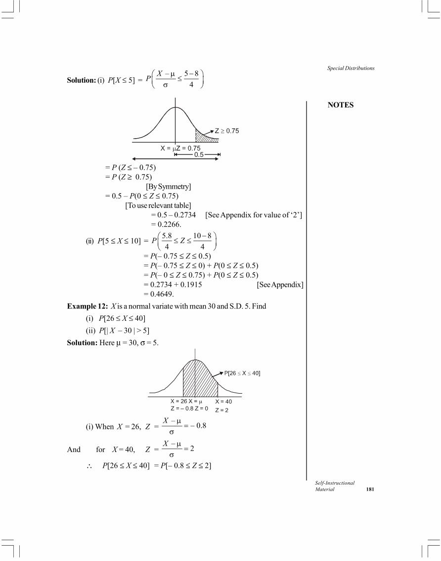
NOTES
Self-InstructionalMaterial 181
Special Distributions
Solution: (i) P[X 5] = – 5 8
4XP µ − ≤ σ
0.5
= P (Z – 0.75)= P (Z 0.75)
[By Symmetry]= 0.5 – P(0 Z 0.75)
[To use relevant table]= 0.5 – 0.2734 [See Appendix for value of ‘2’]= 0.2266.
(ii) P[5 X 10] = 5.8 10 84 4
P Z − ≤ ≤
= P(– 0.75 Z 0.5)= P(– 0.75 Z 0) + P(0 Z 0.5)= P(– 0 Z 0.75) + P(0 Z 0.5)= 0.2734 + 0.1915 [See Appendix]= 0.4649.
Example 12: X is a normal variate with mean 30 and S.D. 5. Find(i) P[26 X 40](ii) P[| X – 30 | > 5]
Solution: Here = 30, = 5.
Z = – 0.8 Z = 0X = 40Z = 2
(i) When X = 26, Z = – – 0.8X µ
=σ
And for X = 40, Z = – 2X µ
=σ
P[26 X 40] = P[– 0.8 Z 2]

Special Distributions
NOTES
Self-Instructional182 Material
= P[0 Z 0.8] + P[0 Z 2]= 0.2881 + 0.4772 = 0.7653
(ii) P[| X – 3 | > 5] = 1 – P[| X – 3 | 5]P[| X – 3 | 5] = P[25 X 35]
= 25 30
5P Z− 35 − 30 ≤ ≤ 5
= 2.P (0 Z 1) = 0.= 2 × 0.3413 = 0.6826.
So P[| X – 3| > 5] = 1 – P[| X – 3 | 5]= 1 – 0.6826 = 0.3174.
Central Limit Theorem
Let X1, X2,.... Xn be n independent random variables all of which have thesame distribution. Let the common expectation and variance be and 2respectively.
Let X = 1
ni
i
Xn=
∑
Then, the distribution of X approches the normal distribution with mean m
and variance 2
nσ
as n
That is, the variate Z = /
Xn
− µσ
has standard normal distribution.
Proof: Moment generating function of Z about origin is given as follows:
MZ(t) = E(etZ) = –
/Xt
nE e µ σ
= – / /( )t n t ne E eµ σ × σ
= 1 2 ...
–.
nt n X X Xnt ne E e+ + +
µ σ σ
= 1 2( ... )–
.n
tn X X Xt ne E e+ + +µ σσ

NOTES
Self-InstructionalMaterial 183
Special Distributions
= –
1 2. ( ... ) .nt
nte M X X X
n
µσ + + +
σ
= –
.
n
ntx
te Mt
n
µσ
σ σ
This is because the random variables are independent and have the sameMGF by using logarithms, you have:
log Mz(t) = log xt n tn M
n − µ
+ σ σ
= 2
2log 1 ...2 !
t n t t inn n
1 − µ µ′ µ′ + + + + σ σ σ
= 22
22
1. ... – ... ...2 ! 2
t n t t t tnn nn
1 1 − µ µ′ µ′ µ′ + + + + + σ σ σσ
= 22 2
2 12 2– ...
2 2t n t n t t1− µ µ′ µ′ µ′
+ + +σ σ σ σ
= 2
– 1/ 2( )2t O n+ [ 2 – 1
2 = 21 = ]
Hence, as n
log(Mz)(t) 2
2t
i.e. M2(t) = et2/2
However, this is the M.G.F. of a standard normal random variable. Thus,the random variable Z converges to N.
This follows that the limiting distribution of x as normal with mean and
variance 2
nσ .
Normal Approximation
Under certain circumstance one can use normal distribution to approximate abinomial distribution as well as Poisson distribution.

Special Distributions
NOTES
Self-Instructional184 Material
If X ~ B(n, p) and value of n is quite large with p quite close to ½, then, Xcan be approximated as N (np, npq), where q = 1 – p.
There are cases in which use of normal distribution is found to be easierthan that of a Binomial distribution.
Also, as already told, normal distribution may also be utilized forapproximating Poisson distribution when value of is large. Here, is the meanof Poisson distribution.
Thus, X ~ Po( ) X ~ N( , ) approximately when values of is large.Continuity Correction
Normal distribution is continuous whereas both the distributions, Binomial as wellas Poisson are discrete random variables. This fact has to be kept in mind whilemaking use of normal distribution for approximating Binomial or Poisson distributionand use continuity correction.
Each probability, in case of discrete distribution, is represented using arectangle as shown in the Figure 7.2(b).
Fig. 7.2 (a) Continuous Distribution
Fig. 7.3 (b) Discrete Distribution
While working out for probabilities, we like inclusion of the whole rectanglesin applying continuity correction.Example 13: A fair coin is tossed 20 times. Find the probability of getting between9 and 11 heads.Solution: Let the random variable be represented by X that shows the number ofheads thrown.
X ~ Bin(20, ½)

NOTES
Self-InstructionalMaterial 185
Special DistributionsAs p is very near to ½, normal approximation can be used for the binomialdistribution and we may write as X ~ N(20 × ½, 20 × ½ × ½) X ~ N(10, 5).
In the diagram as shown in below rectangles show binomial distributionwhich is discrete and curve shows normal distribution which is continuous in nature.
Using normal distribution for showing Binomial distributionIf it is desired to have P(9 X 11) as shown by shaded area one may
note that first rectangle begins at 8.5 and last rectangle terminates at 11.5. Bymaking a continuity correction, probability becomes P(8.5 < X < 11.5) in normaldistribution. We may standardize this, as given below:
= 9 10 – 10 11 10
55 5XP − − < <
= P (– 0.447 < Z < 0.447)
= 2 × 0.67 – 1 (using tables) = 0.34
Check Your Progress
13. What is a normal distribution?14. Explain any four characteristics of normal distribution.15. Define a standard normal variate.
7.6 ANSWERS TO CHECK YOUR PROGRESSQUESTIONS
1. Because of the factorial function in the denominator, the Erlang distributionis only defined when the parameter k is a positive integer. In fact, thisdistribution is sometimes called the Erlang-k distribution.
2. This formula is much more difficult and is often used to calculate how longcallers will have to wait before being connected to a human in a call centreor similar situation.

Special Distributions
NOTES
Self-Instructional186 Material
3. Chi-square test is a non-parametric test of statistical significance for bivariatetabular analysis. Chi-square tests enable us to test whether more than twopopulation proportions can be considered equal.
4. The degree of freedom is determined by the number of constraints. If thereare 10 frequency classes and there is one independent constraint, then thereare 10 – 1 = 9 degrees of freedom.
5. Before the application of chi-square test, the following conditions need to besatisfied:(i) Observations recorded and used are collected on a random basis.
(ii) All the members or items in the sample must be independent.(iii) No group should contain very few items say less than 10. In cases where
the frequencies are less than 10, regrouping is done by combining thefrequencies of adjoining groups so that the new frequencies becomegreater than 10.
(iv) The overall number of items must be reasonably large; it should at leastbe 50 howsoever small the number of groups may be.
(v) The constraints must be linear. Constraints, which involve linear equationsin the cell frequencies of a contingency table, are known as linearconstraints.
6. Chi-square test is applicable in large number of problems. These include:(i) Testing the goodness of fit.
(ii) Testing the homogeneity of a number of frequency distributions.(iii) Testing the significance of association between two attributes.(iv) Establishing hypotheses.(v) Testing independence between two variables.
7. Goodness of fit describes that how well the theoretical distribution fits withthe observed data.
8. The various steps involved in the chi-square test are:(i) Calculation of the expected frequencies.
(ii) Obtaining the difference between observed and expected frequenciesand finding out the squares of these differences.
(iii) Dividing the quantity (f0 – f
e)2 obtained in the result by the corresponding
expected frequency to get 2
0( )e
e
f ff .
(iv) Finding summation of 2
0( )e
e
f ff values also called as required 2 value,
and is represented as 2
0( )e
e
f ff .

NOTES
Self-InstructionalMaterial 187
Special Distributions9. The alternative method of calculating the value of chi-square is used in thecase of a (2 2) table. The cell frequencies and marginal totals of a (2 2)table are written as follows:
a b
c d
( )a + b
( )c + d
( ) a + c ( )b + d N
The alternative formula for calculating the value of 2 is:
2 = 2( )
( )( )( )( )ad bc N
a c b d a b c d
Where, N means the total frequency, ad means the larger cross product, bcmeans the smaller cross product and (a + c), (b + d), (a + b) and (c + d) arethe marginal totals.
10. F. Yates has suggested a correction in 2 value calculated in connection witha (2 2) table particularly when cell frequencies are small and 2 is just onthe significance level. The correction suggested by Yates is popularly knownas Yates’ correction. It involves the reduction of the deviation of observedfrom expected frequencies, which of course reduces the value of 2. Therule for correction is to adjust the observed frequency in each cell of a (2 2)table in such a way as to reduce the deviation of the observed from theexpected frequency for that cell by 0.5, and this adjustment is made in all thecells without disturbing the marginal totals.
11. It is an important property of 2. This means that several values of 2 can beadded together and if the degrees of freedom are also added, this numbergives the degrees of freedom of total value of 2. Thus, if a number of 2
values have been obtained from a number of samples of similar data, thenbecause of the additive nature of 2 we can combine the various values of 2
by just simply adding them.12. The important characteristics of chi-square test are:
(i) This test is based on frequencies and not on the parameters like meanand standard deviation.
(ii) This test is used for testing the hypothesis.(iii) This test possesses the additive property.(iv) This test can also be applied to a complex contingency table with several
classes and as such is a very useful test in research work.(v) This test is an important non-parametric test as no rigid assumptions are
necessary in regard to the type of population.. F. Yates has suggested acorrection in 2 value calculated in connection with a (2 2) tableparticularly when cell frequencies are small and 2 is just on thesignificance level. The correction suggested by Yates is popularly knownas Yates’ correction. It involves the reduction of the deviation of observed
Special Distributions
NOTES
Self-Instructional188 Material
from expected frequencies, which of course reduces the value of 2.The rule for correction is to adjust the observed frequency in each cell ofa (2 2) table in such a way as to reduce the deviation of the observedfrom the expected frequency for that cell by 0.5, and this adjustment ismade in all the cells without disturbing the marginal totals.
13. It is an important property of 2. This means that several values of 2 can beadded together and if the degrees of freedom are also added, this numbergives the degrees of freedom of total value of 2. Thus, if a number of 2
values have been obtained from a number of samples of similar data, thenbecause of the additive nature of 2 we can combine the various values of 2
by just simply adding them.14. The important characteristics of chi-square test are:
(i) This test is based on frequencies and not on the parameters like meanand standard deviation.
(ii) This test is used for testing the hypothesis.(iii) This test possesses the additive property.(iv) This test can also be applied to a complex contingency table with several
classes and as such is a very useful test in research work.(v) This test is an important non-parametric test as no rigid assumptions are
necessary in regard to the type of population.15. A normal variate with mean zero and standard deviation unity, is called a
standard normal variate.
7.7 SUMMARY
The Erlang distribution is a continuous probability distribution with wideapplicability primarily due to its relation to the Exponential and Gammadistributions.The Erlang distribution, which measures the time between incoming calls,can be used in conjunction with the expected duration of incoming calls toproduce information about the traffic load measured in Erlang units.The Erlang distribution is the distribution of the sum of k independent andidentically distributed random variables each having an exponentialdistribution.Chi-square test is a non-parametric test of statistical significance for bivariatetabular analysis (also known as cross-breaks). Any appropriate test ofstatistical significance lets you know the degree of confidence you can havein accepting or rejecting a hypothesis.The constraints must be linear. Constraints which involve linear equations inthe cell frequencies of a contingency table (i.e., equations containing nosquares or higher powers of the frequencies) are known as linear constraints.

NOTES
Self-InstructionalMaterial 189
Special Distributions2 test enables us to see how well the distribution of observe data fits theassumed theoretical distribution such as Binomial distribution, Poissondistribution or the Normal distribution.Chi-square is also used to test the significance of population variance throughconfidence intervals, specially in case of small samples.
2 is used, at times, to test the significance of population variance ( p)2
through confidence intervals.The curve is asymptotic to the base line which means that it continues toapproach but never touches the horizontal axis.The normal distribution has only one mode since the curve has a singlepeak. In other words, it is always a unimodal distribution.
The distribution of a random variable –XZ µ
=σ
which is known as
standard normal variate, is called the standard normal distribution or unitnormal distribution, where X has a normal distribution with mean endvariance 2.Under certain circumstance one can use normal distribution to approximatea binomial distribution as well as Poisson distribution.Normal distribution is continuous whereas both the distributions, Binomialas well as Poisson are discrete random variables. This fact has to be kept inmind while making use of normal distribution for approximating Binomial orPoisson distribution and use continuity correction.
7.8 KEY WORDS
Erlang B distribution: This is the easier of the two distributions and canbe used in a call centre to calculate the number of trunks one need to carrya certain amount of phone traffic with a certain ‘target service’.Degrees of freedom: The number of independent constraints determinesthe number of degrees of freedom2 (or df). If there are 10 frequency classesand there is one independent constraint, then there are (10 – 1) = 9 degreesof freedom.
7.9 SELF-ASSESSMENT QUESTIONS ANDEXERCISES
Short-Answer Questions
1. What is meant by Gamma function?2. Explain stochastic process.

Special Distributions
NOTES
Self-Instructional190 Material
3. Explain chi-square test.4. Why is it considered an important test in statistical analysis?5. Describe the term ‘Degrees of Freedom’.6. Define the necessary conditions required for the application of test?7. What are the areas of application of chi-square test?8. How will you find the value of chi-square?9. Define Yates’ correction formula for chi-square.
10. Chi-square can be used as a test of population variance. Explain.11. Describe the additive properties of chi-square.12. Explain the important characteristics of chi-square test.13. Give the characteristics of normal distribution.14. Explain some examples of normal distribution.15. Define central limit theorem.
Long-Answer Questions
1. Briefly discuss about the Gamma distributions.2. What is Chi-square test? Explain its significance in statistical analysis.3. Write short notes on the following:
(i) Additive property of chi-square(ii) Chi-square as a test of ‘goodness of fit’
(iii) Precautions in applying chi-square test(iv) Conditions for applying chi-square test
4. On of the basis of information given below about the treatment of 200 patientssuffering from a disease, state whether the new treatment is comparativelysuperior to the conventional treatment.
Treatment No. of Patients
Favourable Response No Response
New 60 20
Conventional 70 50
For drawing your inference use the value of 2 for one degree of freedom atthe 5% level of significance, viz., 3.841.
5. 200 digits were chosen at random from a set of tables. The frequencies ofthe digits were:Digit 0 1 2 3 4 5 6 7 89Frequency 18 19 23 21 16 25 22 20 2115
Calculate 2.

NOTES
Self-InstructionalMaterial 191
Special Distributions6. The normal rate of infection for a certain disease in cattle is known to be50%. In an experiment with seven animals injected with a new vaccine itwas found that none of the animals caught infection. Can the evidence beregarded as conclusive (at 1% level of significance) to prove the value of thenew vaccine?
7. Result of throwing dice were recorded as follows:Number Falling
Upwards 1 2 3 4 5 6
Frequency 27 33 31 29 30 24
Is the dice unbiased? Answer on the basis of Chi-square test.8. (i) 1000 babies were born during a certain week in a city of which 600
were boys and 400 girls. Use 2 test to examine the correctness of thehypothesis that the sex ratio is 1:1 in newly born babies.
(ii) The percentage of smokers in a certain city was 90. A random sampleof 100 persons was selected in which 85 persons were found to besmokers. Is the sample proportion significantly different from theproportion of smokers in the city? Answer on the basis of chi-squaretest.
9. How to measure the area under the normal curve? Give examples also.10. Discuss about the standard normal distribution.
7.10 FURTHER READINGS
Hogg, Robert. V., Allen T. Craig and Joseph W. McKean. 2005. Introduction toMathematical Statistics. New Delhi: Pearson Education.
Fisz, Marek. 1963. Probability Theory and Mathematical Statistics, 3rd Edition.New York: John Wiley & Sons, Inc.
Rohatgi, Vijay K. 1985. An Introduction to Probability Theory andMathematical Statistics. New Delhi: Wiley Eastern Limited.
Gupta, C.B. and Vijay Gupta. 2004. An Introduction to Statistical Methods,23rd Edition. New Delhi: Vikas Publishing House.
Levin, Richard I. and David S. Rubin. 1998. Statistics for Management. NewJersey: Prentice Hall.
Chandan, J. S. 1998. Statistics for Business and Economics. New Delhi: VikasPublishing House Pvt. Ltd.
Campbell, Stephen K. 1987. Applied Statistics. New York: Harper & Row.Chance, William A. 1969. Statistical Methods for Decision Making. Illinois:
Richard D Irwin.Hooda, R. P. 2013. Statistics for Business and Economics, 5th Edition. New
Delhi: Vikas Publishing House Pvt. Ltd.

Distribution of Functionsof Random Variableand Sampling
NOTES
Self-Instructional192 Material
UNIT 8 DISTRIBUTION OFFUNCTIONS OF RANDOMVARIABLE AND SAMPLING
Structure8.0 Introduction8.1 Objectives8.2 Distribution of Functions of Random Variable8.3 Sampling Theory8.4 Transformation of Variable of the Discrete Type8.5 Answers to Check Your Progress Questions8.6 Summary8.7 Key Words8.8 Self-Assessment Questions and Exercises8.9 Further Readings
8.0 INTRODUCTION
One of the major objectives of the field of statistical analysis is to know the true oractual values of different parameters of population. The ideal situation would be totake the entire population into consideration in determining these values. However,that is not feasible due to cost, time, labour and other constraints. Accordingly,random samples of a given size are taken from the population and these samplesare properly analysed with the belief that the characteristics of these random samplesrepresent similar characteristics of the population from which these samples havebeen taken. The results obtained from such analyses lead to generalizations thatare considered to be valid for the entire population.
You will study two broad types of sampling: probability samples and non-probability samples. Probability samples involve simple random sampling andrestricted random sampling. Non-probability samples are characterized by non-random sampling. As simple random sampling is costly and time consuming,restricted random sampling is preferred. Sampling distribution of mean is aprobability distribution of all possible sample means of a given size selected froma population, while sampling distribution of proportions is a distribution ofproportions of all possible random samples of a fixed size.
In this unit, you will study about the distribution of functions of randomvariable, sampling theory and transformation of variable of the discrete type.

NOTES
Self-InstructionalMaterial 193
Distribution of Functionsof Random Variable
and Sampling8.1 OBJECTIVES
After going through this unit, you will be able to:Analyse the distribution of functions of random variableUnderstand the various sampling theoriesExplain the transformation of variable of the discrete type
8.2 DISTRIBUTION OF FUNCTIONS OF RANDOMVARIABLE
A random variable takes on different values as a result of the outcomes of a randomexperiment. In other words, a function which assigns numerical values to eachelement of the set of events that may occur (i.e., every element in the samplespace) is termed as random variable. The value of a random variable is the generaloutcome of the random experiment. One should always make a distinction betweenthe random variable and the values that it can take on. All these can be illustratedby a few examples shown in Table 8.1.
Table 8.1 Random Variable
Random Variable Values of the Description of the Values ofRandom Variable the Random Variable
X 0, 1, 2, 3, 4 Possible number of headsin four tosses of a fair coin
Y 1, 2, 3, 4, 5, 6 Possible outcomes in asingle throw of a die
Z 2, 3, 4, 5, 6, 7, 8, 9, 10, 11, 12 Possible outcomes fromthrowing a pair of dice
M 0, 1, 2, 3, . . . . . . . . . . . S Possible sales ofnewspapers by anewspaper boy,S representing his stock
All the stated random variable assignments cover every possible outcomeand each numerical value represents a unique set of outcomes. A random variablecan be either discrete or continuous. If a random variable is allowed to take ononly a limited number of values, it is a discrete random variable, but if it is allowedto assume any value within a given range, it is a continuous random variable.Random variables presented in Table 8.1 are examples of discrete randomvariables. We can have continuous random variables if they can take on any valuewithin a range of values, for example, within 2 and 5, in that case we write thevalues of a random variable x as,
2 x 5

Distribution of Functionsof Random Variableand Sampling
NOTES
Self-Instructional194 Material
Techniques of Assigning Probabilities
We can assign probability values to the random variables. Since the assignment ofprobabilities is not an easy task, we should observe following rules in this context:
(i) A probability cannot be less than zero or greater than one, i.e., 0 pr 1,where pr represents probability.
(ii) The sum of all the probabilities assigned to each value of the random variablemust be exactly one.
There are three techniques of assignment of probabilities to the values of the randomvariable that are as follows:
(i) Subjective Probability Assignment: It is the technique of assigningprobabilities on the basis of personal judgement. Such assignment maydiffer from individual to individual and depends upon the expertise of theperson assigning the probabilities. It cannot be termed as a rational wayof assigning probabilities, but is used when the objective methods cannotbe used for one reason or the other.
(ii) A-Priori Probability Assignment: It is the technique under which theprobability is assigned by calculating the ratio of the number of ways inwhich a given outcome can occur to the total number of possible outcomes.The basic underlying assumption in using this procedure is that every possibleoutcome is likely to occur equally. However, at times the use of this techniquegives ridiculous conclusions. For example, we have to assign probability tothe event that a person of age 35 will live upto age 36. There are twopossible outcomes, he lives or he dies. If the probability assigned inaccordance with a-priori probability assignment is half then the same maynot represent reality. In such a situation, probability can be assigned bysome other techniques.
(iii) Empirical Probability Assignment: It is an objective method of assigningprobabilities and is used by the decision-makers. Using this technique theprobability is assigned by calculating the relative frequency of occurrenceof a given event over an infinite number of occurrences. However, in practiceonly a finite (perhaps very large) number of cases are observed and relativefrequency of the event is calculated. The probability assignment through thistechnique may as well be unrealistic, if future conditions do not happen tobe a reflection of the past.Thus, what constitutes the ‘best’ method of probability assignment can onlybe judged in the light of what seems best to depict reality. It depends uponthe nature of the problem and also on the circumstances under which theproblem is being studied.

NOTES
Self-InstructionalMaterial 195
Distribution of Functionsof Random Variable
and Sampling
Probability Distribution Functions: Discrete and Continuous
When a random variable x takes discrete values x1, x2,...., xn with probabilitiesp1, p2,...,pn, we have a discrete probability distribution of X.
The function p(x) for which X = x1, x2,..., xn takes values p1, p2,....,pn, isthe probability function of X.
The variable is discrete because it does not assume all values. Its propertiesare:
p(xi) = Probability that X assumes the value x= Prob (x = xi) = pi
p(x) 0, p(x) = 1For example, four coins are tossed and the number of heads X noted. X can takevalues 0, 1, 2, 3, 4 heads.
p(X = 0) = 41 1
2 16 =
p(X = 1) = 3
41
1 1 42 2 16
C =
p(X = 2) = 2 2
42
1 1 62 2 16
C =
p(X = 3) = 3
43
1 1 42 2 16
C =
p(X = 4) = 4 0
44
1 1 12 2 16
C =
O0 1 2 3 4
616
516
416
316
216
116

Distribution of Functionsof Random Variableand Sampling
NOTES
Self-Instructional196 Material
4
2
1 4 6 4 1( ) 116 16 16 16 16x
p x=
= + + + + =∑
This is a discrete probability distribution.Example 1: If a discrete variable X has the following probability function, thenfind (i) a (ii) p(X 3) (iii) p(X 3).Solution: The solution is obtained as follows:
x1 p(xi)0 01 a2 2a3 2a2
4 4a2
5 2aSince p(x) = 1 , 0 + a + 2a + 2a2 + 4a2 + 2a = 1
6a2 + 5a – 1 = 0, so that (6a – 1) (a + 1) = 0
a = 16 or a = –1 (Not admissible)
For a = 16 , p(X 3) = 0 + a + 2a + 2a2 = 2a2 + 3a =
59
p(X 3) = 4a2 + 2a = 49
(v) Continuous Probability Distributions
When a random variate can take any value in the given interval a x b, it is acontinuous variate and its distribution is a continuous probability distribution.
Theoretical distributions are often continuous. They are useful in practicebecause they are convenient to handle mathematically. They can serve as goodapproximations to discrete distributions.
The range of the variate may be finite or infinite.A continuous random variable can take all values in a given interval. A
continuous probability distribution is represented by a smooth curve.The total area under the curve for a probability distribution is necessarily
unity. The curve is always above the x axis because the area under the curve forany interval represents probability and probabilities cannot be negative.
If X is a continous variable, the probability of X falling in an interval with endpoints z1, z2 may be written p(z1 X z2).

NOTES
Self-InstructionalMaterial 197
Distribution of Functionsof Random Variable
and Sampling
This probability corresponds to the shaded area under the curve in Figure 8.1.
z1 z2
Fig. 8.1 Continuous Probability Distribution
A function is a probability density function if,
–( ) 1, ( ) 0, – ,
∞
∞= > ∞ < < ∞∫ p x dx p x x i.e., the area under the curve p(x) is
1 and the probability of x lying between two values a, b, i.e., p(a < x < b) ispositive. The most prominent example of a continuous probability function is thenormal distribution.
Cumulative Probability Function (CPF)
The Cumulative Probability Function (CPF) shows the probability that x takes avalue less than or equal to, say, z and corresponds to the area under the curve upto z:
–( ) ( )
zp x z p x dx
∞≤ = ∫
This is denoted by F(x).
Extension to Bivariate Case: Elementary Concepts
If in a bivariate distribution the data is quite large, then they may be summed up inthe form of a two-way table. In this for each variable, the values are grouped intodifferent classes (not necessary same for both the variables), keeping in view thesame considerations as in the case of univariate distribution. In other words, abivariate frequency distribution presents in a table pairs of values of two variablesand their frequencies.
For example, if there is m classes for the X – variable series and n classesfor the Y – variable series then there will be m × n cells in the two-way table. Bygoing through the different pairs of the values (x, y) and using tally marks, we canfind the frequency for each cell and thus get the so called bivariate frequency tableas shown in Table 8.2.

Distribution of Functionsof Random Variableand Sampling
NOTES
Self-Instructional198 Material
Table 8.2 Bivariate Frequency Table
Total of Frequencies of x
ClassesTotal of Frequencies of y
Total = = N f fx y
fx
x Series
Y SeriesMid Points
x1 .... ..... m x x x1 .....
Cla
sses
Mid
Poi
nts
y1
2
.
.
.
.
y
y
yn
fy
Here, f (x,y) is the frequency of the pair (x, y). The formula for computingthe correlation coefficient between x and y for the bivariate frequency table is,
2 2 2 2
( , ) – ( )( )
– ( ) – ( )x y
N xyf x y xfx yfyrN x f xfx N y f yfy
Σ Σ Σ=
Σ Σ × Σ Σ
Where, N is the total frequency.
Check Your Progress
1. What is meant by subjective probability assignment?2. What is continuous probability distribution?
8.3 SAMPLING THEORY
A sample is a portion of the total population that is considered for study andanalysis. For instance, if we want to study the income pattern of professors at CityUniversity of New York and there are 10,000 professors, then we may take arandom sample of only 1,000 professors out of this entire population. Then thisnumber of 1,000 professors constitutes a sample. The summary measure thatdescribes a characteristic, such as average income of this sample is known as astatistic.Sampling is the process of selecting a sample from the population. It is technically andeconomically not feasible to take the entire population for analysis. So we must take
NOTES
Self-InstructionalMaterial 199
Distribution of Functionsof Random Variable
and Sampling
a representative sample out of this population for the purpose of such analysis. Asample is part of the whole, selected in such a manner as to be representingthe whole.
Random SampleIt is a collection of items selected from the population in such a manner that eachitem in the population has exactly the same chance of being selected, so that thesample taken from the population would be truly representative of the population.The degree of randomness of selection would depend upon the process of selectingthe items from the sample. A true random sample would be free from all biaseswhatsoever. For example, if we want to take a random sample of five studentsfrom a class of twenty-five students, then each one of these twenty-five studentsshould have the same chance of being selected in the sample. One way to do thiswould be writing the names of all students on separate but small pieces of paper,folding each piece of this paper in a similar manner, putting each folded piece intoa container, mixing them thoroughly and drawing out five pieces of paper from thiscontainer.
Sampling without ReplacementThe sample as taken in the previous example is known as sampling withoutreplacement, because each person can only be selected once so that once a pieceof paper is taken out of the container, it is kept aside so that the person whosename appears on this piece of paper has no chance of being selected again.
Sampling with ReplacementThere are certain situations in which the piece of paper once selected and takeninto consideration is put back into the container in such a manner that the sameperson has the same chance of being selected again as any other person. Forexample, if we are randomly selecting five persons for award of prizes so thateach person is eligible for any and all prizes, then once the slip of paper is drawnout of the container and the prize is awarded to the person whose name appearson the paper, the same piece of paper is put back into the container and the sameperson has the same chance of winning the second prize as anybody else.
Sample Selection
The third step in the primary data collection process is selecting an adequatesample. It is necessary to take a representative sample from the population, sinceit is extremely costly, time-consuming and cumbersome to do a complete census.Then, depending upon the conclusions drawn from the study of the characteristicsof such a sample, we can draw inferences about the similar characteristics of thepopulation. If the sample is truly representative of the population, then thecharacteristics of the sample can be considered to be the same as those of theentire population. For example, the taste of soup in the entire pot of soup can bedetermined by tasting one spoonful from the pot if the soup is well stirred. Similarly,

Distribution of Functionsof Random Variableand Sampling
NOTES
Self-Instructional200 Material
a small amount of blood sample taken from a patient can determine whether thepatient’s sugar level is normal or not. This is so because the small sample of bloodis truly representative of the entire blood supply in the body.Sampling is necessary because of the following reasons: First, as discussed earlier,it is not technically or economically feasible to take the entire population intoconsideration. Second, due to dynamic changes in business, industrial and socialenvironment, it is necessary to make quick decisions based upon the analysis ofinformation. Managers seldom have the time to collect and process data for theentire population. Thus, a sample is necessary to save time. The time element hasfurther importance in that if the data collection takes a long time, then the values ofsome characteristics may change over the period of time so that data may no longerbe up to date, thus defeating the very purpose of data analysis. Third, samples, ifrepresentative, may yield more accurate results than the total census. This is due tothe fact that samples can be more accurately supervised and data can be morecarefully selected. Additionally, because of the smaller size of the samples, the routineerrors that are introduced in the sampling process can be kept at a minimum. Fourth,the quality of some products must be tested by destroying the products. For example,in testing cars for their ability to withstand accidents at various speeds, theenvironment of accidents must be simulated. Thus, a sample of cars must be selectedand subjected to accidents by remote control. Naturally, the entire population of carscannot be subjected to these accident tests and hence, a sample must be selected.One important aspect to be considered is the size of the sample. The samplingsize—which is the number of sampling units selected from the population forinvestigation—must be optimum. If the sample size is too small, it may notappropriately represent the population or the universe as it is known, thus leadingto incorrect inferences. Too large a sample would be costly in terms of time andmoney. The optimum sample size should fulfil the requirements of efficiency,representativeness, reliability and flexibility. What is an optimum sample size isalso open to question. Some experts have suggested that 5 per cent of thepopulation properly selected would constitute an adequate sample, while othershave suggested as high as 10 per cent depending upon the size of the populationunder study. However, proper selection and representation of the sample is moreimportant than size itself. The following considerations may be taken into accountin deciding about the sample size:
(a) The larger the size of the population, the larger should be the sample size.(b) If the resources available do not put a heavy constraint on the sample size,
a larger sample would be desirable.(c) If the samples are selected by scientific methods, a larger sample size
would ensure greater degree of accuracy in conclusions.(d) A smaller sample could adequately represent the population, if the
population consists of mostly homogeneous units. A heterogeneous universewould require a larger sample.

NOTES
Self-InstructionalMaterial 201
Distribution of Functionsof Random Variable
and Sampling
Census and SamplingUnder the census or complete enumeration survey method, data is collected foreach and every unit (for example, person, consumer, employee, household,organization) of the population or universe which are the complete set of entitiesand which are of interest in any particular situation. In spite of the benefits of suchan all-inclusive approach, it is infeasible in most of the situations. Besides, the timeand resource constraints of the researcher, infinite or huge population, the incidentaldestruction of the population unit during the evaluation process (as in the case ofbullets, explosives etc) and cases of data obsolescence (by the time census ends)do not permit this mode of data collection.
Sampling is simply a process of learning about the population on the basisof a sample drawn from it. Thus, in any sampling technique, instead of every unitof the universe, only a part of the universe is studied and the conclusions aredrawn on that basis for the entire population. The process of sampling involvesselection of a sample based on a set of rules, collection of information and makingan inference about the population. It should be clear to the researcher that a sampleis studied not for its own sake, but the basic objective of its study is to drawinference about the population. In other words, sampling is a tool which helps usknow the characteristics of the universe or the population by examining only asmall part of it. The values obtained from the study of a sample, such as theaverage and dispersion are known as ‘statistics’ and the corresponding such valuesfor the population are called ‘parameters’.
Although diversity is a universal quality of mass data, every population hascharacteristic properties with limited variation. The following two laws of statisticsare very important in this regard.
1. The law of statistical regularity states that a moderately large number ofitems chosen at random from a large group are almost sure on theaverage to possess the characteristics of the large group. By randomselection, we mean a selection where each and every item of thepopulation has an equal chance of being selected.
2. The law of inertia of large numbers states that, other things being equal,larger the size of the sample, more accurate the results are likely to be.
Hence, a sound sampling procedure should result in a representative,adequate and homogeneous sample while ensuring that the selection of items shouldoccur independently of one another.
Sampling TechniquesThe various methods of sampling can be grouped under two broad categories:Probability (or random) sampling and Non-probability (or non-random) sampling.
Probability sampling methods are those in which every item in the universehas a known chance, or probability of being chosen for the sample. Thus, thesample selection process is objective (independent of the person making the study)

Distribution of Functionsof Random Variableand Sampling
NOTES
Self-Instructional202 Material
and hence, random. It is worth noting that randomness is a property of the samplingprocedure instead of an individual sample. As such, randomness can enterprocessed sampling in a number of ways and hence, random samples may be ofmany types. These methods include: (a) Simple Random Sampling, (b) StratifiedRandom Sampling, (c) Systematic Sampling and (d) Cluster Sampling.
Non-probability sampling methods are those which do not provide everyitem in the universe with a known chance of being included in the sample. Theselection process is, at least, partially subjective (dependent on the person makingthe study). The most important difference between random and non-randomsampling is that whereas the pattern of sampling variability can be ascertained incase of random sampling, there is no way of knowing the pattern of variability inthe non-random sampling process. The non-probability methods include:(a) Judgement Sampling, (b) Quota Sampling and (c) Convenience Sampling.
The following Figure 8.2 depicts the broad classification and sub-classification of various methods of sampling.
Fig. 8.2 Methods of Sampling
Non-Probability Sampling Methods
(a) Judgement Sampling: In this method of sampling, the choice of sampleitems depends exclusively on the judgement of the investigator. The samplehere is based on the opinion of the researcher, whose discretion will clinchthe sample. Though the principles of sampling theory are not applicable tojudgement sampling, it is sometimes found to be useful. When we want tostudy some unknown traits of a population, some of whose characteristicsare known, we may then stratify the population according to these knownproperties and select sampling units from each stratum on the basis ofjudgement. Naturally, the success of this method depends upon theexcellence in judgement.
(b) Convenience Sampling: A convenience sample is obtained by selectingconvenient population units. It is also called a chunk, which refers to that

NOTES
Self-InstructionalMaterial 203
Distribution of Functionsof Random Variable
and Sampling
fraction of the population being investigated, which is selected neither byprobability nor by judgement but by convenience. A sample obtained fromreadily available lists such as telephone directories is a convenience sampleand not a random sample, even if the sample is drawn at random from suchlists. In spite of the biased nature of such a procedure, convenience samplingis often used for pilot studies.
(c) Quota Sampling: Quota sampling is a type of judgement sampling and isperhaps the most commonly used sampling technique in non-probabilitycategory. In a quota sample, quotas (or minimum targets) are set upaccording to some specified characteristics, such as age, income group,religious or political affiliations, and so on. Within the quota, the selection ofthe sample items depends on personal judgement. Because of the risk ofpersonal prejudice entering the sample selection process, the quota samplingis not widely used in practical works.
It is worth noting that similarity between quota sampling and stratifiedrandom sampling is confined to dividing the population into different strata.The process of selection of items from each of these strata in the case ofstratified random sampling is random, while it is not so in the case of quotasampling. Quota sampling is often used in public opinion studies.
Probability Sampling Methods
The following are the probability sampling methods:(a) Simple Random Sampling(b) Stratified Random Sampling(c) Systematic Sampling(d) Multistage or Cluster Sampling
Simple Random SamplingIt refers to that sampling technique in which each and every unit of the populationhas an equal chance of being selected in the sample. One should not mistake theterm ‘arbitrary’ for ‘random’. To ensure randomness, one may adopt either thelottery method or consult the table of random numbers, preferably the latter. Beinga random method, it is independent of personal bias creeping into the analysisbesides enhancing the representativeness of the sample. Furthermore, it is easy toassess the accuracy of the sampling estimates because sampling errors follow theprinciples of chance. However, a completely catalogued universe is a prerequisitefor this method. The sample size requirements would be usually larger underrandom sampling than under stratified random sampling, to ensure statisticalreliability. It may escalate the cost of collecting data as the cases selected byrandom sampling tend to be too widely dispersed geographically.

Distribution of Functionsof Random Variableand Sampling
NOTES
Self-Instructional204 Material
Stratified Random SamplingIn this method, the universe to be sampled is subdivided (stratified) into groupswhich are mutually exclusive, but collectively exhaustive based on a variable knownto be correlated with the variable of interest. Then, a simple random sample ischosen independently from each group. This method differs from simple randomsampling in that, in the latter the sample items are chosen at random from the entireuniverse. In stratified random sampling, the sampling is designed in such a waythat a designated number of items is chosen from each stratum. If the ratio ofitems between various strata in the population matches with the ratio ofcorresponding items between various strata in the sample, it is called proportionatestratified sampling; otherwise, it is known as disproportionate stratified sampling.Ideally, we should assign greater representation to a stratum with a larger dispersionand smaller representation to one with small variation. Hence, it results in a morerepresentative sample than simple random sampling.
Systematic SamplingIt is also known as quasi-random sampling method because once the initial startingpoint is determined, the remainder of the items selected for the sample arepredetermined by the sampling interval. A systematic sample is formed by selectingone unit at random and then selecting additional units at evenly spaced intervalsuntil the sample has been formed. This method is popularly used in those caseswhere a complete list of the population from which sample is to be drawn isavailable. The list may be prepared in alphabetical, geographical, numerical orsome other order. The items are serially numbered. The first item is selected atrandom generally by following the lottery method. Subsequent items are selectedby taking every Kth item from the list where ‘K’ stands for the sampling interval orthe sampling ratio, i.e., the ratio of the population size to the size of the sample.
Symbolically,K = N / n , where K = Sampling Interval; N = Universe Size; n = Sample
Size. In case K is a fractional value, it is rounded off to the nearest integer.
Cluster SamplingUnder this method, the random selection is made of primary, intermediate andfinal (or the ultimate) units from a given population or stratum. There are severalstages in which the sampling process is carried out. At first, the stage units aresampled by some suitable method such as simple random sampling. Then, a sampleof second stage units is selected from each of the selected first stage units, byapplying some suitable method which may or may not be the same methodemployed for the first stage units. For example, in a survey of 10,000 householdsin AP, we may choose a few districts in the first stage, a few towns/villages/mandalsin the second stage and select a number of households from each town/village/mandal selected in the previous stage. This method is quite flexible and isparticularly useful in surveys of underdeveloped areas, where no frame is generally
NOTES
Self-InstructionalMaterial 205
Distribution of Functionsof Random Variable
and Sampling
sufficiently detailed and accurate for subdivision of the material into reasonablysmall sampling units. However, a multistage sample is, in general, less accuratethan a sample containing the same number of final stage units which have beenselected by some suitable single stage process.
Sampling and Non-Sampling Errors
The basic objective of a sample is to draw inferences about the population fromwhich such sample is drawn. This means that sampling is a technique which helpsus in understanding the parameters or the characteristics of the universe or thepopulation by examining only a small part of it. Therefore, it is necessary that thesampling technique be a reliable one. The randomness of the sample is especiallyimportant because of the principle of statistical regularity, which states that a sampletaken at random from a population is likely to possess almost the samecharacteristics as those of the population. However, in the total process of statisticalanalysis, some errors are bound to be introduced. These errors may be the samplingerrors or the non-sampling errors. The sampling errors arise due to drawing faultyinferences about the population based upon the results of the samples. In otherwords, it is the difference between the results that are obtained by the samplestudy and the results that would have been obtained if the entire population wastaken for such a study, provided that the same methodology and manner wasapplied in studying both the sample as well as the population. For example, if asample study indicates that 25 per cent of the adult population of a city does notsmoke and the study of the entire adult population of the city indicates that 30 percent are non-smokers, then this difference would be considered as the samplingerror. This sampling error would be smallest if the sample size is large relative tothe population, and vice versa.
Non-sampling errors, on the other hand, are introduced due to technicallyfaulty observations or during the processing of data. These errors could also arisedue to defective methods of data collection and incomplete coverage of thepopulation, because some units of the population are not available for study,inaccurate information provided by the participants in the sample and errorsoccurring during editing, tabulating and mathematical manipulation of data. Theseare the errors which can arise even when the entire population is taken understudy.
Both the sampling as well as the non-sampling errors must be reduced to aminimum in order to get as representative a sample of the population as possible.
Theory of EstimationThe theory of estimation is a very common and popular statistical method and isused to calculate the mathematical model for the data to be considered. Thismethod was introduced by the statistician Sir R. A. Fisher, between 1912 and1922. This method can be used in:
• Finding linear models and generalized linear models

Distribution of Functionsof Random Variableand Sampling
NOTES
Self-Instructional206 Material
• Exploratory and confirmatory factor analysis• Structural equation modelling• Calculating time-delay of arrival (TDOA) in acoustic or electromagnetic
detection• Data modelling in nuclear and particle physics• Finding the result for hypothesis testing
The method of estimation is used with known mean and variance. The samplemean becomes the maximum likelihood estimator of the population mean, and thesample variance becomes the close approximation to the maximum likelihoodestimator of the population variance.
Interval Estimate of the Population Mean (Population Variance Known)
Since the sample means are normally distributed, with a mean of and a standarddeviation of xσ , it follows that sample means follow normal distributioncharacteristics. Transforming the sampling distribution of sample means into thestandard normal distribution, we get:
-
-
x
x
x
xZ
or x Z
or x Z
− µ=
σ
µ = σ
µ = σ
Since falls within a range of values equidistant from x ,
xx Zµ = ± σ
This relationship is shown in the following illustration.
X1 X2Xµ
Zσx Zσx
This means that the population mean is expected to lie between the values of x1
and x2 which are both equidistant from x and this distance depends upon thevalue of Z which is a function of confidence level.
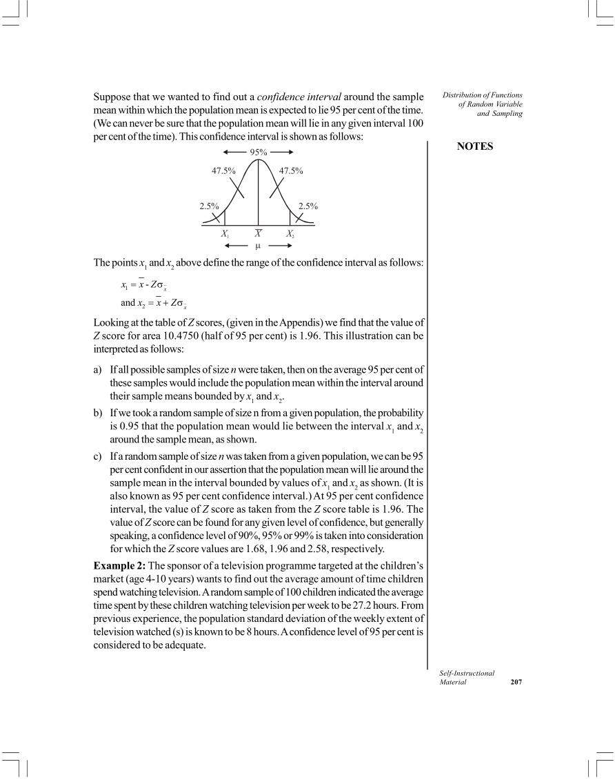
NOTES
Self-InstructionalMaterial 207
Distribution of Functionsof Random Variable
and Sampling
Suppose that we wanted to find out a confidence interval around the samplemean within which the population mean is expected to lie 95 per cent of the time.(We can never be sure that the population mean will lie in any given interval 100per cent of the time). This confidence interval is shown as follows:
X1 X2Xµ
47.5%
95%
47.5%
2.5% 2.5%
The points x1 and x2 above define the range of the confidence interval as follows:
1
2
-
and x
x
x x Z
x x Z
= σ
= + σ
Looking at the table of Z scores, (given in the Appendis) we find that the value ofZ score for area 10.4750 (half of 95 per cent) is 1.96. This illustration can beinterpreted as follows:
a) If all possible samples of size n were taken, then on the average 95 per cent ofthese samples would include the population mean within the interval aroundtheir sample means bounded by x1 and x2.
b) If we took a random sample of size n from a given population, the probabilityis 0.95 that the population mean would lie between the interval x1 and x2around the sample mean, as shown.
c) If a random sample of size n was taken from a given population, we can be 95per cent confident in our assertion that the population mean will lie around thesample mean in the interval bounded by values of x1 and x2 as shown. (It isalso known as 95 per cent confidence interval.) At 95 per cent confidenceinterval, the value of Z score as taken from the Z score table is 1.96. Thevalue of Z score can be found for any given level of confidence, but generallyspeaking, a confidence level of 90%, 95% or 99% is taken into considerationfor which the Z score values are 1.68, 1.96 and 2.58, respectively.
Example 2: The sponsor of a television programme targeted at the children’smarket (age 4-10 years) wants to find out the average amount of time childrenspend watching television. A random sample of 100 children indicated the averagetime spent by these children watching television per week to be 27.2 hours. Fromprevious experience, the population standard deviation of the weekly extent oftelevision watched (s) is known to be 8 hours. A confidence level of 95 per cent isconsidered to be adequate.

Distribution of Functionsof Random Variableand Sampling
NOTES
Self-Instructional208 Material
Solution:
X1 X2X = 27.2µ = 8
1.96σX 1.96σX
The confidence interval is given by:
or -x x xx Z x Z x Z± σ σ < µ < + σ
Where x nσ
σ =
Accordingly, we need only four values, namely x , Z, and n. In our case:
27.21.968100
xZ
n
==
σ ==
Hence 8 8 .8
10100x nσ
σ = = = =
Then:
1 -27.2 - (1.96 .8) 27.2 -1.56825.632
xx x Z= σ
= × ==
And
2
27.2 (1.96 .8) 27.2 1.56828.768
xx x Z= + σ
= + × = +=
This means that we can conclude with 95 per cent confidence that a child on anaverage spends between 25.632 and 28.768 hours per week watching television.(It should be understood that 5 per cent of the time our conclusion would still bewrong. This means that because of the symmetry of distribution, we will be wrong2.5 per cent of the times because the children on an average would be watchingtelevision more than 28.768 hours and another 2.5 per cent of the time we will bewrong in our conclusion, because on an average, the children will be watchingtelevision less than 25.632 hours per week.)

NOTES
Self-InstructionalMaterial 209
Distribution of Functionsof Random Variable
and Sampling
Example 3: Calculate the confidence interval in the previous problem, if we wantto increase our confidence level from 95% to 99%. Other values remain the same.Solution:
X1 X2X = 27.2σ = 8
2.58σX
.495
2.58σX
.495
.005 .005
If we increase our confidence level to 99 per cent, then it would be natural toassume that the range of the confidence interval would be wider, because wewould want to include more values which may be greater than 28.768 or smallerthan 25.632 within the confidence interval range. Accordingly, in this new situation,
2.58 .8x
Z =σ =
Then
1 - 27.2 - (2.58 .8) 27.2 - 2.064 25.136
xx x Zx
= σ
= ==
And
2
27.2 2.064 29.264
xX x Z= + σ
= +=
(The value of Z is established from the table of Z scores against the area of .495 ora figure closest to it. The table shows that the area close to .495 is .4949 for whichthe Z score is 2.57 or .4951 for which the Z score is 2.58. In practice, the Z scoreof 2.58 is taken into consideration when calculating 99 per cent confidence interval.)
Interval Estimate of the Population Mean (Population Variance Unknown)
As the previous example shows, in order to determine the interval estimate of ,the variance (and hence, the standard deviation) must be known, since it figures inthe formula. However, the standard deviation of the population is generally notknown. In such situations and when sample size is reasonably large (30 or more),we can approximate the population standard deviation ( ) by the sample standarddeviation (s), so that the confidence interval,

Distribution of Functionsof Random Variableand Sampling
NOTES
Self-Instructional210 Material
is approximated by the interval.
, when 30.
where and .
x
x
x x
x Z
x Zs nss
n n
± σ
± ≥
σσ = =
Example 4: It is desired to estimate the average age of students who graduatewith an MBA degree in the university system. A random sample of 64 graduatingstudents showed that the average age was 27 years with a standard deviation of 4years.a) Estimate a 95 per cent confidence interval estimate of the true average
(population mean) age of all such graduating students at the university.b) How would the confidence interval limits change if the confidence level was
increased from 95 per cent to 99 per cent.Solution: Since the sample size n is sufficiently large, we can approximate thepopulation standard deviation by the sample standard deviation.(a)
X1 X2X = 27s = 8
Now,1.96
274 4 0.5
864x
Z
xssn
=
=
= = = =
95% confidence interval of population mean is given by:
xx Zs±
So that,
1
27 (1.96 .5) 27 0.98 26.02
xx x Zsx
= −
= − = −=
And
2
=27+0.98 =27.98
xx x Zs= +
Hence, 26.02 27.98.≥ µ ≥

NOTES
Self-InstructionalMaterial 211
Distribution of Functionsof Random Variable
and Sampling
(b) .5xs =
X1 X2X = 27
2.58σX 2.58σX
s = .5 X
Now, Z becomes 2.58 and the other values remain the same. Hence,
1
27 (2.58 .5) 27 1.29 25.71
xx x Zsx
= −
= − = −=
And
2
27 1.29 28.29
xx x Zs= +
= +=
Hence, 25.71 28.29.≤ ≤µ
Sample Size Determination for Estimating the Population Mean
It is understood that the larger the sample size, the closer the sample statistic willbe to the population parameter. Hence, the degree of accuracy we require in ourestimate would be one factor influencing our choice of sample size. The secondelement that influences the choice of the sample size is the degree of confidence inourselves that the error in the estimate remains within the degree of accuracy thatis desired. Hence, the degree of accuracy has two aspects.1. The maximum allowable error in our estimate2. The degree of confidence that the error in our estimate will not exceed the
maximum allowable errorThe ideal situation would be that the sample mean x equals the population mean
That would be the best estimate of based on x . If the entire population wastaken as a sample then x will be equal to and there will be no error in ourestimate. Hence, ( x - ) can be considered as error or deviation of the estimatorx from the population mean This maximum allowable error must be pre-established. Let this error be denoted by E, so that:
( )E x= −µ
Now, we know that

Distribution of Functionsof Random Variableand Sampling
NOTES
Self-Instructional212 Material
/
/
x
xZ
xn
En
− µ=
σ
− µ=
σ
=σ
Or
2 2 2
2 or
E nZ
Z E nZnE
Z ZnE E
=σ
σ =σ
=
σ σ =
Based upon this formula, it can be seen that the size of the sample depends upon:
(a) Confidence interval desired. This will determine the value of Z. For example,95 per cent confidence level yields the value of Z to be = 1.96.
(b)Maximum error allowed (E)(c) The standard deviation of the population ( )
It can further be seen from this formula that the sample size will increase if:
(a) The allowable error becomes smaller(b)The degree of confidence increases(c) The value of the variance within the population is largerExample 5: We would like to know the average time that a child spends watchingtelevision over the weekend. We want our estimate to be within ± 1 hour of thetrue population average. (This means that the maximum allowable error is 1 hour.)Previous studies have shown the population standard deviation to be 3 hours.What sample size should be taken for this purpose, if we want to be 95 per centconfident that the error in our estimate will not exceed the maximum allowableerror?Solution: For 95 per cent confidence level, the values of
Z = 1.96E = 1 hour (given)
= 3 hours (given)

NOTES
Self-InstructionalMaterial 213
Distribution of Functionsof Random Variable
and Sampling
Then,2 2
2
2 2
2
(1.96) (3) (1)
34.57
ZnE
σ=
=
=
To be more accurate in our estimate, we always round off the answer to the nexthigher figure from the decimal. Hence, n = 35.
Confidence Interval Estimation of Population Proportion
So far we have discussed the estimation of population mean, which is quantitativein nature. This concept of estimation can be extended to qualitative data where thedata is available in proportion or percentage form. In this situation the parameterof interest is , which is the proportion of times a certain desirable outcome occurs.This concept lends itself to binomial distribution where we label the outcome ofinterest to us as success with the probability of success being and the probabilityof failure being ( )1− π .
When large samples of size n are selected from a population having a proportionof desirable outcomes , then the sampling distribution of proportions is normallydistributed. For large samples, when (np) as well as (nq) are both at least equal to5, where n is the sample size, p is the probability of a desired outcome (or success)and q is the probability of failure (1-p), then the binomial distribution can also beapproximated to normal distribution, with a mean of and a standard deviation ofσp , where σp is given by:
(1 )p n
π − πσ =
In such cases, we expect 95 per cent of all sample proportions to fall within thefollowing range:
1.96 pπ ± σ
Or
π(1 π)π 1.96n−
±
Similarly, 99 per cent of all such sample proportions will fall within
π(1 π)π 2.58n−
±

Distribution of Functionsof Random Variableand Sampling
NOTES
Self-Instructional214 Material
If all possible samples of size n are selected and the interval 1.96 pp σ± isestablished for each sample, where p is the sample proportion, then 95 per cent ofall such intervals are expected to contain , the population proportion. Then thisrange of,
1.96 pp σ±
Or
π(1 π)1.96pn−
±
Is known as the 95 per cent confidence interval estimate of This formula requires that we know the value of in order to calculate p. But,population proportion is generally not known. In such instances, the sampleproportion is used as an approximation of . Hence, the 95 per cent confidenceinterval estimate of becomes:
1.96 σ pp ±
Where
(1 )p
p pn−
σ =
And 99 per cent confidence interval estimate of becomes:
2.58 pp σ±
Example 6: A survey of 500 persons shopping at a mall, selected at random,showed that 350 of them used credit cards for their purchases and 150 of themused cash.(a) Construct a 95 per cent confidence interval estimate of the proportion of all
persons at the mall, who use credit card for shopping.(b) What would our confidence level be, if we make the assertion that the proportion
of shoppers at the mall who shop with a credit card is between 67 per centand 73 per cent.
Solution: (a) There are 350 people out of a total sample of 500 who pay bycredit card. Hence, the sample proportion of credit card shoppers is:
p = 350/500 = 0.7.
The 95 per cent confidence interval estimate of population proportion is givenas follows:
1.96 σ pp ±

NOTES
Self-InstructionalMaterial 215
Distribution of Functionsof Random Variable
and Sampling
Where,
(1 )p
p pn
σ −=
(Since is not known, we approximate sample proportion p for populationproportion ).
Then,.7(.3)σ .00042 .02500p = = =
Then the confidence limits are:
1
2
–1.96 =.7 –1.96(.02) =.7 – .0392 = .6608 or 66.08%, and
1.96 σ =.7+.0392=.7392 or 73.92%.
p
p
p p
p p
σ=
= +
p1 p2p = 27.6608 .7392σ = .02
This means that the population of people who pay by credit card at the mall isbetween 66.8 per cent and 73.92 per cent.(b) If the population proportion of credit card shoppers is given to be between.67 and .73, when such sample proportion p is .70, then
p1 p2p = .7.67 .73
.4332 .4332
1
1
– Z.67 =.7 – Z (0.2).02 =.7 – .67
.7 – .67 .03 = 1.5.02 .02
pp p
Z
Z
σ=
= =

Distribution of Functionsof Random Variableand Sampling
NOTES
Self-Instructional216 Material
Similarly,
2
2
= + σ
.73 =.7 + (.02).73 – .7 .03 = = =1.5
.02 .02
pp p ZZ
Z
Using the Z score table, we see that the area under the curve for Z=1.5 is .4332.This area is on each side of the mean so that the total area is .8664. In otherwords, our confidence level is 86.64 per cent that the proportion of shoppersusing credit card is between 67 per cent and 73 per cent.
Sample Size Determination for Estimating the Population Proportion
We follow the same procedure as we did in determining the sample size for estimatingthe population mean. As before, there are three factors that are taken intoconsideration. These are:
(a) The level of confidence desired(b) The maximum allowable error permitted in the estimate(c) The estimated population proportion of success
As established previously, – π=σ p
pZ
Whereπ(1 – π)σ =
σpp
Now, (p- ) can be considered as error (E), so that:
= π(1 π)
EZ
n−
By cross-multiplication we get,
π(1 π) E Zn−
=
Squaring both sides we get,2
2
2 2
2
2
π(1 π)
or π(1 π)Z π(1 π)or =
ZEn
nE Z
nE
−=
= −
−

NOTES
Self-InstructionalMaterial 217
Distribution of Functionsof Random Variable
and Sampling
This formula assumes that we know , the population proportion, which we aretrying to estimate in the first place. Accordingly, is unknown. However, if anyprevious studies have estimated this value or a sample proportion p has beencalculated in previous studies, then we can approximate this p for and hence,
2
2
(1 )Z p pnE
−=
However, if no previous surveys have been taken so that we do not know thevalue of or p, then we assume to be equal to 0.5, simply because, other thingsbeing given, the value of being 0.5 will result in a larger sample size than anyother value assumed by . Hence, the sample size would be at least as large orlarger than required for the given conditions. This can be established by the factthat when = 0.5, then (l - ) is .5 × .5 = 0.25. This value is larger than anyother value of (1 - ). This means that when = 0.5 then for a given value of Z,n would be larger than any other value of . This results in a more conservativeestimate which is desirable.Example 7: It is desired to estimate the proportion of children watching televisionon Saturday mornings, in order to develop a promotional strategy for electronicgames. We want to be 95 per cent confident that our estimate will be within ± 2per cent of the true population proportion.(a) What sample size should we take if a previous survey showed that 40 per
cent of children watched television on Saturday mornings?(b) What would be the sample size, for the same degree of confidence and the
same maximum allowable error, if no such previous survey had been taken?Solution: (a) In this case, the following values are given:
Z = 1.96 (95% confidence interval)p = 0.4E = 0.02
Substituting these values in the following formula, we get:2
2
2
2
(1 )
(1.96) (.4)(.6) = (.02)
0.922 = 0.0004
= 2304.96 = 2305
Z p pnE
−=
For the sake of accuracy, we always round off to the next higher figure, in case ofanswer being a fraction.

Distribution of Functionsof Random Variableand Sampling
NOTES
Self-Instructional218 Material
(b) In this case, since no previous surveys have been taken, we assume p = 0.5and follow the earlier procedure.
2
2
2
2
(1 )
(1.96) (.5)(.5) = (.02)
0.9604 = 0.0004
= 2401
Z p pnE
−=
8.4 TRANSFORMATION OF VARIABLE OF THEDISCRETE TYPE
A random variable is defined as a function from Ω to R, which constantly takes thenumerical values. Here, Ω is referred as the set of possible outcomes of a probabilityexperiment, consequently a random variable as a function can be written asX : Ω R, which specifies the method of assigning a numerical value to eachrespective outcome of the probability experiment. Generally, the outcome of aprobability experiment can be identified or known when the experiment is carriedout, therefore X or any another variable name is used for representing this outcomeof the experiment before actually knowing the exact value.
The following examples explain the concept of random variables. When acoin is flipped, then the possibility is that either there is the Head (H) or the Tail(T), however you can define the random variable associated/related with the flippingof coin as X, by means of
X (H) = 0X (T) = 1
Or,Y (H) = 1Y (T) = –1
The numerical values depend on the problem statistics, for example, whenthe coin is flipped in a chance game then the outcome as head gives Rupee 5 whilethe tail gives Rupee 8. The outcomes of the probability experiment, as heads andtails, can be represented by –8, 5 using the profit-loss concept. This can berepresented using W for the random variable signifying the winnings, by means of,
W : H, T 5, –8
NOTES
Self-InstructionalMaterial 219
Distribution of Functionsof Random Variable
and Sampling
A discrete random variable is the variable that takes values in a finite orcountable infinite subset of R. The value of the random variable for the specificrange can be denoted by I.Example 8: A coin is flipped three times. Find out the appearance of heads inthree flips and the range of random variable.Solution: Let X be the random variable which represents the number of timesheads can appear in the three flips.Then,
X : Ω 0, 1, 2, 3 RThe range of X is given by,
I = 0, 1, 2, 3
Example 9: Two dice are rolled simultaneously. What will be the random variableand the range for the maximum roll?Solution: Consider that the random variable is assumed or specified for themaximum roll when the two dice are rolled simultaneously. Assume that themaximum rolls are 6.Here,
X = Value on the First DieY = Outcome of the Second DieZ = max (X, Y) is the Random Variable to consider.
The range of Z is given by,I = 1, 2, 3, 4, 5, 6
The concept of the discrete random variable can be defined using:The probability mass function.The expected value of a random variable.The variance of a random variable.
1. For a discrete random variable, the probability mass function can be findusing the equation,f (k) = P (X = k) for k I
2. The expected value (expectation, mean) of a random variable can be definedusing the probability mass function,
= E (X) =

Distribution of Functionsof Random Variableand Sampling
NOTES
Self-Instructional220 Material
In this case, each outcome is subjective/weighted by its respectiveprobability. The expected value function is specifically written using the notationE[.] or E(.), and for the random variable we can use the notation (mu) for mean.
3. The variance can be defined as,2 = var (X) = E [(X – )2]
This definition defines the expected value of the square of the difference ofX from the mean . The var (.) function can be applied to any random variable,and the notation 2 defines which random variable is being evaluated.
Definition. Two discrete random variables X and Y are independent if for all x inthe range of X and all y in the range of Y, we have
P (X = x, Y = y) = P (X = x) P (Y = y)Here P denotes the probability. If X and Y are not independent, then this
may not be true for all combinations of x and y and hence there will be some event(X = x, Y = y) for which this equation is false.Example 10: A coin is flipped only once. Find the number of heads and tails.Specify that the discrete random variables is independent random variable.Solution: When the coin is flipped only once, then the probability of getting headsand tails on the same flip is zero, i.e., the events are mutually exclusive. Let X bethe number of heads and Y be the number of tails. Then,
P (X = 1) P (Y = 1) = 0.25It can be stated that the joint probability mass function of independent random
variables X and Y factors into the probability mass functions for X and Y.As per the definition of expected value the following fact can be proved for
the discrete random variables:If X and Y are independent random variables, thenE (XY) = E (X) E (Y)Provided that both E (X) and E (Y) exist and are finite.
Check Your Progress
3. Why is sampling without replacement so called?4. What do you mean by sampling with replacement?5. What is the main difference between the above two types of sampling?6. What are the two types of samples?7. What is meant by a simple random sample?8. Define the term discrete random variable.
NOTES
Self-InstructionalMaterial 221
Distribution of Functionsof Random Variable
and Sampling8.5 ANSWERS TO CHECK YOUR PROGRESS
QUESTIONS
1. It is the technique of assigning probabilities on the basis of personaljudgement. Such assignment may differ from individual to individual anddepends upon the expertise of the person assigning the probabilities.
2. When a random variate can take any value in the given interval a x b,it is a continuous variate and its distribution is a continuous probabilitydistribution.
3. Sampling without replacement is so called because in this process, eachperson or element can be selected only once and not replaced for anotherselection.
4. Sampling with replacement means the process where a specific person orelement can be selected once and can also be replaced for another selection.
5. Unlike in the case of sampling without replacement, the same element canget reselected in sampling with replacement.
6. The two types of samples are:(a) Probability Samples(b) Non-Probability Samples
7. A simple random sample is the one in which each and every unit of thepopulation has an equal chance of being selected into the sample.
8. A discrete random variable is the variable that takes values in a finite orcountable infinite subset of R. The value of the random variable for thespecific range can be denoted by I.
8.6 SUMMARY
A random variable takes on different values as a result of the outcomes ofa random experiment.A probability cannot be less than zero or greater than one, i.e., 0 pr 1, where pr represents probability.The sum of all the probabilities assigned to each value of the randomvariable must be exactly one.A continuous random variable can take all values in a given interval. Acontinuous probability distribution is represented by a smooth curve.The Cumulative Probability Function (CPF) shows the probability that xtakes a value less than or equal to, say, z and corresponds to the areaunder the curve up to z:
–( ) ( )
zp x z p x dx
∞≤ = ∫

Distribution of Functionsof Random Variableand Sampling
NOTES
Self-Instructional222 Material
A sample is a portion of the total population that is considered for study andanalysis.Sampling is the process of selecting a sample from the population. It istechnically and economically not feasible to take the entire population foranalysis.There are certain situations in which the piece of paper once selected andtaken into consideration is put back into the container in such a manner thatthe same person has the same chance of being selected again as any otherperson.The third step in the primary data collection process is selecting an adequatesample. It is necessary to take a representative sample from the population,since it is extremely costly, time-consuming and cumbersome to do acomplete census.If the resources available do not put a heavy constraint on the sample size,a larger sample would be desirable.A smaller sample could adequately represent the population, if the populationconsists of mostly homogeneous units. A heterogeneous universe wouldrequire a larger sample.Sampling is simply a process of learning about the population on the basisof a sample drawn from it. Thus, in any sampling technique, instead ofevery unit of the universe, only a part of the universe is studied and theconclusions are drawn on that basis for the entire population.Probability sampling methods are those in which every item in the universehas a known chance, or probability of being chosen for the sample.Non-probability sampling methods are those which do not provide everyitem in the universe with a known chance of being included in the sample.The selection process is, at least, partially subjective (dependent on theperson making the study).Quota sampling is a type of judgement sampling and is perhaps the mostcommonly used sampling technique in non-probability category.The basic objective of a sample is to draw inferences about the populationfrom which such sample is drawn. This means that sampling is a techniquewhich helps us in understanding the parameters or the characteristics of theuniverse or the population by examining only a small part of it.It is understood that the larger the sample size, the closer the sample statisticwill be to the population parameter. Hence, the degree of accuracy werequire in our estimate would be one factor influencing our choice of samplesize.

NOTES
Self-InstructionalMaterial 223
Distribution of Functionsof Random Variable
and Sampling8.7 KEY WORDS
Sample: A portion of the total population that is considered for study andanalysis.Sample size: It is not possible to consider the entire population to conductany study or to do any statistical analysis. Hence, the random representativesamples are taken for the purpose of analysis. The sample size of 30 ormore is considered as a large sample size while below 30 is considered asa small sample size.
8.8 SELF-ASSESSMENT QUESTIONS ANDEXERCISES
Short-Answer Questions
1. What is empirical probability assignment?2. What is meant by cumulative probability function?3. Explain briefly the different types of sampling.4. What is sampling distribution? Give examples.5. Define population in statistical terms.6. Explain briefly the terms sample and sampling.7. What is standard error?
Long-Answer Questions
1. Discuss the techniques of assigning probabilities.2. Describe the continuous probability distributions.3. Give concrete examples of sampling with replacement and sampling without
replacement.4. A dealer of Toyota cars sold 20,000 Toyota Camry cars last year. He is
interested to know if his customers are satisfied with their purchases. 3000questionnaires were mailed at random to the purchasers. 1600 responseswere received. 1440 of these responses indicated satisfaction.
(a) What is the population of interest?(b) What is the sample?(c) Is the percentage of satisfied customer a parameter or a statistic?
5. Differentiate between probability samples and non-probability samples.Under what circumstances would non-probability types of samples be moreuseful in statistical analyses.

Distribution of Functionsof Random Variableand Sampling
NOTES
Self-Instructional224 Material
6. How does sampling with replacement differ from sampling withoutreplacement? Give some examples of situations where sampling has to bedone without replacement.
7. Explain in detail the situations that would require:(a) Judgement sampling(b) Quota sampling(c) Stratified sampling
8. Differentiate between sampling errors and non-sampling errors. Under whatcircumstances would each type of error occur? What steps can be taken tominimize the impact of such errors upon statistical analyses?
9. Your college has a total population of 5000 students. It is desired to estimatethe proportion of students who use drugs.
(a) What type of sampling would be necessary to reach a meaningfulconclusion regarding the drug use habits of all students?
(b) What type of sampling would you select so that the sample is mostrepresentative of the population?
(c) Drug use being a sensitive issue, what type of questions would youinclude in your questionnaire? What type of questions would you avoid?Give reasons.
10. The lottery method of sample selection is still the most often used method.Discuss this method in detail and give reasons as to why a sample selectedby the lottery method would be representative of the population.
11. You are the chairman of the Department of Business Administration andyou have been asked to make a report on the current status of studentswho graduated with B.S. in Business during the two years of 1989 and1990. Records have indicated that a total of 425 students graduated fromthe department during these two years. The report is to include informationregarding sex of the student, grade point average at the time of graduation,whether the students completed MBA degree or started a job after B.S.degree, current employment position and current annual salary. Prepare aproposal for this survey and include in this proposal:
(a) Objectives of the survey.(b) Type of sampling technique.(c) Size of the sample.
12. At New Delhi airport, there is a green channel and a red channel. Passengerswithout any custom duty articles can go through the green channel. Somepassengers are stopped for a random check. What type of random samplingwould be appropriate in such situations? Would judgement sampling bemore appropriate? Give reasons.

NOTES
Self-InstructionalMaterial 225
Distribution of Functionsof Random Variable
and Sampling8.9 FURTHER READINGS
Hogg, Robert. V., Allen T. Craig and Joseph W. McKean. 2005. Introduction toMathematical Statistics. New Delhi: Pearson Education.
Fisz, Marek. 1963. Probability Theory and Mathematical Statistics, 3rd Edition.New York: John Wiley & Sons, Inc.
Rohatgi, Vijay K. 1985. An Introduction to Probability Theory andMathematical Statistics. New Delhi: Wiley Eastern Limited.
Gupta, C.B. and Vijay Gupta. 2004. An Introduction to Statistical Methods,23rd Edition. New Delhi: Vikas Publishing House.
Levin, Richard I. and David S. Rubin. 1998. Statistics for Management. NewJersey: Prentice Hall.
Chandan, J. S. 1998. Statistics for Business and Economics. New Delhi: VikasPublishing House Pvt. Ltd.
Campbell, Stephen K. 1987. Applied Statistics. New York: Harper & Row.Chance, William A. 1969. Statistical Methods for Decision Making. Illinois:
Richard D Irwin.Hooda, R. P. 2013. Statistics for Business and Economics, 5th Edition. New
Delhi: Vikas Publishing House Pvt. Ltd.
Transformation ofVariable of theContinuous Type
NOTES
Self-Instructional226 Material
BLOCK - IIIBETA, t, F, X AND ns2/ 2 DISTRIBUTIONS
UNIT 9 TRANSFORMATION OFVARIABLE OF THECONTINUOUS TYPE
Structure9.0 Introduction9.1 Objectives9.2 Transformation of Variable of the Continuous Type
9.2.1 The Beta Distribution9.2.2 t Distribution9.2.3 F Distribution
9.3 Answers to Check Your Progress Questions9.4 Summary9.5 Key Words9.6 Self-Assessment Questions and Exercises9.7 Further Readings
9.0 INTRODUCTION
A random variable has a probability distribution, which specifies the probability ofBorel subsets of its range. Random variables can be discrete, that is, taking any ofa specified finite or countable list of values (having a countable range), endowedwith a probability mass function characteristic of the random variable’s probabilitydistribution; or continuous, taking any numerical value in an interval or collectionof intervals (having an uncountable range), via a probability density function that ischaracteristic of the random variable’s probability distribution; or a mixture ofboth types. Two random variables with the same probability distribution can stilldiffer in terms of their associations with, or independence from, other randomvariables. The realizations of a random variable, that is, the results of randomlychoosing values according to the variable’s probability distribution function, arecalled random variates.
In this unit, you will study about the transformation of variable of thecontinuous type, beta distribution, t distribution, F Distribution and extensions ofthe change of variable techniques.

NOTES
Self-InstructionalMaterial 227
Transformation ofVariable of the
Continuous Type9.1 OBJECTIVES
After going through this unit, you will be able to:Understand the transformation of variable of the continuous typeDiscuss about the beta distributionBriefly describe the t distribution and F distribution
9.2 TRANSFORMATION OF VARIABLE OF THECONTINUOUS TYPE
A continuous variable is one which can take on an uncountable set of values. Avariable over a non-empty range of the real numbers is continuous, if it can takeon any value in that range. Methods of calculus are often used in problems inwhich the variables are continuous, for example in continuous optimization problems.In statistical theory, the probability distributions of continuous variables can beexpressed in terms of probability density functions. In continuous-time dynamics,the variable time is treated as continuous, and the equation describing the evolutionof some variable over time is a differential equation. The instantaneous rate ofchange is a well-defined concept.
9.2.1 The Beta Distribution
In probability theory and statistics, the Beta distribution is a family of continuousprobability distributions defined on the interval [0, 1] parameterized by two positiveshape parameters, denoted by and that appear as exponents of the randomvariable and control the shape of the distribution.
The beta distribution has been applied to model the behaviour of randomvariables limited to intervals of finite length in a wide variety of disciplines. Forexample, it has been used as a statistical description of allele frequencies inpopulation genetics, time allocation in project management or control systems,sunshine data, variability of soil properties, proportions of the minerals in rocks instratigraphy and heterogeneity in the probability of HIV transmission.
In Bayesian inference, the Beta distribution is the conjugate prior probabilitydistribution for the Bernoulli, Binomial and Geometric distributions. For example,the Beta distribution can be used in Bayesian analysis to describe initial knowledgeconcerning probability of success, such as the probability that a space vehicle willsuccessfully complete a specified mission. The Beta distribution is a suitable modelfor the random behavior of percentages and proportions.
The usual formulation of the Beta distribution is also known as the Betadistribution of the first kind, whereas Beta distribution of the second kind is analternative name for the Beta prime distribution.
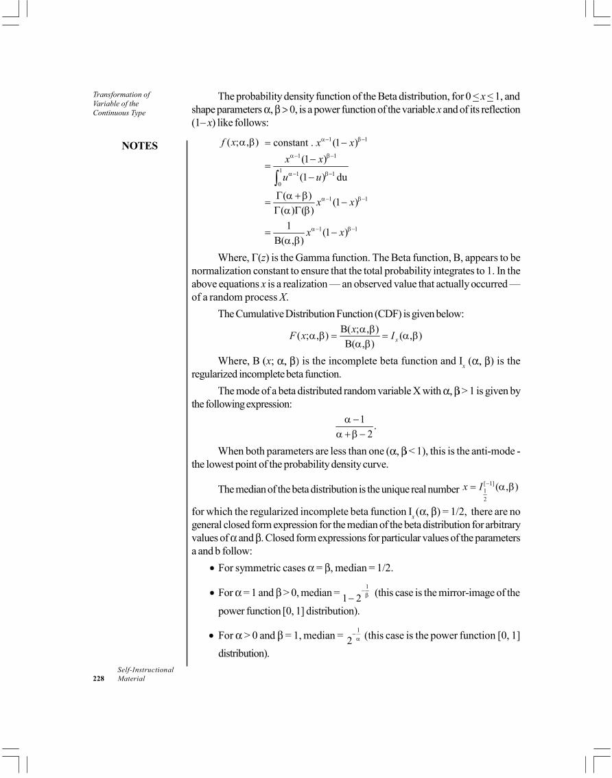
Transformation ofVariable of theContinuous Type
NOTES
Self-Instructional228 Material
The probability density function of the Beta distribution, for 0 < x < 1, andshape parameters , 0, is a power function of the variable x and of its reflection(1– x) like follows:
( ; , )f x α β 1 1constant . (1 )x xα− β−= −1 1
1 1 1
0
(1 )
(1 ) du
x x
u u
α− β−
α− β−
−=
−∫1 1( ) (1 )
( ) ( )x xα− β−Γ α +β
= −Γ α Γ β
1 11 (1 )B( , )
x xα− β−= −α β
Where, (z) is the Gamma function. The Beta function, B, appears to benormalization constant to ensure that the total probability integrates to 1. In theabove equations x is a realization — an observed value that actually occurred —of a random process X.
The Cumulative Distribution Function (CDF) is given below:B( ; , )( ; , ) ( , )B( , ) x
xF x Iα βα β = = α β
α β
Where, B (x; is the incomplete beta function and Ix ( ) is theregularized incomplete beta function.
The mode of a beta distributed random variable X with > 1 is given bythe following expression:
1 .2
α −α +β−
When both parameters are less than one ( < 1), this is the anti-mode -the lowest point of the probability density curve.
The median of the beta distribution is the unique real number [ 1]12
( , )x I −= α β
for which the regularized incomplete beta function Ix ( , ) = 1/2, there are nogeneral closed form expression for the median of the beta distribution for arbitraryvalues of and . Closed form expressions for particular values of the parametersa and b follow:
For symmetric cases = , median = 1/2.
For = 1 and > 0, median = 1
1 2−β− (this case is the mirror-image of the
power function [0, 1] distribution).
For > 0 and = 1, median = 1
2−α (this case is the power function [0, 1]
distribution).

NOTES
Self-InstructionalMaterial 229
Transformation ofVariable of the
Continuous Type
For = 3 and = 2, median = 0.6142724318676105..., the real solutionto the quartic equation 1–8x3+6x4 = 0, which lies in [0, 1].For = 2 and = 3, median = 0.38572756813238945... = 1–median(Beta (3, 2)).The following are the limits with one parameter finite (non zero) and the
other approaching these limits:lim median lim median = 1,
0lim median lim median = 0.
0
= α→∞β→
=α→ β→∞
A reasonable approximation of the value of the median of the Betadistribution, for both and greater or equal to one, is given by the followingformula:
13Median for , 1.2
3When , 1, the relative error (the absolute error divided by the median)
in this approximation is less than 4% and for both 2 and 2 it is less than1%. The absolute error divided by the difference between the mean and the modeis similarly small.
The expected value (mean) ( ) of a beta distribution random variable Xwith two parameters and is a function of only the ratio of these parameters:
[ ]E Xµ =1
0( ; , )xf x dx= α β∫
1 11
0
(1 )B( , )
x xx dxα− β−−
=α β∫
α=α +β
1
1=
β+α
Letting = in the above expression one obtains = 1/2, showing that for = the mean is at the center of the distribution: it is symmetric. Also, the following
limits can be obtained from the above expression:

Transformation ofVariable of theContinuous Type
NOTES
Self-Instructional230 Material
lim1
0
lim0
µ =β→
α
µ =β→∞
α
Therefore, for 0, or for , the mean is located at the rightend, x = 1. For these limit ratios, the Beta distribution becomes a one-pointdegenerate distribution with a Dirac Delta function spike at the right end, x = 1,with probability 1 and zero probability everywhere else. There is 100% probability(absolute certainty) concentrated at the right end, x = 1.
Similarly, for , or for 0, the mean is located at the left end,x = 0. The Beta distribution becomes a 1 point Degenerate distribution with aDirac Delta function spike at the left end, x = 0, with probability 1 and zeroprobability everywhere else. There is 100% probability (absolute certainty)concentrated at the left end, x = 0. Following are the limits with one parameterfinite (non zero) and the other approaching these limits:
lim lim = 10
lim lim = 00
µ µ= α→∞β→µ µ=α→ β→∞
While for typical unimodal distributions with centrally located modes, inflexionpoints at both sides of the mode and longer tails with Beta ( , ) such that
, > 2 it is known that the sample mean as an estimate of location is not asrobust as the sample median, the opposite is the case for uniform or ‘U-shaped’Bimodal distributions with beta( , ) such that ( , 1), with the modes locatedat the ends of the distribution.
The logarithm of the Geometric Mean (GX) of a distribution with randomvariable X is the arithmetic mean of ln (X), or equivalently its expected value:
ln Gx = E [ln X]For a Beta distribution, the expected value integral gives:
E[ln ]X1
0ln ( ; , )xf x dx= α β∫
1 11
0
(1 )lnB( , )
x xx dxα− β−−
=α β∫
1 11
0
1 (1 )B( , )
x x dxα− β−∂ −
=α β ∂α∫

NOTES
Self-InstructionalMaterial 231
Transformation ofVariable of the
Continuous Type1 1 1
0
1 (1 )B( , )
x x dxα− β−∂= −
α β ∂α ∫
1 B( , )B( , )
∂ α β=
α β ∂α
ln B( , )∂ α β=
∂α
ln ( ) ln ( )∂ Γ α ∂ Γ α +β= −
∂α ∂α
( ) ( )= Ψ α −Ψ α +β
Where, is the Digamma Function.Therefore, the geometric mean of a Beta distribution with shape parameters
and is the exponential of the Digamma functions of and as follows:[ln ] ( ) ( )E X
XG e eψ α −ψ α+β= =
While for a Beta distribution with equal shape parameters = , it followsthat Skewness = 0 and Mode = Mean = Median = 1/2, the geometric mean is lessthan 1/2: 0 < GX < 1/2. The reason for this is that the logarithmic transformationstrongly weights the values of X close to zero, as ln (X) strongly tends towardsnegative infinity as X approaches zero, while ln (X) flattens towards zero asX 1.
Along a line = , the following limits apply:
lim0
lim
0
12
X
X
G
G
α=β→
α=β→∞
=
=
Following are the limits with one parameter finite (non zero) and the otherapproaching these limits:
lim lim0
lim lim0
1
0
X X
X X
G G
G G
α→∞β→
α→ β→∞
= =
= =
The accompanying plot shows the difference between the mean and thegeometric mean for shape parameters and from zero to 2. Besides the factthat the difference between them approaches zero as and approach infinityand that the difference becomes large for values of and approaching zero, onecan observe an evident asymmetry of the geometric mean with respect to theshape parameters and . The difference between the geometric mean and themean is larger for small values of in relation to than when exchanging themagnitudes of and .

Transformation ofVariable of theContinuous Type
NOTES
Self-Instructional232 Material
The inverse of the Harmonic Mean (HX) of a distribution with random variableX is the arithmetic mean of 1/X, or, equivalently, its expected value. Therefore, theHarmonic Mean (HX) of a beta distribution with shape parameters and is:
XH11EX
=
1
0
1( ; , )f x dx
x
=α β
∫
1 11
0
1(1 )
B( , )x x dx
x
α− β−=−α β∫
1 if 1 and 01
α −= α > β >α +β−
The Harmonic Mean (HX) of a beta distribution with < 1 is undefined,because its defining expression is not bounded in [0, 1] for shape parameter a lessthan unity.
Letting = in the above expression one can obtain the following:1 ,
2 1XH α −=
α −
Showing that for = the harmonic mean ranges from 0, for = = 1, to1/2, for = .
Following are the limits with one parameter finite (non zero) and the otherapproaching these limits:
lim0
lim lim1
lim lim0
undefined
0
1
X
X X
X X
H
H H
H H
α→
α→ β→∞
α→∞β→
=
= =
= =
The Harmonic mean plays a role in maximum likelihood estimation for thefour parameter case, in addition to the geometric mean. Actually, when performingmaximum likelihood estimation for the four parameter case, besides the harmonicmean HX based on the random variable X, also another harmonic mean appearsnaturally: the harmonic mean based on the linear transformation (1"X), the mirrorimage of X, denoted by H(1–X):
(1 )1 1 if 1,& 0.
11E(1 )
XH
X
−β −
= = β > α >α +β−
−

NOTES
Self-InstructionalMaterial 233
Transformation ofVariable of the
Continuous Type
The Harmonic mean (H(1–X)) of a Beta distribution with < 1 is undefined,because its defining expression is not bounded in [0, 1] for shape parameter less than unity.
Using = in the above expression one can obtain the following:
(1 )1 ,
2 1XH −β −
=β−
This shows that for = the harmonic mean ranges from 0, for = = 1,to 1/2, for = .
Following are the limits with one parameter finite (non zero) and the otherapproaching these limits:
(1 )
(1 ) (1 )
(1 ) (1 )
lim0
lim lim1
lim lim0
undefined
0
1
X
X X
X X
H
H H
H H
−
− −
− −
β→
α→∞β→
α→ β→∞
=
= =
= =
Although both HX and H(1–X) are asymmetric, in the case that both shapeparameters are equal = , the harmonic means are equal: HX = H(1–X). Thisequality follows from the following symmetry displayed between both harmonicmeans:
(1 )(B( , )) (B( , )) if , 1.X XH H −= α β = β α α β >
9.2.2 t DistributionSir William S. Gosset (pen name Student) developed a significance test and throughit made significant contribution in the theory of sampling applicable in case of smallsamples. When population variance is not known, the test is commonly known asStudent’s t-test and is based on the t distribution.
Like the normal distribution, t distribution is also symmetrical but happensto be flatter than the normal distribution. Moreover, there is a different t distributionfor every possible sample size. As the sample size gets larger, the shape of the tdistribution loses its flatness and becomes approximately equal to the normaldistribution. In fact, for sample sizes of more than 30, the t distribution is so closeto the normal distribution that we will use the normal to approximate the tdistribution. Thus, when n is small, the t distribution is far from normal, but whenn is infinite, it is identical with normal distribution.
For applying t-test in context of small samples, the t value is calculated firstof all and, then the calculated value is compared with the table value of t at certainlevel of significance for given degrees of freedom. If the calculated value of texceeds the table value (say t0.05), we infer that the difference is significant at 5%level, but if calculated value is t0, is less than its concerning table value, the differenceis not treated as significant.

Transformation ofVariable of theContinuous Type
NOTES
Self-Instructional234 Material
The t-test is used when two conditions are fullfield,(i) The sample size is less than 30, i.e., when 30.n ≤
(ii) The population standard deviation ( p) must be unknown.In using the t-test, we assume the following:
(i) That the population is normal or approximately normal(ii) That the observations are independent and the samples are randomly drawn
samples;(iii) That there is no measurement error;(iv) That in the case of two samples, population variances are regarded as equal
if equality of the two population means is to be testedThe following formulae are commonly used to calculate the t value:(i) To Test the Significance of the Mean of a Random Sample
| || x
XtS SE X
−µ=
Where, X = Mean of the sample
µ = Mean of the universe
xSE = S.E. of mean in case of small sample and is worked out as follows:
2( )i
sx
x xnSE
n n
Σ −σ
= =
and the degrees of freedom = (n – 1)The above stated formula for t can as well be stated as under:
| |
x
xtSE−µ
=
2
| |( )
1
xx x
nn
−µ=
Σ −−
1
2
| | =( )
1
x nx xn
−µ×
Σ −−
If we want to work out the probable or fiducial limits of population mean (µ) incase of small samples, we can use either of the following:

NOTES
Self-InstructionalMaterial 235
Transformation ofVariable of the
Continuous Type
(a) Probable limits with 95% confidence level:
0.05 ( )xX SE tµ = ±
(b) Probable limits with 99% confidence level:
0.01 ( )xX SE tµ = ±
At other confidence levels, the limits can be worked out in a similar manner, takingthe concerning table value of t just as we have taken t0.05 in (a) and t0.01 in (b)above.(ii) To Test the Difference between the Means of the Two Samples
1 2
1 2| |SE x x
X Xt−
−=
Where, 1X = Mean of the sample 1
2X = Mean of the sample 2
1 2x xSE − = Standard Error of difference between two sample means andis worked out as follows:
1 2
221 1 2 2
1 2
1 2
( ) ( )2
1 1
i ix x
X x X xSE
n n
n n
−
− + −=
+ −
× +
∑ ∑
and the degrees of freedom = (n1 + n2 – 2).When the actual means are in fraction, then use of assumed means is convenient.In such a case, the standard deviation of difference, i.e.,
2 21 1 2 2
1 2
( ) + ( )2
i ix x x xn n
Σ + Σ −+ −
Can be worked out by the following short-cut formula:
2 2 2 21 1 2 1 1 1 2 2 2 2
1 2
( ) ( ) ( ) ( )2
i i i ix A x A n x A n x An n
Σ − + Σ − − − − −=
+ −
Where, A1 = Assumed mean of sample 1A2 = Assumed mean of sample 2X1 = True mean of sample 1X2 = True mean of sample 2
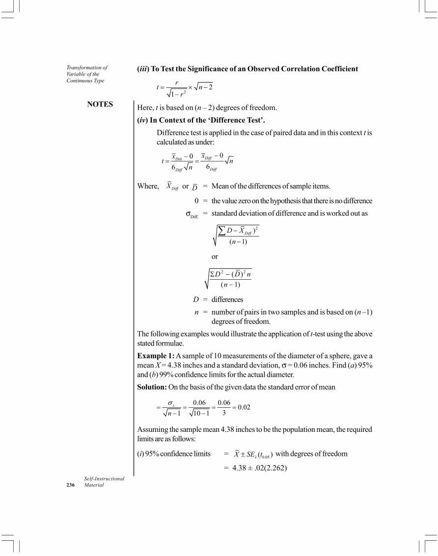
Transformation ofVariable of theContinuous Type
NOTES
Self-Instructional236 Material
(iii) To Test the Significance of an Observed Correlation Coefficient
22
1rt n
r= × −
−
Here, t is based on (n – 2) degrees of freedom.(iv) In Context of the ‘Difference Test’.
Difference test is applied in the case of paired data and in this context t iscalculated as under:
0066
DiffDitt
DiffDiff
xxt nn
−−= =
Where, DiffX or D = Mean of the differences of sample items.
0 = the value zero on the hypothesis that there is no difference
Diff. = standard deviation of difference and is worked out as
2)( 1)
DiffD Xn−
−∑
or
2 2( )( 1)
D D nn
Σ −−
D = differencesn = number of pairs in two samples and is based on (n –1)
degrees of freedom.The following examples would illustrate the application of t-test using the abovestated formulae.Example 1: A sample of 10 measurements of the diameter of a sphere, gave amean X = 4.38 inches and a standard deviation, = 0.06 inches. Find (a) 95%and (b) 99% confidence limits for the actual diameter.Solution: On the basis of the given data the standard error of mean
0.06 0.06 0.0231 10 1
s
nσ
= = = =− −
Assuming the sample mean 4.38 inches to be the population mean, the requiredlimits are as follows:
(i) 95% confidence limits = 0.05( )xX SE t± with degrees of freedom
= 4.38 ± .02(2.262)

NOTES
Self-InstructionalMaterial 237
Transformation ofVariable of the
Continuous Type
= 4.38 ± .04524 i.e., 4.335 to 4.425
(ii) 99% confidence limits = 0.01( )xX SE t± with 9 degrees of freedom
= 4.38 ± .02(3.25) = 4.38 ± .0650 i.e., 4.3150 to 4.4450.Example 2: The specimen of copper wires drawn from a large lot have thefollowing breaking strength (in kg. wt.):
578, 572, 570, 568, 572, 578, 570, 572, 596, 544
Test whether the mean breaking strength of the lot may be taken to be 578 kg. wt.Solution: We take the hypothesis that there is no difference between the meanheight of the sample and the given height of universe. In other words we can write,
0 0: , :H X H Xµ µ= ≠ . Then on the basis of the sample data, the mean andstandard deviation has been worked out as under:
S. No. X (X – X ) (X1 – X )2
1 578 6 362 572 0 03 570 –2 44 568 –4 165 572 0 06 578 6 367 570 –2 48 572 0 09 596 24 57610 544 –28 784
n = 10 Xi = 5720 (Xi – X )2 = 1456
2
572010
= 572
( )1
1456 1456 =10 1 9
=12.72
ss
xXn
x xn
Σ= =
Σ −=
−
=−
σ

Transformation ofVariable of theContinuous Type
NOTES
Self-Instructional238 Material
12.7210
12.72 = 4.033.16
| | | 572 578 |4.03
= 1.488
sx
x
SEn
xtSE
= =
=
− −= =
σ
µ
Degrees of freedom = n –1 = 9At 5% level of significance for 9 degrees of freedom, the table value of t = 2.262.For a two-tailed test.The calculated value of t is less than its table value and hence the difference isinsignificant. The mean breaking strength of the lot may be taken to be 578 Kg.wt. with 95% confidence level.Example 3: Sample of sales in similar shops in two towns are taken for a newproduct with the following results:
Mean sales Variance ‘Size of sample
Town A 57 5.3 5
Town B 61 4.8 7
Is there any evidence of difference in sales in the two towns?Solution: We take the hypothesis that there is no difference between the twosample means concerning sales in the two towns. In other words,
0 1 2 0 1 2: , :H X X H X X= ≠ . Then, we work out the concerning t value as follows:
1 2
1 2| |=x x
X XtSE −
−
Where, 1x = Mean of the sample concerning Town A
2x = Mean of the sample concerning Town B
1 2x xSE − = Standard Error of the difference between two means.
1 2
2 21 1 2 2
1 2 1 2
( ) ( ) 1 1 2
i ix x
x x x xSEn n n n−
Σ − + Σ −= × +
+ −
Hence,
| 57 61| 41.421 1.421
= 2.82
t −= =

NOTES
Self-InstructionalMaterial 239
Transformation ofVariable of the
Continuous Type
Degrees of freedom = (n1 + n2 – 2) = (5 + 7 – 2) = 10Table value of t at 5% level of significance for 10 degrees of freedom is 2.228, fora two-tailed test.The calculated value of t is greater than its table value. Hence, the hypothesis iswrong and the difference is significant.Example 4: The sales data of an item in six shops before and after a specialpromotional campaign are:Shops A B C D E F
Before thepromotionalcampaign 53 28 31 48 50 42
After the campaign 58 29 30 55 56 45
Can the campaign be judged to be a success? Test at 5% level of significance.Solution: We take the hypothesis that the campaign does not bring any improvementin sales. We can thus write:In order to judge this, we apply the ‘difference test’. For this purpose we calculatethe mean and standard deviation of differences in two sample items as follows:
Shops Sales before Sales after Difference = D (D – D ) (D – D )2
campaign campaign (i.e., increase orXBi XAi decrease after the
campaign)
A 53 58 +5 +1.5 2.25 B 28 29 +1 –2.5 6.25 C 31 30 –1 –4.5 20.25 D 48 55 +7 +3.5 12.25 E 50 56 +6 +2.5 6.25 F 42 45 +3 –0.5 0.25
n = 6 D = 21 (D – D )2
= 47.50
Mean of difference or 21 3.56Diff
DXnΣ
= = =
Standard deviation of difference
2( ) 47.50 3.081 6 1
0
Diff
Diff
Diff
D Dn
Xt n
Σ −= = =
− −−
= =
σ
σ
= 1.14 × 2.45 = 2.793
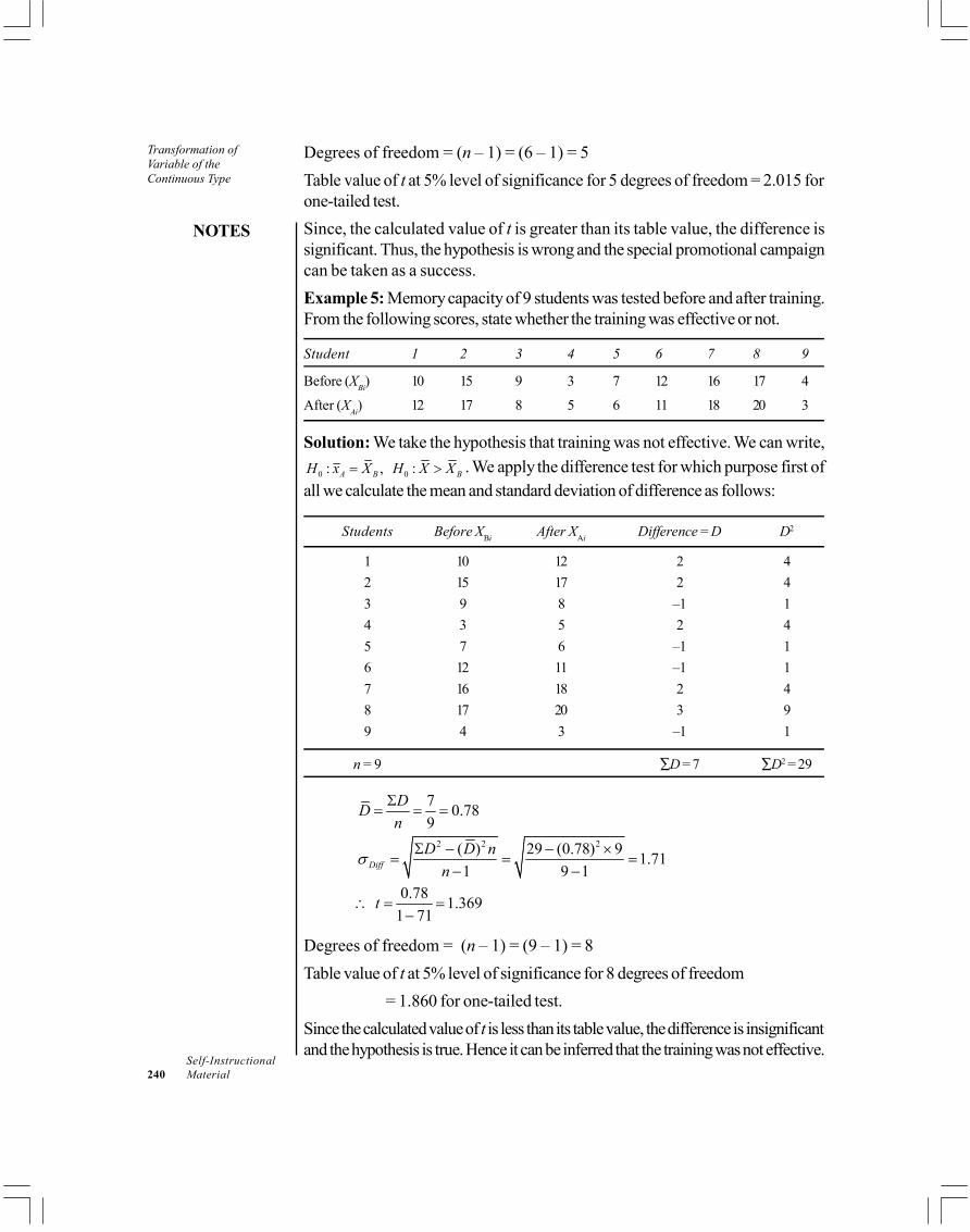
Transformation ofVariable of theContinuous Type
NOTES
Self-Instructional240 Material
Degrees of freedom = (n – 1) = (6 – 1) = 5Table value of t at 5% level of significance for 5 degrees of freedom = 2.015 forone-tailed test.Since, the calculated value of t is greater than its table value, the difference issignificant. Thus, the hypothesis is wrong and the special promotional campaigncan be taken as a success.Example 5: Memory capacity of 9 students was tested before and after training.From the following scores, state whether the training was effective or not.
Student 1 2 3 4 5 6 7 8 9
Before (XBi) 10 15 9 3 7 12 16 17 4
After (XAi) 12 17 8 5 6 11 18 20 3
Solution: We take the hypothesis that training was not effective. We can write,
0 0: , :A B BH x X H X X= > . We apply the difference test for which purpose first ofall we calculate the mean and standard deviation of difference as follows:
Students Before XBi After XAi Difference = D D2
1 10 12 2 42 15 17 2 43 9 8 –1 14 3 5 2 45 7 6 –1 16 12 11 –1 17 16 18 2 48 17 20 3 99 4 3 –1 1
n = 9 D = 7 D2 = 29
2 2 2
7 0.789
( ) 29 (0.78) 9 1.711 9 1
0.78 1.3691 71
Diff
DDn
D D nn
t
σ
Σ= = =
Σ − − ×= = =
− −
∴ = =−
Degrees of freedom = (n – 1) = (9 – 1) = 8Table value of t at 5% level of significance for 8 degrees of freedom
= 1.860 for one-tailed test.Since the calculated value of t is less than its table value, the difference is insignificantand the hypothesis is true. Hence it can be inferred that the training was not effective.

NOTES
Self-InstructionalMaterial 241
Transformation ofVariable of the
Continuous Type
Example 6: It was found that the coefficient of correlation between two variablescalculated from a sample of 25 items was 0.37. Test the significance of r at 5%level with the help of t-test.
Solution: To test the significance of r through t-test, we use the following formulafor calculating t value:
2
2
21
0.37 = 25 21 (0.37)
=1.903
rt nr
= × −−
× −−
Degrees of freedom = (n–2) = (25–2) = 23The table value of at 5% level of significance for 23 degrees of freedom is2.069 for a two-tailed test.The calculated value of t is less than its table value, hence r is insignificant.Example 7: A group of seven week old chickens reared on high protein dietweigh 12, 15, 11, 16, 14, 14 and 16 ounces; a second group of five chickenssimilarly treated except that they receive a low protein diet weigh 8, 10, 14, 10and 13 ounces. Test at 5% level whether there is significant evidence that additionalprotein has increased the weight of chickens. (Use assumed mean (or A1) = 10 forthe sample of 7 and assumed mean (or A2) = 8 for the sample of 5 chickens inyour calculation).Solution: We take the hypothesis that additional protein has not increased theweight of the chickens. We can write, Ho: X1 > X2 Ho : X1 > X2.Applying t-test, we work out the value of t for measuring the significance of twosample means as follows:
1 2
1 2
= X XtSEx x
−
−
Calculation of can be done as under:X1 (Xi1 – A1) (Xi1 – A1)
2 X2 (Xi2 – A2) (Xi2 – A2)2
A1 = 10 A2= 812 2 4 8 0 015 5 25 10 2 411 1 1 14 6 3616 6 36 10 2 414 4 16 13 5 2514 4 1616 6 36
n1=7 (X1i – A1) (X1i– A1)2 n2=5 (X2i – A2) (X2i– A2)
2
=28 =134 =15 = 69

Transformation ofVariable of theContinuous Type
NOTES
Self-Instructional242 Material
1 1 1 1 1( ) /28 =10 + 147
iX A x A n= + Σ −
=
Similarly, 2 22 1
2
( )ix AX An
Σ −= +
15= 8 + 115=
Hence,
1 2
2 2 2 21 1 2 2 1 1 1 2 2 2
1 2 1 2
2 2
( ) ( ) ( ) ( ) 1 12
134 + 69 7 (14 10) 5(11 8) 1 1 =7 5 2 7 5
i iX X
X A X A n X A n X ASEn n n n−
Σ − + Σ − − − − −= × +
+ −
− − − −× +
+ −
= (2.14) (.59) = 1.2626We now calculate the value under t,
1 2
1 2 14 11 2.3761.2626X X
X XtSE −
− −= = =
Degree of freedom = (n1 + n2 – 2) = (7 + 5 – 2) = 10The table value of t at 5% level of significance for 10 degrees of freedom = 1.812for one-tailed test.The calculated value of t is higher than its table value and hence the difference issignificant, which means the hypothesis is wrong. It can therefore be concludedthat additional protein has increased the weight of chickens.
9.2.3 F DistributionIn business decisions, we are often involved in determining if there are significantdifferences among various sample means, from which conclusions can be drawnabout the differences among various population means. In the previous chapters,we discussed and evaluated the differences between two sample means. But,what if we have to compare more than 2 sample means? For example, we may beinterested to find out if there are any significant differences in the average salesfigures of 4 different salesman employed by the same company, or we may beinterested to find out if the average monthly expenditures of a family of 4 in 5different localities are similar or not, or the telephone company may be interestedin checking, whether there are any significant differences in the average number ofrequests for information received in a given day among the 5 areas of New York

NOTES
Self-InstructionalMaterial 243
Transformation ofVariable of the
Continuous Type
City, and so on. The methodology used for such types of determinations is knownas Analysis of Variance.
This technique is one of the most powerful techniques in statistical analysisand was developed by R.A. Fisher. It is also called the F-Test.
There are two types of classifications involved in the analysis of variance.The one-way analysis of variance refers to the situations when only one fact orvariable is considered. For example, in testing for differences in sales for threesalesman, we are considering only one factor, which is the salesman’s selling ability.In the second type of classification, the response variable of interest may be affectedby more than one factor. For example, the sales may be affected not only by thesalesman’s selling ability, but also by the price charged or the extent of advertisingin a given area.
For the sake of simplicity and necessity, our discussion will be limited toOne-way Analysis of Variance.
The null hypothesis, that we are going to test, is based upon the assumptionthat there is no significant difference among the means of different populations.For example, if we are testing for differences in the means of k populations, then,
0 1 2 3 ....... kH = µ = µ = µ = = µ
The alternate hypothesis (H1) will state that at least two means are differentfrom each other. In order to accept the null hypothesis, all means must be equal.Even if one mean is not equal to the others, then we cannot accept the nullhypothesis. The simultaneous comparison of several population means is calledAnalysis of Variance or ANOVA.
Assumptions
The methodology of ANOVA is based on the following assumptions.(i) Each sample of size n is drawn randomly and each sample is independent of
the other samples.(ii) The populations are normally distributed.(iii) The populations from which the samples are drawn have equal variances.
This means that:
σ σ σ σ12
22
32 2= = = .........= k , for k populations.
The Rationale Behind Analysis of Variance
Why do we call it the Analysis of Variance, even though we are testing for means?Why not simply call it the Analysis of Means? How do we test for means byanalysing the variances? As a matter of fact, in order to determine if the means ofseveral populations are equal, we do consider the measure of variance, 2.

Transformation ofVariable of theContinuous Type
NOTES
Self-Instructional244 Material
The estimate of population variance, 2, is computed by two differentestimates of 2, each one by a different method. One approach is to compute anestimator of 2 in such a manner that even if the population means are not equal, itwill have no effect on the value of this estimator. This means that, the differences inthe values of the population means do not alter the value of 2 as calculated by agiven method. This estimator of 2 is the average of the variances found withineach of the samples. For example, if we take 10 samples of size n, then eachsample will have a mean and a variance. Then, the mean of these 10 varianceswould be considered as an unbiased estimator of 2, the population variance, andits value remains appropriate irrespective of whether the population means areequal or not. This is really done by pooling all the sample variances to estimate acommon population variance, which is the average of all sample variances. Thiscommon variance is known as variance within samples or 2
within.The second approach to calculate the estimate of 2, is based upon the
Central Limit Theorem and is valid only under the null hypothesis assumption thatall the population means are equal. This means that in fact, if there are no differencesamong the population means, then the computed value of 2 by the secondapproach should not differ significantly from the computed value of 2 by the firstapproach.
Hence, If these two values of 2 are approximately the same, then we candecide to accept the null hypothesis.
The second approach results in the following computation.Based upon the Central Limit Theorem, we have previously found that the
standard error of the sample means is calculated by:2x n
σσ =
or, the variance would be:2
2x n
σσ =
or, 2 2xnσ = σ
Thus, by knowing the square of the standard error of the mean 2( )xσ , wecould multiply it by n and obtain a precise estimate of 2. This approach of estimating
2 is known as 2between. Now, if the null hypothesis is true, that is if all population
means are equal then,2between value should be approximately the same as 2
within value. A significantdifference between these two values would lead us to conclude that this differenceis the result of differences between the population means.
But, how do we know that any difference between these two values issignificant or not? How do we know whether this difference, if any, is simply dueto random sampling error or due to actual differences among the population means?
NOTES
Self-InstructionalMaterial 245
Transformation ofVariable of the
Continuous Type
R.A. Fisher developed a Fisher test or F-test to answer the above question.He determined that the difference between 2
between and 2within values could be
expressed as a ratio to be designated as the F-value, so that:
2between2within
F σ=σ
In the above case, if the population means are exactly the same, then 2between
will be equal to the 2within and the value of F will be equal to 1.
However, because of sampling errors and other variations, some disparitybetween these two values will be there, even when the null hypothesis is true,meaning that all population means are equal. The extent of disparity between thetwo variances and consequently, the value of F, will influence our decision onwhether to accept or reject the null hypothesis. It is logical to conclude that, if thepopulation means are not equal, then their sample means will also vary greatlyfrom one another, resulting in a larger value of 2
between and hence a larger value ofF ( 2
within is based only on sample variances and not on sample means and hence,is not affected by differences in sample means). Accordingly, the larger the valueof F, the more likely the decision to reject the null hypothesis. But, how large thevalue of F be so as to reject the null hypothesis? The answer is that the computedvalue of F must be larger than the critical value of F, given in the table for a givenlevel of significance and calculated number of degrees of freedom. (The Fdistribution is a family of curves, so that there are different curves for differentdegrees of freedom).
Degrees of Freedom
We have talked about the F-distribution being a family of curves, each curvereflecting the degrees of freedom relative to both 2
between and 2within. This means
that, the degrees of freedom are associated both with the numerator as well aswith the denominator of the F-ratio.
(i) The Numerator: Since the variance between samples, 2between comes
from many samples and if there are k number of samples, then the degreesof freedom, associated with the numerator would be (k –1).
(ii) The Denominator: It is the mean variance of the variances of k samplesand since, each variance in each sample is associated with the size of thesample (n), then the degrees of freedom associated with each sample wouldbe (n – 1). Hence, the total degrees of freedom would be the sum of degreesof freedom of k samples ordf = k(n –1), when each sample is of size n.

Transformation ofVariable of theContinuous Type
NOTES
Self-Instructional246 Material
The F-Distribution
The major characteristics of the F-distribution are as follows:(i) Unlike normal distribution, which is only one type of curve irrespective of
the value of the mean and the standard deviation, the F distribution is afamily of curves. A particular curve is determined by two parameters. Theseare the degrees of freedom in the numerator and the degrees of freedom inthe denominator. The shape of the curve changes as the number of degreesof freedom changes.
(ii) It is a continuous distribution and the value of F cannot be negative.(iii) The curve representing the F distribution is positively skewed.(iv) The values of F theoretically range from zero to infinity.
A diagram of F distribution curve is shown below.
Do notrejectH0
Reject H0
0 F
The rejection region is only in the right end tail of the curve because unlike Zdistribution and t distribution which had negative values for areas below the mean,F distribution has only positive values by definition and only positive values of Fthat are larger than the critical values of F, will lead to a decision to reject the nullhypothesis.
Computation of F
Since F ratio contains only two elements, which are the variance between thesamples and the variance within the samples, the concepts of which have beendiscussed before, let us recapitulate the calculation of these variances.
If all the means of samples were exactly equal and all samples were exactlyrepresentative of their respective populations so that all the sample means, wereexactly equal to each other and to the population mean, then there will be novariance. However, this can never be the case. We always have variation, bothbetween samples and within samples, even if we take these samples randomly andfrom the same population. This variation is known as the total variation.
The total variation designated by 2( - ) ,X X∑ where X represents individual
observations for all samples and X is the grand mean of all sample means and

NOTES
Self-InstructionalMaterial 247
Transformation ofVariable of the
Continuous Type
equals ( ), the population mean, is also known as the total sum of squares orSST, and is simply the sum of squared differences between each observation andthe overall mean. This total variation represents the contribution of two elements.These elements are:(A) Variance between Samples: The variance between samples may be due tothe effect of different treatments, meaning that the population means may beaffected by the factor under consideration, thus, making the population meansactually different, and some variance may be due to the inter-sample variability.This variance is also known as the sum of squares between samples. Let this sumof squares be designated as SSB.Then, SSB is calculated by the following steps:(i) Take k samples of size n each and calculate the mean of each sample, i.e.,
1 2 3, , , .... .kX X X X
(ii) Calculate the grand mean X of the distribution of these sample means, so that,
1
k
ii
xX
k==∑
(iii) Take the difference between the means of the various samples and the grandmean, i.e.,
1 2 3( ), ( ), ( ), ...., ( )kX X X X X X X X− − − −
(iv) Square these deviations or differences individually, multiply each of thesesquared deviations by its respective sample size and sum up all these products, sothat we get;
2
1( ) ,
k
i ii
n X X=
−∑ where ni = size of the ith sample.
This will be the value of the SSB.However, if the individual observations of all samples are not available, and onlythe various means of these samples are available, where the samples are either ofthe same size n or different sizes, ni, n2, n3, ....., nk, then the value of SSB can becalculated as:
2 2 22 2( ) ( ) ..... ( )i i k kSSB n X X n X X n X X= − + − + −
where,n1 = Number of items in sample 1n2 = Number of items in sample 2nk = Number of items in sample k

Transformation ofVariable of theContinuous Type
NOTES
Self-Instructional248 Material
1X = Mean of sample 1
2X = Mean of sample 2
kX = Mean of sample k
X = Grand mean or average of all items in all samples.
(v) Divide SSB by the degrees of freedom, which are (k – 1), where k is thenumber of samples and this would give us the value of 2
between, so that,
2between .
( 1)SSBk
σ =−
(This is also known as mean square between samples or MSB).(B) Variance within Samples: Even though each observation in a given samplecomes from the same population and is subjected to the same treatment, somechance variation can still occur. This variance may be due to sampling errors orother natural causes. This variance or sum of squares is calculated through thefollowing steps:
(i) Calculate the mean value of each sample, i.e., 1 2 3, , , .... .kX X X X
(ii) Take one sample at a time and take the deviation of each item in the samplefrom its mean. Do this for all the samples, so that we would have a differencebetween each value in each sample and their respective means for all values in allsamples.(iii) Square these differences and take a total sum of all these squared differences(or deviations). This sum is also known as SSW or sum of squares within samples.(iv) Divide this SSW by the corresponding degrees of freedom. The degrees offreedom are obtained by subtracting the total number of samples from the totalnumber of items. Thus, if N is the total number of items or observations, and k isthe number of samples, then,
df = (N – k)
These are the degrees of freedom within samples. (If all samples are of equal sizen, then df = k(n –1), since (n – 1) are the degrees of freedom for each sampleand there are k samples).(v) This figure SSW/df, is also known as 2
within, or MSW (mean of sum of squareswithin samples).Now, the value of F can be computed as:
2between2within
//
/( 1) =/( )
SSB dfFSSW df
SSB k MSBSSW N k MSW
σ= =σ
−=
−
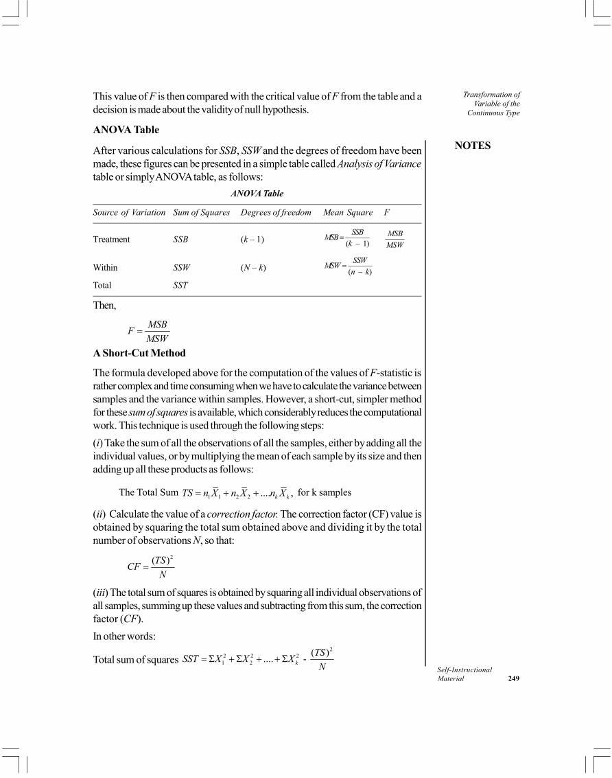
NOTES
Self-InstructionalMaterial 249
Transformation ofVariable of the
Continuous Type
This value of F is then compared with the critical value of F from the table and adecision is made about the validity of null hypothesis.
ANOVA Table
After various calculations for SSB, SSW and the degrees of freedom have beenmade, these figures can be presented in a simple table called Analysis of Variancetable or simply ANOVA table, as follows:
ANOVA Table
Source of Variation Sum of Squares Degrees of freedom Mean Square F
Treatment SSB (k – 1) ( 1)SSBMSB
k=
−MSBMSW
Within SSW (N – k) ( )SSWMSW
n k=
−
Total SST
Then,
MSBFMSW
=
A Short-Cut Method
The formula developed above for the computation of the values of F-statistic israther complex and time consuming when we have to calculate the variance betweensamples and the variance within samples. However, a short-cut, simpler methodfor these sum of squares is available, which considerably reduces the computationalwork. This technique is used through the following steps:(i) Take the sum of all the observations of all the samples, either by adding all theindividual values, or by multiplying the mean of each sample by its size and thenadding up all these products as follows:
The Total Sum 1 1 2 2 .... ,k kTS n X n X n X= + + for k samples
(ii) Calculate the value of a correction factor. The correction factor (CF) value isobtained by squaring the total sum obtained above and dividing it by the totalnumber of observations N, so that:
2( )TSCFN
=
(iii) The total sum of squares is obtained by squaring all individual observations ofall samples, summing up these values and subtracting from this sum, the correctionfactor (CF).In other words:
Total sum of squares 2
2 2 21 2
( ).... - kTSSST X X XN
= Σ + Σ + + Σ

Transformation ofVariable of theContinuous Type
NOTES
Self-Instructional250 Material
Where,21XΣ = Summation of squares for all X’s in sample 1.
22XΣ = Summation of squares for all X’s in sample 2.
::
2kXΣ = Summation of squares for all X’s in sample k.
(iv) The sum of squares between the samples (SSB) is obtained by the followingformula:
22 2 21 2
1 2
( )( ) ( ) ( ).... - k
k
XX X TSSSBn n n N
ΣΣ Σ= + + +
Where,2
1( )XΣ = Square of the total of all values in sample 1.2
2( )XΣ = Square of the total of all values in sample 2.2( )kXΣ = Square of the total of all values in sample k.
(v) Then sum of squares within samples SSW can be calculated as:SSW = Total sum of squares minus the sum of squares between samples = SST – SSB
(vi) The rest of the procedure is similar to the previous method.Example 8: To test whether all professors teach the same material in differentsections of the introductory statistics class or not, four sections of the same coursewere selected and a common test was administered to five students selected atrandom from each section. The scores for each student from each section werenoted and are given below. We want to test for any differences in learning, asreflected in the average scores for each section.
Section 1 Section 2 Section 3 Section 4Student # Scores (X1) Scores (X2) Scores (X3) Scores (X4)
1 8 12 10 122 10 12 13 153 12 10 11 134 10 8 12 105 5 13 14 10
Totals 1 45XΣ = 2 55XΣ = 3 60XΣ = 4 60XΣ =
Means 1 9X = 2 11X = 3 12X = 4 12X =

NOTES
Self-InstructionalMaterial 251
Transformation ofVariable of the
Continuous Type
Solution: A. The Traditional Method(i) State the null hypothesis. We are assuming that there is no significant differenceamong the average scores of students from these four sections and hence, allprofessors are teaching the same material with the same effectiveness, i.e.,
0 1 2 3 4: .H µ = µ = µ = µ
H1: All means are not equal or at least two means differ from each other
(ii) Establish a level of significance. Let a = 0.05.(iii) Calculate the variance between the samples, as follows:
(a) The mean of each sample is:
1 2 3 49, 11, 12, 12X X X X= = = =
(b) The grand mean or X is:
9 11 12 124
11
xXnΣ + + +
= =
=(c) Calculate the value of SSB:
2
2 2 2 2
( ) 5 (9 11) 5 (11 11) 5 (12 11) 5 (12 11) 20 0 5 5 30
SSB n X X= Σ −
= − + − + − + −= + + +=
(d) The variance between samples σbetween2 or MSB is given by:
(30) (30) 10( -1) 3
SSBMSBdf k
= = = =
(iv) Calculate the variance within samples, as follows:To find the sum of squares within samples (SSW), we square each deviationbetween the individual value of each sample and its mean, for all samples and thensum these squared deviations, as follows:
Sample 1: 1 9X =
2 2 2 2 2 211( ) (8 9) (10 9) (12 9) (10 9) (5 9)
1 1 9 1 16 28
X XΣ − = − + − + − + − + −= + + + +=
Sample 2: 2 11X =

Transformation ofVariable of theContinuous Type
NOTES
Self-Instructional252 Material
2 2 2 2 2 222( ) (12 11) (12 11) (10 11) (8 11) (13 11)
1 1 1 9 4 16
X XΣ − = − + − + − + − + −= + + + +=
Sample 3: 3 12X =
2 2 2 2 2 233( ) (10 12) (13 12) (11 12) (12 12) (14 12)
4 1 1 0 4 10
X XΣ − = − + − + − + − + −
= + + + +=
Sample 4: 4 12X =
2 2 2 2 2 244( ) (12 12) (15 12) (13 12) (10 12) (10 12)
0 9 1 4 4 18
X XΣ − = − + − + − + − + −= + + + +=
Then, SSW = 28 + 16 + 10 +18 = 72Now, the variance within samples, 2
within, or MSW is given by:72 72 4.5
( ) 20 4 16SSW SSWMSWdf N k
= = = = =− −
Then, the F-ratio = 10 2.22.4.5
MSBMSW
= =
Now, we check for the critical value of F from the table for = 0.05 and degreesof freedom as follows:
df (numerator) = (k – 1) = (4 – 1) = 3
df (denominator) = (N – k) = (20 – 4) = 16
This value of F from the table is given as 3.24. Now, since our calculated value ofF = 2.22 is less than the critical value of F = 3.24, we cannot reject the nullhypothesis.B. The Short-Cut MethodFollowing the procedure outlined before for using the short-cut method, we get:(i) Total sum (TS) = X
= 220
(ii) Correction before 2 2( ) (220) 2420
20TSCFN
= = =
(iii) Total sum of squares:2( ) –
=2522 2420 102SST X CF= Σ
− −

NOTES
Self-InstructionalMaterial 253
Transformation ofVariable of the
Continuous Type
(iv) Sum of squares betwen the samples SSB is obtained by:
2
1
22 21 2
1 22 2 2 2
( )
( )( ) ( ) ....
(45) (55) (60) (60) (2420)5 5 5 5
405 605 720 720 2420 30
ki
i i
k
k
XSSB CFn
XX X CFn n n
=
= −
= + + + −
= + + + −
= + + + −=
∑
(v) SSW can be calculated by:
SST – SSB = 102 – 30 = 72
Now the F value can be calculated as:
/ 30 /( 1) 30 / 3 10/ 72 /( ) 72 /16 4.5
2.22
SSB df kFSSW df n k
−= = = =
−=
As we see, we get the same value of F as obtained by the traditional method. So,we compare our value of F with the critical value of F from the table for = 0.05and df (numerator = 3), and df (denominator = 16), and we get the critical valueof F as 3.24. As before, we accept the null hypothesis.
The ANOVA Table
We can construct an ANOVA table for the problem solved above as follows:
ANOVA Table
Source of Variation Sum of Squares Degrees of freedom Mean Square F
Treatment SSB = 30 (k – 1) = 3 ( 1)SSBMSB
k=
−MSBMSW
= 303= 10 =
104 5.
Within (or error) SSW = 72 (N – k) = 16 ( )SSWMSW
N k=
− =2.22
= =7216
4 5.
Total SST = 102

Transformation ofVariable of theContinuous Type
NOTES
Self-Instructional254 Material
Check Your Progress
1. Give the value of the median of the beta distribution.2. Who developed t-test? When it is used?3. On what assumptions the ANOVA methodology is based?4. What are the major characteristics of f-distribution?
9.3 ANSWERS TO CHECK YOUR PROGRESSQUESTIONS
1. A reasonable approximation of the value of the median of the Betadistribution, for both and greater or equal to one, is given by the followingformula:
13Median for , 1.2
32. Sir William S. Gosset (pen name Student) developed a significance test
and through it made significant contribution in the theory of samplingapplicable in case of small samples. When population variance is not known,the test is commonly known as Student’s t-test and is based on thet distribution.
3. The methodology of ANOVA is based on the following assumptions.(i) Each sample of size n is drawn randomly and each sample is independent
of the other samples.(ii) The populations are normally distributed.
(iii) The populations from which the samples are drawn have equal variances.This means that:
σ σ σ σ12
22
32 2= = = .........= k , for k populations.
4. The major characteristics of the F-distribution are as follows:(i) Unlike normal distribution, which is only one type of curve irrespective
of the value of the mean and the standard deviation, the F distribution isa family of curves. A particular curve is determined by two parameters.These are the degrees of freedom in the numerator and the degrees offreedom in the denominator. The shape of the curve changes as thenumber of degrees of freedom changes.
(ii) It is a continuous distribution and the value of F cannot be negative.(iii) The curve representing the F distribution is positively skewed.(iv) The values of F theoretically range from zero to infinity.

NOTES
Self-InstructionalMaterial 255
Transformation ofVariable of the
Continuous Type9.4 SUMMARY
In probability theory and statistics, the Beta distribution is a family ofcontinuous probability distributions defined on the interval [0, 1]parameterized by two positive shape parameters, denoted by and thatappear as exponents of the random variable and control the shape of thedistribution.In Bayesian inference, the Beta distribution is the conjugate prior probabilitydistribution for the Bernoulli, Binomial and Geometric distributions.The usual formulation of the Beta distribution is also known as the Betadistribution of the first kind, whereas Beta distribution of the second kind isan alternative name for the Beta prime distribution.The inverse of the Harmonic Mean (HX) of a distribution with random variableX is the arithmetic mean of 1/X, or, equivalently, its expected value.When population variance is not known, the test is commonly known asStudent’s t-test and is based on the t distribution.There are two types of classifications involved in the analysis of variance.The one-way analysis of variance refers to the situations when only one factor variable is considered.In the second type of classification, the response variable of interest may beaffected by more than one factor.The null hypothesis, that we are going to test, is based upon the assumptionthat there is no significant difference among the means of different populations.Each sample of size n is drawn randomly and each sample is independentof the other samples.The variance between samples may be due to the effect of differenttreatments, meaning that the population means may be affected by the factorunder consideration, thus, making the population means actually different,and some variance may be due to the inter-sample variability.
9.5 KEY WORDS
The numerator: Since the variance between samples, 2between comes from
many samples and if there are k number of samples, then the degrees offreedom, associated with the numerator would be (k –1).The denominator: It is the mean variance of the variances of k samples andsince, each variance in each sample is associated with the size of the sample (n),then the degrees of freedom associated with each sample would be (n – 1).The F-Distribution: It is a continuous distribution and the value of F cannotbe negative.

Transformation ofVariable of theContinuous Type
NOTES
Self-Instructional256 Material
9.6 SELF-ASSESSMENT QUESTIONS ANDEXERCISES
Short-Answers Questions
1. What is beta distribution?2. Give the two conditions to use t test.3. What is the analysis of variance?4. Define the term degree of freedom.
Long-Answer Questions
1. Briefly explain about the beta distribution.2. Describe the formulae which are used to calculate the value of t.3. Explain the F distribution and give their assumptions.4. Discuss about the computation of F.
9.7 FURTHER READINGS
Hogg, Robert. V., Allen T. Craig and Joseph W. McKean. 2005. Introduction toMathematical Statistics. New Delhi: Pearson Education.
Fisz, Marek. 1963. Probability Theory and Mathematical Statistics, 3rd Edition.New York: John Wiley & Sons, Inc.
Rohatgi, Vijay K. 1985. An Introduction to Probability Theory andMathematical Statistics. New Delhi: Wiley Eastern Limited.
Gupta, C.B. and Vijay Gupta. 2004. An Introduction to Statistical Methods,23rd Edition. New Delhi: Vikas Publishing House.
Levin, Richard I. and David S. Rubin. 1998. Statistics for Management. NewJersey: Prentice Hall.
Chandan, J. S. 1998. Statistics for Business and Economics. New Delhi: VikasPublishing House Pvt. Ltd.
Campbell, Stephen K. 1987. Applied Statistics. New York: Harper & Row.Chance, William A. 1969. Statistical Methods for Decision Making. Illinois:
Richard D Irwin.Hooda, R. P. 2013. Statistics for Business and Economics, 5th Edition. New
Delhi: Vikas Publishing House Pvt. Ltd.

NOTES
Self-InstructionalMaterial 257
Distributions ofOrder StatisticsUNIT 10 DISTRIBUTIONS OF
ORDER STATISTICS
Structure10.0 Introduction10.1 Objectives10.2 Distributions of Order Statistics
10.2.1 The Moment Generating Function10.3 Answers to Check Your Progress Questions10.4 Summary10.5 Key Words10.6 Self-Assessment Questions and Exercises10.7 Further Readings
10.0 INTRODUCTION
In probability theory and statistics, the moment generating function of a real-valued random variable is an alternative specification of its probability distribution.Thus, it provides the basis of an alternative route to analytical results comparedwith working directly with probability density functions or cumulative distributionfunctions. There are particularly simple results for the moment-generating functionsof distributions defined by the weighted sums of random variables. However, notall random variables have moment-generating functions. As its name implies, themoment generating function can be used to compute a distribution’s moments:the nth moment about 0 is the nth derivative of the moment-generating function,evaluated at 0.
In this unit, you will study about the distributions of order statistics and themoment generating function techniques.
10.1 OBJECTIVES
After going through this unit, you will be able to:Understand the distributions of order statisticsExplain the moment generating function techniques
10.2 DISTRIBUTIONS OF ORDER STATISTICS
In statistics, the kth order statistic of a statistical sample is equal to its kth-smallestvalue. Together with rank statistics, order statistics are among the most fundamentaltools in non-parametric statistics and inference. Important special cases of the order

Distributions ofOrder Statistics
NOTES
Self-Instructional258 Material
statistics are the minimum and maximum value of a sample, and (with somequalifications discussed below) the sample median and other sample quintiles.When using probability theory to analyse order statistics of random samples froma continuous distribution, the cumulative distribution function is used to reduce theanalysis to the case of order statistics of the uniform distribution.
10.2.1 The Moment Generating FunctionA function that generates moments of a random variable is known as the MomentGenerating Function (MGF) of the random variable. A moment generating functionmay or may not exist but if it exists it is unique.
For the random variable X, its moment generating function MX(t) or (t) isdefined as follows:
(t) or MX(t) = E(etx)
=
when is discrete and ( )
( ) when is continuous and ( ) is . . . of .∞
− ∞
= =
∑
∫
itxi i i
tx
e f X f P X x
e f x dx X f x p d f X
Note that E(etX) is a function of t. The rth raw moment of X is the coefficient of
!
rtr
in the power series expansion of MX (t). That is, if
MX (t) = a0 + a1t + a2t2 + ... to ,Then, (r!)a2 = r.
Hence, r = ( )
0( ) = (0)
rr
Xrt
d M t Mdt =
Notes: (i) We have MX (t) = E(etX)
Differentiating MX(t) with respect to t, k times, we get
MXk(t) = E(X ketX)
MXk (0) = E(Xk) = k or k, provided the moment exists. Thus,
k is obtained by differentiating MX(t) k times and putting t = 0.
(ii) We assume that MX(t) or (t) can be expanded as a power series in tby Maclaurin’s theorem. Then we have,
(t) = (0) + t (0) + 2
(0) ... (0) ...2
kkt t
k′′ψ + + ψ +
= 0
(0)k
k
k
tk
∞
=ψ∑ where 0(0) = (0) = E(e0) = E(1) = 1
= 0
k
kk
tk
∞
=α∑

NOTES
Self-InstructionalMaterial 259
Distributions ofOrder Statistics
Thus, it is proved that the kth order moment about origin k if it exists,
is equal to the coefficient of ktk
in the expansion of (t) as a power
series in t for any positive integer k. This is why (t) or MX(t) is calledmoment generating function.
(iii) If a and b are constants, then
(a) MX+ a(t) = E(e(X + a)t) = eat E(eXt) = eat MX(t)
(b) MaX(t) = E(eaXt) = MX(at)
(c) ( )( ) = = =X a at Xt att
b b b bX a X
b
tM t E e e E e e Mb
+
+
Example 1: Find the moment generating function of the random variable X whoseprobability function is,
f (x) =
1 if 121 if 12
0 elsewhere
= − =
x
x
Hence, obtain the first three raw and central moments of X.
Solution: We have,
MX(t) = E(etX) = 1 1 1= ( )2 2 2
t t t te e e e− −+ + = cosh t
Now, for the raw moments, we expand MX (t) in an infinite power series asfollows:
MX(t) = 2 4
1 ... to2! 4!t t
+ + + ∞
Hence, 1 = 0, 2 = 1, 3 = 0, 4 = 1.[Note MX (0) = 0, M X (0) = 1, M iii
X (0) = 0, M ivX (0) = 1]
1 = 0 2 = 2 – 12 = 1 – 02 = 1, 3 = 0, 4 = 6
Example 2: Find the moment generating function of the random variable whoseprobability function is,
f (x) = 1 if 0 220 otherwise
x < <
Find the central moments also.

Distributions ofOrder Statistics
NOTES
Self-Instructional260 Material
Solution: We see,MX(t) = E(etx)
= ( )22
2
00
1 1 1 12 2 2
txtx tee dx e
t t
= = − ∫
Writing in a power series, we get MX(t) = 1 + 2 32 4 8 ... to
2! 3! 4!t t t+ + + ∞
Or, MX(t) = 2 34 21 ... to
1! 3 2! 3!t t t
+ + + + ∞
Now, 1 = 1
2 = 43
3 = 2
4 = 165
1 = 0,
2 = 24 11 =3 3− ,
3 = ( ) 342 3 1 2 (1) = 03
− +
4 = ( )4216 4 14 (2) (1) 6 (1) 3 1 =5 3 5
− + −
Definition: The characteristic function X(t) of a random variable X is defined as:X(t) = E(eitX)
Note that the characteristic function of a random variable always exists.A characteristic function of a random variable also gives the moments of the
random variable In fact, the coefficient of ( )!
ritr
, is the rth raw moment.
Example 3: Obtain the characteristic function of the Laplace variate whoseprobability function is:
f (x) = 12
x
e− µ
−λ
λ, – < x < > 0.
Solution: We have
X(t) = 12
xitx xe e dx
− µ∞ −
−∞λ∫
= ( )
1 12 2
x xitx itxe dx e dx
− µ − µµ ∞+ −λ λ
− ∞ µ
+λ λ∫ ∫

NOTES
Self-InstructionalMaterial 261
Distributions ofOrder Statistics=
1 11 1
2 2
it x it xe e dx e e dx
µ µ µ ∞− +− + λ λ λ λ
− ∞ µ
+λ λ∫ ∫
=
1 1
1 11 12 2
it x it xe ee e
it it
µ ∞ − + µ µλ λ − +
λ λ
−∞ µ
+ λ λ − + λ λ
=
1 1
1 11 12 2
it ite ee e
it it
− µ + µ µ µλ λ − +λ λ−
λ λ− +λ λ
= 12 1 1
it ite eit it
µ µ −
+ λ λ −
= 2 21
itet
µ
+ λ
Probability Differential: Let X be a continuous random variable. If x > 0, thenP(x < X x + x) = F(x + x) – F(x).
= x F (x + x) where 0 < < 1[by Lagrange mean value theorem of differential calculus]
So, p( )x X x xx
< ≤ + δδ
= F (x + x)
0
( )limx
p x X x xxδ →
< ≤ + δδ
= 0
lim ( )x
F x xδ →
′ + θ δ = F (x) if x be a point of continuity
of F (x) = f (x) where f (x) is the probability density function of X.Thus, we get
f (x) = 0
p( )limx
x X x xxδ →
< ≤ + δδ
= 0
( )limdx
p x X x dxdx→
< ≤ +
[ x = differential of x = dx for the independent variable x]Henceforth, we shall write f (x) dx for P(x < X x + dx) which will actually
mean 0
( )limdx
p x X x dxdx→
< ≤ + = f (x).
The expression P(x < X x + dx) will always be used in the above limitingsense and so there will be no ambiguity throughout our discussion. The expressionP(x < X x + dx) which is taken to be equal to f (x) dx is called the probabilitydifferential for the continuous random variable X.

Distributions ofOrder Statistics
NOTES
Self-Instructional262 Material
Calculation of Mean and Variance from Moment Generating Functions1. Binomial Distribution: Let X be a binomial (n, p) variate, then the M.G.F.
of X is given by:(t) = (q + pet)n where q = 1 – p(t) = n(q + pet)n – 1 pet
(t) = n(n – 1) (q + pet) n– 2 (pet)2 + np (q + pet)n–1 et
(0) = n(q + p)n–1p = np = E (X) = m[ ( p + q) = 1]And 2 = (0) = n(n – 1) (q + p)n –2 p2 + np
= n(n –1) p2 + npvar(X) = 2 – m2 = n(n –1)p2 + np – n2p2
= n2p2 – np2 + np – n2p2 = np – np2 = np(1 – p)= npq
2. Poisson Distribution: Let X be a Poisson variate, then the M.G.F. of X isgiven by:
(t) = e (et – 1)
(t) = e (et – 1) . et
(t) = ( et)2 e (et–1) + et e (et–1)
(0) = E(X) = m = And 2 = (0) = 2 +
var(X) = 2 – m2 = 2 + – 2 = 3. Uniform Distribution: Let X be a uniform random variable in [a, b]; then
the M.G.F. of X is given by:
(t) = 1 bt ate eb a t
= 2 2 3 3 2 2 2 31 1 .... – 1 ...
( ) 2 3 2 3b t b t a t a tbt at
t b a
+ + + + + + + + −
= 2 3 4
2 2 3 3 4 41 ( ) ( ) ( ) ( ) ...( ) 2 6 24
t t tb a t b a b a b at b a
− + − + − + − +
−
= 2 2 2 2
2 3( ) ( )1 ( ) ...2 6 24
+ + + ++ + + + +
t b a ab b a b ab a t t
(t) = 2 2 2 2
2( ) ( ) ( )2 3 8
b a b a ab b a b at t+ + + + ++ + + ....
(t) = 2 2 2 2( ) ( )
3 4b a ab b a b a t+ + + +
+ + ....
(0) = E (X) = m = 2
b a

NOTES
Self-InstructionalMaterial 263
Distributions ofOrder StatisticsAnd 2 = (0) =
2 2
3b a ab
var(X) = 2 – m2 = 22 2
3 2b a ab b a
= 2 2 2 24 4 4 3 3 6
12b a ab b a ab
= 2 2 22 ( )=
12 12b a ab b a+ − −
4. Normal Distribution: Let X be a normal (m, ) variate, then the M.G.F. ofX is given by:
(t) = 2 21
2tm t
e+ σ
(t) = 2 21
2tm t
e (m + 2t 2)
(t) = (m + t 2)2 2 21
2tm t
e + 2 2 21
2tm t
e
(0) = E(X) = Mean = mAnd (0) 2 = m2 + 2
var(X) = 2 – m2 = m2 + 2 – m2 = 2
5. Exponential Distribution: Let X be a random variable of the exponentialdistribution, then the M.G.F. of X is given by:
(t) = 11= = 1
1
ttt
−λ − λ − λ −λ
= 1 + 2 3
2 3t t t+ + +
λ λ λ....
(t) = 2
2 31 2 3 ...t t+ + +
λ λ λ
(t) = 2 32 6 ...t
+ +λ λ
(0) = 1 = m = Mean
And (0) = 2 = 22λ
var(X) = 2 – m2 = 2 2 2
2 1 1=−λ λ λ
Example 4: The probability mass function of a random variable X is f i =P(X = i) = 2–i where i = 1, 2, 3, ... Find the M.G.F. of X and hence find the meanand variance of X.

Distributions ofOrder Statistics
NOTES
Self-Instructional264 Material
Solution: Now (t) = M.G.F. of X = E (etx) = 1
tii
ie f
∞
=∑
= 1
1 1 12
2 2 2
i it t tti i
i i i
e e ee−∞ ∞ ∞
−
= = =
= =
∑ ∑ ∑
= 02 2
kt t
k
e e∞
=
∑ where i – 1 = k
= 2
te [1 + r + r2 + r3 + ...] where 2
ter
= 12 1
ter
= 12 1 /2
−
t
te
e =
2
t
te
e−
(t) = 2 2 2(2 ) ( ) [2 ] 2= =
(2 ) (2 – ) (2 )
t t t t t t t t
t t te e e e e e e e
e e e− − − − +
− −
(t) = 2
4 3(2 ) 2 2 2(2 ) (– ) 2 [ (2 ) 2 ]=
(2 ) (2 )− − − +
− −
t t t t t t t t t
t te e e e e e e e e
e e
= 32[ (2 )]
(2 )
t t
te e
e
(0) = m = Mean = E (X) = 2
And (0) = 2 = 32[1(2 1)] 6(2 1)
Var(X) = 2 – m2 = 6 – 4 = 2
Example 5: Find the M.G.F. of the following continuous distribution withprobability density function:
f (x) = 21 for 0
20 otherwise
xx e x− >
and hence find the mean and variance.Solution: The M.G.F. of this distribution is given by:
(t) = E (etx) = 2
0
1( )2
tx tx xe f x dx e x e dx
= 2
(1 )
0 2x t xe dx
= 2
20 (1 )2(1 )
z z dzett
where (1 – t) x = z, dx = 1dz
t
= 23
0
12(1 )
ze z dzt
∞−
− ∫

NOTES
Self-InstructionalMaterial 265
Distributions ofOrder Statistics =
2
30
1 2 212(1 )
zz zz e ze e
t
∞−− −
− − −−
= 32
2(1 )t = 3
1(1 )t
(t) = 43
(1 )t, (t) = 5
12(1 )t
(0) = 3 = E(X) = m = MeanAnd (0) = 2 = 12
var(X) = 2 – m2 = 12 – 9 = 3
Check Your Progress
1. What is moment generating function?2. What is the probability differential?3. Calculate the variance from moment generating function of X, by Poisson
distribution.
10.3 ANSWERS TO CHECK YOUR PROGRESSQUESTIONS
1. A function that generates moments of a random variable is known as theMoment Generating Function (MGF) of the random variable. A momentgenerating function may or may not exist but if it exists it is unique.
2. The expression P(x < X x + dx) will always be used in the above limitingsense and so there will be no ambiguity throughout our discussion. Theexpression P(x < X x + dx) which is taken to be equal to f (x) dx iscalled the probability differential for the continuous random variable X.
3. Poisson Distribution: Let X be a Poisson variate, then the M.G.F. of X isgiven by:
(t) = e (et – 1)
(t) = e (et – 1) . et
(t) = ( et)2 e (et–1) + et e (et–1)
(0) = E(X) = m = And 2 = (0) = 2 +
var(X) = 2 – m2 = 2 + – 2 =

Distributions ofOrder Statistics
NOTES
Self-Instructional266 Material
10.4 SUMMARY
If a and b are constants, then(a) MX+ a(t) = E(e(X + a)t) = eat E(eXt) = eat MX(t)
(b) MaX(t) = E(eaXt) = MX(at)
(c) ( )( ) = = =X a at Xt att
b b b bX a X
b
tM t E e e E e e Mb
+
+
The characteristic function X(t) of a random variable X is defined as:
X(t)= E(eitX)
Let X be a continuous random variable. If x > 0, thenP(x < X x + x) = F(x + x) – F(x).
10.5 KEY WORDS
Moment Generating Function: A function that generates moments of arandom variable is known as the Moment Generating Function (MGF) ofthe random variable.Probability differential: The expression P(x < X x + dx) which istaken to be equal to f (x) dx is called the probability differential for thecontinuous random variable X.
10.6 SELF-ASSESSMENT QUESTIONS ANDEXERCISES
Short-Answer Questions
1. Define moment generating function for the random variable X.2. What is probability differential?3. Calculate the mean and variance form moment generating functions of
binomial distribution.
Long-Answer Questions
1. Describe the distributions of order statistics.2. Briefly explain about the moment generating function.3. Give the calculation of mean and variance from moment generating functions.

NOTES
Self-InstructionalMaterial 267
Distributions ofOrder Statistics10.7 FURTHER READINGS
Hogg, Robert. V., Allen T. Craig and Joseph W. McKean. 2005. Introduction toMathematical Statistics. New Delhi: Pearson Education.
Fisz, Marek. 1963. Probability Theory and Mathematical Statistics, 3rd Edition.New York: John Wiley & Sons, Inc.
Rohatgi, Vijay K. 1985. An Introduction to Probability Theory andMathematical Statistics. New Delhi: Wiley Eastern Limited.
Gupta, C.B. and Vijay Gupta. 2004. An Introduction to Statistical Methods,23rd Edition. New Delhi: Vikas Publishing House.
Levin, Richard I. and David S. Rubin. 1998. Statistics for Management. NewJersey: Prentice Hall.
Chandan, J. S. 1998. Statistics for Business and Economics. New Delhi: VikasPublishing House Pvt. Ltd.
Campbell, Stephen K. 1987. Applied Statistics. New York: Harper & Row.Chance, William A. 1969. Statistical Methods for Decision Making. Illinois:
Richard D Irwin.Hooda, R. P. 2013. Statistics for Business and Economics, 5th Edition. New
Delhi: Vikas Publishing House Pvt. Ltd.

Distributionof X and ns2/ 2
NOTES
Self-Instructional268 Material
UNIT 11 DISTRIBUTIONOF X AND ns2/ 2
Structure11.0 Introduction11.1 Objectives11.2 The Distributions of X and ns2/ 2
11.3 Expectations of Functions of Random Variables11.4 Answers to Check Your Progress Questions11.5 Summary11.6 Key Words11.7 Self-Assessment Questions and Exercises11.8 Further Readings
11.0 INTRODUCTION
In probability theory, the expected value of a random variable is a generalizationof the weighted average and intuitively is the arithmetic mean of a large numberof independent realizations of that variable. The expected value is also known asthe expectation, mathematical expectation, mean, average, or first moment.
In probability theory and statistics, a probability distribution is themathematical function that gives the probabilities of occurrence of different possibleoutcomes for an experiment. More specifically, the probability distribution is amathematical description of a random phenomenon in terms of the probabilities ofevents. For instance, if the random variable X is used to denote the outcome of acoin toss experiment, then the probability distribution of X would take the value0.5 for X = Heads, and 0.5 for X = Tails (assuming the coin is fair).
Suppose that to each point of a sample space we assign a number. We thenhave a function defined on the sample space. This function is called a randomvariable (or stochastic variable) or more precisely a random function (stochasticfunction). It is usually denoted by a capital letter, such as X or Y. In general, arandom variable has some specified physical, geometrical, or other significance.
A probability distribution is a table or an equation that links each outcomeof a statistical experiment with its probability of occurrence.
In this unit, you will study about the distributions of x and ns2/ 2 andexpectations of functions of random variables.
NOTES
Self-InstructionalMaterial 269
Distributionof X and ns2/ 211.1 OBJECTIVES
After going through this unit, you will be able to:Understand the distributions of x and ns2/ 2
Analyse the expectations of functions of random variables
11.2 THE DISTRIBUTIONS OF X AND ns2/ 2
In probability theory and statistics, a probability distribution is the mathematicalfunction that gives the probabilities of occurrence of different possible outcomesfor an experiment. More specifically, the probability distribution is a mathematicaldescription of a random phenomenon in terms of the probabilities of events. Forinstance, if the random variable X is used to denote the outcome of a coin tossexperiment, then the probability distribution of X would take the value 0.5 for X =Heads, and 0.5 for X = Tails (assuming the coin is fair).
An example will make clear the relationship between random variables andprobability distributions. Suppose you flip a coin two times. This simple statisticalexperiment can have four possible outcomes: HH, HT, TH, and TT. Now, let thevariable X represent the number of Heads that result from this experiment. Thevariable X can take on the values 0, 1, or 2. In this example, X is a randomvariable; because its value is determined by the outcome of a statistical experiment.Therefore, a probability distribution is a table or an equation that links each outcomeof a statistical experiment with its probability of occurrence.
Suppose that to each point of a sample space we assign a number. We thenhave a function defined on the sample space. This function is called a randomvariable (or stochastic variable) or more precisely a random function (stochasticfunction). It is usually denoted by a capital letter, such as X or Y. In general, arandom variable has some specified physical, geometrical, or other significance.
In the test of independence, the row and column variables are independentof each other and this is the null hypothesis. The following are properties of the testfor independence:
The data are the observed frequencies.The data is arranged into a contingency table.The degrees of freedom are the degrees of freedom for the row variabletimes the degrees of freedom for the column variable. It is not one lessthan the sample size, it is the product of the two degrees of freedom.It is always a right tail test.It has a Chi-square distribution.
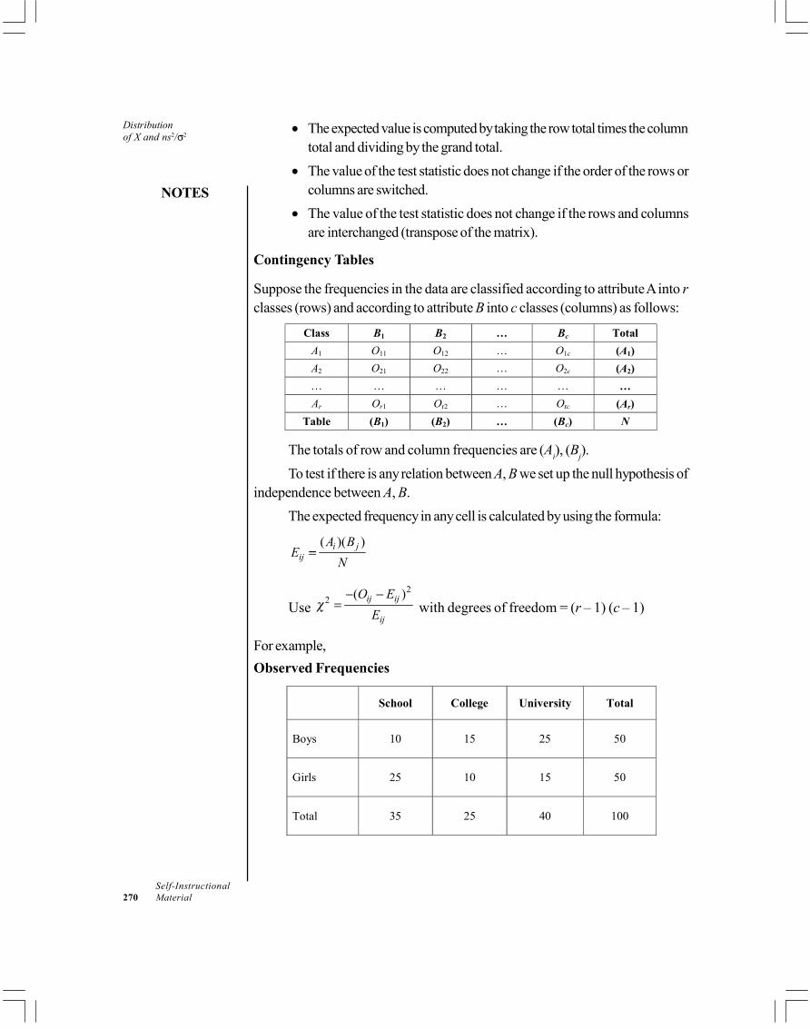
Distributionof X and ns2/ 2
NOTES
Self-Instructional270 Material
The expected value is computed by taking the row total times the columntotal and dividing by the grand total.The value of the test statistic does not change if the order of the rows orcolumns are switched.The value of the test statistic does not change if the rows and columnsare interchanged (transpose of the matrix).
Contingency Tables
Suppose the frequencies in the data are classified according to attribute A into rclasses (rows) and according to attribute B into c classes (columns) as follows:
Class B1 B2 … Bc Total A1 O11 O12 … O1c (A1)
A2 O21 O22 … O2c (A2) … … … … … … Ar Or1 Or2 … Orc (Ar)
Table (B1) (B2) … (Bc) N
The totals of row and column frequencies are (Ai), (Bj).To test if there is any relation between A, B we set up the null hypothesis of
independence between A, B.The expected frequency in any cell is calculated by using the formula:
( )( )i jij
A BE
N
Use 2
2 ( )ij ij
ij
O EE with degrees of freedom = (r – 1) (c – 1)
For example,Observed Frequencies
School College University Total
Boys 10 15 25 50
Girls 25 10 15 50
Total 35 25 40 100
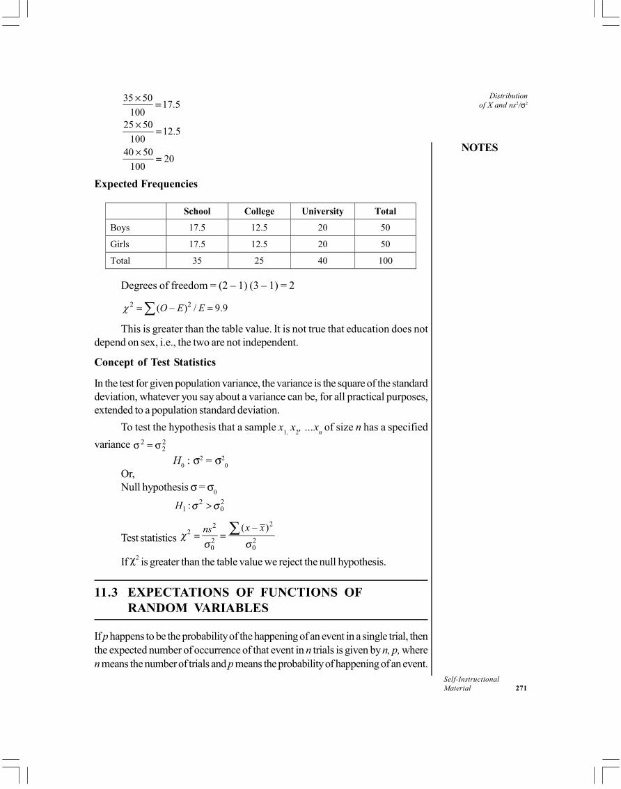
NOTES
Self-InstructionalMaterial 271
Distributionof X and ns2/ 2
35 50 17.5100
25 50 12.5100
40 50 20100
Expected Frequencies
School College University Total
Boys 17.5 12.5 20 50
Girls 17.5 12.5 20 50
Total 35 25 40 100
Degrees of freedom = (2 – 1) (3 – 1) = 22 2( ) / 9.9O E Eχ = − =∑
This is greater than the table value. It is not true that education does notdepend on sex, i.e., the two are not independent.
Concept of Test Statistics
In the test for given population variance, the variance is the square of the standarddeviation, whatever you say about a variance can be, for all practical purposes,extended to a population standard deviation.
To test the hypothesis that a sample x1, x2, …xn of size n has a specifiedvariance 2
H0 : 2 = 2
0Or,Null hypothesis = 0
2 21 0:H
Test statistics 22
22 20 0
( – )x xns
If 2 is greater than the table value we reject the null hypothesis.
11.3 EXPECTATIONS OF FUNCTIONS OFRANDOM VARIABLES
If p happens to be the probability of the happening of an event in a single trial, thenthe expected number of occurrence of that event in n trials is given by n, p, wheren means the number of trials and p means the probability of happening of an event.

Distributionof X and ns2/ 2
NOTES
Self-Instructional272 Material
Thus, the expectation may be regarded as the likely number of success in n trials.If probability p is determined as the Relative Frequency in n trials then themathematical expectation in these n trials would be equal to the actual (observed)number of successes in these n trials. Mathematical expectation does in no waymean that the concerning event must happen the number of times given by themathematical expectation; it simply gives the likely number of the happening of theevent in n trials. Mathematical expectation can be explained with the help of followingexamples.Example 1: In 12000 trials of a draw of two fair dice, what is the expectednumber of items that the sum will be less than 4?Solution: With two fair dice, the total number of equally likely cases = 6 × 6 = 36
Number of cases favourable to the event in a single thrown of two dice = 3viz., (1 + 1, 1 + 2, 2 + 1)
The required 3 1
36 12p = =
Hence, the expected number of times the total will be less than 4 in 12000trials.
1 12000 100012
= × =
The concept of expectation is of great use in the analysis of all games ofchance wherein an effort is made to evaluate the expectations of the players. If prepresents the probability of a player in any game and M the sum of money whichhe will receive in case of success, the sum of money denoted by (p.M) is called hisexpectation. Thus, the expectation is calculated by finding the probability of success(by any of the methods stated so far) and then multiplying it by the money valuewhich the player expects in case of success. The significance of this expectationlies in the fact that if a player pays more than this, by way of fair price, per gamethen he is sure to lose but if he plays long enough and if he pays less than hisexpectation per game he is certain to win in the long run. It is on this principle thatspeculators and businessmen take decisions in real life situations.Example 2: A and B throw with one die for a stake of Rs 44 which is to be wonby the player who first throws 2. If A has the first throw, what are their respectiveexpectation?
Solution: The chance of throwing 2 with one die = 16 , A can win in the first, third,
fifth .... throws.His chance of throwing 2 is,
1 5 5 1 ....6 6 6 6
+ × × +

NOTES
Self-InstructionalMaterial 273
Distributionof X and ns2/ 2
Or21 51 ...
6 6 + +
B can win the second, fourth, sixth ... throwHis chance of throwing 2 is,
5 1 5 5 5 1 ...6 6 6 6 6 6× + × × × +
Or25 51 ...
36 6 + +
A’s chance to B’s chance stands as 6 : 5. Hence their respective chances
are 6
11 and
511
. As such their expectations are as under:
A’s expectation = 6 26444 24
11 11× = = Rs
B’s expectation = 5 22044 20
11 11× = = Rs
Example 3: A person has ten coins which he throws down in succession. He is toreceive one rupee if the first falls head, two rupees if the second also falls head,four rupees if the third also falls head and so on. The amount doubling each timebut as soon as a coin falls tail he ceases to receive any thing. What is the value ofhis expectation?Solution:
Chance of falling head = 12
Chance of falling tail = 12
Chance of falling head in 1st trial = 12
Expectation in 1st trial = 1 112 2× = Re
Now if he succeeds in getting head in the first trial then only he is allowed todo his second trial.
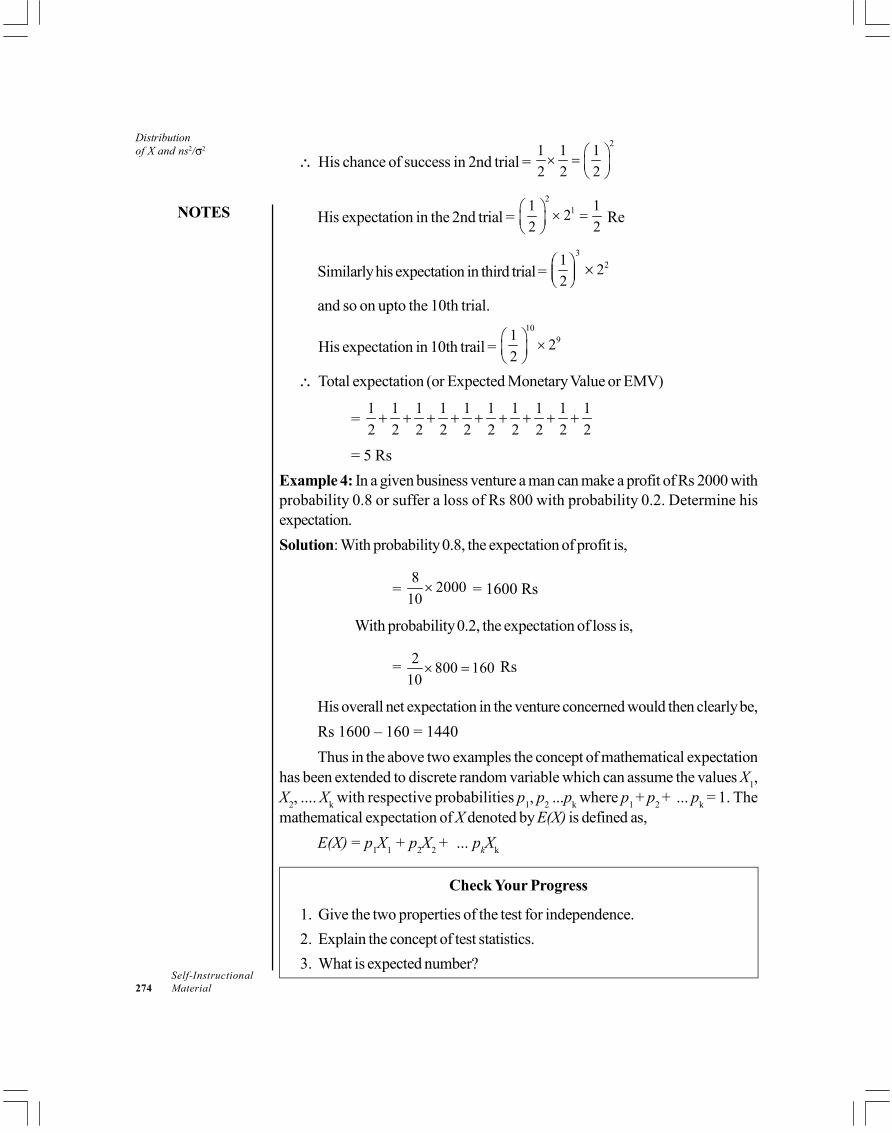
Distributionof X and ns2/ 2
NOTES
Self-Instructional274 Material
His chance of success in 2nd trial = 21 1 1
2 2 2 × =
His expectation in the 2nd trial = 2
11 122 2
× =
Re
Similarly his expectation in third trial = 3
21 22
and so on upto the 10th trial.
His expectation in 10th trail = 10
91 22
×
Total expectation (or Expected Monetary Value or EMV)
= 1 1 1 1 1 1 1 1 1 12 2 2 2 2 2 2 2 2 2+ + + + + + + + +
= 5 RsExample 4: In a given business venture a man can make a profit of Rs 2000 withprobability 0.8 or suffer a loss of Rs 800 with probability 0.2. Determine hisexpectation.Solution: With probability 0.8, the expectation of profit is,
= 8 2000
10× = 1600 Rs
With probability 0.2, the expectation of loss is,
= 2 800 16010
× = Rs
His overall net expectation in the venture concerned would then clearly be,Rs 1600 – 160 = 1440Thus in the above two examples the concept of mathematical expectation
has been extended to discrete random variable which can assume the values X1,X2, .... Xk with respective probabilities p1, p2 ...pk where p1 + p2 + ... pk = 1. Themathematical expectation of X denoted by E(X) is defined as,
E(X) = p1X1 + p2X2 + ... pkXk
Check Your Progress
1. Give the two properties of the test for independence.2. Explain the concept of test statistics.3. What is expected number?

NOTES
Self-InstructionalMaterial 275
Distributionof X and ns2/ 211.4 ANSWERS TO CHECK YOUR PROGRESS
QUESTIONS
1. The following are properties of the test for independence(a) The data are the observed frequencies.(b) The data is arranged into a contingency table.
2. In the test for given population variance, the variance is the square of thestandard deviation, whatever you say about a variance can be, for all practicalpurposes, extended to a population standard deviation.
3. If p happens to be the probability of the happening of an event in a singletrial, then the expected number of occurrence of that event in n trials isgiven by n, p, where n means the number of trials and p means theprobability of happening of an event.
11.5 SUMMARY
The degrees of freedom are the degrees of freedom for the row variabletimes the degrees of freedom for the column variable. It is not one lessthan the sample size, it is the product of the two degrees of freedom.The expected value is computed by taking the row total times the columntotal and dividing by the grand total.The value of the test statistic doesn’t change if the order of the rows orcolumns are switched.The value of the test statistic doesn’t change if the rows and columns areinterchanged (transpose of the matrix).If probability p is determined as the Relative Frequency in n trials then themathematical expectation in these n trials would be equal to the actual(observed) number of successes in these n trials.
11.6 KEY WORDS
Probability distribution: In probability theory and statistics, a probabilitydistribution is the mathematical function that gives the probabilities ofoccurrence of different possible outcomes for an experiment.Null hypothesis: = 0
2 21 0:H
Test statistics: 22
22 20 0
( – )x xns
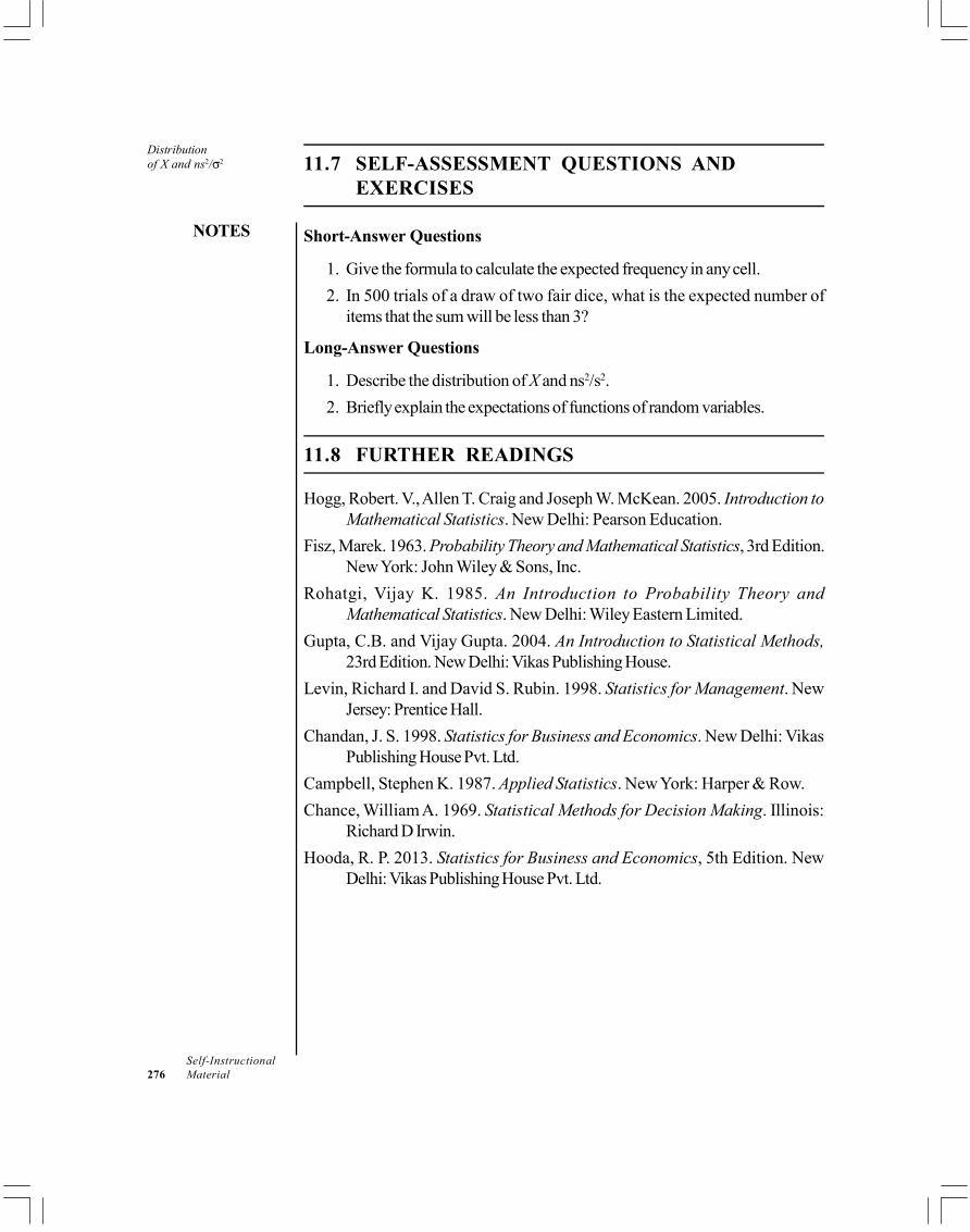
Distributionof X and ns2/ 2
NOTES
Self-Instructional276 Material
11.7 SELF-ASSESSMENT QUESTIONS ANDEXERCISES
Short-Answer Questions
1. Give the formula to calculate the expected frequency in any cell.2. In 500 trials of a draw of two fair dice, what is the expected number of
items that the sum will be less than 3?
Long-Answer Questions
1. Describe the distribution of X and ns2/s2.2. Briefly explain the expectations of functions of random variables.
11.8 FURTHER READINGS
Hogg, Robert. V., Allen T. Craig and Joseph W. McKean. 2005. Introduction toMathematical Statistics. New Delhi: Pearson Education.
Fisz, Marek. 1963. Probability Theory and Mathematical Statistics, 3rd Edition.New York: John Wiley & Sons, Inc.
Rohatgi, Vijay K. 1985. An Introduction to Probability Theory andMathematical Statistics. New Delhi: Wiley Eastern Limited.
Gupta, C.B. and Vijay Gupta. 2004. An Introduction to Statistical Methods,23rd Edition. New Delhi: Vikas Publishing House.
Levin, Richard I. and David S. Rubin. 1998. Statistics for Management. NewJersey: Prentice Hall.
Chandan, J. S. 1998. Statistics for Business and Economics. New Delhi: VikasPublishing House Pvt. Ltd.
Campbell, Stephen K. 1987. Applied Statistics. New York: Harper & Row.Chance, William A. 1969. Statistical Methods for Decision Making. Illinois:
Richard D Irwin.Hooda, R. P. 2013. Statistics for Business and Economics, 5th Edition. New
Delhi: Vikas Publishing House Pvt. Ltd.

NOTES
Self-InstructionalMaterial 277
Limiting Distributionsand ConvergenceBLOCK - IV
LIMITING DISTRIBUTIONS
UNIT 12 LIMITING DISTRIBUTIONSAND CONVERGENCE
Structure12.0 Introduction12.1 Objectives12.2 Limiting Distributions
12.2.1 Convergence in Distribution12.2.2 Convergence in Probability
12.3 Answers to Check Your Progress Questions12.4 Summary12.5 Key Words12.6 Self-Assessment Questions and Exercises12.7 Further Readings
12.0 INTRODUCTION
A ‘Limiting Distribution’ is also termed as an ‘Asymptotic Distribution’.Fundamentally, it is defined as the hypothetical distribution or convergence of asequence of distributions. Since it is hypothetical, it is not considered as a distributionas per the general logic. The asymptotic distribution theory is typically used to finda limiting distribution to a series of distributions. The mode of convergence for asequence of random variables are defined on the basis of the convergence inprobability and in distribution. The concept of convergence leads us to the twofundamental results of probability theory, the Law of Large Number and CentralLimit Theorem (CLT). Limiting probability distributions are significantly used tofind the appropriate sample sizes. When a sample size is large enough, then astatistic’s distribution will form a limiting distribution, assuming that such a distributionexists. In probability theory, there exist several different notions of convergence ofrandom variables. The convergence of sequences of random variables to somelimit random variable is an important concept in probability theory, and itsapplications to statistics and stochastic processes. The same concepts are knownin more general mathematics as ‘Stochastic Convergence’.
In this unit, you will study about the limiting distributions, convergence indistribution and convergence in probability.

Limiting Distributionsand Convergence
NOTES
Self-Instructional278 Material
12.1 OBJECTIVES
After going through this unit, you will be able to:Understand the basic concept of limiting distributionsAnalyse what convergence in distribution isExplain about the convergence in probability
12.2 LIMITING DISTRIBUTIONS
A ‘Limiting Distribution’ is also termed as an ‘Asymptotic Distribution’.Fundamentally, it is defined as the hypothetical distribution or convergence of asequence of distributions. Since it is hypothetical, it is not considered as a distributionas per the general logic. The asymptotic distribution theory is typically used to finda limiting distribution to a series of distributions.
Some of the limiting or asymptotic distributions are well-recognized anddefined by different statisticians. For example, the sampling distribution of the t-statistic will converge to a standard normal distribution if the sample size is largeenough.
In basic statistics, the process includes a random sample of observationsand then fitting that data to a known distribution similar to the normal distributionor t distribution. Fitting the statistical data accurately to a known distribution isgenerally very challenging task because of the limited sample sizes. The accurateapproximation is based on the estimation of ‘presumptions and guesses’ establishedon the nature of large sample statistics. The limiting/asymptotic distribution can beapplied on small, finite samples for approximating the true distribution of a randomvariable.
Limiting probability distributions are significantly used to find the appropriatesample sizes. When a sample size is large enough, then a statistic’s distribution willform a limiting distribution, assuming that such a distribution exists.
The Central Limit Theorem (CLT) uses the limit concept for describing thebehaviour of sample means. The CLT states that the sampling distribution of thesampling means approaches a normal distribution as the sample size increases —irrespective of the shape of the population distribution. For example, if you considerlarge samples then the graph of the sample means will be similar to a normaldistribution, even if the graph is skewed or otherwise non-normal. Alternatively,the ‘Limiting Distribution’ for a large set of sample means is the ‘Normal Distribution’.Definition: Suppose Xn is a random sequence with Cumulative DistributionFunction (CDF) Fn (Xn) and X is a random variable with CDF F(x). If Fn convergesto F as n > (for all points where F(x) is continuous), then the distribution of xnconverges to x. This distribution is called the limiting distribution of xn.
NOTES
Self-InstructionalMaterial 279
Limiting Distributionsand Convergence
In simpler terms, it can be stated that the limiting probability distribution ofXn is the limiting distribution of some function of Xn.
Convergence of Random Variables
In probability theory, there exist several different notions of convergence of randomvariables. The convergence of sequences of random variables to some limit randomvariable is an important concept in probability theory, and its applications to statisticsand stochastic processes. The same concepts are known in more generalmathematics as ‘Stochastic Convergence’ and they formalize the idea that asequence of essentially random or unpredictable events can sometimes be expectedto settle down into a behaviour that is essentially unchanging when items far enoughinto the sequence are studied. The different possible notions of convergence relateto how such a behaviour can be characterized: two readily understood behavioursare that the sequence eventually takes a constant value, and that values in thesequence continue to change but can be described by an unchanging probabilitydistribution.
‘Stochastic Convergence’ validates the notion that a sequence of essentiallyrandom or unpredictable events can sometimes be expected to settle into a pattern.The pattern may be,
Convergence in the classical sense to a fixed value, perhaps itself comingfrom a random event.An increasing similarity of outcomes to what a purely deterministicfunction would produce.An increasing preference towards a certain outcome.An increasing ‘aversion’ against straying far away from a certain outcome.That the probability distribution describing the next outcome may growincreasingly similar to a certain distribution.
Some more theoretical patterns state that the,Series formed by calculating the expected value of the outcome’s distancefrom a particular value may converge to 0.Variance of the random variable describing the next event grows smallerand smaller.
The above mentioned facts define the convergence of a single series to alimiting value, the notion of the convergence of two series towards each other isalso significant and the sequence is defined as either the difference or the ratio ofthe two series.
If the average of n independent random variables Yi, for i = 1, ..., n, allhaving the same finite mean and variance, is given by,

Limiting Distributionsand Convergence
NOTES
Self-Instructional280 Material
Then as n tends to infinity, Xn converges in probability to the common mean,, of the random variables Yi. This result is known as the ‘Weak Law of Large
Numbers’. Other forms of convergence are important in other useful theorems,including the Central Limit Theorem (CLT).
Here we assume that (Xn) is a sequence of random variables, where X is arandom variable, and these are defined on the same probability space ( , , Pr).
12.2.1 Convergence in Distribution
The convergence in distribution mode provide the required expectation to recogniseand observe the next outcome in a sequence of random experiments which is wellmodelled by means of a given probability distribution.
Convergence in distribution is typically considered as the weakest form ofconvergence, since it is implied by all other types of convergence. However,convergence in distribution is very frequently used in practice; most often it arisesfrom application of the Central Limit Theorem (CLT).
Definition: A sequence X1, X2, ... of real-valued random variables is saidto converge in distribution, or converge weakly, or converge in law to a randomvariable X if,
For every number at which F is continuous. Here Fn and F are theCumulative Distribution Functions (CDFs) of random variables Xn and X,respectively.
Essentially, only the continuity points of F should be considered. Forexample, if Xn are distributed uniformly on intervals (0, 1/n), then this sequenceconverges in distribution to degenerate a random variable X = 0. Certainly, wecan state that Fn (x) = 0 for all n when x 0, and Fn (x) = 1 for all x 1/n when n >0. However, for this limiting random variable F (0) = 1, even though Fn (0) =0 for all n.
Thus the convergence of CDFs fails at the point x = 0 where F isdiscontinuous.
Convergence in distribution may be denoted as,
Where is the probability distribution law of X. For example, if X is
standard normal we can write .

NOTES
Self-InstructionalMaterial 281
Limiting Distributionsand Convergence
For random vectors X1, X2, ... Rk the convergence in distribution canbe similarly defined. We say that this sequence converges in distribution to a randomk-vector X if,
For every A Rk which is a continuity set of X.The definition of convergence in distribution may be extended from random
vectors to more general random elements in arbitrary metric spaces, and even tothe ‘random variables’ which are not measurable, for example a situation whichoccurs in the study of empirical processes. This is referred as the ‘WeakConvergence of Laws without Laws Being Defined’ except asymptotically.
In this case the term ‘Weak Convergence’ is preferably used and we saythat a sequence of random elements Xn converges weakly to X (denotedas Xn X) if,
E* h (Xn) E h(X)For all continuous bounded functions h. Here E* denotes the outer
expectation, that is the expectation of a ‘Smallest Measurable Function g thatDominates h(Xn)’.
Example of convergence in distribution can be explained by means of thenewly built dice factory. Suppose a new dice factory has just been built. The firstfew dice come out quite biased, due to imperfections in the production process.The outcome from tossing any of them will follow a distribution markedly differentfrom the desired uniform distribution.
As the production in the factory improves, the dice become less and lessloaded, and the outcomes from tossing a newly produced die will follow the uniformdistribution more and more closely.
12.2.2 Convergence in Probability
The basic notion behind this type of convergence is that the probability of an‘unusual’ outcome becomes smaller and smaller as the sequence progresses.
The concept of convergence in probability is used very often in statistics.For example, an estimator is called consistent if it converges in probability to thequantity being estimated. Convergence in probability is also the type of convergenceestablished by the ‘Weak Law of Large Numbers’.Definition: A sequence Xn of random variables Converges inProbability towards the random variable X if for all > 0,

Limiting Distributionsand Convergence
NOTES
Self-Instructional282 Material
More explicitly, let Pn be the probability that Xn is outside the ball ofradius centred at X. Then Xn is said to converge in probability to X if for any >0 and any > 0 there exists a number N (which may depend on and ) suchthat for all n N, Pn < (the Definition of Limit).
Notice that for the condition to be satisfied, for each n the randomvariables X and Xn cannot be independent and thus convergence in probability isa condition on the joint CDF’s, as opposed to convergence in distribution, whichis a condition on the individual CDF’s, unless X is deterministic like for the ‘WeakLaw of Large Numbers’. At the same time, the case of a deterministic X cannot,whenever the deterministic value is a discontinuity point (not isolated), be handledby convergence in distribution, where discontinuity points have to be explicitlyexcluded.
Convergence in probability is denoted by adding the letter ‘p’ over an arrowindicating convergence, or using the ‘plim’ probability limit operator:
For random elements Xn on a separable metric space (S, d), convergencein probability is defined similarly by,
Properties
‘Convergence in Probability’ implies ‘Convergence in Distribution’.In the opposite direction, convergence in distribution implies convergencein probability when the limiting random variable X is a constant.Convergence in probability does not imply almost sure convergence.The continuous mapping theorem states that for every continuous
function g( ), if , then also .
Check Your Progress
1. Explain the basic concept of limiting distribution?2. When the limiting/asymptotic distribution can be applied?3. Why the limiting probability distributions are used in statistics?4. Elucidate on the convergence in distribution in probability distribution.5. Explain the concept of convergence in probability. Why it is often used in
statistics?

NOTES
Self-InstructionalMaterial 283
Limiting Distributionsand Convergence12.3 ANSWERS TO CHECK YOUR PROGRESS
QUESTIONS
1. A ‘Limiting Distribution’ is also termed as an ‘Asymptotic Distribution’.Fundamentally, it is defined as the hypothetical distribution or convergenceof a sequence of distributions. The asymptotic distribution theory is typicallyused to find a limiting distribution to a series of distributions. Some of thelimiting or asymptotic distributions are well-recognized and defined bydifferent statisticians. For example, the sampling distribution of the t-statisticwill converge to a standard normal distribution if the sample size is largeenough.
2. The limiting/asymptotic distribution can be applied on small, finite samplesfor approximating the true distribution of a random variable.
3. Limiting probability distributions are significantly used to find the appropriatesample sizes. When a sample size is large enough, then a statistic’s distributionwill form a limiting distribution, assuming that such a distribution exists. Instatistics, the process includes a random sample of observations and thenfitting that data to a known distribution similar to the normal distribution ort distribution. Fitting the statistical data accurately to a known distribution isgenerally very challenging task because of the limited sample sizes.
4. The convergence in distribution mode provide the required expectation torecognise and observe the next outcome in a sequence of randomexperiments which is well modelled by means of a given probabilitydistribution. Convergence in distribution is typically considered as the weakestform of convergence, since it is implied by all other types of convergence.
5. The basic notion behind the convergence in probability type is that theprobability of an ‘unusual’ outcome becomes smaller and smaller as thesequence progresses.The concept of convergence in probability is used very often in statistics.For example, an estimator is called consistent if it converges in probabilityto the quantity being estimated.
12.4 SUMMARY
A ‘Limiting Distribution’ is also termed as an ‘Asymptotic Distribution’.Fundamentally, it is defined as the hypothetical distribution or convergenceof a sequence of distributions.The asymptotic distribution theory is typically used to find a limitingdistribution to a series of distributions.

Limiting Distributionsand Convergence
NOTES
Self-Instructional284 Material
Some of the limiting or asymptotic distributions are well-recognized anddefined by different statisticians.In basic statistics, the process includes a random sample of observationsand then fitting that data to a known distribution similar to the normaldistribution or t distribution.The accurate approximation is based on the estimation of ‘presumptionsand guesses’ established on the nature of large sample statistics.The limiting/asymptotic distribution can be applied on small, finite samplesfor approximating the true distribution of a random variable.Limiting probability distributions are significantly used to find the appropriatesample sizes. When a sample size is large enough, then a statistic’s distributionwill form a limiting distribution, assuming that such a distribution exists.The Central Limit Theorem (CLT) uses the limit concept for describing thebehaviour of sample means. The CLT states that the sampling distributionof the sampling means approaches a normal distribution as the sample sizeincreases — irrespective of the shape of the population distribution.In simpler terms, it can be stated that the limiting probability distribution ofXn is the limiting distribution of some function of Xn.The different possible notions of convergence relate to how such a behaviourcan be characterized: two readily understood behaviours are that thesequence eventually takes a constant value, and that values in the sequencecontinue to change but can be described by an unchanging probabilitydistribution.‘Stochastic convergence’ validates the notion that a sequence of essentiallyrandom or unpredictable events can sometimes be expected to settle into apattern.The probability distribution describing the next outcome may growincreasingly similar to a certain distribution.Series formed by calculating the expected value of the outcome’s distancefrom a particular value may converge to 0.Variance of the random variable describing the next event grows smallerand smaller.The convergence in distribution mode provide the required expectation torecognise and observe the next outcome in a sequence of randomexperiments which is well modelled by means of a given probabilitydistribution.Convergence in distribution is typically considered as the weakest form ofconvergence, since it is implied by all other types of convergence.

NOTES
Self-InstructionalMaterial 285
Limiting Distributionsand Convergence
However, convergence in distribution is very frequently used in practice;most often it arises from application of the Central Limit Theorem (CLT).The definition of convergence in distribution may be extended from randomvectors to more general random elements in arbitrary metric spaces, andeven to the ‘random variables’ which are not measurable, for example asituation which occurs in the study of empirical processes.The basic notion behind this type of convergence is that the probability ofan ‘unusual’ outcome becomes smaller and smaller as the sequenceprogresses.The concept of convergence in probability is used very often in statistics.For example, an estimator is called consistent if it converges in probabilityto the quantity being estimated.Convergence in probability is denoted by adding the letter ‘p’ over an arrowindicating convergence, or using the ‘plim’ probability limit operator:
‘Convergence in Probability’ implies ‘Convergence in Distribution’.In the opposite direction, convergence in distribution implies convergencein probability when the limiting random variable X is a constant.
12.5 KEY WORDS
Limiting distribution: A ‘Limiting Distribution’ is also termed as an‘Asymptotic Distribution’, it is defined as the hypothetical distribution orconvergence of a sequence of distributions.Limiting probability distributions: The limiting probability distributionsare significantly used to find the appropriate sample sizes.Central Limit Theorem (CLT): The Central Limit Theorem (CLT) usesthe limit concept for describing the behaviour of sample means, it states thatthe sampling distribution of the sampling means approaches a normaldistribution as the sample size increases — irrespective of the shape of thepopulation distribution.Stochastic convergence: Stochastic convergence validates the notion thata sequence of essentially random or unpredictable events can sometimesbe expected to settle into a pattern.Convergence in distribution: Convergence in distribution mode providethe required expectation to recognise and observe the next outcome in asequence of random experiments which is well modelled by means of agiven probability distribution.

Limiting Distributionsand Convergence
NOTES
Self-Instructional286 Material
12.6 SELF-ASSESSMENT QUESTIONS ANDEXERCISES
Short-Answer Questions
1. What is limiting distribution?2. Define the term convergence.3. What is stochastic convergence?4. Give definition for convergence in distribution.5. Define the basic concept of convergence in probability.6. State the properties of convergence.
Long-Answer Questions
1. Briefly discuss the significance of limiting distributions in the field of probabilityand statistics.
2. Explain about the convergence of random variables giving appropriateexamples.
3. Discuss the concept of convergence in distribution giving definition andappropriate examples.
4. Why the Central Limit Theorem (CLT) uses the limit concept for describingthe behaviour of sample means? Explain giving appropriate examples.
5. Analyse and discuss the significance of convergence in probability givingdefinition and appropriate examples.
6. Is N(0, 1/n) close to the N(1/n, 1/n) distribution? Explain.7. ‘Xn converges in distribution to X’. Justify the statement with appropriate
proof.
12.7 FURTHER READINGS
Hogg, Robert. V., Allen T. Craig and Joseph W. McKean. 2005. Introduction toMathematical Statistics. New Delhi: Pearson Education.
Fisz, Marek. 1963. Probability Theory and Mathematical Statistics, 3rd Edition.New York: John Wiley & Sons, Inc.
Rohatgi, Vijay K. 1985. An Introduction to Probability Theory andMathematical Statistics. New Delhi: Wiley Eastern Limited.
Gupta, C.B. and Vijay Gupta. 2004. An Introduction to Statistical Methods,23rd Edition. New Delhi: Vikas Publishing House.

NOTES
Self-InstructionalMaterial 287
Limiting Distributionsand Convergence
Levin, Richard I. and David S. Rubin. 1998. Statistics for Management. NewJersey: Prentice Hall.
Chandan, J. S. 1998. Statistics for Business and Economics. New Delhi: VikasPublishing House Pvt. Ltd.
Campbell, Stephen K. 1987. Applied Statistics. New York: Harper & Row.Chance, William A. 1969. Statistical Methods for Decision Making. Illinois:
Richard D Irwin.Hooda, R. P. 2013. Statistics for Business and Economics, 5th Edition. New
Delhi: Vikas Publishing House Pvt. Ltd.
Limiting MomentGenerating Function andCentral Limit Theorem
NOTES
Self-Instructional288 Material
UNIT 13 LIMITING MOMENTGENERATING FUNCTIONAND CENTRAL LIMITTHEOREM
Structure13.0 Introduction13.1 Objectives13.2 Limiting Moment Generating Functions13.3 The Central Limit Theorem (CLT)13.4 Answers to Check Your Progress Questions13.5 Summary13.6 Key Words13.7 Self-Assessment Questions and Exercises13.8 Further Readings
13.0 INTRODUCTION
In probability theory, the Central Limit Theorem (CLT) establishes that, in somesituations, when independent random variables are added, their properly normalizedsum tends toward a normal distribution (informally a bell curve) even if the originalvariables themselves are not normally distributed. The theorem is a key concept inprobability theory because it implies that probabilistic and statistical methods thatwork for normal distributions can be applicable to many problems involving othertypes of distributions.
In this unit, you will study about the limiting moment generating function andcentral limit theorem.
13.1 OBJECTIVES
After going through this unit, you will be able to:Explain about the limiting moment generating functionUnderstand the central limit theorem
13.2 LIMITING MOMENT GENERATINGFUNCTIONS
Binomial, Poisson, negative binomial and uniform distribution are some of thediscrete probability distributions. The random variables in these distributions assume

NOTES
Self-InstructionalMaterial 289
Limiting MomentGenerating Function and
Central Limit Theorem
a finite or enumerably infinite number of values but in nature these are randomvariables which take infinite number of values i.e., these variables can take anyvalue in an interval. Such variables and their probability distributions are known ascontinuous probability distributions.
A random variable X is the said to be normally distributed if it has the followingprobability density function:
f(x) =
21 ––21 ,
2
x
eµ
σ
σ π for – x
Where and > 0 are the parameters of distribution.Normal Curve: A curve given by,
yx =
21 ––2
0
x
y eµ
σ
Which is known as the normal curve when origin is taken at mean.
Then, yx =
2
21–2
0
x
y e σ .
O
yxy0
Fig. 13.1 Normal Curve
Standard Normal Variate : A normal variate with mean zero and standarddeviation unity, is called a standard normal variate.
That is; if X is a standard normal variate then E(X) = 0 and V(X) = 1.Then, X ~ N (0, 1)The moment generating function or MGF of a standard normal variate is
given as follows:
MX(t) = 2 2 21 1
2 2
01
t t te eµ + σ
µ =σ =
=

Limiting MomentGenerating Function andCentral Limit Theorem
NOTES
Self-Instructional290 Material
Frequently the exchange of variable in the integral:
2 2– ( – ) / 2
–
12
xe∞
µ σ
∞σ π ∫
Is used by introducing the following new variable:
Z = – ~ (0,1)X Nµσ
This new random variable Z simplifies calculations of probabilities etc.concerning normally distributed variates.
Standard Normal Distribution: The distribution of a random variable –XZ µ
=σ
which is known as standard normal variate, is called the standard normal distributionor unit normal distribution, where X has a normal distribution with mean endvariance 2.
The density function of Z is given as follows:
(Z) = 21–
21 ,2
Ze
π– < Z <
with mean O variance one of MGF 21
2t
e . Normal distribution is the most frequentlyused distribution in statistics. The importance of this distribution is highlighted bycentral limit theorem, mathematical properties, such as the calculation of height,weight, the blood pressure of normal individuals, heart diameter measurement,etc. They all follow normal distribution if the number of observations is very large.Normal distribution also has great importance in statistical inference theory.Examples of Normal Distribution:
1. The height of men of matured age belonging to same race and living insimilar environments provide a normal frequency distribution.
2. The heights of trees of the same variety and age in the same locality wouldconfirm to the laws of normal curve.
3. The length of leaves of a tree form a normal frequency distribution. Thoughsome of them are very short and some are long, yet they try to tend towardstheir mean length.
Example 1: X has normal distribution with = 50 and 2 = 25. Find out(i) The approximate value of the probability density function for X = 50(ii) The value of the distribution function for x = 50.

NOTES
Self-InstructionalMaterial 291
Limiting MomentGenerating Function and
Central Limit TheoremSolution: (i) f(x) = 2 2– ( – ) / 21
2xe µ σ
σ π, – x
for X = 50, 2 = 25, = 50, you have
f(x) = 1
5 2π 0.08.
Distribution function f(x)
= 2 2– ( – ) / 2
–
1 .2
xxe dxµ σ
∞ σ π∫
= 2
–1–2
–
12
x
Ze dZ
µ σ
∞ π∫ , where Z = –x µσ
F(50) = 210 –
2
–
1 . 0.5.2
Ze dZ
∞
=π∫
Example 2: If X is a normal variable with mean 8 and standard deviation 4, find(i) P[X 5](ii) P[5 X 10]
Solution: (i) P[X 5] = – 5 8
4XP µ − ≤ σ
0.5
= P (Z – 0.75)= P (Z 0.75)
[By Symmetry]
= 0.5 – P(0 Z 0.75)[To use relevant table]
= 0.5 – 0.2734 [See Appendix for value of ‘2’]= 0.2266.

Limiting MomentGenerating Function andCentral Limit Theorem
NOTES
Self-Instructional292 Material
(ii) P[5 X 10] = 5.8 10 84 4
P Z − ≤ ≤
= P(– 0.75 Z 0.5)= P(– 0.75 Z 0) + P(0 Z 0.5)
= P(– 0 Z 0.75) + P(0 Z 0.5)
= 0.2734 + 0.1915[See Appendix]
= 0.4649.Example 3: X is a normal variate with mean 30 and S.D. 5. Find
(i) P[26 X 40]
(ii) P[| X – 30 | > 5]Solution: Here = 30, = 5.
Z = – 0.8 Z = 0X = 40Z = 2
(i) When X = 26, Z = – – 0.8X µ
=σ
And for X = 40, Z = – 2X µ
=σ
P[26 X 40] = P[– 0.8 Z 2]= P[0 Z 0.8] + P[0 Z 2]= 0.2881 + 0.4772 = 0.7653
(ii) P[| X – 3 | > 5] = 1 – P[| X – 3 | 5]P[| X – 3 | 5] = P[25 X 35]
= 25 30
5P Z− 35 − 30 ≤ ≤ 5
= 2.P (0 Z 1) = 0.= 2 × 0.3413 = 0.6826.

NOTES
Self-InstructionalMaterial 293
Limiting MomentGenerating Function and
Central Limit Theorem
So P[| X – 3| > 5] = 1 – P[| X – 3 | 5]= 1 – 0.6826 = 0.3174.
13.3 THE CENTRAL LIMIT THEOREM (CLT)
The Central Limit Theorem (CLT) has several variants. In its common form, therandom variables must be identically distributed. In variants, convergence of themean to the normal distribution also occurs for non-identical distributions or fornon-independent observations, if they comply with certain conditions.
The earliest version of this theorem, that the normal distribution may beused as an approximation to the binomial distribution, is the de Moivre–Laplacetheorem.
Let X1, X2,.... Xn be n independent random variables all of whichhave the same distribution. Let the common expectation and variance be
and 2, respectively.
Let X = 1
ni
i
Xn=
∑
Then, the distribution of X approches the normal distribution with mean m
and variance 2
nσ
as n
That is, the variate Z = /
Xn
− µσ
has standard normal distribution.
Proof: Moment generating function of Z about origin is given as follows:
MZ(t) = E(etZ) = –
/Xt
nE e µ σ
= – / /( )t n t ne E eµ σ × σ
= 1 2 ...
–.
nt n X X Xnt ne E e+ + +
µ σ σ
= 1 2( ... )–
.n
tn X X Xt ne E e+ + +µ σσ

Limiting MomentGenerating Function andCentral Limit Theorem
NOTES
Self-Instructional294 Material
= –
1 2. ( ... ) .nt
nte M X X X
n
µσ + + +
σ
= –
.
n
ntx
te Mt
n
µσ
σ σ
This is because the random variables are independent and have the sameMGF by using logarithms, you have:
log Mz(t) = log xt n tn M
n − µ
+ σ σ
= 2
2log 1 ...2 !
t n t t inn n
1 − µ µ′ µ′ + + + + σ σ σ
= 22
22
1. ... – ... ...2 ! 2
t n t t t tnn nn
1 1 − µ µ′ µ′ µ′ + + + + + σ σ σσ
= 22 2
2 12 2– ...
2 2t n t n t t1− µ µ′ µ′ µ′
+ + +σ σ σ σ
= 2
– 1/ 2( )2t O n+ [ 2 – 1
2 = 21 = ]
Hence, as n
log(Mz)(t) 2
2t
i.e. M2(t) = et2/2
However, this is the M.G.F. of a standard normal random variable. Thus,the random variable Z converges to N.
This follows that the limiting distribution of x as normal with mean and
variance 2
nσ .
Check Your Progress
1. What is standard normal variate?2. Define the term standard normal distribution.
NOTES
Self-InstructionalMaterial 295
Limiting MomentGenerating Function and
Central Limit Theorem13.4 ANSWERS TO CHECK YOUR PROGRESS
QUESTIONS
1. A normal variate with mean zero and standard deviation unity, is called astandard normal variate.
2. The distribution of a random variable –XZ µ
=σ
which is known as
standard normal variate, is called the standard normal distribution or unitnormal distribution, where X has a normal distribution with mean endvariance 2.
13.5 SUMMARY
Binomial, Poisson, negative binomial and uniform distribution are some ofthe discrete probability distributions.A normal variate with mean zero and standard deviation unity, is called astandard normal variate.The height of men of matured age belonging to same race and living insimilar environments provide a normal frequency distribution.The length of leaves of a tree form a normal frequency distribution. Thoughsome of them are very short and some are long, yet they try to tend towardstheir mean length.
13.6 KEY WORDS
Variants: In variants, convergence of the mean to the normal distributionalso occurs for non-identical distributions or for non-independentobservations, if they comply with certain conditions.Standard normal variate: A normal variate with mean zero and standarddeviation unity, is called a standard normal variate.
13.7 SELF-ASSESSMENT QUESTIONS ANDEXERCISES
Short-Answer Questions
1. What is meant by normal curve?2. Give the density function of Z.3. Write some examples of normal distribution.

Limiting MomentGenerating Function andCentral Limit Theorem
NOTES
Self-Instructional296 Material
Long-Answer Questions
1. Briefly discuss about the limiting moment generating functions.2. Explain about the moment generating function of a standard normal variate.3. Discuss the central limit theorem. Give examples.
13.8 FURTHER READINGS
Hogg, Robert. V., Allen T. Craig and Joseph W. McKean. 2005. Introduction toMathematical Statistics. New Delhi: Pearson Education.
Fisz, Marek. 1963. Probability Theory and Mathematical Statistics, 3rd Edition.New York: John Wiley & Sons, Inc.
Rohatgi, Vijay K. 1985. An Introduction to Probability Theory andMathematical Statistics. New Delhi: Wiley Eastern Limited.
Gupta, C.B. and Vijay Gupta. 2004. An Introduction to Statistical Methods,23rd Edition. New Delhi: Vikas Publishing House.
Levin, Richard I. and David S. Rubin. 1998. Statistics for Management. NewJersey: Prentice Hall.
Chandan, J. S. 1998. Statistics for Business and Economics. New Delhi: VikasPublishing House Pvt. Ltd.
Campbell, Stephen K. 1987. Applied Statistics. New York: Harper & Row.Chance, William A. 1969. Statistical Methods for Decision Making. Illinois:
Richard D Irwin.Hooda, R. P. 2013. Statistics for Business and Economics, 5th Edition. New
Delhi: Vikas Publishing House Pvt. Ltd.

NOTES
Self-InstructionalMaterial 297
Some Theorems onLimiting DistributionsUNIT 14 SOME THEOREMS ON
LIMITING DISTRIBUTIONS
Structure14.0 Introduction14.1 Objectives14.2 Some Theorems on Limiting Distributions
14.2.1 Weak Law of Large Numbers14.2.2 Strong Law of Large Numbers
14.3 Answers to Check Your Progress Questions14.4 Summary14.5 Key Words14.6 Self-Assessment Questions and Exercises14.7 Further Readings
14.0 INTRODUCTION
A general name for a number of theorems in probability theory that give conditionsfor the appearance of some regularity as the result of the action of a large numberof random sources. The first limit theorems, established by J. Bernoulli (1713) andP. Laplace (1812), are related to the distribution of the deviation of the frequency μn/n of appearance of some event EE in n independent trials from itsprobability p, 0<p<10<p<1( exact statements can be found in the articles Bernoullitheorem; Laplace theorem). S. Poisson (1837) generalized these theorems to thecase when the probability pk of appearance of E in the k- th trial depends on k,by writing down the limiting behaviour, as n , of the distribution of the deviation
of μn/n from the arithmetic mean 1
/n
kkp p n of the probabilities pk,
1 k n (cf. Poisson Theorem).In this unit, you will study about the some theorems of limiting distributions.
14.1 OBJECTIVES
After going through this unit, you will be able to:Analyse the some theorems of limiting distributionsUnderstand some laws of large numbers

Some Theorems onLimiting Distributions
NOTES
Self-Instructional298 Material
14.2 SOME THEOREMS ON LIMITINGDISTRIBUTIONS
Before starting the laws of large numbers, let us define an inequality named asKolmogorov’s inequality. The set of Kolmogorov’s inequalities was defined byKolmogorov in 1928.
Suppose X1, X2, ...., Xn is a set of independent random variables havingmean O and variances 1
2, 22, .... n
2.Let Cn
2 = 12 + 2
2 + .... + n2.
Then the probability that all of the inequalities
| x1 + x2 + .... + x | < Cn, = 1, 2, ...n hold, is at least 211 –
λ
.
14.2.1 Weak Law of Large Numbers
If you put, x = 1 2 1 2.... ....,n nx x x x x xxn n
+ + + + + +=
And 2Enn
λ = = .
where is an arbitrary positive number and En is the mathematical expectation ofthe variate
u = 21 2 1 2( ... – ... )n nx x x x x x+ + + − − −
i.e. En = 21 2 1 2[( ... – ... ) ]n nE x x x x x x+ + + − − −
Then, 1 2 1 2... ...–n nx x x x x xPn n
+ + + − − −< α
2 2 1Enn
≥1− = − ηα
provided 2 2En
n< η
α.
This is known as the Weak Law of Large Numbers. This can also be statedas:
With the probability approaching unity or certainty as near as you please,you can expect that the arithmetic mean of the values actaully assumed by n variateswill differ from the mean by their expectations by less than any given numberhowever small, provided the number of variates can be taken sufficiently large and
provided the condition 2nE as
n→0 →∞ is fulfilled.

NOTES
Self-InstructionalMaterial 299
Some Theorems onLimiting Distributions
In other words, a sequence X1, X2, ... Xn of random variables is said tosatisfy the weak law of large numbers if
lim 1n
Sn SnP En n→∞
− < ε =
for any > 0 where Sn = X1 + X2 + ... + Xn. The law holds provided 2n
nβ
→0 as
n where Bn = Var. (Sn) < .
14.2.2 Strong Law of Large Numbers
Consider the sequence X1, X2,....Xn of independent random variables with
expectation ork kx µ = E(Xk) and variance 2.
If Sn = X1 + X2 + .... + Xn and E(Sn) = mn then it can be said that the sequence S1,S2, .... Sn obeys the strong law of large numbers if every pair > 0, > 0corresponds to N such that there is a probability (1 – ) or better that for every r> 0 all r + 1 inequalities,
–n nS mn
< ε
n = N, N + 1, ... N + r will be satisfied.Example 1: Examine whether the weak law of large numbers holds for thesequence Xk of independent random variables defined as follows:
P(Xk = ± 2k) = 2–(2k + 1)
P(Xk = 0) = 1 – 2–2k
Solution: E(Xk) = Xk pk
= 2k × 2–(2k + 1) + (– 2k) × 2–(2k + 1) + 0 × (1 – 2–2k)= 2–(2k + 1) [2k – 2k] = 0.
E(Xk2) = xk
2 . pk
= (2k)2 × 2–(2k + 1) + (– 2k)2 × 2–(2k + 1) + 02 × (1 – 2–2k)= 2–(2k + 1) [22k + 22k] = 2–1 + 2–1 = 1.
Vari(Xk) = E(Xk2) [E(Xk)]
2 = 1 – 0 = 1
Bn = 1 1
( ) 1n n
ki i
Var X n= =
= =∑ ∑
2limn
Bnn→∞
= 21lim lim 0.
x x
nnn→∞ →∞
= =

Some Theorems onLimiting Distributions
NOTES
Self-Instructional300 Material
Hence, weak law of large numbers holds for the sequence Xk ofindependent random variables.Example 2: Examine whether the laws of large numbers holds for the sequenceXk independent random variables which are defined as follows:
P(Xk = ± k–1/2) = 12
Solution: E(Xk) = Xk pk
= 1 1– –2 21 1( ) 0
2 2k k× + − × =
E(Xk2) = xk
2 . pk =– 1/ 2 2 – 1/ 2 21 1( ) ( )
2 2k k× + − ×
= – 1 – 1 – 11 12 2
k k k× + =
Var. (Xk) = E(Xk2) – [E(Xk)]
2 = k–1 – 0 = k–1
Bn = – 1 – 1
1 1Var (X ) .
n n
ki i
k n k= =
= =∑ ∑
2lim
n
Bnn→∞
= – 1 – 1
2. lim 0
n
n k knn →∞
= =
Hence, the laws of large numbers hold for the sequence Xk of independentrandom variables.
Check Your Progress
1. Who defined the set of Kolmogrov's inequalities and when?2. Under what circumstances normal approximation can be applied to binomial
and Poisson distribution.
14.3 ANSWERS TO CHECK YOUR PROGRESSQUESTIONS
1. The set of Kolmogorov’s inequalities was defined by Kolmogorov in 1928.2. When number of trials is large and probability p is close to 1/2, normal
approximation can be used to for binomial as well as Poisson distribution.
14.4 SUMMARY
The set of Kolmogorov’s inequalities was defined by Kolmogorov in 1928.

NOTES
Self-InstructionalMaterial 301
Some Theorems onLimiting DistributionsSuppose X1, X2, ...., Xn is a set of independent random variables having
mean O and variances 12, 2
2, .... n2.
Let Cn2 = 1
2 + 22 + .... + n
2.Then the probability that all of the inequalities
| x1 + x2 + .... + x | < Cn, = 1, 2, ...n hold, is at least 211 –
λ
.
A sequence X1, X2, ... Xn of random variables is said to satisfy the weaklaw of large numbers if
lim 1n
Sn SnP En n→∞
− < ε =
14.5 KEY WORDS
Strong law of large numbers: If Sn = X1 + X2 + .... + Xn and E(Sn) = mnthen it can be said that the sequence S1, S2, .... Sn obeys the strong law oflarge numbers
14.6 SELF-ASSESSMENT QUESTIONS ANDEXERCISES
Short-Answer Questions
1. Define Kolmogorov’s inequality.2. What is strong law of large numbers?
Long-Answer Questions
1. Briefly describe the weak law of large numbers.2. Discuss about the strong law of large numbers.
14.7 FURTHER READINGS
Hogg, Robert. V., Allen T. Craig and Joseph W. McKean. 2005. Introduction toMathematical Statistics. New Delhi: Pearson Education.
Fisz, Marek. 1963. Probability Theory and Mathematical Statistics, 3rd Edition.New York: John Wiley & Sons, Inc.
Rohatgi, Vijay K. 1985. An Introduction to Probability Theory andMathematical Statistics. New Delhi: Wiley Eastern Limited.

Some Theorems onLimiting Distributions
NOTES
Self-Instructional302 Material
Gupta, C.B. and Vijay Gupta. 2004. An Introduction to Statistical Methods,23rd Edition. New Delhi: Vikas Publishing House.
Levin, Richard I. and David S. Rubin. 1998. Statistics for Management. NewJersey: Prentice Hall.
Chandan, J. S. 1998. Statistics for Business and Economics. New Delhi: VikasPublishing House Pvt. Ltd.
Campbell, Stephen K. 1987. Applied Statistics. New York: Harper & Row.Chance, William A. 1969. Statistical Methods for Decision Making. Illinois:
Richard D Irwin.Hooda, R. P. 2013. Statistics for Business and Economics, 5th Edition. New
Delhi: Vikas Publishing House Pvt. Ltd.