Chapter 12: Statistics and Probability - Menifee County Schools
Upload
khangminh22Category
view
1download
0
Course Material
I MCA
PROBABILITY AND STATISTICS
UNIT I
Probability & Random Variable
Probability Spaces:
Mathematical definition of probability:
If there are n exhaustive, mutually exclusive and equally likely events, probability of
the happening of A is defined as the ration m/n, m is favourable to A.
( )m
P An
=
Number cases favourable to A
Exhaustive number of cases in S=
Statistical definition of probability:
Let a random experiment be repeated n times and let an event A occur nA out of n
trials. The ratio
An
n called the relative frequency of the event A. As n increases,
An
n
shows a tendency to stabilize and to approach a constant value. This value, denoted by
P(A) is called the probability of the event A.
lim( ) An
P An n
=→
Axiomatic definition of Probability:
Let S be the sample space and A be an event associated with a random
experiment. Then the probability of the event A, denoted by P(A), is defined as a
real number satisfying the following axioms,
(i) 0 ( ) 1P A
(ii) P(S)=1
(iii) If A and B are mutually exclusive events, ( ) ( ) ( )P AUB P A P B= + and
(iv) If 1 2, ,...., ,....nA A A are a set of mutually exclusive events,
1 2 1 2( .... ....) ( ) ( ) .... ( )....n nP A A A P A P A P A = + + + Mutually exclusive events:.
When the occurrence of one event procludes the occurrence of all other events, then
such a set of events is said to be mutually exclusive.

Example On tossing a coin , either head or tail can occur but not both. i.e occurrence
of head excludes the occurrence of tail. The events of occurrence of head and tail are
mutually exclusive.
Equally likely events
Two events are said to be equally likely events if each one of them has an equal
chance of occurrence.
In tossing an unbiased coin the occurrence of head or tail are equally likely.
Addition law of probability:
If A and B are any two events, and are not disjoint, then
( ) ( ) ( ) ( )P A B P A P B P A B = + −
Proof:
From the Venn diagram, the events A and A B are disjoint.
Therefore ( )A B A A B =
( ) [ ( )]P A B P A A B =
( ) ( )P A P A B= +
Adding and subtracting ( )P A B ,
( ) ( ) ( ) ( ) ( )P A B P A P A B P A B P A B = + + −
( ) [( ) ( )] ( )P A P A B A B P A B= + −
( ) ( ) ( ) ( )P A B P A P B P A B = + −
Conditional Probability
Ans:The conditional probability of an event B, assuming that the event A has
happened.
( )
( / ) , ( ) 0( )
P A BP B A providedP A
P A
=
Similarly, ( )
( / ) , ( ) 0( )
P A BP A B providedP B
P B
=
Multiplication law of probability

If the events A and B are independent,
( ) ( ). ( )P A B P A P B =
Theorem of total probability
If 1 2, ,...., nB B B be a set of exhaustive and mutually exclusive events, and A is
another event associated with iB , then
1
( ) ( ) ( / )n
i i
i
P A P B P A B=
=
Proof:
The inner circle represents the event A.
A can occur along with 1 2, ,...., nB B B that are exhaustive and mutually exclusive.
Therefore 1 2, ,...., nAB AB AB are also mutually exclusive.
1 2 .... nA AB AB AB= + + +
( ) ( )iP A P AB=
( ) ( )iP A P AB=
1
( ) ( / )n
i i
i
P B P A B=
=
Bayes theorem
If 1 2, ,...., nB B B be a set of exhaustive and mutually exclusive events, and A is
another event associated with iB , then
1
( ) ( / )( / ) , 1,2,...,
( ) ( / )
i i
n
i i
i
P B P A BP B A i n
P B P A B=
= =
Proof:
( ) ( ) ( / )i i iP B A P B P A B = ( ) ( ) ( / )i iP B A P A P B A =
( ) ( / )( / )
( )
i ii
P B P A BP A B
P A
=
1
( ) ( / )
( ) ( / )
i i
n
i i
i
P B P A B
P B P A B=
=
Random Variable:

A real – valued function defined on the outcome of a probability experiment is called
a random variable.
Example :Suppose that a coin is tossed twice so that the sample space is S = {HH, HT,
TH, TT}. Let X represent the number of heads that can come up. With each sample
point we can associate a number for X as shown in Table . Thus, for example, in the
case of HH (i.e., 2 heads), X = 2 while for TH (1 head), X = 1. It follows that X is a
random variable.
Table
Sample
Point
HH HT TH TT
X 2 1 1 0
It should be noted that many other random variables could also be defined on this
sample space, for example, the square of the number of heads or the number of
heads minus the number of tails.
Discrete Random Variable :
A random variable whose set of possible values is either finite or countably infinite is
called discrete random variable.
Example: Number of transmitted bits received in error.
Cumulative Distribution Function :
The cumulative distribution F(x) of a discrete random variable X with probability
distribution f(x) is given by
F(x) = P(X x) = xt
f(t) for - < x <
Mean or Expectation of a discrete Random variable X:
Let X be a discrete random variable assuming values x1, x2,…, xn with corresponding
probabilities P1, P2,…, Pn. Then
E(X) = i
ii )p(xx is called the expected value of X.
E(X) is also commonly called the mean or the expectation of X. A useful identity
states
that for a function g,
E[g(x)] = ix
ii )p(x )g(x
Continuous Random Variable:
A random variable X is said to be continuous if it takes all possible values between
certain limits say from real number ‘a’ to real number ‘b’.
Example: The length of time during which a vacuum tube installed in a circuit
functions is a continuous random variable, number of scratches on a surface,
proposition of defective parts among 1000 tested, number of transmitted in error.

Cumulative distribution function of a continuous random variable:
The cumulative distribution function of a continuous random variable X is
F(x) = P(X x) = dt f(t)
x
−
for - < x <
Mean or Expectation of a Continuous Random variable X:
Suppose X is a continuous random variable with probability density function f(x). The
mean or expected value of X, denoted as or E(X) is
= E(X) =
−
dx f(x)x
A useful identity is that for any function g,
E[g(x)] =
−
dx f(x) g(x)
Variance of X:
The variance of X, denoted as V(X) or 2, is
2 = V(X) =
−
− dx f(x) μ)(x 2=
−
− 22 μdx f(x) x
= E[X2] – [E(X)]2
Moment generating function of a random variable X about the origin:
Moment generating function of a random variable X about the origin is defined as
MX(t) = E[etX] = x
txp(x)e , if X is discrete
−
dx (x)f e X
tx, if X is continuous.
Tchebyshev's Inequality:
Let X be a random variable with mean E(X) = and variance 2var(X) = . Then the
Tchebyshev’s inequality states that
( )2
2P X t
t
−
For any t>0.
Other equivalent form can be written for this inequality is
( )2
2P X t 1
t
− −
( ) 2
1P X n
n−
Problems:

1. Find the chance of throwing (a) four (b) an even number with an ordinary six faced
die.
P (throwing four) = 1
6
P (getting an even number) = 3
6=
1
2.
2. A bag contains 8 white balls and 6 red balls. Find the probability of drawing two balls
of the same colour.
Two balls out of 14 balls can be drawn in 14𝐶2 ways.
Two white balls out of 8 can be drawn in 8𝐶2 ways.
P (drawing two white balls) = 8C2
14C2=
28
91
Two red balls out of 6 can be drawn in 6𝐶2 ways.
P (drawing two red balls) = 6C2
14C2=
15
91
Probability of drawing 2 balls of same colour (either both white or both red)
= 28
91+
15
91=
43
91
3. Find the probability of drawing an ace or a spade or both from a deck of cards?
Probability of drawing an ace event (A) = 4
52.
Probability of drawing a spade event (B) = 13
52
Probability of drawing an ace of spade (A ∩ 𝐵) = 1
52.
The events drawing an ace or a spade are not mutually exclusive , therefore
P(AUB) = P(A) +P(B) - P (A ∩ 𝐵)
= 4
52+
13
52 -
1
52
= 4
13.
4. What is the chance that a leap year selected at random will contain 53 Sundays?
A leap year contains 52 full weeks and extra two days (total of 366 days).
Possible two days combinations are
Monday & Tuesday
Tuesday & Wednesday
Wednesday & Thursday
Thursday & Friday
Friday & Saturday

Saturday & Sunday
Sunday & Monday
There 7 possible combinations. We have Sunday in two combinations
The required probability =2
7
5. When A and B are 2 mutually exclusive events such that P(A) = ½ and
P(B) = 1/3 , find P( AUB) and P(A∩ 𝐵).
P( AUB) = P(A) +P(B) = ½ +1/3 = 5/6
P(A∩ 𝐵) = 0
6. A fair coin is tossed 5 times what is the probability of having at least one head?
n(S) = 25 =32
n(A) = at least one head = 31
P(A) = 31/32
7. Given that P(A) =0.31, P(B) = 0.47 , A and B are mutually exclusive. Then find P(A∩
��).
A and B are mutually exclusive, therefore P(A∩ 𝐵) = 0
W.K.T P(A∩ ��) + P(A∩ 𝐵) = 𝑃(𝐴)
P(A∩ ��) = 0.31.
8. If P(A) =0.35 P(B) = 0.13 and P(A∩ 𝐵) = 0.14 find 𝑃(�� ∪ ��).
𝑃(�� ∪ ��) = P𝐴 ∩ 𝐵 = 1- P(A∩ 𝐵) = 0.86.
9. Given P(A) =1/3 , P(B) =1/4 , P(A∩ 𝐵) = 1/6 find the following probability
𝑃(��), 𝑃(�� ∩ ��).
𝑃(��)= 1- P(A) = 2/3
𝑃(�� ∩ ��).= P(𝐴𝑈𝐵 ). = 1- P(AUB) = 7/12.
10. What is the probability of obtaining 2 heads in two throws of a single coin?
n(S) = 4 n(A) =1 : P(A) = ¼.

11. If P(A)=P(B)=P(AB), show that ( ) 0P AB AB+ =
Soln:
By addition theorem,
( ) ( ) ( ) ( )P A B P A P B P AB = + − --------(1)
We can write,
( ) ( ) ( ) ( )P A B P AB P AB P AB = + + -----(2)
Using the given condition in (1),
( ) ( )P A B P AB = -----------(3)
From (2) and (3), ( ) ( ) 0P AB P AB+ =
12. A box contains tags marked 1,2,…,n. two tags are chosen at random without
replacement. Find the probability that the numbers on the tags will be consecutive
integers.
Soln:
No. of ways of choosing any one pair from the (n-1)pairs = 1( 1) 1n C n− = −
Total no. of ways of choosing 2 tags from the n tags = 2nC
Therefore the required probability = 1
2 /( 1) / 2
nn
n n
−=
−
13. Among the workers in a factory only 30% receive a bonus. Among those receiving the
bonus only 20% are skilled. What is the probability of a randomly selected worker
who is skilled and receiving bonus.
Soln:
P(A)=0.3
P(B/A)=0.2
( ) ( ) ( / )P A B P A P B A = = 0.6
14. Prove that the events A and B are independent, then A and B are also independent.
Proof: ( ) ( )P A B P A B = = 1 ( )P A B−
Using addition and multiplication theorems,
( ) ( ) ( )P A B P A P B = 15. A and B alternately throw a pair of dice. A wins if he throws 6 before B throws 7 and
B wins if he throws 7 before A throws 6. If A begins, show that his chance of winning
is 30/61.
Soln: A- Event of A throwing 6.
B – Event of B throwing 7.
5
( )36
P A =
1( )
6P B =
( ) ( ...)P Awins P Aor ABAor ABABAor=
( ) ( ) ( ) ...P A P ABA P ABABA= + + +
= 30/61

16. In a coin tossing experiment, if the coin shows head, 1 dice is thrown and the result is
recorded. But if the coin shows tail, 2 dice are thrown and their sum is recorded. What
is the probability that the recorded number will be 2?
Soln:
When a single die is thrown, P(2)=1/6.
When 2 dice are thrown, the sum will be 2, only if each dies shows 1.
Therefore P(getting 2 as sum with 2 dice) =1/6 X 1/6=1/36
by theorem of total probability,
(2) ( ) (2 / ) ( ) (2 / )P P H P H P T P T= +
= 7/72.
17. If atleast 1 child in a family with 2 children is a boy, what is the probability that both
children are boys?
Soln:
P=probability that a child is a boy = ½
q=1/2
P(atleast one boy) = P(exactly 1 boy)+P(exactly 2 boys)
= ¾
P(both are boys/atleast one is a boy)=
1
343 4
4
=
18. In a shooting test, the probability of hitting the target is ½ for A, 2/3 for B and ¾ for
C. If all of them fire at the target, find the probability that none of them hits the target.
Soln:
Let A,B, and C are the event of hitting the target.
P(A)=1/2 ; P(B)=2/3 ; P(C)= ¾
( ) ( ) ( ) ( )P A B C P A P B P C =
=1/24
19. If A is the complementary event of A, prove that ( ) 1 ( ) 1P A P A= −
Proof: If A and are mutually exclusive events, such that A A S =
( ) ( )P A A P S =
( ) ( ) 1P A P A+ =
( ) 1 ( )P A P A= −
Since ( ) 0P A , it follows that ( ) 1P A
20. Two fair dice are thrown independently. Three events A, B and C are defined as
follows.
(i) Odd face with the first die
(ii) Odd face with second die
(iii) Sum of the numbers in 2 dice is odd. Are the events A, B and C mutually
independent?
Soln:
P(A)= ½; P(B)= ½; P(C)=1/2
( ) ( ) ( ) 1/ 4P A B P B C P A C = = =
( ) 0P A B C =
Since C cannot happen when A and B occur. Therefore

( ) ( ) ( ) ( )P A B C P A P B P C
Therefore the events are pairwise independent, but not mutually
independent.
21. Two defective tubes get mixed up with 2 good ones. The tubes are tested, one by one,
until both defectives are found. What is the probability that the last defective tube is
obtained on (i) the second test (ii) the third test and (iii) the fourth test.
Soln:
Let D represent defective and N represent non-defective tube.
(i) P(Second D in the II test)=P(D in the I test and D in the II test)
1 2( )P D D=
1 2( ) ( )P D P D= =1/6
(ii) P(Second D in the III test) 1 2 3 1 2 3( )P D N D orN D D= =1/3
(iii) P(Second D in the IV test)
1 2 3 4 1 2 3 4 1 2 3 4( ) 1/ 2P D N N D orN D N D orN N D D= = =
22. If the events A and B are independent then prove that
(i) A and B are independent.
(ii) A and B are independent.
(iii) A and B are independent.
Proof: (i) by Demorgan’s law
A B A B =
( ) ( )P A B P A B =
1 ( )P A B= −
1 [ ( ) ( ) ( )]P A P B P A B= − + −
1 [ ( ) ( ) ( )( )]P A P B P A B= − + −
( ) ( )P A P B=
Therefore A and B are independent.
(ii) the events A B and A B are mutually exclusive.
( ) ( )A B A B B =
( ) ( ) ( )P A B P A B P B + =
( ) ( ) ( )P A B P B P A B = −
( ) ( ) ( ) ( )P A B P B P A P B = − +
( ). ( )P A P B=
Therefore A and B are independent.
(iii) ( ) ( )A A B A B=
( ) ( ) ( )P A P A B P A B= +
( ) ( ) ( )P A B P A P A B = −
( ) ( )P A P B=
Therefore A and B are independent.

23. Show that 2n-(n+1) equations are needed to establish the mutual independence of n
events.
Soln: n events are mutually independent, if they are totally independent when
considered in set of 2,3,…,n events.
Sets of r events can be chosen from the n events in rnC ways.
To establish total independence of r events.
Say A1, A2,…,Ar chosen in any one of the rnC ways.
1 2 1 2( , ,..., ) ( ) ( ) ... ( )r rP A A A P A P A P A=
Therefore to establish total independence of all the rnC sets, each of r events, we
need rnC equations.
Therefore the no.of equations required to establish mutual independence 2
n
r
r
nC=
0 1 2 .... (1 )nnC nC nC nC n= + + + + − +
(1 1) (1 )n n= + − +
(2) (1 )n n= − + 24. A bold is manufactured by 3 machines A,B and C. A turns out twice as many items as
B, and machines B and C produce equal number of items. 2% of bolts produced by A
and B are defective and 4% of bolts produced by C are defective. All bolts are put into
1 stock pile and 1 is chosen from this pile. What is the probability that it is defective?
Soln:
Let A, B and C be the event in which the item has been produced by machine A, B
and C.
Let D be the event of the item being defective.
P(A)=1/2 , P(B)=P(C)=1/4
P(D/A)=P(D/B)= P(an item is defective, given that A has produced it)
=2/100
P(D/C)=4/100
By theorem total of probability,
( ) ( ) ( / ) ( ) ( / ) ( ) ( / )P D P A P D A P B P D B P C P D C= + +
= 1/40
25. A bag contains 5 red and 3 green balls and a second bag 4 red and 5 green balls. One
of the bags is selected at random and a draw of 2 balls is made from it. What is the
probability that one of them red and the other is green.
Soln:
P(A1)=P(A2)=1/2
B denote the event of selecting one red and one green ball.
P(B/A1)=15/28
P(B/A2)=5/9
The required probability = P(A1) P(B/A1)+ P(A2) P(B/A2)
= 275/504
26. An urn contains 10 white and 3 black balls. Another urn contains 3 white and 5 black
balls. Two balls are drawn at random from the first urn and placed in the second urn
and then 1 ball is taken at random from the latter. What is the probability that it is a
white ball?

Soln:
The two balls transferred may be both white or both black or 1 white and 1
black.
Let B1 be the event of drawing 2 white balls from the first urn and B2 be the
event of drawing 2 black balls from it and B3 be the event of drawing 1 white and
1black ball from it.
Let A be the event of drawing a white ball from the second urn after transfer.
P(B1)= 15/26, P(B2)=1/26, P(B3)=10/26,
P(A/B1)=P(drawing a white ball/2 white balls have been transferred)’’
= 5/10.
Similarly, P(A/B2)=3/10 and P(A/B3)=4/10
Therefore 1 1 2 2 3 3( ) ( ) ( / ) ( ) ( / ) ( ) ( / )P A P B P A B P B P A B P B P A B= + +
= 59/130
27. A bag contains 5 balls and it is not known how many of them are white. Two balls are
drawn at random from the bag and they are noted to be white. What is the chance that
all the balls in the bag are white?
Soln:
since 2 white balls have been drawn out, the bag must have contained 2, 3, 4
or 5 white balls.
Let B1 be the event of the bag containing 2 white balls, B2 be the event of the
bag containing 3 white balls, B3 be the event of the bag containing 4 white balls and
B4 be the event of the bag containing 5 white balls.
Let A be the event of drawing 2 white balls.
P(A/B1)=1/10; P(A/B2)=3/10; P(A/B3)=3/5; P(A/B4)=1
P(B1)= P(B2)= P(B3)= P(B4)=1/4
By Bayes theorem,
4 44 4
1
( ) ( / )( / ) , 1,2,3,4
( ) ( / )i i
i
P B P A BP B A i
P B P A B=
= =
=1/2.
28. In a bolt factory, machines A,B and C produce 25, 35 and 40% of the total output
respectively. Of their outputs 5, 4 and 2% respectively are defective bolts. If a bolt is
chosen at random from the combined output, what is the probability that it is
defective? If a bold chosen at random is found to be defective, what is the probability
that it was produced by B?
Soln:
1( ) 0.25P E = ; 2( ) 0.35P E = ; 3( ) 0.40P E =
Let X be the event of drawing defective bolt.
1( / ) 0.05P X E =
2( / ) 0.04P X E =
3( / ) 0.02P X E =
By Baye’s theorem
2 22
1 1 2 2 3 3
( ) ( / )( / )
( ) ( / ) ( ) ( / ) ( ) ( / )
P E P X EP E X
P E P X E P E P X E P E P X E=
+ +
=0.406.

29. The contents of three urns 1, 2, and 3 are as follows:
Urns
Balls
White Black Red
I 1 2 3
II 2 3 1
III 3 1 2
An urn is chosen at random and from it two balls are drawn at random. The two
balls are one red and one white. What is the probability that they come from the
second urn.
Soln:
1 2 3
1( ) ( ) ( )
3P B P B P B= = =
1
2( / )
15P A B =
2
2( / )
5P A B =
3
1( / )
5P A B =
By Baye’s theorem,
1
( ) ( / )( / ) , 1,2,...,
( ) ( / )
i ii n
i i
i
P B P A BP B A i n
P B P A B=
= =
2 22 3
1
( ) ( / )( / ) , 1,2,3
( ) ( / )i i
i
P B P A BP B A i
P B P A B=
= =
= 2/11
30. A Given lot of IC chips contains 2% defective chips. Each is tested before delivery.
The tester itself is not totally reliable. Probability of tester says the chip is good when
it is really good is 0.95 and the probability of tester says chip is defective when it is
actually defective is 0.94. If a tested device is indicated to be defective, what is the
probability that it is actually defective.
Soln:
E be the event of chip is actually good and D be the event of tester says it is
good.
( ) 0.02P E =
( ) 1 ( ) 0.98= − =P E P E
Given that the probability of tester says the chip is good when it is really good is 0.95
( / ) 0.95P D E =
( / ) 1 ( / ) 0.05P D E P D E= − =
( / ) 0.94P D E =
The probability of actually defective
By Baye’s theorem,
( / ) ( )
( / )( / ) ( ) ( / ) ( )
P E D P EP E D
P E D P E P D E P E=
+
=0.2773.

31. A certain firm has plant A, B and C producing IC chips. Plant A produces twice the
output from B and B produces twice the output from C. The probability of a non-
defective product produced by A,B and C are respectively 0.85, 0.75 and 0.95. A
customer receives a defective product. Find the probability that it came from plant B.
Soln:
P(A)=1; P(B)=0.5; P(C)=0.25
P(E/A)=0.85 ; P(E/B)=0.75 ; P(E/C)=0.95
( / ) 0.15P E A =
( / ) 0.25P E B =
( / ) 0.05P E C =
The probability that the customer receives a defective product from plant B is
( ) ( / )
( / )( ) ( / ) ( ) ( / ) ( ) ( / )
P B P E BP B E
P A P E A P B P E B P C P E C=
+ +=0.4348
32. There are 3 true coins and 1 false coin with ‘head’ on both sides. A coin is chosen at
random and tossed 4 times. If ‘head’ occurs all the 4 times, what is the probability that
the false coin has been chosen and used?
Soln:
P(T)=P(the coin is a true coin)=3/4
P(F)=P(the coin is a false coin)=1/4
Let A be the event of getting all heads in 4 tosses.
1 1 1 1 1
( / )2 2 2 2 16
P A T = =
( / ) 1P A F =
By Baye’ theorem,
( ) ( / )
( / )( ) ( / ) ( ) ( / )
P F P A FP F A
P F P A F P T P A T
=
+
= 16/19
33. A coin with is tossed n times. Show that the probability that the number of heads
obtained is even is 0.5 1 ( )nq p + − .
Soln:
P(even no.of heads are obtained)=P(0 head or 2 head or 4 head or …)
=P(0 head or 2 head or 4 heads or …)
0 2 2 4 4
0 2 4 ...n n nnC q p nC q p nC q p− −= + + + --------(1)
( ) 0 1 1 2 2 3 3 4 4
0 1 2 3 4 ...n n n n n nq p nC q p nC q p nC q p nC q p nC q p− − − −+ = + + + + + -------(2)
( ) 0 1 1 2 2 3 3 4 4
0 1 2 3 4 ...n n n n n nq p nC q p nC q p nC q p nC q p nC q p− − − −− = − + − + + -------(3)
Adding (2) and (3),
1+ ( )n
q p− = 0 2 2 4 4
0 2 42[ ...]n n nnC q p nC q p nC q p− −= + + + --------(4)
Using (4) in (1),
The required probability = 0.5 1 ( )nq p + − 34. Let X be a discrete RV whose cumulative distribution function is

( )
−
−
=
10for x 1
10x6for 1/2
6x3for 1/6
3for x 0
xF
i) Find ( ),4X5P4),P(X −
ii) Find the probability distribution of X.
Soln:
a) ( ) ( )
6
14F4XP ==
( )
6
14X5P =−
b) The probability distribution of X is
X: 0 -3 6 10
F(X): 0 1/6 1/2 1
P(X): 0 1/6 2/6 1/2
35. The monthly demand for Titan watches is known to have the following probability
distribution.
Demand 1 2 3 4 5 6 7 8
Probability 0.08 0.12 0.19 0.24 0.16 0.10 0.07 0.04
Determine the expected demand for watches. Also compute the variance.
Soln:
E(X) = i
ii )p(xx
= 1(0.08)+2(0.12)+3(0.19)+4(0.24)+5(0.16)+6(0.10)+7(0.07)+8(0.04)
4.06XE =
E(X2) = 2
i i
i
x p(x )
= 12(0.08)+22(0.12)+32(0.19)+42(0.24)+52(0.16)+62(0.10)+72(0.07)+82(0.04)
= 19.7
( ) ( )22V X E X E X = −
= 19.7-(4.06)2=3.2164
36. If X has the distribution function
( )
=
10Xfor 1
10X 6for 6
5
6X4for 2
1
4X1for 3
11X 0
XF

Find
(i) The probability distribution of X.
(ii) ( )6X2 P
(iii) Mean of X
(iv) Variance of X
Soln:
(i)
(ii) ( )6X2 p 4X p == 6
1=
(iii) Mean of X = ( )= ii xpxXE 6
28 =
E(X2) = 2
i i
i
x p(x )
= 0+12(1/3)+42(1/6)+ 62(2/6)+ 102(1/6)
= 154/6
(iv)Variance of X = ( ) 22 XEX EXVar −=
190 784
6 36
= −
356
36=
9
89 =
37. If ( )
=
==otherwise , 0
p.m.f a represents 1,2,3,4,5 xKx,xXP
(i) Find ‘K’
(ii) Find ( )number prime a being X P
(iii) Find
1X/ 2
5X
2
1 P
(iv) Find the distribution function.
Soln:
(i) K+2K+3K+4K+5K=1
15K=1
15
1K =
(ii) ( )number prime a beingx X P = ( ) ( ) ( )5X P3X P2X P =+=+==
2 3 5 10
15 15 15 15
2
3
= + + =
=
X 0 1 4 6 10
F[x] 0 1/3 ½ 5/6 1
P(X) 0 1/3 1/6 2/6 1/6

(iii)
1 5P x x 1
1 5 2 2P x / x 1
2 2 P(x 1)
=
2K
152K 3K 4K 5K
15 15 15 15
=
+ + +
=1/7
(iv) The Distribution function ( ) ( )xX Px F =
( ) 1 x; 0 xF =
2x1 ; 15
1=
3x2 ; 15
3=
4x3 ; 15
6=
5x4 ; 15
10=
x5 ; 1 =
38. a) A fair coin is tossed three times. Let X be the number of tails appearing. Find the
probability distribution of X. And also calculate E (X).
b) A continuous random variable X has probability density function given by
( ) ( ) 0.05KX Psuch that K Find 1.x0 ,3xxf 2 == Soln:
a) Let X be an event getting tail, Probability of X is
X 0 1 2 3
P(X) 1/8 3/8 3/8 1/8
( )
2
3X E =
b) ( ) =
1
k
0.05dx x f
( ) 0.98300.95k1/3==
39. a) A continuous random variable X that can assume any value between x=2 and x=5
has a
density function given by ( ) ( ) 4XP Find .x1k xf +=

b) Find the value of (a) C and (b) mean of the following distribution given
( )( )
−
=otherwise 0
1x0for xx Cxf
2
Soln:
a) ( )=
4
2
dx x f4X p
27
2k =
27
164]P[X =
b) C = 6
Mean = E[X] = 2
1
40. A continuous r.v. has the pdf of f(x) = kx4; –1 < x < 0. Find the value of k and also
−−
4
1/X
2
1XP
Soln:
k = 5
−−
4
1/X
2
1XP = 0.0303
41. A random variable X has density function given by
=
otherwise 0
kx0for k
1
f(x)
Find (i) m.g.f. (ii) rth moment (iii) mean (iv) variance.
Soln:
MX(t) = 1 + ...1)!(r
(kt)...
2!
kt r
++
+
Coefficient of tr = 1)!(r
K r
+
Mean = 2
K
Variance = 12
K 2
42. The first four moments of a distribution about X = 4 is 1, 4, 10 and 45 respectively.
Show
that the mean is 5, variance is 3, 3 = 0 and 4 = 26.
Soln:

Mean = A + 'μ1 = 5
(Variance) 2 = 'μ 2 – 2
1 'μ = 3
3 = 'μ 3 – 3 'μ 2 'μ1 + 2 3
1 'μ = 0
4 = 'μ 4 + 4 'μ 3 'μ1
+ 6 'μ 2
2
1 'μ – 3 4
1 'μ = 26
43. Find the probability distribution of the total number of heads obtained in four tosses
of a
balanced coin. Hence the MGP of X, mean of X and variance of X.
Soln:
MX(t) = E[etX] = x
txp(x)e , if X is discrete
MX(t) = 16
1[1 + 4et + 6e2t + 4e3t + e4t]
E[X] = 2
Variance[X] = E(X2) – [E(X)]2 = 1
PROBABILITY DISTRIBUTIONS
Introduction
While constructing probabilistic models for observable phenomena, certain
probability distributions arise more frequently than do others. we treat such distributions that
play important roles in many engineering applications as special probability distributions.
DISCRETE DISTRIBUTIONS
Bernoulli Trials and Bernoulli Distributions
Let A be an event ((trail) associated with a random experiment such that p(A) remains
the same for the repetitions of that random experiment, then the events are called Bernoulli
trails.
A random variable X which takes only two values either 1 (success) or 0(failure) with
probability p and q respectively. i.e., P(X=1)=p, P(X=0)=q, p+q=1 is called Bernoulli variate
and is said to have a Bernoulli distribution.
X: Number of heads in 4 tosses of a coin
x: 0 1 2 3 4
p(x):
16
1
16
4
16
6
16
4
16
1

Definition.
A random variable X is said to follow binomial distribution denoted by B(n,p) if it assumes
only non-negative values and its probability mass function is given by
xnxc qpnxXPxp
x
−=== )()( ,x=0,1,2,…,n
=0, otherwise
Where n and p are parameters.
Binomial Frequency Distribution
Suppose that n trails constitute an experiment and if this experiment is repeated N
times the frequency function of the binomial distribution is given by
n0,1,2,..., x,)( == −xnxc qpnNxNp
x
Properties of Binomial Frequency Distribution
1. Each trail results in two mutually disjoint outcomes, termed success and failure.
2. The trails must be independent of each other.
3. All trails have same constant probability of success.
4. The number of trails n is finite.
Mean of Binomial Distributions
Mean = =x
xxpXE )()(
xnxn
x
c qpxnx
−
=
=
0
xnxn
x
qpxnx
nx −
=
−
=
0)!(!
!
=
−−
−−
−=
n
x
xnx
xnx
qppnn
0
1
)!()!1(
)!1(
=
−−
−−
−=
n
x
xnx
xnx
qpnnp
1
1
)!()!1(
)!1(

=
−−
−−
−=
n
x
xnx
xnx
qpnnp
1
1
)!()!1(
)!1(
=
−−−
−=n
x
xnxc qpnnp
x1
11
)1(
=
−−−−−
−=n
x
xnxc qpnnp
x1
)1()1(11
)1(
1)( −+= npqnp
Mean=np
Variance of Binomial Distribution
22 )()()( XEXEXVar −=
The probability mass function of binomial distribution is
n0,1,2,..., x,)()( ==== −xnxc qpnxpxXP
x
=
=n
x
xpxXE
0
22 )()(
=
−=n
x
xnxc qpnx
x0
2
=
−
−=
n
x
xnxc qpn
xnx
nx
x0
2
)!(!
!
=
−
−+−=
n
x
xnxqpxnx
nxxx
0)!(!
!)1(
= =
−−
−+
−−=
n
x
n
x
xnxxnx qpxnx
nxqp
xnx
nxx
0 0)!(!
!
)!(!
!)1(
=
−− +−−
−−=
n
x
xnx XEqppxnx
nnn
0
22 )()!()!2(
)!2)(1(

=
−− +−−
−−=
n
x
xnx npqpxnx
npnn
0
22
)!()!2(
)!2()1(
nppqpnn n ++−= −22 )()1(
nppnnxE +−= 22 )1()(
But, ( ) 22 )E(X Var(X) XE−=
222)1( pnnppnn −+−=
npnnnp +−−= 222
)1( pnp −=
npq=
Moment Generating Function (M.G.F)
The probability mass function of a binomial distribution is
nxqpnxXP xnxcx
,...2,1,0,)( === −
Where n is the number of independent trials and x is the number of success.
By definition of the moment generating function
)()( txx eEtM =
=
−=n
x
xnxc
tx qpnex
0
=
−=n
x
xnxtc qpen
x0
)(
ntntc
ntc
n peqpenqpenq )(.....)()( 221121
++++= −−
ntpeq )( +=
Examples

1. The mean and variance of a binomial distribution are 4 and 4/3 respectively. Find P(X≥1)
if n=6.
Solution
Mean of binomial distribution = np = 4
Variance of binomial distribution = npq = 4/3
4
3
4
=np
npq
3
1=q
Now p = 1-q = 1-1/3 = 2/3
Given n=6
xnxc qpnxXP
x
−== )(
]1[1)1( −= XPXP
]0[1 =−= XP
0600
61 −−= qpc
61 q−=
6)3
1(1−=
729
11−=
729
728=
2. The mean and variance of binomial distributions are 4 and 3 respectively. Find P(X=0),
P(X=1) and P(X≥2).
Solution

Mean of binomial distribution = np = 4
Variance of binomial distribution = npq= 3
4
3=
np
npq
4
3=q
Now p = 1-q = 1-3/4 = 1/4
Since Mean = np = 4
= n(1/4) = 4
n = 16
xnxc qpnxXP
x
−== )(
nc qpnXP 0
0)0( ==
16)
4
3(16
0c=
01.0)4
3( 16 ==
111
)1( −== nc qpnXP
151
116 qpc=
053.0)4
3)(
4
1(16 15 ==
)2(1)2( −= XPXP
)]1()0([1 =+=−= XPXP
063.01]053.001.0[1 −=+−=
937.0=

3. If the mean is 3 and variance is 4 of a random variable X, check whether X follows
binomial distribution,
Solution
No. Because for a binomial distribution mean should be greater than the variance.
If mean = np = 3 and variance = npq = 4
npq/np = q = 4/3 = 1.33
1.33 is greater than 1
q>1 ( but the probability is less than 1 )
Therefore mean should be greater than the variance for a binomial distribution.
3. A binomial variate X satisfies the relation 9P(X=4) = P(X=2) when n=6. Find the
parameter p of the binomial distribution.
Solution
The probability function for a binomial distribution is
xnx
c qpnxXPx
−== )(
464
46)4( −== qpXP c
24
46)4( qpXP c==
42
26)2( qpXP c==
Given 9P(X=4) = P(X=2)
4224
2466*9 qpqp cc =
22 15135 qp =
229 qp =
09 22 =−qp
0)1(9 22 =−− pp

0)21(9 22 =−+− ppp
0219 22 =+−− ppp
0128 2 =−+ pp
16
3242 +−=p
16
62 −=p 16
8,
16
4 −=
2
1,
4
1 −=p
Since p cannot be negative, p=1/4.
4. Out of 800 families with 4 children each, how many families would be expected to have
(i) 2 boys and 2 girls
(ii) at least 1 boy
(iii) at most 2 girls and
(iv) children of both sexes.
Assume equal probabilities for boys and girls.
Solution
Considering each child is a trial, n=4. Assuming that birth of a boy is success, p = 1/2
and q = ½
Let X denote the number of successes (boys)
(i) P[2 boys and 2 girls] = P(X=2)
xnxc qpnxXP
x
−== )(
242 )2
1()
2
1(4)2(
2
−== cXP

8
3)
2
1(6 4==
Therefore number of families having 2 boys and 2 girls=N[P(X=2)]
= 800(3/8) = 100 * 3
= 300
(ii) P[ at least 1 boy ] = P[X≥1]
= P[X=1] + P[X=2] + P[X=3] + P[X=4]
=1- P[X=0]
040 )
2
1()
2
1(4)0(
0
−== cXP
16
15)
2
1(1)0(1 4 =−==− XP
Therefore number of families having at least 1 boy = N [1-(P(X=0)]
= 800 (15/16) = 750
(iii) P( at most 2 girls )= P(exactly 0 girl, 1 girl or 2 girls)
= P[ X=4, X=3, X=2]
= 1-[ P(X=0) + P(X=1) ]
+−= −− 141040 )
2
1()
2
1(4)
2
1()
2
1(41
10 cc
16
51)
16
4
16
1(1)
2
1(4)
2
1(1 44 −=+−=
+−=
16
11=
Therefore number of families having at most 2 girls = N[P(X≥2)]
= 800 (11/16) = 550
(iv) P[ children of both sexes] = 1 – P[ children of same sex]
= 1 –[ P( all are boys) + P( all are girls)]

= 1- [P(X=4) + P(X=0)]
])
2
1()
2
1[(1)
2
1()
2
1(4)
2
1(41 44404
04+−=
+−= cc
= 1- 2/16 = 7/8
Therefore number of families having children of both sexes = 800 * 7/8
= 700
5. An irregular 6 faced die is such that the probability that it gives 3 even numbers in 5 throws
is twice the probability that it gives 2 even numbers in 5 throws. How many sets of exactly 5
trials can be expected to give no even number out of 2500 sets.
Solution
Let the probability of getting an even number with the unfair die bep .
Let X denote the number of even numbers obtained in 5 trials (throws)
Given: P(X=3) = 2 * P(X=2)
322323
5*25 qpqp cc =
p = 2q
p = 2(1-p)
3p = 2
P = 2/3
q=1-p = 1/3
Now P[ getting no even number ] = P[X=0]
243
1)
3
1(5 550
0==qpc
Therefore number of sets having no success ( even number) out of N sets = N [ P(X=0) ]
= 2500 * 1/243
= 10 nearly

7.. Assuming that half of the population is vegetarian and that 100 investigators each take 10
individuals to see whether they are vegetarians, how many would you expect to report that 3
people or less were vegetarians?
Solution
n=10, p=1/2, q=1/2
xnxc qpnxXP
x
−== )(
xx
cx
−= 10)2
1()
2
1(10
10)
2
1(10
xc=
)3()2()1()0()3( =+=+=+== XPXPXPXPXP
10101010 )
2
1(10)
2
1(10)
2
1(10)
2
1(10
3210 cccc +++=
]12045101[)
2
1( 10 +++= \
1718.01024
176]176[)
2
1( 10 ===
Among 100 investigators, the number of investigators who report that 3 or less were
consumers
=100 * 0.1718
=17 investigators
14. A factory produces 10 articles daily. It may be assumed that there is a constant probability
p= 0.1 of producing a defective article. Before the articles are stored, they are inspected and
the defective ones are set aside. Suppose that there is a constant probability r = 0.1, that a
defective article is misclassified. If X denote the number of articles classified as defective at
the end of a production day, find a) P(X=3) and b) P(X>3)
Solution
Let X be the random variable represented by the number of articles which are
defective.

P[ a defective article is classified as defective ] = P( an article produced is defective) *P( it is
classified as defective)
= 0.1 *0.9
p = 0.09
q = 1 – p = 0.91
n= 10
xnxc qpnxXP
x
−== )(
xx
cx
−= 10)91.0()09.0(10
73 )91.0()09.0(10)3(3cXP ==
0452.0=
)3(1)3( −= XPXP
)]3()2()1()0([1 =+=+=+=−= XPXPXPXP
])91.0()09.0(10)91.0()09.0(10)91.0()09.0(10)91.0()09.0(10[1 7382911003210 cccc +++−=
=0.0089
POISSON DISTRIBUTION
Definition
If X is a discrete random variable that assumes only non-negative values such that its
probability mass function is given by
( )
otherwise ,0
0 where.0,1,2,3,.. x,!
=
===−
x
exXP
x
then X is said to follow Poisson distribution with the parameter .
Poisson Distribution is a Limiting case of Binomial Distribution

Suppose in a binomial distribution,
1. The number of trails n is indefinitely large, i.e., →n .
2. The probability of success p for each trail is very small, i.e, 0→p .
3. )( =np is finite and n
p
= , n
pq
−=−= 11 where is a positive constant.
Mean of the Poisson distribution
Mean =
=
==
0
)()(
x
xXxPXE
=
−
=
0!
x
x
x
ex
!
1
1x
xe
x
x
−
=
− =
=
−−
−=
1
1
)!1(x
x
xe
=
= − eeMean
Variance of Poisson distribution
22 )]([)(Var(X) XEXE −=
=
=
0
22 )()]([
x
xpxXE
=
−
=
0
2
!x
x
x
ex
=
−
−+=
0
2
!)(
x
x
x
exxx
=
−
+−=
0!
))1((
x
x
x
exxx

!!)1(
00x
ex
x
exx
x
xx
x −
=
=
−
+−=
=
−
=
−
−+
−=
12)!1()!2(
x
x
x
x
x
e
x
e
=
−−
=
−−
−+
−=
1
1
2
22
)!1()!2(x
x
x
x
x
e
x
e
=
−−
=
−−
−+
−=
1
1
2
22
)!1()!2(x
x
x
x
xe
xe
eeee −− += 2
+= 22 )(XE
=−+=−= 2222 )]([)(Var(X) XEXE
Therefore variance of the poisson distribution is λ
Examples:
1.If X is a Poisson variate such that P(X=1)=3/10 and P(X=2)=1/5. Find P(X=0) and P(X=3)
Solution
( )!x
exXP
x−==
( ) (1) 10
3
!11
1
===− e
XP
( ) (2) 5
1
!22
2
===− e
XP
10
35
1
!1
!2
e
)1(
)2(
2-
=−
e
3
4
3
2
2
)1(
)2(==

( )!
3
4
!
3
4
x
e
x
exXP
x
x
===
−
−
( ) 2637.0!0
3
4
0 3
4
03
4
==
==−
−
e
e
XP
( ) 1047.0!3
3
4
3
33
4
=
==
−e
XP
2. In a certain factory producing razor blades, there is a small chance 1/500 for any blade to
be defective. The blades are supplied in packets of 10.Use Poisson distribution to calculate
the approximate number of packets containing
(i) no defective blade
(ii) at least 1 defective blade and
(iii) at most 1 defective blade in a consignment of 10,000 packets.
Solution
Given p=1/500 and n=10
Let X be the number of defectives in a packet
λ=np=10/500=1/50=0.02
( ) !
)02.0(
!
02.0
x
e
x
exXP
xx −−
===
i) No defective blade : P(X=0)
9802.0!0
)02.0( 002.0
==−e
Therefore the number of pockets containing no defective razor= 10000 * 0.9802
= 9802
ii) At least 1 defective= P(X≥1)
= 1- P(X<1)

= 1-P(X=0)
= 1 – 0.9802 = 0.0198
Therefore the number of packets containing at least one defective= 10000 * 0.0198
= 198
iii) At most 1 defective = P(X≤1)
=P(X=0) + P(X=1)
!1
)02.0(
!0
02.002.0 −−
=+=ee
)02.0(0198.0 02.0−+= e
9997.0=
Therefore the number of packets containing at most 1 defective blade = 10000 * 0.9997
= 9997
3. An insurance company has discovered that only about 0.1% of the population is involved
in a certain type of accident each ear. If its 10000 policy holders were randomly selected from
the population, what is the problem that not more than 5 of its clients are involved in such an
accident next year?
Solution
Given p= 0.1% = 0.1/100 = 0.001
n= 10000
Mean 10001.0*10000 === np
Let X be a random variable of number of clients involved in accident
!
)10(
!)(
10
x
e
x
exXP
xx −−
===
)5()4()3()2()1()0()5( =+=+=+=+=+== XPXPXPXPXPXPXP
!5
)10(
!4
)10(
!3
)10(
!2
)10(
!1
)10(
!0
)10()5(
510410310210110010 −−−−−−
+++++=eeeeee
XP

+++++= −
120
100000
24
10000
6
1000
2
100
1
10110e
0671.0=
4. In a given city 4% of all licenced drivers will be involved in at least 1 road accident in any
given year. Determine the probability that among 150 licenced drivers ran only chosen in this
city
i) only 5 will be involved in atleast 1 accident in any given year and
ii)at most 3 will be involved in atleast 1 accident in any given year.
Solution
6100
4100 === np
i) 1606.0
!5
6)5(
56
===−e
XP
ii) )3()2()1()0()3( =+=+=+== XPXPXPXPXP
1512.031
6
!2
6
!1
6 362666 =+++=
−−−− eee
e
7. Messages arrive at a switch board in a Poisson manner at an average rate of six per hour.
Find the probability for each of the following events
(i) Exactly two messages arrive within one hour
(ii) No message arrives with in one hour
(iii) at least three messages arrive within one hour
Solution
Mean λ = 6 per hour
!
6
!)(
6
x
e
x
exXP
xx −−
===
0446.0!2
6)2(
26
===−e
XP

0025.0!0
6)0(
06
===−e
XP
)]2()1()0([1)3(1)3( =+=+=−=−= XPXPXPXPXP
9380.0)1861(1 6 =++−= −e
8. A car hire firm has 2 cars which it hires out day by day. The number of demands for a car
on each day follows a Poisson distribution with mean 1.5. Calculate the proportion of days on
which
i) neither car is used
ii) some demand is not fulfilled
Solution
Let X be random variable representing the number of demands for cars:
P( x demands in a day)= !
)(x
exXP
x−==
Given: λ = 1.5
Now !
)5.1()(
5.1
x
exXP
x−
==
i) the proportion of days on which neither car is used
2231.0!0
5.1)0( 5.1
05.1
==== −−
ee
XP
ii) The proportion of days on which some demand is refused
The demand is refused when x is more than 2
)]2([1)2( −= XPXP
)]2()1()0([1 =+=+=−= XPXPXP
]!2
)5.1(
!1
)5.1(
!0
)5.1([1
25.115.105.1 −−−
++−=eee
19126.0=

9. The proofs of a 500 page book contains 500 misprints. Find the probability that there are at
least 4 misprints in a randomly chosen page.
Solution
Total number of mistakes= 500
Total number of pages= 500
The average number of mistake per page is 1. λ =1
Let X be a random variable of number of mistakes in a page.
!
1
!)(
1
x
e
x
exXP
xx −−
===
)4(mistakes) 4least at P( = XP
)4(1 −= XP
)]3()2()1()0([1 =+=+=+=−= XPXPXPXP
+++−=−−−−
!3!2!1!01
1111 eeee
+++−= −
6
1
2
1111 1e
0180.0=
NORMAL DISTRIBUTION
Definition
A normal distribution is a continuous distribution given by
2
2
1
2
1
−−
=
x
ey where X is
a continuous normal variate distributed with density function
2
2
1
2
1)(
−−
=
x
ef with mean and standard deviation .
Deviation of the distribution

When mean has been taken at the origin but if however another point is taken as the origin
such that the excess of the mean over the arbitrary origin is m then
2
2
1
2
1
−−
=
mx
ey is the standard form of the normal curve with origin at (m,0).
Area under the normal curve is unity.
Characteristics of the Normal Distribution
The diagram of a normal distribution is given below. It is called normal curve.
Properties of the Normal Distribution
1. The normal distribution is a symmetrical distribution and the graph of the normal
distribution is bell shaped.
2. The curve has a single peak point (i.e.,) the distribution is unimodal
3. The mean of the normal distribution lies at the centre of normal curve.
4.Because of the symmetry of the normal curve, the median and mode are also at the centre of
the normal curve. Hence in a normal distribution the mean, median and mode coincide.
5. The tails of the normal distribution extend indefinitely and never touch the horizontal axes.
That is we say that the normal curve approaches approximately from either side of its
horizontal axes.
6. The normal distribution is a two parameter probability distribution. The parameters mean
and standard deviation (μ,σ) completely determine the distribution.
7. Area property:
In a normal distribution about 67% of the observations will lie between mean S.D
i.e., (μ σ). About 95% of the observations lie between mean 2S.D (i.e., μ 2σ). About
99% of the observation will lie between mean 3S.D i.e.,(μ 3σ) .
Standard Normal Probability Distribution
If X is a normally distributed random variable, μ and σ are respectively its mean and
standard deviation, then
−=
XZ is called standard normal random variable.
Normal table

Special table called table of areas under normal curve is available to determine
probabilities that the random variable lies in a given range of values of the variables. Using
the table, we can determine the probability for X, taking a value less than x (X<x) and also
for a given probability we determine the value x such that X < x
Additive property of Normal Distribution:
If X1, X2 ,…, Xn are independent normal variates with parameters (m1,σ1),(m2,σ2)
,…,(mn, σn) respectively then X1+X2+…..+ Xn is also a normal variate with parameter (m, σ)
Where m=m1+m2+….+mn and σ2= σ12+ σ2
2+……..+ σn2.
Examples
1) X is a normal variate with mean 30 and standard deviation 5. Find the probability that
i) 4026 X ; ii) 45X iii) 530 −X .
Solution
Given 5 ;30 ==
−=
Xz
i) when X= 26, 8.05
3026−=
−=z
when X=40, 25
3040=
−=z
28.04026 −= zPXP
2008.0 +−= zPzP
208.00 += zPzP
=0.2881+0.4772
=0.7653.
ii) when X=45, 35
3045=
−=z
( ) )3(45 = zPXP

=0.5- )30( zP
=0.5-0.4987=0.0013.
iii) To find ( )530 −XP
( ) )3525(530 =− XPXP
When X=25, 15
3025−=
−=z
When X=35, 15
3035=
−=z
)10(2 = zP
=2(0.3413)
=0.6826.
( ) ( )5301530 −−=− XPXP
=1-0.6826
=0.3174
2. A normal distribution has mean 20= and standard deviation 10= .Find
( )4015 XP .
Solution
Given 20= and 10=
We know that
−=
Xz .
When 15=X , 5.010
2015−=
−=z and
When =40, 210
2040=
−=z
( ) ( )5.00)20(25.0 +=− zPzPzP
=0.4772+0.1915

=0.6687.
3. The average seasonal rainfall in a place is 16 inches with a standard deviation of 4 inches.
What is the probability that in a year the rainfall in that place will be between 20 and 24
inches?
Solution
−=
Xz
When X=20, 14
1620=
−=z
When X =24, 24
1624=
−=z
( ) ( )212420 = zPXP
( ) ( )1020 −= zPzP
=0.4772-0.3413
=0.1359.
Note
E(aX+bY)=aE(X)+bE(Y)
Var(aX+bY)=a2V(X)+b2V(Y)
Var(a)=0
E(a)=a
4. X is a normal variate with mean 1 and variance 4. Y is another normal variate independent
of X with mean 2 and variance 3. What is the distribution of X+2Y?
Solution
Since X and Y are independent normal variates, X+2Y will also be a normal variate by the
additive property and
Mean of X+2Y= E(X+2Y)=E(X)+2E(Y)
=1+2(2)=5

Variance of X+2Y=V(X+2Y)=V(X)+22V(Y)
=4+4(3)=16.
X+2Y will follow normal with mean 5 and variance 16.
5. The saving bank account of a customer showed an average balance of Rs.150 and a
standard deviation of Rs.50. Assuming that the account balances are normally distributed.
1. What percentage of account is over Rs. 200?
2. What percentage of account is between Rs.120 and Rs.170?
3. What percentage of account is less than Rs.75?
Solution
1) To find )200( XP
We know that
−=
Xz
When X=200, 150
150200=
−=z
)10(5.0)1()200( −== zPzPXP
=0.5-0.3413
=0.1587.
Percentage of account is over Rs. 200 is 15.87%.
2. To find )170120( XP
When X= 120, 6.050
150120−=
−=z
When X=170, 4.050
150170=
−=z
)4.06.0()170120( −= zPXP
)4.00()6.00( += zPzP
=0.2257+0.1554=0.3811
Therefore, percentage of account between Rs.120 and Rs.170 is 0.3811(100)=38.11.

3. To find )75( XP
When X=75, 5.150
15075−=
−=z
)5.1()75( −= zPXP
)5.10(5.0 −= zP
=0.5-0.4322=0.0668.
Therefore, percentage of account is less than Rs.75 is 6.68%
6. The mean yield for one-acre plot is 662 kilos with standard deviation 32 kilos. Assuming
normal distribution, how many one-acre plots in a patch of 1000 plots would you expect to
have yield over 700 kilos below 650 kilos.
Solution
Given 32,662 ==
32
662−=
−=
XXz
When X=700, 32
662700 −=z =1.19
When X=650, 38.0375.032
662650−=−=
−=z
)19,1(700 = zPXP
= 352.0)38.00(5.0 =− zP
Therefore, the number of plots have yield below 650 kilos=352.

UNIT II
Descriptive Statistics
Measures of Central Tendency
Types of Data:
(i) Individual observations
(ii) Discrete series
(iii) Continuous series
Example: (i)45, 56,78,97,…….,90
(ii)X (height of the student) f(no. of student)
155 7
156 4
157 2
158 5
159 1
160 1
-----
20
----
(iii)Marks X No.of students
0-10 0
10-20 0

20-30 1
30-40 1
40-50 2
50-60 1
60-70 5
70-80 4
80-90 4
90-100 1
20
Measures of Central Tendency:
Individual Observations
Mean = x
n
Mean = d
An
+
where d=x-A, A-Assumed mean( Individual Observations)
Median = n 1
2
+th item( Individual Observations)
Mode = the item which is occurred more number of times.
Discrete Series:
Mean = fx
N
where N f=
Mean = fd
AN
+
where d=x-A, A-Assumed mean
Mean = fd
A iN
+
where x A
di
−= , A-Assumed mean , i= class interval
Median = N 1
2
+th item
Mode = the item which is occurred more number of times.

Continuous Series:
Mean = fm
N
where N f=
Mean = fd
AN
+
where d=m-A, A-Assumed mean
Mean = fd
A iN
+
where m A
di
−= , A-Assumed mean , i= class interval
Median = N
2th item
Median =
Ncf
2L if
−
+
Where L- Lower limit of the median class
N f=
Cf-cumulative frequency preceding the median class
f- frequency of the median class
i-class interval
Mode = 1 00
1 0 2
f fM L i
2f f f
−= +
− −
Where L – lower limit of the modal class
0f -frequency of the class preceding the modal class
1f - frequency of the modal class
2f - frequency of the class succeeding the modal class
i-class interval
Empirical relation:
Mean - Mode =3 (Mean – Median)

(OR)
Mode = Mean - 3 Mean + 3 Median
(OR)
Mode = 3 Median - 2 Mean
Problems :
1.Find the AM , median and mode of the following set of observations:
25,32,28,34,24,31,36; 27,29,30.
Mean= x
n
=(25+32+28+34+24+31+36+ 27+29+30)/10=296/10
=29.6
24,25,27,28,29,30,31,32,34,36
Median =(n+1)/2th item
=(10+1)/2 th item=5.5th item
5.5th item =(5th item+6th item)/2=(29+30)/2=29.5
There is no mode.
2. Find the mode of following data: 2,3,2,1,3,2,3,3,2,1,3,3,3,2,2,1,1,3,3,3
Mode =3 [ since 3 come more number of times ]
3. Find the mean, median and mode.
x f
155 30
156 20
157 5
158 5
159 10
160 15
161 5
162 10
Solution:
x f fx cf(cumulative
frequency)
155(mode) 30 4650 30
156 20 3120 50
157(Median) 5 785 55
158 5 790 60
159 10 1590 70
160 15 2400 85
161 5 805 90
162 10 1620 100
N f= fx

=100 =15760
N=100
Mean=fx
N
=15760/100=157.60
X 157.60=
Median = (N+1)/2 th item=(100+1)/2th item= 50.5th item
Median =157
Mode =155
4.Find the mean, median and mode for the following data:
Class(x) frequency(f)
0-10 20
10-20 5
20-30 3
30-40 8
40-50 10
50-60 35
60-70 10
70-80 4
80-90 3
90-100 2
N f= =100
Solution:
Class(x) m frequency(f) fm cf
0-10 5 20 100 20
10-20 15 5 75 25
20-30 25 3 75 28
30-40 35 8 280 36
40-50 45 10f0 450 46
50-60(median,
Mode)
55 35f1 1925 81
60-70 65 10f2 650 91
70-80 75 4 300 95
80-90 85 3 255 98
90-100 95 2 190 100
N f= =100 fm =4300
N=100
Mean = fm
N
where N f=
=4300/100=43

Median =(N/2)th item = (100/2)th item =50th item
50th item is 50-60 ( the median class)
Median =
Ncf
2L if
−
+
=50 46
50 1035
−+
=50+1.1428=51.1428
Modal class is 50-60
1 00
1 0 2
f fM L i
2f f f
−= +
− −
35 1050 10
2(35) 10 10
−= +
− −
=50+5=55
Another method:
Class(x) m frequency(f) m 55d
10
−=
fd
0-10 5 20 -5 -100
10-20 15 5 -4 -20
20-30 25 3 -3 -9
30-40 35 8 -2 -16
40-50 45 10 -1 -10
50-60 55 35 0 0
60-70 65 10 1 10
70-80 75 4 2 8
80-90 85 3 3 9
90-100 95 2 4 8
N f= =100 fd =-120
Mean = fd
A iN
+
where m A
di
−= , A-Assumed mean , i= class interval
A=55, i=10
Mean=120
55 10100
−+
=55-12=43

MEASURES OF DISPERSION
There are five measures of dispersion:
Range,
Inter-quartile range or Quartile Deviation,
Mean deviation,
Standard Deviation,
and Lorenz curve.
Among them, the first four are mathematical methods and the last one is the graphical
method.
Range:
Range = L-S
L- Largest values ; S- Smallest value
Coefficient of Range = L S
L S
−
+
Problems:
Example 1: Find the range for the following sets of data:
5, 15, 15, 05, 15,05,15,15,15,15
Range = 15-5=10
Coeff.of range= (L-S)/(L+S)
=10/20=1/2
2. Find the range for the following sets of data:
8 , 7, 15, 11, 12, 5, 13, 11 ,15, 9
Range = 15-5=10
Coeff.of range= (L-S)/(L+S)
=10/20=1/2
Example 2: Calculate the coefficient of range separately for the two sets of data

given below:
Set 1 8 10 20 9 15 10 13 28
Set 2 30 35 42 50 32 49 39 33

Solution: It can be seen that the range in both the sets of data is the same:
Set 1 28 -8=20
Set 2 50 -30=20
Coefficient of range in Set 1 is:
28–8 =0.55
28+8
Coefficient of range in set 2 is:
50 – 30
= 0.25 50 +30
3.
3. Compute the range
Range = 166-158=8
Coeff. Of Range = (166-158)/(166+158)=0.0246
X f
158 15
159 20
160 32
161 35
162 33
163 22
164 20
165 10
166 8
N=195

4: Find the range for the following frequency distribution:
Size of Item Frequency
20- 40 7
40- 60 11
60- 80 30
80-100 17
100-120 5
Total 70
Here, the upper limit of the highest class is 120
and the lower limit of the lowest class is 20.
Hence, the range is 120 - 20 = 100.
The coefficient of range is calculated by the formula: (L-S)/ (L+S)
Quartile Deviation :
3 1Q QQD
2
−=
Q1- First quartile
Q3-3rd quartile
Coefficient of quartile deviation = 3 1
3 1
Q Q
Q Q
−
+

To find Q1:
Q1 = N 1
4
+th item (Individual observations)
Q1 = N 1
4
+th item (Discrete series)
Q1 = N
4th item (continuous series)
Ncf
4Q1 L if
−
= +
To find Q3:
Q3 = 3(N 1)
4
+th item (Individual observations)
Q3= 3(N 1)
4
+th item (Discrete series)
Q3 = 3N
4th item (continuous series)
1.
Find the Quartile deviation and the coefficient of QD 3, 8, 6, 10, 12, 9, 11, 10, 12, 7
Solution:
3, 6 , 7, 8,9,10,10,11,12,12
N=10
Q1= 2.75th item
Q1= 2nd item + 0.75(3rd item – 2nd item)
= 6+0.75(7-6)=6.75
Q3= 3(10+1)/4 th item = 8.25th item
Q3=8th item + 0.25(9th item -8th item)
= 11+0.25(12-11)=11.25
QD=(11.25-6.75)/2=2.25
3Ncf
4Q3 L if
−
= +

QD= (Q3-Q1)/2
Coefficient of QD=0.25
2. Compute the Quartile deviation and its relative measure.
Solution:
Q1 = N 1
4
+th item (Discrete series)
=(195+1)/4th item=49 th item
Q1=160
Q3= 3(N 1)
4
+th item (Discrete series)
=3(195+1)/4=147th item
Q3=163
QD=(Q3-Q1)/2
=(163-160)/2=1.5
CQD=0.0092
X f
158 15
159 20
160 32
161 35
162 33
163 22
164 20
165 10
166 8
N=195
X f cf
158 15 15
159 20 35
160Q1 32 67
161 35 102
162 33 135
163Q3 22 157
164 20 177
165 10 187
166 8 195
N=195

3. Find the quartile deviation and its relative measure.
Class(x) frequency(f)
0-10 20
10-20 5
20-30 3
30-40 8
40-50 10
50-60 35
60-70 10
70-80 4
80-90 3
90-100 2
N f= =100
Solution:
Class(x) frequency(f) cf
0-10 20 20
10-20 5 25
20-30 Q1 3 28
30-40 8 36
40-50 10 46
50-60Q3 35 81
60-70 10 91
70-80 4 95
80-90 3 98
90-100 2 100
N f= =100
Q1=(100/4)th item =25th item
Q1 lies between 20-30
=20 +(25-25)/3 x10
=20
Q3= 3(100)/4th item
= 75 th item
Q3 lies between 50-60
3Ncf
4Q3 L if
−
= +
Ncf
4Q1 L if
−
= +

=50+(75-46)/35 X10 = 50+0.829X10
=58.29
QD= (Q3-Q1)/2
=(58.29-20)/2
=19.15
CQD=(58.29-20)/ (58.29+20)
= 0.4890
Mean Deviation:
Mean Deviation about mean:
DMD
N=
where D x x= − (Individual Observations)
(OR)
Mean Deviation about median:
DMD
N=
where D x Median= − (Individual Observations)
Mean Deviation about mean:
f DMD
N=
where D x x= − (Discrete series)
(OR)
Mean Deviation about median:
f DMD
N=
where D x Median= − (Discrete series)
Mean Deviation about mean:
f DMD
N=
where D m x= − (Continuous series)
(OR)
Mean Deviation about median:
f DMD
N=
where D m Median= − (Continuous series)
Coefficient Mean Deviation = MD/mean
Coefficient Mean Deviation = MD/median

PROBLEMS:
1. Find the MD of the set of numbers 3, 8, 6, 10, 12, 9, 11, 10, 12, 7
Soln:
X |D|=|x-8.8|
3 5.8
8 0.8
6 2.8
10 1.2
12 3.2
9 0.2
11 2.2
10 1.2
12 3.2
7 1.8
Total=
X =88
| D | =22.4
N=10
Mean = X =88/10
X =8.8
Mean deviation about mean=| D |
N
= 22.4/10=2.24
2. Compute the Mean deviation about median.
Solution:
Median = (N+1)/2 th item=(195+1)/2th item= 98th item
Median =161
Mean Deviation about median:
f DMD
N=
where D x Median= − (Discrete series)
X f cf |D|=|x-161| f|D|
158 15 15 3 45
159 20 35 2 40
160 32 67 1 32
161
Median
35 102 0 0
162 33 135 1 33
163 22 157 2 44
164 20 177 3 60
165 10 187 4 40
166 8 195 5 40
N=195 f D =334

Mean deviation = 334/195=1.712
Coefficient of Mean deviation = MD/Median = 1.712/161=0.010
3. Find the Mean deviation for the following data:
Size of Item Frequency
2-4 20
4-6 40
6-8 30
8-10 10
Solution:
X m f fm |D|=|m-5.6| f|D|
2-4 3 20 60 2.6 52
4-6 5 40 200 0.6 24
6-8 7 30 210 1.4 42
8-10 9 10 90 3.4 34
N=100 fm =560 f | D |=152
Mean=fm
N
=560/100=5.6
Mean Deviation about mean:
f DMD
N=
where D m x= − (Continuous series)
MD=152/100=1.52
CMD=MD/Mean
=1.52/5.6=0.271
Standard Deviation:

2x
n =
where x X X= − (Individual Observations)
22d d
n n
= −
where d X A= − ; A- Assumed mean(Individual Observations)
2fx
n =
where x X X= − (Discrete series)
22fd fd
n n
= −
where d X A= − ; A- Assumed mean(Discrete series)
2fx
n =
where x m X= − (Continuous series)
22fd fdi
n n
= −
where
m Ad
i
−= ; A- Assumed mean(Continuous series )
1. Find the Standard deviation of the set of numbers 3, 8, 6, 10, 12, 9, 11, 10, 12, 7
Soln:
X x X 8.8= − x2
3 -5.8 33.64
8 -0.8 0.64
6 -2.8 7.84
10 1.2 1.44
12 3.2 10.24
9 0.2 0.04
11 2.2 4.84
10 1.2 1.44
12 3.2 10.24
7 -1.8 3.24
Total=
X =88
2x =73.6
N=10
Mean = X =88/10
X =8.8
Standard deviation =
2x
n =
where x X X= −
73.6
10 =

7.36 2.712= =
2. Compute the Standard deviation.
Mean=fx
N
= 31495/195=161.5128
2fx
n =
where x X X= − (Discrete series)
=856.7055
195 =
=2.09603
3.Find the standard deviation for the following data:
Size of Item Frequency
2-4 20
4-6 40
6-8 30
8-10 10
Coefficient of Variation:
CV 100X
=
X f fx x X 161.5128= − x2 fx2
158 15 2370 -3.5128 12.3398 185.0965
159 20 3180 -2.5128 6.3142 126.2833
160 32 5120 -1.5128 2.2886 73.23404
161 35 5635 -0.5128 0.2630 9.2037
162 33 5346 0.4872 0.2374 7.8330
163 22 3586 1.4872 2.2118 48.6588
164 20 3280 2.4872 6.1862 123.7233
165 10 1650 3.4872 12.1606 121.606
166 8 1328 4.4872 20.1350 100.6748
N=195 31495 856.7055

4. Find the Range, Quartile deviation , Mean deviation and standard deviation for the
following data:
Size of Item Frequency
2-4 20
4-6 40
6-8 30
8-10 10
Solution:
range =
10-2=8
Size of Item
Mid-points
(m)
Frequency
(f)
cf
fm
|D|=|m-
5.6| f |D|
d=(m-A)/2 fd f(d2)
2-4 3 20
40
30
10
20 60 2.6 52 -1 -20 20
4-6(Q1) 5 60 200 0.6 24 0 0 0
6-8Q3 7 90 210 1.4 42 1 30 30
8-10 9 100 90 3.4 34 2 20 40
Total 100 560 152 30 90
Here N=100
f DMD
N=
where D m x= −
Mean=5.6

152MD
100=
MD=1.52
Q1=(N/4)th item
=25th item
Q1 lies in 4-6
Q1=
Ncf
4L if
−
+
25 204 2
40
−= +
Q1=4.25
Q3=(3N/4)th item
=75th item
Q3 lies in 6-8
Q3=
3Ncf
4L if
−
+
75 606 2
30
−= +
Q3=7
QD 3 1Q Q
2
−=
=(7-4.25)/2=1.375
Coefficient of QD=0.244
2fx
n =
where d m X= −
22fd fdi
n n
= −
where
m Ad
i
−= ; A- Assumed mean

290 30
2100 100
= −
=1.8
CV=32.1
6. Compute Range, QD, MD and SD.
X f cf fx |D|=|X-
mean|
|D|=|X-
median|
f|D(mean)
|
f|D|(
med
ian)
x=X-
mean
x2 f(x2)
158 15 15 2370 3.5128 3 52.692 45 -3.5128 12.3398 185.0965
159 20 35 3180 2.5128 2 50.256 40 -2.5128 6.3142 126.2833
Q1160 32 67 5120 1.5128 1 48.4096 32 -1.5128 2.2886 73.23404
M161 35 102 5635 0.5128 0 17.948 0 -0.5128 0.2630 9.2037
162 33 135 5346 0.4872 1 16.0776 33 0.4872 0.2374 7.8330
Q3163 22 157 3586 1.4872 2 32.7184 44 1.4872 2.2118 48.6588
164 20 177 3280 2.4872 3 49.744 60 2.4872 6.1862 123.7233
165 10 187 1650 3.4872 4 34.872 40 3.4872 12.1606 121.606
166 8 195 1328 4.4872 5 35.8976 40 4.4872 20.1350 100.6748
N=195 31495 338.6152 334 856.7055
Mean=161.5128
Median=(195+1)/2th item=98th item=161
Q1=(195+1)/4th item=49th item=160
Q3=3(195+1)/4th item=147th item=163
QD=1.5
CQD=0.0092
MD about mean=1.736
CMD about mean=1.736/161.5128=0.01075
MD about median=1.7128
CMD about median=1.7128/161=0.01063
SD=856.7055
2.096195
=
CV=(2.096/161.5128)X100=1.2977

Range=8
7. The following are scores of two batsmen A and B in a series of innings:
A: 12 115 6 73 7 19 119 36 84 29
B: 47 12 16 42 4 51 37 48 13 0
Who is better scorer and who is more consistent?
Solution:
X x=X-mean x2 Y y=Y-mean y2
12 -38 1444 47 20 400
115 65 4225 12 -15 225
6 -44 1936 16 -11 121
73 23 529 42 15 225
7 -43 1849 4 -23 529
19 -31 961 51 24 576
119 69 4761 37 10 100
36 -14 196 48 21 441
84 34 1156 13 -14 196
29 -21 441 0 -27 729
total=500 17498 270 3542
N=10
xX
n=
=500/10=50
yY
n=
270/10=27
2
x
x
n =
x
174981749.8
10 = =
x 41.8306 =
2
y
y
n =
y
3542354.2 18.846
10 = = =

CV for A:
xcv 100X
=
83.6612%
CV for B:
CV=
y100
Y
69.6%
Mean of A > Mean of B
Therefore A is the better player.
CV for A > CV for B
So here B is the consistent player.
MEASURES OF SKEWNESS
Skewness
Literal meaning of skewness is lack of symmetry. It measures the degree of departure of a distribution from
symmetry and reveals the direction of scatterdness of the items.
A frequency distribution is said to be symmetrical when values of the variables equidistant from their mean
have equal frequencies. If a frequency distribution is not symmetrical, it is said to be asymmetrical or skewed.
Any deviation from symmetry is called skewness.
According to Morris Humberg Skewness refers to the asymmetry or lack of symmetry in the shape of a
frequency distribution.
According to Croxton & Cowden When a series is not symmetrical it is said to be asymmetrical or skewed.
According to Simpson & Kafka Measures of skewness tell us the direction and the extent of skewness. In a
symmetrical distribution the mean, median and mode are identical. The more we move away from the mode,
the larger the asymmetry or skewness.
Symmetrical curve
The figure , given below, presents the shape of a symmetrical curve which is bell shaped having no skewness.
The value of mean (M), median (Md) and mode (Mo) for such a curve would be identical.

Fig. 5.1 Symmetrical distribution
In a symmetrical distribution the values of mean, median and mode coincide. The spread of the frequencies is
the same on both sides of the centre point of the curve. For a symmetrical distribution Mean = Median =
Mode.
Positively skewed curve
A positively skewed curve has a longer tail towards the higher values of X i.e. the frequency curve gradually
slopes down towards the higher values of X. In a positively skewed distribution the mean is greater than the
median and then mode and the median lies in between mean and mode. The frequencies are spread over a
greater range of values on the high value end of the curve (the right hand side) as is clear from the Figure
Fig. Positively skewed distribution
For a positively skewed distribution Mean > Median > Mode.
Negatively skewed curve
A negatively skewed curve has a longer tail towards the lower values of X i.e. the frequency curve gradually
slopes down towards the lower values of X as shown in Figure.

Fig. Negatively skewed distribution
In the negatively skewed distribution the mode is the maximum and mean is the least. The median lies in
between mean and mode. The elongated tail in negatively skewed distribution is on the left hand side as would
be clear from Figure. For a negatively skewed distribution,
Mean < Median < Mode.
Karl pearson’s coefficient of skewness
The first coefficient of skewness as defined by Karl Pearson is
This measure is based on the fact that the mean and the mode are drawn widely apart. Skewness will be
positive if mean > mode and negative if mean < mode. There is no limit to this measure in theory and this is a
slight drawback. But in practice the value given by this formula is rarely very high and its value usually lies
between -1 and +1.
It may also be written as as Mode = 3 Median - 2 Mean
This coefficient is a pure number without units since both numerator and denominator have the same
dimensions. The value of this coefficient lies between -3 and +3.
Problems:
1. Calculate the Karl Pearson’s coefficient of Skewness :
3, 8, 6, 10, 12, 9, 11, 10, 12, 7
Solution:
Ascending order : 3, 6, 7,8, 9,10,10,11,12,12
Mean= x
n
=88/10=8.8
We can’t define Mode.
Median = (n+1)/2th item = (10+1)/2th item
=5.5 th item
Median = (5th item+6th item)/2=(9+10)/2=9.5
X x X 8.8= − x2
3 -5.8 33.64
8 -0.8 0.64
6 -2.8 7.84
10 1.2 1.44
12 3.2 10.24
9 0.2 0.04

11 2.2 4.84
10 1.2 1.44
12 3.2 10.24
7 -1.8 3.24
Total=
X =88
2x =73.6
Standard deviation =
2x
n =
where x X X= −
73.6
10 =
7.36 2.712= =
Karl Pearson’s coefficient of skewness=
3(X Median)−
=3(8.8-9.5)/2.712=-0.77433
Negative skewed.
2. Find the Karl Pearson’s coefficient of Skewness :
x f
155 30
156 20
157 5
158 5
159 10
160 15
161 5
162 10
Solution:
X f fX x=X-mean x2 f x2
155(mode) 30 4650 -2.60 6.76 20.28
156 20 3120 -1.60 2.56 51.20
157 5 785 -0.60 0.36 1.8
158 5 790 0.40 0.16 0.8
159 10 1590 1.40 1.96 19.6
160 15 2400 2.40 5.76 86.4

161 5 805 3.40 11.56 57.8
162 10 1620 4.40 19.36 193.6
N f==100
fx=15760
2f x=431.48
N=100
Mean=fx
N
=15760/100=157.60
X 157.60=
Mode =155
Standard deviation =
2fx
N
x=X-Mean
=431.48
100=2.077
Skewness= X Mode−
=(157.60-155)/2.077=1.252
Positively skewed.
3.Find coefficient of skewness for the following data:
Class(x) frequency(f)
0-10 20
10-20 5
20-30 3
30-40 8
40-50 10
50-60 35
60-70 10
70-80 4
80-90 3
90-100 2
N f= =100
Solution:
Class(x) m frequency(f) fm x=m-mean x2 f x2
0-10 5 20 100 -38 1444 28880
10-20 15 5 75 -28 784 3920

20-30 25 3 75 -18 324 972
30-40 35 8 280 -8 64 512
40-50 45 10f0 450 2 4 40
50-60(Mode) 55 35f1 1925 12 144 5040
60-70 65 10f2 650 22 484 4840
70-80 75 4 300 32 1024 4096
80-90 85 3 255 42 1764 5292
90-100 95 2 190 52 2704 5408
N f==100
fm=4300
59000
N=100
Mean = fm
N
where N f=
=4300/100=43
Modal class is 50-60
1 00
1 0 2
f fM L i
2f f f
−= +
− −
35 1050 10
2(35) 10 10
−= +
− −
=50+5=55
Standard deviation=
2fx
N
x=m-Mean
=59000
590100
=
=24.28
Skewness=(43-55)/24.28=-0.4942
Negatively skewed.
4.. Find the coefficient of skewness from the following data.
A=22.5
X f m cf d=(m-A)/5 fd d2 fd2
0-5 2 2.5 2 -4 -8 16 32
5-10 5 7.5 7 -3 -15 9 45
10-15 7 12.5 14 -2 -14 4 28

Q1
15-20
13 17.5 27 -1 -13 1 13
M
20-25
21 22.5 48 0 0 0 0
Q3
25-30
16 27.5 64 1 16 1 16
30-35 8 32.5 72 2 16 4 32
35-40 3 37.5 75 3 9 9 27
Total 75 -9 193
Q1=15+18.75 14
513
− =16.827
Median= 20+37.5 27
521
− =22.5
Q3=27.57
Sk=(27.57+16.827-45)/(27.57-16.827)=-0.055
Negatively skewed.

UNIT III
Multivariate Analysis
Regression:

1. Find the regression lines
Solution:
X Y dx=X-12 dy=Y-43 dx2 dy2 dxdy
10 40 -2 -3 4 9 6
12 38 0 -5 0 25 0
13 43 1 0 1 0 0
12 45 0 2 0 4 0
16 37 4 -6 16 36 -24
15 43 3 0 9 0 0
78 246 6 -12 30 74 -18
XX
N=
=78/6=13
YY
N= =246/6=41
( )xy 22
N dxdy dx dyb
N dy dy
−=
−
xy 2
6( 18) (6)( 12)b
6(74) ( 12)
− − −=
− −
bxy=-0.12
( )yx 22
N dxdy dx dyb
N dx dx
−=
−
xy 2
6( 18) (6)( 12)b
6(30) (6)
− − −=
−

byx=-0.25
the regression equation of X on Y is
xy(X X) b (Y Y)− = −
X-13=-0.12(Y-41)
X-13=-0.12Y+4.92
X=-0.12Y+4.92+13
X=-0.12Y+17.92
The regression equation of Y on X is
yx(Y Y) b (X X)− = −
Y=-0.25X+44.25
Estimate the demand when price is 20
X=20,
Y=-0.25(20)+44.25
Y=39.25
2. Find the mean and coefficient of correlation from the following
regressionequations.
2Y-X=50 ----- (1)
3Y-2X=10 -----(2)
2X(1) -2X+4Y=100
(2) -2X+3Y=10
(+) (-) (-)
(-)-----------------------
Y=90
i.e., Y 90=
sub y=90 in (1)
2(90)-X=50

180-x=50
180-50=X
X=130
(i.e) X 130=
To find the coefficient of correlation (r):
Let us assume that the regression equation of X on y is
2Y-X=50
X=2Y-50
bxy=2
Let us assume that the regression equation of Y on X is
3Y-2X=10
3Y=2X+10
Y=(2/3)Y+(10/3)
byx=2/3
xy yxr b b= = 2
r 2 1.1553
= =
So our assumption is wrong
Let us assume that the regression equation of Y on X is
2Y-X=50
2Y=X+50
Y=(1/2)X+25
byx=1/2
Let us assume that the regression equation of X on Y is

3Y-2X=10
2X=3Y-10
X=(3/2)Y-5
byx=3/2
xy yxr b b= = 1 3
r 0.86602 2
= =
The correlation coefficient r=0.8660

Chi – Square Test
Probability density function of 2
- distribution:
The probability density function of 2 - distribution is
f(2 ) =
1
2𝑣2√
𝑣
2
. (2 )
𝑣
2−1. 𝑒
−2
2 , 0<2 <∞ where v is the degrees of freedom.
Important Properties of 2
- distribution:
(i). As degree of freedom increases v, the curve becomes more and more
symmetrical. As v decreases, the curve is skewed more and more to the right.
(ii). The mean and variance of 2
- distribution is v and 2v respectively.
Uses:
i. 2
-distribution is used to test the goodness fit i.e It is used to judge whether the
sample is from the hypothetical population.
ii. It is used to test the independence of attributes. i.e If a population is known to
have two attributes then 2
-distribution is used to test whether the attributes are
associated or independent based on the samples drawn from the population.
Definition: 2
- Test
Karl Pearson developed a test for testing the significance of discrepancy between
experimental values and the theoretical values obtained under some theory or
hypothesis.This test is known as 𝜒2 test of goodness of fit. Let o1, o2, ……..on be the
observed frequencies and e1, e2,……….en be the corresponding expected frequencies
such that ∑ 𝑜𝑖 = 𝑁 = ∑ 𝑒𝑖𝑛𝑖=1
𝑛𝑖=1
𝜒2 = ∑(𝑜𝑖 − 𝑒𝑖)2
𝑒𝑖
It is a 2
variable with n – 1 degrees of freedom.

Conditions for the validity of 2
- Test:
i. The number of observations N in the sample must be reasonably large, say ≥ 50.
ii. Individual frequencies must be too small.
iii. The number of classes n must be neither too small nor too large ie 4≤ n ≤16.
Problems
1. A certain drug is claimed to be effective in curing colds. In an experiment on 164 people
with cold, half of them were given drug and half of them given sugar pills. The patients
reaction to the treatment are recorded in the following table
Helped Harmed No
effect
Total
Drug 52 10 20 82
Sugar
pills
44 12 26 82
Total 96 22 46 164
On the basis of this data can it be concluded that there is a significant difference in the
effect of the drug and sugar pills?
Soln :
H0 = There is no difference between the effect of the drug and sugar pills.
O E (O-
E)
(𝑂 − 𝐸)2
𝐸
52 48 4 0.333
10 11 -1 0.091
20 23 -3 0.391
44 48 -4 0.333
12 11 1 0.091
26 23 3 0.391
1.630
Degree of freedom = (r-1)(c-1) = 2
Table value = 5.991
Calculated value < Table value.
The null hypothesis is accepted.
There is no significant difference between effect of drug and sugar pills.
2. The number of automobile accidents per week in a certain community was as follows: 12
8 20 2 14 10 15 6 9 4. Are these frequencies in

agreement with the belief that accident conditions were the same during this 10 week
period?
Soln :
H0 : The given frequencies are consistent with the belief that accident conditions were
the same during the 10 week period.
O E (𝑂 − 𝐸)2
𝐸
12 10 0.4
8 10 0.4
20 10 10
2 10 6.4
14 10 16
10 10 0
15 10 25
6 10 16
9 10 1
4 10 36
26.6
Degree of freedom = (n-1) = 9
Table value = 16.9
Calculated value > Table value.
The null hypothesis is rejected.
3. The theory predicts the proportion of beans in the four groups A,B,C and D should be
9:3:3:1. In a experiment with 1600 beans the number in the four groups were 882,313,287
and 118. Does the experiment result support the theory?
Soln :
H0 : Experimental support the theory.
Expected Frequencies
A = 900 , B = 300 , C = 300 , D = 100.
O E (𝑂 − 𝐸)2
𝐸
882 900 0.360
313 300 0.563
287 300 0.563
118 100 3.240
4.726
Degree of freedom = (n-1) = 3
Table value = 7.81

Calculated value < Table value.
The null hypothesis is accepted.
4. A set of 5 coins is tossed 3200 times and the number of heads appearing each time is noted.
The results are given below:
No of heads 0 1 2 3 4 5
Frequency 80 570 1100 900 500 50
Test the hypothesis that the coins are unbiased.
Soln :
H0 The coins are unbiased.
Under this assumption the theoretical frequencies would follow binomial law and can be
obtained by 3200(p+q)5
Probability of occurrence of head in a single throw = 1
2
Expected frequencies can be obtained 3200 (1
2 +
1
2 )5
Theoretical frequencies are 100, 500, 1000, 1000, 500, 100 respectively.
O E (𝑂 − 𝐸)2
𝐸
80 100 4
570 500 9.8
1100 1000 10
900 1000 10
500 500 0
50 100 25
58.80
Degree of freedom = (6-1) = 5
Table value = 11.07
Calculated value > Table value.
The null hypothesis is rejected.
5. The following mistakes per page observed in a book
No of mistakes per page No of pages
0 211
1 90
2 19
3 5
4 0
Total 325

Fit a Poisson distribution and test the goodness of fit.
Soln :
H0 : Poisson distribution has given a good fit.
Poisson frequencies 209.43 , 92.15 , 20.27, 2.97, 0.33.
O E (𝑂 − 𝐸)2
𝐸
211 209.43 0.012
90 92.15 0.050
19 20.27 0.008
5 2.97
0 0.33
0.07
Degree of freedom = (3-1) = 2
Table value = 3.84
Calculated value < Table value.
The null hypothesis is accepted.
6. The following table gives the classification of 100 workers according to sex and the nature
of work. Test whether nature of work is independent of the sex of the worker.
Skilled Unskilled
Males 40 20
Females 10 30
Soln :
H0 : Nature of work is independent of the sex of worksre.
Expected frequencies
Skilled Unskilled
Males 30 30
Females 20 20
O E (𝑂 − 𝐸)2
𝐸
40 30 3.333
10 20 5
20 30 3.333
30 20 5
Total 16.666
Degree of freedom = (r-1) (c-1) = 1

Table value = 3.84
Calculated value > Table value.
The null hypothesis is rejected.
7. From the adult male population of four large cities, random sample of sizes given below
are taken and the number of married and single men recorded. Do the data indicate any
significant variation among the cities in the tendency of men to marry?
City A B C D Total
Married 137 164 152 147 600
Single 32 57 56 35 180
Total 169 221 208 182 780
Soln :
H0 : There is no significant difference in the tendency for marriage in the 4 towns.
Expected values
City A B C D Total
Married 130 170 160 140 600
Single 39 51 48 42 180
Total 169 221 208 182 780
O E (𝑂 − 𝐸)2
𝐸
137 130 0.377
164 170 0.212
152 160 0.400
147 140 0.350
32 39 1.256
57 51 0.706
56 48 1.333
35 42 1.167
Total 5.801
Degree of freedom = (r-1) (c-1) = 3
Table value = 7.815
Calculated value < Table value.
The null hypothesis is accepted.
There is no significant difference in the tendency for marriage in the 4 towns.

Unit IV Inference Concerning Means & Variances
TEST OF HYPOTHESIS
Basic definitions
Population: The group of individuals, under study is called is called population.
Sample: A finite subset of statistical individuals in a population is called Sample.
Sample size: The number of individuals in a sample is called the Sample size.
Parameters and Statistics: The statistical constants of the population are referred as
Parameters and the statistical constants of the Sample are referred as Statistics.
Standard Error: The standard deviation of sampling distribution of a statistic is
known as its standard error and is denoted by (S.E)
Test of Significance: It enable us to decide on the basis of the sample results if the
deviation between the observed sample statistic and the hypothetical parameter value
is significant or the deviation between two sample statistics is significant.
Null Hypothesis: A definite statement about the population parameter which is
usually a hypothesis of no-difference and is denoted by Ho.
Alternative Hypothesis: Any hypothesis which is complementary to the null
hypothesis is called an Alternative Hypothesis and is denoted by H1.
Errors in Sampling:
Type I and Type II errors.
Type I error : Rejection of H0 when it is true.
Type II error : Acceptance of H0 when it is false.
Two types of errors occurs in practice when we decide to accept or reject a lot
after examining a sample from it. They are Type 1 error occurs while rejecting Ho
when it is true. Type 2 error occurs while accepting Ho when it is wrong.
Critical region: A region corresponding to a statistic t in the sample space S which
lead to the rejection of Ho is called Critical region or Rejection region. Those regions
which lead to the acceptance of Ho are called Acceptance Region.
Level of Significance : The probability α that a random value of the statistic “t”
belongs to the critical region is known as the level of significance. In otherwords the
level of significance is the size of the type I error. The levels of significance usually
employed in testing of hypothesis are 5% and 1%.
One tail and two tailed test: A test of any statistical hyposthesis where the alternate
hypothesis is one tailed(right tailed/ left tailed) is called one tailed test.

For the null hypothesis H0 if µ = µ0 then.
H1 = µ > µ0 (Right tail)
H1 = µ < µ0 (Left tail)
H1 = µ # µ0 (Two tail test)
Types of samples :
Type (i): Small sample
The number of sample is less or equal to 30 is called Small sample. ie. n≤30
(Small sample test: “Students t test, F test , Chi Square test)
Type (ii): Large sample
The number of sample is above 30 is called Large sample. ie (n>30)
Write short notes on critical value.
The critical or rejection region is the region which corresponds to a
predetermined level of significance α. Whenever the sample statistic falls in the
critical region we reject the null hypothesis as it will be considered to be probably
false. The value that separates the rejection region from the acceptance region is
called the critical value.
Define level of significance explain.
The probability α that a random value of the statistic ‘t’ belongs to the critical
region is known as the level of significance. In other words level of significance is
the size of type I error. The levels of significance usually employed in testing of
hypothesis are 5% and 1%.

LARGE SAMPLE TEST
If the size of the sample n>30 then that sample is called large sample.
Type I: Test of significance for single Mean
Type II: Test of significance for Difference of means
Type III: Test of significance for single proportion
Type IV: Test of significance for difference of proportions
TYPE V: Test of significance for difference of standard deviations.
Symbols for populations and samples:
Population size = N
Population mean = µ
Population std.deviation = σ
Population Proportion = P
Sample size = n
Sample mean = x
Sample std.deviation = s
Sample proportion = p
Table value:
Critical value Level of significance
1% 5% 10%
Two tailed test
Z= 2.58
Z= 1.96
Z= 1.645
Right tailed test
Z= 2.33
Z= 1.645
Z= 1.28
Left tailed test
Z= -2.33
Z= -1.645
Z= -1.645

Type I : Test of significance for single Mean
Procedure
(i) Write the given data
(ii) Write the null Hypothesis and alternative Hypothesis
(iii) Write the formula and
(iv) Substitute all the given data in the formula and calculate the statistic value
(v) Write the table value
(vi) Compare the calculated Z value and the table value
(vii) Write the conclusion.
Formula:
(i) Z = x −
n
where x is the sample mean
is the population mean,
is the population std.deviation.
n is the sample size.
(ii)
Z = x −
s n
where x is the sample mean
is the population mean,
s is the sample std.deviation.
n is the sample size.
Null Hypothesis:
H0: = 0
Alternative Hypothesis:
H1: 0

Problem 1
A random sample of 200 tins of coconut oil gave an average weight of 4.95
kgs with a standard deviation of 0.21 kg. Do we accept the hypothesis of net weight 5
kgs per tin at 1% level?
Solution:
Given
Sample size n = 200
Sample mean x = 4.95
Sample std.deviation s = 0.21
Null Hypothesis: H0: = 0
Alternative Hypothesis: H1:
Statistic value:
0 (two tailed test)
Z = x −
s n
Z = 4.95 − 5
0.21 200
Z = −3.36
Calculated value:
Z
Z
= 3.36
= 3.36
Table value:
Conclusion:
The table value of Z at 1% level of significance is 2.58
Cal Z > Tab Z
Reject H0

Problem 2:
A Manufacturer of ball pens claims that a certain pen the manufactures has a
mean writing life of 400 pages with a standard deviation of 20 pages. A purchasing
agent selects a sample of 100 pens and puts them for test. The mean writing life for
the sample was 390 pages. Should the purchasing agent reject the manufactures claim
at 5% level?. Table value of z at 5% level is 1.96 for two tail test and 1.64
approximately for one tail test.
Solution
Given
Sample size n = 100
Population mean µ = 400
Population std.deviation σ = 20
Sample mean x = 390
Null Hypothesis: H0: = 0
Alternative Hypothesis: H1:
Statistic value:
0 (two tailed test)
Z = x −
n
Z = 390 − 400
20 100
Z = −5
Z = 5
Calculated value:
Z = 5
Table value:
The table value of Z at 5% level of significance is 1.96
Conclusion:
Cal Z > Tab Z
Reject H0

Problem 3:
A sample of 900 members has a mean of 3.4 cms and SD 2.61 cms. Is the
sample from a large population of mean is 3.25 cm and SD 2.61 cms. If the
population is normal and its mean is unknown find the 95% confidence limits of true
mean.
Solution
Given
Sample size n = 900
Population mean µ = 3.25
Population std.deviation σ = 2.61
Sample mean x = 3.4
Null Hypothesis: H0: = 0
Alternative Hypothesis: H1:
Statistic value:
0 (two tailed test)
Z = x −
n
Z = 3.4 − 3.25
2.61 900
Z = 1.724
Z
Calculated value:
Z
= 1.724
= 1.724
Table value:
The table value of Z at 5% level of significance is 1.96
Conclusion:
Cal Z < Tab Z
Accept H0

1 + 2
n1 n2
1
+ 1
n1 n2
Type – II Test of significance for Difference of means
Consider two different normal populations with mean
1 and
2 and std,
deviation 1 and 2 respectively. Let a sample size n1 be drawn from first
population and an independent sample of size n2 drawn from second population.
Let
sample.
Formula:
x1 be the mean of the first sample and x2 be the mean of the second
Z = x1 − x2
Where x1 = mean of the first sample
x2 = mean of the second sample
1 = std. deviation of the first population
2 = std. deviation of the second population
Note 1:
n1 = first sample size
n2 = second sample size
If the samples have been drawn from the two population with common
std.deviation
ie. 1 = 2 = ( say)
Z = x1 − x2
Note 2:
If the common std. deviation is not know
Z = x1 − x2
s1 + s2
n1 n2

where
x1 = mean of the first sample
x2 = mean of the second sample
s1 = std. deviation of the first sample
s2 = std. deviation of the second sample
n1 = first sample size
n2 = second sample size
Note 3:
Null hypothesis H0 : 1 = 2
Alternative hypothesis H1 : 1 2

1 + 2
n1 n2
1
1 2
Problem 1:
A simple sample of heights of 6400 English men has a mean of 67.85 inches
and SD of 2.56 inches, while a sample of heights of 1600 Australians has a mean of
68.55 inches and a SD of 2.52 inches. Do the data indicate that Americans, on the
average taller than Englishmen?
Solutions:
Given
first sample size n1 = 6400 second sample size n2 = 1600
mean of first sample x =67.85 mean of 2nd sample x2 =68.55
std. deviation of 1st population =2.5 std. deviation of 2nd population =2.52
Null hypothesis H0 : 1 = 2
Alternative hypothesis H1 : 1 2
The test Statistic :
(two tailed test)
Z = x1 − x2
Z = 67.85 − 68.55
2.56 +
2.52
6400
Z = −10
Calculated value:
1600
Z = 10
Table value:
Conclusion:
Table value of Z at 5% of level of significance is 1.96
Cal Z > tab Z
Reject H0

(400)2
+(550)
2
400 400
Problem 2:
The sales manager of a large company conducted a sample survey in states A
and B taking 400 samples in each case. The results were in the following table.
State A State B
Average sales Rs. 2,500 Rs. 2,200
S.D. Rs. 400 Rs. 550
Test whether the average sales in the same in the 2 states at 1 % level.
Solution:
n1 = 400 ,
x1 = 2500 , s1 = 400
n2 = 400 ,
x2 = 2200 , s2 = 550
H 0 : 1 =
2
H1 : 1
2
[ two
tailed
test ]
The test statistic
Z =
(x1−x2 )
= 2500 − 2000
= 8.82
Calculated value:
Z = 8.82
Table value:
Conclusion:
Table value of Z at 1% of level of significance is 2.58
Cal Z > tab Z
Reject H0
s 2 s 2
n1 n2
1 + 2

1 + 2
n1 n2
1
1 2
Problem3:
A college conducts both day and night classes intended to be identical. A
sample of 100 day students yields examination results as x = 72.4, σ = 14.8, and a
sample of 200 night students as
equal at 10% level?
Solution:
Given
x = 73.9, σ = 17.9. Are the two means statistically
first sample size n1 =100 second sample size n2 = 200
mean of first sample x =72.4 mean of 2nd sample x2 =73.9
std. deviation of !st population =14. std. deviation of 2nd population
Null hypothesis H0 : 1 = 2
=17.9
Alternative hypothesis H1 : 1 2
The test Statistic :
(two tailed test)
Z = x1 − x2
Z = 72.4 − 73.9
14.8 +
17.9
100
Z = −0.77
Calculated value:
200
Z = 0.77
Table value:
Conclusion:
Table value of Z at 10% of level of significance is 1.645
Cal Z < tab Z
Accept H0


Test of Significance(Small samples)
Test of significance based on t – distribution
Definition: t - Test
Consider a normal population with mean µ and s.d σ . Let 𝑥1, 𝑥2, … 𝑥𝑛. be a random
sample of size n with mean 𝑥 and standard deviation s. We know that 𝑧 = ��−𝜇𝜎
√𝑛⁄
standard normal variate N(0,1).
Hence the test statistics is in small sample becomes 𝑡 = ��−𝜇
(𝑠√𝑛𝑛−1⁄ )√𝑛
= ��−𝜇
𝑠√𝑛−1⁄
Now let us define t = ��−𝜇
𝑠√𝑛−1⁄
. This follows student‟s t distribution with n-1 degrees of freedom
1.Test for the difference between the mean of a sample and that of a population
Under the null hypothesis 𝐻0: 𝜇 = �� .
The test statistic 𝑡 =��−𝜇
𝑠√𝑛−1⁄
~𝑡𝑛−1 which can be tested at any level of significance with n-1
degrees of freedom.
II. Test for the difference between the means of two samples
II A. If 𝑥 1and 𝑥 2 are the means of two independent samples of sizes 𝑛1and 𝑛2 from a normal
population with mean µ and standard deviation σ. It found that 𝑥1 −𝑥2
𝜎(√1
𝑛1+
1
𝑛2)
~𝑁(0,1)
𝑡 = 𝑥1 − 𝑥2
√(𝑛1𝑠1
2+𝑛2𝑠22
𝑛1+ 𝑛2− 2)(
1
𝑛1+
1
𝑛2)
which follows a t – distribution with degrees of freedom
𝜗 = 𝑛1 + 𝑛2 − 2
II B. When the sample sizes are equal i.e. n1 = n2 = n. The we have n pair of values. Further we
have assume that the n pair are independent then the test statistic t becomes

𝑡 = 𝑥1 − 𝑥2
√(𝑛(𝑠1
2+𝑠22)
2𝑛− 2) (
2
𝑛)
∴ 𝑡 =𝑥1 − 𝑥2
√((𝑠1
2+𝑠22)
𝑛−1)
is a student t – variate with degrees of freedom 𝜗 = 2𝑛 − 2
II C. Suppose that the sample size are equal and if the n pairs of values in this case are not
independent.
The test statistic 𝑡 =��−𝜇
𝑠√𝑛−1⁄
to test whether the means of differences is significantly different
from zero. In this case the degrees of freedom is n – 1.
Confidence Limits (Fiducial Limits): If 𝜎 is not known and n is small then
1. 95% confidence limits for 𝜇 𝑖𝑠 (�� − 𝑠𝑡0.05
√𝑛−1, 𝑥 +
𝑠𝑡0.05
√𝑛−1)
2. 99% confidence limits for 𝜇 𝑖𝑠 (�� − 𝑠𝑡0.01
√𝑛−1, 𝑥 +
𝑠𝑡0.01
√𝑛−1)
Problems:
1. A sample of 10 house owners is drawn and the following values of their incomes are
obtained. Mean Rs 6000, standard deviation Rs 650. Test the hypothesis that the
average income of the house owners of the town is Rs 5500.
Soln :
Sample size n = 10
Sample mean �� = 6000.
Population mean 𝜇 = 5500
Standard deviation 𝜎 = s = 650.
H0 : 𝜇 = 5500.
H1: 𝜇 ≠ 5500 (Two Tailed test).
Level of significance = 5%
Degree of freedom = n-1 = 10-1 =9
Table value = 2.262
t = ��−𝜇
𝑆
√𝑛
S= 𝑛
𝑛−1𝜎 = 685.16
Therefore

t = 2.189
|𝑡| = 2.189 < 2.262.
H0 is accepted.
The average income of the house owners is Rs 5500.
2. A machinist is expected to make engine parts with axle diameter of 1.75 cm. A
random sample of 10 parts shows a mean diameter of 1.85 cm with S.D of 0.1 cm. On
the basis of this sample, would you say that the work of the machinist is inferior?
Sample size n = 10
Sample mean �� = 1.85.
Population mean 𝜇 = 1.75
Standard deviation s = 0.1.
H0 : �� = 𝜇.
H1: �� ≠ 𝜇.
Two Tailed test).
Level of significance = 5%
Degree of freedom = n-1 = 10-1 =9
Table value = 2.262
t = ��−𝜇
𝑆
√𝑛
Therefore
t = 3
|𝑡| = 3 > 2.262.
H0 is rejected.
3. Samples of two types of electric bulbs were tested for length of life and the following
data were obtained.
Size Mean S.D
Sample I 8 1234 hrs 36 hrs
Sample II 7 1036 hrs 40 hrs
Is the difference in the mean sufficient to warrant that type I bulbs are superior to
type II bulbs?
Soln :
Sample I size n1 = 8 mean ��1 = 1234 hrs 𝑠1 = 36 hrs
Sample II size n2 = 7 mean ��2 = 1036 hrs 𝑠2 = 40 hrs.

H0 : ��1 = ��2
H1 : ��1 > ��2 (Right tailed test)
Level of significance 5 %
t = ��1− ��2
√𝑆 (1
n1 +
1
n2)
S=𝑛1𝑠1
2+𝑛2𝑠22
𝑛1+𝑛2−2
t = 9.39
Degree of freedom v = 13
Table value = 1.77
|𝑡| = 9.39 > 1.77.
H0 is rejected.
Type one bulbs may be regarded superior to type II bulbs.
4. A random sample of 10 boys has the following I.Q (intelligent
quotients). 70, 120, 110, 101, 88, 95, 98, 107, 100. Do these data
support the assumption of a population mean of a population mean I.Q
of 100?
Solution:
Given n = 10, 𝜇 = 100
Set H0 : 𝜇 = 100
Under H0, test statistics 𝑡 =��−𝜇
𝑠√𝑛−1⁄
~𝑡𝑛−1 , where �� and s can be calculated from the
sample data as �� = 972 / 10 = 97.2 and
𝑠2 = ∑(𝑥𝑖 − ��)2
𝑛=
1833.60
10= 183.36
𝐻𝑒𝑛𝑐𝑒 𝑠 = 13.54
∴ 𝑡 =97.2 − 100
13.549⁄
= −2.8 × 3
13.54= −6.204
∴ |𝑡| = 6.2 (𝑛𝑒𝑎𝑟𝑙𝑦)
The table value for 9 d.f at 5% level of significance is t0.05 = 2.26
∴ |𝑡| = 6.2 < t0.05. Hence the difference is not significant at 5% level. Hence H0
may be accepted at 5% level. Hence the data support the assumption of population
mean 100.

5. It was found that a machine has produced pipes having a thickness .05
mm. to determine whether the machine is in proper working order a
sample of 10 pipe is chosen for which the mean thickness is .53mm
and s.d is 0.3mm .test the hypothesis that the machine is in proper
working order using a level of significance of (1) .05 (2) .01
Solution :
Given µ= .50, =.53; = .03; 𝑛 = 10.
Set the null hypothesis 𝐻0 :µ=50
Under H0, test statistics 𝑡 =��−𝜇
𝑠√𝑛−1⁄
~𝑡𝑛−1 , where �� and s can be calculated from the
sample data
𝑡 = 0.53 − 0.50
0.03 × √9 = 3.
(i). The table value for v = 9 d.f at 5% level of significance is t0.05 = 2.26
i. e. |𝑡| = 3 > t0.05
The difference is significant at 5% level of significance.
∴ The null hypothesis is rejected at 5% level of significance.
(ii). The table value for v = 9 d.f at 1% level of significance is t0.01 = 3.25.
Hence |𝑡| = 3 < t0.01
The difference is significant at 1% level of significance.
∴ The null hypothesis is accepted at 1% level of significance.

6. Ten soldiers participated in a shooting competition in the first week. After intensive
training they participated in the competition in the second week. Their scores before and
after coaching were given as follows.
Soldiers 1 2 3 4 5 6 7 8 9 10
Score
before(x)
67 24 57 55 63 54 56 68 33 43
Score
after(y)
70 38 58 58 56 67 68 75 42 38
Do the data indicate that the soldier have been identified by the training ?
Solution:
Here we are connected with the same set of the soldiers in the 2 competitions and their scores
which are related to each other because of the intensive training .we compute the difference in
their scores 𝑧 = 𝑦 − 𝑥and calculate the mean 𝑧 and the s.d 𝑧 as follow
𝑥
𝑦
𝑧 = 𝑦 – 𝑥 𝑧 − 𝑧 𝑧 − 𝑧 2
67 70 3 -2 4
24 38 14 9 81
57 58 1 -4 16
55 58 3 -2 4
63 56 -7 -12 144
54 67 13 8 64
56 68 12 7 49
68 75 7 2 4
33 42 9 4 16
43 38 -5 -10 100
-
- 50
-
482

Given n = 10,
Under H0, test statistics 𝑡 =��−𝜇
𝑠√𝑛−1⁄
~𝑡𝑛−1 , where �� and s can be calculated from
the sample data
as �� = 50 / 10 = 5 and
𝑠2 = ∑(𝑥𝑖 − ��)2
𝑛=
482
10= 48.2
Set the null hypothesis 𝐻0: �� = 0
∴ 𝑡 =15
6.94= 2.16(𝑛𝑒𝑎𝑟𝑙𝑦)
The table value for 𝑣 = 9d.f at 55 level of significance is 𝑡.05 = 2.26.
∴ │𝑡│ = 2.16 <t .05.
The difference is not significant on 5% level of significance .
Hence the null hypothesis is accepted .We can conclude that there is
no significant improvement in the training .

F – Test
Definition: F – Test
Let x1, x2,……….xn and y1, y2,.........ym be independent and identically
distributed samples from two populations which each has a normal distribution. The
expected values for the two populations can be different, and the hypothesis to be
tested is that the variances are equal.
Let �� =1
𝑛∑ 𝑋𝑖
𝑛𝑖=1 and �� =
1
𝑚∑ 𝑌𝑖
𝑚𝑖=1 be the sample means. Let 𝑆𝑋
2 = 1
𝑛−1∑ (𝑋𝑖 −𝑛
𝑖=1
��)2 and 𝑆𝑌2 =
1
𝑚−1∑ (𝑌𝑖 − ��)2𝑚
𝑖=1 be the sample variances. Then the test statistic
F = 𝑆𝑋
2
𝑆𝑌2 has an F – distribution with n -1 and m -1 degrees of freedom.
Important properties:
i. The square of the t- variate with n degrees of freedom follows a F- distribution
with 1 and n degrees of freedom.
ii. The mean of the F- distribution is 𝑣2
𝑣2−2 , 𝑣2 > 2.
iii. The variance of the F- distribution is 2 𝑣2
2(𝑣1+𝑣2−2)
𝑣1(𝑣2−2)2(𝑣2−4) , (𝑣2 > 4)
𝑣1 & 𝑣2 are the degrees of freedom associated with F- distribution.
Uses:
F- distribution is used to test the equality of the variance of the populations from
which two small samples have been drawn.
Assumptions of F – Test:
(i)Normality: The values in each group are normally distributed.
(ii)Homogeneity: The variance within each group should be equal for all group.

Problems:
1. In one sample of 10 observations, the sum of the squares of the deviation of the
sample values from the sample mean was 120 and in the other sample of 12
observations it was 314. Test whether this difference is significant at 5 % level of
significance.
Soln :
n1 = 10 n2 = 12
∑(𝑋1 − 𝑋1 )2 = 120 ∑(𝑋2 − 𝑋2
)2 = 314
𝑆12 =
∑(𝑋1−𝑋1 )2
𝑛1−1 = 13.33
𝑆22 =
∑(𝑋2−𝑋2 )2
𝑛2−1 = 28.55
H0: 𝜎12 = 𝜎2
2
H1 : 𝜎12 ≠ 𝜎2
2(Two tailed test)
Degree of freedom v1 = 10-1 =9
v2 = 12-1 =11
F( 11,9) = 3.10
F = 𝑠1
2
𝑠22 = 2.14
F = 2.14 < 3.10
H0 is accepted.
2. Two independent samples of sizes 9 and 7 from a normal population had the
following values of the variables
Sample I : 18 13 12 15 12 14 16 14 15
Sample II :16 19 13 16 18 13 15
Do the estimates of the population variance differ significantly at 5% level.
Soln :
n1 = 9 and n2 = 7
𝑆12 =
𝑛1𝑠12
𝑛1−1 = 3.751
𝑆22 =
𝑛2𝑠22
𝑛2−1 = 5.2376
H0: 𝜎12 = 𝜎2
2
H1 : 𝜎12 ≠ 𝜎2
2(Two tailed test)
Degree of freedom v1 = 9-1 = 8

v2 = 7-1 = 6
F( 6,8) = 3.58
F = 𝑠2
2
𝑠12 = 1.3963
F = 1.3963 < 3.58
H0 is accepted.
3. In comparing the variability of family income in two areas, a survey yielded the
following data,
Sample I size n1 = 100 𝑠12 = 25
Sample II size n2 = 110 𝑠22 = 10.
Assuming that the populations are normal, test the hypothesis H0: 𝜎12 = 𝜎2
2
and H1 : 𝜎12 > 𝜎2
2 at 5% level of significance.
Soln :
Sample I size n1 = 100 𝑠12 = 25
Sample II size n2 = 110 𝑠22 = 10.
H0: 𝜎12 = 𝜎2
2
H1 : 𝜎12 > 𝜎2
2(right tailed test)
Degree of freedom v1 = 100-1 =99
v2 = 110-1 109
F( 99,109) = 1.38
F = 𝑠1
2
𝑠22 = 2.5
F = 2.5 > 1.38
H0 is rejected .


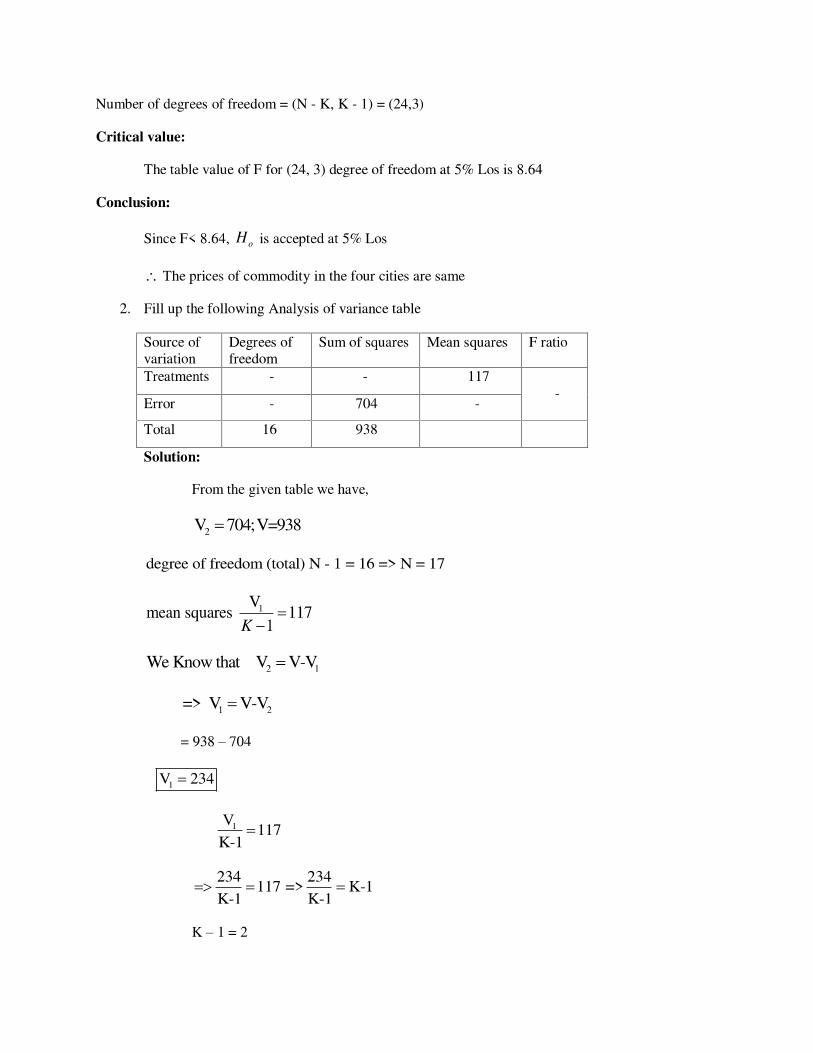


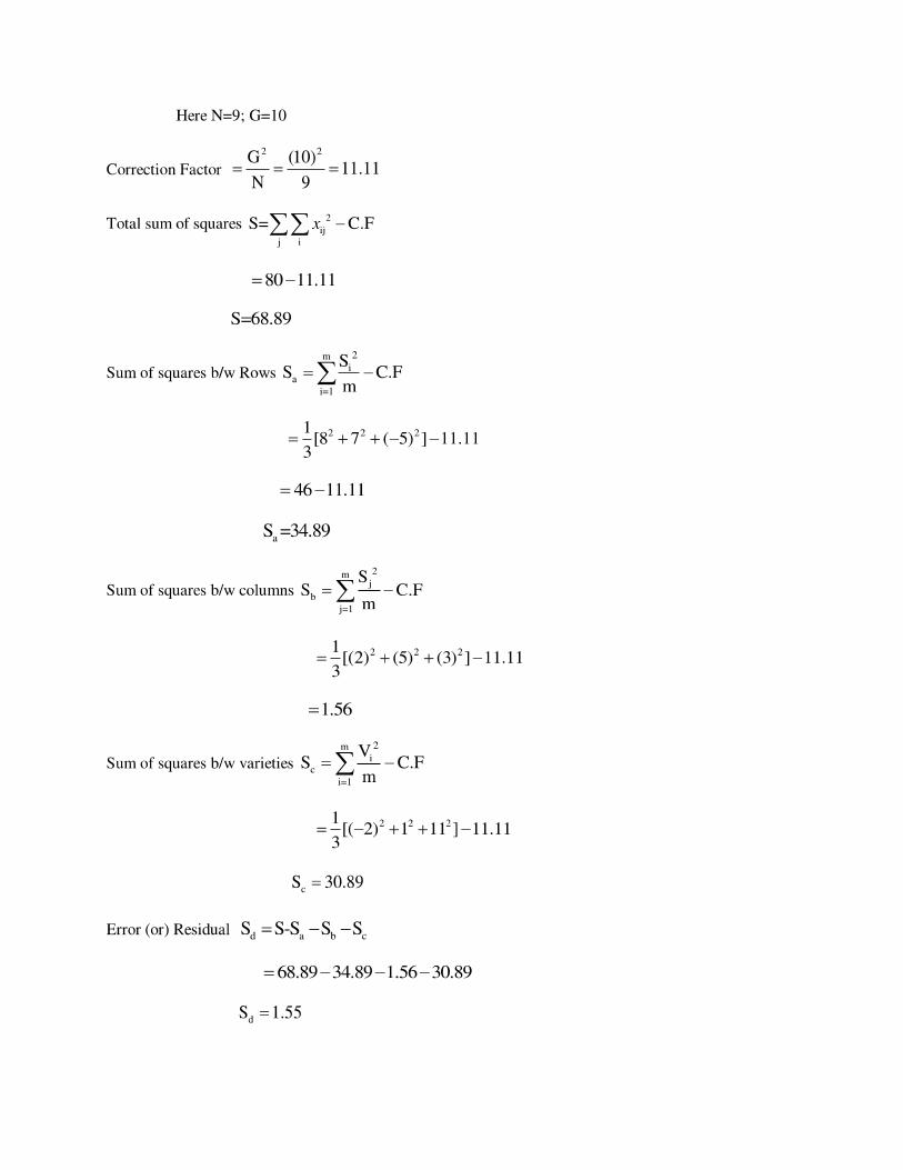


Copyright © 2022 FDOKUMEN