Probability and Statistics
773
Probability and Statistics The Science of Uncertainty Second Edition Michael J. Evans and Je/rey S. Rosenthal University of Toronto
-
Upload
khangminh22 -
Category
Documents
-
view
0 -
download
0
Transcript of Probability and Statistics

Probability and StatisticsThe Science of Uncertainty
Second Edition
Michael J. Evans and Je¤rey S. Rosenthal
University of Toronto

Contents
Preface ix
1 Probability Models 11.1 Probability: A Measure of Uncertainty . . . . . . . . . . . . . . . . . 1
1.1.1 Why Do We Need Probability Theory? . . . . . . . . . . . . 21.2 Probability Models . . . . . . . . . . . . . . . . . . . . . . . . . . . 4
1.2.1 Venn Diagrams and Subsets . . . . . . . . . . . . . . . . . . 71.3 Properties of Probability Models . . . . . . . . . . . . . . . . . . . . 101.4 Uniform Probability on Finite Spaces . . . . . . . . . . . . . . . . . 14
1.4.1 Combinatorial Principles . . . . . . . . . . . . . . . . . . . . 151.5 Conditional Probability and Independence . . . . . . . . . . . . . . . 20
1.5.1 Conditional Probability . . . . . . . . . . . . . . . . . . . . . 201.5.2 Independence of Events . . . . . . . . . . . . . . . . . . . . 23
1.6 Continuity of P . . . . . . . . . . . . . . . . . . . . . . . . . . . . . 281.7 Further Proofs (Advanced) . . . . . . . . . . . . . . . . . . . . . . . 31
2 Random Variables and Distributions 332.1 Random Variables . . . . . . . . . . . . . . . . . . . . . . . . . . . . 342.2 Distributions of Random Variables . . . . . . . . . . . . . . . . . . . 382.3 Discrete Distributions . . . . . . . . . . . . . . . . . . . . . . . . . . 41
2.3.1 Important Discrete Distributions . . . . . . . . . . . . . . . . 422.4 Continuous Distributions . . . . . . . . . . . . . . . . . . . . . . . . 51
2.4.1 Important Absolutely Continuous Distributions . . . . . . . . 532.5 Cumulative Distribution Functions . . . . . . . . . . . . . . . . . . . 62
2.5.1 Properties of Distribution Functions . . . . . . . . . . . . . . 632.5.2 Cdfs of Discrete Distributions . . . . . . . . . . . . . . . . . 642.5.3 Cdfs of Absolutely Continuous Distributions . . . . . . . . . 652.5.4 Mixture Distributions . . . . . . . . . . . . . . . . . . . . . . 682.5.5 Distributions Neither Discrete Nor Continuous (Advanced) . . 70
2.6 One-Dimensional Change of Variable . . . . . . . . . . . . . . . . . 742.6.1 The Discrete Case . . . . . . . . . . . . . . . . . . . . . . . 752.6.2 The Continuous Case . . . . . . . . . . . . . . . . . . . . . . 75
2.7 Joint Distributions . . . . . . . . . . . . . . . . . . . . . . . . . . . . 792.7.1 Joint Cumulative Distribution Functions . . . . . . . . . . . . 80
iii

iv CONTENTS
2.7.2 Marginal Distributions . . . . . . . . . . . . . . . . . . . . . 812.7.3 Joint Probability Functions . . . . . . . . . . . . . . . . . . . 832.7.4 Joint Density Functions . . . . . . . . . . . . . . . . . . . . 85
2.8 Conditioning and Independence . . . . . . . . . . . . . . . . . . . . 932.8.1 Conditioning on Discrete Random Variables . . . . . . . . . . 942.8.2 Conditioning on Continuous Random Variables . . . . . . . . 952.8.3 Independence of Random Variables . . . . . . . . . . . . . . 972.8.4 Order Statistics . . . . . . . . . . . . . . . . . . . . . . . . . 103
2.9 Multidimensional Change of Variable . . . . . . . . . . . . . . . . . 1092.9.1 The Discrete Case . . . . . . . . . . . . . . . . . . . . . . . 1092.9.2 The Continuous Case (Advanced) . . . . . . . . . . . . . . . 1102.9.3 Convolution . . . . . . . . . . . . . . . . . . . . . . . . . . . 113
2.10 Simulating Probability Distributions . . . . . . . . . . . . . . . . . . 1162.10.1 Simulating Discrete Distributions . . . . . . . . . . . . . . . 1172.10.2 Simulating Continuous Distributions . . . . . . . . . . . . . . 119
2.11 Further Proofs (Advanced) . . . . . . . . . . . . . . . . . . . . . . . 125
3 Expectation 1293.1 The Discrete Case . . . . . . . . . . . . . . . . . . . . . . . . . . . . 1293.2 The Absolutely Continuous Case . . . . . . . . . . . . . . . . . . . . 1413.3 Variance, Covariance, and Correlation . . . . . . . . . . . . . . . . . 1493.4 Generating Functions . . . . . . . . . . . . . . . . . . . . . . . . . . 162
3.4.1 Characteristic Functions (Advanced) . . . . . . . . . . . . . . 1693.5 Conditional Expectation . . . . . . . . . . . . . . . . . . . . . . . . 173
3.5.1 Discrete Case . . . . . . . . . . . . . . . . . . . . . . . . . . 1733.5.2 Absolutely Continuous Case . . . . . . . . . . . . . . . . . . 1763.5.3 Double Expectations . . . . . . . . . . . . . . . . . . . . . . 1773.5.4 Conditional Variance (Advanced) . . . . . . . . . . . . . . . 179
3.6 Inequalities . . . . . . . . . . . . . . . . . . . . . . . . . . . . . . . 1843.6.1 Jensen’s Inequality (Advanced) . . . . . . . . . . . . . . . . 187
3.7 General Expectations (Advanced) . . . . . . . . . . . . . . . . . . . 1913.8 Further Proofs (Advanced) . . . . . . . . . . . . . . . . . . . . . . . 194
4 Sampling Distributions and Limits 1994.1 Sampling Distributions . . . . . . . . . . . . . . . . . . . . . . . . . 2004.2 Convergence in Probability . . . . . . . . . . . . . . . . . . . . . . . 203
4.2.1 The Weak Law of Large Numbers . . . . . . . . . . . . . . . 2054.3 Convergence with Probability 1 . . . . . . . . . . . . . . . . . . . . . 208
4.3.1 The Strong Law of Large Numbers . . . . . . . . . . . . . . 2114.4 Convergence in Distribution . . . . . . . . . . . . . . . . . . . . . . 213
4.4.1 The Central Limit Theorem . . . . . . . . . . . . . . . . . . 2154.4.2 The Central Limit Theorem and Assessing Error . . . . . . . 220
4.5 Monte Carlo Approximations . . . . . . . . . . . . . . . . . . . . . . 2244.6 Normal Distribution Theory . . . . . . . . . . . . . . . . . . . . . . 234
4.6.1 The Chi-Squared Distribution . . . . . . . . . . . . . . . . . 2364.6.2 The t Distribution . . . . . . . . . . . . . . . . . . . . . . . . 239

CONTENTS v
4.6.3 The F Distribution . . . . . . . . . . . . . . . . . . . . . . . 2404.7 Further Proofs (Advanced) . . . . . . . . . . . . . . . . . . . . . . . 246
5 Statistical Inference 2535.1 Why Do We Need Statistics? . . . . . . . . . . . . . . . . . . . . . . 2545.2 Inference Using a Probability Model . . . . . . . . . . . . . . . . . . 2585.3 Statistical Models . . . . . . . . . . . . . . . . . . . . . . . . . . . . 2625.4 Data Collection . . . . . . . . . . . . . . . . . . . . . . . . . . . . . 269
5.4.1 Finite Populations . . . . . . . . . . . . . . . . . . . . . . . 2705.4.2 Simple Random Sampling . . . . . . . . . . . . . . . . . . . 2715.4.3 Histograms . . . . . . . . . . . . . . . . . . . . . . . . . . . 2745.4.4 Survey Sampling . . . . . . . . . . . . . . . . . . . . . . . . 276
5.5 Some Basic Inferences . . . . . . . . . . . . . . . . . . . . . . . . . 2825.5.1 Descriptive Statistics . . . . . . . . . . . . . . . . . . . . . . 2825.5.2 Plotting Data . . . . . . . . . . . . . . . . . . . . . . . . . . 2875.5.3 Types of Inference . . . . . . . . . . . . . . . . . . . . . . . 289
6 Likelihood Inference 2976.1 The Likelihood Function . . . . . . . . . . . . . . . . . . . . . . . . 297
6.1.1 Sufficient Statistics . . . . . . . . . . . . . . . . . . . . . . . 3026.2 Maximum Likelihood Estimation . . . . . . . . . . . . . . . . . . . . 308
6.2.1 Computation of the MLE . . . . . . . . . . . . . . . . . . . . 3106.2.2 The Multidimensional Case (Advanced) . . . . . . . . . . . . 316
6.3 Inferences Based on the MLE . . . . . . . . . . . . . . . . . . . . . . 3206.3.1 Standard Errors, Bias, and Consistency . . . . . . . . . . . . 3216.3.2 Confidence Intervals . . . . . . . . . . . . . . . . . . . . . . 3266.3.3 Testing Hypotheses and P-Values . . . . . . . . . . . . . . . 3326.3.4 Inferences for the Variance . . . . . . . . . . . . . . . . . . . 3386.3.5 Sample-Size Calculations: Confidence Intervals . . . . . . . . 3406.3.6 Sample-Size Calculations: Power . . . . . . . . . . . . . . . 341
6.4 Distribution-Free Methods . . . . . . . . . . . . . . . . . . . . . . . 3496.4.1 Method of Moments . . . . . . . . . . . . . . . . . . . . . . 3496.4.2 Bootstrapping . . . . . . . . . . . . . . . . . . . . . . . . . . 3516.4.3 The Sign Statistic and Inferences about Quantiles . . . . . . . 357
6.5 Large Sample Behavior of the MLE (Advanced) . . . . . . . . . . . . 364
7 Bayesian Inference 3737.1 The Prior and Posterior Distributions . . . . . . . . . . . . . . . . . . 3747.2 Inferences Based on the Posterior . . . . . . . . . . . . . . . . . . . . 384
7.2.1 Estimation . . . . . . . . . . . . . . . . . . . . . . . . . . . 3877.2.2 Credible Intervals . . . . . . . . . . . . . . . . . . . . . . . . 3917.2.3 Hypothesis Testing and Bayes Factors . . . . . . . . . . . . . 3947.2.4 Prediction . . . . . . . . . . . . . . . . . . . . . . . . . . . . 400
7.3 Bayesian Computations . . . . . . . . . . . . . . . . . . . . . . . . . 4077.3.1 Asymptotic Normality of the Posterior . . . . . . . . . . . . . 4077.3.2 Sampling from the Posterior . . . . . . . . . . . . . . . . . . 407

vi CONTENTS
7.3.3 Sampling from the Posterior Using Gibbs Sampling(Advanced) . . . . . . . . . . . . . . . . . . . . . . . . . . . 413
7.4 Choosing Priors . . . . . . . . . . . . . . . . . . . . . . . . . . . . . 4217.4.1 Conjugate Priors . . . . . . . . . . . . . . . . . . . . . . . . 4227.4.2 Elicitation . . . . . . . . . . . . . . . . . . . . . . . . . . . . 4227.4.3 Empirical Bayes . . . . . . . . . . . . . . . . . . . . . . . . 4237.4.4 Hierarchical Bayes . . . . . . . . . . . . . . . . . . . . . . . 4247.4.5 Improper Priors and Noninformativity . . . . . . . . . . . . . 425
7.5 Further Proofs (Advanced) . . . . . . . . . . . . . . . . . . . . . . . 4307.5.1 Derivation of the Posterior Distribution for the Location-Scale
Normal Model . . . . . . . . . . . . . . . . . . . . . . . . . 4307.5.2 Derivation of J (θ(ψ0, λ)) for the Location-Scale Normal . . 431
8 Optimal Inferences 4338.1 Optimal Unbiased Estimation . . . . . . . . . . . . . . . . . . . . . . 434
8.1.1 The Rao–Blackwell Theorem and Rao–Blackwellization . . . 4358.1.2 Completeness and the Lehmann–Scheffé Theorem . . . . . . 4388.1.3 The Cramer–Rao Inequality (Advanced) . . . . . . . . . . . . 440
8.2 Optimal Hypothesis Testing . . . . . . . . . . . . . . . . . . . . . . 4468.2.1 The Power Function of a Test . . . . . . . . . . . . . . . . . 4468.2.2 Type I and Type II Errors . . . . . . . . . . . . . . . . . . . . 4478.2.3 Rejection Regions and Test Functions . . . . . . . . . . . . . 4488.2.4 The Neyman–Pearson Theorem . . . . . . . . . . . . . . . . 4498.2.5 Likelihood Ratio Tests (Advanced) . . . . . . . . . . . . . . 455
8.3 Optimal Bayesian Inferences . . . . . . . . . . . . . . . . . . . . . . 4608.4 Decision Theory (Advanced) . . . . . . . . . . . . . . . . . . . . . . 4648.5 Further Proofs (Advanced) . . . . . . . . . . . . . . . . . . . . . . . 473
9 Model Checking 4799.1 Checking the Sampling Model . . . . . . . . . . . . . . . . . . . . . 479
9.1.1 Residual and Probability Plots . . . . . . . . . . . . . . . . . 4869.1.2 The Chi-Squared Goodness of Fit Test . . . . . . . . . . . . . 4919.1.3 Prediction and Cross-Validation . . . . . . . . . . . . . . . . 4959.1.4 What Do We Do When a Model Fails? . . . . . . . . . . . . . 496
9.2 Checking for Prior–Data Conflict . . . . . . . . . . . . . . . . . . . . 5029.3 The Problem with Multiple Checks . . . . . . . . . . . . . . . . . . . 509
10 Relationships Among Variables 51110.1 Related Variables . . . . . . . . . . . . . . . . . . . . . . . . . . . . 512
10.1.1 The Definition of Relationship . . . . . . . . . . . . . . . . . 51210.1.2 Cause–Effect Relationships and Experiments . . . . . . . . . 51610.1.3 Design of Experiments . . . . . . . . . . . . . . . . . . . . . 519
10.2 Categorical Response and Predictors . . . . . . . . . . . . . . . . . . 52710.2.1 Random Predictor . . . . . . . . . . . . . . . . . . . . . . . 52710.2.2 Deterministic Predictor . . . . . . . . . . . . . . . . . . . . . 53010.2.3 Bayesian Formulation . . . . . . . . . . . . . . . . . . . . . 533

CONTENTS vii
10.3 Quantitative Response and Predictors . . . . . . . . . . . . . . . . . 53810.3.1 The Method of Least Squares . . . . . . . . . . . . . . . . . 53810.3.2 The Simple Linear Regression Model . . . . . . . . . . . . . 54010.3.3 Bayesian Simple Linear Model (Advanced) . . . . . . . . . . 55410.3.4 The Multiple Linear Regression Model (Advanced) . . . . . . 558
10.4 Quantitative Response and Categorical Predictors . . . . . . . . . . . 57710.4.1 One Categorical Predictor (One-Way ANOVA) . . . . . . . . 57710.4.2 Repeated Measures (Paired Comparisons) . . . . . . . . . . . 58410.4.3 Two Categorical Predictors (Two-Way ANOVA) . . . . . . . 58610.4.4 Randomized Blocks . . . . . . . . . . . . . . . . . . . . . . 59410.4.5 One Categorical and One Quantitative Predictor . . . . . . . . 594
10.5 Categorical Response and Quantitative Predictors . . . . . . . . . . . 60210.6 Further Proofs (Advanced) . . . . . . . . . . . . . . . . . . . . . . . 607
11 Advanced Topic — Stochastic Processes 61511.1 Simple Random Walk . . . . . . . . . . . . . . . . . . . . . . . . . . 615
11.1.1 The Distribution of the Fortune . . . . . . . . . . . . . . . . 61611.1.2 The Gambler’s Ruin Problem . . . . . . . . . . . . . . . . . 618
11.2 Markov Chains . . . . . . . . . . . . . . . . . . . . . . . . . . . . . 62311.2.1 Examples of Markov Chains . . . . . . . . . . . . . . . . . . 62411.2.2 Computing with Markov Chains . . . . . . . . . . . . . . . . 62611.2.3 Stationary Distributions . . . . . . . . . . . . . . . . . . . . 62911.2.4 Markov Chain Limit Theorem . . . . . . . . . . . . . . . . . 633
11.3 Markov Chain Monte Carlo . . . . . . . . . . . . . . . . . . . . . . 64111.3.1 The Metropolis–Hastings Algorithm . . . . . . . . . . . . . . 64411.3.2 The Gibbs Sampler . . . . . . . . . . . . . . . . . . . . . . . 647
11.4 Martingales . . . . . . . . . . . . . . . . . . . . . . . . . . . . . . . 65011.4.1 Definition of a Martingale . . . . . . . . . . . . . . . . . . . 65011.4.2 Expected Values . . . . . . . . . . . . . . . . . . . . . . . . 65111.4.3 Stopping Times . . . . . . . . . . . . . . . . . . . . . . . . . 652
11.5 Brownian Motion . . . . . . . . . . . . . . . . . . . . . . . . . . . . 65711.5.1 Faster and Faster Random Walks . . . . . . . . . . . . . . . . 65711.5.2 Brownian Motion as a Limit . . . . . . . . . . . . . . . . . . 65911.5.3 Diffusions and Stock Prices . . . . . . . . . . . . . . . . . . 661
11.6 Poisson Processes . . . . . . . . . . . . . . . . . . . . . . . . . . . . 66511.7 Further Proofs . . . . . . . . . . . . . . . . . . . . . . . . . . . . . . 668
Appendices 675
A Mathematical Background 675A.1 Derivatives . . . . . . . . . . . . . . . . . . . . . . . . . . . . . . . 675A.2 Integrals . . . . . . . . . . . . . . . . . . . . . . . . . . . . . . . . . 676A.3 Infinite Series . . . . . . . . . . . . . . . . . . . . . . . . . . . . . . 677A.4 Matrix Multiplication . . . . . . . . . . . . . . . . . . . . . . . . . . 678A.5 Partial Derivatives . . . . . . . . . . . . . . . . . . . . . . . . . . . . 678

viii CONTENTS
A.6 Multivariable Integrals . . . . . . . . . . . . . . . . . . . . . . . . . 679
B Computations 683B.1 Using R . . . . . . . . . . . . . . . . . . . . . . . . . . . . . . . . . 683B.2 Using Minitab . . . . . . . . . . . . . . . . . . . . . . . . . . . . . . 699
C Common Distributions 705C.1 Discrete Distributions . . . . . . . . . . . . . . . . . . . . . . . . . . 705C.2 Absolutely Continuous Distributions . . . . . . . . . . . . . . . . . . 706
D Tables 709D.1 Random Numbers . . . . . . . . . . . . . . . . . . . . . . . . . . . . 710D.2 Standard Normal Cdf . . . . . . . . . . . . . . . . . . . . . . . . . . 712D.3 Chi-Squared Distribution Quantiles . . . . . . . . . . . . . . . . . . 713D.4 t Distribution Quantiles . . . . . . . . . . . . . . . . . . . . . . . . . 714D.5 F Distribution Quantiles . . . . . . . . . . . . . . . . . . . . . . . . 715D.6 Binomial Distribution Probabilities . . . . . . . . . . . . . . . . . . . 724
E Answers to Odd-Numbered Exercises 729
Index 750

Preface
This book is an introductory text on probability and statistics, targeting students whohave studied one year of calculus at the university level and are seeking an introductionto probability and statistics with mathematical content. Where possible, we providemathematical details, and it is expected that students are seeking to gain some masteryover these, as well as to learn how to conduct data analyses. All the usual method-ologies covered in a typical introductory course are introduced, as well as some of thetheory that serves as their justification.
The text can be used with or without a statistical computer package. It is our opin-ion that students should see the importance of various computational techniques inapplications, and the book attempts to do this. Accordingly, we feel that computationalaspects of the subject, such as Monte Carlo, should be covered, even if a statisticalpackage is not used. Almost any statistical package is suitable. A Computationsappendix provides an introduction to the R language. This covers all aspects of thelanguage needed to do the computations in the text. Furthermore, we have providedthe R code for any of the more complicated computations. Students can use theseexamples as templates for problems that involve such computations, for example, us-ing Gibbs sampling. Also, we have provided, in a separate section of this appendix,Minitab code for those computations that are slightly involved, e.g., Gibbs sampling.No programming experience is required of students to do the problems.
We have organized the exercises in the book into groups, as an aid to users. Exer-cises are suitable for all students and offer practice in applying the concepts discussedin a particular section. Problems require greater understanding, and a student can ex-pect to spend more thinking time on these. If a problem is marked (MV), then it willrequire some facility with multivariable calculus beyond the first calculus course, al-though these problems are not necessarily hard. Challenges are problems that moststudents will find difficult; these are only for students who have no trouble with theExercises and the Problems. There are also Computer Exercises and ComputerProblems, where it is expected that students will make use of a statistical package inderiving solutions.
We have included a number of Discussion Topics designed to promote criticalthinking in students. Throughout the book, we try to point students beyond the masteryof technicalities to think of the subject in a larger frame of reference. It is important thatstudents acquire a sound mathematical foundation in the basic techniques of probabilityand statistics, which we believe this book will help students accomplish. Ultimately,however, these subjects are applied in real-world contexts, so it is equally importantthat students understand how to go about their application and understand what issuesarise. Often, there are no right answers to Discussion Topics; their purpose is to get a

x Preface
student thinking about the subject matter. If these were to be used for evaluation, thenthey would be answered in essay format and graded on the maturity the student showedwith respect to the issues involved. Discussion Topics are probably most suitable forsmaller classes, but these will also benefit students who simply read them over andcontemplate their relevance.
Some sections of the book are labelled Advanced. This material is aimed at stu-dents who are more mathematically mature (for example, they are taking, or have taken,a second course in calculus). All the Advanced material can be skipped, with no lossof continuity, by an instructor who wishes to do so. In particular, the final chapter of thetext is labelled Advanced and would only be taught in a high-level introductory courseaimed at specialists. Also, many proofs appear in the final section of many chapters,labelled Further Proofs (Advanced). An instructor can choose which (if any) of theseproofs they wish to present to their students.
As such, we feel that the material in the text is presented in a flexible way thatallows the instructor to find an appropriate level for the students they are teaching. AMathematical Background appendix reviews some mathematical concepts, from afirst course in calculus, in case students could use a refresher, as well as brief introduc-tions to partial derivatives, double integrals, etc.
Chapter 1 introduces the probability model and provides motivation for the studyof probability. The basic properties of a probability measure are developed.
Chapter 2 deals with discrete, continuous, joint distributions, and the effects ofa change of variable. It also introduces the topic of simulating from a probabilitydistribution. The multivariate change of variable is developed in an Advanced section.
Chapter 3 introduces expectation. The probability-generating function is dis-cussed, as are the moments and the moment-generating function of a random variable.This chapter develops some of the major inequalities used in probability. A section oncharacteristic functions is included as an Advanced topic.
Chapter 4 deals with sampling distributions and limits. Convergence in probabil-ity, convergence with probability 1, the weak and strong laws of large numbers, con-vergence in distribution, and the central limit theorem are all introduced, along withvarious applications such as Monte Carlo. The normal distribution theory, necessaryfor many statistical applications, is also dealt with here.
As mentioned, Chapters 1 through 4 include material on Monte Carlo techniques.Simulation is a key aspect of the application of probability theory, and it is our viewthat its teaching should be integrated with the theory right from the start. This revealsthe power of probability to solve real-world problems and helps convince students thatit is far more than just an interesting mathematical theory. No practitioner divorceshimself from the theory when using the computer for computations or vice versa. Webelieve this is a more modern way of teaching the subject. This material can be skipped,however, if an instructor believes otherwise or feels there is not enough time to coverit effectively.
Chapter 5 is an introduction to statistical inference. For the most part, this is con-cerned with laying the groundwork for the development of more formal methodologyin later chapters. So practical issues — such as proper data collection, presenting datavia graphical techniques, and informal inference methods like descriptive statistics —are discussed here.

Preface xi
Chapter 6 deals with many of the standard methods of inference for one-sampleproblems. The theoretical justification for these methods is developed primarily throughthe likelihood function, but the treatment is still fairly informal. Basic methods of in-ference, such as the standard error of an estimate, confidence intervals, and P-values,are introduced. There is also a section devoted to distribution-free (nonparametric)methods like the bootstrap.
Chapter 7 involves many of the same problems discussed in Chapter 6, but nowfrom a Bayesian perspective. The point of view adopted here is not that Bayesian meth-ods are better or, for that matter, worse than those of Chapter 6. Rather, we take theview that Bayesian methods arise naturally when the statistician adds another ingredi-ent — the prior — to the model. The appropriateness of this, or the sampling modelfor the data, is resolved through the model-checking methods of Chapter 9. It is notour intention to have students adopt a particular philosophy. Rather, the text introducesstudents to a broad spectrum of statistical thinking.
Subsequent chapters deal with both frequentist and Bayesian approaches to thevarious problems discussed. The Bayesian material is in clearly labelled sections andcan be skipped with no loss of continuity, if so desired. It has become apparent inrecent years, however, that Bayesian methodology is widely used in applications. Assuch, we feel that it is important for students to be exposed to this, as well as to thefrequentist approaches, early in their statistical education.
Chapter 8 deals with the traditional optimality justifications offered for some sta-tistical inferences. In particular, some aspects of optimal unbiased estimation and theNeyman–Pearson theorem are discussed. There is also a brief introduction to decisiontheory. This chapter is more formal and mathematical than Chapters 5, 6, and 7, and itcan be skipped, with no loss of continuity, if an instructor wants to emphasize methodsand applications.
Chapter 9 is on model checking. We placed model checking in a separate chapterto emphasize its importance in applications. In practice, model checking is the waystatisticians justify the choices they make in selecting the ingredients of a statisticalproblem. While these choices are inherently subjective, the methods of this chapterprovide checks to make sure that the choices made are sensible in light of the objectiveobserved data.
Chapter 10 is concerned with the statistical analysis of relationships among vari-ables. This includes material on simple linear and multiple regression, ANOVA, thedesign of experiments, and contingency tables. The emphasis in this chapter is onapplications.
Chapter 11 is concerned with stochastic processes. In particular, Markov chainsand Markov chain Monte Carlo are covered in this chapter, as are Brownian motion andits relevance to finance. Fairly sophisticated topics are introduced, but the treatment isentirely elementary. Chapter 11 depends only on the material in Chapters 1 through 4.
A one-semester course on probability would cover Chapters 1–4 and perhaps someof Chapter 11. A one-semester, follow-up course on statistics would cover Chapters 5–7 and 9–10. Chapter 8 is not necessary, but some parts, such as the theory of unbiasedestimation and optimal testing, are suitable for a more theoretical course.
A basic two-semester course in probability and statistics would cover Chapters 1–6and 9–10. Such a course covers all the traditional topics, including basic probability

xii Preface
theory, basic statistical inference concepts, and the usual introductory applied statisticstopics. To cover the entire book would take three semesters, which could be organizedin a variety of ways.
The Advanced sections can be skipped or included, depending on the level of thestudents, with no loss of continuity. A similar approach applies to Chapters 7, 8, and11.
Students who have already taken an introductory, noncalculus-based, applied sta-tistics course will also benefit from a course based on this text. While similar topics arecovered, they are presented with more depth and rigor here. For example, Introductionto the Practice of Statistics, 6th ed., by D. Moore and G. McCabe (W. H. Freeman,2009) is an excellent text, and we believe that our book would serve as a strong basisfor a follow-up course.
There is an Instructor’s Solutions Manual available from the publisher.The second edition contains many more basic exercises than the first edition. Also,
we have rewritten a number of sections, with the aim of making the material clearer tostudents. One goal in our rewriting was to subdivide the material into smaller, moredigestible components so that key ideas stand out more boldly. There has been a com-plete typographical redesign that we feel aids in this as well. In the appendices, we haveadded material on the statistical package R as well as answers for the odd-numberedexercises that students can use to check their understanding.
Many thanks to the reviewers and users for their comments: Abbas Alhakim (Clark-son University), Michelle Baillargeon (McMaster University), Arne C. Bathke (Univer-sity of Kentucky), Lisa A. Bloomer (Middle Tennessee State University), ChristopherBrown (California Lutheran University), Jem N. Corcoran (University of Colorado),Guang Cheng (Purdue University), Yi Cheng (Indiana University South Bend), EugeneDemidenko (Dartmouth College), Robert P. Dobrow (Carleton College), John Ferdi-nands (Calvin College), Soledad A. Fernandez (The Ohio State University), ParamjitGill (University of British Columbia Okanagan), Marvin Glover (Milligan College),Ellen Gundlach (Purdue University), Paul Gustafson (University of British Columbia),Jan Hannig (Colorado State University), Solomon W. Harrar (The University of Mon-tana), Susan Herring (Sonoma State University), George F. Hilton (Pacific Union Col-lege), Chun Jin (Central Connecticut State University), Paul Joyce (University of Idaho),Hubert Lilliefors (George Washington University), Andy R. Magid (University of Ok-lahoma), Phil McDonnough (University of Toronto), Julia Morton (Nipissing Univer-sity), Jean D. Opsomer (Colorado State University), Randall H. Rieger (West ChesterUniversity), Robert L. Schaefer (Miami University), Osnat Stramer (University ofIowa), Tim B. Swartz (Simon Fraser University), Glen Takahara (Queen’s University),Robert D. Thompson (Hunter College), David C. Vaughan (Wilfrid Laurier University),Joseph J. Walker (Georgia State University), Chad Westerland (University of Arizona),Dongfeng Wu (Mississippi State University), Yuehua Wu (York University), NicholasZaino (University of Rochester). In particular, Professor Chris Andrews (State Univer-sity of New York) provided many corrections to the first edition.
The authors would also like to thank many who have assisted in the developmentof this project. In particular, our colleagues and students at the University of Torontohave been very supportive. Ping Gao, Aysha Hashim, Gun Ho Jang, Hadas Moshonov,and Mahinda Samarakoon helped in many ways. A number of the data sets in Chapter

Preface xiii
10 have been used in courses at the University of Toronto for many years and were, webelieve, compiled through the work of the late Professor Daniel B. DeLury. ProfessorDavid Moore of Purdue University was of assistance in providing several of the tablesat the back of the text. Patrick Farace, Anne Scanlan-Rohrer, Chris Spavins, DanielleSwearengin, Brian Tedesco, Vivien Weiss, and Katrina Wilhelm of W. H. Freemanprovided much support and encouragement. Our families helped us with their patienceand care while we worked at what seemed at times an unending task; many thanks toRosemary and Heather Evans and Margaret Fulford.
Michael Evans and Jeffrey RosenthalToronto, 2009

Chapter 1
Probability Models
CHAPTER OUTLINE
Section 1 Probability: A Measure of UncertaintySection 2 Probability ModelsSection 3 Properties of Probability ModelsSection 4 Uniform Probability on Finite SpacesSection 5 Conditional Probability and IndependenceSection 6 Continuity of PSection 7 Further Proofs (Advanced)
This chapter introduces the basic concept of the entire course, namely probability. Wediscuss why probability was introduced as a scientific concept and how it has beenformalized mathematically in terms of a probability model. Following this we developsome of the basic mathematical results associated with the probability model.
1.1 Probability: A Measure of UncertaintyOften in life we are confronted by our own ignorance. Whether we are ponderingtonight’s traffic jam, tomorrow’s weather, next week’s stock prices, an upcoming elec-tion, or where we left our hat, often we do not know an outcome with certainty. Instead,we are forced to guess, to estimate, to hedge our bets.
Probability is the science of uncertainty. It provides precise mathematical rules forunderstanding and analyzing our own ignorance. It does not tell us tomorrow’s weatheror next week’s stock prices; rather, it gives us a framework for working with our limitedknowledge and for making sensible decisions based on what we do and do not know.
To say there is a 40% chance of rain tomorrow is not to know tomorrow’s weather.Rather, it is to know what we do not know about tomorrow’s weather.
In this text, we will develop a more precise understanding of what it means to saythere is a 40% chance of rain tomorrow. We will learn how to work with ideas ofrandomness, probability, expected value, prediction, estimation, etc., in ways that aresensible and mathematically clear.
1

2 Section 1.1: Probability: A Measure of Uncertainty
There are also other sources of randomness besides uncertainty. For example, com-puters often use pseudorandom numbers to make games fun, simulations accurate, andsearches efficient. Also, according to the modern theory of quantum mechanics, themakeup of atomic matter is in some sense truly random. All such sources of random-ness can be studied using the techniques of this text.
Another way of thinking about probability is in terms of relative frequency. For ex-ample, to say a coin has a 50% chance of coming up heads can be interpreted as sayingthat, if we flipped the coin many, many times, then approximately half of the time itwould come up heads. This interpretation has some limitations. In many cases (suchas tomorrow’s weather or next week’s stock prices), it is impossible to repeat the ex-periment many, many times. Furthermore, what precisely does “approximately” meanin this case? However, despite these limitations, the relative frequency interpretation isa useful way to think of probabilities and to develop intuition about them.
Uncertainty has been with us forever, of course, but the mathematical theory ofprobability originated in the seventeenth century. In 1654, the Paris gambler Le Cheva-lier de Méré asked Blaise Pascal about certain probabilities that arose in gambling(such as, if a game of chance is interrupted in the middle, what is the probability thateach player would have won had the game continued?). Pascal was intrigued and cor-responded with the great mathematician and lawyer Pierre de Fermat about these ques-tions. Pascal later wrote the book Traité du Triangle Arithmetique, discussing binomialcoefficients (Pascal’s triangle) and the binomial probability distribution.
At the beginning of the twentieth century, Russians such as Andrei AndreyevichMarkov, Andrey Nikolayevich Kolmogorov, and Pafnuty L. Chebyshev (and Ameri-can Norbert Wiener) developed a more formal mathematical theory of probability. Inthe 1950s, Americans William Feller and Joe Doob wrote important books about themathematics of probability theory. They popularized the subject in the western world,both as an important area of pure mathematics and as having important applications inphysics, chemistry, and later in computer science, economics, and finance.
1.1.1 Why Do We Need Probability Theory?
Probability theory comes up very often in our daily lives. We offer a few exampleshere.
Suppose you are considering buying a “Lotto 6/49” lottery ticket. In this lottery,you are to pick six distinct integers between 1 and 49. Another six distinct integersbetween 1 and 49 are then selected at random by the lottery company. If the two setsof six integers are identical, then you win the jackpot.
After mastering Section 1.4, you will know how to calculate that the probabilityof the two sets matching is equal to one chance in 13,983,816. That is, it is about 14million times more likely that you will not win the jackpot than that you will. (Theseare not very good odds!)
Suppose the lottery tickets cost $1 each. After mastering expected values in Chap-ter 3, you will know that you should not even consider buying a lottery ticket unless thejackpot is more than $14 million (which it usually is not). Furthermore, if the jackpotis ever more than $14 million, then likely many other people will buy lottery tickets

Chapter 1: Probability Models 3
that week, leading to a larger probability that you will have to share the jackpot withother winners even if you do win — so it is probably not in your favor to buy a lotteryticket even then.
Suppose instead that a “friend” offers you a bet. He has three cards, one red onboth sides, one black on both sides, and one red on one side and black on the other.He mixes the three cards in a hat, picks one at random, and places it flat on the tablewith only one side showing. Suppose that one side is red. He then offers to bet his $4against your $3 that the other side of the card is also red.
At first you might think it sounds like the probability that the other side is also red is50%; thus a good bet. However, after mastering conditional probability (Section 1.5),you will know that, conditional on one side being red, the conditional probability thatthe other side is also red is equal to 2/3. So, by the theory of expected values (Chap-ter 3), you will know that you should not accept your “friend’s” bet.
Finally, suppose your “friend” suggests that you flip a coin one thousand times.Your “friend” says that if the coin comes up heads at least six hundred times, then hewill pay you $100; otherwise, you have to pay him just $1.
At first you might think that, while 500 heads is the most likely, there is still areasonable chance that 600 heads will appear — at least good enough to justify accept-ing your friend’s $100 to $1 bet. However, after mastering the laws of large numbers(Chapter 4), you will know that as the number of coin flips gets large, it becomes moreand more likely that the number of heads is very close to half of the total number ofcoin flips. In fact, in this case, there is less than one chance in ten billion of gettingmore than 600 heads! Therefore, you should not accept this bet, either.
As these examples show, a good understanding of probability theory will allow youto correctly assess probabilities in everyday situations, which will in turn allow you tomake wiser decisions. It might even save you money!
Probability theory also plays a key role in many important applications of scienceand technology. For example, the design of a nuclear reactor must be such that theescape of radioactivity into the environment is an extremely rare event. Of course, wewould like to say that it is categorically impossible for this to ever happen, but reac-tors are complicated systems, built up from many interconnected subsystems, each ofwhich we know will fail to function properly at some time. Furthermore, we can neverdefinitely say that a natural event like an earthquake cannot occur that would damagethe reactor sufficiently to allow an emission. The best we can do is try to quantify ouruncertainty concerning the failures of reactor components or the occurrence of naturalevents that would lead to such an event. This is where probability enters the picture.Using probability as a tool to deal with the uncertainties, the reactor can be designed toensure that an unacceptable emission has an extremely small probability — say, oncein a billion years — of occurring.
The gambling and nuclear reactor examples deal essentially with the concept ofrisk — the risk of losing money, the risk of being exposed to an injurious level ofradioactivity, etc. In fact, we are exposed to risk all the time. When we ride in a car,or take an airplane flight, or even walk down the street, we are exposed to risk. Weknow that the risk of injury in such circumstances is never zero, yet we still engage inthese activities. This is because we intuitively realize that the probability of an accidentoccurring is extremely low.
4 Section 1.2: Probability Models
So we are using probability every day in our lives to assess risk. As the problemswe face, individually or collectively, become more complicated, we need to refine anddevelop our rough, intuitive ideas about probability to form a clear and precise ap-proach. This is why probability theory has been developed as a subject. In fact, theinsurance industry has been developed to help us cope with risk. Probability is thetool used to determine what you pay to reduce your risk or to compensate you or yourfamily in case of a personal injury.
Summary of Section 1.1
• Probability theory provides us with a precise understanding of uncertainty.
• This understanding can help us make predictions, make better decisions, assessrisk, and even make money.
DISCUSSION TOPICS
1.1.1 Do you think that tomorrow’s weather and next week’s stock prices are “really”random, or is this just a convenient way to discuss and analyze them?1.1.2 Do you think it is possible for probabilities to depend on who is observing them,or at what time?1.1.3 Do you find it surprising that probability theory was not discussed as a mathe-matical subject until the seventeenth century? Why or why not?1.1.4 In what ways is probability important for such subjects as physics, computerscience, and finance? Explain.1.1.5 What are examples from your own life where thinking about probabilities didsave — or could have saved — you money or helped you to make a better decision?(List as many as you can.)1.1.6 Probabilities are often depicted in popular movies and television programs. Listas many examples as you can. Do you think the probabilities were portrayed there in a“reasonable” way?
1.2 Probability ModelsA formal definition of probability begins with a sample space, often written S. Thissample space is any set that lists all possible outcomes (or, responses) of some unknownexperiment or situation. For example, perhaps
S = {rain, snow, clear}when predicting tomorrow’s weather. Or perhaps S is the set of all positive real num-bers, when predicting next week’s stock price. The point is, S can be any set at all,even an infinite set. We usually write s for an element of S, so that s ∈ S. Note that Sdescribes only those things that we are interested in; if we are studying weather, thenrain and snow are in S, but tomorrow’s stock prices are not.

Chapter 1: Probability Models 5
A probability model also requires a collection of events, which are subsets of Sto which probabilities can be assigned. For the above weather example, the subsets{rain}, {snow}, {rain, snow}, {rain, clear}, {rain, snow, clear}, and even the empty set∅ = {}, are all examples of subsets of S that could be events. Note that here the commameans “or”; thus, {rain, snow} is the event that it will rain or snow. We will generallyassume that all subsets of S are events. (In fact, in complicated situations there aresome technical restrictions on what subsets can or cannot be events, according to themathematical subject of measure theory. But we will not concern ourselves with suchtechnicalities here.)
Finally, and most importantly, a probability model requires a probability measure,usually written P . This probability measure must assign, to each event A, a probabilityP(A). We require the following properties:
1. P(A) is always a nonnegative real number, between 0 and 1 inclusive.
2. P(∅) = 0, i.e., if A is the empty set ∅, then P(A) = 0.
3. P(S) = 1, i.e., if A is the entire sample space S, then P(A) = 1.
4. P is (countably) additive, meaning that if A1, A2, . . . is a finite or countablesequence of disjoint events, then
P(A1 ∪ A2 ∪ · · · ) = P(A1)+ P(A2)+ · · · . (1.2.1)
The first of these properties says that we shall measure all probabilities on a scalefrom 0 to 1, where 0 means impossible and 1 (or 100%) means certain. The secondproperty says the probability that nothing happens is 0; in other words, it is impossiblethat no outcome will occur. The third property says the probability that somethinghappens is 1; in other words, it is certain that some outcome must occur.
The fourth property is the most subtle. It says that we can calculate probabilitiesof complicated events by adding up the probabilities of smaller events, provided thosesmaller events are disjoint and together contain the entire complicated event. Note thatevents are disjoint if they contain no outcomes in common. For example, {rain} and{snow, clear} are disjoint, whereas {rain} and {rain, clear} are not disjoint. (We areassuming for simplicity that it cannot both rain and snow tomorrow.) Thus, we shouldhave P({rain}) + P({snow, clear}) = P({rain, snow, clear}), but do not expect tohave P({rain}) + P({rain, clear}) = P({rain, rain, clear}) (the latter being the sameas P({rain, clear})).
We now formalize the definition of a probability model.
Definition 1.2.1 A probability model consists of a nonempty set called the samplespace S; a collection of events that are subsets of S; and a probability measure Passigning a probability between 0 and 1 to each event, with P(∅) = 0 and P(S) = 1and with P additive as in (1.2.1).

6 Section 1.2: Probability Models
EXAMPLE 1.2.1Consider again the weather example, with S = {rain, snow, clear}. Suppose that theprobability of rain is 40%, the probability of snow is 15%, and the probability of aclear day is 45%. We can express this as P({rain}) = 0.40, P({snow}) = 0.15, andP({clear}) = 0.45.
For this example, of course P(∅) = 0, i.e., it is impossible that nothing will happentomorrow. Also P({rain, snow, clear}) = 1, because we are assuming that exactlyone of rain, snow, or clear must occur tomorrow. (To be more realistic, we might saythat we are predicting the weather at exactly 11:00 A.M. tomorrow.) Now, what is theprobability that it will rain or snow tomorrow? Well, by the additivity property, we seethat
P({rain, snow}) = P({rain})+ P({snow}) = 0.40+ 0.15 = 0.55.
We thus conclude that, as expected, there is a 55% chance of rain or snow tomorrow.
EXAMPLE 1.2.2Suppose your candidate has a 60% chance of winning an election in progress. ThenS = {win, lose}, with P(win) = 0.6 and P(lose) = 0.4. Note that P(win)+P(lose) =1.
EXAMPLE 1.2.3Suppose we flip a fair coin, which can come up either heads (H) or tails (T ) with equalprobability. Then S = {H, T }, with P(H) = P(T ) = 0.5. Of course, P(H)+P(T ) =1.
EXAMPLE 1.2.4Suppose we flip three fair coins in a row and keep track of the sequence of heads andtails that result. Then
S = {H H H, H HT, HT H, HT T, T H H, T HT, T T H, T T T }.Furthermore, each of these eight outcomes is equally likely. Thus, P(H H H) = 1/8,P(T T T ) = 1/8, etc. Also, the probability that the first coin is heads and the secondcoin is tails, but the third coin can be anything, is equal to the sum of the probabilitiesof the events HT H and HT T , i.e., P(HT H)+ P(HT T ) = 1/8 + 1/8 = 1/4.
EXAMPLE 1.2.5Suppose we flip three fair coins in a row but care only about the number of headsthat result. Then S = {0, 1, 2, 3}. However, the probabilities of these four outcomesare not all equally likely; we will see later that in fact P(0) = P(3) = 1/8, whileP(1) = P(2) = 3/8.
We note that it is possible to define probability models on more complicated (e.g.,uncountably infinite) sample spaces as well.
EXAMPLE 1.2.6Suppose that S = [0, 1] is the unit interval. We can define a probability measure P onS by saying that
P([a, b]) = b − a , whenever 0 ≤ a ≤ b ≤ 1. (1.2.2)

Chapter 1: Probability Models 7
In words, for any1 subinterval [a, b] of [0, 1], the probability of the interval is simplythe length of that interval. This example is called the uniform distribution on [0, 1].The uniform distribution is just the first of many distributions on uncountable statespaces. Many further examples will be given in Chapter 2.
1.2.1 Venn Diagrams and Subsets
Venn diagrams provide a very useful graphical method for depicting the sample spaceS and subsets of it. For example, in Figure 1.2.1 we have a Venn diagram showing thesubset A ⊂ S and the complement
Ac = {s : s /∈ A}of A. The rectangle denotes the entire sample space S. The circle (and its interior) de-notes the subset A; the region outside the circle, but inside S, denotes Ac.
1
A
S
S
A
Ac
Figure 1.2.1: Venn diagram of the subsets A and Ac of the sample space S.
Two subsets A ⊂ S and B ⊂ S are depicted as two circles, as in Figure 1.2.2 onthe next page. The intersection
A ∩ B = {s : s ∈ A and s ∈ B}of the subsets A and B is the set of elements common to both sets and is depicted bythe region where the two circles overlap. The set
A ∩ Bc = {s : s ∈ A and s ∈ B}is called the complement of B in A and is depicted as the region inside the A circle,but not inside the B circle. This is the set of elements in A but not in B. Similarly, wehave the complement of A in B, namely, Ac ∩ B. Observe that the sets A∩ B, A∩ Bc,and Ac ∩ B are mutually disjoint.
1For the uniform distribution on [0, 1], it turns out that not all subsets of [0, 1] can properly be regardedas events for this model. However, this is merely a technical property, and any subset that we can explicitlywrite down will always be an event. See more advanced probability books, e.g., page 3 of A First Look atRigorous Probability Theory, Second Edition, by J. S. Rosenthal (World Scientific Publishing, Singapore,2006).

8 Section 1.2: Probability Models
The unionA ∪ B = {s : s ∈ A or s ∈ B}
of the sets A and B is the set of elements that are in either A or B. In Figure 1.2.2, itis depicted by the region covered by both circles. Notice that A ∪ B = (A ∩ Bc) ∪(A ∩ B) ∪ (Ac ∩ B) .
There is one further region in Figure 1.2.2. This is the complement of A ∪ B,namely, the set of elements that are in neither A nor B. So we immediately have
(A ∪ B)c = Ac ∩ Bc.
Similarly, we can show that
(A ∩ B)c = Ac ∪ Bc,
namely, the subset of elements that are not in both A and B is given by the set of ele-ments not in A or not in B.
S
A B
Ac ∩ BA ∩ Bc
A ∩ B
Ac ∩ Bc
Figure 1.2.2: Venn diagram depicting the subsets A, B, A ∩ B, A ∩ Bc, Ac ∩ B, Ac ∩ Bc,and A ∪ B.
Finally, we note that if A and B are disjoint subsets, then it makes sense to depictthese as drawn in Figure 1.2.3, i.e., as two nonoverlapping circles because they haveno elements in common.
1
A
S
A B
Figure 1.2.3: Venn diagram of the disjoint subsets A and B.

Chapter 1: Probability Models 9
Summary of Section 1.2
• A probability model consists of a sample space S and a probability measure Passigning probabilities to each event.
• Different sorts of sets can arise as sample spaces.
• Venn diagrams provide a convenient method for representing sets and the rela-tionships among them.
EXERCISES
1.2.1 Suppose S = {1, 2, 3}, with P({1}) = 1/2, P({2}) = 1/3, and P({3}) = 1/6.(a) What is P({1, 2})?(b) What is P({1, 2, 3})?(c) List all events A such that P(A) = 1/2.1.2.2 Suppose S = {1, 2, 3, 4, 5, 6, 7, 8}, with P({s}) = 1/8 for 1 ≤ s ≤ 8.(a) What is P({1, 2})?(b) What is P({1, 2, 3})?(c) How many events A are there such that P(A) = 1/2?1.2.3 Suppose S = {1, 2, 3}, with P({1}) = 1/2 and P({1, 2}) = 2/3. What mustP({2}) be?1.2.4 Suppose S = {1, 2, 3}, and we try to define P by P({1, 2, 3}) = 1, P({1, 2}) =0.7, P({1, 3}) = 0.5, P({2, 3}) = 0.7, P({1}) = 0.2, P({2}) = 0.5, P({3}) = 0.3. IsP a valid probability measure? Why or why not?1.2.5 Consider the uniform distribution on [0, 1]. Let s ∈ [0, 1] be any outcome. Whatis P({s})? Do you find this result surprising?1.2.6 Label the subregions in the Venn diagram in Figure 1.2.4 using the sets A, B, andC and their complements (just as we did in Figure 1.2.2).
A B
C
a b c
de
f
g
S
Figure 1.2.4: Venn diagram of subsets A, B, and C .
1.2.7 On a Venn diagram, depict the set of elements that are in subsets A or B but notin both. Also write this as a subset involving unions and intersections of A, B, andtheir complements.

10 Section 1.3: Properties of Probability Models
1.2.8 Suppose S = {1, 2, 3}, and P({1, 2}) = 1/3, and P({2, 3}) = 2/3. ComputeP({1}), P({2}), and P({3}).1.2.9 Suppose S = {1, 2, 3, 4}, and P({1}) = 1/12, and P({1, 2}) = 1/6, andP({1, 2, 3}) = 1/3. Compute P({1}), P({2}), P({3}), and P({4}).1.2.10 Suppose S = {1, 2, 3}, and P({1}) = P({3}) = 2 P({2}). Compute P({1}),P({2}), and P({3}).1.2.11 Suppose S = {1, 2, 3}, and P({1}) = P({2}) + 1/6, and P({3}) = 2 P({2}).Compute P({1}), P({2}), and P({3}).1.2.12 Suppose S = {1, 2, 3, 4}, and P({1})− 1/8 = P({2}) = 3 P({3}) = 4 P({4}).Compute P({1}), P({2}), P({3}), and P({4}).
PROBLEMS
1.2.13 Consider again the uniform distribution on [0, 1]. Is it true that
P([0, 1]) =s∈[0,1]
P({s})?
How does this relate to the additivity property of probability measures?1.2.14 Suppose S is a finite or countable set. Is it possible that P({s}) = 0 for everysingle s ∈ S? Why or why not?1.2.15 Suppose S is an uncountable set. Is it possible that P({s}) = 0 for every singles ∈ S? Why or why not?
DISCUSSION TOPICS
1.2.16 Does the additivity property make sense intuitively? Why or why not?1.2.17 Is it important that we always have P(S) = 1? How would probability theorychange if this were not the case?
1.3 Properties of Probability ModelsThe additivity property of probability measures automatically implies certain basicproperties. These are true for any probability model at all.
If A is any event, we write Ac (read “A complement”) for the event that A does notoccur. In the weather example, if A = {rain}, then Ac = {snow, clear}. In the coinexamples, if A is the event that the first coin is heads, then Ac is the event that the firstcoin is tails.
Now, A and Ac are always disjoint. Furthermore, their union is always the entiresample space: A ∪ Ac = S. Hence, by the additivity property, we must have P(A) +P(Ac) = P(S). But we always have P(S) = 1. Thus, P(A)+ P(Ac) = 1, or
P(Ac) = 1− P(A). (1.3.1)
In words, the probability that any event does not occur is equal to one minus the prob-ability that it does occur. This is a very helpful fact that we shall use often.

Chapter 1: Probability Models 11
Now suppose that A1, A2, . . . are events that form a partition of the sample spaceS. This means that A1, A2, . . . are disjoint and, furthermore, that their union is equalto S, i.e., A1 ∪ A2 ∪ · · · = S. We have the following basic theorem that allows us todecompose the calculation of the probability of B into the sum of the probabilities ofthe sets Ai ∩ B. Often these are easier to compute.
Theorem 1.3.1 (Law of total probability, unconditioned version) Let A1, A2, . . .be events that form a partition of the sample space S. Let B be any event. Then
P(B) = P(A1 ∩ B)+ P(A2 ∩ B)+ · · · .
PROOF The events (A1∩B), (A2∩B), . . . are disjoint, and their union is B. Hence,the result follows immediately from the additivity property (1.2.1).
A somewhat more useful version of the law of total probability, and applications of itsuse, are provided in Section 1.5.
Suppose now that A and B are two events such that A contains B (in symbols,A ⊇ B). In words, all outcomes in B are also in A. Intuitively, A is a “larger” eventthan B, so we would expect its probability to be larger. We have the following result.
Theorem 1.3.2 Let A and B be two events with A ⊇ B. Then
P(A) = P(B)+ P(A ∩ Bc). (1.3.2)
PROOF We can write A = B∪ (A∩ Bc), where B and A∩ Bc are disjoint. Hence,P(A) = P(B)+ P(A ∩ Bc) by additivity.
Because we always have P(A ∩ Bc) ≥ 0, we conclude the following.
Corollary 1.3.1 (Monotonicity) Let A and B be two events, with A ⊇ B. Then
P(A) ≥ P(B).
On the other hand, rearranging (1.3.2), we obtain the following.
Corollary 1.3.2 Let A and B be two events, with A ⊇ B. Then
P(A ∩ Bc) = P(A)− P(B) . (1.3.3)
More generally, even if we do not have A ⊇ B, we have the following property.
Theorem 1.3.3 (Principle of inclusion–exclusion, two-event version) Let A and Bbe two events. Then
P(A ∪ B) = P(A)+ P(B)− P(A ∩ B). (1.3.4)

12 Section 1.3: Properties of Probability Models
PROOF We can write A ∪ B = (A ∩ Bc) ∪ (B ∩ Ac) ∪ (A ∩ B), where A ∩ Bc,B ∩ Ac, and A ∩ B are disjoint. By additivity, we have
P(A ∪ B) = P(A ∩ Bc)+ P(B ∩ Ac)+ P(A ∩ B). (1.3.5)
On the other hand, using Corollary 1.3.2 (with B replaced by A ∩ B), we have
P(A ∩ Bc) = P(A ∩ (A ∩ B)c) = P(A)− P(A ∩ B) (1.3.6)
and similarly,P(B ∩ Ac) = P(B)− P(A ∩ B). (1.3.7)
Substituting (1.3.6) and (1.3.7) into (1.3.5), the result follows.
A more general version of the principle of inclusion–exclusion is developed in Chal-lenge 1.3.10.
Sometimes we do not need to evaluate the probability content of a union; we needonly know it is bounded above by the sum of the probabilities of the individual events.This is called subadditivity.
Theorem 1.3.4 (Subadditivity) Let A1, A2, . . . be a finite or countably infinite se-quence of events, not necessarily disjoint. Then
P(A1 ∪ A2 ∪ · · · ) ≤ P(A1)+ P(A2)+ · · · .
PROOF See Section 1.7 for the proof of this result.
We note that some properties in the definition of a probability model actually followfrom other properties. For example, once we know the probability P is additive andthat P(S) = 1, it follows that we must have P(∅) = 0. Indeed, because S and ∅ aredisjoint, P(S ∪ ∅) = P(S) + P(∅). But of course, P(S ∪ ∅) = P(S) = 1, so wemust have P(∅) = 0.
Similarly, once we know P is additive on countably infinite sequences of disjointevents, it follows that P must be additive on finite sequences of disjoint events, too.Indeed, given a finite disjoint sequence A1, . . . , An , we can just set Ai = ∅ for alli > n, to get a countably infinite disjoint sequence with the same union and the samesum of probabilities.
Summary of Section 1.3
• The probability of the complement of an event equals one minus the probabilityof the event.
• Probabilities always satisfy the basic properties of total probability, subadditivity,and monotonicity.
• The principle of inclusion–exclusion allows for the computation of P(A ∪ B) interms of simpler events.

Chapter 1: Probability Models 13
EXERCISES
1.3.1 Suppose S = {1, 2, . . . , 100}. Suppose further that P({1}) = 0.1.(a) What is the probability P({2, 3, 4, . . . , 100})?(b) What is the smallest possible value of P({1, 2, 3})?1.3.2 Suppose that Al watches the six o’clock news 2/3 of the time, watches the eleveno’clock news 1/2 of the time, and watches both the six o’clock and eleven o’clock news1/3 of the time. For a randomly selected day, what is the probability that Al watchesonly the six o’clock news? For a randomly selected day, what is the probability that Alwatches neither news?1.3.3 Suppose that an employee arrives late 10% of the time, leaves early 20% of thetime, and both arrives late and leaves early 5% of the time. What is the probability thaton a given day that employee will either arrive late or leave early (or both)?1.3.4 Suppose your right knee is sore 15% of the time, and your left knee is sore 10%of the time. What is the largest possible percentage of time that at least one of yourknees is sore? What is the smallest possible percentage of time that at least one of yourknees is sore?1.3.5 Suppose a fair coin is flipped five times in a row.(a) What is the probability of getting all five heads?(b) What is the probability of getting at least one tail?1.3.6 Suppose a card is chosen uniformly at random from a standard 52-card deck.(a) What is the probability that the card is a jack?(b) What is the probability that the card is a club?(c) What is the probability that the card is both a jack and a club?(d) What is the probability that the card is either a jack or a club (or both)?1.3.7 Suppose your team has a 40% chance of winning or tying today’s game and hasa 30% chance of winning today’s game. What is the probability that today’s game willbe a tie?1.3.8 Suppose 55% of students are female, of which 4/5 (44%) have long hair, and 45%are male, of which 1/3 (15% of all students) have long hair. What is the probabilitythat a student chosen at random will either be female or have long hair (or both)?
PROBLEMS
1.3.9 Suppose we choose a positive integer at random, according to some unknownprobability distribution. Suppose we know that P({1, 2, 3, 4, 5}) = 0.3, that P({4, 5, 6})= 0.4, and that P({1}) = 0.1. What are the largest and smallest possible values ofP({2})?
CHALLENGES
1.3.10 Generalize the principle of inclusion–exclusion, as follows.(a) Suppose there are three events A, B, and C . Prove that
P(A ∪ B ∪ C) = P(A)+ P(B)+ P(C)− P(A ∩ B)− P(A ∩ C)
− P(B ∩ C)+ P(A ∩ B ∩ C).

14 Section 1.4: Uniform Probability on Finite Spaces
(b) Suppose there are n events A1, A2, . . . , An . Prove that
P(A1 ∪ · · · ∪ An) =n
i=1
P(Ai)−n
i, j=1i< j
P(Ai ∩ A j )+n
i, j,k=1i< j<k
P(Ai ∩ A j ∩ Ak)
− · · · ± P(A1 ∩ · · · ∩ An).
(Hint: Use induction.)
DISCUSSION TOPICS
1.3.11 Of the various theorems presented in this section, which ones do you think arethe most important? Which ones do you think are the least important? Explain thereasons for your choices.
1.4 Uniform Probability on Finite SpacesIf the sample space S is finite, then one possible probability measure on S is the uniformprobability measure, which assigns probability 1/|S| to each outcome. Here |S| is thenumber of elements in the sample space S. By additivity, it then follows that for anyevent A we have
P(A) = |A||S| . (1.4.1)
EXAMPLE 1.4.1Suppose we roll a six-sided die. The possible outcomes are S = {1, 2, 3, 4, 5, 6}, sothat |S| = 6. If the die is fair, then we believe each outcome is equally likely. We thusset P({i}) = 1/6 for each i ∈ S so that P({3}) = 1/6, P({4}) = 1/6, etc. It followsfrom (1.4.1) that, for example, P({3, 4}) = 2/6 = 1/3, P({1, 5, 6}) = 3/6 = 1/2, etc.This is a good model of rolling a fair six-sided die once.
EXAMPLE 1.4.2For a second example, suppose we flip a fair coin once. Then S = {heads, tails}, sothat |S| = 2, and P({heads}) = P({tails}) = 1/2.
EXAMPLE 1.4.3Suppose now that we flip three different fair coins. The outcome can be written as asequence of three letters, with each letter being H (for heads) or T (for tails). Thus,
S = {H H H, H HT, HT H, HT T, T H H, T HT, T T H, T T T }.Here |S| = 8, and each of the events is equally likely. Hence, P({H H H}) = 1/8,P({H H H, T T T }) = 2/8 = 1/4, etc. Note also that, by additivity, we have, forexample, that P(exactly two heads) = P({H HT, HT H, T H H}) = 1/8 + 1/8 +1/8 = 3/8, etc.
Chapter 1: Probability Models 15
EXAMPLE 1.4.4For a final example, suppose we roll a fair six-sided die and flip a fair coin. Then wecan write
S = {1H, 2H, 3H, 4H, 5H, 6H, 1T, 2T, 3T, 4T, 5T, 6T }.Hence, |S| = 12 in this case, and P(s) = 1/12 for each s ∈ S.
1.4.1 Combinatorial Principles
Because of (1.4.1), problems involving uniform distributions on finite sample spacesoften come down to being able to compute the sizes |A| and |S| of the sets involved.That is, we need to be good at counting the number of elements in various sets. Thescience of counting is called combinatorics, and some aspects of it are very sophisti-cated. In the remainder of this section, we consider a few simple combinatorial rulesand their application in probability theory when the uniform distribution is appropriate.
EXAMPLE 1.4.5 Counting Sequences: The Multiplication PrincipleSuppose we flip three fair coins and roll two fair six-sided dice. What is the prob-ability that all three coins come up heads and that both dice come up 6? Each coinhas two possible outcomes (heads and tails), and each die has six possible outcomes{1, 2, 3, 4, 5, 6}. The total number of possible outcomes of the three coins and two diceis thus given by multiplying three 2’s and two 6’s, i.e., 2×2×2×6×6 = 288. This issometimes referred to as the multiplication principle. There are thus 288 possible out-comes of our experiment (e.g., H H H66, HT H24, T T H15, etc.). Of these outcomes,only one (namely, H H H66) counts as a success. Thus, the probability that all threecoins come up heads and both dice come up 6 is equal to 1/288.
Notice that we can obtain this result in an alternative way. The chance that anyone of the coins comes up heads is 1/2, and the chance that any one die comes up 6 is1/6. Furthermore, these events are all independent (see the next section). Under inde-pendence, the probability that they all occur is given by the product of their individualprobabilities, namely,
(1/2)(1/2)(1/2)(1/6)(1/6) = 1/288.
More generally, suppose we have k finite sets S1, . . . , Sk and we want to count thenumber of sequences of length k where the i th element comes from Si , i.e., count thenumber of elements in
S = {(s1, . . . , sk) : si ∈ Si } = S1 × · · · × Sk .
The multiplication principle says that the number of such sequences is obtained bymultiplying together the number of elements in each set Si , i.e.,
|S| = |S1| · · · |Sk | .

16 Section 1.4: Uniform Probability on Finite Spaces
EXAMPLE 1.4.6Suppose we roll two fair six-sided dice. What is the probability that the sum of thenumbers showing is equal to 10? By the above multiplication principle, the totalnumber of possible outcomes is equal to 6 × 6 = 36. Of these outcomes, there arethree that sum to 10, namely, (4, 6), (5, 5), and (6, 4). Thus, the probability that thesum is 10 is equal to 3/36, or 1/12.
EXAMPLE 1.4.7 Counting PermutationsSuppose four friends go to a restaurant, and each checks his or her coat. At the endof the meal, the four coats are randomly returned to the four people. What is theprobability that each of the four people gets his or her own coat? Here the total numberof different ways the coats can be returned is equal to 4 × 3 × 2 × 1, or 4! (i.e., fourfactorial). This is because the first coat can be returned to any of the four friends,the second coat to any of the three remaining friends, and so on. Only one of theseassignments is correct. Hence, the probability that each of the four people gets his orher own coat is equal to 1/4!, or 1/24.
Here we are counting permutations, or sequences of elements from a set whereno element appears more than once. We can use the multiplication principle to countpermutations more generally. For example, suppose |S| = n and we want to count thenumber of permutations of length k ≤ n obtained from S, i.e., we want to count thenumber of elements of the set
(s1, . . . , sk) : si ∈ S, si = s j when i = j .
Then we have n choices for the first element s1, n − 1 choices for the second ele-ment, and finally n − (k − 1) = n − k + 1 choices for the last element. So there aren (n − 1) · · · (n − k + 1) permutations of length k from a set of n elements. This canalso be written as n!/(n − k)!. Notice that when k = n, there are
n! = n (n − 1) · · · 2 · 1permutations of length n.
EXAMPLE 1.4.8 Counting SubsetsSuppose 10 fair coins are flipped. What is the probability that exactly seven of themare heads? Here each possible sequence of 10 heads or tails (e.g., H H HT T T HT T T ,T HT T T T H H HT , etc.) is equally likely, and by the multiplication principle the totalnumber of possible outcomes is equal to 2 multiplied by itself 10 times, or 210 = 1024.Hence, the probability of any particular sequence occurring is 1/1024. But of thesesequences, how many have exactly seven heads?
To answer this, notice that we may specify such a sequence by giving the positionsof the seven heads, which involves choosing a subset of size 7 from the set of possibleindices {1, . . . , 10}. There are 10!/3! = 10 · 9 · · · 5 · 4 different permutations of length7 from {1, . . . , 10} , and each such permutation specifies a sequence of seven headsand three tails. But we can permute the indices specifying where the heads go in 7!different ways without changing the sequence of heads and tails. So the total numberof outcomes with exactly seven heads is equal to 10!/3!7! = 120. The probability thatexactly seven of the ten coins are heads is therefore equal to 120/1024, or just under12%.
Chapter 1: Probability Models 17
In general, if we have a set S of n elements, then the number of different subsets ofsize k that we can construct by choosing elements from S is
n
k= n!
k! (n − k)!,
which is called the binomial coefficient. This follows by the same argument, namely,there are n!/(n− k)! permutations of length k obtained from the set; each such permu-tation, and the k! permutations obtained by permuting it, specify a unique subset of S.
It follows, for example, that the probability of obtaining exactly k heads whenflipping a total of n fair coins is given by
n
k2−n = n!
k! (n − k)!2−n.
This is because there are nk different patterns of k heads and n − k tails, and a total of
2n different sequences of n heads and tails.More generally, if each coin has probability θ of being heads (and probability 1−θ
of being tails), where 0 ≤ θ ≤ 1, then the probability of obtaining exactly k headswhen flipping a total of n such coins is given by
n
kθk(1− θ)n−k = n!
k! (n − k)!θk(1− θ)n−k, (1.4.2)
because each of the nk different patterns of k heads and n − k tails has probability
θk(1−θ)n−k of occurring (this follows from the discussion of independence in Section1.5.2). If θ = 1/2, then this reduces to the previous formula.
EXAMPLE 1.4.9 Counting Sequences of Subsets and PartitionsSuppose we have a set S of n elements and we want to count the number of elementsof
(S1, S2, . . . , Sl) : Si ⊂ S, |Si | = ki , Si ∩ Sj = ∅ when i = j ,
namely, we want to count the number of sequences of l subsets of a set where notwo subsets have any elements in common and the i th subset has ki elements. By themultiplication principle, this equals
n
k1
n − k1
k2· · · n − k1 − · · · − kl−1
kl
= n!
k1! · · · kl−1!kl! (n − k1 − · · · − kl)!, (1.4.3)
because we can choose the elements of S1 in nk1
ways, choose the elements of S2 inn−k1
k2ways, etc.
When we have that S = S1 ∪ S2 ∪ · · · ∪ Sl , in addition to the individual sets beingmutually disjoint, then we are counting the number of ordered partitions of a set of n

18 Section 1.4: Uniform Probability on Finite Spaces
elements with k1 elements in the first set, k2 elements in the second set, etc. In thiscase, (1.4.3) equals
n
k1 k2 . . . kl= n!
k1!k2! · · · kl!, (1.4.4)
which is called the multinomial coefficient.
For example, how many different bridge hands are there? By this we mean howmany different ways can a deck of 52 cards be divided up into four hands of 13 cardseach, with the hands labelled North, East, South, and West, respectively. By (1.4.4),this equals
5213 13 13 13
= 52!13! 13! 13! 13!
≈ 5.364474× 1028,
which is a very large number.
Summary of Section 1.4
• The uniform probability distribution on a finite sample space S satisfies P(A) =|A| / |S|.
• Computing P(A) in this case requires computing the sizes of the sets A and S.This may require combinatorial principles such as the multiplication principle,factorials, and binomial/multinomial coefficients.
EXERCISES
1.4.1 Suppose we roll eight fair six-sided dice.(a) What is the probability that all eight dice show a 6?(b) What is the probability that all eight dice show the same number?(c) What is the probability that the sum of the eight dice is equal to 9?1.4.2 Suppose we roll 10 fair six-sided dice. What is the probability that there areexactly two 2’s showing?1.4.3 Suppose we flip 100 fair independent coins. What is the probability that at leastthree of them are heads? (Hint: You may wish to use (1.3.1).)1.4.4 Suppose we are dealt five cards from an ordinary 52-card deck. What is theprobability that(a) we get all four aces, plus the king of spades?(b) all five cards are spades?(c) we get no pairs (i.e., all five cards are different values)?(d) we get a full house (i.e., three cards of a kind, plus a different pair)?1.4.5 Suppose we deal four 13-card bridge hands from an ordinary 52-card deck. Whatis the probability that(a) all 13 spades end up in the same hand?(b) all four aces end up in the same hand?1.4.6 Suppose we pick two cards at random from an ordinary 52-card deck. Whatis the probability that the sum of the values of the two cards (where we count jacks,queens, and kings as 10, and count aces as 1) is at least 4?

Chapter 1: Probability Models 19
1.4.7 Suppose we keep dealing cards from an ordinary 52-card deck until the first jackappears. What is the probability that at least 10 cards go by before the first jack?1.4.8 In a well-shuffled ordinary 52-card deck, what is the probability that the ace ofspades and the ace of clubs are adjacent to each other?1.4.9 Suppose we repeatedly roll two fair six-sided dice, considering the sum of thetwo values showing each time. What is the probability that the first time the sum isexactly 7 is on the third roll?1.4.10 Suppose we roll three fair six-sided dice. What is the probability that two ofthem show the same value, but the third one does not?1.4.11 Consider two urns, labelled urn #1 and urn #2. Suppose urn #1 has 5 red and7 blue balls. Suppose urn #2 has 6 red and 12 blue balls. Suppose we pick three ballsuniformly at random from each of the two urns. What is the probability that all sixchosen balls are the same color?1.4.12 Suppose we roll a fair six-sided die and flip three fair coins. What is the proba-bility that the total number of heads is equal to the number showing on the die?1.4.13 Suppose we flip two pennies, three nickels, and four dimes. What is the proba-bility that the total value of all coins showing heads is equal to $0.31?
PROBLEMS
1.4.14 Show that a probability measure defined by (1.4.1) is always additive in thesense of (1.2.1).1.4.15 Suppose we roll eight fair six-sided dice. What is the probability that the sumof the eight dice is equal to 9? What is the probability that the sum of the eight dice isequal to 10? What is the probability that the sum of the eight dice is equal to 11?1.4.16 Suppose we roll one fair six-sided die, and flip six coins. What is the probabilitythat the number of heads is equal to the number showing on the die?1.4.17 Suppose we roll 10 fair six-sided dice. What is the probability that there areexactly two 2’s showing and exactly three 3’s showing?1.4.18 Suppose we deal four 13-card bridge hands from an ordinary 52-card deck.What is the probability that the North and East hands each have exactly the same num-ber of spades?1.4.19 Suppose we pick a card at random from an ordinary 52-card deck and also flip10 fair coins. What is the probability that the number of heads equals the value of thecard (where we count jacks, queens, and kings as 10, and count aces as 1)?
CHALLENGES
1.4.20 Suppose we roll two fair six-sided dice and flip 12 coins. What is the probabilitythat the number of heads is equal to the sum of the numbers showing on the two dice?1.4.21 (The birthday problem) Suppose there are C people, each of whose birthdays(month and day only) are equally likely to fall on any of the 365 days of a normal (i.e.,non-leap) year.(a) Suppose C = 2. What is the probability that the two people have the same exact

20 Section 1.5: Conditional Probability and Independence
birthday?(b) Suppose C ≥ 2. What is the probability that all C people have the same exactbirthday?(c) Suppose C ≥ 2. What is the probability that some pair of the C people have thesame exact birthday? (Hint: You may wish to use (1.3.1).)(d) What is the smallest value of C such that the probability in part (c) is more than0.5? Do you find this result surprising?
1.5 Conditional Probability and IndependenceConsider again the three-coin example as in Example 1.4.3, where we flip three differ-ent fair coins, and
S = {H H H, H HT, HT H, HT T, T H H, T HT, T T H, T T T },
with P(s) = 1/8 for each s ∈ S. What is the probability that the first coin comesup heads? Well, of course, this should be 1/2. We can see this more formally bysaying that P(first coin heads) = P({H H H, H HT, HT H, HT T }) = 4/8 = 1/2, asit should.
But suppose now that an informant tells us that exactly two of the three coins cameup heads. Now what is the probability that the first coin was heads?
The point is that this informant has changed our available information, i.e., changedour level of ignorance. It follows that our corresponding probabilities should alsochange. Indeed, if we know that exactly two of the coins were heads, then we knowthat the outcome was one of H HT , HT H , and T H H . Because those three outcomesshould (in this case) still all be equally likely, and because only the first two correspondto the first coin being heads, we conclude the following: If we know that exactly twoof the three coins are heads, then the probability that the first coin is heads is 2/3.
More precisely, we have computed a conditional probability. That is, we have de-termined that, conditional on knowing that exactly two coins came up heads, the con-ditional probability of the first coin being heads is 2/3. We write this in mathematicalnotation as
P(first coin heads | two coins heads) = 2/3.
Here the vertical bar | stands for “conditional on,” or “given that.”
1.5.1 Conditional Probability
In general, given two events A and B with P(B) > 0, the conditional probability ofA given B, written P(A | B), stands for the fraction of the time that A occurs once weknow that B occurs. It is computed as the ratio of the probability that A and B bothoccur, divided by the probability that B occurs, as follows.

Chapter 1: Probability Models 21
Definition 1.5.1 Given two events A and B, with P(B) > 0, the conditional prob-ability of A given B is equal to
P(A | B) = P(A ∩ B)
P(B). (1.5.1)
The motivation for (1.5.1) is as follows. The event B will occur a fraction P(B) ofthe time. Also, both A and B will occur a fraction P(A ∩ B) of the time. The ratioP(A ∩ B)/P(B) thus gives the proportion of the times when B occurs, that A alsooccurs. That is, if we ignore all the times that B does not occur and consider only thosetimes that B does occur, then the ratio P(A ∩ B)/P(B) equals the fraction of the timethat A will also occur. This is precisely what is meant by the conditional probability ofA given B.
In the example just computed, A is the event that the first coin is heads, while Bis the event that exactly two coins were heads. Hence, in mathematical terms, A ={H H H, H HT, HT H, HT T } and B = {H HT, HT H, T H H}. It follows that A ∩B = {H HT, HT H}. Therefore,
P(A | B) = P(A ∩ B)
P(B)= P({H HT, HT H})
P({H HT, HT H, T H H}) =2/83/8
= 2/3,
as already computed.On the other hand, we similarly compute that
P(first coin tails | two coins heads) = 1/3.
We thus see that conditioning on some event (such as “two coins heads”) can makeprobabilities either increase (as for the event “first coin heads”) or decrease (as for theevent “first coin tails”).
The definition of P(B | A) immediately leads to the multiplication formula
P(A ∩ B) = P(A)P(B | A). (1.5.2)
This allows us to compute the joint probability of A and B when we are given theprobability of A and the conditional probability of B given A.
Conditional probability allows us to express Theorem 1.3.1, the law of total proba-bility, in a different and sometimes more helpful way.
Theorem 1.5.1 (Law of total probability, conditioned version) Let A1, A2, . . . beevents that form a partition of the sample space S, each of positive probability. LetB be any event. Then P(B) = P(A1)P(B | A1)+ P(A2)P(B | A2)+ · · · .
PROOF The multiplication formula (1.5.2) gives that P(Ai∩B) = P(Ai )P(Ai | B) .The result then follows immediately from Theorem 1.3.1.
22 Section 1.5: Conditional Probability and Independence
EXAMPLE 1.5.1Suppose a class contains 60% girls and 40% boys. Suppose that 30% of the girls havelong hair, and 20% of the boys have long hair. A student is chosen uniformly at randomfrom the class. What is the probability that the chosen student will have long hair?
To answer this, we let A1 be the set of girls and A2 be the set of boys. Then{A1, A2} is a partition of the class. We further let B be the set of all students with longhair.
We are interested in P(B). We compute this by Theorem 1.5.1 as
P(B) = P(A1)P(B | A1)+ P(A2)P(B | A2) = (0.6)(0.3)+ (0.4)(0.2) = 0.26,
so there is a 26% chance that the randomly chosen student has long hair.
Suppose now that A and B are two events, each of positive probability. In some ap-plications, we are given the values of P(A), P(B), and P(B | A) and want to computeP(A | B). The following result establishes a simple relationship among these quanti-ties.
Theorem 1.5.2 (Bayes’ theorem) Let A and B be two events, each of positive prob-ability. Then
P(A | B) = P(A)
P(B)P(B | A).
PROOF We compute that
P(A)
P(B)P(B | A) = P(A)
P(B)
P(A ∩ B)
P(A)= P(A ∩ B)
P(B)= P(A | B).
This gives the result.Standard applications of the multiplication formula, the law of total probabilities,
and Bayes’ theorem occur with two-stage systems. The response for such systems canbe thought of as occurring in two steps or stages. Typically, we are given the prob-abilities for the first stage and the conditional probabilities for the second stage. Themultiplication formula is then used to calculate joint probabilities for what happens atboth stages; the law of total probability is used to compute the probabilities for whathappens at the second stage; and Bayes’ theorem is used to calculate the conditionalprobabilities for the first stage, given what has occurred at the second stage. We illus-trate this by an example.
EXAMPLE 1.5.2Suppose urn #1 has 3 red and 2 blue balls, and urn #2 has 4 red and 7 blue balls.Suppose one of the two urns is selected with probability 1/2 each, and then one of theballs within that urn is picked uniformly at random.
What is the probability that urn #2 is selected at the first stage (event A) and a blueball is selected at the second stage (event B)? The multiplication formula provides thecorrect way to compute this probability as
P (A ∩ B) = P(A)P(B | A) = 12
711= 7
22.

Chapter 1: Probability Models 23
Suppose instead we want to compute the probability that a blue ball is obtained.Using the law of total probability (Theorem 1.5.1), we have that
P(B) = P(A)P(B | A)+ P(Ac)P(B | Ac) = 1
2
2
5+ 1
2
7
11.
Now suppose we are given the information that the ball picked is blue. Then, usingBayes’ theorem, the conditional probability that we had selected urn #2 is given by
P(A | B) = P(A)
P(B)P(B | A) = 1/2
(1/2)(2/5)+ (1/2)(7/11)711
= 35/57 = 0.614.
Note that, without the information that a blue ball occurred at the second stage, wehave that
P(urn #2 selected) = 1/2.
We see that knowing the ball was blue significantly increases the probability that urn#2 was selected.
We can represent a two-stage system using a tree, as in Figure 1.5.1. It can be help-ful to draw such a figure when carrying out probability computations for such systems.There are two possible outcomes at the first stage and three possible outcomes at thesecond stage.
first stageoutcome 1
first stageoutcome 2
second stageoutcome 3
second stageoutcome 1
second stageoutcome 2
second stageoutcome 3
second stageoutcome 1
second stageoutcome 2
S
Figure 1.5.1: A tree depicting a two-stage system with two possible outcomes at the first stageand three possible outcomes at the second stage.
1.5.2 Independence of Events
Consider now Example 1.4.4, where we roll one fair die and flip one fair coin, so that
S = {1H, 2H, 3H, 4H, 5H, 6H, 1T, 2T, 3T, 4T, 5T, 6T }and P({s}) = 1/12 for each s ∈ S. Here the probability that the die comes up 5 isequal to P({5H, 5T }) = 2/12 = 1/6, as it should be.

24 Section 1.5: Conditional Probability and Independence
But now, what is the probability that the die comes up 5, conditional on knowingthat the coin came up tails? Well, we can compute that probability as
P(die = 5 | coin = tails) = P (die = 5 and coin = tails)P (coin = tails)
= P({5T })P ({1T, 2T, 3T, 4T, 5T, 6T })
= 1/126/12
= 1/6.
This is the same as the unconditional probability, P(die = 5). It seems that knowingthat the coin was tails had no effect whatsoever on the probability that the coin cameup 5. This property is called independence. We say that the coin and the die areindependent in this example, to indicate that the occurrence of one does not have anyinfluence on the probability of the other occurring.
More formally, we make the following definition.
Definition 1.5.2 Two events A and B are independent if
P(A ∩ B) = P(A) P(B).
Now, because P(A | B) = P(A ∩ B)/P(B), we see that A and B are independentif and only if P(A | B) = P(A) or P(B | A) = P(B), provided that P(A) > 0 andP(B) > 0. Definition 1.5.2 has the advantage that it remains valid even if P(B) = 0or P(A) = 0, respectively. Intuitively, events A and B are independent if neither onehas any impact on the probability of the other.
EXAMPLE 1.5.3In Example 1.4.4, if A is the event that the die was 5, and B is the event that the coinwas tails, then P(A) = P({5H, 5T }) = 2/12 = 1/6, and
P(B) = P({1T, 2T, 3T, 4T, 5T, 6T }) = 6/12 = 1/2.
Also, P(A ∩ B) = P({5T }) = 1/12, which is indeed equal to (1/6)(1/2). Hence, Aand B are independent in this case.
For multiple events, the definition of independence is somewhat more involved.
Definition 1.5.3 A collection of events A1, A2, A3, . . . are independent if
P(Ai1 ∩ · · · ∩ Ai j ) = P(Ai1) · · · P(Ai j )
for any finite subcollection Ai1, . . . , Ai j of distinct events.

Chapter 1: Probability Models 25
EXAMPLE 1.5.4According to Definition 1.5.3, three events A, B, and C are independent if all of thefollowing equations hold:
P(A ∩ B) = P(A)P(B),
P(A ∩ C) = P(A)P(C),
P(B ∩ C) = P(B)P(C), (1.5.3)
andP(A ∩ B ∩ C) = P(A)P(B)P(C). (1.5.4)
It is not sufficient to check just some of these conditions to verify independence. Forexample, suppose that S = {1, 2, 3, 4}, with P({1}) = P({2}) = P({3}) = P({4}) =1/4. Let A = {1, 2}, B = {1, 3}, and C = {1, 4}. Then each of the three equations(1.5.3) holds, but equation (1.5.4) does not hold. Here, the events A, B, and C arecalled pairwise independent, but they are not independent.
Summary of Section 1.5
• Conditional probability measures the probability that A occurs given that B oc-curs; it is given by P(A | B) = P(A ∩ B) / P(B).
• Conditional probability satisfies its own law of total probability.
• Events are independent if they have no effect on each other’s probabilities. For-mally, this means that P(A ∩ B) = P(A)P(B).
• If A and B are independent, and P(A) > 0 and P(B) > 0, then P(A | B) =P(A) and P(B | A) = P(B).
EXERCISES
1.5.1 Suppose that we roll four fair six-sided dice.(a) What is the conditional probability that the first die shows 2, conditional on theevent that exactly three dice show 2?(b) What is the conditional probability that the first die shows 2, conditional on theevent that at least three dice show 2?1.5.2 Suppose we flip two fair coins and roll one fair six-sided die.(a) What is the probability that the number of heads equals the number showing on thedie?(b) What is the conditional probability that the number of heads equals the numbershowing on the die, conditional on knowing that the die showed 1?(c) Is the answer for part (b) larger or smaller than the answer for part (a)? Explainintuitively why this is so.1.5.3 Suppose we flip three fair coins.(a) What is the probability that all three coins are heads?(b) What is the conditional probability that all three coins are heads, conditional onknowing that the number of heads is odd?

26 Section 1.5: Conditional Probability and Independence
(c) What is the conditional probability that all three coins are heads, given that thenumber of heads is even?1.5.4 Suppose we deal five cards from an ordinary 52-card deck. What is the con-ditional probability that all five cards are spades, given that at least four of them arespades?1.5.5 Suppose we deal five cards from an ordinary 52-card deck. What is the condi-tional probability that the hand contains all four aces, given that the hand contains atleast four aces?1.5.6 Suppose we deal five cards from an ordinary 52-card deck. What is the condi-tional probability that the hand contains no pairs, given that it contains no spades?1.5.7 Suppose a baseball pitcher throws fastballs 80% of the time and curveballs 20%of the time. Suppose a batter hits a home run on 8% of all fastball pitches, and on 5%of all curveball pitches. What is the probability that this batter will hit a home run onthis pitcher’s next pitch?1.5.8 Suppose the probability of snow is 20%, and the probability of a traffic accidentis 10%. Suppose further that the conditional probability of an accident, given that itsnows, is 40%. What is the conditional probability that it snows, given that there is anaccident?1.5.9 Suppose we roll two fair six-sided dice, one red and one blue. Let A be the eventthat the two dice show the same value. Let B be the event that the sum of the two diceis equal to 12. Let C be the event that the red die shows 4. Let D be the event that theblue die shows 4.(a) Are A and B independent?(b) Are A and C independent?(c) Are A and D independent?(d) Are C and D independent?(e) Are A, C, and D all independent?1.5.10 Consider two urns, labelled urn #1 and urn #2. Suppose, as in Exercise 1.4.11,that urn #1 has 5 red and 7 blue balls, that urn #2 has 6 red and 12 blue balls, and thatwe pick three balls uniformly at random from each of the two urns. Conditional on thefact that all six chosen balls are the same color, what is the conditional probability thatthis color is red?1.5.11 Suppose we roll a fair six-sided die and then flip a number of fair coins equal tothe number showing on the die. (For example, if the die shows 4, then we flip 4 coins.)(a) What is the probability that the number of heads equals 3?(b) Conditional on knowing that the number of heads equals 3, what is the conditionalprobability that the die showed the number 5?1.5.12 Suppose we roll a fair six-sided die and then pick a number of cards from awell-shuffled deck equal to the number showing on the die. (For example, if the dieshows 4, then we pick 4 cards.)(a) What is the probability that the number of jacks in our hand equals 2?(b) Conditional on knowing that the number of jacks in our hand equals 2, what is theconditional probability that the die showed the number 3?

Chapter 1: Probability Models 27
PROBLEMS
1.5.13 Consider three cards, as follows: One is red on both sides, one is black on bothsides, and one is red on one side and black on the other. Suppose the cards are placedin a hat, and one is chosen at random. Suppose further that this card is placed flat onthe table, so we can see one side only.(a) What is the probability that this one side is red?(b) Conditional on this one side being red, what is the probability that the card showingis the one that is red on both sides? (Hint: The answer is somewhat surprising.)(c) Suppose you wanted to verify the answer in part (b), using an actual, physicalexperiment. Explain how you could do this.1.5.14 Prove that A and B are independent if and only if AC and B are independent.1.5.15 Let A and B be events of positive probability. Prove that P(A | B) > P(A) ifand only if P(B | A) > P(B).
CHALLENGES
1.5.16 Suppose we roll three fair six-sided dice. Compute the conditional probabilitythat the first die shows 4, given that the sum of the three numbers showing is 12.1.5.17 (The game of craps) The game of craps is played by rolling two fair, six-sideddice. On the first roll, if the sum of the two numbers showing equals 2, 3, or 12, thenthe player immediately loses. If the sum equals 7 or 11, then the player immediatelywins. If the sum equals any other value, then this value becomes the player’s “point.”The player then repeatedly rolls the two dice, until such time as he or she either rollsthe point value again (in which case he or she wins) or rolls a 7 (in which case he orshe loses).(a) Suppose the player’s point is equal to 4. Conditional on this, what is the conditionalprobability that he or she will win (i.e., will roll another 4 before rolling a 7)? (Hint:The final roll will be either a 4 or 7; what is the conditional probability that it is a 4?)(b) For 2 ≤ i ≤ 12, let pi be the conditional probability that the player will win,conditional on having rolled i on the first roll. Compute pi for all i with 2 ≤ i ≤ 12.(Hint: You’ve already done this for i = 4 in part (b). Also, the cases i = 2, 3, 7, 11, 12are trivial. The other cases are similar to the i = 4 case.)(c) Compute the overall probability that a player will win at craps. (Hint: Use part (b)and Theorem 1.5.1.)1.5.18 (The Monty Hall problem) Suppose there are three doors, labeled A, B, and C.A new car is behind one of the three doors, but you don’t know which. You select oneof the doors, say, door A. The host then opens one of doors B or C, as follows: If thecar is behind B, then they open C; if the car is behind C, then they open B; if the caris behind A, then they open either B or C with probability 1/2 each. (In any case, thedoor opened by the host will not have the car behind it.) The host then gives you theoption of either sticking with your original door choice (i.e., A), or switching to theremaining unopened door (i.e., whichever of B or C the host did not open). You thenwin (i.e., get to keep the car) if and only if the car is behind your final door selection.(Source: Parade Magazine, “Ask Marilyn” column, September 9, 1990.) Suppose fordefiniteness that the host opens door B.

28 Section 1.6: Continuity of P
(a) If you stick with your original choice (i.e., door A), conditional on the host havingopened door B, then what is your probability of winning? (Hint: First condition on thetrue location of the car. Then use Theorem 1.5.2.)(b) If you switch to the remaining door (i.e., door C), conditional on the host havingopened door B, then what is your probability of winning?(c) Do you find the result of parts (a) and (b) surprising? How could you design aphysical experiment to verify the result?(d) Suppose we change the rules so that, if you originally chose A and the car was in-deed behind A, then the host always opens door B. How would the answers to parts (a)and (b) change in this case?(e) Suppose we change the rules so that, if you originally chose A, then the host al-ways opens door B no matter where the car is. We then condition on the fact that doorB happened not to have a car behind it. How would the answers to parts (a) and (b)change in this case?
DISCUSSION TOPICS
1.5.19 Suppose two people each flip a fair coin simultaneously. Will the results of thetwo flips usually be independent? Under what sorts of circumstances might they not beindependent? (List as many such circumstances as you can.)1.5.20 Suppose you are able to repeat an experiment many times, and you wish tocheck whether or not two events are independent. How might you go about this?1.5.21 The Monty Hall problem (Challenge 1.5.18) was originally presented by Mar-ilyn von Savant, writing in the “Ask Marilyn” column of Parade Magazine. She gavethe correct answer. However, many people (including some well-known mathemati-cians, plus many laypeople) wrote in to complain that her answer was incorrect. Thecontroversy dragged on for months, with many letters and very strong language writtenby both sides (in the end, von Savant was vindicated). Part of the confusion lay in theassumptions being made, e.g., some people misinterpreted her question as that of themodified version of part (e) of Challenge 1.5.18. However, a lot of the confusion wassimply due to mathematical errors and misunderstandings. (Source: Parade Magazine,“Ask Marilyn” column, September 9, 1990; December 2, 1990; February 17, 1991;July 7, 1991.)(a) Does it surprise you that so many people, including well-known mathematicians,made errors in solving this problem? Why or why not?(b) Does it surprise you that so many people, including many laypeople, cared sostrongly about the answer to this problem? Why or why not?
1.6 Continuity of PSuppose A1, A2, . . . is a sequence of events that are getting “closer” (in some sense) toanother event, A. Then we might expect that the probabilities P(A1), P(A2), . . . aregetting close to P(A), i.e., that limn→∞ P(An) = P(A). But can we be sure aboutthis?

Chapter 1: Probability Models 29
Properties like this, which say that P(An) is close to P(A) whenever An is “close”to A, are called continuity properties. The above question can thus be translated,roughly, as asking whether or not probability measures P are “continuous.” It turnsout that P is indeed continuous in some sense.
Specifically, let us write {An} A and say that the sequence {An} increases toA, if A1 ⊆ A2 ⊆ A3 ⊆ · · · , and also ∞
n=1 An = A. That is, the sequence ofevents is an increasing sequence, and furthermore its union is equal to A. For ex-ample, if An = (1/n, n , then A1 ⊆ A2 ⊆ · · · and ∞
n=1 An = (0,∞) . Hence,(1/n, n (0,∞) . Figure 1.6.1 depicts an increasing sequence of subsets.
1
A
S
S
A1 A2 A3 …A1 A
Figure 1.6.1: An increasing sequence of subsets A1 ⊆ A2 ⊆ A3 ⊆ . . . .
Similarly, let us write {An} A and say that the sequence {An} decreases toA, if A1 ⊇ A2 ⊇ A3 ⊇ · · · , and also ∞
n=1 An = A. That is, the sequence ofevents is a decreasing sequence, and furthermore its intersection is equal to A. Forexample, if An = (−1/n, 1/n , then A1 ⊇ A2 ⊇ · · · and ∞
n=1 An = {0} . Hence,(−1/n, 1/n {0} . Figure 1.6.2 depicts a decreasing sequence of subsets.
1
A
S
S
A1A2… A3A
Figure 1.6.2: A decreasing sequence of subsets A1 ⊇ A2 ⊇ A3 ⊇ . . . .
We will consider such sequences of sets at several points in the text. For this weneed the following result.
Theorem 1.6.1 Let A, A1, A2, . . . be events, and suppose that either {An} A or{An} A. Then
limn→∞ P(An) = P(A).

30 Section 1.6: Continuity of P
PROOF See Section 1.7 for the proof of this theorem.
EXAMPLE 1.6.1Suppose S is the set of all positive integers, with P(s) = 2−s for all s ∈ S. Then whatis P({5, 6, 7, 8, . . .})?
We begin by noting that the events An = {5, 6, 7, 8, . . . , n} increase to A ={5, 6, 7, 8, . . .}, i.e., {An} A. Hence, using continuity of probabilities, we musthave
P({5, 6, 7, 8, . . .}) = limn→∞ P({5, 6, 7, 8, . . . , n})
= limn→∞ (P(5)+ P(6)+ · · · + P(n))
= limn→∞ 2−5 + 2−6 + · · · + 2−n = lim
n→∞2−5 − 2−n−1
1− 2−1
= limn→∞ 2−4 − 2−n = 2−4 = 1/16.
Alternatively, we could use countable additivity directly, to conclude that
P({5, 6, 7, 8, . . .}) = P(5) + P(6) + P(7) + · · · ,which amounts to the same thing.
EXAMPLE 1.6.2Let P be some probability measure on the space S = R1. Suppose
P ((3, 5+ 1/n)) ≥ δfor all n, where δ > 0. Let An = (3, 5 + 1/n). Then {An} A where A = (3, 5].Hence, we must have P(A) = P((3, 5]) ≥ δ as well.
Note, however, that we could still have P((3, 5)) = 0. For example, perhapsP({5}) = δ, but P((3, 5)) = 0.
Summary of Section 1.6
• If {An} A or {An} A, then limn→∞ P(An) = P(A).
• This allows us to compute or bound various probabilities that otherwise couldnot be understood.
EXERCISES
1.6.1 Suppose that S = {1, 2, 3, . . .} is the set of all positive integers and that P({s}) =2−s for all s ∈ S. Compute P(A) where A = {2, 4, 6, . . .} is the set of all evenpositive integers. Do this in two ways — by using continuity of P (together with finiteadditivity) and by using countable additivity.1.6.2 Consider the uniform distribution on [0, 1]. Compute (with proof)
limn→∞ P([1/4, 1− e−n]).

Chapter 1: Probability Models 31
1.6.3 Suppose that S = {1, 2, 3, . . .} is the set of all positive integers and that P issome probability measure on S. Prove that we must have
limn→∞ P({1, 2, . . . , n}) = 1.
1.6.4 Suppose P([0, 84+n ]) = 2+e−n
6 for all n = 1, 2, 3, . . . . What must P({0}) be?1.6.5 Suppose P([0, 1]) = 1, but P([1/n, 1]) = 0 for all n = 1, 2, 3, . . . . What mustP({0}) be?1.6.6 Suppose P([1/n, 1/2]) ≤ 1/3 for all n = 1, 2, 3, . . . .(a) Must we have P((0, 1/2]) ≤ 1/3?(b) Must we have P([0, 1/2]) ≤ 1/3?1.6.7 Suppose P([0,∞)) = 1. Prove that there is some n such that P([0, n]) > 0.9.1.6.8 Suppose P((0, 1/2]) = 1/3. Prove that there is some n such that P([1/n, 1/2]) >1/4.1.6.9 Suppose P([0, 1/2]) = 1/3. Must there be some n such that P([1/n, 1/2]) >1/4?
PROBLEMS
1.6.10 Let P be some probability measure on sample space S = [0, 1].(a) Prove that we must have limn→∞ P((0, 1/n) = 0.(b) Show by example that we might have limn→∞ P ([0, 1/n)) > 0.
CHALLENGES
1.6.11 Suppose we know that P is finitely additive, but we do not know that it iscountably additive. In other words, we know that P(A1 ∪· · · ∪ An) = P(A1) + · · · +P(An) for any finite collection of disjoint events {A1, . . . , An}, but we do not knowabout P(A1 ∪ A2 ∪ · · · ) for infinite collections of disjoint events. Suppose furtherthat we know that P is continuous in the sense of Theorem 1.6.1. Using this, give aproof that P must be countably additive. (In effect, you are proving that continuity ofP is equivalent to countable additivity of P , at least once we know that P is finitelyadditive.)
1.7 Further Proofs (Advanced)Proof of Theorem 1.3.4
We want to prove that whenever A1, A2, . . . is a finite or countably infinite sequence ofevents, not necessarily disjoint, then P(A1 ∪ A2 ∪ · · · ) ≤ P(A1)+ P(A2)+ · · · .
Let B1 = A1, and for n ≥ 2, let Bn = An ∩ (A1 ∪ · · · ∪ An−1)c. Then B1, B2, . . .
are disjoint, B1 ∪ B2 ∪ · · · = A1 ∪ A2 ∪ · · · and, by additivity,
P(A1 ∪ A2 ∪ · · · ) = P(B1 ∪ B2 ∪ · · · ) = P(B1)+ P(B2)+ · · · . (1.7.1)

Furthermore, An ⊇ Bn, so by monotonicity, we have P(An) ≥ P(Bn). It follows from(1.7.1) that
P(A1 ∪ A2 ∪ · · · ) = P(B1)+ P(B2)+ · · · ≤ P(A1)+ P(A2)+ · · ·as claimed.
Proof of Theorem 1.6.1
We want to prove that when A, A1, A2, . . . are events, and either {An} A or {An}A, then limn→∞ P(An) = P(A).
Suppose first that {An} A. Then we can write
A = A1 ∪ (A2 ∩ Ac1) ∪ (A3 ∩ Ac
2) ∪ · · ·where the union is disjoint. Hence, by additivity,
P(A) = P(A1)+ P(A2 ∩ Ac1)+ P(A3 ∩ Ac
2)+ · · · .Now, by definition, writing this infinite sum is the same thing as writing
P(A) = limn→∞ P(A1)+ P(A2 ∩ Ac
1)+ · · · + P(An ∩ Acn−1) . (1.7.2)
However, again by additivity, we see that
P(A1)+ P(A2 ∩ Ac1)+ P(A3 ∩ Ac
2)+ · · · + P(An ∩ Acn−1) = P(An).
Substituting this information into (1.7.2), we obtain P(A) = limn→∞ P(An), whichwas to be proved.
Suppose now that {An} A. Let Bn = Acn, and let B = Ac. Then
we see that {Bn} B (why?). Hence, by what we just proved, we must have P(B) =limn→∞ P(Bn). But then, using (1.3.1), we have
1− P(A) = limn→∞{1− P(An)} ,
from which it follows that P(A) = limn→∞ P(An). This completes the proof.

Chapter 2
Random Variables andDistributions
CHAPTER OUTLINE
Section 1 Random VariablesSection 2 Distributions of Random VariablesSection 3 Discrete DistributionsSection 4 Continuous DistributionsSection 5 Cumulative Distribution FunctionsSection 6 One-Dimensional Change of VariableSection 7 Joint DistributionsSection 8 Conditioning and IndependenceSection 9 Multidimensional Change of VariableSection 10 Simulating Probability DistributionsSection 11 Further Proofs (Advanced)
In Chapter 1, we discussed the probability model as the central object of study in thetheory of probability. This required defining a probability measure P on a class ofsubsets of the sample space S. It turns out that there are simpler ways of presenting aparticular probability assignment than this — ways that are much more convenient towork with than P. This chapter is concerned with the definitions of random variables,distribution functions, probability functions, density functions, and the developmentof the concepts necessary for carrying out calculations for a probability model usingthese entities. This chapter also discusses the concept of the conditional distribution ofone random variable, given the values of others. Conditional distributions of randomvariables provide the framework for discussing what it means to say that variables arerelated, which is important in many applications of probability and statistics.
33

34 Section 2.1: Random Variables
2.1 Random VariablesThe previous chapter explained how to construct probability models, including a sam-ple space S and a probability measure P . Once we have a probability model, we maydefine random variables for that probability model.
Intuitively, a random variable assigns a numerical value to each possible outcomein the sample space. For example, if the sample space is {rain, snow, clear}, then wemight define a random variable X such that X = 3 if it rains, X = 6 if it snows, andX = −2.7 if it is clear.
More formally, we have the following definition.
Definition 2.1.1 A random variable is a function from the sample space S to theset R1 of all real numbers.
Figure 2.1.1 provides a graphical representation of a random variable X taking a re-sponse value s ∈ S into a real number X (s) ∈ R1.
1
S
X(s)
X
R1.s .
Figure 2.1.1: A random variable X as a function on the sample space S and taking values inR1.
EXAMPLE 2.1.1 A Very Simple Random VariableThe random variable described above could be written formally as X : {rain, snow,clear} → R1 by X (rain) = 3, X (snow) = 6, and X (clear) = −2.7. We will return tothis example below.
We now present several further examples. The point is, we can define randomvariables any way we like, as long as they are functions from the sample space to R1.
EXAMPLE 2.1.2For the case S = {rain, snow, clear}, we might define a second random variable Y bysaying that Y = 0 if it rains, Y = −1/2 if it snows, and Y = 7/8 if it is clear. That isY (rain) = 0, Y (snow) = 1/2, and Y (rain) = 7/8.
EXAMPLE 2.1.3If the sample space corresponds to flipping three different coins, then we could let Xbe the total number of heads showing, let Y be the total number of tails showing, letZ = 0 if there is exactly one head, and otherwise Z = 17, etc.
EXAMPLE 2.1.4If the sample space corresponds to rolling two fair dice, then we could let X be thesquare of the number showing on the first die, let Y be the square of the number show-ing on the second die, let Z be the sum of the two numbers showing, let W be the

Chapter 2: Random Variables and Distributions 35
square of the sum of the two numbers showing, let R be the sum of the squares of thetwo numbers showing, etc.
EXAMPLE 2.1.5 Constants as Random VariablesAs a special case, every constant value c is also a random variable, by saying thatc(s) = c for all s ∈ S. Thus, 5 is a random variable, as is 3 or−21.6.
EXAMPLE 2.1.6 Indicator FunctionsOne special kind of random variable is worth mentioning. If A is any event, then wecan define the indicator function of A, written IA, to be the random variable
IA(s) = 1 s ∈ A0 s ∈ A,
which is equal to 1 on A, and is equal to 0 on AC .
Given random variables X and Y , we can perform the usual arithmetic operationson them. Thus, for example, Z = X2 is another random variable, defined by Z(s) =X2(s) = (X (s))2 = X (s) × X (s). Similarly, if W = XY 3, then W (s) = X (s) ×Y (s)× Y (s)× Y (s), etc. Also, if Z = X + Y , then Z(s) = X (s)+ Y (s), etc.
EXAMPLE 2.1.7Consider rolling a fair six-sided die, so that S = {1, 2, 3, 4, 5, 6}. Let X be the numbershowing, so that X (s) = s for s ∈ S. Let Y be three more than the number showing,so that Y (s) = s + 3. Let Z = X2 + Y . Then Z(s) = X (s)2 + Y (s) = s2 + s + 3. SoZ(1) = 5, Z(2) = 9, etc.
We write X = Y to mean that X (s) = Y (s) for all s ∈ S. Similarly, we writeX ≤ Y to mean that X (s) ≤ Y (s) for all s ∈ S, and X ≥ Y to mean that X (s) ≥ Y (s)for all s ∈ S. For example, we write X ≤ c to mean that X (s) ≤ c for all s ∈ S.
EXAMPLE 2.1.8Again consider rolling a fair six-sided die, with S = {1, 2, 3, 4, 5, 6}. For s ∈ S, letX (s) = s, and let Y = X + I{6}. This means that
Y (s) = X (s)+ I{6}(s) = s s ≤ 57 s = 6.
Hence, Y (s) = X (s) for 1 ≤ s ≤ 5. But it is not true that Y = X , because Y (6) =X (6). On the other hand, it is true that Y ≥ X .
EXAMPLE 2.1.9For the random variable of Example 2.1.1 above, it is not true that X ≥ 0, nor is it truethat X ≤ 0. However, it is true that X ≥ −2.7 and that X ≤ 6. It is also true thatX ≥ −10 and X ≤ 100.
If S is infinite, then a random variable X can take on infinitely many differentvalues.
EXAMPLE 2.1.10If S = {1, 2, 3, . . .}, with P{s} = 2−s for all s ∈ S, and if X is defined by X (s) = s2,then we always have X ≥ 1. But there is no largest value of X (s) because the value

36 Section 2.1: Random Variables
X (s) increases without bound as s → ∞. We shall call such a random variable anunbounded random variable.
Finally, suppose X is a random variable. We know that different states s occur withdifferent probabilities. It follows that X (s) also takes different values with differentprobabilities. These probabilities are called the distribution of X ; we consider themnext.
Summary of Section 2.1
• A random variable is a function from the state space to the set of real numbers.
• The function could be constant, or correspond to counting some random quantitythat arises, or any other sort of function.
EXERCISES
2.1.1 Let S = {1, 2, 3, . . .}, and let X (s) = s2 and Y (s) = 1/s for s ∈ S. For eachof the following quantities, determine (with explanation) whether or not it exists. If itdoes exist, then give its value.(a) mins∈S X (s)(b) maxs∈S X (s)(c) mins∈S Y (s)(d) maxs∈S Y (s)
2.1.2 Let S = {high,middle, low}. Define random variables X , Y , and Z by X (high) =−12, X (middle) = −2, X (low) = 3, Y (high) = 0, Y (middle) = 0, Y (low) = 1,Z(high) = 6, Z(middle) = 0, Z(low) = 4. Determine whether each of the followingrelations is true or false.(a) X < Y(b) X ≤ Y(c) Y < Z(d) Y ≤ Z(e) XY < Z(f) XY ≤ Z
2.1.3 Let S = {1, 2, 3, 4, 5}.(a) Define two different (i.e., nonequal) nonconstant random variables, X and Y , on S.(b) For the random variables X and Y that you have chosen, let Z = X +Y 2. ComputeZ(s) for all s ∈ S.2.1.4 Consider rolling a fair six-sided die, so that S = {1, 2, 3, 4, 5, 6}. Let X (s) = s,and Y (s) = s3 + 2. Let Z = XY . Compute Z(s) for all s ∈ S.2.1.5 Let A and B be events, and let X = IA · IB . Is X an indicator function? If yes,then of what event?2.1.6 Let S = {1, 2, 3, 4}, X = I{1,2}, Y = I{2,3}, and Z = I{3,4}. Let W = X+Y+ Z .(a) Compute W (1).(b) Compute W (2).

Chapter 2: Random Variables and Distributions 37
(c) Compute W (4).(d) Determine whether or not W ≥ Z .2.1.7 Let S = {1, 2, 3}, X = I{1}, Y = I{2,3}, and Z = I{1,2}. Let W = X − Y + Z .(a) Compute W (1).(b) Compute W (2).(c) Compute W (3).(d) Determine whether or not W ≥ Z .2.1.8 Let S = {1, 2, 3, 4, 5}, X = I{1,2,3}, Y = I{2,3}, and Z = I{3,4,5}. Let W =X − Y + Z .(a) Compute W (1).(b) Compute W (2).(c) Compute W (5).(d) Determine whether or not W ≥ Z .2.1.9 Let S = {1, 2, 3, 4}, X = I{1,2}, and Y (s) = s2 X (s).(a) Compute Y (1).(b) Compute Y (2).(c) Compute Y (4).
PROBLEMS
2.1.10 Let X be a random variable.(a) Is it necessarily true that X ≥ 0?(b) Is it necessarily true that there is some real number c such that X + c ≥ 0?(c) Suppose the sample space S is finite. Then is it necessarily true that there is somereal number c such that X + c ≥ 0?2.1.11 Suppose the sample space S is finite. Is it possible to define an unboundedrandom variable on S? Why or why not?2.1.12 Suppose X is a random variable that takes only the values 0 or 1. Must X be anindicator function? Explain.2.1.13 Suppose the sample space S is finite, of size m. How many different indicatorfunctions can be defined on S?2.1.14 Suppose X is a random variable. Let Y = √X . Must Y be a random variable?Explain.
DISCUSSION TOPICS
2.1.15 Mathematical probability theory was introduced to the English-speaking worldlargely by two American mathematicians, William Feller and Joe Doob, writing in theearly 1950s. According to Professor Doob, the two of them had an argument aboutwhether random variables should be called “random variables” or “chance variables.”They decided by flipping a coin — and “random variables” won. (Source: StatisticalScience 12 (1997), No. 4, page 307.) Which name do you think would have been abetter choice?

38 Section 2.2: Distributions of Random Variables
2.2 Distributions of Random VariablesBecause random variables are defined to be functions of the outcome s, and becausethe outcome s is assumed to be random (i.e., to take on different values with differentprobabilities), it follows that the value of a random variable will itself be random (asthe name implies).
Specifically, if X is a random variable, then what is the probability that X will equalsome particular value x? Well, X = x precisely when the outcome s is chosen suchthat X (s) = x .
EXAMPLE 2.2.1Let us again consider the random variable of Example 2.1.1, where S = {rain, snow,clear}, and X is defined by X (rain) = 3, X (snow) = 6, and X (clear) = −2.7. Supposefurther that the probability measure P is such that P(rain) = 0.4, P(snow) = 0.15,and P(clear) = 0.45. Then clearly, X = 3 only when it rains, X = 6 only whenit snows, and X = −2.7 only when it is clear. Thus, P(X = 3) = P(rain) = 0.4,P(X = 6) = P(snow) = 0.15, and P(X = −2.7) = P(clear) = 0.45. Also,P(X = 17) = 0, and in fact P(X = x) = P(∅) = 0 for all x ∈ {3, 6,−2.7}. We canalso compute that
P(X ∈ {3, 6}) = P(X = 3)+ P(X = 6) = 0.4+ 0.15 = 0.55,
while
P(X < 5) = P(X = 3)+ P(X = −2.7) = 0.4+ 0.45 = 0.85,
etc.
We see from this example that, if B is any subset of the real numbers, then P(X ∈B) = P({s ∈ S : X (s) ∈ B}). Furthermore, to understand X well requires knowingthe probabilities P(X ∈ B) for different subsets B. That is the motivation for thefollowing definition.
Definition 2.2.1 If X is a random variable, then the distribution of X is the collec-tion of probabilities P(X ∈ B) for all subsets B of the real numbers.
Strictly speaking, it is required that B be a Borel subset, which is a technical restrictionfrom measure theory that need not concern us here. Any subset that we could everwrite down is a Borel subset.
In Figure 2.2.1, we provide a graphical representation of how we compute the dis-tribution of a random variable X. For a set B, we must find the elements in s ∈ S suchthat X (s) ∈ B. These elements are given by the set {s ∈ S : X (s) ∈ B}. Then weevaluate the probability P({s ∈ S : X (s) ∈ B}). We must do this for every subsetB ⊂ R1.
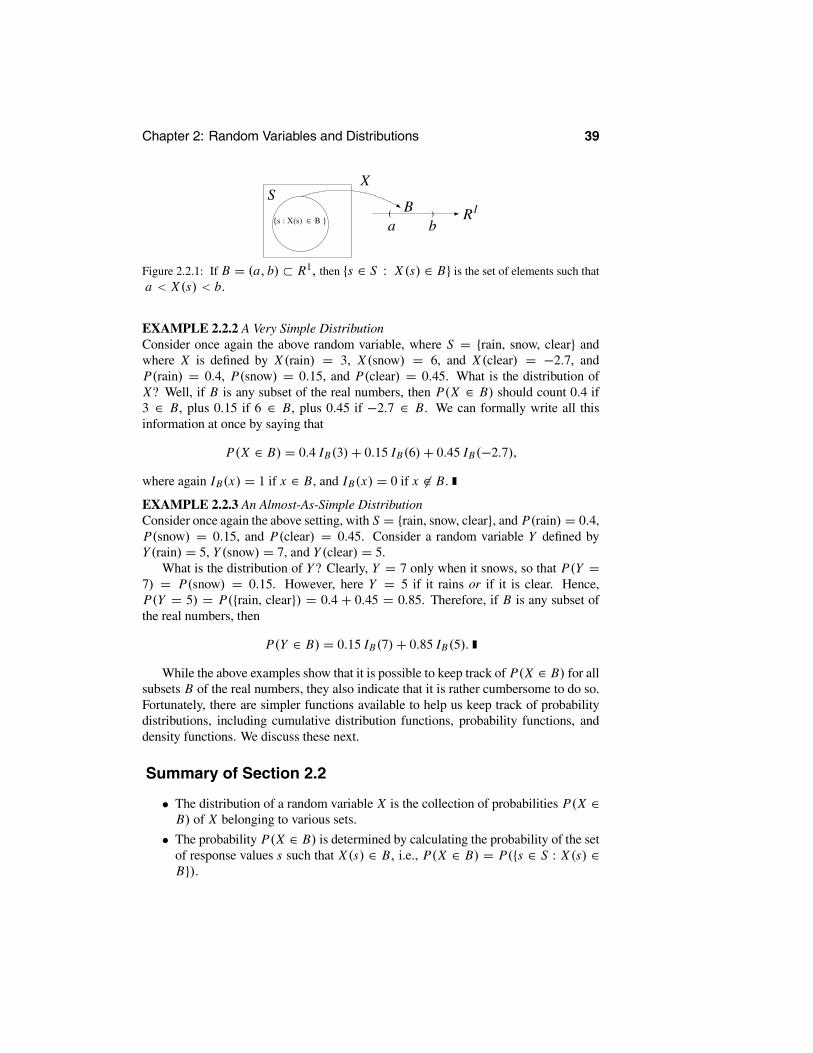
Chapter 2: Random Variables and Distributions 39
1
SX
R1{s : X(s) ∈ B }
( )
a bB
Figure 2.2.1: If B = (a, b) ⊂ R1, then {s ∈ S : X (s) ∈ B} is the set of elements such thata < X (s) < b.
EXAMPLE 2.2.2 A Very Simple DistributionConsider once again the above random variable, where S = {rain, snow, clear} andwhere X is defined by X (rain) = 3, X (snow) = 6, and X (clear) = −2.7, andP(rain) = 0.4, P(snow) = 0.15, and P(clear) = 0.45. What is the distribution ofX? Well, if B is any subset of the real numbers, then P(X ∈ B) should count 0.4 if3 ∈ B, plus 0.15 if 6 ∈ B, plus 0.45 if −2.7 ∈ B. We can formally write all thisinformation at once by saying that
P(X ∈ B) = 0.4 IB(3)+ 0.15 IB(6)+ 0.45 IB(−2.7),
where again IB(x) = 1 if x ∈ B, and IB(x) = 0 if x ∈ B.
EXAMPLE 2.2.3 An Almost-As-Simple DistributionConsider once again the above setting, with S = {rain, snow, clear}, and P(rain) = 0.4,P(snow) = 0.15, and P(clear) = 0.45. Consider a random variable Y defined byY (rain) = 5, Y (snow) = 7, and Y (clear) = 5.
What is the distribution of Y ? Clearly, Y = 7 only when it snows, so that P(Y =7) = P(snow) = 0.15. However, here Y = 5 if it rains or if it is clear. Hence,P(Y = 5) = P({rain, clear}) = 0.4 + 0.45 = 0.85. Therefore, if B is any subset ofthe real numbers, then
P(Y ∈ B) = 0.15 IB(7)+ 0.85 IB(5).
While the above examples show that it is possible to keep track of P(X ∈ B) for allsubsets B of the real numbers, they also indicate that it is rather cumbersome to do so.Fortunately, there are simpler functions available to help us keep track of probabilitydistributions, including cumulative distribution functions, probability functions, anddensity functions. We discuss these next.
Summary of Section 2.2
• The distribution of a random variable X is the collection of probabilities P(X ∈B) of X belonging to various sets.
• The probability P(X ∈ B) is determined by calculating the probability of the setof response values s such that X (s) ∈ B, i.e., P(X ∈ B) = P({s ∈ S : X (s) ∈B}).

40 Section 2.2: Distributions of Random Variables
EXERCISES
2.2.1 Consider flipping two independent fair coins. Let X be the number of heads thatappear. Compute P(X = x) for all real numbers x .2.2.2 Suppose we flip three fair coins, and let X be the number of heads showing.(a) Compute P(X = x) for every real number x .(b) Write a formula for P(X ∈ B), for any subset B of the real numbers.2.2.3 Suppose we roll two fair six-sided dice, and let Y be the sum of the two numbersshowing.(a) Compute P(Y = y) for every real number y.(b) Write a formula for P(Y ∈ B), for any subset B of the real numbers.2.2.4 Suppose we roll one fair six-sided die, and let Z be the number showing. LetW = Z3 + 4, and let V = √Z .(a) Compute P(W = w) for every real number w.(b) Compute P(V = v) for every real number v .(c) Compute P(ZW = x) for every real number x .(d) Compute P(V W = y) for every real number y.(e) Compute P(V +W = r) for every real number r .2.2.5 Suppose that a bowl contains 100 chips: 30 are labelled 1, 20 are labelled 2, and50 are labelled 3. The chips are thoroughly mixed, a chip is drawn, and the number Xon the chip is noted.(a) Compute P(X = x) for every real number x .(b) Suppose the first chip is replaced, a second chip is drawn, and the number Y on thechip noted. Compute P(Y = y) for every real number y.(c) Compute P(W = w) for every real number w when W = X + Y.
2.2.6 Suppose a standard deck of 52 playing cards is thoroughly shuffled and a singlecard is drawn. Suppose an ace has value 1, a jack has value 11, a queen has value 12,and a king has value 13.(a) Compute P(X = x) for every real number x, when X is the value of the carddrawn.(b) Suppose that Y = 1, 2, 3, or 4 when a diamond, heart, club, or spade is drawn.Compute P(Y = y) for every real number y.(c) Compute P(W = w) for every real number w when W = X + Y.
2.2.7 Suppose a university is composed of 55% female students and 45% male stu-dents. A student is selected to complete a questionnaire. There are 25 questions onthe questionnaire administered to a male student and 30 questions on the questionnaireadministered to a female student. If X denotes the number of questions answered by arandomly selected student, then compute P(X = x) for every real number x .
2.2.8 Suppose that a bowl contains 10 chips, each uniquely numbered 0 through 9.The chips are thoroughly mixed, one is drawn and the number on it, X1, is noted. Thischip is then replaced in the bowl. A second chip is drawn and the number on it, X2, isnoted. Compute P(W = w) for every real number w when W = X1 + 10X2.

Chapter 2: Random Variables and Distributions 41
PROBLEMS
2.2.9 Suppose that a bowl contains 10 chips each uniquely numbered 0 through 9. Thechips are thoroughly mixed, one is drawn and the number on it, X1, is noted. This chipis not replaced in the bowl. A second chip is drawn and the number on it, X2, is noted.Compute P(W = w) for every real number w when W = X1 + 10X2.
CHALLENGES
2.2.10 Suppose Alice flips three fair coins, and let X be the number of heads showing.Suppose Barbara flips five fair coins, and let Y be the number of heads showing. LetZ = X − Y . Compute P(Z = z) for every real number z.
2.3 Discrete DistributionsFor many random variables X , we have P(X = x) > 0 for certain x values. Thismeans there is positive probability that the variable will be equal to certain particularvalues.
If
x∈R1
P(X = x) = 1,
then all of the probability associated with the random variable X can be found from theprobability that X will be equal to certain particular values. This prompts the followingdefinition.
Definition 2.3.1 A random variable X is discrete if
x∈R1
P(X = x) = 1. (2.3.1)
At first glance one might expect (2.3.1) to be true for any random variable. How-ever, (2.3.1) does not hold for the uniform distribution on [0, 1] or for other continuousdistributions, as we shall see in the next section.
Random variables satisfying (2.3.1) are simple in some sense because we can un-derstand them completely just by understanding their probabilities of being equal toparticular values x . Indeed, by simply listing out all the possible values x such thatP(X = x) > 0, we obtain a second, equivalent definition, as follows.
Definition 2.3.2 A random variable X is discrete if there is a finite or countable se-quence x1, x2, . . . of distinct real numbers, and a corresponding sequence p1, p2, . . .of nonnegative real numbers, such that P(X = xi ) = pi for all i , and i pi = 1.
This second definition also suggests how to keep track of discrete distributions. Itprompts the following definition.
42 Section 2.3: Discrete Distributions
Definition 2.3.3 For a discrete random variable X , its probability function is thefunction pX : R1 → [0, 1] defined by
pX (x) = P(X = x).
Hence, if x1, x2, . . . are the distinct values such that P(X = xi) = pi for all i with
i pi = 1, then
pX (x) = pi x = xi for some i0 otherwise.
Clearly, all the information about the distribution of X is contained in its probabilityfunction, but only if we know that X is a discrete random variable.
Finally, we note that Theorem 1.5.1 immediately implies the following.
Theorem 2.3.1 (Law of total probability, discrete random variable version) Let Xbe a discrete random variable, and let A be some event. Then
P(A) =x∈R1
P(X = x) P(A | X = x).
2.3.1 Important Discrete Distributions
Certain particular discrete distributions are so important that we list them here.
EXAMPLE 2.3.1 Degenerate DistributionsLet c be some fixed real number. Then, as already discussed, c is also a random variable(in fact, c is a constant random variable). In this case, clearly c is discrete, withprobability function pc satisfying that pc(c) = 1, and pc(x) = 0 for x = c. Because cis always equal to a particular value (namely, c) with probability 1, the distribution ofc is sometimes called a point mass or point distribution or degenerate distribution.
EXAMPLE 2.3.2 The Bernoulli DistributionConsider flipping a coin that has probability θ of coming up heads and probability 1−θof coming up tails, where 0 < θ < 1. Let X = 1 if the coin is heads, while X = 0 ifthe coin is tails. Then pX (1) = P(X = 1) = θ , while pX (0) = P(X = 0) = 1 − θ .The random variable X is said to have the Bernoulli(θ) distribution; we write this asX ∼ Bernoulli(θ).
Bernoulli distributions arise anytime we have a response variable that takes onlytwo possible values, and we label one of these outcomes as 1 and the other as 0. Forexample, 1 could correspond to success and 0 to failure of some quality test applied toan item produced in a manufacturing process. In this case, θ is the proportion of manu-factured items that will pass the test. Alternatively, we could be randomly selecting anindividual from a population and recording a 1 when the individual is female and a 0 ifthe individual is a male. In this case, θ is the proportion of females in the population.

Chapter 2: Random Variables and Distributions 43
EXAMPLE 2.3.3 The Binomial DistributionConsider flipping n coins, each of which has (independent) probability θ of coming upheads, and probability 1− θ of coming up tails. (Again, 0 < θ < 1.) Let X be the totalnumber of heads showing. By (1.4.2), we see that for x = 0, 1, 2, . . . , n,
pX (x) = P(X = x) = n
xθ x (1− θ)n−x = n!
x! (n − x)!θ x (1− θ)n−x .
The random variable X is said to have the Binomial(n, θ) distribution; we write this asX ∼ Binomial(n, θ). The Bernoulli(θ) distribution corresponds to the special case ofthe Binomial(n, θ) distribution when n = 1, namely, Bernoulli(θ) = Binomial(1, θ).Figure 2.3.1 contains the plots of several Binomial(20, θ) probability functions.
20100
0.2
0.1
0.0
x
p
Figure 2.3.1: Plot of the Binomial(20, 1/2) (• • •) and the Binomial(20, 1/5) (◦ ◦ ◦)probability functions.
The binomial distribution is applicable to any situation involving n independentperformances of a random system; for each performance, we are recording whether aparticular event has occurred, called a success, or has not occurred, called a failure. Ifwe denote the event in question by A and put θ = P(A), we have that the number ofsuccesses in the n performances is distributed Binomial(n, θ). For example, we couldbe testing light bulbs produced by a manufacturer, and θ is the probability that a bulbworks when we test it. Then the number of bulbs that work in a batch of n is distributedBinomial(n, θ). If a baseball player has probability θ of getting a hit when at bat, thenthe number of hits obtained in n at-bats is distributed Binomial(n, θ).
There is another way of expressing the binomial distribution that is sometimesuseful. For example, if X1, X2, . . . , Xn are chosen independently and each has theBernoulli(θ) distribution, and Y = X1+· · ·+ Xn, then Y will have the Binomial(n, θ)distribution (see Example 3.4.10 for the details).
EXAMPLE 2.3.4 The Geometric DistributionConsider repeatedly flipping a coin that has probability θ of coming up heads and prob-ability 1− θ of coming up tails, where again 0 < θ < 1. Let X be the number of tails
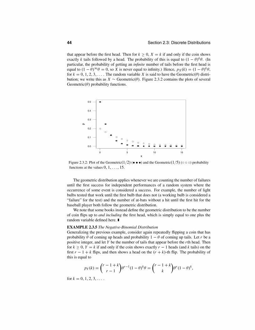
44 Section 2.3: Discrete Distributions
that appear before the first head. Then for k ≥ 0, X = k if and only if the coin showsexactly k tails followed by a head. The probability of this is equal to (1 − θ)kθ . (Inparticular, the probability of getting an infinite number of tails before the first head isequal to (1 − θ)∞θ = 0, so X is never equal to infinity.) Hence, pX (k) = (1− θ)kθ ,for k = 0, 1, 2, 3, . . . . The random variable X is said to have the Geometric(θ) distri-bution; we write this as X ∼ Geometric(θ). Figure 2.3.2 contains the plots of severalGeometric(θ) probability functions.
151050
0.5
0.4
0.3
0.2
0.1
0.0
x
p
Figure 2.3.2: Plot of the Geometric(1/2) (• • •) and the Geometric(1/5) (◦ ◦ ◦) probabilityfunctions at the values 0, 1, . . . , 15.
The geometric distribution applies whenever we are counting the number of failuresuntil the first success for independent performances of a random system where theoccurrence of some event is considered a success. For example, the number of lightbulbs tested that work until the first bulb that does not (a working bulb is considered a“failure” for the test) and the number of at-bats without a hit until the first hit for thebaseball player both follow the geometric distribution.
We note that some books instead define the geometric distribution to be the numberof coin flips up to and including the first head, which is simply equal to one plus therandom variable defined here.
EXAMPLE 2.3.5 The Negative-Binomial DistributionGeneralizing the previous example, consider again repeatedly flipping a coin that hasprobability θ of coming up heads and probability 1− θ of coming up tails. Let r be apositive integer, and let Y be the number of tails that appear before the r th head. Thenfor k ≥ 0, Y = k if and only if the coin shows exactly r − 1 heads (and k tails) on thefirst r − 1 + k flips, and then shows a head on the (r + k)-th flip. The probability ofthis is equal to
pY (k) = r − 1+ k
r − 1θr−1(1− θ)kθ = r − 1+ k
kθr (1− θ)k,
for k = 0, 1, 2, 3, . . . .

Chapter 2: Random Variables and Distributions 45
The random variable Y is said to have the Negative-Binomial(r, θ) distribution; wewrite this as Y ∼ Negative-Binomial(r, θ). Of course, the special case r = 1 cor-responds to the Geometric(θ) distribution. So in terms of our notation, we have thatNegative-Binomial(1, θ) = Geometric(θ). Figure 2.3.3 contains the plots of severalNegative-Binomial(r, θ) probability functions.
20100
0.25
0.20
0.15
0.10
0.05
0.00
x
p
Figure 2.3.3: Plot of the Negative-Binomial(2, 1/2) (• • •) probability function and theNegative-Binomial(10, 1/2) (◦ ◦ ◦) probability function at the values 0, 1, . . . , 20.
The Negative-Binomial(r, θ) distribution applies whenever we are counting thenumber of failures until the r th success for independent performances of a randomsystem where the occurrence of some event is considered a success. For example, thenumber of light bulbs tested that work until the third bulb that does not and the num-ber of at-bats without a hit until the fifth hit for the baseball player both follow thenegative-binomial distribution.
EXAMPLE 2.3.6 The Poisson DistributionWe say that a random variable Y has the Poisson(λ) distribution, and write Y ∼Poisson(λ), if
pY (y) = P(Y = y) = λy
y!e−λ
for y = 0, 1, 2, 3, . . . . We note that since (from calculus) ∞y=0 λ
y/y! = eλ, it isindeed true (as it must be) that ∞
y=0 P(Y = y) = 1. Figure 2.3.4 contains the plotsof several Poisson(λ) probability functions.
20100
0.3
0.2
0.1
0.0
x
p
Figure 2.3.4: Plot of the Poisson(2) (• • •) and the Poisson(10) (◦ ◦ ◦) probability functions atthe values 0, 1, . . . , 20.

46 Section 2.3: Discrete Distributions
We motivate the Poisson distribution as follows. Suppose X ∼ Binomial(n, θ),i.e., X has the Binomial(n, θ) distribution as in Example 2.3.3. Then for 0 ≤ x ≤ n,
P(X = x) = n
xθ x (1− θ)n−x .
If we set θ = λ / n for some λ > 0, then this becomes
P(X = x) = n
x
λ
n
x
1− λn
n−x
= n(n − 1) · · · (n − x + 1)x!
λ
n
x
1− λn
n−x
. (2.3.2)
Let us now consider what happens if we let n → ∞ in (2.3.2), while keeping xfixed at some nonnegative integer. In that case,
n(n − 1) (n − 2) · · · (n − x + 1)nx = 1 1− 1
n1− 2
n· · · 1− x + 1
n
converges to 1 while (since from calculus (1+ (c/n))n → ec for any c)
1− λn
n−x
= 1− λn
n
1− λn
−x
→ e−λ · 1 = e−λ.
Substituting these limits into (2.3.2), we see that
limn→∞ P(X = x) = λ
x
x!e−λ
for x = 0, 1, 2, 3, . . . .Intuitively, we can phrase this result as follows. If we flip a very large number
of coins n, and each coin has a very small probability θ = λ/n of coming up heads,then the probability that the total number of heads will be x is approximately givenby λxe−λ/x!. Figure 2.3.5 displays the accuracy of this estimate when we are ap-proximating the Binomial(100, 1/10) distribution by the Poisson(λ) distribution whereλ = nθ = 100(1/10) = 10.
20100
0.14
0.12
0.10
0.08
0.06
0.04
0.02
0.00
x
p
Figure 2.3.5: Plot of the Binomial(100, 1/10) (• • •) and the Poisson(10) (◦ ◦ ◦) probabilityfunctions at the values 0, 1, . . . , 20.

Chapter 2: Random Variables and Distributions 47
The Poisson distribution is a good model for counting random occurrences of anevent when there are many possible occurrences, but each occurrence has very smallprobability. Examples include the number of house fires in a city on a given day, thenumber of radioactive events recorded by a Geiger counter, the number of phone callsarriving at a switchboard, the number of hits on a popular World Wide Web page on agiven day, etc.
EXAMPLE 2.3.7 The Hypergeometric DistributionSuppose that an urn contains M white balls and N − M black balls. Suppose wedraw n ≤ N balls from the urn in such a fashion that each subset of n balls has thesame probability of being drawn. Because there are N
n such subsets, this probability
is 1/ Nn .
One way of accomplishing this is to thoroughly mix the balls in the urn and thendraw a first ball. Accordingly, each ball has probability 1/N of being drawn. Then,without replacing the first ball, we thoroughly mix the balls in the urn and draw asecond ball. So each ball in the urn has probability 1/(N −1) of being drawn. We thenhave that any two balls, say the i th and j th balls, have probability
P(ball i and j are drawn)
= P(ball i is drawn first)P(ball j is drawn second | ball i is drawn first)
+ P(ball j is drawn first)P(ball i is drawn second | ball j is drawn first)
= 1
N
1
N − 1+ 1
N
1
N − 1= 1/
N
2
of being drawn in the first two draws. Continuing in this fashion for n draws, we obtainthat the probability of any particular set of n balls being drawn is 1/ N
n . This type ofsampling is called sampling without replacement.
Given that we take a sample of n, let X denote the number of white balls obtained.Note that we must have X ≥ 0 and X ≥ n − (N − M) because at most N − M ofthe balls could be black. Hence, X ≥ max(0, n + M − N). Furthermore, X ≤ n andX ≤ M because there are only M white balls. Hence, X ≤ min(n,M).
So suppose max(0, n + M − N) ≤ x ≤ min(n,M). What is the probability thatx white balls are obtained? In other words, what is P(X = x)? To evaluate this, weknow that we need to count the number of subsets of n balls that contain x white balls.Using the combinatorial principles of Section 1.4.1, we see that this number is givenby M
xN−Mn−x . Therefore,
P(X = x) = M
x
N − M
n − x
N
n
for max(0, n + M − N) ≤ x ≤ min(n,M). The random variable X is said to have theHypergeometric(N,M, n) distribution. In Figure 2.3.6, we have plotted some hyperge-ometric probability functions. The Hypergeometric(20, 10, 10) probability function is0 for x > 10, while the Hypergeometric(20, 10, 5) probability function is 0 for x > 5.

48 Section 2.3: Discrete Distributions
20100
0.3
0.2
0.1
0.0
x
p
Figure 2.3.6: Plot of Hypergeometric(20, 10, 10) (• • •) and Hypergeometric(20, 10, 5)(◦ ◦ ◦) probability functions.
Obviously, the hypergeometric distribution will apply to any context wherein weare sampling without replacement from a finite set of N elements and where each el-ement of the set either has a characteristic or does not. For example, if we randomlyselect people to participate in an opinion poll so that each set of n individuals in a pop-ulation of N has the same probability of being selected, then the number of people whorespond yes to a particular question is distributed Hypergeometric(N,M, n), where Mis the number of people in the entire population who would respond yes. We will seethe relevance of this to statistics in Section 5.4.2.
Suppose in Example 2.3.7 we had instead replaced the drawn ball before draw-ing the next ball. This is called sampling with replacement. It is then clear, fromExample 2.3.3, that the number of white balls observed in n draws is distributedBinomial(n,M/N).
Summary of Section 2.3
• A random variable X is discrete if x P(X = x) = 1, i.e., if all its probabilitycomes from being equal to particular values.
• A discrete random variable X takes on only a finite, or countable, number ofdistinct values.
• Important discrete distributions include the degenerate, Bernoulli, binomial, geo-metric, negative-binomial, Poisson, and hypergeometric distributions.
EXERCISES
2.3.1 Consider rolling two fair six-sided dice. Let Y be the sum of the numbers show-ing. What is the probability function of Y ?2.3.2 Consider flipping a fair coin. Let Z = 1 if the coin is heads, and Z = 3 if thecoin is tails. Let W = Z2 + Z .(a) What is the probability function of Z?(b) What is the probability function of W?

Chapter 2: Random Variables and Distributions 49
2.3.3 Consider flipping two fair coins. Let X = 1 if the first coin is heads, and X = 0if the first coin is tails. Let Y = 1 if the second coin is heads, and Y = 5 if the secondcoin is tails. Let Z = XY . What is the probability function of Z?2.3.4 Consider flipping two fair coins. Let X = 1 if the first coin is heads, and X = 0if the first coin is tails. Let Y = 1 if the two coins show the same thing (i.e., both headsor both tails), with Y = 0 otherwise. Let Z = X + Y , and W = XY .(a) What is the probability function of Z?(b) What is the probability function of W?2.3.5 Consider rolling two fair six-sided dice. Let W be the product of the numbersshowing. What is the probability function of W?2.3.6 Let Z ∼ Geometric(θ). Compute P(5 ≤ Z ≤ 9).2.3.7 Let X ∼ Binomial(12, θ). For what value of θ is P(X = 11) maximized?2.3.8 Let W ∼ Poisson(λ). For what value of λ is P(W = 11) maximized?2.3.9 Let Z ∼ Negative-Binomial(3, 1/4). Compute P(Z ≤ 2).2.3.10 Let X ∼ Geometric(1/5). Compute P(X2 ≤ 15).2.3.11 Let Y ∼ Binomial(10, θ). Compute P(Y = 10).2.3.12 Let X ∼ Poisson(λ). Let Y = X − 7. What is the probability function of Y?2.3.13 Let X ∼ Hypergeometric(20, 7, 8). What is the probability that X = 3? Whatis the probability that X = 8?2.3.14 Suppose that a symmetrical die is rolled 20 independent times, and each timewe record whether or not the event {2, 3, 5, 6} has occurred.(a) What is the distribution of the number of times this event occurs in 20 rolls?(b) Calculate the probability that the event occurs five times.2.3.15 Suppose that a basketball player sinks a basket from a certain position on thecourt with probability 0.35.(a) What is the probability that the player sinks three baskets in 10 independent throws?(b) What is the probability that the player throws 10 times before obtaining the firstbasket?(c) What is the probability that the player throws 10 times before obtaining two baskets?2.3.16 An urn contains 4 black balls and 5 white balls. After a thorough mixing, a ballis drawn from the urn, its color is noted, and the ball is returned to the urn.(a) What is the probability that 5 black balls are observed in 15 such draws?(b) What is the probability that 15 draws are required until the first black ball is ob-served?(c) What is the probability that 15 draws are required until the fifth black ball is ob-served?2.3.17 An urn contains 4 black balls and 5 white balls. After a thorough mixing, a ballis drawn from the urn, its color is noted, and the ball is set aside. The remaining ballsare then mixed and a second ball is drawn.(a) What is the probability distribution of the number of black balls observed?(b) What is the probability distribution of the number of white balls observed?

50 Section 2.3: Discrete Distributions
2.3.18 (Poisson processes and queues) Consider a situation involving a server, e.g.,a cashier at a fast-food restaurant, an automatic bank teller machine, a telephone ex-change, etc. Units typically arrive for service in a random fashion and form a queuewhen the server is busy. It is often the case that the number of arrivals at the server, forsome specific unit of time t, can be modeled by a Poisson(λt) distribution and is suchthat the number of arrivals in nonoverlapping periods are independent. In Chapter 3,we will show that λt is the average number of arrivals during a time period of length t,and so λ is the rate of arrivals per unit of time.
Suppose telephone calls arrive at a help line at the rate of two per minute. A Poissonprocess provides a good model.(a) What is the probability that five calls arrive in the next 2 minutes?(b) What is the probability that five calls arrive in the next 2 minutes and then five morecalls arrive in the following 2 minutes?(c) What is the probability that no calls will arrive during a 10-minute period?2.3.19 Suppose an urn contains 1000 balls — one of these is black, and the other 999are white. Suppose that 100 balls are randomly drawn from the urn with replacement.Use the appropriate Poisson distribution to approximate the probability that five blackballs are observed.2.3.20 Suppose that there is a loop in a computer program and that the test to exitthe loop depends on the value of a random variable X. The program exits the loopwhenever X ∈ A, and this occurs with probability 1/3. If the loop is executed at leastonce, what is the probability that the loop is executed five times before exiting?
COMPUTER EXERCISES
2.3.21 Tabulate and plot the Hypergeometric(20, 8, 10) probability function.2.3.22 Tabulate and plot the Binomial(30, 0.3) probability function. Tabulate and plotthe Binomial(30, 0.7) probability function. Explain why the Binomial(30, 0.3) proba-bility function at x agrees with the Binomial(30, 0.7) probability function at n − x .
PROBLEMS
2.3.23 Let X be a discrete random variable with probability function pX (x) = 2−x forx = 1, 2, 3, . . . , with pX (x) = 0 otherwise.(a) Let Y = X2. What is the probability function pY of Y ?(b) Let Z = X − 1. What is the distribution of Z? (Identify the distribution by nameand specify all parameter values.)2.3.24 Let X ∼ Binomial(n1, θ) and Y ∼ Binomial(n2, θ), with X and Y chosenindependently. Let Z = X + Y . What will be the distribution of Z? (Explain yourreasoning.) (Hint: See the end of Example 2.3.3.)2.3.25 Let X ∼ Geometric(θ) and Y ∼ Geometric(θ), with X and Y chosen indepen-dently. Let Z = X + Y . What will be the distribution of Z? Generalize this to r coins.(Explain your reasoning.)

Chapter 2: Random Variables and Distributions 51
2.3.26 Let X ∼ Geometric(θ1) and Y ∼ Geometric(θ2), with X and Y chosen in-dependently. Compute P (X ≤ Y ). Explain what this probability is in terms of cointossing.2.3.27 Suppose that X ∼ Geometric(λ/n). Compute limn→∞ P(X ≤ n).2.3.28 Let X ∼ Negative-Binomial(r, θ) and Y ∼ Negative-Binomial(s, θ), with Xand Y chosen independently. Let Z = X + Y . What will be the distribution of Z?(Explain your reasoning.)2.3.29 (Generalized hypergeometric distribution) Suppose that a set contains N ob-jects, M1 of which are labelled 1, M2 of which are labelled 2, and the remainder ofwhich are labelled 3. Suppose we select a sample of n ≤ N objects from the set usingsampling without replacement, as described in Example 2.3.7. Determine the proba-bility that we obtain the counts ( f1, f2, f3) where fi is the number of objects labelledi in the sample.2.3.30 Suppose that units arrive at a server according to a Poisson process at rate λ (seeExercise 2.3.18). Let T be the amount of time until the first call. Calculate P(T > t).
2.4 Continuous DistributionsIn the previous section, we considered discrete random variables X for which P(X =x) > 0 for certain values of x . However, for some random variables X , such as onehaving the uniform distribution, we have P(X = x) = 0 for all x . This prompts thefollowing definition.
Definition 2.4.1 A random variable X is continuous if
P(X = x) = 0 , (2.4.1)
for all x ∈ R1.
EXAMPLE 2.4.1 The Uniform[0, 1] DistributionConsider a random variable whose distribution is the uniform distribution on [0, 1], aspresented in (1.2.2). That is,
P(a ≤ X ≤ b) = b − a, (2.4.2)
whenever 0 ≤ a ≤ b ≤ 1, with P(X < 0) = P(X > 1) = 0. The random variable Xis said to have the Uniform[0, 1] distribution; we write this as X ∼ Uniform[0, 1]. Forexample,
P12≤ X ≤ 3
4= 3
4− 1
2= 1
4.
Also,
P X ≥ 23= P
23≤ X ≤ 1 + P (X > 1)) = 1− 2
3+ 0 = 1
3.
In fact, for any x ∈ [0, 1],
P(X ≤ x) = P(X < 0)+ P(0 ≤ X ≤ x) = 0+ (x − 0) = x.

52 Section 2.4: Continuous Distributions
Note that setting a = b = x in (2.4.2), we see in particular that P(X = x) = x −x = 0 for every x ∈ R1. Thus, the uniform distribution is an example of a continuousdistribution. In fact, it is one of the most important examples!
The Uniform[0, 1] distribution is fairly easy to work with. However, in general,continuous distributions are very difficult to work with. Because P(X = x) = 0 forall x , we cannot simply add up probabilities like we can for discrete random variables.Thus, how can we keep track of all the probabilities?
A possible solution is suggested by rewriting (2.4.2), as follows. For x ∈ R1, let
f (x) = 1 0 ≤ x ≤ 10 otherwise.
(2.4.3)
Then (2.4.2) can be rewritten as
P(a ≤ X ≤ b) =b
af (x) dx, (2.4.4)
whenever a ≤ b .One might wonder about the wisdom of converting the simple equation (2.4.2) into
the complicated integral equation (2.4.4). However, the advantage of (2.4.4) is that, bymodifying the function f , we can obtain many other continuous distributions besidesthe uniform distribution. To explore this, we make the following definitions.
Definition 2.4.2 Let f : R1 → R1 be a function. Then f is a density function iff (x) ≥ 0 for all x ∈ R1, and ∞
−∞ f (x) dx = 1.
Definition 2.4.3 A random variable X is absolutely continuous if there is a densityfunction f , such that
P(a ≤ X ≤ b) =b
af (x) dx, (2.4.5)
whenever a ≤ b , as in (2.4.4).
In particular, if b = a + δ, with δ a small positive number, and if f is continuous at a,then we see that
P(a ≤ X ≤ a + δ) =a+δ
af (x) dx ≈ δ f (a).
Thus, a density function evaluated at a may be thought of as measuring the probabilityof a random variable being in a small interval about a.
To better understand absolutely continuous random variables, we note the followingtheorem.
Theorem 2.4.1 Let X be an absolutely continuous random variable. Then X is acontinuous random variable, i.e., P(X = a) = 0 for all a ∈ R1.

Chapter 2: Random Variables and Distributions 53
PROOF Let a be any real number. Then P(X = a) = P(a ≤ X ≤ a). On theother hand, setting a = b in (2.4.5), we see that P(a ≤ X ≤ a) = a
a f (x) dx = 0.Hence, P(X = a) = 0 for all a, as required.
It turns out that the converse to Theorem 2.4.1 is false. That is, not all continuousdistributions are absolutely continuous.1 However, most of the continuous distributionsthat arise in statistics are absolutely continuous. Furthermore, absolutely continuousdistributions are much easier to work with than are other kinds of continuous distribu-tions. Hence, we restrict our discussion to absolutely continuous distributions here. Infact, statisticians sometimes say that X is continuous as shorthand for saying that X isabsolutely continuous.
2.4.1 Important Absolutely Continuous Distributions
Certain absolutely continuous distributions are so important that we list them here.
EXAMPLE 2.4.2 The Uniform[0, 1] DistributionClearly, the uniform distribution is absolutely continuous, with the density functiongiven by (2.4.3). We will see, in Section 2.10, that the Uniform[0, 1] distribution hasan important relationship with every absolutely continuous distribution.
EXAMPLE 2.4.3 The Uniform[L, R] DistributionLet L and R be any two real numbers with L < R. Consider a random variable X suchthat
P(a ≤ X ≤ b) = b − a
R − L(2.4.6)
whenever L ≤ a ≤ b ≤ R , with P(X < L) = P(X > R) = 0. The random variableX is said to have the Uniform[L, R] distribution; we write this as X ∼ Uniform[L, R].(If L = 0 and R = 1, then this definition coincides with the previous definition of theUniform[0, 1] distribution.) Note that X ∼ Uniform[L, R] has the same probability ofbeing in any two subintervals of [L, R] that have the same length.
Note that the Uniform[L, R] distribution is also absolutely continuous, with densitygiven by
f (x) =1
R−L L ≤ x ≤ R0 otherwise.
In Figure 2.4.1 we have plotted a Uniform[2, 4] density.
1For examples of this, see more advanced probability books, e.g., page 143 of A First Look at RigorousProbability Theory, Second Edition, by J. S. Rosenthal (World Scientific Publishing, Singapore, 2006).

54 Section 2.4: Continuous Distributions
-5 -4 -3 -2 -1 0 1 2 3 4 5
0.5
1.0
x
f
Figure 2.4.1: A Uniform[2, 4] density function.
EXAMPLE 2.4.4 The Exponential(1) DistributionDefine a function f : R1 → R1 by
f (x) = e−x x ≥ 00 x < 0.
Then clearly, f (x) ≥ 0 for all x . Also,
∞
−∞f (x) dx =
∞
0e−x dx = −e−x
∞0= (−0)− (−1) = 1 .
Hence, f is a density function. See Figure 2.4.2 for a plot of this density.Consider now a random variable X having this density function f . If 0 ≤ a ≤ b <
∞, then
P(a ≤ X ≤ b) =b
af (x) dx =
b
ae−x dx = (−e−b)− (−e−a) = e−a − e−b.
The random variable X is said to have the Exponential(1) distribution, which we writeas X ∼ Exponential(1). The exponential distribution has many important properties,which we will explore in the coming sections.
EXAMPLE 2.4.5 The Exponential(λ) DistributionLet λ > 0 be a fixed constant. Define a function f : R1 → R1 by
f (x) = λ e−λx x ≥ 00 x < 0.
Then clearly, f (x) ≥ 0 for all x . Also,
∞
−∞f (x) dx =
∞
0λe−λx dx = −e−λx
∞0= (−0)− (−1) = 1.

Chapter 2: Random Variables and Distributions 55
Hence, f is again a density function. (If λ = 1, then this corresponds to the Exponential(1)density.)
If X is a random variable having this density function f , then
P(a ≤ X ≤ b) =b
aλ e−λx dx = (−e−λb)− (−e−λa) = e−λa − e−λb
for 0 ≤ a ≤ b < ∞. The random variable X is said to have the Exponential(λ)distribution; we write this as X ∼ Exponential(λ). Note that some books and softwarepackages instead replace λ by 1/λ in the definition of the Exponential(λ) distribution— always check this when using another book or when using software.
An exponential distribution can often be used to model lifelengths. For example, acertain type of light bulb produced by a manufacturer might follow an Exponential(λ)distribution for an appropriate choice of λ. By this we mean that the lifelength X of arandomly selected light bulb from those produced by this manufacturer has probability
P(X ≥ x) =∞
xλe−λz dz = e−λx
of lasting longer than x, in whatever units of time are being used. We will see inChapter 3 that, in a specific application, the value 1/λ will correspond to the averagelifelength of the light bulbs.
As another application of this distribution, consider a situation involving a server,e.g., a cashier at a fast-food restaurant, an automatic bank teller machine, a telephoneexchange, etc. Units arrive for service in a random fashion and form a queue when theserver is busy. It is often the case that the number of arrivals at the server, for somespecific unit of time t, can be modeled by a Poisson(λt) distribution. Now let T1 be thetime until the first arrival. Then we have
P (T1 > t) = P (no arrivals in (0, t]) = (λt)0
0!e−λt = e−λt
and T1 has density given by
f (t) = − d
dt
∞
tf (z) dz = − d
dtP (T1 > t) = λe−λt .
So T1 ∼ Exponential(λ).
EXAMPLE 2.4.6 The Gamma(α, λ) DistributionThe gamma function is defined by
(α) =∞
0tα−1e−t dt , α > 0.
It turns out (see Problem 2.4.15) that
(α + 1) = α (α) (2.4.7)
and that if n is a positive integer, then (n) = (n − 1)!, while (1/2) = √π .
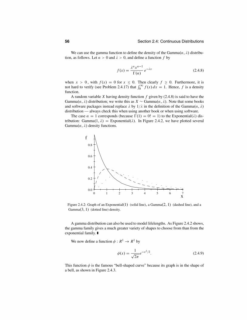
56 Section 2.4: Continuous Distributions
We can use the gamma function to define the density of the Gamma(α, λ) distribu-tion, as follows. Let α > 0 and λ > 0, and define a function f by
f (x) = λαxα−1
(α)e−λx (2.4.8)
when x > 0 , with f (x) = 0 for x ≤ 0. Then clearly f ≥ 0. Furthermore, it isnot hard to verify (see Problem 2.4.17) that ∞
0 f (x) dx = 1. Hence, f is a densityfunction.
A random variable X having density function f given by (2.4.8) is said to have theGamma(α, λ) distribution; we write this as X ∼ Gamma(α, λ). Note that some booksand software packages instead replace λ by 1/λ in the definition of the Gamma(α, λ)distribution — always check this when using another book or when using software.
The case α = 1 corresponds (because (1) = 0! = 1) to the Exponential(λ) dis-tribution: Gamma(1, λ) = Exponential(λ). In Figure 2.4.2, we have plotted severalGamma(α, λ) density functions.
0 1 2 3 4 5 6 70.0
0.2
0.4
0.6
0.8
x
f
Figure 2.4.2: Graph of an Exponential(1) (solid line), a Gamma(2, 1) (dashed line), and aGamma(3, 1) (dotted line) density.
A gamma distribution can also be used to model lifelengths. As Figure 2.4.2 shows,the gamma family gives a much greater variety of shapes to choose from than from theexponential family.
We now define a function φ : R1 → R1 by
φ(x) = 1√2π
e−x2/2. (2.4.9)
This function φ is the famous “bell-shaped curve” because its graph is in the shape ofa bell, as shown in Figure 2.4.3.

Chapter 2: Random Variables and Distributions 57
-5 -4 -3 -2 -1 0 1 2 3 4 5
0.1
0.2
0.3
0.4
x
phi
Figure 2.4.3: Plot of the function φ in (2.4.9).
We have the following result for φ.
Theorem 2.4.2 The function φ given by (2.4.9) is a density function.
PROOF See Section 2.11 for the proof of this result.
This leads to the following important distributions.
EXAMPLE 2.4.7 The N(0, 1) DistributionLet X be a random variable having the density function φ given by (2.4.9). This meansthat for −∞ < a ≤ b <∞,
P(a ≤ X ≤ b) =b
aφ(x) dx =
b
a
1√2π
e−x2/2 dx .
The random variable X is said to have the N(0, 1) distribution (or the standard normaldistribution); we write this as X ∼ N(0, 1).
EXAMPLE 2.4.8 The N(µ, σ 2) DistributionLet µ ∈ R1, and let σ > 0. Let f be the function defined by
f (x) = 1σφ(
x − µσ
) = 1
σ√
2πe−(x−µ)2/2σ 2
.
(If µ = 0 and σ = 1, then this corresponds with the previous example.) Clearly,f ≥ 0. Also, letting y = (x − µ)/σ , we have
∞
−∞f (x) dx =
∞
−∞σ−1φ((x−µ)/σ) dx =
∞
−∞σ−1φ(y)σ dy =
∞
−∞φ(y) dy = 1.
Hence, f is a density function.Let X be a random variable having this density function f . The random variable
X is said to have the N(µ, σ 2) distribution; we write this as X ∼ N(µ, σ 2). In Figure

58 Section 2.4: Continuous Distributions
2.4.4, we have plotted the N(0, 1) and the N(1, 1) densities. Note that changes in µsimply shift the density without changing its shape. In Figure 2.4.5, we have plottedthe N(0, 1) and the N(0, 4) densities. Note that both densities are centered on 0, butthe N(0, 4) density is much more spread out. The value of σ 2 controls the amount ofspread.
-6 -4 -2 0 2 4 6
0.1
0.2
0.3
0.4
x
f
Figure 2.4.4: Graph of the N(1, 1) density (solid line) and the N(0, 1) density (dashed line).
-6 -4 -2 0 2 4 6
0.1
0.2
0.3
0.4
x
f
Figure 2.4.5: Graph of a N(0, 4) density (solid line) and a N(0, 1) density (dashed line).
The N(µ, σ 2) distribution, for some choice of µ and σ 2, arises quite often in ap-plications. Part of the reason for this is an important result known as the central limittheorem. which we will discuss in Section 4.4. In particular, this result leads to usinga normal distribution to approximate other distributions, just as we used the Poissondistribution to approximate the binomial distribution in Example 2.3.6.
In a large human population, it is not uncommon for various body measurements tobe normally distributed (at least to a reasonable degree of approximation). For example,let us suppose that heights (measured in feet) of students at a particular university aredistributed N(µ, σ 2) for some choice ofµ and σ 2. Then the probability that a randomly

Chapter 2: Random Variables and Distributions 59
selected student has height between a and b feet, with a < b, is given by
b
a
1
σ√
2πe−(x−µ)2/2σ 2
dx.
In Section 2.5, we will discuss how to evaluate such an integral. Later in this text, wewill discuss how to select an appropriate value for µ and σ 2 and to assess whether ornot any normal distribution is appropriate to model the distribution of a variable definedon a particular population.
Given an absolutely continuous random variable X , we will write its density as fX ,or as f if no confusion arises. Absolutely continuous random variables will be usedextensively in later chapters of this book.
Remark 2.4.1 Finally, we note that density functions are not unique. Indeed, if f is adensity function and we change its value at a finite number of points, then the value of
ba f (x) dx will remain unchanged. Hence, the changed function will also qualify as
a density corresponding to the same distribution. On the other hand, often a particular“best” choice of density function is clear. For example, if the density function can bechosen to be continuous, or even piecewise continuous, then this is preferred over someother version of the density function.
To take a specific example, for the Uniform[0, 1] distribution, we could replace thedensity f of (2.4.3) by
g(x) = 1 0 < x < 10 otherwise,
or even by
h(x) =
1 0 < x < 3/417 x = 3/41 3/4 < x < 10 otherwise.
Either of these new densities would again define the Uniform[0, 1] distribution, be-cause we would have b
a f (x) dx = ba g(x) dx = b
a h(x) dx for any a < b.On the other hand, the densities f and g are both piecewise continuous and are
therefore natural choices for the density function, whereas h is an unnecessarily com-plicated choice. Hence, when dealing with density functions, we shall always assumethat they are as continuous as possible, such as f and g, rather than having removablediscontinuities such as h. This will be particularly important when discussing likeli-hood methods in Chapter 6.
Summary of Section 2.4
• A random variable X is continuous if P(X = x) = 0 for all x , i.e., if none of itsprobability comes from being equal to particular values.
• X is absolutely continuous if there exists a density function fX with P(a ≤ X ≤b) = b
a fX (x) dx for all a < b.

60 Section 2.4: Continuous Distributions
• Important absolutely continuous distributions include the uniform, exponential,gamma, and normal.
EXERCISES
2.4.1 Let U ∼ Uniform[0, 1]. Compute each of the following.(a) P(U ≤ 0)(b) P(U = 1/2)(c) P(U < −1/3)(d) P(U ≤ 2/3)(e) P(U < 2/3)(f) P(U < 1)(g) P(U ≤ 17)2.4.2 Let W ∼ Uniform[1, 4]. Compute each of the following.(a) P(W ≥ 5)(b) P(W ≥ 2)(c) P(W2 ≤ 9) (Hint: If W 2 ≤ 9, what must W be?)(d) P(W 2 ≤ 2)2.4.3 Let Z ∼ Exponential(4). Compute each of the following.(a) P(Z ≥ 5)(b) P(Z ≥ −5)(c) P(Z2 ≥ 9)(d) P(Z4 − 17 ≥ 9)2.4.4 Establish for which constants c the following functions are densities.(a) f (x) = cx on (0, 1) and 0 otherwise.(b) f (x) = cxn on (0, 1) and 0 otherwise, for n a nonnegative integer.(c) f (x) = cx1/2 on (0, 2) and 0 otherwise.(d) f (x) = c sin x on (0, π/2) and 0 otherwise.2.4.5 Is the function defined by f (x) = x/3 for −1 < x < 2 and 0 otherwise, adensity? Why or why not?2.4.6 Let X ∼ Exponential(3). Compute each of the following.(a) P(0 < X < 1)(b) P(0 < X < 3)(c) P(0 < X < 5)(d) P(2 < X < 5)(e) P(2 < X < 10)(f) P(X > 2).2.4.7 Let M > 0, and suppose f (x) = cx2 for 0 < x < M, otherwise f (x) = 0. Forwhat value of c (depending on M) is f a density?2.4.8 Suppose X has density f and that f (x) ≥ 2 for 0.3 < x < 0.4. Prove thatP(0.3 < X < 0.4) ≥ 0.2.2.4.9 Suppose X has density f and Y has density g. Suppose f (x) > g(x) for 1 <x < 2. Prove that P(1 < X < 2) > P(1 < Y < 2).

Chapter 2: Random Variables and Distributions 61
2.4.10 Suppose X has density f and Y has density g. Is it possible that f (x) > g(x)for all x? Explain.2.4.11 Suppose X has density f and f (x) > f (y) whenever 0 < x < 1 < y < 2.Does it follow that P(0 < X < 1) > P(1 < X < 2)? Explain.2.4.12 Suppose X has density f and f (x) > f (y) whenever 0 < x < 1 < y < 3.Does it follow that P(0 < X < 1) > P(1 < X < 3)? Explain.2.4.13 Suppose X ∼ N(0, 1) and Y ∼ N(1, 1). Prove that P(X < 3) > P(Y < 3).
PROBLEMS
2.4.14 Let Y ∼ Exponential(λ) for some λ > 0. Let y, h ≥ 0. Prove that P(Y −h ≥ y |Y ≥ h) = P(Y ≥ y). That is, conditional on knowing that Y ≥ h, therandom variable Y − h has the same distribution as Y did originally. This is calledthe memoryless property of the exponential distributions; it says that they immediately“forget” their past behavior.2.4.15 Consider the gamma function (α) = ∞
0 tα−1e−t dt , for α > 0.(a) Prove that (α + 1) = α (α). (Hint: Use integration by parts.)(b) Prove that (1) = 1.(c) Use parts (a) and (b) to show that (n) = (n − 1)! if n is a positive integer.2.4.16 Use the fact that (1/2) = √π to give an alternate proof that ∞
−∞ φ(x) dx= 1 (as in Theorem 2.4.2). (Hint: Make the substitution t = x2/2.)2.4.17 Let f be the density of the Gamma(α, λ) distribution, as in (2.4.8). Prove that∞
0 f (x) dx = 1. (Hint: Let t = λx .)2.4.18 (Logistic distribution) Consider the function given by f (x) =e−x 1+ e−x −2 for −∞ < x <∞. Prove that f is a density function.2.4.19 (Weibull(α) distribution) Consider, for α > 0 fixed, the function given byf (x) = αxα−1e−xα for 0 < x < ∞ and 0 otherwise. Prove that f is a densityfunction.2.4.20 (Pareto(α) distribution) Consider, for α > 0 fixed, the function given by f (x) =α (1+ x)−α−1 for 0 < x <∞ and 0 otherwise. Prove that f is a density function.2.4.21 (Cauchy distribution) Consider the function given by
f (x) = 1π
11+ x2
for −∞ < x < ∞. Prove that f is a density function. (Hint: Recall the derivative ofarctan(x) .)2.4.22 (Laplace distribution) Consider the function given by f (x) = e−|x|/2 for−∞ < x <∞ and 0 otherwise. Prove that f is a density function.2.4.23 (Extreme value distribution) Consider the function given by f (x) = e−x exp −e−x
for −∞ < x <∞ and 0 otherwise. Prove that f is a density function.2.4.24 (Beta(a, b) distribution) The beta function is the function B : (0,∞)2 → R1
given by
B (a, b) =1
0xa−1 (1− x)b−1 dx .

62 Section 2.5: Cumulative Distribution Functions
It can be proved (see Challenge 2.4.25) that
B (a, b) = (a) (b)
(a + b)(2.4.10)
(a) Prove that the function f given by f (x) = B−1 (a, b) xa−1 (1− x)b−1 , for 0 <x < 1 and 0 otherwise, is a density function.(b) Determine and plot the density when a = 1, b = 1. Can you name this distribution?(c) Determine and plot the density when a = 2, b = 1.(d) Determine and plot the density when a = 1, b = 2.(e) Determine and plot the density when a = 2, b = 2.
CHALLENGES
2.4.25 Prove (2.4.10). (Hint: Use (a) (b) = ∞0
∞0 xa−1yb−1e−x−y dx dy and
make the change of variable u = x + y, v = x/u.)
DISCUSSION TOPICS
2.4.26 Suppose X ∼ N(0, 1) and Y ∼ N(0, 4). Which do you think is larger, P(X >2) or P(Y > 2)? Why? (Hint: Look at Figure 2.4.5.)
2.5 Cumulative Distribution FunctionsIf X is a random variable, then its distribution consists of the values of P(X ∈ B) forall subsets B of the real numbers. However, there are certain special subsets B that areconvenient to work with. Specifically, if B = (−∞, x] for some real number x , thenP(X ∈ B) = P(X ≤ x). It turns out (see Theorem 2.5.1) that it is sufficient to keeptrack of P(X ≤ x) for all real numbers x .
This motivates the following definition.
Definition 2.5.1 Given a random variable X , its cumulative distribution function(or distribution function, or cdf for short) is the function FX : R1 → [0, 1], definedby FX (x) = P(X ≤ x). (Where there is no confusion, we sometimes write F(x)for FX (x).)
The reason for calling FX the “distribution function” is that the full distributionof X can be determined directly from FX . We demonstrate this for some events ofparticular importance.
First, suppose that B = (a, b] is a left-open interval. Using (1.3.3),
P(X ∈ B) = P(a < X ≤ b) = P(X ≤ b)− P(X ≤ a) = FX (b)− FX (a).
Now, suppose that B = [a, b] is a closed interval. Then using the continuity ofprobability (see Theorem 1.6.1), we have
P(X ∈ B) = P(a ≤ X ≤ b) = limn→∞ P(a − 1/n < X ≤ b)
= limn→∞ (FX (b)− FX (a − 1/n)) = FX (b)− lim
n→∞ FX (a − 1/n).

Chapter 2: Random Variables and Distributions 63
We sometimes write limn→∞ FX (a − 1/n) as FX (a−), so that P(X ∈ [a, b]) =FX (b)− FX (a−). In the special case where a = b, we have
P(X = a) = FX (a)− FX (a−). (2.5.1)
Similarly, if B = (a, b) is an open interval, then
P(X ∈ B) = P(a < X < b) = limn→∞ FX (b − 1/n)− FX (a) = FX (b
−)− FX (a).
If B = [a, b) is a right-open interval, then
P(X ∈ B) = P(a ≤ X < b) = limn→∞ FX (b − 1/n)− lim
n→∞ FX (a − 1/n)
= FX (b−)− FX (a−).
We conclude that we can determine P(X ∈ B) from FX whenever B is any kind ofinterval.
Now, if B is instead a union of intervals, then we can use additivity to again com-pute P(X ∈ B) from FX . For example, if
B = (a1, b1] ∪ (a2, b2] ∪ · · · ∪ (ak, bk],
with a1 < b1 < a2 < b2 < · · · < ak < bk , then by additivity,
P(X ∈ B) = P(X ∈ (a1, b1])+ · · · + P(X ∈ (ak, bk])
= FX (b1)− FX (a1)+ · · · + FX (bk)− FX (ak).
Hence, we can still compute P(X ∈ B) solely from the values of FX (x).
Theorem 2.5.1 Let X be any random variable, with cumulative distribution func-tion FX . Let B be any subset of the real numbers. Then P(X ∈ B) can be deter-mined solely from the values of FX (x).
PROOF (Outline) It turns out that all relevant subsets B can be obtained by apply-ing limiting operations to unions of intervals. Hence, because FX determines P(X ∈B) when B is a union of intervals, it follows that FX determines P(X ∈ B) for allrelevant subsets B.
2.5.1 Properties of Distribution Functions
In light of Theorem 2.5.1, we see that cumulative distribution functions FX are veryuseful. Thus, we note a few of their basic properties here.
Theorem 2.5.2 Let FX be the cumulative distribution function of a random variableX . Then
(a) 0 ≤ FX (x) ≤ 1 for all x ,(b) FX (x) ≤ FX (y) whenever x ≤ y (i.e., FX is increasing),(c) limx→+∞ FX (x) = 1,(d) limx→−∞ FX (x) = 0.

64 Section 2.5: Cumulative Distribution Functions
PROOF (a) Because FX (x) = P(X ≤ x) is a probability, it is between 0 and 1.
(b) Let A = {X ≤ x} and B = {X ≤ y}. Then if x ≤ y, then A ⊆ B, so thatP(A) ≤ P(B). But P(A) = FX (x) and P(B) = FX (y), so the result follows.
(c) Let An = {X ≤ n}. Because X must take on some value and hence X ≤ n forsufficiently large n, we see that {An} increases to S, i.e., {An} S (see Section 1.6).Hence, by continuity of P (see Theorem 1.6.1), limn→∞ P(An) = P(S) = 1. ButP(An) = P(X ≤ n) = FX (n), so the result follows.
(d) Let Bn = {X ≤ −n}. Because X ≥ −n for sufficiently large n, {Bn} decreasesto the empty set, i.e., {Bn} ∅. Hence, again by continuity of P, limn→∞ P(Bn) =P(∅) = 0. But P(Bn) = P(X ≤ −n) = FX (−n), so the result follows.
If FX is a cumulative distribution function, then FX is also right continuous; see Prob-lem 2.5.17. It turns out that if a function F : R1 → R1 satisfies properties (a) through(d) and is right continuous, then there is a unique probability measure P on R1 suchthat F is the cdf of P.We will not prove this result here.2
2.5.2 Cdfs of Discrete Distributions
We can compute the cumulative distribution function (cdf) FX of a discrete randomvariable from its probability function pX , as follows.
Theorem 2.5.3 Let X be a discrete random variable with probability function pX .Then its cumulative distribution function FX satisfies FX (x) = y≤x pX (y).
PROOF Let x1, x2, . . . be the possible values of X . Then FX (x) = P(X ≤ x) =xi≤x P(X = xi ) = y≤x P(X = y) = y≤x pX (y), as claimed.
Hence, if X is a discrete random variable, then by Theorem 2.5.3, FX is piecewiseconstant, with a jump of size pX (xi ) at each value xi . A plot of such a distributionlooks like that depicted in Figure 2.5.1.
We consider an example of a distribution function of a discrete random variable.
EXAMPLE 2.5.1Consider rolling one fair six-sided die, so that S = {1, 2, 3, 4, 5, 6}, with P(s) = 1/6for each s ∈ S. Let X be the number showing on the die divided by 6, so that X (s) =s/6 for s ∈ S. What is FX (x)? Since X (s) ≤ x if and only if s ≤ 6x, we have that
FX (x) = P(X ≤ x) =s∈S, s≤6x
P(s) =s∈S, s≤6x
16= 1
6|{s ∈ S : s ≤ 6x}| .
2For example, see page 67 of A First Look at Rigorous Probability Theory, Second Edition, by J. S. Rosen-thal (World Scientific Publishing, Singapore, 2006).

Chapter 2: Random Variables and Distributions 65
That is, to compute FX (x), we count how many elements s ∈ S satisfy s ≤ 6x andmultiply that number by 1/6. Therefore,
FX (x) =
0 x < 1/61/6 1/6 ≤ x < 2/62/6 2/6 ≤ x < 3/63/6 3/6 ≤ x < 4/64/6 4/6 ≤ x < 5/65/6 5/6 ≤ x < 16/6 1 ≤ x .
In Figure 2.5.1, we present a graph of the function FX and note that this is a stepfunction. Note (see Exercise 2.5.1) that the properties of Theorem 2.5.2 are indeedsatisfied by the function FX .
0.0 0.2 0.4 0.6 0.8 1.0 1.20.0
0.2
0.4
0.6
0.8
1.0
x
F
Figure 2.5.1: Graph of the cdf FX in Example 2.5.1.
2.5.3 Cdfs of Absolutely Continuous Distributions
Once we know the density fX of X , then it is easy to compute the cumulative distribu-tion function of X , as follows.
Theorem 2.5.4 Let X be an absolutely continuous random variable, with densityfunction fX . Then the cumulative distribution function FX of X satisfies
FX (x) =x
−∞fX (t) dt
for x ∈ R1.
PROOF This follows from (2.4.5), by setting b = x and letting a →−∞.
From the fundamental theorem of calculus, we see that it is also possible to computea density fX once we know the cumulative distribution function FX .

66 Section 2.5: Cumulative Distribution Functions
Corollary 2.5.1 Let X be an absolutely continuous random variable, with cumula-tive distribution function FX . Let
fX (x) = d
dxFX (x) = FX (x).
Then fX is a density function for X .
We note that FX might not be differentiable everywhere, so that the function fX of thecorollary might not be defined at certain isolated points. The density function may takeany value at such points.
Consider again the N(0, 1) distribution, with density φ given by (2.4.9). Accordingto Theorem 2.5.4, the cumulative distribution function F of this distribution is givenby
F(x) =x
−∞φ(t) dt =
x
−∞1√2π
e−t2/2 dt.
It turns out that it is provably impossible to evaluate this integral exactly, except forcertain specific values of x (e.g., x = −∞, x = 0, or x = ∞). Nevertheless, thecumulative distribution function of the N(0, 1) distribution is so important that it isassigned a special symbol. Furthermore, this is tabulated in Table D.2 of Appendix Dfor certain values of x .
Definition 2.5.2 The symbol stands for the cumulative distribution function ofa standard normal distribution, defined by
(x) =x
−∞φ(t) dt =
x
−∞1√2π
e−t2/2 dt, (2.5.2)
for x ∈ R1.
EXAMPLE 2.5.2 Normal Probability CalculationsSuppose that X ∼ N(0, 1), and we want to calculate
P(−0.63 ≤ X ≤ 2.0) = P(X ≤ 2.0)− P(X ≤ −0.63).
Then P(X ≤ 2) = (2), while P(X ≤ −0.63) = (−0.63). Unfortunately,(2) and (−0.63) cannot be computed exactly, but they can be approximated us-
ing a computer to numerically calculate the integral (2.5.2). Virtually all statisticalsoftware packages will provide such approximations, but many tabulations such asTable D.2, are also available. Using this table, we obtain (2) = 0.9772, while(−0.63) = 0.2643. This implies that
P(−0.63 ≤ X ≤ 2.0) = (2.0)− (−0.63) = 0.9772− 0.2643 = 0.7129.
Now suppose that X ∼ N(µ, σ 2), and we want to calculate P(a ≤ X ≤ b). Lettingf denote the density of X and following Example 2.4.8, we have
P(a ≤ X ≤ b) =b
af (x) dx =
b
a
1σφ
x − µσ
dx.

Chapter 2: Random Variables and Distributions 67
Then, again following Example 2.4.8, we make the substitution y = (x − µ)/σ in theabove integral to obtain
P(a ≤ X ≤ b) =b−µσ
a−µσ
φ(x) dx = b − µσ
− a − µσ
.
Therefore, general normal probabilities can be computed using the function .Suppose now that a = −0.63, b = 2.0, µ = 1.3, and σ 2 = 4.We obtain
P(−0.63 ≤ X ≤ 2.0) = 2.0− 1.32
− −0.63− 1.32
= (0.35)− (−0.965) = 0.6368− 0.16725
= 0.46955
because, using Table D.2, (0.35) = 0.6368. We approximate (−0.965) by thelinear interpolation between the values (−0.96) = 0.1685, (−0.97) = 0.1660,given by
(−0.965) ≈ (−0.96)+ (−0.97)− (−0.96)−0.97− (−0.96)
(−0.965− (−0.96))
= 0.1685+ 0.1660− 0.1685
−0.97− (−0.96)(−0.965− (−0.96)) = 0.16725.
EXAMPLE 2.5.3Let X be a random variable with cumulative distribution function given by
FX (x) = 0 x < 2(x − 2)4/16 2 ≤ x < 41 4 ≤ x.
In Figure 2.5.2, we present a graph of FX .
1 2 3 4 50.0
0.5
1.0
x
F
Figure 2.5.2: Graph of the cdf FX in Example 2.5.3.
Suppose for this random variable X we want to compute P(X ≤ 3), P(X < 3),P(X > 2.5), and P(1.2 < X ≤ 3.4). We can compute all these probabilities directly

68 Section 2.5: Cumulative Distribution Functions
from FX . We have that
P(X ≤ 3) = FX (3) = (3− 2)4/16 = 1/16,
P(X < 3) = FX (3−) = lim
n→∞(3− (1/n)− 2)4/16 = 1/16,
P(X > 2.5) = 1− P(X ≤ 2.5) = 1− FX (2.5)
= 1− (2.5− 2)4/16 = 1− 0.0625/16 = 0.996,
P(1.2 < X ≤ 3.4) = FX (3.4)− FX (1.2) = (3.4− 2)4/16− 0 = 0.2401.
2.5.4 Mixture Distributions
Suppose now that F1, F2, . . . , Fk are cumulative distribution functions, correspond-ing to various distributions. Also let p1, p2, . . . , pk be positive real numbers with
ki=1 pi = 1 (so these values form a probability distribution). Then we can define a
new function G by
G(x) = p1F1(x)+ p2F2(x)+ · · · + pk Fk(x). (2.5.3)
It is easily verified (see Exercise 2.5.6) that the function G given by (2.5.3) willsatisfy properties (a) through (d) of Theorem 2.5.2 and is right continuous. Hence, Gis also a cdf.
The distribution whose cdf is given by (2.5.3) is called a mixture distribution be-cause it mixes the various distributions with cdfs F1, . . . , Fk according to the probabil-ity distribution given by the p1, p2, . . . , pk .
To see how a mixture distribution arises in applications, consider a two-stage sys-tem, as discussed in Section 1.5.1. Let Z be a random variable describing the outcomeof the first stage and such that P(Z = i) = pi for i = 1, 2, . . . , k. Suppose that forthe second stage, we observe a random variable Y where the distribution of Y dependson the outcome of the first stage, so that Y has cdf Fi when Z = i. In effect, Fi is theconditional distribution of Y, given that Z = i (see Section 2.8). Then, by the law oftotal probability (see Theorem 1.5.1), the distribution function of Y is given by
P(Y ≤ y) =k
i=1
P(Y ≤ y | Z = i)P(Z = i) =k
i=1
pi Fi (y) = G(y).
Therefore the distribution function of Y is given by a mixture of the Fi .Consider the following example of this.
EXAMPLE 2.5.4Suppose we have two bowls containing chips. Bowl #1 contains one chip labelled0, two chips labelled 3, and one chip labelled 5. Bowl #2 contains one chip labelled2, one chip labelled 4, and one chip labelled 5. Now let Xi be the random variablecorresponding to randomly drawing a chip from bowl #i . Therefore, P(X1 = 0) =1/4, P(X1 = 3) = 1/2, and P(X1 = 5) = 1/4, while P(X2 = 2) = P(X2 = 4) =

Chapter 2: Random Variables and Distributions 69
P(X2 = 5) = 1/3. Then X1 has distribution function given by
F1(x) =
0 x < 01/4 0 ≤ x < 33/4 3 ≤ x < 51 x ≥ 5
and X2 has distribution function given by
F2(x) =
0 x < 21/3 2 ≤ x < 42/3 4 ≤ x < 51 x ≥ 5.
Now suppose that we choose a bowl by randomly selecting a card from a deck offive cards where one card is labelled 1 and four cards are labelled 2. Let Z denote thevalue on the card obtained, so that P (Z = 1) = 1/5 and P (Z = 2) = 4/5. Then,having obtained the value Z = i , we observe Y by randomly drawing a chip from bowl#i . We see immediately that the cdf of Y is given by
G(x) = (1/5) F1(x)+ (4/5) F2(x),
and this is a mixture of the cdfs F1 and F2.
As the following examples illustrate, it is also possible to have infinite mixtures ofdistributions.
EXAMPLE 2.5.5 Location and Scale MixturesSuppose F is some cumulative distribution function. Then for any real number y, thefunction Fy defined by Fy(x) = F(x− y) is also a cumulative distribution function. Infact, Fy is just a “shifted” version of F . An example of this is depicted in Figure 2.5.3.
-10 -5 0 5 10
0.5
1.0
x
F
Figure 2.5.3: Plot of the distribution functions F (solid line) and F2 (dashed line) in Example2.5.5, where F(x) = ex/ (ex + 1) for x ∈ R1.
If pi ≥ 0 with i pi = 1 (so the pi form a probability distribution), and y1, y2, . . .are real numbers, then we can define a discrete location mixture by
H(x) =i
pi Fyi (x) =i
pi F(x − yi ).

70 Section 2.5: Cumulative Distribution Functions
Indeed, the shift Fy(x) = F(x − y) itself corresponds to a special case of a discretelocation mixture, with p1 = 1 and y1 = y.
Furthermore, if g is some nonnegative function with ∞−∞ g(t) dt = 1 (so g is a
density function), then we can define
H(x) =∞
−∞Fy(x) g(y) dy =
∞
−∞F(x − y) g(y) dy.
Then it is not hard to see that H is also a cumulative distribution function — one that iscalled a continuous location mixture of F. The idea is that H corresponds to a mixtureof different shifted distributions Fy , with the density g giving the distribution of themixing coefficient y.
We can also define a discrete scale mixture by
K (x) =i
pi F(x/yi )
whenever yi > 0, pi ≥ 0, and i pi = 1. Similarly, if ∞0 g(t) dt = 1, then we can
write
K (x) =∞
0F(x/y)g(y) dy.
Then K is also a cumulative distribution function, called a continuous scale mixture ofF .
You might wonder at this point whether a mixture distribution is discrete or con-tinuous. The answer depends on the distributions being mixed and the mixing distrib-ution. For example, discrete location mixtures of discrete distributions are discrete anddiscrete location mixtures of continuous distributions are continuous.
There is nothing restricting us, however, to mixing only discrete distributions oronly continuous distributions. Other kinds of distribution are considered in the follow-ing section.
2.5.5 Distributions Neither Discrete Nor Continuous (Advanced)
There are some distributions that are neither discrete nor continuous, as the followingexample shows.
EXAMPLE 2.5.6Suppose that X1 ∼ Poisson(3) is discrete with cdf F1, while X2 ∼ N(0, 1) is continu-ous with cdf F2, and Y has the mixture distribution given by FY (y) = (1/5) F1(y) +(4/5) F2(y). Using (2.5.1), we have
P(Y = y) = FY (y)− FY (y−)
= (1/5)F1(y)+ (4/5) F2(y)− (1/5)F1(y−)− (4/5)F2(y−)= (1/5) F1(y)− F1(y
−) + (4/5) F2(y)− F2(y−)
= 15
P(X1 = y)+ 45
P(X2 = y).

Chapter 2: Random Variables and Distributions 71
Therefore,
P(Y = y) =15
3y
y! e−3 y a nonnegative integer0 otherwise.
Because P(Y = y) > 0 for nonnegative integers y, the random variable Y is notcontinuous. On the other hand, we have
yP(Y = y) =
∞
y=0
15
3y
y!e−3 = 1
5< 1.
Hence, Y is not discrete either.In fact, Y is neither discrete nor continuous. Rather, Y is a mixture of a discrete
and a continuous distribution.
For the most part in this book, we shall treat discrete and continuous distributionsseparately. However, it is important to keep in mind that actual distributions may beneither discrete nor continuous but rather a mixture of the two.3 In most applications,however, the distributions we deal with are either continuous or discrete.
Recall that a continuous distribution need not be absolutely continuous, i.e., have adensity. Hence, a distribution which is a mixture of a discrete and a continuous distri-bution might not be a mixture of a discrete and an absolutely continuous distribution.
Summary of Section 2.5
• The cumulative distribution function (cdf) of X is FX (x) = P(X ≤ x).
• All probabilities associated with X can be determined from FX .
• As x increases from −∞ to∞, FX (x) increases from 0 to 1.
• If X is discrete, then FX (x) = y≤x P(X = y).
• If X is absolutely continuous, then FX (x) = x−∞ fX (t) dt , and fX (x) = FX (x).
• We write (x) for the cdf of the standard normal distribution evaluated at x .
• A mixture distribution has a cdf which is a linear combination of other cdfs. Twospecial cases are location and scale mixtures.
• Some mixture distributions are neither discrete nor continuous.
EXERCISES
2.5.1 Verify explicitly that properties (a) through (d) of Theorem 2.5.2 are indeed sat-isfied by the function FX in Example 2.5.1.2.5.2 Consider rolling one fair six-sided die, so that S = {1, 2, 3, 4, 5, 6}, and P(s) =1/6 for all s ∈ S. Let X be the number showing on the die, so that X (s) = s for s ∈ S.Let Y = X2. Compute the cumulative distribution function FY (y) = P(Y ≤ y), for ally ∈ R1. Verify explicitly that properties (a) through (d) of Theorem 2.5.2 are satisfiedby this function FY .
3In fact, there exist probability distributions that cannot be expressed even as a mixture of a discrete anda continuous distribution, but these need not concern us here.

72 Section 2.5: Cumulative Distribution Functions
2.5.3 For each of the following functions F , determine whether or not F is a validcumulative distribution function, i.e., whether or not F satisfies properties (a) through(d) of Theorem 2.5.2.(a) F(x) = x for all x ∈ R1
(b)
F(x) = 0 x < 0
x 0 ≤ x ≤ 11 x > 1
(c)
F(x) = 0 x < 0
x2 0 ≤ x ≤ 11 x > 1
(d)
F(x) = 0 x < 0
x2 0 ≤ x ≤ 31 x > 3
(e)
F(x) = 0 x < 0
x2/9 0 ≤ x ≤ 31 x > 3
(f)
F(x) = 0 x < 1
x2/9 1 ≤ x ≤ 31 x > 3
(g)
F(x) = 0 x < −1
x2/9 −1 ≤ x ≤ 31 x > 3
2.5.4 Let X ∼ N(0, 1). Compute each of the following in terms of the function ofDefinition 2.5.2 and use Table D.2 (or software) to evaluate these probabilities numer-ically.(a) P(X ≤ −5)(b) P(−2 ≤ X ≤ 7)(c) P(X ≥ 3)2.5.5 Let Y ∼ N(−8, 4). Compute each of the following, in terms of the function
of Definition 2.5.2 and use Table D.2 (or software) to evaluate these probabilitiesnumerically.(a) P(Y ≤ −5)(b) P(−2 ≤ Y ≤ 7)(c) P(Y ≥ 3)

Chapter 2: Random Variables and Distributions 73
2.5.6 Verify that the function G given by (2.5.3) satisfies properties (a) through (d) ofTheorem 2.5.2.2.5.7 Suppose FX (x) = x2 for 0 ≤ x ≤ 1. Compute each of the following.(a) P(X < 1/3).(b) P(1/4 < X < 1/2).(c) P(2/5 < X < 4/5).(d) P(X < 0).(e) P(X < 1)(f) P(X < −1)(g) P(X < 3)(h) P(X = 3/7)2.5.8 Suppose FY (y) = y3 for 0 ≤ y < 1/2, and FY (y) = 1 − y3 for 1/2 ≤ y ≤ 1.Compute each of the following.(a) P(1/3 < Y < 3/4)(b) P(Y = 1/3)(c) P(Y = 1/2)2.5.9 Let F(x) = x2 for 0 ≤ x ≤ 2, with F(x) = 0 for x < 0 and F(x) = 4 forx > 2.(a) Sketch a graph of F .(b) Is F a valid cumulative distribution function? Why or why not?2.5.10 Let F(x) = 0 for x < 0, with F(x) = e−x for x ≥ 0.(a) Sketch a graph of F .(b) Is F a valid cumulative distribution function? Why or why not?2.5.11 Let F(x) = 0 for x < 0, with F(x) = 1− e−x for x ≥ 0.(a) Sketch a graph of F .(b) Is F a valid cumulative distribution function? Why or why not?2.5.12 Let X ∼ Exponential(3). Compute the function FX .2.5.13 Let F(x) = 0 for x < 0, with F(x) = 1/3 for 0 ≤ x < 2/5, and F(x) = 3/4for 2/5 ≤ x < 4/5, and F(x) = 1 for x ≥ 4/5.(a) Sketch a graph of F .(b) Prove that F is a valid cumulative distribution function.(c) If X has cumulative distribution function equal to F , then compute P(X > 4/5)and P(−1 < X < 1/2) and P(X = 2/5) and P(X = 4/5).
2.5.14 Let G(x) = 0 for x < 0, with G(x) = 1− e−x2for x ≥ 0.
(a) Prove that G is a valid cumulative distribution function.(b) If Y has cumulative distribution function equal to G, then compute P(Y > 4) andP(−1 < Y < 2) and P(Y = 0).2.5.15 Let F and G be as in the previous two exercises. Let H(x) = (1/3)F(x) +(2/3)G(x). Suppose Z has cumulative distribution function equal to H . Compute eachof the following.(a) P(Z > 4/5)(b) P(−1 < Z < 1/2)(c) P(Z = 2/5)(d) P(Z = 4/5)

74 Section 2.6: One-Dimensional Change of Variable
(e) P(Z = 0)(f) P(Z = 1/2)
PROBLEMS
2.5.16 Let F be a cumulative distribution function. Compute (with explanation) thevalue of limn→∞[F(2n)− F(n)].2.5.17 Let F be a cumulative distribution function. For x ∈ R1, we could defineF(x+) by F(x+) = limn→∞ F(x+ 1
n ). Prove that F is right continuous, meaning thatfor each x ∈ R1, we have F(x+) = F(x). (Hint: You will need to use continuity of P(Theorem 1.6.1).)2.5.18 Let X be a random variable, with cumulative distribution function FX . Provethat P(X = a) = 0 if and only if the function FX is continuous at a. (Hint: Use (2.5.1)and the previous problem.)2.5.19 Let be as in Definition 2.5.2. Derive a formula for (−x) in terms of (x).(Hint: Let s = −t in (2.5.2), and do not forget Theorem 2.5.2.)2.5.20 Determine the distribution function for the logistic distribution of Problem 2.4.18.2.5.21 Determine the distribution function for the Weibull(α) distribution of Problem2.4.19.2.5.22 Determine the distribution function for the Pareto(α) distribution of Problem2.4.20.2.5.23 Determine the distribution function for the Cauchy distribution of Problem2.4.21.2.5.24 Determine the distribution function for the Laplace distribution of Problem2.4.22.2.5.25 Determine the distribution function for the extreme value distribution of Prob-lem 2.4.23.2.5.26 Determine the distribution function for the beta distributions of Problem 2.4.24for parts (b) through (e).
DISCUSSION TOPICS
2.5.27 Does it surprise you that all information about the distribution of a randomvariable X can be stored by a single function FX ? Why or why not? What otherexamples can you think of where lots of different information is stored by a singlefunction?
2.6 One-Dimensional Change of VariableLet X be a random variable with a known distribution. Suppose that Y = h(X), whereh : R1 → R1 is some function. (Recall that this really means that Y (s) = h(X (s)), forall s ∈ S.) Then what is the distribution of Y ?
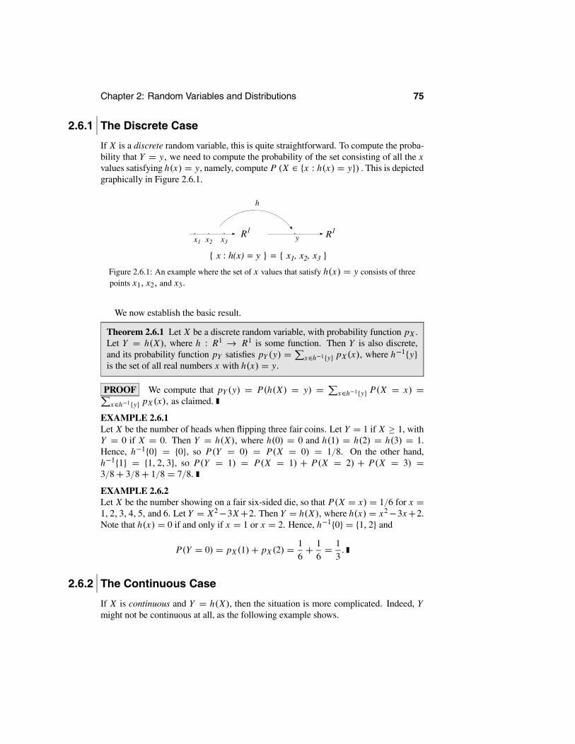
Chapter 2: Random Variables and Distributions 75
2.6.1 The Discrete Case
If X is a discrete random variable, this is quite straightforward. To compute the proba-bility that Y = y, we need to compute the probability of the set consisting of all the xvalues satisfying h(x) = y, namely, compute P (X ∈ {x : h(x) = y}) . This is depictedgraphically in Figure 2.6.1.
1
R1.R1. . .yx1 x2 x3
h
{ x : h(x) = y } = { x1, x2, x3 }
Figure 2.6.1: An example where the set of x values that satisfy h(x) = y consists of threepoints x1, x2, and x3.
We now establish the basic result.
Theorem 2.6.1 Let X be a discrete random variable, with probability function pX .Let Y = h(X), where h : R1 → R1 is some function. Then Y is also discrete,and its probability function pY satisfies pY (y) = x∈h−1{y} pX (x), where h−1{y}is the set of all real numbers x with h(x) = y.
PROOF We compute that pY (y) = P(h(X) = y) = x∈h−1{y} P(X = x) =x∈h−1{y} pX (x), as claimed.
EXAMPLE 2.6.1Let X be the number of heads when flipping three fair coins. Let Y = 1 if X ≥ 1, withY = 0 if X = 0. Then Y = h(X), where h(0) = 0 and h(1) = h(2) = h(3) = 1.Hence, h−1{0} = {0}, so P(Y = 0) = P(X = 0) = 1/8. On the other hand,h−1{1} = {1, 2, 3}, so P(Y = 1) = P(X = 1) + P(X = 2) + P(X = 3) =3/8+ 3/8+ 1/8 = 7/8.
EXAMPLE 2.6.2Let X be the number showing on a fair six-sided die, so that P(X = x) = 1/6 for x =1, 2, 3, 4, 5, and 6. Let Y = X2−3X+2. Then Y = h(X), where h(x) = x2−3x+2.Note that h(x) = 0 if and only if x = 1 or x = 2. Hence, h−1{0} = {1, 2} and
P(Y = 0) = pX (1)+ pX (2) = 16+ 1
6= 1
3.
2.6.2 The Continuous Case
If X is continuous and Y = h(X), then the situation is more complicated. Indeed, Ymight not be continuous at all, as the following example shows.
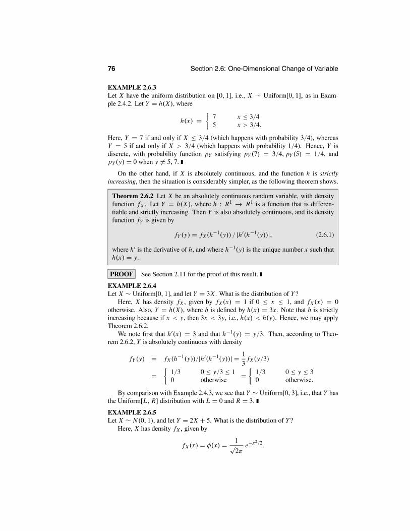
76 Section 2.6: One-Dimensional Change of Variable
EXAMPLE 2.6.3Let X have the uniform distribution on [0, 1], i.e., X ∼ Uniform[0, 1], as in Exam-ple 2.4.2. Let Y = h(X), where
h(x) = 7 x ≤ 3/45 x > 3/4.
Here, Y = 7 if and only if X ≤ 3/4 (which happens with probability 3/4), whereasY = 5 if and only if X > 3/4 (which happens with probability 1/4). Hence, Y isdiscrete, with probability function pY satisfying pY (7) = 3/4, pY (5) = 1/4, andpY (y) = 0 when y = 5, 7.
On the other hand, if X is absolutely continuous, and the function h is strictlyincreasing, then the situation is considerably simpler, as the following theorem shows.
Theorem 2.6.2 Let X be an absolutely continuous random variable, with densityfunction fX . Let Y = h(X), where h : R1 → R1 is a function that is differen-tiable and strictly increasing. Then Y is also absolutely continuous, and its densityfunction fY is given by
fY (y) = fX (h−1(y)) / |h (h−1(y))|, (2.6.1)
where h is the derivative of h, and where h−1(y) is the unique number x such thath(x) = y.
PROOF See Section 2.11 for the proof of this result.
EXAMPLE 2.6.4Let X ∼ Uniform[0, 1], and let Y = 3X . What is the distribution of Y ?
Here, X has density fX , given by fX (x) = 1 if 0 ≤ x ≤ 1, and fX (x) = 0otherwise. Also, Y = h(X), where h is defined by h(x) = 3x . Note that h is strictlyincreasing because if x < y, then 3x < 3y, i.e., h(x) < h(y). Hence, we may applyTheorem 2.6.2.
We note first that h (x) = 3 and that h−1(y) = y/3. Then, according to Theo-rem 2.6.2, Y is absolutely continuous with density
fY (y) = fX (h−1(y))/|h (h−1(y))| = 13
fX (y/3)
= 1/3 0 ≤ y/3 ≤ 10 otherwise
= 1/3 0 ≤ y ≤ 30 otherwise.
By comparison with Example 2.4.3, we see that Y ∼ Uniform[0, 3], i.e., that Y hasthe Uniform[L, R] distribution with L = 0 and R = 3.
EXAMPLE 2.6.5Let X ∼ N(0, 1), and let Y = 2X + 5. What is the distribution of Y ?
Here, X has density fX , given by
fX (x) = φ(x) = 1√2π
e−x2/2.

Chapter 2: Random Variables and Distributions 77
Also, Y = h(X), where h is defined by h(x) = 2x + 5. Note that again, h is strictlyincreasing because if x < y, then 2x + 5 < 2y + 5, i.e., h(x) < h(y). Hence, we mayagain apply Theorem 2.6.2.
We note first that h (x) = 2 and that h−1(y) = (y − 5)/2. Then, according toTheorem 2.6.2, Y is absolutely continuous with density
fY (y) = fX (h−1(y))/|h (h−1(y))| = fX ((y − 5)/2)/2 = 1
2√
2πe−(y−5)2/8.
By comparison with Example 2.4.8, we see that Y ∼ N(5, 4), i.e., that Y has theN(µ, σ 2) distribution with µ = 5 and σ 2 = 4.
If instead the function h is strictly decreasing, then a similar result holds.
Theorem 2.6.3 Let X be an absolutely continuous random variable, with densityfunction fX . Let Y = h(X), where h : R1 → R1 is a function that is differen-tiable and strictly decreasing. Then Y is also absolutely continuous, and its densityfunction fY may again be defined by (2.6.1).
PROOF See Section 2.11 for the proof of this result.
EXAMPLE 2.6.6Let X ∼ Uniform[0, 1], and let Y = ln(1/X). What is the distribution of Y ?
Here, X has density fX , given by fX (x) = 1 for 0 ≤ x ≤ 1, and fX (x) = 0otherwise. Also, Y = h(X), where h is defined by h(x) = ln(1/x). Note that here,h is strictly decreasing because if x < y, then 1/x > 1/y, so ln(1/x) > ln(1/y), i.e.,h(x) > h(y). Hence, we may apply Theorem 2.6.3.
We note first that h (x) = −1/x and that h−1(y) = e−y . Then, by Theorem 2.6.3,Y is absolutely continuous with density
fY (y) = fX (h−1(y))/|h (h−1(y))| = e−y fX (e
−y)
= e−y 0 ≤ e−y ≤ 10 otherwise
= e−y y ≥ 00 otherwise.
By comparison with Example 2.4.4, we see that Y ∼ Exponential(1), i.e., that Y hasthe Exponential(1) distribution.
Finally, we note the following.
Theorem 2.6.4 Theorem 2.6.2 (and 2.6.3) remains true assuming only that h isstrictly increasing (or decreasing) at places for which fX (x) > 0. If fX (x) = 0 foran interval of x values, then it does not matter how the function h behaves in thatinterval (or even if it is well-defined there).
EXAMPLE 2.6.7If X ∼ Exponential(λ), then fX (x) = 0 for x < 0. Therefore, it is required that h bestrictly increasing (or decreasing) only for x ≥ 0. Thus, functions such as h(x) = x2,h(x) = x8, and h(x) = √x could still be used with Theorem 2.6.2, while functionssuch as h(x) = −x2, h(x) = −x8, and h(x) = −√x could still be used with The-orem 2.6.3, even though such functions may not necessarily be strictly increasing (ordecreasing) and well-defined on the entire real line.

78 Section 2.6: One-Dimensional Change of Variable
Summary of Section 2.6
• If X is discrete, and Y = h(X), then P(Y = y) = x : h(x)=y P(X = x).
• If X is absolutely continuous, and Y = h(X) with h strictly increasing or strictlydecreasing, then the density of Y is given by fY (y) = fX (h−1(y)) / |h (h−1(y))|.
• This allows us to compute the distribution of a function of a random variable.
EXERCISES
2.6.1 Let X ∼ Uniform[L, R]. Let Y = cX + d, where c > 0. Prove that Y ∼Uniform[cL + d, cR + d]. (This generalizes Example 2.6.4.)2.6.2 Let X ∼ Uniform[L, R]. Let Y = cX + d, where c < 0. Prove that Y ∼Uniform[cR + d, cL + d]. (In particular, if L = 0 and R = 1 and c = −1 and d = 1,then X ∼ Uniform[0, 1] and also Y = 1− X ∼ Uniform[0, 1].)2.6.3 Let X ∼ N(µ, σ 2). Let Y = cX + d, where c > 0. Prove that Y ∼ N(cµ +d, c2σ 2). (This generalizes Example 2.6.5.)2.6.4 Let X ∼ Exponential(λ). Let Y = cX , where c > 0. Prove that Y ∼Exponential(λ/c).2.6.5 Let X ∼ Exponential(λ). Let Y = X3. Compute the density fY of Y .2.6.6 Let X ∼ Exponential(λ). Let Y = X1/4. Compute the density fY of Y . (Hint:Use Theorem 2.6.4.)2.6.7 Let X ∼ Uniform[0, 3]. Let Y = X2. Compute the density function fY of Y .2.6.8 Let X have a density such that fX (µ+ x) = fX (µ− x) , i.e., it is symmetricabout µ. Let Y = 2µ − X . Show that the density of Y is given by fX . Use this todetermine the distribution of Y when X ∼ N(µ, σ 2).
2.6.9 Let X have density function fX (x) = x3/4 for 0 < x < 2, otherwise fX (x) = 0.(a) Let Y = X2. Compute the density function fY (y) for Y .(b) Let Z = √X . Compute the density function fZ (z) for Z .2.6.10 Let X ∼ Uniform[0, π/2]. Let Y = sin(X). Compute the density functionfY (y) for Y .2.6.11 Let X have density function fX (x) = (1/2) sin(x) for 0 < x < π , otherwisefX (x) = 0. Let Y = X2. Compute the density function fY (y) for Y .2.6.12 Let X have density function fX (x) = 1/x2 for x > 1, otherwise fX (x) = 0.Let Y = X1/3. Compute the density function fY (y) for Y .2.6.13 Let X ∼ Normal(0, 1). Let Y = X3. Compute the density function fY (y) forY .
PROBLEMS
2.6.14 Let X ∼ Uniform[2, 7], Y = X3, and Z = √Y . Compute the density fZ of Z ,in two ways.(a) Apply Theorem 2.6.2 to first obtain the density of Y , then apply Theorem 2.6.2again to obtain the density of Z .(b) Observe that Z = √Y = √X3 = X3/2, and apply Theorem 2.6.2 just once.

Chapter 2: Random Variables and Distributions 79
2.6.15 Let X ∼ Uniform[L, R], and let Y = h(X) where h(x) = (x − c)6. Accordingto Theorem 2.6.4, under what conditions on L, R, and c can we apply Theorem 2.6.2or Theorem 2.6.3 to this choice of X and Y ?2.6.16 Let X ∼ N(µ, σ 2). Let Y = cX + d, where c < 0. Prove that again Y ∼N(cµ+ d, c2σ 2), just like in Exercise 2.6.3.2.6.17 (Log-normal(τ) distribution) Suppose that X ∼ N(0, τ 2). Prove that Y = eX
has density
fτ (y) = 1√2πτ
exp − (ln y)2
2τ 2
1y
for y > 0 and where τ > 0 is unknown. We say that Y ∼ Log-normal(τ) .2.6.18 Suppose that X ∼Weibull(α) (see Problem 2.4.19). Determine the distributionof Y = Xβ.
2.6.19 Suppose that X ∼ Pareto(α) (see Problem 2.4.20). Determine the distributionof Y = (1+ X)β − 1.2.6.20 Suppose that X has the extreme value distribution (see Problem 2.4.23). Deter-mine the distribution of Y = e−X .
CHALLENGES
2.6.21 Theorems 2.6.2 and 2.6.3 require that h be an increasing or decreasing function,at least at places where the density of X is positive (see Theorem 2.6.4). Suppose nowthat X ∼ N(0, 1) and Y = h(X), where h(x) = x2. Then fX (x) > 0 for all x , whileh is increasing only for x > 0 and decreasing only for x < 0. Hence, Theorems 2.6.2and 2.6.3 do not directly apply. Compute fY (y) anyway. (Hint: P(a ≤ Y ≤ b) =P(a ≤ Y ≤ b, X > 0)+ P(a ≤ Y ≤ b, X < 0).)
2.7 Joint DistributionsSuppose X and Y are two random variables. Even if we know the distributions of Xand Y exactly, this still does not tell us anything about the relationship between X andY .
EXAMPLE 2.7.1Let X ∼ Bernoulli(1/2), so that P(X = 0) = P(X = 1) = 1/2. Let Y1 = X , and letY2 = 1 − X . Then we clearly have Y1 ∼ Bernoulli(1/2) and Y2 ∼ Bernoulli(1/2) aswell.
On the other hand, the relationship between X and Y1 is very different from the re-lationship between X and Y2. For example, if we know that X = 1, then we also musthave Y1 = 1, but Y2 = 0. Hence, merely knowing that X , Y1, and Y2 all have the dis-tribution Bernoulli(1/2) does not give us complete information about the relationshipsamong these random variables.
A formal definition of joint distribution is as follows.

80 Section 2.7: Joint Distributions
Definition 2.7.1 If X and Y are random variables, then the joint distribution of Xand Y is the collection of probabilities P((X,Y ) ∈ B), for all subsets B ⊆ R2 ofpairs of real numbers.
Joint distributions, like other distributions, are so complicated that we use vari-ous functions to describe them, including joint cumulative distribution functions, jointprobability functions, and joint density functions, as we now discuss.
2.7.1 Joint Cumulative Distribution Functions
Definition 2.7.2 Let X and Y be random variables. Then their joint cumulativedistribution function is the function FX,Y : R2 → [0, 1] defined by
FX,Y (x, y) = P(X ≤ x, Y ≤ y).
(Recall that the comma means “and” here, so that FX,Y (x, y) is the probability thatX ≤ x and Y ≤ y.)
EXAMPLE 2.7.2 (Example 2.7.1 continued)Again, let X ∼ Bernoulli(1/2), Y1 = X , and Y2 = 1− X . Then we compute that
FX,Y1(x, y) = P(X ≤ x,Y1 ≤ y) = 0 min(x, y) < 0
1/2 0 ≤ min(x, y) < 11 min(x, y) ≥ 1.
On the other hand,
FX,Y2(x, y) = P(X ≤ x, Y2 ≤ y) = 0 min(x, y) < 0 or max(x, y) < 1
1/2 0 ≤ min(x, y) < 1 ≤ max(x, y)1 min(x, y) ≥ 1.
We thus see that FX,Y1 is quite a different function from FX,Y2 . This reflects thefact that, even though Y1 and Y2 each have the same distribution, their relationshipwith X is quite different. On the other hand, the functions FX,Y1 and FX,Y2 are rathercumbersome and awkward to work with.
We see from this example that joint cumulative distribution functions (or joint cdfs)do indeed keep track of the relationship between X and Y . Indeed, joint cdfs tell useverything about the joint probabilities of X and Y , as the following theorem (an analogof Theorem 2.5.1) shows.
Theorem 2.7.1 Let X and Y be any random variables, with joint cumulative dis-tribution function FX,Y . Let B be a subset of R2. Then P((X, Y ) ∈ B) can bedetermined solely from the values of FX,Y (x, y).
We shall not give a proof of Theorem 2.7.1, although it is similar to the proof ofTheorem 2.5.1. However, the following theorem indicates why Theorem 2.7.1 is true,and it also provides a useful computational fact.

Chapter 2: Random Variables and Distributions 81
Theorem 2.7.2 Let X and Y be any random variables, with joint cumulative distri-bution function FX,Y . Suppose a ≤ b and c ≤ d. Then
P(a < X ≤ b , c < Y ≤ d) = FX,Y (b, d)−FX,Y (a, d)−FX,Y (b, c)+FX,Y (a, c).
PROOF According to (1.3.3),
P(a < X ≤ b, c < Y ≤ d)
= P(X ≤ b, Y ≤ d)− P(X ≤ b, Y ≤ d , and either X ≤ a or Y ≤ c).
But by the principle of inclusion–exclusion (1.3.4),
P(X ≤ b, Y ≤ d, and either X ≤ a or Y ≤ c)
= P(X ≤ b, Y ≤ c)+ P(X ≤ a, Y ≤ d)− P(X ≤ a, Y ≤ c).
Combining these two equations, we see that
P(a < X ≤ b, c < Y ≤ d)
= P(X ≤ b, Y ≤ d)− P(X ≤ a,Y ≤ d)− P(X ≤ b, Y ≤ c)+ P(X ≤ a,Y ≤ c)
and from this we obtain
P(a < X ≤ b, c < Y ≤ d) = FX,Y (b, d)− FX,Y (a, d)− FX,Y (b, c)+ FX,Y (a, c),
as claimed.
Joint cdfs are not easy to work with. Thus, in this section we shall also considerother functions, which are more convenient for pairs of discrete or absolutely continu-ous random variables.
2.7.2 Marginal Distributions
We have seen how a joint cumulative distribution function FX,Y tells us about the rela-tionship between X and Y . However, the function FX,Y also tells us everything abouteach of X and Y separately, as the following theorem shows.
Theorem 2.7.3 Let X and Y be two random variables, with joint cumulative distri-bution function FX,Y . Then the cumulative distribution function FX of X satisfies
FX (x) = limy→∞ FX,Y (x, y),
for all x ∈ R1. Similarly, the cumulative distribution function FY of Y satisfies
FY (y) = limx→∞ FX,Y (x, y),
for all y ∈ R1.

82 Section 2.7: Joint Distributions
PROOF Note that we always have Y ≤ ∞. Hence, using continuity of P, we have
FX (x) = P(X ≤ x) = P(X ≤ x, Y ≤∞)= lim
y→∞ P(X ≤ x, Y ≤ y) = limy→∞ FX,Y (x, y),
as claimed. Similarly,
FY (y) = P(Y ≤ y) = P(X ≤ ∞, Y ≤ y)
= limx→∞ P(X ≤ x, Y ≤ y) = lim
x→∞ FX,Y (x, y),
completing the proof.
In the context of Theorem 2.7.3, FX is called the marginal cumulative distribu-tion function of X , and the distribution of X is called the marginal distribution of X .(Similarly, FY is called the marginal cumulative distribution function of Y , and thedistribution of Y is called the marginal distribution of Y .) Intuitively, if we think ofFX,Y as being a function of a pair (x, y), then FX and FY are functions of x and y,respectively, which could be written into the “margins” of a graph of FX,Y .
EXAMPLE 2.7.3In Figure 2.7.1, we have plotted the joint distribution function
FX,Y (x, y) =
0 x < 0 or y < 0xy2 0 ≤ x ≤ 1, 0 ≤ y ≤ 1x 0 ≤ x ≤ 1, y ≥ 1y2 x ≥ 1, 0 ≤ y ≤ 11 x > 1 and y > 1.
It is easy to see that FX (x) = FX,Y (x, 1) = x for 0 ≤ x ≤ 1 and that FY (y) =FX,Y (1, y) = y2 for 0 ≤ y ≤ 1. The graphs of these functions are given by the outer-most edges of the surface depicted in Figure 2.7.1.
Chapter 2: Random Variables and Distributions 83
0.00.0 0.0
y0.5
F 0.5
1.0
0.5
x
1.0
1.0
Figure 2.7.1: Graph of the joint distribution function FX,Y (x, y) = xy2 for 0 ≤ x ≤ 1 and0 ≤ y ≤ 1 in Example 2.7.3.
Theorem 2.7.3 thus tells us that the joint cdf FX,Y is very useful indeed. Not onlydoes it tell us about the relationship of X to Y , but it also contains all the informationabout the marginal distributions of X and of Y .
We will see in the next subsections that joint probability functions, and joint densityfunctions, similarly contain information about both the relationship of X and Y and themarginal distributions of X and Y .
2.7.3 Joint Probability Functions
Suppose X and Y are both discrete random variables. Then we can define a jointprobability function for X and Y , as follows.
Definition 2.7.3 Let X and Y be discrete random variables. Then their joint prob-ability function, pX,Y , is a function from R2 to R1, defined by
pX,Y (x, y) = P(X = x , Y = y).
Consider the following example.

84 Section 2.7: Joint Distributions
EXAMPLE 2.7.4 (Examples 2.7.1 and 2.7.2 continued)Again, let X ∼ Bernoulli(1/2), Y1 = X , and Y2 = 1− X . Then we see that
pX,Y1(x, y) = P(X = x , Y1 = y) = 1/2 x = y = 1
1/2 x = y = 00 otherwise.
On the other hand,
pX,Y2(x, y) = P(X = x , Y2 = y) = 1/2 x = 1, y = 0
1/2 x = 0, y = 10 otherwise.
We thus see that pX,Y1 and pX,Y2 are two simple functions that are easy to workwith and that clearly describe the relationships between X and Y1 and between X andY2. Hence, for pairs of discrete random variables, joint probability functions are usuallythe best way to describe their relationships.
Once we know the joint probability function pX,Y , the marginal probability func-tions of X and Y are easily obtained.
Theorem 2.7.4 Let X and Y be two discrete random variables, with joint probabil-ity function pX,Y . Then the probability function pX of X can be computed as
pX (x) =y
pX,Y (x, y).
Similarly, the probability function pY of Y can be computed as
pY (y) =x
pX,Y (x, y).
PROOF Using additivity of P , we have that
pX (x) = P(X = x) =y
P(X = x , Y = y) =y
pX,Y (x, y),
as claimed. Similarly,
pY (y) = P(Y = y) =x
P(X = x, Y = y) =x
pX,Y (x, y).
EXAMPLE 2.7.5Suppose the joint probability function of X and Y is given by
pX,Y (x, y) =
1/7 x = 5, y = 01/7 x = 5, y = 31/7 x = 5, y = 43/7 x = 8, y = 01/7 x = 8, y = 40 otherwise.

Chapter 2: Random Variables and Distributions 85
Then
pX (5) =y
pX,Y (5, y) = pX,Y (5, 0)+ pX,Y (5, 3)+ pX,Y (5, 4)
= 17+ 1
7+ 1
7= 3
7,
while
pX (8) =y
pX,Y (8, y) = pX,Y (8, 0)+ pX,Y (8, 4) = 37+ 1
7= 4
7.
Similarly,
pY (4) =x
pX,Y (x, 4) = pX,Y (5, 4)+ pX,Y (8, 4) = 17+ 1
7= 2
7,
etc.Note that in such a simple context it is possible to tabulate the joint probability
function in a table, as illustrated below for pX,Y , pX , and pY of this example.
Y = 0 Y = 3 Y = 4X = 5 1/7 1/7 1/7 3/7X = 8 3/7 0 1/7 4/7
4/7 1/7 2/7
Summing the rows and columns and placing the totals in the margins gives the marginaldistributions of X and Y .
2.7.4 Joint Density Functions
If X and Y are continuous random variables, then clearly pX,Y (x, y) = 0 for all x andy. Hence, joint probability functions are not useful in this case. On the other hand, weshall see here that if X and Y are jointly absolutely continuous, then their relationshipmay be usefully described by a joint density function.
Definition 2.7.4 Let f : R2 → R1 be a function. Then f is a joint density functionif f (x, y) ≥ 0 for all x and y, and ∞
−∞∞−∞ f (x, y) dx dy = 1.
Definition 2.7.5 Let X and Y be random variables. Then X and Y are jointly ab-solutely continuous if there is a joint density function f , such that
P(a ≤ X ≤ b , c ≤ Y ≤ d) =d
c
b
af (x, y) dx dy,
for all a ≤ b , c ≤ d .

86 Section 2.7: Joint Distributions
Consider the following example.
EXAMPLE 2.7.6Let X and Y be jointly absolutely continuous, with joint density function f given by
f (x, y) = 4x2y + 2y5 0 ≤ x ≤ 1 , 0 ≤ y ≤ 10 otherwise.
We first verify that f is indeed a density function. Clearly, f (x, y) ≥ 0 for all xand y. Also,
∞
−∞
∞
−∞f (x, y) dx dy =
1
0
1
0(4x2y + 2y5) dx dy =
1
0
43
y + 2y5 dy
= 43
12+ 2
16= 2
3+ 1
3= 1.
Hence, f is a joint density function. In Figure 2.7.2, we have plotted the function f,which gives a surface over the unit square.
1.0
0.51.0
0.5
y
0.0
x
0.00
2
f4
6
Figure 2.7.2: A plot of the density f in Example 2.7.6.

Chapter 2: Random Variables and Distributions 87
We next compute P(0.5 ≤ X ≤ 0.7 , 0.2 ≤ Y ≤ 0.9). Indeed, we have
P(0.5 ≤ X ≤ 0.7 , 0.2 ≤ Y ≤ 0.9)
=0.9
0.2
0.7
0.5(4x2y + 2y5) dx dy
=0.9
0.2
43((0.7)3 − (0.5)3 y + 2y5(0.7− 0.5) dy
= 43(0.7)3 − (0.5)3 1
2((0.9)2 − (0.2)2)+ 2
6((0.9)6 − (0.2)6)(0.7− 0.5)
= 23((0.7)3 − (0.5)3)((0.9)2 − (0.2)2)+ 1
3((0.9)6 − (0.2)6)(0.7− 0.5)
.= 0.147.
Other probabilities can be computed similarly.
Once we know a joint density fX,Y , then computing the marginal densities of Xand Y is very easy, as the following theorem shows.
Theorem 2.7.5 Let X and Y be jointly absolutely continuous random variables,with joint density function fX,Y . Then the (marginal) density fX of X satisfies
fX (x) =∞
−∞fX,Y (x, y) dy,
for all x ∈ R1. Similarly, the (marginal) density fY of Y satisfies
fY (y) =∞
−∞fX,Y (x, y) dx,
for all y ∈ R1 .
PROOF We need to show that, for a ≤ b, P(a ≤ X ≤ b) = ba fX (x) dx =
ba
∞−∞ fX,Y (x, y) dy dx. Now, we always have −∞ < Y < ∞. Hence, using con-
tinuity of P , we have that P(a ≤ X ≤ b) = P(a ≤ X ≤ b ,−∞ < Y < ∞)and
P(a ≤ X ≤ b ,−∞ < Y <∞)= lim
c→−∞d→∞
P(a ≤ X ≤ b, c ≤ Y ≤ d) = limc→−∞d→∞
d
c
b
af (x, y) dx dy
= limc→−∞d→∞
b
a
d
cf (x, y) dy dx =
b
a
∞
−∞fX,Y (x, y) dy dx,
as claimed. The result for fY follows similarly.
EXAMPLE 2.7.7 (Example 2.7.6 continued)Let X and Y again have joint density
fX,Y (x, y) = 4x2y + 2y5 0 ≤ x ≤ 1 , 0 ≤ y ≤ 10 otherwise.

88 Section 2.7: Joint Distributions
Then by Theorem 2.7.5, for 0 ≤ x ≤ 1,
fX (x) =∞
−∞fX,Y (x, y) dy =
1
0(4x2y + 2y5) dy = 2x2 + (1/3),
while for x < 0 or x > 1,
fX (x) =∞
−∞fX,Y (x, y) dy =
∞
−∞0 dy = 0.
Similarly, for 0 ≤ y ≤ 1,
fY (y) =∞
−∞fX,Y (x, y) dx =
1
0(4x2y + 2y5) dx = 4
3y + 2y5,
while for y < 0 or y > 1, fY (y) = 0.
EXAMPLE 2.7.8Suppose X and Y are jointly absolutely continuous, with joint density
fX,Y (x, y) = 120x3y x ≥ 0, y ≥ 0, x + y ≤ 10 otherwise.
Then the region where fX,Y (x, y) > 0 is a triangle, as depicted in Figure 2.7.3.
1
x
y
1
1
Figure 2.7.3: Region of the plane where the density fX,Y in Example 2.7.8 is positive.
We check that∞
−∞
∞
−∞fX,Y (x, y) dx dy =
1
0
1−x
0120x3y dy dx =
1
0120x3 (1− x)2
2dx
=1
060(x3 − 2x4 + x5) dx = 60(
14− 2
15+ 1
6)
= 15− 2(12)+ 10 = 1,
so that fX,Y is indeed a joint density function. We then compute that, for example,
fX (x) =1−x
0120x3y dy = 120x3 (1− x)2
2= 60(x3 − 2x4 + x5)
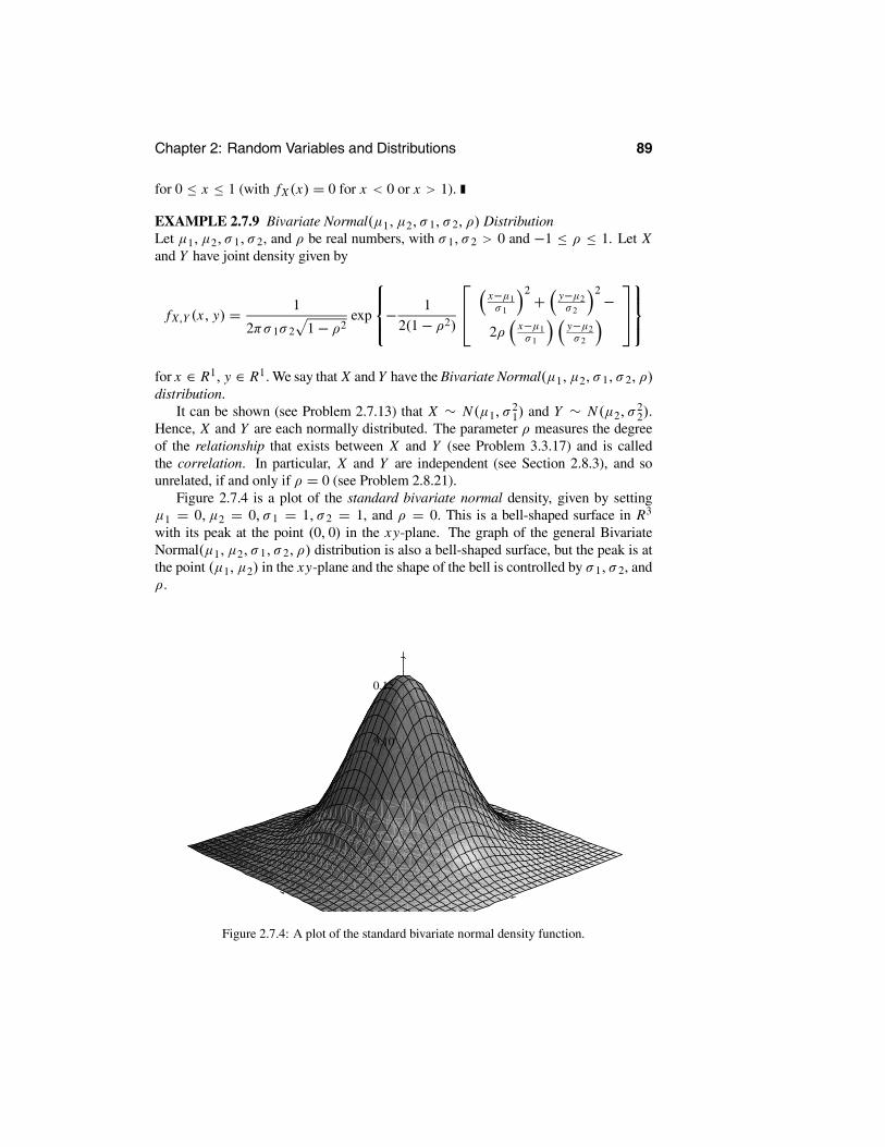
Chapter 2: Random Variables and Distributions 89
for 0 ≤ x ≤ 1 (with fX (x) = 0 for x < 0 or x > 1).
EXAMPLE 2.7.9 Bivariate Normal(µ1, µ2, σ 1, σ 2, ρ) DistributionLet µ1, µ2, σ 1, σ 2, and ρ be real numbers, with σ 1, σ 2 > 0 and −1 ≤ ρ ≤ 1. Let Xand Y have joint density given by
fX,Y (x, y) = 1
2πσ 1σ 2 1− ρ2exp
− 1
2(1− ρ2)
x−µ1σ 1
2 + y−µ2σ 2
2−2ρ x−µ1
σ 1
y−µ2σ 2
for x ∈ R1, y ∈ R1.We say that X and Y have the Bivariate Normal(µ1, µ2, σ 1, σ 2, ρ)distribution.
It can be shown (see Problem 2.7.13) that X ∼ N(µ1, σ21) and Y ∼ N(µ2, σ
22).
Hence, X and Y are each normally distributed. The parameter ρ measures the degreeof the relationship that exists between X and Y (see Problem 3.3.17) and is calledthe correlation. In particular, X and Y are independent (see Section 2.8.3), and sounrelated, if and only if ρ = 0 (see Problem 2.8.21).
Figure 2.7.4 is a plot of the standard bivariate normal density, given by settingµ1 = 0, µ2 = 0, σ 1 = 1, σ 2 = 1, and ρ = 0. This is a bell-shaped surface in R3
with its peak at the point (0, 0) in the xy-plane. The graph of the general BivariateNormal(µ1, µ2, σ 1, σ 2, ρ) distribution is also a bell-shaped surface, but the peak is atthe point (µ1, µ2) in the xy-plane and the shape of the bell is controlled by σ 1, σ 2, andρ.
-2yx
0 0
2
0.00
2 -2
0.05
f
0.15
0.10
Figure 2.7.4: A plot of the standard bivariate normal density function.

90 Section 2.7: Joint Distributions
It can be shown (see Problem 2.9.16) that, when Z1, Z2 are independent randomvariables, both distributed N(0, 1), and we put
X = µ1 + σ 1Z1, Y = µ2 + σ 2 ρZ1 + 1− ρ21/2
Z2 , (2.7.1)
then (X, Y ) ∼ Bivariate Normal(µ1, µ2, σ 1, σ 2, ρ) . This relationship can be quiteuseful in establishing various properties of this distribution. We can also write an
analogous version Y = µ2 + σ 2 Z1, X = µ1 + σ 1(ρZ1 + 1− ρ2 1/2Z2) and obtain
the same distributional result.The bivariate normal distribution is one of the most commonly used bivariate dis-
tributions in applications. For example, if we randomly select an individual from apopulation and measure his weight X and height Y, then a bivariate normal distributionwill often provide a reasonable description of the joint distribution of these variables.
Joint densities can also be used to compute probabilities of more general regions,as the following result shows. (We omit the proof. The special case B = [a, b]× [c, d]corresponds directly to the definition of fX,Y .)
Theorem 2.7.6 Let X and Y be jointly absolutely continuous random variables,with joint density fX,Y , and let B ⊆ R2 be any region. Then
P (X,Y ) ∈ B =B
f (x, y) dx dy.
The previous discussion has centered around having just two random variables,X and Y . More generally, we may consider n random variables X1, . . . , Xn. If therandom variables are all discrete, then we can further define a joint probability functionpX1,...,Xn : Rn → [0, 1] by pX1,...,Xn (x1, . . . , xn) = P(X1 = x1 , . . . , Xn = xn).If the random variables are jointly absolutely continuous, then we can define a jointdensity function fX1,...,Xn : Rn → [0, 1] so that
P(a1 ≤ X1 ≤ b1, . . . , an ≤ Xn ≤ bn)
=bn
an
· · ·b1
a1
fX1,...,Xn (x1, . . . , xn) dx1 · · · dxn,
whenever ai ≤ bi for all i .
Summary of Section 2.7
• It is often important to keep track of the joint probabilities of two random vari-ables, X and Y .
• Their joint cumulative distribution function is given by FX,Y (x, y) = P(X ≤x, Y ≤ y).
• If X and Y are discrete, then their joint probability function is given by pX,Y (x, y)= P(X = x, Y = y).

Chapter 2: Random Variables and Distributions 91
• If X and Y are absolutely continuous, then their joint density function fX,Y (x, y)is such that P(a ≤ X ≤ b, c ≤ Y ≤ d) = d
cb
a fX,Y (x, y) dx dy.
• The marginal density of X and Y can be computed from any of FX,Y , or pX,Y ,or fX,Y .
• An important example of a joint distribution is the bivariate normal distribution.
EXERCISES
2.7.1 Let X ∼ Bernoulli(1/3), and let Y = 4X − 2. Compute the joint cdf FX,Y .2.7.2 Let X ∼ Bernoulli(1/4), and let Y = −7X . Compute the joint cdf FX,Y .2.7.3 Suppose
pX,Y (x, y) =
1/5 x = 2, y = 31/5 x = 3, y = 21/5 x = −3, y = −21/5 x = −2, y = −31/5 x = 17, y = 190 otherwise.
(a) Compute pX .(b) Compute pY .(c) Compute P(Y > X).(d) Compute P(Y = X).(e) Compute P(XY < 0).2.7.4 For each of the following joint density functions fX,Y , find the value of C andcompute fX (x), fY (y), and P(X ≤ 0.8 ,Y ≤ 0.6).(a)
fX,Y (x, y) = 2x2y + Cy5 0 ≤ x ≤ 1 , 0 ≤ y ≤ 10 otherwise.
(b)
fX,Y (x, y) = C(xy + x5y5) 0 ≤ x ≤ 1 , 0 ≤ y ≤ 10 otherwise.
(c)
fX,Y (x, y) = C(xy + x5 y5) 0 ≤ x ≤ 4 , 0 ≤ y ≤ 100 otherwise.
(d)
fX,Y (x, y) = Cx5y5 0 ≤ x ≤ 4 , 0 ≤ y ≤ 100 otherwise.
2.7.5 Prove that FX,Y (x, y) ≤ min(FX (x), FY (y)).
2.7.6 Suppose P(X = x, Y = y) = 1/8 for x = 3, 5 and y = 1, 2, 4, 7, otherwiseP(X = x, Y = y) = 0. Compute each of the following.

92 Section 2.7: Joint Distributions
(a) FX,Y (x, y) for all x, y ∈ R1
(b) pX,Y (x, y) for all x, y ∈ R1
(c) pX (x) for all x ∈ R1
(d) pY (y) for all x ∈ R1
(e) The marginal cdf FX (x) for all x ∈ R1
(f) The marginal cdf FY (y) for all y ∈ R1
2.7.7 Let X and Y have joint density fX,Y (x, y) = c sin(xy) for 0 < x < 1 and0 < y < 2, otherwise fX,Y (x, y) = 0, for appropriate constant c > 0 (which cannotbe computed explicitly). In terms of c, compute each of the following.(a) The marginal density fX (x) for all x ∈ R1
(b) The marginal density fY (y) for all y ∈ R1
2.7.8 Let X and Y have joint density fX,Y (x, y) = (x2 + y)/36 for −2 < x < 1 and0 < y < 4, otherwise fX,Y (x, y) = 0. Compute each of the following.(a) The marginal density fX (x) for all x ∈ R1
(b) The marginal density fY (y) for all y ∈ R1
(c) P(Y < 1)(d) The joint cdf FX,Y (x, y) for all x, y ∈ R1
2.7.9 Let X and Y have joint density fX,Y (x, y) = (x2 + y)/4 for 0 < x < y < 2,otherwise fX,Y (x, y) = 0. Compute each of the following.(a) The marginal density fX (x) for all x ∈ R1
(b) The marginal density fY (y) for all y ∈ R1
(c) P(Y < 1)2.7.10 Let X and Y have the Bivariate-Normal(3, 5, 2, 4, 1/2) distribution.(a) Specify the marginal distribution of X .(b) Specify the marginal distribution of Y .(c) Are X and Y independent? Why or why not?
PROBLEMS
2.7.11 Let X ∼ Exponential(λ), and let Y = X3. Compute the joint cdf, FX,Y (x, y).2.7.12 Let FX,Y be a joint cdf. Prove that for all y ∈ R1, limx→−∞ FX,Y (x, y) = 0.2.7.13 Let X and Y have the Bivariate Normal(µ1, µ2, σ 1, σ 2, ρ) distribution, as inExample 2.7.9. Prove that X ∼ N(µ1, σ
21), by proving that
∞
−∞fX,Y (x, y) dy = 1
σ 1√
2πexp − (x − µ1)
2
2σ 21
.
2.7.14 Suppose that the joint density fX,Y is given by fX,Y (x, y) = Cye−xy for 0 <x < 1, 0 < y < 1 and is 0 otherwise.(a) Determine C so that fX,Y is a density.(b) Compute P (1/2 < X < 1, 1/2 < Y < 1) .(c) Compute the marginal densities of X and Y.
2.7.15 Suppose that the joint density fX,Y is given by fX,Y (x, y) = Cye−xy for 0 <x < y < 1 and is 0 otherwise.

Chapter 2: Random Variables and Distributions 93
(a) Determine C so that fX,Y is a density.(b) Compute P (1/2 < X < 1, 1/2 < Y < 1) .(c) Compute the marginal densities of X and Y.
2.7.16 Suppose that the joint density fX,Y is given by fX,Y (x, y) = Ce−(x+y) for0 < x < y <∞ and is 0 otherwise.(a) Determine C so that fX,Y is a density.(b) Compute the marginal densities of X and Y.
2.7.17 (Dirichlet(α1, α2, α3) distribution) Let (X1, X2) have the joint density
fX1,X2 (x1, x2) = (α1 + α2 + α3)
(α1) (α2) (α3)xα1−1
1 xα2−12 (1− x1 − x2)
α3−1
for x1 ≥ 0, x2 ≥ 0, and 0 ≤ x1 + x2 ≤ 1. A Dirichlet distribution is often applicablewhen X1, X2, and 1− X1 − X2 correspond to random proportions.(a) Prove that fX1,X2 is a density. (Hint: Sketch the region where fX1,X2 is nonnegative,integrate out x1 first by making the transformation u = x1/(1− x2) in this integral, anduse (2.4.10) from Problem 2.4.24.)(b) Prove that X1 ∼ Beta(α1, α2 + α3) and X2 ∼ Beta(α2, α1 + α3) .
2.7.18 (Dirichlet(α1, . . . , αk+1) distribution) Let (X1, . . . , Xk) have the joint density
fX1,...,Xk (x1, . . . , xk)
= (α1 + · · · + αk+1)
(α1) · · · (αk+1)xα1−1
1 · · · xαk−1k (1− x1 − · · · − xk)
αk+1−1
for xi ≥ 0, i = 1, . . . , k, and 0 ≤ x1 + · · · + xk ≤ 1. Prove that fX1,...,Xk is a density.(Hint: Problem 2.7.17.)
CHALLENGES
2.7.19 Find an example of two random variables X and Y and a function h : R1 → R1,such that FX (x) > 0 and FY (x) > 0 for all x ∈ R1, but limx→∞ FX,Y (x, h(x)) = 0.
DISCUSSION TOPICS
2.7.20 What are examples of pairs of real-life random quantities that have interestingrelationships? (List as many as you can, and describe each relationship as well as youcan.)
2.8 Conditioning and IndependenceLet X and Y be two random variables. Suppose we know that X = 5. What doesthat tell us about Y ? Depending on the relationship between X and Y , that may tellus everything about Y (e.g., if Y = X), or nothing about Y . Usually, the answerwill be between these two extremes, and the knowledge that X = 5 will change theprobabilities for Y somewhat.
94 Section 2.8: Conditioning and Independence
2.8.1 Conditioning on Discrete Random Variables
Suppose X is a discrete random variable, with P(X = 5) > 0. Let a < b, and supposewe are interested in the conditional probability P(a < Y ≤ b | X = 5). Well, wealready know how to compute such conditional probabilities. Indeed, by (1.5.1),
P(a < Y ≤ b | X = 5) = P(a < Y ≤ b , X = 5)P(X = 5)
,
provided that P(X = 5) > 0. This prompts the following definition.
Definition 2.8.1 Let X and Y be random variables, and suppose that P(X = x) >0. The conditional distribution of Y , given that X = x , is the probability distributionassigning probability
P(Y ∈ B , X = x)
P(X = x)
to each event Y ∈ B. In particular, it assigns probability
P(a < Y ≤ b , X = x)
P(X = x)
to the event that a < Y ≤ b.
EXAMPLE 2.8.1Suppose as in Example 2.7.5 that X and Y have joint probability function
pX,Y (x, y) =
1/7 x = 5, y = 01/7 x = 5, y = 31/7 x = 5, y = 43/7 x = 8, y = 01/7 x = 8, y = 40 otherwise.
We compute P(Y = 4 | X = 8) as
P(Y = 4 | X = 8) = P(Y = 4 , X = 8)P(X = 8)
= 1/7(3/7)+ (1/7) =
1/74/7
= 1/4.
On the other hand,
P(Y = 4 | X = 5) = P(Y = 4 , X = 5)P(X = 5)
= 1/7(1/7)+ (1/7)+ (1/7) =
1/73/7
= 1/3.
Thus, depending on the value of X , we obtain different probabilities for Y .
Generalizing from the above example, we see that if X and Y are discrete, then
P(Y = y | X = x) = P(Y = y , X = x)
P(X = x)= pX,Y (x, y)
pX (x)= pX,Y (x, y)
z pX,Y (x, z).
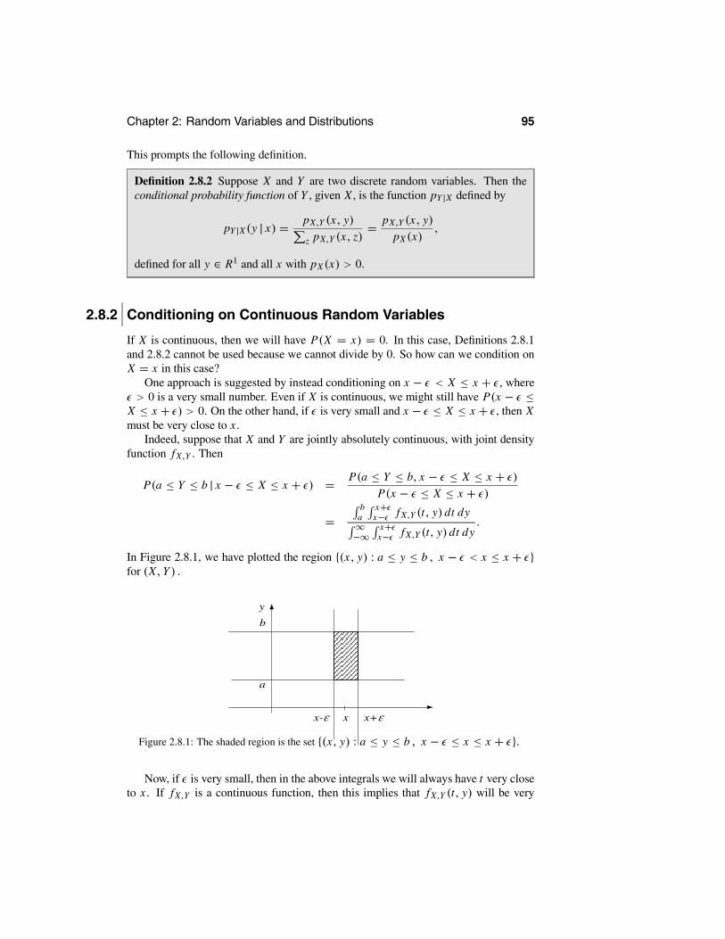
Chapter 2: Random Variables and Distributions 95
This prompts the following definition.
Definition 2.8.2 Suppose X and Y are two discrete random variables. Then theconditional probability function of Y , given X , is the function pY |X defined by
pY |X (y | x) = pX,Y (x, y)
z pX,Y (x, z)= pX,Y (x, y)
pX (x),
defined for all y ∈ R1 and all x with pX (x) > 0.
2.8.2 Conditioning on Continuous Random Variables
If X is continuous, then we will have P(X = x) = 0. In this case, Definitions 2.8.1and 2.8.2 cannot be used because we cannot divide by 0. So how can we condition onX = x in this case?
One approach is suggested by instead conditioning on x − < X ≤ x + , where> 0 is a very small number. Even if X is continuous, we might still have P(x − ≤
X ≤ x + ) > 0. On the other hand, if is very small and x − ≤ X ≤ x + , then Xmust be very close to x .
Indeed, suppose that X and Y are jointly absolutely continuous, with joint densityfunction fX,Y . Then
P(a ≤ Y ≤ b | x − ≤ X ≤ x + ) = P(a ≤ Y ≤ b, x − ≤ X ≤ x + )
P(x − ≤ X ≤ x + )
=b
ax+x− fX,Y (t, y) dt dy
∞−∞
x+x− fX,Y (t, y) dt dy
.
In Figure 2.8.1, we have plotted the region {(x, y) : a ≤ y ≤ b , x − < x ≤ x + }for (X,Y ) .
b
a
y
x x+εx-ε|
Figure 2.8.1: The shaded region is the set {(x, y) : a ≤ y ≤ b , x − ≤ x ≤ x + }.
Now, if is very small, then in the above integrals we will always have t very closeto x . If fX,Y is a continuous function, then this implies that fX,Y (t, y) will be very

96 Section 2.8: Conditioning and Independence
close to fX,Y (x, y). We conclude that, if is very small, then
P(a ≤ Y ≤ b | x − ≤ X ≤ x + ) ≈b
ax+
x− fX,Y (x, y) dt dy∞−∞
x+x− fX,Y (x, y) dt dy
=b
a 2 fX,Y (x, y) dy∞−∞ 2 fX,Y (x, y) dy
=b
a
fX,Y (x, y)∞−∞ fX,Y (x, z) dz
dy.
This suggests that the quantity
fX,Y (x, y)∞−∞ fX,Y (x, z) dz
= fX,Y (x, y)
fX (x)
plays the role of a density, for the conditional distribution of Y, given that X = x . Thisprompts the following definitions.
Definition 2.8.3 Let X and Y be jointly absolutely continuous, with joint den-sity function fX,Y . The conditional density of Y , given X = x , is the functionfY |X (y | x), defined by
fY |X (y | x) = fX,Y (x, y)
fX (x),
valid for all y ∈ R1, and for all x such that fX (x) > 0.
Definition 2.8.4 Let X and Y be jointly absolutely continuous, with joint densityfunction fX,Y . The conditional distribution of Y , given X = x , is defined by sayingthat
P(a ≤ Y ≤ b | X = x) =b
afY |X (y | x) dy,
when a ≤ b, with fY |X as in Definition 2.8.3, valid for all x such that fX (x) > 0.
EXAMPLE 2.8.2Let X and Y have joint density
fX,Y (x, y) = 4x2y + 2y5 0 ≤ x ≤ 1 , 0 ≤ y ≤ 10 otherwise,
as in Examples 2.7.6 and 2.7.7.We know from Example 2.7.7 that
fX (x) = 2x2 + (1/3) 0 ≤ x ≤ 10 otherwise,
while
fY (y) =43 y + 2y5 0 ≤ y ≤ 10 otherwise.

Chapter 2: Random Variables and Distributions 97
Let us now compute P(0.2 ≤ Y ≤ 0.3 | X = 0.8). Using Definitions 2.8.4and 2.8.3, we have
P(0.2 ≤ Y ≤ 0.3 | X = 0.8)
=0.3
0.2fY |X (y | 0.8) dy =
0.30.2 fX,Y (0.8, y) dy
fX (0.8)=
0.30.2 4 (0.8)2 y + 2y5 dy
2 (0.8)2 + 13
=42 (0.8)
2 ((0.3)2 − (0.2)2)+ 26 ((0.3)
6 − (0.2)6)2 (0.8)2 + 1
3
= 0.0398.
By contrast, if we compute the unconditioned (i.e., usual) probability that 0.2 ≤Y ≤ 0.3, we see that
P(0.2 ≤ Y ≤ 0.3) =0.3
0.2fY (y) dy =
0.3
0.2(43
y + 2y5) dy
= 43
12((0.3)2 − (0.2)2)+ 2
6((0.3)6 − (0.2)6) = 0.0336.
We thus see that conditioning on X = 0.8 increases the probability that 0.2 ≤ Y ≤ 0.3,from about 0.0336 to about 0.0398.
By analogy with Theorem 1.3.1, we have the following.
Theorem 2.8.1 (Law of total probability, absolutely continuous random variableversion) Let X and Y be jointly absolutely continuous random variables, and leta ≤ b and c ≤ d. Then
P(a ≤ X ≤ b, c ≤ Y ≤ d) =d
c
b
afX (x) fY |X (y | x) dx dy.
More generally, if B ⊆ R2 is any region, then
P (X,Y ) ∈ B =B
fX (x) fY |X (y | x) dx dy.
PROOF By Definition 2.8.3,
fX (x) fY |X (y | x) = fX,Y (x, y).
Hence, the result follows immediately from Definition 2.7.4 and Theorem 2.7.6.
2.8.3 Independence of Random Variables
Recall from Definition 1.5.2 that two events A and B are independent if P(A ∩ B) =P(A) P(B). We wish to have a corresponding definition of independence for randomvariables X and Y . Intuitively, independence of X and Y means that X and Y have no

98 Section 2.8: Conditioning and Independence
influence on each other, i.e., that the values of X make no change to the probabilitiesfor Y (and vice versa).
The idea of the formal definition is that X and Y give rise to events, of the form“a < X ≤ b” or “Y ∈ B,” and we want all such events involving X to be independentof all such events involving Y . Specifically, our definition is the following.
Definition 2.8.5 Let X and Y be two random variables. Then X and Y are inde-pendent if, for all subsets B1 and B2 of the real numbers,
P(X ∈ B1,Y ∈ B2) = P(X ∈ B1)P(Y ∈ B2).
That is, the events “X ∈ B1” and “Y ∈ B2” are independent events.
Intuitively, X and Y are independent if they have no influence on each other, as weshall see.
Now, Definition 2.8.5 is very difficult to work with. Fortunately, there is a muchsimpler characterization of independence.
Theorem 2.8.2 Let X and Y be two random variables. Then X and Y are indepen-dent if and only if
P(a ≤ X ≤ b, c ≤ Y ≤ d) = P(a ≤ X ≤ b)P(c ≤ Y ≤ d) (2.8.1)
whenever a ≤ b and c ≤ d.
That is, X and Y are independent if and only if the events “a ≤ X ≤ b” and “c ≤ Y ≤d” are independent events whenever a ≤ b and c ≤ d.
We shall not prove Theorem 2.8.2 here, although it is similar in spirit to the proof ofTheorem 2.5.1. However, we shall sometimes use (2.8.1) to check for the independenceof X and Y .
Still, even (2.8.1) is not so easy to check directly. For discrete and for absolutelycontinuous distributions, easier conditions are available, as follows.
Theorem 2.8.3 Let X and Y be two random variables.(a) If X and Y are discrete, then X and Y are independent if and only if their jointprobability function pX,Y satisfies
pX,Y (x, y) = pX (x) pY (y)
for all x, y ∈ R1.(b) If X and Y are jointly absolutely continuous, then X and Y are independent ifand only if their joint density function fX,Y can be chosen to satisfy
fX,Y (x, y) = fX (x) fY (y)
for all x, y ∈ R1.

Chapter 2: Random Variables and Distributions 99
PROOF (a) If X and Y are independent, then setting a = b = x and c = d = yin (2.8.1), we see that P(X = x, Y = y) = P(X = x)P(Y = y).Hence, pX,Y (x, y) =pX (x) pY (y).
Conversely, if pX,Y (x, y) = pX (x) pY (y) for all x and y, then
P(a ≤ X ≤ b, c ≤ Y ≤ d)
=a≤x≤b c≤y≤d
pX,Y (x, y) =a≤x≤b c≤y≤d
pX (x) pY (y)
=a≤x≤b
pX (x)c≤y≤d
pY (y) = P(a ≤ X ≤ b) P(c ≤ Y ≤ d).
This completes the proof of (a).
(b) If fX,Y (x, y) = fX (x) fY (y) for all x and y, then
P(a ≤ X ≤ b, c ≤ Y ≤ d)
=b
a
d
cfX,Y (x, y) dy dx =
b
a
d
cfX (x) fY (y) dy dx
=b
afX (x) dx
d
cfY (y) dy = P(a ≤ X ≤ b) P(c ≤ Y ≤ d).
This completes the proof of the “if” part of (b). The proof of the “only if” part of (b) ismore technical, and we do not include it here.
EXAMPLE 2.8.3Let X and Y have, as in Example 2.7.6, joint density
fX,Y (x, y) = 4x2y + 2y5 0 ≤ x ≤ 1 , 0 ≤ y ≤ 10 otherwise
and so, as derived in as in Example 2.7.7, marginal densities
fX (x) = 2x2 + (1/3) 0 ≤ x ≤ 10 otherwise
and
fY (y) =43 y + 2y5 0 ≤ y ≤ 10 otherwise.
Then we compute that
fX (x) fY (y) = (2x2 + (1/3)) ( 43 y + 2y5) 0 ≤ x ≤ 1, 0 ≤ y ≤ 1
0 otherwise.
We therefore see that fX (x) fY (y) = fX,Y (x, y). Hence, X and Y are not independent.

100 Section 2.8: Conditioning and Independence
EXAMPLE 2.8.4Let X and Y have joint density
fX,Y (x, y) =1
8080 (12xy2 + 6x + 4y2 + 2) 0 ≤ x ≤ 6, 3 ≤ y ≤ 50 otherwise.
We compute the marginal densities as
fX (x) =∞
−∞fX,Y (x, y) dy =
160 + 1
20 x 0 ≤ x ≤ 60 otherwise,
and
fY (y) =∞
−∞fX,Y (x, y) dx =
3202 + 3
101 y2 3 ≤ y ≤ 50 otherwise.
Then we compute that
fX (x) fY (y) = ( 160 + 1
20 x) ( 3202 + 3
101 y2) 0 ≤ x ≤ 6 , 3 ≤ y ≤ 50 otherwise.
Multiplying this out, we see that fX (x) fY (y) = fX,Y (x, y). Hence, X and Y areindependent in this case.
Combining Theorem 2.8.3 with Definitions 2.8.2 and 2.8.3, we immediately obtainthe following result about independence. It says that independence of random vari-ables is the same as saying that conditioning on one has no effect on the other, whichcorresponds to an intuitive notion of independence.
Theorem 2.8.4 Let X and Y be two random variables.(a) If X and Y are discrete, then X and Y are independent if and only if pY |X (y | x) =pY (y), for every x, y ∈ R1.(b) If X and Y are jointly absolutely continuous, then X and Y are independent ifand only if fY |X (y | x) = fY (y), for every x, y ∈ R1.
While Definition 2.8.5 is quite difficult to work with, it does provide the easiestway to prove one very important property of independence, as follows.
Theorem 2.8.5 Let X and Y be independent random variables. Let f, g : R1 → R1
be any two functions. Then the random variables f (X) and g(Y ) are also indepen-dent.
PROOF Using Definition 2.8.5, we compute that
P ( f (X) ∈ B1, g(Y ) ∈ B2) = P X ∈ f −1(B1), Y ∈ g−1(B2)
= P X ∈ f −1(B1) P Y ∈ g−1(B2)
= P ( f (X) ∈ B1) P (g(Y ) ∈ B2) .

Chapter 2: Random Variables and Distributions 101
(Here f −1(B1) = {x ∈ R1 : f (x) ∈ B1} and g−1(B2) = {y ∈ R1 : g(y) ∈ B2}.)Because this is true for any B1 and B2, we see that f (X) and g(Y ) are independent.
Suppose now that we have n random variables X1, . . . , Xn. The random variablesare independent if and only if the collection of events {ai ≤ Xi ≤ bi} are independent,whenever ai ≤ bi , for all i = 1, 2, . . . , n. Generalizing Theorem 2.8.3, we have thefollowing result.
Theorem 2.8.6 Let X1, . . . , Xn be a collection of random variables.(a) If X1, . . . , Xn are discrete, then X1, . . . , Xn are independent if and only if theirjoint probability function pX1,...,Xn satisfies
pX1,...,Xn (x1, . . . , xn) = pX1(x1) · · · pXn (xn)
for all x1, . . . , xn ∈ R1 .(b) If X1, . . . , Xn are jointly absolutely continuous, then X1, . . . , Xn are indepen-dent if and only if their joint density function fX1,...,Xn can be chosen to satisfy
fX1,...,Xn (x, y) = fX1(x1) · · · fXn (xn)
for all x1, . . . , xn ∈ R1.
A particularly common case in statistics is the following.
Definition 2.8.6 A collection X1, . . . , Xn of random variables is independent andidentically distributed (or i.i.d.) if the collection is independent and if, furthermore,each of the n variables has the same distribution. The i.i.d. sequence X1, . . . , Xn isalso referred to as a sample from the common distribution.
In particular, if a collection X1, . . . , Xn of random variables is i.i.d. and discrete, theneach of the probability functions pXi is the same, so that pX1(x) = pX2(x) = · · · =pXn (x) ≡ p(x), for all x ∈ R1. Furthermore, from Theorem 2.8.6(a), it follows that
pX1,...,Xn (x1, . . . , xn) = pX1(x1)pX2(x2) · · · pXn (xn) = p(x1)p(x2) · · · p(xn)
for all x1, . . . , xn ∈ R1.Similarly, if a collection X1, . . . , Xn of random variables is i.i.d. and jointly ab-
solutely continuous, then each of the density functions fXi is the same, so that fX1(x) =fX2(x) = · · · = fXn (x) ≡ f (x) , for all x ∈ R1. Furthermore, from Theorem 2.8.6(b),it follows that
fX1,...,Xn (x1, . . . , xn) = fX1(x1) fX2(x2) · · · fXn (xn) = f (x1) f (x2) · · · f (xn)
for all x1, . . . , xn ∈ R1.We now consider an important family of discrete distributions that arise via sam-
pling.
102 Section 2.8: Conditioning and Independence
EXAMPLE 2.8.5 Multinomial DistributionsSuppose we have a response s that can take three possible values — for convenience,labelled 1, 2, and 3 — with the probability distribution
P (s = 1) = θ1, P (s = 2) = θ2, P (s = 3) = θ3
so that each θ i ≥ 0 and θ1 + θ2 + θ3 = 1. As a simple example, consider a bowlof chips of which a proportion θ i of the chips are labelled i (for i = 1, 2, 3). Ifwe randomly draw a chip from the bowl and observe its label s, then P (s = i) = θ i .Alternatively, consider a population of students at a university of which a proportion θ1live on campus (denoted by s = 1), a proportion θ2 live off-campus with their parents(denoted by s = 2), and a proportion θ3 live off-campus independently (denoted bys = 3). If we randomly draw a student from this population and determine s for thatstudent, then P (s = i) = θ i .
We can also writeP (s = i) = θ I{1}(i)
1 θI{2}(i)2 θ
I{3}(i)3
for i ∈ {1, 2, 3} , where I{j} is the indicator function for {j}. Therefore, if (s1, . . . , sn)is a sample from the distribution on {1, 2, 3} given by the θ i , Theorem 2.8.6(a) impliesthat the joint probability function for the sample equals
P (s1 = k1, . . . , sn = kn) =n
j=1
θI{1}(k j)1 θ
I{2}(k j)2 θ
I{3}(k j)3 = θ x1
1 θx22 θ
x33 (2.8.2)
where xi = nj=1 I{i} k j is equal to the number of i’s in (k1, . . . , kn) .
Now, based on the sample (s1, . . . , sn) , define the random variables
Xi =n
j=1
I{i} s j
for i = 1, 2, and 3. Clearly, Xi is the number of i’s observed in the sample and wealways have Xi ∈ {0, 1, . . . , n} and X1 + X2 + X3 = n. We refer to the Xi as thecounts formed from the sample.
For (x1, x2, x3) satisfying xi ∈ {0, 1, . . . , n} and x1 + x2+ x3 = n, (2.8.2) impliesthat the joint probability function for (X1, X2, X3) is given by
p(X1,X2,X3) (x1, x2, x3) = P (X1 = x1, X2 = x2, X3 = x3)
= C (x1, x2, x3) θx11 θ
x22 θ
x33
where C (x1, x2, x3) equals the number of samples (s1, . . . , sn) with x1 of its elementsequal to 1, x2 of its elements equal to 2, and x3 of its elements equal to 3. To calcu-late C (x1, x2, x3) , we note that there are n
x1choices for the places of the 1’s in the
sample sequence, n−x1x2
choices for the places of the 2’s in the sequence, and finallyn−x1−x2
x3= 1 choices for the places of the 3’s in the sequence (recall the multino-
mial coefficient defined in (1.4.4)). Therefore, the probability function for the counts

Chapter 2: Random Variables and Distributions 103
(X1, X2, X3) is equal to
p(X1,X2,X3) (x1, x2, x3) = n
x1
n − x1
x2
n − x1 − x2
x3θ x1
1 θx22 θ
x33
= n
x1 x2 x3θ x1
1 θx22 θ
x33 .
We say that(X1, X2, X3) ∼ Multinomial (n, θ1, θ2, θ3) .
Notice that the Multinomial(n, θ1, θ2, θ3) generalizes the Binomial(n, θ) distribu-tion, as we are now counting the number of response values in three possible categoriesrather than two. Also, it is immediate that
Xi ∼ Binomial (n, θ i )
because Xi equals the number of occurrences of i in the n independent response values,and i occurs for an individual response with probability equal to θ i (also see Problem2.8.18).
As a simple example, suppose that we have an urn containing 10 red balls, 20 whiteballs, and 30 black balls. If we randomly draw 10 balls from the urn with replacement,what is the probability that we will obtain 3 red, 4 white, and 3 black balls? Becausewe are drawing with replacement, the draws are i.i.d., so the counts are distributedMultinomial(10, 10/60, 20/60, 30/60) . The required probability equals
103 4 3
1060
3 2060
4 3060
3
= 3.0007× 10⁻².
Note that if we had drawn without replacement, then the draws would not be i.i.d., thecounts would thus not follow a multinomial distribution but rather a generalization ofthe hypergeometric distribution, as discussed in Problem 2.3.29.
Now suppose we have a response s that takes k possible values — for convenience,labelled 1, 2, . . . , k — with the probability distribution given by P(s = i) = θ i . Fora sample (s1, . . . , sn) , define the counts Xi = n
j=1 I{i} s j for i = 1, . . . k. Then,arguing as above and recalling the development of (1.4.4), we have
p(X1,...,Xk) (x1, . . . , xk) = n
x1 . . . xkθ x1
1 · · · θ xkk
whenever each xi ∈ {0, . . . , n} and x1 + · · · + xk = n. In this case, we write
(X1, . . . , Xk) ∼ Multinomial (n, θ1, . . . , θk) .
2.8.4 Order Statistics
Suppose now that (X1, . . . , Xn) is a sample. In many applications of statistics, we willhave n data values where the assumption that these arise as an i.i.d. sequence makes

104 Section 2.8: Conditioning and Independence
sense. It is often of interest, then, to order these from smallest to largest to obtain theorder statistics
X(1), . . . , X(n).
Here, X(i) is equal to the i th smallest value in the sample X1, . . . , Xn . So, for example,if n = 5 and
X1 = 2.3, X2 = 4.5, X3 = −1.2, X4 = 2.2, X5 = 4.3
thenX(1) = −1.2, X(2) = 2.2, X(3) = 2.3, X(4) = 4.3, X(5) = 4.5.
Of considerable interest in many situations are the distributions of the order statis-tics. Consider the following examples.
EXAMPLE 2.8.6 Distribution of the Sample MaximumSuppose X1, X2, . . . , Xn are i.i.d. so that FX1(x) = FX2(x) = · · · = FXn (x). Thenthe largest-order statistic X(n) = max(X1, X2, . . . , Xn) is the maximum of these nrandom variables.
Now X(n) is another random variable. What is its cumulative distribution function?We see that X(n) ≤ x if and only if Xi ≤ x for all i . Hence,
FX(n) (x) = P(X(n) ≤ x) = P(X1 ≤ x, X2 ≤ x, . . . , Xn ≤ x)
= P(X1 ≤ x)P(X2 ≤ x) · · · P(Xn ≤ x) = FX1(x)FX2(x) · · · FXn (x)
= FX1(x)n.
If FX1corresponds to an absolutely continuous distribution, then we can differentiate
this expression to obtain the density of X(n).
EXAMPLE 2.8.7As a special case of Example 2.8.6, suppose that X1, X2, . . . , Xn are identically andindependently distributed Uniform[0, 1]. From the above, for 0 ≤ x ≤ 1, we haveFX(n) (x) = FX1(x)
n = xn . It then follows from Corollary 2.5.1 that the densityfX(n) of X(n) equals fX(n) (x) = FX(n)
(x) = nxn−1 for 0 ≤ x ≤ 1, with (of course)fX(n) (x) = 0 for x < 0 and x > 1. Note that, from Problem 2.4.24, we can writeX(n) ∼ Beta(n, 1) .
EXAMPLE 2.8.8 Distribution of the Sample MinimumFollowing Example 2.8.6, we can also obtain the distribution function of the sampleminimum, or smallest-order statistic, X(1) = min(X1, X2, . . . , Xn).We have
FX(1) (x) = P(X(1) ≤ x)
= 1− P(X(1) > x)
= 1− P(X1 > x, X2 > x, . . . , Xn > x)
= 1− P(X1 > x) P(X2 > x) · · · P(Xn > x)
= 1− 1− FX1(x) 1− FX2(x) · · · 1− FXn (x)
= 1− 1− FX1(x)n.

Chapter 2: Random Variables and Distributions 105
Again, if FX1 corresponds to an absolutely continuous distribution, we can differentiatethis expression to obtain the density of X(1).
EXAMPLE 2.8.9Let X1, . . . , Xn be i.i.d. Uniform[0, 1]. Hence, for 0 ≤ x ≤ 1,
FX(1) (x) = P(X(1) ≤ x) = 1− P(X(1) > x) = 1− (1− x)n.
It then follows from Corollary 2.5.1 that the density fX(1) of X(1) satisfies fX(1) (x) =FX(1)
(x) = n(1 − x)n−1 for 0 ≤ x ≤ 1, with (of course) fX(1)(x) = 0 for x < 0 andx > 1. Note that, from Problem 2.4.24, we can write X(1) ∼ Beta(1, n) .
The sample median and sample quartiles are defined in terms of order statisticsand used in statistical applications. These quantities, and their uses, are discussed inSection 5.5.
Summary of Section 2.8
• If X and Y are discrete, then the conditional probability function of Y, given X,equals pY |X (y | x) = pX,Y (x, y)/ pX (x).
• If X and Y are absolutely continuous, then the conditional density function of Y,given X, equals fY |X (y | x) = fX,Y (x, y)/ fX (x).
• X and Y are independent if P(X ∈ B1, Y ∈ B2) = P(X ∈ B1)P(Y ∈ B2) forall B1, B2 ⊆ R1.
• Discrete X and Y are independent if and only if pX,Y (x, y) = pX (x)pY (y) forall x, y ∈ R1 or, equivalently, pY |X (y | x) = pY (y).
• Absolutely continuous X and Y are independent if and only if fX,Y (x, y) =fX (x) fY (y) for all x, y ∈ R1 or, equivalently, fY |X (y | x) = fY (y).
• A sequence X1, X2, . . . , Xn is i.i.d. if the random variables are independent, andeach Xi has the same distribution.
EXERCISES
2.8.1 Suppose X and Y have joint probability function
pX,Y (x, y) =
1/6 x = −2 , y = 31/12 x = −2 , y = 51/6 x = 9 , y = 31/12 x = 9 , y = 51/3 x = 13 , y = 31/6 x = 13 , y = 50 otherwise.
(a) Compute pX (x) for all x ∈ R1.(b) Compute pY (y) for all y ∈ R1.(c) Determine whether or not X and Y are independent.

106 Section 2.8: Conditioning and Independence
2.8.2 Suppose X and Y have joint probability function
pX,Y (x, y) =
1/16 x = −2 , y = 31/4 x = −2 , y = 51/2 x = 9 , y = 31/16 x = 9 , y = 51/16 x = 13 , y = 31/16 x = 13 , y = 50 otherwise.
(a) Compute pX (x) for all x ∈ R1.(b) Compute pY (y) for all y ∈ R1.(c) Determine whether or not X and Y are independent.2.8.3 Suppose X and Y have joint density function
fX,Y (x, y) =1249 2+ x + xy + 4y2 0 ≤ x ≤ 1, 0 ≤ y ≤ 1
0 otherwise.
(a) Compute fX (x) for all x ∈ R1.(b) Compute fY (y) for all y ∈ R1.(c) Determine whether or not X and Y are independent.2.8.4 Suppose X and Y have joint density function
fX,Y (x, y) =
2
5(2+e) 3+ ex + 3y + 3yey + yex + yex+y 0 ≤ x ≤ 1,0 ≤ y ≤ 1
0 otherwise
(a) Compute fX (x) for all x ∈ R1.(b) Compute fY (y) for all y ∈ R1.(c) Determine whether or not X and Y are independent.2.8.5 Suppose X and Y have joint probability function
pX,Y (x, y) =
1/9 x = −4, y = −22/9 x = 5, y = −23/9 x = 9, y = −22/9 x = 9, y = 01/9 x = 9, y = 40 otherwise.
(a) Compute P(Y = 4 | X = 9).(b) Compute P(Y = −2 | X = 9).(c) Compute P(Y = 0 | X = −4).(d) Compute P(Y = −2 | X = 5).(e) Compute P(X = 5 |Y = −2).

Chapter 2: Random Variables and Distributions 107
2.8.6 Let X ∼ Bernoulli(θ) and Y ∼ Geometric(θ), with X and Y independent. LetZ = X + Y . What is the probability function of Z?2.8.7 For each of the following joint density functions fX,Y (taken from Exercise 2.7.4),compute the conditional density fY |X (y | x), and determine whether or not X and Y areindependent.(a)
fX,Y (x, y) = 2x2y + Cy5 0 ≤ x ≤ 1, 0 ≤ y ≤ 10 otherwise.
(b)
fX,Y (x, y) = C(xy + x5y5) 0 ≤ x ≤ 1, 0 ≤ y ≤ 10 otherwise.
(c)
fX,Y (x, y) = C(xy + x5y5) 0 ≤ x ≤ 4, 0 ≤ y ≤ 100 otherwise.
(d)
fX,Y (x, y) = Cx5y5 0 ≤ x ≤ 4, 0 ≤ y ≤ 100 otherwise.
2.8.8 Let X and Y be jointly absolutely continuous random variables. Suppose X ∼Exponential(2) and that P(Y > 5 | X = x) = e−3x . Compute P(Y > 5).2.8.9 Give an example of two random variables X and Y , each taking values in the set{1, 2, 3}, such that P(X = 1,Y = 1) = P(X = 1) P(Y = 1), but X and Y are notindependent.2.8.10 Let X ∼ Bernoulli(θ) and Y ∼ Bernoulli(ψ), where 0 < θ < 1 and 0 < ψ <1. Suppose P(X = 1, Y = 1) = P(X = 1) P(Y = 1). Prove that X and Y must beindependent.2.8.11 Suppose that X is a constant random variable and that Y is any random variable.Prove that X and Y must be independent.2.8.12 Suppose X ∼ Bernoulli(1/3) and Y ∼ Poisson(λ), with X and Y independentand with λ > 0. Compute P(X = 1 |Y = 5).2.8.13 Suppose P(X = x, Y = y) = 1/8 for x = 3, 5 and y = 1, 2, 4, 7, otherwiseP(X = x, Y = y) = 0.(a) Compute the conditional probability function pY |X (y|x) for all x, y ∈ R1 withpX (x) > 0.(b) Compute the conditional probability function pX |Y (x |y) for all x, y ∈ R1 withpY (y) > 0.(c) Are X and Y independent? Why or why not?2.8.14 Let X and Y have joint density fX,Y (x, y) = (x2 + y)/36 for −2 < x < 1 and0 < y < 4, otherwise fX,Y (x, y) = 0.(a) Compute the conditional density fY |X (y|x) for all x, y ∈ R1 with fX (x) > 0.(b) Compute the conditional density fX |Y (x|y) for all x, y ∈ R1 with fY (y) > 0.(c) Are X and Y independent? Why or why not?

108 Section 2.8: Conditioning and Independence
2.8.15 Let X and Y have joint density fX,Y (x, y) = (x2 + y)/4 for 0 < x < y < 2,otherwise fX,Y (x, y) = 0. Compute each of the following.(a) The conditional density fY |X (y|x) for all x, y ∈ R1 with fX (x) > 0(b) The conditional density fX |Y (x|y) for all x, y ∈ R1 with fY (y) > 0(c) Are X and Y independent? Why or why not?2.8.16 Suppose we obtain the following sample of size n = 6: X1 = 12, X2 = 8,X3 = X4 = 9, X5 = 7, and X6 = 11. Specify the order statistics X(i) for 1 ≤ i ≤ 6.
PROBLEMS
2.8.17 Let X and Y be jointly absolutely continuous random variables, having jointdensity of the form
fX,Y (x, y) = C1(2x2y + C2y5) 0 ≤ x ≤ 1, 0 ≤ y ≤ 10 otherwise.
Determine values of C1 and C2, such that fX,Y is a valid joint density function, and Xand Y are independent.2.8.18 Let X and Y be discrete random variables. Suppose pX,Y (x, y) = g(x) h(y),for some functions g and h. Prove that X and Y are independent. (Hint: Use Theo-rem 2.8.3(a) and Theorem 2.7.4.)2.8.19 Let X and Y be jointly absolutely continuous random variables. SupposefX,Y (x, y) = g(x) h(y), for some functions g and h. Prove that X and Y are indepen-dent. (Hint: Use Theorem 2.8.3(b) and Theorem 2.7.5.)2.8.20 Let X and Y be discrete random variables, with P(X = 1) > 0 and P(X =2) > 0. Suppose P(Y = 1 | X = 1) = 3/4 and P(Y = 2 | X = 2) = 3/4. Prove thatX and Y cannot be independent.2.8.21 Let X and Y have the bivariate normal distribution, as in Example 2.7.9. Provethat X and Y are independent if and only if ρ = 0.2.8.22 Suppose that (X1, X2, X3) ∼ Multinomial(n, θ1, θ2, θ3) . Prove, by summingthe joint probability function, that X1 ∼ Binomial(n, θ1) .
2.8.23 Suppose that (X1, X2, X3) ∼Multinomial(n, θ1, θ2, θ3) . Find the conditionaldistribution of X2 given that X1 = x1.
2.8.24 Suppose that X1, . . . , Xn is a sample from the Exponential(λ) distribution.Find the densities fX(1) and fX(n) .
2.8.25 Suppose that X1, . . . , Xn is a sample from a distribution with cdf F. Prove that
FX(i) (x) =n
j=i
n
jF j (x) (1− F (x))n− j .
(Hint: Note that X(i) ≤ x if and only if at least i of X1, . . . , Xn are less than or equalto x .)2.8.26 Suppose that X1, . . . , X5 is a sample from the Uniform[0, 1] distribution. If wedefine the sample median to be X(3), find the density of the sample median. Can youidentify this distribution? (Hint: Use Problem 2.8.25.)

Chapter 2: Random Variables and Distributions 109
2.8.27 Suppose that (X,Y ) ∼Bivariate Normal(µ1, µ2, σ 1, σ 2, ρ) . Prove that Y givenX = x is distributed N(µ2+ρσ 2 (x − µ1) /σ 1, 1− ρ2 σ 2
2). Establish the analogousresult for the conditional distribution of X given Y = y. (Hint: Use (2.7.1) for Y givenX = x and its analog for X given Y = y.)
CHALLENGES
2.8.28 Let X and Y be random variables.(a) Suppose X and Y are both discrete. Prove that X and Y are independent if and onlyif P(Y = y | X = x) = P(Y = y) for all x and y such that P(X = x) > 0.(b) Suppose X and Y are jointly absolutely continuous. Prove that X and Y are inde-pendent if and only if P(a ≤ Y ≤ b | X = x) = P(a ≤ Y ≤ b) for all x and y suchthat fX (x) > 0.
2.9 Multidimensional Change of VariableLet X and Y be random variables with known joint distribution. Suppose that Z =h1(X, Y ) and W = h2(X,Y ), where h1, h2 : R2 → R1 are two functions. What is thejoint distribution of Z and W?
This is similar to the problem considered in Section 2.6, except that we have movedfrom a one-dimensional to a two-dimensional setting. The two-dimensional setting ismore complicated; however, the results remain essentially the same, as we shall see.
2.9.1 The Discrete Case
If X and Y are discrete random variables, then the distribution of Z and W is essentiallystraightforward.
Theorem 2.9.1 Let X and Y be discrete random variables, with joint probabilityfunction pX,Y . Let Z = h1(X, Y ) and W = h2(X, Y ), where h1, h2 : R2 → R1 aresome functions. Then Z and W are also discrete, and their joint probability functionpZ ,W satisfies
pZ ,W (z,w) =x,y
h1(x,y)=z, h2(x,y)=w
pX,Y (x, y).
Here, the sum is taken over all pairs (x, y) such that h1(x, y) = z and h2(x, y) = w.
PROOF We compute that pZ ,W (z,w) = P(Z = z, W = w) = P(h1(X, Y ) =z, h2(X,Y ) = w). This equals
x,yh1(x,y)=z, h2(x,y)=w
P(X = x, Y = y) =x,y
h1(x,y)=z, h2(x,y)=w
pX,Y (x, y),
as claimed.
As a special case, we note the following.

110 Section 2.9: Multidimensional Change of Variable
Corollary 2.9.1 Suppose in the context of Theorem 2.9.1 that the joint functionh = (h1, h2) : R2 → R2 defined by h(x, y) = h1(x, y) , h2(x, y) is one-to-one, i.e., if h1(x1, y1) = h1(x2, y2) and h2(x1, y1) = h2(x2, y2), then x1 = x2 andy1 = y2. Then
pZ ,W (z,w) = pX,Y (h−1(z, w)),
where h−1(z, w) is the unique pair (x, y) such that h(x, y) = (z,w).EXAMPLE 2.9.1Suppose X and Y have joint density function
pX,Y (x, y) =
1/6 x = 2, y = 61/12 x = −2, y = −61/4 x = −3, y = 111/2 x = 3, y = −80 otherwise.
Let Z = X + Y and W = Y − X2. Then pZ ,W (8, 2) = P(Z = 8,W = 2) =P(X = 2,Y = 6) + P(X = −3, Y = 11) = 1/6+ 1/4 = 5/12. On the other hand,pZ,W (−5,−17) = P(Z = −5,W = −17) = P(X = 3, Y = −8) = 1
2 .
2.9.2 The Continuous Case (Advanced)
If X and Y are continuous, and the function h = (h1, h2) is one-to-one, then it isagain possible to compute a formula for the joint density of Z and W , as the followingtheorem shows. To state it, recall from multivariable calculus that, if h = (h1, h2) :R2 → R2 is a differentiable function, then its Jacobian derivative J is defined by
J (x, y) = det
∂h1∂x
∂h2∂x
∂h1∂y
∂h2∂y
= ∂h1
∂x
∂h2
∂y− ∂h2
∂x
∂h1
∂y.
Theorem 2.9.2 Let X and Y be jointly absolutely continuous, with joint densityfunction fX,Y . Let Z = h1(X, Y ) and W = h2(X,Y ), where h1, h2 : R2 → R1 aredifferentiable functions. Define the joint function h = (h1, h2) : R2 → R2 by
h(x, y) = (h1(x, y), h2(x, y)) .
Assume that h is one-to-one, at least on the region {(x, y) : f (x, y) > 0}, i.e., ifh1(x1, y1) = h1(x2, y2) and h2(x1, y1) = h2(x2, y2), then x1 = x2 and y1 = y2.Then Z and W are also jointly absolutely continuous, with joint density functionfZ ,W given by
fZ ,W (z,w) = fX,Y (h−1(z, w)) / |J (h−1(z,w))|,where J is the Jacobian derivative of h and where h−1(z, w) is the unique pair(x, y) such that h(x, y) = (z,w).

Chapter 2: Random Variables and Distributions 111
PROOF See Section 2.11 for the proof of this result.
EXAMPLE 2.9.2Let X and Y be jointly absolutely continuous, with joint density function fX,Y givenby
fX,Y (x, y) = 4x2y + 2y5 0 ≤ x ≤ 1, 0 ≤ y ≤ 10 otherwise,
as in Example 2.7.6. Let Z = X + Y 2 and W = X − Y 2. What is the joint density ofZ and W?
We first note that Z = h1(X,Y ) and W = h2(X,Y ), where h1(x, y) = x + y2 andh2(x, y) = x − y2. Hence,
J (x, y) = ∂h1
∂x
∂h2
∂y− ∂h2
∂x
∂h1
∂y= (1)(−2y)− (1)(2y) = −4y.
We may invert the relationship h by solving for X and Y , to obtain that
X = 12(Z +W ) and Y = Z −W
2.
This means that h = (h1, h2) is invertible, with
h−1(z,w) = 12(z +w) , z −w
2.
Hence, using Theorem 2.9.2, we see that
fZ ,W (z,w)
= fX,Y (h−1(z,w)) / |J (h−1(z,w))|
= fX,Y12(z +w), z −w
2/ |J (h−1(z,w))|
=
4( 1
2 (z +w))2 z−w2 + 2 z−w
2
5/4 z−w
2
0 ≤ 12(z + w) ≤ 1,
0 ≤ z−w2 ≤ 1
0 otherwise
= ( z+w2 )2 + 1
2z−w
22 0 ≤ z +w ≤ 2, 0 ≤ z − w ≤ 2
0 otherwise.
We have thus obtained the joint density function for Z and W .
EXAMPLE 2.9.3Let U1 and U2 be independent, each having the Uniform[0, 1] distribution. (We couldwrite this as U1,U2 are i.i.d. Uniform[0, 1].) Thus,
fU1,U2(u1, u2) = 1 0 ≤ u1 ≤ 1, 0 ≤ u2 ≤ 10 otherwise.

112 Section 2.9: Multidimensional Change of Variable
Then define X and Y by
X = 2 log(1/U1) cos(2πU2), Y = 2 log(1/U1) sin(2πU2).
What is the joint density of X and Y ?We see that here X = h1(U1,U2) and Y = h2(U1,U2), where
h1(u1, u2) = 2 log(1/u1) cos(2πu2), h2(u1, u2) = 2 log(1/u1) sin(2πu2).
Therefore,
∂h1
∂u1(u1, u2) = 1
2(2 log(1/u1))
−1/2 2u1(−1/u21) cos(2πu2).
Continuing in this way, we eventually compute (see Exercise 2.9.1) that
J (u1, u2) = ∂h1
∂u1
∂h2
∂u2− ∂h2
∂u1
∂h1
∂u2= −2π
u1cos2(2πu2)+ sin2(2πu2) = −2π
u1.
On the other hand, inverting the relationship h, we compute that
U1 = e−(X2+Y 2)/2, U2 = arctan(Y/X) / 2π.
Hence, using Theorem 2.9.2, we see that
fX,Y (x, y) = fU1,U2(h−1(x, y)) / |J (h−1(x, y))|
= fU1,U2 e−(x2+y2)/2, arctan(y/x) /2π
× J e−(x2+y2)/2 , arctan(y/x) /2π−1
=
1 / | − 2π / e−(x2+y2)/2| 0 ≤ e−(x2+y2)/2 ≤ 1,0 ≤ arctan(y/x) /2π ≤ 1
0 otherwise
= 12π
e−(x2+y2)/2
where the last expression is valid for all x and y, because we always have
0 ≤ e−(x2+y2)/2 ≤ 1
and 0 ≤ arctan(y/x) /2π ≤ 1.We conclude that
fX,Y (x, y) = 1√2π
e−x2/2 1√2π
e−y2/2 .
We recognize this as a product of two standard normal densities. We thus conclude thatX ∼ N(0, 1) and Y ∼ N(0, 1) and that, furthermore, X and Y are independent.

Chapter 2: Random Variables and Distributions 113
2.9.3 Convolution
Suppose now that X and Y are independent, with known distributions, and that Z =X + Y . What is the distribution of Z? In this case, the distribution of Z is called theconvolution of the distributions of X and of Y . Fortunately, the convolution is oftenreasonably straightforward to compute.
Theorem 2.9.3 Let X and Y be independent, and let Z = X + Y .(a) If X and Y are both discrete, with probability functions pX and pY , then Z isalso discrete, with probability function pZ given by
pZ (z) =w
pX (z −w)pY (w).
(b) If X and Y are jointly absolutely continuous, with density functions fX and fY ,then Z is also absolutely continuous, with density function fZ given by
fZ (z) =∞
−∞fX (z −w) fY (w) dw.
PROOF (a) We let W = Y and consider the two-dimensional transformation from(X, Y ) to (Z,W ) = (X + Y, Y ).
In the discrete case, by Corollary 2.9.1, pZ ,W (z,w) = pX,Y (z−w,w). Then fromTheorem 2.7.4, pZ (z) = w pZ,W (z,w) = w pX,Y (z − w,w). But because Xand Y are independent, pX,Y (x, y) = pX (x) pY (y), so pX,Y (z − w,w) = pX (z −w) pY (w). This proves part (a).(b) In the continuous case, we must compute the Jacobian derivative J (x, y) of thetransformation from (X,Y ) to (Z,W ) = (X + Y, Y ). Fortunately, this is very easy, aswe obtain
J (x, y) = ∂(x + y)
∂x
∂y
∂y− ∂y
∂x
∂(x + y)
∂y= (1)(1)− (0)(1) = 1.
Hence, from Theorem 2.9.2, fZ ,W (z,w) = fX,Y (z−w,w)/|1| = fX,Y (z−w,w) andfrom Theorem 2.7.5,
fZ (z) =∞
−∞fZ ,W (z,w) dw =
∞
−∞fX,Y (z −w,w) dw.
But because X and Y are independent, we may take fX,Y (x, y) = fX (x) fY (y), sofX,Y (z −w,w) = fX (z −w) fY (w). This proves part (b).
EXAMPLE 2.9.4Let X ∼ Binomial(4, 1/5) and Y ∼ Bernoulli(1/4), with X and Y independent. LetZ = X + Y . Then
pZ (3) = P(X + Y = 3) = P(X = 3,Y = 0)+ P(X = 2,Y = 1)
= 43(1/5)3(4/5)1 (3/4)+ 4
2(1/5)2(4/5)2 (1/4)
= 4(1/5)3(4/5)1 (3/4)+ 6(1/5)2(4/5)2 (1/4).= 0.0576.

114 Section 2.9: Multidimensional Change of Variable
EXAMPLE 2.9.5Let X ∼ Uniform[3, 7] and Y ∼ Exponential(6), with X and Y independent. LetZ = X + Y . Then
fZ (5) =∞
−∞fX (x) fY (5− x) dx =
5
3(1/4) 6 e−6(5−x) dx
= −(1/4)e−6(5−x)x=5
x=3= −(1/4)e−12 + (1/4)e0 .= 0.2499985.
Note that here the limits of integration go from 3 to 5 only, because fX (x) = 0 forx < 3, while fY (5− x) = 0 for x > 5.
Summary of Section 2.9
• If X and Y are discrete, and Z = h1(X,Y ) and W = h2(X,Y ), then
pZ ,W (z,w) ={(x,y): h1(x,y)=z, h2(x,y)=w}
pX,Y (x, y).
• If X and Y are absolutely continuous, if Z = h1(X, Y ) and W = h2(X,Y ), andif h = (h1, h2) : R2 → R2 is one-to-one with Jacobian J (x, y), thenfZ,W (z, w) = fX,Y (h−1(z,w))/|J (h−1(z,w))|.
• This allows us to compute the joint distribution of functions of pairs of randomvariables.
EXERCISES
2.9.1 Verify explicitly in Example 2.9.3 that J (u1, u2) = −2π/u1.2.9.2 Let X ∼ Exponential(3) and Y ∼ Uniform[1, 4], with X and Y independent.Let Z = X + Y and W = X − Y .(a) Write down the joint density fX,Y (x, y) of X and Y . (Be sure to consider the rangesof valid x and y values.)(b) Find a two-dimensional function h such that (Z,W ) = h(X,Y ).(c) Find a two-dimensional function h−1 such that (X,Y ) = h−1(Z,W ).(d) Compute the joint density fZ,W (z,w) of Z and W . (Again, be sure to consider theranges of valid z and w values.)2.9.3 Repeat parts (b) through (d) of Exercise 2.9.2, for the same random variables Xand Y , if instead Z = X2 + Y 2 and W = X2 − Y 2.2.9.4 Repeat parts (b) through (d) of Exercise 2.9.2, for the same random variables Xand Y , if instead Z = X + 4 and W = Y − 3.2.9.5 Repeat parts (b) through (d) of Exercise 2.9.2, for the same random variables Xand Y , if instead Z = Y 4 and W = X4.

Chapter 2: Random Variables and Distributions 115
2.9.6 Suppose the joint probability function of X and Y is given by
pX,Y (x, y) =
1/7 x = 5, y = 01/7 x = 5, y = 31/7 x = 5, y = 43/7 x = 8, y = 01/7 x = 8, y = 40 otherwise.
Let Z = X + Y , W = X − Y , A = X2 + Y 2, and B = 2X − 3Y 2.(a) Compute the joint probability function pZ ,W (z,w).(b) Compute the joint probability function pA,B(a, b).(c) Compute the joint probability function pZ ,A(z, a).(d) Compute the joint probability function pW,B(w, b).2.9.7 Let X have probability function
pX (x) =
1/3 x = 01/2 x = 21/6 x = 30 otherwise,
and let Y have probability function
pY (y) =
1/6 y = 21/12 y = 53/4 y = 90 otherwise.
Suppose X and Y are independent. Let Z = X + Y . Compute pZ (z) for all z ∈ R1.2.9.8 Let X ∼ Geometric(1/4), and let Y have probability function
pY (y) =
1/6 y = 21/12 y = 53/4 y = 90 otherwise.
Let W = X + Y . Suppose X and Y are independent. Compute pW (w) for all w ∈ R1.2.9.9 Suppose X and Y are discrete, with P(X = 1,Y = 1) = P(X = 1,Y = 2) =P(X = 1,Y = 3) = P(X = 2, Y = 2) = P(X = 2,Y = 3) = 1/5, otherwiseP(X = x, Y = y) = 0. Let Z = X − Y 2 and W = X2 + 5Y .(a) Compute the joint probability function pZ ,W (z,w) for all z,w ∈ R1.(b) Compute the marginal probability function pZ (z) for Z .(c) Compute the marginal probability function pW (w) for W .2.9.10 Suppose X has density fX (x) = x3/4 for 0 < x < 2, otherwise fX (x) = 0,and Y has density fY (y) = 5y4/32 for 0 < y < 2, otherwise fY (y) = 0. Assume Xand Y are independent, and let Z = X + Y .

116 Section 2.10: Simulating Probability Distributions
(a) Compute the joint density fX,Y (x, y) for all x, y ∈ R1.(b) Compute the density fZ (z) for Z .2.9.11 Suppose again that X has density fX (x) = x3/4 for 0 < x < 2, otherwisefX (x) = 0, that Y has density fY (y) = 5y4/32 for 0 < y < 2, otherwise fY (y) = 0,and that X and Y are independent. Let Z = X − Y and W = 4X + 3Y .(a) Compute the joint density fZ ,W (z,w) for all z, w ∈ R1.(b) Compute the marginal density fZ (z) for Z .(c) Compute the marginal density fW (w) for W .
PROBLEMS
2.9.12 Let X ∼ Binomial(n1, θ) independent of Y ∼ Binomial(n2, θ). Let Z =X + Y . Use Theorem 2.9.3(a) to prove that Z ∼ Binomial(n1 + n2, θ).2.9.13 Let X and Y be independent, with X ∼ Negative-Binomial(r1, θ) and Y ∼Negative-Binomial(r2, θ). Let Z = X + Y . Use Theorem 2.9.3(a) to prove that Z ∼Negative-Binomial(r1 + r2, θ).2.9.14 Let X and Y be independent, with X ∼ N(µ1, σ
21) and Y ∼ N(µ2, σ
22). Let
Z = X + Y . Use Theorem 2.9.3(b) to prove that Z ∼ N(µ1 + µ2, σ21 + σ 2
2).2.9.15 Let X and Y be independent, with X ∼ Gamma(α1, λ) and Y ∼ Gamma(α2, λ).Let Z = X + Y . Use Theorem 2.9.3(b) to prove that Z ∼ Gamma(α1 + α2, λ).2.9.16 (MV) Show that when Z1, Z2 are i.i.d. N(0, 1) and X, Y are given by (2.7.1),then (X, Y ) ∼ Bivariate Normal(µ1, µ2, σ 1, σ 2, ρ) .
2.10 Simulating Probability DistributionsSo far, we have been concerned primarily with mathematical theory and manipulationsof probabilities and random variables. However, modern high-speed computers canbe used to simulate probabilities and random variables numerically. Such simulationshave many applications, including:
• To approximate quantities that are too difficult to compute mathematically
• To graphically simulate complicated physical or biological systems
• To randomly sample from large data sets to search for errors or illegal activities, etc.
• To implement complicated algorithms to sharpen pictures, recognize speech, etc.
• To simulate intelligent behavior
• To encrypt data or generate passwords
• To solve puzzles or break codes by trying lots of random solutions
• To generate random choices for online quizzes, computer games, etc.

Chapter 2: Random Variables and Distributions 117
Indeed, as computers become faster and more widespread, probabilistic simulations arebecoming more and more common in software applications, scientific research, qualitycontrol, marketing, law enforcement, etc.
In most applications of probabilistic simulation, the first step is to simulate ran-dom variables having certain distributions. That is, a certain probability distributionwill be specified, and we want to generate one or more random variables having thatdistribution.
Now, nearly all modern computer languages come with a pseudorandom numbergenerator, which is a device for generating a sequence U1,U2, . . . of random valuesthat are approximately independent and have approximately the uniform distributionon [0, 1]. Now, in fact, the Ui are usually generated from some sort of deterministiciterative procedure, which is designed to “appear” random. So the Ui are, in fact, notrandom, but rather pseudorandom.
Nevertheless, we shall ignore any concerns about pseudorandomness and shall sim-ply assume that
U1,U2,U3, . . . ∼ Uniform[0, 1], (2.10.1)
i.e., the Ui are i.i.d. Uniform[0, 1].Hence, if all we ever need are Uniform[0, 1] random variables, then according
to (2.10.1), we are all set. However, in most applications, other kinds of randomnessare also required. We therefore consider how to use the uniform random variablesof (2.10.1) to generate random variables having other distributions.
EXAMPLE 2.10.1 The Uniform[L, R] DistributionSuppose we want to generate X ∼ Uniform[L, R]. According to Exercise 2.6.1, wecan simply set
X = (R − L)U1 + L,
to ensure that X ∼ Uniform[L, R].
2.10.1 Simulating Discrete Distributions
We now consider the question of how to simulate from discrete distributions.
EXAMPLE 2.10.2 The Bernoulli(θ) DistributionSuppose we want to generate X ∼ Bernoulli(θ), where 0 < θ < 1. We can simply set
X = 1 U1 ≤ θ0 U1 > θ.
Then clearly, we always have either X = 0 or X = 1. Furthermore, P(X = 1) =P(U1 ≤ θ) = θ, because U1 ∼ Uniform[0, 1]. Hence, we see that X ∼ Bernoulli(θ).
EXAMPLE 2.10.3 The Binomial(n, θ) DistributionSuppose we want to generate Y ∼ Binomial(n, θ), where 0 < θ < 1 and n ≥ 1. Thereare two natural methods for doing this.

118 Section 2.10: Simulating Probability Distributions
First, we can simply define Y as follows
Y = min{j :j
k=0
n
kθk(1− θ)n−k ≥ U1}.
That is, we let Y be the largest value of j such that the sum of the binomial probabilitiesup to j − 1 is still no more than U1. In that case,
P(Y = y) = Py−1k=0
nk θ
k(1− θ)n−k < U1
and yk=0
nk θ
k(1− θ)n−k ≥ U1
= Py−1
k=0
n
kθk(1− θ)n−k < U1 ≤
y
k=0
n
kθk(1− θ)n−k
=y
k=0
n
kθk(1− θ)n−k −
y−1
k=0
n
kθk(1− θ)n−k
= n
yθ y(1− θ)n−y .
Hence, we have Y ∼ Binomial(n, θ), as desired.Alternatively, we can set
Xi = 1 Ui ≤ θ0 Ui > θ
for i = 1, 2, 3, . . . . Then, by Example 2.10.2, we have Xi ∼ Bernoulli(θ) for each i ,with the {Xi } independent because the {Ui} are independent. Hence, by the observationat the end of Example 2.3.3, if we set Y = X1 + · · · + Xn, then we will again haveY ∼ Binomial(n, θ).
In Example 2.10.3, the second method is more elegant and is also simpler compu-tationally (as it does not require computing any binomial coefficients). On the otherhand, the first method of Example 2.10.3 is more general, as the following theoremshows.
Theorem 2.10.1 Let p be a probability function for a discrete probability distri-bution. Let x1 < x2 < x3 < · · · be all the values for which p(xi ) > 0. LetU1 ∼ Uniform[0, 1]. Define Y by
Y = min{x j :j
k=1
p(xk) ≥ U1}.
Then Y is a discrete random variable, having probability function p.

Chapter 2: Random Variables and Distributions 119
PROOF We have
P(Y = xi ) = Pi−1
k=1
p(xk) < U1, andi
k=1
p(xk) ≥ U1
= Pi−1
k=1
p(xk) < U1 ≤i
k=1
p(xk)
=i
k=1
p(xk)−i−1
k=1
p(xk) = p(xi ).
Also, clearly P(Y = y) = 0 if y ∈ {x1, x2, . . .}. Hence, for all y ∈ R1, we haveP(Y = y) = p(y), as desired.
EXAMPLE 2.10.4 The Geometric(θ) DistributionTo simulate Y ∼ Geometric(θ), we again have two choices. Using Theorem 2.10.1,we can let U1 ∼ Uniform[0, 1] and then set
Y = min{j :j
k=0
θ(1− θ)k ≥ U1} = min{j : 1− (1− θ) j+1 ≥ U1}
= min{j : j ≥ log(1−U1)
log(1− θ) − 1} = log(1−U1)
log(1− θ) ,
where r means to round down r to the next integer value, i.e., r is the greatestinteger not exceeding r (sometimes called the floor of r).
Alternatively, using the definition of Geometric(θ) from Example 2.3.4, we can set
Xi = 1 Ui ≤ θ0 Ui > θ
for i = 1, 2, 3, . . . (where Ui ∼ Uniform[0, 1]), and then let Y = min{i : Xi = 1}.Either way, we have Y ∼ Geometric(θ), as desired.
2.10.2 Simulating Continuous Distributions
We next turn to the subject of simulating absolutely continuous distributions. In gen-eral, this is not an easy problem. However, for certain particular continuous distribu-tions, it is not difficult, as we now demonstrate.
EXAMPLE 2.10.5 The Uniform[L, R] DistributionWe have already seen in Example 2.10.1 that if U1 ∼ Uniform[0, 1], and we set
X = (R − L)U1 + L,
then X ∼ Uniform[L, R]. Thus, simulating from any uniform distribution is straight-forward.

120 Section 2.10: Simulating Probability Distributions
EXAMPLE 2.10.6 The Exponential(λ) DistributionWe have also seen, in Example 2.6.6, that if U1 ∼ Uniform[0, 1], and we set
Y = ln(1/U1),
then Y ∼ Exponential(1). Thus, simulating from the Exponential(1) distribution isstraightforward.
Furthermore, we know from Exercise 2.6.4 that once Y ∼ Exponential(1), then ifλ > 0, and we set
Z = Y / λ = ln(1/U1)/λ,
then Z ∼ Exponential(λ). Thus, simulating from any Exponential(λ) distribution isalso straightforward.
EXAMPLE 2.10.7 The N(µ, σ 2) DistributionSimulating from the standard normal distribution, N(0, 1), may appear to be moredifficult. However, by Example 2.9.3, if U1 ∼ Uniform[0, 1] and U2 ∼ Uniform[0, 1],with U1 and U2 independent, and we set
X = 2 log(1/U1) cos(2πU2), Y = 2 log(1/U1) sin(2πU2), (2.10.2)
then X ∼ N(0, 1) and Y ∼ N(0, 1) (and furthermore, X and Y are independent). So,using this trick, the standard normal distribution can be easily simulated as well.
It then follows from Exercise 2.6.3 that, once we have X ∼ N(0, 1), if we setZ = σ X + µ, then Z ∼ N(µ, σ 2). Hence, it is straightforward to sample from anynormal distribution.
These examples illustrate that, for certain special continuous distributions, sam-pling from them is straightforward. To provide a general method of sampling from acontinuous distribution, we first state the following definition.
Definition 2.10.1 Let X be a random variable, with cumulative distribution func-tion F . Then the inverse cdf (or quantile function) of X is the function F−1 definedby
F−1(t) = min{x : F(x) ≥ t},for 0 < t < 1.
In Figure 2.10.1, we have provided a plot of the inverse cdf of an N(0, 1) distribu-tion. Note that this function goes to −∞ as the argument goes to 0, and goes to ∞ asthe argument goes to 1.

Chapter 2: Random Variables and Distributions 121
1.00.90.80.70.60.50.40.30.20.10.0
3
2
1
0
-1
-2
-3
Figure 2.10.1: The inverse cdf of the N(0, 1) distribution.
Using the inverse cdf, we obtain a general method of sampling from a continuousdistribution, as follows.
Theorem 2.10.2 (Inversion method for generating random variables) Let F be anycumulative distribution function, and let U ∼ Uniform[0, 1]. Define a randomvariable Y by Y = F−1(U). Then P(Y ≤ y) = F(y), i.e., Y has cumulativedistribution function given by F .
PROOF We begin by noting that P(Y ≤ y) = P(F−1(U) ≤ y). But F−1(U) is thesmallest value x such that F(x) ≥ U . Hence, F−1(U) ≤ y if and only if F(y) ≥ U ,i.e., U ≤ F(y). Therefore,
P(Y ≤ y) = P(F−1(U) ≤ y) = P(U ≤ F(y)).
But 0 ≤ F(y) ≤ 1, and U ∼ Uniform[0, 1], so P(U ≤ F(y)) = F(y). Thus,
P(Y ≤ y) = P(U ≤ F(y)) = F(y).
It follows that F is the cdf of Y , as claimed.
We note that Theorem 2.10.2 is valid for any cumulative distribution function, whetherit corresponds to a continuous distribution, a discrete distribution, or a mixture of thetwo (as in Section 2.5.4). In fact, this was proved for discrete distributions in Theorem2.10.1.
EXAMPLE 2.10.8 Generating from an Exponential DistributionLet F be the cdf of an Exponential(1) random variable. Then
F(x) =x
0e−t dt = 1− e−x .
It then follows that
F−1(t) = min{x : F(x) ≥ t} = min{x : 1− e−x ≥ t}= min{x : x ≥ − ln(1− t)} = − ln(1− t) = ln(1/(1− t)).

122 Section 2.10: Simulating Probability Distributions
Therefore, by Theorem 2.10.2, if U ∼ Uniform[0, 1], and we set
Y = F−1(U) = ln(1/(1−U)), (2.10.3)
then Y ∼ Exponential(1).Now, we have already seen from Example 2.6.6 that, if U ∼ Uniform[0, 1], and we
set Y = ln(1/U), then Y ∼ Exponential(1). This is essentially the same as (2.10.3),except that we have replaced U by 1 − U . On the other hand, this is not surprising,because we already know by Exercise 2.6.2 that, if U ∼ Uniform[0, 1], then also1−U ∼ Uniform[0, 1].
EXAMPLE 2.10.9 Generating from the Standard Normal DistributionLet be the cdf of a N(0, 1) random variable, as in Definition 2.5.2. Then
−1(t) = min{x : (x) ≥ t},and there is no simpler formula for −1(t). By Theorem 2.10.2, ifU ∼ Uniform[0, 1], and we set
Y = −1(U), (2.10.4)
then Y ∼ N(0, 1).On the other hand, due to the difficulties of computing with and −1, the
method of (2.10.4) is not very practical. It is far better to use the method of (2.10.2), tosimulate a normal random variable.
For distributions that are too complicated to sample using the inversion method ofTheorem 2.10.2, and for which no simple trick is available, it may still be possible todo sampling using Markov chain methods, which we will discuss in later chapters, orby rejection sampling (see Challenge 2.10.21).
Summary of Section 2.10
• It is important to be able to simulate probability distributions.
• If X is discrete, taking the value xi with probability pi , where x1 < x2 < · · · ,and U ∼ Uniform[0, 1], and Y = min x j : j
k=1 pk ≥ U , then Y has the
same distribution as X . This method can be used to simulate virtually any dis-crete distribution.
• If F is any cumulative distribution with inverse cdf F−1, U ∼ Uniform[0, 1],and Y = F−1(U), then Y has cumulative distribution function F . This allowsus to simulate virtually any continuous distribution.
• There are simple methods of simulating many standard distributions, includingthe binomial, uniform, exponential, and normal.

Chapter 2: Random Variables and Distributions 123
EXERCISES
2.10.1 Let Y be a discrete random variable with P(Y = −7) = 1/2, P(Y = −2) =1/3, and P(Y = 5) = 1/6. Find a formula for Z in terms of U , such that if U ∼Uniform[0, 1], then Z has the same distribution as Y .2.10.2 For each of the following cumulative distribution functions F , find a formulafor X in terms of U , such that if U ∼ Uniform[0, 1], then X has cumulative distributionfunction F .(a)
F(x) = 0 x < 0
x 0 ≤ x ≤ 11 x > 1
(b)
F(x) = 0 x < 0
x2 0 ≤ x ≤ 11 x > 1
(c)
F(x) = 0 x < 0
x2/9 0 ≤ x ≤ 31 x > 3
(d)
F(x) = 0 x < 1
x2/9 1 ≤ x ≤ 31 x > 3
(e)
F(x) = 0 x < 0
x5/32 0 ≤ x ≤ 21 x > 2
(f)
F(x) =
0 x < 01/3 0 ≤ x < 73/4 7 ≤ x < 111 x ≥ 11
2.10.3 Suppose U ∼ Uniform[0, 1], and Y = ln(1/U) / 3. What is the distribution ofY?2.10.4 Generalising the previous question, suppose U ∼ Uniform[0, 1] and W =ln(1/U) / λ for some fixed λ > 0.(a) What is the distribution of W?(b) Does this provide a way of simulating from a certain well-known distribution?Explain.
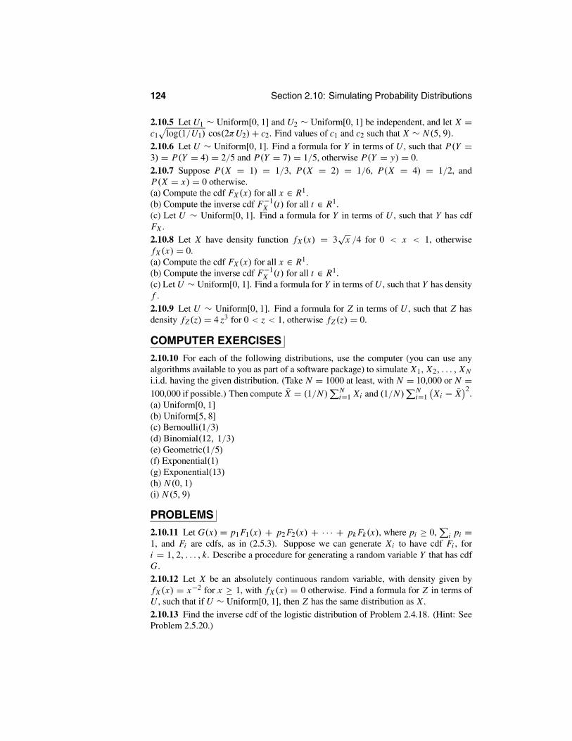
124 Section 2.10: Simulating Probability Distributions
2.10.5 Let U1 ∼ Uniform[0, 1] and U2 ∼ Uniform[0, 1] be independent, and let X =c1 log(1/U1) cos(2πU2)+ c2. Find values of c1 and c2 such that X ∼ N(5, 9).2.10.6 Let U ∼ Uniform[0, 1]. Find a formula for Y in terms of U , such that P(Y =3) = P(Y = 4) = 2/5 and P(Y = 7) = 1/5, otherwise P(Y = y) = 0.2.10.7 Suppose P(X = 1) = 1/3, P(X = 2) = 1/6, P(X = 4) = 1/2, andP(X = x) = 0 otherwise.(a) Compute the cdf FX (x) for all x ∈ R1.(b) Compute the inverse cdf F−1
X (t) for all t ∈ R1.(c) Let U ∼ Uniform[0, 1]. Find a formula for Y in terms of U , such that Y has cdfFX .2.10.8 Let X have density function fX (x) = 3
√x /4 for 0 < x < 1, otherwise
fX (x) = 0.(a) Compute the cdf FX (x) for all x ∈ R1.(b) Compute the inverse cdf F−1
X (t) for all t ∈ R1.(c) Let U ∼ Uniform[0, 1]. Find a formula for Y in terms of U , such that Y has densityf .2.10.9 Let U ∼ Uniform[0, 1]. Find a formula for Z in terms of U , such that Z hasdensity fZ (z) = 4 z3 for 0 < z < 1, otherwise fZ (z) = 0.
COMPUTER EXERCISES
2.10.10 For each of the following distributions, use the computer (you can use anyalgorithms available to you as part of a software package) to simulate X1, X2, . . . , X Ni.i.d. having the given distribution. (Take N = 1000 at least, with N = 10,000 or N =100,000 if possible.) Then compute X = (1/N) N
i=1 Xi and (1/N) Ni=1 Xi − X
2.
(a) Uniform[0, 1](b) Uniform[5, 8](c) Bernoulli(1/3)(d) Binomial(12, 1/3)(e) Geometric(1/5)(f) Exponential(1)(g) Exponential(13)(h) N(0, 1)(i) N(5, 9)
PROBLEMS
2.10.11 Let G(x) = p1F1(x) + p2 F2(x) + · · · + pk Fk(x), where pi ≥ 0, i pi =1, and Fi are cdfs, as in (2.5.3). Suppose we can generate Xi to have cdf Fi , fori = 1, 2, . . . , k. Describe a procedure for generating a random variable Y that has cdfG.2.10.12 Let X be an absolutely continuous random variable, with density given byfX (x) = x−2 for x ≥ 1, with fX (x) = 0 otherwise. Find a formula for Z in terms ofU , such that if U ∼ Uniform[0, 1], then Z has the same distribution as X .2.10.13 Find the inverse cdf of the logistic distribution of Problem 2.4.18. (Hint: SeeProblem 2.5.20.)

Chapter 2: Random Variables and Distributions 125
2.10.14 Find the inverse cdf of the Weibull(α) distribution of Problem 2.4.19. (Hint:See Problem 2.5.21.)2.10.15 Find the inverse cdf of the Pareto(α) distribution of Problem 2.4.20. (Hint:See Problem 2.5.22.)2.10.16 Find the inverse cdf of the Cauchy distribution of Problem 2.4.21. (Hint: SeeProblem 2.5.23.)2.10.17 Find the inverse cdf of the Laplace distribution of Problem 2.4.22. (Hint: SeeProblem 2.5.24.)2.10.18 Find the inverse cdf of the extreme value distribution of Problem 2.4.23. (Hint:See Problem 2.5.25.)2.10.19 Find the inverse cdfs of the beta distributions in Problem 2.4.24(b) through(d). (Hint: See Problem 2.5.26.)2.10.20 (Method of composition) If we generate X ∼ fX obtaining x, and then gener-ate Y from fY |X (· | x) , prove that Y ∼ fY .
CHALLENGES
2.10.21 (Rejection sampling) Suppose f is a complicated density function. Suppose gis a density function from which it is easy to sample (e.g., the density of a uniform orexponential or normal distribution). Suppose we know a value of c such that f (x) ≤cg(x) for all x ∈ R1. The following provides a method, called rejection sampling, forsampling from a complicated density f by using a simpler density g, provided onlythat we know f (x) ≤ cg(x) for all x ∈ R1.(a) Suppose Y has density g. Let U ∼ Uniform[0, c], with U and Y independent.Prove that
P(a ≤ Y ≤ b | f (Y ) ≥ Ucg(Y )) =b
af (x) dx.
(Hint: Use Theorem 2.8.1 to show that P(a ≤ Y ≤ b, f (Y ) ≥ cUg(Y )) =b
a g(y)P( f (Y ) ≥ cUg(Y ) |Y = y) dy.)(b) Suppose that Y1,Y2, . . . are i.i.d., each with density g, and independently U1,U2, . . .are i.i.d. Uniform[0, c]. Let i0 = 0, and for n ≥ 1, let in = min{j > in−1 : U j f (Y j ) ≥cg(Y j )}. Prove that Xi1, Xi2, . . . are i.i.d., each with density f. (Hint: Prove this forXi1, Xi2 .)
2.11 Further Proofs (Advanced)
Proof of Theorem 2.4.2
We want to prove that the function φ given by (2.4.9) is a density function.

126 Section 2.11: Further Proofs (Advanced)
Clearly φ(x) ≥ 0 for all x . To proceed, we set I = ∞−∞ φ(x) dx . Then, using
multivariable calculus,
I 2 =∞
−∞φ(x) dx
2
=∞
−∞φ(x) dx
∞
−∞φ(y) dy
=∞
−∞
∞
−∞φ(x) φ(y) dx dy =
∞
−∞
∞
−∞1
2πe−(x2+y2)/2 dx dy.
We now switch to polar coordinates (r, θ), so that x = r cos θ and y = r sin θ ,where r > 0 and 0 ≤ θ ≤ 2π . Then x2 + y2 = r2 and, by the multivariable change ofvariable theorem from calculus, dx dy = r dr dθ . Hence,
I 2 =2π
0
∞
0
12π
e−r2/2r dr dθ =∞
0e−r2/2r dr
= −e−r2/2r=∞r=0
= (−0)− (−1) = 1,
and we have I 2 = 1. But clearly I ≥ 0 (because φ ≥ 0), so we must have I = 1, asclaimed.
Proof of Theorem 2.6.2
We want to prove that, when X is an absolutely continuous random variable, with den-sity function fX and Y = h(X), where h : R1 → R1 is a function that is differentiableand strictly increasing, then Y is also absolutely continuous, and its density functionfY is given by
fY (y) = fX (h−1(y)) / |h (h−1(y))|, (2.11.1)
where h is the derivative of h, and where h−1(y) is the unique number x such thath(x) = y.
We must show that whenever a ≤ b, we have
P(a ≤ Y ≤ b) =b
afY (y) dy,
where fY is given by (2.11.1). To that end, we note that, because h is strictly increasing,so is h−1. Hence, applying h−1 preserves inequalities, so that
P(a ≤ Y ≤ b) = P(h−1(a) ≤ h−1(Y ) ≤ h−1(b)) = P(h−1(a) ≤ X ≤ h−1(b))
=h−1(b)
h−1(a)fX (x) dx.
We then make the substitution y = h(x), so that x = h−1(y), and
dx = d
dyh−1(y) dy.

Chapter 2: Random Variables and Distributions 127
But by the inverse function theorem from calculus, ddy h−1(y) = 1/h (h−1(y)). Fur-
thermore, as x goes from h−1(a) to h−1(b), we see that y = h(x) goes from a to b.We conclude that
P(a ≤ Y ≤ b) =h−1(b)
h−1(a)fX (x) dx =
b
afX (h
−1(y))(1/|h (h−1(y))|) dy
=b
afY (y) dy,
as required.
Proof of Theorem 2.6.3
We want to prove that when X is an absolutely continuous random variable, with den-sity function fX and Y = h(X), where h : R1 → R1 is a function that is differentiableand strictly decreasing, then Y is also absolutely continuous, and its density functionfY may again be defined by (2.11.1).
We note that, because h is strictly decreasing, so is h−1. Hence, applying h−1
reverses the inequalities, so that
P(a ≤ Y ≤ b) = P(h−1(b) ≤ h−1(Y ) ≤ h−1(a)) = P(h−1(b) ≤ X ≤ h−1(a))
=h−1(a)
h−1(b)fX (x) dx.
We then make the substitution y = h(x), so that x = h−1(y), and
dx = d
dyh−1(y) dy.
But by the inverse function theorem from calculus,
d
dyh−1(y) = 1
h (h−1(y)).
Furthermore, as x goes from h−1(b) to h−1(a), we see that y = h(x) goes from a to b.We conclude that
P(a ≤ Y ≤ b) =h−1(a)
h−1(b)fX (x) dx =
b
afX (h
−1(y)) (1/|h (h−1(y))|) dy
=b
afY (y) dy,
as required.

128 Section 2.11: Further Proofs (Advanced)
Proof of Theorem 2.9.2
We want to prove the following result. Let X and Y be jointly absolutely continuous,with joint density function fX,Y . Let Z = h1(X, Y ) and W = h2(X,Y ), where h1, h2 :R2 → R1 are differentiable functions. Define the joint function h = (h1, h2) : R2 →R2 by
h(x, y) = (h1(x, y), h2(x, y)) .
Assume that h is one-to-one, at least on the region {(x, y) : f (x, y) > 0}, i.e., ifh1(x1, y1) = h1(x2, y2) and h2(x1, y1) = h2(x2, y2), then x1 = x2 and y1 = y2. ThenZ and W are also jointly absolutely continuous, with joint density function fZ ,W givenby
fZ ,W (z,w) = fX,Y (h−1(z, w)) / |J (h−1(z,w))|,
where J is the Jacobian derivative of h, and where h−1(z, w) is the unique pair (x, y)such that h(x, y) = (z,w).
We must show that whenever a ≤ b and c ≤ d, we have
P(a ≤ Z ≤ b , c ≤ W ≤ d) =d
c
b
afZ,W (z, w) dw dz.
If we let S = [a, b]× [c, d] be the two-dimensional rectangle, then we can rewrite thisas
P((Z,W ) ∈ S) =S
fZ,W (z, w) dz dw.
Now, using the theory of multivariable calculus, and making the substitution (x, y) =h−1(z,w) (which is permissible because h is one-to-one), we have
SfZ,W (z, w) dz dw
=S
fX,Y (h−1(z,w)) / |J (h−1(z,w))| dz dw
=h−1(S)
fX,Y (x, y) / |J (x, y)| |J(x, y)| dx dy
=h−1(S)
fX,Y (x, y) dx dy = P((X, Y ) ∈ h−1(S))
= P(h−1(Z,W ) ∈ h−1(S)) = P((Z,W ) ∈ S),
as required.

Chapter 3
Expectation
CHAPTER OUTLINE
Section 1 The Discrete CaseSection 2 The Absolutely Continuous CaseSection 3 Variance, Covariance and CorrelationSection 4 Generating FunctionsSection 5 Conditional ExpectationSection 6 InequalitiesSection 7 General Expectations (Advanced)Section 8 Further Proofs (Advanced)
In the first two chapters we learned about probability models, random variables, anddistributions. There is one more concept that is fundamental to all of probability theory,that of expected value.
Intuitively, the expected value of a random variable is the average value that therandom variable takes on. For example, if half the time X = 0, and the other half ofthe time X = 10, then the average value of X is 5. We shall write this as E(X) = 5.Similarly, if one-third of the time Y = 6 while two-thirds of the time Y = 15, thenE(Y ) = 12.
Another interpretation of expected value is in terms of fair gambling. Supposesomeone offers you a ticket (e.g., a lottery ticket) worth a certain random amount X .How much would you be willing to pay to buy the ticket? It seems reasonable that youwould be willing to pay the expected value E(X) of the ticket, but no more. However,this interpretation does have certain limitations; see Example 3.1.12.
To understand expected value more precisely, we consider discrete and absolutelycontinuous random variables separately.
3.1 The Discrete CaseWe begin with a definition.
129

130 Section 3.1: The Discrete Case
Definition 3.1.1 Let X be a discrete random variable. Then the expected value (ormean value or mean) of X , written E(X) (or µX ), is defined by
E(X) =x∈R1
x P(X = x) =x∈R1
x pX (x).
We will have P(X = x) = 0 except for those values x that are possible values of X .Hence, an equivalent definition is the following.
Definition 3.1.2 Let X be a discrete random variable, taking on distinct valuesx1, x2, . . . , with pi = P(X = xi ). Then the expected value of X is given by
E(X) =i
xi pi .
The definition (in either form) is best understood through examples.
EXAMPLE 3.1.1Suppose, as above, that P(X = 0) = P(X = 10) = 1/2. Then
E(X) = (0)(1/2)+ (10)(1/2) = 5,
as predicted.
EXAMPLE 3.1.2Suppose, as above, that P(Y = 6) = 1/3, and P(Y = 15) = 2/3. Then
E(Y ) = (6)(1/3)+ (15)(2/3) = 2+ 10 = 12,
again as predicted.
EXAMPLE 3.1.3Suppose that P(Z = −3) = 0.2, and P(Z = 11) = 0.7, and P(Z = 31) = 0.1. Then
E(Z) = (−3)(0.2)+ (11)(0.7)+ (31)(0.1) = −0.6+ 7.7+ 3.1 = 10.2.
EXAMPLE 3.1.4Suppose that P(W = −3) = 0.2, and P(W = −11) = 0.7, and P(W = 31) = 0.1.Then
E(W) = (−3)(0.2)+ (−11)(0.7)+ (31)(0.1) = −0.6− 7.7+ 3.1 = −5.2.
In this case, the expected value of W is negative.
We thus see that, for a discrete random variable X , once we know the probabilities thatX = x (or equivalently, once we know the probability function pX ), it is straightfor-ward (at least in simple cases) to compute the expected value of X .
We now consider some of the common discrete distributions introduced in Sec-tion 2.3.

Chapter 3: Expectation 131
EXAMPLE 3.1.5 Degenerate DistributionsIf X ≡ c is a constant, then P(X = c) = 1, so
E(X) = (c)(1) = c,
as it should.
EXAMPLE 3.1.6 The Bernoulli(θ) Distribution and Indicator FunctionsIf X ∼ Bernoulli(θ), then P(X = 1) = θ and P(X = 0) = 1− θ , so
E(X) = (1)(θ)+ (0)(1− θ) = θ.As a particular application of this, suppose we have a response s taking values in a
sample S and A ⊂ S. Letting X (s) = IA (s) , we have that X is the indicator functionof the set A and so takes the values 0 and 1. Then we have that P(X = 1) = P (A) ,and so X ∼ Bernoulli(P (A)) . This implies that
E (X) = E (IA) = P(A).
Therefore, we have shown that the expectation of the indicator function of the set A isequal to the probability of A.
EXAMPLE 3.1.7 The Binomial(n, θ) DistributionIf Y ∼ Binomial(n, θ), then
P(Y = k) = n
kθk(1− θ)n−k
for k = 0, 1, . . . , n. Hence,
E(Y ) =n
k=0
k P(Y = k) =n
k=0
kn
kθk(1− θ)n−k
=n
k=0
kn!
k! (n − k)!θk(1− θ)n−k =
n
k=1
n!(k − 1)! (n − k)!
θk(1− θ)n−k
=n
k=1
n (n − 1)!(k − 1)! (n − k)!
θk(1− θ)n−k =n
k=1
nn − 1k − 1
θk(1− θ)n−k .
Now, the binomial theorem says that for any a and b and any positive integer m,
(a + b)m =m
j=0
m
ja jbm− j .
Using this, and setting j = k − 1, we see that
E(Y ) =n
k=1
nn − 1
k − 1θk(1− θ)n−k =
n−1
j=0
nn − 1
jθ j+1(1− θ)n− j−1
= nθn−1
j=0
n − 1j
θ j (1− θ)n− j−1 = nθ (θ + 1− θ)n−1 = nθ.
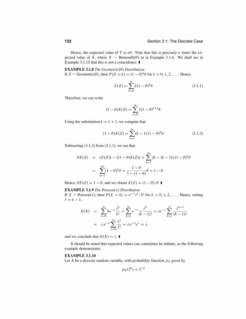
132 Section 3.1: The Discrete Case
Hence, the expected value of Y is nθ . Note that this is precisely n times the ex-pected value of X , where X ∼ Bernoulli(θ) as in Example 3.1.6. We shall see inExample 3.1.15 that this is not a coincidence.
EXAMPLE 3.1.8 The Geometric(θ) DistributionIf Z ∼ Geometric(θ), then P(Z = k) = (1− θ)kθ for k = 0, 1, 2, . . . . Hence,
E(Z) =∞
k=0
k(1− θ)kθ. (3.1.1)
Therefore, we can write
(1− θ)E(Z) =∞
=0
(1− θ) +1θ.
Using the substitution k = + 1, we compute that
(1− θ)E(Z) =∞
k=1
(k − 1) (1− θ)kθ. (3.1.2)
Subtracting (3.1.2) from (3.1.1), we see that
θE(Z) = (E(Z))− ((1− θ)E(Z)) =∞
k=1
(k − (k − 1)) (1− θ)kθ
=∞
k=1
(1− θ)kθ = 1− θ1− (1− θ)θ = 1− θ.
Hence, θE(Z) = 1− θ , and we obtain E(Z) = (1− θ)/θ .
EXAMPLE 3.1.9 The Poisson(λ) DistributionIf X ∼ Poisson(λ), then P(X = k) = e−λλk/k! for k = 0, 1, 2, . . . . Hence, setting= k − 1,
E(X) =∞
k=0
ke−λ λk
k!=
∞
k=1
e−λ λk
(k − 1)!= λe−λ
∞
k=1
λk−1
(k − 1)!
= λ e−λ∞
=0
λ
!= λ e−λeλ = λ,
and we conclude that E(X) = λ.
It should be noted that expected values can sometimes be infinite, as the followingexample demonstrates.
EXAMPLE 3.1.10Let X be a discrete random variable, with probability function pX given by
pX (2k) = 2−k

Chapter 3: Expectation 133
for k = 1, 2, 3, . . . , with pX (x) = 0 for other values of x . That is, pX (2) = 1/2,pX (4) = 1/4, pX (8) = 1/8, etc., while pX (1) = pX (3) = pX (5) = pX (6) = · · · = 0.
Then it is easily checked that pX is indeed a valid probability function (i.e., pX (x) ≥0 for all x , with x pX (x) = 1). On the other hand, we compute that
E(X) =∞
k=1
(2k)(2−k) =∞
k=1
(1) =∞.
We therefore say that E(X) =∞, i.e., that the expected value of X is infinite.
Sometimes the expected value simply does not exist, as in the following example.
EXAMPLE 3.1.11Let Y be a discrete random variable, with probability function pY given by
pY (y) = 1/2y y = 2, 4, 8, 16, . . .
1/2|y| y = −2,−4,−8,−16, . . .0 otherwise.
That is, pY (2) = pY (−2) = 1/4, pY (4) = pY (−4) = 1/8, pY (8) = pY (−8) =1/16, etc. Then it is easily checked that pY is indeed a valid probability function (i.e.,pY (y) ≥ 0 for all y, with y pY (y) = 1).
On the other hand, we compute that
E(Y ) =y
y pY (y) =∞
k=1
(2k)(1/2 2k)+∞
k=1
(−2k)(1/2 2k)
=∞
k=1
(1/2)−∞
k=1
(1/2) =∞−∞,
which is undefined. We therefore say that E(Y ) does not exist, i.e., that the expectedvalue of Y is undefined in this case.
EXAMPLE 3.1.12 The St. Petersburg ParadoxSuppose someone makes you the following deal. You will repeatedly flip a fair coinand will receive an award of 2Z pennies, where Z is the number of tails that appearbefore the first head. How much would you be willing to pay for this deal?
Well, the probability that the award will be 2z pennies is equal to the probability thatyou will flip z tails and then one head, which is equal to 1/2z+1. Hence, the expectedvalue of the award (in pennies) is equal to
∞
z=0
(2z)(1/2z+1) =∞
z=0
1/2 =∞.
In words, the average amount of the award is infinite!Hence, according to the “fair gambling” interpretation of expected value, as dis-
cussed at the beginning of this chapter, it seems that you should be willing to pay aninfinite amount (or, at least, any finite amount no matter how large) to get the award

134 Section 3.1: The Discrete Case
promised by this deal! How much do you think you should really be willing to pay forit?1
EXAMPLE 3.1.13 The St. Petersburg Paradox, TruncatedSuppose in the St. Petersburg paradox (Example 3.1.12), it is agreed that the award willbe truncated at 230 cents (which is just over $10 million!). That is, the award will bethe same as for the original deal, except the award will be frozen once it exceeds 230
cents. Formally, the award is now equal to 2min(30,Z) pennies, where Z is as before.How much would you be willing to pay for this new award? Well, the expected
value of the new award (in cents) is equal to
∞
z=1
(2min(30,z))(1/2z+1) =30
z=1
(2z)(1/2z+1)+∞
z=31
(230)(1/2z+1)
=30
z=1
(1/2)+ (230)(1/231) = 31/2 = 15.5.
That is, truncating the award at just over $10 million changes its expected value enor-mously, from infinity to less than 16 cents!
In utility theory, it is often assumed that each person has a utility function U suchthat, if they win x cents, their amount of “utility” (i.e., benefit or joy or pleasure) isequal to U(x). In this context, the truncation of Example 3.1.13 may be thought ofnot as changing the rules of the game but as corresponding to a utility function of theform U(x) = min(x, 230). In words, this says that your utility is equal to the amountof money you get, until you reach 230 cents (approximately $10 million), after whichpoint you don’t care about money2 anymore. The result of Example 3.1.13 then saysthat, with this utility function, the St. Petersburg paradox is only worth 15.5 cents toyou — even though its expected value is infinite.
We often need to compute expected values of functions of random variables. For-tunately, this is not too difficult, as the following theorem shows.
Theorem 3.1.1(a) Let X be a discrete random variable, and let g : R1 → R1 be some function
such that the expectation of the random variable g(X) exists. Then
E (g(X)) =x
g(x) P(X = x).
(b) Let X and Y be discrete random variables, and let h : R2 → R1 be somefunction such that the expectation of the random variable h(X, Y ) exists. Then
E (h(X,Y )) =x,y
h(x, y)P(X = x, Y = y).
1When one of the authors first heard about this deal, he decided to try it and agreed to pay $1. In fact, hegot four tails before the first head, so his award was 16 cents, but he still lost 84 cents overall.
2Or, perhaps, you think it is unlikely you will be able to collect the money!

Chapter 3: Expectation 135
PROOF We prove part (b) here. Part (a) then follows by simply setting h(x, y) =g(x) and noting that
x,yg(x) P(X = x, Y = y) =
xg(x) P(X = x).
Let Z = h(X,Y ).We have that
E(Z) =z
z P(Z = z) =z
z P(h(X, Y ) = z)
=z
zx,y
h(x,y)=z
P(X = x, Y = y) =x,y z
z=h(x,y)
z P(X = x, Y = y)
=x,y
h(x, y) P(X = x, Y = y),
as claimed.
One of the most important properties of expected value is that it is linear, stated asfollows.
Theorem 3.1.2 (Linearity of expected values) Let X and Y be discrete randomvariables, let a and b be real numbers, and put Z = aX + bY . Then E(Z) =aE(X)+ bE(Y ).
PROOF Let pX,Y be the joint probability function of X and Y . Then using Theo-rem 3.1.1,
E(Z) =x,y(ax + by) pX,Y (x, y) = a
x,yx pX,Y (x, y)+ b
x,yy pX,Y (x, y)
= ax
xy
pX,Y (x, y)+ by
yx
pX,Y (x, y).
Because y pX,Y (x, y) = pX (x) and x pX,Y (x, y) = pY (y), we have that
E(Z) = ax
x pX (x)+ by
y pY (y) = aE(X)+ bE(Y ),
as claimed.
EXAMPLE 3.1.14Let X ∼ Binomial(n, θ1), and let Y ∼ Geometric(θ2). What is E(3X − 2Y )?
We already know (Examples 3.1.6 and 3.1.7) that E(X) = n θ1 and E(Y ) = (1−θ2) / θ2. Hence, by Theorem 3.1.2, E(3X − 2Y ) = 3E(X)− 2E(Y ) = 3nθ1 − 2(1−θ2)/θ2.
EXAMPLE 3.1.15Let Y ∼ Binomial(n, θ). Then we know (cf. Example 2.3.3) that we can think ofY = X1 + · · · + Xn, where each Xi ∼ Bernoulli(θ) (in fact, Xi = 1 if the i th coin is

136 Section 3.1: The Discrete Case
heads, otherwise Xi = 0). Because E(Xi ) = θ for each i , it follows immediately fromTheorem 3.1.2 that
E(Y ) = E(X1)+ · · · + E(Xn) = θ + · · · + θ = nθ.
This gives the same answer as Example 3.1.7, but much more easily.
Suppose that X is a random variable and Y = c is a constant. Then from Theorem3.1.2, we have that E(X + c) = E(X) + c. From this we see that the mean value µXof X is a measure of the location of the probability distribution of X. For example, ifX takes the value x with probability p and the value y with probability 1− p, then themean of X is µX = px + (1− p)y which is a value between x and y. For a constant c,the probability distribution of X + c is concentrated on the points x+c and y+ c, withprobabilities p and 1− p, respectively. The mean of X+c is µX+c,which is betweenthe points x + c and y + c, i.e., the mean shifts with the probability distribution. It isalso true that if X is concentrated on the finite set of points x1 < x2 < · · · < xk, thenx1 ≤ µX ≤ xk, and the mean shifts exactly as we shift the distribution. This is depictedin Figure 3.1.1 for a distribution concentrated on k = 4 points. Using the results ofSection 2.6.1, we have that pX+c(x) = pX (x − c).
x1 x2 x3 x4
pX
•E(X)
x1+c x2+c x3+c x4+c•
E(X+c)
pX+c
Figure 3.1.1: The probability functions and means of discrete random variables X and X + c.
Theorem 3.1.2 says, in particular, that E(X + Y ) = E(X) + E(Y ), i.e., that ex-pectation preserves sums. It is reasonable to ask whether the same property holds forproducts. That is, do we necessarily have E(XY ) = E(X)E(Y )? In general, theanswer is no, as the following example shows.

Chapter 3: Expectation 137
EXAMPLE 3.1.16Let X and Y be discrete random variables, with joint probability function given by
pX,Y (x, y) =
1/2 x = 3, y = 51/6 x = 3, y = 91/6 x = 6, y = 51/6 x = 6, y = 90 otherwise.
Then
E(X) =x
x P(X = x) = (3)(1/2+ 1/6)+ (6)(1/6+ 1/6) = 4
and
E(Y ) =y
y P(Y = y) = (5)(1/2+ 1/6)+ (9)(1/6+ 1/6) = 19/3,
while
E(XY ) =z
z P(XY = z)
= (3)(5)(1/2)+ (3)(9)(1/6)+ (6)(5)(1/6)+ (6)(9)(1/6)= 26.
Because (4)(19/3) = 26, we see that E(X) E(Y ) = E(XY ) in this case.
On the other hand, if X and Y are independent, then we do have E(X)E(Y ) =E(XY ).
Theorem 3.1.3 Let X and Y be discrete random variables that are independent.Then E(XY ) = E(X)E(Y ).
PROOF Independence implies (see Theorem 2.8.3) that P(X = x, Y = y) =P(X = x) P(Y = y). Using this, we compute by Theorem 3.1.1 that
E(XY ) =x,y
xy P(X = x, Y = y) =x,y
xy P(X = x) P(Y = y)
=x
x P(X = x)y
y P(Y = y) = E(X) E(Y ),
as claimed.
Theorem 3.1.3 will be used often in subsequent chapters, as will the following impor-tant property.
Theorem 3.1.4 (Monotonicity) Let X and Y be discrete random variables, andsuppose that X ≤ Y . (Remember that this means X (s) ≤ Y (s) for all s ∈ S.) ThenE(X) ≤ E(Y ).

138 Section 3.1: The Discrete Case
PROOF Let Z = Y − X . Then Z is also discrete. Furthermore, because X ≤ Y ,we have Z ≥ 0, so that all possible values of Z are nonnegative. Hence, if we list thepossible values of Z as z1, z2, . . . , then zi ≥ 0 for all i , so that
E(Z) =i
zi P(Z = zi ) ≥ 0.
But by Theorem 3.1.2, E(Z) = E(Y ) − E(X). Hence, E(Y ) − E(X) ≥ 0, so thatE(Y ) ≥ E(X).
Summary of Section 3.1
• The expected value E(X) of a random variable X represents the long-run averagevalue that it takes on.
• If X is discrete, then E(X) = x x P(X = x).
• The expected values of the Bernoulli, binomial, geometric, and Poisson distrib-utions were computed.
• Expected value has an interpretation in terms of fair gambling, but such interpre-tations require utility theory to accurately reflect human behavior.
• Expected values of functions of one or two random variables can also be com-puted by summing the function values times the probabilities.
• Expectation is linear and monotone.
• If X and Y are independent, then E(XY ) = E(X) E(Y ). But without indepen-dence, this property may fail.
EXERCISES
3.1.1 Compute E(X) when the probability function of X is given by each of the fol-lowing.(a)
pX (x) =
1/7 x = −42/7 x = 04/7 x = 30 otherwise
(b)
pX (x) = 2−x−1 x = 0, 1, 2, . . .0 otherwise
(c)
pX (x) = 2−x+6 x = 7, 8, 9, . . .0 otherwise

Chapter 3: Expectation 139
3.1.2 Let X and Y have joint probability function given by
pX,Y (x, y) =
1/7 x = 5, y = 01/7 x = 5, y = 31/7 x = 5, y = 43/7 x = 8, y = 01/7 x = 8, y = 40 otherwise,
as in Example 2.7.5. Compute each of the following.(a) E(X)(b) E(Y )(c) E(3X + 7Y )(d) E(X2)(e) E(Y 2)(f) E(XY )(g) E(XY + 14)3.1.3 Let X and Y have joint probability function given by
pX,Y (x, y) =
1/2 x = 2, y = 101/6 x = −7, y = 101/12 x = 2, y = 121/12 x = −7, y = 121/12 x = 2, y = 141/12 x = −7, y = 140 otherwise.
Compute each of the following.(a) E(X).(b) E(Y )(c) E(X2)(d) E(Y 2)(e) E(X2 + Y 2)(f) E(XY − 4Y )
3.1.4 Let X ∼ Bernoulli(θ1) and Y ∼ Binomial(n, θ2). Compute E(4X − 3Y ).3.1.5 Let X ∼ Geometric(θ) and Y ∼ Poisson(λ). Compute E(8X − Y + 12).3.1.6 Let Y ∼ Binomial(100, 0.3), and Z ∼ Poisson(7). Compute E(Y + Z).3.1.7 Let X ∼ Binomial(80, 1/4), and let Y ∼ Poisson(3/2). Assume X and Y areindependent. Compute E(XY ).3.1.8 Starting with one penny, suppose you roll one fair six-sided die and get paid anadditional number of pennies equal to three times the number showing on the die. LetX be the total number of pennies you have at the end. Compute E(X).3.1.9 Suppose you start with eight pennies and flip one fair coin. If the coin comes upheads, you get to keep all your pennies; if the coin comes up tails, you have to givehalf of them back. Let X be the total number of pennies you have at the end. ComputeE(X).

140 Section 3.1: The Discrete Case
3.1.10 Suppose you flip two fair coins. Let Y = 3 if the two coins show the sameresult, otherwise let Y = 5. Compute E(Y ).3.1.11 Suppose you roll two fair six-sided dice.(a) Let Z be the sum of the two numbers showing. Compute E(Z).(b) Let W be the product of the two numbers showing. Compute E(W ).3.1.12 Suppose you flip one fair coin and roll one fair six-sided die. Let X be theproduct of the numbers of heads (i.e., 0 or 1) times the number showing on the die.Compute E(X). (Hint: Do not forget Theorem 3.1.3.)3.1.13 Suppose you roll one fair six-sided die and then flip as many coins as the num-ber showing on the die. (For example, if the die shows 4, then you flip four coins.) LetY be the number of heads obtained. Compute E(Y ).3.1.14 Suppose you roll three fair coins, and let X be the cube of the number of headsshowing. Compute E(X).
PROBLEMS
3.1.15 Suppose you start with one penny and repeatedly flip a fair coin. Each time youget heads, before the first time you get tails, you get two more pennies. Let X be thetotal number of pennies you have at the end. Compute E(X).3.1.16 Suppose you start with one penny and repeatedly flip a fair coin. Each time youget heads, before the first time you get tails, your number of pennies is doubled. Let Xbe the total number of pennies you have at the end. Compute E(X).3.1.17 Let X ∼ Geometric(θ), and let Y = min(X, 100).(a) Compute E(Y ).(b) Compute E(Y − X).3.1.18 Give an example of a random variable X such that E min(X, 100) = E(X).3.1.19 Give an example of a random variable X such that E(min(X, 100)) = E(X)/2.3.1.20 Give an example of a joint probability function pX,Y for random variables Xand Y , such that X ∼ Bernoulli(1/4) and Y ∼ Bernoulli(1/2), but E(XY ) = 1/8.3.1.21 For X ∼ Hypergeometric(N,M, n), prove that E(X) = nM/N .
3.1.22 For X ∼ Negative-Binomial (r, θ), prove that E(X) = r(1 − θ)/θ. (Hint:Argue that if X1, . . . , Xr are independent and identically distributed Geometric(θ) ,then X = X1 + · · · + Xr ∼ Negative-Binomial(r, θ) .)3.1.23 Suppose that (X1, X2, X3) ∼Multinomial(n, θ1, θ2, θ3) . Prove thatE(Xi ) = nθ i .
CHALLENGES
3.1.24 Let X ∼ Geometric(θ). Compute E(X2).3.1.25 Suppose X is a discrete random variable, such that E (min(X, M)) = E(X).Prove that P(X > M) = 0.

Chapter 3: Expectation 141
DISCUSSION TOPICS
3.1.26 How much would you be willing to pay for the deal corresponding to the St. Pe-tersburg paradox (see Example 3.1.12)? Justify your answer.3.1.27 What utility function U (as in the text following Example 3.1.13) best describesyour own personal attitude toward money? Why?
3.2 The Absolutely Continuous CaseSuppose now that X is absolutely continuous, with density function fX . How canwe compute E(X) then? By analogy with the discrete case, we might try computing
x x P(X = x), but because P(X = x) is always zero, this sum is always zero aswell.
On the other hand, if is a small positive number, then we could try approximatingE(X) by
E(X) ≈i
i P(i ≤ X < (i + 1) ),
where the sum is over all integers i . This makes sense because, if is small andi ≤ X < (i + 1) , then X ≈ i .
Now, we know that
P(i ≤ X < (i + 1) ) =(i+1)
ifX (x) dx.
This tells us that
E(X) ≈i
(i+1)
ii fX (x) dx.
Furthermore, in this integral, i ≤ x < (i + 1) . Hence, i ≈ x . We therefore see that
E(X) ≈i
(i+1)
ix fX (x) dx =
∞
−∞x fX (x) dx .
This prompts the following definition.
Definition 3.2.1 Let X be an absolutely continuous random variable, with densityfunction fX . Then the expected value of X is given by
E(X) =∞
−∞x fX (x) dx.
From this definition, it is not too difficult to compute the expected values of manyof the standard absolutely continuous distributions.

142 Section 3.2: The Absolutely Continuous Case
EXAMPLE 3.2.1 The Uniform[0, 1] DistributionLet X ∼ Uniform[0, 1] so that the density of X is given by
fX (x) = 1 0 ≤ x ≤ 10 otherwise.
Hence,
E(X) =∞
−∞x fX (x) dx =
1
0x dx = x2
2
x=1
x=0= 1/2,
as one would expect.
EXAMPLE 3.2.2 The Uniform[L, R] DistributionLet X ∼ Uniform[L, R] so that the density of X is given by
fX (x) = 1/(R − L) L ≤ x ≤ R0 otherwise.
Hence,
E(X) =∞
−∞x fX (x) dx =
R
Lx
1R − L
dx = x2
2(R − L)
x=R
x=L
= R2 − L2
2(R − L)= (R − L)(R + L)
2(R − L)= R + L
2,
again as one would expect.
EXAMPLE 3.2.3 The Exponential(λ) DistributionLet Y ∼ Exponential(λ) so that the density of Y is given by
fY (y) = λe−λy y ≥ 00 y < 0.
Hence, integration by parts, with u = y and dv = λ e−λy (so du = dy, v = −e−λy),leads to
E(Y ) =∞
−∞y fY (y) dy =
∞
0y λ e−λy dy = − ye−λy ∞
0 +∞
0e−λy dy
=∞
0e−λy dy = − e−λy
λ
∞
0= −0− 1
λ= 1
λ.
In particular, if λ = 1, then Y ∼ Exponential(1), and E(Y ) = 1.
EXAMPLE 3.2.4 The N(0, 1) DistributionLet Z ∼ N(0, 1) so that the density of Z is given by
fZ (z) = φ(z) = 1√2π
e−z2/2.

Chapter 3: Expectation 143
Hence,
E(Z) =∞
−∞z fZ (z) dz
=∞
−∞z
1√2π
e−z2/2 dz
=0
−∞z
1√2π
e−z2/2 dz +∞
0z
1√2π
e−z2/2 dz. (3.2.1)
But using the substitution w = −z, we see that
0
−∞z
1√2π
e−z2/2 dz =∞
0(−w) 1√
2πe−w2/2 dw.
Then the two integrals in (3.2.1) cancel each other out, and leaving us with E(Z) = 0.
As with discrete variables, means of absolutely continuous random variables canalso be infinite or undefined.
EXAMPLE 3.2.5Let X have density function given by
fX (x) = 1/x2 x ≥ 10 otherwise.
Then
E(X) =∞
−∞x fX (x) dx =
∞
1x (1/x2) dx =
∞
1(1/x) dx = log x
x=∞x=1
=∞.
Hence, the expected value of X is infinite.
EXAMPLE 3.2.6Let Y have density function given by
fY (y) = 1/2y2 y ≥ 1
1/2y2 y ≤ −10 otherwise.
Then
E(Y ) =∞
−∞y fY (y) dy =
−1
−∞y(1/y2) dy +
∞
1y(1/y2) dy
= −∞
1(1/y) dy +
∞
1(1/y) dy = −∞+∞,
which is undefined. Hence, the expected value of Y is undefined (i.e., does not exist)in this case.

144 Section 3.2: The Absolutely Continuous Case
Theorem 3.1.1 remains true in the continuous case, as follows.
Theorem 3.2.1(a) Let X be an absolutely continuous random variable, with density function fX ,and let g : R1 → R1 be some function. Then when the expectation of g(X) exists,
E (g(X)) =∞
−∞g(x) fX (x) dx .
(b) Let X and Y be jointly absolutely continuous random variables, with joint den-sity function fX,Y , and let h : R2 → R1 be some function. Then when the expecta-tion of h(X,Y ) exists,
E (h(X, Y )) =∞
−∞
∞
−∞h(x, y) fX,Y (x, y) dx dy.
We do not prove Theorem 3.2.1 here; however, we shall use it often. For a first useof this result, we prove that expected values for absolutely continuous random variablesare still linear.
Theorem 3.2.2 (Linearity of expected values) Let X and Y be jointly absolutelycontinuous random variables, and let a and b be real numbers. Then E(aX+bY ) =aE(X)+ bE(Y ).
PROOF Let fX,Y be the joint density function of X and Y . Then using Theo-rem 3.2.1, we compute that
E(Z) =∞
−∞
∞
−∞(ax + by) fX,Y (x, y) dx dy
= a∞
−∞
∞
−∞x fX,Y (x, y) dx dy + b
∞
−∞
∞
−∞y fX,Y (x, y) dx dy
= a∞
−∞x
∞
−∞fX,Y (x, y) dy dx
+b∞
−∞y
∞
−∞fX,Y (x, y) dx dy.
But ∞−∞ fX,Y (x, y) dy = fX (x) and ∞
−∞ fX,Y (x, y) dx = fY (y), so
E(Z) = a∞
−∞x fX (x) dx + b
∞
−∞y fY (y) dy = aE(X)+ bE(Y ),
as claimed.
Just as in the discrete case, we have that E(X + c) = E(X) + c for an absolutelycontinuous random variable X. Note, however, that this is not implied by Theorem3.2.2 because the constant c is a discrete, not absolutely continuous, random variable.

Chapter 3: Expectation 145
In fact, we need a more general treatment of expectation to obtain this result (see Sec-tion 3.7). In any case, the result is true and we again have that the mean of a randomvariable serves as a measure of the location of the probability distribution of X. InFigure 3.2.1, we have plotted the densities and means of the absolutely continuous ran-dom variables X and X + c. The change of variable results from Section 2.6.2 givefX+c(x) = fX (x − c) .
•E(X)
•E(X+c)
fX
fX+c
x
x
Figure 3.2.1: The densities and means of absolutely continuous random variables X andX + c.
EXAMPLE 3.2.7 The N(µ, σ 2) DistributionLet X ∼ N(µ, σ 2). Then we know (cf. Exercise 2.6.3) that if Z = (X − µ) / σ , thenZ ∼ N(0, 1). Hence, we can write X = µ+ σ Z , where Z ∼ N(0, 1). But we know(see Example 3.2.4) that E(Z) = 0 and (Example 3.1.5) that E(µ) = µ. Hence, usingTheorem 3.2.2, E(X) = E(µ+ σ Z) = E(µ)+ σ E(Z) = µ+ σ (0) = µ.
If X and Y are independent, then the following results show that we again haveE(XY ) = E(X) E(Y ).
Theorem 3.2.3 Let X and Y be jointly absolutely continuous random variables thatare independent. Then E(XY ) = E(X)E(Y ).
PROOF Independence implies (Theorem 2.8.3) that fX,Y (x, y) = fX (x) fY (y).Using this, along with Theorem 3.2.1, we compute
E(XY ) =∞
−∞
∞
−∞xy fX,Y (x, y) dx dy =
∞
−∞
∞
−∞xy fX (x) fY (y) dx dy
=∞
−∞x fX (x) dx
∞
−∞y fY (y) dy = E(X)E(Y ),
as claimed.

146 Section 3.2: The Absolutely Continuous Case
The monotonicity property (Theorem 3.1.4) still holds as well.
Theorem 3.2.4 (Monotonicity) Let X and Y be jointly continuous random vari-ables, and suppose that X ≤ Y . Then E(X) ≤ E(Y ).
PROOF Let fX,Y be the joint density function of X and Y . Because X ≤ Y , thedensity fX,Y can be chosen so that fX,Y (x, y) = 0 whenever x > y. Now let Z =Y − X . Then by Theorem 3.2.1(b),
E(Z) =∞
−∞
∞
−∞(y − x) fX,Y (x, y) dx dy .
Because fX,Y (x, y) = 0 whenever x > y, this implies that E(Z) ≥ 0. But by Theo-rem 3.2.2, E(Z) = E(Y )− E(X). Hence, E(Y )− E(X) ≥ 0, so that E(Y ) ≥ E(X).
Summary of Section 3.2
• If X is absolutely continuous, then E(X) = x fX (x) dx .
• The expected values of the uniform, exponential, and normal distributions werecomputed.
• Expectation for absolutely continuous random variables is linear and monotone.
• If X and Y are independent, then we still have E(XY ) = E(X) E(Y ).
EXERCISES
3.2.1 Compute C and E(X) when the density function of X is given by each of thefollowing.(a)
fX (x) = C 5 ≤ x ≤ 90 otherwise
(b)
fX (x) = C(x + 1) 6 ≤ x ≤ 80 otherwise
(c)
fX (x) = Cx4 −5 ≤ x ≤ −20 otherwise
3.2.2 Let X and Y have joint density
fX,Y (x, y) = 4x2y + 2y5 0 ≤ x ≤ 1 , 0 ≤ y ≤ 10 otherwise,
as in Examples 2.7.6 and 2.7.7. Compute each of the following.(a) E(X)

Chapter 3: Expectation 147
(b) E(Y )(c) E(3X + 7Y )(d) E(X2)(e) E(Y 2)(f) E(XY )(g) E(XY + 14)3.2.3 Let X and Y have joint density
fX,Y (x, y) = (4xy + 3x2y2)/18 0 ≤ x ≤ 1, 0 ≤ y ≤ 30 otherwise.
Compute each of the following.(a) E(X)(b) E(Y )(c) E(X2)(d) E(Y 2)(e) E(Y 4)(f) E(X2Y 3)
3.2.4 Let X and Y have joint density
fX,Y (x, y) = 6xy + (9/2)x2y2 0 ≤ y ≤ x ≤ 10 otherwise.
Compute each of the following.(a) E(X)(b) E(Y )(c) E(X2)(d) E(Y 2)(e) E(Y 4)(f) E(X2Y 3)
3.2.5 Let X ∼ Uniform[3, 7] and Y ∼ Exponential(9). Compute E(−5X − 6Y ).3.2.6 Let X ∼ Uniform[−12,−9] and Y ∼ N(−8, 9). Compute E(11X + 14Y + 3).3.2.7 Let Y ∼ Exponential(9) and Z ∼ Exponential(8). Compute E(Y + Z).3.2.8 Let Y ∼ Exponential(9) and Z ∼ Gamma(5, 4). Compute E(Y + Z). (Youmay use Problem 3.2.16 below.)3.2.9 Suppose X has density function f (x) = 3/20(x2+x3) for 0 < x < 2, otherwisef (x) = 0. Compute each of E(X), E(X2), and E(X3), and rank them from largest tosmallest.3.2.10 Suppose X has density function f (x) = 12/7(x2 + x3) for 0 < x < 1, oth-erwise f (x) = 0. Compute each of E(X), E(X2), and E(X3) and rank them fromlargest to smallest.3.2.11 Suppose men’s heights (in centimeters) follow the distribution N(174, 202),while those of women follow the distribution N(160, 152). Compute the mean totalheight of a man–woman married couple.3.2.12 Suppose X and Y are independent, with E(X) = 5 and E(Y ) = 6. For each ofthe following variables Z , either compute E(Z) or explain why we cannot determine

148 Section 3.2: The Absolutely Continuous Case
E(Z) from the available information:(a) Z = X + Y(b) Z = XY(c) Z = 2X − 4Y(d) Z = 2X (3+ 4Y )(e) Z = (2+ X)(3+ 4Y )(f) Z = (2+ X)(3X + 4Y )
3.2.13 Suppose darts are randomly thrown at a wall. Let X be the distance (in cen-timeters) from the left edge of the dart’s point to the left end of the wall, and let Y bethe distance from the right edge of the dart’s point to the left end of the wall. Assumethe dart’s point is 0.1 centimeters thick, and that E(X) = 214. Compute E(Y ).3.2.14 Let X be the mean height of all citizens measured from the top of their head,and let Y be the mean height of all citizens measured from the top of their head or hat(whichever is higher). Must we have E(Y ) ≥ E(X)? Why or why not?3.2.15 Suppose basketball teams A and B each have five players and that each memberof team A is being “guarded” by a unique member of team B. Suppose it is noticed thateach member of team A is taller than the corresponding gusrf from team B. Does itnecessarily follow that the mean height of team A is larger than the mean height ofteam B? Why or why not?
PROBLEMS
3.2.16 Let α > 0 and λ > 0, and let X ∼ Gamma(α, λ). Prove that E(X) = α/λ.(Hint: The computations are somewhat similar to those of Problem 2.4.15. You willalso need property (2.4.7) of the gamma function.)3.2.17 Suppose that X follows the logistic distribution (see Problem 2.4.18). Provethat E(X) = 0.3.2.18 Suppose that X follows the Weibull(α) distribution (see Problem 2.4.19). Provethat E(X) = α−1 + 1 .
3.2.19 Suppose that X follows the Pareto(α) distribution (see Problem 2.4.20) for α >1. Prove that E(X) = 1/ (α − 1) .What is E(X) when 0 < α ≤ 1?3.2.20 Suppose that X follows the Cauchy distribution (see Problem 2.4.21). Arguethat E(X) does not exist. (Hint: Compute the integral in two parts, where the integrandis positive and where the integrand is negative.)3.2.21 Suppose that X follows the Laplace distribution (see Problem 2.4.22). Provethat E(X) = 0.3.2.22 Suppose that X follows the Beta(a, b) distribution (see Problem 2.4.24). Provethat E(X) = a/(a + b).
3.2.23 Suppose that (X1, X2) ∼ Dirichlet(α1, α2, α3) (see Problem 2.7.17). Provethat E(Xi ) = αi/ (α1 + α2 + α3) .

Chapter 3: Expectation 149
3.3 Variance, Covariance, and CorrelationNow that we understand expected value, we can use it to define various other quantitiesof interest. The numerical values of these quantities provide information about thedistribution of random variables.
Given a random variable X , we know that the average value of X will be E(X).However, this tells us nothing about how far X tends to be from E(X). For that, wehave the following definition.
Definition 3.3.1 The variance of a random variable X is the quantity
σ 2x = Var(X) = E (X − µX )
2 , (3.3.1)
where µX = E(X) is the mean of X .
We note that it is also possible to write (3.3.1) as Var(X) = E (X − E(X))2 ; how-ever, the multiple uses of “E” may be confusing. Also, because (X − µX )
2 is alwaysnonnegative, its expectation is always defined, so the variance of X is always defined.
Intuitively, the variance Var(X) is a measure of how spread out the distribution ofX is, or how random X is, or how much X varies, as the following example illustrates.
EXAMPLE 3.3.1Let X and Y be two discrete random variables, with probability functions
pX (x) = 1 x = 100 otherwise
and
pY (y) = 1/2 y = 5
1/2 y = 150 otherwise,
respectively.Then E(X) = E(Y ) = 10. However,
Var(X) = (10− 10)2(1) = 0,
whileVar(Y ) = (5− 10)2(1/2)+ (15− 10)2(1/2) = 25.
We thus see that, while X and Y have the same expected value, the variance of Y ismuch greater than that of X . This corresponds to the fact that Y is more random thanX ; that is, it varies more than X does.

150 Section 3.3: Variance, Covariance, and Correlation
EXAMPLE 3.3.2Let X have probability function given by
pX (x) =
1/2 x = 21/6 x = 31/6 x = 41/6 x = 50 otherwise.
Then E(X) = (2)(1/2)+ (3)(1/6)+ (4)(1/6)+ (5)(1/6) = 3. Hence,
Var(X) = ((2− 3)2)12+ ((3− 3)2)
16+ ((4− 3)2)
16+ ((5− 3)2)
16= 4/3.
EXAMPLE 3.3.3Let Y ∼ Bernoulli(θ). Then E(Y ) = θ . Hence,
Var(Y ) = E((Y − θ)2) = ((1− θ)2)(θ)+ ((0− θ)2)(1− θ)= θ − 2θ2 + θ3 + θ2 − θ3 = θ − θ2 = θ(1− θ).
The square in (3.3.1) implies that the “scale” of Var(X) is different from the scaleof X . For example, if X were measuring a distance in meters (m), then Var(X) wouldbe measuring in meters squared (m2). If we then switched from meters to feet, wewould have to multiply X by about 3.28084 but would have to multiply Var(X) byabout (3.28084)2.
To correct for this “scale” problem, we can simply take the square root, as follows.
Definition 3.3.2 The standard deviation of a random variable X is the quantity
σ X = Sd(X) = Var(X) = E((X − µX )2).
It is reasonable to ask why, in (3.3.1), we need the square at all. Now, if we simplyomitted the square and considered E((X − µX )), we would always get zero (becauseµX = E(X)), which is useless. On the other hand, we could instead use E(|X −µX |).This would, like (3.3.1), be a valid measure of the average distance of X from µX .Furthermore, it would not have the “scale problem” that Var(X) does. However, weshall see that Var(X) has many convenient properties. By contrast, E(|X − µX |) isvery difficult to work with. Thus, it is purely for convenience that we define varianceby E((X − µX )
2) instead of E(|X − µX |).Variance will be very important throughout the remainder of this book. Thus, we
pause to present some important properties of Var.
Theorem 3.3.1 Let X be any random variable, with expected value µX = E(X),and variance Var(X). Then the following hold true:(a) Var(X) ≥ 0.(b) If a and b are real numbers, Var(aX + b) = a2 Var(X).(c) Var(X) = E(X2)− (µX )
2 = E(X2)− E(X)2. (That is, variance is equal to thesecond moment minus the square of the first moment.)(d) Var(X) ≤ E(X2).

Chapter 3: Expectation 151
PROOF (a) This is immediate, because we always have (X − µX )2 ≥ 0.
(b) We note that µaX+b = E(aX + b) = aE(X)+ b = aµX + b, by linearity. Hence,again using linearity,
Var(aX + b) = E (aX + b − µaX+b)2 = E (aX + b− aµX + b)2
= a2E (X − µX )2 = a2 Var(X).
(c) Again, using linearity,
Var(X) = E (X − µX )2 = E X2 − 2XµX + (µX )
2
= E(X2)− 2E(X)µX + (µX )2 = E(X2)− 2(µX )
2 + (µX )2
= E(X2)− (µX )2.
(d) This follows immediately from part (c) because we have −(µX )2 ≤ 0.
Theorem 3.3.1 often provides easier ways of computing variance, as in the follow-ing examples.
EXAMPLE 3.3.4 Variance of the Exponential(λ) DistributionLet W ∼ Exponential(λ), so that fW (w) = λe−λw. Then E(W ) = 1/λ. Also, usingintegration by parts,
E(W 2) =∞
0w2λe−λwdw =
∞
02we−λwdw
= (2/λ)∞
0wλe−λwdw = (2/λ)E(W ) = 2/λ2.
Hence, by part (c) of Theorem 3.3.1,
Var(W ) = E(W 2)− (E(W ))2 = (2/λ2)− (1/λ)2 = 1/λ2.
EXAMPLE 3.3.5Let W ∼ Exponential(λ), and let Y = 5W + 3. Then from the above example,Var(W ) = 1/λ2. Then, using part (b) of Theorem 3.3.1,
Var(Y ) = Var(5W + 3) = 25 Var(W ) = 25/λ2.
Because√
a2 = |a|, part (b) of Theorem 3.3.1 immediately implies a correspond-ing fact about standard deviation.
Corollary 3.3.1 Let X be any random variable, with standard deviation Sd(X), andlet a be any real number. Then Sd(aX) = |a|Sd(X).
EXAMPLE 3.3.6Let W ∼ Exponential(λ), and let Y ∼ 5W + 3. Then using the above examples, wesee that Sd(W) = (Var(W ))1/2 = 1/λ2 1/2 = 1/λ. Also, Sd(Y ) = (Var(Y ))1/2 =25/λ2 1/2 = 5/λ. This agrees with Corollary 3.3.1, since Sd(Y ) = |5|Sd(W ).

152 Section 3.3: Variance, Covariance, and Correlation
EXAMPLE 3.3.7 Variance and Standard Deviation of the N(µ, σ 2) DistributionSuppose that X ∼ N(µ, σ 2). In Example 3.2.7 we established that E (X) = µ. Nowwe compute Var(X) .
First consider Z ∼ N(0, 1). Then from Theorem 3.3.1(c) we have that
Var (Z) = E Z2 =∞
−∞z2 1√
2πexp − z2
2dz.
Then, putting u = z, dv = z exp −z2/2 (so du = 1, v = − exp −z2/2 ), and usingintegration by parts, we obtain
Var (Z) = − 1√2π
z exp −z2/2∞
−∞+
∞
−∞1√2π
exp − z2
2dz = 1
and Sd(Z) = 1.Now, for σ > 0, put X = µ+ σ Z . We then have X ∼ N(µ, σ 2). From Theorem
3.3.1(b) we have that
Var (X) = Var (µ+ σ Z) = σ 2 Var (Z) = σ 2
and Sd(X) = σ. This establishes the variance of the N(µ, σ 2) distribution as σ 2 andthe standard deviation as σ.
In Figure 3.3.1, we have plotted three normal distributions, all with mean 0 butdifferent variances.
-5 -4 -3 -2 -1 0 1 2 3 4 5
0.2
0.4
0.6
0.8
1.0
x
f
Figure 3.3.1: Plots of the the N(0, 1) (solid line), the N(0, 1/4) (dashed line) and theN(0, 4) (dotted line) density functions.
The effect of the variance on the amount of spread of the distribution about the meanis quite clear from these plots. As σ 2 increases, the distribution becomes more diffuse;as it decreases, it becomes more concentrated about the mean 0.
So far we have considered the variance of one random variable at a time. How-ever, the related concept of covariance measures the relationship between two randomvariables.
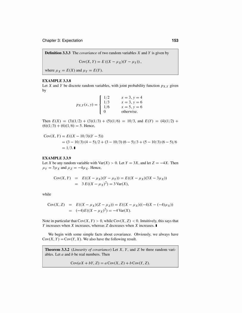
Chapter 3: Expectation 153
Definition 3.3.3 The covariance of two random variables X and Y is given by
Cov(X,Y ) = E ((X − µX )(Y − µY )) ,
where µX = E(X) and µY = E(Y ).
EXAMPLE 3.3.8Let X and Y be discrete random variables, with joint probability function pX,Y givenby
pX,Y (x, y) =
1/2 x = 3, y = 41/3 x = 3, y = 61/6 x = 5, y = 60 otherwise.
Then E(X) = (3)(1/2) + (3)(1/3) + (5)(1/6) = 10/3, and E(Y ) = (4)(1/2) +(6)(1/3)+ (6)(1/6) = 5. Hence,
Cov(X, Y ) = E((X − 10/3)(Y − 5))
= (3− 10/3) (4− 5)/2+ (3− 10/3) (6− 5)/3+ (5− 10/3) (6− 5)/6
= 1/3.
EXAMPLE 3.3.9Let X be any random variable with Var(X) > 0. Let Y = 3X , and let Z = −4X . ThenµY = 3µX and µZ = −4µX . Hence,
Cov(X, Y ) = E((X − µX )(Y − µY )) = E((X − µX )(3X − 3µX ))
= 3 E((X − µX )2) = 3 Var(X),
while
Cov(X, Z) = E((X − µX )(Z − µZ )) = E((X − µX )((−4)X − (−4)µX ))
= (−4)E((X − µX )2) = −4 Var(X).
Note in particular that Cov(X,Y ) > 0, while Cov(X, Z) < 0. Intuitively, this says thatY increases when X increases, whereas Z decreases when X increases.
We begin with some simple facts about covariance. Obviously, we always haveCov(X, Y ) =Cov(Y, X).We also have the following result.
Theorem 3.3.2 (Linearity of covariance) Let X , Y , and Z be three random vari-ables. Let a and b be real numbers. Then
Cov(aX + bY, Z) = a Cov(X, Z)+ b Cov(Y, Z).

154 Section 3.3: Variance, Covariance, and Correlation
PROOF Note that by linearity, µaX+bY ≡ E(aX + bY ) = aE(X) + bE(Y ) ≡aµX + bµY . Hence,
Cov(aX + bY, Z) = E (aX + bY − µaX+bY )(Z − µZ )
= E ((aX + bY − aµX − bµY )(Z − µZ ))
= E ((aX − aµX + bY − bµY )(Z − µZ ))
= aE ((X − µX )(Z − µZ ))+ bE ((Y − µY )(Z − µZ ))
= a Cov(X, Z)+ b Cov(Y, Z),
and the result is established.
We also have the following identity, which is similar to Theorem 3.3.1(c).
Theorem 3.3.3 Let X and Y be two random variables. Then
Cov(X, Y ) = E(XY )− E(X)E(Y ).
PROOF Using linearity, we have
Cov(X,Y ) = E ((X − µX )(Y − µY )) = E (XY − µX Y − XµY + µXµY )
= E(XY )− µX E(Y )− E(X)µY + µXµY
= E(XY )− µXµY − µXµY + µXµY = E(XY )− µXµY .
Corollary 3.3.2 If X and Y are independent, then Cov(X, Y ) = 0.
PROOF Because X and Y are independent, we know (Theorems 3.1.3 and 3.2.3)that E(XY ) = E(X) E(Y ). Hence, the result follows immediately from Theorem 3.3.3.
We note that the converse to Corollary 3.3.2 is false, as the following exampleshows.
EXAMPLE 3.3.10 Covariance 0 Does Not Imply Independence.Let X and Y be discrete random variables, with joint probability function pX,Y givenby
pX,Y (x, y) =
1/4 x = 3, y = 51/4 x = 4, y = 91/4 x = 7, y = 51/4 x = 6, y = 90 otherwise.
Then E(X) = (3)(1/4) + (4)(1/4) + (7)(1/4) + (6)(1/4) = 5, E(Y ) = (5)(1/4) +(9)(1/4) + (5)(1/4) + (9)(1/4) = 7, and E(XY ) = (3)(5)(1/4) + (4)(9)(1/4) +(7)(5)(1/4) + (6)(9)(1/4) = 35. We obtain Cov(X,Y ) = E(XY ) − E(X) E(Y ) =35− (5)(7) = 0.

Chapter 3: Expectation 155
On the other hand, X and Y are clearly not independent. For example, P(X =4) > 0 and P(Y = 5) > 0, but P(X = 4, Y = 5) = 0, so P(X = 4, Y = 5) =P(X = 4) P(Y = 5).
There is also an important relationship between variance and covariance.
Theorem 3.3.4(a) For any random variables X and Y ,
Var(X + Y ) = Var(X)+ Var(Y )+ 2 Cov(X, Y ).
(b) More generally, for any random variables X1, . . . , Xn ,
Vari
Xi =i
Var(Xi )+ 2i< j
Cov(Xi , X j).
PROOF We prove part (b) here; part (a) then follows as the special case n = 2.Note that by linearity,
µi Xi
≡ Ei
Xi =i
E(Xi ) ≡i
µXi.
Therefore, we have that
Vari
Xi
= E
i
Xi − µ i Xi
2 = E
i
Xi −i
µi
2
= E
i
(Xi − µi )
2 = E
i
(Xi − µi )j
(X j − µ j )
= Ei, j
(Xi − µi ) (X j − µ j ) =i, j
E((Xi − µi ) (X j − µ j ))
=i= j
E((Xi − µi ) (X j − µ j ))+ 2i< j
E((Xi − µi ) (X j − µ j ))
=i
Var(Xi )+ 2i< j
Cov(Xi , X j ).
Combining Theorem 3.3.4 with Corollary 3.3.2, we obtain the following.
Corollary 3.3.3(a) If X and Y are independent, then Var(X + Y ) =Var(X)+Var(Y ).(b) If X1, . . . , Xn are independent, then Var n
i=1 Xi = ni=1Var(Xi ).

156 Section 3.3: Variance, Covariance, and Correlation
One use of Corollary 3.3.3 is the following.
EXAMPLE 3.3.11Let Y ∼ Binomial(n, θ). What is Var(Y )? Recall that we can write
Y = X1 + X2 + · · · + Xn,
where the Xi are independent, with Xi ∼ Bernoulli(θ). We have already seen thatVar(Xi ) = θ(1− θ). Hence, from Corollary 3.3.3,
Var(Y ) = Var(X1)+Var(X2)+ · · · + Var(Xn)
= θ(1− θ)+ θ(1− θ)+ · · · + θ(1− θ) = nθ(1− θ).Another concept very closely related to covariance is correlation.
Definition 3.3.4 The correlation of two random variables X and Y is given by
Corr(X,Y ) = Cov(X, Y )Sd(X)Sd(Y )
= Cov(X, Y )√Var(X)Var(Y )
provided Var(X) <∞ and Var(Y ) <∞.EXAMPLE 3.3.12As in Example 3.3.2, let X be any random variable with Var(X) > 0, let Y = 3X , andlet Z = −4X . Then Cov(X,Y ) = 3 Var(X) and Cov(X, Z) = −4 Var(X). But byCorollary 3.3.1, Sd(Y ) = 3 Sd(X) and Sd(Z) = 4 Sd(X). Hence,
Corr(X, Y ) = Cov(X,Y )Sd(X)Sd(Y )
= 3 Var(X)Sd(X)3 Sd(X)
= Var(X)
Sd(X)2= 1,
because Sd(X)2 = Var(X). Also, we have that
Corr(X, Z) = Cov(X, Z)
Sd(X)Sd(Z)= −4 Var(X)
Sd(X)4 Sd(X)= −Var(X)
Sd(X)2= −1.
Intuitively, this again says that Y increases when X increases, whereas Z decreaseswhen X increases. However, note that the scale factors 3 and −4 have cancelled out;only their signs were important.
We shall see later, in Section 3.6, that we always have −1 ≤Corr(X,Y ) ≤ 1, forany random variables X and Y . Hence, in Example 3.3.12, Y has the largest possiblecorrelation with X (which makes sense because Y increases whenever X does, withoutexception), while Z has the smallest possible correlation with X (which makes sensebecause Z decreases whenever X does). We will also see that Corr(X, Y ) is a measureof the extent to which a linear relationship exists between X and Y .
EXAMPLE 3.3.13 The Bivariate Normal(µ1, µ2, σ 1, σ 2, ρ) DistributionWe defined this distribution in Example 2.7.9. It turns out that when (X,Y ) follows thisjoint distribution then, (from Problem 2.7.13) X ∼ N(µ1, σ
21) and Y ∼ N(µ2, σ
22).
Further, we have that (see Problem 3.3.17) Corr(X,Y ) = ρ. In the following graphs,

Chapter 3: Expectation 157
we have plotted samples of n = 1000 values of (X, Y ) from bivariate normal distrib-utions with µ1 = µ2 = 0, σ 2
1 = σ 22 = 1, and various values of ρ. Note that we used
(2.7.1) to generate these samples.From these plots we can see the effect of ρ on the joint distribution. Figure 3.3.2
shows that when ρ = 0, the point cloud is roughly circular. It becomes elliptical inFigure 3.3.3 with ρ = 0.5, and more tightly concentrated about a line in Figure 3.3.4with ρ = 0.9. As we will see in Section 3.6, the points will lie exactly on a line whenρ = 1.
Figure 3.3.5 demonstrates the effect of a negative correlation. With positive corre-lations, the value of Y tends to increase with X, as reflected in the upward slope of thepoint cloud. With negative correlations, Y tends to decrease with X, as reflected in thenegative slope of the point cloud.
543210-1-2-3-4-5
4
3
2
1
0
-1
-2
-3
-4
X
Y
Figure 3.3.2: A sample of n = 1000 values (X,Y ) from the Bivariate Normal (0, 0, 1, 1, 0)distribution.
543210-1-2-3-4-5
4
3
2
1
0
-1
-2
-3
-4
X
Y
Figure 3.3.3: A sample of n = 1000 values (X, Y ) from the Bivariate Normal(0, 0, 1, 1, 0.5) distribution.

158 Section 3.3: Variance, Covariance, and Correlation
543210-1-2-3-4-5
4
3
2
1
0
-1
-2
-3
-4
X
YFigure 3.3.4: A sample of n = 1000 values (X,Y ) from the Bivariate Normal(0, 0, 1, 1, 0.9) distribution.
543210-1-2-3-4-5
4
3
2
1
0
-1
-2
-3
-4
X
Y
Figure 3.3.5: A sample of n = 1000 values (X,Y ) from the Bivariate Normal(0, 0, 1, 1,−0.9) distribution.
Summary of Section 3.3
• The variance of a random variable X measures how far it tends to be from itsmean and is given by Var(X) = E((X − µX )
2) = E(X2)− (E(X))2.
• The variances of many standard distributions were computed.
• The standard deviation of X equals Sd(X) = √Var(X).
• Var(X) ≥ 0, and Var(aX + b) = a2 Var(X); also Sd(aX + b) = |a|Sd(X).
• The covariance of random variables X and Y measures how they are related andis given by Cov(X,Y ) = E((X − µX )(Y − µy)) = E(XY )− E(X) E(Y ).
• If X and Y are independent, then Cov(X,Y ) = 0.
• Var(X + Y ) =Var(X)+Var(Y ) + 2 Cov(X,Y ). If X and Y are independent,this equals Var(X)+Var(Y ) .
• The correlation of X and Y is Corr(X, Y ) =Cov(X,Y )/(Sd(X)Sd(Y )).

Chapter 3: Expectation 159
EXERCISES
3.3.1 Suppose the joint probability function of X and Y is given by
pX,Y (x, y) =
1/2 x = 3, y = 51/6 x = 3, y = 91/6 x = 6, y = 51/6 x = 6, y = 90 otherwise,
with E(X) = 4, E(Y ) = 19/3, and E(XY ) = 26, as in Example 3.1.16.(a) Compute Cov(X, Y ).(b) Compute Var(X) and Var(Y ).(c) Compute Corr(X,Y ).3.3.2 Suppose the joint probability function of X and Y is given by
pX,Y (x, y) =
1/7 x = 5, y = 01/7 x = 5, y = 31/7 x = 5, y = 43/7 x = 8, y = 01/7 x = 8, y = 40 otherwise,
as in Example 2.7.5.(a) Compute E(X) and E(Y ).(b) Compute Cov(X, Y ).(c) Compute Var(X) and Var(Y ).(d) Compute Corr(X, Y ).3.3.3 Let X and Y have joint density
fX,Y (x, y) = 4x2y + 2y5 0 ≤ x ≤ 1, 0 ≤ y ≤ 10 otherwise,
as in Exercise 3.2.2. Compute Corr(X,Y ).3.3.4 Let X and Y have joint density
fX,Y (x, y) = 15x3y4 + 6x2y7 0 ≤ x ≤ 1, 0 ≤ y ≤ 10 otherwise.
Compute E(X), E(Y ), Var(X), Var(Y ), Cov(X,Y ), and Corr(X,Y ).3.3.5 Let Y and Z be two independent random variables, each with positive variance.Prove that Corr(Y, Z) = 0.3.3.6 Let X , Y , and Z be three random variables, and suppose that X and Z are inde-pendent. Prove that Cov(X + Y, Z) =Cov(Y, Z).3.3.7 Let X ∼ Exponential(3) and Y ∼ Poisson(5). Assume X and Y are independent.Let Z = X + Y .(a) Compute Cov(X, Z).(b) Compute Corr(X, Z).

160 Section 3.3: Variance, Covariance, and Correlation
3.3.8 Prove that the variance of the Uniform[L, R] distribution is given by the expres-sion (R − L)2/12.3.3.9 Prove that Var(X) = E(X (X − 1)) − E(X)E(X − 1). Use this to computedirectly from the probability function that when X ∼ Binomial(n, θ), then Var(X) =nθ (1− θ) .3.3.10 Suppose you flip three fair coins. Let X be the number of heads showing, andlet Y = X2. Compute E(X), E(Y ), Var(X), Var(Y ), Cov(X, Y ), and Corr(X, Y ).3.3.11 Suppose you roll two fair six-sided dice. Let X be the number showing on thefirst die, and let Y be the sum of the numbers showing on the two dice. Compute E(X),E(Y ), E(XY ), and Cov(X, Y ).3.3.12 Suppose you flip four fair coins. Let X be the number of heads showing, andlet Y be the number of tails showing. Compute Cov(X,Y ) and Corr(X, Y ).3.3.13 Let X and Y be independent, with X ∼Bernoulli(1/2) and Y ∼Bernoulli(1/3).Let Z = X + Y and W = X − Y . Compute Cov(Z,W) and Corr(Z,W ).3.3.14 Let X and Y be independent, with X ∼ Bernoulli(1/2) and Y ∼ N(0, 1). LetZ = X+Y and W = X−Y . Compute Var(Z), Var(W ), Cov(Z,W ), and Corr(Z,W).3.3.15 Suppose you roll one fair six-sided die and then flip as many coins as the num-ber showing on the die. (For example, if the die shows 4, then you flip four coins.) LetX be the number showing on the die, and Y be the number of heads obtained. ComputeCov(X,Y ).
PROBLEMS
3.3.16 Let X ∼ N (0, 1), and let Y = cX .(a) Compute limc 0 Cov(X,Y ).(b) Compute limc 0 Cov(X, Y ).(c) Compute limc 0 Corr(X,Y ).(d) Compute limc 0 Corr(X, Y ).(e) Explain why the answers in parts (c) and (d) are not the same.3.3.17 Let X and Y have the bivariate normal distribution, as in Example 2.7.9. Provethat Corr(X,Y ) = ρ. (Hint: Use (2.7.1).)3.3.18 Prove that the variance of the Geometric(θ) distribution is given by (1− θ) /θ2.(Hint: Use Exercise 3.3.9 and (1− θ)x = x (x − 1) (1− θ)x−2 .)3.3.19 Prove that the variance of the Negative-Binomial(r, θ) distribution is given byr(1− θ)/θ2. (Hint: Use Problem 3.3.18.)3.3.20 Let α > 0 and λ > 0, and let X ∼ Gamma(α, λ). Prove that Var(X) = α/λ2.(Hint: Recall Problem 3.2.16.)3.3.21 Suppose that X ∼ Weibull(α) distribution (see Problem 2.4.19). Prove thatVar(X) = (2/α + 1)− 2 (1/α + 1) . (Hint: Recall Problem 3.2.18.)3.3.22 Suppose that X ∼ Pareto(α) (see Problem 2.4.20) for α > 2. Prove thatVar(X) = α/((α − 1)2 (α − 2)). (Hint: Recall Problem 3.2.19.)3.3.23 Suppose that X follows the Laplace distribution (see Problem 2.4.22). Provethat Var(X) = 2. (Hint: Recall Problem 3.2.21.)

Chapter 3: Expectation 161
3.3.24 Suppose that X ∼ Beta(a, b) (see Problem 2.4.24). Prove that Var(X) =ab/((a + b)2(a + b+ 1)). (Hint: Recall Problem 3.2.22.)3.3.25 Suppose that (X1, X2, X3) ∼Multinomial(n, θ1, θ2, θ3). Prove that
Var(Xi ) = nθ i (1− θ i ), Cov(Xi , X j ) = −nθ iθ j , when i = j.
(Hint: Recall Problem 3.1.23.)3.3.26 Suppose that (X1, X2) ∼ Dirichlet(α1, α2, α3) (see Problem 2.7.17). Provethat
Var(Xi ) = αi (α1 + α2 + α3 − αi )
(α1 + α2 + α3)2 (α1 + α2 + α3 + 1)
,
Cov (X1, X2) = −α1α2
(α1 + α2 + α3)2 (α1 + α2 + α3 + 1)
.
(Hint: Recall Problem 3.2.23.)3.3.27 Suppose that X ∼ Hypergeometric(N,M, n). Prove that
Var(X) = nM
N1− M
N
N − n
N − 1.
(Hint: Recall Problem 3.1.21 and use Exercise 3.3.9.)3.3.28 Suppose you roll one fair six-sided die and then flip as many coins as the num-ber showing on the die. (For example, if the die shows 4, then you flip four coins.) LetX be the number showing on the die, and Y be the number of heads obtained. ComputeCorr(X, Y ).
CHALLENGES
3.3.29 Let Y be a nonnegative random variable. Prove that E(Y ) = 0 if and only ifP(Y = 0) = 1. (You may assume for simplicity that Y is discrete, but the result is truefor any Y .)3.3.30 Prove that Var(X) = 0 if and only if there is a real number c with P(X = c) =1. (You may use the result of Challenge 3.3.29.)3.3.31 Give an example of a random variable X , such that E(X) = 5, and Var(X) =∞.
3.4 Generating FunctionsLet X be a random variable. Recall that the cumulative distribution function of X ,defined by FX (x) = P(X ≤ x), contains all the information about the distribution ofX (see Theorem 2.5.1). It turns out that there are other functions — the probability-generating function and the moment-generating function — that also provide informa-tion (sometimes all the information) about X and its expected values.
Definition 3.4.1 Let X be a random variable (usually discrete). Then we define itsprobability-generating function, rX , by rX (t) = E(t X ) for t ∈ R1.

162 Section 3.4: Generating Functions
Consider the following examples of probability-generating functions.
EXAMPLE 3.4.1 The Binomial(n, θ) DistributionIf X ∼ Binomial(n, θ), then
rX (t) = E(t X ) =n
i=0
P(X = i)t i =n
i=0
n
iθ i(1− θ)n−i t i
=n
i=0
n
i(tθ)i (1− θ)n−i = (tθ + 1− θ)n,
using the binomial theorem.
EXAMPLE 3.4.2 The Poisson(λ) DistributionIf Y ∼ Poisson(λ), then
rY (t) = E(tY ) =∞
i=0
P(Y = i)t i =∞
i=0
e−λ λi
i!t i
=∞
i=0
e−λ (λt)i
i!= e−λeλt = eλ(t−1).
The following theorem tells us that once we know the probability-generating func-tion rX (t), then we can compute all the probabilities P(X = 0), P(X = 1), P(X = 2),etc.
Theorem 3.4.1 Let X be a discrete random variable, whose possible values are allnonnegative integers. Assume that rX (t0) <∞ for some t0 > 0. Then
rX (0) = P(X = 0),
rX (0) = P(X = 1),
rX (0) = 2 P(X = 2),
etc. In general,r (k)X (0) = k! P(X = k),
where r (k)X is the kth derivative of rX .
PROOF Because the possible values are all nonnegative integers of the form i =0, 1, 2, . . . , we have
rX (t) = E(t X ) =x
t x P(X = x) =∞
i=0
t i P(X = i)
= t0 P(X = 0)+ t1 P(X = 1)+ t2 P(X = 2)+ t3 P(X = 3)+ · · · ,so that
rX (t) = 1P(X = 0)+ t1 P(X = 1)+ t2 P(X = 2)+ t3 P(X = 3)+ · · · . (3.4.1)

Chapter 3: Expectation 163
Substituting t = 0 into (3.4.1), every term vanishes except the first one, and we obtainrX (0) = P(X = 0). Taking derivatives of both sides of (3.4.1), we obtain
rX (t) = 1P(X = 1)+ 2t1 P(X = 2)+ 3t2 P(X = 3)+ · · · ,and setting t = 0 gives rX (0) = P(X = 1). Taking another derivative of both sidesgives
rX (t) = 2P(X = 2)+ 3 · 2 t1 P(X = 3)+ · · ·and setting t = 0 gives rX (0) = 2 P(X = 2). Continuing in this way, we obtain thegeneral formula.
We now apply Theorem 3.4.1 to the binomial and Poisson distributions.
EXAMPLE 3.4.3 The Binomial(n, θ) DistributionFrom Example 3.4.1, we have that
rX (0) = (1− θ)nrX (0) = n(tθ + 1− θ)n−1(θ)
t=0= n(1− θ)n−1θ
rX (0) = n(n − 1)(tθ + 1− θ)n−2(θ)(θ)t=0= n(n − 1)(1− θ)n−2θ2,
etc. It is thus verified directly that
P(X = 0) = rX (0)
P(X = 1) = rX (0)
2 P(X = 2) = rX (0),
etc.
EXAMPLE 3.4.4 The Poisson(λ) DistributionFrom Example 3.4.2, we have that
rX (0) = e−λ
rX (0) = λe−λ
rX (0) = λ2e−λ,
etc. It is again verified that
P(X = 0) = rX (0)
P(X = 1) = rX (0)
2 P(X = 2) = rX (0),
etc.
From Theorem 3.4.1, we can see why rX is called the probability-generating func-tion. For, at least in the discrete case with the distribution concentrated on the non-negative integers, we can indeed generate the probabilities for X from rX . We thus

164 Section 3.4: Generating Functions
see immediately that for a random variable X that takes values only in {0, 1, 2, . . .},rX is unique. By this we mean that if X and Y are concentrated on {0, 1, 2, . . .} andrX = rY , then X and Y have the same distribution. This uniqueness property of theprobability-generating function can be very useful in trying to determine the distribu-tion of a random variable that takes only values in {0, 1, 2, . . .} .
It is clear that the probability-generating function tells us a lot — in fact, everything— about the distribution of random variables concentrated on the nonnegative integers.But what about other random variables? It turns out that there are other quantities,called moments, associated with random variables that are quite informative about theirdistributions.
Definition 3.4.2 Let X be a random variable, and let k be a positive integer. Thenthe kth moment of X is the quantity E(Xk), provided this expectation exists.
Note that if E(Xk) exists and is finite, it can be shown that E(Xl) exists and is finitewhen 0 ≤ l < k.
The first moment is just the mean of the random variable. This can be taken asa measure of where the central mass of probability for X lies in the real line, at leastwhen this distribution is unimodal (has a single peak) and is not too highly skewed. Thesecond moment E(X2), together with the first moment, gives us the variance throughVar(X) = E(X2)− (E(X))2 . Therefore, the first two moments of the distribution tellus about the location of the distribution and the spread, or degree of concentration, ofthat distribution about the mean. In fact, the higher moments also provide informationabout the distribution.
Many of the most important distributions of probability and statistics have all oftheir moments finite; in fact, they have what is called a moment-generating function.
Definition 3.4.3 Let X be any random variable. Then its moment-generating func-tion mX is defined by m X (s) = E(es X ) at s ∈ R1.
The following example computes the moment-generating function of a well-knowndistribution.
EXAMPLE 3.4.5 The Exponential(λ) DistributionLet X ∼ Exponential(λ). Then for s < λ,
mX (s) = E(es X ) =∞
−∞esx fX (x) dx =
∞
0esxλe−λx dx
=∞
0λ e(s−λ)x dx = λ e(s−λ)x
s − λx=∞x=0
= −λe(s−λ)0s − λ
= − λ
s − λ = λ(λ− s)−1.
A comparison of Definitions 3.4.1 and 3.4.3 immediately gives the following.
Theorem 3.4.2 Let X be any random variable. Then m X (s) = rX (es).

Chapter 3: Expectation 165
This result can obviously help us evaluate some moment-generating functions whenwe have rX already.
EXAMPLE 3.4.6Let Y ∼ Binomial(n, θ). Then we know that rY (t) = (tθ + 1− θ)n . Hence, mY (s) =rY (es) = (esθ + 1− θ)n .EXAMPLE 3.4.7Let Z ∼ Poisson(λ). Then we know that rZ (t) = eλ(t−1). Hence, mZ (s) = rZ (es) =eλ(e
s−1).
The following theorem tells us that once we know the moment-generating functionmX (t), we can compute all the moments E(X), E(X2), E(X3), etc.
Theorem 3.4.3 Let X be any random variable. Suppose that for some s0 > 0, it istrue that mX (s) <∞ whenever s ∈ (−s0, s0). Then
m X (0) = 1
m X (0) = E(X)
m X (0) = E(X2),
etc. In general,m(k)X (0) = E(Xk),
where m(k)X is the kth derivative of m X .
PROOF We know that m X (s) = E(es X ). We have
m X (0) = E(e0X ) = E(e0) = E(1) = 1.
Also, taking derivatives, we see3 that m X (s) = E(X es X ), so
mX (0) = E(X e0X ) = E(Xe0) = E(X).
Taking derivatives again, we see that m X (s) = E(X2es X ), so
m X (0) = E(X2 e0X ) = E(X2e0) = E(X2).
Continuing in this way, we obtain the general formula.
We now consider an application of Theorem 3.4.3.
EXAMPLE 3.4.8 The Mean and Variance of the Exponential(λ) DistributionUsing the moment-generating function computed in Example 3.4.5, we have
mX (s) = (−1)λ(λ− s)−2(−1) = λ(λ− s)−2.
3Strictly speaking, interchanging the order of derivative and expectation is justified by analytic functiontheory and requires that mX (s) <∞ whenever |s| < s0.

166 Section 3.4: Generating Functions
Therefore,E(X) = m X (0) = λ(λ− 0)−2 = λ/λ2 = 1/λ,
as it should. Also,
E(X2) = m X (0) = (−2)λ(λ− 0)−3(−1) = 2λ/λ3 = 2/λ2,
so we have
Var(X) = E(X2)− (E(X)) = (2/λ2)− (1/λ)2 = 1/λ2.
This provides an easy way of computing the variance of X .
EXAMPLE 3.4.9 The Mean and Variance of the Poisson(λ) DistributionIn Example 3.4.7, we obtained m Z (s) = exp (λ(es − 1)) . So we have
E(X) = m X (0) = λe0 exp λ(e0 − 1) = λ
E(X2) = m X (0) = λe0 exp λ(e0 − 1) + λe02
exp λ(e0 − 1) = λ+ λ2.
Therefore, Var(X) = E(X2)− (E(X))2 = λ+ λ2 − λ2 = λ.Computing the moment-generating function of a normal distribution is also impor-
tant, but it is somewhat more difficult.
Theorem 3.4.4 If X ∼ N(0, 1), then m X (s) = es2/2.
PROOF Because X has density φ(x) = (2π)−1/2 e−x2/2, we have that
m X (s) = E(es X ) =∞
−∞esxφ(x) dx =
∞
−∞esx 1√
2πe−x2/2 dx
= 1√2π
∞
−∞esx−(x2/2) dx = 1√
2π
∞
−∞e−(x−s)2/2+(s2/2) dx
= es2/2 1√2π
∞
−∞e−(x−s)2/2 dx.
Setting y = x − s (so that dy = dx), this becomes (using Theorem 2.4.2)
m X (s) = es2/2 1√2π
∞
−∞e−y2/2 dy = es2/2
∞
−∞φ(y) dy = es2/2,
as claimed.
One useful property of both probability-generating and moment-generating func-tions is the following.
Theorem 3.4.5 Let X and Y be random variables that are independent. Then wehave(a) rX+Y (t) = rX (t) rY (t), and(b) m X+Y (t) = m X (t)mY (t).

Chapter 3: Expectation 167
PROOF Because X and Y are independent, so are t X and tY (by Theorem 2.8.5).Hence, we know (by Theorems 3.1.3 and 3.2.3) that E(t X tY ) = E(t X ) E(tY ). Usingthis, we have
rX+Y (t) = E t X+Y = E t X tY = E(t X )E(tY ) = rX (t)rY (t).
Similarly,
mX+Y (t) = E et (X+Y ) = E et X etY = E(et X ) E(etY ) = mX (t)mY (t).
EXAMPLE 3.4.10Let Y ∼ Binomial(n, θ). Then, as in Example 3.1.15, we can write
Y = X1 + · · · + Xn,
where the {Xi } are i.i.d. with Xi ∼ Bernoulli(θ). Hence, Theorem 3.4.5 says we musthave rY (t) = rX1(t) rX2(t) · · · rXn (t). But for any i ,
rXi (t) =x
t x P(X = x) = t1θ + t0(1− θ) = θ t + 1− θ.
Hence, we must have
rY (t) = (θ t + 1− θ)(θ t + 1− θ) · · · (θ t + 1− θ) = (θ t + 1− θ)n,as already verified in Example 3.4.1.
Moment-generating functions, when defined in a neighborhood of 0, completelydefine a distribution in the following sense. (We omit the proof, which is advanced.)
Theorem 3.4.6 (Uniqueness theorem) Let X be a random variable, such that forsome s0 > 0, we have m X (s) < ∞ whenever s ∈ (−s0, s0). Then if Y is someother random variable with mY (s) = mX (s) whenever s ∈ (−s0, s0), then X and Yhave the same distribution.
Theorems 3.4.1 and 3.4.6 provide a powerful technique for identifying distribu-tions. For example, if we determine that the moment-generating function of X ismX (t) = exp s2/2 , then we know, from Theorems 3.4.4 and 3.4.6, that X ∼N(0, 1).We can use this approach to determine the distributions of some complicatedrandom variables.
EXAMPLE 3.4.11Suppose that Xi ∼ N(µi , σ
2i ) for i = 1, . . . , n and that these random variables are
independent. Consider the distribution of Y = ni=1 Xi .
When n = 1 we have (from Problem 3.4.15)
mY (s) = exp µ1s + σ21s2
2.

168 Section 3.4: Generating Functions
Then, using Theorem 3.4.5, we have that
mY (s) =n
i=1
m Xi (s) =n
i=1
exp µi s +σ 2
i s2
2
= expn
i=1
µi s +ni=1 σ
2i s2
2.
From Problem 3.4.15, and applying Theorem 3.4.6, we have that
Y ∼ Nn
i=1
µi ,n
i=1
σ 2i .
Generating functions can also help us with compound distributions, which are de-fined as follows.
Definition 3.4.4 Let X1, X2, . . . be i.i.d., and let N be a nonnegative, integer-valuedrandom variable which is independent of the {Xi }. Let
S =N
i=1
Xi . (3.4.2)
Then S is said to have a compound distribution.
A compound distribution is obtained from a sum of i.i.d. random variables, wherethe number of terms in the sum is randomly distributed independently of the terms inthe sum. Note that S = 0 when N = 0. Such distributions have applications in ar-eas like insurance, where the X1, X2, . . . are claims and N is the number of claimspresented to an insurance company during a period. Therefore, S represents the totalamount claimed against the insurance company during the period. Obviously, the in-surance company wants to study the distribution of S, as this will help determine whatit has to charge for insurance to ensure a profit.
The following theorem is important in the study of compound distributions.
Theorem 3.4.7 If S has a compound distribution as in (3.4.2), then(a) E(S) = E(X1)E(N).(b) mS(s) = rN (m X1(s)).
PROOF See Section 3.8 for the proof of this result.
3.4.1 Characteristic Functions (Advanced)
One problem with moment-generating functions is that they can be infinite in any openinterval about s = 0. Consider the following example.

Chapter 3: Expectation 169
EXAMPLE 3.4.12Let X be a random variable having density
fX (x) = 1/x2 x ≥ 10 otherwise.
Then
m X (s) = E(es X ) =∞
1esx(1/x2) dx.
For any s > 0, we know that esx grows faster than x2, so that limx→∞ esx/x2 = ∞.Hence, m X (s) =∞ whenever s > 0.
Does X have any finite moments? We have that
E(X) =∞
1x(1/x2) dx =
∞
1(1/x) dx = ln x |x=∞x=1 =∞,
so, in fact, the first moment does not exist. From this we conclude that X does not haveany moments.
The random variable X in the above example does not satisfy the condition ofTheorem 3.4.3 that m X (s) < ∞ whenever |s| < s0, for some s0 > 0. Hence, The-orem 3.4.3 (like most other theorems that make use of moment-generating functions)does not apply. There is, however, a similarly defined function that does not sufferfrom this defect, given by the following definition.
Definition 3.4.5 Let X be any random variable. Then we define its characteristicfunction, cX , by
cX (s) = E(eis X ) (3.4.3)
for s ∈ R1.
So the definition of cX is just like the definition of m X , except for the introductionof the imaginary number i = √−1. Using properties of complex numbers, we seethat (3.4.3) can also be written as cX (s) = E(cos(s X))+ i E(sin(sX)) for s ∈ R1.
Consider the following examples.
EXAMPLE 3.4.13 The Bernoulli DistributionLet X ∼ Bernoulli(θ). Then
cX (s) = E(eis X ) = (eis0)(1− θ)+ (eis1)(θ)
= (1)(1− θ)+ eis(θ) = 1− θ + θeis
= 1− θ + θ cos s + iθ sin s.
EXAMPLE 3.4.14Let X have probability function given by
pX (x) =
1/6 x = 21/3 x = 31/2 x = 40 otherwise.

170 Section 3.4: Generating Functions
Then
cX (s) = E(eis X ) = (eis2)(1/6)+ (eis3)(1/3)+ (eis4)(1/2)
= (1/6) cos 2s + (1/3) cos 3s + (1/2) cos 4s
+(1/6)i sin 2s + (1/3)i sin 3s + i(1/2) sin 4s.
EXAMPLE 3.4.15Let Z have probability function given by
pZ (z) = 1/2 z = 1
1/2 z = −10 otherwise.
Then
cZ (s) = E(eis Z ) = (eis)(1/2)+ (e−is)(1/2)
= (1/2) cos(s)+ (1/2) cos(−s)+ (1/2) sin(s)+ (1/2) sin(−s)
= (1/2) cos s + (1/2) cos s + (1/2) sin s − (1/2) sin s = cos s.
Hence, in this case, cZ (s) is a real (not complex) number for all s ∈ R1.Once we overcome our “fear” of imaginary and complex numbers, we can see
that the characteristic function is actually much better in some ways than the moment-generating function. The main advantage is that, because eis X = cos(s X)+ i sin(s X)and |eis X | = 1, the characteristic function (unlike the moment-generating function) isalways finite (although it could be a complex number).
Theorem 3.4.8 Let X be any random variable, and let s be any real number. ThencX (s) is finite.
The characteristic function has many properties similar to the moment-generatingfunction. In particular, we have the following. (The proof is just like the proof ofTheorem 3.4.3.)
Theorem 3.4.9 Let X be any random variable with its first k moments finite. ThencX (0) = 1, cX (0) = i E(X), cX (0) = i2 E(X2) = −E(X2), etc. In general,
c(k)X (0) = ik E(Xk), where i = √−1, and where c(k)X is the kth derivative of cX .
We also have the following. (The proof is just like the proof of Theorem 3.4.5.)
Theorem 3.4.10 Let X and Y be random variables which are independent. ThencX+Y (s) = cX (s) cY (s).
For simplicity, we shall generally not use characteristic functions in this book.However, it is worth keeping in mind that whenever we do anything with moment-generating functions, we could usually do the same thing in greater generality usingcharacteristic functions.

Chapter 3: Expectation 171
Summary of Section 3.4
• The probability-generating function of a random variable X is rX (t) = E(t X ).
• If X is discrete, then the derivatives of rX satisfy r (k)X (0) = k! P(X = k).
• The kth moment of a random variable X is E(Xk).
• The moment-generating function of a random variable X is mX (s) = E(es X ) =rX (es).
• The derivatives of m X satisfy m(k)X (0) = E(Xk), for k = 0, 1, 2, . . . .
• If X and Y are independent, then rX+Y (t) = rX (t) rY (y) and mX+Y (s) =m X (s)mY (s).
• If m X (s) is finite in a neighborhood of s = 0, then it uniquely characterizes thedistribution of X .
• The characteristic function cX (s) = E(eis X ) can be used in place of mX (s) toavoid infinities.
EXERCISES
3.4.1 Let Z be a discrete random variable with P(Z = z) = 1/2z for z = 1, 2, 3, . . . .(a) Compute rZ (t). Verify that rZ (0) = P(Z = 1) and rZ (0) = 2 P(Z = 2).(b) Compute m Z (t). Verify that m Z (0) = E(Z) and mZ (0) = E(Z2).3.4.2 Let X ∼ Binomial(n, θ). Use mX to prove that Var(X) = nθ(1− θ).3.4.3 Let Y ∼ Poisson(λ). Use mY to compute the mean and variance of Y .3.4.4 Let Y = 3X + 4. Compute rY (t) in terms of rX .3.4.5 Let Y = 3X + 4. Compute mY (s) in terms of mX .3.4.6 Let X ∼ Binomial(n, θ). Compute E(X3), the third moment of X .3.4.7 Let Y ∼ Poisson(λ). Compute E(Y 3), the third moment of Y .3.4.8 Suppose P(X = 2) = 1/2, P(X = 5) = 1/3, and P(X = 7) = 1/6.(a) Compute rX (t) for t ∈ R1.(b) Verify that rX (0) = P(X = 1) and rX (0) = 2P(X = 2).(c) Compute mX (s) for s ∈ R1.(d) Verify that mX (0) = E(X) and mX (0) = E(X2).
PROBLEMS
3.4.9 Suppose fX (x) = 1/10 for 0 < x < 10, with fX (x) = 0 otherwise.(a) Compute mX (s) for s ∈ R1.(b) Verify that mX (0) = E(X). (Hint: L’Hôpital’s rule.)3.4.10 Let X ∼ Geometric(θ). Compute rX (t) and rX (0)/2.3.4.11 Let X ∼ Negative-Binomial(r, θ). Compute rX (t) and rX (0)/2.3.4.12 Let X ∼ Geometric(θ).(a) Compute mX (s).(b) Use m X to compute the mean of X .(c) Use m X to compute the variance of X .

172 Section 3.4: Generating Functions
3.4.13 Let X ∼ Negative-Binomial(r, θ).(a) Compute m X (s).(b) Use m X to compute the mean of X .(c) Use mX to compute the variance of X .3.4.14 If Y = a + bX, where a and b are constants, then show that rY (t) = tarX (tb)and mY (t) = eatm X (bt).
3.4.15 Let Z ∼ N(µ, σ 2). Show that
mZ (s) = exp µs + σ2s2
2.
(Hint: Write Z = µ+ σ X where X ∼ N(0, 1), and use Theorem 3.4.4.)3.4.16 Let Y be distributed according to the Laplace distribution (see Problem 2.4.22).(a) Compute mY (s). (Hint: Break up the integral into two pieces.)(b) Use mY to compute the mean of Y .(c) Use mY to compute the variance of Y .3.4.17 Compute the kth moment of the Weibull(α) distribution in terms of (seeProblem 2.4.19).3.4.18 Compute the kth moment of the Pareto(α) distribution (see Problem 2.4.20).(Hint: Make the transformation u = (1+ x)−1 and recall the beta distribution.)3.4.19 Compute the kth moment of the Log-normal(τ) distribution (see Problem 2.6.17).(Hint: Make the transformation z = ln x and use Problem 3.4.15.)3.4.20 Prove that the moment-generating function of the Gamma(α, λ) distribution isgiven by λα/ (λ− t)α when t < λ.3.4.21 Suppose that Xi ∼ Poisson(λi ) and X1, . . . , Xn are independent. Using moment-generating functions, determine the distribution of Y = n
i=1 Xi .
3.4.22 Suppose that Xi ∼ Negative-Binomial(ri , θ) and X1, . . . , Xn are independent.Using moment-generating functions, determine the distribution of Y = n
i=1 Xi .
3.4.23 Suppose that Xi ∼ Gamma(αi , λ) and X1, . . . , Xn are independent. Usingmoment-generating functions, determine the distribution of Y = n
i=1 Xi .
3.4.24 Suppose X1, X2, . . . is i.i.d. Exponential(λ) and N ∼ Poisson(λ) independentof the {Xi }. Determine the moment-generating function of SN . Determine the firstmoment of this distribution by differentiating this function.3.4.25 Suppose X1, X2, . . . are i.i.d. Exponential(λ) random variables and N ∼Geometric(θ) , independent of the {Xi }. Determine the moment-generating functionof SN . Determine the first moment of this distribution by differentiating this function.3.4.26 Let X ∼ Bernoulli(θ). Use cX (s) to compute the mean of X .3.4.27 Let Y ∼ Binomial(n, θ).(a) Compute the characteristic function cY (s). (Hint: Make use of cX (s) in Problem3.4.26.)(b) Use cY (s) to compute the mean of Y .3.4.28 The characteristic function of the Cauchy distribution (see Problem 2.4.21) isgiven by c(t) = e−|t|. Use this to determine the characteristic function of the sample

Chapter 3: Expectation 173
mean
X = 1n
n
i=1
Xi
based on a sample of n from the Cauchy distribution. Explain why this implies that thesample mean is also Cauchy distributed. What do you find surprising about this result?3.4.29 The kth cumulant (when it exists) of a random variable X is obtained by cal-culating the kth derivative of ln cX (s) with respect to s, evaluating this at s = 0, anddividing by ik . Evaluate cX (s) and all the cumulants of the N(µ, σ 2) distribution.
3.5 Conditional ExpectationWe have seen in Sections 1.5 and 2.8 that conditioning on some event, or some randomvariable, can change various probabilities. Now, because expectations are defined interms of probabilities, it seems reasonable that expectations should also change whenconditioning on some event or random variable. Such modified expectations are calledconditional expectations, as we now discuss.
3.5.1 Discrete Case
The simplest case is when X is a discrete random variable, and A is some event ofpositive probability. We have the following.
Definition 3.5.1 Let X be a discrete random variable, and let A be some event withP(A) > 0. Then the conditional expectation of X, given A, is equal to
E(X | A) =x∈R1
x P(X = x | A) =x∈R1
xP(X = x, A)
P(A).
EXAMPLE 3.5.1Consider rolling a fair six-sided die, so that S = {1, 2, 3, 4, 5, 6}. Let X be the numbershowing, so that X (s) = s for s ∈ S. Let A = {3, 5, 6} be the event that the die shows3, 5, or 6. What is E(X | A)?
Here we know that
P(X = 3 | A) = P(X = 3 | X = 3, 5, or 6) = 1/3
and that, similarly, P(X = 5 | A) = P(X = 6 | A) = 1/3. Hence,
E(X | A) =x∈R1
x P(X = x | A)
= 3 P(X = 3 | A)+ 5 P(X = 5 | A)+ 6 P(X = 6 | A)
= 3(1/3)+ 5(1/3)+ 6(1/3) = 14/3.
Often we wish to condition on the value of some other random variable. If the otherrandom variable is also discrete, and if the conditioned value has positive probability,then this works as above.

174 Section 3.5: Conditional Expectation
Definition 3.5.2 Let X and Y be discrete random variables, with P(Y = y) > 0.Then the conditional expectation of X, given Y = y, is equal to
E(X |Y = y) =x∈R1
x P(X = x |Y = y) =x∈R1
xpX,Y (x, y)
pY (y).
EXAMPLE 3.5.2Suppose the joint probability function of X and Y is given by
pX,Y (x, y) =
1/7 x = 5, y = 01/7 x = 5, y = 31/7 x = 5, y = 43/7 x = 8, y = 01/7 x = 8, y = 40 otherwise.
Then
E(X |Y = 0) =x∈R1
x P(X = x |Y = 0)
= 5P(X = 5 |Y = 0)+ 8P(X = 8 |Y = 0)
= 5P(X = 5, Y = 0)
P(Y = 0)+ 8
P(X = 8, Y = 0)P(Y = 0)
= 51/7
1/7+ 3/7+ 8
3/71/7+ 3/7
= 294.
Similarly,
E(X |Y = 4) =x∈R1
x P(X = x |Y = 4)
= 5P(X = 5 |Y = 4)+ 8P(X = 8 |Y = 4)
= 51/7
1/7+ 1/7+ 8
1/71/7+ 1/7
= 13/2 .
Also,
E(X |Y = 3) =x∈R1
x P(X = x |Y = 3) = 5P(X = 5 |Y = 3)
= 51/71/7
= 5.
Sometimes we wish to condition on a random variable Y , without specifying in ad-vance on what value of Y we are conditioning. In this case, the conditional expectationE(X |Y ) is itself a random variable — namely, it depends on the (random) value of Ythat occurs.

Chapter 3: Expectation 175
Definition 3.5.3 Let X and Y be discrete random variables. Then the conditionalexpectation of X, given Y , is the random variable E(X |Y ), which is equal toE(X |Y = y) when Y = y. In particular, E(X |Y ) is a random variable thatdepends on the random value of Y .
EXAMPLE 3.5.3Suppose again that the joint probability function of X and Y is given by
pX,Y (x, y) =
1/7 x = 5, y = 01/7 x = 5, y = 31/7 x = 5, y = 43/7 x = 8, y = 01/7 x = 8 y = 40 otherwise.
We have already computed that E(X |Y = 0) = 29/4, E(X |Y = 4) = 13/2, andE(X |Y = 3) = 5. We can express these results together by saying that
E(X |Y ) = 29/4 Y = 0
5 Y = 313/2 Y = 4.
That is, E(X |Y ) is a random variable, which depends on the value of Y . Note that,because P(Y = y) = 0 for y = 0, 3, 4, the random variable E(X |Y ) is undefined inthat case; but this is not a problem because that case will never occur.
Finally, we note that just like for regular expectation, conditional expectation islinear.
Theorem 3.5.1 Let X1, X2, and Y be random variables; let A be an event; let a, b,and y be real numbers; and let Z = aX1 + bX2. Then(a) E(Z | A) = aE(X1 | A)+ bE(X2 | A).(b) E(Z |Y = y) = aE(X1 |Y = y)+ bE(X2 |Y = y).(c) E(Z |Y ) = aE(X1 |Y )+ bE(X2 |Y ).
3.5.2 Absolutely Continuous Case
Suppose now that X and Y are jointly absolutely continuous. Then conditioning onY = y, for some particular value of y, seems problematic, because P(Y = y) = 0.However, we have already seen in Section 2.8.2 that we can define a conditional densityfX |Y (x |y) that gives us a density function for X , conditional on Y = y. And becausedensity functions give rise to expectations, similarly conditional density functions giverise to conditional expectations, as follows.

176 Section 3.5: Conditional Expectation
Definition 3.5.4 Let X and Y be jointly absolutely continuous random variables,with joint density function fX,Y (x, y). Then the conditional expectation of X, givenY = y, is equal to
E(X |Y = y) =x∈R1
x fX |Y (x | y) dx =x∈R1
xfX,Y (x, y)
fY (y)dx .
EXAMPLE 3.5.4Let X and Y be jointly absolutely continuous, with joint density function fX,Y givenby
fX,Y (x, y) = 4x2y + 2y5 0 ≤ x ≤ 1, 0 ≤ y ≤ 10 otherwise.
Then for 0 < y < 1,
fY (y) =∞
−∞fX,Y (x, y) dx =
1
0(4x2y + 2y5) dx = 4y/3+ 2y5.
Hence,
E(X |Y = y) =x∈R1
xfX,Y (x, y)
fY (y)dx =
1
0x
4x2y + 2y5
4y/3+ 2y5 dx
= y + y5
4y/3+ 2y5= 1+ y4
4/3+ 2y4.
As in the discrete case, we often wish to condition on a random variable withoutspecifying in advance the value of that variable. Thus, E(X |Y ) is again a randomvariable, depending on the random value of Y .
Definition 3.5.5 Let X and Y be jointly absolutely continuous random variables.Then the conditional expectation of X, given Y , is the random variable E(X |Y ),which is equal to E(X |Y = y) when Y = y. Thus, E(X |Y ) is a random variablethat depends on the random value of Y .
EXAMPLE 3.5.5Let X and Y again have joint density
fX,Y (x, y) = 4x2y + 2y5 0 ≤ x ≤ 1, 0 ≤ y ≤ 10 otherwise.
We already know that E(X |Y = y) = 1+ y4 / 4/3+ 2y4 . This formula is validfor any y between 0 and 1, so we conclude that E(X |Y ) = 1+ Y 4 / 4/3+ 2Y 4 .Note that in this last formula, Y is a random variable, so E(X |Y ) is also a randomvariable.
Finally, we note that in the absolutely continuous case, conditional expectation isstill linear, i.e., Theorem 3.5.1 continues to hold.

Chapter 3: Expectation 177
3.5.3 Double Expectations
Because the conditional expectation E(X |Y ) is itself a random variable (as a functionof Y ), it makes sense to take its expectation, E (E(X |Y )). This is a double expectation.One of the key results about conditional expectation is that it is always equal to E(X).
Theorem 3.5.2 (Theorem of total expectation) If X and Y are random variables,then E (E(X |Y )) = E(X).
This theorem follows as a special case of Theorem 3.5.3 on the next page. But italso makes sense intuitively. Indeed, conditioning on Y will change the conditionalvalue of X in various ways, sometimes making it smaller and sometimes larger, de-pending on the value of Y . However, if we then average over all possible values of Y ,these various effects will cancel out, and we will be left with just E(X).
EXAMPLE 3.5.6Suppose again that X and Y have joint probability function
pX,Y (x, y) =
1/7 x = 5, y = 01/7 x = 5, y = 31/7 x = 5, y = 43/7 x = 8, y = 01/7 x = 8 y = 40 otherwise.
Then we know that
E(X |Y = y) = 29/4 y = 0
5 y = 313/2 y = 4.
Also, P(Y = 0) = 1/7+ 3/7 = 4/7, P(Y = 3) = 1/7, and P(Y = 4)= 1/7+ 1/7 = 2/7. Hence,
E (E(X |Y ))=
y∈R1
E(X |Y = y)P(Y = y)
= E(X |Y = 0)P(Y = 0)+ E(X |Y = 3)P(Y = 3)+ E(X |Y = 4)P(Y = 4)
= (29/4)(4/7)+ (5)(1/7)+ (13/2)(2/7) = 47/7.
On the other hand, we compute directly that E(X) = 5P(X = 5) + 8P(X = 8) =5(3/7)+ 8(4/7) = 47/7. Hence, E (E(X |Y )) = E(X), as claimed.
EXAMPLE 3.5.7Let X and Y again have joint density
fX,Y (x, y) = 4x2y + 2y5 0 ≤ x ≤ 1, 0 ≤ y ≤ 10 otherwise.

178 Section 3.5: Conditional Expectation
We already know that
E(X |Y ) = 1+ Y 4 / 4/3+ 2Y 4
and that fY (y) = 4y/3+ 2y5 for 0 ≤ y ≤ 1. Hence,
E (E(X |Y ))= E
1+ Y 4
4/3+ 2Y 4 =∞
−∞E(X |Y = y) fY (y) dy
=1
0
1+ y4
4/3+ 2y4 (4y/3+ 2y5) dy =1
0(y + y5) dy = 1/2+ 1/6 = 2/3.
On the other hand,
E(X) =∞
−∞
∞
−∞x fX,Y (x, y) dy dx =
1
0
1
0x (4x2 y + 2y5) dy dx
=1
0x (2x2 + 2/6) dx =
1
0(2x3 + x/3) dx = 2/4+ 1/6 = 2/3 .
Hence, E (E(X |Y )) = E(X), as claimed.
Theorem 3.5.2 is a special case (with g(y) ≡ 1) of the following more generalresult, which in fact characterizes conditional expectation.
Theorem 3.5.3 Let X and Y be random variables, and let g : R1 → R1 be anyfunction. Then E(g(Y )E(X |Y )) = E(g(Y )X).
PROOF See Section 3.8 for the proof of this result.
We also note the following related result. It says that, when conditioning on Y , anyfunction of Y can be factored out since it is effectively a constant.
Theorem 3.5.4 Let X and Y be random variables, and let g : R1 → R1 be anyfunction. Then E(g(Y )X |Y ) = g(Y )E(X |Y ).
PROOF See Section 3.8 for the proof of this result.
Finally, because conditioning twice on Y is the same as conditioning just once onY , we immediately have the following.
Theorem 3.5.5 Let X and Y be random variables. Then E(E(X |Y )|Y ) = E(X |Y ).
3.5.4 Conditional Variance (Advanced)
In addition to defining conditional expectation, we can define conditional variance. Asusual, this involves the expected squared distance of a random variable to its mean.
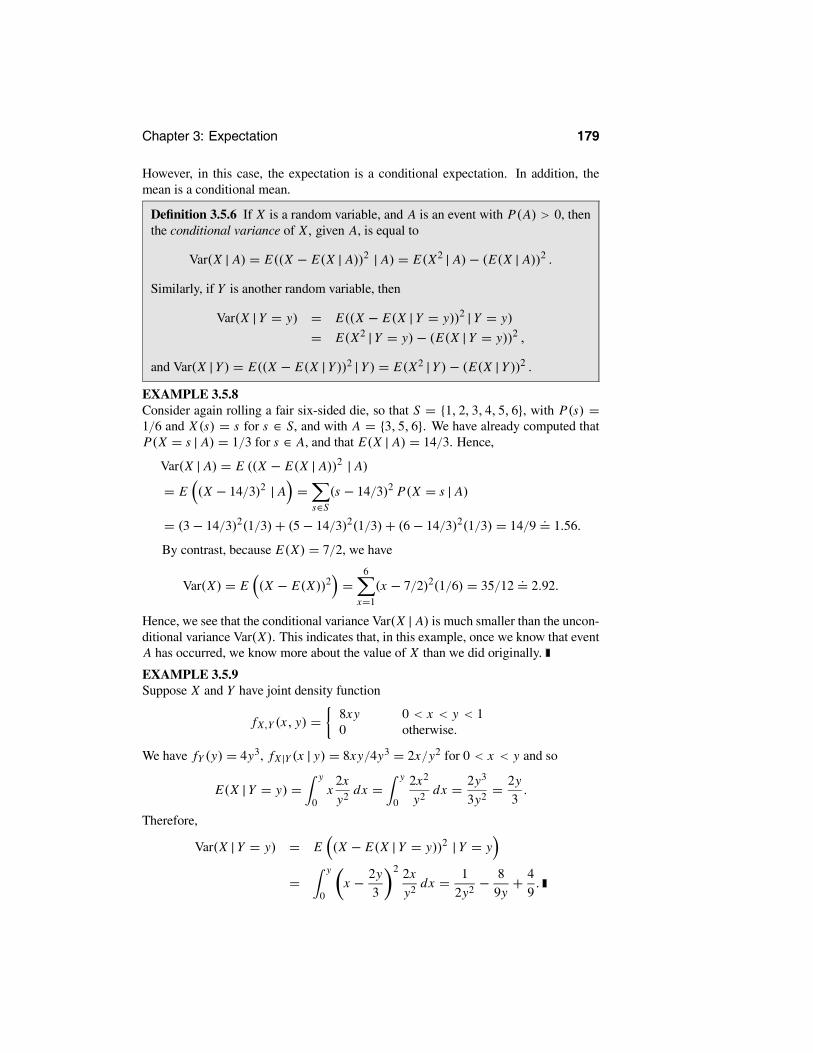
Chapter 3: Expectation 179
However, in this case, the expectation is a conditional expectation. In addition, themean is a conditional mean.
Definition 3.5.6 If X is a random variable, and A is an event with P(A) > 0, thenthe conditional variance of X, given A, is equal to
Var(X | A) = E((X − E(X | A))2 | A) = E(X2 | A)− (E(X | A))2 .
Similarly, if Y is another random variable, then
Var(X |Y = y) = E((X − E(X |Y = y))2 |Y = y)
= E(X2 |Y = y)− (E(X |Y = y))2 ,
and Var(X |Y ) = E((X − E(X |Y ))2 |Y ) = E(X2 |Y )− (E(X |Y ))2 .EXAMPLE 3.5.8Consider again rolling a fair six-sided die, so that S = {1, 2, 3, 4, 5, 6}, with P(s) =1/6 and X (s) = s for s ∈ S, and with A = {3, 5, 6}. We have already computed thatP(X = s | A) = 1/3 for s ∈ A, and that E(X | A) = 14/3. Hence,
Var(X | A) = E ((X − E(X | A))2 | A)
= E (X − 14/3)2 | A =s∈S
(s − 14/3)2 P(X = s | A)
= (3− 14/3)2(1/3)+ (5− 14/3)2(1/3)+ (6− 14/3)2(1/3) = 14/9.= 1.56.
By contrast, because E(X) = 7/2, we have
Var(X) = E (X − E(X))2 =6
x=1
(x − 7/2)2(1/6) = 35/12.= 2.92.
Hence, we see that the conditional variance Var(X | A) is much smaller than the uncon-ditional variance Var(X). This indicates that, in this example, once we know that eventA has occurred, we know more about the value of X than we did originally.
EXAMPLE 3.5.9Suppose X and Y have joint density function
fX,Y (x, y) = 8xy 0 < x < y < 10 otherwise.
We have fY (y) = 4y3, fX |Y (x | y) = 8xy/4y3 = 2x/y2 for 0 < x < y and so
E(X |Y = y) =y
0x
2x
y2dx =
y
0
2x2
y2dx = 2y3
3y2= 2y
3.
Therefore,
Var(X |Y = y) = E (X − E(X |Y = y))2 |Y = y
=y
0x − 2y
3
2 2x
y2dx = 1
2y2− 8
9y+ 4
9.

180 Section 3.5: Conditional Expectation
Finally, we note that conditional expectation and conditional variance satisfy thefollowing useful identity.
Theorem 3.5.6 For random variables X and Y ,
Var(X) = Var (E(X |Y ))+ E (Var(X |Y )) .
PROOF See Section 3.8 for the proof of this result.
Summary of Section 3.5
• If X is discrete, then the conditional expectation of X, given an event A, is equalto E(X | A) = x∈R1 x P(X = x | A).
• If X and Y are discrete random variables, then E(X |Y ) is itself a random vari-able, with E(X |Y ) equal to E(X |Y = y) when Y = y.
• If X and Y are jointly absolutely continuous, then E(X |Y ) is itself a randomvariable, with E(X |Y ) equal to E(X |Y = y) when Y = y, where E(X |Y =y) = x fX |Y (x | y) dx .
• Conditional expectation is linear.
• We always have that E (g(Y ) E(X |Y )) = E (g(Y ) X), and E (E(X |Y )|Y ) =E(X |Y ).
• Conditional variance is given by Var(X |Y ) = E(X2 |Y )− (E(X |Y ))2.
EXERCISES
3.5.1 Suppose X and Y are discrete, with
pX,Y (x, y) =
1/5 x = 2, y = 31/5 x = 3, y = 21/5 x = 3, y = 31/5 x = 2, y = 21/5 x = 3, y = 170 otherwise.
(a) Compute E(X |Y = 3).(b) Compute E(Y | X = 3).(c) Compute E(X |Y ).(d) Compute E(Y | X).3.5.2 Suppose X and Y are jointly absolutely continuous, with
fX,Y (x, y) = 9(xy + x5y5)/16, 000, 900 0 ≤ x ≤ 4, 0 ≤ y ≤ 50 otherwise.
(a) Compute fX (x).
Chapter 3: Expectation 181
(b) Compute fY (y).(c) Compute E(X |Y ).(d) Compute E(Y | X).(e) Compute E (E(X |Y )), and verify that it is equal to E(X).3.5.3 Suppose X and Y are discrete, with
pX,Y (x, y) =
1/11 x = −4, y = 22/11 x = −4, y = 34/11 x = −4, y = 71/11 x = 6, y = 21/11 x = 6, y = 31/11 x = 6, y = 71/11 x = 6, y = 130 otherwise.
(a) Compute E(Y | X = 6).(b) Compute E(Y | X = −4).(c) Compute E(Y | X).3.5.4 Let pX,Y be as in the previous exercise.(a) Compute E(X |Y = 2).(b) Compute E(X |Y = 3).(c) Compute E(X |Y = 7).(d) Compute E(X |Y = 13).(e) Compute E(X |Y ).3.5.5 Suppose that a student must choose one of two summer job offers. If it is not nec-essary to take a summer course, then a job as a waiter will produce earnings (roundedto the nearest $1000) with the following probability distribution.
$1000 $2000 $3000 $40000.1 0.3 0.4 0.2
If it is necessary to take a summer course, then a part-time job at a hotel will produceearnings (rounded to the nearest $1000) with the following probability distribution.
$1000 $2000 $3000 $40000.3 0.4 0.2 0.1
If the probability that the student will have to take the summer course is 0.6, thendetermine the student’s expected summer earnings.3.5.6 Suppose you roll two fair six-sided dice. Let X be the number showing on thefirst die, and let Z be the sum of the two numbers showing.(a) Compute E(X).(b) Compute E(Z | X = 1).(c) Compute E(Z | X = 6).(d) Compute E(X | Z = 2).(e) Compute E(X | Z = 4).

182 Section 3.5: Conditional Expectation
(f) Compute E(X | Z = 6).(g) Compute E(X | Z = 7).(h) Compute E(X | Z = 11).3.5.7 Suppose you roll two fair six-sided dice. Let Z be the sum of the two numbersshowing, and let W be the product of the two numbers showing.(a) Compute E(Z |W = 4).(b) Compute E(W | Z = 4).3.5.8 Suppose you roll one fair six-sided die and then flip as many coins as the numbershowing on the die. (For example, if the die shows 4, then you flip four coins.) Let Xbe the number showing on the die, and Y be the number of heads obtained.(a) Compute E(Y | X = 5).(b) Compute E(X |Y = 0).(c) Compute E(X |Y = 2).3.5.9 Suppose you flip three fair coins. Let X be the number of heads obtained, andlet Y = 1 if the first coin shows heads, otherwise Y = 0.(a) Compute E(X |Y = 0).(b) Compute E(X |Y = 1).(c) Compute E(Y | X = 0).(d) Compute E(Y | X = 1).(e) Compute E(Y | X = 2).(f) Compute E(Y | X = 3).(g) Compute E(Y | X).(h) Verify directly that E[E(Y | X)] = E(Y ).3.5.10 Suppose you flip one fair coin and roll one fair six-sided die. Let X be thenumber showing on the die, and let Y = 1 if the coin is heads with Y = 0 if the coin istails. Let Z = XY .(a) Compute E(Z).(b) Compute E(Z | X = 4).(c) Compute E(Y | X = 4).(d) Compute E(Y | Z = 4).(e) Compute E(X | Z = 4).3.5.11 Suppose X and Y are jointly absolutely continuous, with joint density functionfX,Y (x, y) = (6/19)(x2 + y3) for 0 < x < 2 and 0 < y < 1, otherwise fX,Y (x, y) =0.(a) Compute E(X).(b) Compute E(Y ).(c) Compute E(X |Y ).(d) Compute E(Y | X).(e) Verify directly that E[E(X |Y )] = E(X).(f) Verify directly that E[E(Y | X)] = E(Y ).
PROBLEMS
3.5.12 Suppose there are two urns. Urn I contains 100 chips: 30 are labelled 1, 40are labelled 2, and 30 are labelled 3. Urn 2 contains 100 chips: 20 are labelled 1,

Chapter 3: Expectation 183
50 are labelled 2, and 30 are labelled 3. A coin is tossed and if a head is observed,then a chip is randomly drawn from urn 1, otherwise a chip is randomly drawn fromurn 2. The value Y on the chip is recorded. If an occurrence of a head on the coinis denoted by X = 1, a tail by X = 0, and X ∼ Bernoulli(3/4) , then determineE(X |Y ), E(Y | X), E(Y ), and E(X).
3.5.13 Suppose that five coins are each tossed until the first head is obtained on eachcoin and where each coin has probability θ of producing a head. If you are told that thetotal number of tails observed is Y = 10, then determine the expected number of tailsobserved on the first coin.3.5.14 (Simpson’s paradox) Suppose that the conditional distributions of Y, given X,are shown in the following table. For example, pY |X (1 | i) could correspond to theprobability that a randomly selected heart patient at hospital i has a successful treat-ment.
pY |X (0 | 1) pY |X (1 | 1)0.030 0.970
pY |X (0 | 2) pY |X (1 | 2)0.020 0.980
(a) Compute E(Y | X).
(b) Now suppose that patients are additionally classified as being seriously ill (Z = 1),or not seriously ill (Z = 0). The conditional distributions of Y, given (X, Z), areshown in the following tables. Compute E(Y | X, Z).
pY |X,Z (0 | 1, 0) pY |X,Z (1 | 1, 0)0.010 0.990
pY |X,Z (0 | 2, 0) pY |X,Z (1 | 2, 0)0.013 0.987
pY |X,Z (0 | 1, 1) pY |X,Z (1 | 1, 1)0.038 0.962
pY |X,Z (0 | 2, 1) pY |X,Z (1 | 2, 1)0.040 0.960
(c) Explain why the conditional distributions in part (a) indicate that hospital 2 is thebetter hospital for a patient who needs to undergo this treatment, but all the conditionaldistributions in part (b) indicate that hospital 1 is the better hospital. This phenomenonis known as Simpson’s paradox.(d) Prove that, in general, pY |X (y | x) = z pY |X,Z (y | x, z) pZ |X (z | x) and E(Y | X)= E(E(Y | X, Z) | X).
(e) If the conditional distributions pZ |X (· | x) , corresponding to the example discussedin parts (a) through (c) are given in the following table, verify the result in part (d)numerically and explain how this resolves Simpson’s paradox.
pZ |X (0 | 1) pZ |X (1 | 1)0.286 0.714
pZ |X (0 | 2) pZ |X (1 | 2)0.750 0.250

184 Section 3.6: Inequalities
3.5.15 Present an example of a random variable X , and an event A with P(A) > 0,such that Var(X | A) >Var(X). (Hint: Suppose S = {1, 2, 3} with X (s) = s, andA = {1, 3}.)3.5.16 Suppose that X , given Y = y, is distributed Gamma(α, y) and that the marginaldistribution of Y is given by 1/Y ∼ Exponential(λ) . Determine E (X) .
3.5.17 Suppose that (X,Y ) ∼Bivariate Normal (µ1, µ2, σ 1, σ 2, ρ). Use (2.7.1) (whengiven Y = y) and its analog (when given X = x) to determine E(X |Y ), E(Y | X),Var(X |Y ), and Var(Y | X).
3.5.18 Suppose that (X1, X2, X3) ∼Multinomial(n, θ1, θ2, θ3). Determine E(X1 | X2)and Var(X1 | X2). (Hint: Show that X1, given X2 = x2, has a binomial distribution.)3.5.19 Suppose that (X1, X2) ∼ Dirichlet(α1, α2, α3). Determine E(X1 | X2) andVar(X1 | X2). (Hint: First show that X1/(1 − x2), given X2 = x2, has a beta dis-tribution and then use Problem 3.3.24.)3.5.20 Let fX,Y be as in Exercise 3.5.2.(a) Compute Var(X).(b) Compute Var(E(X |Y )).(c) Compute Var(X |Y ).(d) Verify that Var(X) =Var(E(X |Y ))+ E (Var(X |Y )).3.5.21 Suppose we have three discrete random variables X, Y, and Z . We say that Xand Y are conditionally independent, given Z, if
pX,Y |Z (x, y | z) = pX |Z (x | z) pY |Z (y | z)for every x, y, and z such that P (Z = z) > 0. Prove that when X and Y are condition-ally independent, given Z, then
E (g(X)h(Y ) | Z) = E (g(X) | Z) E (h(Y ) | Z) .
3.6 InequalitiesExpectation and variance are closely related to the underlying distributions of randomvariables. This relationship allows us to prove certain inequalities that are often veryuseful. We begin with a classic result, Markov’s inequality, which is very simple butalso very useful and powerful.
Theorem 3.6.1 (Markov’s inequality) If X is a nonnegative random variable, thenfor all a > 0,
P(X ≥ a) ≤ E(X)
a.
That is, the probability that X exceeds any given value a is no more than the meanof X divided by a.
PROOF Define a new random variable Z by
Z = a X ≥ a0 X < a.

Chapter 3: Expectation 185
Then clearly Z ≤ X , so that E(Z) ≤ E(X) by monotonicity. On the other hand,
E(Z) = a P(Z = a)+ 0 P(Z = 0) = a P(Z = a) = a P(X ≥ a).
So, E(X) ≥ E(Z) = a P(X ≥ a). Rearranging, P(X ≥ a) ≤ E(X)/a, as claimed.
Intuitively, Markov’s inequality says that if the expected value of X is small, thenit is unlikely that X will be too large. We now consider some applications of Theorem3.6.1.
EXAMPLE 3.6.1Suppose P(X = 3) = 1/2, P(X = 4) = 1/3, and P(X = 7) = 1/6. Then E(X) =3(1/2) + 4(1/3) + 7(1/6) = 4. Hence, setting a = 6, Markov’s inequality says thatP(X ≥ 6) ≤ 4/6 = 2/3. In fact, P(X ≥ 6) = 1/6 < 2/3.
EXAMPLE 3.6.2Suppose P(X = 2) = P(X = 8) = 1/2. Then E(X) = 2(1/2) + 8(1/2) = 5.Hence, setting a = 8, Markov’s inequality says that P(X ≥ 8) ≤ 5/8. In fact,P(X ≥ 8) = 1/2 < 5/8.
EXAMPLE 3.6.3Suppose P(X = 0) = P(X = 2) = 1/2. Then E(X) = 0(1/2) + 2(1/2) = 1.Hence, setting a = 2, Markov’s inequality says that P(X ≥ 2) ≤ 1/2. In fact,P(X ≥ 2) = 1/2, so Markov’s inequality is an equality in this case.
Markov’s inequality is also used to prove Chebychev’s inequality, perhaps the mostimportant inequality in all of probability theory.
Theorem 3.6.2 (Chebychev’s inequality) Let Y be an arbitrary random variable,with finite mean µY . Then for all a > 0,
P (|Y − µY | ≥ a) ≤ Var(Y )a2 .
PROOF Set X = (Y−µY )2. Then X is a nonnegative random variable. Thus, using
Theorem 3.6.1, we have P (|Y − µY | ≥ a) = P X ≥ a2 ≤ E(X)/a2 =Var(Y )/a2,and this establishes the result.
Intuitively, Chebychev’s inequality says that if the variance of Y is small, then itis unlikely that Y will be too far from its mean value µY . We now consider someexamples.
EXAMPLE 3.6.4Suppose again that P(X = 3) = 1/2, P(X = 4) = 1/3, and P(X = 7) = 1/6.Then E(X) = 4, as above. Also, E(X2) = 9(1/2) + 16(1/3) + 49(1/6) = 18, sothat Var(X) = 18 − 42 = 2. Hence, setting a = 1, Chebychev’s inequality saysthat P(|X − 4| ≥ 1) ≤ 2/12 = 2, which tells us nothing because we always haveP(|X − 4| ≥ 1) ≤ 1. On the other hand, setting a = 3, we get P(|X − 4| ≥ 3) ≤2/32 = 2/9, which is true because in fact P(|X − 4| ≥ 3) = P(X = 7) = 1/6 < 2/9.

186 Section 3.6: Inequalities
EXAMPLE 3.6.5Let X ∼ Exponential(3), and let a = 5. Then E(X) = 1/3 and Var(X) = 1/9. Hence,by Chebychev’s inequality with a = 1/2, P(|X−1/3| ≥ 1/2) ≤ (1/9)/(1/2)2 = 4/9.On the other hand, because X ≥ 0, P(|X − 1/3| ≥ 1/2) = P(X ≥ 5/6), andby Markov’s inequality, P(X ≥ 5/6) ≤ (1/3)/(5/6) = 2/5. Because 2/5 < 4/9, weactually get a better bound from Markov’s inequality than from Chebychev’s inequalityin this case.
EXAMPLE 3.6.6Let Z ∼ N(0, 1), and a = 5. Then by Chebychev’s inequality, P(|Z | ≥ 5) ≤ 1/5.
EXAMPLE 3.6.7Let X be a random variable having very small variance. Then Chebychev’s inequalitysays that P(|X−µX | ≥ a) is small whenever a is not too small. In other words, usually|X − µX | is very small, i.e., X ≈ µX . This makes sense, because if the variance of Xis very small, then usually X is very close to its mean value µX .
Inequalities are also useful for covariances, as follows.
Theorem 3.6.3 (Cauchy–Schwartz inequality) Let X and Y be arbitrary randomvariables, each having finite, nonzero variance. Then
|Cov(X, Y )| ≤ Var(X)Var(Y ).
Furthermore, if Var(Y ) > 0, then equality is attained if and only if X − µX =λ(Y − µY ) where λ =Cov(X,Y )/Var(Y ).
PROOF See Section 3.8 for the proof.
The Cauchy–Schwartz inequality says that if the variance of X or Y is small, thenthe covariance of X and Y must also be small.
EXAMPLE 3.6.8Suppose X = C is a constant. Then Var(X) = 0. It follows from the Cauchy–Schwartz inequality that, for any random variable Y , we must have Cov(X,Y ) ≤(Var(X)Var(Y ))1/2 = (0 Var(Y ))1/2 = 0, so that Cov(X,Y ) = 0.
Recalling that the correlation of X and Y is defined by
Corr(X,Y ) = Cov(X,Y )√Var(X)Var(Y )
,
we immediately obtain the following important result (which has already been referredto, back when correlation was first introduced).
Corollary 3.6.1 Let X and Y be arbitrary random variables, having finite meansand finite, nonzero variances. Then |Corr(X, Y )| ≤ 1. Furthermore, |Corr(X, Y )| =1 if and only if
X − µX = Cov(X, Y )Var (Y )
(Y − µY ).

Chapter 3: Expectation 187
So the correlation between two random variables is always between −1 and 1. Wealso see that X and Y are linearly related if and only if |Corr(X, Y )| = 1, and thatthis relationship is increasing (positive slope) when Corr(X,Y ) = 1 and decreasing(negative slope) when Corr(X, Y ) = −1.
3.6.1 Jensen’s Inequality (Advanced)
Finally, we develop a more advanced inequality that is sometimes very useful. A func-tion f is called convex if for every x < y, the line segment from (x, f (x)) to (y, f (y))lies entirely above the graph of f, as depicted in Figure 3.6.1.
2.0 2.5 3.0 3.5 4.0 4.5 5.0
100
200
300
400
500
600
x
f
Figure 3.6.1: Plot of the convex function f (x) = x4 and the line segment joining (2, f (2)) to(4, f (4)).
In symbols, we require that for every x < y and every 0 < λ < 1, we haveλ f (x) + (1 − λ) f (y) ≥ f (λx + (1 − λ)y). Examples of convex functions includef (x) = x2, f (x) = x4, and f (x) = max(x,C) for any real number C . We have thefollowing.
Theorem 3.6.4 (Jensen’s inequality) Let X be an arbitrary random variable, and letf : R1 → R1 be a convex function such that E( f (X)) is finite. Then f (E(X)) ≤E( f (X)). Equality occurs if and only if f (X) = a + bX for some a and b.
PROOF Because f is convex, we can find a linear function g(x) = ax + b suchthat g(E(X)) = f (E(X)) and g(x) ≤ f (x) for all x ∈ R1 (see, for example, Figure3.6.2).

188 Section 3.6: Inequalities
2.2 2.4 2.6 2.8 3.0 3.2 3.4 3.6 3.8 4.00
50
100
150
200
250
x
f
Figure 3.6.2: Plot of the convex function f (x) = x4 and the functiong(x) = 81+ 108(x − 3), satisfying g(x) ≤ f (x) on the interval (2, 4) .
But then using monotonicity and linearity, we have E( f (X)) ≥ E(g(X)) =E(aX + b) = aE(X)+ b = g(E(X)) = f (E(X)), as claimed.
We have equality if and only if 0 = E( f (X)− g(X)). Because f (X)− g(X) ≥ 0,this occurs (using Challenge 3.3.29) if and only if f (X) = g(X) = aX + b withprobability 1.
EXAMPLE 3.6.9Let X be a random variable with finite variance. Then setting f (x) = x2, Jensen’sinequality says that E(X2) ≥ (E(X))2. Of course, we already knew this becauseE(X2)− (E(X))2 =Var(X) ≥ 0.
EXAMPLE 3.6.10Let X be a random variable with finite fourth moment. Then setting f (x) = x4,Jensen’s inequality says that E(X4) ≥ (E(X))4.
EXAMPLE 3.6.11Let X be a random variable with finite mean, and let M ∈ R1. Then setting f (x) =max(x,M), we have that E(max(X,M)) ≥ max(E(X),M) by Jensen’s inequality. Infact, we could also have deduced this from the monotonicity property of expectation,using the two inequalities max(X,M) ≥ X and max(X,M) ≥ M.
Summary of Section 3.6
• For nonnegative X,Markov’s inequality says P(X ≥ a) ≤ E(X)/a.
• Chebychev’s inequality says P(|Y − µY | ≥ a) ≤Var(Y )/a2.
• The Cauchy–Schwartz inequality says |Cov(X, Y )| ≤ (Var(X)Var(Y ))1/2, sothat |Corr(X, Y )| ≤ 1.

Chapter 3: Expectation 189
• Jensen’s inequality says f (E(X)) ≤ E( f (X)) whenever f is convex.
EXERCISES
3.6.1 Let Z ∼ Poisson(3). Use Markov’s inequality to get an upper bound on P(Z ≥7).3.6.2 Let X ∼ Exponential(5). Use Markov’s inequality to get an upper bound onP(X ≥ 3) and compare it with the precise value.3.6.3 Let X ∼ Geometric(1/2).(a) Use Markov’s inequality to get an upper bound on P(X ≥ 9).(b) Use Markov’s inequality to get an upper bound on P(X ≥ 2).(c) Use Chebychev’s inequality to get an upper bound on P(|X − 1| ≥ 1).(d) Compare the answers obtained in parts (b) and (c).3.6.4 Let Z ∼ N(5, 9). Use Chebychev’s inequality to get an upper bound on P(|Z −5| ≥ 30).3.6.5 Let W ∼ Binomial(100, 1/2), as in the number of heads when flipping 100 faircoins. Use Chebychev’s inequality to get an upper bound on P(|W − 50| ≥ 10).3.6.6 Let Y ∼ N(0, 100), and let Z ∼ Binomial(80, 1/4). Determine (with explana-tion) the largest and smallest possible values of Cov(Y, Z).3.6.7 Let X ∼ Geometric(1/11). Use Jensen’s inequality to determine a lower boundon E(X4), in two different ways.(a) Apply Jensen’s inequality to X with f (x) = x4.(b) Apply Jensen’s inequality to X2 with f (x) = x2.3.6.8 Let X be the number showing on a fair six-sided die. What bound does Cheby-chev’s inequality give for P(X ≥ 5 or X ≤ 2)?3.6.9 Suppose you flip four fair coins. Let Y be the number of heads obtained.(a) What bound does Chebychev’s inequality give for P(Y ≥ 3 or Y ≤ 1)?(b) What bound does Chebychev’s inequality give for P(Y ≥ 4 or Y ≤ 0)?3.6.10 Suppose W has density function f (w) = 3w2 for 0 < w < 1, otherwisef (w) = 0.(a) Compute E(W).(b) What bound does Chebychev’s inequality give for P(|W − E(W )| ≥ 1/4)?3.6.11 Suppose Z has density function f (z) = z3/4 for 0 < z < 2, otherwise f (z) =0.(a) Compute E(Z).(b) What bound does Chebychev’s inequality give for P(|Z − E(Z)| ≥ 1/2)?3.6.12 Suppose Var(X) = 4 and Var(Y ) = 9.(a) What is the largest possible value of Cov(X, Y )?(b) What is the smallest possible value of Cov(X,Y )?(c) Suppose Z = 3X/2. Compute Var(Z) and Cov(X, Z), and compare your answerwith part (a).(d) Suppose W = −3X/2. Compute Var(W ) and Cov(W, Z), and compare your an-swer with part (b).

190 Section 3.6: Inequalities
3.6.13 Suppose a species of beetle has length 35 millimeters on average. Find an upperbound on the probability that a randomly chosen beetle of this species will be over 80millimeters long.
PROBLEMS
3.6.14 Prove that for any > 0 and δ > 0, there is a positive integer M, such that if Xis the number of heads when flipping M fair coins, then P(|(X/M)− (1/2)| ≥ δ) ≤ .3.6.15 Prove that for any µ and σ 2 > 0, there is a > 0 and a random variable X withE(X) = µ and Var(X) = σ 2, such that Chebychev’s inequality holds with equality,i.e., such that P(|X − µ| ≥ a) = σ 2/a2.3.6.16 Suppose that (X,Y ) is uniform on the set {(x1, y1) , . . . , (xn, yn)} where thex1, . . . , xn are distinct values and the y1, . . . , yn are distinct values.(a) Prove that X is uniformly distributed on x1, . . . , xn, with mean given by x =n−1 n
i=1 xi and variance given by s2X = n−1 n
i=1 (xi − x)2 .
(b) Prove that the correlation coefficient between X and Y is given by
rXY =ni=1 (xi − x) (yi − y)
ni=1 (xi − x)2 n
i=1 (yi − y)2= sXY
sX sY
where sXY = n−1 ni=1 (xi − x) (yi − y) . The value sXY is referred to as the sample
covariance and rXY is referred to as the sample correlation coefficient when the values(x1, y1) , . . . , (xn, yn) are an observed sample from some bivariate distribution.(c) Argue that rXY is also the correlation coefficient between X and Y when we dropthe assumption of distinctness for the xi and yi .(d) Prove that −1 ≤ rXY ≤ 1 and state the conditions under which rXY = ±1.3.6.17 Suppose that X is uniformly distributed on {x1, . . . , xn} and so has mean x =n−1 n
i=1 xi and variance s2X = n−1 n
i=1 (xi − x)2 (see Problem 3.6.16(a)). What isthe largest proportion of the values xi that can lie outside x − 2sX , x + 2sX ?
3.6.18 Suppose that X is distributed with density given by fX (x) = 2/x3 for x > 1and is 0 otherwise.(a) Prove that fX is a density.(b) Calculate the mean of X.
(c) Compute P(X ≥ k) and compare this with the upper bound on this quantity givenby Markov’s inequality.(d) What does Chebyshev’s inequality say in this case?3.6.19 Let g(x) = max(−x,−10).(a) Verify that g is a convex function.(b) Suppose Z ∼ Exponential(5). Use Jensen’s inequality to obtain a lower bound onE(g(Z)).3.6.20 It can be shown that a function f, with continuous second derivative, is convexon (a, b) if f (x) > 0 for all x ∈ (a, b) .(a) Use the above fact to show that f (x) = x p is convex on (0,∞) whenever p ≥ 1.

Chapter 3: Expectation 191
(b) Use part (a) to prove that E |X |p 1/p ≥ |E (X)| whenever p ≥ 1.(c) Prove that Var(X) = 0 if and only if X is degenerate at a constant c.
CHALLENGES
3.6.21 Determine (with proof) all functions that are convex and whose negatives arealso convex. (That is, find all functions f such that f is convex, and also − f isconvex.)
3.7 General Expectations (Advanced)So far we have considered expected values separately for discrete and absolutely con-tinuous random variables only. However, this separation into two different “cases” mayseem unnatural. Furthermore, we know that some random variables are neither discretenor continuous — for example, mixtures of discrete and continuous distributions.
Hence, it seems desirable to have a more general definition of expected value. Suchgenerality is normally considered in the context of general measure theory, an advancedmathematical subject. However, it is also possible to give a general definition in ele-mentary terms, as follows.
Definition 3.7.1 Let X be an arbitrary random variable (perhaps neither discretenor continuous). Then the expected value of X is given by
E(X) =∞
0P(X > t) dt −
0
−∞P(X < t) dt,
provided either ∞0 P(X > t) dt <∞ or 0
−∞ P(X < t) dt <∞.
This definition appears to contradict our previous definitions of E(X). However, infact, there is no contradiction, as the following theorem shows.
Theorem 3.7.1(a) Let X be a discrete random variable with distinct possible values x1, x2, . . . ,and put pi = P(X = xi). Then Definition 3.7.1 agrees with the previous definitionof E(X). That is,
∞
0P(X > t) dt −
0
−∞P(X < t) dt =
i
xi pi .
(b) Let X be an absolutely continuous random variable with density fX . ThenDefinition 3.7.1 agrees with the previous definition of E(X). That is,
∞
0P(X > t) dt −
0
−∞P(X < t) dt =
∞
−∞x fX (x) dx.
PROOF The key to the proof is switching the order of the integration/summation.

192 Section 3.7: General Expectations (Advanced)
(a) We have
∞
0P(X > t) dt =
∞
0 i,xi>t
pi dt =i
pi
xi
0dt =
i
pi xi ,
as claimed.
(b) We have
∞
0P(X > t) dt =
∞
0
∞
tfX (x) dx dt =
∞
0
x
0fX (x) dt dx
=∞
0x fX (x) dx .
Similarly,
0
−∞P(X < t) dt =
0
−∞
t
−∞fX (x) dx dt =
0
−∞
0
xfX (x) dt dx
=0
−∞(−x) fX (x) dx.
Hence,
∞
0P(X > t) dt −
0
−∞P(X < t) dt =
∞
0x fX (x) dx −
0
−∞(−x) fX (x) dx
=∞
−∞x fX (x) dx,
as claimed.
In other words, Theorem 3.7.1 says that Definition 3.7.1 includes our previous defi-nitions of expected value, for both discrete and absolutely continuous random variables,while working for any random variable at all. (Note that to apply Definition 3.7.1 wetake an integral, not a sum, regardless of whether X is discrete or continuous!)
Furthermore, Definition 3.7.1 preserves the key properties of expected value, asthe following theorem shows. (We omit the proof here, but see Challenge 3.7.10 for aproof of part (c).)
Theorem 3.7.2 Let X and Y be arbitrary random variables, perhaps neither discretenor continuous, with expected values defined by Definition 3.7.1.(a) (Linearity) If a and b are any real numbers, then E(aX+bY ) = aE(X)+bE(Y ).(b) If X and Y are independent, then E(XY ) = E(X) E(Y ).(c) (Monotonicity) If X ≤ Y , then E(X) ≤ E(Y ).
Definition 3.7.1 also tells us about expected values of mixture distributions, as fol-lows.

Chapter 3: Expectation 193
Theorem 3.7.3 For 1 ≤ i ≤ k, let Yi be a random variable with cdf Fi . Let X bea random variable whose cdf corresponds to a finite mixture (as in Section 2.5.4)of the cdfs of the Yi , so that FX (x) = i pi Fi (x), where pi ≥ 0 and i pi = 1.Then E(X) = i pi E(Yi ).
PROOF We compute that
P(X > t) = 1− FX (t) = 1−i
pi Fi (t)
=i
pi (1− Fi(t)) =i
pi P(Yi > t).
Similarly,
P(X < t) = FX (t−) =
i
pi Fi (t−) =
i
pi P(Yi < t).
Hence, from Definition 3.7.1,
E(X) =∞
0P(X > t) dt −
0
−∞P(X < t) dt
=∞
0 i
pi P(Yi > t) dt −0
−∞ i
pi P(Yi < t) dt
=i
pi
∞
0P(Yi > t) dt −
0
−∞P(Yi < t) dt
=i
pi E(Yi ),
as claimed.
Summary of Section 3.7
• For general random variables, we can define a general expected value by E(X) =∞0 P(X > t) dt − 0
−∞ P(X < t) dt .
• This definition agrees with our previous one, for discrete or absolutely continu-ous random variables.
• General expectation is still linear and monotone.
EXERCISES
3.7.1 Let X1, X2, and Y be as in Example 2.5.6, so that Y is a mixture of X1 and X2.Compute E(X1), E(X2), and E(Y ).3.7.2 Suppose we roll a fair six-sided die. If it comes up 1, then we roll the same dieagain and let X be the value showing. If it comes up anything other than 1, then we

194 Section 3.8: Further Proofs (Advanced)
instead roll a fair eight-sided die (with the sides numbered 1 through 8), and let X bethe value showing on the eight-sided die. Compute the expected value of X .3.7.3 Let X be a positive constant random variable, so that X = C for some constantC > 0. Prove directly from Definition 3.7.1 that E(X) = C .3.7.4 Let Z be a general random variable (perhaps neither discrete nor continuous),and suppose that P(Z ≤ 100) = 1. Prove directly from Definition 3.7.1 that E(Z) ≤100.3.7.5 Suppose we are told only that P(X > x) = 1/x2 for x ≥ 1, and P(X > x) = 1for x < 1, but we are not told if X is discrete or continuous or neither. Compute E(X).3.7.6 Suppose P(Z > z) = 1 for z ≤ 5, P(Z > z) = (8 − z)/3 for 5 < z < 8, andP(Z > z) = 0 for z ≥ 8. Compute E(Z).3.7.7 Suppose P(W > w) = e−5w for w ≥ 0 and P(W > w) = 1 for w < 0.Compute E(W ).
3.7.8 Suppose P(Y > y) = e−y2/2 for y ≥ 0 and P(Y > y) = 1 for y < 0. ComputeE(Y ). (Hint: The density of a standard normal might help you solve the integral.)3.7.9 Suppose the cdf of W is given by FW (w) = 0 for w < 10, FW (w) = w − 10for 10 ≤ w ≤ 11, and by FW (w) = 1 for w > 11. Compute E(W ). (Hint: Rememberthat FW (w) = P(W ≤ w) = 1− P(W > w).)
CHALLENGES
3.7.10 Prove part (c) of Theorem 3.7.2. (Hint: If X ≤ Y , then how does the event{X > t} compare to the event {Y > t}? Hence, how does P(X > t) compare toP(Y > t)? And what about {X < t} and {Y < t}?)
3.8 Further Proofs (Advanced)Proof of Theorem 3.4.7
We want to prove that if S has a compound distribution as in (3.4.2), then (a) E(S) =E(X1) E(N) and (b) mS(s) = rN (m X1(s)).
Because the {Xi } are i.i.d., we have E(Xi ) = E(X1) for all i . Define Ii by Ii =I{1,...,N } (i). Then we can write S = ∞
i=1 Xi Ii . Also note that ∞i=1 Ii = N .
Because N is independent of Xi , so is Ii , and we have
E(S) = E∞
i=1
Xi Ii =∞
i=1
E(Xi Ii )
=∞
i=1
E(Xi)E(Ii ) =∞
i=1
E(X1)E(Ii )
= E(X1)∞
i=1
E(Ii ) = E(X1)E∞
i=1
Ii
= E(X1)E(N).

Chapter 3: Expectation 195
This proves part (a).
Now, using an expectation version of the law of total probability (see Theorem3.5.3), and recalling that E(exp n
i=1 s Xi ) = m X1(s)n because the {Xi } are i.i.d.,
we compute that
mS(s)
= E expn
i=1
sXi =∞
n=0
P(N = n)E expn
i=1
s Xi | N = n
=∞
n=0
P(N = n)E expn
i=1
s Xi =∞
n=0
P(N = n)mX1(s)n
= E(mX1(s)N ) = rN (m X1(s)),
thus proving part (b).
Proof of Theorem 3.5.3
We want to show that when X and Y are random variables, and g : R1 → R1 is anyfunction, then E (g(Y ) E(X |Y )) = E (g(Y ) X) .
If X and Y are discrete, then
E (g(Y ) E(X |Y )) =y∈R1
g(y)E(X |Y = y) P(Y = y)
=y∈R1
g(y)x∈R1
x P(X = x |Y = y) P(Y = y)
=y∈R1
g(y)x∈R1
xP(X = x, Y = y)
P(Y = y)P(Y = y)
=x∈R1 y∈R1
g(y)x P(X = x, Y = y) = E(g(Y )X),
as claimed.Similarly, if X and Y are jointly absolutely continuous, then
E (g(Y ) E(X |Y )) =∞
−∞g(y) E(X |Y = y) fY (y) dy
=∞
−∞g(y)
∞
−∞x fX |Y (x|y) dx fY (y) dy
=∞
−∞g(y)
∞
−∞x
fX,Y (x, y)
fY (y)dx fY (y) dy
=∞
−∞
∞
−∞g(y) x fX,Y (x, y) dx dy = E(g(Y ) X) ,
as claimed.

196 Section 3.8: Further Proofs (Advanced)
Proof of Theorem 3.5.4
We want to prove that, when X and Y are random variables, and g : R1 → R1 is anyfunction, then E(g(Y ) X |Y ) = g(Y ) E(X |Y ).
For simplicity, we assume X and Y are discrete; the jointly absolutely continuouscase is similar. Then for any y with P(Y = y) > 0,
E(g(Y ) X |Y = y) =x∈R1 z∈R1
g(z) x P(X = x, Y = z |Y = y)
=x∈R1
g(y) x P(X = x |Y = y)
= g(y)x∈R1
x P(X = x |Y = y) = g(y) E (X |Y = y) .
Because this is true for any y, we must have E(g(Y )X |Y ) = g(Y ) E(X |Y ), asclaimed.
Proof of Theorem 3.5.6
We need to show that for random variables X and Y , Var(X) =Var(E(X |Y )) +E (Var(X |Y )) .
Using Theorem 3.5.2, we have that
Var(X) = E((X − µX )2) = E(E((X − µX )
2 |Y )). (3.8.1)
Now,
(X − µX )2 = (X − E(X |Y )+ E(X |Y )− µX )
2
= (X − E(X |Y ))2 + (E(X |Y )− µX )2
+ 2 (X − E(X |Y )) (E(X |Y )− µX ) . (3.8.2)
But E (X − E(X |Y ))2 |Y =Var(X |Y ).Also, again using Theorem 3.5.2,
E(E((E(X |Y )− µX )2 |Y )) = E((E(X |Y )− µX )
2) = Var (E(X |Y )) .Finally, using Theorem 3.5.4 and linearity (Theorem 3.5.1), we see that
E ((X − E(X |Y )) (E(X |Y )− µX ) |Y )= (E(X |Y )− µX ) E (X − E(X |Y ) |Y )= (E(X |Y )− µX ) (E(X |Y )− E (E(X |Y ) |Y ))= (E(X |Y )− µX ) (E(X |Y )− E(X |Y )) = 0.
From (3.8.1), (3.8.2), and linearity, we have that Var(X) = E (Var(X |Y ))+Var(E(X |Y ))+ 0 , which completes the proof.
Chapter 3: Expectation 197
Proof of Theorem 3.6.3 (Cauchy–Schwartz inequality)
We will prove that whenever X and Y are arbitrary random variables, each havingfinite, nonzero variance, then
|Cov(X,Y )| ≤ Var(X)Var(Y ).
Furthermore, if Var(Y ) > 0, then equality is attained if and only if X − µX = λ(Y −µY ) where λ =Cov(X,Y )/Var(Y ).
If Var(Y ) = 0, then Challenge 3.3.30 implies that Y = µY with probability 1(because Var(Y ) = E((Y − µY )
2) ≥ 0). This implies that
Cov (X, Y ) = E ((X − µX ) (µY − µY )) = 0 = Var (X) Var (Y ),
and the Cauchy–Schwartz inequality holds.If Var(Y ) = 0, let Z = X − µX and W = Y − µY . Then for any real number λ,
we compute, using linearity, that
E (Z − λW)2 = E(Z2)− 2λE(ZW )+ λ2E(W2)
= Var(X)− 2λCov(X,Y )+ λ2 Var(Y )
= aλ2 + bλ+ c,
where a =Var(Y ) > 0, b = −2 Cov(X,Y ), and c =Var(X). On the other hand,clearly E (Z − λW )2 ≥ 0 for all λ. Hence, we have a quadratic equation that isalways nonnegative, and so has at most one real root.
By the quadratic formula, any quadratic equation has two real roots provided thatthe discriminant b2 − 4ac > 0. Because that is not the case here, we must haveb2 − 4ac ≤ 0, i.e.,
4 Cov(X,Y )2 − 4 Var(Y )Var(X) ≤ 0.
Dividing by 4, rearranging, and taking square roots, we see that
|Cov(X,Y )| ≤ (Var(X)Var(Y ))1/2 ,
as claimed.Finally, |Cov(X, Y )| = (Var(X)Var(Y ))1/2 if and only if b2 − 4ac = 0, which
means the quadratic has one real root. Thus, there is some real number λ such thatE((Z − λW )2) = 0. Since (Z − λW )2 ≥ 0, it follows from Challenge 3.3.29 that thishappens if and only if Z − λW = 0 with probability 1, as claimed. When this is thecase, then
Cov(X, Y ) = E (ZW ) = E(λW 2) = λE(W2) = λVar (Y )
and so λ =Cov(X,Y )/Var(Y ) when Var(Y ) = 0.

198 Section 3.8: Further Proofs (Advanced)

Chapter 4
Sampling Distributions andLimits
CHAPTER OUTLINE
Section 1 Sampling DistributionsSection 2 Convergence in ProbabilitySection 3 Convergence with Probability 1Section 4 Convergence in DistributionSection 5 Monte Carlo ApproximationsSection 6 Normal Distribution TheorySection 7 Further Proofs (Advanced)
In many applications of probability theory, we will be faced with the following prob-lem. Suppose that X1, X2, . . . , Xn is an identically and independently distributed(i.i.d.) sequence, i.e., X1, X2, . . . , Xn is a sample from some distribution, and weare interested in the distribution of a new random variable Y = h(X1, X2, . . . , Xn) forsome function h. In particular, we might want to compute the distribution function ofY or perhaps its mean and variance. The distribution of Y is sometimes referred to asits sampling distribution, as Y is based on a sample from some underlying distribution.
We will see that some of the methods developed in earlier chapters are useful insolving such problems — especially when it is possible to compute an exact solution,e.g., obtain an exact expression for the probability or density function of Y. Section4.6 contains a number of exact distribution results for a variety of functions of normalrandom variables. These have important applications in statistics.
Quite often, however, exact results are impossible to obtain, as the problem is justtoo complex. In such cases, we must develop an approximation to the distribution ofY.
For many important problems, a version of Y is defined for each sample size n (e.g.,a sample mean or sample variance), so that we can consider a sequence of randomvariables Y1, Y2, . . . , etc. This leads us to consider the limiting distribution of sucha sequence so that, when n is large, we can approximate the distribution of Yn by the
199

200 Section 4.1: Sampling Distributions
limit, which is often much simpler. This approach leads to a famous result, known asthe central limit theorem, discussed in Section 4.4.
Sometimes we cannot even develop useful approximations for large n, due to thedifficulty of the problem or perhaps because n is just too small in a particular applica-tion. Fortunately, however, we can then use the Monte Carlo approach where the powerof the computer becomes available. This is discussed in Section 4.5.
In Chapter 5 we will see that, in statistical applications, we typically do not knowmuch about the underlying distribution of the Xi from which we are sampling. We thencollect a sample and a value, such as Y, that will serve as an estimate of a characteristicof the underlying distribution, e.g., the sample mean X will serve as an estimate ofthe mean of the distribution of the Xi . We then want to know what happens to theseestimates as n grows. If we have chosen our estimates well, then the estimates willconverge to the quantities we are estimating as n increases. Such an estimate is calledconsistent. In Sections 4.2 and 4.3, we will discuss the most important consistencytheorems — namely, the weak and strong laws of large numbers.
4.1 Sampling DistributionsLet us consider a very simple example.
EXAMPLE 4.1.1Suppose we obtain a sample X1, X2 of size n = 2 from the discrete distribution withprobability function given by
pX (x) =
1/2 x = 11/4 x = 21/4 x = 30 otherwise.
Let us take Y2 = (X1 X2)1/2 . This is the geometric mean of the sample values (the
geometric mean of n positive numbers x1, . . . , xn is defined as (x1 · · · xn)1/n).
To determine the distribution of Y2, we first list the possible values for Y2, thesamples that give rise to these values, and their probabilities of occurrence. The valuesof these probabilities specify the sampling distribution of Y. We have the followingtable.
y Sample pY2 (y)1 {(1, 1)} (1/2)(1/2) = 1/4√2 {(1, 2) , (2, 1)} (1/2)(1/4)+ (1/4)(1/2) = 1/4√3 {(1, 3) , (1, 3)} (1/2)(1/4)+ (1/4)(1/2) = 1/42 {(2, 2)} (1/4)(1/4) = 1/16√6 {(2, 3) , (3, 2)} (1/4)(1/4)+ (1/4)(1/4) = 1/83 {(3, 3)} (1/4)(1/4) = 1/16
Now suppose instead we have a sample X1, . . . , X20 of size n = 20, and we want tofind the distribution of Y20 = (X1 · · · X20)
1/20 . Obviously, we can proceed as above,but this time the computations are much more complicated, as there are now 320 =3,486,784,401 possible samples, as opposed to the 32 = 9 samples used to form the

Chapter 4: Sampling Distributions and Limits 201
previous table. Directly computing pY20 , as we have done for pY2 , would be onerous— even for a computer! So what can we do here?
One possibility is to look at the distribution of Yn = (X1 · · · Xn)1/n when n is large
and see if we can approximate this in some fashion. The results of Section 4.4.1 showthat
ln Yn = 1n
n
i=1
ln Xi
has an approximate normal distribution when n is large. In fact, the approximating nor-mal distribution when n = 20 turns out to be an N(0.447940, 0.105167) distribution.We have plotted this density in Figure 4.1.1.
Another approach is to use the methods of Section 2.10 to generate N samples ofsize n = 20 from pX , calculate ln Y20 for each (ln is a 1-1 transformation, and wetransform to avoid the potentially large values assumed by Y20), and then use theseN values to approximate the distribution of ln Y20. For example, in Figure 4.1.2 wehave provided a plot of a density histogram (see Section 5.4.3 for more discussion ofhistograms) of N = 104 values of ln Y20 calculated from N = 104 samples of size n =20 generated (using the computer) from pX . The area of each rectangle correspondsto the proportion of values of ln Y20 that were in the interval given by the base of therectangle. As we will see in Sections 4.2, 4.3, and 4.4, these areas approximate theactual probabilities that ln Y20 falls in these intervals. These approximations improveas we increase N .
Notice the similarity in the shapes of Figures 4.1.1 and 4.1.2. Figure 4.1.2 is notsymmetrical about its center, however, as it is somewhat skewed. This is an indicationthat the normal approximation is not entirely adequate when n = 20.
1.00.50.0
4
3
2
1
0
lnY
Den
sity
Figure 4.1.1: Plot of the approximating N(0.447940, 0.105167) density to the distribution oflnY20 in Example 4.1.1.
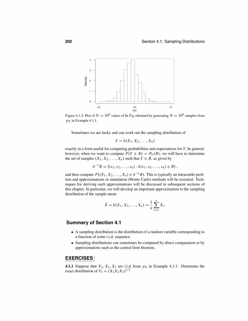
202 Section 4.1: Sampling Distributions
1.00.50.0
4
3
2
1
0
lnY
Den
sity
Figure 4.1.2: Plot of N = 104 values of ln Y20 obtained by generating N = 104 samples frompX in Example 4.1.1.
Sometimes we are lucky and can work out the sampling distribution of
Y = h(X1, X2, . . . , Xn)
exactly in a form useful for computing probabilities and expectations for Y. In general,however, when we want to compute P(Y ∈ B) = PY (B), we will have to determinethe set of samples (X1, X2, . . . , Xn) such that Y ∈ B, as given by
h−1 B = {(x1, x2, . . . , xn) : h(x1, x2, . . . , xn) ∈ B} ,
and then compute P((X1, X2, . . . , Xn) ∈ h−1 B). This is typically an intractable prob-lem and approximations or simulation (Monte Carlo) methods will be essential. Tech-niques for deriving such approximations will be discussed in subsequent sections ofthis chapter. In particular, we will develop an important approximation to the samplingdistribution of the sample mean
X = h(X1, X2, . . . , Xn) = 1n
n
i=1
Xi .
Summary of Section 4.1
• A sampling distribution is the distribution of a random variable corresponding toa function of some i.i.d. sequence.
• Sampling distributions can sometimes be computed by direct computation or byapproximations such as the central limit theorem.
EXERCISES
4.1.1 Suppose that X1, X2, X3 are i.i.d. from pX in Example 4.1.1. Determine theexact distribution of Y3 = (X1 X2 X3)
1/3 .
Chapter 4: Sampling Distributions and Limits 203
4.1.2 Suppose that a fair six-sided die is tossed n = 2 independent times. Computethe exact distribution of the sample mean.4.1.3 Suppose that an urn contains a proportion p of chips labelled 0 and proportion1− p of chips labelled 1. For a sample of n = 2, drawn with replacement, determinethe distribution of the sample mean.4.1.4 Suppose that an urn contains N chips labelled 0 and M chips labelled 1. For asample of n = 2, drawn without replacement, determine the distribution of the samplemean.4.1.5 Suppose that a symmetrical die is tossed n = 20 independent times. Work outthe exact sampling distribution of the maximum of this sample.4.1.6 Suppose three fair dice are rolled, and let Y be the number of 6’s showing. Com-pute the exact distribution of Y .4.1.7 Suppose two fair dice are rolled, and let W be the product of the two numbersshowing. Compute the exact distribution of W .4.1.8 Suppose two fair dice are rolled, and let Z be the difference of the two numbersshowing (i.e., the first number minus the second number). Compute the exact distribu-tion of Z .4.1.9 Suppose four fair coins are flipped, and let Y be the number of pairs of coinswhich land the same way (i.e., the number of pairs that are either both heads or bothtails). Compute the exact distribution of Y .
COMPUTER EXERCISES
4.1.10 Generate a sample of N = 103 values of Y50 in Example 4.1.1. Calculate themean and standard deviation of this sample.4.1.11 Suppose that X1, X2, . . . , X10 is an i.i.d. sequence from an N(0, 1) distribu-tion. Generate a sample of N = 103 values from the distribution of max(X1, X2, . . . ,X10). Calculate the mean and standard deviation of this sample.
PROBLEMS
4.1.12 Suppose that X1, X2, . . . , Xn is a sample from the Poisson(λ) distribution. De-termine the exact sampling distribution of Y = X1+ X2+ · · · + Xn. (Hint: Determinethe moment-generating function of Y and use the uniqueness theorem.)4.1.13 Suppose that X1, X2 is a sample from the Uniform[0,1] distribution. Determinethe exact sampling distribution of Y = X1 + X2. (Hint: Determine the density of Y .)4.1.14 Suppose that X1, X2 is a sample from the Uniform[0,1] distribution. Determinethe exact sampling distribution of Y = (X1 X2)
1/2 . (Hint: Determine the density ofln Y and then transform.)
4.2 Convergence in ProbabilityNotions of convergence are fundamental to much of mathematics. For example, ifan = 1 − 1/n, then a1 = 0, a2 = 1/2, a3 = 2/3, a4 = 3/4, etc. We see that the

204 Section 4.2: Convergence in Probability
values of an are getting “closer and closer” to 1, and indeed we know from calculusthat limn→∞ an = 1 in this case.
For random variables, notions of convergence are more complicated. If the valuesthemselves are random, then how can they “converge” to anything? On the other hand,we can consider various probabilities associated with the random variables and see ifthey converge in some sense.
The simplest notion of convergence of random variables is convergence in prob-ability, as follows. (Other notions of convergence will be developed in subsequentsections.)
Definition 4.2.1 Let X1, X2, . . . be an infinite sequence of random variables, andlet Y be another random variable. Then the sequence {Xn} converges in probability
to Y , if for all > 0, limn→∞ P(|Xn − Y | ≥ ) = 0, and we write XnP→ Y.
In Figure 4.2.1, we have plotted the differences Xn − Y, for selected values of n,for 10 generated sequences {Xn − Y } for a typical situation where the random variablesXn converge to a random variable Y in probability.We have also plotted the horizontallines at ± for = 0.25. From this we can see the increasing concentration of thedistribution of Xn − Y about 0, as n increases, as required by Definition 4.2.1. In fact,the 10 observed values of X100 − Y all satisfy the inequality |X100 − Y | < 0.25.
1005025101
2.00
1.00
0.25
-0.25
-1.00
-2.00
n
diff
eren
ces
Figure 4.2.1: Plot of 10 replications of {Xn−Y } illustrating the convergencein probability of Xn to Y .
We consider some applications of this definition.
EXAMPLE 4.2.1Let Y be any random variable, and let X1 = X2 = X3 = · · · = Y . (That is, the randomvariables are all identical to each other.) In that case, |Xn − Y | = 0, so of course
limn→∞ P(|Xn − Y | ≥ ) = 0
for all > 0. Hence, XnP→ Y .
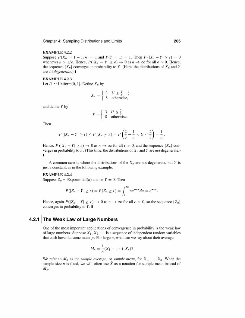
Chapter 4: Sampling Distributions and Limits 205
EXAMPLE 4.2.2Suppose P(Xn = 1 − 1/n) = 1 and P(Y = 1) = 1. Then P (|Xn − Y | ≥ ) = 0whenever n > 1/ . Hence, P(|Xn − Y | ≥ )→ 0 as n →∞ for all > 0. Hence,the sequence {Xn} converges in probability to Y . (Here, the distributions of Xn and Yare all degenerate.)
EXAMPLE 4.2.3Let U ∼ Uniform[0, 1]. Define Xn by
Xn = 3 U ≤ 23 − 1
n8 otherwise,
and define Y by
Y = 3 U ≤ 23
8 otherwise.
Then
P (|Xn − Y | ≥ ) ≤ P (Xn = Y ) = P23− 1
n< U ≤ 2
3= 1
n.
Hence, P (|Xn − Y | ≥ )→ 0 as n →∞ for all > 0, and the sequence {Xn} con-verges in probability to Y . (This time, the distributions of Xn and Y are not degenerate.)
A common case is where the distributions of the Xn are not degenerate, but Y isjust a constant, as in the following example.
EXAMPLE 4.2.4Suppose Zn ∼ Exponential(n) and let Y = 0. Then
P(|Zn − Y | ≥ ) = P(Zn ≥ ) =∞
ne−nx dx = e−n .
Hence, again P(|Zn − Y | ≥ ) → 0 as n → ∞ for all > 0, so the sequence {Zn}converges in probability to Y .
4.2.1 The Weak Law of Large Numbers
One of the most important applications of convergence in probability is the weak lawof large numbers. Suppose X1, X2, . . . is a sequence of independent random variablesthat each have the same mean µ. For large n, what can we say about their average
Mn = 1n(X1 + · · · + Xn)?
We refer to Mn as the sample average, or sample mean, for X1, . . . , Xn . When thesample size n is fixed, we will often use X as a notation for sample mean instead ofMn.

206 Section 4.2: Convergence in Probability
For example, if we flip a sequence of fair coins, and if Xi = 1 or Xi = 0 as the i thcoin comes up heads or tails, then Mn represents the fraction of the first n coins thatcame up heads. We might expect that for large n, this fraction will be close to 1/2, i.e.,to the expected value of the Xi .
The weak law of large numbers provides a precise sense in which average valuesMn tend to get close to E(Xi ), for large n.
Theorem 4.2.1 (Weak law of large numbers) Let X1, X2, . . . be a sequence of inde-pendent random variables, each having the same mean µ and each having varianceless than or equal to v < ∞. Then for all > 0, limn→∞ P (|Mn − µ| ≥ ) = 0.
That is, the averages converge in probability to the common mean µ or MnP→ µ.
PROOF Using linearity of expected value, we see that E(Mn) = µ. Also, usingindependence, we have
Var(Mn) = 1n2 (Var(X1) + Var(X2) + · · · + Var(Xn))
≤ 1
n2(v + v + · · · + v) = 1
n2(nv) = v/n .
Hence, by Chebychev’s inequality (Theorem 3.6.2), we have
P (|Mn − µ| ≥ ) ≤ Var(Mn)/2 ≤ v/ 2n.
This converges to 0 as n →∞, which proves the theorem.
It is a fact that, in Theorem 4.2.1, if we require the Xi variables to be i.i.d. insteadof merely independent, then we do not even need the Xi to have finite variance. But wewill not discuss this result further here. Consider some applications of the weak law oflarge numbers.
EXAMPLE 4.2.5Consider flipping a sequence of identical fair coins. Let Mn be the fraction of the firstn coins that are heads. Then Mn = (X1 + · · · + Xn)/n, where Xi = 1 if the i th coinis heads, otherwise Xi = 0. Hence, by the weak law of large numbers, we have
limn→∞ P(Mn < 0.49) = lim
n→∞ P(Mn − 0.5 < −0.01)
≤ limn→∞ P(Mn − 0.5 < −0.01 or Mn − 0.5 > 0.01 )
= limn→∞ P(|Mn − 0.5| > 0.01) = 0
and, similarly, limn→∞ P(Mn > 0.51) = 0. This illustrates that for large n, it is verylikely that Mn is very close to 0.5.
EXAMPLE 4.2.6Consider flipping a sequence of identical coins, each of which has probability p ofcoming up heads. Let Mn again be the fraction of the first n coins that are heads. Thenby the weak law of large numbers, for any > 0, limn→∞ P(p− < Mn < p+ ) = 1.

Chapter 4: Sampling Distributions and Limits 207
We thus see that for large n, it is very likely that Mn is very close to p. (The previousexample corresponds to the special case p = 1/2.)
EXAMPLE 4.2.7Let X1, X2, . . . be i.i.d. with distribution N(3, 5). Then E(Mn) = 3, and by the weaklaw of large numbers, P(3 − < Mn < 3 + )→ 1 as n →∞. Hence, for large n,the average value Mn is very close to 3.
EXAMPLE 4.2.8Let W1,W2, . . . be i.i.d. with distribution Exponential(6). Then E(Mn) = 1/6, and bythe weak law of large numbers, P(1/6 − < Mn < 1/6 + ) → 1 as n → ∞.Hence, for large n, the average value Mn is very close to 1/6.
Summary of Section 4.2
• A sequence {Xn} of random variables converges in probability to Y if
limn→∞ P(|Xn − Y | ≥ ) = 0.
• The weak law of large numbers says that if {Xn} is i.i.d. (or is independent withconstant mean and bounded variance), then the averages Mn = (X1 + · · · +Xn)/n converge in probability to E(Xi).
EXERCISES
4.2.1 Let U ∼ Uniform[5, 10], and let Z = IU∈[5, 7) and Zn = IU∈[5, 7+1/n2). Provethat Zn → Z in probability.4.2.2 Let Y ∼ Uniform[0, 1], and let Xn = Y n . Prove that Xn → 0 in probability.4.2.3 Let W1,W2, . . . be i.i.d. with distribution Exponential(3). Prove that for some n,we have P(W1 +W2 + · · · +Wn < n/2) > 0.999.4.2.4 Let Y1, Y2, . . . be i.i.d. with distribution N(2, 5). Prove that for some n, we haveP(Y1 + Y2 + · · · + Yn > n) > 0.999.4.2.5 Let X1, X2, . . . be i.i.d. with distribution Poisson(8). Prove that for some n, wehave P(X1 + X2 + · · · + Xn > 9n) < 0.001.
4.2.6 Suppose X ∼ Uniform[0, 1], and let Yn = n−1n X . Prove that Yn
P→ X .
4.2.7 Let Hn be the number of heads when flipping n fair coins, let Xn = e−Hn , and
let Y = 0. Prove that XnP→ Y .
4.2.8 Let Zn ∼ Uniform[0, n], let Wn = 5Zn/(Zn + 1), and let W = 5. Prove that
WnP→ W .
4.2.9 Consider flipping n fair coins. Let Hn be the total number of heads, and let Fnbe the number of heads on coins 1 through n − 1 (i.e., omitting the nth coin). Let
Xn = Hn/(Hn + 1), and Yn = Fn/(Hn + 1), and Z = 0. Prove that Xn − YnP→ Z .
4.2.10 Let Zn be the sum of the squares of the numbers showing when we roll n fair
dice. Find (with proof) a number m such that 1n Zn
P→ m. (Hint: Use the weak law oflarge numbers.)

208 Section 4.3: Convergence with Probability 1
4.2.11 Consider flipping n fair nickels and n fair dimes. Let Xn equal 4 times thenumber of nickels showing heads, plus 5 times the number of dimes showing heads.
Find (with proof) a number r such that 1n Xn
P→ r .
COMPUTER EXERCISES
4.2.12 Generate i.i.d. X1, . . . , Xn distributed Exponential(5) and compute Mn whenn = 20. Repeat this N times, where N is large (if possible, take N = 105, otherwiseas large as is feasible), and compute the proportion of values of Mn that lie between0.19 and 0.21. Repeat this with n = 50. What property of convergence in probabilitydo your results illustrate?4.2.13 Generate i.i.d. X1, . . . , Xn distributed Poisson(7) and compute Mn when n =20. Repeat this N times, where N is large (if possible, take N = 105, otherwise aslarge as is feasible), and compute the proportion of values of Mn that lie between 6.99and 7.01. Repeat this with n = 100. What property of convergence in probability doyour results illustrate?
PROBLEMS
4.2.14 Give an example of random variables X1, X2, . . . such that {Xn} converges to0 in probability, but E(Xn) = 1 for all n. (Hint: Suppose P(Xn = n) = 1/n andP(Xn = 0) = 1− 1/n.)
4.2.15 Prove that XnP→ 0 if and only if |Xn| P→ 0.
4.2.16 Prove or disprove that XnP→ 5 if and only if |Xn| P→ 5.
4.2.17 Suppose XnP→ X , and Yn
P→ Y . Let Zn = Xn + Yn and Z = X + Y . Prove
that ZnP→ Z .
CHALLENGES
4.2.18 Suppose XnP→ X , and f is a continuous function. Prove that f (Xn)
P→ f (X).
4.3 Convergence with Probability 1A notion of convergence for random variables that is closely associated with the con-vergence of a sequence of real numbers is provided by the concept of convergence withprobability 1. This property is given in the following definition.
Definition 4.3.1 Let X1, X2, . . . be an infinite sequence of random variables. Weshall say that the sequence {Xi} converges with probability 1 (or converges almostsurely (a.s.)) to a random variable Y , if P (limn→∞ Xn = Y ) = 1 and we writeXn
a.s.→ Y.
In Figure 4.3.1, we illustrate this convergence by graphing the sequence of differ-ences {Xn − Y } for a typical situation where the random variables Xn converge to a

Chapter 4: Sampling Distributions and Limits 209
random variable Y with probability 1. We have also plotted the horizontal lines at ±for = 0.1. Notice that inevitably all the values Xn − Y are in the interval (−0.1, 0.1)or, in other words, the values of Xn are within 0.1 of the values of Y.
Definition 4.3.1 indicates that for any given > 0, there will exist a value Nsuch that |Xn − Y | < for every n ≥ N . The value of N will vary depending onthe observed value of the sequence {Xn − Y } , but it always exists. Contrast this withthe situation depicted in Figure 4.2.1, which only says that the probability distributionXn − Y concentrates about 0 as n grows and not that the individual values of Xn − Ywill necessarily all be near 0 (also see Example 4.3.2).
10005000
0.2
0.1
0.0
-0.1
-0.2
-0.3
-0.4
n
diff
eren
ces
Figure 4.3.1: Plot of a single replication {Xn−Y } illustrating the convergence with probability1 of Xn to Y .
Consider an example of this.
EXAMPLE 4.3.1Consider again the setup of Example 4.2.3, where U ∼ Uniform[0, 1],
Xn = 3 U ≤ 23 − 1
n8 otherwise
and
Y = 3 U ≤ 23
8 otherwise.
If U > 2/3, then Y = 8 and also Xn = 8 for all n, so clearly Xn → Y . If U < 2/3,then for large enough n we will also have
U ≤ 23− 1
n,
so again Xn → Y . On the other hand, if U = 2/3, then we will always have Xn = 8,even though Y = 3. Hence, Xn → Y except when U = 2/3. Because P(U = 2/3) =0, we do have Xn → Y with probability 1.

210 Section 4.3: Convergence with Probability 1
One might wonder what the relationship is between convergence in probability andconvergence with probability 1. The following theorem provides an answer.
Theorem 4.3.1 Let Z, Z1, Z2, . . . be random variables. Suppose Zn → Z withprobability 1. Then Zn → Z in probability. That is, if a sequence of randomvariables converges almost surely, then it converges in probability to the same limit.
PROOF See Section 4.7 for the proof of this result.
On the other hand, the converse to Theorem 4.3.1 is false, as the following exampleshows.
EXAMPLE 4.3.2Let U have the uniform distribution on [0, 1]. We construct an infinite sequence ofrandom variables {Xn} by setting
X1 = I[0,1/2)(U), X2 = I[1/2,1](U),
X3 = I[0,1/4)(U), X4 = I[1/4,1/2)(U), X5 = I[1/2,3/4)(U), X6 = I[3/4,1](U),
X7 = I[0,1/8)(U), X8 = I[1/8,1/4)(U), . . .
...
where IA is the indicator function of the event A, i.e., IA(s) = 1 if s ∈ A, and IA(s) =0 if s ∈ A.
Note that we first subdivided [0, 1] into two equal-length subintervals and definedX1 and X2 as the indicator functions for the two subintervals. Next we subdivided [0, 1]into four equal-length subintervals and defined X3, X4, X5, and X6 as the indicatorfunctions for the four subintervals. We continued this process by next dividing [0, 1]into eight equal-length subintervals, then 16 equal-length subintervals, etc., to obtainan infinite sequence of random variables.
Each of these random variables Xn takes the values 0 and 1 only and so must followa Bernoulli distribution. In particular, X1 ∼Bernoulli(1/2) , X2 ∼ Bernoulli(1/2) , X3∼ Bernoulli(1/4) , etc.
Then for 0 < < 1, we have that P(|Xn − 0| ≥ ) = P(Xn = 1). Becausethe intervals for U that make Xn = 0 are getting smaller and smaller, we see thatP(Xn = 1) is converging to 0. Hence, Xn converges to 0 in probability.
On the other hand, Xn does not converge to 0 almost surely. Indeed, no matter whatvalue U takes on, there will always be infinitely many different n for which Xn = 1.Hence, we will have Xn = 1 infinitely often, so that we will not have Xn convergingto 0 for any particular value of U . Thus, P(limn→∞ Xn → 0) = 0, and Xn does notconverge to 0 with probability 1.
Theorem 4.3.1 and Example 4.3.2 together show that convergence with probability 1 isa stronger notion than convergence in probability.
Now, the weak law of large numbers (Section 4.2.1) concludes only that the av-erages Mn are converging in probability to E(Xi ). A stronger version of this resultwould instead conclude convergence with probability 1. We consider that now.
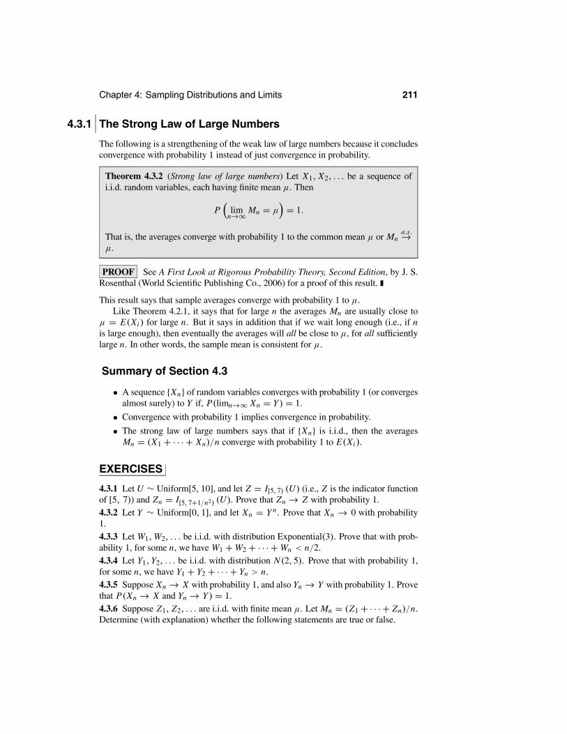
Chapter 4: Sampling Distributions and Limits 211
4.3.1 The Strong Law of Large Numbers
The following is a strengthening of the weak law of large numbers because it concludesconvergence with probability 1 instead of just convergence in probability.
Theorem 4.3.2 (Strong law of large numbers) Let X1, X2, . . . be a sequence ofi.i.d. random variables, each having finite mean µ. Then
P limn→∞ Mn = µ = 1.
That is, the averages converge with probability 1 to the common mean µ or Mna.s.→
µ.
PROOF See A First Look at Rigorous Probability Theory, Second Edition, by J. S.Rosenthal (World Scientific Publishing Co., 2006) for a proof of this result.
This result says that sample averages converge with probability 1 to µ.Like Theorem 4.2.1, it says that for large n the averages Mn are usually close to
µ = E(Xi ) for large n. But it says in addition that if we wait long enough (i.e., if nis large enough), then eventually the averages will all be close to µ, for all sufficientlylarge n. In other words, the sample mean is consistent for µ.
Summary of Section 4.3
• A sequence {Xn} of random variables converges with probability 1 (or convergesalmost surely) to Y if, P(limn→∞ Xn = Y ) = 1.
• Convergence with probability 1 implies convergence in probability.
• The strong law of large numbers says that if {Xn} is i.i.d., then the averagesMn = (X1 + · · · + Xn)/n converge with probability 1 to E(Xi ).
EXERCISES
4.3.1 Let U ∼ Uniform[5, 10], and let Z = I[5, 7) (U) (i.e., Z is the indicator functionof [5, 7)) and Zn = I[5, 7+1/n2) (U). Prove that Zn → Z with probability 1.4.3.2 Let Y ∼ Uniform[0, 1], and let Xn = Y n. Prove that Xn → 0 with probability1.4.3.3 Let W1,W2, . . . be i.i.d. with distribution Exponential(3). Prove that with prob-ability 1, for some n, we have W1 +W2 + · · · +Wn < n/2.4.3.4 Let Y1,Y2, . . . be i.i.d. with distribution N(2, 5). Prove that with probability 1,for some n, we have Y1 + Y2 + · · · + Yn > n.4.3.5 Suppose Xn → X with probability 1, and also Yn → Y with probability 1. Provethat P(Xn → X and Yn → Y ) = 1.4.3.6 Suppose Z1, Z2, . . . are i.i.d. with finite mean µ. Let Mn = (Z1 + · · · + Zn)/n.Determine (with explanation) whether the following statements are true or false.

212 Section 4.3: Convergence with Probability 1
(a) With probability 1, Mn = µ for some n.(b) With probability 1, µ− 0.01 < Mn < µ+ 0.01 for some n.(c) With probability 1, µ− 0.01 < Mn < µ+ 0.01 for all but finitely many n.(d) For any x ∈ R1, with probability 1, x − 0.01 < Mn < x + 0.01 for some n.4.3.7 Let {Xn} be i.i.d., with Xn ∼ Uniform[3, 7]. Let Yn = (X1+ X2+ . . .+ Xn)/n.Find (with proof) a number m such that Yn
a.s.→ m. (Hint: Use the strong law of largenumbers.)4.3.8 Let Zn be the sum of the squares of the numbers showing when we roll n fairdice. Find (with proof) a number m such that 1
n Zna.s.→ m.
4.3.9 Consider flipping n fair nickels and n fair dimes. Let Xn equal 4 times thenumber of nickels showing heads, plus 5 times the number of dimes showing heads.Find (with proof) a number r such that 1
n Xna.s.→ r .
4.3.10 Suppose Yna.s.→ Y . Does this imply that P(|Y5−Y | > |Y4− Y |) = 0? Explain.
4.3.11 Consider repeatedly flipping a fair coin. Let Hn be the number of heads on thefirst n flips, and let Zn = Hn/n.(a) Prove that there is some m such that |Zn − 1/2| < 0.001 for all n ≥ m.(b) Let r be the smallest positive integer satisfying |Zr − 1/2| < 0.001. Must we have|Zn − 1/2| < 0.001 for all n ≥ r? Why or why not?4.3.12 Suppose P(X = 0) = P(X = 1) = 1/2, and let Xn = X for n = 1, 2, 3, . . . .(That is, the random variables Xn are all identical.) Let Yn = (X1+ X2+ . . .+ Xn)/n.(a) Prove that P(limn→∞ Yn = 0) = P(limn→∞ Yn = 1) = 1/2.(b) Prove that there is no number m such that P(limn→∞ Yn = m) = 1.(c) Why does part (b) not contradict the law of large numbers?
COMPUTER EXERCISES
4.3.13 Generate i.i.d. X1, . . . , Xn distributed Exponential(5) with n large (take n =105 if possible). Plot the values M1,M2, . . . ,Mn . To what value are they converging?How quickly?4.3.14 Generate i.i.d. X1, . . . , Xn distributed Poisson(7) with n large (take n = 105 ifpossible). Plot the values M1,M2, . . . ,Mn . To what value are they converging? Howquickly?4.3.15 Generate i.i.d. X1, X2, . . . , Xn distributed N(−4, 3)with n large (take n = 105
if possible). Plot the values M1,M2, . . . ,Mn. To what value are they converging? Howquickly?
PROBLEMS
4.3.16 Suppose for each positive integer k, there are random variables Wk, Xk,1, Xk,2, . . .such that P(limn→∞ Xk,n = Wk) = 1. Prove that P(limn→∞ Xk,n = Wk for all k) =1.4.3.17 Prove that Xn
a.s.→ 0 if and only if |Xn| a.s.→ 0.
4.3.18 Prove or disprove that Xna.s.→ 5 if and only if |Xn| a.s.→ 5.

Chapter 4: Sampling Distributions and Limits 213
4.3.19 Suppose Xna.s.→ X , and Yn
a.s.→ Y . Let Zn = Xn + Yn and Z = X + Y . Provethat Zn
a.s.→ Z .
CHALLENGES
4.3.20 Suppose for each real number r ∈ [0, 1], there are random variables Wr , Xr,1,Xr,2, . . . such that P(limn→∞ Xr,n = Wr ) = 1. Prove or disprove that we must haveP(limn→∞ Xn,r = Wr for all r ∈ [0, 1]) = 1.4.3.21 Give an example of random variables X1, X2, . . . such that {Xn} converges to0 with probability 1, but E(Xn) = 1 for all n.
4.3.22 Suppose Xna.s.→ X , and f is a continuous function. Prove that f (Xn)
a.s.→ f (X).
4.4 Convergence in DistributionThere is yet another notion of convergence of a sequence of random variables that isimportant in applications of probability and statistics.
Definition 4.4.1 Let X, X1, X2, . . . be random variables. Then we say that thesequence {Xn} converges in distribution to X, if for all x ∈ R1 such that P(X =x) = 0 we have limn→∞ P(Xn ≤ x) = P(X ≤ x), and we write Xn
D→ X.
Intuitively, {Xn} converges in distribution to X if for large n, the distribution of Xnis close to that of X . The importance of this, as we will see, is that often the distributionof Xn is difficult to work with, while that of X is much simpler. With Xn convergingin distribution to X, however, we can approximate the distribution of Xn by that of X.
EXAMPLE 4.4.1Suppose P(Xn = 1) = 1/n, and P(Xn = 0) = 1 − 1/n. Let X = 0 so thatP(X = 0) = 1. Then,
P(Xn ≤ x) = 0 x < 0
1− 1/n 0 ≤ x < 11 1 ≤ x
→ P(X ≤ x) = 0 x < 01 0 ≤ x
as n → ∞. As P(Xn ≤ x) → P(X ≤ x) for every x, and in particular at all xwhere P(X = x) = 0, we have that {Xn} converges in distribution to X . Intuitively, asn →∞, it is more and more likely that Xn will equal 0.
EXAMPLE 4.4.2Suppose P(Xn = 1) = 1/2 + 1/n, and P(Xn = 0) = 1/2 − 1/n. Suppose furtherthat P(X = 0) = P(X = 1) = 1/2. Then {Xn} converges in distribution to X becauseP(Xn = 1)→ 1/2 and P(Xn = 0)→ 1/2 as n →∞.
EXAMPLE 4.4.3Let X ∼ Uniform[0, 1], and let P(Xn = i/n) = 1/n for i = 1, 2, . . . , n. Then X isabsolutely continuous, while Xn is discrete. On the other hand, for any 0 ≤ x ≤ 1, we

214 Section 4.4: Convergence in Distribution
have P(X ≤ x) = x, and letting x denote the greatest integer less than or equal tox , we have
P(Xn ≤ x) = nx
n.
Hence, |P(Xn ≤ x) − P(X ≤ x)| ≤ 1/n for all n. Because limn→∞ 1/n = 0, we doindeed have Xn → X in distribution.
EXAMPLE 4.4.4Suppose X1, X2, . . . are i.i.d. with finite mean µ, and Mn = (X1+ · · · + Xn)/n. Thenthe weak law of large numbers says that for any > 0, we have
P (Mn ≤ µ− )→ 0 and P (Mn ≤ µ+ )→ 1
as n →∞. It follows that limn→∞ P(Mn ≤ x) = P(M ≤ x) for any x = µ, whereM is the constant random variable M = µ. Hence, Mn → M in distribution. Note thatit is not necessarily the case that P(Mn ≤ µ)→ P(M ≤ µ) = 1. However, this doesnot contradict the definition of convergence in distribution because P(M = µ) = 0,so we do not need to worry about the case x = µ.
EXAMPLE 4.4.5 Poisson Approximation to the BinomialSuppose Xn ∼ Binomial(n, λ/n) and X ∼ Poisson(λ). We have seen in Example2.3.6 that
P(Xn = j) = n
j
λ
n
j
(1− λn)n− j → e−λ λ
j
j!
as n →∞. This implies that FXn (x)→ FX (x) at every point x /∈ {0, 1, 2, . . .} , andthese are precisely the points for which P(X = x) = 0. Therefore, {Xn} converges indistribution to X . (Indeed, this was our original motivation for the Poisson distribution.)
Many more examples of convergence in distribution are given by the central limittheorem, discussed in the next section. We first pause to consider the relationship ofconvergence in distribution to our previous notions of convergence.
Theorem 4.4.1 If XnP→ X , then Xn
D→ X .
PROOF See Section 4.7 for the proof of this result.
The converse to Theorem 4.4.1 is false. Indeed, the fact that Xn converges indistribution to X says nothing about the underlying relationship between Xn and X ,it says only something about their distributions. The following example illustrates this.
EXAMPLE 4.4.6Suppose X, X1, X2, . . . are i.i.d., each equal to ±1 with probability 1/2 each. In thiscase, P(Xn ≤ x) = P(X ≤ x) for all n and for all x ∈ R1, so of course Xn convergesin distribution to X . On the other hand, because X and Xn are independent,
P (|X − Xn| ≥ 2) = 12

Chapter 4: Sampling Distributions and Limits 215
for all n, which does not go to 0 as n → ∞. Hence, Xn does not converge to X inprobability (or with probability 1). So we can have convergence in distribution withouthaving convergence in probability or convergence with probability 1.
The following result, stated without proof, indicates how moment-generating func-tions can be used to check for convergence in distribution. (This generalizes Theo-rem 3.4.6.)
Theorem 4.4.2 Let X be a random variable, such that for some s0 > 0, we havemX (s) < ∞ whenever s ∈ (−s0, s0). If Z1, Z2, . . . is a sequence of random vari-ables with mZn (s) < ∞ and limn→∞mZn (s) = mX (s) for all s ∈ (−s0, s0), then{Zn} converges to X in distribution.
We will make use of this result to prove one of the most famous theorems of probability— the central limit theorem.
Finally, we note that combining Theorem 4.4.1 with Theorem 4.3.1 reveals thefollowing.
Corollary 4.4.1 If Xn → X with probability 1, then XnD→ X
4.4.1 The Central Limit Theorem
We now present the central limit theorem, one of the most important results in all ofprobability theory. Intuitively, it says that a large sum of i.i.d. random variables, prop-erly normalized, will always have approximately a normal distribution. This showsthat the normal distribution is extremely fundamental in probability and statistics —even though its density function is complicated and its cumulative distribution functionis intractable.
Suppose X1, X2, . . . is an i.i.d. sequence of random variables each having finitemean µ and finite variance σ 2. Let Sn = X1 + · · · + Xn be the sample sum andMn = Sn/n be the sample mean. The central limit theorem is concerned with thedistribution of the random variable
Zn = Sn − nµ√nσ
= Mn − µσ/√
n=√n
Mn − µσ
,
where σ = √σ 2. We know E(Mn) = µ and Var(Mn) = σ 2/n, which implies that
E(Zn) = 0 and Var(Zn) = 1. The variable Zn is thus obtained from the sample mean(or sample sum) by subtracting its mean and dividing by its standard deviation. Thistransformation is referred to as standardizing a random variable, so that it has mean 0and variance 1. Therefore, Zn is the standardized version of the sample mean (samplesum).
Note that the distribution of Zn shares two characteristics with the N(0, 1) distrib-ution, namely, it has mean 0 and variance 1. The central limit theorem shows that thereis an even stronger relationship.

216 Section 4.4: Convergence in Distribution
Theorem 4.4.3 (The central limit theorem) Let X1, X2, . . . be i.i.d. with finite meanµ and finite variance σ 2. Let Z ∼ N(0, 1). Then as n → ∞, the sequence {Zn}converges in distribution to Z , i.e., Zn
D→ Z .
PROOF See Section 4.7 for the proof of this result.
The central limit theorem is so important that we shall restate its conclusions inseveral different ways.
Corollary 4.4.2 For each fixed x ∈ R1, limn→∞ P (Zn ≤ x) = (x), where isthe cumulative distribution function for the standard normal distribution.
We can write this as follows.
Corollary 4.4.3 For each fixed x ∈ R1,
limn→∞ P(Sn ≤ nµ+x
√nσ) = (x) and lim
n→∞ P(Mn ≤ µ+xσ/√
n) = (x).
In particular, Sn is approximately equal to nµ, with deviations from this value oforder
√n, and Mn is approximately equal to µ, with deviations from this value of
order 1/√
n.
We note that it is not essential in the central limit theorem to divide by σ , in whichcase the theorem asserts instead that (Sn − nµ) /
√n (or
√n (Mn − nµ)) converges in
distribution to the N(0, σ 2) distribution. That is, the limiting distribution will still benormal but will have variance σ 2 instead of variance 1.
Similarly, instead of dividing by exactly σ , it suffices to divide by any quantity σ n,provided σ n
a.s.→ σ . A simple modification of the proof of Theorem 4.4.2 leads to thefollowing result.
Corollary 4.4.4 If
Z∗n =Sn − nµ√
nσ n= Mn − µσ n/
√n=√n
Mn − µσ n
and limn→∞ σ na.s.→ σ , then Z∗n
D→ Z as n →∞.
To illustrate the central limit theorem, we consider a simulation experiment.
EXAMPLE 4.4.7 The Central Limit Theorem Illustrated in a SimulationSuppose we generate a sample X1, . . . , Xn from the Uniform[0, 1] density. Note thatthe Uniform[0, 1] density is completely unlike a normal density. An easy calculationshows that when X ∼ Uniform[0, 1], then E (X) = 1/2 and Var(X) = 1/12.
Now suppose we are interested in the distribution of the sample average Mn =Sn/n = (X1 + · · · + Xn) /n for various choices of n. The central limit theorem tellsus that
Zn = Sn − n/2√n/12
=√nMn − 1/2√
1/12
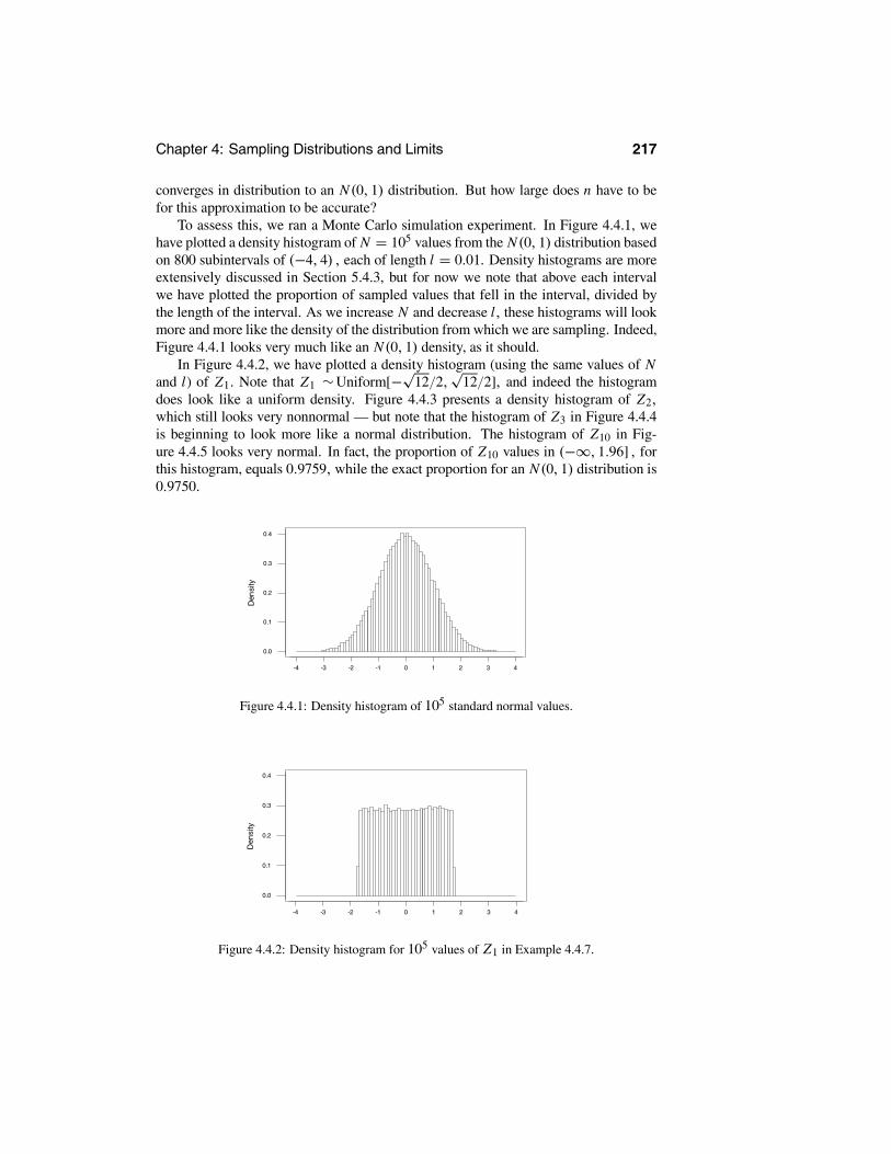
Chapter 4: Sampling Distributions and Limits 217
converges in distribution to an N(0, 1) distribution. But how large does n have to befor this approximation to be accurate?
To assess this, we ran a Monte Carlo simulation experiment. In Figure 4.4.1, wehave plotted a density histogram of N = 105 values from the N(0, 1) distribution basedon 800 subintervals of (−4, 4) , each of length l = 0.01. Density histograms are moreextensively discussed in Section 5.4.3, but for now we note that above each intervalwe have plotted the proportion of sampled values that fell in the interval, divided bythe length of the interval. As we increase N and decrease l, these histograms will lookmore and more like the density of the distribution from which we are sampling. Indeed,Figure 4.4.1 looks very much like an N(0, 1) density, as it should.
In Figure 4.4.2, we have plotted a density histogram (using the same values of Nand l) of Z1. Note that Z1 ∼Uniform[−√12/2,
√12/2], and indeed the histogram
does look like a uniform density. Figure 4.4.3 presents a density histogram of Z2,which still looks very nonnormal — but note that the histogram of Z3 in Figure 4.4.4is beginning to look more like a normal distribution. The histogram of Z10 in Fig-ure 4.4.5 looks very normal. In fact, the proportion of Z10 values in (−∞, 1.96] , forthis histogram, equals 0.9759, while the exact proportion for an N(0, 1) distribution is0.9750.
43210-1-2-3-4
0.4
0.3
0.2
0.1
0.0
Den
sity
Figure 4.4.1: Density histogram of 105 standard normal values.
43210-1-2-3-4
0.4
0.3
0.2
0.1
0.0
Den
sity
Figure 4.4.2: Density histogram for 105 values of Z1 in Example 4.4.7.
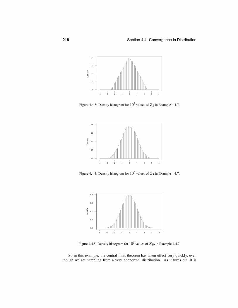
218 Section 4.4: Convergence in Distribution
43210-1-2-3-4
0.4
0.3
0.2
0.1
0.0D
ensi
ty
Figure 4.4.3: Density histogram for 105 values of Z2 in Example 4.4.7.
43210-1-2-3-4
0.4
0.3
0.2
0.1
0.0
Den
sity
Figure 4.4.4: Density histogram for 105 values of Z3 in Example 4.4.7.
43210-1-2-3-4
0.4
0.3
0.2
0.1
0.0
Den
sity
Figure 4.4.5: Density histogram for 105 values of Z10 in Example 4.4.7.
So in this example, the central limit theorem has taken effect very quickly, eventhough we are sampling from a very nonnormal distribution. As it turns out, it is

Chapter 4: Sampling Distributions and Limits 219
primarily the tails of a distribution that determine how large n has to be for the centrallimit theorem approximation to be accurate. When a distribution has tails no heavierthan a normal distribution, we can expect the approximation to be quite accurate forrelatively small sample sizes.
We consider some further applications of the central limit theorem.
EXAMPLE 4.4.8For example, suppose X1, X2, . . . are i.i.d. random variables, each with the Poisson(5)distribution. Recall that this implies that µ = E(Xi ) = 5 and σ 2 =Var(Xi) = 5.Hence, for each fixed x ∈ R1, we have
P Sn ≤ 5n + x√
5n → (x)
as n →∞ .
EXAMPLE 4.4.9 Normal Approximation to the Binomial DistributionSuppose X1, X2, . . . are i.i.d. random variables, each with the Bernoulli(θ) distribu-tion. Recall that this implies that E(Xi ) = θ and v =Var(Xi ) = θ (1− θ). Hence, foreach fixed x ∈ R1, we have
P Sn ≤ nθ + x nθ (1− θ) → (x), (4.4.1)
as n →∞ .But now note that we have previously shown that Yn = Sn ∼ Binomial(n, θ) . So
(4.4.1) implies that whenever we have a random variable Yn ∼ Binomial(n, θ) , then
P (Yn ≤ y) = PYn − nθ√nθ (1− θ) ≤
y − nθ√nθ (1− θ) ≈ y − nθ√
nθ (1− θ) (4.4.2)
for large n.Note that we are approximating a discrete distribution by a continuous distribu-
tion here. Reflecting this, a small improvement is often made to (4.4.2) when y is anonnegative integer. Instead, we use
P (Yn ≤ y) ≈ y + 0.5− nθ√nθ (1− θ) .
Adding 0.5 to y is called the correction for continuity. In effect, this allocates all therelevant normal probability in the interval (y − 0.5, y + 0.5) to the nonnegative integery. This has been shown to improve the approximation (4.4.2).
EXAMPLE 4.4.10 Approximating Probabilities Using the Central Limit TheoremWhile there are tables for the binomial distribution (Table D.6), we often have to com-pute binomial probabilities for situations the tables do not cover. We can always usestatistical software for this, in fact, such software makes use of the normal approxima-tion we derived from the central limit theorem.
For example, suppose that we have a biased coin, where the probability of gettinga head on a single toss is θ = 0.6. We will toss the coin n = 1000 times and then

220 Section 4.4: Convergence in Distribution
calculate the probability of getting at least 550 heads and no more than 625 heads.If Y denotes the number of heads obtained in the 1000 tosses, we have that Y ∼Binomial(1000, 0.6) , so
E(Y ) = 1000 (0.6) = 600,
Var(Y ) = 1000 (0.6) (0.4) = 240.
Therefore, using the correction for continuity and Table D.2,
P(550 ≤ Y ≤ 625) = P(550− 0.5 ≤ Y ≤ 625+ 0.5)
= P549.5− 600√
240≤ Y − 600√
240≤ 625.5− 600√
240
= P −3.2598 ≤ Y − 600√240
≤ 1.646
≈ (1.65)− (−3.26) = 0.9505− 0.0006 = 0.9499.
Note that it would be impossible to compute this probability using the formulas for thebinomial distribution.
One of the most important uses of the central limit theorem is that it leads to amethod for assessing the error in an average when this is estimating or approximatingsome quantity of interest.
4.4.2 The Central Limit Theorem and Assessing Error
Suppose X1, X2, . . . is an i.i.d. sequence of random variables, each with finite meanµ and finite variance σ 2, and we are using the sample average Mn to approximate themean µ. This situation arises commonly in many computational (see Section 4.5) andstatistical (see Chapter 6) problems. In such a context, we can generate the Xi , but wedo not know the value of µ.
If we approximate µ by Mn, then a natural question to ask is: How much error isthere in the approximation? The central limit theorem tells us that
(3)− (−3) = limn→∞ P −3 <
Mn − µσ/√
n< 3
= limn→∞ P Mn − 3
σ√n< µ <Mn + 3
σ√n.
Using Table D.2 (or statistical software), we have that (3)− (−3) = 0.9987− (1−0.9987) = 0.9974. So, for large n, we have that the interval
Mn − 3σ/√
n,Mn + 3σ/√
n
contains the unknown value of µ with virtual certainty (actually with probability about0.9974). Therefore, the half-length 3σ/
√n of this interval gives us an assessment of
the error in the approximation Mn. Note that Var(Mn) = σ 2/n, so the half-length ofthe interval equals 3 standard deviations of the estimate Mn .

Chapter 4: Sampling Distributions and Limits 221
Because we do not know µ, it is extremely unlikely that we will know σ (as itsdefinition uses µ). But if we can find a consistent estimate σ n of σ , then we can useCorollary 4.4.4 instead to construct such an interval.
As it turns out, the correct choice of σ n depends on what we know about the distri-bution we are sampling from (see Chapter 6 for more discussion of this). For example,if X1 ∼ Bernoulli(θ) , then µ = θ and σ 2 =Var(X1) = θ (1− θ). By the strong lawof large numbers (Theorem 4.3.2), Mn
a.s.→ µ = θ and thus
σ n = Mn (1− Mn)a.s.→ θ (1− θ) = σ.
Then, using the same argument as above, we have that, for large n, the interval
Mn − 3 Mn (1− Mn) /n,Mn + 3 Mn (1− Mn) /n (4.4.3)
contains the true value of θ with virtual certainty (again, with probability about 0.9974).The half-length of (4.4.3) is a measure of the accuracy of the estimate Mn — no-tice that this can be computed from the values X1, . . . , Xn. We refer to the quantity(Mn (1− Mn) /n)1/2 as the standard error of the estimate Mn .
For a general random variable X1, let
σ 2n = 1
n − 1
n
i=1
(Xi − Mn)2 = 1
n − 1
n
i=1
X2i − 2Mn
n
i=1
Xi + nM2n
= n
n − 11n
n
i=1
X2i − 2M2
n + M2n = n
n − 11n
n
i=1
X2i − M2
n .
By the strong law of large numbers, we have that Mna.s.→ µ and
1n
n
i=1
X2i
a.s.→ E X21 = σ 2 + µ2.
Because n/ (n − 1) → 1 and M2n
a.s.→ µ2 as well, we conclude that σ 2n
a.s.→ σ 2. This
implies that σ na.s.→ σ hence σ n is consistent for σ. It is common to call σ 2
n the samplevariance of the sample X1, . . . , Xn. When the sample size n is fixed, we will oftendenote this estimate of the variance by S2.
Again, using the above argument, we have that, for large n, the interval
Mn − 3σ n/√
n,Mn + 3σ n/√
n = Mn − 3S/√
n,Mn + 3S/√
n (4.4.4)
contains the true value of µ with virtual certainty (also with probability about 0.9974).Therefore, the half-length is a measure of the accuracy of the estimate Mn — noticethat this can be computed from the values X1, . . . , Xn. The quantity S/
√n is referred
to as the standard error of the estimate Mn.We will make use of these estimates of the error in approximations in the following
section.

222 Section 4.4: Convergence in Distribution
Summary of Section 4.4
• A sequence {Xn} of random variables converges in distribution to Y if, for all y ∈R1 with P(Y = y) = 0, we have limn→∞ FXn (y) = FY (y), i.e., limn→∞ P(Xn≤ y) = P(Y ≤ y).
• If {Xn} converges to Y in probability (or with probability 1), then {Xn} convergesto Y in distribution.
• The very important central limit theorem says that if {Xn} are i.i.d. with finitemean µ and variance σ 2, then the random variables Zn = (Sn − nµ)/
√nσ
converge in distribution to a standard normal distribution.
• The central limit theorem allows us to approximate various distributions by nor-mal distributions, which is helpful in simulation experiments and in many othercontexts. Table D.2 (or any statistical software package) provides values for thecumulative distribution function of a standard normal.
EXERCISES
4.4.1 Suppose P(Xn = i) = (n + i)/(3n + 6) for i = 1, 2, 3. Suppose also thatP(X = i) = 1/3 for i = 1, 2, 3. Prove that {Xn} converges in distribution to X .4.4.2 Suppose P(Yn = k) = (1 − 2−n−1)−1/2k+1 for k = 0, 1, . . . , n. Let Y ∼Geometric(1/2). Prove that {Yn} converges in distribution to Y .4.4.3 Let Zn have density (n + 1)xn for 0 < x < 1, and 0 otherwise. Let Z = 1.Prove that {Zn} converges in distribution to Z .4.4.4 Let Wn have density
1+ x/n
1+ 1/2n
for 0 < x < 1, and 0 otherwise. Let W ∼ Uniform[0, 1]. Prove that {Wn} convergesin distribution to W .4.4.5 Let Y1, Y2, . . . be i.i.d. with distribution Exponential(3). Use the central limittheorem and Table D.2 (or software) to estimate the probability P( 1600
i=1 Yi ≤ 540).4.4.6 Let Z1, Z2, . . . be i.i.d. with distribution Uniform[−20, 10]. Use the centrallimit theorem and Table D.2 (or software) to estimate the probability P( 900
i=1 Zi ≥−4470).4.4.7 Let X1, X2, . . . be i.i.d. with distribution Geometric(1/4). Use the central limittheorem and Table D.2 (or software) to estimate the probability P( 800
i=1 Xi ≥ 2450).4.4.8 Suppose Xn ∼ N(0, 1/n), i.e., Xn has a normal distribution with mean 0 andvariance 1/n. Does the sequence {Xn} converge in distribution to some random vari-able? If yes, what is the distribution of the random variable?4.4.9 Suppose P(Xn = i/n) = 2i/n(n+1) for i = 1, 2, 3, . . . , n. Let Z have densityfunction given by f (z) = 2z for 0 < z < 1, otherwise f (z) = 0.(a) Compute P(Z ≤ y) for 0 < y < 1.(b) Compute P(Xn ≤ m/n) for some integer 1 ≤ m ≤ n. (Hint: Remember that
mi=1 i = m(m + 1)/2.)

Chapter 4: Sampling Distributions and Limits 223
(c) Compute P(Xn ≤ y) for 0 < y < 1.
(d) Prove that XnD→ Z .
4.4.10 Suppose P(Yn ≤ y) = 1−e−2ny/(n+1) for all y > 0. Prove that YnD→ Y where
Y ∼ Exponential(λ) for some λ > 0 and compute λ.
4.4.11 Suppose P(Zn ≤ z) = 1− (1− 3zn )
n for all 0 < z < n/3. Prove that ZnD→ Z
where Z ∼ Exponential(λ) for some λ > 0 and compute λ. (Hint: Recall from calculusthat limn→∞(1+ c
n )n = ec for any real number c.)
4.4.12 Suppose the service time, in minutes, at a bank has the Exponential distributionwith λ = 1/2. Use the central limit theorem to estimate the probability that the averageservice time of the first n customers is less than 2.5 minutes, when:(a) n = 16.(b) n = 36.(c) n = 100.4.4.13 Suppose the number of kilograms of a metal alloy produced by a factory eachweek is uniformly distributed between 20 and 30. Use the central limit theorem to esti-mate the probability that next year’s output will be less than 1280 kilograms. (Assumethat a year contains precisely 52 weeks.)4.4.14 Suppose the time, in days, until a component fails has the Gamma distributionwith α = 5 and θ = 1/10. When a component fails, it is immediately replaced bya new component. Use the central limit theorem to estimate the probability that 40components will together be sufficient to last at least 6 years. (Assume that a yearcontains precisely 365.25 days.)
COMPUTER EXERCISES
4.4.15 Generate N samples X1, X2, . . . , X20 ∼ Exponential(3) for N large (N = 104,if possible). Use these samples to estimate the probability P(1/6 ≤ M20 ≤ 1/2). Howdoes your answer compare to what the central limit theorem gives as an approximation?4.4.16 Generate N samples X1, X2, . . . , X30 ∼ Uniform[−20, 10] for N large (N =104, if possible). Use these samples to estimate the probability P(M30 ≤ −5). Howdoes your answer compare to what the central limit theorem gives as an approximation?4.4.17 Generate N samples X1, X2, . . . , X20 ∼ Geometric(1/4) for N large (N =104, if possible). Use these samples to estimate the probability P(2.5 ≤ M20 ≤ 3.3).How does your answer compare to what the central limit theorem gives as an approxi-mation?4.4.18 Generate N samples X1, X2, . . . , X20 from the distribution of log Z where Z ∼Gamma(4, 1) for N large (N = 104, if possible). Use these samples to construct adensity histogram of the values of M20. Comment on the shape of this graph.4.4.19 Generate N samples X1, X2, . . . , X20 from the Binomial(10, 0.01) distributionfor N large (N = 104, if possible). Use these samples to construct a density histogramof the values of M20. Comment on the shape of this graph.

224 Section 4.5: Monte Carlo Approximations
PROBLEMS
4.4.20 Let a1, a2, . . . be any sequence of nonnegative real numbers with i ai = 1.Suppose P(X = i) = ai for every positive integer i . Construct a sequence {Xn} ofabsolutely continuous random variables, such that Xn → X in distribution.
4.4.21 Let f : [0, 1] → (0,∞) be a continuous positive function such that 10 f (x) dx
= 1. Consider random variables X and {Xn} such that P(a ≤ X ≤ b) = ba f (x) dx
for a ≤ b and
P Xn = i
n= f (i/n)
nj=1 f ( j/n)
for i = 1, 2, 3, . . . , n. Prove that Xn → X in distribution.4.4.22 Suppose that Yi = X3
i and that X1, . . . , Xn is a sample from an N(µ, σ 2)distribution. Indicate how you would approximate the probability P(Mn ≤ m) whereMn = (Y1 + · · · + Yn) /n.
4.4.23 Suppose Yi = cos (2πUi ) and U1, . . . ,Un is a sample from the Uniform[0, 1]distribution. Indicate how you would approximate the probability P(Mn≤ m), where Mn = (Y1 + · · · + Yn) /n.
COMPUTER PROBLEMS
4.4.24 Suppose that Y = X3 and X ∼ N(0, 1). By generating a large sample (n =104, if possible) from the distribution of Y, approximate the probability P(Y ≤ 1) andassess the error in your approximation. Compute this probability exactly and compareit with your approximation.4.4.25 Suppose that Y = X3 and X ∼ N(0, 1). By generating a large sample (n =104, if possible) from the distribution of Y, approximate the expectation E(cos(X3)),and assess the error in your approximation.
CHALLENGES
4.4.26 Suppose Xn → C in distribution, where C is a constant. Prove that Xn → Cin probability. (This proves that if X is constant, then the converse to Theorem 4.4.1does hold, even though it does not hold for general X .)
4.5 Monte Carlo ApproximationsThe laws of large numbers say that if X1, X2, . . . is an i.i.d. sequence of random vari-ables with mean µ, and
Mn = X1 + · · · + Xn
n,
then for large n we will have Mn ≈ µ.Suppose now that µ is unknown. Then, as discussed in Section 4.4.2, it is possible
to change perspective and use Mn (for large n) as an estimator or approximation of µ.Any time we approximate or estimate a quantity, we must also say something about

Chapter 4: Sampling Distributions and Limits 225
how much error is in the estimate. Of course, we cannot say what this error is exactly,as that would require knowing the exact value of µ. In Section 4.4.2, however, weshowed how the central limit theorem leads to a very natural approach to assessing thiserror, using three times the standard error of the estimate. We consider some examples.
EXAMPLE 4.5.1Consider flipping a sequence of identical coins, each of which has probability θ ofcoming up heads, but where θ is unknown. Let Mn again be the fraction of the first ncoins that are heads. Then we know that for large n, it is very likely that Mn is veryclose to θ . Hence, we can use Mn to estimate θ . Furthermore, the discussion in Section4.4.2 indicates that (4.4.3) is the relevant interval to quote when assessing the accuracyof the estimate Mn .
EXAMPLE 4.5.2Suppose we believe a certain medicine lowers blood pressure, but we do not know byhow much. We would like to know the mean amount µ, by which this medicine lowersblood pressure.
Suppose we observe n patients (chosen at random so they are i.i.d.), where patienti has blood pressure Bi before taking the medicine and blood pressure Ai afterwards.Let Xi = Bi − Ai . Then
Mn = 1n
n
i=1
(Bi − Ai )
is the average amount of blood pressure decrease. (Note that Bi − Ai may be negativefor some patients, and it is important to also include those negative terms in the sum.)Then for large n, the value of Mn is a good estimate of E(Xi ) = µ. Furthermore, thediscussion in Section 4.4.2 indicates that (4.4.4) is the relevant interval to quote whenassessing the accuracy of the estimate Mn.
Such estimators can also be used to estimate purely mathematical quantities that donot involve any experimental data (such as coins or medical patients) but that are toodifficult to compute directly. In this case, such estimators are called Monte Carlo ap-proximations (named after the gambling casino in the principality of Monaco becausethey introduce randomness to solve nonrandom problems).
EXAMPLE 4.5.3Suppose we wish to evaluate
I =1
0cos(x2) sin(x4) dx.
This integral cannot easily be solved exactly. But it can be approximately computedusing a Monte Carlo approximation, as follows. We note that
I = E(cos(U2) sin(U4)),
where U ∼ Uniform[0, 1]. Hence, for large n, the integral I is approximately equalto Mn = (T1 + · · · + Tn)/n, where Ti = cos(U2
i ) sin(U 4i ), and where U1,U2, . . . are
i.i.d. Uniform[0, 1].

226 Section 4.5: Monte Carlo Approximations
Putting this all together, we obtain an algorithm for approximating the integral I ,as follows.
1. Select a large positive integer n.
2. Obtain Ui ∼ Uniform[0, 1], independently for i = 1, 2, . . . , n.
3. Set Ti = cos(U2i ) sin(U 4
i ), for i = 1, 2, . . . , n.
4. Estimate I by Mn = (T1 + · · · + Tn)/n.
For large enough n, this algorithm will provide a good estimate of the integral I .For example, the following table records the estimates Mn and the intervals (4.4.4)
based on samples of Uniform[0,1] variables for various choices of n.
n Mn Mn − 3S/√
n Mn + 3S/√
n103 0.145294 0.130071 0.160518104 0.138850 0.134105 0.143595105 0.139484 0.137974 0.140993
From this we can see that the value of I is approximately 0.139484, and the true valueis almost certainly in the interval (0.137974, 0.140993). Notice how the lengths ofthe intervals decrease as we increase n. In fact, it can be shown that the exact value isI = 0.139567, so our approximation is excellent.
EXAMPLE 4.5.4Suppose we want to evaluate the integral
I =∞
025x2 cos(x2)e−25x dx .
This integral cannot easily be solved exactly, but it can also be approximately computedusing a Monte Carlo approximation, as follows.
We note first that I = E(X2 cos(X2)), where X ∼ Exponential(25). Hence, forlarge n, the integral I is approximately equal to Mn = (T1 + · · · + Tn)/n, whereTi = X2
i cos(X2i ), with X1, X2, . . . i.i.d. Exponential(25).
Now, we know from Section 2.10 that we can simulate X ∼ Exponential(25) bysetting X = − ln(U)/25 where U ∼ Uniform[0, 1]. Hence, putting this all together,we obtain an algorithm for approximating the integral I , as follows.
1. Select a large positive integer n.
2. Obtain Ui ∼ Uniform[0, 1], independently for i = 1, 2, . . . , n.
3. Set Xi = − ln(Ui )/25, for i = 1, 2, . . . , n.
4. Set Ti = X2i cos(X2
i ), for i = 1, 2, . . . , n.
5. Estimate I by Mn = (T1 + · · · + Tn)/n.

Chapter 4: Sampling Distributions and Limits 227
For large enough n, this algorithm will provide a good estimate of the integral I .For example, the following table records the estimates Mn and the intervals (4.4.4)
based on samples of Exponential(25) variables for various choices of n.
n Mn Mn − 3S/√
n Mn + 3S/√
n103 3.33846× 10⁻³ 2.63370× 10⁻³ 4.04321× 10⁻³
104 3.29933× 10⁻³ 3.06646× 10⁻³ 3.53220× 10⁻³
105 3.20629× 10⁻³ 3.13759× 10⁻³ 3.27499× 10⁻³
From this we can see that the value of I is approximately 3.20629 × 10⁻³ and that thetrue value is almost certainly in the interval 3.13759× 10⁻³, 3.27499× 10⁻³ .
EXAMPLE 4.5.5Suppose we want to evaluate the sum
S =∞
j=0
( j2 + 3)−75− j .
Though this is very difficult to compute directly, but it can be approximately computedusing a Monte Carlo approximation.
Let us rewrite the sum as
S = 54
∞
j=0
( j2 + 3)−7 45
1− 45
j
.
We then see that S = (5/4) E((X2 + 3)−7), where X ∼ Geometric(4/5).Now, we know from Section 2.10 that we can simulate X ∼ Geometric(4/5) by
setting X = ln(1 − U)/ ln(1 − 4/5) or, equivalently, X = ln(U)/ ln(1 − 4/5) ,where U ∼ Uniform[0, 1] and where · means to round down to the next integervalue. Hence, we obtain an algorithm for approximating the sum S, as follows.
1. Select a large positive integer n.
2. Obtain Ui ∼ Uniform[0, 1], independently for i = 1, 2, . . . , n.
3. Set Xi = ln(Ui)/ ln(1− 4/5) , for i = 1, 2, . . . , n.
4. Set Ti = (X2i + 3)−7, for i = 1, 2, . . . , n.
5. Estimate S by Mn = (5/4)(T1 + · · · + Tn)/n.
For large enough n, this algorithm will provide a good estimate of the sum S.For example, the following table records the estimates Mn and the intervals (4.4.4)
based on samples of Geometric(4/5) variables for various choices of n.
n Mn Mn − 3S/√
n Mn + 3S/√
n103 4.66773× 10⁻⁴ 4.47078× 10⁻⁴ 4.86468× 10⁻⁴
104 4.73538× 10⁻⁴ 4.67490× 10⁻⁴ 4.79586× 10⁻⁴
105 4.69377× 10⁻⁴ 4.67436× 10⁻⁴ 4.71318× 10⁻⁴

228 Section 4.5: Monte Carlo Approximations
From this we can see that the value of S is approximately 4.69377 × 10⁻⁴ and that thetrue value is almost certainly in the interval 4.67436× 10⁻⁴, 4.71318× 10⁻⁴ .
Note that when using a Monte Carlo approximation, it is not necessary that therange of an integral or sum be the entire range of the corresponding random variable,as follows.
EXAMPLE 4.5.6Suppose we want to evaluate the integral
J =∞
0sin(x)e−x2/2 dx.
Again, this is extremely difficult to evaluate exactly.Here
J = √2π E(sin(X)I{X>0}),
where X ∼ N(0, 1) and I{X>0} is the indicator function of the event {X > 0}. Weknow from Section 2.10 that we can simulate X ∼ N(0, 1) by setting
X = 2 log(1/U) cos(2πV ),
where U and V are i.i.d. Uniform[0, 1]. Hence, we obtain the following algorithm forapproximating the integral J .
1. Select a large positive integer n.
2. Obtain Ui , Vi ∼ Uniform[0, 1], independently for i = 1, 2, . . . ,n.
3. Set Xi = 2 log(1/Ui ) cos(2πVi ), for i = 1, 2, . . . , n.
4. Set Ti = sin(Xi )I{Xi>0}, for i = 1, 2, . . . , n. (That is, set Ti =sin(Xi ) if Xi > 0, otherwise set Ti = 0.)
5. Estimate J by Mn =√
2π(T1 + · · · + Tn)/n.
For large enough n, this algorithm will again provide a good estimate of the integral I .For example, the following table records the estimates Mn and the intervals (4.4.4)
based on samples of N(0, 1) variables for various choices of n.
n Mn Mn − 3S/√
n Mn + 3S/√
n103 0.744037 0.657294 0.830779104 0.733945 0.706658 0.761233105 0.722753 0.714108 0.731398
From this we can see that the value of J is approximately 0.722753 and that the truevalue is almost certainly in the interval (0.714108, 0.731398).
Now we consider an important problem for statistical applications of probabilitytheory.

Chapter 4: Sampling Distributions and Limits 229
EXAMPLE 4.5.7 Approximating Sampling Distributions Using Monte CarloSuppose X1, X2, . . . , Xn is an i.i.d. sequence with distribution given by probabilitymeasure P.We want to find the distribution of a new random variable Y = h(X1, X2, . . . , Xn)for some function h. Provided we can generate from P , then Monte Carlo methods giveus a way for to approximate this distribution.
Denoting the cumulative distribution function of Y by FY , we have
FY (y) = P((−∞, y ) = EPY (I(−∞,y] (Y )) = E(I(−∞,y] (h(X1, X2, . . . , Xn))).
So FY (y) can be expressed as the expectation of the random variable
I(−∞,y] (h(X1, X2, . . . , Xn))
based on sampling from P.To estimate this, we generate N samples of size n
(Xi1, Xi2, . . . , Xin),
for i = 1, . . . , N from P (note N is the Monte Carlo sample size and can be varied,whereas the sample size n is fixed here) and then calculate the proportion of valuesh(Xi1, Xi2, . . . , Xin) ∈ (−∞, y . The estimate MN is then given by
FY (y) = 1N
N
i=1
I(−∞,y] (h(Xi1, Xi2, . . . , Xin)) .
By the laws of large numbers, this converges to FY (y) as N → ∞. To evaluate theerror in this approximation, we use (4.4.3), which now takes the form
FY (y)− 3 FY (y) 1− FY (y) /n, FY (y)+ 3 FY (y) 1− FY (y) /n .
We presented an application of this in Example 4.4.7. Note that if the base of a rec-tangle in the histogram of Figure 4.4.2 is given by (a, b] , then the height of this rectan-gle equals the proportion of values that fell in (a, b] times 1/ (b − a) . This can be ex-pressed as (FY (b)− FY (a))/ (b − a) , which converges to (FY (b)− FY (a)) / (b− a)as N → ∞. This proves that the areas of the rectangles in the histogram converge toFY (b)− FY (a) as N →∞.
More generally, we can approximate an expectation E(g (Y )) using the average
1N
N
i=1
g (h(Xi1, Xi2, . . . , Xin)) .
By the laws of large numbers, this average converges to E (g (Y )) as N →∞.Typically, there is more than one possible Monte Carlo algorithm for estimating
a quantity of interest. For example, suppose we want to approximate the integralb
a g(x) dx, where we assume this integral is finite. Let f be a density on the interval

230 Section 4.5: Monte Carlo Approximations
(a, b), such that f (x) > 0 for every x ∈ (a, b) , and suppose we have a convenientalgorithm for generating X1, X2, . . . i.i.d. with distribution given by f . We have that
b
ag(x) dx =
b
a
g(x)
f (x)f (x) dx = E
g(X)
f (X)
when X is distributed with density f . So we can estimate ba g(x) dx by
Mn = 1n
n
i=1
g(Xi )
f (Xi )= 1
n
n
i=1
Ti ,
where Ti = g(Xi )/ f (Xi ). In effect, this is what we did in Example 4.5.3 ( f is theUniform[0, 1] density), in Example 4.5.4 ( f is the Exponential(25) density), and inExample 4.5.6 ( f is the N(0, 1) density). But note that there are many other possiblechoices. In Example 4.5.3, we could have taken f to be any beta density. In Example4.5.4, we could have taken f to be any gamma density, and similarly in Example4.5.6. Most statistical computer packages have commands for generating from thesedistributions. In a given problem, what is the best one to use?
In such a case, we would naturally use the algorithm that was most efficient. Forthe algorithms we have been discussing here, this means that if, based on a sampleof n, algorithm 1 leads to an estimate with standard error σ 1/
√n, and algorithm 2
leads to an estimate with standard error σ 2/√
n, then algorithm 1 is more efficient thanalgorithm 2 whenever σ 1 < σ 2. Naturally, we would prefer algorithm 1 because theintervals (4.4.3) or (4.4.4) will tend to be shorter for algorithm 1 for the same samplesize. Actually, a more refined comparison of efficiency would also take into account thetotal amount of computer time used by each algorithm, but we will ignore this aspect ofthe problem here. See Problem 4.5.21 for more discussion of efficiency and the choiceof algorithm in the context of the integration problem.
Summary of Section 4.5
• An unknown quantity can be approximately computed using a Monte Carlo ap-proximation, whereby independent replications of a random experiment (usuallyon a computer) are averaged to estimate the quantity.
• Monte Carlo approximations can be used to approximate complicated sums, in-tegrals, and sampling distributions, all by choosing the random experiment ap-propriately.
EXERCISES
4.5.1 Describe a Monte Carlo approximation of ∞−∞ cos2(x)e−x2/2 dx .
4.5.2 Describe a Monte Carlo approximation of mj=0 j6 m
j 2 j 3−m . (Hint: Rememberthe Binomial(m, 2/3) distribution.)
4.5.3 Describe a Monte Carlo approximation of ∞0 e−5x−14x2
dx. (Hint: Rememberthe Exponential(5) distribution.)

Chapter 4: Sampling Distributions and Limits 231
4.5.4 Suppose X1, X2, . . . are i.i.d. with distribution Poisson(λ), where λ is unknown.Consider Mn = (X1 + X2 + · · · + Xn)/n as an estimate of λ. Suppose we know thatλ ≤ 10. How large must n be to guarantee that Mn will be within 0.1 of the true valueof λ with virtual certainty, i.e., when is 3 standard deviations smaller than 0.1?4.5.5 Describe a Monte Carlo approximation of ∞
j=0 sin( j2)5 j / j !. Assume youhave available an algorithm for generating from the Poisson(5) distribution.
4.5.6 Describe a Monte Carlo approximation of 100 e−x4
dx. (Hint: Remember theUniform[0, 10] distribution.)4.5.7 Suppose we repeat a certain experiment 2000 times and obtain a sample averageof −5 and a standard error of 17. In terms of this, specify an interval that is virtuallycertain to contain the experiment’s (unknown) true mean µ.4.5.8 Suppose we repeat a certain experiment 400 times and get i.i.d. response valuesX1, X2, . . . , X400. Suppose we compute that the sample average is M400 = 6 andfurthermore that 400
i=1(Xi)2 = 15, 400. In terms of this:
(a) Compute the standard error σ n .(b) Specify an interval that is virtually certain to contain the (unknown) true mean µ ofthe Xi .4.5.9 Suppose a certain experiment has probability θ of success, where 0 < θ < 1but θ is unknown. Suppose we repeat the experiment 1000 times, of which 400 aresuccesses and 600 are failures. Compute an interval of values that are virtually certainto contain θ .4.5.10 Suppose a certain experiment has probability θ of success, where 0 < θ < 1but θ is unknown. Suppose we repeat the experiment n times, and let Y be the fractionof successes.(a) In terms of θ , what is Var(Y )?(b) For what value of θ is Var(Y ) the largest?(c) What is this largest possible value of Var(Y )?(d) Compute the smallest integer n such that we can be sure that Var(Y ) < 0.01,regardless of the value of θ .4.5.11 Suppose X and Y are random variables with joint density given by fX,Y (x, y) =C g(x, y) for 0 ≤ x, y ≤ 1 (with fX,Y (x, y) = 0 for other x, y), for appropriate con-stant C, where
g(x, y) = x2 y3 sin(xy) cos(√
xy ) exp(x2 + y) .
(a) Explain why
E(X) =1
0
1
0x fX,Y (x, y) dx dy =
10
10 x g(x, y) dx dy
10
10 g(x, y) dx dy
.
(b) Describe a Monte Carlo algorithm to approximately compute E(X).
4.5.12 Let g(x, y) = cos(√
xy ), and consider the integral I = 50
40 g(x, y) dy dx .
(a) Prove that I = 20 E[g(X,Y )] where X ∼ Uniform[0, 5] and Y ∼ Uniform[0, 4].(b) Use part (a) to describe a Monte Carlo algorithm to approximately compute I .

232 Section 4.5: Monte Carlo Approximations
4.5.13 Consider the integral J = 10
∞0 h(x, y) dy dx , where
h(x, y) = e−y2cos(
√xy ).
(a) Prove that J = E[eY h(X,Y )], where X ∼Uniform[0, 1] and Y ∼ Exponential(1).(b) Use part (a) to describe a Monte Carlo algorithm to approximately compute J .(c) If X ∼ Uniform[0, 1] and Y ∼ Exponential(5), then prove that
J = (1/5) E[e5Y h(X, Y )].
(d) Use part (c) to describe a Monte Carlo algorithm to approximately compute J .(e) Explain how you might use a computer to determine which is better, the algorithmin part (b) or the algorithm in part (d).
COMPUTER EXERCISES
4.5.14 Use a Monte Carlo algorithm to approximate 10 cos(x3) sin(x4) dx based on a
large sample (take n = 105, if possible). Assess the error in the approximation.4.5.15 Use a Monte Carlo algorithm to approximate ∞
0 25 cos(x4)e−25x dx based ona large sample (take n = 105, if possible). Assess the error in the approximation.4.5.16 Use a Monte Carlo algorithm to approximate ∞
j=0( j2 + 3)−55− j based on alarge sample (take n = 105, if possible). Assess the error in the approximation.4.5.17 Suppose X ∼ N(0, 1). Use a Monte Carlo algorithm to approximate P(X2 −3X + 2 ≥ 0) based on a large sample (take n = 105, if possible). Assess the error inthe approximation.
PROBLEMS
4.5.18 Suppose that X1, X2, . . . are i.i.d. Bernoulli(θ)where θ is unknown. Determinea lower bound on n so that the probability that the estimate Mn will be within δ of theunknown value of θ is about 0.9974. This allows us to run simulations with highconfidence that the error in the approximation quoted, is less than some prescribedvalue δ. (Hint: Use the fact that x (1− x) ≤ 1/4 for all x ∈ [0, 1] .)4.5.19 Suppose that X1, X2, . . . are i.i.d. with unknown meanµ and unknown varianceσ 2. Suppose we know, however, that σ 2 ≤ σ 2
0, where σ 20 is a known value. Determine
a lower bound on n so that the probability that the estimate Mn will be within δ ofthe unknown value of µ is about 0.9974. This allows us to run simulations with highconfidence that the error in the approximation quoted is less than some prescribed valueδ.4.5.20 Suppose X1, X2, . . . are i.i.d. with distribution Uniform[0, θ], where θ is un-known, and consider Zn = n−1 (n + 1) X(n) as an estimate of θ (see Section 2.8.4 onorder statistics).(a) Prove that E (Zn) = θ and compute Var(Zn) .

Chapter 4: Sampling Distributions and Limits 233
(b) Use Chebyshev’s inequality to show that Zn converges in probability to θ.(c) Show that E (2Mn) = θ and compare Mn and Zn with respect to their efficienciesas estimators of θ.Which would you use to estimate θ and why?
4.5.21 (Importance sampling) Suppose we want to approximate the integral ba g(x) dx ,
where we assume this integral is finite. Let f be a density on the interval (a, b) suchthat f (x) > 0 for every x ∈ (a, b) and is such that we have a convenient algorithm forgenerating X1, X2, . . . i.i.d. with distribution given by f.
(a) Prove that
Mn( f ) = 1n
n
i=1
g(Xi )
f (Xi )
a.s.→b
ag(x) dx.
(We refer to f as an importance sampler and note this shows that every f satisfyingthe above conditions, provides a consistent estimator Mn( f ) of b
a g(x) dx.)(b) Prove that
Var(Mn( f )) = 1n
b
a
g2(x)
f (x)dx −
b
ag(x) dx
2
.
(c) Suppose that g(x) = h(x) f (x), where f is as described above. Show that impor-tance sampling with respect to f leads to the estimator
Mn( f ) = 1n
n
i=1
h(Xi).
(d) Show that if there exists c such that |g(x)| ≤ c f (x) for all x ∈ (a, b) , thenVar(Mn ( f )) <∞.(e) Determine the standard error of Mn( f ) and indicate how you would use this toassess the error in the approximation Mn( f ) when Var(Mn( f )) <∞.
COMPUTER PROBLEMS
4.5.22 Use a Monte Carlo algorithm to approximate P(X3 + Y 3 ≤ 3), where X ∼N(1, 2) independently of Y ∼ Gamma(1, 1) based on a large sample (take n = 105,if possible). Assess the error in the approximation. How large does n have to be toguarantee the estimate is within 0.01 of the true value with virtual certainty? (Hint:Problem 4.5.18.)4.5.23 Use a Monte Carlo algorithm to approximate E(X3+Y 3), where X ∼ N(1, 2)independently of Y ∼ Gamma(1, 1) based on a large sample (take n = 105, if possi-ble). Assess the error in the approximation.4.5.24 For the integral of Exercise 4.5.3, compare the efficiencies of the algorithmbased on generating from an Exponential(5) distribution with that based on generatingfrom an N (0, 1/7) distribution.

234 Section 4.6: Normal Distribution Theory
CHALLENGES
4.5.25 (Buffon’s needle) Suppose you drop a needle at random onto a large sheet oflined paper. Assume the distance between the lines is exactly equal to the length of theneedle.(a) Prove that the probability that the needle lands touching a line is equal to 2/π .(Hint: Let D be the distance from the higher end of the needle to the line just below it,and let A be the angle the needle makes with that line. Then what are the distributionsof D and A? Under what conditions on D and A will the needle be touching a line?)(b) Explain how this experiment could be used to obtain a Monte Carlo approximationfor the value of π .4.5.26 (Optimal importance sampling) Consider importance sampling as described inProblem 4.5.21.(a) Prove that Var(Mn( f )) is minimized by taking
f (x) = |g(x)| /b
a|g(x)| dx .
Calculate the minimum variance and show that the minimum variance is 0 when g (x) ≥0 for all x ∈ (a, b).(b) Why is this optimal importance sampler typically not feasible? (The optimal im-portance sampler does indicate, however, that in our search for an efficient importancesampler, we look for an f that is large when |g| is large and small when |g| is small.)
DISCUSSION TOPICS
4.5.27 An integral like ∞0 x2 cos(x2)e−x dx can be approximately computed using a
numerical integration computer package (e.g., using Simpson’s rule). What are someadvantages and disadvantages of using a Monte Carlo approximation instead of a nu-merical integration package?
4.5.28 Carry out the Buffon’s needle Monte Carlo experiment, described in Challenge4.5.25, by repeating the experiment at least 20 times. Present the estimate of π soobtained. How close is it to the true value of π? What could be done to make theestimate more accurate?
4.6 Normal Distribution TheoryBecause of the central limit theorem (Theorem 4.4.3), the normal distribution playsan extremely important role in statistical theory. For this reason, we shall considera number of important properties and distributions related to the normal distribution.These properties and distributions will be very important for the statistical theory inlater chapters of this book.
We already know that if X1 ∼ N(µ1, σ21) independent of X2 ∼ N(µ2, σ
22), then
cX1 + d ∼ N(cµ1 + d, c2σ 2) (see Exercise 2.6.3) and X1 + X2 ∼ N(µ1 +µ2, σ21 +

Chapter 4: Sampling Distributions and Limits 235
σ 22) (see Problem 2.9.14). Combining these facts and using induction, we have the
following result.
Theorem 4.6.1 Suppose Xi ∼ N(µi , σ2i ) for i = 1, 2, . . . , n and that they are
independent random variables. Let Y = ( i ai Xi )+ b for some constants {ai } andb. Then
Y ∼ N (i
aiµi )+ b,i
a2i σ
2i .
This immediately implies the following.
Corollary 4.6.1 Suppose Xi ∼ N(µ, σ 2) for i = 1, 2, . . . , n and that they areindependent random variables. If X = (X1+ · · ·+ Xn)/n, then X ∼ N(µ , σ 2/n).
A more subtle property of normal distributions is the following.
Theorem 4.6.2 Suppose Xi ∼ N(µi , σ2i ) for i = 1, 2, . . . , n and also that the {Xi }
are independent. Let U = ni=1 ai Xi and V = n
i=1 bi Xi for some constants {ai }and {bi }. Then Cov(U, V ) = i ai biσ
2i . Furthermore, Cov(U, V ) = 0 if and only
if U and V are independent.
PROOF The formula for Cov(U,V ) follows immediately from the linearity of co-variance (Theorem 3.3.2) because we have
Cov(U, V ) = Covn
i=1
ai Xi ,n
j=1
b j X j =n
i=1
n
j=1
aib j Cov(Xi , X j )
=n
i=1
ai bi Cov(Xi , Xi ) =n
i=1
ai bi Var(Xi) =n
i=1
aibiσ2i
(note that Cov(Xi , X j ) = 0 for i = j , by independence). Also, if U and V areindependent, then we must have Cov(U,V ) = 0 by Corollary 3.3.2.
It remains to prove that, if Cov(U, V ) = 0, then U and V are independent. Thisinvolves a two-dimensional change of variable, as discussed in the advanced Section2.9.2, so we refer the reader to Section 4.7 for this part of the proof.
Theorem 4.6.2 says that, for the special case of linear combinations of independentnormal distributions, if Cov(U, V ) = 0, then U and V are independent. However, it isimportant to remember that this property is not true in general, and there are randomvariables X and Y such that Cov(X, Y ) = 0 even though X and Y are not independent(see Example 3.3.10). Furthermore, this property is not even true of normal distribu-tions in general (see Problem 4.6.13).

236 Section 4.6: Normal Distribution Theory
Note that using linear algebra, we can write the equations U = ni=1 ai Xi and
V = ni=1 bi Xi of Theorem 4.6.2 in matrix form as
UV
= A
X1X2...
Xn
, (4.6.1)
where
A = a1 a2 . . . anb1 b2 . . . bn
.
Furthermore, the rows of A are orthogonal if and only if i aibi = 0. Now, in the caseσ i = 1 for all i , we have that Cov(U,V ) = i aibi . Hence, if σ i = 1 for all i , thenTheorem 4.6.2 can be interpreted as saying that if U and V are given by (4.6.1), thenU and V are independent if and only if the rows of A are orthogonal. Linear algebra isused extensively in more advanced treatments of these ideas.
4.6.1 The Chi-Squared Distribution
We now introduce another distribution, related to the normal distribution.
Definition 4.6.1 The chi-squared distribution with n degrees of freedom (or chi-squared(n) , or χ2(n)) is the distribution of the random variable
Z = X21 + X2
2 + · · · + X2n,
where X1, . . . , Xn are i.i.d., each with the standard normal distribution N(0, 1).
Most statistical packages have built-in routines for the evaluation of chi-squared prob-abilities (also see Table D.3 in Appendix D).
One property of the chi-squared distribution is easy.
Theorem 4.6.3 If Z ∼ χ2(n), then E(Z) = n.
PROOF Write Z = X21 + X2
2 + · · · + X2n, where {Xi } are i.i.d.∼ N(0, 1). Then
E((Xi )2) = 1. It follows by linearity that E(Z) = 1+ · · · + 1 = n.
The density function of the chi-squared distribution is a bit harder to obtain. Webegin with the case n = 1.
Theorem 4.6.4 Let Z ∼ χ2(1). Then
fZ (z) = 1√2πz
e−z/2 = (1/2)1/2
(1/2)z−1/2e−z/2
for z > 0, with fZ (z) = 0 for z < 0. That is, Z ∼ Gamma(1/2, 1/2) (using(1/2) = √π ).

Chapter 4: Sampling Distributions and Limits 237
PROOF Because Z ∼ χ2(1), we can write Z = X2, where X ∼ N(0, 1). We thencompute that, for z > 0,
z
−∞fZ (s) ds = P(Z ≤ z) = P(X2 ≤ z) = P(−√z ≤ X ≤ √z) .
But because X ∼ N(0, 1)with density function φ(s) = (2π)−1/2 e−s2/2 we can rewritethis as
z
−∞fZ (s) ds =
√z
−√zφ(s) ds =
√z
−∞φ(s) ds −
−√z
−∞φ(s) ds.
Because this is true for all z > 0, we can differentiate with respect to z (using thefundamental theorem of calculus and the chain rule) to obtain
fZ (z) = 1
2√
zφ(√
z)− −1
2√
zφ(−√z) = 1√
zφ(√
z) = 1√2πz
e−z/2,
as claimed.
In Figure 4.6.1, we have plotted the χ2(1) density. Note that the density becomesinfinite at 0.
0.0 0.2 0.4 0.6 0.8 1.0 1.2 1.4
1
2
3
4
z
f
Figure 4.6.1: Plot of the χ2(1) density.
Theorem 4.6.5 Let Z ∼ χ2(n). Then Z ∼ Gamma(n/2, 1/2). That is,
fZ (z) = 12n/2 (n/2)
z(n/2)−1e−z/2
for z > 0, with fZ (z) = 0 for z < 0.
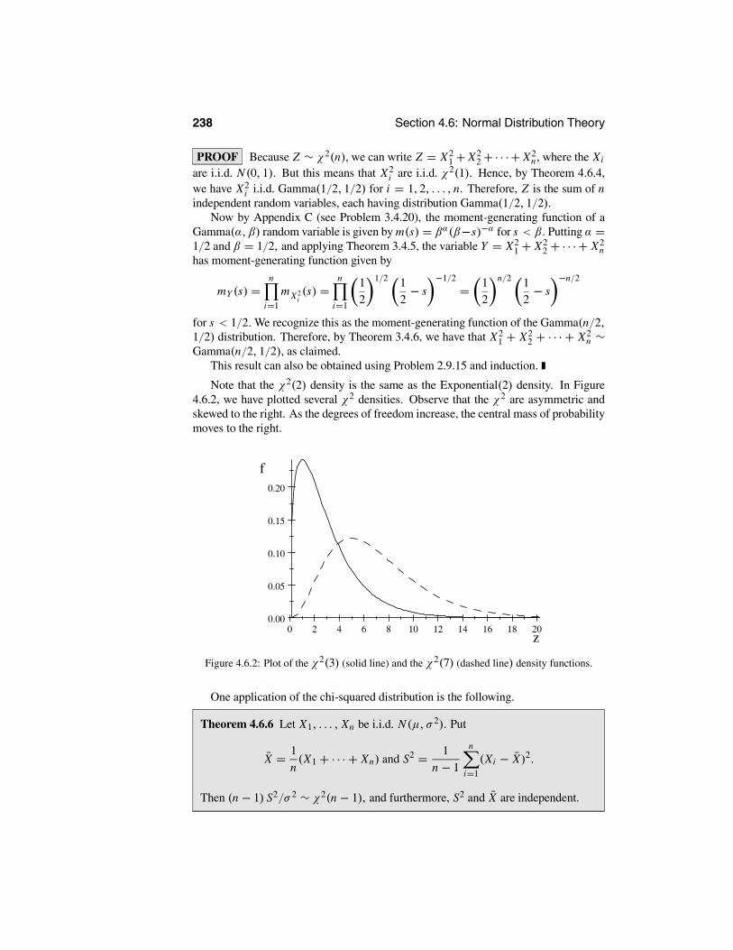
238 Section 4.6: Normal Distribution Theory
PROOF Because Z ∼ χ2(n), we can write Z = X21 + X2
2+· · ·+ X2n, where the Xi
are i.i.d. N(0, 1). But this means that X2i are i.i.d. χ2(1). Hence, by Theorem 4.6.4,
we have X2i i.i.d. Gamma(1/2, 1/2) for i = 1, 2, . . . , n. Therefore, Z is the sum of n
independent random variables, each having distribution Gamma(1/2, 1/2).Now by Appendix C (see Problem 3.4.20), the moment-generating function of a
Gamma(α, β) random variable is given by m(s) = βα(β−s)−α for s < β. Putting α =1/2 and β = 1/2, and applying Theorem 3.4.5, the variable Y = X2
1 + X22 + · · · + X2
nhas moment-generating function given by
mY (s) =n
i=1
m X2i(s) =
n
i=1
12
1/2 12− s
−1/2
= 12
n/2 12− s
−n/2
for s < 1/2.We recognize this as the moment-generating function of the Gamma(n/2,1/2) distribution. Therefore, by Theorem 3.4.6, we have that X2
1 + X22 + · · · + X2
n ∼Gamma(n/2, 1/2), as claimed.
This result can also be obtained using Problem 2.9.15 and induction.
Note that the χ2(2) density is the same as the Exponential(2) density. In Figure4.6.2, we have plotted several χ2 densities. Observe that the χ2 are asymmetric andskewed to the right. As the degrees of freedom increase, the central mass of probabilitymoves to the right.
0 2 4 6 8 10 12 14 16 18 200.00
0.05
0.10
0.15
0.20
z
f
Figure 4.6.2: Plot of the χ2(3) (solid line) and the χ2(7) (dashed line) density functions.
One application of the chi-squared distribution is the following.
Theorem 4.6.6 Let X1, . . . , Xn be i.i.d. N(µ, σ 2). Put
X = 1n(X1 + · · · + Xn) and S2 = 1
n − 1
n
i=1
(Xi − X)2.
Then (n − 1) S2/σ 2 ∼ χ2(n − 1), and furthermore, S2 and X are independent.

Chapter 4: Sampling Distributions and Limits 239
PROOF See Section 4.7 for the proof of this result.
Because the χ2(n − 1) distribution has mean n − 1, we obtain the following.
Corollary 4.6.2 E(S2) = σ 2.
PROOF Theorems 4.6.6 and 4.6.3 imply that E((n − 1) S2/σ 2) = n − 1 and thatE(S2) = σ 2.
Theorem 4.6.6 will find extensive use in Chapter 6. For example, this result, to-gether with Corollary 4.6.1, gives us the joint sampling distribution of the sample meanX and the sample variance S2 when we are sampling from an N(µ, σ 2) distribution. Ifwe do not know µ, then X is a natural estimator of this quantity and, similarly, S2 is anatural estimator of σ 2, when it is unknown. Interestingly, we divide by n − 1 in S2,rather than n, precisely because we want E(S2) = σ 2 to hold, as in Corollary 4.6.2.Actually, this property does not depend on sampling from a normal distribution. It canbe shown that anytime X1, . . . , Xn is a sample from a distribution with variance σ 2,then E(S2) = σ 2.
4.6.2 The t Distribution
The t distribution also has many statistical applications.
Definition 4.6.2 The t distribution with n degrees of freedom (or Student(n) , ort(n)), is the distribution of the random variable
Z = X
(X21 + X2
2 + · · · + X2n) / n
,
where X, X1, . . . , Xn are i.i.d., each with the standard normal distribution N(0, 1).(Equivalently, Z = X/
√Y/n, where Y ∼ χ2(n).)
Most statistical packages have built-in routines for the evaluation of t (n) probabilities(also see Table D.4 in Appendix D).
The density of the t (n) distribution is given by the following result.
Theorem 4.6.7 Let U ∼ t(n). Then
fU (u) =n+1
2√π n
2
1+ u2
n
−(n+1)/21√n
for all u ∈ R1.
PROOF For the proof of this result, see Section 4.7.
The following result shows that, when n is large, the t (n) distribution is very similarto the N(0, 1) distribution.

240 Section 4.6: Normal Distribution Theory
Theorem 4.6.8 As n → ∞, the t (n) distribution converges in distribution to astandard normal distribution.
PROOF Let Z1, . . . , Zn, Z be i.i.d. N(0, 1). As n →∞, by the strong law of largenumbers, (Z2
1+· · ·+ Z2n)/n converges with probability 1 to the constant 1. Hence, the
distribution of
Z
Z21 + · · · + Z2
n /n(4.6.2)
converges to the distribution of Z , which is the standard normal distribution. By Defi-nition 4.6.2, we have that (4.6.2) is distributed t (n).
In Figure 4.6.3, we have plotted several t densities. Notice that the densities of thet distributions are symmetric about 0 and look like the standard normal density.
-10 -8 -6 -4 -2 0 2 4 6 8 10
0.1
0.2
0.3
0.4
u
f
Figure 4.6.3: Plot of the t (1) (solid line) and the t (30) (dashed line) density functions.
The t (n) distribution has longer tails than the N(0, 1) distribution. For example, thet (1) distribution (also known as the Cauchy distribution) has 0.9366 of its probabilityin the interval (−10, 10) , whereas the N(0, 1) distribution has all of its probabilitythere (at least to four decimal places). The t (30) and the N(0, 1) densities are verysimilar.
4.6.3 The F Distribution
Finally, we consider the F distribution.

Chapter 4: Sampling Distributions and Limits 241
Definition 4.6.3 The F distribution with m and n degrees of freedom (or F(m, n))is the distribution of the random variable
Z = (X21 + X2
2 + · · · + X2m) /m
(Y 21 + Y 2
2 + · · · + Y 2n ) / n
,
where X1, . . . , Xm, Y1, . . . ,Yn are i.i.d., each with the standard normal distribution.(Equivalently, Z = (X/m)/(Y/n), where X ∼ χ2(m) and Y ∼ χ2(n).)
Most statistical packages have built-in routines for the evaluation of F(m, n) probabil-ities (also see Table D.5 in Appendix D).
The density of the F(m, n) distribution is given by the following result.
Theorem 4.6.9 Let U ∼ F(m, n). Then
fU (u) =m+n
2m2
n2
m
nu(m/2)−1
1+ m
nu−(m+n)/2 m
n
for u > 0, with fU (u) = 0 for u < 0.
PROOF For the proof of this result, see Section 4.7.
In Figure 4.6.4, we have plotted several F(m, n) densities. Notice that these densitiesare skewed to the right.
0 1 2 3 4 5 6 7 8 9 100.0
0.2
0.4
0.6
u
f
Figure 4.6.4: Plot of the F(2, 1) (solid line) and the F(3, 10) (dashed line) density functions.
The following results are useful when it is necessary to carry out computations withthe F(m, n) distribution.
Theorem 4.6.10 If Z ∼ F(m, n), then 1/Z ∼ F(n,m).
242 Section 4.6: Normal Distribution Theory
PROOF Using Definition 4.6.3, we have
1Z= (Y 2
1 + Y 22 + · · · + Y 2
n ) / n
(X21 + X2
2 + · · · + X2m) /m
and the result is immediate from the definition.
Therefore, if Z ∼ F(m, n), then P(Z ≤ z) = P(1/Z ≥ 1/z) = 1− P(1/Z ≤ 1/z),and P(1/Z ≤ 1/z) is the cdf of the F(n,m) distribution evaluated at 1/z.
In many statistical applications, n can be very large. The following result then givesa useful approximation for that case.
Theorem 4.6.11 If Zn ∼ F(m, n), then mZn converges in distribution to a χ2(m)distribution as n →∞.
PROOF Using Definition 4.6.3, we have
mZ = X21 + X2
2 + · · · + X2m
(Y 21 + Y 2
2 + · · · + Y 2n )/n
.
By Definition 4.6.1, X21 + · · · + X2
m ∼ χ2(m). By Theorem 4.6.3, E(Y 2i ) = 1, so the
strong law of large numbers implies that (Y 21 + Y 2
2 + · · · + Y 2n )/n converges almost
surely to 1. This establishes the result.
Finally, Definitions 4.6.2 and 4.6.3 immediately give the following result.
Theorem 4.6.12 If Z ∼ t (n), then Z2 ∼ F(1, n).
Summary of Section 4.6
• Linear combinations of independent normal random variables are also normal,with appropriate mean and variance.
• Two linear combinations of the same collection of independent normal randomvariables are independent if and only if their covariance equals 0.
• The chi-squared distribution with n degrees of freedom is the distribution corre-sponding to a sum of squares of n i.i.d. standard normal random variables. It hasmean n. It is equal to the Gamma(n/2, 1/2) distribution.
• The t distribution with n degrees of freedom is the distribution corresponding toa standard normal random variable, divided by the square-root of 1/n times anindependent chi-squared random variable with n degrees of freedom. Its densityfunction was presented. As n → ∞, it converges in distribution to a standardnormal distribution.
• The F distribution with m and n degrees of freedom is the distribution corre-sponding to m/n times a chi-squared distribution with m degrees of freedom,divided by an independent chi-squared distribution with n degrees of freedom.

Chapter 4: Sampling Distributions and Limits 243
Its density function was presented. If t has a t (n) distribution, then t2 is distrib-uted F(1, n).
EXERCISES
4.6.1 Let X1 ∼ N(3, 22) and X2 ∼ N(−8, 52) be independent. Let U = X1 − 5X2and V = −6X1 + C X2, where C is a constant.(a) What are the distributions of U and V ?(b) What value of C makes U and V be independent?4.6.2 Let X ∼ N(3, 5) and Y ∼ N(−7, 2) be independent.(a) What is the distribution of Z = 4X − Y/3?(b) What is the covariance of X and Z?4.6.3 Let X ∼ N(3, 5) and Y ∼ N(−7, 2) be independent. Find values of C1,C2,C3,C4,C5 so that C1(X + C2)
2 + C3(Y + C4)2 ∼ χ2(C5).
4.6.4 Let X ∼ χ2(n) and Y ∼ N(0, 1) be independent. Prove that X + Y 2 ∼χ2(n + 1).4.6.5 Let X ∼ χ2(n) and Y ∼ χ2(m) be independent. Prove that X+Y ∼ χ2(n+m).4.6.6 Let X1, X2, . . . , X4n be i.i.d. with distribution N(0, 1). Find a value of C suchthat
CX2
1 + X22 + · · · + X2
n
X2n+1 + X2
n+2 + · · · + X24n
∼ F(n, 3n).
4.6.7 Let X1, X2, . . . , Xn+1 be i.i.d. with distribution N(0, 1). Find a value of C suchthat
CX1
X22 + · · · + X2
n + X2n+1
∼ t (n) .
4.6.8 Let X ∼ N(3, 5) and Y ∼ N(−7, 2) be independent. Find values of C1,C2,C3,C4,C5,C6 so that
C1(X + C2)C3
(Y + C4)C5∼ t (C6).
4.6.9 Let X ∼ N(3, 5) and Y ∼ N(−7, 2) be independent. Find values of C1,C2,C3,C4,C5,C6,C7 so that
C1(X + C2)C3
(Y + C4)C5∼ F(C6,C7).
4.6.10 Let X1, X2, . . . , X100 be independent, each with the standard normal distribu-tion.(a) Compute the distribution of X2
1.
(b) Compute the distribution of X23 + X2
5.
(c) Compute the distribution of X10/ [X220 + X2
30 + X240]/3.
(d) Compute the distribution of 3X210 / [X2
20 + X230 + X2
40].

244 Section 4.6: Normal Distribution Theory
(e) Compute the distribution of
3070
X21 + X2
2 + · · · + X270
X271 + X2
72 + · · · + X2100
.
4.6.11 Let X1, X2, . . . , X61 be independent, each distributed as N(µ, σ 2). Set X =(1/61)(X1 + X2 + · · · + X61) and
S2 = 160
(X1 − X)2 + (X2 − X)2 + · · · + (X61 − X)2
as usual.(a) For what values of K and m is it true that the quantity Y ≡ K (X −µ)/√S2 has a tdistribution with m degrees of freedom?(b) With K as in part (a), find y such that P(Y ≥ y) = 0.05.(c) For what values of a and b and c is it true that the quantity W ≡ a(X −µ)2/S2 hasan F distribution with b and c degrees of freedom?(d) For those values of a and b and c, find a quantity w so that P(W ≥ w) = 0.05.4.6.12 Suppose the core temperature (in degrees celsius, when used intensively) ofthe latest Dell desktop computer is normally distributed with mean 40 and standarddeviation 5, while for the latest Compaq it is normally distributed with mean 45 andstandard deviation 8. Suppose we measure the Dell temperature 20 times (on separatedays) and obtain measurements D1, D2, . . . , D20, and we also measure the Compaqtemperature 30 times and obtain measurements C1,C2, . . . ,C30.(a) Compute the distribution of D ≡ (D1 + · · · + D20)/20.(b) Compute the distribution of C ≡ (C1 + · · · + C30)/30.(c) Compute the distribution of Z ≡ C − D.(d) Compute P(C < D).(e) Let U = (D1 − D)2 + (D2 − D)2 + · · · + (D20 − D)2. What is P(U > 633.25)?
PROBLEMS
4.6.13 Let X ∼ N(0, 1), and let P(Y = 1) = P(Y = −1) = 1/2. Assume X and Yare independent. Let Z = XY .(a) Prove that Z ∼ N(0, 1).(b) Prove that Cov(X, Z) = 0.(c) Prove directly that X and Z are not independent.(d) Why does this not contradict Theorem 4.6.2?4.6.14 Let Z ∼ t (n). Prove that P(Z < −x) = P(Z > x) for x ∈ R1, namely, provethat the t (n) distribution is symmetric about 0.4.6.15 Let Xn ∼ F(n, 2n) for n = 1, 2, 3, . . . . Prove that Xn → 1 in probability andwith probability 1.4.6.16 (The general chi-squared distribution) Prove that for α > 0, the function
f (z) = 12α/2 (α/2)
z(α/2)−1e−z/2

Chapter 4: Sampling Distributions and Limits 245
defines a probability distribution on (0,∞) . This distribution is known as the χ2 (α)distribution, i.e., it generalizes the distribution in Section 4.6.2 by allowing the degreesof freedom to be an arbitrary positive real number. (Hint: The χ2 (α) distribution is thesame as a Gamma(α/2, 1/2) distribution.)4.6.17 (MV) (The general t distribution) Prove that for α > 0, the function
f (u) =α+1
2√π α
2
1+ u2
α
−(α+1)/21√α
defines a probability distribution on (−∞,∞) by showing that the random variable
U = X√Y/α
has this density when X ∼ N(0, 1) independent of Y ∼ χ2(α), as in Problem 4.6.16.This distribution is known as the t (α) distribution, i.e., it generalizes the distributionin Section 4.6.3 by allowing the degrees of freedom to be an arbitrary positive realnumber. (Hint: The proof is virtually identical to that of Theorem 4.6.7.)4.6.18 (MV) (The general F distribution) Prove that for α > 0, β > 0, the function
f (u) =α+β
2
α2
β2
α
βu
(α/2)−1
1+ αβ
u−(α+β)/2 α
β
defines a probability distribution on (0,∞) by showing that the random variable
U = X/α
Y/β
has this density whenever X ∼ χ2(α) independent of Y ∼ χ2(β), as in Problem4.6.16. This distribution is known as the F(α, β) distribution, i.e., it generalizes thedistribution in Section 4.6.4 by allowing the numerator and denominator degrees offreedom to be arbitrary positive real numbers. (Hint: The proof is virtually identical tothat of Theorem 4.6.9).4.6.19 Prove that when X ∼ t (α), as defined in Problem 4.6.17, and α > 1, thenE(X) = 0. Further prove that when α > 2, Var(X) = α/ (α − 2). You can assumethe existence of these integrals — see Challenge 4.6.21. (Hint: To evaluate the secondmoment, use Y = X2 ∼ F(1, α) as defined in Problem 4.6.18.)
4.6.20 Prove that when X ∼ F(α, β), then E(X) = β/ (β − 2) when β > 2 andVar(X) = 2β2(α + β − 2)/α(β − 2)2 (β − 4) when β > 4.
CHALLENGES
4.6.21 Following Problem 4.6.19, prove that the mean of X does not exist whenever0 < α ≤ 1. Further prove that the variance of X does not exist whenever 0 < α ≤ 1and is infinite when 1 < α ≤ 2.
4.6.22 Prove the identity (4.7.1) in Section 4.7, which arises as part of the proof ofTheorem 4.6.6.

246 Section 4.7: Further Proofs (Advanced)
4.7 Further Proofs (Advanced)Proof of Theorem 4.3.1
We want to prove the following result. Let Z , Z1, Z2, . . . be random variables. SupposeZn → Z with probability 1. Then Zn → Z in probability. That is, if a sequence ofrandom variables converges almost surely, then it converges in probability to the samelimit.
Assume P(Zn → Z) = 1. Fix > 0, and let An = {s : |Zm − Z | ≥ for somem ≥ n}. Then {An} is a decreasing sequence of events. Furthermore, if s ∈ ∩∞n=1 An,then Zn(s)9 Z(s) as n →∞. Hence,
P ∩∞n=1 An ≤ P(Zn → Z) = 0.
By continuity of probabilities, we have limn→∞ P(An) = P(∩∞n=1 An) = 0. Hence,P(|Zn − Z | ≥ ) ≤ P(An)→ 0 as n → ∞. Because this is true for any > 0, wesee that Zn → Z in probability.
Proof of Theorem 4.4.1
We show that if XnP→ X, then Xn
D→ X.Suppose Xn → X in probability and that P(X = x) = 0. We wish to show that
limn→∞ P(Xn ≤ x) = P(X ≤ x).Choose any > 0. Now, if Xn ≤ x, then we must have either X ≤ x + or
|X − Xn| ≥ . Hence, by subadditivity,
P(Xn ≤ x) ≤ P(X ≤ x + )+ P(|X − Xn| ≥ ).
Replacing x by x − in this equation, we see also that
P(X ≤ x − ) ≤ P(Xn ≤ x)+ P(|X − Xn| ≥ ).
Rearranging and combining these two inequalities, we have
P(X ≤ x− )−P(|X−Xn| ≥ ) ≤ P(Xn ≤ x) ≤ P(X ≤ x+ )+P(|X−Xn| ≥ ).
This is the key.We next let n →∞. Because Xn → X in probability, we know that
limn→∞ P(|X − Xn| ≥ ) = 0.
This means that limn→∞ P(Xn ≤ x) is “sandwiched” between P(X ≤ x − ) andP(X ≤ x + ).
We then let 0. By continuity of probabilities,
lim0
P(X ≤ x + ) = P(X ≤ x) and lim0
P(X ≤ x − ) = P(X < x).
This means that limn→∞ P(Xn ≤ x) is “sandwiched” between P(X < x) and P(X ≤x).
But because P(X = x) = 0, we must have P(X < x) = P(X ≤ x). Hence,limn→∞ P(Xn ≤ x) = P(X ≤ x), as required.
Chapter 4: Sampling Distributions and Limits 247
Proof of Theorem 4.4.3 (The central limit theorem)
We must prove the following. LetX1, X2, . . . be i.i.d. with finite mean µ and finitevariance σ 2. Let Z ∼ N(0, 1). Set Sn = X1 + · · · + Xn, and
Zn = Sn − nµ√nσ 2
.
Then as n →∞, the sequence {Zn} converges in distribution to the Z, i.e., ZnD→ Z.
Recall that the standard normal distribution has moment-generating function givenby m Z (s) = exp s2/2 .
We shall now assume that m Zn (s) is finite for |s| < s0 for some s0 > 0. (Thisassumption can be eliminated by using characteristic functions instead of moment-generating functions.) Assuming this, we will prove that for each real number s, wehave limn→∞m Zn (s) = m Z (s), where m Zn (s) is the moment-generating function ofZn . It then follows from Theorem 4.4.2 that Zn converges to Z in distribution.
To proceed, let Yi = (Xi − µ) /σ . Then E(Yi) = 0 and E(Y 2i ) =Var(Yi ) = 1.
Also, we have
Zn = 1√n(Y1 + · · · + Yn).
Let mY (s) = E(esYi ) be the moment-generating function of Yi (which is the same forall i , because they are i.i.d.). Then using independence, we compute that
limn→∞mZn (s) = lim
n→∞ E es Zn = limn→∞ E es(Y1+···+Yn)/
√n
= limn→∞ E esY1/
√n esY2/
√n · · · esYn/
√n
= limn→∞ E esY1/
√n E esY2/
√n · · · E esYn/
√n
= limn→∞mY (s/
√n)mY (s/
√n) · · ·mY (s/
√n)
= limn→∞mY (s/
√n)n.
Now, we know from Theorem 3.5.3 that mY (0) = E(e0) = 1. Also, mY (0) =E(Yi ) = 0 and mY (0) = E(Y 2
i ) = 1. But then expanding mY (s) in a Taylor seriesaround s = 0, we see that
mY (s) = 1+ 0s + 12!
s2 + o(s2) = 1+ s2/2+ o(s2),
where o(s2) stands for a quantity that, as s → 0, goes to 0 faster than s2 does —namely, o(s2)/s → 0 as s → 0. This means that
mY (s/√
n) = 1+ (s/√n)2/2+ o((s/√
n)2) = 1+ s2/2n + o(1/n),
where now o(1/n) stands for a quantity that, as n → ∞, goes to 0 faster than 1/ndoes.

248 Section 4.7: Further Proofs (Advanced)
Finally, we recall from calculus that, for any real number c, limn→∞(1+ c/n)n =ec. It follows from this and the above that
limn→∞(mY (s/2
√n))n = lim
n→∞(1+ s2/2n)n = es2/2.
That is, limn→∞mZn (s) = es2/2, as claimed.
Proof of Theorem 4.6.2
We prove the following. Suppose Xi ∼ N(µi , σ2i ) for i = 1, 2, . . . , n and also that the
{Xi } are independent. Let U = ni=1 ai Xi and V = n
i=1 bi Xi , for some constants{ai} and {bi }. Then Cov(U, V ) = i ai biσ
2i . Furthermore, Cov(U, V ) = 0 if and
only if U and V are independent.It was proved in Section 4.6 that Cov(U, V ) = i ai biσ
2i and that Cov(U,V ) = 0
if U and V are independent. It remains to prove that, if Cov(U,V ) = 0, then U and Vare independent. For simplicity, we take n = 2 and µ1 = µ2 = 0 and σ 2
1 = σ 22 = 1;
the general case is similar but messier. We therefore have
U = a1 X1 + a2 X2 and V = b1 X1 + b2 X2.
The Jacobian derivative of this transformation is
J (x1, x2) = ∂U
∂X1
∂V
∂X2− ∂V
∂X1
∂U
∂X2= a1b2 − b1a2.
Inverting the transformation gives
X1 = b2U − a2V
a1b2 − b1a2and X2 = a1V − b1U
a1b2 − b1a2.
Also,
fX1,X2(x1, x2) = 12π
e− x21+x2
2 /2.
Hence, from the multidimensional change of variable theorem (Theorem 2.9.2), wehave
fU,V (u, v) = fX1,X2(x1, x2)b2u − a2v
a1b2 − b1a2,
a1v − b1u
a1b2 − b1a2|J (x1, x2)|−1
= 12π
exp −((b2u − a2v)2 + (a1v − b1u)2) /2(a1b2 − b1a2)
2
|a1b2 − b1a2| .
But
(b2u − a2v)2 + (a1v − b1u)2 = (b2
1 + b22)u
2 + (a21 + a2
2)v2 − 2(a1b1 + a2b2)uv
and Cov(U, V ) = a1b1 + a2b2. Hence, if Cov(U,V ) = 0, then
(b2u − a2v)2 + (a1v − b1u)2 = (b2
1 + b22)u
2 + (a21 + a2
2)v2

Chapter 4: Sampling Distributions and Limits 249
and
fU,V (u, v) = exp −((b21 + b2
2)u2 + (a2
1 + a22)v
2)/2(a1b2 − b1a2)2
2π |a1b2 − b1a2|= exp −(b2
1 + b22)u
2/2(a1b2 − b1a2)2 exp −(a2
1 + a22)v
2/2(a1b2 − b1a2)2
2π |a1b2 − b1a2| .
It follows that we can factor fU,V (u, v) as a function of u times a function of v . Butthis implies (see Problem 2.8.19) that U and V are independent.
Proof of Theorem 4.6.6
We want to prove that when X1, . . . , Xn are i.i.d. N(µ, σ 2) and
X = 1n(X1 + · · · + Xn) and S2 = 1
n − 1
n
i=1
(Xi − X)2,
then (n − 1) S2/σ 2 ∼ χ2(n − 1) and, furthermore, that S2 and X are independent.We have
n − 1
σ 2S2 =
n
i=1
Xi − X
σ
2
.
We rewrite this expression as (see Challenge 4.6.22)
n − 1
σ 2 S2
= X1 − X2
σ√
2
2
+ X1 + X2 − 2X3
σ√
2 · 32
+ X1 + X2 + X3 − 3X4
σ√
3 · 42
+ · · · + X1 + X2 + · · · + Xn−1 − (n − 1)Xn
σ√(n − 1)n
2
. (4.7.1)
Now, by Theorem 4.6.1, each of the n − 1 expressions within brackets in (4.7.1)has the standard normal distribution. Furthermore, by Theorem 4.6.2, the expressionswithin brackets in (4.7.1) are all independent of one another and are also all indepen-dent of X .
It follows that (n − 1) S2/σ 2 is independent of X . It also follows, by the definitionof the chi-squared distribution, that (n − 1) S2/σ 2 ∼ χ2(n − 1).
Proof of Theorem 4.6.7
We want to show that when U ∼ t (n), then
fU (u) =n+1
2√π n
2
1+ u2
n
−(n+1)/21√n
for all u ∈ R1.

250 Section 4.7: Further Proofs (Advanced)
Because U ∼ t(n), we can write U = X/√
Y/n, where X and Y are independentwith X ∼ N(0, 1) and Y ∼ χ2(n). It follows that X and Y have joint density given by
fX,Y (x, y) = e−x2/2y(n/2)−1e−y/2√
2π2n/2 n2
when y > 0 (with fX,Y (x, y) = 0 for y < 0).Let V = Y. We shall use the multivariate change of variables formula (Theo-
rem 2.9.2) to compute the joint density fU,V (u, v) of U and V . Because U = X/√
Y/nand V = Y , it follows that X = U
√V/n and Y = V . We compute the Jacobian term
as
J (x, y) = det
∂u∂x
∂v∂x
∂u∂y
∂v∂y
= det
1√y/n
0
−x√
ny3/2 1
= 1√y/n
.
Hence,
fU,V (u, v) = fX,Y uv
n, v J−1 u
v
n, v
= e− u2v /2nv(n/2)−1e−v/2√2π2n/2 n
2
v
n
= 1√π (n/2)
1
2(n+1)/2
1√nv(n+1)/2−1e−(v/2) 1+u2/n
for v > 0 (with fU,V (u, v) = 0 for v < 0).Finally, we compute the marginal density of U :
fU (u) =∞
−∞fU,V (u, v) dv
= 1√π (n/2)
12(n+1)/2
1√n
∞
0v(n+1)/2−1e−(v/2) 1+u2/n dv
= 1√π (n/2)
1+ u2
n
−(n+1)/21√n
∞
0w(n+1)/2−1e−w/2 dw
=n+1
2√π (n/2)
1+ u2
n
−(n+1)/21√n,
where we have made the substitution w = 1+ u2/n v/2 to get the third equality andthen used the definition of the gamma function to obtain the result.
Proof of Theorem 4.6.9
We want to show that when U ∼ F(m, n), then
fU (u) =m+n
2m2
n2
m
nu(m/2)−1
1+ m
nu−(m+n)/2 m
n

Chapter 4: Sampling Distributions and Limits 251
for u > 0, with fU (u) = 0 for u < 0.Because U ∼ F(n,m), we can write U = (X/m)/(Y/n), where X and Y are
independent with X ∼ χ2(m) and Y ∼ χ2(n). It follows that X and Y have jointdensity given by
fX,Y (x, y) = x(m/2)−1e−x/2y(n/2)−1e−y/2
2m/2 m2 2n/2 n
2
when x, y > 0 (with fX,Y (x, y) = 0 for x < 0 or y < 0).Let V = Y, and use the multivariate change of variables formula (Theorem 2.9.2)
to compute the joint density fU,V (u, v) of U and V . Because U = (X/m)/(Y/n) andV = Y , it follows that X = (m/n)U V and Y = V . We compute the Jacobian term as
J(x, y) = det
∂u∂x
∂v∂x
∂u∂y
∂v∂y
= det
nmy 0
−nXmY 2 1
= n
my.
Hence,
fU,V (u, v) = fX,Y ((m/n)uv, v)J−1((m/n)uv, v)
=mn uv (m/2)−1 e−(m/n)(uv/2)v(n/2)−1e−(v/2)
2m/2 m2 2n/2 n
2
= 1m2
n2
m
nu(m/2)−1 m
n
12m/2 v
(n/2)−1e−(v/2)(1+mu/n)
for u, v > 0 (with fU,V (u, v) = 0 for u < 0 or v < 0).Finally, we compute the marginal density of U as
fU (u)
=∞
−∞fU,V (u, v) dv
= 1m2
n2
m
nu(m/2)−1 m
n
1
2m/2
∞
0v(n/2)−1e−(v/2)(1+mu/n) dv
= 1m2
n2
m
nu(m/2)−1
1+ m
nu−(n+m)/2 m
n
∞
0w(n/2)−1e−w dw
=m+n
2m2
n2
m
nu(m/2)−1
1+ m
nu−(n+m)/2
,
where we have used the substitution w = (1+mu/n) v/2 to get the third equality, andthe final result follows from the definition of the gamma function.

252 Section 4.7: Further Proofs (Advanced)
Chapter 5
Statistical Inference
CHAPTER OUTLINE
Section 1 Why Do We Need Statistics?Section 2 Inference Using a Probability ModelSection 3 Statistical ModelsSection 4 Data CollectionSection 5 Some Basic Inferences
In this chapter, we begin our discussion of statistical inference. Probability theory isprimarily concerned with calculating various quantities associated with a probabilitymodel. This requires that we know what the correct probability model is. In applica-tions, this is often not the case, and the best we can say is that the correct probabilitymeasure to use is in a set of possible probability measures. We refer to this collection asthe statistical model. So, in a sense, our uncertainty has increased; not only do we havethe uncertainty associated with an outcome or response as described by a probabilitymeasure, but now we are also uncertain about what the probability measure is.
Statistical inference is concerned with making statements or inferences about char-acteristics of the true underlying probability measure. Of course, these inferences mustbe based on some kind of information; the statistical model makes up part of it. Anotherimportant part of the information will be given by an observed outcome or response,which we refer to as the data. Inferences then take the form of various statements aboutthe true underlying probability measure from which the data were obtained. These takea variety of forms, which we refer to as types of inferences.
The role of this chapter is to introduce the basic concepts and ideas of statisticalinference. The most prominent approaches to inference are discussed in Chapters 6,7, and 8. Likelihood methods require the least structure as described in Chapter 6.Bayesian methods, discussed in Chapter 7, require some additional ingredients. Infer-ence methods based on measures of performance and loss functions are described inChapter 8.
253

254 Section 5.1: Why Do We Need Statistics?
5.1 Why Do We Need Statistics?While we will spend much of our time discussing the theory of statistics, we shouldalways remember that statistics is an applied subject. By this we mean that ultimatelystatistical theory will be applied to real-world situations to answer questions of practicalimportance.
What is it that characterizes those contexts in which statistical methods are useful?Perhaps the best way to answer this is to consider a practical example where statisticalmethodology plays an important role.
EXAMPLE 5.1.1 Stanford Heart Transplant StudyIn the paper by Turnbull, Brown, and Hu entitled “Survivorship of Heart TransplantData” (Journal of the American Statistical Association, March 1974, Volume 69, 74–80), an analysis is conducted to determine whether or not a heart transplant program,instituted at Stanford University, is in fact producing the intended outcome. In this case,the intended outcome is an increased length of life, namely, a patient who receives anew heart should live longer than if no new heart was received.
It is obviously important to ensure that a proposed medical treatment for a diseaseleads to an improvement in the condition. Clearly, we would not want it to lead to adeterioration in the condition. Also, if it only produced a small improvement, it maynot be worth carrying out if it is very expensive or causes additional suffering.
We can never know whether a particular patient who received a new heart has livedlonger because of the transplant. So our only hope in determining whether the treat-ment is working is to compare the lifelengths of patients who received new hearts withthe lifelengths of patients who did not. There are many factors that influence a patient’slifelength, many of which will have nothing to do with the condition of the patient’sheart. For example, lifestyle and the existence of other pathologies, which will varygreatly from patient to patient, will have a great influence. So how can we make thiscomparison?
One approach to this problem is to imagine that there are probability distributionsthat describe the lifelengths of the two groups. Let these be given by the densities fTand fC , where T denotes transplant and C denotes no transplant. Here we have usedC as our label because this group is serving as a control in the study to provide somecomparison to the treatment (a heart transplant). Then we consider the lifelength of apatient who received a transplant as a random observation from fT and the lifelength ofa patient who did not receive a transplant as a random observation from fC . We wantto compare fT and fC , in some fashion, to determine whether or not the transplanttreatment is working. For example, we might compute the mean lifelengths of eachdistribution and compare these. If the mean lifelength of fT is greater than fC , thenwe can assert that the treatment is working. Of course, we would still have to judgewhether the size of the improvement is enough to warrant the additional expense andpatients’ suffering.
If we could take an arbitrarily large number of observations from fT and fC , thenwe know, from the results in previous chapters, that we could determine these distribu-tions with a great deal of accuracy. In practice, however, we are restricted to a relativelysmall number of observations. For example, in the cited study there were 30 patients

Chapter 5: Statistical Inference 255
P X S P X S P X S1 49 d 11 1400 a 21 2 d2 5 d 12 5 d 22 148 d3 17 d 13 34 d 23 1 d4 2 d 14 15 d 24 68 d5 39 d 15 11 d 25 31 d6 84 d 16 2 d 26 1 d7 7 d 17 1 d 27 20 d8 0 d 18 39 d 28 118 a9 35 d 19 8 d 29 91 a
10 36 d 20 101 d 30 427 a
Table 5.1: Survival times (X) in days and status (S) at the end of the study for eachpatient (P) in the control group.
in the control group (those who did not receive a transplant) and 52 patients in thetreatment group (those who did receive a transplant).
For each control patient, the value of X — the number of days they were aliveafter the date they were determined to be a candidate for a heart transplant until thetermination date of the study — was recorded. For various reasons, these patients didnot receive new hearts, e.g., they died before a new heart could be found for them.These data, together with an indicator for the status of the patient at the terminationdate of the study, are presented in Table 5.1. The indicator value S = a denotes that thepatient was alive at the end of the study and S = d denotes that the patient was dead.
For each treatment patient, the value of Y, the number of days they waited for thetransplant after the date they were determined to be a candidate for a heart transplant,and the value of Z, the number of days they were alive after the date they receivedthe heart transplant until the termination date of the study, were both recorded. Thesurvival times for the treatment group are then given by the values of Y + Z . Thesedata, together with an indicator for the status of the patient at the termination date ofthe study, are presented in Table 5.2.
We cannot compare fT and fC directly because we do not know these distributions.But we do have some information about them because we have obtained values fromeach, as presented in Tables 5.1 and 5.2. So how do we use these data to compare fTand fC to answer the question of central importance, concerning whether or not thetreatment is effective? This is the realm of statistics and statistical theory, namely, pro-viding methods for making inferences about unknown probability distributions basedupon observations (samples) obtained from them.
We note that we have simplified this example somewhat, although our discussionpresents the essence of the problem. The added complexity comes from the fact thattypically statisticians will have available additional data on each patient, such as theirage, gender, and disease history. As a particular example of this, in Table 5.2 we havethe values of both Y and Z for each patient in the treatment group. As it turns out,this additional information, known as covariates, can be used to make our comparisonsmore accurate. This will be discussed in Chapter 10.

256 Section 5.1: Why Do We Need Statistics?
P Y Z S P Y Z S P Y Z S1 0 15 d 19 50 1140 a 37 77 442 a2 35 3 d 20 22 1153 a 38 2 65 d3 50 624 d 21 45 54 d 39 26 419 a4 11 46 d 22 18 47 d 40 32 362 a5 25 127 d 23 4 0 d 41 13 64 d6 16 61 d 24 1 43 d 42 56 228 d7 36 1350 d 25 40 971 a 43 2 65 d8 27 312 d 26 57 868 a 44 9 264 a9 19 24 d 27 0 44 d 45 4 25 d
10 17 10 d 28 1 780 a 46 30 193 a11 7 1024 d 29 20 51 d 47 3 196 a12 11 39 d 30 35 710 a 48 26 63 d13 2 730 d 31 82 663 a 49 4 12 d14 82 136 d 32 31 253 d 50 45 103 a15 24 1379 a 33 40 147 d 51 25 60 a16 70 1 d 34 9 51 d 52 5 43 a17 15 836 d 35 66 479 a18 16 60 d 36 20 322 d
Table 5.2: The number of days until transplant (Y ), survival times in days after trans-plant (Z), and status (S) at the end of the study for each patient (P) in the treatmentgroup.
The previous example provides some evidence that questions of great practical im-portance require the use of statistical thinking and methodology. There are many sit-uations in the physical and social sciences where statistics plays a key role, and thereasons are just like those found in Example 5.1.1. The central ingredient in all ofthese is that we are faced with uncertainty. This uncertainty is caused both by vari-ation, which can be modeled via probability, and by the fact that we cannot collectenough observations to know the correct probability models precisely. The first fourchapters have dealt with building, and using, a mathematical model to deal with thefirst source of uncertainty. In this chapter, we begin to discuss methods for dealingwith the second source of uncertainty.
Summary of Section 5.1
• Statistics is applied to situations in which we have questions that cannot be an-swered definitively, typically because of variation in data.
• Probability is used to model the variation observed in the data. Statistical infer-ence is concerned with using the observed data to help identify the true proba-bility distribution (or distributions) producing this variation and thus gain insightinto the answers to the questions of interest.

Chapter 5: Statistical Inference 257
EXERCISES
5.1.1 Compute the mean survival times for the control group and for the treatmentgroups in Example 5.1.1. What do you conclude from these numbers? Do you thinkit is valid to base your conclusions about the effectiveness of the treatment on thesenumbers? Explain why or why not.5.1.2 Are there any unusual observations in the data presented in Example 5.1.1? If so,what effect do you think these observations have on the mean survival times computedin Exercise 5.1.1?5.1.3 In Example 5.1.1, we can use the status variable S as a covariate. What is thepractical significance of this variable?5.1.4 A student is uncertain about the mark that will be received in a statistics course.The course instructor has made available a database of marks in the course for a numberof years. Can you identify a probability distribution that may be relevant to quantifyingthe student’s uncertainty? What covariates might be relevant in this situation?5.1.5 The following data were generated from an N(µ, 1) distribution by a student.Unfortunately, the student forgot which value of µ was used, so we are uncertain aboutthe correct probability distribution to use to describe the variation in the data.
0.2 −0.7 0.0 −1.9 0.7 −0.3 0.3 0.40.3 −0.8 1.5 0.1 0.3 −0.7 −1.8 0.2
Can you suggest a plausible value for µ? Explain your reasoning.5.1.6 Suppose you are interested in determining the average age of all male studentsat a particular college. The registrar of the college allows you access to a databasethat lists the age of every student at the college. Describe how you might answer yourquestion. Is this a statistical problem in the sense that you are uncertain about anythingand so will require the use of statistical methodology?5.1.7 Suppose you are told that a characteristic X follows an N(µ1, 1) distribution anda characteristic Y follows an N(µ2, 1) distribution where µ1 and µ2 are unknown. Inaddition, you are given the results x1, . . . , xm of m independent measurements on Xand y1, . . . , yn of n independent measurements on Y. Suggest a method for determin-ing whether or not µ1 and µ2 are equal. Can you think of any problems with yourapproach?5.1.8 Suppose we know that a characteristic X follows an Exponential(λ) distributionand you are required to determine λ based on i.i.d. observations x1, . . . , xn from thisdistribution. Suggest a method for doing this. Can you think of any problems with yourapproach?
PROBLEMS
5.1.9 Can you identify any potential problems with the method we have discussed inExample 5.1.1 for determining whether or not the heart transplant program is effectivein extending life?5.1.10 Suppose you are able to generate samples of any size from a probability distri-bution P for which it is very difficult to compute P(C) for some set C . Explain how

258 Section 5.2: Inference Using a Probability Model
you might estimate P(C) based on a sample. What role does the size of the sampleplay in your uncertainty about how good your approximation is. Does the size of P(C)play a role in this?
COMPUTER PROBLEMS
5.1.11 Suppose we want to obtain the distribution of the quantity Y = X4 + 2X3 − 3when X ∼ N(0, 1).Here we are faced with a form of mathematical uncertainty becauseit is very difficult to determine the distribution of Y using mathematical methods. Pro-pose a computer method for approximating the distribution function of Y and estimateP(Y ∈ (1, 2)).What is the relevance of statistical methodology to your approach?
DISCUSSION TOPICS
5.1.12 Sometimes it is claimed that all uncertainties can and should be modeled usingprobability. Discuss this issue in the context of Example 5.1.1, namely, indicate all thethings you are uncertain about in this example and how you might propose probabilitydistributions to quantify these uncertainties.
5.2 Inference Using a Probability ModelIn the first four chapters, we have discussed probability theory, a good part of whichhas involved the mathematics of probability theory. This tells us how to carry outvarious calculations associated with the application of the theory. It is important tokeep in mind, however, our reasons for introducing probability in the first place. Aswe discussed in Section 1.1, probability is concerned with measuring or quantifyinguncertainty.
Of course, we are uncertain about many things, and we cannot claim that prob-ability is applicable to all these situations. Let us assume, however, that we are ina situation in which we feel probability is applicable and that we have a probabilitymeasure P defined on a collection of subsets of a sample space S for a response s.
In an application of probability, we presume that we know P and are uncertainabout a future, or concealed, response value s ∈ S. In such a context, we may berequired, or may wish, to make an inference about the unknown value of s. This cantake the form of a prediction or estimate of a plausible value for s, e.g., under suitableconditions, we might take the expected value of s as our prediction. In other contexts,we may be asked to construct a subset that has a high probability of containing s andis in some sense small, e.g., find the region that contains at least 95% of the probabilityand has the smallest size amongst all such regions. Alternatively, we might be askedto assess whether or not a stated value s0 is an implausible value from the known P,e.g., assess whether or not s0 lies in a region assigned low probability by P and sois implausible. These are examples of inferences that are relevant to applications ofprobability theory.

Chapter 5: Statistical Inference 259
EXAMPLE 5.2.1As a specific application, consider the lifelength X in years of a machine where it isknown that X ∼Exponential(1) (see Figure 5.2.1).
0 1 2 3 4 5 6 7 8 9 100.0
0.2
0.4
0.6
0.8
1.0
x
f
Figure 5.2.1: Plot of the Exponential(1) density f .
Then for a new machine, we might predict its lifelength by E(X) = 1 year. Further-more, from the graph of the Exponential(1) density, it is clear that the smallest intervalcontaining 95% of the probability for X is (0, c) , where c satisfies
0.95 =! c
0e−x dx = 1− e−c
or c = − ln (0.05) = 2.9957. This interval gives us a reasonable range of probablelifelengths for the new machine. Finally, if we wanted to assess whether or not x0 = 5is a plausible lifelength for a newly purchased machine, we might compute the tailprobability as
P(X > 5) =! ∞
5e−x dx = e−5 = 0.0067,
which, in this case, is very small and therefore indicates that x0 = 5 is fairly far out inthe tail. The right tail of this density is a region of low probability for this distribution,so x0 = 5 can be considered implausible. It is thus unlikely that a machine will last 5years, so a purchaser would have to plan to replace the machine before that period isover.
In some applications, we receive some partial information about the unknown staking the form s ∈ C ⊂ S. In such a case, we replace P by the conditional probabilitymeasure P (· |C) when deriving our inferences. Our reasons for doing this are many,and, in general, we can say that most statisticians agree that it is the right thing to do. Itis important to recognize, however, that this step does not proceed from a mathematicaltheorem; rather it can be regarded as a basic axiom or principle of inference. We willrefer to this as the principle of conditional probability, which will play a key role insome later developments.
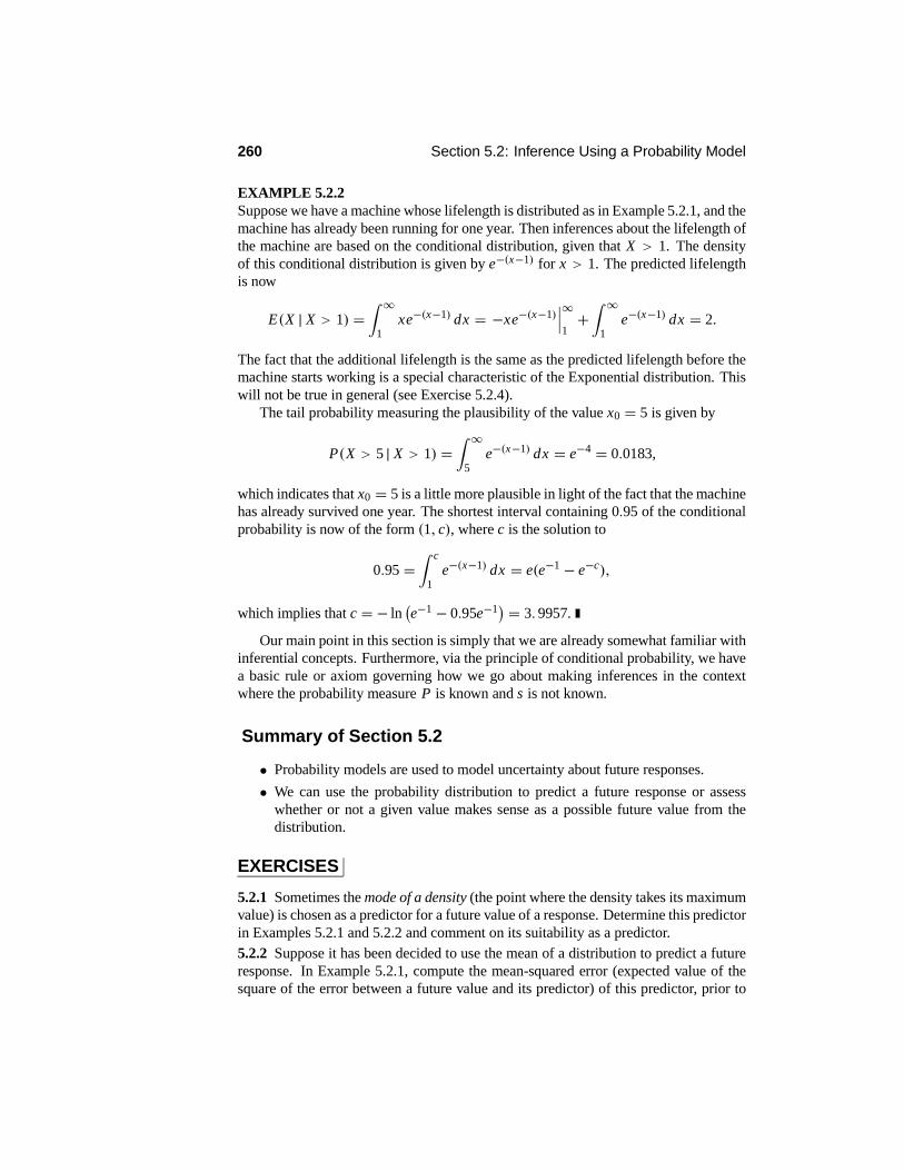
260 Section 5.2: Inference Using a Probability Model
EXAMPLE 5.2.2Suppose we have a machine whose lifelength is distributed as in Example 5.2.1, and themachine has already been running for one year. Then inferences about the lifelength ofthe machine are based on the conditional distribution, given that X > 1. The densityof this conditional distribution is given by e−(x−1) for x > 1. The predicted lifelengthis now
E(X | X > 1) =! ∞
1xe−(x−1) dx = −xe−(x−1)
"""∞1+! ∞
1e−(x−1) dx = 2.
The fact that the additional lifelength is the same as the predicted lifelength before themachine starts working is a special characteristic of the Exponential distribution. Thiswill not be true in general (see Exercise 5.2.4).
The tail probability measuring the plausibility of the value x0 = 5 is given by
P(X > 5 | X > 1) =! ∞
5e−(x−1) dx = e−4 = 0.0183,
which indicates that x0 = 5 is a little more plausible in light of the fact that the machinehas already survived one year. The shortest interval containing 0.95 of the conditionalprobability is now of the form (1, c), where c is the solution to
0.95 =! c
1e−(x−1) dx = e(e−1 − e−c),
which implies that c = − ln#e−1 − 0.95e−1
$ = 3. 9957.
Our main point in this section is simply that we are already somewhat familiar withinferential concepts. Furthermore, via the principle of conditional probability, we havea basic rule or axiom governing how we go about making inferences in the contextwhere the probability measure P is known and s is not known.
Summary of Section 5.2
• Probability models are used to model uncertainty about future responses.
• We can use the probability distribution to predict a future response or assesswhether or not a given value makes sense as a possible future value from thedistribution.
EXERCISES
5.2.1 Sometimes the mode of a density (the point where the density takes its maximumvalue) is chosen as a predictor for a future value of a response. Determine this predictorin Examples 5.2.1 and 5.2.2 and comment on its suitability as a predictor.5.2.2 Suppose it has been decided to use the mean of a distribution to predict a futureresponse. In Example 5.2.1, compute the mean-squared error (expected value of thesquare of the error between a future value and its predictor) of this predictor, prior to

Chapter 5: Statistical Inference 261
observing the value. To what characteristic of the distribution of the lifelength doesthis correspond?5.2.3 Graph the density of the distribution obtained as a mixture of a normal distribu-tion with mean 4 and variance 1 and a normal distribution with mean −4 and variance1, where the mixture probability is 0.5. Explain why neither the mean nor the mode isa suitable predictor in this case. (Hint: Section 2.5.4.)5.2.4 Repeat the calculations of Examples 5.2.1 and 5.2.2 when the lifelength of amachine is known to be distributed as Y = 10X, where X ∼Uniform[0, 1].5.2.5 Suppose that X ∼ N(10, 2). What value would you record as a prediction of afuture value of X? How would you justify your choice?5.2.6 Suppose that X ∼ N(10, 2). Record the smallest interval containing 0.95 of theprobability for a future response. (Hint: Consider a plot of the density.)5.2.7 Suppose that X ∼ Gamma(3, 6). What value would you record as a predictionof a future value of X? How would you justify your choice?5.2.8 Suppose that X ∼ Poisson(5).What value would you record as a prediction of afuture value of X? How would you justify your choice?5.2.9 Suppose that X ∼Geometric(1/3).What value would you record as a predictionof a future value of X?5.2.10 Suppose that X follows the following probability distribution.
x 1 2 3 4P(X = x) 1/2 1/4 1/8 1/8
(a) Record a prediction of a future value of X.
(b) Suppose you are then told that X ≥ 2. Record a prediction of a future value of Xthat uses this information.
PROBLEMS
5.2.11 Suppose a fair coin is tossed 10 times and the response X measured is thenumber of times we observe a head.(a) If you use the expected value of the response as a predictor, then what is the predic-tion of a future response X?(b) Using Table D.6 (or a statistical package), compute a shortest interval containingat least 0.95 of the probability for X. Note that it might help to plot the probabilityfunction of X first.(c) What region would you use to assess whether or not a value s0 is a possible futurevalue? (Hint: What are the regions of low probability for the distribution?) Assesswhether or not x = 8 is plausible.5.2.12 In Example 5.2.1, explain (intuitively) why the interval (0, 2.9957) is the short-est interval containing 0.95 of the probability for the lifelength.5.2.13 (Problem 5.2.11 continued) Suppose we are told that the number of heads ob-served is an even number. Repeat parts (a), (b), and (c).5.2.14 Suppose that a response X is distributed Beta(a, b) with a, b > 1 fixed (seeProblem 2.4.16). Determine the mean and the mode (point where density takes its

262 Section 5.3: Statistical Models
maximum) of this distribution and assess which is the most accurate predictor of afuture X when using mean-squared error, i.e., the expected squared distance betweenX and the prediction.5.2.15 Suppose that a response X is distributed N(0, 1) and that we have decided topredict a future value using the mean of the distribution.(a) Determine the prediction for a future X.
(b) Determine the prediction for a future Y = X2.
(c) Comment on the relationship (or lack thereof) between the answers in parts (a) and(b).5.2.16 Suppose that X ∼ Geometric(1/3). Determine the shortest interval containing0.95 of the probability for a future X. (Hint: Plot the probability function and recordthe distribution function.)5.2.17 Suppose that X ∼ Geometric(1/3) and we are told that X > 5. What valuewould you record as a prediction of a future value of X? Determine the shortest intervalcontaining 0.95 of the probability for a future X. (Hint: Plot the probability functionand record the distribution function.)
DISCUSSION TOPICS
5.2.18 Do you think it is realistic for a practitioner to proceed as if he knows the trueprobability distribution for a response in a problem?
5.3 Statistical ModelsIn a statistical problem, we are faced with uncertainty of a different character thanthat arising in Section 5.2. In a statistical context, we observe the data s, but we areuncertain about P . In such a situation, we want to construct inferences about P basedon s. This is the inverse of the situation discussed in Section 5.2.
How we should go about making these statistical inferences is probably not at allobvious. In fact, there are several possible approaches that we will discuss in subse-quent chapters. In this chapter, we will develop the basic ingredients of all the ap-proaches.
Common to virtually all approaches to statistical inference is the concept of thestatistical model for the data s. This takes the form of a set {Pθ : θ ∈ *} of probabilitymeasures, one of which corresponds to the true unknown probability measure P thatproduced the data s. In other words, we are asserting that there is a random mechanismgenerating s, and we know that the corresponding probability measure P is one of theprobability measures in {Pθ : θ ∈ *} .
The statistical model {Pθ : θ ∈ *} corresponds to the information a statisticianbrings to the application about what the true probability measure is, or at least whatone is willing to assume about it. The variable θ is called the parameter of the model,and the set * is called the parameter space. Typically, we use models where θ ∈ *indexes the probability measures in the model, i.e., Pθ1 = Pθ2 if and only if θ1 = θ2.If the probability measures Pθ can all be presented via probability functions or den-sity functions fθ (for convenience we will not distinguish between the discrete and

Chapter 5: Statistical Inference 263
continuous case in the notation), then it is common to write the statistical model as{ fθ : θ ∈ *}.
From the definition of a statistical model, we see that there is a unique value θ ∈*, such that Pθ is the true probability measure. We refer to this value as the trueparameter value. It is obviously equivalent to talk about making inferences about thetrue parameter value rather than the true probability measure, i.e., an inference aboutthe true value of θ is at once an inference about the true probability distribution. So, forexample, we may wish to estimate the true value of θ, construct small regions in* thatare likely to contain the true value, or assess whether or not the data are in agreementwith some particular value θ0, suggested as being the true value. These are types ofinferences, just like those we discussed in Section 5.2, but the situation here is quitedifferent.
EXAMPLE 5.3.1Suppose we have an urn containing 100 chips, each colored either black B or white W .Suppose further that we are told there are either 50 or 60 black chips in the urn. Thechips are thoroughly mixed, and then two chips are withdrawn without replacement.The goal is to make an inference about the true number of black chips in the urn,having observed the data s = (s1, s2) , where si is the color of the ith chip drawn.
In this case, we can take the statistical model to be {Pθ : θ ∈ *} , where θ is thenumber of black chips in the urn, so that * = {50, 60} , and Pθ is the probabilitymeasure on
S = {(B, B) , (B,W ) , (W, B) , (W,W )}corresponding to θ. Therefore, P50 assigns the probability 50 ·49/ (100 · 99) to each ofthe sequences (B, B) and (W,W ) and the probability 50 · 50/ (100 · 99) to each of thesequences (B,W ) and (W, B) , and P60 assigns the probability 60 · 59/ (100 · 99) tothe sequence (B, B), the probability 40 · 39/ (100 · 99) to the sequence (W,W ) , andthe probability 60 · 40/ (100 · 99) to each of the sequences (B,W ) and (W, B).
The choice of the parameter is somewhat arbitrary, as we could have easily la-belled the possible probability measures as P1 and P2, respectively. The parameter isin essence only a label that allows us to distinguish amongst the possible candidates forthe true probability measure. It is typical, however, to choose this label convenientlyso that it means something in the problem under discussion.
We note some additional terminology in common usage. If a single observed valuefor a response X has the statistical model { fθ : θ ∈ *}, then a sample (X1, . . . , Xn)(recall that sample here means that the Xi are independent and identically distributed— see Definition 2.8.6) has joint density given by fθ (x1) fθ (x2) · · · fθ (xn) for someθ ∈ *. This specifies the statistical model for the response (X1, . . . , Xn) . We refer tothis as the statistical model for a sample. Of course, the true value of θ for the statisticalmodel for a sample is the same as that for a single observation. Sometimes, rather thanreferring to the statistical model for a sample, we speak of a sample from the statisticalmodel { fθ : θ ∈ *} .
Note that, wherever possible, we will use uppercase letters to denote an unobservedvalue of a random variable X and lowercase letters to denote the observed value. So anobserved sample (X1, . . . , Xn) will be denoted (x1, . . . , xn) .

264 Section 5.3: Statistical Models
EXAMPLE 5.3.2Suppose there are two manufacturing plants for machines. It is known that machinesbuilt by the first plant have lifelengths distributed Exponential(1), while machines man-ufactured by the second plant have lifelengths distributed Exponential(1.5). The den-sities of these distributions are depicted in Figure 5.3.1.
0 1 2 3 4 5 6 70.0
0.2
0.4
0.6
0.8
1.0
x
f
Figure 5.3.1: Plot of the Exponential(1) (solid line) and Exponential(1.5) (dashed line)densities.
You have purchased five of these machines knowing that all five came from thesame plant, but you do not know which plant. Subsequently, you observe the lifelengthsof these machines, obtaining the sample (x1, . . . , x5), and want to make inferencesabout the true P .
In this case, the statistical model for a single observation comprises two probabilitymeasures {P1, P2}, where P1 is the Exponential(1) probability measure and P2 is theExponential(1.5) probability measure. Here we take the parameter to be θ ∈ * ={1, 2} .
Clearly, longer observed lifelengths favor θ = 2. For example, if
(x1, . . . , x5) = (5.0, 3.5, 3.3, 4.1, 2.8),
then intuitively we are more certain that θ = 2 than if
(x1, . . . , x5) = (2.0, 2.5, 3.0, 3.1, 1.8).
The subject of statistical inference is concerned with making statements like this moreprecise and quantifying our uncertainty concerning the validity of such assertions.
We note again that the quantity θ serves only as a label for the distributions in themodel. The value of θ has no interpretation other than as a label and we could justas easily have used different values for the labels. In many applications, however, theparameter θ is taken to be some characteristic of the distribution that takes a unique
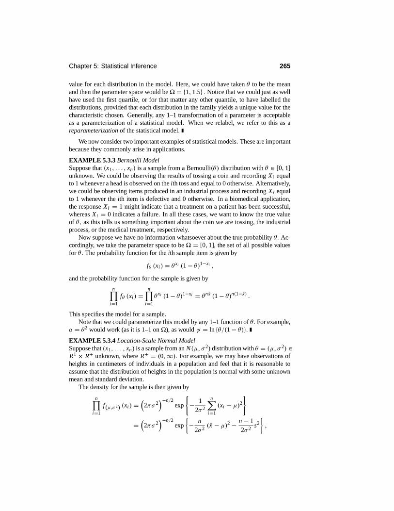
Chapter 5: Statistical Inference 265
value for each distribution in the model. Here, we could have taken θ to be the meanand then the parameter space would be* = {1, 1.5} . Notice that we could just as wellhave used the first quartile, or for that matter any other quantile, to have labelled thedistributions, provided that each distribution in the family yields a unique value for thecharacteristic chosen. Generally, any 1–1 transformation of a parameter is acceptableas a parameterization of a statistical model. When we relabel, we refer to this as areparameterization of the statistical model.
We now consider two important examples of statistical models. These are importantbecause they commonly arise in applications.
EXAMPLE 5.3.3 Bernoulli ModelSuppose that (x1, . . . , xn) is a sample from a Bernoulli(θ) distribution with θ ∈ [0, 1]unknown. We could be observing the results of tossing a coin and recording Xi equalto 1 whenever a head is observed on the ith toss and equal to 0 otherwise. Alternatively,we could be observing items produced in an industrial process and recording Xi equalto 1 whenever the ith item is defective and 0 otherwise. In a biomedical application,the response Xi = 1 might indicate that a treatment on a patient has been successful,whereas Xi = 0 indicates a failure. In all these cases, we want to know the true valueof θ, as this tells us something important about the coin we are tossing, the industrialprocess, or the medical treatment, respectively.
Now suppose we have no information whatsoever about the true probability θ . Ac-cordingly, we take the parameter space to be * = [0, 1], the set of all possible valuesfor θ . The probability function for the ith sample item is given by
fθ (xi) = θ xi (1− θ)1−xi ,
and the probability function for the sample is given by
n%i=1
fθ (xi ) =n%
i=1
θ xi (1− θ)1−xi = θnx (1− θ)n(1−x) .
This specifies the model for a sample.Note that we could parameterize this model by any 1–1 function of θ. For example,
α = θ2 would work (as it is 1–1 on *), as would ψ = ln {θ/(1− θ)}.EXAMPLE 5.3.4 Location-Scale Normal ModelSuppose that (x1, . . . , xn) is a sample from an N(µ, σ 2) distribution with θ = (µ, σ 2) ∈R1 × R+ unknown, where R+ = (0,∞). For example, we may have observations ofheights in centimeters of individuals in a population and feel that it is reasonable toassume that the distribution of heights in the population is normal with some unknownmean and standard deviation.
The density for the sample is then given by
n%i=1
f(µ,σ 2) (xi ) =&
2πσ 2'−n/2
exp
(− 1
2σ 2
n)i=1
(xi − µ)2*
=&
2πσ 2'−n/2
exp+− n
2σ 2 (x − µ)2 −n − 1
2σ 2 s2,,
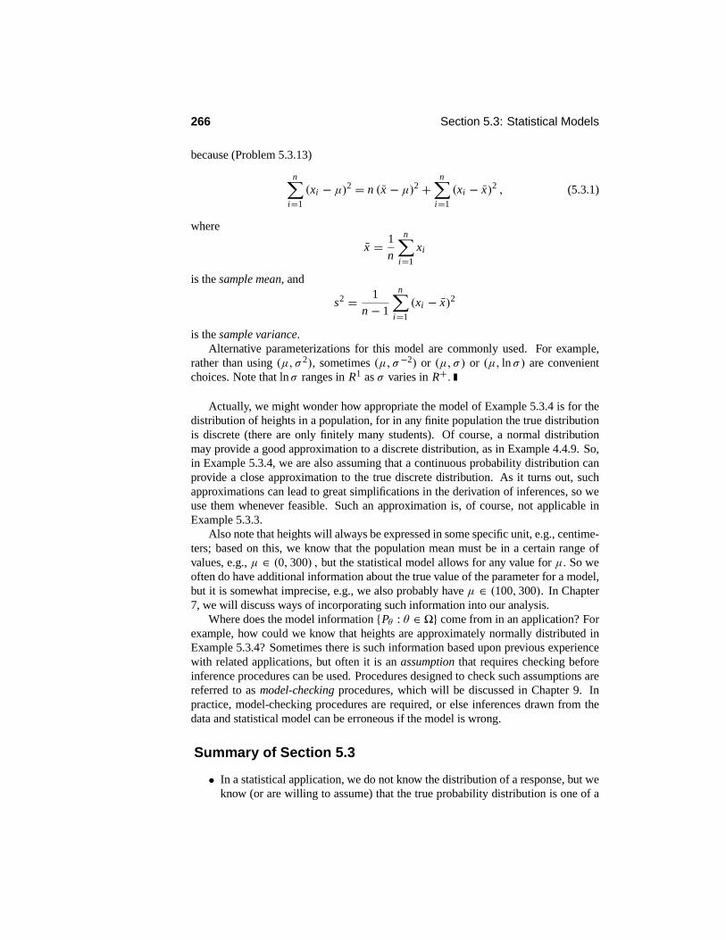
266 Section 5.3: Statistical Models
because (Problem 5.3.13)
n)i=1
(xi − µ)2 = n (x − µ)2 +n)
i=1
(xi − x)2 , (5.3.1)
where
x = 1n
n)i=1
xi
is the sample mean, and
s2 = 1n − 1
n)i=1
(xi − x)2
is the sample variance.Alternative parameterizations for this model are commonly used. For example,
rather than using (µ, σ 2), sometimes (µ, σ−2) or (µ, σ) or (µ, ln σ) are convenientchoices. Note that lnσ ranges in R1 as σ varies in R+.
Actually, we might wonder how appropriate the model of Example 5.3.4 is for thedistribution of heights in a population, for in any finite population the true distributionis discrete (there are only finitely many students). Of course, a normal distributionmay provide a good approximation to a discrete distribution, as in Example 4.4.9. So,in Example 5.3.4, we are also assuming that a continuous probability distribution canprovide a close approximation to the true discrete distribution. As it turns out, suchapproximations can lead to great simplifications in the derivation of inferences, so weuse them whenever feasible. Such an approximation is, of course, not applicable inExample 5.3.3.
Also note that heights will always be expressed in some specific unit, e.g., centime-ters; based on this, we know that the population mean must be in a certain range ofvalues, e.g., µ ∈ (0, 300) , but the statistical model allows for any value for µ. So weoften do have additional information about the true value of the parameter for a model,but it is somewhat imprecise, e.g., we also probably have µ ∈ (100, 300). In Chapter7, we will discuss ways of incorporating such information into our analysis.
Where does the model information {Pθ : θ ∈ *} come from in an application? Forexample, how could we know that heights are approximately normally distributed inExample 5.3.4? Sometimes there is such information based upon previous experiencewith related applications, but often it is an assumption that requires checking beforeinference procedures can be used. Procedures designed to check such assumptions arereferred to as model-checking procedures, which will be discussed in Chapter 9. Inpractice, model-checking procedures are required, or else inferences drawn from thedata and statistical model can be erroneous if the model is wrong.
Summary of Section 5.3
• In a statistical application, we do not know the distribution of a response, but weknow (or are willing to assume) that the true probability distribution is one of a

Chapter 5: Statistical Inference 267
set of possible distributions { fθ : θ ∈ *} , where fθ is the density or probabilityfunction (whichever is relevant) for the response. The set of possible distribu-tions is called the statistical model.
• The set * is called the parameter space, and the variable θ is called the parame-ter of the model. Because each value of θ corresponds to a distinct probabilitydistribution in the model, we can talk about the true value of θ, as this gives thetrue distribution via fθ .
EXERCISES
5.3.1 Suppose there are three coins — one is known to be fair, one has probability 1/3of yielding a head on a single toss, and one has probability 2/3 for head on a single toss.A coin is selected (not randomly) and then tossed five times. The goal is to make aninference about which of the coins is being tossed, based on the sample. Fully describea statistical model for a single response and for the sample.5.3.2 Suppose that one face of a symmetrical six-sided die is duplicated but we do notknow which one. We do know that if 1 is duplicated, then 2 does not appear; otherwise,1 does not appear. Describe the statistical model for a single roll.5.3.3 Suppose we have two populations (I and II) and that variable X is known to bedistributed N(10, 2) on population I and distributed N(8, 3) on population II. A sam-ple (X1, . . . , Xn) is generated from one of the populations; you are not told whichpopulation the sample came from, but you are required to draw inferences about thetrue distribution based on the sample. Describe the statistical model for this problem.Could you parameterize this model by the population mean, by the population vari-ance? Sometimes problems like this are called classification problems because makinginferences about the true distribution is equivalent to classifying the sample as belong-ing to one of the populations.5.3.4 Suppose the situation is as described in Exercise 5.3.3, but now the distributionfor population I is N(10, 2) and the distribution for population II is N(10, 3). Couldyou parameterize the model by the population mean? By the population variance?Justify your answer.5.3.5 Suppose that a manufacturing process produces batteries whose lifelengths areknown to be exponentially distributed but with the mean of the distribution completelyunknown. Describe the statistical model for a single observation. Is it possible toparameterize this model by the mean? Is it possible to parameterize this model by thevariance? Is it possible to parameterize this model by the coefficient of variation (thecoefficient of variation of a distribution equals the standard deviation divided by themean)?5.3.6 Suppose it is known that a response X is distributed Uniform[0, β], where β >0 is unknown. Is it possible to parameterize this model by the first quartile of thedistribution? (The first quartile of the distribution of a random variable X is the point csatisfying P(X ≤ c) = 0.25.) Explain why or why not.

268 Section 5.3: Statistical Models
5.3.7 Suppose it is known that a random variable X follows one of the following dis-tributions.
θ Pθ (X = 1) Pθ (X = 2) Pθ (X = 3)A 1/2 1/2 0B 0 1/2 1/2
(a) What is the parameter space *?(b) Suppose we observe a value X = 1.What is the true value of the parameter? Whatis the true distribution of X?(c) What could you say about the true value of the parameter if you had observedX = 2?5.3.8 Suppose we have a statistical model {P1, P2}, where P1 and P2 are probabilitymeasures on a sample space S. Further suppose there is a subset C ⊂ S such thatP1(C) = 1 while P2(Cc) = 1. Discuss how you would make an inference about thetrue distribution of a response s after you have observed a single observation.5.3.9 Suppose you know that the probability distribution of a variable X is either P1or P2. If you observe X = 1 and P1(X = 1) = 0.75 while P2(X = 1) = 0.001,then what would you guess as the true distribution of X? Give your reasoning for thisconclusion.5.3.10 Suppose you are told that class #1 has 35 males and 65 females while class #2has 45 males and 55 females. You are told that a particular student from one of theseclasses is female, but you are not told which class she came from.(a) Construct a statistical model for this problem, identifying the parameter, the para-meter space, and the family of distributions. Also identify the data.(b) Based on the data, do you think a reliable inference is feasible about the true para-meter value? Explain why or why not.(c) If you had to make a guess about which distribution the data came from, what choicewould you make? Explain why.
PROBLEMS
5.3.11 Suppose in Example 5.3.3 we parameterize the model by ψ = ln {θ/(1− θ)}.Record the statistical model using this parameterization, i.e., record the probabilityfunction using ψ as the parameter and record the relevant parameter space.5.3.12 Suppose in Example 5.3.4 we parameterize the model by (µ, ln σ) = (µ,ψ).Record the statistical model using this parameterization, i.e., record the density func-tion using (µ,ψ) as the parameter and record the relevant parameter space.5.3.13 Establish the identity (5.3.1).5.3.14 A sample (X1, . . . , Xn) is generated from a Bernoulli(θ) distribution with θ ∈[0, 1] unknown, but only T = -n
i=1 Xi is observed by the statistician. Describe thestatistical model for the observed data.5.3.15 Suppose it is known that a response X is distributed N(µ, σ 2), where θ =(µ, σ 2) ∈ R1 × R+ and θ is completely unknown. Show how to calculate the first

Chapter 5: Statistical Inference 269
quartile of each distribution in this model from the values (µ, σ 2). Is it possible toparameterize the model by the first quartile? Explain your answer.5.3.16 Suppose response X is known to be distributed N(Y, σ 2), where Y ∼ N(0, δ2)and σ 2, δ2 > 0 are completely unknown. Describe the statistical model for an obser-vation (X, Y ) . If Y is not observed, describe the statistical model for X.
5.3.17 Suppose we have a statistical model {P1, P2}, where P1 is an N(10, 1) distrib-ution while P2 is an N(0, 1) distribution.(a) Is it possible to make any kind of reliable inference about the true distribution basedon a single observation? Why or why not?(b) Repeat part (a) but now suppose that P1 is a N(1, 1) distribution.5.3.18 Suppose we have a statistical model {P1, P2}, where P1 is an N(1, 1) distri-bution while P2 is an N(0, 1) distribution. Further suppose that we had a samplex1, . . . , x100 from the true distribution. Discuss how you might go about making aninference about the true distribution based on the sample.
DISCUSSION TOPICS
5.3.19 Explain why you think it is important that statisticians state very clearly whatthey are assuming any time they carry out a statistical analysis.5.3.20 Consider the statistical model given by the collection of N(µ, σ 2
0) distributionswhere µ ∈ R1 is considered completely unknown, but σ 2
0 is assumed known. Do youthink this is a reasonable model to use in an application? Give your reasons why orwhy not.
5.4 Data CollectionThe developments of Sections 5.2 and 5.3 are based on the observed response s beinga realization from a probability measure P. In fact, in many applications, this is anassumption. We are often presented with data that could have been produced in thisway, but we cannot always be sure.
When we cannot be sure that the data were produced by a random mechanism, thenthe statistical analysis of the data is known as an observational study. In an observa-tional study, the statistician merely observes the data rather than intervening directlyin generating the data, to ensure that the randomness assumption holds. For example,suppose a professor collects data from his students for a study that examines the rela-tionship between grades and part-time employment. Is it reasonable to regard the datacollected as having come from a probability distribution? If so, how would we justifythis?
It is important for a statistician to distinguish carefully between situations that areobservational studies and those that are not. As the following discussion illustrates,there are qualifications that must be applied to the analysis of an observational study.While statistical analyses of observational studies are valid and indeed important, wemust be aware of their limitations when interpreting their results.

270 Section 5.4: Data Collection
5.4.1 Finite Populations
Suppose we have a finite set 1 of objects, called the population, and a real-valuedfunction X (sometimes called a measurement) defined on 1. So for each π ∈ 1, wehave a real-valued quantity X (π) that measures some aspect or feature of π.
For example, 1 could be the set of all students currently enrolled full-time at aparticular university, with X (π) the height of student π in centimeters. Or, for thesame1, we could take X (π) to be the gender of student π , where X (π) = 1 denotesfemale and X (π) = 2 denotes male. Here, height is a quantitative variable, because itsvalues mean something on a numerical scale, and we can perform arithmetic on thesevalues, e.g., calculate a mean. On the other hand, gender is an example of a categoricalvariable because its values serve only to classify, and any other choice of unique realnumbers would have served as well as the ones we chose. The first step in a statisticalanalysis is to determine the types of variables we are working with because the relevantstatistical analysis techniques depend on this.
The population and the measurement together produce a population distributionover the population. This is specified by the population cumulative distribution func-tion FX : R1 → [0, 1], where
FX (x) = |{π : X (π) ≤ x}|N
,
with |A| being the number of elements in the set A, and N = |1| . Therefore, FX (x)is the proportion of elements in 1 with their measurement less than or equal to x .
Consider the following simple example where we can calculate FX exactly.
EXAMPLE 5.4.1Suppose that 1 is a population of N = 20 plots of land of the same size. Furthersuppose that X (π) is a measure of the fertility of plot π on a 10-point scale and thatthe following measurements were obtained.
4 8 6 7 8 3 7 5 4 69 5 7 5 8 3 4 7 8 3
Then we have
FX (x) =
0 x < 33/20 3 ≤ x < 46/20 4 ≤ x < 59/20 5 ≤ x < 611/20 6 ≤ x < 715/20 7 ≤ x < 819/20 8 ≤ x < 91 9 ≤ x
because, for example, 6 out of the 20 plots have fertility measurements less than orequal to 4.
The goal of a statistician in this context is to know the function FX as preciselyas possible. If we know FX exactly, then we have identified the distribution of X

Chapter 5: Statistical Inference 271
over 1. One way of knowing the distribution exactly is to conduct a census, wherein,the statistician goes out and observes X (π) for every π ∈ 1 and then calculates FX .Sometimes this is feasible, but often it is not possible or even desirable, due to the costsinvolved in the accurate accumulation of all the measurements — think of how difficultit might be to collect the heights of all the students at your school.
While sometimes a census is necessary, even mandated by law, often a very accu-rate approximation to FX can be obtained by selecting a subset
{π1, . . . , πn} ⊂ 1for some n < N . We then approximate FX (x) by the empirical distribution functiondefined by
FX (x) = |{π i : X (π i ) ≤ x, i = 1, . . . , n}|n
= 1n
n)i=1
I(−∞,x] (X (π i )) .
We could also measure more than one aspect of π to produce a multivariate mea-surement X : 1 → Rk for some k. For example, if 1 is again the population ofstudents, we might have X (π) = (X1(π), X2(π)) , where X1(π) is the height in cen-timeters of student π and X2(π) is the weight of student π in kilograms. We will dis-cuss multivariate measurements in Chapter 10, where our concern is the relationshipsamongst variables, but we focus on univariate measurements here.
There are two questions we need to answer now — namely, how should we selectthe subset {π1, . . . , πn} and how large should n be?
5.4.2 Simple Random Sampling
We will first address the issue of selecting {π1, . . . , πn}. Suppose we select this subsetaccording to some given rule based on the unique label that each π ∈ 1 possesses.For example, if the label is a number, we might order the numbers and then take the nelements with the smallest labels. Or we could order the numbers and take every otherelement until we have a subset of n, etc.
There are many such rules we could apply, and there is a basic problem with allof them. If we want FX to approximate FX for the full population, then, when weemploy a rule, we run the risk of only selecting {π1, . . . , πn} from a subpopulation.For example, if we use student numbers to identify each element of a population ofstudents, and more senior students have lower student numbers, then, when n is muchsmaller than N and we select the students with smallest student numbers, FX is reallyonly approximating the distribution of X in the population of senior students at best.This distribution could be very different from FX . Similarly, for any other rule weemploy, even if we cannot imagine what the subpopulation could be, there may besuch a selection effect, or bias, induced that renders the estimate invalid.
This is the qualification we need to apply when analyzing the results of observa-tional studies. In an observational study, the data are generated by some rule, typically

272 Section 5.4: Data Collection
unknown to the statistician; this means that any conclusions drawn based on the dataX (π1), , . . . , X (πn) may not be valid for the full population.
There seems to be only one way to guarantee that selection effects are avoided,namely, the set {π1, . . . , πn} must be selected using randomness. For simple randomsampling, this means that a random mechanism is used to select the π i in such a waythat each subset of n has probability 1/
#Nn
$of being chosen. For example, we might
place N chips in a bowl, each with a unique label corresponding to a population ele-ment, and then randomly draw n chips from the bowl without replacement. The labelson the drawn chips identify the individuals that have been selected from 1. Alterna-tively, for the randomization, we might use a table of random numbers, such as TableD.1 in Appendix D (see Table D.1 for a description of how it is used) or generaterandom values using a computer algorithm (see Section 2.10).
Note that with simple random sampling (X (π1), , . . . , X (πn)) is random. In par-ticular, when n = 1, we then have
P(X (π1) ≤ x) = FX (x),
namely, the probability distribution of the random variable X (π1) is the same as thepopulation distribution.
EXAMPLE 5.4.2Consider the context of Example 5.4.1. When we randomly select the first plot from1, it is clear that each plot has probability 1/20 of being selected. Then we have
P(X (π1) ≤ x) = |{π : X (π) ≤ x}|20
= FX (x)
for every x ∈ R1.
Prior to observing the sample, we also have P(X (π2) ≤ x) = FX (x). Consider,however, the distribution of X (π2) given that X (π1) = x1. Because we have removedone population member, with measurement value x1, then N FX (x) − 1 is the numberof individuals left in1 with X (π) ≤ x1. Therefore,
P (X (π2) ≤ x | X (π1) = x1) =(
N FX (x)−1N−1 x ≥ x1
N FX (x)N−1 x < x1.
Note that this is not equal to FX (x).So with simple random sampling, X (π1) and X (π2) are not independent. Observe,
however, that when N is large, then
P (X (π2) ≤ x | X (π1) = x1) ≈ FX (x),
so that X (π1) and X (π2) are approximately independent and identically distributed(i.i.d.). Similar calculations lead to the conclusion that, when N is large and n is smallrelative to N , then with simple random sampling from the population, the randomvariables
X (π1), . . . , X (πn)

Chapter 5: Statistical Inference 273
are approximately i.i.d. and with distribution given by FX . So we will treat the observedvalues (x1, . . . , xn) of (X (π1), . . . , X (πn)) as a sample (in the sense of Definition2.8.6) from FX . In this text, unless we indicate otherwise, we will always assume thatn is small relative to N so that this approximation makes sense.
Under the i.i.d. assumption, the weak law of large numbers (Theorem 4.2.1) impliesthat the empirical distribution function FX satisfies
FX (x) = 1n
n)i=1
I(−∞,x] (X (π i ))P→ FX (x)
as n → ∞. So we see that FX can be considered as an estimate of the populationcumulative distribution function (cdf) FX .
Whenever the data have been collected using simple random sampling, we will re-fer to the statistical investigation as a sampling study. It is a basic principle of goodstatistical practice that sampling studies are always preferred over observational stud-ies, whenever they are feasible. This is because we can be sure that, with a samplingstudy, any conclusions we draw based on the sample π1, . . . , πn will apply to the pop-ulation1 of interest. With observational studies, we can never be sure that the sampledata have not actually been selected from some proper subset of1. For example, if youwere asked to make inferences about the distribution of student heights at your schoolbut selected some of your friends as your sample, then it is clear that the estimated cdfmay be very unlike the true cdf (possibly more of your friends are of one gender thanthe other).
Often, however, we have no choice but to use observational data for a statisticalanalysis. Sampling directly from the population of interest may be extremely difficultor even impossible. We can still treat the results of such analyses as a form of evidence,but we must be wary about possible selection effects and acknowledge this possibility.Sampling studies constitute a higher level of statistical evidence than observationalstudies, as they avoid the possibility of selection effects.
In Chapter 10, we will discuss experiments that constitute the highest level of sta-tistical evidence. Experiments are appropriate when we are investigating the possibilityof cause–effect relationships existing amongst variables defined on populations.
The second question we need to address concerns the choice of the sample size n. Itseems natural that we would like to choose this as large as possible. On the other hand,there are always costs associated with sampling, and sometimes each sample value isvery expensive to obtain. Furthermore, it is often the case that the more data we collect,the more difficulty we have in making sure that the data are not corrupted by variouserrors that can arise in the collection process. So our answer, concerning how large nneed be, is that we want it chosen large enough so that we obtain the accuracy necessarybut no larger. Accordingly, the statistician must specify what accuracy is required, andthen n is determined.
We will see in the subsequent chapters that there are various methods for specifyingthe required accuracy in a problem and then determining an appropriate value for n.Determining n is a key component in the implementation of a sampling study and isoften referred to as a sample-size calculation.

274 Section 5.4: Data Collection
If we define
fX (x) = |{π : X (π) = x}|N
= 1N
)π∈1
I{x}(X (π)),
namely, fX (x) is the proportion of population members satisfying X (π) = x , then wesee that fX plays the role of the probability function because
FX (x) =)z≤x
fX (z).
We refer to fX as the population relative frequency function. Now, fX (x) may beestimated, based on the sample {π1, . . . , πn} , by
f X (x) = |{π i : X (π i ) = x, i = 1, . . . , n}|n
= 1
n
n)i=1
I{x}(X (π i )),
namely, the proportion of sample members π satisfying X (π) = x.With categorical variables, f X (x) estimates the population proportion fX (x) in
the category specified by x . With some quantitative variables, however, fX is not anappropriate quantity to estimate, and an alternative function must be considered.
5.4.3 Histograms
Quantitative variables can be further classified as either discrete or continuous vari-ables. Continuous variables are those that we can measure to an arbitrary precision aswe increase the accuracy of a measuring instrument. For example, the height of anindividual could be considered a continuous variable, whereas the number of years ofeducation an individual possesses would be considered a discrete quantitative variable.For discrete quantitative variables, fX is an appropriate quantity to describe a popula-tion distribution, but we proceed differently with continuous quantitative variables.
Suppose that X is a continuous quantitative variable. In this case, it makes moresense to group values into intervals, given by
(h1, h2], (h2, h3], . . . , (hm−1, hm],
where the hi are chosen to satisfy h1 < h2 < · · · < hm with (h1, hm) effectivelycovering the range of possible values for X. Then we define
hX (x) =( |{π : X(π)∈(hi ,hi+1]}|
N(hi+1−hi)x ∈ (hi , hi+1]
0 otherwise
and refer to hX as a density histogram function. Here, hX (x) is the proportion ofpopulation elements π that have their measurement X (π) in the interval (hi , hi+1]containing x, divided by the length of the interval.
In Figure 5.4.1, we have plotted a density histogram based on a sample of 10,000from an N(0, 1) distribution (we are treating this sample as the full population) and

Chapter 5: Statistical Inference 275
using the values h1 = −5, h2 = −4, . . . , h11 = 5. Note that the vertical lines are onlyartifacts of the plotting software and do not represent values of hX , as these are givenby the horizontal lines.
543210-1-2-3-4-5
0.35
0.30
0.25
0.20
0.15
0.10
0.05
0.00
Figure 5.4.1: Density histogram function for a sample of 10,000 from an N(0, 1) distributionusing the values h1= −5, h2= −4, . . . , h11= 5.
If x ∈ (hi , hi+1], then hX (x) (hi+1 − hi) gives the proportion of individuals in thepopulation that have their measurement X (π) in (hi , hi+1]. Furthermore, we have
FX (h j ) =! h j
−∞hX (x) dx
for each interval endpoint and
FX (h j )− FX (hi ) =! h j
hi
hX (x) dx
when hi ≤ h j . If the intervals (hi , hi+1] are small, then we expect that
FX (b)− FX (a) ≈! b
ahX (x) dx
for any choice of a < b.Now suppose that the lengths hi+1 − hi are small and N is very large. Then it
makes sense to imagine a smooth, continuous function fX , e.g., perhaps a normal orgamma density function, that approximates hX in the sense that! b
afX (x) dx ≈
! b
ahX (x) dx
for every a < b. Then we will also have! b
afX (x) dx ≈ FX (b)− FX (a)

276 Section 5.4: Data Collection
for every a < b. We will refer to such an fX as a density function for the populationdistribution.
In essence, this is how many continuous distributions arise in practice. In Figure5.4.2, we have plotted a density histogram for the same values used in Figure 5.4.1, butthis time we used the interval endpoints h1 = −5, h2 = −4.75, . . . , h41 = 5.We notethat Figure 5.4.2 looks much more like a continuous function than does Figure 5.4.1.
50-5
0.4
0.3
0.2
0.1
0.0
Figure 5.4.2: Density histogram function for a sample of 10,000 from an N(0, 1) distributionusing the values h1 = −5, h2 = −4.75, . . . , h41 = 5.
5.4.4 Survey Sampling
Finite population sampling provides the formulation for a very important applicationof statistics, namely, survey sampling or polling. Typically, a survey consists of a set ofquestions that are asked of a sample {π1, . . . , πn} from a population1. Each questioncorresponds to a measurement, so if there are m questions, the response from a respon-dent π is the m-dimensional vector (X1(π), X2(π), . . . , Xm(π)) . A very importantexample of survey sampling is the pre-election polling that is undertaken to predict theoutcome of a vote. Also, many consumer product companies engage in extensive mar-ket surveys to try to learn what consumers want and so gain information that can leadto improved sales.
Typically, the analysis of the results will be concerned not only with the populationdistributions of the individual Xi over the population but also the joint population dis-tributions. For example, the joint cumulative distribution function of (X1, X2) is givenby
F(X1,X2)(x1, x2) = |{π : X1(π) ≤ x1, X2(π) ≤ x2}|N
,
namely, F(X1,X2)(x1, x2) is the proportion of the individuals in the population whoseX1 measurement is no greater than x1 and whose X2 measurement is no greater thanx2.Of course, we can also define the joint distributions of three or more measurements.

Chapter 5: Statistical Inference 277
These joint distributions are what we use to answer questions like, is there a relationshipbetween X1 and X2, and if so,what form does it take? This topic will be extensivelydiscussed in Chapter 10. We can also define f(X1,X2) for the joint distribution, and jointdensity histograms are again useful when X1 and X2 are both continuous quantitativevariables.
EXAMPLE 5.4.3Suppose there are four candidates running for mayor in a particular city. A randomsample of 1000 voters is selected; they are each asked if they will vote and, if so,which of the four candidates they will vote for. Additionally, the respondents are askedtheir age. We denote the answer to the question of whether or not they will vote by X1,with X1(π) = 1 meaning yes and X1(π) = 0 meaning no. For those voting, we denoteby X2 the response concerning which candidate they will vote for, with X2(π) = iindicating candidate i. Finally, the age in years of the respondent is denoted by X3. Inaddition to the distributions of X1 and X2, the pollster is also interested in the jointdistributions of (X1, X3) and (X2, X3), as these tell us about the relationship betweenvoter participation and age in the first case and candidate choice and age in the secondcase.
There are many interesting and important aspects to survey sampling that go wellbeyond this book. For example, it is often the case with human populations that a ran-domly selected person will not respond to a survey. This is called nonresponse error,and it is a serious selection effect. The sampler must design the study carefully to tryto mitigate the effects of nonresponse error. Furthermore, there are variants of simplerandom sampling (see Challenge 5.4.20) that can be preferable in certain contexts, asthese increase the accuracy of the results. The design of the actual questionnaire usedis also very important, as we must ensure that responses address the issues intendedwithout biasing the results.
Summary of Section 5.4
• Simple random sampling from a population 1 means that we randomly selecta subset of size n from 1 in such a way that each subset of n has the sameprobability — namely, 1/
#|1|n
$— of being selected.
• Data that arise from a sampling study are generated from the distribution of themeasurement of interest X over the whole population 1 rather than some sub-population. This is why sampling studies are preferred to observational studies.
• When the sample size n is small relative to |1| ,we can treat the observed valuesof X as a sample from the distribution of X over the population.
EXERCISES
5.4.1 Suppose we have a population1 = {π1, . . . , π10} and quantitative measurementX given by:
i 1 2 3 4 5 6 7 8 9 10X (π i ) 1 1 2 1 2 3 3 1 2 4
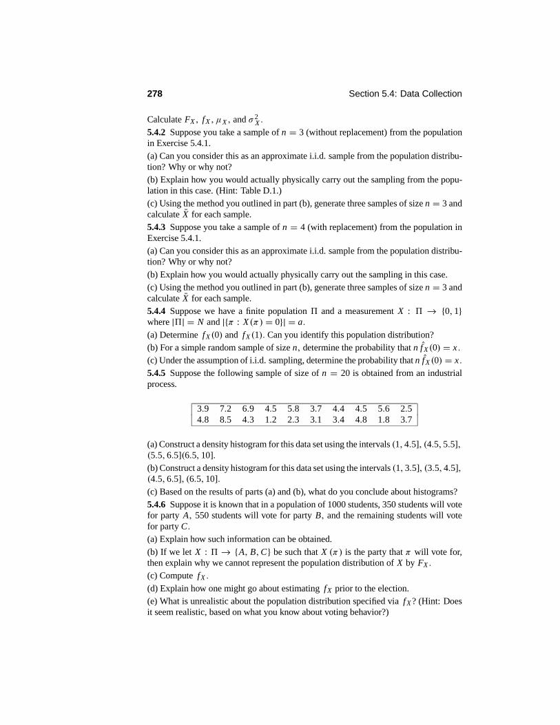
278 Section 5.4: Data Collection
Calculate FX , fX , µX , and σ 2X .
5.4.2 Suppose you take a sample of n = 3 (without replacement) from the populationin Exercise 5.4.1.(a) Can you consider this as an approximate i.i.d. sample from the population distribu-tion? Why or why not?(b) Explain how you would actually physically carry out the sampling from the popu-lation in this case. (Hint: Table D.1.)(c) Using the method you outlined in part (b), generate three samples of size n = 3 andcalculate X for each sample.5.4.3 Suppose you take a sample of n = 4 (with replacement) from the population inExercise 5.4.1.(a) Can you consider this as an approximate i.i.d. sample from the population distribu-tion? Why or why not?(b) Explain how you would actually physically carry out the sampling in this case.(c) Using the method you outlined in part (b), generate three samples of size n = 3 andcalculate X for each sample.5.4.4 Suppose we have a finite population 1 and a measurement X : 1 → {0, 1}where |1| = N and |{π : X (π) = 0}| = a.
(a) Determine fX (0) and fX (1). Can you identify this population distribution?(b) For a simple random sample of size n, determine the probability that n fX (0) = x .
(c) Under the assumption of i.i.d. sampling, determine the probability that n fX (0) = x.
5.4.5 Suppose the following sample of size of n = 20 is obtained from an industrialprocess.
3.9 7.2 6.9 4.5 5.8 3.7 4.4 4.5 5.6 2.54.8 8.5 4.3 1.2 2.3 3.1 3.4 4.8 1.8 3.7
(a) Construct a density histogram for this data set using the intervals (1, 4.5], (4.5, 5.5],(5.5, 6.5](6.5, 10].(b) Construct a density histogram for this data set using the intervals (1, 3.5], (3.5, 4.5],(4.5, 6.5], (6.5, 10].(c) Based on the results of parts (a) and (b), what do you conclude about histograms?5.4.6 Suppose it is known that in a population of 1000 students, 350 students will votefor party A, 550 students will vote for party B, and the remaining students will votefor party C.
(a) Explain how such information can be obtained.(b) If we let X : 1 → {A, B,C} be such that X (π) is the party that π will vote for,then explain why we cannot represent the population distribution of X by FX .
(c) Compute fX .
(d) Explain how one might go about estimating fX prior to the election.(e) What is unrealistic about the population distribution specified via fX ? (Hint: Doesit seem realistic, based on what you know about voting behavior?)

Chapter 5: Statistical Inference 279
5.4.7 Consider the population 1 to be files stored on a computer at a particular time.Suppose that X (π) is the type of file as indicated by its extension, e.g., .mp3. Is X acategorical or quantitative variable?5.4.8 Suppose that you are asked to estimate the proportion of students in a college of15, 000 students who intend to work during the summer.(a) Identify the population1, the variable X , and fX .What kind of variable is X?(b) How could you determine fX exactly?(c) Why might you not be able to determine fX exactly? Propose a procedure forestimating fX in such a situation.(d) Suppose you were also asked to estimate the proportion of students who intendedto work but could not find a job. Repeat parts (a), (b), and (c) for this situation.5.4.9 Sometimes participants in a poll do not respond truthfully to a question. Forexample, students who are asked “Have you ever illegally downloaded music?” maynot respond truthfully even if they are assured that their responses are confidential.Suppose a simple random sample of students was chosen from a college and studentswere asked this question.(a) If students were asked this question by a person, comment on how you think theresults of the sampling study would be affected.(b) If students were allowed to respond anonymously, perhaps by mailing in a ques-tionnaire, comment on how you think the results would be affected.(c) One technique for dealing with the respondent bias induced by such questions isto have students respond truthfully only when a certain random event occurs. Forexample, we might ask a student to toss a fair coin three times and lie whenever theyobtain two heads. What is the probability that a student tells the truth? Once you havecompleted the study and have recorded the proportion of students who said they didcheat, what proportion would you record as your estimate of the proportion of studentswho actually did cheat?5.4.10 A market research company is asked to determine how satisfied owners are withtheir purchase of a new car in the last 6 months. Satisfaction is to be measured by re-spondents choosing a point on a seven-point scale {1, 2, 3, 4, 5, 6, 7}, where 1 denotescompletely dissatisfied and 7 denotes completely satisfied (such a scale is commonlycalled a Likert scale).(a) Identify1, the variable X , and fX .
(b) It is common to treat a variable such as X as a quantitative variable. Do you thinkthis is correct? Would it be correct to treat X as a categorical variable?(c) A common criticism of using such a scale is that the interpretation of a statementsuch as 3 = “I’m somewhat dissatisfied” varies from one person to another. Commenton how this affects the validity of the study.
COMPUTER EXERCISES
5.4.11 Generate a sample of 1000 from an N(3, 2) distribution.(a) Calculate FX for this sample.

280 Section 5.4: Data Collection
(b) Plot a density histogram based on these data using the intervals of length 1 over therange (−5, 10) .(c) Plot a density histogram based on these data using the intervals of length 0.1 overthe range (−5, 10) .(d) Comment on the difference in the look of the histograms in parts (b) and (c). Towhat do you attribute this?(e) What limits the size of the intervals we use to group observations when we areplotting histograms?5.4.12 Suppose we have a population of 10,000 elements, each with a unique labelfrom the set {1, 2, 3, . . . , 10, 000}.(a) Generate a sample of 500 labels from this population using simple random sam-pling.(b) Generate a sample of 500 labels from this population using i.i.d. sampling.
PROBLEMS
5.4.13 Suppose we have a finite population1 and a measurement X : 1→ {0, 1, 2},where |1| = N and |{π : X (π) = 0}| = a and |{π : X (π) = 1}| = b. This problemgeneralizes Exercise 5.4.4.(a) Determine fX (0), fX (1), and fX (2) .(b) For a simple random sample of size n, determine the probability that f X (0) =f0, f X (1) = f1, and f X (2) = f2.
(c) Under the assumption of i.i.d. sampling, determine the probability that f X (0) =f0, f X (1) = f1, and f X (2) = f2.
5.4.14 Suppose X is a quantitative measurement defined on a finite population.(a) Prove that the population mean equals µX =
-x x fX (x), i.e., the average of X (π)
over all population elements π equals µX .(b) Prove that the population variance is given by σ 2
X =-
x (x − µX )2 fX (x), i.e., the
average of (X (π)− µX )2 over all population elements π equals σ 2
X .5.4.15 Suppose we have the situation described in Exercise 5.4.4, and we take a simplerandom sample of size n from1 where |1| = N .
(a) Prove that the mean of f X (0) is given by fX (0). (Hint: Note that we can writef X (0) = n−1-n
i=1 I{0} (X (π i)) and I{0} (X (π i )) ∼ Bernoulli( fX (0)).)
(b) Prove that the variance of f X (0) is given by
fX (0) (1− fX (0))n
N − n
N − 1. (5.4.1)
(Hint: Use the hint in part (a), but note that the I{0} (X (π i )) are not independent. UseTheorem 3.3.4(b) and evaluate Cov
#I{0} (X (π i)) , I{0} (X (π i ))
$in terms of fX (0).)
(c) Repeat the calculations in parts (a) and (b), but this time assume that you take asample of n with replacement. (Hint: Use Exercise 5.4.4(c).)(d) Explain why the factor (N − n)/(N − 1) in (5.4.1) is called the finite samplecorrection factor.
Chapter 5: Statistical Inference 281
5.4.16 Suppose we have a finite population 1 and we do not know |1| = N . Inaddition, suppose we have a measurement variable X : 1 → {0, 1} and we knowthat N fX (0) = a where a is known. Based on a simple random sample of n from 1,determine an estimator of N . (Hint: Use a function of f X (0).)5.4.17 Suppose that X is a quantitative variable defined on a population1 and that wetake a simple random sample of size n from1.
(a) If we estimate the population mean µX by the sample mean X = 1n
-ni=1 X (π i),
prove that E(X) = µX where µX is defined in Problem 5.4.14(a). (Hint: What is thedistribution of each X (π i )?)(b) Under the assumption that i.i.d. sampling makes sense, show that the variance of Xequals σ 2
X/n, where σ 2X is defined in Problem 5.4.14(b).
5.4.18 Suppose we have a finite population 1 and we do not know |1| = N . Inaddition, suppose we have a measurement variable X : 1 → R1 and we know T =-π X (π) . Based on a simple random sample of n from1, determine an estimator of
N . (Hint: Use a function of X .)
5.4.19 Under i.i.d. sampling, prove that f X (x)D→ fX (x) as n →∞. (Hint: f X (x) =
n−1-ni=1 I{x}(X (π i )).)
CHALLENGES
5.4.20 (Stratified sampling) Suppose that X is a quantitative variable defined on a pop-ulation1 and that we can partition1 into two subpopulations11 and12, such that aproportion p of the full population is in11. Let fi X denote the conditional populationdistribution of X on 1i .
(a) Prove that fX (x) = p f1X (x)+ (1− p) f2X (x).
(b) Establish that µX = pµ1X + (1− p) µ2X , where µi X is the mean of X on1i .
(c) Establish that σ 2X = pσ 2
1X + (1− p) σ 22X + p(1− p) (µ1X − µ2X )
2 .
(d) Suppose that it makes sense to assume i.i.d. sampling whenever we take a samplefrom either the full population or either of the subpopulations, i.e., whenever the sam-ple sizes we are considering are small relative to the sizes of these populations. Weimplement stratified sampling by taking a simple random sample of size ni from sub-population 1i . We then estimate µX by pX1 + (1− p) X2, where Xi is the samplemean based on the sample from1i . Prove that E(pX1 + (1− p) X2) = µX and
Var#pX1 + (1− p) X2
$ = p2 σ21X
n1+ (1− p)2
σ 22X
n2.
(e) Under the assumptions of part (d), prove that
Var#pX1 + (1− p) X2
$ ≤ Var#X$
when X is based on a simple random sample of size n from the full population andn1 = pn, n2 = (1− p) n. This is called proportional stratified sampling.(f) Under what conditions is there no benefit to proportional stratified sampling? Whatdo you conclude about situations in which stratified sampling will be most beneficial?

282 Section 5.5: Some Basic Inferences
DISCUSSION TOPICS
5.4.21 Sometimes it is argued that it is possible for a skilled practitioner to pick a moreaccurate representative sample of a population deterministically rather than by employ-ing simple random sampling. This argument is based in part on the argument that it isalways possible with simple random sampling that we could get a very unrepresenta-tive sample through pure chance and that this can be avoided by an expert. Commenton this assertion.5.4.22 Suppose it is claimed that a quantitative measurement X defined on a finitepopulation 1 is approximately distributed according to a normal distribution with un-known mean and unknown variance. Explain fully what this claim means.
5.5 Some Basic InferencesNow suppose we are in a situation involving a measurement X, whose distribution isunknown, and we have obtained the data (x1, x2, . . . , xn) , i.e., observed n values of X.Hopefully, these data were the result of simple random sampling, but perhaps they werecollected as part of an observational study. Denote the associated unknown populationrelative frequency function, or an approximating density, by fX and the populationdistribution function by FX .
What we do now with the data depends on two things. First, we have to determinewhat we want to know about the underlying population distribution. Typically, ourinterest is in only a few characteristics of this distribution — the mean and variance.Second, we have to use statistical theory to combine the data with the statistical modelto make inferences about the characteristics of interest.
We now discuss some typical characteristics of interest and present some informalestimation methods for these characteristics, known as descriptive statistics. Theseare often used as a preliminary step before more formal inferences are drawn and arejustified on simple intuitive grounds. They are called descriptive because they areestimating quantities that describe features of the underlying distribution.
5.5.1 Descriptive Statistics
Statisticians often focus on various characteristics of distributions. We present some ofthese in the following examples.
EXAMPLE 5.5.1 Estimating Proportions and Cumulative ProportionsOften we want to make inferences about the value fX (x) or the value FX (x) for aspecific x. Recall that fX (x) is the proportion of population members whose X mea-surement equals x . In general, FX (x) is the proportion of population members whoseX measurement is less than or equal to x.
Now suppose we have a sample (x1, x2, . . . , xn) from fX . A natural estimate offX (x) is given by f X (x), the proportion of sample values equal to x .A natural estimateof FX (x) is given by FX (x) = n−1-n
i=1 I(−∞,x] (xi ) , the proportion of sample valuesless than or equal to x, otherwise known as the empirical distribution function evaluatedat x.

Chapter 5: Statistical Inference 283
Suppose we obtained the following sample of n = 10 data values.
1.2 2.1 0.4 3.3 −2.1 4.0 −0.3 2.2 1.5 5.0
In this case, f X (x) = 0.1 whenever x is a data value and is 0 otherwise. To computeFX (x), we simply count how many sample values are less than or equal to x anddivide by n = 10. For example, FX (−3) = 0/10 = 0, FX (0) = 2/10 = 0.2, andFX (4) = 9/10 = 0.9.
An important class of characteristics of the distribution of a quantitative variable Xis given by the following definition.
Definition 5.5.1 For p ∈ [0, 1], the pth quantile (or 100pth percentile) xp, forthe distribution with cdf FX , is defined to be the smallest number xp satisfyingp ≤ FX (xp).
For example, if your mark on a test placed you at the 90th percentile, then your markequals x0.9 and 90% of your fellow test takers achieved your mark or lower. Note thatby the definition of the inverse cumulative distribution function (Definition 2.10.1), wecan write xp = F−1
X (p) = min {x : p ≤ FX (x)} .When FX is strictly increasing and continuous, then F−1
X (p) is the unique value xpsatisfying
FX (xp) = p. (5.5.1)
Figure 5.5.1 illustrates the situation in which there is a unique solution to (5.5.1). WhenFX is not strictly increasing or continuous (as when X is discrete), then there may bemore than one, or no, solutions to (5.5.1). Figure 5.5.2 illustrates the situation in whichthere is no solution to (5.5.1).
FX
x
1
p
xp
Figure 5.5.1: The pth quantile xp when there is a unique solution to (5.5.1).

284 Section 5.5: Some Basic Inferences
FX
x
1
p
xp
Figure 5.5.2: The pth quantile xp determined by a cdf FX when there is no solution to(5.5.1).
So, when X is a continuous measurement, a proportion p of the population havetheir X measurement less than or equal to xp. As particular cases, x0.5 = F−1
X (0.5)is the median, while x0.25 = F−1
X (0.25) and x0.75 = F−1X (0.75) are the first and third
quartiles, respectively, of the distribution.
EXAMPLE 5.5.2 Estimating QuantilesA natural estimate of a population quantile xp = F−1
X (p) is to use x p = F−1X (p). Note,
however, that FX is not continuous, so there may not be a solution to (5.5.1) using FX .Applying Definition 5.5.1, however, leads to the following estimate. First, order the
observed sample values (x1, . . . , xn) to obtain the order statistics x(1) < · · · < x(n) (seeSection 2.8.4). Then, note that x(i) is the (i/n)-th quantile of the empirical distribution,because
FX (x(i)) = i
n
and FX (x) < i/n whenever x < x(i). In general, we have that the sample pth quantileis x p = x(i) whenever
i − 1n
< p ≤ i
n. (5.5.2)
A number of modifications to this estimate are sometimes used. For example, if wefind i such that (5.5.2) is satisfied and put
x p = x(i−1) + n#x(i) − x(i−1)
$2p − i − 1
n
3, (5.5.3)
then x p is the linear interpolation between x(i−1) and x(i). When n is even, this defin-ition gives the sample median as x0.5 = x(n/2); a similar formula holds when n is odd(Problem 5.5.21). Also see Problem 5.5.22 for more discussion of (5.5.3).
Quite often the sample median is defined to be
x0.5 =
x((n+1)/2) n odd
12
#x(n/2) + x(n/2+1)
$n even,
(5.5.4)

Chapter 5: Statistical Inference 285
namely, the middle value when n is odd and the average of the two middle values whenn is even. For n large enough, all these definitions will yield similar answers. The useof any of these is permissible in an application.
Consider the data in Example 5.5.1. Sorting the data from smallest to largest, theorder statistics are given by the following table.
x(1) = −2.1 x(2) = −0.3 x(3) = 0.4 x(4) = 1.2 x(5) = 1.5x(6) = 2.1 x(7) = 2.2 x(8) = 3.3 x(9) = 4.0 x(10) = 5.0
Then, using (5.5.3), the sample median is given by x0.5 = x(5) = 1.5, while the samplequartiles are given by
x0.25 = x(2) + 10#x(3) − x(2)
$(0.25− 0.2)
= −0.3+ 10 (0.4− (−0.3)) (0.25− 0.2) = 0.05
and
x0.75 = x(7) + 10#x(8) − x(7)
$(0.75− 0.7)
= 2.2+ 10 (3.3− 2.2) (0.75− 0.7) = 2.75.
So in this case, we estimate that 25% of the population under study has an X measure-ment less than 0.05, etc.
EXAMPLE 5.5.3 Measuring Location and Scale of a Population DistributionOften we are asked to make inferences about the value of the population mean
µX = 1|1|
)π∈1
X (π)
and the population variance
σ 2X =
1|1|
)π∈1
(X (π)− µX )2 ,
where1 is a finite population and X is a real-valued measurement defined on it. Theseare measures of the location and spread of the population distribution about the mean,respectively. Note that calculating a mean or variance makes sense only when X is aquantitative variable.
When X is discrete, we can also write
µX =)
xx fX (x)
because |1| fX (x) equals the number of elements π ∈ 1 with X (π) = x. In thecontinuous case, using an approximating density fX , we can write
µX ≈! ∞
−∞x fX (x) dx .
Similar formulas exist for the population variance of X (see Problem 5.4.14).

286 Section 5.5: Some Basic Inferences
It will probably occur to you that a natural estimate of the population mean µX isgiven by the sample mean
x = 1n
n)i=1
xi .
Also, a natural estimate of the population variance σ 2X is given by the sample variance
s2 = 1n − 1
n)i=1
(xi − x)2 . (5.5.5)
Later we will explain why we divided by n − 1 in (5.5.5) rather than n. Actually, itmakes little difference which we use, for even modest values of n. The sample standarddeviation is given by s, the positive square root of s2. For the data in Example 5.1.1,we obtain x = 1.73 and s = 2.097.
The population mean µX and population standard deviation σ X serve as a pair, inwhich µX measures where the distribution is located on the real line and σ X measureshow much spread there is in the distribution about µX . Clearly, the greater the value ofσ X , the more variability there is in the distribution.
Alternatively, we could use the population median x0.5 as a measure of locationof the distribution and the population interquartile range x0.75 − x0.25 as a measureof the amount of variability in the distribution around the median. The median andinterquartile range are the preferred choice to measure these aspects of the distributionwhenever the distribution is skewed, i.e., not symmetrical. This is because the medianis insensitive to very extreme values, while the mean is not. For example, house pricesin an area are well known to exhibit a right-skewed distribution. A few houses sellingfor very high prices will not change the median price but could result in a big changein the mean price.
When we have a symmetric distribution, the mean and median will agree (providedthe mean exists). The greater the skewness in a distribution, however, the greater willbe the discrepancy between its mean and median. For example, in Figure 5.5.3 we haveplotted the density of a χ2 (4) distribution. This distribution is skewed to the right, andthe mean is 4 while the median is 3.3567.
0 5 10 15 200.00
0.01
0.02
0.03
x
f
Figure 5.5.3: The density f of a χ2 (4) distribution.

Chapter 5: Statistical Inference 287
We estimate the population interquartile range by the sample interquartile range(IQR) given by I QR = x0.75 − x0.25. For the data in Example 5.5.1, we obtain thesample median to be x0.5 = 1.5, while I QR = 2.75− 0.05 = 2.70.
If we change the largest value in the sample from x(10) = 5.0 to x(10) = 500.0 thesample median remains x0.5 = 1.5, but note that the sample mean goes from 1.73 to51.23!
5.5.2 Plotting Data
It is always a good idea to plot the data. For discrete quantitative variables, we can plotf X , i.e., plot the sample proportions (relative frequencies). For continuous quantitativevariables, we introduced the density histogram in section 5.4.3. These plots give ussome idea of the shape of the distribution from which we are sampling. For example,we can see if there is any evidence that the distribution is strongly skewed.
We now consider another very useful plot for quantitative variables.
EXAMPLE 5.5.4 Boxplots and OutliersAnother useful plot for quantitative variables is known as a boxplot. For example,Figure 5.5.4 gives a boxplot for the data in Example 5.5.1. The line in the center of thebox is the median. The line below the median is the first quartile, and the line abovethe median is the third quartile.
The vertical lines from the quartiles are called whiskers, which run from the quar-tiles to the adjacent values. The adjacent values are given by the greatest value lessthan or equal to the upper limit (the third quartile plus 1.5 times the I QR) and by theleast value greater than or equal to the lower limit (the first quartile minus 1.5 timesthe I QR). Values beyond the adjacent values, when these exist, are plotted with a ∗;in this case, there are none. If we changed x(10) = 5.0 to x(10) = 15.0, however, wesee this extreme value plotted as a ∗, as shown in Figure 5.5.5.
5
4
3
2
1
0
-1
-2
Figure 5.5.4: A boxplot of the data in Example 5.5.1.

288 Section 5.5: Some Basic Inferences
15
10
5
0
Figure 5.5.5: A boxplot of the data in Example 5.5.1, changing x(10) = 5.0 tox(10) = 15.0.
Points outside the upper and lower limits, and thus plotted by ∗, are commonlyreferred to as outliers. An outlier is a value that is extreme with respect to the restof the observations. Sometimes outliers occur because a mistake has been made incollecting or recording the data, but they also occur simply because we are samplingfrom a long-tailed distribution. It is often difficult to ascertain which is the case ina particular application, but each such observation should be noted. We have seen inExample 5.5.3 that outliers can have a big impact on statistical analyses. Their effectsshould be recorded when reporting the results of a statistical analysis.
For categorical variables, it is typical to plot the data in a bar chart, as described inthe next example.
EXAMPLE 5.5.5 Bar ChartsFor categorical variables, we code the values of the variable as equispaced numbersand then plot constant-width rectangles (the bars) over these values so that the heightof the rectangle over a value equals the proportion of times that value is assumed. Sucha plot is called a bar chart. Note that the values along the x-axis are only labels andnot to be treated as numbers that we can do arithmetic on, etc.
For example, suppose we take a simple random sample of 100 students and recordtheir favorite flavor of ice cream (from amongst four possibilities), obtaining the resultsgiven in the following table.
Flavor Count ProportionChocolate 42 0.42Vanilla 28 0.28Butterscotch 22 0.22Strawberry 8 0.08
Coding Chocolate as 1, Vanilla as 2, Butterscotch as 3, and Strawberry as 4, Figure5.5.6 presents a bar chart of these data. It is typical for the bars in these charts not totouch.

Chapter 5: Statistical Inference 289
4321
0.4
0.3
0.2
0.1
Flavor
Pro
por
tion
Figure 5.5.6: A bar chart for the data of Example 5.5.5.
5.5.3 Types of Inference
Certainly quoting descriptive statistics and plotting the data are methods used by a sta-tistician to try to learn something about the underlying population distribution. Thereare difficulties with this approach, however, as we have just chosen these methods basedon intuition. Often it is not clear which descriptive statistics we should use. Further-more, these data summaries make no use of the information we have about the true pop-ulation distribution as expressed by the statistical model, namely, fX ∈ { fθ : θ ∈ *} .Taking account of this information leads us to develop a theory of statistical inference,i.e., to specify how we should combine the model information together with the data tomake inferences about population quantities. We will do this in Chapters 6, 7, and 8,but first we discuss the types of inferences that are commonly used in applications.
In Section 5.2, we discussed three types of inference in the context of a knownprobability model as specified by some density or probability function f. We notedthat we might want to do any of the following concerning an unobserved responsevalue s.
(i) Predict an unknown response value s via a prediction t .
(ii) Construct a subset C of the sample space S that has a high probability of containingan unknown response value s.
(iii) Assess whether or not s0 ∈ S is a plausible value from the probability distributionspecified by f.
We refer to (i), (ii), and (iii) as inferences about the unobserved s. The examples ofSection 5.2 show that these are intuitively reasonable concepts.
In a statistical application, we do not know f ; we know only that f ∈ { fθ : θ ∈ *},and we observe the data s. We are uncertain about which candidate fθ is correct, or,equivalently, which of the possible values of θ is correct.
As mentioned in Section 5.5.1, our primary goal may be to determine not the truefθ , but some characteristic of the true distribution such as its mean, median, or the

290 Section 5.5: Some Basic Inferences
value of the true distribution function F at a specified value. We will denote thischaracteristic of interest by ψ(θ). For example, when the characteristic of interestis the mean of the true distribution of a continuous random variable, then
ψ(θ) =! ∞
−∞x fθ (x) dx.
Alternatively, we might be interested in ψ(θ) = F−1θ (0.5), the median of the distribu-
tion of a random variable with distribution function given by Fθ .Different values of θ lead to possibly different values for the characteristic ψ(θ).
After observing the data s, we want to make inferences about what the correct value is.We will consider the three types of inference for ψ(θ).
(i) Choose an estimate T (s) of ψ(θ), referred to as the problem of estimation.
(ii) Construct a subset C(s) of the set of possible values for ψ(θ) that we believecontains the true value, referred to as the problem of credible region or confidenceregion construction.
(iii) Assess whether or not ψ0 is a plausible value for ψ(θ) after having observed s,referred to as the problem of hypothesis assessment.
So estimates, credible or confidence regions, and hypothesis assessment are examplesof types of inference. In particular, we want to construct estimates T (s) of ψ (θ) ,construct credible or confidence regions C(s) for ψ(θ), and assess the plausibility of ahypothesized value ψ0 for ψ(θ).
The problem of statistical inference entails determining how we should combinethe information in the model { fθ : θ ∈ *} and the data s to carry out these inferencesabout ψ(θ).
A very important statistical model for applications is the location-scale normalmodel introduced in Example 5.3.4. We illustrate some of the ideas discussed in thissection via that model.
EXAMPLE 5.5.6 Application of the Location-Scale Normal ModelSuppose the following simple random sample of the heights (in inches) of 30 studentshas been collected.
64.9 61.4 66.3 64.3 65.1 64.4 59.8 63.6 66.5 65.064.9 64.3 62.5 63.1 65.0 65.8 63.4 61.9 66.6 60.961.6 64.0 61.5 64.2 66.8 66.4 65.8 71.4 67.8 66.3
The statistician believes that the distribution of heights in the population can be wellapproximated by a normal distribution with some unknown mean and variance, andshe is unwilling to make any further assumptions about the true distribution. Accord-ingly, the statistical model is given by the family of N(µ, σ 2) distributions, whereθ = (µ, σ 2) ∈ * = R1 × R+ is unknown.
Does this statistical model make sense, i.e., is the assumption of normality appro-priate for this situation? The density histogram (based on 12 equal-length intervalsfrom 59.5 to 71.5) in Figure 5.5.7 looks very roughly normal, but the extreme observa-tion in the right tail might be some grounds for concern. In any case, we proceed as if

Chapter 5: Statistical Inference 291
this assumption is reasonable. In Chapter 9, we will discuss more refined methods forassessing this assumption.
706560
0.2
0.1
0.0
heights
Den
sity
Figure 5.5.7: Density histogram of heights in Example 5.5.6.
Suppose we are interested in making inferences about the population mean height,namely, the characteristic of interest is ψ(µ, σ 2) = µ. Alternatively, we might want tomake inferences about the 90th percentile of this distribution, i.e., ψ(µ, σ 2) = x0.90 =µ + σ z0.90, where z0.90 is the 90th percentile of the N(0, 1) distribution (when X ∼N(µ, σ 2), then P(X ≤ µ+ σ z0.90) = P((X − µ) /σ ≤ z0.90) = 4(z0.90) = 0.90).So 90% of the population under study have height less than x0.90, a value unknownto us because we do not know the value of (µ, σ 2). Obviously, there are many othercharacteristics of the true distribution about which we might want to make inferences.
Just using our intuition, T (x1, . . . , xn) = x seems like a sensible estimate of µ andT (x1, . . . , xn) = x + sz0.90 seems like a sensible estimate of µ+σ z0.90. To justify thechoice of these estimates, we will need the theories developed in later chapters. In thiscase, we obtain x = 64.517, and from (5.5.5) we compute s = 2.379. From Table D.2we obtain z0.90 = 1.2816, so that
x + sz0.90 = 64.517+ 2.379 (1.2816) = 67.566.
How accurate is the estimate x ofµ? A natural approach to answering this questionis to construct a credible interval, based on the estimate, that we believe has a highprobability of containing the true value of µ and is as short as possible. For example,the theory in Chapter 6 leads to using confidence intervals for µ, of the form
[x − sc, x + sc]
for some choice of the constant c. Notice that x is at the center of the interval. Thetheory in Chapter 6 will show that, in this case, choosing c = 0.3734 leads to what isknown as a 0.95-confidence interval for µ.We then take the half-length of this interval,namely,
sc = 2.379 (0.373 4) = 0.888,

292 Section 5.5: Some Basic Inferences
as a measure of the accuracy of the estimate x = 64.517 of µ. In this case, we haveenough information to say that we know the true value of µ to within one inch, at leastwith “confidence” equal to 0.95.
Finally, suppose we have a hypothesized value µ0 for the population mean height.For example, we may believe that the mean height of the population of individualsunder study is the same as the mean height of another population for which this quantityis known to equal µ0 = 65. Then, based on the observed sample of heights, we wantto assess whether or not the value µ0 = 65 makes sense. If the sample mean heightx is far from µ0, this would seem to be evidence against the hypothesized value. InChapter 6, we will show that we can base our assessment on the value of
t = x − µ0
s/√
n= 64.517− 65
2.379/√
30= −1.112.
If the value of |t | is very large, then we will conclude that we have evidence againstthe hypothesized value µ0 = 65. We have to prescribe what we mean by large here,and we will do this in Chapter 6. It turns out that t = −1.112 is a plausible value for t ,when the true value of µ equals 65, so we have no evidence against the hypothesis.
Summary of Section 5.5
• Descriptive statistics represent informal statistical methods that are used to makeinferences about the distribution of a variable X of interest, based on an observedsample from this distribution. These quantities summarize characteristics of theobserved sample and can be thought of as estimates of the corresponding un-known population quantities. More formal methods are required to assess theerror in these estimates or even to replace them with estimates having greateraccuracy.
• It is important to plot the data using relevant plots. These give us some idea ofthe shape of the population distribution from which we are sampling.
• There are three main types of inference: estimates, credible or confidence inter-vals, and hypothesis assessment.
EXERCISES
5.5.1 Suppose the following data are obtained by recording X, the number of cus-tomers that arrive at an automatic banking machine during 15 successive one-minutetime intervals.
2 1 3 2 0 1 4 20 2 3 1 0 0 4
(a) Record estimates of fX (0), fX (1), fX (2), fX (3), and fX (4).(b) Record estimates of FX (0), FX (1), FX (2), FX (3), and FX (4).(c) Plot f X .(d) Record the mean and variance.

Chapter 5: Statistical Inference 293
(e) Record the median and IQR and provide a boxplot. Using the rule prescribed inExample 5.5.4, decide whether there are any outliers.5.5.2 Suppose the following sample of waiting times (in minutes) was obtained forcustomers in a queue at an automatic banking machine.
15 10 2 3 1 0 4 55 3 3 4 2 1 4 5
(a) Record the empirical distribution function.(b) Plot f X .(c) Record the mean and variance.(d) Record the median and IQR and provide a boxplot. Using the rule given in Example5.5.4, decide whether there are any outliers.5.5.3 Suppose an experiment was conducted to see whether mosquitoes are attracteddifferentially to different colors. Three different colors of fabric were used and thenumber of mosquitoes landing on each piece was recorded over a 15-minute interval.The following data were obtained.
Number of landingsColor 1 25Color 2 35Color 3 22
(a) Record estimates of fX (1), fX (2), and fX (3) where we use i for color i .(b) Does it make sense to estimate FX (i)? Explain why or why not.(c) Plot a bar chart of these data.5.5.4 A student is told that his score on a test was at the 90th percentile in the popula-tion of all students who took the test. Explain exactly what this means.5.5.5 Determine the empirical distribution function based on the sample given below.
1.0 −1.2 0.4 1.3 −0.3−1.4 0.4 −0.5 −0.2 −1.3
0.0 −1.0 −1.3 2.0 1.00.9 0.4 2.1 0.0 −1.3
Plot this function. Determine the sample median, the first and third quartiles, and theinterquartile range. What is your estimate of F(1)?5.5.6 Consider the density histogram in Figure 5.5.8. If you were asked to recordmeasures of location and spread for the data corresponding to this plot, what wouldyou choose? Justify your answer.

294 Section 5.5: Some Basic Inferences
1050
0.3
0.2
0.1
0.0
Figure 5.5.8: Density histogram for Exercise 5.5.6.
5.5.7 Suppose that a statistical model is given by the family of N(µ, σ 20) distributions
where θ = µ ∈ R1 is unknown, while σ 20 is known. If our interest is in making
inferences about the first quartile of the true distribution, then determine ψ(µ).5.5.8 Suppose that a statistical model is given by the family of N(µ, σ 2
0) distributionswhere θ = µ ∈ R1 is unknown, while σ 2
0 is known. If our interest is in makinginferences about the third moment of the distribution, then determine ψ(µ).5.5.9 Suppose that a statistical model is given by the family of N(µ, σ 2
0) distributionswhere θ = µ ∈ R1 is unknown, while σ 2
0 is known. If our interest is in makinginferences about the distribution function evaluated at 3, then determine ψ(µ).5.5.10 Suppose that a statistical model is given by the family of N(µ, σ 2) distributionswhere θ = (µ, σ 2) ∈ R1 × R+ is unknown. If our interest is in making inferencesabout the first quartile of the true distribution, then determine ψ(µ, σ 2).
5.5.11 Suppose that a statistical model is given by the family of N(µ, σ 2) distributionswhere θ = (µ, σ 2) ∈ R1 × R+ is unknown. If our interest is in making inferencesabout the distribution function evaluated at 3, then determine ψ(µ, σ 2).
5.5.12 Suppose that a statistical model is given by the family of Bernoulli(θ) distribu-tions where θ ∈ * = [0, 1]. If our interest is in making inferences about the probabilitythat two independent observations from this model are the same, then determine ψ(θ).5.5.13 Suppose that a statistical model is given by the family of Bernoulli(θ) distribu-tions where θ ∈ * = [0, 1]. If our interest is in making inferences about the probabilitythat in two independent observations from this model we obtain a 0 and a 1, then de-termine ψ(θ).5.5.14 Suppose that a statistical model is given by the family of Uniform[0, θ] dis-tributions where θ ∈ * = (0,∞) . If our interest is in making inferences about thecoefficient of variation (see Exercise 5.3.5) of the true distribution, then determineψ(θ).What do you notice about this characteristic?5.5.15 Suppose that a statistical model is given by the family of Gamma(α0, β) distri-butions where θ = β ∈ * = (0,∞) . If our interest is in making inferences about thevariance of the true distribution, then determine ψ(θ).

Chapter 5: Statistical Inference 295
COMPUTER EXERCISES
5.5.16 Do the following based on the data in Exercise 5.4.5.(a) Compute the order statistics for these data.(b) Calculate the empirical distribution function at the data points.(c) Calculate the sample mean and the sample standard deviation.(d) Obtain the sample median and the sample interquartile range.(e) Based on the histograms obtained in Exercise 5.4.5, which set of descriptive statis-tics do you feel are appropriate for measuring location and spread?(f) Suppose the first data value was recorded incorrectly as 13.9 rather than as 3.9.Repeat parts (c) and (d) using this data set and compare your answers with those previ-ously obtained. Can you draw any general conclusions about these measures? Justifyyour reasoning.5.5.17 Do the following based on the data in Example 5.5.6.(a) Compute the order statistics for these data.(b) Plot the empirical distribution function (only at the sample points).(c) Calculate the sample median and the sample interquartile range and obtain a box-plot. Are there any outliers?(d) Based on the boxplot, which set of descriptive statistics do you feel are appropriatefor measuring location and spread?(e) Suppose the first data value was recorded incorrectly as 84.9 rather than as 64.9.Repeat parts (c) and (d) using this data set and see whether any observations are deter-mined to be outliers.5.5.18 Generate a sample of 30 from an N(10, 2) distribution and a sample of 1 froman N(30, 2) distribution. Combine these together to make a single sample of 31.(a) Produce a boxplot of these data.(b) What do you notice about this plot?(c) Based on the boxplot, what characteristic do you think would be appropriate tomeasure the location and spread of the distribution? Explain why.5.5.19 Generate a sample of 50 from a χ2(1) distribution.(a) Produce a boxplot of these data.(b) What do you notice about this plot?(c) Based on the boxplot, what characteristic do you think would be appropriate tomeasure the location and spread of the distribution? Explain why.5.5.20 Generate a sample of 50 from an N(4, 1) distribution. Suppose your interest isin estimating the 90th percentile x0.9 of this distribution and we pretend that µ = 4 andσ = 1 are unknown.(a) Compute an estimate of x0.9 based on the appropriate order statistic.(b) Compute an estimate based on the fact that x0.9 = µ+ σ z0.9 where z0.9 is the 90thpercentile of the N(0, 1) distribution.(c) If you knew, or at least were willing to assume, that the sample came from a normaldistribution, which of the estimates in parts (a) or (b) would you prefer? Explain why.

296 Section 5.5: Some Basic Inferences
PROBLEMS
5.5.21 Determine a formula for the sample median, based on interpolation (i.e., using(5.5.3)) when n is odd. (Hint: Use the least integer function or ceiling 8x9 = smallestinteger greater than or equal to x.)5.5.22 An alternative to the empirical distribution function is to define a distributionfunction F by F(x) = 0 if x < x(1), F(x) = 1 if x ≥ x(n), F(x) = F(x(i)) if x = x(i),and
F(x) = F(x(i))+ F(x(i+1))− F(x(i))
x(i+1) − x(i)
#x − x(i)
$if x(i) ≤ x ≤ x(i+1) for i = 1, . . . , n.
(a) Show that F(x(i)) = F(x(i)) for i = 1, . . . , n and is increasing from 0 to 1.
(b) Prove that F is continuous on#x(1),∞
$and right continuous everywhere.
(c) Show that, for p ∈ [1/n, 1), the value x p defined in (5.5.3) is the solution toF(x p) = p.
DISCUSSION TOPICS
5.5.23 Sometimes it is argued that statistics does not need a formal theory to prescribeinferences. Rather, statistical practice is better left to the skilled practitioner to decidewhat is a sensible approach in each problem. Comment on these statements.5.5.24 How reasonable do you think it is for an investigator to assume that a randomvariable is normally distributed? Discuss the role of assumptions in scientific mod-elling.
Chapter 6
Likelihood Inference
CHAPTER OUTLINE
Section 1 The Likelihood FunctionSection 2 Maximum Likelihood EstimationSection 3 Inferences Based on the MLESection 4 Distribution-Free MethodsSection 5 Large Sample Behavior of the MLE (Advanced)
In this chapter, we discuss some of the most basic approaches to inference. In essence,we want our inferences to depend only on the model {Pθ : θ ∈ *} and the data s.These methods are very minimal in the sense that they require few assumptions. Whilesuccessful for certain problems, it seems that the additional structure of Chapter 7 orChapter 8 is necessary in more involved situations.
The likelihood function is one of the most basic concepts in statistical inference.Entire theories of inference have been constructed based on it. We discuss likeli-hood methods in Sections 6.1, 6.2, 6.3, and 6.5. In Section 6.4, we introduce somedistribution-free methods of inference. These are not really examples of likelihoodmethods, but they follow the same basic idea of having the inferences depend on asfew assumptions as possible.
6.1 The Likelihood FunctionLikelihood inferences are based only on the data s and the model {Pθ : θ ∈ *} — theset of possible probability measures for the system under investigation. From theseingredients we obtain the basic entity of likelihood inference, namely, the likelihoodfunction.
To motivate the definition of the likelihood function, suppose we have a statisticalmodel in which each Pθ is discrete, given by probability function fθ . Having observeds, consider the function L (· | s) defined on the parameter space * and taking valuesin R1, given by L (θ | s) = fθ (s) . We refer to L (· | s) as the likelihood function de-termined by the model and the data. The value L (θ | s) is called the likelihood of θ.
297

298 Section 6.1: The Likelihood Function
Note that for the likelihood function, we are fixing the data and varying the value ofthe parameter.
We see that fθ (s) is just the probability of obtaining the data s when the true valueof the parameter is θ. This imposes a belief ordering on *, namely, we believe in θ1 asthe true value of θ over θ2 whenever fθ1(s) > fθ2(s). This is because the inequalitysays that the data are more likely under θ1 than θ2. We are indifferent between θ1 andθ2 whenever fθ1(s) = fθ2(s). Likelihood inference about θ is based on this ordering.
It is important to remember the correct interpretation of L (θ | s) . The value L (θ | s)is the probability of s given that θ is the true value — it is not the probability of θ giventhat we have observed s. Also, it is possible that the value of L (θ | s) is very small forevery value of θ. So it is not the actual value of the likelihood that is telling us howmuch support to give to a particular θ , but rather its value relative to the likelihoods ofother possible parameter values.
EXAMPLE 6.1.1Suppose S = {1, 2, . . .} and that the statistical model is {Pθ : θ ∈ {1, 2}} , where P1 isthe uniform distribution on the integers
41, . . . , 103
5and P2 is the uniform distribution
on41, . . . , 106
5. Further suppose that we observe s = 10. Then L (1 | 10) = 1/103
and L (2 | 10) = 1/106. Both values are quite small, but note that the likelihood sup-ports θ = 1 a thousand times more than it supports θ = 2.
Accordingly, we are only interested in likelihood ratios L (θ1 | s) /L (θ2 | s) forθ1, θ2 ∈ * when it comes to determining inferences for θ based on the likelihoodfunction. This implies that any function that is a positive multiple of L (· | s) , i.e.,L∗ (· | s) = cL (· | s) for some fixed c > 0, can serve equally well as a likelihoodfunction. We call two likelihoods equivalent if they are proportional in this way. Ingeneral, we refer to any positive multiple of L (· | s) as a likelihood function.
EXAMPLE 6.1.2Suppose that a coin is tossed n = 10 times and that s = 4 heads are observed. Withno knowledge whatsoever concerning the probability of getting a head on a singletoss, the appropriate statistical model for the data is the Binomial(10, θ) model withθ ∈ * = [0, 1] . The likelihood function is given by
L (θ | 4) =2
104
3θ4(1− θ)6, (6.1.1)
which is plotted in Figure 6.1.1.This likelihood peaks at θ = 0.4 and takes the value 0.2508 there. We will ex-
amine uses of the likelihood to estimate the unknown θ and assess the accuracy of theestimate. Roughly speaking, however, this is based on where the likelihood takes itsmaximum and how much spread there is in the likelihood about its peak.

Chapter 6: Likelihood Inference 299
0.0 0.1 0.2 0.3 0.4 0.5 0.6 0.7 0.8 0.9 1.00.00
0.05
0.10
0.15
0.20
0.25
theta
L
Figure 6.1.1: Likelihood function from the Binomial(10, θ) model when s = 4 is observed.
There is a range of approaches to obtaining inferences via the likelihood function.At one extreme is the likelihood principle.
Likelihood Principle: If two model and data combinations yield equivalentlikelihood functions, then inferences about the unknown parameter mustbe the same.
This principle dictates that anything we want to say about the unknown value of θmust be based only on L (· | s) . For many statisticians, this is viewed as a very severeproscription. Consider the following example.
EXAMPLE 6.1.3Suppose a coin is tossed in independent tosses until four heads are obtained and thenumber of tails observed until the fourth head is s = 6. Then s is distributed Negative-Binomial(4, θ), and the likelihood specified by the observed data is
L (θ | 6) =2
96
3θ4(1− θ)6.
Note that this likelihood function is a positive multiple of (6.1.1).So the likelihood principle asserts that these two model and data combinations must
yield the same inferences about the unknown θ . In effect, the likelihood principle sayswe must ignore the fact that the data were obtained in entirely different ways. If, how-ever, we take into account additional model features beyond the likelihood function,then it turns out that we can derive different inferences for the two situations. In partic-ular, assessing a hypothesized value θ = θ0 can be carried out in different ways whenthe sampling method is taken into account. Many statisticians believe this additionalinformation should be used when deriving inferences.

300 Section 6.1: The Likelihood Function
As an example of an inference derived from a likelihood function, consider a set ofthe form
C(s) = {θ : L (θ | s) ≥ c} ,for some c ≥ 0. The set C(s) is referred to as a likelihood region. It contains all thoseθ values for which their likelihood is at least c. A likelihood region, for some c, seemslike a sensible set to quote as possibly containing the true value of θ . For, if θ∗ /∈ C(s),then L (θ∗ | s) < L (θ | s) for every θ ∈ C(s) and so is not as well-supported by theobserved data as any value in C(s). The size of C(s) can then be taken as a measure ofhow uncertain we are about the true value of θ .
We are left with the problem, however, of choosing a suitable value for c and, asExample 6.1.1 seems to indicate, the likelihood itself does not suggest a natural way todo this. In Section 6.3.2, we will discuss a method for choosing c that is based uponadditional model properties beyond the likelihood function.
So far in this section, we have assumed that our statistical models are comprisedof discrete distributions. The definition of the likelihood is quite natural, as L (θ | s)is simply the probability of s occurring when θ is the true value. This interpretationis clearly not directly available, however, when we have a continuous model becauseevery data point has probability 0 of occurring. Imagine, however, that fθ1(s) > fθ2(s)and that s ∈ R1. Then, assuming the continuity of every fθ at s, we have
Pθ1(V ) =! b
afθ1(s) dx > Pθ2(V ) =
! b
afθ2(s) dx
for every interval V = (a, b) containing s that is small enough. We interpret this tomean that the probability of s occurring when θ1 is true is greater than the probabilityof s occurring when θ2 is true. So the data s support θ1 more than θ2. A similarinterpretation applies when s ∈ Rn for n > 1 and V is a region containing s.
Therefore, in the continuous case, we again define the likelihood function by L (θ | s)= fθ (s) and interpret the ordering this imposes on the values of θ exactly as we doin the discrete case.1 Again, two likelihoods will be considered equivalent if one is apositive multiple of the other.
Now consider a very important example.
EXAMPLE 6.1.4 Location Normal ModelSuppose that (x1, . . . , xn) is an observed independently and identically distributed(i.i.d.) sample from an N(θ, σ 2
0) distribution where θ ∈ * = R1 is unknown andσ 2
0 > 0 is known. The likelihood function is given by
L (θ | x1, . . . , xn) =n%
i=1
fθ (xi ) =n%
i=1
&2πσ 2
0
'−1/2exp
6− 1
2σ 20
(xi − θ)27
1Note, however, that whenever we have a situation in which fθ1 (s) = fθ2 (s), we could still havePθ1 (V ) > Pθ2 (V ) for every V containing s, and small enough. This implies that θ1 is supported morethan θ2 rather than these two values having equal support, as implied by the likelihood. This phenomenondoes not occur in the examples we discuss, so we will ignore it here.
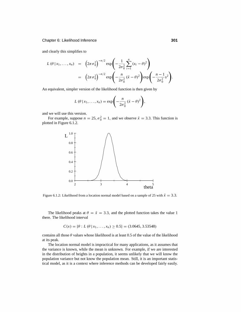
Chapter 6: Likelihood Inference 301
and clearly this simplifies to
L (θ | x1, . . . , xn) =&
2πσ 20
'−n/2exp
6− 1
2σ 20
n)i=1
(xi − θ)27
=&
2πσ 20
'−n/2exp
6− n
2σ 20
(x − θ)27
exp
6−n − 1
2σ 20
s2
7.
An equivalent, simpler version of the likelihood function is then given by
L (θ | x1, . . . , xn) = exp
6− n
2σ 20
(x − θ)27,
and we will use this version.For example, suppose n = 25, σ 2
0 = 1, and we observe x = 3.3. This function isplotted in Figure 6.1.2.
2 3 4 50.0
0.2
0.4
0.6
0.8
1.0
theta
L
Figure 6.1.2: Likelihood from a location normal model based on a sample of 25 with x = 3.3.
The likelihood peaks at θ = x = 3.3, and the plotted function takes the value 1there. The likelihood interval
C(x) = {θ : L (θ | x1, . . . , xn) ≥ 0.5} = (3.0645, 3.53548)
contains all those θ values whose likelihood is at least 0.5 of the value of the likelihoodat its peak.
The location normal model is impractical for many applications, as it assumes thatthe variance is known, while the mean is unknown. For example, if we are interestedin the distribution of heights in a population, it seems unlikely that we will know thepopulation variance but not know the population mean. Still, it is an important statis-tical model, as it is a context where inference methods can be developed fairly easily.

302 Section 6.1: The Likelihood Function
The methodology developed for this situation is often used as a paradigm for inferencemethods in much more complicated models.
The parameter θ need not be one-dimensional. The interpretation of the likelihoodis still the same, but it is not possible to plot it — at least not when the dimension of θis greater than 2.
EXAMPLE 6.1.5 Multinomial ModelsIn Example 2.8.5, we introduced multinomial distributions. These arise in applicationswhen we have a categorical response variable s that can take a finite number k of values,say, {1, . . . , k} , and P (s = i) = θ i .
Suppose, then, that k = 3 and we do not know the value of (θ1, θ2, θ3) . In thiscase, the parameter space is given by
* = {(θ1, θ2, θ3) : θ i ≥ 0, for i = 1, 2, 3, and θ1 + θ2 + θ3 = 1} .
Notice that it is really only two-dimensional, because as soon as we know the value ofany two of the θ i ’s, say, θ1 and θ2, we immediately know the value of the remainingparameter, as θ3 = 1− θ1 − θ2. This fact should always be remembered when we aredealing with multinomial models.
Now suppose we observe a sample of n from this distribution, say, (s1, . . . , sn).The likelihood function for this sample is given by
L (θ1, θ2, θ3 | s1, . . . , sn) = θ x11 θ
x22 θ
x33 , (6.1.2)
where xi is the number of i’s in the sample.Using the fact that we can treat positive multiples of the likelihood as being equiv-
alent, we see that the likelihood based on the observed counts (x1, x2, x3) (since theyarise from a Multinomial(n, θ1, θ2, θ3) distribution) is given by
L (θ1, θ2, θ3 | x1, x2, x3) = θ x11 θ
x22 θ
x33 .
This is identical to the likelihood (as functions of θ1, θ2, and θ3) for the original sam-ple. It is certainly simpler to deal with the counts rather than the original sample. Thisis a very important phenomenon in statistics and is characterized by the concept ofsufficiency, discussed in the next section.
6.1.1 Sufficient Statistics
The equivalence for inference of positive multiples of the likelihood function leads toa useful equivalence amongst possible data values coming from the same model. Forexample, suppose data values s1 and s2 are such that L (· | s1) = cL (· | s2) for somec > 0. From the point of view of likelihood, we are indifferent as to whether weobtained the data s1 or the data s2, as they lead to the same likelihood ratios.
This leads to the definition of a sufficient statistic.
Chapter 6: Likelihood Inference 303
Definition 6.1.1 A function T defined on the sample space S is called a sufficientstatistic for the model if, whenever T (s1) = T (s2), then
L (· | s1) = c (s1, s2) L (· | s2)
for some constant c (s1, s2) > 0.
The terminology is motivated by the fact that we need only observe the value t for thefunction T, as we can pick any value
s ∈ T−1{t} = {s : T (s) = t}and use the likelihood based on s. All of these choices give the same likelihood ratios.Typically, T (s) will be of lower dimension than s, so we can consider replacing s byT (s) as a data reduction which simplifies the analysis somewhat.
We illustrate the computation of a sufficient statistic in a simple context.
EXAMPLE 6.1.6Suppose that S = {1, 2, 3, 4}, * = {a, b}, and the two probability distributions aregiven by the following table.
s = 1 s = 2 s = 3 s = 4θ = a 1/2 1/6 1/6 1/6θ = b 1/4 1/4 1/4 1/4
Then L (· | 2) = L (· | 3) = L (· | 4) (e.g., L (a | 2) = 1/6 and L (b | 2) = 1/4), so thedata values in {2, 3, 4} all give the same likelihood ratios. Therefore, T : S −→ {0, 1}given by T (1) = 0 and T (2) = T (3) = T (4) = 1 is a sufficient statistic. The modelhas simplified a bit, as now the sample space for T has only two elements instead offour for the original model.
The following result helps identify sufficient statistics.
Theorem 6.1.1 (Factorization theorem) If the density (or probability function) fora model factors as fθ (s) = h(s)gθ (T (s)), where gθ and h are nonnegative, then Tis a sufficient statistic.
PROOF By hypothesis, it is clear that, when T (s1) = T (s2), we have
L (· | s1) = h(s1)gθ (T (s1)) = h(s1)gθ (T (s1))
h(s2)gθ (T (s2))h(s2)gθ (T (s2))
= h(s1)
h(s2)h(s2)gθ (T (s2)) = c (s1, s2) L (· | s2)
because gθ (T (s1)) = gθ (T (s2)).
Note that the name of this result is motivated by the fact that we have factored fθas a product of two functions. The important point about a sufficient statistic T is thatwe are indifferent, at least when considering inferences about θ, between observing thefull data s or the value of T (s). We will see in Chapter 9 that there is information inthe data, beyond the value of T (s), that is useful when we want to check assumptions.

304 Section 6.1: The Likelihood Function
Minimal Sufficient Statistics
Given that a sufficient statistic makes a reduction in the data, without losing relevantinformation in the data for inferences about θ, we look for a sufficient statistic thatmakes the greatest reduction. Such a statistic is called a minimal sufficient statistic.
Definition 6.1.2 A sufficient statistic T for a model is a minimal sufficient statistic,whenever the value of T (s) can be calculated once we know the likelihood functionL(· | s).
So a relevant likelihood function can always be obtained from the value of any suffi-cient statistic T, but if T is minimal sufficient as well, then we can also obtain the valueof T from any likelihood function. It can be shown that a minimal sufficient statisticgives the greatest reduction of the data in the sense that, if T is minimal sufficient andU is sufficient, then there is a function h such that T = h(U). Note that the definitionsof sufficient statistic and minimal sufficient statistic depend on the model, i.e., differentmodels can give rise to different sufficient and minimal sufficient statistics.
While the idea of a minimal sufficient statistic is a bit subtle, it is usually quitesimple to find one, as the following examples illustrate.
EXAMPLE 6.1.7 Location Normal ModelBy the factorization theorem we see immediately, from the discussion in Example6.1.4, that x is a sufficient statistic. Now any likelihood function for this model is apositive multiple of
exp
6− n
2σ 20
(x − θ)27
.
Notice that any such function of θ is completely specified by the point where it takesits maximum, namely, at θ = x . So we have that x can be obtained from any likelihoodfunction for this model, and it is therefore a minimal sufficient statistic.
EXAMPLE 6.1.8 Location-Scale Normal ModelSuppose that (x1, . . . , xn) is a sample from an N(µ, σ 2) distribution in which µ ∈R1 and σ > 0 are unknown. Recall the discussion and application of this model inExamples 5.3.4 and 5.5.6.
The parameter in this model is two-dimensional and is given by θ = #µ, σ 2
$ ∈* = R1 × (0,∞) . Therefore, the likelihood function is given by
L (θ | x1, . . . , xn) =&
2πσ 2'−n/2
exp
6− 1
2σ 2
n)i=1
(xi − µ)27
=&
2πσ 2'−n/2
exp&− n
2σ 2 (x − µ)2'
exp2−n − 1
2σ 2 s23
.
We see immediately, from the factorization theorem, that (x, s2) is a sufficient statistic.Now, fixing σ 2, any positive multiple of L(· | x1, . . . , xn) is maximized, as a func-
tion of µ, at µ = x . This is independent of σ 2. Fixing µ at x, we have that
L&&
x, σ 2'| x1, . . . , xn
'=&
2πσ 2'−n/2
exp2−n − 1
2σ 2s23

Chapter 6: Likelihood Inference 305
is maximized, as a function of σ 2, at the same point as ln L((x, σ 2) | x1, . . . , xn) be-cause ln is a strictly increasing function. Now
∂ ln L##
x, σ 2$ | x$
∂σ 2 = ∂
∂σ 2
2−n
2lnσ 2 − n − 1
2σ 2 s23
= − n
2σ 2 +n − 12σ 4 s2.
Setting this equal to 0 yields the solution
σ 2 = n − 1n
s2,
which is a 1–1 function of s2. So, given any likelihood function for this model, we cancompute (x, s2), which establishes that (x, s2) is a minimal sufficient statistic for themodel. In fact, the likelihood is maximized at (x, σ 2) (Problem 6.1.22).
EXAMPLE 6.1.9 Multinomial ModelsWe saw in Example 6.1.5 that the likelihood function for a sample is given by (6.1.2).This makes clear that if two different samples have the same counts, then they have thesame likelihood, so the counts (x1, x2, x3) comprise a sufficient statistic.
Now it turns out that this likelihood function is maximized by taking
(θ1, θ2, θ3) =& x1
n,
x2
n,
x3
n
'.
So, given the likelihood, we can compute the counts (the sample size n is assumedknown). Therefore, (x1, x2, x3) is a minimal sufficient statistic.
Summary of Section 6.1
• The likelihood function for a model and data shows how the data support thevarious possible values of the parameter. It is not the actual value of the likeli-hood that is important but the ratios of the likelihood at different values of theparameter.
• A sufficient statistic T for a model is any function of the data s such that once weknow the value of T (s), then we can determine the likelihood function L (· | s)(up to a positive constant multiple).
• A minimal sufficient statistic T for a model is any sufficient statistic such thatonce we know a likelihood function L (· | s) for the model and data, then we candetermine T (s).
EXERCISES
6.1.1 Suppose a sample of n individuals is being tested for the presence of an antibodyin their blood and that the number with the antibody present is recorded. Record anappropriate statistical model for this situation when we assume that the responses from

306 Section 6.1: The Likelihood Function
individuals are independent. If we have a sample of 10 and record 3 positives, graph arepresentative likelihood function.6.1.2 Suppose that suicides occur in a population at a rate p per person year and thatp is assumed completely unknown. If we model the number of suicides observed in apopulation with a total of N person years as Poisson(Np), then record a representativelikelihood function for p when we observe 22 suicides with N = 30, 345.6.1.3 Suppose that the lifelengths (in thousands of hours) of light bulbs are distributedExponential(θ), where θ > 0 is unknown. If we observe x = 5.2 for a sample of 20light bulbs, record a representative likelihood function. Why is it that we only need toobserve the sample average to obtain a representative likelihood?6.1.4 Suppose we take a sample of n = 100 students from a university with over50, 000 students enrolled. We classify these students as either living on campus, livingoff campus with their parents, or living off campus independently. Suppose we observethe counts (x1, x2, x3) = (34, 44, 22). Determine the form of the likelihood functionfor the unknown proportions of students in the population that are in these categories.6.1.5 Determine the constant that makes the likelihood functions in Examples 6.1.2and 6.1.3 equal.6.1.6 Suppose that (x1, . . . , xn) is a sample from the Bernoulli(θ) distribution, whereθ ∈ [0, 1] is unknown. Determine the likelihood function and a minimal sufficient sta-tistic for this model. (Hint: Use the factorization theorem and maximize the logarithmof the likelihood function.)6.1.7 Suppose (x1, . . . , xn) is a sample from the Poisson(θ) distribution where θ > 0is unknown. Determine the likelihood function and a minimal sufficient statistic forthis model. (Hint: the Factorization Theorem and maximization of the logarithm of thelikelihood function.)6.1.8 Suppose that a statistical model is comprised of two distributions given by thefollowing table:
s = 1 s = 2 s = 3f1 (s) 0.3 0.1 0.6f2 (s) 0.1 0.7 0.2
(a) Plot the likelihood function for each possible data value s.
(b) Find a sufficient statistic that makes a reduction in the data.6.1.9 Suppose a statistical model is given by { f1, f2}, where fi is an N(i, 1) distribu-tion. Compute the likelihood ratio L(1 | 0)/L(2 | 0) and explain how you interpret thisnumber.6.1.10 Explain why a likelihood function can never take negative values. Can a likeli-hood function be equal to 0 at a parameter value?6.1.11 Suppose we have a statistical model { fθ : θ ∈ [0, 1]} and we observe x0. Is ittrue that
8 10 L(θ | x0) dθ = 1? Explain why or why not.
6.1.12 Suppose that (x1, . . . , xn) is a sample from a Geometric(θ) distribution, whereθ ∈ [0, 1] is unknown. Determine the likelihood function and a minimal sufficient sta-tistic for this model. (Hint: Use the factorization theorem and maximize the logarithmof the likelihood.)

Chapter 6: Likelihood Inference 307
6.1.13 Suppose you are told that the likelihood of a particular parameter value is 109.Is it possible to interpret this number in any meaningful way? Explain why or why not.6.1.14 Suppose one statistician records a likelihood function as θ2 for θ ∈ [0, 1] whileanother statistician records a likelihood function as 100θ2 for θ ∈ [0, 1]. Explain whythese likelihood functions are effectively the same.
PROBLEMS
6.1.15 Show that T defined in Example 6.1.6 is a minimal sufficient statistic. (Hint:Show that once you know the likelihood function, you can determine which of the twopossible values for T has occurred.)6.1.16 Suppose that S = {1, 2, 3, 4},* = {a, b, c}, where the three probability distri-butions are given by the following table.
s = 1 s = 2 s = 3 s = 4θ = a 1/2 1/6 1/6 1/6θ = b 1/4 1/4 1/4 1/4θ = c 1/2 1/4 1/4 0
Determine a minimal sufficient statistic for this model. Is the minimal sufficient statis-tic in Example 6.1.6 sufficient for this model?6.1.17 Suppose that (x1, . . . , xn) is a sample from the N(µ, σ 2
0) distribution whereµ ∈ R1 is unknown. Determine the form of likelihood intervals for this model.6.1.18 Suppose that (x1, . . . , xn) ∈ Rn is a sample from fθ , where θ ∈ * is unknown.Show that the order statistics (x(1), . . . , x(n)) is a sufficient statistic for the model.6.1.19 Determine a minimal sufficient statistic for a sample of n from the rate gammamodel, i.e.,
fθ (x) = θα0
6 (α0)xα0−1 exp {−θx}
for x > 0, θ > 0 and where α0 > 0 is fixed.6.1.20 Determine the form of a minimal sufficient statistic for a sample of size n fromthe Uniform[0, θ] model where θ > 0.
6.1.21 Determine the form of a minimal sufficient statistic for a sample of size n fromthe Uniform[θ1, θ2] model where θ1 < θ2.
6.1.22 For the location-scale normal model, establish that the point where the likeli-hood is maximized is given by (x, σ 2) as defined in Example 6.1.8. (Hint: Show thatthe second derivative of ln L((x, σ 2) | x), with respect to σ 2, is negative at σ 2 and thenargue that (x, σ 2) is the maximum.)6.1.23 Suppose we have a sample of n from a Bernoulli(θ) distribution where θ ∈[0, 0.5]. Determine a minimal sufficient statistic for this model. (Hint: It is easy toestablish the sufficiency of x , but this point will not maximize the likelihood whenx > 0.5, so x cannot be obtained from the likelihood by maximization, as in Exercise6.1.6. In general, consider the second derivative of the log of the likelihood at any pointθ ∈ (0, 0.5) and note that knowing the likelihood means that we can compute any ofits derivatives at any values where these exist.)

308 Section 6.2: Maximum Likelihood
6.1.24 Suppose we have a sample of n from the Multinomial(1, θ, 2θ, 1− 3θ) distri-bution, where θ ∈ 90, 1/3: is unknown. Determine the form of the likelihood functionand show that x1+ x2 is a minimal sufficient statistic where xi is the number of samplevalues corresponding to an observation in the i th category. (Hint: Problem 6.1.23.)6.1.25 Suppose we observe s from a statistical model with two densities f1 and f2.Show that the likelihood ratio T (s) = f1(s)/ f2(s) is a minimal sufficient statistic.(Hint: Use the definition of sufficiency directly.)
CHALLENGES
6.1.26 Consider the location-scale gamma model, i.e.,
f(µ,σ) (x) = 16 (α0)
2x − µσ
3α0−1
exp+− x − µ
σ
,1σ
for x > µ ∈ R1, σ > 0 and where α0 > 0 is fixed.(a) Determine the minimal sufficient statistic for a sample of n when α0 = 1. (Hint:Determine where the likelihood is positive and calculate the partial derivative of thelog of the likelihood with respect to µ.)(b) Determine the minimal sufficient statistic for a sample of n when α0 := 1. (Hint:Use Problem 6.1.18, the partial derivative of the log of the likelihood with respect toµ, and determine where it is infinite.)
DISCUSSION TOPICS
6.1.27 How important do you think it is for a statistician to try to quantify how mucherror there is in an inference drawn? For example, if an estimate is being quoted forsome unknown quantity, is it important that the statistician give some indication abouthow accurate (or inaccurate) this inference is?
6.2 Maximum Likelihood EstimationIn Section 6.1, we introduced the likelihood function L (· | s) as a basis for makinginferences about the unknown true value θ ∈ *.We now begin to consider the specifictypes of inferences discussed in Section 5.5.3 and start with estimation.
When we are interested in a point estimate of θ, then a value θ (s) that maximizesL(θ | s) is a sensible choice, as this value is the best supported by the data, i.e.,
L(θ (s) | s) ≥ L(θ | s) (6.2.1)
for every θ ∈ *.
Definition 6.2.1 We call θ : S → * satisfying (6.2.1) for every θ ∈ * a maximumlikelihood estimator, and the value θ (s) is called a maximum likelihood estimate,or MLE for short.
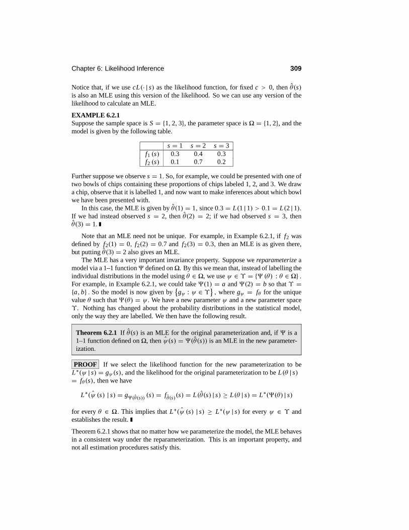
Chapter 6: Likelihood Inference 309
Notice that, if we use cL(· | s) as the likelihood function, for fixed c > 0, then θ (s)is also an MLE using this version of the likelihood. So we can use any version of thelikelihood to calculate an MLE.
EXAMPLE 6.2.1Suppose the sample space is S = {1, 2, 3}, the parameter space is * = {1, 2}, and themodel is given by the following table.
s = 1 s = 2 s = 3f1 (s) 0.3 0.4 0.3f2 (s) 0.1 0.7 0.2
Further suppose we observe s = 1. So, for example, we could be presented with one oftwo bowls of chips containing these proportions of chips labeled 1, 2, and 3. We drawa chip, observe that it is labelled 1, and now want to make inferences about which bowlwe have been presented with.
In this case, the MLE is given by θ (1) = 1, since 0.3 = L(1 | 1) > 0.1 = L(2 | 1).If we had instead observed s = 2, then θ (2) = 2; if we had observed s = 3, thenθ(3) = 1.
Note that an MLE need not be unique. For example, in Example 6.2.1, if f2 wasdefined by f2(1) = 0, f2(2) = 0.7 and f2(3) = 0.3, then an MLE is as given there,but putting θ (3) = 2 also gives an MLE.
The MLE has a very important invariance property. Suppose we reparameterize amodel via a 1–1 function7 defined on*. By this we mean that, instead of labelling theindividual distributions in the model using θ ∈ *, we use ψ ∈ ϒ = {7 (θ) : θ ∈ *} .For example, in Example 6.2.1, we could take 7(1) = a and 7(2) = b so that ϒ ={a, b} . So the model is now given by
4gψ : ψ ∈ ϒ5 , where gψ = fθ for the unique
value θ such that 7(θ) = ψ. We have a new parameter ψ and a new parameter spaceϒ. Nothing has changed about the probability distributions in the statistical model,only the way they are labelled. We then have the following result.
Theorem 6.2.1 If θ (s) is an MLE for the original parameterization and, if 7 is a1–1 function defined on *, then ψ(s) = 7(θ(s)) is an MLE in the new parameter-ization.
PROOF If we select the likelihood function for the new parameterization to beL∗(ψ | s) = gψ(s), and the likelihood for the original parameterization to be L(θ | s)= fθ (s), then we have
L∗(ψ (s) | s) = g7(θ(s)) (s) = fθ (s)(s) = L(θ(s) | s) ≥ L(θ | s) = L∗(7(θ) | s)
for every θ ∈ *. This implies that L∗(ψ (s) | s) ≥ L∗(ψ | s) for every ψ ∈ ϒ andestablishes the result.
Theorem 6.2.1 shows that no matter how we parameterize the model, the MLE behavesin a consistent way under the reparameterization. This is an important property, andnot all estimation procedures satisfy this.

310 Section 6.2: Maximum Likelihood
6.2.1 Computation of the MLE
An important issue is the computation of MLEs. In Example 6.2.1, we were able todo this by simply examining the table giving the distributions. With more complicatedmodels, this approach is not possible. In many situations, however, we can use themethods of calculus to compute θ (s). For this we require that fθ (s) be a continuouslydifferentiable function of θ so that we can use optimization methods from calculus.
Rather than using the likelihood function, it is often convenient to use the log-likelihood function.
Definition 6.2.2 For likelihood function L(· | s), the log-likelihood function l(· | s)defined on *, is given by l( | s) = ln L(· | s).
Note that ln (x) is a 1–1 increasing function of x > 0 and this implies that L(θ(s) | s) ≥L(θ | s) for every θ ∈ * if and only if l(θ(s) | s) ≥ l(θ | s) for every θ ∈ *. So wecan maximize l(· | s) instead when computing an MLE. The convenience of the log-likelihood arises from the fact that, for a sample (s1, . . . , sn) from { fθ : θ ∈ *} , thelikelihood function is given by
L(θ | s1, . . . , sn) =n%
i=1
fθ (si )
whereas the log-likelihood is given by
l(θ | s1, . . . , sn) =n)
i=1
ln fθ (si ).
It is typically much easier to differentiate a sum than a product.Because we are going to be differentiating the log-likelihood, it is convenient to
give a name to this derivative. We define the score function S(θ | s) of a model tobe the derivative of its log-likelihood function whenever this exists. So when θ is aone-dimensional real-valued parameter, then
S(θ | s) = ∂l(θ | s)∂θ
,
provided this partial derivative exists (see Appendix A.5 for a definition of partial deriv-ative). We restrict our attention now to the situation in which θ is one-dimensional.
To obtain the MLE, we must then solve the score equation
S(θ | s) = 0 (6.2.2)
for θ. Of course, a solution to (6.2.2) is not necessarily an MLE, because such a pointmay be a local minimum or only a local maximum rather than a global maximum. Toguarantee that a solution θ(s) is at least a local maximum, we must also check that
∂S(θ | s)∂θ
""""θ=θ (s)
= ∂2l(θ | s)∂θ2
""""θ=θ (s)
< 0. (6.2.3)

Chapter 6: Likelihood Inference 311
Then we must evaluate l (· | s) at each local maximum in order to determine the globalmaximum.
Let us compute some MLEs using calculus.
EXAMPLE 6.2.2 Location Normal ModelConsider the likelihood function
L(θ | x1, . . . , xn) = exp
6− n
2σ 20
(x − θ)27,
obtained in Example 6.1.4 for a sample (x1, . . . , xn) from the N(θ, σ 20) model where
θ ∈ R1 is unknown and σ 20 is known. The log-likelihood function is then
l(θ | x1, . . . , xn) = − n
2σ 20
(x − θ)2 ,
and the score function is
S(θ | x1, . . . , xn) = n
σ 20
(x − θ) .
The score equation is given by
n
σ 20
(x − θ) = 0.
Solving this for θ gives the unique solution θ ( x1, . . . , xn) = x. To check that this is alocal maximum, we calculate
∂S(θ | x1, . . . , xn)
∂θ
""""θ=x .
= − n
σ 20
,
which is negative, and thus indicates that x is a local maximum. Because we have onlyone local maximum, it is also the global maximum and we have indeed obtained theMLE.
EXAMPLE 6.2.3 Exponential ModelSuppose that a lifetime is known to be distributed Exponential(1/θ) , where θ > 0 isunknown. Then based on a sample (x1, . . . , xn), the likelihood is given by
L(θ | x1, . . . , xn) = 1
θn exp2−nx
θ
3,
the log-likelihood is given by
l(θ | x1, . . . , xn) = −n ln θ − nx
θ,
and the score function is given by
S(θ | x1, . . . , xn) = −n
θ+ nx
θ2 .

312 Section 6.2: Maximum Likelihood
Solving the score equation gives θ ( x1, . . . , xn) = x, and because x > 0,
∂S(θ | x1, . . . , xn)
∂θ
""""θ=x
= n
θ2 − 2nx
θ3
""""θ=x
= − n
x2 < 0,
so x is indeed the MLE.
In both examples just considered, we were able to derive simple formulas for theMLE. This is not always possible. Consider the following example.
EXAMPLE 6.2.4Consider a population in which individuals are classified according to one of three typeslabelled 1, 2, and 3, respectively. Further suppose that the proportions of individualsfalling in these categories are known to follow the law p1 = θ, p2 = θ2, p3 = 1− θ −θ2, where
θ ∈ [0, (√
5− 1)/2] = [0, 0.618 03]
is unknown. Here, pi denotes the proportion of individuals in the i th class. Note thatthe requirement that 0 ≤ θ + θ2 ≤ 1 imposes the upper bound on θ, and the precisebound is obtained by solving θ + θ2 − 1 = 0 for θ using the formula for the rootsof a quadratic. Relationships like this, amongst the proportions of the distribution ofa categorical variable, often arise in genetics. For example, the categorical variablemight serve to classify individuals into different genotypes.
For a sample of n (where n is small relative to the size of the population so that wecan assume observations are i.i.d.), the likelihood function is given by
L(θ | x1, . . . , xn) = θ x1θ2x2&
1− θ − θ2'x3,
where xi denotes the sample count in the i th class. The log-likelihood function is then
l(θ | s1, . . . , sn) = (x1 + 2x2) ln θ + x3 ln&
1− θ − θ2'
,
and the score function is
S(θ | s1, . . . , sn) = (x1 + 2x2)
θ− x3 (1+ 2θ)
1− θ − θ2.
The score equation then leads to a solution θ being a root of the quadratic
(x1 + 2x2)&
1− θ − θ2'− x3
&θ + 2θ2
'= − (x1 + 2x2 + 2x3) θ
2 − (x1 + 2x2 + x3) θ + (x1 + 2x2) .
Using the formula for the roots of a quadratic, we obtain
θ = 1
2 (x1 + 2x2 + 2x3)
×2−x1 − 2x2 − x3 ±
;5x2
1 + 20x1x2 + 10x1x3 + 20x22 + 20x2x3 + x2
3
3.

Chapter 6: Likelihood Inference 313
Notice that the formula for the roots does not determine the MLE in a clear way. Infact, we cannot even tell if either of the roots lies in [0, 1]! So there are four possiblevalues for the MLE at this point — either of the roots or the boundary points 0 and0.61803.
We can resolve this easily in an application by simply numerically evaluating thelikelihood at the four points. For example, if x1 = 70, x2 = 5, and x3 = 25, then theroots are −1.28616 and 0.47847, so it is immediate that the MLE is θ (x1, . . . , xn) =0.47847. We can see this graphically in the plot of the log-likelihood provided in Fig-ure 6.2.1.
0.60.550.50.450.4
-90
-95
-100
-105
-110
-115
-120
theta
lnL
theta
lnL
Figure 6.2.1: The log-likelihood function in Example 6.2.4 when x1 = 70, x2 = 5, andx3 = 25.
In general, the score equation (6.2.2) must be solved numerically, using an iterativeroutine like Newton–Raphson. Example 6.2.4 demonstrates that we must be very care-ful not to just accept a solution from such a procedure as the MLE, but to check that thefundamental defining property (6.2.1) is satisfied. We also have to be careful that thenecessary smoothness conditions are satisfied so that calculus can be used. Considerthe following example.
EXAMPLE 6.2.5 Uniform[0, θ] ModelSuppose ( x1, . . . , xn) is a sample from the Uniform[0, θ] model where θ > 0 is un-known. Then the likelihood function is given by
L(θ | x1, . . . , xn) =+θ−n xi ≤ θ for i = 1, . . . , n0 xi > θ for some i
= θ−n I[x(n),∞)(θ),
where x(n) is the largest order statistic from the sample. In Figure 6.2.2, we havegraphed this function when n = 10 and x(n) = 1.916. Notice that the maximum clearlyoccurs at x(n); we cannot obtain this value via differentiation, as L(· | x1, . . . , xn) is notdifferentiable there.

314 Section 6.2: Maximum Likelihood
0 1 2 3 4 50.0000
0.0005
0.0010
0.0015
theta
L
Figure 6.2.2: Plot of the likelihood function in Example 6.2.5 when n = 10 andx(10) = 1.916.
The lesson of Examples 6.2.4 and 6.2.5 is that we have to be careful when com-puting MLEs. We now look at an example of a two-dimensional problem in which theMLE can be obtained using one-dimensional methods.
EXAMPLE 6.2.6 Location-Scale Normal ModelSuppose that (x1, . . . , xn) is a sample from an N(µ, σ 2) distribution, where µ ∈ R1
and σ > 0 are unknown. The parameter in this model is two-dimensional, given byθ = #µ, σ 2
$ ∈ * = R1 × (0,∞) . The likelihood function is then given by
L&µ, σ 2 | x1, . . . , xn
'=&
2πσ 2'−n/2
exp&− n
2σ 2 (x − µ)2'
exp2−n − 1
2σ 2 s23,
as shown in Example 6.1.8. The log-likelihood function is given by
l&µ, σ 2 | x1, . . . , xn
'= −n
2ln 2π − n
2ln σ 2 − n
2σ 2 (x − µ)2 −n − 12σ 2 s2. (6.2.4)
As discussed in Example 6.1.8, it is clear that, for fixed σ 2, (6.2.4) is maximized, as afunction of µ, by µ = x . Note that this does not involve σ 2, so this must be the firstcoordinate of the MLE.
Substituting µ = x into (6.2.4), we obtain
−n
2ln 2π − n
2lnσ 2 − n − 1
2σ 2 s2, (6.2.5)
and the second coordinate of the MLE must be the value of σ 2 that maximizes (6.2.5).Differentiating (6.2.5) with respect to σ 2 and setting this equal to 0 gives
− n
2σ 2+ n − 1
2#σ 2$2 s2 = 0. (6.2.6)

Chapter 6: Likelihood Inference 315
Solving (6.2.6) for σ 2 leads to the solution
σ 2 = n − 1n
s2 = 1n
n)i=1
(xi − x)2 .
Differentiating (6.2.6) with respect to σ 2, and substituting in σ 2,we see that the secondderivative is negative, hence σ 2 is a point where the maximum is attained.
Therefore, we have shown that the MLE of#µ, σ 2
$is given by6
x,1n
n)i=1
(xi − x)27.
In the following section we will show that this result can also be obtained using multi-dimensional calculus.
So far we have talked about estimating only the full parameter θ for a model. Whatabout estimating a general characteristic of interest ψ(θ) for some function ψ definedon the parameter space *? Perhaps the obvious answer here is to use the estimateψ(s) = ψ(θ(s)) where θ (s) is an MLE of θ. This is sometimes referred to as the plug-in MLE of ψ. Notice, however, that the plug-in MLE is not necessarily a true MLE, inthe sense that we have a likelihood function for a model indexed by ψ and that takesits maximum value at ψ(s). If ψ is a 1–1 function defined on *, then Theorem 6.2.1establishes that ψ(s) is a true MLE but not otherwise.
If ψ is not 1–1, then we can often find a complementing function λ defined on* sothat (ψ, λ) is a 1–1 function of θ . Then, by Theorem 6.2.1,&
ψ(s), λ(s)'=&ψ(θ(s)), λ(θ(s))
'is the joint MLE, but ψ(s) is still not formally an MLE. Sometimes a plug-in MLE canperform badly, as it ignores the information in λ(θ(s)) about the true value of ψ. Anexample illustrates this phenomenon.
EXAMPLE 6.2.7 Sum of Squared MeansSuppose that Xi ∼ N(µi , 1) for i = 1, . . . , n and that these are independent with theµi completely unknown. So here, θ = #µ1, . . . , µn
$and * = Rn. Suppose we want
to estimate ψ(θ) = µ21 + · · · + µ2
n.The log-likelihood function is given by
l(θ | x1, . . . , xn) = −12
n)i=1
(xi − µi )2.
Clearly this is maximized by θ (x1, . . . , xn) = (x1, . . . , xn). So the plug-in MLE of ψis given by ψ =-n
i=1 x2i .
Now observe that
Eθ
6n)
i=1
X2i
7=
n)i=1
Eθ (X2i ) =
n)i=1
&Varθ (Xi)+ µ2
i
'= n +ψ(θ),

316 Section 6.2: Maximum Likelihood
where Eθ (g) refers to the expectation of g(s) when s ∼ fθ . So when n is large, it islikely that ψ is far from the true value. An immediate improvement in this estimator isto use
-ni=1 x2
i − n instead.
There have been various attempts to correct problems such as the one illustrated inExample 6.2.7. Typically, these involve modifying the likelihood in some way. We donot pursue this issue further in this text but we do advise caution when using plug-inMLEs. Sometimes, as in Example 6.2.6, where we estimate µ by x and σ 2 by s2, theyseem appropriate; other times, as in Example 6.2.7, they do not.
6.2.2 The Multidimensional Case (Advanced)
We now consider the situation in which θ = (θ1, . . . , θk) ∈ Rk is multidimensional,i.e., k > 1. The likelihood and log-likelihood are then defined just as before, but thescore function is now given by
S (θ | s) =
∂l(θ | s)∂θ1
∂l(θ | s)∂θ2...
∂l(θ | s)∂θk
,
provided all these partial derivatives exist. For the score equation, we get∂l(θ | s)∂θ1
∂l(θ | s)∂θ2...
∂l(θ | s)∂θk
=
00...0
,
and we must solve this k-dimensional equation for (θ1, . . . , θk) . This is often muchmore difficult than in the one-dimensional case, and we typically have to resort tonumerical methods.
A necessary and sufficient condition for (θ1, . . . , θk) to be a local maximum, whenthe log-likelihood has continuous second partial derivatives, is that the matrix of secondpartial derivatives of the log-likelihood, evaluated at (θ1, . . . , θk), must be negativedefinite (equivalently, all of its eigenvalues must be negative). We then must evaluatethe likelihood at each of the local maxima obtained to determine the global maximumor MLE.
We will not pursue the numerical computation of MLEs in the multidimensionalcase any further here, but we restrict our attention to a situation in which we carry outthe calculations in closed form.
EXAMPLE 6.2.8 Location-Scale Normal ModelWe determined the log-likelihood function for this model in (6.2.4). The score functionis then
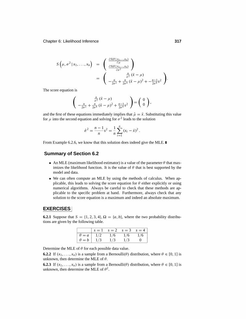
Chapter 6: Likelihood Inference 317
S&µ, σ 2 | x1, . . . , xn
'=
6 ∂S(θ | x1,...,xn)∂µ
∂S(θ | x1,...,xn)∂σ 2
7
=6 n
σ 2 (x − µ)− n
2σ 2 + n2σ 4 (x − µ)2 +−n−1
2σ 4 s2
7.
The score equation is6 nσ 2 (x − µ)
− n2σ 2 + n
2σ 4 (x − µ)2 + n−12σ 4 s2
7=2
00
3,
and the first of these equations immediately implies that µ = x. Substituting this valuefor µ into the second equation and solving for σ 2 leads to the solution
σ 2 = n − 1n
s2 = 1n
n)i=1
(xi − x)2 .
From Example 6.2.6, we know that this solution does indeed give the MLE.
Summary of Section 6.2
• An MLE (maximum likelihood estimator) is a value of the parameter θ that max-imizes the likelihood function. It is the value of θ that is best supported by themodel and data.
• We can often compute an MLE by using the methods of calculus. When ap-plicable, this leads to solving the score equation for θ either explicitly or usingnumerical algorithms. Always be careful to check that these methods are ap-plicable to the specific problem at hand. Furthermore, always check that anysolution to the score equation is a maximum and indeed an absolute maximum.
EXERCISES
6.2.1 Suppose that S = {1, 2, 3, 4},* = {a, b}, where the two probability distribu-tions are given by the following table.
s = 1 s = 2 s = 3 s = 4θ = a 1/2 1/6 1/6 1/6θ = b 1/3 1/3 1/3 0
Determine the MLE of θ for each possible data value.6.2.2 If (x1, . . . , xn) is a sample from a Bernoulli(θ) distribution, where θ ∈ [0, 1] isunknown, then determine the MLE of θ .6.2.3 If (x1, . . . , xn) is a sample from a Bernoulli(θ) distribution, where θ ∈ [0, 1] isunknown, then determine the MLE of θ2.

318 Section 6.2: Maximum Likelihood
6.2.4 If (x1, . . . , xn) is a sample from a Poisson(θ) distribution, where θ ∈ (0,∞) isunknown, then determine the MLE of θ .6.2.5 If (x1, . . . , xn) is a sample from a Gamma(α0, θ) distribution, where α0 > 0 andθ ∈ (0,∞) is unknown, then determine the MLE of θ .6.2.6 Suppose that (x1, . . . , xn) is the result of independent tosses of a coin where wetoss until the first head occurs and where the probability of a head on a single toss isθ ∈ (0, 1]. Determine the MLE of θ .6.2.7 If (x1, . . . , xn) is a sample from a Beta(α, 1) distribution (see Problem 2.4.24)where α > 0 is unknown, then determine the MLE of α. (Hint: Assume 6 (α) is adifferentiable function of α.)6.2.8 If (x1, . . . , xn) is a sample from a Weibull(β) distribution (see Problem 2.4.19),where β > 0 is unknown, then determine the score equation for the MLE of β.6.2.9 If (x1, . . . , xn) is a sample from a Pareto(α) distribution (see Problem 2.4.20),where α > 0 is unknown, then determine the MLE of α.6.2.10 If (x1, . . . , xn) is a sample from a Log-normal(τ) distribution (see Problem2.6.12), where τ > 0 is unknown, then determine the MLE of τ .6.2.11 Suppose you are measuring the volume of a cubic box in centimeters by takingrepeated independent measurements of one of the sides. Suppose it is reasonable to as-sume that a single measurement follows an N(µ, σ 2
0) distribution, where µ is unknownand σ 2
0 is known. Based on a sample of measurements, you obtain the MLE ofµ as 3.2cm. What is your estimate of the volume of the box? How do you justify this in termsof the likelihood function?6.2.12 If (x1, . . . , xn) is a sample from an N(µ0, σ
2) distribution, where σ 2 > 0 isunknown and µ0 is known, then determine the MLE of σ 2. How does this MLE differfrom the plug-in MLE of σ 2 computed using the location-scale normal model?6.2.13 Explain why it is not possible that the function θ3 exp(−(θ −5.3)2) for θ ∈ R1
is a likelihood function.6.2.14 Suppose you are told that a likelihood function has local maxima at the points−2.2, 4.6 and 9.2, as determined using calculus. Explain how you would determinethe MLE.6.2.15 If two functions of θ are equivalent versions of the likelihood when one is apositive multiple of the other, then when are two log-likelihood functions equivalent?6.2.16 Suppose you are told that the likelihood of θ at θ = 2 is given by 1/4. Is thisthe probability that θ = 2? Explain why or why not.
COMPUTER EXERCISES
6.2.17 A likelihood function is given by exp(−(θ − 1)2/2) + 3 exp(−(θ − 2)2/2)for θ ∈ R1. Numerically approximate the MLE by evaluating this function at 1000equispaced points in (−10, 10]. Also plot the likelihood function.6.2.18 A likelihood function is given by exp(−(θ − 1)2/2) + 3 exp(−(θ − 5)2/2)for θ ∈ R1. Numerically approximate the MLE by evaluating this function at 1000equispaced points in (−10, 10]. Also plot the likelihood function. Comment on theform of likelihood intervals.

Chapter 6: Likelihood Inference 319
PROBLEMS
6.2.19 (Hardy–Weinberg law) The Hardy–Weinberg law in genetics says that the pro-portions of genotypes AA, Aa, and aa are θ2, 2θ (1− θ), and (1− θ)2, respectively,where θ ∈ [0, 1] . Suppose that in a sample of n from the population (small relativeto the size of the population), we observe x1 individuals of type AA, x2 individuals oftype Aa, and x3 individuals of type aa.
(a) What distribution do the counts (X1, X2, X3) follow?(b) Record the likelihood function, the log-likelihood function, and the score functionfor θ.(c) Record the form of the MLE for θ .6.2.20 If (x1, . . . , xn) is a sample from an N(µ, 1) distribution where µ ∈ R1 is un-known, determine the MLE of the probability content of the interval (−∞, 1). Justifyyour answer.6.2.21 If (x1, . . . , xn) is a sample from an N(µ, 1) distribution where µ ≥ 0 is un-known, determine the MLE of µ.6.2.22 Prove that, if θ (s) is the MLE for a model for response s and if T is a sufficientstatistic for the model, then θ(s) is also the MLE for the model for T (s).6.2.23 Suppose that (X1, X2, X3) ∼ Multinomial(n, θ1, θ2, θ3) (see Example 6.1.5),where
* = {(θ1, θ2, θ3) : 0 ≤ θ i ≤ 1, θ1 + θ2 + θ3 = 1}and we observe (X1, X2, X3) = (x1, x2, x3).(a) Determine the MLE of (θ1, θ2, θ3).(b) What is the plug-in MLE of θ1 + θ2
2 − θ23?
6.2.24 If (x1, . . . , xn) is a sample from a Uniform[θ1, θ2] distribution with
* =B(θ1, θ2) ∈ R2 : θ1 < θ2
C,
determine the MLE of (θ1, θ2). (Hint: You cannot use calculus. Instead, directlydetermine the maximum over θ1 when θ2 is fixed, and then vary θ2.)
COMPUTER PROBLEMS
6.2.25 Suppose the proportion of left-handed individuals in a population is θ . Basedon a simple random sample of 20, you observe four left-handed individuals.(a) Assuming the sample size is small relative to the population size, plot the log-likelihood function and determine the MLE.(b) If instead the population size is only 50, then plot the log-likelihood function anddetermine the MLE. (Hint: Remember that the number of left-handed individuals fol-lows a hypergeometric distribution. This forces θ to be of the form i/50 for someinteger i between 4 and 34. From a tabulation of the log-likelihood, you can obtain theMLE.)

320 Section 6.3: Inferences Based on the MLE
CHALLENGES
6.2.26 If (x1, . . . , xn) is a sample from a distribution with density
fθ (x) = (1/2) exp (−|x − θ |)for x ∈ R1 and where θ ∈ R1 is unknown, then determine the MLE of θ . (Hint:You cannot use calculus. Instead, maximize the log-likelihood in each of the intervals(−∞, x(1)), [x(1) ≤ θ < x(2)), etc.)
DISCUSSION TOPICS
6.2.27 One approach to quantifying the uncertainty in an MLE θ (s) is to report theMLE together with a liklihood interval {θ : L(θ | s) ≥ cL(θ(s) | s)} for some constantc ∈ (0, 1). What problems do you see with this approach? In particular, how wouldyou choose c?
6.3 Inferences Based on the MLEIn Table 6.3.1. we have recorded n = 66 measurements of the speed of light (pas-sage time recorded as deviations from 24, 800 nanoseconds between two mirrors 7400meters apart) made by A. A. Michelson and S. Newcomb in 1882.
28 26 33 24 34 −44 27 16 40 −2 2922 24 21 25 30 23 29 31 19 24 2036 32 36 28 25 21 28 29 37 25 2826 30 32 36 26 30 22 36 23 27 2728 27 31 27 26 33 26 32 32 24 3928 24 25 32 25 29 27 28 29 16 23
Table 6.3.1: Speed of light measurements.
Figure 6.3.1 is a boxplot of these data with the variable labeled as x . Notice thereare two outliers at x = −2 and x = −44. We will presume there is something veryspecial about these observations and discard them for the remainder of our discussion.
40
30
20
10
0
-10
-20
-30
-40
-50
x
Figure 6.3.1: Boxplot of the data values in Table 6.3.1.

Chapter 6: Likelihood Inference 321
Figure 6.3.2 presents a histogram of these data minus the two data values identifiedas outliers. Notice that the histogram looks reasonably symmetrical, so it seems plau-sible to assume that these data are from an N(µ, σ 2) distribution for some values of µand σ 2. Accordingly, a reasonable statistical model for these data would appear to bethe location-scale normal model. In Chapter 9, we will discuss further how to assessthe validity of the normality assumption.
504540353025201510
0.09
0.08
0.07
0.06
0.05
0.04
0.03
0.02
0.01
0.00
x
Den
sity
Figure 6.3.2: Density histogram of the data in Table 6.3.1 with the outliers removed.
If we accept that the location-scale normal model makes sense, the question arisesconcerning how to make inferences about the unknown parameters µ and σ 2. Thepurpose of this section is to develop methods for handling problems like this. Themethods developed in this section depend on special features of the MLE in a givencontext. In Section 6.5, we develop a more general approach based on the MLE.
6.3.1 Standard Errors, Bias, and Consistency
Based on the justification for the likelihood, the MLE θ (s) seems like a natural estimateof the true value of θ. Let us suppose that we will then use the plug-in MLE estimateψ(s) = ψ(θ(s)) for a characteristic of interest ψ(θ) (e.g., ψ(θ) might be the firstquartile or the variance).
In an application, we want to know how reliable the estimate ψ (s) is. In otherwords, can we expect ψ (s) to be close to the true value ofψ(θ), or is there a reasonablechance that ψ(s) is far from the true value? This leads us to consider the samplingdistribution of ψ (s), as this tells us how much variability there will be in ψ(s) underrepeated sampling from the true distribution fθ . Because we do not know what the truevalue of θ is, we have to look at the sampling distribution of ψ(s) for every θ ∈ *.
To simplify this, we substitute a numerical measure of how concentrated these sam-pling distributions are about ψ(θ). Perhaps the most commonly used measure of theaccuracy of a general estimator T (s) of ψ(θ), i.e., we are not restricting ourselves toplug-in MLEs, is the mean-squared error.

322 Section 6.3: Inferences Based on the MLE
Definition 6.3.1 The mean-squared error (MSE) of the estimator T of ψ(θ) ∈ R1,is given by MSEθ (T ) = Eθ ((T −ψ(θ))2) for each θ ∈ *.
Clearly, the smaller MSEθ (T ) is, the more concentrated the sampling distribution ofT (s) is about the value ψ(θ).
Looking at MSEθ (T ) as a function of θ gives us some idea of how reliable T (s)is as an estimate of the true value of ψ(θ). Because we do not know the true value ofθ, and thus the true value of MSEθ (T ), statisticians record an estimate of the mean-squared error at the true value. Often
MSEθ (s)(T )
is used for this. In other words, we evaluate MSEθ (T ) at θ = θ (s) as a measure of theaccuracy of the estimate T (s).
The following result gives an important identity for the MSE.
Theorem 6.3.1 If ψ(θ) ∈ R1and T is a real-valued function defined on S suchthat Eθ (T ) exists, then
MSEθ (T ) = Varθ (T )+ (Eθ (T )− ψ(θ))2 . (6.3.1)
PROOF We have
Eθ ((T −ψ(θ)))2 = Eθ ((T − Eθ (T )+ Eθ (T )−ψ (θ))2)= Eθ ((T − Eθ (T ))
2)
+ 2Eθ ((T − Eθ (T )) (Eθ (T )−ψ (θ)))+ (Eθ (T )− ψ(θ))2= Varθ (T )+ (Eθ (T )−ψ(θ))2
because
Eθ ((T − Eθ (T )) (Eθ (T )−ψ (θ))) = (Eθ (T − Eθ (T ))) (Eθ (T )−ψ(θ))= 0.
The second term in (6.3.1) is the square of the bias in the estimator T .
Definition 6.3.2 The bias in the estimator T of ψ(θ) is given by Eθ (T ) − ψ(θ)whenever Eθ (T ) exists. When the bias in an estimator T is 0 for every θ , we call Tan unbiased estimator of ψ , i.e., T is unbiased whenever Eθ (T ) = ψ(θ) for everyθ ∈ *.
Note that when the bias in an estimator is 0, then the MSE is just the variance.Unbiasedness tells us that, in a sense, the sampling distribution of the estimator is
centered on the true value. For unbiased estimators,
MSEθ (s)(T ) = Varθ (s)(T )
Chapter 6: Likelihood Inference 323
andSdθ (s)(T ) =
;Varθ (s)(T )
is an estimate of the standard deviation of T and is referred to as the standard errorof the estimate T (s). As a principle of good statistical practice, whenever we quotean estimate of a quantity, we should also provide its standard error — at least whenwe have an unbiased estimator, as this tells us something about the accuracy of theestimate.
We consider some examples.
EXAMPLE 6.3.1 Location Normal ModelConsider the likelihood function
L (µ | x1, . . . , xn) = exp
6− n
2σ 20
(x − µ)27,
obtained in Example 6.1.4 for a sample (x1, . . . , xn) from the N(µ, σ 20) model, where
µ ∈ R1 is unknown and σ 20 > 0 is known. Suppose we want to estimate µ. The MLE
of µ was computed in Example 6.2.2 to be x.In this case, we can determine the sampling distribution of the MLE exactly from
the results in Section 4.6. We have that X ∼ N(µ, σ 20/n) and so X is unbiased, and
MSEµ(X) = Varµ(X) = σ 20
n,
which is independent of µ. So we do not need to estimate the MSE in this case. Thestandard error of the estimate is given by
Sdµ(X) = σ 0√n.
Note that the standard error decreases as the population variance σ 20 decreases and as
the sample size n increases.
EXAMPLE 6.3.2 Bernoulli ModelSuppose (x1, . . . , xn) is a sample from a Bernoulli(θ) distribution where θ ∈ [0, 1] isunknown. Suppose we wish to estimate θ . The likelihood function is given by
L(θ | x1, . . . , xn) = θnx (1− θ)n(1−x) ,
and the MLE of θ is x (Exercise 6.2.2), the proportion of successes in the n perfor-mances. We have Eθ (X) = θ for every θ ∈ [0, 1] , so the MLE is an unbiased estimatorof θ.
Therefore,
MSEθ (X) = Varθ (X) = θ (1− θ)n
,
and the estimated MSE is
MSEθ (X) =x (1− x)
n.

324 Section 6.3: Inferences Based on the MLE
The standard error of the estimate x is then given by
Sdθ (X) =D
x (1− x)
n.
Note how this standard error is quite different from the standard error of x in Example6.3.1.
EXAMPLE 6.3.3 Application of the Bernoulli ModelA polling organization is asked to estimate the proportion of households in the pop-ulation in a specific district who will participate in a proposed recycling program byseparating their garbage into various components. The pollsters decided to take a sam-ple of n = 1000 from the population of approximately 1.5 million households (we willsay more on how to choose this number later).
Each respondent will indicate either yes or no to a question concerning their par-ticipation. Given that the sample size is small relative to the population size, we canassume that we are sampling from a Bernoulli(θ) model where θ ∈ [0, 1] is the pro-portion of individuals in the population who will respond yes.
After conducting the sample, there were 790 respondents who replied yes and 210who responded no. Therefore, the MLE of θ is
θ = x = 7901000
= 0.79
and the standard error of the estimate isDx (1− x)
1000=D
0.79 (1− 0.79)1000
= 0.01288.
Notice that it is not entirely clear how we should interpret the value 0.01288. Doesit mean our estimate 0.79 is highly accurate, modestly accurate, or not accurate at all?We will discuss this further in Section 6.3.2.
EXAMPLE 6.3.4 Location-Scale Normal ModelSuppose that (x1, . . . , xn) is a sample from an N(µ, σ 2) distribution where µ ∈ R1
and σ 2 > 0 are unknown. The parameter in this model is given by θ = #µ, σ 2
$ ∈* = R1 × (0,∞). Suppose that we want to estimate µ = ψ(µ, σ 2), i.e., just the firstcoordinate of the full model parameter.
In Example 6.1.8, we determined that the likelihood function is given by
L&µ, σ 2 | x1, . . . , xn
'=&
2πσ 2'−n/2
exp&− n
2σ 2 (x − µ)2'
exp2−n − 1
2σ 2s23.
In Example 6.2.6 we showed that the MLE of θ is2x,
n − 1n
s23.
Furthermore, from Theorem 4.6.6, the sampling distribution of the MLE is given byX ∼ N(µ, σ 2/n) independent of (n − 1) S2/σ 2 ∼ χ2(n − 1).

Chapter 6: Likelihood Inference 325
The plug-in MLE of µ is x. This estimator is unbiased and has
MSEθ (X) = Varθ (X) = σ 2
n.
Since σ 2 is unknown we estimate MSEθ (X) by
MSEθ (X) =n−1
n s2
n= n − 1
n2s2 ≈ s2
n.
The value s2/n is commonly used instead of MSEθ (X), because (Corollary 4.6.2)
Eθ (S2) = σ 2,
i.e., S2 is an unbiased estimator of σ 2. The quantity s/√
n is referred to as the standarderror of the estimate x.
EXAMPLE 6.3.5 Application of the Location-Scale Normal ModelIn Example 5.5.6, we have a sample of n = 30 heights (in inches) of students. Wecalculated x = 64.517 as our estimate of the mean population heightµ. In addition, weobtained the estimate s = 2.379 of σ. Therefore, the standard error of the estimate x =64.517 is s/
√30 = 2.379/
√30 = 0.43434. As in Example 6.3.3, we are faced with
interpreting exactly what this number means in terms of the accuracy of the estimate.
Consistency of Estimators
Perhaps the most important property that any estimator T of a characteristic ψ(θ) canhave is that it be consistent. Broadly speaking, this means that as we increase theamount of data we collect, then the sequence of estimates should converge to the truevalue of ψ(θ). To see why this is a necessary property of any estimation procedure,consider the finite population sampling context discussed in Section 5.4.1. When thesample size is equal to the population size, then of course we have the full informationand can compute exactly every characteristic of the distribution of any measurementdefined on the population. So it would be an error to use an estimation procedure for acharacteristic of interest that did not converge to the true value of the characteristic aswe increase the sample size.
Fortunately, we have already developed the necessary mathematics in Chapter 4 todefine precisely what we mean by consistency.
Definition 6.3.3 A sequence of of estimates T1, T2, . . . is said to be consistent (in
probability) for ψ(θ) if TnPθ→ ψ(θ) as n →∞ for every θ ∈ *. A sequence of of
estimates T1, T2, . . . is said to be consistent (almost surely) forψ(θ) if Tna.s.→ ψ(θ)
as n →∞ for every θ ∈ *.Notice that Theorem 4.3.1 says that if the sequence is consistent almost surely, then itis also consistent in probability.
Consider now a sample (x1, . . . , xn) from a model { fθ : θ ∈ *} and let Tn =n−1-n
i=1 xi be the nth sample average as an estimator of ψ(θ) = Eθ (X), which

326 Section 6.3: Inferences Based on the MLE
we presume exists. The weak and strong laws of large numbers immediately give usthe consistency of the sequence T1, T2, . . . forψ(θ).We see immediately that this givesthe consistency of some of the estimators discussed in this section. In fact, Theorem6.5.2 gives the consistency of the MLE in very general circumstances. Furthermore,the plug-in MLE will also be consistent under weak restrictions on ψ.Accordingly, wecan think of maximum likelihood estimation as doing the right thing in a problem atleast from the point of view of consistency.
More generally, we should always restrict our attention to statistical proceduresthat perform correctly as the amount of data increases. Increasing the amount of datameans that we are acquiring more information and thus reducing our uncertainty so thatin the limit we know everything. A statistical procedure that was inconsistent would bepotentially misleading.
6.3.2 Confidence Intervals
While the standard error seems like a reasonable quantity for measuring the accuracyof an estimate of ψ(θ), its interpretation is not entirely clear at this point. It turns outthat this is intrinsically tied up with the idea of a confidence interval.
Consider the construction of an interval
C(s) = (l(s), u(s)) ,
based on the data s, that we believe is likely to contain the true value of ψ(θ). To dothis, we have to specify the lower endpoint l(s) and upper endpoint u(s) for each datavalue s. How should we do this?
One approach is to specify a probability γ ∈ [0, 1] and then require that randominterval C have the confidence property, as specified in the following definition.
Definition 6.3.4 An interval C(s) = (l(s), u(s)) is a γ -confidence interval forψ(θ) if Pθ (ψ(θ) ∈ C(s)) = Pθ (l(s) ≤ ψ(θ) ≤ u(s)) ≥ γ for every θ ∈ *.We refer to γ as the confidence level of the interval.
So C is a γ -confidence interval for ψ(θ) if, whenever we are sampling from Pθ , theprobability that ψ(θ) is in the interval is at least equal to γ . For a given data set, suchan interval either covers ψ(θ) or it does not. So note that it is not correct to say thata particular instance of a γ -confidence region has probability γ of containing the truevalue of ψ(θ).
If we choose γ to be a value close to 1, then we are highly confident that thetrue value of ψ(θ) is in C(s). Of course, we can always take C(s) = R1 (a very biginterval!), and we are then 100% confident that the interval contains the true value. Butthis tells us nothing we did not already know. So the idea is to try to make use of theinformation in the data to construct an interval such that we have a high confidence,say, γ = 0.95 or γ = 0.99, that it contains the true value and is not any longer thannecessary. We then interpret the length of the interval as a measure of how accuratelythe data allow us to know the true value of ψ(θ).

Chapter 6: Likelihood Inference 327
z-Confidence Intervals
Consider the following example, which provides one approach to the construction ofconfidence intervals.
EXAMPLE 6.3.6 Location Normal Model and z-Confidence IntervalsSuppose we have a sample (x1, . . . , xn) from the N(µ, σ 2
0) model, where µ ∈ R1 isunknown and σ 2
0 > 0 is known. The likelihood function is as specified in Example6.3.1. Suppose we want a confidence interval for µ.
The reasoning that underlies the likelihood function leads naturally to the followingrestriction for such a region: If µ1 ∈ C(x1, . . . , xn) and
L(µ2 | x1, . . . , xn) ≥ L(µ1 | x1, . . . , xn),
then we should also have µ2 ∈ C(x1, . . . , xn). This restriction is implied by the like-lihood because the model and the data support µ2 at least as well as µ1. Thus, if weconclude that µ1 is a plausible value, so is µ2.
Therefore, C(x1, . . . , xn) is of the form
C(x1, . . . , xn) = {µ : L (µ | x1, . . . , xn) ≥ k (x1, . . . , xn)}for some k (x1, . . . , xn) , i.e., C(x1, . . . , xn) is a likelihood interval for µ. Then
C(x1, . . . , xn) =(µ : exp
6− n
2σ 20
(x − µ)27≥ k(x1, . . . , xn)
*
=(µ : − n
2σ 20
(x − µ)2 ≥ ln k(x1, . . . , xn)
*
=(µ : (x − µ)2 ≤ −2σ 2
0
nln k(x1, . . . , xn)
*
=E
x − k∗(x1, . . . , xn )σ 0√
n, x + k∗(x1, . . . , xn)
σ 0√n
Fwhere k∗(x1, . . . , xn) = √−2 ln k(x1, . . . , xn).
We are now left to choose k, or equivalently k∗, so that the interval C is a γ -confidence interval for µ. Perhaps the simplest choice is to try to choose k∗ so thatk∗(x1, . . . , xn) is constant and is such that the interval as short as possible. Because
Z = X − µσ 0/
√n∼ N(0, 1), (6.3.2)
we have
γ ≤ Pµ (µ ∈ C(x1, . . . , xn)) = Pµ
2X − k∗ σ 0√
n≤ µ ≤ X + k∗ σ 0√
n
3= Pµ
2−k∗ ≤ X − µ
σ 0/√
n≤ c
3= Pµ
2"""" X − µσ 0/
√n
"""" ≤ k∗3
= 1− 2#1−4 #k∗$$ (6.3.3)

328 Section 6.3: Inferences Based on the MLE
for every µ ∈ R1, where 4 is the N(0, 1) cumulative distribution function. We haveequality in (6.3.3) whenever
4#k∗$ = 1+ γ
2,
and so k∗ = z(1+γ )/2, where zα denotes the αth quantile of the N(0, 1) distribution.This is the smallest constant k∗ satisfying (6.3.3).
We have shown that the likelihood interval given byEx − z(1+γ )/2
σ 0√n, x + z(1+γ )/2
σ 0√n
F(6.3.4)
is an exact γ -confidence interval for µ. As these intervals are based on the z-statistic,given by (6.3.2), they are called z-confidence intervals. For example, if we take γ =0.95, then (1+ γ ) /2 = 0.975, and, from a statistical package (or Table D.2 in Appen-dix D), we obtain z0.975 = 1.96. Therefore, in repeated sampling, 95% of the intervalsof the form E
x − 1.96σ 0√
n, x + 1.96
σ 0√n
Fwill contain the true value of µ.
This is illustrated in Figure 6.3.3. Here we have plotted the upper and lower end-points of the 0.95-confidence intervals for µ for each of N = 25 samples of sizen = 10 generated from an N(0, 1) distribution. The theory says that when N is large,approximately 95% of these intervals will contain the true value µ = 0. In the plot,coverage means that the lower endpoint (denoted by •) must be below the horizontalline at 0 and that the upper endpoint (denoted by ◦) must be above this horizontal line.We see that only the fourth and twenty-third confidence intervals do not contain 0, so23/25 = 92% of the intervals contain 0. As N →∞, this proportion will converge to0.95.
24181260
1
0
-1
sample
inte
rval
en
d-p
oin
ts
Figure 6.3.3: Plot of 0.95-confidence intervals for µ = 0 (lower endpoint= •, upper endpoint= ◦) for N = 25 samples of size n = 10 from an N(0, 1) distribution.
Notice that interval (6.3.4) is symmetrical about x . Accordingly, the half-length ofthis interval,
z(1+γ )/2σ 0√
n,

Chapter 6: Likelihood Inference 329
is a measure of the accuracy of the estimate x . The half-length is often referred to asthe margin of error.
From the margin of error, we now see how to interpret the standard error; the stan-dard error controls the lengths of the confidence intervals for the unknown µ. For ex-ample, we know that with probability approximately equal to 1 (actually γ = 0.9974),the interval
9x ± 3σ 0/
√n:
contains the true value of µ.
Example 6.3.6 serves as a standard example for how confidence intervals are oftenconstructed in statistics. Basically, the idea is that we take an estimate and then look atthe intervals formed by taking symmetrical intervals around the estimate via multiplesof its standard error. We illustrate this via some further examples.
EXAMPLE 6.3.7 Bernoulli ModelSuppose that (x1, . . . , xn) is a sample from a Bernoulli(θ) distribution where θ ∈ [0, 1]is unknown and we want a γ -confidence interval for θ . Following Example 6.3.2, wehave that the MLE is x (see Exercise 6.2.2) and the standard error of this estimate isD
x (1− x)
n.
For this model, likelihood intervals take the form
C(x1, . . . , xn) = {θ : θnx (1− θ)n(1−x) ≥ k(x1, . . . , xn)}for some k(x1, . . . , xn). Again restricting to constant k, we see that to determine theseintervals, we have to find the roots of equations of the form
θnx (1− θ)n(1−x) = k(x1, . . . , xn).
While numerical root-finding methods can handle this quite easily, this approach is notvery tractable when we want to find the appropriate value of k(x1, . . . , xn) to give aγ -confidence interval.
To avoid these computational complexities, it is common to use an approximatelikelihood and confidence interval based on the central limit theorem. The central limittheorem (see Example 4.4.9) implies that
√n#X − θ$√
θ (1− θ)D→ N(0, 1)
as n → ∞. Furthermore, a generalization of the central limit theorem (see Section4.4.2), shows that
Z =√
n#X − θ$;
X#1− X
$ D→ N(0, 1).
Therefore, we have
γ = limn→∞ Pθ
−z(1+γ )/2 ≤√
n#X − θ$;
X#1− X
$ ≤ z(1+γ )/2
= lim
n→∞ Pθ
X − z(1+γ )/2
GX#1− X
$n
≤ θ ≤ X + z(1+γ )/2
GX#1− X
$n
,

330 Section 6.3: Inferences Based on the MLE
and Hx − z(1+γ )/2
Dx (1− x)
n, x + z(1+γ )/2
Dx (1− x)
n
I(6.3.5)
is an approximate γ -confidence interval for θ. Notice that this takes the same form asthe interval in Example 6.3.6, except that the standard error has changed.
For example, if we want an approximate 0.95-confidence interval for θ in Example6.3.3, then based on the observed x = 0.79, we obtainH
0.79± 1.96
D0.79 (1− 0.79)
1000
I= [0.76475, 0.81525] .
The margin of error in this case equals 0.025245, so we can conclude that we knowthe true proportion with reasonable accuracy based on our sample. Actually, it may bethat this accuracy is not good enough or is even too good. We will discuss methods forensuring that we achieve appropriate accuracy in Section 6.3.5.
The γ -confidence interval derived here for θ is one of many that you will see rec-ommended in the literature. Recall that (6.3.5) is only an approximate γ -confidenceinterval for θ, and n may need to be large for the approximation to be accurate. Inother words, the true confidence level for (6.3.5) will not equal γ and could be far fromthat value if n is too small. In particular, if the true θ is near 0 or 1, then n may needto be very large. In an actual application, we usually have some idea of a small rangeof possible values a population proportion θ can take. Accordingly, it is advisable tocarry out some simulation studies to assess whether or not (6.3.5) is going to providean acceptable approximation for θ in that range (see Computer Exercise 6.3.21).
t-Confidence Intervals
Now we consider confidence intervals for µ in an N(µ, σ 2) model when we drop theunrealistic assumption that we know the population variance.
EXAMPLE 6.3.8 Location-Scale Normal Model and t-Confidence IntervalsSuppose that (x1, . . . , xn) is a sample from an N(µ, σ 2) distribution, where µ ∈ R1
and σ > 0 are unknown. The parameter in this model is given by θ = (µ, σ 2) ∈ * =R1 × (0,∞). Suppose we want to form confidence intervals for µ = ψ(µ, σ 2).
The likelihood function in this case is a function of two variables, µ and σ 2, and sothe reasoning we employed in Example 6.3.6 to determine the form of the confidenceinterval is not directly applicable. In Example 6.3.4, we developed s/
√n as the stan-
dard error of the estimate x of µ. Accordingly, we restrict our attention to confidenceintervals of the form
C(x1, . . . , xn) =E
x − ks√n, x + k
s√n
Ffor some constant k.

Chapter 6: Likelihood Inference 331
We then have
P(µ,σ 2)
2X − k
S√n≤ µ ≤ X + k
S√n
3= P(µ,σ 2)
2−k ≤ X − µ
S/√
n≤ k
3= P(µ,σ 2)
2"""" X − µS/√
n
"""" ≤ k
3= 1− 2 (1− G (k ; n − 1)) ,
where G (· ; n − 1) is the distribution function of
T = X − µS/√
n. (6.3.6)
Now, by Theorem 4.6.6,X − µσ/√
n∼ N(0, 1)
independent of (n − 1) S2/σ 2 ∼ χ2 (n − 1). Therefore, by Definition 4.6.2,
T =2
X − µσ/√
n
3/
G(n − 1) S2
σ 2= X − µ
S/√
n∼ t (n − 1).
So if we takek = t(1+γ )/2 (n − 1) ,
where tα (λ) is the αth quantile of the t (λ) distribution,Ex − t(1+γ )/2 (n − 1)
s√n, x + t(1+γ )/2 (n − 1)
s√n
Fis an exact γ -confidence interval forµ. The quantiles of the t distributions are availablefrom a statistical package (or Table D.4 in Appendix D). As these intervals are basedon the t-statistic, given by (6.3.6), they are called t-confidence intervals.
These confidence intervals for µ tend to be longer than those obtained in Example6.3.6, and this reflects the greater uncertainty due to σ being unknown. When n = 5,then it can be shown that x ± 3s/
√n is a 0.97-confidence interval. When we replace s
by the true value of σ, then x ± 3σ/√
n is a 0.9974-confidence interval.As already noted, the intervals x ± ks/
√n are not likelihood intervals for µ. So the
justification for using these must be a little different from that given in Example 6.3.6.In fact, the likelihood is defined for the full parameter θ = (µ, σ 2), and it is not entirelyclear how to extract inferences from it when our interest is in a marginal parameter likeµ. There are a number of different attempts at resolving this issue. Here, however,we rely on the intuitive reasonableness of these intervals. In Chapter 7, we will seethat these intervals also arise from another approach to inference, which reinforces ourbelief that the use of these intervals is appropriate.
In Example 6.3.5, we have a sample of n = 30 heights (in inches) of students. Wecalculated x = 64.517 as our estimate of µ with standard error s/
√30 = 0.43434.
Using software (or Table D.4), we obtain t0.975 (29) = 2.0452. So a 0.95-confidenceinterval for µ is given by
[64.517± 2.0452 (0.43434)] = [63.629, 65.405] .

332 Section 6.3: Inferences Based on the MLE
The margin of error is 0.888, so we are very confident that the estimate x = 64.517 iswithin an inch of the true mean height.
6.3.3 Testing Hypotheses and P-Values
As discussed in Section 5.5.3, another class of inference procedures is concerned withwhat we call hypothesis assessment. Suppose there is a theory, conjecture, or hypoth-esis, that specifies a value for a characteristic of interest ψ(θ), say ψ(θ) = ψ0. Oftenthis hypothesis is written H0 : ψ(θ) = ψ0 and is referred to as the null hypothesis.
The word null is used because, as we will see in Chapter 10, the value specifiedin H0 is often associated with a treatment having no effect. For example, if we wantto assess whether or not a proposed new drug does a better job of treating a particularcondition than a standard treatment does, the null hypothesis will often be equivalentto the new drug providing no improvement. Of course, we have to show how this canbe expressed in terms of some characteristic ψ(θ) of an unknown distribution, and wewill do so in Chapter 10.
The statistician is then charged with assessing whether or not the observed s is in ac-cord with this hypothesis. So we wish to assess the evidence in s for ψ(θ) = ψ0 beingtrue. A statistical procedure that does this can be referred to as a hypothesis assessment,a test of significance, or a test of hypothesis. Such a procedure involves measuring howsurprising the observed s is when we assume H0 to be true. It is clear that s is surprisingwhenever s lies in a region of low probability for each of the distributions specified bythe null hypothesis, i.e., for each of the distributions in the model for whichψ(θ) = ψ0is true. If we decide that the data are surprising under H0, then this is evidence againstH0. This assessment is carried out by calculating a probability, called a P-value, so thatsmall values of the P-value indicate that s is surprising.
It is important to always remember that while a P-value is a probability, this prob-ability is a measure of surprise. Small values of the P-value indicate to us that a sur-prising event has occurred if the null hypothesis H0 was true. A large P-value is notevidence that the null hypothesis is true. Moreover, a P-value is not the probability thatthe null hypothesis is true. The power of a hypothesis assessment method (see Section6.3.6) also has a bearing on how we interpret a P-value.
z-Tests
We now illustrate the computation and use of P-values via several examples.
EXAMPLE 6.3.9 Location Normal Model and the z-TestSuppose we have a sample (x1, . . . , xn) from the N(µ, σ 2
0) model, where µ ∈ R1 isunknown and σ 2
0 > 0 is known, and we have a theory that specifies a value for theunknown mean, say, H0 : µ = µ0. Note that, by Corollary 4.6.1, when H0 is true, thesampling distribution of the MLE is given by X ∼ N(µ0, σ
20/n).
So one method of assessing whether or not the hypothesis H0 makes sense is tocompare the observed value x with this distribution. If x is in a region of low probabil-ity for the N(µ0, σ
20/n) distribution, then this is evidence that H0 is false. Because the
density of the N(µ0, σ20/n) distribution is unimodal, the regions of low probability for

Chapter 6: Likelihood Inference 333
this distribution occur in its tails. The farther out in the tails x lies, the more surprisingthis will be when H0 is true, and thus the more evidence we will have against H0.
In Figure 6.3.4, we have plotted a density of the MLE together with an observedvalue x that lies far in the right tail of the distribution. This would clearly be a surprisingvalue from this distribution.
So we want to measure how far out in the tails of the N(µ0, σ20/n) distribution the
value x is. We can do this by computing the probability of observing a value of x asfar, or farther, away from the center of the distribution under H0 as x . The center ofthis distribution is given by µ0. Because
Z = X − µ0
σ 0/√
n∼ N(0, 1) (6.3.7)
under H0, the P-value is then given by
Pµ0
#""X − µ0"" ≥ ""x − µ0
""$ = Pµ0
2"""" X − µ0
σ 0/√
n
"""" ≥ """" x − µ0
σ 0/√
n
""""3= 2
E1−4
2"""" x − µ0
σ 0/√
n
""""3F ,
where 4 denotes the N(0, 1) distribution function. If the P-value is small, then wehave evidence that x is a surprising value because this tells us that x is out in a tail ofthe N(µ0, σ
20/n) distribution. Because this P-value is based on the statistic Z defined
in (6.3.7), this is referred to as the z-test procedure.
1 2 3 4 50.0
0.2
0.4
0.6
0.8
1.0
1.2
MLE
density
Figure 6.3.4: Plot of the density of the MLE in Example 6.3.9 when µ0 = 3, σ 20 = 1, and
n = 10 together with the observed value x = 4.2 (•).
EXAMPLE 6.3.10 Application of the z-TestWe generated the following sample of n = 10 from an N(26, 4) distribution.
29.0651 27.3980 23.4346 26.3665 23.499428.6592 25.5546 29.4477 28.0979 25.2850

334 Section 6.3: Inferences Based on the MLE
Even though we know the true value of µ, let us suppose we do not and test the hypoth-esis H0 : µ = 25. To assess this, we compute (using a statistical package to evaluate4) the P-value
2
H1−4
6""x − µ0""
σ 0/√
n
7I= 2
E1−4
2 |26.6808− 25|2/√
10
3F= 2 (1−4(2.6576)) = 0.0078,
which is quite small. For example, if the hypothesis H0 is correct, then, in repeatedsampling, we would see data giving a value of x at least as surprising as what we haveobserved only 0.78% of the time. So we conclude that we have evidence against H0being true, which, of course, is appropriate in this case.
If you do not use a statistical package for the evaluation of 4(2.6576) , then youwill have to use Table D.2 of Appendix D to get an approximation. For example,rounding 2.6576 to 2.66, Table D.2 gives 4(2.66) = 0.9961 and the approximateP-value is 2 (1− 0.9961) = 0.0078. In this case, the approximation is exact to fourdecimal places.
EXAMPLE 6.3.11 Bernoulli ModelSuppose that (x1, . . . , xn) is a sample from a Bernoulli(θ) distribution, where θ ∈[0, 1] is unknown, and we want to test H0 : θ = θ0. As in Example 6.3.7, when H0 istrue, we have
Z =√
n#X − θ0
$√θ0 (1− θ0)
D→ N(0, 1)
as n →∞. So we can test this hypothesis by computing the approximate P-value
P
2|Z | ≥
"""" √n (x − θ0)√θ0 (1− θ0)
""""3 ≈ 2E
1−42"""" √n (x − θ0)√
θ0 (1− θ0)
""""3Fwhen n is large.
As a specific example, suppose that a psychic claims the ability to predict the valueof a randomly tossed fair coin. To test this, a coin was tossed 100 times and the psy-chic’s guesses were recorded as successes or failures. A total of 54 successes wereobserved.
If the psychic has no predictive ability, then we would expect the successes to occurrandomly, just like heads occur when we toss the coin. Therefore, we want to test thenull hypothesis that the probability θ of a success occurring is equal to θ0 = 1/2. Thisis equivalent to saying that the psychic has no predictive ability. The MLE is 0.54 andthe approximate P-value is given by
2
H1−4
6"""""√
100 (0.54− 0.5)√0.5 (1− 0.5)
"""""7I
= 2 (1−4(0.8)) = 2 (1− 0.7881) = 0.4238,
and we would appear to have no evidence that H0 is false, i.e., no reason to doubt thatthe psychic has no predictive ability.
Often cutoff values like 0.05 or 0.01 are used to determine whether the resultsof a test are significant or not. For example, if the P-value is less than 0.05, then
Chapter 6: Likelihood Inference 335
the results are said to be statistically significant at the 5% level. There is nothingsacrosanct about the 0.05 level, however, and different values can be used depending onthe application. For example, if the result of concluding that we have evidence againstH0 is that something very expensive or important will take place, then naturally wemight demand that the cutoff value be much smaller than 0.05.
When is Statistical Significance Practically Significant?
It is also important to point out here the difference between statistical significanceand practical significance. Consider the situation in Example 6.3.9, when the truevalue of µ is µ1 := µ0, but µ1 is so close to µ0 that, practically speaking, they areindistinguishable. By the strong law of large numbers, we have that X
a.s.→ µ1 asn →∞ and therefore """" X − µ0
σ 0/√
n
"""" a.s.→∞.This implies that
2E
1−42"""" X − µ0
σ 0/√
n
""""3F a.s.→ 0.
We conclude that, if we take a large enough sample size n, we will inevitably concludethat µ := µ0 because the P-value of the z-test goes to 0. Of course, this is correctbecause the hypothesis is false.
In spite of this, we do not want to conclude that just because we have statistical sig-nificance, the difference between the true value and µ0 is of any practical importance.If we examine the observed absolute difference
""x − µ0
"" as an estimate of""µ− µ0
"",however, we will not make this mistake. If this absolute difference is smaller thansome threshold δ that we consider represents a practically significant difference, theneven if the P-value leads us to conclude that difference exists, we might conclude thatno difference of any importance exists. Of course, the value of δ is application de-pendent. For example, in coin tossing, where we are testing θ = 1/2, we might notcare if the coin is slightly unfair, say, |θ − θ0| ≤ 0.01. In testing the abilities of a psy-chic, as in Example 6.3.11, however, we might take δ much lower, as any evidence ofpsychic powers would be an astounding finding. The issue of practical significance issomething we should always be aware of when conducting a test of significance.
Hypothesis Assessment via Confidence Intervals
Another approach to testing hypotheses is via confidence intervals. For example, if wehave a γ -confidence interval C(s) for ψ(θ) and ψ0 /∈ C(s), then this seems like clearevidence against H0 : ψ(θ) = ψ0, at least when γ is close to 1. It turns out that inmany problems, the approach to testing via confidence intervals is equivalent to usingP-values with a specific cutoff for the P-value to determine statistical significance. Weillustrate this equivalence using the z-test and z-confidence intervals.

336 Section 6.3: Inferences Based on the MLE
EXAMPLE 6.3.12 An Equivalence Between z-Tests and z-Confidence IntervalsWe develop this equivalence by showing that obtaining a P-value less than 1 − γ forH0 : µ = µ0 is equivalent to µ0 not being in a γ -confidence interval for µ. Observethat
1− γ ≤ 2E
1−42"""" x − µ0
σ 0/√
n
""""3Fif and only if
4
2"""" x − µ0
σ 0/√
n
""""3 ≤ 1+ γ2
.
This is true if and only if ""x − µ0""
σ 0/√
n≤ z(1+γ )/2,
which holds if and only if
µ0 ∈E
x − z(1+γ )/2σ 0√
n, x + z(1+γ )/2
σ 0√n
F.
This implies that the γ -confidence interval for µ comprises those values µ0 for whichthe P-value for the hypothesis H0 : µ = µ0 is greater than 1− γ .
Therefore, the P-value, based on the z-statistic, for the null hypothesis H0 : µ =µ0, will be smaller than 1 − γ if and only if µ0 is not in the γ -confidence intervalfor µ derived in Example 6.3.6. For example, if we decide that for any P-values lessthan 1 − γ = 0.05, we will declare the results statistically significant, then we knowthe results will be significant whenever the 0.95-confidence interval for µ does notcontain µ0. For the data of Example 6.3.10, a 0.95-confidence interval is given by[25.441, 27.920]. As this interval does not contain µ0 = 25, we have evidence againstthe null hypothesis at the 0.05 level.
We can apply the same reasoning for tests about θ when we are sampling from aBernoulli(θ) model. For the data in Example 6.3.11, we obtain the 0.95-confidenceinterval
x ± z0.975
Dx (1− x)
n= 0.54± 1.96
D0.54 (1− 0.54)
100= [0.44231, 0.63769] ,
which includes the value θ0 = 0.5. So we have no evidence against the null hypothesisof no predictive ability for the psychic at the 0.05 level.
t-Tests
We now consider an example pertaining to the important location-scale normal model.
EXAMPLE 6.3.13 Location-Scale Normal Model and t-TestsSuppose that (x1, . . . , xn) is a sample from an N(µ, σ 2) distribution, where µ ∈ R1
and σ > 0 are unknown, and suppose we want to test the null hypothesis H0 : µ = µ0.In Example 6.3.8, we obtained a γ -confidence interval for µ. This was based on the

Chapter 6: Likelihood Inference 337
t-statistic given by (6.3.6). So we base our test on this statistic also. In fact, it canbe shown that the test we derive here is equivalent to using the confidence intervals toassess the hypothesis as described in Example 6.3.12.
As in Example 6.3.8, we can prove that when the null hypothesis is true, then
T = X − µ0
S/√
n(6.3.8)
is distributed t (n − 1). The t distributions are unimodal, with the mode at 0, and theregions of low probability are given by the tails. So we test, or assess, this hypothesisby computing the probability of observing a value as far or farther away from 0 as(6.3.8). Therefore, the P-value is given by
P(µ0,σ2)
2|T | ≥
"""" x − µ0
s/√
n
""""3 = 2E
1− G
2"""" x − µ0
s/√
n
"""" ; n − 13F,
where G(· ; n − 1) is the distribution function of the t (n − 1) distribution. We thenhave evidence against H0 whenever this probability is small. This procedure is calledthe t-test. Again, it is a good idea to look at the difference
""x − µ0"", when we conclude
that H0 is false, to determine whether or not the detected difference is of practicalimportance.
Consider now the data in Example 6.3.10 and let us pretend that we do not know µor σ 2. Then we have x = 26.6808 and s = √4.8620 = 2.2050, so to test H0 : µ = 25,the value of the t-statistic is
t = x − µ0
s/√
n= 26.6808− 25
2.2050/√
10= 2.4105.
From a statistics package (or Table D.4) we obtain t0.975 (9) = 2.2622, so we havea statistically significant result at the 5% level and conclude that we have evidenceagainst H0 : µ = 25. Using a statistical package, we can determine the precise valueof the P-value to be 0.039 in this case.
One-Sided Tests
All the tests we have discussed so far in this section for a characteristic of interestψ(θ)have been two-sided tests. This means that the null hypothesis specified the value ofψ(θ) to be a single value ψ0. Sometimes, however, we want to test a null hypothesisof the form H0 : ψ(θ) ≤ ψ0 or H0 : ψ(θ) ≥ ψ0. To carry out such tests, we usethe same test statistics as we have developed in the various examples here but computethe P-value in a way that reflects the one-sided nature of the null. These are known asone-sided tests. We illustrate a one-sided test using the location normal model.
EXAMPLE 6.3.14 One-Sided TestsSuppose we have a sample (x1, . . . , xn) from the N(µ, σ 2
0) model, where µ ∈ R1 isunknown and σ 2
0 > 0 is known. Suppose further that it is hypothesized that H0 : µ ≤µ0 is true, and we wish to assess this after observing the data.

338 Section 6.3: Inferences Based on the MLE
We will base our test on the z-statistic
Z = X − µ0
σ 0/√
n= X − µ+ µ− µ0
σ 0/√
n= X − µσ 0/
√n+ µ− µ0
σ 0/√
n.
So Z is the sum of a random variable having an N(0, 1) distribution and the constant√n#µ− µ0
$/σ 0, which implies that
Z ∼ N
2µ− µ0
σ 0/√
n, 13
.
Note thatµ− µ0
σ 0/√
n≤ 0
if and only if H0 is true.This implies that, when the null hypothesis is false, we will tend to see values of
Z in the right tail of the N(0, 1) distribution; when the null hypothesis is true, we willtend to see values of Z that are reasonable for the N(0, 1) distribution, or in the left tailof this distribution. Accordingly, to test H0, we compute the P-value
P
2Z ≥ x − µ0
σ 0/√
n
3= 1−4
2x − µ0
σ 0/√
n
3,
with Z ∼ N(0, 1) and conclude that we have evidence against H0 when this is small.Using the same reasoning, the P-value for the null hypothesis H0 : µ ≥ µ0 equals
P
2Z ≤ x − µ0
σ 0/√
n
3= 4
2x − µ0
σ 0/√
n
3.
For more discussion of one-sided tests and confidence intervals, see Problems 6.3.25through 6.3.32.
6.3.4 Inferences for the Variance
In Sections 6.3.1, 6.3.2, and 6.3.3, we focused on inferences for the unknown mean of adistribution, e.g., when we are sampling from an N(µ, σ 2) distribution or a Bernoulli(θ)distribution and our interest is in µ or θ, respectively. In general, location parameterstend to play a much more important role in a statistical analysis than other characteris-tics of a distribution. There are logical reasons for this, discussed in Chapter 10, whenwe consider regression models. Sometimes we refer to a parameter such as σ 2 as a nui-sance parameter because our interest is in µ. Note that the variance of a Bernoulli(θ)distribution is θ(1 − θ) so that inferences about θ are logically inferences about thevariance too, i.e., there are no nuisance parameters.
But sometimes we are primarily interested in making inferences about σ 2 in theN(µ, σ 2) distribution when it is unknown. For example, suppose that previous expe-rience with a system under study indicates that the true value of the variance is well-approximated by σ 2
0, i.e., the true value does not differ from σ 20 by an amount having

Chapter 6: Likelihood Inference 339
any practical significance. Now based on the new sample,3 we may want to assess thehypothesis H0 : σ 2 = σ 2
0, i.e., we wonder whether or not the basic variability in theprocess has changed.
The discussion in Section 6.3.1 led to consideration of the standard error s/√
n asan estimate of the standard deviation σ/
√n of x. In many ways s2 seems like a very
natural estimator of σ 2, even when we aren’t sampling from a normal distribution.The following example develops confidence intervals and P-values for σ 2.
EXAMPLE 6.3.15 Location-Scale Normal Model and Inferences for the VarianceSuppose that (x1, . . . , xn) is a sample from an N(µ, σ 2) distribution, where µ ∈ R1
and σ > 0 are unknown, and we want to make inferences about the population varianceσ 2. The plug-in MLE is given by (n − 1) s2/n, which is the average of the squareddeviations of the data values from x . Often s2 is recommended as the estimate becauseit has the unbiasedness property, and we will use this here. An expression can bedetermined for the standard error of this estimate, but, as it is somewhat complicated,we will not pursue this further here.
We can form a γ -confidence interval for σ 2 using (n − 1) S2/σ 2 ∼ χ2(n − 1)(Theorem 4.6.6). There are a number of possibilities for this interval, but one is to notethat, letting χ2
α (λ) denote the αth quantile for the χ2(λ) distribution, then
γ = P(µ,σ 2)
2χ2(1−γ )/2 (n − 1) ≤ (n − 1) S2
σ 2 ≤ χ2(1+γ )/2 (n − 1)
3= P(µ,σ 2)
6(n − 1) S2
χ2(1+γ )/2 (n − 1)
≤ σ 2 ≤ (n − 1) S2
χ2(1−γ )/2 (n − 1)
7for every
#µ, σ 2
$ ∈ R1 × (0,∞) . SoH(n − 1) s2
χ2(1+γ )/2 (n − 1)
,(n − 1) s2
χ2(1−γ )/2 (n − 1)
Iis an exact γ -confidence interval for σ 2. To test a hypothesis such as H0 : σ = σ 0 atthe 1 − γ level, we need only see whether or not σ 2
0 is in the interval. The smallestvalue of γ such that σ 2
0 is in the interval is the P-value for this hypothesis assessmentprocedure.
For the data in Example 6.3.10, let us pretend that we do not know that σ 2 = 4.Here, n = 10 and s2 = 4.8620. From a statistics package (or Table D.3 in AppendixD) we obtain χ2
0.025 (9) = 2.700, χ20.975 (9) = 19.023. So a 0.95-confidence interval
for σ 2 is given byH(n − 1) s2
χ2(1+γ )/2 (n − 1)
,(n − 1) s2
χ2(1−γ )/2 (n − 1)
I=
E9 (4.8620)
19.023,
9 (4.8620)2.700
F= [2.300 3, 16.207] .
The length of the interval indicates that there is a reasonable degree of uncertaintyconcerning the true value of σ 2. We see, however, that a test of H0 : σ 2 = 4 wouldnot reject this hypothesis at the 5% level because the value 4 is in the 0.95-confidenceinterval.
340 Section 6.3: Inferences Based on the MLE
6.3.5 Sample-Size Calculations: Confidence Intervals
Quite often a statistician is asked to determine the sample size n to ensure that witha very high probability the results of a statistical analysis will yield definitive results.For example, suppose we are going to take a sample of size n from a population1 andwant to estimate the population mean µ so that the estimate is within 0.5 of the truemean with probability at least 0.95. This means that we want the half-length, or marginof error, of the 0.95-confidence interval for the mean to be guaranteed to be less than0.5.
We consider such problems in the following examples. Note that in general, sample-size calculations are the domain of experimental design, which we will discuss moreextensively in Chapter 10.
First, we consider the problem of selecting the sample size to ensure that a confi-dence interval is shorter than some prescribed value.
EXAMPLE 6.3.16 The Length of a Confidence Interval for a MeanSuppose we are in the situation described in Example 6.3.6, in which we have a sample(x1, . . . , xn) from the N(µ, σ 2
0) model, with µ ∈ R1 unknown and σ 20 > 0 known.
Further suppose that the statistician is asked to determine n so that the margin of errorfor a γ -confidence interval for the population mean µ is no greater than a prescribedvalue δ > 0. This entails that n be chosen so that
z(1+γ )/2σ 0√
n≤ δ
or, equivalently, so that
n ≥ σ 20
2z(1+γ )/2δ
32
.
For example, if σ 20 = 10, γ = 0.95, and δ = 0.5, then the smallest possible value for
n is 154.Now consider the situation described in Example 6.3.8, in which we have a sample
(x1, . . . , xn) from the N(µ, σ 2)model with µ ∈ R1 and σ 2 > 0 both unknown. In thiscase, we want n so that
t(1+γ )/2 (n − 1)s√n≤ δ,
which entails
n ≥ s22
t(1+γ )/2 (n − 1)
δ
32
.
But note this also depends on the unobserved value of s, so we cannot determine anappropriate value of n.
Often, however, we can determine an upper bound on the population standard de-viation, say, σ ≤ b. For example, suppose we are measuring human heights in cen-timeters. Then we have a pretty good idea of upper and lower bounds on the possibleheights we will actually obtain. Therefore, with the normality assumption, the intervalgiven by the population mean, plus or minus three standard deviations, must be con-tained within the interval given by the upper and lower bounds. So dividing the length

Chapter 6: Likelihood Inference 341
of this interval by 6 gives a plausible upper bound b for the value of σ. In any case,when we have such an upper bound, we can expect that s ≤ b, at least if we choose bconservatively. Therefore, we take n to satisfy
n ≥ b22
t(1+γ )/2 (n − 1)
δ
32
.
Note that we need to evaluate t(1+γ )/2 (n − 1) for each n as well. It is wise to be fairlyconservative in our choice of n in this case, i.e., do not choose the smallest possiblevalue.
EXAMPLE 6.3.17 The Length of a Confidence Interval for a ProportionSuppose we are in the situation described in Example 6.3.2, in which we have a sample(x1, . . . , xn) from the Bernoulli(θ) model and θ ∈ [0, 1] is unknown. The statisticianis required to specify the sample size n so that the margin of error of a γ -confidenceinterval for θ is no greater than a prescribed value δ. So, from Example 6.3.7, we wantn to satisfy
z(1+γ )/2D
x (1− x)
n≤ δ, (6.3.9)
and this entails
n ≥ x (1− x)& z(1+γ )/2
δ
'2.
Because this also depends on the unobserved x , we cannot determine n. Note, however,that 0 ≤ x (1− x) ≤ 1/4 for every x (plot this function) and that this upper bound isachieved when x = 1/2. Therefore, if we determine n so that
n ≥ 14
& z(1+γ )/2δ
'2,
then we know that (6.3.9) is satisfied. For example, if γ = 0.95, δ = 0.1, the smallestpossible value of n is 97; if γ = 0.95, δ = 0.01, the smallest possible value of n is9604.
6.3.6 Sample-Size Calculations: Power
Suppose the purpose of a study is to assess a specific hypothesis H0 : ψ(θ) = ψ0 andit is has been decided that the results will be declared statistically significant wheneverthe P-value is less than α. Suppose that the statistician is asked to choose n, so thatthe P-value obtained is smaller than α, with probability at least β0, at some specificθ1 such that ψ(θ1) := ψ0. The probability that the P-value is less than α for a specificvalue of θ is called the power of the test at θ. We will denote this by β(θ) and call βthe power function of the test. The notation β is not really complete, as it suppressesthe dependence of β on ψ,ψ0, α, n, and the test procedure, but we will assume thatthese are clear in a particular context. The problem the statistician is presented withcan then be stated as: Find n so that β(θ1) ≥ β0.
The power function of a test is a measure of the sensitivity of the test to detectdepartures from the null hypothesis. We choose α small (α = 0.05, 0.01, etc.) so that

342 Section 6.3: Inferences Based on the MLE
we do not erroneously declare that we have evidence against the null hypothesis whenthe null hypothesis is in fact true. When ψ(θ) := ψ0, then β(θ) is the probability thatthe test does the right thing and detects that H0 is false.
For any test procedure, it is a good idea to examine its power function, perhapsfor several choices of α, to see how good the test is at detecting departures. For itcan happen that we do not find any evidence against a null hypothesis when it is falsebecause the sample size is too small. In such a case, the power will be small at θ valuesthat represent practically significant departures from H0. To avoid this problem, weshould always choose a valueψ1 that represents a practically significant departure fromψ0 and then determine n so that we reject H0 with high probability when ψ(θ) = ψ1.
We consider the computation and use of the power function in several examples.
EXAMPLE 6.3.18 The Power Function in the Location Normal ModelFor the two-sided z-test in Example 6.3.9, we have
β(µ) = Pµ
22E
1−42"""" X − µ0
σ 0/√
n
""""3F < α3= Pµ
24
2"""" X − µ0
σ 0/√
n
""""3 > 1− α2
3= Pµ
2"""" X − µ0
σ 0/√
n
"""" > z(1−α/2)3
= Pµ
2X − µ0
σ 0/√
n> z(1−α/2)
3+ Pµ
2X − µ0
σ 0/√
n< −z(1−α/2)
3= Pµ
2X − µσ 0/
√n>µ0 − µσ 0/
√n+ z(1−α/2)
3+ Pµ
2X − µσ 0/
√n<µ0 − µσ 0/
√n− z(1−α/2)
3= 1−4
2µ0 − µσ 0/
√n+ z(1−α/2)
3+4
2µ0 − µσ 0/
√n− z(1−α/2)
3. (6.3.10)
Notice thatβ(µ) = β(µ0 +
#µ− µ0
$) = β(µ0 −
#µ− µ0
$),
so β is symmetric about µ0 (put δ = µ − µ0 and µ = µ0 + δ in the expression forβ (µ) and we get the same value).
Differentiating (6.3.10) with respect to√
n, we obtainEϕ
2µ0 − µσ 0/
√n− z(1−α/2)
3− ϕ
2µ0 − µσ 0/
√n+ z(1−α/2)
3Fµ0 − µσ 0
(6.3.11)
where ϕ is the density of the N(0, 1) distribution. We can establish that (6.3.11) isalways nonnegative (see Challenge 6.3.34). This implies that β(µ) is increasing inn, so we need only solve β(µ1) = β0 for n (the solution may not be an integer) todetermine a suitable sample size (all larger values of n will give a larger power).
For example, when σ 0 = 1, α = 0.05, β0 = 0.99, and µ1 = µ0 ± 0.1, we mustfind n satisfying
1−4 #√n(0.1)+ 1.96$+4 #√n(0.1)− 1.96
$ = 0.99. (6.3.12)
(Note the symmetry of β aboutµ0 means we will get the same answer if we useµ0−0.1here instead of µ0 + 0.1.) Tabulating (6.3.12) as a function of n using a statisticalpackage determines that n = 785 is the smallest value achieving the required bound.

Chapter 6: Likelihood Inference 343
Also observe that the derivative of (6.3.10) with respect to µ is given byEϕ
2µ0 − µσ 0/
√n+ z(1−α/2)
3− ϕ
2µ0 − µσ 0/
√n− z(1−α/2)
3F √n
σ 0. (6.3.13)
This is positive when µ > µ0, negative when µ < µ0, and takes the value 0 whenµ = µ0 (see Challenge 6.3.35). From (6.3.10) we have that β(µ)→ 1 as µ→ ±∞.These facts establish that β takes its minimum value at µ0 and that it is increasing aswe move away from µ0. Therefore, once we have determined n so that the power is atleast β0 at some µ1, we know that the power is at least β0 for all values of µ satisfying""µ0 − µ
"" ≥ ""µ0 − µ1
"" .As an example of this, consider Figure 6.3.5, where we have plotted the power
function when n = 10, µ0 = 0, σ 0 = 1, and α = 0.05 so that
β(µ) = 1−4&√
10µ+ 1.96'+4
&√10µ− 1.96
'.
Notice the symmetry about µ0 = 0 and the fact that β (µ) increases as µ moves awayfrom 0. We obtain β(1.2) = 0.967 so that when µ = ±1.2, the probability that theP-value for testing H0 : µ = 0 will be less than 0.05 is 0.967. Of course, as we increasen, this graph will rise even more steeply to 1 as we move away from 0.
50-5
1.0
0.9
0.8
0.7
0.6
0.5
0.4
0.3
0.2
0.1
0.0
mu
pow
er
Figure 6.3.5: Plot of the power function β(µ) for Example 6.3.18 when α = 0.05, µ0 = 0,and σ 0 = 1 is assumed known.
Many statistical packages contain the power function as a built-in function for var-ious tests. This is very convenient for examining the sensitivity of the test and deter-mining sample sizes.
EXAMPLE 6.3.19 The Power Function for θ in the Bernoulli ModelFor the two-sided test in Example 6.3.11, we have that the power function is given by
β (θ) = Pθ
62
H1−4
6"""""√
n#X − θ0
$√θ0 (1− θ0)
"""""7< α
I7.
Under the assumption that we choose n large enough so that X is approximately dis-tributed N(θ, θ (1− θ) /n), the approximate calculation of this power function can be

344 Section 6.3: Inferences Based on the MLE
approached as in Example 6.3.18, when we put σ 0 = θ (1− θ). We do not pursuethis calculation further here but note that many statistical packages will evaluate β as abuilt-in function.
EXAMPLE 6.3.20 The Power Function in the Location-Scale Normal ModelFor the two-sided t-test in Example 6.3.13, we have
βn(µ, σ2) = P(µ,σ 2)
22E
1− G
2"""" X − µ0
S/√
n
"""" ; n − 13F< α
3= P(µ,σ 2)
2"""" X − µ0
S/√
n
"""" > t(1−α/2) (n − 1)3,
where G (· ; n − 1) is the cumulative distribution function of the t (n − 1) distribution.Notice that it is a function of both µ and σ 2. In particular, we have to specify bothµ and σ 2 and then determine n so that βn
#µ, σ 2
$ ≥ β0. Many statistical packageswill have the calculation of this power function built-in so that an appropriate n can bedetermined using this. Alternatively, we can use Monte Carlo methods to approximatethe distribution function of """" X − µ0
S/√
n
""""when sampling from the N(µ, σ 2), for a variety of values of n, to determine an appro-priate value.
Summary of Section 6.3
• The MLE θ is the best supported value of the parameter θ by the model anddata. As such, it makes sense to base the derivation of inferences about somecharacteristic ψ(θ) on the MLE. These inferences include estimates and theirstandard errors, confidence intervals, and the assessment of hypotheses via P-values.
• An important aspect of the design of a sampling study is to decide on the size nof the sample to ensure that the results of the study produce sufficiently accurateresults. Prescribing the half-lengths of confidence intervals (margins of error) orthe power of a test are two techniques for doing this.
EXERCISES
6.3.1 Suppose measurements (in centimeters) are taken using an instrument. Thereis error in the measuring process and a measurement is assumed to be distributedN(µ, σ 2
0), where µ is the exact measurement and σ 20 = 0.5. If the (n = 10) measure-
ments 4.7, 5.5, 4.4, 3.3, 4.6, 5.3, 5.2, 4.8, 5.7, 5.3 were obtained, assess the hypothesisH0 : µ = 5 by computing the relevant P-value. Also compute a 0.95-confidenceinterval for the unknown µ.6.3.2 Suppose in Exercise 6.3.1, we drop the assumption that σ 2
0 = 0.5. Then assessthe hypothesis H0 : µ = 5 and compute a 0.95-confidence interval for µ.

Chapter 6: Likelihood Inference 345
6.3.3 Marks on an exam in a statistics course are assumed to be normally distributedwith unknown mean but with variance equal to 5. A sample of four students is selected,and their marks are 52, 63, 64, 84. Assess the hypothesis H0 : µ = 60 by computingthe relevant P-value and compute a 0.95-confidence interval for the unknown µ.6.3.4 Suppose in Exercise 6.3.3 that we drop the assumption that the population vari-ance is 5. Assess the hypothesis H0 : µ = 60 by computing the relevant P-value andcompute a 0.95-confidence interval for the unknown µ.6.3.5 Suppose that in Exercise 6.3.3 we had only observed one mark and that this was52. Assess the hypothesis H0 : µ = 60 by computing the relevant P-value and computea 0.95-confidence interval for the unknown µ. Is it possible to compute a P-value andconstruct a 0.95-confidence interval for µ without the assumption that we know thepopulation variance? Explain your answer and, if your answer is no, determine theminimum sample size n for which inference is possible without the assumption thatthe population variance is known.6.3.6 Assume that the speed of light data in Table 6.3.1 is a sample from an N(µ, σ 2)distribution for some unknown values of µ and σ 2. Determine a 0.99-confidence inter-val for µ. Assess the null hypothesis H0 : µ = 24.6.3.7 A manufacturer wants to assess whether or not rods are being constructed appro-priately, where the diameter of the rods is supposed to be 1.0 cm and the variation in thediameters is known to be distributed N(µ, 0.1). The manufacturer is willing to toleratea deviation of the population mean from this value of no more than 0.1 cm, i.e., if thepopulation mean is within the interval 1.0 ±0.1 cm, then the manufacturing process isperforming correctly. A sample of n = 500 rods is taken, and the average diameterof these rods is found to be x = 1.05 cm, with s2 = 0.083 cm2. Are these resultsstatistically significant? Are the results practically significant? Justify your answers.6.3.8 A polling firm conducts a poll to determine what proportion θ of voters in a givenpopulation will vote in an upcoming election. A random sample of n = 250 was takenfrom the population, and the proportion answering yes was 0.62. Assess the hypothesisH0 : θ = 0.65 and construct an approximate 0.90-confidence interval for θ.6.3.9 A coin was tossed n = 1000 times, and the proportion of heads observed was0.51. Do we have evidence to conclude that the coin is unfair?6.3.10 How many times must we toss a coin to ensure that a 0.95-confidence intervalfor the probability of heads on a single toss has length less than 0.1, 0.05, and 0 .01,respectively?6.3.11 Suppose a possibly biased die is rolled 30 times and that the face containingtwo pips comes up 10 times. Do we have evidence to conclude that the die is biased?6.3.12 Suppose a measurement on a population is assumed to be distributed N(µ, 2)whereµ ∈ R1 is unknown and that the size of the population is very large. A researcherwants to determine a 0.95-confidence interval for µ that is no longer than 1. What isthe minimum sample size that will guarantee this?6.3.13 Suppose (x1, . . . , xn) is a sample from a Bernoulli(θ)with θ ∈ [0, 1] unknown.(a) Show that
-ni=1(xi − x)2 = nx(1− x). (Hint: x2
i = xi .)

346 Section 6.3: Inferences Based on the MLE
(b) If X ∼ Bernoulli(θ), then σ 2 = Var(X) = θ(1 − θ). Record the relationshipbetween the plug-in estimate of σ 2 and that given by s2 in (5.5.5).(c) Since s2 is an unbiased estimator of σ 2 (see Problem 6.3.23), use the results in part(b) to determine the bias in the plug-in estimate. What happens to this bias as n →∞?6.3.14 Suppose you are told that, based on some data, a 0.95-confidence interval fora characteristic ψ(θ) is given by (1.23, 2.45). You are than asked if there is any evi-dence against the hypothesis H0 : ψ(θ) = 2. State your conclusion and justify yourreasoning.6.3.15 Suppose that x1 is a value from a Bernoulli(θ) with θ ∈ [0, 1] unknown.(a) Is x1 an unbiased estimator of θ?(a) Is x2
1 an unbiased estimator of θ2?6.3.16 Suppose a plug-in MLE of a characteristicψ(θ) is given by 5.3. Also a P-valuewas computed to assess the hypothesis H0 : ψ(θ) = 5 and the value was 0.000132. Ifyou are told that differences among values of ψ(θ) less than 0.5 are of no importanceas far as the application is concerned, then what do you conclude from these results?Suppose instead you were told that differences among values of ψ(θ) less than 0.25are of no importance as far as the application is concerned, then what do you concludefrom these results?6.3.17 A P-value was computed to assess the hypothesis H0 : ψ(θ) = 0 and the value0.22 was obtained. The investigator says this is strong evidence that the hypothesis iscorrect. How do you respond?6.3.18 A P-value was computed to assess the hypothesis H0 : ψ(θ) = 1 and the value0.55 was obtained. You are told that differences inψ(θ) greater than 0.5 are consideredto be practically significant but not otherwise. The investigator wants to know if enoughdata were collected to reliably detect a difference of this size or greater. How wouldyou respond?
COMPUTER EXERCISES
6.3.19 Suppose a measurement on a population can be assumed to follow the N(µ, σ 2)distribution, where
#µ, σ 2
$ ∈ R1 × (0,∞) is unknown and the size of the populationis very large. A very conservative upper bound on σ is given by 5. A researcher wantsto determine a 0.95-confidence interval for µ that is no longer than 1. Determine asample size that will guarantee this. (Hint: Start with a large sample approximation.)6.3.20 Suppose a measurement on a population is assumed to be distributed N(µ, 2),where µ ∈ R1 is unknown and the size of the population is very large. A researcherwants to assess a null hypothesis H0 : µ = µ0 and ensure that the probability is atleast 0.80 that the P-value is less than 0.05 when µ = µ0 ± 0.5.What is the minimumsample size that will guarantee this? (Hint: Tabulate the power as a function of thesample size n.)6.3.21 Generate 103 samples of size n = 5 from the Bernoulli(0.5) distribution. Foreach of these samples, calculate (6.3.5) with γ = 0.95 and record the proportion ofintervals that contain the true value. What do you notice? Repeat this simulation withn = 20.What do you notice?

Chapter 6: Likelihood Inference 347
6.3.22 Generate 104 samples of size n = 5 from the N(0, 1) distribution. For each ofthese samples, calculate the interval (x−s/
√5, x+s/
√5), where s is the sample stan-
dard deviation, and compute the proportion of times this interval contains µ. Repeatthis simulation with n = 10 and 100 and compare your results.
PROBLEMS
6.3.23 Suppose that (x1, . . . , xn) is a sample from a distribution with mean µ andvariance σ 2.
(a) Prove that s2 given by (5.5.5) is an unbiased estimator of σ 2.
(b) If instead we estimate σ 2 by (n − 1)s2/n, then determine the bias in this estimateand what happens to it as n →∞.6.3.24 Suppose we have two unbiased estimators T1 and T2 of ψ(θ) ∈ R1.(a) Show that αT1 + (1 − α)T2 is also an unbiased estimator of ψ(θ) whenever α ∈[0, 1].(b) If T1 and T2 are also independent, e.g., determined from independent samples, thencalculate Varθ (αT1 + (1− α)T2) in terms of Varθ (T1) and Varθ (T2).
(c) For the situation in part (b), determine the best choice of α in the sense that for thischoice Varθ (αT1+(1−α)T2) is smallest. What is the effect on this combined estimatorof T1 having a very large variance relative to T2?(d) Repeat part (b) and (c), but now do not assume that T1 and T2 are independent soVarθ (αT1 + (1− α)T2) will also involve Covθ (T1, T2).
6.3.25 (One-sided confidence intervals for means) Suppose that (x1, . . . , xn) is a sam-ple from an N(µ, σ 2
0) distribution, where µ ∈ R1 is unknown and σ 20 is known. Sup-
pose we want to make inferences about the interval ψ(µ) = (−∞, µ). Consider theproblem of finding an interval C(x1, . . . , xn) = (−∞, u (x1, . . . , xn)) that covers theinterval (−∞, µ) with probability at least γ . So we want u such that for every µ,
Pµ (µ ≤ u (X1, . . . , Xn)) ≥ γ .Note that (−∞, µ) ⊂ (−∞, u (x1, . . . , xn)) if and only if µ ≤ u (x1, . . . , xn), soC(x1, . . . , xn) is called a left-sided γ -confidence interval for µ. Obtain an exact left-sided γ -confidence interval for µ using u (x1, . . . , xn) = x + k
#σ 0/
√n$, i.e., find the
k that gives this property.6.3.26 (One-sided hypotheses for means ) Suppose that (x1, . . . , xn) is a sample froma N(µ, σ 2
0) distribution, where µ is unknown and σ 20 is known. Suppose we want
to assess the hypothesis H0 : µ ≤ µ0. Under these circumstances, we say that theobserved value x is surprising if x occurs in a region of low probability for everydistribution in H0. Therefore, a sensible P-value for this problem is maxµ∈H0 Pµ(X >x). Show that this leads to the P-value 1−4((x − µ0)/(σ 0/
√n)).
6.3.27 Determine the form of the power function associated with the hypothesis assess-ment procedure of Problem 6.3.26, when we declare a test result as being statisticallysignificant whenever the P-value is less than α.6.3.28 Repeat Problems 6.3.25 and 6.3.26, but this time obtain a right-sided γ -confidenceinterval for µ and assess the hypothesis H0 : µ ≥ µ0.

348 Section 6.3: Inferences Based on the MLE
6.3.29 Repeat Problems 6.3.25 and 6.3.26, but this time do not assume the populationvariance is known. In particular, determine k so that u (x1, . . . , xn) = x + k
#s/√
n$
gives an exact left-sided γ -confidence interval for µ and show that the P-value fortesting H0 : µ ≤ µ0 is given by
1− G
2x − µ0
σ 0/√
n; n − 1
3.
6.3.30 (One-sided confidence intervals for variances) Suppose that (x1, . . . , xn) is asample from the N(µ, σ 2) distribution, where
#µ, σ 2
$ ∈ R1× (0,∞) is unknown, andwe want a γ -confidence interval of the form
C(x1, . . . , xn) = (0, u (x1, . . . , xn))
for σ 2. If u (x1, . . . , xn) = ks2, then determine k so that this interval is an exact γ -confidence interval.6.3.31 (One-sided hypotheses for variances) Suppose that (x1, . . . , xn) is a samplefrom the N(µ, σ 2) distribution, where
#µ, σ 2
$ ∈ R1 × (0,∞) is unknown, and wewant to assess the hypothesis H0 : σ 2 ≤ σ 2
0. Argue that the sample variance s2 issurprising if s2 is large and that, therefore, a sensible P-value for this problem is tocompute max(µ,σ 2)∈H0
Pµ#S2 > s2
$. Show that this leads to the P-value
1− H
6(n − 1) s2
σ 20
; n − 1
7,
where H (· ; n − 1) is the distribution function of the χ2 (n − 1) distribution.6.3.32 Determine the form of the power function associated with the hypothesis as-sessment procedure of Problem 6.3.31, for computing the probability that the P-valueis less than α.6.3.33 Repeat Exercise 6.3.7, but this time do not assume that the population varianceis known. In this case, the manufacturer deems the process to be under control if thepopulation standard deviation is less than or equal to 0.1 and the population mean is inthe interval 1.0 ±0.1 cm. Use Problem 6.3.31 for the test concerning the populationvariance.
CHALLENGES
6.3.34 Prove that (6.3.11) is always nonnegative. (Hint: Use the facts that ϕ is sym-metric about 0, increases to the left of 0, and decreases to the right of 0.)6.3.35 Establish that (6.3.13) is positive when µ > µ0, negative when µ < µ0, andtakes the value 0 when µ = µ0.
DISCUSSION TOPICS
6.3.36 Discuss the following statement: The accuracy of the results of a statisticalanalysis are so important that we should always take the largest possible sample size.

Chapter 6: Likelihood Inference 349
6.3.37 Suppose we have a sequence of estimators T1, T2, . . . for ψ(θ) and TnP→
ψ(θ) + <(θ) as n → ∞ for each θ ∈ *. Discuss under what circumstances youmight consider Tn a useful estimator of ψ(θ).
6.4 Distribution-Free MethodsThe likelihood methods we have been discussing all depend on the assumption that thetrue distribution lies in {Pθ : θ ∈ *}. There is typically nothing that guarantees thatthe assumption {Pθ : θ ∈ *} is correct. If the distribution we are sampling from is fardifferent from any of the distributions in {Pθ : θ ∈ *}, then methods of inference thatdepend on this assumption, such as likelihood methods, can be very misleading. Soit is important in any application to check that our assumptions make sense. We willdiscuss the topic of model checking in Chapter 9.
Another approach to this problem is to take the model {Pθ : θ ∈ *} as large aspossible, reflecting the fact that we may have very little information about what thetrue distribution is like. For example, inferences based on the Bernoulli(θ) model withθ ∈ * = [0, 1] really specify no information about the true distribution because thismodel includes all the possible distributions on the sample space S = {0, 1}. Infer-ence methods that are suitable when {Pθ : θ ∈ *} is very large are sometimes calleddistribution-free, to reflect the fact that very little information is specified in the modelabout the true distribution.
For finite sample spaces, it is straightforward to adopt the distribution-free ap-proach, as with the just cited Bernoulli model, but when the sample space is infinite,things are more complicated. In fact, sometimes it is very difficult to determine infer-ences about characteristics of interest when the model is very big. Furthermore, if wehave
{Pθ : θ ∈ *1} ⊂ {Pθ : θ ∈ *} ,then, when the smaller model contains the true distribution, methods based on thesmaller model will make better use of the information in the data about the true valuein *1 than will methods using the bigger model {Pθ : θ ∈ *}. So there is a trade-offbetween taking too big a model and taking too precise a model. This is an issue that astatistician must always address.
We now consider some examples of distribution-free inferences. In some cases, theinferences have approximate sampling properties, while in other cases the inferenceshave exact sampling properties for very large models.
6.4.1 Method of Moments
Suppose we take {Pθ : θ ∈ *} to be the set of all distributions on R1 that have theirfirst l moments, and we want to make inferences about the moments
µi = Eθ (Xi ),

350 Section 6.4: Distribution-Free Methods
for i = 1, . . . , l based on a sample (x1, . . . , xn). The natural sample analog of thepopulation moment µi is the i th sample moment
mi = 1n
n)j=1
xij ,
which would seem to be a sensible estimator.In particular, we have that Eθ (Mi ) = µi for every θ ∈ *, so mi is unbiased,
and the weak and strong laws of large numbers establish that mi converges to µi as nincreases. Furthermore, the central limit theorem establishes that
Mi − µi√Varθ (Mi )
D→ N(0, 1)
as n → ∞, provided that Varθ (Mi ) < ∞. Now, because X1, . . . , Xn are i.i.d., wehave that
Varθ (Mi) = 1
n2
n)j=1
Varθ (Xij ) =
1
nVarθ
&Xi
1
'= 1
nEθ (&
Xi1 − µi
'2)
= 1n
Eθ (X2i1 − 2µi Xi
1 + µ2i ) =
1n(µ2i − µ2
i ),
so we have that Varθ (Mi ) < ∞, provided that i ≤ l/2. In this case, we can estimateµ2i − µ2
i by
s2i =
1n − 1
n)j=1
&xi
j −mi
'2,
as we can simply treat#xi
1, . . . , xin
$as a sample from a distribution with mean µi
and variance µ2i − µ2i . Problem 6.3.23 establishes that s2
i is an unbiased estimate ofVarθ (Mi ). So, as with inferences for the population mean based on the z-statistic, wehave that
mi ± z(1+γ )/2si√n
is an approximate γ -confidence interval for µi whenever i ≤ l/2 and n is large. Also,we can test hypotheses H0 : µi = µi0 in exactly the same fashion, as we did this forthe population mean using the z-statistic.
Notice that the model {Pθ : θ ∈ *} is very large (all distributions on R1 having theirfirst l/2 moments finite), and these approximate inferences are appropriate for everydistribution in the model. A cautionary note is that estimation of moments becomesmore difficult as the order of the moments rises. Very large sample sizes are requiredfor the accurate estimation of high-order moments.
The general method of moments principle allows us to make inference about char-acteristics that are functions of moments. This takes the following form:
Method of moments principle: A functionψ(µ1, . . . , µk) of the first k ≤ lmoments is estimated by ψ(m1, . . . ,mk).
Chapter 6: Likelihood Inference 351
When ψ is continuously differentiable and nonzero at#µ1, . . . , µk
$, and k ≤ l/2, then
it can be proved that ψ(M1, . . . ,Mk) converges in distribution to a normal with meangiven by ψ(µ1, . . . , µk) and variance given by an expression involving the variancesand covariances of M1, . . . ,Mk and the partial derivatives of ψ.We do not pursue thistopic further here but note that, in the case k = 1 and l = 2, these conditions lead tothe so-called delta theorem, which says that
√n#ψ(X)− ψ(µ1)
$""ψ >(X)"" s D→ N(0, 1) (6.4.1)
as n →∞, provided that ψ is continuously differentiable at µ1 and ψ >(µ1) := 0; seeApproximation Theorems of Mathematical Statistics, by R. J. Serfling (John Wiley &Sons, New York, 1980), for a proof of this result. This result provides approximateconfidence intervals and tests for ψ(µ1).
EXAMPLE 6.4.1 Inference about a Characteristic Using the Method of MomentsSuppose (x1, . . . , xn) is a sample from a distribution with unknown mean µ and vari-ance σ 2, and we want to construct a γ -confidence interval for ψ (µ) = 1/µ2. Thenψ >(µ) = −2/µ3, so the delta theorem says that
√n#1/X2 − 1/µ2
$2s/X3
D→ N(0, 1)
as n →∞. Therefore, 21x
32
± 2s√nx3
z(1+γ )/2
is an approximate γ -confidence interval for ψ(µ) = 1/µ2.Notice that if µ = 0, then this confidence interval is not valid because ψ is not
continuously differentiable at 0. So if you think the population mean could be 0, oreven close to 0, this would not be an appropriate choice of confidence interval for ψ .
6.4.2 Bootstrapping
Suppose that {Pθ : θ ∈ *} is the set of all distributions on R1 and that (x1, . . . , xn) isa sample from some unknown distribution with cdf Fθ . Then the empirical distributionfunction
F(x) = 1n
n)i=1
I(−∞,x] (xi ) ,
introduced in Section 5.4.1, is a natural estimator of the cdf F(x).We have
Eθ (F(x)) = 1n
n)i=1
Eθ (I(−∞,x] (Xi )) = 1n
n)i=1
Fθ (x) = Fθ (x)
for every θ ∈ * so that F is unbiased for Fθ . The weak and strong laws of largenumbers then establish the consistency of F(x) for Fθ (x) as n →∞. Observing that

352 Section 6.4: Distribution-Free Methods
the I(−∞,x] (xi ) constitute a sample from the Bernoulli(Fθ (x)) distribution, we havethat the standard error of F(x) is given byG
F(x)(1− F(x))
n.
These facts can be used to form approximate confidence intervals and test hypothesesfor Fθ (x), just as in Examples 6.3.7 and 6.3.11.
Observe that F(x) prescribes a distribution on the set {x1, . . . , xn}, e.g., if the sam-ple values are distinct, this probability distribution puts mass 1/n on each xi . Note thatit is easy to sample a value from F , as we just select a value from {x1, . . . , xn} whereeach point has probability 1/n of occurring. When the xi are not distinct, then this ischanged in an obvious way, namely, xi has probability fi/n, where fi is the number oftimes xi occurs in x1, . . . , xn .
Suppose we are interested in estimating ψ(θ) = T (Fθ ), where T is a functionof the distribution Fθ . We use this notation to emphasize that ψ(θ) corresponds tosome characteristic of the distribution rather than just being an arbitrary mathematicalfunction of θ. For example, T (Fθ ) could be a moment of Fθ , a quantile of Fθ , etc.
Now suppose we have an estimator ψ(x1, . . . , xn) that is being proposed for in-ferences about ψ(θ). Naturally, we are interested in the accuracy of ψ , and we couldchoose to measure this by
MSEθ (ψ) =&
Eθ (ψ)− ψ(θ)'2 +Varθ (ψ). (6.4.2)
Then, to assess the accuracy of our estimate ψ(x1, . . . , xn), we need to estimate (6.4.2).When n is large, we expect F to be close to Fθ , so a natural estimate of ψ(θ) is
T (F), i.e., simply compute the same characteristic of the empirical distribution. Thisis the approach adopted in Chapter 5 when we discussed descriptive statistics. Thenwe estimate the square of the bias in ψ by
(ψ − T (F))2. (6.4.3)
To estimate the variance of ψ , we use
VarF (ψ) = EF(ψ2)− E2
F(ψ)
= 1nn
n)i1=1
· · ·n)
in=1
ψ2(xi1, . . . , xin )−
61nn
n)i1=1
· · ·n)
in=1
ψ(xi1, . . . , xin )
72
, (6.4.4)
i.e., we treat x1, . . . , xn as i.i.d. random values with cdf given by F. So to calculatean estimate of (6.4.2), we simply have to calculate VarF (ψ). This is rarely feasible,however, because the sums in (6.4.4) involve nn terms. For even very modest samplesizes, like n = 10, this cannot be carried out, even on a computer.
The solution to this problem is to approximate (6.4.4) by drawing m indepen-dent samples of size n from F, evaluating ψ for each of these samples to obtain

Chapter 6: Likelihood Inference 353
ψ1, . . . , ψm, and then using the sample variance
JVarF(ψ) =1
m − 1
m)i=1
ψ2i −
61
m
m)i=1
ψ i
72 (6.4.5)
as the estimate. The m samples from F are referred to as bootstrap samples or re-samples, and this technique is referred to as bootstrapping or resampling. Combining(6.4.3) and (6.4.5) gives an estimate of MSEθ (ψ). Furthermore, m−1-m
i=1 ψ i is calledthe bootstrap mean, and ;JVarF(ψ)
is the bootstrap standard error. Note that the bootstrap standard error is a valid estimateof the error in ψ whenever ψ has little or no bias.
Consider the following example.
EXAMPLE 6.4.2 The Sample Median as an Estimator of the Population MeanSuppose we want to estimate the location of a unimodal, symmetric distribution. Whilethe sample mean might seem like the obvious choice for this, it turns out that for somedistributions there are better estimators. This is because the distribution we are sam-pling may have long tails, i.e., may produce extreme values that are far from the centerof the distribution. This implies that the sample average itself could be highly influ-enced by a few extreme observations and would thus be a poor estimate of the truemean.
Not all estimators suffer from this defect. For example, if we are sampling from asymmetric distribution, then either the sample mean or the sample median could serveas an estimator of the population mean. But, as we have previously discussed, thesample median is not influenced by extreme values, i.e., it does not change as we movethe smallest (or largest) values away from the rest of the data, and this is not the casefor the sample mean.
A problem with working with the sample median x0.5, rather than the sample meanx, is that the sampling distribution for x0.5 is typically more difficult to study thanthat of x . In this situation, bootstrapping becomes useful. If we are estimating thepopulation mean T (Fθ ) by using the sample median (which is appropriate when weknow the distribution we were sampling from is symmetric), then the estimate of thesquared bias in the sample median is given by
(ψ − T (F))2 = #x0.5 − x$2
because ψ = x0.5 and T (F) = x (the mean of the empirical distribution is x). Thisshould be close to 0, or else our assumption of a symmetric distribution would seemto be incorrect. To calculate (6.4.5), we have to generate m samples of size n from{x1, . . . , xn} (with replacement) and calculate x0.5 for each sample.
To illustrate, suppose we have a sample of size n = 15, given by the followingtable.
−2.0 −0.2 −5.2 −3.5 −3.9−0.6 −4.3 −1.7 −9.5 1.6−2.9 0.9 −1.0 −2.0 3.0

354 Section 6.4: Distribution-Free Methods
Then, using the definition of x0.5 given by (5.5.4) (denoted x0.5 there), ψ = −2.000and x = −2.087. The estimate of the squared bias (6.4.3) equals (−2.000+ 2.087)2 =7.569× 10⁻³, which is appropriately small. Using a statistical package, we generatedm = 103 samples of size n = 15 from the distribution that has probability 1/15 at eachof the sample points and obtained
JVarF (ψ) = 0.770866.
Based on m = 104 samples, we obtained
JVarF(ψ) = 0.718612,
and based on m = 105 samples we obtained
JVarF (ψ) = 0.704928.
Because these estimates appear to be stabilizing, we take this as our estimate. So inthis case, the bootstrap estimate of the MSE of the sample median at the true value ofθ is given by
[MSEθ (ψ) = 0.007569+ 0.704928 = 0.71250.
Note that the estimated MSE of the sample average is given by s2 = 0.62410, sothe sample mean and sample median appear to be providing similar accuracy in thisproblem. In Figure 6.4.1, we have plotted a density histogram of the sample mediansobtained from the m = 105 bootstrap samples. Note that the histogram is very skewed.See Appendix B for more details on how these computations were carried out.
10-1-2-3-4-5
0.6
0.5
0.4
0.3
0.2
0.1
0.0
sample median
Den
sity
Figure 6.4.1: A density histogram of m = 105 sample medians, each obtained from a bootstrapsample of size n = 15 from the data in Example 6.4.2.
Even with the very small sample size here, it was necessary to use the computer tocarry out our calculations. To evaluate (6.4.4) exactly would have required computing

Chapter 6: Likelihood Inference 355
the median of 1515 (roughly 4.4 × 10¹⁷) samples, which is clearly impossible evenusing a computer. So the bootstrap is a very useful device.
The validity of the bootstrapping technique depends on ψ having its first two mo-ments. So the family {Pθ : θ ∈ *}must be appropriately restricted, but we can see thatthe technique is very general.
Broadly speaking, it is not clear how to choose m. Perhaps the most direct methodis to implement bootstrapping for successively higher values of m and stop when wesee that the results stabilize for several values. This is what we did in Example 6.4.2,but it must be acknowledged that this approach is not foolproof, as we could have asample (x1, . . . , xn) such that the estimate (6.4.5) is very slowly convergent.
Bootstrap Confidence Intervals
Bootstrap methods have also been devised to obtain approximate γ -confidence inter-vals for characteristics such as ψ(θ) = T (Fθ ). One very simple method, is to simplyform the bootstrap t γ -confidence interval
ψ ± t(1+γ )/2(n − 1);JVarF (ψ),
where t(1+γ )/2(n− 1) is the (1+ γ )/2th quantile of the t (n− 1) distribution. Anotherpossibility is to compute a bootstrap percentile confidence interval given by
(ψ(1+γ )/2, ψ(1+γ )/2),
where ψ p denotes the pth empirical quantile of ψ in the bootstrap sample of m.It should be noted that to be applicable, these intervals require some conditions to
hold. In particular, ψ should be at least approximately unbiased for ψ(θ) and the boot-strap distribution should be approximately normal. Looking at the plot of the bootstrapdistribution in Figure 6.4.1 we can see that the median does not have an approximatelynormal bootstrap distribution, so these intervals are not applicable with the median.
Consider the following example.
EXAMPLE 6.4.3 The 0.25-Trimmed Mean as an Estimator of the Population MeanOne of the virtues of the sample median as an estimator of the population mean isthat it is not affected by extreme values in the sample. On the other hand, the samplemedian discards all but one or two of the data values and so seems to be discardinga lot of information. Estimators known as trimmed means can be seen as an attemptat retaining the virtues of the median while at the same time not discarding too muchinformation. Let ?x@ denote the greatest integer less than or equal to x ∈ R1.
Definition 6.4.1 For α ∈ [0, 1], a sample α-trimmed mean is given by
xα = 1n − 2 ?αn@
n−?αn@)i=?αn@+1
x(i),
where x(i) is the i th-order statistic.

356 Section 6.4: Distribution-Free Methods
Thus for a sample α-trimmed mean, we toss out (approximately) αn of the smallestdata values and αn of the largest data values and calculate the average of the n − 2αnof the data values remaining. We need the greatest integer function because in general,αn will not be an integer. Note that the sample mean arises with α = 0 and the samplemedian arises with α = 0.5.
For the data in Example 6.4.1 and α = 0.25, we have (0.25)15 = 3.75, so wediscard the three smallest and three largest observations leaving the nine data val-ues−3.9,−3.5,−2.9,−2.0,−2.0,−1.7,−1.0,−0.6,−0.2. The average of these ninevalues gives ψ = x0.25 = −1.97778, which we note is close to both the sample medianand the sample mean.
Now suppose we use a 0.25-trimmed mean as an estimator ψ of a population meanwhere we believe the population distribution is symmetric. Consider the data in Ex-ample 6.4.1 and suppose we generated m = 104 bootstrap samples. We have plotted ahistogram of the 104 values of ψ in Figure 6.4.2. Notice that it is very normal looking,so we feel justified in using the confidence intervals associated with the bootstrap. Inthis case, we obtained ;JVarF(ψ) = 0.7380,
so the bootstrap t 0.95-confidence interval for the mean is given by −1.97778 +(2.14479)(0.7380) A (−3.6,−0.4). Sorting the bootstrap sample gives a bootstrappercentile 0.95-confidence interval as (−3.36667,−0.488889) A (−3.4,−0.5) whichshows that the two intervals are very similar.
0.90.0-0.9-1.8-2.7-3.6-4.5-5.4
0.6
0.5
0.4
0.3
0.2
0.1
0.0
.25-trimmed mean
Den
sity
Figure 6.4.2: A density histogram of m = 104 sample 0.25-trimmed means, each obtainedfrom a bootstrap sample of size n = 15 from the data in Example 6.4.3
More details about the bootstrap can be found in An Introduction to the Bootstrap,by B. Efron and R. J. Tibshirani (Chapman and Hall, New York, 1993).

Chapter 6: Likelihood Inference 357
6.4.3 The Sign Statistic and Inferences about Quantiles
Suppose that {Pθ : θ ∈ *} is the set of all distributions on R1 such that the associateddistribution functions are continuous. Suppose we want to make inferences about a pthquantile of Pθ .We denote this quantile by xp(θ) so that, when the distribution functionassociated with Pθ is denoted by Fθ , we have p = Fθ (xp(θ)). Note that continuityimplies there is always a solution in x to p = Fθ (x), and that xp(θ) is the smallestsolution.
Recall the definitions and discussion of estimation of these quantities in Example5.5.2 based on a sample (x1, . . . , xn). For simplicity, let us restrict attention to thecases where p = i/n for some i ∈ {1, . . . , n}. In this case, we have that x p = x(i) isthe natural estimate of xp.
Now consider assessing the evidence in the data concerning the hypothesis H0 :xp(θ) = x0. For testing this hypothesis, we can use the sign test statistic, given byS =-n
i=1 I(−∞,x0](xi ). So S is the number of sample values less than or equal to x0.Notice that when H0 is true, I(−∞,x0](x1), . . . , I(−∞,x0](xn) is a sample from the
Bernoulli(p) distribution. This implies that, when H0 is true, S ∼Binomial(n, p) .Therefore, we can test H0 by computing the observed value of S, denoted So, and
seeing whether this value lies in a region of low probability for the Binomial(n, p) dis-tribution. Because the binomial distribution is unimodal, the regions of low probabilitycorrespond to the left and right tails of this distribution. See, for example, Figure 6.4.3,where we have plotted the probability function of a Binomial(20, 0.7) distribution.
The P-value is therefore obtained by computing the probability of the set+i :2
n
i
3pi (1− p)n−i ≤
2n
So
3pSo(1− p)n−So
,(6.4.6)
using the Binomial(n, p) probability distribution. This is a measure of how far out inthe tails the observed value So is (see Figure 6.4.3). Notice that this P-value is com-pletely independent of θ and is thus valid for the entire model. Tables of binomialprobabilities (Table D.6 in Appendix D), or built-in functions available in most statis-tical packages, can be used to calculate this P-value.
20100
0.2
0.1
0.0
Figure 6.4.3: Plot of the Binomial(20, 0.7) probability function.
When n is large, we have that, under H0,
Z = S − np√np (1− p)
D→ N(0, 1)

358 Section 6.4: Distribution-Free Methods
as n →∞. Therefore, an approximate P-value is given by
2+
1−42"""" So − 0.5− np√
np (1− p)
""""3,(as in Example 6.3.11), where we have replaced So by So − 0.5 as a correction forcontinuity (see Example 4.4.9 for discussion of the correction for continuity).
A special case arises when p = 1/2, i.e., when we are making inferences aboutan unknown population median x0.5(θ). In this case, the distribution of S under H0 isBinomial(n, 1/2). Because the Binomial(n, 1/2) is unimodal and symmetrical aboutn/2, (6.4.6) becomes
{i : |So − n/2| ≤ |i − n/2|} .
If we want a γ -confidence interval for x0.5(θ), then we can use the equivalencebetween tests, which we always reject when the P-value is less than or equal to 1− γ ,and γ -confidence intervals (see Example 6.3.12). For this, let j be the smallest integergreater than n/2 satisfying
P ({i : |i − n/2| ≥ j − n/2}) ≤ 1− γ , (6.4.7)
where P is the Binomial(n, 1/2) distribution. If S ∈ {i : |i − n/2| ≥ j − n/2}, wewill reject H0 : x0.5(θ) = x0 at the 1 − γ level and will not otherwise. This leadsto the γ -confidence interval, namely, the set of all those values x0.5 such that the nullhypothesis H0 : x0.5(θ) = x0.5 is not rejected at the 1− γ level, equaling
C(x1, . . . , xn) =(
x0 :
""""" n)i=1
I(−∞,x0](xi )− n/2
""""" < j − n/2
*
=(
x0 : n − j <n)
i=1
I(−∞,x0](xi ) < j
*= [x(n− j+1), x( j)) (6.4.8)
because, for example, n − j <-n
i=1 I(−∞,x0](xi ) if and only if x0 ≥ x(n− j+1).
EXAMPLE 6.4.4 Application of the Sign TestSuppose we have the following sample of size n = 10 from a continuous randomvariable X, and we wish to test the hypothesis H0 : x0.5(θ) = 0.
0.44 −0.06 0.43 −0.16 −2.131.15 1.08 5.67 −4.97 0.11
The boxplot in Figure 6.4.4 indicates that it is very unlikely that this sample came froma normal distribution, as there are two extreme observations. So it is appropriate tomeasure the location of the distribution of X by the median.

Chapter 6: Likelihood Inference 359
5
0
-5
x
Figure 6.4.4: Boxplot of the data in Example 6.4.4.
In this case, the sample median (using (5.5.4)) is given by (0.11+ 0.43) /2 = 0.27.The sign statistic for the null is given by
S =10)
i=1
I(−∞,0](xi ) = 4.
The P-value is given by
P ({i : |4− 5| ≤ |i − 5|}) = P ({i : |i − 5| ≥ 1}) = 1− P ({i : |i − 5| < 1})
= 1− P ({5}) = 1−2
105
3212
310
= 1− 0.24609 = 0.75391,
and we have no reason to reject the null hypothesis.Now suppose that we want a 0.95-confidence interval for the median. Using soft-
ware (or Table D.6), we calculate#105
$#12
$10 = 0.24609#10
4
$#12
$10 = 0.20508#103
$#12
$10 = 0.11719#10
2
$#12
$10 = 4.3945× 10⁻²#101
$#12
$10 = 9.7656× 10⁻³#10
0
$#12
$10 = 9.7656× 10⁻⁴.
We will use these values to compute the value of j in (6.4.7).We can use the symmetry of the Binomial(10, 1/2) distribution about n/2 to com-
pute the values of P ({i : |i − n/2| ≥ j − n/2}) as follows. For j = 10, we have that(6.4.7) equals
P ({i : |i − 5| ≥ 5}) = P ({0, 10}) = 22
100
3212
310
= 1.9531× 10⁻³,
and note that 1.9531×10⁻³ < 1−0.95 = 0.05. For j = 9,we have that (6.4.7) equals
P ({i : |i − 5| ≥ 4}) = P ({0, 1, 9, 10}) = 22
100
3212
310
+ 22
101
3212
310
= 2.148 4× 10⁻²,

360 Section 6.4: Distribution-Free Methods
which is also less than 0.05. For j = 8, we have that (6.4.7) equals
P ({i : |i − 5| ≥ 3}) = P ({0, 1, 2, 8, 9, 10})= 2
2100
3212
310
+ 22
101
3212
310
+ 22
102
3212
310
= 0.10938,
and this is greater than 0.05. Therefore, the appropriate value is j = 9, and a 0.95-confidence interval for the median is given by
9x(2), x(9)
$ = [−0.16, 1.15).
There are many other distribution-free methods for a variety of statistical situations.While some of these are discussed in the problems, we leave a thorough study of suchmethods to further courses in statistics.
Summary of Section 6.4
• Distribution-free methods of statistical inference are appropriate methods whenwe feel we can make only very minimal assumptions about the distribution fromwhich we are sampling.
• The method of moments, bootstrapping, and methods of inference based on thesign statistic are three distribution-free methods that are applicable in differentcircumstances.
EXERCISES
6.4.1 Suppose we obtained the following sample from a distribution that we know hasits first six moments. Determine an approximate 0.95-confidence interval for µ3.
3.27 −1.24 3.97 2.25 3.47 −0.09 7.45 6.20 3.74 4.121.42 2.75 −1.48 4.97 8.00 3.26 0.15 −3.64 4.88 4.55
6.4.2 Determine the method of moments estimator of the population variance. Is thisestimator unbiased for the population variance? Justify your answer.6.4.3 (Coefficient of variation) The coefficient of variation for a population measure-ment with nonzero mean is given by σ/µ, where µ is the population mean and σ is thepopulation standard deviation. What is the method of moments estimate of the coeffi-cient of variation? Prove that the coefficient of variation is invariant under rescalings ofthe distribution, i.e., under transformations of the form T (x) = cx for constant c > 0.It is this invariance that leads to the coefficient of variation being an appropriate mea-sure of sampling variability in certain problems, as it is independent of the units we usefor the measurement.6.4.4 For the context described in Exercise 6.4.1, determine an approximate 0.95-confidence interval for exp(µ1).
6.4.5 Verify that the third moment of an N(µ, σ 2) distribution is given by µ3 =µ3 + 3µσ 2. Because the normal distribution is specified by its first two moments,any characteristic of the normal distribution can be estimated by simply plugging in

Chapter 6: Likelihood Inference 361
the MLE estimates of µ and σ 2. Compare the method of moments estimator of µ3with this plug-in MLE estimator, i.e., determine whether they are the same or not.6.4.6 Suppose we have the sample data 1.48, 4.10, 2.02, 56.59, 2.98, 1.51, 76.49,50.25, 43.52, 2.96. Consider this as a sample from a normal distribution with unknownmean and variance, and assess the hypothesis that the population median (which isthe same as the mean in this case) is 3. Also carry out a sign test that the populationmedian is 3 and compare the results. Plot a boxplot for these data. Does this supportthe assumption that we are sampling from a normal distribution? Which test do youthink is more appropriate? Justify your answer.6.4.7 Determine the empirical distribution function based on the sample given below.
1.06 −1.28 0.40 1.36 −0.35−1.42 0.44 −0.58 −0.24 −1.34
0.00 −1.02 −1.35 2.05 1.060.98 0.38 2.13 −0.03 −1.29
Using the empirical cdf, determine the sample median, the first and third quartiles, andthe interquartile range. What is your estimate of F(2)?6.4.8 Suppose you obtain the sample of n = 3 distinct values given by 1, 2, and 3.(a) Write down all possible bootstrap samples.(b) If you are bootstrapping the sample median, what are the possible values for thesample median for a bootstrap sample?(c) If you are bootstrapping the sample mean, what are the possible values for thesample mean for a bootstrap sample?(d) What do you conclude about the bootstrap distribution of the sample median com-pared to the bootstrap distribution of the sample mean?6.4.9 Explain why the central limit theorem justifies saying that the bootstrap distri-bution of the sample mean is approximately normal when n and m are large. Whatresult justifies the approximate normality of the bootstrap distribution of a function ofthe sample mean under certain conditions?6.4.10 For the data in Exercise 6.4.1, determine an approximate 0.95-confidence inter-val for the population median when we assume the distribution we are sampling fromis symmetric with finite first and second moments. (Hint: Use large sample results.)6.4.11 Suppose you have a sample of n distinct values and are interested in the boot-strap distribution of the sample range given by x(n) − x(1). What is the maximumnumber of values that this statistic can take over all bootstrap samples? What are thelargest and smallest values that the sample range can take in a bootstrap sample? Doyou think the bootstrap distribution of the sample range will be approximately normal?Justify your answer.6.4.12 Suppose you obtain the data 1.1,−1.0, 1.1, 3.1, 2.2, and 3.1. How many dis-tinct bootstrap samples are there?

362 Section 6.4: Distribution-Free Methods
COMPUTER EXERCISES
6.4.13 For the data of Exercise 6.4.7, assess the hypothesis that the population medianis 0. State a 0.95-confidence interval for the population median. What is the exactcoverage probability of this interval?6.4.14 For the data of Exercise 6.4.7, assess the hypothesis that the first quartile of thedistribution we are sampling from is −1.0.6.4.15 With a bootstrap sample size of m = 1000, use bootstrapping to estimate theMSE of the plug-in MLE estimator of µ3 for the normal distribution, using the sampledata in Exercise 6.4.1. Determine whether m = 1000 is a large enough sample foraccurate results.6.4.16 For the data of Exercise 6.4.1, use the plug-in MLE to estimate the first quartileof an N(µ, σ 2) distribution. Use bootstrapping to estimate the MSE of this estimatefor m = 103 and m = 104 (use (5.5.3) to compute the first quartile of the empiricaldistribution).6.4.17 For the data of Exercise 6.4.1, use the plug-in MLE to estimate F(3) for anN(µ, σ 2) distribution. Use bootstrapping to estimate the MSE of this estimate form = 103 and m = 104.6.4.18 For the data of Exercise 6.4.1, form a 0.95-confidence interval for µ assumingthat this is a sample from an N(µ, σ 2) distribution. Also compute a 0.95-confidenceinterval for µ based on the sign statistic, a bootstrap t 0.95-confidence interval, anda bootstrap percentile 0.95-confidence interval using m = 103 for the bootstrapping.Compare the four intervals.6.4.19 For the data of Exercise 6.4.1, use the plug-in MLE to estimate the first quintile,i.e., x0.2, of an N(µ, σ 2) distribution. Plot a density histogram estimate of the bootstrapdistribution of this estimator for m = 103 and compute a bootstrap t 0.95-confidenceinterval for x0.2, if you think it is appropriate.6.4.20 For the data of Exercise 6.4.1, use the plug-in MLE to estimate µ3 of anN(µ, σ 2) distribution. Plot a density histogram estimate of the bootstrap distribu-tion of this estimator for m = 103 and compute a bootstrap percentile 0.95-confidenceinterval for µ3, if you think it is appropriate.
PROBLEMS
6.4.21 Prove that when (x1, . . . , xn) is a sample of distinct values from a distributionon R1, then the i th moment of the empirical distribution on R1 (i.e., the distributionwith cdf given by F) is mi .
6.4.22 Suppose that (x1, . . . , xn) is a sample from a distribution on R1. Determine thegeneral form of the i th moment of F, i.e., in contrast to Problem 6.4.21, we are nowallowing for several of the data values to be equal.6.4.23 (Variance stabilizing transformations) From the delta theorem, we have thatψ (M1) is asymptotically normal with meanψ (µ1) and variance (ψ >(µ1))
2σ 2/n whenψ is continuously differentiable, ψ >(µ1) := 0, and M1 is asymptotically normal withmean µ1 and variance σ 2/n. In some applications, it is important to choose the trans-formation ψ so that the asymptotic variance does not depend on the mean µ1, i.e.,

Chapter 6: Likelihood Inference 363
(ψ >(µ1))2σ 2 is constant as µ1 varies (note that σ 2 may change as µ1 changes). Such
transformations are known as variance stabilizing transformations.(a) If we are sampling from a Poisson(λ) distribution, then show that ψ(x) = √
x isvariance stabilizing.(b) If we are sampling from a Bernoulli(θ) distribution, show that ψ(x) = arcsin
√x
is variance stabilizing.(c) If we are sampling from a distribution on (0,∞) whose variance is proportionalto the square of its mean (like the Gamma(α, β) distribution), then show that ψ(x) =ln (x) is variance stabilizing.
CHALLENGES
6.4.24 Suppose that X has an absolutely continuous distribution on R1 with density fthat is symmetrical about its median. Assuming that the median is 0, prove that |X |and
sgn(X) = −1 x < 0
0 x = 01 x > 0
are independent, with |X | having density 2 f and sgn(X) uniformly distributed on{−1, 1} .6.4.25 (Fisher signed deviation statistic) Suppose that (x1, . . . , xn) is a sample froman absolutely continuous distribution on R1 with density that is symmetrical about itsmedian. Suppose we want to assess the hypothesis H0 : x0.5(θ) = x0.
One possibility for this is to use the Fisher signed deviation test based on the sta-tistic S+. The observed value of S+ is given by S+o = -n
i=1 |xi − x0| sgn (xi − x0) .We then assess H0 by comparing S+o with the conditional distribution of S+ given theabsolute deviations |x1 − x0| , . . . , |xn − x0|. If a value S+o occurs near the smallest orlargest possible value for S+, under this conditional distribution, then we assert thatwe have evidence against H0.We measure this by computing the P-value given by theconditional probability of obtaining a value as far, or farther, from the center of theconditional distribution of S+ using the conditional mean as the center. This is an ex-ample of a randomization test, as the distribution for the test statistic is determined byrandomly modifying the observed data (in this case, by randomly changing the signsof the deviations of the xi from x0).(a) Prove that S+o = n (x − x0).(b) Prove that the P-value described above does not depend on which distribution weare sampling from in the model. Prove that the conditional mean of S+ is 0 and theconditional distribution of S+ is symmetric about this value.(c) Use the Fisher signed deviation test statistic to assess the hypothesis H0 : x0.5(θ) =2 when the data are 2.2, 1.5, 3.4, 0.4, 5.3, 4.3, 2.1, with the results declared to bestatistically significant if the P-value is less than or equal to 0.05. (Hint: Based on theresults obtained in part (b), you need only compute probabilities for the extreme valuesof S+.)

364 Section 6.5: Large Sample Behavior of the MLE (Advanced)
(d) Show that using the Fisher signed deviation test statistic to assess the hypothesisH0 : x0.5(θ) = x0 is equivalent to the following randomized t-test statistic hypothesisassessment procedure. For this, we compute the conditional distribution of
T =#X − x0
$S/√
n
when the |Xi − x0| = |xi − x0| are fixed and the sgn (Xi − x0) are i.i.d. uniform on{−1, 1}. Compare the observed value of the t-statistic with this distribution, as wedid for the Fisher signed deviation test statistic. (Hint: Show that
-ni=1 (xi − x)2 =-n
i=1 (xi − x0)2 − n (x − x0)
2 and that large absolute values of T correspond to largeabsolute values of S+.)
6.5 Large Sample Behavior of the MLE(Advanced)As we saw in Examples 6.3.7 and 6.3.11, implementing exact sampling proceduresbased on the MLE can be difficult. In those examples, because the MLE was the sampleaverage and we could use the central limit theorem, large sample theory allowed us towork out approximate procedures. In fact, there is some general large sample theoryavailable for the MLE that allows us to obtain approximate sampling inferences. Thisis the content of this section. The results we develop are all for the case when θ is one-dimensional. Similar results exist for the higher-dimensional problems, but we leavethose to a later course.
In Section 6.3, the basic issue was the need to measure the accuracy of the MLE.One approach is to plot the likelihood and examine how concentrated it is about itspeak, with a more highly concentrated likelihood implying greater accuracy for theMLE. There are several problems with this. In particular, the appearance of the likeli-hood will depend greatly on how we choose the scales for the axes. With appropriatechoices, we can make a likelihood look as concentrated or as diffuse as we want. Also,when θ is more than two-dimensional, we cannot even plot the likelihood. One solu-tion, when the likelihood is a smooth function of θ, is to compute a numerical measureof how concentrated the log-likelihood is at its peak. The quantity typically used forthis is called the observed Fisher information.
Definition 6.5.1 The observed Fisher information is given by
I (s) = − ∂2l (θ | s)∂θ2
""""θ=θ (s)
, (6.5.1)
where θ (s) is the MLE.
The larger the observed Fisher information is, the more peaked the likelihood func-tion is at its maximum value. We will show that the observed Fisher information isestimating a quantity of considerable importance in statistical inference.
Chapter 6: Likelihood Inference 365
Suppose that response X is real-valued, θ is real-valued, and the model { fθ : θ ∈ *}satisfies the following regularity conditions:
∂2 ln fθ (x)
∂θ2 exists for each x, (6.5.2)
Eθ (S (θ | X)) =! ∞
−∞∂ ln fθ (x)
∂θfθ (x) dx = 0, (6.5.3)! ∞
−∞∂
∂θ
+∂ ln fθ (x)
∂θfθ (x)
,dx = 0, (6.5.4)
and ! ∞
−∞
""""∂2 ln fθ (x)
∂θ2
"""" fθ (x) dx <∞. (6.5.5)
Note that we have∂ fθ (x)
∂θ= ∂ ln fθ (x)
∂θfθ (x),
so we can write (6.5.3) equivalently as! ∞
−∞∂ fθ (x)
∂θdx = 0.
Also note that (6.5.4) can be written as
0 =! ∞
−∞∂
∂θ
+∂l(θ | x)∂θ
fθ (x)
,dx
=! ∞
−∞
(∂2l(θ | x)∂θ2
+2∂l(θ | x)∂θ
32*
fθ (x) dx
=! ∞
−∞
+∂2l(θ | x)∂θ2
+ S2(θ | x),
fθ (x) dx = Eθ
2∂2l(θ | x)∂θ2
+ S2(θ | X)3.
This together with (6.5.3) and (6.5.5), implies that we can write (6.5.4) equivalently as
Varθ (S(θ | X)) = Eθ (S2(θ | X)) = Eθ
2− ∂2
∂θ2 l(θ | X)3
.
We give a name to the quantity on the left.
Definition 6.5.2 The function I (θ) =Varθ (S(θ | X)), is called the Fisher informa-tion of the model.
Our developments above have proven the following result.
Theorem 6.5.1 If (6.5.2) and (6.5.3) are satisfied, then Eθ (S(θ | X)) = 0. If, inaddition, (6.5.4) and (6.5.5) are satisfied, then
I (θ) = Varθ (S(θ | X)) = Eθ
2−∂
2l(θ | X)∂θ2
3.

366 Section 6.5: Large Sample Behavior of the MLE (Advanced)
Now we see why I is called the observed Fisher information, as it is a natural estimateof the Fisher information at the true value θ. We note that there is another naturalestimate of the Fisher information at the true value, given by I (θ). We call this theplug-in Fisher information.
When we have a sample (x1, . . . , xn) from fθ , then
S(θ | x1, . . . , xn) = ∂
∂θln
n%i=1
fθ (xi) =n)
i=1
∂ ln fθ (xi )
∂θ=
n)i=1
S(θ | xi ).
So, if (6.5.3) holds for the basic model, then Eθ (S(θ | X1, . . . , Xn)) = 0 and (6.5.3)also holds for the sampling model. Furthermore, if (6.5.4) holds for the basic model,then
0 =n)
i=1
Eθ
2∂2
∂θ2 ln fθ (Xi )
3+
n)i=1
Eθ (S2(θ | Xi))
= Eθ
2∂2
∂θ2 l(θ | X1, . . . , Xn)
3+Varθ (S(θ | X1, . . . , Xn)),
which implies
Varθ (S(θ | X1, . . . , Xn)) = −Eθ
2∂2
∂θ2 l(θ | X1, . . . , Xn)
3= nI (θ),
because l(θ | x1, . . . , xn) = -ni=1 ln fθ (xi ). Therefore, (6.5.4) holds for the sampling
model as well, and the Fisher information for the sampling model is given by the sam-ple size times the Fisher information for the basic model. We have established thefollowing result.
Corollary 6.5.1 Under i.i.d. sampling from a model with Fisher information I (θ).the Fisher information for a sample of size n is given by nI (θ).
The conditions necessary for Theorem 6.5.1 to apply do not hold in general andhave to be checked in each example. There are, however, many models where theseconditions do hold.
EXAMPLE 6.5.1 Nonexistence of the Fisher InformationIf X ∼ U [0, θ], then fθ (x) = θ−1 I[0,θ ](x), which is not differentiable at θ = x forany x. Indeed, if we ignored the lack of differentiability at θ = x and wrote
∂ fθ (x)
∂θ= − 1
θ2I[0,θ](x),
then ! ∞
−∞∂ fθ (x)
∂θdx = −
! ∞
−∞1
θ2 I[0,θ](x) dx = −1θ:= 0.
So we cannot define the Fisher information for this model.

Chapter 6: Likelihood Inference 367
EXAMPLE 6.5.2 Location NormalSuppose we have a sample (x1, . . . , xn) from an N(θ, σ 2
0) distribution where θ ∈ R1
is unknown and σ 20 is known. We saw in Example 6.2.2 that
S(θ | x1, . . . , xn) = n
σ 20
(x − θ)
and therefore∂2
∂θ2 l(θ | x1, . . . , xn) = − n
σ 20
,
nI (θ) = Eθ
2− ∂2
∂θ2 l(θ | X1, . . . , Xn)
3= n
σ 20
.
We also determined in Example 6.2.2 that the MLE is given by θ(x1, . . . , xn) = x.Then the plug-in Fisher information is
nI (x) = n
σ 20
,
while the observed Fisher information is
I (x1, . . . , xn) = − ∂2l(θ | x1, . . . , xn)
∂θ2
""""θ=x
= n
σ 20
.
In this case, there is no need to estimate the Fisher information, but it is comfortingthat both of our estimates give the exact value.
We now state, without proof, some theorems about the large sample behavior of theMLE under repeated sampling from the model. First, we have a result concerning theconsistency of the MLE as an estimator of the true value of θ.
Theorem 6.5.2 Under regularity conditions (like those specified above) for themodel { fθ : θ ∈ *}, the MLE θ exists a.s. and θ
a.s.→ θ as n →∞.
PROOF See Approximation Theorems of Mathematical Statistics, by R. J. Serfling(John Wiley & Sons, New York, 1980), for the proof of this result.
We see that Theorem 6.5.2 serves as a kind of strong law for the MLE. It also turnsout that when the sample size is large, the sampling distribution of the MLE is approx-imately normal.
Theorem 6.5.3 Under regularity conditions (like those specified above) for the
model { fθ : θ ∈ *} , then (nI (θ))1/2 (θ − θ) D→ N(0, 1) as n →∞.
PROOF See Approximation Theorems of Mathematical Statistics, by R. J. Serfling(John Wiley & Sons, New York, 1980), for the proof of this result.

368 Section 6.5: Large Sample Behavior of the MLE (Advanced)
We see that Theorem 6.5.3 serves as a kind of central limit theorem for the MLE. Tomake this result fully useful to us for inference, we need the following corollary to thistheorem.
Corollary 6.5.2 When I is a continuous function of θ, then&nI (θ)
'1/2 &θ − θ
'D→ N(0, 1).
In Corollary 6.5.2, we have estimated the Fisher information I (θ) by the plug-inFisher estimation I (θ). Often it is very difficult to evaluate the function I . In such acase, we instead estimate nI (θ) by the observed Fisher information I (x1, . . . , xn). Aresult such as Corollary 6.5.2 again holds in this case.
From Corollary 6.5.2, we can devise large sample approximate inference methodsbased on the MLE. For example, the approximate standard error of the MLE is
(nI (θ))−1/2.
An approximate γ -confidence interval is given by
θ ± (nI (θ))−1/2z(1+γ )/2.
Finally, if we want to assess the hypothesis H0 : θ = θ0, we can do this by computingthe approximate P-value
2B
1−4&(nI (θ0))
1/2"""θ − θ0
"""'C .Notice that we are using Theorem 6.5.3 for the P-value, rather than Corollary 6.5.2, as,when H0 is true, we know the asymptotic variance of the MLE is (nI (θ0))
−1. So wedo not have to estimate this quantity.
When evaluating I is difficult, we can replace nI (θ) by I (x1, . . . , xn) in the aboveexpressions for the confidence interval and P-value. We now see very clearly the sig-nificance of the observed information. Of course, as we move from using nI (θ) tonI (θ) to I (x1, . . . , xn), we expect that larger sample sizes n are needed to make thenormality approximation accurate.
We consider some examples.
EXAMPLE 6.5.3 Location Normal ModelUsing the Fisher information derived in Example 6.5.2, the approximate γ -confidenceinterval based on the MLE is
θ ± (nI (θ))−1/2z(1+γ )/2 = x ± (σ 0/√
n)z(1+γ )/2.
This is just the z-confidence interval derived in Example 6.3.6. Rather than being anapproximate γ -confidence interval, the coverage is exact in this case. Similarly, theapproximate P-value corresponds to the z-test and the P-value is exact.

Chapter 6: Likelihood Inference 369
EXAMPLE 6.5.4 Bernoulli ModelSuppose that (x1, . . . , xn) is a sample from a Bernoulli(θ) distribution, where θ ∈[0, 1] is unknown. The likelihood function is given by
L(θ | x1, . . . , xn) = θnx (1− θ)n(1−x) ,
and the MLE of θ is x . The log-likelihood is
l(θ | x1, . . . , xn) = nx ln θ + n (1− x) ln (1− θ) ,
the score function is given by
S(θ | x1, . . . , xn) = nx
θ− n (1− x)
1− θ ,
and∂
∂θS(θ | x1, . . . , xn) = −nx
θ2 −n (1− x)
(1− θ)2 .
Therefore, the Fisher information for the sample is
nI (θ) = Eθ
2− ∂
∂θS(θ | X1, . . . , Xn)
3= Eθ
6nX
θ2 +n#1− X
$(1− θ)2
7= n
θ (1− θ) ,
and the plug-in Fisher information is
nI (x) = n
x (1− x).
Note that the plug-in Fisher information is the same as the observed Fisher informationin this case.
So an approximate γ -confidence interval is given by
θ ± (nI (θ))−1/2z(1+γ )/2 = x ± z(1+γ )/2N
x (1− x) /n,
which is precisely the interval obtained in Example 6.3.7 using large sample consider-ations based on the central limit theorem. Similarly, we obtain the same P-value as inExample 6.3.11 when testing H0 : θ = θ0.
EXAMPLE 6.5.5 Poisson ModelSuppose that (x1, . . . , xn) is a sample from a Poisson(λ) distribution, where λ > 0 isunknown. The likelihood function is given by
L(λ | x1, . . . , xn) = λnx e−nλ.
The log-likelihood isl(λ | x1, . . . , xn) = nx lnλ− nλ,
the score function is given by
S(λ | x1, . . . , xn) = nx
λ− n,

370 Section 6.5: Large Sample Behavior of the MLE (Advanced)
and∂
∂λS(λ | x1, . . . , xn) = −nx
λ2.
From this we deduce that the MLE of λ is λ = x .Therefore, the Fisher information for the sample is
nI (λ) = Eλ
2− ∂
∂λS(λ | X1, . . . , Xn)
3= Eλ
2nX
λ2
3= n
λ,
and the plug-in Fisher information is
nI (x) = n
x.
Note that the plug-in Fisher information is the same as the observed Fisher informationin this case.
So an approximate γ -confidence interval is given by
λ± (nI (λ))−1/2z(1+γ )/2 = x ± z(1+γ )/2N
x/n.
Similarly, the approximate P-value for testing H0 : λ = λ0 is given by
2B
1−4&(nI (λ0))
1/2"""λ− λ0
"""'C = 2B
1−4&(n/λ0)
1/2 |x − λ0|'C
.
Note that we have used the Fisher information evaluated at λ0 for this test.
Summary of Section 6.5
• Under regularity conditions on the statistical model with parameter θ, we candefine the Fisher information I (θ) for the model.
• Under regularity conditions on the statistical model, it can be proved that, whenθ is the true value of the parameter, the MLE is consistent for θ and the MLEis approximately normally distributed with mean given by θ and with variancegiven by (nI (θ))−1.
• The Fisher information I (θ) can be estimated by plugging in the MLE or byusing the observed Fisher information. These estimates lead to practically usefulinferences for θ in many problems.
EXERCISES
6.5.1 If (x1, . . . , xn) is a sample from an N(µ0, σ2) distribution, where µ0 is known
and σ 2 ∈ (0,∞) is unknown, determine the Fisher information.6.5.2 If (x1, . . . , xn) is a sample from a Gamma(α0, θ) distribution, where α0 is knownand θ ∈ (0,∞) is unknown, determine the Fisher information.6.5.3 If (x1, . . . , xn) is a sample from a Pareto(α) distribution (see Exercise 6.2.9),where α > 0 is unknown, determine the Fisher information.

Chapter 6: Likelihood Inference 371
6.5.4 Suppose the number of calls arriving at an answering service during a givenhour of the day is Poisson(λ), where λ ∈ (0,∞) is unknown. The number of callsactually received during this hour was recorded for 20 days and the following datawere obtained.
9 10 8 12 11 12 5 13 9 97 5 16 13 9 5 13 8 9 10
Construct an approximate 0.95-confidence interval for λ. Assess the hypothesis thatthis is a sample from a Poisson(11) distribution. If you are going to decide that thehypothesis is false when the P-value is less than 0.05, then compute an approximatepower for this procedure when λ = 10.6.5.5 Suppose the lifelengths in hours of lightbulbs from a manufacturing process areknown to be distributed Gamma(2, θ), where θ ∈ (0,∞) is unknown. A randomsample of 27 bulbs was taken and their lifelengths measured with the following dataobtained.
336.87 2750.71 2199.44 292.99 1835.55 1385.36 2690.52710.64 2162.01 1856.47 2225.68 3524.23 2618.51 361.68979.54 2159.18 1908.94 1397.96 914.41 1548.48 1801.84
1016.16 1666.71 1196.42 1225.68 2422.53 753.24
Determine an approximate 0.90-confidence interval for θ.6.5.6 Repeat the analysis of Exercise 6.5.5, but this time assume that the lifelengthsare distributed Gamma(1, θ). Comment on the differences in the two analyses.6.5.7 Suppose that incomes (measured in thousands of dollars) above $20K can beassumed to be Pareto(α), where α > 0 is unknown, for a particular population. Asample of 20 is taken from the population and the following data obtained.
21.265 20.857 21.090 20.047 20.019 32.509 21.622 20.69320.109 23.182 21.199 20.035 20.084 20.038 22.054 20.19020.488 20.456 20.066 20.302
Construct an approximate 0.95-confidence interval for α. Assess the hypothesis thatthe mean income in this population is $25K.6.5.8 Suppose that (x1, . . . , xn) is a sample from an Exponential(θ) distribution. Con-struct an approximate left-sided γ -confidence interval for θ. (See Problem 6.3.25.)6.5.9 Suppose that (x1, . . . , xn) is a sample from a Geometric(θ) distribution. Con-struct an approximate left-sided γ -confidence interval for θ. (See Problem 6.3.25.)6.5.10 Suppose that (x1, . . . , xn) is a sample from a Negative-Binomial(r, θ) distrib-ution. Construct an approximate left-sided γ -confidence interval for θ. (See Problem6.3.25.)
PROBLEMS
6.5.11 In Exercise 6.5.1, verify that (6.5.2), (6.5.3), (6.5.4), and (6.5.5) are satisfied.6.5.12 In Exercise 6.5.2, verify that (6.5.2), (6.5.3), (6.5.4), and (6.5.5) are satisfied.

372 Section 6.5: Large Sample Behavior of the MLE (Advanced)
6.5.13 In Exercise 6.5.3, verify that (6.5.2), (6.5.3), (6.5.4), and (6.5.5) are satisfied.6.5.14 Suppose that sampling from the model { fθ : θ ∈ *} satisfies (6.5.2), (6.5.3),(6.5.4), and (6.5.5). Prove that n−1 I
a.s.→ I (θ) as n →∞.6.5.15 (MV) When θ = (θ1, θ2) , then, under appropriate regularity conditions for themodel { fθ : θ ∈ *} , the Fisher information matrix is defined by
I (θ) =
Eθ
2− ∂2
∂θ21l (θ | X)
3Eθ&− ∂2
∂θ1∂θ2l (θ | X)
'Eθ&− ∂2
∂θ1∂θ2l (θ | X)
'Eθ
2− ∂2
∂θ22l (θ | X)
3 .
If (X1, X2, X3) ∼ Multinomial(1, θ1, θ2, θ3) (Example 6.1.5), then determine theFisher information for this model. Recall that θ3 = 1− θ1 − θ2 and so is determinedfrom (θ1, θ2).6.5.16 (MV) Generalize Problem 6.5.15 to the case where
(X1, . . . , Xk) ∼ Multinomial (1, θ1, . . . , θk) .
6.5.17 (MV) Using the definition of the Fisher information matrix in Exercise 6.5.15,determine the Fisher information for the Bivariate Normal(µ1, µ2, 1, 1, 0)model, whereµ1, µ2 ∈ R1 are unknown.6.5.18 (MV) Extending the definition in Exercise 6.5.15 to the three-dimensional case,determine the Fisher information for the Bivariate Normal
#µ1, µ2, σ
2, σ 2, 0$
modelwhere µ1, µ2 ∈ R1, and σ 2 > 0 are unknown.
CHALLENGES
6.5.19 Suppose that model { fθ : θ ∈ *} satisfies (6.5.2), (6.5.3), (6.5.4), (6.5.5), andhas Fisher information I (θ). If 7 : * → R1 is 1–1, and 7 and 7−1 are continu-ously differentiable, then, putting ϒ = {7 (θ) : θ ∈ *}, prove that the model given by4gψ : ψ ∈ ϒ5 satisfies the regularity conditions and that its Fisher information at ψ is
given by I (7−1(ψ))((7−1)>(ψ))2.
DISCUSSION TOPICS
6.5.20 The method of moments inference methods discussed in Section 6.4.1 are es-sentially large sample methods based on the central limit theorem. The large samplemethods in Section 6.5 are based on the form of the likelihood function. Which meth-ods do you think are more likely to be correct when we know very little about the formof the distribution from which we are sampling? In what sense will your choice be“more correct”?

Chapter 7
Bayesian Inference
CHAPTER OUTLINE
Section 1 The Prior and Posterior DistributionsSection 2 Inferences Based on the PosteriorSection 3 Bayesian ComputationsSection 4 Choosing PriorsSection 5 Further Proofs (Advanced)
In Chapter 5, we introduced the basic concepts of inference. At the heart of the the-ory of inference is the concept of the statistical model { fθ : θ ∈ "} that describes thestatistician’s uncertainty about how the observed data were produced. Chapter 6 dealtwith the analysis of this uncertainty based on the model and the data alone. In somecases, this seemed quite successful, but we note that we only dealt with some of thesimpler contexts there.
If we accept the principle that, to be amenable to analysis, all uncertainties need tobe described by probabilities, then the prescription of a model alone is incomplete, asthis does not tell us how to make probability statements about the unknown true valueof θ. In this chapter, we complete the description so that all uncertainties are describedby probabilities. This leads to a probability distribution for θ, and, in essence, we are inthe situation of Section 5.2, with the parameter now playing the role of the unobservedresponse. This is the Bayesian approach to inference.
Many statisticians prefer to develop statistical theory without the additional ingre-dients necessary for a full probability description of the unknowns. In part, this ismotivated by the desire to avoid the prescription of the additional model ingredientsnecessary for the Bayesian formulation. Of course, we would prefer to have our sta-tistical analysis proceed based on the fewest and weakest model assumptions possible.For example, in Section 6.4, we introduced distribution-free methods. A price is paidfor this weakening, however, and this typically manifests itself in ambiguities abouthow inference should proceed. The Bayesian formulation in essence removes the am-biguity, but at the price of a more involved model.
The Bayesian approach to inference is sometimes presented as antagonistic to meth-ods that are based on repeated sampling properties (often referred to as frequentist
373

374 Section 7.1: The Prior and Posterior Distributions
methods), as discussed, for example, in Chapter 6. The approach taken in this text,however, is that the Bayesian model arises naturally from the statistician assumingmore ingredients for the model. It is up to the statistician to decide what ingredientscan be justified and then use appropriate methods. We must be wary of all modelassumptions, because using inappropriate ones may invalidate our inferences. Modelchecking will be taken up in Chapter 9.
7.1 The Prior and Posterior DistributionsThe Bayesian model for inference contains the statistical model { fθ : θ ∈ "} for thedata s ∈ S and adds to this the prior probability measure % for θ. The prior describesthe statistician’s beliefs about the true value of the parameter θ a priori, i.e., beforeobserving the data. For example, if " = [0, 1] and θ equals the probability of gettinga head on the toss of a coin, then the prior density π plotted in Figure 7.1.1 indicatesthat the statistician has some belief that the true value of θ is around 0.5. But this in-formation is not very precise.
0.0 0.1 0.2 0.3 0.4 0.5 0.6 0.7 0.8 0.9 1.00.0
0.5
1.0
1.5
theta
prior
Figure 7.1.1: A fairly diffuse prior on [0,1].
On the other hand, the prior density π plotted in Figure 7.1.2indicates that the statis-tician has very precise information about the true value of θ. In fact, if the statisticianknows nothing about the true value of θ , then using the uniform distribution on [0, 1]might then be appropriate.

Chapter 7: Bayesian Inference 375
0.1 0.2 0.3 0.4 0.5 0.6 0.7 0.8 0.9 1.00
2
4
6
8
10
theta
prior
Figure 7.1.2: A fairly precise prior on [0,1].
It is important to remember that the probabilities prescribed by the prior repre-sent beliefs. They do not in general correspond to long-run frequencies, although theycould in certain circumstances. A natural question to ask is: Where do these beliefscome from in an application? An easy answer is to say that they come from previousexperience with the random system under investigation or perhaps with related sys-tems. To be honest, however, this is rarely the case, and one has to admit that theprior, as well as the statistical model, is often a somewhat arbitrary construction usedto drive the statistician’s investigations. This raises the issue as to whether or not theinferences derived have any relevance to the practical context, if the model ingredientssuffer from this arbitrariness. This is where the concept of model checking comes intoplay, a topic we will discuss in Chapter 9. At this point, we will assume that all theingredients make sense, but remember that in an application, these must be checked ifthe inferences taken are to be practically meaningful.
We note that the ingredients of the Bayesian formulation for inference prescribe amarginal distribution for θ, namely, the prior %, and a set of conditional distributionsfor the data s given θ, namely, { fθ : θ ∈ "}. By the law of total probability (Theorems2.3.1 and 2.8.1), these ingredients specify a joint distribution for (s, θ) , namely,
π(θ) fθ (s),
where π denotes the probability or density function associated with%. When the priordistribution is absolutely continuous, the marginal distribution for s is given by
m(s) =!"π(θ) fθ (s) dθ
and is referred to as the prior predictive distribution of the data. When the prior distri-bution of θ is discrete, we replace (as usual) the integral by a sum.

376 Section 7.1: The Prior and Posterior Distributions
If we did not observe any data, then the prior predictive distribution is the relevantdistribution for making probability statements about the unknown value of s. Similarly,the prior π is the relevant distribution to use in making probability statements about θ,before we observe s. Inference about these unobserved quantities then proceeds asdescribed in Section 5.2.
Recall now the principle of conditional probability; namely, P(A) is replaced byP(A |C) after we are told that C is true. Therefore, after observing the data, the rel-evant distribution to use in making probability statements about θ is the conditionaldistribution of θ given s. We denote this conditional probability measure by %(· | s)and refer to it as the posterior distribution of θ. Note that the density (or probabilityfunction) of the posterior is obtained immediately by taking the joint density π(θ) fθ (s)of (s, θ) and dividing it by the marginal m(s) of s.
Definition 7.1.1 The posterior distribution of θ is the conditional distribution ofθ , given s. The posterior density, or posterior probability function (whichever isrelevant), is given by
π(θ | s) = π(θ) fθ (s)
m(s). (7.1.1)
Sometimes this use of conditional probability is referred to as an application ofBayes’ theorem (Theorem 1.5.2). This is because we can think of a value of θ beingselected first according to π , and then s is generated from fθ . We then want to makeprobability statements about the first stage, having observed the outcome of the sec-ond stage. It is important to remember, however, that choosing to use the posteriordistribution for probability statements about θ is an axiom, or principle, not a theorem.
We note that in (7.1.1) the prior predictive of the data s plays the role of the inversenormalizing constant for the posterior density. By this we mean that the posteriordensity of θ is proportional to π(θ) fθ (s), as a function of θ ; to convert this into aproper density function, we need only divide by m(s). In many examples, we do notneed to compute the inverse normalizing constant. This is because we recognize thefunctional form, as a function of θ, of the posterior from the expression π(θ) fθ (s)and so immediately deduce the posterior probability distribution of θ. Also, there areMonte Carlo methods, such as those discussed in Chapter 4, that allow us to samplefrom π(θ | s) without knowing m(s) (also see Section 7.3).
We consider some applications of Bayesian inference.
EXAMPLE 7.1.1 Bernoulli ModelSuppose that we observe a sample (x1, . . . , xn) from the Bernoulli(θ) distribution withθ ∈ [0, 1] unknown. For the prior, we take π to be equal to a Beta(α, β) density (seeProblem 2.4.16). Then the posterior of θ is proportional to the likelihood
n"i=1
θ xi (1− θ)1−xi = θnx (1− θ)n(1−x)
times the prior
B−1 (α, β) θα−1 (1− θ)β−1 .

Chapter 7: Bayesian Inference 377
This product is proportional to
θnx+α−1 (1− θ)n(1−x)+β−1 .
We recognize this as the unnormalized density of a Beta(nx + α, n (1− x)+ β) dis-tribution. So in this example, we did not need to compute m(x1, . . . , xn) to obtain theposterior.
As a specific case, suppose that we observe nx = 10 in a sample of n = 40 andα = β = 1, i.e., we have a uniform prior on θ. Then the posterior of θ is given by theBeta(11, 31) distribution. We plot the posterior density in Figure 7.1.3 as well as theprior.
0.0 0.1 0.2 0.3 0.4 0.5 0.6 0.7 0.8 0.9 1.00
1
2
3
4
5
6
theta
Figure 7.1.3: Prior (dashed line) and posterior densities (solid line) in Example 7.1.1.
The spread of the posterior distribution gives us some idea of the precision of anyprobability statements we make about θ . Note how much information the data haveadded, as reflected in the graphs of the prior and posterior densities.
EXAMPLE 7.1.2 Location Normal ModelSuppose that (x1, . . . , xn) is a sample from an N(µ, σ 2
0) distribution, where µ ∈ R1 isunknown and σ 2
0 is known. The likelihood function is then given by
L (µ | x1, . . . , xn) = exp
#− n
2σ 20
(x − µ)2$.
Suppose we take the prior distribution of µ to be an N(µ0, τ20) for some specified
choice of µ0 and τ 20. The posterior density of µ is then proportional to

378 Section 7.1: The Prior and Posterior Distributions
exp
%− 1
2τ 20
&µ− µ0
'2( exp
%− n
2σ 20
(x − µ)2(
= exp
%− 1
2τ 20
)µ2 − 2µµ0 + µ2
0
*− n
2σ 20
)x2 − 2µx + µ2
*(
= exp
−12
#1
τ 20
+ n
σ 20
$µ2 − 2
#1
τ 20
+ n
σ 20
$−1#µ0
τ 20
+ n
σ 20
x
$µ
× exp
%− µ
20
2τ 20
− nx2
2σ 20
(
= exp
−1
2
#1
τ 20
+ n
σ 20
$µ− # 1
τ 20
+ n
σ 20
$−1 #µ0
τ 20
+ n
σ 20
x
$2
× exp
1
2
#1
τ 20
+ n
σ 20
$−1 #µ0
τ20
+ n
σ 20
x
$2
× exp
%−1
2
#µ2
0
τ 20
+ nx2
σ 20
$(. (7.1.2)
We immediately recognize this, as a function of µ, as being proportional to the densityof an
N
# 1
τ 20
+ n
σ 20
$−1#µ0
τ 20
+ n
σ 20
x
$,
#1
τ 20
+ n
σ 20
$−1
distribution.Notice that the posterior mean is a weighted average of the prior mean µ0 and the
sample mean x , with weights#1
τ 20
+ n
σ 20
$−11
τ20
and
#1
τ 20
+ n
σ 20
$−1n
σ 20
,
respectively. This implies that the posterior mean lies between the prior mean and thesample mean.
Furthermore, the posterior variance is smaller than the variance of the sample mean.So if the information expressed by the prior is accurate, inferences about µ based onthe posterior will be more accurate than those based on the sample mean alone. Notethat the more diffuse the prior is — namely, the larger τ 2
0 is — the less influence theprior has. For example, when n = 20 and σ 2
0 = 1, τ 20 = 1, then the ratio of the
posterior variance to the sample mean variance is 20/21 ≈ 0.95. So there has been a5% improvement due to the use of prior information.

Chapter 7: Bayesian Inference 379
For example, suppose that σ 20 = 1, µ0 = 0, τ 2
0 = 2, and that for n = 10, weobserve x = 1.2. Then the prior is an N(0, 2) distribution, while the posterior is an
N
#:12+ 10
1
;−1 :02+ 10
11.2;,
:12+ 10
1
;−1$= N(1.1429, 9.523 8× 10⁻²)
distribution. These densities are plotted in Figure 7.1.4. Notice that the posterior isquite concentrated compared to the prior, so we have learned a lot from the data.
-5 -4 -3 -2 -1 0 1 2 3 4 5
0.2
0.4
0.6
0.8
1.0
1.2
x
Figure 7.1.4: Plot of the N(0, 2) prior (dashed line) and the N&1.1429, 9.523 8× 10⁻²
'posterior (solid line) in Example 7.1.2.
EXAMPLE 7.1.3 Multinomial ModelSuppose we have a categorical response s that takes k possible values, say, s ∈ S ={1, . . . , k}. For example, suppose we have a bowl containing chips labelled one of1, . . . , k. A proportion θ i of the chips are labelled i , and we randomly draw a chip,observing its label.
When the θ i are unknown, the statistical model is given by<p(θ1,...,θk) : (θ1, . . . , θk) ∈ "
=,
where p(θ1,...,θk) (i) = P(s = i) = θ i and
" = {(θ1, . . . , θk) : 0 ≤ θ i ≤ 1, i = 1, . . . , k and θ1 + · · · + θk = 1} .Note that the parameter space is really only (k− 1)-dimensional because, for example,θk = 1 − θ1 − · · · − θk−1, namely, once we have determined k − 1 of the θ i , theremaining value is specified.
Now suppose we observe a sample (s1, . . . , sn) from this model. Let the frequency(count) of the i th category in the sample be denoted by xi . Then, from Example 2.8.5,we see that the likelihood is given by
L (θ1, . . . , θk | (s1, . . . , sn)) = θ x11 θ
x22 · · · θ xk
k .

380 Section 7.1: The Prior and Posterior Distributions
For the prior we assume that (θ1, . . . , θk−1) ∼Dirichlet(α1, α2, . . . , αk)with den-sity (see Problem 2.7.13) given by
/ (α1 + · · · + αk)
/ (α1) · · ·/ (αk)θα1−1
1 θα2−12 · · · θαk−1
k (7.1.3)
for (θ1, . . . , θk) ∈ " (recall that θk = 1 − θ1 − · · · − θk). The αi are nonnegativeconstants chosen by the statistician to reflect her beliefs about the unknown value of(θ1, . . . , θk). The choice α1 = α2 = · · · = αk = 1 corresponds to a uniform distribu-tion, as then (7.1.3) is constant on ".
The posterior density of (θ1, . . . , θk−1) is then proportional to
θ x1+α1−11 θ x2+α2−1
2 · · · θ xk+αk−1k
for (θ1, . . . , θk) ∈ ". From (7.1.3), we immediately deduce that the posterior distrib-ution of (θ1, . . . , θk−1) is Dirichlet(x1 + α1, x2 + α2, . . . , xk + αk).
EXAMPLE 7.1.4 Location-Scale Normal ModelSuppose that (x1, . . . , xn) is a sample from an N(µ, σ 2) distribution, where µ ∈ R1
and σ > 0 are unknown. The likelihood function is then given by
L)µ, σ 2 | x1, . . . , xn
*=)
2πσ 2*−n/2
exp)− n
2σ 2 (x − µ)2*
exp:−n − 1
2σ 2s2;.
Suppose we put the following prior on (µ, σ 2). First, we specify that
µ |σ 2 ∼ N(µ0, τ20σ
2),
i.e., the conditional prior distribution of µ given σ 2 is normal with mean µ0 and vari-ance τ 2
0σ2. Then we specify the marginal prior distribution of σ 2 as
1
σ 2∼ Gamma(α0, β0). (7.1.4)
Sometimes (7.1.4) is referred to by saying that σ 2 is distributed inverse Gamma. Thevalues µ0, τ
20, α0, and β0 are selected by the statistician to reflect his prior beliefs.
From this, we can deduce (see Section 7.5 for the full derivation) that the posteriordistribution of (µ, σ 2) is given by
µ | σ 2, x1, . . . , xn ∼ N
µx ,
#n + 1
τ 20
$−1
σ 2
(7.1.5)
and1σ 2 | x1, . . . , xn ∼ Gamma(α0 + n/2, βx ) (7.1.6)
where
µx =#
n + 1
τ 20
$−1#µ0
τ 20
+ nx
$(7.1.7)

Chapter 7: Bayesian Inference 381
and
βx = β0 +n − 1
2s2 + 1
2n(x − µ0)
2
1+ nτ 20
. (7.1.8)
To generate a value (µ, σ 2) from the posterior, we can make use of the method ofcomposition (see Problem 2.10.13) by first generating σ 2 using (7.1.6) and then using(7.1.5) to generate µ.We will discuss this further in Section 7.3.
Notice that as τ 0 → ∞, i.e., as the prior on µ becomes increasingly diffuse,the conditional posterior distribution of µ given σ 2 converges in distribution to anN(x, σ 2/n) distribution because
µx → x (7.1.9)
and #n + 1
τ 20
$−1
→ 1n. (7.1.10)
Furthermore, as τ 0 → ∞ and β0 → 0, the marginal posterior of 1/σ 2 converges indistribution to a Gamma
&α0 + n/2, (n − 1) s2/2
'distribution, because
βx → (n − 1) s2/2. (7.1.11)
Actually, it does not really seem to make sense to let τ0 → ∞ and β0 → 0 inthe prior distribution of (µ, σ 2), as the prior does not converge to a proper probabilitydistribution. The idea here, however, is that we think of taking τ 0 large and β0 small,so that the posterior inferences are approximately those obtained from the limitingposterior. There is still a need to choose α0, however, even in the diffuse case, as thelimiting inferences are dependent on this quantity.
Summary of Section 7.1
• Bayesian inference adds the prior probability distribution to the sampling modelfor the data as an additional ingredient to be used in determining inferences aboutthe unknown value of the parameter.
• Having observed the data, the principle of conditional probability leads to theposterior distribution of the parameter as the basis for inference.
• Inference about marginal parameters is handled by marginalizing the full poste-rior.
EXERCISES
7.1.1 Suppose that S = {1, 2} ," = {1, 2, 3} , and the class of probability distributionsfor the response s is given by the following table.
s = 1 s = 2f1 (s) 1/2 1/2f2 (s) 1/3 2/3f3 (s) 3/4 1/4

382 Section 7.1: The Prior and Posterior Distributions
If we use the prior π(θ) given by the table
θ = 1 θ = 2 θ = 3π (θ) 1/5 2/5 2/5
,
then determine the posterior distribution of θ for each possible sample of size 2.7.1.2 In Example 7.1.1, determine the posterior mean and variance of θ .
7.1.3 In Example 7.1.2, what is the posterior probability that µ is positive, given thatn = 10, x = 1 when σ 2
0 = 1, µ0 = 0, and τ 20 = 10? Compare this with the prior
probability of this event.7.1.4 Suppose that (x1, . . . , xn) is a sample from a Poisson(λ) distribution with λ ≥ 0unknown. If we use the prior distribution for λ given by the Gamma(α, β) distribution,then determine the posterior distribution of λ.7.1.5 Suppose that (x1, . . . , xn) is a sample from a Uniform[0, θ] distribution withθ > 0 unknown. If the prior distribution of θ is Gamma(α, β) , then obtain the form ofthe posterior density of θ .7.1.6 Find the posterior mean and variance of θ i in Example 7.1.3 when k = 3. (Hint:See Problems 3.2.16 and 3.3.20.)7.1.7 Suppose we have a sample
6.56 6.39 3.30 3.03 5.31 5.62 5.10 2.45 8.24 3.714.14 2.80 7.43 6.82 4.75 4.09 7.95 5.84 8.44 9.36
from an N(µ, σ 2) distribution and we determine that a prior specified by µ |σ 2 ∼N(3, 4σ 2), σ−2 ∼ Gamma(1, 1) is appropriate. Determine the posterior distributionof&µ, 1/σ 2
'.
7.1.8 Suppose that the prior probability of θ being in a set A ⊂ " is 0.25 and theposterior probability of θ being in A is 0.80.(a) Explain what effect the data have had on your beliefs concerning the true value ofθ being in A.
(b) Explain why a posterior probability is more relevant to report than is a prior proba-bility.7.1.9 Suppose you toss a coin and put a Uniform[0.4, 0.6] prior on θ , the probabilityof getting a head on a single toss.(a) If you toss the coin n times and obtain n heads, then determine the posterior densityof θ.(b) Suppose the true value of θ is, in fact, 0.99. Will the posterior distribution of θ everput any probability mass around θ = 0.99 for any sample of n?(c) What do you conclude from part (b) about how you should choose a prior ?7.1.10 Suppose that for statistical model { fθ : θ ∈ R1}, we assign the prior densityπ. Now suppose that we reparameterize the model via the function ψ = 3(θ), where3 : R1 → R1 is differentiable and strictly increasing.(a) Determine the prior density of ψ.(b) Show that m(x) is the same whether we parameterize the model by θ or by ψ.

Chapter 7: Bayesian Inference 383
7.1.11 Suppose that for statistical model { fθ : θ ∈ "}, where" = {−2,−1, 0, 1, 2, 3},we assign the prior probability function π , which is uniform on ". Now suppose weare interested primarily in making inferences about |θ |.(a) Determine the prior probability distribution of |θ |. Is this distribution uniform?(b) A uniform prior distribution is sometimes used to express complete ignorance aboutthe value of a parameter. Does complete ignorance about the value of a parameter implycomplete ignorance about a function of a parameter? Explain.7.1.12 Suppose that for statistical model { fθ : θ ∈ [0, 1]}, we assign the prior densityπ , which is uniform on" = [0, 1].Now suppose we are interested primarily in makinginferences about θ2.
(a) Determine the prior density of θ2. Is this distribution uniform?(b) A uniform prior distribution is sometimes used to express complete ignorance aboutthe value of a parameter. Does complete ignorance about the value of a parameter implycomplete ignorance about a function of a parameter? Explain.
COMPUTER EXERCISES
7.1.13 In Example 7.1.2, when µ0 = 2, τ 20 = 1, σ 2
0 = 1, n = 20, and x = 8.2,generate a sample of 104 (or as large as possible) from the posterior distribution of µand estimate the posterior probability that the coefficient of variation is greater than0.125, i.e., the posterior probability that σ 0/µ > 0.125. Estimate the error in yourapproximation.7.1.14 In Example 7.1.2, when µ0 = 2, τ 2
0 = 1, σ 20 = 1, n = 20, and x = 8.2,
generate a sample of 104 (or as large as possible) from the posterior distribution of µand estimate the posterior expectation of the coefficient of variation σ 0/µ. Estimatethe error in your approximation.7.1.15 In Example 7.1.1, plot the prior and posterior densities on the same graph andcompare them when n = 30, x = 0.73, α = 3, and β = 3. (Hint: Calculate thelogarithm of the posterior density and then exponentiate this. You will need the log-gamma function defined by ln/ (α) for α > 0.)
PROBLEMS
7.1.16 Suppose the prior of a real-valued parameter θ is given by the N(θ0, τ2) dis-
tribution. Show that this distribution does not converge to a probability distribution asτ →∞. (Hint: Consider the limits of the distribution functions.)7.1.17 Suppose that (x1, . . . , xn) is a sample from { fθ : θ ∈ "} and that we have aprior π . Show that if we observe a further sample (xn+1, . . . , xn+m), then the posterioryou obtain from using the posterior π (· | x1, . . . , xn) as a prior, and then condition-ing on (xn+1, . . . , xn+m), is the same as the posterior obtained using the prior π andconditioning on (x1, . . . , xn, xn+1, . . . , xn+m) . This is the Bayesian updating property.7.1.18 In Example 7.1.1, determine m(x). If you were asked to generate a value fromthis distribution, how would you do it? (Hint: For the generation part, use the theoremof total probability.)

384 Section 7.2: Inferences Based on the Posterior
7.1.19 Prove that the posterior distribution depends on the data only through the valueof a sufficient statistic.
COMPUTER PROBLEMS
7.1.20 For the data of Exercise 7.1.7, plot the prior and posterior densities of σ 2 over(0, 10) on the same graph and compare them. (Hint: Evaluate the logarithms of thedensities first and then plot the exponential of these values.)7.1.21 In Example 7.1.4, when µ0 = 0, τ 2
0 = 1, α0 = 2, β0 = 1, n = 20, x = 8.2,and s2 = 2.1, generate a sample of 104 (or as large as is feasible) from the posteriordistribution of σ 2 and estimate the posterior probability that σ > 2. Estimate the errorin your approximation.7.1.22 In Example 7.1.4, when µ0 = 0, τ 2
0 = 1, α0 = 2, β0 = 1, n = 20, x = 8.2,and s2 = 2.1, generate a sample of 104 (or as large as is feasible) from the posteriordistribution of
&µ, σ 2
'and estimate the posterior expectation of σ . Estimate the error
in your approximation.
DISCUSSION TOPICS
7.1.23 One of the objections raised concerning Bayesian inference methodology isthat it is subjective in nature. Comment on this and the role of subjectivity in scientificinvestigations.7.1.24 Two statisticians are asked to analyze a data set x produced by a system understudy. Statistician I chooses to use a sampling model { fθ : θ ∈ "} and prior π I , whilestatistician II chooses to use a sampling model {gψ : ψ ∈ 3} and prior π I I . Commenton the fact that these ingredients can be completely different and so the subsequentanalyses completely different. What is the relevance of this for the role of subjectivityin scientific analyses of data?
7.2 Inferences Based on the PosteriorIn Section 7.1, we determined the posterior distribution of θ as a fundamental objectof Bayesian inference. In essence, the principle of conditional probability asserts thatthe posterior distribution π(θ | s) contains all the relevant information in the samplingmodel { fθ : θ ∈ "} , the prior π and the data s, about the unknown true value of θ.While this is a major step forward, it does not completely tell us how to make the typesof inferences we discussed in Section 5.5.3.
In particular, we must specify how to compute estimates, credible regions, and carryout hypothesis assessment — which is what we will do in this section. It turns out thatthere are often several plausible ways of proceeding, but they all have the commoncharacteristic that they are based on the posterior.
In general, we are interested in specifying inferences about a real-valued charac-teristic of interest ψ(θ). One of the great advantages of the Bayesian approach is thatinferences about ψ are determined in the same way as inferences about the full para-meter θ , but with the marginal posterior distribution for ψ replacing the full posterior.

Chapter 7: Bayesian Inference 385
This situation can be compared with the likelihood methods of Chapter 6, where itis not always entirely clear how we should proceed to determine inferences about ψbased upon the likelihood. Still, we have paid a price for this in requiring the additionof another model ingredient, namely, the prior.
So we need to determine the posterior distribution of ψ. This can be a difficult taskin general, even if we have a closed-form expression for π(θ | s). When the posteriordistribution of θ is discrete, the posterior probability function of ψ is given by
ω(ψ0 | s) =>
{θ :ψ(θ)=ψ0}π(θ | s).
When the posterior distribution of θ is absolutely continuous, we can often find acomplementing function λ(θ) so that h(θ) = (ψ(θ), λ(θ)) is 1–1, and such that themethods of Section 2.9.2 can be applied. Then, denoting the inverse of this transforma-tion by θ = h−1(ψ, λ), the methods of Section 2.9.2 show that the marginal posteriordistribution of ψ has density given by
ω&ψ0 | s
' = ! π(h−1(ψ0, λ) | s)|J (h−1(ψ0, λ))|−1 dλ, (7.2.1)
where J denotes the Jacobian derivative of this transformation (see Problem 7.2.35).Evaluating (7.2.1) can be difficult, and we will generally avoid doing so here. Anexample illustrates how we can sometimes avoid directly implementing (7.2.1) andstill obtain the marginal posterior distribution of ψ .
EXAMPLE 7.2.1 Location-Scale Normal ModelSuppose that (x1, . . . , xn) is a sample from an N(µ, σ 2) distribution, where µ ∈ R1
and σ > 0 are unknown, and we use the prior given in Example 7.1.4. The posteriordistribution for
&µ, σ 2
'is then given by (7.1.5) and (7.1.6).
Suppose we are primarily interested in ψ(µ, σ 2) = σ 2. We see immediately thatthe marginal posterior of σ 2 is prescribed by (7.1.6) and thus have no further work todo, unless we want a form for the marginal posterior density of σ 2. We can use themethods of Section 2.6 for this (see Exercise 7.2.4).
If we want the marginal posterior distribution of ψ(µ, σ 2) = µ, then things are notquite so simple because (7.1.5) only prescribes the conditional posterior distributionof µ given σ 2. We can, however, avoid the necessity to implement (7.2.1). Note that(7.1.5) implies that
Z = µ− µx&n + 1/τ 2
0
'−1/2σ|σ 2, x1, . . . , xn ∼ N(0, 1),
where µx is given in (7.1.7). Because this distribution does not involve σ 2, the pos-terior distribution of Z is independent of the posterior distribution of σ. Now if X ∼Gamma(α, β), then Y = 2βX ∼ Gamma(α, 1/2) = χ2 (2α) (see Problem 4.6.13 forthe definition of the general chi-squared distribution) and so, from (7.1.6),
2βx
σ 2 | x1, . . . , xn ∼ χ2 (2α0 + n) ,

386 Section 7.2: Inferences Based on the Posterior
where βx is given in (7.1.8). Therefore (using Problem 4.6.14), as we are dividing anN(0, 1) variable by the square root of an independent χ2 (2α0 + n) random variabledivided by its degrees of freedom, we conclude that the posterior distribution of
T = Z?)2βxσ 2
*/ (2α0 + n)
= µ− µx?2βx
(2α0+n)&n+1/τ2
0
'is t (2α0 + n). Equivalently, we can say the posterior distribution of µ is the same as
µx +@
12α0 + n
@2βx
n + 1/τ 20
T ,
where T ∼ t (2α0 + n). By (7.1.9), (7.1.10), and (7.1.11), we have that the posteriordistribution of µ converges to the distribution of
x +@
n − 1
(2α0 + n)
s√n
T
as τ 0 →∞ and β0 → 0.In other cases, we cannot avoid the use of (7.2.1) if we want the marginal posterior
density of ψ. For example, suppose we are interested in the posterior distribution of thecoefficient of variation (we exclude the line given by µ = 0 from the parameter space)
ψ = ψ(µ, σ−2) = σ
µ= 1µ
:1σ 2
;−1/2
.
Then a complementing function to ψ is given by
λ = λ(µ, σ−2) = 1σ 2 ,
and it can be shown (see Section 7.5) that
J (θ(ψ, λ)) = ψ−2λ−1/2.
If we let π(· |λ−1, x1, . . . , xn) and ρ (· | x1, . . . , xn) denote the posterior densities ofµ given λ, and the posterior density of λ, respectively, then, from (7.2.1), the marginaldensity of ψ is given by
ψ−2! ∞
0π(ψ−1λ−1/2 | λ−1, x1, . . . , xn)ρ (λ | x1, . . . , xn) λ
−1/2 dλ. (7.2.2)
Without writing this out (see Problem 7.2.22), we note that we are left with a rathermessy integral to evaluate.
In some cases, integrals such as (7.2.2) can be evaluated in closed form; in othercases, they cannot. While it is convenient to have a closed form for a density, oftenthis is not necessary, as we can use Monte Carlo methods to approximate posterior

Chapter 7: Bayesian Inference 387
probabilities and expectations of interest. We will return to this in Section 7.3. Weshould always remember that our goal, in implementing Bayesian inference methods,is not to find the marginal posterior densities of quantities of interest, but rather to havea computational algorithm that allows us to implement our inferences.
Under fairly weak conditions, it can be shown that the posterior distribution of θconverges, as the sample size increases, to a distribution degenerate at the true value.This is very satisfying, as it indicates that Bayesian inference methods are consistent.
7.2.1 Estimation
Suppose now that we want to calculate an estimate of a characteristic of interest ψ(θ).We base this on the posterior distribution of this quantity. There are several differentapproaches to this problem.
Perhaps the most natural estimate is to obtain the posterior density (or probabilityfunction when relevant) of ψ and use the posterior mode ψ, i.e., the point where theposterior probability or density function of ψ takes its maximum. In the discrete case,this is the value of ψ with the greatest posterior probability; in the continuous case,it is the value that has the greatest amount of posterior probability in short intervalscontaining it.
To calculate the posterior mode, we need to maximize ω(ψ | s) as a function of ψ.Note that it is equivalent to maximize m(s)ω(ψ | s) so that we do not need to computethe inverse normalizing constant to implement this. In fact, we can conveniently chooseto maximize any function that is a 1–1 increasing function of ω(· | s) and get the sameanswer. In general, ω(· | s) may not have a unique mode, but typically there is onlyone.
An alternative estimate is commonly used and has a natural interpretation. This isgiven by the posterior mean
E(ψ(θ) | s),whenever this exists. When the posterior distribution of ψ is symmetrical about itsmode, and the expectation exists, then the posterior expectation is the same as theposterior mode; otherwise, these estimates will be different. If we want the estimate toreflect where the central mass of probability lies, then in cases where ω(· | s) is highlyskewed, perhaps the mode is a better choice than the mean. We will see in Chapter 8,however, that there are other ways of justifying the posterior mean as an estimate.
We now consider some examples.
EXAMPLE 7.2.2 Bernoulli ModelSuppose we observe a sample (x1, . . . , xn) from the Bernoulli(θ) distribution with θ ∈[0, 1] unknown and we place a Beta(α, β) prior on θ . In Example 7.1.1, we determinedthe posterior distribution of θ to be Beta(nx + α, n (1− x)+ β). Let us suppose thatthe characteristic of interest is ψ(θ) = θ.
The posterior expectation of θ is given by

388 Section 7.2: Inferences Based on the Posterior
E(θ | x1, . . . , xn)
=! 1
0θ
/ (n + α + β)/ (nx + α)/ (n (1− x)+ β) θ
nx+α−1 (1− θ)n(1−x)+β−1 dθ
= / (n + α + β)/ (nx + α)/ (n (1− x)+ β)
! 1
0θnx+α (1− θ)n(1−x)+β−1 dθ
= / (n + α + β)/ (nx + α)/ (n (1− x)+ β)
/ (nx + α + 1)/ (n (1− x)+ β)/ (n + α + β + 1)
= nx + αn + α + β .
When we have a uniform prior, i.e., α = β = 1 , the posterior expectation is given by
E(θ | x) = nx + 1
n + 2.
To determine the posterior mode, we need to maximize
ln θnx+α−1 (1− θ)n(1−x)+β−1 = (nx + α − 1) ln θ + (n (1− x)+ β − 1) ln (1− θ) .This function has first derivative
nx + α − 1θ
− n (1− x)+ β − 11− θ
and second derivative
−nx + α − 1
θ2 − n (1− x)+ β − 1
(1− θ)2 .
Setting the first derivative equal to 0 and solving gives the solution
θ = nx + α − 1
n + α + β − 2.
Now, if α ≥ 1, β ≥ 1, we see that the second derivative is always negative, and so θis the unique posterior mode. The restriction on the choice of α ≥ 1, β ≥ 1 impliesthat the prior has a mode in (0, 1) rather than at 0 or 1. Note that when α = 1, β = 1,namely, when we put a uniform prior on θ, the posterior mode is θ = x . This is thesame as the maximum likelihood estimate (MLE).
The posterior is highly skewed whenever nx + α and n (1− x) + β are far apart(plot Beta densities to see this). Thus, in such a case, we might consider the posteriormode as a more sensible estimate of θ . Note that when n is large, the mode and themean will be very close together and in fact very close to the MLE x .
EXAMPLE 7.2.3 Location Normal ModelSuppose that (x1, . . . , xn) is a sample from an N(µ, σ 2
0) distribution, where µ ∈ R1 isunknown and σ 2
0 is known, and we take the prior distribution on µ to be N(µ, τ 20). Let
us suppose, that the characteristic of interest is ψ(µ) = µ.
Chapter 7: Bayesian Inference 389
In Example 7.1.2 we showed that the posterior distribution of µ is given by the
N
# 1
τ 20
+ n
σ 20
$−1 #µ0
τ 20
+ n
σ 20
x
$,
#1
τ 20
+ n
σ 20
$−1
distribution. Because this distribution is symmetric about its mode, and the mean exists,the posterior mode and mean agree and equal#
1
τ 20
+ n
σ 20
$−1 #µ0
τ 20
+ n
σ 20
x
$.
This is a weighted average of the prior mean and the sample mean and lies betweenthese two values.
When n is large, we see that this estimator is approximately equal to the samplemean x, which we also know to be the MLE for this situation. Furthermore, when wetake the prior to be very diffuse, namely, when τ 2
0 is very large, then again this estimatoris close to the sample mean.
Also observe that the ratio of the sampling variance of x to the posterior varianceof µ is
σ 20
n
#1
τ 20
+ n
σ 20
$= 1+ σ 2
0
nτ 20
,
is always greater than 1. The closer τ 20 is to 0, the larger this ratio is. Furthermore, as
τ20 → 0, the Bayesian estimate converges to µ0.
If we are pretty confident that the population mean µ is close to the prior mean µ0,we will take τ 2
0 small so that the bias in the Bayesian estimate will be small and itsvariance will be much smaller than the sampling variance of x. In such a situation, theBayesian estimator improves on accuracy over the sample mean. Of course, if we arenot very confident that µ is close to the prior mean µ0, then we choose a large valuefor τ 2
0, and the Bayesian estimator is basically the MLE.
EXAMPLE 7.2.4 Multinomial ModelSuppose we have a sample (s1, . . . , sn) from the model discussed in Example 7.1.3and we place a Dirichlet(α1, α2, . . . , αk) distribution on (θ1, . . . , θk−1). The posteriordistribution of (θ1, . . . , θk−1) is then
Dirichlet(x1 + α1, x2 + α2, . . . , xk + αk),
where xi is the number of responses in the i th category.Now suppose we are interested in estimating ψ(θ) = θ1, the probability that
a response is in the first category. It can be shown (see Problem 7.2.25) that, if(θ1, . . . , θk−1) is distributed Dirichlet(α1, α2, . . . , αk), then θ i is distributed
Dirichlet(αi , α−i ) = Beta(αi , α−i)
where α−i = α1 + α2 + · · · + αk − αi . This result implies that the marginal posteriordistribution of θ1 is
Beta(x1 + α1, x2 + · · · + xk + α2 + · · · + αk).

390 Section 7.2: Inferences Based on the Posterior
Then, assuming that each αi ≥ 1, and using the argument in Example 7.2.2 andx1 + · · · + xk = n, the marginal posterior mode of θ1 is
θ1 = x1 + α1 − 1n − 2+ α1 + · · · + αk
.
When the prior is the uniform, namely, α1 = · · · = αk = 1, then
θ1 = x1
n + k − 2.
As in Example 7.2.2, we compute the posterior expectation to be
E(θ1 | x) = x1 + α1
n + α1 + · · · + αk.
The posterior distribution is highly skewed whenever x1+α1 and x2+· · ·+ xk+α2+· · · + αk are far apart.
From Problem 7.2.26, we have that the plug-in MLE of θ1 is x1/n. When n islarge, the Bayesian estimates are close to this value, so there is no conflict between theestimates. Notice, however, that when the prior is uniform, then α1 + · · · + αk = k,hence the plug-in MLE and the Bayesian estimates will be quite different when k islarge relative to n. In fact, the posterior mode will always be smaller than the plug-inMLE when k > 2 and x1 > 0. This is a situation in which the Bayesian and frequentistapproaches to inference differ.
At this point, the decision about which estimate to use is left with the practitioner,as theory does not seem to provide a clear answer. We can be comforted by the factthat the estimates will not differ by much in many contexts of practical importance.
EXAMPLE 7.2.5 Location-Scale Normal ModelSuppose that (x1, . . . , xn) is a sample from an N(µ, σ 2) distribution, where µ ∈ R1
and σ > 0 are unknown, and we use the prior given in Example 7.1.4. Let us supposethat the characteristic of interest is ψ(µ, σ 2) = µ.
In Example 7.2.1, we derived the marginal posterior distribution of µ to be thesame as the distribution of
µx +@
12α0 + n
@2βx
n + 1/τ 20
T ,
where T ∼ t (n + 2α0). This is a t (n + 2α0) distribution relocated to have its mode atµx and rescaled by the factor @
12α0 + n
@2βx
n + 1/τ 20
.
So the marginal posterior mode of µ is
µx =#
n + 1
τ 20
$−1 #µ0
τ 20
+ nx
$.

Chapter 7: Bayesian Inference 391
Because a t distribution is symmetric about its mode, this is also the posterior mean ofµ, provided that n + 2α0 > 1, as a t (λ) distribution has a mean only when λ > 1 (seeProblem 4.6.16). This will always be the case as the sample size n ≥ 1. Again, µx is aweighted average of the prior mean µ0 and the sample average x.
The marginal posterior mode and expectation can also be obtained for ψ(µ, σ 2) =σ 2. These computations are left to the reader (see Exercise 7.2.4).
One issue that we have not yet addressed is how we will assess the accuracy ofBayesian estimates. Naturally, this is based on the posterior distribution and how con-centrated it is about the estimate being used. In the case of the posterior mean, thismeans that we compute the posterior variance as a measure of spread for the posteriordistribution of ψ about its mean. For the posterior mode, we will discuss this issuefurther in Section 7.2.3.
EXAMPLE 7.2.6 Posterior VariancesIn Example 7.2.2, the posterior variance of θ is given by (see Exercise 7.2.6)
(nx + α) (n (1− x)+ β)(n + α + β)2 (n + α + β + 1)
.
Notice that the posterior variance converges to 0 as n →∞.In Example 7.2.3, the posterior variance is given by
&1/τ 2
0 + n/σ 20
'−1. Notice that
the posterior variance converges to 0 as τ 20 → 0 and converges to σ 2
0/n, the samplingvariance of x , as τ 2
0 →∞.In Example 7.2.4, the posterior variance of θ1 is given by (see Exercise 7.2.7)
(x1 + α1) (x2 + · · · + xk + α2 + · · · + αk)
(n + α1 + · · · + αk)2 (n + α1 + · · · + αk + 1)
.
Notice that the posterior variance converges to 0 as n →∞ .In Example 7.2.5, the posterior variance of µ is given by (see Problem 7.2.28):
1n + 2α0
;#2βx
n + 1/τ 20
$:n + 2α0
n + 2α0 − 2
;=#
2βx
n + 1/τ 20
$:1
n + 2α0 − 2
;,
provided n + 2α0 > 2, because the variance of a t (λ) distribution is λ/(λ − 2) whenλ > 2 (see Problem 4.6.16). Notice that the posterior variance goes to 0 as n →∞.
7.2.2 Credible Intervals
A credible interval, for a real-valued parameterψ(θ), is an interval C(s) = [l(s), u(s)]that we believe will contain the true value of ψ.As with the sampling theory approach,we specify a probability γ and then find an interval C(s) satisfying
%(ψ(θ) ∈ C(s) | s) = %({θ : l(s) ≤ ψ(θ) ≤ u(s)} | s) ≥ γ . (7.2.3)
We then refer to C(s) as a γ -credible interval for ψ.
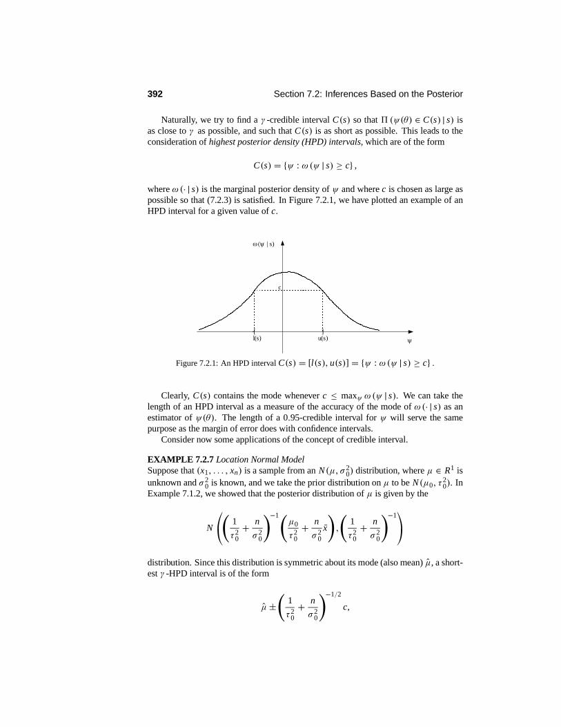
392 Section 7.2: Inferences Based on the Posterior
Naturally, we try to find a γ -credible interval C(s) so that %(ψ(θ) ∈ C(s) | s) isas close to γ as possible, and such that C(s) is as short as possible. This leads to theconsideration of highest posterior density (HPD) intervals, which are of the form
C(s) = {ψ : ω (ψ | s) ≥ c} ,
where ω (· | s) is the marginal posterior density of ψ and where c is chosen as large aspossible so that (7.2.3) is satisfied. In Figure 7.2.1, we have plotted an example of anHPD interval for a given value of c.
ω(ψ | s)
ψ
c
l(s) u(s)[ ]
Figure 7.2.1: An HPD interval C(s) = [l(s), u(s)] = {ψ : ω (ψ | s) ≥ c} .
Clearly, C(s) contains the mode whenever c ≤ maxψ ω (ψ | s). We can take thelength of an HPD interval as a measure of the accuracy of the mode of ω (· | s) as anestimator of ψ(θ). The length of a 0.95-credible interval for ψ will serve the samepurpose as the margin of error does with confidence intervals.
Consider now some applications of the concept of credible interval.
EXAMPLE 7.2.7 Location Normal ModelSuppose that (x1, . . . , xn) is a sample from an N(µ, σ 2
0) distribution, where µ ∈ R1 isunknown and σ 2
0 is known, and we take the prior distribution on µ to be N(µ0, τ20). In
Example 7.1.2, we showed that the posterior distribution of µ is given by the
N
# 1
τ 20
+ n
σ 20
$−1#µ0
τ 20
+ n
σ 20
x
$,
#1
τ20
+ n
σ 20
$−1
distribution. Since this distribution is symmetric about its mode (also mean) µ, a short-est γ -HPD interval is of the form
µ±#
1
τ 20
+ n
σ 20
$−1/2
c,

Chapter 7: Bayesian Inference 393
where c is such that
γ = %
µ ∈µ± # 1
τ 20
+ n
σ 20
$−1/2
c
AAAAAA x1, . . . , xn
= %
−c ≤#
1
τ 20
+ n
σ 20
$1/2 &µ− µ' ≤ c
AAAAAA x1, . . . , xn
.Since #
1
τ 20
+ n
σ 20
$1/2 &µ− µ' | x1, . . . , xn ∼ N(0, 1),
we have γ = 8(c)−8(−c), where 8 is the standard normal cumulative distributionfunction (cdf). This immediately implies that c = z(1+γ )/2 and the γ -HPD interval isgiven by
#1
τ 20
+ n
σ 20
$−1 #µ0
τ20
+ n
σ 20
x
$±#
1
τ 20
+ n
σ 20
$−1/2
z(1+γ )/2.
Note that as τ20 → ∞, namely, as the prior becomes increasingly diffuse, this
interval converges to the interval
x ± σ 0√n
z(1+γ )/2,
which is also the γ -confidence interval derived in Chapter 6 for this problem. So undera diffuse normal prior, the Bayesian and frequentist approaches agree.
EXAMPLE 7.2.8 Location-Scale Normal ModelSuppose that (x1, . . . , xn) is a sample from an N(µ, σ 2) distribution, where µ ∈ R1
and σ ≥ 0 are unknown, and we use the prior given in Example 7.1.4. In Example7.2.1, we derived the marginal posterior distribution of µ to be the same as
µx +@
12α0 + n
@2βx
n + 1/τ 20
T,
where T ∼ t (2α0 + n). Because this distribution is symmetric about its mode µx , aγ -HPD interval is of the form
µx ±@
12α0 + n
@2βx
n + 1/τ 20
c,

394 Section 7.2: Inferences Based on the Posterior
where c satisfies
γ = %
#µ ∈
Bµx ±
@1
2α0 + n
@2βx
n + 1/τ20
c
C AAAAA x1, . . . , xn
$
= %
−c ≤#
2βx
(2α0 + n)&n + 1/τ 2
0
'$−1/2 &µ− µ' ≤ c
AAAAAA x1, . . . , xn
= G2α0+n (c)− G2α0+n (−c) .
Here, G2α0+n is the t (2α0 + n) cdf, and therefore c = t(1+γ )/2(2α0 + n).Using (7.1.9), (7.1.10), and (7.1.11) we have that this interval converges to the
interval
x ±@
n − 1(2α0 + n)
s√n
t (n + 2α0)
as τ 0 → ∞ and β0 → 0. Note that this is a little different from the γ -confidenceinterval we obtained for µ in Example 6.3.8, but when α0/n is small, they are virtuallyidentical.
In the examples we have considered so far, we could obtain closed-form expres-sions for the HPD intervals. In general, this is not the case. In such situations, we haveto resort to numerical methods to obtain the HPD intervals, but we do not pursue thistopic further here.
There are other methods of deriving credible intervals. For example, a commonmethod of obtaining a γ -credible interval for ψ is to take the interval
Dψ l, ψr
Ewhere
ψl is a (1− γ ) /2 quantile for the posterior distribution ofψ andψr is a 1−(1− γ ) /2quantile for this distribution. Alternatively, we could form one-sided intervals. Thesecredible intervals avoid the more extensive computations that may be needed for HPDintervals.
7.2.3 Hypothesis Testing and Bayes Factors
Suppose now that we want to assess the evidence in the observed data concerningthe hypothesis H0 : ψ(θ) = ψ0. It seems clear how we should assess this, namely,compute the posterior probability
%(ψ(θ) = ψ0 | s). (7.2.4)
If this is small, then conclude that we have evidence against H0. We will see furtherjustification for this approach in Chapter 8.
EXAMPLE 7.2.9Suppose we want to assess the evidence concerning whether or not θ ∈ A. If we letψ = IA, then we are assessing the hypothesis H0 : ψ(θ) = 1 and
%(ψ(θ) = 1 | s) = %(A | s).So in this case, we simply compute the posterior probability that θ ∈ A.

Chapter 7: Bayesian Inference 395
There can be a problem, however, with using (7.2.4) to assess a hypothesis. Forwhen the prior distribution of ψ is absolutely continuous, then%(ψ(θ) = ψ0 | s) = 0for all data s. Therefore, we would always find evidence against H0 no matter whatis observed, which does not make sense. In general, if the value ψ0 is assigned smallprior probability, then it can happen that this value also has a small posterior probabilityno matter what data are observed.
To avoid this problem, there is an alternative approach to hypothesis assessment thatis sometimes used. Recall that, if ψ0 is a surprising value for the posterior distributionof ψ , then this is evidence that H0 is false. The value ψ0 is surprising whenever itoccurs in a region of low probability for the posterior distribution ofψ . A region of lowprobability will correspond to a region where the posterior density ω (· | s) is relativelylow. So, one possible method for assessing this is by computing the (Bayesian) P-value
%(<θ : ω(ψ(θ) | s) ≤ ω(ψ0 | s)
= | s). (7.2.5)
Note that when ω(· | s) is unimodal, (7.2.5) corresponds to computing a tail probability.If the probability (7.2.5) is small, then ψ0 is surprising, at least with respect to ourposterior beliefs. When we decide to reject H0 whenever the P-value is less than 1−γ ,then this approach is equivalent to computing a γ -HPD region for ψ and rejecting H0whenever ψ0 is not in the region.
EXAMPLE 7.2.10 (Example 7.2.9 continued)Applying the P-value approach to this problem, we see that ψ(θ) = IA (θ) has pos-terior given by the Bernoulli(%(A | s)) distribution. Therefore, ω(·| s) is defined byω(0| s) = 1−%(A | s) = %(Ac | s) andω(1| s) = %(A | s).
Now ψ0 = 1, so
{θ : ω(ψ(θ) | s) ≤ ω(1 | s)} = {θ : ω(IA (θ) | s) ≤ %(A | s)}=
F" %(A | s) ≥ %(Ac | s)A %(A | s) < %(Ac | s).
Therefore, (7.2.5) becomes
%({θ : ω(ψ(θ) | s) ≤ ω(1 | s)} | s) =F
1 %(A | s) ≥ %(Ac | s)% (A | s) %(A | s) < %(Ac | s),
so again we have evidence against H0 whenever%(A | s) is small.
We see from Examples 7.2.9 and 7.2.10 that computing the P-value (7.2.5) is essen-tially equivalent to using (7.2.4), whenever the marginal parameter ψ takes only twovalues. This is not the case whenever ψ takes more than two values, however, and thestatistician has to decide which method is more appropriate in such a context.
As previously noted, when the prior distribution of ψ is absolutely continuous,then (7.2.4) is always 0, no matter what data are observed. As the following exampleillustrates, there is also a difficulty with using (7.2.5) in such a situation.
EXAMPLE 7.2.11Suppose that the posterior distribution of θ is Beta(2, 1), i.e., ω (θ | s) = 2θ when0 ≤ θ ≤ 1, and we want to assess H0 : θ = 3/4. Then ω(θ | s) ≤ ω(3/4 | s) if and

396 Section 7.2: Inferences Based on the Posterior
only if θ ≤ 3/4, and (7.2.5) is given by! 3/4
02θ dθ = 9/16.
On the other hand, suppose we make a 1–1 transformation to ρ = θ2 so thatthe hypothesis is now H0 : ρ = 9/16. The posterior distribution of ρ is Beta(1, 1).Since the posterior density of ρ is constant, this implies that the posterior density atevery possible value is less than or equal to the posterior density evaluated at 9/16.Therefore, (7.2.5) equals 1, and we would never find evidence against H0 using thisparameterization.
This example shows that our assessment of H0 via (7.2.5) depends on the parame-terization used, which does not seem appropriate.
The difficulty in using (7.2.5), as demonstrated in Example 7.2.11, only occurs withcontinuous posterior distributions. So, to avoid this problem, it is often recommendedthat the hypothesis to be tested always be assigned a positive prior probability. Asdemonstrated in Example 7.2.10, the approach via (7.2.5) is then essentially equivalentto using (7.2.4) to assess H0.
In problems where it seems natural to use continuous priors, this is accomplished bytaking the prior % to be a mixture of probability distributions, as discussed in Section2.5.4, namely, the prior distribution equals
% = p%1 + (1− p)%2,
where %1(ψ(θ) = ψ0) = 1 and %2(ψ (θ) = ψ0) = 0, i.e., %1 is degenerate at ψ0and %2 is continuous at ψ0. Then
%(ψ(θ) = ψ0) = p%1(ψ(θ) = ψ0)+ (1− p)%2(ψ(θ) = ψ0) = p > 0
is the prior probability that H0 is true.The prior predictive for the data s is then given by
m(s) = pm1(s)+ (1− p)m2(s),
where mi is the prior predictive obtained via prior %i (see Problem 7.2.34). This im-plies (see Problem 7.2.34) that the posterior probability measure for θ, when using theprior%, is
%(A | s)= pm1(s)
pm1(s)+ (1− p)m2(s)%1(A | s)+ (1− p)m2(s)
pm1(s)+ (1− p)m2(s)%2(A | s) (7.2.6)
where %i (· | s) is the posterior measure obtained via the prior %i . Note that this amixture of the posterior probability measures%1(· | s) and%2(· | s)with mixture prob-abilities
pm1(s)
pm1(s)+ (1− p)m2(s)and
(1− p)m2(s)
pm1(s)+ (1− p)m2(s).

Chapter 7: Bayesian Inference 397
Now%1(· | s) is degenerate atψ0 (if the prior is degenerate at a point then the posteriormust be degenerate at that point too) and%2(· | s) is continuous at ψ0. Therefore,
%(ψ(θ) = ψ0 | s) =pm1(s)
pm1(s)+ (1− p)m2(s), (7.2.7)
and we use this probability to assess H0.The following example illustrates this approach.
EXAMPLE 7.2.12 Location Normal ModelSuppose that (x1, . . . , xn) is a sample from an N(µ, σ 2
0) distribution, where µ ∈ R1
is unknown and σ 20 is known, and we want to assess the hypothesis H0 : µ = µ0. As
in Example 7.1.2, we will take the prior for µ to be an N(µ0, τ20) distribution. Given
that we are assessing whether or not µ = µ0, it seems reasonable to place the mode ofthe prior at the hypothesized value. The choice of the hyperparameter τ 2
0 then reflectsthe degree of our prior belief that H0 is true. We let %2 denote this prior probabilitymeasure, i.e.,%2 is the N(µ0, σ
20) probability measure.
If we use%2 as our prior, then, as shown in Example 7.1.2, the posterior distributionofµ is absolutely continuous. This implies that (7.2.4) is 0. So, following the precedingdiscussion, we consider instead the prior % = p%1 + (1− p)%2 obtained by mixing%2 with a probability measure %1 degenerate at µ0. Then %1(
<µ0=) = 1 and so
%(<µ0=) = p. As shown in Example 7.1.2, under%2 the posterior distribution of µ is
N
# 1
τ 20
+ n
σ 20
$−1#µ0
τ 20
+ n
σ 20
x
$,
#1
τ20
+ n
σ 20
$−1 ,
while the posterior under %1 is the distribution degenerate at µ0. We now need toevaluate (7.2.7), and we will do this in Example 7.2.13.
Bayes Factors
Bayes factors comprise another method of hypothesis assessment and are defined interms of odds.
Definition 7.2.1 In a probability model with sample space S and probability mea-sure P, the odds in favor of event A ⊂ S is defined to be P(A)/P(Ac), namely, theratio of the probability of A to the probability of Ac.
Obviously, large values of the odds in favor of A indicate a strong belief that A is true.Odds represent another way of presenting probabilities that are convenient in certaincontexts, e.g., horse racing. Bayes factors compare posterior odds with prior odds.
Definition 7.2.2 The Bayes factor BFH0 in favor of the hypothesis H0 : ψ(θ) = ψ0is defined, whenever the prior probability of H0 is not 0 or 1, to be the ratio of theposterior odds in favor of H0 to the prior odds in favor of H0, or
BFH0 =F
%(ψ(θ) = ψ0 | s)1−%(ψ(θ) = ψ0 | s)
GHF%(ψ(θ) = ψ0)
1−%(ψ(θ) = ψ0)
G. (7.2.8)
398 Section 7.2: Inferences Based on the Posterior
So the Bayes factor in favor of H0 is measuring the degree to which the data havechanged the odds in favor of the hypothesis. If BFH0 is small, then the data are provid-ing evidence against H0 and evidence in favor of H0 when BFH0 is large.
There is a relationship between the posterior probability of H0 being true andBFH0 . From (7.2.8), we obtain
%(ψ(θ) = ψ0 | s) =r BFH0
1+ r BFH0
, (7.2.9)
where
r = %(ψ(θ) = ψ0)
1−%(ψ(θ) = ψ0)
is the prior odds in favor of H0. So, when BFH0 is small, then %(ψ(θ) = ψ0| s) issmall and conversely.
One reason for using Bayes factors to assess hypotheses is the following result.This establishes a connection with likelihood ratios.
Theorem 7.2.1 If the prior% is a mixture% = p%1+(1− p)%2, where%1(A) =1,%2(AC) = 1, and we want to assess the hypothesis H0 : θ ∈ A, then
BFH0 = m1(s)/m2(s),
where mi is the prior predictive of the data under%i .
PROOF Recall that, if a prior concentrates all of its probability on a set, then theposterior concentrates all of its probability on this set, too. Then using (7.2.6), we have
BFH0 =%(A | s)
1−%(A | s)H
%(A)
1−%(A) =pm1(s)
(1− p)m2(s)
Hp
1− p= m1(s)
m2(s).
Interestingly, Theorem 7.2.1 indicates that the Bayes factor is independent of p.Wenote, however, that it is not immediately clear how to interpret the value of BFH0 . Inparticular, how large does BFH0 have to be to provide strong evidence in favor of H0?One approach to this problem is to use (7.2.9), as this gives the posterior probabilityof H0, which is directly interpretable. So we can calibrate the Bayes factor. Note,however, that this requires the specification of p.
EXAMPLE 7.2.13 Location Normal Model (Example 7.2.12 continued)We now compute the prior predictive under %2. We have that the joint density of(x1, . . . , xn) given µ equals
)2πσ 2
0
*−n/2exp
#−n − 1
2σ 20
s2
$exp
#− n
2σ 20
(x − µ)2$

Chapter 7: Bayesian Inference 399
and so
m2(x1, . . . , xn)
=! ∞
−∞
&2πσ 2
0
'−n/2exp
:−n−1
2σ 20s2;
exp:− n
2σ20(x − µ)2
;× &2πτ 2
0
'−1/2exp
:− 1
2τ20
&µ− µ0
'2; dµ
=)
2πσ 20
*−n/2exp
#−n − 1
2σ 20
s2
$
× τ−10 (2π)−1/2
! ∞
−∞exp
#− n
2σ 20
(x − µ)2$
exp
#− 1
2τ 20
&µ− µ0
'2$dµ.
Then using (7.1.2), we have
τ−10 (2π)−1/2
! ∞
−∞exp
#− n
2σ 20
(x − µ)2$
exp
#− 1
2τ20
&µ− µ0
'2$ dµ
= τ−10 exp
12
#1
τ 20
+ n
σ 20
$−1#µ0
τ 20
+ n
σ 20
x
$2
× exp
#−1
2
#µ2
0
τ 20
+ nx2
σ 20
$$#n
σ 20
+ 1
τ 20
$−1/2
. (7.2.10)
Therefore,
m2(x1, . . . , xn)
=)
2πσ 20
*−n/2exp
#−n − 1
2σ 20
s2
$τ−1
0 exp
12
#1
τ 20
+ n
σ 20
$−1 #µ0
τ 20
+ n
σ 20
x
$2
× exp
#−1
2
#µ2
0
τ 20
+ nx2
σ 20
$$#n
σ 20
+ 1
τ 20
$−1/2
.
Because %1 is degenerate at µ0, it is immediate that the prior predictive under%1is given by
m1(x1, . . . , xn) =)
2πσ 20
*−n/2exp
#−n − 1
2σ 20
s2
$exp
#− n
2σ 20
&x − µ0
'2$.
Therefore, BFH0 equals
exp
#− n
2σ 20
&x − µ0
'2$divided by (7.2.10).

400 Section 7.2: Inferences Based on the Posterior
For example, suppose that µ0 = 0, τ 20 = 2, σ 2
0 = 1, n = 10, and x = 0.2. Then
exp
#− n
2σ 20
&x − µ0
'2$ = exp:−10
2(0.2)2
;= 0.81873,
while (7.2.10) equals
1√2
exp
#1
2
:1
2+ 10
;−1
(10 (0.2))2$
exp
#−10 (0.2)2
2
$:10+ 1
2
;−1/2
= 0.21615.
So
BFH0 =0.818730.21615
= 3.7878,
which gives some evidence in favor of H0 : µ = µ0. If we suppose that p = 1/2,so that we are completely indifferent between H0 being true and not being true, thenr = 1, and (7.2.9) gives
%(µ = 0 | x1, . . . , xn) = 3.78781+ 3.7878
= 0.79114,
indicating a large degree of support for H0.
7.2.4 Prediction
Prediction problems arise when we have an unobserved response value t in a samplespace T and observed response s ∈ S. Furthermore, we have the statistical model{Pθ : θ ∈ "} for s and the conditional statistical model {Qθ (· | s) : θ ∈ "} for t givens. We assume that both models have the same true value of θ ∈ ". The objective is toconstruct a prediction t(s) ∈ T, of the unobserved value t, based on the observed datas. The value of t could be unknown simply because it represents a future outcome.
If we denote the conditional density or probability function (whichever is relevant)of t by qθ (· | s), the joint distribution of (θ, s, t) is given by
qθ (t | s) fθ (s)π(θ).
Then, once we have observed s (assume here that the distributions of θ and t are ab-solutely continuous; if not, we replace integrals by sums), the conditional density of(t, θ), given s, is
qθ (t | s) fθ (s)π(θ)I"
IT qθ (t | s) fθ (s)π(θ) dt dθ
= qθ (t | s) fθ (s)π(θ)I" fθ (s)π(θ) dθ
= qθ (t | s) fθ (s)π(θ)
m(s).
Then the marginal posterior distribution of t, known as the posterior predictive of t, is
q(t | s) =!"
qθ (t | s) fθ (s)π(θ)
m(s)dθ =
!"
qθ (t | s)π(θ | s) dθ.

Chapter 7: Bayesian Inference 401
Notice that the posterior predictive of t is obtained by averaging the conditional densityof t, given (θ, s) , with respect to the posterior distribution of θ.
Now that we have obtained the posterior predictive distribution of t,we can use it toselect an estimate of the unobserved value. Again, we could choose the posterior modet or the posterior expectation E(t | x) = IT tq(t | s) dt as our prediction, whichever isdeemed most relevant.
EXAMPLE 7.2.14 Bernoulli ModelSuppose we want to predict the next independent outcome Xn+1, having observeda sample (x1, . . . , xn) from the Bernoulli(θ) and θ ∼ Beta(α, β). Here, the futureobservation is independent of the observed data. The posterior predictive probabilityfunction of Xn+1 at t is then given by
q(t | x1, . . . , xn)
=! 1
0θ t (1− θ)1−t / (n + α + β)
/ (nx + α)/ (n (1− x)+ β)θnx+α−1 (1− θ)n(1−x)+β−1 dθ
= / (n + α + β)/ (nx + α)/ (n (1− x)+ β)
! 1
0θnx+α+t−1 (1− θ)n(1−x)+β+(1−t)−1 dθ
= / (n + α + β)/ (nx + α)/ (n (1− x)+ β)
/ (nx + α + t) / (n (1− x)+ β + 1− t)
/ (n + α + β + 1)
=% nx+α
n+α+β t = 1n(1−x)+β
n+α+β t = 0,
which is the probability function of a Bernoulli((nx + α) / (n + α + β)) distribution.Using the posterior mode as the predictor, i.e., maximizing q(t | x1, . . . , xn) for t,
leads to the prediction
t =%
1 if nx+αn+α+β ≥ n(1−x)+β
n+α+β ,0 otherwise.
The posterior expectation predictor is given by
E(t | x1, . . . , xn) = nx + αn + α + β .
Note that the posterior mode takes a value in {0, 1}, and the future Xn+1 will be in thisset, too. The posterior mean can be any value in [0, 1].
EXAMPLE 7.2.15 Location Normal ModelSuppose that (x1, . . . , xn) is a sample from an N(µ, σ 2
0) distribution, whereµ ∈ R1 is unknown and σ 2
0 is known, and we use the prior given in Example 7.1.2.Suppose we want to predict a future observation Xn+1, but this time Xn+1 is from the
N
x,
#1
τ 20
+ n
σ 20
$−1
σ 20
(7.2.11)

402 Section 7.2: Inferences Based on the Posterior
distribution. So, in this case, the future observation is not independent of the observeddata, but it is independent of the parameter. A simple calculation (see Exercise 7.2.9)shows that (7.2.11) is the posterior predictive distribution of t and so we would predictt by x , as this is both the posterior mode and mean.
We can also construct a γ -prediction region C(s) for a future value t from themodel {qθ (· | s) : θ ∈ "} . A γ -prediction region for t satisfies Q(C(s) | s ≥ γ ), whereQ(· | s) is the posterior predictive measure for t. One approach to constructing C(s) isto apply the HPD concept to q(t | s). We illustrate this via several examples.
EXAMPLE 7.2.16 Bernoulli Model (Example 7.2.14 continued)Suppose we want a γ -prediction region for a future value Xn+1. In Example 7.2.14,we derived the posterior predictive distribution of Xn+1 to be
Bernoulli:
nx + αn + α + β
;.
Accordingly, a γ -prediction region for t , derived via the HPD concept, is given by
C(x1, . . . , xn) =
{0, 1} if max
Jnx+α
n+α+β ,n(1−x)+β
n+α+βK≤ γ ,
{1} if γ ≤ maxJ
nx+αn+α+β ,
n(1−x)+βn+α+β
K= nx+α
n+α+β ,
{0} if γ ≤ maxJ
nx+αn+α+β ,
n(1−x)+βn+α+β
K= n(1−x)+β
n+α+β .
We see that this predictive region contains just the mode or encompasses all possiblevalues for Xn+1. In the latter case, this is not an informative inference.
EXAMPLE 7.2.17 Location Normal Model (Example 7.2.15 continued)Suppose we want a γ -prediction interval for a future observation Xn+1 from a
N
x,
#1
τ 20
+ n
σ 20
$−1
σ 20
distribution. As this is also the posterior predictive distribution of Xn+1 and is sym-metric about x, a γ -prediction interval for Xn+1, derived via the HPD concept, is givenby
x ±#
1
τ20
+ n
σ 20
$−1/2
σ 0 z(1+γ )/2.
Summary of Section 7.2
• Based on the posterior distribution of a parameter, we can obtain estimates ofthe parameter (posterior modes or means), construct credible intervals for theparameter (HPD intervals), and assess hypotheses about the parameter (posteriorprobability of the hypothesis, Bayesian P-values, Bayes factors).

Chapter 7: Bayesian Inference 403
• A new type of inference was discussed in this section, namely, prediction prob-lems where we are concerned with predicting an unobserved value from a sam-pling model.
EXERCISES
7.2.1 For the model discussed in Example 7.1.1, derive the posterior mean of ψ = θm
where m > 0.7.2.2 For the model discussed in Example 7.1.2, determine the posterior distributionof the third quartile ψ = µ+ σ 0z0.75. Determine the posterior mode and the posteriorexpectation of ψ.7.2.3 In Example 7.2.1, determine the posterior expectation and mode of 1/σ 2.7.2.4 In Example 7.2.1, determine the posterior expectation and mode of σ 2. (Hint:You will need the posterior density of σ 2 to determine the mode.)7.2.5 Carry out the calculations to verify the posterior mode and posterior expectationof θ1 in Example 7.2.4.7.2.6 Establish that the variance of the θ in Example 7.2.2 is as given in Example 7.2.6.Prove that this goes to 0 as n →∞.7.2.7 Establish that the variance of θ1 in Example 7.2.4 is as given in Example 7.2.6.Prove that this goes to 0 as n →∞.7.2.8 In Example 7.2.14, which of the two predictors derived there do you find moresensible? Why?7.2.9 In Example 7.2.15, prove that the posterior predictive distribution for Xn+1 is asstated. (Hint: Write the posterior predictive distribution density as an expectation.)7.2.10 Suppose that (x1, . . . , xn) is a sample from the Exponential(λ) distribution,where λ > 0 is unknown and λ ∼ Gamma
&α0, β0
'. Determine the mode of posterior
distribution of λ. Also determine the posterior expectation and posterior variance of λ.7.2.11 Suppose that (x1, . . . , xn) is a sample from the Exponential(λ) distributionwhere λ > 0 is unknown and λ ∼ Gamma
&α0, β0
'. Determine the mode of poste-
rior distribution of a future independent observation Xn+1. Also determine the poste-rior expectation of Xn+1 and posterior variance of Xn+1. (Hint: Problems 3.2.12 and3.3.16.)7.2.12 Suppose that in a population of students in a course with a large enrollment, themark, out of 100, on a final exam is approximately distributed N(µ, 9). The instructorplaces the prior µ ∼ N(65, 1) on the unknown parameter. A sample of 10 marks isobtained as given below.
46 68 34 86 75 56 77 73 53 64
(a) Determine the posterior mode and a 0.95-credible interval for µ. What does thisinterval tell you about the accuracy of the estimate?(b) Use the 0.95-credible interval for µ to test the hypothesis H0 : µ = 65.(c) Suppose we assign prior probability 0.5 to µ = 65. Using the mixture prior % =0.5%1+0.5%2, where%1 is degenerate at µ = 65 and%2 is the N(65, 1) distribution,compute the posterior probability of the null hypothesis.

404 Section 7.2: Inferences Based on the Posterior
(d) Compute the Bayes factor in favor of H0 : µ = 65 when using the mixture prior.7.2.13 A manufacturer believes that a machine produces rods with lengths in centime-ters distributed N(µ0, σ
2), where µ0 is known and σ 2 > 0 is unknown, and that theprior distribution 1/σ 2 ∼ Gamma
&α0, β0
'is appropriate.
(a) Determine the posterior distribution of σ 2 based on a sample (x1, . . . , xn).(b) Determine the posterior mean of σ 2.(c) Indicate how you would assess the hypothesis H0 : σ 2 ≤ σ 2
0.7.2.14 Consider the sampling model and prior in Exercise 7.1.1.(a) Suppose we want to estimate θ based upon having observed s = 1. Determine theposterior mode and posterior mean. Which would you prefer in this situation? Explainwhy.(b) Determine a 0.8 HPD region for θ based on having observed s = 1.(c) Suppose instead interest was in ψ(θ) = I{1,2}(θ). Identify the prior distribution ofψ. Identify the posterior distribution of ψ based on having observed s = 1. Determinea 0.5 HPD region for ψ.7.2.15 For an event A, we have that P(Ac) = 1− P(A).
(a) What is the relationship between the odds in favor of A and the odds in favor of Ac?(b) When A is a subset of the parameter space, what is the relationship between theBayes factor in favor of A and the Bayes factor in favor of Ac?7.2.16 Suppose you are told that the odds in favor of a subset A are 3 to 1. What is theprobability of A? If the Bayes factor in favor of A is 10 and the prior probability of Ais 1/2, then determine the posterior probability of A.
7.2.17 Suppose data s is obtained. Two statisticians analyze these data using the samesampling model but different priors, and they are asked to assess a hypothesis H0. Bothstatisticians report a Bayes factor in favor of H0 equal to 100. Statistician I assignedprior probability 1/2 to H0 whereas statistician II assigned prior probability 1/4 to H0.Which statistician has the greatest posterior degree of belief in H0 being true?7.2.18 You are told that a 0.95-credible interval, determined using the HPD criterion,for a quantity ψ(θ) is given by (−3.3, 2.6). If you are asked to assess the hypothesisH0 : ψ(θ) = 0, then what can you say about the Bayesian P-value? Explain youranswer.7.2.19 What is the range of possible values for a Bayes factor in favor of A ⊂ "?Under what conditions will a Bayes factor in favor of A ⊂ " take its smallest value?
PROBLEMS
7.2.20 Suppose that (x1, . . . , xn) is a sample from the Uniform[0, θ] distribution, whereθ > 0 is unknown, and we have θ ∼ Gamma
&α0, β0
'. Determine the mode of the pos-
terior distribution of θ . (Hint: The posterior is not differentiable at θ = x(n).)7.2.21 Suppose that (x1, . . . , xn) is a sample from the Uniform[0, θ] distribution, whereθ ∈ (0, 1) is unknown, and we have θ ∼ Uniform[0, 1]. Determine the form of the γ -credible interval for θ based on the HPD concept.7.2.22 In Example 7.2.1, write out the integral given in (7.2.2).

Chapter 7: Bayesian Inference 405
7.2.23 (MV) In Example 7.2.1, write out ithe integral that you would need to evaluateif you wanted to compute the posterior density of the third quartile of the populationdistribution, i.e., ψ = µ+ σ z0.75.7.2.24 Consider the location normal model discussed in Example 7.1.2 and the popu-lation coefficient of variation ψ = σ 0/µ.(a) Show that the posterior expectation of ψ does not exist. (Hint: Show that we canwrite the posterior expectation as
! ∞
−∞σ 0
a + bz
1√2π
e−z2/2 dz,
where b > 0, and show that this integral does not exist by considering the behavior ofthe integrand at z = −a/b.)(b) Determine the posterior density of ψ.(c) Show that you can determine the posterior mode of ψ by evaluating the posteriordensity at two specific points. (Hint: Proceed by maximizing the logarithm of the pos-terior density using the methods of calculus.)7.2.25 (MV) Suppose that (θ1, . . . , θk−1) ∼ Dirichlet(α1, α2, . . . , αk).(a) Prove that (θ1, . . . , θk−2) ∼ Dirichlet(α1, α2, . . . , αk−1 + αk). (Hint: In the inte-gral to integrate out θk−1,make the transformation θk−1 → θk−1/(1−θ1−· · ·−θk−2).)(b) Prove that θ1 ∼ Beta(α1, α2 + · · · + αk). (Hint: Use part (a).)(c) Suppose (i1, . . . , ik) is a permutation of (1, . . . , k). Prove that (θ i1 , . . . , θ ik−1) ∼Dirichlet(αi1, αi2, . . . , αik ). (Hint: What is the Jacobian of this transformation?)(d) Prove that θ i ∼ Beta(αi , α−i ). (Hint: Use parts (b) and (c).)7.2.26 (MV) In Example 7.2.4, show that the plug-in MLE of θ1 is given by x1/n, i.e.,find the MLE of (θ1, . . . , θk) and determine the first coordinate. (Hint: Show there isa unique solution to the score equations and then use the facts that the log-likelihood isbounded above and goes to −∞ whenever θ i → 0.)7.2.27 Compare the results obtained in Exercises 7.2.3 and 7.2.4. What do you con-clude about the invariance properties of these estimation procedures? (Hint: ConsiderTheorem 6.2.1.)7.2.28 In Example 7.2.5, establish that the posterior variance of µ is as stated in Ex-ample 7.2.6. (Hint: Problem 4.6.16.)7.2.29 In a prediction problem, as described in Section 7.2.4, derive the form of theprior predictive density for t when the joint density of (θ, s, t) is qθ (t | s) fθ (s)π(θ)(assume s and θ are real-valued).7.2.30 In Example 7.2.16, derive the posterior predictive probability function of(Xn+1, Xn+2), having observed x1, . . . , xn when X1, . . . , Xn, Xn+1, Xn+2 are inde-pendently and identically distributed (i.i.d.) Bernoulli(θ).7.2.31 In Example 7.2.15, derive the posterior predictive distribution for Xn+1, havingobserved x1, . . . , xn when X1, . . . , Xn, Xn+1 are i.i.d. N(µ, σ 2
0). (Hint: We can writeXn+1 = µ+ σ 0 Z , where Z ∼ N(0, 1) is independent of the posterior distribution ofµ.)

406 Section 7.2: Inferences Based on the Posterior
7.2.32 For the context of Example 7.2.1, prove that the posterior predictive distributionof an additional future observation Xn+1 from the population distribution has the samedistribution as
µx +
LMMN2βx
)&n + 1/τ 2
0
'−1 + 1*
(2α0 + n)T ,
where T ∼ t (2α0 + n). (Hint: Note that we can write Xn+1 = µ + σU , whereU ∼ N (0, 1) independent of X1, . . . , Xn, µ, σ and then reason as in Example 7.2.1.)7.2.33 In Example 7.2.1, determine the form of an exact γ -prediction interval for anadditional future observation Xn+1 from the population distribution, based on the HPDconcept. (Hint: Use Problem 7.2.32.)7.2.34 Suppose that%1 and%2 are discrete probability distributions on the parameterspace ". Prove that when the prior % is a mixture % = p%1 + (1− p)%2, then theprior predictive for the data s is given by m(s) = pm1(s) + (1 − p)m2(s), and theposterior probability measure is given by (7.2.6).7.2.35 (MV) Suppose that θ = (θ1, θ2) ∈ R2 and h(θ1, θ2) = (ψ(θ), λ(θ)) ∈ R2.Assume that h satisfies the necessary conditions and establish (7.2.1). (Hint: Theorem2.9.2.)
CHALLENGES
7.2.36 Another way to assess the null hypothesis H0 : ψ(θ) = ψ0 is to compute theP-value
%
:ω(ψ(θ) | s)ω(ψ(θ))
≤ ω(ψ0 | s)ω(ψ0)
AAAA s
;(7.2.12)
where ω is the marginal prior density or probability function of ψ.We call (7.2.12) theobserved relative surprise ofH0.
The quantity ω&ψ0 | s
'/ω&ψ0'
is a measure of how the data s have changed our apriori belief that ψ0 is the true value of ψ. When (7.2.12) is small, ψ0 is a surprisingvalue for ψ , as this indicates that the data have increased our belief more for othervalues of ψ.(a) Prove that (7.2.12) is invariant under 1–1 continuously differentiable transforma-tions of ψ.(b) Show that a value ψ0 that makes (7.2.12) smallest, maximizes ω
&ψ0 | s
'/ω&ψ0'.
We call such a value a least relative suprise estimate of ψ.(c) Indicate how to use (7.2.12) to form a γ -credible region, known as a γ -relativesurprise region, for ψ.(d) Suppose that ψ is real-valued with prior density ω and posterior density ω (· | s)both continuous and positive at ψ0. Let A: = (ψ0 − :,ψ0 + :). Show that BFA: →ω&ψ0 | s
'/ω&ψ0'
as : ↓ 0. Generalize this to the case where ψ takes its values in anopen subset of Rk . This shows that we can think of the observed relative surprise as away of calibrating Bayes factors.

Chapter 7: Bayesian Inference 407
7.3 Bayesian ComputationsIn virtually all the examples in this chapter so far, we have been able to work out theexact form of the posterior distributions and carry out a number of important com-putations using these. It often occurs, however, that we cannot derive any convenientform for the posterior distribution. Furthermore, even when we can derive the posteriordistribution, there computations might arise that cannot be carried out exactly — e.g.,recall the discussion in Example 7.2.1 that led to the integral (7.2.2). These calculationsinvolve evaluating complicated sums or integrals. Therefore, when we apply Bayesianinference in a practical example, we need to have available methods for approximatingthese quantities.
The subject of approximating integrals is an extensive topic that we cannot dealwith fully here.1 We will, however, introduce several approximation methods that arisevery naturally in Bayesian inference problems.
7.3.1 Asymptotic Normality of the Posterior
In many circumstances, it turns out that the posterior distribution of θ ∈ R1 is approx-imately normally distributed. We can then use this to compute approximate credibleregions for the true value of θ , carry out hypothesis assessment, etc. One such re-sult says that, under conditions that we will not describe here, when (x1, . . . , xn) is asample from fθ , then
%
#θ − θ (x1, . . . , xn)
σ (x1, . . . , xn)≤ z
AAAAA x1, . . . , xn
$→ 8(z)
as n →∞ where θ (x1, . . . , xn) is the posterior mode, and
σ 2(x1, . . . , xn) =:−∂
2 ln(L(θ | x1, . . . , xn)π(θ))
∂θ2
AAAAθ=θ
;−1
.
Note that this result is similar to Theorem 6.5.3 for the MLE. Actually, we can replaceθ(x1, . . . , xn) by the MLE and replace σ 2(x1, . . . , xn) by the observed information(see Section 6.5), and the result still holds. When θ is k-dimensional, there is a similarbut more complicated result.
7.3.2 Sampling from the Posterior
Typically, there are many things we want to compute as part of implementing a Bayesiananalysis. Many of these can be written as expectations with respect to the posterior dis-tribution of θ. For example, we might want to compute the posterior probability contentof a subset A ⊂ ", namely,
%(A | s) = E(IA(θ) | s).1See, for example, Approximating Integrals via Monte Carlo and Deterministic Methods, by M. Evans
and T. Swartz (Oxford University Press, Oxford, 2000).

408 Section 7.3: Bayesian Computations
More generally, we want to be able to compute the posterior expectation of some arbi-trary function w (θ), namely
E(w(θ) | s). (7.3.1)
It would certainly be convenient if we could compute all these quantities exactly,but quite often we cannot. In fact, it is not really necessary that we evaluate (7.3.1)exactly. This is because we naturally expect any inference we make about the truevalue of the parameter to be subject (different data sets of the same size lead to differentinferences) to sampling error. It is not necessary to carry out our computations to amuch higher degree of precision than what sampling error contributes. For example, ifthe sampling error only allows us to know the value of a parameter to within only±0.1units, then there is no point in computing an estimate to many more digits of accuracy.
In light of this, many of the computational problems associated with implementingBayesian inference are effectively solved if we can sample from the posterior for θ.For when this is possible, we simply generate an i.i.d. sequence θ1, θ2, . . . , θN fromthe posterior distribution of θ and estimate (7.3.1) by
w = 1N
N>i=1
w(θ i ).
We know then, from the strong law of large numbers (see Theorem 4.3.2), that wa.s.→
E(w(θ) | x) as N →∞.Of course, for any given N, the value of w only approximates (7.3.1); we would like
to know that we have chosen N large enough so that the approximation is appropriatelyaccurate. When E(w2 (θ) | s) <∞, then the central limit theorem (see Theorem 4.4.3)tells us that
w − E(w(θ) | s)σw/
√N
D→ N (0, 1)
as N →∞, where σ 2w =Var(w(θ) | s). In general, we do not know the value of σ 2
w,but we can estimate it by
s2w =
1
N − 1
N>i=1
(w(θ i )− w)2
whenw (θ) is a quantitative variable, and by s2w = w(1−w) whenw = IA for A ⊂ ".
As shown in Section 4.4.2, in either case, s2w is a consistent estimate of σ 2
w. Then, byCorollary 4.4.4, we have that
w − E(w(θ) | s)sw/√
N
D→ N (0, 1)
as N →∞.From this result we know that
w ± 3sw√
N

Chapter 7: Bayesian Inference 409
is an approximate 100% confidence interval for E(w(θ) | s), so we can look at 3sw/√
Nto determine whether or not N is large enough for the accuracy required.
One caution concerning this approach to assessing error is that 3sw/√
N is itselfsubject to error, as sw is an estimate of σw, so this could be misleading. A commonrecommendation then is to monitor the value of 3sw/
√N for successively larger values
of N and stop the sampling only when it is clear that the value of 3sw/√
N is smallenough for the accuracy desired and appears to be declining appropriately. Even thisapproach, however, will not give a guaranteed bound on the accuracy of the computa-tions, so it is necessary to be cautious.
It is also important to remember that application of these results requires that σ 2w <
∞. For a bounded w, this is always true, as any bounded random variable always hasa finite variance. For an unbounded w, however, this must be checked — sometimesthis is very difficult to do.
We consider an example where it is possible to exactly sample from the posterior.
EXAMPLE 7.3.1 Location-Scale NormalSuppose that (x1, . . . , xn) is a sample from an N(µ, σ 2) distribution where µ ∈ R1
and σ > 0 are unknown, and we use the prior given in Example 7.1.4. The posteriordistribution for (µ, σ 2) developed there is
µ | σ 2, x1, . . . , xn ∼ N
:µx ,
)n + 1/τ 2
0
*−1σ 2;
(7.3.2)
and1/σ 2 | x1, . . . , xn ∼ Gamma
&α0 + n/2, βx
', (7.3.3)
where µx is given by (7.1.7) and βx is given by (7.1.8).Most statistical packages have built-in generators for gamma distributions and for
the normal distribution. Accordingly, it is very easy to generate a sample (µ1, σ21), . . . ,
(µN , σ2N ) from this posterior. We simply generate a value for 1/σ 2
i from the specifiedgamma distribution; then, given this value, we generate the value of µi from the speci-fied normal distribution.
Suppose, then, that we want to derive the posterior distribution of the coefficientof variation ψ = σ/µ. To do this we generate N values from the joint posterior of(µ, σ 2), using (7.3.2) and (7.3.3), and compute ψ for each of these. We then knowimmediately that ψ1, . . . , ψN is a sample from the posterior distribution of ψ.
As a specific numerical example, suppose that we observed the following sample(x1, . . . , x15) .
11.6714 1.8957 2.1228 2.1286 1.07518.1631 1.8236 4.0362 6.8513 7.64611.9020 7.4899 4.9233 8.3223 7.9486
Here, x = 5.2 and s = 3.3. Suppose further that the prior is specified by µ0 = 4, τ 20 =
2, α0 = 2, and β0 = 1.From (7.1.7), we have
µx =:
15+ 12
;−1 :42+ 15 · 5.2
;= 5.161,

410 Section 7.3: Bayesian Computations
and from (7.1.8),
βx = 1+ 152(5.2)2 + 42
2 · 2 +142(3.3)2 − 1
2
:15+ 1
2
;−1 :42+ 15 · 5.2
;2
= 77.578.
Therefore, we generate
1/σ 2 | x1, . . . , xn ∼ Gamma(9.5, 77.578),
followed by
µ | σ 2, x1, . . . , xn ∼ N(5.161, (15.5)−1 σ 2).
See Appendix B for some code that can be used to generate from this joint distribution.In Figure 7.3.1, we have plotted a sample of N = 200 values of (µ, σ 2) from this
joint posterior. In Figure 7.3.2, we have plotted a density histogram of the 200 valuesof ψ that arise from this sample.
76543
25
15
5
mu
sigm
a sq
uare
d
Figure 7.3.1: A sample of 200 values of (µ, σ 2) from the joint posterior in Example 7.3.1when n = 15, x = 5.2, s = 3.3, µ0 = 4, τ 2
0 = 2, α0 = 2, and β0 = 1.

Chapter 7: Bayesian Inference 411
3.53.02.52.01.51.00.50.0
4
3
2
1
0
Figure 7.3.2: A density histogram of 200 values from the posterior distribution of ψ inExample 7.3.1.
A sample of 200 is not very large, so we next generated a sample of N = 103
values from the posterior distribution of ψ. A density histogram of these values is pro-vided in Figure 7.3.3. In Figure 7.3.4, we have provided a density histogram based ona sample of N = 104 values. We can see from this that at N = 103, the basic shape ofthe distribution has been obtained, although the right tail is not being very accuratelyestimated. Things look better in the right tail for N = 104, but note there are still someextreme values quite disconnected from the main mass of values. As is characteristicof most distributions, we will need very large values of N to accurately estimate thetails. In any case, we have learned that this distribution is skewed to the right with along right tail.
3.53.02.52.01.51.00.50.0
4
3
2
1
0
Figure 7.3.3: A density histogram of 1000 values from the posterior distribution of ψ inExample 7.3.1.

412 Section 7.3: Bayesian Computations
3.53.02.52.01.51.00.50.0
4
3
2
1
0
Figure 7.3.4: A density histogram of N = 104 values from the posterior distribution of ψ inExample 7.3.1.
Suppose we want to estimate
%(ψ ≤ 0.5 | x1, . . . , xn) = E(I(−∞,0.5)(ψ) | x1, . . . , xn).
Now w = I(−∞,0.5) is bounded so its posterior variance exists. In the following table,we have recorded the estimates for each N together with the standard error based oneach of the generated samples. We have included some code for computing theseestimates and their standard errors in Appendix B. Based on the results from N = 104,it would appear that this posterior probability is in the interval 0.289 ± 3 (0.0045) =[0.2755, 0.3025].
N Estimate of%(ψ ≤ 0.5 | x1, . . . , xn) Standard Error200 0.265 0.0312103 0.271 0.0141104 0.289 0.0045
This example also demonstrates an important point. It would be very easy for us tocalculate the sample mean of the values of ψ generated from its posterior distributionand then consider this as an estimate of the posterior mean of ψ. But Problem 7.2.24suggests (see Problem 7.3.15) that this mean will not exist. Accordingly, a Monte Carloestimate of this quantity does not make any sense! So we must always check first thatany expectation we want to estimate exists, before we proceed with some estimationprocedure.
When we cannot sample directly from the posterior, then the methods of the fol-lowing section are needed.

Chapter 7: Bayesian Inference 413
7.3.3 Sampling from the Posterior Using Gibbs Sampling(Advanced)
Sampling from the posterior, as described in Section 7.3.2, is very effective, when itcan be implemented. Unfortunately, it is often difficult or even impossible to do thisdirectly, as we did in Example 7.3.1. There are, however, a number of algorithms thatallow us to approximately sample from the posterior. One of these, known as Gibbssampling, is applicable in many statistical contexts.
To describe this algorithm, suppose we want to generate samples from the jointdistribution of (Y1, . . . ,Yk) ∈ Rk . Further suppose that we can generate from each ofthe full conditional distributions Yi |Y−i = y−i , where
Y−i = (Y1, . . . ,Yi−1, Yi+1, . . . , Yk) ,
namely, we can generate from the conditional distribution of Yi given the values of allthe other coordinates. The Gibbs sampler then proceeds iteratively as follows.
1. Specify an initial value&y1(0), . . . , yk(0)
'for (Y1, . . . ,Yk).
2. For N > 0, generate Yi(N ) from its conditional distribution given&y1(N ), . . . , yi−1(N), yi+1(N−1), . . . , yk(N−1)
'for each i = 1, . . . , k.
For example, if k = 3, we first specify&y1(0), y2(0), y3(0)
'. Then we generate
Y1(1) |Y2(0) = y2(0), Y3(0) = y3(0)
Y2(1) |Y1(1) = y1(1), Y3(0) = y3(0)
Y3(1) |Y1(1) = y1(1), Y2(1) = y2(1)
to obtain&Y1(1), Y2(1), Y3(1)
'. Next we generate
Y1(2) |Y2(1) = y2(1), Y3(1) = y3(1)
Y2(2) |Y1(2) = y1(2), Y3(1) = y3(1)
Y3(2) |Y1(2) = y1(2), Y2(2) = y2(2)
to obtain&Y1(2),Y2(2),Y3(2)
', etc. Note that we actually did not need to specify Y1(0),
as it is never used.It can then be shown (see Section 11.3) that, in fairly general circumstances, (Y1(N ),
. . . ,Yk(N)) converges in distribution to the joint distribution of (Y1, . . . ,Yk) as N →∞. So for large N , we have that the distribution of
&Y1(N), . . . ,Yk(N )
'is approximately
the same as the joint distribution of (Y1, . . . , Yk) from which we want to sample. SoGibbs sampling provides an approximate method for sampling from a distribution ofinterest.
Furthermore, and this is the result that is most relevant for simulations, it can beshown that, under conditions,
w = 1N
N>i=1
w(Y1(i), . . . ,Yk(i)a.s.)→ E(w(Y1, . . . ,Yk)).

414 Section 7.3: Bayesian Computations
Estimation of the variance of w is different than in the i.i.d. case, where we used thesample variance, because now the w(Y1(i), . . . ,Yk(i)) terms are not independent.
There are several approaches to estimating the variance of w, but perhaps the mostcommonly used is the technique of batching. For this we divide the sequence
w(Y1(0), . . . , Yk(0)), . . . , w(Y1(N ), . . . ,Yk(N))
into N/m nonoverlapping sequential batches of size m (assuming here that N is divisi-ble by m), calculate the mean in each batch obtaining w1, . . . , wN/m , and then estimatethe variance of w by
s2b
N/m, (7.3.4)
where s2b is the sample variance obtained from the batch means, i.e.,
s2b =
1N/m − 1
N/m>i=1
(wi − w)2 .
It can be shown that&Y1(i), . . . , Yk(i)
'and
&Y1(i+m), . . . ,Yk(i+m)
'are approxi-
mately independent for m large enough. Accordingly, we choose the batch size mlarge enough so that the batch means are approximately independent, but not so largeas to leave very few degrees of freedom for the estimation of the variance. Under idealconditions, w1, . . . , wN/m is an i.i.d. sequence with sample mean
w = 1N/m
N/m>i=1
wi ,
and, as usual, we estimate the variance of w by (7.3.4).Sometimes even Gibbs sampling cannot be directly implemented because we can-
not obtain algorithms to generate from all the full conditionals. There are a varietyof techniques for dealing with this, but in many statistical applications the techniqueof latent variables often works. For this, we search for some random variables, say(V1, . . . ,Vl) , where each Yi is a function of (V1, . . . ,Vl) and such that we can applyGibbs sampling to the joint distribution of (V1, . . . , Vl) .We illustrate Gibbs samplingvia latent variables in the following example.
EXAMPLE 7.3.2 Location-Scale StudentSuppose now that (x1, . . . , xn) is a sample from a distribution that is of the form X =µ+ σ Z , where Z ∼ t (λ) (see Section 4.6.2 and Problem 4.6.14). If λ > 2, then µ isthe mean and σ(λ/(λ−2))1/2 is the standard deviation of the distribution (see Problem4.6.16). Note that λ =∞ corresponds to normal variation, while λ = 1 corresponds toCauchy variation.
We will fix λ at some specified value to reflect the fact that we are interested inmodeling situations in which the variable under consideration has a distribution withlonger tails than the normal distribution. Typically, this manifests itself in a histogramof the data with a roughly symmetric shape but exhibiting a few extreme values out inthe tails, so a t (λ) distribution might be appropriate.

Chapter 7: Bayesian Inference 415
Suppose we place the prior on (µ, σ 2), given byµ |σ 2 ∼ N(µ0, τ20σ
2) and 1/σ 2 ∼Gamma
&α0, β0
'. The likelihood function is given by
:1σ 2
;n/2 n"i=1
B1+ 1
λ
:xi − µσ
;2C−(λ+1)/2
, (7.3.5)
hence the posterior density of&µ, 1/σ 2
'is proportional to
:1
σ 2
;n/2 n"i=1
B1+ 1
λ
:xi − µσ
;2C−(λ+1)/2
×:
1σ 2
;1/2
exp
#− 1
2τ 20σ
2
&µ− µ0
'2$: 1σ 2
;α0−1
exp:−β0
σ 2
;.
This distribution is not immediately recognizable, and it is not at all clear how to gen-erate from it.
It is natural, then, to see if we can implement Gibbs sampling. To do this directly,we need an algorithm to generate from the posterior of µ given the value of σ 2, andan algorithm to generate from the posterior of σ 2 given µ. Unfortunately, neither ofthese conditional distributions is amenable to the techniques discussed in Section 2.10,so we cannot implement Gibbs sampling directly.
Recall, however, that when V ∼ χ2(λ) = Gamma(λ/2, 1/2) (see Problem 4.6.13)independent of Y ∼ N(µ, σ 2), then (Problem 4.6.14)
Z = Y − µσ√
V/λ∼ t(λ).
Therefore, writing
X = µ+ σ Z = µ+ σ Y − µσ√
V/λ= µ+ Y − µ√
V/λ,
we have that X | V = v ∼ N(µ, σ 2λ/v).We now introduce the n latent or hidden variables (V1, . . . , Vn) , which are i.i.d.
χ2(λ) and suppose Xi | Vi = υi ∼ N(µ, σ 2λ/υi ). The Vi are considered latent be-cause they are not really part of the problem formulation but have been added here forconvenience (as we shall see). Then, noting that there is a factor v1/2
i associated withthe density of Xi | Vi = υi , the joint density of the values (X1,V1) , . . . , (Xn, Vn) isproportional to:
1
σ 2
;n/2 n"i=1
exp)− υi
2σ 2λ(xi − µ)2
*υ(λ/2)−(1/2)i exp
)−υi
2
*.
From the above argument, the marginal joint density of (X1, . . . , Xn) (after integratingout the υi ’s) is proportional to (7.3.5), namely, a sample of n from the distribution

416 Section 7.3: Bayesian Computations
specified by X = µ+ σ Z , where Z ∼ t (λ). With the same prior structure as before,we have that the joint density of
(X1,V1) , . . . , (Xn,Vn) , µ, 1/σ 2
is proportional to:1σ 2
;n/2 n"i=1
exp)− υi
2σ 2λ(xi − µ)2
*υ(λ/2)−(1/2)i exp
)−υ i
2
*×
:1
σ 2
;1/2
exp
#− 1
2τ20σ
2
&µ− µ0
'2$: 1
σ 2
;α0−1
exp:−β0
σ 2
;. (7.3.6)
In (7.3.6) treat x1, . . . , xn as constants (we observed these values) and considerthe conditional distributions of each of the variables V1, . . . , Vn, µ, 1/σ 2 given all theother variables. From (7.3.6) we have that the full conditional density of µ is propor-tional to
exp
%− 1
2σ 2
#n>
i=1
υi
λ(xi − µ)2 + 1
τ 20
&µ− µ0
'2$( ,
which is proportional to
exp
%− 1
2σ 2
B#n>
i=1
υi
λ
$+ 1
τ 20
Cµ2 + 2
2σ 2
B#n>
i=1
υi
λxi
$+ µ0
τ 20
Cµ
(.
From this, we immediately deduce that
µ | x1, . . . , xn, υ1, . . . , υn, σ2
∼ N
#r(υ1, . . . , υn)
B#n>
i=1
υi
λxi
$+ µ0
τ20
C, r(υ1, . . . , υn)σ
2
$,
where
r(υ1, . . . , υn) =B#
n>i=1
υi
λ
$+ 1
τ 20
C−1
.
From (7.3.6), we have that the conditional density of 1/σ 2 is proportional to:1σ 2
;(n/2)+α0−(1/2)exp
%−# On
i=1υiλ (xi − µ)2
+ 1τ2
0
&µ− µ0
'2 + 2β0
$1
2σ 2
(,
and we immediately deduce that
1
σ 2| x1, . . . , xn, υ1, . . . , υn, µ
∼ Gamma
#n
2+ α0 + 1
2,
12
#n>
i=1
υi
λ(xi − µ)2 + 1
τ 20
&µ− µ0
'2 + 2β0
$$.

Chapter 7: Bayesian Inference 417
Finally, the conditional density of Vi is proportional to
υ(λ/2)−(1/2)i exp
%−B(xi − µ)2
2σ 2λ+ 1
2
Cυi
(,
and it is immediate that
Vi |x1, . . . , xn, υ1, . . . , υi−1, υi+1, . . . , υn, µ, σ2
∼ Gamma
#λ
2+ 1
2,
12
#(xi − µ)2σ 2λ
+ 1
$$.
We can now easily generate from all these distributions and implement a Gibbssampling algorithm. As we are not interested in the values of V1, . . . ,Vn, we simplydiscard these as we iterate.
Let us now consider a specific computation using the same data and prior as inExample 7.3.1. The analysis of Example 7.3.1 assumed that the data were coming froma normal distribution, but now we are going to assume that the data are a sample froma µ + σ t (3) distribution, i.e., λ = 3. We again consider approximating the posteriordistribution of the coefficient of variation ψ = σ/µ.
We carry out the Gibbs sampling iteration in the order υ1, . . . , υn, µ, 1/σ 2. Thisimplies that we need starting values only for µ and σ 2 (the full conditionals of the υido not depend on the other υ j ). We take the starting value of µ to be x = 5.2 and thestarting value of σ to be s = 3.3. For each generated value of (µ, σ 2), we calculate ψto obtain the sequence ψ1, ψ2, . . . , ψN .
The values ψ1, ψ2, . . . , ψN are not i.i.d. from the posterior of ψ . The best we cansay is that
ψmD→ ψ ∼ ω(· | x1, . . . , xn)
as m → ∞, where ω (· | x1, . . . , xn) is the posterior density of ψ . Also values suffi-ciently far apart in the sequence, will be like i.i.d. values from ω(· | x1, . . . , xn). Thus,one approach is to determine an appropriate value m and then extractψm, ψ2m, ψ3m, . . .as an approximate i.i.d. sequence from the posterior. Often it is difficult to determinean appropriate value for m, however.
In any case, it is known that, under fairly weak conditions,
w = 1N
N>i=1
w(ψ i
a.s.)→ E(w(ψ) | x1, . . . , xn)
as N →∞. So we can use the whole sequence ψ1, ψ2, . . . , ψN and record a densityhistogram for ψ, just as we did in Example 7.3.1. The value of the density histogrambetween two cut points will converge almost surely to the correct value as N → ∞.However, we will have to take N larger when using the Gibbs sampling algorithm thanwith i.i.d. sampling, to achieve the same accuracy. For many examples, the effect of thedeviation of the sequence from being i.i.d. is very small, so N will not have to be muchlarger. We always need to be cautious, however, and the general recommendation is to

418 Section 7.3: Bayesian Computations
compute estimates for successively higher values of N, only stopping when the resultsseem to have stabilized.
In Figure 7.3.5, we have plotted the density histogram of the ψ values that resultedfrom 104 iterations of the Gibbs sampler. In this case, plotting the density histogram ofψ based upon N = 5× 10⁴ and N = 8× 10⁴ resulted in only minor deviations fromthis plot. Note that this density looks very similar to that plotted in Example 7.3.1, butit is not quite so peaked and it has a shorter right tail.
3.53.02.52.01.51.00.50.0
4
3
2
1
0
Figure 7.3.5: A density histogram of N = 104 values of ψ generated sequentially via Gibbssampling in Example 7.3.2.
We can also estimate %(ψ ≤ 0.5 | x1, . . . , xn), just as we did in Example 7.3.1,by recording the proportion of values in the sequence that are smaller than 0.5, i.e.,w(ψ) = IA(ψ), where A = {θ : ψ ≤ 0.5}. In this case, we obtained the estimate0.5441, which is quite different from the value obtained in Example 7.3.1. So using at (3) distribution to describe the variation in the response has made a big difference inthe results.
Of course, we must also quantify how accurate we believe our estimate is. Usinga batch size of m = 10, we obtained the standard error of the estimate 0.5441 to be0.00639. When we took the batch size to be m = 20, the standard error of the meanis 0.00659; with a batch size of m = 40, the standard error of the mean is 0.00668.So we feel quite confident that we are assessing the error in the estimate appropriately.Again, under conditions, we have that w is asymptotically normal so that in this casewe can assert that the interval 0.5441±3(0.0066) = [0.5243, 0.5639] contains the truevalue of%(ψ ≤ 0.5 | x1, . . . , xn) with virtual certainty.
See Appendix B for some code that was used to implement the Gibbs samplingalgorithm described here.
It is fair to say that the introduction of Gibbs sampling has resulted in a revolutionin statistical applications due to the wide variety of previously intractable problemsthat it successfully handles. There are a number of modifications and closely related

Chapter 7: Bayesian Inference 419
algorithms. We refer the interested reader to Chapter 11, where the general theory ofwhat is called Markov chain Monte Carlo (MCMC) is discussed.
Summary of Section 7.3
• Implementation of Bayesian inference often requires the evaluation of compli-cated integrals or sums.
• If, however, we can sample from the posterior of the parameter, this will oftenlead to sufficiently accurate approximations to these integrals or sums via MonteCarlo.
• It is often difficult to sample exactly from a posterior distribution of interest.In such circumstances, Gibbs sampling can prove to be an effective method forgenerating an approximate sample from this distribution.
EXERCISES
7.3.1 Suppose we have the following sample from an N(µ, 2) distribution, where µ isunknown.
2.6 4.2 3.1 5.2 3.7 3.8 5.6 1.8 5.3 4.03.0 4.0 4.1 3.2 2.2 3.4 4.5 2.9 4.7 5.2
If the prior on µ is Uniform(2, 6), determine an approximate 0.95-credible interval forµ based on the large sample results described in Section 7.3.1.7.3.2 Determine the form of the approximate 0.95-credible interval of Section 7.3.1,for the Bernoulli model with a Beta(α, β) prior, discussed in Example 7.2.2.7.3.3 Determine the form of the approximate 0.95-credible intervals of Section 7.3.1,for the location-normal model with an N(µ0, τ
20) prior, discussed in Example 7.2.3.
7.3.4 Suppose that X ∼ Uniform[0, 1/θ] and θ ∼ Exponential(1). Derive a crudeMonte Carlo algorithm, based on generating from a gamma distribution, to generate avalue from the conditional distribution θ | X = x .Generalize this to a sample of n fromthe Uniform[0, 1/θ] distribution. When will this algortithm be inefficient in the sensethat we need a lot of computation to generate a single value?7.3.5 Suppose that X ∼ N(θ, 1) and θ ∼ Uniform[0, 1]. Derive a crude Monte Carloalgorithm, based on generating from a normal distribution, to generate from the con-ditional distribution θ | X = x. Generalize this to a sample of n from the N(θ, 1)distribution. When will this algortithm be inefficient in the sense that we need a lot ofcomputation to generate a single value?7.3.6 Suppose that X ∼ 0.5N(θ, 1) + 0.5N(θ, 2) and θ ∼ Uniform[0, 1]. Derive acrude Monte Carlo algorithm, based on generating from a mixure of normal distrib-utions, to generate from the conditional distribution θ | X = x. Generalize this to asample of n = 2 from the 0.5N(θ, 1)+ 0.5N(θ, 2) distribution.

420 Section 7.3: Bayesian Computations
COMPUTER EXERCISES
7.3.7 In the context of Example 7.3.1, construct a density histogram of the posteriordistribution of ψ = µ+ σ z0.25, i.e., the population first quartile, using N = 5 × 10³
and N = 104, and compare the results. Estimate the posterior mean of this distributionand assess the error in your approximation. (Hint: Modify the program in AppendixB.)7.3.8 Suppose that a manufacturer takes a random sample of manufactured items andtests each item as to whether it is defective or not. The responses are felt to be i.i.d.Bernoulli(θ), where θ is the probability that the item is defective. The manufacturerplaces a Beta(0.5, 10) distribution on θ. If a sample of n = 100 items is taken and 5defectives are observed, then, using a Monte Carlo sample with N = 1000, estimatethe posterior probability that θ < 0.1 and assess the error in your estimate.7.3.9 Suppose that lifelengths (in years) of a manufactured item are known to followan Exponential(λ) distribution, where λ > 0 is unknown and for the prior we take λ ∼Gamma(10, 2). Suppose that the lifelengths 4.3, 6.2, 8.4, 3.1, 6.0, 5.5, and 7.8 wereobserved.(a) Using a Monte Carlo sample of size N = 103, approximate the posterior probabilitythat λ ∈ [3, 6] and assess the error of your estimate.(b) Using a Monte Carlo sample of size N = 103, approximate the posterior probabilityfunction of 81/λ9 (8x9 equals the greatest integer less than or equal to x).(c) Using a Monte Carlo sample of size N = 103, approximate the posterior expecta-tion of 81/λ9 and assess the error in your approximation.7.3.10 Generate a sample of n = 10 from a Pareto(2) distribution. Now pretend youonly know that you have a sample from a Pareto(α) distribution, where α > 0 isunknown, and place a Gamma(2, 1) prior on α. Using a Monte Carlo sample of sizeN = 104, approximate the posterior expectation of 1/ (α + 1) based on the observedsample, and assess the accuracy of your approximation by quoting an interval thatcontains the exact value with virtual certainty. (Hint: Problem 2.10.8.)
PROBLEMS
7.3.11 Suppose X1, . . . , Xn is a sample from the model { fθ : θ ∈ "} and all the reg-ularity conditions of Section 6.5 apply. Assume that the prior π(θ) is a continuousfunction of θ and that the posterior mode θ (X1, . . . , Xn)
a.s.→ θ when X1, . . . , Xn is asample from fθ (the latter assumption holds under very general conditions).
(a) Using the fact that, if Yna.s.→ Y and g is a continuous function, then g(Yn)
a.s.→ g (Y ),prove that
−1n
∂2 ln(L(θ | x1, . . . , xn)π(θ))
∂θ2|θ=θ
a.s.→ I (θ)
when X1, . . . , Xn is a sample from fθ .(b) Explain to what extent the large sample approximate methods of Section 7.3.1 de-pend on the prior if the assumptions just described apply.
Chapter 7: Bayesian Inference 421
7.3.12 In Exercise 7.3.10, explain why the interval you constructed to contain the pos-terior mean of 1/ (α + 1) with virtual certainty may or may not contain the true valueof 1/ (α + 1).7.3.13 Suppose that (X,Y ) is distributed Bivariate Normal(µ1, µ2, σ 1, σ 2, ρ). Deter-mine a Gibbs sampling algorithm to generate from this distribution. Assume that youhave an algorithm for generating from univariate normal distributions. Is this the bestway to sample from this distribution? (Hint: Problem 2.8.23.)7.3.14 Suppose that the joint density of (X, Y ) is given by fX,Y (x, y) = 8xy for0 < x < y < 1. Fully describe a Gibbs sampling algorithm for this distribution. Inparticular, indicate how you would generate all random variables. Can you design analgorithm to generate exactly from this distribution?7.3.15 In Example 7.3.1, prove that the posterior mean of ψ = σ/µ does not exist.(Hint: Use Problem 7.2.24 and the theorem of total expectation to split the integral intotwo parts, where one part has value∞ and the other part has value−∞.)7.3.16 (Importance sampling based on the prior) Suppose we have an algorithm togenerate from the prior.(a) Indicate how you could use this to approximate a posterior expectation using im-portance sampling (see Problem 4.5.14).(b) What do you suppose is the major weakness is of this approach?
COMPUTER PROBLEMS
7.3.17 In the context of Example 7.3.2, construct a density histogram of the posteriordistribution of ψ = µ+ σ z0.25, i.e., the population first quartile, using N = 104. Esti-mate the posterior mean of this distribution and assess the error in your approximation.
7.4 Choosing PriorsThe issue of selecting a prior for a problem is an important one. Of course, the idea isthat we choose a prior to reflect our a priori beliefs about the true value of θ. Becausethis will typically vary from statistician to statistician, this is often criticized as beingtoo subjective for scientific studies. It should be remembered, however, that the sam-pling model { fθ : θ ∈ "} is also a subjective choice by the statistician. These choicesare guided by the statistician’s judgment. What then justifies one choice of a statisticalmodel or prior over another?
In effect, when statisticians choose a prior and a model, they are prescribing a jointdistribution for (θ, s). The only way to assess whether or not an appropriate choicewas made is to check whether the observed s is reasonable given this choice. If s issurprising, when compared to the distribution prescribed by the model and prior, thenwe have evidence against the statistician’s choices. Methods designed to assess thisare called model-checking procedures, and are discussed in Chapter 9. At this point,however, we should recognize the subjectivity that enters into statistical analyses, buttake some comfort that we have a methodology for checking whether or not the choicesmade by the statistician make sense.

422 Section 7.4: Choosing Priors
Often a statistician will consider a particular family {πλ : λ ∈ ?} of priors for aproblem and try to select a suitable prior πλ0 ∈ {πλ : λ ∈ ?}. In such a context theparameter λ is called a hyperparameter. Note that this family could be the set of allpossible priors, so there is no restriction in this formulation. We now discuss somecommonly used families {πλ : λ ∈ ?} and methods for selecting λ0 ∈ ?.
7.4.1 Conjugate Priors
Depending on the sampling model, the family may be conjugate.
Definition 7.4.1 The family of priors {πλ : λ ∈ ?} for the parameter θ of the model{ fθ : θ ∈ "} is conjugate, if for all data s ∈ S and all λ ∈ ? the posterior πλ (· | s) ∈{πλ : λ ∈ ?}.
Conjugacy is usually a great convenience as we start with some choice λ0 ∈ ? forthe prior, and then we find the relevant λs ∈ ? for the posterior, often without muchcomputation. While conjugacy can be criticized as a mere mathematical convenience,it has to be acknowledged that many conjugate families offer sufficient variety to allowfor the expression of a wide spectrum of prior beliefs.
EXAMPLE 7.4.1 Conjugate FamiliesIn Example 7.1.1, we have effectively shown that the family of all Beta distributions isconjugate for sampling from the Bernoulli model. In Example 7.1.2, it is shown thatthe family of normal priors is conjugate for sampling from the location normal model.In Example 7.1.3, it is shown that the family of Dirichlet distributions is conjugate forMultinomial models. In Example 7.1.4, it is shown that the family of priors specifiedthere is conjugate for sampling from the location-scale normal model.
Of course, using a conjugate family does not tell us how to select λ0. Perhaps themost justifiable approach is to use prior elicitation.
7.4.2 Elicitation
Elicitation involves explicitly using the statistician’s beliefs about the true value of θto select a prior in {πλ : λ ∈ ?} that reflects these beliefs. Typically, these involve thestatistician asking questions of himself, or of experts in the application area, in such away that the answers specify a prior from the family.
EXAMPLE 7.4.2 Location NormalSuppose we are sampling from an N(µ, σ 2
0) distribution with µ unknown and σ 20
known, and we restrict attention to the family<N(µ0, τ
20) : µ0 ∈ R1, τ 2
0 > 0=
of priorsfor µ. So here, λ = (µ0, τ
20) and there are two degrees of freedom in this family. Thus,
specifying two independent characteristics specifies a prior.Accordingly, we could ask an expert to specify two quantiles of his or her prior
distribution for µ (see Exercise 7.4.10), as this specifies a prior in the family. Forexample, we might ask an expert to specify a number µ0 such that the true value of µwas as likely to be greater than as less than µ0, so that µ0 is the median of the prior.

Chapter 7: Bayesian Inference 423
We might also ask the expert to specify a value υ0 such that there is 99% certainty thatthe true value of µ is less than υ0. This of course is the 0.99-quantile of their prior.
Alternatively, we could ask the expert to specify the center µ0 of their prior dis-tribution and for a constant τ 0 such that µ0 ± 3τ 0 contains the true value of µ withvirtual certainty. Clearly, in this case, µ0 is the prior mean and τ 0 is the prior standarddeviation.
Elicitation is an important part of any Bayesian statistical analysis. If the expertsused are truly knowledgeable about the application, then it seems intuitively clear thatwe will improve a statistical analysis by including such prior information.
The process of elicitation can be somewhat involved, however, for complicatedproblems. Furthermore, there are various considerations that need to be taken into ac-count involving, prejudices and flaws in the way we reason about probability outside ofa mathematical formulation. See Garthwaite, Kadane and O’Hagan (2005), “Statisti-cal methods for eliciting probability distributions”, Journal of the American StatisticalAssociation (Vol. 100, No. 470, pp. 680–700), for a deeper discussion of these issues.
7.4.3 Empirical Bayes
When the choice of λ0 is based on the data s, these methods are referred to as empiricalBayesian methods. Logically, such methods would seem to violate a basic principleof inference, namely, the principle of conditional probability. For when we computethe posterior distribution of θ using a prior based on s, in general this is no longerthe conditional distribution of θ given the data. While this is certainly an importantconcern, in many problems the application of empirical Bayes leads to inferences withsatisfying properties.
For example, one empirical Bayesian method is to compute the prior predictivemλ(s) for the data s, and then base the choice of λ on these values. Note that theprior predictive is like a likelihood function for λ (as it is the density or probabilityfunction for the observed s), and so the methods of Chapter 6 apply for inference aboutλ. For example, we could select the value of λs that maximizes mλ9s). The requiredcomputations can be extensive, as λ is typically multidimensional. We illustrate with asimple example.
EXAMPLE 7.4.3 BernoulliSuppose we have a sample x1, . . . , xn from a Bernoulli(θ) distribution and we contem-plate putting a Beta(λ, λ) prior on θ for some λ > 0. So the prior is symmetric about1/2 and the spread in this distribution is controlled by λ. Since the prior mean is 1/2and the prior variance is λ2/[(2λ+ 1)(2λ)2] = 1/4(2λ + 1)→ 0 as λ→∞, we seethat choosing λ large leads to a very precise prior. Then we have that
mλ(x1, . . . , xn) = /(2λ)
/2(λ)
! 1
0θnx+λ−1(1− θ)n(1−x)+λ−1 dθ
= /(2λ)
/2(λ)
/(nx + λ)/(n(1− x)+ λ)/(n + 2λ)
.
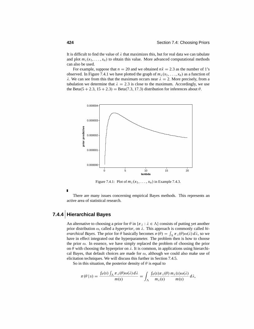
424 Section 7.4: Choosing Priors
It is difficult to find the value of λ that maximizes this, but for real data we can tabulateand plot mλ(x1, . . . , xn) to obtain this value. More advanced computational methodscan also be used.
For example, suppose that n = 20 and we obtained nx = 2.3 as the number of 1’sobserved. In Figure 7.4.1 we have plotted the graph of mλ(x1, . . . , xn) as a function ofλ. We can see from this that the maximum occurs near λ = 2. More precisely, from atabulation we determine that λ = 2.3 is close to the maximum. Accordingly, we usethe Beta(5+ 2.3, 15+ 2.3) = Beta(7.3, 17.3) distribution for inferences about θ.
20151050
0.000004
0.000003
0.000002
0.000001
0.000000
lambda
prio
r pr
edic
tive
Figure 7.4.1: Plot of mλ(x1, . . . , xn) in Example 7.4.3.
There are many issues concerning empirical Bayes methods. This represents anactive area of statistical research.
7.4.4 Hierarchical Bayes
An alternative to choosing a prior for θ in {πλ : λ ∈ ?} consists of putting yet anotherprior distribution ω, called a hyperprior, on λ. This approach is commonly called hi-erarchical Bayes. The prior for θ basically becomes π(θ) = I? πλ(θ)ω(λ) dλ, so wehave in effect integrated out the hyperparameter. The problem then is how to choosethe prior ω. In essence, we have simply replaced the problem of choosing the prioron θ with choosing the hyperprior on λ. It is common, in applications using hierarchi-cal Bayes, that default choices are made for ω, although we could also make use ofelicitation techniques.We will discuss this further in Section 7.4.5.
So in this situation, the posterior density of θ is equal to
π(θ | s) = fθ (s)I? πλ(θ)ω(λ) dλ
m(s)=!?
fθ (s)πλ(θ)
mλ(s)
mλ(s)ω(λ)
m(s)dλ,

Chapter 7: Bayesian Inference 425
where m(s) = I? I" fθ (s)πλ(θ)ω (λ) dθ dλ = I?mλ(s)ω(λ) dλ and mλ(s) =I
fθ (s)πλ(θ) dθ(assuming λ is continuous with prior given by ω). Note that the posterior density ofλ is given by mλ(s)ω(λ)/m(s) while fθ (s)πλ(θ)/mλ(s) is the posterior density of θgiven λ.
Therefore, we can use π(θ | s) for inferences about the model parameter θ (e.g.,estimation, credible regions, and hypothesis assessment) and mλ(s)ω(λ)/m(s) for in-ferences about λ. Typically, however, we are not interested in λ and in fact it doesn’treally make sense to talk about the “true” value of λ. The true value of θ correspondsto the distribution that actually produced the observed data s, at least when the modelis correct, while we are not thinking of λ as being generated from ω. This also impliesanother distinction between θ and λ. For θ is part of the likelihood function based onhow the data was generated, while λ is not.
EXAMPLE 7.4.4 Location-Scale NormalSuppose the situation is as is discussed in Example 7.1.4. In that case, both µ andσ 2 are part of the likelihood function and so are model parameters, while µ0, τ
20, α0,
and β0 are not, and so they are hyperparameters. To complete this specification as ahierarchical model, we need to specify a prior ω(µ0, τ
20, α0, β0), a task we leave to a
higher-level course.
7.4.5 Improper Priors and Noninformativity
One approach to choosing a prior, and to stop the chain of priors in a hierarchical Bayesapproach, is to prescribe a noninformative prior based on ignorance. Such a prior isalso referred to as a default prior or reference prior. The motivation is to specify aprior that puts as little information into the analysis as possible and in some sensecharacterizes ignorance. Surprisingly, in many contexts, statisticians have been led tochoose noninformative priors that are improper, i.e.,
I" π(θ) dθ = ∞, so they do not
correspond to probability distributions.The idea here is to give a rule such that, if a statistician has no prior beliefs about
the value of a parameter or hyperparameter, then a prior is prescribed that reflects this.In the hierarchical Bayes approach, one continues up the chain until the statisticiandeclares ignorance, and a default prior completes the specification.
Unfortunately, just how ignorance is to be expressed turns out to be a rather subtleissue. In many cases, the default priors turn out to be improper, i.e., the integral orsum of the prior over the whole parameter space equals ∞, e.g.,
I" π(θ) dθ = ∞, so
the prior is not a probability distribution. The interpretation of an improper prior is notat all clear, and their use is somewhat controversial. Of course, (s, θ) no longer has ajoint probability distribution when we are using improper priors, and we cannot use theprinciple of conditional probability to justify basing our inferences on the posterior.
There have been numerous difficulties associated with the use of improper priors,which is perhaps this is not surprising. In particular, it is important to note that there isno reason in general for the posterior of θ to exist as a proper probability distributionwhen π is improper. If an improper prior is being used, then we should always checkto make sure the posterior is proper, as inferences will not make sense if we are usingan improper posterior.

426 Section 7.4: Choosing Priors
When using an improper prior π , it is completely equivalent to instead use the priorcπ for any c > 0, for the posterior under π is proper if and only if the posterior undercπ is proper; then the posteriors are identical (see Exercise 7.4.6).
The following example illustrates the use of an improper prior.
EXAMPLE 7.4.5 Location Normal Model with an Improper PriorSuppose that (x1, . . . , xn) is a sample from an N(µ, σ 2
0) distribution, where µ ∈ " =R1 is unknown and σ 2
0 is known.Many arguments for default priors in this context leadto the choice π(µ) = 1, which is clearly improper.
Proceeding as in Example 7.1.2, namely, pretending that this π is a proper proba-bility density, we get that the posterior density of µ is proportional to
exp
#− n
2σ 20
(x − µ)2$
.
This immediately implies that the posterior distribution of µ is N(x, σ 20/n). Note
that this is the same as the limiting posterior obtained in Example 7.1.2 as τ 0 → ∞,although the point of view is quite different.
One commonly used method of selecting a default prior is to use, when it is avail-able, the prior given by I 1/2 (θ) when θ ∈ R1 (and by (det I (θ))1/2 in the multidimen-sional case), where I is the Fisher information for the statistical model as defined inSection 6.5. This is referred to as Jeffreys’ prior. Note that Jeffreys’ prior is dependenton the model.
Jeffreys’ prior has an important invariance property. From Challenge 6.5.19, wehave that, under some regularity conditions, if we make a 1–1 transformation of thereal-valued parameter θ via ψ = 3(θ), then the Fisher information of ψ is given by
I)3−1 (ψ)
*:)3−1
*:(ψ)
;2
.
Therefore, the default Jeffreys’ prior for ψ is
I 1/2)3−1 (ψ)
* AAAA)3−1*:(ψ)
AAAA . (7.4.1)
Now we see that, if we had started with the default prior I 1/2(θ) for θ and made thechange of variable to ψ, then this prior transforms to (7.4.1) by Theorems 2.6.2 and2.6.3. A similar result can be obtained when θ is multidimensional.
Jeffreys’ prior often turns out to be improper, as the next example illustrates.
EXAMPLE 7.4.6 Location Normal (Example 7.4.5 continued)In this case, Jeffreys’ prior is given by π(θ) = √n/σ 0, which gives the same posterioras in Example 7.4.5. Note that Jeffreys’ prior is effectively a constant and hence theprior of Example 7.4.5 is equivalent to Jeffreys’ prior.
Research into rules for determining noninformative priors and the consequences ofusing such priors is an active area in statistics. While the impropriety seems counterin-tuitive, their usage often produces inferences with good properties.

Chapter 7: Bayesian Inference 427
Summary of Section 7.4
• To implement Bayesian inference, the statistician must choose a prior as well asthe sampling model for the data.
• These choices must be checked if the inferences obtained are supposed to havepractical validity. This topic is discussed in Chapter 9.
• Various techniques have been devised to allow for automatic selection of a prior.These include empirical Bayes methods, hierarchical Bayes, and the use of non-informative priors to express ignorance.
• Noninformative priors are often improper. We must always check that an im-proper prior leads to a proper posterior.
EXERCISES
7.4.1 Prove that the family {Gamma(α, β) : α > 0, β > 0} is a conjugate family ofpriors with respect to sampling from the model given by Pareto(λ) distributions withλ > 0.7.4.2 Prove that the family
<πα,β(θ) : α > 1, β > 0
=of priors given by
πα,β(θ) = θ−α I[β,∞)(θ)(α − 1)βα−1
is a conjugate family of priors with respect to sampling from the model given by theUniform[0, θ] distributions with θ > 0. 7.4.3 Suppose that the statistical model isgiven by
pθ (1) pθ (2) pθ (3) pθ (4)θ = a 1/3 1/6 1/3 1/6θ = b 1/2 1/4 1/8 1/8
and that we consider the family of priors given by
πτ (a) πτ (b)τ = 1 1/2 1/2τ = 2 1/3 2/3
and we observe the sample x1 = 1, x2 = 1, x2 = 3.(a) If we use the maximum value of the prior predictive for the data to determine thevalue of τ, and hence the prior, which prior is selected here?(b) Determine the posterior of θ based on the selected prior.7.4.4 For the situation described in Exercise 7.4.3, put a uniform prior on the hyperpa-rameter τ and determine the posterior of θ. (Hint: Theorem of total probability.)7.4.5 For the model for proportions described in Example 7.1.1, determine the priorpredictive density. If n = 10 and nx = 7, which of the priors given by (α, β) = (1, 1)or (α, β) = (5, 5) would the prior predictive criterion select for further inferencesabout θ?

428 Section 7.4: Choosing Priors
7.4.6 Prove that when using an improper prior π, the posterior under π is proper if andonly if the posterior under cπ is proper for c > 0, and then the posteriors are identical.7.4.7 Determine Jeffreys’ prior for the Bernoulli(θ)model and determine the posteriordistribution of θ based on this prior.7.4.8 Suppose we are sampling from a Uniform[0, θ], θ > 0 model and we want touse the improper prior π(θ) ≡ 1.(a) Does the posterior exist in this context?(b) Does Jeffreys’ prior exist in this context?7.4.9 Suppose a student wants to put a prior on the mean grade out of 100 that theirclass will obtain on the next statistics exam. The student feels that a normal priorcentered at 66 is appropriate and that the interval (40, 92) should contain 99% of themarks. Fully identify the prior.7.4.10 A lab has conducted many measurements in the past on water samples froma particular source to determine the existence of a certain contaminant. From theirrecords, it was determined that 50% of the samples had contamination less than 5.3parts per million, while 95% had contamination less than 7.3 parts per million. If anormal prior is going to be used for a future analysis, what prior do these data deter-mine?7.4.11 Suppose that a manufacturer wants to construct a 0.95-credible interval for themean lifetime θ of an item sold by the company. A consulting engineer is 99% certainthat the mean lifetime is less than 50 months. If the prior on θ is an Exponential(λ),then determine λ based on this information.7.4.12 Suppose the prior on a model parameter µ is taken to be N(µ0, σ
20), where µ0
and σ 20 are hyperparameters. The statistician is able to elicit a value for µ0 but feels
unable to do this for σ 20. Accordingly, the statistician puts a hyperprior on σ 2
0 given by1/σ 2
0 ∼ Gamma(α0, 1) for some value of α0. Determine the prior on µ. (Hint: Writeµ = µ0 + σ 0z, where z ∼ N(0, 1).)
COMPUTER EXERCISES
7.4.13 Consider the situation discussed in Exercise 7.4.5.(a) If we observe n = 10, nx = 7, and we are using a symmetric prior, i.e., α = β, plotthe prior predictive as a function of α in the range (0, 20) (you will need a statisticalpackage that provides evaluations of the gamma function for this). Does this graphclearly select a value for α?(b) If we observe n = 10, nx = 9, plot the prior predictive as a function of α in therange (0, 20). Compare this plot with that in part (a).7.4.14 Reproduce the plot given in Example 7.4.3 and verify that the maximum occursnear λ = 2.3.
PROBLEMS
7.4.15 Show that a distribution in the family<N(µ0, τ
20) : µ0 ∈ R1, τ 2
0 > 0=
is com-pletely determined once we specify two quantiles of the distribution.

Chapter 7: Bayesian Inference 429
7.4.16 (Scale normal model) Consider the family of N(µ0, σ2) distributions, where
µ0 is known and σ 2 > 0 is unknown. Determine Jeffreys’ prior for this model.7.4.17 Suppose that for the location-scale normal model described in Example 7.1.4,we use the prior formed by the Jeffreys’ prior for the location model (just a constant)times the Jeffreys’ prior for the scale normal model. Determine the posterior distribu-tion of
&µ, σ 2
'.
7.4.18 Consider the location normal model described in Example 7.1.2.(a) Determine the prior predictive density m. (Hint: Write down the joint density ofthe sample and µ. Use (7.1.2) to integrate out µ and do not worry about getting m intoa recognizable form.)(b) How would you generate a value (X1, . . . , Xn) from this distribution?(c) Are X1, . . . , Xn mutually independent? Justify your answer. (Hint: Write Xi =µ+ σ 0 Zi , µ = µ0 + τ 0 Z , where Z, Z1, . . . , Zn are i.i.d. N(0, 1).)7.4.19 Consider Example 7.3.2, but this time use the prior π(µ, σ 2) = 1/σ 2. De-velop the Gibbs sampling algorithm for this situation. (Hint: Simply adjust each fullconditional in Example 7.3.2 appropriately.)
COMPUTER PROBLEMS
7.4.20 Use the formulation described in Problem 7.4.17 and the data in the followingtable
2.6 4.2 3.1 5.2 3.7 3.8 5.6 1.8 5.3 4.03.0 4.0 4.1 3.2 2.2 3.4 4.5 2.9 4.7 5.2
generate a sample of size N = 104 from the posterior. Plot a density histogram estimateof the posterior density of ψ = σ/µ based on this sample.
CHALLENGES
7.4.21 When θ = (θ1, θ2), the Fisher information matrix I (θ1, θ2) is defined in Prob-lem 6.5.15. The Jeffreys’ prior is then defined as (det I (θ1, θ2))
1/2. Determine Jef-freys’ prior for the location-scale normal model and compare this with the prior usedin Problem 7.4.17.
DISCUSSION TOPICS
7.4.22 Using empirical Bayes methods to determine a prior violates the Bayesian prin-ciple that all unknowns should be assigned probability distributions. Comment on this.Is the hierarchical Bayesian approach a solution to this problem?

430 Section 7.5: Further Proofs (Advanced)
7.5 Further Proofs (Advanced)7.5.1 Derivation of the Posterior Distribution for the Location-Scale
Normal Model
In Example 7.1.4, the likelihood function is given by
L(θ | x1, . . . , xn) =)
2πσ 2*−n/2
exp)− n
2σ 2 (x − µ)2*
exp:−n − 1
2σ 2 s2;.
The prior on&µ, σ 2
'is given by µ | σ 2 ∼ N(µ0, τ
20σ
2) and 1/σ 2 ∼Gamma&α0, β0
',
where µ0, τ20, α0 and β0 are fixed and known.
The posterior density of&µ, σ−2
'is then proportional to the likelihood times the
joint prior. Therefore, retaining only those parts of the likelihood and the prior thatdepend on µ and σ 2, the joint posterior density is proportional to%:
1
σ 2
;n/2
exp)− n
2σ 2 (x − µ)2*
exp:−n − 1
2σ 2s2;(
×%:1
σ 2
;1/2
exp
#− 1
2τ 20σ
2
&µ− µ0
'2$(%: 1
σ 2
;α0−1
exp:−β0
σ 2
;(
= exp
#− n
2σ 2 (x − µ)2 −1
2τ 20σ
2
&µ− µ0
'2$: 1σ 2
;α0+n/2−1/2
×
exp:−Pβ0 +
n − 12
s2Q
1
σ 2
;= exp
#− 1
2σ 2
B#n + 1
τ 20
$µ2 − 2
#nx + µ0
τ 20
$µ
C$×
:1σ 2
;α0+n/2−1/2
exp
#−Bβ0 +
n
2x2 + 1
2τ 20
µ20 +
n − 12
s2
C1σ 2
$
=:
1σ 2
;1/2
exp
− 12σ 2
#n + 1
τ 20
$µ− #n + 1
τ 20
$−1 #µ0
τ 20
+ nx
$2×
:1σ 2
;α0+n/2−1
exp
− β0 + n
2 x2 + 12τ2
0µ2
0 + n−12 s2
−12
:n + 1
τ20
;−1 :µ0τ2
0+ nx
;2
1σ 2
From this, we deduce that the posterior distribution of
&µ, σ 2
'is given by
µ |σ 2, x ∼ N
µx ,
#n + 1
τ 20
$−1
σ 2

Chapter 7: Bayesian Inference 431
and1σ 2 | x ∼ Gamma
&α0 + n/2, βx
',
where
µx =#
n + 1
τ 20
$−1 #µ0
τ 20
+ nx
$and
βx = β0 +n
2x2 + µ2
0
2τ 20
+ n − 1
2s2 − 1
2
#n + 1
τ 20
$−1 #µ0
τ 20
+ nx
$2
.
7.5.2 Derivation of J (θ(ψ0, λ)) for the Location-Scale Normal
Here we have that
ψ = ψ)µ, σ−2
*= σ
µ= 1µ
:1σ 2
;−1/2
and
λ = λ)µ, σ−2
*= 1σ 2 .
We have thatAAAAAAAAdet
∂ψ∂µ
∂ψ
∂)
1σ2
*∂λ∂µ
∂λ
∂)
1σ2
*AAAAAAAA =
AAAAAAdet
−µ−2)
1σ 2
*−1/2 −12µ
−1)
1σ 2
*−3/2
0 1
AAAAAA=
AAAAAdet
# −ψ2λ1/2 −12ψλ
−1
0 1
$AAAAA = ψ2λ1/2
and so
J&θ(ψ0, λ)
' = )ψ2λ1/2*−1
.

432 Section 7.5: Further Proofs (Advanced)

Chapter 8
Optimal Inferences
CHAPTER OUTLINE
Section 1 Optimal Unbiased EstimationSection 2 Optimal Hypothesis TestingSection 3 Optimal Bayesian InferencesSection 4 Decision Theory (Advanced)Section 5 Further Proofs (Advanced)
In Chapter 5, we introduced the basic ingredient of statistical inference — the statisticalmodel. In Chapter 6, inference methods were developed based on the model alone viathe likelihood function. In Chapter 7, we added the prior distribution on the modelparameter, which led to the posterior distribution as the basis for deriving inferencemethods.
With both the likelihood and the posterior, however, the inferences were derivedlargely based on intuition. For example, when we had a characteristic of interest ψ(θ),there was nothing in the theory in Chapters 6 and 7 that forced us to choose a particularestimator, confidence or credible interval, or testing procedure. A complete theory ofstatistical inference, however, would totally prescribe our inferences.
One attempt to resolve this issue is to introduce a performance measure on infer-ences and then choose an inference that does best with respect to this measure. Forexample, we might choose to measure the performance of estimators by their mean-squared error (MSE) and then try to obtain an estimator that had the smallest possibleMSE. This is the optimality approach to inference, and it has been quite successfulin a number of problems. In this chapter, we will consider several successes for theoptimality approach to deriving inferences.
Sometimes the performance measure we use can be considered to be based onwhat is called a loss function. Loss functions form the basis for yet another approachto statistical inference called decision theory. While it is not always the case that aperformance measure is based on a loss function, this holds in some of the most impor-tant problems in statistical inference. Decision theory provides a general framework inwhich to discuss these problems. A brief introduction to decision theory is provided inSection 8.4 as an advanced topic.
433

434 Section 8.1: Optimal Unbiased Estimation
8.1 Optimal Unbiased EstimationSuppose we want to estimate the real-valued characteristic ψ(θ) for the statisticalmodel { fθ : θ ∈ "} . If we have observed the data s, an estimate is a value T (s) that thestatistician hopes will be close to the true value of ψ(θ). We refer to T as an estimatorof ψ. The error in the estimate is given by |T (s)−ψ(θ)|. For a variety of reasons(mostly to do with mathematics) it is more convenient to consider the squared error(T (s)−ψ(θ))2.
Of course, we would like this squared error to be as small as possible. Becausewe do not know the true value of θ, this leads us to consider the distributions of thesquared error, when s has distribution given by fθ , for each θ ∈ ". We would thenlike to choose the estimator T so that these distributions are as concentrated as possibleabout 0. A convenient measure of the concentration of these distributions about 0 isgiven by their means, or
MSEθ (T ) = Eθ ((T −ψ(θ))2), (8.1.1)
called the mean-squared error (recall Definition 6.3.1).An optimal estimator of ψ(θ) is then a T that minimizes (8.1.1) for every θ ∈ ".
In other words, T would be optimal if, for any other estimator T ∗ defined on S, wehave that
MSEθ (T ) ≤ MSEθ (T∗)
for each θ. Unfortunately, it can be shown that, except in very artificial circumstances,there is no such T, so we need to modify our optimization problem.
This modification takes the form of restricting the estimators T that we will enter-tain as possible choices for the inference. Consider an estimator T such that Eθ (T )does not exist or is infinite. It can then be shown that (8.1.1) is infinite (see Challenge8.1.26). So we will first restrict our search to those T for which Eθ (T ) is finite forevery θ.
Further restrictions on the types of estimators that we consider make use of thefollowing result (recall also Theorem 6.3.1).
Theorem 8.1.1 If T is such that E(T 2) is finite, then
E((T − c)2) = Var(T )+ (E(T )− c)2,
This is minimized by taking c = E(T ).
PROOF We have that
E((T − c)2) = E((T − E (T )+ E (T )− c)2)
= E((T − E (T ))2)+ 2E (T − E (T )) (E (T )− c)+ (E (T )− c)2
= Var(T )+ (E(T )− c)2, (8.1.2)
because E(T − E (T )) = E(T ) − E(T ) = 0. As (E(T ) − c)2 ≥ 0, and Var(T ) doesnot depend on c, the value of (8.1.2) is minimized by taking c = E(T ).

Chapter 8: Optimal Inferences 435
8.1.1 The Rao–Blackwell Theorem and Rao–Blackwellization
We will prove that, when we are looking for T to minimize (8.1.1), we can furtherrestrict our attention to estimators T that depend on the data only through the valueof a sufficient statistic. This simplifies our search, as sufficiency often results in areduction of the dimension of the data (recall the discussion and examples in Section6.1.1). First, however, we need the following property of sufficiency.
Theorem 8.1.2 A statistic U is sufficient for a model if and only if the conditionaldistribution of the data s given U = u is the same for every θ ∈ ".
PROOF See Section 8.5 for the proof of this result.
The implication of this result is that information in the data s beyond the value ofU(s) = u can tell us nothing about the true value of θ, because this information comesfrom a distribution that does not depend on the parameter. Notice that Theorem 8.1.2is a characterization of sufficiency, alternative to that provided in Section 6.1.1.
Consider a simple example that illustrates the content of Theorem 8.1.2.
EXAMPLE 8.1.1Suppose that S = {1, 2, 3, 4}," = {a, b}, where the two probability distributions aregiven by the following table.
s = 1 s = 2 s = 3 s = 4θ = a 1/2 1/6 1/6 1/6θ = b 1/4 1/4 1/4 1/4
Then L(· | 2) = L(· | 3) = L(· | 4), and so U : S −→ {0, 1}, given by U(1) = 0 andU(2) = U(3) = U(4) = 1 is a sufficient statistic.
As we must have s = 1 when we observe U(s) = 0, the conditional distribution ofthe response s, given U(s) = 0, is degenerate at 1 (i.e., all the probability mass is atthe point 1) for both θ = a and θ = b.When θ = a, the conditional distribution of theresponse s, given U(s) = 1, places 1/3 of its mass at each of the points in {2, 3, 4} andsimilarly when θ = b. So given U(s) = 1, the conditional distributions are as in thefollowing table.
s = 1 s = 2 s = 3 s = 4θ = a 0 1/3 1/3 1/3θ = b 0 1/3 1/3 1/3
Thus, we see that indeed the conditional distributions are independent of θ .
We now combine Theorems 8.1.1 and 8.1.2 to show that we can restrict our at-tention to estimators T that depend on the data only through the value of a sufficientstatistic U . By Theorem 8.1.2 we can denote the conditional probability measure fors, given U(s) = u, by P (· |U = u), i.e., this probability measure does not depend onθ , as it is the same for every θ ∈ ".
For estimator T of ψ(θ), such that Eθ (T ) is finite for every θ, put TU (s) equal tothe conditional expectation of T given the value of U(s), namely,
TU (s) = EP(· |U=U(s))(T ),

436 Section 8.1: Optimal Unbiased Estimation
i.e., TU is the average value of T when we average using P (· |U = U(s)) . Noticethat TU (s1) = TU (s2) whenever U(s1) = U(s2) (this is because P (· |U = U(s1)) =P (· |U = U(s2))), and so TU depends on the data s only through the value of U(s).
Theorem 8.1.3 (Rao–Blackwell) Suppose that U is a sufficient statistic and Eθ (T 2)is finite for every θ . Then MSEθ (TU ) ≤MSEθ (T ) for every θ ∈ ".
PROOF Let Pθ,U denote the marginal probability measure of U induced by Pθ . Bythe theorem of total expectation (see Theorem 3.5.2), we have that
MSEθ (T ) = EPθ,U
)EP(· |U=u)((T −ψ(θ))2)
*,
where EP(· |U=u)((T − ψ(θ)))2 denotes the conditional MSE of T , given U = u. Nowby Theorem 8.1.1,
EP(· |U=u)((T −ψ(θ))2) = VarP(· |U=u)(T )+ (EP(· |U=u))(T )−ψ(θ))2. (8.1.3)
As both terms in (8.1.3) are nonnegative, and recalling the definition of TU , we have
MSEθ (T ) = EPθ,U (VarP(· |U=u)(T ))+ EPθ,U ((TU (s)−ψ(θ))2)≥ EPθ,U ((TU (s)−ψ(θ))2).
Now (TU (s) − ψ(θ))2 = EP(· |U=u)((TU (s) − ψ(θ))2) (Theorem 3.5.4) and so, bythe theorem of total expectation,
EPθ,U ((TU (s)− ψ(θ))2) = EPθ,U
)EP(· |U=u)((TU (s)−ψ(θ))2)
*= EPθ ((TU (s)−ψ(θ))2) = MSEθ (TU )
and the theorem is proved.
Theorem 8.1.3 shows that we can always improve on (or at least make no worse)any estimator T that possesses a finite second moment, by replacing T (s) by the esti-mate TU (s). This process is sometimes referred to as the Rao-Blackwellization of anestimator.
Notice that putting E = Eθ and c = ψ(θ) in Theorem 8.1.1 implies that
MSEθ (T ) = Varθ (T )+ (Eθ (T )− ψ(θ))2. (8.1.4)
So the MSE of T can be decomposed as the sum of the variance of T plus the squaredbias of T (this was also proved in Theorem 6.3.1).
Theorem 8.1.1 has another important implication, for (8.1.4) is minimized by tak-ing ψ(θ) = Eθ (T ). This indicates that, on average, the estimator T comes closer (interms of squared error) to Eθ (T ) than to any other value. So, if we are sampling fromthe distribution specified by θ, T (s) is a natural estimate of Eθ (T ). Therefore, for ageneral characteristic ψ(θ), it makes sense to restrict attention to estimators that havebias equal to 0. This leads to the following definition.

Chapter 8: Optimal Inferences 437
Definition 8.1.1 An estimator T of ψ(θ) is unbiased if Eθ (T ) = ψ(θ) for everyθ ∈ ".
Notice that, for unbiased estimators with finite second moment, (8.1.4) becomes
MSEθ (T ) = Varθ (T ).
Therefore, our search for an optimal estimator has become the search for an unbiasedestimator with smallest variance. If such an estimator exists, we give it a special name.
Definition 8.1.2 An unbiased estimator of ψ(θ) with smallest variance for eachθ ∈ " is called a uniformly minimum variance unbiased (UMVU) estimator.
It is important to note that the Rao–Blackwell theorem (Theorem 8.1.3) also ap-plies to unbiased estimators. This is because the Rao–Blackwellization of an unbiasedestimator yields an unbiased estimator, as the following result demonstrates.
Theorem 8.1.4 (Rao–Blackwell for unbiased estimators) If T has finite second mo-ment, is unbiased for ψ(θ), and U is a sufficient statistic, then Eθ (TU ) = ψ(θ) forevery θ ∈ " (so TU is also unbiased for ψ(θ)) and Varθ (TU ) ≤Varθ (T ).
PROOF Using the theorem of total expectation (Theorem 3.5.2), we have
Eθ (TU ) = EPθ,U (TU ) = EPθ,U
&EP· |U=u) (T )
' = Eθ (T ) = ψ(θ).So TU is unbiased for ψ(θ) and MSEθ (T ) =Varθ (T ), MSEθ (TU ) =Varθ (TU ) . Ap-plying Theorem 8.1.3 gives Varθ (TU ) ≤ Varθ (T ).
There are many situations in which the theory of unbiased estimation leads to goodestimators. However, the following example illustrates that in some problems, thereare no unbiased estimators and hence the theory has some limitations.
EXAMPLE 8.1.2 The Nonexistence of an Unbiased EstimatorSuppose that (x1, . . . , xn) is a sample from the Bernoulli(θ) and we wish to find aUMVU estimator ofψ(θ) = θ/ (1− θ), the odds in favor of a success occurring. FromTheorem 8.1.4, we can restrict our search to unbiased estimators T that are functionsof the sufficient statistic nx .
Such a T satisfies Eθ (T (nX)) = θ/ (1− θ) for every θ ∈ [0, 1]. Recalling thatnX ∼ Binomial(n, θ) , this implies that
θ
1− θ =n>
k=0
T (k)
:n
k
;θk (1− θ)n−k
for every θ ∈ [0, 1]. By the binomial theorem, we have
(1− θ)n−k =n−k>l=0
:n − k
l
;(−1)l θ l .

438 Section 8.1: Optimal Unbiased Estimation
Substituting this into the preceding expression for θ/ (1− θ) and writing this in termsof powers of θ leads to
θ
1− θ =n>
m=0
#m>
k=0
T (k)
:n
k
;(−1)m−k
$θm . (8.1.5)
Now the left-hand side of (8.1.5) goes to ∞ as θ → 1, but the right-hand side is apolynomial in θ , which is bounded in [0, 1] . Therefore, an unbiased estimator of ψcannot exist.
If a characteristic ψ(θ) has an unbiased estimator, then it is said to be U-estimable.It should be kept in mind, however, that just because a parameter is not U-estimabledoes not mean that we cannot estimate it! For example, ψ in Example 8.1.2, is a 1–1function of θ, so the MLE of ψ is given by x/ (1− x) (see Theorem 6.2.1); this seemslike a sensible estimator, even if it is biased.
8.1.2 Completeness and the Lehmann–Scheffé Theorem
In certain circumstances, if an unbiased estimator exists, and is a function of a sufficientstatistic U, then there is only one such estimator — so it must be UMVU. We need theconcept of completeness to establish this.
Definition 8.1.3 A statistic U is complete if any function h of U, which satisfiesEθ (h(U)) = 0 for every θ ∈ ", also satisfies h(U(s)) = 0 with probability 1 foreach θ ∈ " (i.e., Pθ ({s : h(U(s)) = 0}) = 1 for every θ ∈ ").
In probability theory, we treat two functions as equivalent if they differ only on a sethaving probability content 0, as the probability of the functions taking different valuesat an observed response value is 0. So in Definition 8.1.3, we need not distinguishbetween h and the constant 0. Therefore, a statistic U is complete if the only unbiasedestimator of 0, based on U, is given by 0 itself.
We can now derive the following result.
Theorem 8.1.5 (Lehmann–Scheffé) If U is a complete sufficient statistic, and if Tdepends on the data only through the value of U, has finite second moment for everyθ, and is unbiased for ψ(θ), then T is UMVU.
PROOF Suppose that T ∗ is also an unbiased estimator of ψ(θ). By Theorem 8.1.4we can assume that T ∗ depends on the data only through the value of U. Then thereexist functions h and h∗ such that T (s) = h(U(s)) and T ∗(s(= h∗(U(s)) and
0 = Eθ (T )− Eθ (T∗) = Eθ (h(U))− Eθ (h
∗(U)) = Eθ (h(U)− h∗(U)).
By the completeness of U , we have that h(U) = h∗(U) with probability 1 for eachθ ∈ ", which implies that T = T ∗ with probability 1 for each θ ∈ ". This saysthere is essentially only one unbiased estimator forψ(θ) based on U, and so it must beUMVU.

Chapter 8: Optimal Inferences 439
The Rao–Blackwell theorem for unbiased estimators (Theorem 8.1.4), togetherwith the Lehmann–Scheffé theorem, provide a method for obtaining a UMVU esti-mator of ψ(θ). Suppose we can find an unbiased estimator T that has finite secondmoment. If we also have a complete sufficient statistic U, then by Theorem 8.1.4TU (s) = EP(· |U=U(s)) (T ) is unbiased for ψ(θ) and depends on the data only throughthe value of U, because TU (s1) = TU (s2) whenever U(s1) = U(s2). Therefore, byTheorem 8.1.5, TU is UMVU for ψ(θ).
It is not necessary, in a given problem, that a complete sufficient statistic exist.In fact, it can be proved that the only candidate for this is a minimal sufficient statistic(recall the definition in Section 6.1.1). So in a given problem, we must obtain a minimalsufficient statistic and then determine whether or not it is complete. We illustrate thisvia an example.
EXAMPLE 8.1.3 Location NormalSuppose that (x1, . . . , xn) is a sample from an N(µ, σ 2
0) distribution, where µ ∈ R1
is unknown and σ 20 > 0 is known. In Example 6.1.7, we showed that x is a minimal
sufficient statistic for this model.In fact, x is also complete for this model. The proof of this is a bit involved and is
presented in Section 8.5.Given that x is a complete, minimal sufficient statistic, this implies that T (x) is a
UMVU estimator of its mean Eµ(T (X)) whenever T has a finite second moment forevery µ ∈ R1. In particular, x is the UMVU estimator of µ because Eµ(X) = µ andEµ(X2) = (σ 2
0/n) + µ2 < ∞. Furthermore, x + σ 0z p is the UMVU estimator ofEµ(X + σ 0z p) = µ+ σ 0zp (the pth quantile of the true distribution).
The arguments needed to show the completeness of a minimal sufficient statistic ina problem are often similar to the one required in Example 8.1.3 (see Challenge 8.1.27).Rather than pursue such technicalities here, we quote some important examples inwhich the minimal sufficient statistic is complete.
EXAMPLE 8.1.4 Location-Scale NormalSuppose that (x1, . . . , xn) is a sample from an N(µ, σ 2) distribution, where µ ∈ R1
and σ > 0 are unknown. The parameter in this model is two-dimensional and is givenby (µ, σ 2) ∈ R1 × (0,∞).
We showed, in Example 6.1.8, that (x, s2) is a minimal sufficient statistic for thismodel. In fact, it can be shown that (x, s2) is a complete minimal sufficient statistic.Therefore, T (x, s2) is a UMVU estimator of Eθ (T (X, S2)) whenever the second mo-ment of T (x, s2) is finite for every (µ, σ 2). In particular, x is the UMVU estimator ofµ and s2 is UMVU for σ 2.
EXAMPLE 8.1.5 Distribution-Free ModelsSuppose that (x1, . . . , xn) is a sample from some continuous distribution on R1. Thestatistical model comprises all continuous distributions on R1.
It can be shown that the order statistics (x(1), . . . , x(n))make up a complete minimalsufficient statistic for this model. Therefore, T (x(1), . . . , x(n)) is UMVU for
Eθ (T (X(1), . . . , X(n)))

440 Section 8.1: Optimal Unbiased Estimation
wheneverEθ (T 2(X(1), . . . , X(n))) <∞ (8.1.6)
for every continuous distribution. In particular, if T : Rn → R1 is bounded, then thisis the case. For example, if
T (x(1), . . . , x(n)) = 1
n
n>i=1
IA(x(i)),
the relative frequency of the event A in the sample, then T (x(1), . . . , x(n)) is UMVUfor Eθ (T (X(1), . . . , X(n))) = Pθ (A).
Now change the model assumption so that (x1, . . . , xn) is a sample from somecontinuous distribution on R1 that possesses its first m moments. Again, it can beshown that the order statistics make up a complete minimal sufficient statistic. There-fore, T (x(1), . . . , x(n)) is UMVU for Eθ (T (X(1), . . . , X(n)))whenever (8.1.6) holds forevery continuous distribution possessing its first m moments. For example, if m = 2,then this implies that T (x(1), . . . , x(n)) = x is UMVU for Eθ (X). When m = 4, wehave that s2 is UMVU for the population variance (see Exercise 8.1.2).
8.1.3 The Cramer–Rao Inequality (Advanced)
There is a fundamental inequality that holds for the variance of an estimator T . This isgiven by the Cramer–Rao inequality (sometimes called the information inequality). Itis a corollary to the following inequality.
Theorem 8.1.6 (Covariance inequality) Suppose T,Uθ : S → R1 and Eθ (T 2) <∞, 0 < Eθ (U2
θ ) <∞ for every θ ∈ ". Then
Varθ (T ) ≥ (Covθ (T,Uθ ))2
Varθ (Uθ )
for every θ ∈ ". Equality holds if and only if
T (s) = Eθ (T )+ Covθ (T,Uθ )Varθ (Uθ )
(Uθ (s)− Eθ (Uθ (s)))
with probability 1 for every θ ∈ " (i.e., if and only if T (s) and Uθ (s) are linearlyrelated).
PROOF This result follows immediately from the Cauchy–Schwartz inequality (The-orem 3.6.3).
Now suppose that " is an open subinterval of R1 and we take
Uθ (s) = S(θ | s) = ∂ ln fθ (s)
∂θ, (8.1.7)
i.e., Uθ is the score function. Assume that the conditions discussed in Section 6.5 hold,so that Eθ (S(θ | s)) = 0 for all θ, and, Fisher’s information I (θ) =Varθ (S(θ | s)) is

Chapter 8: Optimal Inferences 441
finite. Then using∂ ln fθ (s)
∂θ= ∂ fθ (s)
∂θ
1fθ (s)
,
we have
Covθ (T,Uθ )
= Eθ
:T (s)
∂ ln fθ (s)
∂θ
;= Eθ
:T (s)
∂ fθ (s)
∂θ
1fθ (s)
;=>
s
:T (s)
∂ fθ (s)
∂θ
1fθ (s)
;fθ (s) = ∂
∂θ
>s
T (s) fθ (s) = ∂Eθ (T )
∂θ, (8.1.8)
in the discrete case, where we have assumed conditions like those discussed in Section6.5, so we can pull the partial derivative through the sum. A similar argument gives theequality (8.1.8) in the continuous case as well.
The covariance inequality, applied with Uθ specified as in (8.1.7) and using (8.1.8),gives the following result.
Corollary 8.1.1 (Cramer–Rao or information inequality) Under conditions,
Varθ (T ) ≥:∂Eθ (T )
∂θ
;2
(I (θ))−1
for every θ ∈ ". Equality holds if and only if
T (s) = Eθ (T )+ ∂Eθ (T )
∂θ(I (θ))−1S(θ | s)
with probability 1 for every θ ∈ ".
The Cramer–Rao inequality provides a fundamental lower bound on the varianceof an estimator T . From (8.1.4), we know that the variance is a relevant measure of theaccuracy of an estimator only when the estimator is unbiased, so we restate Corollary8.1.1 for this case.
Corollary 8.1.2 Under the conditions of Corollary 8.1.1, when T is an unbiasedestimator of ψ(θ),
Varθ (T ) ≥&ψ :(θ)
'2(I (θ))−1
for every θ ∈ ". Equality holds if and only if
T (s) = ψ(θ)+ ψ :(θ)(I (θ))−1S(θ | s) (8.1.9)
with probability 1 for every θ ∈ ".
Notice that when ψ(θ) = θ, then Corollary 8.1.2 says that the variance of theunbiased estimator T is bounded below by the reciprocal of the Fisher information.More generally, when ψ is a 1–1, smooth transformation, we have (using Challenge6.5.19) that the variance of an unbiased T is again bounded below by the reciprocal of

442 Section 8.1: Optimal Unbiased Estimation
the Fisher information, but this time the model uses the parameterization in terms ofψ(θ).
Corollary 8.1.2 has several interesting implications. First, if we obtain an unbiasedestimator T with variance at the lower bound, then we know immediately that it isUMVU. Second, we know that any unbiased estimator that achieves the lower boundis of the form given in (8.1.9). Note that the right-hand side of (8.1.9) must be inde-pendent of θ in order for this to be an estimator. If this is not the case, then there are noUMVU estimators whose variance achieves the lower bound. The following exampledemonstrates that there are cases in which UMVU estimators exist, but their variancedoes not achieve the lower bound.
EXAMPLE 8.1.6 Poisson(λ)ModelSuppose that (x1, . . . , xn) is a sample from the Poisson(λ) distribution where λ > 0 isunknown. The log-likelihood is given by l(λ | x1, . . . , xn) = nx ln λ− nλ, so the scorefunction is given by S(λ | x1, . . . , xn) = nx/λ− n. Now
∂S(λ | x1, . . . , xn)
∂λ= −nx
λ2,
and thus
I (λ) = Eλ
:nx
λ2
;= n
λ.
Suppose we are estimating λ. Then the Cramer–Rao lower bound is given byI−1(λ) = λ/n. Noting that x is unbiased for λ and that Varλ(X) = λ/n, we seeimmediately that x is UMVU and achieves the lower bound.
Now suppose that we are estimating ψ(λ) = e−λ = Pλ({0}). The Cramer-Raolower bound equals λe−2λ/n and
ψ(λ)+ψ :(λ)I−1(λ)S(λ | x1, . . . , xn) = e−λ − e−λ:λ
n
;:nx
λ− n
;= e−λ(1− x + λ),
which is clearly not independent of λ. So there does not exist a UMVU estimator forψ that attains the lower bound.
Does there exist a UMVU estimator for ψ? Observe that when n = 1, then I{0}(x1)is an unbiased estimator of ψ . As it turns out, x is (for every n) a complete mini-mal sufficient statistic for this model, so by the Lehmann-Scheffé theorem I{0}(x1) isUMVU for ψ. Further I{0}(X1) has variance
Pλ(X1 = 0) (1− Pλ(X1 = 0)) = e−λ(1− e−λ)
since I{0}(X1) ∼ Bernoulli(e−λ). This implies that e−λ(1− e−λ) > λe−2λ.In general we have that
1n
n>i=1
I{0}(xi )
is an unbiased estimator of ψ , but it is not a function of x . Thus we cannot apply theLehmann–Scheffé theorem, but we can Rao–Blackwellize this estimator. Therefore,

Chapter 8: Optimal Inferences 443
the UMVU estimator of ψ is given by
1n
n>i=1
E(I{0}(Xi ) | X = x).
To determine this estimator in closed form, we reason as follows. The condi-tional probability function of (X1, . . . , Xn) given X = x , because nX is distributedPoisson(nλ) , isF
λx1
x1!· · · λ
xn
xn!e−nλ
G%(nλ)nx
(nx)!e−nλ
(−1
=:
nx
x1 . . . xn
;:1n
;x1
· · ·:
1n
;xn
,
i.e., (X1, . . . , Xn) given X = x is distributed Multinomial(nx, 1/n, . . . , 1/n) . Ac-cordingly, the UMVU estimator is given by
E(I{0}(X1) | X = x) = P(X1 = 0 | X = x) =:
1− 1n
;nx
because Xi | X = x ∼ Binomial(nx, 1/n) for each i = 1, . . . , n.Certainly, it is not at all obvious from the functional form that this estimator is
unbiased, let alone UMVU. So this result can be viewed as a somewhat remarkableapplication of the theory.
Recall now Theorems 6.5.2 and 6.5.3. The implications of these results, with someadditional conditions, are that the MLE of θ is asymptotically unbiased for θ and thatthe asymptotic variance of the MLE is at the information lower bound. This is ofteninterpreted to mean that, with large samples, the MLE makes full use of the informationabout θ contained in the data.
Summary of Section 8.1
• An estimator comes closest (using squared distance) on average to its mean (seeTheorem 8.1.1), so we can restrict attention to unbiased estimators for quantitiesof interest.
• The Rao–Blackwell theorem says that we can restrict attention to functions of asufficient statistic when looking for an estimator minimizing MSE.
• When a sufficient statistic is complete, then any function of that sufficient statis-tic is UMVU for its mean.
• The Cramer–Rao lower bound gives a lower bound on the variance of an unbi-ased estimator and a method for obtaining an estimator that has variance at thislower bound when such an estimator exists.

444 Section 8.1: Optimal Unbiased Estimation
EXERCISES
8.1.1 Suppose that a statistical model is given by the two distributions in the followingtable.
s = 1 s = 2 s = 3 s = 4fa (s) 1/3 1/6 1/12 5/12fb (s) 1/2 1/4 1/6 1/12
If T : {1, 2, 3, 4} → {1, 2, 3, 4} is defined by T (1) = T (2) = 1 and T (s) = sotherwise, then prove that T is a sufficient statistic. Derive the conditional distributionsof s given T (s) and show that these are independent of θ.8.1.2 Suppose that (x1, . . . , xn) is a sample from a distribution with mean µ and vari-ance σ 2. Prove that s2 = (n − 1)−1On
i=1 (xi − x)2 is unbiased for σ 2.
8.1.3 Suppose that (x1, . . . , xn) is a sample from an N(µ, σ 20) distribution, where µ ∈
R1 is unknown and σ 20 is known. Determine a UMVU estimator of the second moment
µ2 + σ 20.
8.1.4 Suppose that (x1, . . . , xn) is a sample from an N(µ, σ 20) distribution, where µ ∈
R1 is unknown and σ 20 is known. Determine a UMVU estimator of the first quartile
µ+ σ 0z0.25.8.1.5 Suppose that (x1, . . . , xn) is a sample from an N(µ, σ 2
0) distribution, where µ ∈R1 is unknown and σ 2
0 is known. Is 2x+3 a UMVU estimator of anything? If so, whatis it UMVU for? Justify your answer.8.1.6 Suppose that (x1, . . . , xn) is a sample from a Bernoulli(θ) distribution, whereθ ∈ [0, 1] is unknown. Determine a UMVU estimator of θ (use the fact that a minimalsufficient statistic for this model is complete).8.1.7 Suppose that (x1, . . . , xn) is a sample from a Gamma(α0, β) distribution, whereα0 is known and β > 0 is unknown. Using the fact that x is a complete sufficientstatistic (see Challenge 8.1.27), determine a UMVU estimator of β−1.8.1.8 Suppose that (x1, . . . , xn) is a sample from an N(µ0, σ
2) distribution, where µ0
is known and σ 2 > 0 is unknown. Show thatOn
i=1
&xi − µ0
'2 is a sufficient statisticfor this problem. Using the fact that it is complete, determine a UMVU estimator forσ 2.8.1.9 Suppose a statistical model comprises all continuous distributions on R1. Basedon a sample of n, determine a UMVU estimator of P((−1, 1)), where P is the trueprobability measure. Justify your answer.8.1.10 Suppose a statistical model comprises all continuous distributions on R1 thathave a finite second moment. Based on a sample of n, determine a UMVU estimatorof µ2, where µ is the true mean. Justify your answer. (Hint: Find an unbiased esti-mator for n = 2, Rao–Blackwellize this estimator for a sample of n, and then use theLehmann–Scheffé theorem.)8.1.11 The estimator determined in Exercise 8.1.10 is also unbiased for µ2 when thestatistical model comprises all continuous distributions on R1 that have a finite firstmoment. Is this estimator still UMVU for µ2?

Chapter 8: Optimal Inferences 445
PROBLEMS
8.1.12 Suppose that (x1, . . . , xn) is a sample from a Uniform[0, θ] distribution, whereθ > 0 is unknown. Show that x(n) is a sufficient statistic and determine its distribution.Using the fact that x(n) is complete, determine a UMVU estimator of θ .8.1.13 Suppose that (x1, . . . , xn) is a sample from a Bernoulli(θ) distribution, whereθ ∈ [0, 1] is unknown. Then determine the conditional distribution of (x1, . . . , xn),given the value of the sufficient statistic x .8.1.14 Prove that L(θ, a) = (θ − a)2 satisfies
L(θ, αa1 + (1− α)a2) ≤ αL(θ, a1)+ (1− α) L(θ, a2)
when a ranges in a subinterval of R1. Use this result together with Jensen’s inequality(Theorem 3.6.4) to prove the Rao–Blackwell theorem.8.1.15 Prove that L(θ, a) = |θ − a| satisfies
L(θ, αa1 + (1− α)a2) ≤ αL(θ, a1)+ (1− α)L(θ, a2)
when a ranges in a subinterval of R1. Use this result together with Jensen’s inequality(Theorem 3.6.4) to prove the Rao–Blackwell theorem for absolute error. (Hint: Firstshow that |x + y| ≤ |x| + |y| for any x and y.)8.1.16 Suppose that (x1, . . . , xn) is a sample from an N(µ, σ 2) distribution, where&µ, σ 2
' ∈ R1 × (0,∞) is unknown. Show that the optimal estimator (in the senseof minimizing the MSE), of the form cs2 for σ 2, is given by c = (n − 1)/ (n + 1).Determine the bias of this estimator and show that it goes to 0 as n →∞.8.1.17 Prove that if a statistic T is complete for a model and U = h(T ) for a 1–1function h, then U is also complete.8.1.18 Suppose that (x1, . . . , xn) is a sample from an N(µ, σ 2) distribution, where&µ, σ 2
' ∈ R1 × (0,∞) is unknown. Derive a UMVU estimator of the standard devia-tion σ. (Hint: Calculate the expected value of the sample standard deviation s.)8.1.19 Suppose that (x1, . . . , xn) is a sample from an N(µ, σ 2) distribution, where&µ, σ 2
' ∈ R1 × (0,∞) is unknown. Derive a UMVU estimator of the first quartileµ+ σ z0.25. (Hint: Problem 8.1.17.)8.1.20 Suppose that (x1, . . . , xn) is a sample from an N(µ, σ 2
0) distribution, whereθ ∈ " = {µ1, µ2} is unknown and σ 2
0 > 0 is known. Establish that x is a minimalsufficient statistic for this model but that it is not complete.8.1.21 Suppose that (x1, . . . , xn) is a sample from an N(µ, σ 2
0) distribution, whereµ ∈ R1 is unknown and σ 2
0 is known. Determine the information lower bound, for anunbiased estimator, when we consider estimating the second moment µ2 + σ 2
0. Doesthe UMVU estimator in Exercise 8.1.3 attain the information lower bound?8.1.22 Suppose that (x1, . . . , xn) is a sample from a Gamma(α0, β) distribution, whereα0 is known and β > 0 is unknown. Determine the information lower bound for theestimation of β−1 using unbiased estimators, and determine if the UMVU estimatorobtained in Exercise 8.1.7 attains this.8.1.23 Suppose that (x1, . . . , xn) is a sample from the distribution with density fθ(x) = θxθ−1 for x ∈ [0, 1] and θ > 0 is unknown. Determine the information lower

446 Section 8.2: Optimal Hypothesis Testing
bound for estimating θ using unbiased estimators. Does a UMVU estimator with vari-ance at the lower bound exist for this problem?8.1.24 Suppose that a statistic T is a complete statistic based on some statistical model.A submodel is a statistical model that comprises only some of the distributions in theoriginal model. Why is it not necessarily the case that T is complete for a submodel?8.1.25 Suppose that a statistic T is a complete statistic based on some statistical model.If we construct a larger model that contains all the distributions in the original modeland is such that any set that has probability content equal to 0 for every distribution inthe original model also has probability content equal to 0 for every distribution in thelarger model, then prove that T is complete for the larger model as well.
CHALLENGES
8.1.26 If X is a random variable such that E(X) either does not exist or is infinite, thenshow that E((X − c)2) =∞ for any constant c.8.1.27 Suppose that (x1, . . . , xn) is a sample from a Gamma(α0, β) distribution, whereα0 is known and β > 0 is unknown. Show that x is a complete minimal sufficientstatistic.
8.2 Optimal Hypothesis TestingSuppose we want to assess a hypothesis about the real-valued characteristic ψ(θ) forthe model { fθ : θ ∈ "}. Typically, this will take the form H0 : ψ(θ) = ψ0, where wehave specified a value for ψ . After observing data s, we want to assess whether or notwe have evidence against H0.
In Section 6.3.3, we discussed methods for assessing such a hypothesis based onthe plug-in MLE for ψ(θ). These involved computing a P-value as a measure of howsurprising the data s are when the null hypothesis is assumed to be true. If s is sur-prising for each of the distributions fθ for which ψ(θ) = ψ0, then we have evidenceagainst H0. The development of such procedures was largely based on the intuitivejustification for the likelihood function.
8.2.1 The Power Function of a Test
Closely associated with a specific procedure for computing a P-value is the conceptof a power function β(θ), as defined in Section 6.3.6. For this, we specified a criticalvalue α, such that we declare the results of the test statistically significant whenever theP-value is less than or equal to α. The power β(θ) is then the probability of the P-valuebeing less than or equal to α when we are sampling from fθ . The greater the valueof β(θ), when ψ(θ) == ψ0, the better the procedure is at detecting departures fromH0. The power function is thus a measure of the sensitivity of the testing procedure todetecting departures from H0.
Recall the following fundamental example.

Chapter 8: Optimal Inferences 447
EXAMPLE 8.2.1 Location Normal ModelSuppose we have a sample (x1, . . . , xn) from the N(µ, σ 2
0) model, where µ ∈ R1 isunknown and σ 2
0 > 0 is known, and we want to assess the null hypothesis H0 : µ = µ0.In Example 6.3.9, we showed that a sensible test for this problem is based on the z-statistic
z = x − µ0
σ 0/√
n,
with Z ∼ N(0, 1) under H0. The P-value is then given by
Pµ0
:|Z | ≥
AAAA x − µ0
σ 0/√
n
AAAA; = 2P
1−8:AAAA x − µ0
σ 0/√
n
AAAA;Q ,where8 denotes the N(0, 1) distribution function.
In Example 6.3.18, we showed that, for critical value α, the power function of thez-test is given by
β(µ) = Pµ
:2P
1−8:AAAA X − µ0
σ 0/√
n
AAAA;Q < α; = Pµ
:8
:AAAA X − µ0
σ 0/√
n
AAAA; > 1− α2
;= 1−8
:µ0 − µσ 0/
√n+ z1−(α/2)
;+8
:µ0 − µσ 0/
√n− z1−(α/2)
;because X ∼ N(µ, σ 2
0/n).We see that specifying a value for α specifies a set of data values
R =F(x1, . . . , xn) : 8
:AAAA x − µ0
σ 0/√
n
AAAA; > 1− α2
Gsuch that the results of the test are determined to be statistically significant whenever(x1, . . . , xn) ∈ R. Using the fact that 8 is 1–1 increasing, we can also write R as
R =F(x1, . . . , xn) :
AAAA x − µ0
σ 0/√
n
AAAA > 8−1)
1− α2
*G=
F(x1, . . . , xn) :
AAAA x − µ0
σ 0/√
n
AAAA > z1−(α/2)G.
Furthermore, the power function is given by β(µ) = Pµ(R) and β(µ0) = Pµ0(R) = α.
8.2.2 Type I and Type II Errors
We now adopt a different point of view. We are going to look for tests that are optimalfor testing the null hypothesis H0 : ψ(θ) = ψ0. First, we will assume that, havingobserved the data s, we will decide to either accept or reject H0. If we reject H0, thenthis is equivalent to accepting the alternative Ha : ψ(θ) == ψ0. Our performancemeasure for assessing testing procedures will then be the probability that the testingprocedure makes an error.

448 Section 8.2: Optimal Hypothesis Testing
There are two types of error. We can make a type I error — rejecting H0 when it istrue — or make a type II error — accepting H0 when H0 is false. Note that if we rejectH0, then this implies that we are accepting the alternative hypothesis Ha : ψ (θ) == ψ0.
It turns out that, except in very artificial circumstances, there are no testing proce-dures that simultaneously minimize the probabilities of making the two kinds of errors.Accordingly, we will place an upper bound α, called the critical value, on the proba-bility of making a type I error. We then search among those tests whose probability ofmaking a type I error is less than or equal to α, for a testing procedure that minimizesthe probability of making a type II error.
Sometimes hypothesis testing problems for real-valued parameters are distinguishedas being one-sided or two-sided. For example, if θ is real-valued, then H0 : θ = θ0 ver-sus Ha : θ == θ0 is a two-sided testing problem, while H0 : θ ≤ θ0 versus Ha : θ > θ0or H0 : θ ≥ θ0 versus Ha : θ < θ0 are examples of one-sided problems. Notice,however, that if we define
ψ(θ) = I(θ0,∞)(θ),
then H0 : θ ≤ θ0 versus Ha : θ > θ0 is equivalent to the problem H0 : ψ(θ) = 0versus Ha : ψ(θ) == 0. Similarly, if we define
ψ(θ) = I(−∞,θ0)(θ),
then H0 : θ ≥ θ0 versus Ha : θ < θ0 is equivalent to the problem H0 : ψ(θ) = 0versus Ha : ψ(θ) == 0. So the formulation we have adopted for testing problems abouta general ψ includes the one-sided problems as special cases.
8.2.3 Rejection Regions and Test Functions
One approach to specifying a testing procedure is to select a subset R ⊂ S before weobserve s. We then reject H0 whenever s ∈ R and accept H0 whenever s /∈ R. Theset R is referred to as a rejection region. Putting an upper bound on the probability ofrejecting H0 when it is true leads to the following.
Definition 8.2.1 A rejection region R satisfying
Pθ (R) ≤ α (8.2.1)
whenever ψ(θ) = ψ0 is called a size α rejection region for H0.
So (8.2.1) expresses the bound on the probability of making a type I error.Among all size α rejection regions R, we want to find the one (if it exists) that will
minimize the probability of making a type II error. This is equivalent to finding thesize α rejection region R that maximizes the probability of rejecting the null hypothesiswhen it is false. This probability can be expressed in terms of the power function of Rand is given by β(θ) = Pθ (R) whenever ψ(θ) == ψ0.
To fully specify the optimality approach to testing hypotheses, we need one addi-tional ingredient. Observe that our search for an optimal size α rejection region R isequivalent to finding the indicator function IR that satisfies β(θ) = Eθ (IR) = Pθ (R) ≤

Chapter 8: Optimal Inferences 449
α, when ψ(θ) = ψ0, and maximizes β(θ) = Eθ (IR) = Pθ (R), when ψ(θ) == ψ0. Itturns out that, in a number of problems, there is no such rejection region.
On the other hand, there is often a solution to the more general problem of findinga function ϕ : S → [0, 1] satisfying
β(θ) = Eθ (ϕ) ≤ α, (8.2.2)
when ψ(θ) = ψ0, and maximizes
β(θ) = Eθ (ϕ),
when ψ(θ) == ψ0.We have the following terminology.
Definition 8.2.2 We call ϕ : S → [0, 1] a test function and β(θ) = Eθ (ϕ) thepower function associated with the test function ϕ. If ϕ satisfies (8.2.2) whenψ(θ) = ψ0, it is called a size α test function. If ϕ satisfies Eθ (ϕ) = α whenψ(θ) = ψ0, it is called an exact size α test function. A size α test function ϕ thatmaximizes β(θ) = Eθ (ϕ) when ψ(θ) == ψ0 is called a uniformly most powerful(UMP) size α test function.
Note that ϕ = IR is a test function with power function given by β(θ) = Eθ (IR) =Pθ (R).
For observed data s,we interpret ϕ(s) = 0 to mean that we accept H0 and interpretϕ(s) = 1 to mean that we reject H0. In general, we interpret ϕ(s) to be the conditionalprobability that we reject H0 given the data s. Operationally, this means that, after weobserve s, we generate a Bernoulli(ϕ(s)) random variable. If we get a 1, we rejectH0; if we get a 0, we accept H0. Therefore, by the theorem of total expectation, Eθ (ϕ)is the unconditional probability of rejecting H0. The randomization that occurs when0 < ϕ(s) < 1 may seem somewhat counterintuitive, but it is forced on us by our searchfor a UMP size α test, as we can increase power by doing this in certain problems.
8.2.4 The Neyman–Pearson Theorem
For a testing problem specified by a null hypothesis H0 : ψ(θ) = ψ0 and a criticalvalue α, we want to find a UMP size α test function ϕ. Note that a UMP size α testfunction ϕ0 for H0 : ψ(θ) = ψ0 is characterized (letting βϕ denote the power functionof ϕ) by
βϕ0(θ) ≤ α,
when ψ(θ) = ψ0, and byβϕ0(θ) ≥ βϕ(θ),
when ψ(θ) == ψ0, for any other size α test function ϕ.Still, this optimization problem does not have a solution in general. In certain prob-
lems, however, an optimal solution can be found. The following result gives one suchexample. It is fundamental to the entire theory of optimal hypothesis testing.

450 Section 8.2: Optimal Hypothesis Testing
Theorem 8.2.1 (Neyman–Pearson) Suppose that " = {θ0, θ1} and that we want totest H0 : θ = θ0. Then an exact size α test function ϕ0 exists of the form
ϕ0 (s) =
1 fθ1 (s) / fθ0 (s) > c0
γ fθ1 (s) / fθ0 (s) = c0
0 fθ1 (s) / fθ0 (s) < c0
(8.2.3)
for some γ ∈ [0, 1] and c0 ≥ 0. This test is UMP size α.
PROOF See Section 8.5 for the proof of this result.
The following result can be established by a simple extension of the proof of theNeyman–Pearson theorem.
Corollary 8.2.1 If ϕ is a UMP size α test, then ϕ(s) = ϕ0(s) everywhere exceptpossibly on the boundary B = {s : fθ1(s)/ fθ0(s) = c0}. Furthermore, ϕ has exactsize α unless the power of a UMP size α test equals 1.
PROOF See Challenge 8.2.22.
Notice the intuitive nature of the test given by the Neyman–Pearson theorem, for(8.2.3) indicates that we categorically reject H0 as being true when the likelihood ratioof θ1 versus θ0 is greater than the constant c0, and we accept H0 when it is smaller.When the likelihood ratio equals c0, we randomly decide to reject H0 with probabilityγ . Also, Corollary 8.2.1 says that a UMP size α test is basically unique, although thereare possibly different randomization strategies on the boundary.
The proof of the Neyman–Pearson theorem reveals that c0 is the smallest real num-ber such that
Pθ0
:fθ1(s)
fθ0(s)> c0
;≤ α (8.2.4)
and
γ =
α−Pθ0
:fθ1
(s)
fθ0(s) >c0
;Pθ0
:fθ1
(s)
fθ0(s)=c0
; Pθ0
)fθ1 (s)fθ0 (s)
= c0
*== 0
0 otherwise.
(8.2.5)
We use (8.2.4) and (8.2.5) to calculate c0 and γ , and so determine the UMP size α test,in a particular problem.
Note that the test is nonrandomized whenever Pθ0( fθ1(s)/ fθ0(s) > c0) = α, asthen γ = 0, i.e., we categorically accept or reject H0 after seeing the data. Thisalways occurs whenever the distribution of fθ1(s)/ fθ0(s) is continuous when s ∼ Pθ0 .Interestingly, it can happen that the distribution of the ratio is not continuous even whenthe distribution of s is continuous (see Problem 8.2.17).
Before considering some applications of the Neyman–Pearson theorem, we estab-lish the analog of the Rao–Blackwell theorem for hypothesis testing problems. Given

Chapter 8: Optimal Inferences 451
the value of the sufficient statistic U(s) = u, we denote the conditional probabilitymeasure for the response s by P(· |U = u) (by Theorem 8.1.2, this probability mea-sure does not depend on θ). For test function ϕ put ϕU (s) equal to the conditionalexpectation of ϕ given the value of U(s), namely,
ϕU (s) = EP(· |U=U(s))(ϕ).
Theorem 8.2.2 Suppose that U is a sufficient statistic and ϕ is a size α test functionfor H0 : ψ(θ) = ψ0. Then ϕU is a size α test function for H0 : ψ(θ) = ψ0 thatdepends on the data only through the value of U. Furthermore, ϕ and ϕU have thesame power function.
PROOF It is clear that ϕU (s1) = ϕU (s2) whenever U(s1) = U(s2), and so ϕUdepends on the data only through the value of U. Now let Pθ,U denote the marginalprobability measure of U induced by Pθ . Then by the theorem of total expectation, wehave Eθ (ϕ) = EPθ,U (EP(· |U=u)(ϕ)) = EPθ,U (ϕU ) = Eθ (ϕU ). Now Eθ (ϕ) ≤ α whenψ(θ) = ψ0, which implies that Eθ (ϕU ) ≤ α when ψ(θ) = ψ0, and β(θ) = Eθ (ϕ) =Eθ (ϕU ) when ψ(θ) == ψ0.
This result allows us to restrict our search for a UMP size α test to those test functionsthat depend on the data only through the value of a sufficient statistic.
We now consider some applications of the Neyman–Pearson theorem. The follow-ing example shows that this result can lead to solutions to much more general problemsthan the simple case being addressed.
EXAMPLE 8.2.2 Optimal Hypothesis Testing in the Location Normal ModelSuppose that (x1, . . . , xn) is a sample from an N(µ, σ 2
0) distribution, where µ ∈ " ={µ0, µ1} and σ 2
0 > 0 is known, and we want to test H0 : µ = µ0 versus Ha : µ = µ1.The likelihood function is given by
L(µ | x1, . . . , xn) = exp
#− n
2σ 20
(x − µ)2$
,
and x is a sufficient statistic for this restricted model.By Theorem 8.2.2, we can restrict our attention to test functions that depend on the
data through x. Now X ∼ N(µ, σ 20/n) so that
fµ1(x)
fµ0(x)=
exp:− n
2σ 20(x − µ1)
2;
exp:− n
2σ20
&x − µ0
'2;= exp
#− n
2σ 20
)x2 − 2xµ1 + µ2
1 − x2 + 2xµ0 − µ20
*$
= exp
#n
σ 20
&µ1 − µ0
'x
$exp
#− n
2σ 20
)µ2
1 − µ20
*$.

452 Section 8.2: Optimal Hypothesis Testing
Therefore,
Pµ0
#fµ1(X)
fµ0(X)> c0
$
= Pµ0
#exp
#n
σ 20
&µ1 − µ0
'X
$exp
#− n
2σ 20
)µ2
1 − µ20
*$> c0
$
= Pµ0
#exp
#n
σ 20
&µ1 − µ0
'X
$> c0 exp
#n
2σ 20
)µ2
1 − µ20
*$$
= Pµ0
#&µ1 − µ0
'X >
σ 20
nln
%c0 exp
#n
2σ 20
)µ2
1 − µ20
*$($
=
Pµ0
)X−µ0σ 0/
√n> c:0
*µ1 > µ0
Pµ0
)X−µ0σ 0/
√n< c:0
*µ1 < µ0,
where
c:0 =√
n
σ 0
%σ 2
0
n&µ1 − µ0
' ln
%c0 exp
#n
2σ 20
)µ2
1 − µ20
*$(− µ0
(.
Using (8.2.4), when µ1 > µ0, we select c0 so that c:0 = z1−α; when µ1 < µ0, weselect c0 so that c:0 = zα. These choices imply that
Pµ0
#fµ1(X)
fµ0(X)> c0
$= α
and, by (8.2.5), γ = 0.So the UMP size α test is nonrandomized. When µ1 > µ0, the test is given by
ϕ0 (x) =
1 x ≥ µ0 + σ 0√
nz1−α
0 x < µ0 + σ 0√nz1−α.
(8.2.6)
When µ1 < µ0, the test is given by
ϕ∗0 (x) =
1 x ≤ µ0 + σ 0√
nzα
0 x > µ0 + σ 0√nzα.
(8.2.7)
Notice that the test function in (8.2.6) does not depend on µ1 in any way. Thesubsequent implication is that this test function is UMP size α for H0 : µ = µ0 versusHa : µ = µ1 for any µ1 > µ0. This implies that ϕ0 is UMP size α for H0 : µ = µ0versus the alternative Ha : µ > µ0.

Chapter 8: Optimal Inferences 453
Furthermore, we have
βϕ0(µ) = Pµ
:X ≥ µ0 + σ 0√
nz1−α
;= Pµ
:X − µσ 0/
√n≥ µ0 − µσ 0/
√n+ z1−α
;= 1−8
:µ0 − µσ 0/
√n+ z1−α
;.
Note that this is increasing in µ, which implies that ϕ0 is a size α test function forH0 : µ ≤ µ0 versus Ha : µ > µ0. Observe that, if ϕ is a size α test function forH0 : µ ≤ µ0 versus Ha : µ > µ0, then it is also a size α test for H0 : µ = µ0 versusHa : µ > µ0. From this, we conclude that ϕ0 is UMP size α for H0 : µ ≤ µ0 versusHa : µ > µ0. Similarly (see Problem 8.2.12), it can be shown that ϕ∗0 in (8.2.7) isUMP size α for H0 : µ ≥ µ0 versus Ha : µ < µ0.
We might wonder if a UMP size α test exists for the two-sided problem H0 : µ =µ0 versus Ha : µ == µ0. Suppose that ϕ is a size α UMP test for this problem. Then ϕis also size α for H0 : µ = µ0 versus Ha : µ = µ1 when µ1 > µ0. Using Corollary8.2.1 and the preceding developments (which also shows that there does not exist a testof the form (8.2.3) having power equal to 1 for this problem), this implies that ϕ = ϕ0(the boundary B has probability 0 here). But ϕ is also UMP size α for H0 : µ = µ0versus Ha : µ = µ1 when µ1 < µ0; thus, by the same reasoning, ϕ = ϕ∗0. But clearlyϕ0 == ϕ∗0, so there is no UMP size α test for the two-sided problem.
Intuitively, we would expect that the size α test given by
ϕ (x) =
1
AAA x−µ0σ 0/
√n
AAA ≥ z1−α/2
0AAA x−µ0σ 0/
√n
AAA < z1−α/2(8.2.8)
would be a good test to use, but it is not UMP size α. It turns out, however, that the testin (8.2.8) is UMP size α among all tests satisfying βϕ(µ0) ≤ α and βϕ(µ) ≥ α whenµ == µ0.
Example 8.2.2 illustrated a hypothesis testing problem for which no UMP size αtest exists. Sometimes, however, by requiring that the test possess another very naturalproperty, we can obtain an optimal test.
Definition 8.2.3 A test ϕ that satisfies βϕ(θ) ≤ α, when ψ(θ) = ψ0, and βϕ(θ) ≥α, when ψ(θ) == ψ0, is said to be an unbiased size α test for the hypothesis testingproblem H0 : ψ(θ) = ψ0.
So (8.2.8) is a UMP unbiased size α test. An unbiased test has the property that theprobability of rejecting the null hypothesis, when the null hypothesis is false, is alwaysgreater than the probability of rejecting the null hypothesis, when the null hypothesisis true. This seems like a very reasonable property. In particular, it can be proved thatany UMP size α is always an unbiased size α test (Problem 8.2.14). We do not pursuethe theory of unbiased tests further in this text.
We now consider an example which shows that we cannot dispense with the use ofrandomized tests.

454 Section 8.2: Optimal Hypothesis Testing
EXAMPLE 8.2.3 Optimal Hypothesis Testing in the Bernoulli(θ)ModelSuppose that (x1, . . . , xn) is a sample from a Bernoulli(θ) distribution, where θ ∈ " ={θ0, θ1}, and we want to test H0 : θ = θ0 versus Ha : θ = θ1, where θ1 > θ0. Thennx is a minimal sufficient statistic and, by Theorem 8.2.2, we can restrict our attentionto test functions that depend on the data only through nx.
Now nX ∼ Binomial(n, θ) , so
fθ1(nx)
fθ0(nx)= θnx
1 (1− θ1)n−nx
θnx0 (1− θ0)n−nx
=:θ1
θ0
;nx :1− θ1
1− θ0
;n−nx
.
Therefore,
Pθ0
:fθ1(nX)
fθ0(nX)> c0
;= Pθ0
#:θ1
θ0
;nX :1− θ1
1− θ0
;n−nX
> c0
$
= Pθ0
#:θ1
1− θ1
1− θ0
θ0
;nX
> c0
:1− θ1
1− θ0
;−n$
= Pθ0
#nX
Pln:
θ1
1− θ1
1− θ0
θ0
;Q> ln c0
:1− θ1
1− θ0
;−n$
= Pθ0
nX >ln c0
)1−θ11−θ0
*−n
ln)θ1
1−θ1
1−θ0θ0
* = Pθ0
&nX > c:0
'because
ln:
θ1
1− θ1
1− θ0
θ0
;> 0
as θ/ (1− θ) is increasing in θ, which implies θ1/(1− θ1) > θ0/(1− θ0).Now, using (8.2.4), we choose c0 so that c:0 is an integer satisfying
Pθ0(nX > c:0) ≤ α and Pθ0(nX > c:0 − 1) > α.
Because nX ∼ Binomial(n, θ0) is a discrete distribution, we see that, in general, wewill not be able to achieve Pθ0(nX > c:0) = α exactly. So, using (8.2.5),
γ = α − Pθ0(nX > c:0)Pθ0(nX = c:0)
will not be equal to 0. Then
ϕ0 (nx) =
1 nx > c:0
γ nx = c:0
0 nx < c:0

Chapter 8: Optimal Inferences 455
is UMP size α for H0 : θ = θ0 versus Ha : θ = θ1. Note that we can use statisticalsoftware (or Table D.6) for the binomial distribution to obtain c:0.
For example, suppose n = 6 and θ0 = 0.25. The following table gives the valuesof the Binomial(6, 0.25) distribution function to three decimal places.
x 0 1 2 3 4 5 6F(x) 0.178 0.534 0.831 0.962 0.995 1.000 1.000
Therefore, if α = 0.05, we have that c:0 = 3 because P0.25&nX > 3
' = 1− 0.962 =0.038 and P0.25
&nX > 2
' = 1− 0.831 = 0.169. This implies that
γ = 0.05− (1− 0.962)0.962
= 0.012.
So with this test, we reject H0 : θ = θ0 categorically if the number of successes isgreater than 3, accept H0 : θ = θ0 categorically when the number of successes is lessthan 3, and when the number of 1’s equals 3, we randomly reject H0 : θ = θ0 withprobability 0.012 (e.g., generate U ∼ Uniform[0, 1] and reject whenever U ≤ 0.012).
Notice that the test ϕ0 does not involve θ1, so indeed it is UMP size α for H0 : θ =θ0 versus Ha : θ > θ0. Furthermore, using Problem 8.2.18, we have
Pθ (nX > c:0) =n>
k=c:0+1
:n
k
;θk (1− θ)n−k
= 1− / (n + 1)
/&c:0 + 1
'/&n − c:0
' ! 1
θuc:0 (1− u)n−c:0−1 du.
Because ! 1
θuc:0 (1− u)n−c:0−1 du
is decreasing in θ, we must have that Pθ (nX > c:0) is increasing in θ. Arguing as inExample 8.2.2, we conclude that ϕ0 is UMP size α for H0 : θ ≤ θ0 versus Ha : θ > θ0.
Similarly, we obtain a UMP size α test for H0 : θ ≤ θ0 versus Ha : θ > θ0. As inExample 8.2.2, there is no UMP size α test for H0 : θ = θ0 versus Ha : θ == θ0, butthere is a UMP unbiased size α test for this problem.
8.2.5 Likelihood Ratio Tests (Advanced)
In the examples considered so far, the Neyman–Pearson theorem has led to solutionsto problems in which H0 or Ha are not just single values of the parameter, even thoughthe theorem was only stated for the single-value case. We also noted, however, thatthis is not true in general (for example, the two-sided problems discussed in Examples8.2.2 and 8.2.3).
The method of generalized likelihood ratio tests for H0 : ψ(θ) = ψ0 has beendeveloped to deal with the general case. This is motivated by the Neyman–Pearson

456 Section 8.2: Optimal Hypothesis Testing
theorem, for observe that in (8.2.3),
fθ1(s)
fθ0(s)= L(θ1 | s)
L(θ0 | s) .
Therefore, (8.2.3) can be thought of as being based on the ratio of the likelihood at θ1to the likelihood at θ0, and we reject H0 : θ = θ0 when the likelihood gives much moresupport to θ1 than to θ0. The amount of the additional support required for rejection isdetermined by c0. The larger c0 is, the larger the likelihood L (θ1 | s) has to be relativeto L(θ0 | s) before we reject H0 : θ = θ0.
Denote the overall MLE of θ by θ(s), and the MLE, when θ ∈ H0, by θH0(s). Sowe have
L(θ | s) ≤ L(θH0(s) | s)for all θ such that ψ(θ) = ψ0. The generalized likelihood ratio test then rejects H0when
L(θ(s) | s)L(θH0(s) | s)
(8.2.9)
is large, as this indicates evidence against H0 being true.How do we determine when (8.2.9) is large enough to reject? Denoting the ob-
served data by s0, we do this by computing the P-values
Pθ
#L(θ(s) | s)
L(θH0(s) | s)>
L(θ(s0) | s0)
L(θH0(s0) | s0)
$(8.2.10)
when θ ∈ H0. Small values of (8.2.10) are evidence against H0. Of course, whenψ(θ) = ψ0 for more than one value of θ, then it is not clear which value of (8.2.10) touse. It can be shown, however, that under conditions such as those discussed in Section6.5, if s corresponds to a sample of n values from a distribution, then
2 lnL(θ(s) | s)
L(θH0(s) | s)D→ χ2(dim"− dim H0)
as n → ∞, whenever the true value of θ is in H0. Here, dim" and dim H0 are thedimensions of these sets. This leads us to a test that rejects H0 whenever
2 lnL(θ(s) | s)
L(θH0(s) | s)(8.2.11)
is greater than a particular quantile of the χ2(dim"− dim H0) distribution.For example, suppose that in a location-scale normal model, we are testing H0 :
µ = µ0. Then " = R1 × [0,∞), H0 = {µ0} × [0,∞), dim" = 2, dim H0 = 1, and,for a size 0.05 test, we reject whenever (8.2.11) is greater than χ2
0.95 (1). Note that,strictly speaking, likelihood ratio tests are not derived via optimality considerations.We will not discuss likelihood ratio tests further in this text.

Chapter 8: Optimal Inferences 457
Summary of Section 8.2
• In searching for an optimal hypothesis testing procedure, we place an upperbound on the probability of making a type I error (rejecting H0 when it is true)and search for a test that minimizes the probability of making a type II error(accepting H0 when it is false).
• The Neyman–Pearson theorem prescribes an optimal size α test when H0 andHa each specify a single value for the full parameter θ .
• Sometimes the Neyman–Pearson theorem leads to solutions to hypothesis test-ing problems when the null or alternative hypotheses allow for more than onepossible value for θ, but in general we must resort to likelihood ratio tests forsuch problems.
EXERCISES
8.2.1 Suppose that a statistical model is given by the two distributions in the followingtable.
s = 1 s = 2 s = 3 s = 4fa (s) 1/3 1/6 1/12 5/12fb (s) 1/2 1/4 1/6 1/12
Determine the UMP size 0.10 test for testing H0 : θ = a versus Ha : θ = b. What isthe power of this test? Repeat this with the size equal to 0.05.8.2.2 Suppose for the hypothesis testing problem of Exercise 8.2.1, a statistician de-cides to generate U ∼ Uniform[0, 1] and reject H0 whenever U ≤ 0.05. Show thatthis test has size 0.05. Explain why this is not a good choice of test and why the testderived in Exercise 8.2.1 is better. Provide numerical evidence for this.8.2.3 Suppose an investigator knows that an industrial process yields a response vari-able that follows an N(1, 2) distribution. Some changes have been made in the indus-trial process, and the investigator believes that these have possibly made a change inthe mean of the response (not the variance), increasing its value. The investigator wantsthe probability of a type I error occurring to be less than 1%. Determine an appropriatetesting procedure for this problem based on a sample of size 10.8.2.4 Suppose you have a sample of 20 from an N(µ, 1) distribution. You form a0.975-confidence interval for µ and use it to test H0 : µ = 0 by rejecting H0 whenever0 is not in the confidence interval.(a) What is the size of this test?(b) Determine the power function of this test.8.2.5 Suppose you have a sample of size n = 1 from a Uniform[0, θ] distribution,where θ > 0 is unknown. You test H0 : θ ≤ 1 by rejecting H0 whenever the sampledvalue is greater than 1.(a) What is the size of this test?(b) Determine the power function of this test.8.2.6 Suppose you are testing a null hypothesis H0 : θ = 0, where θ ∈ R1. You use asize 0.05 testing procedure and accept H0. You feel you have a fairly large sample, but

458 Section 8.2: Optimal Hypothesis Testing
when you compute the power at ±0.2, you obtain a value of 0.10 where 0.2 representsthe smallest difference from 0 that is of practical importance. Do you believe it makessense to conclude that the null hypothesis is true? Justify your conclusion.8.2.7 Suppose you want to test the null hypothesis H0 : µ = 0 based on a sample ofn from an N(µ, 1) distribution, where µ ∈ {0, 2}. How large does n have to be so thatthe power at µ = 2, of the optimal size 0.05 test, is equal to 0.99?8.2.8 Suppose we have available two different test procedures in a problem and thesehave the same power function. Explain why, from the point of view of optimal hypoth-esis testing theory, we should not care which test is used.8.2.9 Suppose you have a UMP size α test ϕ for testing the hypothesis H0 : ψ(θ) =ψ0, where ψ is real-valued. Explain how the graph of the power function of anothersize α test that was not UMP would differ from the graph of the power function of ϕ.
COMPUTER EXERCISES
8.2.10 Suppose you have a coin and you want to test the hypothesis that the coin isfair, i.e., you want to test H0 : θ = 1/2 where θ is the probability of getting a headon a single toss. You decide to reject H0 using the rejection region R = {0, 1, 7, 8}based on n = 10 tosses. Tabulate the power function for this procedure for θ ∈{0, 1/8, 2/8, . . . , 7/8, 1}.8.2.11 On the same graph, plot the power functions for the two-sided z-test of H0 :µ = 0 for samples of sizes n = 1, 4, 10, 20, and 100 based on α = 0.05.(a) What do you observe about these graphs?(b) Explain how these graphs demonstrate the unbiasedness of this test.
PROBLEMS
8.2.12 Prove that ϕ∗0 in (8.2.7) is UMP size α for H0 : µ ≥ µ0 versus Ha : µ < µ0.8.2.13 Prove that the test function ϕ (s) = α for every s ∈ S is an exact size α testfunction. What is the interpretation of this test function?8.2.14 Using the test function in Problem 8.2.13, show that a UMP size α test is also aUMP unbiased size α test.8.2.15 Suppose that (x1, . . . , xn) is a sample from a Gamma(α0, β) distribution, whereα0 is known and β > 0 is unknown. Determine the UMP size α test for testing H0 :β = β0 versus Ha : β = β1, where β1 > β0. Is this test UMP size α for H0 : β ≤ β0versus Ha : β > β0?8.2.16 Suppose that (x1, . . . , xn) is a sample from an N(µ0, σ
2) distribution, whereµ0 is known and σ 2 > 0 is unknown. Determine the UMP size α test for testingH0 : σ 2 = σ 2
0 versus Ha : σ 2 = σ 21 where σ 2
0 > σ 21. Is this test UMP size α for
H0 : σ 2 ≤ σ 20 versus Ha : σ 2 > σ 2
0?8.2.17 Suppose that (x1, . . . , xn) is a sample from a Uniform[0, θ] distribution, whereθ > 0 is unknown. Determine the UMP size α test for testing H0 : θ = θ0 versusHa : θ = θ1, where θ0 < θ1. Is this test function UMP size α for H0 : θ ≤ θ0 versusHa : θ > θ0?

Chapter 8: Optimal Inferences 459
8.2.18 Suppose that F is the distribution function for the Binomial(n, θ) distribution.Then prove that
F(x) = / (n + 1)/ (x + 1) / (n − x)
! 1
θyx (1− y)n−x−1 dy
for x = 0, 1, . . . , n−1. This establishes a relationship between the binomial probabilitydistribution and the beta function. (Hint: Integration by parts.)8.2.19 Suppose that F is the distribution function for the Poisson(λ) distribution. Thenprove that
F(x) = 1x!
! ∞
λyxe−y dy
for x = 0, 1, . . . . This establishes a relationship between the Poisson probabilitydistribution and the gamma function. (Hint: Integration by parts.)8.2.20 Suppose that (x1, . . . , xn) is a sample from a Poisson(λ) distribution, whereλ > 0 is unknown. Determine the UMP size α test for H0 : λ = λ0 versus Ha : λ = λ1,where λ0 < λ1. Is this test function UMP size α for H0 : λ ≤ λ0 versus Ha : λ > λ0?(Hint: You will need the result of Problem 8.2.19.)8.2.21 Suppose that (x1, . . . , xn) is a sample from an N(µ, σ 2) distribution, where&µ, σ 2
' ∈ R1 × (0,∞) is unknown. Derive the form of the exact size α likelihoodratio test for testing H0 : µ = µ0 versus H0 : µ == µ0.
8.2.22 (Optimal confidence intervals) Suppose that for model { fθ : θ ∈ "} we have aUMP size α test function ϕψ0
for H0 : ψ(θ) = ψ0, for each possible value of ψ0. Sup-pose further that each ϕψ0
only takes values in {0, 1}, i.e., each ϕψ0is a nonrandomized
size α test function.(a) Prove that
C(s) = {ψ0 : ϕψ0(s) = 0}
satisfiesPθ (ψ(θ) ∈ C(s)) ≥ 1− α
for every θ ∈ ". Conclude that C(s) is a (1− α)-confidence set for ψ(θ).(b) If C∗ is a (1− α)-confidence set for ψ(θ), then prove that the test function definedby
ϕ∗ψ0(s) =
1 ψ0 /∈ C(s)
0 ψ0 ∈ C(s)
is size α for H0 : ψ(θ) = ψ0.(c) Suppose that for each value ψ0, the test function ϕψ0
is UMP size α for testingH0 : ψ(θ) = ψ0 versus H0 : ψ(θ) == ψ0. Then prove that
Pθ (ψ(θ∗) ∈ C(s)) (8.2.12)
is minimized, when ψ(θ) == ψ0, among all (1 − α)-confidence sets for ψ(θ). Theprobability (8.2.12) is the probability of C containing the false value ψ(θ∗), and a

460 Section 8.3: Optimal Bayesian Inferences
(1− α)-confidence region that minimizes this probability when ψ(θ) == ψ0 is called auniformly most accurate (UMA) (1− α)-confidence region for ψ(θ).
CHALLENGES
8.2.23 Prove Corollary 8.2.1 in the discrete case.
8.3 Optimal Bayesian InferencesWe now add the prior probability measure % with density π . As we will see, thiscompletes the specification of an optimality problem, as now there is always a solution.Solutions to Bayesian optimization problems are known as Bayes rules.
In Section 8.1, the unrestricted optimization problem was to find the estimator Tof ψ(θ) that minimizes MSEθ (T ) = Eθ ((T −ψ(θ))2), for each θ ∈ ". The Bayesianversion of this problem is to minimize
E%(MSEθ (T )) = E%(Eθ ((T −ψ(θ))2)). (8.3.1)
By the theorem of total expectation (Theorem 3.5.2), (8.3.1) is the expected value ofthe squared error (T (s)−ψ(θ))2 under the joint distribution on (θ, s) induced by theconditional distribution for s, given θ (the sampling model), and by the marginal dis-tribution for θ (the prior distribution of θ). Again, by the theorem of total expectation,we can write this as
E%(MSEθ (T )) = EM (E%(· | s)((T −ψ(θ))2)), (8.3.2)
where %(· | s) denotes the posterior probability measure for θ, given the data s (theconditional distribution of θ given s), and M denotes the prior predictive probabilitymeasure for s (the marginal distribution of s).
We have the following result.
Theorem 8.3.1 When (8.3.1) is finite, a Bayes rule is given by
T (s) = E%(· | s) (ψ(θ)) ,
namely, the posterior expectation of ψ(θ).
PROOF First, consider the expected posterior squared error
E%(· | s))&
T :(s)−ψ(θ))'2*of an estimate T :(s). By Theorem 8.1.1 this is minimized by taking T :(s) equal toT (s) = E%(· | s) (ψ(θ)) (note that the “random” quantity here is θ).
Now suppose that T : is any estimator of ψ(θ). Then we have just shown that
0 ≤ E%(· | s))(T (s)−ψ(θ))2
*≤ E%(· | s)
)&T :(s)−ψ(θ)'2*

Chapter 8: Optimal Inference Methods 461
and thus,
E% (MSEθ (T )) = EM
)E%(· | s)
)(T (s)−ψ(θ))2
**≤ EM
)E%(· | s)
)&T :(s)− ψ(θ)'2** = E%
&MSEθ (T
:)'
.
Therefore, T minimizes (8.3.1) and is a Bayes rule.
So we see that, under mild conditions, the optimal Bayesian estimation problemalways has a solution and there is no need to restrict ourselves to unbiased estimators,etc.
For the hypothesis testing problem H0 : ψ(θ) = ψ0, we want to find the testfunction ϕ that minimizes the prior probability of making an error (type I or type II).Such a ϕ is a Bayes rule. We have the following result.
Theorem 8.3.2 A Bayes rule for the hypothesis testing problem H0 : ψ(θ) = ψ0is given by
ϕ0(s) = 1 %
&{ψ(θ) = ψ0} | s' ≤ % &{ψ &θ) == ψ0
= | s'0 otherwise.
PROOF Consider test function ϕ and let I{ψ(θ)=ψ0}(θ) denote the indicator functionof the set {θ : ψ(θ) = ψ0} (so I{ψ(θ)=ψ0}(θ) = 1 when ψ(θ) = ψ0 and equals 0otherwise). Observe that ϕ(s) is the probability of rejecting H0, having observed s,which is an error when I{ψ(θ)=ψ0}(θ) = 1; 1−ϕ(s) is the probability of accepting H0,having observed s, which is an error when I{ψ(θ)=ψ0}(θ) = 0. Therefore, given s andθ, the probability of making an error is
e(θ, s) = ϕ(s)I{ψ(θ)=ψ0}(θ)+ (1− ϕ(s)) (1− I{ψ(θ)=ψ0}(θ)).
By the theorem of total expectation, the prior probability of making an error (takingthe expectation of e(θ, s) under the joint distribution of (θ, s)) is
EM&E%(· | s) (e(θ, s))
'. (8.3.3)
As in the proof of Theorem 8.3.1, if we can find ϕ that minimizes E%(· | s) (e(θ, s)) foreach s, then ϕ also minimizes (8.3.3) and is a Bayes rule.
Using Theorem 3.5.4 to pull ϕ(s) through the conditional expectation, and the factthat E%(· | s) (IA(θ)) = %(A | s) for any event A, then
E%(· | s) (e(θ, s)) = ϕ(s)%&{ψ(θ) = ψ0} | s
'+ (1− ϕ(s)) (1−% &{ψ(θ) = ψ0} | s').
Because ϕ(s) ∈ [0, 1] , we have
min<%&{ψ(θ) = ψ0} | s
', 1−% &{ψ(θ) = ψ0} | s
'=≤ ϕ(s)% &{ψ(θ) = ψ0} | s
'+ (1− ϕ(s)) (1−% &{ψ(θ) = ψ0} | s').

462 Section 8.3: Optimal Bayesian Inferences
Therefore, the minimum value of E%(· | s) (e(θ, s)) is attained by ϕ(s) = ϕ0(s).
Observe that Theorem 8.3.2 says that the Bayes rule rejects H0 whenever the pos-terior probability of the null hypothesis is less than or equal to the posterior probabilityof the alternative. This is an intuitively satisfying result.
The following problem does arise with this approach, however. We have
%&{ψ(θ) = ψ0} | s
' = E%&I{θ :ψ(θ)=ψ0}(θ) fθ (s)
'm(s)
≤ max{θ :ψ(θ)=ψ0} fθ (s)%&{ψ(θ) = ψ0}
'm(s)
. (8.3.4)
When %&{ψ(θ) = ψ0}
' = 0, (8.3.4) implies that %&{ψ(θ) = ψ0} | s
' = 0 for everys. Therefore, using the Bayes rule, we would always reject H0 no matter what data sare obtained, which does not seem sensible. As discussed in Section 7.2.3, we haveto be careful to make sure we use a prior % that assigns positive mass to H0 if we aregoing to use the optimal Bayes approach to a hypothesis testing problem.
Summary of Section 8.3
• Optimal Bayesian procedures are obtained by minimizing the expected perfor-mance measure using the posterior distribution.
• In estimation problems, when using squared error as the performance measure,the posterior mean is optimal.
• In hypothesis testing problems, when minimizing the probability of making anerror as the performance measure, then computing the posterior probability ofthe null hypothesis and accepting H0 when this is greater than 1/2 is optimal.
EXERCISES
8.3.1 Suppose that S = {1, 2, 3} ," = {1, 2}, with data distributions given by thefollowing table. We place a uniform prior on θ and want to estimate θ.
s = 1 s = 2 s = 3f1(s) 1/6 1/6 2/3f2(s) 1/4 1/4 1/2
Using a Bayes rule, test the hypothesis H0 : θ = 2 when s = 2 is observed.8.3.2 For the situation described in Exercise 8.3.1, determine the Bayes rule estimatorof θ when using expected squared error as our performance measure for estimators.8.3.3 Suppose that we have a sample (x1, . . . , xn) from an N(µ, σ 2
0) distribution,where µ is unknown and σ 2
0 is known, and we want to estimate µ using expectedsquared error as our performance measure for estimators. If we use the prior distrib-ution µ ∼ N(µ, τ2
0), then determine the Bayes rule for this problem. Determine thelimiting Bayes rule as τ 0 →∞.

Chapter 8: Optimal Inference Methods 463
8.3.4 Suppose that we observe a sample (x1, . . . , xn) from a Bernoulli(θ) distribution,where θ is completely unknown, and we want to estimate θ using expected squarederror as our performance measure for estimators. If we use the prior distribution θ ∼Beta(α, β), then determine a Bayes rule for this problem.8.3.5 Suppose that (x1, . . . , xn) is a sample from a Gamma(α0, β) distribution, whereα0 is known, and β ∼ Gamma(τ 0, υ0), where τ 0 and υ0 are known. If we want toestimate β using expected squared error as our performance measure for estimators,then determine the Bayes rule. Use the weak (or strong) law of large numbers todetermine what this estimator converges to as n →∞.8.3.6 For the situation described in Exercise 8.3.5, determine the Bayes rule for esti-mating β−1 when using expected squared error as our performance measure for esti-mators.8.3.7 Suppose that we have a sample (x1, . . . , xn) from an N(µ, σ 2
0) distribution,where µ is unknown and σ 2
0 is known, and we want to find the test of H0 : µ = µ0that minimizes the prior probability of making an error (type I or type II). If we use theprior distribution µ ∼ p0 I{µ0} + (1− p0)N(µ0, τ
20), where p0 ∈ (0, 1) is known (i.e.,
the prior is a mixture of a distribution degenerate at µ0 and an N(µ0, τ20) distribution),
then determine the Bayes rule for this problem. Determine the limiting Bayes rule asτ0 →∞. (Hint: Make use of the computations in Example 7.2.13.)8.3.8 Suppose that we have a sample (x1, . . . , xn) from a Bernoulli(θ) distribution,where θ is unknown, and we want to find the test of H0 : θ = θ0 that minimizes theprior probability of making an error (type I or type II). If we use the prior distributionθ ∼ p0 I{θ0} + (1− p0)Uniform[0, 1], where p0 ∈ (0, 1) is known (i.e., the prior is amixture of a distribution degenerate at θ0 and a uniform distribution), then determinethe Bayes rule for this problem.
PROBLEMS
8.3.9 Suppose that " = {θ1, θ2}, that we put a prior π on ", and that we want to esti-mate θ. Suppose our performance measure for estimators is the probability of makingan incorrect choice of θ . If the model is denoted { fθ : θ ∈ "}, then obtain the form ofthe Bayes rule when data s are observed.8.3.10 For the situation described in Exercise 8.3.1, use the Bayes rule obtained via themethod of Problem 8.3.9 to estimate θ when s = 2. What advantage does this estimatehave over that obtained in Exercise 8.3.2?8.3.11 Suppose that (x1, . . . , xn) is a sample from an N(µ, σ 2) distribution where&µ, σ 2
' ∈ R1 × (0,∞) is unknown, and want to estimate µ using expected squarederror as our performance measure for estimators. Using the prior distribution given by
µ |σ 2 ∼ N(µ0, τ20σ
2),
and using1
σ 2∼ Gamma
&α0, β0
',
where µ0, τ20, α0, and β0 are fixed and known, then determine the Bayes rule for µ.

464 Section 8.4: Decision Theory (Advanced)
8.3.12 (Model selection) Generalize Problem 8.3.9 to the case" = {θ1, . . . , θk}.
CHALLENGES
8.3.13 In Section 7.2.4, we described the Bayesian prediction problem. Using thenotation found there, suppose we wish to predict t ∈ R1 using a predictor T (s). If weassess the accuracy of a predictor by
E((T (s)− t)2) = E%(EPθ (EQθ (· | s)((T (s)− t)2))),
then determine the prior predictor that minimizes this quantity (assume all relevantexpectations are finite). If we observe s0, then determine the best predictor. (Hint:Assume all the probability measures are discrete.)
8.4 Decision Theory (Advanced)To determine an optimal inference, we chose a performance measure and then at-tempted to find an inference, of a given type, that has optimal performance with respectto this measure. For example, when considering estimates of a real-valued character-istic of interest ψ(θ), we took the performance measure to be MSE and then searchedfor the estimator that minimizes this for each value of θ.
Decision theory is closely related to the optimal approach to deriving inferences,but it is a little more specialized. In the decision framework, we take the point of viewthat, in any statistical problem, the statistician is faced with making a decision, e.g.,deciding on a particular value for ψ(θ). Furthermore, associated with a decision isthe notion of a loss incurred whenever the decision is incorrect. A decision rule is aprocedure, based on the observed data s, that the statistician uses to select a decision.The decision problem is then to find a decision rule that minimizes the average lossincurred.
There are a number of real-world contexts in which losses are an obvious part ofthe problem, e.g., the monetary losses associated with various insurance plans that aninsurance company may consider offering. So the decision theory approach has manyapplications. It is clear in many practical problems, however, that losses (as well asperformance measures) are somewhat arbitrary components of a statistical problem,often chosen simply for convenience. In such circumstances, the approaches to deriv-ing inferences described in Chapters 6 and 7 are preferred by many statisticians.
So the decision theory model for inference adds another ingredient to the samplingmodel (or to the sampling model and prior) to derive inferences — the loss function. Toformalize this, we conceive of a set of possible actions or decisions that the statisticiancould take after observing the data s. This set of possible actions is denoted by A andis called the action space. To connect these actions with the statistical model, thereis a correct action function A : "→ A such that A(θ) is the correct action to takewhen θ is the true value of the parameter. Of course, because we do not know θ, wedo not know the correct action A(θ), so there is uncertainty involved in our decision.Consider a simple example.

Chapter 8: Optimal Inference Methods 465
EXAMPLE 8.4.1Suppose you are told that an urn containing 100 balls has either 50 white and 50 blackballs or 60 white and 40 black balls. Five balls are drawn from the urn without replace-ment and their colors are observed. The statistician’s job is to make a decision aboutthe true proportion of white balls in the urn based on these data.
The statistical model then comprises two distributions {P1, P2} where, using para-meter space" = {1, 2} , P1 is the Hypergeometric(100, 50, 5) distribution (see Exam-ple 2.3.7) and P2 is the Hypergeometric(100, 60, 5) distribution. The action space isA = {0.5, 0.6}, and A : "→ A is given by A(1) = 0.5 and A(2) = 0.6. The data aregiven by the colors of the five balls drawn.
We suppose now that there is also a loss or penalty L(θ, a) incurred when we selectaction a ∈ A and θ is true. If we select the correct action, then the loss is 0; it is greaterthan 0 otherwise.
Definition 8.4.1 A loss function is a function L defined on"×A and taking valuesin [0,∞) such that L(θ, a) = 0 if and only if a = A(θ).
Sometimes the loss can be an actual monetary loss. Actually, decision theory is alittle more general than what we have just described, as we can allow for negativelosses (gains or profits), but the restriction to nonnegative losses is suitable for purelystatistical applications.
In a specific problem, the statistician chooses a loss function that is believed tolead to reasonable statistical procedures. This choice is dependent on the particularapplication. Consider some examples.
EXAMPLE 8.4.2 (Example 8.4.1 continued)Perhaps a sensible choice in this problem would be
L(θ, a) = 1 θ = 1, a = 0.6
2 θ = 2, a = 0.50 otherwise.
Here we have decided that selecting a = 0.5 when it is not correct is a more seriouserror than selecting a = 0.6 when it is not correct. If we want to treat errors symmetri-cally, then we could take
L(θ, a) = I{(1,0.6),(2,0.5)}(θ, a),
i.e., the losses are 1 or 0.
EXAMPLE 8.4.3 Estimation as a Decision ProblemSuppose we have a marginal parameter ψ(θ) of interest, and we want to specify anestimate T (s) after observing s ∈ S. Here, the action space is A = {ψ(θ) : θ ∈ "}and A(θ) = ψ(θ). Naturally, we want T (s) ∈ A.
For example, suppose (x1, . . . , xn) is a sample from an N(µ, σ 2) distribution,where (µ, σ 2) ∈ " = R1×R+ is unknown, and we want to estimateψ(µ, σ 2) = µ. Inthis case, A = R1 and a possible estimator is the sample average T (x1, . . . , xn) = x .

466 Section 8.4: Decision Theory (Advanced)
There are many possible choices for the loss function. Perhaps a natural choice isto use
L(θ, a) = |ψ(θ)− a| , (8.4.1)
the absolute deviation between ψ(θ) and a. Alternatively, it is common to use
L(θ, a) = (ψ(θ)− a)2 , (8.4.2)
the squared deviations between ψ(θ) and a.We refer to (8.4.2) as squared error loss. Notice that (8.4.2) is just the square of
the Euclidean distance between ψ(θ) and a. It might seem more natural to actually usethe distance (8.4.1) as the loss function. It turns out, however, that there are a numberof mathematical conveniences that arise from using squared distance.
EXAMPLE 8.4.4 Hypothesis Testing as a Decision ProblemIn this problem, we have a characteristic of interest ψ(θ) and want to assess the plau-sibility of the value ψ0 after viewing the data s. In a hypothesis testing problem, this iswritten as H0 : ψ(θ) = ψ0 versus Ha : ψ(θ) == ψ0. As in Section 8.2, we refer to H0as the null hypothesis and to Ha as the alternative hypothesis.
The purpose of a hypothesis testing procedure is to decide which of H0 or Ha istrue based on the observed data s. So in this problem, the action space is A ={H0, Ha}and the correct action function is
A(θ) =F
H0 ψ(θ) = ψ0Ha ψ(θ) == ψ0.
An alternative, and useful, way of thinking of the two hypotheses is as subsets of". We write H0 = ψ−1{ψ0} as the subset of all θ values that make the null hypothesistrue, and Ha = Hc
0 is the subset of all θ values that make the null hypothesis false.Then, based on the data s, we want to decide if the true value of θ is in H0 or if θ is inHa . If H0 (or Ha) is composed of a single point, then it is called a simple hypothesis ora point hypothesis; otherwise, it is referred to as a composite hypothesis.
For example, suppose that (x1, . . . , xn) is a sample from an N(µ, σ 2) distributionwhere θ = (µ, σ 2) ∈ " = R1×R+, ψ(θ) = µ, and we want to test the null hypothesisH0 : µ = µ0 versus the alternative Ha : µ == µ0. Then H0 = {µ0} × R+ andHa = {µ0}c × R+. For the same model, let
ψ(θ) = I(−∞,µ0]×R+(µ, σ2),
i.e., ψ is the indicator function for the subset&−∞, µ0
E×R+. Then testing H0 : ψ = 1versus the alternative Ha : ψ = 0 is equivalent to testing that the mean is less than orequal to µ0 versus the alternative that it is greater than µ0. This one-sided hypothesistesting problem is often denoted as H0 : µ ≤ µ0 versus Ha : µ > µ0.
There are a number of possible choices for the loss function, but the most com-monly used is of the form
L(θ, a) =
0 θ ∈ H0, a = H0 or θ ∈ Ha, a = Ha
b θ /∈ H0, a = H0
c θ /∈ Ha, a = Ha.

Chapter 8: Optimal Inference Methods 467
If we reject H0 when H0 is true (a type I error), we incur a loss of c; if we accept H0when H0 is false (a type II error), we incur a loss of b. When b = c, we can takeb = c = 1 and produce the commonly used 0–1 loss function.
A statistician faced with a decision problem — i.e., a model, action space, correctaction function, and loss function — must now select a rule for choosing an element ofthe action space A when the data s are observed. A decision function is a procedurethat specifies how an action is to be selected in the action space A.
Definition 8.4.2 A nonrandomized decision function d is a function d : S → A.
So after observing s, we decide that the appropriate action is d(s).Actually, we will allow our decision procedures to be a little more general than this,
as we permit a random choice of an action after observing s.
Definition 8.4.3 A decision function δ is such that δ(s, ·) is a probability measureon the action space A for each s ∈ S (so δ(s, A) is the probability that the actiontaken is in A ⊂ A).
Operationally, after observing s, a random mechanism with distribution specified byδ (s, ·) is used to select the action from the set of possible actions. Notice that if δ (s, ·)is a probability measure degenerate at the point d(s) (so δ(s, {d(s)}) = 1) for eachs, then δ is equivalent to the nonrandomized decision function d and conversely (seeProblem 8.4.8).
The use of randomized decision procedures may seem rather unnatural, but, aswe will see, sometimes they are an essential ingredient of decision theory. In manyestimation problems, the use of randomized procedures provides no advantage, but thisis not the case in hypothesis testing problems. We let D denote the set of all decisionfunctions δ for the specific problem of interest.
The decision problem is to choose a decision function δ ∈ D. The selected δ willthen be used to generate decisions in applications. We base this choice on how thevarious decision functions δ perform with respect to the loss function. Intuitively, wewant to choose δ to make the loss as small as possible. For a particular δ, becauses ∼ fθ and a ∼ δ(s, ·), the loss L(θ, a) is a random quantity. Therefore, ratherthan minimizing specific losses, we speak instead about minimizing some aspect of thedistribution of the losses for each θ ∈ ". Perhaps a reasonable choice is to minimizethe average loss. Accordingly, we define the risk function associated with δ ∈ D asthe average loss incurred by δ. The risk function plays a central role in determining anappropriate decision function for a problem.
Definition 8.4.4 The risk function associated with decision function δ is given by
Rδ(θ) = Eθ (Eδ(s,·)(L(θ, a))). (8.4.3)
Notice that to calculate the risk function we first calculate the average of L(θ, a),based on s fixed and a ∼ δ(s, ·). Then we average this conditional average with respectto s ∼ f . By the theorem of total expectation, this is the average loss. When δ(s, ·) is

468 Section 8.4: Decision Theory (Advanced)
degenerate at d(s) for each s, then (8.4.3) simplifies (see Problem 8.4.8) to
Rδ (θ) = Eθ (L(θ, d (s))).
Consider the following examples.
EXAMPLE 8.4.5Suppose that S = {1, 2, 3} , " = {1, 2}, and the distributions are given by the followingtable.
s = 1 s = 2 s = 3f1(s) 1/3 1/3 1/3f2(s) 1/2 1/2 0
Further suppose that A =", A (θ) = θ, and the loss function is given by L (θ, a) = 1when θ == a but is 0 otherwise.
Now consider the decision function δ specified by the following table.
a = 1 a = 2δ(1, {a}) 1/4 3/4δ(2, {a}) 1/4 3/4δ(3, {a}) 1 0
So when we observe s = 1, we randomly choose the action a = 1 with probability 1/4and choose the action a = 2 with probability 3/4, etc. Notice that this decision functiondoes the sensible thing and selects the decision a = 1 when we observe s = 3, as weknow unequivocally that θ = 1 in this case.
We have
Eδ(1,·)(L(θ, a)) = 14
L(θ, 1)+ 34
L(θ, 2)
Eδ(2,·)(L(θ, a)) = 14
L(θ, 1)+ 34
L(θ, 2)
Eδ(3,·)(L(θ, a)) = L(θ, 1),
so the risk function of δ is then given by
Rδ(1) = E1(Eδ(s,·) (L(1, a)))
= 13
:14
L(1, 1)+ 34
L(1, 2);+ 1
3
:14
L(1, 1)+ 34
L(1, 2);+ 1
3L(1, 1)
= 312+ 3
12+ 0 = 1
2
and
Rδ(2) = E2(Eδ(s,·) (L (2, a)))
= 1
2
:1
4L(2, 1)+ 3
4L(2, 2)
;+ 1
2
:1
4L(2, 1)+ 3
4L(2, 2)
;+ 0L(2, 1)
= 18+ 1
8+ 0 = 1
4.
Chapter 8: Optimal Inference Methods 469
EXAMPLE 8.4.6 EstimationWe will restrict our attention to nonrandomized decision functions and note that theseare also called estimators. The risk function associated with estimator T and loss func-tion (8.4.1) is given by
RT (θ) = Eθ (|ψ(θ)− T |)and is called the mean absolute deviation (MAD). The risk function associated withthe estimator T and loss function (8.4.2) is given by
RT (θ) = Eθ ((ψ(θ)− T )2)
and is called the MSE.We want to choose the estimator T to minimize RT (θ) for every θ ∈ ". Note that,
when using (8.4.2), this decision problem is exactly the same as the optimal estimationproblem discussed in Section 8.1.
EXAMPLE 8.4.7 Hypothesis TestingWe note that for a given decision function δ for this problem, and a data value s, thedistribution δ (s, ·) is characterized by ϕ(s) = δ(s, Ha), which is the probability ofrejecting H0 when s have been observed. This is because the probability measureδ(s, ·) is concentrated on two points, so we need only give its value at one of these tocompletely specify it. We call ϕ the test function associated with δ and observe that adecision function for this problem is also specified by a test function ϕ.
We have immediately that
Eδ(s,·)(L(θ, a)) = (1− ϕ(s)) L(θ, H0)+ ϕ(s)L(θ, Ha). (8.4.4)
Therefore, when using the 0–1 loss function,
Rδ(θ) = Eθ ((1− ϕ(s)) L(θ, H0)+ ϕ(s)L(θ, Ha))
= L(θ, H0)+ Eθ (ϕ(s)) (L(θ, Ha)− L(θ, H0))
=%
Eθ (ϕ(s)) θ ∈ H0
1− Eθ (ϕ(s)) θ ∈ Ha.
Recall that in Section 6.3.6, we introduced the power function associated with ahypothesis assessment procedure that rejected H0 whenever the P-value was smallerthan some prescribed value. The power function, evaluated at θ, is the probability thatsuch a procedure rejects H0 when θ is the true value. Because ϕ(s) is the conditionalprobability, given s, that H0 is rejected, the theorem of total expectation implies thatEθ (ϕ(s)) equals the unconditional probability that we reject H0 when θ is the truevalue. So in general, we refer to the function
βϕ(θ) = Eθ (ϕ(s))
as the power function of the decision procedure δ or, equivalently, as the power functionof the test function ϕ.
Therefore, minimizing the risk function in this case is equivalent to choosing ϕto minimize βϕ(θ) for every θ ∈ H0 and to maximize βϕ(θ) for every θ ∈ Ha . Ac-cordingly, this decision problem is exactly the same as the optimal inference problemdiscussed in Section 8.2.

470 Section 8.4: Decision Theory (Advanced)
Once we have written down all the ingredients for a decision problem, it is thenclear what form a solution to the problem will take. In particular, any decision functionδ0 that satisfies
Rδ0(θ) ≤ Rδ(θ)
for every θ ∈ " and δ ∈ D is an optimal decision function and is a solution. Iftwo decision functions have the same risk functions, then, from the point of view ofdecision theory, they are equivalent. So it is conceivable that there might be more thanone solution to a decision problem.
Actually, it turns out that an optimal decision function exists only in extremelyunrealistic cases, namely, the data always tell us categorically what the correct decisionis (see Problem 8.4.9). We do not really need statistical inference for such situations.For example, suppose we have two coins — coin A has two heads and coin B has twotails. As soon as we observe an outcome from a coin toss, we know exactly which coinwas tossed and there is no need for statistical inference.
Still, we can identify some decision rules that we do not want to use. For example,if δ ∈ D is such that there exists δ0 ∈ D satisfying Rδ0(θ) ≤ Rδ(θ) for every θ, and ifthere is at least one θ for which Rδ0(θ) < Rδ(θ), then naturally we strictly prefer δ0 toδ.
Definition 8.4.5 A decision function δ is said to be admissible if there is no δ0 thatis strictly preferred to it.
A consequence of decision theory is that we should use only admissible decisionfunctions. Still, there are many admissible decision functions and typically none isoptimal. Furthermore, a procedure that is only admissible may be a very poor choice(see Challenge 8.4.11).
There are several routes out of this impasse for decision theory. One approach isto use reduction principles. By this we mean that we look for an optimal decisionfunction in some subclass D0 ⊂ D that is considered appropriate. So we then look fora δ0 ∈ D0 such that Rδ0(θ) ≤ Rδ(θ) for every θ ∈ " and δ ∈ D0, i.e., we look for anoptimal decision function in D0. Consider the following example.
EXAMPLE 8.4.8 Size α Tests for Hypothesis TestingConsider a hypothesis testing problem H0 versus Ha . Recall that in Section 8.2, werestricted attention to those test functions ϕ that satisfy Eθ (ϕ) ≤ α for every θ ∈ H0.Such a ϕ is called a size α test function for this problem. So in this case, we arerestricting to the class D0 of all decision functions δ for this problem, which correspondto size α test functions.
In Section 8.2, we showed that sometimes there is an optimal δ ∈ D0. For example,when H0 and Ha are simple, the Neyman–Pearson theorem (Theorem 8.2.1) providesan optimal ϕ; thus, δ, defined by δ(s, Ha) = ϕ(s), is optimal. We also showed inSection 8.2, however, that in general there is no optimal size α test function ϕ and sothere is no optimal δ ∈ D0. In this case, further reduction principles are necessary.
Another approach to selecting a δ ∈ D is based on choosing one particular real-valued characteristic of the risk function of δ and ordering the decision functions basedon that. There are several possibilities.

Chapter 8: Optimal Inference Methods 471
One way is to introduce a prior π into the problem and then look for the decisionprocedure δ ∈ D that has smallest prior risk
rδ = Eπ(Rδ(θ)).
We then look for a rule that has prior risk equal to minδ∈D rδ (or infδ∈D rδ). This ap-proach is called Bayesian decision theory.
Definition 8.4.6 The quantity rδ is called the prior risk of δ, minδ∈D rδ is called theBayes risk, and a rule with prior risk equal to the Bayes risk is called a Bayes rule.
We derived Bayes rules for several problems in Section 8.3. Interestingly, Bayesiandecision theory always effectively produces an answer to a decision problem. This is avery desirable property for any theory of statistics.
Another way to order decision functions uses the maximum (or supremum) risk.So for a decision function δ, we calculate
maxθ∈" Rδ(θ)
(or supθ∈" Rδ(θ)) and then select a δ ∈ D that minimizes this quantity. Such a δ hasthe smallest, largest risk or the smallest, worst behavior.
Definition 8.4.7 A decision function δ0 satisfying
maxθ∈" Rδ0(θ) = min
δ∈Dmaxθ∈" Rδ(θ) (8.1)
is called a minimax decision function.
Again, this approach will always effectively produce an answer to a decision problem(see Problem 8.4.10).
Much more can be said about decision theory than this brief introduction to thebasic concepts. Many interesting, general results have been established for the decisiontheoretic approach to statistical inference.
Summary of Section 8.4
• The decision theoretic approach to statistical inference introduces an action spaceA and a loss function L .
• A decision function δ prescribes a probability distribution δ(s, ·) on A. Thestatistician generates a decision in A using this distribution after observing s.
• The problem in decision theory is to select δ; for this, the risk function Rδ(θ)is used. The value Rδ(θ) is the average loss incurred when using the decisionfunction δ, and the goal is to minimize risk.
• Typically, no optimal decision function δ exists. So, to select a δ, various re-duction criteria are used to reduce the class of possible decision functions, or thedecision functions are ordered using some real-valued characteristic of their riskfunctions, e.g., maximum risk or average risk with respect to some prior.

472 Section 8.4: Decision Theory (Advanced)
EXERCISES
8.4.1 Suppose we observe a sample (x1, . . . , xn) from a Bernoulli(θ) distribution,where θ is completely unknown, and we want to estimate θ using squared error loss.Write out all the ingredients of this decision problem. Calculate the risk function of theestimator T (x1, . . . , xn) = x . Graph the risk function when n = 10.8.4.2 Suppose we have a sample (x1, . . . , xn) from a Poisson(λ) distribution, where λis completely unknown, and we want to estimate λ using squared error loss. Write outall the ingredients of this decision problem. Consider the estimator T (x1, . . . , xn) = xand calculate its risk function. Graph the risk function when n = 25.8.4.3 Suppose we have a sample (x1, . . . , xn) from an N(µ, σ 2
0) distribution, where µis unknown and σ 2
0 is known, and we want to estimateµ using squared error loss. Writeout all the ingredients of this decision problem. Consider the estimator T (x1, . . . , xn) =x and calculate its risk function. Graph the risk function when n = 25, σ 2
0 = 2.8.4.4 Suppose we observe a sample (x1, . . . , xn) from a Bernoulli(θ) distribution,where θ is completely unknown, and we want to test the null hypothesis that θ = 1/2versus the alternative that it is not equal to this quantity, and we use 0-1 loss. Writeout all the ingredients of this decision problem. Suppose we reject the null hypothesiswhenever we observe nx ∈ {0, 1, n − 1, n}. Determine the form of the test functionand its associated power function. Graph the power function when n = 10.8.4.5 Consider the decision problem with sample space S = {1, 2, 3, 4}, parameterspace " = {a, b}, with the parameter indexing the distributions given in the followingtable.
s = 1 s = 2 s = 3 s = 4fa(s) 1/4 1/4 0 1/2fb(s) 1/2 0 1/4 1/4
Suppose that the action space A = ", with A(θ) = θ, and the loss function is givenby L(θ, a) = 1 when a == A(θ) and is equal to 0 otherwise.(a) Calculate the risk function of the deterministic decision function given by d(1) =d(2) = d(3) = a and d(4) = b.
(b) Is d in part (a) optimal?
COMPUTER EXERCISES
8.4.6 Suppose we have a sample (x1, . . . , xn) from a Poisson(λ) distribution, whereλ is completely unknown, and we want to test the hypothesis that λ ≤ λ0 versus thealternative that λ > λ0, using the 0–1 loss function. Write out all the ingredientsof this decision problem. Suppose we decide to reject the null hypothesis whenevernx > 8nλ0 + 2
√nλ09 and randomly reject the null hypothesis with probability 1/2
when nx = 8nλ0+ 2√
nλ09. Determine the form of the test function and its associatedpower function. Graph the power function when λ0 = 1 and n = 5.8.4.7 Suppose we have a sample (x1, . . . , xn) from an N(µ, σ 2
0) distribution, whereµ is unknown and σ 2
0 is known, and we want to test the null hypothesis that the meanresponse is µ0 versus the alternative that the mean response is not equal to µ0, usingthe 0–1 loss function. Write out all the ingredients of this decision problem. Suppose

Chapter 8: Optimal Inference Methods 473
that we decide to reject whenever x /∈ [µ0 − 2σ 0/√
n, µ0 + 2σ 0/√
n]. Determine theform of the test function and its associated power function. Graph the power functionwhen µ0 = 0, σ 0 = 3, and n = 10.
PROBLEMS
8.4.8 Prove that a decision function δ that gives a probability measure δ(s, ·) degen-erate at d(s) for each s ∈ S is equivalent to specifying a function d : S → A andconversely. For such a δ, prove that Rδ(θ) = Eθ (L(θ, d(s))).8.4.9 Suppose we have a decision problem and that each probability distribution in themodel is discrete.(a) Prove that δ is optimal in D if and only if δ (s, ·) is degenerate at A(θ) for each sfor which Pθ ({s}) > 0.(b) Prove that if there exist θ1, θ2 ∈ " such that A(θ1) == A(θ2), and Pθ1, Pθ2 are notconcentrated on disjoint sets, then there is no optimal δ ∈ D.
8.4.10 If decision function δ has constant risk and is admissible, then prove that δ isminimax.
CHALLENGES
8.4.11 Suppose we have a decision problem in which θ0 ∈ " is such that Pθ0(C) = 0implies that Pθ (C) = 0 for every θ ∈ ". Further assume that there is no optimaldecision function (see Problem 8.4.9). Then prove that the nonrandomized decisionfunction d given by d(s) ≡ A(θ0) is admissible. What does this result tell you aboutthe concept of admissibility?
DISCUSSION TOPICS
8.4.12 Comment on the following statement: A natural requirement for any theory ofinference is that it produce an answer for every inference problem posed. Have wediscussed any theories so far that you believe will satisfy this?
8.4.13 Decision theory produces a decision in a given problem. It says nothing abouthow likely it is that the decision is in error. Some statisticians argue that a valid ap-proach to inference must include some quantification of our uncertainty concerning anystatement we make about an unknown, as only then can a recipient judge the reliabilityof the inference. Comment on this.
8.5 Further Proofs (Advanced)Proof of Theorem 8.1.2
We want to show that a statistic U is sufficient for a model if and only if the conditionaldistribution of the data s given U = u is the same for every θ ∈ ".
We prove this in the discrete case so that fθ (s) = Pθ ({s}). The general case re-quires more mathematics, and we leave that to a further course.

474 Section 8.5: Further Proofs (Advanced)
Let u be such that Pθ (U−1{u}) > 0 where U−1{u} = {s : U(s) = u}, so U−1{u}is the set of values of s such that U(s) = u.We have
Pθ (s = s1 |U = u) = Pθ (s = s1,U = u)
Pθ (U = u). (8.5.1)
Whenever s1 /∈ U−1{u},Pθ (s = s1,U = u) = Pθ ({s1} ∩ {s : U(s) = u}) = Pθ (φ) = 0
independently of θ. Therefore, Pθ (s = s1 |U = u) = 0 independently of θ.So let us suppose that s1 ∈ U−1{u}. Then
Pθ (s = s1,U = u) = Pθ ({s1} ∩ {s : U(s) = u}) = Pθ ({s1}) = fθ (s1).
If U is a sufficient statistic, the factorization theorem (Theorem 6.1.1) implies fθ (s) =h(s)gθ (U(s)) for some h and g. Therefore, since
Pθ (U = u) =>
s∈U−1{u}fθ (s),
(8.5.1) equals
fθ (s1)Os∈U−1{u} fθ (s)
= fθ (s1)Os∈U−1{u} c(s, s1) fθ (s1)
= 1Os∈U−1{u} c(s, s1)
wherefθ (s)
fθ (s1)= h(s)
h(s1)= c(s, s1).
We conclude that (8.5.1) is independent of θ.Conversely, if (8.5.1) is independent of θ, then for s1, s2 ∈ U−1{u} we have
Pθ (U = u) = Pθ (s = s2)
Pθ (s = s2 |U = u).
Thus
fθ (s1) = Pθ (s = s1) = Pθ (s = s1 |U = u)Pθ (U = u)
= Pθ (s = s1 |U = u)Pθ (s = s2)
Pθ (s = s2 |U = u)
= Pθ (s = s1 |U = u)
Pθ (s = s2 |U = u)fθ (s2) = c(s1, s2) fθ (s2),
where
c(s1, s2) = Pθ (s = s1 |U = u)
Pθ (s = s2 |U = u).
By the definition of sufficiency in Section 6.1.1, this establishes the sufficiency of U.

Chapter 8: Optimal Inference Methods 475
Establishing the Completeness of x in Example 8.1.3
Suppose that (x1, . . . , xn) is a sample from an N(µ, σ 20) distribution, where µ ∈ R1
is unknown and σ 20 > 0 is known. In Example 6.1.7, we showed that x is a minimal
sufficient statistic.Suppose that the function h is such that Eµ(h(x)) = 0 for every µ ∈ R1. Then
definingh+(x) = max (0, h(x)) and h−(x) = max (0,−h(x)) ,
we have h(x) = h+(x)− h−(x). Therefore, setting
c+(µ) = Eµ(h+(X)) and c−(µ) = Eµ(h
−(X)),
we must have
Eµ(h(X)) = Eµ(h+(X))− Eµ(h
−(X)) = c+(µ)− c−(µ) = 0,
and so c+(µ) = c−(µ). Because h+ and h− are nonnegative functions, we have thatc+(µ) ≥ 0 and c−(µ) ≥ 0.
If c+(µ) = 0, then we have that h+(x) = 0 with probability 1, because a non-negative function has mean 0 if and only if it is 0 with probability 1 (see Challenge3.3.22). Then h−(x) = 0 with probability 1 also, and we conclude that h(x) = 0 withprobability 1.
If c+(µ0) > 0, then h+(x) > 0 for all x in a set A having positive probabilitywith respect to the N(µ0, σ
20/n) distribution (otherwise h+(x) = 0 with probability 1,
which implies, as above, that c+(µ0) = 0). This implies that c+(µ) > 0 for every µbecause every N(µ, σ 2
0/n) distribution assigns positive probability to A as well (youcan think of A as a subinterval of R1).
Now note that
g+(x) = h+(x) 1√2πσ 0
exp(−nx2/2σ 20)
is nonnegative and is strictly positive on A. We can write
c+(µ) = Eµ(h+(X)) =
! ∞
−∞h+(x) 1√
2πσ 0exp(−n (x − µ)2 /2σ 2
0) dx
= exp(−nµ2/2σ 20)
! ∞
−∞exp(nµx/σ 2
0)g+(x) dx. (8.5.2)
Setting µ = 0 establishes that 0 <I∞−∞ g+(x) dx <∞, because 0 < c+(µ) <∞ for
every µ. Therefore,g+(x)I∞
−∞ g+(x) dx
is a probability density of a distribution concentrated on A+ = {x : h(x) > 0}. Fur-thermore, using (8.5.2) and the definition of moment-generating function in Section3.4,
c+(µ) exp(nµ2/2σ 20)I∞
−∞ g+(x) dx(8.5.3)

476 Section 8.5: Further Proofs (Advanced)
is the moment-generating function of this distribution evaluated at nµ/σ 20.
Similarly, we define
g−(x) = h−(x) 1√2πσ 0
exp(−nx2/2σ 20)
so thatg−(x)I∞
−∞ g−(x) dx
is a probability density of a distribution concentrated on A− = {x : h (x) < 0} . Also,
c−(µ) exp(nµ2/2σ 20)I∞
−∞ g−(x) dx(8.5.4)
is the moment-generating function of this distribution evaluated at nµ/σ 20.
Because c+(µ) = c−(µ), we have that (setting µ = 0)! ∞
−∞g+(x) dx =
! ∞
−∞g−(x) dx.
This implies that (8.5.3) equals (8.5.4) for every µ, and so the moment-generatingfunctions of these two distributions are the same everywhere. By Theorem 3.4.6, thesedistributions must be the same. But this is impossible, as the distribution given by g+is concentrated on A+ whereas the distribution given by g− is concentrated on A− andA+ ∩ A− = φ. Accordingly, we conclude that we cannot have c+(µ) > 0, and we aredone.
The Proof of Theorem 8.2.1 (the Neyman–Pearson Theorem)
We want to prove that when " = {θ0, θ1}, and we want to test H0 : θ = θ0, then anexact size α test function ϕ0 exists of the form
ϕ0(s) =
1 fθ1(s)/ fθ0(s) > c0
γ fθ1(s)/ fθ0(s) = c0
0 fθ1(s)/ fθ0(s) < c0
(8.5.5)
for some γ ∈ [0, 1] and c0 ≥ 0, and this test is UMP size α.
We develop the proof of this result in the discrete case. The proof in the moregeneral context is similar.
First, we note that<s : fθ0(s) = fθ1(s) = 0
=has Pθ measure equal to 0 for both
θ = θ0 and θ = θ1. Accordingly, without loss we can remove this set from the samplespace and assume hereafter that fθ0(s) and fθ1(s) cannot be simultaneously 0. There-fore, the ratio fθ1(s)/ fθ0(s) is always defined.
Suppose that α = 1. Then setting c = 0 and γ = 1 in (8.5.5), we see that ϕ0(s) ≡1, and so Eθ1(ϕ0) = 1. Therefore, ϕ0 is UMP size α, because no test can have powergreater than 1.
Chapter 8: Optimal Inference Methods 477
Suppose that α = 0. Setting c0 =∞ and γ = 1 in (8.5.5), we see that ϕ0(s) = 0 ifand only if fθ0(s) > 0 (if fθ0(s) = 0, then fθ1(s)/ fθ0(s) =∞ and conversely). So ϕ0is the indicator function for the set A = {s : fθ0(s) = 0}, and therefore Eθ0(ϕ0) = 0.Further, any size 0 test function ϕ must be 0 on Ac to have Eθ0(ϕ) = 0. On A we havethat 0 ≤ ϕ(s) ≤ 1 = ϕ0(s) and so Eθ1(ϕ) ≤ Eθ1(ϕ0). Therefore, ϕ0 is UMP size α.
Now assume that 0 < α < 1. Consider the distribution function of the likelihoodratio when θ = θ0, namely,
1− α∗(c) = Pθ0( fθ1(s)/ fθ0(s) ≤ c).
So 1−α∗(c) is a nondecreasing function of c with 1−α∗(−∞) = 0 and 1−α∗(∞) = 1.Let c0 be the smallest value of c such that 1− α ≤ 1− α∗(c) (recall that 1− α∗(c)
is right continuous because it is a distribution function). Then we have that 1−α∗(c0−0) = 1− limε@0 α
∗(c0 − ε) ≤ 1 − α ≤ 1 − α∗(c0) and (using the fact that the jumpin a distribution function at a point equals the probability of the point)
Pθ0( fθ1(s)/ fθ0(s) = c0) = (1− α∗(c0))− (1− α∗(c0 − 0))
= α∗(c0 − 0)− α∗(c0).
Using this value of c0 in (8.5.5), put
γ =
α−α∗(c0)α∗(c0−0)−α∗(c0)
α∗(c0 − 0) == α∗(c0)
0 otherwise,
and note that γ ∈ [0, 1]. Then we have
Eθ0(ϕ0) = γ Pθ0( fθ1(s)/ fθ0(s) = c0)+ Pθ0( fθ1(s)/ fθ0(s) > c0)
= α − α∗(c0)+ α∗(c0) = α,so ϕ0 has exact size α.
Now suppose that ϕ is another size α test and Eθ1(ϕ) ≥ Eθ1(ϕ0).We partition thesample space as S = S0 ∪ S1 ∪ S2 where
S0 = {s : ϕ0(s)− ϕ(s) = 0},S1 = {s : ϕ0(s)− ϕ(s) < 0},S2 = {s : ϕ0(s)− ϕ(s) > 0}.
Note thatS1 = {s : ϕ0(s)− ϕ(s) < 0, fθ1(s)/ fθ0(s) ≤ c0}
because fθ1(s)/ fθ0(s) > c0 implies ϕ0(s) = 1, which implies ϕ0(s) − ϕ(s) = 1 −ϕ(s) ≥ 0 as 0 ≤ ϕ(s) ≤ 1. Also
S2 = {s : ϕ0(s)− ϕ(s) > 0, fθ1(s)/ fθ0(s) ≥ c0}because fθ1(s)/ fθ0(s) < c0 implies ϕ0(s) = 0,which implies ϕ0(s)−ϕ(s) = −ϕ(s) ≤0 as 0 ≤ ϕ(s) ≤ 1.

478 Section 8.5: Further Proofs (Advanced)
Therefore,
0 ≥ Eθ1(ϕ0)− Eθ1(ϕ) = Eθ1(ϕ0 − ϕ)= Eθ1(IS1(s)(ϕ0(s)− ϕ(s)))+ Eθ1(IS2(s)(ϕ0(s)− ϕ(s))).
Now note that
Eθ1(IS1(s)(ϕ0(s)− ϕ(s))) =>s∈S1
(ϕ0(s)− ϕ(s)) fθ1(s)
≥ c0
>s∈S1
(ϕ0(s)− ϕ(s)) fθ0(s) = c0Eθ0(IS1(s)(ϕ0(s)− ϕ(s)))
because ϕ0(s) − ϕ(s) < 0 and fθ1(s)/ fθ0(s) ≤ c0 when s ∈ S1. Similarly, we havethat
Eθ1(IS2(s)(ϕ0(s)− ϕ(s))) =>s∈S2
(ϕ0(s)− ϕ(s)) fθ1(s)
≥ c0
>s∈S2
(ϕ0(s)− ϕ(s)) fθ0(s) = c0Eθ0(IS2(s)(ϕ0(s)− ϕ(s)))
because ϕ0(s)− ϕ(s) > 0 and fθ1(s)/ fθ0(s) ≥ c0 when s ∈ S2.Combining these inequalities, we obtain
0 ≥ Eθ1(ϕ0)− Eθ1(ϕ) ≥ c0Eθ0(ϕ0 − ϕ)= c0(Eθ0(ϕ0)− Eθ0(ϕ)) = c0(α − Eθ0(ϕ)) ≥ 0
because Eθ0(ϕ) ≤ 0. Therefore, Eθ1(ϕ0) = Eθ1(ϕ), which proves that ϕ0 is UMPamong all size α tests.
Chapter 9
Model Checking
CHAPTER OUTLINE
Section 1 Checking the Sampling ModelSection 2 Checking for Prior–Data ConflictSection 3 The Problem with Multiple Checks
The statistical inference methods developed in Chapters 6 through 8 all depend onvarious assumptions. For example, in Chapter 6 we assumed that the data s weregenerated from a distribution in the statistical model {Pθ : θ ∈ "}. In Chapter 7, wealso assumed that our uncertainty concerning the true value of the model parameter θcould be described by a prior probability distribution#. As such, any inferences drawnare of questionable validity if these assumptions do not make sense in a particularapplication.
In fact, all statistical methodology is based on assumptions or choices made bythe statistical analyst, and these must be checked if we want to feel confident thatour inferences are relevant. We refer to the process of checking these assumptions asmodel checking, the topic of this chapter. Obviously, this is of enormous importancein applications of statistics, and good statistical practice demands that effective modelchecking be carried out. Methods range from fairly informal graphical methods tomore elaborate hypothesis assessment, and we will discuss a number of these.
9.1 Checking the Sampling ModelFrequency-based inference methods start with a statistical model { fθ : θ ∈ "}, for thetrue distribution that generated the data s. This means we are assuming that the truedistribution for the observed data is in this set. If this assumption is not true, thenit seems reasonable to question the relevance of any subsequent inferences we makeabout θ .
Except in relatively rare circumstances, we can never know categorically that amodel is correct. The most we can hope for is that we can assess whether or not theobserved data s could plausibly have arisen from the model.
479

480 Section 9.1: Checking the Sampling Model
If the observed data are surprising for each distribution in the model, then we haveevidence that the model is incorrect. This leads us to think in terms of computing aP-value to check the correctness of the model. Of course, in this situation the nullhypothesis is that the model is correct; the alternative is that the model could be any ofthe other possible models for the type of data we are dealing with.
We recall now our discussion of P-values in Chapter 6, where we distinguishedbetween practical significance and statistical significance. It was noted that, while a P-value may indicate that a null hypothesis is false, in practical terms the deviation fromthe null hypothesis may be so small as to be immaterial for the application. When thesample size gets large, it is inevitable that any reasonable approach via P-values willdetect such a deviation and indicate that the null hypothesis is false. This is also truewhen we are carrying out model checking using P-values. The resolution of this is toestimate, in some fashion, the size of the deviation of the model from correctness, andso determine whether or not the model will be adequate for the application. Even ifwe ultimately accept the use of the model, it is still valuable to know, however, that wehave detected evidence of model incorrectness when this is the case.
One P-value approach to model checking entails specifying a discrepancy statisticD : S → R1 that measures deviations from the model under consideration. Typically,large values of D are meant to indicate that a deviation has occurred. The actual valueD(s) is, of course, not necessarily an indication of this. The relevant issue is whetheror not the observed value D(s) is surprising under the assumption that the model is cor-rect. Therefore, we must assess whether or not D(s) lies in a region of low probabilityfor the distribution of this quantity when the model is correct. For example, considerthe density of a potential D statistic plotted in Figure 9.1.1. Here a value D(s) in theleft tail (near 0), right tail (out past 15), or between the two modes (in the interval fromabout 7 to 9) all would indicate that the model is incorrect, because such values have alow probability of occurrence when the model is correct.
0 2 4 6 8 10 12 14 16 18 200.0
0.1
0.2
0.3
D
Figure 9.1.1: Plot of a density for a discrepancy statistic D.

Chapter 9: Model Checking 481
The above discussion places the restriction that, when the model is correct, D musthave a single distribution, i.e., the distribution cannot depend on θ . For many com-monly used discrepancy statistics, this distribution is unimodal. A value in the righttail then indicates a lack of fit, or underfitting, by the model (the discrepancies areunnaturally large); a value in the left tail then indicates overfitting by the model (thediscrepancies are unnaturally small).
There are two general methods available for obtaining a single distribution for thecomputation of P-values. One method requires that D be ancillary.
Definition 9.1.1 A statistic D whose distribution under the model does not dependupon θ is called ancillary, i.e., if s ∼ Pθ , then D(s) has the same distribution forevery θ ∈ ".
If D is ancillary, then it has a single distribution specified by the model. If D(s) is asurprising value for this distribution, then we have evidence against the model beingtrue.
It is not the case that any ancillary D will serve as a useful discrepancy statistic.For example, if D is a constant, then it is ancillary, but it is obviously not useful formodel checking. So we have to be careful in choosing D.
Quite often we can find useful ancillary statistics for a model by looking at resid-uals. Loosely speaking, residuals are based on the information in the data that is leftover after we have fit the model. If we have used all the relevant information in the datafor fitting, then the residuals should contain no useful information for inference aboutthe parameter θ . Example 9.1.1 will illustrate more clearly what we mean by residuals.Residuals play a major role in model checking.
The second method works with any discrepancy statistic D. For this, we use theconditional distribution of D, given the value of a sufficient statistic T . By Theorem8.1.2, this conditional distribution is the same for every value of θ . If D(s) is a surpris-ing value for this distribution, then we have evidence against the model being true.
Sometimes the two approaches we have just described agree, but not always. Con-sider some examples.
EXAMPLE 9.1.1 Location NormalSuppose we assume that (x1, . . . , xn) is a sample from an N(µ, σ 2
0) distribution, whereµ ∈ R1 is unknown and σ 2
0 is known. We know that x is a minimal sufficient statisticfor this problem (see Example 6.1.7). Also, x represents the fitting of the model to thedata, as it is the estimate of the unknown parameter value µ.
Now consider
r = r (x1, . . . , xn) = (r1, . . . , rn) = (x1 − x, . . . , xn − x)
as one possible definition of the residual. Note that we can reconstruct the original datafrom the values of x and r .
It turns out that R = !X1 − X, . . . , Xn − X"
has a distribution that is independentof µ, with E(Ri ) = 0 and Cov(Ri , R j ) = σ 2
0(δi j − 1/n) for every i, j (δi j = 1 wheni = j and 0 otherwise). Moreover, R is independent of X and Ri ∼ N(0, σ 2
0 (1− 1/n))(see Problems 9.1.19 and 9.1.20).

482 Section 9.1: Checking the Sampling Model
Accordingly, we have that r is ancillary and so is any discrepancy statistic D thatdepends on the data only through r . Furthermore, the conditional distribution of D(R)given X = x is the same as the marginal distribution of D(R) because they are inde-pendent. Therefore, the two approaches to obtaining a P-value agree here, wheneverthe discrepancy statistic depends on the data only through r.
By Theorem 4.6.6, we have that
D(R) = 1
σ 20
n#i=1
R2i =
1
σ 20
n#i=1
!Xi − X
"2is distributed χ2 (n − 1), so this is a possible discrepancy statistic. Therefore, the P-value
P(D > D(r)), (9.1.1)
where D ∼ χ2 (n − 1), provides an assessment of whether or not the model is correct.Note that values of (9.1.1) near 0 or near 1 are both evidence against the model, as
both indicate that D(r) is in a region of low probability when assuming the model iscorrect. A value near 0 indicates that D(r) is in the right tail, whereas a value near 1indicates that D(r) is in the left tail.
The necessity of examining the left tail of the distribution of D(r), as well as theright, is seen as follows. Consider the situation where we are in fact sampling from anN(µ, σ 2) distribution where σ 2 is much smaller than σ 2
0. In this case, we expect D(r)to be a value in the left tail, because E(D(R)) = (n − 1)σ 2/σ 2
0.There are obviously many other choices that could be made for the D statistic.
At present, there is not a theory that prescribes one choice over another. One cautionshould be noted, however. The choice of a statistic D cannot be based upon looking atthe data first. Doing so invalidates the computation of the P-value as described above,as then we must condition on the data feature that led us to choose that particular D.
EXAMPLE 9.1.2 Location-Scale NormalSuppose we assume that (x1, . . . , xn) is a sample from an N(µ, σ 2) distribution, where!µ, σ 2
" ∈ R1 × (0,∞) is unknown. We know that!x, s2
"is a minimal sufficient
statistic for this model (Example 6.1.8). Consider
r = r (x1, . . . , xn) = (r1, . . . , rn) =$
x1 − x
s, . . . ,
xn − x
s
%as one possible definition of the residual. Note that we can reconstruct the data fromthe values of (x, s2) and r .
It turns out R has a distribution that is independent of (µ, σ 2) (and hence is an-cillary — see Challenge 9.1.28) as well as independent of (X , S2). So again, the twoapproaches to obtaining a P-value agree here, as long as the discrepancy statistic de-pends on the data only through r.
One possible discrepancy statistic is given by
D(r) = −1n
n#i=1
ln
&r2
i
n − 1
'.

Chapter 9: Model Checking 483
To use this statistic for model checking, we need to obtain its distribution when themodel is correct. Then we compare the observed value D(r) with this distribution, tosee if it is surprising.
We can do this via simulation. Because the distribution of D(R) is independentof (µ, σ 2), we can generate N samples of size n from the N(0, 1) distribution (orany other normal distribution) and calculate D(R) for each sample. Then we lookat histograms of the simulated values to see if D(r), from the original sample, is asurprising value, i.e., if it lies in a region of low probability like a left or right tail.
For example, suppose we observed the sample
−2.08 −0.28 2.01 −1.37 40.08
obtaining the value D(r) = 4.93. Then, simulating 104 values from the distributionof D, under the assumption of model correctness, we obtained the density histogramgiven in Figure 9.1.2. See Appendix B for some code used to carry out this simulation.The value D(r) = 4.93 is out in the right tail and thus indicates that the sample is notfrom a normal distribution. In fact, only 0.0057 of the simulated values are larger, sothis is definite evidence against the model being correct.
7654321
0.8
0.7
0.6
0.5
0.4
0.3
0.2
0.1
0.0
D
den
sity
Figure 9.1.2: A density histogram for a simulation of 104 values of D in Example 9.1.2.
Obviously, there are other possible functions of r that we could use for modelchecking here. In particular, Dskew(r) = (n − 1)−3/2(n
i=1 r3i , the skewness statis-
tic, and Dkurtosis(r) = (n − 1)−2(ni=1 r4
i , the kurtosis statistic, are commonly used.The skewness statistic measures the symmetry in the data, while the kurtosis statisticmeasures the “peakedness” in the data. As just described, we can simulate the distribu-tion of these statistics under the normality assumption and then compare the observedvalues with these distributions to see if we have any evidence against the model (seeComputer Problem 9.1.26).
The following examples present contexts in which the two approaches to computinga P-value for model checking are not the same.

484 Section 9.1: Checking the Sampling Model
EXAMPLE 9.1.3 Location-Scale CauchySuppose we assume that (x1, . . . , xn) is a sample from the distribution given by µ +σ Z, where Z ∼ t (1) and (µ, σ 2) ∈ R1 × (0,∞) is unknown. This time, (x, s2) isnot a minimal sufficient statistic, but the statistic r defined in Example 9.1.2 is stillancillary (Challenge 9.1.28). We can again simulate values from the distribution of R(just generate samples from the t (1) distribution and compute r for each sample) toestimate P-values for any discrepancy statistic such as the D(r) statistics discussed inExample 9.1.2.
EXAMPLE 9.1.4 Fisher’s Exact TestSuppose we take a sample of n from a population of students and observe the values(a1, b1) , . . . , (an, bn) , where ai is gender (A = 1 indicating male, A = 2 indicatingfemale) and bi is a categorical variable for part-time employment status (B = 1 indicat-ing employed, B = 2 indicating unemployed). So each individual is being categorizedinto one of four categories, namely,
Category 1, when A = 1, B = 1,
Category 2, when A = 1, B = 2,
Category 3, when A = 2, B = 1,
Category 4, when A = 2, B = 2.
Suppose our model for this situation is that A and B are independent with P(A =1) = α1, P(B = 1) = β1 where α1 ∈ [0, 1] and β1 ∈ [0, 1] are completely unknown.Then letting Xi j denote the count for the category, where A = i, B = j , Example 2.8.5gives that
(X11, X12, X21, X22) ∼ Multinomial(n, α1β1, α1β2, α2β1, α2β2).
As we will see in Chapter 10, this model is equivalent to saying that there is no rela-tionship between gender and employment status.
Denoting the observed cell counts by (x11, x12, x21, x22), the likelihood function isgiven by !
α1β1"x11
!α1β2
"x12!α2β1
"x21!α2β2
"x22
= αx11+x121 (1− α1)
n−x11−x12 βx11+x211
!1− β1
"n−x11−x21
= αx1·1 (1− α1)
n−x1· βx·11
!1− β1
"n−x·1 ,
where (x1·, x·1) = (x11 + x12, x11 + x21). Therefore, the MLE (Problem 9.1.14) isgiven by )
α1, β1
*=) x1·
n,
x·1n
*.
Note that α1 is the proportion of males in the sample and β1 is the proportion of allemployed in the sample. Because (x1·, x·1) determines the likelihood function and canbe calculated from the likelihood function, we have that (x1·, x·1) is a minimal sufficientstatistic.

Chapter 9: Model Checking 485
In this example, a natural definition of residual does not seem readily apparent.So we consider looking at the conditional distribution of the data, given the minimalsufficient statistic. The conditional distribution of the sample (A1, B1), . . . , (An, Bn),given the values (x1·, x·1), is the uniform distribution on the set of all samples wherethe restrictions
x11 + x12 = x1·,x11 + x21 = x·1,
x11 + x12 + x21 + x22 = n (9.1.2)
are satisfied. Notice that, given (x1·, x·1), all the other values in (9.1.2) are determinedwhen we specify a value for x11.
It can be shown that the number of such samples is equal to (see Problem 9.1.21)$n
x1·
%$n
x·1
%.
Now the number of samples with prescribed values for x1·, x·1, and x11 = i is given by$n
x1·
%$x1·i
%$n − x1·x·1 − i
%.
Therefore, the conditional probability function of x11, given (x1·, x·1) , is
P(x11 = i | x1·, x·1) =! n
x1·"!x1·
i
"!n−x1·x·1−i
"! nx1·"! n
x·1" =
!x1·i
"!n−x1·x·1−i
"! nx·1" .
This is the Hypergeometric(n, x·1, x1·) probability function.So we have evidence against the model holding whenever x11 is out in the tails of
this distribution. Assessing this requires a tabulation of this distribution or the use of astatistical package with the hypergeometric distribution function built in.
As a simple numerical example, suppose that we took a sample of n = 20 students,obtaining x·1 = 12 unemployed, x1· = 6 males, and x11 = 2 employed males. Thenthe Hypergeometric(20, 12, 6) probability function is given by the following table.
i 0 1 2 3 4 5 6p(i) 0.001 0.017 0.119 0.318 0.358 0.163 0.024
The probability of getting a value as far, or farther, out in the tails than x11 = 2 is equalto the probability of observing a value of x11 with probability of occurrence as smallas or smaller, than x11 = 2. This P-value equals
(0.119+ 0.017+ 0.001)+ 0.024 = 0.161.
Therefore, we have no evidence against the model of independence between A and B.Of course, the sample size is quite small here.

486 Section 9.1: Checking the Sampling Model
There is another approach here to testing the independence of A and B. In particu-lar, we could only assume the independence of the initial unclassified sample, and thenwe always have
(X11, X12, X21, X22) ∼ Multinomial(n, α11, α12, α21, α22),
where the αi j comprise an unknown probability distribution. Given this model, wecould then test for the independence of A and B.We will discuss this in Section 10.2.
Another approach to model checking proceeds as follows. We enlarge the model toinclude more distributions and then test the null hypothesis that the true model is thesubmodel we initially started with. If we can apply the methods of Section 8.2 to comeup with a uniformly most powerful (UMP) test of this null hypothesis, then we willhave a check of departures from the model of interest — at least as expressed by thepossible alternatives in the enlarged model. If the model passes such a check, however,we are still required to check the validity of the enlarged model. This can be viewed asa technique for generating relevant discrepancy statistics D.
9.1.1 Residual and Probability Plots
There is another, more informal approach to checking model correctness that is oftenused when we have residuals available. These methods involve various plots of theresiduals that should exhibit specific characteristics if the model is correct. While thisapproach lacks the rigor of the P-value approach, it is good at demonstrating grossdeviations from model assumptions. We illustrate this via some examples.
EXAMPLE 9.1.5 Location and Location-Scale Normal ModelsUsing the residuals for the location normal model discussed in Example 9.1.1, we havethat E(Ri ) = 0 and Var(Ri ) = σ 2
0(1− 1/n).We standardize these values so that theyalso have variance 1, and so obtain the standardized residuals (r∗1 , . . . , r∗n ) given by
r∗i =+
n
σ 20 (n − 1)
(xi − x). (9.1.3)
The standardized residuals are distributed N(0, 1), and, assuming that n is reasonablylarge, it can be shown that they are approximately independent. Accordingly, we canthink of r∗1 , . . . , r∗n as an approximate sample from the N(0, 1) distribution.
Therefore, a plot of the points!i, r∗i
"should not exhibit any discernible pattern.
Furthermore, all the values in the y-direction should lie in (−3, 3), unless of coursen is very large, in which case we might expect a few values outside this interval. Adiscernible pattern, or several extreme values, can be taken as some evidence that themodel assumption is not correct. Always keep in mind, however, that any observedpattern could have arisen simply from sampling variability when the true model iscorrect. Simulating a few of these residual plots (just generating several samples of nfrom the N(0, 1) distribution and obtaining a residual plot for each sample) will giveus some idea of whether or not the observed pattern is unusual.

Chapter 9: Model Checking 487
Figure 9.1.3 shows a plot of the standardized residuals (9.1.3) for a sample of 100from the N(0, 1) distribution. Figure 9.1.4 shows a plot of the standardized residualsfor a sample of 100 from the distribution given by 3−1/2 Z, where Z ∼ t (3). Note thata t (3) distribution has mean 0 and variance equal to 3, so Var(3−1/2Z) = 1 (Problem4.6.16). Figure 9.1.5 shows the standardized residuals for a sample of 100 from anExponential(1) distribution.
100500
6
5
4
3
2
1
0
-1
-2
-3
-4
-5
-6
i
stan
dar
diz
ed r
esid
ual
Figure 9.1.3: A plot of the standardized residuals for a sample of 100 from an N(0, 1)distribution.
100500
6
5
4
3
2
1
0
-1
-2
-3
-4
-5
-6
i
stan
dard
ized
res
idua
l
Figure 9.1.4: A plot of the standardized residuals for a sample of 100 from X = 3−1/2Zwhere Z ∼ t(3).

488 Section 9.1: Checking the Sampling Model
100500
6
5
4
3
2
1
0
-1
-2
-3
-4
-5
-6
i
stan
dard
ized
res
idua
l
Figure 9.1.5: A plot of the standardized residuals for a sample of 100 from an Exponential(1)distribution.
Note that the distributions of the standardized residuals for all these samples havemean 0 and variance equal to 1. The difference in Figures 9.1.3 and 9.1.4 is due to thefact that the t distribution has much longer tails. This is reflected in the fact that a fewof the standardized residuals are outside (−3, 3) in Figure 9.1.4 but not in Figure 9.1.3.Even though the two distributions are quite different — e.g., the N(0, 1) distributionhas all of its moments whereas the 3−1/2 t (3) distribution has only two moments —the plots of the standardized residuals are otherwise very similar. The difference inFigures 9.1.3 and 9.1.5 is due to the asymmetry in the Exponential(1) distribution, asit is skewed to the right.
Using the residuals for the location-scale normal model discussed in Example 9.1.2,we define the standardized residuals r∗1 , . . . , r∗n by
r∗i =,
n
s2 (n − 1)(xi − x). (9.1.4)
Here, the unknown variance is estimated by s2. Again, it can be shown that when n islarge, then
!r∗1 , . . . , r∗n
"is an approximate sample from the N(0, 1) distribution. So we
plot the values!i, r∗i
"and interpret the plot just as we described for the location normal
model.
It is very common in statistical applications to assume some basic form for the dis-tribution of the data, e.g., we might assume we are sampling from a normal distributionwith some mean and variance. To assess such an assumption, the use of a probabilityplot has proven to be very useful.
To illustrate, suppose that (x1, . . . , xn) is a sample from an N(µ, σ 2) distribution.Then it can be shown that when n is large, the expectation of the i-th order statisticsatisfies
E(X(i)) ≈ µ+ σ0−1(i/(n + 1)). (9.1.5)
If the data value x j corresponds to order statistic x(i) (i.e., x(i) = x j ), then we call0−1 (i/ (n + 1)) the normal score of x j in the sample. Then (9.1.5) indicates that if

Chapter 9: Model Checking 489
we plot the points (x(i),0−1(i/(n + 1))), these should lie approximately on a linewith intercept µ and slope σ . We call such a plot a normal probability plot or normalquantile plot. Similar plots can be obtained for other distributions.
EXAMPLE 9.1.6 Location-Scale NormalSuppose we want to assess whether or not the following data set can be considered asample of size n = 10 from some normal distribution.
2.00 0.28 0.47 3.33 1.66 8.17 1.18 4.15 6.43 1.77
The order statistics and associated normal scores for this sample are given in the fol-lowing table.
i 1 2 3 4 5x(i) 0.28 0.47 1.18 1.66 1.77
0−1(i/(n + 1)) −1.34 −0.91 −0.61 −0.35 −0.12i 6 7 8 9 10
x(i) 2.00 3.33 4.15 6.43 8.170−1(i/(n + 1)) 0.11 0.34 0.60 0.90 1.33
The values(x(i),0
−1(i/(n + 1)))
are then plotted in Figure 9.1.6. There is some definite deviation from a straight linehere, but note that it is difficult to tell whether this is unexpected in a sample of thissize from a normal distribution. Again, simulating a few samples of the same size (say,from an N(0, 1) distribution) and looking at their normal probability plots is recom-mended. In this case, we conclude that the plot in Figure 9.1.6 looks reasonable.
876543210
1
0
-1
x
Nor
mal
sco
res
Figure 9.1.6: Normal probability plot of the data in Example 9.1.6.
We will see in Chapter 10 that the use of normal probability plots of standardizedresiduals is an important part of model checking for more complicated models. So,while they are not really needed here, we consider some of the characteristics of suchplots when assessing whether or not a sample is from a location normal or location-scale normal model.

490 Section 9.1: Checking the Sampling Model
Assume that n is large so that we can consider the standardized residuals, givenby (9.1.3) or (9.1.4) as an approximate sample from the N(0, 1) distribution. Then anormal probability plot of the standardized residuals should be approximately linear,with y-intercept approximately equal to 0 and slope approximately equal to 1. If weget a substantial deviation from this, then we have evidence that the assumed model isincorrect.
In Figure 9.1.7, we have plotted a normal probability plot of the standardized resid-uals for a sample of n = 25 from an N(0, 1) distribution. In Figure 9.1.8, we haveplotted a normal probability plot of the standardized residuals for a sample of n = 25from the distribution given by X = 3−1/2 Z, where Z ∼ t (3). Both distributions havemean 0 and variance 1, so the difference in the normal probability plots is due to otherdistributional differences.
210-1-2
2
1
0
-1
-2
Standardized residuals
Nor
mal
sco
res
Figure 9.1.7: Normal probability plot of the standardized residuals of a sample of 25 from anN(0, 1) distribution.
3210-1-2
2
1
0
-1
-2
Standardized residuals
Nor
mal
sco
res
Figure 9.1.8: Normal probability plot of the standardized residuals of a sample of 25 fromX = 3−1/2 Z where Z ∼ t(3) .

Chapter 9: Model Checking 491
9.1.2 The Chi-Squared Goodness of Fit Test
The chi-squared goodness of fit test has an important historical place in any discussionof assessing model correctness. We use this test to assess whether or not a categoricalrandom variable W , which takes its values in the finite sample space {1, 2, . . . , k}, has aspecified probability measure P, after having observed a sample (w1, . . . ,wn). Whenwe have a random variable that is discrete and takes infinitely many values, then wepartition the possible values into k categories and let W simply indicate which categoryhas occurred. If we have a random variable that is quantitative, then we partition R1
into k subintervals and let W indicate in which interval the response occurred. In effect,we want to check whether or not a specific probability model, as given by P, is correctfor W based on an observed sample.
Let (X1, . . . , Xk) be the observed counts or frequencies of 1, . . . , k, respectively.If P is correct, then, from Example 2.8.5,
(X1, . . . , Xk) ∼ Multinomial(n, p1, . . . , pk)
where pi = P({i}). This implies that E(Xi) = npi and Var(Xi) = npi (1− pi ) (recallthat Xi ∼ Binomial(n, pi )). From this, we deduce that
Ri = Xi − npi√npi (1− pi )
D→ N(0, 1) (9.1.6)
as n →∞ (see Example 4.4.9).For finite n, the distribution of Ri , when the model is correct, is dependent on
P, but the limiting distribution is not. Thus we can think of the Ri as standardizedresiduals when n is large. Therefore, it would seem that a reasonable discrepancystatistic is given by the sum of the squares of the standardized residuals with
(ki=1 R2
iapproximately distributed χ2 (k) . The restriction x1+· · ·+ xk = n holds, however, sothe Ri are not independent and the limiting distribution is not χ2(k). We do, however,have the following result, which provides a similar discrepancy statistic.
Theorem 9.1.1 If (X1, . . . , Xk) ∼Multinomial(n, p1, . . . , pk), then
X2 =k#
i=1
(1− pi ) R2i =
k#i=1
(Xi − npi )2
npi
D→ χ2 (k − 1)
as n →∞.The proof of this result is a little too involved for this text, so see, for example, Theorem17.2 of Asymptotic Statistics by A. W. van der Vaart (Cambridge University Press,Cambridge, 1998), which we will use here.
We refer to X2 as the chi-squared statistic. The process of assessing the correctnessof the model by computing the P-value P(X2 ≥ X2
0), where X2 ∼ χ2 (k − 1) andX2
0 is the observed value of the chi-squared statistic, is referred to as the chi-squaredgoodness of fit test. Small P-values near 0 provide evidence of the incorrectness of theprobability model. Small P-values indicate that some of the residuals are too large.

492 Section 9.1: Checking the Sampling Model
Note that the i th term of the chi-squared statistic can be written as
(Xi − npi )2
npi= (number in the i th cell − expected number in the i th cell)2
expected number in the i th cell.
It is recommended, for example, in Statistical Methods, by G. Snedecor and W. Cochran(Iowa State Press, 6th ed., Ames, 1967) that grouping (combining cells) be employed toensure that E(Xi ) = npi ≥ 1 for every i, as simulations have shown that this improvesthe accuracy of the approximation to the P-value.
We consider an important application.
EXAMPLE 9.1.7 Testing the Accuracy of a Random Number GeneratorIn effect, every Monte Carlo simulation can be considered to be a set of mathematicaloperations applied to a stream of numbers U1,U2, . . . in [0, 1] that are supposed tobe i.i.d. Uniform[0, 1]. Of course, they cannot satisfy this requirement exactly becausethey are generated according to some deterministic function. Typically, a functionf : [0, 1]m → [0, 1] is chosen and is applied iteratively to obtain the sequence. So weselect U1, . . . ,Um as initial seed values and then Um+1 = f (U1, . . . ,Um) ,Um+2 =f (U2, . . . ,Um+1) , etc. There are many possibilities for f, and a great deal of re-search and study have gone into selecting functions that will produce sequences thatadequately mimic the properties of an i.i.d. Uniform[0, 1] sequence.
Of course, it is always possible that the underlying f used in a particular statisticalpackage or other piece of software is very poor. In such a case, the results of thesimulations can be grossly in error. How do we assess whether a particular f is goodor not? One approach is to run a battery of statistical tests to see whether the sequenceis behaving as we know an ideal sequence would.
For example, if the sequence U1,U2, . . . is i.i.d. Uniform[0, 1], then
310U14, 310U24, . . .is i.i.d. Uniform{1, 2, . . . , 10} (3x4 denotes the smallest integer greater than x, e.g.,33.24 = 4). So we can test the adequacy of the underlying function f by generatingU1, . . . ,Un for large n, putting xi = 310Ui4, and then carrying out a chi-squaredgoodness of fit test with the 10 categories {1, . . . , 10} with each cell probability equalto 1/10.
Doing this using a popular statistical package (with n = 104) gave the followingtable of counts xi and standardized residuals ri as specified in (9.1.6).
i xi ri
1 993 −0.233332 1044 1.466673 1061 2.033334 1021 0.700005 1017 0.566676 973 −0.900007 975 −0.833338 965 −1.166679 996 −0.13333
10 955 −1.50000

Chapter 9: Model Checking 493
All the standardized residuals look reasonable as possible values from an N(0, 1) dis-tribution. Furthermore,
X20 = (1− 0.1)
(−0.23333)2 + (1.46667)2 + (2.03333)2
+ (0.70000)2 + (0.56667)2 + (−0.90000)2
+ (−0.83333)2 + (−1.16667)2 + (−0.13333)2
+ (−1.50000)2
= 11.0560
gives the P-value P(X2 ≥ 11.0560) = 0.27190 when X2 ∼ χ2(9). This indicates thatwe have no evidence that the random number generator is defective.
Of course, the story does not end with a single test like this. Many other featuresof the sequence should be tested. For example, we might want to investigate the inde-pendence properties of the sequence and so test if each possible combination of (i, j)occurs with probability 1/100, etc.
More generally, we will not have a prescribed probability distribution P for X butrather a statistical model {Pθ : θ ∈ "}, where each Pθ is a probability measure on thefinite set {1, 2, . . . , k}. Then, based on the sample from the model, we have that
(X1, . . . , Xk) ∼ Multinomial(n, p1(θ), . . . , pk(θ))
where pi (θ) = Pθ ({i}).Perhaps a natural way to assess whether or not this model fits the data is to find the
MLE θ from the likelihood function
L(θ | x1, . . . , xk) = (p1(θ))x1 · · · (pk(θ))
xk
and then look at the standardized residuals
ri (θ) = xi − npi (θ)4npi (θ)(1− pi(θ))
.
We have the following result, which we state without proof.
Theorem 9.1.2 Under conditions (similar to those discussed in Section 6.5), we
have that Ri (θ)D→ N(0, 1) and
X2 =k#
i=1
(1− pi(θ))R2i (θ) =
k#i=1
(Xi − npi (θ))2
npi(θ)
D→ χ2 (k − 1− dim")
as n →∞.By dim", we mean the dimension of the set ". Loosely speaking, this is the mini-mum number of coordinates required to specify a point in the set, e.g., a line requiresone coordinate (positive or negative distance from a fixed point), a circle requires onecoordinate, a plane in R3 requires two coordinates, etc. Of course, this result impliesthat the number of cells must satisfy k > 1+ dim".

494 Section 9.1: Checking the Sampling Model
Consider an example.
EXAMPLE 9.1.8 Testing for ExponentialitySuppose that a sample of lifelengths of light bulbs (measured in thousands of hours)is supposed to be from an Exponential(θ) distribution, where θ ∈ " = (0,∞) isunknown. So here dim" = 1, and we require at least two cells for the chi-squaredtest. The manufacturer expects that most bulbs will last at least 1000 hours, 50% willlast less than 2000 hours, and most will have failed by 3000 hours. So based on this,we partition the sample space as
(0,∞) = (0, 1] ∪ (1, 2] ∪ (2, 3] ∪ (3,∞).Suppose that a sample of n = 30 light bulbs was taken and that the counts x1 = 5,
x2 = 16, x3 = 8, and x4 = 1 were obtained for the four intervals, respectively. Thenthe likelihood function based on these counts is given by
L(θ | x1, . . . , x40 = (1− e−θ )5(e−θ − e−2θ )16(e−2θ − e−3θ )8(e−3θ )1,
because, for example, the probability of a value falling in (1, 2] is e−θ − e−2θ , and wehave x2 = 16 observations in this interval. Figure 9.1.9 is a plot of the log-likelihood.
0.0 0.2 0.4 0.6 0.8 1.0 1.2 1.4 1.6 1.8 2.0
-500
-400
-300
-200
-100
theta
ln L
Figure 9.1.9: Plot of the log-likelihood function in Example 9.1.8.
By successively plotting the likelihood on shorter and shorter intervals, the MLEwas determined to be θ = 0.603535. This value leads to the probabilities
p1(θ) = 1− e−0.603535 = 0.453125,
p2(θ) = e−0.603535 − e−2(0.603535) = 0.247803,
p3(θ) = e−2(0.603535) − e−3(0.603535) = 0.135517,
p4(θ) = e−3(0.603535) = 0.163555,

Chapter 9: Model Checking 495
the fitted values
30p1(θ) = 13.59375,
30p2(θ) = 7.43409,
30p3(θ) = 4.06551,
30p4(θ) = 4.90665,
and the standardized residuals
r1(θ) = (5− 13.59375) /5
30 (0.453125) (1− 0.453125) = −3.151875,
r2(θ) = (16− 7.43409) /5
30 (0.247803) (1− 0.247803) = 3.622378,
r3(θ) = (8− 4.06551) /5
30 (0.135517) (1− 0.135517) = 2.098711,
r4(θ) = (1− 4.90665) /5
30 (0.163555) (1− 0.163555) = −1.928382.
Note that two of the standardized residuals look large. Finally, we compute
X20 = (1− 0.453125) (−3.151875)2 + (1− 0.247803) (3.622378)2
+ (1− 0.135517) (2.098711)2 + (1− 0.163555) (−1.928382)2
= 22.221018
andP)
X2 ≥ 22.221018*= 0.0000
when X2 ∼ χ2 (2) . Therefore, we have strong evidence that the Exponential(θ)modelis not correct for these data and we would not use this model to make inference aboutθ .
Note that we used the MLE of θ based on the count data and not the original sample!If instead we were to use the MLE for θ based on the original sample (in this case, equalto x and so much easier to compute), then Theorem 9.1.2 would no longer be valid.
The chi-squared goodness of fit test is but one of many discrepancy statistics thathave been proposed for model checking in the statistical literature. The general ap-proach is to select a discrepancy statistic D, like X2, such that the exact or asymptoticdistribution of D is independent of θ and known. We then compute a P-value based onD. The Kolmogorov–Smirnov test and the Cramer–von Mises test are further examplesof such discrepancy statistics, but we do not discuss these here.
9.1.3 Prediction and Cross-Validation
Perhaps the most rigorous test that a scientific model or theory can be subjected tois assessing how well it predicts new data after it has been fit to an independent dataset. In fact, this is a crucial step in the acceptance of any new empirically developedscientific theory — to be accepted, it must predict new results beyond the data that ledto its formulation.
If a model does not do a good job at predicting new data, then it is reasonable to saythat we have evidence against the model being correct. If the model is too simple, then

496 Section 9.1: Checking the Sampling Model
the fitted model will underfit the observed data and also the future data. If the model istoo complicated, then the model will overfit the original data, and this will be detectedwhen we consider the new data in light of this fitted model.
In statistical applications, we typically cannot wait until new data are generated tocheck the model. So statisticians use a technique called cross-validation. For this, wesplit an original data set x1, . . . , xn into two parts: the training set T, comprising k ofthe data values and used to fit the model; and the validation set V , which comprisesthe remaining n− k data values. Based on the training data, we construct predictors ofvarious aspects of the validation data. Using the discrepancies between the predictedand actual values, we then assess whether or not the validation set V is surprising as apossible future sample from the model.
Of course, there are $n
k
%possible such splits of the data and we would not want to make a decision based onjust one of these. So a cross-validational analysis will have to take this into account.Furthermore, we will have to decide how to measure the discrepancies between T andV and choose a value for k.We do not pursue this topic any further in this text.
9.1.4 What Do We Do When a Model Fails?
So far we have been concerned with determining whether or not an assumed model isappropriate given observed data. Suppose the result of our model checking is that wedecide a particular model is inappropriate. What do we do now?
Perhaps the obvious response is to say that we have to come up with a more appro-priate model — one that will pass our model checking. It is not obvious how we shouldgo about this, but statisticians have devised some techniques.
One of the simplest techniques is the method of transformations. For example, sup-pose that we observe a sample y1, . . . , yn from the distribution given by Y = exp(X)with X ∼ N(µ, σ 2). A normal probability plot based on the yi , as in Figure 9.1.10,will detect evidence of the nonnormality of the distribution. Transforming these yivalues to ln yi will, however, yield a reasonable looking normal probability plot, as inFigure 9.1.11.
So in this case, a simple transformation of the sample yields a data set that passesthis check. In fact, this is something statisticians commonly do. Several transforma-tions from the family of power transformations given by Y p for p 6= 0, or the logarithmtransformation ln Y, are tried to see if a distributional assumption can be satisfied by atransformed sample. We will see some applications of this in Chapter 10. Surprisingly,this simple technique often works, although there are no guarantees that it always will.
Perhaps the most commonly applied transformation is the logarithm when our datavalues are positive (note that this is a necessity for this transformation). Another verycommon transformation is the square root transformation, i.e., p = 1/2,when we havecount data. Of course, it is not correct to try many, many transformations until we findone that makes the probability plots or residual plots look acceptable. Rather, we try afew simple transformations.

Chapter 9: Model Checking 497
6543210
2
1
0
-1
-2
Y
Nor
mal
sco
res
Figure 9.1.10: A normal probability plot of a sample of n = 50 from the distribution given byY = exp(X) with X ∼ N(0, 1).
210-1-2-3
2
1
0
-1
-2
Y
Nor
mal
sco
res
Figure 9.1.11: A normal probability plot of a sample of n = 50 from the distribution given byln Y , where Y = exp(X) and X ∼ N (0, 1).
Summary of Section 9.1
• Model checking is a key component of the practical application of statistics.
• One approach to model checking involves choosing a discrepancy statistic D andthen assessing whether or not the observed value of D is surprising by computinga P-value.

498 Section 9.1: Checking the Sampling Model
• Computation of the P-value requires that the distribution of D be known underthe assumption that the model is correct. There are two approaches to accom-plishing this. One involves choosing D to be ancillary, and the other involvescomputing the P-value using the conditional distribution of the data given theminimal sufficient statistic.
• The chi-squared goodness of fit statistic is a commonly used discrepancy statis-tic. For large samples, with the expected cell counts determined by the MLEbased on the multinomial likelihood, the chi-squared goodness of fit statistic isapproximately ancillary.
• There are also many informal methods of model checking based on various plotsof residuals.
• If a model is rejected, then there are several techniques for modifying the model.These typically involve transformations of the data. Also, a model that fails amodel-checking procedure may still be useful, if the deviation from correctnessis small.
EXERCISES
9.1.1 Suppose the following sample is assumed to be from an N(θ, 4) distribution withθ ∈ R1 unknown.
1.8 2.1 −3.8 −1.7 −1.3 1.1 1.0 0.0 3.3 1.0−0.4 −0.1 2.3 −1.6 1.1 −1.3 3.3 −4.9 −1.1 1.9
Check this model using the discrepancy statistic of Example 9.1.1.9.1.2 Suppose the following sample is assumed to be from an N(θ, 2) distribution withθ unknown.
−0.4 1.9 −0.3 −0.2 0.0 0.0 −0.1 −1.1 2.0 0.4
(a) Plot the standardized residuals.(b) Construct a normal probability plot of the standardized residuals.(c) What conclusions do you draw based on the results of parts (a) and (b)?9.1.3 Suppose the following sample is assumed to be from an N(µ, σ 2) distribution,where µ ∈ R1 and σ 2 > 0 are unknown.
14.0 9.4 12.1 13.4 6.3 8.5 7.1 12.4 13.3 9.1
(a) Plot the standardized residuals.(b) Construct a normal probability plot of the standardized residuals.(c) What conclusions do you draw based on the results of parts (a) and (b)?9.1.4 Suppose the following table was obtained from classifying members of a sampleof n = 10 from a student population according to the classification variables A and B,where A = 0, 1 indicates male, female and B = 0, 1 indicates conservative, liberal.
B = 0 B = 1A = 0 2 1A = 1 3 4

Chapter 9: Model Checking 499
Check the model that says gender and political orientation are independent, usingFisher’s exact test.9.1.5 The following sample of n = 20 is supposed to be from a Uniform[0, 1] distrib-ution.
0.11 0.56 0.72 0.18 0.26 0.32 0.42 0.22 0.96 0.040.45 0.22 0.08 0.65 0.32 0.88 0.76 0.32 0.21 0.80
After grouping the data, using a partition of five equal-length intervals, carry out thechi-squared goodness of fit test to assess whether or not we have evidence against thisassumption. Record the standardized residuals.9.1.6 Suppose a die is tossed 1000 times, and the following frequencies are obtainedfor the number of pips up when the die comes to a rest.
x1 x2 x3 x4 x5 x6163 178 142 150 183 184
Using the chi-squared goodness of fit test, assess whether we have evidence that this isnot a symmetrical die. Record the standardized residuals.9.1.7 Suppose the sample space for a response is given by S = {0, 1, 2, 3, . . .}.(a) Suppose that a statistician believes that in fact the response will lie in the set S ={10, 11, 12, 13, . . .} and so chooses a probability measure P that reflects this. Whenthe data are collected, however, the value s = 3 is observed. What is an appropriateP-value to quote as a measure of how surprising this value is as a potential value fromP?(b) Suppose instead P is taken to be a Geometric(0.1) distribution. Determine an ap-propriate P-value to quote as a measure of how surprising s = 3 is as a potential valuefrom P .
9.1.8 Suppose we observe s = 3 heads in n = 10 independent tosses of a purportedlyfair coin. Compute a P-value that assesses how surprising this value is as a potentialvalue from the distribution prescribed. Do not use the chi-squared test.9.1.9 Suppose you check a model by computing a P-value based on some discrepancystatistic and conclude that there is no evidence against the model. Does this mean themodel is correct? Explain your answer.9.1.10 Suppose you are told that standardized scores on a test are distributed N(0, 1).A student’s standardized score is−4. Compute an appropriate P-value to assess whetheror not the statement is correct.9.1.11 It is asserted that a coin is being tossed in independent tosses. You are somewhatskeptical about the independence of the tosses because you know that some peoplepractice tossing coins so that they can increase the frequency of getting a head. So youwish to assess the independence of (x1, . . . , xn) from a Bernoulli(θ) distribution.(a) Show that the conditional distribution of (x1, . . . , xn) given x is uniform on the setof all sequences of length n with entries from {0, 1}.(b) Using this conditional distribution, determine the distribution of the number of 1’sobserved in the first 8n/29 observations. (Hint: The hypergeometric distribution.)

500 Section 9.1: Checking the Sampling Model
(c) Suppose you observe (1, 1, 1, 1, 1, 0, 0, 0, 0, 1). Compute an appropriate P-value toassess the independence of these tosses using (b).
COMPUTER EXERCISES
9.1.12 For the data of Exercise 9.1.1, present a normal probability plot of the standard-ized residuals and comment on it.9.1.13 Generate 25 samples from the N(0, 1) distribution with n = 10 and look attheir normal probability plots. Draw any general conclusions.9.1.14 Suppose the following table was obtained from classifying members of a sam-ple on n = 100 from a student population according to the classification variables Aand B, where A = 0, 1 indicates male, female and B = 0, 1 indicates conservative,liberal.
B = 0 B = 1A = 0 20 15A = 1 36 29
Check the model that gender and political orientation are independent using Fisher’sexact test.9.1.15 Using software, generate a sample of n = 1000 from the Binomial(10, 0.2)distribution. Then, using the chi-squared goodness of fit test, check that this sample isindeed from this distribution. Use grouping to ensure E(Xi ) = npi ≥ 1. What wouldyou conclude if you got a P-value close to 0?9.1.16 Using a statistical package, generate a sample of n = 1000 from the Poisson(5)distribution. Then, using the chi-squared goodness of fit test based on grouping theobservations into five cells chosen to ensure E(Xi ) = npi ≥ 1, check that this sampleis indeed from this distribution. What would you conclude if you got a P-value closeto 0?9.1.17 Using a statistical package, generate a sample of n = 1000 from the N (0, 1)distribution. Then, using the chi-squared goodness of fit test based on grouping theobservations into five cells chosen to ensure E(Xi ) = npi ≥ 1, check that this sampleis indeed from this distribution. What would you conclude if you got a P-value closeto 0?
PROBLEMS
9.1.18 (Multivariate normal distribution) A random vector Y = (Y1, . . . , Yk) is said tohave a multivariate normal distribution with mean vector µ ∈ Rk and variance matrix2 = (σ i j) ∈ Rk×k if
a1Y1 + · · · + akYk ∼ N
&k#
i=1
aiµi ,k#
i=1
k#j=1
ai a jσ i j
'
for every choice of a1, . . . , ak ∈ R1. We write Y ∼ Nk(µ,2). Prove that E(Yi ) = µi ,Cov(Yi ,Y j) = σ i j and that Yi ∼ N(µi , σ ii ). (Hint: Theorem 3.3.4.)

Chapter 9: Model Checking 501
9.1.19 In Example 9.1.1, prove that the residual R = (R1, . . . , Rn) is distributed mul-tivariate normal (see Problem 9.1.18) with mean vector µ = (0, . . . , 0) and variancematrix 2 = (σ i j) ∈ Rk×k , where σ i j = −σ 2
0/n when i 6= j and σ i i = σ 20(1− 1/n).
(Hint: Theorem 4.6.1.)9.1.20 If Y = (Y1, . . . ,Yk) is distributed multivariate normal with mean vectorµ ∈ Rk
and variance matrix 2 = (σ i j ) ∈ Rk×k, and if X = (X1, . . . , Xl) is distributed multi-variate normal with mean vector ν ∈ Rl and variance matrix ϒ = (τ i j ) ∈ Rl×l , then itcan be shown that Y and X are independent whenever
(ki=1 ai Yi and
(li=1 bi Xi are
independent for every choice of (a1, . . . , ak) and (b1, . . . , bl). Use this fact to showthat, in Example 9.1.1, X and R are independent. (Hint: Theorem 4.6.2 and Problem9.1.19.)9.1.21 In Example 9.1.4, prove that (α1, β1) = (x1·/n, x·1/n) is the MLE.
9.1.22 In Example 9.1.4, prove that the number of samples satisfying the constraints(9.1.2) equals $
n
x1·
%$n
x·1
%.
(Hint: Using i for the count x11, show that the number of such samples equals$n
x1·
% min{x1·,x·1}#i=max{0,x1·+x·1−n}
$x1·i
%$n − x1·x·1 − i
%and sum this using the fact that the sum of Hypergeometric(n, x·1, x1·) probabilitiesequals 1.)
COMPUTER PROBLEMS
9.1.23 For the data of Exercise 9.1.3, carry out a simulation to estimate the P-value forthe discrepancy statistic of Example 9.1.2. Plot a density histogram of the simulatedvalues. (Hint: See Appendix B for appropriate code.)9.1.24 When n = 10, generate 104 values of the discrepancy statistic in Example 9.1.2when we have a sample from an N(0, 1) distribution. Plot these in a density histogram.Repeat this, but now generate from a Cauchy distribution. Compare the histograms (donot forget to make sure both plots have the same scales).9.1.25 The following data are supposed to have come from an Exponential(θ) distrib-ution, where θ > 0 is unknown.
1.5 1.6 1.4 9.7 12.1 2.7 2.2 1.6 6.8 0.10.8 1.7 8.0 0.2 12.3 2.2 0.2 0.6 10.1 4.9
Check this model using a chi-squared goodness of fit test based on the intervals
(−∞, 2.0], (2.0, 4.0], (4.0, 6.0], (6.0, 8.0], (8.0, 10.0], (10.0,∞).(Hint: Calculate the MLE by plotting the log-likelihood over successively smaller in-tervals.)

502 Section 9.2: Checking for Prior–Data Conflict
9.1.26 The following table, taken from Introduction to the Practice of Statistics, by D.Moore and G. McCabe (W. H. Freeman, New York, 1999), gives the measurements inmilligrams of daily calcium intake for 38 women between the ages of 18 and 24 years.
808 882 1062 970 909 802 374 416 784 997651 716 438 1420 1425 948 1050 976 572 403626 774 1253 549 1325 446 465 1269 671 696
1156 684 1933 748 1203 2433 1255 110
(a) Suppose that the model specifies a location normal model for these data with σ 20 =
(500)2. Carry out a chi-squared goodness of fit test on these data using the intervals(−∞, 600], (600, 1200], (1200, 1800], (1800,∞). (Hint: Plot the log-likelihood oversuccessively smaller intervals to determine the MLE to about one decimal place. Todetermine the initial range for plotting, use the overall MLE of µminus three standarderrors to the overall MLE plus three standard errors.)(b) Compare the MLE of µ obtained in part (a) with the ungrouped MLE.(c) It would be more realistic to assume that the variance σ 2 is unknown as well. Recordthe log-likelihood for the grouped data. (More sophisticated numerical methods areneeded to find the MLE of
!µ, σ 2
"in this case.)
9.1.27 Generate 104 values of the discrepancy statistics Dskew and Dkurtosis in Example9.1.2 when we have a sample of n = 10 from an N(0, 1) distribution. Plot thesein density histograms. Indicate how you would use these histograms to assess thenormality assumption when we had an actual sample of size 10. Repeat this for n = 20and compare the distributions.
CHALLENGES
9.1.28 (MV) Prove that when (x1, . . . , xn) is a sample from the distribution given byµ + σ Z , where Z has a known distribution and (µ, σ 2) ∈ R1 × (0,∞) is unknown,then the statistic
r(x1, . . . , xn) =$
x1 − x
s, . . . ,
xn − x
s
%is ancillary. (Hint: Write a sample element as xi = µ + σ zi and then show thatr(x1, . . . , xn) can be written as a function of the zi .)
9.2 Checking for Prior–Data ConflictBayesian methodology adds the prior probability measure # to the statistical model{Pθ : θ ∈ "}, for the subsequent statistical analysis. The methods of Section 9.1 aredesigned to check that the observed data can realistically be assumed to have comefrom a distribution in {Pθ : θ ∈ "}. When we add the prior, we are in effect sayingthat our knowledge about the true distribution leads us to assign the prior predictiveprobability M, given by M(A) = E#(Pθ (A)) for A ⊂ ", to describe the processgenerating the data. So it would seem, then, that a sensible Bayesian model-checking

Chapter 9: Model Checking 503
approach would be to compare the observed data s with the distribution given by M,to see if it is surprising or not.
Suppose that we were to conclude that the Bayesian model was incorrect afterdeciding that s is a surprising value from M. This only tells us, however, that theprobability measure M is unlikely to have produced the data and not that the model{Pθ : θ ∈ "} was wrong. Consider the following example.
EXAMPLE 9.2.1 Prior–Data ConflictSuppose we obtain a sample consisting of n = 20 values of s = 1 from the model with" = {1, 2} and probability functions for the basic response given by the followingtable.
s = 0 s = 1f1 (s) 0.9 0.1f2 (s) 0.1 0.9
Then the probability of obtaining this sample from f2 is given by (0.9)20 = 0.12158,which is a reasonable value, so we have no evidence against the model { f1, f2}.
Suppose we place a prior on " given by#({1}) = 0.9999, so that we are virtuallycertain that θ = 1. Then the probability of getting these data from the prior predictiveM is
(0.9999) (0.1)20 + (0.0001) (0.9)20 = 1.2158× 10⁻⁵.
The prior probability of observing a sample of 20, whose prior predictive probability isno greater than 1.2158× 10⁻⁵, can be calculated (using statistical software to tabulatethe prior predictive) to be approximately 0.04. This tells us that the observed data are“in the tails” of the prior predictive and thus are surprising, which leads us to concludethat we have evidence that M is incorrect.
So in this example, checking the model { fθ : θ ∈ "} leads us to conclude that it isplausible for the data observed. On the other hand, checking the model given by Mleads us to the conclusion that the Bayesian model is implausible.
The lesson of Example 9.2.1 is that we can have model failure in the Bayesian con-text in two ways. First, the data s may be surprising in light of the model { fθ : θ ∈ "}.Second, even when the data are plausibly from this model, the prior and the data mayconflict. This conflict will occur whenever the prior assigns most of its probability todistributions in the model for which the data are surprising. In either situation, infer-ences drawn from the Bayesian model may be flawed.
If, however, the prior assigns positive probability (or density) to every possiblevalue of θ, then the consistency results for Bayesian inference mentioned in Chapter 7indicate that a large amount of data will overcome a prior–data conflict (see Example9.2.4). This is because the effect of the prior decreases with increasing amounts of data.So the existence of a prior–data conflict does not necessarily mean that our inferencesare in error. Still, it is useful to know whether or not this conflict exists, as it is oftendifficult to detect whether or not we have sufficient data to avoid the problem.
Therefore, we should first use the checks discussed in Section 9.1 to ensure that thedata s is plausibly from the model { fθ : θ ∈ "}. If we accept the model, then we lookfor any prior–data conflict. We now consider how to go about this.

504 Section 9.2: Checking for Prior–Data Conflict
The prior predictive distribution of any ancillary statistic is the same as its distrib-ution under the sampling model, i.e., its prior predictive distribution is not affected bythe choice of the prior. So the observed value of any ancillary statistic cannot tell usanything about the existence of a prior–data conflict. We conclude from this that, if weare going to use some function of the data to assess whether or not there is prior–dataconflict, then its marginal distribution has to depend on θ .
We now show that the prior predictive conditional distribution of the data given aminimal sufficient statistic T is independent of the prior.
Theorem 9.2.1 Suppose T is a sufficient statistic for the model { fθ : θ ∈ "} fordata s. Then the conditional prior predictive distribution of the data s given T isindependent of the prior π .
PROOF We will prove this in the case that each sample distribution fθ and the priorπ are discrete. A similar argument can be developed for the more general case.
By Theorem 6.1.1 (factorization theorem) we have that
fθ (s) = h(s)gθ (T (s))
for some functions gθ and h. Therefore the prior predictive probability function of s isgiven by
m(s) = h(s)#θ∈"
gθ (T (s))π(θ).
The prior predictive probability function of T at t is given by
m∗(t) =#
{s:T (s)=t}h(s)
#θ∈"
gθ (t)π(θ).
Therefore, the conditional prior predictive probability function of the data s givenT (s) = t is
m(s | T = t) = h(s)(θ∈" gθ (t)π(θ)(
{s;:T (s;)=t} h(s;)(θ∈" gθ (t)π(θ)
= h(s)({s;:t (s;)=t} h(s;),
which is independent of π.
So, from Theorem 9.2.1, we conclude that any aspects of the data, beyond the valueof a minimal sufficient statistic, can tell us nothing about the existence of a prior–data conflict. Therefore, if we want to base our check for a prior–data conflict on theprior predictive, then we must use the prior predictive for a minimal sufficient statistic.Consider the following examples.
EXAMPLE 9.2.2 Checking a Beta Prior for a Bernoulli ModelSuppose that (x1, . . . , xn) is a sample from a Bernoulli(θ) model, where θ ∈ [0, 1] isunknown, and θ is given a Beta(α, β) prior distribution. Then we have that the samplecount y = (n
i=1 xi is a minimal sufficient statistic and is distributed Binomial(n, θ).
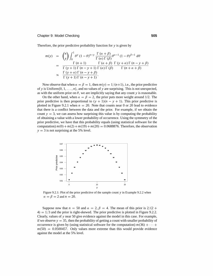
Chapter 9: Model Checking 505
Therefore, the prior predictive probability function for y is given by
m(y) =$
n
y
%6 1
0θ y (1− θ)n−y 7 (α + β)
7 (α)7 (β)θα−1 (1− θ)β−1 dθ
= 7 (n + 1)7 (y + 1) 7 (n − y + 1)
7 (α + β)7 (α)7 (β)
7 (y + α)7 (n − y + β)7 (n + α + β)
∝ 7 (y + α)7 (n − y + β)7 (y + 1) 7 (n − y + 1)
.
Now observe that when α = β = 1, then m(y) = 1/(n+1), i.e., the prior predictiveof y is Uniform{0, 1, . . . , n}, and no values of y are surprising. This is not unexpected,as with the uniform prior on θ, we are implicitly saying that any count y is reasonable.
On the other hand, when α = β = 2, the prior puts more weight around 1/2. Theprior predictive is then proportional to (y + 1)(n − y + 1). This prior predictive isplotted in Figure 9.2.1 when n = 20. Note that counts near 0 or 20 lead to evidencethat there is a conflict between the data and the prior. For example, if we obtain thecount y = 3, we can assess how surprising this value is by computing the probabilityof obtaining a value with a lower probability of occurrence. Using the symmetry of theprior predictive, we have that this probability equals (using statistical software for thecomputation) m(0)+m(2)+m(19)+m(20) = 0.0688876. Therefore, the observationy = 3 is not surprising at the 5% level.
20100
0.07
0.06
0.05
0.04
0.03
0.02
0.01
y
Prio
r pr
edic
tive
Figure 9.2.1: Plot of the prior predictive of the sample count y in Example 9.2.2 whenα = β = 2 and n = 20.
Suppose now that n = 50 and α = 2, β = 4. The mean of this prior is 2/(2 +4) = 1/3 and the prior is right-skewed. The prior predictive is plotted in Figure 9.2.2.Clearly, values of y near 50 give evidence against the model in this case. For example,if we observe y = 35, then the probability of getting a count with smaller probability ofoccurrence is given by (using statistical software for the computation) m(36) + · · · +m(50) = 0.0500457. Only values more extreme than this would provide evidenceagainst the model at the 5% level.

506 Section 9.2: Checking for Prior–Data Conflict
50403020100
0.04
0.03
0.02
0.01
0.00
y
Prio
r p
red
ictiv
e
Figure 9.2.2: Plot of the prior predictive of the sample count y in Example 9.2.2 whenα = 2, β = 4 and n = 50.
EXAMPLE 9.2.3 Checking a Normal Prior for a Location Normal ModelSuppose that (x1, . . . , xn) is a sample from an N(µ, σ 2
0) distribution, where µ ∈ R1
is unknown and σ 20 is known. Suppose we take the prior distribution of µ to be an
N(µ0, τ20) for some specified choice of µ0 and τ 2
0. Note that x is a minimal sufficientstatistic for this model, so we need to compare the observed of this statistic to its priorpredictive distribution to assess whether or not there is prior–data conflict.
Now we can write x = µ + z, where µ ∼ N(µ0, τ20) independent of z ∼
N(0, σ 20/n). From this, we immediately deduce (see Exercise 9.2.3) that the prior pre-
dictive distribution of x is N(µ0, τ20+σ 2
0/n). From the symmetry of the prior predictivedensity about µ0, we immediately see that the appropriate P-value is
M(|X − µ0| ≤ |x − µ0|) = 2(1−0(|x − µ0|/(τ 20 + σ 2
0/n)1/2)). (9.2.1)
So a small value of (9.2.1) is evidence that there is a conflict between the observed dataand the prior, i.e., the prior is putting most of its mass on values of µ for which theobserved data are surprising.
Another possibility for model checking in this context is to look at the posteriorpredictive distribution of the data. Consider, however, the following example.
EXAMPLE 9.2.4 (Example 9.2.1 continued)Recall that, in Example 9.2.1, we concluded that a prior–data conflict existed. Note,however, that the posterior probability of θ = 2 is
(0.0001) (0.9)20
(0.9999) (0.1)20 + (0.0001) (0.9)20≈ 1.
Therefore, the posterior predictive probability of the observed sequence of 20 values of1 is 0.12158, which does not indicate any prior–data conflict. We note, however, thatin this example, the amount of data are sufficient to overwhelm the prior; thus we areled to a sensible inference about θ.
Chapter 9: Model Checking 507
The problem with using the posterior predictive to assess whether or not a prior–data conflict exists is that we have an instance of the so-called double use of the data.For we have fit the model, i.e., constructed the posterior predictive, using the observeddata, and then we tried to use this posterior predictive to assess whether or not a prior–data conflict exists. The double use of the data results in overly optimistic assessmentsof the validity of the Bayesian model and will often not detect discrepancies. We willnot discuss posterior model checking further in this text.
We have only touched on the basics of checking for prior–data conflict here. Withmore complicated models, the possibility exists of checking individual components of aprior, e.g., the components of the prior specified in Example 7.1.4 for the location-scalenormal model, to ascertain more precisely where a prior–data conflict is arising. Also,ancillary statistics play a role in checking for prior–data conflict as we must remove anyancillary variation when computing the P-value because this variation does not dependon the prior. Furthermore, when the prior predictive distribution of a minimal sufficientstatistic is continuous, then issues concerning exactly how P-values are to be computedmust be addressed. These are all topics for a further course in statistics.
Summary of Section 9.2
• In Bayesian inference, there are two potential sources of model incorrectness.First, the sampling model for the data may be incorrect. Second, even if thesampling model is correct, the prior may conflict with the data in the sense thatmost of the prior probability is assigned to distributions in the model for whichthe data are surprising.
• We first check for the correctness of the sampling model using the methods ofSection 9.1. If we do not find evidence against the sampling model, we nextcheck for prior–data conflict by seeing if the observed value of a minimal suffi-cient statistic is surprising or not, with respect to the prior predictive distributionof this quantity.
• Even if a prior–data conflict exists, posterior inferences may still be valid if wehave enough data.
EXERCISES
9.2.1 Suppose we observe the value s = 2 from the model, given by the followingtable.
s = 1 s = 2 s = 3f1(s) 1/3 1/3 1/3f2(s) 1/3 0 2/3
(a) Do the observed data lead us to doubt the validity of the model? Explain why orwhy not.(b) Suppose the prior, given by π(1) = 0.3, is placed on the parameter θ ∈ {1, 2}.Is there any evidence of a prior–data conflict? (Hint: Compute the prior predictive foreach possible data set and assess whether or not the observed data set is surprising.)

508 Section 9.2: Checking for Prior–Data Conflict
(c) Repeat part (b) using the prior given by π(1) = 0.01.9.2.2 Suppose a sample of n = 6 is taken from a Bernoulli(θ) distribution, where θhas a Beta(3, 3) prior distribution. If the value nx = 2 is obtained, then determinewhether there is any prior–data conflict.9.2.3 In Example 9.2.3, establish that the prior predictive distribution of x is given bythe N(µ0, τ
20 + σ 2
0/n) distribution.9.2.4 Suppose we have a sample of n = 5 from an N(µ, 2) distribution where µ isunknown and the value x = 7.3 is observed. An N(0, 1) prior is placed on µ. Computethe appropriate P-value to check for prior–data conflict.9.2.5 Suppose that x ∼ Uniform[0, θ] and θ ∼Uniform[0, 1]. If the value x = 2.2 isobserved, then determine an appropriate P-value for checking for prior–data conflict.
COMPUTER EXERCISES
9.2.6 Suppose a sample of n = 20 is taken from a Bernoulli(θ) distribution, whereθ has a Beta(3, 3) prior distribution. If the value nx = 6 is obtained, then determinewhether there is any prior–data conflict.
PROBLEMS
9.2.7 Suppose that (x1, . . . , xn) is a sample from an N(µ, σ 20) distribution, where µ ∼
N(µ0, τ20). Determine the prior predictive distribution of x.
9.2.8 Suppose that (x1, . . . , xn) is a sample from an Exponential(θ) distribution whereθ ∼ Gamma(α0, β0). Determine the prior predictive distribution of x.
9.2.9 Suppose that (s1, . . . , sn) is a sample from a Multinomial(1, θ1, . . . , θk) distri-bution, where (θ1, . . . , θk−1) ∼ Dirichlet(α1, . . . , αk). Determine the prior predictivedistribution of (x1, . . . , xk), where xi is the count in the i th category.9.2.10 Suppose that (x1, . . . , xn) is a sample from a Uniform[0, θ] distribution, whereθ has prior density given by πα,β(θ) = θ−α I[β,∞)(θ)/(α−1)βα−1,where α > 1, β >0. Determine the prior predictive distribution of x(n).9.2.11 Suppose we have the context of Example 9.2.3. Determine the limiting P-valuefor checking for prior–data conflict as n → ∞. Interpret the meaning of this P-valuein terms of the prior and the true value of µ.9.2.12 Suppose that x ∼ Geometric(θ) distribution and θ ∼ Uniform[0, 1].(a) Determine the appropriate P-value for checking for prior–data conflict.(b) Based on the P-value determined in part (a), describe the circumstances under whichevidence of prior–data conflict will exist.(c) If we use a continuous prior that is positive at a point, then this an assertion thatthe point is possible. In light of this, discuss whether or not a continuous prior that ispositive at θ = 0 makes sense for the Geometric(θ) distribution.
CHALLENGES
9.2.13 Suppose that X1, . . . , Xn is a sample from an N(µ, σ 2) distribution whereµ |σ 2 ∼ N(µ0, τ
20σ
2) and 1/σ 2 ∼ Gamma(α0, β0). Then determine a form for the

Chapter 9: Model Checking 509
prior predictive density of (X, S2) that you could evaluate without integrating. (Hint:Use the algebraic manipulations found in Section 7.5.)
9.3 The Problem with Multiple ChecksAs we have mentioned throughout this text, model checking is a part of good statisticalpractice. In other words, one should always be wary of the value of statistical workin which the investigators have not engaged in, and reported the results of, reasonablyrigorous model checking. It is really the job of those who report statistical results toconvince us that their models are reasonable for the data collected, bearing in mind theeffects of both underfitting and overfitting.
In this chapter, we have reported some of the possible model-checking approachesavailable. We have focused on the main categories of procedures and perhaps themost often used methods from within these. There are many others. At this point, wecannot say that any one approach is the best possible method. Perhaps greater insightalong these lines will come with further research into the topic, and then a clearerrecommendation could be made.
One recommendation that can be made now, however, is that it is not reasonable togo about model checking by implementing every possible model-checking procedureyou can. A simple example illustrates the folly of such an approach.
EXAMPLE 9.3.1Suppose that (x1, . . . , xn) is supposed to be a sample from the N(0, 1) distribution.Suppose we decide to check this model by computing the P-values
Pi = P(X2i ≥ x2
i )
for i = 1, . . . , n, where X2i ∼ χ2(1). Furthermore, we will decide that the model is
incorrect if the minimum of these P-values is less than 0.05.Now consider the repeated sampling behavior of this method when the model is
correct. We have thatmin {P1, . . . , Pn} < 0.05
if and only ifmax{x2
1, . . . , x2n} ≥ χ2
0.95(1),
and so
P (min {P1, . . . , Pn} < 0.05)
= P(max{X21, . . . , X2
n} ≥ χ20.95(1)) = 1− P(max{X2
1, . . . , X2n} ≤ χ2
0.05(1))
= 1−n7
i=1
P(X2i ≤ χ2
0.95(1)) = 1− (0.95)n → 1
as n →∞. This tells us that if n is large enough, we will reject the model with virtualcertainty even though it is correct! Note that n does not have to be very large for thereto be an appreciable probability of making an error. For example, when n = 10, the

510 Section 9.3: The Problem with Multiple Checks
probability of making an error is 0.40; when n = 20 the probability of making an erroris 0.64; and when n = 100, the probability of making an error is 0.99.
We can learn an important lesson from Example 9.3.1, for, if we carry out too manymodel-checking procedures, we are almost certain to find something wrong — even ifthe model is correct. The cure for this is that before actually observing the data (sothat our choices are not determined by the actual data obtained), we decide on a fewrelevant model-checking procedures to be carried out and implement only these.
The problem we have been discussing here is sometimes referred to as the problemof multiple comparisons, which comes up in other situations as well — e.g., see Sec-tion 10.4.1, where multiple means are compared via pairwise tests for differences inthe means. One approach for avoiding the multiple-comparisons problem is to simplylower the cutoff for the P-value so that the probability of making a mistake is appro-priately small. For example, if we decided in Example 9.3.1 that evidence against themodel is only warranted when an individual P-value is smaller than 0.0001, then theprobability of making a mistake is 0.01 when n = 100. A difficulty with this approachgenerally is that our model-checking procedures will not be independent, and it doesnot always seem possible to determine an appropriate cutoff for the individual P-values.More advanced methods are needed to deal with this problem.
Summary of Section 9.3
• Carrying out too many model checks is not a good idea, as we will invariablyfind something that leads us to conclude that the model is incorrect. Rather thanengaging in a “fishing expedition,” where we just keep on checking the model,it is better to choose a few procedures before we see the data, and use these, andonly these, for the model checking.

Chapter 10
Relationships AmongVariables
CHAPTER OUTLINE
Section 1 Related VariablesSection 2 Categorical Response and PredictorsSection 3 Quantitative Response and PredictorsSection 4 Quantitative Response and Categorical PredictorsSection 5 Categorical Response and Quantitative PredictorsSection 6 Further Proofs (Advanced)
In this chapter, we are concerned with perhaps the most important application of sta-tistical inference: the problem of analyzing whether or not a relationship exists amongvariables and what form the relationship takes. As a particular instance of this, recallthe example and discussion in Section 5.1.
Many of the most important problems in science and society are concerned with re-lationships among variables. For example, what is the relationship between the amountof carbon dioxide placed into the atmosphere and global temperatures? What is the re-lationship between class size and scholastic achievement by students? What is therelationship between weight and carbohydrate intake in humans? What is the relation-ship between lifelength and the dosage of a certain drug for cancer patients? These areall examples of questions whose answers involve relationships among variables. Wewill see that statistics plays a key role in answering such questions.
In Section 10.1, we provide a precise definition of what it means for variables tobe related, and we distinguish between two broad categories of relationship, namely,association and cause–effect. Also, we discuss some of the key ideas involved in col-lecting data when we want to determine whether a cause–effect relationship exists. Inthe remaining sections, we examine the various statistical methodologies that are usedto analyze data when we are concerned with relationships.
We emphasize the use of frequentist methodologies in this chapter. We give someexamples of the Bayesian approach, but there are some complexities involved with thedistributional problems associated with Bayesian methods that are best avoided at this
511

512 Section 10.1: Related Variables
stage. Sampling algorithms for the Bayesian approach have been developed, along thelines of those discussed in Chapter 7 (see also Chapter 11), but their full discussionwould take us beyond the scope of this text. It is worth noting, however, that Bayesiananalyses with diffuse priors will often yield results very similar to those obtained viathe frequentist approach.
As discussed in Chapter 9, model checking is an important feature of any statisticalanalysis. For the models used in this chapter, a full discussion of the more rigorous P-value approach to model checking requires more development than we can accomplishin this text. As such, we emphasize the informal approach to model checking, viaresidual and probability plots. This should not be interpreted as a recommendation thatthese are the preferred methods for such models.
10.1 Related VariablesConsider a population# with two variables X,Y : #→ R1 defined on it. What doesit mean to say that the variables X and Y are related? Perhaps our first inclination is tosay that there must be a formula relating the two variables, such as Y = a + bX2 forsome choice of constants a and b, or Y = exp(X), etc. But consider a population #of humans and suppose X (π) is the weight of π in kilograms and Y (π) is the heightof individual π ∈ # in centimeters. From our experience, we know that taller peopletend to be heavier, so we believe that there is some kind of relationship between heightand weight. We know, too, that there cannot be an exact formula that describes thisrelationship, because people with the same weight will often have different heights,and people with the same height will often have different weights.
10.1.1 The Definition of Relationship
If we think of all the people with a given weight x , then there will be a distributionof heights for all those individuals π that have weight x . We call this distribution theconditional distribution of Y, given that X = x .
We can now express what we mean by our intuitive idea that X and Y are related,for, as we change the value of the weight that we condition on, we expect the condi-tional distribution to change. In particular, as x increases, we expect that the locationof the conditional distribution will increase, although other features of the distributionmay change as well. For example, in Figure 10.1.1 we provide a possible plot of twoapproximating densities for the conditional distributions of Y given X = 70 kg andthe conditional distribution of Y given X = 90 kg.
We see that the conditional distribution has shifted up when X goes from 70 to 90kg but also that the shape of the distribution has changed somewhat as well. So we cansay that a relationship definitely exists between X and Y, at least in this population. No-tice that, as defined so far, X and Y are not random variables, but they become so whenwe randomly select π from the population. In that case, the conditional distributionsreferred to become the conditional probability distributions of the random variable Y,given that we observe X = 70 and X = 90, respectively.
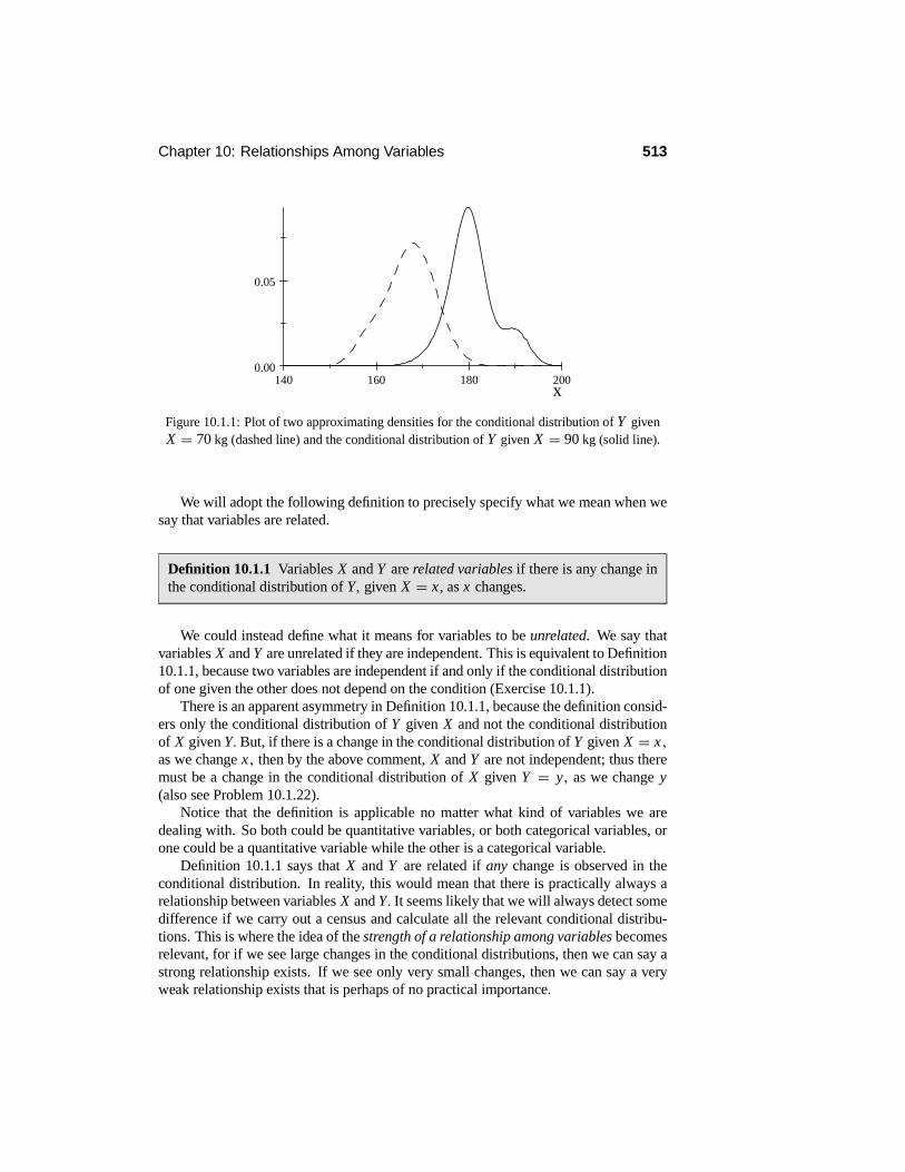
Chapter 10: Relationships Among Variables 513
140 160 180 2000.00
0.05
x
Figure 10.1.1: Plot of two approximating densities for the conditional distribution of Y givenX = 70 kg (dashed line) and the conditional distribution of Y given X = 90 kg (solid line).
We will adopt the following definition to precisely specify what we mean when wesay that variables are related.
Definition 10.1.1 Variables X and Y are related variables if there is any change inthe conditional distribution of Y, given X = x , as x changes.
We could instead define what it means for variables to be unrelated. We say thatvariables X and Y are unrelated if they are independent. This is equivalent to Definition10.1.1, because two variables are independent if and only if the conditional distributionof one given the other does not depend on the condition (Exercise 10.1.1).
There is an apparent asymmetry in Definition 10.1.1, because the definition consid-ers only the conditional distribution of Y given X and not the conditional distributionof X given Y. But, if there is a change in the conditional distribution of Y given X = x,as we change x, then by the above comment, X and Y are not independent; thus theremust be a change in the conditional distribution of X given Y = y, as we change y(also see Problem 10.1.22).
Notice that the definition is applicable no matter what kind of variables we aredealing with. So both could be quantitative variables, or both categorical variables, orone could be a quantitative variable while the other is a categorical variable.
Definition 10.1.1 says that X and Y are related if any change is observed in theconditional distribution. In reality, this would mean that there is practically always arelationship between variables X and Y. It seems likely that we will always detect somedifference if we carry out a census and calculate all the relevant conditional distribu-tions. This is where the idea of the strength of a relationship among variables becomesrelevant, for if we see large changes in the conditional distributions, then we can say astrong relationship exists. If we see only very small changes, then we can say a veryweak relationship exists that is perhaps of no practical importance.

514 Section 10.1: Related Variables
The Role of Statistical Models
If a relationship exists between two variables, then its form is completely described bythe set of conditional distributions of Y given X . Sometimes it may be necessary todescribe the relationship using all these conditional distributions. In many problems,however, we look for a simpler presentation. In fact, we often assume a statisticalmodel that prescribes a simple form for how the conditional distributions change as wechange X.
Consider the following example.
EXAMPLE 10.1.1 Simple Normal Linear Regression ModelIn Section 10.3.2, we will discuss the simple normal linear regression model, wherethe conditional distribution of quantitative variable Y, given the quantitative variableX = x , is assumed to be distributed
N(β1 + β2x, σ 2),
where β1, β2, and σ 2 are unknown. For example, Y could be the blood pressure of anindividual and X the amount of salt the person consumed each day.
In this case, the conditional distributions have constant shape and change, as xchanges, only through the conditional mean. The mean moves along the line given byβ1+β2x for some intercept β1 and slope β2. If this model is correct, then the variablesare unrelated if and only if β2 = 0, as this is the only situation in which the conditionaldistributions can remain constant as we change x.
Statistical models, like that described in Example 10.1.1, can be wrong. Thereis nothing requiring that two quantitative variables must be related in that way. Forexample, the conditional variance of Y can vary with x , and the very shape of theconditional distribution can vary with x , too. The model of Example 10.1.1 is aninstance of a simplifying assumption that is appropriate in many practical contexts.However, methods such as those discussed in Chapter 9 must be employed to checkmodel assumptions before accepting statistical inferences based on such a model. Wewill always consider model checking as part of our discussion of the various modelsused to examine the relationship among variables.
Response and Predictor Variables
Often, we think of Y as a dependent variable (depending on X) and of X as an indepen-dent variable (free to vary). Our goal, then, is to predict the value of Y given the valueof X . In this situation, we call Y the response variable and X the predictor variable.
Sometimes, though, there is really nothing to distinguish the roles of X and Y . Forexample, suppose that X is the weight of an individual in kilograms and Y is the heightin centimeters. We could then think of predicting weight from height or conversely. Itis then immaterial which we choose to condition on.
In many applications, there is more than one response variable and more than onepredictor variable X. We will not consider the situation in which we have more thanone response variable, but we will consider the case in which X = (X1, . . . , Xk) is

Chapter 10: Relationships Among Variables 515
k-dimensional. Here, the various predictors that make up X could be all categorical,all quantitative, or some mixture of categorical and quantitative variables.
The definition of a relationship existing between response variable Y and the set ofpredictors (X1, . . . , Xk) is exactly as in Definition 10.1.1. In particular, a relationshipexists between Y and (X1, . . . , Xk) if there is any change in the conditional distributionof Y given (X1, . . . , Xk) = (x1, . . . , xk)when (x1, . . . , xk) is varied. If such a relation-ship exists, then the form of the relationship is specified by the full set of conditionaldistributions. Again, statistical models are often used where simplifying assumptionsare made about the form of the relationship. Consider the following example.
EXAMPLE 10.1.2 The Normal Linear Model with k PredictorsIn Section 10.3.4, we will discuss the normal multiple linear regression model. Forthis, the conditional distribution of quantitative variable Y, given that the quantitativepredictors (X1, . . . , Xk) = (x1, . . . , xk), is assumed to be the
N(β1 + β2x1 + · · · + βk+1xk, σ2)
distribution, where β1, . . . , βk+1 and σ 2 are unknown. For example, Y could be bloodpressure, X1 the amount of daily salt intake, X2 the age of the individual, X3 the weightof the individual, etc.
In this case, the conditional distributions have constant shape and change, as thevalues of the predictors (x1, . . . , xk) change only through the conditional mean, whichchanges according to the function β1+β2x1+· · ·+βk+1xk . Notice that, if this modelis correct, then the variables are unrelated if and only if β2 = · · · = βk+1 = 0, as thisis the only situation in which the conditional distributions can remain constant as wechange (x1, . . . , xk).
When we split a set of variables Y, X1, . . . , Xk into response Y and predictors(X1, . . . , Xk), we are implicitly saying that we are directly interested only in the con-ditional distributions of Y given (X1, . . . , Xk). There may be relationships among thepredictors X1, . . . , Xk, however, and these can be of interest.
For example, suppose we have two predictors X1 and X2, and the conditional dis-tribution of X1 given X2 is virtually degenerate at a value a + cX2 for some constantsa and c. Then it is not a good idea to include both X1 and X2 in a model, such asthat discussed in Example 10.1.2, as this can make the analysis very sensitive to smallchanges in the data. This is known as the problem of multicollinearity. The effect ofmulticollinearity, and how to avoid it, will not be discussed any further in this text. Thisis, however, a topic of considerable practical importance.
Regression Models
Suppose that the response Y is quantitative and we have k predictors (X1, . . . , Xk).One of the most important simplifying assumptions used in practice is the regressionassumption, namely, we assume that, as we change (X1, . . . , Xk), the only thing thatcan possibly change about the conditional distribution of Y given (X1, . . . , Xk), is theconditional mean E(Y | X1, . . . , Xk). The importance of this assumption is that, to an-alyze the relationship between Y and (X1, . . . , Xk), we now need only consider how

516 Section 10.1: Related Variables
E(Y | X1, . . . , Xk) changes as (X1, . . . , Xk) changes. Indeed, if E(Y | X1, . . . , Xk)does not change as (X1, . . . , Xk) changes, then there is no relationship between Yand the predictors. Of course, this kind of an analysis is dependent on the regressionassumption holding, and the methods of Section 9.1 must be used to check this. Regres-sion models — namely, statistical models where we make the regression assumption— are among the most important statistical models used in practice. Sections 10.3 and10.4 discuss several instances of regression models.
Regression models are often presented in the form
Y = E(Y | X1, . . . , Xk)+ Z, (10.1.1)
where Z = Y − E(Y | X1, . . . , Xk) is known as the error term. We see immedi-ately that, if the regression assumption applies, then the conditional distribution of Zgiven (X1, . . . , Xk) is fixed as we change (X1, . . . , Xk) and, conversely, if the con-ditional distribution of Z given (X1, . . . , Xk) is fixed as we change (X1, . . . , Xk),then the regression assumption holds. So when the regression assumption applies,(10.1.1) provides a decomposition of Y into two parts: (1) a part possibly dependent on(X1, . . . , Xk), namely, E(Y | X1, . . . , Xk), and (2) a part that is always independentof (X1, . . . , Xk), namely, the error Z . Note that Examples 10.1.1 and 10.1.2 can bewritten in the form (10.1.1), where Z ∼ N(0, σ 2).
10.1.2 Cause–Effect Relationships and Experiments
Suppose now that we have variables X and Y defined on a population # and haveconcluded that a relationship exists according to Definition 10.1.1. This may be basedon having conducted a full census of #, or, more typically, we will have drawn asimple random sample from# and then used the methods of the remaining sections ofthis chapter to conclude that such a relationship exists. If Y is playing the role of theresponse and if X is the predictor, then we often want to be able to assert that changesin X are causing the observed changes in the conditional distributions of Y. Of course,if there are no changes in the conditional distributions, then there is no relationshipbetween X and Y and hence no cause–effect relationship, either.
For example, suppose that the amount of carbon dioxide gas being released in theatmosphere is increasing, and we observe that mean global temperatures are rising. Ifwe have reason to believe that the amount of carbon dioxide released can have an effecton temperature, then perhaps it is sensible to believe that the increase in carbon dioxideemissions is causing the observed increase in mean global temperatures. As anotherexample, for many years it has been observed that smokers suffer from respiratorydiseases much more frequently than do nonsmokers. It seems reasonable, then, toconclude that smoking causes an increased risk for respiratory disease. On the otherhand, suppose we consider the relationship between weight and height. It seems clearthat a relationship exists, but it does not make any sense to say that changes in one ofthe variables is causing the changes in the conditional distributions of the other.

Chapter 10: Relationships Among Variables 517
Confounding Variables
When can we say that an observed relationship between X and Y is a cause–effectrelationship? If a relationship exists between X and Y, then we know that there are atleast two values x1 and x2 such that fY (· | X = x1) 6= fY (· | X = x2), i.e., these twoconditional distributions are not equal. If we wish to say that this difference is causedby the change in X , then we have to know categorically that there is no other variableZ defined on # that confounds with X. The following example illustrates the idea oftwo variables confounding.
EXAMPLE 10.1.3Suppose that # is a population of students such that most females hold a part-timejob and most males do not. A researcher is interested in the distribution of grades, asmeasured by grade point average (GPA), and is looking to see if there is a relationshipbetween GPA and gender. On the basis of the data collected, the researcher observesa difference in the conditional distribution of GPA given gender and concludes that arelationship exists between these variables. It seems clear, however, that an assertionof a cause–effect relationship existing between GPA and gender is not warranted, asthe difference in the conditional distributions could also be attributed to the differencein part-time work status rather than gender. In this example, part-time work status andgender are confounded.
A more careful analysis might rescue the situation described in Example 10.1.3, forif X and Z denote the confounding variables, then we could collect data on Z as welland examine the conditional distributions fY (· | X = x, Z = z). In Example 10.1.3,these will be the conditional distributions of GPA, given gender and part-time workstatus. If these conditional distributions change as we change x, for some fixed valueof z, then we could assert that a cause–effect relationship exists between X and Yprovided there are no further confounding variables. Of course, there are probably stillmore confounding variables, and we really should be conditioning on all of them. Thisbrings up the point that, in any practical application, we almost certainly will nevereven know all the potential confounding variables.
Controlling Predictor Variable Assignments
Fortunately, there is sometimes a way around the difficulties raised by confoundingvariables. Suppose we can control the value of the variable X for any π ∈ #, i.e.,we can assign the value x to π so that X (π) = x for any of the possible values of x.In Example 10.1.3, this would mean that we could assign a part-time work status toany student in the population. Now consider the following idealized situation. Imagineassigning every element π ∈ # the value X (π) = x1 and then carrying out a censusto obtain the conditional distribution fY (· | X = x1). Now imagine assigning everyπ ∈ # the value X (π) = x2 and then carrying out a census to obtain the conditionaldistribution fY (· | X = x2). If there is any difference in fY (· | X = x1) and fY (· | X =x2), then the only possible reason is that the value of X differs. Therefore, if fY (· | X =x1) 6= fY (· | X = x2), we can assert that a cause–effect relationship exists.

518 Section 10.1: Related Variables
A difficulty with the above argument is that typically we can never exactly deter-mine fY (· | X = x1) and fY (· | X = x2). But in fact, we may be able to sample fromthem, then the methods of statistical inference become available to us to infer whetheror not there is any difference. Suppose we take a random sample π1, . . . , πn1+n2 from# and randomly assign n1 of these the value X = x1, with the remaining π’s assignedthe value x2. We obtain the Y values y11, . . . , y1n1 for those π’s assigned the value x1and obtain the Y values y21, . . . , y2n2 for those π’s assigned the value x2. Then it is ap-parent that y11, . . . , y1n1 is a sample from fY (· | X = x1) and y21, . . . , y2n2 is a samplefrom fY (· | X = x2). In fact, provided that n1 + n2 is small relative to the populationsize, then we can consider these as i.i.d. samples from these conditional distributions.
So we see that in certain circumstances, it is possible to collect data in such a waythat we can make inferences about whether or not a cause–effect relationship exists.We now specify the characteristics of the relevant data collection technique.
Conditions for Cause–Effect Relationships
First, if our inferences are to apply to a population #, then we must have a randomsample from that population. This is just the characteristic of what we called a samplingstudy in Section 5.4, and we must do this to avoid any selection effects. So if thepurpose of a study is to examine the relationship between the duration of migraineheadaches and the dosage of a certain drug, the investigator must have a random samplefrom the population of migraine headache sufferers.
Second, we must be able to assign any possible value of the predictor variable Xto any selected π . If we cannot do this, or do not do this, then there may be hiddenconfounding variables (sometimes called lurking variables) that are influencing theconditional distributions of Y . So in a study of the effects of the dosage of a drugon migraine headaches, the investigator must be able to impose the dosage on eachparticipant in the study.
Third, after deciding what values of X we will use in our study, we must randomlyallocate these values to members of the sample. This is done to avoid the possibility ofselection effects. So, after deciding what dosages to use in the study of the effects ofthe dosage of a drug on migraine headaches, and how many participants will receiveeach dosage, the investigator must randomly select the individuals who will receiveeach dosage. This will (hopefully) avoid selection effects, such as only the healthiestindividuals getting the lowest dosage, etc.
When these requirements are met, we refer to the data collection process as anexperiment. Statistical inference based on data collected via an experiment has the ca-pability of inferring that cause–effect relationships exist, so this represents an importantand powerful scientific tool.
A Hierarchy of Studies
Combining this discussion with Section 5.4, we see a hierarchy of data collection meth-ods. Observational studies reside at the bottom of the hierarchy. Inferences drawnfrom observational studies must be taken with a degree of caution, for selection effectscould mean that the results do not apply to the population intended, and the existence

Chapter 10: Relationships Among Variables 519
of confounding variables means that we cannot make inferences about cause–effect re-lationships. For sampling studies, we know that any inferences drawn will be aboutthe appropriate population; but the existence of confounding variables again causesdifficulties for any statements about the existence of cause–effect relationships, e.g.,just taking random samples of males and females from the population # of Example10.1.3 will not avoid the confounding variables. At the top of the hierarchy resideexperiments.
It is probably apparent that it is often impossible to conduct an experiment. InExample 10.1.3, we cannot assign the value of gender, so nothing can be said about theexistence of a cause–effect relationship between GPA and gender.
There are many notorious examples in which assertions are made about the exis-tence of cause–effect relationships but for which no experiment is possible. For exam-ple, there have been a number of studies conducted where differences have been notedamong the IQ distributions of various racial groups. It is impossible, however, to con-trol the variable racial origin, so it is impossible to assert that the observed differencesin the conditional distributions of IQ, given race, are caused by changes in race.
Another example concerns smoking and lung cancer in humans. It has been pointedout that it is impossible to conduct an experiment, as we cannot assign values of thepredictor variable (perhaps different amounts of smoking) to humans at birth and thenobserve the response, namely, whether someone contracts lung cancer or not. Thisraises an important point. We do not simply reject the results of analyses based onobservational studies or sampling studies because the data did not arise from an ex-periment. Rather, we treat these as evidence — potentially flawed evidence, but stillevidence.
Think of eyewitness evidence in a court of law suggesting that a crime was com-mitted by a certain individual. Eyewitness evidence may be unreliable, but if two orthree unconnected eyewitnesses give similar reports, then our confidence grows in thereliability of the evidence. Similarly, if many observational and sampling studies seemto indicate that smoking leads to an increased risk for contracting lung cancer, then ourconfidence grows that a cause–effect relationship does indeed exist. Furthermore, if wecan identify potentially confounding variables, then observational or sampling studiescan be conducted taking these into account, increasing our confidence still more. Ul-timately, we may not be able to definitively settle the issue via an experiment, but it isstill possible to build overwhelming evidence that smoking and lung cancer do have acause–effect relationship.
10.1.3 Design of Experiments
Suppose we have a response Y and a predictor X (sometimes called a factor in experi-mental contexts) defined on a population #, and we want to collect data to determinewhether a cause–effect relationship exists between them. Following the discussion inSection 10.1.1, we will conduct an experiment. There are now a number of decisionsto be made, and our choices constitute what we call the design of the experiment.
For example, we are going to assign values of X to the sampled elements, nowcalled experimental units, π1, . . . , πn from #. Which of the possible values of X

520 Section 10.1: Related Variables
should we use? When X can take only a small finite number of values, then it isnatural to use these values. On the other hand, when the number of possible values ofX is very large or even infinite, as with quantitative predictors, then we have to choosevalues of X to use in the experiment.
Suppose we have chosen the values x1, . . . , xk for X . We refer to x1, . . . , xk asthe levels of X ; any particular assignment xi to a π j in the sample will be called atreatment. Typically, we will choose the levels so that they span the possible range ofX fairly uniformly. For example, if X is temperature in degrees Celsius, and we wantto examine the relationship between Y and X for X in the range [0, 100], then, usingk = 5 levels, we might take x1 = 0, x2 = 25, x3 = 50, x4 = 75, and x5 = 100.
Having chosen the levels of X , we then have to choose how many treatments of eachlevel we are going to use in the experiment, i.e., decide how many response values niwe are going to observe at level xi for i = 1, . . . , k.
In any experiment, we will have a finite amount of resources (money, time, etc.) atour disposal, which determines the sample size n from #. The question then is howshould we choose the ni so that n1 + · · · + nk = n? If we know nothing about theconditional distributions fY (· | X = xi ), then it makes sense to use balance, namely,choose n1 = · · · = nk .
On the other hand, suppose we know that some of the fY (· | X = xi ) will exhibitgreater variability than others. For example, we might measure variability by the vari-ance of fY (· | X = xi ). Then it makes sense to allocate more treatments to the levels ofX where the response is more variable. This is because it will take more observationsto make accurate inferences about characteristics of such an fY (· | X = xi ) than for theless variable conditional distributions.
As discussed in Sections 6.3.4 and 6.3.5, we also want to choose the ni so that anyinferences we make have desired accuracy. Methods for choosing the sample sizes ni ,similar to those discussed in Chapter 7, have been developed for these more compli-cated designs, but we will not discuss these any further here.
Suppose, then, that we have determined {(x1, n1) , . . . , (xk, nk)} . We refer to thisset of ordered pairs as the experimental design.
Consider some examples.
EXAMPLE 10.1.4Suppose that # is a population of students at a given university. The administrationis concerned with determining the value of each student being assigned an academicadvisor. The response variable Y will be a rating that a student assigns on a scale of 1 to10 (completely dissatisfied to completely satisfied with their university experience) atthe end of a given semester. We treat Y as a quantitative variable. A random sample ofn = 100 students is selected from #, and 50 of these are randomly selected to receiveadvisers while the remaining 50 are not assigned advisers.
Here, the predictor X is a categorical variable that indicates whether or not thestudent has an advisor. There are only k = 2 levels, and both are used in the experiment.If x1 = 0 denotes no advisor and x2 = 1 denotes having an advisor, then n1 = n2 = 50and we have a balanced experiment. The experimental design is given by
{(0, 50) , (1, 50)}.

Chapter 10: Relationships Among Variables 521
At the end of the experiment, we want to use the data to make inferences aboutthe conditional distributions fY (· | X = 0) and fY (· | X = 1) to determine whether acause–effect relationship exists. The methods of Section 10.4 will be relevant for this.
EXAMPLE 10.1.5Suppose that # is a population of dairy cows. A feed company is concerned with therelationship between weight gain, measured in kilograms, over a specific time periodand the amount of a supplement, measured in grams/liter, of an additive put into thecows’ feed. Here, the response Y is the weight gain — a quantitative variable. The pre-dictor X is the concentration of the additive. Suppose X can plausibly range between0 and 2, so it is also a quantitative variable.
The experimenter decides to use k = 4 levels with x1 = 0.00, x2 = 0.66, x3 =1.32, and x4 = 2.00. Further, the sample sizes n1 = n2 = n3 = n4 = 10 weredetermined to be appropriate. So the balanced experimental design is given by
{(0.00, 10) , (0.66, 10) , (1.32, 10) , (2.00, 10)}.
At the end of the experiment, we want to make inferences about the conditional distri-butions fY (· | X = 0.00), fY (· | X = 0.66), fY (· | X = 1.32), and fY (· | X = 2.00).The methods of Section 10.3 are relevant for this.
Control Treatment, the Placebo Effect, and Blinding
Notice that in Example 10.1.5, we included the level X = 0, which corresponds tono application of the additive. This is called a control treatment, as it gives a baselineagainst which we can assess the effect of the predictor. In many experiments, it isimportant to include a control treatment.
In medical experiments, there is often a placebo effect — that is, a disease sufferergiven any treatment will often record an improvement in symptoms. The placebo effectis believed to be due to the fact that a sufferer will start to feel better simply becausesomeone is paying attention to the condition. Accordingly, in any experiment to de-termine the efficacy of a drug in alleviating disease symptoms, it is important that acontrol treatment be used as well. For example, if we want to investigate whether ornot a given drug alleviates migraine headaches, then among the dosages we select forthe experiment, we should make sure that we include a pill containing none of the drug(the so-called sugar pill); that way we can assess the extent of the placebo effect. Ofcourse, the recipients should not know whether they are receiving the sugar pill or thedrug. This is called a blind experiment. If we also conceal the identity of the treatmentfrom the experimenters, so as to avoid any biasing of the results on their part, then thisis known as a double-blind experiment.
In Example 10.1.5, we assumed that it is possible to take a sample from the popula-tion of all dairy cows. Strictly speaking, this is necessary if we want to avoid selectioneffects and make sure that our inferences apply to the population of interest. In prac-tice, however, taking a sample of experimental units from the full population of interestis often not feasible. For example, many medical experiments are conducted on ani-

522 Section 10.1: Related Variables
mals, and these are definitely not random samples from the population of the particularanimal in question, e.g., rats.
In such cases, however, we simply recognize the possibility that selection effects orlurking variables could render invalid the conclusions drawn from such analyses whenthey are to be applied to the population of interest. But we still regard the results asevidence concerning the phenomenon under study. It is the job of the experimenter tocome as close as possible to the idealized situation specified by a valid experiment; forexample, randomization is still employed when assigning treatments to experimentalunits so that selection effects are avoided as much as possible.
Interactions
In the experiments we have discussed so far, there has been one predictor. In manypractical contexts, there is more than one predictor. Suppose, then, that there are twopredictors X and W and that we have decided on the levels x1, . . . , xk for X and thelevels w1, . . . , wl for W. One possibility is to look at the conditional distributionsfY (· | X = xi ) for i = 1, . . . , k and fY (· |W = w j ) for j = 1, . . . , l to determinewhether X and W individually have a relationship with the response Y. Such an ap-proach, however, ignores the effect of the two predictors together. In particular, theway the conditional distributions fY (· | X = x,W = w) change as we change x maydepend on w; when this is the case, we say that there is an interaction between thepredictors.
To investigate the possibility of an interaction existing between X and W, we mustsample from each of the kl distributions fY (· | X = xi ,W = w j ) for i = 1, . . . , k andj = 1, . . . , l. The experimental design then takes the form
{(x1,w1, n11) , (x2,w1, n21) , . . . , (xk,wl, nkl)},where ni j gives the number of applications of the treatment
!xi ,w j
". We say that the
two predictors X and W are completely crossed in such a design because each valueof X used in the experiment occurs with each value of W used in the experiment.Of course, we can extend this discussion to the case where there are more than twopredictors. We will discuss in Section 10.4.3 how to analyze data to determine whetherthere are any interactions between predictors.
EXAMPLE 10.1.6Suppose we have a population # of students at a particular university and are investi-gating the relationship between the response Y, given by a student’s grade in calculus,and the predictors W and X . The predictor W is the number of hours of academicadvising given monthly to a student; it can take the values 0, 1, or 2. The predictor Xindicates class size, where X = 0 indicates small class size and X = 1 indicates largeclass size. So we have a quantitative response Y, a quantitative predictor W takingthree values, and a categorical predictor X taking two values. The crossed values ofthe predictors (W, X) are given by the set
{(0, 0) , (1, 0) , (2, 0) , (0, 1) , (1, 1) , (2, 1)},so there are six treatments. To conduct the experiment, the university then takes arandom sample of 6n students and randomly assigns n students to each treatment.

Chapter 10: Relationships Among Variables 523
Sometimes we include additional predictors in an experimental design even whenwe are not primarily interested in their effects on the response Y.We do this because weknow that such a variable has a relationship with Y . Including such predictors allowsus to condition on their values and so investigate more precisely the relationship Y haswith the remaining predictors. We refer to such a variable as a blocking variable.
EXAMPLE 10.1.7Suppose the response variable Y is yield of wheat in bushels per acre, and the predictorvariable X is an indicator variable for which of three types of wheat is being planted inan agricultural study. Each type of wheat is going to be planted on a plot of land, whereall the plots are of the same size, but it is known that the plots used in the experimentwill vary considerably with respect to their fertility. Note that such an experimentis another example of a situation in which it is impossible to randomly sample theexperimental units (the plots) from the full population of experimental units.
Suppose the experimenter can group the available experimental units into plots oflow fertility and high fertility. We call these two classes of fields blocks. Let W indicatethe type of plot. So W is a categorical variable taking two values. It then seems clearthat the conditional distributions fY (· | X = x,W = w)will be much less variable thanthe conditional distributions fY (· | X = x).
In this case, W is serving as a blocking variable. The experimental units in a par-ticular block, the one of low fertility or the one of high fertility, are more homogeneousthan the full set of plots, so variability will be reduced and inferences will be moreaccurate.
Summary of Section 10.1
• We say two variables are related if the conditional distribution of one given theother changes at all, as we change the value of the conditioning variable.
• To conclude that a relationship between two variables is a cause–effect relation-ship, we must make sure that (through conditioning) we have taken account ofall confounding variables.
• Statistics provides a practical way of avoiding the effects of confounding vari-ables via conducting an experiment. For this, we must be able to assign the val-ues of the predictor variable to experimental units sampled from the populationof interest.
• The design of experiments is concerned with determining methods of collectingthe data so that the analysis of the data will lead to accurate inferences concerningquestions of interest.
EXERCISES
10.1.1 Prove that discrete random variables X and Y are unrelated if and only if X andY are independent.10.1.2 Suppose that two variables X and Y defined on a finite population# are func-tionally related as Y = g(X) for some unknown nonconstant function g. Explain how

524 Section 10.1: Related Variables
this situation is covered by Definition 10.1.1, i.e., the definition will lead us to concludethat X and Y are related. What about the situation in which g(x) = c for some value cfor every x? (Hint: Use the relative frequency functions of the variables.)10.1.3 Suppose that a census is conducted on a population and the joint distribution of(X,Y ) is obtained as in the following table.
Y = 1 Y = 2 Y = 3X = 1 0.15 0.18 0.40X = 2 0.12 0.09 0.06
Determine whether or not a relationship exists between Y and X.
10.1.4 Suppose that a census is conducted on a population and the joint distribution of(X,Y ) is obtained as in the following table.
Y = 1 Y = 2 Y = 3X = 1 1/6 1/6 1/3X = 2 1/12 1/12 1/6
Determine whether or not a relationship exists between Y and X.
10.1.5 Suppose that X is a random variable and Y = X2. Determine whether or not Xand Y are related. What happens when X has a degenerate distribution?10.1.6 Suppose a researcher wants to investigate the relationship between birth weightand performance on a standardized test administered to children at two years of age. Ifa relationship is found, can this be claimed to be a cause–effect relationship? Explainwhy or why not?10.1.7 Suppose a large study of all doctors in Canada was undertaken to determinethe relationship between various lifestyle choices and lifelength. If the conditionaldistribution of lifelength given various smoking habits changes, then discuss what canbe concluded from this study.10.1.8 Suppose a teacher wanted to determine whether an open- or closed-book examwas a more appropriate way to test students on a particular topic. The response variableis the grade obtained on the exam out of 100. Discuss how the teacher could go aboutanswering this question.10.1.9 Suppose a researcher wanted to determine whether or not there is a cause–effect relationship between the type of political ad (negative or positive) seen by avoter from a particular population and the way the voter votes. Discuss your advice tothe researcher about how best to conduct the study.10.1.10 If two random variables have a nonzero correlation, are they necessarily re-lated? Explain why or why not.10.1.11 An experimenter wants to determine the relationship between weight changeY over a specified period and the use of a specially designed diet. The predictor variableX is a categorical variable indicating whether or not a person is on the diet. A total of200 volunteers signed on for the study; a random selection of 100 of these were giventhe diet and the remaining 100 continued their usual diet.(a) Record the experimental design.
Chapter 10: Relationships Among Variables 525
(b) If the results of the study are to be applied to the population of all humans, whatconcerns do you have about how the study was conducted?(c) It is felt that the amount of weight lost or gained also is dependent on the initialweight W of a participant. How would you propose that the experiment be altered totake this into account?10.1.12 A study will be conducted, involving the population of people aged 15 to 19 ina particular country, to determine whether a relationship exists between the response Y(amount spent in dollars in a week on music downloads) and the predictors W (gender)and X (age in years).(a) If observations are to be taken from every possible conditional distribution of Ygiven the two factors, then how many such conditional distributions are there?(b) Identify the types of each variable involved in the study.(c) Suppose there are enough funds available to monitor 2000 members of the popula-tion. How would you recommend that these resources be allocated among the variouscombinations of factors?(d) If a relationship is found between the response and the predictors, can this beclaimed to be a cause–effect relationship? Explain why or why not.(e) Suppose that in addition, it was believed that family income would likely have aneffect on Y and that families could be classified into low and high income. Indicatehow you would modify the study to take this into account.10.1.13 A random sample of 100 households, from the set of all households contain-ing two or more members in a given geographical area, is selected and their televisionviewing habits are monitored for six months. A random selection of 50 of the house-holds is sent a brochure each week advertising a certain program. The purpose ofthe study is to determine whether there is any relationship between exposure to thebrochure and whether or not this program is watched.(a) Identify suitable response and predictor variables.(b) If a relationship is found, can this be claimed to be a cause–effect relationship?Explain why or why not.10.1.14 Suppose we have a quantitative response variable Y and two categorical pre-dictor variables W and X , both taking values in {0, 1}. Suppose the conditional distri-butions of Y are given by
Y |W = 0, X = 0 ∼ N (3, 5)
Y |W = 1, X = 0 ∼ N (3, 5)
Y |W = 0, X = 1 ∼ N (4, 5)
Y |W = 1, X = 1 ∼ N (4, 5).
Does W have a relationship with Y ? Does X have a relationship with Y ? Explain youranswers.10.1.15 Suppose we have a quantitative response variable Y and two categorical pre-dictor variables W and X, both taking values in {0, 1}. Suppose the conditional distri-

526 Section 10.1: Related Variables
butions of Y are given by
Y |W = 0, X = 0 ∼ N (2, 5)
Y |W = 1, X = 0 ∼ N (3, 5)
Y |W = 0, X = 1 ∼ N (4, 5)
Y |W = 1, X = 1 ∼ N (4, 5).
Does W have a relationship with Y ? Does X have a relationship with Y ? Explain youranswers.10.1.16 Do the predictors interact in Exercise 10.1.14? Do the predictors interact inExercise 10.1.15? Explain your answers.10.1.17 Suppose we have variables X and Y defined on the population# = {1, 2, . . . ,10}, where X (i) = 1 when i is odd and X (i) = 0 when i is even, Y (i) = 1 when i isdivisible by 3 and Y (i) = 0 otherwise.(a) Determine the relative frequency function of X.
(b) Determine the relative frequency function of Y.
(c) Determine the joint relative frequency function of (X,Y ).(d) Determine all the conditional distributions of Y given X.
(e) Are X and Y related? Justify your answer.10.1.18 A mathematical approach to examining the relationship between variables Xand Y is to see whether there is a function g such that Y = g(X). Explain why thisapproach does not work for many practical applications where we are examining therelationship between variables. Explain how statistics treats this problem.10.1.19 Suppose a variable X takes the values 1 and 2 on a population and the condi-tional distributions of Y given X are N(0, 5) when X = 1, and N(0, 7) when X = 2.Determine whether X and Y are related and if so, describe their relationship.10.1.20 A variable Y has conditional distribution given X specified by N (1+ 2x, |x|)when X = x. Determine if X and Y are related and if so, describe what their relation-ship is.10.1.21 Suppose that X ∼ Uniform[−1, 1] and Y = X2. Determine the correlationbetween Y and X. Are X and Y related?
PROBLEMS
10.1.22 If there is more than one predictor involved in an experiment, do you thinkit is preferable for the predictors to interact or not? Explain your answer. Can theexperimenter control whether or not predictors interact?10.1.23 Prove directly, using Definition 10.1.1, that when X and Y are related variablesdefined on a finite population#, then Y and X are also related.10.1.24 Suppose that X, Y, Z are independent N(0, 1) random variables and that U =X+Z, V = Y+Z .Determine whether or not the variables U and V are related. (Hint:Calculate Cov(U,V ) .)10.1.25 Suppose that (X, Y, Z) ∼ Multinomial(n, 1/3, 1/3, 1/3). Are X and Y re-lated?

Chapter 10: Relationships Among Variables 527
10.1.26 Suppose that (X, Y ) ∼Bivariate-Normal(µ1, µ2, σ 1, σ 2, ρ). Show that X andY are unrelated if and only if Corr(X,Y ) = 0.10.1.27 Suppose that (X, Y, Z) have probability function pX,Y,Z . If Y is related to Xbut not to Z, then prove that pX,Y,Z (x, y, z) = pY |X (y | x)pX |Z (x | z)pZ (z).
10.2 Categorical Response and PredictorsThere are two possible situations when we have a single categorical response Y and asingle categorical predictor X. The categorical predictor is either random or determin-istic, depending on how we sample. We examine these two situations separately.
10.2.1 Random Predictor
We consider the situation in which X is categorical, taking values in {1, . . . , a}, andY is categorical, taking values in {1, . . . , b}. If we take a sample π1, . . . , πn from thepopulation, then the values X (π i) = xi are random, as are the values Y (π i) = y j .
Suppose the sample size n is very small relative to the population size (so we canassume that i.i.d. sampling is applicable). Then, letting θ i j = P(X = i,Y = j), weobtain the likelihood function (see Problem 10.2.15)
L(θ11, . . . , θab | (x1, y1) , . . . , (xn, yn)) =a7
i=1
b7j=1
θfi ji j , (10.2.1)
where fi j is the number of sample values with (X,Y ) = (i, j). An easy computation(see Problem 10.2.16) shows that the MLE of (θ11, . . . , θkl) is given by θ i j = fi j/nand that the standard error of this estimate (because the incidence of a sample memberfalling in the (i, j)-th cell is distributed Bernoulli(θ i j ) and using Example 6.3.2) isgiven by +
θ i j (1− θ i j )
n.
We are interested in whether or not there is a relationship between X and Y . Toanswer this, we look at the conditional distributions of Y given X. The conditionaldistributions of Y given X, using θ i · = θ i1 + · · · + θ ib = P(X = i), are given in thefollowing table.
Y = 1 · · · Y = bX = 1 θ11/θ1· · · · θ1b/θ1·...
......
X = a θa1/θa· · · · θab/θa·

528 Section 10.2: Categorical Response and Predictors
Then estimating θ i j/θ i · by θ i j/θ i · = fi j/ fi ·, where fi · = fi1+· · ·+ fib, the estimatedconditional distributions are as in the following table.
Y = 1 · · · Y = bX = 1 f11/ f1· · · · f1b/ f1·...
......
X = a fa1/ fa· · · · fab/ fa·
If we conclude that there is a relationship between X and Y, then we look at the table ofestimated conditional distributions to determine the form of the relationship, i.e., howthe conditional distributions change as we change the value of X we are conditioningon.
How, then, do we infer whether or not a relationship exists between X and Y?No relationship exists between Y and X if and only if the conditional distributions ofY given X = x do not change with x . This is the case if and only if X and Y areindependent, and this is true if and only if
θ i j = P(X = i,Y = j) = P(X = i)P(Y = j) = θ i ·θ · j ,
for every i and j where θ · j = θ1 j + · · · + θaj = P(Y = j). Therefore, to assesswhether or not there is a relationship between X and Y, it is equivalent to assess thenull hypothesis H0 : θ i j = θ i ·θ · j for every i and j .
How should we assess whether or not the observed data are surprising when H0holds? The methods of Section 9.1.2, and in particular Theorem 9.1.2, can be appliedhere, as we have that
(F11, F12, . . . , Fab) ∼ Multinomial(n, θ1·θ ·1, θ1·θ ·2, . . . , θa·θ ·b)
when H0 holds, where Fi j is the count in the (i, j)-th cell.To apply Theorem 9.1.2, we need the MLE of the parameters of the model under
H0. The likelihood, when H0 holds, is
L(θ1·, . . . , θa·, θ ·1, . . . , θ ·b | (x1, y1) , . . . , (xn, yn)) =a7
i=1
b7j=1
!θ i ·θ · j
" fi j . (10.2.2)
From this, we deduce (see Problem 10.2.17) that the MLE’s of the θ i · and θ · j are givenby θ i · = fi ·/n and θ · j = f· j/n. Therefore, the relevant chi-squared statistic is
X2 =a#
i=1
b#j=1
)fi j − nθ i·θ · j
*2
nθ i ·θ · j.
Under H0, the parameter space has dimension (a − 1) + (b − 1) = a + b− 2, so wecompare the observed value of X2 with the χ2((a − 1) (b − 1)) distribution becauseab − 1− a − b + 2 = (a − 1) (b − 1).
Consider an example.

Chapter 10: Relationships Among Variables 529
EXAMPLE 10.2.1 Piston Ring DataThe following table gives the counts of piston ring failures, where variable Y is thecompressor number and variable X is the leg position based on a sample of n = 166.These data were taken from Statistical Methods in Research and Production, by O. L.Davies (Hafner Publishers, New York, 1961).
Here, Y takes four values and X takes three values (N = North, C = Central, and S= South).
Y = 1 Y = 2 Y = 3 Y = 4X = N 17 11 11 14X = C 17 9 8 7X = S 12 13 19 28
The question of interest is whether or not there is any relation between compressor andleg position. Because f1· = 53, f2· = 41, and f3· = 72, the conditional distributionsof Y given X are estimated as in the rows of the following table.
Y = 1 Y = 2 Y = 3 Y = 4X = N 17/53 = 0.321 11/53 = 0.208 11/53 = 0.208 14/53 = 0.264X = C 17/41 = 0.415 9/41 = 0.222 8/41 = 0.195 7/41 = 0.171X = S 12/72 = 0.167 13/72 = 0.181 19/72 = 0.264 28/72 = 0.389
Comparing the rows, it certainly looks like there is a difference in the conditionaldistributions, but we must assess whether or not the observed differences can be ex-plained as due to sampling error. To see if the observed differences are real, we carryout the chi-squared test.
Under the null hypothesis of independence, the MLE’s are given by
θ ·1 = 46166 , θ ·2 = 33
166 , θ ·3 = 38166 , θ ·4 = 49
166
for the Y probabilities, and by
θ1· = 53166 , θ2· = 41
166 , θ3· = 72166
for the X probabilities. Then the estimated expected counts nθ i ·θ · j are given by thefollowing table.
Y = 1 Y = 2 Y = 3 Y = 4X = N 14.6867 10.5361 12.1325 15.6446X = C 11.3614 8.1506 9.3855 12.1024X = S 19.9518 14.3133 16.4819 21.2530
The standardized residuals (using (9.1.6))
fi j − nθ i ·θ · j4nθ i ·θ · j (1− θ i·θ · j )
are as in the following table.

530 Section 10.2: Categorical Response and Predictors
Y = 1 Y = 2 Y = 3 Y = 4X = N 0.6322 0.1477 −0.3377 −0.4369X = C 1.7332 0.3051 −0.4656 −1.5233X = S −1.8979 −0.3631 0.6536 1.5673
All of the standardized residuals seem reasonable, and we have that X2 = 11.7223with P(χ2(6) > 11.7223) = 0.0685, which is not unreasonably small.
So, while there may be some indication that the null hypothesis of no relationshipis false, this evidence is not overwhelming. Accordingly, in this case, we may assumethat Y and X are independent and use the estimates of cell probabilities obtained underthis assumption.
We must also be concerned with model checking, i.e., is the model that we have as-sumed for the data (x1, y1) , . . . , (xn, yn) correct? If these observations are i.i.d., thenindeed the model is correct, as that is all that is being effectively assumed. So we needto check that the observations are a plausible i.i.d. sample. Because the minimal suffi-cient statistic is given by ( f11, . . . , fab), such a test could be based on the conditionaldistribution of the sample (x1, y1) , . . . , (xn, yn) given ( f11, . . . , fab). The distributiontheory for such tests is computationally difficult to implement, however, and we do notpursue this topic further in this text.
10.2.2 Deterministic Predictor
Consider again the situation in which X is categorical, taking values in {1, . . . , a}, andY is categorical, taking values in {1, . . . , b}. But now suppose that we take a sampleπ1, . . . , πn from the population, where we have specified that ni sample members havethe value X = i, etc. This could be by assignment, when we are trying to determinewhether a cause–effect relationship exists; or we might have a populations#1, . . . ,#aand want to see whether there is any difference in the distribution of Y between popu-lations. Note that n1 + · · · + na = n.
In both cases, we again want to make inferences about the conditional distributionsof Y given X as represented by the following table.
Y = 1 · · · Y = bX = 1 θ1|X=1 · · · θb|X=1...
......
X = a θ1|X=a · · · θb|X=a
A difference in the conditional distributions means there is a relationship between Yand X. If we denote the number of observations in the i th sample that have Y = jby fi j , then assuming the sample sizes are small relative to the population sizes, thelikelihood function is given by
L(θ1|X=1, . . . , θb|X=a | (x1, y1) , . . . , (xn, yn)) =a7
i=1
b7j=1
(θ j |X=i)fi j , (10.2.3)

Chapter 10: Relationships Among Variables 531
and the MLE is given by θ j |X=i = fi j/ni (Problem 10.2.18).There is no relationship between Y and X if and only if the conditional distributions
do not vary as we vary X, or if and only if
H0 : θ j |X=1 = · · · = θ j|X=a = θ j
for all j = 1, . . . , b for some probability distribution θ1, . . . , θb. Under H0, the likeli-hood function is given by
L(θ1, . . . , θb | (x1, y1) , . . . , (xn, yn)) =b7
j=1
θf· jj , (10.2.4)
and the MLE of θ j is given by θ j = f· j/n (see Problem 10.2.19). Then, applyingTheorem 9.1.2, we have that the statistic
X2 =a#
i=1
b#j=1
( fi j − ni θ j )2
ni θ j
has an approximate χ2((a−1)(b−1)) distribution under H0 because there are a(b−1)free parameters in the full model, (b − 1) parameters in the independence model, anda(b− 1)− (b− 1) = (a − 1)(b − 1).
Consider an example.
EXAMPLE 10.2.2This example is taken from a famous applied statistics book, Statistical Methods, 6thed., by G. Snedecor and W. Cochran (Iowa State University Press, Ames, 1967). In-dividuals were classified according to their blood type Y (O, A, B, and AB, althoughthe AB individuals were eliminated, as they were small in number) and also classifiedaccording to X, their disease status (peptic ulcer = P, gastric cancer = G, or control =C). So we have three populations; namely, those suffering from a peptic ulcer, thosesuffering from gastric cancer, and those suffering from neither. We suppose furtherthat the individuals involved in the study can be considered as random samples fromthe respective populations.
The data are given in the following table.
Y = O Y = A Y = B TotalX = P 983 679 134 1796X = G 383 416 84 883X = C 2892 2625 570 6087
The estimated conditional distributions of Y given X are then as follows.
Y = O Y = A Y = BX = P 983/1796 = 0.547 679/1796 = 0.378 134/1796 = 0.075X = G 383/883 = 0.434 416/883 = 0.471 84/883 = 0.095X = C 2892/6087 = 0.475 2625/6087 = 0.431 570/6087 = 0.093

532 Section 10.2: Categorical Response and Predictors
We now want to assess whether or not there is any evidence for concluding that adifference exists among these conditional distributions. Under the null hypothesis thatno difference exists, the MLE’s of the probabilities θ1 = P(Y =O), θ2 = P(Y =A),and θ3 = P(Y =B) are given by
θ1 = 983+ 383+ 28921796+ 883+ 6087
= 0.4857,
θ2 = 679+ 416+ 26251796+ 883+ 6087
= 0.4244,
θ3 = 134+ 84+ 5701796+ 883+ 6087
= 0.0899.
Then the estimated expected counts ni θ j are given by the following table.
Y = O Y = A Y = BX = P 872.3172 762.2224 161.4604X = G 428.8731 374.7452 79.3817X = C 2956.4559 2583.3228 547.2213
The standardized residuals (using (9.1.6)) ( fi j − ni θ j )/(ni θ (1− θ j ))1/2 are given by
the following table.
Y = O Y = A Y = BX = P 5.2219 −3.9705 −2.2643X = G −3.0910 2.8111 0.5441X = C −1.659 2 1.0861 1.0227
We have that X2 = 40.5434 and P(χ2(4) > 40.5434) = 0.0000, so we have strongevidence against the null hypothesis of no relationship existing between Y and X. Ob-serve the large residuals when X = P and Y = O, Y = A.
We are left with examining the conditional distributions to ascertain what formthe relationship between Y and X takes. A useful tool in this regard is to plot theconditional distributions in bar charts, as we have done in Figure 10.2.1. From this,we see that the peptic ulcer population has greater proportion of blood type O than theother populations.
Y = BY = AY = OY = BY = AY = OY = BY = AY = O
1.0
0.9
0.8
0.7
0.6
0.5
0.4
0.3
0.2
0.1
0.0
X = CX = GX = P
Figure 10.2.1: Plot of the conditional distributions of Y, given X, in Example 10.2.2.

Chapter 10: Relationships Among Variables 533
10.2.3 Bayesian Formulation
We now add a prior density π for the unknown values of the parameters of the modelsdiscussed in Sections 10.2.1 and 10.2.2. Depending on how we choose π , and de-pending on the particular computation we want to carry out, we could be faced withsome difficult computational problems. Of course, we have the Monte Carlo methodsavailable in such circumstances, which can often render a computation fairly straight-forward.
The most common choice of prior in these circumstances is to choose a conjugateprior. Because the likelihoods discussed in this section are as in Example 7.1.3, we seeimmediately that Dirichlet priors will be conjugate for the full model in Section 10.2.1and that products of independent Dirichlet priors will be conjugate for the full modelin Section 10.2.2.
In Section 10.2.1, the general likelihood — i.e., no restrictions on the θ i j — is ofthe form
L(θ11, . . . , θab | (x1, y1) , . . . , (xn, yn)) =a7
i=1
b7j=1
θfi ji j .
If we place a Dirichlet(α11, . . . , αab) prior on the parameter, then the posterior densityis proportional to
a7i=1
b7j=1
θfi j+αi j−1i j ,
so the posterior is a Dirichlet( f11 + α11, . . . , fab + αab) distribution.In Section 10.2.2, the general likelihood is of the form
L(θ1|X=1, . . . , θb|X=a | (x1, y1) , . . . , (xn, yn)) =a7
i=1
b7j=1
(θ j|X=i )fi j .
Because(b
j=1 θ j|X=i = 1 for each i = 1, . . . , a, we must place a prior on eachdistribution (θ1|X=i , . . . , θb|X=i ). If we choose the prior on the i th distribution to beDirichlet(α1|i , . . . , αa|i ), then the posterior density is proportional to
a7i=1
b7j=1
θfi j+α j|i−1j|i .
We recognize this as the product of independent Dirichlet distributions, with the poste-rior distribution on
!θ1|X=i , . . . , θb|X=i
"equal to a
Dirichlet( fi1 + α1|i , . . . , fib + αb|i )
distribution.A special and important case of the Dirichlet priors corresponds to the situation in
which we feel that we have no information about the parameter. In such a situation, it

534 Section 10.2: Categorical Response and Predictors
makes sense to choose all the parameters of the Dirichlet to be 1, so that the priors areall uniform.
There are many characteristics of a Dirichlet distribution that can be evaluated inclosed form, e.g., the expectation of any polynomial (see Problem 10.2.20). But stillthere will be many quantities for which exact computations will not be available. Itturns out that we can always easily generate samples from Dirichlet distributions, pro-vided we have access to a generator for beta distributions. This is available with moststatistical packages. We now discuss how to do this.
EXAMPLE 10.2.3 Generating from a Dirichlet(α1, . . . , αk) DistributionThe technique we discuss here is a commonly used method for generating from multi-variate distributions. If we want to generate a value of the random vector (X1, . . . , Xk),then we can proceed as follows. First, generate a value x1 from the marginal distrib-ution of X1. Next, generate a value x2 from the conditional distribution of X2 givenX1 = x1. Then generate a value x3 from the conditional distribution of X3, given thatX1 = x1 and X2 = x2, etc.
If the distribution of X is discrete, then we have that the probability of a particularvector of values (x1, x2, . . . , xk) arising via this scheme is
P(X1 = x1)P(X2 = x2 | X1 = x1) · · · P(Xk = xk | X1 = x1, . . . , Xk−1 = xk−1).
Expanding each of these conditional probabilities, we obtain
P(X1 = x1)P(X1=x1,X2=x2)
P(X1=x1)· · · P(X1=x1,...,Xk−1=xk−1,Xk=xk)
P(X1=x1,...,Xk−1=xk−1),
which equals P(X1 = x1, . . . , Xk−1 = xk−1, Xk = xk), and so (x1, x2, . . . , xk) isa value from the joint distribution of (X1, . . . , Xk). This approach also works for ab-solutely continuous distributions, and the proof is the same but uses density functionsinstead.
In the case of (X1, . . . , Xk−1) ∼ Dirichlet(α1, . . . , αk), we have that (see Chal-lenge 10.2.23) X1 ∼Beta(α1, α2+· · ·+αk) and Xi given X1 = x1, . . . , Xi−1 = xi−1has the same distribution as (1− x1 − · · · − xi−1)Ui , where
Ui ∼ Beta(αi , αi+1 + · · · + αk)
and U2, . . . ,Uk−1 are independent. Note that Xk = 1 − X1 − · · · − Xk−1 for anyDirichlet distribution. So we generate X1 ∼ Beta(α1, α2 + · · · + αk), generate U2 ∼Beta(α2, α3 + · · · + αk) and put X2 = (1−X1)U2, generate U3 ∼Beta(α3, α4+· · ·+αk) and put X3 = (1− X1 − X2)U3, etc.
Below, we present a table of a sample of n = 5 values from a Dirichlet(2, 3, 1, 1.5)distribution.
X1 X2 X3 X4
1 0.116159 0.585788 0.229019 0.0690342 0.166639 0.566369 0.056627 0.2103663 0.411488 0.183686 0.326451 0.0783754 0.483124 0.316647 0.115544 0.0846845 0.117876 0.147869 0.418013 0.316242
Appendix B contains the code used for this. It can be modified to generate from anyDirichlet distribution.

Chapter 10: Relationships Among Variables 535
Summary of Section 10.2
• In this section, we have considered the situation in which we have a categoricalresponse variable and a categorical predictor variable.
• We distinguished two situations. The first arises when the value of the predictorvariable is not assigned, and the second arises when it is.
• In both cases, the test of the null hypothesis that no relationship exists involvedthe chi-squared test.
EXERCISES
10.2.1 The following table gives the counts of accidents for two successive years in aparticular city.
June July AugustYear 1 60 100 80Year 2 80 100 60
Is there any evidence of a difference in the distribution of accidents for these monthsbetween the two years?10.2.2 The following data are from a study by Linus Pauling (1971) (“The significanceof the evidence about ascorbic acid and the common cold,”Proceedings of the NationalAcademy of Sciences, Vol. 68, p. 2678), concerned with examining the relationshipbetween taking vitamin C and the incidence of colds. Of 279 participants in the study,140 received a placebo (sugar pill) and 139 received vitamin C.
No Cold ColdPlacebo 31 109Vitamin C 17 122
Assess the null hypothesis that there is no relationship between taking vitamin C andthe incidence of the common cold.10.2.3 A simulation experiment is carried out to see whether there is any relationshipbetween the first and second digits of a random variable generated from a Uniform[0, 1]distribution. A total of 1000 uniforms were generated; if the first and second digits werein {0, 1, 2, 3, 4} they were recorded as a 0, and as a 1 otherwise. The cross-classifieddata are given in the following table.
Second digit 0 Second digit 1First digit 0 240 250First digit 1 255 255
Assess the null hypothesis that there is no relationship between the digits.10.2.4 Grades in a first-year calculus course were obtained for randomly selected stu-dents at two universities and classified as pass or fail. The following data were ob-tained.
Fail PassUniversity 1 33 143University 2 22 263

536 Section 10.2: Categorical Response and Predictors
Is there any evidence of a relationship between calculus grades and university?10.2.5 The following data are recorded in Statistical Methods for Research Workers ,by R. A. Fisher (Hafner Press, New York, 1922), and show the classifications of 3883Scottish children by gender (X) and hair color (Y ).
Y = fair Y = red Y = medium Y = dark Y = jet blackX = m 592 119 849 504 36X = f 544 97 677 451 14
(a) Is there any evidence for a relationship between hair color and gender?(b) Plot the appropriate bar chart(s).(c) Record the residuals and relate these to the results in parts (a) and (b). What do youconclude about the size of any deviation from independence?10.2.6 Suppose we have a controllable predictor X that takes four different values, andwe measure a binary-valued response Y. A random sample of 100 was taken from thepopulation and the value of X was randomly assigned to each individual in such a waythat there are 25 sample members taking each of the possible values of X. Suppose thatthe following data were obtained.
X = 1 X = 2 X = 3 X = 4Y = 0 12 10 16 14Y = 1 13 15 9 11
(a) Assess whether or not there is any evidence against a cause–effect relationshipexisting between X and Y.
(b) Explain why it is possible in this example to assert that any evidence found that arelationship exists is evidence that a cause–effect relationship exists.10.2.7 Write out in full how you would generate a value from a Dirichlet(1, 1, 1, 1)distribution.10.2.8 Suppose we have two categorical variables defined on a population # and weconduct a census. How would you decide whether or not a relationship exists betweenX and Y ? If you decided that a relationship existed, how would you distinguish betweena strong and a weak relationship?10.2.9 Suppose you simultaneously roll two dice n times and record the outcomes.Based on these values, how would you assess the null hypothesis that the outcome oneach die is independent of the outcome on the other?10.2.10 Suppose a professor wants to assess whether or not there is any differencein the final grade distributions (A, B, C, D, and F) between males and females in aparticular class. To assess the null hypothesis that there is no difference between thesedistributions, the professor carries out a chi-squared test.(a) Discuss how the professor carried out this test.(b) If the professor obtained evidence against the null hypothesis, discuss what con-cerns you have over the use of the chi-squared test.10.2.11 Suppose that a chi-squared test is carried out, based on a random sample ofn from a population, to assess whether or not two categorical variables X and Y are

Chapter 10: Relationships Among Variables 537
independent. Suppose the P-value equals 0.001 and the investigator concludes thatthere is evidence against independence. Discuss how you would check to see if thedeviation from independence was of practical significance.
PROBLEMS
10.2.12 In Example 10.2.1, place a uniform prior on the parameters (a Dirichlet distri-bution with all parameters equal to 1) and then determine the posterior distribution ofthe parameters.10.2.13 In Example 10.2.2, place a uniform prior on the parameters of each population(a Dirichlet distribution with all parameters equal to 1) and such that the three priorsare independent. Then determine the posterior distribution.10.2.14 In a 2×2 table with probabilities θ i j , prove that the row and column variablesare independent if and only if
θ11θ22
θ12θ21= 1,
namely, we have independence if and only if the cross-ratio equals 1.10.2.15 Establish that the likelihood in (10.2.1) is correct when the population size isinfinite (or when we are sampling with replacement from the population).10.2.16 (MV) Prove that the MLE of (θ11, . . . , θab) in (10.2.1) is given by θ i j =fi j/n. Assume that fi j > 0 for every i, j. (Hint: Use the facts that a continuousfunction on this parameter space " must achieve its maximum at some point in "and that, if the function is continuously differentiable at such a point, then all its first-order partial derivatives are zero there. This will allow you to conclude that the uniquesolution to the score equations must be the point where the log-likelihood is maximized.Try the case where a = 2, b = 2 first.)10.2.17 (MV) Prove that the MLE of (θ1·, . . . , θa·, θ ·1, . . . , θ ·b) in (10.2.2) is givenby θ i · = fi ·/n and θ · j = f· j/n. Assume that fi· > 0, f· j > 0 for every i, j. (Hint:Use the hint in Problem 10.2.16.)10.2.18 (MV) Prove that the MLE of
!θ1|X=1, . . . , θb|X=a
"in (10.2.3) is given by
θ j|X=i = fi j/ni . Assume that fi j > 0 for every i, j . (Hint: Use the hint in Problem10.2.16.)10.2.19 (MV) Prove that the MLE of (θ1, . . . , θb) in (10.2.4) is given by θ j = f· j/n.Assume that f· j > 0 for every i, j. (Hint: Use the hint in Problem 10.2.16.)10.2.20 Suppose that X = (X1, . . . , Xk−1) ∼ Dirichlet(α1, . . . , αk). DetermineE(Xl1
1 · · · Xlkk ) in terms of the gamma function, when li > 0 for i = 1, . . . , k.
COMPUTER PROBLEMS
10.2.21 Suppose that (θ1, θ2, θ3, θ4) ∼ Dirichlet(1, 1, 1, 1) , as in Exercise 10.2.7.Generate a sample of size N = 104 from this distribution and use this to estimate theexpectations of the θ i . Compare these estimates with their exact values. (Hint: Thereis some relevant code in Appendix B for the generation; see Appendix C for formulasfor the exact values of these expectations.)

538 Section 10.3: Quantitative Response and Predictors
10.2.22 For Problem 10.2.12, generate a sample of size N = 104 from the posteriordistribution of the parameters and use this to estimate the posterior expectations of thecell probabilities. Compare these estimates with their exact values. (Hint: There issome relevant code in Appendix B for the generation; see Appendix C for formulas forthe exact values of these expectations.)
CHALLENGES
10.2.23 (MV) Establish the validity of the method discussed in Example 10.2.3 forgenerating from a Dirichlet(α1, . . . , αk) distribution.
10.3 Quantitative Response and PredictorsWhen the response and predictor variables are all categorical, it can be difficult to for-mulate simple models that adequately describe the relationship between the variables.We are left with recording the conditional distributions and plotting these in bar charts.When the response variable is quantitative, however, useful models have been formu-lated that give a precise mathematical expression for the form of the relationship thatmay exist. We will study these kinds of models in the next three sections. This sectionconcentrates on the situation in which all the variables are quantitative.
10.3.1 The Method of Least Squares
The method of least squares is a general method for obtaining an estimate of a distribu-tion mean. It does not require specific distributional assumptions and so can be thoughtof as a distribution-free method (see Section 6.4).
Suppose we have a random variable Y, and we want to estimate E(Y ) based on asample (y1, . . . , yn). The following principle is commonly used to generate estimates.
The least-squares principle says that we select the point t (y1, . . . , yn) ,in the set of possible values for E(Y ), that minimizes the sum of squareddeviations (hence, “least squares”) given by
(ni=1(yi − t (y1, . . . , yn))
2.Such an estimate is called a least-squares estimate.
Note that a least-squares estimate is defined for every sample size, even n = 1.To implement least squares, we must find the minimizing point t (y1, . . . , yn). Per-
haps a first guess at this value is the sample average y. Because(n
i=1(yi − y)( y −t (y1, . . . , yn)) = ( y − t(y1, . . . , yn))(
(ni=1 yi − ny) = 0, we have
n#i=1
(yi − t (y1, . . . , yn))2 =
n#i=1
(yi − y + y − t (y1, . . . , yn))2
=n#
i=1
(yi − y)2 + 2n#
i=1
(yi − y) (y − t (y1, . . . , yn))+n#
i=1
(y − t (y1, . . . , yn))2
=n#
i=1
(yi − y)2 + n (y − t (y1, . . . , yn))2 . (10.3.1)

Chapter 10: Relationships Among Variables 539
Therefore, the smallest possible value of (10.3.1) is(n
i=1(yi− y2), and this is assumedby taking t (y1, . . . , yn) = y. Note, however, that y might not be a possible value forE(Y ) and that, in such a case, it will not be the least-squares estimate. In general,(10.3.1) says that the least-squares estimate is the value t (y1, . . . , yn) that is closest toy and is a possible value for E(Y ).
Consider the following example.
EXAMPLE 10.3.1Suppose that Y has one of the distributions on S = {0, 1} given in the following table.
y = 0 y = 1p1 (y) 1/2 1/2p2 (y) 1/3 2/3
Then the mean of Y is given by
E1 (Y ) = 0$
12
%+ 1
$12
%= 1
2or E2 (Y ) = 0
$13
%+ 1
$23
%= 2
3.
Now suppose we observe the sample (0, 0, 1, 1, 1) and so y = 3/5. Because thepossible values for E(Y ) are in {1/2, 2/3} , we see that t (0, 0, 1, 1, 1) = 2/3 because(3/5− 2/3)2 = 0.004 while (3/5− 1/2)2 = 0.01.
Whenever the set of possible values for E(Y ) is an interval (a, b) , however, andP(Y ∈ (a, b)) = 1, then y ∈ (a, b). This implies that y is the least-squares estimatorof E(Y ). So we see that in quite general circumstances, y is the least-squares estimate.
There is an equivalence between least squares and the maximum likelihood methodwhen we are dealing with normal distributions.
EXAMPLE 10.3.2 Least Squares with Normal DistributionsSuppose that (y1, . . . , yn) is a sample from an N(µ, σ 2
0) distribution, where µ is un-known. Then the MLE of µ is obtained by finding the value of µ that maximizes
L(µ | y1, . . . , yn) = exp
8− n
2σ 20
(y − µ)29.
Equivalently, the MLE maximizes the log-likelihood
l(µ | y1, . . . , yn) = − n
2σ 20
(y − µ)2.
So we need to find the value of µ that minimizes (y − µ)2 just as with least squares.In the case of the normal location model, we see that the least-squares estimate and
the MLE of θ agree. This equivalence is true in general for normal models (e.g., thelocation-scale normal model), at least when we are considering estimates of locationparameters.
Some of the most important applications of least squares arise when we have thatthe response is a random vector Y = (Y1, . . . ,Yn)
; ∈ Rn (the prime ; indicates that

540 Section 10.3: Quantitative Response and Predictors
we consider Y as a column), and we observe a single observation y = (y1, . . . , yn); ∈
Rn . The expected value of Y ∈ Rn is defined to be the vector of expectations of itscomponent random variables, namely,
E(Y ) = E(Y1)
...E(Yn)
∈ Rn.
The least-squares principle then says that, based on the single observation y = (y1, . . . ,yn), we must find
t (y) = t (y1, . . . , yn) = t1(y1, . . . , yn), . . . , tn(y1, . . . , yn));,
in the set of possible values for E(Y ) (a subset of Rn), that minimizes
n#i=1
(yi − ti (y1, . . . , yn))2. (10.3.2)
So t (y) is the possible value for E(Y ) that is closest to y, as the squared distancebetween two points x, y ∈ Rn is given by
(ni=1(xi − yi )
2.As is common in statistical applications, suppose that there are predictor variables
that may be related to Y and whose values are observed. In this case, we will replaceE(Y ) by its conditional mean, given the observed values of the predictors. The least-squares estimate of the conditional mean is then the value t (y1, . . . , yn), in the set ofpossible values for the conditional mean of Y, that minimizes (10.3.2). We will use thisdefinition in the following sections.
Finding the minimizing value of t(y) in (10.3.2) can be a challenging optimizationproblem when the set of possible values for the mean is complicated. We will nowapply least squares to some important problems where the least-squares solution canbe found in closed form.
10.3.2 The Simple Linear Regression Model
Suppose we have a single quantitative response variable Y and a single quantitativepredictor X, e.g., Y could be blood pressure measured in pounds per square inch andX could be age in years. To study the relationship between these variables, we examinethe conditional distributions of Y, given X = x, to see how these change as we changex.
We might choose to examine a particular characteristic of these distributions to seehow it varies with x . Perhaps the most commonly used characteristic is the conditionalmean of Y given X = x, or E(Y | X = x) (see Section 3.5).
In the regression model (see Section 10.1), we assume that the conditional distrib-utions have constant shape and that they change, as we change x, at most through theconditional mean. In the simple linear regression model, we assume that the only waythe conditional mean can change is via the relationship
E(Y | X = x) = β1 + β2x,

Chapter 10: Relationships Among Variables 541
for some unknown values of β1 ∈ R1 (the intercept term) and β2 ∈ R1 (the slopecoefficient). We also refer to β1 and β2 as the regression coefficients.
Suppose we observe the independent values (x1, y1) , . . . , (xn, yn) for (X,Y ).Then,using the simple linear regression model, we have that
E
Y1
...Yn
@@@@@@@ X1 = x1, . . . , Xn = xn
= β1 + β2x1
...β1 + β2xn
. (10.3.3)
Equation (10.3.3) tells us that the conditional expected value of the response(Y1, . . . ,Yn)
; is in a particular subset of Rn. Furthermore, (10.3.2) becomes
n#i=1
(yi − ti (y))2 =n#
i=1
(yi − β1 − β2xi)2, (10.3.4)
and we must find the values of β1 and β2 that minimize (10.3.4). These values arecalled the least-squares estimates of β1 and β2.
Before we show how to do this, consider an example.
EXAMPLE 10.3.3Suppose we obtained the following n = 10 data points (xi , yi).
(3.9, 8.9) (2.6, 7.1) (2.4, 4.6) (4.1, 10.7) (−0.2, 1.0)(5.4, 12.6) (0.6, 3.3) (−5.6,−10.4) (−1.1,−2.3) (−2.1,−1.6)
In Figure 10.3.1, we have plotted these points together with the line y = 1+ x.
50-5
10
0
-10
x
y
Figure 10.3.1: A plot of the data points (xi , yi ) (+) and the line y = 1+ x in Example 10.3.3.
Notice that with β1 = 1 and β2 = 1, then!yi − β1 − β2xi
"2 = (yi − 1− xi )2

542 Section 10.3: Quantitative Response and Predictors
is the squared vertical distance between the point (xi , yi ) and the point on the line withthe same x value. So (10.3.4) is the sum of these squared deviations and in this caseequals
(8.9− 1− 3.9)2 + (7.1− 1− 2.6)2 + · · · + (−1.6− 1+ 2.1)2 = 141.15.
If β1 = 1 and β2 = 1 were the least-squares estimates, then 141.15 would be equal tothe smallest possible value of (10.3.4). In this case, it turns out (see Example 10.3.4)that the least-squares estimates are given by the values β1 = 1.33, β2 = 2.06, and theminimized value of (10.3.4) is given by 8.46, which is much smaller than 141.15.
So we see that, in finding the least-squares estimates, we are in essence findingthe line β1 + β2x that best fits the data, in the sense that the sum of squared verticaldeviations of the observed points to the line is minimized.
Scatter Plots
As part of Example 10.3.3, we plotted the points (x1, y1) , . . . , (xn, yn) in a graph. Thisis called a scatter plot, and it is a recommended first step as part of any analysis of therelationship between quantitative variables X and Y . A scatter plot can give us a verygeneral idea of whether or not a relationship exists and what form it might take.
It is important to remember, however, that the appearance of such a plot is highlydependent on the scales we choose for the axes. For example, we can make a scatterplot look virtually flat (and so indicate that no relationship exists) by choosing to placetoo wide a range of tick marks on the y-axis. So we must always augment a scatter plotwith a statistical analysis based on numbers.
Least-Squares Estimates, Predictions, and Standard Errors
For the simple linear regression model, we can work out exact formulas for the least-squares estimates of β1and β2.
Theorem 10.3.1 Suppose that E(Y | X = x) = β1+β2x, and we observe the inde-pendent values (x1, y1) , . . . , (xn, yn) for (X,Y ). Then the least-squares estimatesof β1 and β2 are given by
b1 = y − b2 x and b2 =(n
i=1 (xi − x) (yi − y)(ni=1 (xi − x)2
,
respectively, whenever(n
i=1 (xi − x)2 6= 0.
PROOF The proof of this result can be found in Section 10.6.
We call the line y = b1+b2x the least-squares line, or best-fitting line, and b1+b2xis the least-squares estimate of E(Y | X = x). Note that
(ni=1 (xi − x)2 = 0 if and
only if x1 = · · · = xn . In such a case we cannot use least squares to estimate β1 andβ2, although we can still estimate E(Y | X = x) (see Problem 10.3.19).

Chapter 10: Relationships Among Variables 543
Now that we have estimates b1, b2 of the regression coefficients, we want to usethese for inferences about β1 and β2. These estimates have the unbiasedness property.
Theorem 10.3.2 If E(Y | X = x) = β1 + β2x, and we observe the independentvalues (x1, y1) , . . . , (xn, yn) for (X,Y ) , then
(i) E(B1 | X1 = x1, . . . , Xn = xn) = β1,
(ii) E(B2 | X1 = x1, . . . , Xn = xn) = β2.
PROOF The proof of this result can be found in Section 10.6.
Note that Theorem 10.3.2 and the theorem of total expectation imply that E(B1) = β1and E(B2) = β2 unconditionally as well.
Adding the assumption that the conditional variances exist, we have the followingtheorem.
Theorem 10.3.3 If E(Y | X = x) = β1 + β2x, Var(Y | X = x) = σ 2 for every x,and we observe the independent values (x1, y1), . . . , (xn, yn) for (X,Y ), then
(i) Var(B1 | X1 = x1, . . . , Xn = xn) = σ 2(1/n + x2/(n
i=1(xi − x)2),
(ii) Var(B2 | X1 = x1, . . . , Xn = xn) = σ 2/(n
i=1(xi − x)2,
(iii) Cov(B1, B2 | X1 = x1, . . . , Xn = xn) = −σ 2 x/(n
i=1(xi − x)2.
PROOF See Section 10.6 for the proof of this result.
For the least-squares estimate b1+b2x of the mean E(Y | X = x) = β1+β2x , wehave the following result.
Corollary 10.3.1
Var(B1 + B2x | X1 = x1, . . . , Xn = xn) = σ 2
&1n+ (x − x)2(n
i=1 (xi − x)2
'(10.3.5)
PROOF See Section 10.6 for the proof of this result.
A natural predictor of a future value of Y, when X = x, is given by the conditionalmean E(Y | X = x) = β1+β2x. Because we do not know the values of β1and β2, weuse the estimated mean b1 + b2x as the predictor.
When we are predicting Y at an x value that lies within the range of the observedvalues of X , we refer to this as an interpolation. When we want to predict at an xvalue that lies outside this range, we refer to this as an extrapolation. Extrapolationsare much less reliable than interpolations. The farther away x is from the observedrange of X values, then, intuitively, the less reliable we feel such a prediction will be.Such considerations should always be borne in mind. From (10.3.5), we see that thevariance of the prediction at the value X = x increases as x moves away from x. So toa certain extent, the standard error does reflect this increased uncertainty, but note thatits form is based on the assumption that the simple linear regression model is correct.

544 Section 10.3: Quantitative Response and Predictors
Even if we accept the simple linear regression model based on the observed data (wewill discuss model checking later in this section), this model may fail to apply for verydifferent values of x, and so the predictions would be in error.
We want to use the results of Theorem 10.3.3 and Corollary 10.3.1 to calculatestandard errors of the least-squares estimates. Because we do not know σ 2, however,we need an estimate of this quantity as well. The following result shows that
s2 = 1n − 2
n#i=1
(yi − b1 − b2xi )2 (10.3.6)
is an unbiased estimate of σ 2.
Theorem 10.3.4 If E(Y | X = x) = β1 + β2x, Var(Y | X = x) = σ 2 for every x,and we observe the independent values (x1, y1), . . . , (xn, yn) for (X,Y ), then
E(S2 | X1 = x1, . . . , Xn = xn) = σ 2.
PROOF See Section 10.6 for the proof of this result.
Therefore, the standard error of b1 is then given by
s
&1n+ x2(n
i=1 (xi − x)2
'1/2
,
and the standard error of b2 is then given by
s
&n#
i=1
(xi − x)2'−1/2
.
Under further assumptions, these standard errors can be interpreted just as we inter-preted standard errors of estimates of the mean in the location and location-scale nor-mal models.
EXAMPLE 10.3.4 (Example 10.3.3 continued)Using the data in Example 10.3.3 and the formulas of Theorem 10.3.1, we obtain b1 =1.33, b2 = 2.06 as the least-squares estimates of the intercept and slope, respectively.So the least-squares line is given by 1.33+2.06x . Using (10.3.6), we obtain s2 = 1.06as the estimate of σ 2.
Using the formulas of Theorem 10.3.3, the standard error of b1 is 0.3408, while thestandard error of b2 is 0.1023.
The prediction of Y at X = 2.0 is given by 1.33+2.06 (2) = 5.45.Using Corollary10.3.1, this estimate has standard error 0.341. This prediction is an interpolation.
The ANOVA Decomposition and the F-Statistic
The following result gives a decomposition of the total sum of squares(n
i=1 (yi − y)2.
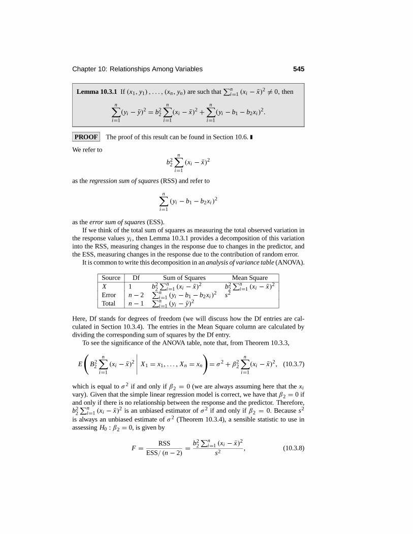
Chapter 10: Relationships Among Variables 545
Lemma 10.3.1 If (x1, y1) , . . . , (xn, yn) are such that(n
i=1 (xi − x)2 6= 0, then
n#i=1
(yi − y)2 = b22
n#i=1
(xi − x)2 +n#
i=1
(yi − b1 − b2xi )2.
PROOF The proof of this result can be found in Section 10.6.
We refer to
b22
n#i=1
(xi − x)2
as the regression sum of squares (RSS) and refer to
n#i=1
(yi − b1 − b2xi )2
as the error sum of squares (ESS).If we think of the total sum of squares as measuring the total observed variation in
the response values yi , then Lemma 10.3.1 provides a decomposition of this variationinto the RSS, measuring changes in the response due to changes in the predictor, andthe ESS, measuring changes in the response due to the contribution of random error.
It is common to write this decomposition in an analysis of variance table (ANOVA).
Source Df Sum of Squares Mean SquareX 1 b2
2
(ni=1 (xi − x)2 b2
2
(ni=1 (xi − x)2
Error n − 2(n
i=1 (yi − b1 − b2xi )2 s2
Total n − 1(n
i=1 (yi − y)2
Here, Df stands for degrees of freedom (we will discuss how the Df entries are cal-culated in Section 10.3.4). The entries in the Mean Square column are calculated bydividing the corresponding sum of squares by the Df entry.
To see the significance of the ANOVA table, note that, from Theorem 10.3.3,
E
&B2
2
n#i=1
(xi − x)2@@@@@ X1 = x1, . . . , Xn = xn
'= σ 2 + β2
2
n#i=1
(xi − x)2, (10.3.7)
which is equal to σ 2 if and only if β2 = 0 (we are always assuming here that the xivary). Given that the simple linear regression model is correct, we have that β2 = 0 ifand only if there is no relationship between the response and the predictor. Therefore,b2
2
(ni=1 (xi − x)2 is an unbiased estimator of σ 2 if and only if β2 = 0. Because s2
is always an unbiased estimate of σ 2 (Theorem 10.3.4), a sensible statistic to use inassessing H0 : β2 = 0, is given by
F = RSSESS/ (n − 2)
= b22
(ni=1 (xi − x)2
s2, (10.3.8)

546 Section 10.3: Quantitative Response and Predictors
as this is the ratio of two unbiased estimators of σ 2 when H0 is true. We then concludethat we have evidence against H0 when F is large, as (10.3.7) also shows that thenumerator will tend to be larger than σ 2 when H0 is false. We refer to (10.3.8) as theF-statistic. We will subsequently discuss the sampling distribution of F to see how todetermine when the value F is so large as to be evidence against H0.
EXAMPLE 10.3.5 (Example 10.3.3 continued)Using the data of Example 10.3.3, we obtain
n#i=1
(yi − y)2 = 437.01,
b22
n#i=1
(xi − x)2 = 428.55,
n#i=1
(yi − b1 − b2xi )2 = 437.01− 428.55 = 8.46,
and so
F = b22
(ni=1 (xi − x)2
s2 = 428.551.06
= 404.29.
Note that F is much bigger than 1, and this seems to indicate a linear effect due to X .
The Coefficient of Determination and Correlation
Lemma 10.3.1 implies that
R2 = b22
(ni=1 (xi − x)2(n
i=1 (yi − y)2
satisfies 0 ≤ R2 ≤ 1. Therefore, the closer R2 is to 1, the more of the observed totalvariation in the response is accounted for by changes in the predictor. In fact, weinterpret R2, called the coefficient of determination, as the proportion of the observedvariation in the response explained by changes in the predictor via the simple linearregression.
The coefficient of determination is an important descriptive statistic, for, even ifwe conclude that a relationship does exist, it can happen that most of the observedvariation is due to error. If we want to use the model to predict further values of theresponse, then the coefficient of determination tells us whether we can expect highlyaccurate predictions or not. A value of R2 near 1 means highly accurate predictions,whereas a value near 0 means that predictions will not be very accurate.
EXAMPLE 10.3.6 (Example 10.3.3 continued)Using the data of Example 10.3.3, we obtain R2 = 0.981. Therefore, 98.1% of the ob-served variation in Y can be explained by the changes in X through the linear relation.This indicates that we can expect fairly accurate predictions when using this model, atleast when we are predicting within the range of the observed X values.

Chapter 10: Relationships Among Variables 547
Recall that in Section 3.3, we defined the correlation coefficient between randomvariables X and Y to be
ρXY = Corr(X,Y ) = Cov(X,Y )
Sd(X)Sd(Y ).
In Corollary 3.6.1, we proved that −1 ≤ ρXY ≤ 1 with ρXY = ±1 if and only ifY = a ± cX for some constants a ∈ R1 and c > 0. So ρXY can be taken as a measureof the extent to which a linear relationship exists between X and Y.
If we do not know the joint distribution of (X, Y ) , then we will have to estimateρXY . Based on the observations (x1, y1), . . . , (xn, yn), the natural estimate to use isthe sample correlation coefficient
rxy = sxy
sx sy,
where
sxy = 1n − 1
n#i=1
(xi − x) (yi − y)
is the sample covariance estimating Cov(X, Y ), and sx , sy are the sample standarddeviations for the X and Y variables, respectively. Then −1 ≤ rxy ≤ 1 with rxy = ±1if and only if yi = a± cxi for some constants a ∈ R1 and c > 0, for every i (the proofis the same as in Corollary 3.6.1 using the joint distribution that puts probability mass1/n at each point (xi , yi )— see Problem 3.6.16).
The following result shows that the coefficient of determination is the square of thecorrelation between the observed X and Y values.
Theorem 10.3.5 If (x1, y1) , . . . , (xn, yn) are such that(n
i=1 (xi − x)2 6= 0,(ni=1 (yi − y)2 6= 0, then R2 = r2
xy .
PROOF We have
r2xy =
!(ni=1 (xi − x) (yi − y)
"2(ni=1 (xi − x)2
(ni=1 (yi − y)2
= b22
(ni=1 (xi − x)2(ni=1 (yi − y)2
= R2,
where we have used the formula for b2 given in Theorem 10.3.1.
Confidence Intervals and Testing Hypotheses
We need to make some further assumptions in order to discuss the sampling distribu-tions of the various statistics that we have introduced. We have the following results.

548 Section 10.3: Quantitative Response and Predictors
Theorem 10.3.6 If Y , given X = x , is distributed N(β1 + β2x, σ 2), and we ob-serve the independent values (x1, y1), . . . , (xn, yn) for (X, Y ), then the conditionaldistributions of B1, B2, and S2, given X1 = x1, . . . , Xn = xn, are as follows.
(i) B1 ∼ N(β1, σ2(1/n + x2/
(ni=1(xi − x)2))
(ii) B2 ∼ N(β2, σ2/(n
i=1(xi − x)2)
(iii) B1 + B2x ∼ N(β1 + β2x, σ 2(1/n + (x − x)2/(n
i=1(xi − x)2))
(iv) (n − 2) S2/σ 2 ∼ χ2(n − 2) independent of (B1, B2)
PROOF The proof of this result can be found in Section 10.6.
Corollary 10.3.2(i) (B1 − β1)/(S(1/n + x2/
(ni=1(xi − x)2)1/2) ∼ t (n − 2)
(ii) (B2 − β2)((n
i=1(xi − x)2)1/2/S ∼ t (n − 2)
(iii)B1 + B2x − β1 − β2x
S((1/n + (x − x)2)/(n
i=1(xi − x)2)1/2∼ t (n − 2)
(iv) If F is defined as in (10.3.8), then H0 : β2 = 0 is true if and only if F ∼F(1, n − 2).
PROOF The proof of this result can be found in Section 10.6.
Using Corollary 10.3.2(i), we have that
b1 ± s
&1/n + x2/
n#i=1
(xi − x)2'1/2
t(1+γ )/2 (n − 2)
is an exact γ -confidence interval for β1. Also, from Corollary 10.3.2(ii),
b2 ± s
&n#
i=1
(xi − x)2'−1/2
t(1+γ )/2 (n − 2)
is an exact γ -confidence interval for β2.From Corollary 10.3.2(iv), we can test H0 : β2 = 0 by computing the P-value
P
&F ≥ b2
2
(ni=1 (xi − x)2
s2
', (10.3.9)
where F ∼ F(1, n−2), to see whether or not the observed value (10.3.8) is surprising.This is sometimes called the ANOVA test. Note that Corollary 10.3.2(ii) implies thatwe can also test H0 : β2 = 0 by computing the P-value
P
&|T | ≥ b2
!(ni=1 (xi − x)2
"1/2s
', (10.3.10)

Chapter 10: Relationships Among Variables 549
where T ∼ t (n − 2). The proof of Corollary 10.3.2(iv) reveals that (10.3.9) and(10.3.10) are equal.
EXAMPLE 10.3.7 (Example 10.3.3 continued)Using software or Table D.4, we obtain t0.975 (8) = 2.306. Then, using the data ofExample 10.3.3, we obtain a 0.95-confidence interval for β1 as
b1 ± s
&1/n + x2/
n#i=1
(xi − x)2'1/2
t(1+γ )/2(n − 2)
= 1.33± (0.3408) (2.306) = [0.544, 2.116]
and a 0.95-confidence interval for β2 as
b2 ± s
&n#
i=1
(xi − x)2'−1/2
t(1+γ )/2(n − 2)
= 2.06± (0.1023) (2.306) = [1.824, 2.296] .
The 0.95-confidence interval for β2 does not include 0, so we have evidence againstthe null hypothesis H0 : β2 = 0 and conclude that there is evidence of a relationshipbetween X and Y. This is confirmed by the F-test of this null hypothesis, as it gives theP-value P(F ≥ 404.29) = 0.000 when F ∼ F(1, 8).
Analysis of Residuals
In an application of the simple regression model, we must check to make sure thatthe assumptions make sense in light of the data we have collected. Model checking isbased on the residuals yi − b1 − b2xi (after standardization), as discussed in Section9.1. Note that the i th residual is just the difference between the observed value yi at xiand the predicted value b1 + b2xi at xi .
From the proof of Theorem 10.3.4, we have the following result.
Corollary 10.3.3(i) E(Yi − B1 − B2xi | X1 = x1, . . . , Xn = xn) = 0
(ii) Var(Yi − B1 − B2xi | X1 = x1, . . . , Xn = xn) = σ 2)
1− 1n − (xi−x)2(n
i=1(xi−x)2
*This leads to the definition of the i th standardized residual as
yi − b1 − b2xi
s)
1− 1n − (xi − x)2 /
(nj=1
!x j − x
"2*1/2 . (10.3.11)
Corollary 10.3.3 says that (10.3.11), with σ replacing s, is a value from a distri-bution with conditional mean 0 and conditional variance 1. Furthermore, when theconditional distribution of the response given the predictors is normal, then the con-ditional distribution of this quantity is N(0, 1) (see Problem 10.3.21). These results

550 Section 10.3: Quantitative Response and Predictors
are approximately true for (10.3.11) for large n. Furthermore, it can be shown (seeProblem 10.3.20) that
Cov(Yi − B1 − B2xi , Y j − B1 − B2x j | X1 = x1, . . . , Xn = xn)
= −σ 2
&1n+ (xi − x)
!x j − x
"(nk=1 (xk − x)2
'.
Therefore, under the normality assumption, the residuals are approximately indepen-dent when n is large and
xi − x4(nk=1 (xk − x)2
→ 0
as n → ∞. This will be the case whenever Var(X) is finite (see Challenge 10.3.27)or, in the design context, when the values of the predictor are chosen accordingly. Soone approach to model checking here is to see whether the values given by (10.3.11)look at all like a sample from the N(0, 1) distribution. For this, we can use the plotsdiscussed in Chapter 9.
EXAMPLE 10.3.8 (Example 10.3.3 continued)Using the data of Example 10.3.3, we obtain the following standardized residuals.
−0.49643 0.43212 −1.73371 1.00487 0.083580.17348 0.75281 −0.28430 −1.43570 1.51027
These are plotted against the predictor x in Figure 10.3.2.
50-5
1
0
-1
-2
x
Sta
nd
ard
ized
Res
idu
als
Figure 10.3.2: Plot of the standardized residuals in Example 10.3.8.
It is recommended that we plot the standardized residuals against the predictor, asthis may reveal some underlying relationship that has not been captured by the model.This residual plot looks reasonable. In Figure 10.3.3, we have a normal probability plotof the standardized residuals. These points lie close to the line through the origin withslope equal to 1, so we conclude that we have no evidence against the model here.

Chapter 10: Relationships Among Variables 551
10-1-2
1
0
-1
Standardized Residual
Nor
mal
Sco
re
Figure 10.3.3: Normal probability plot of the standardized residuals in Example 10.3.8.
What do we do if model checking leads to a failure of the model? As discussedin Chapter 9, perhaps the most common approach is to consider making various trans-formations of the data to see whether there is a simple modification of the model thatwill pass. We can make transformations, not only to the response variable Y, but to thepredictor variable X as well.
An Application of Simple Linear Regression Analysis
The following data set is taken from Statistical Methods, 6th ed., by G. Snedecor andW. Cochran (Iowa State University Press, Ames, 1967) and gives the record speed Yin miles per hour at the Indianapolis Memorial Day car races in the years 1911–1941,excepting the years 1917–1918. We have coded the year X starting at 0 in 1911 andincrementing by 1 for each year. There are n = 29 data points (xi , yi ). The goal ofthe analysis is to obtain the least-squares line and, if warranted, make inferences aboutthe regression coefficients. We take the normal simple linear regression model as ourstatistical model. Note that this is an observational study.
Year Speed Year Speed Year Speed0 74.6 12 91.0 22 104.21 78.7 13 98.2 23 104.92 75.9 14 101.1 24 106.23 82.5 15 95.9 25 109.14 89.8 16 97.5 26 113.65 83.3 17 99.5 27 117.28 88.1 18 97.6 28 115.09 88.6 19 100.4 29 114.3
10 89.6 20 96.6 30 115.111 94.5 21 104.1
Using Theorem 10.3.1, we obtain the least-squares line as y = 77.5681+1.27793x.This line, together with a scatter plot of the values (xi , yi ), is plotted in Figure 10.3.4.
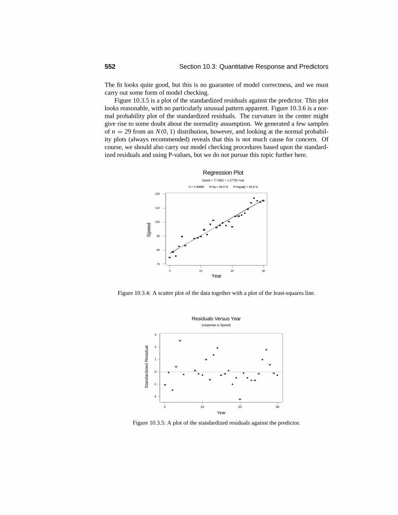
552 Section 10.3: Quantitative Response and Predictors
The fit looks quite good, but this is no guarantee of model correctness, and we mustcarry out some form of model checking.
Figure 10.3.5 is a plot of the standardized residuals against the predictor. This plotlooks reasonable, with no particularly unusual pattern apparent. Figure 10.3.6 is a nor-mal probability plot of the standardized residuals. The curvature in the center mightgive rise to some doubt about the normality assumption. We generated a few samplesof n = 29 from an N(0, 1) distribution, however, and looking at the normal probabil-ity plots (always recommended) reveals that this is not much cause for concern. Ofcourse, we should also carry out model checking procedures based upon the standard-ized residuals and using P-values, but we do not pursue this topic further here.
302010 0
120
110
100
90
80
70
Year
Spe
ed
S = 2.99865 R-Sq = 94.0 % R-Sq(adj) = 93.8 %
Speed = 77.5681 + 1.27793 Year
Regression Plot
Figure 10.3.4: A scatter plot of the data together with a plot of the least-squares line.
3020100
3
2
1
0
-1
-2
Year
Sta
ndar
dize
d R
esid
ual
Residuals Versus Year(response is Speed)
Figure 10.3.5: A plot of the standardized residuals against the predictor.

Chapter 10: Relationships Among Variables 553
3210-1-2
2
1
0
-1
-2
Nor
mal
Sco
re
Standardized Residual
Normal Probability Plot of the Residuals(response is Speed)
Figure 10.3.6: A normal probability plot of the standardized residuals.
Based on the results of our model checking, we decide to proceed to inferencesabout the regression coefficients. The estimates and their standard errors are given inthe following table, where we have used the estimate of σ 2 given by s2 = (2.999)2,to compute the standard errors. We have also recorded the t-statistics appropriate fortesting each of the hypotheses H0 : β1 = 0 and H0 : β2 = 0.
Coefficient Estimate Standard Error t-statisticβ1 77.568 1.118 69.39β2 1.278 0.062 20.55
From this, we see that the P-value for assessing H0 : β2 = 0 is given by
P(|T | ≥ 20.55) = 0.000,
when T ∼ t (27), and so we have strong evidence against H0. It seems clear that thereis a strong positive relationship between Y and X . Since the 0.975 point of the t (27)distribution equals 2.0518, a 0.95-confidence interval for β2 is given by
1.278± (0.062) 2.0518 = [1.1508, 1.4052] .
The ANOVA decomposition is given in the following table.
Source Df Sum of Squares Mean SquareRegression 1 3797.0 3797.0Error 27 242.8 9.0Total 28 4039.8
Accordingly, we have that F = 3797.0/9.0 = 421.888 and, as F ∼ F(1, 27) whenH0 : β2 = 0 is true, P(F > 421.888) = 0.000, which simply confirms (as it must)what we got from the preceding t-test.
The coefficient of determination is given by R2 = 3797.0/4039.8 = 0.94. There-fore, 94% of the observed variation in the response variable can be explained by the

554 Section 10.3: Quantitative Response and Predictors
changes in the predictor through the simple linear regression. The value of R2 indicatesthat the fitted model will be an excellent predictor of future values, provided that thevalue of X that we want to predict at, is in the range (or close to it) of the values of Xused to fit the model.
10.3.3 Bayesian Simple Linear Model (Advanced)
For the Bayesian formulation of the simple linear regression model with normal error,we need to add a prior distribution for the unknown parameters of the model, namely,β1, β2, and σ 2. There are many possible choices for this. A relevant prior is dependenton the application.
To help simplify the calculations, we reparameterize the model as follows. Letα1 = β1 + β2 x and α2 = β2. It is then easy to show (see Problem 10.3.24) that
n#i=1
(yi − β1 − β2xi )2 =
n#i=1
(yi − α1 − α2(xi − x))2
=n#
i=1
((yi − y)− (α1 − y)− α2(xi − x))2
=n#
i=1
(yi − y)2 + n(α1 − y)2 + α22
n#i=1
(xi − x)2
− 2α2
n#i=1
(xi − x)(yi − y). (10.3.12)
The likelihood function, using this reparameterization, then equals
)2πσ 2
*−n/2exp
&− 1
2σ 2
n#i=1
(yi − α1 − α2 (xi − x))2'.
From (10.3.12), and setting
c2x =
n#i=1
(xi − x)2,
c2y =
n#i=1
(yi − y)2,
cxy =n#
i=1
(xi − x)(yi − y),
we can write this as

Chapter 10: Relationships Among Variables 555
)2πσ 2
*−n/2exp
&− c2
y
2σ 2
'exp
)− n
2σ 2 (α1 − y)2*
× exp$− 1
2σ 2
Aα2
2c2x − 2α2cxy
B%=)
2πσ 2*−n/2
exp
&−c2
y − c2xa2
2σ 2
'exp
)− n
2σ 2 (α1 − y)2*
× exp$− c2
x
2σ 2 (α2 − a)2%
,
where the last equality follows from α22c2
x − 2α2cxy = c2x (α2 − a)2 − c2
x a2 with a =cxy /c2
x .This implies that, whenever the prior distribution on (α1, α2) is such that α1 and
α2 are independent given σ 2, then the posterior distributions of α1 and α2 are alsoindependent given σ 2. Note also that y and a are the least-squares estimates (as wellas the MLE’s) of α1 and α2, respectively (see Problem 10.3.24).
Now suppose we take the prior to be
α1 |α2, σ2 ∼ N(µ1, τ
21σ
2),
α2 | σ 2 ∼ N(µ2, τ22σ
2),
1/σ 2 ∼ Gamma(κ, ν).
Note that α1 and α2 are independent given σ 2.As it turns out, this prior is conjugate, so we can easily determine an exact form for
the posterior distribution (see Problem 10.3.25). The joint posterior of!α1, α2, 1/σ 2
"is given by
α1 |α2, σ2 ∼ N
&n + 1
τ 21
'−1 &ny + µ1
τ 21
',
&n + 1
τ 21
'−1
σ 2
,
α2 | σ 2 ∼ N
&c2x +
1
τ 22
'−1 &c2
xa + µ2
τ 22
',
&c2
x +1
τ 22
'−1
σ 2
,
1
σ 2∼ Gamma
)κ + n
2, νxy
*,
where
νxy = 1
2
c2
y − c2x a2 +
Cny2 + µ2
1τ2
1−$
n + 1τ2
1
%−1 $ny + µ1
τ21
%2D
+C
c2x a2 + µ2
2τ2
2−$
c2x + 1
τ22
%−1$c2
xa + µ2τ2
2
%2D
+ ν.

556 Section 10.3: Quantitative Response and Predictors
Of course, we must select the values of the hyperparameters µ1, τ 1, µ2, τ 2, κ, and νto fully specify the prior.
Now observe that for a diffuse analysis, i.e., when we have little or no prior infor-mation about the parameters, we let τ 1 →∞, τ 2 →∞, and ν→ 0, and the posteriorconverges to
α1 |α2, σ2 ∼ N(y, σ 2/n),
α2 |σ 2 ∼ N(a, σ 2/c2x ),
1/σ 2 ∼ Gamma(κ + n/2, νxy)
where νxy = (1/2){c2y − c2
xa2}. But this still leaves us with the necessity of choosingthe hyperparameter κ. We will see, however, that this choice has only a small effect onthe analysis when n is not too small.
We can easily work out the marginal posterior distribution of the αi . For example,in the diffuse case, the marginal posterior density of α2 is proportional to6 ∞
0
$1
σ 2
%1/2
expE− c2
x
2σ 2 (α2 − a)2F$
1
σ 2
%κ+(n/2)−1
expA−νxy
σ 2
Bd
$1
σ 2
%=6 ∞
0
$1
σ 2
%κ+(n/2)−(1/2)exp
E−$νxy + c2
x
2(α2 − a)2
%1
σ 2
Fd
$1
σ 2
%.
Making the change of variable 1/σ 2 → w, where
w =$νxy + c2
x
2(α2 − a)2
%1
σ 2
in the preceding integral, shows that the marginal posterior density of α2 is proportionalto $
1+ c2x
2νxy(α2 − a)2
%−(κ+(n+1)/2) 6 ∞
0wκ+(n/2)−(1/2) exp {−w} dw,
which is proportional to $1+ c2
x
2νxy(α2 − a)2
%−(2κ+n+1)/2
.
This establishes (see Problem 4.6.17) that the posterior distribution of α2 is specifiedby √
2κ + nα2 − a42νxy/c2
x
∼ t (2κ + n).
So a γ -HPD (highest posterior density) interval for α2 is given by
a ± 1√2κ + n
+2νxy
c2x
t(1+γ )/2(2κ + n).

Chapter 10: Relationships Among Variables 557
Note that these intervals will not change much as we change κ, provided that n is nottoo small.
We consider an application of a Bayesian analysis for such a model.
EXAMPLE 10.3.9 Haavelmo’s Data on Income and InvestmentThe data for this example were taken from An Introduction to Bayesian Inference inEconometrics, by A. Zellner (Wiley Classics, New York, 1996). The response variableY is income in U.S. dollars per capita (deflated), and the predictor variable X is invest-ment in dollars per capita (deflated) for the United States for the years 1922–1941. Thedata are provided in the following table.
Year Income Investment Year Income Investment1922 433 39 1932 372 221923 483 60 1933 381 171924 479 42 1934 419 271925 486 52 1935 449 331926 494 47 1936 511 481927 498 51 1937 520 511928 511 45 1938 477 331929 534 60 1939 517 461930 478 39 1940 548 541931 440 41 1941 629 100
In Figure 10.3.7, we present a normal probability plot of the standardized residuals,obtained via a least-squares fit. In Figure 10.3.8, we present a plot of the standardizedresiduals against the predictor. Both plots indicate that the model assumptions arereasonable.
Suppose now that we analyze these data using the limiting diffuse prior with κ = 2.Here, we have that y = 483, c2
y = 64993, c2x = 5710.55, and cxy = 17408.3, so that
a = 17408.3/5710.55 = 3.05 and νxy = (64993− 17408.3) /2 = 23792.35. Theposterior is then given by
α1 |α2, σ2 ∼ N(483, σ 2/20),
α2 | σ 2 ∼ N(3.05, σ 2/5710.55),
1/σ 2 ∼ Gamma(12, 23792.35).
The primary interest here is in the investment multiplier α2. By the above results, a0.95-HPD interval for α2, using t0.975(24) = 2.0639, is given by
a ± 1√2κ + n
+2νxy
r2x
t(1+γ )/2(2κ + n − 1)
= 3.05± 1√24
,2 · 23792.35
5710.55t0.975(24) = 3.05± (0.589) 2.0639
= (1.834, 4.266).

558 Section 10.3: Quantitative Response and Predictors
10-1-2
2
1
0
-1
-2
Nor
mal
Sco
re
Standardized Residual
Normal Probability Plot of the Residuals(response is Income)
Figure 10.3.7: Normal probability plot of the standardized residuals in Example 10.3.9.
100908070605040302010
1
0
-1
-2
Investm ent
Sta
nda
rdiz
ed R
esid
uals
Figure 10.3.8: Plot of the standardized residuals against the predictor in Example 10.3.9.
10.3.4 The Multiple Linear Regression Model (Advanced)
We now consider the situation in which we have a quantitative response Y and quanti-tative predictors X1, . . . , Xk . For the regression model, we assume that the conditionaldistributions of Y, given the predictors, have constant shape and that they change, as thepredictors change, at most through the conditional mean E (Y | X1 = x1, . . . , Xk = xk).For the linear regression model, we assume that this conditional mean is of the form
E(Y | X1 = x1, . . . , Xk = xk) = β1x1 + · · · + βk xk . (10.3.13)
This is linear in the unknown β i ∈ R1 for i = 1, . . . , k.

Chapter 10: Relationships Among Variables 559
We will develop only the broad outline of the analysis of the multiple linear regres-sion model here. All results will be stated without proofs provided. The proofs can befound in more advanced texts. It is important to note, however, that all of these resultsare just analogs of the results we developed by elementary methods in Section 10.3.2,for the simple linear regression model.
Matrix Formulation of the Least-Squares Problem
For the analysis of the multiple linear regression model, we need some matrix concepts.We will briefly discuss some of these here, but also see Appendix A.4.
Let A ∈ Rm×n denote a rectangular array of numbers with m rows and n columns,and let ai j denote the entry in the i th row and j th column (referred to as the (i, j)-thentry of A). For example,
A =$
1.2 1.0 0.03.2 0.2 6.3
%∈ R2×3
denotes a 2× 3 matrix and, for example, a22 = 0.2.We can add two matrices of the same dimensions m and n by simply adding their
elements componentwise. So if A, B ∈ Rm×n and C = A + B, then ci j = ai j +bi j . Furthermore, we can multiply a matrix by a real number c by simply multiplyingevery entry in the matrix by c. So if A ∈ Rm×n , then B = cA ∈ Rm×n and bi j =cai j . We will sometimes write a matrix A ∈ Rm×n in terms of its columns as A =( a1 . . . an ) so that here ai ∈ Rm . Finally, if A ∈ Rm×n and b ∈ Rn, then wedefine the product of A times b as Ab = b1a1 + · · · + bnan ∈ Rm.
Suppose now that Y ∈ Rn and that E(Y ) is constrained to lie in a set of the form
S = {β1v1 + · · · + βkvk : β i ∈ R1, i = 1, . . . , k},where v1, . . . , vk are fixed vectors in Rn. A set such as S is called a linear subspace ofRn . When {v1, . . . , vk} has the linear independence property, namely,
β1v1 + · · · + βkvk = 0
if and only if β1 = · · · = βk = 0, then we say that S has dimension k and {v1, . . . , vk}is a basis for S.
If we set
V = (v1 · · · vk) =
v11 v12 · · · v1kv21 v22 · · · v2k...
......
vn1 vn2 · · · vnk
∈ Rn×k,
then we can write
E(Y ) = β1v1 + · · · + βkvk =
β1v11 + β2v12 + · · · + βkv1kβ1v21 + β2v22 + · · · + βkv2k
...β1vn1 + β2vn2 + · · · + βkvnk
= Vβ

560 Section 10.3: Quantitative Response and Predictors
for some unknown point β = (β1, β2, . . . , βk);. When we observe y ∈ Rn, then the
least-squares estimate of E(Y ) is obtained by finding the value of β that minimizes
n#i=1
!yi − β1vi1 − β2vi2 − · · · − βkvik
"2 .
It can be proved that a unique minimizing value for β ∈ Rk exists whenever{v1, . . . , vk} is a basis. The minimizing value of β will be denoted by b and is calledthe least-squares estimate of β. The point b1v1+ · · · + bkvk = V b is the least-squaresestimate of E(Y ) and is sometimes called the vector of fitted values. The point y− V bis called the vector of residuals.
We now consider how to calculate b. For this, we need to understand what it meansto multiply the matrix A ∈ Rm×k on the right by the matrix B ∈ Rk×n . The matrixproduct AB is defined to be the m × n matrix whose (i, j)-th entry is given by
k#l=1
ailbl j .
Notice that the array A must have the same number of columns as the number of rowsof B for this product to be defined. The transpose of a matrix A ∈ Rm×k is defined tobe
A; =
a11 · · · am1...
...a1k · · · amk
∈ Rk×m,
namely, the i th column of A becomes the i th row of A;. For a matrix A ∈ Rk×k , the
matrix inverse of A is defined to be the matrix A−1 such that
AA−1 = A−1 A = I,
where I ∈ Rk×k has 1’s along its diagonal and 0’s everywhere else; it is called the k×kidentity matrix. It is not always the case that A ∈ Rk×k has an inverse, but when it doesit can be shown that the inverse is unique. Note that there are many mathematical andstatistical software packages that include the facility for computing matrix products,transposes, and inverses.
We have the following fundamental result.
Theorem 10.3.7 If E(Y ) ∈ S = Gβ1v1 + · · · + βkvk : βi ∈ R1, i = 1, . . . , k
Hand the columns of V = (v1 · · · vk) have the linear independence property, then!V ;V
"−1 exists, the least-squares estimate of β is unique, and it is given by
b = b1
...bk
= !V ;V "−1 V ;y. (10.3.14)

Chapter 10: Relationships Among Variables 561
Least-Squares Estimates, Predictions, and Standard Errors
For the linear regression model (10.3.13), we have that (writing Xi j for the j th valueof Xi )
E
Y1
...Yn
@@@@@@@ Xi j = xi j for all i, j
= β1x11 + · · · + βk x1k
...β1xn1 + · · · + βk xnk
= β1v1 + · · · + βkvk = Vβ,
where β = (β1, . . . , βk); and
V = ( v1 v2 . . . vk ) = x11 · · · x1k
......
xn1 · · · xnk
∈ Rn×k .
We will assume, hereafter, that the columns v1, . . . , vk of V have the linear indepen-dence property. Then (replacing expectation by conditional expectation) it is immediatethat the least-squares estimate of β is given by (10.3.14).
As with the simple linear regression model, we have a number of results concerningthe least-squares estimates. We state these here without proof.
Theorem 10.3.8 If the (xi1, . . . , xik, yi ) are independent observations for i = 1, . . . ,n, and the linear regression model applies, then
E(Bi | Xi j = xi j for all i, j) = βi
for i = 1, . . . , k.
So Theorem 10.3.8 states that the least-squares estimates are unbiased estimates of thelinear regression coefficients.
If we want to assess the accuracy of these estimates, then we need to be able tocompute their standard errors.
Theorem 10.3.9 If the (xi1, . . . , xik, yi ) are independent observations for i = 1, . . . ,n, from the linear regression model, and if Var(Y | X1 = x1, . . . , Xk = xk) = σ 2
for every x1, . . . , xk, then
Cov(Bi , Bj | Xi j = xi j for all i, j) = σ 2ci j , (10.3.15)
where ci j is the (i, j)-th entry in the matrix (V ;V )−1.
We have the following result concerning the estimation of the mean
E(Y | X1 = x1, . . . , Xk) = xk = β1x1 + · · · + βk xk
by the estimate b1x1 + · · · + bk xk .

562 Section 10.3: Quantitative Response and Predictors
Corollary 10.3.4
Var(B1x1 + · · · + Bk xk | Xi j = xi j for all i, j)
= σ 2(k#
i=1
x2i ci i + 2
#i< j
xi x j ci j ) = σ 2x ;(V ;V )−1x, (10.3.16)
where x = (x1, . . . , xk).
We also use b1x1 + · · · + bk xk = b;x as a prediction of a new response value whenX1 = x1, . . . , Xk = xk .
We see, from Theorem 10.3.9 and Corollary 10.3.4, that we need an estimate of σ 2
to compute standard errors. The estimate is given by
s2 = 1n − k
n#i=1
(yi − b1xi1 − · · · − bk xik)2 = 1
n − k(y − Xb);(y − Xb), (10.3.17)
and we have the following result.
Theorem 10.3.10 If the (xi1, . . . , xik, yi ) are independent observations for i =1, . . . , n, from the linear regression model, and if Var(Y | X1 = x1, . . . , Xk = xk) =σ 2, then
E(S2 | Xi j = xi j for all i, j) = σ 2.
Combining (10.3.15) and (10.3.17), we deduce that the standard error of bi is s√
cii .Combining (10.3.16) and (10.3.17), we deduce that the standard error of b1x1 + · · · +bk xk is
s
&k#
i=1
x2i ci i + 2
#i< j
xi x j ci j
'1/2
= s(x ;(V ;V )−1x)1/2.
The ANOVA Decomposition and F-Statistics
When one of the predictors X1, . . . , Xk is constant, then we say that the model has anintercept term. By convention, we will always take this to be the first predictor. Sowhen we want the model to have an intercept term, we take X1 ≡ 1 and β1 is theintercept, e.g., the simple linear regression model. Note that it is common to denote theintercept term by β0 so that X0 ≡ 1 and X1, . . . , Xk denote the predictors that actuallychange. We will also adopt this convention when it seems appropriate.
Basically, inclusion of an intercept term is very common, as this says that, whenthe predictors that actually change have no relationship with the response Y , then theintercept is the unknown mean of the response. When we do not include an intercept,then this says we know that the mean response is 0 when there is no relationship be-tween Y and the nonconstant predictors. Unless there is substantive, application-basedevidence to support this, we will generally not want to make this assumption.
Denoting the intercept term by β1, so that X1 ≡ 1, we have the following ANOVAdecomposition for this model that shows how to isolate the observed variation in Y thatcan be explained by changes in the nonconstant predictors.

Chapter 10: Relationships Among Variables 563
Lemma 10.3.2 If, for i = 1, . . . , n, the values (xi1, . . . , xik, yi ) are such that thematrix V has linearly independent columns, with v1 equal to a column of ones, thenb1 = y − b2 x2 − · · · − bk xk and
n#i=1
(yi − y)2 =n#
i=1
(b2(xi2 − x2)+ · · · + bk(xik − xk))2
+n#
i=1
(yi − b1xi1 − · · · − bk xik)2.
We call
RSS (X2, . . . , Xk) =n#
i=1
(b2 (xi2 − x2)+ · · · + bk (xik − xk))2
the regression sum of squares and
ESS =n#
i=1
(yi − b1xi1 − · · · − bk xik)2
the error sum of squares. This leads to the following ANOVA table.
Source Df Sum of Squares Mean SquareX2, . . . , Xk k − 1 RSS(X2, . . . , Xk) RSS(X2, . . . , Xk)/ (k − 1)Error n − k ESS s2
Total n − 1(n
i=1(yi − y)2
When there is an intercept term, the null hypothesis of no relationship between theresponse and the predictors is equivalent to H0 : β2 = · · · = βk = 0. As with thesimple linear regression model, the mean square for regression can be shown to be anunbiased estimator of σ 2 if and only if the null hypothesis is true. Therefore, a sensiblestatistic to use for assessing the null hypothesis is the F-statistic
F = RSS(X2, . . . , Xk)/ (k − 1)s2 ,
with large values being evidence against the null.Often, we want to assess the null hypothesis H0 : βl+1 = · · · = βk = 0 or,
equivalently, the hypothesis that the model is given by
E(Y | X1 = x1, . . . , Xk = xk) = β1x1 + · · · + βl xl,
where l < k. This hypothesis says that the last k − l predictors Xl+1, . . . , Xk, have norelationship with the response.
If we denote the least-squares estimates of β1, . . . , βl, obtained by fitting the smallermodel, by b∗1, . . . , b∗l , then we have the following result.

564 Section 10.3: Quantitative Response and Predictors
Lemma 10.3.3 If the (xi1, . . . , xik, yi ) for i = 1, . . . , n are values for which thematrix V has linearly independent columns, with v1 equal to a column of ones, then
RSS(X2, . . . , Xk) =n#
i=1
(b2(xi2 − x2)+ · · · + bk(xik − xk))2
≥n#
i=1
(b∗2(xi2 − x2)+ · · · + b∗l (xil − xl))2
= RSS(X2, . . . , Xl). (10.3.18)
On the right of the inequality in (10.3.18), we have the regression sum of squaresobtained by fitting the model based on the first l predictors. Therefore, we can interpretthe difference of the left and right sides of (10.3.18), namely,
RSS(Xl+1, . . . , Xk | X2, . . . , Xl) = RSS(X2, . . . , Xk)− RSS(X2, . . . , Xl)
as the contribution of the predictors Xl+1, . . . , Xk to the regression sum of squareswhen the predictors X1, . . . , Xl are in the model. We get the following ANOVA ta-ble (actually only the first three columns of the ANOVA table) corresponding to thisdecomposition of the total sum of squares.
Source Df Sum of SquaresX2, . . . , Xl l − 1 RSS(X2, . . . , Xl)Xl+1, . . . , Xk | X2, . . . , Xl k − l RSS(Xl+1, . . . , Xk | X2, . . . , Xl)Error n − k ESSTotal n − 1
(ni=1 (yi − y)2
It can be shown that the null hypothesis H0 : βl+1 = · · · = βk = 0 holds if andonly if
RSS(Xl+1, . . . , Xk | X2, . . . , Xl)/ (k − l)
is an unbiased estimator of σ 2. Therefore, a sensible statistic to use for assessing thisnull hypothesis is the F-statistic
F = RSS(Xl+1, . . . , Xk | X2, . . . , Xl)/ (k − l)
s2 ,
with large values being evidence against the null.
The Coefficient of Determination
The coefficient of determination for this model is given by
R2 = RSS(X2, . . . , Xk)(ni=1(yi − y)2
,
which, by Lemma 10.3.2, is always between 0 and 1. The value of R2 gives the propor-tion of the observed variation in Y that is explained by the inclusion of the nonconstantpredictors in the model.

Chapter 10: Relationships Among Variables 565
It can be shown that R2 is the square of the multiple correlation coefficient betweenY and X1, . . . , Xk . However, we do not discuss the multiple correlation coefficient inthis text.
Confidence Intervals and Testing Hypotheses
For inference, we have the following result.
Theorem 10.3.11 If the conditional distribution of Y given (X1, . . . , Xk) = (x1, . . . ,xk) is N(β1x1+· · ·+βk xk, σ
2), and if we observe the independent values (xi1, . . ., xik, yi ) for i = 1, . . . , n, then the conditional distributions of the Bi and S2, givenXi j = xi j for all i, j, are as follows.
(i) Bi ∼ N(βi , σ2cii )
(ii) B1x1 + · · · + Bk xk is distributed
N
&β1x1 + · · · + βk xk, σ
2
&k#
i=1
x2i cii + 2
#i< j
xi x j ci j
''
(iii) (n − k) S2/σ 2 ∼ χ2(n − k) independent of (B1, . . . , Bk)
Corollary 10.3.5(i) (Bi − βi )/sc1/2
ii ∼ t (n − k)
(ii)B1x1 + · · · + Bk xk − β1x1 − · · · − βk xk
S)(k
i=1 x2i ci i + 2
(i< j xi x j ci j
*1/2 ∼ t (n − k)
(iii) H0 : βl+1 = · · · = βk = 0 is true if and only if
F = (RSS(X2, . . . , Xk)− RSS(X2, . . . , Xl))/(k − l)
S2∼ F(k − l, n − k)
Analysis of Residuals
In an application of the multiple regression model, we must check to make sure thatthe assumptions make sense. Model checking is based on the residuals yi − b1xi1 −· · · − bk xik (after standardization), just as discussed in Section 9.1. Note that the i thresidual is simply the difference between the observed value yi at (xi1, . . . , xik) andthe predicted value b1xi1 + · · · + bk xik at (xi1, . . . , xik).
We also have the following result (this can be proved as a Corollary of Theorem10.3.10).

566 Section 10.3: Quantitative Response and Predictors
Corollary 10.3.6(i) E(Yi − B1xi1 − · · · − Bk xik | V ) = 0
(ii) Cov(Yi − B1xi1− · · · − Bk xik, Y j − B1x j1− · · · − Bk x jk, | V ) = σ 2di j , wheredi j is the (i, j)-th entry of the matrix I − V (V ;V )−1V ;.
Therefore, the standardized residuals are given by
y j − b1x j1 − · · · − bk x jk
sd1/2ii
. (10.3.19)
When s is replaced by σ in (10.3.19), Corollary 10.3.6 implies that this quantity hasconditional mean 0 and conditional variance 1. Furthermore, when the conditionaldistribution of the response given the predictors is normal, then it can be shown thatthe conditional distribution of this quantity is N(0, 1). These results are also approxi-mately true for (10.3.19) for large n. Furthermore, it can be shown that the covariancesbetween the standardized residuals go to 0 as n → ∞, under certain reasonable con-ditions on distribution of the predictor variables. So one approach to model checkinghere is to see whether the values given by (10.3.19) look at all like a sample from theN(0, 1) distribution.
What do we do if model checking leads to a failure of the model? As in Chapter 9,we can consider making various transformations of the data to see if there is a simplemodification of the model that will pass. We can make transformations not only to theresponse variable Y, but to the predictor variables X1, . . . , Xk as well.
An Application of Multiple Linear Regression Analysis
The computations needed to implement a multiple linear regression analysis cannotbe carried out by hand. These are much too time-consuming and error-prone. It istherefore important that a statistician have a computer with suitable software availablewhen doing a multiple linear regression analysis.
The data in Table 10.1 are taken from Statistical Theory and Methodology in Sci-ence and Engineering, 2nd ed., by K. A. Brownlee (John Wiley & Sons, New York,1965). The response variable Y is stack loss (Loss), which represents 10 times the per-centage of ammonia lost as unabsorbed nitric oxide. The predictor variables are X1 =air flow (Air), X2 = temperature of inlet water (Temp), and X3 = the concentration ofnitric acid (Acid). Also recorded is the day (Day) on which the observation was taken.
We consider the model Y | x1, x2, x3 ∼ N(β0+β1x1+β2x2+β3x3, σ2). Note that
we have included an intercept term. Figure 10.3.9 is a normal probability plot of thestandardized residuals. This looks reasonable, except for one residual, −2.63822, thatdiverges quite distinctively from the rest of the values, which lie close to the 45-degreeline. Printing out the standardized residuals shows that this residual is associated withthe observation on the twenty-first day. Possibly there was something unique about thisday’s operations, and so it is reasonable to discard this data value and refit the model.Figure 10.3.10 is a normal probability plot obtained by fitting the model to the first20 observations. This looks somewhat better, but still we might be concerned about atleast one of the residuals that deviates substantially from the 45-degree line.

Chapter 10: Relationships Among Variables 567
Day Air Temp Acid Loss Day Air Temp Acid Loss1 80 27 89 42 12 58 17 88 132 80 27 88 37 13 58 18 82 113 75 25 90 37 14 58 19 93 124 62 24 87 28 15 50 18 89 85 62 22 87 18 16 50 18 86 76 62 23 87 18 17 50 19 72 87 62 24 93 19 18 50 19 79 88 62 24 93 20 19 50 20 80 99 58 23 87 15 20 56 20 82 15
10 58 18 80 14 21 70 20 91 1511 58 18 89 14
Table 10.1: Data for Application of Multiple Linear Regression Analysis
210-1-2-3
2
1
0
-1
-2
Nor
mal
Sco
re
Standardized Residual
Normal Probability Plot of the Residuals(response is Loss)
Figure 10.3.9: Normal probability plot of the standardized residuals based on all the data.
3210-1
2
1
0
-1
-2
Nor
mal
Sco
re
Standardized Residual
Normal Probability Plot of the Residuals(response is Loss)
Figure 10.3.10: Normal probability plot of the standardized residuals based on the first 20 datavalues.

568 Section 10.3: Quantitative Response and Predictors
Following the analysis of these data in Fitting Equations to Data, by C. Daniel andF. S. Wood (Wiley-Interscience, New York, 1971), we consider instead the model
ln Y | x1, x2, x3 ∼ N(β0 + β1x1 + β2x2 + β3x3, σ2), (10.3.20)
i.e., we transform the response variable by taking its logarithm and use all of the data.Often, when models do not fit, simple transformations like this can lead to major im-provements. In this case, we see a much improved normal probability plot, as providedin Figure 10.3.11.
210-1-2
2
1
0
-1
-2
Nor
mal
Sco
re
Standardized Residual
Normal Probability Plot of the Residuals(response is Loss)
Figure 10.3.11: Normal probability plot of the standardized residuals for all the data using ln Yas the response.
We also looked at plots of the standardized residuals against the various predic-tors, and these looked reasonable. Figure 10.3.12 is a plot of the standardized residualsagainst the values of Air.
80706050
2
1
0
-1
-2
Air
Sta
ndar
dize
d R
esi
dual
Residuals Versus Air(response is Loss)
Figure 10.3.12: A plot of the standardized residuals for all the data, using ln Y as the response,against the values of the predictor Air.

Chapter 10: Relationships Among Variables 569
Now that we have accepted the model (10.3.20), we can proceed to inferences aboutthe unknowns of the model. The least-squares estimates of the βi ,their standard errors(Se), the corresponding t-statistics for testing the βi = 0, and the P-values for this aregiven in the following table.
Coefficient Estimate Se t-statistic P-valueβ0 −0.948700 0.647700 −1.46 0.161β1 0.034565 0.007343 4.71 0.000β2 0.063460 0.020040 3.17 0.006β3 0.002864 0.008510 0.34 0.742
The estimate of σ 2 is given by s2 = 0.0312.To test the null hypothesis that there is no relationship between the response and
the predictors, or that, equivalently, H0 : β1 = β2 = β3 = 0, we have the followingANOVA table.
Source Df Sum of Squares Mean SquareX1, X2, X3 3 4.9515 1.6505Error 17 0.5302 0.0312Total 20 5.4817
The value of the F-statistic is given by 1.6505/0.0312 = 52.900, and when F ∼F(3, 17), we have that P (F > 52.900) = 0.000. So there is substantial evidenceagainst the null hypothesis. To see how well the model explains the variation in theresponse, we computed the value of R2 = 86.9%. Therefore, approximately 87% ofthe observed variation in Y can be explained by changes in the predictors in the model.
While we have concluded that a relationship exists between the response and thepredictors, it may be that some of the predictors have no relationship with the response.For example, the table of t-statistics above would seem to indicate that perhaps X3(acid) is not affecting Y . We can assess this via the following ANOVA table, obtainedby fitting the model ln Y | x1, x2, x3 ∼ N(β0 + β1x1 + β2x2, σ
2).
Source Df Sum of Squares Mean SquareX1, X2 2 4.9480 2.4740X3 | X1, X2 1 0.0035 0.0035Error 17 0.5302 0.0312Total 20 5.4817
Note that RSS(X3 | X1, X2) = 4.9515−4.9480 = 0.0035. The value of the F-statisticfor testing H0 : β3 = 0 is 0.0035/0.0312 = 0.112, and when F ∼ F(1, 17), wehave that P(F > 0.112) = 0.742. So we have no evidence against the null hypothesisand can drop X3 from the model. Actually, this is the same P-value as obtained via thet-test of this null hypothesis, as, in general, the t-test that a single regression coefficientis 0 is equivalent to the F-test. Similar tests of the need to include X1 and X2 do notlead us to drop these variables from the model.
So based on the above results, we decide to drop X3 from the model and use theequation
E(Y | X1 = x1, X2 = x2) = −0.7522+ 0.035402X1 + 0.06346X2 (10.3.21)

570 Section 10.3: Quantitative Response and Predictors
to describe the relationship between Y and the predictors. Note that the least-squaresestimates of β0, β1, and β2 in (10.3.21) are obtained by refitting the model withoutX3.
Summary of Section 10.3
• In this section, we examined the situation in which the response variable and thepredictor variables are quantitative.
• In this situation, the linear regression model provides a possible description ofthe form of any relationship that may exist between the response and the predic-tors.
• Least squares is a standard method for fitting linear regression models to data.
• The ANOVA is a decomposition of the total variation observed in the responsevariable into a part attributable to changes in the predictor variables and a partattributable to random error.
• If we assume a normal linear regression model, then we have inference methodsavailable such as confidence intervals and tests of significance. In particular, wehave available the F-test to assess whether or not a relationship exists betweenthe response and the predictors.
• A normal linear regression model is checked by examining the standardizedresiduals.
EXERCISES
10.3.1 Suppose that (x1, . . . , xn) is a sample from a Bernoulli(θ) distribution, whereθ ∈ [0, 1] is unknown. What is the least-squares estimate of the mean of this distribu-tion?10.3.2 Suppose that (x1, . . . , xn) is a sample from the Uniform[0, θ], where θ > 0 isunknown. What is the least-squares estimate of the mean of this distribution?10.3.3 Suppose that (x1, . . . , xn) is a sample from the Exponential(θ), where θ > 0 isunknown. What is the least-squares estimate of the mean of this distribution?10.3.4 Consider the n = 11 data values in the following table.
Observation X Y Observation X Y1 −5.00 −10.00 7 1.00 3.522 −4.00 −8.83 8 2.00 5.643 −3.00 −9.15 9 3.00 7.284 −2.00 −4.26 10 4.00 7.625 −1.00 −0.30 11 5.00 8.516 0.00 −0.04
Suppose we consider the simple normal linear regression to describe the relationshipbetween the response Y and the predictor X.
(a) Plot the data in a scatter plot.

Chapter 10: Relationships Among Variables 571
(b) Calculate the least-squares line and plot this on the scatter plot in part (a).(c) Plot the standardized residuals against X.
(d) Produce a normal probability plot of the standardized residuals.(e) What are your conclusions based on the plots produced in parts (c) and (d)?(f) If appropriate, calculate 0.95-confidence intervals for the intercept and slope.(g) Construct the ANOVA table to test whether or not there is a relationship betweenthe response and the predictors. What is your conclusion?(h) If the model is correct, what proportion of the observed variation in the response isexplained by changes in the predictor?(i) Predict a future Y at X = 0.0. Is this prediction an extrapolation or an interpolation?Determine the standard error of this prediction.(j) Predict a future Y at X = 6.0. Is this prediction an extrapolation or an interpolation?Determine the standard error of this prediction.(k) Predict a future Y at X = 20.0. Is this prediction an extrapolation or an interpola-tion? Determine the standard error of this prediction. Compare this with the standarderrors obtained in parts (i) and (j) and explain the differences.10.3.5 Consider the n = 11 data values in the following table.
Observation X Y Observation X Y1 −5.00 65.00 7 1.00 6.522 −4.00 39.17 8 2.00 17.643 −3.00 17.85 9 3.00 34.284 −2.00 7.74 10 4.00 55.625 −1.00 2.70 11 5.00 83.516 0.00 −0.04
Suppose we consider the simple normal linear regression to describe the relationshipbetween the response Y and the predictor X.
(a) Plot the data in a scatter plot.(b) Calculate the least-squares line and plot this on the scatter plot in part (a).(c) Plot the standardized residuals against X.
(d) Produce a normal probability plot of the standardized residuals.(e) What are your conclusions based on the plots produced in parts (c) and (d)?(f) If appropriate, calculate 0.95-confidence intervals for the intercept and slope.(g) Do the results of your analysis allow you to conclude that there is a relationshipbetween Y and X? Explain why or why not.(h) If the model is correct, what proportion of the observed variation in the response isexplained by changes in the predictor?10.3.6 Suppose the following data record the densities of an organism in a containmentvessel for 10 days. Suppose we consider the simple normal linear regression to describethe relationship between the response Y (density) and the predictor X (day).

572 Section 10.3: Quantitative Response and Predictors
Day Number/Liter Day Number/Liter1 1.6 6 1341.62 16.7 7 2042.93 65.2 8 7427.04 23.6 9 15571.85 345.3 10 33128.5
(a) Plot the data in a scatter plot.(b) Calculate the least-squares line and plot this on the scatter plot in part (a).(c) Plot the standardized residuals against X.
(d) Produce a normal probability plot of the standardized residuals.(e) What are your conclusions based on the plots produced in parts (c) and (d)?(f) Can you think of a transformation of the response that might address any problemsfound? If so, repeat parts (a) through (e) after performing this transformation. (Hint:The scatter plot looks like exponential growth. What transformation is the inverse ofexponentiation?)(g) Calculate 0.95-confidence intervals for the appropriate intercept and slope.(h) Construct the appropriate ANOVA table to test whether or not there is a relationshipbetween the response and the predictors. What is your conclusion?(i) Do the results of your analysis allow you to conclude that there is a relationshipbetween Y and X? Explain why or why not.(j) Compute the proportion of variation explained by the predictor for the two modelsyou have considered. Compare the results.(k) Predict a future Y at X = 12. Is this prediction an extrapolation or an interpolation?10.3.7 A student takes weekly quizzes in a course and receives the following gradesover 12 weeks.
Week Grade Week Grade1 65 7 742 55 8 763 62 9 484 73 10 805 68 11 856 76 12 90
(a) Plot the data in a scatter plot with X = week and Y = grade.(b) Calculate the least-squares line and plot this on the scatter plot in part (a).(c) Plot the standardized residuals against X .(d) What are your conclusions based on the plot produced in (c)?(e) Calculate 0.95-confidence intervals for the intercept and slope.(f) Construct the ANOVA table to test whether or not there is a relationship betweenthe response and the predictors. What is your conclusion?(g) What proportion of the observed variation in the response is explained by changesin the predictor?
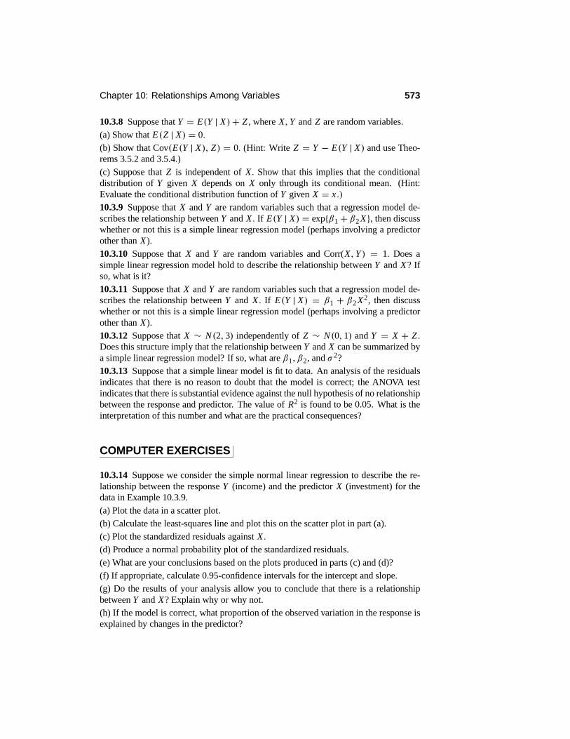
Chapter 10: Relationships Among Variables 573
10.3.8 Suppose that Y = E(Y | X)+ Z , where X,Y and Z are random variables.(a) Show that E(Z | X) = 0.(b) Show that Cov(E(Y | X), Z) = 0. (Hint: Write Z = Y − E(Y | X) and use Theo-rems 3.5.2 and 3.5.4.)(c) Suppose that Z is independent of X. Show that this implies that the conditionaldistribution of Y given X depends on X only through its conditional mean. (Hint:Evaluate the conditional distribution function of Y given X = x.)
10.3.9 Suppose that X and Y are random variables such that a regression model de-scribes the relationship between Y and X. If E(Y | X) = exp{β1 + β2 X}, then discusswhether or not this is a simple linear regression model (perhaps involving a predictorother than X).10.3.10 Suppose that X and Y are random variables and Corr(X, Y ) = 1. Does asimple linear regression model hold to describe the relationship between Y and X? Ifso, what is it?10.3.11 Suppose that X and Y are random variables such that a regression model de-scribes the relationship between Y and X. If E(Y | X) = β1 + β2 X2, then discusswhether or not this is a simple linear regression model (perhaps involving a predictorother than X).10.3.12 Suppose that X ∼ N(2, 3) independently of Z ∼ N(0, 1) and Y = X + Z .Does this structure imply that the relationship between Y and X can be summarized bya simple linear regression model? If so, what are β1, β2, and σ 2?10.3.13 Suppose that a simple linear model is fit to data. An analysis of the residualsindicates that there is no reason to doubt that the model is correct; the ANOVA testindicates that there is substantial evidence against the null hypothesis of no relationshipbetween the response and predictor. The value of R2 is found to be 0.05. What is theinterpretation of this number and what are the practical consequences?
COMPUTER EXERCISES
10.3.14 Suppose we consider the simple normal linear regression to describe the re-lationship between the response Y (income) and the predictor X (investment) for thedata in Example 10.3.9.(a) Plot the data in a scatter plot.(b) Calculate the least-squares line and plot this on the scatter plot in part (a).(c) Plot the standardized residuals against X.
(d) Produce a normal probability plot of the standardized residuals.(e) What are your conclusions based on the plots produced in parts (c) and (d)?(f) If appropriate, calculate 0.95-confidence intervals for the intercept and slope.(g) Do the results of your analysis allow you to conclude that there is a relationshipbetween Y and X? Explain why or why not.(h) If the model is correct, what proportion of the observed variation in the response isexplained by changes in the predictor?

574 Section 10.3: Quantitative Response and Predictors
10.3.15 The following data are measurements of tensile strength (100 lb/in2) and hard-ness (Rockwell E) on 20 pieces of die-cast aluminum.
Sample Strength Hardness Sample Strength Hardness1 293 53 11 298 602 349 70 12 292 513 340 78 13 380 954 340 55 14 345 885 340 64 15 257 516 354 71 16 265 547 322 82 17 246 528 334 67 18 286 649 247 56 19 324 8310 348 86 20 282 56
Suppose we consider the simple normal linear regression to describe the relationshipbetween the response Y (strength) and the predictor X (hardness).(a) Plot the data in a scatter plot.(b) Calculate the least-squares line and plot this on the scatter plot in part (a).(c) Plot the standardized residuals against X.
(d) Produce a normal probability plot of the standardized residuals.(e) What are your conclusions based on the plots produced in parts (c) and (d)?(f) If appropriate, calculate 0.95-confidence intervals for the intercept and slope.(g) Do the results of your analysis allow you to conclude that there is a relationshipbetween Y and X? Explain why or why not.(h) If the model is correct, what proportion of the observed variation in the response isexplained by changes in the predictor?10.3.16 Tests were carried out to determine the effect of gas inlet temperature (degreesFahrenheit) and rotor speed (rpm) on the tar content (grains/cu ft) of a gas stream,producing the following data.
Observation Tar Speed Temperature1 60.0 2400 54.52 65.0 2450 58.53 63.5 2500 58.04 44.0 2700 62.55 54.5 2700 68.06 26.0 2775 45.57 54.0 2800 63.08 53.5 2900 64.59 33.5 3075 57.010 44.0 3150 64.0
Suppose we consider the normal linear regression model
Y |W = w, X = x ∼ N(β1 + β2w + β3x, σ 2)

Chapter 10: Relationships Among Variables 575
to describe the relationship between Y (tar content) and the predictors W (rotor speed)and X (temperature).(a) Plot the response in scatter plots against each predictor.(b) Calculate the least-squares equation.(c) Plot the standardized residuals against W and X.
(d) Produce a normal probability plot of the standardized residuals.(e) What are your conclusions based on the plots produced in parts (c) and (d)?(f) If appropriate, calculate 0.95-confidence intervals for the regression coefficients.(g) Construct the ANOVA table to test whether or not there is a relationship betweenthe response and the predictors. What is your conclusion?(h) If the model is correct, what proportion of the observed variation in the response isexplained by changes in the predictors?(i) In an ANOVA table, assess the null hypothesis that there is no effect due to W, giventhat X is in the model.(j) Estimate the mean of Y when W = 2750 and X = 50.0. If we consider this valueas a prediction of a future Y at these settings, is this an extrapolation or interpolation?10.3.17 Suppose we consider the normal linear regression model
Y | X = x ∼ N(β1 + β2x + β3x2, σ 2)
for the data of Exercise 10.3.5.(a) Plot the response Y in a scatter plot against X .(b) Calculate the least-squares equation.(c) Plot the standardized residuals against X.
(d) Produce a normal probability plot of the standardized residuals.(e) What are your conclusions based on the plots produced in parts (c) and (d)?(f) If appropriate, calculate 0.95-confidence intervals for the regression coefficients.(g) Construct the ANOVA table to test whether or not there is a relationship betweenthe response and the predictor. What is your conclusion?(h) If the model is correct, what proportion of the observed variation in the response isexplained by changes in the predictors?(i) In an ANOVA table, assess the null hypothesis that there is no effect due to X2,given that X is in the model.(j) Compare the predictions of Y at X = 6 using the simple linear regression modeland using the linear model with a linear and quadratic term.
PROBLEMS
10.3.18 Suppose that (x1, . . . , xn) is a sample from the mixture distribution
0.5Uniform[0, 1]+ 0.5Uniform[2, θ],
where θ > 2 is unknown. What is the least-squares estimate of the mean of thisdistribution?

576 Section 10.3: Quantitative Response and Predictors
10.3.19 Consider the simple linear regression model and suppose that for the data col-lected, we have
(ni=1 (xi − x)2 = 0. Explain how, and for which value of x , you
would estimate E(Y | X = x).
10.3.20 For the simple linear regression model, under the assumptions of Theorem10.3.3, establish that
Cov(Yi − B1 − B2xi , Y j − B1 − B2x j | X1 = x1, . . . , Xn = xn)
= σ 2δi j − σ 2
&1n+ (xi − x)
!x j − x
"(nk=1 (xk − x)2
',
where δi j = 1 when i = j and is 0 otherwise. (Hint: Use Theorems 3.3.2 and 10.3.3.)10.3.21 Establish that (10.3.11) is distributed N(0, 1) when S is replaced by σ in thedenominator. (Hint: Use Theorem 4.6.1 and Problem 10.3.20.)10.3.22 (Prediction intervals) Under the assumptions of Theorem 10.3.6, prove thatthe interval
b1 + b2x ± s
&1+ 1
n+ (xi − x)2(n
k=1 (xk − x)2
'1/2
t(1+γ )/2(n − 2),
based on independent (x1, y1), . . . , (xn, yn), will contain Y with probability equal toγ for a future independent (X,Y ) with X = x. (Hint: Theorems 4.6.1 and 3.3.2 andCorollary 10.3.1.)10.3.23 Consider the regression model with no intercept, given by E(Y | X = x) =βx ,where β ∈ R1 is unknown. Suppose we observe the independent values x1, y1),. . . , (xn, yn).
(a) Determine the least-squares estimate of β.(b) Prove that the least-squares estimate b of β is unbiased and, when Var(Y | X = x) =σ 2, prove that
Var(B | X1 = x1, . . . , Xn = xn) = σ 2(ni=1 x2
i
.
(c) Under the assumptions given in part (b), prove that
s2 = 1n − 1
n#i=1
(yi − bxi )2
is an unbiased estimator of σ 2.
(d) Record an appropriate ANOVA decomposition for this model and a formula for R2,measuring the proportion of the variation observed in Y due to changes in X.
(e) When Y | X = x ∼ N(βx, σ 2), and we observe the independent values (x1, y1),. . . , (xn, yn), prove that b ∼ N(β, σ 2/
(ni=1 x2
i ).
(f) Under the assumptions of part (e), and assuming that (n − 1)S2/σ 2 ∼ χ2(n − 1)independent of B (this can be proved), indicate how you would test the null hypothesisof no relationship between Y and X.

Chapter 10: Relationships Among Variables 577
(g) How would you define standardized residuals for this model and use them to checkmodel validity?10.3.24 For data (x1, y1), . . . , (xn, yn), prove that if α1 = β1 + β2 x and α2 = β2,then
(ni=1(yi − β1 − β2xi )
2 equals
n#i=1
(yi − y)2 + n(α1 − y)2 + α22
n#i=1
(xi − x)2 − 2α2
n#i=1
(xi − x)(yi − y).
From this, deduce that y and a =(ni=1(xi − x)(yi − y)/
(ni=1(xi − x)2 are the least
squares of α1 and α2, respectively.10.3.25 For the model discussed in Section 10.3.3, prove that the prior given by α1 |α2,σ 2 ∼ N(µ1, τ
21σ
2), α2 | σ 2 ∼ N(µ2, τ22σ
2), and 1/σ 2 ∼ Gamma(κ, ν). Concludethat this prior is conjugate with the posterior distribution, as specified. (Hint: Thedevelopment is similar to Example 7.1.4, as detailed in Section 7.5.)10.3.26 For the model specified in Section 10.3.3, prove that when τ 1 → ∞, τ 2 →∞, and ν → 0, the posterior distribution of α1 is given by the distribution of y +!2νxy/n (2κ + n)
"1/2 Z , where Z ∼ t(2κ + n) and νxy = (c2y − a2c2
x )/2.
CHALLENGES
10.3.27 If X1, . . . , Xn is a sample from a distribution with finite variance, then provethat
Xi − X4(nk=1
!Xk − X
"2 a.s.→ 0.
10.4 Quantitative Response and CategoricalPredictorsIn this section, we consider the situation in which the response is quantitative and thepredictors are categorical. There can be many categorical predictors, but we restrictour discussion to at most two, as this gives the most important features of the generalcase. The general case is left to a further course.
10.4.1 One Categorical Predictor (One-Way ANOVA)
Suppose now that the response Y is quantitative and the predictor X is categorical,taking a values or levels denoted 1, . . . , a. With the regression model, we assume thatthe only aspect of the conditional distribution of Y , given X = x, that changes as xchanges, is the mean. We let
βi = E(Y | X = i)
denote the mean response when the predictor X is at level i . Note that this is immedi-ately a linear regression model.
578 Section 10.4: Quantitative Response and Categorical Predictors
We introduce the dummy variables
Xi =E
1 X = i0 X 6= i
for i = 1, . . . , a. Notice that, whatever the value is of the response Y , only one of thedummy variables takes the value 1, and the rest take the value 0. Accordingly, we canwrite
E(Y | X1 = x1, . . . , Xa) = xa = β1x1 + · · · + βaxa,
because one and only one of the xi = 1, whereas the rest are 0. This has exactlythe same form as the model discussed in Section 10.3.4, as the Xi are quantitative.As such, all the results of Section 10.3.4 immediately apply (we will restate relevantresults here).
Inferences About Individual Means
Now suppose that we observe ni values!yi1, . . . , yini
"when X = i, and all the re-
sponse values are independent. Note that we have a independent samples. The least-squares estimates of the βi are obtained by minimizing
a#i=1
ni#j=1
(yi j − βi )2.
The least-squares estimates are then equal to (see Problem 10.4.14)
bi = yi = 1ni
ni#j=1
yi j .
These can be shown to be unbiased estimators of the βi .Assuming that the conditional distributions of Y, given X = x, all have variance
equal to σ 2, we have that the conditional variance of Yi is given by σ 2/ni , and theconditional covariance between Yi and Y j , when i 6= j, is 0. Furthermore, under theseconditions, an unbiased estimator of σ 2 is given by
s2 = 1N − a
a#i=1
ni#j=1
(yi j − yi )2,
where N = n1 + · · · + nk .If, in addition, we assume the normal linear regression model, namely,
Y | X = i ∼ N(β i , σ2),
then Yi ∼ N(β i , σ2/ni ) independent of (N − a) S2/σ 2 ∼ χ2(N − a). Therefore, by
Definition 4.6.2,
T = Yi − β i
S/√
ni∼ t (N − a),

Chapter 10: Relationships Among Variables 579
which leads to a γ -confidence interval of the form
yi ± s√ni
t(1+γ )/2(N − a)
for βi . Also, we can test the null hypothesis H0 : βi = βi0 by computing the P-value
P
$|T | ≥
@@@@ yi − βi0
s/√
ni
@@@@% = 2$
1− G
$@@@@ yi − βi0
s/√
ni
@@@@ ; N − a
%%,
where G(· ; N − a) is the cdf of the t (N − a) distribution. Note that these inferencesare just like those derived in Section 6.3 for the location-scale normal model, exceptwe now use a different estimator of σ 2 (with more degrees of freedom).
Inferences about Differences of Means and Two SampleInferences
Often we want to make inferences about a difference of means βi − β j . Note thatE(Yi − Y j ) = βi − β j and
Var(Yi − Y j ) = Var(Yi )+Var(Y j ) = σ 2(1/ni + 1/n j)
because Yi and Y j are independent. By Theorem 4.6.1,
Yi − Y j ∼ N(βi − β j , σ2(1/ni + 1/n j )).
Furthermore, !Yi − Y j
"− !βi − β j"
σ(1/ni + 1/n j )1/2∼ N(0, 1)
independent of (N − a) S2/σ 2 ∼ χ2(N − a). Therefore, by Definition 4.6.2,
T =&!
Yi − Y j"− !β i − β j
"σ(1/ni + 1/n j )1/2
'/
+(N − a) S2
(N − a) σ 2
=!Yi − Y j
"− !βi − β j"
S(1/ni + 1/n j )1/2∼ t (N − a). (10.4.1)
This leads to the γ -confidence interval
yi − y j ± s
+1ni+ 1
n jt(1+γ )/2(N − a)
for the difference of means βi −β j . We can test the null hypothesis H0 : βi = β j , i.e.,that the difference in the means equals 0, by computing the P-value
P
|T | ≥@@@@@@ yi − y j
s4
1ni+ 1
n j
@@@@@@ = 2
1− G
@@@@@@ yi − y j
s4
1ni+ 1
n j
@@@@@@ ; N − a
.

580 Section 10.4: Quantitative Response and Categorical Predictors
When a = 2, i.e., there are just two values for X, we refer to (10.4.1) as thetwo-sample t-statistic, and the corresponding inference procedures are called the two-sample t-confidence interval and the two-sample t-test for the difference of means. Inthis case, if we conclude that β1 6= β2, then we are saying that a relationship existsbetween Y and X.
The ANOVA for Assessing a Relationship with the Predictor
Suppose, in the general case when a ≥ 2, we are interested in assessing whether or notthere is a relationship between the response and the predictor. There is no relationshipif and only if all the conditional distributions are the same; this is true, under ourassumptions, if and only if β1 = · · · = βa, i.e., if and only if all the means are equal.So testing the null hypothesis that there is no relationship between the response and thepredictor is equivalent to testing the null hypothesis H0 : β1 = · · · = βa = β for someunknown β.
If the null hypothesis is true, the least-squares estimate of β is given by y, theoverall average response value. In this case, we have that the total variation decomposesas (see Problem 10.4.15)
a#i=1
ni#j=1
!yi j − y
"2 = a#i=1
ni ( yi − y)2 +a#
i=1
ni#j=1
!yi j − yi
"2,
and so the relevant ANOVA table for testing H0 is given below.
Source Df Sum of Squares Mean SquareX a − 1
(ai=1 ni ( yi − y)2
(ai=1 ni (yi − y)2 / (a − 1)
Error N − a(a
i=(ni
j=1
!yi j − yi
"2s2
Total N − 1(a
i=(ni
j=1
!yi j − y
"2To assess H0, we use the F-statistic
F =(a
i=1 ni ( yi − y)2 / (a − 1)
s2
because, under the null hypothesis, both the numerator and the denominator are un-biased estimators of σ 2. When the null hypothesis is false, the numerator tends to belarger than σ 2. When we add the normality assumption, we have that F ∼ F(a− 1, N−a), and so we compute the P-value
P
&F >
(ai=1 ni (yi − y)2 / (a − 1)
s2
'
to assess whether the observed value of F is so large as to be surprising. Note thatwhen a = 2, this P-value equals the P-value obtained via the two-sample t-test.

Chapter 10: Relationships Among Variables 581
Multiple Comparisons
If we reject the null hypothesis of no differences among the means, then we want tosee where the differences exist. For this, we use inference methods based on (10.4.1).Of course, we have to worry about the problem of multiple comparisons, as discussedin Section 9.3. Recall that this problem arises whenever we are testing many nullhypotheses using a specific critical value, such as 5%, as a cutoff for a P-value, todecide whether or not a difference exists. The cutoff value for an individual P-valueis referred to as the individual error rate. In effect, even if no differences exist, theprobability of concluding that at least one difference exists, the family error rate, canbe quite high.
There are a number of procedures designed to control the family error rate whenmaking multiple comparisons. The simplest is to lower the individual error rate, asthe family error rate is typically an increasing function of this quantity. This is theapproach we adopt here, and we rely on statistical software to compute and report thefamily error rate for us. We refer to this procedure as Fisher’s multiple comparisontest.
Model Checking
To check the model, we look at the standardized residuals (see Problem 10.4.17) givenby
yi j − yi
s4
1− 1ni
. (10.4.2)
We will restrict our attention to various plots of the standardized residuals for modelchecking.
We now consider an example.
EXAMPLE 10.4.1A study was undertaken to determine whether or not eight different types of fat areabsorbed in different amounts during the cooking of donuts. Results were collectedbased on cooking six different donuts and then measuring the amount of fat in gramsabsorbed. We take the variable X to be the type of fat and use the model of this section.
The collected data are presented in the following table.
Fat 1 164 177 168 156 172 195Fat 2 172 197 167 161 180 190Fat 3 177 184 187 169 179 197Fat 4 178 196 177 181 184 191Fat 5 163 177 144 165 166 178Fat 6 163 193 176 172 176 178Fat 7 150 179 146 141 169 183Fat 8 164 169 155 149 170 167
A normal probability plot of the standardized residuals is provided in Figure 10.4.1.A plot of the standardized residuals against type of fat is provided in Figure 10.4.2.

582 Section 10.4: Quantitative Response and Categorical Predictors
Neither plot gives us great grounds for concern over the validity of the model, althoughthere is some indication of a difference in the variability of the response as the type offat changes. Another useful plot in this situation is a side-by-side boxplot, as it showsgraphically where potential differences may lie. Such a plot is provided in Figure10.4.3.
The following table gives the mean amounts of each fat absorbed.
Fat 1 Fat 2 Fat 3 Fat 4 Fat 5 Fat 6 Fat 7 Fat 8172.00 177.83 182.17 184.50 165.50 176.33 161.33 162.33
The grand mean response is given by 172.8.
210-1-2
2
1
0
-1
-2
Normal Score
Sta
ndar
dize
d R
esid
ual
Figure 10.4.1: Normal probability plot of the standardized residuals in Example 10.4.1.
87654321
2
1
0
-1
-2
Type of Fat
Sta
ndar
dize
d R
esid
uals
Figure 10.4.2: Standardized residuals versus type of fat in Example 10.4.1.

Chapter 10: Relationships Among Variables 583
87654321
200
190
180
170
160
150
140
Type of Fat
Y
Figure 10.4.3: Side-by-side boxplots of the response versus type of fat in Example 10.4.1.
To assess the null hypothesis of no differences among the types of fat, we calculatethe following ANOVA table.
Source Df Sum of Squares Mean SquareX 7 3344 478
Error 40 5799 145Total 47 9143
Then we use the F-statistic given by F = 478/145 = 3.3. Because F ∼ F (7, 40)under H0, we obtain the P-value P (F > 3.3) = 0.007. Therefore, we conclude thatthere is a difference among the fat types at the 0.05 level.
To ascertain where the differences exist, we look at all pairwise differences. Thereare 8 · 7/2 = 28 such comparisons. If we use the 0.05 level to determine whetheror not a difference among means exists, then software computes the family error rateas 0.481, which seems uncomfortably high. When we use the 0.01 level, the familyerror rate falls to 0.151. With the individual error rate at 0.003, the family error rate is0.0546. Using the individual error rate of 0.003, the only differences detected amongthe means are those between Fat 4 and Fat 7, and Fat 4 and Fat 8. Note that Fat 4 hasthe highest absorption whereas Fats 7 and 8 have the lowest absorptions.
Overall, the results are somewhat inconclusive, as we see some evidence of dif-ferences existing, but we are left with some anomalies as well. For example, Fats 4and 5 are not different and neither are Fats 7 and 5, but Fats 4 and 7 are deemed to bedifferent. To resolve such conflicts requires either larger sample sizes or a more refinedexperiment so that the comparisons are more accurate.

584 Section 10.4: Quantitative Response and Categorical Predictors
10.4.2 Repeated Measures (Paired Comparisons)
Consider k quantitative variables Y1, . . . ,Yk defined on a population #. Suppose thatour purpose is to compare the distributions of these variables. Typically, these will besimilar variables, all measured in the same units.
EXAMPLE 10.4.2Suppose that # is a set of students enrolled in a first-year program requiring studentsto take both calculus and physics, and we want to compare the marks achieved in thesesubjects. If we let Y1 denote the calculus grade and Y2 denote the physics grade, thenwe want to compare the distributions of these variables.
EXAMPLE 10.4.3Suppose we want to compare the distributions of the duration of headaches for twotreatments (A and B) in a population of migraine headache sufferers. We let Y1 denotethe duration of a headache after being administered treatment A, and let Y2 denote theduration of a headache after being administered treatment B.
The repeated-measures approach to the problem of comparing the distributions ofY1, . . . , Yk, involves taking a random sample π1, . . . , πn from # and, for each π i ,obtaining the k-dimensional value (Y1(π i ), . . . ,Yk(π i )) = (yi1, . . . , yik). This givesa sample of n from a k-dimensional distribution. Obviously, this is called repeatedmeasures because we are taking the measurements Y1(π i ), . . . ,Yk(π i ) on the sameπ i .
An alternative to repeated measures is to take k independent samples from #and, for each of these samples, to obtain the values of one and only one of the vari-ables Yi . There is an important reason why the repeated-measures approach is pre-ferred: We expect less variation in the values of differences, like Yi − Y j , underrepeated-measures sampling, than we do under independent sampling because the val-ues Y1(π), . . . , Yk(π) are being taken on the same member of the population in re-peated measures.
To see this more clearly, suppose all of the variances and covariances exist for thejoint distribution of Y1, . . . ,Yk . This implies that
Var(Yi − Y j ) = Var(Yi )+Var(Y j )− 2 Cov(Yi ,Y j ). (10.4.3)
Because Yi and Y j are similar variables, being measured on the same individual, weexpect them to be positively correlated. Now with independent sampling, we have thatVar!Yi − Y j
" =Var(Yi ) +Var(Yi ), so the variances of differences should be smallerwith repeated measures than with independent sampling.
When we assume that the distributions of the Yi differ at most in their means, then itmakes sense to make inferences about the differences of the population meansµi−µ j ,using the differences of the sample means yi − y j . In the repeated-measures context,we can write
yi − y j = 1n
n#l=1
(yli − yl j ).

Chapter 10: Relationships Among Variables 585
Because the individual components of this sum are independent and so,
Var(Yi − Y j ) = Var(Yi )+Var(Y j )− 2 Cov(Yi , Y j )
n.
We can consider the differences d1 = y1i − y1 j , . . . , dn = yni − ynj to be a sampleof n from a one-dimensional distribution with mean µi −µ j and variance σ 2 given by(10.4.3). Accordingly, we estimate µi − µ j by d = yi − y j and estimate σ 2 by
s2 = 1n − 1
n#i=1
!di − d
"2. (10.4.4)
If we assume that the joint distribution of Y1, . . . ,Yk is multivariate normal (thismeans that any linear combination of these variables is normally distributed — seeProblem 9.1.18), then this forces the distribution of Yi − Y j to be N(µi − µ j , σ
2).Accordingly, we have all the univariate techniques discussed in Chapter 6 for inferencesabout µi − µ j .
The discussion so far has been about whether the distributions of variables differed.Assuming these distributions differ at most in their means, this leads to a comparison ofthe means. We can, however, record an observation as (X,Y ) , where X takes valuesin {1, . . . , k} and X = i means that Y = Yi . Then the conditional distribution of Ygiven X = i is the same as the distribution of Yi . Therefore, if we conclude that thedistributions of the Yi are different, we can conclude that a relationship exists betweenY and X. In Example 10.4.2, this means that a relationship exists between a student’sgrade and whether or not the grade was in calculus or physics. In Example 10.4.3, thismeans that a relationship exists between length of a headache and the treatment.
When can we assert that such a relationship is in fact a cause–effect relationship?Applying the discussion in Section 10.1.2, we know that we have to be able to assignthe value of X to a randomly selected element of the population. In Example 10.4.2,we see this is impossible, so we cannot assert that such a relationship is a cause–effectrelationship. In Example 10.4.3, however, we can indeed do this — namely, for arandomly selected individual, we randomly assign a treatment to the first headacheexperienced during the study period and then apply the other treatment to the secondheadache experienced during the study period.
A full discussion of repeated measures requires more advanced concepts in statis-tics. We restrict our attention now to the presentation of an example when k = 2,which is commonly referred to as paired comparisons.
EXAMPLE 10.4.4 Blood Pressure StudyThe following table came from a study of the effect of the drug captopril on bloodpressure, as reported in Applied Statistics, Principles and Examples by D. R. Cox andE. J. Snell (Chapman and Hall, London, 1981). Each measurement is the difference inthe systolic blood pressure before and after having been administered the drug.
−9 −4 −21 −3 −20−31 −17 −26 −26 −10−23 −33 −19 −19 −23

586 Section 10.4: Quantitative Response and Categorical Predictors
Figure 10.4.4 is a normal probability plot for these data and, because this looks rea-sonable, we conclude that the inference methods based on the assumption of normalityare acceptable. Note that here we have not standardized the variable first, so we areonly looking to see if the plot is reasonably straight.
0-8-16-24-32
2
1
0
-1
-2
Blood pressure difference
Nor
mal
sco
re
Figure 10.4.4: Normal probability plot for the data in Example 10.4.4.
The mean difference is given by d = −18.93 with standard deviation s = 9.03.Accordingly, the standard error of the estimate of the difference in the means, using(10.4.4), is given by s/
√15 = 2.33. A 0.95-confidence interval for the difference in
the mean systolic blood pressure, before and after being administered captopril, is then
d ± s√n
t0.975(n − 1) = −18.93± 2.33 t0.975(14) = (−23.93,−13.93).
Because this does not include 0, we reject the null hypothesis of no difference in themeans at the 0.05 level. The actual P-value for the two-sided test is given by
P(|T | > | − 18.93/2.33|) = 0.000
because T ∼ t (14) under the null hypothesis H0 that the means are equal. Therefore,we have strong evidence against H0. It seems that we have strong evidence that thedrug is leading to a drop in blood pressure.
10.4.3 Two Categorical Predictors (Two-Way ANOVA)
Now suppose that we have a single quantitative response Y and two categorical pre-dictors A and B, where A takes a levels and B takes b levels. One possibility is toconsider running two one-factor studies. One study will examine the relationship be-tween Y and A, and the second study will examine the relationship between Y and B.There are several disadvantages to such an approach, however.
First, and perhaps foremost, doing two separate analyses will not allow us to de-termine the joint relationship A and B have with Y. This relates directly to the concept

Chapter 10: Relationships Among Variables 587
of interaction between predictors. We will soon define this concept more precisely,but basically, if A and B interact, then the conditional relationship between Y and A,given B = j , changes in some substantive way as we change j . If the predictors Aand B do not interact, then indeed we will be able to examine the relationship betweenthe response and each of the predictors separately. But we almost never know that thisis the case beforehand and must assess whether or not an interaction exists based oncollected data.
A second reason for including both predictors in the analysis is that this will oftenlead to a reduction in the contribution of random error to the results. By this, we meanthat we will be able to explain some of the observed variation in Y by the inclusionof the second variable in the model. This depends, however, on the additional variablehaving a relationship with the response. Furthermore, for the inclusion of a secondvariable to be worthwhile, this relationship must be strong enough to justify the loss indegrees of freedom available for the estimation of the contribution of random error tothe experimental results. As we will see, including the second variable in the analysisresults in a reduction in the degrees of freedom in the Error row of the ANOVA table.Degrees of freedom are playing the role of sample size here. The fewer the degrees offreedom in the Error row, the less accurate our estimate of σ 2 will be.
When we include both predictors in our analysis, and we have the opportunity todetermine the sampling process, it is important that we cross the predictors. By this,we mean that we observe Y at each combination
(A, B) = (i, j) ∈ {1, . . . , a} × {1, . . . , b}.
Suppose, then, that we have ni j response values at the (A, B) = (i, j) setting of thepredictors. Then, letting
E(Y | (A, B) = (i, j)) = β i j
be the mean response when A = i and B = j , and introducing the dummy variables
Xi j =E
1 A = i, B = j0 A 6= i or B 6= j,
we can write
E(Y | Xi j = xi j for all i, j) = β11x11 + β21x21 + · · · + βabxab
=a#
i=1
b#j=1
βi j xi j .
The relationship between Y and the predictors is completely encompassed in the changesin the βi j as i and j change. From this, we can see that a regression model for this sit-uation is immediately a linear regression model.

588 Section 10.4: Quantitative Response and Categorical Predictors
Inferences About Individual Means and Differences of Means
Now let yi jk denote the kth response value when Xi j = 1. Then, as in Section 10.4.1,the least-squares estimate of βi j is given by
bi j = yi j = 1
ni j
ni j#k=1
yi jk,
the mean of the observations when Xi j = 1. If in addition we assume that the condi-tional distributions of Y, given the predictors all have variance equal to σ 2, then withN = n11 + n21 + · · · + nab, we have that
s2 = 1N − ab
a#i=1
b#j=1
ni j#k=1
!yi jk − yi j
"2 (10.4.5)
is an unbiased estimator of σ 2. Therefore, using (10.4.5), the standard error of yi j isgiven by s/
√ni j .
With the normality assumption, we have that Yi j ∼ N(βi j , σ2/ni j ), independent
of(N − ab) S2
σ 2 ∼ χ2(N − ab).
This leads to the γ -confidence intervals
yi j ± s√ni j
t(1+γ )/2(N − ab)
for β i j and
yi j − ykl ± s
+1
ni j+ 1
nklt(1+γ )/2(N − ab)
for the difference of means βi j − βkl .
The ANOVA for Assessing Interaction and Relationships withthe Predictors
We are interested in whether or not there is any relationship between Y and the pre-dictors. There is no relationship between the response and the predictors if and onlyif all the βi j are equal. Before testing this, however, it is customary to test the nullhypothesis that there is no interaction between the predictors. The precise definition ofno interaction here is that
βi j = µi + υ j
for all i and j for some constantsµi and υ j , i.e., the means can be expressed additively.Note that if we fix B = j and let A vary, then these response curves (a response curveis a plot of the means of one variable while holding the value of the second variablefixed) are all parallel. This is an equivalent way of saying that there is no interactionbetween the predictors.

Chapter 10: Relationships Among Variables 589
In Figure 10.4.5, we have depicted response curves in which the factors do not in-teract, and in Figure 10.4.6 we have depicted response curves in which they do. Notethat the solid lines, for example, joining β11 and β21, are there just to make it easier todisplay the parallelism (or lack thereof) and have no other significance.
A1 2 3
β11
β12
β22
β21
β32
β31B = 1
B = 2•
•
•
•
•
•
E(Y | A, B)
Figure 10.4.5: Response curves for expected response with two predictors, with A taking threelevels and B taking two levels. Because they are parallel, the predictors do not interact.
A1 2 3
β11
β12
β22
β21
β32
β31B = 1
B = 2
•
•
•
•
•
•
E(Y | A, B)
Figure 10.4.6: Response curves for expected response with two predictors, with A taking threelevels and B taking two levels. They are not parallel, so the predictors interact.
To test the null hypothesis of no interaction, we must first fit the model whereβi j = µi + υ j , i.e., find the least-squares estimates of the β i j under these constraints.We will not pursue the mathematics of obtaining these estimates here, but rely onsoftware to do this for us and to compute the sum of squares relevant for testing thenull hypothesis of no interaction (from the results of Section 10.3.4, we know that this

590 Section 10.4: Quantitative Response and Categorical Predictors
is obtained by differencing the regression sum of squares obtained from the full modeland the regression sums of squares obtained from the model with no interaction).
If we decide that an interaction exists, then it is immediate that both A and B havean effect on Y (if A does not have an effect, then A and B cannot interact — seeProblem 10.4.16); we must look at differences among the yi j to determine the formof the relationship. If we decide that no interaction exists, then A has an effect if andonly if the µi vary, and B has an effect if and only if the υ j vary. We can test thenull hypothesis H0 : µ1 = · · · = µa of no effect due to A and the null hypothesisH0 : υ1 = · · · = υb of no effect due to V separately, once we have decided that nointeraction exists.
The details for deriving the relevant sums of squares for all these hypotheses arenot covered here, but many statistical packages will produce an ANOVA table, as givenbelow.
Source Df Sum of SquaresA a − 1 RSS(A)B b− 1 RSS(B)A× B (a − 1) (b− 1) RSS(A× B)
Error N − ab(a
i=1(b
j=1(ni j
k=1
!yi jk − yi j
"2Total N − 1
(ai=1(b
j=1(ni j
k=1
!yi jk − y
"2Note that if we had included only A in the model, then there would be N − a degreesof freedom for the estimation of σ 2. By including B, we lose (N − a) − (N − ab) =a (b − 1) degrees of freedom for the estimation of σ 2.
Using this table, we first assess the null hypothesis H0 : no interaction between Aand B, using F ∼ F((a − 1) (b− 1) , N − ab) under H0, via the P-value
P
$F >
RSS(A× B)/ (a − 1) (b− 1)s2
%,
where s2 is given by (10.4.5). If we decide that no interaction exists, then we assessthe null hypothesis H0 : no effect due to A, using F ∼ F(a − 1, N − ab) under H0,via the P-value
P
$F >
RSS(A)/ (a − 1)s2
%,
and assess H0 : no effect due to B, using F ∼ F(b − 1, N − ab) under H0, via theP-value
P
$F >
RSS(B)/ (b− 1)s2
%.
Model Checking
To check the model, we look at the standardized residuals given by (see Problem10.4.18)
yi jk − yi j
s5
1− 1/ni j. (10.4.6)

Chapter 10: Relationships Among Variables 591
We will restrict our attention to various plots of the standardized residuals for modelchecking.
We consider an example of a two-factor analysis.
EXAMPLE 10.4.5The data in the following table come from G. E. P. Box and D. R. Cox, “An analysis oftransformations” (Journal of the Royal Statistical Society, 1964, Series B, p. 211) andrepresent survival times, in hours, of animals exposed to one of three different types ofpoisons and allocated four different types of treatments. We let A denote the treatmentsand B denote the type of poison, so we have 3×4 = 12 different (A, B) combinations.Each combination was administered to four different animals; i.e., ni j = 4 for every iand j.
A1 A2 A3 A4B1 3.1, 4.5, 4.6, 4.3 8.2, 11.0, 8.8, 7.2 4.3, 4.5, 6.3, 7.5 4.5, 7.1, 6.6, 6.2B2 3.6, 2.9, 4.0, 2.3 9.2, 6.1, 4.9, 12.4 4.4, 3.5, 3.1, 4.0 5.6, 10.2, 7.1, 3.8B3 2.2, 2.1, 1.8, 2.3 3.0, 3.7, 3.8, 2.9 2.3, 2.5, 2.4, 2.2 3.0, 3.6, 3.1, 3.3
A normal probability plot for these data, using the standardized residuals after fit-ting the two-factor model, reveals a definite problem. In the above reference, a trans-formation of the response to the reciprocal 1/Y is suggested, based on a more sophis-ticated analysis, and this indeed leads to much more appropriate standardized residualplots. Figure 10.4.7 is a normal probability plot for the standardized residuals based onthe reciprocal response. This normal probability plot looks reasonable.
210-1-2
3
2
1
0
-1
-2
Normal Scores
Sta
ndar
dize
d R
esid
uals
Figure 10.4.7: Normal probability plot of the standardized residuals in Example 10.4.5 usingthe reciprocal of the response.
Figure 10.4.8 is a plot of the standardized residuals against the various (A, B)combinations, where we have coded the combination (i, j) as b(i − 1) + j withb = 3, i = 1, 2, 3, 4, and j = 1, 2, 3. This coding assigns a unique integer to eachcombination (i, j) and is convenient when comparing scatter plots of the response for

592 Section 10.4: Quantitative Response and Categorical Predictors
each treatment. Again, this residual plot looks reasonable.
121110987654321
3
2
1
0
-1
-2
(Treatment, Poison)
Sta
ndar
dize
d R
esid
uals
Figure 10.4.8: Scatter plot for the data in Example 10.4.5 of the standardized residuals againsteach value of (A, B) using the reciprocal of the response.
Below we provide the least-squares estimates of the βi j for the transformed model.
A1 A2 A3 A4B1 0.24869 0.11635 0.18627 0.16897B2 0.32685 0.13934 0.27139 0.17015B3 0.48027 0.30290 0.42650 0.30918
The ANOVA table for the data, as obtained from a standard statistical package, is givenbelow.
Source Df Sum of Squares Mean SquareA 3 0.20414 0.06805B 2 0.34877 0.17439A× B 6 0.01571 0.00262Error 36 0.08643 0.00240Total 47 0.65505
From this, we determine that s = √0.00240 = 4.89898 × 10⁻², and so the standard
errors of the least-squares estimates are all equal to s/2 = 0.0244949.To test the null hypothesis of no interaction between A and B, we have, using
F ∼ F(6, 36) under H0, the P-value
P
$F >
0.002620.00240
%= P (F > 1.09) = 0.387.
We have no evidence against the null hypothesis.So we can go on to test the null hypothesis of no effect due to A and we have, using
F ∼ F (2, 36) under H0, the P-value
P
$F >
0.068050.00240
%= P(F > 28.35) = 0.000.

Chapter 10: Relationships Among Variables 593
We reject this null hypothesis.Similarly, testing the null hypothesis of no effect due to B, we have, using F ∼
F(2, 36) under H0, the P-value
P
$F >
0.174390.00240
%= P(F > 72.66) = 0.000.
We reject this null hypothesis as well.Accordingly, we have decided that the appropriate model is the additive model
given by E(1/Y | (A, B)) = (i, j) = µi + υ j (we are still using the transformedresponse 1/Y ). We can also write this as E(1/Y | (A, B)) = (i, j) = !
µi + α" +!
υ j − α"
for any choice of α. Therefore, there is no unique estimate of the additiveeffects due to A or B. However, we still have unique least-squares estimates of themeans, which are obtained (using software) by fitting the model with constraints on theβi j corresponding to no interaction existing. These are recorded in the following table.
A1 A2 A3 A4B1 0.26977 0.10403 0.21255 0.13393B2 0.31663 0.15089 0.25942 0.18080B3 0.46941 0.30367 0.41219 0.33357
As we have decided that there is no interaction between A and B, we can assesssingle-factor effects by examining the response means for each factor separately. Forexample, the means for investigating the effect of A are given in the following table.
A1 A2 A3 A40.352 0.186 0.295 0.216
We can compare these means using procedures based on the t-distribution. For exam-ple, a 0.95-confidence interval for the difference in the means at levels A1 and A2 isgiven by
y1· − y2· ± s√12
t0.975 (36) = (0.352− 0.186)±,
0.0024012
2.0281
= (0.13732, 0.19468). (10.4.7)
This indicates that we would reject the null hypothesis of no difference between thesemeans at the 0.05 level.
Notice that we have used the estimate of σ 2 based on the full model in (10.4.7).Logically, it would seem to make more sense to use the estimate based on fitting theadditive model because we have decided that it is appropriate. When we do so, this isreferred to as pooling, as it can be shown that the new error estimate is calculated byadding RSS(A× B) to the original ESS and dividing by the sum of the A× B degreesof freedom and the error degrees of freedom. Not to pool is regarded as a somewhatmore conservative procedure.

594 Section 10.4: Quantitative Response and Categorical Predictors
10.4.4 Randomized Blocks
With two-factor models, we generally want to investigate whether or not both of thesefactors have a relationship with the response Y. Suppose, however, that we know that afactor B has a relationship with Y , and we are interested in investigating whether or notanother factor A has a relationship with Y . Should we run a single-factor experimentusing the predictor A, or run a two-factor experiment including the factor B?
The answer is as we have stated at the start of Section 10.4.2. Including the factorB will allow us, if B accounts for a lot of the observed variation, to make more accuratecomparisons. Notice, however, that if B does not have a substantial effect on Y, thenits inclusion will be a waste, as we sacrificed a(b − 1) degrees of freedom that wouldotherwise go toward the estimation of σ 2.
So it is important that we do indeed know that B has a substantial effect. In sucha case, we refer to B as a blocking variable. It is important again that the blockingvariable B be crossed with A. Then we can test for any effect due to A by first testingfor an interaction between A and B; if no such interaction is found, then we test for aneffect due to A alone, just as we have discussed in Section 10.4.3.
A special case of using a blocking variable arises when we have ni j = 1 for all i andj. In this case, N = ab, so there are no degrees of freedom available for the estimationof error. In fact, we have that (see Problem 10.4.19) s2 = 0. Still, such a design haspractical value, provided we are willing to assume that there is no interaction betweenA and B. This is called a randomized block design.
For a randomized block design, we have that
s2 = RSS(A× B)
(a − 1) (b− 1)(10.4.8)
is an unbiased estimate of σ 2, and so we have (a − 1) (b − 1) degrees of freedom forthe estimation of error. Of course, this will not be correct if A and B do interact,but when they do not, this can be a highly efficient design, as we have removed theeffect of the variation due to B and require only ab observations for this. When therandomized block design is appropriate, we test for an effect due to A, using F ∼F(a − 1, (a − 1) (b− 1)) under H0, via the P-value
P
$F >
RSS(A)/(a − 1)
s2
%.
10.4.5 One Categorical and One Quantitative Predictor
It is also possible that the response is quantitative while some of the predictors arecategorical and some are quantitative. We now consider the situation where we haveone categorical predictor A, taking a values, and one quantitative predictor W . Weassume that the regression model applies. Furthermore, we restrict our attention to thesituation where we suppose that, within each level of A, the mean response varies as
E(Y | (A,W )) = (i, w) = βi1 + βi2w,

Chapter 10: Relationships Among Variables 595
so that we have a simple linear regression model within each level of A.If we introduce the dummy variables
Xi j =E
W j−1 A = i0 A 6= i
for i = 1, . . . , a and j = 1, 2, then we can write the linear regression model as
E(Y | !Xi j" = !xi j
") = (β11x11 + β12x12)+ · · · + (βa1xa1 + βa2xa2).
Here, βi1 is the intercept and βi2 is the slope specifying the relationship between Y andW when A = i. The methods of Section 10.3.4 are then available for inference aboutthis model.
We also have a notion of interaction in this context, as we say that the two pre-dictors interact if the slopes of the lines vary across the levels of A. So saying thatno interaction exists is the same as saying that the response curves are parallel whengraphed for each level of A. If an interaction exists, then it is definite that both A andW have an effect on Y. Thus the null hypothesis that no interaction exists is equivalentto H0 : β12 = · · · = βa2.
If we decide that no interaction exists, then we can test for no effect due to W bytesting the null hypothesis that the common slope is equal to 0, or we can test the nullhypothesis that there is no effect due to A by testing H0 : β11 = · · · = βa1, i.e., thatthe intercept terms are the same across the levels of A.
We do not pursue the analysis of this model further here. Statistical software isavailable, however, that will calculate the relevant ANOVA table for assessing the var-ious null hypotheses.
Analysis of Covariance
Suppose we are running an experimental design and for each experimental unit we canmeasure, but not control, a quantitative variable W that we believe has an effect on theresponse Y. If the effect of this variable is appreciable, then good statistical practicesuggests we should include this variable in the model, as we will reduce the contri-bution of error to our experimental results and thus make more accurate comparisons.Of course, we pay a price when we do this, as we lose degrees of freedom that wouldotherwise be available for the estimation of error. So we must be sure that W does havea significant effect in such a case. Also, we do not test for an effect of such a variable,as we presumably know it has an effect. This technique is referred to as the analysis ofcovariance and is obviously similar in nature to the use of blocking variables.
Summary of Section 10.4
• We considered the situation involving a quantitative response and categoricalpredictor variables.
• By the introduction of dummy variables for the predictor variables, we can con-sider this situation as a particular application of the multiple regression model ofSection 10.3.4.

596 Section 10.4: Quantitative Response and Categorical Predictors
• If we decide that a relationship exists, then we typically try to explain whatform this relationship takes by comparing means. To prevent finding too manystatistically significant differences, we lower the individual error rate to ensure asensible family error rate.
• When we have two predictors, we first check to see if the factors interact. If thetwo predictors interact, then both have an effect on the response.
• A special case of a two-way analysis arises when one of the predictors serves asa blocking variable. It is generally important to know that the blocking variablehas an effect on the response, so that we do not waste degrees of freedom byincluding it.
• Sometimes we can measure variables on individual experimental units that weknow have an effect on the response. In such a case, we include these variablesin our model, as they will reduce the contribution of random error to the analysisand make our inferences more accurate.
EXERCISES
10.4.1 The following values of a response Y were obtained for three settings of acategorical predictor A.
A = 1 2.9976 0.3606 4.7716 1.5652A = 2 0.7468 1.3308 2.2167 −0.3184A = 3 2.1192 2.3739 0.3335 3.3015
Suppose we assume the normal regression model for these data with one categoricalpredictor.(a) Produce a side-by-side boxplot for the data.(b) Plot the standardized residuals against A (if you are using a computer for your cal-culations, also produce a normal probability plot of the standardized residuals). Doesthis give you grounds for concern that the model assumptions are incorrect?(c) Carry out a one-way ANOVA to test for any difference among the conditional meansof Y given A.
(d) If warranted, construct 0.95-confidence intervals for the differences between themeans and summarize your findings.10.4.2 The following values of a response Y were obtained for three settings of acategorical predictor A.
A = 1 0.090 0.800 33.070 −1.890A = 2 5.120 1.580 1.760 1.740A = 3 5.080 −3.510 4.420 1.190
Suppose we assume the normal regression model for these data with one categoricalpredictor.(a) Produce a side-by-side boxplot for the data.

Chapter 10: Relationships Among Variables 597
(b) Plot the standardized residuals against A (if you are using a computer for your cal-culations, also produce a normal probability plot of the standardized residuals). Doesthis give you grounds for concern that the model assumptions are incorrect?(c) If concerns arise about the validity of the model, can you “fix” the problem?(d) If you have been able to fix any problems encountered with the model, carry out aone-way ANOVA to test for any differences among the conditional means of Y givenA.
(e) If warranted, construct 0.95-confidence intervals for the differences between themeans and summarize your findings.10.4.3 The following table gives the percentage moisture content of two different typesof cheeses determined by randomly sampling batches of cheese from the productionprocess.
Cheese 1 39.02, 38.79, 35.74, 35.41, 37.02, 36.00Cheese 2 38.96, 39.01, 35.58, 35.52, 35.70, 36.04
Suppose we assume the normal regression model for these data with one categoricalpredictor.(a) Produce a side-by-side boxplot for the data.(b) Plot the standardized residuals against Cheese (if you are using a computer foryour calculations, also produce a normal probability plot of the standardized residuals).Does this give you grounds for concern that the model assumptions are incorrect?(c) Carry out a one-way ANOVA to test for any differences among the conditionalmeans of Y given Cheese. Note that this is the same as a t-test for the difference in themeans.10.4.4 In an experiment, rats were fed a stock ration for 100 days with various amountsof gossypol added. The following weight gains in grams were recorded.
0.00% Gossypol228, 229, 218, 216, 224, 208, 235, 229,233, 219, 224, 220, 232, 200, 208, 232
0.04% Gossypol186, 229, 220, 208, 228, 198, 222, 273,216, 198, 213
0.07% Gossypol179, 193, 183, 180, 143, 204, 114, 188,178, 134, 208, 196
0.10% Gossypol130, 87, 135, 116, 118, 165, 151, 59,126, 64, 78, 94, 150, 160, 122, 110, 178
0.13% Gossypol154, 130, 118, 118, 118, 104, 112, 134,98, 100, 104
Suppose we assume the normal regression model for these data and treat gossypol as acategorical predictor taking five levels.(a) Create a side-by-side boxplot graph for the data. Does this give you any reasonto be concerned about the assumptions that underlie an analysis based on the normalregression model?(b) Produce a plot of the standardized residuals against the factor gossypol (if you areusing a computer for your calculations, also produce a normal probability plot of thestandardized residuals). What are your conclusions?

598 Section 10.4: Quantitative Response and Categorical Predictors
(c) Carry out a one-way ANOVA to test for any differences among the mean responsesfor the different amounts of gossypol.(d) Compute 0.95-confidence intervals for all the pairwise differences of means andsummarize your conclusions.10.4.5 In an investigation into the effect of deficiencies of trace elements on a variableY measured on sheep, the data in the following table were obtained.
Control 13.2, 13.6, 11.9, 13.0, 14.5, 13.4Cobalt 11.9, 12.2, 13.9, 12.8, 12.7, 12.9Copper 14.2, 14.0, 15.1, 14.9, 13.7, 15.8Cobalt + Copper 15.0, 15.6, 14.5, 15.8, 13.9, 14.4
Suppose we assume the normal regression model for these data with one categoricalpredictor.(a) Produce a side-by-side boxplot for the data.(b) Plot the standardized residuals against the predictor (if you are using a computer foryour calculations, also produce a normal probability plot of the standardized residuals).Does this give you grounds for concern that the model assumptions are incorrect?(c) Carry out a one-way ANOVA to test for any differences among the conditionalmeans of Y given the predictor.(d) If warranted, construct 0.95-confidence intervals for all the pairwise differencesbetween the means and summarize your findings.10.4.6 Two diets were given to samples of pigs over a period of time, and the followingweight gains (in lbs) were recorded.
Diet A 8, 4, 14, 15, 11, 10, 6, 12, 13, 7Diet B 7, 13, 22, 15, 12, 14, 18, 8, 21, 23, 10, 17
Suppose we assume the normal regression model for these data.(a) Produce a side-by-side boxplot for the data.(b) Plot the standardized residuals against Diet. Also produce a normal probability plotof the standardized residuals. Does this give you grounds for concern that the modelassumptions are incorrect?(c) Carry out a one-way ANOVA to test for a difference between the conditional meansof Y given Diet.(d) Construct 0.95-confidence intervals for differences between the means.10.4.7 Ten students were randomly selected from the students in a university who tookfirst-year calculus and first-year statistics. Their grades in these courses are recordedin the following table.
Student 1 2 3 4 5 6 7 8 9 10Calculus 66 61 77 62 66 68 64 75 59 71Statistics 66 63 79 63 67 70 71 80 63 74
Suppose we assume the normal regression model for these data.

Chapter 10: Relationships Among Variables 599
(a) Produce a side-by-side boxplot for the data.(b) Treating the calculus and statistics marks as separate samples, carry out a one-wayANOVA to test for any difference between the mean mark in calculus and the meanmark in statistics. Produce the appropriate plots to check for model assumptions.(c) Now take into account that each student has a calculus mark and a statistics markand test for any difference between the mean mark in calculus and the mean mark instatistics. Produce the appropriate plots to check for model assumptions. Compareyour results with those obtained in part (b).(d) Estimate the correlation between the calculus and statistics marks.10.4.8 The following data were recorded in Statistical Methods, 6th ed., by G. Snedecorand W. Cochran (Iowa State University Press, Ames, 1967) and represent the averagenumber of florets observed on plants in seven plots. Each of the plants was plantedwith either high corms or low corms (a type of underground stem).
Plot 1 Plot 2 Plot 3 Plot 4 Plot 5 Plot 6 Plot 7Corm High 11.2 13.3 12.8 13.7 12.2 11.9 12.1Corm Low 14.6 12.6 15.0 15.6 12.7 12.0 13.1
Suppose we assume the normal regression model for these data.(a) Produce a side-by-side boxplot for the data.(b) Treating the Corm High and Corm Low measurements as separate samples, carryout a one-way ANOVA to test for any difference between the population means. Pro-duce the appropriate plots to check for model assumptions.(c) Now take into account that each plot has a Corm High and Corm Low measurement.Compare your results with those obtained in part (b). Produce the appropriate plots tocheck for model assumptions.(d) Estimate the correlation between the calculus and statistics marks.10.4.9 Suppose two measurements, Y1 and Y2, corresponding to different treatments,are taken on the same individual who has been randomly sampled from a population#. Suppose that Y1 and Y2 have the same variance and are negatively correlated. Ourgoal is to compare the treatment means. Explain why it would have been better tohave randomly sampled two individuals from # and applied the treatments to theseindividuals separately. (Hint: Consider Var(Y1−Y2) in these two sampling situations.)10.4.10 List the assumptions that underlie the validity of the one-way ANOVA testdiscussed in Section 10.4.1.10.4.11 List the assumptions that underlie the validity of the paired comparison testdiscussed in Section 10.4.2.10.4.12 List the assumptions that underlie the validity of the two-way ANOVA testdiscussed in Section 10.4.3.10.4.13 List the assumptions that underlie the validity of the test used with the ran-domized block design, discussed in Section 10.4.4, when ni j = 1 for all i and j .

600 Section 10.4: Quantitative Response and Categorical Predictors
PROBLEMS
10.4.14 Prove that(a
i=1(ni
j=1
!yi j − βi
"2is minimized as a function of the βi by
βi = yi =!yi1 + · · · + yini
"/ni for i = 1, . . . , a.
10.4.15 Prove that
a#i=1
ni#j=1
!yi j − y
"2 = a#i=1
ni (yi − y)2 +a#
i=1
ni#j=1
!yi j − yi
"2where yi =
!yi1 + · · · + yini
"/ni and y is the grand mean.
10.4.16 Argue that if the relationship between a quantitative response Y and two cat-egorical predictors A and B is given by a linear regression model, then A and B bothhave an effect on Y whenever A and B interact. (Hint: What does it mean in terms ofresponse curves for an interaction to exist, for an effect due to A to exist?)10.4.17 Establish that (10.4.2) is the appropriate expression for the standardized resid-ual for the linear regression model with one categorical predictor.10.4.18 Establish that (10.4.6) is the appropriate expression for the standardized resid-ual for the linear regression model with two categorical predictors.10.4.19 Establish that s2 = 0 for the linear regression model with two categoricalpredictors when ni j = 1 for all i and j.
10.4.20 How would you assess whether or not the randomized block design was ap-propriate after collecting the data?
COMPUTER PROBLEMS
10.4.21 Use appropriate software to carry out Fisher’s multiple comparison test on thedata in Exercise 10.4.5 so that the family error rate is between 0.04 and 0.05. Whatindividual error rate is required?10.4.22 Consider the data in Exercise 10.4.3, but now suppose we also take into ac-count that the cheeses were made in lots where each lot corresponded to a productionrun. Recording the data this way, we obtain the following table.
Lot 1 Lot 2 Lot 3Cheese 1 39.02, 38.79 35.74, 35.41 37.02, 36.00Cheese 2 38.96, 39.01 35.58, 35.52 35.70, 36.04
Suppose we assume the normal regression model for these data with two categoricalpredictors.(a) Produce a side-by-side boxplot for the data for each treatment.(b) Produce a table of cell means.(c) Produce a normal probability plot of the standardized residuals and a plot of thestandardized residuals against each treatment combination (code the treatment combi-nations so there is a unique integer corresponding to each). Comment on the validityof the model.

Chapter 10: Relationships Among Variables 601
(d) Construct the ANOVA table testing first for no interaction between A and B and, ifnecessary, an effect due to A and an effect due to B.
(e) Based on the results of part (d), construct the appropriate table of means, plot thecorresponding response curve, and make all pairwise comparisons among the means.(f) Compare your results with those obtained in Exercise 10.4.4 and comment on thedifferences.10.4.23 A two-factor experimental design was carried out, with factors A and B bothcategorical variables taking three values. Each treatment was applied four times andthe following response values were obtained.
A = 1 A = 2 A = 3
B = 119.86 20.8820.15 25.44
26.37 24.3824.87 30.93
29.72 29.6430.06 35.49
B = 215.35 15.8621.86 26.92
22.82 20.9829.38 34.13
27.12 24.2734.78 40.72
B = 34.01 4.48
21.66 25.9310.34 9.3830.59 40.04
15.64 14.0336.80 42.55
Suppose we assume the normal regression model for these data with two categoricalpredictors.(a) Produce a side-by-side boxplot for the data for each treatment.(b) Produce a table of cell means.(c) Produce a normal probability plot of the standardized residuals and a plot of thestandardized residuals against each treatment combination (code the treatment combi-nations so there is a unique integer corresponding to each). Comment on the validityof the model.(d) Construct the ANOVA table testing first for no interaction between A and B and, ifnecessary, an effect due to A and an effect due to B.
(e) Based on the results of part (d), construct the appropriate table of means, plot thecorresponding response curves, and make all pairwise comparisons among the means.10.4.24 A chemical paste is made in batches and put into casks. Ten delivery batcheswere randomly selected for testing; then three casks were randomly selected from eachdelivery and the paste strength was measured twice, based on samples drawn from eachsampled cask. The response was expressed as a percentage of fill strength. The col-lected data are given in the following table. Suppose we assume the normal regressionmodel for these data with two categorical predictors.
Batch 1 Batch 2 Batch 3 Batch 4 Batch 5Cask 1 62.8, 62.6 60.0, 61.4 58.7, 57.5 57.1, 56.4 55.1, 55.1Cask 2 60.1, 62.3 57.5, 56.9 63.9, 63.1 56.9, 58.6 54.7, 54.2Cask 3 62.7, 63.1 61.1, 58.9 65.4, 63.7 64.7, 64.5 58.5, 57.5
Batch 6 Batch 7 Batch 8 Batch 9 Batch 10Cask 1 63.4, 64.9 62.5, 62.6 59.2, 59.4 54.8, 54.8 58.3, 59.3Cask 2 59.3, 58.1 61.0, 58.7 65.2, 66.0 64.0, 64.0 59.2, 59.2Cask 3 60.5, 60.0 56.9, 57.7 64.8, 64.1 57.7, 56.8 58.9, 56.8

602 Section 10.5: Categorical Response and Quantitative Predictors
(a) Produce a side-by-side boxplot for the data for each treatment.(b) Produce a table of cell means.(c) Produce a normal probability plot of the standardized residuals and a plot of thestandardized residuals against each treatment combination (code the treatment combi-nations so there is a unique integer corresponding to each). Comment on the validityof the model.(d) Construct the ANOVA table testing first for no interaction between Batch and Caskand, if necessary, no effect due to Batch and no effect due to Cask.(e) Based on the results of part (d), construct the appropriate table of means and plotthe corresponding response curves.10.4.25 The following data arose from a randomized block design, where factor B isthe blocking variable and corresponds to plots of land on which cotton is planted. Eachplot was divided into five subplots, and different concentrations of fertilizer were ap-plied to each, with the response being a strength measurement of the cotton harvested.There were three blocks and five different concentrations of fertilizer. Note that there isonly one observation for each block and concentration combination. Further discussionof these data can be found in Experimental Design, 2nd ed., by W. G. Cochran and G.M. Cox (John Wiley & Sons, New York, 1957, pp. 107–108). Suppose we assume thenormal regression model with two categorical predictors.
B = 1 B = 2 B = 3A = 36 7.62 8.00 7.93A = 54 8.14 8.15 7.87A = 72 7.70 7.73 7.74A = 108 7.17 7.57 7.80A = 144 7.46 7.68 7.21
(a) Construct the ANOVA table for testing for no effect due to fertilizer and which alsoremoves the variation due to the blocking variable.(b) Beyond the usual assumptions that we are concerned about, what additional as-sumption is necessary for this analysis?(c) Actually, the factor A is a quantitative variable. If we were to take this into ac-count by fitting a model that had the same slope for each block but possibly differentintercepts, then what benefit would be gained?(d) Carry out the analysis suggested in part (c) and assess whether or not this modelmakes sense for these data.
10.5 Categorical Response and QuantitativePredictorsWe now consider the situation in which the response is categorical but at least someof the predictors are quantitative. The essential difficulty in this context lies with thequantitative predictors, so we will focus on the situation in which all the predictors

Chapter 10: Relationships Among Variables 603
are quantitative. When there are also some categorical predictors, these can be han-dled in the same way, as we can replace each categorical predictor by a set of dummyquantitative variables, as discussed in Section 10.4.5.
For reasons of simplicity, we will restrict our attention to the situation in whichthe response variable Y is binary valued, and we will take these values to be 0 and 1.Suppose, then, that there are k quantitative predictors X1, . . . , Xk . Because Y ∈ {0, 1},we have
E(Y | X1 = x1, . . . , Xk = xk) = P(Y = 1 | X1 = x1, . . . , Xk = xk) ∈ [0, 1] .
Therefore, we cannot write E(Y | x1, . . . , xk) = β1x1 + · · · + βk xk without placingsome unnatural restrictions on the βi to ensure that β1x1 + · · · + βk xk ∈ [0, 1].
Perhaps the simplest way around this is to use a 1–1 function l : [0, 1] → R1 andwrite
l(P(Y = 1 | X1 = x1, . . . , Xk = xk)) = β1x1 + · · · + βk xk,
so thatP(Y = 1 | X1 = x1, . . . , Xk = xk) = l−1(β1x1 + · · · + βk xk).
We refer to l as a link function. There are many possible choices for l. For example, itis immediate that we can take l to be any inverse cdf for a continuous distribution.
If we take l = 0−1, i.e., the inverse cdf of the N(0, 1) distribution, then this iscalled the probit link. A more commonly used link, due to some inherent mathematicalsimplicities, is the logistic link given by
l(p) = ln$
p
1− p
%. (10.5.1)
The right-hand side of (10.5.1) is referred to as the logit or log odds. The logistic linkis the inverse cdf of the logistic distribution (see Exercise 10.5.1). We will restrict ourdiscussion to the logistic link hereafter.
The logistic link implies that (see Exercise 10.5.2)
P(Y = 1 | X1 = x1, . . . , Xk = xk) = exp{β1x1 + · · · + βk xk}1+ exp{β1x1 + · · · + βk xk} , (10.5.2)
which is a relatively simple relationship. We see immediately, however, that
Var(Y | X1 = x1, . . . , Xk = xk)
= P(Y = 1 | X1 = x1, . . . , Xk) = xk(1− P(Y = 1 | X1 = x1, . . . , Xk = xk)),
so the variance of the conditional distribution of Y , given the predictors, depends on thevalues of the predictors. Therefore, these models are not, strictly speaking, regressionmodels as we have defined them. Still when we use the link function given by (10.5.1),we refer to this as the logistic regression model.
Now suppose we observe n independent observations (xi1, . . . , xik, yi ) for i =1, . . . , n. We then have that, given (xi1, . . . , xik), the response yi is an observation

604 Section 10.5: Categorical Response and Quantitative Predictors
from the Bernoulli(P(Y = 1 | X1 = x1, . . . , Xk = xk)) distribution. Then (10.5.2)implies that the conditional likelihood, given the values of the predictors, is
n7i=1
$exp{β1x1 + · · · + βk xk}
1+ exp{β1x1 + · · · + βk xk}%yi
$1
1+ exp{β1x1 + · · · + βk xk}%1−yi
.
Inference about the βi then proceeds via the likelihood methods discussed in Chap-ter 6. In fact, we need to use software to obtain the MLE’s, and, because the exactsampling distributions of these quantities are not available, the large sample methodsdiscussed in Section 6.5 are used for approximate confidence intervals and P-values.Note that assessing the null hypothesis H0 : βi = 0 is equivalent to assessing the nullhypothesis that the predictor Xi does not have a relationship with the response.
We illustrate the use of logistic regression via an example.
EXAMPLE 10.5.1The following table of data represent the
(number of failures, number of successes)
for ingots prepared for rolling under different settings of the predictor variables, U =soaking time and V = heating time, as reported in Analysis of Binary Data, by D. R.Cox (Methuen, London, 1970). A failure indicates that an ingot is not ready for rollingafter the treatment. There were observations at 19 different settings of these variables.
V = 7 V = 14 V = 27 V = 51U = 1.0 (0, 10) (0, 31) (1, 55) (3, 10)U = 1.7 (0, 17) (0, 43) (4, 40) (0, 1)U = 2.2 (0, 7) (2, 31) (0, 21) (0, 1)U = 2.8 (0, 12) (0, 31) (1, 21) (0, 0)U = 4.0 (0, 9) (0, 19) (1, 15) (0, 1)
Including an intercept in the model and linear terms for U and V leads to threepredictor variables X1 ≡ 1, X2 = U, X3 = V, and the model takes the form
P(Y = 1 | X2 = x2, X3 = x3) = exp{β1 + β2x2 + β3x3}1+ exp{β1 + β2x2 + β3x3} .
Fitting the model via the method of maximum likelihood leads to the estimates givenin the following table. Here, z is the value of estimate divided by its standard error.Because this is approximately distributed N(0, 1) when the corresponding βi equals0, the P-value for assessing the null hypothesis that βi = 0 is P(|Z | > |z|) withZ ∼ N(0, 1).
Coefficient Estimate Std. Error z P-valueβ1 5.55900 1.12000 4.96 0.000β2 −0.05680 0.33120 −0.17 0.864β3 −0.08203 0.02373 −3.46 0.001
Of course, we have to feel confident that the model is appropriate before we canproceed to make formal inferences about the βi . In this case, we note that the number

Chapter 10: Relationships Among Variables 605
of successes s(x2, x3) in the cell of the table, corresponding to the setting (X2, X3) =(x2, x3), is an observation from a
Binomial(m(x2, x3), P(Y = 1 | X2 = x2, X3 = x3))
distribution, where m(x2, x3) is the sum of the number of successes and failures in thatcell. So, for example, if X2 = U = 1.0 and X3 = V = 7, then m(1.0, 7) = 10 ands (1.0, 7) = 10. Denoting the estimate of P(Y = 1 | X2 = x2, X3 = x3) by p(x2, x3),obtained by plugging in the MLE, we have that (see Problem 10.5.8)
X2 =#(x2,x3)
(s(x2, x3)−m(x2, x3) p(x2, x3))2
m(x2, x3) p(x2, x3)(10.5.3)
is asymptotically distributed as a χ2(19− 3) = χ2(16) distribution when the model iscorrect. We determine the degrees of freedom by counting the number of cells wherethere were observations (19 in this case, as no observations were obtained when U =2.8, V = 51) and subtracting the number of parameters estimated. For these data,X2 = 13.543 and the P-value is P(χ2(16) > 13.543) = 0.633. Therefore, we have noevidence that the model is incorrect and can proceed to make inferences about the βibased on the logistic regression model.
From the preceding table, we see that the null hypothesis H0 : β2 = 0 is notrejected. Accordingly, we drop X2 and fit the smaller model given by
P(Y = 1 | X3 = x3) = exp{β1 + β3x3}1+ exp{β1 + β3x3} .
This leads to the estimates β1 = 5.4152 and β3 = −0.08070. Note that these are onlymarginally different from the previous estimates. In Figure 10.5.1, we present a graphof the fitted function over the range where we have observed X3.
5040302010
1.0
0.9
0.8
V
Pro
babi
lity
of S
ucce
ss
Figure 10.5.1: The fitted probability of obtaining an ingot ready to be rolled as a function ofheating time in Example 10.5.1.

606 Section 10.5: Categorical Response and Quantitative Predictors
Summary of Section 10.5
• We have examined the situation in which we have a single binary-valued re-sponse variable and a number of quantitative predictors.
• One method of expressing a relationship between the response and predictors isvia the use of a link function.
• If we use the logistic link function, then we can carry out a logistic regressionanalysis using likelihood methods of inference.
EXERCISES
10.5.1 Prove that the function f : R1 → R1, defined by f (x) = e−x (1+ e−x)−2 forx ∈ R1, is a density function with distribution function given by F(x) = (1+ e−x )−1
and inverse cdf given by F−1(p) = ln p − ln(1− p) for p ∈ [0, 1]. This is called thelogistic distribution.10.5.2 Establish (10.5.2).10.5.3 Suppose that a logistic regression model for a binary-valued response Y is givenby
P(Y = 1 | x) = exp{β1 + β2x}1+ exp{β1 + β2x} .
Prove that the log odds at X = x is given by β1 + β2x.
10.5.4 Suppose that instead of the inverse logistic cdf as the link function, we usethe inverse cdf of a Laplace distribution (see Problem 2.4.22). Determine the form ofP(Y = 1|X1 = x1, . . . , Xk = xk).10.5.5 Suppose that instead of the inverse logistic cdf as the link function, we usethe inverse cdf of a Cauchy distribution (see Problem 2.4.21). Determine the form ofP(Y = 1|X1 = x1, . . . , Xk = xk).
COMPUTER EXERCISES
10.5.6 Use software to replicate the results of Example 10.5.1.10.5.7 Suppose that the following data were obtained for the quantitative predictor Xand the binary-valued response variable Y.
X −5 −4 −3 −2 −1 0 1 2 3 4 5Y 0, 0 0, 0 0, 0 0, 0 1, 0 0, 0 1, 0 0, 1 1, 1 1, 1 1, 1
(a) Using these data, fit the logistic regression model given by
P(Y = 1 | x) = exp{β1 + β2x + β3x2}1+ exp{β1 + β2x + β3x2} .
(b) Does the model fit the data?(c) Test the null hypothesis H0 : β3 = 0.

Chapter 10: Relationships Among Variables 607
(d) If you decide there is no quadratic effect, refit the model and test for any lineareffect.(e) Plot P(Y = 1 | x) as a function of x.
PROBLEMS
10.5.8 Prove that (10.5.3) is the correct form for the chi-squared goodness-of-fit teststatistic.
10.6 Further Proofs (Advanced)Proof of Theorem 10.3.1
We want to prove that, when E(Y | X = x) = β1+β2x and we observe the independentvalues (x1, y1), . . . , (xn, yn) for (X, Y ), then the least-squares estimates of β1 and β2are given by b1 = y − b2 x and
b2 =(n
i=1(xi − x)(yi − y)(ni=1(xi − x)2
,
whenever(n
i=1(xi − x)2 6= 0.
We need an algebraic result that will simplify our calculations.
Lemma 10.6.1 If (x1, y1) , . . . , (xn, yn) are such that(n
i=1 (xi − x)2 6= 0 andq, r ∈ R1, then
(ni=1 (yi − b1 − b2xi ) (q + rxi ) = 0.
PROOF We have
n#i=1
(yi − b1 − b2xi ) = ny − nb1 − nb2 x = n( y − y + b2 x − b2 x) = 0,
which establishes that(n
i=1(yi − b1 − b2xi )q = 0 for any q. Now using this, and theformulas in Theorem 10.3.1, we obtain
n#i=1
(yi − b1 − b2xi)xi
=n#
i=1
(yi − b1 − b2xi)(xi − x)
=n#
i=1
(yi − y − b2(xi − x))(xi − x) =n#
i=1
(yi − y)(xi − x)−n#
i=1
(yi − y)(xi − x) = 0.
This establishes the lemma.

608 Section 10.6: Further Proofs (Advanced)
Returning to the proof of Theorem 10.3.1, we have
n#i=1
(yi − β1 − β2xi )2 =
n#i=1
(yi − b1 − b2xi − (β1 − b1)− (β2 − b2)xi )2
=n#
i=1
(yi − b1 − b2xi )2 − 2
n#i=1
(yi − b1 − b2xi ){(β1 − b1)+ (β2 − b2)xi }
+n#
i=1
((β1 − b1)+ (β2 − b2)xi )2
=n#
i=1
(yi − b1 − b2xi )2 +
n#i=1
((β1 − b1)+ (β2 − b2xi ))2,
as the middle term is 0 by Lemma 10.6.1. Therefore,
n#i=1
(yi − β1 − β2xi )2 ≥
n#i=1
(yi − b1 − b2xi)2
and(n
i=1(yi − β1 − β2xi )2 takes its minimum value if and only if
n#i=1
((β1 − b1)+ (β2 − b2)xi )2 = 0.
This occurs if and only if (β1 − b1)+ (β2 − b2)xi = 0 for every i. Because the xi arenot all the same value, this is true if and only if β1 = b1 and β2 = b2, which completesthe proof.
Proof of Theorem 10.3.2
We want to prove that, if E(Y | X = x) = β1 + β2x and we observe the independentvalues (x1, y1), . . . , (xn, yn) for (X, Y ), then(i) E(B1 | X1 = x1, . . . , Xn = xn) = β1,
(ii) E(B2 | X1 = x1, . . . , Xn = xn) = β2.
From Theorem 10.3.1 and E(Y | X1 = x1, . . . , Xn = xn) = β1 + β2 x, we havethat
E(B2 | X1 = x1, . . . , Xn = xn) =(n
i=1(xi − x)(β1 + β2xi − β1 − β2 x)(ni=1(xi − x)2
= β2
(ni=1(xi − x)2(ni=1(xi − x)2
= β2.
Also, from Theorem 10.3.1 and what we have just proved,
E(B1 | X1 = x1, . . . , Xn = xn) = β1 + β2 x − β2 x = β1.

Chapter 10: Relationships Among Variables 609
Proof of Theorem 10.3.3
We want to prove that, if E(Y | X = x) = β1 + β2x, Var(Y | X = x) = σ 2 for everyx, and we observe the independent values (x1, y1), . . . , (xn, yn) for (X,Y ), then
(i) Var(B1 | X1 = x1, . . . , Xn = xn) = σ 2(1/n + x2/(n
i=1(xi − x)2)),
(ii) Var(B2 | X1 = x1, . . . , Xn = xn) = σ 2/(n
i=1(xi − x)2,
(iii) Cov(B1, B2 | X1 = x1, . . . , Xn = xn) = −σ 2 x/(n
i=1(xi − x)2.
We first prove (ii). Observe that b2 is a linear combination of the yi − y values,so we can evaluate the conditional variance once we have obtained the conditionalvariances and covariances of the Yi − Y values. We have that
Yi − Y =$
1− 1n
%Yi − 1
n
#j 6=i
Y j ,
so the conditional variance of Yi − Y is given by
σ 2$
1− 1n
%2
+ σ 2 n − 1n2 = σ 2
$1− 1
n
%.
When i 6= j, we can write
Yi − Y =$
1− 1n
%Yi − 1
nY j − 1
n
#k 6=i, j
Yk,
and the conditional covariance between Yi − Y and Y j − Y is then given by
−2σ 2$
1− 1
n
%1
n+ σ 2 n − 2
n2 = −σ2
n
(note that you can assume that the means of the expectations of the Y ’s are 0 for thiscalculation). Therefore, the conditional variance of B2 is given by
Var(B2 | x1, . . . , xn)
= σ 2$
1− 1n
% (ni=1(xi − x)2!(n
i=1(xi − x)2"2 − σ 2
n
(i 6= j (xi − x)(x j − x)!(n
i=1(xi − x)2"2
= σ 2(ni=1(xi − x)2
,
because
#i 6= j
(xi − x)(x j − x) =&
n#i=1
(xi − x)
'2
−n#
i=1
(xi − x)2
= −n#
i=1
(xi − x)2.

610 Section 10.6: Further Proofs (Advanced)
For (iii), we have that
Cov(B1, B2 | X1 = x1, . . . , Xn = xn)
= Cov(Y − B2 X, B2 | X1 = x1, . . . , Xn = xn)
= Cov(Y , B2 | X1 = x1, . . . , Xn = xn)− x Var(B2 | X1 = x1, . . . , Xn = xn)
and
Cov(Y , B2 | X1 = x1, . . . , Xn = xn)
=(
i=1(xi − x )Cov((Yi − Y ), Y | X1 = x1, . . . , Xn = xn)(ni=1(xi − x)2
= σ 2(1− 1/n)
(i=1(xi − x)(n
i=1(xi − x)2= 0.
Therefore, Cov(B1, B2 | X1 = x1, . . . , Xn = xn) = −σ 2 x/(n
i=1(xi − x)2.
Finally, for (i), we have,
Var(B1 | X1 = x1, . . . , Xn = xn) = Var(Y − B2 x | X1 = x1, . . . , Xn = xn)
= Var(Y | X1 = x1, . . . , Xn = xn)+ x2 Var(B2 | X1 = x1, . . . , Xn = xn)
− 2 Cov(Y , B2 | X1 = x1, . . . , Xn = xn)
where Var(Y | X1 = x1, . . . , Xn = xn) = σ 2/n. Substituting the results for (ii) and(iii) completes the proof of the theorem.
Proof of Corollary 10.3.1
We need to show that
Var(B1 + B2x | X1 = x1, . . . , Xn = xn) = σ 2$
1n+ (x − x)2(n
i=1(xi − x)2
%.
For this, we have that
Var(B1 + B2x | X1 = x1, . . . , Xn = xn)
= Var(B1 | X1 = x1, . . . , Xn = xn)+ x2 Var(B2 | X1 = x1, . . . , Xn = xn)
+ 2x Cov(B1, B2 | X1 = x1, . . . , Xn = xn)
= σ 2$
1n+ x2 + x2 − 2x x(n
i=1(xi − x)2
%= σ 2
$1n+ (x − x)2(n
i=1(xi − x)2
%.
Proof of Theorem 10.3.4
We want to show that, if E(Y | X = x) = β1 + β2x, Var(Y | X = x) = σ 2 for everyx, and we observe the independent values (x1, y1), . . . , (xn, yn) for (X, Y ), then
E(S2 | X1 = x1, . . . , Xn = xn) = σ 2.

Chapter 10: Relationships Among Variables 611
We have that
E((n − 2)S2 | X1 = x1, . . . , Xn = xn)
= E
&n#
i=1
(Yi − B1 − B2xi )2 | X1 = x1, . . . , Xn = xn
'
=n#
i=1
E((Yi − Y − B2(xi − x))2 | X1 = x1, . . . , Xn = xn)
=n#
i=1
Var(Yi − Y − B2(xi − x) | X1 = x1, . . . , Xn = xn)
because
E(Yi − Y − B2(xi − x) | X1 = x1, . . . , Xn = xn)
= β1 + β2xi − β1 − β2 x − β2(xi − x) = 0.
Now,
Var(Yi − Y − B2(xi − x) | X1 = x1, . . . , Xn = xn)
= Var(Yi − Y | X1 = x1, . . . , Xn = xn)
− 2(xi − x)Cov((Yi − Y ), B2 | X1 = x1, . . . , Xn = xn)
+ (xi − x)2 Var(B2 | X1 = x1, . . . , Xn = xn)
and, using the results established about the covariances of the Yi − Y in the proof ofTheorem 10.3.3, we have that
Var(Yi − Y | X1 = x1, . . . , Xn = xn) = σ 2(1− 1/n)
and
Cov(Yi − Y , B2 | X1 = x1, . . . , Xn = xn)
= 1(ni=1(xi − x)2
n#j=1
(x j − x)Cov(Yi − Y ,Y j − Y | X1 = x1, . . . , Xn = xn)
= σ 2(ni=1(xi − x)2
&$1− 1
n
%(xi − x)− 1
n
#j 6=i
!x j − x
"' = σ 2(xi − x)(ni=1(xi − x)2
,
because(
j 6=i (x j − x) = −(xi − x). Therefore,
Var(Yi − Y − B2(xi − x) | X1 = x1, . . . , Xn = xn)
= σ 2$
1− 1
n
%− 2
σ 2(xi − x)2(ni=1(xi − x)2
+ σ 2(xi − x)2(ni=1(xi − x)2
= σ 2$
1− 1n− (xi − x)2(n
i=1(xi − x)2
%

612 Section 10.6: Further Proofs (Advanced)
and
E(S2 | X1 = x1, . . . , Xn = xn) = σ 2
n − 2
n#i=1
$1− 1
n− (xi − x)2(n
i=1(xi − x)2
%= σ 2,
as was stated.
Proof of Lemma 10.3.1
We need to show that, if (x1, y1), . . . , (xn, yn) are such that(n
i=1(xi − x)2 6= 0, then
n#i=1
(yi − y)2 = b22
n#i=1
(xi − x)2 +n#
i=1
(yi − b1 − b2xi )2.
We have thatn#
i=1
(yi − y)2 =n#
i=1
y2i − ny2
=n#
i=1
(yi − b1 − b2xi + b1 + b2xi)2 − ny2
=n#
i=1
(yi − b1 − b2xi )2 +
n#i=1
(b1 + b2xi)2 − ny2
because(n
i=1(yi−b1−b2xi )(b1+b2xi ) = 0 by Lemma 10.6.1. Then, using Theorem10.3.1, we have
n#i=1
(b1 + b2xi )2 − ny2 =
n#i=1
(y + b2(xi − x))2 − ny2 = b22
n#i=1
(xi − x)2,
and this completes the proof.
Proof of Theorem 10.3.6
We want to show that, if Y, given X = x, is distributed N(β1 + β2x, σ 2) and weobserve the independent values (x1, y1), . . . , (xn, yn) for (X, Y ), then the conditionaldistributions of B1, B2, and S2, given X1 = x1, . . . , Xn = xn, are as follows.
(i) B1 ∼ N(β1, σ2(1/n + x2/
(ni=1(xi − x)2))
(ii) B2 ∼ N(β2, σ2/(n
i=1(xi − x)2)
(iii)
B1 + B2x ∼ N
$β1 + β2x, σ 2
$1n+ (x − x)2(n
i=1(xi − x)2
%%(iv) (n − 2) S2/σ 2 ∼ χ2(n − 2) independent of (B1, B2)
We first prove (i). Because B1 can be written as a linear combination of the Yi ,Theorem 4.6.1 implies that the distribution of B1 must be normal. The result thenfollows from Theorems 10.3.2 and 10.3.3. A similar proof establishes (ii) and (iii).The proof of (iv) is similar to the proof of Theorem 4.6.6, and we leave this to a furthercourse in statistics.
Chapter 10: Relationships Among Variables 613
Proof of Corollary 10.3.2
We want to show(i) (B1 − β1)/S
!1/n + x2/
(ni=1(xi − x)2
"1/2 ∼ t (n − 2)
(ii) (B2 − β2)!(n
i=1(xi − x)2"1/2
/S ∼ t (n − 2)
(iii)B1 + B2x − β1 − β2x
S!(1/n + (x − x)2)/
(ni=1 (xi − x)2
"1/2 ∼ t (n − 2)
(iv) If F is defined as in (10.3.8), then H0 : β2 = 0 is true if and only if F ∼F(1, n − 2).
We first prove (i). Because B1 and S2 are independent
B1 − β1
σ!1/n + x2/
(ni=1(xi − x)2
"1/2 ∼ N(0, 1)
independent of (n − 2)S2/σ 2 ∼ χ2(n − 2). Therefore, applying Definition 4.6.2, wehave
B1 − β1
σ!1/n + x2/
(ni=1(xi − x)2
"1/2 !(n − 2) S2/ (n − 2) σ 2
"1/2= B1 − β1
S!1/n + x2/
(ni=1(xi − x)2
"1/2 ∼ t (n − 2).
For (ii), the proof proceeds just as in the proof of (i).For (iii), the proof proceeds just as in the proof of (i) and also using Corollary
10.3.1.
We now prove (iv). Taking the square of the ratio in (ii) and applying Theorem4.6.11 implies
G = (B2 − β2)2
S2!(n
i=1(xi − x)2"−1
= (B2 − β2)2(n
i=1(xi − x)2
S2∼ F(1, n − 2).
Now observe that F defined by (10.3.8) equals G when β2 = 0. The converse thatF ∼ F(1, n − 2) only if β2 = 0 is somewhat harder to prove and we leave this to afurther course.

614 Section 10.6: Further Proofs (Advanced)

Chapter 11
Advanced Topic —Stochastic Processes
CHAPTER OUTLINE
Section 1 Simple Random WalkSection 2 Markov ChainsSection 3 Markov Chain Monte CarloSection 4 MartingalesSection 5 Brownian MotionSection 6 Poisson ProcessesSection 7 Further Proofs
In this chapter, we consider stochastic processes, which are processes that proceedrandomly in time. That is, rather than consider fixed random variables X , Y , etc., oreven sequences of independent and identically distributed (i.i.d.) random variables, weshall instead consider sequences X0, X1, X2, . . . , where Xn represents some randomquantity at time n. In general, the value Xn at time n might depend on the quantityXn−1 at time n−1, or even the values Xm for other times m < n. Stochastic processeshave a different “flavor” from ordinary random variables — because they proceed intime, they seem more “alive.”
We begin with a simple but very interesting case, namely, simple random walk.
11.1 Simple Random WalkSimple random walk can be thought of as a model for repeated gambling. Specifically,suppose you start with $a, and repeatedly make $1 bets. At each bet, you have proba-bility p of winning $1 and probability q of losing $1, where p + q = 1. If Xn is theamount of money you have at time n (henceforth, your fortune at time n), then X0 = a,while X1 could be a + 1 or a − 1, depending on whether you win or lose your firstbet. Then X2 could be a + 2 (if you win your first two bets), or a (if you win once andlose once), or a − 2 (if you lose your first two bets). Continuing in this way, we obtain
615

616 Section 11.1: Simple Random Walk
a whole sequence X0, X1, X2, . . . of random values, corresponding to your fortune attimes 0, 1, 2, . . . .
We shall refer to the stochastic process {Xn} as simple random walk. Another wayto define this model is to start with random variables {Zi } that are i.i.d. with P(Zi =1) = p and P(Zi = −1) = 1− p ≡ q, where 0 < p < 1. (Here, Zi = 1 if you winthe i th bet, while Zi = −1 if you lose the i th bet.) We then set X0 = a, and for n ≥ 1we set
Xn = a + Z1 + Z2 + · · · + Zn .
The following is a specific example of this.
EXAMPLE 11.1.1Consider simple random walk with a = 8 and p = 1/3, so you start with $8 and haveprobability 1/3 of winning each bet. Then the probability that you have $9 after onebet is given by
P(X1 = 9) = P(8+ Z1 = 9) = P(Z1 = 1) = 1/3,
as it should be. Also, the probability that you have $7 after one bet is given by
P(X1 = 7) = P(8+ Z1 = 7) = P(Z1 = −1) = 2/3.
On the other hand, the probability that you have $10 after two bets is given by
P(X2 = 10) = P(8+ Z1 + Z2 = 10) = P(Z1 = Z2 = 1) = (1/3)(1/3) = 1/9.
EXAMPLE 11.1.2Consider again simple random walk with a = 8 and p = 1/3. Then the probabilitythat you have $7 after three bets is given by
P(X3 = 7) = P(8+ Z1 + Z2 + Z3 = 7) = P(Z1 + Z2 + Z3 = −1).
Now, there are three different ways we could have Z1 + Z2 + Z3 = −1, namely: (a)Z1 = 1, while Z2 = Z3 = −1; (b) Z2 = 1, while Z1 = Z3 = −1; or (c) Z3 = 1,while Z1 = Z2 = −1. Each of these three options has probability (1/3)(2/3)(2/3).Hence,
P(X3 = 7) = (1/3)(2/3)(2/3)+ (1/3)(2/3)(2/3)+ (1/3)(2/3)(2/3) = 4/9.
If the number of bets is much larger than three, then it becomes less and less con-venient to compute probabilities in the above manner. A more systematic approach isrequired. We turn to that next.
11.1.1 The Distribution of the Fortune
We first compute the distribution of Xn , i.e., the probability that your fortune Xn aftern bets takes on various values.

Chapter 11: Advanced Topic — Stochastic Processes 617
Theorem 11.1.1 Let {Xn} be simple random walk as before, and let n be a positiveinteger. If k is an integer such that −n ≤ k ≤ n and n + k is even, then
P(Xn = a + k) =$
nn+k
2
%p(n+k)/2q(n−k)/2.
For all other values of k, we have P(Xn = a + k) = 0. Furthermore, E(Xn) =a + n(2p − 1).
PROOF See Section 11.7.
This theorem tells us the entire distribution, and expected value, of the fortune Xnat time n.
EXAMPLE 11.1.3Suppose p = 1/3, n = 8, and a = 1. Then P(Xn = 6) = 0 because 6 = 1 + 5, andn + 5 = 13 is not even. Also, P(Xn = 13) = 0 because 13 = 1+ 12 and 12 > n. Onthe other hand,
P(Xn = 5) = P(Xn = 1+ 4) =$
nn+4
2
%p(n+4)/2q(n−4)/2 =
$86
%(1/3)6(2/3)
= 8 · 72(1/3)6(2/3)1
.= 0.0256.
Also, E(Xn) = a + n(2p − 1) = 1+ 8(2/3− 1) = −5/3.
Regarding E(Xn), we immediately obtain the following corollary.
Corollary 11.1.1 If p = 1/2, then E(Xn) = a for all n ≥ 0. If p < 1/2, thenE(Xn) < a for all n ≥ 1. If p > 1/2, then E(Xn) > a for all n ≥ 1.
This corollary has the following interpretation. If p = 1/2, then the game is fair,i.e., both you and your opponent have equal chance of winning each bet. Thus, thecorollary says that for fair games, your expected fortune E(Xn) will never changefrom its initial value, a.
On the other hand, if p < 1/2, then the game is subfair, i.e., your opponent’schances are better than yours. In this case, the corollary says your expected fortunewill decrease, i.e., be less than its initial value of a. Similarly, if p > 1/2, then thegame is superfair, and the corollary says your expected fortune will increase, i.e., bemore than its initial value of a.
Of course, in a real gambling casino, the game is always subfair (which is how thecasino makes its profit). Hence, in a real casino, the average amount of money withwhich you leave will always be less than the amount with which you entered!
EXAMPLE 11.1.4Suppose a = 10 and p = 1/4. Then E(Xn) = 10+ n(2p − 1) = 10− 3n/4. Hence,we always have E(Xn) ≤ 10, and indeed E(Xn) < 0 if n ≥ 14. That is, your expectedfortune is never more than your initial value of $10 and in fact is negative after 14 ormore bets.

618 Section 11.1: Simple Random Walk
Finally, we note as an aside that it is possible to change your probabilities by chang-ing your gambling strategy, as in the following example. Hence, the preceding analysisapplies only to the strategy of betting just $1 each time.
EXAMPLE 11.1.5Consider the “double ’til you win” gambling strategy, defined as follows. We first bet$1. Each time we lose, we double our bet on the succeeding turn. As soon as we winonce, we stop playing (i.e., bet zero from then on).
It is easily seen that, with this gambling strategy, we will be up $1 as soon as wewin a bet (which must happen eventually because p > 0). Hence, with probability 1we will gain $1 with this gambling strategy for any positive value of p.
This is rather surprising, because if 0 < p < 1/2, then the odds in this game areagainst us. So it seems that we have “cheated fate,” and indeed we have. On the otherhand, we may need to lose an arbitrarily large amount of money before we win our $1,so “infinite capital” is required to follow this gambling strategy. If only finite capitalis available, then it is impossible to cheat fate in this manner. For a proof of this, seemore advanced probability books, e.g., page 64 of A First Look at Rigorous ProbabilityTheory, 2nd ed., by J. S. Rosenthal (World Scientific Publishing, Singapore, 2006).
11.1.2 The Gambler’s Ruin Problem
The previous subsection considered the distribution and expected value of the fortuneXn at a fixed time n. Here, we consider the gambler’s ruin problem, which requiresthe consideration of many different n at once, i.e., considers the time evolution of theprocess.
Let {Xn} be simple random walk as before, for some initial fortune a and someprobability p of winning each bet. Assume a is a positive integer. Furthermore, letc > a be some other integer. The gambler’s ruin question is: If you repeatedly bet $1,then what is the probability that you will reach a fortune of $c before you lose all yourmoney by reaching a fortune $0? In other words, will the random walk hit c beforehitting 0? Informally, what is the probability that the gambler gets rich (i.e., has $c)before going broke?
More formally, let
τ 0 = min{n ≥ 0 : Xn = 0},τ c = min{n ≥ 0 : Xn = c}
be the first hitting times of 0 and c, respectively. That is, τ 0 is the first time your fortunereaches 0, while τ c is the first time your fortune reaches c.
The gambler’s ruin question is: What is
P(τ c < τ 0),
the probability of hitting c before hitting 0? This question is not so easy to answer,because there is no limit to how long it might take until either c or 0 is hit. Hence, it isnot sufficient to just compute the probabilities after 10 bets, or 20 bets, or 100 bets, oreven 1,000,000 bets. Fortunately, it is possible to answer this question, as follows.

Chapter 11: Advanced Topic — Stochastic Processes 619
Theorem 11.1.2 Let {Xn} be simple random walk, with some initial fortune aand probability p of winning each bet. Assume 0 < a < c. Then the probabilityP(τ c < τ0) of hitting c before 0 is given by
P(τ c < τ 0) =
a/c p = 1/21−)
qp
*a
1−)
qp
*c p 6= 1/2.
PROOF See Section 11.7 for the proof.
Consider some applications of this result.
EXAMPLE 11.1.6Suppose you start with $5 (i.e., a = 5) and your goal is to win $10 before going broke(i.e., c = 10). If p = 0.500, then your probability of success is a/c = 0.500. Ifp = 0.499, then your probability of success is given by&
1−$
0.5010.499
%5'&
1−$
0.5010.499
%10'−1
,
which is approximately 0.495. If p = 0.501, then your probability of success is givenby &
1−$
0.4990.501
%5'&
1−$
0.4990.501
%10'−1
,
which is approximately 0.505. We thus see that in this case, small changes in p lead tosmall changes in the probability of winning at gambler’s ruin.
EXAMPLE 11.1.7Suppose now that you start with $5000 (i.e., a = 5000) and your goal is to win $10,000before going broke (i.e., c = 10, 000). If p = 0.500, then your probability of successis a/c = 0.500, same as before. On the other hand, if p = 0.499, then your probabilityof success is given by&
1−$
0.5010.499
%5000'&
1−$
0.5010.499
%10,000'−1
,
which is approximately 2 × 10⁻⁹, i.e., two parts in a billion! Finally, if p = 0.501,then your probability of success is given by&
1−$
0.4990.501
%5000'&
1−$
0.4990.501
%10,000'−1
,
which is extremely close to 1. We thus see that in this case, small changes in p lead toextremely large changes in the probability of winning at gambler’s ruin. For example,even a tiny disadvantage on each bet can lead to a very large disadvantage in the long

620 Section 11.1: Simple Random Walk
run! The reason for this is that, to get from 5000 to 10,000, many bets must be made,so small changes in p have a huge effect overall.
Finally, we note that it is also possible to use the gambler’s ruin result to computeP(τ 0 < ∞), the probability that the walk will ever hit 0 (equivalently, that you willever lose all your money), as follows.
Theorem 11.1.3 Let {Xn} be simple random walk, with initial fortune a > 0 andprobability p of winning each bet. Then the probability P(τ 0 < ∞) that the walkwill ever hit 0 is given by
P(τ 0 <∞) =E
1 p ≤ 1/2(q/p)a p > 1/2.
PROOF See Section 11.7 for the proof.
EXAMPLE 11.1.8Suppose a = 2 and p = 2/3. Then the probability that you will eventually lose allyour money is given by (q/p)a = ((1/3)/(2/3))2 = 1/4. Thus, starting with just $2,we see that 3/4 of the time, you will be able to bet forever without ever losing all yourmoney.
On the other hand, if p ≤ 1/2, then no matter how large a is, it is certain that youwill eventually lose all your money.
Summary of Section 11.1
• A simple random walk is a sequence {Xn} of random variables, with X0 = 1 andP(Xn+1 = Xn + 1) = p = 1− P(Xn+1 = Xn − 1).
• It follows that P(Xn = a + k) = ! nn+k
2
"p(n+k)/2q(n−k)/2 for k = −n,−n +
2,−n + 4, . . . , n, and E(Xn) = a + n(2p − 1).
• If 0 < a < c, then the gambler’s ruin probability of reaching c before 0 is equalto a/c if p = 1/2, otherwise to (1− ((1− p)/p)a)/(1− ((1− p)/p)c).
EXERCISES
11.1.1 Let {Xn} be simple random walk, with initial fortune a = 12 and probabilityp = 1/3 of winning each bet. Compute P(Xn = x) for the following values of n andx .(a) n = 0, x = 13(b) n = 1, x = 12(c) n = 1, x = 13(d) n = 1, x = 11(e) n = 1, x = 14(f) n = 2, x = 12(g) n = 2, x = 13(h) n = 2, x = 14

Chapter 11: Advanced Topic — Stochastic Processes 621
(i) n = 2, x = 15(j) n = 20, x = 15(k) n = 20, x = 16(l) n = 20, x = −18(m) n = 20, x = 1011.1.2 Let {Xn} be simple random walk, with initial fortune a = 5 and probabilityp = 2/5 of winning each bet.(a) Compute P(X1 = 6, X2 = 5).(b) Compute P(X1 = 4, X2 = 5).(c) Compute P(X2 = 5).(d) What is the relationship between the quantities in parts (a), (b), and (c)? Why isthis so?11.1.3 Let {Xn} be simple random walk, with initial fortune a = 7 and probabilityp = 1/6 of winning each bet.(a) Compute P(X1 = X3 = 8).(b) Compute P(X1 = 6, X3 = 8).(c) Compute P(X3 = 8).(d) What is the relationship between the quantities in parts (a), (b), and (c)? Why isthis so?11.1.4 Suppose a = 1000 and p = 0.49.(a) Compute E(Xn) for n = 0, 1, 2, 10, 20, 100, and 1000.(b) How large does n need to be before E(Xn) < 0?11.1.5 Let {Xn} be simple random walk, with initial fortune a and probability p =0.499 of winning each bet. Compute the gambler’s ruin probability P(τ c < τ 0) for thefollowing values of a and c. Interpret your results in words.(a) a = 9, c = 10(b) a = 90, c = 100(c) a = 900, c = 1000(d) a = 9000, c = 10,000(e) a =90,000, c =100,000(f) a =900,000, c = 1,000,00011.1.6 Let {Xn} be simple random walk, with initial fortune a = 10 and probability pof winning each bet. Compute P(τ 0 < ∞), where p = 0.4 and also where p = 0.6.Interpret your results in words.11.1.7 Let {Xn} be simple random walk, with initial fortune a = 5, and probabilityp = 1/4 of winning each bet.(a) Compute P(X1 = 6).(b) Compute P(X1 = 4).(c) Compute P(X2 = 7).(d) Compute P(X2 = 7 | X1 = 6).(e) Compute P(X2 = 7 | X1 = 4).(f) Compute P(X1 = 6 | X2 = 7).(g) Explain why the answer to part (f) equals what it equals.

622 Section 11.1: Simple Random Walk
11.1.8 Let {Xn} be simple random walk, with initial fortune a = 1000 and probabilityp = 2/5 of winning each bet.(a) Compute E(X1).(b) Compute E(X10).(c) Compute E(X100).(d) Compute E(X1000).(e) Find the smallest value of n such that E(Xn) ≤ 0.11.1.9 Let {Xn} be simple random walk, with initial fortune a = 100 and probabilityp = 18/38 of winning each bet (as when betting on Red in roulette).(a) Compute P(X1 ≥ a).(b) Compute P(X2 ≥ a).(c) Compute P(X3 ≥ a).(d) Guess the value of limn→∞ P(Xn ≥ a).(e) Interpret part (d) in plain English.
PROBLEMS
11.1.10 Suppose you start with $10 and repeatedly bet $2 (instead of $1), having prob-ability p of winning each time. Suppose your goal is $100, i.e., you keep on bettinguntil you either lose all your money, or reach $100.(a) As a function of p, what is the probability that you will reach $100 before losing allyour money? Be sure to justify your solution. (Hint: You may find yourself dividingboth 10 and 100 by 2.)(b) Suppose p = 0.4. Compute a numerical value for the solution in part (a).(c) Compare the probabilities in part (b) with the corresponding probabilities if you betjust $1 each time. Which is larger?(d) Repeat part (b) for the case where you bet $10 each time. Does the probability ofsuccess increase or decrease?
CHALLENGES
11.1.11 Prove that the formula for the gambler’s ruin probability P(τ c < τ 0) is acontinuous function of p, by proving that it is continuous at p = 1/2. That is, provethat
limp→1/2
1− ((1− p)/p)a
1− ((1− p)/p)c= a
c.
DISCUSSION TOPICS
11.1.12 Suppose you repeatedly play roulette in a real casino, betting the same amounteach time, continuing forever as long as you have money to bet. Is it certain that youwill eventually lose all your money? Why or why not?11.1.13 In Problem 11.1.7, parts (c) and (d), can you explain intuitively why the prob-abilities change as they do, as we increase the amount we bet each time?11.1.14 Suppose you start at a and need to reach c, where c > a > 0. You must keepgambling until you reach either c or 0. Suppose you are playing a subfair game (i.e.,
Chapter 11: Advanced Topic — Stochastic Processes 623
p < 1/2), but you can choose how much to bet each time (i.e., you can bet $1, or $2,or more, though of course you cannot bet more than you have). What betting amountsdo you think1 will maximize your probability of success, i.e., maximize P(τ c < τ 0)?(Hint: The results of Problem 11.1.7 may provide a clue.)
11.2 Markov ChainsIntuitively, a Markov chain represents the random motion of some object. We shallwrite Xn for the position (or value) of the object at time n. There are then rules thatgive the probabilities for where the object will jump next.
A Markov chain requires a state space S, which is the set of all places the objectcan go. (For example, perhaps S = {1, 2, 3}, or S = {top, bottom}, or S is the set of allpositive integers.)
A Markov chain also requires transition probabilities, which give the probabilitiesfor where the object will jump next. Specifically, for i, j ∈ S, the number pi j isthe probability that, if the object is at i , it will next jump to j . Thus, the collection{pi j : i, j ∈ S} of transition probabilities satisfies pi j ≥ 0 for all i, j ∈ S, and#
j∈S
pi j = 1
for each i ∈ S.We also need to consider where the Markov chain starts. Often, we will simply
set X0 = s for some particular state s ∈ S. More generally, we could have an initialdistribution {µi : i ∈ S}, where µi = P(X0 = i). In this case, we need µi ≥ 0 foreach i ∈ S, and #
i∈S
µi = 1.
To summarize, here S is the state space of all places the object can go; µi representsthe probability that the object starts at the point i ; and pi j represents the probabilitythat, if the object is at the point i , it will then jump to the point j on the next step. Interms of the sequence of random values X0, X1, X2, . . ., we then have that
P(Xn+1 = j | Xn = i) = pi j
for any positive integer n and any i, j ∈ S. Note that we also require that this jumpprobability does not depend on the chain’s previous history. That is, we require
P(Xn+1 = j | Xn = i, Xn−1 = xn−1, . . . , X0 = x0) = pi j
for all n and all i, j, x0, . . . , xn−1 ∈ S.
1For more advanced results about this, see, e.g., Theorem 7.3 of Probability and Measure, 3rd ed., byP. Billingsley (John Wiley & Sons, New York, 1995).

624 Section 11.2: Markov Chains
11.2.1 Examples of Markov Chains
We present some examples of Markov chains here.
EXAMPLE 11.2.1Let S = {1, 2, 3} consist of just three elements, and define the transition probabilitiesby p11 = 0, p12 = 1/2, p13 = 1/2, p21 = 1/3, p22 = 1/3, p23 = 1/3, p31 = 1/4,p32 = 1/4, and p33 = 1/2. This means that, for example, if the chain is at the state 3,then it has probability 1/4 of jumping to state 1 on the next jump, probability 1/4 ofjumping to state 2 on the next jump, and probability 1/2 of remaining at state 3 on thenext jump.
This Markov chain jumps around on the three points {1, 2, 3} in a random andinteresting way. For example, if it starts at the point 1, then it might jump to 2 or to 3(with probability 1/2 each). If it jumps to (say) 3, then on the next step it might jump to1 or 2 (probability 1/4 each) or 3 (probability 1/2). It continues making such randomjumps forever.
Note that we can also write the transition probabilities pi j in matrix form, as
!pi j" =
0 1/2 1/21/3 1/3 1/31/4 1/4 1/2
(so that p31 = 1/4, etc.). The matrix
!pi j"
is then called a stochastic matrix. Thismatrix representation is convenient sometimes.
EXAMPLE 11.2.2Again, let S = {1, 2, 3}. This time define the transition probabilities
Gpi jH
in matrixform, as
!pi j" =
1/4 1/4 1/21/3 1/3 1/30.01 0.01 0.98
.
This also defines a Markov chain on S. For example, from the state 3, there is proba-bility 0.01 of jumping to state 1, probability 0.01 of jumping to state 2, and probability0.98 of staying in state 3.
EXAMPLE 11.2.3Let S = {bedroom, kitchen, den}. Define the transition probabilities
Gpi jH
in matrixform by !
pi j" =
1/4 1/4 1/20 0 1
0.01 0.01 0.98
.
This defines a Markov chain on S. For example, from the bedroom, the chain hasprobability 1/4 of staying in the bedroom, probability 1/4 of jumping to the kitchen,and probability 1/2 of jumping to the den.

Chapter 11: Advanced Topic — Stochastic Processes 625
EXAMPLE 11.2.4This time let S = {1, 2, 3, 4}, and define the transition probabilities {pi j } in matrixform, as
!pi j" =
0.2 0.4 0 0.40.4 0.2 0.4 00 0.4 0.2 0.4
0.4 0 0.4 0.2
.
This defines a Markov chain on S. For example, from the state 4, it has probability 0.4of jumping to the state 1, but probability 0 of jumping to the state 2.
EXAMPLE 11.2.5This time, let S = {1, 2, 3, 4, 5, 6, 7}, and define the transition probabilities {pi j } inmatrix form, as
!pi j" =
1 0 0 0 0 0 01/2 0 1/2 0 0 0 00 1/5 4/5 0 0 0 00 0 1/3 1/3 1/3 0 0
1/10 0 0 0 7/10 0 1/50 0 0 0 0 0 10 0 0 0 0 1 0
.
This defines a (complicated!) Markov chain on S.
EXAMPLE 11.2.6 Random Walk on the CircleLet S = {0, 1, 2, . . . , d − 1}, and define the transition probabilities by saying thatpii = 1/3 for all i ∈ S, and also pi j = 1/3 whenever i and j are “next to” each otheraround the circle. That is, pi j = 1/3 whenever j = i , or j = i +1, or j = i−1. Also,p0,d−1 = pd−1,0 = 1/3. Otherwise, pi j = 0.
If we think of the d elements of S as arranged in a circle, then our object, at eachstep, either stays where it is, or moves one step clockwise, or moves one step counter-clockwise — each with probability 1/3. (Note in particular that it can go around the“corner” by jumping from d − 1 to 0, or from 0 to d − 1, with probability 1/3.)
EXAMPLE 11.2.7 Ehrenfest’s UrnConsider two urns, urn #1 and urn #2, where d balls are divided between the two urns.Suppose at each step, we choose one ball uniformly at random from among the d ballsand switch it to the opposite urn. We let Xn be the number of balls in urn #1 at time n.Thus, there are d − Xn balls in urn #2 at time n.
Here, the state space is S = {0, 1, 2, . . . , d} because these are all the possiblenumbers of balls in urn #1 at any time n.
Also, if there are i balls in urn #1 at some time, then there is probability i/n thatwe next choose one of those i balls, in which case the number of balls in urn #1 goesdown to i − 1. Hence,
pi,i−1 = i/d.
Similarly,pi,i+1 = (d − i)/d

626 Section 11.2: Markov Chains
because there is probability (d − i)/d that we will instead choose one of the d − iballs in urn #2. Thus, this Markov chain moves randomly among the possible numbers{0, 1, . . . , d} of balls in urn #1 at each time.
One might expect that, if d is large and the Markov chain is run for a long time,there would most likely be approximately d/2 balls in urn #1. (We shall consider suchquestions in Section 11.2.4.)
The above examples should convince you that Markov chains on finite state spacescome in all shapes and sizes. Markov chains on infinite state spaces are also important.Indeed, we have already seen one such class of Markov chains.
EXAMPLE 11.2.8 Simple Random WalkLet S = {. . . ,−2,−1, 0, 1, 2, . . .} be the set of all integers. Then S is infinite, so wecannot write the transition probabilities
Gpi jH
in matrix form.Fix a ∈ S, and let X0 = a. Fix a real number p with 0 < p < 1, and let pi,i+1 = p
and pi,i−1 = 1 − p for each i ∈ Z, with pi j = 0 if j 6= i ± 1. Thus, this Markovchain begins at the point a (with probability 1) and at each step either increases by 1(with probability p) or decreases by 1 (with probability 1 − p). It is easily seen thatthis Markov chain corresponds precisely to the random walk (i.e., repeated gambling)model of Section 11.1.2.
Finally, we note that in a group, you can create your own Markov chain, as follows(try it — it’s fun!).
EXAMPLE 11.2.9Form a group of between 5 and 50 people. Each group member should secretly pickout two other people from the group, an “A person” and “B person.” Also, each groupmember should have a coin.
Take any object, such as a ball, or a pen, or a stuffed frog. Give the object to onegroup member to start. This person should then immediately flip the coin. If the coincomes up heads, the group member gives (or throws!) the object to his or her A person.If it comes up tails, the object goes to his or her B person. The person receiving theobject should then immediately flip the coin and continue the process. (Saying yourname when you receive the object is a great way for everyone to meet each other!)
Continue this process for a large number of turns. What patterns do you observe?Does everyone eventually receive the object? With what frequency? How long does ittake the object to return to where it started? Make as many interesting observations asyou can; some of them will be related to the topics that follow.
11.2.2 Computing with Markov Chains
Suppose a Markov chain {Xn} has transition probabilities {pi j } and initial distribution{µi }. Then P(X0 = i) = µi for all states i . What about P(X1 = i)? We have thefollowing result.

Chapter 11: Advanced Topic — Stochastic Processes 627
Theorem 11.2.1 Consider a Markov chain {Xn}with state space S, transition prob-abilities {pi j }, and initial distribution {µi }. Then for any i ∈ S,
P(X1 = i) =#k∈S
µk pki .
PROOF From the law of total probability,
P(X1 = i) =#k∈S
P(X0 = k, X1 = i).
But P(X0 = k, X1 = i) = P(X0 = k) P(X1 = i | X0 = k) = µk pki and the resultfollows.
Consider an example of this.
EXAMPLE 11.2.10Again, let S = {1, 2, 3}, and
!pi j" =
1/4 1/4 1/21/3 1/3 1/30.01 0.01 0.98
.
Suppose that P(X0 = 1) = 1/7, P(X0 = 2) = 2/7, and P(X0 = 3) = 4/7. Then
P(X1 = 3) =#k∈S
µk pk3 = (1/7)(1/2)+ (2/7)(1/3)+ (4/7)(0.98).= 0.73.
Thus, about 73% of the time, this chain will be in state 3 after one step.To proceed, let us write
Pi(A) = P(A | X0 = i)
for the probability of the event A, assuming that the chain starts in the state i , that is,assuming that µi = 1 and µ j = 0 for j 6= i . We then see that Pi (Xn = j) is theprobability that, if the chain starts in state i and is run for n steps, it will end up in statej . Can we compute this?
For n = 0, we must have X0 = i . Hence, Pi (X0 = j) = 1 if i = j , whilePi(X0 = j) = 0 if i 6= j .
For n = 1, we see that Pi (X1 = j) = pi j . That is, the probability that we will beat the state j after one step is given by the transition probability pi j .
What about for n = 2? If we start at i and end up at j after 2 steps, then we haveto be at some state after 1 step. Let k be this state. Then we see the following.
Theorem 11.2.2 We have Pi (X1 = k, X2 = j) = pik pk j .
PROOF If we start at i , then the probability of jumping first to k is equal to pik .Given that we have jumped first to k, the probability of then jumping to j is given by

628 Section 11.2: Markov Chains
pkj . Hence,
Pi(X1 = k, X2 = j) = P(X1 = k, X2 = j | X0 = i)
= P(X1 = k | X0 = i) P(X2 = k | X1 = j, X0 = i)
= pik pk j .
Using this, we obtain the following.
Theorem 11.2.3 We have Pi(X2 = j) =(k∈S pik pk j .
PROOF By the law of total probability,
Pi (X2 = j) =#k∈S
Pi (X1 = k, X2 = j),
so the result follows from Theorem 11.2.2.
EXAMPLE 11.2.11Consider again the chain of Example 11.2.1, with S = {1, 2, 3} and
!pi j" =
0 1/2 1/21/3 1/3 1/31/4 1/4 1/2
.
Then
P1(X2 = 3) =#k∈S
p1k pk3 = p11 p13 + p12 p23 + p13 p33
= (0)(1/2)+ (1/2)(1/3)+ (1/2)(1/2) = 1/6+ 1/4 = 5/12.
By induction (see Problem 11.2.18), we obtain the following.
Theorem 11.2.4 We have
Pi (Xn = j) =#
i1,i2,...,in−1∈S
pii1 pi1i2 pi2i3 . . . pin−2in−1 pin−1 j .
PROOF See Problem 11.2.18.
Theorem 11.2.4 thus gives a complete formula for the probability, starting at astate i at time 0, that the chain will be at some other state j at time n. We see fromTheorem 11.2.4 that, once we know the transition probabilities pi j for all i, j ∈ S,then we can compute the values of Pi (Xn = j) for all i, j ∈ S, and all positiveintegers n. (The computations get pretty messy, though!) The quantities Pi(Xn = j)are sometimes called the higher-order transition probabilities.
Consider an application of this.

Chapter 11: Advanced Topic — Stochastic Processes 629
EXAMPLE 11.2.12Consider once again the chain with S = {1, 2, 3} and
!pi j" =
0 1/2 1/21/3 1/3 1/31/4 1/4 1/2
.
Then
P1(X3 = 2) =#k∈S
#>∈S
p1k pk> p>3
= p11 p11 p13 + p11 p12 p23 + p11 p13 p33 + p12 p21 p13 + p12 p22 p23 + p12 p23 p33
+ p13 p31 p13 + p13 p32 p23 + p13 p33 p33
= (0)(0)(1/2)+ (0)(1/2)(1/3)+ (0)(1/2)(1/2)+ (1/2)(1/3)(1/2)+ (1/2)(1/3)(1/3)+ (1/2)(1/4)(1/2)+ (1/2)(1/4)(1/2)+ (1/2)(1/4)(1/3)+ (1/2)(1/2)(1/2)
= 31/72.
Finally, we note that if we write A for the matrix!
pi j", write v0 for the row vec-
tor!µi" = (P(X0 = i)), and write v1 for the row vector (P(X1 = i)), then Theo-
rem 11.2.1 can be written succinctly using matrix multiplication as v1 = v0 A. Thatis, the (row) vector of probabilities for the chain after one step v1 is equal to the (row)vector of probabilities for the chain after zero steps v0, multiplied by the matrix A oftransition probabilities. In fact, if we write vn for the row vector (P(Xn = i)), thenproceeding by induction, we see that vn+1 = vn A for each n. Therefore, vn = v0 An,where An is the nth power of the matrix A. In this context, Theorem 11.2.4 has a par-ticularly nice interpretation. It says that Pi (Xn = j) is equal to the (i, j) entry of thematrix An, i.e., the nth power of the matrix A.
11.2.3 Stationary Distributions
Suppose we have Markov chain transition probabilities {pi j } on a state space S. Let{π i : i ∈ S} be a probability distribution on S, so that π i ≥ 0 for all i , and
(i∈S π i =
1.We have the following definition.
Definition 11.2.1 The distribution {π i : i ∈ S} is stationary for a Markov chainwith transition probabilities {pi j } on a state space S, if
(i∈S π i pi j = π j for all
j ∈ S.
The reason for the terminology “stationary” is that, if the chain begins with thoseprobabilities, then it will always have those same probabilities, as the following theo-rem and corollary show.
Theorem 11.2.5 Suppose {π i : i ∈ S} is a stationary distribution for a Markovchain with transition probabilities {pi j } on a state space S. Suppose that for someinteger n, we have P(Xn = i) = π i for all i ∈ S. Then we also have P(Xn+1 =i) = π i for all i ∈ S.

630 Section 11.2: Markov Chains
PROOF If {π i} is stationary, then we compute that
P(Xn+1 = j) =#i∈S
P(Xn = i, Xn+1 = j)
=#i∈S
P(Xn = i) P(Xn+1 = j | Xn = i) =#i∈S
π i pi j = π j .
By induction, we obtain the following corollary.
Corollary 11.2.1 Suppose {π i : i ∈ S} is a stationary distribution for a Markovchain with transition probabilities {pi j } on a state space S. Suppose that for someinteger n, we have P(Xn = i) = π i for all i ∈ S. Then we also have P(Xm = i) =π i for all i ∈ S and all integers m > n.
The above theorem and corollary say that, once a Markov chain is in its stationarydistribution, it will remain in its stationary distribution forevermore.
EXAMPLE 11.2.13Consider the Markov chain with S = {1, 2, 3}, and
!pi j" =
1/2 1/4 1/41/2 1/4 1/41/2 1/4 1/4
.
No matter where this Markov chain is, it always jumps with the same probabilities,i.e., to state 1 with probability 1/2, to state 2 with probability 1/4, or to state 3 withprobability 1/4.
Indeed, if we set π1 = 1/2, π2 = 1/4, and π3 = 1/4, then we see that pi j = π jfor all i, j ∈ S. Hence,#
i∈S
π i pi j =#i∈S
π iπ j = π j
#i∈S
π i = π j(1) = π j .
Thus, {π i} is a stationary distribution. Hence, once in the distribution {π i }, the chainwill stay in the distribution {π i } forever.
EXAMPLE 11.2.14Consider a Markov chain with S = {0, 1} and!
pi j" = $ 0.1 0.9
0.6 0.4
%.
If this chain had a stationary distribution {π i}, then we must have that
π0(0.1)+ π1(0.6) = π0,
π0(0.9)+ π1(0.4) = π1.
The first equation gives π1(0.6) = π0(0.9), so π1 = (3/2)(π0). This is also consistentwith the second equation. In addition, we require that π0 + π1 = 1, i.e., that π0 +(3/2)π0 = 1, so that π0 = 2/5. Then π1 = (3/2)(2/5) = 3/5.

Chapter 11: Advanced Topic — Stochastic Processes 631
We then check that the settings π0 = 2/5 and π1 = 3/5 satisfy the above equa-tions. Hence, {π i } is indeed a stationary distribution for this Markov chain.
EXAMPLE 11.2.15Consider next the Markov chain with S = {1, 2, 3}, and
!pi j" =
0 1/2 1/21/2 0 1/21/2 1/2 0
.
We see that this Markov chain has the property that, in addition to having(
j∈S pi j =1, for all i , it also has
(i∈S pi j = 1, for all j . That is, not only do the rows of the
matrix!
pi j"
sum to 1, but so do the columns. (Such a matrix is sometimes calleddoubly stochastic.)
Let π1 = π2 = π3 = 1/3, so that {π i} is the uniform distribution on S. Then wecompute that#
i∈S
π i pi j =#i∈S
(1/3)pi j = (1/3)#i∈S
pi j = (1/3)(1) = π j .
Because this is true for all j , we see that {π i } is a stationary distribution for this Markovchain.
EXAMPLE 11.2.16Consider the Markov chain with S = {1, 2, 3}, and
!pi j" =
1/2 1/4 1/41/3 1/3 1/30 1/4 3/4
.
Does this Markov chain have a stationary distribution?Well, if it had a stationary distribution {π i }, then the following equations would
have to be satisfied:
π1 = (1/2)π1 + (1/3)π2 + (0)π3,
π2 = (1/4)π1 + (1/3)π2 + (1/4)π3,
π3 = (1/4)π1 + (1/3)π2 + (3/4)π3.
The first equation gives π1 = (2/3)π2. The second equation then gives
(1/4)π3 = π2 − (1/4)π1 − (1/3)π2 = π2 − (1/4)(2/3)π2 − (1/3)π2 = (1/2)π2,
so that π3 = 2π2.But we also require π1 + π2 + π3 = 1, i.e., (2/3)π2 + π2 + 2π2 = 1, so that
π2 = 3/11. Then π1 = 2/11, and π3 = 6/11.It is then easily checked that the distribution given by π1 = 2/11, π2 = 3/11, and
π3 = 6/11 satisfies the preceding equations, so it is indeed a stationary distribution forthis Markov chain.

632 Section 11.2: Markov Chains
EXAMPLE 11.2.17Consider again random walk on the circle, as in Example 11.2.6. We observe that forany state j , there are precisely three states i (namely, the state i = j , the state oneclockwise from j , and the state one counterclockwise from j ) with pi j = 1/3. Hence,(
i∈S pi j = 1. That is, the transition matrix!
pi j"
is again doubly stochastic.It then follows, just as in Example 11.2.15, that the uniform distribution, given by
π i = 1/d for i = 0, 1, . . . , d − 1, is a stationary distribution for this Markov chain.
EXAMPLE 11.2.18For Ehrenfest’s urn (see Example 11.2.7), it is not obvious what might be a stationarydistribution. However, a possible solution emerges by thinking about each ball individ-ually. Indeed, any given ball usually stays still but occasionally gets flipped from oneurn to the other. So it seems reasonable that in stationarity, it should be equally likelyto be in either urn, i.e., have probability 1/2 of being in urn #1.
If this is so, then the total number of balls in urn #1 would have the distributionBinomial(n, 1/2), since there would be n balls, each having probability 1/2 of beingin urn #1.
To test this, we set π i =!d
i
"/2d , for i = 0, 1, . . . , d. We then compute that if
1 ≤ j ≤ d − 1, then#i∈S
π i pi j = π j−1 p j−1, j + π j+1 p j+1, j
=$
d
j − 1
%1
2d
d − ( j − 1)
d+$
d
j + 1
%1
2d
j + 1
d
=$
d − 1j − 1
%12d +
$d − 1
j
%12d .
Next, we use the identity known as Pascal’s triangle, which says that$d − 1j − 1
%+$
d − 1j
%=$
d
j
%.
Hence, we conclude that #i∈S
π i pi j =$
d
j
%12d = π j .
With minor modifications (see Problem 11.2.15), the preceding argument works forj = 0 and j = d as well. We therefore conclude that
(i∈S π i pi j = π j , for all j ∈ S.
Hence, {π i } is a stationary distribution.
One easy way to check for stationarity is the following.
Definition 11.2.2 A Markov chain is said to be reversible with respect to a distrib-ution {π i } if, for all i, j ∈ S, we have π i pi j = π j p ji .
Theorem 11.2.6 If a Markov chain is reversible with respect to {π i}, then {π i } is astationary distribution for the chain.

Chapter 11: Advanced Topic — Stochastic Processes 633
PROOF We compute, using reversibility, that for any j ∈ S,#i∈S
π i pi j =#i∈S
π j p ji = π j
#i∈S
p ji = π j (1) = π j .
Hence, {π i} is a stationarity distribution.
EXAMPLE 11.2.19Suppose S = {1, 2, 3, 4, 5}, and the transition probabilities are given by
!pi j" =
1/3 2/3 0 0 01/3 0 2/3 0 00 1/3 0 2/3 00 0 1/3 0 2/30 0 0 1/3 2/3
.
It is not immediately clear what stationary distribution this chain may possess. Fur-thermore, to compute directly as in Example 11.2.16 would be quite messy.
On the other hand, we observe that for 1 ≤ i ≤ 4, we always have pi,i+1 =2 pi+1,i . Hence, if we set π i = C2i for some C > 0, then we will have
π i pi,i+1 = C2i pi,i+1 = C2i 2 pi+1,i ,
whileπ i+1 pi+1,i = C2i+1 pi+1,i .
Hence, π i pi,i+1 = π i+1 pi+1,i for each i .Furthermore, pi j = 0 if i and j differ by at least 2. It follows that π i pi j = π j p ji
for each i, j ∈ S. Hence, the chain is reversible with respect to {π i }, and so {π i } is astationary distribution for the chain.
Finally, we solve for C. We need(
i∈S π i = 1. Hence, we must have C =1/(
i∈S 2i = 1/(5
i=1 2i = 1/63. Thus, π i = 2i/63, for i ∈ S.
11.2.4 Markov Chain Limit Theorem
Suppose now that {Xn} is a Markov chain, which has a stationary distribution {π i }. Wehave already seen that, if P(Xn = i) = π i for all i for some n, then also P(Xm = i) =π i for all i for all m > n.
Suppose now that it is not the case that P(Xn = i) = π i for all i . One might stillexpect that, if the chain is run for a long time (i.e., n → ∞), then the probability ofbeing at a particular state i ∈ S might converge to π i , regardless of the initial statechosen. That is, one might expect that
limn→∞ P(Xn = i) = π i , (11.2.1)
for each i ∈ S , regardless of the initial distribution {µi }.This is not true in complete generality, as the following two examples show. How-
ever, we shall see in Theorem 11.2.8 that this is indeed true for most Markov chains.

634 Section 11.2: Markov Chains
EXAMPLE 11.2.20Suppose that S = {1, 2} and that the transition probabilities are given by
!pi j" = $ 1 0
0 1
%.
That is, this Markov chain never moves at all! Suppose also that µ1 = 1, i.e., that wealways have X0 = 1.
In this case, any distribution is stationary for this chain. In particular, we can takeπ1 = π2 = 1/2 as a stationary distribution. On the other hand, we clearly haveP1(Xn = 1) = 1 for all n. Because π1 = 1/2, and 1 6= 1/2, we do not havelimn→∞ P(Xn = i) = π i in this case.
We shall see later that this Markov chain is not “irreducible,” which is the obstacleto convergence.
EXAMPLE 11.2.21Suppose again that S = {1, 2}, but that this time the transition probabilities are givenby !
pi j" = $ 0 1
1 0
%.
That is, this Markov chain always moves from 1 to 2, and from 2 to 1. Suppose againthat µ1 = 1, i.e., that we always have X0 = 1.
We may again take π1 = π2 = 1/2 as a stationary distribution (in fact, this timethe stationary distribution is unique). On the other hand, this time we clearly haveP1(Xn = 1) = 1 for n even, and P1(Xn = 1) = 0 for n odd. Hence, again we do nothave limn→∞ P1(Xn = 1)→ π1 = 1/2.
We shall see that here the obstacle to convergence is that the Markov chain is “pe-riodic,” with period 2.
In light of these examples, we make some definitions.
Definition 11.2.3 A Markov chain is irreducible if it is possible for the chain tomove from any state to any other state. Equivalently, the Markov chain is irreducibleif for any i, j ∈ S, there is a positive integer n with Pi (Xn = j) > 0.
Thus, the Markov chain of Example 11.2.20 is not irreducible because it is notpossible to get from state 1 to state 2. Indeed, in that case, P1(Xn = 2) = 0 for all n.
EXAMPLE 11.2.22Consider the Markov chain with S = {1, 2, 3}, and
!pi j" =
1/2 1/2 01/2 1/4 1/41/2 1/4 1/4
.
For this chain, it is not possible to get from state 1 to state 3 in one step. On the otherhand, it is possible to get from state 1 to state 2, and then from state 2 to state 3. Hence,this chain is still irreducible.

Chapter 11: Advanced Topic — Stochastic Processes 635
EXAMPLE 11.2.23Consider the Markov chain with S = {1, 2, 3}, and
!pi j" =
1/2 1/2 03/4 1/4 01/2 1/4 1/4
.
For this chain, it is not possible to get from state 1 to state 3 in one step. Furthermore,it is not possible to get from state 2 to state 3, either. In fact, there is no way to ever getfrom state 1 to state 3, in any number of steps. Hence, this chain is not irreducible.
Clearly, if a Markov chain is not irreducible, then the Markov chain convergence(11.2.1) will not always hold, because it will be impossible to ever get to certain statesof the chain.
We also need the following definition.
Definition 11.2.4 Given Markov chain transitions {pi j } on a state space S, anda state i ∈ S, the period of i is the greatest common divisor (g.c.d.) of the set{n ≥ 1 : p(n)ii > 0}, where p(n)ii = P(Xn = i | X0 = i).
That is, the period of i is the g.c.d. of the times at which it is possible to travel fromi to i . For example, the period of i is 2 if it is only possible to travel from i to i in aneven number of steps. (Such was the case for Example 11.2.21.) On the other hand, ifpii > 0, then clearly the period of i is 1.
Clearly, if the period of some state is greater than 1, then again (11.2.1) will notalways hold, because the chain will be able to reach certain states at certain times only.This prompts the following definition.
Definition 11.2.5 A Markov chain is aperiodic if the period of each state is equalto 1.
EXAMPLE 11.2.24Consider the Markov chain with S = {1, 2, 3}, and
!pi j" =
0 1 00 0 11 0 0
.
For this chain, from state 1 it is possible only to get to state 2. And from state 2 itis possible only to get to state 3. Then from state 3 it is possible only to get to state1. Hence, it is possible only to return to state 1 after an integer multiple of 3 steps.Hence, state 1 (and, indeed, all three states) has period equal to 3, and the chain is notaperiodic.
EXAMPLE 11.2.25Consider the Markov chain with S = {1, 2, 3}, and
!pi j" =
0 1 00 0 1
1/2 0 1/2
.

636 Section 11.2: Markov Chains
For this chain, from state 1 it is possible only to get to state 2. And from state 2 it ispossible only to get to state 3. However, from state 3 it is possible to get to either state1 or state 3. Hence, it is possible to return to state 1 after either 3 or 4 steps. Becausethe g.c.d. of 3 and 4 is 1, we conclude that the period of state 1 (and, indeed, of allthree states) is equal to 1, and the chain is indeed aperiodic.
We note the following simple fact.
Theorem 11.2.7 If a Markov chain has pi j > 0 for all i, j ∈ S, then the chain isirreducible and aperiodic.
PROOF If pi j > 0 for all i, j ∈ S, then Pi(X1 = j) > 0 for all i, j ∈ S. Hence,the Markov chain must be irreducible.
Also, if pi j > 0 for all i, j ∈ S, then the set {n ≥ 1 : p(n)ii > 0} contains the valuen = 1 (and, indeed, all positive integers n). Hence, its greatest common divisor mustbe 1. Therefore, each state i has period 1, so the chain is aperiodic.
In terms of the preceding definitions, we have the following very important theoremabout Markov chain convergence.
Theorem 11.2.8 Suppose a Markov chain is irreducible and aperiodic and has astationary distribution {π i }. Then regardless of the initial distribution {µi}, we havelimn→∞ P(Xn = i) = π i for all states i .
PROOF For a proof of this, see more advanced probability books, e.g., pages 92–93of A First Look at Rigorous Probability Theory, 2nd ed., by J. S. Rosenthal (WorldScientific Publishing, Singapore, 2006).
Theorem 11.2.8 shows that stationary distributions are even more important. Notonly does a Markov chain remain in a stationary distribution once it is there, but formost chains (irreducible and aperiodic ones), the probabilities converge to the station-ary distribution in any case. Hence, the stationary distribution provides fundamentalinformation about the long-term behavior of the Markov chain.
EXAMPLE 11.2.26Consider again the Markov chain with S = {1, 2, 3}, and
!pi j" =
1/2 1/4 1/41/2 1/4 1/41/2 1/4 1/4
.
We have already seen that if we set π1 = 1/2, π2 = 1/4, and π3 = 1/4, then {π i}is a stationary distribution. Furthermore, we see that pi j > 0 for all i, j ∈ S, so byTheorem 11.2.7 the Markov chain must be irreducible and aperiodic.
We conclude that limn→∞ P(Xn = i) = π i for all states i . For example, limn→∞P(Xn = 1) = 1/2. (Also, this limit does not depend on the initial distribution, so, forexample, limn→∞ P1(Xn = 1) = 1/2 and limn→∞ P2(Xn = 1) = 1/2, as well.)
In fact, for this example we will have P(Xn = i) = π i for all i provided n ≥ 1.

Chapter 11: Advanced Topic — Stochastic Processes 637
EXAMPLE 11.2.27Consider again the Markov chain of Example 11.2.14, with S = {0, 1} and
!pi j" = $ 0.1 0.9
0.6 0.4
%.
We have already seen that this Markov chain has a stationary distribution, given byπ0 = 2/5 and π1 = 3/5.
Furthermore, because pi j > 0 for all i, j ∈ S, this Markov chain is irreducibleand aperiodic. Therefore, we conclude that limn→∞ P(Xn = i) = π i . So, if (say)n = 100, then we will have P(X100 = 0) ≈ 2/5, and P(X100 = 1) ≈ 3/5. Once again,this conclusion does not depend on the initial distribution, so, e.g., limn→∞ P0(Xn =i) = limn→∞ P1(Xn = i) = π i as well.
EXAMPLE 11.2.28Consider again the Markov chain of Example 11.2.16, with S = {1, 2, 3}, and
!pi j" =
1/2 1/4 1/41/3 1/3 1/30 1/4 3/4
.
We have already seen that this chain has a stationary distribution {π i } given by π1 =2/11, π2 = 3/11, and π3 = 6/11.
Now, in this case, we do not have pi j > 0 for all i, j ∈ S because p31 = 0. On theother hand, p32 > 0 and p21 > 0, so by Theorem 11.2.3, we have
P3(X2 = 1) =#k∈S
p3k pk1 ≥ p32 p21 > 0.
Hence, the chain is still irreducible.Similarly, we have P3(X2 = 3) ≥ p32 p23 > 0, and P3(X3 = 3) ≥ p32 p21 p13 > 0.
Therefore, because the g.c.d. of 2 and 3 is 1, we see that the g.c.d. of the set of n withP3(Xn = 3) > 0 is also 1. Hence, the chain is still aperiodic.
Because the chain is irreducible and aperiodic, it follows from Theorem 11.2.8 thatlimn→∞ P(Xn = i) = π i , for all states i . Hence, limn→∞ P(Xn = 1) = 2/11,limn→∞ P(Xn = 2) = 3/11, and limn→∞ P(Xn = 3) = 6/11. Thus, if (say) n =500, then we expect that P(X500 = 1) ≈ 2/11, P(X500 = 2) ≈ 3/11, and P(X500 =3) ≈ 6/11.
Summary of Section 11.2
• A Markov chain is a sequence {Xn} of random variables, having transition prob-abilities {pi j } such that P(Xn+1 = j | Xn = i) = pi j , and having an initialdistribution {µi } such that P(X0 = i) = µi .
• There are many different examples of Markov chains.
• All probabilities for all the Xn can be computed in terms of {µi } and {pi j }.• A distribution {π i } is stationary for the chain if
(i∈S π i pi j = π j for all j ∈ S.

638 Section 11.2: Markov Chains
• If the Markov chain is irreducible and aperiodic, and {π i } is stationary, thenlimn→∞ P(Xn = i) = π i for all i ∈ S.
EXERCISES
11.2.1 Consider a Markov chain with S = {1, 2, 3}, µ1 = 0.7, µ2 = 0.1, µ3 = 0.2,and !
pi j" =
1/4 1/4 1/21/6 1/2 1/31/8 3/8 1/2
.
Compute the following quantities.(a) P(X0 = 1)(b) P(X0 = 2)(c) P(X0 = 3)(d) P(X1 = 2 | X0 = 1)(e) P(X3 = 2 | X2 = 1)(f) P(X1 = 2 | X0 = 2)(g) P(X1 = 2).11.2.2 Consider a Markov chain with S = {high, low}, µhigh = 1/3, µlow = 2/3, and
!pi j" = $ 1/4 3/4
1/6 5/6
%.
Compute the following quantities.(a) P(X0 = high)(b) P(X0 = low)(c) P(X1 = high | X0 = high)(d) P(X3 = high | X2 = low)(e) P(X1 = high)11.2.3 Consider a Markov chain with S = {0, 1}, and
!pi j" = $ 0.2 0.8
0.3 0.7
%.
(a) Compute Pi (X2 = j) for all four combinations of i, j ∈ S.(b) Compute P0(X3 = 1).11.2.4 Consider again the Markov chain with S = {0, 1} and
!pi j" = $ 0.2 0.8
0.3 0.7
%.
(a) Compute a stationary distribution {π i } for this chain.(b) Compute limn→∞ P0(Xn = 0).(c) Compute limn→∞ P1(Xn = 0).

Chapter 11: Advanced Topic — Stochastic Processes 639
11.2.5 Consider the Markov chain of Example 11.2.5, with S = {1, 2, 3, 4, 5, 6, 7}and
!pi j" =
1 0 0 0 0 0 01/2 0 1/2 0 0 0 00 1/5 4/5 0 0 0 00 0 1/3 1/3 1/3 0 0
1/10 0 0 0 7/10 0 1/50 0 0 0 0 0 10 0 0 0 0 1 0
.
Compute the following quantities.(a) P2(X1 = 1)(b) P2(X1 = 2)(c) P2(X1 = 3)(d) P2(X2 = 1)(e) P2(X2 = 2)(f) P2(X2 = 3)(g) P2(X3 = 3)(h) P2(X3 = 1)(i) P2(X1 = 7)(j) P2(X2 = 7)(k) P2(X3 = 7)(l) maxn P2(Xn = 7) (i.e., the largest probability of going from state 2 to state 7 in nsteps, for any n)(m) Is this Markov chain irreducible?11.2.6 For each of the following transition probability matrices, determine (with ex-planation) whether it is irreducible, and whether it is aperiodic.(a) !
pi j" = $ 0.2 0.8
0.3 0.7
%(b) !
pi j" =
1/4 1/4 1/21/6 1/2 1/31/8 3/8 1/2
(c) !
pi j" = $ 0 1
0.3 0.7
%(d) !
pi j" =
0 1 01/3 1/3 1/30 1 0
(e) !
pi j" =
0 1 00 0 11 0 0

640 Section 11.2: Markov Chains
(f) !pi j" =
0 1 00 0 1
1/2 0 1/2
11.2.7 Compute a stationary distribution for the Markov chain of Example 11.2.4.(Hint: Do not forget Example 11.2.15.)11.2.8 Show that the random walk on the circle process (see Example 11.2.6) is(a) irreducible.(b) aperiodic. and(c) reversible with respect to its stationary distribution.11.2.9 Show that the Ehrenfest’s Urn process (see Example 11.2.7) is(a) irreducible.(b) not aperiodic.(c) reversible with respect to its stationary distribution.11.2.10 Consider the Markov chain with S = {1, 2, 3}, and
!pi j" =
0 1 00 0 1
1/2 1/2 0
.
(a) Determine (with explanation) whether or not the chain is irreducible.(b) Determine (with explanation) whether or not the chain is aperiodic.(c) Compute a stationary distribution for the chain.(d) Compute (with explanation) a good approximation to P1(X500 = 2).11.2.11 Repeat all four parts of Exercise 11.2.10 if S = {1, 2, 3} and
!pi j" =
0 1/2 1/20 0 1
1/2 1/2 0
.
11.2.12 Consider a Markov chain with S = {1, 2, 3} and
!pi j" =
0.3 0.3 0.40.2 0.2 0.60.1 0.2 0.7
.
(a) Is this Markov chain irreducible and aperiodic? Explain. (Hint: Do not forgetTheorem 11.2.7.)(b) Compute P1(X1 = 3).(c) Compute P1(X2 = 3).(d) Compute P1(X3 = 3).(e) Compute limn→∞ P1(Xn = 3). (Hint: find a stationary distribution for the chain.)11.2.13 For the Markov chain of the previous exercise, compute P1(X1 + X2 ≥ 5).11.2.14 Consider a Markov chain with S = {1, 2, 3} and
!pi j" =
1 0 00 0 10 1 0
.
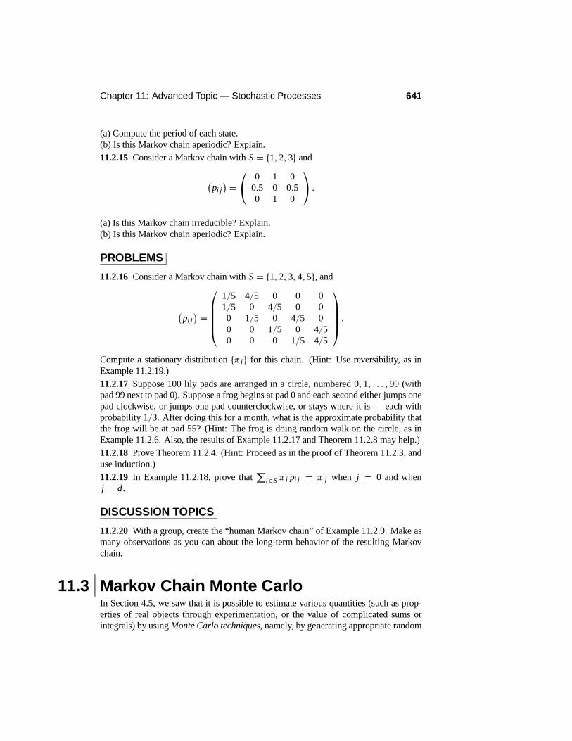
Chapter 11: Advanced Topic — Stochastic Processes 641
(a) Compute the period of each state.(b) Is this Markov chain aperiodic? Explain.11.2.15 Consider a Markov chain with S = {1, 2, 3} and
!pi j" =
0 1 00.5 0 0.50 1 0
.
(a) Is this Markov chain irreducible? Explain.(b) Is this Markov chain aperiodic? Explain.
PROBLEMS
11.2.16 Consider a Markov chain with S = {1, 2, 3, 4, 5}, and
!pi j" =
1/5 4/5 0 0 01/5 0 4/5 0 00 1/5 0 4/5 00 0 1/5 0 4/50 0 0 1/5 4/5
.
Compute a stationary distribution {π i} for this chain. (Hint: Use reversibility, as inExample 11.2.19.)11.2.17 Suppose 100 lily pads are arranged in a circle, numbered 0, 1, . . . , 99 (withpad 99 next to pad 0). Suppose a frog begins at pad 0 and each second either jumps onepad clockwise, or jumps one pad counterclockwise, or stays where it is — each withprobability 1/3. After doing this for a month, what is the approximate probability thatthe frog will be at pad 55? (Hint: The frog is doing random walk on the circle, as inExample 11.2.6. Also, the results of Example 11.2.17 and Theorem 11.2.8 may help.)11.2.18 Prove Theorem 11.2.4. (Hint: Proceed as in the proof of Theorem 11.2.3, anduse induction.)11.2.19 In Example 11.2.18, prove that
(i∈S π i pi j = π j when j = 0 and when
j = d.
DISCUSSION TOPICS
11.2.20 With a group, create the “human Markov chain” of Example 11.2.9. Make asmany observations as you can about the long-term behavior of the resulting Markovchain.
11.3 Markov Chain Monte CarloIn Section 4.5, we saw that it is possible to estimate various quantities (such as prop-erties of real objects through experimentation, or the value of complicated sums orintegrals) by using Monte Carlo techniques, namely, by generating appropriate random

642 Section 11.3: Markov Chain Monte Carlo
variables on a computer. Furthermore, we have seen in Section 2.10 that it is quite easyto generate random variables having certain special distributions. The Monte Carlomethod was used several times in Chapters 6, 7, 9, and 10 to assist in the implementa-tion of various statistical methods.
However, for many (in fact, most!) probability distributions, there is no simple,direct way to simulate (on a computer) random variables having such a distribution.We illustrate this with an example.
EXAMPLE 11.3.1Let Z be a random variable taking values on the set of all integers, with
P(Z = j) = C( j − 1/2)4e−3| j | cos2( j) (11.3.1)
for j = . . . ,−2,−1, 0, 1, 2, 3, . . ., where C = 1/(∞
j=−∞( j − 1/2)4e−3| j | cos2( j).
Now suppose that we want to compute the quantity A = E((Z − 20)2).Well, if we could generate i.i.d. random variables Y1, Y2, . . . ,YM with distribution
given by (11.3.1), for very large M , then we could estimate A by
A ≈ A = 1M
M#i=1
(Yi − 20)2.
Then A would be a Monte Carlo estimate of A.The problem, of course, is that it is not easy to generate random variables Yi with
this distribution. In fact, it is not even easy to compute the value of C .
Surprisingly, the difficulties described in Example 11.3.1 can sometimes be solvedusing Markov chains. We illustrate this idea as follows.
EXAMPLE 11.3.2In the context of Example 11.3.1, suppose we could find a Markov chain on the statespace S = {. . . ,−2,−1, 0, 1, 2, . . .} of all integers, which was irreducible and aperi-odic and which had a stationary distribution given by π j = C( j − 1/2)4e−3| j | cos2( j)for j ∈ S.
If we did, then we could run the Markov chain for a long time N , to get randomvalues X0, X1, X2, . . . , X N . For large enough N , by Theorem 11.2.8, we would have
P(X N = j) ≈ π j = C( j − 1/2)4e−3| j | cos2( j).
Hence, if we set Y1 = X N , then we would have P(Y1 = j) approximately equal to(11.3.1), for all integers j . That is, the value of X N would be approximately as goodas a true random variable Y1 with this distribution.
Once the value of Y1 was generated, then we could repeat the process by againrunning the Markov chain, this time to generate new random values
X [2]0 , X [2]
1 , X [2]2 , . . . , X [2]
N
(say). We would then have
P(X [2]N = j) ≈ π j = C( j − 1/2)4e−3| j | cos2( j).

Chapter 11: Advanced Topic — Stochastic Processes 643
Hence, if we set Y2 = X [2]N , then we would have P(Y2 = j) approximately equal to
(11.3.1), for all integers j .Continuing in this way, we could generate values Y1,Y2, Y3, . . . ,YM , such that
these are approximately i.i.d. from the distribution given by (11.3.1). We could then,as before, estimate A by
A ≈ A = 1M
M#i=1
(Yi − 20)2.
This time, the approximation has two sources of error. First, there is Monte Carloerror because M might not be large enough. Second, there is Markov chain error,because N might not be large enough. However, if M and N are both very large, thenA will be a good approximation to A.
We summarize the method of the preceding example in the following theorem.
Theorem 11.3.1 (The Markov chain Monte Carlo method) Suppose we wish toestimate the expected value A = E (h(Z)) , where P(Z = j) = π j for j ∈ S, withP(Z = j) = 0 for j 6∈ S. Suppose for i = 1, 2, . . . ,M, we can generate valuesX [i]
0 , X [i]1 , X [i]
2 , . . . , X [i]N from some Markov chain that is irreducible, aperiodic, and
has {π j } as a stationary distribution. Let
A = 1M
M#i=1
h(X [i]N ).
If M and N are sufficiently large, then A ≈ A.
It is somewhat inefficient to run M different Markov chains. Instead, practitionersoften just run a single Markov chain, and average over the different values of the chain.For an irreducible Markov chain run long enough, this will again converge to the rightanswer, as the following theorem states.
Theorem 11.3.2 (The single-chain Markov chain Monte Carlo method) Supposewe wish to estimate the expected value A = E (h(Z)) , where P(Z = j) = π jfor j ∈ S, with P(Z = j) = 0 for j 6∈ S. Suppose we can generate valuesX0, X1, X2, . . . , X N from some Markov chain that is irreducible, aperiodic, andhas {π j } as a stationary distribution. For some integer B ≥ 0, let
A = 1N − B + 1
N#i=B+1
h(Xi).
If N − B is sufficiently large, then A ≈ A.
Here, B is the burn-in time, designed to remove the influence of the chain’s startingvalue X0. The best choice of B remains controversial among statisticians. However, ifthe starting value X0 is “reasonable,” then it is okay to take B = 0, provided that N issufficiently large. This is what was done, for instance, in Example 7.3.2.

644 Section 11.3: Markov Chain Monte Carlo
These theorems indicate that, if we can construct a Markov chain that has {π i}as a stationary distribution, then we can use that Markov chain to estimate quantitiesassociated with {π i }. This is a very helpful trick, and it has made the Markov chainMonte Carlo method into one of the most popular techniques in the entire subject ofcomputational statistics.
However, for this technique to be useful, we need to be able to construct a Markovchain that has {π i } as a stationary distribution. This sounds like a difficult problem!Indeed, if {π i } were very simple, then we would not need to use Markov chain MonteCarlo at all. But if {π i } is complicated, then how can we possibly construct a Markovchain that has that particular stationary distribution?
Remarkably, this problem turns out to be much easier to solve than one mightexpect. We now discuss one of the best solutions, the Metropolis–Hastings algorithm.
11.3.1 The Metropolis–Hastings Algorithm
Suppose we are given a probability distribution {π i } on a state space S. How can weconstruct a Markov chain on S that has {π i } as a stationary distribution?
One answer is given by the Metropolis–Hastings algorithm. It designs a Markovchain that proceeds in two stages. In the first stage, a new point is proposed fromsome proposal distribution. In the second stage, the proposed point is either acceptedor rejected. If the proposed point is accepted, then the Markov chain moves there. Ifit is rejected, then the Markov chain stays where it is. By choosing the probabilityof accepting to be just right, we end up creating a Markov chain that has {π i} as astationary distribution.
The details of the algorithm are as follows. We start with a state space S, anda probability distribution {π i } on S. We then choose some (simple) Markov chaintransition probabilities {qi j : i, j ∈ S} called the proposal distribution. Thus, werequire that qi j ≥ 0, and
(j∈S qi j = 1 for each i ∈ S. However, we do not assume
that {π i } is a stationary distribution for the chain {qi j }; indeed, the chain {qi j} mightnot even have a stationary distribution.
Given Xn = i , the Metropolis–Hastings algorithm computes the value Xn+1 asfollows.
1. Choose Yn+1 = j according to the Markov chain {qi j}.
2. Set αi j = minA
1,π j q jiπ i qi j
B(the acceptance probability).
3. With probability αi j , let Xn+1 = Yn+1 = j (i.e., accepting the proposal Yn+1).Otherwise, with probability 1 − αi j , let Xn+1 = Xn = i (i.e., rejecting theproposal Yn+1).
The reason for this unusual algorithm is given by the following theorem.
Theorem 11.3.3 The preceding Metropolis–Hastings algorithm results in a Markovchain X0, X1, X2, . . . , which has {π i } as a stationary distribution.

Chapter 11: Advanced Topic — Stochastic Processes 645
PROOF See Section 11.7 for the proof.
We consider some applications of this algorithm.
EXAMPLE 11.3.3As in Example 11.3.1, suppose S = {. . . ,−2,−1, 0, 1, 2, . . .}, and
π j = C( j − 1/2)4e−3| j| cos2( j),
for j ∈ S. We shall construct a Markov chain having {π i} as a stationary distribution.We first need to choose some simple Markov chain {qi j }. We let {qi j } be simple
random walk with p = 1/2, so that qi j = 1/2 if j = i + 1 or j = i − 1, and qi j = 0otherwise.
We then compute that if j = i + 1 or j = i − 1, then
αi j = minE
1,q jiπ j
qi jπ i
F= min
E1,(1/2)C( j − 1/2)4e−3| j | cos2( j)
(1/2)C(i − 1/2)4e3i cos2(i)
F= min
E1,( j − 1/2)4e−3| j | cos2( j)
(i − 1/2)4e3i cos2(i)
F. (11.3.2)
Note that C has cancelled out, so that αi j does not depend on C. (In fact, this willalways be the case.) Hence, we see that αi j , while somewhat messy, is still very easyfor a computer to calculate.
Given Xn = i , the Metropolis–Hastings algorithm computes the value Xn+1 asfollows.
1. Let Yn+1 = Xn + 1 or Yn+1 = Xn − 1, with probability 1/2 each.
2. Let j = Yn+1, and compute αi j as in (11.3.2).
3. With probability αi j , let Xn+1 = Yn+1 = j . Otherwise, with probability 1−αi j ,let Xn+1 = Xn = i .
These steps can all be easily performed on a computer. If we repeat this for n =0, 1, 2, . . . , N−1, for some large number N of iterations, then we will obtain a randomvariable X N , where P(X N = j) ≈ π j = C( j − 1/2)4e−3| j | cos2( j), for all j ∈ S.
EXAMPLE 11.3.4Again, let S = {. . . ,−2,−1, 0, 1, 2, . . .}, and this time let π j = K e− j4
, for j ∈ S.Let the proposal distribution {qi j } correspond to a simple random walk with p = 1/4,so that Yn+1 = Xn + 1 with probability 1/4, and Yn+1 = Xn − 1 with probability 3/4.
In this case, we compute that if j = i + 1, then
αi j = minE
1,q jiπ j
qi jπ i
F= min
81,(3/4)K e− j4
(1/4)Ke−i4
9= min
A1, 3e j4−i4
B. (11.3.3)
If instead j = i − 1, then
αi j = minE
1,q jiπ j
qi jπ i
F= min
81,(1/4)K e− j4
(3/4)K e−i4
9= min
A1, (1/3)e j4−i4
B. (11.3.4)

646 Section 11.3: Markov Chain Monte Carlo
(Note that the constant K has again cancelled out, as expected.) Hence, again αi j isvery easy for a computer to calculate.
Given Xn = i , the Metropolis–Hastings algorithm computes the value Xn+1 asfollows.
1. Let Yn+1 = Xn + 1 with probability 1/4, or Yn+1 = Xn − 1 with probability3/4.
2. Let j = Yn+1, and compute αi j using (11.3.3) and (11.3.4).
3. With probability αi j , let Xn+1 = Yn+1 = j . Otherwise, with probability 1−αi j ,let Xn+1 = Xn = i .
Once again, these steps can all be easily performed on a computer; if repeated forsome large number N of iterations, then P(X N = j) ≈ π j = Ke− j4
for j ∈ S.
The Metropolis–Hastings algorithm can also be used for continuous random vari-ables by using densities, as follows.
EXAMPLE 11.3.5Suppose we want to generate a sample from the distribution with density proportionalto
f (y) = e−y4(1+ |y|)3.
So the density is C f (y), where C = 1/I∞−∞ f (y) dy. How can we generate a random
variable Y such that Y has approximately this distribution, i.e., has probability densityapproximately equal to C f (y)?
Let us use a proposal distribution given by an N(x, 1) distribution, namely, a nor-mal distribution with mean x and variance 1. That is, given Xn = x , we choose Yn+1
by Yn+1 ∼ N(x, 1). Because the N(x, 1) distribution has density (2π)−1/2 e−(y−x)2/2,
this corresponds to a proposal density of q(x, y) = (2π)−1/2 e−(y−x)2/2.As for the acceptance probability α(x, y), we again use densities, so that
α(x, y) = minE
1,C f (y) q(y, x)
C f (x) q(x, y)
F= min
81,$
1+ |y|1+ |x |
%3 C e−y4(2π)−1/2 e−(y−x)2/2
C e−x4(2π)−1/2 e−(x−y)2/2
9
= min
81,$
1+ |y|1+ |x |
%3
e−y4+x4
9. (11.3.5)
Given Xn = x , the Metropolis–Hastings algorithm computes the value Xn+1 asfollows.
1. Generate Yn+1 ∼ N(Xn, 1).
2. Let y = Yn+1, and compute α(x, y), as before.
3. With probability α(x, y), let Xn+1 = Yn+1 = y. Otherwise, with probability1− α(x, y), let Xn+1 = Xn = x .

Chapter 11: Advanced Topic — Stochastic Processes 647
Once again, these steps can all be easily performed on a computer; if repeated forsome large number N of iterations, then the random variable X N will approximatelyhave density given by C f (y).
11.3.2 The Gibbs Sampler
In Section 7.3.3 we discussed the Gibbs sampler and its application in a Bayesianstatistics problem. As we will now demonstrate, the Gibbs sampler is a specializedversion of the Metropolis–Hastings algorithm, designed for multivariate distributions.It chooses the proposal probabilities qi j just right so that we always have αi j = 1, i.e.,so that no rejections are ever required.
Suppose that S = {. . . ,−2,−1, 0, 1, 2, . . .} × {. . . ,−2,−1, 0, 1, 2, . . .}, i.e., S isthe set of all ordered pairs of integers i = (i1, i2). (Thus, (2, 3) ∈ S, and (−6, 14) ∈ S,etc.) Suppose that some distribution {π i } is defined on S. Define a proposal distribution{q(1)i j } as follows.
Let V (i) = {j ∈ S : j2 = i2}. That is, V (i) is the set of all states j ∈ S such that iand j agree in their second coordinate. Thus, V (i) is a vertical line in S, which passesthrough the point i .
In terms of this definition of V (i), define q(1)i j = 0 if j 6∈ V (i), i.e., if i and j differin their second coordinate. If j ∈ V (i), i.e., if i and j agree in their second coordinate,then define
q(1)i j = π j(k∈V (i) πk
.
One interpretation is that, if Xn = i , and P(Yn+1 = j) = q(1)i j for j ∈ S, then thedistribution of Yn+1 is the conditional distribution of {π i }, conditional on knowing thatthe second coordinate must be equal to i2.
In terms of this choice of q(1)i j , what is αi j ? Well, if j ∈ V (i), then i ∈ V ( j), andalso V ( j) = V (i). Hence,
αi j = min
81,π j q
(1)ji
π i q(1)i j
9= min
1,π j
)π i/
(k∈V ( j) π k
*π i
)π j/
(l∈V (i) π l
*
= minE
1,π jπ i
π iπ j
F= min {1, 1} = 1.
That is, this algorithm accepts the proposal Yn+1 with probability 1, and never rejectsat all!
Now, this algorithm by itself is not very useful because it proposes only states inV (i), so it never changes the value of the second coordinate at all. However, we cansimilarly define a horizontal line through i by H(i) = {j ∈ S : j1 = i1}, so that H(i)is the set of all states j such that i and j agree in their first coordinate. That is, H(i) isa horizontal line in S that passes through the point i .

648 Section 11.3: Markov Chain Monte Carlo
We can then define q(2)i j = 0 if j 6∈ H(i) (i.e., if i and j differ in their first coordi-nate), while if j ∈ V (i) (i.e., if i and j agree in their first coordinate), then
q(2)i j = π j(k∈H(i) πk
.
As before, we compute that for this proposal, we will always have αi j = 1, i.e., theMetropolis–Hastings algorithm with this proposal will never reject.
The Gibbs sampler works by combining these two different Metropolis–Hastingsalgorithms, by alternating between them. That is, given a value Xn = i , it produces avalue Xn+1 as follows.
1. Propose a value Yn+1 ∈ V (i), according to the proposal distribution {q(1)i j }.2. Always accept Yn+1 and set j = Yn+1, thus moving vertically.
3. Propose a value Zn+1 ∈ H( j), according to the proposal distribution {q(2)i j }.4. Always accept Zn+1, thus moving horizontally.
5. Set Xn+1 = Zn+1.
In this way, the Gibbs sampler does a “zigzag” through the state space S, alternatelymoving in the vertical and in the horizontal direction.
In light of Theorem 11.3.2, we immediately obtain the following.
Theorem 11.3.4 The preceding Gibbs sampler algorithm results in a Markov chainX0, X1, X2, . . . that has {π i } as a stationary distribution.
The Gibbs sampler thus provides a particular way of implementing the Metropolis–Hastings algorithm in multidimensional problems, which never rejects the proposedvalues.
Summary of Section 11.3
• In cases that are too complicated for ordinary Monte Carlo techniques, it is pos-sible to use Markov chain Monte Carlo techniques instead, by averaging valuesarising from a Markov chain.
• The Metropolis–Hastings algorithm provides a simple way to create a Markovchain with stationary distribution {π i }. Given Xn , it generates a proposal Yn+1from a proposal distribution {qi j }, and then either accepts this proposal (and setsXn+1 = Yn+1) with probability αi j , or rejects this proposal (and sets Xn+1 =Xn) with probability 1− αi j .
• Alternatively, the Gibbs sampler updates the coordinates one at a time from theirconditional distribution, such that we always have αi j = 1.

Chapter 11: Advanced Topic — Stochastic Processes 649
EXERCISES
11.3.1 Suppose π i = C e−(i−13)4 for i ∈ S = {. . . ,−2,−1, 0, 1, 2, . . .}, where C =1/(∞
i=−∞ e−(i−13)4 . Describe in detail a Metropolis–Hastings algorithm for {π i},which uses simple random walk with p = 1/2 for the proposals.11.3.2 Suppose π i = C (i + 6.5)−8 for i ∈ S = {. . . ,−2,−1, 0, 1, 2, . . .}, whereC = 1/
(∞i=−∞(i + 6.5)−8. Describe in detail a Metropolis–Hastings algorithm for
{π i }, which uses simple random walk with p = 5/8 for the proposals.
11.3.3 Suppose π i = K e−i4−i6−i8for i ∈ S = {. . . ,−2,−1, 0, 1, 2, . . .}, where
C = 1/(∞
i=−∞ e−i4−i6−i8. Describe in detail a Metropolis–Hastings algorithm for
{π i }, which uses simple random walk with p = 7/9 for the proposals.
11.3.4 Suppose f (x) = e−x4−x6−x8for x ∈ R1. Let K = 1/
I∞−∞ e−x4−x6−x8
dx.Describe in detail a Metropolis–Hastings algorithm for the distribution having densityK f (x), which uses the proposal distribution N(x, 1), i.e., a normal distribution withmean x and variance 1.11.3.5 Let f (x) = e−x4−x6−x8
for x ∈ R1, and let K = 1/I∞−∞ e−x4−x6−x8
dx .Describe in detail a Metropolis–Hastings algorithm for the distribution having densityK f (x), which uses the proposal distribution N(x, 10), i.e., a normal distribution withmean x and variance 10.
COMPUTER EXERCISES
11.3.6 Run the algorithm of Exercise 11.3.1. Discuss the output.
11.3.7 Run the algorithm of Exercise 11.3.2. Discuss the output.
PROBLEMS
11.3.8 Suppose S = {1, 2, 3, . . .}×{1, 2, 3, . . .}, i.e., S is the set of all pairs of positiveintegers. For i = (i1, i2) ∈ S, suppose π i = C / 2i1+i2 for appropriate positive constantC . Describe in detail a Gibbs sampler algorithm for this distribution {π i }.
COMPUTER PROBLEMS
11.3.9 Run the algorithm of Exercise 11.3.4. Discuss the output.11.3.10 Run the algorithm of Exercise 11.3.5. Discuss the output.
DISCUSSION TOPICS
11.3.11 Why do you think Markov chain Monte Carlo algorithms have become sopopular in so many branches of science? (List as many reasons as you can.)11.3.12 Suppose you will be using a Markov chain Monte Carlo estimate of the form
A = 1M
M#i=1
h(X [i]N ).

650 Section 11.4: Martingales
Suppose also that, due to time constraints, your total number of iterations cannot bemore than one million. That is, you must have N M ≤ 1,000,000. Discuss the advan-tages and disadvantages of the following choices of N and M.(a) N =1,000,000 M = 1.(b) N = 1, M =1,000,000(c) N = 100, M = 10,000(d) N = 10,000, M = 100(e) N = 1000, M = 1000(f) Which choice do you think would be best, under what circumstances? Why?
11.4 MartingalesIn this section, we study a special class of stochastic processes called martingales. Weshall see that these processes are characterized by “staying the same on average.”
As motivation, consider again a simple random walk in the case of a fair game, i.e.,with p = 1/2. Suppose, as in the gambler’s ruin setup, that you start at a and keepgoing until you hit either c or 0, where 0 < a < c. Let Z be the value that you end upwith, so that we always have either Z = c or Z = 0. We know from Theorem 11.1.2that in fact P(Z = c) = a/c, so that P(Z = 0) = 1− a/c.
Let us now consider the expected value of Z . We have that
E(Z) =#z∈R1
z P(Z = z) = cP(Z = c)+ 0P(Z = 0) = c(a/c) = a.
That is, the average value of where you end up is a. But a is also the value at whichyou started!
This is not a coincidence. Indeed, because p = 1/2 (i.e., the game was fair), thismeans that “on average” you always stayed at a. That is, {Xn} is a martingale.
11.4.1 Definition of a Martingale
We begin with the definition of a martingale. For simplicity, we assume that the mar-tingale is a Markov chain, though this is not really necessary.
Definition 11.4.1 Let X0, X1, X2, . . . be a Markov chain. The chain is a martingaleif for all n = 0, 1, 2, . . . , we have E(Xn+1 − Xn | Xn) = 0. That is, on average thechain’s value does not change, regardless of what the current value Xn actually is.
EXAMPLE 11.4.1Let {Xn} be simple random walk with p = 1/2. Then Xn+1 − Xn is equal to either 1or −1, with probability 1/2 each. Hence,
E(Xn+1 − Xn | Xn) = (1)(1/2)+ (−1)(1/2) = 0,
so {Xn} stays the same on average and is a martingale. (Note that we will never actuallyhave Xn+1 − Xn = 0. However, on average we will have Xn+1 − Xn = 0.)

Chapter 11: Advanced Topic — Stochastic Processes 651
EXAMPLE 11.4.2Let {Xn} be simple random walk with p = 2/3. Then Xn+1 − Xn is equal to either 1or −1, with probabilities 2/3 and 1/3, respectively. Hence,
E(Xn+1 − Xn | Xn) = (1)(2/3)+ (−1)(1/3) = 1/3 6= 0.
Thus, {Xn} is not a martingale in this case.
EXAMPLE 11.4.3Suppose we start with the number 5 and then repeatedly do the following. We either add3 to the number (with probability 1/4), or subtract 1 from the number (with probability3/4). Let Xn be the number obtained after repeating this procedure n times. Then,given the value of Xn, we see that Xn+1 = Xn+3 with probability 1/4, while Xn+1 =Xn − 1 with probability 3/4. Hence,
E(Xn+1 − Xn | Xn) = (3)(1/4)+ (−1)(3/4) = 3/4− 3/4 = 0
and {Xn} is a martingale.
It is sometimes possible to create martingales in subtle ways, as follows.
EXAMPLE 11.4.4Let {Xn} again be simple random walk, but this time for general p. Then Xn+1 − Xn
is equal to 1 with probability p, and to −1 with probability q = 1− p. Hence,
E(Xn+1 − Xn | Xn) = (1)(p)+ (−1)(q) = p − q = 2p − 1.
If p 6= 1/2, then this is not equal to 0. Hence, {Xn} does not stay the same on average,so {Xn} is not a martingale.
On the other hand, let
Zn =$
1− p
p
%Xn
,
i.e., Zn equals the constant (1− p)/p raised to the power of Xn . Then increasing Xn by1 corresponds to multiplying Zn by (1− p)/p, while decreasing Xn by 1 correspondsto dividing Zn by (1− p)/p, i.e., multiplying by p/(1− p). But Xn+1 = Xn + 1 withprobability p, while Xn+1 = Xn − 1 with probability q = 1 − p. Therefore, we seethat, given the value of Zn, we have
E(Zn+1 − Zn | Zn) =$
1− p
pZn − Zn
%p +
$p
1− pZn − Zn
%(1− p)
= ((1− p)Zn − pZn)+ (pZn − (1− p)Zn) = 0.
Accordingly, E(Zn+1−Zn | Zn) = 0, so that {Zn} stays the same on average, i.e., {Zn}is a martingale.
11.4.2 Expected Values
Because martingales stay the same on average, we immediately have the following.

652 Section 11.4: Martingales
Theorem 11.4.1 Let {Xn} be a martingale with X0 = a. Then E(Xn) = a for alln.
This theorem sometimes provides very useful information, as the following exam-ples demonstrate.
EXAMPLE 11.4.5Let {Xn} again be simple random walk with p = 1/2. Then we have already seen that{Xn} is a martingale. Hence, if X0 = a, then we will have E(Xn) = a for all n. Thatis, for a fair game (i.e., for p = 1/2), no matter how long you have been gambling,your average fortune will always be equal to your initial fortune a.
EXAMPLE 11.4.6Suppose we start with the number 10 and then repeatedly do the following. We eitheradd 2 to the number (with probability 1/3), or subtract 1 from the number (with proba-bility 2/3). Suppose we repeat this process 25 times. What is the expected value of thenumber we end up with?
Without martingale theory, this problem appears to be difficult, requiring lengthycomputations of various possibilities for what could happen on each of the 25 steps.However, with martingale theory, it is very easy.
Indeed, let Xn be the number after n steps, so that X0 = 10, X1 = 12 (withprobability 1/3) or X1 = 9 (with probability 2/3), etc. Then, because Xn+1 − Xnequals either 2 (with probability 1/3) or −1 (with probability 2/3), we have
E(Xn+1 − Xn | Xn) = 2(1/3)+ (−1)(2/3) = 2/3− 2/3 = 0.
Hence, {Xn} is a martingale.It then follows that E(Xn) = X0 = 10, for any n. In particular, E(X25) = 10.
That is, after 25 steps, on average the number will be equal to 10.
11.4.3 Stopping Times
If {Xn} is a martingale with X0 = a, then it is very helpful to know that E(Xn) = afor all n. However, it is sometimes even more helpful to know that E(XT ) = a, whereT is a random time. Now, this is not always true; however, it is often true, as we shallsee. We begin with another definition.
Definition 11.4.2 Let {Xn} be a stochastic process, and let T be a random variabletaking values in {0, 1, 2, . . .}. Then T is a stopping time if for all m = 0, 1, 2, . . .,the event {T = m} is independent of the values Xm+1, Xm+2, . . . . That is, whendeciding whether or not T = m (i.e., whether or not to “stop” at time m), we arenot allowed to look at the future values Xm+1, Xm+2, . . . .
EXAMPLE 11.4.7Let {Xn} be simple random walk, let b be any integer, and let τ b = min{n ≥ 0 : Xn =b} be the first time we hit the value b. Then τ b is a stopping time because the eventτ b = n depends only on X0, . . . , Xn , not on Xn+1, Xn+2, . . . .

Chapter 11: Advanced Topic — Stochastic Processes 653
On the other hand, let T = τ b − 1, so that T corresponds to stopping just beforewe hit b. Then T is not a stopping time because it must look at the future value Xm+1to decide whether or not to stop at time m.
A key result about martingales and stopping times is the optional stopping theorem,as follows.
Theorem 11.4.2 (Optional stopping theorem) Suppose {Xn} is a martingale withX0 = a, and T is a stopping time. Suppose further that either
(a) the martingale is bounded up to time T , i.e., for some M > 0 we have |Xn| ≤ Mfor all n ≤ T ; or(b) the stopping time is bounded, i.e., for some M > 0 we have T ≤ M .
Then E(XT ) = a, i.e., on average the value of the process at the random time T isequal to the starting value a.
PROOF For a proof and further discussion, see, e.g., page 273 of Probability: The-ory and Examples, 2nd ed., by R. Durrett (Duxbury Press, New York, 1996).
Consider a simple application of this.
EXAMPLE 11.4.8Let {Xn} be simple random walk with initial value a and with p = 1/2. Let r > a > sbe integers. Let T = min{τ r , τ s} be the first time the process hits either r or s. Thenr ≥ Xn ≥ s for n ≤ T , so that condition (a) of the optional stopping theorem applies.We conclude that E(XT ) = a, i.e., that at time T , the walk will on average be equal toa.
We shall see that the optional stopping theorem is useful in many ways.
EXAMPLE 11.4.9We can use the optional stopping theorem to find the probability that the simple randomwalk with p = 1/2 will hit r before hitting another value s.
Indeed, again let {Xn} be simple random walk with initial value a and p = 1/2,with r > a > s integers and T = min{τ r , τ s}. Then as earlier, E(XT ) = a. We canuse this to solve for P(XT = r), i.e., for the probability that the walk hits r beforehitting s.
Clearly, we always have either XT = r or XT = s. Let h = P(XT = r). ThenE(XT ) = hr + (1 − h)s. Because E(XT ) = a, we must have a = hr + (1 − h)s.Solving for h, we see that
P(XT = r) = a − s
r − s.
We conclude that the probability that the process will hit r before it hits s is equalto (a − s)/(r − s). Note that absolutely no difficult computations were required toobtain this result.
A special case of the previous example is particularly noteworthy.

654 Section 11.4: Martingales
EXAMPLE 11.4.10In the previous example, suppose r = c and s = 0. Then the value h = P(XT = r)is precisely the same as the probability of success in the gambler’s ruin problem. Theprevious example shows that h = (a − s)/(r − s) = a/c. This gives the same answeras Theorem 11.1.2, but with far less effort.
It is impressive that, in the preceding example, martingale theory can solve thegambler’s ruin problem so easily in the case p = 1/2. Our previous solution, withoutusing martingale theory, was much more difficult (see Section 11.7). Even more sur-prising, martingale theory can also solve the gambler’s ruin problem when p 6= 1/2, asfollows.
EXAMPLE 11.4.11Let {Xn} be simple random walk with initial value a and with p 6= 1/2. Let 0 < a < cbe integers. Let T = min {τ c, τ 0} be the first time the process hits either c or 0. Tosolve the gambler’s ruin problem in this case, we are interested in g = P(XT = c).We can use the optional stopping theorem to solve for the gambler’s ruin probability g,as follows.
Now, {Xn} is not a martingale, so we cannot apply martingale theory to it. However,let
Zn =$
1− p
p
%Xn
.
Then {Zn} has initial value Z0 = ((1− p)/p)a . Also, we know from Example 11.4.4that {Zn} is a martingale. Furthermore,
0 ≤ Zn ≤ max
8$1− p
p
%c
,
$1− p
p
%−c9
for n ≤ T , so that condition (a) of the optional stopping theorem applies. We concludethat
E(ZT ) = Z0 =$
1− p
p
%a
.
Now, clearly, we always have either XT = c (with probability g) or XT = 0(with probability 1 − g). In the former case, ZT = ((1 − p)/p)c, while in the lattercase, ZT = 1. Hence, E(ZT ) = g((1 − p)/p)c + (1 − g)(1). Because E(ZT ) =((1− p) /p)a , we must have$
1− p
p
%a
= g
$1− p
p
%c
+ (1− g)(1).
Solving for g, we see that
g = ((1− p)/p)a − 1((1− p)/p)c − 1
.
This again gives the same answer as Theorem 11.1.2, this time for p 6= 1/2, butagain with far less effort.
Martingale theory can also tell us other surprising facts.

Chapter 11: Advanced Topic — Stochastic Processes 655
EXAMPLE 11.4.12Let {Xn} be simple random walk with p = 1/2 and with initial value a = 0. Willthe walk hit the value −1 some time during the first million steps? Probably yes, butnot for sure. Furthermore, conditional on not hitting −1, it will probably be extremelylarge, as we now discuss.
Let T = min{106, τ−1}. That is, T is the first time the process hits−1, unless thattakes more than one million steps, in which case T = 106.
Now, {Xn} is a martingale. Also T is a stopping time (because it does not lookinto the future when deciding whether or not to stop). Furthermore, we always haveT ≤ 106, so condition (b) of the optional stopping theorem applies. We conclude thatE(XT ) = a = 0.
On the other hand, by the law of total expectation, we have
E(XT ) = E(XT | XT = −1) P(XT = −1)+ E(XT | XT 6= −1) P(XT 6= −1).
Also, clearly E(XT | XT = −1) = −1. Let u = P(XT = −1), so that P(XT 6=−1) = 1− u. Then we conclude that 0 = (−1)u + E(XT | XT 6= −1)(1− u), so that
E(XT | XT 6= −1) = u
1− u.
Now, clearly, u will be very close to 1, i.e., it is very likely that within 106 steps theprocess will have hit −1. Hence, E(XT | XT 6= −1) is extremely large.
We may summarize this discussion as follows. Nearly always we have XT = −1.However, very occasionally we will have XT 6= −1. Furthermore, the average valueof XT when XT 6= −1 is so large that overall (i.e., counting both the case XT = −1and the case XT 6= −1), the average value of XT is 0 (as it must be because {Xn} is amartingale)!
If one is not careful, then it is possible to be tricked by martingale theory, as follows.
EXAMPLE 11.4.13Suppose again that {Xn} is simple random walk with p = 1/2 and with initial valuea = 0. Let T = τ−1, i.e., T is the first time the process hits −1 (no matter how longthat takes).
Because the process will always wait until it hits −1, we always have XT = −1.Because this is true with probability 1, we also have E(XT ) = −1.
On the other hand, again {Xn} is a martingale, so again it appears that we shouldhave E(XT ) = 0. What is going on?
The answer, of course, is that neither condition (a) nor condition (b) of the optionalstopping theorem is satisfied in this case. That is, there is no limit to how large T mighthave to be or how large Xn might get for some n ≤ T . Hence, the optional stoppingtheorem does not apply in this case, and we cannot conclude that E(XT ) = 0. Instead,E(XT ) = −1 here.
Summary of Section 11.4
• A Markov chain {Xn} is a martingale if it stays the same on average, i.e., ifE(Xn+1 − Xn | Xn) = 0 for all n. There are many examples.

656 Section 11.4: Martingales
• A stopping time T for the chain is a nonnegative integer-valued random variablethat does not look into the future of {Xn}. For example, perhaps T = τ b is thefirst time the chain hits some state b.
• If {Xn} is a martingale with stopping time T , and if either T or {Xn}n≤T isbounded, then E(XT ) = X0. This can be used to solve many problems, e.g.,gambler’s ruin.
EXERCISES
11.4.1 Suppose we define a process {Xn} as follows. Given Xn, with probability 3/8we let Xn+1 = Xn−4, while with probability 5/8 we let Xn+1 = Xn+C . What valueof C will make {Xn} be a martingale?11.4.2 Suppose we define a process {Xn} as follows. Given Xn, with probability p welet Xn+1 = Xn + 7, while with probability 1− p we let Xn+1 = Xn − 2. What valueof p will make {Xn} be a martingale?11.4.3 Suppose we define a process {Xn} as follows. Given Xn, with probability p welet Xn+1 = 2Xn, while with probability 1− p we let Xn+1 = Xn/2. What value of pwill make {Xn} be a martingale?11.4.4 Let {Xn} be a martingale, with initial value X0 = 14. Suppose for some n, weknow that P(Xn = 8)+ P(Xn = 12)+ P(Xn = 17) = 1, i.e., Xn is always either 8,12, or 17. Suppose further that P(Xn = 8) = 0.1. Compute P(Xn = 14).11.4.5 Let {Xn} be a martingale, with initial value X0 = 5. Suppose we know thatP(X8 = 3) + P(X8 = 4) + P(X8 = 6) = 1, i.e., X8 is always either 3, 4, or 6.Suppose further that P(X8 = 3) = 2 P(X8 = 6). Compute P(X8 = 4).11.4.6 Suppose you start with 175 pennies. You repeatedly flip a fair coin. Each timethe coin comes up heads, you win a penny; each time the coin comes up tails, you losea penny.(a) After repeating this procedure 20 times, how many pennies will you have on aver-age?(b) Suppose you continue until you have either 100 or 200 pennies, and then you stop.What is the probability you will have 200 pennies when you stop?11.4.7 Define a process {Xn} by X0 = 27, and Xn+1 = 3Xn with probability 1/4, orXn+1 = Xn/3 with probability 3/4. Let T = min {τ 1, τ81} be the first time the processhits either 1 or 81.(a) Show that {Xn} is a martingale.(b) Show that T is a stopping time.(c) Compute E(XT ).(d) Compute the probability P(XT = 1) that the process hits 1 before hitting 81.
PROBLEMS
11.4.8 Let {Xn} be a stochastic process, and let T1 be a stopping time. Let T2 = T1+ iand T3 = T1 − i , for some positive integer i . Which of T2 and T3 is necessarily astopping time, and which is not? (Explain your reasoning.)

Chapter 11: Advanced Topic — Stochastic Processes 657
11.4.9 Let {Xn} be a stochastic process, and let T1 and T2 be two different stoppingtimes. Let T3 = min {T1, T2}, and T4 = max {T1, T2}.(a) Is T3 necessarily a stopping time? (Explain your reasoning.)(b) Is T4 necessarily a stopping time? (Explain your reasoning.)
11.5 Brownian MotionThe simple random walk model of Section 11.1.2 (with p = 1/2) can be extended toan interesting continuous-time model, called Brownian motion, as follows. Roughly,the idea is to speed up time faster and faster by a factor of M (for very large M),while simultaneously shrinking space smaller and smaller by a factor of 1/
√M. The
factors of M and 1/√
M are chosen just right so that, using the central limit theorem,we can derive properties of Brownian motion. Indeed, using the central limit theorem,we shall see that various distributions related to Brownian motion are in fact normaldistributions.
Historically, Brownian motion gets its name from Robert Brown, a botanist, whoin 1828 observed the motions of tiny particles in solution, under a microscope, asthey were bombarded from random directions by many unseen molecules. Brownianmotion was proposed as a model for the observed chaotic, random movement of suchparticles. In fact, Brownian motion turns out not to be a very good model for suchmovement (for example, Brownian motion has infinite derivative, which would onlymake sense if the particles moved infinitely quickly!). However, Brownian motion hasmany useful mathematical properties and is also very important in the theory of financebecause it is often used as a model of stock price fluctuations. A proper mathematicaltheory of Brownian motion was developed in 1923 by Norbert Wiener2; as a result,Brownian motion is also sometimes called the Wiener process.
We shall construct Brownian motion in two steps. First, we construct faster andfaster random walks, to be called {Y (M)t } where M is large. Then, we take the limit asM →∞ to get Brownian motion.
11.5.1 Faster and Faster Random Walks
To begin, we let Z1, Z2, . . . be i.i.d. with P(Zi = +1) = P(Zi = −1) = 1/2. Foreach M ∈ {1, 2, . . .}, define a discrete-time random process
{Y (M)i/M : i = 0, 1, . . .},by Y (M)0 = 0, and
Y (M)(i+1)/M = Y (M)iM
+ 1√M
Zi+1,
for i = 0, 1, 2, . . . so that
Y (M)i/M = 1√M(Z1 + Z2 + · · · + Zi ).
2Wiener was such an absent-minded professor that he once got lost and could not find his house. In hisconfusion, he asked a young girl for directions, without recognizing the girl as his daughter!

658 Section 11.5: Brownian Motion
Intuitively, then, {Y (M)i/M } is like an ordinary (discrete-time) random walk (with p =1/2), except that time has been sped up by a factor of M and space has been shrunkby a factor of
√M (each step in the new walk moves a distance 1/
√M). That is, this
process takes lots and lots of very small steps.To make {Y (M)i/M } into a continuous-time process, we can then “fill in” the missing
values by making the function linear on the intervals [i/M, (i + 1) /M]. In this way,we obtain a continuous-time process
{Y ∗(M)t : t ≥ 0},
which agrees with {Y (M)i/M } whenever t = 1/M. In Figure 11.5.1, we have plotted
{Y (10)i/10 : i = 0, 1, . . . , 20}
(the dots) and the corresponding values of
{Y ∗(10)t : 0 ≤ t ≤ 20}
(the solid line), arising from the realization
(Z1, . . . , Z20) = (1,−1,−1,−1,−1, 1, . . .) ,
where we have taken 1/√
10 = 0.316.
2.01.91.81.71.61.51.41.31.21.11.00.90.80.70.60.50.40.30.20.10.0
0.9490.949
0.6320.6320.6320.6320.632
0.3160.3160.3160.3160.3160.316
0.0000.0000.0000.0000.000
-0.316-0.316
-0.632
t
Y
Figure 11.5.1: Plot of some values of Y (10)i/10 and Y ∗(10)
t .
The collection of variables {Y ∗(M)t : t ≥ 0} is then a stochastic process but is nowindexed by the continuous time parameter t ≥ 0. This is an example of a continuous-time stochastic process.
Now, the factors M and√
M have been chosen carefully, as the following theoremillustrates.

Chapter 11: Advanced Topic — Stochastic Processes 659
Theorem 11.5.1 Let {Y ∗(M)t : t ≥ 0} be as defined earlier. Then for large M:(a) For t ≥ 0, the distribution of Y ∗(M)t is approximately N(0, t), i.e., normallydistributed with mean t .(b) For s, t ≥ 0, the covariance
Cov)
Y ∗(M)t ,Y ∗(M)t
*is approximately equal to min {s, t}.(c) For t ≥ s ≥ 0, the distribution of the increment Y ∗(M)t − Y ∗(M)s is approxi-mately N(0, t − s), i.e., normally distributed with mean 0 and variance t − s, andis approximately independent of Y ∗(M)s .(d) Y ∗(M)t is a continuous function of t .
PROOF See Section 11.7 for the proof of this result.
We shall use this limit theorem to construct Brownian motion.
11.5.2 Brownian Motion as a Limit
We have now developed the faster and faster processes {Y ∗(M)t : t ≥ 0}, and someof their properties. Brownian motion is then defined as the limit as M → ∞ of theprocesses {Y ∗(M)t : t ≥ 0}. That is, we define Brownian motion {Bt : t ≥ 0} by sayingthat the distribution of {Bt : t ≥ 0} is equal to the limit as M →∞ of the distributionof {Y ∗(M)t : t ≥ 0}. A graph of a typical run of Brownian motion is in Figure 11.5.2.
2.52.01.51.00.50.0
2
1
0
-1
t
B
Figure 11.5.2: A typical outcome from Brownian motion.
In this way, all the properties of Y ∗(M)t for large M , as developed in Theorem 11.5.1,will apply to Brownian motion, as follows.

660 Section 11.5: Brownian Motion
Theorem 11.5.2 Let {Bt : t ≥ 0} be Brownian motion. Then(a) Bt is normally distributed: Bt ∼ N(0, t) for any t ≥ 0;(b) Cov(Bs, Bt ) = E(Bs Bt) = min {s, t} for s, t ≥ 0;(c) if 0 < s < t , then the increment Bt − Bs is normally distributed: Bt − Bs ∼N(0, t − s), and furthermore Bt − Bs is independent of Bs ;(d) the function {Bt }t≥0 is a continuous function.
This theorem can be used to compute many things about Brownian motion.
EXAMPLE 11.5.1Let {Bt } be Brownian motion. What is P(B5 ≤ 3)?
We know that B5 ∼ N(0, 5). Hence, B5/√
5 ∼ N(0, 1). We conclude that
P(B5 ≤ 3) = P(B5/√
5 ≤ 3/√
5) = 0(3/√5) = 0.910,
where
0(x) =6 x
−∞1√2π
e−s2/2 ds
is the cdf of a standard normal distribution, and we have found the numerical valuefrom Table D.2. Thus, about 91% of the time, Brownian motion will be less than 3 attime 5.
EXAMPLE 11.5.2Let {Bt } be Brownian motion. What is P(B7 ≥ −4)?
We know that B7 ∼ N(0, 7). Hence, B7/√
7 ∼ N(0, 1). We conclude that
P(B7 ≥ −4) = 1− P(B7 ≤ −4) = 1− P(B7/√
7 ≤ −4/√
7)
= 1−0(−4/√
7) = 1− 0.065 = 0.935.
Thus, over 93% of the time, Brownian motion will be at least −4 at time 7.
EXAMPLE 11.5.3Let {Bt } be Brownian motion. What is P(B8 − B6 ≤ −1.5)?
We know that B8−B6 ∼ N(0, 8−6) = N(0, 2). Hence, (B8−B6)/√
2 ∼ N(0, 1).We conclude that
P(B8 − B6 ≤ −1.5) = P((B8 − B6)/√
2 ≤ −1.5/√
2) = 0(−1.5/√
2) = 0.144.
Thus, about 14% of the time, Brownian motion will decrease by at least 1.5 betweentime 6 and time 8.
EXAMPLE 11.5.4Let {Bt } be Brownian motion. What is P(B2 ≤ −0.5, B5 − B2 ≥ 1.5)?
By Theorem 11.5.2, we see that B5 − B2 and B2 are independent. Hence,
P(B2 ≤ −0.5, B5 − B2 ≥ 1.5) = P(B2 ≤ −0.5) P(B5 − B2 ≥ 1.5).
Now, we know that B2 ∼ N(0, 2). Hence, B2/√
2 ∼ N(0, 1), and
P(B2 ≤ −0.5) = P(B2/√
2 ≤ −0.5/√
2) = 0(−0.5/√
2).

Chapter 11: Advanced Topic — Stochastic Processes 661
Similarly, B5 − B2 ∼ N(0, 3), so (B5 − B2)/√
3 ∼ N(0, 1), and
P(B5 − B2 ≥ 1.5) = P((B5 − B2)/√
3 ≥ 1.5/√
3)
= 1− P((B5 − B2)/√
3 < 1.5/√
3) = 0(1.5/√3).
We conclude that
P(B2 ≤ −0.5, B5 − B2 ≥ 1.5) = P(B2 ≤ −0.5) P(B5 − B2 ≥ 1.5)
= 0(−0.5/√
2)0(1.5/√
3) = 0.292.
Thus, about 29% of the time, Brownian motion will be no more than −1/2 at time 2and will then increase by at least 1.5 between time 2 and time 5.
We note also that, because Brownian motion was created from simple randomwalks with p = 1/2, it follows that Brownian motion is a martingale. This impliesthat E(Bt) = 0 for all t , but of course, we already knew that because Bt ∼ N(0, t).On the other hand, we can now use the optional stopping theorem (Theorem 11.4.2) toconclude that E(BT ) = 0, where T is a stopping time (provided, as usual, that eitherT or {Bt : t ≤ T } is bounded). This allows us to compute certain probabilities, asfollows.
EXAMPLE 11.5.5Let {Bt} be Brownian motion. Let c < 0 < b. What is the probability the process willhit c before it hits b?
To solve this problem, we let τ c be the first time the process hits c, and τ b be thefirst time the process hits b. We then let T = min {τ c, τ b} be the first time the processeither hits c or hits b. The question becomes, what is P(τ c < τ b)? Equivalently, whatis P(BT = c)?
To solve this, we note that we must have E(BT ) = B0 = 0. But if h = P(BT = c),then BT = c with probability h, and BT = b with probability 1− h. Hence, we musthave 0 = E(BT ) = hc + (1− h)b, so that h = b/(b − c). We conclude that
P(BT = c) = P(τ c < τ b) = b
b − c.
(Recall that c < 0, so that b− c = |b| + |c| here.)
Finally, we note that although Brownian motion is a continuous function, it turnsout that, with probability one, Brownian motion is not differentiable anywhere at all!This is part of the reason that Brownian motion is not a good model for the movement ofreal particles. (See Challenge 11.5.15 for a result related to this.) However, Brownianmotion has many other uses, including as a model for stock prices, which we nowdescribe.
11.5.3 Diffusions and Stock Prices
Brownian motion is used to construct various diffusion processes, as follows.Given Brownian motion {Bt}, we can let
Xt = a + δt + σ Bt ,

662 Section 11.5: Brownian Motion
where a and δ are any real numbers, and σ ≥ 0. Then {Xt} is a diffusion.Here, a is the initial value, δ (called the drift) is the average rate of increase, and σ
(called the volatility parameter) represents the amount of randomness of the diffusion.Intuitively, Xt is approximately equal to the linear function a + δt , but due to
the randomness of Brownian motion, Xt takes on random values around this linearfunction.
The precise distribution of Xt can be computed, as follows.
Theorem 11.5.3 Let {Bt} be Brownian motion, and let Xt = a + δt + σ Bt be adiffusion. Then(a) E(Xt) = a + δt ,(b) Var(Xt) = σ 2t ,(c) Xt ∼ N(a + δt, σ 2t).
PROOF We know Bt ∼ N(0, 1), so E(Bt ) = 0 and Var(Bt) = t . Also, a + δt isnot random (i.e., is a constant from the point of view of random variables). Hence,
E(Xt) = E(a + δt + σ Bt) = a + δt + σ E(Bt) = a + δt ,proving part (a).
Similarly,
Var(Xt) = Var(a + δt + σ Bt) = Var(σ Bt) = σ 2Var(Bt ) = σ 2t ,
proving part (b).Finally, because Xt is a linear function of the normally distributed random variable
Bt , Xt must be normally distributed by Theorem 4.6.1. This proves part (c).
Diffusions are often used as models for stock prices. That is, it is often assumedthat the price Xt of a stock at time t is given by Xt = a + δt + σ Bt for appropriatevalues of a, δ, and σ .
EXAMPLE 11.5.6Suppose a stock has initial price $20, drift of $3 per year, and volatility parameter 1.4.What is the probability that the stock price will be over $30 after two and a half years?
Here, the stock price after t years is given by Xt = 20 + 3t + 1.4Bt and is thus adiffusion.
So, after 2.5 years, we have X2.5 = 20+ 7.5+ 1.4B2.5 = 27.5+ 1.4B2.5. Hence,
P(X2.5 > 30) = P(27.5+ 1.4B2.5 > 30) = P(B2.5 > (30− 27.5)/1.4)
= P(B2.5 > 1.79).
But like before,
P(B2.5 > 1.79) = 1− P(B2.5 ≤ 1.79) = 1− P(B2.5/√
2.5 ≤ 1.79/√
2.5)
= 1−0(1.79/√
2.5) = 0.129.
We conclude that P(X2.5 > 30) = 0.129.

Chapter 11: Advanced Topic — Stochastic Processes 663
Hence, there is just under a 13% chance that the stock will be worth more than $30after two and a half years.
EXAMPLE 11.5.7Suppose a stock has initial price $100, drift of −$2 per year, and volatility parameter5.5. What is the probability that the stock price will be under $90 after just half a year?
Here, the stock price after t years is given by Xt = 100 − 2t + 5.5Bt and is againa diffusion. So, after 0.5 years, we have X0.5 = 100− 1.0+ 5.5B0.5 = 99+ 5.5B0.5.Hence,
P(X0.5 < 90) = P(99+ 5.5B0.5 < 90) = P(B0.5 < (90− 99)/5.5)
= P(B0.5 < −1.64) = P(B0.5/√
0.5 ≤ −1.64/√
0.5)
= 0(−1.64/√
0.5) = 0(−2.32) = 0.010.
Therefore, there is about a 1% chance that the stock will be worth less than $90 afterhalf a year.
More generally, the drift δ and volatility σ could be functions of the value Xt ,leading to more complicated diffusions {Xt}, though we do not pursue this here.
Summary of Section 11.5
• Brownian motion {Bt}t≥0 is created from simple random walk with p = 1/2, byspeeding up time by a large factor M, and shrinking space by a factor 1/
√M.
• Hence, B0 = 0, Bt ∼ N(0, t), and {Bt } has independent normal increments withBt − Bs ∼ N(0, t − s) for 0 ≤ s < t , and Cov(Bs, Bt ) = min(s, t), and {Bt } isa continuous function.
• Diffusions (often used to model stock prices) are of the form Xt = a+δt+σ Bt .
EXERCISES
11.5.1 Consider the speeded-up processes {Y (M)i/M } used to construct Brownian motion.Compute the following quantities.(a) P(Y (1)1 = 1)
(b) P(Y (2)1 = 1)
(c) P(Y (2)1 = √2) (Hint: Don’t forget that√
2 = 2/√
2.)
(d) P(Y (M)1 ≥ 1) for M = 1, M = 2, M = 3, and M = 411.5.2 Let {Bt } be Brownian motion. Compute P(B1 ≥ 1).11.5.3 Let {Bt } be Brownian motion. Compute each of the following quantities.(a) P(B2 ≥ 1)(b) P(B3 ≤ −4)(c) P(B9 − B5 ≤ 2.4)(d) P(B26 − B11 > 9.8)(e) P(B26.3 ≤ −6)(f) P(B26.3 ≤ 0)

664 Section 11.5: Brownian Motion
11.5.4 Let {Bt} be Brownian motion. Compute each of the following quantities.(a) P(B2 ≥ 1, B5 − B2 ≥ 2)(b) P(B5 < −2, B13 − B5 ≥ 4)(c) P(B8.4 > 3.2, B18.6 − B8.4 ≥ 0.9)11.5.5 Let {Bt } be Brownian motion. Compute E(B13 B8). (Hint: Do not forgetpart (b) of Theorem 11.5.2.)11.5.6 Let {Bt} be Brownian motion. Compute E((B17 − B14)
2) in two ways.(a) Use the fact that B17 − B14 ∼ N(0, 3).(b) Square it out, and compute E(B2
17)− 2 E(B17 B14)+ E(B214).
11.5.7 Let {Bt} be Brownian motion.(a) Compute the probability that the process hits −5 before it hits 15.(b) Compute the probability that the process hits −15 before it hits 5.(c) Which of the answers to Part (a) or (b) is larger? Why is this so?(d) Compute the probability that the process hits 15 before it hits −5.(e) What is the sum of the answers to parts (a) and (d)? Why is this so?11.5.8 Let Xt = 5 + 3t + 2Bt be a diffusion (so that a = 5, δ = 3, and σ = 2).Compute each of the following quantities.(a) E(X7)(b) Var(X8.1)(c) P(X2.5 < 12)(d) P(X17 > 50)11.5.9 Let Xt = 10− 1.5 t + 4Bt . Compute E(X3 X5).11.5.10 Suppose a stock has initial price $400 and has volatility parameter equal to 9.Compute the probability that the stock price will be over $500 after 8 years, if the driftper year is equal to(a) $0.(b) $5.(c) $10.(d) $20.11.5.11 Suppose a stock has initial price $200 and drift of $3 per year. Computethe probability that the stock price will be over $250 after 10 years, if the volatilityparameter is equal to(a) 1.(b) 4.(c) 10.(d) 100.
PROBLEMS
11.5.12 Let {Bt } be Brownian motion, and let X = 2B3 − 7B5. Compute the meanand variance of X .11.5.13 Prove that P(Bt < x) = P(Bt > −x) for any t ≥ 0 and any x ∈ R1.

Chapter 11: Advanced Topic — Stochastic Processes 665
CHALLENGES
11.5.14 Compute P(Bs ≤ x | Bt = y), where 0 < s < t , and x, y ∈ R1. (Hint: Youwill need to use conditional densities.)11.5.15 (a) Let f : R1 → R1 be a Lipschitz function, i.e., a function for which thereexists K <∞ such that | f (x)− f (y)| ≤ K |x − y| for all x, y ∈ R1. Compute
limhA0
( f (t + h)− f (t))2
h
for any t ∈ R1.(b) Let {Bt} be Brownian motion. Compute
limhA0
E
$(Bt+h − Bt)
2
h
%for any t > 0.(c) What do parts (a) and (b) seem to imply about Brownian motion?(d) It is a known fact that all functions that are continuously differentiable on a closedinterval are Lipschitz. In light of this, what does part (c) seem to imply about Brownianmotion?
DISCUSSION TOPICS
11.5.16 Diffusions such as those discussed here (and more complicated, varying co-efficient versions) are very often used by major investors and stock traders to modelstock prices.(a) Do you think that diffusions provide good models for stock prices?(b) Even if diffusions did not provide good models for stock prices, why might in-vestors still need to know about them?
11.6 Poisson ProcessesFinally, we turn our attention to Poisson processes. These processes are models forevents that happen at random times Tn. For example, Tn could be the time of thenth fire in a city, or the detection of the nth particle by a Geiger counter, or the nth carpassing a checkpoint on a road. Poisson processes provide a model for the probabilitiesfor when these events might take place.
More formally, we let a > 0, and let R1, R2, . . . be i.i.d. random variables, eachhaving the Exponential(a) distribution. We let T0 = 0, and for n ≥ 1,
Tn = R1 + R2 + · · · + Rn .
The value Tn thus corresponds to the (random) time of the nth event.We also define a collection of counting variables Nt , as follows. For t ≥ 0, we let
Nt = max{n : Tn ≤ t}.

666 Section 11.6: Poisson Processes
That is, Nt counts the number of events that have happened by time t . (In particular,N0 = 0. Furthermore, Nt = 0 for all t < T1, i.e., before the first event occurs.)
We can think of the collection of variables Nt for t ≥ 0 as being a stochasticprocess, indexed by the continuous time parameter t ≥ 0. The process {Nt : t ≥ 0} isthus another example, like Brownian motion, of a continuous-time stochastic process.
In fact, {Nt : t ≥ 0} is called a Poisson process (with intensity a). This name comesfrom the following.
Theorem 11.6.1 For any t > 0, the distribution of Nt is Poisson(at).
PROOF See Section 11.7 for the proof of this result.
In fact, even more is true.
Theorem 11.6.2 Let 0 = t0 ≤ t1 < t2 < t3 < · · · < td . Then for i = 1, 2, . . . , d,the distribution of Nti − Nti−1 is Poisson(a(ti − ti−1)). Furthermore, the randomvariables Nti − Nti−1 , for i = 1, . . . , d, are independent.
PROOF See Section 11.7 for the proof of this result.
EXAMPLE 11.6.1Let {Nt } be a Poisson process with intensity a = 5. What is P(N3 = 12)?
Here, N3 ∼ Poisson(3a) = Poisson(15). Hence, from the definition of the Poissondistribution, we have
P(N3 = 12) = e−15(15)12 / 12! = 0.083,
which is a little more than 8%.
EXAMPLE 11.6.2Let {Nt } be a Poisson process with intensity a = 2. What is P(N6 = 11)?
Here N6 ∼ Poisson(6a) = Poisson(12). Hence,
P(N6 = 11) = e−12(12)11/11! = 0.114,
or just over 11%.
EXAMPLE 11.6.3Let {Nt } be a Poisson process with intensity a = 4. What is P(N2 = 3, N5 = 4)?(Recall that here the comma means “and” in probability statements.)
We begin by writing P(N2 = 3, N5 = 4) = P(N2 = 3, N5 − N2 = 1). Thisis just rewriting the question. However, it puts it into a context where we can useTheorem 11.6.2.
Indeed, by that theorem, N2 and N5 − N2 are independent, with N2 ∼ Poisson(8)and N5 − N2 ∼ Poisson(12). Hence,
P(N2 = 3, N5 = 4) = P(N2 = 3, N5 − N2 = 1)
= P(N2 = 3) P(N5 − N2 = 1)
= e−8 83
3!e−12 121
1!= 0.0000021.
We thus see that the event {N2 = 3, N5 = 4} is very unlikely in this case.

Chapter 11: Advanced Topic — Stochastic Processes 667
Summary of Section 11.6
• Poisson processes are models of events that happen at random times Tn.
• It is assumed that the time Rn = Tn − Tn−1 between consecutive events inExponential(a) for some a > 0. Then Nt represents the total number of eventsby time t .
• It follows that Nt ∼ Poisson(at), and in fact the process {Nt }t≥0 has independentincrements, with Nt − Ns ∼ Poisson(a(t − s)) for 0 ≤ s < t .
EXERCISES
11.6.1 Let {N(t)}t≥0 be a Poisson process with intensity a = 7. Compute the follow-ing probabilities.(a) P(N2 = 13)(b) P(N5 = 3)(c) P(N6 = 20).(d) P(N50 = 340)(e) P(N2 = 13, N5 = 3).(f) P(N2 = 13, N6 = 20)(g) P(N2 = 13, N5 = 3, N6 = 20)11.6.2 Let {N(t)}t≥0 be a Poisson process with intensity a = 3. Compute P(N1/2 =6) and P(N0.3 = 5).11.6.3 Let {N(t)}t≥0 be a Poisson process with intensity a = 1/3. Compute P(N2 =6) and P(N3 = 5).11.6.4 Let {N(t)}t≥0 be a Poisson process with intensity a = 3. Compute P(N2 =6, N3 = 5). Explain your answer.11.6.5 Let {N(t)}t≥0 be a Poisson process with intensity a > 0. Compute (with expla-nation) the conditional probability P (N2.6 = 2 | N2.9 = 2) .11.6.6 Let {N(t)}t≥0 be a Poisson process with intensity a = 1/3. Compute (withexplanation) the following conditional probabilities.(a) P(N6 = 5 | N9 = 5)(b) P(N6 = 5 | N9 = 7)(c) P(N9 = 5 | N6 = 7)(d) P(N9 = 7 | N6 = 7)(e) P(N9 = 12 | N6 = 7)
PROBLEMS
11.6.7 Let {Nt : t ≥ 0} be a Poisson process with intensity a > 0. Let 0 < s < t , andlet j be a positive integer.(a) Compute (with explanation) the conditional probability P(Ns = j | Nt = j).(b) Does the answer in part (a) depend on the value of the intensity a? Intuitively, whyor why not?11.6.8 Let {Nt : t ≥ 0} be a Poisson process with intensity a > 0. Let T1 be the timeof the first event, as usual. Let 0 < s < t .

668 Section 11.7: Further Proofs
(a) Compute P(Ns = 1 | Nt = 1). (If you wish, you may use the previous problem,with j = 1.)(b) Suppose t is fixed, but s is allowed to vary in the interval (0, t). What does the an-swer to part (b) say about the “conditional distribution” of T1, conditional on knowingthat Nt = 1?
11.7 Further ProofsProof of Theorem 11.1.1
We want to prove that when {Xn} is a simple random walk, n is a positive integer, andif k is an integer such that −n ≤ k ≤ n and n + k is even, then
P(Xn = a + k) =$
nn+k
2
%p(n+k)/2q(n−k)/2.
For all other values of k, we have P(Xn = a + k) = 0. Furthermore,
E(Xn) = a + n(2p − 1).
Of the first n bets, let Wn be the number won, and let Ln be the number lost. Thenn = Wn + Ln . Also, Xn = a +Wn − Ln.
Adding these two equations together, we conclude that n + Xn = Wn + Ln + a +Wn − Ln = a + 2Wn. Solving for Wn, we see that Wn = (n + Xn − a)/2. BecauseWn must be an integer, it follows that n + Xn − a must be even. We conclude thatP(Xn = a + k) = 0 unless n + k is even.
On the other hand, solving for Xn, we see that Xn = a + 2Wn − n, or Xn −a = 2Wn − n. Because 0 ≤ Wn ≤ n, it follows that −n ≤ Xn − a ≤ n, i.e., thatP(Xn = a + k) = 0 if k < −n or k > n.
Suppose now that k + n is even, and −n ≤ k ≤ n. Then from the above, P(Xn =a + k) = P(Wn = (n + k)/2). But the distribution of Wn is clearly Binomial(n, p).We conclude that
P(Xn = a + k) =$
nn+k
2
%p(n+k)/2q(n−k)/2,
provided that k + n is even and −n ≤ k ≤ n.Finally, because Wn ∼ Binomial(n, p), therefore E(Wn) = np. Hence, because
Xn = a+2Wn−n, therefore E(Xn) = a+2E(Wn)−n = a+2np−n = a+n(2p−1),as claimed.
Proof of Theorem 11.1.2
We want to prove that when {Xn} is a simple random walk, with some initial fortune aand probability p of winning each bet, and 0 < a < c, then the probability P(τ c < τ0)

Chapter 11: Advanced Topic — Stochastic Processes 669
of hitting c before 0 is given by
P(τ c < τ 0) =
a/c p = 1/21−)
qp
*a
1−)
qp
*c p 6= 1/2.
To begin, let us write s(b) for the probability P(τ c < τ0)when starting at the initialfortune b, for any 0 ≤ b ≤ c. We are interested in computing s(a). However, it turnsout to be easier to solve for all of the values s(0), s(1), s(2), . . . , s(c) simultaneously,and this is the trick we use.
We have by definition that s(0) = 0 (i.e., if we start with $0, then we can neverwin) and s(c) = 1 (i.e., if we start with $c, then we have already won). So, those twocases are easy. However, the values of s(b) for 1 ≤ b ≤ c − 1 are not obtained aseasily.
Our trick will be to develop equations that relate the values s(b) for different valuesof b. Indeed, suppose 1 ≤ b ≤ c − 1. It is difficult to compute s(b) directly. However,it is easy to understand what will happen on the first bet — we will either lose $1 withprobability p, or win $1 with probability q. That leads to the following result.
Lemma 11.7.1 For 1 ≤ b ≤ c − 1, we have
s(b) = ps(b + 1)+ qs(b− 1). (11.7.1)
PROOF Suppose first that we win the first bet, i.e., that Z1 = 1. After this firstbet, we will have fortune b + 1. We then get to “start over” in our quest to reach cbefore reaching 0, except this time starting with fortune b+1 instead of b. Hence, afterwinning this first bet, our chance of reaching c before reaching 0 is now s(b+ 1). (Westill do not know what s(b + 1) is, but at least we are making a connection betweens(b) and s(b+ 1).)
Suppose instead that we lose this first bet, i.e., that Z1 = −1. After this first bet,we will have fortune b− 1. We then get to “start over” with fortune b− 1 instead of b.Hence, after this first bet, our chance of reaching c before reaching 0 is now s(b− 1).
We can combine all of the preceding information, as follows.
s(b) = P(τ c < τ 0)
= P(Z1 = 1, τ c < τ0)+ P(Z1 = −1, τ c < τ0)
= ps(b + 1)+ qs(b− 1)
That is, s(b) = p s(b + 1)+ q s(b− 1), as claimed.
So, where are we? We had c + 1 unknowns, s(0), s(1), . . . , s(c). We now knowthe two equations s(0) = 0 and s(c) = 1, plus the c − 1 equations of the form s(b) =p s(b+1)+q s(b−1) for b = 1, 2, . . . , c−1. In other words, we have c+1 equationsin c + 1 unknowns, so we can now solve our problem!
The solution still requires several algebraic steps, as follows.

670 Section 11.7: Further Proofs
Lemma 11.7.2 For 1 ≤ b ≤ c − 1, we have
s(b + 1)− s(b) = q
p(s(b)− s(b − 1)).
PROOF Recalling that p + q = 1, we rearrange (11.7.1) as follows.
s(b) = p s(b+ 1)+ q s(b − 1)
(p + q)s(b) = p s(b+ 1)+ q s(b − 1)
q(s(b)− s(b − 1)) = p(s(b + 1)− s(b))
And finally,
s(b + 1)− s(b) = q
p(s(b)− s(b − 1)),
which gives the result.
Lemma 11.7.3 For 0 ≤ b ≤ c, we have
s(b) =b−1#i=0
$q
p
%i
s(1). (11.7.2)
PROOF Applying the equation of Lemma 11.7.2 with b = 1, we obtain
s(2)− s(1) = q
p(s(1)− s(0)) = q
ps(1)
(because s(0) = 0). Applying it again with b = 2, we obtain
s(3)− s(2) = q
p(s(2)− s(1)) =
$q
p
%2
(s(1)− s(0)) =$
q
p
%2
s(1).
By induction, we see that
s(b + 1)− s(b) =$
q
p
%b
s(1),
for b = 0, 1, 2, . . . , c − 1. Hence, we compute that for b = 0, 1, 2, . . . , c,
s(b)
= (s(b)− s(b − 1))+ (s(b − 1)− s(b− 2))+ (s(b− 2)− s(b − 3))+ · · ·+ (s(1)− s(0))
=b−1#i=0
(s(i + 1)− s(i)) =b−1#i=0
$q
p
%i
s(1).
This gives the result.

Chapter 11: Advanced Topic — Stochastic Processes 671
We are now able to finish the proof of Theorem 11.1.2.If p = 1/2, then q/p = 1, so (11.7.2) becomes s(b) = bs(1). But s(c) = 1, so we
must have cs(1) = 1, i.e., s(1) = 1/c. Then s(b) = bs(1) = b/c. Hence, s(a) = a/cin this case.
If p 6= 1/2, then q/p 6= 1, so (11.7.2) is a geometric series, and becomes
s(b) = (q/p)b − 1(q/p)− 1
s(1).
Because s(c) = 1, we must have
1 = (q/p)c − 1
(q/p)− 1s(1),
so
s(1) = (q/p)− 1
(q/p)c − 1.
Then
s(b) = (q/p)b − 1(q/p)− 1
s(1) = (q/p)b − 1(q/p)− 1
(q/p)− 1(q/p)c − 1
= (q/p)b − 1(q/p)c − 1
.
Hence,
s(a) = (q/p)a − 1(q/p)c − 1
in this case.
Proof of Theorem 11.1.3
We want to prove that when {Xn} is a simple random walk, with initial fortune a > 0and probability p of winning each bet, then the probability P(τ 0 < ∞) that the walkwill ever hit 0 is given by
P(τ 0 <∞) =E
1 p ≤ 1/2(q/p)a p > 1/2.
By continuity of probabilities, we see that
P(τ 0 <∞) = limc→∞ P(τ 0 < τ c) = lim
c→∞ (1− P(τ c < τ 0)) .
Hence, if p = 1/2, then P(τ 0 <∞) = limc→∞ (1− a/c) = 1.Now, if p 6= 1/2, then
P(τ 0 <∞) = limc→∞
$1− 1− (q/p)a
1− (q/p)c
%.
If p < 1/2, then q/p > 1, so limc→∞(q/p)c =∞, and P(τ 0 <∞) = 1. If p > 1/2,then q/p < 1, so limc→∞(q/p)c = 0, and P(τ 0 <∞) = (q/p)a .

672 Section 11.7: Further Proofs
Proof of Theorem 11.3.3
We want to prove that the Metropolis–Hastings algorithm results in a Markov chainX0, X1, X2, . . . , which has {π i } as a stationary distribution.
We shall prove that the resulting Markov chain is reversible with respect to {π i },i.e., that
π i P(Xn+1 = j | Xn = i) = π j P(Xn+1 = i | Xn = j), (11.7.3)
for i, j ∈ S. It will then follow from Theorem 11.2.6 that {π i } is a stationary distribu-tion for the chain.
We thus have to prove (11.7.3). Now, (11.7.3) is clearly true if i = j , so we canassume that i 6= j .
But if i 6= j , and Xn = i , then the only way we can have Xn+1 = j is if Yn+1 = j(i.e., we propose the state j , which we will do with probability pi j ). Also we acceptthis proposal (which we will do with probability αi j ). Hence,
P(Xn+1 = j | Xn = i) = qi jαi j = qi j minE
1,π j q ji
π i qi j
F= min
Eqi j ,
π j q ji
π i
F.
It follows that π i P(Xn+1 = j | Xn = i) = minGπ i qi j , π j q ji
H.
Similarly, we compute that π j P(Xn+1 = i | Xn = j) = minGπ j q ji , π i qi j
H. It
follows that (11.7.3) is true.
Proof of Theorem 11.5.1
We want to prove that when {Y ∗(M)t : t ≥ 0} is as defined earlier, then for large M:(a) For t ≥ 0, the distribution of Y ∗(M)t is approximately N(0, t), i.e., normally dis-tributed with mean t.(b) For s, t ≥ 0, the covariance
Cov)
Y ∗(M)t ,Y ∗(M)t
*is approximately equal to min {s, t}.(c) For t ≥ s ≥ 0, the distribution of the increment
Y ∗(M)t − Y ∗(M)s
is approximately N(0, t− s), i.e., normally distributed with mean 0 and variance t− s,and is approximately independent of Y ∗(M)s .(d) Y ∗(M)t is a continuous function of t .
Write 8r9 for the greatest integer not exceeding r , so that, e.g., 87.69 = 7. Then wesee that for large M, t is very close to 8t M9 /M, so that Y ∗(M)t is very close (formally,within O(1/M) in probability) to
A = Y (M)8t M9/M = 1√M(Z1 + Z2 + · · · + Z8t M9).

Chapter 11: Advanced Topic — Stochastic Processes 673
Now, A is equal to 1/√
M times the sum of 8t M9 different i.i.d. random variables,each having mean 0 and variance 1. It follows from the central limit theorem that Aconverges in distribution to the distribution N(0, t) as M →∞. This proves part (a).
For part (b), note that also Y ∗(M)s is very close to
B = Y (M)8s M9/M = 1√M(Z1 + Z2 + · · · + Z8s M9).
Because E(Zi ) = 0, we must have E(A) = E(B) = 0, so that Cov(A, B) = E(AB).For simplicity, assume s ≤ t ; the case s > t is similar. Then we have
Cov(A, B) = E(AB)
= 1M
E!(Z1 + Z2 + · · · + Z8sM9)(Z1 + Z2 + · · · + Z8t M9)
"= 1
ME
&8sM9#i=1
8t M9#j=1
Zi Z j
'= 1
M
8sM9#i=1
8t M9#j=1
E(Zi Z j ).
Now, we have E(Zi Z j ) = 0 unless i = j , in which case E(Zi Z j ) = 1. There willbe precisely 8sM9 terms in the sum for which i = j , namely, one for each value of i(since t ≥ s). Hence,
Cov(A, B) = 8sM9M
,
which converges to s as M →∞. This proves part (b).Part (c) follows very similarly to part (a). Finally, part (d) follows because the
function Y (M)t was constructed in a continuous manner (as in Figure 11.5.1).
Proof of Theorem 11.6.1
We want to prove that for any t > 0, the distribution of Nt is Poisson(at).
We first require a technical lemma.
Lemma 11.7.4 Let gn(t) = e−atantn−1/(n − 1)! be the density of theGamma(n, a) distribution. Then for n ≥ 1,6 t
0gn(s) ds =
∞#i=n
e−at(at)i/ i!. (11.7.4)
PROOF If t = 0, then both sides are 0. For other t , differentiating with respectto t , we see (setting j = i − 1) that ∂
∂t
(∞i=n e−at (at)i = (∞
i=n(−ae−at(at)i/ i!) +e−atai t i−1/(i − 1)!) =(∞
i=n(−e−atai+1t i/ i!)+(∞j=n−1 e−ata j+1t j/j! =
e−ata(n−1)+1tn−1/(n−1)! = gn(t) = ∂∂t
I t0 gn(s) ds. Because this is true for all t ≥ 0,
we see that (11.7.4) is satisfied for any n ≥ 0.
Recall (see Example 2.4.16) that the Exponential(λ) distribution is the same as theGamma(1, λ) distribution. Furthermore, (see Problem 2.9.15) if X ∼ Gamma(α1, λ)and Y ∼ Gamma(α2, λ) are independent, then X + Y ∼ Gamma(α1 + α2, λ).

674 Section 11.7: Further Proofs
Now, in our case, we have Tn = R1+ R2+· · ·+ Rn, where Ri ∼ Exponential(a) =Gamma(1, a). It follows that Tn ∼ Gamma(n, a). Hence, the density of Tn is gn(t) =e−atantn−1/(n − 1)!.
Now, the event that Nt ≥ n (i.e., that the number of events by time t is at least n) isthe same as the event that Tn ≤ t (i.e., that the nth event occurs before time n). Hence,
P(Nt ≥ n) = P(Tn ≤ t) =6 t
0gn(s) ds.
Then by Lemma 11.7.4,
P(Nt ≥ n) =∞#
i=n
e−at (at)i
i !(11.7.5)
for any n ≥ 1. If n = 0, then both sides are 1, so in fact (11.7.5) holds for any n ≥ 0.Using this, we see that
P(Nt = j) = P(Nt ≥ j)− P(Nt ≥ j + 1)
=& ∞#
i= j
e−at(at)i/i!
'−& ∞#
i= j+1
e−at(at)i/ i!
'= e−at(at) j/j!.
It follows that Nt ∼ Poisson(at), as claimed.
Proof of Theorem 11.6.2
We want to prove that when 0 = t0 ≤ t1 < t2 < t3 < · · · < td , then for i = 1, 2, . . . , d,the distribution of Nti − Nti−1 is Poisson(a(ti − ti−1)). Furthermore, the randomvariables Nti − Nti−1, for i = 1, . . . , d, are independent.
From the memoryless property of the exponential distributions (see Problem 2.4.14),it follows that regardless of the values of Ns for s ≤ ti−1, this will have no effect onthe distribution of the increments Nt − Nti−1 for t > ti−1. That is, the process {Nt}starts fresh at each time ti−1, except from a different initial value Nti−1 instead of fromN0 = 0.
Hence, the distribution of Nti−1+u − Nti−1 for u ≥ 0 is identical to the distributionof Nu − N0 = Nu and is independent of the values of Ns for s ≤ ti−1. Because wealready know that Nu ∼ Poisson(au), it follows that Nti−1+u − Nti−1 ∼ Poisson(au)as well. In particular, Nti − Nti−1 ∼ Poisson(a(ti − ti−1)) as well, with Nti − Nti−1
independent of {Ns : s ≤ ti−1}. The result follows.

Appendix A
Mathematical Background
To understand this book, it is necessary to know certain mathematical subjects listedbelow. Because it is assumed the student has already taken a course in calculus, topicssuch as derivatives, integrals, and infinite series are treated quite briefly here. Multi-variable integrals are treated in somewhat more detail.
A.1 DerivativesFrom calculus, we know that the derivative of a function f is its instantaneous rate ofchange:
f !(x) = d
dxf (x) = lim
h→0
f (x + h)− f (x)
h.
In particular, the reader should recall from calculus that
ddx 5 = 0, d
dx x3 = 3x2, ddx xn = nxn−1,
ddx ex = ex , d
dx sin x = cos x, ddx cos x = − sin x,
etc. Hence, if f (x) = x3, then f !(x) = 3x2 and, e.g., f !(7) = 3 72 = 147.Derivatives respect addition and scalar multiplication, so if f and g are functions
and C is a constant, then
d
dx(C f (x)+ g(x)) = C f !(x)+ g!(x).
Thus,
d
dx(5x3 − 3x2 + 7x + 12) = 15x2 − 6x + 7,
etc.
675

676 Appendix A: Mathematical Background
Finally, derivatives satisfy a chain rule; if a function can be written as a compositionof two other functions, as in f (x) = g(h(x)), then f !(x) = g!(h(x)) h!(x). Thus,
ddx e5x = 5e5x ,
ddx sin(x2) = 2x cos(x2),
ddx (x
2 + x3)5 = 5(x2 + x3)4(2x + 3x2),
etc.Higher-order derivatives are defined by
f !!(x) = d
dxf !(x), f !!!(x) = d
dxf !!(x),
etc. In general, the r th-order derivative f (r)(x) can be defined inductively by f (0)(x) =f (x) and
f (r)(x) = d
dxf (r−1)(x)
for r ≥ 1. Thus, if f (x) = x4, then f !(x) = 4x3, f !!(x) = f (2)(x) = 12x2, f (3)(x) =24x , f (4)(x) = 24, etc.
Derivatives are used often in this text.
A.2 IntegralsIf f is a function, and a < b are constants, then the integral of f over the interval[a, b], written ! b
af (x) dx,
represents adding up the values f (x), multiplied by the widths of small intervals aroundx . That is,
" ba f (x) dx ≈#d
i=1 f (xi )(xi−xi−1),where a = x0 < x1 < . . . < xd = b,and where xi − xi−1 is small.
More formally, we can set xi = a + (i/d)(b − a) and let d →∞, to get a formaldefinition of integral as! b
af (x) dx = lim
d→∞
d$i=1
f (a + (i/d)(b− a)) (1/d).
To compute" b
a f (x) dx in this manner each time would be tedious. Fortunately, thefundamental theorem of calculus provides a much easier way to compute integrals. Itsays that if F(x) is any function with F !(x) = f (x), then
" ba f (x) dx = F(b)− F(a).
Hence, " ba 3x2 dx = b3 − a3," ba x2 dx = 1
3 (b3 − a3)," b
a xn dx = 1n+1 (b
n+1 − an+1),

Appendix A.3: Infinite Series 677
and " ba cos x dx = sin b − sin a," ba sin x dx = −(cos b− cos a)," ba e5x dx = 1
5(e5b − e5a).
A.3 Infinite SeriesIf a1, a2, a3, . . . is an infinite sequence of numbers, we can consider the infinite sum(or series)
∞$i=1
ai = a1 + a2 + a3 + · · ·
Formally,#∞
i=1 ai = limN→∞#N
i=1 ai . This sum may be finite or infinite.For example, clearly
#∞i=1 1 = 1 + 1 + 1 + 1 + · · · = ∞. On the other hand,
because12+ 1
4+ 1
8+ 1
16+ · · · + 1
2n =2n − 1
2n ,
we see that
12+ 1
4+ 1
8+ 1
16+ · · · =
∞$i=1
12i = lim
N→∞
N$i=1
12i = lim
N→∞2N − 1
2N = 1.
More generally, we compute that
∞$i=1
ai = a
1− a
whenever |a| < 1.One particularly important kind of infinite series is a Taylor series. If f is a func-
tion, then its Taylor series is given by
f (0)+ x f !(0)+ 1
2!x2 f !!(0)+ 1
3!x3 f (3)(0)+ · · · =
∞$i=0
1
i!xi f (i)(0).
(Here i! = i(i − 1)(i − 2) · · · (2)(1) stands for i factorial, with 0! = 1! = 1, 2! = 2,3! = 6, 4! = 24, etc.) Usually, f (x)will be exactly equal to its Taylor series expansion,thus,
sin x = x − x3/3+ x5/5− x7/7+ · · · ,cos x = 1− x2/2+ x4/4− x5/5+ · · · ,
ex = 1+ x + x2/2!+ x3/3!+ x4/4!+ · · · ,e5x = 1+ 5x + (5x)2/2!+ (5x)3/3!+ (5x)4/4!+ · · · ,
etc. If f (x) is a polynomial (e.g., f (x) = x3 − 3x2 + 2x − 6), then the Taylor seriesof f (x) is precisely the same function as f (x) itself.

678 Appendix A: Mathematical Background
A.4 Matrix MultiplicationA matrix is any r × s collection of numbers, e.g.,
A =%
8 65 2
&, B =
%3 6 2
−7 6 0
&, C =
2 −13/5 2/5−0.6 −17.9
,etc.
Matrices can be multiplied, as follows. If A is an r×s matrix, and B is an s×u ma-trix, then the product AB is an r×u matrix whose i, j entry is given by
#sk=1 Aik Bkj ,
a sum of products. For example, with A and B as above, if M = AB, then
M =%
8 65 2
&%3 6 2
−7 6 0
&=
%8 (3)+ 6 (−7) 8 (6)+ 6 (6) 8 (2)+ 6 (0)5 (3)+ 2 (−7) 5 (6)+ 2 (6) 5 (2)+ 2 (0)
&=% −18 84 16
1 42 10
&,
as, for example, the (2, 1) entry of M equals 5 (3)+ 2 (−7) = 1.Matrix multiplication turns out to be surprisingly useful, and it is used in various
places in this book.
A.5 Partial DerivativesSuppose f is a function of two variables, as in f (x, y) = 3x2y3. Then we can take apartial derivative of f with respect to x , writing
∂
∂xf (x, y),
by varying x while keeping y fixed. That is,
∂
∂xf (x, y) = lim
h→0
f (x + h, y)− f (x, y)
h.
This can be computed simply by regarding y as a constant value. For the exampleabove,
∂
∂x(3x2y3) = 6xy3.
Similarly, by regarding x as constant and varying y, we see that
∂
∂y(3x2y3) = 9x2y2.
Other examples include
∂
∂x(18exy + x6y8 − sin(y3)) = 18yexy + 6x5y8,
∂
∂y(18exy + x6y8 − sin(y3)) = 18xexy + 8x6y7 − 3y2 sin(y3),

Appendix A.6: Multivariable Integrals 679
etc.If f is a function of three or more variables, then partial derivatives may similarly
be taken. Thus,
∂
∂x(x2y4z6) = 2xy4z6,
∂
∂y(x2y4z6) = 4x2y3z6,
∂
∂z(x2y4z6) = 6x2y4z5,
etc.
A.6 Multivariable IntegralsIf f is a function of two or more variables, we can still compute integrals of f . How-ever, instead of taking integrals over an interval [a, b], we must take integrals overhigher-dimensional regions.
For example, let f (x, y) = x2 y3, and let R be the rectangular region given byR = {0 ≤ x ≤ 1, 5 ≤ y ≤ 7} = [0, 1]× [5, 7] .What is!
R
!f (x, y) dx dy,
the integral of f over the region R? In geometrical terms, it is the volume under thegraph of f (and this is a surface) over the region R. But how do we compute this?
Well, if y is constant, we know that! 1
0f (x, y) dx =
! 1
0x2y3 dx = 1
3y3. (A.6.1)
This corresponds to adding up the values of f along one “strip” of the region R, wherey is constant. In Figure A.6.1, we show the region on integration R = [0, 1]× [5, 7].The value of (A.6.1), when y = 6.2, is (6.2)3 /3 = 79.443; this is the area under thecurve x2 (6.2)3 over the line [0, 1]× {6.2} .
y
x1
5
7
y = 6.2
Figure A.6.1: Plot of the region of integration (shaded) R = [0, 1]× [5, 7] together with theline at y = 6.2.

680 Appendix A: Mathematical Background
If we then add up the values of the areas over these strips along all different possibley values, then we obtain the overall integral or volume, as follows:!
R
!f (x, y) dx dy =
! 7
5
+! 1
0f (x, y) dx
,dy =
! 7
5
+ ! 1
0x2y3 dx
,dy
=! 7
5
+13
y3,
dy = 13
14(74 − 54) = 148 .
So the volume under the the graph of f and over the region R is given by 148.Note that we can also compute this integral by integrating first y and then x , and
we get the same answer:!R
!f (x, y) dx dy =
! 1
0
+! 7
5f (x, y) dy
,dx =
! 1
0
+ ! 7
5x2y3 dy
,dx
=! 1
0
+14
x2(74 − 54),
dx = 13
14(74 − 54) = 148.
Nonrectangular Regions
If the region R is not a rectangle, then the computation is more complicated. The ideais that, for each value of x , we integrate y over only those values for which the point(x, y) is inside R.
For example, suppose that R is the triangle given by R = {(x, y) : 0 ≤ 2y ≤x ≤ 6}. In Figure A.6.2, we have plotted this region together with the slices at x = 3and y = 3/2. We use the x-slices to determine the limits on y for fixed x when weintegrate out y first; we use the y-slices to determine the limits on x for fixed y whenwe integrate out x first.
y
xx = 3 x = 6
y = 3/2
2y = x
Figure A.6.2: The integration region (shaded) R = {(x, y) : 0 ≤ 2y ≤ x ≤ 6} together withthe slices at x = 3 and y = 3/2.

Appendix A.6: Multivariable Integrals 681
Then x can take any value between 0 and 6. However, once we know x , then y canonly take values between 0 and x/2. Hence, if f (x, y) = xy + x6y8, then!
R
!f (x, y) dx dy
=! 6
0
+! x/2
0f (x, y) dy
,dx =
! 6
0
+! x/2
0(xy + x6y8) dy
,dx
=! 6
0
+x
12((x/2)2 − 02)+ (x6 1
9((x/2)9 − 09))
,dx
=! 6
0
+18
x3 + 14608
x15,
dx
= 18
14(64 − 04)+ 1
46081
16(616 − 016)
= 3.8264× 10⁷.
Once again, we can compute the same integral in the opposite order, by integratingfirst x and then y. In this case, y can take any value between 0 and 3. Then, for a givenvalue of y, we see that x can take values between 0 and 2y. Hence,!
R
!f (x, y) dx dy =
! 3
0
+! 2y
0f (x, y) dx
,dy =
! 3
0
+! 2y
0(xy + x6y8) dx
,dy.
We leave it as an exercise for the reader to finish this integral, and see that the sameanswer as above is obtained.
Functions of three or more variables can also be integrated over regions of thecorresponding dimension three or higher. For simplicity, we do not emphasize suchhigher-order integrals in this book.


Appendix B
Computations
We briefly describe two computer packages that can be used for all the computationscarried out in the text. We recommend that students familiarize themselves with atleast one of these. The description of R is quite complete, at least for the computationsbased on material in this text, whereas another reference is required to learn Minitab.
B.1 Using RR is a free statistical software package that can be downloaded (http://cran.r-project.org/)and installed on your computer. A free manual is also available at this site.
Once you have R installed on your system, you can invoke it by clicking on therelevant icon (or, on Unix systems, simply typing "R"). You then see a window, calledthe R Console that contains some text and a prompt ‘ > ’ after which you type com-mands. Commands are separated by new lines or ‘ ; ’. Output from commands is alsodisplayed in this window, unless it is purposefully directed elsewhere. To quit R, typeq() after the prompt. To learn about anything in R, a convenient resource is to useHelp on the menu bar available at the top of the R window. Alternatively, type ?nameafter the prompt (and press enter) to display information about name, e.g., ?q bringsup a page with information about the terminate command q.
Basic Operations and Functions
A basic command evaluates an expression, such as
> 2+3[1] 5
which adds 2 and 3 and produces the answer 5. Alternatively, we could assign the valueof the expression to a variable such as
> a <- 2
where <- (less than followed by minus) assigns the value 2 to a variable called a.Alternatively = can be used for assignment as in a = 2 but we will use <-. We can
683
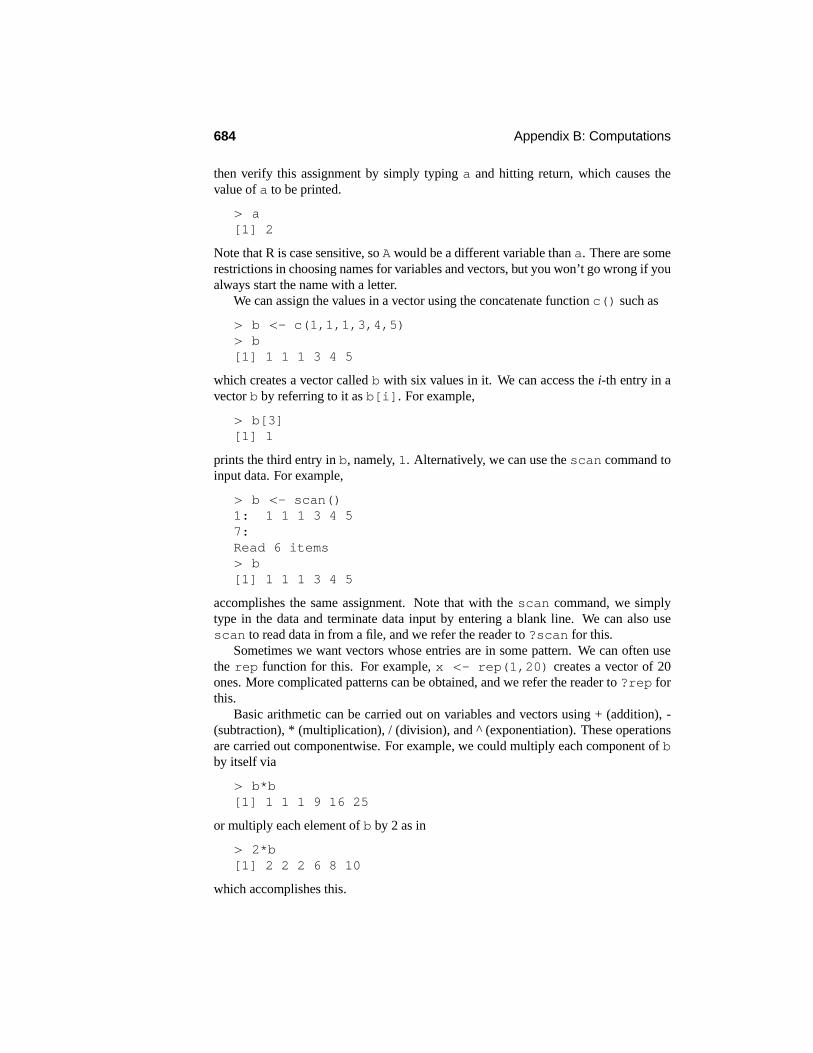
684 Appendix B: Computations
then verify this assignment by simply typing a and hitting return, which causes thevalue of a to be printed.
> a[1] 2
Note that R is case sensitive, so A would be a different variable than a. There are somerestrictions in choosing names for variables and vectors, but you won’t go wrong if youalways start the name with a letter.
We can assign the values in a vector using the concatenate function c() such as
> b <- c(1,1,1,3,4,5)> b[1] 1 1 1 3 4 5
which creates a vector called b with six values in it. We can access the i-th entry in avector b by referring to it as b[i]. For example,
> b[3][1] 1
prints the third entry in b, namely, 1. Alternatively, we can use the scan command toinput data. For example,
> b <- scan()1: 1 1 1 3 4 57:Read 6 items> b[1] 1 1 1 3 4 5
accomplishes the same assignment. Note that with the scan command, we simplytype in the data and terminate data input by entering a blank line. We can also usescan to read data in from a file, and we refer the reader to ?scan for this.
Sometimes we want vectors whose entries are in some pattern. We can often usethe rep function for this. For example, x <- rep(1,20) creates a vector of 20ones. More complicated patterns can be obtained, and we refer the reader to ?rep forthis.
Basic arithmetic can be carried out on variables and vectors using + (addition), -(subtraction), * (multiplication), / (division), and ^ (exponentiation). These operationsare carried out componentwise. For example, we could multiply each component of bby itself via
> b*b[1] 1 1 1 9 16 25
or multiply each element of b by 2 as in
> 2*b[1] 2 2 2 6 8 10
which accomplishes this.

Appendix B.1: Using R 685
There are various functions available in R, such as abs(x) (calculates the absolutevalue of x), log(x) (calculates the natural logarithm of x), exp(x) (calculates eraised to the power x), sin(x), cos(x), tan(x) (which calculate the trigonomet-ric functions), sqrt(x) (which calculates the square root of x), ceiling(x), andfloor(x) (calculate the ceiling and floor of x). When such a function is applied toa vector x, it returns a vector of the same length, with the function applied to eachelement of the original vector. There are numerous special functions available in R, buttwo important ones are gamma(x), which returns the gamma function applied to x,and lgamma(x), which returns the natural logarithm of the gamma function.
There are also functions that return a single value when applied to a vector. Forexample, min(x) and max(x) return respectively the smallest and largest elementsin x; length(x) gives the number of elements in x; and sum(x) gives the sum ofthe values in x.
R also operates on logical quantities TRUE (or T for true) and FALSE (or F forfalse). Logical values are generated by conditions that are either true or false. Forexample,
> a <- c(-3,4,2,-1,-5)> b <- a>0> b[1] FALSE TRUE TRUE FALSE FALSE
compares each element of the vector awith 0, returning TRUE when it is greater than 0and FALSE otherwise, and these logical values are stored in the vector b. The follow-ing logical operators can be used: <,<=,>=,>, == (for equality), != (for inequality)as well as & (for conjunction), | (for disjunction) and ! (for negation). For example, ifwe create a logical vector c as follows:
> c <- c(T,T,T,T,T)> b&c[1] FALSE TRUE TRUE FALSE FALSE> b|c[1] TRUE TRUE TRUE TRUE TRUE
then an element of b&c is TRUE when both corresponding elements of b and c areTRUE, while an element of b|c is TRUE when at least one of the corresponding ele-ments of b and c is TRUE.
Sometimes we may have variables that take character values. While it is alwayspossible to code these values as numbers, there is no need to do this, as R can alsohandle character-valued variables. For example, the commands
> A <- c(’a’,’b’)> A[1] "a" "b"
create a character vector A, containing two values a and b, and then we print out thisvector. Note that we included the character values in single quotes when doing theassignment.
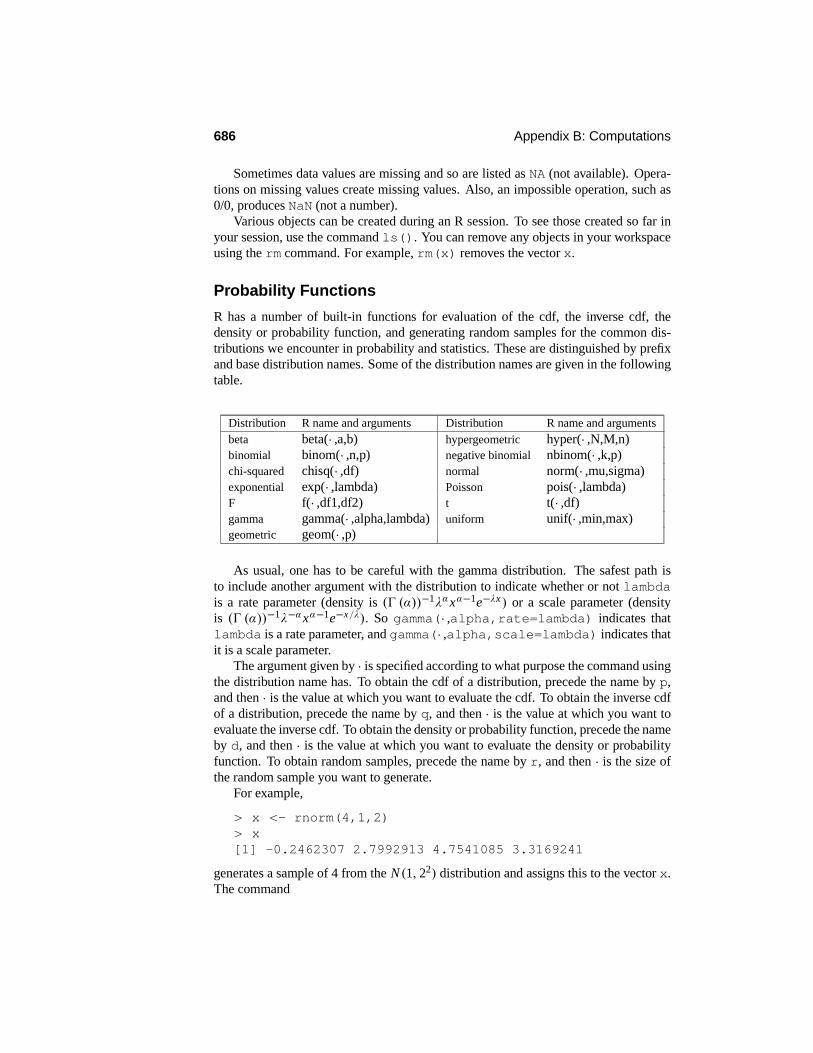
686 Appendix B: Computations
Sometimes data values are missing and so are listed as NA (not available). Opera-tions on missing values create missing values. Also, an impossible operation, such as0/0, produces NaN (not a number).
Various objects can be created during an R session. To see those created so far inyour session, use the command ls(). You can remove any objects in your workspaceusing the rm command. For example, rm(x) removes the vector x.
Probability Functions
R has a number of built-in functions for evaluation of the cdf, the inverse cdf, thedensity or probability function, and generating random samples for the common dis-tributions we encounter in probability and statistics. These are distinguished by prefixand base distribution names. Some of the distribution names are given in the followingtable.
Distribution R name and arguments Distribution R name and argumentsbeta beta(· ,a,b) hypergeometric hyper(· ,N,M,n)binomial binom(· ,n,p) negative binomial nbinom(· ,k,p)chi-squared chisq(· ,df) normal norm(· ,mu,sigma)exponential exp(· ,lambda) Poisson pois(· ,lambda)F f(· ,df1,df2) t t(· ,df)gamma gamma(· ,alpha,lambda) uniform unif(· ,min,max)geometric geom(· ,p)
As usual, one has to be careful with the gamma distribution. The safest path isto include another argument with the distribution to indicate whether or not lambdais a rate parameter (density is () (α))−1λαxα−1e−λx ) or a scale parameter (densityis () (α))−1λ−αxα−1e−x/λ). So gamma(· ,alpha,rate=lambda) indicates thatlambda is a rate parameter, and gamma(· ,alpha,scale=lambda) indicates thatit is a scale parameter.
The argument given by · is specified according to what purpose the command usingthe distribution name has. To obtain the cdf of a distribution, precede the name by p,and then · is the value at which you want to evaluate the cdf. To obtain the inverse cdfof a distribution, precede the name by q, and then · is the value at which you want toevaluate the inverse cdf. To obtain the density or probability function, precede the nameby d, and then · is the value at which you want to evaluate the density or probabilityfunction. To obtain random samples, precede the name by r, and then · is the size ofthe random sample you want to generate.
For example,
> x <- rnorm(4,1,2)> x[1] -0.2462307 2.7992913 4.7541085 3.3169241
generates a sample of 4 from the N(1, 22) distribution and assigns this to the vector x.The command

Appendix B.1: Using R 687
> dnorm(3.2,2,.5)[1] 0.04478906
evaluates the N(2, .25) pdf at 3.2, while
> pnorm(3.2,2,.5)[1] 0.9918025
evaluates the N(2, 0.25) cdf at 3.2, and
> qnorm(.025,2,.5)[1] 1.020018
gives the 0.025 quantile of the N(2, 0.25) distribution.If we have data stored in a vector x, then we can sample values from x, with or
without replacement, using the sample function. For example, sample(x,n,T)will generate a sample of n from x with replacement, while sample(x,n,F) willgenerate a sample of n from x without replacement (note n must be no greater thanlength(x) in the latter case).
Sometimes it is convenient to be able to repeat a simulation so the same randomvalues are generated. For this, you can use the set.seed command. For example,set.seed(12345) establishes the seed as 12345.
Tabulating Data
The table command is available for tabulating data. For example, table(x) re-turns a table containing a list of the unique values found in x and their frequency ofoccurrence in x. This table can be assigned to a variable via
y <- table(x)
for further analysis (see The Chi-Squared Test section on the next page).If x and y are vectors of the same length, then table(x,y) produces a cross-
tabulation, i.e., counts the number of times each possible value of (x, y) is obtained,where x can be any of the values taken in x and y can be any of the values taken in y.
Plotting Data
R has a number of commands available for plotting data. For example, suppose wehave a sample of size n stored in the vector x.
The command hist(x) will provide a frequency histogram of the data where thecutpoints are chosen automatically by R. We can add optional arguments to hist. Thefollowing are some of the arguments available.
breaks - A vector containing the cutpoints.
freq - A logical variable; when freq=T (the default), a frequency his-togram is obtained, and when freq=F, a density histogram is obtained.
For example, hist(x,breaks=c(-10,-5,-2,0,2,5,10),freq=F)will plota density histogram with cutpoints−10,−5,−2, 0, 2, 5, 10,where we have been care-ful to ensure that min(x)> −10 and max(x) < 10.

688 Appendix B: Computations
If y is another vector of the same length as x, then we can produce a scatter plot ofy against x via the command plot(x,y). The command plot(x,y,type="l")provides a scatter plot of y against x, but now the points are joined by lines. Thecommand plot(x) plots the values in x against their index. The plot(ecdf(x))command plots the empirical cdf of the data in x.
A boxplot of the data in x is obtained via the boxplot(x) command. Side-by-side boxplots of the data in x, y, z, etc., can be obtained via boxplot(x,y,z).
A normal probability plot of the values in x can be obtained using the commandqqnorm(x).
A barplot can be obtained using the barplot command. For example,
> h <- c(1,2,3)> barplot(h)
produces a barplot with 3 bars of heights 1, 2, and 3.There are many other aspects to plotting in R that allow the user considerable con-
trol over the look of plots. We refer the reader to the manual for more discussion ofthese.
Statistical Inference
R has a powerful approach to fitting and making inference about models. Models arespecified by the symbol ~. We do not discuss this fully here but only indicate how to usethis to handle the simple and multiple linear regression models (where the response andthe predictors are all quantitative), the one and two-factor models (where the responseis quantitative but the predictors are categorical), and the logistic regression model(where the response is categorical but the predictors are quantitative). Suppose, then,that we have a vector y containing the response values.
Basic Statistics
The function mean(y) returns the mean of the values in y, var(y) returns thesample variance of the values in y, and sd(y) gives the sample standard devia-tion. The command median(y)returns the median of y, while quantile(y,p)returns the sample quantiles as specified in the vector of probabilities p. For example,quantile(y,c(.25,.5,.75)) returns the median and the first and third quan-tiles. The function sort(y) returns a vector with the values in y sorted from smallestto largest, and rank(y) gives the ranks of the values in y.
The t-Test
For the data in y, we can use the command
> t.test(y,mu=1,alternative="two.sided",conf.level=.95)
to carry out a t-test. This computes the P-value for testing H0 : µ = 1 and forms a0.95-confidence interval for µ.
The Chi-Squared Test
Suppose y contains a vector of counts for k cells and prob contains hypothesizedprobabilities for these cells. Then the command
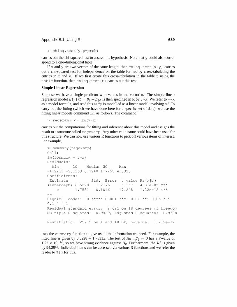
Appendix B.1: Using R 689
> chisq.test(y,p=prob)
carries out the chi-squared test to assess this hypothesis. Note that y could also corre-spond to a one-dimensional table.
If x and y are two vectors of the same length, then chisq.test(x,y) carriesout a chi-squared test for independence on the table formed by cross-tabulating theentries in x and y. If we first create this cross-tabulation in the table t using thetable function, then chisq.test(t) carries out this test.
Simple Linear Regression
Suppose we have a single predictor with values in the vector x. The simple linearregression model E(y | x) = β1 + β2x is then specified in R by y~x. We refer to y~xas a model formula, and read this as “y is modelled as a linear model involving x.” Tocarry out the fitting (which we have done here for a specific set of data), we use thefitting linear models command lm, as follows. The command
> regexamp <- lm(y~x)
carries out the computations for fitting and inference about this model and assigns theresult to a structure called regexamp. Any other valid name could have been used forthis structure. We can now use various R functions to pick off various items of interest.For example,
> summary(regexamp)Call:lm(formula = y~x)Residuals:Min 1Q Median 3Q Max
-4.2211 -2.1163 0.3248 1.7255 4.3323Coefficients:Estimate Std. Error t value Pr(>|t|)(Intercept) 6.5228 1.2176 5.357 4.31e-05 ***
x 1.7531 0.1016 17.248 1.22e-12 ***--Signif. codes: 0 ‘***’ 0.001 ‘**’ 0.01 ‘*’ 0.05 ‘.’0.1 ‘ ’ 1Residual standard error: 2.621 on 18 degrees of freedomMultiple R-squared: 0.9429, Adjusted R-squared: 0.9398
F-statistic: 297.5 on 1 and 18 DF, p-value: 1.219e-12
uses the summary function to give us all the information we need. For example, thefitted line is given by 6.5228 + 1.7531x. The test of H0 : β2 = 0 has a P-value of1.22 × 10−12, so we have strong evidence against H0. Furthermore, the R2 is givenby 94.29%. Individual items can be accessed via various R functions and we refer thereader to ?lm for this.

690 Appendix B: Computations
Multiple Linear Regression
If we have two quantitative predictors in the vectors x1 and x2, then we can proceedjust as with simple linear regression to fit the linear regression model E(y | x1, x2)= β1 + β2x1 + β2x2. For example, the commands
> regex <- lm(y~x1+x2)> summary(regex)
fit the above linear model, assign the results of this to the structure regex, and thenthe summary function prints out (suppressed here) all the relevant quantities. We ready~x1+x2 as, “y is modelled as a linear model involving x1 and x2.” In particular,the F-statistic, and its associated P-value, is obtained for testing H0 : β2 = β3 = 0.
This generalizes immediately to linear regression models with k quantitative pre-dictors x1, ..., xk . Furthermore, suppose we want to test that the model only involvesx1, ..., xl for l < k. We use lm to fit the model for all k predictors, assign this toregex, and also use lm to fit the model that only involves l predictors and assignthis to regex1. Then the command anova(regex,regex1) will output the F-statistics, and its P-value, for testing H0 : βl+1 = · · · = βk = 0.
One- and Two-Factor ANOVA
Suppose now that A denotes a categorical predictor taking two levels a1 and a2. Notethat the values of A may be character in value rather than numeric, e.g., x is a charactervector containing the values a1 and a2, used to denote at which level the correspond-ing value of y was observed. In either case, we need to make this into a factor A, viathe command
> A <- factor(x)
so that A can be used in the analysis. Then the command
> aov(y~A)
produces the one-way ANOVA table. Of course, aov also handles factors with morethan two levels. To produce the cell means, use the command tapply(y,A,mean).
Suppose there is a second factor B taking 5 levels b1, . . . , b5. If this is the factor Bin R, then the command
> aov(y~A+B+A:B)
produces the two-way ANOVA for testing for interactions between factors A and B. Toproduce the cell means, use the command tapply(y,list(A,B),mean). Thecommand aov(y~A+B) produces the ANOVA table, assuming that there are no inter-actions.
Logistic Regression
Suppose we have binary data stored in the vector y, and x contains the correspondingvalues of a quantitative predictor. Then we can use the generalized linear model com-mand glm to fit the logistic regression model P(Y = 1 | x) = exp{β1 + β2x}/(1 +exp{β1 + β2x}). The commands

Appendix B.1: Using R 691
> logreg <- glm(y~x,family=binomial)> summary(logreg)
fit the logistic regression model, assign the results to logreg and then the summarycommand outputs this material. This gives us the estimates of the β i , their standarderrors, and P-values for testing that the βi = 0.
Control Statements and R Programs
A basic control statement is of the formif (expr1) expr2 else expr3, whereexpr1 takes a logical value, expr2 is executed if expr1 is T, andexpr3 is executedif expr1 is F. For example, if x is a variable taking value−2, then
> if (x<0) {y <- -1} else {y <- 1}
results in y being assigned the value −1. Note that the else part of the statement canbe dropped.
The command for (name in expr) expr2 executes expr2 for each valueof name in expr1. For example,
> for (i in 1:10) print(i)
prints the value of the variable i as i is sequentially assigned values in {1, 2, . . . ., 10}.Note that m:n is a shorthand for the sequence (m,m + 1, . . . , n) in R. As anotherexample,
> for (i in 1:20) y[i] <- 2^i
creates a vector y with 20 entries, where the i-th element of y equals 2i .The break terminates a loop, perhaps based on some condition holding, while
next halts the processing of the current iteration and advances the looping index.Both break and next apply only to the innermost of nested loops.
Commands in R can be grouped by placing them within braces{expr1; expr2;...}. The commands within the braces are executed as a unit. For example,
> for (i in 1:20) {print(i); y[i] <- 2^i}; print(y[i])}
causes i to be printed, y[i] to be assigned, and y[i] to be printed, all within a forloop.
Often when a computation is complicated, such as one that involves looping, itis better to put all the R commands in a single file and then execute the file in batchmode. For example, suppose you have a file prog.R containing R code. Then thecommand source("pathname/prog.R") causes all the commands in the file tobe executed.
It is often convenient to put comments in R programs to explain what the lines ofcode are doing. A comment line is preceded by # and of course it is not executed.
User-Defined Functions
R also allows user-defined functions. The syntax of a function definition is as follows.

692 Appendix B: Computations
function name <- function(arguments) {function body;return(return value);
}
For example, the following function computes the sample coefficient of variation of thedata x.
coef_var <- function(x) {result <- sd(x)/mean(x);return(result);
}
Then if we want to subsequently compute the coefficient of variation of data y wesimply type coef_var(y).
Arrays and Lists
A vector of length m can also be thought of as one-dimensional array of length m. Rcan handle multidimensional arrays, e.g., m× n,m× n× p arrays, etc. If a is a three-dimensional array, then a[i,j,k] refers to the entry in the (i, j, k)-th position of thearray. There are various operations that can be carried out on arrays and we refer thereader to the manual for these. Later in this manual, we will discuss the special case oftwo-dimensional arrays, which are also known as matrices. For now, we just think ofarrays as an object in which we store data.
A very general data structure in R is given by a list. A list is similar to an arraywith several important differences.
1. Any entry in an array is referred to by its index. But any entry in a list maybe referred to by a character name. For example, the fitted regression coeffi-cients are referred to by regex$coefficients after fitting the linear modelregex <- lm(y ∼ x1 + x2). The dollar mark ($) is the entry referenceoperator, that is, varname$entname indicates the “entname” entry in the list“varname.”
2. While an array stores only the same type of data, a list can store any R objects.For example, the coefficients entry in a linear regression object is a nu-meric vector, and the model entry is a list.
3. The reference operators are different: arr[i] refers to the i-th entry in thearray arr, and lst[[i]] refers to the i-th entry in the list lst. Note that ican be the entry name, i.e., lst$entname and lst[[’entname’]] referto the same data.
Examples
We now consider some examples relevant to particular sections or examples in the maintext. To run any of these codes, you first have to define the functions. To do this, load

Appendix B.1: Using R 693
the code using the source command. Arguments to the functions then need to bespecified. Note that lines in the listings may be broken unnaturally and continue on thefollowing line.
EXAMPLE B.1.1 Bootstrapping in Example 6.4.2The following R code generates bootstrap samples and calculates the median of eachof these samples. To run this code, type y <- bootstrap_median(m,x), wherem is the number of bootstrap samples, x contains the original sample, and the mediansof the resamples are stored in y. The statistic to be bootstrapped can be changed bysubstituting for median in the code.
# Example B.2.1# function name: bootstrap_median# parameters:# m resample size# x original data# return value:# a vector of resampled medians# description: resamples and stores its median
bootstrap_median <- function(m,x) {n <- length(x);result <- rep(0,m);for(i in 1:m) result[i] <- median(sample(x,n,T));
return(result);}
EXAMPLE B.1.2 Sampling from the Posterior in Example 7.3.1The following R code generates a sample of from the joint posterior in Example 7.3.1.To run a simulation, type
post <- post_normal(m,x,alpha0,beta0,mu0,tau0square)
where m is the Monte Carlo sample size and the remaining arguments are the hyperpa-rameters of the prior. The result is a list called (in this case) post, where post$muand post$sigmasq contain the generated values of µ and σ 2, respectively. Forexample,
> x <- c(11.6714, 1.8957, 2.1228, 2.1286, 1.0751, 8.1631,1.8236, 4.0362, 6.8513, 7.6461, 1.9020, 7.4899, 4.9233,8.3223, 7.9486);> post <- post_normal(10**4,x,2,1,4,2)> z <- sqrt(post$sigmasq)/post$mu
runs a simulation as in Example 7.3.1, with N = 104.
# Example B.2.2# function name: post_normal# parameters:# m sample size

694 Appendix B: Computations
# x data# alpha0 shape parameter for 1/sigma^2# beta0 rate parameter for 1/sigma^2# mu0 location parameter for mu# tau0square variance ratio parameter for mu# returned values:# mu sampled mu# sigmasq sampled sigmasquare# description: samples from the posterior distribution# in Example 7.3.1#post_normal<-function(m,x,alpha0,beta0,mu0,tau0square){# set the length of the datan <- length(x);# the shape and rate parameters of the posterior dist.# alpha_x = first parameter of the gamma dist.# = (alpha0 + n/2)alpha_x <- alpha0 + n/2# beta_x = the rate parameter of the gamma dist.beta_x <- beta0 + (n-1)/2 * var(x) + n*(mean(x)-mu0)**2/
2/(1+n*tau0square);# mu_x = the mean parameter of the normal dist.mu_x <- (mu0/tau0square+n*mean(x))/(n+1/tau0square);# tausq_x = the variance ratio parameter of the normal# distributiontausq_x <- 1/(n+1/tau0square);# initialize the resultresult <- list();result$sigmasq <- 1/rgamma(m,alpha_x,rate=beta_x);result$mu <- rnorm(m,mu_x,sqrt(tausq_x *
result$sigmasq));return(result);}
EXAMPLE B.1.3 Calculating the Estimates and Standard Errors in Example 7.3.1Once we have a sample of values from the posterior distribution of ψ stored in psi,we can calculate the interval given by the mean value of psi plus or minus 3 standarddeviations as a measure of the accuracy of the estimation.
# Example B.2.3# set the datax <- c(11.6714, 1.8957, 2.1228, 2.1286, 1.0751, 8.1631,
1.8236, 4.0362, 6.8513, 7.6461, 1.9020, 7.4899,4.9233, 8.3223, 7.9486);
post <- post_normal(10**4,x,2,1,4,2);# compute the coefficient of variation

Appendix B.1: Using R 695
psi <- sqrt(post$sigmasq)/post$mu;psi_hat <- mean(psi <= .5);psi_se <- sqrt(psi_hat * (1-psi_hat))/sqrt(length(psi));# the intervalcq <- 3cat("The three times s.e. interval is ",
"[",psi_hat-cq*psi_se, ", ", psi_hat+cq*psi_se,"]\n");
EXAMPLE B.1.4 Using the Gibbs Sampler in Example 7.3.2To run this function, type
post<-gibbs_normal(m,x,alpha0,beta0,lambda,mu0,tau0sq,burnin=0)
as this creates a list called post, where post$mu and post$sigmasq contain thegenerated values of µ and σ 2, respectively. Note that the burnin argument is set toa nonnegative integer and indicates that we wish to discard the first burnin values ofµ and σ 2 and retain the last m. The default value is burnin=0.
# Example B.2.4# function name: gibbs_normal# parameters# m the size of posterior sample# x data# alpha0 shape parameter for 1/sigma^2# beta0 rate parameter for 1/sigma^2# lambda degree of freedom of Student’s t-dist.# mu0 location parameter for mu# tau0sq scale parameter for mu# burnin size of burn in. the default value is 0.## returnrd values# mu sampled mu’s# sigmasq sampled sigma^2’s# description: samples from the posterior in Ex. 7.3.2#gibbs_normal <- function(m,x,alpha0,beta0,lambda,mu0,
tau0sq,burnin=0) {# initialize the resultresult <- list();result$sigmasq <- result$mu <- rep(0,m);# set the initial parametermu <- mean(x);sigmasq <- var(x);n <- length(x);
# set parameters

696 Appendix B: Computations
alpha_x <- n/2 + alpha0 + 1/2;# loopfor(i in (1-burnin):m) {# update v_i’sv <- rgamma(n,(lambda+1)/2,rate=((x-mu)**2/
sigmasq/lambda+1)/2);# update sigma-squarebeta_x <-(sum(v*(x-mu)**2)/lambda+(mu-mu0)**2/
tau0sq)/2+beta0;sigmasq<- 1/rgamma(1,alpha_x,rate=beta_x);# update mur <- 1/(sum(v)/lambda+1/tau0sq);mu <- rnorm(1,r*(sum(v*x)/lambda+mu0/tau0sq),
sqrt(r*sigmasq));# burnin checkif(i < 1) next;result$mu[i] <- mu;result$sigmasq[i] <- sigmasq;}result$psi <- sqrt(result$sigmasq)/result$mu;return(result);
}
EXAMPLE B.1.5 Batching in Example 7.3.2The following R code divides a series of data into batches and calculates the batchmeans. To run the code, type y<-batching(k,x) to place the consecutive batchmeans of size k, of the data in the vector x, in the vector y.
# Example B.2.5# function name: batching# parameters:# k size of each batch# x data# return value:# an array of the averages of each batch# description: this function separates the data x into# floor(length(x)/k) batches and returns the array of# the averages of each batchbatching <- function(k,x) {
m <- floor(length(x)/k);result <- rep(0,m);for(i in 1:m) result[i] <- mean(x[(i-1)*k+(1:k)]);return(result);
}

Appendix B.1: Using R 697
EXAMPLE B.1.6 Simulating a Sample from the Distribution of the Discrepancy Sta-tistic in Example 9.1.2The following R code generates a sample from the discrepancy statistic specified inExample 9.1.2. To generate the sample, type y<-discrepancy(m,n) to place asample of size m in y, where n is the size of the original data set. This code can beeasily modified to generate samples from other discrepancy statistics.
# Example B.2.6# function name: discrepancy# parameters:# m resample size# n size of data# return value:# an array of m discrepancies# description: this function generates m discrepancies# when the data size is ndiscrepancy <- function(m,n) {
result <- rep(0,m);for(i in 1:m) {
x <- rnorm(n);xbar <- mean(x);r <- (x-xbar)/sqrt((sum((x-xbar)**2)));result[i] <- -sum(log(r**2));
}return(result/n);
}
EXAMPLE B.1.7 Generating from a Dirichlet Distribution in Example 10.2.3The following R code generates a sample from a Dirichlet(α1, α2, α3, α4) distribution.To generate from this distribution, first assign values to the vector alpha, and thentype ddirichlet(n,alpha) where n is the sample size.
# Example B.2.7# function name: ddirichlet# parameters:# n sample size# alpha vector(alpha1,...,alphak)# return value:# a (n x k) matrix. rows are i.i.d. samples# description: this function generates n random samples# from Dirichlet(alpha1,...,alphak) distributionddirichlet <- function(n,alpha) {
k <- length(alpha);result <- matrix(0,n,k);for(i in 1:k) result[,i] <- rgamma(n,alpha[i]);for(i in 1:n) result[i,] <- result[i,] /
sum(result[i,]);
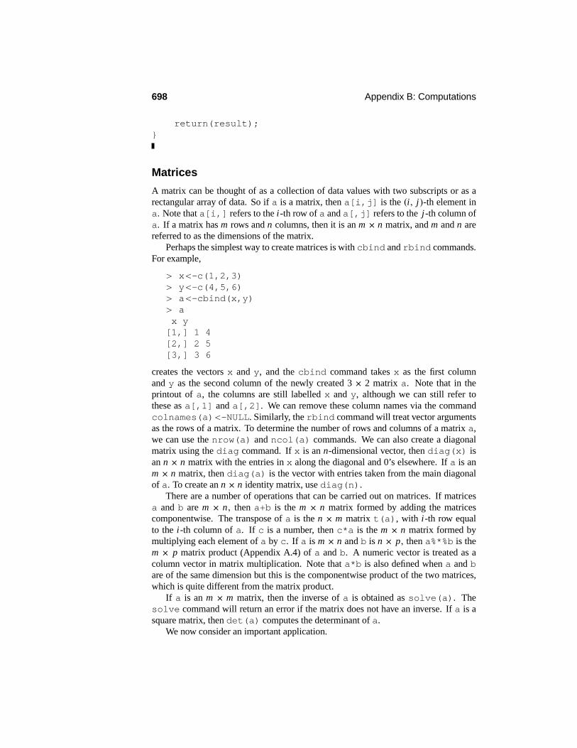
698 Appendix B: Computations
return(result);}
Matrices
A matrix can be thought of as a collection of data values with two subscripts or as arectangular array of data. So if a is a matrix, then a[i,j] is the (i, j)-th element ina. Note that a[i,] refers to the i-th row of a and a[,j] refers to the j-th column ofa. If a matrix has m rows and n columns, then it is an m × n matrix, and m and n arereferred to as the dimensions of the matrix.
Perhaps the simplest way to create matrices is with cbind and rbind commands.For example,
> x<-c(1,2,3)> y<-c(4,5,6)> a<-cbind(x,y)> ax y[1,] 1 4[2,] 2 5[3,] 3 6
creates the vectors x and y, and the cbind command takes x as the first columnand y as the second column of the newly created 3 × 2 matrix a. Note that in theprintout of a, the columns are still labelled x and y, although we can still refer tothese as a[,1] and a[,2]. We can remove these column names via the commandcolnames(a)<-NULL. Similarly, the rbind command will treat vector argumentsas the rows of a matrix. To determine the number of rows and columns of a matrix a,we can use the nrow(a) and ncol(a) commands. We can also create a diagonalmatrix using the diag command. If x is an n-dimensional vector, then diag(x) isan n × n matrix with the entries in x along the diagonal and 0’s elsewhere. If a is anm × n matrix, then diag(a) is the vector with entries taken from the main diagonalof a. To create an n × n identity matrix, use diag(n).
There are a number of operations that can be carried out on matrices. If matricesa and b are m × n, then a+b is the m × n matrix formed by adding the matricescomponentwise. The transpose of a is the n × m matrix t(a), with i-th row equalto the i-th column of a. If c is a number, then c*a is the m × n matrix formed bymultiplying each element of a by c. If a is m × n and b is n × p, then a%*%b is them × p matrix product (Appendix A.4) of a and b. A numeric vector is treated as acolumn vector in matrix multiplication. Note that a*b is also defined when a and bare of the same dimension but this is the componentwise product of the two matrices,which is quite different from the matrix product.
If a is an m × m matrix, then the inverse of a is obtained as solve(a). Thesolve command will return an error if the matrix does not have an inverse. If a is asquare matrix, then det(a) computes the determinant of a.
We now consider an important application.

Appendix B.1: Using Minitab 699
EXAMPLE B.1.8 Fitting Regression ModelsSuppose the n-dimensional vector y corresponds to the response vector and the n × kmatrix V corresponds to the design matrix when we are fitting a linear regression modelgiven by E(y | V ) = Vβ. The least-squares estimate of β is given by b as computed in
b<-solve(t(V)%*%V)%*%t(V)%*%y
with the vector of predicted values p and residuals r given by
> p<-V%*%b> r<-y-p
with squared lengths
> slp<-t(p)%*%p> slr<-t(r)%*%r
where slp is the squared length of p and slr is the squared length of r. Note thatthe matrix solve(t(V)%*%V) is used for forming confidence intervals and tests forthe individual βi . Virtually all the computations involved in fitting and inference forthe linear regression matrix can be carried out using matrix computations in R like theones we have illustrated.
Packages
There are many packages that have been written to extend the capability of basic R. It isvery likely that if you have a data analysis need that cannot be met with R, then you canfind a freely available package to add. We refer the reader to ?install.packagesand ?library for more on this.
B.2 Using MinitabAll the computations found in this text were carried out using Minitab. This statisticalsoftware package is very easy to learn and use. Other packages such as SAS or R (seesection B.1) could also be used for this purpose.
Most of the computations were performed using Minitab like a calculator, i.e., datawere entered and then a number of Minitab commands were accessed to obtain thequantities desired. No programming is required for these computations.
There were a few computations, however, that did involve a bit of programming.Typically, this was a computation in which numerous operations to be performed manytimes, and so looping was desirable. In each such case, we have recorded here theMinitab code that we used for these computations. As the following examples show,these programs were never very involved.
Students can use these programs as templates for writing their own Minitab pro-grams. Actually, the language is so simple that we feel that anyone using anotherlanguage for programming can read these programs and use them as templates in thesame way. Simply think of the symbols c1, c2, etc. as arrays where we address thei-th element in the array c1 by c1(i). Furthermore, there are constants k1, k2, etc.

700 Appendix B: Computations
A Minitab program is called a macro and must start with the statement gmacroand end with the statement endmacro. The first statement after gmacro gives a nameto the program. Comments in a program, put there for explanatory purposes, start withnote.
If the file containing the program is called prog.txt and this is stored in the rootdirectory of a disk drive called c, then the Minitab command
MTB> %c:/prog.txt
will run the program. Any output will either be printed in the Session window (if youhave used a print command) or stored in the Minitab worksheet.
More details on Minitab can be found by using Help in the program. We providesome examples of Minitab macros used in the text.
EXAMPLE B.2.1 Bootstrapping in Example 6.4.2The following Minitab code generates 1000 bootstrap samples from the data in c1,calculates the median of each of these samples, and then calculates the sample varianceof these medians.
gmacrobootstrappingbase 34256734note - original sample is stored in c1note - bootstrap sample is placed in c2 with each onenote overwrittennote - medians of bootstrap samples are stored in c3note - k1 = size of data set (and bootstrap samples)let k1=15do k2=1:1000sample 15 c1 c2;replace.let c3(k2)=median(c2)enddonote - k3 equals (6.4.5)let k3=(stdev(c3))**2print k3endmacro
EXAMPLE B.2.2 Sampling from the Posterior in Example 7.3.1The following Minitab code generates a sample of 104 from the joint posterior in Ex-ample 7.3.1. Note that in Minitab software, the Gamma(α, β) density takes the form(β−α/) (α))xα−1e−x/β. So to generate from a Gamma(α, β) distribution, as definedin this book, we must put the second shape parameter equal to 1/β in Minitab.
gmacronormalpostnote - the base command sets the seed for the randomnote numbers

Appendix B.1: Using Minitab 701
base 34256734note - the parameters of the posteriornote - k1 = first parameter of the gamma distributionnote = (alpha_0 + n/2)let k1=9.5note - k2 = 1/betalet k2=1/77.578note - k3 = posterior mean of mulet k3=5.161note - k4 = (n + 1/(tau_0 squared) )^(-1)let k4=1/15.5note - main loopnote - c3 contains generated value of sigma**2note - c4 contains generated value of munote - c5 contains generated value of coefficient of
variationdo k5=1:10000random 1 c1;gamma k1 k2.let c3(k5)=1/c1(1)let k6=sqrt(k4/c1(1))random 1 c2;normal k3 k6.let c4(k5)=c2(1)let c5(k5)=sqrt(c3(k5))/c4(k5)enddoendmacro
EXAMPLE B.2.3 Calculating the Estimates and Standard Errors in Example 7.3.1We have a sample of 104 values from the posterior distribution of ψ stored in C5.The following computations use this sample to calculate an estimate of the posteriorprobability that ψ ≤ 0.5 (k1), as well as to calculate the standard error of this estimate(k2), the estimate minus three times its standard error (k3), and the estimate plus threetimes its standard error (k4).
let c6=c5 le .5let k1=mean(c6)let k2=sqrt(k1*(1-k1))/sqrt(10000)let k3=k1-3*k2let k4=k1+3*k2print k1 k2 k3 k4

702 Appendix B: Computations
EXAMPLE B.2.4 Using the Gibbs Sampler in Example 7.3.2The following Minitab code generates a chain of length 104 values using the Gibbssampler described in Example 7.3.2.
gmacrogibbsbase 34256734note - data sample is stored in c1note - starting value for mu.let k1=mean(c1)note - starting value for sigma**2let k2=stdev(c1)let k2=k2**2note - lambdalet k3=3note - sample sizelet k4=15note - n/2 + alpha_0 + 1/2let k5=k4/2 +2+.5note - mu_0let k6=4note - tau_0**2let k7=2note - beta_0let k8=1let k9=(k3/2+.5)note - main loopdo k100=1:10000note - generate the nu_i in c10do k111=1:15let k10=.5*(((c1(k111)-k1)**2)/(k2*k3) +1)let k10=1/k10random 1 c2;gamma k9 k10.let c10(k111)=c2(1)enddonote - generate sigma**2 in c20let c11=c10*((c1-k1)**2)let k11=.5*sum(c11)/k3+.5*((k1-k6)**2)/k7 +k8let k11=1/k11random 1 c2;gamma k5 k11.let c20(k100)=1/c2(1)let k2=1/c2(1)note - generate mu in c21let k13=1/(sum(c10)/k3 +1/k7)

Appendix B.1: Using Minitab 703
let c11=c1*c10/k3let k14=sum(c11)+k6/k7let k14=k13*k14let k13=sqrt(k13*k2)random 1 c2;normal k14 k13.let c21(k100)=c2(1)let k1=c2(1)enddoendmacro
EXAMPLE B.2.5 Batching in Example 7.3.2The following Minitab code divides the generated sample, obtained via the Gibbs sam-pling code for Example 7.3.2, into batches, and calculates the batch means.
gmacrobatchingnote - k2= batch sizelet k2=40note - k4 holds the batch sumsnote - c1 contains the data to be batched (10000 data values)note - c2 will contain the batch means (250 batch means)do k10=1:10000/40let k4=0do k20=0:39let k3=c1(k10+k20)let k4=k4+k3enddolet k11=floor(k10/k2) +1let c2(k11)=k4/k2enddoendmacro
EXAMPLE B.2.6 Simulating a Sample from the Distribution of the Discrepancy Sta-tistic in Example 9.1.2The following code generates a sample from the discrepancy statistic specified in Ex-ample 9.1.2.
gmacrogoodnessoffitbase 34256734note - generated sample is stored in c1note - residuals are placed in c2note - value of D(r) are placed in c3note - k1 = size of data setlet k1=5

704 Appendix B: Computations
do k2=1:10000random k1 c1let k3=mean(c1)let k4=sqrt(k1-1)*stdev(c1)let c2=((c1-k3)/k4)**2let c2=loge(c2)let k5=-sum(c2)/k1let c3(k2)=k5enddoendmacro
EXAMPLE B.2.7 Generating from a Dirichlet Distribution in Example 10.2.3The following code generates a sample from a Dirichlet(α1, α2, α3, α4) distribution,where α1 = 2, α2 = 3, α3 = 1, α4 = 1.5.
gmacrodirichletnote - the base command sets the seed for the randomnote number generator (so you can repeat a simulation).base 34256734note - here we provide the algorithm for generating fromnote a Dirichlet(k1,k2,k3,k4) distribution.note - assign the values of the parameters.let k1=2let k2=3let k3=1let k4=1.5let k5=K2+k3+k4let k6=k3+k4note - generate the sample with i-th sample in i-th rownote of c2, c3, c4, c5, ....do k10=1:5random 1 c1;beta k1 k5.let c2(k10)=c1(1)random 1 c1;beta k2 k6.let c3(k10)=(1-c2(k10))*c1(1)random 1 c1;beta k3 k4.let c4(k10)=(1-c2(k10)-c3(k10))*c1(1)let c5(k10)= 1-c2(k10)-c3(k10)-c4(k10)enddoendmacro

Appendix C
Common Distributions
We record here the most commonly used distributions in probability and statistics aswell as some of their basic characteristics.
C.1 Discrete Distributions1. Bernoulli(θ), θ ∈ [0, 1] (same as Binomial(1, θ)).
probability function: p(x) = θ x (1− θ)1−x for x = 0, 1.mean: θ.variance: θ(1− θ).moment-generating function: m(t) = (1− θ + θet ) for t ∈ R1.
2. Binomial(n, θ), n > 0 an integer, θ ∈ [0, 1] .
probability function: p(x) = -nx.θ x (1− θ)n−x for x = 0, 1, . . . , n.mean: nθ.variance: nθ(1− θ).moment-generating function: m(t) = (1− θ + θet )n for t ∈ R1.
3. Geometric(θ), θ ∈ (0, 1] (same as Negative-Binomial(1, θ)).
probability function: p(x) = (1− θ)xθ for x = 0, 1, 2, . . . .mean: (1− θ)/θ.variance: (1− θ)/θ2.moment-generating function: m(t) = θ(1− (1− θ) et)−1 for t < − ln(1− θ).4. Hypergeometric(N,M, n), M ≤ N, n ≤ N all positive integers.
probability function:
p(x) =%
M
x
&%N − M
n − x
&/
%N
n
&for max(0, n + M − N) ≤ x ≤ min(n,M).
mean: n MN .
variance: n MN
-1− M
N
. N−nN−1 .
5. Multinomial(n, θ1, . . . , θk), n > 0 an integer, each θ i ∈ [0, 1] , θ1 + · · · + θk = 1.
705

706 Appendix C: Common Distributions
probability function:
p(x1, . . . , xk) =%
n
x1 . . . xk
&θ x1
1 · · · θ xkk where each xi ∈ {0, 1, . . . , n}
and x1 + · · · + xk = n.
mean: E(Xi ) = nθ i .variance: Var(Xi) = nθ i (1− θ i ).covariance: Cov(Xi , X j ) = −nθ iθ j when i 3= j.
6. Negative-Binomial(r, θ) , r > 0 an integer, θ ∈ (0, 1].
probability function: p(x) = -r−1+xx
.θr (1− θ)x for x = 0, 1, 2, 3, . . . .
mean: r(1− θ)/θ.variance: r(1− θ)/θ2.moment-generating function: m(t) = θr (1− (1− θ) et)−r for t < − ln(1− θ).7. Poisson(λ), λ > 0.
probability function: p(x) = λx
x! e−λ for x = 0, 1, 2, 3, . . . .mean: λ.variance: λ.moment-generating function: m(t) = exp{λ(et − 1)} for t ∈ R1.
C.2 Absolutely Continuous Distributions1. Beta(a, b), a > 0, b > 0 (same as Dirichlet(a, b)).
density function: f (x) = )(a+b))(a))(b) x
a−1(1− x)b−1 for x ∈ (0, 1).mean: a/(a + b).variance: ab/(a + b + 1)(a + b)2.
2. Bivariate Normal(µ1, µ2, σ21, σ
22, ρ) for µ1, µ2 ∈ R1, σ 2
1, σ22 > 0, ρ ∈ [−1, 1] .
density function:
fX1,X2(x1, x2)
= 1
2πσ 1σ 2/
1− ρ2exp
− 1
2(1− ρ2)
+
x1−µ1σ 1
,2 ++
x2−µ2σ 2
,2−2ρ+
x1−µ1σ 1
,+x2−µ2σ 2
,
for x1 ∈ R1, x2 ∈ R1.
mean: E(Xi ) = µi .variance: Var(Xi) = σ 2
i .covariance: Cov(X1, X2) = ρσ 1σ 2.
3. Chi-squared(α) or χ2(α), α > 0 (same as Gamma(α/2, 1/2)).
density function: f (x) = 2−α/2()(α/2))−1x (α/2)−1e−x/2 for x > 0.mean: α.variance: 2α.

Appendix C.2: Absolutely Continuous Distributions 707
moment-generating function: m(t) = (1− 2t)−α/2 for t < 1/2.
4. Dirichlet(α1, . . . , αk+1) , αi > 0 for each i.
density function:
fX1,...,Xk (x1, . . . , xk)
= )(α1 + · · · + αk+1)
)(α1) · · ·)(αk+1)xα1−1
1 · · · xαk−1k (1− x1 − · · · − xk)
αk+1−1
for xi ≥ 0, i = 1, . . . , k and 0 ≤ x1 + · · · + xk ≤ 1.
mean:E(Xi ) = αi
α1 + · · · + αk+1.
variance:
Var(Xi ) = αi (α1 + · · · + αk+1 − αi )
(α1 + · · · + αk+1)2(1+ α1 + · · · + αk+1).
covariance: when i 3= j
Cov(Xi , X j ) = −αiα j
(α1 + · · · + αk+1)2(1+ α1 + · · · + αk+1).
5. Exponential(λ), λ > 0 (same as Gamma(1, λ)).
density function: f (x) = λe−λx for x > 0.mean: λ−1.variance: λ−2.moment-generating function: m(t) = λ(λ− t)−1 for t < λ.
Note that some books and software packages instead replace λ by 1/λ in the definitionof the Exponential(λ) distribution — always check this when using another book orwhen using software to generate from this distribution.
6. F (α, β) , α > 0, β > 0.
density function:
f (x) =)+α+β
2
,)-α2
.)+β2
, %αβ
x
&α/2−1 %1+ α
βx
&−(α+β)/2 αβ
for x > 0.
mean: β/(β − 2) when β > 2.variance: 2β2(α + β − 2)/α(β − 2)2(β − 4) when β > 4.
7. Gamma(α, λ), α > 0, λ > 0.
density function: f (x) = λαxα−1
)(α) e−λx for x > 0.mean: α/λ.variance: α/λ2.moment-generating function: m(t) = λα(λ− t)−α for t < λ.

708 Appendix C: Common Distributions
Note that some books and software packages instead replace λ by 1/λ in the definitionof the Gamma(α, λ) distribution — always check this when using another book orwhen using software to generate from this distribution.
8. Lognormal or log N(µ, σ 2), µ ∈ R1, σ 2 > 0.
density function: f (x) = (2πσ 2)−1/2x−1 exp+− 1
2σ 2 (ln x − µ)2,
for x > 0.
mean: exp(µ+ σ 2/2).variance: exp(2µ+ σ 2)(exp(σ 2)− 1).
9. N(µ, σ 2), µ ∈ R1, σ 2 > 0.
density function: f (x) = (2πσ 2)−1/2 exp+− 1
2σ 2 (x − µ)2,
for x ∈ R1.mean: µ.variance: σ 2.moment-generating function: m(t) = exp(µt + σ 2t2/2) for t ∈ R1.
10. Student(α) or t (α), α > 0 (α = 1 gives the Cauchy distribution).
density function:
f (x) =)+α+1
2
,)+
12
,)-α2
. %1+ x2
α
&−(α+1)/21√α
for x ∈ R1.
mean: 0 when α > 1.variance: α/(α − 2) when α > 2.
11. Uniform[L, R], R > L .
density function: f (x) = 1/(R − L) for L < x < R.mean: (L + R)/2.variance: (R − L)2/12.moment-generating function: m(t) = (eRt − eLt)/t (R − L).

Appendix D
Tables
The following tables can be used for various computations. It is recommended, how-ever, that the reader become familiar with the use of a statistical software packageinstead of relying on the tables. Computations of a much greater variety and accuracycan be carried out using the software, and, in the end, it is much more convenient.
709

710 Appendix D: Tables
D.1 Random NumbersEach line in Table D.1 is a sample of 40 random digits, i.e., 40 independent and identi-cally distributed (i.i.d.) values from the uniform distribution on the set {0, 1, 2, 3, 4, 5,6, 7, 8, 9}.
Suppose we want a sample of five i.i.d. values from the uniform distribution onS = {1, 2, . . . , 25}, i.e., a random sample of five, with replacement, from S. To dothis, pick a starting point in the table and start reading off successive (nonoverlapping)two-digit numbers, treating a pair such as 07 as 7, and discarding any pairs that are notin the range 1 to 25, until you have five values. For example, if we start at line 110, weread the pairs (∗ indicates a sample element) 38, 44, 84, 87, 89, 18∗, 33, 82, 46, 97, 39,36, 44, 20∗, 06∗, 76, 68, 80, 87, 08∗, 81, 48, 66, 94, 87, 60, 51, 30, 92, 97, 00, 41, 27,12∗. We can see at this point that we have a sample of five given by 18, 20, 6, 8, 12.
If we want a random sample of five, without replacement, from S, then we proceedas above but now ignore any repeats in the generated sample until we get the fivenumbers. In this preceding case, we did not get any repeats, so this is also a simplerandom sample of size five without replacement.
Table D.1 Random NumbersLine
101 19223 95034 05756 28713 96409 12531 42544 82853
102 73676 47150 99400 01927 27754 42648 82425 36290
103 45467 71709 77558 00095 32863 29485 82226 90056
104 52711 38889 93074 60227 40011 85848 48767 52573
105 95592 94007 69971 91481 60779 53791 17297 59335
106 68417 35013 15529 72765 85089 57067 50211 47487
107 82739 57890 20807 47511 81676 55300 94383 14893
108 60940 72024 17868 24943 61790 90656 87964 18883
109 36009 19365 15412 39638 85453 46816 83485 41979
110 38448 48789 18338 24697 39364 42006 76688 08708
111 81486 69487 60513 09297 00412 71238 27649 39950
112 59636 88804 04634 71197 19352 73089 84898 45785
113 62568 70206 40325 03699 71080 22553 11486 11776
114 45149 32992 75730 66280 03819 56202 02938 70915
115 61041 77684 94322 24709 73698 14526 31893 32592
116 14459 26056 31424 80371 65103 62253 50490 61181
117 38167 98532 62183 70632 23417 26185 41448 75532
118 73190 32533 04470 29669 84407 90785 65956 86382
119 95857 07118 87664 92099 58806 66979 98624 84826
120 35476 55972 39421 65850 04266 35435 43742 11937
121 71487 09984 29077 14863 61683 47052 62224 51025
122 13873 81598 95052 90908 73592 75186 87136 95761
123 54580 81507 27102 56027 55892 33063 41842 81868
124 71035 09001 43367 49497 72719 96758 27611 91596
125 96746 12149 37823 71868 18442 35119 62103 39244

Appendix D.1: Random Numbers 711
Table D.1 Random Numbers (continued)Line
126 96927 19931 36809 74192 77567 88741 48409 41903
127 43909 99477 25330 64359 40085 16925 85117 36071
128 15689 14227 06565 14374 13352 49367 81982 87209
129 36759 58984 68288 22913 18638 54303 00795 08727
130 69051 64817 87174 09517 84534 06489 87201 97245
131 05007 16632 81194 14873 04197 85576 45195 96565
132 68732 55259 84292 08796 43165 93739 31685 97150
133 45740 41807 65561 33302 07051 93623 18132 09547
134 27816 78416 18329 21337 35213 37741 04312 68508
135 66925 55658 39100 78458 11206 19876 87151 31260
136 08421 44753 77377 28744 75592 08563 79140 92454
137 53645 66812 61421 47836 12609 15373 98481 14592
138 66831 68908 40772 21558 47781 33586 79177 06928
139 55588 99404 70708 41098 43563 56934 48394 51719
140 12975 13258 13048 45144 72321 81940 00360 02428
141 96767 35964 23822 96012 94591 65194 50842 53372
142 72829 50232 97892 63408 77919 44575 24870 04178
143 88565 42628 17797 49376 61762 16953 88604 12724
144 62964 88145 83083 69453 46109 59505 69680 00900
145 19687 12633 57857 95806 09931 02150 43163 58636
146 37609 59057 66967 83401 60705 02384 90597 93600
147 54973 86278 88737 74351 47500 84552 19909 67181
148 00694 05977 19664 65441 20903 62371 22725 53340
149 71546 05233 53946 68743 72460 27601 45403 88692
150 07511 88915 41267 16853 84569 79367 32337 03316
151 03802 29341 29264 80198 12371 13121 54969 43912
152 77320 35030 77519 41109 98296 18984 60869 12349
153 07886 56866 39648 69290 03600 05376 58958 22720
154 87065 74133 21117 70595 22791 67306 28420 52067
155 42090 09628 54035 93879 98441 04606 27381 82637
156 55494 67690 88131 81800 11188 28552 25752 21953
157 16698 30406 96587 65985 07165 50148 16201 86792
158 16297 07626 68683 45335 34377 72941 41764 77038
159 22897 17467 17638 70043 36243 13008 83993 22869
160 98163 45944 34210 64158 76971 27689 82926 75957
161 43400 25831 06283 22138 16043 15706 73345 26238
162 97341 46254 88153 62336 21112 35574 99271 45297
163 64578 67197 28310 90341 37531 63890 52630 76315
164 11022 79124 49525 63078 17229 32165 01343 21394
165 81232 43939 23840 05995 84589 06788 76358 26622

712 Appendix D: Tables
D.2 Standard Normal CdfIf Z ∼ N(0, 1), then we can use Table D.2 to compute the cumulative distributionfunction (cdf) 4 for Z . For example, suppose we want to compute 4(z) = P(Z <1.03). The symmetry of the N(0, 1) distribution about 0 implies that 4(z) = 1 −4(−z), so using Table D.2, we have that P(Z < 1.03) = P(Z < 1.03) = 1− P(Z <−1.03) = 1− 0.1515 = 0.8485.
Table D.2 Standard Normal Cdfz .00 .01 .02 .03 .04 .05 .06 .07 .08 .09
−3.4 .0003 .0003 .0003 .0003 .0003 .0003 .0003 .0003 .0003 .0002
−3.3 .0005 .0005 .0005 .0004 .0004 .0004 .0004 .0004 .0004 .0003
−3.2 .0007 .0007 .0006 .0006 .0006 .0006 .0006 .0005 .0005 .0005
−3.1 .0010 .0009 .0009 .0009 .0008 .0008 .0008 .0008 .0007 .0007
−3.0 .0013 .0013 .0013 .0012 .0012 .0011 .0011 .0011 .0010 .0010
−2.9 .0019 .0018 .0018 .0017 .0016 .0016 .0015 .0015 .0014 .0014
−2.8 .0026 .0025 .0024 .0023 .0023 .0022 .0021 .0021 .0020 .0019
−2.7 .0035 .0034 .0033 .0032 .0031 .0030 .0029 .0028 .0027 .0026
−2.6 .0047 .0045 .0044 .0043 .0041 .0040 .0039 .0038 .0037 .0036
−2.5 .0062 .0060 .0059 .0057 .0055 .0054 .0052 .0051 .0049 .0048
−2.4 .0082 .0080 .0078 .0075 .0073 .0071 .0069 .0068 .0066 .0064
−2.3 .0107 .0104 .0102 .0099 .0096 .0094 .0091 .0089 .0087 .0084
−2.2 .0139 .0136 .0132 .0129 .0125 .0122 .0119 .0116 .0113 .0110
−2.1 .0179 .0174 .0170 .0166 .0162 .0158 .0154 .0150 .0146 .0143
−2.0 .0228 .0222 .0217 .0212 .0207 .0202 .0197 .0192 .0188 .0183
−1.9 .0287 .0281 .0274 .0268 .0262 .0256 .0250 .0244 .0239 .0233
−1.8 .0359 .0351 .0344 .0336 .0329 .0322 .0314 .0307 .0301 .0294
−1.7 .0446 .0436 .0427 .0418 .0409 .0401 .0392 .0384 .0375 .0367
−1.6 .0548 .0537 .0526 .0516 .0505 .0495 .0485 .0475 .0465 .0455
−1.5 .0668 .0655 .0643 .0630 .0618 .0606 .0594 .0582 .0571 .0559
−1.4 .0808 .0793 .0778 .0764 .0749 .0735 .0721 .0708 .0694 .0681
−1.3 .0968 .0951 .0934 .0918 .0901 .0885 .0869 .0853 .0838 .0823
−1.2 .1151 .1131 .1112 .1093 .1075 .1056 .1038 .1020 .1003 .0985
−1.1 .1357 .1335 .1314 .1292 .1271 .1251 .1230 .1210 .1190 .1170
−1.0 .1587 .1562 .1539 .1515 .1492 .1469 .1446 .1423 .1401 .1379
−0.9 .1841 .1814 .1788 .1762 .1736 .1711 .1685 .1660 .1635 .1611
−0.8 .2119 .2090 .2061 .2033 .2005 .1977 .1949 .1922 .1894 .1867
−0.7 .2420 .2389 .2358 .2327 .2296 .2266 .2236 .2206 .2177 .2148
−0.6 .2743 .2709 .2676 .2643 .2611 .2578 .2546 .2514 .2483 .2451
−0.5 .3085 .3050 .3015 .2981 .2946 .2912 .2877 .2843 .2810 .2776
−0.4 .3446 .3409 .3372 .3336 .3300 .3264 .3228 .3192 .3156 .3121
−0.3 .3821 .3783 .3745 .3707 .3669 .3632 .3594 .3557 .3520 .3483
−0.2 .4207 .4168 .4129 .4090 .4052 .4013 .3974 .3936 .3897 .3859
−0.1 .4602 .4562 .4522 .4483 .4443 .4404 .4364 .4325 .4286 .4247
−0.0 .5000 .4960 .4920 .4880 .4840 .4801 .4761 .4721 .4681 .4641

Appendix D.3: Chi-Squared Distribution Quantiles 713
D.3 Chi-Squared Distribution QuantilesIf X ∼ χ2(d f ), then we can use Table D.3 to obtain some quantiles for this distribution.For example, if d f = 10 and P = 0.98, then x0.98 = 21.16 is the 0.98 quantile of thisdistribution.
Table D.3 χ2(d f ) QuantilesP
d f 0.75 0.85 0.90 0.95 0.975 0.98 0.99 0.995 0.9975 0.999
1 1.32 2.07 2.71 3.84 5.02 5.41 6.63 7.88 9.14 10.83
2 2.77 3.79 4.61 5.99 7.38 7.82 9.21 10.60 11.98 13.82
3 4.11 5.32 6.25 7.81 9.35 9.84 11.34 12.84 14.32 16.27
4 5.39 6.74 7.78 9.49 11.14 11.67 13.28 14.86 16.42 18.47
5 6.63 8.12 9.24 11.07 12.83 13.39 15.09 16.75 18.39 20.51
6 7.84 9.45 10.64 12.59 14.45 15.03 16.81 18.55 20.25 22.46
7 9.04 10.75 12.02 14.07 16.01 16.62 18.48 20.28 22.04 24.32
8 10.22 12.03 13.36 15.51 17.53 18.17 20.09 21.95 23.77 26.12
9 11.39 13.29 14.68 16.92 19.02 19.68 21.67 23.59 25.46 27.88
10 12.55 14.53 15.99 18.31 20.48 21.16 23.21 25.19 27.11 29.59
11 13.70 15.77 17.28 19.68 21.92 22.62 24.72 26.76 28.73 31.26
12 14.85 16.99 18.55 21.03 23.34 24.05 26.22 28.30 30.32 32.91
13 15.98 18.20 19.81 22.36 24.74 25.47 27.69 29.82 31.88 34.53
14 17.12 19.41 21.06 23.68 26.12 26.87 29.14 31.32 33.43 36.12
15 18.25 20.60 22.31 25.00 27.49 28.26 30.58 32.80 34.95 37.70
16 19.37 21.79 23.54 26.30 28.85 29.63 32.00 34.27 36.46 39.25
17 20.49 22.98 24.77 27.59 30.19 31.00 33.41 35.72 37.95 40.79
18 21.60 24.16 25.99 28.87 31.53 32.35 34.81 37.16 39.42 42.31
19 22.72 25.33 27.20 30.14 32.85 33.69 36.19 38.58 40.88 43.82
20 23.83 26.50 28.41 31.41 34.17 35.02 37.57 40.00 42.34 45.31
21 24.93 27.66 29.62 32.67 35.48 36.34 38.93 41.40 43.78 46.80
22 26.04 28.82 30.81 33.92 36.78 37.66 40.29 42.80 45.20 48.27
23 27.14 29.98 32.01 35.17 38.08 38.97 41.64 44.18 46.62 49.73
24 28.24 31.13 33.20 36.42 39.36 40.27 42.98 45.56 48.03 51.18
25 29.34 32.28 34.38 37.65 40.65 41.57 44.31 46.93 49.44 52.62
26 30.43 33.43 35.56 38.89 41.92 42.86 45.64 48.29 50.83 54.05
27 31.53 34.57 36.74 40.11 43.19 44.14 46.96 49.64 52.22 55.48
28 32.62 35.71 37.92 41.34 44.46 45.42 48.28 50.99 53.59 56.89
29 33.71 36.85 39.09 42.56 45.72 46.69 49.59 52.34 54.97 58.30
30 34.80 37.99 40.26 43.77 46.98 47.96 50.89 53.67 56.33 59.70
40 45.62 49.24 51.81 55.76 59.34 60.44 63.69 66.77 69.70 73.40
50 56.33 60.35 63.17 67.50 71.42 72.61 76.15 79.49 82.66 86.66
60 66.98 71.34 74.40 79.08 83.30 84.58 88.38 91.95 95.34 99.61
80 88.13 93.11 96.58 101.9 106.6 108.1 112.3 116.3 120.1 124.8
100 109.1 114.7 118.5 124.3 129.6 131.1 135.8 140.2 144.3 149.4

714 Appendix D: Tables
D.4 t Distribution QuantilesTable D.4 contains some quantiles for t or Student distributions. For example, if X ∼t (d f ),with d f = 10 and P = 0.98, then x0.98 = 2.359 is the 0.98 quantile of the t (10)distribution. Recall that the t (d f ) distribution is symmetric about 0 so, for example,x0.25 = −x0.75.
Table D.4 t(d f ) QuantilesP
d f 0.75 0.85 0.90 0.95 0.975 0.98 0.99 0.995 0.9975 0.999
1 1.000 1.963 3.078 6.314 12.71 15.89 31.82 63.66 127.3 318.3
2 0.816 1.386 1.886 2.920 4.303 4.849 6.965 9.925 14.09 22.33
3 0.765 1.250 1.638 2.353 3.182 3.482 4.541 5.841 7.453 10.21
4 0.741 1.190 1.533 2.132 2.776 2.999 3.747 4.604 5.598 7.173
5 0.727 1.156 1.476 2.015 2.571 2.757 3.365 4.032 4.773 5.893
6 0.718 1.134 1.440 1.943 2.447 2.612 3.143 3.707 4.317 5.208
7 0.711 1.119 1.415 1.895 2.365 2.517 2.998 3.499 4.029 4.785
8 0.706 1.108 1.397 1.860 2.306 2.449 2.896 3.355 3.833 4.501
9 0.703 1.100 1.383 1.833 2.262 2.398 2.821 3.250 3.690 4.297
10 0.700 1.093 1.372 1.812 2.228 2.359 2.764 3.169 3.581 4.144
11 0.697 1.088 1.363 1.796 2.201 2.328 2.718 3.106 3.497 4.025
12 0.695 1.083 1.356 1.782 2.179 2.303 2.681 3.055 3.428 3.930
13 0.694 1.079 1.350 1.771 2.160 2.282 2.650 3.012 3.372 3.852
14 0.692 1.076 1.345 1.761 2.145 2.264 2.624 2.977 3.326 3.787
15 0.691 1.074 1.341 1.753 2.131 2.249 2.602 2.947 3.286 3.733
16 0.690 1.071 1.337 1.746 2.120 2.235 2.583 2.921 3.252 3.686
17 0.689 1.069 1.333 1.740 2.110 2.224 2.567 2.898 3.222 3.646
18 0.688 1.067 1.330 1.734 2.101 2.214 2.552 2.878 3.197 3.611
19 0.688 1.066 1.328 1.729 2.093 2.205 2.539 2.861 3.174 3.579
20 0.687 1.064 1.325 1.725 2.086 2.197 2.528 2.845 3.153 3.552
21 0.686 1.063 1.323 1.721 2.080 2.189 2.518 2.831 3.135 3.527
22 0.686 1.061 1.321 1.717 2.074 2.183 2.508 2.819 3.119 3.505
23 0.685 1.060 1.319 1.714 2.069 2.177 2.500 2.807 3.104 3.485
24 0.685 1.059 1.318 1.711 2.064 2.172 2.492 2.797 3.091 3.467
25 0.684 1.058 1.316 1.708 2.060 2.167 2.485 2.787 3.078 3.450
26 0.684 1.058 1.315 1.706 2.056 2.162 2.479 2.779 3.067 3.435
27 0.684 1.057 1.314 1.703 2.052 2.158 2.473 2.771 3.057 3.421
28 0.683 1.056 1.313 1.701 2.048 2.154 2.467 2.763 3.047 3.408
29 0.683 1.055 1.311 1.699 2.045 2.150 2.462 2.756 3.038 3.396
30 0.683 1.055 1.310 1.697 2.042 2.147 2.457 2.750 3.030 3.385
40 0.681 1.050 1.303 1.684 2.021 2.123 2.423 2.704 2.971 3.307
50 0.679 1.047 1.299 1.676 2.009 2.109 2.403 2.678 2.937 3.261
60 0.679 1.045 1.296 1.671 2.000 2.099 2.390 2.660 2.915 3.232
80 0.678 1.043 1.292 1.664 1.990 2.088 2.374 2.639 2.887 3.195
100 0.677 1.042 1.290 1.660 1.984 2.081 2.364 2.626 2.871 3.174
1000 0.675 1.037 1.282 1.646 1.962 2.056 2.330 2.581 2.813 3.098
∞ 0.674 1.036 1.282 1.645 1.960 2.054 2.326 2.576 2.807 3.091
50% 70% 80% 90% 95% 96% 98% 99% 99.5% 99.8%
Confidence level

Appendix D.5: F Distribution Quantiles 715
D.5 F Distribution QuantilesIf X ∼ F(nd f, dd f ), then we can use Table D.5 to obtain some quantiles for thisdistribution. For example, if nd f = 3, dd f = 4, and P = 0.975, then x0.975 = 9.98is the 0.975 quantile of the F(3, 4) distribution. Note that, if X ∼ F(nd f, dd f ), thenY = 1/X ∼ F(dd f, nd f ) and P(X ≤ x) = P(Y ≥ 1/x).
Table D.5 F(nd f, dd f ) Quantilesnd f
dd f P 1 2 3 4 5 6
1 0.900 39.86 49.50 53.59 55.83 57.24 58.20
0.950 161.45 199.50 215.71 224.58 230.16 233.99
0.975 647.79 799.50 864.16 899.58 921.85 937.11
0.990 4052.18 4999.50 5403.35 5624.58 5763.65 5858.99
0.999 405284.07 499999.50 540379.20 562499.58 576404.56 585937.11
2 0.900 8.53 9.00 9.16 9.24 9.29 9.33
0.950 18.51 19.00 19.16 19.25 19.30 19.33
0.975 38.51 39.00 39.17 39.25 39.30 39.33
0.990 98.50 99.00 99.17 99.25 99.30 99.33
0.999 998.50 999.00 999.17 999.25 999.30 999.33
3 0.900 5.54 5.46 5.39 5.34 5.31 5.28
0.950 10.13 9.55 9.28 9.12 9.01 8.94
0.975 17.44 16.04 15.44 15.10 14.88 14.73
0.990 34.12 30.82 29.46 28.71 28.24 27.91
0.999 167.03 148.50 141.11 137.10 134.58 132.85
4 0.900 4.54 4.32 4.19 4.11 4.05 4.01
0.950 7.71 6.94 6.59 6.39 6.26 6.16
0.975 12.22 10.65 9.98 9.60 9.36 9.20
0.990 21.20 18.00 16.69 15.98 15.52 15.21
0.999 74.14 61.25 56.18 53.44 51.71 50.53
5 0.900 4.06 3.78 3.62 3.52 3.45 3.40
0.950 6.61 5.79 5.41 5.19 5.05 4.95
0.975 10.01 8.43 7.76 7.39 7.15 6.98
0.990 16.26 13.27 12.06 11.39 10.97 10.67
0.999 47.18 37.12 33.20 31.09 29.75 28.83
6 0.900 3.78 3.46 3.29 3.18 3.11 3.05
0.950 5.99 5.14 4.76 4.53 4.39 4.28
0.975 8.81 7.26 6.60 6.23 5.99 5.82
0.990 13.75 10.92 9.78 9.15 8.75 8.47
0.999 35.51 27.00 23.70 21.92 20.80 20.03
7 0.900 3.59 3.26 3.07 2.96 2.88 2.83
0.950 5.59 4.74 4.35 4.12 3.97 3.87
0.975 8.07 6.54 5.89 5.52 5.29 5.12
0.990 12.25 9.55 8.45 7.85 7.46 7.19
0.999 29.25 21.69 18.77 17.20 16.21 15.52

716 Appendix D: Tables
Table D.5 F(nd f, dd f ) Quantiles (continued)nd f
dd f P 7 8 9 10 11 12
1 0.900 58.91 59.44 59.86 60.19 60.47 60.71
0.950 236.77 238.88 240.54 241.88 242.98 243.91
0.975 948.22 956.66 963.28 968.63 973.03 976.71
0.990 5928.36 5981.07 6022.47 6055.85 6083.32 6106.32
0.999 592873.29 598144.16 602283.99 605620.97 608367.68 610667.82
2 0.900 9.35 9.37 9.38 9.39 9.40 9.41
0.950 19.35 19.37 19.38 19.40 19.40 19.41
0.975 39.36 39.37 39.39 39.40 39.41 39.41
0.990 99.36 99.37 99.39 99.40 99.41 99.42
0.999 999.36 999.37 999.39 999.40 999.41 999.42
3 0.900 5.27 5.25 5.24 5.23 5.22 5.22
0.950 8.89 8.85 8.81 8.79 8.76 8.74
0.975 14.62 14.54 14.47 14.42 14.37 14.34
0.990 27.67 27.49 27.35 27.23 27.13 27.05
0.999 131.58 130.62 129.86 129.25 128.74 128.32
4 0.900 3.98 3.95 3.94 3.92 3.91 3.90
0.950 6.09 6.04 6.00 5.96 5.94 5.91
0.975 9.07 8.98 8.90 8.84 8.79 8.75
0.990 14.98 14.80 14.66 14.55 14.45 14.37
0.999 49.66 49.00 48.47 48.05 47.70 47.41
5 0.900 3.37 3.34 3.32 3.30 3.28 3.27
0.950 4.88 4.82 4.77 4.74 4.70 4.68
0.975 6.85 6.76 6.68 6.62 6.57 6.52
0.990 10.46 10.29 10.16 10.05 9.96 9.89
0.999 28.16 27.65 27.24 26.92 26.65 26.42
6 0.900 3.01 2.98 2.96 2.94 2.92 2.90
0.950 4.21 4.15 4.10 4.06 4.03 4.00
0.975 5.70 5.60 5.52 5.46 5.41 5.37
0.990 8.26 8.10 7.98 7.87 7.79 7.72
0.999 19.46 19.03 18.69 18.41 18.18 17.99
7 0.900 2.78 2.75 2.72 2.70 2.68 2.67
0.950 3.79 3.73 3.68 3.64 3.60 3.57
0.975 4.99 4.90 4.82 4.76 4.71 4.67
0.990 6.99 6.84 6.72 6.62 6.54 6.47
0.999 15.02 14.63 14.33 14.08 13.88 13.71

Appendix D.5: F Distribution Quantiles 717
Table D.5 F(nd f, dd f ) Quantiles (continued)nd f
dd f P 15 20 30 60 120 10000
1 0.900 61.22 61.74 62.26 62.79 63.06 63.32
0.950 245.95 248.01 250.10 252.20 253.25 254.30
0.975 984.87 993.10 1001.41 1009.80 1014.02 1018.21
0.990 6157.28 6208.73 6260.65 6313.03 6339.39 6365.55
0.999 615763.66 620907.67 626098.96 631336.56 633972.40 636587.61
2 0.900 9.42 9.44 9.46 9.47 9.48 9.49
0.950 19.43 19.45 19.46 19.48 19.49 19.50
0.975 39.43 39.45 39.46 39.48 39.49 39.50
0.990 99.43 99.45 99.47 99.48 99.49 99.50
0.999 999.43 999.45 999.47 999.48 999.49 999.50
3 0.900 5.20 5.18 5.17 5.15 5.14 5.13
0.950 8.70 8.66 8.62 8.57 8.55 8.53
0.975 14.25 14.17 14.08 13.99 13.95 13.90
0.990 26.87 26.69 26.50 26.32 26.22 26.13
0.999 127.37 126.42 125.45 124.47 123.97 123.48
4 0.900 3.87 3.84 3.82 3.79 3.78 3.76
0.950 5.86 5.80 5.75 5.69 5.66 5.63
0.975 8.66 8.56 8.46 8.36 8.31 8.26
0.990 14.20 14.02 13.84 13.65 13.56 13.46
0.999 46.76 46.10 45.43 44.75 44.40 44.06
5 0.900 3.24 3.21 3.17 3.14 3.12 3.11
0.950 4.62 4.56 4.50 4.43 4.40 4.37
0.975 6.43 6.33 6.23 6.12 6.07 6.02
0.990 9.72 9.55 9.38 9.20 9.11 9.02
0.999 25.91 25.39 24.87 24.33 24.06 23.79
6 0.900 2.87 2.84 2.80 2.76 2.74 2.72
0.950 3.94 3.87 3.81 3.74 3.70 3.67
0.975 5.27 5.17 5.07 4.96 4.90 4.85
0.990 7.56 7.40 7.23 7.06 6.97 6.88
0.999 17.56 17.12 16.67 16.21 15.98 15.75
7 0.900 2.63 2.59 2.56 2.51 2.49 2.47
0.950 3.51 3.44 3.38 3.30 3.27 3.23
0.975 4.57 4.47 4.36 4.25 4.20 4.14
0.990 6.31 6.16 5.99 5.82 5.74 5.65
0.999 13.32 12.93 12.53 12.12 11.91 11.70

718 Appendix D: Tables
Table D.5 F(nd f, dd f ) Quantiles (continued)nd f
dd f P 1 2 3 4 5 6
8 0.900 3.46 3.11 2.92 2.81 2.73 2.67
0.950 5.32 4.46 4.07 3.84 3.69 3.58
0.975 7.57 6.06 5.42 5.05 4.82 4.65
0.990 11.26 8.65 7.59 7.01 6.63 6.37
0.999 25.41 18.49 15.83 14.39 13.48 12.86
9 0.900 3.36 3.01 2.81 2.69 2.61 2.55
0.950 5.12 4.26 3.86 3.63 3.48 3.37
0.975 7.21 5.71 5.08 4.72 4.48 4.32
0.990 10.56 8.02 6.99 6.42 6.06 5.80
0.999 22.86 16.39 13.90 12.56 11.71 11.13
10 0.900 3.29 2.92 2.73 2.61 2.52 2.46
0.950 4.96 4.10 3.71 3.48 3.33 3.22
0.975 6.94 5.46 4.83 4.47 4.24 4.07
0.990 10.04 7.56 6.55 5.99 5.64 5.39
0.999 21.04 14.91 12.55 11.28 10.48 9.93
11 0.900 3.23 2.86 2.66 2.54 2.45 2.39
0.950 4.84 3.98 3.59 3.36 3.20 3.09
0.975 6.72 5.26 4.63 4.28 4.04 3.88
0.990 9.65 7.21 6.22 5.67 5.32 5.07
0.999 19.69 13.81 11.56 10.35 9.58 9.05
12 0.900 3.18 2.81 2.61 2.48 2.39 2.33
0.950 4.75 3.89 3.49 3.26 3.11 3.00
0.975 6.55 5.10 4.47 4.12 3.89 3.73
0.990 9.33 6.93 5.95 5.41 5.06 4.82
0.999 18.64 12.97 10.80 9.63 8.89 8.38
13 0.900 3.14 2.76 2.56 2.43 2.35 2.28
0.950 4.67 3.81 3.41 3.18 3.03 2.92
0.975 6.41 4.97 4.35 4.00 3.77 3.60
0.990 9.07 6.70 5.74 5.21 4.86 4.62
0.999 17.82 12.31 10.21 9.07 8.35 7.86
14 0.900 3.10 2.73 2.52 2.39 2.31 2.24
0.950 4.60 3.74 3.34 3.11 2.96 2.85
0.975 6.30 4.86 4.24 3.89 3.66 3.50
0.990 8.86 6.51 5.56 5.04 4.69 4.46
0.999 17.14 11.78 9.73 8.62 7.92 7.44

Appendix D.5: F Distribution Quantiles 719
Table D.5 F(nd f, dd f ) Quantiles (continued)nd f
dd f P 7 8 9 10 11 12
8 0.900 2.62 2.59 2.56 2.54 2.52 2.50
0.950 3.50 3.44 3.39 3.35 3.31 3.28
0.975 4.53 4.43 4.36 4.30 4.24 4.20
0.990 6.18 6.03 5.91 5.81 5.73 5.67
0.999 12.40 12.05 11.77 11.54 11.35 11.19
9 0.900 2.51 2.47 2.44 2.42 2.40 2.38
0.950 3.29 3.23 3.18 3.14 3.10 3.07
0.975 4.20 4.10 4.03 3.96 3.91 3.87
0.990 5.61 5.47 5.35 5.26 5.18 5.11
0.999 10.70 10.37 10.11 9.89 9.72 9.57
10 0.900 2.41 2.38 2.35 2.32 2.30 2.28
0.950 3.14 3.07 3.02 2.98 2.94 2.91
0.975 3.95 3.85 3.78 3.72 3.66 3.62
0.990 5.20 5.06 4.94 4.85 4.77 4.71
0.999 9.52 9.20 8.96 8.75 8.59 8.45
11 0.900 2.34 2.30 2.27 2.25 2.23 2.21
0.950 3.01 2.95 2.90 2.85 2.82 2.79
0.975 3.76 3.66 3.59 3.53 3.47 3.43
0.990 4.89 4.74 4.63 4.54 4.46 4.40
0.999 8.66 8.35 8.12 7.92 7.76 7.63
12 0.900 2.28 2.24 2.21 2.19 2.17 2.15
0.950 2.91 2.85 2.80 2.75 2.72 2.69
0.975 3.61 3.51 3.44 3.37 3.32 3.28
0.990 4.64 4.50 4.39 4.30 4.22 4.16
0.999 8.00 7.71 7.48 7.29 7.14 7.00
13 0.900 2.23 2.20 2.16 2.14 2.12 2.10
0.950 2.83 2.77 2.71 2.67 2.63 2.60
0.975 3.48 3.39 3.31 3.25 3.20 3.15
0.990 4.44 4.30 4.19 4.10 4.02 3.96
0.999 7.49 7.21 6.98 6.80 6.65 6.52
14 0.900 2.19 2.15 2.12 2.10 2.07 2.05
0.950 2.76 2.70 2.65 2.60 2.57 2.53
0.975 3.38 3.29 3.21 3.15 3.09 3.05
0.990 4.28 4.14 4.03 3.94 3.86 3.80
0.999 7.08 6.80 6.58 6.40 6.26 6.13

720 Appendix D: Tables
Table D.5 F(nd f, dd f ) Quantiles (continued)nd f
dd f P 15 20 30 60 120 10000
8 0.900 2.46 2.42 2.38 2.34 2.32 2.29
0.950 3.22 3.15 3.08 3.01 2.97 2.93
0.975 4.10 4.00 3.89 3.78 3.73 3.67
0.990 5.52 5.36 5.20 5.03 4.95 4.86
0.999 10.84 10.48 10.11 9.73 9.53 9.34
9 0.900 2.34 2.30 2.25 2.21 2.18 2.16
0.950 3.01 2.94 2.86 2.79 2.75 2.71
0.975 3.77 3.67 3.56 3.45 3.39 3.33
0.990 4.96 4.81 4.65 4.48 4.40 4.31
0.999 9.24 8.90 8.55 8.19 8.00 7.82
10 0.900 2.24 2.20 2.16 2.11 2.08 2.06
0.950 2.85 2.77 2.70 2.62 2.58 2.54
0.975 3.52 3.42 3.31 3.20 3.14 3.08
0.990 4.56 4.41 4.25 4.08 4.00 3.91
0.999 8.13 7.80 7.47 7.12 6.94 6.76
11 0.900 2.17 2.12 2.08 2.03 2.00 1.97
0.950 2.72 2.65 2.57 2.49 2.45 2.41
0.975 3.33 3.23 3.12 3.00 2.94 2.88
0.990 4.25 4.10 3.94 3.78 3.69 3.60
0.999 7.32 7.01 6.68 6.35 6.18 6.00
12 0.900 2.10 2.06 2.01 1.96 1.93 1.90
0.950 2.62 2.54 2.47 2.38 2.34 2.30
0.975 3.18 3.07 2.96 2.85 2.79 2.73
0.990 4.01 3.86 3.70 3.54 3.45 3.36
0.999 6.71 6.40 6.09 5.76 5.59 5.42
13 0.900 2.05 2.01 1.96 1.90 1.88 1.85
0.950 2.53 2.46 2.38 2.30 2.25 2.21
0.975 3.05 2.95 2.84 2.72 2.66 2.60
0.990 3.82 3.66 3.51 3.34 3.25 3.17
0.999 6.23 5.93 5.63 5.30 5.14 4.97
14 0.900 2.01 1.96 1.91 1.86 1.83 1.80
0.950 2.46 2.39 2.31 2.22 2.18 2.13
0.975 2.95 2.84 2.73 2.61 2.55 2.49
0.990 3.66 3.51 3.35 3.18 3.09 3.01
0.999 5.85 5.56 5.25 4.94 4.77 4.61
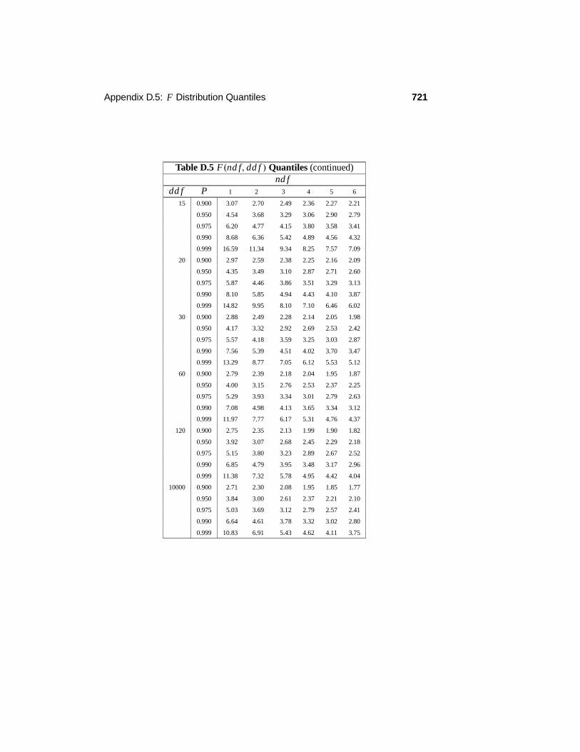
Appendix D.5: F Distribution Quantiles 721
Table D.5 F(nd f, dd f ) Quantiles (continued)nd f
dd f P 1 2 3 4 5 6
15 0.900 3.07 2.70 2.49 2.36 2.27 2.21
0.950 4.54 3.68 3.29 3.06 2.90 2.79
0.975 6.20 4.77 4.15 3.80 3.58 3.41
0.990 8.68 6.36 5.42 4.89 4.56 4.32
0.999 16.59 11.34 9.34 8.25 7.57 7.09
20 0.900 2.97 2.59 2.38 2.25 2.16 2.09
0.950 4.35 3.49 3.10 2.87 2.71 2.60
0.975 5.87 4.46 3.86 3.51 3.29 3.13
0.990 8.10 5.85 4.94 4.43 4.10 3.87
0.999 14.82 9.95 8.10 7.10 6.46 6.02
30 0.900 2.88 2.49 2.28 2.14 2.05 1.98
0.950 4.17 3.32 2.92 2.69 2.53 2.42
0.975 5.57 4.18 3.59 3.25 3.03 2.87
0.990 7.56 5.39 4.51 4.02 3.70 3.47
0.999 13.29 8.77 7.05 6.12 5.53 5.12
60 0.900 2.79 2.39 2.18 2.04 1.95 1.87
0.950 4.00 3.15 2.76 2.53 2.37 2.25
0.975 5.29 3.93 3.34 3.01 2.79 2.63
0.990 7.08 4.98 4.13 3.65 3.34 3.12
0.999 11.97 7.77 6.17 5.31 4.76 4.37
120 0.900 2.75 2.35 2.13 1.99 1.90 1.82
0.950 3.92 3.07 2.68 2.45 2.29 2.18
0.975 5.15 3.80 3.23 2.89 2.67 2.52
0.990 6.85 4.79 3.95 3.48 3.17 2.96
0.999 11.38 7.32 5.78 4.95 4.42 4.04
10000 0.900 2.71 2.30 2.08 1.95 1.85 1.77
0.950 3.84 3.00 2.61 2.37 2.21 2.10
0.975 5.03 3.69 3.12 2.79 2.57 2.41
0.990 6.64 4.61 3.78 3.32 3.02 2.80
0.999 10.83 6.91 5.43 4.62 4.11 3.75

722 Appendix D: Tables
Table D.5 F(nd f, dd f ) Quantiles (continued)nd f
dd f P 7 8 9 10 11 12
15 0.900 2.16 2.12 2.09 2.06 2.04 2.02
0.950 2.71 2.64 2.59 2.54 2.51 2.48
0.975 3.29 3.20 3.12 3.06 3.01 2.96
0.990 4.14 4.00 3.89 3.80 3.73 3.67
0.999 6.74 6.47 6.26 6.08 5.94 5.81
20 0.900 2.04 2.00 1.96 1.94 1.91 1.89
0.950 2.51 2.45 2.39 2.35 2.31 2.28
0.975 3.01 2.91 2.84 2.77 2.72 2.68
0.990 3.70 3.56 3.46 3.37 3.29 3.23
0.999 5.69 5.44 5.24 5.08 4.94 4.82
30 0.900 1.93 1.88 1.85 1.82 1.79 1.77
0.950 2.33 2.27 2.21 2.16 2.13 2.09
0.975 2.75 2.65 2.57 2.51 2.46 2.41
0.990 3.30 3.17 3.07 2.98 2.91 2.84
0.999 4.82 4.58 4.39 4.24 4.11 4.00
60 0.900 1.82 1.77 1.74 1.71 1.68 1.66
0.950 2.17 2.10 2.04 1.99 1.95 1.92
0.975 2.51 2.41 2.33 2.27 2.22 2.17
0.990 2.95 2.82 2.72 2.63 2.56 2.50
0.999 4.09 3.86 3.69 3.54 3.42 3.32
120 0.900 1.77 1.72 1.68 1.65 1.63 1.60
0.950 2.09 2.02 1.96 1.91 1.87 1.83
0.975 2.39 2.30 2.22 2.16 2.10 2.05
0.990 2.79 2.66 2.56 2.47 2.40 2.34
0.999 3.77 3.55 3.38 3.24 3.12 3.02
10000 0.900 1.72 1.67 1.63 1.60 1.57 1.55
0.950 2.01 1.94 1.88 1.83 1.79 1.75
0.975 2.29 2.19 2.11 2.05 1.99 1.95
0.990 2.64 2.51 2.41 2.32 2.25 2.19
0.999 3.48 3.27 3.10 2.96 2.85 2.75

Appendix D.5: F Distribution Quantiles 723
Table D.5 F(nd f, dd f ) Quantiles (continued)nd f
dd f P 15 20 30 60 120 10000
15 0.900 1.97 1.92 1.87 1.82 1.79 1.76
0.950 2.40 2.33 2.25 2.16 2.11 2.07
0.975 2.86 2.76 2.64 2.52 2.46 2.40
0.990 3.52 3.37 3.21 3.05 2.96 2.87
0.999 5.54 5.25 4.95 4.64 4.47 4.31
20 0.900 1.84 1.79 1.74 1.68 1.64 1.61
0.950 2.20 2.12 2.04 1.95 1.90 1.84
0.975 2.57 2.46 2.35 2.22 2.16 2.09
0.990 3.09 2.94 2.78 2.61 2.52 2.42
0.999 4.56 4.29 4.00 3.70 3.54 3.38
30 0.900 1.72 1.67 1.61 1.54 1.50 1.46
0.950 2.01 1.93 1.84 1.74 1.68 1.62
0.975 2.31 2.20 2.07 1.94 1.87 1.79
0.990 2.70 2.55 2.39 2.21 2.11 2.01
0.999 3.75 3.49 3.22 2.92 2.76 2.59
60 0.900 1.60 1.54 1.48 1.40 1.35 1.29
0.950 1.84 1.75 1.65 1.53 1.47 1.39
0.975 2.06 1.94 1.82 1.67 1.58 1.48
0.990 2.35 2.20 2.03 1.84 1.73 1.60
0.999 3.08 2.83 2.55 2.25 2.08 1.89
120 0.900 1.55 1.48 1.41 1.32 1.26 1.19
0.950 1.75 1.66 1.55 1.43 1.35 1.26
0.975 1.94 1.82 1.69 1.53 1.43 1.31
0.990 2.19 2.03 1.86 1.66 1.53 1.38
0.999 2.78 2.53 2.26 1.95 1.77 1.55
10000 0.900 1.49 1.42 1.34 1.24 1.17 1.03
0.950 1.67 1.57 1.46 1.32 1.22 1.03
0.975 1.83 1.71 1.57 1.39 1.27 1.04
0.990 2.04 1.88 1.70 1.48 1.33 1.05
0.999 2.52 2.27 1.99 1.66 1.45 1.06

724 Appendix D: Tables
D.6 Binomial Distribution ProbabilitiesIf X ∼ Binomial(n, p) , then Table D.6 contains entries computing
P(X = k) =%
nk
&pk(1− p)n−k
for various values of n, k, and p.Note that, if X ∼ Binomial(n, p) , then P(X = k) = P(Y = n − k), where
Y = n − X ∼ Binomial(n, 1− p).
Table D.6 Binomial Probabilitiesp
n k .01 .02 .03 .04 .05 .06 .07 .08 .092 0 .9801 .9604 .9409 .9216 .9025 .8836 .8649 .8464 .8281
1 .0198 .0392 .0582 .0768 .0950 .1128 .1302 .1472 .16382 .0001 .0004 .0009 .0016 .0025 .0036 .0049 .0064 .0081
3 0 .9703 .9412 .9127 .8847 .8574 .8306 .8044 .7787 .75361 .0294 .0576 .0847 .1106 .1354 .1590 .1816 .2031 .22362 .0003 .0012 .0026 .0046 .0071 .0102 .0137 .0177 .02213 .0001 .0001 .0002 .0003 .0005 .0007
4 0 .9606 .9224 .8853 .8493 .8145 .7807 .7481 .7164 .68571 .0388 .0753 .1095 .1416 .1715 .1993 .2252 .2492 .27132 .0006 .0023 .0051 .0088 .0135 .0191 .0254 .0325 .04023 .0001 .0002 .0005 .0008 .0013 .0019 .00274 .0001
5 0 .9510 .9039 .8587 .8154 .7738 .7339 .6957 .6591 .62401 .0480 .0922 .1328 .1699 .2036 .2342 .2618 .2866 .30862 .0010 .0038 .0082 .0142 .0214 .0299 .0394 .0498 .06103 .0001 .0003 .0006 .0011 .0019 .0030 .0043 .00604 .0001 .0001 .0002 .00035
6 0 .9415 .8858 .8330 .7828 .7351 .6899 .6470 .6064 .56791 .0571 .1085 .1546 .1957 .2321 .2642 .2922 .3164 .33702 .0014 .0055 .0120 .0204 .0305 .0422 .0550 .0688 .08333 .0002 .0005 .0011 .0021 .0036 .0055 .0080 .01104 .0001 .0002 .0003 .0005 .000856
7 0 .9321 .8681 .8080 .7514 .6983 .6485 .6017 .5578 .51681 .0659 .1240 .1749 .2192 .2573 .2897 .3170 .3396 .35782 .0020 .0076 .0162 .0274 .0406 .0555 .0716 .0886 .10613 .0003 .0008 .0019 .0036 .0059 .0090 .0128 .01754 .0001 .0002 .0004 .0007 .0011 .00175 .0001 .000167
8 0 .9227 .8508 .7837 .7214 .6634 .6096 .5596 .5132 .47031 .0746 .1389 .1939 .2405 .2793 .3113 .3370 .3570 .37212 .0026 .0099 .0210 .0351 .0515 .0695 .0888 .1087 .12883 .0001 .0004 .0013 .0029 .0054 .0089 .0134 .0189 .02554 .0001 .0002 .0004 .0007 .0013 .0021 .00315 .0001 .0001 .0002678

Appendix D6: Binomial Distribution Probabilities 725
Table D.6 Binomial Probabilities (continued)p
n k .10 .15 .20 .25 .30 .35 .40 .45 .502 0 .8100 .7225 .6400 .5625 .4900 .4225 .3600 .3025 .2500
1 .1800 .2550 .3200 .3750 .4200 .4550 .4800 .4950 .50002 .0100 .0225 .0400 .0625 .0900 .1225 .1600 .2025 .2500
3 0 .7290 .6141 .5120 .4219 .3430 .2746 .2160 .1664 .12501 .2430 .3251 .3840 .4219 .4410 .4436 .4320 .4084 .37502 .0270 .0574 .0960 .1406 .1890 .2389 .2880 .3341 .37503 .0010 .0034 .0080 .0156 .0270 .0429 .0640 .0911 .1250
4 0 .6561 .5220 .4096 .3164 .2401 .1785 .1296 .0915 .06251 .2916 .3685 .4096 .4219 .4116 .3845 .3456 .2995 .25002 .0486 .0975 .1536 .2109 .2646 .3105 .3456 .3675 .37503 .0036 .0115 .0256 .0469 .0756 .1115 .1536 .2005 .25004 .0001 .0005 .0016 .0039 .0081 .0150 .0256 .0410 .0625
5 0 .5905 .4437 .3277 .2373 .1681 .1160 .0778 .0503 .03131 .3280 .3915 .4096 .3955 .3602 .3124 .2592 .2059 .15632 .0729 .1382 .2048 .2637 .3087 .3364 .3456 .3369 .31253 .0081 .0244 .0512 .0879 .1323 .1811 .2304 .2757 .31254 .0004 .0022 .0064 .0146 .0284 .0488 .0768 .1128 .15625 .0001 .0003 .0010 .0024 .0053 .0102 .0185 .0312
6 0 .5314 .3771 .2621 .1780 .1176 .0754 .0467 .0277 .01561 .3543 .3993 .3932 .3560 .3025 .2437 .1866 .1359 .09382 .0984 .1762 .2458 .2966 .3241 .3280 .3110 .2780 .23443 .0146 .0415 .0819 .1318 .1852 .2355 .2765 .3032 .31254 .0012 .0055 .0154 .0330 .0595 .0951 .1382 .1861 .23445 .0001 .0004 .0015 .0044 .0102 .0205 .0369 .0609 .09376 .0001 .0002 .0007 .0018 .0041 .0083 .0156
7 0 .4783 .3206 .2097 .1335 .0824 .0490 .0280 .0152 .00781 .3720 .3960 .3670 .3115 .2471 .1848 .1306 .0872 .05472 .1240 .2097 .2753 .3115 .3177 .2985 .2613 .2140 .16413 .0230 .0617 .1147 .1730 .2269 .2679 .2903 .2918 .27344 .0026 .0109 .0287 .0577 .0972 .1442 .1935 .2388 .27345 .0002 .0012 .0043 .0115 .0250 .0466 .0774 .1172 .16416 .0001 .0004 .0013 .0036 .0084 .0172 .0320 .05477 .0001 .0002 .0006 .0016 .0037 .0078
8 0 .4305 .2725 .1678 .1001 .0576 .0319 .0168 .0084 .00391 .3826 .3847 .3355 .2670 .1977 .1373 .0896 .0548 .03132 .1488 .2376 .2936 .3115 .2965 .2587 .2090 .1569 .10943 .0331 .0839 .1468 .2076 .2541 .2786 .2787 .2568 .21884 .0046 .0185 .0459 .0865 .1361 .1875 .2322 .2627 .27345 .0004 .0026 .0092 .0231 .0467 .0808 .1239 .1719 .21886 .0002 .0011 .0038 .0100 .0217 .0413 .0703 .10947 .0001 .0004 .0012 .0033 .0079 .0164 .03128 .0001 .0002 .0007 .0017 .0039

726 Appendix D: Tables
Table D.6 Binomial Probabilities (continued)p
n k .01 .02 .03 .04 .05 .06 .07 .08 .099 0 .9135 .8337 .7602 .6925 .6302 .5730 .5204 .4722 .4279
1 .0830 .1531 .2116 .2597 .2985 .3292 .3525 .3695 .38092 .0034 .0125 .0262 .0433 .0629 .0840 .1061 .1285 .15073 .0001 .0006 .0019 .0042 .0077 .0125 .0186 .0261 .03484 .0001 .0003 .0006 .0012 .0021 .0034 .00525 .0001 .0002 .0003 .00056789
10 0 .9044 .8171 .7374 .6648 .5987 .5386 .4840 .4344 .38941 .0914 .1667 .2281 .2770 .3151 .3438 .3643 .3777 .38512 .0042 .0153 .0317 .0519 .0746 .0988 .1234 .1478 .17143 .0001 .0008 .0026 .0058 .0105 .0168 .0248 .0343 .04524 .0001 .0004 .0010 .0019 .0033 .0052 .00785 .0001 .0001 .0003 .0005 .00096 .0001789
10
12 0 .8864 .7847 .6938 .6127 .5404 .4759 .4186 .3677 .32251 .1074 .1922 .2575 .3064 .3413 .3645 .3781 .3837 .38272 .0060 .0216 .0438 .0702 .0988 .1280 .1565 .1835 .20823 .0002 .0015 .0045 .0098 .0173 .0272 .0393 .0532 .06864 .0001 .0003 .0009 .0021 .0039 .0067 .0104 .01535 .0001 .0002 .0004 .0008 .0014 .00246 .0001 .0001 .0003789
101112
15 0 .8601 .7386 .6333 .5421 .4633 .3953 .3367 .2863 .24301 .1303 .2261 .2938 .3388 .3658 .3785 .3801 .3734 .36052 .0092 .0323 .0636 .0988 .1348 .1691 .2003 .2273 .24963 .0004 .0029 .0085 .0178 .0307 .0468 .0653 .0857 .10704 .0002 .0008 .0022 .0049 .0090 .0148 .0223 .03175 .0001 .0002 .0006 .0013 .0024 .0043 .00696 .0001 .0003 .0006 .00117 .0001 .000189
101112131415

Appendix D6: Binomial Distribution Probabilities 727
Table D.6 Binomial Probabilities (continued)p
n k .10 .15 .20 .25 .30 .35 .40 .45 .509 0 .3874 .2316 .1342 .0751 .0404 .0207 .0101 .0046 .0020
1 .3874 .3679 .3020 .2253 .1556 .1004 .0605 .0339 .01762 .1722 .2597 .3020 .3003 .2668 .2162 .1612 .1110 .07033 .0446 .1069 .1762 .2336 .2668 .2716 .2508 .2119 .16414 .0074 .0283 .0661 .1168 .1715 .2194 .2508 .2600 .24615 .0008 .0050 .0165 .0389 .0735 .1181 .1672 .2128 .24616 .0001 .0006 .0028 .0087 .0210 .0424 .0743 .1160 .16417 .0003 .0012 .0039 .0098 .0212 .0407 .07038 .0001 .0004 .0013 .0035 .0083 .01769 .0001 .0003 .0008 .0020
10 0 .3487 .1969 .1074 .0563 .0282 .0135 .0060 .0025 .00101 .3874 .3474 .2684 .1877 .1211 .0725 .0403 .0207 .00982 .1937 .2759 .3020 .2816 .2335 .1757 .1209 .0763 .04393 .0574 .1298 .2013 .2503 .2668 .2522 .2150 .1665 .11724 .0112 .0401 .0881 .1460 .2001 .2377 .2508 .2384 .20515 .0015 .0085 .0264 .0584 .1029 .1536 .2007 .2340 .24616 .0001 .0012 .0055 .0162 .0368 .0689 .1115 .1596 .20517 .0001 .0008 .0031 .0090 .0212 .0425 .0746 .11728 .0001 .0004 .0014 .0043 .0106 .0229 .04399 .0001 .0005 .0016 .0042 .0098
10 .0001 .0003 .0010
12 0 .2824 .1422 .0687 .0317 .0138 .0057 .0022 .0008 .00021 .3766 .3012 .2062 .1267 .0712 .0368 .0174 .0075 .00292 .2301 .2924 .2835 .2323 .1678 .1088 .0639 .0339 .01613 .0852 .1720 .2362 .2581 .2397 .1954 .1419 .0923 .05374 .0213 .0683 .1329 .1936 .2311 .2367 .2128 .1700 .12085 .0038 .0193 .0532 .1032 .1585 .2039 .2270 .2225 .19346 .0005 .0040 .0155 .0401 .0792 .1281 .1766 .2124 .22567 .0006 .0033 .0115 .0291 .0591 .1009 .1489 .19348 .0001 .0005 .0024 .0078 .0199 .0420 .0762 .12089 .0001 .0004 .0015 .0048 .0125 .0277 .0537
10 .0002 .0008 .0025 .0068 .016111 .0001 .0003 .0010 .002912 .0001 .0002
15 0 .2059 .0874 .0352 .0134 .0047 .0016 .0005 .00011 .3432 .2312 .1319 .0668 .0305 .0126 .0047 .0016 .00052 .2669 .2856 .2309 .1559 .0916 .0476 .0219 .0090 .00323 .1285 .2184 .2501 .2252 .1700 .1110 .0634 .0318 .01394 .0428 .1156 .1876 .2252 .2186 .1792 .1268 .0780 .04175 .0105 .0449 .1032 .1651 .2061 .2123 .1859 .1404 .09166 .0019 .0132 .0430 .0917 .1472 .1906 .2066 .1914 .15277 .0003 .0030 .0138 .0393 .0811 .1319 .1771 .2013 .19648 .0005 .0035 .0131 .0348 .0710 .1181 .1647 .19649 .0001 .0007 .0034 .0116 .0298 .0612 .1048 .1527
10 .0001 .0007 .0030 .0096 .0245 .0515 .091611 .0001 .0006 .0024 .0074 .0191 .041712 .0001 .0004 .0016 .0052 .013913 .0001 .0003 .0010 .003214 .0001 .000515

728 Appendix D: Tables
Table D.6 Binomial Probabilities (continued)p
n k .01 .02 .03 .04 .05 .06 .07 .08 .0920 0 .8179 .6676 .5438 .4420 .3585 .2901 .2342 .1887 .1516
1 .1652 .2725 .3364 .3683 .3774 .3703 .3526 .3282 .30002 .0159 .0528 .0988 .1458 .1887 .2246 .2521 .2711 .28183 .0010 .0065 .0183 .0364 .0596 .0860 .1139 .1414 .16724 .0006 .0024 .0065 .0133 .0233 .0364 .0523 .07035 .0002 .0009 .0022 .0048 .0088 .0145 .02226 .0001 .0003 .0008 .0017 .0032 .00557 .0001 .0002 .0005 .00118 .0001 .00029
1011121314151617181920
Table D.6 Binomial Probabilities (continued)p
n k .10 .15 .20 .25 .30 .35 .40 .45 .5020 0 .1216 .0388 .0115 .0032 .0008 .0002
1 .2702 .1368 .0576 .0211 .0068 .0020 .0005 .00012 .2852 .2293 .1369 .0669 .0278 .0100 .0031 .0008 .00023 .1901 .2428 .2054 .1339 .0716 .0323 .0123 .0040 .00114 .0898 .1821 .2182 .1897 .1304 .0738 .0350 .0139 .00465 .0319 .1028 .1746 .2023 .1789 .1272 .0746 .0365 .01486 .0089 .0454 .1091 .1686 .1916 .1712 .1244 .0746 .03707 .0020 .0160 .0545 .1124 .1643 .1844 .1659 .1221 .07398 .0004 .0046 .0222 .0609 .1144 .1614 .1797 .1623 .12019 .0001 .0011 .0074 .0271 .0654 .1158 .1597 .1771 .1602
10 .0002 .0020 .0099 .0308 .0686 .1171 .1593 .176211 .0005 .0030 .0120 .0336 .0710 .1185 .160212 .0001 .0008 .0039 .0136 .0355 .0727 .120113 .0002 .0010 .0045 .0146 .0366 .073914 .0002 .0012 .0049 .0150 .037015 .0003 .0013 .0049 .014816 .0003 .0013 .004617 .0002 .001118 .00021920

Appendix E
Answers to Odd-NumberedExercises
Answers are provided here to odd-numbered exercises that require a computation.No details of the computations are given. If the Exercise required that something bedemonstrated, then a significant hint is provided.
1.2.1 (a) P({1, 2}) = 5/6 (b) P({1, 2, 3}) = 1 (c) P({1}) = P({2, 3}) = 1/2
1.2.3 P({2}) = 1/6
1.2.5 P({s}) = 0 for any s ∈ [0, 1]
1.2.7 This is the subset (A ∩ Bc) ∪ (Ac ∩ B) .
1.2.9 P({1}) = 1/12, P({2}) = 1/12, P({3}) = 1/6, P({4}) = 2/3
1.2.11 P({2}) = 5/24, P({1}) = 3/8, P({3}) = 5/121.3.1 (a) P({2, 3, 4, . . . , 100}) = 0.9 (b) 0.1
1.3.3 P(late or early or both) = 25%
1.3.5 (a) 1/32 = 0.03125. (b) 0.96875
1.3.7 10%
1.4.1 (a) (1/6)8 = 1/1679616 (b) (1/6)7 = 1/279936 (c) 8 (1/6)8 = 1/209952
1.4.3 1− 5051/2100
1.4.5 (a)-4
1
.-1313
.- 3913 13 13
./- 52
13 13 13 13
.(b)-4
1
.-44
.-489
.- 3913 13 13
./- 52
13 13 13 13
.1.4.7
-4810
./-52
10
. = 246/595 = 0.4134
1.4.9 (5/6)2(1/6) = 25/216
1.4.11+-5
3
./-12
3
., +-63
./-18
3
.,+ +-73. / -123
., +-123
./-18
3
.,1.4.13
-21
. 122 ·
-32
. 123 ·
-42
. 124 +
-21
. 122 ·
-30
. 123 ·
-43
. 124 = 11
128 = 0.0859
1.5.1 (a) 3/4 (b) 16/21
1.5.3 (a) 1/8 (b) (1/8)/ (1/2) = 1/4 (c) 0/(1/2) = 0
1.5.5 1
1.5.7 0.074
729

730 Appendix E: Answers to Odd-Numbered Exercises
1.5.9 (a) No (b) Yes (c) Yes (d) Yes (e) No
1.5.11 (a) 0.1667 (b) 0.3125
1.6.1 1/3
1.6.3 {An} 8 A = {1, 2, 3, . . .} = S
1.6.5 1
1.6.7 Suppose there is no n such that P([0, n]) > 0.9 and then note this implies1 = P([0,∞)) = limn→∞ P([0, n]) ≤ 0.9.
1.6.9 Yes
2.1.1 (a) 1 (b) Does not exist (c) Does not exist (d) 1
2.1.3 (a) X (s) = s and Y (s) = s2 for all s ∈ S. (b) For this example, Z(1) =2, Z(2) = 18, Z(3) = 84, Z(4) = 260, Z(5) = 630.2.1.5 Yes, for A ∩ B.
2.1.7 (a) W(1) = 1 (b) W(2) = 0 (c) W (3) = 0 (d) W ≥ Z is not true.
2.1.9 (a) Y (1) = 1 (b) Y (2) = 4 (c) Y (4) = 0
2.2.1 P(X = 0) = P(X = 2) = 1/4, P(X = 1) = 1/2, P(X = x) = 0 forx 3= 0, 1, 2
2.2.3 (a) P(Y = y) = 0 for y 3= 2, 3, 4, 5, 6, 7, 8, 9, 10, 11, 12, P(Y = 2) =1/36, P(Y = 3) = 2/36, P(Y = 4) = 3/36, P(Y = 5) = 4/36, P(Y = 6) =5/36, P(Y = 7) = 6/36, P(Y = 8) = 5/36, P(Y = 9) = 4/36, P(Y = 10) =3/36, P(Y = 11) = 2/36, P(Y = 12) = 1/36 (b) P(Y ∈ B) = (1/36)IB(2) +(2/36)IB(3)+(3/36)IB(4)+(4/36)IB(5)+(5/36)IB(6)+(6/36)IB(7)+(5/36)IB(8)+(4/36)IB(9)+ (3/36)IB(10)+ (2/36)IB(11)+ (1/36)IB(12)
2.2.5 (a) P(X = 1) = 0.3, P(X = 2) = 0.2, P(X = 3) = 0.5, and P(X = x) = 0for all x /∈ {1, 2, 3} (b) P(Y = 1) = 0.3, P(Y = 2) = 0.2, P(Y = 3) = 0.5, andP(Y = y) = 0 for all y /∈ {1, 2, 3} (c) P(W = 2) = 0.09, P(W = 3) = 0.12,P(W = 4) = 0.34, P(W = 5) = 0.2, P(W = 6) = 0.25, and P(W = w) = 0 for allother choices of w.
2.2.7 P(X = 25) = 0.45, P(X = 30) = 0.55, and P(X = x) = 0 otherwise
2.3.1 pY (2) = 1/36, pY (3) = 2/36, pY (4) = 3/36, pY (5) = 4/36, pY (6) = 5/36,pY (7) = 6/36, pY (8) = 5/36, pY (9) = 4/36, pY (10) = 3/36, pY (11) = 2/36,pY (12) = 1/36, and pY (y) = 0 otherwise
2.3.3 pZ (1) = pZ (5) = 1/4, pZ (0) = 1/2, and pZ (z) = 0 otherwise
2.3.5 pW (1) = 1/36, pW (2) = 2/36, pW (3) = 2/36, pW (4) = 3/36, pW (5) =2/36, pW (6) = 4/36, pW (8) = 2/36, pW (9) = 1/36, pW (10) = 2/36, pW (12) =4/36, pW (15) = 2/36, pW (16) = 1/36, pW (18) = 2/36, pW (20) = 2/36, pW (24) =2/36, pW (25) = 1/36, pW (30) = 2/36, and pW (36) = 1/36, with pW (w) = 0otherwise
2.3.7 θ = 11/12
2.3.9 53/512
2.3.11 θ10
2.3.15 (a)-10
3
.(0.35)3 (0.65)7 (b) (0.35) (0.65)9 (c)
-91
.(0.35)2 (0.65)8
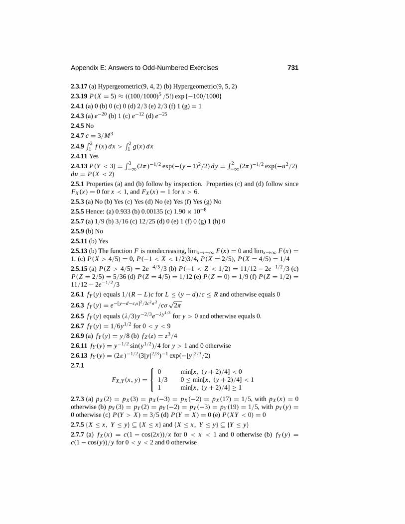
Appendix E: Answers to Odd-Numbered Exercises 731
2.3.17 (a) Hypergeometric(9, 4, 2) (b) Hypergeometric(9, 5, 2)
2.3.19 P(X = 5) ≈ ((100/1000)5 /5!) exp {−100/1000}2.4.1 (a) 0 (b) 0 (c) 0 (d) 2/3 (e) 2/3 (f) 1 (g) = 1
2.4.3 (a) e−20 (b) 1 (c) e−12 (d) e−25
2.4.5 No
2.4.7 c = 3/M3
2.4.9" 2
1 f (x) dx >" 2
1 g(x) dx
2.4.11 Yes
2.4.13 P(Y < 3) = " 3−∞(2π)−1/2 exp(−(y−1)2/2) dy = " 2
−∞(2π)−1/2 exp(−u2/2)du = P(X < 2)
2.5.1 Properties (a) and (b) follow by inspection. Properties (c) and (d) follow sinceFX (x) = 0 for x < 1, and FX (x) = 1 for x > 6.
2.5.3 (a) No (b) Yes (c) Yes (d) No (e) Yes (f) Yes (g) No
2.5.5 Hence: (a) 0.933 (b) 0.00135 (c) 1.90× 10⁻⁸
2.5.7 (a) 1/9 (b) 3/16 (c) 12/25 (d) 0 (e) 1 (f) 0 (g) 1 (h) 0
2.5.9 (b) No
2.5.11 (b) Yes
2.5.13 (b) The function F is nondecreasing, limx→−∞ F(x) = 0 and limx→∞ F(x) =1. (c) P(X > 4/5) = 0, P(−1 < X < 1/2)3/4, P(X = 2/5), P(X = 4/5) = 1/4
2.5.15 (a) P(Z > 4/5) = 2e−4/5/3 (b) P(−1 < Z < 1/2) = 11/12 − 2e−1/2/3 (c)P(Z = 2/5) = 5/36 (d) P(Z = 4/5) = 1/12 (e) P(Z = 0) = 1/9 (f) P(Z = 1/2) =11/12− 2e−1/2/3
2.6.1 fY (y) equals 1/(R − L)c for L ≤ (y − d)/c ≤ R and otherwise equals 0
2.6.3 fY (y) = e−[y−d−cµ]2/2c2σ 2/cσ
√2π
2.6.5 fY (y) equals (λ/3)y−2/3e−λy1/3for y > 0 and otherwise equals 0.
2.6.7 fY (y) = 1/6y1/2 for 0 < y < 9
2.6.9 (a) fY (y) = y/8 (b) fZ (z) = z3/4
2.6.11 fY (y) = y−1/2 sin(y1/2)/4 for y > 1 and 0 otherwise
2.6.13 fY (y) = (2π)−1/2(3|y|2/3)−1 exp(−|y|2/3/2)2.7.1
FX,Y (x, y) = 0 min[x, (y + 2)/4] < 0
1/3 0 ≤ min[x, (y + 2)/4] < 11 min[x, (y + 2)/4] ≥ 1
2.7.3 (a) pX (2) = pX (3) = pX (−3) = pX (−2) = pX (17) = 1/5, with pX (x) = 0otherwise (b) pY (3) = pY (2) = pY (−2) = pY (−3) = pY (19) = 1/5, with pY (y) =0 otherwise (c) P(Y > X) = 3/5 (d) P(Y = X) = 0 (e) P(XY < 0) = 0
2.7.5 {X ≤ x, Y ≤ y} ⊆ {X ≤ x} and {X ≤ x, Y ≤ y} ⊆ {Y ≤ y}2.7.7 (a) fX (x) = c(1 − cos(2x))/x for 0 < x < 1 and 0 otherwise (b) fY (y) =c(1− cos(y))/y for 0 < y < 2 and 0 otherwise

732 Appendix E: Answers to Odd-Numbered Exercises
2.7.9 (a) fX (x) = (4 + 3x2 − 2x3)/8 for x ∈ (0, 2) and 0 otherwise (b) fY (y) =(y3 + 3y2)/12 for y ∈ (0, 2) and 0 otherwise (c) P(Y < 1) = 5/48
2.8.1 (a) pX (−2) = 1/4, pX (9) = 1/4, pX (13) = 1/2, otherwise, pX (x) = 0 (b)pY (3) = 2/3, pY (5) = 1/3; otherwise, pY (y) = 0 (c) Yes
2.8.3 (a) fX (x) = (18x/49) + (40/49) for 0 ≤ x ≤ 1 and fX (x) = 0 otherwise (b)fY (y) = (48y2 + 6y + 30)/49 for 0 ≤ y ≤ 1 and fY (y) = 0 otherwise (c) No
2.8.5 (a) P(Y = 4 | X = 9) = 1/6 (b) P(Y = −2 | X = 9) = 1/2 (c) P(Y = 0 | X =−4) = 0 (d) P(Y = −2 | X = 5) = 1 (e) P(X = 5 |Y = −2) = 1/3
2.8.7 (a) fX (x) = x2 + 2/3, fY (y) = 4y5 + 2y/3 for 0 ≤ x ≤ 1 and 0 ≤ y ≤ 1,fY |X (y | x) = (2x2y + 4y5) / (x2 + 2/3) (otherwise, fY |X (y | x) = 0), thus, X andY are not independent. (b) fX (x) = C(x5/6 + x/2), fY (y) = C(y5/6 + y/2) for0 ≤ x ≤ 1 and 0 ≤ y ≤ 1, fY |X (y | x) = (xy + x5y5) / (x5/6 + x/2) (other-wise, fY |X (y | x) = 0) X and Y are not independent. (c) fX (x) = C(50,000x5/3 +50x), fY (y) = C(2048y5/3 + 8y) for 0 ≤ x ≤ 4 and 0 ≤ y ≤ 10, fY |X (y | x) =(xy + x5y5) / (50,000x5/3+ 50x) (otherwise, fY |X (y | x) = 0), thus, X and Y are notindependent. (d) fX (x) = C(50,000x5/3) and fY (y) = C(2048y5/3) for 0 ≤ x ≤ 4and 0 ≤ y ≤ 10, fY |X (y | x) = 3y5 /50000 (otherwise, fY |X (y | x) = 0), X and Y areindependent.
2.8.9 P(X = 1, Y = 1) = P(X = 1, Y = 2) = P(X = 2, Y = 1) = P(X = 3, Y =3) = 1/4
2.8.11 If X = C is constant, then P(X ∈ B1) = IB1(C) and P(X ∈ B1, Y ∈ B2) =IB1(C) P(Y ∈ B2).
2.8.13 (a)
pY |X (y|x) y = 1 y = 2 y = 4 y = 7 Othersx = 3 1/4 1/4 1/4 1/4 0x = 5 1/4 1/4 1/4 1/4 0
(b)pX |Y (x|y) x = 3 x = 5 Others
y = 1 1/2 1/2 0y = 2 1/2 1/2 0y = 4 1/2 1/2 0y = 7 1/2 1/2 0
(c) X and Y are independent.
2.8.15 fY |X (y|x) = 2(x2 + y)/(4 + 3x2 − 2x3) for x < y < 2, and 0 otherwise (b)fX |Y (x|y) = 3(x2+ y)/(y3+3y2) for 0 < x < y and 0 otherwise (c) Not independent
2.9.1 ∂h1∂u1
= − cos(2πu2) / u1/
2 log(1/u1),∂h1∂u2
= −2√
2π sin(2πu2)/
2 log(1/u1),∂h2∂u1
= − sin(2πu2) / u1/
2 log(1/u1),∂h2∂u2
= −2√
2π cos(2πu2)×/
2 log(1/u1)
2.9.3 (b) h(x, y) = (x2 + y2, x2 − y2) (c) h−1(z,w) = (√(z +w)/2, √(z −w)/2),at least for z + w ≥ 0 and z − w ≥ 0 (d) fZ ,W (z,w) = e−
√(z+w)/2 /2
√z2 −w2 for√
(z +w)/2 ≥ 0 and 1 ≤ √(z −w)/2 ≤ 4, i.e., for z ≥ 4 and max(−z, z − 64) ≤w ≤ z − 4, and 0 otherwise

Appendix E: Answers to Odd-Numbered Exercises 733
2.9.5 (b) h(x, y) = (y4, x4) (c) h−1(z, w) = (w1/4, z1/4) (d) fZ ,W (z,w) = e−w1/4
for w1/4 ≥ 0 and 1 ≤ z1/4 ≤ 4, i.e., for w ≥ 0 and 1 ≤ z ≤ 256, and 0 otherwise
2.9.7 pZ (2) = 1/18, pZ (4) = 1/12, pZ (5) = 1/18, pZ (7) = 1/24, pZ (8) = 1/72,pZ (9) = 1/4, pZ (11) = 3/8, pZ (12) = 1/8, pZ (z) = 0 otherwise
2.9.9(a)
(z,w) (−8,16) (−7,19) (−3,11) (−2,14) (0,6) otherwiseP(Z = z,W = w) 1/5 1/5 1/5 1/5 1/5 0
(b) pZ (z) = 1/5 for z = −8,−7,−3,−2, 0, and otherwise pZ (z) = 0. (c) pW (w) =1/5 for w = 6, 11, 14, 16, 19, and otherwise pW (w) = 0
2.10.1 Z = −7 if U ≤ 1/2, Z = −2 if 1/2 < U ≤ 5/6, and Z = 5 if U > 5/6
2.10.3 Y ∼ Exponential(3)
2.10.5 c1 = ±3√
2 and c2 = 5
2.10.7 (a) For x < 1, FX (x) = 0, for 1 ≤ x < 2, FX (x) = 1/3, for 2 ≤ x < 4,FX (x) = 1/2, for x ≥ 4, FX (x) = 1. (b) The range of t must be restricted on (0, 1]because F−1
X (0) = −∞. F−1X (t) = 1 for t ∈ (0, 1/3], F−1
X (t) = 2 for t ∈ (1/3, 1/2],and F−1
X (t) = 4 for t ∈ (1/2, 1]. (c) For y < 1, FY (y) = 0, for 1 ≤ y < 2,FY (y) = 1/3, for 2 ≤ y < 4, FY (y) = 1/2, for y ≥ 4, FY (y) = 1.
2.10.9 Y = F−1Z (U) = U1/4
3.1.1 (a) E(X) = 8/7 (b) E(X) = 1 (c) E(X) = 8
3.1.3 (a) E(X) = −173/12 (b) E(Y ) = 11 (c) E(X2) = 19 (d) E(Y 2) = 370/3 (e)E(X2 + Y 2) = 427/3 (f) E(XY − 4Y ) = −113/2
3.1.5 E(8X − Y + 12) = 8((1− p)/p)− λ+ 12
3.1.7 E(XY ) = 30
3.1.9 E(X) = 6
3.1.11 (a) E(Z) = 7 (b) E(W ) = 49/4
3.1.13 E(Y ) = 7/4
3.2.1 (a) C = 1/4, E(X) = 7 (b) C = 1/16, E(X) = 169/24 (c) C = 5/3093,E(X) = −8645/2062
3.2.3 (a) E(X) = 17/24 (b) E(Y ) = 17/8 (c) E(X2) = 11/20 (d) E(Y 2) = 99/20 (e)E(Y 4) = 216/7 (f) E(X2Y 3) = 27/4
3.2.5 E(−5X − 6Y ) = −76/3
3.2.7 E(Y + Z) = 17/72
3.2.9 Let µk = E(Xk), then µ1 = 39/25, µ2 = 64/25, µ3 = 152/35
3.2.11 334
3.2.13 E(Y ) = 214.1
3.2.15 Yes
3.3.1 (a) Cov(X,Y ) = 2/3 (b) Var(X) = 2, Var(Y ) = 32/9 (c) Corr(X,Y ) = 1/4

734 Appendix E: Answers to Odd-Numbered Exercises
3.3.3 Corr(X, Y ) = −0.18292
3.3.5 E(XY ) = E(X)E(Y )
3.3.7 (a) Cov(X, Z) = 1/9 (b) Corr(X, Z) = 1/√
46
3.3.9 E (X (X − 1)) = E-X2.−E (X), when X ∼ Binomial(n, θ) , E (X (X − 1)) =
n (n − 1) θ2
3.3.11 E(X) = E(Y ) = 7/2, E(XY ) = 49/4, Cov(X, Y ) = 0
3.3.13 Cov(Z,W) = 0, Corr(Z,W) = 0
3.3.15 Cov(X,Y ) = 35/24
3.4.1 (a) rZ (t) = t/(2 − t), r !Z (t) = 2/(2 − t)2, r !!Z (t) = −4/(t − 2)3 (b) E(Z) = 2,Var(Z) = 2, mZ (t) = et/(2−et),m!Z (t) = 2et/(2−et)2,m!!Z (t) = 2et(2+et)/(2−et)
3.4.3 mY (s) = eλ(es−1), m!Y (s) = λeseλ(e
s−1), so m!Y (s) = λ, m!!Y (s) = (λes +λ2e2s)eλ(e
s−1), so m!!Y (s) = λ+ λ2, Var(Y ) = λ+ λ2 − (λ)2 = λ3.4.5 mY (s) = e4smX (3s)
3.4.7 m!!!Y (s) = eλ(es−1)esλ(1+ 3esλ+ e2sλ2), E(Y 3) = m!!!Y (0) = λ(1+ 3λ+ λ2)
3.5.1 (a) E(X |Y = 3) = 5/2 (b) E(Y | X = 3) = 22/3 (c) E(X |Y = 2) =5/2, E(X |Y = 17) = 3 (d) E(Y | X = 2) = 5/2, E(Y | X = 3) = 22/3
3.5.3 (a) E(Y | X = 6) = 25/4 (b) E(Y | X = −4) = 36/7 (c) E(Y | X) = 25/4whenever X = 6, and E(Y | X) = 36/7 whenever X = −4.
3.5.7 E(Z |W = 4) = 14/3 (b) E(W |Z = 4) = 10/3
3.5.9 (a) E(X |Y = 0) = 1 (b) E(X |Y = 1) = 2 (c) E(Y |X = 0) = 0 (d) E(Y |X =1) = 1/3 (e) E(Y |X = 2) = 2/3 (f) E(Y |X = 3) = 1 (g) E(Y |X) = X/3
3.5.11 (a) E(X) = 27/19 (b) E(Y ) = 52/95 (c) E(X |Y ) = 3(2 + y3)/4 + 3y3 (d)
E(Y |X) = (x2/2+1/5)/x2+1/4 (e) E[E(Y |X)] = " 20
3(2+y3)4+3y3 · 4
19 (4+3y3) dy = 2719
(f) E[E(Y |X)] = " 10
x2/2+1/5x2+1/4
· 619 (x
2 + 14) dx = 52
95
3.6.1 3/7
3.6.3 (a) 1/9 (b) 1/2 (c) 2 (d) The upper bound in part (b) is smaller and thus moreuseful than that in part (c).
3.6.5 1/4
3.6.7 (a) 10,000 (b) 12,100
3.6.9 (a) 1 (b) 1/4
3.6.11 (a) E(Z) = 8/5 (b) 32/75
3.6.13 7/16
3.7.1 E(X1) = 3, E(X2) = 0, E(Y ) = 3/5
3.7.3 P(X < t) = 0 for t < 0, while P(X > t) = 1 for 0 < t < C and P(X > t) = 0for t > C
3.7.5 E(X) = 2
3.7.7 E(W) = 1/5
3.7.9 E(W) = 21/2

Appendix E: Answers to Odd-Numbered Exercises 735
4.1.1 P(Y3 = 1) = 1/64, P(Y3 = 3) = 1/64, P(Y3 = 21/3) = 3/16, P(Y3 = 31/3) =3/16, P(Y3 = 41/3) = 3/32, P(Y3 = 91/3) = 3/32, P(Y3 = 121/3) = 3/64, P(Y3 =181/3) = 3/64, P(Y3 = 61/3) = 3/16
4.1.3 If Z is the sample mean, then P(Z = 0) = p2, P(Z = 0.5) = 2p(1 − p), andP(Z = 1) = (1− p)2.
4.1.5 For 1 ≤ j ≤ 6, P(max = j) = ( j/6)20 − (( j − 1)/6)20.
4.1.7 If W = XY, then
P(W = w) =
1/36 if w = 1, 9, 16, 25, 36,1/18 if w = 2, 3, 5, 8, 10, 15, 18, 20, 24, 30,1/12 if w = 4,1/9 if w = 6, 12,0 otherwise.
4.1.9 pY (y) = 1/2 for y = 1, 2; otherwise, pY (y) = 0
4.2.1 Note that Zn = Z unless 7 ≤ U < 7+1/n2. Hence, for any 6 > 0, P(|Zn−Z | ≥6) ≤ P(7 ≤ U < 7+ 1/n2) = 1/5n2 → 0 as n →∞.
4.2.3 P(W1 + · · · +Wn < n/2) = 1− P(W1 + · · · +Wn ≥ n/2) ≥ 1− P(| 1n (W1 +· · · +Wn)− 1
3 | ≥ 1/6)
4.2.5 P(X1 + · · · + Xn > 9n) ≤ P(|(X1 + · · · + Xn)/n − 8| ≥ 1)
4.2.7 For all 6 > 0 and n > −2 ln 6, P(|Xn − Y | ≥ 6) = P(e−Hn ≥ 6) = P(Hn ≤− ln 6) ≤ P(|Hn − n/2| ≥ |n/2+ ln 6|) n →∞.
4.2.9 By definition, Hn − 1 ≤ Fn ≤ Hn and P(|Xn − Yn − Z | ≥ 6) = P(|Hn −Fn|/(Hn + 1) ≥ 6) ≤ P(1/(Hn + 1) ≥ 6) = P(Hn ≤ (1/6) − 1) = P(Hn − n/2 ≤(1/6)− 1− n/2) ≤ P(|Hn − n/2| ≥ |1+ n/2− 1/6|).4.2.11 r = 9/2
4.3.1 Note that Zn = Z unless 7 ≤ U < 7 + 1/n2. Also, if U > 7, then Zn = Zwhenever 1/n2 < 7−U , i.e., n > 1/
√7−U . Hence, P(Zn → Z) ≥ P(U 3= 7).
4.3.3 {(W1 + · · · +Wn)/n → 1/3} ⊆ {∃n; (W1 + · · · +Wn)/n < 1/2} = {∃n; W1 +· · · +Wn < n/2}4.3.5 P(Xn → X and Yn → Y ) = 1 − P(Xn 3→ X or Yn 3→ Y ) ≥ 1 − P(Xn 3→X)− P(Yn 3→ Y )
4.3.7 m = 5
4.3.9 r = 9/2
4.3.11 (a) Suppose there is no such m and from this get a contradiction to the stronglaw of large numbers. (b) No
4.4.1 limn→∞ P(Xn = i) = 1/3 = P(X = i) for i = 1, 2, 3
4.4.3 Here, P(Zn ≤ 1) = 1, for 0 ≤ z < 1, P(Zn ≤ z) = zn+1, and P(Z ≤ z) = 1for z ≥ 1.
4.4.5 P(S ≤ 540) ≈ 4(1/2) = 0.6915
4.4.7 P(S ≥ 2450) ≈ 4(−0.51) = 0.3050

736 Appendix E: Answers to Odd-Numbered Exercises
4.4.9 (a) For 0 < y < 1, P(Z ≤ y) = y2. (b) For 1 ≤ m ≤ n, P(Xn ≤ m/n) =m(m+ 1)/[n(n+ 1)]. (c) For 0 < y < 1, let m = <ny=, the biggest integer not greaterthan ny. Since there is no integer in (m, ny), P(m/n < Xn < y) ≤ P(m/n < Xn <(m + 1)/n) = 0. Thus, P(Xn ≤ y) = m(m + 1)/[n(n + 1)], where m = <ny=.(d) For 0 < y < 1, let mn = <ny=, show mn/n → y as n → ∞. Then showP(Xn ≤ y)→ y2 as n →∞.
4.4.11 λ = 3
4.4.13 The yearly output, Y , is approximately normally distributed with mean 1300and variance 433. So, P(Y < 1280) ≈ 0.1685.
4.5.1 The integral equals√
2πE(cos2(Z)), where Z ∼ N(0, 1).
4.5.3 This integral equals (1/5)E(e−14Z2), where Z ∼ Exponential(5).
4.5.5 This sum is approximately equal to e5 E(sin(Z2)), where Z ∼ Poisson(5).
4.5.7 (−6.1404,−3.8596)
4.5.9 (0.354, 0.447)
4.5.11 (a) C = {" 10
" 10 g(x, y) dx dy}−1 (b) Generate Xi ’s from fX (x) = 3x2 for 0 <
x < 1 a and Yi ’s from fY (y) = 4y3 for 0 < y < 1. Set Di = sin(XiYi ) cos(√
XiYi )×exp(X2
i + Yi )/12 and Ni = Xi · Di for i = 1, . . . , n. 5. Estimate E(X) by Mn =N/D = (N1 + · · · + Nn)/(D1 + · · · + Dn).
4.5.13 (a) J = " 10
"∞0 ey h(x, y) I[0,∞)(y)e−y dy I[0,1](x) dx (b) Generate Xi and Yi
appropriately, set Ti = eYi h(Xi ,Yi), and estimate J by Mn = (T1 + · · · + Tn)/n.(c) J = " 1
0
"∞0 e5y h(x, y) I[0,∞)(y)5e−5y dy I[0,1](x) dx (d) As in part (b). (e) The
estimator having smaller variance is better. So use sample variances to choose betweenthem.
4.6.1 (a) U ∼ N(44, 629),V ∼ N(−18− 8C, 144+ 25C2) (b) C = −24/125
4.6.3 C1 = 1/√
5,C2 = −3,C3 = 1/√
2,C4 = 7,C5 = 2
4.6.5 Let Z1, . . . , Zn,W1, . . . ,Wm ∼ N(0, 1) be i.i.d. and set X = (Z1)2+· · ·+(Zn)
2
and Y = (W1)2 + · · · + (Wn)
2.
4.6.7 C = √n
4.6.9 C1 = 2/5,C2 = −3,C3 = 2,C4 = 7,C5 = 2,C6 = 1,C7 = 1
4.6.11 (a) m = 60, K = √61 (b) y = 1.671 (c) a = 61, b = 1, c = 60 (d) w = 4.00
5.1.1 The mean survival times for the control group and the treatment group are 93.2days and 356.2 days, respectively.
5.1.3 For those who are still alive, their survival times will be longer than the recordedvalues, so these data values are incomplete.
5.1.5 x = −0.1375
5.1.7 Use the difference x − y.
5.2.1 In Example 5.2.1, the mode is 0. In Example 5.2.2, the mode is 1.
5.2.3 The mixture has density (5/√
2π) exp{− (x + 4)2 /2}+(5/√2π) exp{− (x − 4)2
/2} for −∞ < x <∞.5.2.5 x = 10

Appendix E: Answers to Odd-Numbered Exercises 737
5.2.7 The mode is 1/3.
5.2.9 The mode is x = 0.
5.3.1 The statistical model for a single response consists of three probability functions{Bernoulli(1/2), Bernoulli(1/3), Bernoulli(2/3)} .5.3.3 The sample (X1, . . . , Xn) is a sample from an N(µ, σ 2) distribution, where θ =(µ, σ 2) ∈ 7 = {(10, 2), (8, 3)}. Both the population mean and variance uniquelyidentify the population distribution.
5.3.5 A single observation is from an Exponential(θ) distribution, where θ ∈ 7 =[0,∞). We can parameterize this model by the mean or variance but not by the coeffi-cient of variation.
5.3.7 (a) 7 = {A, B} (b) The value X = 1 is observable only when θ = A. (c) Bothθ = A and θ = B are possible.
5.3.9 P1
5.4.1
FX (x) =
0 x < 1410 1 ≤ x < 2710 2 ≤ x < 3910 3 ≤ x < 4
1 4 ≤ x
, fX (x) =
410 x = 13
10 x = 22
10 x = 31
10 x = 4
µX =#4
x=1 x fX (x) = 2, σ 2X =
+#4x=1 x2 fX (x)
,− 22 = 1
5.4.3 (a) Yes (b) Use Table D.1 by selecting a row and reading off the first three singlenumbers (treat 0 in the table as a 10). (c) Using row 108 of Table D.1 (treating 0 as10): First sample — we obtain random numbers 6, 0, 9, and so compute (X (π6) +X (π10)+ X (π9))/3 = 3.0. Second sample — we obtain random numbers 4, 0, 7, andso compute (X (π6) + X (π10) + X (π9))/3 = 2.666 7. Third sample — we obtainrandom numbers 2, 0, 2 (note we do not skip the second 2), and so compute (X (π6)+X (π10)+ X (π9))/3 = 2.0.
5.4.5 (c) The shape of a histogram depends on the intervals being used.
5.4.7 It is a categorical variable.
5.4.9 (a) Students are more likely to lie when they have illegally downloaded music sothe results of the study will be flawed. (b) Under anonymity, students are more likelyto tell the truth, so there will be less error. (c) The probability a student tells the truthis p = 0.625. Let Yi be the answer from student i . Then (Y − (1 − p))/(2p − 1) isrecorded as an estimate of the proportion of students who have ever downloaded musicillegally.
5.5.1 (a) f X (0) = 0.2667, f X (1) = 0.2, f X (2) = 0.2667, f X (3) = f X (4) = 0.1333(b) FX (0) = 0.2667, FX (1) = 0.4667, FX (2) = 0.7333, FX (3) = 0.8667, FX (4) =1.000 (d) The mean x = 15 and the variance s2 = 1.952. (e) The median is 2 and theI QR = 3. According to the 1.5 I QR rule, there are no outliers.
5.5.3 (a) f X (1) = 25/82, f X (2) = 35/82, f X (3) = 22/82 (b) No

738 Appendix E: Answers to Odd-Numbered Exercises
5.5.5 The sample median is 0, first quartile is −1.150, third quartile is 0.975, and theI QR = 2.125. We estimate FX (1) by FX (1) = 17/20 = 0.85.
5.5.7 ψ(µ) = µ+ σ 0z0.25, where z0.25 satisfies 4(z0.25) = 0.25
5.5.9 ψ(µ) = 4((3− µ) /σ 0)
5.5.11 ψ(µ, σ 2) = 4((3− µ) /σ)5.5.13 ψ(θ) = 2θ(1− θ)5.5.15 ψ(θ) = α0/β
2
6.1.1 The appropriate statistical model is Binomial(n, θ), where θ ∈ 7 = [0, 1] is theprobability of having this antibody in the blood. The likelihood function is L(θ | 3) =-10
3
.θ3(1− θ)7.
6.1.3 L(θ | x1, . . . , x20) = θ20 exp(− (20x) θ) and x is a sufficient statistic.
6.1.5 c = -104
./-9
3
.6.1.7 L(θ | x1, ..., xn) = =n
i=1 θxi e−θ/xi ! = θnx e−nθ/
=xi ! and x is a minimal suffi-
cient statistic.
6.1.9 L(1|0)/L(2|0) = 4.4817, the distribution f1 is 4.4817 times more likely than f2.
6.1.11 No
6.1.13 No
6.2.1 θ (1) = a, θ(2) = b, θ(3) = b, θ(4) = a
6.2.3 ψ(θ) = θ2 is 1–1 and so ψ(θ(x1, ..., xn)) = x2 is the MLE.
6.2.5 θ = α0/x
6.2.7 α = −n/#n
i=1 ln xi
6.2.9 α = n/#n
i=1 ln (1+ xi )
6.2.11 µ3 = 32.768 cm3 is the MLE
6.2.13 A likelihood function can’t take negative values.
6.2.15 Equivalent log-likelihood functions differ by an additive constant.
6.3.1 P-value = 0.592 and .95-confidence interval is (4.442, 5.318).
6.3.3 P-value = 0.000 and .95-confidence interval is (63.56, 67.94).
6.3.5 P-value = 0.00034 and .95 confidence interval is [47. 617, 56.383]. The mini-mum required sample size is 2.
6.3.7 P-value = 0.1138, so not statistically significant and the observed difference of1.05− 1 = 0.05 is well within the range of practical significance.
6.3.9 P-value = 0.527
6.3.11 P-value = 0.014
6.3.13 (a)#n
i=1(xi− x)2 =#ni=1 x2
i −nx2 (b) The plug-in estimator is σ 2 = x(1− x),
so σ 2 = s2(n − 1)/n. (c) bias(σ 2) = −σ 2/n → 0 as n →∞6.3.15 (a) Yes (b) No
6.3.17 The P-value 0.22 does not imply the null hypothesis is correct. It may be thatwe have just not taken a large enough sample size to detect a difference.
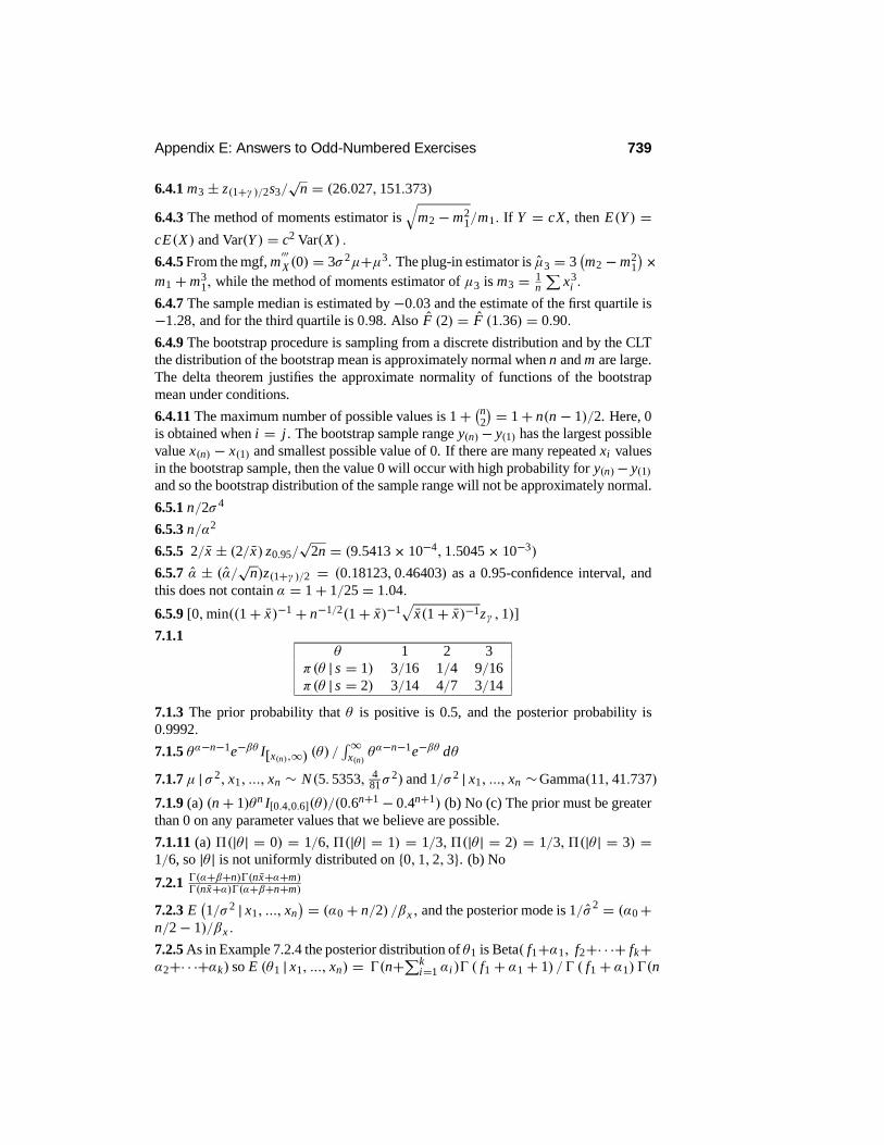
Appendix E: Answers to Odd-Numbered Exercises 739
6.4.1 m3 ± z(1+γ )/2s3/√
n = (26.027, 151.373)
6.4.3 The method of moments estimator is>
m2 −m21/m1. If Y = cX, then E(Y ) =
cE(X) and Var(Y ) = c2 Var(X) .
6.4.5 From the mgf, m!!!X (0) = 3σ 2µ+µ3. The plug-in estimator is µ3 = 3
-m2 −m2
1
.×m1 +m3
1, while the method of moments estimator of µ3 is m3 = 1n
#x3
i .
6.4.7 The sample median is estimated by −0.03 and the estimate of the first quartile is−1.28, and for the third quartile is 0.98. Also F (2) = F (1.36) = 0.90.
6.4.9 The bootstrap procedure is sampling from a discrete distribution and by the CLTthe distribution of the bootstrap mean is approximately normal when n and m are large.The delta theorem justifies the approximate normality of functions of the bootstrapmean under conditions.
6.4.11 The maximum number of possible values is 1+ -n2. = 1+ n(n − 1)/2. Here, 0is obtained when i = j . The bootstrap sample range y(n)− y(1) has the largest possiblevalue x(n) − x(1) and smallest possible value of 0. If there are many repeated xi valuesin the bootstrap sample, then the value 0 will occur with high probability for y(n)− y(1)and so the bootstrap distribution of the sample range will not be approximately normal.
6.5.1 n/2σ 4
6.5.3 n/α2
6.5.5 2/x ± (2/x) z0.95/√
2n = (9.5413× 10⁻⁴, 1.5045× 10⁻³)
6.5.7 α ± (α/√n)z(1+γ )/2 = (0.18123, 0.46403) as a 0.95-confidence interval, andthis does not contain α = 1+ 1/25 = 1.04.
6.5.9 [0,min((1+ x)−1 + n−1/2(1+ x)−1/
x(1+ x)−1zγ , 1)]
7.1.1θ 1 2 3
π(θ | s = 1) 3/16 1/4 9/16π(θ | s = 2) 3/14 4/7 3/14
7.1.3 The prior probability that θ is positive is 0.5, and the posterior probability is0.9992.
7.1.5 θα−n−1e−βθ I[x(n),∞) (θ) /"∞
x(n)θα−n−1e−βθ dθ
7.1.7µ | σ 2, x1, ..., xn ∼ N(5. 5353, 481σ
2) and 1/σ 2 | x1, ..., xn ∼Gamma(11, 41.737)
7.1.9 (a) (n + 1)θn I[0.4,0.6](θ)/(0.6n+1 − 0.4n+1) (b) No (c) The prior must be greaterthan 0 on any parameter values that we believe are possible.
7.1.11 (a) 9(|θ | = 0) = 1/6,9(|θ | = 1) = 1/3,9(|θ | = 2) = 1/3,9(|θ | = 3) =1/6, so |θ | is not uniformly distributed on {0, 1, 2, 3}. (b) No
7.2.1 )(α+β+n))(nx+α+m))(nx+α))(α+β+n+m)
7.2.3 E-1/σ 2 | x1, ..., xn
. = (α0 + n/2) /βx , and the posterior mode is 1/σ 2 = (α0+n/2− 1)/βx .
7.2.5 As in Example 7.2.4 the posterior distribution of θ1 is Beta( f1+α1, f2+· · ·+ fk+α2+· · ·+αk) so E (θ1 | x1, ..., xn) = )(n+#k
i=1 αi )) ( f1 + α1 + 1) /) ( f1 + α1) )(n

740 Appendix E: Answers to Odd-Numbered Exercises
+#ki=1 αi+1) and maximizes ln((θ1)
f1+α1−1 (1− θ1)#k
i=2( fi+αi )−1) for the posteriormode.
7.2.7 Recall that the posterior distribution of θ1 in Example 7.2.2 is Beta( f1+α1, f2+· · · + fk + α2 + · · · + αk). Find the second moment and use Var(θ1 | x1, ..., xn) =E-θ2
1 | x1, ..., xn.−(E (θ1 | x1, ..., xn))
2 .Now 0 ≤ f1/n ≤ 1, so Var(θ1 | x1, ..., xn) =( f1/n + α1) (
#ki=2 ( fi/n + αi ))/{n(1+#k
i=1 αi/n + 1/n)(1+#ki=1 αi/n)2} → 0
as n →∞.7.2.9 The posterior predictive density of xn+1 is obtained by averaging the N(x, (1/τ 2
0+n/σ 2
0)−1σ 2
0) density with respect to the posterior density of µ, so we must have thatthis is also the posterior predictive distribution.
7.2.11 The posterior predictive distribution of t = xn+1 is (nx + β0)Pareto(n + α0).So the posterior mode is t = 0, the posterior expectation is (nx + β0)/(n + α0 − 1),and the posterior variance is (nx + β0)
2(n + α0)/[(n + α0 − 1)2(n + α0 − 2)].
7.2.13 (a) The posterior distribution of σ 2 is inverse Gamma(n/2 + α0, βx ), whereβx = (n − 1)s2/2 + n(x − µ0)
2/2 + β0. (b) E(σ 2 | x1, ..., xn) = βx/(n/2 + α0 −1). (c) To assess the hypothesis H0 : σ 2 ≤ σ 2
0, compute the probability 9(1/σ 2 ≥1/σ 2
0 | x1, .., xn) = 1−G(2βx/σ20; 2α0 + n) where G(· ; 2α0 + n) is the χ2(2α0 + n)
cdf.
7.2.15 (a) The odds in favor of A = 1/odds in favor of Ac. (b) BF(A) = 1/BF(Ac)
7.2.17 Statistician I’s posterior probability for H0 is 0.0099. Statistician II’s posteriorprobability for H0 is 0.0292. Hence, Statistician II has the bigger posterior belief inH0.
7.2.19 The range of a Bayes factor in favor of A ranges in [0,∞). If A has posteriorprobability equal to 0, then the Bayes factor will be 0.
7.3.1 (3.2052, 4.4448)
7.3.3 The posterior mode is µ = (nt/v20+µ0/σ
20)/(n/v
20+1/σ 2
0) and σ 2(x1, . . . , xn) =(n/v2
0 + 1/σ 20)−1. Hence, the asymptotic γ -credible interval is (µ − z(1+γ )/2σ , µ +
z(1+γ )/2σ ).7.3.5 For a sample (x1, . . . , xn) the posterior distribution is N(x, 1/n) restricted to[0, 1]. A simple Monte Carlo algorithm for the posterior distribution is 1. Generate ηfrom N(x, 1/n), 2. Accept η if it is in [0, 1] and return to step 1 otherwise. If the truevalue θ∗ is not in [0, 1], then the acceptance rate will be very small for large n.
7.4.1 The posterior density is proportional to λn+α−1 exp{−λ(ln -=(1+ xi.)+ β)}.
7.4.3 (a) The maximum value of the prior predictive is obtained when τ = 1. (b) Theposterior of θ given τ = 1 is
π1 (θ | 1, 1, 3) = (1/2)(1/3)3
59/1728 = 3259 θ = a
(1/2)(1/2)2(1/8)59/1728 = 27
59 θ = b.
7.4.5 The prior predictive is given by mα,β (x1, ..., xn) = )(α+β))(α))(β)
)(α+nx))(β+n(1−x)))(α+β+n) .
Based on the prior predictive, we would select the prior given by α = 1, β = 1.

Appendix E: Answers to Odd-Numbered Exercises 741
7.4.7 Jeffreys’ prior is√
nθ−1/2 (1− θ)−1/2 . The posterior distribution of θ is Beta(nx+1/2, n (1− x)+ 1/2).
7.4.9 The prior distribution is θ ∼ N(66, σ 2) with σ 2 = 101.86.
7.4.11 Let the prior be θ ∼ Exponential(λ) with λ = 0.092103.
8.1.1 L(1 | ·) = (3/2) L(2 | ·), so by Section 6.1.1 T is a sufficient statistic. The condi-tional distributions of s are as follows.
s = 1 s = 2 s = 3 s = 4fa (s | T = 1) 1/3
1/3+1/6 = 23
1/61/3+1/6 = 1
3 0 0
fb (s | T = 1) 1/21/2+1/4 = 2
31/4
1/2+1/4 = 13 0 0
s = 1 s = 2 s = 3 s = 4fa (s | T = 3) 0 0 1 0fb (s | T = 3) 0 0 1 0
s = 1 s = 2 s = 3 s = 4fa (s | T = 4) 0 0 0 1fb (s | T = 4) 0 0 0 1
8.1.3 x2 + (1− 1/n) σ 20
8.1.5 UMVU for 5+ 2µ
8.1.7 x/α0
8.1.9 n−1#ni=1 I(−1,1)(Xi)
8.1.11 Yes
8.2.1 When α = 0.1, c0 = 3/2 and γ = ((1/10)− (1/12)) / (1/2) = 1/30. Thepower of the test is 23/120.When α = 0.05, c0 = 2 and γ = ((1/20)− 0) / (1/12) =3/5.The power of the test is 1/10.
8.2.3 By (8.2.6) the optimal 0.01 test is of the form
ϕ0 (x) =
1 x ≥ 1+
√2√
102.3263
0 x < 1+√
2√10
2.3263
= 1 x ≥ 2.0404
0 x < 2.0404.
8.2.5 (a) 0 (b) Suppose θ > 1. The power function is β(θ) = 1− 1/θ .
8.2.7 n ≥ 4
8.2.9 The graph of the power function of the UMP size α test function lies above thegraph of the power function of any other size test α function.
8.3.1 9(θ = 1 | 2) = 2/5,9 (θ = 2 | 2) = 3/5, so 9(θ = 2 | 2) > 9(θ = 1 | 2) andwe accept H0 : θ = 2.
8.3.3 The Bayes rule is given by (1/τ 20 + n/σ 2
0)−1(µ0/τ
20 + nx/σ 2
0), which convergesto x as τ 0 →∞.8.3.5 The Bayes rule is given by (nα0 + τ 0) / (nx + υ0) and by the weak law of largenumbers this converges in probability to β as n →∞.

742 Appendix E: Answers to Odd-Numbered Exercises
8.3.7 The Bayes rule rejects whenever
BFH0 =exp
%− n
2σ 20
-x − µ0
.2&τ−1
0
%nσ 2
0+ 1τ2
0
&−1/2
exp
?12
%1τ2
0+ nσ 2
0
&−1%µ0τ2
0+ nσ 2
0x
&2
− 12
%µ2
0τ2
0+ nx2
σ 20
&@
is less than (1− p0)/p0. As τ 20 →∞, the denominator converges to 0, so in the limit
we never reject H0.
8.4.1 The model is given by the collection of probability functions {θnx (1− θ)n−nx :θ ∈ [0, 1]} on the set of all sequences (x1, . . . , xn) of 0’s and 1’s. The action space isA = [0, 1] , the correct action function is A (θ) = θ, and the loss function is L (θ, a) =(θ − a)2 . The risk function for T is RT (θ) = Varθ (x) = θ (1− θ) /n.8.4.3 The model is the set of densities {(2πσ 2
0)−1/2 exp{−#n
i=1 (xi − µ)2 /2σ 20} : µ ∈
R1} on Rn . The action space is A = R1, the correct action function is A (µ) = µ,and the loss function is L (µ, a) = (µ− a)2 . The risk function for T is RT (µ) =Varµ (x) = σ 2
0/n.
8.4.5 (a) Rd (a) = 1/2, Rd (b) = 3/4 (b) No. Consider the risk function of the decisionfunction d∗ given by d∗ (1) = b, d∗ (2) = a, d∗ (3) = b, d∗ (4) = a.
9.1.1 The observed discrepancy statistic is given by D (r) = 22.761 and the P-value isP (D(R) > 22.761) = 0. 248, which doesn’t suggest evidence against the model.
9.1.3 (c) The plots suggest that the normal assumption seems reasonable.
9.1.5 The observed counts are given in the following table.
Interval Count(0.0, 0.2] 4(0.2, 0.4] 7(0.4, 0.6] 3(0.6, 0.8] 4(0.8, 1] 2
The Chi-squared statistic is equal to 3.50 and the P-value is given by (X2 ∼ χ2 (4))P-X2 ≥ 3.5
. = 0.4779. Therefore, we have no evidence against the Uniform modelbeing correct.
9.1.7 (a) The probability of the event s = 3 is 0 based on the probability measure Phaving S as its support. The most appropriate P-value is 0. (b) 0.729
9.1.9 No
9.1.11 (a) The conditional probability function of (x1, . . . , xn) is
θnx (1− θ)n(1−x)/
%n
nx
&θnx (1− θ)n(1−x) = 1/
%n
nx
&.
(b) Hypergeometric(n, <n/2=, nx0) (c) 0.0476

Appendix E: Answers to Odd-Numbered Exercises 743
9.2.1 (a) No (b) P-value is 1/10, so there is little evidence of a prior–data conflict. (c)P-value is 1/300, so there is some evidence of a prior–data conflict.
9.2.3 We can write x = µ + z, where z ∼ N(0, σ 20/n) is independent of µ ∼
N(µ0, τ20).
9.2.5 The P-value for checking prior–data conflict is 0. Hence, there is definitely aprior–data conflict.
10.1.1 For any x1, x2 (that occur with positive probability) and y, we have P(Y =y | X = x1) = P(Y = y | X = x2). Thus P(X = x1,Y = y) = P(X = x2, Y =y)P(X = x1)/P(X = x2), and summing this over x1 leads to P(X = x2, Y = y) =P(X = x2)P(Y = y). For the converse, show P(Y = y | X = x) = P(Y = y).
10.1.3 X and Y are related.
10.1.5 The conditional distributions P (Y = y | X = x) will change with x wheneverX is not degenerate.
10.1.7 If the conditional distribution of life-length given various smoking habits changes,then we can conclude that these two variables are related, but we cannot conclude thatthis relationship is a cause–effect relationship due to the possible existence of con-founding variables.
10.1.9 The researcher should draw a random sample from the population of votersand ask them to measure their attitude toward a particular political party on a scalefrom favorably disposed to unfavorably disposed. Then the researcher should randomlyselect half of this sample to be exposed to a negative ad, while the other half is exposedto a positive ad. They should all then be asked to measure their attitude toward theparticular political party on the same scale. Next compare the conditional distributionof the response variable Y (the change in attitude from before seeing the ad to after)given the predictor X (type of ad exposed to), using the samples to make inferenceabout these distributions.
10.1.11 (a) {(0, 100) , (1, 100)} (b) A sample has not been taken from the populationof interest. The individuals involved in the study have volunteered and, as a group,they might be very different from the full population. (c) We should group the indi-viduals according to their initial weight W into homogenous groups (blocks) and thenrandomly apply the treatments to the individuals in each block.
10.1.13 (a) The response variable could be the number of times an individual haswatched the program. A suitable predictor variable is whether or not they receivedthe brochure. (b) Yes, as we have controlled the assignment of the predictor variable.
10.1.15 W has a relationship with Y and X has a relationship with Y.
10.1.17 (a)
X = 0 X = 1 SumRel. Freq. 0.5 0.5 1.0
(b)
Y = 0 Y = 1 SumRel. Freq. 0.7 0.3 1.0

744 Appendix E: Answers to Odd-Numbered Exercises
(c)
Rel. Freq. X = 0 X = 1 SumY = 0 0.3 0.4 0.7Y = 1 0.2 0.1 0.3sum 0.5 0.5 1.0
(d)
P(Y = y|X = x) y = 0 y = 1 sumx = 0 0.6 0.4 1.0x = 1 0.8 0.2 1.0
(e) Yes
10.1.19 X and Y are related. We see that only the variance of the conditional distribu-tion changes as we change X.
10.1.21 The correlation is 0, but X and Y are related.
10.2.1 The chi-squared statistic is equal to X20 = 5.7143 and, with X2 ∼ χ2(2), the P-
value equals P(X2 > 5. 7143) = 0.05743. Therefore, we don’t have evidence againstthe null hypothesis of no difference in the distributions of thunderstorms between thetwo years, at least at the 0.05 level.
10.2.3 The chi-squared statistic is equal to X20 = 0. 10409 and, with X2 ∼ χ2 (1) , the
P-value equals P(X2 > 4. 8105) = 0.74698. Therefore, we have no evidence againstthe null hypothesis of no relationship between the two digits.
10.2.5 (a) The chi-squared statistic is equal to X20 = 10.4674 and, with X2 ∼ χ2(4),
the P-value equals P(X2 > 10.4674) = 0.03325. Therefore, we have some evidenceagainst the null hypothesis of no relationship between hair color and gender. (c) Thestandardized residuals are given in the following table. They all look reasonable, sonothing stands out as an explanation of why the model of independence does not fit.Overall, it looks like a large sample size has detected a small difference.
Y = fair Y = red Y = medium Y = dark Y = jet blackX =m −1.07303 0.20785 1.05934 −0.63250 1.73407X = f 1.16452 −0.22557 −1.14966 0.68642 −1.88191
10.2.7 We should first generate a value for X1 ∼ Dirichlet(1, 3). Then generate U2from the Beta(1, 2) distribution and set X2 = (1− X1)U2. Next generate U3 from theBeta(1, 1) distribution and set X3 = (1− X1 − X2)U3. Finally set X4 = 1 − X1 −X2 − X3.
10.2.9 Then there are 36 possible pairs (i, j) for i, j = 1, . . . , 6. Let fi j denotethe frequency for (i, j) and compute chi-squared statistic, X2 = #6
i=1#6
j=1( fi j −fi · f· j/n)2/( fi · f· j/n). Compute the P-value P(χ2(25) > X2).
10.2.11 We look at the differencesAA fi j − f i · f· j/n
AA to see how big these are.
10.3.1 x

Appendix E: Answers to Odd-Numbered Exercises 745
10.3.3 x
10.3.5 (b) y = 29.9991+2.10236x (e) The plot of the standardized residuals against Xindicates very clearly that there is a problem with this model. (f) Based on part (e), it isnot appropriate to calculate confidence intervals for the intercept and slope. (g) Nothingcan be concluded about the relationship between Y and X based on this model, as wehave determined that it is inappropriate. (h) R2 = 486.193/7842.01 = 0.062, whichis very low.
10.3.7 (b) b2 = 1.9860 and b1 = 58.9090(d) The standardized residual of the ninth week departs from the other residuals in part(c). This provides some evidence that the model is not correct. (e) The confidence inter-val for β1 is [44.0545, 72.1283], and the confidence interval for β2 is [0.0787, 3.8933].(f) The ANOVA table is as follows.
Source Df Sum of Squares Mean SquareX 1 564.0280 564.0280
Error 10 1047.9720 104.7972Total 11 1612.0000
So the F-statistic is F = 5.3821 and P(F(1, 10) ≥ 5.3821) < 0.05 from TableD.5. Hence, we conclude there is evidence against the null hypothesis of no linearrelationship between the response and the predictor. (g) R2 = 0.3499 so, almost 35%of the observed variation in the response is explained by changes in the predictor.
10.3.9 In general, E(Y | X) = exp(β1 + β2 X) is not a simple linear regression modelsince it cannot be written in the form E(Y | X) = β∗1 + β∗2V, where V is an observedvariable and the β∗i are unobserved parameter values.
10.3.11 We can write E(Y | X) = E(Y | X2) in this case and E(Y | X2) = β1+ β2 X2,so this is a simple linear regression model but the predictor is X2 not X.
10.3.13 R2 = 0.05 indicates that the linear model explains only 5% of the variation inthe response, so the model will not have much predictive power.
10.4.1 (b) Both plots look reasonable, indicating no serious concerns about the correct-ness of the model assumptions. (c) The ANOVA table for testing H0 : β1 = β2 = β3is given below.
Source Df SS MSA 2 4.37 2.18
Error 9 18.85 2.09Total 11 23.22
The F statistic for testing H0 is given by F = 2.18/2.09 = 1.0431, with P-valueP(F > 1.0431) = 0.39135. Therefore, we don’t have evidence against the null hy-pothesis of no difference among the conditional means of Y given X . (d) Since wedid not find any relationship between Y and X, there is no need to calculate theseconfidence intervals.

746 Appendix E: Answers to Odd-Numbered Exercises
10.4.3 (b) Both plots indicate a possible problem with the model assumptions. (c) TheANOVA table for testing H0 : β1 = β2 is given below.
Source Df SS MSCheese 1 0.114 0.114Error 10 26.865 2.686Total 11 26.979
The F statistic for testing H0 is given by F = 0.114/2.686 = .04 and with the P-value P(F > .04) = 0.841. Therefore, we do not have any evidence against the nullhypothesis of no difference among the conditional means of Y given Cheese.
10.4.5 (b) Both plots look reasonable, indicating no concerns about the correctness ofthe model assumptions. (c) The ANOVA table for testing H0 : β1 = β2 = β3 = β4follows.
Source Df SS MSTreatment 3 19.241 6.414
Error 20 11.788 0.589Total 23 31.030
The F statistic for testing H0 is given by F = 6.414/0.589 = 10. 89 and with P-value P(F > 10. 89) = 0.00019. Therefore, we have strong evidence against the nullhypothesis of no difference among the conditional means of Y, given the predictor. (d)The 0.95-confidence intervals for the difference between the means are given in thefollowing table.
Family error rate = 0.192 Individual error rate = 0.0500 Critical value = 2.086 Intervals for (column level mean) - (row level mean) 1 2 3 2 -0.3913 1.4580 3 -2.2746 -2.8080 -0.4254 -0.9587 4 -2.5246 -3.0580 -1.1746 -0.6754 -1.2087 0.6746
10.4.7 (b) Treating the marks as separate samples, the ANOVA table for testing anydifference between the mean mark in Calculus and the mean mark in Statistics follows.
Source Df SS MSCourse 1 36.45 36.45Error 18 685.30 38.07Total 19 721.75
The F statistic for testing H0 : β1 = β2 is given by F = 36.45/38.07 = 0.95745,with the P-value equal to P(F > 0.95745) = 0.3408. Therefore, we do not have any

Appendix E: Answers to Odd-Numbered Exercises 747
evidence against the null hypothesis of no difference among the conditional means ofY given Course.
Both residual plots look reasonable, indicating no concerns about the correctnessof the model assumptions. (c) Treating these data as repeated measures, the meandifference between the mark in Calculus and the mark in Statistics is given by d =−2.7 with standard deviation s = 2.00250. The P-value for testing H0 : µ1 = µ2,is 0.0021, so we have strong evidence against the null. Hence, we conclude that thereis a difference between the mean mark in Calculus and the mean mark in Statistics.A normal probability plot of the data does not indicate any reason to doubt modelassumptions. (d) rxy = 0.944155
10.4.9 When Y1 and Y2 are measured on the same individual, we have that Var(Y1 −Y2) = 2(Var(Y1)− Cov(Y1,Y2)) > 2Var(Y1) since Cov(Y1,Y2) < 0. If we had mea-sured Y1 and Y2 on independently randomly selected individuals, then we would havethat Var(Y1 − Y2) = 2Var(Y1).
10.4.11 The difference of the two responses Y1 and Y2 is normally distributed, i.e.,Y1 − Y2 ∼ N(µ, σ 2).
10.4.13 (1) The conditional distribution of Y given (X1, X2), depends on (X1, X2)only through E(Y | X1, X2), and the error Z = Y − E(Y | X1, X2) is independent of(X1, X2). (2) The error Z = Y − E(Y | X1, X2) is normally distributed. (3) X1 and X2do not interact.
10.5.1 F (x) = " x−∞ e−t
-1+ e−t
.−2 dt = -1+ e−t.−1 |x−∞ = -1+ e−x
.−1 → 1 asx →∞ and p = F (x) , implies x = ln (p/ (1− p)).
10.5.3 Let l = l(p) = ln(p/(1− p)) be the log odds so el = p/(1− p) = 1/(1/p−1).Hence, el/(1+ el) = p, and substitute l = β1 + β2x.
10.5.5 P(Y = 1|X1 = x1, . . . , Xk = xk) = 1/2+ arctan(β1x1 + · · · + βk xk)/π
11.1.1 (a) 0 (b) 0 (c) 1/3 (d) 2/3 (e) 0 (f) 4/9 (g) 0 (h) 1/9 (i) 0 (j) 0 (k) 0.00925 (l) 0(m) 0.0987
11.1.3 (a) 5/108 (b) 5/216 (c) 5/72 (d) By the law of total probability, P(X3 = 8) =P(X1 = 6, X3 = 8)+ P(X1 = 8, X3 = 8).
11.1.5 (a) Here, P(τ c < τ 0).= 0.89819. That is, if you start with $9 and repeatedly
make $1 bets having probability 0.499 of winning each bet, then the probability youwill reach $10 before going broke is equal to 0.89819 (b) 0.881065 (c) 0.664169 (d)0.0183155 (e) 4× 10⁻¹⁸ (f) 2× 10−174
11.1.7 We use Theorem 11.1.1. (a) 1/4 (b) 3/4 (c) 0.062 5 (d) 1/4 (e) 0 (f) 1 (g) Weknow that the initial fortune is 5, so to get to 7 in two steps, the walk must have beenat 6 after the first step.
11.1.9 (a) 18/38 (b) 0.72299 (c) 0.46056 (d) 0 (e) In the long run, the gambler losesmoney.
11.2.1 (a) 0.7 (b) 0.1 (c) 0.2 (d) 1/4 (e) 1/4 (f) 1/2 (g) 0.311.2.3 (a) P0(X2 = 0) = 0.28, P0(X2 = 1) = 0.72, P1(X2 = 0) = 0.27, P1(X2 =1) = 0.73 (b) P0(X3 = 1) = 0.728
11.2.5 (a) 1/2 (b) 0 (c) 1/2 (d) 1/2 (e) 1/10 (f) 2/5 (g) 37/100 (h) 11/20 (i) 0 (j) 0 (k)0 (l) 0 (m) No

748 Appendix E: Answers to Odd-Numbered Exercises
11.2.7 This chain is doubly stochastic, i.e., has#
i pi j = 1 for all j . Hence, we musthave the uniform distribution (π1 = π2 = π3 = π4 = 1/4) as a stationary distribution.
11.2.9 (a) By either increasing or decreasing one step at a time, we see that for alli and j , we have p(n)i j > 0 for some n ≤ d. (b) Each state has period 2. (c) If iand j are two or more apart, then pi j = p ji = 0. If j = i + 1, then π i pi j =(1/2d)((d − 1)!/i !(d − i − 1)!), while π j p ji = (1/2d)((d − 1)!/ i!(d − i − 1)!).
11.2.11 (a) This chain is irreducible. (b) The chain is aperiodic. (c) π1 = 2/9, π2 =3/9, π3 = 4/9 (d) limn→∞ P1(Xn = 2) = π2 = 3/9 = 1/3, so P1(X500 = 2) ≈ 1/3.
11.2.13 P1(X1 + X2 ≥ 5) = 0.54
11.2.15 (a) The chain is irreducible. (b) The chain is not aperiodic.
11.3.1 First, choose any initial value X0. Then, given Xn = i , let Yn+1 = i+1 or i−1,with probability 1/2 each. Let j = Yn+1 and let αi j = min(1, e−( j−13)4+(i−13)4).Then let Xn+1 = j with probability αi j , otherwise let Xn+1 = i with probability1− αi j .
11.3.3 First, choose any initial value X0. Then, given Xn = i , let Yn+1 = i + 1with probability 7/9 or Yn+1 = i − 1 with probability 2/9. Let j = Yn+1 and, ifj = i + 1, let αi j = min(1, e− j4− j6− j8
(2/9)/e−i4−i6−i8(7/9)) or, if j = i − 1,
then let αi j = min(1, e− j4− j6− j8(7/9)/e−i4−i6−i8
(2/9)). Then let Xn+1 = j withprobability αi j , otherwise let Xn+1 = i with probability 1− αi j .
11.3.5 Let {Zn} be i.i.d. ∼ N(0, 1). First, choose any initial value X0. Then, givenXn = x , let Yn+1 = Xn +
√10 Zn+1. Let y = Yn+1 and let αxy = min(1, exp{−y4 −
y6 − y8 + x4 + x6 + x8}). Then let Xn+1 = y with probability αxy , otherwise letXn+1 = x with probability 1− αxy .
11.4.1 C = 12/5
11.4.3 p = 1/3
11.4.5 P(Xn = 4) = 5/8
11.4.7 (a) Here, E(Xn+1 | Xn) = (1/4)(3Xn) + (3/4)(Xn/3) = Xn. (b) T is non-negative, integer-valued, and does not look into the future, so it is a stopping time. (c)E(XT ) = X0 = 27. (d) P(XT = 1) = 27/40
11.5.1 (a) 1/2 (b) 0 (c) 1/4 (d) We have P(Y (M)1 ≥ 1) = P(Y (M)M/M ≥ √M/√
M).
Hence, P(Y (1)1 ≥ 1) = 1/2, P(Y (2)1 ≥ 1) = 1/4, P(Y (3)1 ≥ 1) = 3/8, P(Y (4)1 ≥ 1) =5/16.
11.5.3 (a) P(B2 ≥ 1) = 4(−1/√
2) (b) P(B3 ≤ −4) = 4(−4/√
3) (c) P(B9− B5 ≤2.4) = 1 − 4(−2.4/2) (d) P(B26 − B11 > 9.8) = 4(−9.8/
√15) (e) P(B26.3 ≤
−6) = 4(−6/√
26.3) (f) P(B26.3 ≤ 0) = 4(0/√26.3) = 1/2
11.5.5 E(B13 B8) = 811.5.7 (a) 3/4 (b) 1/4 (c) The answer in part (a) is larger because−5 is closer to B0 = 0than 15 is, whereas−15 is farther than 5 is. (d) 1/4 (e) We have 3/4+ 1/4 = 1, whichit must since the events in parts (a) and (d) are complementary events.
11.5.9 E(X3 X5) = 61.75
11.5.11 (a) P(X10 > 250) = 4(−20/1√
10) (b) P(X10 > 250) = 4(−20/4√
10) (c)P(X10 > 250) = 4(−20/10
√10) (d) P(X10 > 250) = 4(−20/100
√10)

Appendix E: Answers to Odd-Numbered Exercises 749
11.6.1 (a) e−141413/13! (b) e−35353/3! (c) e−424220/20! (d) e−350350340/340! (e) 0(f) (e−141413/13!) (e−21217/7!) (g) 0
11.6.3 P(N2 = 6) = e−2/3(2/3)6/6!, P(N3 = 5) = e−3/3(3/3)5/5!
11.6.5 P(N2.6 = 2 | N2.9 = 2) = (2.6/2.9)2

Index
0–1 loss function, 467
a priori, 374abs command, 685absolutely continuous
jointly, 85absolutely continuous random variable, 52acceptance probability, 644action space, 464additive, 5additive model, 593adjacent values, 287admissible, 470admissiblity, 470alternative hypothesis, 448analysis of covariance, 595analysis of variance (ANOVA), 545analysis of variance (ANOVA) table, 545ancillary, 481anova command, 690ANOVA (analysis of variance), 545ANOVA test, 548aov command, 690aperiodicity, 635
balance, 520ball, 626bar chart, 288barplot command, 688basis, 559batching, 414Bayes factor, 397Bayes risk, 471Bayes rule, 460, 471Bayes’ Theorem, 22Bayesian decision theory, 471Bayesian model, 374
Bayesian P-value, 395Bayesian updating, 383bell-shaped curve, 56Bernoulli distribution, 42, 131best-fitting line, 542beta command , 686beta distribution, 61beta function, 61bias, 271, 322binom command, 686binomial coefficient, 17binomial distribution, 43, 116, 131, 162,
163, 167binomial theorem, 131birthday problem, 19bivariate normal distribution, 89blinding, 521blocking variable, 523, 594blocks, 523bootstrap mean, 353bootstrap percentile confidence interval, 355bootstrap samples, 353bootstrap standard error, 353bootstrap t confidence interval, 355bootstrapping, 351, 353Borel subset, 38boxplot, 287boxplot command, 688Brown, R., 657Brownian motion, 657, 659
properties, 659Buffon’s needle, 234burn-in, 643
calculus, 675fundamental theorem of, 676
categorical variable, 270
750

751
Cauchy distribution, 61, 240Cauchy–Schwartz inequality, 186, 197cause–effect relationship, 516cbind command, 698cdf
inverse, 120cdf (cumulative distribution function), 62ceiling command, 685ceiling (least integer function), 296census, 271central limit theorem, 215, 247chain rule, 676characteristic function, 169Chebychev’s inequality, 185Chebychev, P. L., 2chi-squared distribution, 236chi-squared goodness of fit test, 491chi-squared statistic, 491chi-squared(n), 236χ2(n), 236chisq command, 686chisq.test command, 688classification problems, 267coefficient of determination (R2), 546coefficient of variation, 267, 360combinatorics, 15complement, 7, 10complement of B in A, 7complementing function, 315completely crossed, 522completeness, 438composite hypothesis, 466composition, 676conditional density, 96conditional distribution, 94, 96conditional expectation, 173conditional probability, 20conditional probability function, 95conditionally independent, 184confidence interval, 326confidence level, 326confidence property, 326confidence region, 290confounds, 517conjugate prior, 422consistency, 325
consistent, 200, 325constant random variable, 42continuity properties, 28continuous random variable, 51–53continuous-time stochastic process, 658,
666control, 254control treatment, 521convergence
almost surely , 208in distribution, 213in probability, 204, 206, 210, 211, 246with probability 1, 208, 210, 211, 246
convolution, 113correct action function, 464correction for continuity, 219, 358correlation, 89, 156cos command, 685countably additive, 5counts, 102covariance, 152, 153covariance inequality, 440Cramer–Rao inequality, 441Cramer–von Mises test, 495craps (game), 27credible interval, 391credible region, 290critical value, 446, 448cross, 587cross-ratio, 537cross-tabulation, 687cross-validation, 496cumulative distribution function
joint, 80properties of, 63
cumulative distribution function, (cdf), 62
data reduction, 303decision function, 467decision theory model, 464decreasing sequence, 28default prior, 425degenerate distribution, 42, 131delta theorem, 351density
conditional, 96

752
proposal, 646density function, 52
joint, 85density histogram function, 274derivative, 675
partial, 678descriptive statistics, 282design, 519det command, 698diag command, 698diffusions, 661Dirichlet distribution, 93discrepancy statistic, 480discrete random variable, 41disjoint, 5distribution
F , 241t , 239Bernoulli, 42, 131beta, 61binomial, 43, 116, 131, 162, 163, 167Cauchy, 61chi-squared, 236conditional, 94, 96degenerate, 42, 131exponential, 54, 61, 142, 165, 166extreme value, 61gamma, 55, 116geometric, 43, 132hypergeometric, 47joint, 80Laplace, 61log-normal, 79logistic, 61mixture, 68negative-binomial, 44, 116normal, 57, 89, 116, 142, 145, 234Pareto, 61point, 42Poisson, 45, 132, 162, 164proposal, 644standard normal, 57stationary, 629uniform, 7, 53, 141, 142Weibull, 61
distribution function, 62
joint, 80properties of, 63
distribution of a random variable, 38distribution-free, 349Doob, J., 2, 37double ’til you win, 618double blind, 521double expectation, 177double use of the data, 507doubly stochastic matrix, 631, 632drift, 662dummy variables, 578
ecdf command, 688Ehrenfest’s urn, 625empirical Bayesian methods, 423empirical distribution function, 271empty set, 5error sum of squares (ESS), 545error term, 516ESS (error sum of squares), 545estimation, 290estimation, decision theory, 465estimator, 224, 434event, 5exact size α test function, 449exp command, 686expectation, 173expected value, 129, 130, 141, 191
linearity of, 135, 144, 192monotonicity of, 137, 146, 192
experiment, 518experimental design, 520experimental units, 519exponential distribution, 54, 142, 165, 166
memoryless property of, 61extrapolation, 543extreme value distribution, 61
F , 62f command, 686F distribution, 241FX , 62FX (a−), 63fX , 59F(m, n), 241

753
F-statistic, 546factor, 519factorial, 16, 677fair game, 617family error rate, 581Feller, W., 2, 37Fermat, P. de, 2finite sample correction factor, 280first hitting time, 618Fisher information, 365Fisher information matrix, 372Fisher signed deviation statistic, 363Fisher’s exact test, 484Fisher’s multiple comparison test, 581fitted values, 560floor command, 685floor (greatest integer function), 119for command, 691fortune, 615frequentist methods, 374frog, 626, 641function
Lipschitz, 665fundamental theorem of calculus, 676
gambler’s ruin, 618gambling, 615gambling strategy
double ’til you win, 618gamma command (function), 685gamma command (distribution), 686gamma distribution, 55, 116gamma function, 55γ -confidence interval, 326generalized hypergeometric distribution, 51generalized likelihood ratio tests, 455generating function
characteristic function, 169moment, 165probability, 162
geom command, 686geometric distribution, 43, 132geometric mean, 200Gibbs sampler, 647Gibbs sampling, 413glm command, 690
greatest integer function (floor), 119grouping, 274
Hall, Monty, 27, 28hierarchical Bayes, 424higher-order transition probabilities, 628highest posterior density (HPD) intervals,
392hist command, 687hitting time, 618HPD (highest posterior density) intervals,
392hyper command, 686hypergeometric distribution, 47hyperparameter, 422hyperprior, 424hypothesis assessment, 290, 332hypothesis testing, 446hypothesis testing, decision theory, 466
i.i.d. (independent and identically distrib-uted), 101
identity matrix, 560if command, 691importance sampler, 233importance sampling, 233improper prior, 425inclusion–exclusion, principle of, 11, 13increasing sequence, 28independence, 24, 98, 101, 137
pairwise, 24independent and identically distributed (i.i.d.),
101indicator function, 35, 210indicator function, expectation, 131individual error rate, 581inequality
Cauchy–Schwartz, 186, 197Chebychev’s, 185Jensen’s, 187Markov’s, 185
inference, 258infinite series, 677information inequality, 441initial distribution, 623integral, 676

754
intensity, 666interaction, 522, 587intercept term, 562interpolation, 543interquartile range (IQR), 286intersection, 7inverse cdf, 120inverse Gamma, 380inverse normalizing constant, 376inversion method for generating random
variables, 121IQR (interquartile range), 286irreducibility, 634
Jacobian, 110Jeffreys’ prior, 426Jensen’s inequality, 187joint cumulative distribution function, 80joint density function, 85joint distribution, 80jointly absolutely continuous, 85
k-th cumulant, 173Kolmogorov, A. N., 2Kolmogorov–Smirnov test, 495kurtosis statistic, 483
Laplace distribution, 61large numbers
law of, 206, 211largest-order statistic, 104latent variables, 414, 415law of large numbers
strong, 211weak, 206
law of total probability, 11, 21least integer function (ceiling), 296least relative suprise estimate, 406least-squares estimate, 538, 560least-squares line, 542least-squares method, 538least-squares principle, 538Lehmann–Scheffé theorem, 438length command, 685levels, 520lgamma command, 685
likelihood, 298likelihood function, 298likelihood principle, 299likelihood ratios, 298likelihood region, 300Likert scale, 279linear independence property, 559linear regression model, 558linear subspace, 559linearity of expected value, 135, 144, 192link function, 603Lipschitz function, 665lm command, 689location, 136location mixture, 69log command, 685log odds, 603log-gamma function, 383log-likelihood function, 310log-normal distribution, 79logistic distribution, 61, 606logistic link, 603logistic regression model, 603logit, 603loss function, 465lower limit, 287ls command, 686lurking variables, 518
macro, 700MAD (mean absolute deviation), 469margin of error, 329marginal distribution, 82Markov chain, 122, 623Markov chain Monte Carlo, 643Markov’s inequality, 185Markov, A. A., 2martingale, 650matrix, 559, 678matrix inverse, 560matrix product, 560max command, 685maximum likehood estimator, 308maximum likelihood estimate (MLE), 308maximum of random variables, 104mean command, 688

755
mean absolute deviation (MAD), 469mean value, 129, 130mean-squared error (MSE), 321, 434, 469measurement, 270measuring surprise (P-value), 332median, 284median command, 688memoryless property, 61Méré, C. de, 2method of composition, 125method of least squares, 538method of moments, 349method of moments principle, 350method of transformations, 496Metropolis–Hastings algorithm, 644min command, 685minimal sufficient statistic, 304minimax decision function, 471Minitab, 699mixture distribution, 68
location, 69scale, 70
MLE (maximum likelihood estimate), 308mode of a density, 260model checking, 266, 479model formula, 688model selection, 464moment, 164moment-generating function, 165monotonicity of expected value, 137, 146,
192monotonicity of probabilities, 11Monte Carlo approximation, 225Monty Hall problem, 27, 28MSE (mean-squared error), 321, 434, 469multicollinearity, 515multinomial coefficient, 18multinomial distributions, 102multinomial models, 302, 305multiple comparisons, 510, 581multiple correlation coefficient, 565multiplication formula, 21multiplication principle, 15multivariate measurement, 271multivariate normal, 500
N(0, 1), 57N(µ, σ 2), 57NA (not available in R), 686nbinom command, 686ncol command, 698negative-binomial distribution, 44, 116Neyman–Pearson theorem, 450noninformative prior, 425nonrandomized decision function, 467nonresponse error, 277norm command, 686normal distribution, 57, 89, 116, 142, 145,
234normal probability calculations, 66normal probability plot, 489normal quantile plot, 489normal score, 488nrow command, 698nuisance parameter, 338null hypothesis, 332
observational study, 269observed Fisher information, 364observed relative surprise, 406odds in favor, 397one-sided confidence intervals, 347one-sided hypotheses, 347one-sided tests, 337one-to-one function, 110one-way ANOVA, 577optimal decision function, 470optimal estimator, 434optional stopping theorem, 653order statistics, 103, 284ordered partitions, 17orthogonal rows, 236outcome, 4outliers, 288overfitting, 481
pX , 42p-th percentile, 283p-th quantile, 283P-value, 332paired comparisons, 585pairwise independence, 24

756
parameter, 262parameter space, 262Pareto distribution, 61partial derivative, 678partition, 11Pascal’s triangle, 2, 632Pascal, B., 2pen, 626percentile, 283period of Markov chain, 635permutations, 164, 66Pi , 627placebo effect, 521plot command, 688plug-in Fisher information, 366plug-in MLE, 315point distribution, 42point hypothesis, 466point mass, 42pois command, 686Poisson distribution, 45, 132, 162, 164Poisson process, 50, 666polling, 276pooling, 593population, 270population cumulative distribution function,
270population distribution, 270population interquartile range, 286population mean, 285population relative frequency function, 274population variance, 285posterior density, 376posterior distribution, 376posterior mode, 387posterior odds, 397posterior predictive, 400posterior probability function, 376power, 341power function, 341, 449, 469power transformations, 496practical significance, 335prediction, 258, 400prediction intervals, 576prediction region, 402
predictor variable, 514principle of conditional probability, 259principle of inclusion–exclusion, 11, 13prior elicitation, 422prior odds, 397prior predictive distribution, 375prior probability distribution, 374prior risk, 471prior–data conflict, 503probability, 1
conditional, 20law of total, 11, 21
probability function, 42conditional, 95
probability measure, 5probability model, 5probability plot, 488probability-generating function, 162probit link, 603problem of statistical inference, 290process
Poisson, 666random, 615stochastic, 615
proportional stratified sampling, 281proposal density, 646proposal distribution, 644pseudorandom numbers, 2, 117
q command, 683qqnorm command, 688quantile, 283quantile command, 688quantile function, 120quantiles, 284quantitative variable, 270quartiles, 284queues, 50quintile, 362
R+, 265R2 (coefficient of determination), 546random numbers, 710random process, 615random variable, 34, 104
absolutely continuous, 52

757
constant, 42continuous, 51–53discrete, 41distribution, 80expected value, 129, 130, 141, 191mean, 130standard deviation, 150unbounded, 36variance, 149
random walk, 615, 616on circle, 625
randomization test, 363randomized block design, 594rank command, 688Rao–Blackwell theorem, 436Rao–Blackwellization, 436rate command, 686rbind command, 698reduction principles, 470reference prior, 425regression assumption, 515regression coefficients, 541regression model, 516, 540regression sum of squares (RSS), 545reject, 448rejection region, 448rejection sampling, 122, 125related variables, 513relative frequency, 2γ -relative surprise region, 406rep command, 684reparameterization, 265reparameterize, 309repeated measures, 584resamples, 353resampling, 353residual plot, 486residuals, 481, 560response, 4response curves, 588response variable, 514reversibility, 632right-continuous, 74risk, 3risk function, 467rm command, 686
RSS (regression sum of squares), 545
sample, 101sample command, 687sample α-trimmed mean, 355sample average, 205sample correlation coefficient, 190, 547sample covariance, 190, 547sample interquartile range
I QR, 287sample mean, 205, 266sample median, 284sample moments, 350sample p-th quantile, 284sample range, 361sample space, 4sample standard deviation, 286sample variance, 221, 266, 286sample-size calculation, 273, 340sampling
importance, 233Monte Carlo, 122rejection, 122, 125
sampling distribution, 199sampling study, 273sampling with replacement, 48sampling without replacement, 47, 48scale mixture, 70scan command, 684scatter plot, 542, 551score equation, 310score function, 310sd command, 688seed values, 492selection effect, 271series
Taylor, 677series, infinite, 677set.seed command, 687sign statistic, 357sign test statistic, 357simple hypothesis, 466simple linear regression model, 540simple random sampling, 271, 272simple random walk, 615, 616Simpson’s paradox, 183

758
sin command, 685size α rejection region, 448size α test function, 449skewed
skewness, 286skewness statistic, 483SLLN (strong law of large numbers), 211smallest-order statistic, 104solve command, 698sort command, 688source command, 691sqrt command, 685squared error loss, 466St. Petersburg paradox, 133, 134, 141standard bivariate normal density, 89standard deviation, 150standard error, 221, 325standard error of the estimate, 323standard normal distribution, 57standardizing a random variable, 215state space, 623stationary distribution, 629statistical inference, 262statistical model, 262statistical model for a sample, 263statistically significant, 335stochastic matrix, 624
doubly, 631, 632stochastic process, 615
continuous-time, 658, 666martingale, 650
stock prices, 662stopping theorem, 653stopping time, 652stratified sampling, 281strength of a relationship, 513strong law of large numbers (SLLN), 211Student(n), 239subadditivity, 12subfair game, 617sufficient statistic, 302sugar pill, 521sum command, 685summary command, 689superfair game, 617surprise (P-value), 332
survey sampling, 276
t command, 686t distribution, 239t(n), 239t-confidence intervals, 331t-statistic, 331t-test, 337t.test command, 688table command, 687tables
binomial probabilities, 724χ2 quantiles, 713F distribution quantiles, 715random numbers, 710standard normal cdf, 712t distribution quantiles, 714
tail probability, 259tan command, 685Taylor series, 677test function, 449, 469test of hypothesis, 332test of significance, 332theorem of total expectation, 177total expectation, theorem of, 177total probability, law of, 11, 21total sum of squares, 544training set, 496transition probabilities, 623
higher-order, 628transpose, 560treatment, 520two-sample t-confidence interval, 580two-sample t-statistic, 580two-sample t-test, 580two-sided tests, 337two-stage systems, 22two-way ANOVA, 586type I error, 448type II error, 448types of inferences, 289
UMA (uniformly most accurate), 460UMP (uniformly most powerful), 449UMVU (uniformly minimum variance un-
biased), 437

759
unbiased, 437unbiased estimator, 322, 436unbiasedness, hypothesis testing, 453unbounded random variable, 36underfitting, 481unif command, 686uniform distribution, 7, 53, 141, 142uniformly minimum variance unbiased (UMVU),
437uniformly most accurate (UMA), 460uniformly most powerful (UMP), 449union, 8upper limit, 287utility function, 134, 141utility theory, 134, 141
validation set, 496var command, 688variance, 149variance stabilizing transformations, 362Venn diagrams, 7volatility parameter, 662von Savant, M., 28
weak law of large numbers (WLLN), 206Weibull distribution, 61whiskers, 287Wiener process, 657, 659Wiener, N., 2, 657WLLN (weak law of large numbers), 206
z-confidence intervals, 328z-statistic, 328z-test, 333