AP Statistics (Barron's Ap Statistics)
1297
-
Upload
khangminh22 -
Category
Documents
-
view
0 -
download
0
Transcript of AP Statistics (Barron's Ap Statistics)


AUTHOR’S NOTE
In 1997, 7,667 students took the AP Statistics exam, and as enrollment in APStatistics classes increased at a higher rate than in any other AP class, 152,699students took the exam in 2012. The number of students required to takestatistics in college has surpassed the number of students required to takecalculus. High schools across the country have recognized this trend and aredeveloping and expanding their statistics offerings. The new Common Coremathematics standards feature statistics and probability in a primary rolethroughout the high school curriculum. This Barron’s ebook is intended both as atopical review during the year and for final review in the weeks before the APexam. Step-by-step solutions with detailed explanations are provided for themany illustrative examples and practice problems as well as for the six practicetests, including a diagnostic test.
Special thanks are due to Steve Hanson, Dave Bock, Lee Kucera, Ruth Reece,Diann Resnick, and Jane Viau (and her KIPP students!) for their many usefulsuggestions. Thanks to Linda Turner, senior editor at Barron’s, for her guidance.Thanks to my brother, Allan, my sons, Jonathan and Jeremy, my daughters-in-law, Cheryl and Asia, and my grandson, Jaiden, for their heartfelt love andsupport. Most thanks of all are due to my wife, Faith, whose love, warmencouragement, and always calm and optimistic perspective on life provide ahome environment in which deadlines can be met and goals easily achieved.
Ithaca College Spring 2013

Martin Sternstein

© Copyright 2013, 2012, 2010, 2007 by Barron’s Educational Series, Inc.© Copyright 2004, 2000, 1998 by Barron’s Educational Series, Inc., under the title How to Prepare for the AP Advanced Placement Exam in Statistics.
All rights reserved.No part of this publication may be reproduced or distributed in any form or by any means without the written permission of the copyright owner.
All inquiries should be addressed to: Barron’s Educational Series, Inc.

250 Wireless BoulevardHauppauge, New York 11788www.barronseduc.com
eISBN: 978-1-4380-9215-7First eBook publication: February, 2013

Contents
Barron’s Essential 5
Introduction
Diagnostic ExaminationAnswers ExplainedAP Score for the Diagnostic ExamStudy Guide for the Diagnostic Test
Multiple-Choice Questions
THEME ONE: EXPLORATORY ANALYSIS
Topic One: Graphical DisplaysDotplots; bar charts; histograms; stemplots; center and spread; clusters and gaps;outliers; modes; shape; cumulative relative frequency plots; skewness.Multiple-Choice Questions and AnswersFree-Response Questions and Answers
Topic Two: Summarizing DistributionsMeasuring the center: median and mean; measuring spread: range, interquartile range,variance, and standard deviation; measuring position: simple ranking, percentileranking, and z-score; empirical rule; histograms and measures of central tendency;histograms, z-scores, and percentile rankings; boxplots; effect of changing units.Multiple-Choice Questions and AnswersFree-Response Questions and Answers
Topic Three: Comparing Distributions
Dotplots; double bar charts; back-to-back stemplots; parallel boxplots; cumulativefrequency plots.Multiple-Choice Questions and AnswersFree-Response Questions and Answers
Topic Four: Exploring Bivariate DataScatterplots; correlation and linearity; least squares regression line; residual plots;outliers and influential points; transformations to achieve linearity.Multiple-Choice Questions and AnswersFree-Response Questions and Answers
Topic Five: Exploring Categorical Data: FrequencyTablesMarginal frequencies for two-way tables; conditional relative frequencies andassociation.Multiple-Choice Questions and AnswersFree-Response Questions and Answers
THEME TWO: PLANNING A STUDY
Topic Six: Overview of Methods of Data CollectionCensus; sample survey; experiment; observational study.Multiple-Choice Questions and Answers
Topic Seven: Planning and Conducting SurveysSimple random sampling; characteristics of a well-designed, well-conducted survey;sampling error: the variation inherent in a survey; sources of bias in surveys; othersampling methods.Multiple-Choice Questions and AnswersFree-Response Questions and Answers
Topic Eight: Planning and Conducting Experiments

Experiments versus observational studies versus surveys; confounding, control groups,placebo effects, and blinding; treatments, experimental units, and randomization;completely randomized design for two treatments; randomized paired comparisondesign; replication, blocking, and generalizability of results.Multiple-Choice Questions and AnswersFree-Response Questions and Answers
THEME THREE: PROBABILITY
Topic Nine: Probability as Relative FrequencyThe law of large numbers; addition rule, multiplication rule, conditional probabilities,and independence; multistage probability calculations; discrete random variables andtheir probability distributions; simulation of probability distributions, includingbinomial and geometric; mean (expected value) and standard deviation of a randomvariable, including binomial.Multiple-Choice Questions and AnswersFree-Response Questions and Answers
Topic Ten: Combining Independent Random VariablesIndependence versus dependence; mean and standard deviation for sums anddifferences of independent random variables.Multiple-Choice Questions and Answers
Topic Eleven: The Normal DistributionProperties of the normal distribution; using tables of the normal distribution; using acalculator with areas under a normal curve; the normal distribution as a model formeasurement; commonly used probabilities and z-scores; finding means and standarddeviations; normal approximation to the binomial; checking normality.Multiple-Choice Questions and AnswersFree-Response Questions and Answers
Topic Twelve: Sampling DistributionsSampling distribution of a sample proportion; sampling distribution of a sample mean;central limit theorem; sampling distribution of a difference between two independentsample proportions; sampling distribution of a difference between two independentsample means; the t-distribution; the chi-square distribution; the standard error.

Multiple-Choice Questions and AnswersFree-Response Questions and Answers
THEME FOUR: STATISTICAL INFERENCE
Topic Thirteen: Confidence IntervalsThe meaning of a confidence interval; confidence interval for a proportion; confidenceinterval for a difference of two proportions; confidence interval for a mean;confidence interval for a difference between two means; confidence interval for theslope of a least squares regression line.Multiple-Choice Questions and AnswersFree-Response Questions and Answers
Topic Fourteen: Tests of Significance—Proportions andMeansLogic of significance testing, null and alternative hypotheses, P-values, one-and two-sided tests, Type I and Type II errors, and the concept of power; hypothesis test for aproportion; hypothesis test for a difference between two proportions; hypothesis testfor a mean; hypothesis test for a difference between two means (unpaired and paired);more on power and Type II errors; confidence intervals versus hypothesis tests.Multiple-Choice Questions and AnswersFree-Response Questions and Answers
Topic Fifteen: Tests of Significance—Chi-Square andSlope of Least Squares LineChi-square test for goodness of fit; chi-square test for independence; chi-square testfor homogeneity of proportions; hypothesis test for slope of least squares line;independence.Multiple-Choice Questions and AnswersFree-Response Questions and Answers
Practice ExaminationsPractice Examination 1
Answers ExplainedPractice Examination 2

Answers ExplainedPractice Examination 3
Answers ExplainedPractice Examination 4
Answers ExplainedPractice Examination 5
Answers ExplainedRelating Multiple-Choice Problems to Review Book Topics
AppendixChecking Assumptions for Inference35 AP Exam HintsAP Scoring GuideBasic Uses of the TI-83/TI-84FormulasGraphical DisplaysTable A: Standard Normal ProbabilitiesTable B: t-distribution Critical ValuesTable C: χ2 Critical ValuesTable D: Random Number Table

Barron’s Essential 5
As you review the content in this book and work toward earning that 5 on yourAP STATISTICS exam, here are five things that you MUST know:
1
Graders want to give you credit—help them! Make them understandwhat you are doing, why you are doing it, and how you are doing it. Don’tmake the reader guess at what you are doing.• Communication is just as important as statistical knowledge!• Be sure you understand exactly what you are being asked to do or
find or explain.• Naked or bald answers will receive little or no credit! You must show
where answers come from.• On the other hand, don’t give more than one solution to the same
problem—you will receive credit only for the weaker one.
2
Random sampling and random assignment are different ideas!• Random sampling is use of chance in selecting a sample from a
population.– A simple random sample (SRS) is when every possible sample
of a given size has the same chance of being selected.– A stratified random sample is when the population is divided
into homogeneous units called strata, and random samples arechosen from each strata.
– A cluster sample is when the population is divided intoheterogeneous units called clusters, and a random sample of theclusters is chosen.
• Random assignment in experiments is when subjects are randomlyassigned to treatments.
– This randomization evens out effects over which we have nocontrol.
– Randomized block design refers to when the randomizationoccurs only within groups of similar experimental units calledblocks.

3
Distributions describe variability! Understand the difference between: •a population distribution (variability in an entire population), • a sampledistribution (variability in a particular sample), and • a samplingdistribution (variability between samples).• The larger the sample size, the more the sample distribution looks like
the population distribution.• Central Limit Theorem: the larger the sample size, the more the
sampling distribution (probability distribution of the sample means)looks like a normal distribution.
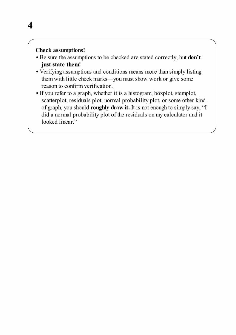
4
Check assumptions!• Be sure the assumptions to be checked are stated correctly, but don’t
just state them!• Verifying assumptions and conditions means more than simply listing
them with little check marks—you must show work or give somereason to confirm verification.
• If you refer to a graph, whether it is a histogram, boxplot, stemplot,scatterplot, residuals plot, normal probability plot, or some other kindof graph, you should roughly draw it. It is not enough to simply say, “Idid a normal probability plot of the residuals on my calculator and itlooked linear.”

5
Calculating the P-value is not the final step of a hypothesis test!• There must be a decision to reject or fail to reject the null hypothesis.• You must indicate how you interpret the P-value, that is, you need
linkage. So, “Given that P = .007, I reject ...” isn’t enough. You needsomething like, “Because P = .007 is less than .05, there is sufficient evidence to reject ...”
• Finally, you need a conclusion in context of the problem.

This eBook may look differently depending on which device you areusing. Please adjust accordingly.
This eBook also contains hyperlinks, which allow you to navigate throughcontent, go to helpful resources, and click between all questions andanswers.

Introduction
The contents of this book cover the topics recommended by the AP StatisticsDevelopment Committee. A review of each of the 15 topics is followed bymultiple-choice and free-response questions on that topic. Detailed explanationsare provided for all answers. It should be noted that some of the topic questionsare not typical AP exam questions but rather are intended to help review thetopic. Finally, there is a diagnostic exam, and there are five full-length practiceexams, totaling 276 questions, all with instructive, complete answers. The printversion of this book contains an optional disk that has two new, full-lengthexams with 92 more questions.
Several points with regard to particular answers should be noted. First, step-by-step calculations using the given tables sometimes give minor differencesfrom calculator answers due to round-off error. Second, there are exampleswhere the case may be made for using t-scores or z-scores, again with minordifferences in resulting answers. Third, calculator packages easily handledegrees of freedom that are not whole numbers, also resulting in minor answerdifferences. In all of the above cases, multiple-choice answers in this ebookhave only one reasonable correct answer, and written explanations arenecessary when answering free-response questions.
Students taking the AP Statistics Examination will be furnished with a list offormulas (from descriptive statistics, probability, and inferential statistics) andtables (including standard normal probabilities, t-distribution critical values, χ2
critical values, and random digits). While students will be expected to bring agraphing calculator with statistics capabilities to the examination, answersshould not be in terms of calculator syntax. Furthermore, many students havecommented that calculator usage was less than they had anticipated. However,even though the calculator is simply a tool, to be used sparingly, as needed,students should be proficient with this technology.
The examination will consist of two parts: a 90-minute section with 40multiple-choice problems and a 90-minute free-response section with five open-ended questions and an investigative task to complete. In grading, the twosections of the exam will be given equal weight. Students have remarked that thefirst section involves “lots of reading,” while the second section involves “lotsof writing.” The percentage of questions from each content area isapproximately 25% data analysis, 15% experimental design, 25% probability,and 35% inference. Questions in both sections may involve reading generic
computer output.Note that in the multiple-choice section the questions are much more
conceptual than computational, and thus use of the calculator is minimal.In the free-response section, students must show all their work, and
communication skills go hand in hand with statistical knowledge. Methods mustbe clearly indicated, as the problems will be graded on the correctness of themethods as well as on the accuracy of the results and explanation. That is, thefree-response answers should address why a particular test was chosen, not justhow the test is performed. Even if a statistical test is performed on a calculatorsuch as the TI-84, formulas should still be stated. Choice of test, in inference,must include confirmation of underlying assumptions, and answers must bestated in context, not just as numbers. Work is graded holistically; that is, astudent’s complete response is considered as a whole, with positive scoresdepending on if the answer is complete, substantial, developing, or minimal.
The score on the multiple-choice section is based on the number of correctanswers, with no points deducted for incorrect answers. Blank answers areignored. Free-response questions are scored on a 0 to 4 scale, with each open-ended question counting 15% of the total free-response score and theinvestigative task counting 25% of the free-response score. The first open-endedquestion is typically the most straightforward, and after doing this one to buildconfidence, students might consider looking at the investigative task since itcounts more. Each completed AP examination paper will receive a grade basedon a 5-point scale, with 5 the highest score and 1 the lowest score. Mostcolleges and universities accept a grade of 3 or better for credit or advancedplacement or both.
While a review book such as this can be extremely useful in helping preparestudents for the AP exam (practice problems, practice more problems, andpractice even more problems are the three strongest pieces of advice), nothingcan substitute for a good high school teacher and a good textbook. This authorpersonally recommends the following texts from among the many excellentbooks on the market: Workshop Statistics by Rossman, Activity-BasedStatistics by Scheaffer, Introduction to Statistics and Data Analysis byDevore, Olsen, and Peck, Stats, Modeling the World by Bock, Velleman, andDeVeaux, Statistics: The Art and Science of Learning from Data by Agretsiand Franklin, Introduction to the Practice of Statistics by Moore and McCabe,Statistics in Action: Understanding a World of Data by Cobb, Scheaffer, andWatkins and The Practice of Statistics by Starnes, Yates, and Moore.
Other wonderful sources of information are the College Board’s websites:www.collegeboard.com for students and parents, andwww.apcentral.collegeboard.com for teachers. After registering at the APCentral site, teachers should especially note the sections (1) AP Statistics
Course Description, (2) The Statistics Exam, and (3) Exam Tips: Statistics.A good piece of advice is for the student from day one to develop critical
practices (like checking assumptions and conditions), to acquire strong technicalskills, and to always write clear and thorough, yet to the point, interpretations incontext. Final answers to most problems should be not numbers, but rathersentences explaining and analyzing numerical results. To help develop skillsand insights to tackle AP free response questions (which often choose contextsstudents haven’t seen before), pick up newspapers and magazines and figure outhow to apply what you are learning to better understand articles in print thatreference numbers, graphs, and statistical studies.
The student who uses this Barron’s review book should study the text andillustrative examples carefully and try to complete the practice problems beforereferring to the solution keys. Simply reading the detailed explanations to theanswers without first striving to work through the problems on one’s own is notthe best approach. There is an old adage: Mathematics is not a spectator sport!Teachers clearly may use this book with a class in many profitable ways.Ideally, each individual topic review, together with practice problems, shouldbe assigned after the topic has been covered in class. The full-length practiceexams should be reserved for final review shortly before the AP examination.

All directions in the Diagnostic Exam are similar to those on the actualtest. Since this is an eBook, please record all answers separately.Answer Sheets are for reference only.
All questions are linked to their answers. Simply click on the questionnumber to see the answers explained.
Diagnostic Examination
SECTION IQuestions 1–40Spend 90 minutes on this part of the exam.
Directions: The questions or incomplete statements that follow are eachfollowed by five suggested answers or completions. Choose theresponse that best answers the question or completes the statement.
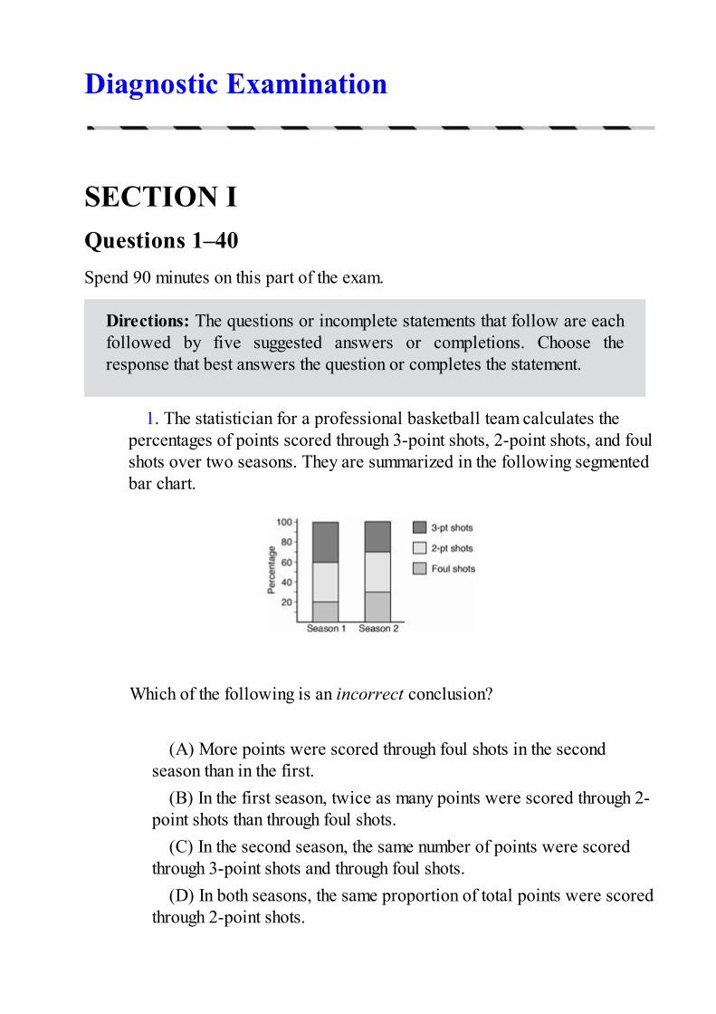
1. The statistician for a professional basketball team calculates thepercentages of points scored through 3-point shots, 2-point shots, and foulshots over two seasons. They are summarized in the following segmentedbar chart.
Which of the following is an incorrect conclusion?
(A) More points were scored through foul shots in the second
season than in the first.(B) In the first season, twice as many points were scored through 2-
point shots than through foul shots.(C) In the second season, the same number of points were scored
through 3-point shots and through foul shots.(D) In both seasons, the same proportion of total points were scored
through 2-point shots.

(E) In the first season, a greater proportion of the points werescored through 3-point shots than in the second season.
2. Is there a linear relationship between calories and sodium content in
beef hot dogs? A study of 20 beef hot dogs gives the following regressionoutput:
Which of the following gives a 99% confidence interval for the slope ofthe regression line?
(A) 4.0133 ± 2.861
(B) 4.0133 ± (2.861)(0.4922)(C) 4.0133 ± (2.878)(0.4922)(D) 4.0133 ± 2.861
(E) 4.0133 ± 2.878
3. In tossing a fair coin, which of the following sequences is more
likely to appear?
(A) HHHHH(B) HTHTHT(C) HTHHTTH(D) TTHTHHTH(E) All are equally likely.
4. An entomologist hypothesizes that the mean life expectancy of a
particular species of insect is 12.5 days. Researchers believing that thetrue mean is less than 12.5 days plan a hypothesis test at the 5%

significance level on a random sample of 50 of these insects. If thealternative hypothesis is correct, for which of the following values of µwill the power of the test be greatest?
(A) 9(B) 11(C) 12.5(D) 14(E) 17
5. A simple random sample is defined by
(A) the method of selection(B) how representative the sample is of the population(C) whether or not a random number generator is used(D) the assignment of different numbers associated with the
outcomes of some chance situation(E) examination of the outcome
6. Can shoe size be predicted from height? In a random sample of 50
adults, the standard deviation in heights was 8.7 cm, while the standarddeviation in shoe size was 2.3. The least squares regression equationwas:Predicted shoe size = –33.6 + 0.25 (Height in cm). What was thecorrelation?
(A)
(B)
(C)
(D)
(E) There is not enough information to calculate the correlation.
Questions 7–9 refer to the following situation:
A researcher would like to show that a new oral diabetes medication hedeveloped helps control blood sugar level better than insulin injection.He plans to run a hypothesis test at the 5% significance level.
7. What would be a Type I error?
(A) The researcher concludes he has evidence his new medication
helps more than insulin injection, and his medication really is betterthan insulin injection.
(B) The researcher concludes he has evidence his new medicationhelps more than insulin injection, when in reality his medication is notbetter than insulin injection.
(C) The researcher concludes he has no evidence his newmedication helps more than insulin injection, and his medication reallyis not better than insulin injection.
(D) The researcher concludes he has no evidence his newmedication helps more than insulin injection, when in reality hismedication is better than insulin injection.
(E) The researcher concludes he has evidence his new medicationcontrols blood sugar level the same as insulin injection, and in realitythere is a difference.
8. What would be a Type II error?
(A) The researcher concludes he has evidence his new medication
helps more than insulin injection, and his medication really is betterthan insulin injection.
(B) The researcher concludes he has evidence his new medicationhelps more than insulin injection, when in reality his medication is notbetter than insulin injection.
(C) The researcher concludes he has no evidence his newmedication helps more than insulin injection, and his medication reallyis not better than insulin injection.
(D) The researcher concludes he has no evidence his new

medication helps more than insulin injection, when in reality hismedication is better than insulin injection.
(E) The researcher concludes he has evidence his new medicationcontrols blood sugar level the same as insulin injection, and in realitythere is a difference.
9. The researcher thinks he can improve his chances by running five
such identical hypotheses tests, each using a different group of diabeticvolunteers, hoping that at least one of the tests will show that his new oraldiabetes medication helps control blood sugar level better than insulininjection. What is the probability of committing at least one Type I error?
(A) .05(B) .204(C) .226(D) .774(E) .95
10. A financial analyst determines the yearly research and development
investments for 50 blue chip companies. She notes that the distribution isdistinctly not bell-shaped. If the 50 dollar amounts are converted to z-scores, what can be said about the standard deviation of the 50 z-scores?
(A) It depends on the distribution of the raw scores.(B) It is less than the standard deviation of the raw scores.(C) It is greater than the standard deviation of the raw scores.(D) It is equal to the standard deviation of the raw scores.(E) It equals 1.
11. Tossing a fair die has outcomes {1,2,3,4,5,6} with mean 3.5 and
standard deviation 1.708. If a fair die is thrown three times, and the meanof the resulting triplet is calculated, the mean and standard deviation ofthe set of all possible such triplets is

(A) = 3.5, σ = 0.569(B) = 3.5, σ = 0.986(C) = 6.062, σ = 1.208(D) = 10.5, σ = 0.569(E) = 10.5, σ = 0.986
12. A 40-question multiple-choice statistics exam is graded as number
correct minus ¼ number incorrect, so scores can range from –10 to +40.Suppose the standard deviation for one class’s results is reported to be –3.14. What is the proper conclusion?
(A) More students received negative scores than positive scores.(B) At least half the class received negative scores.(C) Some students must have received negative scores.(D) Some students must have received positive scores.(E) An error was made in calculating the standard deviation.
13. Of the 423 seniors graduating this year from a city high school, 322
plan to go on to college. When the principal asks an AP student tocalculate a 95% confidence interval for the proportion of this year’sgraduates who plan to go to college, the student says that this would beinappropriate. Why?
(A) The independence assumption may have been violated (students
tend to do what their friends do).(B) There is no evidence that the data come from a normal or nearly
normal population (GPAs help determine college admission and maybe skewed).
(C) Randomization was not used.(D) There is a difference between a confidence interval and a
hypothesis test with regard to the proportion of graduates planning oncollege.
(E) Some other reason.

14. An AP Statistics student in a large high school plans to survey hisfellow students with regard to their preference between using a laptop orusing an iPad. Which of the following survey methods would result in anunbiased result?
(A) The student comes to school early and surveys the first 50
students who arrive.(B) The student passes a survey card to every student with
instructions to fill it out at home and drop the filled out card in a boxby the school entrance the next day.
(C) The student posts the survey on his Facebook page, askingeveryone to respond.
(D) The student goes to all of the high school sports events for aweek, hands out the survey, and waits for each student to fill it out andhand it back.
(E) All the above would lead to biased results.
15. The mean combined SAT score for students in one state is 1758
with a standard deviation of 213, while for a second state the mean is1725 with a standard deviation of 228. Assuming both distributions areapproximately normal, what is the probability that a randomly selectedstudent in the first state scores higher than a randomly selected student inthe second state?
(A) 0.458(B) 0.500(C) 0.524(D) 0.542(E) 0.559
16. In a random sample of 10 insects of a newly discovered species, an
entomologist measures an average life expectancy of 17.3 days with astandard deviation of 2.3 days. Assuming all conditions for inference aremet, what is a 95% confidence interval for the mean life expectancy forinsects of this species?

(A) 17.3 ± 1.96
(B) 17.3 ± 1.96
(C) 17.3 ± 2.228
(D) 17.3 ± 2.228
(E) 17.3 ± 2.262
17. A coin is weighted so that heads is twice as likely to occur as tails.
The coin is flipped repeatedly until a tail occurs. Let X be the number offlips made. What is the most probable value for X?
(A) 1(B) 2(C) 3(D) 4(E) 5
18. Suppose we are interested in determining whether or not a student’s
score on the AP Statistics Exam is a reasonable predictor of the student’sGPA in the first year of college. Which of the following is the beststatistical test?
(A) Two-sample t-test of population means(B) Linear regression t-test(C) Chi-square test of independence(D) Chi-square test of homogeneity(E) Chi-square test of goodness of fit
19. Following are the graphs of three normal curves and three
cumulative distribution graphs:

Which normal curve corresponds to which cumulative curve?
(A) X-1, Y-2, Z-3(B) X-1, Y-3, Z-2(C) X-2, Y-1, Z-3(D) X-3, Y-1, Z-2(E) X-3, Y-2, Z-1
20. A campus has 55% male students. Suppose 30% of the male
students pick basketball as their favorite sport compared to 20% of thefemales. If a randomly chosen student picks basketball as the student’sfavorite sport, what is the probability the student is male?
(A)
(B)
(C)
(D)
(E)
21. The kelvin is a unit of measurement for temperature; 0 K is absolute

zero, the temperature at which all thermal motion ceases. Conversionfrom Fahrenheit to Kelvin is given by K = 5/9 × (F – 32) + 273. Theaverage daily temperature in Monrovia, Liberia, is 78.35°F with astandard deviation of 6.3°F. If a scientist converts Monrovia dailytemperatures to the Kelvin scale, what will be the new mean and standarddeviation?
(A) Mean, 25.75 K; standard deviation, 3.5 K(B) Mean, 231.75 K; standard deviation, 3.5 K(C) Mean, 298.75 K; standard deviation, 3.5 K(D) Mean, 298.75 K; standard deviation, 258.72 K(E) Mean, 298.75 K; standard deviation, 276.5 K
22. A cattle veterinarian is considering two experimental designs to
compare two sources of bovine growth hormone, or BVH, to spurincreased milk production in Guernsey cattle. Design 1 involves flippinga coin as each cow enters the stockade, and if heads, giving it BVH frombovine cadavers, and if tails, giving it BVH from engineered E. coli.Design 2 involves flipping a coin as each cow enters the stockade, and ifheads, giving it BVH from bovine cadavers for a specified period of timeand then switching to BVH from engineered E. coli for the same period oftime, and if tails, the order is reversed. With both designs, daily milkproduction is noted. Which of the following is accurate?
(A) Neither design uses randomization since there is no indication
that cows will be randomly picked from the population of all Guernseycattle.
(B) Design 1 is a completely randomized design, while Design 2 isa block design.
(C) Both designs use double-blinding, but neither uses a placebo.(D) In the second design, BVH from bovine cadavers and BVH from
engineered E. coli are confounded.(E) One of the two designs is actually an observational study, while
the other is an experiment.
23. The purpose of the linear regression t-test is
(A) to determine if there is a linear association between two
numerical variables(B) to find a confidence interval for the slope of a regression line(C) to find the y-intercept of a regression line(D) to be able to calculate residuals(E) to be able to determine the consequences of Type I and Type II
errors
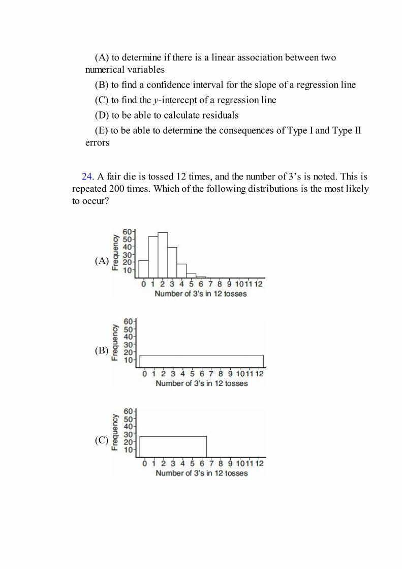
24. A fair die is tossed 12 times, and the number of 3’s is noted. This is
repeated 200 times. Which of the following distributions is the most likelyto occur?
(A)
(B)
(C)

(D)
(E)
25. Which of the following is a true statement about sampling?
(A) If the sample is random, the size of the sample doesn’t matter.(B) If the sample is random, the size of the population doesn’t
matter.(C) A sample of less than 1% of the population is too small for
statistical inference.(D) A sample of more than 10% of the population is too large for
statistical inference.(E) All of the above are true statements.
26. Suppose, in a study of mated pairs of soldier beetles, it is found that
the measure of the elytron (hardened forewing) length is always 0.5millimeters longer in the female. What is the correlation between elytronlengths of mated females and males?
(A) –1(B) –0.5(C) 0(D) 0.5(E) 1

27. A random sample of 100 individuals who were singled out at an
international airport security checkpoint is reviewed, and the individualsare classified according to country of origin:
The proportion of travelers in each category who use this airport follows:
We wish to test whether the distribution of people singled out is the sameas the distribution of people who use the airport with regard to country oforigin. What is the appropriate χ2 statistic?
(A)
(B)
(C)
(D)
(E)
28. The age distribution for a particular debilitating disease has a mean
greater than the median. Which of the following graphs most likelyillustrates this distribution?
(A)

(B)
(C)
(D)
(E)
29. Suppose we have a random variable X where the probabilityassociated with the value
k is (.38)k(.62)10–k for k = 0, . . . , 10.
What is the mean of X?
(A) 0.38(B) 0.62(C) 3.8(D) 5.0(E) 6.2
30. It is hypothesized that high school varsity pitchers throw fastballs at
an average of 80 mph. A random sample of varsity pitchers are timed withradar guns resulting in a 95% confidence interval of (74.5, 80.5). Whichof the following is a correct statement?
(A) There is a 95% chance that the mean fastball speed of all
varsity pitchers is 80 mph.
(B) There is a 95% chance that the mean fastball speed of all varsitypitchers is 77.5 mph.
(C) Most of the interval is below 80, so there is evidence at the 5%significance level that the mean of all varsity pitchers is somethingdifferent than 80 mph.
(D) The test H0: µ = 80, Ha: µ ≠ 80 is not significant at the 5%significance level, but it would be at the 1% level.
(E) It is likely that the true mean fastball speed of all varsitypitchers is within 3 mph of the sample mean fastball speed.
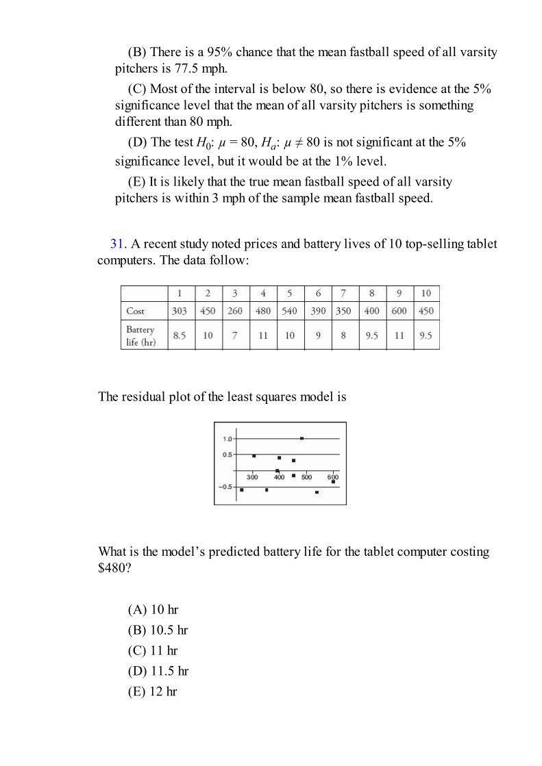
31. A recent study noted prices and battery lives of 10 top-selling tablet
computers. The data follow:
The residual plot of the least squares model is
What is the model’s predicted battery life for the tablet computer costing$480?
(A) 10 hr(B) 10.5 hr(C) 11 hr(D) 11.5 hr(E) 12 hr

32. Should college athletes be required to give their coaches their
Facebook IDs and passwords? A survey of student-athletes is to be taken.The statistician believes that Division I, II, and III players may differ intheir views, so she selects a random sample of athletes from eachDivision to survey. This is a
(A) simple random sample(B) stratified sample(C) cluster sample(D) systematic sample(E) convenience sample
33. Which of the following use of a random number table would be
appropriate to simulate tossing 3 fair coins and noting the number ofheads?
(A) Assign “0,1” to 0 heads, “2,3” to 1 head, “4,5” to 2 heads,
“6,7” to 3 heads, and ignore “8,9.”(B) Assign “0,1” to 0 heads, “2,3,4” to 1 head, “5,6,7” to 2 heads,
and “8,9” to 3 heads.(C) Assign “0” to 0 heads, “1,2” to 1 head, “3,4” to 2 heads, “5” to
3 heads, and ignore “6,7,8,9.”(D) Assign “0” to 0 heads, “1,2,3” to 1 head, “4,5,6” to 2 heads,
“7” to 3 heads, and ignore “8,9.”(E) Assign “0” to 0 heads, “1,2,3,4” to 1 head, “5,6,7,8” to 2 heads,
and “9” to 3 heads.
34. The 2012 population of the Greater Tokyo area is 34,400,000 and
of Karachi is 17,200,000. A random sample of citizens is to be taken ineach city, and confidence intervals for the mean age in each city will becalculated. Assuming roughly equal sample standard deviations, to obtainthe same margin of error for each confidence interval,

(A) the sample sizes should be the same(B) the sample in Greater Tokyo should be twice the size of the
sample in Karachi(C) the sample in Karachi should be twice the size of the sample in
Greater Tokyo(D) the sample in Greater Tokyo should be four times the size of the
sample in Karachi(E) the sample in Karachi should be four times the size of the
sample in Greater Tokyo
35. The midhinge is defined to be the average of the first and third
quartiles. If the midhinge is 20 and the interquartile range is also 20, whatis the first quartile?
(A) 0(B) 10(C) 20(D) 30(E) Impossible to determine from the given information
36. Which of the following is an incorrect statement?
(A) Statistics are random variables with their own probability
distributions.(B) The standard error does not depend on the size of the
population.(C) Bias means that, on average, our estimate of a parameter is
different from the true value of the parameter.(D) There are some statistics for which the sampling distribution is
not approximately normal, no matter how large the sample size.(E) The larger the sample size, the closer the sample distribution is
to a normal distribution.
37. For male Air Force cadets, the recommended fitness level with
regard to the number of push-ups is 34. In a test whether or not currentclasses of recruits can meet this standard, a t-test of H0: µ = 34 againstHa: µ < 34 gives a P-value of 0.068. Using this data, among thefollowing, which is the largest level of confidence for a two-sidedconfidence interval that does not contain 34?
(A) 85%(B) 90%(C) 92%(D) 95%(E) 96%
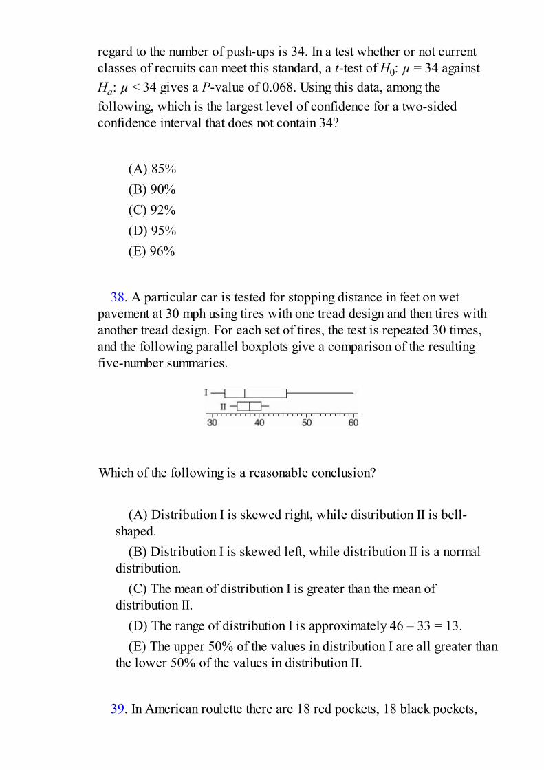
38. A particular car is tested for stopping distance in feet on wet
pavement at 30 mph using tires with one tread design and then tires withanother tread design. For each set of tires, the test is repeated 30 times,and the following parallel boxplots give a comparison of the resultingfive-number summaries.
Which of the following is a reasonable conclusion?
(A) Distribution I is skewed right, while distribution II is bell-
shaped.(B) Distribution I is skewed left, while distribution II is a normal
distribution.(C) The mean of distribution I is greater than the mean of
distribution II.(D) The range of distribution I is approximately 46 – 33 = 13.(E) The upper 50% of the values in distribution I are all greater than
the lower 50% of the values in distribution II.
39. In American roulette there are 18 red pockets, 18 black pockets,
and two green pockets (labeled 0 and 00). The ball is equally likely toland in any of the 38 pockets. What is the probability that a player ends upwith a positive outcome, that is, makes money, after 50 equal bets on“red” (that is, for each of 50 spins of the wheel, the player wins or losesthe specified identical dollar bet depending on whether or not the balllands in a red or non-red pocket, respectively)?
(A) 0.105(B) 0.212(C) 0.303(D) 0.408(E) 0.500
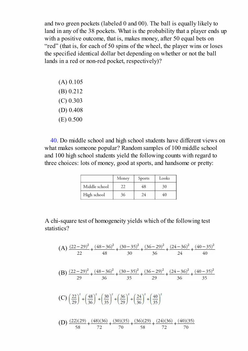
40. Do middle school and high school students have different views on
what makes someone popular? Random samples of 100 middle schooland 100 high school students yield the following counts with regard tothree choices: lots of money, good at sports, and handsome or pretty:
A chi-square test of homogeneity yields which of the following teststatistics?
(A)
(B)
(C)
(D)

(E)
If there is still time remaining, you may review your answers.
SECTION II
Part A
Questions 1–5Spend about 65 minutes on this part of the exam.Percentage of Section II grade—75
You must show all work and indicate the methods you use. You will begraded on the correctness of your methods and on the accuracy of yourresults and explanations.
1. A horticulturist plans a study on the use of compost tea for plantdisease management. She obtains 16 identical beds, each containing arandom selection of five mini-pink rose plants. She plans to use twodifferent composting times (two and five days), two different compostpreparations (aerobic and anaerobic), and two different sprayingtechniques (with and without adjuvants). Midway into the growing seasonshe will check all plants for rose powdery mildew disease.
(a) List the complete set of treatments.(b) Describe a completely randomized design for the treatments
above.(c) Explain the advantage of using only mini-pink roses in this
experiment.(d) Explain a disadvantage of using only mini-pink roses in this
experiment.
2. A top-100, 7.0-rated tennis pro wishes to compare a new Wilson N1racquet against his current model. He strings the new racquet with thesame Luxilon strings at 60 pounds tension that he uses on his old racquet.From past testing he knows that the average forehand cross court volleywith his old racquet is 82 miles per hour (mph). On an indoor court, usinga ball machine set at 70 mph, the same speed he had his old racquet testedagainst, he takes 47 swings with the new racquet. An associate with aspeed gun records an average of 83.5 mph with a standard deviation of3.4 mph. Assuming that the 47 swings represents a random sample of his

swings, is there statistical evidence that his speed with the new racquet isan improvement over the old? Justify your answer.
3. In October 2008, a comprehensive residential college in upstateNew York reported undergraduate enrollment by ethnic/racial categoriesas follows: 2.7% non-Hispanic Black, 3.7% Asian or Pacific Islander,4.0% Hispanic, 80.0% non-Hispanic White, and the rest other/unknown.While racial/ethnic status is not considered in the admissions process, anadmissions counselor is interested in whether or not the makeup of thenew freshman class will change, and plans to do a statistical analysis onan appropriately drawn simple random sample.
(a) What statistical test/procedure should be used?(b) State the null and alternative hypotheses. Is the test appropriate
for an intended sample size of 200?(c) If the admissions counselor performs the indicated test on the
following data, is there statistical evidence of a change in ethnic/racialcomposition? Explain.
(d) Suppose the data was obtained by noting the racial/ethnic statusof a simple random sample of 200 potential new students visiting thecampus during fall 2008. Did the test/procedure target the intendedpopulation? Explain.
4. Concrete is made by mixing sand and pebbles with water and cementand then hardening through hydration. Different densities result fromdifferent proportions of the aggregates. Assume that concrete densities arenormally distributed with mean 2317 kilograms per cubic meter andstandard deviation 128 kilograms per cubic meter.
(a) What is the probability that a given concrete density is over

2400 kg/m3?(b) In a random sample of five independent concrete densities, what
is the probability that a majority have densities over 2400 kg/m3?(c) What is the probability that the mean of the five independent
concrete densities is over 2400 kg/m3?
5. A small art gallery in Laguna Beach has the choice of stocking eitheroil paintings or finger paintings for a given tourist season. The oilpaintings require a substantial investment, but the potential returns arealso greater. The return (profit or loss) depends on whether or not thetourists that season are primarily serious art collectors or more casualbuyers. A sales analysis gives the following expectations.
Let p be the probability that the type of tourist is primarily art collectors,so (1 – p) is the probability of primarily casual buyers.
(a) As a function of p, what is the expected return for stocking oilpaintings?
(b) As a function of p, what is the expected return for stocking fingerpaintings?
(c) For what value of p are the two expected returns the same, andwhat does it mean in context for p to be greater or less than this value?
(d) In a random sample of similar establishments in similar touristregions, 33 out of 150 reported seasons with tourists who wereprimarily art collectors. Construct a 95% confidence interval for theproportion of similar establishments with tourists who were primarilyart collectors.

(e) Use the above results to justify a decision to stock fingerpaintings.
SECTION II
Part B
Question 6
Spend about 25 minutes on this part of the exam.Percentage of Section II grade—25
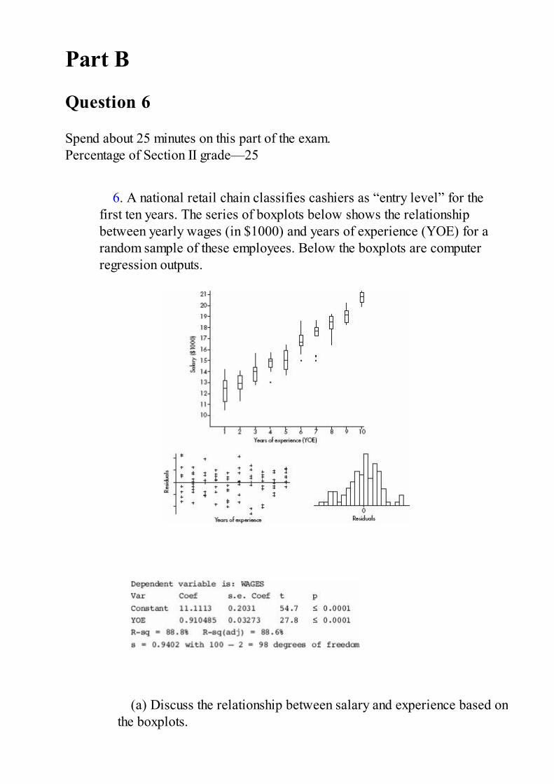
6. A national retail chain classifies cashiers as “entry level” for the
first ten years. The series of boxplots below shows the relationshipbetween yearly wages (in $1000) and years of experience (YOE) for arandom sample of these employees. Below the boxplots are computerregression outputs.
(a) Discuss the relationship between salary and experience based onthe boxplots.
(b) Discuss how conditions for regression inference are met.(c) Determine a 95% confidence interval for the regression slope,
and interpret in context.(d) Using only the given information, give a rough estimate of the
probability that a salary is at least $1000 over what is predicted by theregression line.
If there is still time remaining, you may review your answers.

AP SCORE FOR THE DIAGNOSTICEXAM

STUDY GUIDE FOR THE DIAGNOSTICTESTMULTIPLE-CHOICE QUESTIONSNote in which Themes your missed questions fall. Then give special note to theTopics corresponding to the missed questions. Additionally, whenever you wishto test yourself on a particular Theme, go back to the designated questions.
Theme One: Exploratory AnalysisQuestion 1 Topic Five: Exploring Categorical DataQuestion 6 Topic Four: Exploring Bivariate DataQuestion 10 Topic Two: Summarizing DistributionsQuestion 12 Topic Two: Summarizing Distributions
Question 19 Topic One: Graphical DisplaysTopic Eleven: The Normal Distribution
Question 21 Topic Two: Summarizing DistributionsQuestion 26 Topic Four: Exploring Bivariate Data
Question 28 Topic One: Graphical DisplaysTopic Two: Summarizing Distributions
Question 31 Topic Four: Exploring Bivariate DataQuestion 35 Topic Two: Summarizing Distributions
Question 38 Topic One: Graphical DisplaysTopic Two: Summarizing Distributions
Theme Two: Planning a StudyQuestion 5 Topic Seven: Planning and Conducting SurveysQuestion 14 Topic Seven: Planning and Conducting SurveysQuestion 22 Topic Eight: Planning and Conducting ExperimentsQuestion 25 Topic Seven: Planning and Conducting SurveysQuestion 32 Topic Seven: Planning and Conducting Surveys
Theme Three: Probability

Question 3 Topic Nine: Probability as Relative Frequency
Question 9Topic Nine: Probability as Relative FrequencyTopic Fourteen: Tests of Significance—Proportions andMeans
Question 11 Topic Twelve: Sampling Distributions
Question 15 Topic Ten: Combining Independent Random VariablesTopic Eleven: The Normal Distribution
Question 17 Topic Nine: Probability as Relative Frequency
Question 19 Topic Eleven: The Normal DistributionTopic One: Graphical Displays
Question 20 Topic Nine: Probability as Relative FrequencyQuestion 24 Topic Nine: Probability as Relative FrequencyQuestion 29 Topic Nine: Probability as Relative FrequencyQuestion 33 Topic Nine: Probability as Relative FrequencyQuestion 36 Topic Twelve: Sampling DistributionsQuestion 39 Topic Nine: Probability as Relative Frequency
Theme Four: Statistical InferenceQuestion 2 Topic Thirteen: Confidence Intervals
Question 4 Topic Fourteen: Tests of Significance—Proportions andMeans
Question 7 Topic Fourteen: Tests of Significance—Proportions andMeans
Question 8 Topic Fourteen: Tests of Significance—Proportions andMeans
Question 9Topic Fourteen: Tests of Significance—Proportions andMeansTopic Nine: Probability as Relative Frequency
Question 13 Topic Thirteen: Confidence IntervalsQuestion 16 Topic Thirteen: Confidence Intervals
Question 18 Topic Fifteen: Tests of Significance—Chi-Square andSlope of Least Squares Line
Question 23 Topic Fifteen: Tests of Significance—Chi-Square andSlope of Least Squares Line
Question 27 Topic Fifteen: Tests of Significance—Chi-Square andSlope of Least Squares LineTopic Thirteen: Confidence Intervals

Question 30 Topic Fourteen: Tests of Significance—Proportions andMeans
Question 34 Topic Thirteen: Confidence Intervals
Question 37Topic Thirteen: Confidence IntervalsTopic Fourteen: Tests of Significance—Proportions andMeans
Question 40 Topic Fifteen: Tests of Significance—Chi-Square andSlope of Least Squares Line

THEME ONE: EXPLORATORYANALYSIS
TOPIC 1Graphical Displays
• Dotplots• Bar Charts• Histograms• Stemplots• Center and Spread• Clusters and Gaps
• Outliers• Modes• Shape• Cumulative Relative Frequency Plots• Skewness
There are a variety of ways to organize and arrange data. Much informationcan be put into tables, but these arrays of bare figures tend to be spiritless andsometimes even forbidding. Some form of graphical display is often best forseeing patterns and shapes and for presenting an immediate impression ofeverything about the data. Among the most common visual representations ofdata are dotplots, bar charts, histograms, and stemplots. It is important toremember that all graphical displays should be clearly labeled, leaving no doubtwhat the picture represents—AP Statistics scoring guides harshly penalizethe lack of titles and labels!

TIPThe first thing to do with data is to draw a picture—always.
DOTPLOTSDotplots and bar charts are particularly useful with regard to categorical (orqualitative) variables, that is, variables that note the category to which eachindividual belongs. This is in contrast to quantitative variables, which take onnumerical values.

TIPJust because a variable has numerical values doesn’tnecessarily mean that it’s quantitative.
EXAMPLE 1.1Suppose that in a class of 35 students, 10 choose basketball as their favorite sport while 7pick baseball, 6 pick football, 5 pick tennis, 5 pick soccer, and 2 pick hockey. These datacan be displayed in the following dotplot:
The frequency of each result is indicated by the number of dots representing that result.
The dotplot can also be drawn with a vertical axis and horizontal rows of dots.In fact, in almost all displays, vertical and horizontal can be switched dependingupon which picture seems easier to read or simply which better fits the page.
BAR CHARTSA common visual display to compare the sizes of categories or groups is the barchart. Sizes can be measured as frequencies or as percents.
EXAMPLE 1.2In a survey taken during the first week of January 1999, 55% of those surveyed wanted theClinton impeachment trial to end immediately, 15% wanted it to continue with witnesses,25% wanted the trial to continue without calling witnesses, and 5% expressed no opinion.These data can be displayed in the following bar chart (or bar graph):
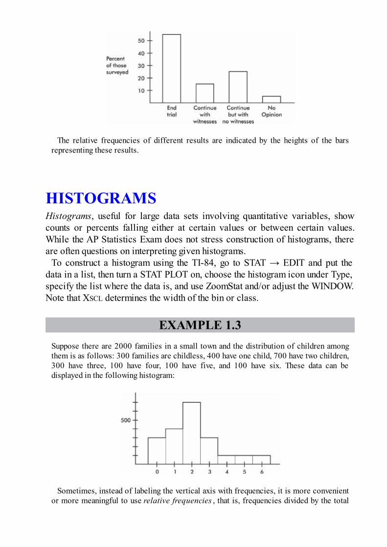
The relative frequencies of different results are indicated by the heights of the barsrepresenting these results.
HISTOGRAMSHistograms, useful for large data sets involving quantitative variables, showcounts or percents falling either at certain values or between certain values.While the AP Statistics Exam does not stress construction of histograms, thereare often questions on interpreting given histograms.
To construct a histogram using the TI-84, go to STAT → EDIT and put thedata in a list, then turn a STAT PLOT on, choose the histogram icon under Type,specify the list where the data is, and use ZoomStat and/or adjust the WINDOW.Note that XSCL determines the width of the bin or class.
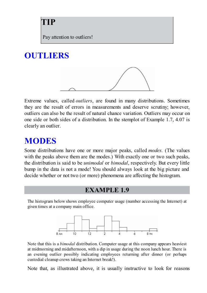
EXAMPLE 1.3Suppose there are 2000 families in a small town and the distribution of children amongthem is as follows: 300 families are childless, 400 have one child, 700 have two children,300 have three, 100 have four, 100 have five, and 100 have six. These data can bedisplayed in the following histogram:
Sometimes, instead of labeling the vertical axis with frequencies, it is more convenientor more meaningful to use relative frequencies , that is, frequencies divided by the total

number in the population.
Note that the shape of the histogram is the same whether the vertical axis is labeled withfrequencies or with relative frequencies. Sometimes we show both frequencies andrelative frequencies on the same graph.
EXAMPLE 1.4Consider the following histogram displaying 40 salaries paid to the top-level executivesof a large company.
What can we learn from this histogram? For example, none of the executives earned morethan $90,000 or less than $20,000. Twelve earned between $50,000 and $60,000.

Twenty-five percent earned between $40,000 and $50,000. Note how this histogramshows the number of items (salaries) falling between certain values, whereas thepreceding histogram showed the number of items (families) falling at each value. Forexample, in Example 1.4 we see that ten salaries fell somewhere between $40,000 and$50,000, while in Example 1.3 we see that 700 families had exactly two children.
EXAMPLE 1.5Consider the following histogram where the vertical axis has not been labeled. What canwe learn from this histogram?
Answer: It is impossible to determine the actual frequencies; however, we candetermine the relative frequencies by noting the fraction of the total area that is over anyinterval:
We can divide the area into ten equal portions, and then note that or 10% of the area isabove 25–26, 20% is above 26–27, 40% is above 27–28, and 30% is above 28–29.
Although it is usually not possible to divide histograms so nicely into ten equal areas,the principle of relative frequencies corresponding to relative areas still applies.
Relative frequencies are the usual choice when comparing distributions of different sizepopulations.
STEMPLOTS

Although a histogram may show how many scores fall into each grouping orinterval, the exact values of individual scores are often lost. An alternativepictorial display, called a stemplot, retains this individual information.
EXAMPLE 1.6Consider the set {17, 17, 18, 13, 28, 38, 31, 27, 35, 50, 43, 37, 24} of percentages ofthree-point shots made by Michael Jordan during his 13 years with the Bulls. Let 1, 2, 3,4, and 5 be placeholders for 10, 20, 30, 40, and 50. List the last digit of each value fromthe original set after the appropriate placeholder.
The result is a stemplot (also called a stem and leaf display) of these data:
Drawing a continuous line around the leaves would result in a horizontal histogram:
Note that the stemplot gives the shape of the histogram and, unlike the histogram,indicates the values of the original data.
Sometimes further structure is shown by rearranging the numbers in each rowin ascending order. This ordered display shows a second level of informationfrom the original stemplot.
The revised display of the data in Example 1.6 is as follows:
EXAMPLE 1.7Using a “torsion balance,” Henry Cavendish (in 1798) made 29 measurements of Earth’sdensity, obtaining values of 5.5, 5.57, 5.42, 5.61, 5.53, 5.47, 4.88, 5.62, 5.63, 4.07, 5.29,5.34, 5.26, 5.44, 5.46, 5.55, 5.34, 5.3, 5.36, 5.79, 5.75, 5.29, 5.1, 5.86, 5.58, 5.27, 5.85,

5.65, and 5.39 gm/cm3.Below is a stemplot of this data.Note that the scale is such that one must multiply each value in the dataset by 0.01 toreturn the original value. For example, 407 × 0.01 = 4.07.
CENTER AND SPREADLooking at a graphical display, we see that two important aspects of the overallpattern are
1. the center, which separates the values (or area under the curve in the
case of a histogram) roughly in half, and2. the spread, that is, the scope of the values from smallest to largest.
In the histogram of Example 1.3, the center is 2 children while the spread isfrom 0 to 6 children.
In the histogram of Example 1.4 the center is between $50,000 and $60,000,and the spread is from $20,000 to $90,000; in the histogram of Example 1.5, thecenter is between 27 and 28, and the spread is from 25 to 29.

TIPCenter and spread should always be described together.
In the stemplot of Example 1.6, the center is 28%, and the spread is from 13%to 50%; in the stemplot of Example 1.7, the center is 5.46, and the spread isfrom 4.07 to 5.86.
CLUSTERS AND GAPSOther important aspects of the overall pattern are
1. clusters, which show natural subgroups into which the values fall (for
example, the salaries of teachers in Ithaca, NY, fall into three overlappingclusters, one for public school teachers, a higher one for Ithaca Collegeprofessors, and an even higher one for Cornell University professors), and
2. gaps, which show holes where no values fall (for example, the Officeof the Dean sends letters to students being put on the honor roll and to thosebeing put on academic warning for low grades; thus the GPA distribution ofstudents receiving letters from the Dean has a huge middle gap).
EXAMPLE 1.8Consider the following histogram:
Simply saying that the center of the distribution is around 42 and the spread is from 31to 52 clearly misses something. The values fall into two distinct clusters with a gapbetween.
TIPPay attention to outliers!
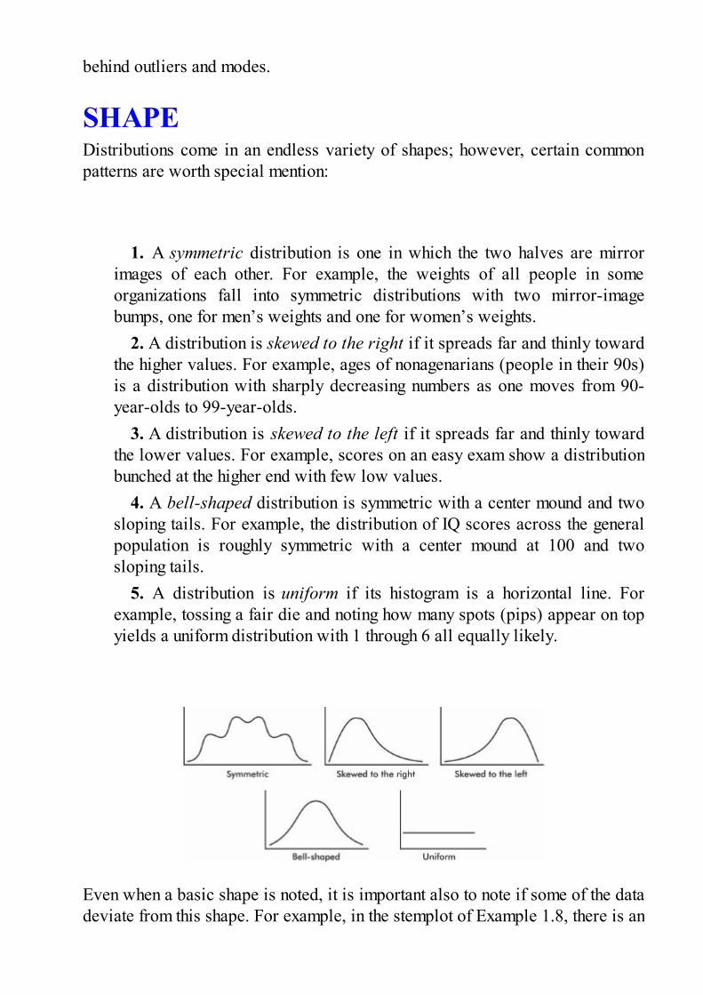
OUTLIERS
Extreme values, called outliers, are found in many distributions. Sometimesthey are the result of errors in measurements and deserve scrutiny; however,outliers can also be the result of natural chance variation. Outliers may occur onone side or both sides of a distribution. In the stemplot of Example 1.7, 4.07 isclearly an outlier.
MODESSome distributions have one or more major peaks, called modes. (The valueswith the peaks above them are the modes.) With exactly one or two such peaks,the distribution is said to be unimodal or bimodal, respectively. But every littlebump in the data is not a mode! You should always look at the big picture anddecide whether or not two (or more) phenomena are affecting the histogram.
EXAMPLE 1.9The histogram below shows employee computer usage (number accessing the Internet) atgiven times at a company main office.
Note that this is a bimodal distribution. Computer usage at this company appears heaviestat midmorning and midafternoon, with a dip in usage during the noon lunch hour. There isan evening outlier possibly indicating employees returning after dinner (or perhapscustodial cleanup crews taking an Internet break!).
Note that, as illustrated above, it is usually instructive to look for reasons
behind outliers and modes.
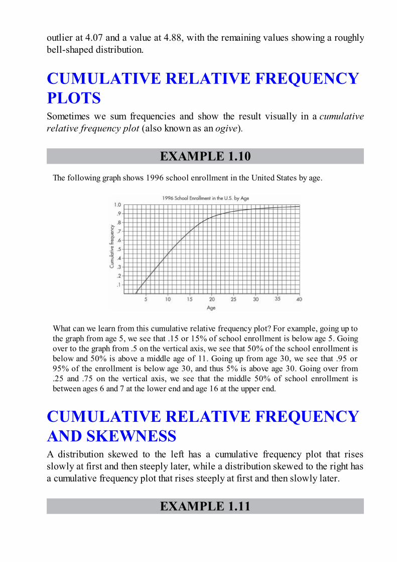
SHAPEDistributions come in an endless variety of shapes; however, certain commonpatterns are worth special mention:
1. A symmetric distribution is one in which the two halves are mirrorimages of each other. For example, the weights of all people in someorganizations fall into symmetric distributions with two mirror-imagebumps, one for men’s weights and one for women’s weights.
2. A distribution is skewed to the right if it spreads far and thinly towardthe higher values. For example, ages of nonagenarians (people in their 90s)is a distribution with sharply decreasing numbers as one moves from 90-year-olds to 99-year-olds.
3. A distribution is skewed to the left if it spreads far and thinly towardthe lower values. For example, scores on an easy exam show a distributionbunched at the higher end with few low values.
4. A bell-shaped distribution is symmetric with a center mound and twosloping tails. For example, the distribution of IQ scores across the generalpopulation is roughly symmetric with a center mound at 100 and twosloping tails.
5. A distribution is uniform if its histogram is a horizontal line. Forexample, tossing a fair die and noting how many spots (pips) appear on topyields a uniform distribution with 1 through 6 all equally likely.
Even when a basic shape is noted, it is important also to note if some of the datadeviate from this shape. For example, in the stemplot of Example 1.8, there is an
outlier at 4.07 and a value at 4.88, with the remaining values showing a roughlybell-shaped distribution.
CUMULATIVE RELATIVE FREQUENCYPLOTSSometimes we sum frequencies and show the result visually in a cumulativerelative frequency plot (also known as an ogive).
EXAMPLE 1.10The following graph shows 1996 school enrollment in the United States by age.
What can we learn from this cumulative relative frequency plot? For example, going up tothe graph from age 5, we see that .15 or 15% of school enrollment is below age 5. Goingover to the graph from .5 on the vertical axis, we see that 50% of the school enrollment isbelow and 50% is above a middle age of 11. Going up from age 30, we see that .95 or95% of the enrollment is below age 30, and thus 5% is above age 30. Going over from.25 and .75 on the vertical axis, we see that the middle 50% of school enrollment isbetween ages 6 and 7 at the lower end and age 16 at the upper end.
CUMULATIVE RELATIVE FREQUENCYAND SKEWNESSA distribution skewed to the left has a cumulative frequency plot that risesslowly at first and then steeply later, while a distribution skewed to the right hasa cumulative frequency plot that rises steeply at first and then slowly later.
EXAMPLE 1.11

Consider the essay grading policies of three teachers, Abrams, who gives very highscores, Brown, who gives equal numbers of low and high scores, and Connors, who givesvery low scores. Histograms of the grades (with 1 the highest score and 4 the lowestscore) are as follows:
These translate into the following cumulative frequency plots:
Summary• The three keys to describing a distribution are shape, center, and spread.• Also consider clusters, gaps, modes, and outliers.• Look for reasons behind any unusual features.• A few common shapes arise from symmetric, skewed to the right, skewed to
the left, bell-shaped, and uniform distributions.• For categorical (qualitative) data, dotplots and bar charts give useful displays.• For quantitative data, histograms, cumulative relative frequency plots
(ogives), and stemplots give useful displays.• In a histogram, relative area corresponds to relative frequency.
Questions on Topic One:Graphical Displays
Multiple-Choice Questions
Directions: The questions or incomplete statements that follow are eachfollowed by five suggested answers or completions. Choose the responsethat best answers the question or completes the statement.
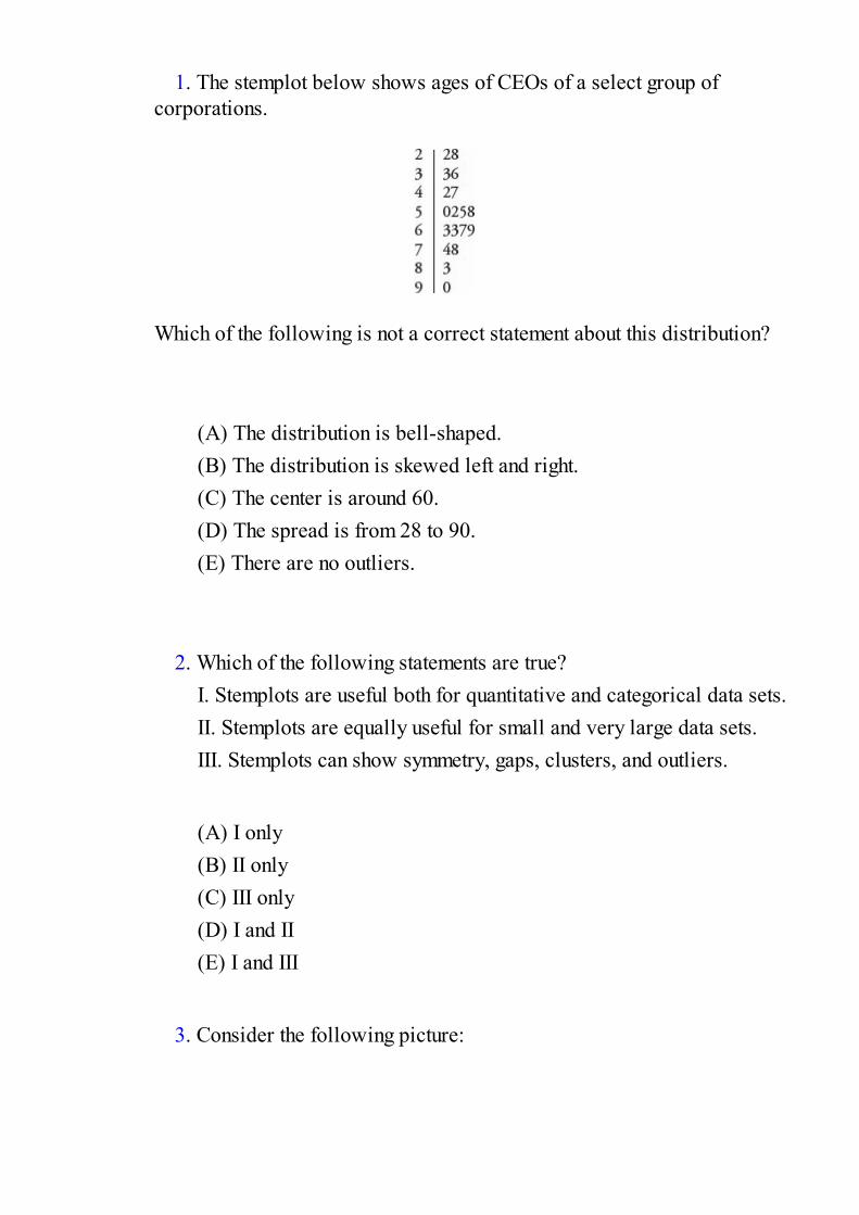
1. The stemplot below shows ages of CEOs of a select group ofcorporations.
Which of the following is not a correct statement about this distribution?
(A) The distribution is bell-shaped.(B) The distribution is skewed left and right.(C) The center is around 60.(D) The spread is from 28 to 90.(E) There are no outliers.
2. Which of the following statements are true?I. Stemplots are useful both for quantitative and categorical data sets.II. Stemplots are equally useful for small and very large data sets.III. Stemplots can show symmetry, gaps, clusters, and outliers.
(A) I only(B) II only(C) III only(D) I and II(E) I and III
3. Consider the following picture:
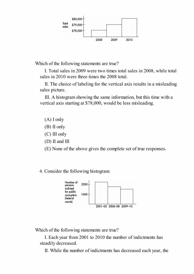
Which of the following statements are true?I. Total sales in 2009 were two times total sales in 2008, while total
sales in 2010 were three times the 2008 total.II. The choice of labeling for the vertical axis results in a misleading
sales picture.III. A histogram showing the same information, but this time with a
vertical axis starting at $78,000, would be less misleading.
(A) I only(B) II only(C) III only(D) II and III(E) None of the above gives the complete set of true responses.
4. Consider the following histogram:
Which of the following statements are true?I. Each year from 2001 to 2010 the number of indictments has
steadily decreased.II. While the number of indictments has decreased each year, the
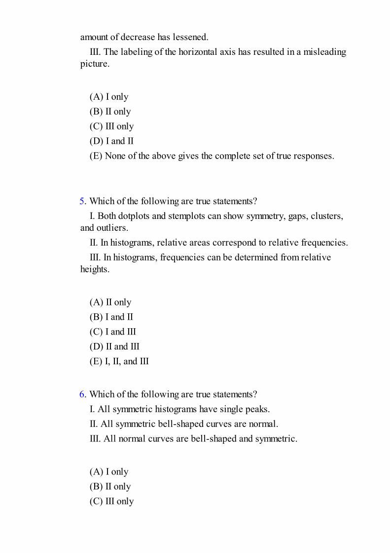
amount of decrease has lessened.III. The labeling of the horizontal axis has resulted in a misleading
picture.
(A) I only(B) II only(C) III only(D) I and II(E) None of the above gives the complete set of true responses.
5. Which of the following are true statements?I. Both dotplots and stemplots can show symmetry, gaps, clusters,
and outliers.II. In histograms, relative areas correspond to relative frequencies.III. In histograms, frequencies can be determined from relative
heights.
(A) II only(B) I and II(C) I and III(D) II and III(E) I, II, and III
6. Which of the following are true statements?
I. All symmetric histograms have single peaks.II. All symmetric bell-shaped curves are normal.III. All normal curves are bell-shaped and symmetric.
(A) I only(B) II only(C) III only

(D) I and II(E) None of the above gives the complete set of true responses.
7. Which of the following distributions are more likely to be skewed tothe right than skewed to the left?
I. Household incomesII. Home pricesIII. Ages of teenage drivers
(A) II only(B) I and II(C) I and III(D) II and III(E) I, II, and III
8. Which of the following are true statements?
I. Two students working with the same set of data may come up withhistograms that look different.
II. Displaying outliers is less problematic when using histogramsthan when using stemplots.
III. Histograms are more widely used than stemplots or dotplotsbecause histograms display the values of individual observations.
(A) I only(B) II only(C) III only(D) I and II(E) II and III
9. Following is a histogram of test scores.

Which of the following statements are true?I. The middle (median) score was 75.II. If the passing score was 60, most students failed.III. More students scored between 50 and 60 than between 90 and
100.
(A) I only(B) II only(C) III only(D) II and III(E) I, II, and III
Questions 10–14 refer to the following five cumulative relative frequency plots:
10. To which of the above cumulative relative frequency plots does thefollowing histogram correspond?

(A) A(B) B(C) C(D) D(E) E
11. To which of the above cumulative relative frequency plots does the
following histogram correspond?
(A) A(B) B(C) C(D) D(E) E
12. To which of the above cumulative relative frequency plots does the
following histogram correspond?
(A) A

(B) B(C) C(D) D(E) E
13. To which of the above cumulative relative frequency plots does the
following histogram correspond?
(A) A(B) B(C) C(D) D(E) E
14. To which of the above cumulative relative frequency plots does the
following histogram correspond?
(A) A(B) B(C) C(D) D(E) E

Free-Response Questions
Directions: You must show all work and indicate the methods you use. Youwill be graded on the correctness of your methods and on the accuracy ofyour final answers.
Three Open-Ended Questions1. The dotplot below shows the numbers of goals scored by the 20
teams playing in a city’s high school soccer games on a particular day.
(a) Describe the distribution.(b) One superstar scored six goals, but his team still lost. What are
all possible final scores for that game? Explain.(c) Is it possible that all the teams scoring exactly two goals won
their games? Explain.
2. The winning percentages for a major league baseball team over thepast 22 years are shown in the following stemplot:
(a) Interpret the lowest value.(b) Describe the distribution.(c) Give a reason that one might argue that the team is more likely to
lose a given game than win it.(d) Give a reason that one might argue that the team is more likely to
win a given game than lose it.
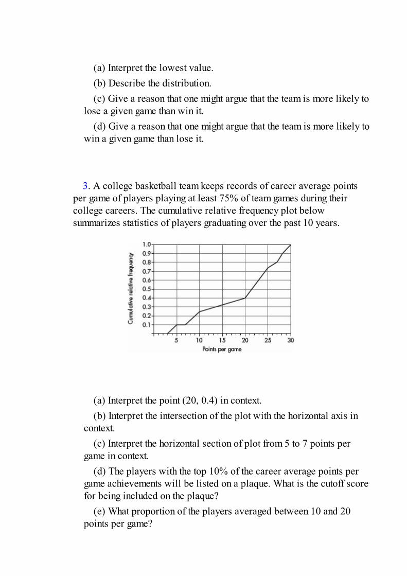
3. A college basketball team keeps records of career average pointsper game of players playing at least 75% of team games during theircollege careers. The cumulative relative frequency plot belowsummarizes statistics of players graduating over the past 10 years.
(a) Interpret the point (20, 0.4) in context.(b) Interpret the intersection of the plot with the horizontal axis in
context.(c) Interpret the horizontal section of plot from 5 to 7 points per
game in context.(d) The players with the top 10% of the career average points per
game achievements will be listed on a plaque. What is the cutoff scorefor being included on the plaque?
(e) What proportion of the players averaged between 10 and 20points per game?


TOPIC 2Summarizing Distributions
• Measuring the Center• Measuring Spread• Measuring Position• Empirical Rule
• Histograms• Boxplots• Changing Units
Given a raw set of data, often we can detect no overall pattern. Perhaps somevalues occur more frequently, a few extreme values may stand out, and the rangeof values is usually apparent. The presentation of data, includingsummarizations and descriptions, and involving such concepts as representativeor average values, measures of dispersion, positions of various values, and theshape of a distribution, falls under the broad topic of descriptive statistics. Thisaspect of statistics is in contrast to statistical analysis, the process of drawinginferences from limited data, a subject discussed in later topics.
MEASURING THE CENTER: MEDIANAND MEANThe word average is used in phrases common to everyday conversation. Peoplespeak of bowling and batting averages or the average life expectancy of abattery or a human being. Actually the word average is derived from the Frenchavarie, which refers to the money that shippers contributed to help compensatefor losses suffered by other shippers whose cargo did not arrive safely (i.e., thelosses were shared, with everyone contributing an average amount). In commonusage average has come to mean a representative score or a typical value or thecenter of a distribution. Mathematically, there are a variety of ways to define theaverage of a set of data. In practice, we use whichever method is mostappropriate for the particular case under consideration. However, beware of aheadline with the word average; the writer has probably chosen the method thatemphasizes the point he or she wishes to make.
In the following paragraphs we consider the two primary ways of denoting anaverage:

1. The median, which is the middle number of a set of numbers arrangedin numerical order.
2. The mean, which is found by summing items in a set and dividing bythe number of items.
EXAMPLE 2.1Consider the following set of home run distances (in feet) to center field in 13 ballparks:{387, 400, 400, 410, 410, 410, 414, 415, 420, 420, 421, 457, 461}. What is the average?
Answer: The median is 414 (there are six values below 414 and six values above), whilethe mean is
MedianThe word median is derived from the Latin medius which means “middle.” Thevalues under consideration are arranged in ascending or descending order. Ifthere is an odd number of values, the median is the middle one. If there is aneven number, the median is found by adding the two middle values and dividingby 2. Thus the median of a set has the same number of elements above it asbelow it.
The median is not affected by exactly how large the larger values are or byexactly how small the smaller values are. Thus it is a particularly usefulmeasurement when the extreme values, called outliers, are in some waysuspicious or when we want do diminish their effect. For example, if ten micetry to solve a maze, and nine succeed in less than 15 minutes while one is stilltrying after 24 hours, the most representative value is the median (not the mean,which is over 2 hours). Similarly, if the salaries of four executives are eachbetween $240,000 and $245,000 while a fifth is paid less than $20,000, againthe most representative value is the median (the mean is under $200,000). It isoften said that the median is “resistant” to extreme values.
In certain situations the median offers the most economical and quickest way tocalculate an average. For example, suppose 10,000 lightbulbs of a particularbrand are installed in a factory. An average life expectancy for the bulbs canmost easily be found by noting how much time passes before exactly one-half ofthem have to be replaced. The median is also useful in certain kinds of medical

research. For example, to compare the relative strengths of different poisons, ascientist notes what dosage of each poison will result in the death of exactlyone-half the test animals. If one of the animals proves especially susceptible to aparticular poison, the median lethal dose is not affected.
TIPDon’t forget to put the data in order before finding the median.
MeanWhile the median is often useful in descriptive statistics, the mean, or moreaccurately, the arithmetic mean, is most important for statistical inference andanalysis. Also, for the layperson, the average is usually understood to be themean.
The mean of a whole population (the complete set of items of interest) is oftendenoted by the Greek letter (mu), while the mean of a sample (a part of apopulation) is often denoted by . For example, the mean value of the set of allhouses in the United States might be = $56,400, while the mean value of 100randomly chosen houses might be = $52,100 or perhaps = $63,800 or even
= $124,000.In statistics we learn how to estimate a population mean from a sample mean.
Throughout this eBook, the word sample often implies a simple random sample(SRS), that is, a sample selected in such a way that every possible sample of thedesired size has an equal chance of being included. (It is also true that eachelement of the population will have an equal chance of being included.) In thereal world, this process of random selection is often very difficult to achieve,and so we proceed, with caution, as long as we have good reason to believe thatour sample is representative of the population.
Mathematically, the mean = , where x represents the sum of all theelements of the set under consideration and n is the actual number of elements.
is the uppercase Greek letter sigma.
EXAMPLE 2.2Suppose that the numbers of unnecessary procedures recommended by five doctors in a1-month period are given by the set {2, 2, 8, 20, 33}. Note that the median is 8 and themean is . If it is discovered that the fifth doctor also recommended anadditional 25 unnecessary procedures, how will the median and mean be affected?
Answer: The set is now {2, 2, 8, 20, 58}. The median is still 8; however, the meanchanges to .
The above example illustrates how the mean, unlike the median, is sensitive to

a change in any value.
EXAMPLE 2.3Suppose the salaries of six employees are $3000, $7000, $15,000, $22,000, $23,000,and $38,000, respectively.
a. What is the mean salary?
Answer:
b. What will the new mean salary be if everyone receives a $3000 increase?
Answer:
Note that $18,000 + $3000 = $21,000.
c. What if everyone receives a 10% raise?
Answer:
Note that 110% of $18,000 is $19,800.
The above example illustrates how adding the same constant to each valueincreases the mean (and median) by a like amount. Similarly, multiplying eachvalue by the same constant multiplies the mean (and median) by a like amount.

TIPUnderstanding variation is the key to understanding statistics.
MEASURING SPREAD: RANGE,INTERQUARTILE RANGE, VARIANCE,AND STANDARD DEVIATIONIn describing a set of numbers, not only is it useful to designate an average valuebut it is also important to be able to indicate the variability or the dispersion ofthe measurements. A producer of time bombs aims for small variability—itwould not be good for his 30-minute fuses actually to have a range of 10–50minutes before detonation. On the other hand, a teacher interested indistinguishing better students from poorer students aims to design exams withlarge variability in results—it would not be helpful if all her students scoredexactly the same. The players on two basketball teams may have the sameaverage height, but this observation doesn’t tell the whole story. If thedispersions are quite different, one team may have a 7-foot player, whereas theother has no one over 6 feet tall. Two Mediterranean holiday cruises mayadvertise the same average age for their passengers. One, however, may haveonly passengers between 20 and 25 years old, while the other has only middle-aged parents in their forties together with their children under age 10.
There are four primary ways of describing variability or dispersion:
1. The range, which is the difference between the largest and smallestvalues
2. The interquartile range, IQR, which is the difference between thelargest and smallest values after removing the lower and upper quarters(i.e., IQR is the range of the middle 50%); that is, IQR = Q3 – Q1 = 75thpercentile minus 25th percentile
3. The variance, which is determined by averaging the squareddifferences of all the values from the mean
4. The standard deviation, which is the square root of the variance.

EXAMPLE 2.4The monthly rainfall in Monrovia, Liberia, where May through October is the rainy seasonand November through April the dry season, is as follows:
The mean is
What are the measures of variability?Answer: Range: The maximum is 37 inches (June), and the minimum is 1 inch
(January). Thus the range is 37 – 1 = 36 inches of rain.Interquartile range: Removing the lower and upper quarters leaves 4, 6, 9, 16, 18, and24. Thus the interquartile range is 24 – 4 = 20. [The interquartile range is sometimescalculated as follows: The median of the lower half is , the median of the upperhalf is , and the interquartile range is Q3 – Q1 = 22. When there is a largenumber of values in the set, the two methods give the same answer.]Variance:
Standard deviation: inches
RangeThe simplest, most easily calculated measure of variability is the range. Thedifference between the largest and smallest values can be noted quickly, and therange gives some impression of the dispersion. However, it is entirelydependent on the two extreme values and is insensitive to the ones in the middle.
One use of the range is to evaluate samples with very few items. For example,some quality control techniques involve taking periodic small samples andbasing further action on the range found in several such samples.
Interquartile RangeFinding the interquartile range is one method of removing the influence ofextreme values on the range. It is calculated by arranging the data in numericalorder, removing the upper and lower quarters of the values, and noting the rangeof the remaining values. That is, it is the range of the middle 50% of the values.
A numerical rule sometimes used for designating outliers is to calculate 1.5times the interquartile range (IQR) and then call a value an outlier if it is more
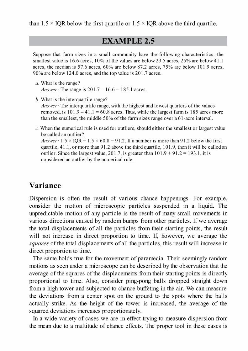
than 1.5 × IQR below the first quartile or 1.5 × IQR above the third quartile.
EXAMPLE 2.5Suppose that farm sizes in a small community have the following characteristics: thesmallest value is 16.6 acres, 10% of the values are below 23.5 acres, 25% are below 41.1acres, the median is 57.6 acres, 60% are below 87.2 acres, 75% are below 101.9 acres,90% are below 124.0 acres, and the top value is 201.7 acres.
a. What is the range?Answer: The range is 201.7 – 16.6 = 185.1 acres.
b. What is the interquartile range?Answer: The interquartile range, with the highest and lowest quarters of the valuesremoved, is 101.9 – 41.1 = 60.8 acres. Thus, while the largest farm is 185 acres morethan the smallest, the middle 50% of the farm sizes range over a 61-acre interval.
c. When the numerical rule is used for outliers, should either the smallest or largest valuebe called an outlier?Answer: 1.5 × IQR = 1.5 × 60.8 = 91.2. If a number is more than 91.2 below the firstquartile, 41.1, or more than 91.2 above the third quartile, 101.9, then it will be called anoutlier. Since the largest value, 201.7, is greater than 101.9 + 91.2 = 193.1, it isconsidered an outlier by the numerical rule.
VarianceDispersion is often the result of various chance happenings. For example,consider the motion of microscopic particles suspended in a liquid. Theunpredictable motion of any particle is the result of many small movements invarious directions caused by random bumps from other particles. If we averagethe total displacements of all the particles from their starting points, the resultwill not increase in direct proportion to time. If, however, we average thesquares of the total displacements of all the particles, this result will increase indirect proportion to time.
The same holds true for the movement of paramecia. Their seemingly randommotions as seen under a microscope can be described by the observation that theaverage of the squares of the displacements from their starting points is directlyproportional to time. Also, consider ping-pong balls dropped straight downfrom a high tower and subjected to chance buffeting in the air. We can measurethe deviations from a center spot on the ground to the spots where the ballsactually strike. As the height of the tower is increased, the average of thesquared deviations increases proportionately.
In a wide variety of cases we are in effect trying to measure dispersion fromthe mean due to a multitude of chance effects. The proper tool in these cases is
the average of the squared deviations from the mean; it is called the varianceand is denoted by σ2 (σ is the lowercase Greek letter sigma):
For circumstances specified later, the variance of a sample, denoted by s2, iscalculated as
EXAMPLE 2.6During the years 1929–39 of the Great Depression, the weekly average hours worked inmanufacturing jobs were 45, 43, 41, 39, 39, 35, 37, 40, 39, 36, and 37, respectively.What is the variance?Answer: The variance can be quickly found on any calculator with a simple statisticalpackage, or it can be found as follows:
EXAMPLE 2.7Let X = {3, 7, 15, 23}. What is the variance?Answer: Again, use the statistical package on your calculator, or
The variance can be calculated from its definition:
Standard Deviation
Suppose we wish to pick a representative value for the variability of a certainpopulation. The preceding discussions indicate that a natural choice is the valuewhose square is the average of the squared deviations from the mean. Thus weare led to consider the square root of the variance. This value is called thestandard deviation, is denoted by σ, and is calculated on your calculator or asfollows:
Similarly, the standard deviation of a sample is denoted by s and is calculatedon your calculator or as follows:
While variance is measured in square units, standard deviation is measured inthe same units as are the data.
For the various x-values, the deviations x – are called residuals, and s is a“typical value” for the residuals. While s is not the average of the residuals (theaverage of the residuals is always 0), s does give a measure of the spread of thex-values around the sample mean.
EXAMPLE 2.8Putting the data {1, 6, 3, 8} into a calculator such as the TI-84 gives what value for thestandard deviation?Answer: The TI-84 gives
Thus, if the data are a population, the standard deviation is σ = 2.693, while if the data area sample, the standard deviation is s = 3.109.
MEASURING POSITION: SIMPLERANKING, PERCENTILE RANKING,AND Z-SCORE

We have seen several ways of choosing a value to represent the center of adistribution. We also need to be able to talk about the position of any othervalues. In some situations, such as wine tasting, simple rankings are of interest.Other cases, for example, evaluating college applications, may involvepositioning according to percentile rankings. There are also situations in whichposition can be specified by making use of measurements of both centraltendency and variability.
There are three important, recognized procedures for designating position:
1. Simple ranking, which involves arranging the elements in some orderand noting where in that order a particular value falls
2. Percentile ranking, which indicates what percentage of all values fallbelow the value under consideration
3. The z-score, which states very specifically by how many standarddeviations a particular value varies from the mean.
EXAMPLE 2.9The water capacities (in gallons) of the 57 major solid-fuel boilers sold in the UnitedStates are 6.3, 7.4, 8.6, 10, 12.1, 50, 8.2, 9.8, 11.4, 12.9, 14.5, 16.1, 26, 21, 27, 40, 55,30, 35, 55, 65, 18.8, 23.3, 28.3, 33.8, 26.4, 33, 50, 35, 21, 21, 18.5, 26.4, 37, 12, 12, 50,65, 65, 56, 66, 60, 70, 27.7, 34.3, 42, 46.2, 33, 25, 29, 40, 19, 9, 12.5, 15.8, 24.5, and16.5, respectively (John W. Bartok, Solid-Fuel Furnaces and Boilers, Garden Way,Charlotte, Vermont). What is the position of the Passat HO-45, which has a capacity of46.2 gallons?Answer: Since there are 12 boilers with higher capacities on the list, the Passat has asimple ranking of thirteenth (out of 57). Forty-four boilers have lower capacities, and sothe Passat has a percentile ranking of = 77.2%. The above list has a mean of 30.3 and astandard deviation of 17.8, so the Passat has a z-score of .
Simple RankingSimple ranking is easily calculated and easily understood. We know what itmeans for someone to graduate second in a class of 435, or for a player from ateam of size 30 to have the seventh-best batting average. Simple ranking isuseful even when no numerical values are associated with the elements. Forexample, detergents can be ranked according to relative cleansing ability

without any numerical measurements of strength.
Percentile RankingPercentile ranking, another readily understood measurement of position, ishelpful in comparing positions with different bases. We can more easilycompare a rank of 176 out of 704 with a rank of 187 out of 935 by noting that thefirst has a rank of 75%, and the second, a rank of 80%. Percentile rank is alsouseful when the exact population size is not known or is irrelevant. Forexample, it is more meaningful to say that Jennifer scored in the 90th percentileon a national exam rather than trying to determine her exact ranking among somelarge number of test takers.
The quartiles, Q1 and Q3, lie one-quarter and three-quarters of the way up alist, respectively. Their percentile ranks are 25% and 75%, respectively. Theinterquartile range defined earlier can also be defined to be Q3 – Q1. Thedeciles lie one-tenth and nine-tenths of the way up a list, respectively, and havepercentile ranks of 10% and 90%.
z-ScoreThe z-score is a measure of position that takes into account both the center andthe dispersion of the distribution. More specifically, the z-score of a value tellshow many standard deviations the value is from the mean. Mathematically, x – gives the raw distance from to x; dividing by σ converts this to number ofstandard deviations. Thus , where x is the raw score, is the mean, and σis the standard deviation. If the score x is greater than the mean , then z ispositive; if x is less than , then z is negative.
Given a z-score, we can reverse the procedure and find the corresponding rawscore. Solving for x gives x = + z σ.
EXAMPLE 2.10Suppose the average (mean) price of gasoline in a large city is $1.80 per gallon with astandard deviation of $0.05. Then $1.90 has a z-score of , while $1.65 has a z-score of . Alternatively, a z-score of +2.2 corresponds to a raw score of 1.80+ 2.2(0.05) = 1.80 + 0.11 = 1.91, while a z-score of –1.6 corresponds to 1.80 –1.6(0.05) = 1.72.It is often useful to portray integer z-scores and the corresponding raw scores as follows:

EXAMPLE 2.11Suppose the attendance at a movie theater averages 780 with a standard deviation of 40.Adding multiples of 40 to and subtracting multiples of 40 from the mean 780 gives
A theater attendance of 835 is converted to a z-score as follows: . A z-score of –2.15 is converted to a theater attendance as follows: 780 – 2.15(40) = 694.
EMPIRICAL RULEThe empirical rule (also called the 68-95-99.7 rule) applies specifically tosymmetric bell-shaped data (not to skewed data!). In this case, about 68% of thevalues lie within 1 standard deviation of the mean, about 95% of the values liewithin 2 standard deviations of the mean, and more than 99% of the values liewithin 3 standard deviations of the mean.
In the following figure the horizontal axis shows z-scores:

EXAMPLE 2.12Suppose that taxicabs in New York City are driven an average of 75,000 miles per yearwith a standard deviation of 12,000 miles. What information does the empirical rule giveus?
Answer: Assuming that the distribution is bell-shaped, we can conclude thatapproximately 68% of the taxis are driven between 63,000 and 87,000 miles per year,approximately 95% are driven between 51,000 and 99,000 miles, and virtually all aredriven between 39,000 and 111,000 miles.
The empirical rule also gives a useful quick estimate of the standard deviationin terms of the range. We can see in the figure above that 95% of the data fallwithin a span of 4 standard deviations (from –2 to +2 on the z-score line) and99.7% of the data fall within 6 standard deviations (from –3 to +3 on the z-score line). It is therefore reasonable to conclude that for these data the standarddeviation is roughly between one-fourth and one-sixth of the range. Since wecan find the range of a set almost immediately, the empirical rule technique forestimating the standard deviation is often helpful in pointing out gross arithmeticerrors.
EXAMPLE 2.13If the range of a data set is 60, what is an estimate for the standard deviation?
Answer: By the empirical rule, the standard deviation is expected to be between and . If the standard deviation is calculated to be 0.32 or 87, there is
probably an arithmetic error; a calculation of 12, however, is reasonable.
However, it must be stressed that the above use of the range is not intended toprovide an accurate value for the standard deviation. It is simply a tool forpointing out unreasonable answers rather than, for example, blindly acceptingcomputer outputs.
HISTOGRAMS AND MEASURES OFCENTRAL TENDENCYSuppose we have a detailed histogram such as
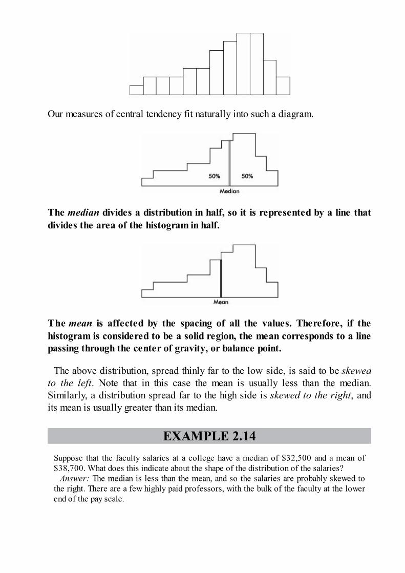
Our measures of central tendency fit naturally into such a diagram.
The median divides a distribution in half, so it is represented by a line thatdivides the area of the histogram in half.
The mean is affected by the spacing of all the values. Therefore, if thehistogram is considered to be a solid region, the mean corresponds to a linepassing through the center of gravity, or balance point.
The above distribution, spread thinly far to the low side, is said to be skewedto the left. Note that in this case the mean is usually less than the median.Similarly, a distribution spread far to the high side is skewed to the right, andits mean is usually greater than its median.
EXAMPLE 2.14Suppose that the faculty salaries at a college have a median of $32,500 and a mean of$38,700. What does this indicate about the shape of the distribution of the salaries?
Answer: The median is less than the mean, and so the salaries are probably skewed tothe right. There are a few highly paid professors, with the bulk of the faculty at the lowerend of the pay scale.

It should be noted that the above principle is a useful, but not hard-and-fast,rule.
EXAMPLE 2.15The set given by the dotplot below is skewed to the right; however, its median (3) isgreater than its mean (2.97).
HISTOGRAMS, Z-SCORES, ANDPERCENTILE RANKINGSWe have seen that relative frequencies are represented by relative areas, and solabeling the vertical axis is not crucial. If we know the standard deviation, thehorizontal axis can be labeled in terms of z-scores. In fact, if we are given thepercentile rankings of various z-scores, we can construct a histogram.
EXAMPLE 2.16Suppose we are asked to construct a histogram from these data:
We note that the entire area is less than z-score +2 and greater than z-score –2. Also,20% of the area is between z-scores –2 and –1, 40% is between –1 and 0, 10% isbetween 0 and 1, and 30% is between 1 and 2. Thus the histogram is as follows:
Now suppose we are given four in-between z-scores as well:

With 1000 z-scores perhaps the histogram would look like
The height at any point is meaningless; what is important is relative areas. For example,in the final diagram above, what percentage of the area is between z-scores of +1 and +2?
Answer: Still 30%.What percent is to the left of 0?
Answer: Still 60%.
BOXPLOTSA boxplot (also called a box and whisker display) is a visual representation ofdispersion that shows the smallest value, the largest value, the middle (median),the middle of the bottom half of the set (Q1), and the middle of the top half of theset (Q3).
EXAMPLE 2.17The total farm product indexes for the years 1919–45 (with 1910–14 as 100) are 215,210, 130, 140, 150, 150, 160, 150, 140, 150, 150, 125, 85, 70, 75, 90, 115, 120, 125,100, 95, 100, 130, 160, 200, 200, 210, respectively. (Note the instability of pricesreceived by farmers!) The largest value is 215, the smallest is 70, the middle is 140, themiddle of the top half is 160, and the middle of the bottom half is 100. A boxplot of thesefive numbers is

Note that the display consists of two “boxes” together with two “whiskers”—hence thealternative name. The boxes show the spread of the two middle quarters; the whiskersshow the spread of the two outer quarters. This relatively simple display conveysinformation not immediately available from histograms or stem and leaf displays.
Putting the above data into a list, for example, L1, on the TI-84, not only gives the five-number summary
but also gives the boxplot itself using STAT PLOT, choosing the boxplot from among thesix type choices, and then using ZoomStat or in WINDOW letting Xmin=0 andXmax=225.On the TI-Nspire the data can be put in a list (here called index), and then a simultaneousmultiple view is possible.
When a distribution is strongly skewed, or when it has pronounced outliers,drawing a boxplot with its five-number summary including median, quartiles,and extremes, gives a more useful description than calculating a mean and astandard deviation.
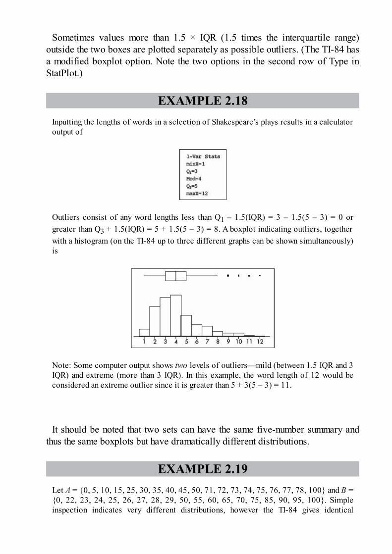
Sometimes values more than 1.5 × IQR (1.5 times the interquartile range)outside the two boxes are plotted separately as possible outliers. (The TI-84 hasa modified boxplot option. Note the two options in the second row of Type inStatPlot.)
EXAMPLE 2.18Inputting the lengths of words in a selection of Shakespeare’s plays results in a calculatoroutput of
Outliers consist of any word lengths less than Q1 – 1.5(IQR) = 3 – 1.5(5 – 3) = 0 orgreater than Q3 + 1.5(IQR) = 5 + 1.5(5 – 3) = 8. A boxplot indicating outliers, togetherwith a histogram (on the TI-84 up to three different graphs can be shown simultaneously)is
Note: Some computer output shows two levels of outliers—mild (between 1.5 IQR and 3IQR) and extreme (more than 3 IQR). In this example, the word length of 12 would beconsidered an extreme outlier since it is greater than 5 + 3(5 – 3) = 11.
It should be noted that two sets can have the same five-number summary andthus the same boxplots but have dramatically different distributions.
EXAMPLE 2.19Let A = {0, 5, 10, 15, 25, 30, 35, 40, 45, 50, 71, 72, 73, 74, 75, 76, 77, 78, 100} and B ={0, 22, 23, 24, 25, 26, 27, 28, 29, 50, 55, 60, 65, 70, 75, 85, 90, 95, 100}. Simpleinspection indicates very different distributions, however the TI-84 gives identical

boxplots with Min = 0, Q1 = 25, Med = 50, Q3 = 75, and Max = 100 for each.
EFFECT OF CHANGING UNITSChanging units, for example, from dollars to rubles or from miles to kilometers,is common in a world that seems to become smaller all the time. It is instructiveto note how measures of center and spread are affected by such changes.
Adding the same constant to every value increases the mean and median by thatsame constant; however, the distances between the increased values stay thesame, and so the range and standard deviation are unchanged.
EXAMPLE 2.20A set of experimental measurements of the freezing point of an unknown liquid yield amean of 25.32 degrees Celsius with a standard deviation of 1.47 degrees Celsius. If allthe measurements are converted to the Kelvin scale, what are the new mean and standarddeviation?
Answer: Kelvins are equivalent to degrees Celsius plus 273.16. The new mean is thus25.32 + 273.16 = 298.48 kelvins. However, the standard deviation remains numericallythe same, 1.47 kelvins. Graphically, you should picture the whole distribution movingover by the constant 273.16; the mean moves, but the standard deviation (which measuresspread) doesn’t change.
Multiplying every value by the same constant multiplies the mean, median,range, and standard deviation all by that constant.
EXAMPLE 2.21Measurements of the sizes of farms in an upstate New York county yield a mean of 59.2hectares with a standard deviation of 11.2 hectares. If all the measurements are convertedfrom hectares (metric system) to acres (one acre was originally the area a yoke of oxencould plow in one day), what are the new mean and standard deviation?
Answer: One hectare is equivalent to 2.471 acres. The new mean is thus 2.471 × 59.2 =146.3 acres with a standard deviation of 2.471 × 11.2 = 27.7 acres. Graphically,multiplying each value by the constant 2.471 both moves and spreads out the distribution.
Summary
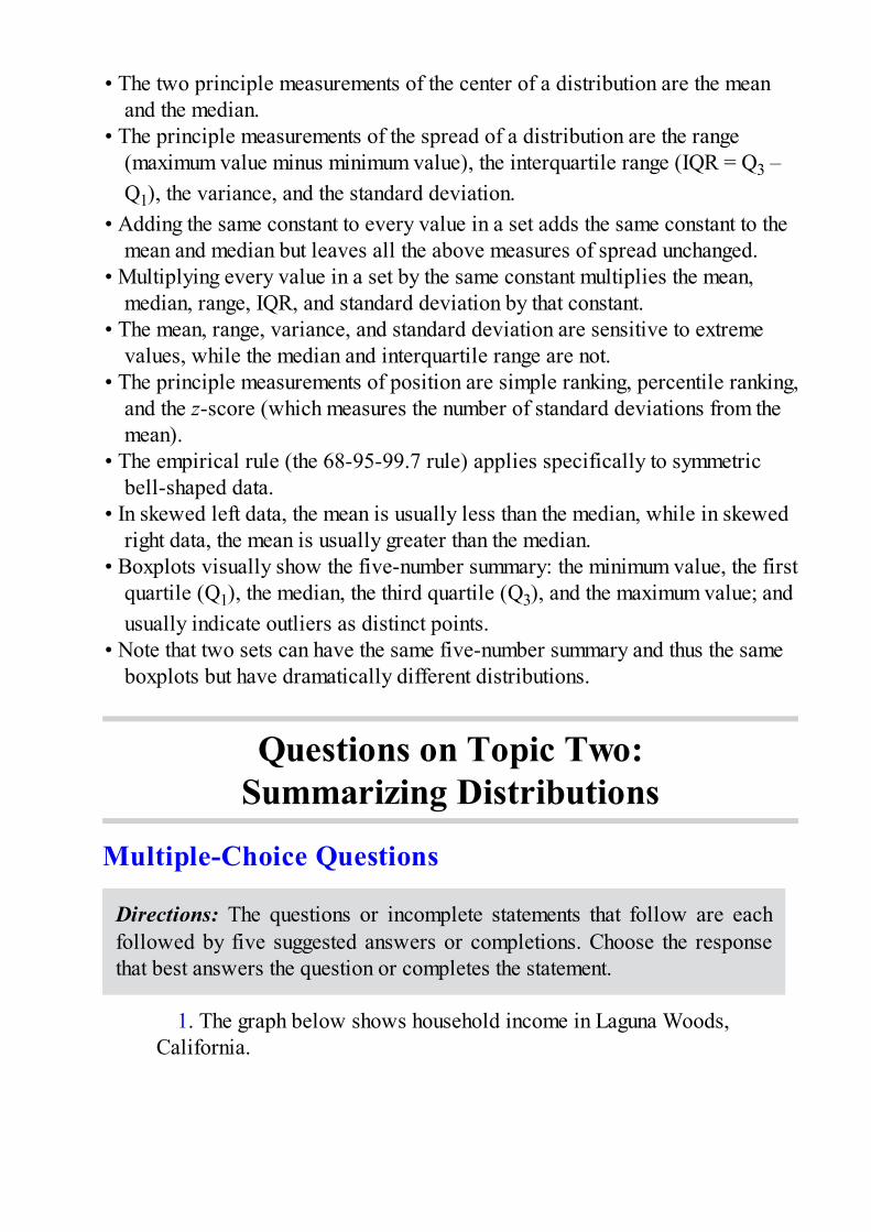
• The two principle measurements of the center of a distribution are the meanand the median.
• The principle measurements of the spread of a distribution are the range(maximum value minus minimum value), the interquartile range (IQR = Q3 –Q1), the variance, and the standard deviation.
• Adding the same constant to every value in a set adds the same constant to themean and median but leaves all the above measures of spread unchanged.
• Multiplying every value in a set by the same constant multiplies the mean,median, range, IQR, and standard deviation by that constant.
• The mean, range, variance, and standard deviation are sensitive to extremevalues, while the median and interquartile range are not.
• The principle measurements of position are simple ranking, percentile ranking,and the z-score (which measures the number of standard deviations from themean).
• The empirical rule (the 68-95-99.7 rule) applies specifically to symmetricbell-shaped data.
• In skewed left data, the mean is usually less than the median, while in skewedright data, the mean is usually greater than the median.
• Boxplots visually show the five-number summary: the minimum value, the firstquartile (Q1), the median, the third quartile (Q3), and the maximum value; andusually indicate outliers as distinct points.
• Note that two sets can have the same five-number summary and thus the sameboxplots but have dramatically different distributions.
Questions on Topic Two:Summarizing Distributions
Multiple-Choice Questions
Directions: The questions or incomplete statements that follow are eachfollowed by five suggested answers or completions. Choose the responsethat best answers the question or completes the statement.
1. The graph below shows household income in Laguna Woods,California.
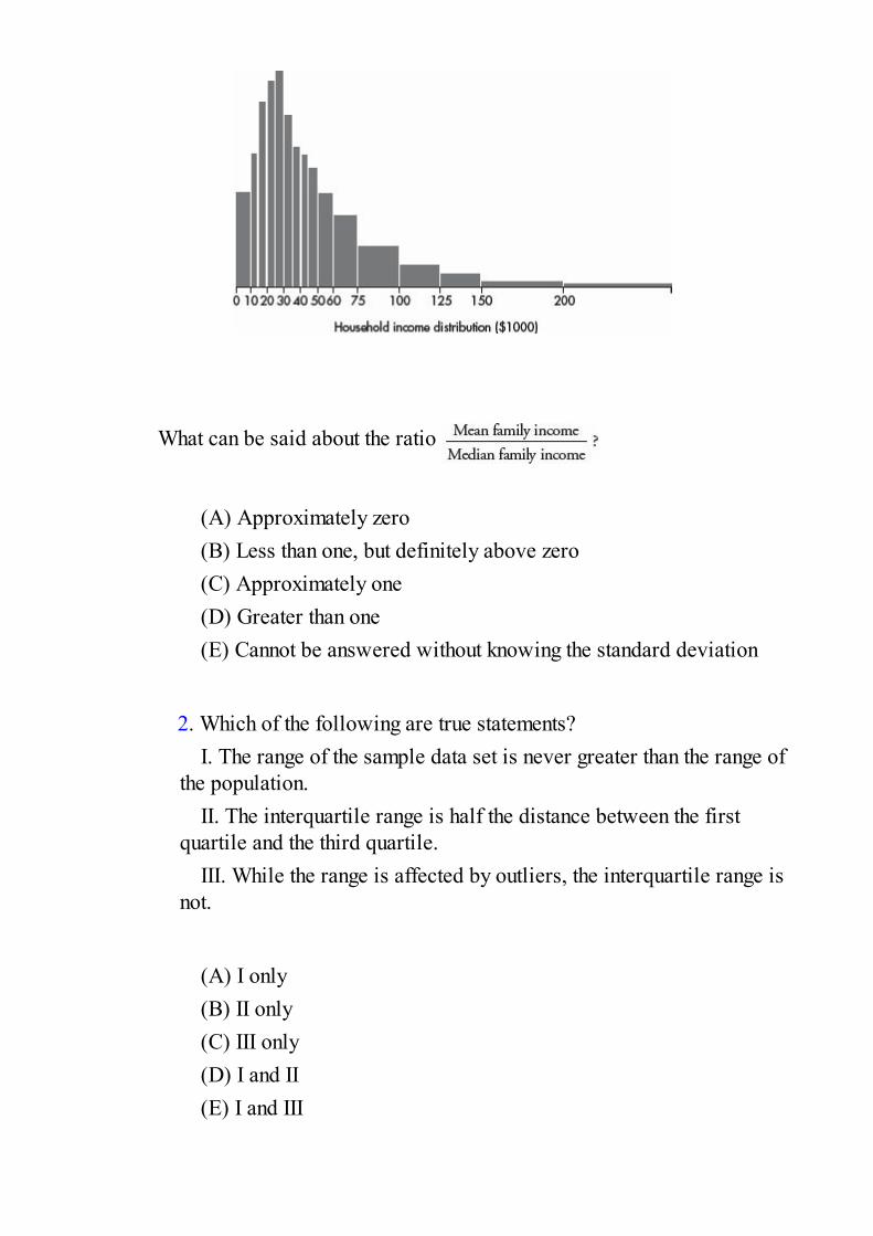
What can be said about the ratio
(A) Approximately zero(B) Less than one, but definitely above zero(C) Approximately one(D) Greater than one(E) Cannot be answered without knowing the standard deviation
2. Which of the following are true statements?
I. The range of the sample data set is never greater than the range ofthe population.
II. The interquartile range is half the distance between the firstquartile and the third quartile.
III. While the range is affected by outliers, the interquartile range isnot.
(A) I only(B) II only(C) III only(D) I and II(E) I and III

3. Dieticians are concerned about sugar consumption in teenagers’ diets(a 12-ounce can of soft drink typically has 10 teaspoons of sugar). In arandom sample of 55 students, the number of teaspoons of sugar consumedfor each student on a randomly selected day is tabulated. Summarystatistics are noted below:
Which of the following is a true statement?
(A) None of the values are outliers.(B) The value 10 is an outlier, and there can be no others.(C) The value 60 is an outlier, and there can be no others.(D) Both 10 and 60 are outliers, and there may be others.(E) The value 60 is an outlier, and there may be others at the high
end of the data set.
Problems 4–6 refer to the following five boxplots.
4. To which of the above boxplots does the following histogram

correspond?
(A) A(B) B(C) C(D) D(E) E
5. To which of the above boxplots does the following histogramcorrespond?
(A) A(B) B(C) C(D) D(E) E
6. To which of the above boxplots does the following histogram
correspond?

(A) A(B) B(C) C(D) D(E) E
Problems 7–9 refer to the following five histograms:
7. To which of the above histograms does the following boxplotcorrespond?
(A) A(B) B(C) C(D) D(E) E

8. To which of the above histograms does the following boxplot
correspond?
(A) A(B) B(C) C(D) D(E) E
9. To which of the above histograms does the following boxplot
correspond?
(A) A(B) B(C) C(D) D(E) E
10. Below is a boxplot of CO2 levels (in grams per kilometer) for a
sampling of 2008 vehicles.
Suppose follow-up testing determines that the low outlier should be 10grams per kilometer less and the two high outliers should each be 5 gramsper kilometer greater. What effect, if any, will these changes have on themean and median CO2 levels?
(A) Both the mean and median will be unchanged.(B) The median will be unchanged, but the mean will increase.(C) The median will be unchanged, but the mean will decrease.(D) The mean will be unchanged, but the median will increase.(E) Both the mean and median will change.
11. Below is a boxplot of yearly tuition and fees of all four yearcolleges and universities in a Western state. The low outlier is from aprivate university that gives full scholarships to all accepted students,while the high outlier is from a private college catering to the very rich.
Removing both outliers will effect what changes, if any, on the mean andmedian costs for this state’s four year institutions of higher learning?
(A) Both the mean and the median will be unchanged.(B) The median will be unchanged, but the mean will increase.(C) The median will be unchanged, but the mean will decrease.(D) The mean will be unchanged, but the median will increase.(E) Both the mean and median will change.

12. Suppose the average score on a national test is 500 with a standarddeviation of 100. If each score is increased by 25, what are the new meanand standard deviation?
(A) 500, 100(B) 500, 125(C) 525, 100(D) 525, 105(E) 525, 125
13. Suppose the average score on a national test is 500 with a standarddeviation of 100. If each score is increased by 25%, what are the newmean and standard deviation?
(A) 500, 100(B) 525, 100(C) 625, 100(D) 625, 105(E) 625, 125
14. If quartiles Q1 = 20 and Q3 = 30, which of the following must be
true?I. The median is 25.II. The mean is between 20 and 30.III. The standard deviation is at most 10.
(A) I only(B) II only

(C) III only(D) All are true.(E) None are true.
15. A 1995 poll by the Program for International Policy askedrespondents what percentage of the U.S. budget they thought went toforeign aid. The mean response was 18%, and the median was 15%. (Theactual amount is less than 1%.) What do these responses indicate aboutthe likely shape of the distribution of all the responses?
(A) The distribution is skewed to the left.(B) The distribution is skewed to the right.(C) The distribution is symmetric around 16.5%.(D) The distribution is bell-shaped with a standard deviation of 3%.(E) The distribution is uniform between 15% and 18%.
16. Assuming that batting averages have a bell-shaped distribution,arrange in ascending order:
I. An average with a z-score of –1.II. An average with a percentile rank of 20%.III. An average at the first quartile, Q1.
(A) I, II, III(B) III, I, II(C) II, I, III(D) II, III, I(E) III, II, I
17. Which of the following are true statements?I. If the sample has variance zero, the variance of the population is
also zero.II. If the population has variance zero, the variance of the sample is
also zero.III. If the sample has variance zero, the sample mean and the sample
median are equal.
(A) I and II(B) I and III(C) II and III(D) I, II, and III(E) None of the above gives the complete set of true responses.
18. When there are multiple gaps and clusters, which of the followingis the best choice to give an overall picture of a distribution?
(A) Mean and standard deviation(B) Median and interquartile range(C) Boxplot with its five-number summary(D) Stemplot or histogram(E) None of the above are really helpful in showing gaps and
clusters.
19. Suppose the starting salaries of a graduating class are as follows:

What is the mean starting salary?
(A) $30,000(B) $30,533(C) $32,500(D) $32,533(E) $35,000
20. When a set of data has suspect outliers, which of the following arepreferred measures of central tendency and of variability?
(A) mean and standard deviation(B) mean and variance(C) mean and range(D) median and range(E) median and interquartile range
21. If the standard deviation of a set of observations is 0, you can
conclude

(A) that there is no relationship between the observations.(B) that the average value is 0.(C) that all observations are the same value.(D) that a mistake in arithmetic has been made.(E) none of the above.
22. A teacher is teaching two AP Statistics classes. On the final exam,the 20 students in the first class averaged 92 while the 25 students in thesecond class averaged only 83. If the teacher combines the classes, whatwill the average final exam score be?
(A) 87(B) 87.5(C) 88(D) None of the above(E) More information is needed to make this calculation.
23. The 60 longest rivers in the world have lengths distributed asfollows:
(The Nile is the longest with a length of 4145 miles, and the Amazon isthe second longest at 3900 miles.)
Which of the following best describes these data?

(A) Skewed distribution, mean greater than median(B) Skewed distribution, median greater than mean(C) Symmetric distribution, mean greater than median(D) Symmetric distribution, median greater than mean(E) Symmetric distribution with outliers on high end
24. In 1993 the seven states with the fewest business bankruptcies wereVermont (900), Alaska (1000), North Dakota (1100), Wyoming (1300),South Dakota (1400), Hawaii (1500), and Delaware (1600).
Which of the following are reasonable conclusions about the distributionof bankruptcies throughout the 50 states in 1993?
I. The total number of bankruptcies in the United States in 1993 wasapproximately 50(1300) = 65,000.
II. Because of these low values, the distribution was skewed to theleft.
III. The range of the distribution was approximately 50(1600 – 1000)= 30,000.
(A) I only(B) II only(C) III only(D) All are reasonable.(E) None are reasonable.
25. Suppose 10% of a data set lie between 40 and 60. If 5 is first addedto each value in the set and then each result is doubled, which of thefollowing is true?

(A) 10% of the resulting data will lie between 85 and 125.(B) 10% of the resulting data will lie between 90 and 130.(C) 15% of the resulting data will lie between 80 and 120.(D) 20% of the resulting data will lie between 45 and 65.(E) 30% of the resulting data will lie between 85 and 125.
26. A stemplot for the 1988 per capita personal income (in hundreds ofdollars) for the 50 states is
Which of the following best describes these data?
(A) Skewed distribution, mean greater than median(B) Skewed distribution, median greater than mean(C) Symmetric distribution, mean greater than median(D) Symmetric distribution, median greater than mean(E) Symmetric distribution with outliers on high end
27. Which of the following statements are true?
I. If the right and left sides of a histogram are mirror images of eachother, the distribution is symmetric.
II. A distribution spread far to the right side is said to be skewed tothe right.
III. If a distribution is skewed to the right, its mean is often greater

than its median.
(A) I only(B) I and II(C) I and III(D) II and III(E) None of the above gives the complete set of true responses.
28. Which of the following statements are true?I. In a stemplot the number of leaves equals the size of the set of data.II. Both the dotplot and the stemplot are useful in identifying outliers.III. Histograms do not retain the identity of individual scores;
however, dotplots, stemplots, and boxplots all do.
(A) I and II(B) I and III(C) II and III(D) I, II, and III(E) None of the above gives the complete set of true responses.
29. The 70 highest dams in the world have an average height of 206meters with a standard deviation of 35 meters. The Hoover and GrandCoulee dams have heights of 221 and 168 meters, respectively. TheRussian dams, the Nurek and Charvak, have heights with z-scores of+2.69 and –1.13, respectively. List the dams in order of ascending size.
(A) Charvak, Grand Coulee, Hoover, Nurek(B) Charvak, Grand Coulee, Nurek, Hoover(C) Grand Coulee, Charvak, Hoover, Nurek(D) Grand Coulee, Charvak, Nurek, Hoover(E) Grand Coulee, Hoover, Charvak, Nurek
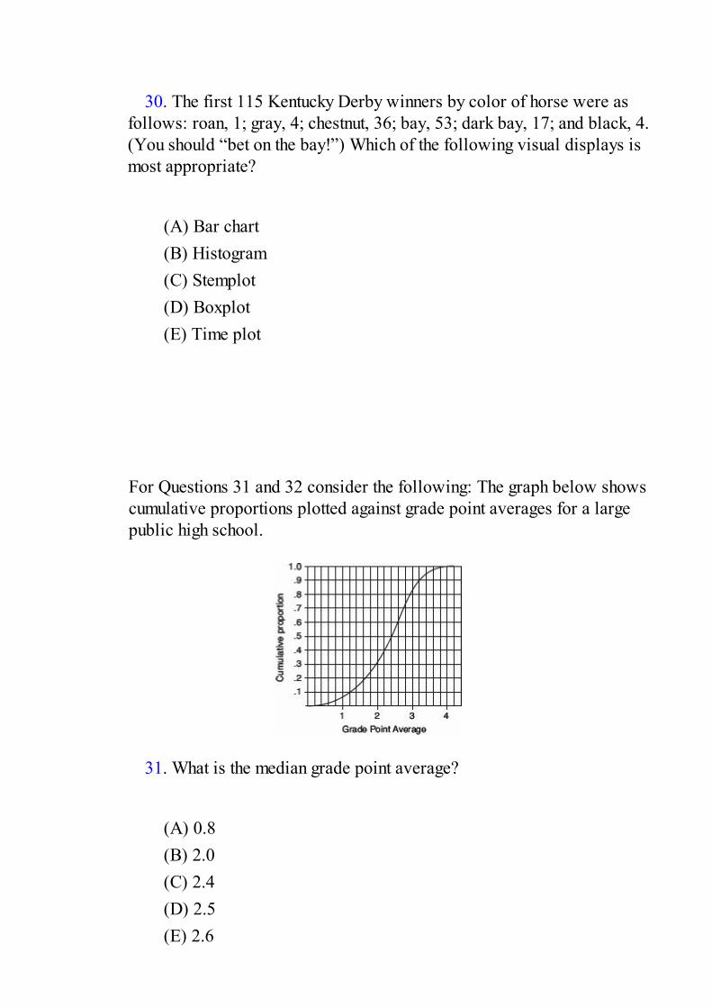
30. The first 115 Kentucky Derby winners by color of horse were as
follows: roan, 1; gray, 4; chestnut, 36; bay, 53; dark bay, 17; and black, 4.(You should “bet on the bay!”) Which of the following visual displays ismost appropriate?
(A) Bar chart(B) Histogram(C) Stemplot(D) Boxplot(E) Time plot
For Questions 31 and 32 consider the following: The graph below showscumulative proportions plotted against grade point averages for a largepublic high school.
31. What is the median grade point average?
(A) 0.8(B) 2.0(C) 2.4(D) 2.5(E) 2.6
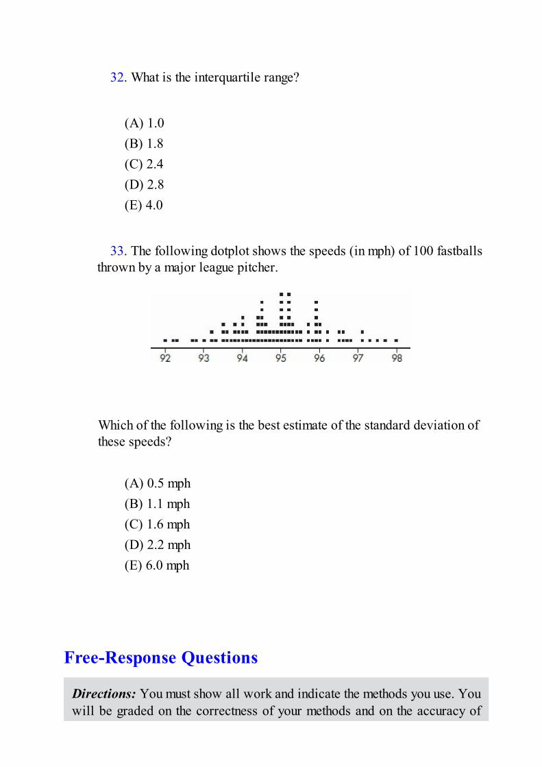
32. What is the interquartile range?
(A) 1.0(B) 1.8(C) 2.4(D) 2.8(E) 4.0
33. The following dotplot shows the speeds (in mph) of 100 fastballs
thrown by a major league pitcher.
Which of the following is the best estimate of the standard deviation ofthese speeds?
(A) 0.5 mph(B) 1.1 mph(C) 1.6 mph(D) 2.2 mph(E) 6.0 mph
Free-Response Questions
Directions: You must show all work and indicate the methods you use. Youwill be graded on the correctness of your methods and on the accuracy of
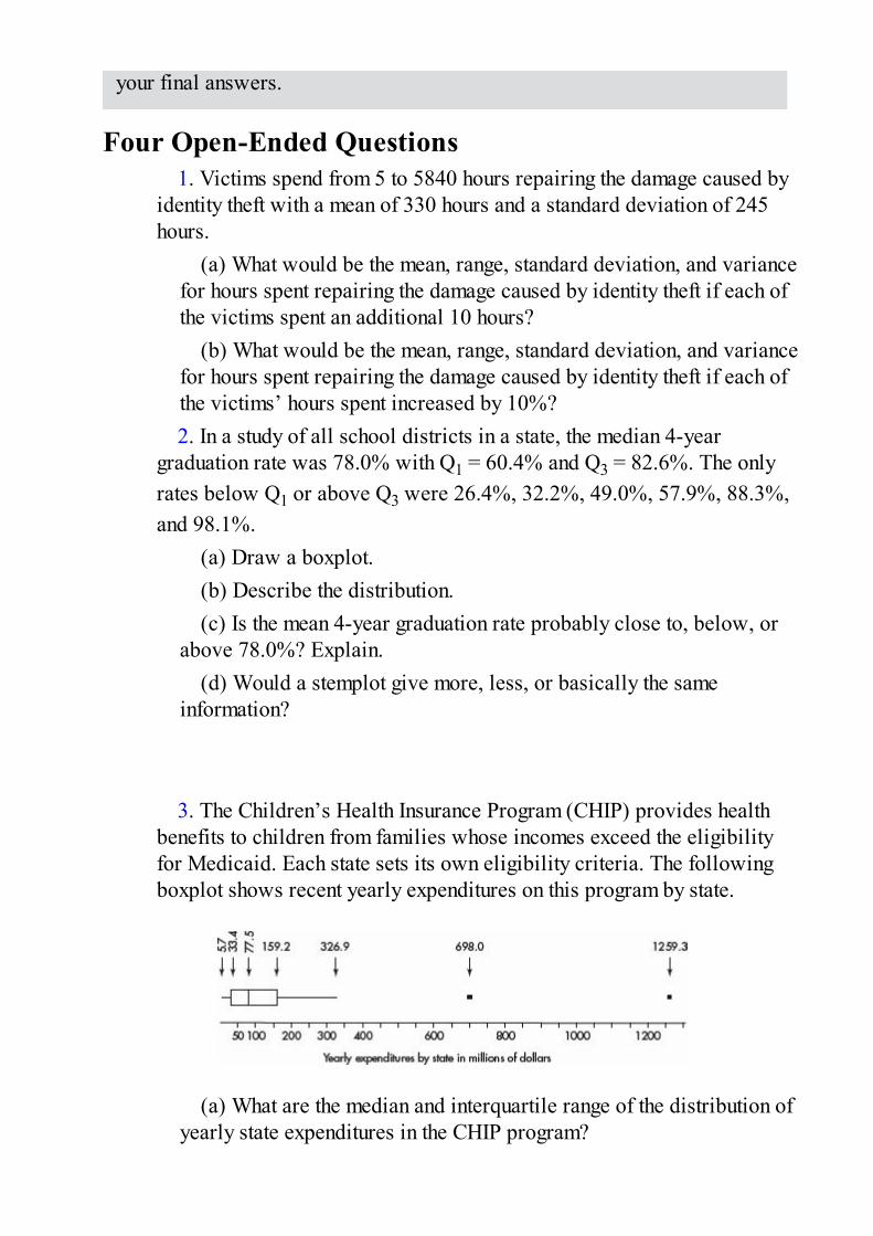
your final answers.
Four Open-Ended Questions1. Victims spend from 5 to 5840 hours repairing the damage caused by
identity theft with a mean of 330 hours and a standard deviation of 245hours.
(a) What would be the mean, range, standard deviation, and variancefor hours spent repairing the damage caused by identity theft if each ofthe victims spent an additional 10 hours?
(b) What would be the mean, range, standard deviation, and variancefor hours spent repairing the damage caused by identity theft if each ofthe victims’ hours spent increased by 10%?2. In a study of all school districts in a state, the median 4-year
graduation rate was 78.0% with Q1 = 60.4% and Q3 = 82.6%. The onlyrates below Q1 or above Q3 were 26.4%, 32.2%, 49.0%, 57.9%, 88.3%,and 98.1%.
(a) Draw a boxplot.(b) Describe the distribution.(c) Is the mean 4-year graduation rate probably close to, below, or
above 78.0%? Explain.(d) Would a stemplot give more, less, or basically the same
information?
3. The Children’s Health Insurance Program (CHIP) provides healthbenefits to children from families whose incomes exceed the eligibilityfor Medicaid. Each state sets its own eligibility criteria. The followingboxplot shows recent yearly expenditures on this program by state.
(a) What are the median and interquartile range of the distribution ofyearly state expenditures in the CHIP program?

(b) Suppose the federal government takes over three million dollarsof administrative costs from the state CHIP expenditures. What are themedian and interquartile range of the new reduced expendituredistribution?
(c) Suppose instead the federal government picks up the tab for halfof all state CHIP expenditures. What are the median and interquartilerange of this new reduced expenditure distribution?
(d) Based on the above boxplot, which of the following is the mostreasonable value for the mean state expenditure (in millions ofdollars): 78, 135, 325, 630, or 750? Explain.4. Suppose a distribution has mean 300 and standard deviation 25. If
the z-score of Q1 is –0.7 and the z-score of Q3 is 0.7, what values wouldbe considered to be outliers?

TOPIC 3Comparing Distributions
• Dotplots• Double Bar Charts• Back-to-back Stemplots
• Parallel Boxplots• Cumulative Frequency Plots
Many real-life applications of statistics involve comparisons of twopopulations. Such comparisons can involve modifications of graphical displayssuch as dotplots, bar charts, stemplots, boxplots, and cumulative frequency plotsto portray both sets simultaneously.
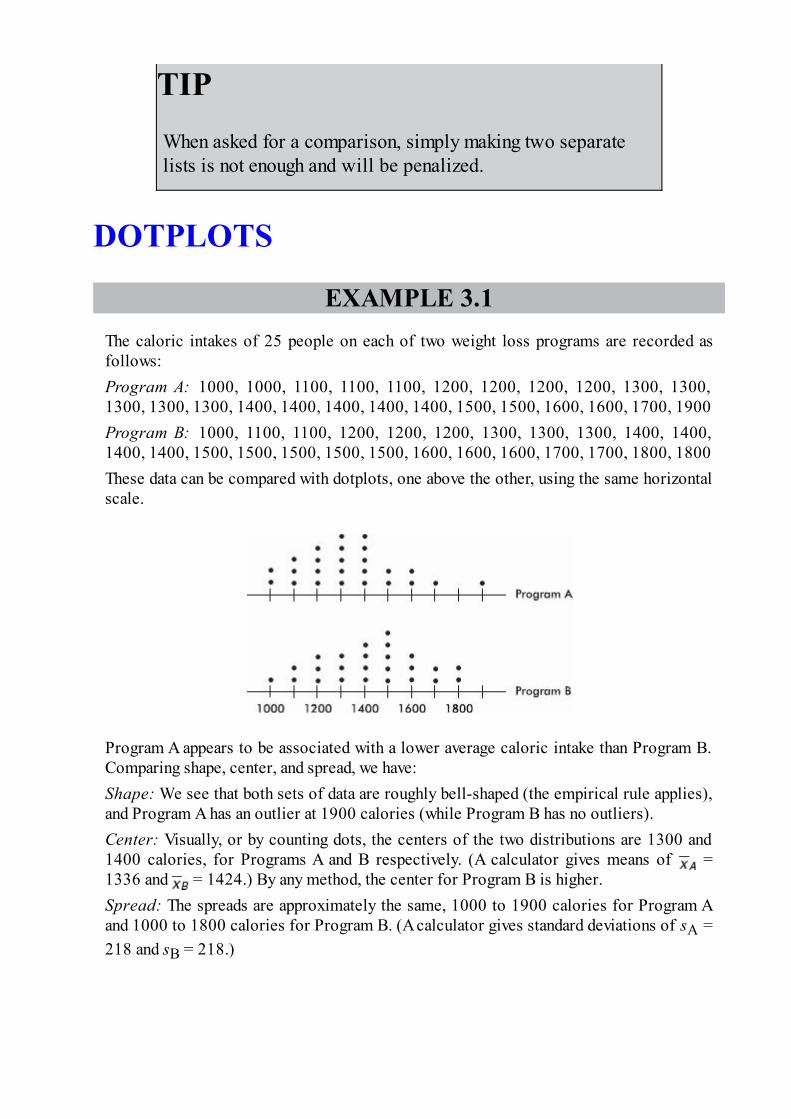
TIPWhen asked for a comparison, simply making two separatelists is not enough and will be penalized.
DOTPLOTS
EXAMPLE 3.1The caloric intakes of 25 people on each of two weight loss programs are recorded asfollows:Program A: 1000, 1000, 1100, 1100, 1100, 1200, 1200, 1200, 1200, 1300, 1300,1300, 1300, 1300, 1400, 1400, 1400, 1400, 1400, 1500, 1500, 1600, 1600, 1700, 1900Program B: 1000, 1100, 1100, 1200, 1200, 1200, 1300, 1300, 1300, 1400, 1400,1400, 1400, 1500, 1500, 1500, 1500, 1500, 1600, 1600, 1600, 1700, 1700, 1800, 1800These data can be compared with dotplots, one above the other, using the same horizontalscale.
Program A appears to be associated with a lower average caloric intake than Program B.Comparing shape, center, and spread, we have:Shape: We see that both sets of data are roughly bell-shaped (the empirical rule applies),and Program A has an outlier at 1900 calories (while Program B has no outliers).Center: Visually, or by counting dots, the centers of the two distributions are 1300 and1400 calories, for Programs A and B respectively. (A calculator gives means of =1336 and = 1424.) By any method, the center for Program B is higher.Spread: The spreads are approximately the same, 1000 to 1900 calories for Program Aand 1000 to 1800 calories for Program B. (A calculator gives standard deviations of sA =218 and sB = 218.)
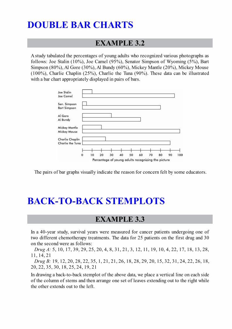
DOUBLE BAR CHARTS
EXAMPLE 3.2A study tabulated the percentages of young adults who recognized various photographs asfollows: Joe Stalin (10%), Joe Camel (95%), Senator Simpson of Wyoming (5%), BartSimpson (80%), Al Gore (30%), Al Bundy (60%), Mickey Mantle (20%), Mickey Mouse(100%), Charlie Chaplin (25%), Charlie the Tuna (90%). These data can be illustratedwith a bar chart appropriately displayed in pairs of bars.
The pairs of bar graphs visually indicate the reason for concern felt by some educators.
BACK-TO-BACK STEMPLOTS
EXAMPLE 3.3In a 40-year study, survival years were measured for cancer patients undergoing one oftwo different chemotherapy treatments. The data for 25 patients on the first drug and 30on the second were as follows:
Drug A: 5, 10, 17, 39, 29, 25, 20, 4, 8, 31, 21, 3, 12, 11, 19, 10, 4, 22, 17, 18, 13, 28,11, 14, 21
Drug B: 19, 12, 20, 28, 22, 35, 1, 21, 21, 26, 18, 28, 29, 20, 15, 32, 31, 24, 22, 26, 18,20, 22, 35, 30, 18, 25, 24, 19, 21In drawing a back-to-back stemplot of the above data, we place a vertical line on each sideof the column of stems and then arrange one set of leaves extending out to the right whilethe other extends out to the left.
Note that even though drug A showed the longest-surviving patient (39 years) and drug Bshowed the shortest-surviving patient (1 year), the back-to-back stemplot indicates thatthe bulk of patients on drug B survived longer than the bulk of patients on drug A.Comparing shape, center, and spread, we have:Shape: Both distributions are roughly bell-shaped (the empirical rule applies). The drug Adistribution appears to have a high outlier at 39, while the drug B distribution appears tohave a low outlier at 1.Center: Visually, or by counting values, the centers of the two distributions are 17 and22, respectively. (A calculator gives means of = 16.48 and = 22.73.) By eithermethod, the drug B distribution has a greater center.Spread: The spreads are 3 to 39 survival years for drug A and 1 to 35 survival years fordrug B. (A calculator gives standard deviations of sA = 9.25 and sB = 6.97.) By eithermethod, the drug A distribution has a greater spread than the drug B distribution.
PARALLEL BOXPLOTS
EXAMPLE 3.4Mail-order labs and 1-hour minilabs were compared with regard to price for developingand printing one 24-exposure roll of 35-millimeter color-print film. Prices includedshipping and handling charges where applicable. Following is a computer outputdescribing the results:For mail-order labs:
For 1-hour minilabs:
In drawing parallel boxplots (also called side-by-side boxplots) of the above data, weplace both on the same diagram:
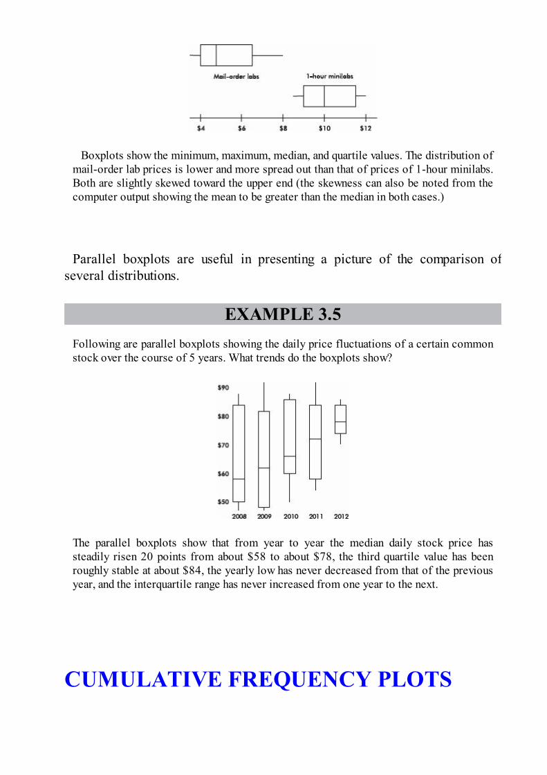
Boxplots show the minimum, maximum, median, and quartile values. The distribution ofmail-order lab prices is lower and more spread out than that of prices of 1-hour minilabs.Both are slightly skewed toward the upper end (the skewness can also be noted from thecomputer output showing the mean to be greater than the median in both cases.)
Parallel boxplots are useful in presenting a picture of the comparison ofseveral distributions.
EXAMPLE 3.5Following are parallel boxplots showing the daily price fluctuations of a certain commonstock over the course of 5 years. What trends do the boxplots show?
The parallel boxplots show that from year to year the median daily stock price hassteadily risen 20 points from about $58 to about $78, the third quartile value has beenroughly stable at about $84, the yearly low has never decreased from that of the previousyear, and the interquartile range has never increased from one year to the next.
CUMULATIVE FREQUENCY PLOTS
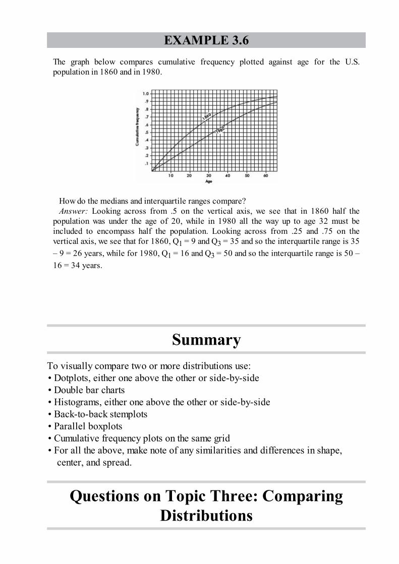
EXAMPLE 3.6The graph below compares cumulative frequency plotted against age for the U.S.population in 1860 and in 1980.
How do the medians and interquartile ranges compare?Answer: Looking across from .5 on the vertical axis, we see that in 1860 half the
population was under the age of 20, while in 1980 all the way up to age 32 must beincluded to encompass half the population. Looking across from .25 and .75 on thevertical axis, we see that for 1860, Q1 = 9 and Q3 = 35 and so the interquartile range is 35– 9 = 26 years, while for 1980, Q1 = 16 and Q3 = 50 and so the interquartile range is 50 –16 = 34 years.
SummaryTo visually compare two or more distributions use:• Dotplots, either one above the other or side-by-side• Double bar charts• Histograms, either one above the other or side-by-side• Back-to-back stemplots• Parallel boxplots• Cumulative frequency plots on the same grid• For all the above, make note of any similarities and differences in shape,
center, and spread.
Questions on Topic Three: ComparingDistributions

Multiple-Choice Questions
Directions: The questions or incomplete statements that follow are eachfollowed by five suggested answers or completions. Choose the responsethat best answers the question or completes the statement.
1. The dotplots below show the yearly wages of all male and femaleexecutives at a large firm.
Which of the following conclusions cannot be drawn from the plots?
(A) A greater proportion of male employees than female employeesare executives at this firm.
(B) No executive receives a salary less than $25,000.(C) The median salary paid to male executives is less than the
median salary paid to female executives.(D) The range of salaries paid to male executives is less than the
range of salaries paid to female executives.(E) More male than female executives have salaries over $70,000.
For Questions 2 and 3 consider the following two histograms:

2. Which of the following statements are true?I. Both sets have the same mean.II. Both sets have the same range.III. Both sets have the same variance.
(A) I only(B) I and II(C) I and III(D) I, II, and III(E) None of the above gives the complete set of true responses.
3. Which of the following statements are true?I. The empirical rule applies only to set A.II. You can be sure that the standard deviation of set A is greater than
5.III. You can be sure that the standard deviation of set B is greater
than 5.
(A) I only(B) II only(C) I and II(D) I and III(E) II and III
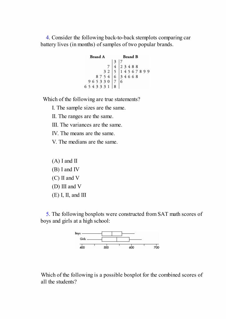
4. Consider the following back-to-back stemplots comparing carbattery lives (in months) of samples of two popular brands.
Which of the following are true statements?I. The sample sizes are the same.II. The ranges are the same.III. The variances are the same.IV. The means are the same.V. The medians are the same.
(A) I and II(B) I and IV(C) II and V(D) III and V(E) I, II, and III
5. The following boxplots were constructed from SAT math scores of
boys and girls at a high school:
Which of the following is a possible boxplot for the combined scores ofall the students?

(A)
(B)
(C)
(D)
(E)
Questions 6–8 refer to the following population pyramids (source: U.S.Census Bureau).

6. What is the approximate median age of the Liberian population?
(A) 0–4(B) 15–19(C) 30–34(D) 40–44(E) There is insufficient information to approximate the median.
7. Which country has more children younger than 10 years of age?
(A) Liberia(B) Canada(C) You can’t tell without calculating means.(D) You can’t tell without calculating medians.(E) You can’t tell without calculating some measure of variability.

8. Which of the following statements are plausible, given the graphs?I. Canadian women tend to live longer than men.II. The recent civil war in Liberia, with the extensive use of child
soldiers, has had an impact on the population age distribution.III. Canadian demographics show a decreasing birth rate.
(A) I only(B) I and II only(C) I and III only(D) II and III only(E) All three are plausible.
Free-Response Questions
Directions: You must show all work and indicate the methods you use. Youwill be graded on the correctness of your methods and on the accuracy ofyour final answers.
Four Open-Ended Questions1. Census data was used to compare the marital status versus age of
residents of a small town in rural upstate New York. Resulting histogramsare given below.
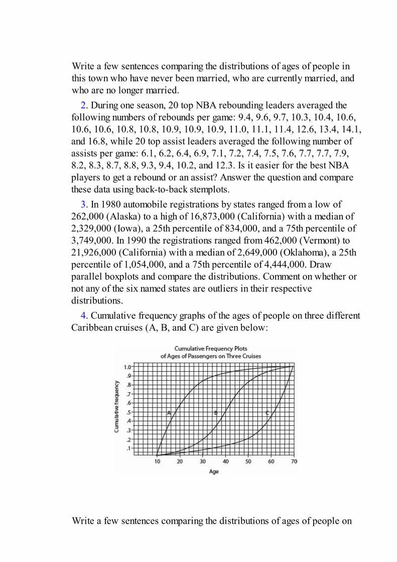
Write a few sentences comparing the distributions of ages of people inthis town who have never been married, who are currently married, andwho are no longer married.
2. During one season, 20 top NBA rebounding leaders averaged thefollowing numbers of rebounds per game: 9.4, 9.6, 9.7, 10.3, 10.4, 10.6,10.6, 10.6, 10.8, 10.8, 10.9, 10.9, 10.9, 11.0, 11.1, 11.4, 12.6, 13.4, 14.1,and 16.8, while 20 top assist leaders averaged the following number ofassists per game: 6.1, 6.2, 6.4, 6.9, 7.1, 7.2, 7.4, 7.5, 7.6, 7.7, 7.7, 7.9,8.2, 8.3, 8.7, 8.8, 9.3, 9.4, 10.2, and 12.3. Is it easier for the best NBAplayers to get a rebound or an assist? Answer the question and comparethese data using back-to-back stemplots.
3. In 1980 automobile registrations by states ranged from a low of262,000 (Alaska) to a high of 16,873,000 (California) with a median of2,329,000 (Iowa), a 25th percentile of 834,000, and a 75th percentile of3,749,000. In 1990 the registrations ranged from 462,000 (Vermont) to21,926,000 (California) with a median of 2,649,000 (Oklahoma), a 25thpercentile of 1,054,000, and a 75th percentile of 4,444,000. Drawparallel boxplots and compare the distributions. Comment on whether ornot any of the six named states are outliers in their respectivedistributions.
4. Cumulative frequency graphs of the ages of people on three differentCaribbean cruises (A, B, and C) are given below:
Write a few sentences comparing the distributions of ages of people on

the three cruises.

TOPIC 4Exploring Bivariate Data
• Scatterplots• Correlation and Linearity• Least Squares Regression Line• Residual Plots
• Outliers and Influential Points• Transformations to Achieve Linearity
Our studies so far have been concerned with measurements of a singlevariable. However, many important applications of statistics involve examiningwhether two or more variables are related to one another. For example, is therea relationship between the smoking histories of pregnant women and the birthweights of their children? Between SAT scores and success in college?Between amount of fertilizer used and amount of crop harvested?
Two questions immediately arise. First, how can the strength of an apparentrelationship be measured? Second, how can an observed relationship be put intofunctional terms? For example, a real estate broker might not only wish todetermine whether a relationship exists between the prime rate and the numberof new homes sold in a month but might also find useful an expression withwhich to predict the number of home sales given a particular value of the primerate.
A graphical display, called a scatterplot, gives an immediate visualimpression of a possible relationship between two variables, while a numericalmeasurement, called a correlation coefficient, is often used as a quantitativevalue of the strength of a linear relationship. In either case, evidence of arelationship is not evidence of causation.
SCATTERPLOTSSuppose a relationship is perceived between two quantitative variables X andY, and we graph the pairs (x, y). We are interested in the strength of thisrelationship, the scatterplot arising from the relationship, and any deviation fromthe basic pattern of this relationship. In this topic we examine whether therelationship can be reasonably explained in terms of a linear function, that is,one whose graph is a straight line.
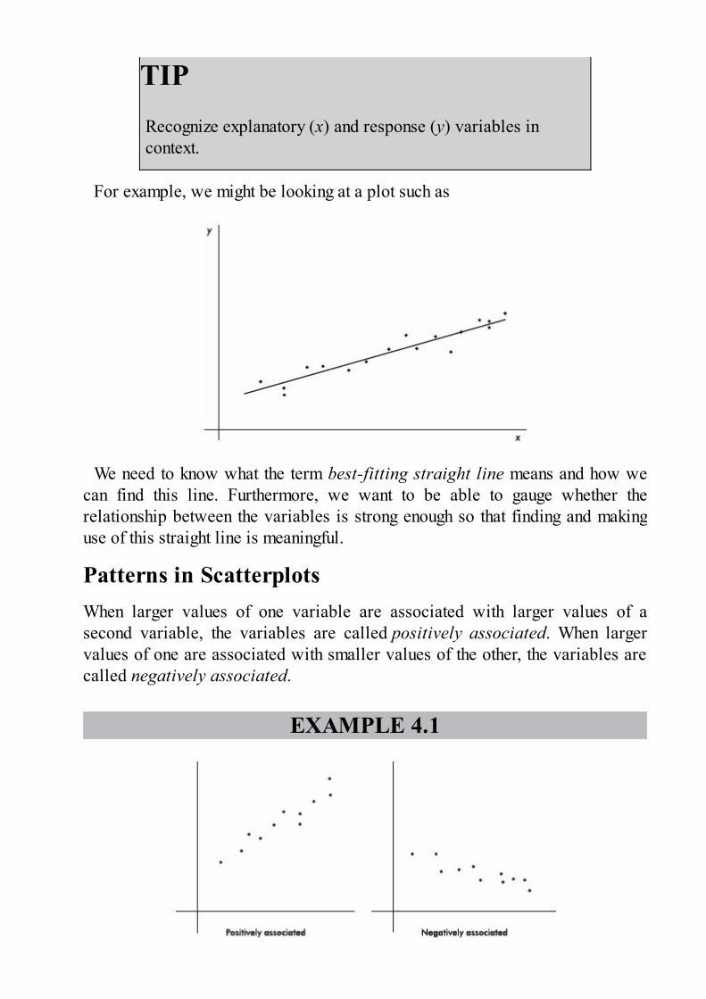
TIPRecognize explanatory (x) and response (y) variables incontext.
For example, we might be looking at a plot such as
We need to know what the term best-fitting straight line means and how wecan find this line. Furthermore, we want to be able to gauge whether therelationship between the variables is strong enough so that finding and makinguse of this straight line is meaningful.
Patterns in ScatterplotsWhen larger values of one variable are associated with larger values of asecond variable, the variables are called positively associated. When largervalues of one are associated with smaller values of the other, the variables arecalled negatively associated.
EXAMPLE 4.1

The strength of the association is gauged by how close the plotted points are to a straightline.
EXAMPLE 4.2
Sometimes different dots in a scatterplot are labeled with different symbols or differentcolors to show a categorical variable. The resulting labeled scatterplot might distinguishbetween men and women, between stocks and bonds, and so on.
EXAMPLE 4.3
The above diagram is a labeled scatterplot distinguishing men with plus signs and womenwith square dots to show a categorical variable.
When analyzing the overall pattern in a scatterplot, it is also important to noteclusters and outliers.

EXAMPLE 4.4An experiment was conducted to note the effect of temperature and light on the potencyof a particular antibiotic. One set of vials of the antibiotic was stored under differenttemperatures, but under the same lighting, while a second set of vials was stored underdifferent lightings, but under the same temperature.
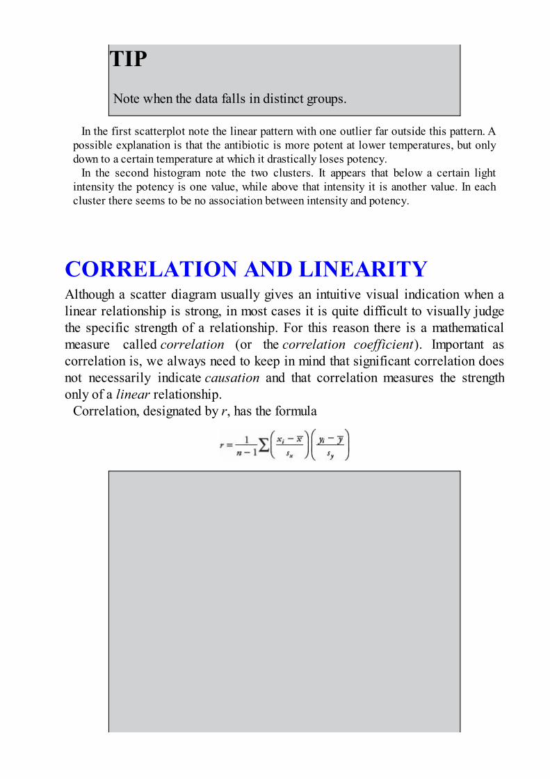
TIPNote when the data falls in distinct groups.
In the first scatterplot note the linear pattern with one outlier far outside this pattern. Apossible explanation is that the antibiotic is more potent at lower temperatures, but onlydown to a certain temperature at which it drastically loses potency.
In the second histogram note the two clusters. It appears that below a certain lightintensity the potency is one value, while above that intensity it is another value. In eachcluster there seems to be no association between intensity and potency.
CORRELATION AND LINEARITYAlthough a scatter diagram usually gives an intuitive visual indication when alinear relationship is strong, in most cases it is quite difficult to visually judgethe specific strength of a relationship. For this reason there is a mathematicalmeasure called correlation (or the correlation coefficient). Important ascorrelation is, we always need to keep in mind that significant correlation doesnot necessarily indicate causation and that correlation measures the strengthonly of a linear relationship.
Correlation, designated by r, has the formula

TIPCorrelation does not imply causation!
in terms of the means and standard deviations of the two sets. We note that theformula is actually the sum of the products of the corresponding z-scoresdivided by 1 less than the sample size. However, you should be able to quicklycalculate correlation using the statistical package on your calculator.(Examining the formula helps you understand where correlation is coming from,but you will NOT have to use the formula to calculate r.)

TIPWith standardized data (z-scores), r is the slope of theregression line.
Note from the formula that correlation does not distinguish between whichvariable is called x and which is called y. The formula is also based onstandardized scores (z-scores), and so changing units does not change thecorrelation. Finally, since means and standard deviations can be stronglyinfluenced by outliers, correlation is also strongly affected by extreme values.
The value of r always falls between –1 and +1, with –1 indicating perfectnegative correlation and +1 indicating perfect positive correlation. It should bestressed that a correlation at or near zero doesn’t mean there isn’t a relationshipbetween the variables; there may still be a strong nonlinear relationship.
EXAMPLE 4.5
It can be shown that r2, called the coefficient of determination, is the ratio of the varianceof the predicted values to the variance of the observed values y. That is, there is apartition of the y-variance, and r2 is the proportion of this variance that is predictablefrom a knowledge of x. Alternatively, we can say that r2 gives the percentage of variationin y that is explained by the variation in x. In either case, always interpret r2 in context ofthe problem. Remember when calculating r from r2 that r may be positive or negative.
While the correlation r is given as a decimal between –1.0 and 1.0, the coefficient ofdetermination r2 is usually given as a percentage. An r2 of 100% is a perfect fit, with allthe variation in y explained by variation in x. How large a value of r2 is desirable dependson the application under consideration. While scientific experiments often aim for an r2
in the 90% or above range, observational studies with r2 of 10% to 20% might beconsidered informative. Note that while a correlation of .6 is twice a correlation of .3, the

corresponding r2 of 36% is four times the corresponding r2 of 9%.
LEAST SQUARES REGRESSION LINEWhat is the best-fitting straight line that can be drawn through a set of points?
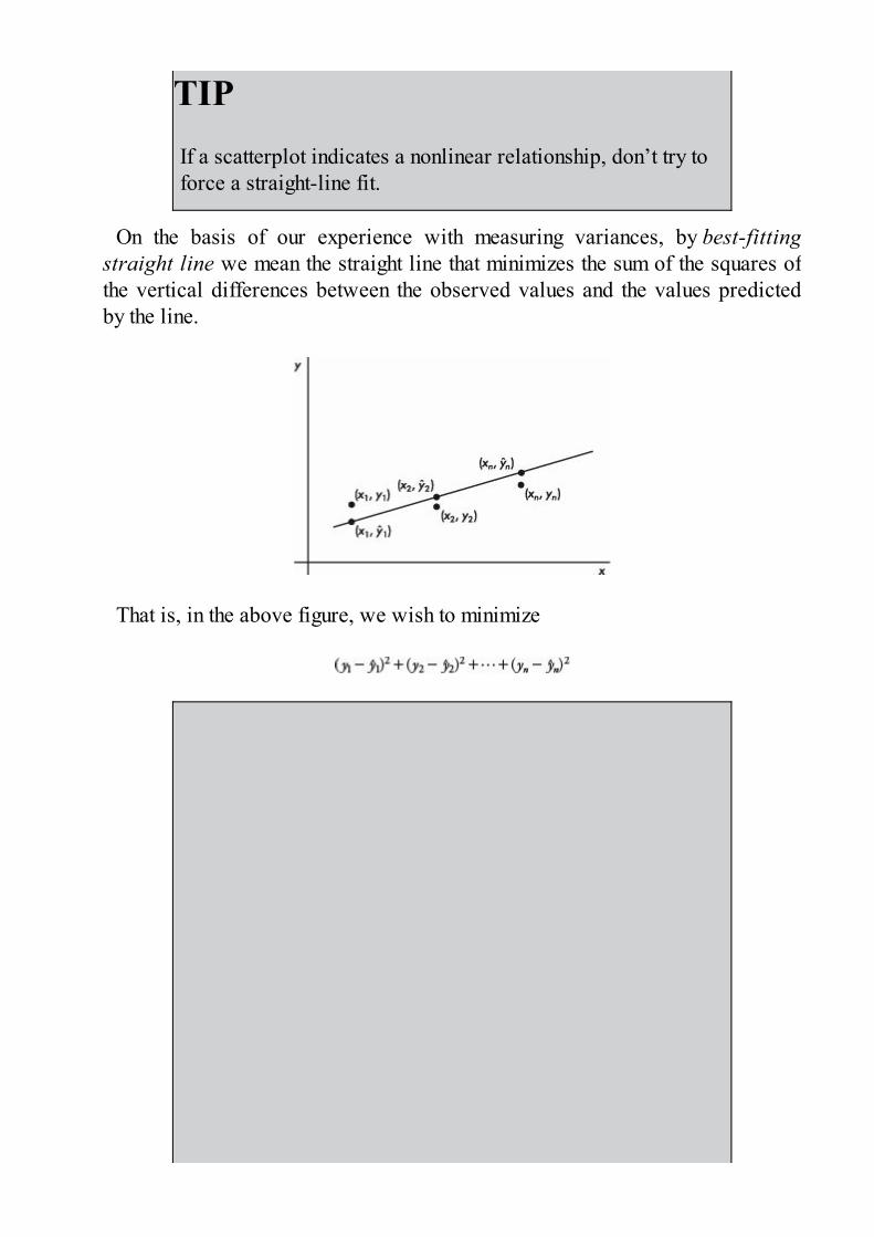
TIPIf a scatterplot indicates a nonlinear relationship, don’t try toforce a straight-line fit.
On the basis of our experience with measuring variances, by best-fittingstraight line we mean the straight line that minimizes the sum of the squares ofthe vertical differences between the observed values and the values predictedby the line.
That is, in the above figure, we wish to minimize
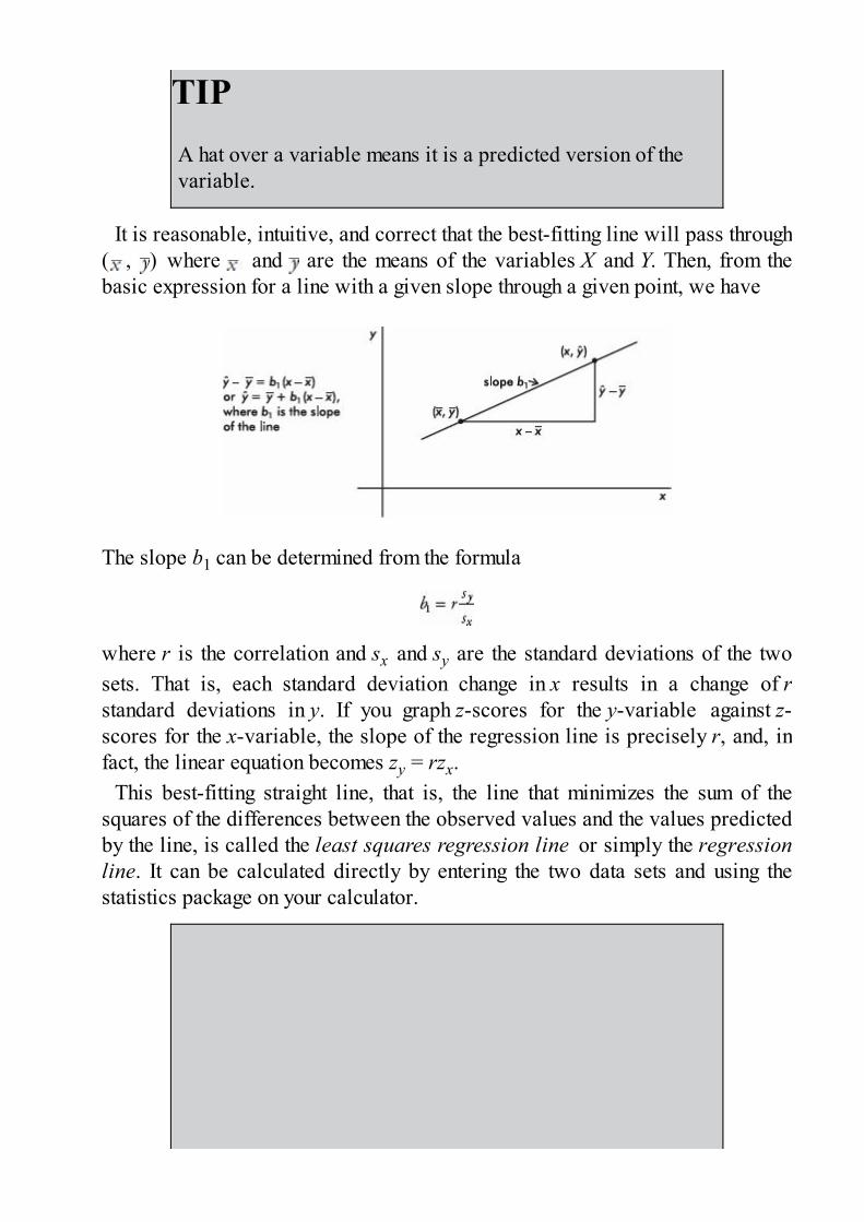
TIPA hat over a variable means it is a predicted version of thevariable.
It is reasonable, intuitive, and correct that the best-fitting line will pass through( , ) where and are the means of the variables X and Y. Then, from thebasic expression for a line with a given slope through a given point, we have
The slope b1 can be determined from the formula
where r is the correlation and sx and sy are the standard deviations of the twosets. That is, each standard deviation change in x results in a change of rstandard deviations in y. If you graph z-scores for the y-variable against z-scores for the x-variable, the slope of the regression line is precisely r, and, infact, the linear equation becomes zy = rzx.
This best-fitting straight line, that is, the line that minimizes the sum of thesquares of the differences between the observed values and the values predictedby the line, is called the least squares regression line or simply the regressionline. It can be calculated directly by entering the two data sets and using thestatistics package on your calculator.

TIPJust because we can calculate a regression line doesn’t meanit is useful.
EXAMPLE 4.6An insurance company conducts a survey of 15 of its life insurance agents. The averagenumber of minutes spent with each potential customer and the number of policies sold ina week are noted for each agent. Letting X and Y represent the average number of minutesand the number of sales, respectively, we have
Find the equation of the best-fitting straight line for the data.Answer: Plotting the 15 points (25, 10), (23, 11), . . . , (20, 11) gives an intuitive visual
impression of the relationship:

TIPBe sure to label axes and show number scales wheneverpossible.
This scatter diagram indicates the existence of a relationship that appears to be linear;that is, the points lie roughly on a straight line. Furthermore, the linear relationship ispositive; that is, as one variable increases, so does the other (the straight line slopesupward).Using a calculator, we find the correlation to be r = .8836, the coefficient ofdetermination to be r2 = .78 (indicating that 78% of the variation in the number ofpolicies is explained by the variation in the number of minutes spent), and the regressionline to be
We also write: = –1.73 + 0.5492 MinutesAdding this to our scatterplot yields
Thus, for example, we might predict that agents who average 24 minutes per customerwill average 0.5492(24) – 1.73 = 11.45 sales per week. We also note that each additionalminute spent seems to produce an average 0.5492 extra sale.

TIPUse meaningful variable names.
EXAMPLE 4.7

TIPBe careful about extrapolation beyond the observed x-values.
Following are advertising expenditures and total sales for six detergent products:
Predict the total sales if $5000 is spent on advertising and interpret the slope of theregression line. What if $100,000 is spent on advertising?
Answer: With your calculator, the equation of the regression line is found to be
(A calculator like the TI-84, with less round-off error, directly gives = 59.683 +7.295x.)
It is also worthwhile to replace the x and y with more appropriately named variables,resulting, for example, in
The regression line predicts that if $5000 is spent on advertising, the resulting totalsales will be 7.293(5) + 59.691 = 96.156 thousands of dollars ($96,156).
The slope of the regression line indicates that every extra $1000 spent on advertisingwill result in an average of $7293 in added sales.
If $100,000 is spent on advertising, we calculate 7.293(100) + 59.691 = 788.991thousands of dollars (≈ $789,000). How much confidence should we have in this answer?Not much! We are trying to use the regression line to predict a value far outside the rangeof the data values. This procedure is called extrapolation and must be used with greatcare.
It should be noted that when we use the regression line to predict a y-value for a given x-value, we are actually predicting the mean y-value for that given x-value. For any given x-value, there are many possible y-values, and we are predicting their mean. So if $5000 isspent many times on advertising, various resulting total sales figures may result, but theirpredicted average is $96,156.
The TI-Nspire gives
EXAMPLE 4.8A random sample of 30 U.S. farm regions surveyed during the summer of 2003 producedthe following statistics:
Average temperature (°F) during growing season: = 81, sx = 3Average corn yield per acre (bu.): = 131, sy = 5Correlation r = .32
Based on this study, what is the mean predicted corn yield for a region where the averagegrowing season temperature is 76.5°F?
Answer: 76.5 is standard deviations below the average temperaturereported in the study, so with a correlation of r = .32, the predicted corn yield is .32(–1.5) = –0.48 standard deviations below the average corn yield, or 131 – 0.48(5) = 128.6bushels per acre.
Alternatively, we could have found the linear regression equation relating thesevariables: , intercept ≈ 131 – 81(0.533) ≈ 87.8, and thus =0.533 Temp + 87.8. Then 0.533(76.5) + 87.8 ≈ 128.6.
RESIDUAL PLOTSThe difference between an observed and predicted value is called the residual.When the regression line is graphed on the scatterplot, the residual of a point isthe vertical distance the point is from the regression line.
The regression line is the line that minimizes the sum of the squares of theresiduals.

TIPBe able to calculate the residual for each data value.
EXAMPLE 4.9We calculate the predicted values from the regression line in Example 4.7 and subtractfrom the observed values to obtain the residuals:
Note that the sum of the residuals is0.5 + 3.7 + 1.3 + 5.1 – 0.7 – 9.9 = 0.0
The TI-Nspire easily shows the “squares of the residuals,” the sum of which is minimizedby the regression line.
The above equation is true in general; that is, the sum and thus the mean ofthe residuals is always zero.
The notation for residuals is and so The standard deviation
of the residuals is calculated as follows:
se gives a measure of how the points are spread around the regression line.Plotting the residuals gives further information. In particular, a residual plot

with a definite pattern is an indication that a nonlinear model will show a betterfit to the data than the straight regression line. In addition to whether or not theresiduals are randomly distributed, one should look at the balance betweenpositive and negative residuals and also the size of the residuals in comparisonto the associated y-values.
The residuals can be plotted against either the x-values or the -values (since is a linear transformation of x, the plots are identical except for scale and a
left-right reversal when the slope is negative).
It is also important to understand that a linear model may be appropriate, butweak, with a low correlation. And, alternatively, a linear model may not be thebest model (as evidenced by the residual plot), but it still might be a very goodmodel with high r2.
EXAMPLE 4.10Suppose the drying time of a paint product varies depending on the amount of a certainadditive it contains.
Using a calculator, we find the regression line = 0.327x + 1.062, and we find theresiduals:
The resulting residual plot shows a strong pattern:
This pattern indicates that a nonlinear model will be a better fit than a straight-line model.A scatterplot of the original data shows clearly what is happening:

The ability to interpret computer output is important not only to do well on theAP Statistics exam, but also to understand statistical reports in the business andscientific world.
EXAMPLE 4.11Miles per gallon versus speed for a new model automobile is fitted with a least squaresregression line. The graph of the residuals and some computer output for the regressionare as follows:Regression Analysis: MPG Versus Speed
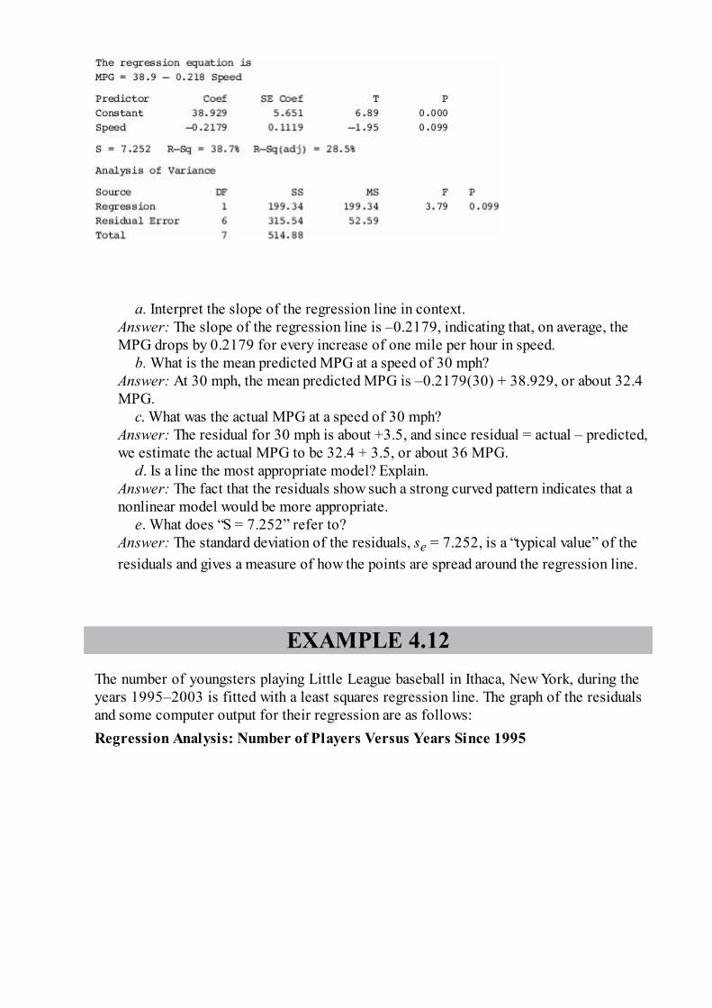
a. Interpret the slope of the regression line in context.Answer: The slope of the regression line is –0.2179, indicating that, on average, theMPG drops by 0.2179 for every increase of one mile per hour in speed.
b. What is the mean predicted MPG at a speed of 30 mph?Answer: At 30 mph, the mean predicted MPG is –0.2179(30) + 38.929, or about 32.4MPG.
c. What was the actual MPG at a speed of 30 mph?Answer: The residual for 30 mph is about +3.5, and since residual = actual – predicted,we estimate the actual MPG to be 32.4 + 3.5, or about 36 MPG.
d. Is a line the most appropriate model? Explain.Answer: The fact that the residuals show such a strong curved pattern indicates that anonlinear model would be more appropriate.
e. What does “S = 7.252” refer to?Answer: The standard deviation of the residuals, se = 7.252, is a “typical value” of theresiduals and gives a measure of how the points are spread around the regression line.
EXAMPLE 4.12The number of youngsters playing Little League baseball in Ithaca, New York, during theyears 1995–2003 is fitted with a least squares regression line. The graph of the residualsand some computer output for their regression are as follows:Regression Analysis: Number of Players Versus Years Since 1995
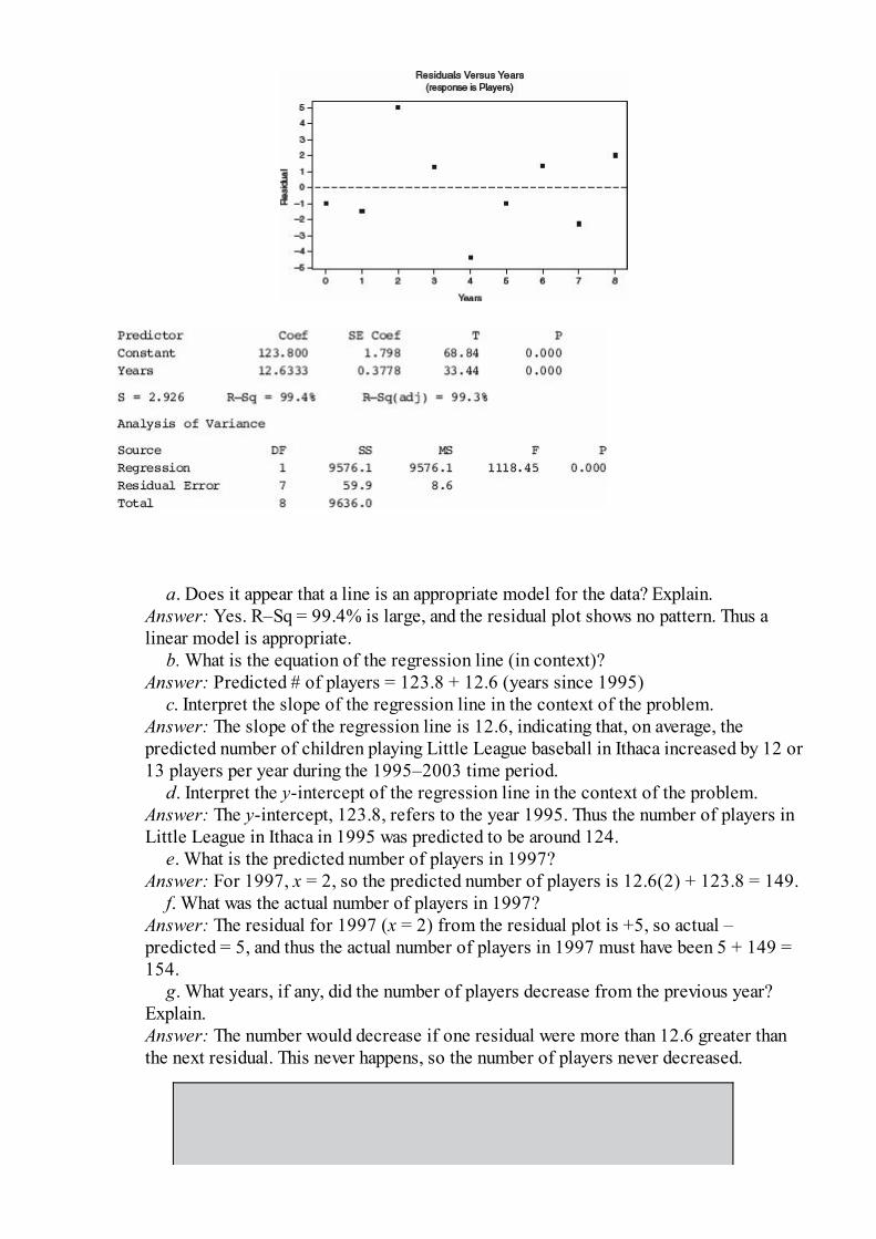
a. Does it appear that a line is an appropriate model for the data? Explain.Answer: Yes. R–Sq = 99.4% is large, and the residual plot shows no pattern. Thus alinear model is appropriate.
b. What is the equation of the regression line (in context)?Answer: Predicted # of players = 123.8 + 12.6 (years since 1995)
c. Interpret the slope of the regression line in the context of the problem.Answer: The slope of the regression line is 12.6, indicating that, on average, thepredicted number of children playing Little League baseball in Ithaca increased by 12 or13 players per year during the 1995–2003 time period.
d. Interpret the y-intercept of the regression line in the context of the problem.Answer: The y-intercept, 123.8, refers to the year 1995. Thus the number of players inLittle League in Ithaca in 1995 was predicted to be around 124.
e. What is the predicted number of players in 1997?Answer: For 1997, x = 2, so the predicted number of players is 12.6(2) + 123.8 = 149.
f. What was the actual number of players in 1997?Answer: The residual for 1997 (x = 2) from the residual plot is +5, so actual –predicted = 5, and thus the actual number of players in 1997 must have been 5 + 149 =154.
g. What years, if any, did the number of players decrease from the previous year?Explain.Answer: The number would decrease if one residual were more than 12.6 greater thanthe next residual. This never happens, so the number of players never decreased.
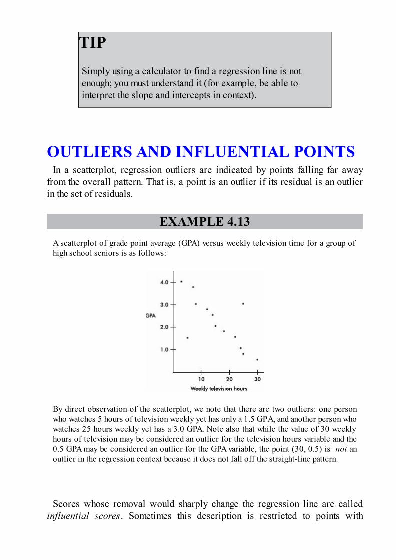
TIPSimply using a calculator to find a regression line is notenough; you must understand it (for example, be able tointerpret the slope and intercepts in context).
OUTLIERS AND INFLUENTIAL POINTSIn a scatterplot, regression outliers are indicated by points falling far away
from the overall pattern. That is, a point is an outlier if its residual is an outlierin the set of residuals.
EXAMPLE 4.13A scatterplot of grade point average (GPA) versus weekly television time for a group ofhigh school seniors is as follows:
By direct observation of the scatterplot, we note that there are two outliers: one personwho watches 5 hours of television weekly yet has only a 1.5 GPA, and another person whowatches 25 hours weekly yet has a 3.0 GPA. Note also that while the value of 30 weeklyhours of television may be considered an outlier for the television hours variable and the0.5 GPA may be considered an outlier for the GPA variable, the point (30, 0.5) is not anoutlier in the regression context because it does not fall off the straight-line pattern.
Scores whose removal would sharply change the regression line are calledinfluential scores. Sometimes this description is restricted to points with

extreme x-values. An influential score may have a small residual but still have agreater effect on the regression line than scores with possibly larger residualsbut average x-values.
EXAMPLE 4.14Consider the following scatterplot of six points and the regression line:
The heavy line in the scatterplot on the left below shows what happens when point A isremoved, and the heavy line in the scatterplot on the right below shows what happenswhen point B is removed.
Note that the regression line is greatly affected by the removal of point A but not by theremoval of point B. Thus point A is an influential score, while point B is not. This is truein spite of the fact that point A is closer to the original regression line than point B.
TRANSFORMATIONS TO ACHIEVELINEARITYOften a straight-line pattern is not the best model for depicting a relationshipbetween two variables. A clear indication of this problem is when thescatterplot shows a distinctive curved pattern. Another indication is when theresiduals show a distinctive pattern rather than a random scattering. In such acase, the nonlinear model can sometimes be revealed by transforming one orboth of the variables and then noting a linear relationship. Usefultransformations often result from using the log or ln buttons on your calculator to

create new variables.
EXAMPLE 4.15Consider the following years and corresponding populations:
The scatterplot and residual plot indicate that a nonlinear relationship would be an evenstronger model.
Letting log y be a new variable, we obtain
The scatterplot and residual plot now indicate a stronger linear relationship.

A regression analysis yields = 0.013x – 23.65. In context we have: = –23.65+ 0.013(Year). So, for example, the population predicted for the year 2000 would becalculated = 0.013(2000) – 23.65 = 2.35, and so Pop = 102.35 ≈ 224 thousand, or224,000. The “linear” equation = 0.013x – 23.65 can be re-expressed as =100.013x–23.65 [= 10–23.65 × (100.013)x = 2.2387E–24 × 1.0304x].
There are many useful transformations. For example:
Log y as a linear function of x, log y = ax + b, re-expresses as an exponential:
y = 10ax+b or y = b110ax where b1 = 10b
Log y as a linear function of log x, log y = a log x + b, re-expresses as a power :
y = 10a log x+b or y = b1xa where b1 = 10b
as a linear function of x, = ax + b, re-expresses as a quadratic:
y = (ax + b)2
as a linear function of x, = ax + b, re-expresses as a reciprocal:
y as a linear function of log x, y = a log x + b, is a logarithmic function.
Note: Although you need to be able to recognize the need for a transformation,justify its appropriateness (residuals plot), use whichever is appropriate from
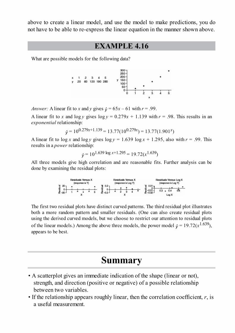
above to create a linear model, and use the model to make predictions, you donot have to be able to re-express the linear equation in the manner shown above.
EXAMPLE 4.16What are possible models for the following data?
Answer: A linear fit to x and y gives = 65x – 61 with r = .99.A linear fit to x and log y gives log y = 0.279x + 1.139 with r = .98. This results in anexponential relationship:
= 100.279x+1.139 = 13.77(100.279x) = 13.77(1.901x)A linear fit to log x and log y gives log y = 1.639 log x + 1.295, also with r = .99. Thisresults in a power relationship:
= 101.639 log x+1.295 = 19.72(x1.639)All three models give high correlation and are reasonable fits. Further analysis can bedone by examining the residual plots:
The first two residual plots have distinct curved patterns. The third residual plot illustratesboth a more random pattern and smaller residuals. (One can also create residual plotsusing the derived curved models, but we choose to restrict our attention to residual plotsof the linear models.) Among the above three models, the power model = 19.72(x1.639),appears to be best.
Summary• A scatterplot gives an immediate indication of the shape (linear or not),
strength, and direction (positive or negative) of a possible relationshipbetween two variables.
• If the relationship appears roughly linear, then the correlation coefficient, r, isa useful measurement.
• The value of r is always between –1 and +1, with positive values indicatingpositive association and negative values indicating negative association; andvalues close to –1 or +1 indicating a stronger linear association than valuesclose to 0, which indicate a weaker linear association.
• Evidence of an association is not evidence of a cause-and-effect relationship!• Correlation is not affected by which variable is called x and which y or by
changing units.• Correlation can be strongly affected by extreme values.• The differences between the observed and predicted values are called
residuals.• The best-fitting straight line, called the regression line, minimizes the sum of
the squares of the residuals.• For the linear regression model, the mean of the residuals is always 0.• A definite pattern in the residual plot indicates that a nonlinear model may fit
the data better than the straight regression line.• The coefficient of determination, r2, gives the percentage of variation in y that
is accounted for by the variation in x.• Influential scores are scores whose removal would sharply change the
regression line.• Nonlinear models can sometimes be studied by transforming one or both
variables and then noting a linear relationship.• It is very important to be able to interpret generic computer output.
Questions on Topic Four:Exploring Bivariate Data
Multiple-Choice Questions
Directions: The questions or incomplete statements that follow are eachfollowed by five suggested answers or completions. Choose the responsethat best answers the question or completes the statement.
1. A study collects data on average combined SAT scores (math,critical reading, and writing) and percentage of students who took theexam at 100 randomly selected high schools. Following is part of thecomputer printout for regression:

Which of the following is a correct conclusion?
(A) SAT in the variable column indicates that SAT is the dependent(response) variable.
(B) The correlation is ±0.875, but the sign cannot be determined.(C) The y-intercept indicates the mean combined SAT score if
percent of students taking the exam has no effect on combined SATscores.
(D) The R2 value indicates that the residual plot does not show astrong pattern.
(E) Schools with lower percentages of students taking the exam tendto have higher average combined SAT scores.
2. A simple random sample of 35 world-ranked chess players providesthe following statistics:
Number of hours of study per day: = 6.2, sx = 1.3Yearly winnings: = $208,000, sy = $42,000Correlation r = .15
Based on this data, what is the resulting linear regression equation?
(A) = 178,000 + 4850 Hours
(B) = 169,000 + 6300 Hours

(C) = 14,550 + 31,200 Hours
(D) = 7750 + 32,300 Hours
(E) = –52,400 + 42,000 Hours
3. A rural college is considering constructing a windmill to generateelectricity but is concerned over noise levels. A study is performedmeasuring noise levels (in decibels) at various distances (in feet) from thecampus library, and a least squares regression line is calculated with acorrelation of 0.74. Which of the following is a proper and mostinformative conclusion for an observation with a negative residual?
(A) The measured noise level is 0.74 times the predicted noiselevel.
(B) The predicted noise level is 0.74 times the measured noise level.(C) The measured noise level is greater than the predicted noise
level.(D) The predicted noise level is greater than the measured noise
level.(E) The slope of the regression line at that point must also be
negative.
4. Consider the following three scatterplots:

Which has the greatest correlation coefficient?
(A) I(B) II(C) III(D) They all have the same correlation coefficient.(E) This question cannot be answered without additional
information.
5. Suppose the correlation is negative. Given two points from thescatterplot, which of the following is possible?
I. The first point has a larger x-value and a smaller y-value than thesecond point.
II. The first point has a larger x-value and a larger y-value than thesecond point.
III. The first point has a smaller x-value and a larger y-value than thesecond point.
(A) I only(B) II only(C) III only(D) I and III(E) I, II, and III
6. Consider the following residual plot:
Which of the following scatterplots could have resulted in the aboveresidual plot? (The y-axis scales are not the same in the scatterplots as inthe residual plot.)

(A)
(B)
(C)
(D)
(E) None of these could result in the given residual plot.
7. Suppose the regression line for a set of data, = 3x + b, passesthrough the point (2, 5). If and are the sample means of the x- and y-values, respectively, then =
(A) .(B) – 2.(C) + 5.(D) 3 .(E) 3 – 1.
8. Suppose a study finds that the correlation coefficient relating familyincome to SAT scores is r = +1. Which of the following are properconclusions?
I. Poverty causes low SAT scores.

II. Wealth causes high SAT scores.III. There is a very strong association between family income and
SAT scores.
(A) I only(B) II only(C) III only(D) I and II(E) I, II, and III
9. A study of department chairperson ratings and student ratings of the
performance of high school statistics teachers reports a correlation of r =1.15 between the two ratings. From this information we can conclude that
(A) chairpersons and students tend to agree on who is a goodteacher.
(B) chairpersons and students tend to disagree on who is a goodteacher.
(C) there is little relationship between chairperson and studentratings of teachers.
(D) there is strong association between chairperson and studentratings of teachers, but it would be incorrect to infer causation.
(E) a mistake in arithmetic has been made.
10. Which of the following statements about correlation r is true?
(A) A correlation of .2 means that 20% of the points are highlycorrelated.
(B) Perfect correlation, that is, when the points lie exactly on astraight line, results in r = 0.
(C) Correlation is not affected by which variable is called x and

which is called y.(D) Correlation is not affected by extreme values.(E) A correlation of .75 indicates a relationship that is 3 times as
linear as one for which the correlation is only .25.
Questions 11–13 refer to the following:
The relationship between winning game proportions when facing the sunand when the sun is on one’s back is analyzed for a random sample of 10professional players. The computer printout for regression is below:
11. What is the equation of the regression line, where face and back are thewinning game proportions when facing the sun and with back to the sun,respectively?
(A) = 0.056 + 0.920 back(B) = 0.056 + 0.920 facing(C) = 0.920 + 0.056 back(D) = 0.920 + 0.056 facing(E) = 0.024 + 0.039 back

12. What is the correlation?
(A) –.984(B) –.986(C) .984(D) .986(E) .993
13. For one player, the winning game proportions were 0.55 and 0.59
for facing and back, respectively. What was the associated residual?
(A) –0.028(B) 0.028(C) –0.0488(D) 0.0488(E) 0.3608
14. Which of the following statements about residuals are true?
I. The mean of the residuals is always zero.II. The regression line for a residual plot is a horizontal line.III. A definite pattern in the residual plot is an indication that a
nonlinear model will show a better fit to the data than the straightregression line.
(A) I and II(B) I and III(C) II and III(D) I, II, and III(E) None of the above gives the complete set of true responses.
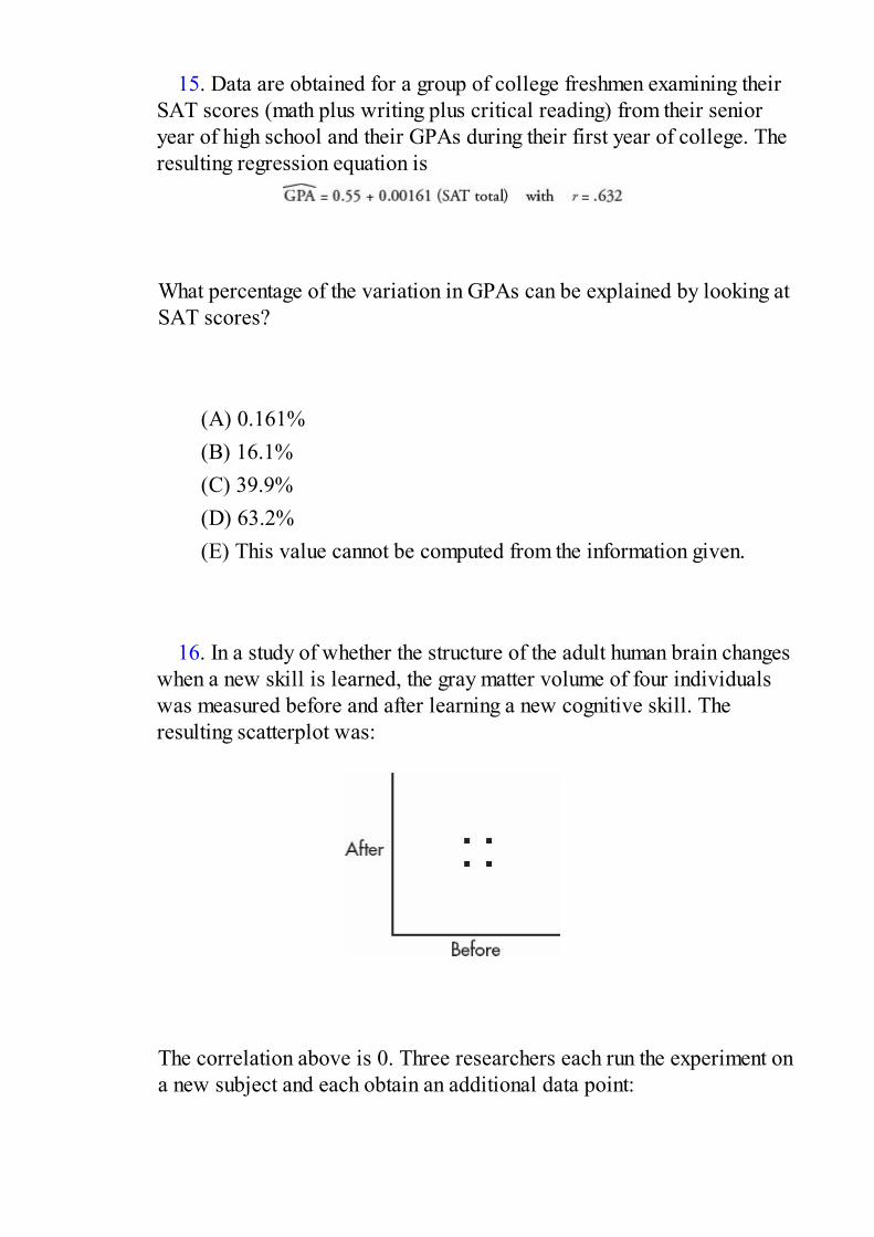
15. Data are obtained for a group of college freshmen examining theirSAT scores (math plus writing plus critical reading) from their senioryear of high school and their GPAs during their first year of college. Theresulting regression equation is
What percentage of the variation in GPAs can be explained by looking atSAT scores?
(A) 0.161%(B) 16.1%(C) 39.9%(D) 63.2%(E) This value cannot be computed from the information given.
16. In a study of whether the structure of the adult human brain changeswhen a new skill is learned, the gray matter volume of four individualswas measured before and after learning a new cognitive skill. Theresulting scatterplot was:
The correlation above is 0. Three researchers each run the experiment ona new subject and each obtain an additional data point:

Match the above scatterplots with their new correlations.
(A) (B) (C) (D) (E)
17. In a study of winning percentage in home games versus averagehome attendance for professional baseball teams, the resulting regressionline is:
What is the residual if a team has a winning percentage of 55% with anaverage attendance of 34,000?
(A) –11.0(B) –0.8(C) 0.8(D) 11.0(E) 23.0

18. Consider the following scatterplot of midterm and final exam
scores for a class of 15 students.
Which of the following is incorrect?
(A) The same number of students scored 100 on the midterm exam asscored 100 on the final exam.
(B) Students who scored higher on the midterm exam tended to scorehigher on the final exam.
(C) The scatterplot shows a moderate negative correlation betweenmidterm and final exam scores.
(D) The coefficient of determination here is positive.(E) No one scored 90 or above on both exams.
19. If every woman married a man who was exactly 2 inches taller thanshe, what would the correlation between the heights of married men andwomen be?
(A) Somewhat negative(B) 0(C) Somewhat positive

(D) Nearly 1(E) 1
20. Suppose the correlation between two variables is r = .23. What
will the new correlation be if .14 is added to all values of the x-variable,every value of the y-variable is doubled, and the two variables areinterchanged?
(A) .23(B) .37(C) .74(D) –.23(E) –.74
21. Suppose the correlation between two variables is –.57. If each of
the y-scores is multiplied by –1, which of the following is true about thenew scatterplot?
(A) It slopes up to the right, and the correlation is –.57.(B) It slopes up to the right, and the correlation is +.57.(C) It slopes down to the right, and the correlation is –.57.(D) It slopes down to the right, and the correlation is +.57.(E) None of the above is true.
22. Consider the set of points {(2, 5), (3, 7), (4, 9), (5, 12), (10, n)}.What should n be so that the correlation between the x- and y-values is 1?
(A) 21(B) 24(C) 25(D) A value different from any of the above.
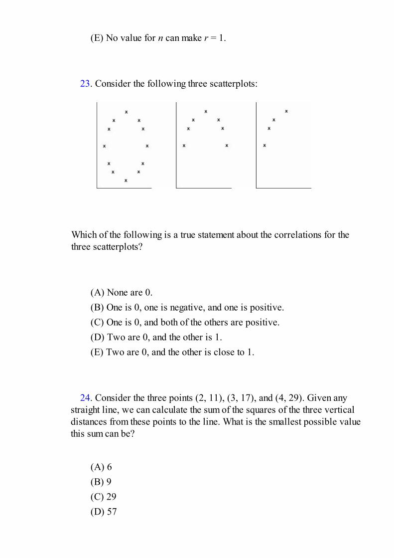
(E) No value for n can make r = 1.
23. Consider the following three scatterplots:
Which of the following is a true statement about the correlations for thethree scatterplots?
(A) None are 0.(B) One is 0, one is negative, and one is positive.(C) One is 0, and both of the others are positive.(D) Two are 0, and the other is 1.(E) Two are 0, and the other is close to 1.
24. Consider the three points (2, 11), (3, 17), and (4, 29). Given anystraight line, we can calculate the sum of the squares of the three verticaldistances from these points to the line. What is the smallest possible valuethis sum can be?
(A) 6(B) 9(C) 29(D) 57

(E) None of these values
25. Suppose that the scatterplot of log X and log Y shows a strong
positive correlation close to 1. Which of the following is true?
(A) The variables X and Y also have a correlation close to 1.(B) A scatterplot of the variables X and Y shows a strong nonlinear
pattern.(C) The residual plot of the variables X and Y shows a random
pattern.(D) A scatterplot of X and log Y shows a strong linear pattern.(E) A cause-and-effect relationship can be concluded between log X
and log Y.
26. Consider n pairs of numbers. Suppose = 2, sx = 3, = 4, and sy =5. Of the following, which could be the least squares line?
(A) = –2 + x(B) = 2x(C) = –2 + 3x(D) = – x
(E) = 6 – x
Free-Response Questions
Directions: You must show all work and indicate the methods you use. Youwill be graded on the correctness of your methods and on the accuracy ofyour final answers.
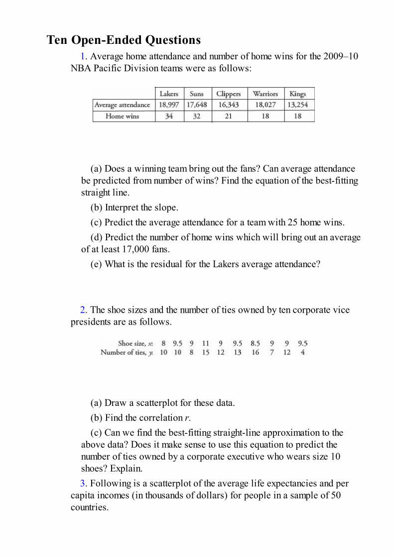
Ten Open-Ended Questions1. Average home attendance and number of home wins for the 2009–10
NBA Pacific Division teams were as follows:
(a) Does a winning team bring out the fans? Can average attendancebe predicted from number of wins? Find the equation of the best-fittingstraight line.
(b) Interpret the slope.(c) Predict the average attendance for a team with 25 home wins.(d) Predict the number of home wins which will bring out an average
of at least 17,000 fans.(e) What is the residual for the Lakers average attendance?
2. The shoe sizes and the number of ties owned by ten corporate vicepresidents are as follows.
(a) Draw a scatterplot for these data.(b) Find the correlation r.(c) Can we find the best-fitting straight-line approximation to the
above data? Does it make sense to use this equation to predict thenumber of ties owned by a corporate executive who wears size 10shoes? Explain.3. Following is a scatterplot of the average life expectancies and per
capita incomes (in thousands of dollars) for people in a sample of 50countries.
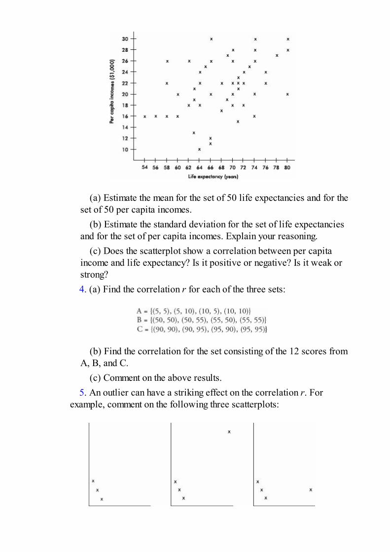
(a) Estimate the mean for the set of 50 life expectancies and for theset of 50 per capita incomes.
(b) Estimate the standard deviation for the set of life expectanciesand for the set of per capita incomes. Explain your reasoning.
(c) Does the scatterplot show a correlation between per capitaincome and life expectancy? Is it positive or negative? Is it weak orstrong?4. (a) Find the correlation r for each of the three sets:
(b) Find the correlation for the set consisting of the 12 scores fromA, B, and C.
(c) Comment on the above results.5. An outlier can have a striking effect on the correlation r. For
example, comment on the following three scatterplots:

6. Fuel economy y (in miles per gallon) is tabulated for various speedsx (in miles per hour) for a certain car model. A linear regression modelgives Predicted fuel economy = 34.8 – 0.16 (Speed) with the followingresidual plot:
A quadratic regression model gives = –0.0032x2 + 0.26x + 23.8 withthe following residual plot:
(a) What does each model predict for fuel economy at 50 miles perhour?
(b) Which model is a better fit? Explain.7. The following scatterplot shows the grades for research papers for a
sociology professor’s class plotted against the lengths of the papers (inpages).

Mary turned in her paper late and was told by the professor that her gradewould have been higher if she had turned it in on time. A computerprintout fitting a straight line to the data (not including Mary’s score) bythe method of least squares gives
(a) Find the correlation coefficient for the relationship betweengrade and length of paper based on these data (excluding Mary’spaper).
(b) What is the slope of the regression line and what does it signify?(c) How will the correlation coefficient change if Mary’s paper is
included? Explain your answer.(d) How will the slope of the regression line change if Mary’s paper
is included? Explain your answer.(e) What grade did Mary receive? Predict what she would have
received if her paper had been on time.
8. Data show a trend in winning long jump distances for aninternational competition over the years 1972–92. With jumps recorded ininches and dates in years since 1900, a least squares regression line is fit

to the data. The computer output and a graph of the residuals are asfollows:
(a) Does a line appear to be an appropriate model? Explain.(b) What is the slope of the least squares line? Give an interpretation
of the slope.(c) What is the correlation?(d) What is the predicted winning distance for the 1980 competition?(e) What was the actual winning distance in 1980?
9. A scatterplot of the number of accidents per day on a particularinterstate highway during a 30-day month is as follows:
(a) Draw a histogram of the frequencies of the number of accidents.(b) Draw a boxplot of the number of accidents.(c) Name a feature apparent in the scatterplot but not in the histogram
or boxplot.(d) Name a feature clearly shown by the histogram and boxplot but
not as obvious in the scatterplot.
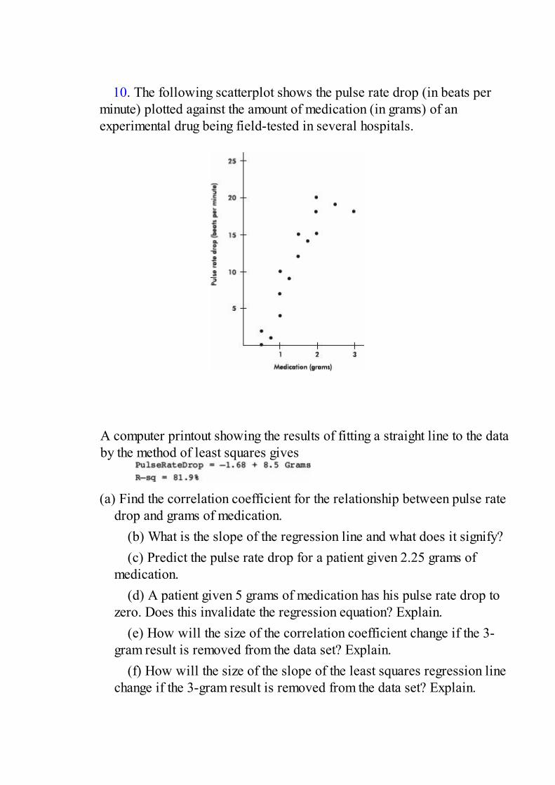
10. The following scatterplot shows the pulse rate drop (in beats perminute) plotted against the amount of medication (in grams) of anexperimental drug being field-tested in several hospitals.
A computer printout showing the results of fitting a straight line to the databy the method of least squares gives
(a) Find the correlation coefficient for the relationship between pulse ratedrop and grams of medication.
(b) What is the slope of the regression line and what does it signify?(c) Predict the pulse rate drop for a patient given 2.25 grams of
medication.(d) A patient given 5 grams of medication has his pulse rate drop to
zero. Does this invalidate the regression equation? Explain.(e) How will the size of the correlation coefficient change if the 3-
gram result is removed from the data set? Explain.(f) How will the size of the slope of the least squares regression line
change if the 3-gram result is removed from the data set? Explain.


TOPIC 5Exploring Categorical Data: FrequencyTables
• Marginal Frequencies for Two-Way Tables• Conditional Relative Frequencies and Association
While many variables such as age, income, and years of education arequantitative or numerical in nature, others such as gender, race, brandpreference, mode of transportation, and type of occupation are qualitative orcategorical. Quantitative variables, too, are sometimes grouped into categoricalclasses.
MARGINAL FREQUENCIES FOR TWO-WAY TABLESQualitative data often encompass two categorical variables that may or may nothave a dependent relationship. These data can be displayed in a two-waycontingency table.
EXAMPLE 5.1A 4-year study, reported in The New York Times, on men more than 70 years old analyzedblood cholesterol and noted how many men with different cholesterol levels sufferednonfatal or fatal heart attacks.
Severity of heart attacks is the row variable , while cholesterol level is the columnvariable.
One method of analyzing these data involves first calculating the totals for each row and

each column:
These totals are placed in the right and bottom margins of the table and thus are calledmarginal frequencies.
These marginal frequencies are often put in the form of proportions or percentages. Themarginal distribution of the cholesterol level is
This distribution can also be displayed in a bar graph as follows:
Similarly we can determine the marginal distribution for the severity of heart attacks:

The representative bar graph is
CONDITIONAL RELATIVEFREQUENCIES AND ASSOCIATIONThe marginal distributions described and calculated above do not describe ormeasure the relationship between the two categorical variables. For this wemust consider the information in the body of the table, not just the sums in themargins.
EXAMPLE 5.2Is hair loss pattern related to body mass index? One study (Journal of the AmericanMedical Association, February 24, 1993, page 1000) of 769 men showed the followingnumbers:
The analysis first involves finding the row and column totals as we did before.
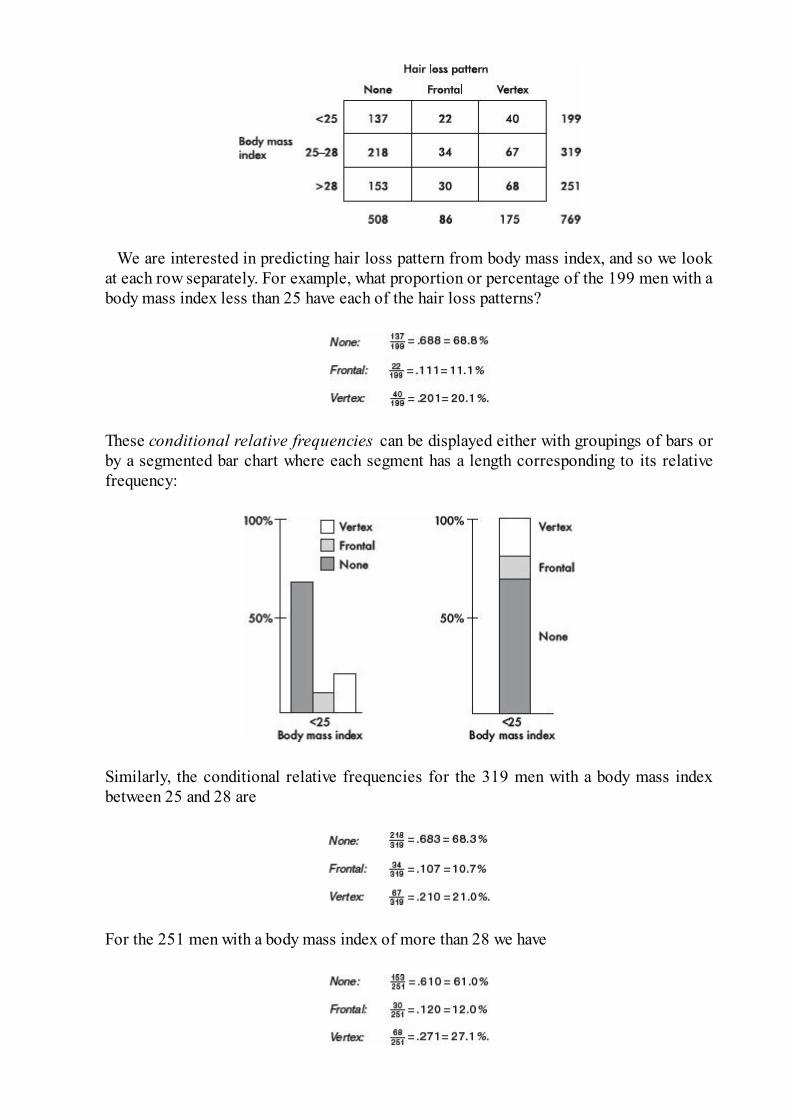
We are interested in predicting hair loss pattern from body mass index, and so we lookat each row separately. For example, what proportion or percentage of the 199 men with abody mass index less than 25 have each of the hair loss patterns?
These conditional relative frequencies can be displayed either with groupings of bars orby a segmented bar chart where each segment has a length corresponding to its relativefrequency:
Similarly, the conditional relative frequencies for the 319 men with a body mass indexbetween 25 and 28 are
For the 251 men with a body mass index of more than 28 we have

Both of the following bar charts give good visual pictures:
Segmented bar charts indicate a slight relationship between higher vertex pattern baldnessand a body mass index of more than 28.
EXAMPLE 5.3A study was made to compare year in high school with preference for vanilla or chocolateice cream with the following results:
What are the conditional relative frequencies for each class?
In such a case, where all the conditional relative frequency distributions are identical, wesay that the two variables show perfect independence. (However, it should be noted thateven if the two variables are completely independent, the chance is very slim that aresulting contingency table will show perfect independence.)
EXAMPLE 5.4

Suppose you need heart surgery and are trying to decide between two surgeons, Dr. Fixitand Dr. Patch. You find out that each operated 250 times last year with the followingresults:
Whom should you go to? Among Dr. Fixit’s 250 patients 190 survived, for a survival rateof or 76%, while among Dr. Patch’s 250 patients 200 survived, for a survival rateof or 80%. Your choice seems clear.
However, everything may not be so clear-cut. Suppose that on further investigation youdetermine that the surgeons operated on patients who were in either good or poorcondition with the following results:
Note that adding corresponding boxes from these two tables gives the original tableabove.
How do the surgeons compare when operating on patients in good health? Dr. Fixit’s 68patients in good condition have a survival rate of or 88.2%, while Dr. Patch’s137 patients in good condition have a survival rate of or 87.6%. Similarly, wenote that Dr. Fixit’s 182 patients in poor condition have a survival rate of or71.4%, while Dr. Patch’s 113 patients in poor condition have a survival rate of or 70.8%.
Thus Dr. Fixit does better with patients in good condition (88.2% versus Dr. Patch’s87.6%) and also does better with patients in poor condition (71.4% versus Dr. P’s70.8%). However, Dr. Fixit has a lower overall patient survival rate (76% versus Dr.Patch’s 80%)! How can this be?
This problem is an example of Simpson’s paradox, where a comparison can be reversedwhen more than one group is combined to form a single group. The effect of anothervariable, sometimes called a lurking variable, is masked when the groups are combined.In this particular example, closer scrutiny reveals that Dr. Fixit operates on many morepatients in poor condition than Dr. Patch, and these patients in poor condition areprecisely the ones with lower survival rates. Thus even though Dr. Fixit does better withall patients, his overall rating is lower. Our original table hid the effect of the lurkingvariable related to the condition of the patients.
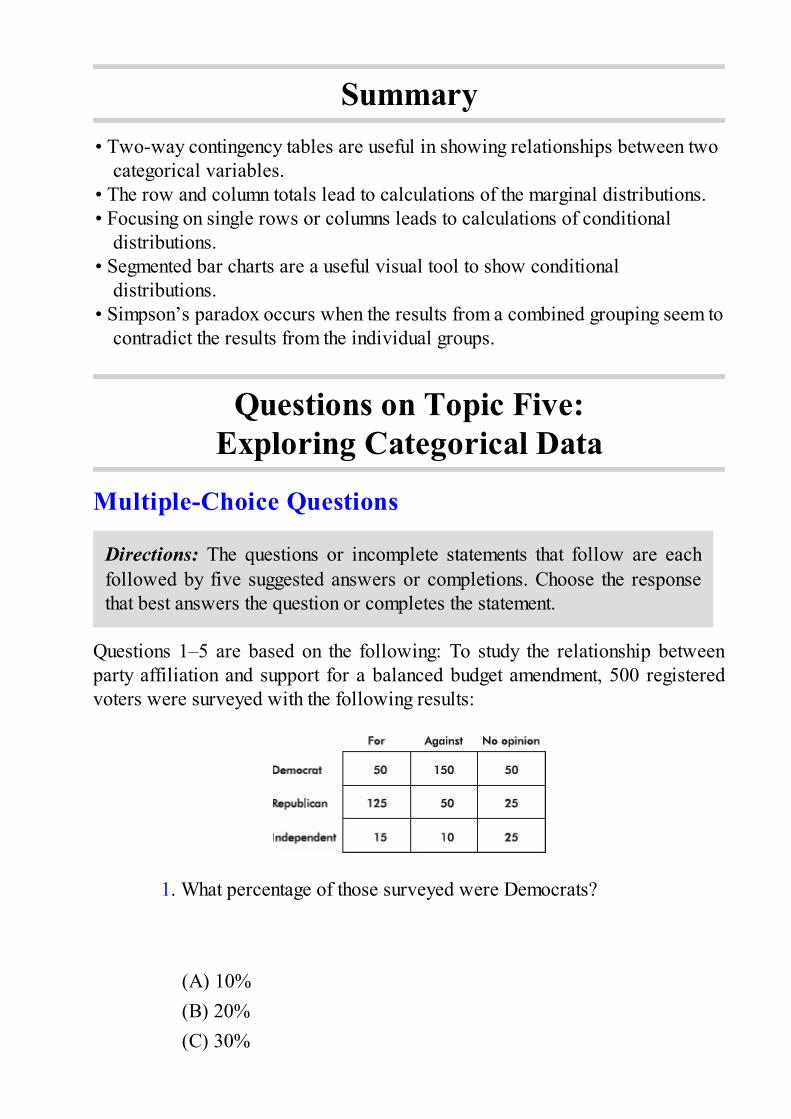
Summary• Two-way contingency tables are useful in showing relationships between two
categorical variables.• The row and column totals lead to calculations of the marginal distributions.• Focusing on single rows or columns leads to calculations of conditional
distributions.• Segmented bar charts are a useful visual tool to show conditional
distributions.• Simpson’s paradox occurs when the results from a combined grouping seem to
contradict the results from the individual groups.
Questions on Topic Five:Exploring Categorical Data
Multiple-Choice Questions
Directions: The questions or incomplete statements that follow are eachfollowed by five suggested answers or completions. Choose the responsethat best answers the question or completes the statement.
Questions 1–5 are based on the following: To study the relationship betweenparty affiliation and support for a balanced budget amendment, 500 registeredvoters were surveyed with the following results:
1. What percentage of those surveyed were Democrats?
(A) 10%(B) 20%(C) 30%
(D) 40%(E) 50%
2. What percentage of those surveyed were for the amendment and wereRepublicans?
(A) 25%(B) 38%(C) 40%(D) 62.5%(E) 65.8%
3. What percentage of Independents had no opinion?
(A) 5%(B) 10%(C) 20%(D) 25%(E) 50%
4. What percentage of those against the amendment were Democrats?
(A) 30%(B) 42%(C) 50%(D) 60%
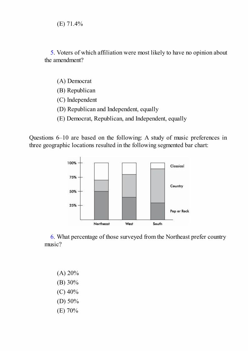
(E) 71.4%
5. Voters of which affiliation were most likely to have no opinion aboutthe amendment?
(A) Democrat(B) Republican(C) Independent(D) Republican and Independent, equally(E) Democrat, Republican, and Independent, equally
Questions 6–10 are based on the following: A study of music preferences inthree geographic locations resulted in the following segmented bar chart:
6. What percentage of those surveyed from the Northeast prefer countrymusic?
(A) 20%(B) 30%(C) 40%(D) 50%(E) 70%

7. Which of the following is greatest?
(A) The percentage of those from the Northeast who prefer classical.(B) The percentage of those from the West who prefer country.(C) The percentage of those from the South who prefer pop or rock.(D) The above are all equal.(E) It is impossible to determine the answer without knowing the
actual numbers of people involved.
8. Which of the following is greatest?
(A) The number of people in the Northeast who prefer pop or rock.(B) The number of people in the West who prefer classical.(C) The number of people in the South who prefer country.(D) The above are all equal.(E) It is impossible to determine the answer without knowing the
actual numbers of people involved.
9. All three bars have a height of 100%.
(A) This is a coincidence.(B) This happened because each bar shows a complete distribution.(C) This happened because there are three bars each divided into
three segments.(D) This happened because of the nature of musical patterns.(E) None of the above is true.
10. Based on the given segmented bar chart, does there seem to be arelationship between geographic location and music preference?
(A) Yes, because the corresponding segments of the three bars havedifferent lengths.
(B) Yes, because the heights of the three bars are identical.(C) Yes, because there are three segments and three bars.(D) No, because the heights of the three bars are identical.(E) No, because summing the corresponding segments for classical,
summing the corresponding segments for country, and summing thecorresponding segments for pop or rock all give approximately thesame total.
11. In the following table, what value for n results in a table showingperfect independence?
(A) 10(B) 40(C) 60(D) 75(E) 100
12. A company employs both men and women in its secretarial and
executive positions. In reports filed with the government, the companyshows that the percentage of female employees who receive raises ishigher than the percentage of male employees who receive raises. Agovernment investigator claims that the percentage of male secretarieswho receive raises is higher than the percentage of female secretarieswho receive raises, and that the percentage of male executives who

receive raises is higher than the percentage of female executives whoreceive raises. Is this possible?
(A) No, either the company report is wrong or the investigator’sclaim is wrong.
(B) No, if the company report is correct, then either a greaterpercentage of female secretaries than of male secretaries receive raisesor a greater percentage of female executives than of male executivesreceive raises.
(C) No, if the investigator is correct, then by summation of thecorresponding numbers, the total percentage of male employees whoreceive raises would have to be greater than the total percentage offemale employees who receive raises.
(D) All of the above are true.(E) It is possible for both the company report to be true and the
investigator’s claim to be correct.
Free-Response Questions
Directions: You must show all work and indicate the methods you use. Youwill be graded on the correctness of your methods and on the accuracy ofyour final answers.
Two Open-Ended Questions1. The following table gives the numbers (in thousands) of officers and
enlisted personnel by military branch in the U.S. armed forces.
(a) Calculate the percentagei. of military men and women who are enlisted.
ii. of military men and women who are not Marine Corps officers.iii. of officers who are in the Navy.

(b) Construct a graphical display showing the association betweencareer path (officer vs. enlisted) and military branch.
(c) Summarize what the graphical display illustrates about theassociation between career path (officer vs. enlisted) and militarybranch.2. The graduate school at the University of California at Berkeley
reported that in 1973 they accepted 44% of 8442 male applicants and35% of 4321 female applicants. Concerned that one of their programswas guilty of gender bias, the graduate school analyzed admissions to thesix largest graduate programs and obtained the following results:
(a) Find the percentage of men and the percentage of womenaccepted by each program. Comment on any pattern or bias you see.
(b) Find the percentage of men and the percentage of womenaccepted overall by these six programs. Does this appear to contradictthe results from part (a)?
(c) If you worked in the Graduate Admissions Office, what wouldyou say to an inquiring reporter who is investigating gender bias ingraduate admissions?
THEME TWO: PLANNING A STUDYTOPIC 6
Overview of Methods of Data Collection
• Census• Sample Survey
• Experiment• Observational Study
In the real world, time and cost considerations usually make it impossible toanalyze an entire population. Does the government question you and yourparents before announcing the monthly unemployment rates? Does a televisionproducer check every household’s viewing preferences before deciding whethera pilot program will be continued? In studying statistics we learn how toestimate population characteristics by considering a sample. For example, laterin this ebook we will see how to estimate population means and proportions bylooking at sample means and proportions.
To derive conclusions about the larger population, we need to be confidentthat the sample we have chosen represents that population fairly. Analyzing thedata with computers is often easier than gathering the data, but the frequentlyquoted “Garbage in, garbage out” applies here. Nothing can help if the data arebadly collected. Unfortunately, many of the statistics with which we arebombarded by newspapers, radio, and television are based on poorly designeddata collection procedures.
CENSUSA census is a complete enumeration of an entire population. In common use, it isoften thought of as an official attempt to contact every member of the population,usually with details regarding age, marital status, race, gender, occupation,income, years of school completed, and so on. Every 10 years the U.S. Bureauof the Census divides the nation into nine regions and attempts to gatherinformation about everyone in the country. A massive amount of data isobtained, but even with the resources of the U.S. government, the census is notcomplete. For example, many homeless people are always missed, or counted attwo temporary residences, and there are always households that do not respond
even after repeated requests for information. It was estimated that the 2000census missed about 3.3 million people (1.2% of the population).
In most studies, both in the private and public sectors, a complete census isunreasonable because of time and cost involved. Furthermore, attempts to gathercomplete data have been known to lead to carelessness. Finally, and mostimportant, a well-designed, well-conducted sample survey is far superior to apoorly designed study involving a complete census. For example, a poorlyworded question might give meaningless data even if everyone in the populationanswers.
SAMPLE SURVEYThe census tries to count everyone; it is not a sample. A sample survey aims toobtain information about a whole population by studying a part of it, that is, asample. The goal is to gather information without disturbing or changing thepopulation. Numerous procedures are used to collect data through sampling, andmuch of the statistical information distributed to us comes from sample surveys.Often, controlled experiments are later undertaken to demonstrate relationshipssuggested by sample surveys.
However, the one thing that most quickly invalidates a sample and makesuseful information impossible to obtain is bias. A sample is biased if in somecritical way it does not represent the population. The main technique to avoidbias is to incorporate randomness into the selection process. Randomizationprotects us from effects and influences, both known and unknown. Finally, thelarger the sample, the better the results, but what is critical is the sample size,not the percentage or fraction of the population. That is, a random sample of size500 from a population of size 100,000 is just as representative as a randomsample of size 500 from a population of size 1,000,000.
EXPERIMENTIn a controlled study, called an experiment, the researcher should randomlydivide subjects into appropriate groups. Some action is taken on one or more ofthe groups, and the response is observed. For example, patients may berandomly given unmarked capsules of either aspirin or acetaminophen and theeffects of the medication measured. Experiments often have a treatment groupand a control group ; in the ideal situation, neither the subjects nor theresearcher knows which group is which. The Salk vaccine experiment of the1950s, in which half the children received the vaccine and half were given aplacebo, with not even their doctors knowing who received what, is a classicexample of this double-blind approach. Controlled experiments can indicate

cause-and-effect relationships.The critical principles behind good experimental design include control
(outside of who receives what treatments, conditions should be as similar aspossible for all involved groups), blocking (the subjects can be divided intorepresentative groups to bring certain differences directly into the picture),randomization (unknown and uncontrollable differences are handled byrandomizing who receives what treatments), replication (treatments need to berepeated on a sufficient number of subjects), and generalizability (ability torepeat an experiment in a variety of settings).
OBSERVATIONAL STUDYSample surveys are one example of what are called observational studies. Inobservational studies there is no choice in regard to who goes into the treatmentand control groups. For example, a researcher cannot ethically tell 100 peopleto smoke three packs of cigarettes a day and 100 others to smoke only one packper day; he can only observe people who habitually smoke these amounts. Inobservational studies the researcher strives to determine which variables affectthe noted response. While results may suggest relationships, it is difficult toconclude cause and effect.
Observational studies are primary, vital sources of data; however, they are apoor method of measuring the effect of change. To evaluate responses to change,one must impose change, that is, perform an experiment. Furthermore,observational studies on the impact of some variable on another variable oftenfail because explanatory variables are confounded with other variables.

Summary• A complete census is usually unreasonable because of time and cost
constraints.• Estimate population characteristics (called parameters) by considering
statistics from a sample.• Analysis of badly gathered sample data is usually a meaningless exercise.• A sample is biased if in some critical way it does not represent the
population.• The main technique to avoid bias is to incorporate randomness into the
selection process.• Experiments involve applying a treatment to one or more groups and
observing the responses.• Observational studies involve observing responses to choices people make.
Questions on Topic Six: Overview ofMethods of Data Collection
Multiple-Choice Questions
Directions: The questions or incomplete statements that follow are eachfollowed by five suggested answers or completions. Choose the responsethat best answers the question or completes the statement.
1. When travelers change airlines during connecting flights, each airlinereceives a portion of the fare. Several years ago, the major airlines used asample trial period to determine what percentage of certain fares eachshould collect. Using these statistical results to determine fare splits, theairlines now claim huge savings over previous clerical costs. Which ofthe following is true?
I. The airlines ran an experiment using a trial period for the controlgroup.
II. The airlines ran an observational study using the calculations froma trial period as a sample.
III. The airlines feel that any monetary error in fare splitting resultingfrom using a statistical sample is smaller than the previous clericalcosts necessary to calculate exact fare splits.

(A) I only(B) II only(C) III only(D) I and III(E) II and III
2. Which of the following are true statements?
I. In an experiment some treatment is intentionally forced on onegroup to note the response.
II. In an observational study information is gathered on an alreadyexisting situation.
III. Sample surveys are observational studies, not experiments.
(A) I and II(B) I and III(C) II and III(D) I, II, and III(E) None of the above gives the complete set of true responses.
3. Which of the following are true statements?I. In an experiment researchers decide how people are placed in
different groups.II. In an observational study, the participants select which group they
are in.III. A control group is most often a self-selected grouping in an
experiment.
(A) I and II(B) I and III
(C) II and III(D) I, II, and III(E) None of the above gives the complete set of true responses.
4. In one study on the effect of niacin on cholesterol level, 100 subjectswho acknowledged being long-time niacin takers had their cholesterollevels compared with those of 100 people who had never taken niacin. Ina second study, 50 subjects were randomly chosen to receive niacin and50 were chosen to receive a placebo.
(A) The first study was a controlled experiment, while the secondwas an observational study.
(B) The first study was an observational study, while the second wasa controlled experiment.
(C) Both studies were controlled experiments.(D) Both studies were observational studies.(E) Each study was part controlled experiment and part
observational study.
5. In one study subjects were randomly given either 500 or 1000milligrams of vitamin C daily, and the number of colds they came downwith during a winter season was noted. In a second study peopleresponded to a questionnaire asking about the average number of hoursthey sleep per night and the number of colds they came down with duringa winter season.
(A) The first study was an experiment without a control group, whilethe second was an observational study.
(B) The first study was an observational study, while the second wasa controlled experiment.
(C) Both studies were controlled experiments.
(D) Both studies were observational studies.(E) None of the above is a correct statement.
6. In a 1992 London study, 12 out of 20 migraine sufferers were givenchocolate whose flavor was masked by peppermint, while the remainingeight sufferers received a similar-looking, similar-tasting tablet that hadno chocolate. Within 1 day, five of those receiving chocolate complainedof migraines, while no complaints were made by any of those who did notreceive chocolate. Which of the following is a true statement?
(A) This study was an observational study of 20 migraine sufferersin which it was noted how many came down with migraines after eatingchocolate.
(B) This study was a sample survey in which 12 out of 20 migrainesufferers were picked to receive peppermint-flavored chocolate.
(C) A census of 20 migraine sufferers was taken, noting how manywere given chocolate and how many developed migraines.
(D) A study was performed using chocolate as a placebo to studyone cause of migraines.
(E) An experiment was performed comparing a treatment group thatwas given chocolate to a control group that was not.
7. Suppose you wish to compare the average class size of mathematicsclasses to the average class size of English classes in your high school.Which is the most appropriate technique for gathering the needed data?
(A) Census(B) Sample survey(C) Experiment(D) Observational study(E) None of these methods is appropriate.
8. Which of the following are true statements?I. Based on careful use of control groups, experiments can often
indicate cause-and-effect relationships.II. While observational studies may suggest relationships, great care
must be taken in concluding that there is cause and effect because of thelack of control over lurking variables.
III. A complete census is the only way to establish a cause-and-effectrelationship absolutely.
(A) I and II(B) I and III(C) II and III(D) I, II, and III(E) None of the above gives the complete set of true responses.
9. Two studies are run to compare the experiences of families living inhigh-rise public housing to those of families living in townhousesubsidized rentals. The first study interviews 25 families who have beenin each government program for at least 1 year, while the secondrandomly assigns 25 families to each program and interviews them after 1year. Which of the following is a true statement?
(A) Both studies are observational studies because of the timeperiod involved.
(B) Both studies are observational studies because there are nocontrol groups.
(C) The first study is an observational study, while the second is anexperiment.
(D) The first study is an experiment, while the second is anobservational study.

(E) Both studies are experiments.
10. Two studies are run to determine the effect of low levels of wineconsumption on cholesterol level. The first study measures the cholesterollevels of 100 volunteers who have not consumed alcohol in the past yearand compares these values with their cholesterol levels after 1 year,during which time each volunteer drinks one glass of wine daily. Thesecond study measures the cholesterol levels of 100 volunteers who havenot consumed alcohol in the past year, randomly picks half the group todrink one glass of wine daily for a year while the others drink no alcoholfor the year, and finally measures their levels again. Which of thefollowing is a true statement?
(A) The first study is an observational study, while the second is anexperiment.
(B) The first study is an experiment, while the second is anobservational study.
(C) Both studies are observational studies, but only one uses bothrandomization and a control group.
(D) The first study is a census of 100 volunteers, while the secondstudy is an experiment.
(E) Both studies are experiments.

TOPIC 7Planning and Conducting Surveys
• Simple Random Sampling• Characteristics of a Well-Designed, Well-
Conducted Survey
• Sampling Error• Sources of Bias• Other Sampling Methods
Most data collection involves observational studies, not controlledexperiments. Furthermore, while most data collection has some purpose, manystudies come to mind after the data have been assembled and examined. For datacollection to be useful, the resulting sample must be representative of thepopulation under consideration.
SIMPLE RANDOM SAMPLINGHow can a good, that is, a representative, sample be chosen? The most accuratetechnique would be to write the name of each member of the population on acard, mix the cards thoroughly in a large box, and pull out a specified number ofcards. This method would give everyone in the population an equal chance ofbeing selected as part of the sample. Unfortunately, this method is usually tootime-consuming and too costly, and bias might still creep in if the mixing is notthorough. A simple random sample, that is, one in which every possiblesample of the desired size has an equal chance of being selected, can moreeasily be obtained by assigning a number to everyone in the population andusing a random number table or having a computer generate random numbers toindicate choices.
EXAMPLE 7.1Suppose 80 students are taking an AP Statistics course and the teacher wants to randomlypick out a sample of 10 students to try out a practice exam. She first assigns the studentsnumbers 01, 02, 03, . . . , 80. Reading off two digits at a time from a random numbertable, she ignores any over 80 and ignores repeats, stopping when she has a set of ten. Ifthe table began 75425 56573 90420 48642 27537 61036 15074 84675, she wouldchoose the students numbered 75, 42, 55, 65, 73, 04, 27, 53, 76, and 10. Note that 90 and86 are ignored because they are over 80, and the second and third occurrences of 42 are

ignored because they are repeats.
CHARACTERISTICS OF A WELL-DESIGNED, WELL-CONDUCTEDSURVEYA well-designed survey always incorporates chance, such as using randomnumbers from a table or a computer. However, the use of probability techniquesis not enough to ensure a representative sample. Often we don’t have a completelisting of the population, and so we have to be careful about exactly how we areapplying “chance.” Even when subjects are picked by chance, they may choosenot to respond to the survey or they may not be available to respond, thus callinginto question how representative the final sample really is. The wording of thequestions must be neutral—subjects give different answers depending on thephrasing.
EXAMPLE 7.2Suppose we are interested in determining the percentage of adults in a small town who eata nutritious breakfast. How about randomly selecting 100 numbers out of the telephonebook, calling each one, and asking whether the respondent is intelligent enough to eat anutritious breakfast every morning?
Answer: Random selection is good, but a number of questions should be addressed. Forexample, are there many people in the town without telephones or with unlisted numbers?How will the time of day the calls are made affect whether the selected people arereachable? If people are unreachable, will replacements be randomly chosen in the sameway or will this lead to a certain class of people being underrepresented? Finally, even ifthese issues are satisfactorily addressed, the wording of the question is clearly not neutral—unless the phrase intelligent enough is dropped, answers will be almost meaningless.
SAMPLING ERROR: THE VARIATIONINHERENT IN A SURVEYNo matter how well-designed and well-conducted a survey is, it still gives asample statistic as an estimate for a population parameter. Different samplesgive different sample statistics, all of which are estimates for the samepopulation parameter, and so error, called sampling error, is naturally present.This error can be described using probability; that is, we can say how likely we

are to have a certain size error. Generally, the chance of this error occurring issmaller when the sample size is larger. However, the way the data are obtainedis crucial—a large sample size cannot make up for a poor survey design orfaulty collection techniques.
EXAMPLE 7.3Each of four major news organizations surveys likely voters and separately reports thatthe percentage favoring the incumbent candidate is 53.4%, 54.1%, 52.0%, and 54.2%,respectively. What is the correct percentage? Did three or more of the newsorganizations make a mistake?
Answer: There is no way of knowing the correct population percentage from theinformation given. The four surveys led to four statistics, each an estimate of thepopulation parameter. No one made a mistake unless there was a bad survey, for example,one without the use of chance, or not representative of the population, or with poorwording of the question. Sampling differences are natural.
SOURCES OF BIAS IN SURVEYSPoorly designed sampling techniques result in bias, that is, in a tendency tofavor the selection of certain members of a population. If a study is biased, sizedoesn’t help—a large sample size will simply result in a large worthless study.Think about bias before running a study, because once all the data comes in,there is no way to recover if the sample was biased. Sometimes pilot testingwith a small sample will show bias that can be corrected before a larger sampleis obtained. Although each of the following sources of bias is definedseparately, there is overlap, and many if not most examples of bias involvemore than one of the following.

TIPSampling error is to be expected, while bias is to be avoided.
Household bias: When a sample includes only one member of any givenhousehold, members of large households are underrepresented. To respond tothis, pollsters sometimes give greater weight to members of larger households.
Nonresponse bias: A good example is that of most mailed questionnaires, asthey tend to have very low response percentages, and it is often unclear whichpart of the population is responding. Sometimes people chosen for a surveysimply refuse to respond or are unreachable or too difficult to contact.Answering machines and caller ID prevent easy contacts. To maximizeresponse rates, one can use multiple follow-up contacts and cash or otherincentives. Also, short, easily understood surveys generally have higherresponse rates.
Quota sampling bias: This results when interviewers are given free choice inpicking people, for example, to obtain a particular percentage men, aparticular percentage Catholic, or a particular percentage African-American.This flawed technique resulted in misleading polls leading to the ChicagoTribune making an early incorrect call of Thomas E. Dewey as the winnerover Harry S. Truman in the 1948 presidential election.
Response bias: The very question itself can lead to misleading results. Peopleoften don’t want to be perceived as having unpopular or unsavory views andso may respond untruthfully when face to face with an interviewer or whenfilling out a questionnaire that is not anonymous. Patients may lie aboutfollowing doctors’ orders, dieters may be dishonest about how strictly they’vefollowed a weight loss program, students may shade the truth about how manyhours they’ve studied for exams, and viewers may not want to admit they theywatch certain television programs.

TIPThink about potential bias before collecting data.
Selection bias: An often-cited example is the Literary Digest opinion poll thatpredicted a landslide victory for Alfred Landon over Franklin D. Roosevelt inthe 1936 presidential election. The Digest surveyed people with cars andtelephones, but in 1936 only the wealthy minority, who mainly votedRepublican, had cars and telephones. In spite of obtaining more than twomillion responses, the Digest picked a landslide for the wrong man!
Size bias: Throwing darts at a map to decide in which states to sample wouldbias in favor of geographically large states. Interviewing people checking outof the hospital would bias in favor of patients with short stays, since due tocosts, more people today have shorter stays. Having each student pick one coinout of a bag of 1000 coins to help estimate the total monetary value of thecoins in the bag would bias in favor of large coins, for example, quarters overdimes.
Undercoverage bias: This happens when there is inadequate representation.For example, telephone surveys simply ignore all those possible subjects whodon’t have telephones. In the 2008 presidential election surveys, phonesurveys went only to land line phones, leaving out many young adults whohave only cell phones. Another example is convenience samples, likeinterviews at shopping malls, which are based on choosing individuals whoare easy to reach. These interviews tend to produce data highlyunrepresentative of the entire population. Door-to-door household surveystypically miss college students and prison inmates, as well as the homeless.
Voluntary response bias: Samples based on individuals who offer toparticipate typically give too much emphasis to people with strong opinions.For example, radio call-in programs about controversial topics such as guncontrol, abortion, and school segregation do not produce meaningful data onwhat proportion of the population favor or oppose related issues. Onlinesurveys posted to websites are a modern source of voluntary response bias.
Wording bias: Nonneutral or poorly worded questions may lead to answersthat are very unrepresentative of the population. To avoid such bias, do not useleading questions, and write questions that are clear and relatively short. Alsobe careful of sequences of questions that lead respondents toward certainanswers.
Note: Again, it should be understood that there is considerable overlap amongthe above classifications. For example, a nonneutral question may be said tohave both response bias and wording bias. Selection bias and undercoveragebias often go hand in hand. Voluntary response bias and nonresponse bias areclearly related.
OTHER SAMPLING METHODSTime-and cost-saving modifications are often used to implement samplingprocedures other than simple random samples.
Systematic sampling involves listing the population in some order (forexample, alphabetically), choosing a random point to start, and then pickingevery tenth (or hundredth, or thousandth, or kth) person from the list. This givesa reasonable sample as long as the original order of the list is not in any wayrelated to the variables under consideration.

TIPKnow the difference between strata and clusters.
I n stratified sampling the population is divided into homogeneous groupscalled strata, and random samples of persons from all strata are chosen. Forexample, we can stratify by age or gender or income level or race and pick asample of people from each stratum. Note that all individuals in a given stratumhave a characteristic in common. We could further do proportional sampling,where the sizes of the random samples from each stratum depend on theproportion of the total population represented by the stratum.
I n cluster sampling the population is divided into heterogeneous groupscalled clusters, and we then take a random sample of clusters from among allthe clusters. For example, to survey high school seniors we could randomly pickseveral senior class homerooms in which to conduct our study. Note that eachcluster should resemble the entire population.
Multistage sampling refers to a procedure involving two or more steps, eachof which could involve any of the various sampling techniques. The Galluporganization often follows a procedure in which nationwide locations arerandomly selected, then neighborhoods are randomly selected in each of theselocations, and finally households are randomly selected in each of theseneighborhoods.
EXAMPLE 7.4Suppose a sample of 100 high school students from a school of size 5000 is to be chosento determine their views on the death penalty. One method would be to have each studentwrite his or her name on a slip of paper, put the papers in a box, and have the principalreach in and pull out 100 of the papers. However, questions could arise regarding howwell the papers are mixed up in the box. For example, how might the outcome be affectedif all students in one homeroom toss in their names at the same time so that their papersare clumped together? Another method would be to assign each student a number from 1to 5000 and then use a random number table, picking out four digits at a time and tossingout repeats and numbers over 5000 (simple random sampling). What are alternativeprocedures?
Answer: From a list of the students, the surveyor could simply note every fiftieth name(systematic sampling). Since students in each class have certain characteristics incommon, the surveyor could use a random selection method to pick 25 students fromeach of the separate lists of freshmen, sophomores, juniors, and seniors (stratifiedsampling). The researcher could separate the homerooms by classes; then randomly pickfive freshmen homerooms, five sophomore homerooms, five junior homerooms, and fivesenior homerooms (cluster sampling); and then randomly pick five students from each ofthe homerooms (multistage sampling). The surveyor could separately pick random
samples of males and females (stratified sampling), the size of each of the two sampleschosen according to the proportion of male and female students attending the school(proportional sampling).
It should be noted that none of the alternative procedures in the above exampleresult in a simple random sample because every possible sample of size 100does not have an equal chance of being selected.
Summary• A simple random sample (SRS) is one in which every possible sample of the
desired size has an equal chance of being selected.• Sampling error is not an error, but rather refers to the natural variability
between samples.• Bias is the tendency to favor the selection of certain members of a population.• Nonresponse bias occurs when a large fraction of those sampled do not
respond (most mailed questionnaires are good examples).• Response bias happens when the question itself leads to misleading results
(for example, people don’t want to be perceived as having unpopular,unsavory, or illegal views).
• Undercoverage bias occurs when part of the population is ignored (forexample, telephone surveys miss all those without phones).
• Voluntary response bias occurs when individuals choose whether to respond(for example, radio call-in surveys).
• Systematic sampling involves listing the population, choosing a random pointto start, and then picking every nth person for some n.
• Stratified sampling involves dividing the population into homogeneous groupscalled strata and then picking random samples from each of the strata.
• Cluster sampling involves dividing the population into heterogeneous groupscalled clusters, and then picking everyone in a random sample of the clusters.
• Multistage sampling refers to procedures involving two or more steps, each ofwhich could involve any of the sampling techniques.
Questions on Topic Seven: Planning andConducting Surveys
Multiple-Choice Questions
Directions: The questions or incomplete statements that follow are eachfollowed by five suggested answers or completions. Choose the responsethat best answers the question or completes the statement.
1. Ann Landers, who wrote a daily advice column appearing innewspapers across the country, once asked her readers, “If you had it todo over again, would you have children?” Of the more than 10,000readers who responded, 70% said no. What does this show?
(A) The survey is meaningless because of voluntary response bias.(B) No meaningful conclusion is possible without knowing
something more about the characteristics of her readers.(C) The survey would have been more meaningful if she had picked
a random sample of the 10,000 readers who responded.(D) The survey would have been more meaningful if she had used a
control group.(E) This was a legitimate sample, randomly drawn from her readers
and of sufficient size to allow the conclusion that most of her readerswho are parents would have second thoughts about having children.
2. Which of the following is a true statement?
(A) If bias is present in a sampling procedure, it can be overcome bydramatically increasing the sample size.
(B) There is no such thing as a “bad sample.”(C) Sampling techniques that use probability techniques effectively
eliminate bias.(D) Convenience samples often lead to undercoverage bias.(E) Voluntary response samples often underrepresent people with
strong opinions.

3. Two possible wordings for a questionnaire on gun control are asfollows: I. The United States has the highest rate of murder by handgunsamong all countries. Most of these murders are known to be crimes ofpassion or crimes provoked by anger between acquaintances. Are you infavor of a 7-day cooling-off period between the filing of an application topurchase a handgun and the resulting sale?
II. The United States has one of the highest violent crime rates amongall countries. Many people want to keep handguns in their homes forself-protection. Fortunately, U.S. citizens are guaranteed the right tobear arms by the Constitution. Are you in favor of a 7-day waitingperiod between the filing of an application to purchase a neededhandgun and the resulting sale?
One of these questions showed that 25% of the population favored a 7-day waiting period between application for purchase of a handgun and theresulting sale, while the other question showed that 70% of the populationfavored the waiting period. Which produced which result and why?
(A) The first question probably showed 70% and the secondquestion 25% because of the lack of randomization in the choice ofpro-gun and anti-gun subjects as evidenced by the wording of thequestions.
(B) The first question probably showed 25% and the secondquestion 70% because of a placebo effect due to the wording of thequestions.
(C) The first question probably showed 70% and the secondquestion 25% because of the lack of a control group.
(D) The first question probably showed 25% and the secondquestion 70% because of response bias due to the wording of thequestions.
(E) The first question probably showed 70% and the second question25% because of response bias due to the wording of the questions.
4. Each of the 29 NBA teams has 12 players. A sample of 58 players is
to be chosen as follows. Each team will be asked to place 12 cards withits players’ names into a hat and randomly draw out two names. The twonames from each team will be combined to make up the sample. Will thismethod result in a simple random sample of the 348 basketball players?
(A) Yes, because each player has the same chance of being selected.(B) Yes, because each team is equally represented.(C) Yes, because this is an example of stratified sampling, which is
a special case of simple random sampling.(D) No, because the teams are not chosen randomly.(E) No, because not each group of 58 players has the same chance of
being selected.
5. To survey the opinions of bleacher fans at Wrigley Field, a surveyorplans to select every one-hundredth fan entering the bleachers oneafternoon. Will this result in a simple random sample of Cub fans who sitin the bleachers?
(A) Yes, because each bleacher fan has the same chance of beingselected.
(B) Yes, but only if there is a single entrance to the bleachers.(C) Yes, because the 99 out of 100 bleacher fans who are not
selected will form a control group.(D) Yes, because this is an example of systematic sampling, which is
a special case of simple random sampling.(E) No, because not every sample of the intended size has an equal
chance of being selected.
6. Which of the following is a true statement about sampling error?

(A) Sampling error can be eliminated only if a survey is bothextremely well designed and extremely well conducted.
(B) Sampling error concerns natural variation between samples, isalways present, and can be described using probability.
(C) Sampling error is generally larger when the sample size islarger.
(D) Sampling error implies an error, possibly very small, but still anerror, on the part of the surveyor.
(E) Sampling error is higher when bias is present.
7. What fault do all these sampling designs have in common?I. The Wall Street Journal plans to make a prediction for a
presidential election based on a survey of its readers.II. A radio talk show asks people to phone in their views on whether
the United States should pay off its huge debt to the United Nations.III. A police detective, interested in determining the extent of drug
use by teenagers, randomly picks a sample of high school students andinterviews each one about any illegal drug use by the student during thepast year.
(A) All the designs make improper use of stratification.(B) All the designs have errors that can lead to strong bias.(C) All the designs confuse association with cause and effect.(D) None of the designs satisfactorily controls for sampling error.(E) None of the designs makes use of chance in selecting a sample.
8. A state auditor is given an assignment to choose and audit 26companies. She lists all companies whose name begins with A, assignseach a number, and uses a random number table to pick one of thesenumbers and thus one company. She proceeds to use the same procedurefor each letter of the alphabet and then combines the 26 results into agroup for auditing. Which of the following is a true statement?
(A) Each company has an equal probability of being audited.(B) Each set of 26 companies has an equal chance of being selected.(C) Her procedure results in a simple random sample.(D) Her procedure doesn’t truly make use of chance.(E) She could have used a calculator random number generator in
place of using a random number table to achieve similar results.
9. A researcher planning a survey of heads of households in a particularstate has census lists for each of the 23 counties in that state. Theprocedure will be to obtain a random sample of heads of households fromeach of the counties rather than grouping all the census lists together andobtaining a sample from the entire group. Which of the following is anincorrect statement about the resulting stratified sample?
(A) It is not a simple random sample.(B) It is easier and less costly to obtain than a simple random
sample.(C) It gives comparative information that a simple random sample
wouldn’t give.(D) A cluster sample would have been more appropriate.(E) Differences in county sizes could be taken into account by
making the size of the random sample from each county depend on theproportion of the total population represented by the county.
10. To find out the average occupancy size of student-rentedapartments, a researcher picks a simple random sample of 100 suchapartments. Even after one follow-up visit, the interviewer is unable tomake contact with anyone in 27 of these apartments. Concerned aboutnonresponse bias, the researcher chooses another simple random sampleand instructs the interviewer to continue this procedure until contact ismade with someone in a total of 100 apartments. The average occupancy

size in the final 100-apartment sample is 2.78. Is this estimate probablytoo low or too high?
(A) Too low, because of undercoverage bias.(B) Too low, because convenience samples overestimate average
results.(C) Too high, because of undercoverage bias.(D) Too high, because convenience samples overestimate average
results.(E) Too high, because voluntary response samples overestimate
average results.
11. To conduct a survey of long-distance calling patterns, a researcheropens a telephone book to a random page, closes his eyes, puts his fingerdown on the page, and then reads off the next 50 names. Which of thefollowing is incorrect?
(A) The survey design incorporates chance.(B) Assuming the page and starting point on the page are randomly
selected, each person in the phone book has an equal chance of beingselected.
(C) The procedure could easily result in selection bias.(D) The procedure does not result in a simple random sample.(E) This is the typical methodology of a systematic sample.
12. Consider the following three events: I. Although 18% of the studentbody are minorities, in a random sample of 20 students, 5 are minorities.
II. In a survey about sexual habits, an embarrassed studentdeliberately gives the wrong answers.
III. A surveyor mistakenly records answers to one question in thewrong space.

Which of the following correctly characterizes the above?
(A) I, sampling error; II, response bias; III, human mistake(B) I, sampling error; II, nonresponse bias; III, hidden error(C) I, hidden bias; II, voluntary sample bias; III, sampling error(D) I, undercoverage error; II, voluntary error; III, unintentional error(E) I, small sample error; II, deliberate error; III, mistaken error
13. A researcher plans a study to examine the depth of belief in God
among the adult population. He obtains a simple random sample of 100adults as they leave church one Sunday morning. All but one of them agreeto participate in the survey. Which of the following is a true statement?
(A) Proper use of chance as evidenced by the simple random samplemakes this a well-designed survey.
(B) The high response rate makes this a well-designed survey.(C) Selection bias makes this a poorly designed survey.(D) The validity of this survey depends on whether or not the adults
attending this church are representative of all churches.(E) The validity of this survey depends upon whether or not similar
numbers of those surveyed are male and female.
Free-Response Questions
Directions: You must show all work and indicate the methods you use. Youwill be graded on the correctness of your methods and on the accuracy ofyour final answers.
Seven Open-Ended Questions1. Cell phones emit a form of electromagnetic radiation, and there is a
concern on how this affects the human body. A World Health Organization(WHO) study of 12,000 people found no connection between moderatecell phone use and brain cancer, although the report does mention a higherincidence of brain cancer for heavy users (defined as those who used theirphone for at least half an hour a day). A study of 420,095 persons inDenmark found no correlation between length of cell phone subscriptions(in years) and brain tumor incidence.
(a) Were these studies observational studies or experiments or oneof each? Explain.
(b) Does the WHO study definition of “heavy users” seemreasonable? Explain.
(c) Neither study tries to distinguish between voice or text messaginguse of the cell phone. Should this have any affect on conclusions?Explain.
(d) What is a weakness in the Denmark study that the WHO studydoes take into account?2. A questionnaire is being designed to determine whether most people
are or are not in favor of legislation protecting the habitat of the spottedowl. Give two examples of poorly worded questions, one biased towardeach response.
3. To obtain a sample of 25 students from among the 500 studentspresent in school one day, a surveyor decides to pick every twentiethstudent waiting in line to attend a required assembly in the gym.
(a) Explain why this procedure will not result in a simple randomsample of the students present that day.
(b) Describe a procedure that will result in a simple random sampleof the students present that day.4. A hot topic in government these days is welfare reform. Suppose a
congresswoman wishes to survey her constituents concerning theiropinions on whether the federal government should turn welfare over tothe states. Discuss possible sources of bias with regard to the followingfour options: (1) conducting a survey via random telephone dialing intoher district, (2) sending out a mailing using a registered voter list, (3)having a pollster interview everyone who walks past her downtownoffice, and (4) broadcasting a radio appeal urging interested citizens inher district to call in their opinions to her office.
5. You and nine friends go to a restaurant and check your coats. You allforget to pick up the ticket stubs, and so when you are ready to leave,
Hilda, the hatcheck girl, randomly gives each of you one of the ten coats.You are surprised that one person actually receives the correct coat. Youwould like to explore this further and decide to use a random numbertable to simulate the situation. Describe how the random number table canbe used to simulate one trial of the coat episode. Explain what each of thedigits 0 through 9 will represent.
6.
You are supposed to interview the residents of two of the above fivehouses.
(a) How would you choose which houses to interview?(b) You plan to visit the homes at 9 a.m. If someone isn’t home,
explain the reasons for and against substituting another house.(c) Are there any differences you might expect to find among the
residents based on the above sketch?7. A cable company plans to survey potential customers in a small city
currently served by satellite dishes. Two sampling methods are beingconsidered. Method A is to randomly select a sample of 25 city blocksand survey every family living on those blocks. Method B is to randomlyselect a sample of families from each of the five natural neighborhoodsmaking up the city.
(a) What is the statistical name for the sampling technique used inMethod A, and what is a possible reason for using it rather than anSRS?
(b) What is the statistical name for the sampling technique used inMethod B, and what is a possible reason for using it rather than anSRS?

TOPIC 8Planning and Conducting Experiments
• Experiments versus Observational Studies• Confounding, Control Groups, Placebo Effects,
Blinding
• Treatments, Experimental Units,Randomization
• Replication, Blocking, Generalizability ofResults
There are several primary principles dealing with the proper planning andconducting of experiments. First, possible confounding variables must becontrolled for, usually through the use of comparison. Second, chance should beused in assigning which subjects are to be placed in which groups for whichtreatment. Third, natural variation in outcomes can be lessened by using moresubjects.
EXPERIMENTS VERSUSOBSERVATIONAL STUDIES VERSUSSURVEYSIn an experiment we impose some change or treatment and measure the result orresponse. In an observational study we simply observe and measure somethingthat has taken place or is taking place, while trying not to cause any changes byour presence. A sample survey is an observational study in which we drawconclusions about an entire population by considering an appropriately chosensample to look at. An experiment often suggests a causal relationship, while anobservational study may show only the existence of associations.
EXAMPLE 8.1A study is to be designed to determine whether daily calcium supplements benefit womenby increasing bone mass. How can an observational study be performed? An experiment?Which is more appropriate here?
Answer: An observational study might interview and run tests on women seenpurchasing calcium supplements in a pharmacy. Or perhaps all patients hospitalized duringa particular time period could be interviewed with regard to taking calcium and then their
bone mass measured. The bone mass measurements of those taking calcium supplementscould then be compared to that of those not taking supplements.
An experiment could be performed by selecting some number of subjects, using chanceto pick half to receive calcium supplements while the other half receives similar-lookingplacebos, and noting the difference in bone mass before and after treatment for eachgroup.
The experimental approach is more appropriate here. With the observational study therecould be many explanations for any bone mass difference noted between patients whotake calcium and those who don’t. For example, women who have voluntarily been takingcalcium supplements might be precisely those who take better care of themselves ingeneral and thus have higher bone mass for other reasons. The experiment tries to controlfor lurking variables by randomly giving half the subjects calcium.
EXAMPLE 8.2A study is to be designed to examine the life expectancies of tall people versus those ofshort people. Which is more appropriate, an observational study or an experiment?
Answer: An observational study, examining medical records of heights and ages at timeof death, seems straightforward. An experiment where subjects are randomly chosen to bemade short or tall, followed by recording age at death, would be groundbreaking (and, ofcourse, nonsensical).
EXAMPLE 8.3A study is to be designed to examine the GPAs of students who take marijuana regularlyand those who don’t. Which is more appropriate, an observational study or an experiment?
Answer: As much as some researchers might want to randomly require half the subjectsto take an illegal drug, this would be unethical. The proper procedure here is anobservational study, having students anonymously fill out questionnaires asking aboutmarijuana usage and GPA.
Experiments involve explanatory variables, called factors, that are believed tohave an effect on response variables. A group is treated with some level of theexplanatory variable, and the outcome on the response variable is measured.
EXAMPLE 8.4To test the value of help sessions outside the classroom, students could be divided intothree groups, with one group receiving 4 hours of help sessions per week outside theclassroom, a second group receiving 2 hours of help sessions outside the classroom, anda third group receiving no help outside the classroom. What are the explanatory andresponse variables and what are the levels?

Answer: The explanatory variable, help sessions outside the classroom, is being given atthree levels: 4 hours weekly, 2 hours weekly, and 0 hours weekly. The response variableis not specified but might be a final exam score or performance on a particular test.
The different factor-level combinations are called treatments. In Example 8.4, there arethree treatments (corresponding to the three levels of the one factor). Suppose thestudents were further randomly divided into a morning class and an afternoon class. Therewould then be two factors, one with three levels and one with two levels, and a total of sixtreatments (AM class with 4 hours help, AM class with 2 hours help, AM class with 0hours help, PM class with 4 hours help, PM class with 2 hours help, and PM class with 0hours help).
CONFOUNDING, CONTROL GROUPS,PLACEBO EFFECTS, AND BLINDINGWhen there is uncertainty with regard to which variable is causing an effect, wesay the variables are confounded. For example, suppose two fertilizers requiredifferent amounts of watering. In an experiment it might be difficult to determineif the difference in fertilizers or the difference in watering is the real cause ofobserved differences in plant growth. Sometimes we can control forconfounding. For example, we can have many test plots using one or the other ofthe fertilizers, with equal numbers of sunny and shady plots for each fertilizer,so that fertilizer and sun are not confounded.
A lurking variable is a variable that drives two other variables, creating themistaken impression that the two other variables are related by cause and effect.For example, elementary school students with larger shoe sizes appear to havehigher reading levels. However, there is a lurking variable, age, which drivesboth the other variables. That is, older students tend to wear larger shoes thanyounger students, and older students also tend to have higher reading levels.Wearing larger shoes will not improve reading skills! Instead of lurkingvariable, another standard terminology is simply to say there is a commonresponse; that is, changes in both shoe size and reading level are caused bychanges in age.
In an experiment there is a group that receives the treatment, and there is acontrol group that doesn’t. The experiment compares the responses in thetreatment group to the responses in the control group. Randomly putting subjectsinto treatment and control groups can help reduce the problems posed byconfounding and lurking variables. Thus these problems are easier to control forwhen doing experiments than when doing observational studies.
It is a fact that many people respond to any kind of perceived treatment. This iscalled the placebo effect. For example, when given a sugar pill after surgery buttold that it is a strong pain reliever, many patients feel immediate relief from

their pain. In many studies, subjects appear to consciously or subconsciouslywant to help the researcher prove a point. Thus when responses are noticed inany experiment, there is concern whether real physical responses are beingcaused by the psychological placebo effect. Blinding occurs when the subjectsor the response evaluators don’t know which subjects are receiving differenttreatments such as placebos.

TIPBlinding and placebos in experiments are important but arenot always feasible. You can still have “experiments” withoutthese.
EXAMPLE 8.5A study is intended to test the effects of vitamin E and beta carotene on heart attack rates.How should it be set up?
Answer: Using randomization, the subjects should be split into four groups: those whowill be given just vitamin E, just beta carotene, both vitamin E and beta carotene, andneither vitamin E nor beta carotene. For example, as each subject joins the test, the nextdigit in a random number table can be read off, ignoring 0 and 5–9, and with 1, 2, 3, and 4designating which group the subject is placed in. Or if the total number of subjects isknown and available, for example, 800, then each can be assigned a number and threedigits at a time be read off the random number table. With repeats and numbers over 800thrown away, the first 200 numbers picked represent one group, the next 200 another, andso on. More meaningful results will be obtained if the study is double-blind, that is, if notonly are the subjects unaware of what kind of tablets they are taking but so are the doctorsevaluating whether or not they have heart problems. Many diagnoses are not clear-cut, anddoctors can be influenced if they know exactly which potential preventive their patientsare taking.
TREATMENTS, EXPERIMENTAL UNITS,AND RANDOMIZATIONAn experiment is performed on objects called experimental units, and if theunits are people, they are called subjects. The experimental units or subjects aretypically divided into two groups. One group receives a treatment and is calledthe treatment group . A comparison is made between the response noted in thetreatment group and the response noted in the control group , the group thatreceives no treatment.
To help minimize the effect of lurking variables, and of confounding, it isimportant to use randomization, that is, to use chance in deciding whichsubjects go into which group. It is not sufficient to try to systematically matchcharacteristics between the two groups. It seems reasonable, for example, tohand-sort subjects so that both the treatment group and the control group havethe same number of women, the same number of Catholics, the same number ofHispanics, the same number of short people, and so on, but this method does not

work well. There are always other variables that one might not think ofconsidering until after the results of the experiment start coming in. The bestmethod to use is randomization employing a computer, a hat with names in it, ora random number table.
Note that randomization usually refers to how given subjects are assigned totreatments, not to how a group of subjects are chosen from an entire population.The object of an experiment is to see if different treatments lead to differentresponses, and so we randomly assign subjects to treatments to balanceunknown sources of variability. Random assignment to treatments is critical,especially if the subjects are not randomly selected, as is the case inmedical/drug experiments. Generalizing the findings of the study is a separatequestion, one that depends on how the initial group of subjects was assembled.
COMPLETELY RANDOMIZED DESIGNFOR TWO TREATMENTSComparing two treatments using randomization is often the design of choice. Tohelp minimize hidden bias, it is best if subjects do not know which treatmentthey are receiving. This is called single-blinding. Another precaution is the useo f double-blinding, in which neither the subjects nor those evaluating theirresponses know who is receiving which treatment.
EXAMPLE 8.6There is a pressure point on the wrist that some doctors believe can be used to helpcontrol the nausea experienced following certain medical procedures. The idea is to placea band containing a small marble firmly on a patient’s wrist so that the marble is locateddirectly over the pressure point. Describe how an experiment might be run on 50postoperative patients.
Answer: Assign each patient a number from 01 to 50. From a random number table readoff two digits at a time, throwing away repeats, 00, and numbers over 50, until 25 numbershave been selected. Put wristbands with marbles over the pressure point on the patientswith these assigned numbers. Put wristbands with marbles on the remaining patients also,but not over the pressure point. Have a researcher check by telephone with all 50 patientsat designated time intervals to determine the degree of nausea being experienced. Neitherthe patients nor the researcher on the telephone should know which patients have themarbles over the correct pressure point.
EXAMPLE 8.7A chemical fertilizer company wishes to test whether using their product results in

superior vegetables. After dividing a large field into small plots, how might theexperiment proceed?
Answer: If the company has one recommended fertilizer application level, half the plotscan be randomly selected (assigning the plots numbers and using a random number table)to receive the prescribed dosage of fertilizer. This random selection of plots is to ensurethat neither fertilized plants nor unfertilized plants are inadvertently given land with betterrainfall, sunshine, soil type, and so on. To avoid possible bias on the part of employeeswho will weed and water the plants, they should not know which plots have received thefertilizer. It might be necessary to have containers, one for each plot, of a similar-looking, similar-smelling substance, half of which contain the fertilizer while the restcontain a chemically inactive material. Finally, if the vegetables are to be judged byquantity and size, the measurements will be less subject to bias. However, if they are to bejudged qualitatively, for example, by taste, the judges should not know which vegetableswere treated with the fertilizer and which were not.
If the researchers also wish to consider level, that is, the amount of fertilizer,randomization should be used for more groupings. For example, if there are 60 plots onwhich to test four levels of fertilizer, the first 12 different two-digit numbers in the range01–60 appearing on a random number table might receive one level, the next 12 new two-digit numbers a second level, and so on, with the last 12 plots receiving the “placebo”treatment.
RANDOMIZED PAIRED COMPARISONDESIGNTwo treatments can be compared based on the responses of paired subjects, oneof whom receives one treatment while the other receives the second treatment.Often the paired subjects are really single subjects who are given bothtreatments, one at a time.
EXAMPLE 8.8The famous Pepsi-Coke tests had subjects compare the taste of samples of each drink.How could such a paired comparison test be set up?
Answer: It is crucial that such a test be blind, that is, that the subjects not know whichcup contains which drink. Furthermore, to help avoid hidden bias, which drink the subjectstaste first should be decided by chance. For example, as each subject arrives, theresearcher could read off the next digit from a random number table, with the subjectreceiving Pepsi or Coke first depending on whether the digit is odd or even.
Note: Even though the subjects are being given a drink, and there is some randomizationgoing on, some statisticians consider this to be a sample survey aimed at estimating apopulation proportion rather than a true experiment.

EXAMPLE 8.9Does seeing pictures of accidents caused by drunk drivers influence one’s opinion onpenalties for drunk drivers? How could a comparison test be designed?
Answer: The subjects could be asked questions about drunk driving penalties before andthen again after seeing the pictures, and any change in answers noted. This would be apoor design because there is no control group, there is no use of randomization, andsubjects might well change their answers because they realize that that is what is expectedof them after seeing the pictures.
A better design is to use randomization to split the subjects into two groups, half ofwhom simply answer the questions while the other half first see the pictures and thenanswer the questions.
Another possibility is to use a group of twins as subjects. One of each set of twins israndomly picked (e.g., based on choosing an odd or even digit from a random numbertable) to answer the questions without seeing the pictures, while the other first sees thepictures and then answers the questions. The answers could be compared from each set oftwins. This is a paired comparison test that might help minimize lurking variables due tofamily environment, heredity, and so on.
REPLICATION, BLOCKING, ANDGENERALIZABILITY OF RESULTSWhen differences are observed in a comparison test, the researcher must decidewhether these differences are statistically significant or whether they can beexplained by natural variation. One important consideration is the size of thesample—the larger the sample, the more significant the observation. This is theprinciple of replication; that is, the treatment should be repeated on a sufficientnumber of subjects so that real response differences are more apparent.
Just as stratification in sampling design first divides the population intorepresentative groups called strata, blocking in experiment design first dividesthe subjects into representative groups called blocks. One can think of blockingas running a separate experiment on each block. This technique helps controlcertain lurking variables by bringing them directly into the picture and helpsmake conclusions more specific. The paired comparison design is a specialcase of blocking in which each pair (or each subject if the subjects serve astheir own controls) can be considered a block.

TIPUse proper terminology! For example, the language ofexperiments is different from the language of observationalstudies—you shouldn’t mix up blocking and stratification.
EXAMPLE 8.10There is a rising trend for star college athletes to turn professional without finishing theirdegrees. A study is performed to assess whether reading an article about professionalsalaries has an impact on such decisions. Randomization can be used to split the subjectsinto two groups, and those in one group given the article before answering questions. Howcan a block design be incorporated into the design of this experiment?
Answer: The subjects can be split into two blocks, underclass and upperclass, beforeusing randomization to assign some to read the article before questioning. With thisdesign, the impact of the salary article on freshmen and sophomores can be distinguishedfrom the impact on juniors and seniors.
Similarly, blocking can be used to separately analyze men and women, those with highGPAs and those with low GPAs, those in different sports, those with different majors, andso on.
A major goal of experiments is to be able to generalize the results to broaderpopulations. Often an experiment must be repeated in a variety of settings. Forexample, it is hard to generalize from the effect a television commercial has on

students at a private midwestern high school to the effect the same commercialhas on retired senior citizens in Florida. Generally, comparison andrandomization are important, blinding is sometimes critical, and taking care toavoid hidden bias as much as possible is always indicative of a well-designedexperiment. However, knowledge of the subject so that realistic situations canbe created in testing should also be emphasized. Testing and experimenting onpeople does not put them in natural states, and this situation can lead to artificialresponses.
Summary• Experiments involve applying a treatment to one or more groups and
observing the responses.• Experiments often have a treatment group and a control group.• Blocking is the process of dividing the subjects into representative groups to
bring certain differences into the picture (for example, blocking by gender,age, or race).
• Randomization of who receives what treatments is extremely important inhandling unknown and uncontrollable differences.
• Variables are said to be confounded when there is uncertainty as to whichvariable is causing an effect.
• The placebo effect refers to the fact that many people respond to any kind ofperceived treatment.
• Blinding refers to subjects not knowing which treatment they are receiving.• Double-blinding refers to subjects and those evaluating their responses not
knowing who received which treatments.• Completely randomized designs refer to experiments in which everyone has an
equal chance of receiving any treatment.• Randomized block designs refer to experiments in which the randomization
occurs only within blocks.• Randomized paired comparison designs refer to experiments in which subjects
are paired and randomization is used to decide who in each pair receiveswhat treatment.
Questions on Topic Eight: Planning andConducting Experiments
Multiple-Choice Questions

Directions: The questions or incomplete statements that follow are eachfollowed by five suggested answers or completions. Choose the responsethat best answers the question or completes the statement.
1. A study is made to determine whether studying Latin helps studentsachieve higher scores on the verbal section of the SAT exam. Incomparing records of 200 students, half of whom have taken at least 1year of Latin, it is noted that the average SAT verbal score is higher forthose 100 students who have taken Latin than for those who have not.Based on this study, guidance counselors begin to recommend Latin forstudents who want to do well on the SAT exam. Which of the following isincorrect?
(A) While this study indicates a relation, it does not prove causation.(B) There could well be a confounding variable responsible for the
seeming relationship.(C) Self-selection here makes drawing the counselors’ conclusion
difficult.(D) A more meaningful study would be to compare an SRS from
each of the two groups of 100 students.(E) This is an observational study, not an experiment.
2. In a 1927–32 Western Electric Company study on the effect oflighting on worker productivity, productivity increased with each increasein lighting but then also increased with every decrease in lighting. If it isassumed that the workers knew a study was in progress, this is anexample of
(A) the effect of a treatment unit.(B) the placebo effect.(C) the control group effect.(D) sampling error.(E) voluntary response bias.

3. When the estrogen-blocking drug tamoxifen was first introduced totreat breast cancer, there was concern that it would cause osteoporosis asa side effect. To test this concern, cancer subjects were randomly selectedand given tamoxifen, and their bone density was measured before andafter treatment. Which of the following is a true statement?
(A) This study was an observational study.(B) This study was a sample survey of randomly selected cancer
patients.(C) This study was an experiment in which the subjects were used as
their own controls.(D) With the given procedure, there cannot be a placebo effect.(E) Causation cannot be concluded without knowing the survival
rates.
4. In designing an experiment, blocking is used
(A) to reduce bias.(B) to reduce variation.(C) as a substitute for a control group.(D) as a first step in randomization.(E) to control the level of the experiment.
5. Which of the following is incorrect?
(A) Blocking is to experiment design as stratification is to samplingdesign.
(B) By controlling certain variables, blocking can make conclusionsmore specific.

(C) The paired comparison design is a special case of blocking.(D) Blocking results in increased accuracy because the blocks have
smaller size than the original group.(E) In a randomized block design, the randomization occurs within
the blocks.
6. Consider the following studies being run by three different nursinghome establishments.
I. One nursing home has pets brought in for an hour every day to seeif patient morale is improved.
II. One nursing home allows hourly visits every day by kindergartenchildren to see if patient morale is improved.
III. One nursing home administers antidepressants to all patients tosee if patient morale is improved.
Which of the following is true?
(A) None of these studies uses randomization.(B) None of these studies uses control groups.(C) None of these studies uses blinding.(D) Important information can be obtained from all these studies, but
none will be able to establish causal relationships.(E) All of the above
7. A consumer product agency tests miles per gallon for a sample of
automobiles using each of four different octanes of gasoline. Which of thefollowing is true?
(A) There are four explanatory variables and one response variable.(B) There is one explanatory variable with four levels of response.

(C) Miles per gallon is the only explanatory variable, but there arefour response variables corresponding to the different octanes.
(D) There are four levels of a single explanatory variable.(E) Each explanatory level has an associated level of response.
8. Is hot oatmeal with fruit or a Western omelet with home fries a moresatisfying breakfast? Fifty volunteers are randomly split into two groups.One group is fed oatmeal with fruit, while the other is fed Westernomelets with home fries. Each volunteer then rates his/her breakfast on aone to ten scale for satisfaction. If the Western omelet with home friesreceives a substantially higher average score, what is a reasonableconclusion?
(A) In general, people find Western omelets with home fries moresatisfying for breakfast than hot oatmeal with fruit.
(B) There is no reasonable conclusion because the subjects werevolunteering rather than being randomly selected from the generalpopulation.
(C) There is no reasonable conclusion because of the small size ofthe sample.
(D) There is no reasonable conclusion because blinding was notused.
(E) There is no reasonable conclusion because there are too manypossible confounding variables such as age, race, and ethnicbackground of the individual volunteers and season when the study wasperformed.
9. Which of the following is a true statement?
(A) In well-designed observational studies, responses aresystematically influenced during the collection of data.
(B) In well-designed experiments, the treatments result in responses

that are as similar as possible.(C) A well-designed experiment always has a single treatment but
may test that treatment at different levels.(D) Causation and association are unrelated concepts.(E) In well-designed, well-conducted experiments, strong
association implies cause and effect.
10. Which of the following is not important in the design ofexperiments?
(A) Control of confounding variables(B) Randomization in assigning subjects to different treatments(C) Replication of the experiment using sufficient numbers of
subjects(D) Care in observing without imposing change(E) Isolating variability due to differences between blocks
11. Which of the following is a true statement about the design of
matched-pair experiments?
(A) Each subject might receive both treatments.(B) Each pair of subjects receives the identical treatment, and
differences in their responses are noted.(C) Blocking is one form of matched-pair design.(D) Stratification into two equal sized strata is an example of
matched pairs.(E) Randomization is unnecessary in true matched pair designs.
12. Do teenagers prefer sports drinks colored blue or green? Twodifferent colorings, which have no effect on taste, are used on theidentical drink to result in a blue and a green beverage; volunteer
teenagers are randomly assigned to drink one or the other coloredbeverage; and the volunteers then rate the beverage on a one to ten scale.Because of concern that sports interest may affect the outcome, thevolunteers are first blocked by whether or not they play on a high schoolteam. Is blinding possible in this experiment?
(A) No, because the volunteers know whether they are drinking ablue or green drink.
(B) No, because the volunteers know whether or not they play on ahigh school team.
(C) Yes, by having the experimenter in a separate room randomlypick one of two containers and remotely have a drink poured from thatcontainer.
(D) Yes, by having the statistician analyzing the results not knowwhich volunteer sampled which drink.
(E) Yes, by having the volunteers drink out of solid coloredthermoses, so that they don’t know the color of the drink they aretasting.
13. Some researchers believe that too much iron in the blood can raisethe level of cholesterol. The iron level in the blood can be lowered bymaking periodic blood donations. A study is performed by randomlyselecting half of a group of volunteers to give periodic blood donationswhile the rest do not. Is this an experiment or an observational study?
(A) An experiment with a single factor(B) An experiment with control group and blinding(C) An experiment with blocking(D) An observational study with comparison and randomization(E) An observational study with little if any bias
Free-Response Questions

Directions: You must show all work and indicate the methods you use. Youwill be graded on the correctness of your methods and on the accuracy ofyour final answers.
Eleven Open-Ended Questions1. The belief that sugar causes hyperactivity is the most popular
example of how people believe that food influences behavior.(a) Many parents, witnessing the aftermath of cake and ice cream at
birthday parties, attest to the relationship between sugar andhyperactivity. Are these observational studies or experiments?Explain.
(b) Name a confounding variable to the above and explain how it isconfounded with sugar.
(c) Design a study to allow a parent to determine whether sugarcauses hyperactivity in his/her child and explain why double blindingis so important here.
2. Suppose a new drug is developed that appears in laboratory settingsto completely prevent people who test positive for humanimmunodeficiency virus (HIV) from ever developing full-blown acquiredimmunodeficiency syndrome (AIDS). Putting all ethical considerationsaside, design an experiment to test the drug. What ethical considerationsmight arise during the testing that would force an early end to theexperiment?
3. A new weight-loss supplement is to be tested at three different levels(once, twice, and three times a day). Design an experiment, including acontrol group and including blocking for gender, for 80 overweightvolunteers, half of whom are men. Explain carefully how you will userandomization.
4. Two studies are run to measure the health benefits of long-time useof daily high doses of vitamin C. Researchers in the first study send aquestionnaire to all 50,000 subscribers to a health magazine, askingwhether they have taken large doses of vitamin C for at least a 2-yearperiod and what they perceive to be the health benefits, if any. Theresponse rate is 80%. The 10,000 people who did not respond to the firstmailing receive follow-up telephone calls, and eventually responses areregistered from 98% of the magazine subscribers. Researchers in asecond study take a group of 200 volunteers and randomly select 100 toreceive high doses of vitamin C while the others receive a similar-

looking, similar-tasting placebo. The volunteers are not told whether theyare receiving the vitamin, but their doctors know and are asked to notehealth changes during a 2-year period. Comment on the designs of the twostudies, remarking on their good points and on possible sources of error.
5. Explain how you would design an experiment to evaluate whethersubliminal advertising (flashing “BUY POPCORN” on the screen for afraction of a second) results in more popcorn being sold in a movietheater. Show how you will incorporate comparison, randomization, andblinding.
6. Throughout history millions of people have used garlic to obtain avariety of perceived health benefits. A vitamin production companydecides to run a scientific test to assess the value of garlic in promoting ageneral sense of well-being. They randomly pick 250 of their employees,and once a day for 2 months the employees fill out questionnaires abouttheir sense of well-being that day. For the next 2 months the employeestake garlic capsules daily and again fill out the same questionnaires.Finally, for 2 concluding months the employees stop taking the pills andcontinue to fill out the daily questionnaires. Comment on the design of thisexperiment.
7. A new pain control procedure has been developed in which thepatient uses a small battery pack to vary the intensity and duration ofelectric signals to electrodes surgically embedded in the afflicted area.Putting all ethical considerations aside, design an experiment to test theprocedure. What ethical considerations might arise during the testing thatwould force an early end to the experiment?
8. A new vegetable fertilizer is to be tested at two different levels(regular concentration and double concentration). Design an experiment,including a control, for 30 test plots, half of which are in shade. Explaincarefully how you will use randomization.
9. Two studies are run to measure the extent to which taking zinclozenges helps to shorten the duration of the common cold. Researchers inthe first study send questionnaires to all 5000 employees of a majorteaching hospital asking whether they have taken zinc lozenges to fight thecommon cold and what they perceive to be the benefits, if any. Theresponse rate is 90%. The 500 people who did not respond to the firstmailing receive follow-up telephone calls, and eventually responses areobtained from over 99% of the hospital employees. Researchers in thesecond study take a group of 100 volunteers and randomly select 50 toreceive zinc lozenges while the others receive a similar-looking, similar-tasting placebo. The volunteers are not told whether they are taking the

zinc lozenges, but their doctors know and are asked to accurately measurethe duration of common cold symptoms experienced by the volunteers.Comment on the designs of the two studies, remarking on their good pointsand on possible sources of error.
10. Explain how you would design an experiment to evaluate whetherpraying for a hospitalized heart attack patient leads to a speedierrecovery. Show how you would incorporate comparison, randomization,and blinding.
11. The computer science department plans to offer three introductory-level CS courses: one using Pascal, one using C++, and one using Java.
(a) The department chairperson plans to give all students the samegeneral programming exam at the end of the year and to compare therelative effectiveness of using each of the programming languages bycomparing the mean grades of the students from each course. What iswrong, if anything, with the chairperson’s plan?
(b) The chairperson also wishes to determine whether math majorsor science majors do better in the courses. Suppose he calculates thatthe average grade of science majors was higher than the average gradeof math majors in each of the courses. Does it follow that the averagegrade of all the science majors taking the three courses must be higherthan the average grade of all the math majors? Explain.
(c) Suppose 300 students wish to take introductory programming.How would you randomly assign 100 students to each of the threecourses?
(d) How would you randomly assign students to the three courses ifyou wanted the assignment to be independent from student to studentwith each student in turn having a one-third probability of taking eachof the three classes.
(e) Name a lurking variable that all the above methods miss.
An Investigative Task
A high school offers two precalculus courses, one that uses a traditionallecture and drill method, and a second that divides students into smallgroups to work on open-ended problems. To compare the effectiveness ofthe two methods, the administration proposes to compare average SATmath scores for the students in the two courses.

(a) What is wrong with the administration’s proposal?(b) Suppose a group of 50 students are willing to take either course.
Explain how you would use a random number table to set up anexperiment comparing the effectiveness of the two courses.
(c) Apply your setup procedure to the given random number table:
(d) Discuss any lurking variables that your setup doesn’t consider.

THEME THREE: PROBABILITYTOPIC 9
Probability as Relative Frequency
• Law of Large Numbers• Addition Rule• Multiplication Rule• Conditional Probabilities• Independence• Multistage Probability Calculations
• Discrete Random Variables and ProbabilityDistributions
• Simulation of Probability Distributions• Mean and Standard Deviation of a Random
Variable
In the world around us, unlikely events sometimes take place. At other times,events that seem inevitable do not occur. Because of the myriad and minuteorigins of various happenings, it is often impracticable, or simply impossible, topredict exact outcomes. However, while we may not be able to foretell aspecific result, we can sometimes assign what is called a probability to indicatethe likelihood that a particular event will occur.
THE LAW OF LARGE NUMBERST he relative frequency of an event is the proportion of times the eventhappened, that is, the number of times the event happened divided by the totalnumber of trials.
EXAMPLE 9.1If there were 12 cloudy days during a 30-day period, the relative frequency of cloudy dayswas .
Relative frequencies may change every time an experiment is performed.
However, when an experiment is performed a large number of times, therelative frequency of an event tends to become closer to what is called theprobability of the event. (In some cases, probability can be defined as long-termrelative frequency.)

EXAMPLE 9.2A nurse notes that on one day 19 out of 50 new patients had a fever, while on another day28 out of 56 had a fever. The two relative frequencies and are different.What would be the outcome of summing up a very long series of daily measurements?Although individual daily measurements are uncertain, the long-term proportion ofpatients arriving with a fever will “settle down” to a fixed number, called the probabilityof this event. Whatever the probability of a patient arriving with a fever is—for example,perhaps it is .412—summing up the outcomes from an indefinitely long series of daysshould arrive at this idealized result.
EXAMPLE 9.3Suppose the numbers in the following random number table correspond to people
arriving for work at a large factory. Let 0, 1, and 2 be smokers and 3–9 be nonsmokers.After each ten arrivals, calculate the total relative frequency of smokers and graph theresults.
Answer: The cumulative relative frequencies are and so on. Graphing these and
further values gives
Note how the cumulative relative frequency at first fluctuates considerably but
then seems to level off. The concept that the relative frequency tends closer andcloser to a certain number (the probability) as an experiment is repeated moreand more times is called the law of large numbers.
The probability of a particular outcome of an experiment is a mathematical

statement about the likelihood of that event occurring. Probabilities are alwaysbetween 0 and 1, with a probability close to 0 meaning that an event is unlikelyto occur and a probability close to 1 meaning that the event is likely to occur.The sum of the probabilities of all the separate outcomes of an experiment isalways 1.
ADDITION RULE, MULTIPLICATIONRULE, CONDITIONAL PROBABILITIES,AND INDEPENDENCEComplementary EventsThe probability that an event will not occur, that is, the probability of itscomplement, is equal to 1 minus the probability that the event will occur:
EXAMPLE 9.4If the probability that a company will win a contract is .3, what is the probability that itwill not win the contract?
Answer: 1 – .3 = .7
TIPDon’t add probabilities unless the events are mutuallyexclusive.
Addition PrincipleIf two events are mutually exclusive, that is, they cannot occur simultaneously,the probability that at least one event will occur is equal to the sum of therespective probabilities of the two events:
where A B (read “A intersect B”), means that both A and B occur, while A B(read “A union B”) means that either A or B or both occur.
EXAMPLE 9.5If the probabilities that Jane, Tom, and Mary will be chosen chairperson of the board are.5, .3, and .2, respectively, the probability that the chairperson will be either Jane or Maryis .5 + .2 = .7.
When two events are not mutually exclusive, the sum of their probabilitiescounts their shared occurrence twice. This leads to the following rule.
General Addition RuleFor any pair of events A and B,
EXAMPLE 9.6Suppose the probability that a construction company will be awarded a certain contract is.25, the probability that it will be awarded a second contract is .21, and the probability thatit will get both contracts is .13. What is the probability that the company will win at leastone of the two contracts?
Answer: .25 + .21 – .13 = .33

Multiplication RuleIf the chance that one event will happen is not influenced by whether or not asecond event happens, the probability that both events will occur is the productof their separate probabilities.

TIPDon’t multiply probabilities unless the events are independent.
EXAMPLE 9.7The probability that a student will receive a state grant is while the probability that shewill be awarded a federal grant is If whether or not she receives one grant is notinfluenced by whether or not she receives the other, what is the probability of herreceiving both grants?
Answer:
TIPDon’t confuse independence with mutally exclusive.
The multiplication rule can be extended to more than two events; that is, givena sequence of independent events, the probability that all will happen is equalto the product of their individual probabilities.
EXAMPLE 9.8Suppose a reputed psychic in an extrasensory perception (ESP) experiment has calledheads or tails correctly on ten successive tosses of a coin, What is the probability thatguessing would have yielded this perfect score?
Answer:
Conditional Probability and IndependenceTo best understand independence as mentioned above, we first examine the ideaof conditional probability, that is, the probability of an event given that anotherevent has occurred.
EXAMPLE 9.9The table below gives the results of a survey of the drinking and smoking habits of 1200college students. Rows and columns have also been summed.
What is the probability that someone in this group smokes?Answer: What is the probability a student smokes given that she is a beer drinker?Answer: We now narrow our attention to the 900 beer drinkers, and thus we calculate
We use the following notation: P(smoke|drink) (read “the probability thatpeople smoke given that they drink”).

What is the probability that someone drinks?Answer:
What is the probability that students drink given that they smoke?Answer:
A formula for conditional probability is given by
EXAMPLE 9.10If 90% of the households in a certain region have answering machines and 50% have bothanswering machines and call waiting, what is the probability that a household chosen atrandom and found to have an answering machine also has call waiting?
Answer:
EXAMPLE 9.11A psychologist interested in right-handedness versus left-handedness and in IQ scorescollected the following data from a random sample of 2000 high school students.
What is the probability that a student from this group has a high IQ?Answer:
What is the probability that a student has a high IQ given that she is left-handed?Answer: Shrinking the population of interest to the 100 left-handed students gives
Note that the probability of having a high IQ is not affected by the fact that the student isleft-handed. We say that the two events, high IQ and left-handed, are independent.
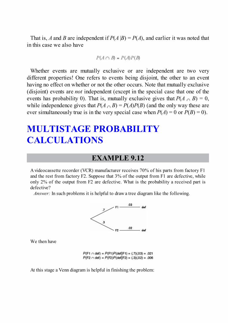
That is, A and B are independent if P(A |B) = P(A), and earlier it was noted thatin this case we also have
Whether events are mutually exclusive or are independent are two verydifferent properties! One refers to events being disjoint, the other to an eventhaving no effect on whether or not the other occurs. Note that mutually exclusive(disjoint) events are not independent (except in the special case that one of theevents has probability 0). That is, mutually exclusive gives that P(A B) = 0,while independence gives that P(A B) = P(A)P(B) (and the only way these areever simultaneously true is in the very special case when P(A) = 0 or P(B) = 0).
MULTISTAGE PROBABILITYCALCULATIONS
EXAMPLE 9.12A videocassette recorder (VCR) manufacturer receives 70% of his parts from factory F1and the rest from factory F2. Suppose that 3% of the output from F1 are defective, whileonly 2% of the output from F2 are defective. What is the probability a received part isdefective?
Answer: In such problems it is helpful to draw a tree diagram like the following.
We then have
At this stage a Venn diagram is helpful in finishing the problem:

We can take the above analysis one stage further and answer such questions as: If arandomly chosen part is defective, what is the probability it came from factory F1? Fromfactory F2?

TIPTree diagrams can be very useful in working with conditionalprobabilities.
EXAMPLE 9.13Suppose that three branches of a local bank average, respectively, 120, 180, and 100clients per day. Suppose further that the probabilities that a client will transact businessinvolving more than $100 during a visit are, respectively, .5, .6, and .7. A client is chosenat random. What is the probability that the client will transact business involving over$100? What is the probability that the client went to the first branch given that shetransacted business involving over $100?
Answer: and Then we have
Now P(> $100) = .15 + .27 + .175 = .595, and

TIPNaked or bald answers will receive little or no credit. Youmust show where answers come from.
DISCRETE RANDOM VARIABLES ANDTHEIR PROBABILITY DISTRIBUTIONSOften each outcome of an experiment has not only an associated probability butalso an associated real number. For example, the probability may be that thereare five defective batteries, the probability may be .01 that a company receivesseven contracts, or the probability may be .95 that three people recover from adisease. If X represents the different numbers associated with the potentialoutcomes of some chance situation, we call X a random variable.
EXAMPLE 9.14A prison official knows that of the inmates he admits stay only 1 day, stay 2 days, stay 3 days, and stay 4 days before they are either released or are sent on to the countyjail. If X represents the number of days, then X is a random variable that takes the value 1with probability , the value 2 with probability , the value 3 with probability , and thevalue 4 with probability .
The random variable in Example 9.14 is called discrete because it can assumeonly a countable number of values. The random variable in Example 9.15,however, is said to be continuous because it can assume values associated witha whole line interval.
EXAMPLE 9.15Let X be a random variable whose values correspond to the speeds at which a jet plane canfly. The jet may be traveling at 623.478 . . . miles per hour or at any other speed in somewhole interval. We might ask what the probability is that the plane is flying at between300 and 400 miles per hour.
A probability distribution for a discrete variable is a listing or formula givingthe probability for each value of the random variable.
In many applications, such as coin tossing, there are only two possibleoutcomes. For example, on each toss either the psychic guesses correctly or sheguesses incorrectly, either a radio is defective or it is not defective, either theworkers will go on strike or they will not walk out, either the manager’s salaryis above $50,000 or it does not exceed $50,000. In some applications such two-outcome situations are repeated many times. For example, we can ask about thechances that at most one out of four tires is defective, that at least three out offive unions will vote to go on strike, or that exactly two out of three executiveshave salaries above $50,000. For applications in which a two-outcome situationis repeated a certain number of times and the probability of each of the twooutcomes remains the same for each repetition, the resulting calculationsinvolve what are known as binomial probabilities.
EXAMPLE 9.16Suppose the probability that a lightbulb is defective is .1. What is the probability that fourlightbulbs are all defective?
Answer: Because of independence (i.e., whether one lightbulb is defective is notinfluenced by whether any other lightbulb is defective), we can multiply individualprobabilities of being defective to find the probability that all the bulbs are defective:
EXAMPLE 9.17Again suppose the probability that a lightbulb is defective is .1. What is the probabilitythat exactly two out of three lightbulbs are defective?
Answer: We subdivide the problem as follows: The probability that the first two bulbsare defective and the third is good is (.1)(.1)(.9) = .009. (Note that if the probability ofbeing defective is .1, the probability of being good is .9.) The probability that the firstbulb is good and the other two are defective is (.9)(.1)(.1) = .009. Finally, the probabilitythat the second bulb is good and the other two are defective is (.1)(.9)(.1) = .009.Summing, we find that the probability that exactly two out of three bulbs are defective is.009 + .009 + .009 = .027.
EXAMPLE 9.18

If the probability that a lightbulb is defective is .1, what is the probability that exactlythree out of eight lightbulbs are defective?
Answer: Again we can subdivide the problem. For example, the probability that the first,third, and seventh bulbs are defective and the rest are good is
The probability that the second, third, and fifth bulbs are defective and the rest are good is
As can be seen, the probability of any particular arrangement of three defective and fivegood bulbs is (.1)3(.9)5 = .00059049. How many such arrangements are there? In otherwords, in how many ways can we pick three of eight positions for the defective bulbs (theremaining five positions are for good bulbs)? The answer is given by combinations:
Each of these 56 arrangements has a probability of .00059049. Thus, the probability thatexactly three out of eight lightbulbs are defective is 56 × .00059049 = .03306744:
[On the TI-84 one can calculate binompdf(8, .1, 3) = .03306744.]
Note the application CATALOG HELP on the TI-84. For example, go to 2ndDISTR and scroll down to binompdf( . Instead of ENTER, click on the + button.You are then reminded of the order in which the variables must be entered: firstthe number of trials, then the probability of success p, and finally, optionally, thenumber of successes x.
EXAMPLE 9.19Suppose 30% of the employees in a large factory are smokers. What is the probabilitythat there will be exactly two smokers in a randomly chosen five-person work group?
Answer: We reason as follows. The probability that a person smokes is 30% = .3, andso the probability that he or she does not smoke is 1 – .3 = .7. The probability of aparticular arrangement of two smokers and three nonsmokers is (.3)2(.7)3 = .03087. Thenumber of such arrangements is

Each such arrangement has probability .03087, and so the final answer is 10 × .03087 =.3087.
[Or binompdf(5, .3, 2) = .3087.]
We can state the general principle as follows.
Binomial FormulaSuppose an experiment has two possible outcomes, called success and failure,with the probability of success equal to p and the probability of failure equal toq (of course, p + q = 1 and q = 1 – p). Suppose further that the experiment isrepeated n times and that the outcome at any particular time has no influenceover the outcome at any other time. Then the probability of exactly k successes(and thus n–k failures) is
EXAMPLE 9.20A manager notes that there is a .125 probability that any employee will arrive late forwork. What is the probability that exactly one person in a six-person department willarrive late?
Answer: If the probability of being late is .125, the probability of being on time is 1 –.125 = .875. If one person out of six is late, 6 – 1 = 5 will be on time. Thus the desiredprobability is
[Or going to 2nd DISTR on the TI-84, binompdf(6, .125, 1) ≈ .385.]
Many, perhaps most, applications of probability involve such phrases as atleast, at most, less than, and more than. In these cases, solutions involve

summing two or more cases. For such calculations, the TI-84 binomcdf is veryuseful. binomcdf(n,p,x) gives the probability of x or fewer successes in abinomial distribution with number of trials n and probability of success p.
EXAMPLE 9.21A manufacturer has the following quality control check at the end of a production line: Ifat least eight of ten randomly picked articles meet all specifications, the whole shipmentis approved. If, in reality, 85% of a particular shipment meet all specifications, what is theprobability that the shipment will make it through the control check?
Answer: The probability of an item meeting specifications is .85, and so the probabilityof it not meeting specifications must be .15. We want to determine the probability that atleast eight out of ten articles will meet specifications, that is, the probability that exactlyeight or exactly nine or exactly ten articles will meet specifications. We sum the threebinomial probabilities:
[On the TI-84 one can calculate 1 – binomcdf(10, .85, 7) ≈ .820 or binomcdf(10, .15, 2)≈ .820.]
EXAMPLE 9.22For the problem in Example 9.21, what is the probability that a shipment in which only70% of the articles meet specifications will make it through the control check?
Answer:
[Or binomcdf(10, .3, 2) ≈ .383.]
In some situations it is easier to calculate the probability of the complementaryevent and subtract this value from 1.
EXAMPLE 9.23Joe DiMaggio had a career batting average of .325. What was the probability that he
would get at least one hit in five official times at bat?Answer: We could sum the probabilities of exactly one hit, two hits, three hits, four
hits, and five hits. However, the complement of “at least one hit” is “zero hits.” Theprobability of no hit is
and thus the probability of at least one hit in five times at bat is 1 – .140 = .860.[Or binomcdf(5, .675, 4) ≈ .860.]
EXAMPLE 9.24A grocery store manager notes that 35% of customers who buy a particular product makeuse of a store coupon to receive a discount. If seven people purchase the product, what isthe probability that fewer than four will use a coupon?
Answer: In this situation, “fewer than four” means zero, one, two, or three.
[Or binomcdf(7, .35, 3) ≈ .800.]
Sometimes we are asked to calculate the probability of each of the possibleoutcomes (the results should sum to 1).
EXAMPLE 9.25If the probability that a male birth will occur is .51, what is the probability that a five-childfamily will have all boys? Exactly four boys? Exactly three boys? Exactly two boys?Exactly one boy? All girls?
Answer:

[Or binompdf(5, .49) = {.0345 .1657 .3185 .3060 .1470 .0283}.]
A list such as the one in Example 9.25 shows the entire probabilitydistribution, which in this case refers to a listing of all outcomes and theirprobabilities.
Geometric ProbabilitiesSuppose an experiment has two possible outcomes, called success and failure,with the probability of success equal to p and the probability of failure equal toq = 1 – p, and the trials are independent. Then the probability that the firstsuccess is on trial number X = k is
EXAMPLE 9.26Suppose only 12% of men in ancient Greece were honest. What is the probability that thefirst honest man Diogenes encounters will be the third man he meets?
Answer : (.88)2(.12) = .092928 [or geometpdf (.12, 3) = .092928]What is the probability that the first honest man he encounters will be no later than thefourth man he meets?
Answer : (.12) + (.88)(.12) + (.88)2(.12) + (.88)3(.12) = .40030464[or geometcdf (.12, 4) = .40030464]
SIMULATION OF PROBABILITYDISTRIBUTIONS, INCLUDINGBINOMIAL AND GEOMETRICInstead of algebraic calculations, sometimes we can use simulation to answerprobability questions.
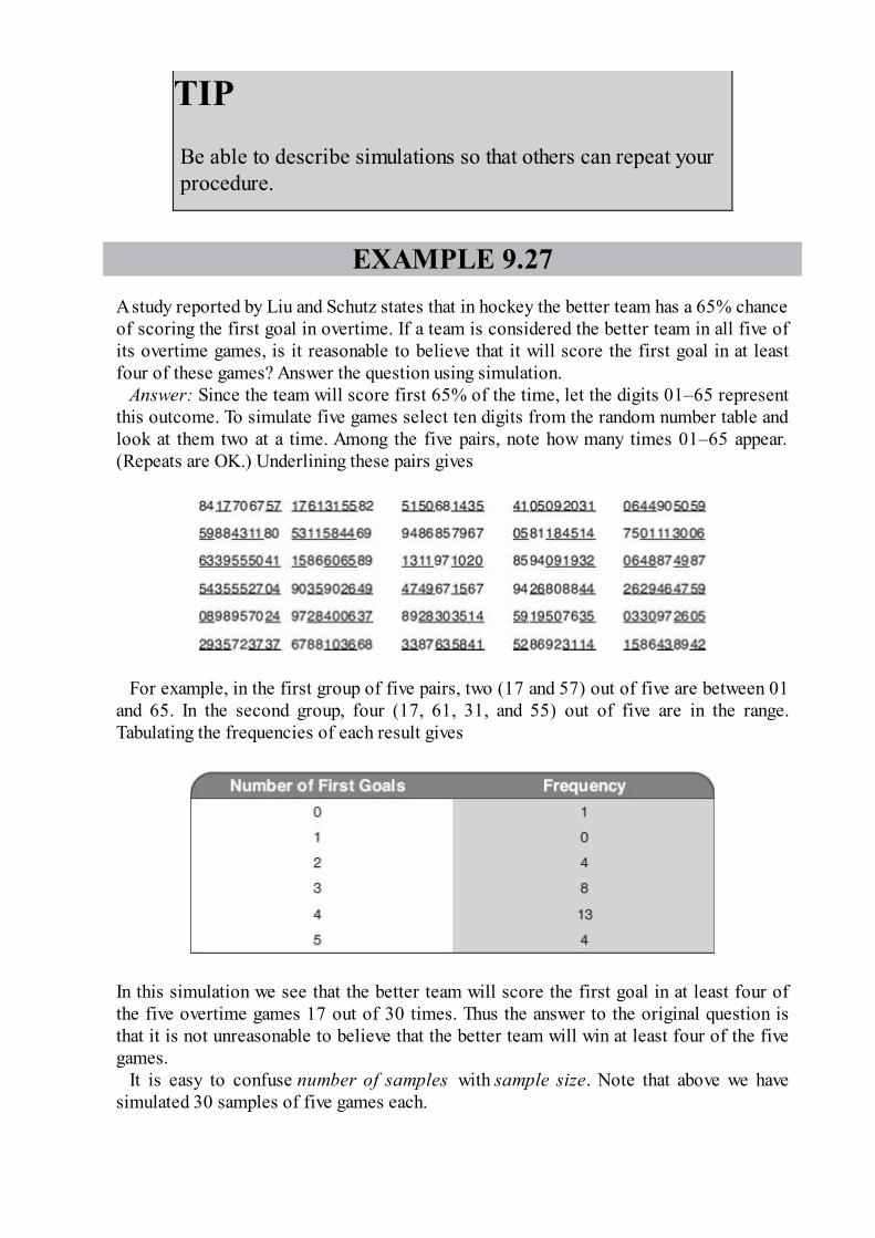
TIPBe able to describe simulations so that others can repeat yourprocedure.
EXAMPLE 9.27A study reported by Liu and Schutz states that in hockey the better team has a 65% chanceof scoring the first goal in overtime. If a team is considered the better team in all five ofits overtime games, is it reasonable to believe that it will score the first goal in at leastfour of these games? Answer the question using simulation.
Answer: Since the team will score first 65% of the time, let the digits 01–65 representthis outcome. To simulate five games select ten digits from the random number table andlook at them two at a time. Among the five pairs, note how many times 01–65 appear.(Repeats are OK.) Underlining these pairs gives
For example, in the first group of five pairs, two (17 and 57) out of five are between 01and 65. In the second group, four (17, 61, 31, and 55) out of five are in the range.Tabulating the frequencies of each result gives
In this simulation we see that the better team will score the first goal in at least four ofthe five overtime games 17 out of 30 times. Thus the answer to the original question isthat it is not unreasonable to believe that the better team will win at least four of the fivegames.
It is easy to confuse number of samples with sample size. Note that above we havesimulated 30 samples of five games each.

In Example 9.27 simulation is used with regard to a binomial distribution,while in the example below it is used with regard to a geometric distribution. Ageometric distribution shows the number of trials needed until a success isachieved.
EXAMPLE 9.28Suppose the probability that a company will land a contract is .3. Use simulation to findthe probability that the company will first land a contract on the first bid, on the second,on the third, and so on.
Answer: Let 0, 1, and 2 represent landing a contract, while 3–9 represent not getting thecontract. Read the random number table, one digit at a time, noting how many digits mustbe read until a 0, 1, or 2 is encountered. Using the table in Example 9.27 results in
841(first success in third try)770(first success in third try)67571(first success in fifth try)761(first success in third try)31(first success in second try).Continuing in this fashion and tabulating the results, we have
Thus we estimate the probabilities as follows:

The actual probabilities are .3, (.7)(.3) = .21, (.7)2(.3) = .147, (.7)3(.3) = .1029,(.7)4(.3) = .07203, and 1 – (.3 + .21 + .147 + .1029 + .07203) = .16807.
[On the TI-84 one can calculate the geometric probabilities geometpdf(.3, 1) =.3, . . . , geometpdf(.3, 5) = .07203, and 1 – geometcdf(.3, 5) = .16807.]
One example of simulating a nonbinomial, nongeometric distribution is thefollowing.
EXAMPLE 9.29If a two-person committee is chosen at random from a group consisting of threesupervisors and six employees, what is the probability that the committee will haveexactly one supervisor and one employee? Use simulation to estimate the answer.
Answer: Let the digits 1, 2, and 3 represent the supervisors, and the digits 4, 5, 6, 7, 8,and 9 represent the employees. Our procedure is to pick digits one at a time from arandom number table, ignoring repeats and ignoring 0’s, until two different digits havebeen chosen. Reading from the random number table in Example 9.27 results in thecommittees (8, 4) with two employees, (1, 7) with one of each, (7, 6) with twoemployees, (7, 5) with two employees, (7, 1) with one of each, (7, 6) with twoemployees, (1, 3) with two supervisors, and so on. Tabulating from the table gives
Two supervisors: 11One of each: 53Two employees: 66.Thus an estimate of the probability that the committee will consist of one supervisor andone employee is
[The actual probability is ]

In performing a simulation, you must:
1. Set up a correspondence between outcomes and random numbers.2. Give a procedure for choosing the random numbers (for example, pick
three digits at a time from a designated row in a random number table).3. Give a stopping rule.4. Note what is to be counted (what is the purpose of the simulation), and
give the count if requested.
MEAN (EXPECTED VALUE) ANDSTANDARD DEVIATION OF A RANDOMVARIABLE, INCLUDING BINOMIALA bettor placing a chip on a number in roulette has a small chance of winning alot and a large chance of losing a little. To determine whether the bet is “fair,”we must be able to calculate the expected value of the game to the bettor. Aninsurance company in any given year pays out a large sum of money to each of arelatively small number of people, while collecting a small sum of money fromeach of many other individuals. To determine policy premiums an actuary mustcalculate the expected values relating to deaths in various age groups ofpolicyholders.
EXAMPLE 9.30Concessionaires know that attendance at a football stadium will be 60,000 on a clear day,45,000 if there is light snow, and 15,000 if there is heavy snow. Furthermore, theprobability of clear skies, light snow, or heavy snow on any particular day is , and ,respectively. (Here we have a random variable X that takes the values 60,000, 45,000, and15,000.)
What average attendance should be expected for the season?Answer: We reason as follows. Suppose on, say, 12 game days we have clear skies of
the time (6 days), a light snow of the time (4 days), and a heavy snow of the time (2days). Then the average attendance will be

Note that we could have divided the 12 into each of the three terms in the numerator toobtain
or, equivalently,
Actually, there was no need to consider 12 days. We could have simply multipliedprobabilities by corresponding attendances and summed the resulting products.
The final calculation in Example 9.30 motivates our definition of expectedvalue. The expected value (or average or mean) of a random variable X is thesum of the products obtained by multiplying each value xi by the correspondingprobability pi:
EXAMPLE 9.31In a lottery, 10,000 tickets are sold at $1 each with a prize of $7500 for one winner. Whatis the average result for each bettor?
Answer: The actual winning payoff is $7499 because the winner paid $1 for a ticket, sowe have
Thus the average result for each person betting on the lottery is a $0.25 loss.Alternatively, we can say that the expected payoff to the lottery system is $0.25 for eachticket sold.

EXAMPLE 9.32A manager must choose among three options. Option A has a 10% chance of resulting in a$250,000 gain but otherwise will result in a $10,000 loss. Option B has a 50% chance ofgaining $40,000 and a 50% chance of losing $2000. Finally, option C has a 5% chance ofgaining $800,000 but otherwise will result in a loss of $20,000. Which option should themanager choose?
Answer: Calculate the expected values of the three options:
The manager should choose option C! However, although option C has the greatestmean (expected value), the manager may well wish to consider the relative riskiness ofthe various options. If, for example, a $5000 loss would be disastrous for the company,the manager might well decide to choose option B with its maximum possible loss of$2000. (It should be intuitively clear that some concept of variance would be helpful herein measuring the risk; later in this topic the variance of a random variable will be defined.)
Suppose we have a binomial random variable, that is, a random variablewhose values are the numbers of “successes” in some binomial probabilitydistribution.
EXAMPLE 9.33Of the automobiles produced at a particular plant, 40% had a certain defect. Suppose acompany purchases five of these cars. What is the expected value for the number of carswith defects?
Answer: We might guess that the average or mean or expected value is 40% of 5 = .4 ×5 = 2, but let’s calculate from the definition. Letting X represent the number of cars withthe defect, we have
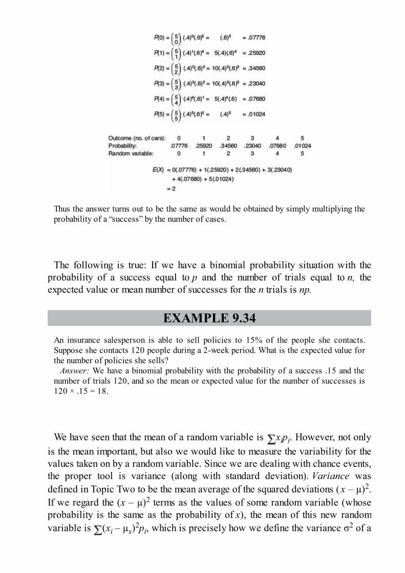
Thus the answer turns out to be the same as would be obtained by simply multiplying theprobability of a “success” by the number of cases.
The following is true: If we have a binomial probability situation with theprobability of a success equal to p and the number of trials equal to n, theexpected value or mean number of successes for the n trials is np.
EXAMPLE 9.34An insurance salesperson is able to sell policies to 15% of the people she contacts.Suppose she contacts 120 people during a 2-week period. What is the expected value forthe number of policies she sells?
Answer: We have a binomial probability with the probability of a success .15 and thenumber of trials 120, and so the mean or expected value for the number of successes is120 × .15 = 18.
We have seen that the mean of a random variable is xipi. However, not onlyis the mean important, but also we would like to measure the variability for thevalues taken on by a random variable. Since we are dealing with chance events,the proper tool is variance (along with standard deviation). Variance wasdefined in Topic Two to be the mean average of the squared deviations (x – µ)2.If we regard the (x – µ)2 terms as the values of some random variable (whoseprobability is the same as the probability of x), the mean of this new randomvariable is (xi – µx)2pi, which is precisely how we define the variance σ2 of a

random variable:
As before, the standard deviation σ is the square root of the variance.
EXAMPLE 9.35A highway engineer knows that his crew can lay 5 miles of highway on a clear day, 2 mileson a rainy day, and only 1 mile on a snowy day. Suppose the probabilities are as follows:
What are the mean (expected value) and the variance?Answer:
EXAMPLE 9.36Look again at Example 9.33. We calculated the mean to be 2. What is the variance?
Answer: σ2 = (0 – 2)2(.07776) + (1 – 2)2(.2592) + (2 – 2)2(.3456) + (3 – 2)2(.2304) +(4 – 2)2(.0768) + (5 – 2)2(.01024) = 1.2Could we have calculated the above result more easily? In this case, we have a binomialrandom variable and the variance can be simply calculated as npq = np(1 – p).
EXAMPLE 9.37How can we use this method to calculate the variance in Example 9.33 more simply?
Answer: np(1 – p) = 5(.4)(.6) = 1.2
Thus, for a random variable X,
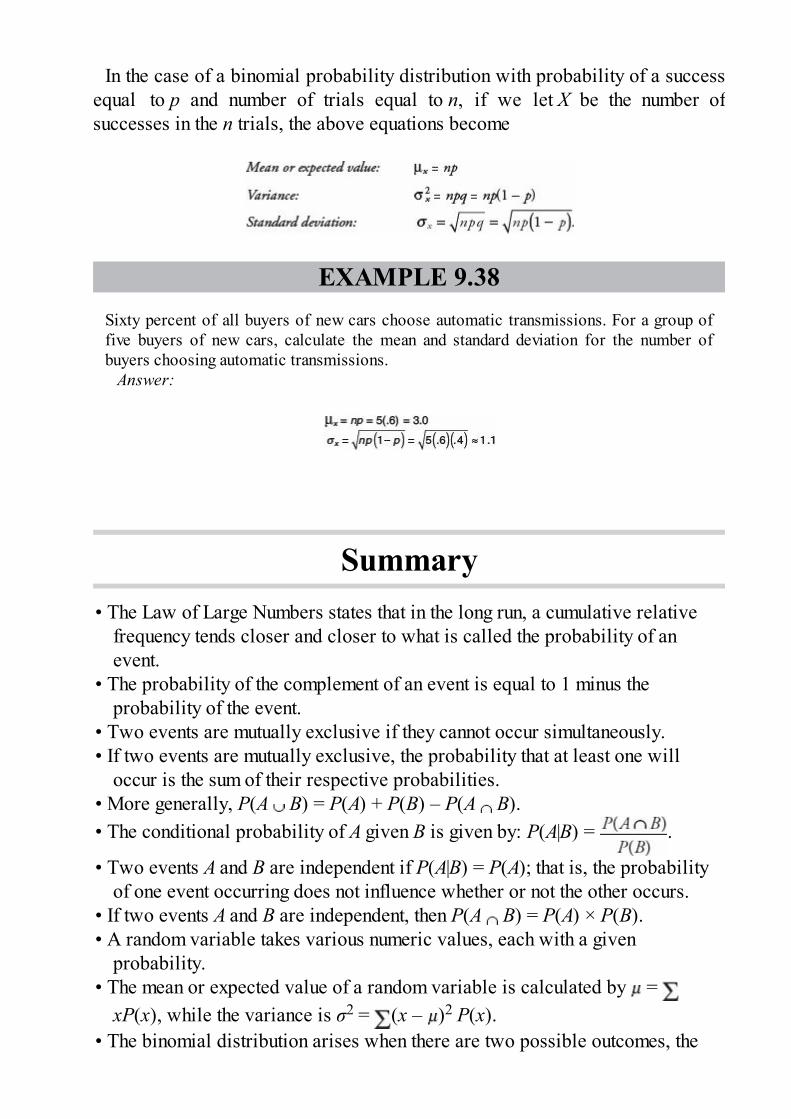
In the case of a binomial probability distribution with probability of a successequal to p and number of trials equal to n, if we let X be the number ofsuccesses in the n trials, the above equations become
EXAMPLE 9.38Sixty percent of all buyers of new cars choose automatic transmissions. For a group offive buyers of new cars, calculate the mean and standard deviation for the number ofbuyers choosing automatic transmissions.
Answer:
Summary• The Law of Large Numbers states that in the long run, a cumulative relative
frequency tends closer and closer to what is called the probability of anevent.
• The probability of the complement of an event is equal to 1 minus theprobability of the event.
• Two events are mutually exclusive if they cannot occur simultaneously.• If two events are mutually exclusive, the probability that at least one will
occur is the sum of their respective probabilities.• More generally, P(A B) = P(A) + P(B) – P(A B).• The conditional probability of A given B is given by: P(A|B) = .
• Two events A and B are independent if P(A|B) = P(A); that is, the probabilityof one event occurring does not influence whether or not the other occurs.
• If two events A and B are independent, then P(A B) = P(A) × P(B).• A random variable takes various numeric values, each with a given
probability.• The mean or expected value of a random variable is calculated by =
xP(x), while the variance is σ2 = (x – )2 P(x).• The binomial distribution arises when there are two possible outcomes, the
probability of success is constant, and the trials are independent.• In a binomial distribution, the mean number of successes is np and the
standard deviation is .
Questions on Topic Nine: Probability asRelative Frequency
Multiple-Choice Questions
Directions: The questions or incomplete statements that follow are eachfollowed by five suggested answers or completions. Choose response thatbest answers the question or completes the statement.
1. A student reasons that either he will or will not receive a 5 on theAP Statistics exam, and therefore the probability of receiving a 5 is 0.5.Why is this incorrect reasoning?
(A) The events are mutually exclusive.(B) The events are independent.(C) The events are not independent.(D) The events are complements.(E) The events are not equally probable.
2. In the November 27, 1994, issue of Parade magazine, the “AskMarilyn” section contained this question: “Suppose a person was havingtwo surgeries performed at the same time. If the chances of success forsurgery A are 85%, and the chances of success for surgery B are 90%,what are the chances that both would fail?” What do you think ofMarilyn’s solution: (.15)(.10) = .015 or 1.5%?
(A) Her solution is mathematically correct but not explained verywell.

(B) Her solution is both mathematically correct and intuitivelyobvious.
(C) Her use of complementary events is incorrect.(D) Her use of the general addition formula is incorrect.(E) She assumed independence of events, which is most likely
wrong.
3. A weighted die comes up spots with the following probabilities:
If two of these dice are thrown, what is the probability the sum is10?
(A) (.25)(.10) + (.20)2
(B) 2(.25)(.10) + (.20)2
(C) 2(.25)(.10) + 2(.20)2
(D) (.10)(.20)(.10) + (.20)2
(E) (.10)(.20)(.10) + (.15)(.25)2 + (.15)(.20)(.20) + (.25)(.10)
4. According to a CBS/New York Times poll taken in 1992, 15% of thepublic have responded to a telephone call-in poll. In a random group offive people, what is the probability that exactly two have responded to acall-in poll?
(A) .138(B) .165(C) .300(D) .835(E) .973
5. In a 1974 “Dear Abby” letter a woman lamented that she had just
given birth to her eighth child, and all were girls! Her doctor had assuredher that the chance of the eighth child being a girl was only 1 in 100. Whatwas the real probability that the eighth child would be a girl?
(A) .01(B) .5(C) (.5)7
(D) (.5)8
(E)
6. The yearly mortality rate for American men from prostate cancer hasbeen constant for decades at about 25 of every 100,000 men. (This ratehas not changed in spite of new diagnostic techniques and newtreatments.) In a group of 100 American men, what is the probability thatat least 1 will die from prostate cancer in a given year?
(A) .00025(B) .0247(C) .025(D) .9753(E) .99975
7. Alan Dershowitz, one of O. J. Simpson’s lawyers, has stated that
only 1 out of every 1000 abusive relationships ends in murder each year.If he is correct, and if there are approximately 1.5 million abusiverelationships in the United States, what is the expected value for thenumber of people who are killed each year by an abusive partner?
(A) 1(B) 500

(C) 1000(D) 1500(E) None of the above
8. For an advertising promotion, an auto dealer hands out 1000 lotterytickets with a prize of a new car worth $25,000. For someone with asingle ticket, what is the standard deviation for the amount won?
(A) $7.07(B) $25.00(C) $49.95(D) $790.17(E) $624,375
9. Suppose that among the 6000 students at a high school, 1500 are
taking honors courses and 1800 prefer watching basketball to watchingfootball. If taking honors courses and preferring basketball areindependent, how many students are both taking honors courses and preferbasketball to football?
(A) 300(B) 330(C) 450(D) 825(E) There is insufficient information to answer this question.
10. An inspection procedure at a manufacturing plant involves pickingthree items at random and then accepting the whole lot if at least two ofthe three items are in perfect condition. If in reality 90% of the whole lotare perfect, what is the probability that the lot will be accepted?

(A) .600(B) .667(C) .729(D) .810(E) .972
11. Suppose that, in a certain part of the world, in any 50-year period
the probability of a major plague is .39, the probability of a major famineis .52, and the probability of both a plague and a famine is .15. What isthe probability of a famine given that there is a plague?
(A) .240(B) .288(C) .370(D) .385(E) .760
12. Suppose that, for any given year, the probabilities that the stock
market declines, that women’s hemlines are lower, and that both eventsoccur are, respectively, .4, .35, and .3. Are the two events independent?
(A) Yes, because (.4)(.35) ≠ .3.(B) No, because (.4)(.35) ≠ .3.(C) Yes, because .4 > .35 > .3.(D) No, because .5(.3 + .4) = .35.(E) There is insufficient information to answer this question.
13. If P(A) = .2 and P(B) = .1, what is P(A B) if A and B areindependent?
(A) .02(B) .28(C) .30(D) .32(E) There is insufficient information to answer this question.
14. The following data are from The Commissioner’s StandardOrdinary Table of Mortality:
What is the probability that a 20-year-old will survive to be 70?
(A) .407(B) .421(C) .559(D) .579(E) .966
15. At a warehouse sale 100 customers are invited to choose one of
100 identical boxes. Five boxes contain $700 color television sets, 25boxes contain $540 camcorders, and the remaining boxes contain $260cameras. What should a customer be willing to pay to participate in thesale?
(A) $260(B) $352
(C) $500(D) $540(E) $699
16. There are two games involving flipping a coin. In the first game you
win a prize if you can throw between 40% and 60% heads. In the secondgame you win if you can throw more than 75% heads. For each gamewould you rather flip the coin 50 times or 500 times?
(A) 50 times for each game(B) 500 times for each game(C) 50 times for the first game, and 500 for the second(D) 500 times for the first game, and 50 for the second(E) The outcomes of the games do not depend on the number of flips.
17. Two cards are picked, without replacement, from a standard deck.Which of the following pairs are independent events?
(A) Getting a heart on the first pick; getting a diamond on the second.(B) Getting a red card on the first pick; getting a black card on the
second.(C) Getting an ace on the first pick; getting an ace on the second.(D) Getting two aces; getting two kings.(E) Getting two aces; getting a black card on the second pick.
18. Two cards are picked, with replacement, from a standard deck.Which of the following pairs are independent events?
(A) Getting two aces; getting two kings.

(B) Getting an ace on the first pick; getting a king on the second.(C) Getting at least one ace; getting at least one king.(D) Getting exactly one ace; getting exactly one king.(E) Getting no aces; getting no kings.
19. The average annual incomes of high school and college graduates ina midwestern town are $21,000 and $35,000, respectively. If a companyhires only personnel with at least a high school diploma and 20% of itsemployees have been through college, what is the mean income of thecompany employees?
(A) $23,800(B) $27,110(C) $28,000(D) $32,200(E) $56,000
20. An insurance company charges $800 annually for car insurance.
The policy specifies that the company will pay $1000 for a minoraccident and $5000 for a major accident. If the probability of a motoristhaving a minor accident during the year is .2, and of having a majoraccident, .05, how much can the insurance company expect to make on apolicy?
(A) $200(B) $250(C) $300(D) $350(E) $450
21. You can choose one of three boxes. Box A has four $5 bills and a
single $100 bill, box B has 400 $5 bills and 100 $100 bills, and box Chas 24 $1 bills. You can have all of box C or blindly pick one bill out of
either box A or box B. Which offers the greatest expected winning?
(A) Box A(B) Box B(C) Box C(D) Either A or B, but not C(E) All offer the same expected winning.
22. Given that 52% of the U.S. population are female and 15% areolder than age 65, can we conclude that (.52)(.15) = 7.8% are womenolder than age 65?
(A) Yes, by the multiplication rule.(B) Yes, by conditional probabilities.(C) Yes, by the law of large numbers.(D) No, because the events are not independent.(E) No, because the events are not mutually exclusive.
Questions 23–27 refer to the following study: One thousand students at a cityhigh school were classified both according to GPA and whether or not theyconsistently skipped classes.
23. What is the probability that a student has a GPA between 2.0 and3.0?
(A) .025(B) .227(C) .450(D) .475(E) .506
24. What is the probability that a student has a GPA under 2.0 and has
skipped many classes?
(A) .080(B) .281(C) .285(D) .314(E) .727
25. What is the probability that a student has a GPA under 2.0 or has
skipped many classes?
(A) .080(B) .281(C) .285(D) .314(E) .727
26. What is the probability that a student has a GPA under 2.0 giventhat he has skipped many classes?
(A) .080(B) .281

(C) .285(D) .314(E) .727
27. Are “GPA between 2.0 and 3.0” and “skipped few classes”
independent?
(A) No, because .475 ≠ .506.(B) No, because .475 ≠ .890.(C) No, because .450 ≠ .475.(D) Yes, because of conditional probabilities.(E) Yes, because of the product rule.
28. Mathematically speaking, casinos and life insurance companiesmake a profit because of
(A) their understanding of sampling error and sources of bias.(B) their use of well-designed, well-conducted surveys and
experiments.(C) their use of simulation of probability distributions.(D) the central limit theorem.(E) the law of large numbers.
29. Consider the following table of ages of U.S. senators:
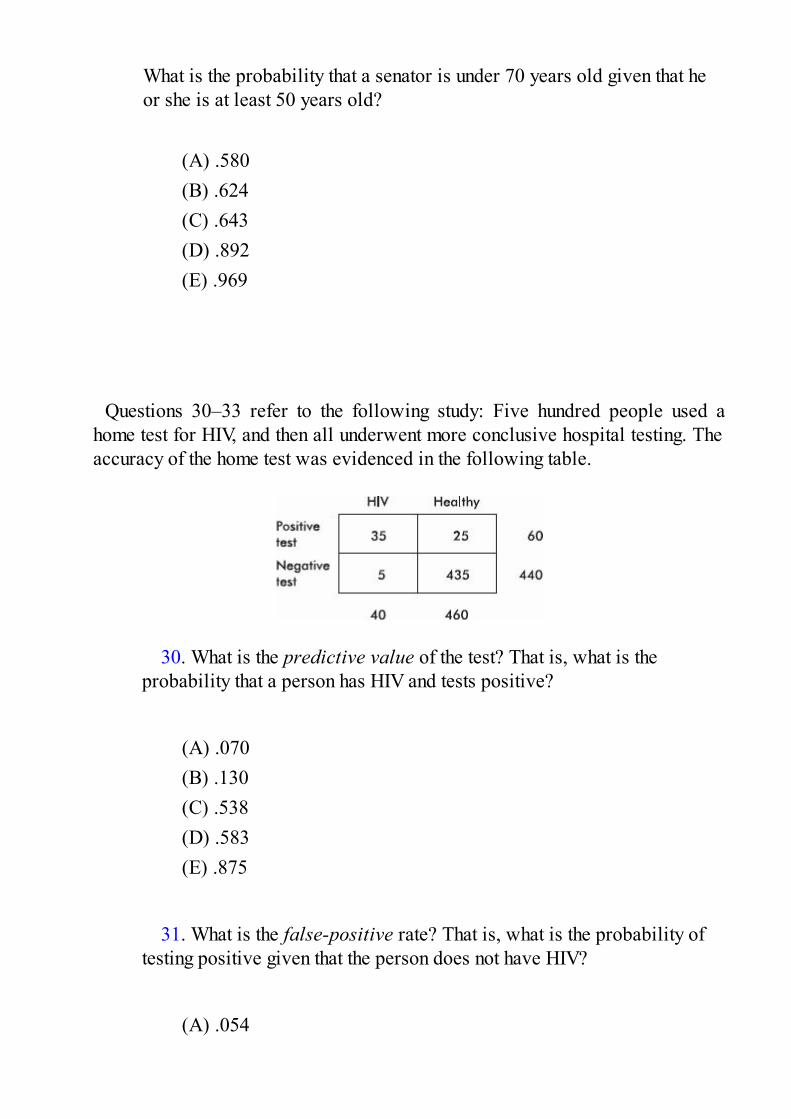
What is the probability that a senator is under 70 years old given that heor she is at least 50 years old?
(A) .580(B) .624(C) .643(D) .892(E) .969
Questions 30–33 refer to the following study: Five hundred people used ahome test for HIV, and then all underwent more conclusive hospital testing. Theaccuracy of the home test was evidenced in the following table.
30. What is the predictive value of the test? That is, what is theprobability that a person has HIV and tests positive?
(A) .070(B) .130(C) .538(D) .583(E) .875
31. What is the false-positive rate? That is, what is the probability of
testing positive given that the person does not have HIV?
(A) .054

(B) .050(C) .130(D) .417(E) .875
32. What is the sensitivity of the test? That is, what is the probability of
testing positive given that the person has HIV?
(A) .070(B) .130(C) .538(D) .583(E) .875
33. What is the specificity of the test? That is, what is the probability of
testing negative given that the person does not have HIV?
(A) .125(B) .583(C) .870(D) .950(E) .946
34. Suppose that 2% of a clinic’s patients are known to have cancer. A
blood test is developed that is positive in 98% of patients with cancer butis also positive in 3% of patients who do not have cancer. If a person whois chosen at random from the clinic’s patients is given the test and itcomes out positive, what is the probability that the person actually hascancer?
(A) .02(B) .4(C) .5
(D) .6(E) .98
35. Suppose the probability that you will receive an A in AP Statistics
is .35, the probability that you will receive A’s in both AP Statistics andAP Biology is .19, and the probability that you will receive an A in APStatistics but not in AP Biology is .17. Which of the following is a properconclusion?
(A) The probability that you will receive an A in AP Biology is .36.(B) The probability that you didn’t take AP Biology is .01.(C) The probability that you will receive an A in AP Biology but not
in AP Statistics is .18.(D) The given probabilities are impossible.(E) None of the above
36. Suppose you are one of 7.5 million people who send in their name
for a drawing with 1 top prize of $1 million, 5 second-place prizes of$10,000, and 20 third-place prizes of $100. Is it worth the $0.44 postageit cost you to send in your name?
(A) Yes, because = 2,272,727, which is less than 7,500,000.
(B) No, because your expected winnings are only $0.14.(C) Yes, because
(D) No, because 1,052,000 < 7,500,000.(E) Yes, because
37. You have a choice of three investments, the first of which gives youa 10% chance of making $1 million, otherwise you lose $25,000; thesecond of which gives you a 50% chance of making $500,000, otherwiseyou lose $345,000; and the third of which gives you an 80% chance of

making $50,000, otherwise you make only $1,000. Assuming you will gobankrupt if you don’t show a profit, which option should you choose forthe best chance of avoiding bankruptcy?
(A) First choice(B) Second choice(C) Third choice(D) Either the first or the second choice(E) All the choices give an equal chance of avoiding bankruptcy.
38. Can the function , for x = 1, 2, and 3, be the probabilitydistribution for some random variable?
(A) Yes.(B) No, because probabilities cannot be negative.(C) No, because probabilities cannot be greater than 1.(D) No, because the probabilities do not sum to 1.(E) Not enough information is given to answer the question.
39. Sixty-five percent of all divorce cases cite incompatibility as theunderlying reason. If four couples file for a divorce, what is theprobability that exactly two will state incompatibility as the reason?
(A) .104(B) .207(C) .254(D) .311(E) .423

40. Suppose we have a random variable X where the probability
associated with the value for k = 0, . . . , 10. What is the
mean of X?
(A) 0.37(B) 0.63(C) 3.7(D) 6.3(E) None of the above
41. A computer technician notes that 40% of computers fail because of
the hard drive, 25% because of the monitor, 20% because of a disk drive,and 15% because of the microprocessor. If the problem is not in themonitor, what is the probability that it is in the hard drive?
(A) .150(B) .400(C) .417(D) .533(E) .650
42. Suppose you toss a coin ten times and it comes up heads every time.
Which of the following is a true statement?
(A) By the law of large numbers, the next toss is more likely to betails than another heads.
(B) By the properties of conditional probability, the next toss ismore likely to be heads given that ten tosses in a row have been heads.
(C) Coins actually do have memories, and thus what comes up on thenext toss is influenced by the past tosses.
(D) The law of large numbers tells how many tosses will be
necessary before the percentages of heads and tails are again inbalance.
(E) The probability that the next toss will again be heads is .5.
43. A city water supply system involves three pumps, the failure of anyone of which crashes the system. The probabilities of failure for eachpump in a given year are .025, .034, and .02, respectively. Assuming thepumps operate independently of each other, what is the probability thatthe system does crash during the year?
(A) Less than .05(B) .077(C) .079(D) .081(E) .923
44. Which of the following are true statements?
I. The histogram of a binomial distribution with p = .5 is alwayssymmetric no matter what n, the number of trials, is.
II. The histogram of a binomial distribution with p = .9 is skewed tothe right.
III. The histogram of a binomial distribution with p = .9 is almostsymmetric if n is very large.
(A) I and II(B) I and III(C) II and III(D) I, II, and III(E) None of the above gives the complete set of true responses.

45. Suppose that 60% of students who take the AP Statistics exam score4 or 5, 25% score 3, and the rest score 1 or 2. Suppose further that 95%of those scoring 4 or 5 receive college credit, 50% of those scoring 3receive such credit, and 4% of those scoring 1 or 2 receive credit. If astudent who is chosen at random from among those taking the examreceives college credit, what is the probability that she received a 3 onthe exam?
(A) .125(B) .178(C) .701(D) .813(E) .822
46. Given the probabilities P(A) = .4 and P(A B) = .6, what is the
probability P(B) if A and B are mutually exclusive? If A and B areindependent?
(A) .2, .4(B) .2, .33(C) .33, .2(D) .6, .33(E) .6, .4
47. There are 20 students in an AP Statistics class. Suppose all are
unprepared and randomly guess on each of ten multiple-choice questions,each with a choice of five possible answers. Which of the following isone run of a simulation to estimate the probability at least one studentguesses correctly on over half the questions?
(A) Assume “1” is the correct answer and “2, 3, 4, 5” are incorrectanswers. Randomly pick 200 numbers between 1 and 5. Arrange thenumbers into 20 groups of 10 each, each group corresponding to one ofthe students. For each student, count how many correct (“1”) answers
there are. Record whether at least one student has six or more correctanswers.
(B) Assume “2” is the correct answer and “1, 3, 4, 5” are incorrectanswers. Assign the numbers 1–20 to the students. Randomly choose200 numbers between 1 and 20. For each number chosen, randomlypick a number between 1 and 5. Record how many correct (“2”)answers there are, divide by 20, and record whether this quotient is atleast six.
(C) Assume “3” is the correct answer and “1, 2, 4, 5” are incorrectanswers. Assign the numbers 1–10 to the questions. Randomly choose200 numbers between 1 and 10. For each number chosen, randomlypick a number between 1 and 5. Record how many correct (“3”)answers there are, divide by 20, and record whether this quotient is atleast six.
(D) Assume “4” is the correct answer and “1, 2, 3, 5” are incorrectanswers. Randomly choose 200 numbers between 1 and 5. Record howmany correct (“1”) answers there are, divide by 20, and recordwhether this quotient is at least six.
(E) Assume “5” is the correct answer and “1, 2, 3, 4” are incorrectanswers. Randomly pick 20 numbers between 1 and 5. Do this 10times, and for each group of 20 note how many correct (“5”) answersthere are. Record whether at least one group has over half correctanswers.
Free-Response Questions
Directions: You must show all work and indicate the methods you use. Youwill be graded on the correctness of your methods and on the accuracy ofyour final answers.
Seven Open-Ended Questions1. A manufacturer is considering two options for a quality control
check at the end of a production line:Option A: If at least five of six randomly picked articles meet all
specifications, the day’s production is approved.Option B: If at least ten of twelve randomly picked articles meet all
specifications, the day’s production is approved.

If you are a buyer wanting the most assurance that a day’s production willnot be accepted if there were only 75% of the articles meeting allspecifications, which option would you request the manufacturer to use?Give statistical justification.
2. A sample of applicants for a management position yields thefollowing numbers with regard to age and experience:
(a) What is the probability that an applicant is less than 50 yearsold? Has more than 10 years’ experience? Is more than 50 years oldand has five or fewer years’ experience?
(b) What is the probability that an applicant is less than 50 years oldgiven that she has between 6 and 10 years’ experience?
(c) Are the two events “less than 50 years old” and “more than 10years’ experience” independent events? How about the two events“more than 50 years old” and “between 6 and 10 years’ experience”?Explain.3. Suppose USAir accounts for 20% of all U.S. domestic flights. As of
mid-1994, USAir was involved in four of the previous seven majordisasters. “That’s enough to begin getting suspicious but not enough tohang them,” said Dr. Brad Efton in The New York Times (September 11,1994, Sec. 4, p. 4). Using a binomial distribution, comment on Dr. Efton’sremark.
4. Assume there is no overlap between the 56% of the population whowear glasses and the 4% who wear contacts. If 55% of those who wearglasses are women and 63% of those who wear contacts are women, whatis the probability that the next person you encounter on the street will be awoman with glasses? A woman with contacts? A man with glasses? Aman with contacts? A person not wearing glasses or contacts? Explainyour reasoning.
5. Explain what is wrong with each of the following statements:(a) The probability that a student will score high on the AP Statistics
exam is .43, while the probability that she will not score high is .47.(b) The probability that a student plays tennis is .18, while the
probability that he plays basketball is six times as great.(c) The probability that a student enjoys her English class is .64,
while the probability that she enjoys both her English and her socialstudies classes is .71.
(d) The probability that a student will be accepted by his first choicefor college is .38, while the probability that he will be accepted by hisfirst or second choice is .32.
(e) The probability that a student fails AP Statistics and will still beaccepted by an Ivy League school is –.17.6. Player A rolls a die with 7 on four sides and 11 on two sides. Player
B flips a coin with 6 on one side and 10 on the other. Assume a fair dieand a fair coin.
(a) Suppose the winner is the player with the higher numbershowing. Explain who you would rather be. If player A receives $0.25for every win, what should player B receive for every win to make thegame fair?
(b) Suppose player A receives $0.70 from player B when the 7shows and $1.10 when the 11 shows, while player B receives $0.60from player A when the 6 shows and $1.00 when the 10 shows.Explain whom you would rather be.7. Could hands-free, automatic faucets actually be housing more
bacteria than the old-fashioned, manual kind? The concern is thatdecreased water flow may increase the chance that bacteria grows,because the automatic faucets are not being thoroughly flushed through. Itis known that 15% of water cultures from older faucets in hospital patientcare areas test positive for Legionella bacteria. A recent study at JohnsHopkins Hospital found Legionella bacteria growing in 10 of culturedwater samples from 20 electronic faucets.
(a) If the probability of Legionella bacteria growing in a faucet is.15, what is the probability that in a sample of 20 faucets, 10 or morehave the bacteria growing?
(b) Does the Johns Hopkins study provide sufficient evidence thatthe probability of Legionella bacteria growing in electronic faucets isgreater than 15%? Explain.
An Investigative Task

If a car is stopped for speeding, the probability that the driver has illegaldrugs hidden in the car is .14. A police officer manning a speed trap plansto thoroughly search cars he stops for speeding until he finds one withillegal drugs.
(a) Use simulation to estimate the probability that illegal drugs willturn up before he stops the tenth car. Explain your work. Use thefollowing random number table to run as many trials as possible.
(b) The results of a 100-trial simulation are shown below. Each trialends when a car with illegal drugs is found.
Use the above 100-trial results to estimate the mean number of carssearched before finding one with illegal drugs.
(c) Use probability to calculate the probability that illegal drugs willbe found before he stops the tenth car. Show your work.
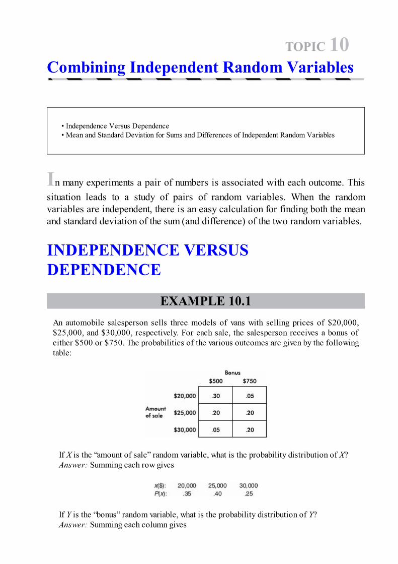
TOPIC 10Combining Independent Random Variables
• Independence Versus Dependence• Mean and Standard Deviation for Sums and Differences of Independent Random Variables
In many experiments a pair of numbers is associated with each outcome. Thissituation leads to a study of pairs of random variables. When the randomvariables are independent, there is an easy calculation for finding both the meanand standard deviation of the sum (and difference) of the two random variables.
INDEPENDENCE VERSUSDEPENDENCE
EXAMPLE 10.1An automobile salesperson sells three models of vans with selling prices of $20,000,$25,000, and $30,000, respectively. For each sale, the salesperson receives a bonus ofeither $500 or $750. The probabilities of the various outcomes are given by the followingtable:
If X is the “amount of sale” random variable, what is the probability distribution of X?Answer: Summing each row gives
If Y is the “bonus” random variable, what is the probability distribution of Y?Answer: Summing each column gives
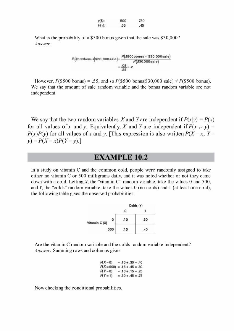
What is the probability of a $500 bonus given that the sale was $30,000?Answer:
However, P($500 bonus) = .55, and so P($500 bonus|$30,000 sale) ≠ P($500 bonus).We say that the amount of sale random variable and the bonus random variable are notindependent.
We say that the two random variables X and Y are independent if P(x|y) = P(x)for all values of x and y. Equivalently, X and Y are independent if P(x y) =P(x)P(y) for all values of x and y. [This expression is also written P(X = x, Y =y) = P(X = x)P(Y = y).]
EXAMPLE 10.2In a study on vitamin C and the common cold, people were randomly assigned to takeeither no vitamin C or 500 milligrams daily, and it was noted whether or not they camedown with a cold. Letting X, the “vitamin C” random variable, take the values 0 and 500,and Y, the “colds” random variable, take the values 0 (no colds) and 1 (at least one cold),the following table gives the observed probabilities:
Are the vitamin C random variable and the colds random variable independent?Answer: Summing rows and columns gives
Now checking the conditional probabilities,

Thus we conclude that X and Y are independent.Note that an alternative check for independence is the following: P(X = 0, Y = 0) = .10and P(X = 0)P(Y = 0) = (.40)(.25) = .10. Similarly, P(X = 0, Y = 1) = P(X = 0)P(Y = 1) =.30, P(X = 500, Y = 0) = P(X = 500)P(Y = 0) = .15, andP(X = 500, Y = 1) = P(X = 500)P(Y = 1) = .45.
MEAN AND STANDARD DEVIATIONFOR SUMS AND DIFFERENCES OFINDEPENDENT RANDOM VARIABLESOne way of comparing two populations is to analyze their set of differences.
EXAMPLE 10.3Suppose set X = {2, 9, 11, 22} and set Y = {5, 7, 15}. Note that the mean of set X is
and the mean of set Y is Form the set Z of differences bysubtracting each element of Y from each element of X:
What is the mean of Z?Answer:
Note that z = x – y .In general, the mean of a set of differences is equal to the difference of the means of
the two original sets. Even more generally, if a sum is formed by picking one elementfrom each of several sets, the mean of such sums is simply the sum of the means of thevarious sets.
How is the variance of Z related to the variances of the original sets?Answer:
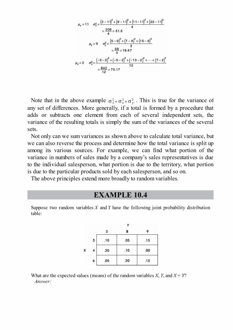
Note that in the above example . This is true for the variance ofany set of differences. More generally, if a total is formed by a procedure thatadds or subtracts one element from each of several independent sets, thevariance of the resulting totals is simply the sum of the variances of the severalsets.
Not only can we sum variances as shown above to calculate total variance, butwe can also reverse the process and determine how the total variance is split upamong its various sources. For example, we can find what portion of thevariance in numbers of sales made by a company’s sales representatives is dueto the individual salesperson, what portion is due to the territory, what portionis due to the particular products sold by each salesperson, and so on.
The above principles extend more broadly to random variables.
EXAMPLE 10.4Suppose two random variables X and Y have the following joint probability distributiontable:
What are the expected values (means) of the random variables X, Y, and X + Y?Answer:
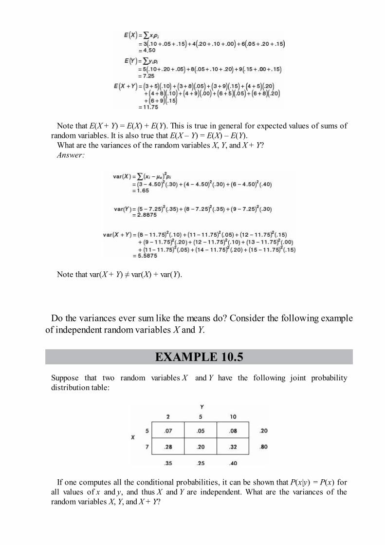
Note that E(X + Y) = E(X) + E(Y). This is true in general for expected values of sums ofrandom variables. It is also true that E(X – Y) = E(X) – E(Y).
What are the variances of the random variables X, Y, and X + Y?Answer:
Note that var(X + Y) ≠ var(X) + var(Y).
Do the variances ever sum like the means do? Consider the following exampleof independent random variables X and Y.
EXAMPLE 10.5Suppose that two random variables X and Y have the following joint probabilitydistribution table:
If one computes all the conditional probabilities, it can be shown that P(x|y) = P(x) forall values of x and y, and thus X and Y are independent. What are the variances of therandom variables X, Y, and X + Y?

Answer: First we calculate
Then we calculate the variances
Note that 0.64 + 12.2475 = 12.8875; that is, var(X + Y) = var(X) + var(Y).
More generally, if two random variables are independent, the variance of thesum (or the difference) of the two random variables is equal to the sum of thetwo individual variances.

TIPVariances of independent random variables add, but standarddeviations don’t!
EXAMPLE 10.6Suppose the mean SAT verbal score is 425 with standard deviation 100, while the meanSAT math score is 475 with standard deviation 100. What can be said about the mean andstandard deviation of the combined math and verbal scores?
Answer: The mean is 425 + 475 = 900. Can we add the two variances to obtain 1002 +1002 = 20,000 and then take the square root to obtain 141.4? No, because we don’t haveindependence—students with high math scores tend to have high verbal scores, and thosewith low math scores tend to have low verbal scores. The standard deviation of thecombined scores cannot be calculated from the given information.
For random variables X and Y the generalizations for transforming X and forcombining X and Y are sometimes written as
Does it make sense that variances add for both sums and differences ofindependent random variables? Ranges may illustrate this point more clearly:suppose prices for primary residences in a community go from $210,000 to$315,000, while prices for summer cottages go from $50,000 to $120,000.Someone wants to purchase a primary residence and a summer cottage. Theminimum total spent will be $260,000, the maximum possible is $435,000, andthus the range for the total is $435,000 – $260,000 = $175,000. The minimumdifference spent between the two homes will be $90,000, the maximumdifference will be $265,000, and thus the range for the difference is $265,000 –$90,000 = $175,000, the same as the range for the total. (Variances and rangesare both measures of spread and behave the same way with regard to the aboverule.)
Summary

• Two random variables X and Y are independent if P(x|y) = P(x) for all valuesof x and y.
• When combining two random variables, E(X + Y) = E(X) + E(Y) and E(X – Y)= E(X) – E(Y).
• When combining two independent random variables, the variances alwaysadd: var(X ± Y) = var(X) + var(Y).
Questions on Topic Ten: CombiningIndependent Random Variables
Multiple-Choice Questions
Directions: The questions or incomplete statements that follow are eachfollowed by five suggested answers or completions. Choose the responsethat best answers the question or completes the statement.
Questions 1–4 refer to the following: Students are classified by televisionusage (unending, average, and infrequent) and how often they exercise (regular,occasional, and never), resulting in the following joint probability table.
1. What is the probability distribution for X?
(A) P(X = 1) = .05, P(X = 2) = .20, P(X = 3) = .15(B) P(X = 1) = .10, P(X = 2) = .35, P(X = 3) = .30(C) P(X = 1) = .20, P(X = 2) = .45, P(X = 3) = .35(D) P(X = 1) = .40, P(X = 2) = .35, P(X = 3) = .25(E) It cannot be determined from the given information.
2. What is the probability P(X = 2, Y = 3), that is, the probability that astudent has average television usage but never exercises?
(A) .10(B) .1125(C) .22(D) .40(E) .60
3. What is the probability P(X = 2|Y = 3), that is, the probability that a
student has average television usage given that he never exercises?
(A) .10(B) .17(C) .22(D) .40(E) .60
4. Are X and Y independent?
(A) Yes, because the conditional probabilities P(X = x |Y = y) equalthe corresponding unconditional probabilities P(X = x).
(B) Yes, because the joint probabilities are equal to the product ofthe respective probabilities.
(C) Yes, because of either of the above answers.(D) No.(E) The answer cannot be determined from the given information.
5. Following are parts of the probability distributions for the randomvariables X and Y.

If X and Y are independent and the joint probability P (X = 1, Y = 2) = .1,what is P (X = 4)?
(A) .1(B) .2(C) .3(D) .4(E) .5
6. Suppose X and Y are random variables with E (X ) = 25, var(X ) = 3,
E (Y ) = 30, and var(Y ) = 4. What are the expected value and variance ofthe random variable X + Y ?
(A) E (X + Y ) = 55, var(X + Y ) = 3.5(B) E (X + Y ) = 55, var(X + Y ) = 5(C) E (X + Y ) = 55, var(X + Y ) = 7(D) E (X + Y ) = 27.5, var(X + Y ) = 7(E) There is insufficient information to answer this question.
7. Suppose X and Y are random variables with x = 10, σx = 3, y = 15,and σy = 4. Given that X and Y are independent, what are the mean andstandard deviation of the random variable X + Y ?
(A) x+y = 25, σx+y = 3.5
(B) x+y = 25, σx+y = 5
(C) x+y = 25, σx+y = 7
(D) x+y = 12.5, σx+y = 7
(E) There is insufficient information to answer this question.
8. Suppose X and Y are random variables with E(X ) = 500, var(X ) =50, E(Y ) = 400, and var(Y ) = 30. Given that X and Y are independent,what are the expected value and variance of the random variable X – Y?
(A) E(X – Y ) = 100, var(X – Y ) = 20(B) E(X – Y ) = 100, var(X – Y ) = 80(C) E(X – Y ) = 900, var(X – Y ) = 20(D) E(X – Y ) = 900, var(X – Y ) = 80(E) There is insufficient information to answer this question.
9. Suppose the average height of policemen is 71 inches with astandard deviation of 4 inches, while the average for policewomen is 66inches with a standard deviation of 3 inches. If a committee looks at allways of pairing up one male with one female officer, what will be themean and standard deviation for the difference in heights for the set ofpossible partners?
(A) Mean of 5 inches with a standard deviation of 1 inch(B) Mean of 5 inches with a standard deviation of 3.5 inches(C) Mean of 5 inches with a standard deviation of 5 inches(D) Mean of 68.5 inches with a standard deviation of 1 inch(E) Mean of 68.5 inches with a standard deviation of 3.5 inches
10. Consider the set of scores of all students taking the AP Statistics exam.
What is true about the variance of this set?

(A) Given a boxplot of this distribution, if the whisker lengths areequal, the variance will equal the interquartile range.
(B) If the distribution of scores is bell-shaped, the variance will bebetween –3 and +3.
(C) If there are a few high scores with the bulk of the scores lessthan the mean, the variance will be skewed to the right.
(D) If the distribution is symmetric, the variance will equal thestandard deviation.
(E) The variance is the sum of variances coming from a variety offactors such as study time, course grade, IQ, and so on.

TOPIC 11The Normal Distribution
• Properties• Using Tables• A Model for Measurement• Commonly Used Probabilities and z-scores
• Finding Means and Standard Deviations• Normal Approximation to the Binomial• Checking Normality
Some of the most useful probability distributions are symmetric and bell-shaped:
In this topic we study one such distribution called the normal distribution (notall symmetric, unimodal distributions are normal). The normal distribution isvaluable in describing various natural phenomena, especially those involvinggrowth or decay. However, the real importance of the normal distribution instatistics is that it can be used to describe the results of sampling procedures.
The normal distribution can be viewed as a limiting case of the binomial.More specifically, we start with any fixed probability of success p and considerwhat happens as n becomes arbitrarily large. To obtain a visual representationof the limit, we draw histograms using an increasingly large n for each fixed p.

For greater clarity, different scales have been used for the histogramsassociated with different values of n. From the diagrams above it is reasonableto accept that as n becomes larger without bound, the resulting histogramsapproach a smooth bell-shaped curve. This is the curve associated with thenormal distribution.
PROPERTIES OF THE NORMALDISTRIBUTIONThe normal distribution curve is bell-shaped and symmetric and has an infinitebase. Long, flat-looking tails cover many values but only a small proportion ofthe area. The flat appearance of the tails is deceptive. Actually, far out in thetails, the curve drops proportionately at an ever-increasing rate. In other words,when two intervals of equal length are compared, the one closer to the centermay experience a greater numerical drop, but the one further out in the tailexperiences a greater drop when measured as a proportion of the height at thebeginning of the interval.
The mean here is the same as the median and is located at the center. We wanta unit of measurement that applies equally well to any normal distribution, andwe choose a unit that arises naturally out of the curve’s shape. There is a pointon each side where the slope is steepest. These two points are called points ofinflection, and the distance from the mean to either point is precisely equal toone standard deviation. Thus, it is convenient to measure distances under thenormal curve in terms of z-scores (recall from Topic 2 that z-scores arefractions or multiples of standard deviations from the mean).
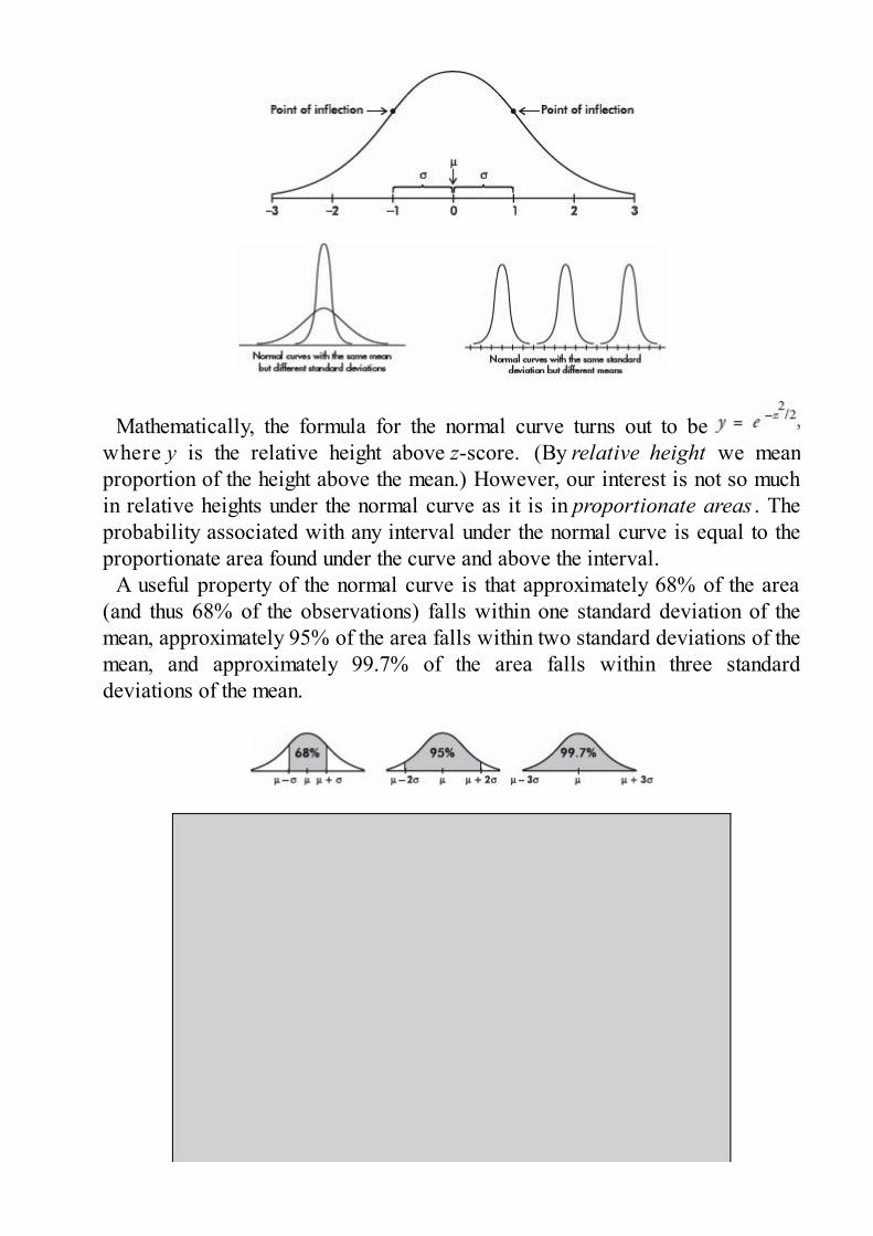
Mathematically, the formula for the normal curve turns out to be where y is the relative height above z-score. (By relative height we meanproportion of the height above the mean.) However, our interest is not so muchin relative heights under the normal curve as it is in proportionate areas . Theprobability associated with any interval under the normal curve is equal to theproportionate area found under the curve and above the interval.
A useful property of the normal curve is that approximately 68% of the area(and thus 68% of the observations) falls within one standard deviation of themean, approximately 95% of the area falls within two standard deviations of themean, and approximately 99.7% of the area falls within three standarddeviations of the mean.

TIPThe notation N( , ) stands for a normal model with mean and standard deviation .
USING TABLES OF THE NORMALDISTRIBUTIONTable A in the Appendix shows areas under the normal curve. Specifically, thistable shows the area to the left of a given point. It shows, for example, that to theleft of a z-score of 1.2 there is .8849 of the area:
Because the total area is 1, the area to the right of a point can be calculated bycalculating 1 minus the area to the left of the point. For example, the area to theright of a z-score of – 2.13 is 1 – .0166 = .9834. (Alternatively, by symmetry,we could have said that the area to the right of –2.13 is the same as that to theleft of +2.13 and then read the answer directly from Table A.)
The area between two points can be found by subtraction. For example, thearea between the z-scores of 1.23 and 2.71 is equal to .9966 – .8907 = .1059.
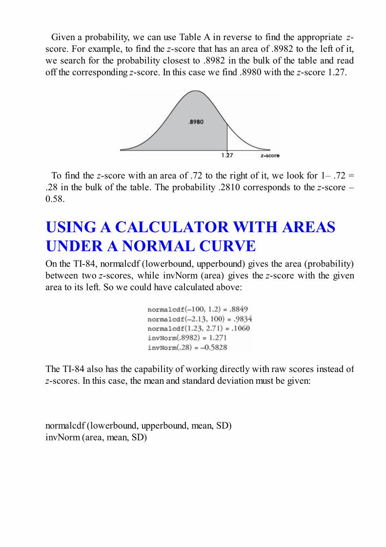
Given a probability, we can use Table A in reverse to find the appropriate z-score. For example, to find the z-score that has an area of .8982 to the left of it,we search for the probability closest to .8982 in the bulk of the table and readoff the corresponding z-score. In this case we find .8980 with the z-score 1.27.
To find the z-score with an area of .72 to the right of it, we look for 1– .72 =.28 in the bulk of the table. The probability .2810 corresponds to the z-score –0.58.
USING A CALCULATOR WITH AREASUNDER A NORMAL CURVEOn the TI-84, normalcdf (lowerbound, upperbound) gives the area (probability)between two z-scores, while invNorm (area) gives the z-score with the givenarea to its left. So we could have calculated above:
The TI-84 also has the capability of working directly with raw scores instead ofz-scores. In this case, the mean and standard deviation must be given:
normalcdf (lowerbound, upperbound, mean, SD)invNorm (area, mean, SD)
THE NORMAL DISTRIBUTION AS AMODEL FOR MEASUREMENTIn solving a problem using the normal distribution as a model, drawing a pictureof a normal curve with horizontal lines showing raw scores and z-scores isusually helpful.
TIPDon’t use the normal model if the distribution isn’t symmetricand unimodal.

TIPDraw a picture!
EXAMPLE 11.1The life expectancy of a particular brand of lightbulb is normally distributed with a meanof 1500 hours and a standard deviation of 75 hours.
a. What is the probability that a lightbulb will last less than 1410 hours?Answer: The z-score of 1410 is and from Table A the probability to theleft of –1.2 is .1151. [On the TI-84, normalcdf(0, 1410, 1500, 75) = .1151 andnormalcdf(–10, –1.2) = .1151.]
b. What is the probability that a lightbulb will last between 1563 and 1648 hours?Answer: The z-score of 1563 is and the z-score of 1648 is
In Table A, 0.84 and 1.97 give probabilities of .7995 and .9756,respectively. Thus between 1563 and 1648 there is a probability of .9756 – .7995 =.1761. [normalcdf(1563, 1648, 1500, 75) = .1762 and normalcdf(.84, 1.97) = .1760.]

c. What is the probability that a lightbulb will last between 1416 and 1677 hours?Answer: The z-score of 1416 is and the z-score of 1677 is
In Table A, –1.12 gives a probability of .1314, and 2.36 gives aprobability of .9909. Thus between 1416 and 1677 there is a probability of .9909 –.1314 = .8595. [normalcdf(1416, 1677, 1500, 75) = .8595 and normalcdf(–1.12, 2.36)= .8595.]
EXAMPLE 11.2A packing machine is set to fill a cardboard box with a mean of 16.1 ounces of cereal.Suppose the amounts per box form a normal distribution with a standard deviation equal to0.04 ounce.
a. What percentage of the boxes will end up with at least 1 pound of cereal?

Answer: The z-score of 16 is and –2.5 in Table A gives a probability of.0062. Thus the probability of having more than 1 pound in a box is 1 – .0062 = .9938or 99.38%. [normalcdf(16, 1000, 16.10, .04) = .9938 and normalcdf(–2.5, 10) =.9938.]
b. Ten percent of the boxes will contain less than what number of ounces?Answer: In Table A, we note that .1 area (actually .1003) is found to the left of a –1.28z-score. [On the TI-84, invNorm(.1) = –1.2816.] Converting the z-score of –1.28 into araw score yields or 16.1 – 1.28(0.04) = 16.049 ounces. [Or directly onthe TI-84, invNorm(.1, 16.10, .04) = 16.049.]
c. Eighty percent of the boxes will contain more than what number of ounces?Answer: In Table A, we note that 1 – .8 = .2 area (actually .2005) is found to the left ofa z-score of –0.84, and so to the right of a –0.84 z-score must be 80% of the area. [OrinvNorm(.2) = .8416.] Converting the z-score of –0.84 into a raw score yields 16.1 –0.84(0.04) = 16.066 ounces. [Or directly on the TI-84, invNorm(.2, 16.10, .04) =16.066.]
d. The middle 90% of the boxes will be between what two weights?Answer: Ninety percent in the middle leaves five percent in each tail. In Table A, wenote that .0505 area is found to the left of a z-score of –1.64, while 0.495 area is found
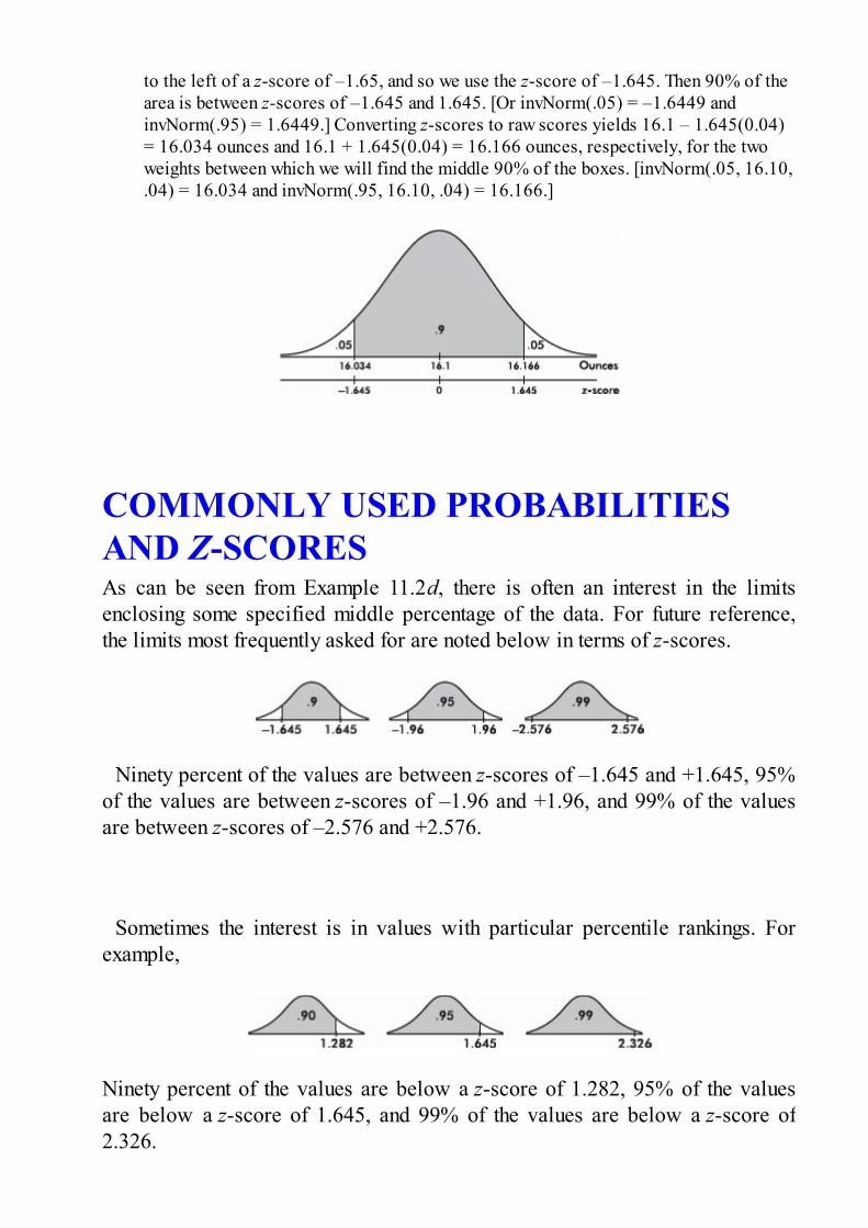
to the left of a z-score of –1.65, and so we use the z-score of –1.645. Then 90% of thearea is between z-scores of –1.645 and 1.645. [Or invNorm(.05) = –1.6449 andinvNorm(.95) = 1.6449.] Converting z-scores to raw scores yields 16.1 – 1.645(0.04)= 16.034 ounces and 16.1 + 1.645(0.04) = 16.166 ounces, respectively, for the twoweights between which we will find the middle 90% of the boxes. [invNorm(.05, 16.10,.04) = 16.034 and invNorm(.95, 16.10, .04) = 16.166.]
COMMONLY USED PROBABILITIESAND Z-SCORESAs can be seen from Example 11.2d, there is often an interest in the limitsenclosing some specified middle percentage of the data. For future reference,the limits most frequently asked for are noted below in terms of z-scores.
Ninety percent of the values are between z-scores of –1.645 and +1.645, 95%of the values are between z-scores of –1.96 and +1.96, and 99% of the valuesare between z-scores of –2.576 and +2.576.
Sometimes the interest is in values with particular percentile rankings. Forexample,
Ninety percent of the values are below a z-score of 1.282, 95% of the valuesare below a z-score of 1.645, and 99% of the values are below a z-score of2.326.

There are corresponding conclusions for negative z-scores:
Ninety percent of the values are above a z-score of –1.282, 95% of the valuesare above a z-score of –1.645, and 99% of the values are above a z-score of –2.326.
It is also useful to note the percentages corresponding to values fallingbetween integer z-scores. For example,
Note that 68.26% of the values are between z-scores of –1 and +1, 95.44% ofthe values are between z-scores of –2 and +2, and 99.74% of the values arebetween z-scores of –3 and +3.
EXAMPLE 11.3Suppose that the average height of adult males in a particular locality is 70 inches with astandard deviation of 2.5 inches.
a. If the distribution is normal, the middle 95% of males are between what twoheights?Answer: As noted above, the critical z-scores in this case are ±1.96, and so the twolimiting heights are 1.96 standard deviations from the mean. Therefore, 70 ± 1.96(2.5)= 70 ± 4.9, or from 65.1 to 74.9 inches.
b. Ninety percent of the heights are below what value?Answer: The critical z-score is 1.282, and so the value in question is 70 + 1.282(2.5) =73.205 inches.
c. Ninety-nine percent of the heights are above what value?Answer: The critical z-score is –2.326, and so the value in question is 70 – 2.326(2.5)= 64.185 inches.
d. What percentage of the heights are between z-scores of ±1? Of ±2? Of ±3?Answer: 68.26%, 95.44%, and 99.74%, respectively.

FINDING MEANS AND STANDARDDEVIATIONSIf we know that a distribution is normal, we can calculate the mean µ and thestandard deviation σ using percentage information from the population.
EXAMPLE 11.4Given a normal distribution with a mean of 25, what is the standard deviation if 18% ofthe values are above 29?
Answer: Looking for a .82 probability in Table A, we note that the corresponding z-score is 0.92. Thus 29 – 25 = 4 is equal to a standard deviation of 0.92, that is, 0.92σ = 4,and
EXAMPLE 11.5Given a normal distribution with a standard deviation of 10, what is the mean if 21% ofthe values are below 50?
Answer: Looking for a .21 probability in Table A leads us to a z-score of –0.81. Thus50 is –0.81 standard deviation from the mean, and so = 50 + 0.81(10) = 58.1.
EXAMPLE 11.6

Given a normal distribution with 80% of the values above 125 and 90% of the valuesabove 110, what are the mean and standard deviation?
Answer: Table A gives critical z-scores of –0.84 and –1.28. Thus we have a n d Solving the system {125 – = –0.84σ, 110 – = –1.28σ}simultaneously gives = 153.64 and σ = 34.09.
NORMAL APPROXIMATION TO THEBINOMIALMany practical applications of the binomial involve examples in which n islarge. However, for large n, binomial probabilities can be quite tedious tocalculate. Since the normal can be viewed as a limiting case of the binomial, itis natural to use the normal to approximate the binomial in appropriatesituations.
The binomial takes values only at integers, while the normal is continuous withprobabilities corresponding to areas over intervals. Therefore, we establish atechnique for converting from one distribution to the other. For approximationpurposes we do as follows. Each binomial probability corresponds to thenormal probability over a unit interval centered at the desired value. Thus, forexample, to approximate the binomial probability of eight successes wedetermine the normal probability of being between 7.5 and 8.5.

TIPWhen n is small, you cannot use the normal model toapproximate the binomial model.
EXAMPLE 11.7Suppose that 15% of the cars coming out of an assembly plant have some defect. In adelivery of 40 cars what is the probability that exactly 5 cars have defects?
Answer: The actual answer is ( ) (.15)5(.85)35, but clearly this involves a nontrivialcalculation. [If one has a calculator such as the TI-84, then binompdf(40, .15, 5) = .1692.]To approximate the answer using the normal, we first calculate the mean µ and thestandard deviation σ as follows:
We then calculate the appropriate z-scores: and –0.22. Looking upthe corresponding probabilities in Table A, we obtain a final answer of .4129 – .2546 =.1583. (The actual answer is .1692.)
Even more useful are approximations relating to probabilities over intervals.
EXAMPLE 11.8
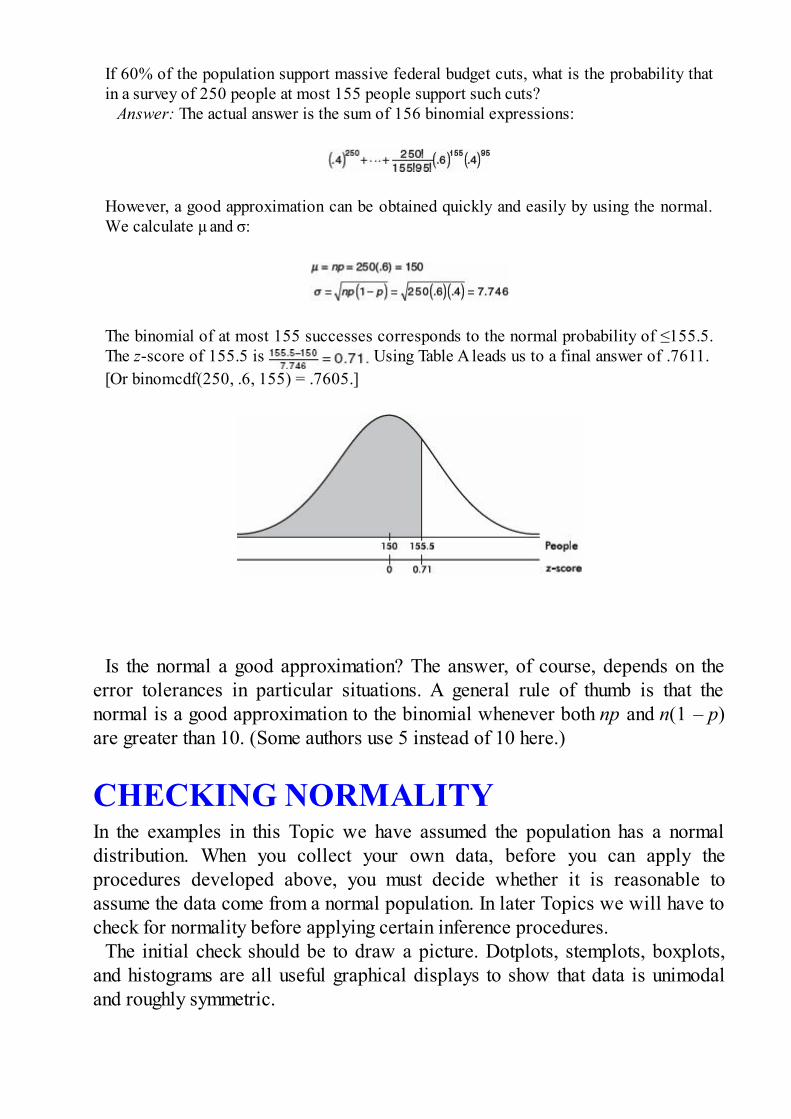
If 60% of the population support massive federal budget cuts, what is the probability thatin a survey of 250 people at most 155 people support such cuts?
Answer: The actual answer is the sum of 156 binomial expressions:
However, a good approximation can be obtained quickly and easily by using the normal.We calculate µ and σ:
The binomial of at most 155 successes corresponds to the normal probability of ≤155.5.The z-score of 155.5 is Using Table A leads us to a final answer of .7611.[Or binomcdf(250, .6, 155) = .7605.]
Is the normal a good approximation? The answer, of course, depends on theerror tolerances in particular situations. A general rule of thumb is that thenormal is a good approximation to the binomial whenever both np and n(1 – p)are greater than 10. (Some authors use 5 instead of 10 here.)
CHECKING NORMALITYIn the examples in this Topic we have assumed the population has a normaldistribution. When you collect your own data, before you can apply theprocedures developed above, you must decide whether it is reasonable toassume the data come from a normal population. In later Topics we will have tocheck for normality before applying certain inference procedures.
The initial check should be to draw a picture. Dotplots, stemplots, boxplots,and histograms are all useful graphical displays to show that data is unimodaland roughly symmetric.
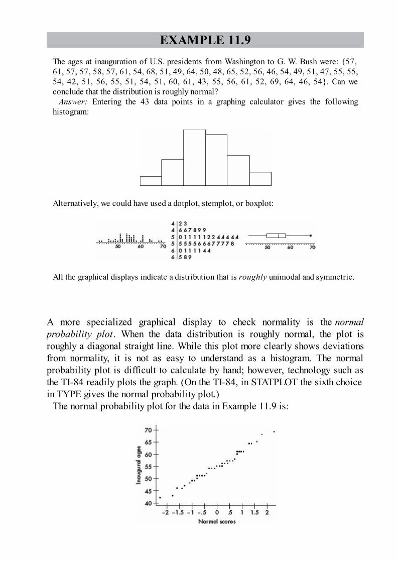
EXAMPLE 11.9The ages at inauguration of U.S. presidents from Washington to G. W. Bush were: {57,61, 57, 57, 58, 57, 61, 54, 68, 51, 49, 64, 50, 48, 65, 52, 56, 46, 54, 49, 51, 47, 55, 55,54, 42, 51, 56, 55, 51, 54, 51, 60, 61, 43, 55, 56, 61, 52, 69, 64, 46, 54}. Can weconclude that the distribution is roughly normal?
Answer: Entering the 43 data points in a graphing calculator gives the followinghistogram:
Alternatively, we could have used a dotplot, stemplot, or boxplot:
All the graphical displays indicate a distribution that is roughly unimodal and symmetric.
A more specialized graphical display to check normality is the normalprobability plot. When the data distribution is roughly normal, the plot isroughly a diagonal straight line. While this plot more clearly shows deviationsfrom normality, it is not as easy to understand as a histogram. The normalprobability plot is difficult to calculate by hand; however, technology such asthe TI-84 readily plots the graph. (On the TI-84, in STATPLOT the sixth choicein TYPE gives the normal probability plot.)
The normal probability plot for the data in Example 11.9 is:

A graph this close to a diagonal straight line indicates that the data have adistribution very close to normal.
Note that alternatively, one could have plotted the data (in this case, inauguralages) on the x-axis and the normal scores on the y-axis.
Summary• The normal distribution is one particular symmetric, unimodal distribution.• Drawing pictures of normal curves with horizontal lines showing raw scores
and z-scores is usually helpful.• Areas (probabilities) under a normal curve can be found using the given table
or calculator functions, such as normalcdf on TI calculators.• Critical values corresponding to given probabilities can be found using the
given table or calculator functions, such as invNorm on TI calculators.• The normal probability plot is very useful in gauging whether a given
distribution of data is approximately normal: If the plot is nearly straight, thedata is nearly normal.
Questions on Topic Eleven: The NormalDistribution
Multiple-Choice Questions
Directions: The questions or incomplete statements that follow are eachfollowed by five suggested answers or completions. Choose the responsethat best answers the question or completes the statement.
1. Which of the following is a true statement?
(A) The area under a normal curve is always equal to 1, no matterwhat the mean and standard deviation are.
(B) All bell-shaped curves are normal distributions for some choiceof μ and σ.
(C) The smaller the standard deviation of a normal curve, the lowerand more spread out the graph.
(D) Depending upon the value of the standard deviation, normalcurves with different means may be centered around the same number.
(E) Depending upon the value of the standard deviation, the meanand median of a particular normal distribution may be different.
2. Which of the following is a true statement?
(A) The area under the standard normal curve between 0 and 2 istwice the area between 0 and 1.
(B) The area under the standard normal curve between 0 and 2 ishalf the area between –2 and 2.
(C) For the standard normal curve, the interquartile range isapproximately 3.
(D) For the standard normal curve, the range is 6.(E) For the standard normal curve, the area to the left of 0.1 is the
same as the area to the right of 0.9.
3. Populations P1 and P2 are normally distributed and have identicalmeans. However, the standard deviation of P1 is twice the standarddeviation of P2. What can be said about the percentage of observationsfalling within two standard deviations of the mean for each population?
(A) The percentage for P1 is twice the percentage for P2.(B) The percentage for P1 is greater, but not twice as great, as the
percentage for P2.(C) The percentage for P2 is twice the percentage for P1.(D) The percentage for P2 is greater, but not twice as great, as the
percentage for P1.(E) The percentages are identical.
4. Consider the following two normal curves:
Which has the larger mean and which has the larger standard deviation?
(A) Larger mean, a; larger standard deviation, a(B) Larger mean, a; larger standard deviation, b(C) Larger mean, b; larger standard deviation, a(D) Larger mean, b; larger standard deviation, b(E) Larger mean, b; same standard deviation
In Questions 5–15, assume the given distributions are normal.
5. A trucking firm determines that its fleet of trucks averages a mean of12.4 miles per gallon with a standard deviation of 1.2 miles per gallon oncross-country hauls. What is the probability that one of the trucksaverages fewer than 10 miles per gallon?
(A) .0082(B) .0228(C) .4772(D) .5228(E) .9772
6. A factory dumps an average of 2.43 tons of pollutants into a river
every week. If the standard deviation is 0.88 tons, what is the probabilitythat in a week more than 3 tons are dumped?

(A) .2578(B) .2843(C) .6500(D) .7157(E) .7422
7. An electronic product takes an average of 3.4 hours to move through
an assembly line. If the standard deviation is 0.5 hour, what is theprobability that an item will take between 3 and 4 hours?
(A) .2119(B) .2295(C) .3270(D) .3811(E) .6730
8. The mean score on a college placement exam is 500 with a standard
deviation of 100. Ninety-five percent of the test takers score above what?
(A) 260(B) 336(C) 405(D) 414(E) 664
9. The average noise level in a restaurant is 30 decibels with a
standard deviation of 4 decibels. Ninety-nine percent of the time it isbelow what value?
(A) 20.7(B) 32.0(C) 33.4
(D) 37.8(E) 39.3
10. The mean income per household in a certain state is $9500 with a
standard deviation of $1750. The middle 95% of incomes are betweenwhat two values?
(A) $5422 and $13,578(B) $6070 and $12,930(C) $6621 and $12,379(D) $7260 and $11,740(E) $8049 and $10,951
11. One company produces movie trailers with mean 150 seconds and
standard deviation 40 seconds, while a second company produces trailerswith mean 120 seconds and standard deviation 30 seconds. What is theprobability that two randomly selected trailers, one produced by eachcompany, will combine to less than three minutes?
(A) .000(B) .036(C) .099(D) .180(E) .405
12. Jay Olshansky from the University of Chicago was quoted in
Chance News as arguing that for the average life expectancy to reach 100,18% of people would have to live to 120. What standard deviation is heassuming for this statement to make sense?
(A) 21.7(B) 24.4(C) 25.2
(D) 35.0(E) 111.1
13. Cucumbers grown on a certain farm have weights with a standard
deviation of 2 ounces. What is the mean weight if 85% of the cucumbersweigh less than 16 ounces?
(A) 13.92(B) 14.30(C) 14.40(D) 14.88(E) 15.70
14. If 75% of all families spend more than $75 weekly for food, while
15% spend more than $150, what is the mean weekly expenditure andwhat is the standard deviation?
(A) = 83.33, σ = 12.44(B) = 56.26, σ = 11.85(C) = 118.52, σ = 56.26(D) = 104.39, σ = 43.86(E) = 139.45, σ = 83.33
15. A coffee machine can be adjusted to deliver any fixed number ofounces of coffee. If the machine has a standard deviation in delivery equalto 0.4 ounce, what should be the mean setting so that an 8-ounce cup willoverflow only 0.5% of the time?
(A) 6.97 ounces(B) 7.22 ounces(C) 7.34 ounces

(D) 7.80 ounces(E) 9.03 ounces
16. Assume that a baseball team has an average pitcher, that is, one
whose probability of winning any decision is .5. If this pitcher has 30decisions in a season, what is the probability that he will win at least 20games?
(A) .0505(B) .2514(C) .2743(D) .3333(E) .4300
17. Given that 10% of the nails made using a certain manufacturing
process have a length less than 2.48 inches, while 5% have a lengthgreater than 2.54 inches, what are the mean and standard deviation of thelengths of the nails? Assume that the lengths have a normal distribution.
(A) = 2.506, σ = 0.0205(B) = 2.506, σ = 0.0410(C) = 2.516, σ = 0.0825(D) = 2.516, σ = 0.1653(E) The mean and standard deviation cannot be computed from the
information given.
Free-Response Questions
Directions: You must show all work and indicate the methods you use. Youwill be graded on the correctness of your methods and on the accuracy ofyour final answers.

Two Open-Ended Questions1. The time it takes Steve to walk to school follows a normal
distribution with mean 30 minutes and standard deviation 5 minutes,while the time it takes Jan to walk to school follows a normal distributionwith mean 25 minutes and standard deviation 4 minutes. Assume theirwalking times are independent of each other.
(a) If they leave at the same time, what is the probability that Stevearrives before Jan?
(b) How much earlier than Jan should Steve leave so that he has a90% chance of arriving before Jan?
2. (a) Two components are in series so the failure of either will cause thesystem to fail. The time to failure for a new component is normallydistributed with a mean of 3000 hours and a standard deviation of 400hours. One of the components has already run for 2500 hours, whilethe other has run for 2800 hours. Assuming component failures areindependent, what is the probability the system survives for 10 moredays (240 hours)?
(b) If the components are put in parallel, the system will fail only ifboth components fail. If the two components in (a) are put in parallel,what is the probability that the system survives for 10 more days?
Two Investigative Tasks1. When Michael Jordan came up to try for a sixth free throw after
having made five straight free throws, the announcer commented that thelaw of averages would be working against Jordan.
(a) What did the announcer mean? Was this a correct interpretationof probability? Explain.
(b) Jordan makes 90% of his free throws. What is the probabilitythat he will make six straight free throws? That he will make fivestraight free throws and then miss the next? That he will make the nextfree throw given that he has made the last five in a row?
(c) How could you set up a simulation using a random number tableto analyze the situation the announcer was commenting on?
(d) If Jordan shoots six times from the free throw line, what are themean and standard deviation for the number of shots he is expected tomake?
(e) If Jordan makes only 35 out of 40 free throw tries during theplayoffs, is this sufficient evidence that the probability of his making a

free throw is really below .90? Explain.
2. Many people have lactose intolerance leading to cramps anddiarrhea when they eat dairy products. Substantial relief can be obtainedby taking dietary supplements of lactase, an enzyme. One product consistsof caplets containing a mean of 9000 FCC lactase units with a standarddeviation of 590 units and a normal distribution of lactase units. A personwith severe lactose intolerance may need to take two such tabletswhenever they eat dairy products. Tablets with under 8500 FCC lactaseunits can produce noticeably less relief.
(a) Determine the probability that a caplet has less than 8500 FCClactase units. Round off to the nearest tenth.
(b) Using the random number table below, run five simulations forthe number of tablets a lab technician samples before finding two withless than 8500 units each.
84177 06757 17613 15582 51506 81435 41050 92031 06449 0505959884 31180 53115 84469 94868 57967 05811 84514 75011 1300663395 55041 15866 06589 13119 71020 85940 91932 06488 7498754355 52704 90359 02649 47496 71567 94268 08844 26294 6475908989 57024 97284 00637 89283 03514 59195 07635 03309 7260529357 23737 67881 03668 33876 35841 52869 23114 15864 38942
(c) The results of two 100-trial simulations, one looking for twotablets each less than 8500 units and one looking for two tablets eachgreater than 9000 units, are shown below. Which distribution is which?Explain your answer.
(d) Using the correct barplot above, estimate the expected number ofcaplets a laboratory will sample before finding two with less than8500 units each.
TOPIC 12Sampling Distributions
• Sample Proportion• Sample Mean• Central Limit Theorem• Difference Between Two Independent Sample
Proportions
• Difference Between Two Independent SampleMeans
• The t-distribution• The Chi-Square Distribution• The Standard Error
The population is the complete set of items of interest. A sample is a part of apopulation used to represent the population. The population mean andpopulation standard deviation σ are examples of population parameters. Thesample mean and the sample standard deviation s are examples of statistics.Statistics are used to make inferences about population parameters. While apopulation parameter is a fixed quantity, statistics vary depending on theparticular sample chosen. The probability distribution showing how a statisticvaries is called a sampling distribution. The sampling distribution is unbiasedif its mean is equal to the associated population parameter.

TIPA sampling distribution is not the same thing as thedistribution of a sample.
We want to know some important truth about a population, but in practicalterms this truth is unknowable. What’s the average adult human body weight?What proportion of people have high cholesterol? What we can do is carefullycollect data from as large and representative a group of individuals as possibleand then use this information to estimate the value of the population parameter.How close are we to the truth? We know that different samples would givedifferent estimates, and so sampling error is unavoidable. What is wonderful,and what we will learn in this Topic, is that we can quantify this sampling error!We can make statements like “the average weight must almost surely be within 5pounds of 176 pounds” or “the proportion of people with high cholesterol mustalmost surely be within ±3% of 37%.”
SAMPLING DISTRIBUTION OF ASAMPLE PROPORTIONWhereas the mean is basically a quantitative measurement, the proportionrepresents essentially a qualitative approach. The interest is simply in thepresence or absence of some attribute. We count the number of yes responsesand form a proportion. For example, what proportion of drivers wear seatbelts? What proportion of SCUD missiles can be intercepted? What proportionof new stereo sets have a certain defect?
This separation of the population into “haves” and “have-nots” suggests thatwe can make use of our earlier work on binomial distributions. We also keep inmind that, when n (trials, or in this case sample size) is large enough, thebinomial can be approximated by the normal.
In this topic we are interested in estimating a population proportion p byconsidering a single sample proportion . This sample proportion is just one ofa whole universe of sample proportions, and to judge its significance we mustknow how sample proportions vary. Consider the set of proportions from allpossible samples of a specified size n. It seems reasonable that theseproportions will cluster around the population proportion (the sampleproportion is an unbiased statistic of the population proportion) and that thelarger the chosen sample size, the tighter the clustering.
How do we calculate the mean and standard deviation of the set of population

proportions? Suppose the sample size is n and the actual population proportionis p. From our work on binomial distributions, we remember that the mean andstandard deviation for the number of successes in a given sample are pn and
respectively, and for large n the complete distribution begins to look“normal.”
Here, however, we are interested in the proportion rather than in the number ofsuccesses. From Topic Two we remember that when we multiply or divideevery element by a constant, we multiply or divide both the mean and thestandard deviation by the same constant. In this case, to change number ofsuccesses to proportion of successes, we divide by n:
Furthermore, if each element in an approximately normal distribution is dividedby the same constant, it is reasonable that the result will still be anapproximately normal distribution.
Thus the principle forming the basis of the following discussion is
Start with a population with a given proportion p. Take all samples ofsize n. Compute the proportion in each of these samples. Then
1. the set of all sample proportions is approximately normallydistributed (often stated: the distribution of sample proportions isapproximately normal).
2. the mean of the set of sample proportions equals p, thepopulation proportion.
3. the standard deviation σ of the set of sample proportions isapproximately equal to
Alternatively, we say that the sampling distribution of is approximatelynormal with mean p and standard deviation
Since we are using the normal approximation to the binomial, both np and n(1– p) should be at least 10. Furthermore, in making calculations and drawingconclusions from a specific sample, it is important that the sample be a simplerandom sample.
Finally, because sampling is usually done without replacement, the sample

cannot be too large; the sample size n should be no larger than 10% of thepopulation. (We’re actually worried about independence, but randomlyselecting a relatively small sample allows us to assume independence. Ofcourse, it’s always better to have larger samples—it’s just that if the sample islarge relative to the population, then the proper inference techniques aredifferent from those taught in introductory statistics classes.)
EXAMPLE 12.1Suppose that 70% of all dialysis patients will survive for at least 5 years. In a simplerandom sample (SRS) of 100 new dialysis patients, what is the probability that theproportion surviving for at least 5 years will exceed 80%?
Answer: Both np = (100)(.7) = 70 > 10 and n(1 – p) = (100)(.3) = 30 > 10, and oursample is clearly less than 10% of all dialysis patients. So the set of sample proportionsis approximately normally distributed with mean .70 and standard deviation
With a z-score of the probability that the sample proportion will exceed80% is 1 – .9854 = .0146. [normalcdf(.8, 1, .7, .0458) = .0145.]
EXAMPLE 12.2It is estimated that 48% of all motorists use their seat belts. If a police officer observes400 cars go by in an hour, what is the probability that the proportion of drivers wearingseat belts is between 45% and 55%?
Answer: Both np = (400)(.48) = 192 > 10 and n(1 – p) = (400)(.52) = 208 > 10, andour sample is clearly less than 10% of all motorists. So the set of sample proportions isapproximately normally distributed with mean .48 and standard deviation
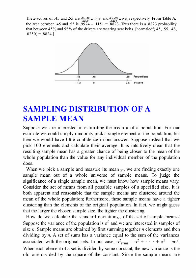
The z-scores of .45 and .55 are and respectively. From Table A,the area between .45 and .55 is .9974 – .1151 = .8823. Thus there is a .8823 probabilitythat between 45% and 55% of the drivers are wearing seat belts. [normalcdf(.45, .55, .48,.0250) = .8824.]
SAMPLING DISTRIBUTION OF ASAMPLE MEANSuppose we are interested in estimating the mean µ of a population. For ourestimate we could simply randomly pick a single element of the population, butthen we would have little confidence in our answer. Suppose instead that wepick 100 elements and calculate their average. It is intuitively clear that theresulting sample mean has a greater chance of being closer to the mean of thewhole population than the value for any individual member of the populationdoes.
When we pick a sample and measure its mean , we are finding exactly onesample mean out of a whole universe of sample means. To judge thesignificance of a single sample mean, we must know how sample means vary.Consider the set of means from all possible samples of a specified size. It isboth apparent and reasonable that the sample means are clustered around themean of the whole population; furthermore, these sample means have a tighterclustering than the elements of the original population. In fact, we might guessthat the larger the chosen sample size, the tighter the clustering.
How do we calculate the standard deviation of the set of sample means?Suppose the variance of the population is σ2 and we are interested in samples ofsize n. Sample means are obtained by first summing together n elements and thendividing by n. A set of sums has a variance equal to the sum of the variancesassociated with the original sets. In our case, σ2
sums = σ2 + · · · + σ2 = nσ2.When each element of a set is divided by some constant, the new variance is theold one divided by the square of the constant. Since the sample means are
obtained by dividing the sums by n, the variance of the sample means isobtained by dividing the variance of the sums by n2. Thus if symbolizes thestandard deviation of the sample means, we find that
In terms of standard deviations, we have We have shown the following:
Start with a population with a given mean and standard deviation σ.Compute the mean of all samples of size n. Then the mean of the set ofsample means will equal , the mean of the population, and the standarddeviation of the set of sample means will be approximately equal to
that is, the standard deviation of the whole population divided by thesquare root of the sample size.
Note that the variance of the set of sample means varies directly as thevariance of the original population and inversely as the size of the samples,while the standard deviation of the set of sample means varies directly as thestandard deviation of the original population and inversely as the square root ofthe size of the samples.
EXAMPLE 12.3Suppose that tomatoes weigh an average of 10 ounces with a standard deviation of 3ounces and a store sells boxes containing 12 tomatoes each. If customers determine theaverage weight of the tomatoes in each box they buy, what will be the mean and standarddeviation of these averages?
Answer: We have samples of size 12. The mean of these sample means will equal thepopulation mean, 10 ounces. The standard deviation of these sample means will equal
ounces.
Note that while giving the mean and standard deviation of the set of samplemeans, we did not describe the shape of the distribution. If we are also giventhat the original population is normal, then we can conclude that the set ofsample means has a normal distribution.

EXAMPLE 12.4Suppose that the distribution for total amounts spent by students vacationing for a week inFlorida is normally distributed with a mean of $650 and a standard deviation of $120.What is the probability that an SRS of 10 students will spend an average of between $600and $700?
Answer: The mean and standard deviation of the set of all sample means of size 10 are:
The z-scores of 600 and 700 are and respectively. UsingTable A, we find the desired probability is .9066 – .0934 = .8132. [normalcdf(600, 700,650, 37.95) = .8123.]
CENTRAL LIMIT THEOREMWe assumed above that the original population had a normal distribution.Unfortunately, few populations are normal, let alone exactly normal. However,it can be shown mathematically that no matter how the original population isdistributed, if n is large enough, then the set of sample means is approximatelynormally distributed. For example, there is no reason to suppose that theamounts of money that different people spend in grocery stores are normallydistributed. However, if each day we survey 30 people leaving a store anddetermine the average grocery bill, these daily averages will have a nearlynormal distribution.
The following principle forms the basis of much of what we discuss in thistopic and in those following. It is a simplified statement of the central limittheorem of statistics.
Start with a population with a given mean , a standard deviation σ, and

any shape distribution whatsoever. Pick n sufficiently large (at least 30)and take all samples of size n. Compute the mean of each of thesesamples. Then
1. the set of all sample means is approximately normallydistributed (often stated: the distribution of sample means isapproximately normal).
2. the mean of the set of sample means equals , the mean of thepopulation.
3. the standard deviation of the set of sample means isapproximately equal to that is, equal to the standard deviation ofthe whole population divided by the square root of the sample size.
Alternatively, we say that the sampling distribution of is approximatelynormal with mean and standard deviation
While we mention n ≥ 30 as a rough rule of thumb, n ≥ 40 is often used, and nshould be chosen even larger if more accuracy is required or if the originalpopulation is far from normal. As with proportions, we have the assumptions ofa simple random sample and of sample size n no larger than 10% of thepopulation.
EXAMPLE 12.5Suppose that the average outstanding credit card balance for young couples is $650 with astandard deviation of $420. In an SRS of 100 couples, what is the probability that themean outstanding credit card balance exceeds $700?
Answer: The sample size is over 30, we have an SRS, and our sample is less than 10%of all couples with outstanding balances, and so by the central limit theorem the set ofsample means is approximately normally distributed with mean 650 and standarddeviation With a z-score of the probability that the sample meanexceeds 700 is 1 –.8830 = .1170. [normalcdf(700, 10000, 650, 42) = .1169.]
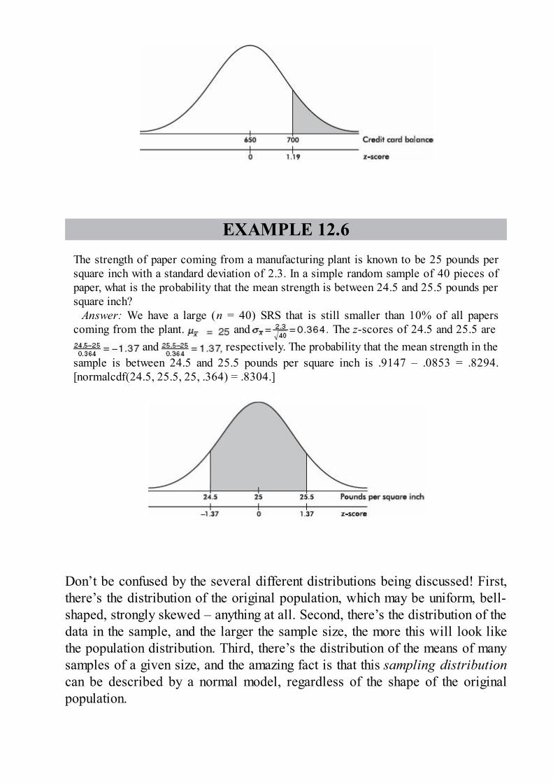
EXAMPLE 12.6The strength of paper coming from a manufacturing plant is known to be 25 pounds persquare inch with a standard deviation of 2.3. In a simple random sample of 40 pieces ofpaper, what is the probability that the mean strength is between 24.5 and 25.5 pounds persquare inch?
Answer: We have a large (n = 40) SRS that is still smaller than 10% of all paperscoming from the plant. and The z-scores of 24.5 and 25.5 are
and respectively. The probability that the mean strength in thesample is between 24.5 and 25.5 pounds per square inch is .9147 – .0853 = .8294.[normalcdf(24.5, 25.5, 25, .364) = .8304.]
Don’t be confused by the several different distributions being discussed! First,there’s the distribution of the original population, which may be uniform, bell-shaped, strongly skewed – anything at all. Second, there’s the distribution of thedata in the sample, and the larger the sample size, the more this will look likethe population distribution. Third, there’s the distribution of the means of manysamples of a given size, and the amazing fact is that this sampling distributioncan be described by a normal model, regardless of the shape of the originalpopulation.

SAMPLING DISTRIBUTION OF ADIFFERENCE BETWEEN TWOINDEPENDENT SAMPLEPROPORTIONSNumerous important and interesting applications of statistics involve thecomparison of two population proportions. For example, is the proportion ofsatisfied purchasers of American automobiles greater than that of buyers ofJapanese cars? How does the percentage of surgeons recommending a newcancer treatment compare with the corresponding percentage of oncologists?What can be said about the difference between the proportion of single parentson welfare and the proportion of two-parent families on welfare?
Our procedure involves comparing two sample proportions. When is adifference between two such sample proportions significant? Note that we aredealing with one difference from the set of all possible differences obtained bysubtracting sample proportions of one population from sample proportions of asecond population. To judge the significance of one particular difference, wemust first determine how the differences vary among themselves. Remember thatthe variance of a set of differences is equal to the sum of the variances of theindividual sets; that is,
Now if
then
Then we have the following about the sampling distribution of 1 – 2:
Start with two populations with given proportions p1 and p2. Take allsamples of sizes n1 and n2, respectively. Compute the difference 1 – 2of the two proportions in each pair of samples. Then

1. the set of all differences of sample proportions isapproximately normally distributed (alternatively stated: thedistribution of differences of sample proportions is approximatelynormal).
2. the mean of the set of differences of sample proportions equalsp1 – p2, the difference of population proportions.
3. the standard deviation σd of the set of differences of sampleproportions is approximately equal to
Since we are using the normal approximation to the binomial, n1p1, n1(1 – p1),n2p2, and n2(1 – p2) should all be at least 10. Furthermore, in makingcalculations and drawing conclusions from specific samples, it is important boththat the samples be simple random samples and that they be takenindependently of each other. Finally, each sample cannot be too large; thesample sizes should be no larger than 10% of the populations.
EXAMPLE 12.7A promoter knows that 23% of males enjoy watching boxing matches; however, only 12%of females enjoy watching this sport. In an SRS of 100 men and an independent SRS of125 women, what is the probability that the difference in the percentages of men andwomen who enjoy watching boxing is more than 10%?
Answer: We note that n1p1 = 23, n1(1 – p1) = 77, n2p2 = 15, and n2(1 – p2) = 110 areall >10; we have independent SRSs, and the samples are less than 10% of their respectivepopulations. For the sampling distribution of 1 – 2, the mean is .23 – .12 = .11 and thestandard deviation is
The z-score of .10 is Using Table A, we find 1 – .4207 = .5793 for theprobability that the difference is more than 10%. [normalcdf(.10, 1, .11, .0511) = .5776.]
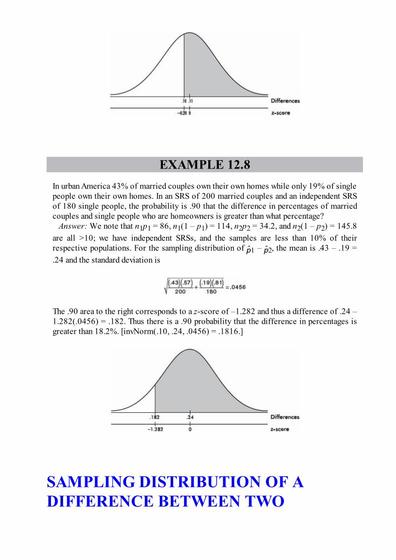
EXAMPLE 12.8In urban America 43% of married couples own their own homes while only 19% of singlepeople own their own homes. In an SRS of 200 married couples and an independent SRSof 180 single people, the probability is .90 that the difference in percentages of marriedcouples and single people who are homeowners is greater than what percentage?
Answer: We note that n1p1 = 86, n1(1 – p1) = 114, n2p2 = 34.2, and n2(1 – p2) = 145.8are all >10; we have independent SRSs, and the samples are less than 10% of theirrespective populations. For the sampling distribution of 1 – 2, the mean is .43 – .19 =.24 and the standard deviation is
The .90 area to the right corresponds to a z-score of –1.282 and thus a difference of .24 –1.282(.0456) = .182. Thus there is a .90 probability that the difference in percentages isgreater than 18.2%. [invNorm(.10, .24, .0456) = .1816.]
SAMPLING DISTRIBUTION OF ADIFFERENCE BETWEEN TWO

INDEPENDENT SAMPLE MEANSMany real-life applications of statistics involve comparisons of two populationmeans. For example, is the average weight of laboratory rabbits receiving aspecial diet greater than that of rabbits on a standard diet? Which of twoaccounting firms pays a higher mean starting salary? Is the life expectancy of acoal miner less than that of a school teacher?
First we consider how to compare the means of samples, one from eachpopulation. When is a difference between two such sample means significant?The answer is more apparent when we realize that what we are looking at is onedifference from a set of differences. That is, there is the set of all possibledifferences obtained by subtracting sample means from one set from samplemeans from a second set. To judge the significance of one particular differencewe must first determine how the differences vary among themselves. Thenecessary key is the fact that the variance of a set of differences is equal to thesum of the variances of the individual sets. Thus,
Now if
then
Then we have the following about the sampling distribution of 1 – 2:
Start with two normal populations with means 1 and 2 and standarddeviations σ1 and σ2. Take all samples of sizes n1 and n2, respectively.Compute the difference 1 – 2 of the two means in each pair of thesesamples. Then
1. the set of all differences of sample means is approximatelynormally distributed (alternatively stated: the distribution ofdifferences of sample means is approximately normal).
2. the mean of the set of differences of sample means equals 1 –
2, the difference of population means.
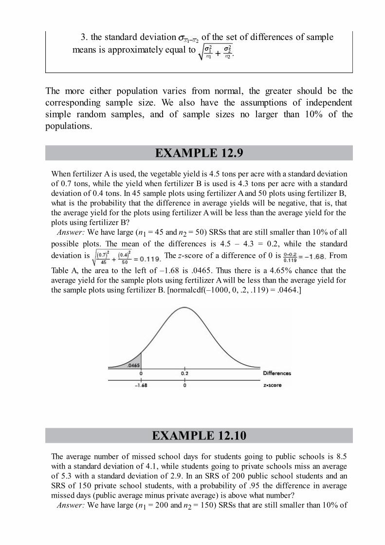
3. the standard deviation of the set of differences of samplemeans is approximately equal to
The more either population varies from normal, the greater should be thecorresponding sample size. We also have the assumptions of independentsimple random samples, and of sample sizes no larger than 10% of thepopulations.
EXAMPLE 12.9When fertilizer A is used, the vegetable yield is 4.5 tons per acre with a standard deviationof 0.7 tons, while the yield when fertilizer B is used is 4.3 tons per acre with a standarddeviation of 0.4 tons. In 45 sample plots using fertilizer A and 50 plots using fertilizer B,what is the probability that the difference in average yields will be negative, that is, thatthe average yield for the plots using fertilizer A will be less than the average yield for theplots using fertilizer B?
Answer: We have large (n1 = 45 and n2 = 50) SRSs that are still smaller than 10% of allpossible plots. The mean of the differences is 4.5 – 4.3 = 0.2, while the standarddeviation is The z-score of a difference of 0 is From
Table A, the area to the left of –1.68 is .0465. Thus there is a 4.65% chance that theaverage yield for the sample plots using fertilizer A will be less than the average yield forthe sample plots using fertilizer B. [normalcdf(–1000, 0, .2, .119) = .0464.]
EXAMPLE 12.10The average number of missed school days for students going to public schools is 8.5with a standard deviation of 4.1, while students going to private schools miss an averageof 5.3 with a standard deviation of 2.9. In an SRS of 200 public school students and anSRS of 150 private school students, with a probability of .95 the difference in averagemissed days (public average minus private average) is above what number?
Answer: We have large (n1 = 200 and n2 = 150) SRSs that are still smaller than 10% of

all public and private school students. The mean of the differences is 8.5 – 5.3 = 3.2,while the standard deviation is An area of .95 to the right
corresponds to a z-score of –1.645. The difference in days is 3.2 – 1.645(0.374) = 2.6.Thus there is a .95 probability that the difference in average missed days between publicand private school samples is over 2.6 days. [invNorm(.05, 3.2, .374) = 2.585.]
THE T-DISTRIBUTIONWhen the population standard deviation σ is unknown, we use the samplestandard deviation s as an estimate for σ. But then does not follow a
normal distribution. If, however, the original population is normallydistributed, there is a distribution that can be used when working with the ratios. This Student t-distribution was introduced in 1908 by W. S. Gosset, aBritish mathematician employed by the Guiness Breweries. (When we areworking with small samples from a population that is not nearly normal, wemust use very different “nonparametric” techniques not discussed in this reviewbook.)
Thus, for a sample from a normally distributed population, we work with thevariable
with a resulting t-distribution that is bell-shaped and symmetric, but lower at themean, higher at the tails, and so more spread out than the normal distribution.

Like the binomial distribution, the t-distribution is different for differentvalues of n. In the tables these distinct t-distributions are associated with thevalues for degrees of freedom (df ). For this discussion the df value is equal tothe sample size minus 1. The smaller the df value, the larger the dispersion inthe distribution. The larger the df value, that is, the larger the sample size, thecloser the distribution to the normal distribution.
Since there is a separate t-distribution for each df value, fairly complete tableswould involve many pages; therefore, in Table B of the Appendix we list areasand t-values for only the more commonly used percentages or probabilities. Thelast row of Table B is the normal distribution, which is a special case of thet-distribution taken when n is infinite. For practical purposes, the twodistributions are very close for any n ≥ 30 (some use n ≥ 40). However, whenmore accuracy is required, the Student t-distribution can be used for much largervalues of n, and the calculations are easy with technology.
Note that, whereas Table A gives areas under the normal curve to the left ofgiven z-values, Table B gives areas to the right of given positive t-values. Forexample, suppose the sample size is 20, and so df = 20 – 1 = 19. Then aprobability of .05 in the tail corresponds with a t-value of 1.729, while .01 inthe tail corresponds to t = 2.539.
Thus the t-distribution is the proper choice whenever the population standarddeviation σ is unknown. In the real world σ is almost always unknown, and sowe should almost always use the t-distribution. In the past this was difficultbecause extensive tables were necessary for the various t-distributions.However, with calculators such as the TI-84, this problem has diminished. It isno longer necessary to assume that the t-distribution is close enough to the z-distribution whenever n is greater than the arbitrary number 30.
The issue of sample size is refined even further by some statisticians:
THE CHI-SQUARE DISTRIBUTION

There is a family of sampling distribution models, called the chi-squaremodels, which we will use for testing (not confidence intervals). The chi-squaredistribution has a parameter called degrees of freedom (df ). For small df thedistribution is skewed to the right; however, for large df it becomes moresymmetric and bell-shaped (as does the t-distribution). For one or two degreesof freedom the peak occurs at 0, while for three or more degrees of freedom thepeak is at df – 2.
The chi-square distribution, like the t-distribution, has a separate curve for eachdf value; therefore, in Table C of the Appendix we list critical chi-squarevalues for only the more commonly used tail probabilities. The chi-squaredistribution has numerous applications, two of the best known of which aregoodness of fit of an observed distribution to a theoretical one, andindependence of two criteria of classification of qualitative data. While we willbe using chi-square for categorical data, the chi-square distribution as seenabove is a continuous distribution, and applying it to counting data is just anapproximation.
THE STANDARD ERRORWith proportions and means we typically do not know population parameters.So in calculating standard deviations of the sampling models, we actuallyestimate using sample statistics. In this case, we use the term standard error .That is, for proportions,
Similarly, for means,

Summary• Provided that the sample size n is large enough, the sampling distribution of
sample proportions is approximately normal with mean p and standarddeviation (where p is the population proportion).
• Provided that the sample size n is large enough, the sampling distribution ofsample means is approximately normal with mean µ and standard deviation
(where µ and σ are the population mean and standard deviation).• When the population standard deviation σ is unknown (which is almost always
the case), and provided that the original population is normally distributed orthe sample size n is large enough, the sampling distribution of sample meansfollows a t-distribution with mean µ and standard deviation (where µ is
the population mean and s is the sample standard deviation).
Questions on Topic Twelve: SamplingDistributions
Multiple-Choice Questions
Directions: The questions or incomplete statements that follow are eachfollowed by five suggested answers or completions. Choose the responsethat best answers the question or completes the statement.
1. Which of the following is a true statement?
(A) The larger the sample, the larger the spread in the samplingdistribution.
(B) Bias has to do with the spread of a sampling distribution.(C) Provided that the population size is significantly greater than the
sample size, the spread of the sampling distribution does not depend onthe population size.
(D) Sample parameters are used to make inferences about populationstatistics.
(E) Statistics from smaller samples have less variability.

2. Which of the following is an incorrect statement?
(A) The sampling distribution of has mean equal to the populationmean even if the population is not normally distributed.
(B) The sampling distribution of has standard deviation even
if the population is not normally distributed.(C) The sampling distribution of is normal if the population has a
normal distribution.(D) When n is large, the sampling distribution of is approximately
normal even if the population is not normally distributed.(E) The larger the value of the sample size n, the closer the standard
deviation of the sampling distribution of is to the standard deviationof the population.
3. Which of the following is a true statement?
(A) The sampling distribution of has a mean equal to thepopulation proportion p.
(B) The sampling distribution of has a standard deviation equal to .
(C) The sampling distribution of has a standard deviation whichbecomes larger as the sample size becomes larger.
(D) The sampling distribution of is considered close to normalprovided that n ≥ 30.
(E) The sampling distribution of is always close to normal.

4. In a school of 2500 students, the students in an AP Statistics class areplanning a random survey of 100 students to estimate the proportion whowould rather drop lacrosse rather than band during this time of severebudget cuts. Their teacher suggests instead to survey 200 students in orderto
(A) reduce bias.(B) reduce variability.(C) increase bias.(D) increase variability.(E) make possible stratification between lacrosse and band.
5. The ages of people who died last year in the United States is skewedleft. What happens to the sampling distribution of sample means as thesample size goes from n = 50 to n = 200?
(A) The mean gets closer to the population mean, the standarddeviation stays the same, and the shape becomes more skewed left.
(B) The mean gets closer to the population mean, the standarddeviation becomes smaller, and the shape becomes more skewed left.
(C) The mean gets closer to the population mean, the standarddeviation stays the same, and the shape becomes closer to normal.
(D) The mean gets closer to the population mean, the standarddeviation becomes smaller, and the shape becomes closer to normal.
(E) The mean stays the same, the standard deviation becomessmaller, and the shape becomes closer to normal.
6. Which of the following is the best reason that the sample maximum isnot used as an estimator for the population maximum?

(A) The sample maximum is biased.(B) The sampling distribution of the sample maximum is not
binomial.(C) The sampling distribution of the sample maximum is not normal.(D) The sampling distribution of the sample maximum has too large a
standard deviation.(E) The sample mean plus three sample standard deviations gives a
much superior estimate for the population maximum.
7. Which of the following are unbiased estimators for thecorresponding population parameters?
I. Sample meansII. Sample proportionsIII. Difference of sample meansIV. Difference of sample proportions
(A) None are unbiased.(B) I and II(C) I and III(D) III and IV(E) All are unbiased.
8. Suppose that 35% of all business executives are willing to switchcompanies if offered a higher salary. If a headhunter randomly contacts anSRS of 100 executives, what is the probability that over 40% will bewilling to switch companies if offered a higher salary?
(A) .1469(B) .1977(C) .4207(D) .8023(E) .8531

9. Given that 58% of all gold dealers believe next year will be a good
one to speculate in South African gold coins, in a simple random sampleof 150 dealers, what is the probability that between 55% and 60%believe that it will be a good year to speculate?
(A) .0500(B) .1192(C) .3099(D) .4619(E) .9215
10. The average outstanding bill for delinquent customer accounts for a
national department store chain is $187.50 with a standard deviation of$54.50. In a simple random sample of 50 delinquent accounts, what is theprobability that the mean outstanding bill is over $200?
(A) .0526(B) .0667(C) .4090(D) .5910(E) .9474
11. The average number of daily emergency room admissions at a hospital is85 with a standard deviation of 37. In a simple random sample of 30 days,what is the probability that the mean number of daily emergencyadmissions is between 75 and 95?
(A) .1388(B) .2128(C) .8612
(D) .8990(E) .9970
12. Two companies offer classes designed to improve students’ SAT scores.
Suppose that 83% of students enrolling in the first program improve theirscores, while 74% of those signing up for the second program also raisetheir scores. In an SRS of 60 students taking the first program and anindependent SRS of 50 taking the second, what is the probability that thedifference between the percentages of students improving their scores(first program minus second) is more than 15%?
(A) .0281(B) .2236(C) .2764(D) .3632(E) .7764
13. Pepper plants watered lightly every day for a month show an average
growth of 27 centimeters with a standard deviation of 8.3 centimeters,while pepper plants watered heavily once a week for a month show anaverage growth of 29 centimeters with a standard deviation of 7.9centimeters. In a simple random sample of 60 plants, half of which aregiven each of the watering treatments, what is the probability that thedifference in average growth between the two halves is between –3 and+3 centimeters?
(A) .3156(B) .3240(C) .4639(D) .6760(E) .6844
14. Which of the following statements are true?
I. Like the normal, t-distributions are always symmetric.
II. Like the normal, t-distributions are always mound-shaped.III. The t-distributions have less spread than the normal, that is, they
have less probability in the tails and more in the center than the normal.
(A) II only(B) I and II(C) I and III(D) II and III(E) I, II, and III
15. Which of the following statements about t-distributions are true?
I. The greater the number of degrees of freedom, the narrower thetails.
II. The smaller the number of degrees of freedom, the closer thecurve is to the normal curve.
III. Thirty degrees of freedom gives the normal curve.
(A) I only(B) I and II(C) I and III(D) II and III(E) I, II, and III
Free-Response Questions
Directions: You must show all work and indicate the methods you use. Youwill be graded on the correctness of your methods and on the accuracy ofyour final answers.
Four Open-Ended Questions1. Car insurance policies for teenagers are typically higher than
insurance rates for adult drivers because teenagers, with their lesserdriving experience, are considered to be a “high risk” population. The
average yearly cost of teenage auto insurance is $2171 with a standarddeviation of $612. An SRS is taken of 100 teenage drivers.
(a) Explain why there is insufficient information to determine theprobability a randomly chosen teenage driver pays over $2300 a yearfor auto insurance.
(b) What are the mean and standard deviation for the samplingdistribution for , the mean amount paid for insurance.
(c) What is the probability that the average amount paid in thesample is over $2300?2. A health foods magazine conducts a large random sample of honey
prices with the resulting data showing a roughly normal distribution withmean $1.87/lb and standard deviation $0.193/lb.
(a) What is the interquartile range (IQR) of the distribution of honeyprices?
(b) What is the probability that a majority in a random sample ofthree honey prices are over $2.00/lb?
(c) What is the probability that the mean price in a random sample ofthree honey prices is over $2.00/lb?3. Suppose that the heights of college basketball players are normally
distributed with a mean of 74 inches and a standard deviation of 4 inches.(a) What percentage of players are over 7 feet?(b) What is the probability that at least one of ten randomly selected
players is over 7 feet?(c) What is the probability that the mean height in an SRS of size 10
is over 6 feet?(d) If an outlier is defined to be any value more than 1.5 interquartile
ranges above the third quartile or below the first quartile, whatpercentage of heights of players are outliers?4. The mathematics department at a state university notes that the SAT
math scores of high school seniors applying for admission into theirprogram are normally distributed with a mean of 610 and standarddeviation of 50.
(a) What is the probability that a randomly chosen applicant to thedepartment has an SAT math score above 700?
(b) What are the shape, mean, and standard deviation of the samplingdistribution of the mean of a sample of 40 randomly selectedapplicants?
(c) What is the probability that the mean SAT math score in an SRSof 40 applicants is above 625?
(d) Would your answers to (a), (b), or (c) be affected if the originalpopulation of SAT math scores were highly skewed instead of normal?Explain.
An Investigative TaskConsider a population of size N = 5 consisting of the elements 3, 6, 8, 10,and 18.
(a) Determine the population mean and the population standarddeviation σ.
(b) List all possible samples of size n = 2 [there are C(5, 2) = 10 ofthem] and determine the mean of each.
(c) Show that the mean of the set of ten sample means is equal to thepopulation mean.
(d) Show that the standard deviation of the set of ten sample means is
(e) More generally, what can be said about if the populationsize N is very large?

THEME FOUR: STATISTICALINFERENCE
TOPIC 13Confidence Intervals
• Definition• For a Proportion• For a Difference of Two Proportions• For a Mean
• For a Difference Between Two Means• For the Slope of a Least Squares Regression
Line
Using a measurement from a sample, we are never able to say exactly what apopulation proportion or mean is; rather we always say we have a certainconfidence that the population proportion or mean lies in a particular interval.The particular interval is centered around a sample proportion or mean (or otherstatistic) and can be expressed as the sample estimate plus or minus anassociated margin of error.
THE MEANING OF A CONFIDENCEINTERVALUsing what we know about sampling distributions, we are able to establish acertain confidence that a sample proportion or mean lies within a specifiedinterval around the population proportion or mean. However, we then have thesame confidence that the population proportion or mean lies within a specifiedinterval around the sample proportion or mean (e.g., the distance from Missoulato Whitefish is the same as the distance from Whitefish to Missoula).
Typically we consider 90%, 95%, and 99% confidence interval estimates, butany percentage is possible. The percentage is the percentage of samples thatwould pinpoint the unknown p or within plus or minus a certain margin orerror. We do not say there is a .90, .95, or .99 probability that p or is within acertain margin of error of a given sample proportion or mean. For a givensample proportion or mean, p or either is or isn’t within the specified interval,and so the probability is either 1 or 0.

As will be seen, there are two aspects to this concept. First, there is theconfidence interval, usually expressed in the form:
estimate ± margin of error
Second, there is the success rate for the method, that is, the proportion of timesrepeated applications of this method would capture the true populationparameter.
CONFIDENCE INTERVAL FOR APROPORTIONWe are interested in estimating a population proportion p by considering asingle sample proportion . This sample proportion is just one of a wholeuniverse of sample proportions, and from Topic 12 we remember the following:
1. The set of all sample proportions is approximately normally
distributed.2. The mean of the set of sample proportions equals p, the population
proportion.3. The standard deviation of the set of sample proportions is
approximately equal to
In finding confidence interval estimates of the population proportion p, how do
we find since p is unknown? The reasonable procedure is to use the
sample proportion :
When the standard deviation is estimated in this way (using the sample), we usethe term standard error. That is,
Remember that we are really using a normal approximation to the binomial, so n

and n(1 – ) should both be at least 10. Furthermore, in making calculationsand drawing conclusions from a specific sample, it is important that the samplebe a simple random sample. Finally, the population should be large, typicallychecked by the assumption that the sample is less than 10% of the population. (Ifthe population is small and the sample exceeds 10% of the population, thenmodels other than the normal are more appropriate.)

TIPVerifying assumptions and conditions means more than simplylisting them with little check marks. You must show work orgive some reason to confirm verification.
EXAMPLE 13.1If 64% of an SRS of 550 people leaving a shopping mall claim to have spent over $25,determine a 99% confidence interval estimate for the proportion of shopping mallcustomers who spend over $25.
Answer: We check that n = 550(.64) = 352 > 10 and n(1 – ) = 550(.36) = 198 > 10,we are given that the sample is an SRS, and it is reasonable to assume that 550 is less than10% of all mall shoppers. Since = .64, the standard deviation of the set of sampleproportions is
From Topic 11 we know that 99% of the sample proportions should be within 2.576standard deviations of the population proportion. Equivalently, we are 99% certain thatthe population proportion is within 2.576 standard deviations of any sample proportion.1Thus the 99% confidence interval estimate for the population proportion is .64 ±2.576(.0205) = .64 ± .053. We say that the margin of error is ±.053. We are 99%certain that the proportion of shoppers spending over $25 is between .587 and .693.
We can also say, using the definition of confidence level, that if the interviewingprocedure were repeated many times, about 99% of the resulting confidence intervalswould contain the true proportion (thus we’re 99% confident that the method worked forthe interval we got).
1 Note that we cannot say there is a .99 probability that the population proportion is within2.576 standard deviations of a given sample proportion. For a given sample proportion, thepopulation proportion either is or isn’t within the specified interval, and so the probabilityis either 1 or 0.

EXAMPLE 13.2In a simple random sample of machine parts, 18 out of 225 were found to have beendamaged in shipment. Establish a 95% confidence interval estimate for the proportion ofmachine parts that are damaged in shipment.
Answer: We check that n = 18 > 10 and n(1 – ) = 225 – 18 = 207 > 10, we are giventhat the sample is an SRS, and it is reasonable to assume that 225 is less than 10% of allshipped machine parts. The sample proportion is and the standard deviationof the set of sample proportions is
The 95% confidence interval estimate for the population proportion is .08 ± 1.96(.0181)= .08 ± .035. Thus we are 95% certain that the proportion of machine parts damaged inshipment is between .045 and .115.
[On the TI-84, under STAT and then TESTS, go to 1-PropZInt. With x:18, n:225, and C-Level:.95, Calculate gives (.04455, .11545).]
On the TI-Nspire the result shows as:
Suppose there are 50,000 parts in the entire shipment. We can translate fromproportions to actual numbers:
and so we can be 95% confident that there are between 2250 and 5750 defective parts inthe whole shipment.
EXAMPLE 13.3A telephone survey of 1000 adults was taken shortly after the United States beganbombing Iraq.
a. If 832 voiced their support for this action, with what confidence can it be assertedthat 83.2% ± 3% of the adult U.S. population supported the decision to go to war?Answer: We check that n = 832 > 10 and n(1 – ) = 1000 – 832 = 168 > 10, weassume an SRS, and clearly 1000 is <10% of the adult U.S. population.

The relevant z-scores are Table A gives probabilities of .0055 and.9945, and so our answer is .9945 – .0055 = .9890. In other words, 83.2% ± 3% is a98.90% confidence interval estimate for U.S. adult support of the war decision.
b. If the adult U.S. population is 191 million, estimate the actual numerical support.Answer: Since
while
we can be 98.90% confident that between 153 and 165 million adults supported theinitial bombing decision.
EXAMPLE 13.4A U.S. Department of Labor survey of 6230 unemployed adults classified people bymarital status, gender, and race. The raw numbers are as follows:
a. Find a 90% confidence interval estimate for the proportion of unemployed menwho are married.Answer: Totaling the first row across both tables, we find that there are 3499 men inthe survey; 1090 + 266 = 1356 of them are married. We check that n = 1356 > 10 andn(1 – ) = 3499 – 1356 = 2143 > 10, we assume an SRS, and clearly the sample is<10% of the total unemployed adult population. Therefore and

Thus the 90% confidence interval estimate is .3875 ± 1.645(.008236) = .3875 ±.0135. [On the TI-84, 1-PropZInt gives (.37399, .40109).]
b. Find a 98% confidence interval estimate of the proportion of unemployed singlepersons who are women.Answer: There are 1168 + 632 + 503 + 349 = 2652 singles in the survey. Of these,632 + 349 = 981 are women [n = 981 > 10 and n(1 – ) = 2652 – 981 = 1671 > 10],so and
The 98% confidence interval estimate is .3699 ± 2.326(.009375) = .3699 ± .0218. [Onthe TI-84, 1-PropZInt gives (.3481, .39172).]
As we have seen, there are two types of statements that come out of confidence intervals.First, we can interpret the confidence interval and say we are 90% confident that between60% and 66% of all voters favor a bond issue. Second, we can interpret the confidencelevel and say that if this survey were conducted many times, then about 90% of theresulting confidence intervals would contain the true proportion of voters who favor thebond issue.
Incorrect statements include “The percentage of all voters who support the bond issue isbetween 60% and 66%,” “There is a .90 probability that the true percentage of all voterswho favor the bond issue is between 60% and 66%,” and “If this survey were conductedmany times, then about 90% of the sample proportions would be in the interval (.60,.66).”
One important consideration in setting up a survey is the choice of sample size. Toobtain a smaller, more precise interval estimate of the population proportion, we musteither decrease the degree of confidence or increase the sample size. Similarly, if wewant to increase the degree of confidence, we can either accept a wider interval estimateor increase the sample size. Again, while choosing a larger sample size may seemdesirable, in the real world this decision involves time and cost considerations.
In setting up a survey to obtain a confidence interval estimate of the populationproportion, what should we use for ? To answer this question, we first must considerhow large can be. We plot various values of p:
which gives .5 as the intuitive answer. Thus is at most We make use of this fact
to determine sample sizes in problems such as Examples 13.5 and 13.6.
EXAMPLE 13.5
An Environmental Protection Agency (EPA) investigator wants to know the proportion offish that are inedible because of chemical pollution downstream of an offending factory.If the answer must be within ±.03 at the 96% confidence level, how many fish should bein the sample tested?
Answer: We want 2.05 ≤ .03. From the above remark, is at most and so it is
sufficient to consider 2.05 ≤ .03. Algebraically, we have and n ≥
1167.4. Therefore, choosing a sample of 1168 fish gives the inedible proportion towithin ±.03 at the 96% level.
Note that the accuracy of the estimate does not depend on what fraction of thewhole population we have sampled. What is critical is the absolute size of thesample. Is some minimal value of n necessary for the procedures we are usingto be meaningful? Since we are using the normal approximation to the binomial,both np and n(1 – p) should be at least 10 (see Topic 11).
EXAMPLE 13.6A study is undertaken to determine the proportion of industry executives who believe thatworkers’ pay should be based on individual performance. How many executives should beinterviewed if an estimate is desired at the 99% confidence level to within ±.06? Towithin ±.03? To within ±.02?
Answer: Algebraically, 2.576 ≤ .06 gives so n ≥ 462.25. Similarly,2.576 ≤ .03 gives so n ≥ 1840.4. Finally, 2.576 ≤ .02 gives
so n ≥ 4147.4. Thus 463, 1841, or 4148 executives should beinterviewed, depending on the accuracy desired.
Note that to cut the interval estimate in half (from ±.06 to ±.03), we would have toincrease the sample size fourfold, and to cut the interval estimate to a third (from ±.06 to±.02), a ninefold increase in the sample size would be required (answers are not exactbecause of round-off error.)
More generally, to divide the interval estimate by d without affecting theconfidence level, we must increase the sample size by a multiple of d 2.
A formula for the calculations in Examples 13.5 and 13.6 is
(Note: this formula is not given on the AP Exam formula page.)

CONFIDENCE INTERVAL FOR ADIFFERENCE OF TWO PROPORTIONSFrom Topic 12, we have the following information about the samplingdistribution of 1 – 2:
1. The set of all differences of sample proportions is approximatelynormally distributed.
2. The mean of the set of differences of sample proportions equals p1 –p2, the difference of population proportions.
3. The standard deviation σd of the set of differences of sampleproportions is approximately equal to
Remember that we are using the normal approximation to the binomial, so n1
1, n1(1 – 1) , n2 2, and n2(1 – 2) should all be at least 10. In makingcalculations and drawing conclusions from specific samples, it is important boththat the samples be simple random samples and that they be takenindependently of each other. Finally, the original populations should be largecompared to the sample sizes.
EXAMPLE 13.7Suppose that 84% of an SRS of 125 nurses working 7 a.m. to 3 p.m. shifts in cityhospitals express positive job satisfaction, while only 72% of an SRS of 150 nurses on11 p.m. to 7 a.m. shifts express similar fulfillment. Establish a 90% confidence intervalestimate for the difference.
Answer: Note that n1 1 = (125)(.84) = 105, n1(1 – 1) = (125)(.16) = 20, n2 2 =(150)(.72) = 108, and n2(1 – 2) = (150)(.28) = 42 are all >10, we are given SRSs, andthe population of city hospital nurses is assumed to be large.

The observed difference is .84 – .72 = .12, and the critical z-scores are ±1.645. Theconfidence interval estimate is .12 ± 1.645(.0492) = .12 ± .081. We can be 90% certainthat the proportion of satisfied nurses on 7 a.m. to 3 p.m. shifts is between .039 and .201higher than the proportion for nurses on 11 p.m. to 7 a.m. shifts.
EXAMPLE 13.8A grocery store manager notes that in an SRS of 85 people going through the expresscheckout line, only 10 paid with checks, whereas, in an SRS of 92 customers passingthrough the regular line, 37 paid with checks. Find a 95% confidence interval estimate forthe difference between the proportion of customers going through the two different lineswho use checks.
Answer: Note that n1 1 = 10, n1(1 – 1) = 75, n2 2 = 37, and n2(1 – 2) = 55 are all atleast 10, we are given SRSs, and the total number of customers is large.
The observed difference is .118 – .402 = –.284, and the critical z-scores are ±1.96.Thus, the confidence interval estimate is –.284 ± 1.96(.0619) = –.284 ± .121. Themanager can be 95% sure that the proportion of customers passing through the expressline who use checks is between .163 and .405 lower than the proportion going through theregular line who use checks.
With regard to choosing a sample size, is at most .5. Thus
Now, if we simplify by insisting that n1 = n2 = n, the above statement can bereduced as follows:
(Note: this formula is not given on the AP Exam formula page.)
EXAMPLE 13.9

A pollster wants to determine the difference between the proportions of high-incomevoters and low-income voters who support a decrease in the capital gains tax. If theanswer must be known to within ±.02 at the 95% confidence level, what size samplesshould be taken?
Answer: Assuming we will pick the same size samples for the two sample proportions,we have and 1.96σd ≤ .02. Thus ≤ .02. Algebraically we find that
. Therefore, n ≥ 69.32 = 4802.5, and the pollster should use 4803people for each sample.
CONFIDENCE INTERVAL FOR A MEANWe are interested in estimating a population mean by considering a singlesample mean . This sample mean is just one of a whole universe of samplemeans, and from Topic 12 we remember that if n is sufficiently large,
1. the set of all sample means is approximately normally distributed.2. the mean of the set of sample means equals , the mean of the
population.3. the standard deviation σ of the set of sample means is approximately
equal to that is, equal to the standard deviation of the whole populationdivided by the square root of the sample size.
Frequently we do not know σ, the population standard deviation. In such cases,we must use s, the standard deviation of the sample, as an estimate of σ. In thiscase is called the standard error, SE , and is used as an estimate for σ =
(Note that we use t-distributions instead of the standard normal curvewhenever σ is unknown, no matter what the sample size, and the population mustbe assumed approximately normal.)
Remember that in making calculations and drawing conclusions from aspecific sample, it is important that the sample be a simple random sample andbe no more than 10% of the population.
EXAMPLE 13.10A bottling machine is operating with a standard deviation of 0.12 ounce. Suppose that in

an SRS of 36 bottles the machine inserted an average of 16.1 ounces into each bottle.
a. Estimate the mean number of ounces in all the bottles this machine fills. Morespecifically, give an interval within which we are 95% certain that the mean lies.Answer: For samples of size 36, the sample means are approximately normallydistributed with a standard deviation of From Topic 11 we knowthat 95% of the sample means should be within 1.96 standard deviations of thepopulation mean. Equivalently, we are 95% certain that the population mean is within1.96 standard deviations of any sample mean. In our case, 16.1 ± 1.96(0.02) = 16.1 ±0.0392, and we are 95% sure that the mean number of ounces in all bottles is between16.0608 and 16.1392. This is called a 95% confidence interval estimate. [On the TI-84, under STAT and then TESTS, go to ZInterval. With Inpt:Stats, σ:.12, :16.1, n:36,and C-Level:.95, Calculate gives (16.061, 16.139).]
b. How about a 99% confidence interval estimate?Answer: Here, 16.1 ± 2.576(0.02) = 16.1 ± 0.0515, and we are 99% sure that the meannumber of ounces in all bottles is between 16.0485 and 16.1515. [On the TI-84,ZInterval gives (16.048, 16.152).] We can also say, using the definition of confidencelevel, that if the sampling procedure were repeated many times, about 99% of theresulting confidence intervals would contain the true population mean (thus we’re 99%confident that the method worked for the interval we got).
Note that when we wanted a higher certainty (99% instead of 95%), we had to settle fora larger, less specific interval (±0.0515 instead of ±0.0392).
EXAMPLE 13.11At a certain plant, batteries are being produced with a life expectancy that has a varianceof 5.76 months squared. Suppose the mean life expectancy in an SRS of 64 batteries is12.35 months.
a. Find a 90% confidence interval estimate of life expectancy for all the batteriesproduced at this plant.Answer: The standard deviation of the population is and the standarddeviation of the sample means is The 90% confidence intervalestimate for the population mean is 12.35 ± 1.645(0.3) = 12.35 ± 0.4935. Thus we are90% certain that the mean life expectancy of the batteries is between 11.8565 and12.8435 months. [The TI-84 gives (11.857, 12.843).]
b. What would the 90% confidence interval estimate be if the sample mean of 12.35had come from a sample of 100 batteries?Answer: The standard deviation of the sample means would then have been σ =
and the 90% confidence interval estimate would be 12.35 ±
1.645(0.24) = 12.35 ± 0.3948. [The TI-84 gives (11.955, 12.745).]
Note that when the sample size increased (from 64 to 100), the same sample meanresulted in a narrower, more specific interval (±0.3948 versus ±0.4935).
EXAMPLE 13.12A new drug results in lowering the heart rate by varying amounts with a standard deviationof 2.49 beats per minute.
a. Find a 95% confidence interval estimate for the mean lowering of the heart rate inall patients if a 50-person SRS averages a drop of 5.32 beats per minute.Answer: The standard deviation of sample means is We are 95%certain that the mean lowering of the heart rate is in the range 5.32 ± 1.96(0.352) =5.32 ± 0.69 or between 4.63 and 6.01 heartbeats per minute. [The TI-84 gives (4.6298,6.0102).]
b. With what certainty can we assert that the new drug lowers the heart rate by a meanof 5.32 ± 0.75 beats per minute?Answer: Converting ±0.75 to z-scores yields From Table A, these z-scores give probabilities of .0166 and .9834, respectively, so our answer is .9834 –.0166 = .9668. In other words, 5.32 ± 0.75 beats per minute is a 96.68% confidenceinterval estimate of the mean lowering of the heart rate effected by this drug.
Remember, when σ is unknown (which is almost always the case), we use thet-distribution instead of the z-distribution. Furthermore, we must have that theparent population is normal, or at least nearly normal, which we can roughlycheck using a dotplot, stemplot, boxplot, histogram, or normal probability plotof the sample data. If we are not given that the parent population is normal, thenfor small samples (n ≤ 15) the sample data should be unimodal and symmetricwith no outliers and no skewness; for medium samples (15< n < 40) the sampledata should be unimodal and reasonably symmetric with no extreme values andlittle, if any, skewness; while for large samples (n ≥ 40) the t-methods can beused no matter what the sample data show.
EXAMPLE 13.13When ten cars of a new model were tested for gas mileage, the results showed a mean of27.2 miles per gallon with a standard deviation of 1.8 miles per gallon. What is a 95%

confidence interval estimate for the gas mileage achieved by this model? (Assume thatthe population of mpg results for all the new model cars is approximately normallydistributed.)
Answer: The population standard is unknown, and so we use the t-distribution. Thestandard deviation of the sample means is With 10 – 1 = 9 degrees offreedom and 2.5% in each tail, the appropriate t-scores are ±2.262. Thus we can be 95%certain that the gas mileage of the new model is in the range 27.2 ± 2.262(0.569) = 27.2± 1.3 or between 25.9 and 28.5 miles per gallon.
[On the TI-84, go to STAT, then TESTS, then TInterval. Using Stats, put in :27.2,Sx:1.8, n:10, and C-level:.95. Then Calculate gives (25.912, 28.488).]
EXAMPLE 13.14A new process for producing synthetic gems yielded six stones weighing 0.43, 0.52, 0.46,0.49, 0.60, and 0.56 carats, respectively, in its first run. Find a 90% confidence intervalestimate for the mean carat weight from this process. (Assume that the population ofcarats of all gems produced by this new process is approximately normally distributed.)
Answer: Using the statistical package on your calculator or, much more laboriously, byhand, calculate the sample mean and standard deviation s, and then find σ the standarddeviation of the set of sample means:
and
With df = 6 – 1 = 5 and 5% in each tail, the t-scores are ±2.015. Thus we can be 90%sure that the new process will yield stones weighing 0.51 ± 2.015(0.0258) = 0.51 ±0.052 or between 0.458 and 0.562 carats.
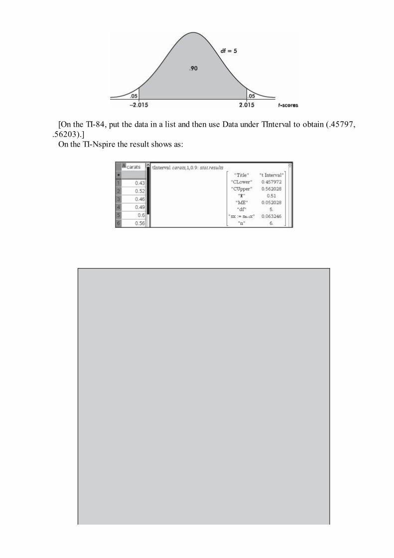
[On the TI-84, put the data in a list and then use Data under TInterval to obtain (.45797,.56203).]
On the TI-Nspire the result shows as:
TIPRead the question carefully! Be sure you understand exactlywhat you are being asked to do or find or explain.
EXAMPLE 13.15A survey was conducted involving 250 out of 125,000 families living in a city. Theaverage amount of income tax paid per family in the sample was $3540 with a standarddeviation of $1150. Establish a 99% confidence interval estimate for the total taxes paidby all the families in the city. (Assume that the population of all income taxes paid isapproximately normally distributed.)
Answer: We are given = 3540 and s = 1150. We use s as an estimate for σ andcalculate the standard deviation of the sample means to be
Since σ is unknown, we use a t-distribution. In this case we obtain 3540 ± 2.596(72.73)= 3540 ± 188.8 and then 125,000(3540 ± 188.8) = 442,500,000 ± 23,600,000. That is,we are 99% confident that the total tax paid by all families in the city is between$418,900,000 and $466,100,000.
Statistical principles are useful not only in analyzing data but also in setting upexperiments, and one important consideration is the choice of a sample size. Inmaking interval estimates of population means, we have seen that each inferencemust go hand in hand with an associated confidence level statement. Generally,if we want a smaller, more precise interval estimate, we either decrease thedegree of confidence or increase the sample size. Similarly, if we want toincrease the degree of confidence, we either accept a wider interval estimate orincrease the sample size. Thus, choosing a larger sample size always seemsdesirable; in the real world, however, time and cost considerations areinvolved.
EXAMPLE 13.16Ball bearings are manufactured by a process that results in a standard deviation indiameter of 0.025 inch. What sample size should be chosen if we wish to be 99% sure ofknowing the diameter to within ±0.01 inch?
Answer: We have
Thus
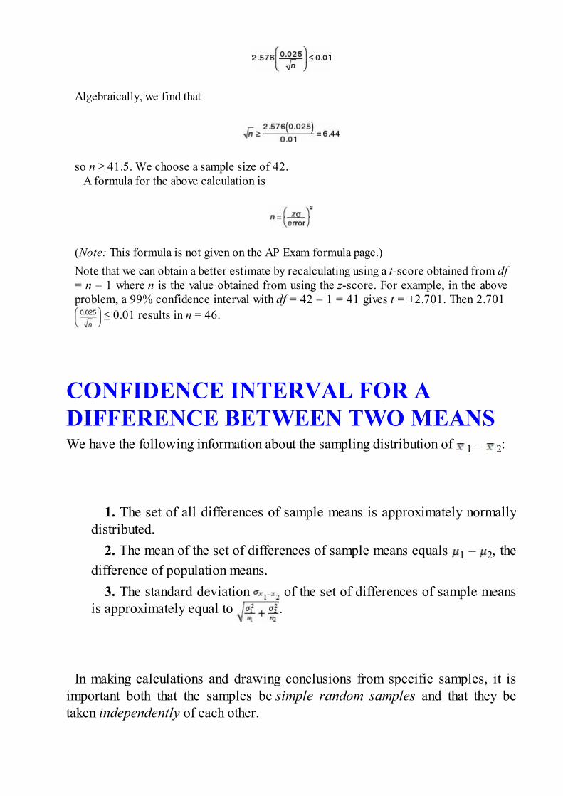
Algebraically, we find that
so n ≥ 41.5. We choose a sample size of 42.A formula for the above calculation is
(Note: This formula is not given on the AP Exam formula page.)Note that we can obtain a better estimate by recalculating using a t-score obtained from df= n – 1 where n is the value obtained from using the z-score. For example, in the aboveproblem, a 99% confidence interval with df = 42 – 1 = 41 gives t = ±2.701. Then 2.701
≤ 0.01 results in n = 46.
CONFIDENCE INTERVAL FOR ADIFFERENCE BETWEEN TWO MEANSWe have the following information about the sampling distribution of 1 – 2:
1. The set of all differences of sample means is approximately normallydistributed.
2. The mean of the set of differences of sample means equals 1 – 2, thedifference of population means.
3. The standard deviation of the set of differences of sample meansis approximately equal to .
In making calculations and drawing conclusions from specific samples, it isimportant both that the samples be simple random samples and that they betaken independently of each other.

EXAMPLE 13.17A 30-month study is conducted to determine the difference in the numbers of accidentsper month occurring in two departments in an assembly plant. Suppose the firstdepartment averages 12.3 accidents per month with a standard deviation of 3.5, while thesecond averages 7.6 accidents with a standard deviation of 3.4. Determine a 95%confidence interval estimate for the difference in the numbers of accidents per month.(Assume that the two populations are independent and approximately normallydistributed.)
Answer:
The observed difference is 12.3 – 7.6 = 4.7, and with df = (n1 – 1) + (n2 – 1) = 58, thecritical t-scores are ±2.00. Thus the confidence interval estimate is 4.7 ± 2.00(0.89) =4.7 ± 1.78. We are 95% confident that the first department has between 2.92 and 6.48more accidents per month than the second department. (Using the conservative df =min(x1 – 1, x2 – 1) = 29 gives 4.7 ± 2.045(0.89) = 4.7 ± 1.82.)
[On the TI-84, 2-SampTInt gives (2.9167, 6.4833).]
EXAMPLE 13.18A survey is run to determine the difference in the cost of groceries in suburban storesversus inner city stores. A preselected group of items is purchased in a sample of 45suburban and 35 inner city stores, and the following data are obtained.
Find a 90% confidence interval estimate for the difference in the cost of groceries.(Assume that the two populations are independent and approximately normallydistributed.)
Answer:
The observed difference is 36.52 – 39.40 = –2.88, the critical t-scores are ±1.664, andthe confidence interval estimate is –2.88 ± 1.664(0.265) = –2.88 ± 0.44. Thus we are90% certain that the selected group of items costs between $2.44 and $3.32 less in
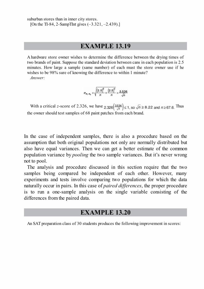
suburban stores than in inner city stores.[On the TI-84, 2-SampTInt gives (–3.321, –2.439).]
EXAMPLE 13.19A hardware store owner wishes to determine the difference between the drying times oftwo brands of paint. Suppose the standard deviation between cans in each population is 2.5minutes. How large a sample (same number) of each must the store owner use if hewishes to be 98% sure of knowing the difference to within 1 minute?
Answer:
With a critical z-score of 2.326, we have Thusthe owner should test samples of 68 paint patches from each brand.
In the case of independent samples, there is also a procedure based on theassumption that both original populations not only are normally distributed butalso have equal variances. Then we can get a better estimate of the commonpopulation variance by pooling the two sample variances. But it’s never wrongnot to pool.
The analysis and procedure discussed in this section require that the twosamples being compared be independent of each other. However, manyexperiments and tests involve comparing two populations for which the datanaturally occur in pairs. In this case of paired differences, the proper procedureis to run a one-sample analysis on the single variable consisting of thedifferences from the paired data.
EXAMPLE 13.20An SAT preparation class of 30 students produces the following improvement in scores:

Find a 90% confidence interval estimate of the average improvement in test scores.Answer: The two sets of test scores (before and after the course) are not independent;
they are associated in matched pairs, with one pair of scores for each student. The properprocedure is to run a one-sample analysis on the single variable consisting of the set ofimprovements. In this case we obtain and a 90%confidence interval estimate of 63.2 ± 1.699(7.648) = 63.2 ± 13.0. We can be 90%confident that the average improvement in test scores is between 50.2 and 76.2.
When to do a two-sample analysis versus a matched pair analysis can beconfusing. The key idea is whether or not the two groups are independent. Thedifference has to do with design. What is the average reaction time of peoplewho are sober compared to that of people who have had two beers? If ourexperimental design calls for randomly assigning half of a group of volunteers todrink two beers and then comparing reaction times with the remaining sobervolunteers, then a two-sample analysis is called for. However, if ourexperimental design calls for testing reaction times of all the volunteers and then

giving all the volunteers two beers and retesting, then a matched pair analysis iscalled for. Matching may come about as above because you have made twomeasurements on the same person, or measurements might be made on sets oftwins, or between salaries of president and provost at a number of universities,etc. The key is whether the two sets of measurements are independent, or relatedin some way relevant to the question under consideration.
CONFIDENCE INTERVAL FOR THESLOPE OF A LEAST SQUARESREGRESSION LINEIn Topic 4 we discussed the least squares line
where b1 is the slope of the line. This slope is readily found using the statisticalsoftware on a calculator. It is an estimate of the slope β of the true regressionline. A confidence interval estimate for β can be found using t-scores, where df= n – 2, and the appropriate standard deviation is
where the sum in the numerator is the sum of the squared residuals (see Topic 4)and the sum in the denominator is the sum of the squared deviations from themean. The value of sb1
is found at the same time that the statistical software onyour calculator finds the value of b1. Some calculators calculate the numerator
and then the denominator can be calculated by
Assumptions here include: (1) the sample must be randomly selected; (2) thescatterplot should be approximately linear; (3) there should be no apparentpattern in the residuals plot (On the TI-84, after Stat → Calc → LinReg, the listof residuals is stored in RESID under LIST NAMES); and (4) the distribution ofthe residuals should be approximately normal. (The fourth point can be checkedby a histogram, dotplot, stemplot, or a normal probability plot of the residuals.)

TIPIf you refer to a graph, whether it is a histogram, boxplot,stemplot, scatterplot, residuals plot, normal probability plot,or some other kind of graph, you should roughly draw it. It isnot enough to simply say, “I did a normal probability plot ofthe residuals on my calculator and it looked linear.”
EXAMPLE 13.21A random sample of ten high school students produced the following results for numberof hours of television watched per week and GPA.
Determine the least squares line and give a 95% confidence interval estimate for the trueslope.
Answer: Checking the assumptions:We are told that the data come from a random sample of students.
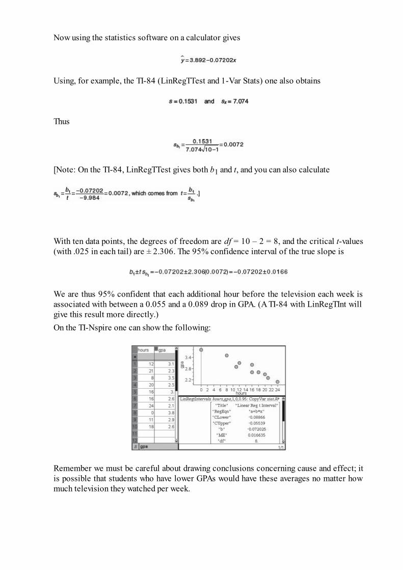
Now using the statistics software on a calculator gives
Using, for example, the TI-84 (LinRegTTest and 1-Var Stats) one also obtains
Thus
[Note: On the TI-84, LinRegTTest gives both b1 and t, and you can also calculate
With ten data points, the degrees of freedom are df = 10 – 2 = 8, and the critical t-values(with .025 in each tail) are ± 2.306. The 95% confidence interval of the true slope is
We are thus 95% confident that each additional hour before the television each week isassociated with between a 0.055 and a 0.089 drop in GPA. (A TI-84 with LinRegTInt willgive this result more directly.)On the TI-Nspire one can show the following:
Remember we must be careful about drawing conclusions concerning cause and effect; itis possible that students who have lower GPAs would have these averages no matter howmuch television they watched per week.

Note that s = , called the standard deviation of the residuals , is
sometimes written se . It is a measure of the spread about the regression line,and is almost always in the regression output (usually simply labeled as s or S).Note that Sb1
is sometimes written SE(b1) and is also referred to as the standarderror of the slope. So we can also write . We see that increasing se
(that is, increasing spread about the line) increases the slope’s standard error,while increasing sx (that is, increasing the range of x-values) or increasing n(the sample size) decreases the slope’s standard error.
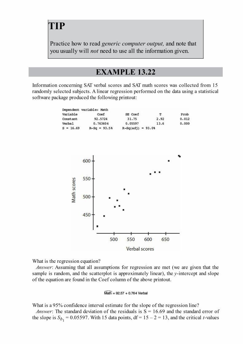
TIPPractice how to read generic computer output, and note thatyou usually will not need to use all the information given.
EXAMPLE 13.22Information concerning SAT verbal scores and SAT math scores was collected from 15randomly selected subjects. A linear regression performed on the data using a statisticalsoftware package produced the following printout:
What is the regression equation?Answer: Assuming that all assumptions for regression are met (we are given that the
sample is random, and the scatterplot is approximately linear), the y-intercept and slopeof the equation are found in the Coef column of the above printout.
What is a 95% confidence interval estimate for the slope of the regression line?Answer: The standard deviation of the residuals is S = 16.69 and the standard error of
the slope is Sb1 = 0.05597. With 15 data points, df = 15 – 2 = 13, and the critical t-values

are ± 2.160. The 95% confidence interval of the true slope is:
We are 95% confident that for every 1-point increase in verbal SAT score, the averageincrease in math SAT score is between .64 and .89
Summary• Important assumptions/conditions always must be checked before calculating
confidence intervals.• We are never able to say exactly what a population parameter is; rather, we
say that we have a certain confidence that it lies in a certain interval.• If we want a narrower interval, we must either decrease the confidence level
or increase the sample size.• If we want a higher level of confidence, we must either accept a wider
interval or increase the sample size.• The level of confidence refers to the percentage of samples that produce
intervals that capture the true population parameter.
Questions on Topic Thirteen:Confidence Intervals
Multiple-Choice Questions
Directions: The questions or incomplete statements that follow are eachfollowed by five suggested answers or completions. Choose the responsethat best answers the question or completes the statement.
1. Changing from a 95% confidence interval estimate for a populationproportion to a 99% confidence interval estimate, with all other thingsbeing equal,
(A) increases the interval size by 4%.(B) decreases the interval size by 4%.
(C) increases the interval size by 31%.(D) decreases the interval size by 31%.(E) This question cannot be answered without knowing the sample
size.
2. In general, how does doubling the sample size change the confidenceinterval size?
(A) Doubles the interval size(B) Halves the interval size(C) Multiplies the interval size by 1.414(D) Divides the interval size by 1.414(E) This question cannot be answered without knowing the sample
size.
3. A confidence interval estimate is determined from the GPAs of asimple random sample of n students. All other things being equal, whichof the following will result in a smaller margin of error?
(A) A smaller confidence level(B) A larger sample standard deviation(C) A smaller sample size(D) A larger population size(E) A smaller sample mean
4. A survey was conducted to determine the percentage of high school
students who planned to go to college. The results were stated as 82%with a margin of error of ±5%. What is meant by ±5%?
(A) Five percent of the population were not surveyed.
(B) In the sample, the percentage of students who plan to go tocollege was between 77% and 87%.
(C) The percentage of the entire population of students who plan togo to college is between 77% and 87%.
(D) It is unlikely that the given sample proportion result would beobtained unless the true percentage was between 77% and 87%.
(E) Between 77% and 87% of the population were surveyed.
5. Most recent tests and calculations estimate at the 95% confidencelevel that the maternal ancestor to all living humans called mitochondrialEve lived 273,000 ±177,000 years ago. What is meant by “95%confidence” in this context?
(A) A confidence interval of the true age of mitochondrial Eve hasbeen calculated using z-scores of ±1.96.
(B) A confidence interval of the true age of mitochondrial Eve hasbeen calculated using t-scores consistent with df = n – 1 and tailprobabilities of ±.025.
(C) There is a .95 probability that mitochondrial Eve lived between96,000 and 450,000 years ago.
(D) If 20 random samples of data are obtained by this method, and a95% confidence interval is calculated from each, then the true age ofmitochondrial Eve will be in 19 of these intervals.
(E) 95% of all random samples of data obtained by this method willyield intervals that capture the true age of mitochondrial Eve.
6. One month the actual unemployment rate in France was 13.4%. Ifduring that month you took an SRS of 100 Frenchmen and constructed aconfidence interval estimate of the unemployment rate, which of thefollowing would have been true?
(A) The center of the interval was 13.4.

(B) The interval contained 13.4.(C) A 99% confidence interval estimate contained 13.4.(D) The z-score of 13.4 was between ±2.576.(E) None of the above are true statements.
7. In a recent Zogby International survey, 11% of 10,000 Americansunder 50 said they would be willing to implant a device in their brain tobe connected to the Internet if it could be done safely. What is the marginof error at the 99% confidence level?
(A)
(B)
(C)
(D)
(E)
8. The margin of error in a confidence interval estimate using z-scorescovers which of the following?
(A) Sampling variability(B) Errors due to undercoverage and nonresponse in obtaining
sample surveys

(C) Errors due to using sample standard deviations as estimates forpopulation standard deviations
(D) Type I errors(E) Type II errors
9. In an SRS of 50 teenagers, two-thirds said they would rather text a
friend than call. What is the 98% confidence interval for the proportion ofteens who would rather text than call a friend?
(A)
(B)
(C)
(D)
(E)
10. In a survey funded by Burroughs-Welcome, 750 of 1000 adultAmericans said they didn’t believe they could come down with a sexuallytransmitted disease (STD). Construct a 95% confidence interval estimateof the proportion of adult Americans who don’t believe they can contractan STD.
(A) (.728, .772)(B) (.723, .777)

(C) (.718, .782)(D) (.713, .787)(E) (.665, .835)
11. A 1993 Los Angeles Times poll of 1703 adults revealed that only17% thought the media was doing a “very good” job. With what degree ofconfidence can the newspaper say that 17% ± 2% of adults believe themedia is doing a “very good” job?
(A) 72.9%(B) 90.0%(C) 95.0%(D) 97.2%(E) 98.6%
12. A politician wants to know what percentage of the voters supporther position on the issue of forced busing for integration. What size votersample should be obtained to determine with 90% confidence the supportlevel to within 4%?
(A) 21(B) 25(C) 423(D) 600(E) 1691
13. In a New York Times poll measuring a candidate’s popularity, the
newspaper claimed that in 19 of 20 cases its poll results should be nomore than three percentage points off in either direction. What confidencelevel are the pollsters working with, and what size sample should theyhave obtained?

(A) 3%, 20(B) 6%, 20(C) 6%, 100(D) 95%, 33(E) 95%, 1068
14. In an SRS of 80 teenagers, the average number of texts handled in aday was 50 with a standard deviation of 15. What is the 96% confidenceinterval for the average number of texts handled by teens daily?
(A) 50 ± 2.054(15)(B) 50 ± 2.054
(C) 50 ± 2.054
(D) 50 ± 2.088
(E) 50 ± 2.088
15. One gallon of gasoline is put in each of 30 test autos, and theresulting mileage figures are tabulated with = 28.5 and s = 1.2.Determine a 95% confidence interval estimate of the mean mileage.
(A) (28.46, 28.54)(B) (28.42, 28.58)(C) (28.1, 28.9)(D) (27.36, 29.64)(E) (27.3, 29.7)

16. The number of accidents per day at a large factory is noted for eachof 64 days with = 3.58 and s = 1.52. With what degree of confidencecan we assert that the mean number of accidents per day at the factory isbetween 3.20 and 3.96?
(A) 48%(B) 63%(C) 90%(D) 95%(E) 99%
17. A company owns 335 trucks. For an SRS of 30 of these trucks, theaverage yearly road tax paid is $9540 with a standard deviation of $1205.What is a 99% confidence interval estimate for the total yearly road taxespaid for the 335 trucks?
(A) $9540 ± $103(B) $9540 ± $567(C) $3,196,000 ± $606(D) $3,196,000 ± $35,000(E) $3,196,000 ± $203,000
18. What sample size should be chosen to find the mean number of
absences per month for school children to within ±.2 at a 95% confidencelevel if it is known that the standard deviation is 1.1?
(A) 11(B) 29(C) 82(D) 96
(E) 117
19. Hospital administrators wish to learn the average length of stay of
all surgical patients. A statistician determines that, for a 95% confidencelevel estimate of the average length of stay to within ±0.5 days, 50surgical patients’ records will have to be examined. How many recordsshould be looked at to obtain a 95% confidence level estimate to within±0.25 days?
(A) 25(B) 50(C) 100(D) 150(E) 200
20. The National Research Council of the Philippines reported that 210
of 361 members in biology are women, but only 34 of 86 members inmathematics are women. Establish a 95% confidence interval estimate ofthe difference in proportions of women in biology and women inmathematics in the Philippines.
(A) .187 ± .115(B) .187 ± .154(C) .395 ± .103(D) .543 ± .154(E) .582 ± .051
21. In a simple random sample of 300 elderly men, 65% were married,
while in an independent simple random sample of 400 elderly women,48% were married. Determine a 99% confidence interval estimate for thedifference between the proportions of elderly men and women who aremarried.

(A) (.65 – .48) ± 2.326
(B) (.65 – .48) ± 2.576
(C) (.65 – .48) ± 2.576
(D) ± 2.576
(E) ± 2.807
22. A researcher plans to investigate the difference between theproportion of psychiatrists and the proportion of psychologists whobelieve that most emotional problems have their root causes in childhood.How large a sample should be taken (same number for each group) to be90% certain of knowing the difference to within ±.03?
(A) 39(B) 376(C) 752(D) 1504(E) 3007
23. In a study aimed at reducing developmental problems in low-birth-
weight (under 2500 grams) babies (Journal of the American MedicalAssociation, June 13, 1990, page 3040), 347 infants were exposed to aspecial educational curriculum while 561 did not receive any specialhelp. After 3 years the children exposed to the special curriculum showeda mean IQ of 93.5 with a standard deviation of 19.1; the other childrenhad a mean IQ of 84.5 with a standard deviation of 19.9. Find a 95%confidence interval estimate for the difference in mean IQs of low-birth-weight babies who receive special intervention and those who do not.
(A) (93.5 – 84.5) ± 1.97
(B) (93.5 – 84.5) ± 1.97
(C) (93.5 – 84.5) ± 1.65
(D) (93.5 – 84.5) ± 1.65
(E) (93.5 – 84.5) ± 1.65
24. Does socioeconomic status relate to age at time of HIV infection?For 274 high-income HIV-positive individuals the average age ofinfection was 33.0 years with a standard deviation of 6.3, while for 90low-income individuals the average age was 28.6 years with a standarddeviation of 6.3 (The Lancet, October 22, 1994, page 1121). Find a 90%confidence interval estimate for the difference in ages of high-and low-income people at the time of HIV infection.
(A) 4.4 ± 0.963(B) 4.4 ± 1.26(C) 4.4 ± 2.51(D) 30.8 ± 2.51(E) 30.8 ± 6.3
25. An engineer wishes to determine the difference in life expectancies
of two brands of batteries. Suppose the standard deviation of each brandis 4.5 hours. How large a sample (same number) of each type of batteryshould be taken if the engineer wishes to be 90% certain of knowing thedifference in life expectancies to within 1 hour?
(A) 10(B) 55(C) 110(D) 156(E) 202
26. Two confidence interval estimates from the same sample are (16.4,
29.8) and (14.3, 31.9). What is the sample mean, and if one estimate is at

the 95% level while the other is at the 99% level, which is which?
(A) = 23.1; (16.4, 29.8) is the 95% level.(B) = 23.1; (16.4, 29.8) is the 99% level.(C) It is impossible to completely answer this question without
knowing the sample size.(D) It is impossible to completely answer this question without
knowing the sample standard deviation.(E) It is impossible to completely answer this question without
knowing both the sample size and standard deviation.
27. Two 90% confidence interval estimates are obtained: I (28.5, 34.5)and II (30.3, 38.2).
a. If the sample sizes are the same, which has the larger standarddeviation?
b. If the sample standard deviations are the same, which has thelarger size?
(A) a. I b. I(B) a. I b. II(C) a. II b. I(D) a. II b. II(E) More information is needed to answer these questions.
28. Suppose (25, 30) is a 90% confidence interval estimate for apopulation mean . Which of the following are true statements?
(A) There is a .90 probability that is between 25 and 30.(B) 90% of the sample values are between 25 and 30.(C) There is a .90 probability that is between 25 and 30.

(D) If 100 random samples of the given size are picked and a 90%confidence interval estimate is calculated from each, then will be in90 of the resulting intervals.
(E) If 90% confidence intervals are calculated from all possiblesamples of the given size, will be in 90% of these intervals.
29. Under what conditions would it be meaningful to construct aconfidence interval estimate when the data consist of the entirepopulation?
(A) If the population size is small (n < 30)(B) If the population size is large (n ≥ 30)(C) If a higher level of confidence is desired(D) If the population is truly random(E) Never
30. A social scientist wishes to determine the difference between the
percentage of Los Angeles marriages and the percentage of New Yorkmarriages that end in divorce in the first year. How large a sample (samefor each group) should be taken to estimate the difference to within ±.07at the 94% confidence level?
(A) 181(B) 361(C) 722(D) 1083(E) 1443
31. What is the critical t-value for finding a 90% confidence interval
estimate from a sample of 15 observations?
(A) 1.341

(B) 1.345(C) 1.350(D) 1.753(E) 1.761
32. Acute renal graft rejection can occur years after the graft. In one
study (The Lancet, December 24, 1994, page 1737), 21 patients showedsuch late acute rejection when the ages of their grafts (in years) were 9, 2,7, 1, 4, 7, 9, 6, 2, 3, 7, 6, 2, 3, 1, 2, 3, 1, 1, 2, and 7, respectively.Establish a 90% confidence interval estimate for the ages of renal graftsthat undergo late acute rejection.
(A) 2.024 ± 0.799(B) 2.024 ± 1.725(C) 4.048 ± 0.799(D) 4.048 ± 1.041(E) 4.048 ± 1.725
33. Nine subjects, 87 to 96 years old, were given 8 weeks of
progressive resistance weight training (Journal of the American MedicalAssociation, June 13, 1990, page 3032). Strength before and after trainingfor each individual was measured as maximum weight (in kilograms)lifted by left knee extension:
Find a 95% confidence interval estimate for the strength gain.
(A) 11.61 ± 3.03(B) 11.61 ± 3.69(C) 11.61 ± 3.76(D) 19.11 ± 1.25

(E) 19.11 ± 3.69
34. A catch of five fish of a certain species yielded the following
ounces of protein per pound of fish: 3.1, 3.5, 3.2, 2.8, and 3.4. What is a90% confidence interval estimate for ounces of protein per pound of thisspecies of fish?
(A) 3.2 ± 0.202(B) 3.2 ± 0.247(C) 3.2 ± 0.261(D) 4.0 ± 0.202(E) 4.0 ± 0.247
35. In a random sample of 25 professional baseball players, their
salaries (in millions of dollars) and batting averages result in thefollowing regression analysis:
Which of the following gives a 98% confidence interval for the slope ofthe regression line?
(A) 0.008051 ± 2.326(0.001058)(B) 0.008051 ± 2.326(0.0169461)
(C) 0.008051 ± 2.485
(D) 0.008051 ± 2.492
(E) 0.008051 ± 2.500(0.001058)

36. Is there a relationship between mishandled-baggage rates (numberof mishandled bags per 1000 passengers) and percentage of on-timearrivals? Regression analysis of ten airlines gives the following TI-Nspire output (baggage rate is independent variable):
We are 95% confident that if an airline averages one more mishandledbag per 1000 passengers than a second airline, then its percentage of on-time arrivals will average
(A) between 0.15 and 4.19 less than that of the second airline.(B) between 0.00 and 4.33 less than that of the second airline.(C) between 4.46 less and 0.13 more than that of the second airline.(D) between 4.49 less and 0.17 more than that of the second airline.(E) between 4.54 less and 0.21 more than that of the second airline.
37. Smoking is a known risk factor for cardiovascular and cancerdiseases. A recent study (Rusanen et al., Archives of Internal Medicine,October 25, 2010) surveyed 21,123 members of a California health caresystem looking at smoking levels and risk of dementia (as measured by theCox hazard ratio). Results are summarized in the following graph of 95%confidence intervals.

Which of the following is an appropriate conclusion?
(A) Dementia somehow causes an urge to smoke.(B) Heavier smoking leads to a greater risk of dementia.(C) Cutting down on smoking will lower one’s risk of dementia.(D) Heavier smoking is associated with more precise confidence
intervals of dementia as measured by the hazard ratio.(E) There is a positive association between smoking and risk of
dementia.
Free-Response Questions
Directions: You must show all work and indicate the methods you use. Youwill be graded on the correctness of your methods and on the accuracy ofyour final answers.
Eleven Open-Ended Questions1. An SRS of 1000 voters finds that 57% believe that competence is
more important than character in voting for President of the United States.(a) Determine a 95% confidence interval estimate for the percentage
of voters who believe competence is more important than character.(b) If your parents know nothing about statistics, how would you
explain to them why you can’t simply say that 57% of voters believethat competence is more important.
(c) Also explain to your parents what is meant by 95% confidencelevel.2. During the H1N1 pandemic, one published study concluded that if
someone in your family had H1N1, you had a 1 in 8 chance of also comingdown with the disease. A state health officer tracks a random sample ofnew H1N1 cases in her state and notes that 129 out of a potential 876family members later come down with the disease.
(a) Calculate a 90% confidence interval for the proportion of familymembers who come down with H1N1 after an initial family memberdoes in this state.
(b) Based on this confidence interval, is there evidence that theproportion of family members who come down with H1N1 after aninitial family member does in this state is different from the 1 in 8chance concluded in the published study? Explain.
(c) Would the conclusion in (b) be any different with a 99%confidence interval? Explain.3. In a random sample of 500 new births in the United States, 41.2%
were to unmarried women, while in a random sample of 400 new births inthe United Kingdom, 46.5% were to unmarried women.
(a) Calculate a 95% confidence interval for the difference in theproportions of new births to unmarried women in the United States andUnited Kingdom.
(b) Does the confidence interval support the belief by a UN healthcare statistician that the proportions of new births to unmarried womenis different in the United States and United Kingdom? Explain.4. An SRS of 40 inner city gas stations shows a mean price for regular
unleaded gasoline to be $3.45 with a standard deviation of $0.05, whilean SRS of 120 suburban stations shows a mean of $3.38 with a standarddeviation of $0.08.
(a) Construct 95% confidence interval estimates for the mean priceof regular gas in inner city and in suburban stations.
(b) The confidence interval for the inner city stations is wider thanthe interval for the suburban stations even though the standard deviationfor inner city stations is less than that for suburban stations. Explainwhy this happened.
(c) Based on your answer in part (a), are you confident that the mean

price of inner city gasoline is less than $3.50? Explain.5. In a simple random sample of 30 subway cars during rush hour, the
average number of riders per car was 83.5 with a standard deviation of5.9. Assume the sample data are unimodal and reasonably symmetric withno extreme values and little, if any, skewness.
(a) Establish a 90% confidence interval estimate for the averagenumber of riders per car during rush hour. Show your work.
(b) Assuming the same standard deviation of 5.9, how large a sampleof cars would be necessary to determine the average number of ridersto within ±1 at the 90% confidence level? Show your work.6. In a sample of ten basketball players the mean income was $196,000
with a standard deviation of $315,000.(a) Assuming all necessary assumptions are met, find a 95%
confidence interval estimate of the mean salary of basketball players.(b) What assumptions are necessary for the above estimate? Do they
seem reasonable here?7. An SRS of ten brands of breakfast cereals is tested for the number of
calories per serving. The following data result: 185, 190, 195, 200, 205,205, 210, 210, 225, 230.
Establish a 95% confidence interval estimate for the mean number ofcalories for servings of breakfast cereals. Be sure to check assumptions.
8. Bisphenol A (BPA), a synthetic estrogen found in packagingmaterials, has been shown to leach into infant formula and beverages.Most recently it has been detected in high concentrations in cash registerreceipts. Random sample biomonitoring data to see if retail workers carryhigher amounts of BPA in their bodies than non-retail workers is asfollows:
(a) Calculate a 99% confidence interval for the difference in meanBPA body concentrations of non-retail and retail workers.

(b) Does the confidence interval support the belief that retailworkers carry higher amounts of BPA in their bodies than non-retailworkers? Explain.9. A new drug is tested for relief of allergy symptoms. In a double-
blind experiment, 12 patients are given varying doses of the drug andreport back on the number of hours of relief. The following tablesummarizes the results:
(a) Determine the equation of the least squares regression line.(b) Construct a 90% confidence interval estimate for the slope of the
regression line, and interpret this in context.10. Information with regard to the assessed values (in $1000) and the
selling prices (in $1000) of a random sample of homes sold in an NEmarket yields the following computer output:
(a) Determine the equation of the least squares regression line.(b) Construct a 99% confidence interval estimate for the slope of the
regression line, and interpret this in context.11. In a July 2008 study of 1050 randomly selected smokers, 74% said
they would like to give up smoking.(a) At the 95% confidence level, what is the margin of error?(b) Explain the meaning of “95% confidence interval” in this
example.(c) Explain the meaning of “95% confidence level” in this example.(d) Give an example of possible response bias in this example.(e) If we want instead to be 99% confident, would our confidence

interval need to be wider or narrower?(f) If the sample size were greater, would the margin of error be
smaller or greater?
TOPIC 14Tests of Significance—Proportions andMeans
• Logic of Significance Testing• Null and Alternative Hypotheses• P-values
• Type I and Type II Errors• Concept of Power• Hypothesis Testing
Closely related to the problem of estimating a population proportion or meanis the problem of testing a hypothesis about a population proportion or mean.For example, a travel agency might determine an interval estimate for theproportion of sunny days in the Virgin Islands or, alternatively, might test atourist bureau’s claim about the proportion of sunny days. A major stockholderin a construction company might ascertain an interval estimate for the proportionof successful contract bids or, alternatively, might test a companyspokesperson’s claim about the proportion of successful bids. A consumerprotection agency might determine an interval estimate for the mean nicotinecontent of a particular brand of cigarettes or, alternatively, might test amanufacturer’s claim about the mean nicotine content of its cigarettes. Anagricultural researcher could find an interval estimate for the mean productivitygain caused by a specific fertilizer or, alternatively, might test the developer’sclaimed mean productivity gain. In each of these cases, the experimenter mustdecide whether the interest lies in an interval estimate of a populationproportion or mean or in a hypothesis test of a claimed proportion or mean.
LOGIC OF SIGNIFICANCE TESTING,NULL AND ALTERNATIVEHYPOTHESIS, P-VALUES, ONE-ANDTWO-SIDED TESTS, TYPE I AND TYPEII ERRORS, AND THE CONCEPT OFPOWER
The general testing procedure is to choose a specific hypothesis to be tested,called the null hypothesis, pick an appropriate random sample, and then usemeasurements from the sample to determine the likelihood of the nullhypothesis. If the sample statistic is far enough away from the claimedpopulation parameter, we say that there is sufficient evidence to reject the nullhypothesis. We attempt to show that the null hypothesis is unacceptable byshowing that it is improbable.
Consider the context of the population proportion. The null hypothesis H0 isstated in the form of an equality statement about the population proportion (forexample, H0: p = .37). There is an alternative hypothesis, stated in the form ofan inequality (for example, Ha: p < .37 or Ha: p > .37 or Ha: p ≠ .37). Thestrength of the sample statistic can be gauged through its associated P-value,which is the probability of obtaining a sample statistic as extreme (or moreextreme) as the one obtained if the null hypothesis is assumed to be true. Thesmaller the P-value, the more significant the difference between the nullhypothesis and the sample results.
Note that only population parameter symbols appear in H0 and Ha. Samplestatistics like and do NOT appear in H0 or Ha.

TIPNever base your hypotheses on what you find in the sampledata.
There are two types of possible errors: the error of mistakenly rejecting a truenull hypothesis and the error of mistakenly failing to reject a false nullhypothesis. The α-risk, also called the significance level of the test, is theprobability of committing a Type I error and mistakenly rejecting a true nullhypothesis. A Type II error , a mistaken failure to reject a false null hypothesis,has associated probability . There is a different value of for each possiblecorrect value for the population parameter p. For each , 1 – is called thepower of the test against the associated correct value. The power of ahypothesis test is the probability that a Type II error is not committed. That is,given a true alternative, the power is the probability of rejecting the false nullhypothesis. Increasing the sample size and increasing the significance level areboth ways of increasing the power.

TIPThe P-value relates to the probability of the data given that thenull hypothesis is true; it is not the probability of the nullhypothesis being true.
A simple illustration of the difference between a Type I and a Type II error isas follows: Suppose the null hypothesis is that all systems are operatingsatisfactorily with regard to a NASA liftoff. A Type I error would be to delaythe liftoff mistakenly thinking that something was malfunctioning wheneverything was actually OK. A Type II error would be to fail to delay the liftoffmistakenly thinking everything was OK when something was actuallymalfunctioning. The power is the probability of recognizing a particularmalfunction. (Note the complimentary aspect of power, a “good” thing, withType II error, a “bad” thing.)
Our justice system provides another often quoted illustration. If the nullhypothesis is that a person is innocent, then a Type I error results when aninnocent person is found guilty, while a Type II error results when a guiltyperson is not convicted. We try to minimize Type I errors in criminal trials bydemanding unanimous jury guilty verdicts. In civil suits, however, many statestry to minimize Type II errors by accepting simple majority verdicts.
It should be emphasized that with regard to calculations, questions like “Whatis the power of this test?” and “What is the probability of a Type II error in thistest?” cannot be answered without reference to a specific alternative hypothesis.Furthermore, AP students are not required to know how to calculate theseprobabilities. However, they are required to understand the concepts andinteractions among the concepts.

TIPBe able to identify Type I and Type II errors and give possibleconsequences of each.
HYPOTHESIS TEST FOR APROPORTIONWe assume that we have a simple random sample, that both np0 and n(1 – p0)are at least 10, and that the sample size is less than 10% of the population.

TIPAlways check assumptions/conditions before proceeding witha test.
EXAMPLE 14.1A union spokesperson claims that 75% of union members will support a strike if theirbasic demands are not met. A company negotiator believes the true percentage is lowerand runs a hypothesis test at the 10% significance level. What is the conclusion if 87 outof an SRS of 125 union members say they will strike?
Answer: We note that np0 = (125)(.75) = 93.75 and n(1 – p0) = (125)(.25) = 31.25 areboth >10 and that we have an SRS, and we assume that 125 is less than 10% of the totalunion membership.
We use the claimed proportion to calculate the standard deviation of the sampleproportions:
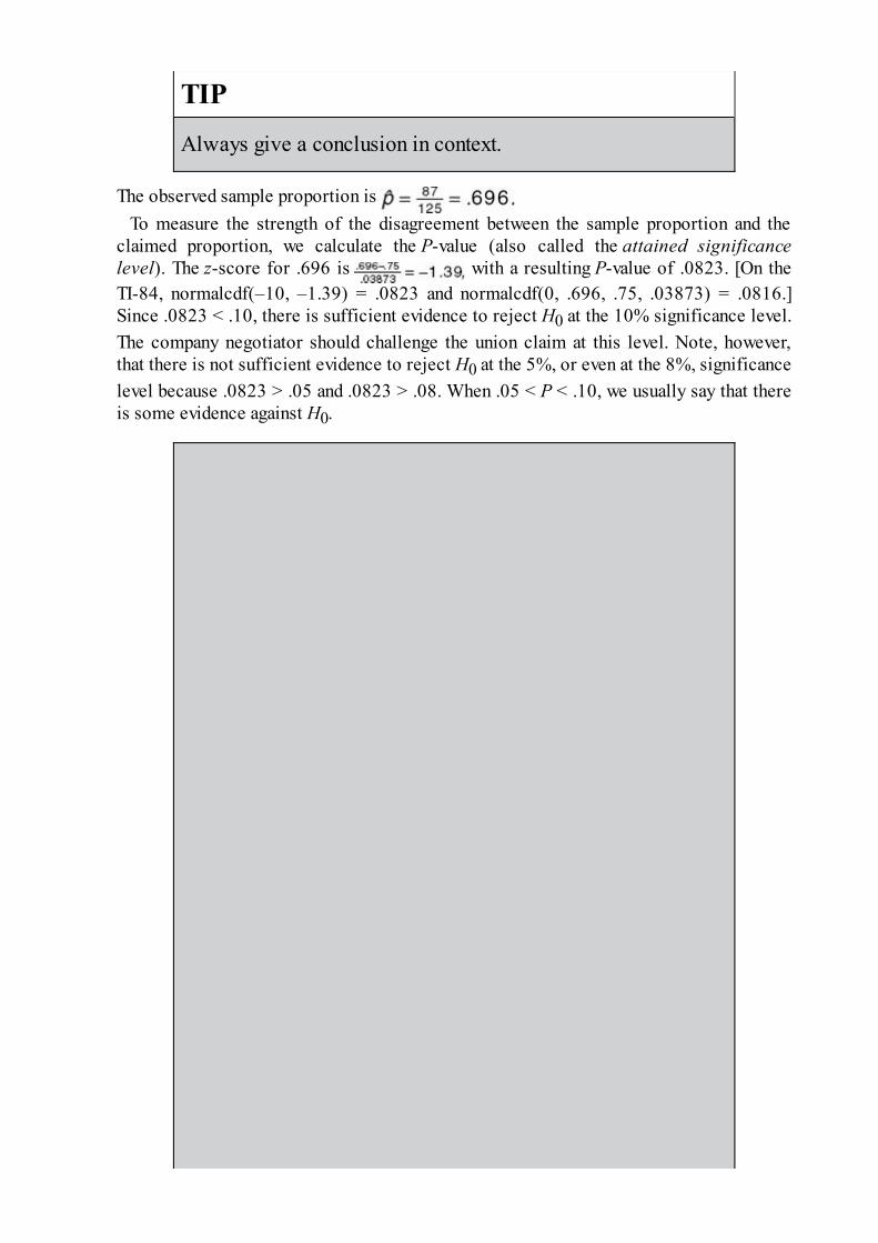
TIPAlways give a conclusion in context.
The observed sample proportion is To measure the strength of the disagreement between the sample proportion and the
claimed proportion, we calculate the P-value (also called the attained significancelevel). The z-score for .696 is with a resulting P-value of .0823. [On theTI-84, normalcdf(–10, –1.39) = .0823 and normalcdf(0, .696, .75, .03873) = .0816.]Since .0823 < .10, there is sufficient evidence to reject H0 at the 10% significance level.The company negotiator should challenge the union claim at this level. Note, however,that there is not sufficient evidence to reject H0 at the 5%, or even at the 8%, significancelevel because .0823 > .05 and .0823 > .08. When .05 < P < .10, we usually say that thereis some evidence against H0.

TIPWe never “accept” a null hypothesis; we either do or do nothave evidence to reject it.
[On the TI-84, under STAT and then TESTS, go to 1-PropZTest. With Po:.75, x:87,n:125, and prop < Po, Calculate gives P = .0816.]
On the TI-Nspire the result shows as:
EXAMPLE 14.2A cancer research group surveys 500 women more than 40 years old to test thehypothesis that 28% of women in this age group have regularly scheduled mammograms.Should the hypothesis be rejected at the 5% significance level if 151 of the womenrespond affirmatively?
Answer: Note that np0 = (500)(.28) = 140 and n(1 – p0) = (500)(.72) = 360 are both>10, we assume an SRS, and clearly 500 < 10% of all women over 40 years old. Since nosuspicion is voiced that the 28% claim is low or high, we run a two-sided z-test forproportions:
The observed . The z-score for .302 is which corresponds to aprobability of 1 – .8621 = .1379 in the tail. Doubling this value (because the test is two-sided), we obtain a P-value of 2(.1379) = .2758. Since .2758 > .05, there is not sufficient

evidence to reject H0; that is, the cancer research group should not dispute the 28%claim. Note, for example, that the null hypothesis should not be rejected even if α is arelatively large .25. When P > .10, we usually say there is little or no evidence to rejectH0.
[On the TI-84, 1-PropZTest gives P = .2732.]
HYPOTHESIS TEST FOR ADIFFERENCE BETWEEN TWOPROPORTIONSAs with confidence intervals for the difference of two proportions, n1 1, n1(1 –
1) , n2 2, and n2(1 – 2) should all be at least 10, it is important both that thesamples be simple random samples and that they be taken independently ofeach other, and the original populations should be large compared to the samplesizes.

TIPThe samples must be independent to use these two sampleproportion methods.
The fact that a sample proportion from one population is greater than a sampleproportion from a second population does not automatically justify a similarconclusion about the population proportions themselves. Two points need to bestressed. First, sample proportions from the same population can vary from eachother. Second, what we are really comparing are confidence interval estimates,not just single points.
For many problems the null hypothesis states that the population proportionsare equal or, equivalently, that their difference is 0:

The alternative hypothesis is then
where the first two possibilities lead to one-sided tests and the third possibilityleads to two-sided tests.
Since the null hypothesis is that p1 = p2, we call this common value p and useit in calculating σd:
In practice, if and we use as an estimate of p incalculating σd.
EXAMPLE 14.3Suppose that early in an election campaign a telephone poll of 800 registered votersshows 460 in favor of a particular candidate. Just before election day, a second pollshows only 520 of 1000 registered voters expressing the same preference. At the 10%significance level is there sufficient evidence that the candidate’s popularity hasdecreased?
Answer: Note that n1 1 = 460, n1(1 – 1) = 340, n2 2 = 520, and n2(1 – 2) = 480 areall at least 10, we assume the samples are independent SRSs, and clearly the totalpopulation of registered voters is large.
The observed difference is .575 – .520 = .055. The z-score for .055 is and sothe P-value is 1 – .9901 = .0099. [normalcdf(2.33, 100) = .00990 and normalcdf(.055, 1,0, .0236) = .00989.] Since .0099 < .10, we conclude that at the 10% significance levelthe candidate’s popularity has dropped. We note that .0099 < .01, so that the observeddifference is statistically significant even at the 1% level.

[On the TI-84, 2-PropZTest gives P = .00995.]
EXAMPLE 14.4An automobile manufacturer tries two distinct assembly procedures. In a sample of 350cars coming off the line using the first procedure there are 28 with major defects, while asample of 500 autos from the second line shows 32 with defects. Is the differencesignificant at the 10% significance level?
Answer: Note that n1 1 = 28, n1(1 – 1) = 322, n2 2 = 32, and n2(1 – 2) = 468 are allat least 10, we assume the samples are independent SRSs, and the total population ofautos manufactured at the plant is large. Since there is no mention that one procedure isbelieved to be better or worse than the other, this is a two-sided test.
The observed difference is .080 – .064 = .016. The z-score for .016 is whichcorresponds to a tail probability of 1 – .8133 = .1867. [normalcdf(.89, 100) = .1867 andnormalcdf(.016, 1, 0, .0179) = .1857.] Doubling this value because the test is two-sidedresults in a P-value of 2(.1867) = .3734. Since .3734 > .10, we conclude that theobserved difference is not significant at the 10% level. We note that the smallestsignificance level for which the observed difference is significant is more than 37.34%.When P is so large, we can safely say that there is no evidence against H0. That is, theobserved difference in proportions of cars with major defects coming from the twoassembly procedures is not significant.
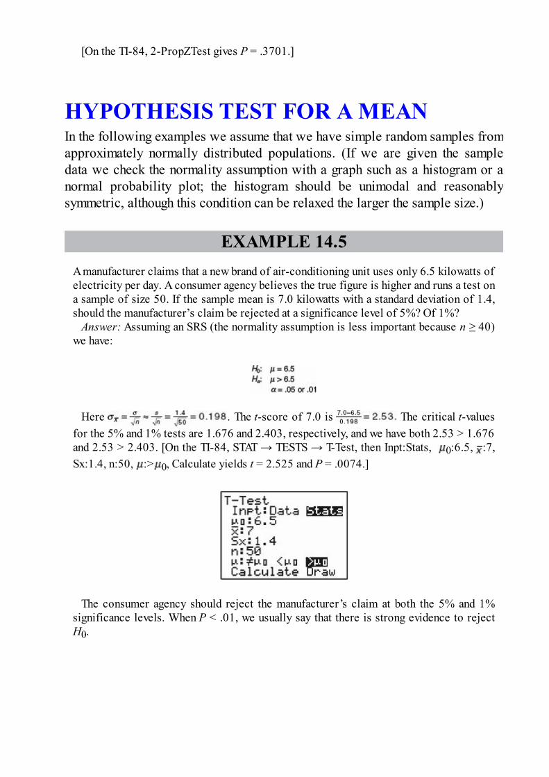
[On the TI-84, 2-PropZTest gives P = .3701.]
HYPOTHESIS TEST FOR A MEANIn the following examples we assume that we have simple random samples fromapproximately normally distributed populations. (If we are given the sampledata we check the normality assumption with a graph such as a histogram or anormal probability plot; the histogram should be unimodal and reasonablysymmetric, although this condition can be relaxed the larger the sample size.)
EXAMPLE 14.5A manufacturer claims that a new brand of air-conditioning unit uses only 6.5 kilowatts ofelectricity per day. A consumer agency believes the true figure is higher and runs a test ona sample of size 50. If the sample mean is 7.0 kilowatts with a standard deviation of 1.4,should the manufacturer’s claim be rejected at a significance level of 5%? Of 1%?
Answer: Assuming an SRS (the normality assumption is less important because n ≥ 40)we have:
Here . The t-score of 7.0 is The critical t-valuesfor the 5% and 1% tests are 1.676 and 2.403, respectively, and we have both 2.53 > 1.676and 2.53 > 2.403. [On the TI-84, STAT → TESTS → T-Test, then Inpt:Stats, 0:6.5, :7,Sx:1.4, n:50, :> 0, Calculate yields t = 2.525 and P = .0074.]
The consumer agency should reject the manufacturer’s claim at both the 5% and 1%significance levels. When P < .01, we usually say that there is strong evidence to rejectH0.
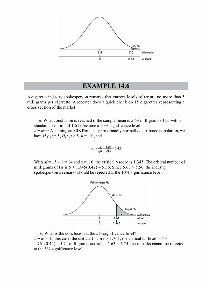
EXAMPLE 14.6A cigarette industry spokesperson remarks that current levels of tar are no more than 5milligrams per cigarette. A reporter does a quick check on 15 cigarettes representing across section of the market.
a. What conclusion is reached if the sample mean is 5.63 milligrams of tar with a
standard deviation of 1.61? Assume a 10% significance level.Answer: Assuming an SRS from an approximately normally distributed population, wehave H0: = 5, Ha: > 5, α = .10, and
With df = 15 – 1 = 14 and α = .10, the critical t-score is 1.345. The critical number ofmilligrams of tar is 5 + 1.345(0.42) = 5.56. Since 5.63 > 5.56, the industryspokesperson’s remarks should be rejected at the 10% significance level.
b. What is the conclusion at the 5% significance level?Answer: In this case, the critical t-score is 1.761, the critical tar level is 5 +1.761(0.42) = 5.74 milligrams, and since 5.63 < 5.74, the remarks cannot be rejectedat the 5% significance level.
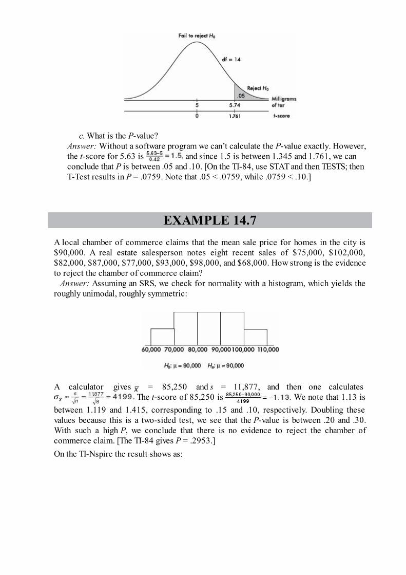
c. What is the P-value?Answer: Without a software program we can’t calculate the P-value exactly. However,the t-score for 5.63 is and since 1.5 is between 1.345 and 1.761, we canconclude that P is between .05 and .10. [On the TI-84, use STAT and then TESTS; thenT-Test results in P = .0759. Note that .05 < .0759, while .0759 < .10.]
EXAMPLE 14.7A local chamber of commerce claims that the mean sale price for homes in the city is$90,000. A real estate salesperson notes eight recent sales of $75,000, $102,000,$82,000, $87,000, $77,000, $93,000, $98,000, and $68,000. How strong is the evidenceto reject the chamber of commerce claim?
Answer: Assuming an SRS, we check for normality with a histogram, which yields theroughly unimodal, roughly symmetric:
A calculator gives = 85,250 and s = 11,877, and then one calculates The t-score of 85,250 is We note that 1.13 is
between 1.119 and 1.415, corresponding to .15 and .10, respectively. Doubling thesevalues because this is a two-sided test, we see that the P-value is between .20 and .30.With such a high P, we conclude that there is no evidence to reject the chamber ofcommerce claim. [The TI-84 gives P = .2953.]On the TI-Nspire the result shows as:

HYPOTHESIS TEST FOR ADIFFERENCE BETWEEN TWO MEANS(UNPAIRED AND PAIRED)We assume that we have two independent simple random samples, each from anapproximately normally distributed population (the normality assumptions canbe relaxed if the sample sizes are large).
In this situation the null hypothesis is usually that the means of the populationsare the same or, equivalently, that their difference is 0:

The alternative hypothesis is then
The first two possibilities lead to one-sided tests, and the third possibility leadsto two-sided tests.
EXAMPLE 14.8A sales representative believes that his company’s computer has more average downtimeper week than a similar computer sold by a competitor. Before taking this concern to hisdirector, the sales representative gathers data and runs a hypothesis test. He determinesthat in a simple random sample of 40 week-long periods at different firms using hiscompany’s product, the average downtime was 125 minutes with a standard deviation of37 minutes. However, 35 week-long periods involving the competitor’s computer yield anaverage downtime of only 115 minutes with a standard deviation of 43 minutes. Whatconclusion should the sales representative draw assuming a 10% significance level?
Answer: We are given independent SRSs and large enough sample sizes to relax thenormality assumptions, so we continue:
H0: 1 – 2 = 0 (where 1 = mean down time of company’s computersHα: 1 – 2 > 0 and 2 = mean down time of competitor’s computers)
α = .10df = (40 – 1) + (35 – 1) = 73
(or the more conservative df = min(40–1, 35–1) = 34)
The difference in sample means is 125 – 115 = 10, and the t-score is UsingTable B, we find the P-value to be between .10 and .15. Thus, the observed difference isnot significant at the 10% significance level. The sales representative does not havesufficient evidence that his company’s computer has more downtime. While the observeddifference would be significant at, for example, the 15% level, still, with P > .1, we saythat the evidence is weak that the salesman’s company’s computer has more downtimethan that of the competitor’s.
Remark: On the TI-84, STAT → TESTS → 2-SampTTest, then Inpt : Stats, 1 : 125, Sx1: 37, n1 : 40, 2 : 115, Sx2 : 43, n2 : 35, 1 : > 2 and Calculate yields t = 1.0718 and P= .1438.

TIPAvoid “calculator speak.” For example, do not simply write“2-SampTTest…” or “binomcdf…” There are lots ofcalculators out there, each with their own abbreviations.
EXAMPLE 14.9A store manager wishes to determine whether there is a significant difference betweentwo trucking firms with regard to the handling of egg cartons. In a simple random sampleof 200 cartons on one firm’s truck there was an average of 0.7 broken eggs per cartonwith a standard deviation of 0.31, while a sample of 300 cartons on the second firm’struck showed an average of 0.775 broken eggs per carton with a standard deviation of0.42. Is the difference between the averages significant at a significance level of 5%? At asignificance level of 1%?
Answer: We are given independent SRSs and large enough sample sizes to relax thenormality assumptions, so we continue:
α = .05df = (200 – 1) + (300 – 1) = 498
(or the more conservative df = min(200 – 1, 300 – 1) = 199)
Since there is no mention that it is believed that one firm does better than the other, thisis a two-sided test. The observed difference of 0.7 – 0.775 = –0.075 has a t-score of
Using Table B, we find that this gives a probability between .01 and .02.The test is two-sided, and so the P-value is between .02 and .04. So the observeddifference in average number of broken eggs per carton is statistically significant at the5% level but not at the 1% level. With .01 < P < .05, we usually say that there ismoderate evidence to reject H0. [On the TI-84, 2-SampTTest gives P = .0222.]
EXAMPLE 14.10A city council member claims that male and female officers wait equal times forpromotion in the police department. A women’s spokesperson, however, believes womenmust wait longer than men. If five men waited 8, 7, 10, 5, and 7 years, respectively, forpromotion while four women waited 9, 5, 12, and 8 years, respectively, what conclusionshould be drawn?
Answer: We must assume that we have two independent SRSs, each from an

approximately normally distributed population (the samples are too small for histogramsto show anything, but at least a quick calculation indicates no outliers and normalprobability plots are fairly linear).
We have H0: 1 – 2 = 0 and Ha: 1 – 2 < 0. Using a calculator we find 1 = 7.4, s1 =1.82, 2 = 8.5, and s2 = 2.89. Then
The t-score of the observed difference is With df = 5 + 4 – 2 = 7, we notethat 0.66 < 0.711, where 0.711 corresponds to a tail probability of .25. Thus the P-valueis greater than .25, and we conclude there is no evidence to dispute the council member’sclaim. (Using the conservative df = min(5–1, 4–1) = 3 leads to the same conclusion.) [Onthe TI-84, inserting the data into lists and using 2-SampTTest with Data gives P = .2685.]
The analysis and procedure described above require that the two samples
being compared be independent of each other. However, many experiments andtests involve comparing two populations for which the data naturally occur inpairs. In this case, the proper procedure is to run a one-sample test on a singlevariable consisting of the differences from the paired data.
EXAMPLE 14.11Does a particular drug slow reaction times? If so, the government might require a warninglabel concerning driving a car while taking the medication. An SRS of 30 people aretested before and after taking the drug, and their reaction times (in seconds) to a standardtesting procedure are noted. The resulting data are as follows:


TIPWhen the data comes in pairs, you cannot use a two sample t-test.
We can calculate the mean reaction times before and after, 1.46 seconds and 1.50seconds, respectively, and ask if this observed rise is significant. If we performed a two-sample test, we would calculate the P-value to be .2708 and would conclude that withsuch a large P, the observed rise is not significant. However, this would not be the propertest or conclusion! The two-sample test works for independent sets. However, in thiscase, there is a clear relationship between the data, in pairs, and this relationship iscompletely lost in the procedure for the two-sample test. The proper procedure is toform the set of 30 differences, being careful with signs, {–0.06, 0.12, 0.03, –0.24, . . .},and to perform a single sample hypothesis test as follows:
Name the test:
We are using a paired t-test, that is, a single sample hypothesis test on the set ofdifferences.
State the hypothesis:
H0: The reaction times of individuals to a standard testing procedure are the same
before and after they take a particular drug; the mean difference is zero: d = 0.Ha: The reaction time is greater after they take the drug; the mean difference is less
than zero: d < 0.
Check the conditions:
1. The data are paired because they are measurements on the same individuals
before and after taking the drug.2. The reaction times of any individual are independent of the reaction times of the
others, so the differences are independent.3. A random sample of people are tested.4. The histogram of the differences looks nearly normal (roughly unimodal and
symmetric):
Perform the mechanics:
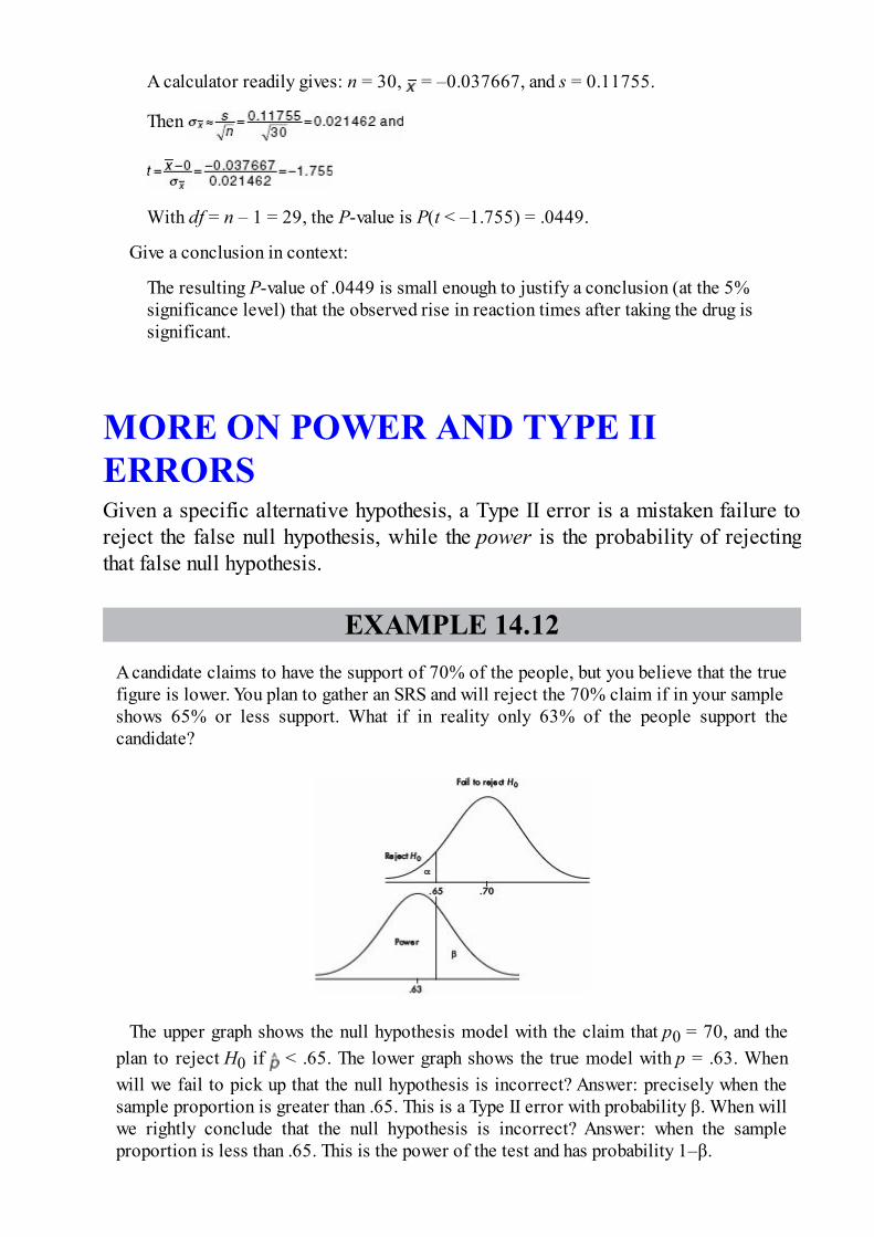
A calculator readily gives: n = 30, = –0.037667, and s = 0.11755.
Then
With df = n – 1 = 29, the P-value is P(t < –1.755) = .0449.
Give a conclusion in context:
The resulting P-value of .0449 is small enough to justify a conclusion (at the 5%significance level) that the observed rise in reaction times after taking the drug issignificant.
MORE ON POWER AND TYPE IIERRORSGiven a specific alternative hypothesis, a Type II error is a mistaken failure toreject the false null hypothesis, while the power is the probability of rejectingthat false null hypothesis.
EXAMPLE 14.12A candidate claims to have the support of 70% of the people, but you believe that the truefigure is lower. You plan to gather an SRS and will reject the 70% claim if in your sampleshows 65% or less support. What if in reality only 63% of the people support thecandidate?
The upper graph shows the null hypothesis model with the claim that p0 = 70, and theplan to reject H0 if < .65. The lower graph shows the true model with p = .63. Whenwill we fail to pick up that the null hypothesis is incorrect? Answer: precisely when thesample proportion is greater than .65. This is a Type II error with probability β. When willwe rightly conclude that the null hypothesis is incorrect? Answer: when the sampleproportion is less than .65. This is the power of the test and has probability 1–β.

The following points should be emphasized:
• Power gives the probability of avoiding a Type II error.
• Power has a different value for different possible correct values of the
population parameter; thus it is actually a function where the independentvariable ranges over specific alternative hypotheses.
• Choosing a smaller α (that is, a tougher standard to reject H0) results in a
higher risk of Type II error and a lower power—observe in the above graphshow making α smaller (in this case moving the critical cutoff value to the left)makes the power less and β more!
• The greater the difference between the null hypothesis p0 and the true value p,
the smaller the risk of a Type II error and the greater the power—observe inthe above picture how moving the lower graph to the left makes the powergreater and β less. (The difference between p0 and p is sometimes called theeffect—thus the greater the effect, the greater is the power to pick it up.)
• A larger sample size n will reduce the standard deviations, making both
graphs narrower resulting in smaller α, smaller β, and larger power!
CONFIDENCE INTERVALS VERSUSHYPOTHESIS TESTSA question sometimes arises as to whether a problem calls for calculating aconfidence interval or performing a hypothesis test. Generally, a claim about apopulation parameter indicates a hypothesis test, while an estimate of apopulation parameter asks for a confidence interval. However, some confusionmay arise because sometimes it is possible to conduct a hypothesis test byconstructing a confidence interval estimate of the parameter and then checkingwhether or not the null parameter value is in the interval. While, when possible,this alternative approach is accepted on the AP exam, it does require veryspecial care in still remembering to state hypotheses, in dealing with one-sidedversus two-sided, and in how standard errors are calculated in problemsinvolving proportions. So the recommendation is to conduct a hypothesis testlike a hypothesis test. Carefully read the question. If it asks whether or not there

is evidence, then this is a hypothesis test; if it involves how much or howeffective, then this is a confidence interval calculation. However, it should benoted that there have been AP free-response questions where part (a) calls for aconfidence interval calculation and part (b) asks if this calculation providesevidence relating to a hypothesis test.
Summary• Important assumptions/conditions always must be checked before proceeding
with a hypothesis test.• The null hypothesis is stated in the form of an equality statement about a
population parameter, while the alternative hypothesis is in the form of aninequality.
• We attempt to show that a null hypothesis is unacceptable by showing it isimprobable.
• The P-value is the probability of obtaining a sample statistic as extreme (ormore extreme) as the one obtained if the null hypothesis is assumed to be true.
• When the P-value is small (typically, less than .05 or .10), we say we haveevidence to reject the null hypothesis.
• A Type I error is the probability of mistakenly rejecting a true null hypothesis.• A Type II error is the probability of mistakenly failing to reject a false null
hypothesis.• The power of a hypothesis test is the probability that a Type II error is not
committed.
Questions on Topic Fourteen: Tests ofSignificance—Proportions and Means
Multiple-Choice Questions
Directions: The questions or incomplete statements that follow are eachfollowed by five suggested answers or completions. Choose the responsethat best answers the question or completes the statement.
1. Which of the following is a true statement?
(A) A well-planned hypothesis test should result in a statement eitherthat the null hypothesis is true or that it is false.
(B) The alternative hypothesis is stated in terms of a sample statistic.(C) If a sample is large enough, the necessity for it to be a simple
random sample is diminished.

(D) When the null hypothesis is rejected, it is because it is not true.(E) Hypothesis tests are designed to measure the strength of evidence
against the null hypothesis.
2. Which of the following is a true statement?
(A) The P-value of a test is the probability of obtaining a result asextreme (or more extreme) as the one obtained assuming the nullhypothesis is false.
(B) If the P-value for a test is .015, the probability that the nullhypothesis is true is .015.
(C) The larger the P-value, the more evidence there is against thenull hypothesis.
(D) If possible, always examine your data before deciding whetherto use a one-sided or two-sided hypothesis test.
(E) The alternative hypothesis is one-sided if there is interest indeviations from the null hypothesis in only one direction.
Questions 3–4 refer to the following:
Video arcades provide a vehicle for competition and status withinteenage peer groups and are recognized as places where teens can hangout and meet their friends. The national PTA organization, concernedabout the time and money being spent in video arcades by middle schoolstudents, commissions a statistical study to investigate whether or notmiddle school students are spending an average of over two hours perweek in video arcades. Twenty communities are randomly chosen, fivemiddle schools are randomly picked in each of the communities, and tenstudents are randomly interviewed at each school.
3. What is the parameter of interest?

(A) Video arcades(B) A particular concern of the national PTA organization(C) 1000 randomly chosen middle school students(D) The mean amount of money spent in video arcades by middle
school students(E) The mean number of hours per week spent in video arcades by
middle school students
4. What are the null and alternative hypotheses which the PTA is
testing?
(A) H0: = 2 Ha: < 2
(B) H0: = 2 Ha: ≤ 2
(C) H0: = 2 Ha: > 2
(D) H0: = 2 Ha: ≥ 2
(E) H0: = 2 Ha: ≠ 2
5. A hypothesis test comparing two population proportions results in aP-value of .032. Which of the following is a proper conclusion?
(A) The probability that the null hypothesis is true is .032.(B) The probability that the alternative hypothesis is true is .032.(C) The difference in sample proportions is .032.(D) The difference in population proportions is .032.(E) None of the above are proper conclusions.
6. A company manufactures a synthetic rubber (jumping) bungee cord

with a braided covering of natural rubber and a minimum breakingstrength of 450 kg. If the mean breaking strength of a sample drops belowa specified level, the production process is halted and the machineryinspected. Which of the following would result from a Type I error?
(A) Halting the production process when too many cords break.(B) Halting the production process when the breaking strength is
below the specified level.(C) Halting the production process when the breaking strength is
within specifications.(D) Allowing the production process to continue when the breaking
strength is below specifications.(E) Allowing the production process to continue when the breaking
strength is within specifications.
7. One ESP test asks the subject to view the backs of cards and identifywhether a circle, square, star, or cross is on the front of each card. If p isthe proportion of correct answers, this may be viewed as a hypothesis testwith H0: p = .25 and Ha: p > .25. The subject is recognized to have ESPwhen the null hypothesis is rejected. What would a Type II error resultin?
(A) Correctly recognizing someone has ESP(B) Mistakenly thinking someone has ESP(C) Not recognizing that someone really has ESP(D) Correctly realizing that someone doesn’t have ESP(E) Failing to understand the nature of ESP
8. A coffee-dispensing machine is supposed to deliver 12 ounces of
liquid into a large paper cup, but a consumer believes that the actualamount is less. As a test he plans to obtain a sample of 5 cups of thedispensed liquid and if the mean content is less than 11.5 ounces, to rejectthe 12-ounce claim. If the machine operates with a known standard
deviation of 0.9 ounces, what is the probability that the consumer willmistakenly reject the 12-ounce claim even though the claim is true?
(A) .054(B) .107(C) .214(D) .289(E) .393
9. A pharmaceutical company claims that a medicine will produce a
desired effect for a mean time of 58.4 minutes. A government researcherruns a hypothesis test of 40 patients and calculates a mean of = 59.5with a standard deviation of s = 8.3. What is the P-value?
(A) P with df = 39
(B) P with df = 40
(C) 2P with df = 39
(D) 2P with df = 40
(E) 2P
10. You plan to perform a hypothesis test with a level of significance ofα = .05. What is the effect on the probability of committing a Type I errorif the sample size is increased?
(A) The probability of committing a Type I error decreases.(B) The probability of committing a Type I error is unchanged.(C) The probability of committing a Type I error increases.

(D) The effect cannot be determined without knowing the relevantstandard deviation.
(E) The effect cannot be determined without knowing if a Type IIerror is committed.
11. A fast food chain advertises that their large bag of french fries has aweight of 150 grams. Some high school students, who enjoy french fries atevery lunch, suspect that they are getting less than the advertised amount.With a scale borrowed from their physics teacher, they weigh a randomsample of 15 bags. What is the conclusion if the sample mean is 145.8 gand standard deviation is 12.81 g?
(A) There is sufficient evidence to prove the fast food chainadvertisement is true.
(B) There is sufficient evidence to prove the fast food chainadvertisement is false.
(C) The students have sufficient evidence to reject the fast foodchain’s claim.
(D) The students do not have sufficient evidence to reject the fastfood chain’s claim.
(E) There is not sufficient data to reach any conclusion.
12. A researcher believes a new diet should improve weight gain inlaboratory mice. If ten control mice on the old diet gain an average of 4ounces with a standard deviation of 0.3 ounces, while the average gain forten mice on the new diet is 4.8 ounces with a standard deviation of 0.2ounces, what is the P-value?
(A) P

(B) P
(C) P
(D) P
(E) P
13. A school superintendent must make a decision whether or not tocancel school because of a threatening snow storm. What would theresults be of Type I and Type II errors for the null hypothesis: Theweather will remain dry?
(A) Type I error: don’t cancel school, but the snow storm hits.Type II error: weather remains dry, but school is needlessly canceled.
(B) Type I error: weather remains dry, but school is needlesslycanceled.Type II error: don’t cancel school, but the snow storm hits.
(C) Type I error: cancel school, and the storm hits.Type II error: don’t cancel school, and weather remains dry.
(D) Type I error: don’t cancel school, and snow storm hits.Type II error: don’t cancel school, and weather remains dry.
(E) Type I error: don’t cancel school, but the snow storm hits.Type II error: cancel school, and the storm hits.
14. A pharmaceutical company claims that 8% or fewer of the patientstaking their new statin drug will have a heart attack in a 5-year period. Ina government-sponsored study of 2300 patients taking the new drug, 198have heart attacks in a 5-year period. Is this strong evidence against thecompany claim?

(A) Yes, because the P-value is .005657.(B) Yes, because the P-value is .086087.(C) No, because the P-value is only .005657.(D) No, because the P-value is only .086087.(E) No, because the P-value is over .10.
15. Is Internet usage different in the Middle East and Latin America? Ina random sample of 500 adults in the Middle East, 151 claimed to beregular Internet users, while in a random sample of 1000 adults in LatinAmerica, 345 claimed to be regular users. What is the P-value for theappropriate hypothesis test?
(A) P
(B) 2P
(C) P
(D) 2P
(E) 2(.095167)
16. What is the probability of mistakenly failing to reject a false nullhypothesis when a hypothesis test is being conducted at the 5%significance level (α = .05)?
(A) .025

(B) .05(C) .10(D) .95(E) There is insufficient information to answer this question.
17. A research dermatologist believes that cancers of the head and neckwill occur most often of the left side, the side next to a window when aperson is driving. In a review of 565 cases of head/neck cancers, 305occurred on the left side. What is the resulting P-value?
(A) P
(B) 2P
(C) P
(D) P
(E) 2P
18. Suppose you do five independent tests of the form H0: = 38versus Ha: > 38, each at the α = .01 significance level. What is theprobability of committing a Type I error and incorrectly rejecting a truenull hypothesis with at least one of the five tests?
(A) .01(B) .049(C) .05(D) .226(E) .951

19. Given an experiment with H0: = 35, Ha: < 35, and a possiblecorrect value of 32, you obtain a sample statistic of = 33. After doinganalysis, you realize that the sample size n is actually larger than you firstthought. Which of the following results from reworking with the increasein sample size?
(A) Decrease in probability of a Type I error; decrease inprobability of a Type II error; decrease in power.
(B) Increase in probability of a Type I error; increase in probabilityof a Type II error; decrease in power.
(C) Decrease in probability of a Type I error; decrease inprobability of a Type II error; increase in power.
(D) Increase in probability of a Type I error; decrease in probabilityof a Type II error; decrease in power.
(E) Decrease in probability of a Type I error; increase in probabilityof a Type II error; increase in power.
20. Thirty students volunteer to test which of two strategies for takingmultiple-choice exams leads to higher average results. Each student flipsa coin, and if heads, uses Strategy A on the first exam and then Strategy Bon the second, while if tails, uses Strategy B first and then Strategy A. Theaverage of all 30 Strategy A results is then compared to the average of all30 Strategy B results. What is the conclusion at the 5% significance levelif a two-sample hypothesis test, H0: 1 = 2, Ha: 1 ≠ 2,results in a P-value of .18?
(A) The observed difference in average scores is significant.(B) The observed difference in average scores is not significant.(C) A conclusion is not possible without knowing the average scores
resulting from using each strategy.(D) A conclusion is not possible without knowing the average scores
and the standard deviations resulting from using each strategy.(E) A two-sample hypothesis test should not be used here.

21. Choosing a smaller level of significance, that is, a smaller α-risk,results in
(A) a lower risk of Type II error and lower power.(B) a lower risk of Type II error and higher power.(C) a higher risk of Type II error and lower power.(D) a higher risk of Type II error and higher power.(E) no change in risk of Type II error or in power.
22. The greater the difference between the null hypothesis claim and thetrue value of the population parameter,
(A) the smaller the risk of a Type II error and the smaller the power.(B) the smaller the risk of a Type II error and the greater the power.(C) the greater the risk of a Type II error and the smaller the power.(D) the greater the risk of a Type II error and the greater the power.(E) the greater the probability of no change in Type II error or in
power.
23. A company selling home appliances claims that the accompanyinginstruction guides are written at a 6th grade reading level. An Englishteacher believes that the true figure is higher and with the help of an APStatistics student runs a hypothesis test. The student randomly picks onepage from each of 25 of the company’s instruction guides, and the teachersubjects the pages to a standard readability test. The reading levels of the25 pages are given in the following table:

Is there statistical evidence to support the English teacher’s belief?
(A) No, because the P-value is greater than .10.(B) Yes, the P-value is between .05 and .10 indicating some
evidence for the teacher’s belief.(C) Yes, the P-value is between .01 and .05 indicating evidence for
the teacher’s belief.(D) Yes, the P-value is between .001 and .01 indicating strong
evidence for the teacher’s belief.(E) Yes, the P-value is less than .001 indicating very strong
evidence for the teacher’s belief.
24. Suppose H0: p = .4, and the power of the test for the alternativehypothesis p = .35 is .75. Which of the following is a valid conclusion?
(A) The probability of committing a Type I error is .05.(B) The probability of committing a Type II error is .65.(C) If the alternative p = .35 is true, the probability of failing to
reject H0 is .25.
(D) If the null hypothesis is true, the probability of rejecting it is .25.(E) If the null hypothesis is false, the probability of failing to reject it
is .65.
25. A factory is located close to a city high school. The manager claimsthat the plant’s smokestacks spew forth an average of no more than 350pounds of pollution per day. As an AP Statistics project, the class plans aone-sided hypothesis test with a critical value of 375 pounds. Suppose thestandard deviation in daily pollution poundage is known to be 150 poundsand the true mean is 385 pounds. If the sample size is 100 days, what is
the probability that the class will mistakenly fail to reject the factorymanager’s false claim?
(A) .0475(B) .2525(C) .7475(D) .7514(E) .9525
Free-Response Questions
Directions: You must show all work and indicate the methods you use. Youwill be graded on the correctness of your methods and on the accuracy ofyour final answers.
Ten Open-Ended Questions1. Next to good brakes, proper tire pressure is the most crucial safety
issue on your car. Incorrect tire pressure compromises cornering, braking,and stability. Both underinflation and overinflation can lead to problems.The number on the tire is the maximum allowable air pressure—not therecommended pressure for that tire. At a roadside vehicle safetycheckpoint, officials randomly select 30 cars for which 35 psi is therecommended tire pressure and calculate the average of the actual tirepressure in the front right tires. What is the parameter of interest, and whatare the null and alternative hypotheses that the officials are testing?
2. No vaccinations are 100% risk free, and the theoretical risk of rarecomplications always have to be balanced against the severity of thedisease. Suppose the CDC decides that a risk of one in a million is themaximum acceptable risk of GBS (Guillain-Barre syndrome)complications for a new vaccine for a particularly serious strain ofinfluenza. A large sample study of the new vaccine is conducted with thefollowing hypotheses:H0: The proportion of GBS complications is .000001 (one in a million)Ha: The proportion of GBS complications is greater than .000001 (one in
a million)
The P-value of the test is .138.(a) Interpret the P-value in context of this study.(b) What conclusion should be drawn at the α = .10 significance
level?(c) Given this conclusion, what possible error, Type I or Type II,
might be committed, and give a possible consequence of committingthis error.3. A particular wastewater treatment system aims at reducing the most
probable number per ml (MPN/ml) of E. coli to 1000 MPN/100 ml. Arandom study of 40 of these systems in current use is conducted with thedata showing a mean of 1002.4 MPN/100 ml and a standard deviation of7.12 MPN/100 ml. A test of significance is conducted with:H0: The mean concentration of E. coli after treatment under this system is
1000 MPN/100 ml.Ha: The mean concentration of E. coli after treatment under this system is
greater than 1000 MPN/100 ml.The resulting P-value is .0197 with df = 39 and t = 2.132.
(a) Interpret the P-value in context of this study.(b) What conclusion should be drawn at a 5% significance level?(c) Given this conclusion, what possible error, Type I or Type II,
might be committed, and give a possible consequence of committingthis error.4. A 20-year study of 5000 British adults noted four bad habits:
smoking, drinking, inactivity, and poor diet. The study looked to show thatthere is a higher death rate (proportion who die in a 20-year period)among people with all four bad habits than among people with none of thefour bad habits.
(a) Was this an experiment or observational study? Explain.(b) What are the null and alternative hypotheses?(c) What would be the result of a Type I error?(d) What would be the result of a Type II error?
Of the 314 people who had all four bad habits, 91 died during the study,
while of the 387 people with none of the four bad habits, 32 died duringthe study.
(e) Calculate and interpret the P-value in context of this study.5. It is estimated that 17.4% of all U.S. households own a Roth IRA.
The American Association of University Professors (AAUP) believes thisfigure is higher among their members and commissions a study. If 150 outof a random sample of 750 AAUP members own Roth IRAs, is thissufficient evidence to support the AAUP belief?
6. A long accepted measure of the discharge rate (in 1000 ft3/sec) at themouth of the Mississippi River is 593. To test if this has changed, tenmeasurements at random times are taken: 590, 596, 592, 588, 589, 594,590, 586, 591, 589. Is there statistical evidence of a change?
7. A behavior study of high school students looked at whether a higherproportion of boys than girls met a recommended level of physicalactivity (increased heart rate for 60 minutes/day for at least 5 days duringthe 7 days before the survey). What is the proper conclusion if 370 out ofa random sample of 850 boys and 218 out of an independent randomsample of 580 girls met the recommended level of activity?
8. In a random sample of 35 NFL games the average attendance was68,729 with a standard deviation of 6,110, while in a random sample of30 Big 10 Conference football games the average attendance was 70,358with a standard deviation of 9,139. Is there evidence that the averageattendance at Big 10 Conference football games is greater than that at NFLgames?
9. A study is proposed to compare two treatments for patients withsignificantly narrowed neck arteries. Some patients will be treated withsurgery to remove built-up plaque, while others will be treated with stentsto improve circulation. The response variable will be the proportion ofpatients who suffer a major complication such as a stroke or heart attackwithin one month of the treatment. The researchers decide to block onwhether or not a patient has had a mini stroke in the previous year.
(a) There are 1000 patients available for this study, half of whomhave had a mini stroke in the previous year. Explain a block design toassign patients to treatments.
(b) Give two methods other than blocking to increase the power ofdetecting a difference between using surgery versus stents for patientswith this medical condition. Explain your choice of methods.10. A car simulator was used to compare effect on reaction time
between DWI (driving while intoxicated) and DWT (driving while
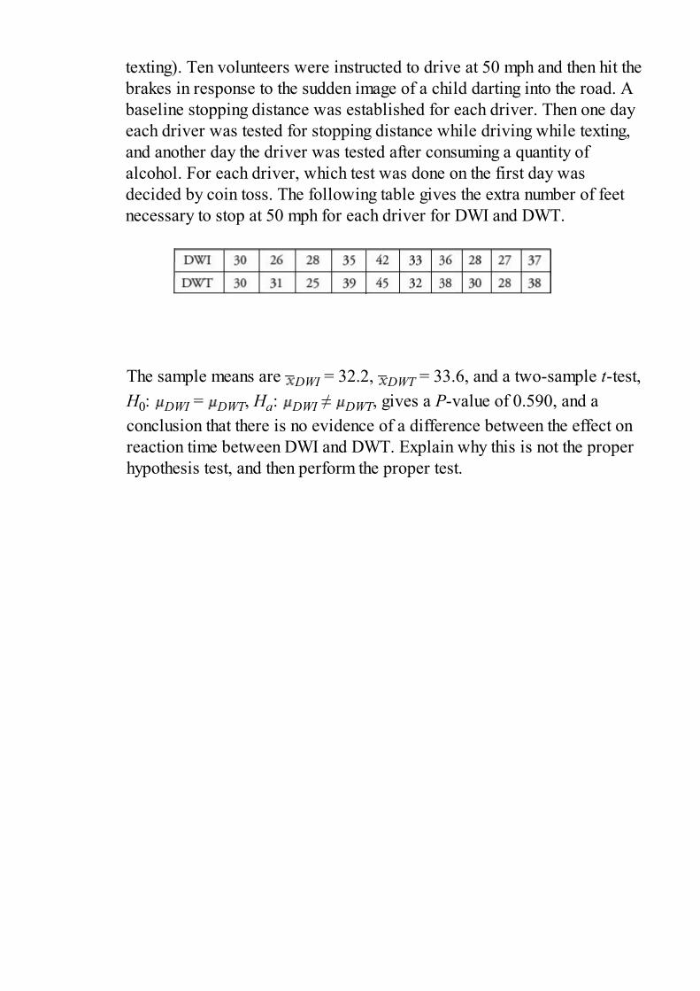
texting). Ten volunteers were instructed to drive at 50 mph and then hit thebrakes in response to the sudden image of a child darting into the road. Abaseline stopping distance was established for each driver. Then one dayeach driver was tested for stopping distance while driving while texting,and another day the driver was tested after consuming a quantity ofalcohol. For each driver, which test was done on the first day wasdecided by coin toss. The following table gives the extra number of feetnecessary to stop at 50 mph for each driver for DWI and DWT.
The sample means are DWI = 32.2, DWT = 33.6, and a two-sample t-test,H0: DWI = DWT, Ha: DWI ≠ DWT, gives a P-value of 0.590, and aconclusion that there is no evidence of a difference between the effect onreaction time between DWI and DWT. Explain why this is not the properhypothesis test, and then perform the proper test.
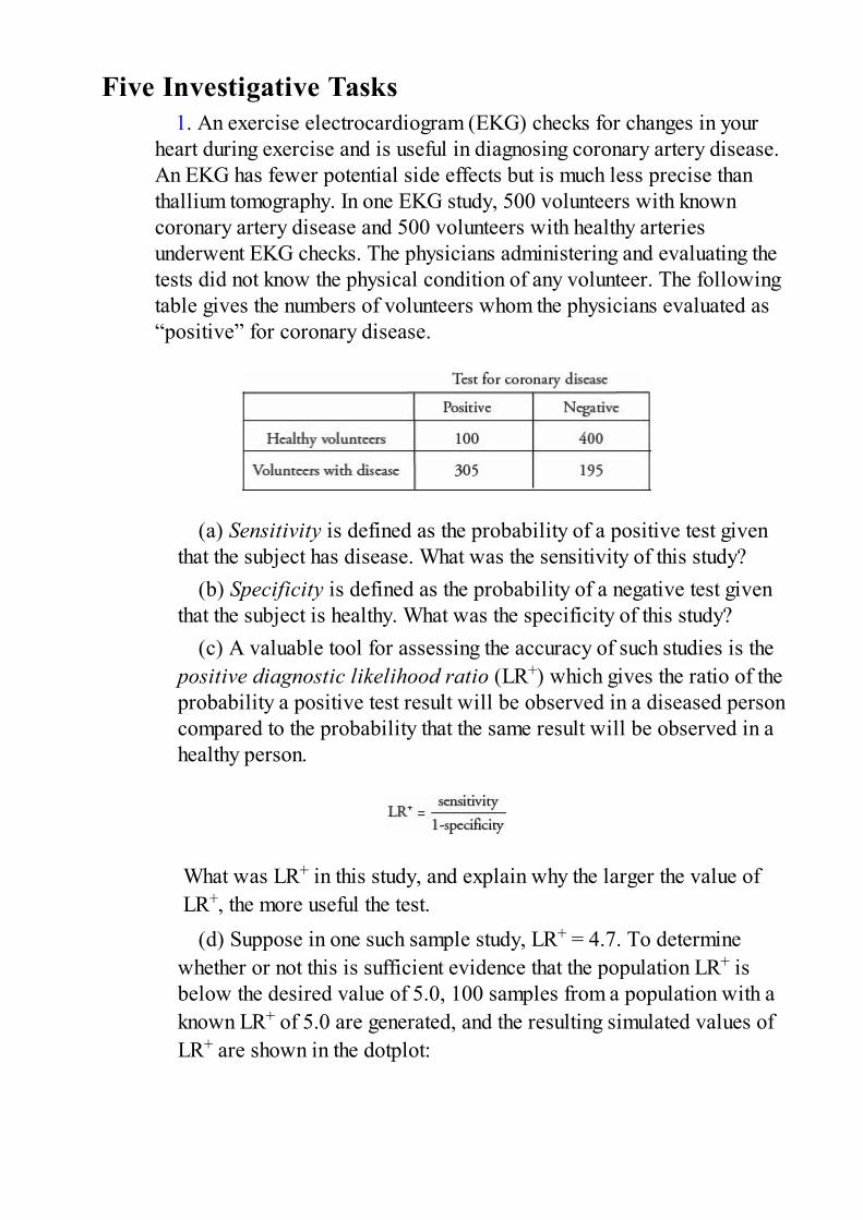
Five Investigative Tasks1. An exercise electrocardiogram (EKG) checks for changes in your
heart during exercise and is useful in diagnosing coronary artery disease.An EKG has fewer potential side effects but is much less precise thanthallium tomography. In one EKG study, 500 volunteers with knowncoronary artery disease and 500 volunteers with healthy arteriesunderwent EKG checks. The physicians administering and evaluating thetests did not know the physical condition of any volunteer. The followingtable gives the numbers of volunteers whom the physicians evaluated as“positive” for coronary disease.
(a) Sensitivity is defined as the probability of a positive test giventhat the subject has disease. What was the sensitivity of this study?
(b) Specificity is defined as the probability of a negative test giventhat the subject is healthy. What was the specificity of this study?
(c) A valuable tool for assessing the accuracy of such studies is thepositive diagnostic likelihood ratio (LR+) which gives the ratio of theprobability a positive test result will be observed in a diseased personcompared to the probability that the same result will be observed in ahealthy person.
What was LR+ in this study, and explain why the larger the value ofLR+, the more useful the test.
(d) Suppose in one such sample study, LR+ = 4.7. To determinewhether or not this is sufficient evidence that the population LR+ isbelow the desired value of 5.0, 100 samples from a population with aknown LR+ of 5.0 are generated, and the resulting simulated values ofLR+ are shown in the dotplot:

Based on this dotplot and the sample LR+ = 4.7, is there evidence thatthe population LR+ is below the desired value of 5.0? Explain.
2. An engineer wishes to test which of two drills can more quickly boreholes in various materials. He assembles a random sampling of tenmaterials of various hardnesses and thicknesses.
(a) Given that a drill’s efficiency is influenced by how long and howhard it has been operating, the engineer decided to randomly choose theorder in which the materials will be tested. Design and implement ascheme to place the materials in random order using the followingrandom number table:
51844 73424 84380 82259 28273 58102 18727 69708
(b) Suppose the drilling times (in seconds) are summarized asfollows:
What is the mean drilling time for each drill? Is the differencesignificant? Justify your answer.
3. Paul the octopus, who lives in a tank at Sea Life Centre inOberhausen, Germany, correctly predicted the winner in 12 out of 14soccer matches (by choosing to eat mussels from the boxes labeled withnational flags of the eventual winning teams). Assume these 14 matchesrepresent a random sample of matches which Paul could predict, andassume that all matches end in a win for one of the teams (using suddendeath overtime or penalty kicks to settle tie scores from regulation time).
(a) Why would it be incorrect to perform a one-sample z-test onwhether the above is sufficient evidence that Paul can correctly predictthe results of more than 50% of soccer matches?
(b) Perform a proper hypothesis test for the question in (a).
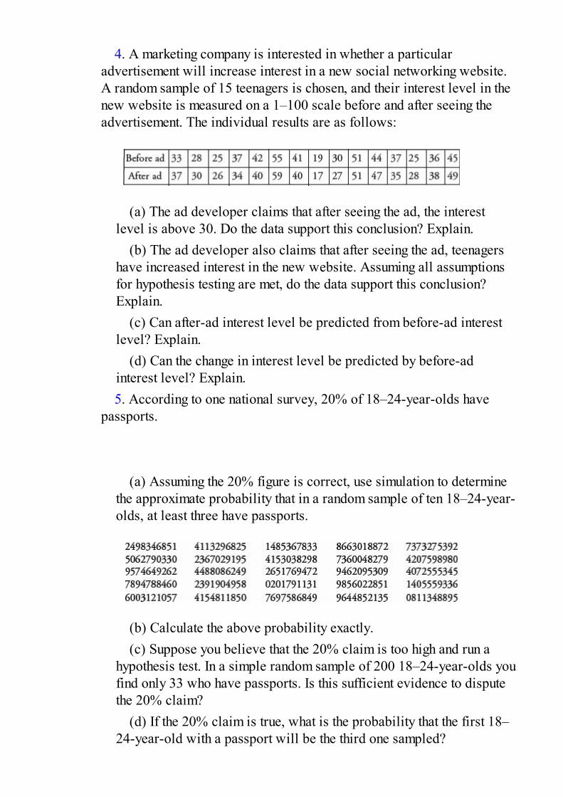
4. A marketing company is interested in whether a particularadvertisement will increase interest in a new social networking website.A random sample of 15 teenagers is chosen, and their interest level in thenew website is measured on a 1–100 scale before and after seeing theadvertisement. The individual results are as follows:
(a) The ad developer claims that after seeing the ad, the interestlevel is above 30. Do the data support this conclusion? Explain.
(b) The ad developer also claims that after seeing the ad, teenagershave increased interest in the new website. Assuming all assumptionsfor hypothesis testing are met, do the data support this conclusion?Explain.
(c) Can after-ad interest level be predicted from before-ad interestlevel? Explain.
(d) Can the change in interest level be predicted by before-adinterest level? Explain.5. According to one national survey, 20% of 18–24-year-olds have
passports.
(a) Assuming the 20% figure is correct, use simulation to determinethe approximate probability that in a random sample of ten 18–24-year-olds, at least three have passports.
(b) Calculate the above probability exactly.(c) Suppose you believe that the 20% claim is too high and run a
hypothesis test. In a simple random sample of 200 18–24-year-olds youfind only 33 who have passports. Is this sufficient evidence to disputethe 20% claim?
(d) If the 20% claim is true, what is the probability that the first 18–24-year-old with a passport will be the third one sampled?
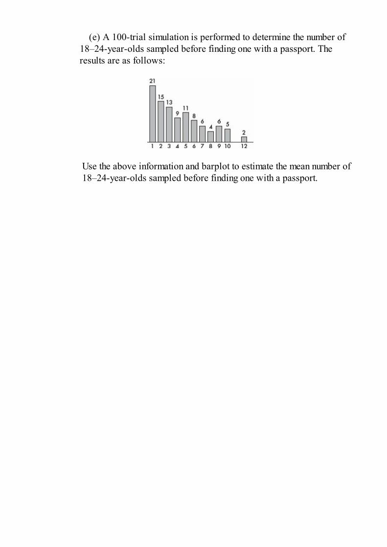
(e) A 100-trial simulation is performed to determine the number of18–24-year-olds sampled before finding one with a passport. Theresults are as follows:
Use the above information and barplot to estimate the mean number of18–24-year-olds sampled before finding one with a passport.

TOPIC 15Tests of Significance—Chi-Square and Slopeof Least Squares Line
• Chi-Square Test for Goodness of Fit• Chi-Square Test for Independence• Chi-Square Test for Homogeneity of
Proportions
• Hypothesis Test for Slope of Least SquaresLine
In this topic we continue our development of tools to analyze data. We learnabout inference on distributions of counts using chi-square models. This can beused to solve such problems as “Do test results support Mendel’s geneticprinciples?” (goodness-of-fit test); “Was surviving the Titanic sinkingindependent of a passenger’s status?” (independence test); and “Do students,teachers, and staff show the same distributions in types of cars driven?”(homogeneity test). We then learn about inference with regard to linearassociation of two variables. This can be used to solve such problems as “Isthere a linear relationship between the grade received on a term paper and thenumber of pages turned in?”

TIP
Unless you have counts, you cannot use χ2 methods.
CHI-SQUARE TEST FOR GOODNESS OFFITA critical question is often whether or not an observed pattern of data fits somegiven distribution. A perfect fit cannot be expected, and so we must look atdiscrepancies and make judgments as to the goodness of fit.
One approach is similar to that developed earlier. There is the null hypothesisof a good fit, that is, the hypothesis that a given theoretical distribution correctlydescribes the situation, problem, or activity under consideration. Our observeddata consist of one possible sample from a whole universe of possible samples.We ask about the chance of obtaining a sample with the observed discrepanciesif the null hypothesis is really true. Finally, if the chance is too small, we rejectthe null hypothesis and say that the fit is not a good one.
How do we decide about the significance of observed discrepancies? It shouldcome as no surprise that the best information is obtained from squaring thediscrepancy values, as this has been our technique for studying variances fromthe beginning. Furthermore, since, for example, an observed difference of 23 ismore significant if the original values are 105 and 128 than if they are 10,602and 10,625, we must appropriately weight each difference. Such weighting isaccomplished by dividing each difference by the expected values. The sum ofthese weighted differences or discrepancies is called chi-square and is denotedas χ2 (χ is the lowercase Greek letter chi):
The smaller the resulting χ2-value, the better the fit. The P-value is theprobability of obtaining a χ2 value as extreme as the one obtained if the nullhypothesis is assumed true. If the χ2 value is large enough, that is, if the P-valueis small enough, we say there is sufficient evidence to reject the null hypothesisand to claim that the fit is poor.
To decide how large a calculated χ2-value must be to be significant, that is, tochoose a critical value, we must understand how χ2-values are distributed. A χ2-distribution is not symmetric and is always skewed to the right. There aredistinct χ2-distributions, each with an associated number of degrees of freedom

(df ). The larger the df value, the closer the χ2-distribution to a normaldistribution. Note, for example, that squaring the often-used z-scores 1.645,1.96, and 2.576 results in 2.71, 3.84, and 6.63, respectively, which are entriesfound in the first row of the χ2-distribution table.
A large χ2-value may or may not be significant—the answer depends on whichχ2-distribution we are using. A table is given of critical χ2-values for the morecommonly used percentages or probabilities. To use the χ2-distribution forapproximations in goodness-of-fit problems, the individual expected valuescannot be too small. An often-used rule of thumb is that no expected valueshould be less than 5. Finally, as in all hypothesis tests we’ve looked at, thesample should be randomly chosen from the given population.
EXAMPLE 15.1In a recent year, at the 6 p.m. time slot, television channels 2, 3, 4, and 5 captured theentire audience with 30%, 25%, 20%, and 25%, respectively. During the first week of thenext season, 500 viewers are interviewed.
a. If viewer preferences have not changed, what number of persons is expected to
watch each channel?Answer: .30(500) = 150, .25(500) = 125, .20(500) = 100, and .25(500) = 125, so wehave
b. Suppose that the actual observed numbers are as follows:

Do these numbers indicate a change? Are the differences significant?Answer: Check the conditions:
1. Randomization: We must assume that the 500 viewers are a representative sample.2. We note that the expected values (150, 125, 100, 125) are all ≥ 5.
H0: The television audience is distributed over channels 2, 3, 4, and 5 with percentages30%, 25%, 20%, and 25%, respectively.
Ha: The audience distribution is not 30%, 25%, 20%, and 25%, respectively.
We calculate
Then the P-value is P = P(χ2 > 5.167) = .1600. [With df = n – 1 = 3, the TI-84 givesχ2cdf(5.167,1000,3) = .1600, or a direct test for goodness of fit can be downloadedonto older TI-84+ calculators and comes preloaded on most!]
Conclusion:
With this large a P-value (.1600) there is not sufficient evidence to reject H0. That is,there is not sufficient evidence that viewer preferences have changed.
Note: While the TI-83 does not have the goodness of fit download that is available onthe TI-84, one can still use a TI-83 to calculate the above χ2 by putting the observedvalues in list L1 and the expected values in L2, then calculating (L1 – L2)2/L2 → L3and χ2 = sum(L3), where “sum” is found under LIST → MATH.
EXAMPLE 15.2A grocery store manager wishes to determine whether a certain product will sell equallywell in any of five locations in the store. Five displays are set up, one in each location,and the resulting numbers of the product sold are noted.
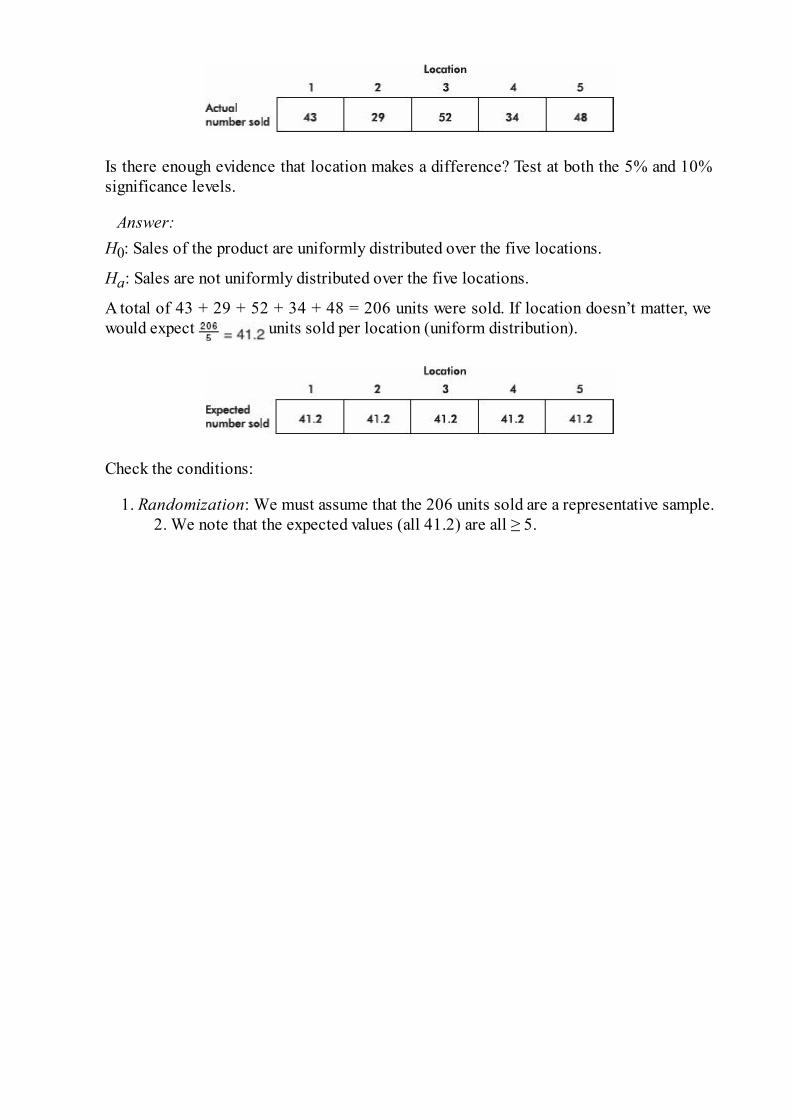
Is there enough evidence that location makes a difference? Test at both the 5% and 10%significance levels.
Answer:H0: Sales of the product are uniformly distributed over the five locations.
Ha: Sales are not uniformly distributed over the five locations.
A total of 43 + 29 + 52 + 34 + 48 = 206 units were sold. If location doesn’t matter, wewould expect units sold per location (uniform distribution).
Check the conditions:
1. Randomization: We must assume that the 206 units sold are a representative sample.2. We note that the expected values (all 41.2) are all ≥ 5.

Thus
The number of degrees of freedom is the number of classes minus 1; that is, df = 5 – 1 =4.
The P-value is P = P(χ2 > 8.903) = .0636. [On the TI-84: χ2cdf(8.903,1000,4).]With P = .0636 there is sufficient evidence to reject H0 at the 10% level but not at the5% level. If the grocery store manager is willing to accept a 10% chance of committing aType I error, there is enough evidence to claim location makes a difference.
CHI-SQUARE TEST FORINDEPENDENCEIn the goodness-of-fit problems above, a set of expectations was based on anassumption about how the distribution should turn out. We then tested whetheran observed sample distribution could reasonably have come from a larger setbased on the assumed distribution.
In many real-world problems we want to compare two or more observedsamples without any prior assumptions about an expected distribution. In whatis called a test of independence, we ask whether the two or more samples mightreasonably have come from some larger set. For example, do nonsmokers, lightsmokers, and heavy smokers all have the same likelihood of being eventuallydiagnosed with cancer, heart disease, or emphysema? Is there a relationship(association) between smoking status and being diagnosed with one of thesediseases?
We classify our observations in two ways and then ask whether the two waysare independent of each other. For example, we might consider several agegroups and within each group ask how many employees show various levels ofjob satisfaction. The null hypothesis is that age and job satisfaction areindependent, that is, that the proportion of employees expressing a given level ofjob satisfaction is the same no matter which age group is considered.
Analysis involves calculating a table of expected values, assuming the nullhypothesis about independence is true. We then compare these expected valueswith the observed values and ask whether the differences are reasonable if H0 istrue. The significance of the differences is gauged by the same χ2-value of
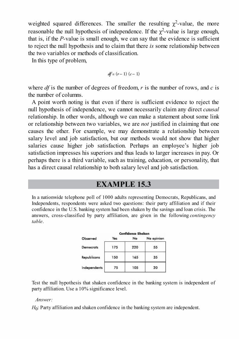
weighted squared differences. The smaller the resulting χ2-value, the morereasonable the null hypothesis of independence. If the χ2-value is large enough,that is, if the P-value is small enough, we can say that the evidence is sufficientto reject the null hypothesis and to claim that there is some relationship betweenthe two variables or methods of classification.
In this type of problem,
where df is the number of degrees of freedom, r is the number of rows, and c isthe number of columns.
A point worth noting is that even if there is sufficient evidence to reject thenull hypothesis of independence, we cannot necessarily claim any direct causalrelationship. In other words, although we can make a statement about some linkor relationship between two variables, we are not justified in claiming that onecauses the other. For example, we may demonstrate a relationship betweensalary level and job satisfaction, but our methods would not show that highersalaries cause higher job satisfaction. Perhaps an employee’s higher jobsatisfaction impresses his superiors and thus leads to larger increases in pay. Orperhaps there is a third variable, such as training, education, or personality, thathas a direct causal relationship to both salary level and job satisfaction.
EXAMPLE 15.3In a nationwide telephone poll of 1000 adults representing Democrats, Republicans, andIndependents, respondents were asked two questions: their party affiliation and if theirconfidence in the U.S. banking system had been shaken by the savings and loan crisis. Theanswers, cross-classified by party affiliation, are given in the following contingencytable.
Test the null hypothesis that shaken confidence in the banking system is independent ofparty affiliation. Use a 10% significance level.
Answer:H0: Party affiliation and shaken confidence in the banking system are independent.

Ha: Party affiliation and shaken confidence in the banking system are not independent.
The above table gives the observed results. To determine the expected values, we mustfirst determine the row and column totals:
To calculate, for example, the expected value in the upper left box, we can proceed inany of several equivalent ways. First, we could note that the proportion of Democrats is
and so, if independent, the expected number of Democrat yes responses is.45(400) = 180. Instead, we could note that the proportion of yes responses is ;and so, if independent, the expected number of Democrat yes responses is .4(450) = 180.Finally, we could note that both these calculations simply involve .
In other words, the expected value of any box can be calculated by multiplying thecorresponding row total by the appropriate column total and then dividing by thegrand total. Thus, for example, the expected value for the middle box, which correspondsto Republican no responses, is .
Continuing in this manner, we fill in the table as follows:
[An appropriate check at this point is that each expected cell count is at least 5.]
Next we calculate the value of chi-square:

[On the TI-84, go to MATRIX and EDIT. Put the data into a matrix. Then STAT, TESTS,χ2-Test, will give χ2 = 3.0243. Note also that the expected values are automatically storedin a second matrix.]Note that, once the 180, 220.5, 140, and 171.5 boxes are calculated, the other expectedvalues can be found by using the row and column totals. Thus the number of degrees offreedom here is 4. Or we calculate
The P-value is calculated to be P = P(χ2 > 3.024) = .5538.With such a large P-value, there is no evidence of any relationship between partyaffiliation and shaken confidence in the banking system.On the TI-Nspire the result shows as:
As for conditions to check for chi-square tests for independence, we shouldcheck that the sample is randomly chosen and that the expected values for allcells are at least 5. If a category has one of its expected cell count less than 5,we can combine categories that are logically similar (for example “disagree”and “strongly disagree”), or combine numerically small categories collectivelyas “other.”
EXAMPLE 15.4To determine whether men with a combination of childhood abuse and a certain abnormalgene are more likely to commit violent crimes, a study is run on a simple random sampleof 575 males in the 25 to 35 age group. The data are summarized in the following table:

a. Is there evidence of a relationship between the four categories (based onchildhood abuse and abnormal genetics) and behavior (criminal versus normal)?Explain.
b. Is there evidence that among men with the normal gene, the proportion of abusedmen who commit violent crimes is greater than the proportion of nonabused men whocommit violent crimes? Explain.
c. Is there evidence that among men who were not abused as children, the proportionof men with the abnormal gene who commit violent crimes is greater than theproportion of men with the normal gene who commit violent crimes? Explain.
d. Is there a contradiction in the above results? Explain.
Answers:
a. A chi-square test for independence is indicated. The expected cell counts are as
follows:
The condition that all cell counts are greater than 5 is met.
H0: The four categories (based on childhood abuse and abnormal genetics) and
behavior (criminal versus normal) are independent.Ha: The four categories (based on childhood abuse and abnormal genetics) and
behavior (criminal versus normal) are not independent (there is a relationship).
Running a chi-square test gives χ2 = 7.752. With df = (r – 1)(c – 1) = 3, we get P = .0514.Since .0514 < .10, the data do provide some evidence (at least at the 10% significancelevel) to reject H0 and conclude that there is evidence of a relationship between the fourcategories (based on childhood abuse and abnormal genetics) and behavior (criminalversus normal).
b. A two-proportion z-test is indicated. We must check that n is large enough:
. We must assumesimple random samples from the target population, since this is not given.
H0: p1 – p2 = 0 (where p1 is the proportion of abused men with normal genetics whocommit violent crimes and p2 is the proportion of nonabused men with normal geneticswho commit violent crimes)
Ha: p1 – p2 > 0 (the proportion of abused men with normal genetics who commit

violent crimes is greater than the proportion of nonabused men with normal geneticswho commit violent crimes)
With such a large P-value there is no evidence to reject H0, and thus we conclude thatthere is no evidence that the proportion of abused men with normal genetics who commitviolent crimes is greater than the proportion of nonabused men with normal genetics whocommit violent crimes.
c. A two-proportion z-test is indicated. We must check that n is large enough:
. We must assume simplerandom samples from the target population, since this is not given.
H0: p1 – p2 = 0 (where p1 is the proportion of nonabused men with abnormal genetics whocommit violent crimes and p2 is the proportion of nonabused men with normal geneticswho commit violent crimes)
Ha: p1 – p2 > 0 (the proportion of nonabused men with abnormal genetics whocommit violent crimes is greater than the proportion of nonabused men with normalgenetics who commit violent crimes)
With such a large P-value there is no evidence to reject H0, and thus we conclude thatthere is no evidence that the proportion of nonabused men with the abnormal gene whocommit violent crimes is greater than the proportion of nonabused men with the normalgene who commit violent crimes.
d. There is no contradiction. It is possible to have evidence of an overall relationship
without significant evidence showing in a subset of the categories.
CHI-SQUARE TEST FOR

HOMOGENEITY OF PROPORTIONSIn chi-square goodness-of-fit tests we work with a single variable in comparinga single sample to a population model. In chi-square independence tests wework with a single sample classified on two variables. Chi-square procedurescan also be used with a single variable to compare samples from two or morepopulations. It is important that the samples be simple random samples, thatthey be taken independently of each other, that the original populations be largecompared to the sample sizes, and that the expected values for all cells be atleast 5. The contingency table used has a row for each sample.
EXAMPLE 15.5In a large city, a group of AP Statistics students work together on a project to determinewhich group of school employees has the greatest proportion who are satisfied with theirjobs. In independent simple random samples of 100 teachers, 60 administrators, 45custodians, and 55 secretaries, the numbers satisfied with their jobs were found to be 82,38, 34, and 36, respectively. Is there evidence that the proportion of employees satisfiedwith their jobs is different in different school system job categories?Answer:
H0: The proportion of employees satisfied with their jobs is the same across the variousschool system job categories.
Ha: At least two of the job categories differ in the proportion of employeessatisfied with their jobs.
The observed counts are as follows:
Just as we did in the previous section, we can calculate the expected value of any cell bymultiplying the corresponding row total by the appropriate column total and then dividingby the grand total. In this case, this results in the following expected counts:

We note that all expected cell counts are >5, and then calculate chi-square:
With 4 – 1 = 3 degrees of freedom, we calculate the P-value to be P(χ2 > 8.640) = .0345.[On the TI-84: χ2cdf(8.640,1000,3).] With this small a P-value, there is sufficientevidence to reject H0, and we can conclude that there is evidence that the proportion ofemployees satisfied with their jobs is not the same across all the school system jobcategories.
Note: On the TI-84 we could also have put the observed data into a matrix and used χ2-Test, resulting in χ2 = 8.707 and P = .0335.
The difference between the test for independence and the test for homogeneitycan be confusing. When we’re simply given a two-way table, it’s not obviouswhich test is being performed. The crucial difference is in the design of thestudy. Did we pick samples from each of two or more populations to comparethe distribution of some variable among the different populations? If so, we aredoing a test for homogeneity. Did we pick one sample from a single populationand cross-categorize on two variables to see if there is an association betweenthe variables? If so, we are doing a test for independence.
For example, if we separately sample Democrats, Republicans, andIndependents to determine whether they are for, against, or have no opinion withregard to stem cell research (several samples, one variable), then we do a testfor homogeneity with a null hypothesis that the distribution of opinions on stemcell research is the same among Democrats, Republicans, and Independents.However, if we sample the general population, noting the political preferenceand opinions on stem cell research of the respondents (one sample, twovariables), then we do a test for independence with a null hypothesis thatpolitical preference is independent of opinion on stem cell research.
Finally, it should be remembered that while we used χ2 for categorical data,the χ2 distribution is a continuous distribution, and applying it to counting datais just an approximation.
HYPOTHESIS TEST FOR SLOPE OFLEAST SQUARES LINEIn addition to finding a confidence interval for the true slope, one can alsoperform a hypothesis test for the value of the slope. Often one uses the nullhypothesis H0: = 0, that is, that there is no linear relationship between the twovariables. Assumptions for inference for the slope of the least squares line

include the following: (1) the sample must be randomly selected; (2) thescatterplot should be approximately linear; (3) there should be no apparentpattern in the residuals plot; and (4) the distribution of the residuals should beapproximately normal. (This third point can be checked by a histogram, dotplot,stemplot, or normal probability plot of the residuals.)
TIPBe careful about abbreviations. For example, your teachermight use LOBF (line of best fit), but the grader may have noidea what this refers to.
Note that a low P-value tells us that if the two variables did not have somelinear relationship, it would be highly unlikely to find such a random sample;however, strong evidence that there is some association does not mean theassociation is strong.
EXAMPLE 15.6
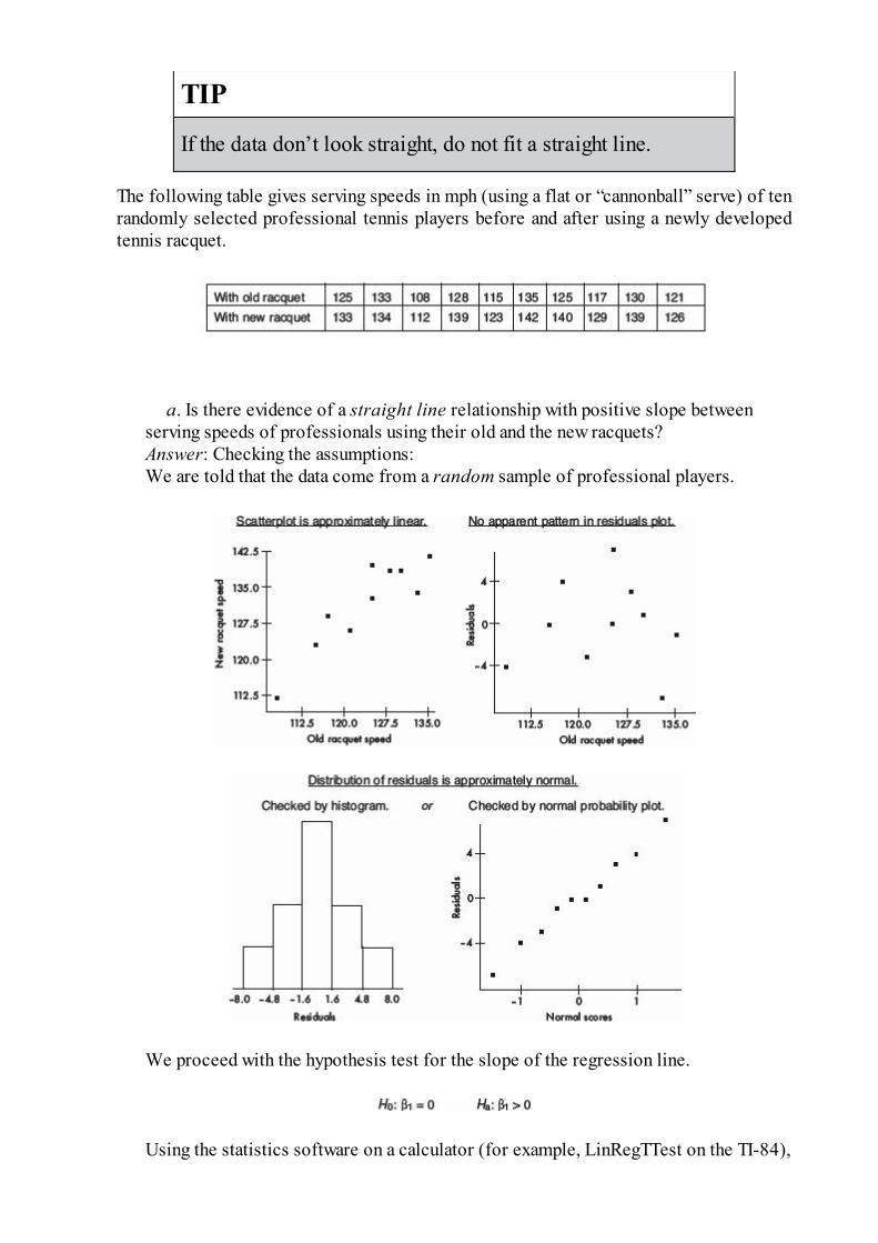
TIPIf the data don’t look straight, do not fit a straight line.
The following table gives serving speeds in mph (using a flat or “cannonball” serve) of tenrandomly selected professional tennis players before and after using a newly developedtennis racquet.
a. Is there evidence of a straight line relationship with positive slope between
serving speeds of professionals using their old and the new racquets?Answer: Checking the assumptions:We are told that the data come from a random sample of professional players.
We proceed with the hypothesis test for the slope of the regression line.
Using the statistics software on a calculator (for example, LinRegTTest on the TI-84),

gives:New speed = 8.76 + 0.99 (Old speed) with t = 5.853 and P = .00019
With such a small P value, there is very strong evidence of a straight line relationshipwith positive slope between serving speeds of professionals using their old and the newracquets.
b. Interpret in context the least squares line.
Answer: With a slope of approximately 1 and a y-intercept of 8.76, the regression lineindicates that use of the new racquet increases serving speed on the average by 8.76 mphregardless of the old racquet speed. That is, players with lower and higher old racquetspeeds experience on the average the same numerical (rather than percentage) increasewhen using the new racquet.On the TI-Nspire the result shows as:
It is important to be able to interpret computer output, and appropriate computeroutput is helpful in checking the assumptions for inference.
EXAMPLE 15.7A company offers a 10-lesson program of study to improve students’ SAT scores. Asurvey is made of a random sampling of 25 students. A scatterplot of improvement intotal (math + verbal) SAT score versus number of lessons taken is as follows:
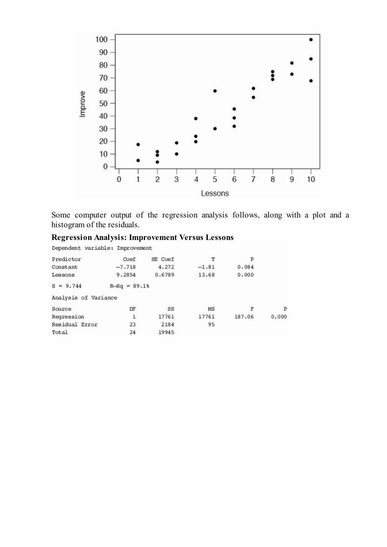
Some computer output of the regression analysis follows, along with a plot and ahistogram of the residuals.Regression Analysis: Improvement Versus Lessons

a. What is the equation of the regression line that predicts score improvement as afunction of number of lessons?
b. Interpret, in context, the slope of the regression line.c. What is the meaning of R–Sq in context of this study?d. Give the value of the correlation coefficient.e. Perform a test of significance for the slope of the regression line.
Answers:a. Improvement = –7.718 + 9.2854 (Lessons)b. The slope of the regression line is 9.2854, meaning that on the average, each
additional lesson is predicted to improve one’s total SAT score by 9.2854.c. R-Sq = 89.1% means that 89.1% of the variation in total SAT score improvement
can be explained by variation in the number of lessons taken.d. where the sign is positive because the slope is positive.e. A test of significance of the slope of the regression line with H0: β = 0, Ha: β ≠ 0
(test of significance of correlation) is as follows:Assumptions: We are told the data came from a random sample, the scatterplot appears tobe approximately linear, there is no apparent pattern in the residuals plot, and thehistogram of residuals appears to be approximately normal.
(Or t and P can simply be read off the computer output.)With this small a P-value, there is very strong evidence to reject H0 and conclude that therelationship between improvement in total SAT score and number of lessons taken issignificant.

INDEPENDENCEThroughout this review book the concept of independence has arisen manytimes, with different meanings in different contexts, and a quick review isworthwhile.
1. If the outcome of one event, E, doesn’t affect the outcome of anothere v e nt , F, we say the events are independent, and we have
2. When the distribution of one variable in a contingency table is the
same for all categories of another variable, we say the two variables areindependent.
3. When two random variables are independent, we can use the rule foradding variances with regard to the random variables X + Y and X – Y.
4. In a binomial distribution, the trials must be independent; that is, theprobability of success must be the same on every trial, irrespective of whathappened on a previous trial. However, when we pick a sample from apopulation, we do change the size and makeup of the remaining population.We typically allow this as long as the sample is not too large—the usualrule of thumb is that the sample size should be smaller than 10% of thepopulation.
5. In inference we wish to make conclusions about a populationparameter by analyzing a sample. A crucial assumption is always that thesampled values are independent of each other. This typically involveschecking if there was proper randomization in the gathering of data. Also, tominimize the effect on independence from samples being drawn withoutreplacement, we check that less than 10% of the population is sampled.
6. Furthermore, if inference involves the comparison of two groups, thetwo groups must be independent of each other.
7. With paired data, while the observations in each pair are notindependent, the differences must be independent of each other.
8. With regression, the errors in the regression model must beindependent, and one may check this by confirming there are no patterns inthe residual plot.

Summary• Chi-square analysis is an important tool for inference on distributions of
counts.• The chi-square statistic is found by summing the weighted squared differences
between observed and expected counts.• A chi-square goodness-of-fit test compares an observed distribution to some
expected distribution.• A chi-square test of independence tests for evidence of an association
between two categorical variables from a single sample.• A chi-square test of homogeneity compares samples from two or more
populations with regard to a single categorical variable.• The sampling distribution for the slope of a regression line can be modeled by
a t-distribution with df = n – 2.
Questions on Topic Fifteen: Tests ofSignificance—Chi-Square and Slope of Least
Squares Line
Multiple-Choice Questions
Directions: The questions or incomplete statements that follow are eachfollowed by five suggested answers or completions. Choose the responsethat best answers the question or completes the statement.
1. A random sample of mice is obtained, and each mouse is timed as itmoves through a maze to a reward treat at the end. After several days oftraining, each mouse is timed again. The data should be analyzed using
(A) a z-test of proportions.(B) a two-sample test of means.(C) a paired t-test.(D) a chi-square test.(E) a regression analysis.
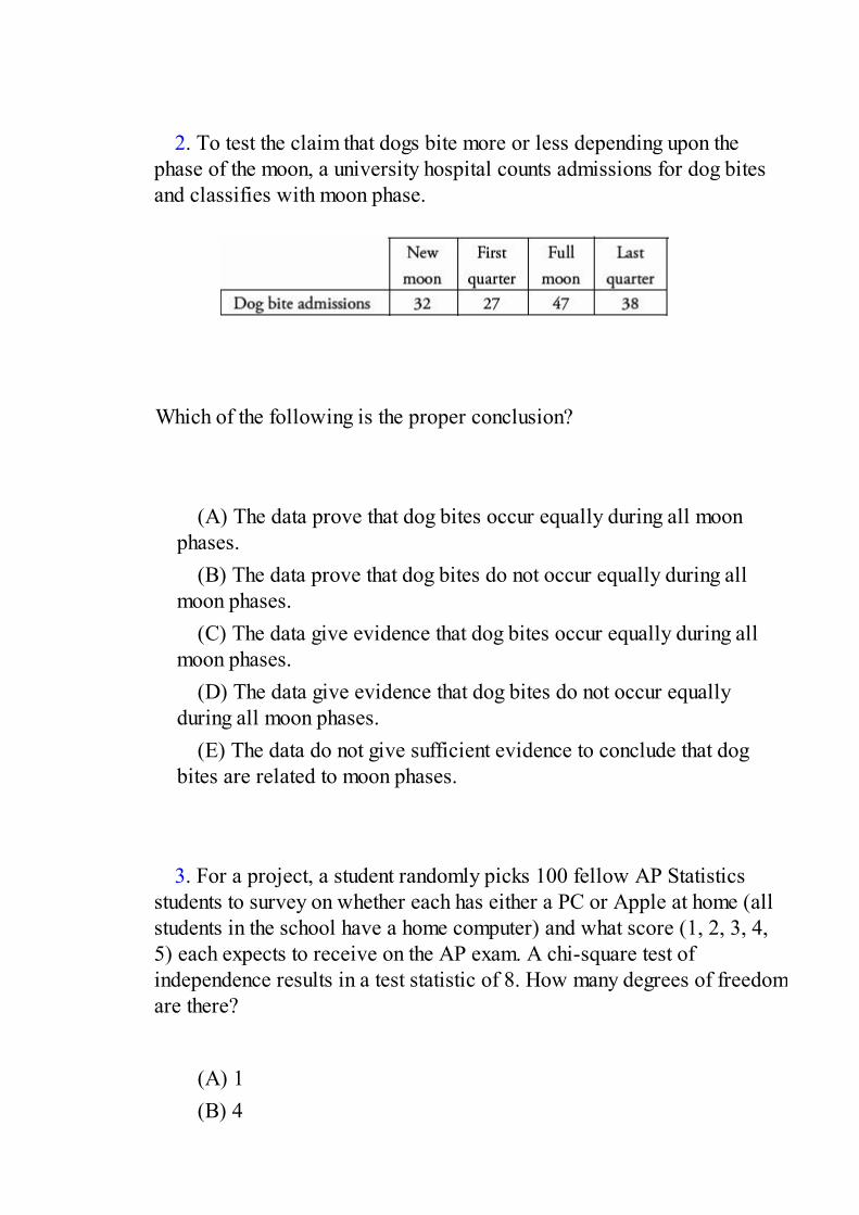
2. To test the claim that dogs bite more or less depending upon thephase of the moon, a university hospital counts admissions for dog bitesand classifies with moon phase.
Which of the following is the proper conclusion?
(A) The data prove that dog bites occur equally during all moonphases.
(B) The data prove that dog bites do not occur equally during allmoon phases.
(C) The data give evidence that dog bites occur equally during allmoon phases.
(D) The data give evidence that dog bites do not occur equallyduring all moon phases.
(E) The data do not give sufficient evidence to conclude that dogbites are related to moon phases.
3. For a project, a student randomly picks 100 fellow AP Statisticsstudents to survey on whether each has either a PC or Apple at home (allstudents in the school have a home computer) and what score (1, 2, 3, 4,5) each expects to receive on the AP exam. A chi-square test ofindependence results in a test statistic of 8. How many degrees of freedomare there?
(A) 1(B) 4
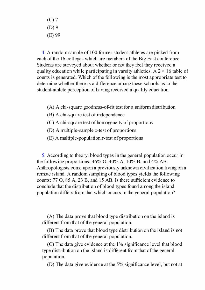
(C) 7(D) 9(E) 99
4. A random sample of 100 former student-athletes are picked from
each of the 16 colleges which are members of the Big East conference.Students are surveyed about whether or not they feel they received aquality education while participating in varsity athletics. A 2 × 16 table ofcounts is generated. Which of the following is the most appropriate test todetermine whether there is a difference among these schools as to thestudent-athlete perception of having received a quality education.
(A) A chi-square goodness-of-fit test for a uniform distribution(B) A chi-square test of independence(C) A chi-square test of homogeneity of proportions(D) A multiple-sample z-test of proportions(E) A multiple-population z-test of proportions
5. According to theory, blood types in the general population occur in
the following proportions: 46% O, 40% A, 10% B, and 4% AB.Anthropologists come upon a previously unknown civilization living on aremote island. A random sampling of blood types yields the followingcounts: 77 O, 85 A, 23 B, and 15 AB. Is there sufficient evidence toconclude that the distribution of blood types found among the islandpopulation differs from that which occurs in the general population?
(A) The data prove that blood type distribution on the island isdifferent from that of the general population.
(B) The data prove that blood type distribution on the island is notdifferent from that of the general population.
(C) The data give evidence at the 1% significance level that bloodtype distribution on the island is different from that of the generalpopulation.
(D) The data give evidence at the 5% significance level, but not at
the 1% significance level, that blood type distribution on the island isdifferent from that of the general population.
(E) The data do not give evidence at the 5% significance level thatblood type distribution on the island is different from that of the generalpopulation.
6. Is there a relationship between education level and sports interest? Astudy cross-classified 1500 randomly selected adults in three categoriesof education level (not a high school graduate, high school graduate, andcollege graduate) and five categories of major sports interest (baseball,basketball, football, hockey, and tennis). The χ2-value is 13.95. Is thereevidence of a relationship between education level and sports interest?
(A) The data prove there is a relationship between education leveland sports interest.
(B) The evidence points to a cause-and-effect relationship betweeneducation and sports interest.
(C) There is evidence at the 5% significance level of a relationshipbetween education level and sports interest.
(D) There is evidence at the 10% significance level, but not at the5% significance level, of a relationship between education level andsports interest.
(E) The P-value is greater than .10, so there is no evidence of arelationship between education level and sports interest.
7. A disc jockey wants to determine whether middle school studentsand high school students have similar music tastes. Independent randomsamples are taken from each group, and each person is asked whetherhe/she prefers hip-hop, pop, or alternative. A chi-square test ofhomogeneity of proportions is performed, and the resulting P-value isbelow .05. Which of the following is a proper conclusion?

(A) There is evidence that for all three music choices the proportionof middle school students who prefer each choice is equal to thecorresponding proportion of high school students.
(B) There is evidence that the proportion of middle school studentswho prefer hip-hop is different from the proportion of high schoolstudents who prefer hip-hop.
(C) There is evidence that for all three music choices the proportionof middle school students who prefer each choice is different from thecorresponding proportion of high school students.
(D) There is evidence that for at least one of the three music choicesthe proportion of middle school students who prefer that choice isequal to the corresponding proportion of high school students.
(E) There is evidence that for at least one of the three music choicesthe proportion of middle school students who prefer that choice isdifferent from the corresponding proportion of high school students.
8. A geneticist claims that four species of fruit flies should appear inthe ratio 1:3:3:9. Suppose that a sample of 2000 flies contained 110, 345,360, and 1185 flies of each species, respectively. Is there sufficientevidence to reject the geneticist’s claim?
(A) The data prove the geneticist’s claim.(B) The data prove the geneticist’s claim is false.(C) The data do not give sufficient evidence to reject the geneticist’s
claim.(D) The data give sufficient evidence to reject the geneticist’s claim.(E) The evidence from this data is inconclusive.
9. A food biologist surveys people at an ice cream parlor, noting theirtaste preferences and cross-classifying against the presence or absence ofa particular marker in a saliva swab test.

Is there evidence of a relationship between taste preference and themarker presence?
(A) At the 10% significance level, the data prove that there is arelationship between taste preference and the presence of the marker.
(B) At the 10% significance level, the data prove that there is norelationship between taste preference and the presence of the marker.
(C) There is evidence at the 5% significance level of a relationshipbetween taste preference and the presence of the marker.
(D) There is evidence at the 10% significance level, but not at the5% significance level, of a relationship between taste preference andthe presence of the marker.
(E) There is not evidence at the 10% significance level of arelationship between taste preference and the presence of the marker.
10. Random samples of 25 students are chosen from each high schoolclass level, students are asked whether or not they are satisfied with theschool cafeteria food, and the results are summarized in the followingtable:
Is there evidence of a difference in cafeteria food satisfaction among theclass levels?
(A) The data prove that there is a difference in cafeteria foodsatisfaction among the class levels.
(B) There is evidence of a linear relationship between foodsatisfaction and class level.
(C) There is evidence at the 1% significance level of a difference incafeteria food satisfaction among the class levels.
(D) There is evidence at the 5% significance level, but not at the 1%significance level, of a difference in cafeteria food satisfaction amongthe class levels.
(E) With P = .1117 there is not evidence of a difference in cafeteriafood satisfaction among the class levels.
11. Can dress size be predicted from a woman’s height? In a randomsample of 20 female high school students, dress size versus height (cm)gives the following regression results:
Is there statistical evidence of a linear relationship between dress sizeand height?
(A) No, because r2, the coefficient of determination, is too small.(B) No, because 0.128 is above any reasonable significance level.(C) Yes, because by any reasonable observation, taller women tend
to have larger dress sizes.(D) Yes, because the computer printout does give a regression
equation.

(E) There is evidence at the 10% significance level, but not at the5% level.
12. To study the relationship between calories (kcal) and fat (g) inpizza, slices of 14 randomly selected major brand pizzas are chemicallyanalyzed. Computer printout for regression:
What is measured by S = 1.27515?
(A) Variability in calories among slices(B) Variability in fat among slices(C) Variability in the slope (g/kcal) of the regression line(D) Variability in the y-intercept of the regression line(E) Variability in the residuals
Free-Response Questions
Directions: You must show all work and indicate the methods you use. Youwill be graded on the correctness of your methods and on the accuracy ofyour final answers.
Seven Open-Ended Questions1. A candy manufacturer advertises that their fruit-flavored sweets have
hard sugar shells in five colors with the following distribution: 35%cherry red, 10% vibrant orange, 10% daffodil yellow, 25% emeraldgreen, and 20% royal purple. A random sample of 300 sweets yielded thecounts in the following table:

Is there evidence that the distribution is different from what is claimed bythe manufacturer?
2. You want to study whether smokers and nonsmokers have equalfitness levels (low, medium, high) and are considering two surveydesigns:
I. Take a random sample of 200 people, asking each whether or notthey smoke, and measuring the fitness level of each.
II. Take a random sample of 100 smokers and measure the fitnesslevel of each, and take a random sample of 100 nonsmokers andmeasure the fitness level of each.
(a) Which of the designs results in a test of independence and whichresults in a test of homogeneity? Explain.
(b) If we are interested in whether the proportion of people whohave various fitness levels differs among smokers and nonsmokers,which design should be used? Explain.
(c) If we are interested in the conditional distribution of people withgiven fitness levels who are smokers or are not smokers, which designshould be used? Explain.3. Is there a difference in happiness levels between busy and idle
people? In one study, after filling out a survey, 175 randomly chosen highschool students were told they could either sit 15 minutes while thesurvey was being tabulated, or they could walk 15 minutes to anotherbuilding where the survey was being tabulated. Then they were given aquestionnaire asking how good they felt during the past 15 minutes (on ascale of 1, “not good,” to 5, “very good”). The results of the questionnairewere as follows:
(a) Does the above data give statistical evidence of a relationship

between happiness level and busy/idle choice of the students?(b) If the answer above is positive for a relationship, is it reasonable
to conclude that encouraging high school students to keep more busywill lead to higher happiness levels?4. A poll, asking a random sample of adults whether or not they eat
breakfast and to rate their morning energy level, results in the table:
(a) If the sample size was n = 500, is there evidence of arelationship between eating breakfast and morning energy level?
(b) Does the answer to part (a) change if n = 1000 instead? Explain.5. A survey on acne treatments randomly selected 100 teenagers using
topical treatments, 100 using oral medications, and 50 using laser therapy,and asked each subject about satisfaction level. The resulting countswere:
(a) Do the different treatments lead to different satisfaction levels?Perform an appropriate hypothesis test.
(b) What is a possible confounding variable which could lead you tojump to a misleading conclusion? Explain.6. A study of 100 randomly selected teenagers, ages 13–17, looked at
number of texts per waking hour versus age, yielding the computerregression output below:
(a) Interpret the slope in context.(b) What three graphs should be checked with regard to conditions
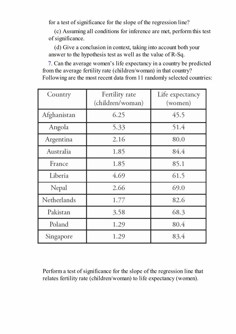
for a test of significance for the slope of the regression line?(c) Assuming all conditions for inference are met, perform this test
of significance.(d) Give a conclusion in context, taking into account both your
answer to the hypothesis test as well as the value of R-Sq.7. Can the average women’s life expectancy in a country be predicted
from the average fertility rate (children/woman) in that country?Following are the most recent data from 11 randomly selected countries:
Perform a test of significance for the slope of the regression line thatrelates fertility rate (children/woman) to life expectancy (women).

Three Investigative Tasks1. Use of placebos are now the norm for medical studies, but disclosing
the compositions of these placebos is unexplicitly not all that common,even though these placebos could have effects. For example, olive oil hasbeen used as a placebo in cholesterol drug tests, and there is someevidence that olive oil can affect cholesterol level. Composition of aplacebo injection is disclosed more often than that of a placebo pill, butstill it can be difficult to make this finding. In a survey of 800 studiesusing placebo injections, three researchers independently try to determinethe compositions of the placebos, and the counts of successes are asfollows:
(a) Find the complete binomial distribution (probabilities of 0through 3 successes) for n = 3 and p = 0.2.
(b) Given 800 studies, if the number of researchers who determinecomposition of a placebo follows a binomial with probability ofsuccess p = 0.2, what are the expected values for the numbers (0through 3) of researchers able to determine composition of a placebo?
(c) Test the null hypothesis that the number of researchers whodetermine composition of a placebo follows a binomial withprobability of success p = 0.2.2. Twelve high schools are randomly selected, and in each, the math
teachers, the English teachers, and the students on the honor roll all take alogic puzzle test, and average scores for each group are noted in thefollowing table:

The regression analysis of the data follows.Regression Analysis: Student versus EnglishDependent variable: Student
Regression Analysis: Student versus MathDependent variable: Student
(a) Is there evidence that the average student score is greater thanthat of the English teachers?
(b) Is there evidence that the average student score is greater thanthat of the math teachers?
(c) Is the score of the English or math teachers a better predictor ofthe student score? Explain.
(d) Given the analysis in part (c), predict the average student scorein a school where the average English teachers’ score is 11.0 and theaverage math teachers’ score is 10.0.
(e) Given the analysis in parts (c) and (d), what is the approximate

range of average student scores at schools where the average Englishteachers’ score is 11.0 and the average math teachers’ score is 10.0.3. A heavy backpack can cause chronic shoulder, neck, and back pain.
Wide, padded shoulder straps, a waist belt, and avoidance of single-strapbags all help, but weight is the main problem. The recommendation for asafe weight for school backpacks is no more than 10% of body weight. Ina study of 500 randomly selected high school students, the weights of theirbackpacks give rise to the following:
(a) In a normal distribution with = 20 and σ = 5, what are theprobabilities of z < 12.5, 12.5 < z < 17.5, 17.5 < z < 22.5, 22.5 < z <27.5, and z > 27.5?
(b) Given 500 students, if the data follow a normal distribution with = 20 and σ = 5, what are the expected values for the numbers of
backpacks in each of the indicated weight ranges?(c) Test the null hypothesis that the data follow a normal distribution
with = 20 and σ = 5.

All answer sheets are for reference only.
Practice Examination 1
SECTION IQuestions 1–40Spend 90 minutes on this part of the exam.
Directions: The questions or incomplete statements that follow are eachfollowed by five suggested answers or completions. Choose the responsethat best answers the question or completes the statement.
1. Following is a histogram of home sale prices (in thousands ofdollars) in one community:
Which of the following conclusions is most correct?
(A) The median price was $125,000.(B) The mean price was $125,000.(C) More homes sold for between $100,000 and $125,000 than for
over $125,000.(D) $10,000 is a reasonable estimate of the standard deviation in
selling prices.(E) 1.5 × 10⁹ ($2) is a reasonable estimate of the variance in selling
prices.
2. Which of the following is most useful in establishing cause-and-
effect relationships?
(A) A complete census(B) A least squares regression line showing high correlation(C) A simple random sample (SRS)(D) A well-designed, well-conducted survey incorporating chance
to ensure a representative sample(E) An experiment
3. The average yearly snowfall in a city is 55 inches. What is the
standard deviation if 15% of the years have snowfalls above 60 inches?Assume yearly snowfalls are normally distributed.
(A) 4.83(B) 5.18(C) 6.04(D) 8.93(E) The standard deviation cannot be computed from the information
given.
4. To determine the average cost of running for a congressional seat, a
simple random sample of 50 politicians is chosen and the politicians’records examined. The cost figures show a mean of $125,000 with astandard deviation of $32,000. Which of the following is the bestinterpretation of a 90% confidence interval estimate for the average costof running for office?
(A) 90% of politicians running for a congressional seat spend
between $117,500 and $132,500.(B) 90% of politicians running for a congressional seat spend a
mean dollar amount that is between $117,500 and $132,500.(C) We are 90% confident that politicians running for a
congressional seat spend between $117,500 and $132,500.(D) We are 90% confident that politicians running for a
congressional seat spend a mean dollar amount between $117,500 and
$132,500.(E) We are 90% confident that in the chosen sample, the mean
dollar amount spent running for a congressional seat is between$117,500 and $132,500.
5. In one study on the effect that eating meat products has on weight
level, an SRS of 500 subjects who admitted to eating meat at least once aday had their weights compared with those of an independent SRS of 500people who claimed to be vegetarians. In a second study, an SRS of 500subjects were served at least one meat meal per day for 6 months, whilean independent SRS of 500 others were chosen to receive a strictlyvegetarian diet for 6 months, with weights compared after 6 months.
(A) The first study is a controlled experiment, while the second is
an observational study.(B) The first study is an observational study, while the second is a
controlled experiment.(C) Both studies are controlled experiments.(D) Both studies are observational studies.(E) Each study is part controlled experiment and part observational
study.
6. A plumbing contractor obtains 60% of her boiler circulators from a
company whose defect rate is 0.005, and the rest from a company whosedefect rate is 0.010. If a circulator is defective, what is the probabilitythat it came from the first company?
(A) .429(B) .500(C) .571(D) .600(E) .750
7. A kidney dialysis center periodically checks a sample of its
equipment and performs a major recalibration if readings are sufficiently
off target. Similarly, a fabric factory periodically checks the sizes oftowels coming off an assembly line and halts production if measurementsare sufficiently off target. In both situations, we have the null hypothesisthat the equipment is performing satisfactorily. For each situation, whichis the more serious concern, a Type I or Type II error?
(A) Dialysis center: Type I error, towel manufacturer: Type I error(B) Dialysis center: Type I error, towel manufacturer: Type II error(C) Dialysis center: Type II error, towel manufacturer: Type I error(D) Dialysis center: Type II error, towel manufacturer: Type II error(E) This is impossible to answer without making an expected value
judgment between human life and accurate towel sizes.
8. A coin is weighted so that the probability of heads is .75. The coin is
tossed 10 times and the number of heads is noted. This procedure isrepeated a total of 50 times, and the number of heads is recorded eachtime. What kind of distribution has been simulated?
(A) The sampling distribution of the sample proportion with n = 10
and p = .75(B) The sampling distribution of the sample proportion with n = 50
and p = .75(C) The sampling distribution of the sample mean with = 10(.75)
and (D) The binomial distribution with n = 10 and p = .75(E) The binomial distribution with n = 50 and p = .75
9. During the years 1886 through 2000 there were an average of 8.7
tropical cyclones per year, of which an average of 5.1 became hurricanes.Assuming that the probability of any cyclone becoming a hurricane isindependent of what happens to any other cyclone, if there are fivecyclones in one year, what is the probability that at least three becomehurricanes?
(A) .313

(B) .345(C) .586(D) .658(E) .686
10. Given the probabilities P(A) = .3 and P(B) = .2, what is the
probability of the union P(A ∪ B) if A and B are mutually exclusive? If Aand B are independent? If B is a subset of A?
(A) .44, .5, .2(B) .44, .5, .3(C) .5, .44, .2(D) .5, .44, .3(E) 0, .5, .3
11. A nursery owner claims that a recent drought stunted the growth of
22% of all her evergreens. A botanist tests this claim by examining anSRS of 1100 evergreens and finds that 268 trees in the sample show signsof stunted growth. With H0: p = .22 and Ha: p ≠ .22, what is the value ofthe test statistic?
(A)
(B)
(C)
(D)
(E)
12. A medical research team tests for tumor reduction in a sample ofpatients using three different dosages of an experimental cancer drug.
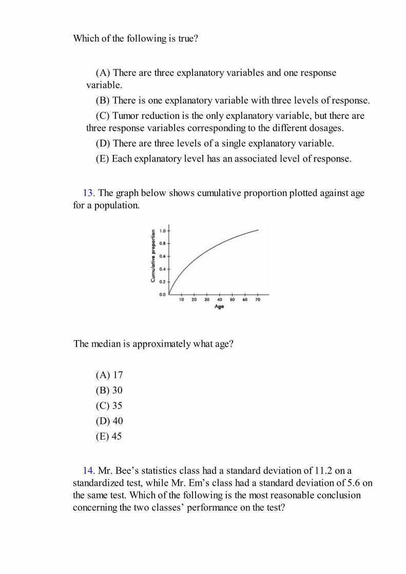
Which of the following is true?
(A) There are three explanatory variables and one response
variable.(B) There is one explanatory variable with three levels of response.(C) Tumor reduction is the only explanatory variable, but there are
three response variables corresponding to the different dosages.(D) There are three levels of a single explanatory variable.(E) Each explanatory level has an associated level of response.
13. The graph below shows cumulative proportion plotted against age
for a population.
The median is approximately what age?
(A) 17(B) 30(C) 35(D) 40(E) 45
14. Mr. Bee’s statistics class had a standard deviation of 11.2 on a
standardized test, while Mr. Em’s class had a standard deviation of 5.6 onthe same test. Which of the following is the most reasonable conclusionconcerning the two classes’ performance on the test?

(A) Mr. Bee’s class is less heterogeneous than Mr. Em’s.(B) Mr. Em’s class is more homogeneous than Mr. Bee’s.(C) Mr. Bee’s class performed twice as well as Mr. Em’s.(D) Mr. Em’s class did not do as well as Mr. Bee’s.(E) Mr. Bee’s class had the higher mean, but this may not be
statistically significant.
15. A college admissions officer is interested in comparing the SAT
math scores of high school applicants who have and have not taken APStatistics. She randomly pulls the files of five applicants who took APStatistics and five applicants who did not, and proceeds to run a t-test tocompare the mean SAT math scores of the two groups. Which of thefollowing is a necessary assumption?
(A) The population variances from each group are known.(B) The population variances from each group are unknown.(C) The population variances from the two groups are equal.(D) The population of SAT scores from each group is normally
distributed.(E) The samples must be independent simple random samples, and
for each sample np and n(1 – p) must both be at least 10.
16. The appraised values of houses in a city have a mean of $125,000
with a standard deviation of $23,000. Because of a new teachers’contract, the school district needs an extra 10% in funds compared to theprevious year. To raise this additional money, the city instructs theassessment office to raise all appraised house values by $5,000. Whatwill be the new standard deviation of the appraised values of houses inthe city?
(A) $23,000(B) $25,300(C) $28,000(D) $30,300(E) $30,800
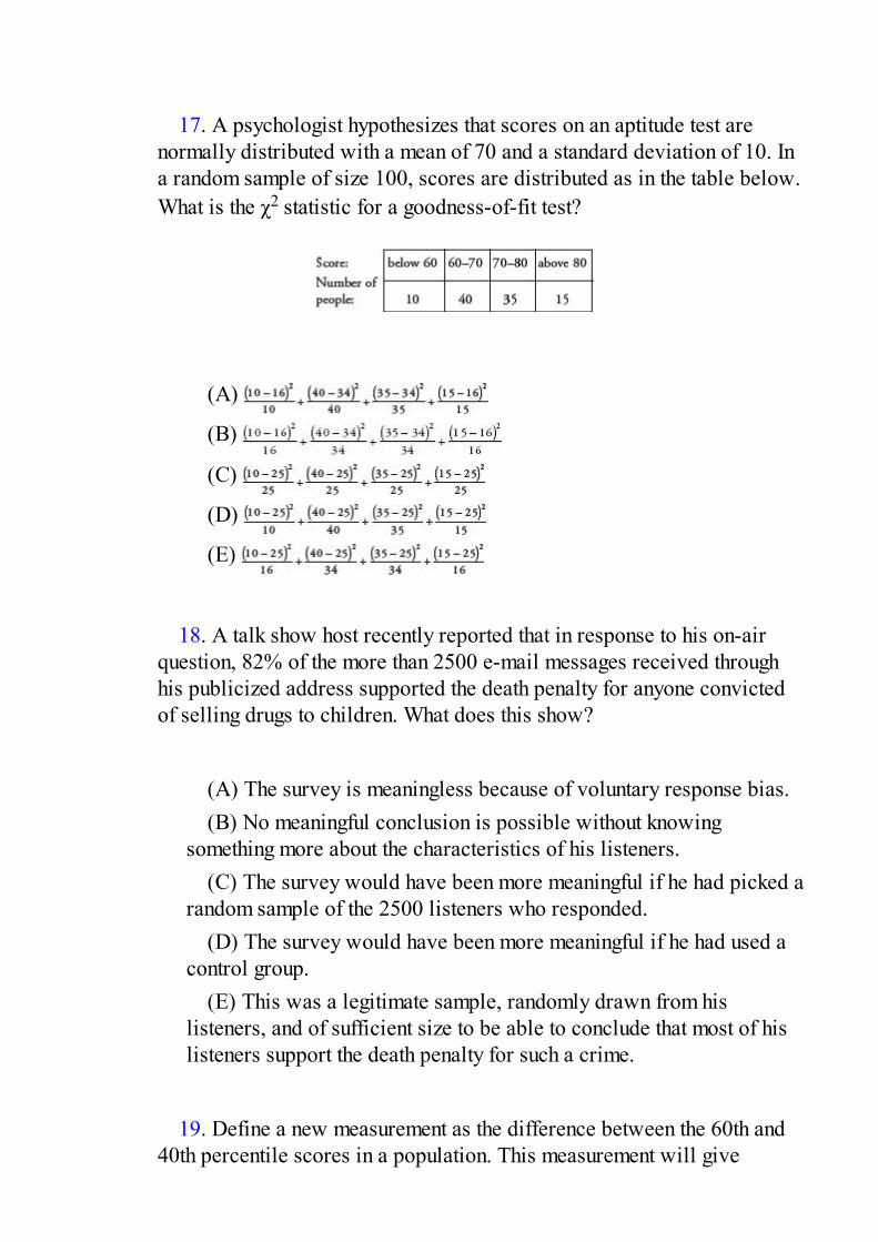
17. A psychologist hypothesizes that scores on an aptitude test are
normally distributed with a mean of 70 and a standard deviation of 10. Ina random sample of size 100, scores are distributed as in the table below.What is the χ2 statistic for a goodness-of-fit test?
(A)
(B)
(C)
(D)
(E)
18. A talk show host recently reported that in response to his on-air
question, 82% of the more than 2500 e-mail messages received throughhis publicized address supported the death penalty for anyone convictedof selling drugs to children. What does this show?
(A) The survey is meaningless because of voluntary response bias.(B) No meaningful conclusion is possible without knowing
something more about the characteristics of his listeners.(C) The survey would have been more meaningful if he had picked a
random sample of the 2500 listeners who responded.(D) The survey would have been more meaningful if he had used a
control group.(E) This was a legitimate sample, randomly drawn from his
listeners, and of sufficient size to be able to conclude that most of hislisteners support the death penalty for such a crime.
19. Define a new measurement as the difference between the 60th and
40th percentile scores in a population. This measurement will give

information concerning
(A) central tendency.(B) variability.(C) symmetry.(D) skewness.(E) clustering.
20. Suppose X and Y are random variables with E(X ) = 37, var(X ) =
5, E(Y ) = 62, and var(Y ) = 12. What are the expected value and varianceof the random variable X + Y?
(A) E(X + Y ) = 99, var(X + Y ) = 8.5(B) E(X + Y ) = 99, var(X + Y ) = 13(C) E(X + Y ) = 99, var(X + Y ) = 17(D) E(X + Y ) = 49.5, var(X + Y ) = 17(E) There is insufficient information to answer this question.
21. Which of the following can affect the value of the correlation r?
(A) A change in measurement units(B) A change in which variable is called x and which is called y(C) Adding the same constant to all values of the x-variable(D) All of the above can affect the r value.(E) None of the above can affect the r value.
22. The American Medical Association (AMA) wishes to determine
the percentage of obstetricians who are considering leaving the professionbecause of the rapidly increasing number of lawsuits againstobstetricians. How large a sample should be taken to find the answer towithin ±3% at the 95% confidence level?

(A) 6(B) 33(C) 534(D) 752(E) 1068
23. Suppose you did 10 independent tests of the form H0: = 25 versus
Ha: < 25, each at the α = .05 significance level. What is the probabilityof committing a Type I error and incorrectly rejecting a true H0 with atleast one of the 10 tests?
(A) .05(B) .40(C) .50(D) .60(E) .95
24. Which of the following sets has the smallest standard deviation?
Which has the largest?
I. 1, 2, 3, 4, 5, 6, 7II. 1, 1, 1, 4, 7, 7, 7III. 1, 4, 4, 4, 4, 4, 7
(A) I, II(B) II, III(C) III, I(D) II, I(E) III, II
25. A researcher plans a study to examine long-term confidence in the
U.S. economy among the adult population. She obtains a simple random

sample of 30 adults as they leave a Wall Street office building oneweekday afternoon. All but two of the adults agree to participate in thesurvey. Which of the following conclusions is correct?
(A) Proper use of chance as evidenced by the simple random
sample makes this a well-designed survey.(B) The high response rate makes this a well-designed survey.(C) Selection bias makes this a poorly designed survey.(D) A voluntary response study like this gives too much emphasis to
persons with strong opinions.(E) Lack of anonymity makes this a poorly designed survey.
26. Which among the following would result in the narrowest
confidence interval?
(A) Small sample size and 95% confidence(B) Small sample size and 99% confidence(C) Large sample size and 95% confidence(D) Large sample size and 99% confidence(E) This cannot be answered without knowing an appropriate
standard deviation.
27. Consider the following three scatterplots:
What is the relationship among r1, r2, and r3, the correlations associatedwith the first, second, and third scatterplots, respectively?
(A) r1 < r2 < r3
(B) r1 < r3 < r2

(C) r2 < r3 < r1
(D) r3 < r1 < r2
(E) r3 < r2 < r1
28. There are two games involving flipping a coin. In the first game you
win a prize if you can throw between 45% and 55% heads. In the secondgame you win if you can throw more than 80% heads. For each gamewould you rather flip the coin 30 times or 300 times?
(A) 30 times for each game(B) 300 times for each game(C) 30 times for the first game and 300 times for the second(D) 300 times for the first game and 30 times for the second(E) The outcomes of the games do not depend on the number of
flips.
29. City planners are trying to decide among various parking plan
options ranging from more on-street spaces to multilevel facilities tospread-out small lots. Before making a decision, they wish to test thedowntown merchants’ claim that shoppers park for an average of only 47minutes in the downtown area. The planners have decided to tabulateparking durations for 225 shoppers and to reject the merchants’ claim ifthe sample mean exceeds 50 minutes. If the merchants’ claim is wrong andthe true mean is 51 minutes, what is the probability that the randomsample will lead to a mistaken failure to reject the merchants’ claim?Assume that the standard deviation in parking durations is 27 minutes.
(A)
(B)
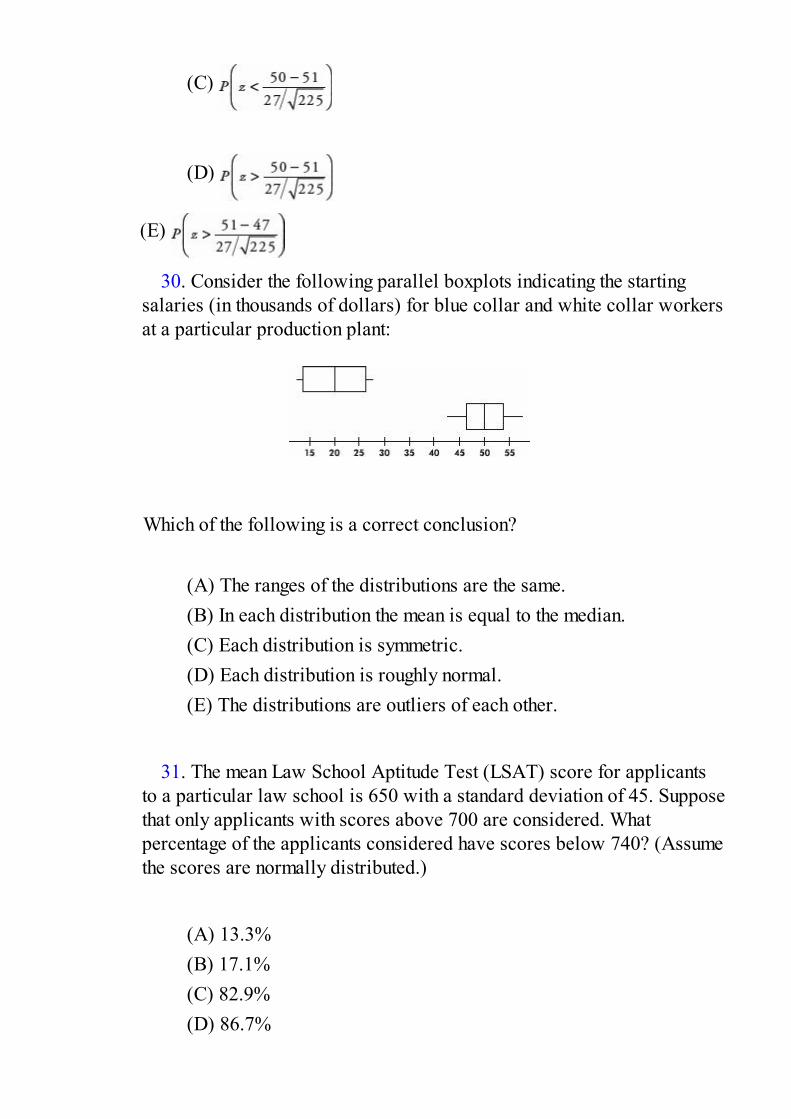
(C)
(D)
(E)
30. Consider the following parallel boxplots indicating the startingsalaries (in thousands of dollars) for blue collar and white collar workersat a particular production plant:
Which of the following is a correct conclusion?
(A) The ranges of the distributions are the same.(B) In each distribution the mean is equal to the median.(C) Each distribution is symmetric.(D) Each distribution is roughly normal.(E) The distributions are outliers of each other.
31. The mean Law School Aptitude Test (LSAT) score for applicants
to a particular law school is 650 with a standard deviation of 45. Supposethat only applicants with scores above 700 are considered. Whatpercentage of the applicants considered have scores below 740? (Assumethe scores are normally distributed.)
(A) 13.3%(B) 17.1%(C) 82.9%(D) 86.7%
(E) 97.7%
32. If all the other variables remain constant, which of the following
will increase the power of a hypothesis test?
I. Increasing the sample size.II. Increasing the significance level.III. Increasing the probability of a Type II error.
(A) I only(B) II only(C) III only(D) I and II(E) All are true.
33. A researcher planning a survey of school principals in a particular
state has lists of the school principals employed in each of the 125 schooldistricts. The procedure is to obtain a random sample of principals fromeach of the districts rather than grouping all the lists together andobtaining a sample from the entire group. Which of the following is acorrect conclusion?
(A) This is a simple random sample obtained in an easier and less
costly manner than procedures involving sampling from the entirepopulation of principals.
(B) This is a cluster sample in which the population was dividedinto heterogeneous groups called clusters.
(C) This is an example of systematic sampling, which gives areasonable sample as long as the original order of the list is notrelated to the variables under consideration.
(D) This is an example of proportional sampling based on sizes ofthe school districts.
(E) This is a stratified sample, which may give comparativeinformation that a simple random sample wouldn’t give.

34. A simple random sample is defined by
(A) the method of selection.(B) examination of the outcome.(C) both of the above.(D) how representative the sample is of the population.(E) the size of the sample versus the size of the population.
35. Changing from a 90% confidence interval estimate for a population
proportion to a 99% confidence interval estimate, with all other thingsbeing equal,
(A) increases the interval size by 9%.(B) decreases the interval size by 9%.(C) increases the interval size by 57%.(D) decreases the interval size by 57%.(E) This question cannot be answered without knowing the sample
size.
36. Which of the following is a true statement about hypothesis testing?
(A) If there is sufficient evidence to reject a null hypothesis at the
10% level, then there is sufficient evidence to reject it at the 5% level.(B) Whether to use a one-or a two-sided test is typically decided
after the data are gathered.(C) If a hypothesis test is conducted at the 1% level, there is a 1%
chance of rejecting the null hypothesis.(D) The probability of a Type I error plus the probability of a Type
II error always equal 1.(E) The power of a test concerns its ability to detect an alternative
hypothesis.

37. A population is normally distributed with mean 25. Consider allsamples of size 10. The variable
(A) has a normal distribution.(B) has a t-distribution with df = 10.(C) has a t-distribution with df = 9.(D) has neither a normal distribution or a t-distribution.(E) has either a normal or a t-distribution depending on the
characteristics of the population standard deviation.
38. A correlation of .6 indicates that the percentage of variation in y
that is explained by the variation in x is how many times the percentageindicated by a correlation of .3?
(A) 2(B) 3(C) 4(D) 6(E) There is insufficient information to answer this question.
39. As reported on CNN, in a May 1999 national poll 43% of high
school students expressed fear about going to school. Which of thefollowing best describes what is meant by the poll having a margin oferror of 5%?
(A) It is likely that the true proportion of high school students afraid
to go to school is between 38% and 48%.(B) Five percent of the students refused to participate in the poll.(C) Between 38% and 48% of those surveyed expressed fear about
going to school.(D) There is a .05 probability that the 43% result is in error.(E) If similar size polls were repeatedly taken, they would be wrong
about 5% of the time.

40. In a high school of 1650 students, 132 have personal investments in
the stock market. To estimate the total stock investment by students in thisschool, two plans are proposed. Plan I would sample 30 students atrandom, find a confidence interval estimate of their average investment,and then multiply both ends of this interval by 1650 to get an intervalestimate of the total investment. Plan II would sample 30 students atrandom from among the 132 who have investments in the market, find aconfidence interval estimate of their average investment, and then multiplyboth ends of this interval by 132 to get an interval estimate of the totalinvestment. Which is the better plan for estimating the total stock marketinvestment by students in this school?
(A) Plan I(B) Plan II(C) Both plans use random samples and so will produce equivalent
results.(D) Neither plan will give an accurate estimate.(E) The resulting data must be seen to evaluate which is the better
plan.
If there is still time remaining, you may review your answers.
SECTION II
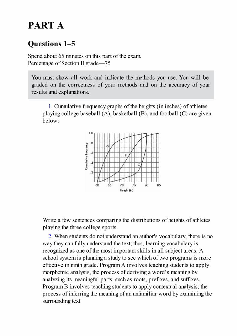
PART A
Questions 1–5Spend about 65 minutes on this part of the exam.Percentage of Section II grade—75
You must show all work and indicate the methods you use. You will begraded on the correctness of your methods and on the accuracy of yourresults and explanations.
1. Cumulative frequency graphs of the heights (in inches) of athletesplaying college baseball (A), basketball (B), and football (C) are givenbelow:
Write a few sentences comparing the distributions of heights of athletesplaying the three college sports.
2. When students do not understand an author's vocabulary, there is noway they can fully understand the text; thus, learning vocabulary isrecognized as one of the most important skills in all subject areas. Aschool system is planning a study to see which of two programs is moreeffective in ninth grade. Program A involves teaching students to applymorphemic analysis, the process of deriving a word’s meaning byanalyzing its meaningful parts, such as roots, prefixes, and suffixes.Program B involves teaching students to apply contextual analysis, theprocess of inferring the meaning of an unfamiliar word by examining thesurrounding text.
(a) Explain the purpose of incorporating a control group in thisexperiment.
(b) To comply with informed consent laws, parents will be askedtheir consent for their children to be randomly assigned to be taught inone of the new programs or by the local standard method. Students ofparents who do not return the consent forms will continue to be taughtby the local standard method. Explain why these students should not beconsidered part of the control group.
(c) Given 90 students randomly selected from ninth grade studentswith parental consent, explain how to assign them to the three groups,Program A, Program B, and Control, for a completely randomizeddesign.
3. An experiment is designed to test a home insulation product. Twoside-by-side identical houses are chosen, and in one the insulationproduct is installed (blown into the attic). Both homes use natural gas forheating, and the thermostat in each house is fixed at 68 degreesFahrenheit. On 30 randomly chosen winter days, the quantity of gas (inhundreds of cubic feet) used to heat each house is measured. The tablebelow summarizes the data.
(a) Is there evidence that the insulation product does result in alower mean quantity of gas being used?
Two least square regression calculations are performed with thefollowing computer output, where Temp is the average outside

temperature, and WithOut and With are the quantities of gas (in hundredsof cubic feet) used to heat the two homes on a day with that outsidetemperature:
(b) Compare the slopes of the regression lines in context of thisproblem.
(c) Compare the y-intercepts of the regression lines in context of thisproblem.
4. A new anti-spam software program is field tested on 1000 e-mailsand the results are summarized in the following table (positive test =program labels e-mail as spam):
Using the above empirical results, determine the followingprobabilities.
(a) (i) What is the predictive value of the test? That is, what is theprobability that an e-mail is spam and the test is positive?
(ii) What is the false-positive rate? That is, what is the probabilityof testing positive given that the e-mail is legitimate?
(b) (i) What is the sensitivity of the test? That is, what is theprobability of testing positive given that the e-mail is spam?
(ii) What is the specificity of the test? That is, what is theprobability of testing negative given that the e-mail is legitimate?
(c) (i) Given a random sample of five legitimate e-mails, what is theprobability that the program labels at least one as spam?
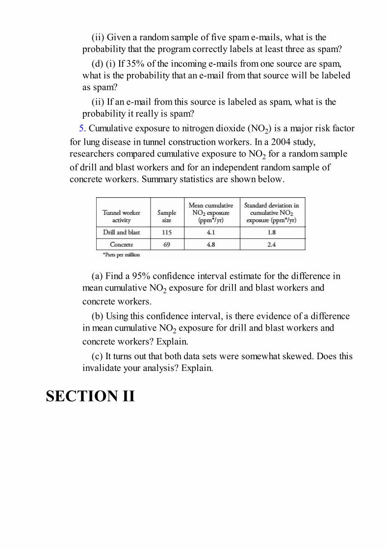
(ii) Given a random sample of five spam e-mails, what is theprobability that the program correctly labels at least three as spam?
(d) (i) If 35% of the incoming e-mails from one source are spam,what is the probability that an e-mail from that source will be labeledas spam?
(ii) If an e-mail from this source is labeled as spam, what is theprobability it really is spam?
5. Cumulative exposure to nitrogen dioxide (NO2) is a major risk factorfor lung disease in tunnel construction workers. In a 2004 study,researchers compared cumulative exposure to NO2 for a random sampleof drill and blast workers and for an independent random sample ofconcrete workers. Summary statistics are shown below.
(a) Find a 95% confidence interval estimate for the difference inmean cumulative NO2 exposure for drill and blast workers andconcrete workers.
(b) Using this confidence interval, is there evidence of a differencein mean cumulative NO2 exposure for drill and blast workers andconcrete workers? Explain.
(c) It turns out that both data sets were somewhat skewed. Does thisinvalidate your analysis? Explain.
SECTION II

PART B
Question 6
Spend about 25 minutes on this part of the exam.Percentage of Section II grade—25
6. Do strong magnetic fields have an effect on the early development ofmice? A study is performed on 120 one-month-old mice. Each issubjected to a strong magnetic field for one week and no magnetic fieldfor one week, the order being decided randomly for each mouse. Theweight gain in grams during each week for each mouse is recorded. Theweight gains with no magnetic field are approximately normallydistributed with a mean of 25.1 grams and a standard deviation of 3.1grams, while the weight gains in the magnetic field are approximatelynormally distributed with a mean of 17.3 grams and a standard deviationof 5.7 grams. Of the 120 mice, 101 gained more weight with no magneticfield.
(a) Calculate and interpret a 95% confidence interval for theproportion of mice that gain more weight with no magnetic field.
(b) Suppose two of these mice were chosen at random. What is theprobability that the first mouse gained more weight with no magneticfield than the second mouse gained in the magnetic field?
(c) Based on your answers to (a) and (b), is there evidence that formice, weight gain with no magnetic field and in a magnetic field areindependent?
(d) In a test for variances on whether or not the variances of the twosets of weight gains are significantly different, , ,with α = .05, for samples of this size, the critical cut-off scores for
are 0.698 (left tail of .025) and 1.43 (right tail of .025). What is theresulting conclusion about variances?
If there is still time remaining, you may review your answers.
All answer sheets are for reference only.

Practice Examination 2
SECTION IQuestions 1–40Spend 90 minutes on this part of the exam.
Directions: The questions or incomplete statements that follow are eachfollowed by five suggested answers or completions. Choose theresponse that best answers the question or completes the statement.
1. Suppose that the regression line for a set of data, y = mx + 3, passesthrough the point (2, 7). If and are the sample means of the x- and y-values, respectively, then =
(A) .(B) – 2.(C) + 3.(D) 2 + 3.(E) 3.5 + 3.
2. A study is made to determine whether more hours of academic
studying leads to higher point scoring by basketball players. In surveying50 basketball players, it is noted that the 25 who claim to study the mosthours have a higher point average than the 25 who study less. Based onthis study, the coach begins requiring the players to spend more timestudying. Which of the following is a correct statement?
(A) While this study may have its faults, it still does prove
causation.(B) There could well be a confounding variable responsible for the
seeming relationship.

(C) While this is a controlled experiment, the conclusion of thecoach is not justified.
(D) To get the athletes to study more, it would be more meaningfulto have them put in more practice time on the court to boost their pointaverages, as higher point averages seem to be associated with morestudy time.
(E) No proper conclusion is possible without somehow introducingblinding.
3. The longevity of people living in a certain locality has a standard
deviation of 14 years. What is the mean longevity if 30% of the peoplelive longer than 75 years? Assume a normal distribution for life spans.
(A) 61.00(B) 67.65(C) 74.48(D) 82.35(E) The mean cannot be computed from the information given.
4. Which of the following is a correct statement about correlation?
(A) If the slope of the regression line is exactly 1, then the
correlation is exactly 1.(B) If the correlation is 0, then the slope of the regression line is
undefined.(C) Switching which variable is called x and which is called y
changes the sign of the correlation.(D) The correlation r is equal to the slope of the regression line
when z-scores for the y-variable are plotted against z-scores for the x-variable.
(E) Changes in the measurement units of the variables may changethe correlation.
5. Which of the following are affected by outliers?

I. MeanII. MedianIII. Standard deviationIV. RangeV. Interquartile range(A) I, III, and V(B) II and IV(C) I and V(D) III and IV(E) I, III, and IV
6. An engineer wishes to determine the quantity of heat being generated
by a particular electronic component. If she knows that the standarddeviation is 2.4, how many of these components should she consider to be99% sure of knowing the mean quantity to within ±0.6?
(A) 27(B) 87(C) 107(D) 212(E) 425
7. A company that produces facial tissues continually monitors tissue
strength. If the mean strength from sample data drops below a specifiedlevel, the production process is halted and the machinery inspected.Which of the following would result from a Type I error?
(A) Halting the production process when sufficient customer
complaints are received.(B) Halting the production process when the tissue strength is below
specifications.(C) Halting the production process when the tissue strength is within
specifications.(D) Allowing the production process to continue when the tissue
strength is below specifications.(E) Allowing the production process to continue when the tissue
strength is within specifications.
8. Suppose that for a certain Caribbean island in any 3-year period the
probability of a major hurricane is .25, the probability of water damage is.44, and the probability of both a hurricane and water damage is .22. Whatis the probability of water damage given that there is a hurricane?
(A) .25 + .44 – .22(B)
(C) .25 + .44(D)
(E) .25 + .44 + .22
9. Two possible wordings for a questionnaire on a proposed school
budget increase are as follows:I. This school district has one of the highest per student expenditure
rates in the state. This has resulted in low failure rates, highstandardized test scores, and most students going on to good collegesand universities. Do you support the proposed school budget increase?
II. This school district has one of the highest per student expenditure
rates in the state. This has resulted in high property taxes, with manypeople on fixed incomes having to give up their homes because theycannot pay the school tax. Do you support the proposed school budgetincrease?
One of these questions showed that 58% of the population favor theproposed school budget increase, while the other question showed thatonly 13% of the population support the proposed increase. Whichproduced which result and why?

(A) The first showed 58% and the second 13% because of the lackof randomization as evidenced by the wording of the questions.
(B) The first showed 13% and the second 58% because of aplacebo effect due to the wording of the questions.
(C) The first showed 58% and the second 13% because of the lackof a control group.
(D) The first showed 13% and the second 58% because of responsebias due to the wording of the questions.
(E) The first showed 58% and the second 13% because of responsebias due to the wording of the questions.
10. A union spokesperson is trying to encourage a college faculty to
join the union. She would like to argue that faculty salaries are not trulybased on years of service as most faculty believe. She gathers data andnotes the following scatterplot of salary versus years of service.
Which of the following most correctly interprets the overall scatterplot?
(A) The faculty member with the fewest years of service makes the
lowest salary, and the faculty member with the most service makes thehighest salary.
(B) A faculty member with more service than another has the greatersalary than the other.
(C) There is a strong positive correlation with little deviation.(D) There is no clear relationship between salary and years of
service.(E) While there is a strong positive correlation, there is a distinct
deviation from the overall pattern for faculty with fewer than ten years

of service.
11. Two random samples of students are chosen, one from those taking
an AP Statistics class and one from those not. The following back-to-backstemplots compare the GPAs.
Which of the following is true about the ranges and standard deviations?
(A) The first set has both a greater range and a greater standard
deviation.(B) The first set has a greater range, while the second has a greater
standard deviation.(C) The first set has a greater standard deviation, while the second
has a greater range.(D) The second set has both a greater range and a greater standard
deviation.(E) The two sets have equal ranges and equal standard deviations.
12. In a group of 10 scores, the largest score is increased by 40 points.
What will happen to the mean?
(A) It will remain the same.(B) It will increase by 4 points.(C) It will increase by 10 points.(D) It will increase by 40 points.(E) There is not sufficient information to answer this question.
13. Suppose X and Y are random variables with x = 32, σx = 5, y = 44, and

σy = 12. Given that X and Y are independent, what are the mean andstandard deviation of the random variable X + Y ?
(A) x+y = 76, σx+y = 8.5
(B) x+y = 76, σx+y = 13
(C) x+y = 76, σx+y = 17
(D) x+y = 38, σx+y = 17
(E) There is insufficient information to answer this question.
14. Suppose you toss a fair die three times and it comes up an even
number each time. Which of the following is a true statement?
(A) By the law of large numbers, the next toss is more likely to be
an odd number than another even number.(B) Based on the properties of conditional probability the next toss
is more likely to be an even number given that three in a row havebeen even.
(C) Dice actually do have memories, and thus the number that comesup on the next toss will be influenced by the previous tosses.
(D) The law of large numbers tells how many tosses will benecessary before the percentages of evens and odds are again inbalance.
(E) The probability that the next toss will again be even is .5.
15. A pharmaceutical company is interested in the association between
advertising expenditures and sales for various over-the-counter products.A sales associate collects data on nine products, looking at sales (in$1000) versus advertising expenditures (in $1000). The results of theregression analysis are shown below.
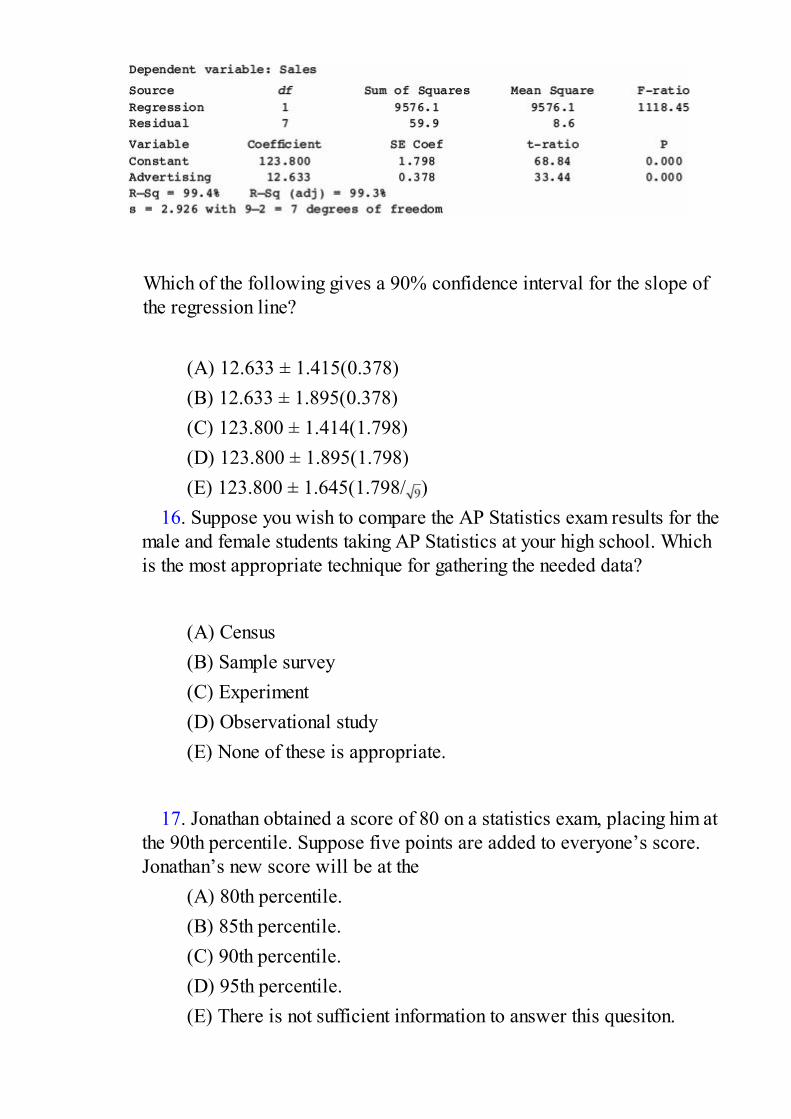
Which of the following gives a 90% confidence interval for the slope ofthe regression line?
(A) 12.633 ± 1.415(0.378)(B) 12.633 ± 1.895(0.378)(C) 123.800 ± 1.414(1.798)(D) 123.800 ± 1.895(1.798)(E) 123.800 ± 1.645(1.798/ )
16. Suppose you wish to compare the AP Statistics exam results for themale and female students taking AP Statistics at your high school. Whichis the most appropriate technique for gathering the needed data?
(A) Census(B) Sample survey(C) Experiment(D) Observational study(E) None of these is appropriate.
17. Jonathan obtained a score of 80 on a statistics exam, placing him at
the 90th percentile. Suppose five points are added to everyone’s score.Jonathan’s new score will be at the
(A) 80th percentile.(B) 85th percentile.(C) 90th percentile.(D) 95th percentile.(E) There is not sufficient information to answer this quesiton.
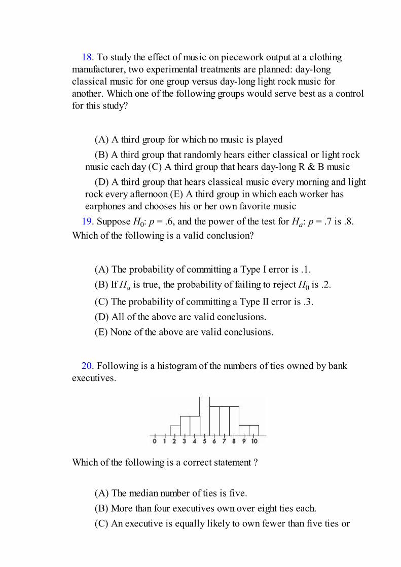
18. To study the effect of music on piecework output at a clothing
manufacturer, two experimental treatments are planned: day-longclassical music for one group versus day-long light rock music foranother. Which one of the following groups would serve best as a controlfor this study?
(A) A third group for which no music is played(B) A third group that randomly hears either classical or light rock
music each day (C) A third group that hears day-long R & B music(D) A third group that hears classical music every morning and light
rock every afternoon (E) A third group in which each worker hasearphones and chooses his or her own favorite music
19. Suppose H0: p = .6, and the power of the test for Ha: p = .7 is .8.Which of the following is a valid conclusion?
(A) The probability of committing a Type I error is .1.(B) If Ha is true, the probability of failing to reject H0 is .2.
(C) The probability of committing a Type II error is .3.(D) All of the above are valid conclusions.(E) None of the above are valid conclusions.
20. Following is a histogram of the numbers of ties owned by bank
executives.
Which of the following is a correct statement ?
(A) The median number of ties is five.(B) More than four executives own over eight ties each.(C) An executive is equally likely to own fewer than five ties or

more than seven ties.(D) One tie is a reasonable estimate for the standard deviation.(E) Removing all the executives with three, nine, and ten ties may
change the median.
21. Which of the following is a binomial random variable?
(A) The number of tosses before a “5” appears when tossing a fair
die.(B) The number of points a hockey team receives in 10 games,
where two points are awarded for wins, one point for ties, and nopoints for losses.
(C) The number of hearts out of five cards randomly drawn from adeck of 52 cards, without replacement.
(D) The number of motorists not wearing seat belts in a randomsample of five drivers.
(E) None of the above.
22. Company I manufactures bomb fuses that burn an average of 50
minutes with a standard deviation of 10 minutes, while company IIadvertises fuses that burn an average of 55 minutes with a standarddeviation of 5 minutes. Which company’s fuse is more likely to last atleast 1 hour? Assume normal distributions of fuse times.
(A) Company I’s, because of its greater standard deviation(B) Company II’s, because of its greater mean(C) For both companies, the probability that a fuse will last at least
1 hour is 15.9%(D) For both companies, the probability that a fuse will last at least
1 hour is 84.1%(E) The problem cannot be solved from the information given.
23. Which of the following is not important in the design of
experiments?

(A) Control of confounding variables(B) Randomization in assigning subjects to different treatments(C) Use of a lurking variable to control the placebo effect(D) Replication of the experiment using sufficient numbers of
subjects(E) All of the above are important in the design of experiments.
24. The travel miles claimed in weekly expense reports of the sales
personnel at a corporation are summarized in the following boxplot.
Which of the following is the most reasonable conclusion?
(A) The mean and median numbers of travel miles are roughly
equal.(B) The mean number of travel miles is greater than the median
number.(C) Most of the claimed numbers of travel miles are in the [0, 200]
interval.(D) Most of the claimed numbers of travel miles are in the [200,
240] interval.(E) The left and right whiskers contain the same number of values
from the set of personnel travel mile claims.
25. Which of the following statements about residuals is true?
(A) Influential scores have large residuals.(B) If the linear model is good, the number of positive residuals
will be the same as the number of negative residuals.(C) The mean of the residuals is always zero.
(D) If the correlation is 0, there will be a distinct pattern in theresidual plot.
(E) If the correlation is 1, there will not be a distinct pattern in theresidual plot.
26. Four pairs of data are used in determining a regression line y = 3x +
4. If the four values of the independent variable are 32, 24, 29, and 27,respectively, what is the mean of the four values of the dependentvariable?
(A) 68(B) 84(C) 88(D) 100(E) The mean cannot be determined from the given information.
27. According to one poll, 12% of the public favor legalizing all drugs.
In a simple random sample of six people, what is the probability that atleast one person favors legalization?
(A) 6(.12)(.88)5
(B) (.88)6
(C) 1 – (.88)6
(D) 1 – 6(.12)(.88)5
(E) 6(.12)(.88)5 + (.88)6
28. Sampling error occurs
(A) when interviewers make mistakes resulting in bias.(B) because a sample statistic is used to estimate a population
parameter.(C) when interviewers use judgment instead of random choice in
picking the sample.(D) when samples are too small.
(E) in all of the above cases.
29. A telephone executive instructs an associate to contact 104
customers using their service to obtain their opinions in regard to an ideafor a new pricing package. The associate notes the number of customerswhose names begin with A and uses a random number table to pick four ofthese names. She then proceeds to use the same procedure for each letterof the alphabet and combines the 4 × 26 = 104 results into a group to becontacted. Which of the following is a correct conclusion?
(A) Her procedure makes use of chance.(B) Her procedure results in a simple random sample.(C) Each customer has an equal probability of being included in the
survey.(D) Her procedure introduces bias through sampling error.(E) With this small a sample size, it is better to let the surveyor pick
representative customers to be surveyed based on as many featuressuch as gender, political preference, income level, race, age, and soon, as are in the company’s data banks.
30. The graph below shows cumulative proportions plotted against
GPAs for high school seniors.
What is the approximate interquartile range?
(A) 0.85(B) 2.25

(C) 2.7(D) 2.75(E) 3.1
31. PCB contamination of a river by a manufacturer is being measured
by amounts of the pollutant found in fish. A company scientist claims thatthe fish contain only 5 parts per million, but an investigator believes thefigure is higher. The investigator catches six fish that show the followingamounts of PCB (in parts per million): 6.8, 5.6, 5.2, 4.7, 6.3, and 5.4. Inperforming a hypothesis test with H0: = 5 and Ha: > 5, what is the teststatistic?
(A)
(B)
(C)
(D)
(E)
32. The distribution of weights of 16-ounce bags of a particular brand
of potato chips is approximately normal with a standard deviation of 0.28ounce. How does the weight of a bag at the 40th percentile compare withthe mean weight?
(A) 0.40 ounce above the mean(B) 0.25 ounce above the mean(C) 0.07 ounce above the mean(D) 0.07 ounce below the mean(E) 0.25 ounce below the mean
33. In general, how does tripling the sample size change the confidence
interval size?
(A) It triples the interval size.(B) It divides the interval size by 3.(C) It multiples the interval size by 1.732.(D) It divides the interval size by 1.732.(E) This question cannot be answered without knowing the sample
size.
34. Which of the following statements is false?
(A) Like the normal distribution, the t-distributions are symmetric.(B) The t-distributions are lower at the mean and higher at the tails,
and so are more spread out than the normal distribution.(C) The greater the df, the closer the t-distributions are to the
normal distribution.(D) The smaller the df, the better the 68–95–99.7 Rule works for t-
models.(E) The area under all t-distribution curves is 1.
35. A study on school budget approval among people with different
party affiliations resulted in the following segmented bar chart:
Which of the following is greatest?
(A) Number of Democrats who are for the proposed budget(B) Number of Republicans who are against the budget(C) Number of Independents who have no opinion on the budget(D) The above are all equal.

(E) The answer is impossible to determine without additionalinformation.
36. The sampling distribution of the sample mean is close to the normal
distribution(A) only if both the original population has a normal distribution
and n is large.(B) if the standard deviation of the original population is known.(C) if n is large, no matter what the distribution of the original
population.(D) no matter what the value of n or what the distribution of the
original population.(E) only if the original population is not badly skewed and does not
have outliers.
37. What is the probability of a Type II error when a hypothesis test is
being conducted at the 10% significance level (α = .10)?
(A) .05(B) .10(C) .90(D) .95(E) There is insufficient information to answer this question.
38.
Above is the dotplot for a set of numbers. One element is labeled X.Which of the following is a correct statement?
(A) X has the largest z-score, in absolute value, of any element in
the set.

(B) A modified boxplot will plot an outlier like X as an isolatedpoint.
(C) A stemplot will show X isolated from two clusters.(D) Because of X, the mean and median are different.(E) The IQR is exactly half the range.
39. A 2008 survey of 500 households concluded that 82% of the
population uses grocery coupons. Which of the following best describeswhat is meant by the poll having a margin of error of 3%?
(A) Three percent of those surveyed refused to participate in the
poll.(B) It would not be unexpected for 3% of the population to begin
using coupons or stop using coupons.(C) Between 395 and 425 of the 500 households surveyed
responded that they used grocery coupons.(D) If a similar survey of 500 households were taken weekly, a 3%
change in each week’s results would not be unexpected.(E) It is likely that between 79% and 85% of the population use
grocery coupons.
40.
The above two-way table summarizes the results of a survey of highschool seniors conducted to determine if there is a relationship betweenwhether or not a student is taking AP Statistics and whether he or sheplans to attend a public or a private college after graduation. Which of thefollowing is the most reasonable conclusion about the relationshipbetween taking AP Statistics and the type of college a student plans toattend?
(A) There appears to be no association since the proportion of AP
Statistics students planning to attend public schools is almost identicalto the proportion of students not taking AP Statistics who plan to attendpublic schools.
(B) There appears to be an association since the proportion of APStatistics students planning to attend public schools is almost identicalto the proportion of students not taking AP Statistics who plan to attendpublic schools.
(C) There appears to be an association since more students plan toattend private than public schools.
(D) There appears to be an association since fewer students aretaking AP Statistics than are not taking AP Statistics.
(E) These data do not address the question of association.
If there is still time remaining, you may review your answers.
SECTION II
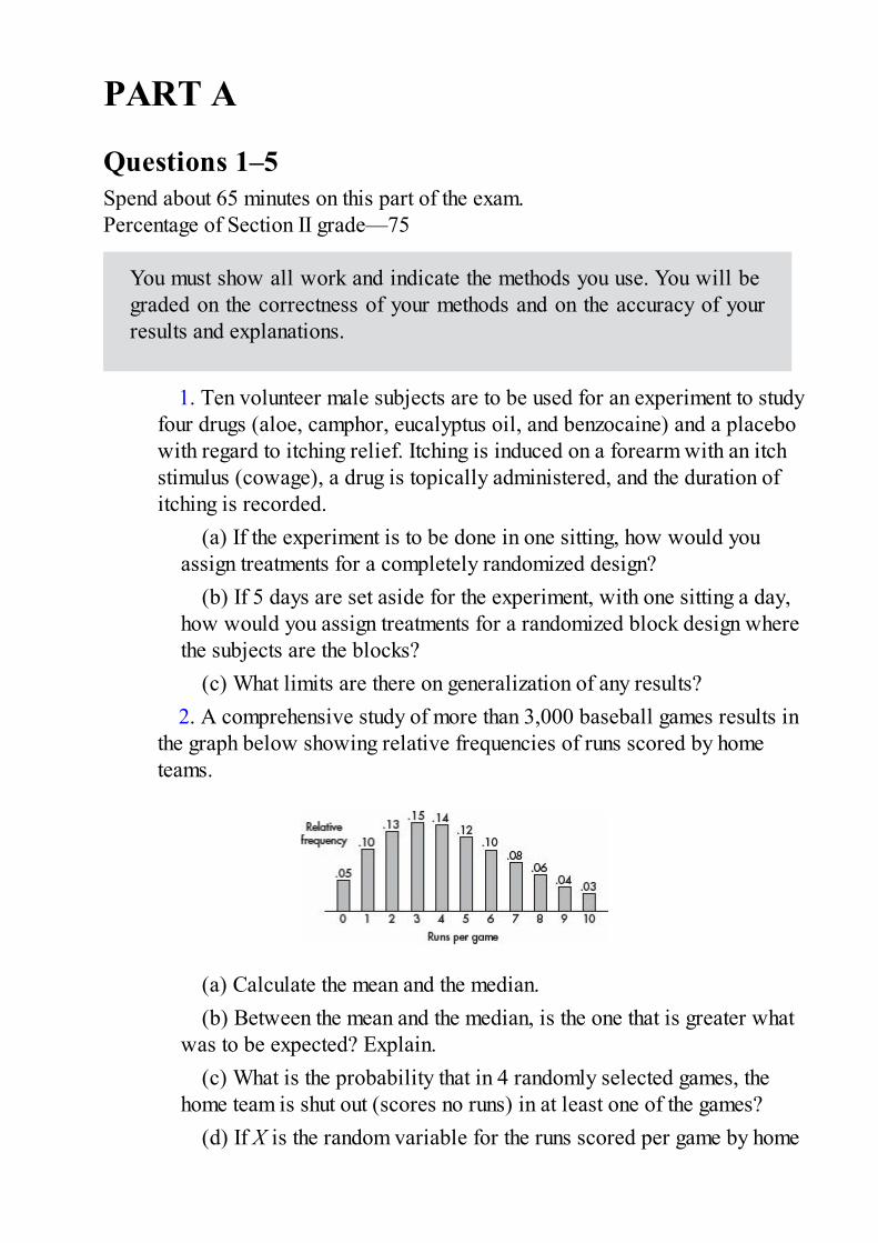
PART A
Questions 1–5Spend about 65 minutes on this part of the exam.Percentage of Section II grade—75
You must show all work and indicate the methods you use. You will begraded on the correctness of your methods and on the accuracy of yourresults and explanations.
1. Ten volunteer male subjects are to be used for an experiment to studyfour drugs (aloe, camphor, eucalyptus oil, and benzocaine) and a placebowith regard to itching relief. Itching is induced on a forearm with an itchstimulus (cowage), a drug is topically administered, and the duration ofitching is recorded.
(a) If the experiment is to be done in one sitting, how would youassign treatments for a completely randomized design?
(b) If 5 days are set aside for the experiment, with one sitting a day,how would you assign treatments for a randomized block design wherethe subjects are the blocks?
(c) What limits are there on generalization of any results?2. A comprehensive study of more than 3,000 baseball games results in
the graph below showing relative frequencies of runs scored by hometeams.
(a) Calculate the mean and the median.(b) Between the mean and the median, is the one that is greater what
was to be expected? Explain.(c) What is the probability that in 4 randomly selected games, the
home team is shut out (scores no runs) in at least one of the games?(d) If X is the random variable for the runs scored per game by home

teams, its standard deviation is 2.578. Suppose 200 games are selectedat random, and , the mean number of runs scored by the home teams,is calculated. Describe the sampling distribution of .3. A study is performed to explore the relationship, if any, between 24-
hour urinary metabolite 3-methoxy-4-hydroxyphenylglycol (MHPG)levels and depression in bipolar patients. The MHPG level is measuredin micrograms per 24 hours while the manic-depression (MD) scale usedgoes from 0 (manic delirium), through 5 (euthymic), up to 10 (depressivestupor). A partial computer printout of regression analysis with MHPG asthe independent variable follows:
(a) Calculate the slope of the regression line and interpret it in thecontext of this problem.
(b) Find the equation of the regression line.(c) Calculate and interpret the value of r2 in the context of this
problem.(d) What does the correlation say about causation in the context of
this problem.4. An experiment is run to test whether daily stimulation of specific
reflexes in young infants will lead to earlier walking. Twenty infants wererecruited through a pediatrician’s service, and were randomly split intotwo groups of ten. One group received the daily stimulation while theother was considered a control group. The ages (in months) at which theinfants first walked alone were recorded.
Is there statistical evidence that infants walk earlier with daily stimulationof specific reflexes?
5. A city sponsors two charity runs during the year, one 5 miles and theother 10 kilometers. Both runs attract many thousands of participants. Astatistician is interested in comparing the types of runners attracted toeach race. She obtains a random sample of 100 runners from each race,calculates five-number summaries of the times, and displays the results in

the parallel boxplots below.
(a) Compare the distributions of times above.
The statistician notes that 5 miles equals 8 kilometers and so decides tomultiply the times from the 5-mile event by and then compare boxplots. This display is below.
(b) How do the distributions now compare?(c) Given that the 10-kilometer race was a longer distance than the
5-mile race, was the change from the first set of boxplots to the secondset as expected? Explain.
(d) Based on the boxplots, would you expect the difference in meantimes in the first set of parallel boxplots to be less than, greater than, orabout the same as the difference in mean times in the second set ofparallel boxplots? Explain.
SECTION II
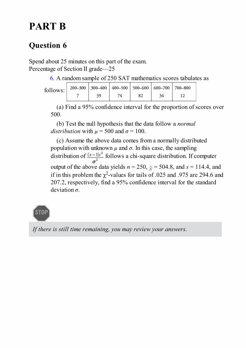
PART B
Question 6
Spend about 25 minutes on this part of the exam.Percentage of Section II grade—25
6. A random sample of 250 SAT mathematics scores tabulates as
follows:
(a) Find a 95% confidence interval for the proportion of scores over500.
(b) Test the null hypothesis that the data follow a normaldistribution with = 500 and σ = 100.
(c) Assume the above data comes from a normally distributedpopulation with unknown and σ. In this case, the samplingdistribution of follows a chi-square distribution. If computer
output of the above data yields n = 250, = 504.8, and s = 114.4, andif in this problem the χ2-values for tails of .025 and .975 are 294.6 and207.2, respectively, find a 95% confidence interval for the standarddeviation σ.
If there is still time remaining, you may review your answers.
All answer sheets are for reference only.

Practice Examination 3
SECTION IQuestions 1–40Spend 90 minutes on this part of the exam.
Directions: The questions or incomplete statements that follow are eachfollowed by five suggested answers or completions. Choose theresponse that best answers the question or completes the statement.
1. Which of the following is a true statement?
(A) While properly designed experiments can strongly suggest
cause-and-effect relationships, a complete census is the only way ofestablishing such a relationship.
(B) If properly designed, observational studies can establish cause-and-effect relationships just as strongly as properly designedexperiments.
(C) Controlled experiments are often undertaken later to establishcause-and-effect relationships first suggested by observational studies.
(D) A useful approach to overcome bias in observational studies isto increase the sample size.
(E) In an experiment, the control group is a self-selected group whochoose not to receive a designated treatment.
2. Two classes take the same exam. Suppose a certain score is at the
40th percentile for the first class and at the 80th percentile for the secondclass. Which of the following is the most reasonable conclusion?
(A) Students in the first class generally scored higher than students
in the second class.
(B) Students in the second class generally scored higher thanstudents in the first class.
(C) A score at the 20th percentile for the first class is at the 40thpercentile for the second class.
(D) A score at the 50th percentile for the first class is at the 90thpercentile for the second class.
(E) One of the classes has twice the number of students as the other.
3. In an experiment, the control group should receive
(A) treatment opposite that given the experimental group.(B) the same treatment given the experimental group without
knowing they are receiving the treatment.(C) a procedure identical to that given the experimental group
except for receiving the treatment under examination.(D) a procedure identical to that given the experimental group
except for a random decision on receiving the treatment underexamination.
(E) none of the procedures given the experimental group.
4. In a random sample of Toyota car owners, 83 out of 112 said they
were satisfied with the Toyota front-wheel drive, while in a similarsurvey of Subaru owners, 76 out of 81 said they were satisfied with theSubaru four-wheel drive. A 90% confidence interval estimate for thedifference in proportions between Toyota and Subaru car owners who aresatisfied with their drive systems is reported to be –.197 ± .081. Which isa proper conclusion?
(A) The interval is invalid because probabilities cannot be negative.(B) The interval is invalid because it does not contain zero.(C) Subaru owners are approximately 19.7% more satisfied with
their drive systems than are Toyota owners.(D) 90% of Subaru owners are approximately 19.7% more satisfied
with their drive systems than are Toyota owners.(E) We are 90% confident that the difference in proportions

between Toyota and Subaru car owners who are satisfied with theirdrive systems is between –.278 and –.116.
5. In a study on the effect of music on worker productivity, employees
were told that a different genre of background music would be playedeach day and the corresponding production outputs noted. Every change inmusic resulted in an increase in production. This is an example of
(A) the effect of a treatment unit.(B) the placebo effect.(C) the control group effect.(D) sampling error.(E) voluntary response bias.
6. A computer manufacturer sets up three locations to provide technical
support for its customers. Logs are kept noting whether or not calls aboutproblems are solved successfully. Data from a sample of 1000 calls aresummarized in the following table:
Assuming there is no association between location and whether or not aproblem is resolved successfully, what is the expected number ofsuccessful calls (problem solved) from location 1?
(A)
(B)
(C)
(D)

(E)
7. Which of the following statements about the correlation coefficient is
true?
(A) The correlation coefficient and the slope of the regression line
may have opposite signs.(B) A correlation of 1 indicates a perfect cause-and-effect
relationship between the variables.(C) Correlations of +.87 and –.87 indicate the same degree of
clustering around the regression line.(D) Correlation applies equally well to quantitative and categorical
data.(E) A correlation of 0 shows little or no association between two
variables.
8. Suppose X and Y are random variables with E(X) = 780, var(X) =
75, E(Y) = 430, and var(Y) = 25. Given that X and Y are independent, whatis the variance of the random variable X – Y?
(A) 75 – 25(B) 75 + 25(C) (D) (E)
9. What is a sample?
(A) A measurable characteristic of a population(B) A set of individuals having a characteristic in common(C) A value calculated from raw data(D) A subset of a population(E) None of the above
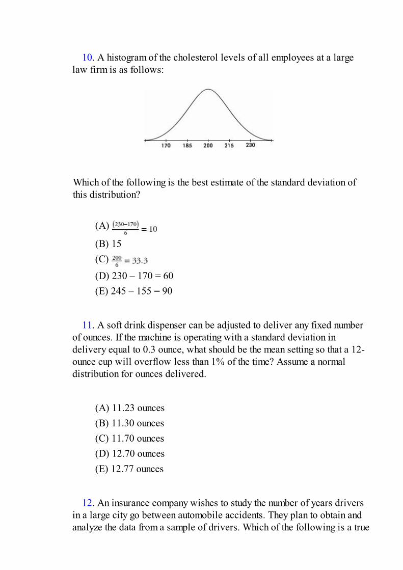
10. A histogram of the cholesterol levels of all employees at a large
law firm is as follows:
Which of the following is the best estimate of the standard deviation ofthis distribution?
(A)
(B) 15(C)
(D) 230 – 170 = 60(E) 245 – 155 = 90
11. A soft drink dispenser can be adjusted to deliver any fixed number
of ounces. If the machine is operating with a standard deviation indelivery equal to 0.3 ounce, what should be the mean setting so that a 12-ounce cup will overflow less than 1% of the time? Assume a normaldistribution for ounces delivered.
(A) 11.23 ounces(B) 11.30 ounces(C) 11.70 ounces(D) 12.70 ounces(E) 12.77 ounces
12. An insurance company wishes to study the number of years drivers
in a large city go between automobile accidents. They plan to obtain andanalyze the data from a sample of drivers. Which of the following is a true

statement?
(A) A reasonable time-and-cost-saving procedure would be to use
systematic sampling on an available list of all AAA (AutomobileAssociation of America) members in the city.
(B) A reasonable time-and-cost-saving procedure would be torandomly choose families and include all drivers in each of thesefamilies in the sample.
(C) To determine the mean number of years between accidents,randomness in choosing a sample of drivers is not important as long asthe sample size is very large.
(D) The larger a simple random sample, the more likely its standarddeviation will be close to the population standard deviation dividedby the square root of the sample size.
(E) None of the above are true statements.
13. The probability that a person will show a certain gene-transmitted
trait is .8 if the father shows the trait and .06 if the father doesn’t show thetrait. Suppose that the children in a certain community come from familiesin 25% of which the father shows the trait. Given that a child shows thetrait, what is the probability that her father shows the trait?
(A) .245(B) .250(C) .750(D) .816(E) .860
14. Given an experiment with H0: = 10, Ha: > 10, and a possible
correct value of 11, which of the following increases as n increases?
I. The probability of a Type I error.II. The probability of a Type II error.III. The power of the test.

(A) I only(B) II only(C) III only(D) II and III(E) None will increase.
15. If all the values of a data set are the same, all of the following must
equal zero except for which one?
(A) Mean(B) Standard deviation(C) Variance(D) Range(E) Interquartile range
16. To determine the average number of minutes it takes to manufacture
one unit of a new product, an assembly line manager tracks a randomsample of 15 units and records the number of minutes it takes to makeeach unit. The assembly times are assumed to have a normal distribution.If the mean and standard deviation of the sample are 3.92 and 0.45minutes respectively, which of the following gives a 90% confidenceinterval for the mean assembly time, in minutes, for units of the newproduct?
(A)
(B)
(C)
(D)
(E)

17. A company has 1000 employees evenly distributed throughout five
assembly plants. A sample of 30 employees is to be chosen as follows.Each of the five managers will be asked to place the 200 time cards oftheir respective employees in a bag, shake them up, and randomly drawout six names. The six names from each plant will be put together to makeup the sample. Will this method result in a simple random sample of the1000 employees?
(A) Yes, because every employee has the same chance of being
selected.(B) Yes, because every plant is equally represented.(C) Yes, because this is an example of stratified sampling, which is
a special case of simple random sampling.(D) No, because the plants are not chosen randomly.(E) No, because not every group of 30 employees has the same
chance of being selected.
18. Given that P(E) = .32, P(F) = .15, and P(E ∩ F) = .048, which of
the following is a correct conclusion?
(A) The events E and F are both independent and mutually
exclusive.(B) The events E and F are neither independent nor mutually
exclusive.(C) The events E and F are mutually exclusive but not independent.(D) The events E and F are independent but not mutually exclusive.(E) The events E and F are independent, but there is insufficient
information to determine whether or not they are mutually exclusive.
19. The number of leasable square feet of office space available in a
city on any given day has a normal distribution with mean 640,000 squarefeet and standard deviation 18,000 square feet. What is the interquartilerange for this distribution?
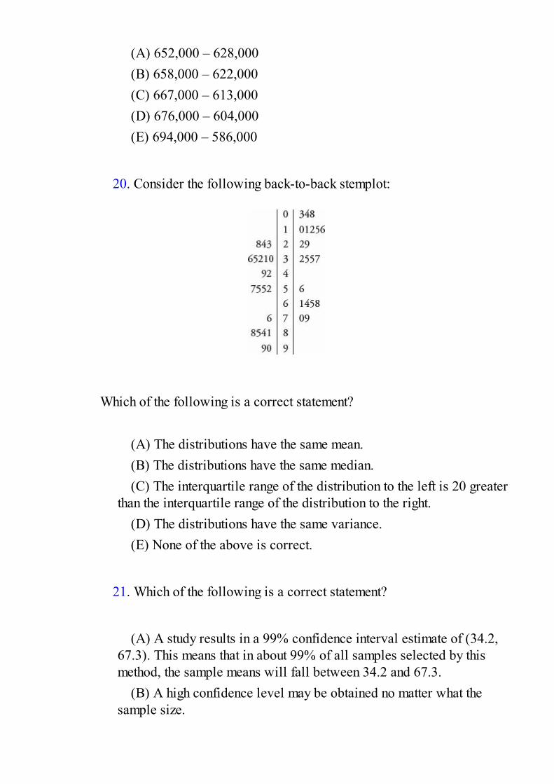
(A) 652,000 – 628,000(B) 658,000 – 622,000(C) 667,000 – 613,000(D) 676,000 – 604,000(E) 694,000 – 586,000
20. Consider the following back-to-back stemplot:
Which of the following is a correct statement?
(A) The distributions have the same mean.(B) The distributions have the same median.(C) The interquartile range of the distribution to the left is 20 greater
than the interquartile range of the distribution to the right.(D) The distributions have the same variance.(E) None of the above is correct.
21. Which of the following is a correct statement?
(A) A study results in a 99% confidence interval estimate of (34.2,
67.3). This means that in about 99% of all samples selected by thismethod, the sample means will fall between 34.2 and 67.3.
(B) A high confidence level may be obtained no matter what thesample size.
(C) The central limit theorem is most useful when drawing samplesfrom normally distributed populations.
(D) The sampling distribution for a mean has standard deviation only when n is sufficiently large (typically one uses n ≥ 30).
(E) The center of any confidence interval is the populationparameter.
22. The binomial distribution is an appropriate model for which of the
following?
(A) The number of minutes in an hour for which the Dow-Jones
average is above its beginning average for the day.(B) The number of cities among the 10 largest in New York State
for which the weather is cloudy for most of a given day.(C) The number of drivers wearing seat belts if 10 consecutive
drivers are stopped at a police roadblock.(D) The number of A’s a student receives in his/her five college
classes.(E) None of the above.
23. Suppose two events, E and F, have nonzero probabilities p and q,
respectively. Which of the following is impossible?
(A) p + q > 1(B) p – q < 0(C) p /q > 1(D) E and F are neither independent nor mutually exclusive.(E) E and F are both independent and mutually exclusive.
24. An inspection procedure at a manufacturing plant involves picking
four items at random and accepting the whole lot if at least three of thefour items are in perfect condition. If in reality 90% of the whole lot areperfect, what is the probability that the lot will be accepted?

(A) (.9)4
(B) 1 – (.9)4
(C) 4(.9)3(.1)(D) .1 – 4(.9)3(.1)(E) 4(.9)3(.1) + (.9)4
25. A town has one high school, which buses students from urban,
suburban, and rural communities. Which of the following samples isrecommended in studying attitudes toward tracking of students in honors,regular, and below-grade classes?
(A) Convenience sample(B) Simple random sample (SRS)(C) Stratified sample(D) Systematic sample(E) Voluntary response sample
26. Suppose there is a correlation of r = 0.9 between number of hours
per day students study and GPAs. Which of the following is a reasonableconclusion?
(A) 90% of students who study receive high grades.(B) 90% of students who receive high grades study a lot.(C) 90% of the variation in GPAs can be explained by variation in
number of study hours per day.(D) 10% of the variation in GPAs cannot be explained by variation
in number of study hours per day.(E) 81% of the variation in GPAs can be explained by variation in
number of study hours per day.
27. To determine the average number of children living in single-family
homes, a researcher picks a simple random sample of 50 such homes.However, even after one follow-up visit the interviewer is unable to
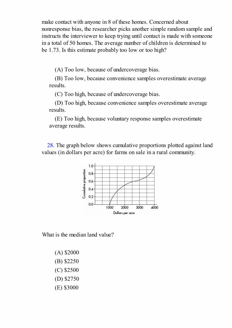
make contact with anyone in 8 of these homes. Concerned aboutnonresponse bias, the researcher picks another simple random sample andinstructs the interviewer to keep trying until contact is made with someonein a total of 50 homes. The average number of children is determined tobe 1.73. Is this estimate probably too low or too high?
(A) Too low, because of undercoverage bias.(B) Too low, because convenience samples overestimate average
results.(C) Too high, because of undercoverage bias.(D) Too high, because convenience samples overestimate average
results.(E) Too high, because voluntary response samples overestimate
average results.
28. The graph below shows cumulative proportions plotted against land
values (in dollars per acre) for farms on sale in a rural community.
What is the median land value?
(A) $2000(B) $2250(C) $2500(D) $2750(E) $3000

29. An experiment is to be conducted to determine whether taking fishoil capsules or garlic capsules has more of an effect on cholesterol levels.In past studies it was noted that daily exercise intensity (low, moderate,high) is associated with cholesterol level, but average sleep length (< 5, 5– 8, > 8 hours) is not associated with cholesterol level. This experimentshould be done
(A) by blocking on exercise intensity(B) by blocking on sleep length(C) by blocking on cholesterol level(D) by blocking on capsule type(E) without blocking
30. A confidence interval estimate is determined from the monthly
grocery expenditures in a random sample of n families. Which of thefollowing will result in a smaller margin of error?
I. A smaller confidence levelII. A smaller sample standard deviationIII. A smaller sample size
(A) II only(B) I and II(C) I and III(D) II and III(E) I, II, and III
31. A medical research team claims that high vitamin C intake
increases endurance. In particular, 1000 milligrams of vitamin C per dayfor a month should add an average of 4.3 minutes to the length ofmaximum physical effort that can be tolerated. Army training officersbelieve the claim is exaggerated and plan a test on an SRS of 400 soldiersin which they will reject the medical team’s claim if the sample mean isless than 4.0 minutes. Suppose the standard deviation of added minutes is
3.2. If the true mean increase is only 4.2 minutes, what is the probabilitythat the officers will fail to reject the false claim of 4.3 minutes?
(A)
(B)
(C)
(D)
(E)
32. Consider the two sets X = {10, 30, 45, 50, 55, 70, 90} and Y = {10,
30, 35, 50, 65, 70, 90}. Which of the following is false?
(A) The sets have identical medians.(B) The sets have identical means.(C) The sets have identical ranges.(D) The sets have identical boxplots.(E) None of the above are false.
33. The weight of an aspirin tablet is 300 milligrams according to the
bottle label. An FDA investigator weighs a simple random sample ofseven tablets, obtains weights of 299, 300, 305, 302, 299, 301, and 303,and runs a hypothesis test of the manufacturer’s claim. Which of thefollowing gives the P-value of this test?
(A) P(t > 1.54) with df = 6(B) 2P(t > 1.54) with df = 6(C) P(t > 1.54) with df = 7(D) 2P(t > 1.54) with df = 7(E) 0.5P(t > 1.54) with df = 7

34. A teacher believes that giving her students a practice quiz every
week will motivate them to study harder, leading to a greater overallunderstanding of the course material. She tries this technique for a year,and everyone in the class achieves a grade of at least C. Is this anexperiment or an observational study?
(A) An experiment, but with no reasonable conclusion possible
about cause and effect(B) An experiment, thus making cause and effect a reasonable
conclusion(C) An observational study, because there was no use of a control
group(D) An observational study, but a poorly designed one because
randomization was not used(E) An observational study, and thus a reasonable conclusion of
association but not of cause and effect
35. Which of the following is not true with regard to contingency tables
for chi-square tests for independence?
(A) The categories are not numerical for either variable.(B) Observed frequencies should be whole numbers.(C) Expected frequencies should be whole numbers.(D) Expected frequencies in each cell should be at least 5, and to
achieve this, one sometimes combines categories for one or the otheror both of the variables.
(E) The expected frequency for any cell can be found by multiplyingthe row total by the column total and dividing by the sample size.
36. Which of the following is a correct statement?
(A) The probability of a Type II error does not depend on the
probability of a Type I error.
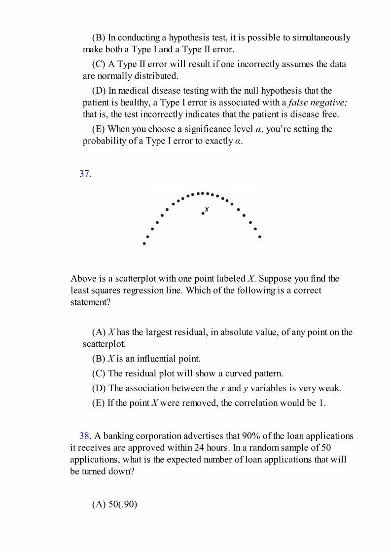
(B) In conducting a hypothesis test, it is possible to simultaneouslymake both a Type I and a Type II error.
(C) A Type II error will result if one incorrectly assumes the dataare normally distributed.
(D) In medical disease testing with the null hypothesis that thepatient is healthy, a Type I error is associated with a false negative;that is, the test incorrectly indicates that the patient is disease free.
(E) When you choose a significance level α, you’re setting theprobability of a Type I error to exactly α.
37.
Above is a scatterplot with one point labeled X. Suppose you find theleast squares regression line. Which of the following is a correctstatement?
(A) X has the largest residual, in absolute value, of any point on the
scatterplot.(B) X is an influential point.(C) The residual plot will show a curved pattern.(D) The association between the x and y variables is very weak.(E) If the point X were removed, the correlation would be 1.
38. A banking corporation advertises that 90% of the loan applications
it receives are approved within 24 hours. In a random sample of 50applications, what is the expected number of loan applications that willbe turned down?
(A) 50(.90)

(B) 50(.10)(C) 50(.90)(.10)(D)
(E)
39. The parallel boxplots below show monthly rainfall summaries for
Liberia, West Africa.
Which of the following months has the least variability as measured byinterquartile range?
(A) January(B) February(C) March(D) May
(E) December
40. In comparing the life expectancies of two models of refrigerators,
the average years before complete breakdown of 10 model Arefrigerators is compared with that of 15 model B refrigerators. The 90%confidence interval estimate of the difference is (6, 12). Which of thefollowing is the most reasonable conclusion?
(A) The mean life expectancy of one model is twice that of the
other.(B) The mean life expectancy of one model is 6 years, while the
mean life expectancy of the other is 12 years.(C) The probability that the life expectancies are different is .90.(D) The probability that the difference in life expectancies is greater
than 6 years is .90.(E) We should be 90% confident that the difference in life
expectancies is between 6 and 12 years.
If there is still time remaining, you may review your answers.
SECTION II

PART A
Questions 1–5Spend about 65 minutes on this part of the exam.Percentage of Section II grade—75
You must show all work and indicate the methods you use. You will begraded on the correctness of your methods and on the accuracy of yourresults and explanations.
1. The Information Technology Services division at a university isconsidering installing a new spam filter software product on all campuscomputers to combat unwanted advertising and spyware. A sample of 60campus computers was randomly divided into two groups of 30computers each. One group of 30 was considered to be a control group,while each computer in the other group had the spam filter softwareinstalled. During a two-week period each computer user was instructed tokeep track of the number of unwanted spam e-mails received. The back-to-back stemplot below shows the distribution of such e-mails receivedfor the control and treatment groups.
(a) Compare the distribution of spam e-mails from the control andtreatment groups.
(b) The standard deviation of the numbers of e-mails in the controlgroup is 8.1. How does this value summarize variability for thecontrol group data?
(c) A researcher in Information Technology Services calculates a95% confidence interval for the difference in mean number of spam e-mails received between the control group and the treatment group withthe new software and obtains (1.5, 10.9). Assuming all conditions fora two-sample t-interval are met, comment on whether or not there isevidence of a difference in the means for the number of spam e-mailsreceived during a two-week period by computers with and without the
software.(d) The computer users on campus fall into four groups:
administrators, staff, faculty, and students. Explain why a researchermight decide to use blocking in setting up this experiment.
2. A game contestant flips three fair coins and receives a score equal tothe absolute value of the difference between the number of heads andnumber of tails showing.
(a) Construct the probability distribution table for the possiblescores in this game.
(b) Calculate the expected value of the score for a player.(c) What is the probability that if a player plays this game three
times the total score will be 3?(d) Suppose a player wins a major prize if he or she can average a
score of at least 2. Given the choice, should he or she try for thisaverage by playing 10 times or by playing 15 times? Explain.
3. A high school has a room set aside after school for students to playgames. The attendance data are summarized in the following table.
A student plugs these data into his calculator and comes up with:
(a) Interpret the slope of the regression line in context. Does thisseem to adequately explain the data? Why or why not?
Another student points out that during the first 4 weeks the school allowedcomputer games, but then the policy changed.
(b) Give a more appropriate regression analysis modelingattendance in terms of week. Include correlation and interpretation ofslope in your analysis.
(c) Explain the above results in terms of a scatterplot.
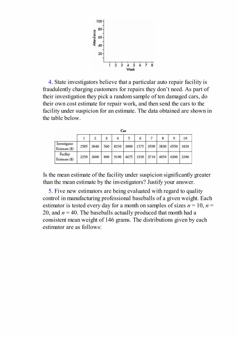
4. State investigators believe that a particular auto repair facility isfraudulently charging customers for repairs they don’t need. As part oftheir investigation they pick a random sample of ten damaged cars, dotheir own cost estimate for repair work, and then send the cars to thefacility under suspicion for an estimate. The data obtained are shown inthe table below.
Is the mean estimate of the facility under suspicion significantly greaterthan the mean estimate by the investigators? Justify your answer.
5. Five new estimators are being evaluated with regard to qualitycontrol in manufacturing professional baseballs of a given weight. Eachestimator is tested every day for a month on samples of sizes n = 10, n =20, and n = 40. The baseballs actually produced that month had aconsistent mean weight of 146 grams. The distributions given by eachestimator are as follows:

(a) Which of the above appear to be unbiased estimators of thepopulation parameter? Explain.
(b) Which of the above exhibits the lowest variability for n = 40?Explain.
(c) Which of the above is the best estimator if the selected estimatorwill eventually be used with a sample of size n = 100? Explain.
SECTION II

PART B
Question 6
Spend about 25 minutes on this part of the exam.Percentage of Section II grade—25
6. Dose intensity in chemotherapy is a balance between minimizingadverse side effects and maximizing therapeutic effect of the treatment. Astudy is performed on 800 patients with stage 4 colon cancer to determinethe relationship between nausea (a side effect of most types ofchemotherapy) and dosage of an experimental chemotherapy agent. Eachpatient is randomly placed in one of eight groups, each group receiving adifferent dose intensity, and the numbers of patients experiencing severenausea are noted. The table below summarizes the data collected.
(a) A medical researcher notes that a total of 205 out of 405 patientsgiven higher doses (≥ 50 mg/week) experienced severe nausea, whileonly 88 of the 395 patients given lower doses (≤ 25 mg/week)experienced severe nausea. Do these data support that a greaterproportion of patients receiving higher doses experience severenausea than patients receiving lower doses?
(b) Another researcher thinks there is more of a relation betweendose intensity and proportion experiencing severe nausea than one cansee by simply looking at low and high doses. She runs a regressionanalysis with the following computer output.

Find a 95% confidence interval for the slope of the regression line,and interpret your answer in context.
(c) A researcher plans to interview five patients randomly chosenfrom among the 800 participants in this experiment. What is theprobability that a majority of those chosen will have experiencedsevere nausea?
If there is still time remaining, you may review your answers.
All answer sheets are for reference only.

Practice Examination 4
SECTION IQuestions 1–40Spend 90 minutes on this part of the exam.
Directions: The questions or incomplete statements that follow are eachfollowed by five suggested answers or completions. Choose the responsethat best answers the question or completes the statement.
1. A company wishes to determine the relationship between the numberof days spent training employees and their performances on a job aptitudetest. Collected data result in a least squares regression line, = 12.1 +6.2x, where x is the number of training days and is the predicted scoreon the aptitude test. Which of the following statements best interprets theslope and y-intercept of the regression line?
(A) The base score on the test is 12.1, and for every day of training
one would expect, on average, an increase of 6.2 on the aptitude test.(B) The base score on the test is 6.2, and for every day of training
one would expect, on average, an increase of 12.1 on the aptitude test.(C) The mean number of training days is 12.1, and for every
additional 6.2 days of training one would expect, on average, anincrease of one unit on the aptitude test.
(D) The mean number of training days is 6.2, and for everyadditional 12.1 days of training one would expect, on average, anincrease of one unit on the aptitude test.
(E) The mean number of training days is 12.1, and for every day oftraining one would expect, on average, an increase of 6.2 on theaptitude test.
2. To survey the opinions of the students at your high school, a

researcher plans to select every twenty-fifth student entering the school inthe morning. Assuming there are no absences, will this result in a simplerandom sample of students attending your school?
(A) Yes, because every student has the same chance of being
selected.(B) Yes, but only if there is a single entrance to the school.(C) Yes, because the 24 out of every 25 students who are not
selected will form a control group.(D) Yes, because this is an example of systematic sampling, which
is a special case of simple random sampling.(E) No, because not every sample of the intended size has an equal
chance of being selected.
3. Consider a hypothesis test with H0: = 70 and Ha: < 70. Which of
the following choices of significance level and sample size results in thegreatest power of the test when = 65?
(A) α = 0.05, n = 15(B) α = 0.01, n = 15(C) α = 0.05, n = 30(D) α = 0.01, n = 30(E) There is no way of answering without knowing the strength of
the given power.
4. Suppose that 60% of a particular electronic part last over 3 years,
while 70% last less than 6 years. Assuming a normal distribution, whatare the mean and standard deviation with regard to length of life of theseparts?
(A) = 3.677, σ = 3.561(B) = 3.977, σ = 3.861(C) = 4.177, σ = 3.561(D) = 4.377, σ = 3.261

(E) The mean and standard deviation cannot be computed from theinformation given.
5. The graph below shows cumulative proportions plotted against
numbers of employees working in mid-sized retail establishments.
What is the approximate interquartile range?
(A) 18(B) 35(C) 57(D) 68(E) 75
6. The label on a package of cords claims that the breaking strength of a
cord is 3.5 pounds, but a hardware store owner believes the real value isless. She plans to test 36 such cords; if their mean breaking strength isless than 3.25 pounds, she will reject the claim on the label. If thestandard deviation for the breaking strengths of all such cords is 0.9pounds, what is the probability of mistakenly rejecting a true claim?
(A) .05(B) .10(C) .15(D) .45(E) .94
7. What is a placebo?
(A) A method of selection(B) An experimental treatment(C) A control treatment(D) A parameter(E) A statistic
8. To study the effect of alcohol on reaction time, subjects were
randomly selected and given three beers to consume. Their reaction timeto a simple stimulus was measured before and after drinking the alcohol.Which of the following is a correct statement?
(A) This study was an observational study.(B) Lack of blocking makes this a poorly designed study.(C) The placebo effect is irrelevant in this type of study.(D) This study was an experiment with no controls.(E) This study was an experiment in which the subjects were used
as their own controls.
9. Suppose that the regression line for a set of data, y = 7x + b, passes
through the point (–2, 4). If and are the sample means of the x- and y-values, respectively, then =
(A) (B) + 2(C) – 4(D) 7(E) 7 + 18
10. Which of the following is a false statement about simple random
samples?

(A) A sample must be reasonably large to be properly considered a
simple random sample.(B) Inspection of a sample will give no indication of whether or not
it is a simple random sample.(C) Attributes of a simple random sample may be very different
from attributes of the population.(D) Every element of the population has an equal chance of being
picked.(E) Every sample of the desired size has an equal chance of being
picked.
11. A local school has seven math teachers and seven English teachers.
When comparing their mean salaries, which of the following is mostappropriate?
(A) A two-sample z-test of population means.(B) A two-sample t-test of population means.(C) A one-sample z-test on a set of differences.(D) A one-sample t-test on a set of differences.(E) None of the above are appropriate.
12. Following is a histogram of ages of people applying for a particular
high school teaching position.
Which of the following is a correct statement?
(A) The median age is between 24 and 25.(B) The mean age is between 22 and 23.

(C) The mean age is greater than the median age.(D) More applicants are under 23 years of age than are over 23.(E) There are a total of 10 applicants.
13. To conduct a survey of which long distance carriers are used in aparticular locality, a researcher opens a telephone book to a random page,closes his eyes, puts his finger down on the page, and then calls the next75 names. Which of the following is a correct statement?
(A) The procedure results in a simple random sample.(B) While the survey design does incorporate chance, the procedure
could easily result in selection bias.(C) This is an example of cluster sampling with 26 clusters.(D) This is an example of stratified sampling with 26 strata.(E) Given that the researcher truly keeps his eyes closed, this is a
good example of blinding.
14. Which of the following is not true about t-distributions?
(A) There are different t-distributions for different values of df
(degrees of freedom).(B) t-distributions are bell-shaped and symmetric.(C) t-distributions always have mean 0 and standard deviation 1.(D) t-distributions are more spread out than the normal distribution.(E) The larger the df value, the closer the distribution is to the
normal distribution.
15. Suppose the probability that a person picked at random has lung cancer
is .035 and the probability that the person both has lung cancer and is aheavy smoker is .014. Given that someone picked at random has lungcancer, what is the probability that the person is a heavy smoker?

(A) .035 – .014(B) .035 + .014(C) .035 + .014 – (.035)(.014)(D)
(E)
16. Taxicabs in a metropolitan area are driven an average of 75,000 miles
per year with a standard deviation of 12,000 miles. What is theprobability that a randomly selected cab has been driven less than100,000 miles if it is known that it has been driven over 80,000 miles?Assume a normal distribution of miles per year among cabs.
(A) .06(B) .34(C) .66(D) .68(E) .94
17. A plant manager wishes to determine the difference in number of
accidents per day between two departments. How many days’ recordsshould be examined to be 90% certain of the difference in daily averagesto within 0.25 accidents per day? Assume standard deviations of 0.8 and0.5 accidents per day in the two departments, respectively.
(A) 39(B) 55(C) 78(D) 109(E) 155
18. Suppose the correlation between two variables is r = .19. What is the
new correlation if .23 is added to all values of the x-variable, every value

of the y-variable is doubled, and the two variables are interchanged?
(A) .19(B) .42(C) .84(D) –.19(E) –.84
19. Two commercial flights per day are made from a small county airport.
The airport manager tabulates the number of on-time departures for asample of 200 days.
What is the χ2 statistic for a goodness-of-fit test that the distribution isbinomial with probability equal to .8 that a flight leaves on time?
(A)
(B)
(C)
(D)
(E)
20. A company has a choice of three investment schemes. Option I gives a
sure $25,000 return on investment. Option II gives a 50% chance ofreturning $50,000 and a 50% chance of returning $10,000. Option IIIgives a 5% chance of returning $100,000 and a 95% chance of returningnothing. Which option should the company choose?
(A) Option II if it wants to maximize expected return
(B) Option I if it needs at least $20,000 to pay off an overdue loan(C) Option III if it needs at least $80,000 to pay off an overdue loan(D) All of the above answers are correct.(E) Because of chance, it really doesn’t matter which option it
chooses.
21. Suppose P(X) = .35 and P(Y) = .40. If P(X|Y) = .28, what is P(Y|X)?
(A)
(B)
(C)
(D)
(E)
22. To test whether extensive exercise lowers the resting heart rate, a study
is performed by randomly selecting half of a group of volunteers toexercise 1 hour each morning, while the rest are instructed to perform noexercise. Is this study an experiment or an observational study?
(A) An experiment with a control group and blinding(B) An experiment with blocking(C) An observational study with comparison and randomization(D) An observational study with little if any bias(E) None of the above
23. The waiting times for a new roller coaster ride are normally distributed
with a mean of 35 minutes and a standard deviation of 10 minutes. If thereare 150,000 riders the first summer, which of the following is the shortesttime interval associated with 100,000 riders?

(A) 0 to 31.7 minutes(B) 31.7 to 39.3 minutes(C) 25.3 to 44.7 minutes(D) 25.3 to 35 minutes(E) 39.3 to 95 minutes
24. A medical researcher, studying the effective durations of three over-the-counter pain relievers, obtains the following boxplots from three equal-sized groups of patients, one group using each of the pain relievers.
I.
II.
III.
Which of the following is a correct statement with regard to comparingthe effective durations in minutes of the three pain relievers?
(A) All three have the same interquartile range.(B) More patients had over 210 minutes of pain relief in the (I)
group than in either of the other two groups.(C) More patients had over 240 minutes of pain relief in the (I)
group than in either of the other two groups.(D) More patients had less than 120 minutes of pain relief in the
(III) group than in either of the other two groups.(E) The durations of pain relief in the (II) group form a normal
distribution.

25. For their first exam, students in an AP Statistics class studied an average
of 4 hours with a standard deviation of 1 hour. Almost everyone didpoorly on the exam, and so for the second exam every student studied 10hours. What is the correlation between the numbers of hours studentsstudied for each exam?
(A) –1(B) 0(C) .4(D) 1(E) There is not sufficient information to answer this question.
26. Suppose that 54% of the graduates from your high school go on to 4-year
colleges, 20% go on to 2-year colleges, 19% find employment, and theremaining 7% search for a job. If a randomly selected student is not goingon to a 2-year college, what is the probability she will be going on to a 4-year college?
(A) .460(B) .540(C) .630(D) .675(E) .730
27. We are interested in the proportion p of people who are unemployed in a
large city. Eight percent of a simple random sample of 500 people areunemployed. What is the midpoint for a 95% confidence interval estimateof p?
(A) .012(B) .025(C) .475
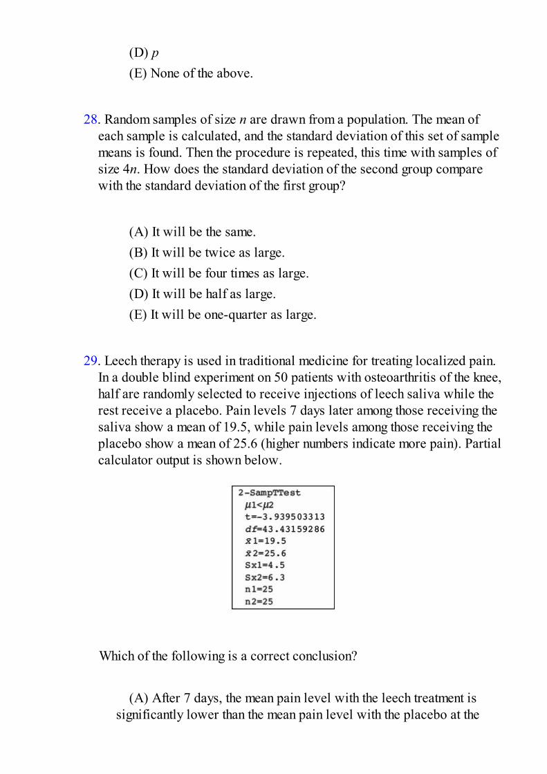
(D) p(E) None of the above.
28. Random samples of size n are drawn from a population. The mean of
each sample is calculated, and the standard deviation of this set of samplemeans is found. Then the procedure is repeated, this time with samples ofsize 4n. How does the standard deviation of the second group comparewith the standard deviation of the first group?
(A) It will be the same.(B) It will be twice as large.(C) It will be four times as large.(D) It will be half as large.(E) It will be one-quarter as large.
29. Leech therapy is used in traditional medicine for treating localized pain.
In a double blind experiment on 50 patients with osteoarthritis of the knee,half are randomly selected to receive injections of leech saliva while therest receive a placebo. Pain levels 7 days later among those receiving thesaliva show a mean of 19.5, while pain levels among those receiving theplacebo show a mean of 25.6 (higher numbers indicate more pain). Partialcalculator output is shown below.
Which of the following is a correct conclusion?
(A) After 7 days, the mean pain level with the leech treatment is
significantly lower than the mean pain level with the placebo at the

0.01 significance level.(B) After 7 days, the mean pain level with the leech treatment is
significantly lower than the mean pain level with the placebo at the0.05 significance level, but not at the 0.01 level.
(C) After 7 days, the mean pain level with the leech treatment issignificantly lower than the mean pain level with the placebo at the0.10 significance level, but not at the 0.05 level.
(D) After 7 days, the mean pain level with the leech treatment is notsignificantly lower than the mean pain level with the placebo at the0.10 significance level.
(E) The proper test should be a one-sample t-test on a set ofdifferences.
30. A survey was conducted to determine the percentage of parents whowould support raising the legal driving age to 18. The results were statedas 67% with a margin of error of ±3%. What is meant by ±3%?
(A) Three percent of the population were not surveyed.(B) In the sample, the percentage of parents who would support
raising the driving age is between 64% and 70%.(C) The percentage of the entire population of parents who would
support raising the driving age is between 64% and 70%.(D) It is unlikely that the given sample proportion result could be
obtained unless the true percentage was between 64% and 70%.(E) Between 64% and 70% of the population were surveyed.
31. It is estimated that 30% of all cars parked in a metered lot outside City
Hall receive tickets for meter violations. In a random sample of 5 carsparked in this lot, what is the probability that at least one receives aparking ticket?
(A) 1 – (.3)5
(B) 1 – (.7)5

(C) 5(.3)(.7)4
(D) 5(.3)4 (.7)(E) 5(.3)4(.7) + 10(.3)3(.7)2 + 10(.3)2(.7)3 + 5(.3)(.7)4 + (.7)5
32. Data are collected on income levels x versus number of bank accounts y.
Summary calculations give = 32,000; sx = 11,500; = 1.7; sy = 0.4, andr = .42. What is the slope of the least squares regression line of number ofbank accounts on income level?
(A) 0.000015(B) 0.000022(C) 0.000035(D) 0.000053(E) 0.000083
33. Given that the sample has a standard deviation of zero, which of the
following is a true statement?
(A) The standard deviation of the population is also zero.(B) The sample mean and sample median are equal.(C) The sample may have outliers.(D) The population has a symmetric distribution.(E) All samples from the same population will also have a standard
deviation of zero.
34. In one study half of a class were instructed to watch exactly 1 hour of
television per day, the other half were told to watch 5 hours per day, andthen their class grades were compared. In a second study students in aclass responded to a questionnaire asking about their television usage andtheir class grades.
(A) The first study was an experiment without a control group,
while the second was an observational study.
(B) The first study was an observational study, while the secondwas a controlled experiment.
(C) Both studies were controlled experiments.(D) Both studies were observational studies.(E) Each study was part controlled experiment and part
observational study.
35. All of the following statements are true for all discrete random variables
except for which one?
(A) The possible outcomes must all be numerical.(B) The possible outcomes must be mutually exclusive.(C) The mean (expected value) always equals the sum of the
products obtained by multiplying each value by its correspondingprobability.
(D) The standard deviation of a random variable can never benegative.
(E) Approximately 95% of the outcomes will be within twostandard deviations of the mean.
36. In leaving for school on an overcast April morning you make a judgment
on the null hypothesis: The weather will remain dry. What would theresults be of Type I and Type II errors?
(A) Type I error: get drenched
Type II error: needlessly carry around an umbrella(B) Type I error: needlessly carry around an umbrella
Type II error: get drenched(C) Type I error: carry an umbrella, and it rains
Type II error: carry no umbrella, but weather remains dry(D) Type I error: get drenched
Type II error: carry no umbrella, but weather remains dry(E) Type I error: get drenched
Type II error: carry an umbrella, and it rains37. The mean thrust of a certain model jet engine is 9500 pounds. Concerned
that a production process change might have lowered the thrust, aninspector tests a sample of units, calculating a mean of 9350 pounds witha z-score of –2.46 and a P-value of .0069. Which of the following is themost reasonable conclusion?
(A) 99.31% of the engines produced under the new process will
have a thrust under 9350 pounds.(B) 99.31% of the engines produced under the new process will
have a thrust under 9500 pounds.(C) 0.69% of the time an engine produced under the new process
will have a thrust over 9500 pounds.(D) There is evidence to conclude that the new process is producing
engines with a mean thrust under 9350 pounds.(E) There is evidence to conclude that the new process is producing
engines with a mean thrust under 9500 pounds.
38. In a group of 10 third graders, the mean height is 50 inches with amedian of 47 inches, while in a group of 12 fourth graders, the meanheight is 54 inches with a median of 49 inches. What is the median heightof the combined group?
(A) 48 inches(B) 52 inches(C)
(D)
(E) The median of the combined group cannot be determined fromthe given information.
39. A reading specialist in a large public school system believes that the
more time students spend reading, the better they will do in school. Sheplans a middle school experiment in which an SRS of 30 eighth graderswill be assigned four extra hours of reading per week, an SRS of 30

seventh graders will be assigned two extra hours of reading per week,and an SRS of 30 sixth graders with no extra assigned reading will be acontrol group. After one school year, the mean GPAs from each groupwill be compared. Is this a good experimental design?
(A) Yes(B) No, because while this design may point out an association
between reading and GPA, it cannot establish a cause-and-effectrelationship.
(C) No, because without blinding, there is a strong chance of aplacebo effect.
(D) No, because any conclusion would be flawed because ofblocking bias.
(E) No, because grade level is a lurking variable which may wellbe confounded with the variables under consideration.
40. A study at 35 large city high schools gives the following back-to-back
stemplot of the percentages of students who say they have tried alcohol.
Which of the following does not follow from the above data?
(A) In general, the percentage of students trying alcohol seems to
have increased from 1995–96 to 1998–99.(B) The median alcohol percentage among the 35 schools increased
from 1995–96 to 1998–99.(C) The spread between the lowest and highest alcohol percentages

decreased from 1995–96 to 1998–99.(D) For both school years in most of the 35 schools, most of the
students said they had tried alcohol.(E) The percentage of students trying alcohol increased in each of
the schools between 1995–96 and 1998–99.
If there is still time remaining, you may review your answers.
SECTION II

Part A
Questions 1–5Spend about 65 minutes on this part of the exam.Percentage of Section II grade—75
You must show all work and indicate the methods you use. You will begraded on the correctness of your methods and on the accuracy of yourresults and explanations.
1. A student is interested in estimating the average length of words in a 600-page textbook, and plans the following three-stage sampling procedure:
(1) Noting that each of the 12 chapters has a different author, the studentdecides to obtain a sample of words from each chapter.
(2) Each chapter is approximately 50 pages long. The student uses arandom number generator to pick three pages from each chapter.
(3) On each chosen page the student notes the length of every tenth word.(a) The first stage above represents what kind of sampling procedure?
Give an advantage in using it in this context.(b) The second stage above represents what kind of sampling
procedure? Give an advantage in using it in this context.(c) The third stage above represents what kind of sampling
procedure? Give a disadvantage to using it dependent upon an author’swriting style.
2. (a) Suppose that nationwide, 69% of all registered voters would answer“Yes” to the question “Do you consider yourself highly focused on thisyear’s presidential election?” Which of the following is more likely: anSRS of 50 registered voters having over 75% answer “Yes,” or an SRS of100 registered voters having over 75% answer “Yes” to the givenquestion? Explain.
(b) A particular company with 95 employees wishes to survey theiremployees with regard to interest in the presidential election. They pick anSRS of 30 employees and ask “Do you consider yourself highly focused onthis year’s presidential election?” Suppose that in fact 60% of all 95employees would have answered “Yes.” Explain why it is not reasonable

to say that the distribution for the count in the sample who say “Yes” is abinomial with n = 30 and p = .6.
(c) Suppose that nationwide, 78% of all registered voters would answer“Yes” to the question “Do you consider yourself highly focused on thisyear’s presidential election?” You plan to interview an SRS of 20registered voters. Explain why it is not reasonable to say that thedistribution for the proportion in the sample who say “Yes” isapproximately a normal distribution.
3. An instructor takes an anonymous survey and notes exam score, hours studied,and gender for the first exam in a large college statistics class (n = 250). Aresulting regression model is:
Score = 50.90 + 9.45(Hours) + 4.40(Gender)
where Gender takes the value 0 for males and 1 for females.
(a) Provide an interpretation in context for each of the three numbersappearing in the above model formula.
(b) Sketch the separate prediction lines for males and females resultingfrom using 0 or 1 in the above model.
Looking at the data separately by gender results in the following tworegression models:
(c) What comparative information do the slope coefficients from thesetwo models give that does not show in the original model?
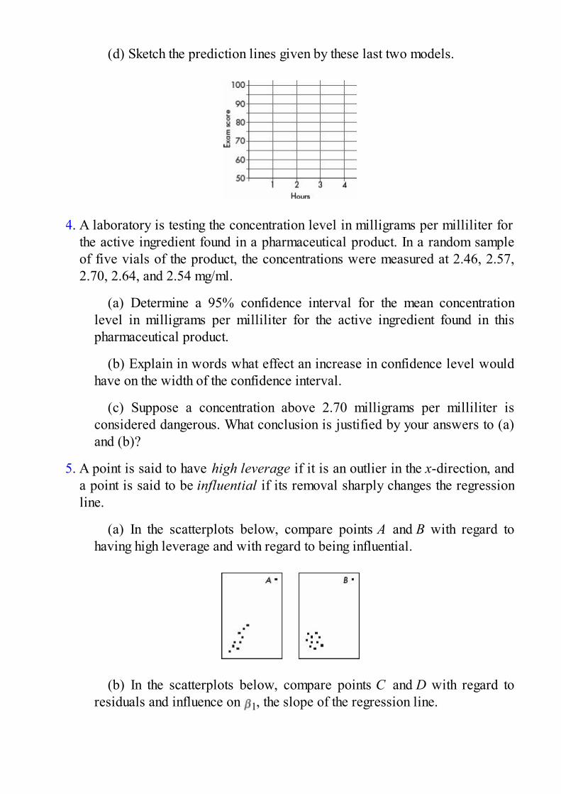
(d) Sketch the prediction lines given by these last two models.
4. A laboratory is testing the concentration level in milligrams per milliliter forthe active ingredient found in a pharmaceutical product. In a random sampleof five vials of the product, the concentrations were measured at 2.46, 2.57,2.70, 2.64, and 2.54 mg/ml.
(a) Determine a 95% confidence interval for the mean concentrationlevel in milligrams per milliliter for the active ingredient found in thispharmaceutical product.
(b) Explain in words what effect an increase in confidence level wouldhave on the width of the confidence interval.
(c) Suppose a concentration above 2.70 milligrams per milliliter isconsidered dangerous. What conclusion is justified by your answers to (a)and (b)?
5. A point is said to have high leverage if it is an outlier in the x-direction, anda point is said to be influential if its removal sharply changes the regressionline.
(a) In the scatterplots below, compare points A and B with regard tohaving high leverage and with regard to being influential.
(b) In the scatterplots below, compare points C and D with regard toresiduals and influence on 1, the slope of the regression line.

(c) In the scatterplot below, compare the effect of removing point E orpoint F to that of removing both E and F.
(d) In the scatterplot below, compare the effect of removing point G orpoint H to that of removing both G and H.
SECTION II

Part B
Question 6
Spend about 25 minutes on this part of the exam.Percentage of Section II grade—25
6. In two random samples of adults, one from each of two communities, countswere made of the number of people with different years of schooling andtabulated as follows:
(a) Is there evidence of a difference in the mean years of schoolingbetween the two communities?
(b) Is there evidence of a difference in the distribution of years ofschooling in the two communities?
(c) Use histograms to help explain the above results.
If there is still time remaining, you may review your answers.

All answer sheets are for reference only.

Practice Examination 5
SECTION IQuestions 1–40Spend 90 minutes on this part of the exam.
Directions: The questions or incomplete statements that follow are eachfollowed by five suggested answers or completions. Choose theresponse that best answers the question or completes the statement.
1. The mean and standard deviation of the population {1, 5, 8, 11, 15}are = 8 and σ = 4.8, respectively. Let S be the set of the 125 orderedtriples (repeats allowed) of elements of the original population. Which ofthe following is a correct statement about the mean and standarddeviation of the means of the triples in S?
(A) = 8, = 4.8(B) = 8, < 4.8(C) = 8, > 4.8(D) < 8, = 4.8(E) > 8, > 4.8
2. A survey to measure job satisfaction of high school mathematics
teachers was taken in 1993 and repeated 5 years later in 1998. Each yeara random sample of 50 teachers rated their job satisfaction on a 1-to-100scale with higher numbers indicating greater satisfaction. The results aregiven in the following back-to-back stemplot.
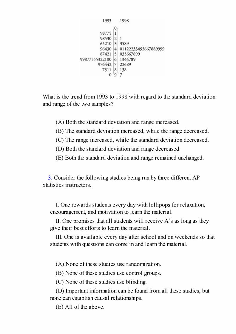
What is the trend from 1993 to 1998 with regard to the standard deviationand range of the two samples?
(A) Both the standard deviation and range increased.(B) The standard deviation increased, while the range decreased.(C) The range increased, while the standard deviation decreased.(D) Both the standard deviation and range decreased.(E) Both the standard deviation and range remained unchanged.
3. Consider the following studies being run by three different AP
Statistics instructors.
I. One rewards students every day with lollipops for relaxation,
encouragement, and motivation to learn the material.II. One promises that all students will receive A’s as long as they
give their best efforts to learn the material.III. One is available every day after school and on weekends so that
students with questions can come in and learn the material.
(A) None of these studies use randomization.(B) None of these studies use control groups.(C) None of these studies use blinding.(D) Important information can be found from all these studies, but
none can establish causal relationships.(E) All of the above.
4. The number of days it takes to build a new house has a variance of
386. A sample of 40 new homes shows an average building time of 83days. With what confidence can we assert that the average building timefor a new house is between 80 and 90 days?
(A) 15.4%(B) 17.8%(C) 20.0%(D) 38.8%(E) 82.2%
5. A shipment of resistors have an average resistance of 200 ohms with
a standard deviation of 5 ohms, and the resistances are normallydistributed. Suppose a randomly chosen resistor has a resistance under194 ohms. What is the probability that its resistance is greater than 188ohms?
(A) .07(B) .12(C) .50(D) .93(E) .97
6. Suppose 4% of the population have a certain disease. A laboratory
blood test gives a positive reading for 95% of people who have thedisease and for 5% of people who do not have the disease. If a persontests positive, what is the probability the person has the disease?
(A) .038(B) .086(C) .442(D) .558

(E) .950
7. For which of the following is it appropriate to use a census?
(A) A 95% confidence interval of mean height of teachers in a small
town.(B) A 95% confidence interval of the proportion of students in a
small town who are taking some AP class.(C) A two-tailed hypothesis test where the null hypothesis was that
the mean expenditure on entertainment by male students at a highschool is the same as that of female students.
(D) Calculation of the standard deviation in the number of brokeneggs per carton in a truckload of eggs.
(E) All of the above.
8. On the same test, Mary and Pam scored at the 64th and 56th
percentiles, respectively. Which of the following is a true statement?
(A) Mary scored eight more points than Pam.(B) Mary’s score is 8% higher than Pam’s.(C) Eight percent of those who took the test scored between Pam
and Mary.(D) Thirty-six people scored higher than both Mary and Pam.(E) None of the above.
9. Which of the following is a true statement?
(A) While observational studies gather information on an already
existing condition, they still often involve intentionally forcing sometreatment to note the response.
(B) In an experiment, researchers decide on the treatment buttypically allow the subjects to self-select into the control group.
(C) If properly designed, either observational studies or controlledexperiments can easily be used to establish cause and effect.

(D) Wording to disguise hidden interests in observational studies isthe same idea as blinding in experimental design.
(E) Stratifying in sampling is the same idea as blocking forexperiments.
10. The random variable describing the number of minutes high school
students spend in front of a computer daily has a mean of 200 minutes.Samples of two different sizes result in sampling distributions with thetwo graphs below.
Which of the following is a true statement?
(A) Based on these graphs, no comparison between the two sample
sizes is possible.(B) More generally, sample sizes have no effect on sampling
distributions.(C) The sample size in A is the same as the sample size in B.(D) The sample size in A is less than the sample size in B.(E) The sample size in A is greater than the sample size in B.
11. To determine the mean cost of groceries in a certain city, an
identical grocery basket of food is purchased at each store in a randomsample of ten stores. If the average cost is $47.52 with a standarddeviation of $1.59, find a 98% confidence interval estimate for the cost ofthese groceries in the city.
(A)
(B)

(C)
(D)
(E)
12. A set consists of four numbers. The largest value is 200, and the
range is 50. Which of the following statements is true?
(A) The mean is less than 185.(B) The mean is greater than 165.(C) The median is less than 195.(D) The median is greater than 155.(E) The median is the mean of the second and third numbers if the
set is arranged in ascending order.
13. A telephone survey of 400 registered voters showed that 256 had
not yet made up their minds 1 month before the election. How sure can webe that between 60% and 68% of the electorate were still undecided atthat time?
(A) 2.4%(B) 8.0%(C) 64.0%(D) 90.5%(E) 95.3%
14. Suppose we have a random variable X where the probability
associated with the value k is

What is the mean of X?
(A) 0.29(B) 0.71(C) 4.35(D) 10.65(E) None of the above
15. The financial aid office at a state university conducts a study to
determine the total student costs per semester. All students are charged$4500 for tuition. The mean cost for books is $350 with a standarddeviation of $65. The mean outlay for room and board is $2800 with astandard deviation of $380. The mean personal expenditure is $675 witha standard deviation of $125. Assuming independence among categories,what is the standard deviation of the total student costs?
(A) $24(B) $91(C) $190(D) $405(E) $570
16. Suppose X and Y are random variables with E(X) = 312, var(X) =
6, E(X) = 307, and var(Y) = 8. What are the expected value and varianceof the random variable X + Y?
(A) E(X + Y) = 619, var(X + Y) = 7(B) E(X + Y) = 619, var(X + Y) = 10(C) E(X + Y) = 619, var(X + Y) = 14(D) E(X + Y) = 309.5, var(X + Y) = 14(E) There is insufficient information to answer this question.
17. In sample surveys, what is meant by bias?

(A) A systematic error in a sampling method that leads to an
unrepresentative sample.(B) Prejudice, for example in ethnic and gender related studies.(C) Natural variability seen between samples.(D) Tendency for some distributions to be skewed.(E) Tendency for some distributions to vary from normality.
18. The following histogram gives the shoe sizes of people in an
elementary school building one morning.
Which of the following is a true statement?
(A) The distribution of shoe sizes is bimodal.(B) The median shoe size is 7 .
(C) The mean shoe size is less than the median shoe size.(D) The five-number summary is: 5 – 6 – 7 – 8 – 9 .
(E) Only 10% of the people had size 5 shoes.
19. When comparing the standard normal (z) distribution to the t-
distribution with df = 30, which of (A)–(D), if any, are false?
(A) Both are symmetric.(B) Both are bell-shaped.(C) Both have center 0.(D) Both have standard deviation 1.

(E) All the above are true statements.
20. Given a probability of .65 that interest rates will jump this year,
and a probability of .72 that if interest rates jump the stock market willdecline, what is the probability that interest rates will jump and the stockmarket will decline?
(A) .72 + .65 – (.72)(.65)(B) (.72)(.65)(C) 1 – (.72)(.65)(D)
(E)
21. Sampling error is
(A) the mean of a sample statistic.(B) the standard deviation of a sample statistic.(C) the standard error of a sample statistic.(D) the result of bias.(E) the difference between a population parameter and an estimate
of that parameter.
22. Suppose that the weights of trucks traveling on the interstate
highway system are normally distributed. If 70% of the trucks weigh morethan 12,000 pounds and 80% weigh more than 10,000 pounds, what arethe mean and standard deviation for the weights of trucks traveling on theinterstate system?
(A) = 14,900; σ = 6100(B) = 15,100; σ = 6200(C) = 15,300; σ = 6300(D) = 15,500; σ = 6400(E) The mean and standard deviation cannot be computed from the

information given.
23. If the correlation coefficient r = .78, what percentage of variation in
y is explained by variation in x?
(A) 22%(B) 39%(C) 44%(D) 61%(E) 78%
24. Consider the following scatterplot:
Which of the following is the best estimate of the correlation between xand y?
(A) –.95(B) –.15(C) 0(D) .15(E) .95
25. For one NBA playoff game the actual percentage of the television
viewing public who watched the game was 24%. If you had taken asurvey of 50 television viewers that night and constructed a confidenceinterval estimate of the percentage watching the game, which of thefollowing would have been true?
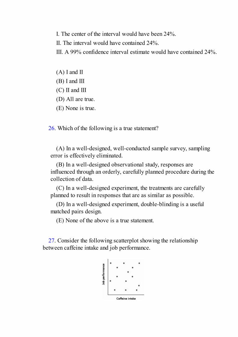
I. The center of the interval would have been 24%.II. The interval would have contained 24%.III. A 99% confidence interval estimate would have contained 24%.
(A) I and II(B) I and III(C) II and III(D) All are true.(E) None is true.
26. Which of the following is a true statement?
(A) In a well-designed, well-conducted sample survey, sampling
error is effectively eliminated.(B) In a well-designed observational study, responses are
influenced through an orderly, carefully planned procedure during thecollection of data.
(C) In a well-designed experiment, the treatments are carefullyplanned to result in responses that are as similar as possible.
(D) In a well-designed experiment, double-blinding is a usefulmatched pairs design.
(E) None of the above is a true statement.
27. Consider the following scatterplot showing the relationship
between caffeine intake and job performance.

Which of the following is a reasonable conclusion?
(A) Low caffeine intake is associated with low job performance.(B) Low caffeine intake is associated with high job performance.(C) High caffeine intake is associated with low job performance.(D) High caffeine intake is associated with high job performance.(E) Job performance cannot be predicted from caffeine intake.
28. An author of a new book claims that anyone following his suggested
diet program will lose an average of 2.8 pounds per week. A researcherbelieves that the true figure will be lower and plans a test involving arandom sample of 36 overweight people. She will reject the author’sclaim if the mean weight loss in the volunteer group is less than 2.5pounds per week. Assume that the standard deviation among individualsis 1.2 pounds per week. If the true mean value is 2.4 pounds per week,what is the probability that the researcher will mistakenly fail to reject theauthor’s false claim of 2.8 pounds?
(A)
(B)
(C)
(D)
(E)
29. Which of the following is the central limit theorem?
(A) No matter how the population is distributed, as the sample size
increases, the mean of the sample means becomes closer to the meanof the population.
(B) No matter how the population is distributed, as the sample size
increases, the standard deviation of the sample means becomes closerto the standard deviation of the population divided by the square rootof the sample size.
(C) If the population is normally distributed, then as the sample sizeincreases, the sampling distribution of the sample mean becomescloser to a normal distribution.
(D) All of the above together make up the central limit theorem.(E) The central limit theorem refers to something else.
30. What is a sampling distribution?
(A) A distribution of all the statistics that can be found in a given
sample(B) A histogram, or other such visual representation, showing the
distribution of a sample(C) A normal distribution of some statistic(D) A distribution of all the values taken by a statistic from all
possible samples of a given size(E) All of the above
31. A judge chosen at random reaches a just decision roughly 80% of
the time. What is the probability that in randomly chosen cases at leasttwo out of three judges reach a just decision?
(A) 3(.8)2(.2)(B) 1 – 3(.8)2(.2)(C) (.8)3
(D) 1 – (.8)3
(E) 3(.8)2(.2) + (.8)3
32. Miles per gallon versus speed (miles per hour) for a new model
automobile is fitted with a least squares regression line. Following iscomputer output of the statistical analysis of the data.
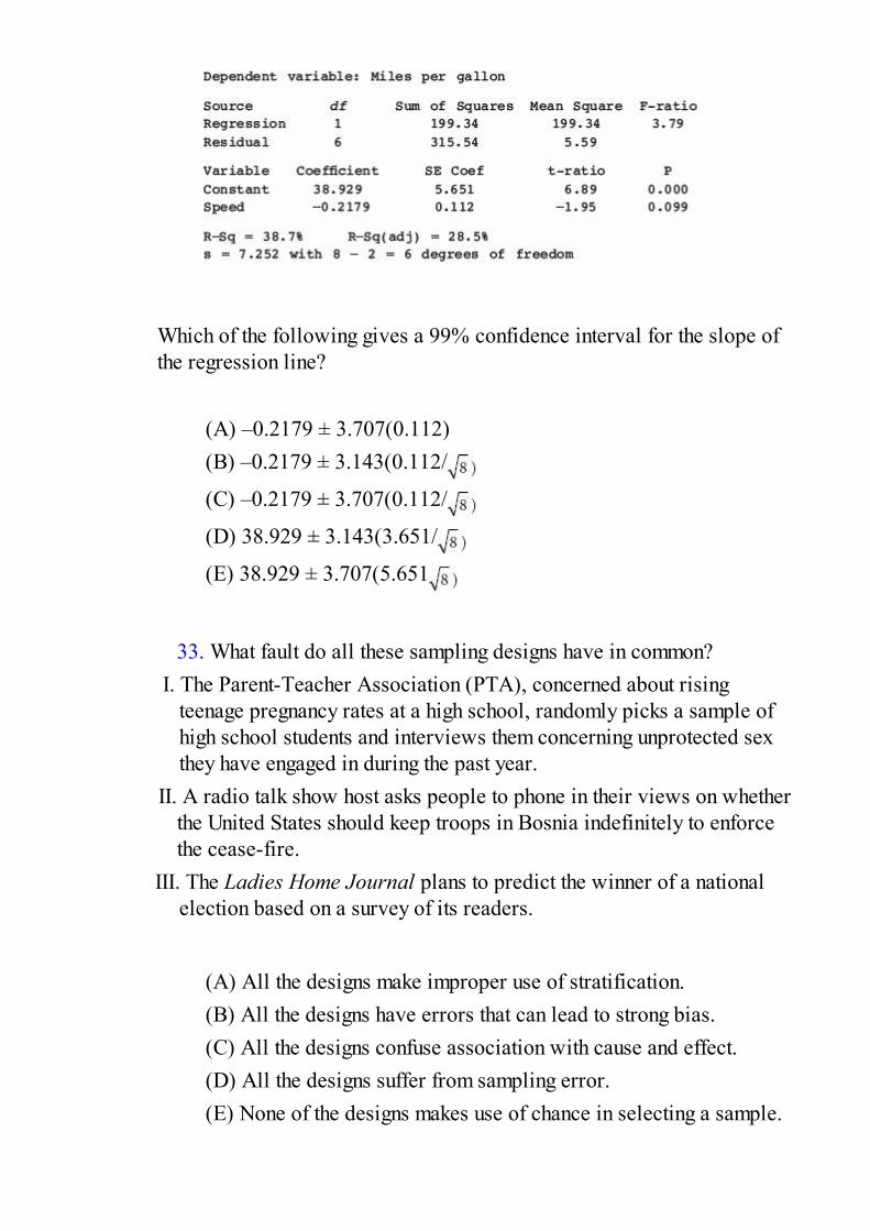
Which of the following gives a 99% confidence interval for the slope ofthe regression line?
(A) –0.2179 ± 3.707(0.112)(B) –0.2179 ± 3.143(0.112/
(C) –0.2179 ± 3.707(0.112/
(D) 38.929 ± 3.143(3.651/
(E) 38.929 ± 3.707(5.651
33. What fault do all these sampling designs have in common?
I. The Parent-Teacher Association (PTA), concerned about risingteenage pregnancy rates at a high school, randomly picks a sample ofhigh school students and interviews them concerning unprotected sexthey have engaged in during the past year.
II. A radio talk show host asks people to phone in their views on whetherthe United States should keep troops in Bosnia indefinitely to enforcethe cease-fire.
III. The Ladies Home Journal plans to predict the winner of a nationalelection based on a survey of its readers.
(A) All the designs make improper use of stratification.(B) All the designs have errors that can lead to strong bias.(C) All the designs confuse association with cause and effect.(D) All the designs suffer from sampling error.(E) None of the designs makes use of chance in selecting a sample.
34. Hospital administrators wish to determine the average length of stay
for all surgical patients. A statistician determines that for a 95%confidence level estimate of the average length of stay to within ±0.50days, 100 surgical patients’ records would have to be examined. Howmany records should be looked at for a 95% confidence level estimate towithin ±0.25 days?
(A) 25(B) 50(C) 200(D) 400(E) There is not enough information given to determine the
necessary sample size.
35. A chess master wins 80% of her games, loses 5%, and draws the
rest. If she receives 1 point for a win, point for a draw, and no pointsfor a loss, what is true about the sampling distribution X of the pointsscored in two independent games?
(A) X takes on the values 0, 1, and 2 with respective probabilities
.10, .26, and .64.(B) X takes on the values 0, , 1, 1 , and 2 with respective
probabilities .0025, .015, .1025, .24, and .64.(C) X takes on values according to a binomial distribution with n =
2 and p = .8.(D) X takes on values according to a binomial distribution with
mean 1(.8) + (.15) + 0(.05).
(E) X takes on values according to a distribution with mean (2)(.8)and standard deviation .
36. Which of the following is a true statement?
(A) The P-value is a conditional probability.

(B) The P-value is usually chosen before an experiment isconducted.
(C) The P-value is based on a specific test statistic and thus shouldnot be used in a two-sided test.
(D) P-values are more appropriately used with t-distributions thanwith z-distributions.
(E) If the P-value is less than the level of significance, then the nullhypothesis is proved false.
37. An assembly line machine is supposed to turn out ball bearings with
a diameter of 1.25 centimeters. Each morning the first 30 bearingsproduced are pulled and measured. If their mean diameter is under 1.23centimeters or over 1.27 centimeters, the machinery is stopped and anengineer is called to make adjustments before production is resumed. Thequality control procedure may be viewed as a hypothesis test with the nullhypothesis H0: = 1.25 and the alternative hypothesis Ha: ≠ 1.25. Theengineer is asked to make adjustments when the null hypothesis isrejected. In test terminology, what would a Type II error result in?
(A) A warranted halt in production to adjust the machinery(B) An unnecessary stoppage of the production process(C) Continued production of wrong size ball bearings(D) Continued production of proper size ball bearings(E) Continued production of ball bearings that randomly are the
right or wrong size
38. Both over-the-counter niacin and the prescription drug Lipitor are
known to lower blood cholesterol levels. In one double-blind studyLipitor outperformed niacin. The 95% confidence interval estimate of thedifference in mean cholesterol level lowering was (18, 41). Which of thefollowing is a reasonable conclusion?
(A) Niacin lowers cholesterol an average of 18 points, while
Lipitor lowers cholesterol an average of 41 points.(B) There is a .95 probability that Lipitor will outperform niacin in
lowering the cholesterol level of any given individual.
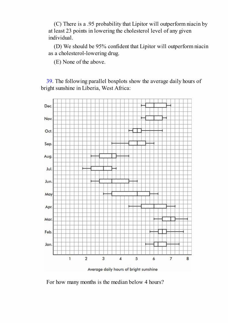
(C) There is a .95 probability that Lipitor will outperform niacin byat least 23 points in lowering the cholesterol level of any givenindividual.
(D) We should be 95% confident that Lipitor will outperform niacinas a cholesterol-lowering drug.
(E) None of the above.
39. The following parallel boxplots show the average daily hours of
bright sunshine in Liberia, West Africa:
For how many months is the median below 4 hours?

(A) One(B) Two(C) Three(D) Four(E) Five
40. Following is a cumulative probability graph for the number of
births per day in a city hospital.
Assuming that a birthing room can be used by only one woman per day,how many rooms must the hospital have available to be able to meet thedemand at least 90 percent of the days?
(A) 5(B) 10(C) 15(D) 20(E) 25
If there is still time remaining, you may review your answers.
SECTION II

PART A
Questions 1–5Spend about 65 minutes on this part of the exam.Percentage of Section II grade—75
You must show all work and indicate the methods you use. You will begraded on the correctness of your methods and on the accuracy of yourresults and explanations.
1. An experiment is being planned to study urban land use practices aimedat reviving and sustaining native bird populations. Vegetation types A andB are to be compared, and eight test sites are available. After planting,volunteer skilled birdwatchers will collect data on the abundance of birdspecies making each of the two habitat types their home. The east side ofthe city borders a river, while the south side borders an industrial park.
(a) Suppose the decision is made to block using the scheme below (oneblock is white, one gray). How would you use randomization, and whatis the purpose of the randomization?
(b) Comment on the strength and weakness of the above scheme ascompared to the following blocking scheme (one block is white, onegray).
2. A world organization report gives the following percentages for primary-school-age children enrolled in school in the 17 countries of each of twogeographic regions.
Region A: 36, 45, 52, 56, 56, 58, 60, 63, 65, 66, 69, 71, 72, 74, 77, 82, 92Region B: 35, 37, 41, 43, 43, 48, 50, 54, 65, 71, 78, 82, 83, 87, 89, 91, 92(a) Draw a back-to-back stemplot of this data.(b) The report describes both regions as having the same median
percentage (for primary-school-age children enrolled in school) amongtheir 17 countries and approximately the same range. What about thedistributions is missed by the report?
(c) If the organization has education funds to help only one region, give anargument for which should be helped.
(d) A researcher plans to run a two-sample t-test to study the difference inmeans between the percentages from each region. Comment on his plan.
3. Data were collected from a random sample of 100 student athletes at alarge state university. The plot below shows grade point average (GPA)versus standard normal value (z-score) corresponding to the percentile ofeach GPA (when arranged in order). Also shown is the normal line, thatis, a line passing through expected values for a normal distribution withthe mean and SD of the given data.

(a) What is the shape of this distribution? Explain.(b) What is the 95th percentile of the data? Explain.(c) In a normal distribution with the mean and SD of this data, what is the
95th percentile? Explain.
4. Although blood type frequencies in the United States are in the ratios of9:8:2:1 for types O, A, B, and AB, respectively, local differences areoften found depending upon a variety of demographic characteristics.Two researchers are independently assigned to determine if patients at aparticular large city general hospital exhibit blood types supporting theabove model. The table below gives the data results from what eachresearcher claims to be random samples of 500 patient lab results.
(a) Do the data reported by Researcher 1 support the 9:8:2:1 model forblood types of patients at the particular hospital? Justify your answer.
(b) The editorial board of a medical publication rejects the findings ofResearcher 2, claiming that his data are suspicious in that they are toogood to be true. Give a statistical justification for the board’s decision.
5. In a random sample of automobiles the highway mileage (in mpg) and theengine size (in liters) are measured, and the following computer output forregression is obtained:
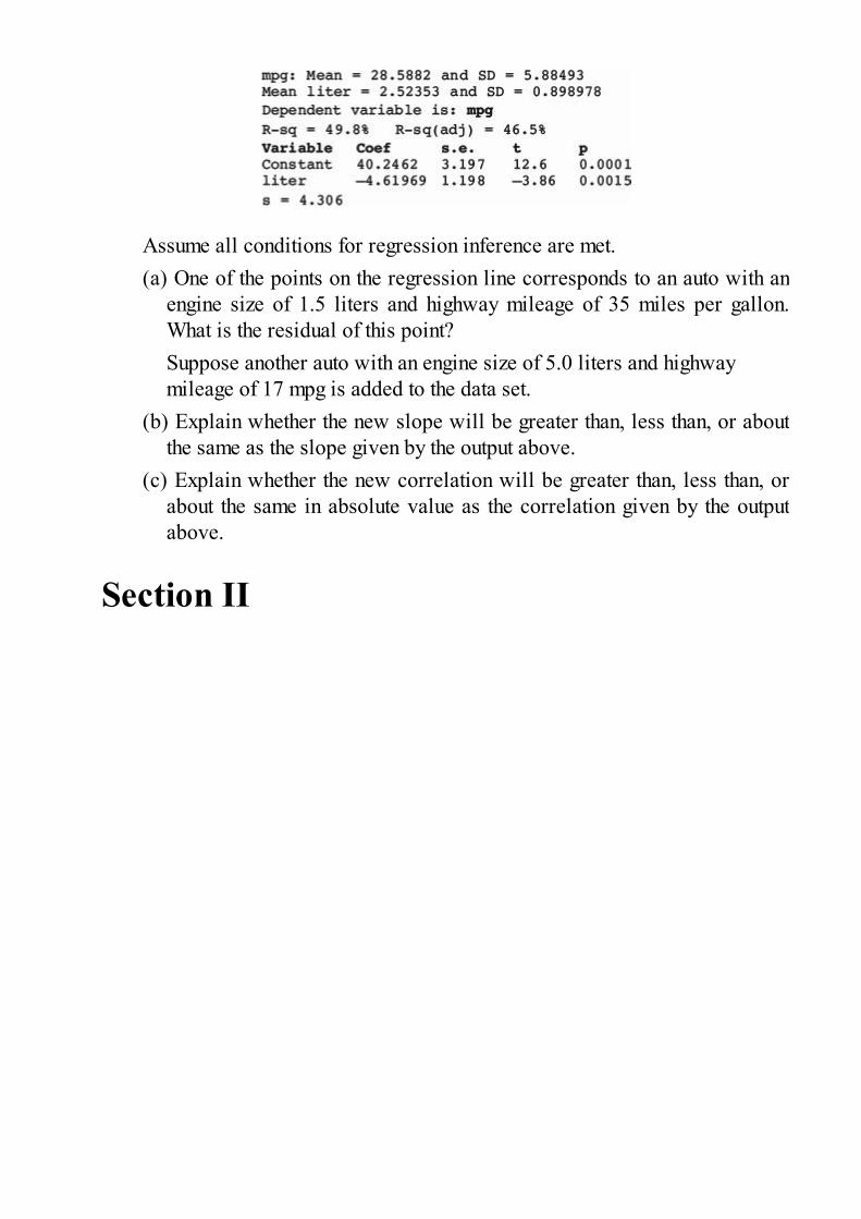
Assume all conditions for regression inference are met.(a) One of the points on the regression line corresponds to an auto with an
engine size of 1.5 liters and highway mileage of 35 miles per gallon.What is the residual of this point?Suppose another auto with an engine size of 5.0 liters and highwaymileage of 17 mpg is added to the data set.
(b) Explain whether the new slope will be greater than, less than, or aboutthe same as the slope given by the output above.
(c) Explain whether the new correlation will be greater than, less than, orabout the same in absolute value as the correlation given by the outputabove.
Section II
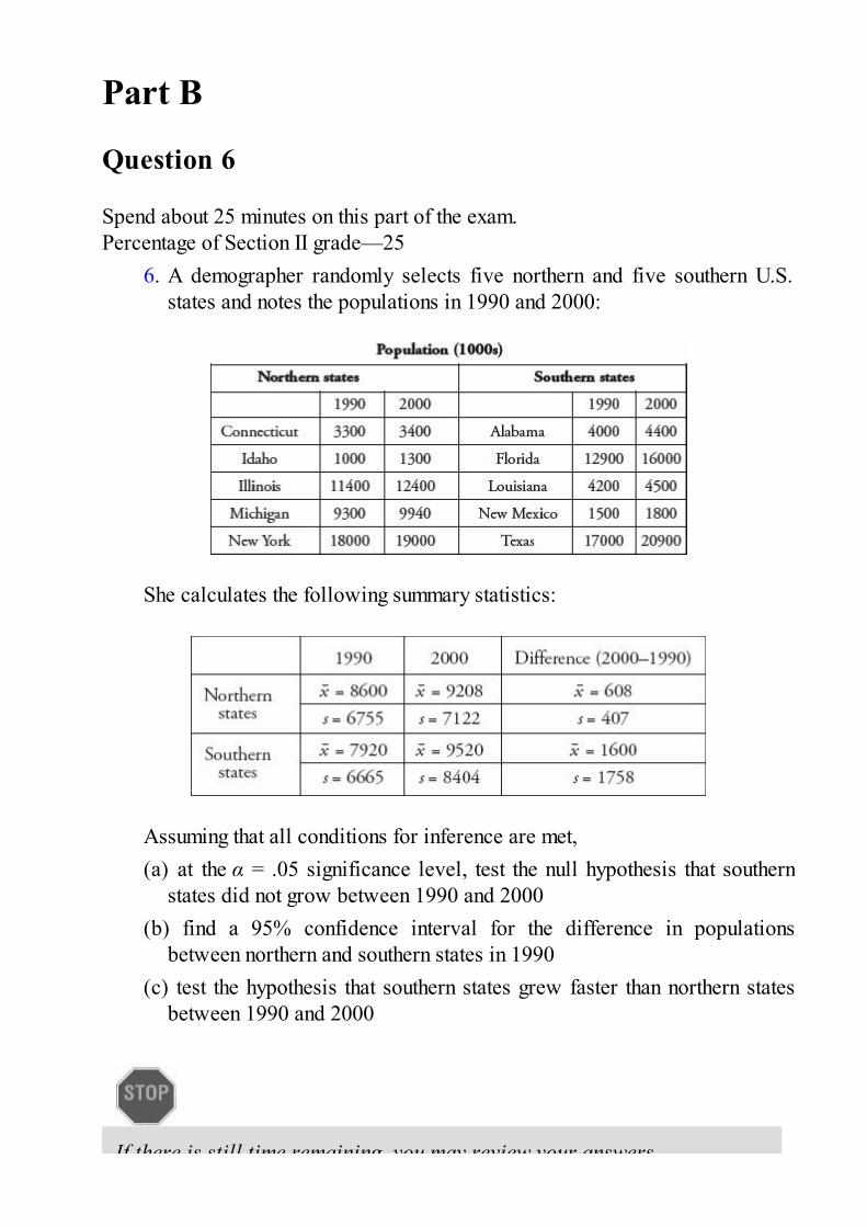
Part B
Question 6
Spend about 25 minutes on this part of the exam.Percentage of Section II grade—25
6. A demographer randomly selects five northern and five southern U.S.states and notes the populations in 1990 and 2000:
She calculates the following summary statistics:
Assuming that all conditions for inference are met,(a) at the α = .05 significance level, test the null hypothesis that southern
states did not grow between 1990 and 2000(b) find a 95% confidence interval for the difference in populations
between northern and southern states in 1990(c) test the hypothesis that southern states grew faster than northern states
between 1990 and 2000
If there is still time remaining, you may review your answers.

If there is still time remaining, you may review your answers.
Relating Multiple-Choice Problems to
Review Book Topics
Topic 1: Graphical Displays
Topic 2: Summarizing Distributions
Topic 3: Comparing Distributions
Topic 4: Exploring Bivariate Data
Topic 5: Exploring Categorical Data: Frequency Tables Topic 6: Overview ofMethods of Data Collection Topic 7: Planning and Conducting Surveys Topic 8:Planning and Conducting Experiments Topic 9: Probability as RelativeFrequency Topic 10: Combining Independent Random Variables Topic 11: TheNormal Distribution
Topic 12: Sampling Distributions
Topic 13: Confidence Intervals
Topic 14: Tests of Significance—Proportions and Means Topic 15: Tests ofSignificance—Chi-Square and Slope of Least Squares Line
The table below gives the above Topic corresponding to each MC question.


Appendix
CHECKING ASSUMPTIONS FORINFERENCE
35 AP EXAM HINTSThe top ten:
1. Graders want to give you credit—help them! Make them understandwhat you are doing, why you are doing it, and how you are doing it. Don’tmake the reader guess at what you are doing. Communication is just asimportant as statistical knowledge!
2. For both multiple choice and free response questions, read thequestion carefully! Be sure you understand exactly what you are beingasked to do or find or explain.

3. Check assumptions. Don’t just state them! Be sure the assumptionsto be checked are stated correctly. Verifying assumptions and conditionsmeans more than simply listing them with little check marks—you mustshow work or give some reason to confirm verification.
4. Learn and practice how to read generic computer output. And inanswering questions using computer output, realize that you usually will notneed to use all the information given.
5. Naked or bald answers will receive little or no credit! You must showwhere answers come from. On the other hand, don’t give more than onesolution to the same problem—you will receive credit only for the weakerone.
6. If you refer to a graph, whether it is a histogram, boxplot, stemplot,scatterplot, residuals plot, normal probability plot, or some other kind ofgraph, you should roughly draw it. It is not enough to simply say, “I did anormal probability plot of the residuals on my calculator and it lookedlinear.” Be sure to label axes and show number scales whenever possible.
7. Use proper terminology! For example, the language of experiments isdifferent from the language of observational studies—you shouldn’t mix upblocking and stratification. Know what confounding means and when it isproper to use this term. Replication on many subjects to reduce chancevariation is different from replication of an experiment itself to achievevalidation.
8. Avoid “calculator speak”! For example, do not simply write “2-SampTTest …” or “binomcdf…” There are lots of calculators out there,each with its own abbreviations.
9. Be careful about using abbreviations in general. For example, yourteacher might use LOBF (line of best fit), but the grader may have no ideawhat this refers to.
10. Don’t automatically “parrot” the stem of the problem! For example,the question might refer to sample data; however, your hypotheses must bestated in terms of a population parameter.
25 more hints:11. Insert new calculator batteries or carry replacement batteries with
you.12. Underline key words and phrases while reading questions.13. Some problems look scary on first reading but are not overly difficult
and are surprisingly straightforward if you approach them systematically.And some questions might take you beyond the scope of the AP curriculum;however, remember that they will be phrased in such ways that you shouldbe able to answer them based on what you have learned in your AP Statclass.
14. Read through all six free-response questions, unerlining key points.Go back and do those questions you think are easiest (this will usually, butnot always, include Problem 1). Then tackle the heavily weighted Problem6 for a while. Finally, try the remaining problems. If you have a fewminutes at the end to try some more on Problem 6, that’s great!
15. Answers do not have to be in paragraph form. Symbols and algebraare fine. Just be sure that your method, reasoning, and calculations will beclear to the reader, and that the explanations and conclusions are given incontext of the problem.
16. If you show calculations carefully, a wrong answer due to acomputational error might still result in full credit.
17. If you can’t solve part of a problem, but that solution is necessary toproceed, make up a reasonable answer to the first part and use this toproceed to the remaining parts of the problem.
18. When using a formula, write down the formula and then substitute thevalues.
19. Conclusions should be stated in proper English. For example, don’tuse double negatives.
20. Read carefully and recognize that sometimes very different tests arerequired in different parts of the same problem.
21. Realize that there may be several reasonable approaches to a givenproblem. In such cases pick either the one you feel most comfortable withor the one you feel will require the least time.
22. Realize that there may not be one clear, correct answer. Somequestions are designed to give you an opportunity to creatively synthesize arelationship among the problem’s statistical components.
23. Punching a long list of data into the calculator doesn’t showstatistical knowledge. Be sure it’s necessary!
24. Remember that uniform and symmetric are not the same, and that notall symmetric unimodal distributions are normal.
25. When making predictions and interpreting slopes and intercepts,don’t become confused between your original data and your regressionmodel.
26. If the slope is close to ±1, it does not follow that the correlation isstrong.
27. When describing residual graphs, “randomly scattered” does notmean the same as “half below and half above.” You should comment onwhether or not there are nonlinear patterns, and increasing or decreasingspread, and on whether the residuals are small or large compared to theassociated y-values.
28. Simply using a calculator to find a regression line is not enough; youmust understand it (for example, be able to interpret the slope andintercepts in context).
29. With regard to hypothesis test problems, (1) the hypotheses must bestated in terms of population parameters with all variables clearly defined;(2) the test must be specified by name or formula, and you must show howthe test assumptions are met; (3) the test statistic and associated P-valueshould be calculated; (4) the P-value must be linked to a decision; and (5)a conclusion must be stated in the context of the problem.
30. For any inference problem, be sure to ask yourself whether thevariable is categorical (usually leading to proportions) or quantitative(usually leading to means), whether you are working with raw data orsummary statistics, whether there is a single population of interest or twopopulations being compared, and in the case of comparison whether thereare independent samples or a paired comparison.
31. A simple random sample (SRS) and a random assignment oftreatments to subjects both have to do with randomness, but they are not thesame. Understand the difference!
32. Simply saying to “randomly assign” subjects to treatment groups isusually an incomplete response. You need to explain how to make theassignments, for example, using a random number table or throughgenerating random numbers on a calculator.
33. Blinding and placebos in experiments are important but are notalways feasible. You can still have “experiments” without these.

34. The distribution of a particular sample (data set) is not the same asthe sampling distribution of a statistic. Understand the difference!
35. Just because a sample is large does not imply that the distribution ofthe sample will be close to a normal distribution.
AP SCORING GUIDEThe Multiple-Choice and Free-Response sections are weighted equally.There is no penalty for guessing in the Multiple-Choice section.The Investigative Task counts for 25% of the Free-Response section. Each ofthe Free-Response questions has a possible four points.To find your score use the following guide:Multiple-Choice section (40 questions)Number correct × 1.25 = __________Free-Response section (5 Open-Ended questions plus an Investigative Task)
Total points from Multiple-Choice and Free-Response sections = __________Conversion chart based on a recent AP exam
In the past, roughly 10% of students scored 5, 20% scored 4, 25% scored 3,20% scored 2, and 25% scored 1 on the AP Statistics exam. Colleges generallyrequire a score of at least 3 for a student to receive college credit.
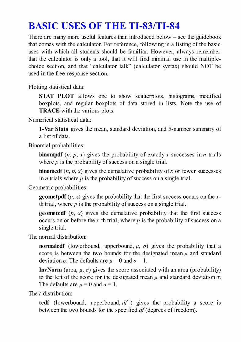
BASIC USES OF THE TI-83/TI-84There are many more useful features than introduced below – see the guidebookthat comes with the calculator. For reference, following is a listing of the basicuses with which all students should be familiar. However, always rememberthat the calculator is only a tool, that it will find minimal use in the multiple-choice section, and that “calculator talk” (calculator syntax) should NOT beused in the free-response section.
Plotting statistical data:STAT PLOT allows one to show scatterplots, histograms, modifiedboxplots, and regular boxplots of data stored in lists. Note the use ofTRACE with the various plots.
Numerical statistical data:1-Var Stats gives the mean, standard deviation, and 5-number summary ofa list of data.
Binomial probabilities:binompdf (n, p, x) gives the probability of exactly x successes in n trialswhere p is the probability of success on a single trial.binomcdf (n, p, x) gives the cumulative probability of x or fewer successesin n trials where p is the probability of success on a single trial.
Geometric probabilities:geometpdf (p, x) gives the probability that the first success occurs on the x-th trial, where p is the probability of success on a single trial.geometcdf (p, x) gives the cumulative probability that the first successoccurs on or before the x-th trial, where p is the probability of success on asingle trial.
The normal distribution:normalcdf (lowerbound, upperbound, , σ) gives the probability that ascore is between the two bounds for the designated mean and standarddeviation σ. The defaults are = 0 and σ = 1.InvNorm (area, , σ) gives the score associated with an area (probability)to the left of the score for the designated mean and standard deviation σ.The defaults are = 0 and σ = 1.
The t-distribution:tcdf (lowerbound, upperbound, df ) gives the probability a score isbetween the two bounds for the specified df (degrees of freedom).

invT(area, df ) gives the t-score associated with an area (probability) to theleft of the score under the student t-probability function for the specified df(degrees of freedom). [Note: this is available on the new operating systemfor the TI-84+.]
The chi-square distribution:χ2cdf (lowerbound, upperbound, df ) gives the probability a score isbetween the two bounds for the specified df (degrees of freedom).χ2GOF-Test is a chi-square goodness-of-fit test to confirm whether sampledata conforms to a specified distribution. [Note: this is available on thenew operating system for the TI-84+.]
Linear regression and correlation:LinReg (ax + b) fits the equation y = ax + b to the data in lists L1 and L2using a least-squares fit. When DiagnosticOn is set, the values for r2 and rare also displayed.
Confidence intervals:For proportions—
1-PropZInt gives a confidence interval for a proportion of successes.2-PropZInt gives a confidence interval for the difference between theproportion of successes in two populations.
For means—TInterval gives a confidence interval for a population mean (use the t-distribution because population variances are never really known).2-SampTInt gives a confidence interval for the difference between twopopulation means.
Hypothesis tests:For proportions—
1-PropZTest2-PropZTest compares the proportion of successes from two populations(making use of the pooled sample proportion).
For means—T-Test2-SampTTest
For chi-square test for association—χ2-Test gives the χ2-value and P-value for the null hypothesis H0: noassociation between row and column variables, and the alternative
hypothesis Ha: the variables are related. The observed counts must first beentered into a matrix.
For linear regression—LinRegTTest calculates a linear regression and performs a t-test on thenull hypothesis H0: = 0 (H0: ρ = 0). The regression equation is stored inRegEQ (under VARS Statistics EQ ) and the list of residuals is stored inRESID (under LIST NAMES).
Catalog help:To activate Catalog Help, press APPS, choose CtlgHelp, and pressENTER. Then, for example, if you press 2nd, DISTR, arrow down tonormalcdf, and press +, you are prompted to insert (lowerbound,upperbound, [ ,σ]), that is, to insert the bounds and, optionally, the meanand SD.
FORMULASThe following are in the form and notation as recommended by the CollegeBoard.

Inferential Statistics
Confidence interval:Estimate ± (critical value) · (standard deviation of the estimate)

GRAPHICAL DISPLAYS

TABLE A: STANDARD NORMAL PROBABILITIES
TABLE A: STANDARD NORMAL PROBABILITIES(CONTINUED)
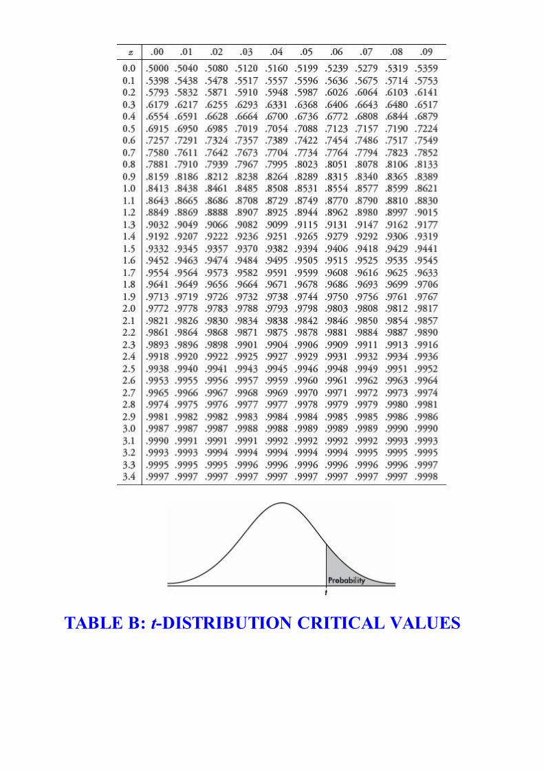
TABLE B: t-DISTRIBUTION CRITICAL VALUES

TABLE C: χ2 CRITICAL VALUES
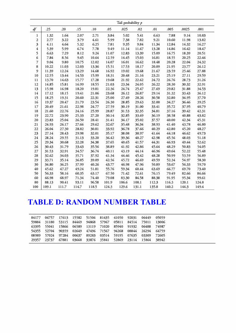
TABLE D: RANDOM NUMBER TABLE

Answers Explained, Section I1. (A) Without knowing the actual number of points scored each season,
only proportions, not numbers of points, can be compared betweenseasons.

2. (C) The critical t-values with df = 20 – 2 = 18 are ± 2.878. Thus, we
have b1 ± t* × SE(b1) = 4.0133 ± (2.878)(0.4922).

3. (A) The shortest sequence has a greater probability than any longer
sequence.

4. (A) Power, the probability of rejecting a false null hypothesis, will
be the greatest for parameter values farthest from the hypothesized value,in the direction of the alternative hypothesis.

5. (A) A simple random sample may or may not be representative of the
population. It is a method of selection in which every possible sample ofthe desired size has an equal chance of being selected.
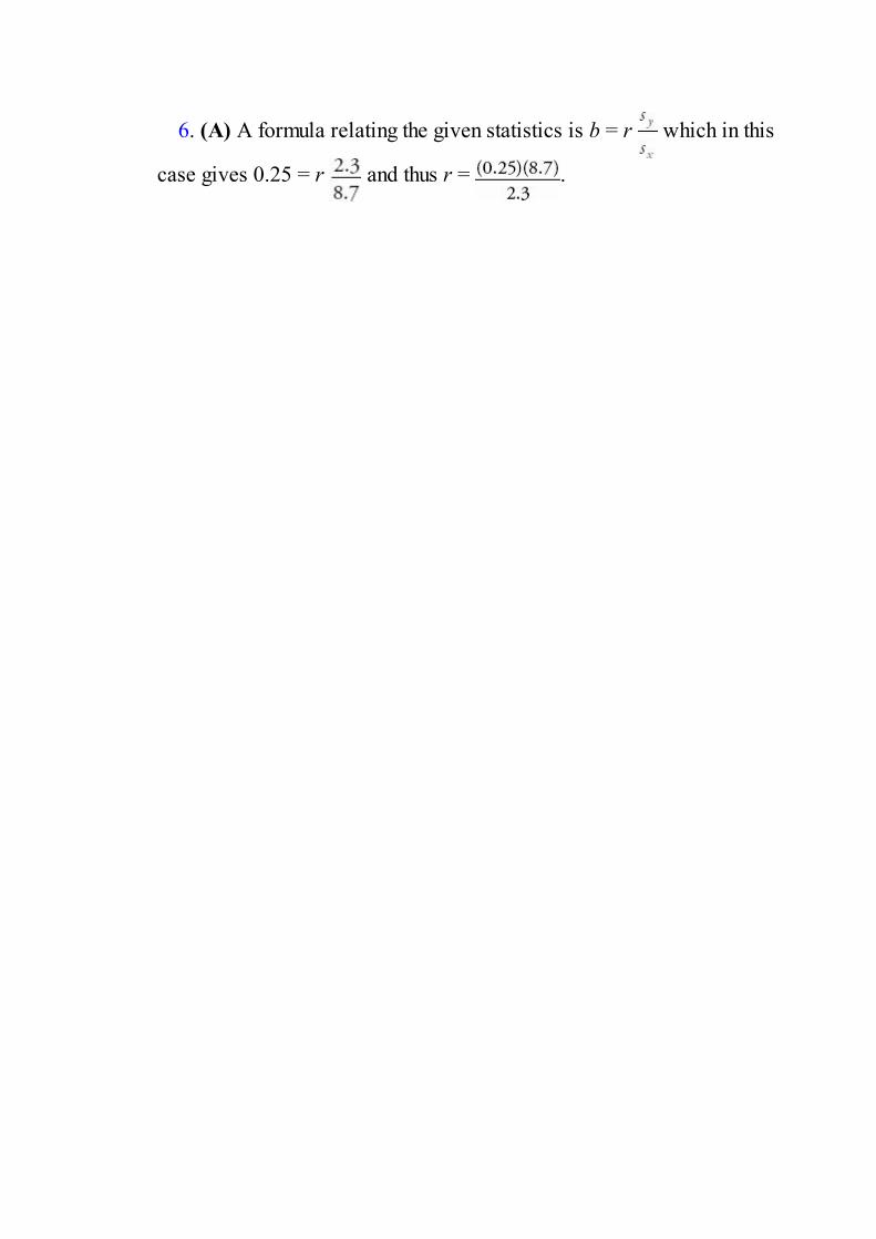
6. (A) A formula relating the given statistics is b = r which in this
case gives 0.25 = r and thus r = .

7. (B) The null hypothesis is that the new medication is no better than
insulin injection, while the alternative hypothesis is that the newmedication is better. A Type I error means a mistaken rejection of a truenull hypothesis.

8. (D) A Type II error means a mistaken failure to reject a false null
hypothesis.

9. (C) Running a hypothesis test at the 5% significance level means that
the probability of committing a Type I error is .05. Then the probability ofnot committing a Type I error is .95. Assuming the tests are independent,the probability of not committing a Type I error on any of the five tests is(.95)5 = .77378, and the probability of at least one Type I error is 1 –.77378 = .22622.
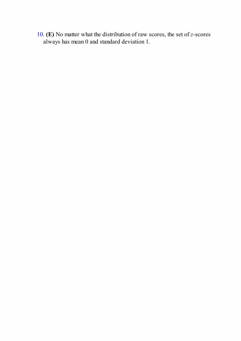
10. (E) No matter what the distribution of raw scores, the set of z-scores
always has mean 0 and standard deviation 1.

11. (B) In the sampling distribution of , the mean is equal to the population
mean, and the standard deviation is equal to the population standarddeviation divided by the square root of the sample size, in this case, σ =
= 0.986.

12. (E) The standard deviation can never be negative.

13. (E) When a complete census is taken (all 423 seniors were in the study),
the population proportion is known and a confidence interval has nomeaning.
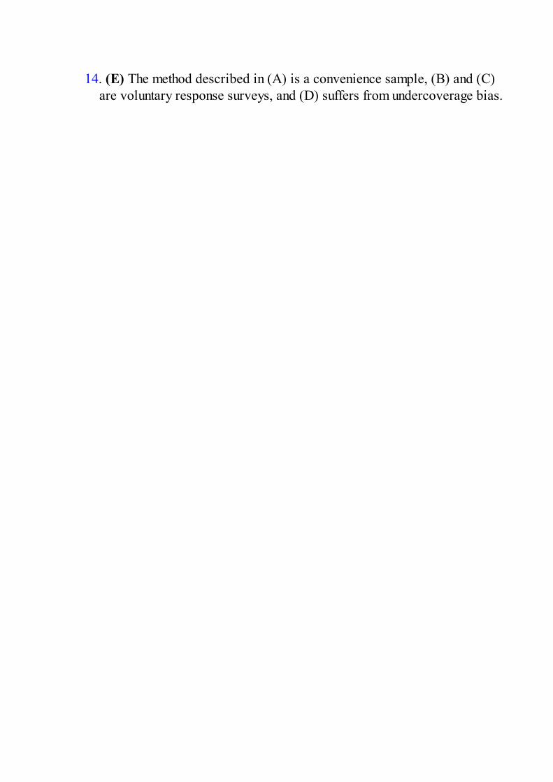
14. (E) The method described in (A) is a convenience sample, (B) and (C)
are voluntary response surveys, and (D) suffers from undercoverage bias.

15. (D) Since each set is normally distributed so is the set of differences, X1
– X2. We calculate µx1 σ x2
= 1758 – 1725 = 33 and σx1 – x2
=
= 312.0. So P(X1 – X2) = P(X1 – X2 > 0) = P =
P(z > –0.1058) = 0.542.

16. (E) With df = n – 1 = 10 – 1 = 9 and 95% confidence, the critical t-
values are ±2.262. Also SE( ) = = .

17. (A) P(X = 1) = , P(X = 2) = , P(X = 3) = ,
P(X = 4) = , P(X = 5) = , . . . , and we see that the
distribution has its maximum value at X = 1.

18. (B) The chi-square tests all involve counts, and comparing means
doesn’t make sense in this context.

19. (A) The median of X is –2, and this is also true of distribution 1 (note
that a horizontal line from 0.5 strikes curve 1 above –2 on the x-axis). Yhas a smaller standard deviation than Z (tighter clustering around themean), so Y must correspond to distribution 2, which shows almost allvalues are between –1 and 1.

20. (E)
P(B-ball) = (.55)(.30) + (.45)(.20)
P(male|B-ball) =

21. (C) Adding the same constant to every value in a set adds the same
constant to the mean but leaves the standard deviation unchanged.Multiplying every value in a set by the same constant multiplies the meanand standard deviation by that constant. So the new mean is 5/9 × (78.35– 32) + 273 = 298.75, and the new standard deviation is 5/9 × 6.3 = 3.5.

22. (B) Design 2 is an example of a matched pairs design, a special case of
a block design; here, each subject is compared to itself with respect to thetwo treatments. Both designs definitely use randomization with regard toassignment of treatments, but since they do not use randomization inselecting subjects from the general population, care must be taken ingeneralizing any conclusions. It’s not clear whether or not the researcherswho do the observations and measurements know which treatmentindividual cows are receiving, so there is no way to conclude if there isor is not blinding. The two sources of BVH are different treatments, andso they are not being confounded. In both designs treatments are randomlyapplied, so neither is an observational study.
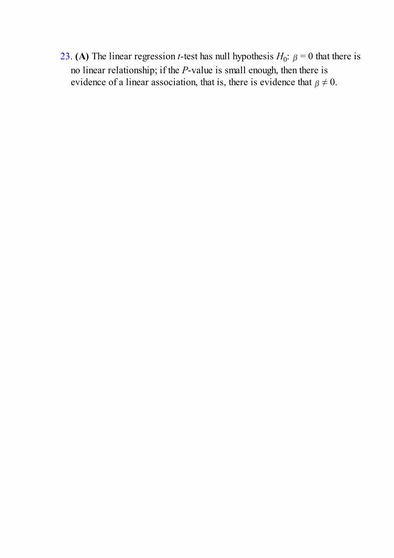
23. (A) The linear regression t-test has null hypothesis H0: = 0 that there is
no linear relationship; if the P-value is small enough, then there isevidence of a linear association, that is, there is evidence that ≠ 0.

24. (A) We have a binomial distribution with mean = np = 12 = 2.
Answer (A) is the only reasonable choice.

25. (B) The size of the sample always matters; the larger the sample, the
greater the power of statistical tests. One percent of a large population islarge. Larger samples are better, but if the sample is greater than 10% ofthe population, the best statistical techniques are not those covered in theAP curriculum.

26. (E) The points on the scatterplot all fall on the straight line:
Female length = Male length + 0.5

27. (A) and expected are found by multiplying
the proportions times the sample size of 100.

28. (D) The distributions in (A), (B), and (C) appear roughly symmetric, so
the mean and median will be roughly the same. The distribution in (D) isskewed to the right, so the mean will be greater than the median, while thedistribution in (E) is skewed to the left, so the mean will be less than themedian.

29. (C) This is a binomial with n = 10 and p = .38, so the mean is np =
10(.38) = 3.8.

30. (E) Answers (A), (B), and (C) are common misconceptions. Since the
95% confidence interval contains 80, a two-sided test would not besignificant at the 5% significance level or lower. The interval can beexpressed as 77.5 ± 3, that is, we are 95% confident that the true meanfastball speed is within 3 mph of 77.5 mph.

31. (A) Residual = Observed – Predicted, so 1.0 = 11 – Predicted and
Predicted =10.

32. (B) Stratified sampling is when the population is divided into
homogeneous groups (the three Divisions in this example), and a randomsample of individuals is chosen from each group.
33. (D) There are 8 outcomes {TTT, TTH, THT, THH, HTT, HTH, HHT,
HHH}, so P(0 heads) = 1/8, P(1 head) = 3/8, P(2 heads) = 3/8, and P(3heads) = 1/8. Thus, we assign one digit to the results of 0 heads and 3heads and 3 digits to the results of 1 head and 2 heads and ignore the other2 digits (of the 10 available digits).
34. (A) The margin of error, ±t * , depends on the sample size, not the
population size.

35. (B) We have (Q1 + Q3)/2 = 20 or Q3 + Q1 = 40, and Q3 – Q1 = 20, which
algebraically gives Q1 = 10 and Q3 = 30 [add the equations to obtain 2Q3= 60 so Q3 = 30; then plugging into either equation and solving for Q1gives Q1 = 10.]

36. (E) The larger the sample size, the closer the sample distribution is to
the population distribution. The central limit theorem roughly says that ifmultiple samples of size n are drawn randomly and independently from apopulation, then the histogram of the means of those samples will beapproximately normal. Statistics have probability distributions calledsampling distributions. The standard error is based on the spread of thepopulation and on the sample size. The central limit theorem does notapply to all statistics as it does to sample means. Many samplingdistributions are not normal; for example, the sampling distribution of thesample max is not a normal distribution. An estimator of a parameter isunbiased if we have a method that, through repeated samples, is onaverage the same value as the parameter.

37. (A) With 0.068 in a tail, the confidence interval with 34 at one end
would have a confidence level of 1 – 2(0.068) = .864, so anything higherthan 86.4% confidence will contain 34.

38. (C) From a boxplot there is no way of telling if a distribution is bell-
shaped (very different distributions can have the same five-numbersummary). Distribution I appears strongly skewed right, and so its mean isprobably much greater than its median, while distribution II appearsroughly symmetric, and so its mean is probably close to its median. Theinterquartile range, not the range, in I is 13.

39. (C) To make money, there must be more wins than losses, so with 50
plays, we need to calculate P(X > 25). We have a binomial distributionwith n = 50 and probability of success p = 18/38. On a calculator such asthe TI-84 we find P(X > 25) = 1 – P(X ≤ 25) = 1–binomcdf (50, 18/38,25) = 0.303. [or on the Nspire: binomcdf (50, 18/38, 26, 50)].

40. (B) and cell calculations [expected value of
a cell equals (row total)(column total)/(table total)] or χ2-test on acalculator such as the TI-84 will yield expected cells of 29, 36, 35, 29,36, 35.

Answers Explained, Section II1. (a) There are 2 × 2 × 2 = 8 different treatments:
Two-day, aerobic, with adjuvantTwo-day, aerobic, without adjuvantTwo-day, anaerobic, with adjuvantTwo-day, anaerobic, without adjuvantFive-day, aerobic, with adjuvantFive-day, aerobic, without adjuvantFive-day, anaerobic, with adjuvantFive-day, anaerobic, without adjuvant
(b) We must randomly assign the treatment combinations to the beds.
(Roses have already been randomly assigned to the beds.) With 8treatments and 16 beds, each treatment should be assigned to 2 beds.For example, give each bed a random number between 1 and 16 (norepeats), and then assign the first treatment in the above list to the bedswith the numbers 1 and 2, assign the second treatment in the above listto the beds with the numbers 3 and 4, and so on.
(c) Using only mini-pink roses in this experiment gives reduced
variability and increases the likelihood of determining differencesamong the treatments.
(d) Using only mini-pink roses in this experiment limits the scope
and makes it difficult to generalize the results to other species of roses.
Scoring
Part (a) is essentially correct for correctly listing all eight treatmentcombinations and is incorrect otherwise.
Part (b) is essentially correct if each treatment combination is randomlyassigned to two beds of roses. Part (b) is partially correct if eachtreatment is randomly assigned to two beds but the method is unclear, orif a method of randomization is correctly described but the method maynot assure that each treatment is assigned to two beds.

Part (c) is essentially correct for noting reduced variability and forexplaining that this increases likelihood of determining differencesamong the treatments. Part (c) is partially correct for only one of thesetwo components.
Part (d) is essentially correct noting limited scope and for explainingthat this makes generalization to other species difficult. Part (d) ispartially correct for only one of these two components.
Count partially correct answers as one-half an essentially correctanswer.
4 Complete Answer Four essentially correct answers.3 Substantial Answer Three essentially correct answers.2 Developing Answer Two essentially correct answers.1 Minimal Answer One essentially correct answer.
Use a holistic approach to decide a score totaling between twonumbers.

TIPGraders want to give you credit. Help them! Make themunderstand what you are doing, why you are doing it, and howyou are doing it. Don’t make the reader guess at what you aredoing. Communication is just as important as statisticalknowledge!

2. Part 1: State the correct hypotheses.H0 : = 82 and Ha : > 82
Part 2: Identify the correct test and check assumptions.
One-sample t-test with
Assumptions: Random sample (given) and either a normal populationdistribution or a large sample (in this case, the sample size, n = 47, islarge).
Part 3: Correctly calculate the test statistic t, the degrees of freedom df,and the p-value.
t = = 3.02, df = 47 – 1 = 46, and p = .002
Part 4: Using the p-value, give a correct conclusion in context. With thissmall a p-value, p = .002, there is strong evidence to reject H0 andconclude that there is strong evidence that his speed with the new racquetis an improvement over the old.
Scoring
Part 1 either is essentially correct or is incorrect.
Part 2 is essentially correct if the test is correctly identified by name orformula and the assumptions are checked. Part 2 is partially correct ifonly one of these two elements is correct.
Part 3 is essentially correct if the t-value is calculated and both df and pare stated. Part 3 is partially correct if only one of these two elements iscorrect.

Part 4 is essentially correct if the correct conclusion is given in contextand the conclusion is linked to the p-value. Part 4 is partially correct ifthe correct conclusion is given in context but there is no linkage to thep-value.
Count partially correct answers as one-half an essentially correctanswer.
4 Complete Answer Four essentially correct answers.3 Substantial Answer Three essentially correct answers.2 Developing Answer Two essentially correct answers.1 Minimal Answer One essentially correct answer.
Use a holistic approach to decide a score totaling between twonumbers.
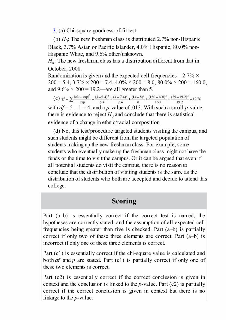
3. (a) Chi-square goodness-of-fit test(b) H0: The new freshman class is distributed 2.7% non-Hispanic
Black, 3.7% Asian or Pacific Islander, 4.0% Hispanic, 80.0% non-Hispanic White, and 9.6% other/unknown.Ha: The new freshman class has a distribution different from that inOctober, 2008.Randomization is given and the expected cell frequencies—2.7% ×200 = 5.4, 3.7% × 200 = 7.4, 4.0% × 200 = 8.0, 80.0% × 200 = 160.0,and 9.6% × 200 = 19.2—are all greater than 5.
(c)
with df = 5 – 1 = 4, and a p-value of .013. With such a small p-value,there is evidence to reject H0 and conclude that there is statisticalevidence of a change in ethnic/racial composition.
(d) No, this test/procedure targeted students visiting the campus, andsuch students might be different from the targeted population ofstudents making up the new freshman class. For example, somestudents who eventually make up the freshman class might not have thefunds or the time to visit the campus. Or it can be argued that even ifall potential students do visit the campus, there is no reason toconclude that the distribution of visiting students is the same as thedistribution of students who both are accepted and decide to attend thiscollege.
Scoring
Part (a–b) is essentially correct if the correct test is named, thehypotheses are correctly stated, and the assumption of all expected cellfrequencies being greater than five is checked. Part (a–b) is partiallycorrect if only two of these three elements are correct. Part (a–b) isincorrect if only one of these three elements is correct.
Part (c1) is essentially correct if the chi-square value is calculated andboth df and p are stated. Part (c1) is partially correct if only one ofthese two elements is correct.
Part (c2) is essentially correct if the correct conclusion is given incontext and the conclusion is linked to the p-value. Part (c2) is partiallycorrect if the correct conclusion is given in context but there is nolinkage to the p-value.

Part (d) is essentially correct or incorrect. It is essentially correct forboth stating that the intended population is not targeted and giving aclear argument for this answer.
A partially correct answer counts half of an essentially correct answer.
4 Complete Answer Four essentially correct answers.3 Substantial Answer Three essentially correct answers.2 Developing Answer Two essentially correct answers.1 Minimal Answer One essentially correct answer.
Use a holistic approach to decide a score totaling between twonumbers.

4. (a) P(x > 2400) = = P(z > 0.6484) = .258
(b) P(at least 3 out of 5 are > 2400) = 10(.258)3(.742)2 +5(.258)4(.742) + (.258)5 = .112[On the TI-84, 1 – binomcdf(5,.258,2) = .112]
(c) The distribution of is normal with mean = 2317 andstandard deviation
= 57.24. So
P( > 2400) = = P(z > 1.450) = .0735
Scoring
Part (a) is essentially correct if the correct probability is calculated andthe derivation is clear. Simply writing normalcdf(2400,∞,2317,128) =.258 is a partially correct response.
Part (b) is essentially correct if the correct probability is calculated andthe derivation is clear. Part (b) is partially correct for indicating abinomial with n = 5 and p = answer from (a) but calculating incorrectly.Simply writing 1-binomcdf(5,.258,2) = .112 is also a partially correctresponse.
Part (c) is essentially correct for specifying both and σ andcorrectly calculating the probability. Part (c) is partially correct forspecifying both and σ but incorrectly calculating the probability,or for failing to specify both and σ but correctly calculating theprobability.
4 Complete Answer All three parts essentially correct.
3 Substantial Answer Two parts essentially correct andone part partially correct.
2 Developing Answer
Two parts essentially correct ORone part essentially correct and oneor two parts partially correct ORall three parts partially correct.

1 Minimal Answer One part essentially correct OR twoparts partially correct.

5. (a) xP(x) = 135p + (–35)(1 – p) = –35 + 170p(b) xP(x) = (–5)p + 25(1 – p) = 25 – 30p(c) –35 + 170p = 25 – 30p gives p = .3. When p > .3, the expected
return for oil paintings is greater than that for finger paintings, andwhen p < .3, the expected return for finger paintings is greater than foroil paintings. (These statements follow from the positive slope of R =–35 + 170p and the negative slope of R = 25 – 30p.)
(d) First, name the confidence interval: a 95% confidence intervalfor the proportion p of similar establishments with tourists who wereprimarily art collectors.Second, check conditions: We are given that this is a random sample,it is reasonable to assume that the sample is less than 10 percent of allsimilar establishments, and the sample size is large enough (np = 33and n(1 – p) = 117 are both greater than 10).
Third, demonstrate correct mechanics: With , we have
Fourth, interpret in context: We are 95% confident that the trueproportion of similar establishments with tourists who were primarilyart collectors is between .154 and .286.
(e) The entire interval in (d) is below p = .3, so based on (c), theexpected return for finger paintings is greater than for oil paintings forall p in this interval.
Scoring
Parts (a) and (b) are scored together. They are essentially correct ifboth answers are correct and partially correct if one answer is correct.
Part (c) is essentially correct for a correct calculation of theintersection together with a correct conclusion of what it means when pis greater or less than .3. Part (c) is partially correct if the intersectionis not correctly calculated, but the conclusions are correct based on theincorrect intersection value.
Part (d) is essentially correct if steps 2, 3, and 4 are correct. (Step 1 is

only a restatement from the question.) Part 3 is partially correct if onlytwo of these three steps are correct.
Part (e) is essentially correct if the correct conclusion is given withclear linkage to the results from both (c) and (d). Part (e) is partiallycorrect if the explanation of the linkage is present but weak.
Give 1 point for each essentially correct part and ½ point for eachpartially correct part.
4 Complete Answer 4 points3 Substantial Answer 3 points2 Developing Answer 2 points1 Minimal Answer 1 point
Use a holistic approach to decide a score totaling between twonumbers.

TIPRead carefully and recognize that sometimes very differenttests are required in different parts of the same problem.

6. (a) Salary and years of experience exhibit an approximately linearrelationship. As years of experience increase, so does the mediansalary. The third-quartile, Q3, salary also increases with years, and sodoes the Q1 salary with the exception of one year. As years ofexperience increase, there are only minor differences in measures ofvariability in the salaries, with roughly the same range (except for thelast two) and fairly consistent interquartile ranges.
(b) First, the boxplots indicate that an overall scatterplot patternwould be roughly linear. Second, the residual plot shows no pattern.Third, the histogram of residuals appears roughly normal (unimodal,symmetric, and without clear skewness or outliers).
(c) With df = 98 and .025 in each tail, the critical t-values are±1.984. b1 ± tsb1
= 0.910 ± 1.984(0.03273) = 0.910 ± .065. We are95% confident that for each additional year of experience, the averageincrease in salary is between $845 and $975.
(d) The sum and thus the mean of the residuals is always 0. Thestandard deviation of the residuals is σ, which can be estimated with s= 0.9402. With a roughly normal distribution, we have P(X ≥ 1) = .14.
Scoring
Part (a) is essentially correct for correctly noting a linear relationship,noting that as years of experience increase so does the median salary(or Q3 or generally Q1), and noting that measures of variability (rangeor IQR) stay roughly the same. Part (a) is partially correct for correctlynoting two of the three features.
Part (b) is essentially correct for noting the three conditions (roughlylinear scatterplot, no pattern in the residual plot, and roughly normalhistogram of residuals). Part (b) is partially correct for correctly notingtwo of the three conditions.
Part (c) is essentially correct for both a correct calculation of theconfidence interval and a correct interpretation in context. Part (c) ispartially correct for a correct calculation without the interpretation incontext, or for a correct interpretation based on an incorrect calculation.
Part (d) is essentially correct noting that the distribution of residuals is
roughly normal with mean 0 and standard deviation 0.9402, and thenusing this to correctly calculate the probability. Part (d) is partiallycorrect for correctly noting the distribution of residuals but incorrectlycalculating the probability, or for making a calculation based on anormal distribution with mean 0 but using an incorrect standarddeviation.
Count partially correct answers as one-half an essentially correctanswer.
4 Complete Answer Four essentially correct answers.3 Substantial Answer Three essentially correct answers.2 Developing Answer Two essentially correct answers.1 Minimal Answer One essentially correct answer.
Use a holistic approach to decide a score totaling between twonumbers.

Answers Explained, Multiple-Choice1. (B) There is no such thing as being skewed both left and right.

2. (C) Stemplots are not used for categorical data sets and are toounwieldy to be used for very large data sets.

3. (B) The vertical axis, starting at $77,000, results in a misleadingsales picture. It would be better to start at $0, not $78,000.

4. (C) Labeling the horizontal axis with different year spans results in amisleading picture. The number of indictments per year is actuallyincreasing.
5. (B) In general, histograms give information about relativefrequencies, not actual frequencies.
6. (C) Symmetric histograms can have any number of peaks. All normalcurves are bell-shaped and symmetric, but not all symmetric bell-shapedcurves are normal.

7. (B) Incomes and home prices tend to have a few very high scoresthat make the distributions skewed to the right. Teenage drivers mostlyhave ages in the last teenage years with a scattering of younger drivers,and thus a distribution skewed to the left.

8. (A) Choice of width and number of classes changes the appearanceof a histogram. Displaying outliers is more problematic with histograms.Histograms do not show individual observations.
9. (C) The median score splits the area in half, and so the median is not75. The area between 50 and 60 is greater than the area between 90 and100 but is less than the area between 60 and 100.
10. (B) A histogram with little area under the curve early and muchgreater area later results in a cumulative relative frequency plot whichrises slowly at first and then at a much faster rate later.

11. (C) A histogram with large area under the curve early and muchless area later results in a cumulative relative frequency plot which risesquickly at first and then at a much slower rate later.
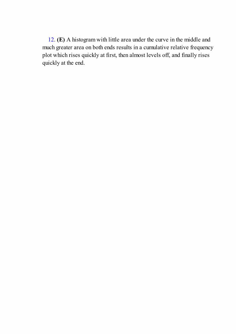
12. (E) A histogram with little area under the curve in the middle andmuch greater area on both ends results in a cumulative relative frequencyplot which rises quickly at first, then almost levels off, and finally risesquickly at the end.

13. (D) A histogram with little area under the curve on the ends andmuch greater area in the middle results in a cumulative relative frequencyplot which rises slowly at first, then quickly in the middle, and finallyslowly again at the end.

14. (A) Uniform distributions result in cumulative relative frequencyplots which rise at constant rates, thus linear.
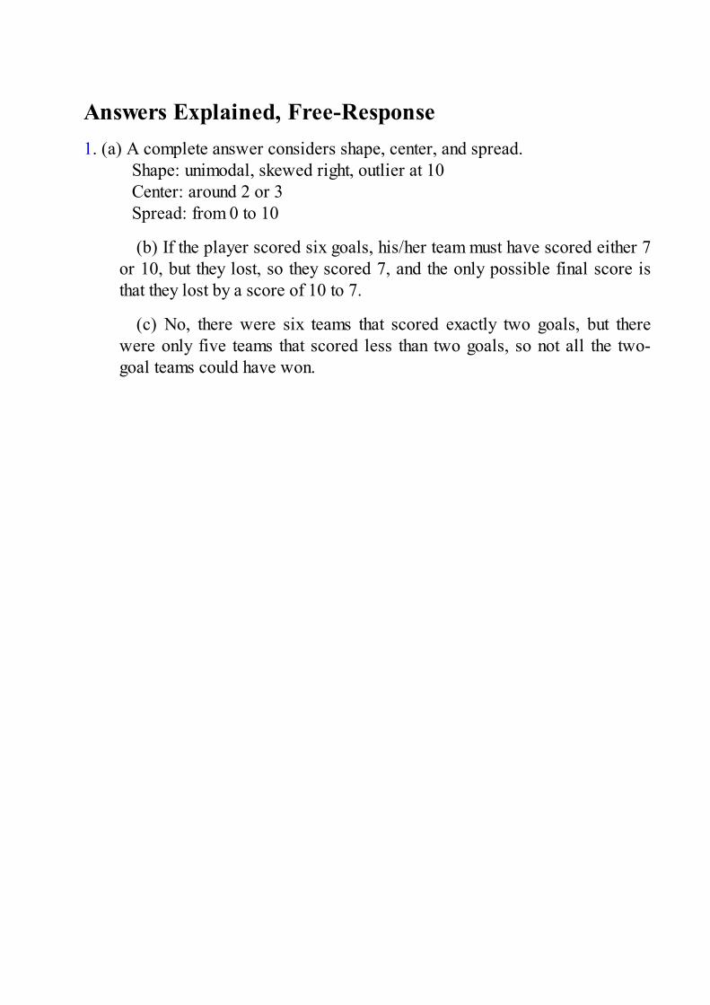
Answers Explained, Free-Response1. (a) A complete answer considers shape, center, and spread.
Shape: unimodal, skewed right, outlier at 10Center: around 2 or 3Spread: from 0 to 10
(b) If the player scored six goals, his/her team must have scored either 7or 10, but they lost, so they scored 7, and the only possible final score isthat they lost by a score of 10 to 7.
(c) No, there were six teams that scored exactly two goals, but therewere only five teams that scored less than two goals, so not all the two-goal teams could have won.

2. (a) The lowest winning percentage over the past 22 years is 46.0%.
(b) A complete answer considers shape, center, and spread.Shape: two clusters, each somewhat bell-shapedCenter: around 50%Spread: from 46.0 to 55.6%
(c) The team had more losing seasons (13) than winning seasons (9).
(d) The cluster of winning percentages is further above 50% than thecluster of losing percentages is below 50%.

3. (a) 40% of the players averaged fewer than 20 points per game.
(b) All the players averaged at least 3 points per game.
(c) No players averaged between 5 and 7 points per game because thecumulative relative frequency was 10% for both 5 and 7 points.
(d) Go over to the plot from 0.9 on the vertical axis, and then down tothe horizontal axis to result in 28 points per game.
(e) Reading up to the plot and then over from 10 and from 20 shows that0.25 of the players averaged under 10 points per game and 0.4 of theplayers averaged under 20 points per game. Thus, 0.4 – 0.25 = 0.15 givesthe proportion of players who averaged between 10 and 20 points pergame.

Answers Explained, Multiple-Choice1. (D) The distribution is clearly skewed right, so the mean is greater
than the median, and the ratio is greater than one.
2. (E) All elements of the sample are taken from the population, and sothe smallest value in the sample cannot be less than the smallest value inthe population; similarly, the largest value in the sample cannot be greaterthan the largest value in the population. The interquartile range is the fulldistance between the first quartile and the third quartile. Outliers areextreme values, and while they may affect the range, they do not affect theinterquartile range when the lower and upper quarters have been removedbefore calculation.

3. (E) Outliers are any values below Q1 – 1.5(IQR) = 5.5 or above Q3+ 1.5(IQR) = 57.5.
4. (A) The value 50 seems to split the area under the histogram in two,so the median is about 50. Furthermore, the histogram is skewed to the leftwith a tail from 0 to 30.
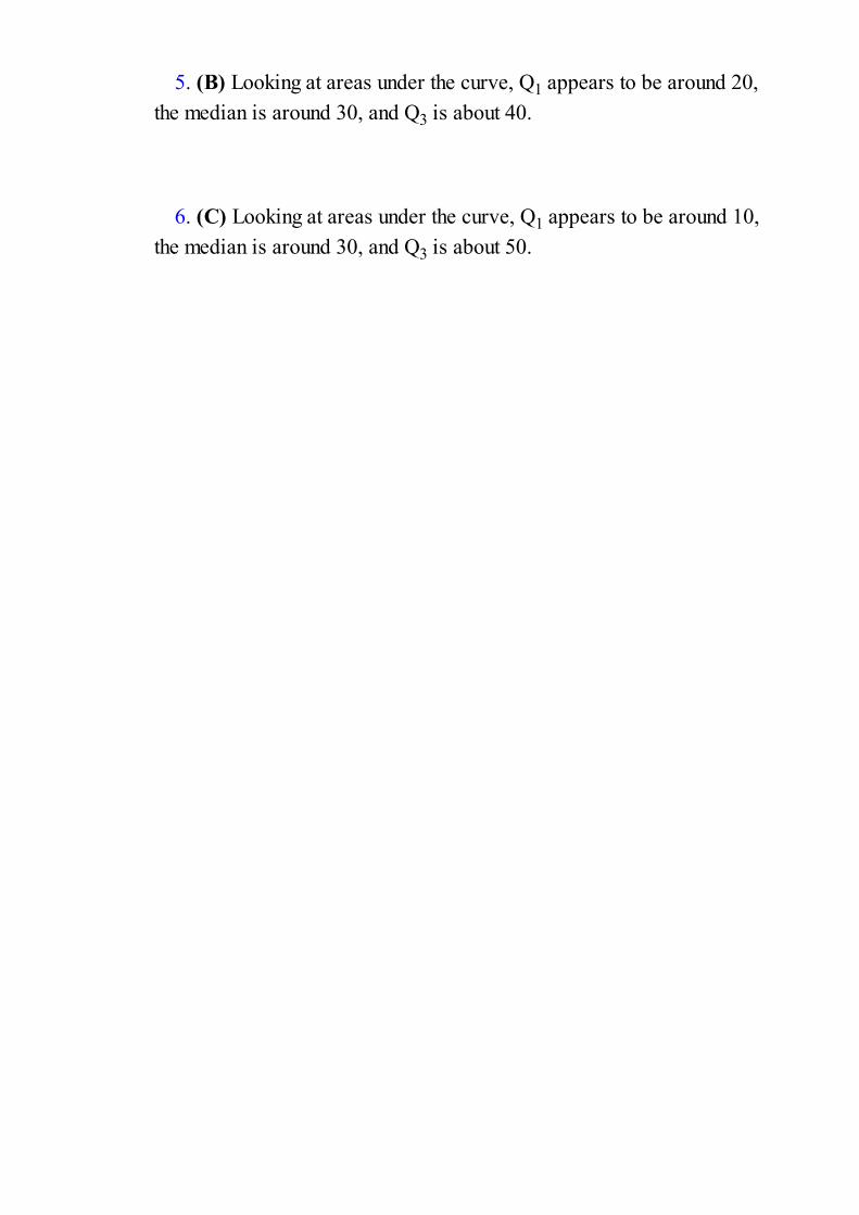
5. (B) Looking at areas under the curve, Q1 appears to be around 20,the median is around 30, and Q3 is about 40.
6. (C) Looking at areas under the curve, Q1 appears to be around 10,the median is around 30, and Q3 is about 50.
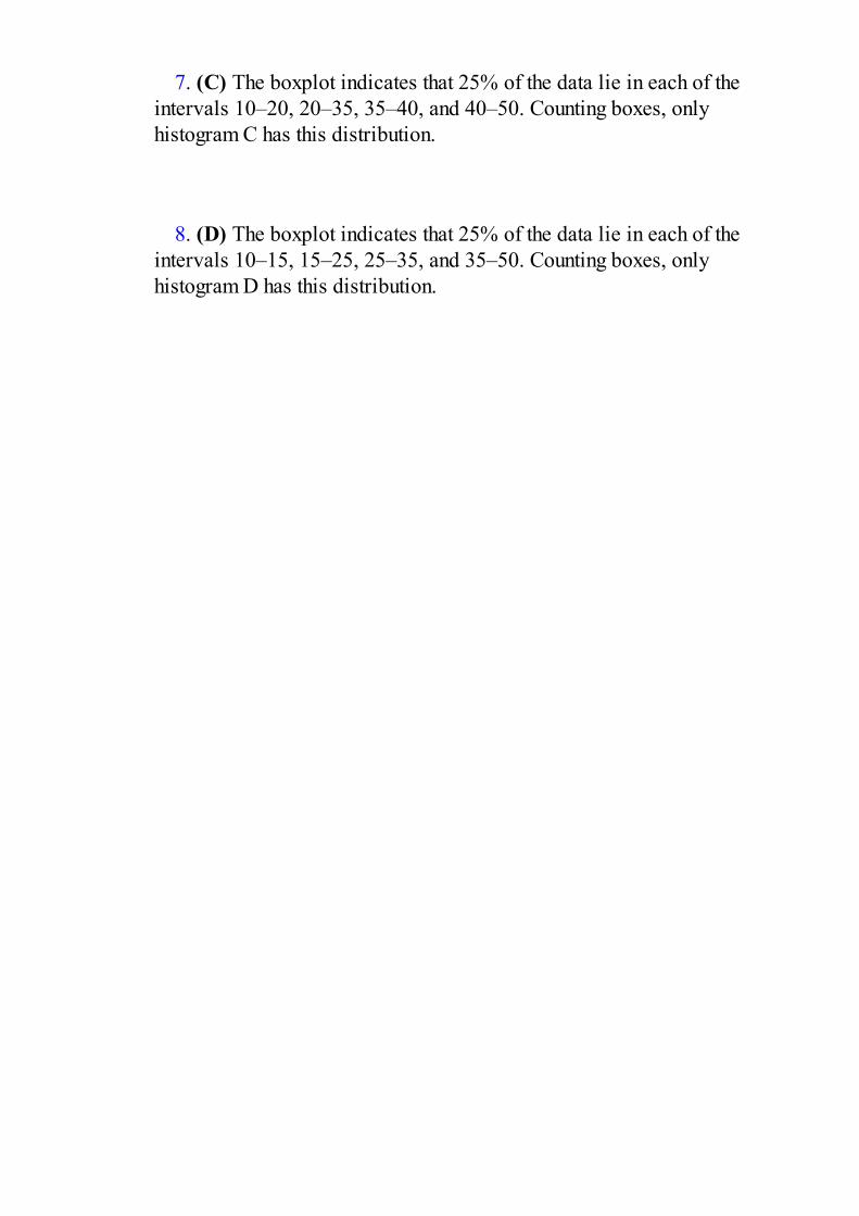
7. (C) The boxplot indicates that 25% of the data lie in each of theintervals 10–20, 20–35, 35–40, and 40–50. Counting boxes, onlyhistogram C has this distribution.
8. (D) The boxplot indicates that 25% of the data lie in each of theintervals 10–15, 15–25, 25–35, and 35–50. Counting boxes, onlyhistogram D has this distribution.

9. (E) The boxplot indicates that 25% of the data lie in each of theintervals 10–20, 20–30, 30–40, and 40–50. Counting boxes, onlyhistogram E has this distribution.
10. (A) Subtracting 10 from one value and adding 5 to two valuesleaves the sum of the values unchanged, so the mean will be unchanged.Exactly what values the outliers take will not change what value is in themiddle, so the median will be unchanged.

11. (C) The high outlier is further from the mean than is the low outlier,so removing both will decrease the mean. However, removing the lowestand highest values will not change what value is in the middle, so themedian will be unchanged.
12. (C) Adding the same constant to every value increases the mean bythat same constant; however, the distances between the increased valuesand the increased mean stay the same, and so the standard deviation isunchanged. Graphically, you should picture the whole distribution asmoving over by a constant; the mean moves, but the standard deviation(which measures spread) doesn’t change.

13. (E) Multiplying every value by the same constant multiplies boththe mean and the standard deviation by that constant. Graphically,increasing each value by 25% (multiplying by 1.25) both moves andspreads out the distribution.
14. (E) The median is somewhere between 20 and 30, but notnecessarily at 25. Even a single very large score can result in a mean over30 and a standard deviation over 10.

15. (B) The median is less than the mean, and so the responses areprobably skewed to the right; there are a few high guesses, with most ofthe responses on the lower end of the scale.
16. (A) Given that the empirical rule applies, a z-score of –1 has apercentile rank of about 16%. The first quartile Q1 has a percentile rankof 25%.
17. (C) If the variance of a set is zero, all the values in the set areequal. If all the values of the population are equal, the same holds true forany subset; however, if all the values of a subset are the same, this maynot be true of the whole population. If all the values in a set are equal, themean and the median both equal this common value and so equal eachother.
18. (D) Stemplots and histograms can show gaps and clusters that arehidden when one simply looks at calculations such as mean, median,standard deviation, quartiles, and extremes.

19. (B) There are a total of 10 + 17 + 25 + 38 + 27 + 21 + 12 = 150students. Their total salary is 10(15,000) + 17(20,000) + 25(25,000) +38(30,000) + 27(35,000) + 21(40,000) + 12(45,000) = $4,580,000. Themean is = $30,533.
20. (E) The mean, standard deviation, variance, and range are allaffected by outliers; the median and interquartile range are not.

21. (C) Because of the squaring operation in the definition, the standarddeviation (and also the variance) can be zero only if all the values in theset are equal.
22. (A) The sum of the scores in one class is 20 × 92 = 1840, while thesum in the other is 25 × 83 = 2075. The total sum is 1840 + 2075 = 3915.There are 20 + 25 = 45 students, and so the average score is = 87.
23. (A) A distribution spread thinly on the high end is a skeweddistribution with the mean greater than the median.

24. (E) None are reasonable because we are not looking at a randomsample of states but rather only at the seven lowest values, that is, at thevery low end of the tail of the whole distribution. (The distribution wasactually skewed to the right, with California having 159,700 bankruptcies,followed by New York with 51,300, and all other states below 50,000.)

25. (B) Increasing every value by 5 gives 10% between 45 and 65, andthen doubling gives 10% between 90 and 130.
26. (A) A distribution spread thinly on the high end is a skeweddistribution with the mean greater than the median.

27. (E) All three statements are true.
28. (A) Dotplots and stemplots retain the identity of individual scores;however, histograms and boxplots do not.

29. (A) 206 + 2.69(35) = 300; 206 – 1.13(35) = 166.
30. (A) Bar charts are used for categorical variables.
31. (C) The median corresponds to the 0.5 cumulative proportion.
32. (A) The 0.25 and 0.75 cumulative proportions correspond to Q1 =1.8 and Q3 = 2.8, respectively, and so the interquartile range is 2.8 – 1.8= 1.0.
33. (B) With bell-shaped data the empirical rule applies, giving that thespread from 92 to 98 is roughly 6 standard deviations, and so one SD isabout 1.

Answers Explained, Free-Response1. (a) Adding 10 to each value increases the mean by 10, but leaves measures of
variability unchanged, so the new mean is 340 hours while the range staysat 5835 hours, the standard deviation remains at 245 hours, and thevariance remains at 2452 = 60,025 hr2.
(b) Increasing each value by 10% (multiplying by 1.10) will increase themean to 1.1(330) = 363 hours, the range to 1.1(5835) = 6418.5 hours, thestandard deviation to 1.1(245) = 269.5 hours, and the variance to (269.5)2
= 72,630.25 hr2. (Note that the variance increases by a multiple of (1.1)2
not by a multiple of 1.1.)

2. (a) Check for outliers: IQR = 82.6 – 60.4 = 22.2. Q1 – 1.5(IQR) = 27.1 whileQ3 + 1.5(IQR) = 115.9, so the only outlier is 26.4.
(b) A complete answer considers shape, center, and spread.
Shape: appears skewed left with an outlier at 26.4Center: median is 78.0Spread: from 26.4 to 98.1
(c) When the distribution is skewed left, the mean is usually less than themedian.
(d) A stemplot would show more information because it shows all theoriginal data, not just the few values given above; a stemplot can showclusters and gaps which are hidden by a boxplot.
3. (a) The median is 77.5 (millions of dollars), and the IQR = Q3 – Q1 = 159.2 –33.4 = 125.8 (millions of dollars).
(b) Reducing every value by 3 will reduce the median by 3 but leavemeasures of variability unchanged, so the new mean is 77.5 – 3 = 74.5(millions of dollars), and the IQR will still be 125.8 (millions of dollars).
(c) Reducing every value by 50% reduces the median to (0.5)(77.5) =38.75 (millions of dollars) and reduces the IQR to (0.5)(125.8) = 62.9(millions of dollars).
(d) The boxplot indicates that the distribution is skewed right, so themean will be greater than the median. It is unlikely that the two outlierswill pull the mean out as far as 325, so the most reasonable value for themean is 135 (millions of dollars).
4. Z-scores give the number of standard deviations from the mean, soQ1 = 300 – 0.7(25) = 282.5 and Q3 = 300 + 0.7(25) = 317.5.

The interquartile range is IQR = 317.5 – 282.5 = 35, and 1.5(IQR) =1.5(35) = 52.5.The standard definition of outliers encompasses all values less than Q1 –52.5 = 230 and all values greater than Q3 + 52.5 = 370.
Answers Explained, Multiple-Choice1. (A) The numbers of male and female employees are not given so
proportions who are executives cannot be determined.
2. (B) Both sets are symmetric about 150 and so have the same mean.Both sets have the range 170–130 = 40. Set A is much more spread outthan set B, and so set A has the greater variance.
3. (E) The empirical rule applies to bell-shaped data like those foundin set B, not in set A. For bell-shaped data, 95% of the values fall withintwo standard deviations of the mean, and 99.7% within three. However,in the histogram for set B one sees that 95% of the data are not between140 and 160 and 99.7% are not between 135 and 165. Thus the standarddeviation for set B must be greater than 5. The standard deviation for set Ais even larger, and so it too must be greater than 5.
4. (A) Both sets have 20 elements. The ranges, 76–37 = 39 and 86–47= 39, are equal. Brand A clearly has the larger mean and median, andwith its skewness it also has the larger variance.

5. (E) The minimum of the combined set of scores must be the min ofthe boys since it is lower; the maximum of the combined set of scoresmust be the max of the girls since it is higher; the first quartile must be thesame as the identical first quartiles of the two original distributions.There are no outliers (scores more than 1.5(IQR) from the first and thirdquartiles).
6. (B) Roughly 50% of total bar length is above and below the 15–19interval.

7. (B) There are about 1.2 million younger than the age of 10 in Liberia(boys and girls) and roughly 3.5 million in Canada.
8. (E) In the Canadian graph, all higher age groups show greaternumbers of women than men. In the Liberian graph, the smaller 15–19 agegroup shows a definite break with the overall pattern (a great number ofchild soldiers died in the fighting). In the Canadian graph, the narrowingbase indicates a decreasing birth rate.

Answers Explained, Free-Response1. A complete answer compares shape, center, and spread.
Shape: The “never married” and “married” distributions are skewed right(toward the higher ages), while the “once married” distribution appearsmore bell-shaped and symmetric. The “never married” has a gap between60 and 70 with a cluster between 70 and 90, while the “once married”has a small gap between 25 and 30 with perhaps outliers between 20 and25.Center: Considering the center to be a value separating the area under thehistogram roughly in half, the center of the “never married” distribution isthe least (at approximately 20), and the center of the “once married” is thegreatest (at approximately 60).Spread: The spread of the “married” distribution is the least (with arange of approximately 85 – 18 = 67), and the spread of the “nevermarried” distribution is the greatest (with a range of approximately 90 – 0= 90).
2.
Clearly the number of rebounds that the best rebounders get per game isgreater than the number of assists that the best assist leaders get per game.A complete answer compares shape, center, and spread.Shape: Both distributions are skewed right (toward higher values). Thelower 16 values of each distribution look symmetric and bell-shaped.Each distribution has a clear outlier on the upper end (summary statisticswere not asked for, but would actually have shown four upper-end

outliers in the “rebound” distribution).Center: The center of the “assists” distribution (at a little under 8) is lessthan the spread of the “rebounds” distribution (at a little under 11).Spread: The spread of the “assists” distribution (with a range of 12.3 –6.1 = 6.2) is less than the spread of the “rebounds” distribution (with arange of 16.8 – 9.4 = 7.4).
3.
A complete answer compares shape, center, and spread, and notesoutliers.Shape: The most striking aspect is how skewed to the right (towardshigher values) both sets of data appear to be.Center: The median value changed very little from 1980 to 1990 (risingslightly from 2,329,000 to 2,649,000).Spread: The difference between the lowest value and the median changedvery little between 1980 and 1990 (2,329,000 – 262,000 = 2,067,000 in1980, and 2,649,000 – 462,000 = 2,187,000 in 1990), while the upper-half spread increased substantially (from 16,873,000 – 2,329,000 =14,544,000 in 1980 to 21,926,000 – 2,649,000 = 19,277,000 in 1990).Outliers: For 1980, IQR = Q3 – Q1 = 3,749,000 – 834,000 = 2,915,000,and outliers are any values less than Q1 – 1.5(IQR) = –3,538,500 orgreater than Q3 + 1.5(IQR) = 8,121,500, so California does represent anoutlier. For 1990, IQR = Q3 – Q1 = 4,444,000 – 1,054,000 = 3,390,000,and outliers are any values less than Q1 – 1.5(IQR) = –4,031,000 orgreater than Q3 + 1.5(IQR) = 9,529,000, so again California represents anoutlier.
4. A complete answer compares shape, center, and spread.Shape: Cruise A, for which the cumulative frequency plot rises steeply at
first, has more younger passengers, and thus a distribution skewed to theright (towards the higher ages). Cruise C, for which the cumulativefrequency plot rises slowly at first and then steeply towards the end, hasmore older passengers, and thus a distribution skewed to the left (towardsthe younger ages). Cruise B, for which the cumulative frequency plot risesslowly at each end and steeply in the middle, has a more bell-shapeddistribution.Center: Considering the center to be a value separating the area under thehistogram roughly in half, the centers will correspond to a cumulativefrequency of 0.5. Reading across from 0.5 to the intersection of eachgraph, and then down to the x-axis, shows centers of approximately 18,40, and 61 years, respectively. Thus, the center of distribution A is theleast, and the center of distribution C is the greatest.Spread: The spreads of the age distributions of all three cruises are thesame: from 10 to 70 years.

Answers Explained, Multiple-Choice1. (E) The variable column indicates the independent (explanatory)
variable. The sign of the correlation is the same as the sign of the slope(negative here). In this example, the y-intercept is meaningless (predictedSAT result if no students take the exam). There can be a strong linearrelation, with high R2 value, but still a distinct pattern in the residual plotindicating that a nonlinear fit may be even stronger. The negative value ofthe slope (–2.84276) gives that the predicted combined SAT score of aschool is 2.84 points lower for each one unit higher in the percentage ofstudents taking the exam, on average.

2. (A) Slope = .15( ) ≈ 4850 and intercept = 208,000 – 4850(6.2)≈ 178,000.

3. (D) Residual = Measured – Predicted, so if the residual is negative,the predicted must be greater than the measured (observed).

4. (D) The correlation coefficient is not changed by adding the samenumber to each value of one of the variables or by multiplying each valueof one of the variables by the same positive number.

5. (E) A negative correlation shows a tendency for higher values of onevariable to be associated with lower values of the other; however, givenany two points, anything is possible.
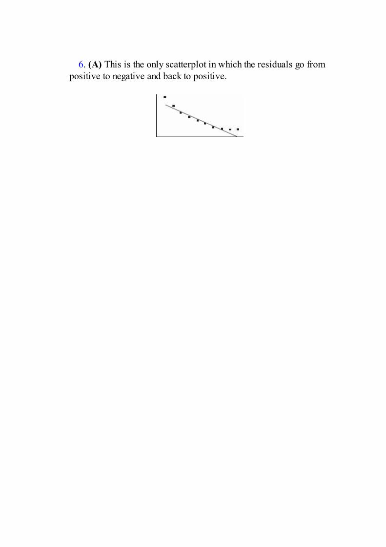
6. (A) This is the only scatterplot in which the residuals go frompositive to negative and back to positive.

7. (E) Since (2, 5) is on the line y = 3x + b, we have 5 = 6 + b and b =–1. Thus the regression line is y = 3x – 1. The point ( , ) is always onthe regression line, and so we have = 3 – 1.

8. (C) The correlation r measures association, not causation.

9. (E) The correlation r cannot take a value greater than 1.
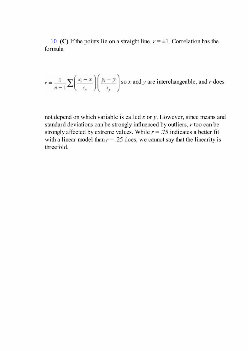
10. (C) If the points lie on a straight line, r = ±1. Correlation has theformula
so x and y are interchangeable, and r does
not depend on which variable is called x or y. However, since means andstandard deviations can be strongly influenced by outliers, r too can bestrongly affected by extreme values. While r = .75 indicates a better fitwith a linear model than r = .25 does, we cannot say that the linearity isthreefold.

11. (B) The “Predictor” column indicates the independent variable withits coefficient to the right.

12. (E)

13. (B) = 0.056 + 0.920 (0.55) = 0.562 and so the residual = 0.59– 0.562 = 0.028
14. (D) The sum and thus the mean of the residuals are always zero. Ina good straight-line fit, the residuals show a random pattern.
15. (C) The coefficient of determination r 2 gives the proportion of they-variance that is predictable from a knowledge of x. In this case r2 =(.632)2 = .399 or 39.9%.

16. (B) The point I doesn’t contribute to a line with negative or positiveslope. In none of the scatterplots do the points fall on a straight line, sonone of them have correlation 1.0.

17. (C) Predicted winning percentage = 44 + 0.0003(34,000) = 54.2,and
Residual = Observed – Predicted = 55 – 54.2 = 0.8.

18. (B) On each exam, two students had scores of 100. There is ageneral negative slope to the data showing a moderate negativecorrelation. The coefficient of determination, r 2, is always ≥ 0. Whileseveral students scored 90 or above on one or the other exam, no studentdid so on both exams.

19. (E) On the scatterplot all the points lie perfectly on a line slopingup to the right, and so r = 1.

20. (A) The correlation is not changed by adding the same number toevery value of one of the variables, by multiplying every value of one ofthe variables by the same positive number, or by interchanging the x- andy-variables.

21. (B) The slope and the correlation coefficient have the same sign.Multiplying every y-value by –1 changes this sign.

22. (E) A scatterplot readily shows that while the first three points lieon a straight line, the fourth point does not lie on this line. Thus no matterwhat the fifth point is, all the points cannot lie on a straight line, and so rcannot be 1.

23. (E) All three scatterplots show very strong nonlinear patterns;however, the correlation r measures the strength of only a linearassociation. Thus r = 0 in the first two scatterplots and is close to 1 in thethird.

24. (A) Using your calculator, find the regression line to be = 9x – 8.The regression line, also called the least squares regression line,minimizes the sum of the squares of the vertical distances between thepoints and the line. In this case (2, 10), (3, 19), and (4, 28) are on the line,and so the minimum sum is (10 – 11)2 + (19 – 17)2 + (28 – 29)2 = 6.

25. (B) When transforming the variables leads to a linear relationship,the original variables have a nonlinear relationship, their correlation(which measures linearity) is not close to 1, and the residuals do not showa random pattern. While r close to 1 indicates strong association, it doesnot indicate cause and effect.

26. (E) The least squares line passes through and the slopeb satisfies Since –1 ≤ r ≤ 1, we have .

Answers Explained, Free-Response1. (a) A calculator gives (Wins).
(b) Each additional home win raises the average attendance by about 180people, on average.
(c) 12,416 + 180.4(25) = 16,926(d) 17,000 = 12,416 + 180.4(Wins) gives Wins = 25.4 so 26 wins needed to
average at least 17,000 average attendance.(e) With 34 wins, the predicted average attendance is 12,416 + 180.4(34) =
18,550 so the residual is 18,997 – 18,550 = 447.

2. (a)
(b) A calculator gives r = .1568.(c) The correlation r is low for this number of data scores, and the scatterplot
shows no linear pattern whatsoever. Although theoretically we could useour techniques to find the best-fitting straight-line approximation, the resultwould be meaningless and should not be used for predictions.

3. (a) By visual inspection ≈ 68 and ≈ 21.(b) The range of the life expectancies is 80 – 54 = 26, and so the standard
deviation is roughly . Similarly the standard deviation of the percapita incomes is roughly .
(c) While the points generally fall from the lower left to the upper right, theyare still widely scattered. Thus the scatterplot shows a weak positivecorrelation between per capita income and life expectancy.
4. (a) The correlation for each of the three sets is 0.(b) The correlation for the set consisting of all 12 scores is .9948.(c) The data from each set taken separately show no linear pattern. However,
together they show a strong linear fit. Note the positions of the data fromthe separate sets in the complete scatterplot.

5. In the first scatterplot, the points fall exactly on a downward sloping straightline, so r = –1. In the second scatterplot, the isolated point is an influentialpoint, and r is close to +1. In the third scatterplot, the isolated point is alsoinfluential, and r is close to 0.

6. (a) = –0.16(50) + 34.8 = 26.8 miles per gallon, and = –0.0032(50)2 +0.258(50) + 23.8 = 28.7 miles per gallon.
(b) Model 2 is the better fit. First, the residuals are much smaller for model 2,indicating that this model gives values much closer to the observed values.Second, a curved residual pattern like that in model 1 indicates that anonlinear model would be better. A more uniform residual scatter as inmodel 2 indicates a better fit.

7. (a) The correlation coefficient is r = = .864. It is positive because theslope of the regression line is positive.
(b) The slope is 1.106, signifying that each additional page raises a grade by1.106.
(c) Including Mary’s paper will lower the correlation coefficient because herresult seems far off the regression line through the other points.
(d) Including Mary’s paper will swing the regression line down and lower thevalue of the slope.
(e) From the graph, Mary received an 82. From the regression line, Marywould have received = 46.51 + 1.106(45) = 96.3 if she had turned in herpaper on time.

8. (a) Yes. The residual graph is not curved, does not show fanning, and appearsto be random or scattered.
(b) The slope is 0.95893, indicating that the winning jump improves 0.95893inches per year on average or about 3.8 inches every four years onaverage.
(c) With r 2 = .921, the correlation r is .96.(d) 0.95893(80) + 256.576 ≈ 333.3 inches(e) The residual for 1980 is +2, and so the actual winning distance must have
been 333.3 + 2 = 335.3 inches.
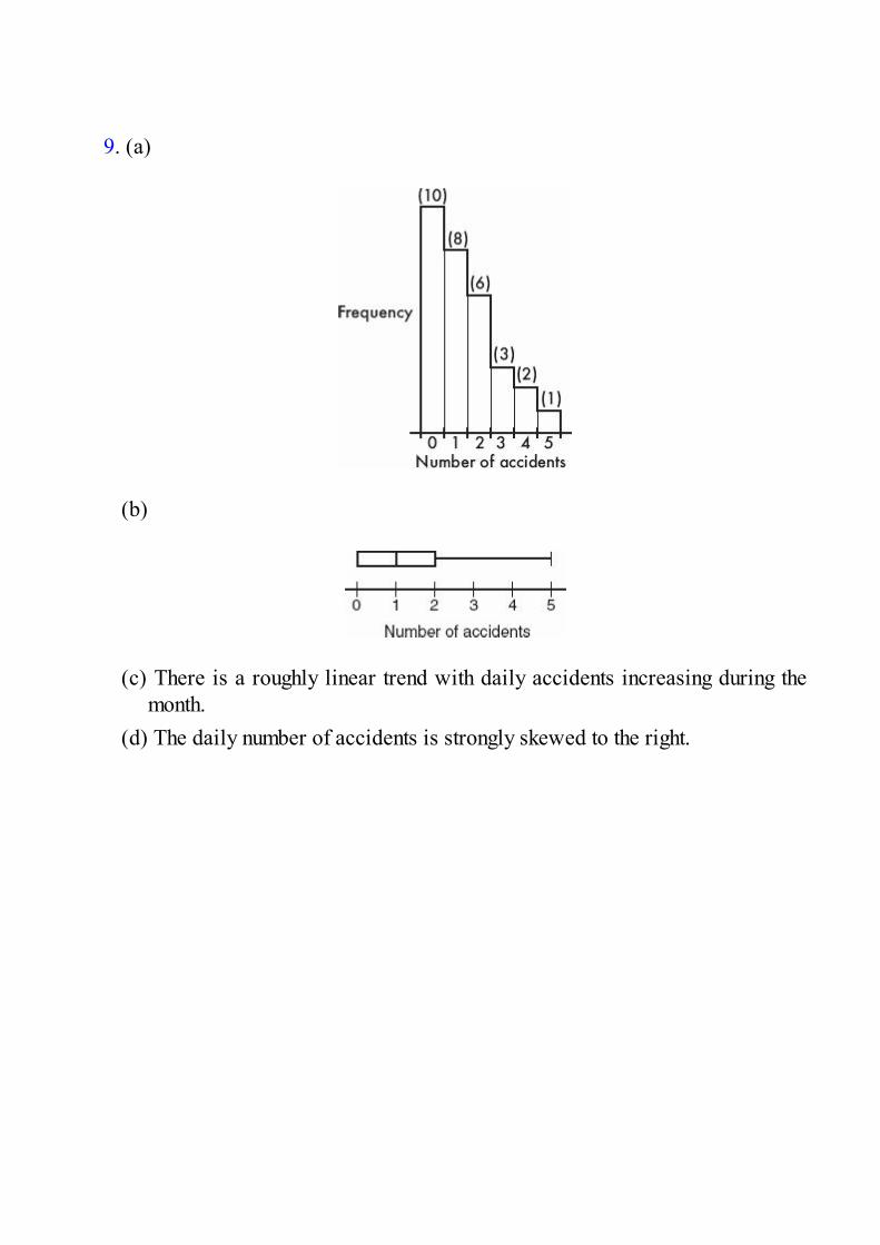
9. (a)
(b)
(c) There is a roughly linear trend with daily accidents increasing during themonth.
(d) The daily number of accidents is strongly skewed to the right.

10. (a) The correlation coefficient r = = .905. It is positive because theslope of the regression line is positive.
(b) The slope is 8.5, signifying that each gram of medication lowers the pulserate by 8.5 beats per minute.
(c) = –1.68 + 8.5(2.25) = 17.4 beats per minute.(d) There is always danger in using a regression line to extrapolate beyond the
values of x contained in the data. In this case, the 5 grams was an overdose,the patient died, and the regression line cannot be used for such valuesbeyond the data set.
(e) Removing the 3-gram result from the data set will increase the correlationcoefficient because the 3-gram result appears to be far off a regression linethrough the remaining points.
(f) Removing the 3-gram result from the data set will swing the regression lineupward so that the slope will increase.

Answers Explained, Multiple-Choice1. (E) Of the 500 people surveyed, 50 + 150 + 50 = 250 were
Democrats, and or 50%.

2. (A) Of the 500 people surveyed, 125 were both for the amendmentand Republicans, and or 25%.
3. (E) There were 15 + 10 + 25 = 50 Independents; 25 of them had noopinion, and or 50%.

4. (E) There were 150 + 50 + 10 = 210 people against the amendment;150 of them were Democrats, and or 71.4%.

5. (C) The percentages of Democrats, Republicans, and Independentswith no opinion are 20%, 12.5%, and 50%, respectively.
6. (A) In the bar corresponding to the Northeast, the segmentcorresponding to country music stretches from the 50% level to the 70%level, indicating a length of 20%.

7. (B) Based on lengths of indicated segments, the percentage from theWest who prefer country is the greatest.

8. (E) The given bar chart shows percentages, not actual numbers.
9. (B) In a complete distribution, the probabilities sum to 1, and therelative frequencies total 100%.

10. (A) The different lengths of corresponding segments show that indifferent geographic regions different percentages of people prefer eachof the music categories.
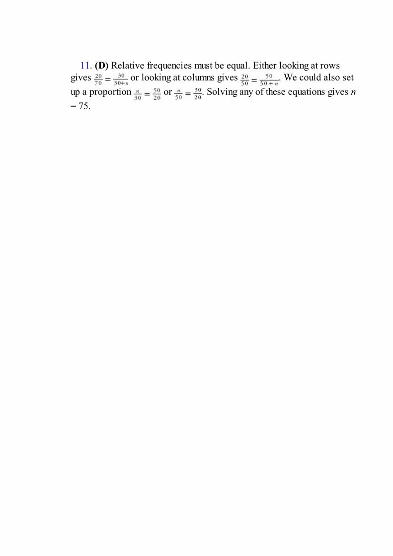
11. (D) Relative frequencies must be equal. Either looking at rowsgives or looking at columns gives . We could also setup a proportion or . Solving any of these equations gives n= 75.

12. (E) It is possible for both to be correct, for example, if there were11 secretaries (10 women, 3 of whom receive raises, and 1 man whoreceives a raise) and 11 executives (10 men, 1 of whom receives a raise,and 1 woman who does not receive a raise). Then 100% of the malesecretaries receive raises while only 30% of the female secretaries do;and 10% of the male executives receive raises while 0% of the femaleexecutives do. However, overall 3 out of 11 women receive raises, whileonly 2 out of 11 men receive raises. This is an example of Simpson’sparadox.
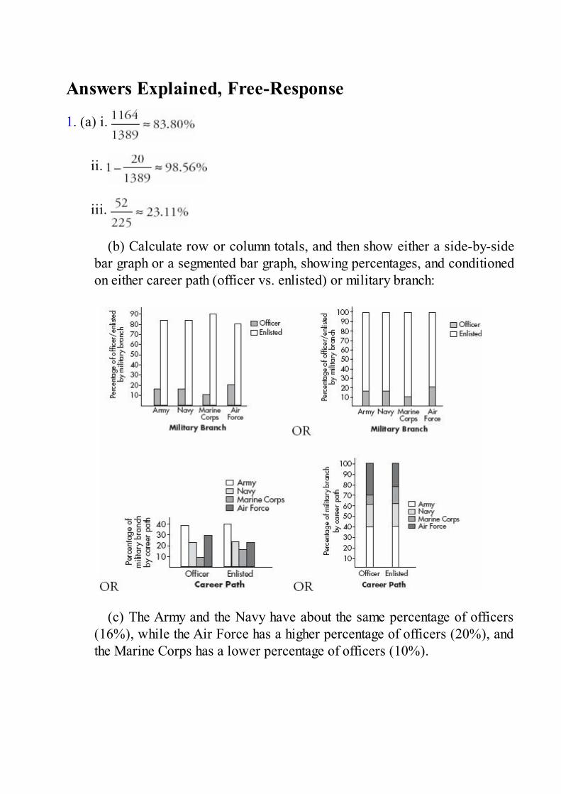
Answers Explained, Free-Response
1. (a) i.
ii.
iii.
(b) Calculate row or column totals, and then show either a side-by-sidebar graph or a segmented bar graph, showing percentages, and conditionedon either career path (officer vs. enlisted) or military branch:
(c) The Army and the Navy have about the same percentage of officers(16%), while the Air Force has a higher percentage of officers (20%), andthe Marine Corps has a lower percentage of officers (10%).

ORAmong the officers and the enlisted career paths there are about the samepercentage Army (39%), and about the same percentage Navy (23%),while the officers have a lower percentage Marine Corps than the enlisted(9% vs. 16%) and the officers have a higher percentage Air Force than theenlisted (29% vs. 22%).

2. (a)
There doesn’t appear to be any real pattern; however, women seem to befavored in four of the programs, while men seem to be slightly favored inthe other two programs.
(b) Overall, 1195 out of 2681 male applicants were accepted, for a 45%acceptance rate, while 559 out of 1835 female applicants were accepted,for a 30% acceptance rate. This appears to contradict the results from parta.
(c) You should tell the reporter that while it is true that the overallacceptance rate for women is 30% compared to the 44% acceptance ratefor men, program by program women have either higher acceptance ratesor only slightly lower acceptance rates than men. The reason behind thisapparent paradox is that most men applied to programs A and B, which areeasy to get into and have high acceptance rates. However, most womenapplied to programs C, D, E, and F, which are much harder to get into andhave low acceptance rates.

Answers Explained, Multiple-Choice1. (E) This study is not an experiment in which responses are being
compared. It is an observational study in which the airlines use split farecalculations from a trial period as a sample to indicate the pattern of allsplit fare transactions. They claim that this leads to “huge savings.”
2. (D) I and II can be considered part of the definitions of experimentand observational study. A sample survey does not impose any treatment;it simply counts a certain outcome, and so it is an observational study, notan experiment.

3. (A) In an experiment a control group is the untreated group picked bythe researchers. It is usually best when the selection process involveschance.
4. (B) The first study was observational because the subjects were notchosen for treatment.
5. (A) The first study was an experiment with two treatment groups andno control group. The second study was observational; the researcher didnot randomly divide the subjects into groups and have each group sleep adesignated number of hours per night.
6. (E) This study was an experiment in which the researchers dividedthe subjects into treatment and control groups. A census would involve astudy of all migraine sufferers, not a sample of 20. The response of thetreatment group receiving chocolate was compared to the response of thecontrol group receiving a placebo. The peppermint tablet with nochocolate was the placebo.
7. (A) The main office at your school should be able to give you theclass sizes of every math and English class. If need be, you can checkwith every math and English teacher.
8. (A) A complete census can provide much information about apopulation, but it doesn’t necessarily establish a cause-and-effectrelationship among seemingly related population parameters.

9. (C) In the first study the families were already in the housing units,while in the second study one of two treatments was applied to eachfamily.
10. (E) Both studies apply treatments and measure responses, and soboth are experiments.
Answers Explained, Multiple-Choice1. (A) This survey provides a good example of voluntary response
bias, which often overrepresents negative opinions. The people whochose to respond were most likely parents who were very unhappy, andso there is very little chance that the 10,000 respondents wererepresentative of the population. Knowing more about her readers, ortaking a sample of the sample would not have helped.
2. (D) If there is bias, taking a larger sample just magnifies the bias ona larger scale. If there is enough bias, the sample can be worthless. Evenwhen the subjects are chosen randomly, there can be bias due, forexample, to non-response or to the wording of the questions. Conveniencesamples, like shopping mall surveys, are based on choosing individualswho are easy to reach, and they typically miss a large segment of thepopulation. Voluntary response samples, like radio call-in surveys, arebased on individuals who offer to participate, and they typicallyoverrepresent persons with strong opinions.

3. (E) The wording of the questions can lead to response bias. Theneutral way of asking this question would simply have been: Are you infavor of a 7-day waiting period between the filing of an application topurchase a handgun and the resulting sale?
4. (E) In a simple random sample, every possible group of the givensize has to be equally likely to be selected, and this is not true here. Forexample, with this procedure it will be impossible for all the Bulls to betogether in the final sample. This procedure is an example of stratifiedsampling, but stratified sampling does not result in simple randomsamples.

5. (E) In a simple random sample, every possible group of the givensize has to be equally likely to be selected, and this is not true here. Forexample, with this procedure it will be impossible for all the earlyarrivals to be together in the final sample. This procedure is an exampleof systematic sampling, but systematic sampling does not result in simplerandom samples.

6. (B) Different samples give different sample statistics, all of whichare estimates of a population parameter. Sampling error relates to naturalvariation between samples, can never be eliminated, can be describedusing probability, and is generally smaller if the sample size is larger.

7. (B) The Wall Street Journal survey has strong selection bias; that is,people who read the Journal are not very representative of the generalpopulation. The talk show survey results in a voluntary response sample,which typically gives too much emphasis to persons with strong opinions.The police detective’s survey has strong response bias in that studentsmay not give truthful responses to a police detective about their illegaldrug use.

8. (E) While the auditor does use chance, each company will have thesame chance of being audited only if the same number of companies havenames starting with each letter of the alphabet. This will not result in asimple random sample because each possible set of 26 companies doesnot have the same chance of being picked as the sample. For example, agroup of companies whose names all start with A will not be chosen.Calculator random number generators and random number tables havesimilar uses and results.
9. (D) This is not a simple random sample because all possible sets ofthe required size do not have the same chance of being picked. Forexample, a set of households all from just half the counties has no chanceof being picked to be the sample. Stratified samples are often easier andless costly to obtain and also make comparative data available. In thiscase responses can be compared among various counties. There is noreason to assume that each county has heads of households with the samecharacteristics and opinions as the state as a whole, so cluster sampling isnot appropriate. When conducting stratified sampling, proportionalsampling is used when one wants to take into account the different sizes ofthe strata.

10. (C) It is most likely that the apartments at which the interviewer haddifficulty finding someone home were apartments with fewer studentsliving in them. Replacing these with other randomly picked apartmentsmost likely replaces smaller-occupancy apartments with larger-occupancyones.

11. (E) While the procedure does use some element of chance, allpossible groups of size 50 do not have the same chance of being picked,and so the result is not a simple random sample. There is a very realchance of selection bias. For example, a number of relatives with thesame name and similar long-distance calling patterns might be selected.The typical methodology of a systematic sample involves picking everynth member from the list, where n is roughly the population size dividedby the desired sample size.

12. (A) The natural variation in samples is called sampling error.Embarrassing questions and resulting untruthful answers are an exampleof response bias. Inaccuracies and mistakes due to human error are one ofthe real concerns of researchers.
13. (C) Surveying people coming out of any church results in a veryunrepresentative sample of the adult population, especially given thequestion under consideration. Using chance and obtaining a high responserate will not change the selection bias and make this into a well-designedsurvey.

Answers Explained, Free-Response1. (a) Both studies were observational because no treatments were applied.
(b) Typical cell phone use today, especially among younger people, iswell over half an hour, so half an hour does not seem to be a reasonablesplit between moderate and heavy use.
(c) This absolutely affects conclusions in that both studies look forrelationships with brain cancer. While voice conversation involvesholding the phone against one’s head, text messaging does not.
(d) The Denmark study looks at how many years individuals used theircell phones, but not at the extent of daily use, while the WHO study doesconsider daily usage.

2. There are many possible examples, such as Are you in favor of protecting thehabitat of the spotted owl, which is almost extinct and desperately in need ofhelp from an environmentally conscious government? and Are you in favor ofprotecting the habitat of the spotted owl no matter how much unemploymentand resulting poverty this causes among hard-working loggers?

3. (a) To be a simple random sample, every possible group of size 25 has to beequally likely to be selected, and this is not true here. For example, if thereare 40 students who always rush to be first in line, this procedure willallow for only 2 of them to be in the sample. Or if each homeroom of size20 arrives as a unit, this procedure will allow for only 1 person from eachhomeroom to be in the sample.
(b) A simple random sample of the students can be obtained bynumbering them from 001 to 500 and then picking three digits at a timefrom a random number table, ignoring numbers over 500 and ignoringrepeats, until a group of 25 numbers is obtained. The studentscorresponding to these 25 numbers will be a simple random sample.

4. The direct telephone and mailing options will both suffer from undercoveragebias. For example, especially affected by the legislation under discussion arethe homeless, and they do not have telephones or mailing addresses. Thepollster interviews will result in a convenience sample, which can be highlyunrepresentative of the population. In this case, there might be a real questionconcerning which members of her constituency spend any time in thedowntown area where her office is located. The radio appeal will lead to avoluntary response sample, which typically gives too much emphasis topersons with strong opinions.

5. In numbering the people 0 through 9, each digit stands for whose coatsomeone receives. Pick the digits, omitting repeats, until a group of tendifferent digits is obtained. Check for a match (1 appearing in the firstposition corresponding to person 1, or 2 appearing in the next positioncorresponding to person 2, and so on, up to 0 appearing in the last positioncorresponding to person 10).
6. (a) To obtain an SRS, you might use a random number table and note the firsttwo different numbers between 1 and 5 that appear. Or you could use acalculator to generate numbers between 1 and 5, again noting the first twodifferent numbers that result.
(b) Time and cost considerations would be the benefit of substitution.However, substitution rather than returning to the same home later couldlead to selection bias because certain types of people are not and will notbe home at 9 a.m. With substitution the sample would no longer be asimple random sample.
(c) Corner lot homes like homes 1 and 5 might have different residents(perhaps with higher income levels) than other homes.
7. (a) Method A is an example of cluster sampling, where the population isdivided into heterogeneous groups called clusters and individuals from arandom sample of the clusters are surveyed. It is often more practical tosimply survey individuals from a random sample of clusters (in this case, arandom sample of city blocks) than to try to randomly sample a wholepopulation (in this case the entire city population).
(b) Method B is an example of stratified sampling, where thepopulation is divided into homogeneous groups called strata and randomindividuals from each stratum are chosen. Stratified samples can often giveuseful information about each stratum (in this case, about each of the fiveneighborhoods) in addition to information about the whole population (thecity population).
Answers Explained, Multiple-Choice1. (D) It may well be that very bright students are the same ones who
both take Latin and do well on the SAT verbal exam. If students could berandomly assigned to take or not take Latin, the results would be moremeaningful. Of course, ethical considerations might make it impossible toisolate the confounding variable in this way. Only using a sample from theobservations gives less information.

2. (B) The desire of the workers for the study to be successful led to aplacebo effect.

3. (C) In experiments on people, the subjects can be used as their owncontrols, with responses noted before and after the treatment. However,with such designs there is always the danger of a placebo effect. Thus thedesign of choice would involve a separate control group to be used forcomparison.

4. (B) Blocking divides the subjects into groups, such as men andwomen, or political affiliations, and thus reduces variation.
5. (D) Blocking in experiment design first divides the subjects intorepresentative groups called blocks, just as stratification in samplingdesign first divides the population into representative groups calledstrata. This procedure can control certain variables by bringing themdirectly into the picture, and thus conclusions are more specific. Thepaired comparison design is a special case of blocking in which each paircan be considered a block. Unnecessary blocking detracts from accuracybecause of smaller sample sizes.

6. (E) None of the studies has any controls, such as randomization,control groups, or blinding, and so while they may give valuableinformation, they cannot establish cause and effect.
7. (D) Octane is the only explanatory variable, and it is being tested atfour levels. Miles per gallon is the single response variable.
8. (A) There is nothing wrong with using volunteers—what is importantis to randomly assign the volunteers into the two treatment groups. Thereis no way to use blinding in this study—the subjects will clearly knowwhich breakfast they are eating. The main idea behind randomly assigningsubjects to the different treatments is to control for various possibleconfounding variables—it is reasonable to assume that people of variousages, races, ethnic backgrounds, etc., are assigned to receive each of thetreatments.

9. (E) In good observational studies, the responses are not influencedduring the collecting of data. In good experiments, treatments arecompared as to differences in responses. In an experiment, there can bemany treatments, each at a different level. Well-designed experiments canshow cause and effect.

10. (D) Control, randomization, and replication are all importantaspects of well-designed experiments. Care in observing withoutimposing change refers to observational studies, not experiments.
11. (A) Each subject might receive both treatments, as, for example, inthe Pepsi-Coke taste comparison study. The point is to give each subjectin a matched pair a different treatment and note any difference inresponses. Matched-pair experiments are a particular example ofblocking, not vice versa. Stratification refers to a sampling method, not toexperimental design. Randomization is used to decide which of a pair getswhich treatment or which treatment is given first if one subject is toreceive both.

12. (A) Blinding does have to do with whether or not the subjects knowwhich treatment (color in this experiment) they are receiving. However,drinking out of solid colored thermoses makes no sense since thebeverages are identical except for color and the point of the experiment isthe teenager’s reaction to color. Blinding has nothing to do with blocking(team participation in this experiment).

13. (A) This study is an experiment because a treatment (periodicremoval of a pint of blood) is imposed. There is no blinding because thesubjects clearly know whether or not they are giving blood. There is noblocking because the subjects are not divided into blocks before randomassignment to treatments. For example, blocking would have been used ifthe subjects had been separated by gender or age before randomassignment to give or not give blood donations. There is a single factor—giving or not giving blood.

Answers Explained, Free-Response1. (a) These are observational studies as there is no randomization of treatments
to subjects.
(b) The excitement of a birthday party is a confounding variable. Withoutconducting a proper experiment, there is no way of telling whetherobserved hyperactivity is caused by sugar or by the excitement of a partyor by some other variable.
(c) The parent should randomly give the child sugar or sugar-free sweetsat parties and observe the child’s behavior. It is important that the parentnot know which the child is receiving (double blinding), because the parentmight perceive a difference in behavior which is not really there if he/sheknows whether or not the child is being given a sugary food.

2. Ask doctors, hospitals, or blood testing laboratories to make known that youare looking for HIV-positive volunteers. As the volunteers arrive, use arandom number table to give each one the drug or a placebo (e.g., if the nextdigit in the table is odd, the volunteer gets the drug, while if the next digit iseven, the volunteer gets a placebo). Use double-blinding; that is, both thevolunteers and their doctors should not know if they are receiving the drug orthe placebo. Ethical considerations will arise, for example, if the drug is verysuccessful. If volunteers on the placebo are steadily developing full-blownAIDS while no one on the drug is, then ethically the test should be stoppedand everyone put on the drug. Or if most of the volunteers on the drug aredying from an unexpected fatal side effect, the test should be stopped andeveryone taken off the drug.
TIPSimply saying to “randomly assign” subjects to treatmentgroups is usually an incomplete response. You need to explainhow to make the assignments—for example, by using a randomnumber table or through generating random numbers on acalculator.

3. To achieve blocking by gender, first separate the men and women. Label the40 men 01 through 40. Use a random number table to pick two digits at a time,ignoring 00 and numbers greater than 40, and ignoring repeats, until a groupof ten such numbers is obtained. These men will receive the supplement at theonce-a-day level. Follow along in the table, continuing to ignore repeats, untilanother group of ten is selected. These men will receive the supplement at thetwice-a-day level. Again ignore repeats until a third group of ten is selectedto receive the supplement at the three-times-a-day level, while the remainingmen will be a control group and not receive the supplement. Now repeat theentire procedure, starting by labeling the women 01 through 40. A decisionshould be made whether or not to use a placebo and have all participants take“something” three times a day. Weigh all 80 overweight volunteers beforeand after a predetermined length of time. Calculate the change in weight foreach individual. Calculate the average change in weight among the ten peoplein each of the eight groups. Compare the four averages from each block (menand women) to determine the effect, if any, of different levels of thesupplement for men and for women.

4. The first study, an observational study, does not suffer from nonresponse bias,as do most mailed questionnaires, because it involved follow-up telephonecalls and achieved a high response rate. However, this study suffers terriblyfrom selection bias because people who subscribe to a health magazine arenot representative of the general population. One would expect most of themto strongly believe that vitamins improve their health. The second study, acontrolled experiment, used comparison between a treatment group and acontrol group, used randomization in selecting who went into each group, andused blinding to control for a placebo effect on the part of the volunteers.However, it did not use double-blinding; that is, the doctors knew whethertheir patients were receiving the vitamin, and this could have introducedhidden bias when they made judgments regarding their patients’ health.

5. Every day for some specified period of time, look at the next digit on arandom number table. If it is odd, flash the subliminal message all day on thescreen, while if it is even, don’t flash the message that day (randomization).Don’t let the customers know what is happening (blinding) and don’t let theclerks selling the popcorn know what is happening (double-blinding).Compare the quantity of popcorn bought by the treatment group, that is, by thepeople who receive the subliminal message, to the quantity bought by thecontrol group, the people who don’t receive the message (comparison).

6. Any conclusions would probably be meaningless. There is a substantialdanger of the placebo effect here; that is, real physical responses could becaused by the psychological effect of knowing the intent of the research. Theexperiment would be considerably strengthened by using a control grouptaking a look-alike capsule. Any conclusions are further suspect because ofthe choice of subjects. Rather than making a random selection from theintended population, the company is using a sample from its own employees,a sample almost guaranteed to have concerns, interests, and backgrounds thatwill confound the responses or limit their generalizability.
7. Ask doctors and hospitals to make known that you are looking for volunteersfrom among intractable pain sufferers. As the volunteers arrive, use a randomnumber table to decide which will have the electrodes properly embedded intheir pain centers and which will have the electrodes harmlessly embedded inwrong positions. For example, if the next digit in the table is odd, thevolunteer receives the proper embedding, while if the next digit is even, thevolunteer does not. Use double-blinding; that is, both the volunteers and theirdoctors should not know if the volunteers are receiving the properembedding. Ethical considerations will arise, for example, if the procedure isvery successful. If volunteers with the wrong embeddings are in constant pain,while everyone with proper embedding is pain-free, then ethically the testshould be stopped and everyone given the proper embedding. Or if most ofthe volunteers with proper embedding develop an unexpected side effect ofthe pain spreading to several nearby sites, then the test should be stopped andthe procedure discontinued for everyone.

8. To achieve blocking by sunlight, first separate the sunlit and shaded plots.Label the 15 sunlit plots 01 through 15. Using a random number table, picktwo digits at a time, ignoring 00 and numbers above 15 and ignoring repeats,until a group of five such numbers is obtained. These sunlit plots will receivethe fertilizer at regular concentration. Continue in the table, ignoring repeats,until another group of five is selected. These sunlit plots will receive thefertilizer at double concentration, while the remaining sunlit plots will be acontrol group receiving no fertilizer. Now repeat the procedure, this timelabeling the shaded plots 01 through 15. Assuming size is the pertinentoutcome, weigh all vegetables at the end of the season, compare the averageweights among the three sunlit groups, and compare the average weightsamong the three shaded groups to determine the effect of the fertilizer, if any,at different levels on sunlit plots and separately on shaded plots.

9. The first study, an observational study, does not suffer from nonresponse bias,as do most studies involving mailed questionnaires, because the researchersmade follow-up telephone calls and achieved a very high response rate.However, the first study suffers terribly from selection bias. People whowork at a teaching hospital are not representative of the general population.One would expect many of them to have heard about how zinc coats the throatto hinder the propagation of viruses. The second study, a controlledexperiment, used comparison between a treatment group and a control group,used randomization in selecting who went into each group, and used blindingto control for a placebo effect on the part of the volunteers. However, theydid not use double-blinding; that is, the doctors knew whether their patientswere receiving the zinc lozenges, and this could introduce hidden bias as thedoctors make judgments about their patients’ health.

10. For each new heart attack patient entering the hospital, look at the next digitfrom a random number table. If it is odd, give the name to a group of peoplewho will pray for the patient throughout his or her hospitalization, while if itis even, don’t ask the group to pray (randomization). Don’t let the patientsknow what is happening (blinding) and don’t let the doctors know what ishappening (double-blinding). Compare the lengths of hospitalization ofpatients who receive prayers with those of control group patients who don’treceive prayers (comparison).

11. (a) Allowing the students to self-select which class to take leads to a lurkingvariable that could be significant. For example, perhaps the brighterstudents all want to learn a certain one of the three languages.
(b) It is possible for the average score of all science majors to be lowerthan the average for all math majors even though the science majorsaveraged higher in each class. For example, suppose that the studentstaking Java scored much higher than the students in the other two classes.Furthermore, only one science major took Java, and she scored tops in theclass. Then the overall average of the math majors could well be higher.This is an example of Simpson’s paradox, in which a comparison can bereversed when more than one group is combined to form a single group.
(c) Number the students 001 through 300. Read off three digits at a timefrom a random number table, noting all triplets between 001 and 300 andignoring repeats, until 100 such numbers have been selected. Keep readingoff three digits, ignoring repeats, until 100 new numbers between 001 and300 are selected. These get C++, while the remaining 100 get Java. Evenquicker would be to use a calculator to generate random digits between001 and 300.
(d) Go through the list of students, flipping a die for each. If a 1 or a 2shows, the student takes Pascal, if a 3 or a 4 shows, C++, and if a 5 or a 6shows, Java.
(e) A possible lurking variable are the teachers. For example, perhapsthe better teachers teach Java.
Investigative Task(a) There is no reason to believe that there was anything random about
which students took which course. Perhaps all the weaker students self-selected or were advised to choose the traditional course.
(b) The students could be labeled 01 through 50. Pairs of digits couldthen be read off a random number table, ignoring numbers over 50 andignoring duplicates, until a set of 25 numbers is obtained. The studentscorresponding to these numbers could be enrolled in the traditional course,and the remaining students in the other.
(c) Applying the above procedure results in {17, 31, 14, 35, 41, 05, 09,20, 06, 44, 50, 43, 11, 18, 45, 01, 13, 33, 04, 19, 02, 08, 40, 49, 03}.Enroll the students with these numbers in the traditional course.
(d) Which teachers teach which courses is not considered. Perhaps themore interesting, exciting teachers teach the new version. Even though acontrol group is selected, there is no blinding, and so students in the newversion might work harder because they realize they are part of anexperiment.

Answers Explained, Multiple-Choice1. (E) There is no reason to assume that the probability of getting a 5 is
the same as that of not getting a 5.

2. (E) The probability that both events will occur is the product of theirseparate probabilities only if the events are independent, that is, only ifthe chance that one event will happen is not influenced by whether or notthe second event happens. In this case the probability of differentsurgeries failing are probably closely related.
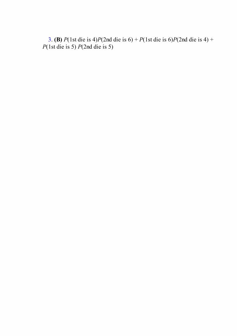
3. (B) P(1st die is 4)P(2nd die is 6) + P(1st die is 6)P(2nd die is 4) +P(1st die is 5) P(2nd die is 5)

4. (A) 10(.15)2(.85)3 = .138 or binompdf(5, .15, 2) = .138

5. (B) The probability of the next child being a girl is independent ofthe gender of the previous children.

6. (B) 1 – (.99975)100 = .0247

7. (D) .001(1,500,000) = 1500

8. (D) = E(X) = = 25
[Or on the TI-84, put returns and probabilities into two lists and run 1-Var Stats L1,L2]

9. (C) are honors students, and prefer basketball.Because of independence, their intersection is (.25)(.3) = .075 of thestudents, and .075(6000) = 450.

10. (E) (.9)3 + 3(.9)2(.1) = .972
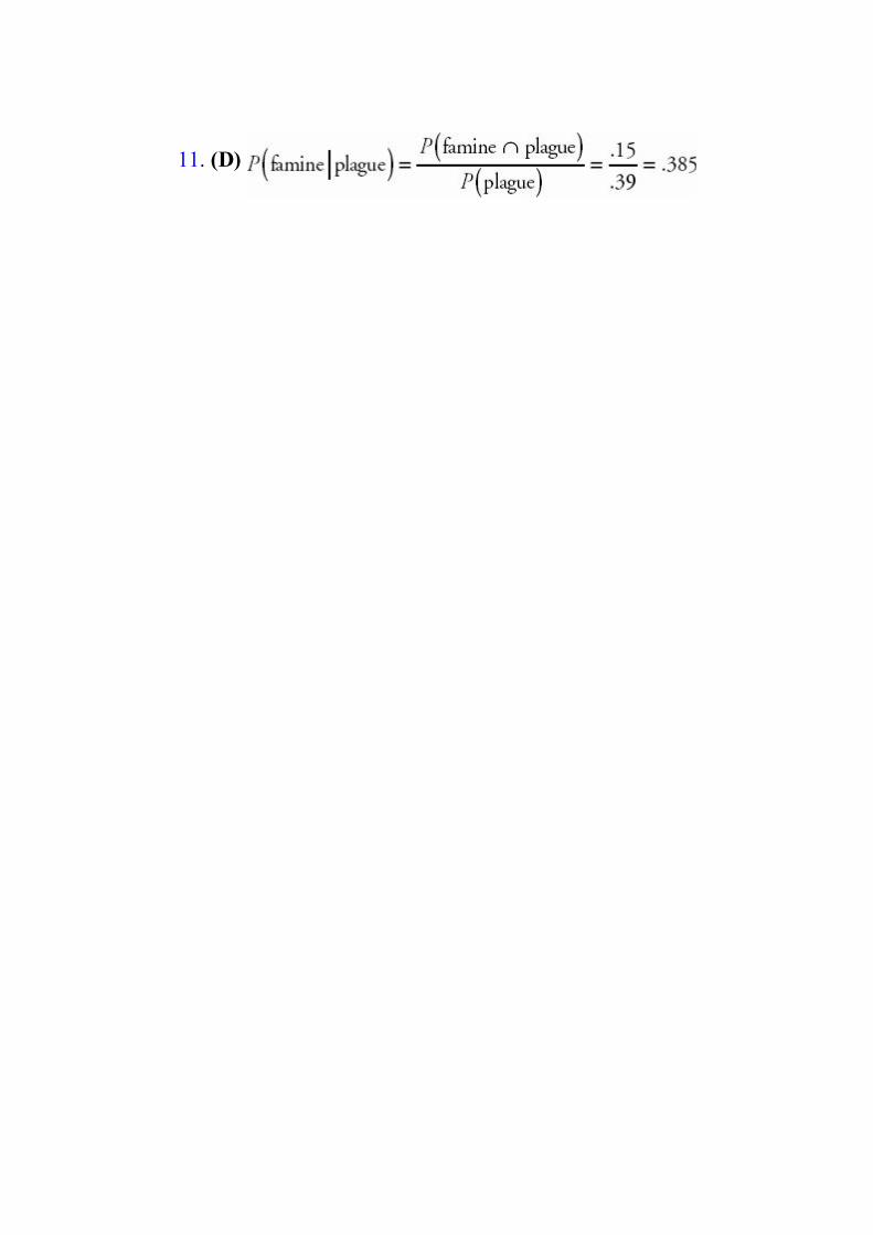
11. (D)

12. (B) If E and F are independent, then P(E F) = P(E)P(F);however, in this problem, (.4)(.35) ≠ .3.

13. (B) Because A and B are independent, we have P(A B) =P(A)P(B), and thus P(A B) = .2 + .1 – (.2)(.1) = .28.

14. (D)
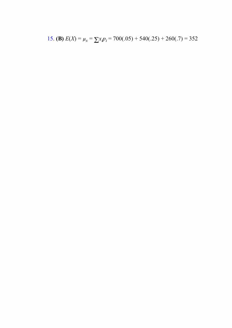
15. (B) E(X) = x = xipi = 700(.05) + 540(.25) + 260(.7) = 352
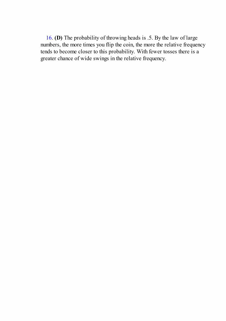
16. (D) The probability of throwing heads is .5. By the law of largenumbers, the more times you flip the coin, the more the relative frequencytends to become closer to this probability. With fewer tosses there is agreater chance of wide swings in the relative frequency.

17. (E) P(diamond on 2nd pick) = 1/4; however,P(diamond on 2nd pick | heart on first pick) = 13/51P(black on 2nd pick) = 1/2; however, P(black on 2nd pick | red on 1stpick) = 26/51P(ace on 2nd pick) = 1/13; however, P(ace on 2nd pick | ace on 1st pick)= 3/51P(two kings) = (1/13)(3/51); however, P(two kings | two aces) = 0P(black on 2nd pick) = 1/2 and P(black on 2nd pick | two aces) = 6/12

18. (B) P(two kings) = (1/13)(1/13); however, P(two kings | two aces) = 0P(king on 2nd pick) = 1/13, and P(king on 2nd pick | ace on 1st pick) =1/13P(at least one king) = 1 – (12/13)2 = 25/169; however,P(at least one king | at least one ace) = [(1/13)(1/13) + (1/13)(1/13)]/[25/169] = 2/25P(exactly one king) = (1/13)(12/13) + (12/13)(1/13) = 24/169; however,P(exactly one king | exactly one ace) = (2/169)/(24/169) = 1/12P(no kings) = (12/13)2; however, P(no kings | no aces) = (11/12)2
19. (A) E(X) = x = xipi = 21,000(.8) + 35,000(.2) = 23,800

20. (D) 1000(.2) + 5000(.05) = 450, and 800 – 450 = 350.

21. (E)

22. (D) P(E F) = P(E)P(F) only if the events are independent. In thiscase, women live longer than men and so the events are not independent.
For questions 23–27, we first sum the rows and columns:

23. (D)

24. (A) (probability of an intersection)
25. (C) (probability of a union)

26. (E) (conditional probability)
27. (A) however,
If independent, these would havebeen equal.

28. (E) While the outcome of any single play on a roulette wheel or theage at death of any particular person is uncertain, the law of largenumbers gives that the relative frequencies of specific outcomes in thelong run tend to become closer to numbers called probabilities.
29. (D)

30. (A)

31. (A)

32. (E)

33. (E)
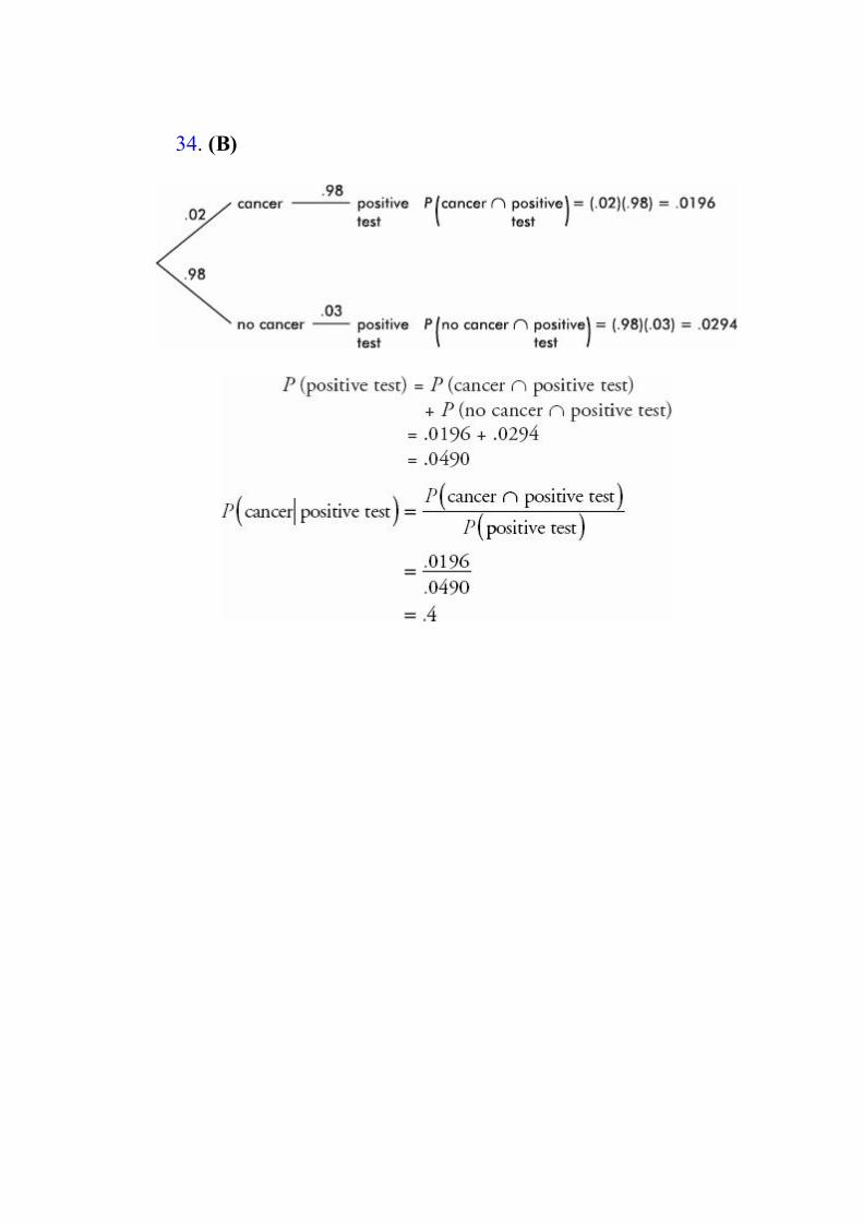
34. (B)
35. (D) The probability that you will receive an A in AP Statistics butnot in AP Biology must be .35 – .19 = .16, not .17.

36. (B) Your expected winnings are only

37. (C) Even though the first two choices have a higher expected valuethan the third choice, the third choice gives a 100% chance of avoidingbankruptcy.

38. (A) The probabilities and are all nonnegative, and theysum to 1.

39. (D) 6(.65)2(.35)2 = .311 or binompdf(4, .65, 2) = .311
40. (C) This is a binomial with n = 10 and p = .37, and so the mean isnp = 10(.37) = 3.7.

41. (D)

42. (E) Coins have no memory, and so the probability that the next tosswill be heads is .5 and the probability that it will be tails is .5. The law oflarge numbers says that as the number of tosses becomes larger, thepercentage of heads tends to become closer to .5.
43. (B) The probabilites of each pump not failing are 1 – .025 = .975, 1– .034 = .966, and 1 – .02 = .98, respectively. The probability of nonefailing is (.975)(.966)(.98) = .923, and so the probability of at least onefailing is 1 – .923 = .077.
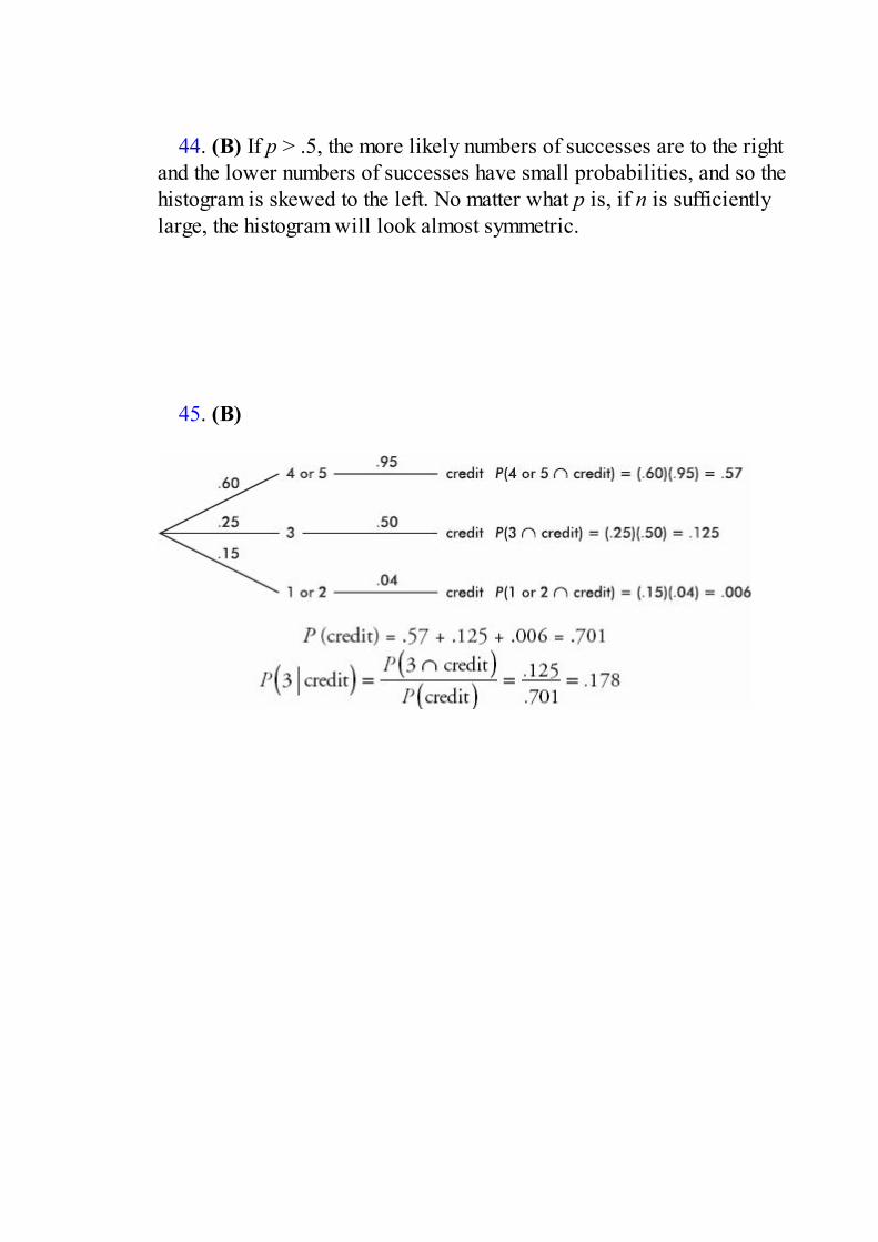
44. (B) If p > .5, the more likely numbers of successes are to the rightand the lower numbers of successes have small probabilities, and so thehistogram is skewed to the left. No matter what p is, if n is sufficientlylarge, the histogram will look almost symmetric.
45. (B)

46. (B) If A and B are mutually exclusive, P(A B) = 0. Thus .6 = .4 +P(B) – 0, and so P(B) = .2. If A and B are independent, then P(A B) =P(A)P(B). Thus .6 = .4 + P(B) – .4P(B), and so

47. (A) For each of the 20 students, we must generate an answer to eachof the 10 questions, and record if any student has at least 6 out of 10correct answers.

Answers Explained, Free-Response1. With Option A, if in reality only 75% of the articles meet all specifications,
the probability of rejecting the day’s production is:
[On the TI-84, binomcdf(6,.75,4) = .466]
With Option B, if in reality only 75% of the articles meet all specifications,the probability of rejecting the day’s production is:
[On the TI-84, binomcdf(12,.75,9) = .609]
For the greatest probability of rejecting the day’s production if only 75% ofthe articles meet all specifications, the buyer should request the manufacturerto use Option B with a probability of rejection of .609 as opposed to OptionA with a probability of rejection of only .466.

2. It’s easiest to first sum the rows and columns:
(a)
(b)
(c) however,
= .286 and so they are not independent.
and also
= .375 and so these two are independent.
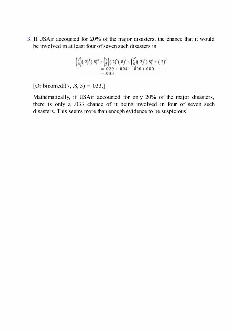
3. If USAir accounted for 20% of the major disasters, the chance that it wouldbe involved in at least four of seven such disasters is
[Or binomcdf(7, .8, 3) = .033.]
Mathematically, if USAir accounted for only 20% of the major disasters,there is only a .033 chance of it being involved in four of seven suchdisasters. This seems more than enough evidence to be suspicious!
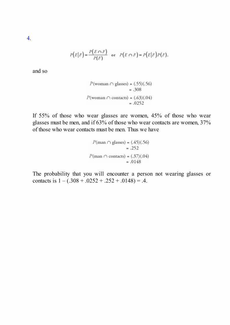
4.
and so
If 55% of those who wear glasses are women, 45% of those who wearglasses must be men, and if 63% of those who wear contacts are women, 37%of those who wear contacts must be men. Thus we have
The probability that you will encounter a person not wearing glasses orcontacts is 1 – (.308 + .0252 + .252 + .0148) = .4.
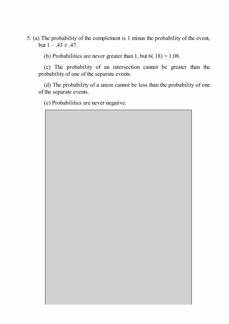
5. (a) The probability of the complement is 1 minus the probability of the event,but 1 – .43 ≠ .47.
(b) Probabilities are never greater than 1, but 6(.18) = 1.08.
(c) The probability of an intersection cannot be greater than theprobability of one of the separate events.
(d) The probability of a union cannot be less than the probability of oneof the separate events.
(e) Probabilities are never negative.

TIPWhen using a formula, write down the formula and thensubstitute the values.
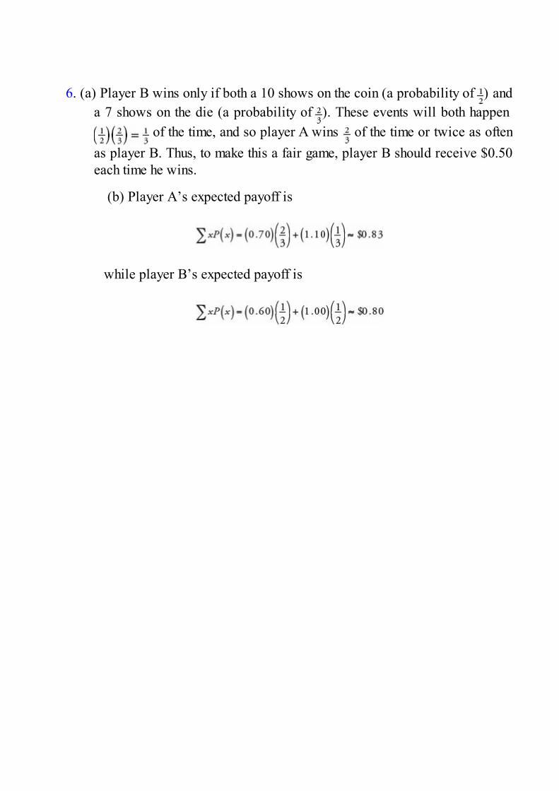
6. (a) Player B wins only if both a 10 shows on the coin (a probability of ) anda 7 shows on the die (a probability of ). These events will both happen
of the time, and so player A wins of the time or twice as oftenas player B. Thus, to make this a fair game, player B should receive $0.50each time he wins.
(b) Player A’s expected payoff is
while player B’s expected payoff is
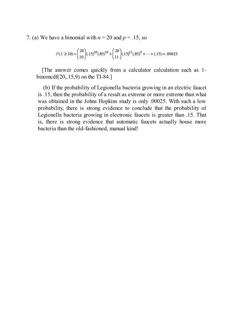
7. (a) We have a binomial with n = 20 and p = .15, so
[The answer comes quickly from a calculator calculation such as 1-binomcdf(20,.15,9) on the TI-84.]
(b) If the probability of Legionella bacteria growing in an electric faucetis .15, then the probability of a result as extreme or more extreme than whatwas obtained in the Johns Hopkins study is only .00025. With such a lowprobability, there is strong evidence to conclude that the probability ofLegionella bacteria growing in electronic faucets is greater than .15. Thatis, there is strong evidence that automatic faucets actually house morebacteria than the old-fashioned, manual kind!

Investigative Task(a) Let the numbers 01 through 14 represent finding an illegal drug,
while 15 through 99 and 00 represent no drugs. Read off pairs of digitsfrom the random number table until a number representing illegal drugs isfound or until nine clean cars are allowed to pass. Note whether a car withillegal drugs is found before nine clean cars pass. Repeat this procedure.Underlining numbers representing the presence of illegal drugs gives
The first nine cars are clean. Then 14 is found after four clean cars, then05 after two clean cars, then 09 before any clean cars, then 06 after twoclean cars, then 11 after seven free cars, and so on. Tabulating gives
First nine cars clean: 5Illegal drugs found before tenth car: 24The probability that illegal drugs will be found before the tenth car is
estimated to be
(b) xP(x) = 1(.15) + 2(.12) + · · · + 25(.01) = 6.81
(c) The probability that the first stopped car will have illegal drugs is.14. The probability that the first will be clean but that the second willhave drugs is (.86)(.14). The probability that two clean cars will befollowed by one with drugs is (.86)2(.14). The probability that three cleanones will be followed by one with drugs is (.86)3(.14), and so on. Theprobability of drugs being found before the tenth car is
Or more simply we could solve by subtracting the complementaryprobability from 1, that is, 1 – (.86)9 = .7427.

Answers Explained, Multiple-Choice1. (C) Summing each row gives P(X = 1) = .20, P(X = 2) = .45, and
P(X = 3) = .35.
2. (A) This question asks for the probability of an intersection, and theanswer is found in the second row, third column.
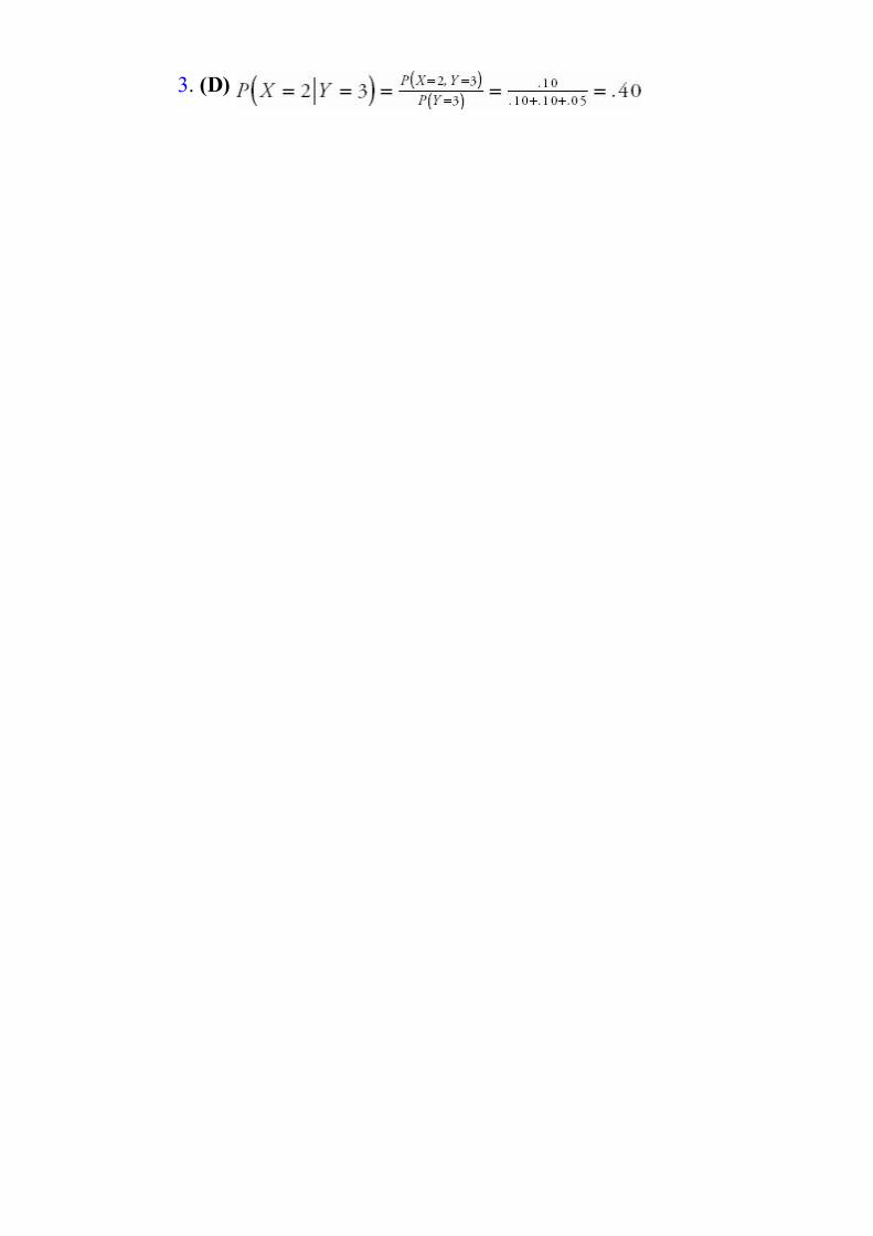
3. (D)

4. (D) For example, P(X = 2 |Y = 3) = .40, but P(X = 2) = .45. Forindependence this has to hold for all values of x and y.

5. (C) P(Y = 2) = 1 – (.4 + .1) = .5. By independence, P(X = 1, Y = 2) =P(X = 1)P(Y = 2), and so .1 = P(X = 1)(.5) and P(X = 1) = .2. Then P(X =4) = 1 – (.2 + .2 + .3) = .3.
6. (E) Without independence we cannot determine var(X + Y) from theinformation given.

7. (B) The means and the variances add. Thus the new variance is 32 +42 = 25, and the new standard deviation is 5.
8. (B) If two random variables are independent, the mean of thedifference of the two random variables is equal to the difference of thetwo individual means; however, the variance of the difference of the tworandom variables is equal to the sum of the two individual variances.

9. (C) The mean of a set of differences is the difference of the means ofthe two sets, while the variance is the sum of the two variances. Thus 71 –66 = 5, while 42 + 32 = 25 and

10. (E) The total variance can be split up among its various sources.Also, the alternative choices are all nonsense.

Answers Explained, Multiple-Choice1. (A) The area under any probability distribution is equal to 1. Many
bell-shaped curves are not normal curves. The smaller the standarddeviation of a normal curve, the higher and narrower the graph. The meandetermines the value around which the curve is centered; different meansgive different centers. Because of symmetry, the mean and median areidentical for normal distributions.
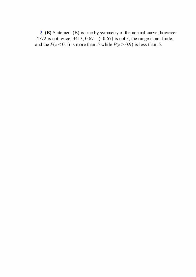
2. (B) Statement (B) is true by symmetry of the normal curve, however.4772 is not twice .3413, 0.67 – (–0.67) is not 3, the range is not finite,and the P(z < 0.1) is more than .5 while P(z > 0.9) is less than .5.

3. (E) All normal distributions have about 95% of their observationswithin two standard deviations of the mean.
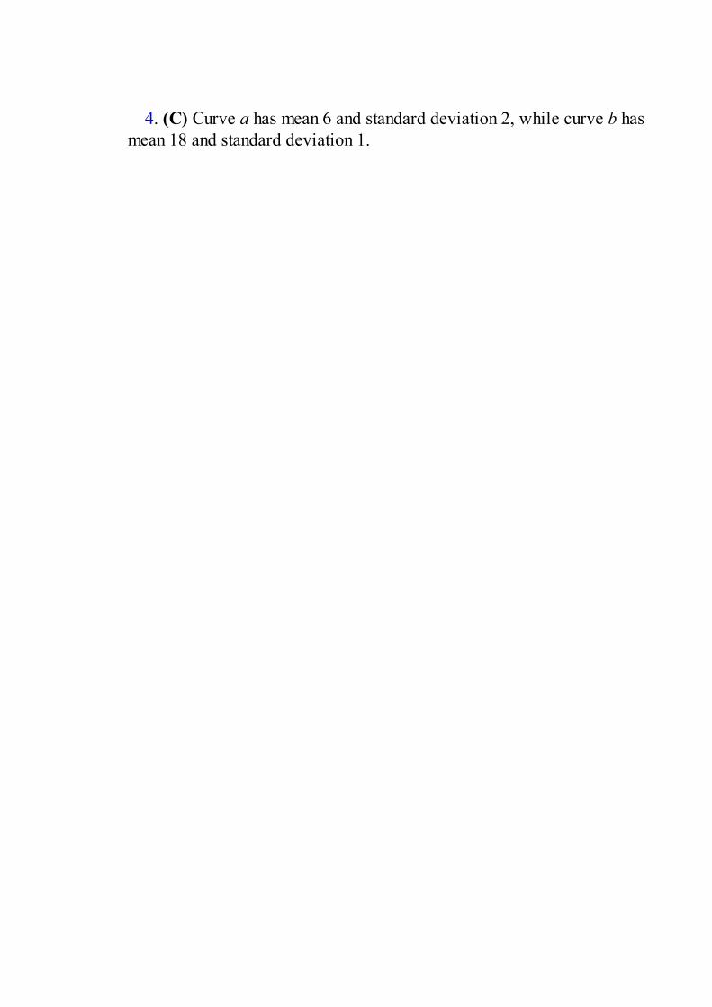
4. (C) Curve a has mean 6 and standard deviation 2, while curve b hasmean 18 and standard deviation 1.

5. (B) The z-score of 10 is From Table A, to the left of –2is an area of .0228. [normalcdf(0, 10, 12.4, 1.2) = .0228.]
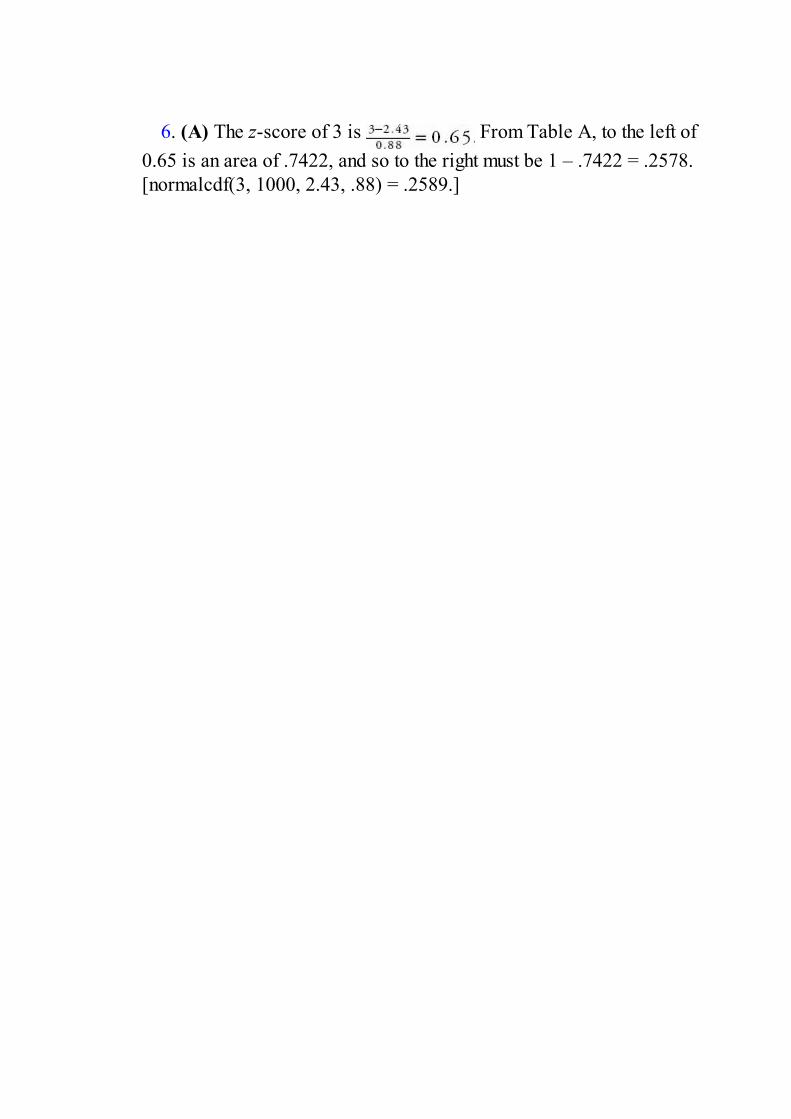
6. (A) The z-score of 3 is From Table A, to the left of0.65 is an area of .7422, and so to the right must be 1 – .7422 = .2578.[normalcdf(3, 1000, 2.43, .88) = .2589.]

7. (E) The z-scores of 3 and 4 are and respectively. From Table A, to the left of –0.8 is an area of .2119, and tothe left of 1.2 is an area of .8849. Thus between 3 and 4 is an area of.8849 – .2119 = .6730. [normalcdf(3, 4, 3.4, .5) = .6731.]

8. (B) If 95% of the area is to the right of a score, 5% is to the left.Looking for .05 in the body of Table A, we note the z-score of –1.645.Converting this to a raw score gives 500 – 1.645(100) = 336.[invNorm(.05, 500, 100) = 336.]

9. (E) The critical z-score associated with 99% to the left is 2.326, and30 + 2.326(4) = 39.3. [invNorm(.99, 30, 4) = 39.3.]

10. (B) The critical z-scores associated with the middle 95% are±1.96, and 9500 ± 1.96(1750) = 6070 and 12,930. [invNorm(.025, 9500,1750) = 6070 and invNorm(.975, 9500, 1750) = 12,930.]

11. (B) X+Y = 150 + 120 = 270 and σX+Y = = 50. Then
= .036
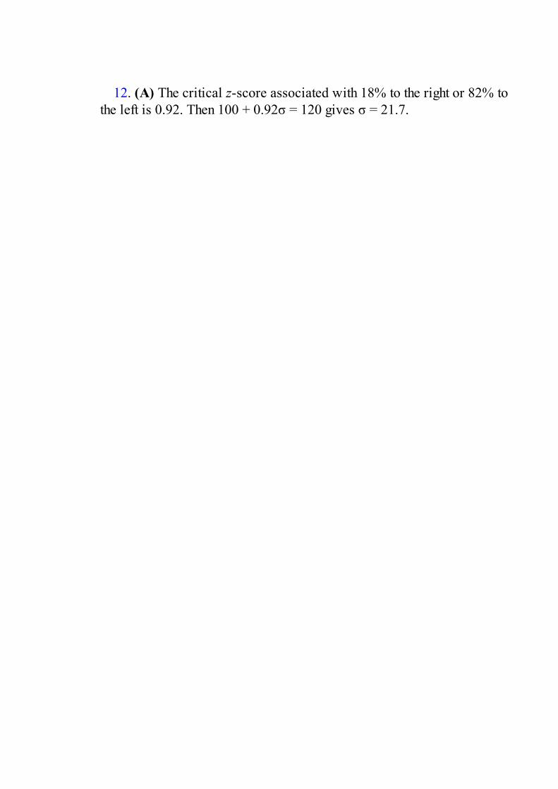
12. (A) The critical z-score associated with 18% to the right or 82% tothe left is 0.92. Then 100 + 0.92σ = 120 gives σ = 21.7.
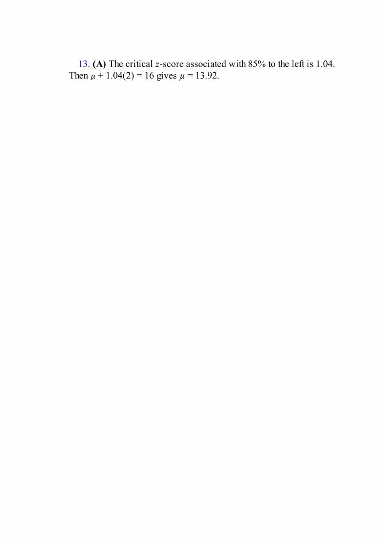
13. (A) The critical z-score associated with 85% to the left is 1.04.Then + 1.04(2) = 16 gives µ = 13.92.

14. (D) The critical z-scores associated with 75% to the right (25% tothe left) and with 15% to the right (85% to the left) are –0.67 and 1.04,respectively. Then { – 0.67σ = 75, + 1.04σ = 150} gives = 104.39and σ = 43.86.

15. (A) The critical z-score associated with .5% to the right (99.5% tothe left) is 2.576. Then c + 2.576(0.4) = 8 gives c = 6.97.

16. (A) Using the normal as an approximation to the binomial, we have = 30(.5) = 15, σ2 = 30(.5)(.5) = 7.5, σ = 2.739, and 1 –
.9495 = .0505. [Or binomcdf(30, .5, 10) = .0494.]

17. (A) The critical z-scores for 10% to the left and 5% to the right are–1.282 and 1.645, respectively. Then { – 1.282σ = 2.48, + 1.645σ =2.54} gives = 2.506 and σ = 0.0205.
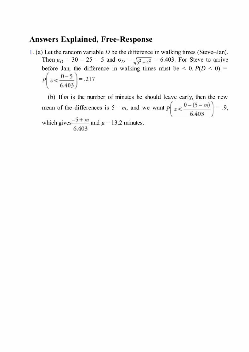
Answers Explained, Free-Response1. (a) Let the random variable D be the difference in walking times (Steve–Jan).
Then D = 30 – 25 = 5 and σD = = 6.403. For Steve to arrivebefore Jan, the difference in walking times must be < 0. P(D < 0) =
= .217
(b) If m is the number of minutes he should leave early, then the new
mean of the differences is 5 – m, and we want = .9,
which gives and = 13.2 minutes.

2. (a)
Given independence, the probability that both components last 240more hours is (0.829825)(0.665506) = 0.552.
(b) The probability that both fail is (1 – 0.829825)(1 – 0.665506) =0.056923.
The probability that at least one doesn’t fail is 1 – 0.056923 ≈ 0.943.

Answers Explained, Investigative Tasks1. (a) The announcer meant that to maintain his tabulated free throw percentage,
Jordan would have to soon miss one. This is not a correct use ofprobability. If Jordan makes a certain percentage of free throws, thatprobability applies to each throw irrespective of the previous throws. Bythe law of large numbers, in the long run the relative frequency tendstoward the correct probability, but no conclusion is possible about anygiven outcome.
(b) P(six in a row) = (.9)6 = .531P(five, then a miss) = (.9)5(.1) = .059P(next|previous five) = P(next) = .9
(c) Let the digits 1 through 9 stand for making a free throw, while 0stands for a miss. Look at blocks of five random numbers. If all stand for“makes” (no 0), look at the very next digit to see if it is a 0 or not. Keep atally of how many times five makes in a row are followed by a make andhow many times five makes in a row are followed by a miss.
(d) This is a binomial distribution with n = 6 and p = .9, and so the meani s np = 6(9) = 5.4 while the standard deviation is
(e) Since nq = 40(1 – .90) = 4, the normal approximation to the binomialis not recommended. However, a direct binomial calculation yields
[Or simply use binomcdf(40, .9, 35) on the TI-84.] With such a highprobability, there is no evidence to conclude that Jordan’s average hasdropped!

2. (a) With Table A gives a probability of .1977 ≈ .2.
(b) For example, letting 0 and 1 represent caplets containing less than8500 units and 2 through 9 represent caplets containing more than 8500units, we can read off digits until we find two containing less than 8500caplets. Five simulations would yield
841770 67571761 31558251 50681 435410giving 6, 8, 8, 5, and 6 tablets sampled before finding two with less than8500 units apiece.
(c) The probability of a caplet having more than 9000 units is .5, andthus one would expect to find two caplets with more than 9000 units muchquicker than finding two caplets with less than 8500 units. Thus the firsthistogram results from looking for two caplets with more than 9000 unitsand the second histogram results from looking for two caplets with lessthan 8500 units.
(d) An estimate for the expected value is obtained by
Answers Explained, Multiple-Choice1. (C) The larger the sample, the smaller the spread in the sampling
distribution. Bias has to do with the center, not the spread, of a samplingdistribution. Sample statistics are used to make inferences aboutpopulation proportions. Statistics from smaller samples have morevariability.
2. (E) It is always true that the sampling distribution of has mean and standard deviation . In addition, the sampling distribution will be
normal if the population is normal and will be approximately normal if nis large even if the population is not normal. and σ are not equal
unless n = 1.
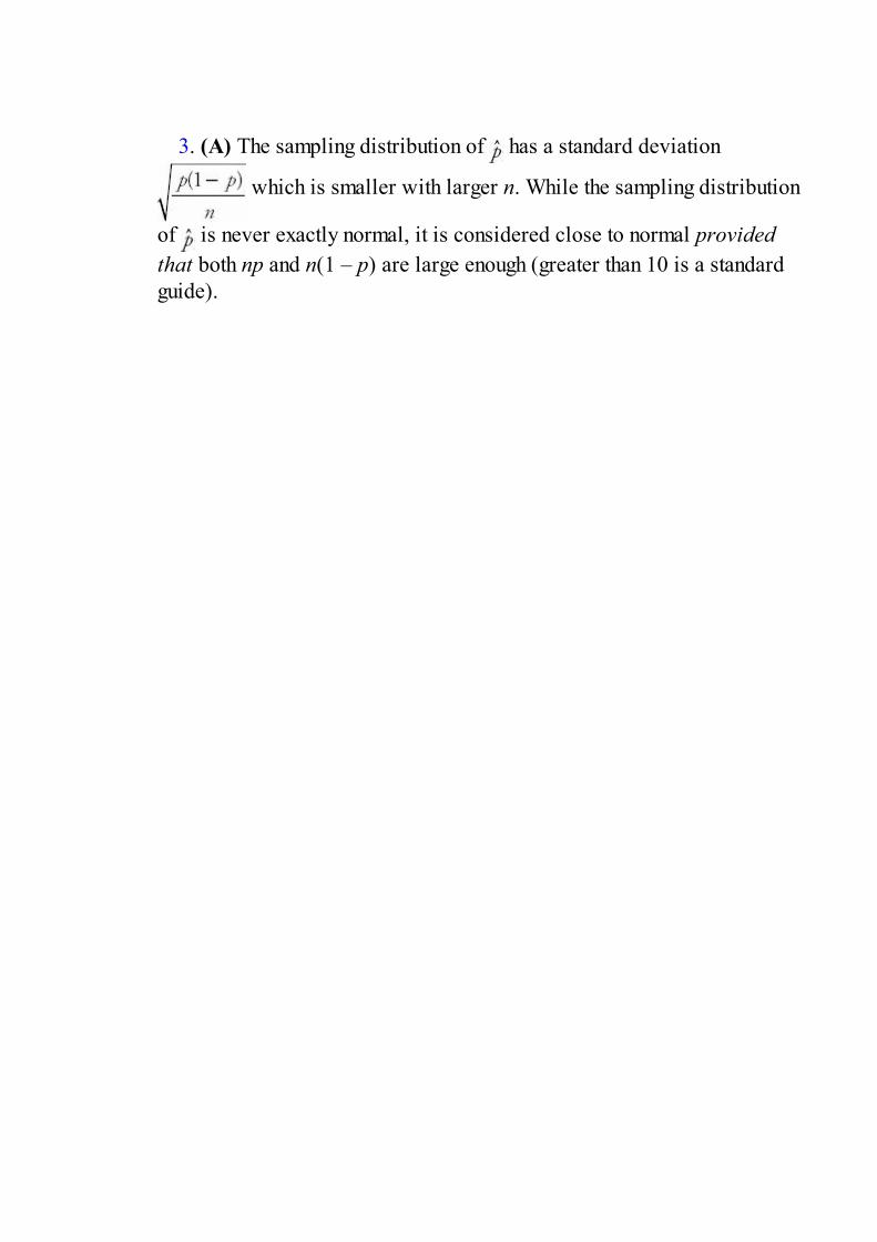
3. (A) The sampling distribution of has a standard deviation
which is smaller with larger n. While the sampling distribution
of is never exactly normal, it is considered close to normal providedthat both np and n(1 – p) are large enough (greater than 10 is a standardguide).

4. (B) Sample proportions are an unbiased estimator for the populationproportion, and larger sample sizes lead to reduced variability.
5. (E) The sampling distribution of has mean , standard deviation , and shape, which becomes closer to normal with larger n.

6. (A) The maximum of a sample is never larger than the maximum ofthe population, so the mean of the sample maximums will not be equal tothe population maximum. (A sampling distribution is unbiased if its meanis equal to the population parameter.)
7. (E) All are unbiased estimators for the corresponding populationparameters; that is, the means of their sampling distributions are equal tothe population parameters.
8. (A) Both np = (100)(.35) = 35 > 10 and n(1 – p) = (100)(.65) = 65 >10. The set of sample proportions is approximately normally distributedwith mean .35 and standard deviation With a z-
score of the probability that the sample proportion exceeds40% is 1 – .8531 = .1469. [normalcdf(.40, 1, .35, .0477) = .1473.]

9. (D) Both np = (150)(.58) = 87 > 10 and n(1 – p) = (150)(.42) = 63 >10. The set of sample proportions is approximately normally distributed
with mean .58 and standard deviation With z-
scores of and the probability the sampleproportion is between .55 and .60 is .6915 – .2296 = .4619.[normalcdf(.55, .60, .58, .0403) = .4618.]

10. (A) The set of sample means is approximately normally distributedwith = 187.50 and The z-score of 200 is
and the probability that the mean outstanding bill is
over $200 is 1 – .9474 = .0526. [normalcdf(200, 10000, 187.5, 7.707) =.0524.]
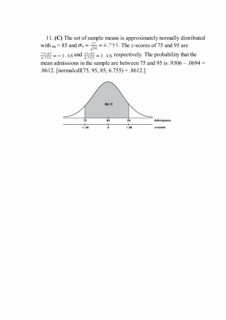
11. (C) The set of sample means is approximately normally distributedwith = 85 and The z-scores of 75 and 95 are
and respectively. The probability that themean admissions in the sample are between 75 and 95 is .9306 – .0694 =.8612. [normalcdf(75, 95, 85, 6.755) = .8612.]
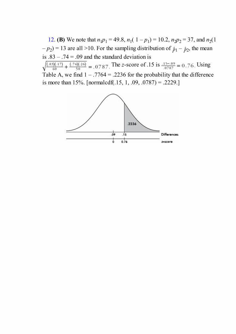
12. (B) We note that n1p1 = 49.8, n1( 1 – p1) = 10.2, n2p2 = 37, and n2(1– p2) = 13 are all >10. For the sampling distribution of 1 – 2, the meanis .83 – .74 = .09 and the standard deviation is
The z-score of .15 is Using
Table A, we find 1 – .7764 = .2236 for the probability that the differenceis more than 15%. [normalcdf(.15, 1, .09, .0787) = .2229.]

13. (D) The mean of the differences equals 27 – 29 = –2, while thestandard deviation is The z-scores of +3 and –3
are and respectively. The probability thatthe difference is between these two values is .9916 – .3156 = .6760.[normalcdf(–3, 3, –2, 2.092) = .6753.]

14. (B) The t-distributions are symmetric and mound-shaped, and theyhave more, not less, spread than the normal distribution.

15. (A) The larger the number of degrees of freedom, the closer thecurve to the normal curve. While around the 30 level is often considered areasonable approximation to the normal curve, it is not the normal curve.

Answers Explained, Free-Response1. (a) We do not know the shape of the distribution of the amount individual
teenage drivers pay for insurance, so there is no way of calculating theprobability a randomly chosen teenage driver pays over $3000 a year forauto insurance.
(b) = = 2171 and σ = = 61.2
(c) With this large a sample size (100 > 30), the Central Limit Theoremtells us that the sampling distribution of sample means is approximatelynormal. We calculate P( > 2300) = P( ) = P(z > 2.1078)
=.0175[On the TI-84, normalcdf(2.1078,1000) = .0175]

2. (a) The z-scores corresponding to cumulative probabilities of 25% and 75%are ±0.674. Thus, Q1 = 1.87 – 0.674(0.193) = 1.740, Q3 = 1.87 +0.674(0.193) = 2.000, and IQR = Q3 – Q1 = 2.000 – 1.740 = $0.260/lb.
(b) From part (a) we have that the probability a honey price is below$2.00/lb is .75, and thus the probability of being above $2.00/lb is 1 – .75= .25. Now we have a binomial with n = 3 and p = .25. P(majority >$2.00/lb) = P(2 or 3 are > $2.00/lb) = 3(.25)2(.75) + (.25)3 = 0.15625.
(c) The distribution of is normal with a mean of 1.87 and a standarddeviation
of = 0.1114. Thus, P( > 2.00) = P( ) = P(z >
1.167) = .01216[On the TI-84, normalcdf(1.167,1000) = .1216]

3. (a) The z-score of 84 is which gives a probability of .0062 or0.62%. [normalcdf(84, 1000, 74, 4) = .0062.]
(b) 1 – (.9938)10 = .06
(c) Checking conditions: the original population is given to be normal,we have an SRS, and our sample is less than 10% of all college basketballplayers.
The z-score of 72 is with a resulting probability of
.9429. [normalcdf(72, 1000, 74, 1.265) = .9431.]
(d) We have Q1 = 74 – 0.674(4) = 71.3, Q3 = 74 + 0.674(4) = 76.7, and1.5(IQR) = 1.5(Q3 – Q1) = 8.1. Then 71.3 – 8.1 = 63.2 has a z-score of –2.7, while 76.7 + 8.1 = 84.8 has a z-score of 2.7. The correspondingprobabilities give .0035 + .0035 = .007 or 0.7%. The problem could alsohave been worked simply in terms of z-scores: 1.5(0.674 + 0.674) = 2.02and 0.674 + 2.02 ≈ 2.7, and so on.
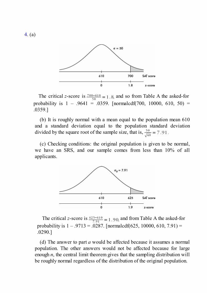
4. (a)
The critical z-score is and so from Table A the asked-forprobability is 1 – .9641 = .0359. [normalcdf(700, 10000, 610, 50) =.0359.]
(b) It is roughly normal with a mean equal to the population mean 610and a standard deviation equal to the population standard deviationdivided by the square root of the sample size, that is,
(c) Checking conditions: the original population is given to be normal,we have an SRS, and our sample comes from less than 10% of allapplicants.
The critical z-score is and from Table A the asked-forprobability is 1 – .9713 = .0287. [normalcdf(625, 10000, 610, 7.91) =.0290.]
(d) The answer to part a would be affected because it assumes a normalpopulation. The other answers would not be affected because for largeenough n, the central limit theorem gives that the sampling distribution willbe roughly normal regardless of the distribution of the original population.

Investigative Task(a) Using a calculator, find = 9 and σ = 5.0596.
(b)
(c)
(d) Using a calculator, find = 3.0984 and then note that
(e) If N is very large, is approximately equal to 1 and so theexpression simplifies to

Answers Explained, Multiple-Choice1. (C) The critical z-scores will go from ±1.96 to ±2.576, resulting in
an increase in the interval size: or an increase of 31%.

2. (D) Increasing the sample size by a multiple of d divides the intervalestimate by

3. (A) The margin of error varies directly with the critical z-value anddirectly with the standard deviation of the sample, but inversely with thesquare root of the sample size. The value of the sample mean and thepopulation size do not affect the margin of error.

4. (D) Although the sample proportion is between 77% and 87% (morespecifically, it is 82%), this is not the meaning of ±5%. Although thepercentage of the entire population is likely to be between 77% and 87%,this is not known for certain.

5. (E) The 95% refers to the method: 95% of all intervals obtained bythis method will capture the true population parameter. Nothing is certainabout any particular set of 20 intervals. For any particular interval, theprobability that it captures the true parameter is 1 or 0 depending uponwhether the parameter is or isn’t in it.

6. (E) There is no guarantee that 13.4 is anywhere near the interval, sonone of the statements are true.

7. (E) The critical z-score with .005 in each tail is 2.576 (from last lineon Table B or invNorm(.005) on the TI-84), and
.

8. (A) The margin of error has to do with measuring chance variationbut has nothing to do with faulty survey design. As long as n is large, s isa reasonable estimate of σ; however, again this is not measured by themargin of error. (With t-scores, there is a correction for using s as anestimate of σ.)

9. (B) The critical z-score with .01 in the tails is 2.326 (invNorm(.01)
on the TI-84), and .

10. (B)

11. (D)
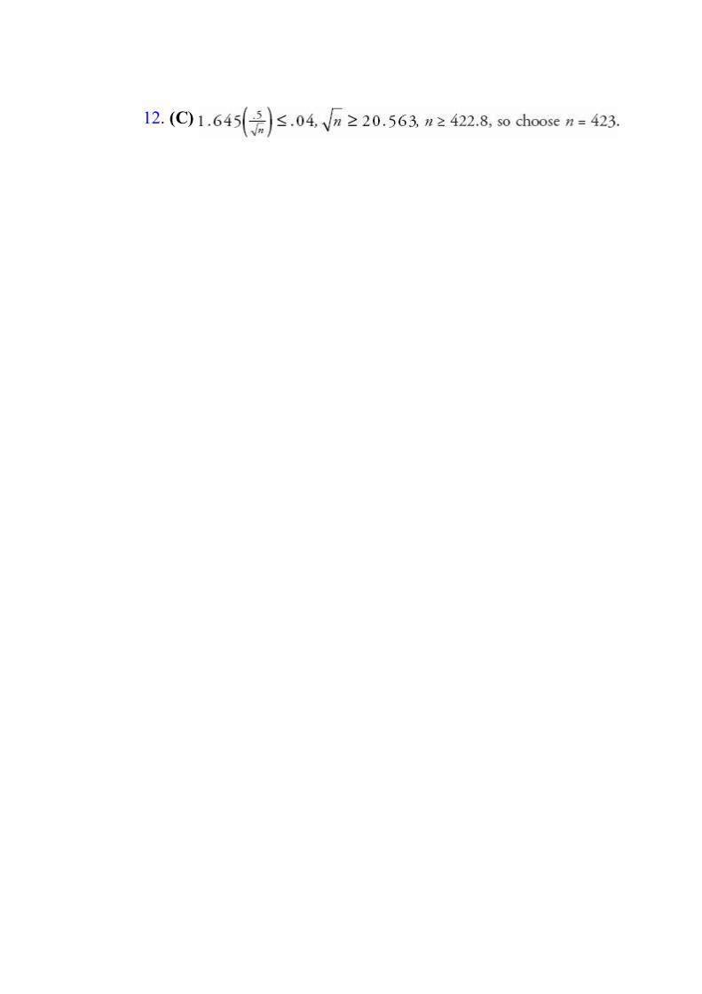
12. (C)

13. (E) and so the
pollsters should have obtained a sample size of at least 1068. (Theyactually interviewed 1148 people.)
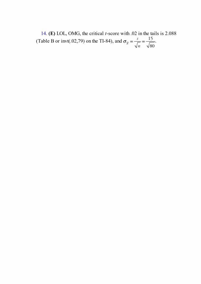
14. (E) LOL, OMG, the critical t-score with .02 in the tails is 2.088(Table B or invt(.02,79) on the TI-84), and .
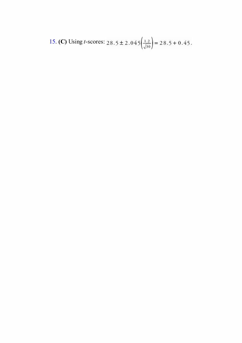
15. (C) Using t-scores:

16. (D) and .4772 + .4772 = .9544 ≈ 95%.

17. (E) Using t-scores:

18. (E) and n ≥ 116.2; choose n = 117.

19. (E) To divide the interval estimate by d without affecting theconfidence level, multiply the sample size by a multiple of d 2. In thiscase, 4(50) = 200.
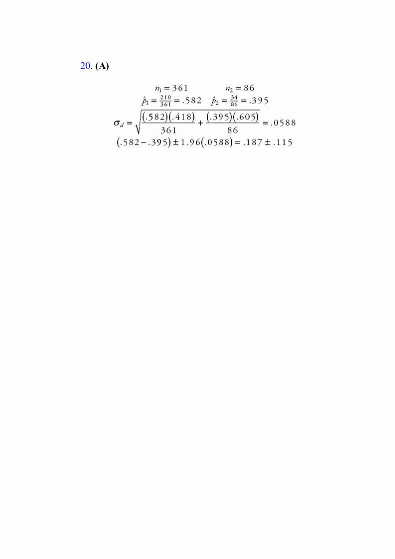
20. (A)

21. (B)
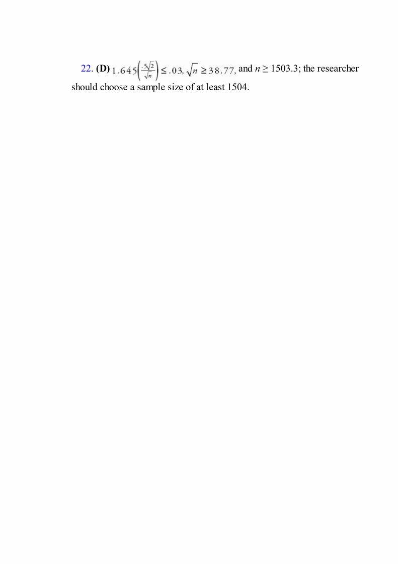
22. (D) and n ≥ 1503.3; the researcher
should choose a sample size of at least 1504.

23. (A) and with df = min(347 – 1, 561 – 1),
critical t-scores are ±1.97.

24. (B)

25. (C)
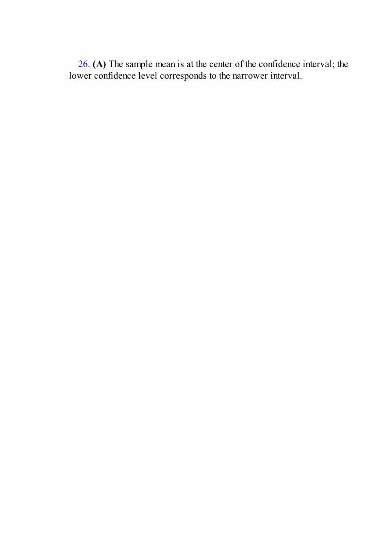
26. (A) The sample mean is at the center of the confidence interval; thelower confidence level corresponds to the narrower interval.

27. (C) Narrower intervals result from smaller standard deviations andfrom larger sample sizes.

28. (E) Only III is true. The 90% refers to the method; 90% of allintervals obtained by this method will capture . Nothing is sure aboutany particular set of 100 intervals. For any particular interval, theprobability that it captures is either 1 or 0 depending on whether is orisn’t in it.

29. (E) In determining confidence intervals, one uses sample statisticsto estimate population parameters. If the data are actually the wholepopulation, making an estimate has no meaning.
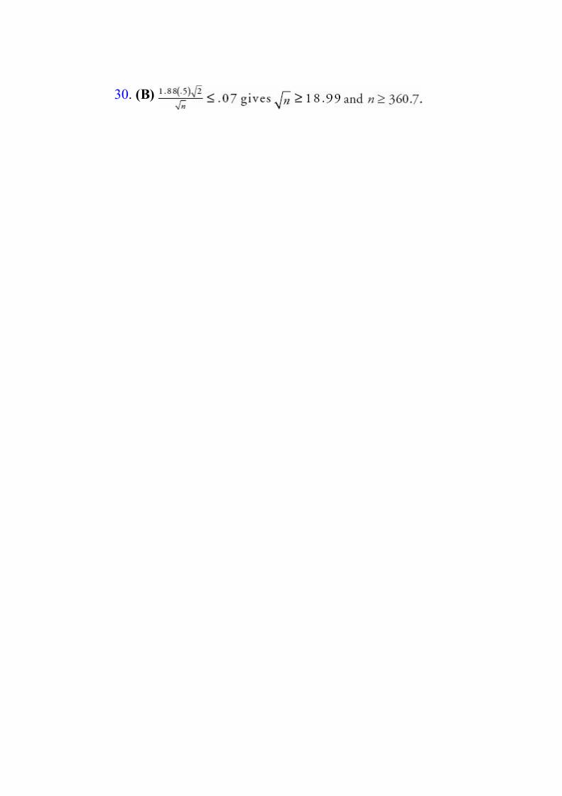
30. (B)

31. (E) With df = 15 – 1 = 14 and .05 in each tail, the critical t-value is1.761.

32. (D)

33. (C) The confidence interval estimate of the set of nine differencesis

34. (C)
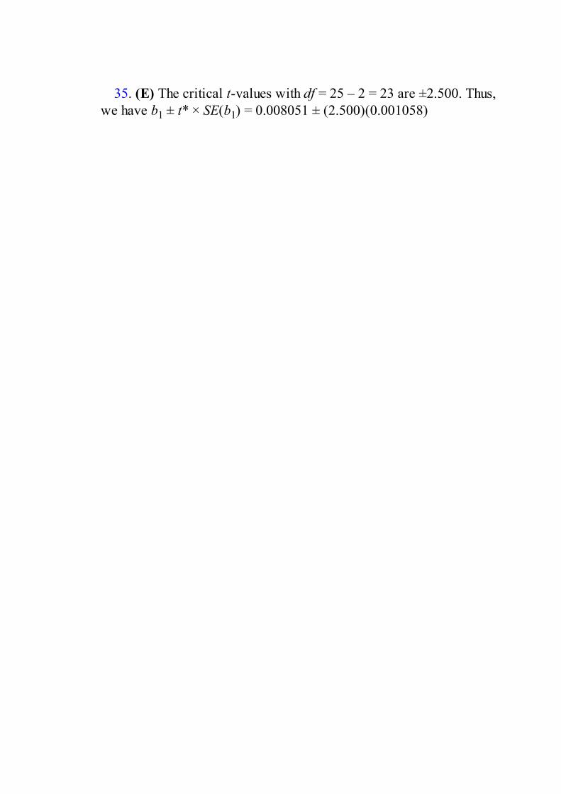
35. (E) The critical t-values with df = 25 – 2 = 23 are ±2.500. Thus,we have b1 ± t* × SE(b1) = 0.008051 ± (2.500)(0.001058)

36. (E) The critical t-values with df = n – 2 = 8 are ±2.306. Thus, wehave b ± t* × SE(b) = –2.16661 ± 2.306(1.03092) = –2.16661 ± 2.3773or (–4.54,0.21).

37. (E) While there is clearly a positive association between smokinglevels and hazard ratios, this was an observational study, not anexperiment, so cause and effect (as implied in I, II, and III) is not anappropriate conclusion. The margins of error of the confidence intervalsbecome greater (less precision) with heavier smoking.

Answers Explained, Free-Response1. (a) = .57 and [Note that n = 1000(.57) = 570 and
n = 1000(.43) = 430 are both greater than 10, we are given an SRS, and1000 < 10% of all voters.] The critical z-scores associated with the 95%level are ±1.96. Thus the confidence interval estimate is .57 ± 1.96(.0157)= .57 ± .031, or between 54% and 60%. (We are 95% confident thatbetween 54% and 60% of the voters believe competence is more importantthan character.)
(b) Explain to your parents that by using a measurement from a samplewe are never able to say exactly what a population proportion is; ratherwe are only able to say we are confident that it is within some range ofvalues, in this case between 54% and 60%.
(c) In 95% of all possible samples of 1000 voters, the method usedgives an estimate that is within three percentage points of the true answer.

2. (a) First, identify the confidence interval and check the conditions:This is a one-sample z-interval for the proportion of family members
who come down with H1N1 after an initial family member does in this
state, that is, .
It is given that this is a random sample, and we calculate np = 129 ≥ 10and n(1 – ) = 747 ≥ 10.
Second, calculate the interval:Calculator software (such as 1-PropZInt on the TI-84) gives (.12757,
.16695). [For instructional purposes in this review book, we note that
and .147 ± 1.645 = .147 ± .020 or (.127,
.167)]Third, interpret in context:We are 90% confident that the proportion of family members who come
down with H1N1 after an initial family member does in this state isbetween .127 and .167.
(b) Because 1/8 = .125 is not in the interval of plausible values for thepopulation proportion, there is evidence that the proportion of familymembers who come down with H1N1 after an initial family member doesin this state is different from the 1 in 8 chance concluded in the publishedstudy.
(c) .147 ± 2.576 = .147 ± .031 or (.116, .178) which does
include .125, so in this case there is not evidence that the proportion offamily members who come down with H1N1 after an initial family memberdoes in this state is different from the 1 in 8 chance concluded in thepublished study.

3. (a) First, identify the confidence interval and check the conditions:This is a two-sample z-interval for pUS – pUK, the difference in
population proportions of new births to unmarried women in the UnitedStates and United Kingdom, that is,
It is given that these are random samples, they are clearly independent,and we calculate nUS US = (500)(.412) = 206 ≥ 10,
Second, calculate the interval:Calculator software (such as 2-PropZInt on the TI-84) gives (–.1182,
.01219). [For instructional purposes in this review book, we note that:
Third, interpret in context:We are 95% confident that the difference in proportions, pUS – pUK, of
new births to unmarried women in the United States and United Kingdom isbetween –0.118 and 0.012.
(b) Because 0 is in the interval of plausible values for the difference ofpopulation proportions, this confidence interval does not support the beliefby the UN health care statistician that the proportions of new births tounmarried women is different in the United States and United Kingdom.

4. (a) Checking conditions: We are given random samples and must assume thatthe parent populations are nearly normal. Then a calculator like the TI-84g i v e s for inner city stations and
for suburban stations. That is, we are 95% confident
that the mean price for gas in inner city stations is between $3.434 and$3.466, and are 95% confident that the mean price for gas in suburbanstations is between $3.366 and $3.394.
(b) Because the sample size of inner city stations is smaller.
(c) Yes, because the standard deviation of the set of sample means is .0079, and so $3.50 is more than three standard deviations away
from $3.45.
Thus the probability that the true mean is this far from the sample meanis extremely small.

5. (a) Checking conditions: We are given a simple random sample and mustassume that the numbers of riders per car during rush hour are normallydistributed. Then That is, we
are 90% confident that the average number of riders per car during rushhour is between 81.67 and 85.33.
( b ) and n ≥ 94.2, so you must choose a
random sample of at least 95 subway cars.

6. (a) Calculator software (such as TIinterval on the TI-84 gives (–29,337,421,337), or we are 95% confident that the mean salary of all basketballsalaries from the population from which this sample was taken is between–$29,337 and $421,337. [For instructional purposes in this review book,we note that with df = 9,
(b) We must assume the sample is an SRS and that basketball salariesare normally distributed. This does not seem reasonable—the salaries areprobably strongly skewed to the right by a few high ones. With the givenmean and standard deviation, and noting that salaries are not negative,clearly we do not have a normal distribution, and furthermore, the samplesize, n = 10, is too small to invoke the CLT. The calculated confidenceinterval is not meaningful.
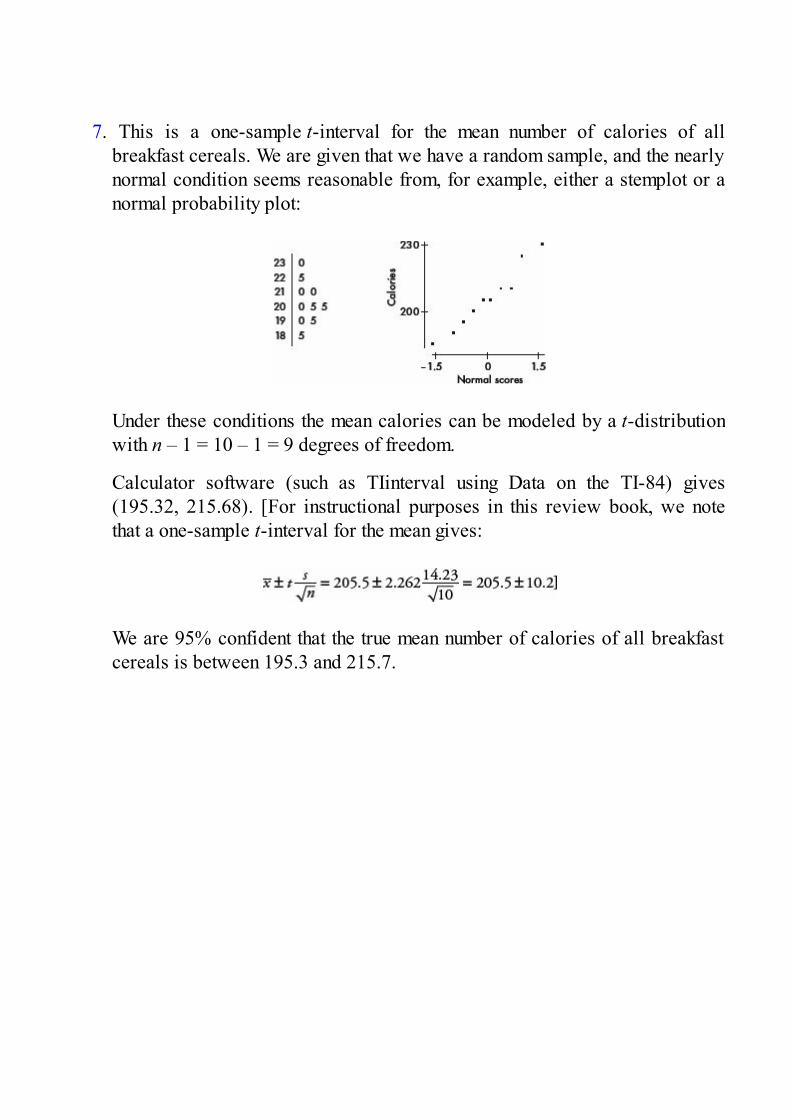
7. This is a one-sample t-interval for the mean number of calories of allbreakfast cereals. We are given that we have a random sample, and the nearlynormal condition seems reasonable from, for example, either a stemplot or anormal probability plot:
Under these conditions the mean calories can be modeled by a t-distributionwith n – 1 = 10 – 1 = 9 degrees of freedom.
Calculator software (such as TIinterval using Data on the TI-84) gives(195.32, 215.68). [For instructional purposes in this review book, we notethat a one-sample t-interval for the mean gives:
We are 95% confident that the true mean number of calories of all breakfastcereals is between 195.3 and 215.7.

8. (a) First, identify the confidence interval and check the conditions:This is a two-sample t-interval for NRW – μRW, the difference in
population means of BPA body concentrations in non-retail workers andretail workers, that is,
It is given that these are random samples, it is reasonable to assume thesamples are independent, and both samples sizes (528 and 197) are largeenough so that by the CLT, the distributions of sample means areapproximately normal and a t-interval may be found.
Second, calculate the interval:Calculator software (such as 2-SampTInt on the TI-84) gives (–.9521,
–.7479) with df = 332.3. [For instructional purposes in this review book,
we also write (2.43 – 3.28) ± t* .]
Third, interpret in context:We are 99% confident that the difference in means of BPA body
concentrations in non-retail and retail workers is between –0.75 and –0.95 g/L.
(b) Because 0 is not in the interval of plausible values for the differenceof population means, and the entire interval is negative, the interval doessupport the belief that retail workers carry higher amounts of BPA in theirbodies than non-retail workers.
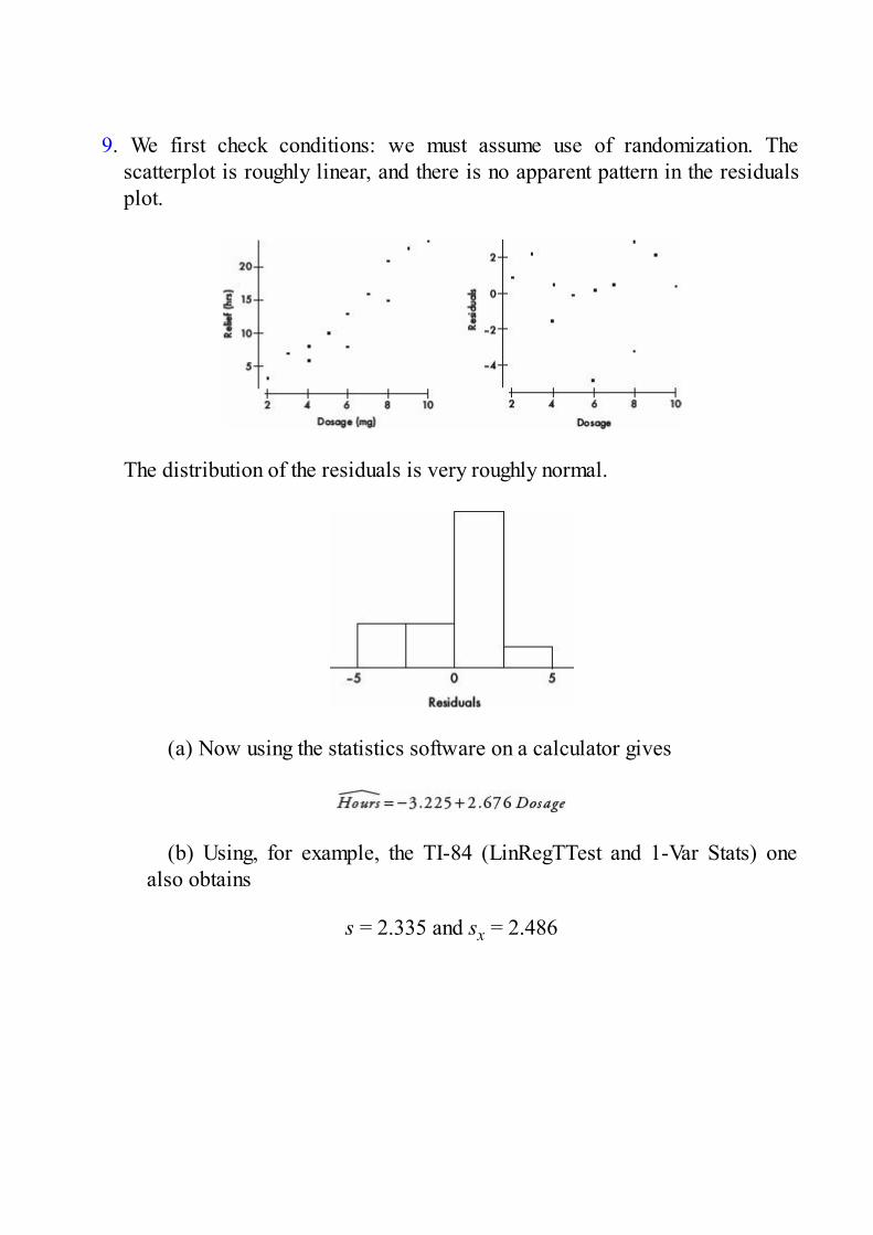
9. We first check conditions: we must assume use of randomization. Thescatterplot is roughly linear, and there is no apparent pattern in the residualsplot.
The distribution of the residuals is very roughly normal.
(a) Now using the statistics software on a calculator gives
(b) Using, for example, the TI-84 (LinRegTTest and 1-Var Stats) onealso obtains
s = 2.335 and sx = 2.486

Thus
[Note: On the TI-84, LinRegTTest gives both b1 and t, and you can alsocalculate which comes from ]
With 12 data points, the degrees of freedom are df = 12 – 2 = 10, and thecritical t-values (with .05 in each tail) are ± 1.812. The 99% confidenceinterval of the true slope is
We are thus 99% confident that each additional gram of the new drug isassociated with an average of between 2.2 and 3.2 more hours of allergyrelief. (A TI-84+ with LinRegTInt will give this result more directly.) Weshould be careful about extrapolating; note how the scatterplot of Reliefversus Dosage seems to be leveling off at the higher end.

10. (a) Assuming that all assumptions for regression are met, the y-intercept andslope of the equation are found in the Coeff column of the computerprintout.
where both the selling price and the assessed value are in $1000.
(b) From the printout, the standard error of the slope is sb1= 0.08192.
With df = 18 and .005 in each tail, the critical t-values are ± 2.878. The99% confidence interval of the true slope is:
We are 99% confident that for every $1 increase in assessed value, theaverage increase in selling price is between $0.79 and $1.27 (or for every$1000 increase in assessed value, the average increase in selling price isbetween $790 and $1270).
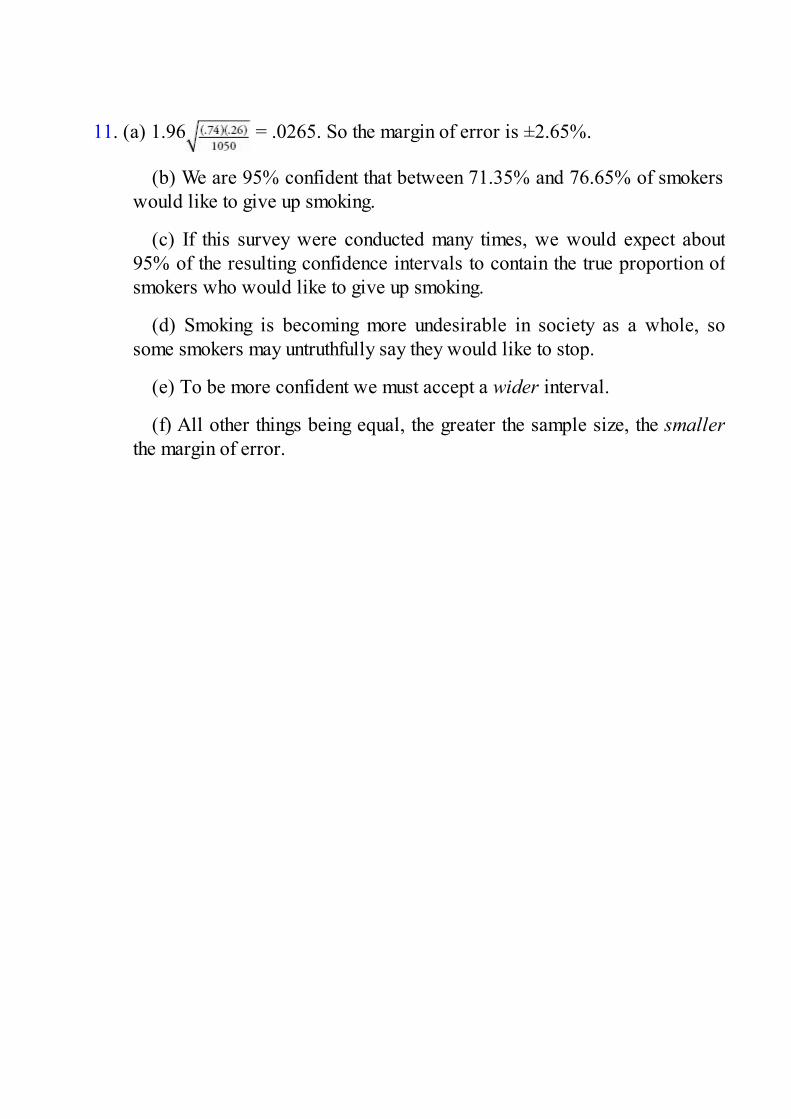
11. (a) 1.96 = .0265. So the margin of error is ±2.65%.
(b) We are 95% confident that between 71.35% and 76.65% of smokerswould like to give up smoking.
(c) If this survey were conducted many times, we would expect about95% of the resulting confidence intervals to contain the true proportion ofsmokers who would like to give up smoking.
(d) Smoking is becoming more undesirable in society as a whole, sosome smokers may untruthfully say they would like to stop.
(e) To be more confident we must accept a wider interval.
(f) All other things being equal, the greater the sample size, the smallerthe margin of error.

Answers Explained, Multiple-Choice1. (E) We attempt to show that the null hypothesis is unacceptable by
showing that it is improbable; however, we cannot show that it isdefinitely true or false. Both the null and alternative hypotheses are statedin terms of a population parameter, not a sample statistic. Thesehypotheses tests assume simple random samples.
2. (E) The P-value of a test is the probability of obtaining a result asextreme (or more extreme) as the one obtained assuming the nullhypothesis is true. Small P-values are evidence against the nullhypothesis. The null and alternative hypotheses are decided upon beforethe data come in.

3. (E) The parameter of interest is = the mean number of hours perweek which middle school students spend in video arcades.

4. (C) The alternative hypothesis is always an inequality, either <, or >,or ≠. In this case, the concern is whether middle school students arespending an average of more than two hours per week in video arcades.
5. (E) The P-value is a conditional probability; in this case, there is a.032 probability of an observed difference in sample proportions asextreme (or more extreme) as the one obtained if the null hypothesis isassumed to be true.

6. (C) This is a hypothesis test with H0: breaking strength is withinspecifications, and Ha: breaking strength is below specifications. A TypeI error is committed when a true null hypothesis is mistakenly rejected.
7. (C) A Type II error is a mistaken failure to reject a false nullhypothesis or, in this case, a failure to realize that a person really doeshave ESP.
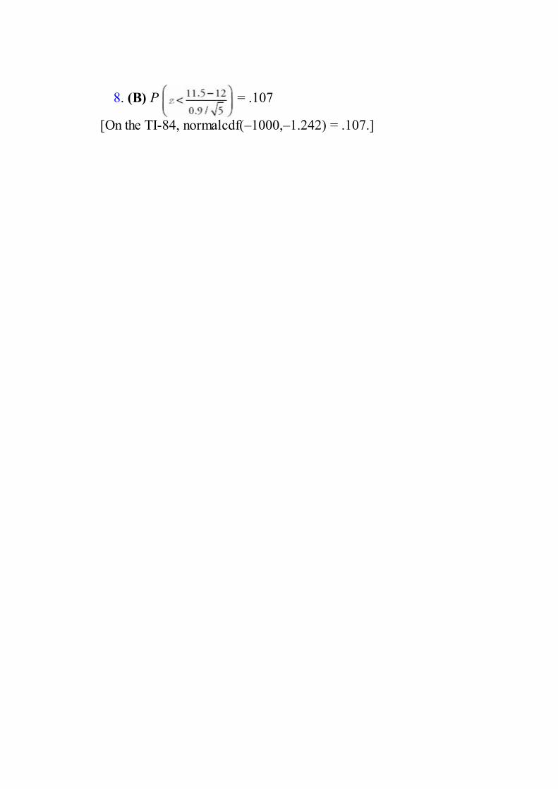
8. (B) P = .107
[On the TI-84, normalcdf(–1000,–1.242) = .107.]

9. (C) Medications having an effect shorter or longer than claimedshould be of concern, so this is a two-sided test: Ha: ≠ 58.4, and df = n– 1 = 40 – 1 = 39.
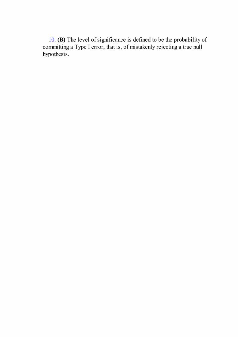
10. (B) The level of significance is defined to be the probability ofcommitting a Type I error, that is, of mistakenly rejecting a true nullhypothesis.
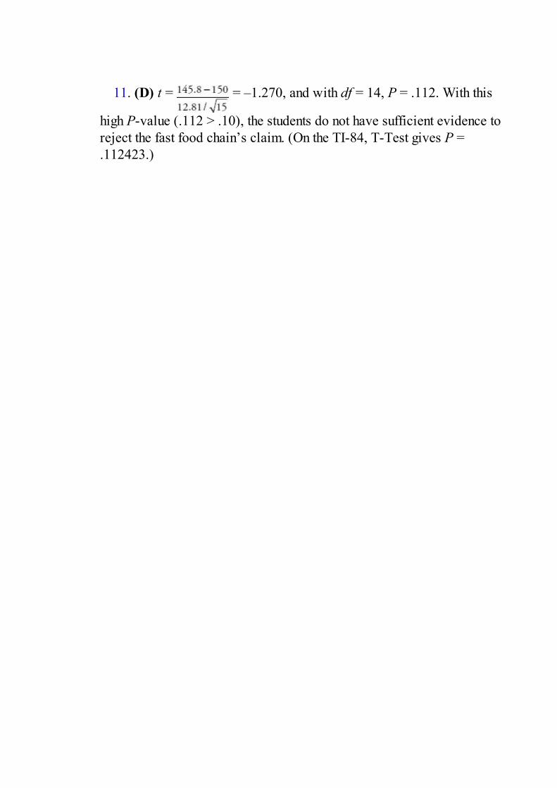
11. (D) t = = –1.270, and with df = 14, P = .112. With this
high P-value (.112 > .10), the students do not have sufficient evidence toreject the fast food chain’s claim. (On the TI-84, T-Test gives P =.112423.)

12. (A) With unknown population standard deviations, the t-distribution
must be used, and

13. (B) A Type I error means that the null hypothesis is true (theweather remains dry), but you reject it (thus you needlessly cancelschool). A Type II error means that the null hypothesis is wrong (the snowstorm hits), but you fail to reject it (so school is not canceled).

14.(E) With = .086087, get z = = 1.076 and P =
.141. With a P-value this high (.141 > .10), the government does not havesufficient evidence to reject the company’s claim. (On the TI-84,1PropZTest gives P = .140956.)

15.(D) This is a two-
sided test (H0: p1 – p2 = 0, Ha: p1 – p2 ≠ 0) with

16. (E) There is a different answer for each possible correct value forthe population parameter.

17. (A) This is a one-sided z-test, Ha: p > .5, with

18. (B) P(at least one Type I error) = 1 – P(no Type I errors) = 1 –(.99)5 = .049

19. (C) A larger sample size n reduces the standard deviation of thesampling distributions resulting in narrower sampling distributions so thatfor the given sample statistic, the P-value is smaller, and the probabilitiesof mistakenly rejecting a true null hypothesis or mistakenly failing toreject a false null hypothesis are both decreased. Furthermore, a lowerType II error results in higher power.

20. (E) The two-sample hypothesis test is not the proper one and canonly be used when the two sets are independent. In this case, there is aclear relationship between the data, in pairs, one pair for each student,and this relationship is completely lost in the procedure for the two-sample test. The proper procedure is to run a one-sample test on thesingle variable consisting of the differences from the paired data.

21. (C) With a smaller α, that is, with a tougher standard to reject H0,there is a greater chance of failing to reject a false null hypothesis, that is,there is a greater chance of committing a Type II error. Power is theprobability that a Type II error is not committed, so a higher Type II errorresults in lower power.

22. (B) If the null hypothesis is far off from the true parameter value,there is a greater chance of rejecting the false null hypothesis and thus asmaller risk of a Type II error. Power is the probability that a Type IIerror is not committed, so a lower Type II error results in higher power.

23. (C) With = 6.48 and s = 1.388, t = = 1.729. Given df =
29,P = .048.[On the TI-84, T-Test gives P = .048322.]

24. (C) If the alternative is true, the probability of failing to reject H0and thus committing a Type II error is 1 minus the power, that is, 1 – .75 =.25.

25. (B) P = .2525 [On the TI-84, normalcdf(–100, –
10/15) = .252492.]

Answers Explained, Free-Response1. The parameter of interest is = the mean tire pressure in the front right tires
of cars with recommended tire pressure of 35 psi. H0: = 35 and Ha: ≠ 35.
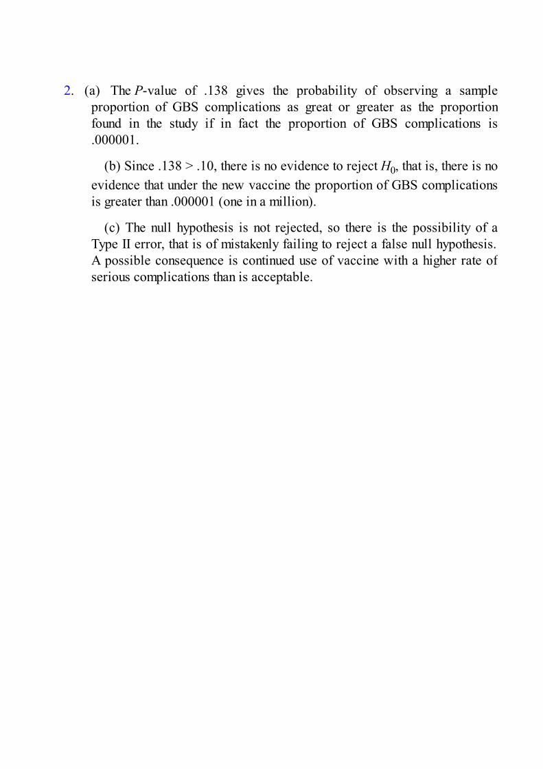
2. (a) The P-value of .138 gives the probability of observing a sampleproportion of GBS complications as great or greater as the proportionfound in the study if in fact the proportion of GBS complications is.000001.
(b) Since .138 > .10, there is no evidence to reject H0, that is, there is noevidence that under the new vaccine the proportion of GBS complicationsis greater than .000001 (one in a million).
(c) The null hypothesis is not rejected, so there is the possibility of aType II error, that is of mistakenly failing to reject a false null hypothesis.A possible consequence is continued use of vaccine with a higher rate ofserious complications than is acceptable.
3. (a) The P-value of .0197 gives the probability of observing a sample mean of1002.4 or greater if in fact this system results in a mean E. coliconcentration of 1000 MPN/100 ml.
(b) Since .0197 < .05, there is evidence to reject H0, that is, there isevidence that the mean E. coli concentration is greater than 1000 MPN/100ml, and the system is not working properly.
(c) With rejection of the null hypothesis, there is the possibility of aType I error, that is of mistakenly rejecting a true null hypothesis. Possibleconsequences are that sales of the system drop even though the system isdoing what it claims, or that the company performs an overhaul to fix thesystem even though the system is operating properly.

4. (a) This was an observational study as no treatments were imposed. It wouldhave been highly unethical to impose treatments, that is, to instructrandomly chosen volunteers to smoke, drink, skip exercise, and eat poorly.
(b) H0: p4 = p0, Ha: p4 > p0 where p4 is the proportion of adults with allfour bad habits who die during a 20-year period, and p0 is the proportionof adults with none of the four bad habits who die during a 20-year period.(Note that the hypotheses are about the population of all adults with andwith none of the four bad habits, not about the volunteers who took part inthe study.)
(c) A Type I error, that is, a mistaken rejection of a true null hypothesis,would result in people being encouraged to not smoke, not drink, exercise,and eat well, when these actions actually will not help decrease 20-yeardeath rates.
(d) A Type II error, that is, a mistaken failure to reject a false nullhypothesis, would result in people thinking that smoking, drinking,inactivity, and poor diet don’t increase 20-year death rates, when actuallythey do contribute to higher 20-year death rates.
(e) Calculator software (such as 2-PropZTest on the TI-84) gives P =.000. [For instructional purposes in this review book, we note that:
If the null hypothesis were true, that is, if there was no difference in the 20-year death rates between people with all four bad habits and people withnone of the bad habits, then the probability of sample proportions with adifference as extreme or more extreme than observed is .000 (to threedecimals).
5. First, state the hypotheses:
H0: p = .174 and Ha: p > .174. (If asked to state the parameter, then state“where p is the proportion of AAUP members who own Roth IRAs.”)
Second, identify the test by name or formula and check the assumptions.
This is a one-sample z-test for a population proportion.
Assumptions: Random sample (given), np = 750(.174) = 130.5 ≥ 10, and n(1– p) = 750(.826) = 619.5 ≥ 10.
Third, calculate the test statistic z and the P-value. Calculator software (suchas 1PropZTest on the TI-84) gives z = 1.878 and P = .030.[For instructional purposes in this review book, we note that
Fourth, linking to the P-value, give a conclusion in context.
With a P-value this small (.030 < .05), there is evidence that more than17.4% of AAUP members own Roth IRAs.

6. First, state the hypotheses: H0: = 593 and Ha: ≠ 593 (If asked to state theparameter, then state “where is the mean discharge rate (in 1000 ft3 /sec) atthe mouth of the Mississippi River.”)
Second, identify the test by name or formula and check the assumptions:
This is a one-sample t-test for the mean with t = Assumptions: The
measurements were taken at random times, and either a dotplot of the sampleis roughly unimodal and symmetric or the normal probability plot is roughlylinear:
Third, calculate the test statistic t and the P-value:
Calculator software (such as T-Test using Data on the TI-84) gives t = –2.7116 and P = .0239. [For instructional purposes in this review book, wenote that = 590.5 and s = 2.9155 which gives
Since this is a two-sided test, we double this value to find the P-value to be P= .0240.]
Fourth, linking to the P-value, give a conclusion in context: With a P-valuethis small (.0239 < .05), there is evidence that the long accepted measure ofthe discharge rate at the mouth of the Mississippi River has changed.

7. First, state the hypotheses: H0: pB – pG = 0 (or pB = pG) and Ha: pB – pG > 0(or pB > pG). If asked to state the parameters, then state “where pB is theproportion of high school boys who meet the recommended level of physicalactivity, and pG is the proportion of high school girls who meet therecommended level of physical activity.”)
Second, identify the test by name or formula and check the assumptions:
This is a two-sample z-test for proportions. Assumptions: Independentrandom samples (given), and nB B = 370 ≥ 10, nB (1 – B) = 480 ≥ 10, nG G= 218 ≥ 10, and nG (1 – G) = 362 ≥ 10.
Third, calculate the test statistic z and the P-value. Calculator software (suchas 2-PropZTest on the TI-84) gives z = 2.2427 and P = .012. (Forinstructional purposes in this review book, we note that
Fourth, linking to the P-value, give a conclusion in context. With a P-valuethis small (.012 < .05), there is evidence that the proportion of high schoolboys who meet the recommended level of physical activity is greater than theproportion of high school girls who meet the recommended level of physicalactivity.

8. First, state the hypotheses: H0: NFL – 10 = 0 (or NFL = 10) and Ha: NFL –
10 < 0 (or NFL < 10) (or “>” depending on choice of variables). (If askedto state the parameters, then state “where NFL is the mean attendance at NFLgames and 10 is the mean attendance at Big 10 football games.”]
Second, identify the test by name or formula and check the assumptions: Thisis a two-sample t-test for means. Assumptions: Independent random samples(given), and both samples sizes, 35 and 30, are large enough so that by theCLT, the distribution of sample means is approximately normal and a t-testmay be run.
Third, calculate the test statistic t and the P-value. Calculator software (suchas 2-SampTTest on the TI-84) gives t = –0.8301, df = 49.3, and P = .2052.[For instructional purposes in this review book, we note that:
Fourth, linking to the P-value, give a conclusion in context. With a P-valuethis large (.2052 > .10), there is no evidence that the average attendance atBig 10 Conference football games is greater than that at NFL games.

9. (a) One block consists of the 500 patients who have had a mini stroke in theprevious year, and a second block consists of the 500 patients who havenot. In one block, number the patients 1 through 500, and then using arandom number generator, pick numbers between 1 and 500, throwing outrepeats, until 250 patients are picked. Assign surgery to these patients andstents to the remaining 250. Repeat for the other block.
(b) One method is to increase the sample size, resulting in a reduction inthe standard error of the sampling distribution, which in turn increases theprobability of rejecting the null hypothesis if it is false. A second method isto increase α, the significance level, which in turn also increases theprobability of rejecting the null hypothesis if it is false. In either case, thereis increased probability of detecting any difference in the proportions ofpatients suffering major complications between the surgery and stentrecipients.

10. The data come in pairs, and the two-sample test does not apply theknowledge of what happened to each individual driver (the condition ofindependence of the two samples is violated). The appropriate test is a one-population, small-sample hypothesis test on the set of differences: {0, –5, 3, –4, –3, 1, –2, –2, –1, –1}. We proceed as follows:
First, state the hypotheses: H0: D = 0, Ha: D ≠ 0 (If asked to state theparameter, then state “where D is the mean difference in reaction timesbetween DWI and DWT.”)
Second, identify the test and check the assumptions: This is a paired t-test,that is, a single-sample hypothesis test on the set of differences.
The data are paired because they are measurements on the same individualsunder DWI and DWT.
The reaction times of any individual are assumed independent of the reactiontimes of the others, so the differences are independent.
We must assume that the volunteers are a representative sample.
Either a dotplot of the sample is roughly unimodal and symmetric or thenormal probability plot is roughly linear:
Third, calculate the test statistic t and the P-value: Calculator software (suchas T-Test and Data on the TI-84) gives t = –1.871 and P = .094174. [Forinstructional purposes in this review book, we note that
= –1.4 and s = 2.366 giving t = = –1.871, and with df = 10 – 1
= 9, P(t < –1.871) = .0471. Since this is a two-sided test, we double thisvalue to find the P-value to be P = .0942.]
Fourth, linking to the P-value, give a conclusion in context: With a P-value

this small (.0942 < .10), there is evidence at the 10% significance level of adifference between the effect on reaction time between DWI and DWT. Or,with a P-value this large (.0942 > .05), there is no evidence at the 5%significance level of a difference between the effect on reaction time betweenDWI and DWT.

Answers Explained, Investigative Tasks1. (a) P(positive test | disease) = = .61.
(b) P(negative test | healthy) = = .8.
(c) LR+ = = 3.05. A positive test given a diseased subject and a
negative test given a healthy subject are both desired outcomes, so highervalues for both Sensitivity and Specificity are good. Higher values ofSensitivity, the numerator of LR+, lead to greater values of LR+. Highervalues of Specificity give lower values of 1 – Specificity, the denominatorof LR+, again leading to greater values of LR+.
(d) The estimated P-value is the proportion of the simulated statisticswhich are less than or equal to the sample statistic of 4.7. Counting valuesin the dotplot gives a P-value of .04. With a P-value this small, there isevidence that the population LR+ is below the desired value of 5.0.
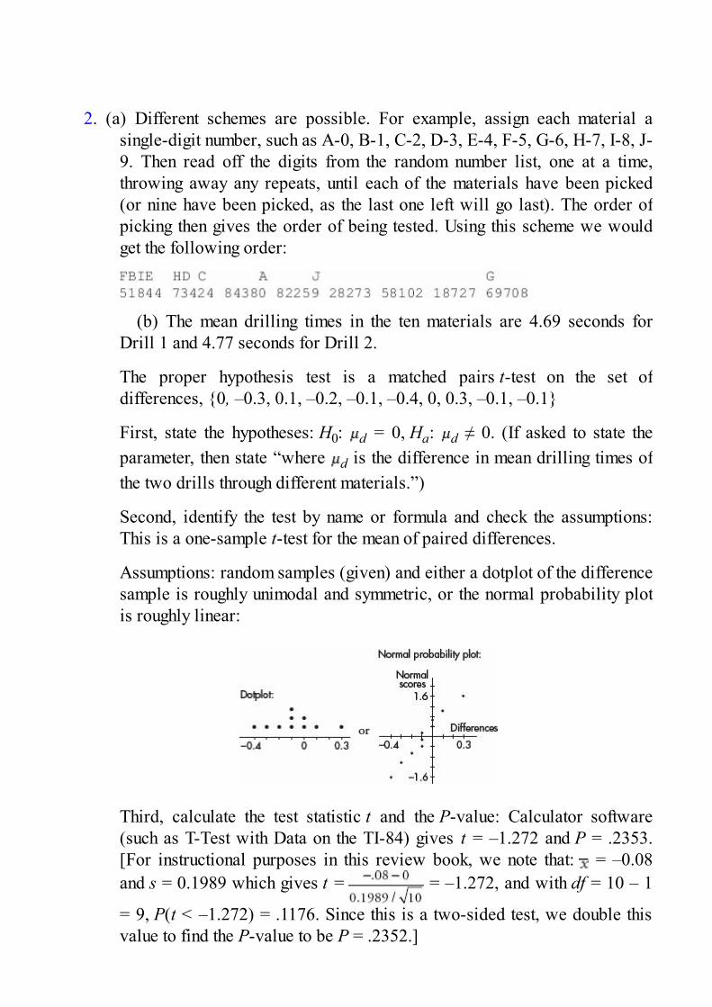
2. (a) Different schemes are possible. For example, assign each material asingle-digit number, such as A-0, B-1, C-2, D-3, E-4, F-5, G-6, H-7, I-8, J-9. Then read off the digits from the random number list, one at a time,throwing away any repeats, until each of the materials have been picked(or nine have been picked, as the last one left will go last). The order ofpicking then gives the order of being tested. Using this scheme we wouldget the following order:
(b) The mean drilling times in the ten materials are 4.69 seconds forDrill 1 and 4.77 seconds for Drill 2.
The proper hypothesis test is a matched pairs t-test on the set ofdifferences, {0, –0.3, 0.1, –0.2, –0.1, –0.4, 0, 0.3, –0.1, –0.1}
First, state the hypotheses: H0: d = 0, Ha: d ≠ 0. (If asked to state theparameter, then state “where d is the difference in mean drilling times ofthe two drills through different materials.”)
Second, identify the test by name or formula and check the assumptions:This is a one-sample t-test for the mean of paired differences.
Assumptions: random samples (given) and either a dotplot of the differencesample is roughly unimodal and symmetric, or the normal probability plotis roughly linear:
Third, calculate the test statistic t and the P-value: Calculator software(such as T-Test with Data on the TI-84) gives t = –1.272 and P = .2353.[For instructional purposes in this review book, we note that: = –0.08and s = 0.1989 which gives t = = –1.272, and with df = 10 – 1
= 9, P(t < –1.272) = .1176. Since this is a two-sided test, we double thisvalue to find the P-value to be P = .2352.]

Fourth, linking to the P-value, give a conclusion in context. With a P-valuethis large (.2353 > .10), there is no evidence of a difference in meandrilling times of the two drills through different materials.

3. (a) The conditions for a one-sample z-test on a population proportion includethat both n ≥ 10 and n(1 – ) ≥ 10. In this case, n = 12 but n(1 – ) = 2.
(b) First, state the hypotheses: H0:p = .5 and Ha: p > .5, [If asked to statethe parameter, then state “where p is the proportion of soccer matches forwhich Paul the octopus can correctly predict the winning team.”]
Second, identify the test and check the assumptions:
This is a test of a binomial model.
For each trial there are two outcomes (Paul has a choice of two boxes ofmussels), the trials are independent, and the probability of Paul picking awinner can be assumed to be the same for each trial. We are given that the14 matches are a random sample of all matches.
Third, calculate the P-value: With p = .5, P(x ≥ 12) = (.5)12(.5)2 +
(.5)13 (.5) + (.5)14 = .00647
Fourth, linking to the P-value, give a conclusion in context: With a P-valuethis small (.00647 < .01), there is strong evidence that Paul can correctlypredict the results of more than 50% of soccer matches.

4. (a) First, state the hypotheses: H0: = 30, Ha: > 30. (If asked to state theparameter, then state “where is the mean interest level of all teenagersafter seeing the ad.”)
Second, identify the test and check the assumptions: This is a one-sample t-test for the mean. The sample was randomly chosen, and a dotplot isroughly unimodal and symmetric:
Third, calculate the test statistic t and the P-value: Calculator software(such as T-Test with Data on the TI-84) gives t = 2.526 and P = .012113.[For instructional purposes in this review book, we note that = 37.2 ands = 11.04 which gives t = = 2.526 and with df = 15 – 1 = 14, P(t
> 2.526) = .0121.]
Fourth, linking to the P-value, give a conclusion in context: With a P-valuethis small (.0121 < .05), there is evidence to support the ad developer’sclaim that after seeing the ad, the interest level is above 30.
(b) First, state the hypotheses: H0: D = 0, Ha: D ≠ 0, where D is themean difference between after-ad and before-ad interest level.
Second, identify the test and check the assumptions: This is a paired t-test,that is, a single sample hypothesis test on the set of differences, and it isgiven that all assumptions for hypothesis testing are met.
Third, calculate the test statistic t and the P-value: Calculator software(such as T-Test with Data on the TI-84) gives t = 0.9693 and P = .174415.[For instructional purposes in this review book, we note that = 0.6667and s = 2.664 giving t = = 0.9693 and with df = 15 – 1 = 14, P(t
> 0.9693) = .1744.]
Fourth, linking to the P-value, give a conclusion in context: With a P-valuethis large (.1744 > .10), there is no evidence that after seeing the ad,teenagers have increased interest in the new website.
(c) A least square regression line using the after-ad and before-ad

interest levels has a high correlation of r = .972, which when combinedwith the scatterplot, indicates a strong association. Thus, after-ad interestlevel can be predicted from before-ad interest level.
(d) A least square regression line using the before-ad and the change ininterest levels yields a very low correlation of r = .235, which whencombined with the scatterplot, indicates almost no association. Thus, after-ad interest level cannot be predicted from before-ad interest level.

5. (a) One of many ways to proceed: let the digits 1 and 2 represent having apassport, while the remaining single digits represent not having a passport.Read off groups of ten digits, checking for the number of 1s and 2s in eachgroup.
Tabulating from the table gives:
No passports (no 1s or 2s): 2One passport (one 1 or 2): 8Two passports (two 1s or 2s): 8Three passports (three 1s or 2s): 5Four passports (four 1s or 2s): 1Five passports (five 1s or 2s): 1
The estimated probability of at least three passports among ten 18–24-year-olds is thus = .28.
(b) In a binomial distribution with n = 10 and p = .20, P(x ≥ 3) = .3222.(On the TI-84, 1 – binomcdf(10, .20, 2) = 1 – .6778 = .3222.)
(c) First, state the hypotheses: H0: p = .20, Ha: p < .20 (If asked to statethe parameter, then state “where p is the proportion of all 18–24-year-oldswho have passports.”)
Second, identify the test and check the assumptions: This is a one-samplez-test for a population proportion, we have an SRS, np = (200)(.20) = 40 >10, n(1 – p) = (200)(.80) = 160 > 10, and clearly 200 < 10% of all 18–24-year-olds.
Third, calculate the test statistic z and the P-value: Calculator software(such as 1PropZTest on the TI-84) gives z = –1.2374 and P = .107963.[For instructional purposes in this review book, we note that:
Fourth, linking to the P-value, give a conclusion in context. With a P-value

this large (.1080 > .10), there is not sufficient evidence to dispute the claimthat 20% of 18–24-year-olds have passports.
(d) This geometric probability is (.8)2(.2) = .128.
(e) = 1(.21) + 2(.15) + 3(.13) + ... + 12(.02) = 4.31 (On the TI-84, put 1–12 in L1, put the frequencies 21, 15, 13, ... , 2 in L2, and then 1-VarStats gives = 4.31.)
Answers Explained, Multiple-Choice1. (C) There are two observations of each mouse, a before time and an
after time. These two times are dependent so a paired t-test isappropriate, not a two-sample test.
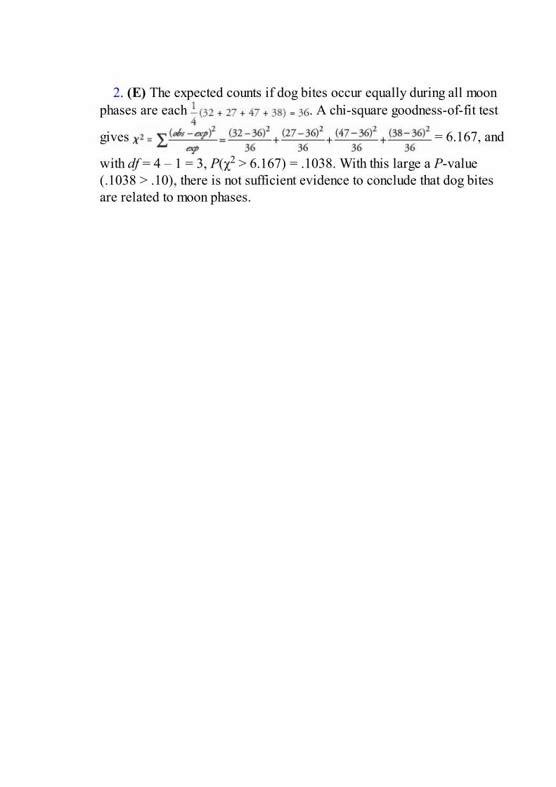
2. (E) The expected counts if dog bites occur equally during all moonphases are each . A chi-square goodness-of-fit test
gives = 6.167, and
with df = 4 – 1 = 3, P(χ2 > 6.167) = .1038. With this large a P-value(.1038 > .10), there is not sufficient evidence to conclude that dog bitesare related to moon phases.

3. (B) df = (rows – 1)(columns – 1) = (2 – 1)(5 – 1) = 4

4. (C) Picking separate samples from each of 16 populations andclassifying according to one variable (perception of quality education) isa survey design which is most appropriately analyzed using a chi-squaretest of homogeneity of proportions.

5. (D) With 77 + 85 + 23 + 15 = 200 samples, the expected counts ifthe blood type distribution on the island is the same as that of the generalpopulation are 46% of 200 = 92, 40% of 200 = 80, 10% of 200 = 20, and4% of 200 = 8. A chi-square goodness-of-fit test gives
= 9.333, and with df
= 4 – 1 = 3, P(χ2 > 9.333) = .0252. With a P-value this small (.0252 <.05), there is sufficient evidence at the 5% significance level that bloodtype distribution on the island is different from that of the generalpopulation.

6. (D) With df = (3 – 1)(5 – 1) = 8, P(χ2 > 13.95) = .083. Since .05 <.083 < .10, there is evidence at the 10% significance level, but not at the5% significance level, of a relationship between education level andsports interest.

7. (E) With a P-value this small (less than .05), there is evidence insupport of the alternative hypothesis Ha: the distributions of musicpreferences are different, that is, they differ for at least one of theproportions.
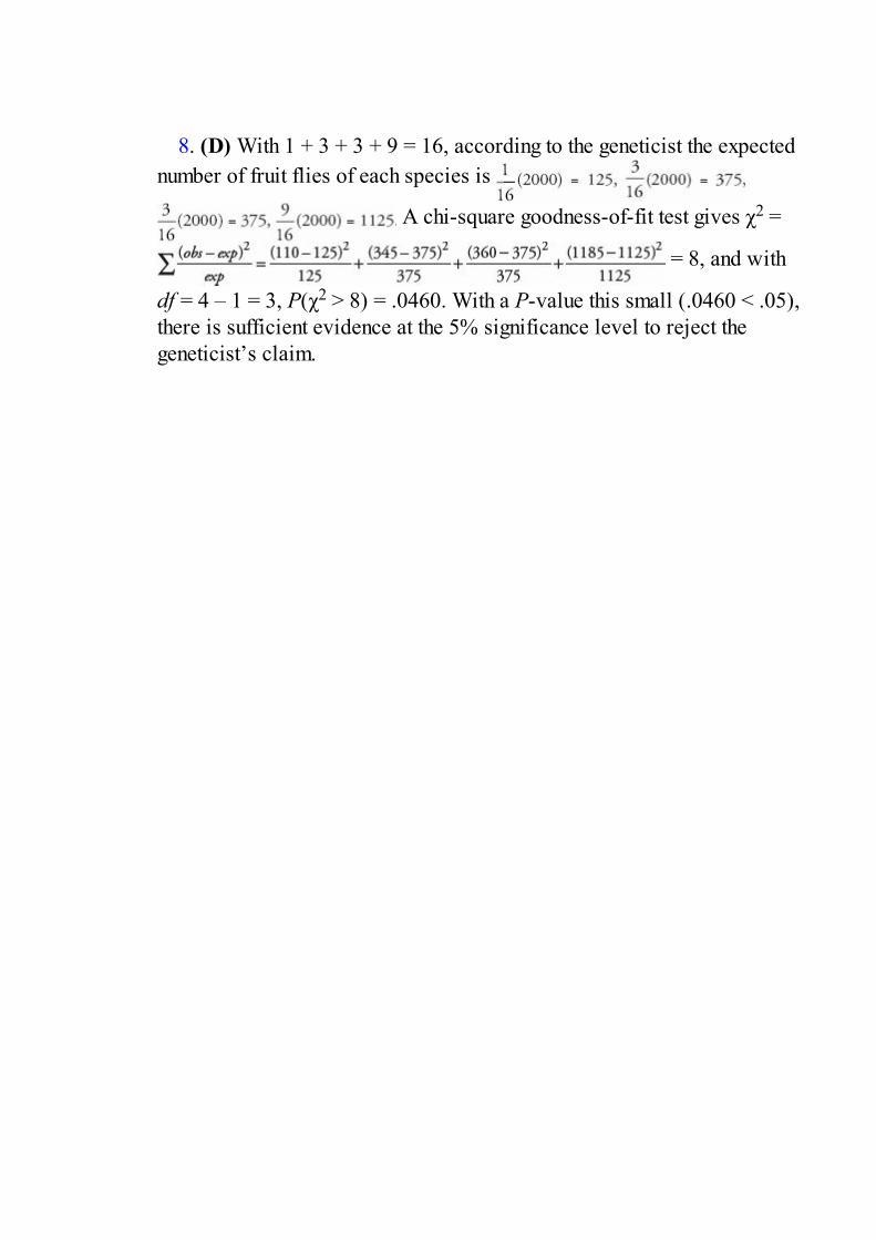
8. (D) With 1 + 3 + 3 + 9 = 16, according to the geneticist the expectednumber of fruit flies of each species is
A chi-square goodness-of-fit test gives χ2 =
= 8, and with
df = 4 – 1 = 3, P(χ2 > 8) = .0460. With a P-value this small (.0460 < .05),there is sufficient evidence at the 5% significance level to reject thegeneticist’s claim.

9. (E) A chi-square test of independence gives χ2 = 2.852, and with df= 2, we find P = .2403, and since .2403 > .10, there is not evidence at the10% significance level of a relationship between taste preference and thepresence of the marker.

10. (E) A chi-square test of homogeneity gives χ2 = 5.998, and with df= 3, the P-value is .1117. With a P-value this large (.1117 > .10) there isnot evidence of a difference in cafeteria food satisfaction among the classlevels.

11. (E) The relevant P-value is 0.065 which is less than 0.10 butgreater than 0.05.

12. (E) In computer printouts of regression analysis, “S” typically givesthe standard deviation of the residuals.

Answers Explained, Free-Response1. First, state the hypotheses: H0: The colors of the sugar shells are distributed
according to 35% cherry red, 10% vibrant orange, 10% daffodil yellow, 25%emerald green, and 20% royal purple, and Ha: The colors of the sugar shellsare not distributed as claimed by the manufacturer. Or [H0: PCR = .35, PVO =.10, PDY = .10, PEG = .25, PRP = .20, and Ha: at least one proportion isdifferent from this distribution.]
Second, identify the test and check the assumptions: χ2 goodness-of-fit test.We are given a random sample, and calculate that all expected cells are atleast 5: 35% of 300 = 105, 10% of 300 = 30, 25% of 300 = 75, and 20% of300 = 60.
Third, calculate the test statistic χ2 and the P-value: A calculator gives
Fourth, linking to the P-value, give a conclusion in context: With a P-valuethis large (.153 > .10), there is not evidence that the distribution is differentfrom what is claimed by the manufacturer.

2. (a) Design I, with a single sample from one population classified on twovariables (smoking and fitness), will result in a test of independence.Design II, with independent samples from two populations each with thesingle variable (fitness), will result in a test of homogeneity.
(b) Design II, with its test of homogeneity, and using an equal samplesize from each of the two populations (smokers and non-smokers), is bestfor comparing proportions of smokers who have different fitness levelswith proportions of non-smokers who have different fitness levels.
(c) Design I, which classifies one population on the two variables,smoking and fitness, is the only one of these two designs which will givedata on the conditional distribution of people with given fitness levels whoare smokers or are not smokers.

3. (a) First, state the hypotheses: H0: Happiness level is independent ofbusy/idle choice for high school students and Ha: Happiness level is notindependent of busy/idle choice for high school students.
Second, identify the procedure and check the conditions: This is a chi-square test of independence. It is given that there is a random sample, thedata are measured as “counts,” and the expected counts are all at least 5(put the observed counts in a matrix; then χ2-Test on the TI-84 givesexpected counts of
Third, calculate the test statistic and the P-value: Calculator software (χ2-Test on the TI-84) gives χ2 = 14.54 withP = .0058 and df = 4.
Fourth, give a conclusion in context with linkage to the P-value: With a P-value this small (.0058 < .01), there is strong evidence of a relationshipbetween happiness level and busy/idle choice for high school students.
(b) No, it is not reasonable to conclude that encouraging high schoolstudents to keep more busy will lead to higher happiness levels. This wasnot an experiment with students randomly chosen to sit or walk. Thestudents themselves chose whether or not to sit or walk so no cause-and-effect conclusion is possible. For example, it could well be that thehappier students choose to walk, whereas the less happy students choose tosit.
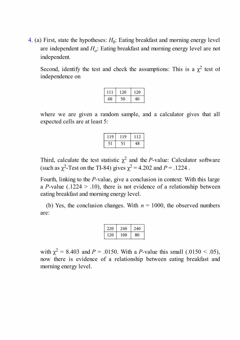
4. (a) First, state the hypotheses: H0: Eating breakfast and morning energy levelare independent and Ha: Eating breakfast and morning energy level are notindependent.
Second, identify the test and check the assumptions: This is a χ2 test ofindependence on
where we are given a random sample, and a calculator gives that allexpected cells are at least 5:
Third, calculate the test statistic χ2 and the P-value: Calculator software(such as χ2-Test on the TI-84) gives χ2 = 4.202 and P = .1224 .
Fourth, linking to the P-value, give a conclusion in context: With this largea P-value (.1224 > .10), there is not evidence of a relationship betweeneating breakfast and morning energy level.
(b) Yes, the conclusion changes. With n = 1000, the observed numbersare:
with χ2 = 8.403 and P = .0150. With a P-value this small (.0150 < .05),now there is evidence of a relationship between eating breakfast andmorning energy level.
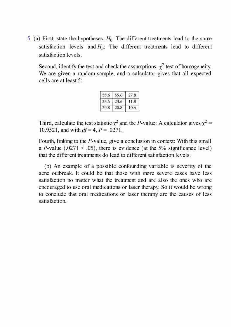
5. (a) First, state the hypotheses: H0: The different treatments lead to the samesatisfaction levels and Ha: The different treatments lead to differentsatisfaction levels.
Second, identify the test and check the assumptions: χ2 test of homogeneity.We are given a random sample, and a calculator gives that all expectedcells are at least 5:
Third, calculate the test statistic χ2 and the P-value: A calculator gives χ2 =10.9521, and with df = 4, P = .0271.
Fourth, linking to the P-value, give a conclusion in context: With this smalla P-value (.0271 < .05), there is evidence (at the 5% significance level)that the different treatments do lead to different satisfaction levels.
(b) An example of a possible confounding variable is severity of theacne outbreak. It could be that those with more severe cases have lesssatisfaction no matter what the treatment and are also the ones who areencouraged to use oral medications or laser therapy. So it would be wrongto conclude that oral medications or laser therapy are the causes of lesssatisfaction.
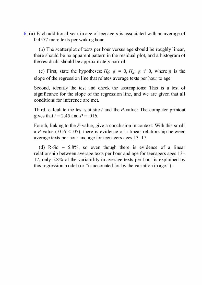
6. (a) Each additional year in age of teenagers is associated with an average of0.4577 more texts per waking hour.
(b) The scatterplot of texts per hour versus age should be roughly linear,there should be no apparent pattern in the residual plot, and a histogram ofthe residuals should be approximately normal.
(c) First, state the hypotheses: H0: = 0, Ha: ≠ 0, where is theslope of the regression line that relates average texts per hour to age.
Second, identify the test and check the assumptions: This is a test ofsignificance for the slope of the regression line, and we are given that allconditions for inference are met.
Third, calculate the test statistic t and the P-value: The computer printoutgives that t = 2.45 and P = .016.
Fourth, linking to the P-value, give a conclusion in context: With this smalla P-value (.016 < .05), there is evidence of a linear relationship betweenaverage texts per hour and age for teenagers ages 13–17.
(d) R-Sq = 5.8%, so even though there is evidence of a linearrelationship between average texts per hour and age for teenagers ages 13–17, only 5.8% of the variability in average texts per hour is explained bythis regression model (or “is accounted for by the variation in age.”).

7. First, state the hypotheses: H0: = 0, Ha: ≠ 0. (If asked to state theparameter, then state “where is the slope of the regression line that relatesaverage fertility rate to women’s life expectancy.”)
Second, identify the test and check the assumptions: This is a test ofsignificance for the slope of the regression line. We are given that the datacome from a random sample of countries.
Distribution of residuals is approximately normal (Checked by normalprobability plot)
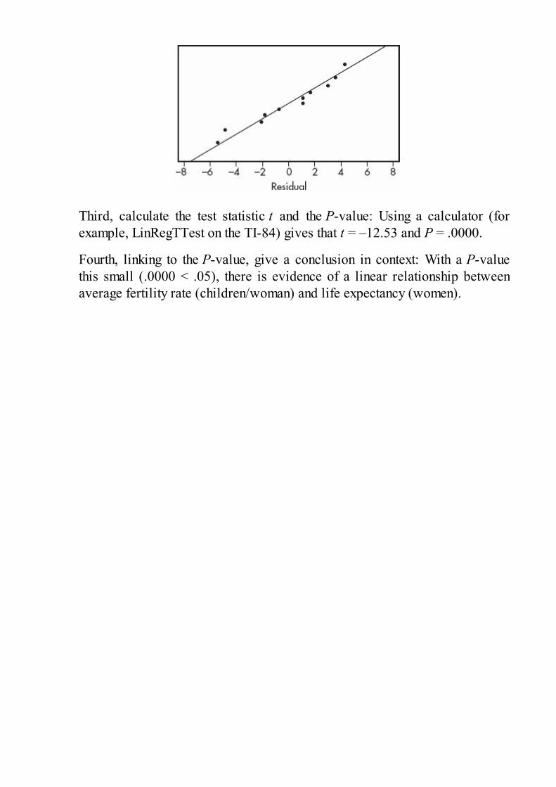
Third, calculate the test statistic t and the P-value: Using a calculator (forexample, LinRegTTest on the TI-84) gives that t = –12.53 and P = .0000.
Fourth, linking to the P-value, give a conclusion in context: With a P-valuethis small (.0000 < .05), there is evidence of a linear relationship betweenaverage fertility rate (children/woman) and life expectancy (women).

Answers Explained, Investigative Task1. (a) The binomial distribution with p = 0.2 and n = 3 results in: P(0) = (.8)3 =
.512, P(1) = 3(.2)(.8)2 = .384, P(2) = 3(.2)2(.8) = .096, P(3) = (.8)3 =
.008.
(b) Multiplying each of the probabilities in (a) by 800 gives the expectednumber of occurrences:
(c) First, state the hypotheses: H0: The number of researchers able todetermine the composition of a placebo follows a binomial with p = 0.2and Ha: The number of researchers able to determine the composition of aplacebo does not follow a binomial with p = 0.2.
Second, identify the test and check the assumptions: This is a chi-squaretest of goodness-of-fit. We must assume that the 800 studies form arepresentative sample. We note from (b) that all expected cells are ≥5:
Third, calculate the test statistic χ2 and the P-value: A calculator gives and with df = 4 – 1 = 3, P = .02549.
Fourth, linking to the P-value, give a conclusion in context: With a P-valuethis small (.02549 < .05), there is evidence that the number of researchersable to determine the composition of a placebo does not follow a binomialwith p = 0.2.

2. (a) This is a matched-pair t-test on the set of differences {–1.7, –0.2, 1.0, 2.0,1.3, 0.4, –0.1, 0.4, 0.8, –1.2, 0.4, 0.9}, with H0: d = 0 and Ha: d > 0. Thesample is random (given), and a dotplot of the differences is roughlyunimodal and symmetric (so a normal population distribution is areasonable assumption):
Calculator software (such as T-Test with Data on the TI-84) gives t =1.121 and P = .143. [For instructional purposes in this review book, wenote that = 0.3333, s = 1.030, and with df = 12 – 1
= 11, P = .143.] With a P-value this large (.143 > .10), there is notevidence that the average student score is greater than that of the Englishteachers.
(b) This is a matched-pair t-test on the set of differences {–0.3, 1.6, 0.7,0.3, 0.5, –0.1, –0.8, 0.9, 0.5, –0.1, 0.2, 1.1}, with H0: d = 0 and Ha: d >0. The sample is random (given), and a dotplot of the differences is roughlyunimodal and symmetric (so a normal population distribution is areasonable assumption):
Calculator software (such as T-Test with Data on the TI-84) gives t =1.974 and P = .0370. [For instructional purposes in this review book, wenote that = 0.375, s = 0.6580, and with df = 12 – 1
= 11, P = .037.] With a P-value this small (.037 < .05), there is evidencethat the average student score is greater than that of the math teachers.
(c) In both regression analyses, the scatterplots are roughly linear andthe residual plots show no apparent pattern; however, while 70.1% of thevariance in student scores is explained by the variance in math teacherscores, only 27.8% of the variance in student scores is explained byvariance in English teacher scores. Thus, the math teacher scores are abetter predictor of student scores.
(d) Using the regression equation giving predicted student score as a

function of math teacher score gives –0.330 + 1.0701(10.0) = 10.37.
(e) The regression output gives a standard deviation of s = 0.6867. Usingthe 10.37 estimate from part (d) gives a range of scores for students whosemath teachers’ average score is 10.0 to be 10.37 ± 3(0.6867) = 10.37 ±2.06. Thus, for schools where the math teachers’ average score is 10.0,almost all the average student scores will be between 8.31 and 12.4.

3. (a) The z-scores for 22.5 and 27.5 are, respectively, and
Similarly, 17.5 and 12.5 have z-scores of –0.5 and –1.5,
respectively. Using the normal probability table or a calculator gives theprobabilities: P(z < –1.5) = .0668, P(–1.5 < z < –0.5) = .2417, P(–0.5 < z< 0.5) = .3830, P(0.5 < z < 1.5) = .2417, P(z > 1.5) = .0668.
(b) Multiplying each probability by 500: .0668(500) = 33.4, .2417(500)= 120.85, .3830(500) = 191.5, .2417(500) = 120.85, and .0668(500) =33.4.
(c) First, state the hypotheses: H0: The weights of student backpacksfollow a normal distribution with = 20 and σ = 5 and Ha: The weights ofstudent backpacks do not follow a normal distribution with = 20 and σ =5.
Second, identify the test and check the assumptions: This is a chi-squaretest of goodness-of-fit. We are given that the weights are from a randomsample of students. We note from above that all expected cells are ≥5:
Third, calculate the test statistic χ2 and the P-value: A calculator gives and with df = 5 – 1 = 4, P = .1476.
Fourth, linking to the P-value, give a conclusion in context: With a P-valuethis large (.1476 > .10), there is no evidence that the data do not follow anormal distribution with = 20 and σ = 5.
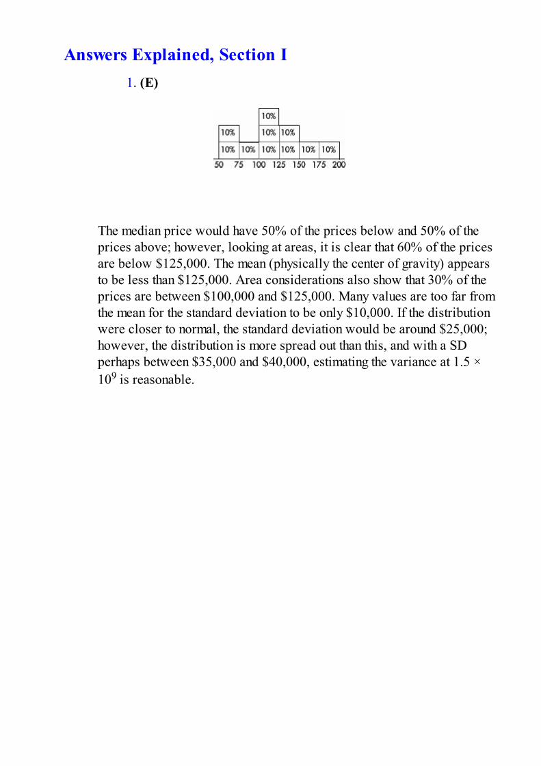
Answers Explained, Section I1. (E)
The median price would have 50% of the prices below and 50% of theprices above; however, looking at areas, it is clear that 60% of the pricesare below $125,000. The mean (physically the center of gravity) appearsto be less than $125,000. Area considerations also show that 30% of theprices are between $100,000 and $125,000. Many values are too far fromthe mean for the standard deviation to be only $10,000. If the distributionwere closer to normal, the standard deviation would be around $25,000;however, the distribution is more spread out than this, and with a SDperhaps between $35,000 and $40,000, estimating the variance at 1.5 ×10⁹ is reasonable.
2. (E) Regression lines show association, not causation. Surveyssuggest relationships, which experiments can help to show to be causeand effect.
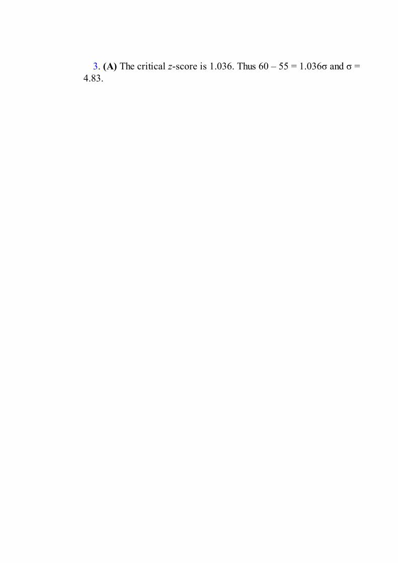
3. (A) The critical z-score is 1.036. Thus 60 – 55 = 1.036σ and σ =4.83.

4. (D) We are 90% confident that the population mean is within theinterval calculated using the data from the sample.
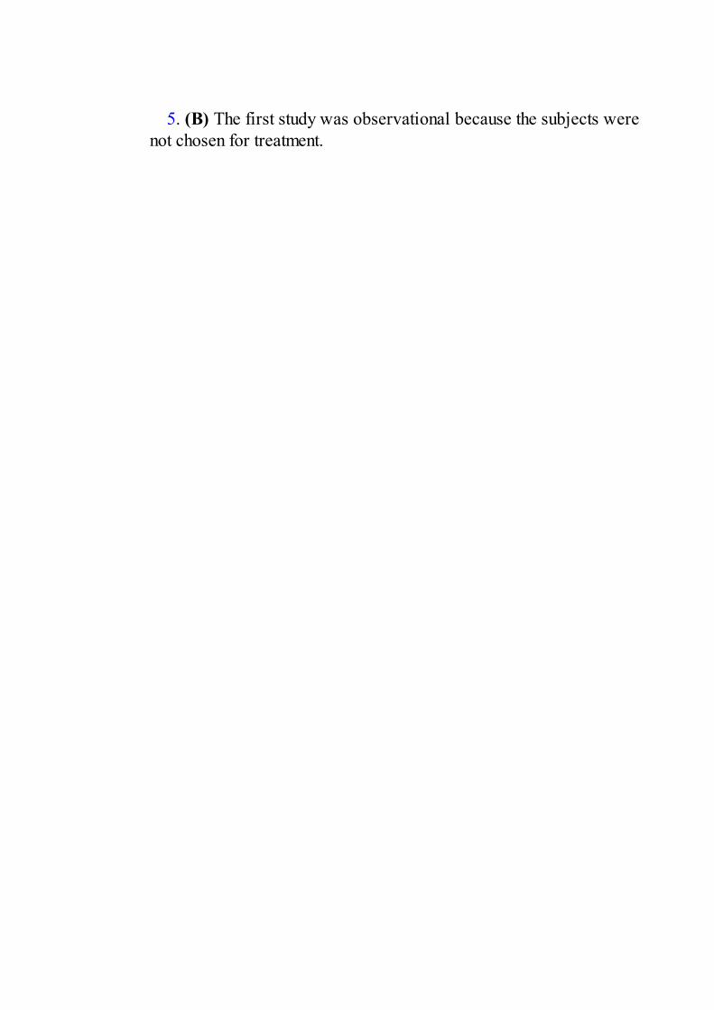
5. (B) The first study was observational because the subjects werenot chosen for treatment.

6. (A)
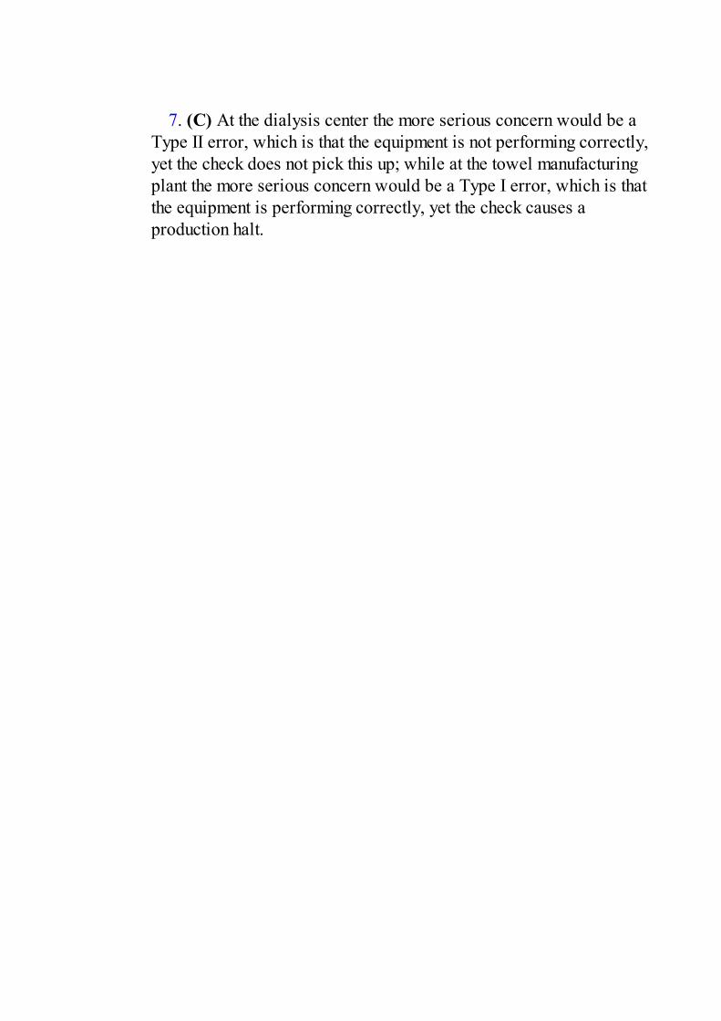
7. (C) At the dialysis center the more serious concern would be aType II error, which is that the equipment is not performing correctly,yet the check does not pick this up; while at the towel manufacturingplant the more serious concern would be a Type I error, which is thatthe equipment is performing correctly, yet the check causes aproduction halt.

8. (D) There are two possible outcomes (heads and tails), with theprobability of heads always .75 (independent of what happened on theprevious toss), and we are interested in the number of heads in 10tosses. Thus, this is a binomial model with n = 10 and p = .75.Repeating this over and over (in this case 50 times) simulates theresulting binomial distribution.

9. (D) In a binomial distribution with probability of success , the probability of at least 3 successes is
+ (.586)5 = .658, or using the TI-83, one finds that 1-binomcdf(5, .586, 2)= .658.

10. (D) If A and B are mutually exclusive, then P(A ∩ B) = 0, and soP(A ∪ B) = .3 + .2 – 0 = .5. If A and B are independent, then P(A ∩ B) =P(A)P(B), and so P(A ∪ B) = .3 + .2 – (.3)(.2) = .44. If B is a subset of A,then A ∪ B = A, and so P(A ∪ B) = P(A) = .3.

11. (C) The standard deviation of the test statistic is .
Since this is a two-sided test, the P-value will be twice the tailprobability of the test statistic; however, the test statistic itself is notdoubled.

12. (D) Dosage is the only explanatory variable, and it is being testedat three levels. Tumor reduction is the single response variable.

13. (A) The median corresponds to a cumulative proportion of 0.5.

14. (B) Standard deviation is a measure of variability. The lessvariability, the more homogeneity.

15. (D) Since the sample sizes are small, the samples must come fromnormally distributed populations. While the samples should beindependent simple random samples, np and n(1 – p) refer to conditionsfor tests involving sample proportions, not means.

16. (A) Adding the same constant to all values in a set will increase themean by that constant, but will leave the standard deviation unchanged.
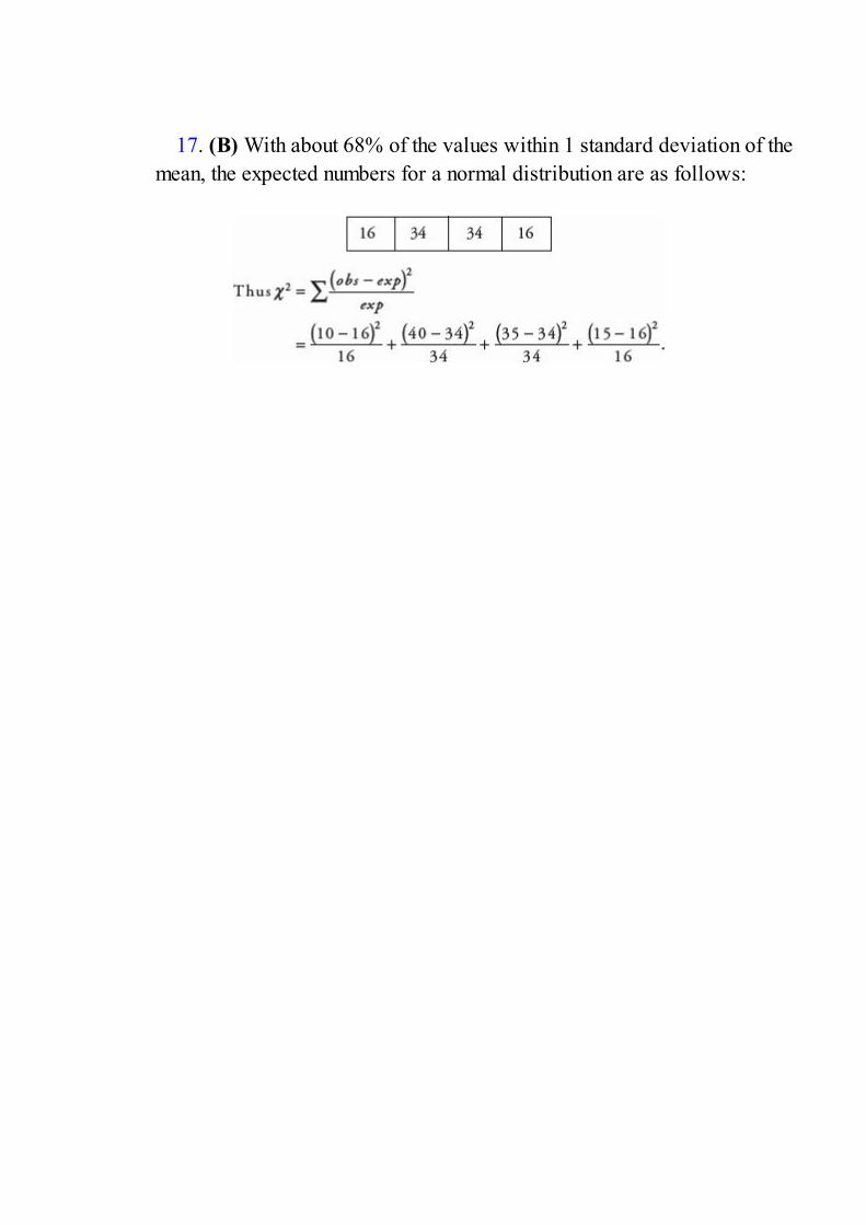
17. (B) With about 68% of the values within 1 standard deviation of themean, the expected numbers for a normal distribution are as follows:
18. (A) This is a good example of voluntary response bias, which oftenoverrepresents strong or negative opinions. The people who chose torespond were very possibly the parents of children facing drug problemsor people who had had bad experiences with drugs being sold in theirneighborhoods. There is very little chance that the 2500 respondents wererepresentative of the population. Knowing more about his listeners ortaking a sample of the sample would not have helped.
19. (B) The range (difference between largest and smallest values), theinterquartile range (Q3 – Q1), and this difference between the 60th and40th percentile scores all are measures of variability, or how spread outis the population or a subset of the population.

20. (E) Without independence we cannot determine var(X + Y) from theinformation given.

21. (E) The correlation coefficient r is not affected by changes in units,by which variable is called x or y, or by adding or multiplying all thevalues of a variable by the same constant.

22. (E) 1.96 ≤ .03 gives ≥ 32.67 and n ≥ 1067.1.

23. (B) P(at least one Type I error) = 1 – P(no Type I errors) = 1 –(.95)10 = .40.

24. (E) Note that all three sets have the same mean and the same range.The third set has most of its values concentrated right at the mean, whilethe second set has most of its values concentrated far from the mean.
25. (C) People coming out of a Wall Street office building are a veryunrepresentative sample of the adult population, especially given thequestion under consideration. Using chance and obtaining a high responserate will not change the selection bias and make this into a well-designedsurvey. This is a convenience sample, not a voluntary response sample.
26. (C) Larger samples (so is smaller) and less confidence (so thecritical z or t is smaller) both result in smaller intervals.
27. (D) The third scatterplot shows perfect negative association, so r3= –1. The first scatterplot shows strong, but not perfect, negativecorrelation, so –1 < r1 < 0. The second scatterplot shows no correlation,so r2 = 0.

28. (D) The probability of throwing heads is .5. By the law of largenumbers, the more times you flip the coin, the more the relative frequencytends to become closer to this probability. With fewer tosses there ismore chance for wide swings in the relative frequency.

29. (C) If the true mean parking duration is 51minutes, the normal curve should be centered at 51. The critical value of50 has a z-score of

30. (A) The overall lengths (between tips of whiskers) are the same,and so the ranges are the same. Just because the min and max areequidistant from the median, and Q1 and Q3 are equidistant from themedian, does not imply that a distribution is symmetric or that the meanand median are equal. And even if a distribution is symmetric, this doesnot imply that it is roughly normal. Particular values, not distributions,may be outliers.

31. (C) Critical z-scores are and with righttail probabilities of .1335 and .0228, respectively. The percentage below740 given that the scores are above 700 is .
32. (D) There is a different probability of Type II error for eachpossible correct value of the population parameter, and 1 minus thisprobability is the power of the test against the associated correct value.

33. (E) This is not a simple random sample because all possible sets ofthe required size do not have the same chance of being picked. Forexample, a set of principals all from just half the school districts has nochance of being picked to be the sample. This is not a cluster sample inthat there is no reason to believe that each school district resembles thepopulation as a whole, and furthermore, there was no random sampletaken of the school districts. This is not systematic sampling as thedistricts were not put in some order with every nth district chosen.Stratified samples are often easier and less costly to obtain and also makecomparative data available. In this case responses can be comparedamong various districts.

34. (A) A simple random sample can be any size and may or may not berepresentative of the population. It is a method of selection in which everypossible sample of the desired size has an equal chance of being selected.
35. (C) The critical z-scores go from ±1.645 to ±2.576, resulting in anincrease in the interval size: or an increase of 57%.
36. (E) If the P-value is less than .10, it does not follow that it is lessthan .05. Decisions such as whether a test should be one-or two-sided aremade before the data are gathered. If α = .01, there is a 1% chance ofrejecting the null hypothesis if the null hypothesis is true. There is oneprobability of a Type I error, the significance level, while there is adifferent probability of a Type II error associated with each possiblecorrect alternative, so the sum does not equal 1.

37. (C) has a t-distribution with df = n – 1.
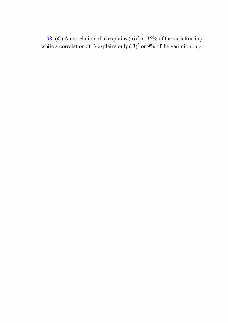
38. (C) A correlation of .6 explains (.6)2 or 36% of the variation in y,while a correlation of .3 explains only (.3)2 or 9% of the variation in y.

39. (A) Using a measurement from a sample, we are never able to sayexactly what a population proportion is; rather we always say we have acertain confidence that the population proportion lies in a particularinterval. In this case that interval is 43% ± 5% or between 38% and 48%.

40. (B) With Plan I the expected number of students with stockinvestments is only 2.4 out of 30. Plan II allows an estimate to be madeusing a full 30 investors.

Answers Explained, Section II1. A complete answer compares shape, center, and spread.
Shape: The baseball players, (A), for which the cumulative frequencyplot rises steeply at first, include more shorter players, and thus thedistribution is skewed to the right (toward the greater heights). Thefootball players, (C), for which the cumulative frequency plot risesslowly at first, and then steeply toward the end, include more tallerplayers, and thus the distribution is skewed to the left (toward the lowerheights). The basketball players, (B), for which the cumulative frequencyplot rises slowly at each end, and steeply in the middle, have a more bell-shaped distribution of heights.
Center: The medians correspond to relative frequencies of 0.5. Readingacross from 0.5 and then down to the x-axis shows the median heights tobe about 63.5 inches for baseball players, about 72.5 inches forbasketball players, and about 79 inches for football players. Thus, thecenter of the baseball height distribution is the least, and the center of thefootball height distribution is the greatest.
Spread: The range of the football players is the smallest, 80 – 65 = 15inches, then comes the range of the baseball players, 80 – 60 = 20 inches,and finally the range of the basketball players is the greatest, 85 – 60 = 25inches.
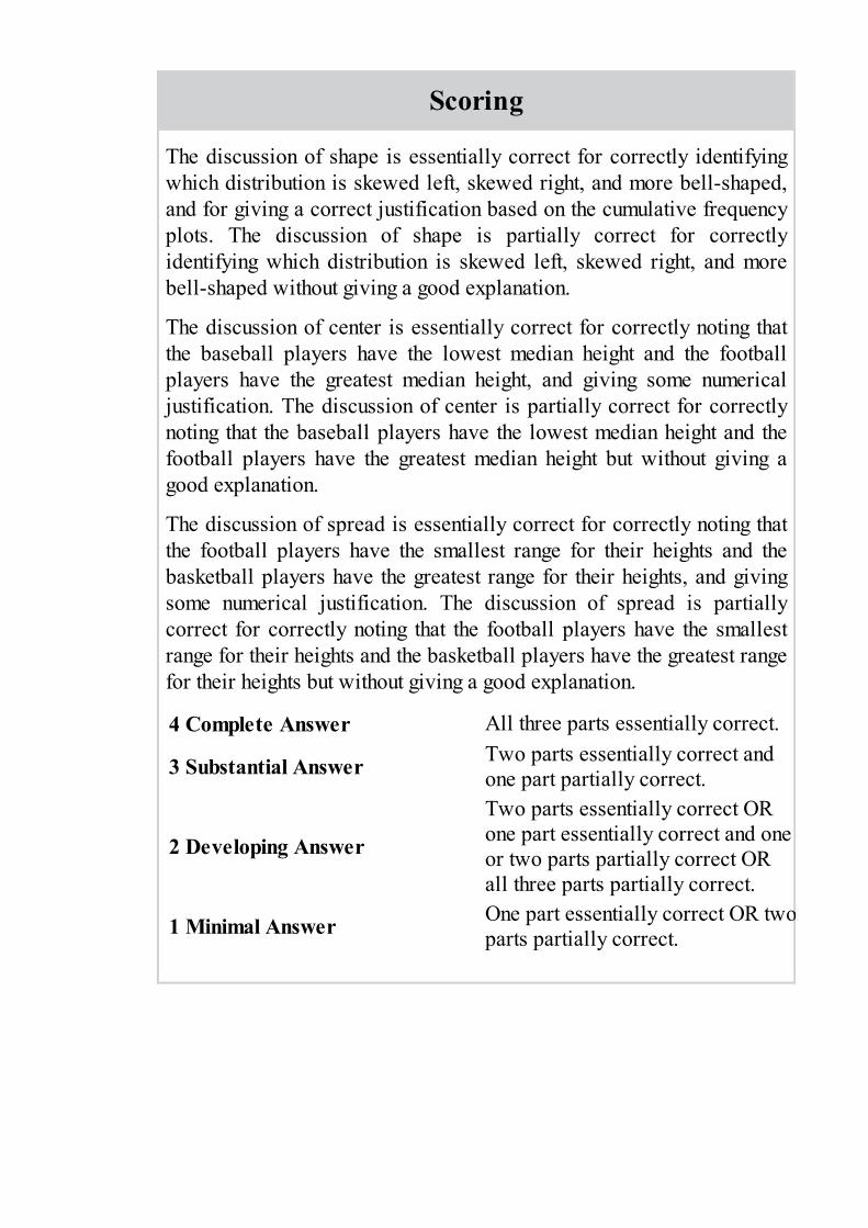
Scoring
The discussion of shape is essentially correct for correctly identifyingwhich distribution is skewed left, skewed right, and more bell-shaped,and for giving a correct justification based on the cumulative frequencyplots. The discussion of shape is partially correct for correctlyidentifying which distribution is skewed left, skewed right, and morebell-shaped without giving a good explanation.
The discussion of center is essentially correct for correctly noting thatthe baseball players have the lowest median height and the footballplayers have the greatest median height, and giving some numericaljustification. The discussion of center is partially correct for correctlynoting that the baseball players have the lowest median height and thefootball players have the greatest median height but without giving agood explanation.
The discussion of spread is essentially correct for correctly noting thatthe football players have the smallest range for their heights and thebasketball players have the greatest range for their heights, and givingsome numerical justification. The discussion of spread is partiallycorrect for correctly noting that the football players have the smallestrange for their heights and the basketball players have the greatest rangefor their heights but without giving a good explanation.
4 Complete Answer All three parts essentially correct.
3 Substantial Answer Two parts essentially correct andone part partially correct.
2 Developing Answer
Two parts essentially correct ORone part essentially correct and oneor two parts partially correct ORall three parts partially correct.
1 Minimal Answer One part essentially correct OR twoparts partially correct.

2. (a) A control group would allow the school system to comparethe effectiveness of each of the new programs to the local standardmethod currently being used.
(b) Parents who fail to return the consent form are a specialcategory who may well place less priority on education. The effect ofusing their children may distort results, since their children could onlybe placed in the control group.
(c) Assign each student a unique number 01–90. Using a randomnumber table or a random number generator on a calculator, picknumbers between 01 and 90, throwing out repeats. The studentscorresponding to the first 30 such numbers picked will be assigned toProgram A, the next 30 picked to Program B, and the remaining to thecontrol group.
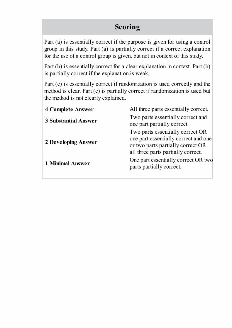
Scoring
Part (a) is essentially correct if the purpose is given for using a controlgroup in this study. Part (a) is partially correct if a correct explanationfor the use of a control group is given, but not in context of this study.
Part (b) is essentially correct for a clear explanation in context. Part (b)is partially correct if the explanation is weak.
Part (c) is essentially correct if randomization is used correctly and themethod is clear. Part (c) is partially correct if randomization is used butthe method is not clearly explained.
4 Complete Answer All three parts essentially correct.
3 Substantial Answer Two parts essentially correct andone part partially correct.
2 Developing Answer
Two parts essentially correct ORone part essentially correct and oneor two parts partially correct ORall three parts partially correct.
1 Minimal Answer One part essentially correct OR twoparts partially correct.

3. (a) This is a paired data test, not a two-sample test. There arefour parts to a complete solution.Part 1: Must state a correct pair of hypotheses.H0: d = 0 and Ha: d > 0, where d is the mean daily difference inquantity of gas used (in 100 cu ft) between the house without insulationand the house with insulation.Part 2: Must name the test and check the conditions.This is a paired t-test, that is, a single sample hypothesis test on the setof differences.Conditions: We are given that the sample of days was randomlychosen. The population may not be normal, but with n = 30 it is OK toproceed with the t-test.Part 3: Must find the test statistic t and the P-value.A calculator quickly gives t = 6.41 and P = .000.
Or with d = 1.557 and sd = 1.331 we have and
with df = 29, P = .000.Part 4: Must state the conclusion in context with linkage to the P-value.With this small a P-value (.000), there is very strong evidence toreject H0. That is, there is very strong evidence that the mean daily gasusage in a home without the insulation product is greater than the meandaily gas usage in a home with the insulation product.
(b) In the house without the insulation product an estimate for theaverage increase in quantity of gas used when the outside temperaturegoes down 1 degree Fahrenheit is 0.15 hundred cubic feet, while in thehouse with the insulation product an estimate for the average increasein quantity of gas used when the outside temperature goes down 1degree Fahrenheit is 0.10 hundred cubic feet. So when the temperaturegoes down, the increase in gas used is less in the house with theinsulation product than in the house without the insulation product.
(c) In the house without the insulation product an estimate for theaverage quantity of gas used when the outside temperature is 0 degreesFahrenheit is 10.02 hundred cubic feet, while in the house with theinsulation product an estimate for the average quantity of gas usedwhen the outside temperature is 0 degrees Fahrenheit is 7.59 hundredcubic feet. So at an outside temperature of 0 degrees Fahrenheit, the

average quantity of gas used is less in the house with the insulationproduct than in the house without the insulation product.

Scoring
In Part (a), Parts 1–2 are essentially correct for a correct statement ofthe hypotheses (in terms of population means), together with naming thetest and checking the conditions, and partially correct for one of Part 1or Part 2 completely correct.
Parts 3–4 are essentially correct for a correct calculation of both thetest statistic t and the P-value, together with a correct conclusion incontext linked to the P-value, and partially correct for one of Part 3 orPart 4 completely correct.
Part (b) is essentially correct for giving the correct values for theslopes, in context of the problem, and making a direct comparison. Part(b) is partially correct for giving the correct slopes but missing thecontext or the direct comparison.
Part (c) is essentially correct for giving the correct values for the y-intercepts, in context of the problem, and making a direct comparison.Part (c) is partially correct for giving the correct y-intercepts butmissing the context or the direct comparison.
Count essentially correct answers as one point and partially correctanswers as one-half point.
4 Complete Answer Four points3 Substantial Answer Three points2 Developing Answer Two points1 Minimal Answer One point
Use a holistic approach to decide a score totaling between twonumbers.

4. (a) (i) P(spam positive) = = .205
(ii) P(positive | legitimate) = = .12
(b) (i) P(positive | spam) = = .82
(ii) P(negative | legitimate) = = .88
(c) (i) 1 – (.88)5 = .4723(ii) 10(.82)3(.18)2 + 5(.82)4(.18) + (.82)5 = .9563
(d) (i) P(positive) = P(positive ∩ spam) + P(positive ∩ legitimate)= P(spam) P(positive | spam) + P(legitimate)P(positive | legitimate)= (.35)(.82) + (.65)(.12) = .365
(ii) P(spam | positive) = = .7863
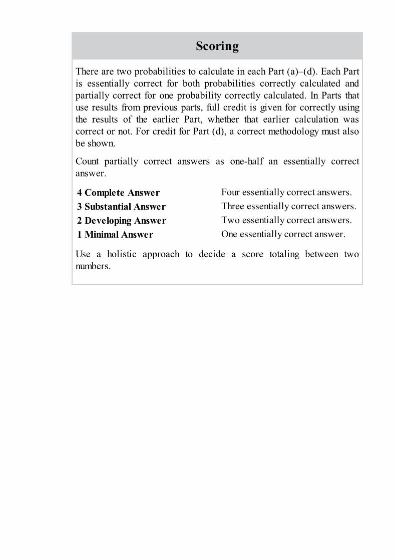
Scoring
There are two probabilities to calculate in each Part (a)–(d). Each Partis essentially correct for both probabilities correctly calculated andpartially correct for one probability correctly calculated. In Parts thatuse results from previous parts, full credit is given for correctly usingthe results of the earlier Part, whether that earlier calculation wascorrect or not. For credit for Part (d), a correct methodology must alsobe shown.
Count partially correct answers as one-half an essentially correctanswer.
4 Complete Answer Four essentially correct answers.3 Substantial Answer Three essentially correct answers.2 Developing Answer Two essentially correct answers.1 Minimal Answer One essentially correct answer.
Use a holistic approach to decide a score totaling between twonumbers.
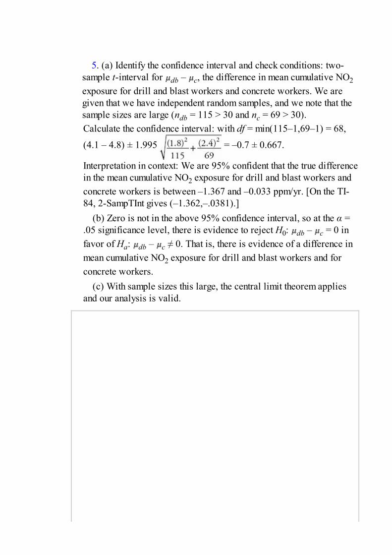
5. (a) Identify the confidence interval and check conditions: two-sample t-interval for db – c, the difference in mean cumulative NO2exposure for drill and blast workers and concrete workers. We aregiven that we have independent random samples, and we note that thesample sizes are large (ndb = 115 > 30 and nc = 69 > 30).Calculate the confidence interval: with df = min(115–1,69–1) = 68,
(4.1 – 4.8) ± 1.995 = –0.7 ± 0.667.
Interpretation in context: We are 95% confident that the true differencein the mean cumulative NO2 exposure for drill and blast workers andconcrete workers is between –1.367 and –0.033 ppm/yr. [On the TI-84, 2-SampTInt gives (–1.362,–.0381).]
(b) Zero is not in the above 95% confidence interval, so at the α =.05 significance level, there is evidence to reject H0: db – c = 0 infavor of Ha: db – c ≠ 0. That is, there is evidence of a difference inmean cumulative NO2 exposure for drill and blast workers and forconcrete workers.
(c) With sample sizes this large, the central limit theorem appliesand our analysis is valid.

Scoring
Part (a) has two components. The first component, identifying theconfidence interval and checking conditions, is essentially correct fornaming the confidence interval procedure, noting independent randomsamples, and noting the large sample sizes. This component is partiallycorrect for correctly noting two of the three points.
The second component of Part (a) is essentially correct for correctmechanics in calculating the confidence interval and for a correct(based on the shown mechanics) interpretation in context, and ispartially correct for one of these two features.
Part (b) is essentially correct for noting that zero is not in the interval sothe observed difference is significant and stating this in context of theproblem. Part (b) is partially correct for noting that zero is not in theinterval so the observed difference is significant, but failing to put thisconclusion in context of the problem.
Part (c) is essentially correct for relating the central limit theorem(CLT) to the samples being large. Part (c) is partially correct forreferring to the CLT or to the large samples, but not linking the two.
Count partially correct answers as one-half an essentially correctanswer.
4 Complete Answer Four essentially correct answers.3 Substantial Answer Three essentially correct answers.2 Developing Answer Two essentially correct answers.1 Minimal Answer One essentially correct answer.
Use a holistic approach to decide a score totaling between twonumbers.

6. (a) Identify the confidence interval by name or formula.95% confidence interval for the population proportion
Check the assumptions.
Calculate the confidence interval.
Interpret the confidence interval in context.
We are 95% confident that between 77.7% and 90.7% of mice willgain more weight with no magnetic field.
(b) The distribution of the set of all possible differences of weightgains without and with magnetic fields is approximately normal, withmean 25.1 – 17.3 = 7.8 and standard deviation = 6.49.Then the probability that the first mouse gained more weight than thesecond equals
(c) From the answer to (b), if weight gains without or with themagnetic field are independent, we would expect approximately88.5% of mice will gain more weight with no magnetic field. From theanswer to (a) we estimate the percent of mice who gain more weightwith no magnetic field to be between 77.7% and 90.7%. Since 88.5%is in this interval, there is no evidence to suggest that weight gain withno magnetic field and in a magnetic field are not independent.
(d) Calculating = 0.296 or = 3.38, the test statistic
is outside the critical cutoff scores of 0.698 and 1.43. Thus there is

evidence that the variances of the distributions of weight gains withoutand with magnetic fields are different.

Scoring
Part (a) has four parts: 1) identifying the confidence interval; 2)checking assumptions; 3) calculating the confidence interval; and 4)interpreting the confidence interval in context. Part (a) is essentiallycorrect if three or four of these parts are correct and partially correct ifone or two of these parts are correct.
Part (b) is essentially correct for a complete answer, and partiallycorrect for finding the mean and SD of the set of differences butincorrectly finding the probability, OR making a mistake in finding themean or standard deviation but using these correctly in finding theprobability.
Part (c) is essentially correct for a complete answer and is partiallycorrect if the conclusion is right but the links to (a) and (b) are unclear.
Part (d) is essentially correct for a correct calculation of the quotient ofsample variances together with a correct conclusion in context, and ispartially correct for one of these two parts correct.
Count partially correct answers as one-half an essentially correctanswer.
4 Complete Answer Four essentially correct answers.3 Substantial Answer Three essentially correct answers.2 Developing Answer Two essentially correct answers.1 Minimal Answer One essentially correct answer.
Use a holistic approach to decide a score totaling between twonumbers.
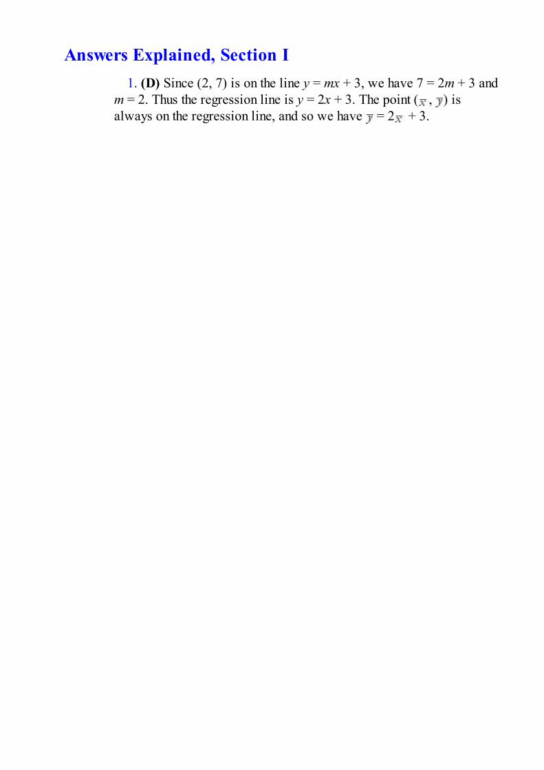
Answers Explained, Section I1. (D) Since (2, 7) is on the line y = mx + 3, we have 7 = 2m + 3 and
m = 2. Thus the regression line is y = 2x + 3. The point ( , ) isalways on the regression line, and so we have = 2 + 3.
2. (B) It could well be that conscientious students are the same oneswho both study and do well on the basketball court. If students couldbe randomly assigned to study or not study, the results would be moremeaningful. Of course, ethical considerations might make it impossibleto isolate the confounding variable in this way.

3. (B) The critical z-score is 0.525. Thus 75 – = 0.525(14) and = 67.65.

4. (D) The slope of the regression line and the correlation arerelated by When using z-scores, the standard deviations sx and
sy are 1. If r = 0, then b1 = 0. Switching which variable is x and whichis y, or changing units, will not change the correlation.

5. (E) The median and interquartile range are specifically usedwhen outliers are suspected of unduly influencing the mean, range, orstandard deviation.
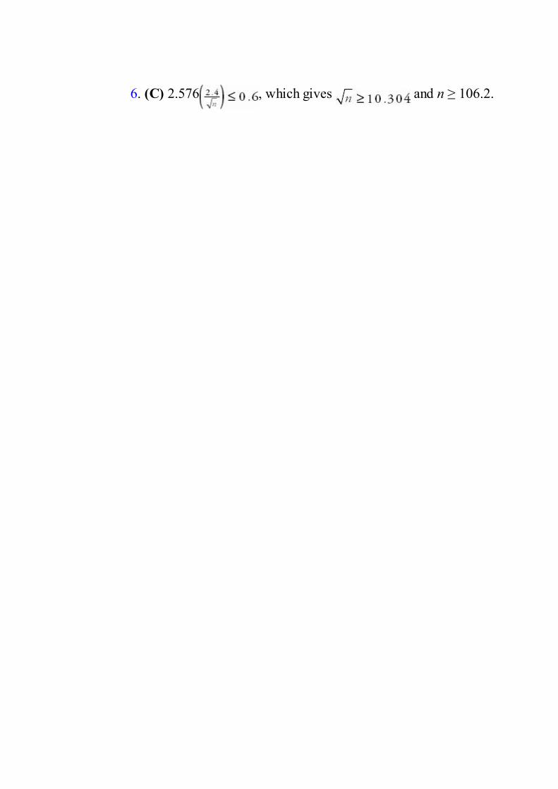
6. (C) 2.576 , which gives and n ≥ 106.2.

7. (C) This is a hypothesis test with H0: tissue strength is withinspecifications, and Ha: tissue strength is below specifications. A TypeI error is committed when a true null hypothesis is mistakenly rejected.

8. (D)

9. (E) The wording of questions can lead to response bias. Theneutral way of asking this question would simply have been, “Do yousupport the proposed school budget increase?”

10. (E) While it is important to look for basic patterns, it is alsoimportant to look for deviations from these patterns. In this case, there isan overall positive correlation; however, those faculty with under tenyears of service show little relationship between years of service andsalary. While (A) is a true statement, it does not give an overallinterpretation of the scatterplot.

11. (D) The second set has a greater range, 3.8 – 1.8 = 2.0 as comparedto 4.1 – 2.3 = 1.8, and with its skewness it also has a greater standarddeviation.

12. (B) With n = 10, increasing x by 40 increases by 4.
13. (B) The means and the variances can be added. Thus the newvariance is 52 + 122 = 169, and the new standard deviation is 13.

14. (E) Dice have no memory, so the probability that the next toss willbe an even number is .5 and the probability that it will be an odd numberis .5. The law of large numbers says that as the number of tosses becomeslarger, the proportion of even numbers tends to become closer to .5.
15. (B) The critical t-scores for 90% confidence with df = 7 are±1.895.

16. (A) Either directly or anonymously, you should be able to obtain thetest results for every student.

17. (C) Percentile ranking is a measure of relative position. Addingfive points to everyone’s score will not change the relative positions.

18. (A) The control group should have experiences identical to those ofthe experimental groups except for the treatment under examination. Theyshould not be given a new treatment.

19. (B) If Ha is true, the probability of failing to reject H0 and thuscommitting a Type II error is 1 minus the power, that is, 1 – .8 = .2.
20. (C) Five does not split the area in half, so 5 is not the median.Histograms such as these show relative frequencies, not actualfrequencies. The area from 1.5 to 4.5 is the same as that between 7.5 and10.5, each being about 25% of the total. Given the spread, 1 is too smallan estimate of the standard deviation. The area above 3 looks to be thesame as the area above 9 and 10, so the median won’t change.

21. (D) There must be a fixed number of trials, which rules out (A);only two possible outcomes, which rules out (B); and a constantprobability of success on any trial, which rules out (C).

22. (C) In both cases 1 hour is one standard deviation from the meanwith a right tail probability of .1587.
23. (C) Control, randomization, and replication are all importantaspects of well-designed experiments. We try to control lurking variables,not to use them to control something else.

24. (D) The data are strongly skewed to the left, indicating that themean is less than the median. The median appears to be roughly 215,indicating that the interval [200, 240] probably has more than 50% of thevalues. While in a standard boxplot each whisker contains 25% of thevalues, this is a modified boxplot showing four outliers, and so the leftwhisker has four fewer values than the right whisker.

25. (C) For the regression line, the sum and thus the mean of theresiduals are always zero. An influential score may have a small residualbut still have a great effect on the regression line. If the correlation is 1,all the residuals would be 0, resulting in a very distinct pattern.
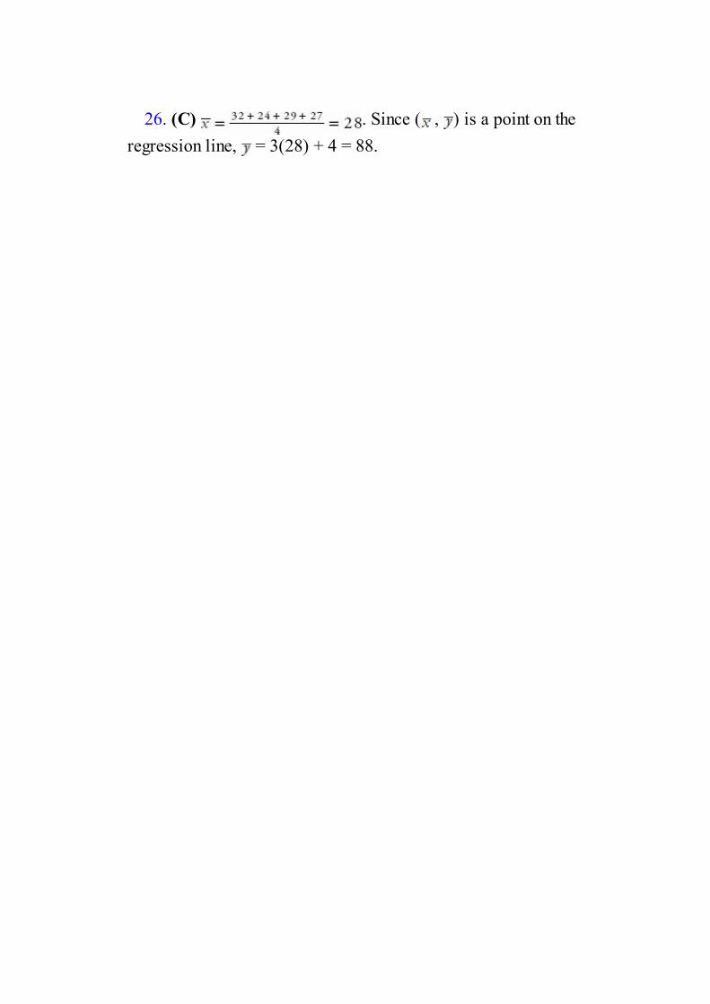
26. (C) . Since ( , ) is a point on theregression line, = 3(28) + 4 = 88.
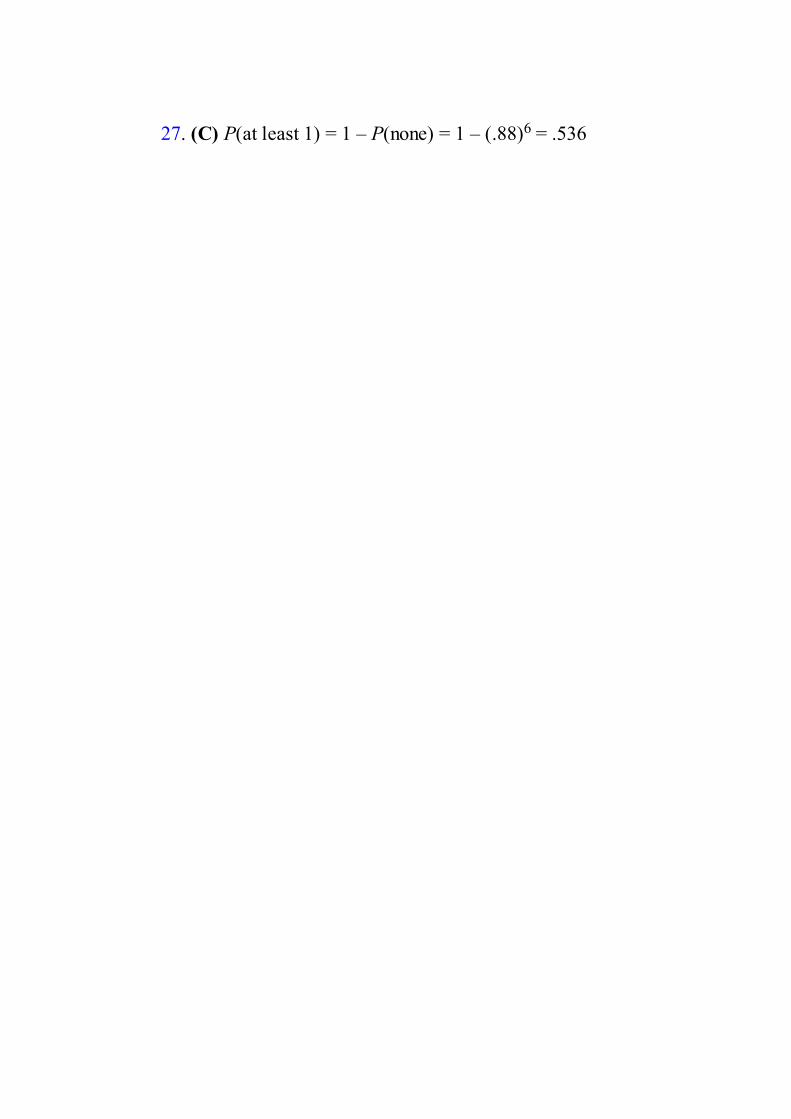
27. (C) P(at least 1) = 1 – P(none) = 1 – (.88)6 = .536

28. (B) Different samples give different sample statistics, all of whichare estimates for the same population parameter, and so error, calledsampling error, is naturally present.
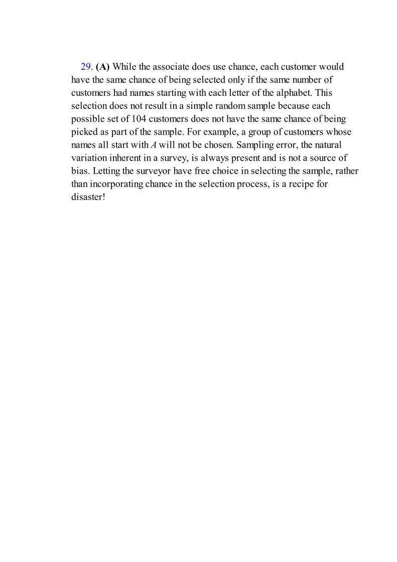
29. (A) While the associate does use chance, each customer wouldhave the same chance of being selected only if the same number ofcustomers had names starting with each letter of the alphabet. Thisselection does not result in a simple random sample because eachpossible set of 104 customers does not have the same chance of beingpicked as part of the sample. For example, a group of customers whosenames all start with A will not be chosen. Sampling error, the naturalvariation inherent in a survey, is always present and is not a source ofbias. Letting the surveyor have free choice in selecting the sample, ratherthan incorporating chance in the selection process, is a recipe fordisaster!

30. (A) Corresponding to cumulative proportions of 0.25 and 0.75 areQ1 = 2.25 and Q3 = 3.1, respectively, and so the interquartile range is 3.1– 2.25 = 0.85.

31. (E) The standard deviation of the test statistic is

32. (D) From a table or a calculator (for example invNorm on the TI-84), the 40th percentile corresponds to a z-score of –0.2533, and –0.2533(.28) = –0.0709.

33. (D) Increasing the sample size by a multiple of d divides theinterval estimate
by .

34. (D) The t-distributions are symmetric; however, they are lower atthe mean and higher at the tails and so are more spread out than the normaldistribution. The greater the df, the closer the t-distributions are to thenormal distribution. The 68–95–99.7 Rule applies to the z-distributionand will work for t-models with very large df. All probability densitycurves have an area of 1 below them.

35. (E) The given bar chart shows percentages, not actual numbers.

36. (C) This follows from the central limit theorem.
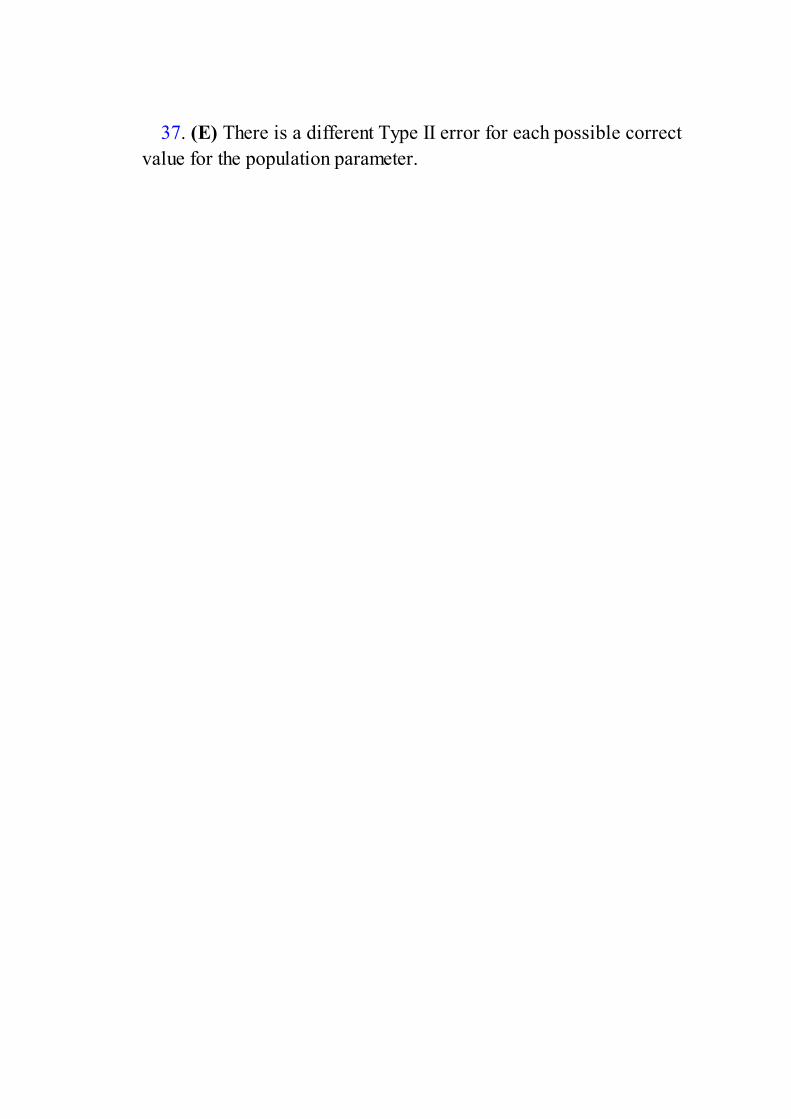
37. (E) There is a different Type II error for each possible correctvalue for the population parameter.
38. (C) X is close to the mean and so will have a z-score close to 0.Modified boxplots show only outliers that are far from the mean. X andthe two clusters are clearly visible in a stemplot of these data. Insymmetric distributions the mean and median are equal. The IQR here isclose to the range.
39. (E) Using a measurement from a sample, we are never able to sayexactly what a population proportion is; rather we always say we have acertain confidence that the population proportion lies in a particularinterval. In this case that interval is 82% ± 3% or between 79% and 85%.
40. (A) Whether or not students are taking AP Statistics seems to haveno relationship to which type of school they are planning to go to. Chi-square is close to 0.

Answers Explained, Section II1. (a) Number the volunteers 1 through 10. Use a random number generator to
pick numbers between 1 and 10, throwing out repeats. The volunteerscorresponding to the first two numbers chosen will receive aloe, the nexttwo will receive camphor, the next two eucalyptus oil, the next twobenzocaine, and the remaining two a placebo.
(b) Each volunteer (the volunteers are “blocks”) should receive all fivetreatments, one a day, with the time-order randomized. For example, labelaloe 1, camphor 2, eucalyptus oil 3, benzocaine 4, and the placebo 5. Thenfor each volunteer use a random number generator to pick numbersbetween 1 and 5, throwing away repeats. The order picked gives the dayon which each volunteer receives each treatment.
(c) Results cannot be generalized to women.
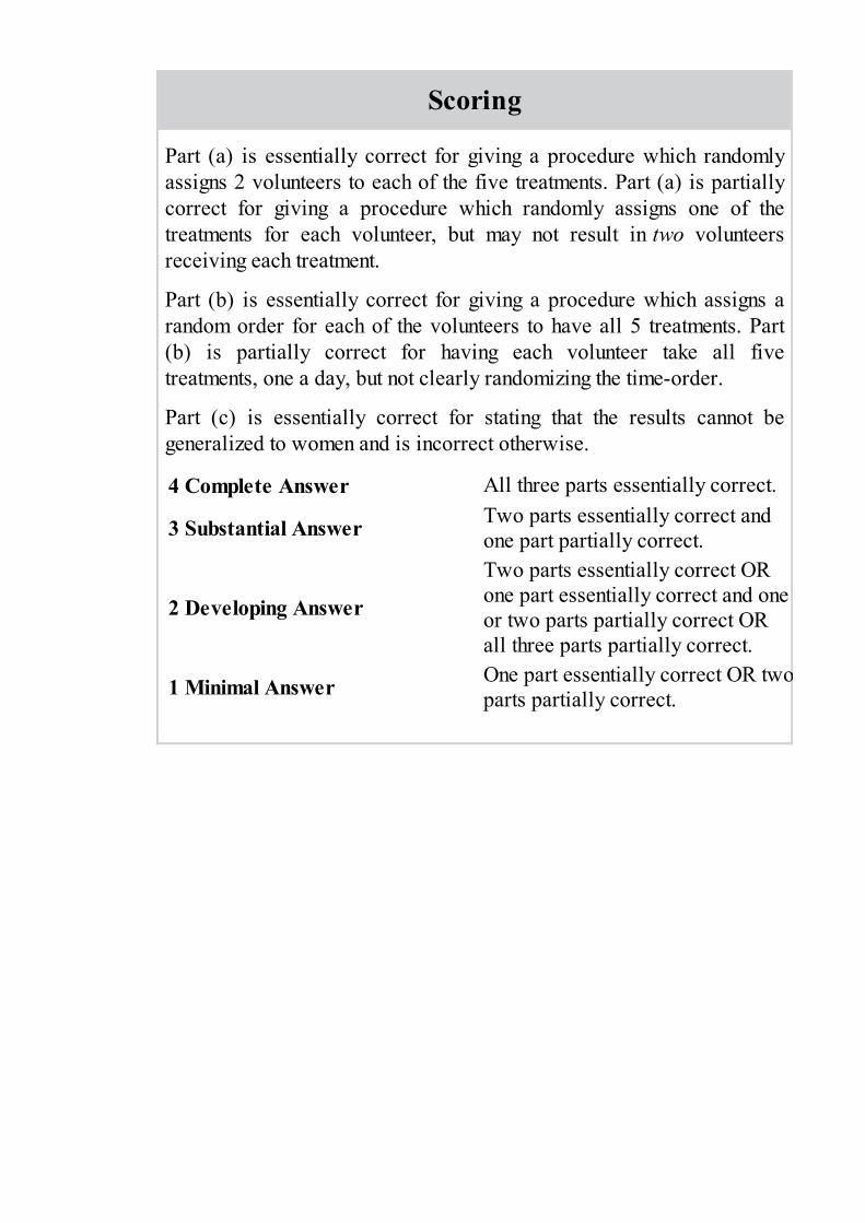
Scoring
Part (a) is essentially correct for giving a procedure which randomlyassigns 2 volunteers to each of the five treatments. Part (a) is partiallycorrect for giving a procedure which randomly assigns one of thetreatments for each volunteer, but may not result in two volunteersreceiving each treatment.
Part (b) is essentially correct for giving a procedure which assigns arandom order for each of the volunteers to have all 5 treatments. Part(b) is partially correct for having each volunteer take all fivetreatments, one a day, but not clearly randomizing the time-order.
Part (c) is essentially correct for stating that the results cannot begeneralized to women and is incorrect otherwise.
4 Complete Answer All three parts essentially correct.
3 Substantial Answer Two parts essentially correct andone part partially correct.
2 Developing Answer
Two parts essentially correct ORone part essentially correct and oneor two parts partially correct ORall three parts partially correct.
1 Minimal Answer One part essentially correct OR twoparts partially correct.

2. (a) = xp(x) = 0(.05) + 1(.10) + 2(.13) + 3(.15) + 4(.14) + 5(.12) + 6(.10)+ 7(.08) + 8(.06) + 9(.04) + 10(.03) = 4.27.With (.05 + .10 + .13 + .15) = .43 below 4 runs, and (.12 + .10 + .08 + .06+ .04 + .03) = .43 above 4 runs, the median must be 4.
(b) The mean is greater than the median, as was to be expected becausethe distribution is skewed to the right.
(c) P(at least one shutout in 4 games) = 1 – P(no shutouts in the 4 games)
= 1 – (1 – .05)4 = 1 – (.95)4 = .1855
(d) The distribution of is approximately normal with mean = 4.27(from above) and standard deviation .
Scoring
Part (a) is essentially correct for correctly calculating both the meanand median.Part (a) is partially correct for correctly calculating one of these twomeasures.
Part (b) is essentially correct for noting that the mean is greater than themedian and relating this to the skew.
Part (c) is essentially correct for recognizing this as a binomialprobability calculation and making the correct calculation. Part (c) ispartially correct for recognizing this as a binomial probabilitycalculation, but with an error such as 1 – (.05)4 or 4(.05)(.95)3.
Part (d) is essentially correct for “approximately normal,” = 4.27,and = 0.1823, and partially correct for two of these three answers.
Count partially correct answers as one-half an essentially correctanswer.
4 Complete Answer Four essentially correct answers.3 Substantial Answer Three essentially correct answers.2 Developing Answer Two essentially correct answers.1 Minimal Answer One essentially correct answer.
Use a holistic approach to decide a score totaling between twonumbers.

3. (a) The slope b1 is in the center of the confidence interval, so b1 = =–0.0056. In context, 0.0056 estimates the average decrease in the manic-depressive scale score for each 1-microgram increase in the level ofurinary MHPG. (Thus high levels of MHPG are associated with increasedmania, and conversely, low levels of MHPG are associated with increaseddepression.)
(b) Recalling that the regression line goes through the point ( ) orusing the AP Exam formula page, bo = – b1 = 5.4 – (–0.0056)(1243.1)= 12.36, and thus the equation of the regression line is = 12.36 –0.0056(MHPG) (or = 12.36 – 0.0056x, where x is the level of urinaryMHPG in micrograms per 24 hours, and y is the score on a 0-10 manic-depressive scale).
(c) Recalling that on the regression line, each one SD increase in theindependent variable corresponds to an increase of r SD in the dependent
variable, or using the AP Exam formula page, b1 = r , so
and r 2 = 56.2%. Thus, 56.2% of the variation in the manic-depressionscale level is explained by urinary MHPG levels.
(d) Correlation never proves causation. It could be that depressioncauses biochemical changes leading to low levels of urinary MHPG, or itcould be that low levels of urinary MHPG cause depression, or it could bethat some other variable (a lurking variable) simultaneously affects bothurinary MHPG levels and depression.

Scoring
Part (a) is essentially correct if the slope is correctly calculated andcorrectly interpreted in context. Part (a) is partially correct if the slopeis not correctly calculated but a correct interpretation is given using theincorrect value for the slope.
Part (b) is essentially correct if the regression equation is correctlycalculated (using the slope found in part (a)) and it is clear what thevariables stand for. Part (b) is partially correct if the correct equation isfound (using the slope found in part (a)) but it is unclear what thevariables stand for.
Part (c) is essentially correct if the coefficient of determination, r 2, iscorrectly calculated and correctly interpreted in context. Part (c) ispartially correct if r2 is not correctly calculated but a correctinterpretation is given using the incorrect value for r2.
Part (d) is essentially correct for noting that correlation never provescausation, and referring to context. Part (d) is partially correct for acorrect statement about correlation and causation, but with no referenceto context.
A partially correct answer counts half of an essentially correct answer.
4 Complete Answer 4 essentially correct answers.3 Substantial Answer 3 essentially correct answers.2 Developing Answer 2 essentially correct answers.1 Minimal Answer 1 essentially correct answer.
Use a holistic approach to decide a score totaling between twonumbers.

4. There are four parts to this solution.
(a) State the hypotheses.
H0: 1 – 2 = 0 and Ha: 1 – 2 < 0
where µ1 = mean number of months at which first steps alone are takenfor infants receiving daily stimulation, and µ2 = mean number of months atwhich first steps are taken for infants in the control group. [Other notationsare also possible, for example, H0: 1 = 2 and Ha: 1 < 2.]
(b) Identify the test by name or formula and check the assumptions.
Two-sample t-test OR
Assumptions:1. Randomization: We are given that the infants were randomly split
into the two groups.2. Nearly normal populations: Dotplots of the two samples show
no outliers and are roughly bell-shaped.
(c) Demonstrate correct mechanics.
and with df = 9, we have a P-value = .1293[with a calculator’s df = 16.69, we get P = .1234]
(d) State the conclusion in context with linkage to the P-value.With this large a P-value (.1293 > .10), there is no evidence that infants
walk earlier with daily stimulation of specific reflexes.

Scoring
Part (a) is essentially correct for stating the hypotheses and identifyingthe variables. Part (a) is partially correct for correct hypotheses, butmissing identification of the variables.
Part (b) is essentially correct for identifying the test and checking theassumptions. Part (b) is partially correct for only one of these twoelements.
Part (c) is essentially correct for correctly calculating both the t-scoreand the P-value. Part (c) is partially correct for only one of these twoelements.
Part (d) is essentially correct for a conclusion in context with linkage tothe P-value. Part (d) is partially correct for only one of these twoelements.
Count partially correct answers as one-half an essentially correctanswer.
4 Complete Answer Four essentially correct answers.3 Substantial Answer Three essentially correct answers.2 Developing Answer Two essentially correct answers.1 Minimal Answer One essentially correct answer.
Use a holistic approach to decide a score totaling between twonumbers.

5. (a) A complete answer compares shape, center, and spread.Shape: The 10-kilometer distribution appears symmetric, while the 5-
mile distribution is skewed right.Center: The median of the 10-kilometer distribution is 4 minutes greater
than the median of the 5-mile distribution.Spread: The ranges of the two distributions are equal, both about 7
minutes.
( b ) Shape: Again, the 10-kilometer distribution appears symmetric,while the 5-mile distribution is still skewed right.
Center: Now the median of the 10-kilometer distribution is about 3.5minutes less than the median of the 5-mile distribution.
Spread: Now the range of the 10-kilometer distribution is less than therange of the 5-mile distribution.
(c) One possible answer is that this was not as expected with thefollowing explanation: One would expect that for 5 miles, the shorter run,the speeds would be faster, so adjusting the 5-mile run times would resultin faster times (less minutes) than the 10-kilometer times, but this was notthe case. [Perhaps slower, less serious runners participate in the shorterrace, so when their times are adjusted, the minutes are greater than thetimes for the 10-kilometer run.]
(d) In each set of parallel boxplots, the 10-kilometer distributionappears symmetric, so that the mean will be about the same as the median,while the 5-mile distribution is skewed right so that the mean will in alllikelihood be greater than the median. In the first set of boxplots (where the5-mile median < 10-kilometer median) this will result in the means beingcloser, while in the second set of boxplots (where the 5-mile median > 10-kilometer median) this will result in the means being further apart. Thus wewould expect the difference in mean times in the first set of parallelboxplots to be less than the difference in mean times in the second set ofparallel boxplots.

Scoring
Part (a) is essentially correct for correctly comparing shape, center, andspread.Part (a) is partially correct for correctly comparing two of the threefeatures.
Part (b) is essentially correct for correctly comparing shape, center, andspread.Part (b) is partially correct for correctly comparing two of the threefeatures.
Part (c) is essentially correct for a reasonable statement about thechange between the two sets of parallel boxplots together with a correctexplanation to go along with the statement. Part (c) is partially correct ifthe explanation is weak.
Part (d) is essentially correct for a correct prediction about the meanstogether with a reasonable justification based on symmetry of the 10-kilometer distribution and skewness of the 5-mile distribution. Part (d)is partially correct if the justification is weak.
Count partially correct answers as one-half an essentially correctanswer.
4 Complete Answer Four essentially correct answers.3 Substantial Answer Three essentially correct answers.2 Developing Answer Two essentially correct answers.1 Minimal Answer One essentially correct answer.
Use a holistic approach to decide a score totaling between twonumbers.

6. (a) Identify the confidence interval by name or formula.95% confidence interval for the population proportion
Check the assumptions.We are given that this is a random sample.n = 250 = 130 > 10 and n(1 – ) = 250 = 120 > 10.Calculate the confidence interval.
= = .52 and .52 ± 1.96 = .52 ± .062Interpret the confidence interval in context.We are 95% confident that between 45.8% and 58.2% of SAT
mathematics scores are over 500.
(b) State the hypotheses.H0: The distribution of SAT mathematics scores is normal with =
500 and σ = 100.Ha: The distribution of SAT mathematics scores is not normal with
= 500 and σ = 100.Identify the test by name or formula and check the assumptions.Chi-square goodness-of-fit test
Check assumptionsWe have a random sample.A normal distribution has 34.13% on each side of the mean and
within one SD, 13.59% on each side between one and two SDs fromthe mean, and 2.28% on each side more than two SDs from the mean.This gives expected cell counts of (.0228)250 = 5.7, (.1359)500 =34.0, and (.3413)500 = 85.3, each of which is at least 5.
Demonstrate correct mechanics.
With df = 6 – 1 = 5, the P-value is .083

State the conclusion in context with linkage to the P-value.Either with this small a P-value (.083 < α = .10) there is some
evidence that the distribution of SAT mathematics scores is notnormal, OR with this large a P-value (.083 > α = .05) there is noevidence that the distribution of SAT mathematics scores is notnormal.
(c) 207.2 < < 294.6
207.2 < < 294.6
15,729 > σ2 > 11,062125.4 > σ > 105.2
Thus we are 95% confident that the standard deviation for thedistribution of SAT mathematics scores is between 105.2 and 125.4.

Scoring
Part (a) has four parts: 1) identifying the confidence interval; 2)checking assumptions; 3) calculating the confidence interval; and 4)interpreting the confidence interval in context. Part (a) is essentiallycorrect if three or four of these parts are correct and partially correct ifone or two of these parts are correct.
Part (b) has four parts: 1) stating the hypotheses; 2) identifying the testand checking assumptions; 3) calculating the test statistic and the P-value; and 4) giving a conclusion in context with linkage to the P-value.Part (b) is essentially correct if three or four of these parts are correctand partially correct if one or two of these parts are correct.
Part (c) is essentially correct for calculating the confidence interval andinterpreting it in context. Part (c) is partially correct for one of thesetwo parts correct.
4 Complete Answer All three parts essentially correct.
3 Substantial Answer Two parts essentially correct andone part partially correct.
2 Developing Answer
Two parts essentially correct ORone part essentially correct and oneor two parts partially correct ORall three parts partially correct.
1 Minimal Answer One part essentially correct OR twoparts partially correct.
Answers Explained, Section I1. (C) A complete census can give much information about a
population, but it doesn’t necessarily establish a cause-and-effectrelationship among seemingly related population parameters. While theresults of well-designed observational studies might suggestrelationships, it is difficult to conclude that there is cause and effectwithout running a well-designed experiment. If bias is present, increasingthe sample size simply magnifies the bias. The control group is selectedby the researchers making use of chance procedures.

2. (A) In the first class only 40% of the students scored below the givenscore, while in the second class 80% scored below the same score.
3. (C) The control group should have experiences identical to those ofthe experimental groups except for the treatment under examination. Theyshould not be given a new treatment.
4. (E) The negative sign comes about because we are dealing with thedifference of proportions. The confidence interval estimate means that wehave a certain confidence that the difference in population proportionslies in a particular interval.

5. (B) The desire of the workers for the study to be successful led to aplacebo effect.

6. (E) The proportion of successful calls (problem solved) is , so (450) is the expected number of calls from location 1 that are
successful. Alternatively, the proportion of calls from location 1 is ,so (700) gives the expected number of successful calls from location1.

7. (C) The slope and the correlation always have the same sign.Correlation shows association, not causation. Correlation does not applyto categorical data. Correlation measures linear association, so even witha correlation of 0, there may be very strong nonlinear association.

8. (B) If two random variables are independent, the mean of thedifference of the two random variables is equal to the difference of thetwo individual means; however, the variance of the difference of the tworandom variables is equal to the sum of the two individual variances.

9. (D) A sample is simply a subset of a population.

10. (B) The markings, spaced 15 apart, clearly look like the standarddeviation spacings associated with a normal curve.

11. (B) With a right tail having probability .01, the critical z-score is2.326. Thus + 2.326(.3) = 12, giving = 11.3.
12. (E) There is no reason to think that AAA members arerepresentative of the city’s drivers. Family members may have similardriving habits and the independence condition would be violated.Random selection is important regardless of the sample size. The larger arandom sample, the closer its standard deviation will be to the populationstandard deviation.
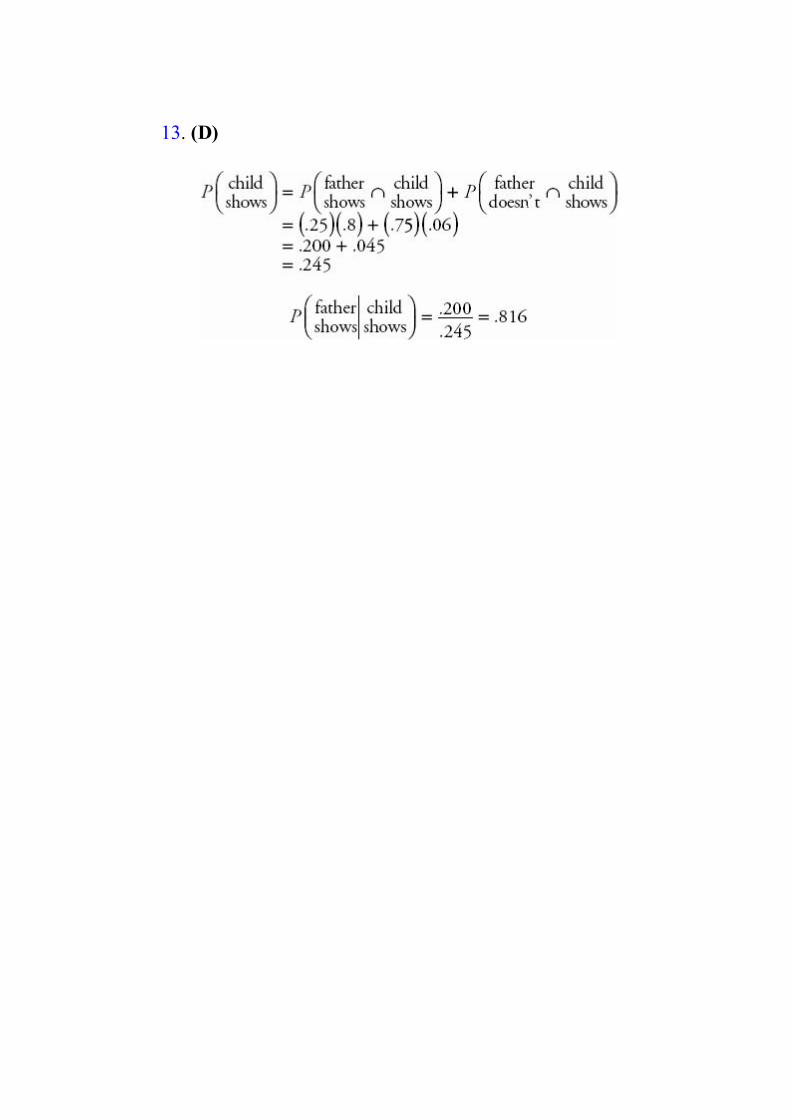
13. (D)

14. (C) As n increases the probabilities of Type I and Type II errorsboth decrease.

15. (A) The mean equals the common value of all the data elements.The other terms all measure variability, which is zero when all the dataelements are equal.
16. (E) and with df = 15 – 1 = 14, the critical t-scores
are ±1.761.

17. (E) In a simple random sample, every possible group of the givensize has to be equally likely to be selected, and this is not true here. Forexample, with this procedure it is impossible for the employees in thefinal sample to all be from a single plant. This method is an example ofstratified sampling, but stratified sampling does not result in simplerandom samples.

18. (D) (.32)(.15) = .048 so P(E ∩ F) = P(E)P(F) and thus E and F areindependent. P(E ∩ F) ≠ 0, so E and F are not mutually exclusive.

19. (A) The quartiles Q1 and Q3 have z-scores of ±0.67, so Q1 =640,000 – (0.67)18,000 ≈ 628,000, while Q3 = 640,000 + (0.67)18,000 ≈652,000. The interquartile range is the difference Q3 – Q1.

20. (D) One set is a shift of 20 units from the other, so they havedifferent means and medians, but they have identical shapes and thus thesame variability including IQR, standard deviation, and variance.
21. (B) A 99% confidence interval estimate means that in about 99% ofall samples selected by this method, the population mean will be includedin the confidence interval. The wider the confidence interval, the higherthe confidence level. The central limit theorem applies to any population,no matter if it is normally distributed or not. The sampling distribution fora mean always has standard deviation ; large enough sample size n
refers to the closer the distribution will be to a normal distribution. Thecenter of a confidence interval is the sample statistic, not the populationparameter.
22. (E) In none of these are the trials independent. For example, as eachconsecutive person is stopped at a roadblock, the probability the nextperson has a seat belt on will quickly increase; if a student has one A, theprobability is increased that he or she has another A.

23. (E) Independence implies P(E ∩ F) = P(E)P(F), while mutuallyexclusive implies P(E ∩ F) = 0.
24. (E) In a binomial with n = 4 and p = .9, P(at least 3 successes) =P(exactly 3 successes) + P(exactly 4 successes) = 4(.9)3(.1) + (.9)4.

25. (C) In stratified sampling the population is divided intorepresentative groups, and random samples of persons from each groupare chosen. In this case it might well be important to be able to considerseparately the responses from each of the three groups—urban, suburban,and rural.

26. (E) r 2, the coefficient of determination, indicates the percentage ofvariation in y that is explained by variation in x.

27. (C) It is most likely that the homes at which the interviewer haddifficulty finding someone home were homes with fewer children living inthem. Replacing these homes with other randomly picked homes will mostlikely replace homes with fewer children with homes with more children.
28. (A) The median corresponds to the 0.5 cumulative proportion.

29. (A) Blocking divides the subjects into groups of similarindividuals, in this case individuals with similar exercise habits, and runsthe experiment on each separate group. This controls the known effect ofvariation in exercise level on cholesterol level.

30. (B) The margin of error varies directly with the critical z-value anddirectly with the standard deviation of the sample, but inversely with thesquare root of the sample size.

31. (E) . With a true mean increase of 4.2, the z-scorefor 4.0 is and the officers fail to reject the claim if thesample mean has z-score greater than this.

32. (E) Both have 50 for their means and medians, both have a range of90 – 10 = 80, and both have identical boxplots, with first quartile 30 andthird quartile 70.

33. (B) Since we are not told that the investigator suspects that theaverage weight is over 300 mg or is under 300 mg, and since a tabletcontaining too little or too much of a drug clearly should be brought to themanufacturer’s attention, this is a two-sided test. Thus the P-value istwice the tail probability obtained (using the t-distribution with df = n – 1= 6.)

34. (A) This study was an experiment because a treatment (weeklyquizzes) was imposed on the subjects. However, it was a poorly designedexperiment with no use of randomization and no control over lurkingvariables.

35. (C) The expected frequencies, as calculated by the rule in (E), maynot be whole numbers.

36. (E) The probabilities of Type I and Type II error are related; forexample, lowering the Type I error increases the probability of a Type IIerror. A Type I error can be made only if the null hypothesis is true, whilea Type II error can be made only if the null hypothesis is false. In medicaltesting, with the usual null hypothesis that the patient is healthy, a Type Ierror is that a healthy patient is diagnosed with a disease, that is, a falsepositive. We reject H0 when the P-value falls below α, and when H0 istrue this rejection will happen precisely with probability α.

37. (C) X is probably very close to the least squares regression lineand so has a small residual. Removing X will change the regression linevery little if at all, and so it is not an influential point. The associationbetween the x and y variables is very strong, just not linear. Correlationmeasures the strength of a linear relationship, which is very weakregardless of whether the point X is present or not.
38. (B) The probability of an application being turned down is 1 – .90= .10, and the expected value of a binomial with n = 50 and p = .10 is np= 50(.10).

39. (E) A boxplot gives a five-number summary: smallest value, 25thpercentile (Q1), median, 75th percentile (Q3), and largest value. Theinterquartile range is given by Q3 – Q1, or the total length of the two“boxes” minus the “whiskers.”

40. (E) Using a measurement from a sample, we are never able to sayexactly what a population mean is; rather we always say we have acertain confidence that the population mean lies in a particular interval.
Answers Explained, Section II1. (a) A complete answer compares shape, center, and spread.
Shape. The control group distribution is somewhat bell-shaped andsymmetric, while the treatment group distribution is somewhat skewed right.
Center. The center of the control group distribution is around 20, which isgreater than the center of the treatment group distribution, which issomewhere around 10 to 12.
Spread. The spread of the control group distribution, 5 to 34, is less than thespread of the treatment group distribution, which is 2 to 41.
(b) For computers in the control group (no spam software), the number ofspam e-mails received varies an “average” amount of 8.1 from the meannumber of spam e-mails received in the control group.
(c) Since the 95% confidence interval for the difference does not containzero, the researcher can conclude the observed difference in mean numbersof spam e-mails received between the control group and the treatment groupthat received spam software is significant.
(d) It may well be that the four groups—administrators, staff, faculty, andstudents—are each exposed to different kinds of spam e-mail risks, andpossibly the software will be more or less of a help to each group. In thatcase, the researcher should in effect run four separate experiments on thehomogeneous groups, called blocks. Conclusions will be more specific.

Scoring
Part (a) is essentially correct for correctly comparing shape, center, andspread. Part (a) is partially correct for correctly comparing two of thethree features.
Part (b) is essentially correct if standard deviation is explainedcorrectly in context of this problem. Part (b) is partially correct if thereis a correct explanation of SD but no reference to context.
Part (c) is essentially correct for noting that zero is not in the interval sothe observed difference is significant, and stating this in context of theproblem. Part (c) is partially correct for noting that zero is not in theinterval so the observed difference is significant, but failing to put thisconclusion in context of the problem.
Part (d) is essentially correct if the purpose of blocking is correctlyexplained in context of this problem. Part (d) is partially correct if thegeneral purpose of blocking is correctly explained but not in context ofthis problem.
Count partially correct answers as one-half an essentially correctanswer.
4 Complete Answer Four essentially correct answers.3 Substantial Answer Three essentially correct answers.2 Developing Answer Two essentially correct answers.1 Minimal Answer One essentially correct answer.
Use a holistic approach to decide a score totaling between twonumbers.

2. (a) Listing the eight possibilities: {HHH, HHT, HTH, HTT, THH, THT,TTH, TTT} clearly shows that the only possibilities for the absolute value ofthe difference are 1 with probability 6/8 = .75 and 3 with probability 2/8 =.25. The table is:
(b) E = xP(x) = 1(.75) + 3(.25) = 1.5
(c) Since the only possible scores for each game are 1 and 3, the only way tohave a total score of 3 in three games is to score 1 in each game. Theprobability of this is (.75)3 = .421875
(d) The more times the game is played, the closer the average score will beto the expected value of 1.5. The player does not want to average close to1.5, so should prefer playing 10 times rather than 15 times.

Scoring
Part (a) is essentially correct for the correct probability distributiontable. Part (a) is partially correct for one minor error.
Part (b) is essentially correct for the correct calculation of expectedvalue based on the answer given in Part (a). Part (b) is partially correctfor the correct formula for expected value but an incorrect calculationbased on the answer given in Part (a).
Part (c) is essentially correct for the correct probability calculationwith some indication of where the answer is coming from. Part (c) ispartially correct for the correct probability with no work shown.
Part (d) is essentially correct for choosing 10 and giving a clearexplanation. Part (d) is partially correct for choosing 10 and giving aweak explanation. Part (d) is incorrect for choosing 10 with noexplanation or with an incorrect explanation.
Count partially correct answers as one-half an essentially correctanswer.
4 Complete Answer Four essentially correct answers.3 Substantial Answer Three essentially correct answers.2 Developing Answer Two essentially correct answers.1 Minimal Answer One essentially correct answer.
Use a holistic approach to decide a score totaling between twonumbers.

3. (a) The slope of –7.19 says that the attendance dropped an average of 7.19students per week. No, this does not seem to adequately explain the data,because the attendance increased every week during the first 4 weeks, andagain increased every week during the final 4 weeks.
(b) Modeling the first 4 weeks (computer games allowed) gives Attendance= 68 + 5.1(Week) with r = .997, and modeling the final 4 weeks (nocomputer games) gives Attendance = 4.9 + 4.9(Week) with r = .997. Thesemodels give an average increase in attendance each week of 5.1 and 4.9,respectively, as well as much higher correlations.
(c)
The scatterplot clearly shows the linearity in the first 4 weeks and in the final4 weeks, and also the nonlinearity of the full set of data.

Scoring
Part (a) is essentially correct if the slope is correctly interpreted incontext and a reasonable explanation is given as to why this slope doesnot explain the data. Part (a) is partially correct for one of these twocomponents correct.
Part (b) is essentially correct for two separate regression models,correct interpretations of the slopes, and noting the increasedcorrelation. Part (b) is partially correct if one of these components ismissing.
Part (c) is essentially correct if the scatterplot is correctly drawn andthe strong linearity in the first four weeks and separately in the finalfour weeks is noted. Part (c) is partially correct for a correctly drawnscatterplot but no observations on linearity.
4 Complete Answer All three parts essentially correct.
3 Substantial Answer Two parts essentially correct andone part partially correct.
2 Developing Answer
Two parts essentially correct ORone part essentially correct and oneor two parts partially correct ORall three parts partially correct.
1 Minimal Answer One part essentially correct OR twoparts partially correct.

4. This is a paired data test, not a two-sample test, with four parts to a completesolution.
Part 1: Must state a correct pair of hypotheses.Either H0: d = 0 and Ha: d < 0 where d is the mean differencebetween the investigator and facility estimates; orH0: 1 – 2 = 0 and Ha: 1 – 2 < 0 where 1 is the mean estimate ofthe investigator and 2 is the mean estimate of the facility.
Part 2: Must name the test and check the conditions.This is a paired t-test, that is, a single sample hypothesis test on theset of differences.Conditions:It is reasonable to assume that the 10 data pairs are independent ofeach other. Normality of the population distribution of differencesshould be checked graphically on the sample data using a histogram,or a boxplot, or a normal probability plot:
Part 3: Must find the test statistic t and the P-value.A calculator quickly gives t = –2.56 and P = .015 .
Or, with d = –400.5 and sd = 494.0 we have
and with df = 9, P = .015.
Part 4: Linking to the P-value, give a correct conclusion in context.With this small a P-value (.015), there is evidence to reject H0. Thatis, there is evidence that the mean estimate of the facility undersuspicion is significantly greater than the mean estimate by theinvestigators.
Scoring
Part 1 is essentially correct for a correct statement of the hypotheses (interms of population means).
Part 2 is essentially correct if the test is correctly identified by name orformula and a graphical check of the normality condition is given.
Part 3 is essentially correct for a correct calculation of both the teststatistic t and the P-value.
Part 4 is essentially correct for a correct conclusion in context, linkedto the P-value.
4 Complete Answer All four parts essentially correct.3 Substantial Answer Three parts essentially correct.2 Developing Answer Two parts essentially correct.1 Minimal Answer One part essentially correct.
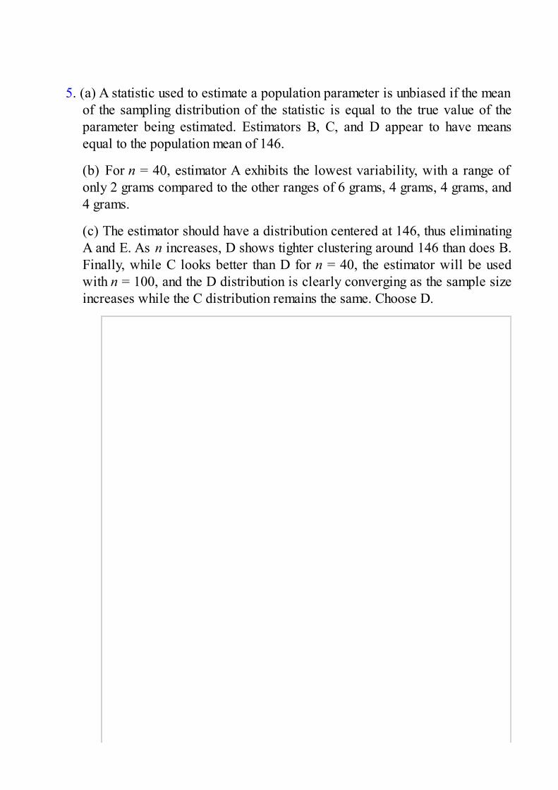
5. (a) A statistic used to estimate a population parameter is unbiased if the meanof the sampling distribution of the statistic is equal to the true value of theparameter being estimated. Estimators B, C, and D appear to have meansequal to the population mean of 146.
(b) For n = 40, estimator A exhibits the lowest variability, with a range ofonly 2 grams compared to the other ranges of 6 grams, 4 grams, 4 grams, and4 grams.
(c) The estimator should have a distribution centered at 146, thus eliminatingA and E. As n increases, D shows tighter clustering around 146 than does B.Finally, while C looks better than D for n = 40, the estimator will be usedwith n = 100, and the D distribution is clearly converging as the sample sizeincreases while the C distribution remains the same. Choose D.

Scoring
Part (a) is essentially correct for a correct answer with a goodexplanation of what unbiased means, and is partially correct for acorrect answer with a weak explanation. Part (a) is incorrect for acorrect answer with no explanation or with an incorrect explanation.
Part (b) is essentially correct for a correct answer together with somenumerical justification, and is partially correct for a correct answerwith a weak explanation. Part (b) is incorrect for a correct answer withno explanation or with an incorrect explanation.
Part (c) is essentially correct for a correct answer with a goodexplanation, and is partially correct for a correct answer with a weakexplanation. Part (c) is incorrect for a correct answer with noexplanation or with an incorrect explanation.
4 Complete Answer All three parts essentially correct.
3 Substantial Answer Two parts essentially correct andone part partially correct.
2 Developing Answer
Two parts essentially correct ORone part essentially correct and oneor two parts partially correct ORall three parts partially correct.
1 Minimal Answer One part essentially correct OR twoparts partially correct.

6. (a) State the hypotheses:H0: pH – pL = 0 and Ha: pH – pL > 0 where pH is the proportion ofpatients receiving higher doses who experience severe nausea, andpL is the proportion of patients receiving lower doses whoexperience severe nausea [other possible expressions include H0: pH= pL and Ha: pH > pL].
Identify the test by name or formula and check the assumptions:Two-sample test for proportions
Assumptions: Patients were randomly placed in different groups, soit is reasonable to assume independence of samples. Then we notethat with H = = .506 and L = = .223, we have nH H = 205,
nH(1 – H) = 200, nL L = 88, and nL(1 – L) = 307. These are allgreater than 10.
Calculate the test statistic and the P-value:
P-value = .000[Note: a graphing calculator will give z = 8.31792 with P =4.5279E–17]
State the conclusion in context with linkage to the P-value:With this small a P-value (P < .001), there is very strong evidence toreject H0. That is, there is very strong evidence that a greaterproportion of patients receiving higher doses experience severenausea than patients receiving lower doses.

(b) Identify the confidence interval by name or formula:95% confidence interval for the slope of the regression line b ± tsb
Check the assumptions:The scatterplot is roughly linear, there is no apparent pattern in theresiduals plot, and the distribution of the residuals is approximatelynormal (because the normal probability plot is roughly linear).
Calculate the confidence interval:df = n – 2 = 8 – 2 = 60.006659 ± 2.447(0.001761) = 0.006659 ± 0.004309(0.00235, 0.010968)
Interpret the confidence interval in context:We are 95% confident that the mean proportion of patientsexperiencing severe nausea goes up between 0.00235 and 0.010968with each increase of 1 milligram per week in dose intensity.
(c) The probability that a randomly chosen patient experienced severe nauseais = .366, so the probability that at least 3 out of 5 experienced severe
nausea is (.366)3(.634)2 + (.366)4(.634) + (.366)5 = 10(.366)3(.634)2
+ 5(.366)4(.634) + (.366)5 = .261 [Or 1 – binomcdf(5,.366,2)]
Scoring
Part (a) has four parts: 1) stating the hypotheses; 2) identifying the testand checking assumptions; 3) calculating the test statistic and the P-value; and 4) giving a conclusion in context with linkage to the P-value.Part (a) is essentially correct if three or four of these parts are correctand partially correct if one or two of these parts are correct.
Part (b) has four parts: 1) identifying the confidence interval; 2)checking assumptions; 3) calculating the confidence interval; and 4)interpreting the confidence interval in context. Part (b) is essentiallycorrect if three or four of these parts are correct and partially correct ifone or two of these parts are correct.
Part (c) is essentially correct if the correct probability is calculated andthe derivation is clear. Part (c) is partially correct for indicating abinomial with n = 5 and p = .366, but then calculating incorrectly.
4 Complete Answer All three parts essentially correct.
3 Substantial Answer Two parts essentially correct andone part partially correct.
2 Developing Answer
Two parts essentially correct ORone part essentially correct and oneor two parts partially correct ORall three parts partially correct.
1 Minimal Answer One part essentially correct OR twoparts partially correct.

Answers Explained, Section I1. (A) The slope, 6.2, gives the predicted increase in the y-variable for
each unit increase in the x-variable.
2. (E) For a simple random sample, every possible group of the givensize has to be equally likely to be selected, and this is not true here. Forexample, with this procedure it will be impossible for all the earlyarrivals to be together in the final sample. This procedure is an exampleof systematic sampling, but systematic sampling does not result in simplerandom samples.

3. (C) Power = 1 – , and is smallest when α is more and n is more.

4. (B) The critical z-scores for 60% to the right and 70% to the left are–0.253 and 0.524, respectively. Then { – 0.253σ = 3, + 0.524σ = 6}gives = 3.977 and σ = 3.861.
5. (A) The cumulative proportions of 0.25 and 0.75 correspond to Q1 =57 and Q3 = 75, respectively, and so the interquartile range is 75 – 57 =18.
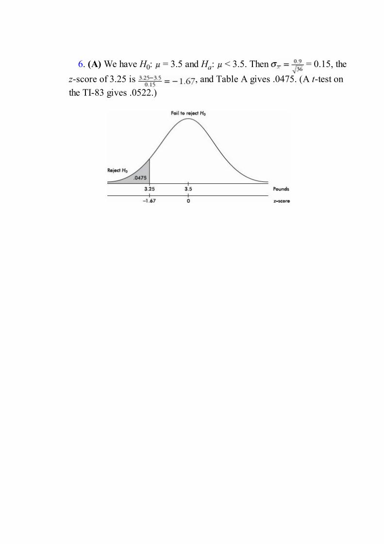
6. (A) We have H0: = 3.5 and Ha: < 3.5. Then = 0.15, thez-score of 3.25 is , and Table A gives .0475. (A t-test onthe TI-83 gives .0522.)

7. (C) A placebo is a control treatment in which members of the controlgroup do not realize whether or not they are receiving the experimentaltreatment.
8. (E) In experiments on people, subjects can be used as their owncontrols, with responses noted before and after the treatment. However,with such designs there is always the danger of a placebo effect. In thiscase, subjects might well have slower reaction times after drinking thealcohol because they think they should. Thus the design of choice wouldinvolve a separate control group to use for comparison. Blocking is notnecessary for a well-designed experiment, and there is no indication thatit would be useful here.

9. (E) Since (–2, 4) is on the line y = 7x + b, we have 4 = –14 + b andb = 18. Thus the regression line is y = 7x + 18. The point ( , ) isalways on the regression line, and so we have = 7 + 18.
10. (A) A simple random sample can be any size.
11. (E) With such small populations, censuses instead of samples areused, and there is no resulting probability statement about the difference.
12. (C) Half the area is on either side of 23, so 23 is the median. Thedistribution is skewed to the right, and so the mean is greater than themedian. With half the area to each side of 23, half the applicants’ ages areto each side of 23. Histograms such as this show relative frequencies, notactual frequencies.

13. (B) While the procedure does use some element of chance, allpossible groups of size 75 do not have the same chance of being picked,so the result is not a simple random sample. There is a real chance ofselection bias. For example, a number of relatives with the same nameand all using the same long-distance carrier might be selected.
14. (C) While t-distributions do have mean 0, their standard deviationsare greater than 1.

15. (E)

16. (E) The critical z-scores are and , with corresponding right tail probabilities of .3372
and .0188. The probability of being less than 100,000 given that themileage is over 80,000 is
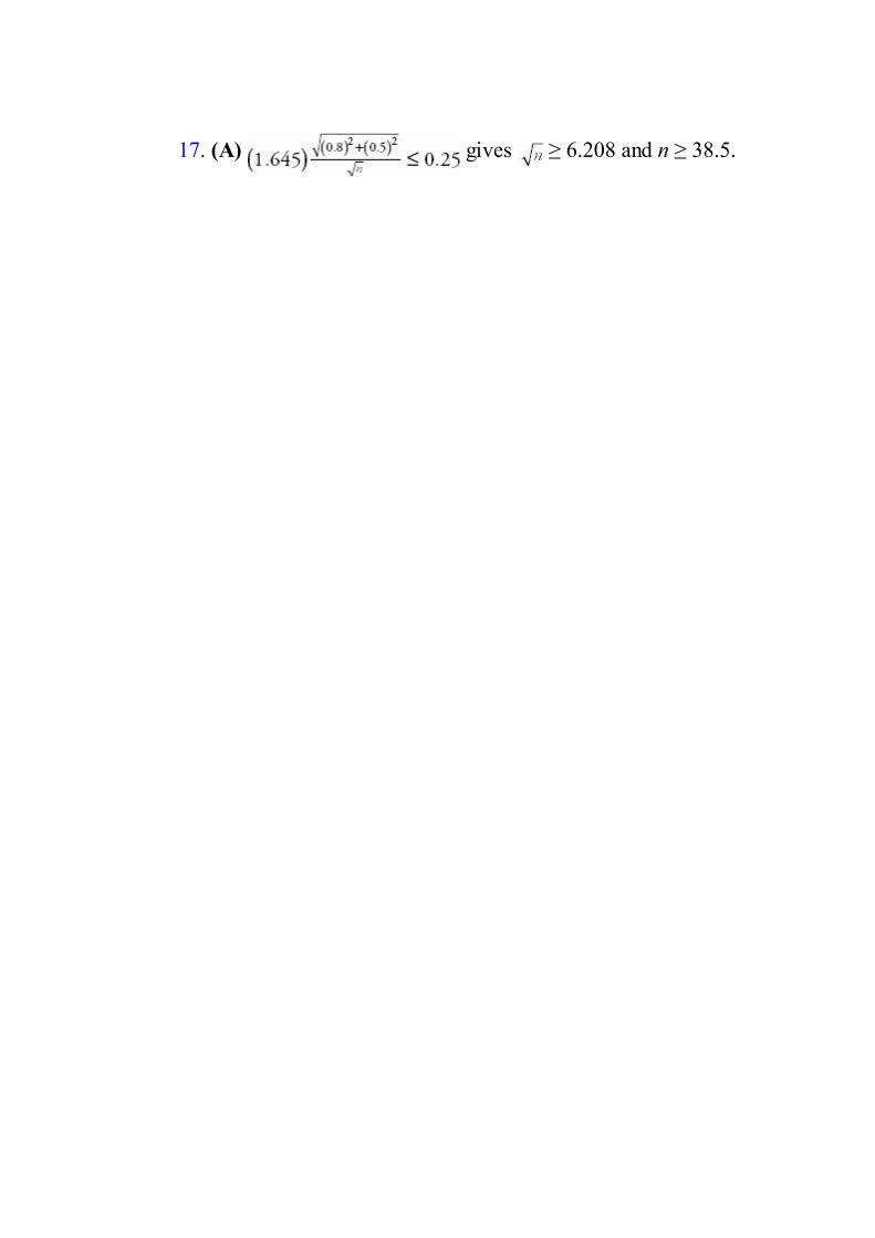
17. (A) gives ≥ 6.208 and n ≥ 38.5.

18. (A) The correlation coefficient is not changed by adding the samenumber to every value of one of the variables, by multiplying every valueof one of the variables by the same positive number, or by interchangingthe x- and y-variables.

19. (A) The binomial distribution with n = 2 and p = .8 is P(0) = (.2)2
= .04, P(1) = 2(.2)(.8) = .32, and P(2) = (.8)2 = .64, resulting in expectednumbers of .04(200) = 8, .32(200) = 64, and .64(200) = 128. Thus,
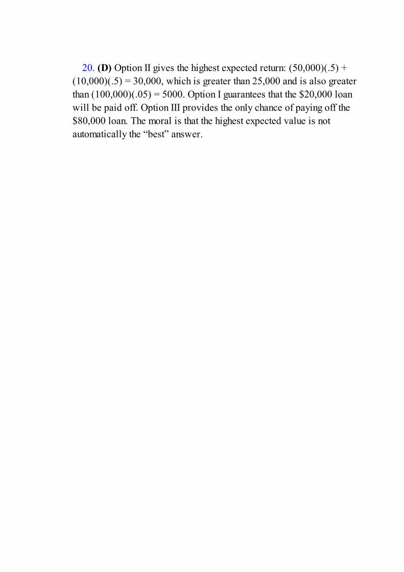
20. (D) Option II gives the highest expected return: (50,000)(.5) +(10,000)(.5) = 30,000, which is greater than 25,000 and is also greaterthan (100,000)(.05) = 5000. Option I guarantees that the $20,000 loanwill be paid off. Option III provides the only chance of paying off the$80,000 loan. The moral is that the highest expected value is notautomatically the “best” answer.

21. (B)
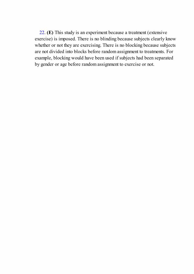
22. (E) This study is an experiment because a treatment (extensiveexercise) is imposed. There is no blinding because subjects clearly knowwhether or not they are exercising. There is no blocking because subjectsare not divided into blocks before random assignment to treatments. Forexample, blocking would have been used if subjects had been separatedby gender or age before random assignment to exercise or not.

23. (C) From the shape of the normal curve, the answer is in themiddle. The middle two-thirds is between z-scores of ±0.97, and 35 ±0.97(10) gives (25.3, 44.7).
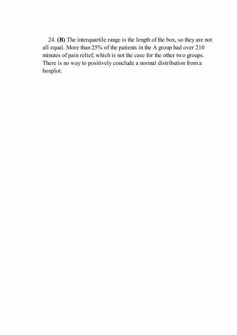
24. (B) The interquartile range is the length of the box, so they are notall equal. More than 25% of the patients in the A group had over 210minutes of pain relief, which is not the case for the other two groups.There is no way to positively conclude a normal distribution from aboxplot.
25. (B) A scatterplot would be horizontal; the correlation is zero.

26. (D)

27. (E) The midpoint of the confidence interval is .08.

28. (D) While the sample proportion is between 64% and 70% (morespecifically, it is 67%), this is not the meaning of ±3%. While thepercentage of the entire population is likely to be between 64% and 70%,this is not known for certain.
29. (A) With df = 43.43 and t = –3.94, the P-value is .000146 < .01.[On the TI-84, use tcdf.]

30. (D) Increasing the sample size by a multiple of d 2 divides thestandard deviation of the set of sample means by d.

31. (B) In this binomial situation, the probability that a car does notreceive a ticket is 1 – 3 = .7, the probability that none of the five carsreceives a ticket is (.7)5, and thus the probability that at least one receivesa ticket is 1 – (.7)5.
32. (A)

33. (B) If the standard deviation of a set is zero, all the values in the setare equal. The mean and median would both equal this common value andso would equal each other. If all the values are equal, there are nooutliers. Just because the sample happens to have one common value,there is no reason for this to be true for the whole population. Statisticsfrom one sample can be different from statistics from any other sample.

34. (A) The first study is an experiment with two treatment groups andno control group. The second study is observational; the researcher didnot randomly divide the subjects into groups and have each group watch adesignated number of hours of television per night.

35. (E) This refers only to very particular random variables, forexample, random variables whose values are the numbers of successes ina binomial probability distribution with large n.

36. (B) A Type I error means that the null hypothesis is correct (theweather will remain dry), but you reject it (thus you needlessly carryaround an umbrella). A Type II error means that the null hypothesis iswrong (it will rain), but you fail to reject it (thus you get drenched).

37. (E) If the sample statistic is far enough away from the claimedpopulation parameter, we say that there is sufficient evidence to reject thenull hypothesis. In this case the null hypothesis is that = 9500. The P-value is the probability of obtaining a sample statistic as extreme as theone obtained if the null hypothesis is assumed to be true. The smaller theP-value, the more significant the difference between the null hypothesisand the sample results. With P = .0069, there is strong evidence to rejectH0.
38. (E) There are 10 + 12 = 22 students in the combined group. Inascending order, where are the two middle scores? At least 5 thirdgraders and 6 fourth graders have heights less than or equal to 49 inches,so at most 11 students have heights greater than or equal to 49 and thus themedian is less than or equal to 49. At least 5 third graders and 6 fourthgraders have heights greater than or equal to 47 inches, so at most 11students have heights less than or equal to 47 and thus the median isgreater than or equal to 47. All that can be said about the median of thecombined group is that it is between 47 and 49 inches.

39. (E) Good experimental design aims to give each group the sameexperiences except for the treatment under consideration, Thus, all threeSRSs should be picked from the same grade level.

40. (E) The stemplot does not indicate what happened for anyindividual school.

Answers Explained, Section II1. (a) This is an example of stratified sampling, where the chapters are
strata. The advantage is that the student is ensuring that the final samplewill represent the 12 different authors, who may well use differentaverage word lengths.
(b) This is an example of cluster sampling, where for each chapterthe three chosen pages are clusters. It is reasonable to assume that eachpage (cluster) resembles the author’s overall pattern. The advantage isthat using these clusters is much more practical than trying to samplefrom among all an author’s words.
(c) This is an example of systematic sampling, which is quicker andeasier than many other procedures. A possible disadvantage is that ifordering is related to the variable under consideration, this procedurewill likely result in an unrepresentative sample. For example, in thisstudy if an author’s word length is related to word order in sentences,the student could end up with words of particular lengths.
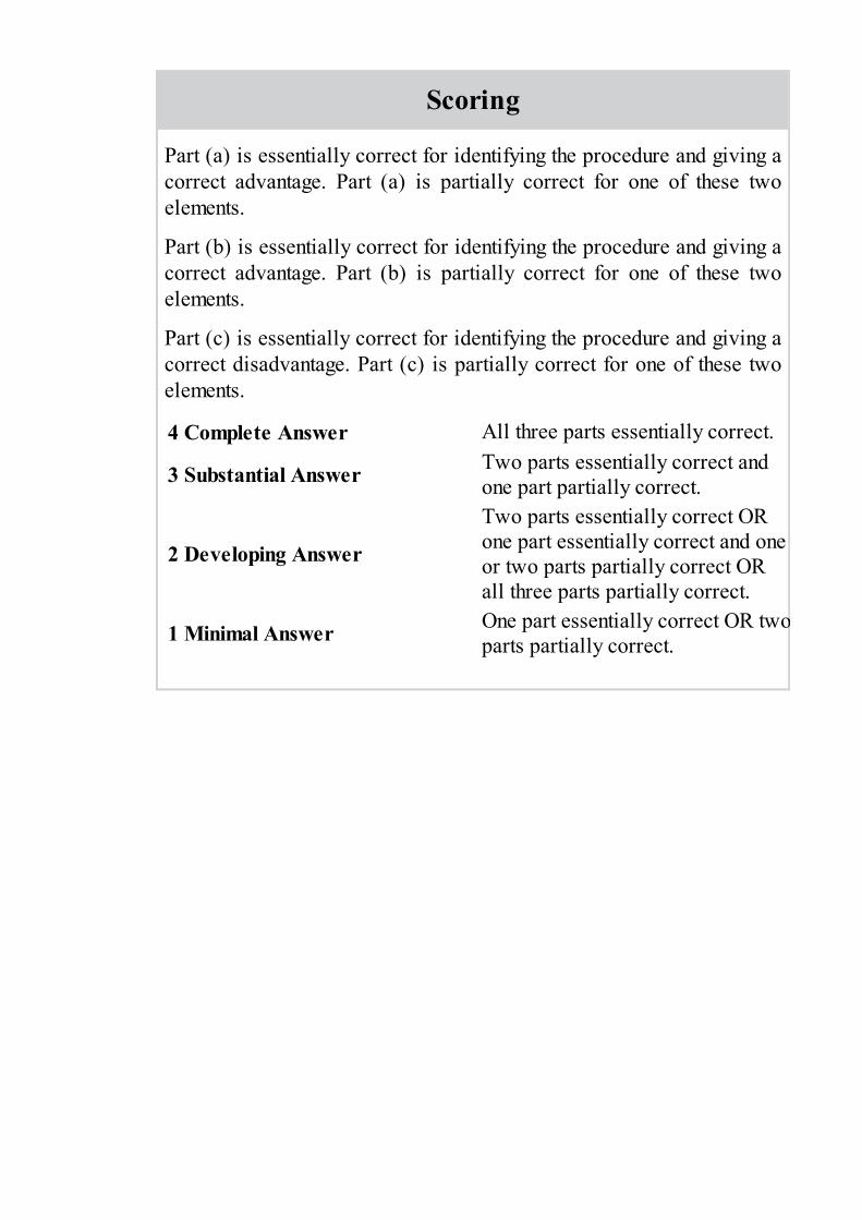
Scoring
Part (a) is essentially correct for identifying the procedure and giving acorrect advantage. Part (a) is partially correct for one of these twoelements.
Part (b) is essentially correct for identifying the procedure and giving acorrect advantage. Part (b) is partially correct for one of these twoelements.
Part (c) is essentially correct for identifying the procedure and giving acorrect disadvantage. Part (c) is partially correct for one of these twoelements.
4 Complete Answer All three parts essentially correct.
3 Substantial Answer Two parts essentially correct andone part partially correct.
2 Developing Answer
Two parts essentially correct ORone part essentially correct and oneor two parts partially correct ORall three parts partially correct.
1 Minimal Answer One part essentially correct OR twoparts partially correct.

2. (a) The SRS with n = 50 is more likely to have a sample proportiongreater than 75%. In each case, the sampling distribution of isapproximately normal with a mean of .69 and a standard deviation of
. Thus the sampling distribution with n = 50
will have more variability than the sampling distribution with n = 100.Thus the tail area ( > .75) will be larger for n = 50.
(b) The size of the sample, 30, is much too large compared to thesize of the population, 95. With a sample size this close to thepopulation size, the necessary assumption of independence does notfollow. A commonly accepted condition is that the sample should beno more than 10% of the population.
(c) A normal distribution may be used to approximate a binomialdistribution only if the sample size n is not too small. The commonlyused condition check is that both np and nq are at least 10. In this casenq = (20)(1 – .78) = 4.4.

Scoring
Part (a) is essentially correct for correctly giving n = 50 and linking incontext to variability in the sampling distributions. Part (a) is partiallycorrect for a correct answer missing comparison of variability in thesampling distributions.
Part (b) is essentially correct for a clear explanation in context. Part (b)is partially correct for saying the sample size is too close to thepopulation size but not linking to this context (sample size 30 andpopulation size 95).
Part (c) is essentially correct for a clear explanation in context. Part (c)is partially correct for saying the sample size is too small but notlinking to this context (nq = 4.4 < 10).
4 Complete Answer All three parts essentially correct.
3 Substantial Answer Two parts essentially correct andone part partially correct.
2 Developing Answer
Two parts essentially correct ORone part essentially correct and oneor two parts partially correct ORall three parts partially correct.
1 Minimal Answer One part essentially correct OR twoparts partially correct.

3. (a) The value 50.90 estimates the average score of males who spend0 hours studying. The value 9.45 estimates the average increase in scorefor each additional hour study time. For any fixed number of hours studytime, the value 4.40 estimates the average number of points that femalesscore higher than males.
(b)
(c) For each additional hour of study time, the scores of malesincrease an average of 8.5 while those of females increase an averageof 10.4. Additional hours of study time appear to benefit females morethan males, something that does not show in the original model.
(d)


Scoring
Part (a) is essentially correct for correctly interpreting all threenumbers in context and partially correct for correctly interpreting twoof the three numbers.
Part (b) is essentially correct for correct graphs, clearly parallel andlabeled as to which is which. Part (b) is partially correct for correctparallel graphs but missing labels, or for labeled, parallel graphs withincorrect y-intercepts.
Part (c) is essentially correct for correctly interpreting both slopes andfor some comparative statement about additional hours study timeappearing to benefit females more than males. Part (c) is partiallycorrect for correctly interpreting both slopes but failing to make acomparative statement, or for making a correct comparative statementwithout interpreting the slopes.
Part (d) is essentially correct for correct graphs, clearly showingdifferent slopes and labeled as to which is which. Part (d) is partiallycorrect for graphs, clearly showing different slopes but missing labels,or for labeled graphs with different slopes but with incorrect y-intercepts.
Count partially correct answers as one-half an essentially correctanswer.
4 Complete Answer Four essentially correct answers.3 Substantial Answer Three essentially correct answers.2 Developing Answer Two essentially correct answers.1 Minimal Answer One essentially correct answer.
Use a holistic approach to decide a score totaling between twonumbers.

4. (a) Name the procedure: This is a one-sample t-interval for themean.
Check the conditions: We are given that this is a random sample, and adotplot.
makes the nearly normal condition reasonable.
Mechanics: A calculator readily gives = 2.582 and s = 0.0923. With df= 4, the critical t-scores are ± 2.776. Thus the confidence interval is
Conclusion in context: We are 95% confident that the mean concentrationlevel for the active ingredient found in this pharmaceutical product isbetween 2.467 and 2.697 milligrams per milliliter. [On the TI-84, withthe data in L1, TInterval readily confirms this result.]
(b) Raising the confidence level would increase the width of theconfidence interval.
(c) Since the whole confidence interval (2.467, 2.697) is below thecritical 2.7, at the 95% confidence level the mean concentration is at a

safe level. However, with 2.697 so close to 2.7, based on thestatement in (c), if the confidence level is raised we are no longerconfident that the mean concentration is at a safe level.
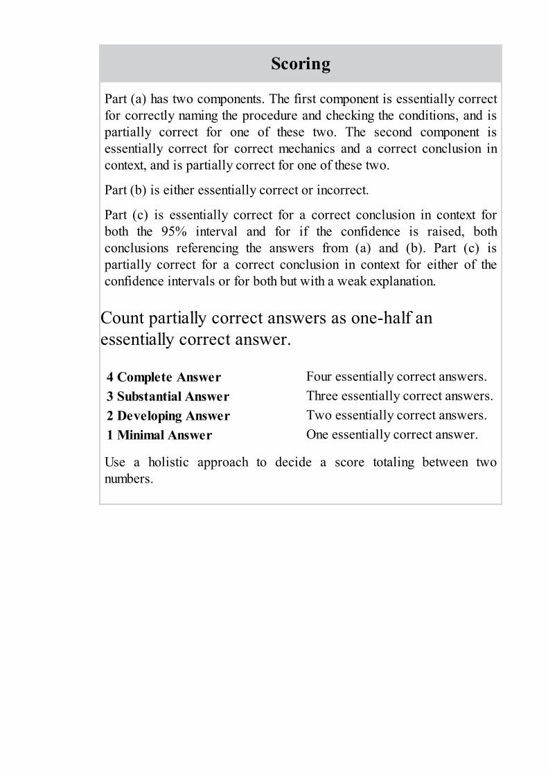
Scoring
Part (a) has two components. The first component is essentially correctfor correctly naming the procedure and checking the conditions, and ispartially correct for one of these two. The second component isessentially correct for correct mechanics and a correct conclusion incontext, and is partially correct for one of these two.
Part (b) is either essentially correct or incorrect.
Part (c) is essentially correct for a correct conclusion in context forboth the 95% interval and for if the confidence is raised, bothconclusions referencing the answers from (a) and (b). Part (c) ispartially correct for a correct conclusion in context for either of theconfidence intervals or for both but with a weak explanation.
Count partially correct answers as one-half anessentially correct answer.
4 Complete Answer Four essentially correct answers.3 Substantial Answer Three essentially correct answers.2 Developing Answer Two essentially correct answers.1 Minimal Answer One essentially correct answer.
Use a holistic approach to decide a score totaling between twonumbers.
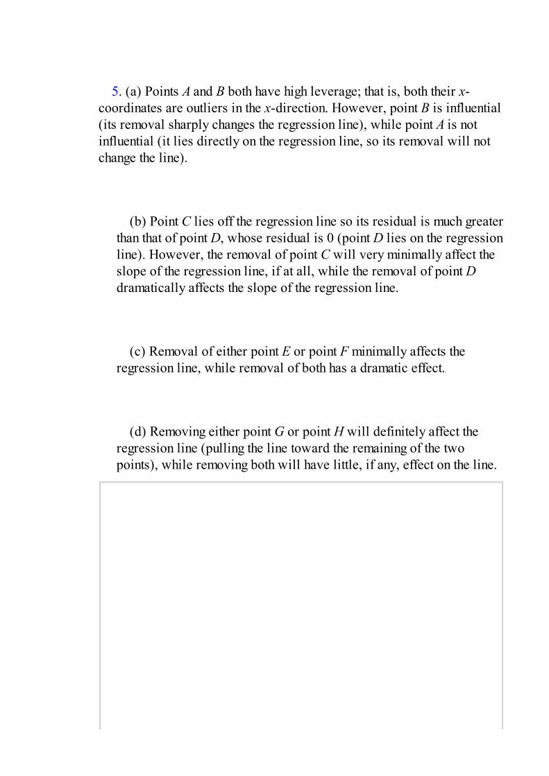
5. (a) Points A and B both have high leverage; that is, both their x-coordinates are outliers in the x-direction. However, point B is influential(its removal sharply changes the regression line), while point A is notinfluential (it lies directly on the regression line, so its removal will notchange the line).
(b) Point C lies off the regression line so its residual is much greaterthan that of point D, whose residual is 0 (point D lies on the regressionline). However, the removal of point C will very minimally affect theslope of the regression line, if at all, while the removal of point Ddramatically affects the slope of the regression line.
(c) Removal of either point E or point F minimally affects theregression line, while removal of both has a dramatic effect.
(d) Removing either point G or point H will definitely affect theregression line (pulling the line toward the remaining of the twopoints), while removing both will have little, if any, effect on the line.

Scoring
Each of parts (a), (b), (c), and (d) has two components and is scoredessentially correct for both components correct and partially correct forone component correct.
Give 1 point for each essentially correct part and point for eachpartially correct part.
4 Complete Answer 4 points3 Substantial Answer 3 points2 Developing Answer 2 points1 Minimal Answer 1 point
Use a holistic approach to decide a score totaling between twonumbers.

6. (a) State the hypotheses: H0: A – B = 0 and Ha: A – B ≠ 0
Identify the test and check conditions: two-sample t-test. It is given thatthe samples are random. The populations may not be normal, but since nA= 390 and nB = 235 are both large, it is OK to proceed with the t-test.
Calculate the test statistic t and the P-value: and
with df = 199, we have P = 2(.066) = .133. [Or use df = 623. Or acalculator using the given sample statistics gives t = –1.51, df = 408.25,and P = .131. Or a calculator using the sample data gives t = –1.53, df =408.27, and P = .127.]
Conclusion in context: With this large a P-value, there is no evidence of adifference in the mean years of schooling between the two communities.
(b) State the hypotheses: H0: The distribution of years of schoolingis the same in the two communities. Ha: The distribution of years ofschooling is not the same in the two communities.
Identify the test and check conditions: Chi-square test (of homogeneity).All expected counts are > 5.
Calculate the test statistic and the P-value: χ2 = 57.85 and with df = (7 –1) (2 – 1) = 6, we have P = .000.

State the conclusion in context: With this small a P-value, there is strongevidence that the distribution of years of schooling is not the same in thetwo communities.
(c)
Although the two distributions have roughly the same center, their shapesare different. The distribution of years of schooling for Community A isunimodal, symmetric, and bell-shaped, while that of Community B isroughly bimodal with few scores in the center.

Scoring
Part (a) is essentially correct if all four steps for a two-sample t-testare correct and partially correct if three steps are correct.
Part (b) is essentially correct if all four steps for a chi-square test (ofhomogeneity) are correct and partially correct if three steps are correct.
Part (c) is essentially correct for an accurate comparison of thedistributions linked to correctly drawn histograms. Part (c) is partiallycorrect if only one of the two parts (comparison and histograms) iscorrect or if both are correct but there is no linkage.
4 Complete Answer All three parts essentially correct.
3 Substantial Answer Two parts essentially correct andone part partially correct.
2 Developing Answer
Two parts essentially correct ORone part essentially correct and oneor two parts partially correct ORall three parts partially correct.
1 Minimal Answer One part essentially correct OR twoparts partially correct.
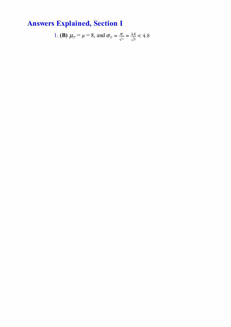
Answers Explained, Section I1. (B) = = 8, and

2. (C) The range increased from 90 – 15 = 75 to 97 – 21 = 76, whilethe standard deviation decreased (note how the values are bunchedtogether more closely in 1998).

3. (E) None of the studies have any controls such as randomization,a control group, or blinding, and so while they may give valuableinformation, they cannot establish cause and effect.
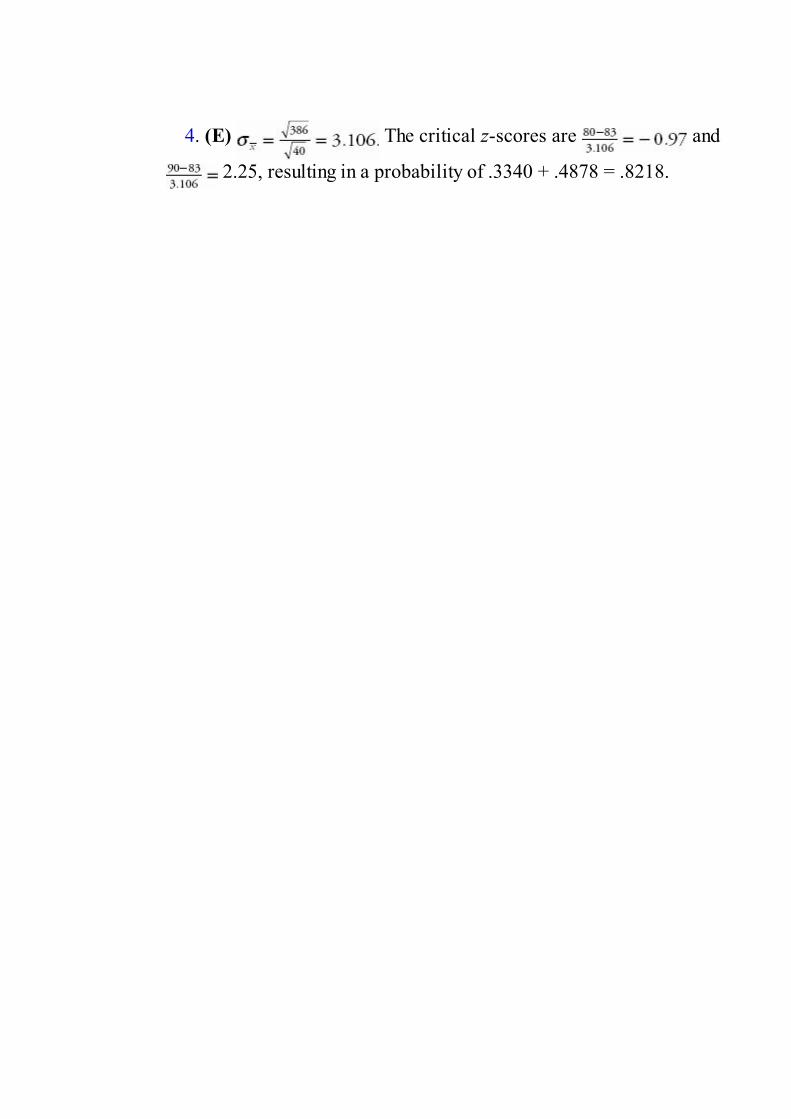
4. (E) The critical z-scores are and
2.25, resulting in a probability of .3340 + .4878 = .8218.

5. (D) The critical z-scores are and ,with corresponding left tail probabilities of .0082 and .1151,respectively. The probability of being greater than 188 given that it isless than 194 is

6. (C)

7. (D) Given a census, the population parameter is known, and thereis no need to use the techniques of inference.

8. (C) Sixty-four percent of the students scored below Mary and56% scored below Pam, and so 8% must have scored between them.

9. (E) Intentionally forcing some treatment to note the response isassociated with controlled experiments, not with observational studies.In experiments, the researchers decide how people are placed indifferent groups; self-selection is associated with observationalstudies. Results of observational studies may suggest cause-and-effectrelationships; however, controlled studies are used to establish suchrelationships.
10. (E) With = , the greater the sample size n, the smaller the
standard deviation .
11. (D) df = 9, and

12. (E) The set could be {150, 150, 150, 200} with mean 162.5 andmedian 150. It might also be {150, 200, 200, 200} with mean 187.5 andmedian 200. The median of a set of four elements is the mean of the twomiddle elements.

13. (D) and The z-scores of .60 and
.68 are for a probability of .9525 – .0475 = .9050.

14. (C) This is a binomial with n = 15 and p = .29, and so the mean isnp = 15(.29) = 4.35.

15. (D) With independence, variances add, so .

16. (E) Without independence we cannot determine var(X + Y) from theinformation given.

17. (A) Bias is the tendency to favor the selection of certain membersof a population. It has nothing to do with the shape of distributions. Thenatural variability between samples is called sampling error.

18. (C) There are not two distinct peaks, so the distribution is notbimodal. Relative frequency is given by relative area. The distribution isskewed to the left, and so the mean is less than the median.

19. (D) While the standard deviation of the z-distribution is 1, thestandard deviation of the t-distribution is greater than 1.

20. (B)

21. (E) Different samples give different sample statistics, all of whichare estimates for the same population parameter, and so error, calledsampling error, is naturally present.

22. (C) With four-digit accuracy as found on the TI-83, the critical z-scores for 70% to the right and 80% to the right are –0.5244 and –0.8416,respectively. Then { – 0.5244σ = 12,000, – 0.8416σ = 10,000} gives
= 15,306 and σ = 6305. Using two-digit accuracy as found in Table A,that is, –0.52 and –0.84, results in = 15,250 and σ = 6250.

23. (D) The percentage of the variation in y explained by the variationin x is given by the coefficient of determination r 2. In this example, (.78)2
= .61.

24. (B) There is a weak negative correlation, and so –.15 is the onlyreasonable possibility among the choices given.

25. (E) There is no guarantee that 24 is anywhere near the interval, andso none of the statements is true.
26. (E) Sampling error relates to natural variation between samples,and it can never be eliminated. In good observational studies, responsesare not influenced during the collection of data. In good experiments,treatments are compared as to the differences in responses.

27. (E) The scatterplot suggests a zero correlation.

28. (A) . The z-score of 2.5 is , and to the
right of 2.5 is the probability of failing to reject the false claim.

29. (E) The central limit theorem says that no matter how the originalpopulation is distributed, as the sample size increases, the samplingdistribution of the sample mean becomes closer to a normal distribution.

30. (D) A sampling distribution is the distribution of all the valuestaken by a statistic, such as sample mean or sample proportion, from allpossible samples of a given size.

31. (E) P(at least 2) = P(exactly 2) + P(exactly 3) = 3(.8)2(.2) + (.8)3

32. (A) The critical t-scores for 99% confidence with df = 6 are±3.707.

33. (B) The PTA survey has strong response bias in that students maynot give truthful responses to a parent or teacher about their engaging inunprotected sex. The talk show survey results in a voluntary responsesample, which typically gives too much emphasis to persons with strongopinions. The Ladies Home Journal survey has strong selection bias; thatis, people who read the Journal are not representative of the generalpopulation.
34. (D) To divide the interval estimate by d, the sample size must beincreased by a multiple of d 2.

35. (B) P(0 pts) = (.05)2, P( pt) = 2(.05)(.15), P(1 pt) = (.15)2 +2(.05)(.8), P(1 pts) = 2(.15)(.8), and P(2 pts) = (.8)2.
36. (A) The P-value is the probability of obtaining a result as extremeas the one seen given that the null hypothesis is true; thus it is aconditional probability. The P-value depends on the sample chosen. TheP-value in a two-sided test is calculated by doubling the indicated tailprobability. P-values are not restricted to use with any particulardistribution. With a small P-value, there is evidence to reject the nullhypothesis, but we’re not proving anything.
37. (C) A Type II error is a mistaken failure to reject a false nullhypothesis or, in this case, a failure to realize that the machinery is turningout wrong size ball bearings.

38. (E) Using a measurement from a sample, we are never able to sayexactly what a population mean is; rather we always say we have acertain confidence that the population mean lies in a particularinterval. In this case we are 95% confident that Lipitor will outperformniacin by 18 to 41 points.

39. (C) The median number of hours is less than four for June, July, andAugust.

40. (D) A horizontal line drawn at the .9 probability level correspondsto roughly 19 rooms.

Answers Explained, Section II1. (a) In each block, two of the sites will be randomly assigned to
receive Type A vegetation, while the remaining two sites in the blockwill receive Type B vegetation. Randomization of vegetation type tothe sites within each block should reduce bias due to any confoundingvariables. In particular, the randomization in blocks in the first schemeshould even out the effect of the distance vegetation in blocks is fromthe industrial park.
(b) The first scheme creates homogeneous blocks with respect todistance from the river, while the second scheme creates homogeneousblocks with respect to the industrial park. Randomization of vegetationtypes to sites within blocks in the first scheme should even out effectsof distance from the industrial park, while randomization of vegetationtypes to sites within blocks in the second scheme should even outeffects of distance from the river.

Scoring
It is important to explain why randomization is important within thecontext of this problem, so use of terms like bias and confounding mustbe in context. One must explain the importance of homogeneousexperimental units (sites, not vegetation types) within blocks.
4 Complete Answer
Correct explanation both of use ofblocking and of use ofrandomization in context of thisproblem.
3 Substantial Answer
Correct explanation of use of eitherblocking or randomization incontext and a weak explanation ofthe other.
2 Developing Answer
Correct explanation of use of eitherblocking or randomization incontext OR weak explanations ofboth.
1 Minimal Answer Weak explanation of either blockingor randomization in context.
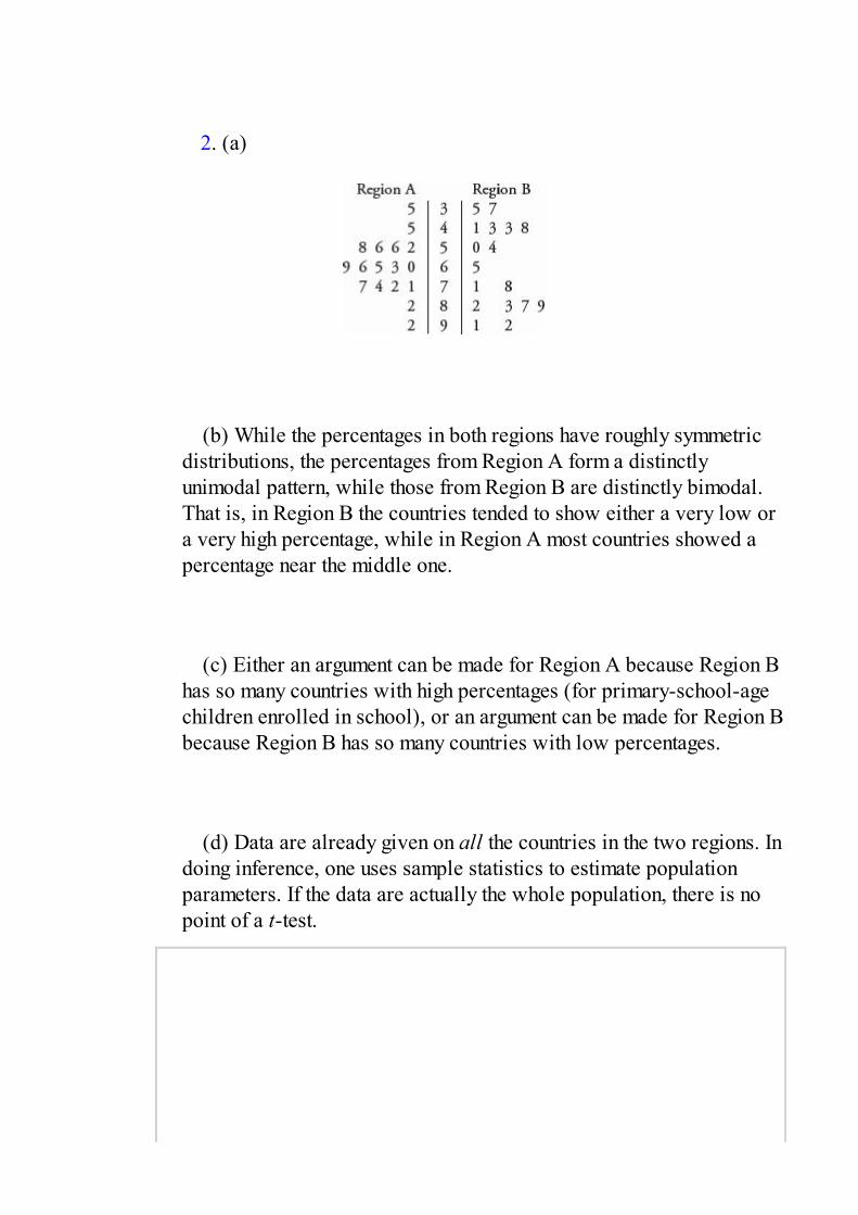
2. (a)
(b) While the percentages in both regions have roughly symmetricdistributions, the percentages from Region A form a distinctlyunimodal pattern, while those from Region B are distinctly bimodal.That is, in Region B the countries tended to show either a very low ora very high percentage, while in Region A most countries showed apercentage near the middle one.
(c) Either an argument can be made for Region A because Region Bhas so many countries with high percentages (for primary-school-agechildren enrolled in school), or an argument can be made for Region Bbecause Region B has so many countries with low percentages.
(d) Data are already given on all the countries in the two regions. Indoing inference, one uses sample statistics to estimate populationparameters. If the data are actually the whole population, there is nopoint of a t-test.

Scoring
Part (a) is essentially correct for a correct stemplot (numbers in eachrow do not have to be in order) with labeling as to which side refers towhich region. Part (a) is partially correct for a correct stemplot missingthe labeling.
Part (b) is essentially correct for noting that the percentages fromRegion A form a distinctly unimodal pattern, while those from Region Bare distinctly bimodal. Part (b) is partially correct for noting either theunimodal pattern from the Region A data or the bimodal pattern fromthe Region B data.
Part (c) is essentially correct for choosing either region and giving areasonable argument for the choice. Part (c) is partially correct if theargument is weak. Part (c) is incorrect for no argument or an incorrectargument for the choice given.
Part (d) is essentially correct for explaining that inference is not properwhen the data are the whole population. Part (d) is partially correct ifthe explanation is correct but weak.
Count partially correct answers as one-half an essentially correctanswer.
4 Complete Answer Four essentially correct answers.3 Substantial Answer Three essentially correct answers.2 Developing Answer Two essentially correct answers.1 Minimal Answer One essentially correct answer.
Use a holistic approach to decide a score totaling between twonumbers.
3. (a) Note that there are a great number of values between 2.0 and2.4, fewer values between 2.4 and 2.8, on down to the fewest valuesbeing between 3.6 and 4.0. Thus the distribution is skewed right(skewed toward the higher values).
(b) Note that the greatest five values, out of the 100 values, areabove a point roughly at 3.4 or 3.5, so the 95th percentile is roughly3.4 or 3.5.
(c) In a normal distribution, the 95th percentile has a z-score of1.645. Reading up from the x-axis to the normal line and across to they-axis gives a GPA of approximately 3.2.
Scoring
Part (a) is essentially correct if the shape is correctly identified asskewed right, and a correct explanation based on the given normalprobability plot is given. Part (a) is partially correct for a correctidentification with a weak explanation. Part (a) is incorrect if a correctidentification is given with no explanation.
Part (b) is essentially correct for correctly noting 3.4 or 3.5 as the 95thpercentile with a correct explanation. Part (b) is partially correct forgiving 3.4 or 3.5 with a weak explanation or no explanation.
Part (c) is essentially correct for noting approximately 3.2 as the GPAand stating the method clearly. Part (c) is partially correct for giving 3.2with a weak explanation or no explanation.
4 Complete Answer All three parts essentially correct.
3 Substantial Answer Two parts essentially correct andone part partially correct.
2 Developing Answer
Two parts essentially correct ORone part essentially correct and oneor two parts partially correct ORall three parts partially correct.
1 Minimal Answer One part essentially correct OR twoparts partially correct.

4. (a) There are four elements to this solution.
State the hypotheses:
H0: The distribution of blood types among patients at this hospital isin the ratios of 9:8:2:1 for types O, A, B, and AB, respectively.
Ha: The distribution of blood types among patients at this hospital isnot in the ratios of 9:8:2:1 for types O, A, B, and AB, respectively.
Identify the test by name or formula and check the assumptions:
Chi-square goodness-of-fit test:
Check the assumptions:1. The researcher claims that the data are from a random sample of
patient records.2. The ratios 9:8:2:1 give expected cell frequencies of (500) =
225, (500) = 200, (500) = 50, (500) = 25, each of which is atleast 5.
Demonstrate correct mechanics:

With df = 4 – 1 = 3, the P-value is .0145.State the conclusion in context with linkage to the P-value:
With this small a P-value (for example, less than = .05), there isevidence that the distribution of blood types among patients at thishospital is not in the ratios of 9:8:2:1 for types O, A, B, and AB,respectively.
(b) In this case the mechanics give:
With df = 4 – 1 = 3, the probability that χ2 is less than or equal to0.311 is .0421. With such a small probability, there is evidence thatthe data are too good to be true; that is, there is evidence thatResearcher 2 made up the data to fit the 9:8:2:1 model.

Scoring
Part (a1) is essentially correct if the hypotheses are given, the test isidentified, and the assumptions are checked. Part (a1) is partiallycorrect for two of these three steps.
Part (a2) is essentially correct for correct mechanics and the conclusiongiven in context with linkage to the P-value. Part (a2) is partiallycorrect if there is a minor error in mechanics OR the conclusion is notin context OR there is no linkage to the P-value.
Part (b) is essentially correct for noting that the probability of a χ2
value of only 0.311 is very small, and thus the data are suspicious. Part(b) is partially correct for a correct idea but with a weak explanation.
4 Complete Answer All three parts essentially correct.
3 Substantial Answer Two parts essentially correct andone part partially correct.
2 Developing Answer
Two parts essentially correct ORone part essentially correct and oneor two parts partially correct ORall three parts partially correct.
1 Minimal Answer One part essentially correct OR twoparts partially correct.
5. (a) The regression line is = 40.2462 – 4.61969 liter.
Then 40.2462 – 4.61969(1.5) ≈ 33.32.
Residual = actual – predicted = 35 – 33.32 = 1.68
(b) The predicted value for mpg is 40.2462 – 4.61969(5.0) ≈ 17.15,which is very close to the actual value of 17. The added point is consistentwith the linear pattern given by the computer output, so the new slopeshould be about the same as the old slope.
(c) Since the new point fits the old linear pattern so well, and has anx-value (liter) much greater than = 2.52, the absolute value of thecorrelation will increase.

Scoring
Part (a) is essentially correct for a correct calculation of the residual.Part (a) is partially correct for noting that residual = actual – predicted,but obtaining an incorrect answer because of an incorrect derivation ofthe regression line.
Part (b) is essentially correct for showing that the actual value is veryclose to the predicted value and concluding that the new slope shouldbe about the same. Part (b) is partially correct if the predicted value ismiscalculated but a proper conclusion based on the miscalculation isreached.
Part (c) is essentially correct for concluding that the absolute value ofthe correlation will increase because the new point fits the old linearpattern so well. Part (c) is partially correct for concluding that theabsolute value of the correlation will increase but giving a weakexplanation.
4 Complete Answer All three parts essentially correct.
3 Substantial Answer Two parts essentially correct andone part partially correct.
2 Developing Answer
Two parts essentially correct ORone part essentially correct and oneor two parts partially correct ORall three parts partially correct.
1 Minimal Answer One part essentially correct OR twoparts partially correct.
6. (a) State the hypotheses: H0: d = 0 and Ha: d > 0 where d isthe mean difference (2000 – 1999) in the populations of the southernstates.Identify the test: paired t-test.
Calculate the test statistic t and the P-value: with
df = 5 – 1 = 4, P = .056Conclusion in context: Since P = .056 > .05, at the = .05significance level, there is no evidence to conclude that southern statesgrew between 1990 and 2000.
(b) Identify the confidence interval: two-sample t-interval for N –
S, the difference in mean populations between northern and southernstates in 1990.Calculate the confidence interval: with df = (5 – 1) + (5 – 1) = 8,
(8600 – 7929) ± 2.306 = 680 ± 9,786
Interpretation in context: We are 95% confident that the true differencein the average populations of northern and southern states in 1990 wasbetween –9,106 and 10,466 thousand people.
(c) State the hypotheses: H0: d = 0 and Ha: d >0 where d is thedifference in the mean growths of populations of southern and northernstates.
Identify the test: two-sample t-test.
Calculate the test statistic t and the P-value: t =
and withdf = min{5 – 1,5 – 1} = 4 we have P = .14.State the conclusion in context: With this large a P-value, there is no
evidence that southern states grew faster than northern states between1990 and 2000.
Scoring
Conditions for inference are assumed to be met and don’t have to bementioned.
Part (a) is essentially correct if all four steps are correct and partiallycorrect if three steps are correct.
Part (b) is essentially correct if all three steps are correct and partiallycorrect if two steps are correct. Full credit for df = 4 or 8.
Part (c) is essentially correct if all four steps are correct and partiallycorrect if three steps are correct. Full credit for df = 4, 4.43, or 8.
4 Complete Answer All three parts essentially correct.
3 Substantial Answer Two parts essentially correct andone part partially correct.
2 Developing Answer
Two parts essentially correct ORone part essentially correct and oneor two parts partially correct ORall three parts partially correct.
1 Minimal Answer One part essentially correct OR twoparts partially correct.