AP Statistics
385
-
Upload
khangminh22 -
Category
Documents
-
view
3 -
download
0
Transcript of AP Statistics


5 STEPS TO A 5AP Statistics

Other books in McGraw-Hill’s 5 STEPS TO A 5 series include:
AP Biology
AP Calculus AB/BC
AP Chemistry
AP Computer Science
AP English Language
AP English Literature
AP European History
AP Environmental Science
AP Microeconomics/Macroeconomics
AP Physics B and C
AP Psychology
AP Spanish Language
AP U.S. Government and Politics
AP U.S. History
AP World History
11 Practice Tests for the AP Exams
Writing the AP English Essay

5 STEPS TO A5AP Statistics
Duane C. Hinders
2010–2011
New York Chicago San Francisco Lisbon London MadridMexico City Milan New Delhi San Juan Seoul Singapore Sydney Toronto

Copyright © 2010, 2008, 2004 by The McGraw-Hill Companies, Inc. All rights reserved. Except as permitted under the United States Copyright Act of1976, no part of this publication may be reproduced or distributed in any form or by any means, or stored in a database or retrieval system, without theprior written permission of the publisher.
ISBN: 978-0-07-162189-2
MHID: 0-07-162189-X
The material in this eBook also appears in the print version of this title: ISBN: 978-0-07-162188-5, MHID: 0-07-162188-1.
All trademarks are trademarks of their respective owners. Rather than put a trademark symbol after every occurrence of a trademarked name, we use namesin an editorial fashion only, and to the benefit of the trademark owner, with no intention of infringement of the trademark. Where such designations appearin this book, they have been printed with initial caps.
McGraw-Hill eBooks are available at special quantity discounts to use as premiums and sales promotions, or for use in corporate training programs. Tocontact a representative please e-mail us at [email protected].
TERMS OF USE
This is a copyrighted work and The McGraw-Hill Companies, Inc. (“McGraw-Hill”) and its licensors reserve all rights in and to the work. Use of thiswork is subject to these terms. Except as permitted under the Copyright Act of 1976 and the right to store and retrieve one copy of the work, you may notdecompile, disassemble, reverse engineer, reproduce, modify, create derivative works based upon, transmit, distribute, disseminate, sell, publish or sublicense the work or any part of it without McGraw-Hill’s prior consent. You may use the work for your own noncommercial and personal use; anyother use of the work is strictly prohibited. Your right to use the work may be terminated if you fail to comply with these terms.
THE WORK IS PROVIDED “AS IS.” McGRAW-HILL AND ITS LICENSORS MAKE NO GUARANTEES OR WARRANTIES AS TO THE ACCURACY, ADEQUACY OR COMPLETENESS OF OR RESULTS TO BE OBTAINED FROM USING THE WORK, INCLUDING ANY INFORMATION THAT CAN BE ACCESSED THROUGH THE WORK VIA HYPERLINK OR OTHERWISE, AND EXPRESSLY DISCLAIM ANYWARRANTY, EXPRESS OR IMPLIED, INCLUDING BUT NOT LIMITED TO IMPLIED WARRANTIES OF MERCHANTABILITY OR FITNESSFOR A PARTICULAR PURPOSE. McGraw-Hill and its licensors do not warrant or guarantee that the functions contained in the work will meet yourrequirements or that its operation will be uninterrupted or error free. Neither McGraw-Hill nor its licensors shall be liable to you or anyone else for anyinaccuracy, error or omission, regardless of cause, in the work or for any damages resulting therefrom. McGraw-Hill has no responsibility for the contentof any information accessed through the work. Under no circumstances shall McGraw-Hill and/or its licensors be liable for any indirect, incidental, special, punitive, consequential or similar damages that result from the use of or inability to use the work, even if any of them has been advised of thepossibility of such damages. This limitation of liability shall apply to any claim or cause whatsoever whether such claim or cause arises in contract, tortor otherwise.

CONTENTS
Preface, ixAcknowledgments, xiAbout the Author, xiiIntroduction: The Five-Step Program, xiii
STEP 1 Set Up Your Study Program, 1
1 What You Need to Know About the AP Statistics Exam, 3Background Information, 3Some Frequently Asked Questions About the AP Statistics Exam, 4
2 How to Plan Your Time, 10Three Approaches to Preparing for the AP Statistics Exam, 10Calendar for Each Plan, 12
STEP 2 Determine Your Test Readiness, 15
3 Take a Diagnostic Exam, 17Interpretation: How Ready Are You?, 41Section I: Multiple-Choice Questions, 41Section II: Free-Response Questions, 41Composite Score, 41
STEP 3 Develop Strategies for Success, 43
4 Tips for Taking the Exam, 45General Test-Taking Tips, 46Tips for Multiple-Choice Questions, 46Tips for Free-Response Questions, 47Specific Statistics Content Tips, 49
STEP 4 Review the Knowledge You Need to Score High, 51
5 Overview of Statistics/Basic Vocabulary, 53Quantitative Versus Qualitative Data, 54Descriptive Versus Inferential Statistics, 54Collecting Data: Surveys, Experiments, Observational Studies, 55Random Variables, 56
6 One-Variable Data Analysis, 59Graphical Analysis, 60Measures of Center, 66Measures of Spread, 68Position of a Term in a Distribution, 71Normal Distribution, 74Practice Problems, 80
� v

Cumulative Review Problems, 85Solutions to Practice Problems, 86Solutions to Cumulative Review Problems, 91
7 Two-Variable Data Analysis, 93Scatterplots, 93Correlation, 95Lines of Best Fit, 99Residuals, 102Coefficient of Determination, 104Outliers and Influential Observations, 105Transformations to Achieve Linearity, 106Practice Problems, 109Cumulative Review Problems, 115Solutions to Practice Problems, 116Free Response, 117Solutions to Cumulative Review Problems, 119
8 Design of a Study: Sampling, Surveys,and Experiments, 121Samples, 122Sampling Bias, 124Experiments and Observational Studies, 126Practice Problems, 132Free Response, 134Cumulative Review Problems, 137Solutions to Practice Problems, 137Free Response, 138Solutions to Cumulative Review Problems, 141
9 Probability and Random Variables, 143Probability, 143Random Variables, 148Normal Probabilities, 152Simulation and Random Number Generation, 154Transforming and Combining Random Variables, 157Rules for the Mean and Standard Deviation of CombinedRandom Variables, 157Practice Problems, 159Free Response, 162Cumulative Review Problems, 165Solutions to Practice Problems, 166Solutions to Cumulative Review Problems, 172
10 Binomial Distributions, Geometric Distributions,and Sampling Distributions, 174Binomial Distributions, 174Normal Approximation to the Binomial, 177Geometric Distributions, 179Sampling Distributions, 180Sampling Distributions of a Sample Proportion, 184
vi � Contents

Practice Problems, 186Cumulative Review Problems, 190Solutions to Practice Problems, 191Solutions to Cumulative Review Problems, 196
11 Confidence Intervals and Introductionto Inference, 197Estimation and Confidence Intervals, 198Confidence Intervals for Means and Proportions, 201Sample Size, 206Statistical Significance and P-Value, 208The Hypothesis-Testing Procedure, 210Type-I and Type-II Errors and the Power of a Test, 211Practice Problems, 215Cumulative Review Problems, 220Solutions to Practice Problems, 221Free Response, 222Solutions to Cumulative Review Problems, 227
12 Inference for Means and Proportions, 229Significance Testing, 230Inference for a Single Population Mean, 232Inference for the Difference Between Two Population Means, 235Inference for a Single Population Proportion, 237Inference for the Difference Between Two PopulationProportions, 239Practice Problems, 243Cumulative Review Problems, 248Solutions to Practice Problems, 249
13 Inference for Regression, 258Simple Linear Regression, 258Inference for the Slope of a Regression Line, 260Confidence Interval for the Slope of a Regression Line, 262Inference for Regression Using Technology, 264Practice Problems, 268Free Response, 269Cumulative Review Problems, 272Solutions to Practice Problems, 273Solutions to Cumulative Review Problems, 277
14 Inference for Categorical Data: Chi Square, 279Chi Square Goodness-of-Fit Test, 279Inference for Two-Way Tables, 284Practice Problems, 291Free Response, 293Cumulative Review Problems, 296Solutions to Practice Problems, 296Free Response, 297Solutions to Cumulative Review Problems, 300
Contents � vii

STEP 5 Build Your Test-Taking Confidence, 301AP Statistics Practice Exam 1, 305AP Statistics Practice Exam 2, 331
Appendixes, 355Formulas, 356Tables, 358Bibliography, 362Web Sites, 363Glossary, 364
viii � Contents

PREFACE
Congratulations, you are now an AP Statistics student. AP Statistics is one of the mostinteresting and useful subjects you will study in school. Sometimes it has the reputation ofbeing easy compared to calculus. However, it can be deceptively difficult, especially in thesecond half. It is different and challenging in its own way. Unlike calculus, where you areexpected to get precise answers, in statistics you are expected to learn to become comfort-able with uncertainly. Instead of saying things like, “The answer is . . .” you will more oftenfind yourself saying things like, “We are confident that . . .” or “We have evidence that . . .”It’s a new and exciting way of thinking.
How do you do well on the AP exam (by well, I mean a 4 or a 5 although most stu-dents consider 3 or better to be passing)? By reading this book; by staying on top of thematerial during your AP Statistics class; by studying when it is time to study. Note that thequestions on the AP exam are only partially computational—they also involve thinkingabout the process you are involved in and communicating your thoughts clearly to theperson reading your exam. You can always use a calculator so the test designers make surethe questions involve more than just button pushing.
This book is self-contained in that it covers all of the material required by the coursecontent description published by the College Board. However, it is not designed to substi-tute for an in-class experience or for your textbook. Use this book as a supplement to yourin-class studies, as a reference for a quick refresher on a topic, and as one of your majorresource as you prepare for the AP exam.
This edition extends and updates previous editions. It takes into account changes inthinking about AP Statistics since the publication of the first edition in 2004 and includessome topics that, while not actually included in the official AP Statistics syllabus, some-times appear on the actual exam. New multiple-choice questions have been added to eachchapter, and the first part of the Diagnostic Exam has been updated so that it now containsonly multiple-choice questions. In addition, about half of the multiple-choice questions onthe two practice exams have been replaced to better reflect the types of questions seen onthe most recently released exam.
You should begin your preparations by reading through the Introduction and STEP I.However, you shouldn’t attempt the Diagnostic Exam in Chapter 3 until you have beenthrough all of the material in the course. Then you can take the exam to help you deter-mine which topics need more of your attention during the course of your review. Note thatthe Diagnostic Test simulates the AP exam to a reasonable extent (although the questionsare more basic) and the Practice Tests are similar in style and length to the AP exam.
So, how do you get the best possible score on the AP Statistics exam?
• Pick one of the study plans from this book.• Study the chapters and do the practice problems.• Take the Diagnostic Test and the Practice Tests.• Review as necessary based on your performance on the Diagnostic Test and the Practice
Tests.• Get a good night’s sleep before the exam.
� ix

Selected Epigrams about Statistics
Statistics are like a bikini. What they reveal is suggestive, but what they conceal is vital.—Aaron Levenstein
Torture numbers, and they’ll confess to anything.—Gregg Easterbrook
Satan delights equally in statistics and in quoting scripture . . .—H.G. Wells, The Undying Fire
One survey found that ten percent of Americans thought Joan of Arc was Noah’s wife . . .—Rita May Brown
In God we trust. All others must bring data.—Robert W. Hayden
The lottery is a tax on people who flunked math.—Monique Lloyd
x � Preface

ACKNOWLEDGMENTS
With gratitude, I acknowledge the following for their assistance and support:
The Woodrow Wilson National Fellowship Foundation, for getting me started thinking seriously about statistics.
The College Board, for giving me opportunity to be a reader for the AP Statistics exam andto present workshops for teachers in Advanced Placement Statistics.
The participants who attended the College Board workshops—I learned as much fromthem as they did from me.
My AP Statistics classes at Gunn High School in Palo Alto, California, for being willingsubjects as I learned to teach AP Statistics.
Grace Feedson, for giving me the opportunity to write this book.
My family, for their encouragement and patience at my unavailability as I worked throughthe writing process (especially Petra, Sophia, and Sammy—the world’s three cutestgrandchildren).
� xi

DUANE HINDERS taught mathematics at the high school level for 37 years, including 12 yearsas chair of the Mathematics Department at Gunn High School in Palo Alto, California. Hetaught AP Calculus for more than 25 years and AP Statistics for 5 years before retiring fromthe public school system. He holds a BA (mathematics) from Pomona College, an MA andan EdD (mathematics education) from Stanford University. He was a reader for the APCalculus exam for six years and was a table leader for the AP Statistics reading for the firstseven years of the exam. He has conducted over 50 one-day workshops and over 15 one-week workshops for teachers of AP Statistics. He was a co-author of an online AP Statisticscourse and is also the author of the Annotated Teacher’s Edition for the 3rd edition of ThePractice of Statistics by Yates, Moore, and Starnes (W.H. Freeman & Co., New York, 2008).He was a Woodrow Wilson Fellow in 1984, a Tandy Technology Scholar in 1994, and served onthe Editorial Panel of the Mathematics Teacher for 3 years. He currently lives in MountainView, California and teaches Statistics at Foothill College in Los Altos Hills, California.
ABOUT THE AUTHOR
xii �

The BasicsSometime, probably last Spring, you signed up for AP Statistics. Now you are lookingthrough a book that promises to help you achieve the highest grade in AP Statistics: a 5.Your in-class experiences are all-important in helping you toward this goal but are often notsufficient by themselves. In statistical terms, we would say that there is strong evidence thatspecific preparation for the AP exam beyond the classroom results in significantly improvedperformance on the exam. If that last sentence makes sense to you, you should probablybuy this book. If it didn’t make sense, you should definitely buy this book.
Introducing the Five-Step Preparation ProgramThis book is organized as a five-step program to prepare you for success on the exam. Thesesteps are designed to provide you with the skills and strategies vital to the exam and thepractice that can lead you to that perfect 5. Each of the five steps will provide you with theopportunity to get closer and closer to that level of success. Here are the five steps.
Step 1: Set Up Your Study ProgramIn this step you will read an overview of the AP Statistics exam (Chapter 1). Included inthis overview are: an outline of the topics included in the course; the percentage of the examthat you can expect to cover each topic; the format of the exam; how grades on the exam are determined; the calculator policy for Statistics; and what you need to bring to theexam. You will also learn about a process to help determine which type of exam prepara-tion you want to commit yourself to (Chapter 2):
1. Month-by-month: September through mid-May2. The calendar year: January through mid-May3. Basic training: Six weeks prior to the exam
Step 2: Determine Your Test ReadinessIn this step you will take a diagnostic exam in statistics (Chapter 3). This pretest should giveyou an idea of how prepared you are to take both of the practice tests in Step 5 as you pre-pare for the real exam. The diagnostic exam covers the material on the AP exam, but thequestions are more basic. Solutions to the exams are given as well as suggestions for how to use your results to determine your level of readiness. You should go through thediagnostic exam and the given solutions step-by-step and question-by-question to buildyour confidence level.
Step 3: Develop Strategies for SuccessIn this step, you’ll learn strategies that will help you do your best on the exam (Chapter 4).These cover general strategies for success as well as more specific tips and strategies for boththe multiple-choice and free-response sections of the exam. Many of these are drawn from
INTRODUCTION: THE FIVE-STEPPROGRAM
� xiii

my 7 years of experience as a grader for the AP exam; others are the collected wisdom ofpeople involved in the development and grading of the exam.
Step 4: Review the Knowledge You Need to Score HighThis step represents the major part, at least in length, of this book. You will review the sta-tistical content you need to know for the exam. Step 4 includes Chapters 5–14 and providesa comprehensive review of statistics as well as sample questions relative to the topics cov-ered in each chapter. If you thoroughly review this material, you will have studied all thatis tested on the exam and hence have increased your chances of earning a 5. A combinationof good effort all year long in your class and the review provided in these chapters shouldprepare you to do well.
Step 5: Build Your Test-Taking ConfidenceIn this step you’ll complete your preparation by testing yourself on practice exams. Thereare two complete sample exams in Step 5 as well as complete solutions to each exam. Theseexams mirror the AP exam (although they are not reproduced questions from the actualexam) in content and difficulty.
Finally, at the back of this book you’ll find additional resources to aid your preparation:
• A summary of formulas related to the AP Statistics exam• A set of tables needed on the exam• A brief bibliography• A short list of Web sites that might be helpful• A glossary of terms related to the AP Statistics exam.
The Graphics Used in This BookTo emphasize particular skills and strategies, we use several icons throughout this book. Anicon in the margin will alert you to pay particular attention to the accompanying text. Weuse four icons:
This icon indicates a very important concept that you should not pass over.
This icon highlights a strategy that you might want to try.
This icon alerts you to a tip that you might find useful.
This icon indicates a tip that will help you with your calculator.
Boldfaced words indicate terms included in the glossary at the end of this book.
xiv � Introduction
KEY IDEA
STRATEGY
TIP

5 STEPS TO A 5AP Statistics

This page intentionally left blank

Set Up Your Study ProgramCHAPTER 1 What You Need to Know About the AP Statistics ExamCHAPTER 2 How to Plan Your Time
1STEP

This page intentionally left blank

� 3
What You Need to Know About the AP Statistics Exam
IN THIS CHAPTERSummary: Learn what topics are tested, how the test is scored, and basic test-taking information.
Key Ideas
� Most colleges will award credit for a score of 4 or 5. Some will award credit for a 3.
� Multiple-choice questions account for one-half of your final score.� One-quarter of a point is deducted for each wrong answer on
multiple-choice questions.� Free-response questions account for one-half of your final score.� Your composite score out of a possible 100 on the two test sections is
converted to a score on the 1-to-5 scale.
Background InformationThe AP Statistics exam that you are taking was first offered by the College Board in 1997.In that year, 7,667 students took the Stat exam (the largest first year exam ever). Since then,the number of students taking the test has grown rapidly. By 2008, the number of studentstaking the Statistics exam had increased to 108,284. Statistics is now one of the 10 largestAP exams. The mean score in 2008 was 2.86.
KEY IDEA
CHAPTER 1

Some Frequently Asked Questions About the AP Statistics Exam
Why Take the AP Statistics Exam?Most of you take the AP Statistics exam because you are seeking college credit. The major-ity of colleges and universities will accept a 4 or 5 as acceptable credit for their noncalculus-based statistics courses. A small number of schools will sometimes accept a 3 on the exam.This means you are one or two courses closer to graduation before you even begin. Even ifyou do not score high enough to earn college credit, the fact that you elected to enroll inAP courses tells admission committees that you are a high achiever and serious about youreducation. In 2008, 59.3% of students scored 3 or higher on the AP Statistics exam.
What Is the Format of the Exam?AP Statistics
SECTION NUMBER OF QUESTIONS TIME LIMIT
I. 40 90 Minutes
Multiple-Choice
II.
A. Free-Response 5 60–65 Minutes
B. Investigative Task 1 25–30 Minutes
Approved graphing calculators are allowed during all parts of the test. The two sections ofthe test are completely separate and are administered in separate 90-minute blocks. Pleasenote that you are not expected to be able answer all the questions in order to receive a gradeof 5. Specific instructions for each part of the test are given in the diagnostic test and thesample exams at the end of this book.
You will be provided with a set of common statistical formulas and necessary tables.Copies of these materials are in the appendices to this book.
Who Writes the AP Statistics Exam?Development of each AP exam is a multiyear effort that involves many education and test-ing professionals and students. At the heart of the effort is the AP Statistics TestDevelopment Committee, a group of college and high school statistics teachers who aretypically asked to serve for three years. The committee and other college professors create alarge pool of multiple-choice questions. With the help of the testing experts at EducationalTesting Service (ETS), these questions are then pretested with college students enrolled inStatistics courses for accuracy, appropriateness, clarity, and assurance that there is only onepossible answer. The results of this pretesting allow each question to be categorized bydegree of difficulty.
The free-response essay questions that make up Section II go through a similar processof creation, modification, pre-testing, and final refinement so that the questions cover thenecessary areas of material and are at an appropriate level of difficulty and clarity. The com-mittee also makes a great effort to construct a free-response exam that will allow for clearand equitable grading by the AP readers.
4 � Step 1. Set Up Your Study Program

At the conclusion of each AP reading and scoring of exams, the exam itself and theresults are thoroughly evaluated by the committee and by ETS. In this way, the CollegeBoard can use the results to make suggestions for course development in high schools andto plan future exams.
What Topics Appear on the Exam?The College Board, after consulting with teachers of statistics, develops a curriculum thatcovers material that college professors expect to cover in their first-year classes. Based uponthis outline of topics, the exams are written such that those topics are covered in propor-tion to their importance to the expected statistics understanding of the student. There arefour major content themes in AP Statistics: exploratory data analysis (20%–30% of theexam); planning and conducting a study (10%–15% of the exam); probability and randomvariables (20%–30% of the exam); and statistical inference (30%–40% of the exam). Belowis an outline of the curriculum topic areas:
What You Need to Know About the AP Statistics Exam � 5
TOPIC AREA/SECTION PERCENT OF EXAM TOPICS
I Exploring Data A. Graphical displays of distributions of one-(20%–30%) variable data (dotplot, stemplot, histogram,
ogive).B. Summarizing distributions of one-variable
data (center, spread, position, boxplots, changing units).
C. Comparing distributions of one-variable data.D. Exploring two-variable data (scatterplots,
linearity, regression, residuals, transformations).E. Exploring categorical data (tables, bar charts,
marginal and joint frequencies, conditional relative frequencies).
II Sampling and A. Methods of data collection (census, survey, Experimentation experiment, observational study).(10%–15%) B. Planning and conducting surveys (populations
and samples, randomness, sources of bias, sampling methods—esp. SRS).
C. Experiments (treatments and control groups, random assignment, replication, sources of bias, confounding, placebo effect, blinding, randomized design, block design).
D. Generalizabilty of results
III Anticipating Patterns A. Probability (relative frequency, law of large (Probability and numbers, addition and multiplication rules, Random Variables) conditional probability, independence, random (20%–30%) variables, simulation, mean and standard
deviation of a random variable).B. Combining independent random variables
(means and standard deviations).Continued

Who Grades My AP Statistics Exam?Every June a group of statistics teachers (roughly half college professors and half high schoolteachers of statistics) gather for a week to assign grades to your hard work. Each of theseFaculty Consultants spends several hours getting trained on the scoring rubric for eachquestion they grade (an individual reader may read two to three questions during the week).Because each reader becomes an expert on that question, and because each exam book isanonymous, this process provides a very consistent and unbiased scoring of that question.During a typical day of grading, a random sample of each reader’s scores is selected andcrosschecked by other experienced Table Leaders to ensure that the consistency is main-tained throughout the day and the week. Each reader’s scores on a given question are alsostatistically analyzed to make sure that he or she not giving scores that are significantlyhigher or lower than the mean scores given by other readers of that question. All measuresare taken to maintain consistency and fairness for your benefit.
Will My Exam Remain Anonymous?Absolutely. Even if your high school teacher happens to randomly read your booklet, thereis virtually no way he or she will know it is you. To the reader, each student is a number,and to the computer, each student is a bar code.
What About That Permission Box on the Back?The College Board uses some exams to help train high school teachers so that they can helpthe next generation of statistics students avoid common mistakes. If you check this box, yousimply give permission to use your exam in this way. Even if you give permission, youranonymity is still maintained.
6 � Step 1. Set Up Your Study Program
TOPIC AREA/SECTION PERCENT OF EXAM TOPICS
C. The normal distribution.D. Sampling distributions (mean, proportion,
differences between two means, difference between two proportions, central limit theorem, simulation, t-distribution, chi-square distribution).
IV Statistical Inference A. Estimation (population parameters, margin (30%–40%) of error, point estimators, confidence interval
for a proportion, confidence interval for the difference between two proportions, confidence interval for a mean, confidence interval for the difference between two means, confidence interval for the slope of a least-squares regression line).
B. Tests of significance (logic of hypothesis testing, Type I and Type II errors, power of a test, inference for means and proportions, chi-square test, test for the slope of a least-squares line).

How Is My Multiple-Choice Exam Scored?The multiple-choice section contains 40 questions and is worth one-half of your final score.Your answer sheet is run through the computer, which adds up your correct responses andsubtracts a fraction for each incorrect response. For every incorrect answer that you give,one-quarter of a point is deducted and the total is a raw score. Then this score is multipliedby 1.25 so that the score is a fraction of 50.
How Is My Free-Response Exam Scored?Your performance on the free-response section is worth one-half of your final score. Thereare six questions and each question is given a score from 0–4 (4 = complete response, 3 = substantial response, 2 = developing response, 1 = minimal response, and 0 = insufficientresponse). Unlike, say, calculus, your response does not have to be perfect to earn the topscore. These questions are scored holistically—that is, your entire response is consideredbefore a score is assigned.
The raw score on each of questions 1–5 is then multiplied by 1.875 (this forces ques-tions 1–5 to be worth 75% of your free-response score, based on a total of 50) and the rawscore on question 6 is multiplied by 3.125 (making question 6 worth 25% of your free-response score). The result is a score based on 50 for the free-response part of the exam.
How Is My Final Grade Determined and What Does It Mean?The scores on the multiple-choice and free-response sections of the test are then combinedto give a single composite score based on 100 points. As can be seen from the descriptionsabove, this is not really a percentage score, and it’s best not to think of it as one.
In the end, when all of the numbers have been crunched, the Chief Faculty Consultantconverts the range of composite scores to the 5-point scale of the AP grades.
The table below gives the conversion for 2007 and, as you complete the practice exams,you may use this to give yourself a hypothetical grade. Keep in mind that the conversionchanges every year to adjust for the difficulty of the questions. You should receive yourgrade in early July.
What You Need to Know About the AP Statistics Exam � 7
COMPOSITE SCORING RANGE (OUT OF 100) AP GRADE INTERPRETATION OF GRADE
60–100 5 Extremely well qualified
45–59 4 Well qualified
32–44 3 Qualified
23–31 2 Possibly qualified
0–22 1 No recommendation
There is no official passing grade on the AP Exam. However, most people think in termsof 3 or better as passing.
How Do I Register and How Much Does It Cost?If you are enrolled in AP Statistics in your high school, your teacher is going to provide allof these details, but a quick summary wouldn’t hurt. After all, you do not have to enroll inthe AP course to register for and complete the AP exam. When in doubt, the best sourceof information is the College Board’s Web site: www.collegeboard.com.

8 � Step 1. Set Up Your Study Program
The fee for taking the exam was $84 in 2008 but tends to go up each year. Students whodemonstrate financial need may receive a $22 refund to help offset the cost of testing. In addi-tion, for each fee-reduced exam, schools forgo their $8 rebate, so the final fee for these stu-dents is $54 per exam. Finally, most states offer exam subsidies to cover all or part of the cost.You can learn more about fee reductions and subsidies from the coordinator of your AP pro-gram or by checking specific information on the official website: www.collegeboard.com.
There are also several optional fees that must be paid if you want your scores rushed toyou or if you wish to receive multiple grade reports.
The coordinator of the AP program at your school will inform you where and whenyou will take the exam. If you live in a small community, your exam may not be adminis-tered at your school, so be sure to get this information.
What Is the Graphing Calculator Policy?The following is the policy on graphing calculators as stated on the College Board’s APCentral Web site:
Each student is expected to bring to the exam a graphing calculator with statistical capa-bilities. The computational capabilities should include standard statistical univariate andbivariate summaries, through linear regression. The graphical capabilities should includecommon univariate and bivariate displays such as histograms, boxplots, and scatterplots.
• You can bring two calculators to the exam.• The calculator memory will not be cleared but you may only use the memory to store
programs, not notes.• For the exam, you’re not allowed to access any information in your graphing calcula-
tors or elsewhere if it’s not directly related to upgrading the statistical functionality ofolder graphing calculators to make them comparable to statistical features found onnewer models. The only acceptable upgrades are those that improve the computationalfunctionalities and/or graphical functionalities for data you key into the calculatorwhile taking the examination. Unacceptable enhancements include, but aren’t limitedto, keying or scanning text or response templates into the calculator.
During the exam, you can’t use minicomputers, pocket organizers, electronic writingpads, or calculators with QWERTY (i.e., typewriter) keyboards.
You may use a calculator to do needed computations. However, remember that theperson reading your exam needs to see your reasoning in order to score your exam. Yourteacher can check for a list of acceptable calculators on AP Central. The TI-83/84 is certainly OK.
What Should I Bring to the Exam?• Several #2 pencils (and a pencil sharpener) and a good eraser that doesn’t leave smudges• Black or blue colored pens for the free-response section; some students like to use two
colors to make their graphs stand out for the reader• One or two graphing calculators with fresh batteries• A watch so that you can monitor your time• Your school code• A simple snack if the test site permits it• Your photo identification and social security number• A light jacket if you know that the test site has strong air conditioning

• Tissues• Your quiet confidence that you are prepared
What Should I NOT Bring to the Exam?• A calculator that is not approved for the AP Statistics Exam (for example, anything with
a QWERTY keyboard)• A cell phone, beeper, PDA, or walkie-talkie• Books, a dictionary, study notes, flash cards, highlighting pens, correction fluid, any
other office supplies• Wite Out or scrap paper• Portable music of any kind: no CD players, MP3 players, or iPods• Panic or fear: it’s natural to be nervous, but you can comfort yourself that you have used
this book well, and that there is no room for fear on your exam
What You Need to Know About the AP Statistics Exam � 9

CHAPTER 2How to Plan Your Time
IN THIS CHAPTERSummary: The right preparation plan for you depends on your study habitsand the amount of time you have before the test.
Key Idea
� Choose the study plan that’s right for you.
Three Approaches to Preparing for the AP Statistics ExamNo one knows your study habits, likes, and dislikes better than you. So, you are the onlyone who can decide which approach you want and, or need, to adopt to prepare for the AP Statistics exam. This may help you place yourself in a particular prep mode. This chapterpresents three possible study plans, labeled A, B, and C. Look at the brief profiles belowand try to determine which of these three plans is right for you.
You’re a full-school-year prep student if:
1. You are the kind of person who likes to plan for everything far in advance.2. You arrive at the airport two hours before your flight.3. You like detailed planning and everything in its place.4. You feel that you must be thoroughly prepared.5. You hate surprises.
If you fit this profile, consider Plan A.
10 �
KEY IDEA

You’re a one-semester prep student if:
1. You get to the airport one hour before your flight is scheduled to leave.2. You are willing to plan ahead to feel comfortable in stressful situations, but are okay
with skipping some details.3. You feel more comfortable when you know what to expect, but a surprise or two is OK.4. You are always on time for appointments.
If you fit this profile, consider Plan B.
You’re a 6-week prep student if:
1. You get to the airport at the last possible moment.2. You work best under pressure and tight deadlines.3. You feel very confident with the skills and background you’ve learned in your AP
Statistics class.4. You decided late in the year to take the exam.5. You like surprises.6. You feel okay if you arrive 10–15 minutes late for an appointment.
If you fit this profile, consider Plan C.
Summary of the Three Study Plans
PLAN A PLAN B PLAN CMONTH (FULL SCHOOL YEAR) (1 SEMESTER) (6 WEEKS)
September–October Chapters 5, 6, and 7
November Chapter 8Review Chs. 5 and 6
December Chapter 9Review Chs. 6 and 7
January Chapter 10 Chapters 5–8Review Chs. 7–9
February Chapter 11 Chapters 9 and 10Review Chs. 8–10 Review Chs. 5–8
March Chapters 12 and 13 Chapters 11 and 12Review Chs. 9–11 Review Chs. 7–10
April Chapter 14 Chapters 13 and 14 Review Chs. 5–14Review Chs. 11–13 Review Chs. 9–12 Rapid Reviews 5–14Diagnostic Exam Diagnostic Exam Diagnostic Exam
May Practice Exam 1 Practice Exam 1 Practice Exam 1Practice Exam 2 Practice Exam 2 Practice Exam 2
How to Plan Your Time � 11

Calendar for Each PlanPlan A: You Have a Full School Year to Prepare
12 � Step 1. Set Up Your Study Program
SEPTEMBER–OCTOBER (check off the activities asyou complete them)—— Determine into which student mode you
would place yourself.—— Carefully read Chapters 1–4 of this book.—— Get on the Web and take a look at the
AP Central website(s).—— Skim the Comprehensive Review section
(these areas will be part of your year-longpreparation).
—— Buy a few highlighters.—— Flip through the entire book. Break the book
in. Write in it. Toss it around a little bit . . .highlight it.
—— Get a clear picture of your school’s APStatistics curriculum.
—— Begin to use the book as a resource to supple-ment the classroom learning.
—— Read and study Chapter 5 – Overview ofStatistics and Basic Vocabulary.
—— Read and study Chapter 6 – One-VariableData Analysis.
—— Read and study Chapter 7 – Two-VariableData Analysis.
NOVEMBER—— Read and study Chapter 8 – Design of a
Study: Sampling, Surveys, and Experiments.—— Review Chapters 5 and 6.
DECEMBER—— Read and study Chapter 9 – Random
Variables and Probability.—— Review Chapters 7 and 8.
JANUARY (20 weeks have elapsed)—— Read and study Chapter 10 – Binomial
Distribution, Geometric Distribution, andSampling Distributions.
—— Review Chapters 7–9.
FEBRUARY—— Read and study Chapter 11 – Confidence
Intervals and Introduction to Inference.—— Review Chapters 8–10.—— Look over the Diagnostic Exam.
MARCH (30 weeks have elapsed)—— Read and study Chapter 12 – Inference for
Means and Proportions.—— Read and study Chapter 13 – Inference for
Regression.—— Review Chapters 9–11.
APRIL—— Read and study Chapter 14 – Inference for
Categorical Data: Chi-Square.—— Review Chapters 11–13.—— Take the Diagnostic Exam.—— Evaluate your strengths and weaknesses.—— Study appropriate chapters to correct
weaknesses.
MAY (first two weeks)—— Review Chapters 5–14 (that’s everything!).—— Take and score Practice Exam 1.—— Study appropriate chapters to correct
weaknesses.—— Take and score Practice Exam 2.—— Study appropriate chapters to correct
weaknesses.—— Get a good night’s sleep the night before
the exam.
GOOD LUCK ON THE TEST!

JANUARY—— Carefully read Chapters 1–4 of this book.—— Read and study Chapter 5 – Overview
of Statistics/Basic Vocabulary.—— Read and study Chapter 6 – One-Variable
Data Analysis.—— Read and Study Chapter 7 – Two-Variable
Data Analysis.—— Read and Study Chapter 8 – Design of a
Study: Sampling, Surveys, and Experiments.
FEBRUARY—— Read and study Chapter 9 – Random
Variables and Probability.—— Read and study chapter 10 – Binomial
Distributions, Geometric Distributions, andSampling Distributions.
—— Review Chapters 5–8.
MARCH—— Read and study Chapter 11 – Confidence
Intervals and Introduction to Inference.—— Read and study Chapter 12 – Inference
for Means and Proportions.—— Review Chapters 7–10.
APRIL—— Read and study Chapter 13 – Inference
for Regression.—— Read and study Chapter 14 – Inference
for Categorical Data: Chi-Square.—— Review Chapters 9–12.—— Take Diagnostic Exam.—— Evaluate your strengths and weaknesses.—— Study appropriate chapters to correct
weaknesses.
MAY (first two weeks)—— Take and score Practice Exam 1.—— Study appropriate chapters to correct
weaknesses.—— Take and score Practice Exam 2.—— Study appropriate chapters to correct
weaknesses.—— Get a good night’s sleep the night before
the exam.
GOOD LUCK ON THE TEST!
How to Plan Your Time � 13
Plan B: You Have One Semester to PrepareWorking under the assumption that you’ve completed one semester of statistics in the classroom, the
following calendar will use those skills you’ve been practicing to prepare you for the May exam.

14 � Step 1. Set Up Your Study Program
Plan C: You Have Six Weeks to PrepareAt this point, we are going to assume that you have been building your statistics knowledge base for morethan six months. You will, therefore, use this book primarily as a specific guide to the AP Statistics Exam.
Given the time constraints, now is not the time to expand your AP Statistics curriculum. Rather, it is thetime to limit and refine what you already do know.
APRIL 1 – 15—— Skim Chapters 1–4 of this book.—— Skim Chapters 5–10.—— Carefully go over the “Rapid Review”
sections of Chapter 5–10.
APRIL 16 – 30—— Skim Chapters 11–14.—— Carefully go over the “Rapid Review”
sections of Chapters 11–14.—— Take the Diagnostic Exam.—— Evaluate your strengths and weaknesses.—— Study appropriate chapters to correct
weaknesses.
MAY (first two weeks)—— Take and score Practice Exam 1.—— Study appropriate chapters to correct
weaknesses.—— Take and score Practice Exam 2.—— Study appropriate chapters to correct
weaknesses.—— Get a good night’s sleep the night before
the exam.
GOOD LUCK ON THE TEST!

Determine Your Test Readiness
CHAPTER 3 Take a Diagnostic Exam
2STEP

This page intentionally left blank

� 17
Take a Diagnostic ExamIN THIS CHAPTERSummary: The following diagnostic exam begins with 40 short-answer or multiple-choice questions (note that on the real AP Statistics exam, all of thequestions in Section I are multiple choice). The diagnostic exam also includesfive free-response questions and one investigative task much like those onthe actual exam. All of these test questions have been written to approximatethe coverage of material that you will see on the AP exam but are intentionallysomewhat more basic than actual exam questions (which are more closelyapproximated by the Practice Exams at the end of the book). Once you aredone with the exam, check your work against the given answers, which alsoindicate where you can find the corresponding material in the book. You willalso be given a way to convert your score to a rough AP score.
Key Ideas
� Practice the kind of questions you will be asked on the real AP Statisticsexam.
� Answer questions that approximate the coverage of topics on the realexam.
� Check your work against the given answers.� Determine your areas of strength and weakness.
CHAPTER 3
KEY IDEA

This page intentionally left blank

Take a Diagnostic Exam � 19
AP Statistics Diagnostic Test
ANSWER SHEET FOR SECTION I
1 A B C D E
2 A B C D E
3 A B C D E
4 A B C D E
5 A B C D E
16 A B C D E
17 A B C D E
18 A B C D E
19 A B C D E
20 A B C D E
31 A B C D E
32 A B C D E
33 A B C D E
34 A B C D E
35 A B C D E
6 A B C D E
7 A B C D E
8 A B C D E
9 A B C D E
10 A B C D E
21 A B C D E
22 A B C D E
23 A B C D E
24 A B C D E
25 A B C D E
36 A B C D E
37 A B C D E
38 A B C D E
39 A B C D E
40 A B C D E
11 A B C D E
12 A B C D E
13 A B C D E
14 A B C D E
15 A B C D E
26 A B C D E
27 A B C D E
28 A B C D E
29 A B C D E
30 A B C D E

This page intentionally left blank

AP Statistics Diagnostic Test
SECTION I
Time: 1 hour and 30 minutes
Number of questions: 40
Percent of total grade: 50
Directions: Use the answer sheet provided on the previous page. All questions are given equal weight. There is no penaltyfor unanswered questions, but 1⁄4 of the number of incorrect answers will be subtracted from the number of correctanswers. The use of a calculator is permitted in all parts of this test. You have 90 minutes for this part of the test.
1. Eighteen trials of a binomial random variable X are conducted. If the probability of success for any one trialis 0.4, write the mathematical expression you would need to evaluate to find P(X = 7). Do not evaluate.
a.
b.
c.
d.
e.
2. Two variables, x and y, seem to be exponentially related. The natural logarithm of each y value is taken andthe least-squares regression line of ln(y) on x is determined to be ln(y) = 3.2 + 0.42x. What is the predictedvalue of y when x = 7?
a. 464.05
b. 1380384.27
c. 521.35
d. 6.14
e. 1096.63
3. You need to construct a large sample 94% confidence interval for a population mean. What is the uppercritical value of z to be used in constructing this interval?
a. 0.9699b. 1.96c. 1.555d. –1.88e. 1.88
187
0 4 0 618 7⎛
⎝⎜
⎞
⎠⎟( . ) ( . )
187
0 4 0 67 18⎛
⎝⎜
⎞
⎠⎟( . ) ( . )
187
0 4 0 67 11⎛
⎝⎜
⎞
⎠⎟( . ) ( . )
1811
0 4 0 67 11⎛
⎝⎜
⎞
⎠⎟( . ) ( . )
187
0 4 0 611 7⎛
⎝⎜
⎞
⎠⎟( . ) ( . )
Take a Diagnostic Exam � 21
GO ON TO THE NEXT PAGE

4.
Which of the following best describes the shape of the histogram at the left.
a. Approximately normalb. Skewed leftc. Skewed rightd. Approximately normal with an outliere. Symmetric
5. The probability is 0.2 that a term selected at random from a normal distribution with mean 600 and standard deviation 15 will be above what number?
a. 0.84b. 603.80c. 612.6d. 587.4e. 618.8
6. Which of the following are examples of continuous data?
I. The speed your car goesII. The number of outcomes of a binomial experiment
III. The average temperature in San FranciscoIV. The wingspan of a birdV. The jersey numbers of a football team
a. I, III, and IV onlyb. II and V onlyc. I, III, and V onlyd. II, III, and IV onlye. I, II, and IV only
Use the following computer output for a least-squares regression in Questions 7 and 8.
7. What is the equation of the least-squares regression line?
a. –0.6442x + 22.94
b. 22.94 + 0.5466x
c. 22.94 + 2.866x
d.
e. –0.6442 + 0.5466xy =
ˆ . .y x= −22 94 0 6442
y =
y =
y =
The regression equation is
Predictor Coef St Dev t ratio PConstant 22.94 11.79 1.95 0.088x −0.6442 0.5466 −1.18 —
s = 2.866 R-sq = 14.8% R-sq(adj) = 4.1%
22 � Step 2. Determine Your Test Readiness
GO ON TO THE NEXT PAGE

8. Given that the analysis is based on 10 datapoints, and using Table B (see Appendix), what is the P-value for thet-test of the hypothesis H0: β = 0 versus HA: β 0?
a. 0.02 < P < 0.03b. 0.20 < P < 0.30c. 0.01 < P < 0.05d. 0.15 < P < 0.20e. 0.10 < P < 0.15
9. “A hypothesis test yields a P-value of 0.20.” Which of the following best describes what is meant by this statement?
a. The probability of getting a finding at least as extreme as obtained by chance alone if the nullhypothesis is true is 0.20.
b. The probability of getting a finding as extreme as obtained by chance alone from repeated randomsampling is 0.20.
c. The probability is 0.20 that our finding is significant.d. The probability of getting this finding is 0.20.e. The finding we got will occur less than 20% of the time in repeated trials of this hypothesis test.
10. A random sample of 25 men and a separate random sample of 25 women are selected to answer questionsabout attitudes toward abortion. The answers were categorized as “pro-life” or “pro-choice.” Which of thefollowing is the proper null hypothesis for this situation?
a. The variables “gender” and “attitude toward abortion” are related.b. The proportion of “pro-life” men is the same as the proportion of “pro-life” women.c. The proportion of “pro-life” men is related to the proportion of “pro-life” women.d. The proportion of “pro-choice” men is the same as the proportion of “pro-life” women.e. The variables “gender” and “attitude toward abortion” are independent.
11. A sports talk show asks people to call in and give their opinion of the officiating in the local basketballteam’s most recent loss. What will most likely be the typical reaction?
a. They will most likely feel that the officiating could have been better, but that it was the team’s poorplay, not the officiating, that was primarily responsible for the loss.
b. They would most likely call for the team to get some new players to replace the current ones.c. The team probably wouldn’t have lost if the officials had been doing their job.d. Because the team had been foul-plagued all year, the callers would most likely support the officials.e. They would support moving the team to another city.
12. A major polling organization wants to predict the outcome of an upcoming national election (in terms of theproportion of voters who will vote for each candidate). They intend to use a 95% confidence interval withmargin of error of no more than 2.5%. What is the minimum sample size needed to accomplish this goal?
a. 1536b. 39c. 1537d. 40e. 2653
13. A sample of size 35 is to be drawn from a large population. The sampling technique is such that every possible sample of size 35 that could be drawn from the population is equally likely. What name is givento this type of sample?
a. Systematic sampleb. Cluster samplec. Voluntary response sampled. Random samplee. Simple random sample
Take a Diagnostic Exam � 23
GO ON TO THE NEXT PAGE

14. A teacher’s union and a school district are negotiating salaries for the coming year. The teachers want moremoney, and the district, claiming, as always, budget constraints, wants to pay as little as possible. The district,like most, has a large number of moderately paid teachers and a few highly paid administrators. The salaries ofall teachers and administrators are included in trying to figure out, on average, how much the professional staffcurrently earn. Which of the following would the teachers’ union be most likely to quote during negotiations?
a. The mean of all the salaries.b. The mode of all the salaries.c. The standard deviation of all the salaries.d. The interquartile range of all the salaries.e. The median of all the salaries.
15. Alfred and Ben don’t know each other but are each considering asking the lovely Charlene to the school prom.The probability that at least one of them will ask her is 0.72. The probability that they both ask her is 0.18.The probability that Alfred asks her is 0.6. What is the probability that Ben asks Charlene to the prom?
a. 0.78b. 0.30c. 0.24d. 0.48e. 0.54
16. A significance test of the hypothesis H0: p = 0.3 against the alternative HA: p > 0.3 found a value of = 0.35 for a random sample of size 95. What is the P-value of this test?
a. 1.06b. 0.1446c. 0.2275d. 0.8554e. 0.1535
17. Which of the following best describes the Central Limit Theorem?I. The mean of the sampling distribution of x– is the same as the mean of the population.II. The standard deviation of the sampling distribution of x– is the same as the standard deviation of x–
divided by the square root of the sample size.III. If the sample size is large, the shape of the sampling distribution of x– is approximately normal.
a. I onlyb. I & II onlyc. II onlyd. III onlye. I, II, and III
18. If three fair coins are flipped, P (0 heads) = 0.125, P (exactly 1 head) = 0.375, P (exactly 2 heads) = 0.375, andP (exactly 3 heads) = 0.125. The following results were obtained when three coins were flipped 64 times:
What is the value of the X 2 statistic used to test if the coins arebehaving as expected, and how many degrees of freedom does thedetermination of the P-value depend on?
a. 3.33, 3b. 3.33, 4c. 11.09, 3d. 3.33, 2e. 11.09, 4
p
24 � Step 2. Determine Your Test Readiness
GO ON TO THE NEXT PAGE
# Heads Observed0 101 282 223 4
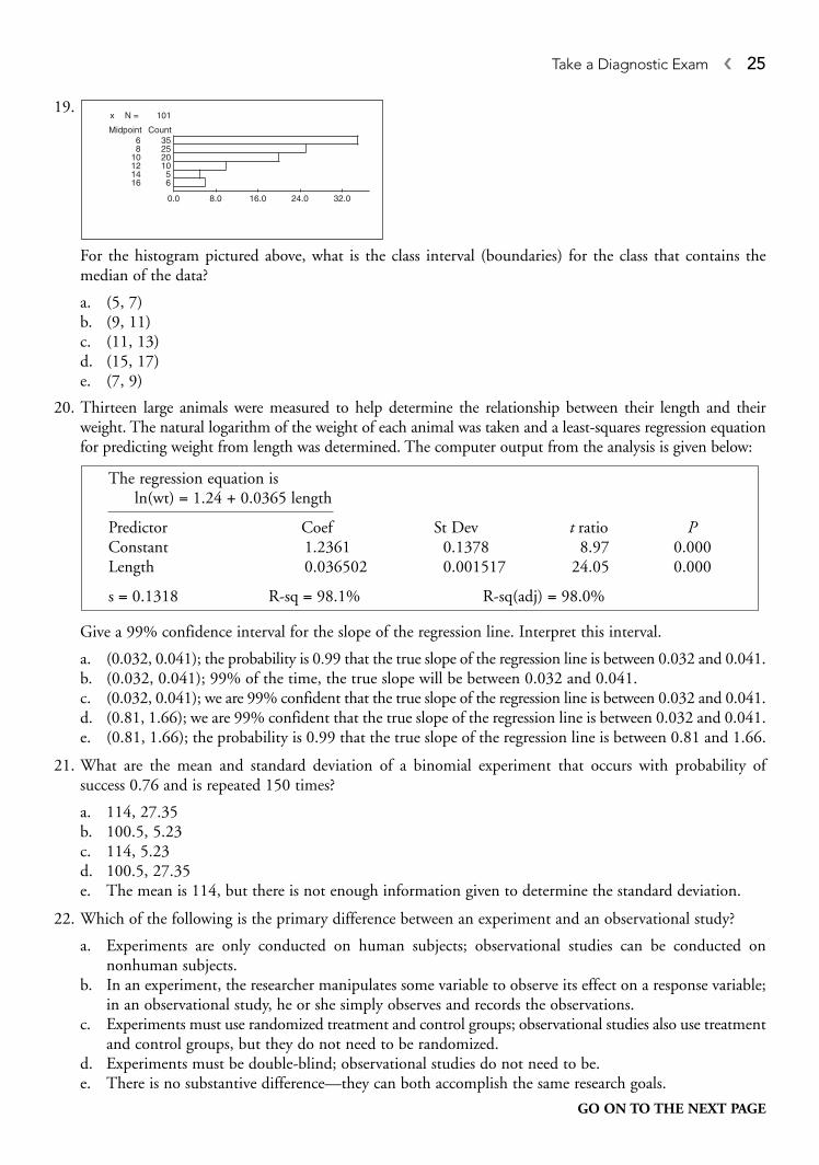
19.
For the histogram pictured above, what is the class interval (boundaries) for the class that contains themedian of the data?
a. (5, 7)b. (9, 11)c. (11, 13)d. (15, 17)e. (7, 9)
20. Thirteen large animals were measured to help determine the relationship between their length and theirweight. The natural logarithm of the weight of each animal was taken and a least-squares regression equationfor predicting weight from length was determined. The computer output from the analysis is given below:
Give a 99% confidence interval for the slope of the regression line. Interpret this interval.
a. (0.032, 0.041); the probability is 0.99 that the true slope of the regression line is between 0.032 and 0.041.b. (0.032, 0.041); 99% of the time, the true slope will be between 0.032 and 0.041.c. (0.032, 0.041); we are 99% confident that the true slope of the regression line is between 0.032 and 0.041.d. (0.81, 1.66); we are 99% confident that the true slope of the regression line is between 0.032 and 0.041.e. (0.81, 1.66); the probability is 0.99 that the true slope of the regression line is between 0.81 and 1.66.
21. What are the mean and standard deviation of a binomial experiment that occurs with probability of success 0.76 and is repeated 150 times?
a. 114, 27.35b. 100.5, 5.23c. 114, 5.23d. 100.5, 27.35e. The mean is 114, but there is not enough information given to determine the standard deviation.
22. Which of the following is the primary difference between an experiment and an observational study?
a. Experiments are only conducted on human subjects; observational studies can be conducted on nonhuman subjects.
b. In an experiment, the researcher manipulates some variable to observe its effect on a response variable;in an observational study, he or she simply observes and records the observations.
c. Experiments must use randomized treatment and control groups; observational studies also use treatmentand control groups, but they do not need to be randomized.
d. Experiments must be double-blind; observational studies do not need to be.e. There is no substantive difference—they can both accomplish the same research goals.
The regression equation is ln(wt) = 1.24 + 0.0365 length
Predictor Coef St Dev t ratio PConstant 1.2361 0.1378 8.97 0.000Length 0.036502 0.001517 24.05 0.000
s = 0.1318 R-sq = 98.1% R-sq(adj) = 98.0%
x N = 101
Midpoint Count
0.0 8.0 16.0 24.0 32.0
6 358 25
10 2012 1014 516 6
Take a Diagnostic Exam � 25
GO ON TO THE NEXT PAGE

23. The regression analysis of question 20 indicated that “R-sq = 98.1%.” Which of the following is (are)true?
I. There is a strong positive linear relationship between the explanatory and response variables.II. There is a strong negative linear relationship between the explanatory and response variables.
III. About 98% of the variation in the response variable can be explained by the regression on theexplanatory variable.
a. I and III onlyb. I or II onlyc. I or II (but not both) and IIId. II and III onlye. I, II, and III
24. A hypothesis test is set up so that P (rejecting H0 when H0 is true) = 0.05 and P (failing to reject H0 whenH0 is false) = 0.26. What is the power of the test?
a. 0.26b. 0.05c. 0.95d. 0.21e. 0.74
25. For the following observations collected while doing a chi-square test for independence between the twovariables A and B, find the expected value of the cell marked with “XXXX.”
a. 4.173b. 9.00c. 11.56d. 8.667e. 9.33
26. The following is a probability histogram for a discrete random variable X.
What is μx?
a. 3.5b. 4.0c. 3.7d. 3.3e. 3.0
5432
.4
.3
.2
.1
5 10(XXXX) 11
6 9 12
7 8 13
26 � Step 2. Determine Your Test Readiness
GO ON TO THE NEXT PAGE

27. A psychologist believes that positive rewards for proper behavior is more effective than punishment forbad behavior in promoting good behavior in children. A scale of “proper behavior” is developed. μ1 =the “proper behavior” rating for children receiving positive rewards, and μ2 = the “proper behavior”rating for children receiving punishment. If H0: μ1 − μ2 = 0, which of the following is the proper state-ment of HA?
a. HA: μ1 − μ2 > 0b. HA: μ1 − μ2 < 0c. HA: μ1 − μ2 ≠ 0d. Any of the above is an acceptable alternative to the given null.e. There isn’t enough information given in the problem for us to make a decision.
28. Estrella wants to become a paramedic and takes a screening exam. Scores on the exam have been approximatelynormally distributed over the years it has been given. The exam is normed with a mean of 80 and a standarddeviation of 9. Only those who score in the top 15% on the test are invited back for further evaluation. Estrellareceived a 90 on the test. What was her percentile rank on the test, and did she qualify for further evaluation?
a. 13.35; she didn’t qualify.b. 54.38; she didn’t qualify.c. 86.65; she qualified.d. 84.38; she didn’t qualify.e. 88.69; she qualified.
29. Which of the following statements is (are) true?I. In order to use a χ2 procedure, the expected value for each cell of a one- or two-way table must be at least 5.
II. In order to use χ2 procedures, you must have at least 2 degrees of freedom.III. In a 4 × 2 two-way table, the number of degrees of freedom is 3.
a. I onlyb. I and III onlyc. I and II onlyd. III onlye. I, II, and III
30. When the point (15,2) is included, the slope of regression line ( y = a + bx) is b = −0.54. The correlationis r = −0.82. When the point is removed, the new slope is –1.04 and the new correlation coefficient is−0.95. What name is given to a point whose removal has this kind of effect on statistical calculations?
a. Outlierb. Statistically significant pointc. Point of discontinuityd. Unusual pointe. Influential point
31. A one-sided test of a hypothesis about a population mean, based on a sample of size 14, yields a P-value of 0.075. Using Table B (p. 360), which of the following best describes the range of t values that wouldhave given this P-value?
a. 1.345 < t < 1.761b. 1.356 < t < 1.782c. 1.771 < t < 2.160d. 1.350 < t < 1.771e. 1.761 < t < 2.145
Take a Diagnostic Exam � 27
GO ON TO THE NEXT PAGE

32. Use the following excerpt from a random digits table for assigning six people to treatment and control groups:98110 35679 14520 51198 12116 98181 99120 75540 03412 25631The subjects are labeled: Arnold: 1; Betty: 2; Clive: 3; Doreen: 4; Ernie: 5; Florence: 6. The first three subjects randomly selected will be in the treatment group; the other three in the control group. Assumingyou begin reading the table at the extreme left digit, which three subjects would be in the control group?
a. Arnold, Clive, Ernestb. Arnold, Betty, Florencec. Betty, Clive, Doreend. Clive, Ernest, Florencee. Betty, Doreen, Florence
33. A null hypothesis, H0: μ = μ0 is to be tested against a two-sided hypothesis. A sample is taken, x– is determined and used as the basis for a C-level confidence interval (e.g., C = 0.95) for μ. The researchernotes that μ0 is not in the interval. Another researcher chooses to do a significance test for μ using the samedata. What significance level must the second researcher choose in order to guarantee getting the same con-clusion about H0: μ = μ0 (that is, reject or not reject) as the first researcher?
a. 1 − Cb. Cc. αd. 1 – αe. α = 0.05
34. Which of the following is not required in a binomial setting?
a. Each trial is considered either a success or a failure.b. Each trial is independent.c. The value of the random variable of interest is the number of trials until the first success occurs.d. There is a fixed number of trials.e. Each trial succeeds or fails with the same probability.
35. X and Y are independent random variables with μX = 3.5, μY = 2.7, σX = 0.8, and σY = 0.65. What are μX+Y and σX+Y?
a. μX+Y = 6.2, σX+Y = 1.03b. μX+Y = 6.2, σX+Y = 1.0625c. μX+Y = 3.1, σX+Y = 0.725d. μX+Y = 6.2, σX+Y = 1.45e. μX+Y = 6.2, σX+Y cannot be determined from the information given.
36. A researcher is hoping to find a predictive linear relationship between the explanatory and response variables in her study. Accordingly, as part of her analysis she plans to generate a 95% confidence intervalfor the slope of the regression line for the two variables. The interval is determined to be (0.45, 0.80).Which of the following is (are) true?
I. She has good evidence of a predictive linear relationship between the variables.II. It is likely that there is a non-zero correlation (r) between the two variables.
III. It is likely that the true slope of the regression line is 0.
a. I and II onlyb. I and III onlyc. II and III onlyd. I onlye. II only
28 � Step 2. Determine Your Test Readiness
GO ON TO THE NEXT PAGE

37. In the casino game of roulette, there are 38 slots for a ball to drop into when it is rolled around the rim ofa revolving wheel: 18 red, 18 black, and 2 green. What is the probability that the first time a ball dropsinto the red slot is on the 8th trial (in other words, suppose you are betting on red every time—what is theprobability of losing 7 straight times before you win the first time?)?
a. 0.0278b. 0.0112c. 0.0053d. 0.0101e. 0.0039
38. You are developing a new strain of strawberries (say, Type X) and are interested in its sweetness as comparedto another strain (say, Type Y). You have four plots of land, call them A, B, C, and D, which are roughlyfour squares in one large plot for your study (see the figure below). A river runs alongside of plots C andD. Because you are worried that the river might influence the sweetness of the berries, you randomly planttype X in either A or B (and Y in the other) and randomly plant type X in either C or D (and Y in theother). Which of the following terms best describes this design?
a. A completely randomized designb. A randomized studyc. A randomized observational studyd. A block design, controlling for the strain of strawberrye. A block design, controlling for the effects of the river
39. Grumpy got 38 on the first quiz of the quarter. The class average on the first quiz was 42 with a standarddeviation of 5. Dopey, who was absent when the first quiz was given, got 40 on the second quiz. The classaverage on the second quiz was 45 with a standard deviation of 6.1. Grumpy was absent for the secondquiz. After the second quiz, Dopey told Grumpy that he was doing better in the class because they had eachtaken one quiz, and he had gotten the higher score. Did he really do better? Explain.
a. Yes. zDopey is more negative than zGrumpy.b. Yes. zDopey is less negative than zGrumpy.c. No. zDopey is more negative than zGrumpy.d. Yes. zDopey is more negative than zGrumpy.e. No. zDopey is less negative than zGrumpy.
40. A random sample size of 45 is obtained for the purpose of testing the hypothesis H0: p = 0.80. The sampleproportion is determined to be = 0.75. What is the value of the standard error of for this test?
a. 0.0042b. 0.0596c. 0.0036d. 0.0645e. 0.0055
pp
A
B D
C
Take a Diagnostic Exam � 29
GO ON TO THE NEXT PAGE

SECTION II—PART A, QUESTIONS 1–5Spend about 65 minutes on this part of the exam. Percentage of Section II grade—75.
Directions: Show all of your work. Indicate clearly the methods you use because you will be graded on the cor-rectness of your methods as well as on the accuracy of your results and explanation.
1. The ages (in years) and heights (in cm) of 10 girls, ages 2 through 11, were recorded. Part of the regressionoutput and the residual plot for the data are given below.
a. What is the equation of the least-squares regression line for predicting height from age?b. Interpret the slope of the regression line in the context of the problem.c. Suppose you wanted to predict the height of a girl 5.5 years of age. Would the prediction made by the
regression equation you gave in (a) be too small, too large, or is there not enough information to tell?
2. You want to determine whether a greater proportion of men or women purchase vanilla latte (regular ordecaf ). To collect data, you hire a person to stand inside the local Scorebucks for 2 hours one morning andtally the number of men and women who purchase the vanilla latte as well as the total number of men andwomen customers: 63% of the women and 59% of the men purchase a vanilla latte.
a. Is this an experiment or an observational study? Explain.b. Based on the data collected, you write a short article for the local newspaper claiming that a greater
proportion of women than men prefer vanilla latte as their designer coffee of choice. A student in thelocal high school AP Statistics class writes a letter to the editor criticizing your study. What might thestudent have pointed out?
c. Suppose you wanted to conduct a study less open to criticism. How might you redo the study?
3. Sophia is a nervous basketball player. Over the years she has had a 40% chance of making the first shot shetakes in a game. If she makes her first shot, her confidence goes way up, and the probability of her makingthe second shot she takes rises to 70%. But if she misses her first shot, the probability of her making thesecond shot she takes doesn’t change—it’s still 40%.
a. What is the probability that Sophia makes her second shot?b. If Sophia does make her second shot, what is the probability that she missed her first shot?
−2.5
0.0
RESI1
Age2.0 4.0 6.0 8.0 10.0
x
x
xx x
xxxx x
The regression equation is
Predictor Coef St Dev t ratio PConstant 76.641 1.188 64.52 0.000Age 6.3661 0.1672 38.08 0.000
s = 1.518 R-sq = 99.5% R-sq(adj) = 99.4%
30 � Step 2. Determine Your Test Readiness
GO ON TO THE NEXT PAGE

4. A random sample of 72 seniors taken 3 weeks before the selection of the school Homecoming Queenidentified 60 seniors who planned to vote for Buffy for queen. Unfortunately, Buffy said some rather cattythings about some of her opponents, and it got into the school newspaper. A second random sample of80 seniors taken shortly after the article appeared showed that 56 planned to vote for Buffy. Does thisindicate a serious drop in support for Buffy? Use good statistical reasoning to support your answer.
5. Some researchers believe that education influences IQ. One researcher specifically believes that the moreeducation a person has, the higher, on average, will be his or her IQ. The researcher sets out to investigatethis belief by obtaining eight pairs of identical twins reared apart. He identifies the better educated twin asTwin A and the other twin as Twin B for each pair. The data for the study are given in the table below. Dothe data give good statistical evidence, at the 0.05 level of significance, that the twin with more educationis likely to have the higher IQ? Give good statistical evidence to support your answer.
SECTION II—PART B, QUESTION 6Spend about 25 minutes on this part of the exam. Percentage of Section II grade—25.
Directions: Show all of your work. Indicate clearly the methods you use because you will be graded on the cor-rectness of your methods as well as on the accuracy of your results and explanation.
6. A paint manufacturer claims that the average drying time for its best-selling paint is 2 hours. A randomsample of drying times for 20 randomly selected cans of paint are obtained to test the manufacturers claim.The drying times observed, in minutes, were: 123, 118, 115, 121, 130, 127, 112, 120, 116, 136, 131, 128,139, 110, 133, 122, 133, 119, 135, 109.
a. Obtain a 95% confidence interval for the true mean drying time of the paint.b. Interpret the confidence interval obtained in part (a) in the context of the problem.c. Suppose, instead, a significance test, at the 0.05 level, of the hypothesis H0: μ = 120 was conducted
against the alternative HA: μ ≠120. What is the P-value of the test?d. Are the answers you got in part (a) and part (c) consistent? Explain.e. At the 0.05 level, would your conclusion about the mean drying time have been different if the alter-
native hypothesis had been HA: μ > 120? Explain.
Pair 1 2 3 4 5 6 7 8
Twin A 103 110 90 97 92 107 115 102Twin B 97 103 91 93 92 105 111 103
Take a Diagnostic Exam � 31
END OF DIAGNOSTIC EXAM

32 � Step 2. Determine Your Test Readiness
1. c
2. a
3. e
4. d
5. c
6. a
7. d
8. b
9. a
10. b
11. c
12. c
13. e
14. e
15. b
16. b
17. d
18. a
19. e
20. c
21. c
22. b
23. c
24. e
25. d
26. d
27. a
28. c
29. b
30. e
31. d
32. e
33. a
34. c
35. a
36. a
37. c
38. e
39. c
40. b
SOLUTIONS TO DIAGNOSTIC TEST—SECTION I
1. From Chapter 10The correct answer is (c). If X has B(n, p), then, in general,
P (X = k) = .
In this problem, n = 18, p = 0.4, x = 7 so that
P (X = 7) = .187
0 4 0 67 11⎛
⎝⎜
⎞
⎠⎟( . ) ( . )
nk
p pk n k⎛
⎝⎜⎜
⎞
⎠⎟⎟ − −( ) ( )1
� Answers and Explanations
Answers to Diagnostic Test—Section I

Take a Diagnostic Exam � 33
2. From Chapter 7The correct answer is (a). ln(y) = 3.2 + 0.42(7) = 6.14⇒⇒y = e6.14 = 464.05.
3. From Chapter 11The correct answer is (e). For a 94% z-interval, there will be 6% of the area outside of theinterval. That is, there will be 97% of the area less than the upper critical value of z. Thenearest entry to 0.97 in the table of standard normal probabilities is 0.9699, which corre-sponds to a z-score of 1.88.(Using the TI-83/84, we have invNorm (0.97) = 1.8808.)
4. From Chapter 6The correct answer is (d). If the bar to the far left was not there, this graph would bedescribed as approximately normal. It still has that same basic shape but, because thereis an outlier, the best description is: approximately normal with an outlier.
5. From Chapter 9The correct answer is (c). Let x be the value in question. If there is 0.2 of the area above x,then there is 0.8 of the area to the left of x. This corresponds to a z-score of 0.84 (fromTable A, the nearest entry is 0.7995). Hence,
(Using the TI-83/84, we have invNorm (0.8) = 0.8416.)
6. From Chapter 5The correct answer is (a). Discrete data are countable; continuous data correspond tointervals or measured data. Hence, speed, average temperature, and wingspan are exam-ples of continuous data. The number of outcomes of a binomial experiment and thejersey numbers of a football team are countable and, therefore, discrete.
7. From Chapter 7The correct answer is (d). The slope of the regression line. −0.6442, can be found under“Coef” to the right of “x.” The intercept of the regression line, 22.94, can be found under“Coef” to the right of “Constant.”
8. From Chapter 13The correct answer is (b). The t statistic for H0: β = 0 is given in the printout as −1.18. Weare given that n = 10 ⇒ df = 10 − 2 = 8. From the df = 8 row of Table B (the t DistributionCritical Values table), we see, ignoring the negative sign since it’s a two-sided test,
1.108 < 1.18 < 1.397 ⇒ 2(0.10) < P < 2(0.15),
which is equivalent to 0.20 < P < 0.30. Using the TI-83/84, we have 2 × tcdf(−100, −1.18,8) = 0.272.
9. From Chapter 12The correct answer is (a). The statement is basically a definition of P-value. It is the likelihoodof obtaining by chance as value as extreme or more extreme by chance alone if the null hypoth-esis is true. A very small P-value sheds doubt on the truth of the null hypothesis.
10. From Chapter 14The correct answer is (b). Because the samples of men and women represent differentpopulations, this is a chi-square test of homogeneity of proportions: the proportions ofeach value of the categorical variable (in this case, “pro-choice” or “pro-life”) will be the
z x
xx= =
−→ =0 84
600
15612 6. . .

34 � Step 2. Determine Your Test Readiness
same across the different populations. Had there been only one sample of 50 peopledrawn, 25 of whom happened to be men and 25 of whom happened to be women, thiswould have been a test of independence.
11. From Chapter 8The correct answer is (c). This is a voluntary response survey and is subject to volun-tary response bias. That is, people who feel the most strongly about an issue are thosemost likely to respond. Because most callers would be fans, they would most likelyblame someone besides the team.
12. From Chapter 11The correct answer is (c). The “recipe” we need to use is n ≥ . Since
we have no basis for an estimate for P *, we use P * = 0.5. In this situation the formulareduces to
n ≥ .
Since n must be an integer, choose n = 1537.
13. From Chapter 8The correct answer is (e). A random sample from a population is one in which everymember of the population is equally likely to selected. A simple random sample is onein which every sample of a given size is equally likely to be selected. A sample can be arandom sample without being a simple random sample.
14. From Chapter 6The correct answer is (e). The teachers are interested in showing that the averageteacher salary is low. Because the mean is not resistant, it is pulled in the direction ofthe few higher salaries and, hence, would be higher than the median, which is notaffected by a few extreme values. The teachers would choose the median. The mode,standard deviation, and IQR tell you nothing about the average salary.
15. From Chapter 9The correct answer is (b). P (at least one of them will ask her) = P (A or B) = 0.72.P (they both ask her) = P (A and B) = 0.18.P (Alfred asks her) = P (A) = 0.6.In general, P (A or B) = P (A) + P (B) − P (A and B). Thus, 0.72 = 0.6 + P (B) − 0.18 P (B) = 0.3.
16. From Chapter 12The correct answer is (b).
P-value = P = 1 − 0.8554 = 0.1446.
(Using the TI-83/84, we find normalcdf (1.06,100) = 0.1446.)
17. From Chapter 10The correct answer is (d). Although all three of the statements are true of a samplingdistribution, only III is a statement of the Central Limit Theorem.
z >−
=
⎛
⎝
⎜⎜⎜⎜
⎞
⎠
⎟⎟⎟⎟
0 35 0 30
0 3 0 795
1 06. .
( . )( . ).
⇒
zM* .
( . ).
2
1 96
2 0 0251536 64
2 2⎛
⎝⎜
⎞
⎠⎟ =
⎛
⎝⎜
⎞
⎠⎟ =
zM
P P*
* ( *)⎛
⎝⎜
⎞
⎠⎟ −
2
1

Take a Diagnostic Exam � 35
18. From Chapter 14The correct answer is (a).
(This calculation can be done on the TI-83/84 as follows: let L1 = observed values; let L2 =expected values; let L3 = (L2-L1)2/L2; Then X2 = LIST MATH sum(L3)=3.33.)In a chi-square goodness-of-fit test, the number of degrees of freedom equals one lessthan the number of possible outcomes. In this case, df = n−1 = 4 − 1 = 3.
19. From Chapter 6The correct answer is (e). There are 101 terms, so the median is located at the 56thposition in an ordered list of terms. From the counts given, the median must be in theinterval whose midpoint is 8. Because the intervals are each of width 2, the class inter-val for the interval whose midpoint is 8 must be (7, 9).
20. From Chapter 13The correct answer is (c). df = 13 − 2 = 11 t* = 3.106 (from Table B; if you havea TI-84 with the invT function, t* = invT(0.995,11)). Thus, a 99% confidenceinterval for the slope is:0.0365 ± 3.106(0.0015) = (0.032, 0.041).We are 99% confident that the true slope of the regression line is between 0.032 unitsand 0.041 units.
21. From Chapter 10 The correct answer is (c).
22. From Chapter 8The correct answer is (b). In an experiment, the researcher imposes some sort of treat-ment on the subjects of the study. Both experiments and observational studies can beconducted on human and nonhuman units; there should be randomization to groupsin both to the extent possible; they can both be double blind.
23. From Chapter 7The correct answer is (c). III is basically what is meant when we say R-sq = 98.1%.However, R-sq is the square of the correlation coefficient.
could be either positive or negative, but not both. We can’t telldirection from R 2.
24. From Chapter 11The correct answer is (e). The power of a test if the probability of correctly rejecting H0
when HA is true. You can either fail to reject H0 when it is false (Type II) or reject iswhen it is false (Power). Thus, Power = 1 − P (Type II) = 1 − 0.26 = 0.74.
R R r2 0 99=± =± ⇒.
μ σx x
= = = − =150 0 76 114 150 0 76 1 0 76 5 23( . ) , ( . )( . ) . .
⇒
X 22 2 2 210 8
8
28 24
24
22 24
24
4 8
83 33=
−+
−+
−+
−=
( ) ( ) ( ) ( ). .
# Heads Observed Expected
0 10 (0.125)(64) = 8
1 28 (0.375)(64) = 24
2 22 (0.375)(64) = 24
3 4 (0.125)(64) = 8

36 � Step 2. Determine Your Test Readiness
25. From Chapter 14The correct answer is (d). There are 81 observations total, 27 observations in the secondcolumn, 26 observations in the first row. The expected number in the first row andsecond column equals
26. From Chapter 9The correct answer is (d).
μX = 2(0.3) + 3(0.2) + 4(0.4) + 5(0.1) = 3.3.
27. From Chapter 12The correct answer is (a). The psychologist’s belief implies that, if she’s correct, that μ1 > μ2. Hence, the proper alternative is HA: μ1 − μ2 > 0.
28. From Chapter 6 The correct answer is (c).
= Percentile rank = normal cdf(-100,1.11)86.65.
Because she had to be in the top 15%, she had to be higher than the 85th percentile,so she was invited back.
29. From Chapter 14The correct answer is (b). I is true. Another common standard is that there can beno empty cells, and at least 80% of the expected counts are greater than 5. II is notcorrect because you can have 1 degree of freedom (for example, a 2 × 2 table). III iscorrect because df = (4 − 1) (2 − 1) = 3.
30. From Chapter 7The correct answer is (e). An influential point is a point whose removal will have amarked effect on a statistical calculation. Because the slope changes from −0.54 to−1.04, it is an influential point.
31. From Chapter 12The correct answer is (d). df = 14 − 1 = 13. For a one-sided test and 13 degrees of free-dom, 0.075 lies between tail probability values of 0.05 and 0.10. These correspond, fora one-sided test, to t* values of 1.771 and 1.350. (If you have a TI-84 with the invTfunction, t* = invT(1−0.075,13) = 1.5299.)
32. From Chapter 8The correct answer is (e). Numbers of concern are 1, 2, 3, 4, 5, 6. We ignore the rest.We also ignore repeats. Reading from the left, the first three numbers we encounter forour subjects are 1, 3, and 5. They are in the treatment group, so numbers 2, 4, and 6are in the control group. That’s Betty, Doreen, and Florence. You might be concernedthat the three women were selected and that, somehow, that makes the drawing non-random. However, drawing their three numbers had exactly the same probability ofoccurrence as any other group of three numbers from the six.
33. From Chapter 11The correct answer is (a). If a significance test at level α rejects a null hypothesis (H0:μ = μ0) against a two-sided alternative, then μ0 will not be contained in a C = 1 − αlevel confidence interval constructed using the same value of x– . Thus, α = 1 − C.
z =−
= =>90 80
91 11.
27
8126 8 667
⎛
⎝⎜
⎞
⎠⎟ =( ) . .

34. From Chapter 10The correct answer is (c). The statement in (c) describes the random variable for a geo-metric setting. In a binomial setting, the random variable of interest is the numbercount of successes in the fixed number of trials.
35. From Chapter 9The correct answer is (a).
is correct for any random variables X and Y. However, is correct only if X
and Y are independent.A necessary condition for this to be true is that the variables X and Y are independent.
36. From Chapter 14 The correct answer is (a). Because 0 is not in the interval (0.45, 0.80), it is unlikely thatthe true slope of the regression line is 0 (III is false). This implies a non-zero correla-tion coefficient and the existence of a linear relationship between the two variables.
37. From Chapter 10 The correct answer is (c). This is a geometric setting (independent trials, each succeed-ing or failing with the same probability).
(On the TI-83/84, this is found as geometpdf (18/38,8).)
38. From Chapter 8The correct answer is (e). The choice is made here to treat plots A and B as a block andplots C and D as a block. That way, we are controlling for the possible confoundingeffects of the river. Hence the answer is (c). If you answered (e), be careful of confusingthe treatment variable with the blocking variable.
39. From Chapter 6The correct answer is (c).
They are both below average, but Grumpy’s z score puts him slightly above Dopey.Note that if Grumpy had been 4 points above the mean on the first test and Dopey 5 points above the mean on the second, then Dopey would have done slightly betterthan Grumpy.
40. From Chapter 12The correct answer is (b).
The standard error of for a test of H0: p = p0 is
If you got an answer of 0.0645, it means you used the value of rather than the valueof p0 in the formula for s
p.
p
sp p
Np
( ).=
−0 0
1
p
sp
( . )( . ). .= =
0 8 0 2
450 0596
z zGrumpy Dopey=−
= − =−
= −38 42
50 8
40 45
6 10 82. ,
.. .
P(1st success is on the 8th trial) = 1838 1 18( ) − 338 0 0053
7
( ) = . .
σ X Y+μX Y+
Take a Diagnostic Exam � 37

38 � Step 2. Determine Your Test Readiness
SOLUTIONS TO DIAGNOSTIC TEST—SECTION II, PART A
1. a. Height = 76.641 + 6.3661 (Age)b. For each additional year of age, the height (in cm) is predicted to increase by 6.36 cm.c.
We would expect the residual for 5.5 to be in the same general area as the residuals for4, 5, 6, and 7 (circled on the graph). The residuals in this area are all positive ⇒ actual-predicted > 0 ⇒ actual > predicted. The prediction would probably be too small.
2. a. It is an observational study. The researcher made no attempt to impose a treatment onthe subjects in the study. The hired person simply observed and recorded behavior.
b. � The article made no mention of the sample size. Without that you are unableto judge how much sampling variability there might have been. It’s possiblethat the 63–59 split was attributable to sampling variability.
� The study was done at one Scorebucks, on one morning, for a single 2-hourperiod. The population at that Scorebucks might differ in some significant wayfrom the patrons at other Scorebucks around the city (and there are many, manyof them). It might have been different on a different day or during a differenttime of the day. A single 2-hour period may not have been enough time to collect sufficient data (we don’t know because the sample size wasn’t given) and,again, a 2-hour period in the afternoon might have yielded different results.
c. You would conduct the study at multiple Scorebucks, possibly blocking by locationif you believe that might make a difference (i.e., would a working-class neighbor-hood have different preferences than the ritziest neighborhood?). You would observeat different times of the day and on different days. You would make sure that thetotal sample size was large enough to control for sampling variability (replication).
3. From the information given, we have� P (hit the first and hit the second) = (0.4) (0.7) = 0.28� P (hit the first and miss the second) = (0.4) (0.3) = 0.12� P (miss the first and hit the second) = (0.6) (0.4) = 0.24� P (miss the first and miss the second) = (0.6) (0.6) = 0.36This information can be summarized in the following table:
a. P (hit on second shot) = 0.28 + 0.24 = 0.52b. P (miss on first | hit on second) = (0.24)/(0.52) = 6/13 = 0.46.
Second Shot
Hit Miss
First Shot Hit 0.28 0.12
Miss 0.24 0.36
-2.5
0.0
RESI1
Age2.0 4.0 6.0 8.0 10.0
x
x
xx x
xxxx x

Take a Diagnostic Exam � 39
4. Let p1 be the true proportion who planned to vote for Buffy before her remarks. Let p2
be the true proportion who plan to vote for Buffy after her remarks.
H0:(or: H0: P1 ≤ P2) p1 = p2
HA: p1 > p2
We want to use a 2-proportion z test for this situation. The problem tells us that thesamples are random samples.
Now, 72(0.83), 72(1 − 0.83), 80(0.70), and 80(1 − 0.70) are all greater than 5, so theconditions for the test are present.
Because P is very low, we have evidence against the null. We have reason to believe thatthe level of support for Buffy has declined since her “unfortunate” remarks.
5. The data are paired, so we will use a matched pairs test.Let μd = the true mean difference between Twin A and Twin B for identical twins rearedapart.
H0: μd = 0 (or: H0: μd ≤ 0)
HA: μd > 0
We want to use a one-sample t-test for this situation. We need the difference scores:
A dotplot of the difference scores shows no significant departures from normality:
The conditions needed for the one sample t-test are present.
, df = 8 − 1 = 7 ⇒ 0.02 < P-value < 0.025
(from Table B; on the TI-83/84, tcdf (2.39,100,7)=0.024).
t =−
=2 25 02 66
8
2 39..
.
x sd= 2.25, = 2.66.
.: ...
+---------+---------+---------+---------+−Diff−2.0 0.0 2.0 4.0 6.0
:
Pair 1 2 3 4 5 6 7 8
Twin A 103 110 90 97 92 107 115 102Twin B 97 103 91 93 92 105 111 103d 6 7 −1 4 0 2 4 −1
ˆ . ,. .
( . )( . )
p z=+
+= =
−
+
60 56
72 800 76
0 83 0 70
0 76 0 24172
1880
0 13
0 0691 88
⎛
⎝⎜
⎞
⎠⎟
= = ⇒.
.. -value= 0.03.P
ˆ . , ˆ . .p p1 2
60
720 83
56
800 70= = = =

40 � Step 2. Determine Your Test Readiness
Because P < 0.05, reject H0. We have evidence that, in identical twins reared apart, thebetter educated twin is likely to have the higher IQ score.
6. a. . We are told that the 20 cans of paint have been randomlyselected. It is reasonable to assume that a sample of this size is small relative to thetotal population of such cans. A box-plot of the data shows no significant depar-tures from normality. The conditions necessary to construct a 95% t confidenceinterval are present.
n = 20 ⇒ df = 19 ⇒ t* = 2.093
b. We are 95% confident that the true mean drying time for the paint is between119.6 minutes and 128.1 minutes. Because 120 minutes is in this interval, wewould not consider an average drying time of 120 minutes for the population fromwhich this sample was drawn to be unusual.
c. df = 20 − 1 = 19 ⇒ 0.05 < P-value < 0.10.
(On the TI-83/84, we find P-value = 2 × tcdf (1.90,100,19) = 0.073.)d. We know that if a two-sided α-level significance test rejects (fails to reject) a null
hypothesis, then the hypothesized value of μ will not be (will be) in a C = 1 − αconfidence interval. In this problem, 120 was in the C = 0.95 confidence intervaland a significance test at α = 0.05 failed to reject the null as expected.
e. For the one-sided test, t = 1.90, df = 19 ⇒ 0.025 < P-value < 0.05 (On the TI-83/84, we find P-value = tcdf (1.90,100,19) = 0.036.)
For the two-sided test, we concluded that we did not have evidence to reject the claimof the manufacturer. However, for the one-sided test, we have stronger evidence (P < 0.05) and would conclude that the average drying time is most likely greater than120 minutes.
t =−
=123 85 120
9 0720
1 90.
..
123 85 2 0939 07
20. .
.±
⎛
⎝⎜
⎞
⎠⎟
±= 123.85 2.093(2.03) = (119.60,128.10).
109 117 122.5 132 139
x s= =123 85 9 07. , .

Take a Diagnostic Exam � 41
Interpretation: How Ready Are You?
Scoring Sheet for Diagnostic Test
Section I: Multiple-Choice Questions
Section II: Free-Response Questions
Composite Score
weighted sectionI
score
weighted sectionII
score
co+ =
mmposite score
(round to nearest whole number)
Question1(out of 4) not round
Question(
× =1 875
2
.( )do
oout of 4) o not round
Question(out of 4)
× =
×
1 875
3
.( )d
11 875
4 1 875
.( )
.(
=
× =
d
d
o not round
Question(out of 4) o nnot round
Question(out of 4) o not round
)
.( )
5 1 875× =d
QQuestion(out of 4) do not round
Sumweigh
6 3 125× =
=
.( )
tted sectionII score
(do not round)
[ ( )]
number correct
(out of 40)
number wrong− ×1
4 ×× =1 25.
multiple-1 score
(if less than zero,enter zzero)
weighted sectionI
score(do not round)
=

This page intentionally left blank

Develop Strategies for Success
CHAPTER 4 Tips for Taking the Exam
3STEP

This page intentionally left blank

� 45
Tips for Taking the Exam
IN THIS CHAPTERSummary: Use these question-answering strategies to raise your AP score.
Key Ideas
General Test-Taking Tips� Read through the entire exam.� Be aware of time.� Know the format of the test in advance.� Be neat.� Do as many problems on every topic as you can in preparation for the exam.
Tips for Multiple-Choice Questions� Read each question carefully.� Try to answer the question yourself before you look at the answers.� Guess only if you can eliminate one or more of the answer choices.� Drawing a picture can sometimes help.
Tips for Free-Response Questions� Write clearly and legibly.� Communicate: make your reasoning clear. Use complete sentences.
Don't ramble.� Be sure your answer is in the context of the problem.� Avoid calculator syntax as part of your answer.� Be consistent from one part of your answer to another.� Draw a graph if one is required.� If the question can be answered with one word or number, don't write more.� If a question asks “how,” tell “why” as well.
KEY IDEA
CHAPTER 4

General Test-Taking TipsMuch of being good at test-taking is experience. Your own test-taking history and these tipsshould help you demonstrate what you know (and you know a lot) on the exam. The tipsin this section are of a general nature—they apply to taking tests in general as well as toboth multiple-choice and free-response type questions. If you want more information thanyou possibly have time to process, simply Google “test-taking tips.”
1. Look over the entire exam first, whichever part you are working on. With the exceptionof, maybe, Question #1 in each section, the questions are not presented in order of difficulty. Find and do the easy questions first.
2. Don’t spend too much time on any one question. Remember that you have an average ofslightly more than two minutes each for each multiple-choice question, 12–13 minutesfor Questions 1–5 of the free-response section, and 25–30 minutes for the investigativetask. Some questions are very short and will give you extra time to spend on the moredifficult questions. At the other time extreme, spending 10 minutes on one multiple-choice question (or 30 minutes on one free-response question) is not a good use oftime—you won’t have time to finish.
3. Become familiar with the instructions for the different parts of the exam before the day of theexam. You don’t want to have to waste time figuring out how to process the exam. You’llhave your hands full using the available time figuring out how to do the questions. Lookat the Practice Exams at the end of this book so you understand the nature of the test.
4. Be neat! On the Statistics exam, communication is very important. This means no smudges on the multiple-choice part of the exam and legible responses on the free-response. A machine may score a smudge as incorrect and readers will spend onlyso long trying to decipher your hieroglyphics.
5. Practice working as many exam-like problems as you can in the weeks before the exam. Thiswill help you know which statistical technique to choose on each question. It’s a greatfeeling to see a problem on the exam and know that you can do it quickly and easilybecause it’s just like a problem you’ve practiced on.
6. Make sure your calculator has new batteries. There’s nothing worse than a “Replace batteries now” warning at the start of the exam. Bring a spare calculator if you have orcan borrow one (it’s perfectly legal to have two calculators).
7. Bring a supply of sharpened pencils to the exam. You don’t want to have to waste timewalking to the pencil sharpener during the exam. (The other students will be gratefulfor the quiet, as well.) Also, bring a good-quality eraser to the exam so that any erasuresare neat and complete.
8. Get a good night’s sleep before the exam. You’ll do your best if you are relaxed and confidentin your knowledge. If you don’t know the material by the night before the exam, youaren’t going to learn it in one evening. Relax. Maybe watch an early movie. If you knowyour stuff and aren’t overly tired, you should do fine.
Tips for Multiple-Choice QuestionsThere are whole industries dedicated to teaching you how to take a test. A less expensivealternative for multiple-choice questions, as indicated in Section I, is to Google “test-takingtips,” and check out the multiple-choice questions of some of the listings. In reality, noamount of test-taking strategy will replace knowledge of the subject. If you are on top ofthe subject, you’ll most likely do well even if you haven’t paid $500 for a test-prep course.
46 � Step 3. Develop Strategies for Success

The following tips, when combined with your statistics knowledge, should help you do well.
1. Read the question carefully before beginning. A lot of mistakes get made because studentsdon’t completely understand the question before trying to answer it. The result is thatthey will often answer a different question than they were asked.
2. Try to answer the question before you look at the answers. Looking at the choices andtrying to figure out which one works best is not a good strategy. You run the risk ofbeing led astray by an incorrect answer. Instead, try to answer the question first, as ifthere was just a blank for the answer and no choices.
3. Understand that the incorrect answers (which are called distractors) are designed to appearreasonable. Watch out for words like never and always in answer choices. These frequentlyindicate distractors. Don’t get suckered into choosing an answer just because it soundsgood! The question designers try to make all the logical mistakes you might make andthe answers they come up with become the distractors. For example, suppose you areasked for the median of the five numbers 3, 4, 6, 7, and 15. The correct answer is 6 (themiddle score in the ordered list). But suppose you misread the question and calculatedthe mean instead. You’d get 7 and, be assured, 7 will appear as one of the distractors.
4. Drawing a picture can often help visualize the situation described in the problem.Sometimes, relationships become clearer when a picture is used to display them. Forexample, using Venn diagrams can often help you “see” the nature of a probabilityproblem. Another example would be using a graph or a scatterplot of some given dataas part of doing a regression analysis.
5. Leave an answer blank if you have no clue what the answer is. The “guess penalty” is designedto yield an average score of 0 for guessed questions (that is, if you guessed at every ques-tions, you’d get, on average, 0—you’re a statistics student, figure out how that works!). Onthe other hand, if you can definitely eliminate at least one choice, it is to your advantagein the long run to guess. You don’t have to answer every question to get a top score.
6. Double check that you have (a) answered the question you are working on, especially ifyou’ve left some questions blank (it’s horrible to realize at some point that all of yourresponses are one question off!) and (b) that you have filled in the correct bubble for youranswer. If you need to make changes, make sure you erase completely and neatly.
Tips for Free-Response QuestionsThere are many helpful strategies for maximizing your performance on free-response questions, but actually doing so is a learned skill. Students are often too brief, too sloppy,or too willing to assume the reader will fill in the blanks for them. You have to know thematerial to do well on the free-response, but knowing the material alone is not sufficient—you must also demonstrate to the reader that you know the material. Many of the followingtips will help you do just that.
1. Read all parts of a question first before beginning. There’s been a trend in recent years tohave more and more sub-parts to each question (a, b, c, …). The sub-parts are usuallyrelated and later parts may rely on earlier parts. Students often make the mistake ofanswering, say, part (c) as part of their answer to part (a). Understanding the wholequestion first can help you answer each part correctly.
2. WRITE LEGIBLY!!! I was a table leader for the AP Statistics Exam for seven years andnothing drove me, or other readers, crazier than trying to decipher illegible scribbling.
Tips for Taking the Exam � 47

This may sound silly to you, but you’d be amazed at just how badly some studentswrite! It doesn’t need to look like it was typewritten, but a person with normal eyesightought to be able to read the words you’ve written with minimal effort.
3. Use good English, write complete sentences, and organize your solutions. You must make iteasy for the reader to follow your line of reasoning. This will make the reader happyand it’s in your self-interest to make the reader (very) happy. The reader wants you todo well, but has only a limited amount of time to dedicate to figuring out what youmean. Don’t expect the reader to fill in the blanks for you and make inferences aboutyour intent—it doesn’t work that way. Also, answer questions completely but don’tramble. While some nonsense ramblings may not hurt you as long as the correct answeris there, you will be docked if you say something statistically inaccurate or somethingthat contradicts an otherwise correct answer. Quit while you are ahead. Remember thatthe amount of space provided for a given question does not necessarily mean that youshould fill the space. Answers should be complete but concise. Don’t fill space justbecause it’s there. When you’ve completely answered a question, move on.
4. Answers alone (sometimes called “naked” answers) may receive some credit but usually not much. If the correct answer is “I’m 95% confident that the true proportion of voters who favor legalizing statistics is between 75% and 95%” and your answer is(0.75, 0.95), you simply won’t get full credit. Same thing when units or measurementare required. If the correct answer is 231 feet and you just say 231, you most likely willnot receive full credit.
5. Answers, and this is important, must be in context. A conclusion to an inference problem thatsays, “Reject the null hypothesis” is simply not enough. A conclusion in context would besomething like, “At the 0.05 level of significance, we reject the null hypothesis and conclude that there is good evidence that a majority of people favor legalizing statistics.”
6. Make sure you answer the question you are being asked. Brilliant answers to questions noone asked will receive no credit. (Seriously, this is very common—some students thinkthey will get credit if they show that they know something, even if it’s not what theyshould know at the time.) Won’t work. And don’t make the reader hunt for your finalanswer. Highlight it in some way.
7. Simplify algebraic or numeric expressions for final answers. You may still earn credit for anunsimplified answer but you’ll make the reader work to figure out that your answer isequivalent to what is written in the rubric. That will make the reader unhappy, and, asmentioned earlier, a happy reader is in your best interest.
8. If you write a formula as part of your solution, use numbers from the question. No credit isgiven for simply writing a formula from a textbook (after all, you are given a formulasheet as part of the exam; you won’t get credit for simply copying one of them ontoyour test page). The reader wants to know if you know how to use the formula in thecurrent problem.
9. If you are using your calculator to do a problem, round final answers to two or three decimal places unless specifically directed otherwise. Don’t round off at each step of theproblem as that creates a cumulative rounding error and can affect the accuracy of yourfinal answer. Also, avoid writing calculator syntax as part of your solution. The readersare instructed to ignore things like normalcdf, 1PropZTest, etc. This is called “calculator-speak” and should not appear on your exam
10. Try to answer all parts of every question—you can’t get any credit for a blank answer. Onthe other hand, you can’t snow the readers—your response must be reasonable andresponsive to the question. Never provide two solutions to a question and expect thereader to pick the better one. In fact, readers have been instructed to pick the worse one.Cross out clearly anything you’ve written that you don’t want the reader to look at.
48 � Step 3. Develop Strategies for Success

11. You don’t necessarily need to answer a question in paragraph form. A bulleted list or algebraic demonstration may work well if you are comfortable doing it that way.
12. Understand that Question #6, the investigative task, may contain questions about materialyou’ve never studied. The goal of such a question is to see how well you think statisticallyin a situation for which you have no rote answer. Unlike every other question on thetest, you really don’t need to worry about preparing for this question above normal testpreparation and being sure that you understand as much of the material in the courseas possible.
Specific Statistics Content TipsThe following set of tips are things that are most worth remembering about specific contentissues in statistics. These are things that have been consistent over the years of the reading.This list is not exhaustive! The examples, exercises, and solutions that appear in this book areillustrative of the manner in which you are expected to answer free-response problems, butthis list is just a sampling of some of the most important things you need to remember.
1. When asked to describe a one-variable data set, always discuss shape, center, and spread.2. Understand how skewness can be used to differentiate between the mean and the median.3. Know how transformations of a data set affect summary statistics.4. Be careful when using “normal” as an adjective. Normal refers to a specific distribution,
not the general shape of a graph of a data set. It’s better to use approximately normal,mound-shaped, bell-shaped, etc., instead. You will be docked for saying something like,“The shape of the data set is normal.”
5. Remember that a correlation does not necessarily imply a real association between twovariables (correlation is not causation). Conversely, the absence of a strong correlationdoes not mean there is no relationship (it might not be linear).
6. Be able to use a residual plot to help determine if a linear model for a data set is appropriate. Be able to explain your reasoning.
7. Be able to interpret, in context, the slope and y-intercept of a least-squares regression line.8. Be able to read computer regression output.9. Know the definition of a simple random sample (SRS).
10. Be able to design an experiment using a completely randomized design. Understandthat an experiment that utilizes blocking cannot, by definition, be a completely rando-mized design.
11. Know the difference between the purposes of randomization and blocking.12. Know what blinding and confounding variables are.13. Know how to create a simulation for a probability problem.14. Be clear on the distinction between independent events and mutually exclusive events
(and why mutually exclusive events can’t be independent).15. Be able to find the mean and standard deviation of a discrete random variable.16. Recognize binomial and geometric situations.17. Never forget that hypotheses are always about parameters, never about statistics.18. Any inference procedure involves four steps. Know what they are and that they must
always be there. And never forget that your conclusion in context (Step 4) must belinked to Step 3 in some way.
19. When doing inference problems, remember that you must show that the conditionsnecessary to do the procedure you are doing are present. It is not sufficient to simplydeclare them present.
Tips for Taking the Exam � 49

20. Be clear on the concepts of Type I and Type II errors and the power of a test.21. If you are required to construct a confidence interval, remember that there are three
things you must do to receive full credit: justify that the conditions necessary to construct the interval are present; construct the interval; and interpret the interval incontext. You’ll need to remember this; often, the only instruction you will see is to construct the interval.
22. If you include graphs as part of your solution, be sure that axes are labeled and that scalesare clearly indicated. This is part of communication.
50 � Step 3. Develop Strategies for Success

Review the Knowledge YouNeed to Score High
CHAPTER 5 Overview of Statistics/Basic VocabularyCHAPTER 6 One-Variable Data AnalysisCHAPTER 7 Two-Variable Data AnalysisCHAPTER 8 Design of a Study: Sampling, Surveys,
and ExperimentsCHAPTER 9 Random Variables and Probability
CHAPTER 10 Binomial Distributions, Geometric Distributions, and Sampling Distributions
CHAPTER 11 Confidence Intervals and Introduction to InferenceCHAPTER 12 Inference for Means and ProportionsCHAPTER 13 Inference for RegressionCHAPTER 14 Inference for Categorical Data: Chi-Square
4STEP

This page intentionally left blank

� 53
Overview of Statistics/ Basic Vocabulary
IN THIS CHAPTERSummary: Statistics is the science of data analysis. This involves activities such as thecollection of data, the organization and analysis of data, and drawing inferencesfrom data. Statistical methods and statistical thinking can be thought of as usingcommon sense and statistical tools to analyze and draw conclusions from data.
Statistics has been developing as a field of study since the 16th century.Historical figures, some of whom you may have heard of, such as IsaacNewton, Abraham DeMoivre, Carl Friedrich Gauss, Adolph Quetelet, FlorenceNightingale (yes, Florence Nightingale!), Sir Francis Galton, Karl Pearson,Sir Ronald Fisher, and John Tukey have been major contributors to what weknow today as the science of statistics.
Statistics is one of the most practical subjects studied in school. A mathe-matics teacher may have some trouble justifying the everyday use of algebrafor the average citizen, but no statistics teacher ever has that problem. We are bombarded constantly with statistical arguments in the media and,through real-life examples, we can develop the skills to become intelligentconsumers of numerical-based knowledge claims.
Key Ideas
� The Meaning of Statistics� Quantitative versus Qualitative Data� Descriptive versus Inferential Statistics� Collecting Data� Experiments versus Observational Studies� Random Variables
KEY IDEA
CHAPTER 5

Quantitative Versus Qualitative DataQuantitative data, or numerical data are data measured or identified on a numerical scale.Qualitative data or categorical data are data that can be classified into a group.
Examples of Quantitative (Numerical) Data: The heights of students in an AP Statistics class; the number of freckles on the face of a redhead; the averagespeed on a busy expressway; the scores on a final exam; the concentration ofDDT in a creek; the daily temperatures in Death Valley; the number of peoplejailed for marijuana possession each year
Examples of Qualitative (Categorical) Data: Gender; political party preference;eye color; ethnicity; level of education; socioeconomic level; birth order of aperson (first-born, second-born, etc.)
There are times that the distinction between quantitative and qualitative data is somewhatless clear than in the examples above. For example, we could view the variable “family size” asa categorical variable if we were labeling a person based on the size of his or her family. Thatis, a woman would go in category “TWO” if she was married but there were no children.Another woman would be in category “FOUR” if she was married and had two children. Onthe other hand, “family size” would be a quantitative variable if we were observing families and recording the number of people in each family (2, 4, . . .). In situations like this,the context will make it clear whether we are dealing with quantitative or a qualitative data.
Discrete and Continuous DataQuantitative data can be either discrete or continuous. Discrete data are data that can belisted or placed in order. Usually, but not always, there is a finite quantity of discrete data(e.g., a list of the possible outcomes of an activity such as rolling a die). However, discrete
data can be “countably” infinite. For example, suppose p(x) = 5 , where n = 1, 2, 3,. . .
Then the first outcome corresponds to n = 1, the second to n = 2, etc. There is an infinitenumber of outcomes, but they are countable (you can identify the first term, the second,etc., but there is no last term). Continuous data can be measured, or take on values in aninterval. The number of heads we get on 20 flips of a coin is discrete; the time of day is continuous. We will see more about discrete and continuous data later on.
Descriptive Versus Inferential StatisticsStatistics has two primary functions: to describe data and to make inferences from data.Descriptive statistics is often referred to as exploratory data analysis (EDA). The com-ponents of EDA are analytical and graphical. When we have collected some one-variabledata, we can examine these data in a variety of ways: look at measures of center for the dis-tribution (such as the mean and median); look at measures of spread (variance, standarddeviation, range, interquartile range); graph the data to identify features such as shape andwhether or not there are clusters or gaps (using dotplots, boxplots, histograms, and stemplots).
With two-variable data, we look for relationships between variables and ask questions like:“Are these variables related to each other and, if so, what is the nature of that relationship?”Here we consider such analytical ideas as correlation and regression, and graphical techniquessuch as scatterplots. Chapters 6 and 7 of this book are primarily concerned with exploratorydata analysis.
1
2
1⎛
⎝⎜
⎞
⎠⎟
−n
54 � Step 4. Review the Knowledge You Need to Score High

Procedures for collecting data are discussed in Chapter 8. Chapters 9 and 10 are concerned with the probabilistic underpinnings of inference.
Inferential statistics involves using data from samples to make inferences about the population from which the sample was drawn. If we are interested in the average height ofstudents at a local community college, we could select a random sample of the students andmeasure their heights. Then we could use the average height of the students in our sampleto estimate the true average height of the population from which the sample was drawn. In the real world we often are interested in some characteristic of a population (e.g., whatpercentage of the voting public favors the outlawing of handguns?), but it is often too difficult or too expensive to do a census of the entire population. The common techniqueis to select a random sample from the population and, based on an analysis of the data, makeinferences about the population from which the sample was drawn. Chapters 11–14 of thisbook are primarily concerned with inferential statistics.
Parameters versus StatisticsValues that describe a sample are called statistics, and values that describe a population arecalled parameters. In inferential statistics, we use statistics to estimate parameters. For example, ifwe draw a sample of 35 students from a large university and compute their mean GPA (thatis, the grade point average, usually on a 4-point scale, for each student), we have a statistic. If wecould compute the mean GPA for all students in the university, we would have a parameter.
Collecting Data: Surveys, Experiments, Observational Studies
In the preceding section, we discussed data analysis and inferential statistics. A question notconsidered in many introductory statistics courses (but considered in detail in AP Statistics)is how the data are collected. Often times we are interested in collecting data in order tomake generalizations about a population. One way to do this is to conduct a survey. In awell-designed survey, you take a random sample of the population of interest, compute statistics of interest (like the proportion of baseball fans in the sample who think Pete Roseshould be in the Hall of Fame), and use those to make predictions about the population.
We are often more interested in seeing the reactions of persons or things to certain stimuli. If so, we are likely to conduct an experiment or an observational study. We dis-cuss the differences between these two types of studies in Chapter 8, but both basicallyinvolve collecting comparative data on groups (called treatment and control) constructedin such a way that the only difference between the groups (we hope) is the focus of thestudy. Because experiments and observational studies are usually done on volunteers, ratherthan on random samples from some population of interest (it’s been said that most exper-iments are done on graduate students in psychology), the results of such studies may lackgeneralizability to larger populations. Our ability to generalize involves the degree to whichwe are convinced that the only difference between our groups is the variable we are studying(otherwise some other variable could be producing the responses).
It is extremely important to understand that data must be gathered correctly in order tohave analysis and inference be meaningful. You can do all the number crunching you wantwith bad data, but the results will be meaningless.
In 1936, the magazine The Literary Digest did a survey of some 10 million peoplein an effort to predict the winner of the presidential election that year. They predicted thatAlf Landon would defeat Franklin Roosevelt by a landslide, but the election turned out
Overview of Statistics/Basic Vocabulary � 55

just the opposite. The Digest had correctly predicted the outcome of the preceding fivepresidential elections using similar procedures, so this was definitely unexpected. Its problem was not in the size of the sample it based its conclusions on. Its problem was inthe way it collected its data—the Digest simply failed to gather a random sample of the pop-ulation. It turns out that its sampling frame (the population from which it drew its sample)was composed of a majority of Republicans. The data were extensive (some 2.4 million bal-lots were returned), but they weren’t representative of the voting population. In part becauseof the fallout from this fiasco, the Digest went bankrupt and out of business the followingyear. If you are wondering why the Digest was wrong this time with essentially the sametechniques used in earlier years, understand that 1936 was the heart of the Depression. Inearlier years the lists used to select the sample may have been more reflective of the votingpublic, but in 1936 only the well-to-do, Republicans generally, were in the Digest’s sampletaken from its own subscriber lists, telephone books, etc.
We look more carefully at sources of bias in data collection in Chapter 8, but the pointyou need to remember as you progress through the next couple of chapters is that conclu-sions based on data are only meaningful to the extent that the data are representative of thepopulation being studied.
In an experiment or an observational study, the analogous issue to a biased sample in asurvey is the danger of treatment and control groups being somehow systematically different.For example, suppose we wish to study the effects of exercise on stress reduction. We let 100 volunteers for the study decide if they want to be in the group that exercises or in thegroup that doesn’t. There are many reasons why one group might be systematically differentfrom the other, but the point is that any comparisons between these two groups is confounded by the fact that the two groups could be different in substantive ways.
Random VariablesWe consider random variables in detail in Chapter 9, but it is important at the beginningto understand the role they play in statistics. A random variable can be thought of as a numerical outcome of a random phenomenon or an experiment. As an example of a discrete random variable, we can toss three fair coins, and let X be the count of heads; wethen note that X can take on the values 0, 1, 2, or 3. An example of a continuous randomvariable might be the number of centimeters a child grows from age 5 to age 6.
An understanding of random variables is what will allow us to use our knowledge ofprobability (Chapter 9) in statistical inference. Random variables give rise to probabilitydistributions (a way of matching outcomes with their probabilities of success), which in turn give rise to our ability to make probabilistic statements about samplingdistributions (distributions of sample statistics such as means and proportions). This language, in turn, allows us to talk about the probability of a given sample being as different from expected as it is. This is the basis for inference. All of this will be examinedin detail later in this book, but it’s important to remember that random variables are thefoundation for inferential statistics.
There are a number of definitions in this chapter and many more throughout the book (summarized in the Glossary). Although you may not be asked specific definitions onthe AP Exam, you are expected to have the working vocabulary needed to understand any statistical situation you might be presented with. In other words, you need to know and understand the vocabulary presented in the course in order to do your best on the AP Exam.
56 � Step 4. Review the Knowledge You Need to Score High
TIP

� Rapid Review1. True or False: A study is done in which the data collected are the number of cars a
person has owned in his or her lifetime. This is an example of qualitative data.
Answer: False. The data are measured on a numerical, not categorical, scale.
2. True or False: The data in the study of question number 1 are discrete.
Answer: True. The data are countable (e.g., Leroy has owned 8 cars).
3. What are the names given to values that describe samples and values that describe populations ?
Answer: Values that describe samples are called statistics, and values that describe populations are called parameters. (A mnemonic for remembering this is that both statistic and sample begin with “s,” and both p- arameter and p- opulation begin with “p.”)
4. What is a random variable ?
Answer: A numerical outcome of an experiment or random phenomenon.
5. Why do we need to sample ?
Answer: Because it is usually too difficult or too expensive to observe every member ofthe population. Our purpose is to make inferences about the unknown, and probablyunknowable, parameters of a population.
6. Why do we need to take care with data collection?
Answer: In order to avoid bias. It makes no sense to try to predict the outcome of thepresidential election if we survey only Republicans.
7. Which of the following are examples of qualitative data?
(a) The airline on which a person chooses to book a flight(b) The average number of women in chapters of the Gamma Goo sorority(c) The race (African American, Asian, Hispanic, Pacific Islander, White) of survey
respondents(d) The closing Dow Jones average on 50 consecutive market days(e) The number of people earning each possible grade on a statistics test(f ) The scores on a given examination
Answer: a, c, and e are qualitative. f could be either depending on how the data are reported: qualitative if letter grades were given, quantitative if number scores weregiven.
Overview of Statistics/Basic Vocabulary � 57

8. Which of the following are discrete and which are continuous?
(a) The number of jelly beans in a jar(b) The ages of a group of students(c) The humidity in Atlanta(d) The number of ways to select a committee of three from a group of ten(e) The number of people who watched the Super Bowl in 2002(f ) The lengths of fish caught on a sport fishing trip
Answer: Discrete: a, d, eContinuous: b, c, f
Note that (b) could be considered discrete if by age we mean the integer part of theage—a person is considered to be 17, for example, regardless of where that person isafter his/her 17th birthday and before his/her 18th birthday.
9. Which of the following are statistics and which are parameters?
(a) The proportion of all voters who will vote Democrat in the next election(b) The proportion of voters in a Gallup Poll who say they will vote Democrat in the
next election(c) The mean score of the home team in all NFL games in 1999(d) The proportion of Asian students attending high school in the state of California(e) The mean difference score between a randomly selected class taught statistics by a
new method and another class taught by an old method(f ) The speed of a car
Answer: Statistics: b, e, fParameters: a, c, d
58 � Step 4. Review the Knowledge You Need to Score High

� 59
One-Variable Data AnalysisIN THIS CHAPTERSummary: We begin our study of statistics by considering distributions of datacollected on a single variable. This will have both graphical and analyticalcomponents and is often referred to as exploratory data analysis (EDA).“Seeing” the data can often help us understand it and, to that end, we willlook at a variety of graphs that display the data. Following that, we will consider a range of numerical measures for center and spread that helpdescribe the dataset. When we are finished, we will be able to describe adataset in terms of its shape, its center, and its spread (or: variability). We will consider both ways to describe the whole dataset and ways todescribe individual terms within the dataset. A very important one-variabledistribution, the normal distribution, will be considered in some detail.
Key Ideas
� Shape of a Distribution� Dotplot� Stemplot� Histogram� Measures of Center� Measures of Spread� Five-Number Summary� Boxplot� z-Score� Density Curve� Normal Distribution� The Empirical Rule� Chebyshev’s Rule
KEY IDEA
CHAPTER 6

If you are given an instruction to “describe” a set of data, be sure you discuss the shape ofthe data (including gaps and clusters in the data), the center of the data (mean, median,mode), and the spread of the data (range, interquartile range, standard deviation).
Graphical AnalysisOur purpose in drawing a graph of data is to get a visual sense of it. We are interested inthe shape of the data as well as gaps in the data, clusters of datapoints, and outliers (whichare datapoints that lie well outside of the general pattern of the data).
ShapeWhen we describe shape, what we are primarily interested in is the extent to which the graphappears to be symmetric (has symmetry around some axis), mound-shaped (bell-shaped),skewed (data are skewed to the left if the tail is to the left; to the right if the tail is to theright), bimodal (has more than one location with many scores), or uniform (frequenciesof the various values are more-or-less constant).
This graph could be described as symmetric and mound-shaped (or bell-shaped). Note that it doesn’t have to beperfectly symmetrical to be classified as symmetric.
This graph is of a uniform distribution. Again, note thatit does not have to be perfectly uniform to be describedas uniform.
This distribution is skewed left because the tail is to theleft. If the tail were to the right, the graph would bedescribed at skewed right.
There are four types of graph we want to look at in order to help us understand theshape of a distribution: dotplot, stemplot, histogram, and boxplot. We use the following 31 scores from a 50-point quiz given to a community college statistics class to illustrate thefirst three plots (we will look at a boxplot in a few pages):
28 38 42 33 29 28 41 40 15 36 27 34 22
23 28 50 42 46 28 27 43 29 50 29 32 34
27 26 27 41 18
60 � Step 4. Review the Knowledge You Need to Score High
TIP

DotplotA dotplot is a very simple type of graph that involves plotting the data values, with dots,above the corresponding values on a number line. A dotplot of the scores on the statisticsquiz, drawn by a statistics computer package, looks like this:
[Calculator note: Most calculators do not have a built-in function for drawing dotplots.There are work-arounds that will allow you to draw a boxplot on a calculator, but theyinvolve more effort than they worth.]
Stemplot (Stem and Leaf Plot)A stemplot is a bit more complicated than a dotplot. Each data value has a stem and a leaf.There are no mathematical rules for what constitutes the stem and what constitutes the leaf.Rather, the nature of the data will suggest reasonable choices for the stem and leaves. Withthe given score data, we might choose the first digit to be the stem and the second digit tobe the leaf. So, the number 42 in a stem and leaf plot would show up as 4 | 2. All the leavesfor a common stem are often on the same line. Often, these are listed in increasing order,so the line with stem 4 could be written as: 4 | 0112236. The complete stemplot of the quizdata looks like this:
1 58 3 | 5 means 352 236777788889993 2344684 01122365 00
Using the 10’s digit for the stem and the units digit for the leaf made good sense withthis data set; other choices make sense depending on the type of data. For example, sup-pose we had a set of gas mileage tests on a particular car (e.g., 28.3, 27.5, 28.1, . . .). In thiscase, it might make sense to make the stems the integer part of the number and the leaf thedecimal part. As another example, consider measurements on a microscopic computer part(0.0018, 0.0023, 0.0021, . . .). Here you’d probably want to ignore the 0.00 (since that doesn’t help distinguish between the values) and use the first nonzero digit as the stem andthe second nonzero digit as the leaf.
Some data lend themselves to breaking the stem into two or more parts. For these data,the stem “4” could be shown with leaves broken up 0–4 and 5–9. Done this way, the stem-plot for the scores data would look like this (there is a single “1” because there are no leaveswith the values 0–4 for a stem of 1; similarly, there is only one “5” since there are no valuesin the 55–59 range.):
1 582 232 6777788889993 23443 684 0112234 65 00
: .:::
::: :: ......... ...
+---------+---------+---------+---------+-Scores10 20 30 40 50
One-Variable Data Analysis � 61

The visual image are of data that are slightly skewed to the right (that is, toward thehigher scores). We do notice a cluster of scores in the high 20s that was not obvious whenwe used an increment of 10 rather than 5. There is no hard and fast rule about how to breakup the stems—it’s easy to try different arrangements on most computer packages.
Sometimes plotting more than one stemplot, side-by-side or back-to-back, can provideus with comparative information. The following stemplot shows the results of two quizzesgiven for this class (one of them the one discussed above):
Stem-and-leaf of Scores 1 Stem-and-leaf of Scores 2
1 33 1 582 0567799 2 236777788889993 1125 3 2344684 0235778889999 4 01122365 00000 5 00
Or, as a back-to-back stemplot:
Quiz 1 Quiz 2
33 1 589977650 2 3677778888999
5211 3 234468999888775320 4 0112236
00000 5 00
It can be seen from this comparison that the scores on Quiz #1 (on the left) were generally higher than for those on Quiz #2—there are a lot more scores at the upper end.Although both distributions are reasonably symmetric, the one on the left is skewed some-what toward the smaller scores, and the one on the right is skewed somewhat toward thelarger numbers.
[Note: Most calculators do not have a built-in function for drawing stemplots. However,most computer programs do have this ability and it’s quite easy to experiment with variousstem increments.]
HistogramA bar graph is used to illustrate qualitative data, and a histogram is used to illustrate quantitative data. The horizontal axis in a bar graph contains the categories, and the verti-cal axis contains the frequencies, or relative frequencies, of each category. The horizontalaxis in a histogram contains numerical values, and the vertical axis contains the frequencies,or relative frequencies, of the values (often intervals of values).
example: Twenty people were asked to state their preferences for candidates in anupcoming election. The candidates were Arnold, Betty, Chuck, Dee, and Edward.Five preferred Arnold, three preferred Betty, six preferred Chuck, two preferredDee, and four preferred Edward. A bar graph of their preferences is shown below:
A B C D E
654321
62 � Step 4. Review the Knowledge You Need to Score High

A histogram is composed of bars of equal width, usually with common edges. When youchoose the intervals, be sure that each of the datapoints fits into a category (it must be clearin which class any given value is). A histogram is much like a stemplot that has been rotated90 degrees.
Consider again the quiz scores we looked at when we discussed dotplots:
28 38 42 33 29 28 41 40 15 36 27 34 2223 28 50 42 46 28 27 43 29 50 29 32 3427 26 27 41 18
Because the data are integral and range from 15 to 50, reasonable intervals might be ofsize 10 or of size 5. The graphs below show what happens with the two choices:
Typically, the interval with midpoint 15 would have class boundaries 12.5 ≤ x <17.5;the interval with midpoint 20 would have class boundaries 17.5 ≤ x <22.5, etc.
There are no hard and fast rules for how wide to make the bars (called “class intervals”).You should use computer or calculator software to help you find a picture to which youreye reacts. In this case, intervals of size 5 give us a better sense of the data. Note that somecomputer programs will label the boundaries of each interval rather than the midpoint.
5045403530252015
8
7
6
5
4
3
2
1
0
Scores
Fre
quen
cy
50403020
15
10
5
0
Scores
Fre
quen
cy
One-Variable Data Analysis � 63

The following is the histogram of the same data (with bar width 5) produced by theTI-83/84 calculator:
Calculator Tip: If you are using your calculator to draw a histogram of data in a list, youmight be tempted to use the ZoomStat command in the ZOOM menu. This commandcauses the calculator to choose a window for your graph. This might be a good idea forother types of graphs, but the TI-83/84 does a poor job getting the window right for ahistogram. The bar width (or bin width) of a histogram is determined by XScl and youshould choose this to fit your data. The graph above has XScl=5 and, therefore, a barwidth of 5. Xmin and Xmax represent the upper and lower boundaries on the screen. In this example, they are set at 12.5 and 53.5, respectively.
example: For the histogram below, identify the boundaries for the class intervals.
solution: The midpoints of the intervals begin at 15 and go by increments of 5.So the boundaries of each interval are 2.5 above and below the midpoints.Hence, the boundaries for the class intervals are 12.5, 17.5, 22.5, 27.5, 32.5,37.5, 42.5, 47.5, and 52.5.
example: For the histogram given in the previous example, what proportion ofthe scores are less than 27.5?
solution: From the graph we see that there is 1 value in the first bar, 2 in thesecond, 6 in the third, etc., for a total of 31 altogether. Of these, 1 + 2 + 6 = 9are less than 27.5. 9/31 = 0.29.
example: The following are the heights of 100 college-age women, followed by a histogram and stemplot of the data. Describe the graph of the data usingeither the histogram, the stemplot, or both.
5045403530252015
8
765
432
10
Scores
Fre
quen
cy
64 � Step 4. Review the Knowledge You Need to Score High

Height
63 65 68 62 63 67 66 64 68 64 65 65 67
66 66 65 65 66 65 66 63 64 70 65 66 62
64 65 67 66 62 66 65 68 61 66 63 67 65
63 67 66 61 66 66 61 67 65 63 69 63 65
62 68 63 59 67 62 70 63 69 66 65 66 67
65 63 67 66 60 66 72 67 67 66 68 64 68
60 61 64 65 64 60 69 63 64 65 66 67 64
63 63 68 67 66 65 60 63 63
This stemplot breaks 5 9
the heights into 6 00001111
increments of 2 inches: 6 22222333333333333333
6 44444444455555555555555555
6 66666666666666666667777777777777
6 8888888999
7 00
7 2
solution: Both the stemplot and the histogram show symmetric, bell-shaped dis-tributions. The graph is symmetric and centered about 66 inches. In the histo-gram, the boundaries of the bars are 59 ≤ x < 61, 61 ≤ x < 63, 63 ≤ x< 65, . . ., 71 ≤ x < 73. Note that, for each interval, the lower bound is con-tained in the interval, while the upper bound is part of the next larger interval.Also note that the stemplot and the histogram convey the same visual image forthe shape of the data.
72706866646260
40
30
20
10
0
Height
Fre
quen
cy
One-Variable Data Analysis � 65

Measures of CenterIn the last example of the previous section, we said that the graph appeared to be centeredabout a height of 66′′. In this section, we talk about ways to describe the center of a distribution. There are two primary measures of center: the mean and the median. Thereis a third measure, the mode, but it tells where the most frequent values occur for inch morethan it describes the center. In some distributions, the mean, median, and mode will beclose in value, but the mode can appear at any point in the distribution.
MeanLet xi represent any value in a set of n values (i = 1, 2, . . ., n). The mean of the set is defined
as the sum of the x’s divided by n. Symbolically, = . Usually, the indices on the
summation symbol in the numerator are left out and the expression is simplified to
means “the sum of x” and is defined as follows: = . Think of itas the “add-’em-up” symbol to help remember what it means. is used for a mean basedon a sample (a statistic). In the event that you have access to an entire distribution (such asin Chapters 9 and 10), its mean is symbolized by the Greek letter m.
(Note: in the previous chapter, we made a distinction between statistics, which are valuesthat describe sample data, and parameters, which are values that describe populations.Unless we are clear that we have access to an entire population, or that we are discussing a distribution, we use the statistics rather than parameters.)
example: During his major league career, Babe Ruth hit the following number ofhome runs (1914–1935): 0, 4, 3, 2, 11, 29, 54, 59, 35, 41, 46, 25, 47, 60, 54,46, 49, 46, 41, 34, 22, 6. What was the mean number of home runs per yearfor his major league career?
Solution:
Calculator Tip: You should use a calculator to do examples like the above—it’s a waste oftime to do it by hand, or even to use a calculator to add up the numbers and divide by n.To use the TI-83/84, press STAT; select EDIT; enter the data in a list, say L1 (you can clearthe list, if needed, by moving the cursor on top of the L1, pressing CLEAR and ENTER).Once the data are in L1, press STAT, select CALC, select 1-Var Stats and press ENTER. 1-Var Stats will appear on the home screen followed by a blinking cursor — the calculator wants to know where your data are. Enter L1 (It’s above the 1; enter 2ND 1 to get it). The calculator will return x and a lot more. Note that, if you fail to enter a listname after 1-Var Stats (that is, you press ENTER at this point), the calculator willassume you mean L1. It’s a good idea to get used to entering the list name where you’veput your data, even if it is L1.
xx
n= =
+ + + + + +
= =
Σ 0 4 3 2 22 6
22714
2232 45
�
.
xx x xn1 2+ + +…x∑x∑
xx
n=
∑.
x
n
ii
n
=
∑1x
66 � Step 4. Review the Knowledge You Need to Score High

MedianThe median of a ordered dataset is the “middle” value in the set. If the dataset has an oddnumber of values, the median is a member of the set and is the middle value. If there are 3 values, the median is the second value. If there are 5, it is the third, etc. If the dataset has aneven number of values, the median is the mean of the two middle numbers. If there are 4 values,the median is the mean of the second and third values. In general, if there are n values
in the ordered dataset, the median is at the position. If you have 28 terms in order,
you will find the median at the position (that is, between the 14th and
15th terms). Be careful not to interpret as the value of the median rather than as the
location of the median.
example: Consider once again the data in the previous example from Babe Ruth’scareer. What was the median number of home runs per year he hit during hismajor league career?
solution: First, put the numbers in order from smallest to largest: 0, 2, 3, 4, 6,11, 22, 25, 29, 34, 35, 41, 41, 46, 46, 46, 47, 49, 54, 54, 59, 60. There are 22 scores, so the median is found at the 11.5th position, between the 11th and12th scores (35 and 41). So the median is
The 1-Var Stats procedure, described in the previous Calculator Tip box, will, if you scrolldown to the second screen of output, give you the median (as part of the entire five-numbersummary of the data: minimum, lower quartile; median, upper quartile; maximum).
ResistantAlthough the mean and median are both measures of center, the choice of which to usedepends on the shape of the distribution. If the distribution is symmetric and moundshaped, the mean and median will be close. However, if the distribution has outliers or isstrongly skewed, the median is probably the better choice to describe the center. This isbecause it is a resistant statistic, one whose numerical value is not dramatically affected byextreme values, while the mean is not resistant.
example: A group of five teachers in a small school have salaries of $32,700, $32,700,$38,500, $41,600, and $44,500. The mean and median salaries for these teachersare $38,160 and $38,500, respectively. Suppose the highest paid teacher gets sick,and the school superintendent volunteers to substitute for her. The superintendent’ssalary is $174,300. If you replace the $44,500 salary with the $174,300 one, themedian doesn’t change at all (it’s still $38,500), but the new mean is $64,120—almosteverybody is below average if, by “average,” you mean mean. It’s sort of like LakeWobegon, where all of the children are expected to be above average.
35 41
238
+= .
n +1
2
28 1
214 5
+= . th
n +1
2
One-Variable Data Analysis � 67

example: For the graph given below, would you expect the mean or median to belarger? Why?
solution: You would expect the median to be larger than the mean. Because thegraph is skewed to the left, and the mean is not resistant, you would expect the mean to be pulled to the left (in fact, the dataset from which this graph wasdrawn from has a mean of 5.4 and a median of 6, as expected, given the skewness).
Measures of SpreadSimply knowing about the center of a distribution doesn’t tell you all you might want toknow about the distribution. One group of 20 people earning $20,000 each will have thesame mean and median as a group of 20 where 10 people earn $10,000 and 10 people earn$30,000. These two sets of 20 numbers differ not in terms of their center but in terms oftheir spread, or variability. Just as there were measures of center based on the mean and themedian, we also have measures of spread based on the mean and the median.
Variance and Standard DeviationOne measure of spread based on the mean is the variance. By definition, the variance is theaverage squared deviation from the mean. That is, it is a measure of spread because the moredistant a value is from the mean, the larger will be the square of the difference between itand the mean.
Symbolically, the variance is defined by
Note that we average by dividing by n − 1 rather than n as you might expect. This isbecause there are only n − 1 independent datapoints, not n, if you know . That is, if youknow n − 1 of the values and you also know , then the nth datapoint is determined.
One problem using the variance as a measure of spread is that the units for the variancewon’t match the units of the original data because each difference is squared. For example, ifyou find the variance of a set of measurements made in inches, the variance will be in squareinches. To correct this, we often take the square root of the variance as our measure of spread.
The square root of the variance is known as the standard deviation. Symbolically,
sn
x xii
n
=−
−−
∑1
12
1
( ) .
xx
sn
x xii
n2 2
1
1
1=
−−
=
∑( ) .
68 � Step 4. Review the Knowledge You Need to Score High

As discussed earlier, it is common to leave off the indices and write:
In practice, you will rarely have to do this calculation by hand because it is one of thevalues returned when you use you calculator to do 1-Var Stats on a list (it’s the Sx nearthe bottom of the first screen).
Calculator Tip: When you use 1-Var Stats, the calculator will, in addition to Sx, return σx, which is the standard deviation of a distribution. Its formal definition is
. Note that this assumes you know μ, the population mean, which
you rarely do in practice unless you are dealing with a probability distribution (seeChapter 9). Most of the time in Statistics, you are dealing with sample data and not a distribution. Thus, with the exception of the type of probability material found inChapters 9 and 10, you should use only s and not σ.
The definition of standard deviation has three useful qualities when it comes to describingthe spread of a distribution:
� It is independent of the mean. Because it depends on how far datapoints are from themean, it doesn’t matter where the mean is.
� It is sensitive to the spread. The greater the spread, the larger will be the standard deviation.For two datasets with the same mean, the one with the larger standard deviation hasmore variability.
� It is independent of n. Because we are averaging squared distances from the mean, thestandard deviation will not get larger just because we add more terms.
example: Find the standard deviation of the following 6 numbers: 3, 4, 6, 6, 7, 10.
solution:
Note that the standard deviation, like the mean, is not resistant to extreme values.Because it depends upon distances from the mean, it should be clear that extreme valueswill have a major impact on the numerical value of the standard deviation. Note also that,in practice, you will never have to do the calculation above by hand—you will rely on your calculator.
Interquartile RangeAlthough the standard deviation works well in situations where the mean works well (reasonably symmetric distributions), we need a measure of spread that works well when a mean-based measure is not appropriate. That measure is called the interquartile range.
Remember that the median of a distribution divides the distribution in two—it is themiddle of the distribution. The medians of the upper and lower halves of the distribution,not including the median itself in either half, are called quartiles. The median of the lowerhalf is called the lower quartile, or the first quartile (which is the 25th percentile—Q1on the calculator). The median of the upper half is called the upper quartile, or the
x s= ⇒ =− + − + − + − + − + −
63 6 4 6 6 6 6 6 7 6 10 62 2 2 2 2( ) ( ) ( ) ( ) ( ) ( )22
6 12 449
−= .
σ = −∑1 2
nx( )μ
sn
x x=−
−1
12Σ( ) .
One-Variable Data Analysis � 69

third quartile (which is in the 75th percentile—Q3 on the calculator). The median itselfcan be thought of as the second quartile or Q2 (although we usually don’t).
The interquartile range (IQR) is the difference between Q3 and Q1. That is, IQR =Q3 – Q1. When you do 1-Var Stats, the calculator will return Q1 and Q3 along witha lot of other stuff. You have to compute the IQR from Q1 and Q3. Note that the IQR comprises the middle 50% of the data.
example: Find Q1, Q3, and the IQR for the following dataset: 5, 5, 6, 7, 8, 9,11, 13, 17.
solution: Because the data are in order, and there is an odd number of values (9),the median is 8. The bottom half of the data comprises 5, 5, 6, 7. The medianof the bottom half is the average of 5 and 6, or 5.5 which is Q1. Similarly, Q3is the medians of the top half, which is the mean of 11 and 13, or 12. The IQR = 12 − 5.5 = 6.5.
example: Find the standard deviation and IQR for the number of home runs hitby Babe Ruth in his major league career. The number of home runs was: 0, 4,3, 2, 11, 29, 54, 59, 35, 41, 46, 25, 47, 60, 54, 46, 49, 46, 41, 34, 22, 6.
solution: We put these numbers into a TI-83/84 list and do 1-Var Stats onthat list. The calculator returns Sx = 20.21, Q1 = 11, and Q3 = 47. Hencethe IQR = Q3 – Q1 = 47 – 11 = 36.
The range of the distribution is the difference between the maximum and minimumscores in the distribution. For the home run data, the range equals 60 − 0 = 60. Althoughthis is sometimes used as a measure of spread, it is not very useful because we are usuallyinterested in how the data spread out from the center of the distribution, not in just howfar it is from the minimum to the maximum values.
OutliersWe have a pretty good intuitive sense of what an outlier is: it’s a value far removed from theothers. There is no rigorous mathematical formula for determining whether or not some-thing is an outlier, but there are a few conventions that people seem to agree on. Not sur-prisingly, some of them are based on the mean and some are based on the median!
A commonly agreed-upon way to think of outliers based on the mean is to considerhow many standard deviations away from the mean a term is. Some texts define an outlieras a datapoint that is more than two or three standard deviations from the mean.
In a mound-shaped, symmetric, distribution, this is a value has only about a 5% chance(for two standard deviations) or a 0.3% chance (for three standard deviations) of being asfar removed from the center of the distribution as it is. Think of it as a value that is way outin one of the tails of the distribution.
Most texts now use a median-based measure and define outliers in terms of how far a datapoint is above or below the quartiles in a distribution. To find if a distribution hasany outliers, do the following (this is known as the “1.5 (IQR) rule”):
� Find the IQR.� Multiply the IQR by 1.5.� Find Q1 − 1.5(IQR) and Q3 + 1.5(IQR).� Any value below Q1 − 1.5(IQR) or above Q3 + 1.5(IQR) is an outlier.
Some texts call an outlier defined as above a mild outlier. An extreme outlier would thenbe one that lies more than 3 IQRs beyond Q1 or Q3.
70 � Step 4. Review the Knowledge You Need to Score High

example: The following data represent the amount of money, in British pounds,spent weekly on tobacco for 11 regions in Britain: 4.03, 3.76, 3.77, 3.34, 3.47,2.92, 3.20, 2.71, 3.53, 4.51, 4.56. Do any of the regions seem to be spending a lot more or less than the other regions? That is, are there any outliers in the data?
solution: Using a calculator, we find , Sx = s = .59, Q1 = 3.2, Q3 = 4.03.
� Using means: 3.62 ± 2(0.59) = (2.44, 4.8). There are no values in the dataset less than2.44 or greater than 4.8, so there are no outliers by this method. We don’t need to check± 3s since there were no outliers using ± 2s.
� (using the 1.5IQR Rule): Q1 − 1.5(IQR) = 3.2 − 1.5(4.03 − 3.2) = 1.96, Q3 + 1.5(IQR)= 4.03 + 1.5(4.03 − 3.2) = 5.28. Because there are no values in the data less than 1.96 or greater than 5.28, there are no outliers by this method either.
Outliers are important because they will often tell us that something unusual or unex-pected is going on with the data that we need to know about. A manufacturing process thatproduces products so far out of spec that they are outliers often indicates that something iswrong with the process. Sometimes outliers are just a natural, but rare, variation. Often,however, an outlier can indicate that the process generating the data is out of control insome fashion.
Position of a Term in a DistributionUp until now, we have concentrated on the nature of a distribution as a whole. We havebeen concerned with the shape, center, and spread of the entire distribution. Now we lookbriefly at individual terms in the distribution.
Five-Number SummaryThere are positions in a dataset that give us valuable information about the dataset. The five-number summary of a dataset is composed of the minimum value, the lower quartile,the median, the upper quartile, and the maximum value.
On the TI-83/84, these are reported on the second screen of data when you do 1-VarStats as: minX, Q1, Med, Q3, and maxX.
example: The following data are standard of living indices for 20 cities: 2.8, 3.9,4.6, 5.3, 10.2, 9.8, 7.7, 13, 2.1, 0.3, 9.8, 5.3, 9.8, 2.7, 3.9, 7.7, 7.6, 10.1, 8.4,8.3. Find the 5-number summary for the data.
solution: Put the 20 values into a list on your calculator and do 1-Var Stats. We find: minX=0.3, Q1=3.9, Med=7.65, Q3=9.8, and maxX=13.
Boxplots (Outliers Revisited)In the first part of this chapter, we discussed three types of graphs: dotplot, stemplot, and histogram. Using the five-number summary, we can add a fourth type of one-variablegraph to this group: the boxplot. A boxplot is simply a graphical version of the five-numbersummary. A box is drawn that contains the middle 50% of the data (from Q1 to Q3) and “whiskers” extend from the lines at the ends of the box (the lower and upper quartiles)to the minimum and maximum values of the data if there are no outliers. If there are outliers, the “whiskers” extend to the last value before the outlier that is not an outlier.
x = 3 62.
One-Variable Data Analysis � 71

The outliers themselves are marked with a special symbol, such as a point, a box, or a plus sign.
The boxplot is sometimes referred to as a box and whisker plot.
example: Consider again the data from the previous example: 2.8, 3.9, 4.6, 5.3,10.2, 9.8, 7.7, 13, 2.1, 0.3, 9.8, 5.3, 9.8, 2.7, 3.9, 7.7, 7.6, 10.1, 8.4, 8.3. A boxplot of this data, done on the TI-83/84, looks like this (the five-numbersummary was [0.3, 3.9, 7.65, 9.8, 13]):
Calculator Tip: To get the graph above on your calculator, go to the STAT PLOTS menu,open one of the plots, say Plot1, and you will see a screen something like this:
Note that there are two boxplots available. The one that is highlighted is the one that willshow outliers. The calculator determines outliers by the 1.5(IQR) rule. Note that the data are in L2 for this example. Once this screen is set up correctly, press GRAPH to displaythe boxplot.
example: Using the same dataset as the previous example, but replacing the 10.2with 20, which would be an outlier in this dataset (the largest possible non-outlierfor these data would be 9.8 + 1.5(9.8 – 3.9) = 18.65), we get the following graphon the calculator:
Note that the “whisker” ends at the largest value in the dataset, 13, which is not an outlier.
0.3 3.9 7.659.8
13 20
+
0.3 3.9 7.65 9.8 13
72 � Step 4. Review the Knowledge You Need to Score High

Percentile Rank of a TermThe percentile rank of a term in a distribution equals the proportion of terms in the distribution less than the term. A term that is at the 75th percentile is larger than 75% ofthe terms in a distribution. If we know the five-number summary for a set of data, then Q1 is at the 25th percentile, the median is at the 50th percentile, and Q3 is at the 75thpercentile. Some texts define the percentile rank of a term to be the proportion of terms lessthan or equal to the term. By this definition, being at the 100th percentile is possible.
z-ScoresOne way to identify the position of a term in a distribution is to note how many standarddeviations the term is above or below the mean. The statistic that does this is the z-score:
The z-score is positive when x is above the mean and negative when it is below the mean.
example: z3 = 1.5 tells us that the value 3 is 1.5 standard deviations above themean. z3 = –2 tells us that the value 3 is two standard deviations below themean.
example: For the first test of the year, Harvey got a 68. The class average (mean)was 73, and the standard deviation was 3. What was Harvey’s z-score on this test?
solution:
Thus, Harvey was 1.67 standard deviations below the mean.
Suppose we have a set of data with mean and standard deviation s. If we subtract from every term in the distribution, it can be shown that the new distribution will have a mean of . If we divide every term by s, then the new distribution will have astandard deviation of s/s = 1. Conclusion: If you compute the z-score for every term in adistribution, the distribution of z scores will have a mean of 0 and a standard deviation of 1.
Calculator Tip: We have used 1-Var Stats a number of times so far. Each of the sta-tistics generated by that command is stored as a variable in the VARS menu. To find, say,
, after having done 1-Var Stats on L1, press VARS and scroll down to STATISTICS.Once you press ENTER to access the STATISTICS menu, you will see several lists. is inthe XY column (as is Sx). Scroll through the other menus to see what they contain. (TheEQ and TEST menus contain saved variables from procedures studied later in the course.)
To demonstrate the truth of the assertion about a distribution of z-scores in the pre-vious paragraph, do 1-Var Stats on, say, data in L1. Then move the cursor to the top ofL2 and enter (L1− )/Sx, getting the and Sx from the VARS menu. This will give youthe z-score for each value in L1. Now do 1-Var Stats L2 to verify that = 0 andSx = 1. (Well, for , you might get something like 5.127273E–14. That’s the calculator’squaint way of saying 5.127 × 10⁻¹⁴, which is 0.00000000000005127. That’s basically 0.)
You need to be aware that only the most recently calculated set of statistics will be displayed in the VARS Statistics menu—it changes each time you perform an opera-tion on a set of data.
xx
xx
xx
x x− = 0
xx
z 68
68 73
31 67=
−= − . .
zx x
sxii=−
.
One-Variable Data Analysis � 73

Normal DistributionWe have been discussing characteristics of distributions (shape, center, spread) and of theindividual terms (percentiles, z-scores) that make up those distributions. Certain distribu-tions have particular interest for us in statistics, in particular those that are known to besymmetric and mound shaped. The following histogram represents the heights of 100 males whose average height is 70′′ and whose standard deviation is 3′′.
This is clearly approximately symmetric and mound shaped. We are going to modelthis with a curve that idealizes what we see in this sample of 100. That is, we will modelthis with a continuous curve that “describes” the shape of the distribution for very largesamples. That curve is the graph of the normal distribution. A normal curve, when super-imposed on the above histogram, looks like this:
The function that yields the normal curve is defined completely in terms of its mean andstandard deviation. Although you are not required to know it, you might be interested toknow that the function that defines the normal curve is:
One consequence of this definition is that the total area under the curve, and above the
x-axis, is 1 (for you calculus students, this is because ).
This fact will be of great use to us later when we consider areas under the normal curveas probabilities.
Empirical RuleThe empirical rule, or the 68-95-99.7 rule, states that approximately 68% of the terms ina normal distribution are within one standard deviation of the mean, 95% are within twostandard deviation of the mean, and 99.7% are within three standard deviations of themean. The following three graphs illustrate the empirical rule.
1
21
12
2
σ π
μσe d x
x−
−⎛⎝⎜
⎞⎠⎟
−∞
∞
∫ =
f x ex
( ) .=− ( )−1
2
12
2
σ π
μσ
70
70
74 � Step 4. Review the Knowledge You Need to Score High

Standard Normal DistributionBecause we are dealing with a theoretical distribution, we will use m and s, rather than and s when referring to the normal curve. If X is a variable that has a normal distributionwith mean m and standard deviation σ (we say “X has N(m,s)”), there is a related distribu-tion we obtain by standardizing the data in the distribution to produce the standardnormal distribution. To do this, we convert the data to a set of z-scores, using the formula
The algebraic effect of this, as we saw earlier, is to produce a distribution of z-scoreswith mean 0 and standard deviation 1. Computing z-scores is just a linear transformationof the original data, which means that the transformed data will have the same shape as theoriginal distribution. In this case then, the distribution of z-scores is normal. We say z hasN(0,1). This simplifies the defining density function to
For the standardized normal curve, the empirical rule says that approximately 68% ofthe terms lie between z = 1 and z = −1, 95% between z = −2 and z = 2, and 99.7% between z = −3 and z = 3. (Trivia for calculus students: one standard deviation fromthe mean is a point of inflection.)
Because many naturally occurring distributions are approximately normal (heights,SAT scores, for example), we are often interested in knowing what proportion of terms liein a given interval under the normal curve. Problems of this sort can be solved either by useof a calculator or a table of Standard Normal Probabilities (Table A in this book). In a typical table, the marginal entries are z-scores, and the table entries are the areas under thecurve to the left of a given z-score. All statistics texts have such tables.
example: What proportion of the area under a normal curve lies to the left of z = −1.37?
solution: There are two ways to do this problem, and you should be able to do iteither way.
The table entry for z is the area tothe left of z and under the curve.
Z
f x e x( ) .= −1
2
12
2
π
zx
=− μσ
.
x
68% within one standarddeviation of the mean
95% within two standarddeviations of the mean
99.7% within three standarddeviations of the mean
One-Variable Data Analysis � 75

(i) The first way is to use the table of Standard Normal Probabilities. To read thetable, move down the left column (titled “z”) until you come to the row whoseentry is −1.3. The third digit, the 0.07 part, is found by reading across the toprow until you come to the column whose entry is 0.07. The entry at the inter-section of the row containing −1.3 and the column containing 0.07 is the areaunder the curve to the left of z = −1.37. That value is 0.0853.
(ii) The second way is to use your calculator. It is the more accurate and moreefficient way. In the DISTR menu, the second entry is normalcdf (see the nextCalculator Tip for a full explanation of the normalpdf and normalcdf functions).The calculator syntax for a standard normal distribution is normalcdf (lowerbound, upper bound). In this example, the lower bound can be any large negative number, say –100.normalcdf(-100,-1.37)= 0.0853435081.
Calculator Tip: Part (ii) of the previous example explained how to use normalcdf forstandard normal probabilities. If you are given a nonstandard normal distribution, the fullsyntax is normalcdf(lower bound, upper bound, mean, standard deviation). Ifonly the first two parameters are given, the calculator assumes a standard normal distri-bution (that is, m = 0 and s = 1). You will note that there is also a normalpdf function,but it really doesn’t do much for you in this course. Normalpdf(X) returns the y-value onthe normal curve. You are almost always interested in the area under the curve and betweentwo points on the number line, so normalcdf is what you will use a lot in this course.
It can be difficult to remember the parameters that go with the various functions onyour calculator—knowing, for example, that for normalcdf, you put lower bound, upperbound, mean, standard deviation in the parentheses. The APP “CtlgHelp” can rememberfor you. It comes on the TI-83/84 and is activated by choosing CtlgHelp from the APPSmenu and pressing ENTER twice.
To use CtlgHelp, move the cursor to the desired function on the DISTR menu andpress +. The function syntax will be displayed. Then press ENTER to use the function onthe home screen. Note that, at this writing, CtlgHelp does not work for invT or gof.
The following is a screen capture of using CtlgHelp that displays the parameters for normalcdf:
example: What proportion of the area under a normal curve lies between z = −1.2 and z = 0.58?
solution: (i) Reading from Table A, the area to the left of z = −1.2 is 0.1151, andthe area to the left of z = 0.58 is 0.7190. The geometry of the situation (seebelow) tells us that the area between the two values is 0.7190 − 0.1151 = 0.6039.
χ 2
76 � Step 4. Review the Knowledge You Need to Score High

example: In an earlier example, we saw that heights of men are approximately nor-mally distributed with a mean of 70 and a standard deviation of 3. What propor-tion of men are more than 6′ (72′′) tall? Be sure to include a sketch of the situation.
solution: (i) Another way to state this is to ask what proportion of terms in anormal distribution with mean 70 and standard deviation 3 are greater than 72.In order to use the table of Standard Normal Probabilities, we must first con-vert to z-scores. The z-score corresponding to a height of 72′′ is
.
The area to the left of z = 0.67 is 0.7486. However, we want the area to the right of 0.67,and that is 1 − 0.7486 = 0.2514.
example: For the population of men in the previous example, how tall must aman be to be in the top 10% of all men in terms of height?
solution: This type of problem has a standard approach. The idea is to express zx intwo different ways (which are, of course, equal since they are different ways ofwriting the z-score for the same point): (i) as a numerical value obtained fromTable A or from your calculator and (ii) in terms of the definition of a z-score.
(i) We are looking for the value of x in thedrawing. Look at Table A to find the nearesttable entry equal to 0.90 (because we knowan area, we need to read the table from theinside out to the margins). It is 0.8997 andcorresponds to a z-score of 1.28.
70
0.90 0.10
x
(ii) Using the calculator, we have normal-cdf(0.67,100) = 0.2514. We could getthe answer from the raw data as follows:normalcdf(72,1000,70,3) = 0.2525,with the difference being due to round-ing. (As explained in the last CalculatorTip, simply add the mean and standarddeviation of a nonstandard normal curveto the list of parameters for normalcdf.)
0.67
0.7486 1–0.7486
z =−
=72 70
30 67.
(ii) Using the calculator, we have normalcdf(-1.2, 0.58) = 0.603973005.
Round to 0.6040 (difference from theanswer in part (i) caused by rounding).
–1.2 .58
One-Variable Data Analysis � 77

So zx = 1.28. But also,
So,
A man would have to be at least 73.84′′ tall to be in the top 10% of all men.
(ii) Using the calculator, the z-score corresponding to an area of 90% to the left ofx is given by invNorm(0.90) = 1.28. Otherwise, the solution is the same as isgiven in part (i). See the following Calculator Tip for a full explanation of theinvNorm function.
Calculator Tip: invNorm essentially reverses normalcdf. That is, rather than readingfrom the margins in, it reads from the table out (as in the example above). invNorm(A)returns the z-score that corresponds to an area equal to A lying to the left of z.invNorm(A, m,s) returns the value of x that has area A to the left of x if x has N(m,s).
Chebyshev’s RuleThe empirical rule works fine as long as the distribution is approximately normal. But whatdo you do if the shape of the distribution is unknown or distinctly nonnormal (as, say, skewed strongly to the right)? Remember that the empirical rule told you that, ina normal distribution, approximately 68% of the data are within one standard deviation ofthe mean, approximately 95% are within two standard deviations, and approximately99.7% are within three standard deviations. Chebyshev’s rule isn’t as strong as the empirical rule, but it does provide information about the percent of terms contained in aninterval about the mean for any distribution.
Let k be a number of standard deviations. Then, according to Chebyshev’s rule, for k > 1,
at least of the data lie within k standard deviations of the mean. For example,
if k = 2.5, then Chebyshev’s rule says that at least = 84% of the data lie with
2.5 standard deviations of the mean. If k = 3, note the difference between the empirical ruleand Chebyshev’s rule. The empirical rule says that approximately 99.7% of the data are within
three standard deviations of . Chebyshev’s says that at least of the data
are within three standard deviations of . This also illustrates what was said in the previousparagraph about the empirical rule being stronger than Chebyshev’s. Note that, if at least
of the data are within k standard deviations of , it follows (algebraically) that
at most lie more than k standard deviations from .
Knowledge of Chebyshev’s rule is not required in the AP Exam, but its use is certainlyOK and is common enough that it will be recognized by AP readers.
x1
2k%
x11
2−
⎛
⎝⎜
⎞
⎠⎟
k%
x
11
389
2−
⎛
⎝⎜
⎞
⎠⎟ ≈% %x
11
2 52−
⎛
⎝⎜
⎞
⎠⎟
.%
11
2−
⎛
⎝⎜
⎞
⎠⎟
k%
zx
xx =−
= ⇒ =70
31 28 73 84. . .
zx
x =− 70
3.
78 � Step 4. Review the Knowledge You Need to Score High

� Rapid Review1. Describe the shape of the histogram below:
Answer: Bi-modal, somewhat skewed to the left.
2. For the graph of problem #1, would you expect the mean to be larger than the medianor the median to be larger than the mean? Why?
Answer: The graph is slightly skewed to the left, so we would expect the mean, whichis not resistant, to be pulled slightly in that direction. Hence, we might expect to havethe median be larger than the mean.
3. The first quartile (Q1) of a dataset is 12 and the third quartile (Q3) is 18. What is thelargest value above Q3 in the dataset that would not be an outlier?
Answer: Outliers lie more than 1.5 IQRs below Q1 or above Q3. Q3 + 1.5(IQR) = 18 +1.5(18 − 12) = 27. Any value greater than 27 would be an outlier. 27 is the largest valuethat would not be an outlier.
4. A distribution of quiz scores has = 35 and s = 4. Sara got 40. What was her z-score?What information does that give you?
Answer:
This means that Sara’s score was 1.25 standard deviations above the mean, which putsit at the 89.4th percentile (normalcdf(-100,1.25)).
5. In a normal distribution with mean 25 and standard deviation 7, what proportions ofterms are less than 20?
Answer :
(By calculator: normalcdf(-100,20,25,7)=0.2375.)
6. What are the mean, median, mode, and standard deviation of a standard normal curve?
Answer: Mean = median = mode = 0. Standard deviation = 1.
7. Find the five-number summary and draw the modified box plot for the following setof data: 12, 13, 13, 14, 16, 17, 20, 28.
Answer: The five-number summary is [12, 13, 15, 18.5, 28]. 28 is an outlier (anythinglarger than 18.5 + 1.5(18.5 – 13) = 26.75 is an outlier by the 1.5(IQR) rule). Since 20 is
z 20
20 25
70 71 0 2389=
−= − ⇒ =. . .Area
z =−
=40 35
41 25. .
x
One-Variable Data Analysis � 79

the largest nonoutlier in the dataset, it is the end of the upper whisker, as shown in the following diagram:
8. A distribution is strongly skewed to the right. Would you prefer to use the mean andstandard deviation, or the median and interquartile range, to describe the center andspread of the distribution?
Answer: Because the mean is not resistant and is pulled toward the tail of the skeweddistribution, you would prefer to use the median and IQR.
9. A distribution is strongly skewed to the left (like a set of scores on an easy quiz) with amean of 48 and a standard deviation of 6. What can you say about the proportion ofscores that are between 40 and 56?
Answer : Since the distribution is skewed to the left, we must use Chebyshev’s rule. Wenote that the interval given is the same distance (8) above and below = 48. Solving
48 + k (6) = 56 gives k = 1.33. Hence, there are at least of theterms between 40 and 56.
Practice ProblemsMultiple Choice
1. The following list is ordered from smallest to largest: 25, 26, 26, 30,y, y, y, 33, 150.Which of the following statements is (are) true?
I. The mean is greater than the medianII. The mode is 26
III. There are no outliers in the dataa. I onlyb. I and II onlyc. III onlyd. I and III onlye. II and III only
2. Jenny is 5′10′′ tall and is worried about her height. The heights of girls in the schoolare approximately normally distributed with a mean of 5′5′′ and a standard deviationof 2.6′′. What is the percentile rank of Jenny’s height?
a. 59b. 65c. 74d. 92e. 97
11
1 3343 5
2−
⎛
⎝⎜
⎞
⎠⎟ =
.% . %
x
Outlier12 13 15 18.5 20 28
80 � Step 4. Review the Knowledge You Need to Score High

3. The mean and standard deviation of a normally distributed dataset are 19 and 4,respectively. 19 is subtracted from every term in the dataset and then the result isdivided by 4. Which of the following best describes the resulting distribution?
a. It has a mean of 0 and a standard deviation of 1.b. It has a mean of 0, a standard deviation of 4, and its shape is normal.c. It has a mean of 1 and a standard deviation of 0.d. It has a mean of 0, a standard deviation of 1, and its shape is normal.e. It has a mean of 0, a standard deviation of 4, and its shape is unknown.
4. The five-number summary for a one-variable dataset is {5, 18, 20, 40, 75}. If you wantedto construct a modified boxplot for the dataset (that is, one that would show outliers ifthere are any), what would be the maximum possible length of the right side “whisker”?
a. 35b. 33c. 5d. 55e. 53
5. A set of 5,000 scores on a college readiness exam are known to be approximately nor-mally distributed with mean 72 and standard deviation 6. To the nearest integer value,how many scores are there between 63 and 75?
a. 0.6247b. 4,115c. 3,650d. 3,123e. 3,227
6. For the data given in #5 above, suppose you were not told that the scores were approx-imately normally distributed. What can be said about the number of scores that areless than 58 (to the nearest integer)?
a. There are at least 919 scores less than 58.b. There are at most 919 scores less than 58.c. There are approximately 919 scores less than 58.d. There are at most 459 scores less than 58.e. There are at least 459 scores less than 58.
7. The following histogram pictures the number of students who visited the CareerCenter each week during the school year.
1
3
Cou
nt
35302520151050
5
7
One-Variable Data Analysis � 81

The shape of this graph could best be described as
a. Mound-shaped and symmetricb. Bi-modalc. Skewed to the leftd. Uniforme. Skewed to the right
8. Which of the following statements is (are) true?I. The median is resistant to extreme values.
II. The mean is resistant to extreme values.III. The standard deviation is resistant to extreme values.
a. I onlyb. II onlyc. III onlyd. II and III onlye. I and III only
9. One of the values in a normal distribution is 43 and its z-score is 1.65. If the mean ofthe distribution is 40, what is the standard deviation of the distribution?a. 3b. –1.82c. –0.55d. 1.82e. –0.55
10. Free-response questions on the AP Statistics Exam are graded on 4, 3, 2, 1, or 0 basis.Question #2 on the exam was of moderate difficulty. The average score on question #2was 2.05 with a standard deviation of 1. To the nearest tenth, what score was achievedby a student who was at the 90th percentile of all students on the test? You may assumethat the scores on the question were approximately normally distributed.a. 3.5b. 3.3c. 2.9d. 3.7e. 3.1
Free Response
1. Mickey Mantle played with the New York Yankees from 1951 through 1968. He hadthe following number of home runs for those years: 13, 23, 21, 27, 37, 52, 34, 42, 31,40, 54, 30, 15, 35, 19, 23, 22, 18. Were any of these years outliers? Explain.
2. Which of the following are properties of the normal distribution? Explain youranswers.
a. It has a mean of 0 and a standard deviation of 1.b. Its mean = median = mode.c. All terms in the distribution lie within four standard deviations of the mean.d. It is bell-shaped.e. The total area under the curve and above the horizontal axis is 1.
82 � Step 4. Review the Knowledge You Need to Score High

3. Make a stemplot for the number of home runs hit by Mickey Mantle during hiscareer (from question #1, the numbers are: 13, 23, 21, 27, 37, 52, 34, 42, 31, 40, 54,30, 15, 35, 19, 23, 22, 18). Do it first using an increment of 10, then do it againusing an increment of 5. What can you see in the second graph that was not obviousin the first?
4. A group of 15 students were identified as needing supplemental help in basic arith-metic skills. Two of the students were put through a pilot program and achievedscores of 84 and 89 on a test of basic skills after the program was finished. The other13 students received scores of 66, 82, 76, 79, 72, 98, 75, 80, 76, 55, 77, 68, and 69.Find the z-scores for the students in the pilot program and comment on the successof the program.
5. For the 15 students whose scores were given in question #4, find the five-numbersummary and construct a boxplot of the data. What are the distinguishing features ofthe graph?
6. Assuming that the batting averages in major league baseball over the years have beenapproximately normally distributed with a mean of 0.265 and a standard deviation of0.032, what would be the percentile rank of a player who bats 0.370 (as Barry Bondsdid in the 2002 season)?
7. In problem #1, we considered the home runs hit by Mickey Mantle during his career.The following is a stemplot of the number of doubles hit by Mantle during his career.What is the interquartile range (IQR) of this data? (Hint: .)
1 0 85 1 1224
(5) 1 567778 2 12344 2 5581 31 3 7
8. For the histogram pictured below, what proportion of the terms are less than 3.5?
54321
9
87
65
43
2
10
C1
Fre
quen
cy
n = 18
One-Variable Data Analysis � 83
Note: The column of numbers to the left of the stemplot gives thecumulative frequencies from each end of the stemplot (e.g., thereare 5 values, reading from the top, when you finish the secondrow). The (5) identifies the location of the row that contains themedian of the distribution. It is standard for computer packagesto draw stemplots in this manner

9. The following graph shows boxplots for the number of career home runs for HankAaron and Barry Bonds. Comment on the graphs. Which player would you ratherhave on your team most seasons? A season in which you needed a lot of home runs?
10. Suppose that being in the top 20% of people with high blood cholesterol level is con-sidered dangerous. Assume that cholesterol levels are approximately normally distrib-uted with mean 185 and standard deviation 25. What is the maximum cholesterollevel you can have and not be in the top 20%?
11. The following are the salaries, in millions of dollars, for members of the 2001–2002Golden State Warriors: 6.2, 5.4, 5.4, 4.9, 4.4, 4.4, 3.4, 3.3, 3.0, 2.4, 2.3, 1.3, .3, .3. Whichgives a better “picture” of these salaries, mean-based or median-based statistics? Explain.
12. The following table gives the results of an experiment in which the ages of 525 pen-nies from current change were recorded. “0” represents the current year, “1” representspennies one year old, etc.
Describe the distribution of ages of pennies (remember that the instruction “describe”means to discuss center, spread, and shape). Justify your answer.
13. A wealthy woman is trying to decide whether or not to buy a coin collection that con-tains 1450 coins. She will buy the collection only if at least 225 of the coins are worthmore than $170. The present owner of the collection reports that the average coin inthe collection is worth $130 with a standard deviation of $15. Should the woman buythe collection?
14. The mean of a set of 150 values is 35, its median is 33, its standard deviation is 6, and itsIQR is 12. A new set is created by first subtracting 10 from every term and then multiply-ing by 5. What are the mean, median, variance, standard deviation, and IQR of the new set?
15. The following graph shows the distribution of the heights of 300 women whose aver-age height is 65′′ and whose standard deviation is 2.5′′. Assume that the heights ofwomen are approximately normally distributed. How many of the women would youexpect to be less than 5′2′′ tall?
Age 0 1 2 3 4 5 6 7 8 9 10 11Count 163 87 52 75 44 24 36 14 11 5 12 2
AARON
BONDS
84 � Step 4. Review the Knowledge You Need to Score High

16. Which of the following are properties of the standard deviation? Expain your answer.
a. It’s the square root of the average squared deviation from the mean.b. It’s resistant to extreme values.c. It’s independent of the number of terms in the distribution.d. If you added 25 to every value in the dataset, the standard deviation wouldn’t change.e. The interval ± 2s contains 50% of the data in the distribution.
17. Look again at the salaries of the Golden State Warriors in question 11 (in millions, 6.2, 5.4, 5.4, 4.9, 4.4, 4.4, 3.4, 3.3, 3.0, 2.4, 2.3, 1.3, .3, .3). Erick Dampier was thehighest paid player at $6.2 million. What sort of raise would he need so that his salarywould be an outlier among these salaries?
18. Given the histogram below, draw, as best you can, the boxplot for the same data.
19. On the first test of the semester, the class average was 72 with a standard deviation of 6.On the second test, the class average was 65 with a standard deviation of 8. Nathanscored 80 on the first test and 76 on the second. Compared to the rest of the class, onwhich test did Nathan do better?
20. What is the mean of a set of data where s = 20, S x = 245, and S (x − )2 = 13 600?
Cumulative Review Problems
1. Which of the following are examples of quantitative data?
a. The number of years each of your teachers has taughtb. Classifying a statistic as quantitative or qualitativec. The length of time spent by the typical teenager watching television in a monthd. The daily amount of money lost by the airlines in the 15 months after the
9/11 attackse. The colors of the rainbow
2. Which of the following are discrete and which are continuous?
a. The weights of a sample of dieters from a weight-loss programb. The SAT scores for students who have taken the test over the past 10 yearsc. The AP Statistics exam scores for the almost 50,000 students who took the exam
in 2002d. The number of square miles in each of the 20 largest statese. The distance between any two points on the number line
x
x
One-Variable Data Analysis � 85

3. Just exactly what is statistics and what are its two main divisions?
4. What are the main differences between the goals of a survey and an experiment?
5. Why do we need to understand the concept of a random variable in order to do infer-ential statistics?
Solutions to Practice ProblemsMultiple Choice
1. The correct answer is (a). I is correct since the mean is pulled in the direction of thelarge maximum value, 150 (well, large compared to the rest of the numbers in the set).II is not correct because the mode is y—there are three ys and only two 26s. III is notcorrect because 150 is an outlier (you can’t actually compute the upper boundary foran outlier since the third quartile is y , but even if you use a larger value, 33, in placeof y, 150 is still an outlier).
2. The correct answer is (e).
→ percentile = 0.9726 (see drawing below):
(On the TI-83/84, normalcdf (−100,1.92) = normalcdf(−1000,70,65,206)=
0.9726 up to rounding error.)
3. The correct answer is (d). The effect on the mean of a dataset of subtracting the samevalue is to reduce the old mean by that amount (that is, mx−k = mx−k). Because the orig-inal mean was 19, and 19 has been subtracted from every term, the new mean is 0.The effect on the standard deviation of a dataset of dividing each term by the samevalue is to divide the standard deviation by that value, that is,
Because the old standard deviation was 4, dividing every term by 4 yields a new stan-dard deviation of 1. Note that the process of subtracting the mean from each term anddividing by the standard deviation creates a set of z-scores
so that any complete set of z-scores has a mean of 0 and a standard deviation of 1. Theshape is normal since any linear transformation of a normal distribution will still be normal.
zx x
sx =−
σσ
xk
x
k= .
z =−
=70 65
2 61 92
..
86 � Step 4. Review the Knowledge You Need to Score High
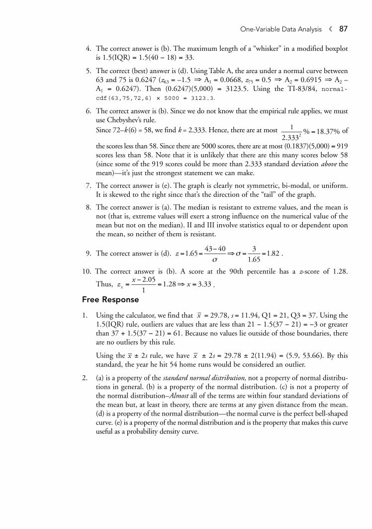
4. The correct answer is (b). The maximum length of a “whisker” in a modified boxplotis 1.5(IQR) = 1.5(40 − 18) = 33.
5. The correct (best) answer is (d). Using Table A, the area under a normal curve between63 and 75 is 0.6247 (z63 = –1.5 A1 = 0.0668, z75 = 0.5 A2 = 0.6915 A2 –A1 = 0.6247). Then (0.6247)(5,000) = 3123.5. Using the TI-83/84, normal-cdf(63,75,72,6) × 5000 = 3123.3.
6. The correct answer is (b). Since we do not know that the empirical rule applies, we mustuse Chebyshev’s rule. Since 72–k (6) = 58, we find k = 2.333. Hence, there are at most of
the scores less than 58. Since there are 5000 scores, there are at most (0.1837)(5,000) = 919scores less than 58. Note that it is unlikely that there are this many scores below 58(since some of the 919 scores could be more than 2.333 standard deviation above themean)—it’s just the strongest statement we can make.
7. The correct answer is (e). The graph is clearly not symmetric, bi-modal, or uniform.It is skewed to the right since that’s the direction of the “tail” of the graph.
8. The correct answer is (a). The median is resistant to extreme values, and the mean isnot (that is, extreme values will exert a strong influence on the numerical value of themean but not on the median). II and III involve statistics equal to or dependent uponthe mean, so neither of them is resistant.
9. The correct answer is (d). .
10. The correct answer is (b). A score at the 90th percentile has a z-score of 1.28.
Thus, .
Free Response
1. Using the calculator, we find that = 29.78, s = 11.94, Q1 = 21, Q3 = 37. Using the1.5(IQR) rule, outliers are values that are less than 21 − 1.5(37 − 21) = −3 or greaterthan 37 + 1.5(37 − 21) = 61. Because no values lie outside of those boundaries, thereare no outliers by this rule.
Using the ± 2s rule, we have ± 2s = 29.78 ± 2(11.94) = (5.9, 53.66). By this standard, the year he hit 54 home runs would be considered an outlier.
2. (a) is a property of the standard normal distribution, not a property of normal distribu-tions in general. (b) is a property of the normal distribution. (c) is not a property ofthe normal distribution–Almost all of the terms are within four standard deviations ofthe mean but, at least in theory, there are terms at any given distance from the mean.(d) is a property of the normal distribution—the normal curve is the perfect bell-shapedcurve. (e) is a property of the normal distribution and is the property that makes this curveuseful as a probability density curve.
xx
x
zx
xx =−
= ⇒ =2 05
11 28 3 33
.. .
z = =−
⇒ = =1 6543 40 3
1 651 82.
..
σσ
1
2 33318 37
2.% . %=
⇒⇒⇒
One-Variable Data Analysis � 87

3. 1 3589 1 32 12337 1 5893 01457 2 12334 02 2 75 24 3 014
3 574 0245 24
What shows up when done by 5 rather than 10 is the gap between 42 and 52. In 16 out of 18 years, Mantle hit 42 or fewer home runs. He hit more than 50 only twice.
4. = 76.4 and s = 10.17.
Using the Standard Normal Probability table, a score of 84 corresponds to the 77.34thpercentile, and a score of 89 corresponds to the 89.25th percentile. Both students werein the top quartile of scores after the program and performed better than all but oneof the other students. We don’t know that there is a cause-and-effect relationshipbetween the pilot program and the high scores (that would require comparisons witha pretest), but it’s reasonable to assume that the program had a positive impact. Youmight wonder how the student who got the 98 did so well!
5.
The most distinguishing feature is that the range (43) is quite large compared to themiddle 50% of the scores (13). That is, we can see from the graph that the scores arepacked somewhat closely about the median. The shape of a histogram of the datawould be symmetric and mound shaped.
6. Area of the left of 3.28 is 0.9995.
That is, Bond’s average in 2002 would have placed him in the 99.95th percentile of batters.
7. There are 18 values in the stemplot. The median is 17 (actually between the last two7s in the row marked by the (5) in the count column of the plot —it’s still 17). Becausethere are 9 values in each half of the stemplot, the median of the lower half of the data,Q1, is the 5th score from the top. So, Q1 = 14. Q3 = the 5th score counting from thebottom = 24. Thus, IQR = 24 − 14 = 10.
⇒z 0 370
0 370 0 265
0 0323 28.
. .
.. .=
−=
55 69 76 82 98
z z84 89
84 76 4
10 170 75
89 76 4
10 171 24=
−= =
−=
.
.. .
.
.. .
x
88 � Step 4. Review the Knowledge You Need to Score High

8. There are 3 values in the first bar, 6 in the second, 2 in the third, 9 in the fourth, and5 in the fifth for a total of 25 values in the dataset. Of these, 3 + 6 + 2 = 11 are lessthan 3.5. There are 25 terms altogether, so the proportion of terms less than 3.5 is11/25 = 0.44.
9. With the exception of the one outlier for Bonds, the most obvious thing about thesetwo is just how similar the two are. The medians of the two are almost identical andthe IQRs are very similar. The data do not show it, but with the exception of 2001,the year Bonds hit 73 home runs, neither batter ever hit 50 or more home runs in aseason. So, for any given season, you should be overjoyed to have either on your team,but there is no good reason to choose one over the other. However, if you based yourdecision on who had the most home runs in a single season, you would certainlychoose Bonds.
10. Let x be the value in question. Because we do not want to be in the top 20%, the areato the left of x is 0.8. Hence zx = 0.84 (found by locating the nearest table entry to 0.8, which is 0.7995 and reading the corresponding z-score as 0.84). Then
[Using the calculator, the solution to this problem is given by invNorm(0.8,185,25).]
11. = $3.36 million, s = $1.88 million, Med = $3.35 million, IQR = $2.6 million. A boxplot of the data looks like this:
The fact that the mean and median are virtually the same, and that the boxplot shows that the data are more or less symmetric, indicates that either set of measureswould be appropriate.
12. The easiest way to do this is to use the calculator. Put the age data in L1 and the fre-quencies in L2. Then do 1-Var Stats L1,L2 (the calculator will read the second listas frequencies for the first list).
� The mean is 2.48 years, and the median is 2 years. This indicates that the mean isbeing pulled to the right—and that the distribution is skewed to the right or hasoutliers in the direction of the larger values.
� The standard deviation is 2.61 years. Because one standard deviation to left wouldyield a negative value, this also indicates that the distribution extends further to theright than the left.
x
zx
xx = =−
⇒ =0 84185
25206. .
One-Variable Data Analysis � 89

� A histogram of the data, drawn on the TI–83/84, is drawn below. This definitelyindicates that the ages of these pennies is skewed to the right.
13. Since we don’t know the shape of the distribution of coin values, we must useChebyshev’s rule to help us solve this problem. Let k = the number of standard devia-tions that 170 is above the mean. Then 130 + k·(15) = 170. So, k ∼∼ 2.67. Thus,
at most , or 14%, of the coins are valued at more than $170. Her
requirement was that , or 15.5%, of the coins must be valued at more
than $170. Since at most 14% can be valued that highly, she should not buy thecollection.
14. The new mean is 5(35 − 10) = 125.The new median is 5(33 − 10) = 115.The new variance is 52(62) = 900.The new standard deviation is 5(6) = 30.The new IQR is 5(12) = 60.
15. First we need to find the proportion of women who would be less than 62′′ tall:
⇒ Area = 0.1151.
So 0.1151 of the terms in the distribution would be less than 62′′. This means that0.1151(300) = 34.53, so you would expect that 34 or 35 of the women would be lessthan 62′′ tall.
16. a, c, and d are properties of the standard deviation. (a) serves as a definition of the stan-dard deviation. It is independent of the number of terms in the distribution in thesense that simply adding more terms will not necessarily increase or decrease s. (d) isanother way of saying that the standard deviation is independent of the mean—it’s a measure of spread, not a measure of center.
The standard deviation is not resistant to extreme values (b) because it is based on themean, not the median. (e) is a statement about the interquartile range. In general,unless we know something about the curve, we don’t know what proportion of termsare within 2 standard deviations of the mean.
17. For these data, Q1 = $2.3 million, Q3 = $4.9 million. To be an outlier, Erick wouldneed to make at least 4.9 + 1.5(4.9 − 2.3) = 8.8 million. In other words, he would needa $2.6 million dollar raise in order to have his salary be an outlier.
z55
62 65
2 51 2=
−= −
..
225
14500 155≈ .
1 1
2 670 14
2 2k≈ ≈
( . ).
90 � Step 4. Review the Knowledge You Need to Score High

18. You need to estimate the median and the quartiles. Note that the histogram is skewedto the left, so that the scores tend to pack to the right. This means that the median isto the right of center and that the boxplot would have a long whisker to the left. Theboxplot looks like this:
19. If you standardize both scores, you can compare them on the same scale. Accordingly,
Nathan did slightly, but only slightly, better on the second test.
20.
Solutions to Cumulative Review Problems
1. a, c, and d are quantitative.
2. a, d, and e are continuous; b and c are discrete. Note that (d) could be considered discrete if what we meant by “number of square miles” was the integer number ofsquare miles.
3. Statistics is the science of data. Its two main divisions are data analysis and inference.Data analysis (EDA) utilizes graphical and analytical methods to try to see what thedata “say.” That is, EDA looks at data in a variety of ways in order to understand them.Inference involves using information from samples to make statements or predictionsabout the population from which the sample was drawn.
4. A survey, based on a sample from some population, is usually given in order to be ableto make statements or predictions about the population. An experiment, on the otherhand, usually has as its goal studying the differential effects of some treatment on twoor more samples, which are often comprised of volunteers.
sx x
n n
nn
xx
n
= =−
−=
−
=−
⇒ =
= =
∑
∑
201
13600
1
2013600
135
2
2
( )
2245
357=
z z80 76
80 72
61 333
76 65
81 375=
−= =
−=. , . .
One-Variable Data Analysis � 91

5. Statistical inference is based on being able to determine the probability of getting a par-ticular sample statistic from a population with a hypothesized parameter. For example,we might ask how likely it is to get 55 heads on 100 flips of a fair coin. If it seemsunlikely, we might reject the notion that the coin we actually flipped is fair. The prob-abilistic underpinnings of inference can be understood through the language ofrandom variables. In other words, we need random variables to bridge the gap betweensimple data analysis and inference.
92 � Step 4. Review the Knowledge You Need to Score High
� 93
Two-Variable Data Analysis
IN THIS CHAPTERSummary: In the previous chapter we used exploratory data analysis to helpus understand what a one-variable dataset was saying to us. In this chapterwe extend those ideas to consider the relationships between two variablesthat might, or might not, be related. In this chapter, and in this course, we areprimarily concerned with variables that have a linear relationship and, for themost part, leave other types of relationships to more advanced courses. Wewill spend some time considering nonlinear relationships which, through somesort of transformation, can be analyzed as though the relationship was linear.Finally, we’ll consider a statistic that tells the proportion of variability in onevariable that can be attributed to the linear relationship with another variable.
Key Ideas
� Scatterplots� Lines of Best Fit� The Correlation Coefficient� Least Squares Regression Line� Coefficient of Determination� Residuals� Outliers and Influential Points� Transformations to Achieve Linearity
ScatterplotsIn the previous chapter, we looked at several different ways to graph one-variable data. Bychoosing from dotplots, stemplots, histograms, or boxplots, we were able to examine visually patterns in the data. In this chapter, we consider techniques of data analysis for
KEY IDEA
CHAPTER 7

two-variable (bivariate) data. Specifically, our interest is whether or not two variables have a linear relationship and how changes in one variable can predict changes in the othervariable.
example: For an AP Statistics class project, a statistics teacher had her studentskeep diaries of how many hours they studied before their midterm exam. Thefollowing are the data for 15 of the students.
The teacher wanted to know if additional studying resulted in higher grades and drew thefollowing graph, called a scatterplot. It seemed pretty obvious to the teacher that additionalhours spent studying generally resulted in higher grades on the exam and, in fact, the pat-tern appears to be roughly linear.
In the previous example, we were interested in seeing whether studying has an effect ontest performance. To do this we drew a scatterplot, which is just a two-dimensional graphof ordered pairs. We put one variable on the horizontal axis and the other on the verticalaxis. In the example, the horizontal axis is for “hours studied” and the vertical axis is for“score on test.” Each point on the graph represents the ordered pair for one student. If wehave an explanatory variable, it should be on the horizontal axis, and the response variableshould be on the vertical axis.
50
75
100
Score
Hours0.0 1.5 3.0 4.5 6.0
x
xxx
xx x x
xx
xx xx
x
STUDENT HOURS STUDIED SCORE ON EXAM
A 0.5 65B 2.5 80C 3.0 77D 1.5 60E 1.25 68F 0.75 70G 4.0 83H 2.25 85I 1.5 70J 6.0 96K 3.25 84L 2.5 84M 0.0 51N 1.75 63O 2.0 71
94 � Step 4. Review the Knowledge You Need to Score High

In the previous example, we observed a situation in which the variable on the verticalaxis tends to increase as the variable on the horizontal axis increases. We say that two vari-ables are positively associated if one of them increases as the other increases and negativelyassociated if one of them decreases as the other increases.
Calculator Tip: In order to draw a scatterplot on your calculator, first enter the data intwo lists, say the horizontal-axis variable in L1 and the vertical-axis variable in L2. Thengo to STAT PLOT and choose the scatterplot icon from Type. Enter L1 for Xlist and L2for Ylist. Choose whichever Mark pleases you. Be sure there are no equations active inthe Y = list. Then do ZOOM ZoomStat (Zoom-9) and the calculator will draw the scat-terplot for you. The calculator seems to do a much better job with scatterplots than it doeswith histograms but, if you wish, you can still go back and adjust the WINDOW in any wayyou want.
The scatterplot of the data in the example, drawn on the calculator, looks like this(the window used was [0, 6.5, 1, 40, 105, 5, 1]):
example: Which of the following statements best describes the scatterplot pictured?
I. A line might fit the data well.II. The variables are positively associated.
III. The variables are negatively associated.a. I onlyb. II onlyc. III onlyd. I and II onlye. I and III only
solution: e is correct. The data look as though a line might be a good model, andthe y-variable decreases as the x-variable increases so that they are negativelyassociated.
CorrelationWe have seen how to graph two-variable data in a scatterplot. Following the pattern we setin the previous chapter, we now want to do some numerical analysis of the data in anattempt to understand the relationship between the variables better.
+
+ ++
+x
y
++ ++
+++
++
++ +
+
y
x
+
Two-Variable Data Analysis � 95

In AP Statistics, we are primarily interested in determining the extent to which two variables are linearly associated. Two variables are linearly related to the extent that their relationship can be modeled by a line. Sometimes, and we will look at this more closely laterin this chapter, variables may not be linearly related but can be transformed in such a way thatthe transformed data are linear. Sometimes the data are related but not linearly (e.g., theheight of a thrown ball, t seconds after it is thrown, is a quadratic function of the number ofseconds elapsed since it was released).
The first statistic we have to determine a linear relationship is the Pearson productmoment correlation, or more simply, the correlation coefficient, denoted by the letter r.The correlation coefficient is a measure of the strength of the linear relationship betweentwo variables as well as an indicator of the direction of the linear relationship (whether thevariables are positively or negatively associated).
If we have a sample of size n of paired data, say (x,y), and assuming that we have computedsummary statistics for x and y (means and standard deviations), the correlation coefficient ris defined as follows:
Because the terms after the summation symbol are nothing more than the z-scores ofthe individual x and y values, an easy way to remember this definition is:
or, easier to remember, .
example: Earlier in the section, we saw some data for hours studied and the corresponding scores on an exam. It can be shown that, for these data, r = 0.864.This indicates a strong positive linear relationship between hours studied andexam score. That is, the more hours studied, the higher the exam score.
The correlation coefficient r has a number of properties you should be familiar with:
� −1 ≤ r ≤ 1. If r = −1 or r = 1, the points all lie on a line.� Although there are no hard and fast rules about how strong a correlation is based on its
numerical value, the following guidelines might help you categorize r:
Remember that these are only very rough guidelines. A value of r = 0.2 might well indi-cate a significant linear relationship (that is, it’s unlikely to have gotten 0.2 unless therereally was a linear relationship), and an r of 0.8 might be reflective of a single influentialpoint rather than an actual linear relationship between the variables.
VALUE OF r STRENGTH OF LINEAR RELATIONSHIP
−1 ≤ r ≤ −0.8 strong
0.8 ≤ r ≤ 1
−0.8 ≤ r ≤ −0.5 moderate
0.5 ≤ r ≤ 0.8
−0.5 ≤ r ≤ 0.5 weak
rn
z zx y=− ∑1
1r
nz zx y
i
n
i i=
−⋅
=∑
1
1 1
rn
x x
s
y y
si
xi
ni
y
=−
−⎛
⎝⎜⎜
⎞
⎠⎟⎟
−⎛
⎝⎜⎜
⎞
⎠⎟⎟
=
∑1
1 1
.
96 � Step 4. Review the Knowledge You Need to Score High

� If r > 0, it indicates that the variables are positively associated. If r < 0, it indicates thatthe variables are negatively associated.
� If r = 0, it indicates that there is no linear association that would allow us to predict yfrom x. It does not mean that there is no relationship—just not a linear one.
� It does not matter which variable you call x and which variable you call y. r will be thesame. In other words, r depends only on the paired points, not the ordered pairs.
� r does not depend on the units of measurement. In the previous example, convert “hoursstudied” to “minutes studied” and r would still equal 0.864.
� r is not resistant to extreme values because it is based on the mean. A single extreme valuecan have a powerful impact on r and may cause us to overinterpret the relationship. Youmust look at the scatterplot of the data as well as r.
example: To illustrate that r is not resistant, consider the following two graphs.The graph on the left, with 12 points, has a marked negative linear associationbetween x and y. The graph on the right has the same basic visual pattern but,as you can see, the addition of the one outlier has a dramatic effect on r—making what is generally a negative association between two variablesappear to have a moderate, positive association.
example: The following computer output, again for the hours studied versus exam score data, indicates R-sq, which is the square of r. Accordingly,
There is a lot of other stuff in the box that doesn’t concernus just yet. We will learn about other important parts of the output as we proceedthrough the rest of this book. Note that we cannot determine the sign of r fromR-sq. We need additional information.
(“R-sq” is called the “coefficient of determination” and has a lot of meaning inits own right in regression. It is difficult to show that R-sq is actually the squareof r. We will consider the coefficient of determination later in this chapter.)
The regression equation isScore = 59.0 + 6.77 Hours
Predictor Coef St Dev t ratio PConstant 59.026 2.863 20.62 .000Hours 6.767 1.092 6.20 .000
s = 6.135 R-sq = 74.7% R-sq(adj) = 72.8%
r = 0 747. = 0.864.
negative associationr = −0.80
positive associationr = 0.51
y
x
y
x
Two-Variable Data Analysis � 97

Calculator Tip: In order to find r on your calculator, you will first need to change a setting from the factory. Enter CATALOG and scroll down to “Diagnostic On.” PressENTER twice. Now you are ready to find r.
Assuming you have entered the x- and y-values in L1 and L2, enter STAT CALC
LinReg(a+bx) [that’s STAT CALC 8 on the TI-83/84] and press ENTER. Then enter L1,L2 and press ENTER. You should get a screen that looks like this (using the data from theStudy Time vs. Score on Test study):
(Note that reversing L1 and L2 in this operation—entering STAT CALC LinReg(a+bx)
L2, L1—will change a and b but will not change r since order doesn’t matter in correlation.)If you compare this with the computer output above, you will see that it contains someof the same data, including both r and r 2. At the moment, all you care about in this print-out is the value of r.
Correlation and CausationTwo variables, x and y, may have a strong correlation, but you need to take care not to inter-pret that as causation. That is, just because two things seems to go together does not meanthat one caused the other—some third variable may be influencing them both. Seeing a firetruck at almost every fire doesn’t mean that fire trucks cause fires.
example: Consider the following dataset that shows the increase in the number ofMethodist ministers and the increase in the amount of imported Cuban rumfrom 1860 to 1940.
NUMBER OF METHODIST NUMBER OF BARRELS OF CUBAN YEAR MINISTERS IN NEW ENGLAND RUM IMPORTED TO BOSTON
1860 63 83761865 48 64061870 53 70051875 64 84861880 72 95951885 80 10,6431890 85 11,2651895 76 10,0711900 80 10,5471905 83 11,0081910 105 13,8851915 140 18,5591920 175 23,0241925 183 24,1851930 192 25,4341935 221 29,2381940 262 34,705
98 � Step 4. Review the Knowledge You Need to Score High

For these data, it turns out that r = .999986.Is the increase in number of ministers responsible for the increase in imported rum? Some
cynics might want to believe so, but the real reason is that the population was increasing from1860 to 1940, so the area needed more ministers, and more people drank more rum.
In this example, there was a lurking variable, increasing population—one we didn’t con-sider when we did the correlation—that caused both of these variables to change the waythey did. We will look more at lurking variables in the next chapter, but in the meantimeremember, always remember, that correlation is not causation.
Lines of Best FitWhen we discussed correlation, we learned that it didn’t matter which variable we called xand which variable we called y—the correlation r is the same. That is, there is no explana-tory and response variable, just two variables that may or may not vary linearly. In this sec-tion we will be more interested in predicting, once we’ve determined the strength of thelinear relationship between the two variables, the value of one variable (the response) basedon the value of the other variable (the explanatory). In this situation, called linear regres-sion, it matters greatly which variable we call x and which one we call y.
Least-Squares Regression LineRecall again the data from the study that looked at hours studied versus score on test:
For these data, r = 0.864, so we have a strong, positive, linear association between the vari-ables. Suppose we wanted to predict the score of a person who studied for 2.75 hours. Ifwe knew we were working with a linear model—a line that seemed to fit the data well—we would feel confident about using the equation of the line to make such a prediction. Weare looking for a line of best fit. We want to find a regression line—a line that can be usedfor predicting response values from explanatory values. In this situation, we would use theregression line to predict the exam score for a person who studied 2.75 hours.
The line we are looking for is called the least-squares regression line. We could drawa variety of lines on our scatterplot trying to determine which has the best fit. Let be the y
HOURS STUDIED SCORE ON EXAM
0.5 652.5 803.0 771.5 601.25 680.75 704.0 832.25 851.5 706.0 963.25 842.5 840.0 511.75 632.0 71
Two-Variable Data Analysis � 99

predicted value of y for a given value of x. Then y − y represents the error in prediction. We want our line to minimize errors in prediction, so we might first think that Σ (y − y ) would be a good measure (y − y is the actual value minus the predicted value).However, because our line is going to average out the errors in some fashion, we find thatΣ (y − y)= 0. To get around this problem, we use Σ (y −y )2. This expression will vary withdifferent lines and is sensitive to the fit of the line. That is, Σ (y − y)2 is small when thelinear fit is good and large when it is not.
The least-squares regression line (LSRL) is the line that minimizes the sum of squarederrors. If y = a + bx is the LSRL, then y minimizes Σ (y − y)2.
100 � Step 4. Review the Knowledge You Need to Score High
TIP
Digression for calculus students only: It should be clear that trying to find a and b for theline y = a + bx that minimizes Σ is a typical calculus problem. The difference isthat, since y is a function of two variables, it requires multivariable calculus to derive it.That is, you need to be beyond first-year calculus to derive the results that follow.
( ˆ)y y− 2
For n ordered pairs (x, y), we calculate: x, y, sx, sy, and r. Then we have:
If y = a + bx is the LSRL, b = r , and a = .
example: For the hours studied (x) versus score (y) study, the LSRL is y = 59.03 +6.77x. We asked earlier what score would we predict for someone who studied2.75 hours. Plugging this value into the LSRL, we have y = (2.75) = 59.03 +6.77(2.75) = 77.63. It’s important to understand that this is the predictedvalue, not the exact value such a person will necessarily get.
example: Consider once again the computer printout for the data of the preced-ing example:
The regression equation is given as “Score = 59 + 6.77 Hours.” The y-intercept, whichis the predicted score when the number of hours studied is zero, and the slope of the regres-sion line are listed in the table under the column “Coef.”
example: We saw earlier that the calculator output for these data was
The regression equation isScore = 59.0 + 6.77 Hours
Predictor Coef St Dev t ratio PConstant 59.026 2.863 20.62 .000Hours 6.767 1.092 6.20 .000
s = 6.135 R-sq = 74.7% R-sq(adj) = 72.8%
y bx−s
sy
x
Exam Tip: An AP Exam question in which you are asked to determine the regressionequation from the printout has been common. Be sure you know where the interceptand slope of the regression line are located in the printout (they are under “Coef”).

The values of a and b are given as part of the output. Remember that these values wereobtained by putting the “Hours Studied” data in L1, the “Test Score” data in L2, and doingLinReg(ax+b)L1,L2. When using LinReg(ax+b), the explanatory variable must comefirst and the response variable second.
Calculator Tip: The easiest way to see the line on the graph is to store the regression equation in Y1 when you do the regression on the TI-83/84. This can be done by entering LinReg(a+bx)L1,L2,Y1. The Y1 can be pasted into this expression by enteringVARS Y-VARS Function Y1. By creating a scatterplot of L1 and L2, you then get the following graphic:
example: An experiment is conducted on the effects of having convicted criminalsprovide restitution to their victims rather than serving time. The followingtable gives the data for 10 criminals. The monthly salaries (X) and monthlyrestitution payments (Y) were as follows:
(a) Find the correlation between X and Y and the regression equation that can be used topredict monthly restitution payments from monthly salaries.
(b) Draw a scatterplot of the data and put the LSRL on the graph.(c) Interpret the slope of the regression line in the context of the problem.(d) How much would a criminal earning $1400 per month be expected to pay in restitution?
solution: Put the monthly salaries (x) in L1 and the monthly restitution payments (y)in L2. Then enter STAT CALC LinReg(a+bx)L1,L2,Y1.
(a) r = 0.97, Payments = –56.22 + 0.46 (Salary). (If you answered = 56.22 + 0.46x, youmust define x and y so that the regression equation can be understood in the contextof the problem. An algebra equation, without a contextual definition of the variables,will not receive full credit.)
(b)
(c) The slope of the regression line is 0.46. This tells us that, for each $1 increase in thecriminal’s salary, the amount of restitution is predicted to increase by $0.46. Or youcould say that the average increase is $0.46.
(d) Payment = −56.22 + 0.46 (1400) = $587.78.
y
x
y
y
x
Two-Variable Data Analysis � 101
X 300 880 1000 1540 1560 1600 1600 2200 3200 6000
Y 200 380 400 200 800 600 800 1000 1600 2700

Calculator Tip: The fastest, and most accurate, way to perform the computation above,assuming you have stored the LSRL in Y1 (or some “Y=” location), is to do Y1(1400)on the home screen. To paste Y1 to the home screen, remember that you enter VARSY-VARS Function Y1. If you do this, you will get an answer of $594.64 with the differ-ence caused by rounding due to the more accurate 12-place accuracy of the TI-83/84.
ResidualsWhen we developed the LSRL, we referred to y – y (the actual value – the predicted value)as an error in prediction. The formal name for y – y is the residual. Note that the order isalways “actual” – “predicted” so that a positive residual means that the prediction was toosmall and a negative residual means that the prediction was too large.
example: In the previous example, a criminal earning $1560/month paid restitutionof $800/month. The predicted restitution for this amount would be y = −56.22 + 0.46(1560) = $661.38. Thus, the residual for this case is $800 − $ 661.38 = $138.62.
Calculator Tip: The TI-83/84 will generate a complete set of residuals when you performa LinReg. They are stored in a list called RESID which can be found in the LIST menu.RESID stores only the current set of residuals. That is, a new set of residuals is stored inRESID each time you perform a new regression.
Residuals can be useful to us in determining the extent to which a linear model isappropriate for a dataset. If a line is an appropriate model, we would expect to find theresiduals more or less randomly scattered about the average residual (which is, of course, 0).In fact, we expect to find them approximately normally distributed about 0. A pattern ofresiduals that does not appear to be more or less randomly distributed about 0 (that is, thereis a systematic nature to the graph of the residuals) is evidence that a line is not a goodmodel for the data. If the residuals are small, the line may predict well even though it isn’ta good theoretical model for the data. The usual method of determining if a line is a goodmodel is to examine visually a plot of the residuals plotted against the explanatory variable.
Calculator Tip: In order to draw a residual plot on the TI-83/84, and assuming that yourx-data are in L1 and your y-data are in L2, first do LinReg(a+bx)L1,L2. Next, you createa STAT PLOT scatterplot, where Xlist is set to L1 and Ylist is set to RESID. RESID canbe retrieved from the LIST menu (remember that only the residuals for the most recentlydone regression are stored in RESID). ZOOM ZoomStat will then draw the residual plot forthe current list of residuals. It’s a good idea to turn off any equations you may have in theY= list before doing a residual plot or you may get an unwanted line on your plot.
example: The data given below show the height (in cm) at various ages (inmonths) for a group of children.
(a) Does a line seem to be a good model for the data? Explain.(b) What is the value of the residual for a child of 19 months?
102 � Step 4. Review the Knowledge You Need to Score High
Age 18 19 20 21 22 23 24 25 26 27 28 29
Height 76 77.1 78.1 78.3 78.8 79.4 79.9 81.3 81.1 82.0 82.6 83.5

solution:
(a) Using the calculator (LinReg(a+bx) L1, L2, Y1), we find height = 64.94 +0.634(age), r = 0.993. The large value of r tells us that the points are close to aline. The scatterplot and LSLR are shown below on the graph at the left.
From the graph on the left, a line appears to be a good fit for the data (thepoints lie close to the line). The residual plot on the right shows no readilyobvious pattern, so we have good evidence that a line is a good model for thedata and we can feel good about using the LSRL to predict height from age.
(b) The residual (actual minus predicted) for age = 19 months is 77.1 − (64.94 +0.634 · 19) = 0.114. Note that 77.1– Y1(19)= 0.112.
(Note that you can generate a complete set of residuals, which will match whatis stored in RESID, in a list. Assuming your data are in L1 and L2 and that youhave found the LSRL and stored it in Y1, let L3 = L2–Y1(L1). The residualsfor each value will then appear in L3. You might want to let L4 = RESID (bypasting RESID from the LIST menu) and observe that L3 and L4 are the same.
Age Age
Scatter plot and LSRL forpredicting height from age
Scatter plot of residualsvs. age
Hei
ght
Res
idua
ls
Two-Variable Data Analysis � 103
Digression: Whenever we have graphed a residual plot in this section, the vertical axishas been the residuals and the horizontal axis has been the x-variable. On some computerprintouts, you may see the horizontal axis labeled “Fits” (as in the graph below) or“Predicted Value.”
What you are interested in is the visual image given by the residual plot, and it doesn’tmatter if the residuals are plotted against the x-variable or something else, like“FITS2”—the scatter of the points above and below 0 stays the same. All that changesare the horizontal distances between points. This is the way it must be done in multipleregression, since there is more than one independent variable and, as you can see, it canbe done in simple linear regression.
−30
0
30
RESI1
FITS230 45 60 75 90
xx
xx xx x
xx
x
x

If we are trying to predict a value of y from a value of x, it is called interpolation if weare predicting from an x-value within the range of x-values. It is called extrapolation if weare predicting from a value of x outside of the x-values.
example: Using the age/height data from the previous example, we are interpolating
if we attempt to predict height from an age between 18 and 29 months. It is interpolationif we try to predict the height of a 20.5-month-old baby. We are extrapolating if we try topredict the height of a child less than 18 months old or more than 29 months old.
If a line has been shown to be a good model for the data and if it fits the line well (i.e.,we have a strong r and a more or less random distribution of residuals), we can have confi-dence in interpolated predictions. We can rarely have confidence in extrapolated values. In theexample above, we might be willing to go slightly beyond the ages given because of the highcorrelation and the good linear model, but it’s good practice not to extrapolate beyond thedata given. If we were to extrapolate the data in the example to a child of 12 years of age (144 months), we would predict the child to be 156.2 inches, or more than 13 feet tall!
Coefficient of DeterminationIn the absence of a better way to predict y-values from x-values, our best guess for any givenx might well be , the mean value of y.
example: Suppose you had access to the heights and weights of each of the students in your statistics class. You compute the average weight of all the students. You write the heights of each student on a slip of paper, put the slipsin a hat, and then draw out one slip. You are asked to predict the weight of thestudent whose height is on the slip of paper you have drawn. What is your bestguess as to the weight of the student?
solution: In the absence of any known relationship between height and weight,your best guess would have to be the average weight of all the students. You knowthe weights vary about the average and that is about the best you could do.
If we guessed at the weight of each student using the average, we would be wrong mostof the time. If we took each of those errors and squared them, we would have what is calledthe sum of squares total (SST). It’s the total squared error of our guesses when our best guessis simply the mean of the weights of all students, and represents the total variability of y.
Now suppose we have a least-squares regression line that we want to use as a model forpredicting weight from height. It is, of course, the LSRL we discussed in detail earlier inthis chapter, and our hope is that there will be less error in prediction than by using .Now, we still have errors from the regression line (called residuals, remember?). We call thesum of those errors the sum of squared errors (SSE). So, SST represents the total errorfrom using as the basis for predicting weight from height, and SSE represents the totalerror from using the LSRL. SST–SSE represents the benefit of using the regression linerather than for prediction. That is, by using the LSRL rather than , we have explaineda certain proportion of the total variability by regression.
yy
y
y
y
Age 18 19 20 21 22 23 24 25 26 27 28 29
Height 76 77.1 78.1 78.3 78.8 79.4 79.9 81.3 81.1 82.0 82.6 83.5
104 � Step 4. Review the Knowledge You Need to Score High

The proportion of the total variability in y that is explained by the regression of y on xis called the coefficient of determination, The coefficient of determination is symbolized by r2.Based on the above discussion, we note that
It can be shown algebraically, although it isn’t easy to do so, that this r2 is actually thesquare of the familiar r, the correlation coefficient. Many computer programs will reportthe value of r2 only (usually as “R-sq”), which means that we must take the square root ofr2 if we only want to know r (remember that r and b, the slope of the regression line, areeither both positive or negative so that you can check the sign of b to determine the sign ofr if all you are given is r2). The TI-83/84 calculator will report both r and r2, as well as theregression coefficient, when you do LinReg(a+bx).
example: Consider the following output for a linear regression:
We can see that the LSRL for these data is y = −1.95 + 0.8863x. r2 = 53.2% = 0.532.This means that 53.2% of the total variability in y can be explained by the regression of y on x. Further, (r is positive since b = 0.8863 is positive). We learnmore about the other items in the printout later.
You might note that there are two standard errors (estimates of population standarddeviations) in the computer printout above. The first is the “St Dev of x” (0.2772 in thisexample). This is the standard error of the slope of the regression line, sb the estimate of thestandard deviation of the slope (for information, although you don’t need to know this,
). The second standard error given is the standard error of the residuals,
the “s” (s = 16.57) at the lower left corner of the table. This is the estimate of the standard
deviation of the residuals (again you don’t need to know this, ).
Outliers and Influential ObservationsSome observations have an impact on correlation and regression. We defined an outlierquite specifically when we were dealing with one-variable data (remember the 1.5 IQRrule?). There is no analogous definition when dealing with two-variable data, but it is thesame basic idea: an outlier lies outside of the general pattern of the data. An outlier can cer-tainly influence a correlation and, depending on where it is located, may also exert an influ-ence on the slope of the regression line.
An influential observation is often an outlier in the x-direction. Its influence, if it doesn’t line up with the rest of the data, is on the slope of the regression line. More generally,an influential observation is a datapoint that exerts a strong influence on a measure.
sy y
n=
−
−∑ ( ˆ)2
2
ss
x xb =
−∑ ( )2
r = =0 532 0 729. .
Predictor Coef St Dev t ratio PConstant −1.95 21.97 −0.09 .931x 0.8863 0.2772 3.20 .011
s = 16.57 R-sq = 53.2% R-sq(adj) = 48.0%
rSST SSE
SST2 =
−.
Two-Variable Data Analysis � 105

example: Graphs I, II, and III are the same except for the point symbolized by thebox in graphs II and III. Graph I below has no outliers or influential points.Graph II has an outlier that is an influential point that has an effect on the correlation. Graph III has an outlier that is an influential point that has an effecton the regression slope. Compare the correlation coefficients and regression linesfor each graph. Note that the outlier in Graph II has some effect on the slopeand a significant effect on the correlation coefficient. The influential point inGraph III has about the same effect on the correlation coefficient as the outlierin Graph II, but a major influence on the slope of the regression line.
Transformations to Achieve LinearityUntil now, we have been concerned with data that can be modeled with a line. Of course,there are many two-variable relationships that are nonlinear. The path of an object thrownin the air is parabolic (quadratic). Population tends to grow exponentially, at least for awhile. Even though you could find a LSRL for nonlinear data, it makes no sense to do so.The AP Statistics course deals only with two-variable data that can be modeled by a lineOR non-linear two-variable data that can be transformed in such a way that the transformeddata can be modeled by a line.
example: Let g(x) = 2x, which is exponential and clearly nonlinear. Let f (x) = ln(x).Then, f [g(x)] = ln(2x) = xln(2), which is linear. That is, we can transform anexponential function such as g(x) into a linear function by taking the log ofeach value of g(x).
example: Let g(x) = 4x2, which is quadratic. Let f (x) = Then f [g(x)] =
=2x, which is linear.
example: The number of a certain type of bacteria present (in thousands) after acertain number of hours is given in the following chart:
HOURS NUMBER
1.0 1.81.5 2.42.0 3.12.5 4.33.0 5.83.5 8.04.0 10.64.5 14.05.0 18.0
4 2x
x.
Graph I: y = 4.01−0.68xˆ Graph II: y = 3.82−0.48xˆ Graph III: y = 2.71−0.11xˆ
106 � Step 4. Review the Knowledge You Need to Score High
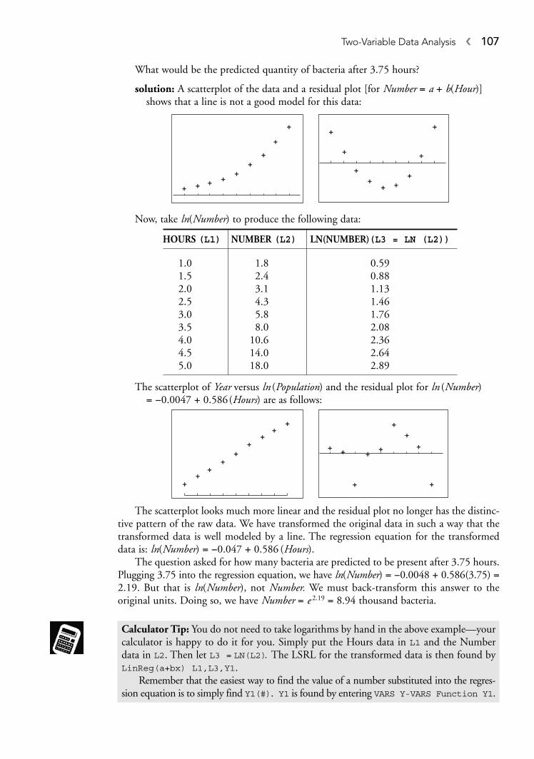
What would be the predicted quantity of bacteria after 3.75 hours?
solution: A scatterplot of the data and a residual plot [for Number = a + b(Hour)]shows that a line is not a good model for this data:
Now, take ln(Number) to produce the following data:
The scatterplot of Year versus ln (Population) and the residual plot for ln (Number)= −0.0047 + 0.586(Hours) are as follows:
The scatterplot looks much more linear and the residual plot no longer has the distinc-tive pattern of the raw data. We have transformed the original data in such a way that thetransformed data is well modeled by a line. The regression equation for the transformeddata is: ln(Number) = −0.047 + 0.586 (Hours).
The question asked for how many bacteria are predicted to be present after 3.75 hours.Plugging 3.75 into the regression equation, we have ln(Number) = −0.0048 + 0.586(3.75) =2.19. But that is ln(Number), not Number. We must back-transform this answer to theoriginal units. Doing so, we have Number = e 2.19 = 8.94 thousand bacteria.
Calculator Tip: You do not need to take logarithms by hand in the above example—yourcalculator is happy to do it for you. Simply put the Hours data in L1 and the Numberdata in L2. Then let L3 = LN(L2). The LSRL for the transformed data is then found byLinReg(a+bx) L1,L3,Y1.
Remember that the easiest way to find the value of a number substituted into the regres-sion equation is to simply find Y1(#). Y1 is found by entering VARS Y-VARS Function Y1.
HOURS (L1) NUMBER (L2) LN(NUMBER)(L3 = LN (L2))
1.0 1.8 0.591.5 2.4 0.882.0 3.1 1.132.5 4.3 1.463.0 5.8 1.763.5 8.0 2.084.0 10.6 2.364.5 14.0 2.645.0 18.0 2.89
Two-Variable Data Analysis � 107

It may be worth your while to try several different transformations to see if you canachieve linearity. Some possible transformations are: take the log of both variables, raise oneor both variables to a power, take the square root of one of the variables, take the reciprocalof one or both variables, etc.
� Rapid Review1. The correlation between two variables x and y is 0.85. Interpret this statement.
Answer: There is a strong, positive, linear association between x and y. That is, as oneof the variables increases, the other variable increases as well.
2. The following is a residual plot of a least-squares regression. Does it appear that a lineis a good model for the data? Explain.
Answer: The residual plot shows a definite pattern. If a line was a good model, we wouldexpect to see a more or less random pattern of points about 0. A line is unlikely to bea good model for this data.
3. Consider the following scatterplot. Is the point A an outlier, an influential observation,or both? What effect would its removal have on the slope of the regression line?
Answer: A is an outlier because it is removed from the general pattern of the rest of the points.It is an influential observation since its removal would have an effect on a calculation, specif-ically the slope of the regression line. Removing A would increase the slope of the LSRL.
Exam Tip: Also remember, when taking the AP exam, NO calculatorspeak. If you do alinear regression on your calculator, simply report the result. The person reading yourexam will know that you used a calculator and is NOT interested in seeing somethinglike LinReg L1,L2,Y1 written on your exam.
Digression: You will find a number of different regression expressions in the STAT CALCmenu: LinReg(ax+b), QuadReg, CubicReg, QuartReg, LinReg(a+bx), LnReg,
ExpReg, PwrReg, Logistic, and SinReg. While each of these has its use, onlyLinReg(a+bx) needs to be used in this course (well, LinReg(ax+b) gives the sameequation—with the a and b values reversed, just in standard algebraic form rather thanin the usual statistical form).
108 � Step 4. Review the Knowledge You Need to Score High
TIP
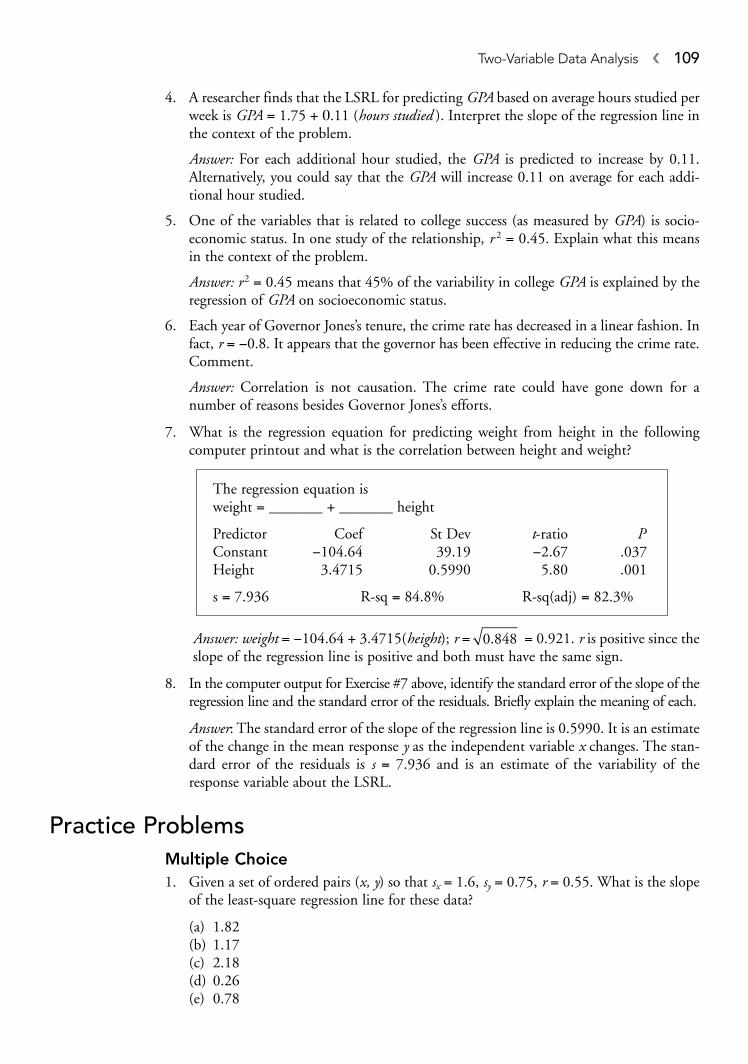
4. A researcher finds that the LSRL for predicting GPA based on average hours studied perweek is GPA = 1.75 + 0.11 (hours studied ). Interpret the slope of the regression line inthe context of the problem.
Answer: For each additional hour studied, the GPA is predicted to increase by 0.11.Alternatively, you could say that the GPA will increase 0.11 on average for each addi-tional hour studied.
5. One of the variables that is related to college success (as measured by GPA) is socio-economic status. In one study of the relationship, r 2 = 0.45. Explain what this meansin the context of the problem.
Answer: r 2 = 0.45 means that 45% of the variability in college GPA is explained by theregression of GPA on socioeconomic status.
6. Each year of Governor Jones’s tenure, the crime rate has decreased in a linear fashion. Infact, r = −0.8. It appears that the governor has been effective in reducing the crime rate.Comment.
Answer: Correlation is not causation. The crime rate could have gone down for anumber of reasons besides Governor Jones’s efforts.
7. What is the regression equation for predicting weight from height in the followingcomputer printout and what is the correlation between height and weight?
Answer: weight = −104.64 + 3.4715(height); r = = 0.921. r is positive since theslope of the regression line is positive and both must have the same sign.
8. In the computer output for Exercise #7 above, identify the standard error of the slope of theregression line and the standard error of the residuals. Briefly explain the meaning of each.
Answer: The standard error of the slope of the regression line is 0.5990. It is an estimateof the change in the mean response y as the independent variable x changes. The stan-dard error of the residuals is s = 7.936 and is an estimate of the variability of theresponse variable about the LSRL.
Practice ProblemsMultiple Choice1. Given a set of ordered pairs (x, y) so that sx = 1.6, sy = 0.75, r = 0.55. What is the slope
of the least-square regression line for these data?
(a) 1.82(b) 1.17(c) 2.18(d) 0.26(e) 0.78
0 848.
The regression equation isweight = _______ + _______ height
Predictor Coef St Dev t-ratio PConstant −104.64 39.19 −2.67 .037Height 3.4715 0.5990 5.80 .001
s = 7.936 R-sq = 84.8% R-sq(adj) = 82.3%
Two-Variable Data Analysis � 109

2.
The regression line for the two-variable dataset given above is = 2.35 + 0.86x. Whatis the value of the residual for the point whose x-value is 29?
(a) 1.71(b) −1.71(c) 2.29(d) 5.15(e) −2.29
3. A study found a correlation of r = −0.58 between hours per week spent watching televisionand hours per week spent exercising. That is, the more hours spent watching television, theless hours spent exercising per week. Which of the following statements is most accurate?
(a) About one-third of the variation in hours spent exercising can be explained byhours spent watching television.
(b) A person who watches less television will exercise more.(c) For each hour spent watching television, the predicted decrease in hours spent
exercising is 0.58 hrs.(d) There is a cause-and-effect relationship between hours spent watching television
and a decline in hours spent exercising.(e) 58% of the hours spent exercising can be explained by the number of hours watching
television.
4. A response variable appears to be exponentially related to the explanatory variable. Thenatural logarithm of each y-value is taken and the least-squares regression line is foundto be ln(y) = 1.64 − 0.88x. Rounded to two decimal places, what is the predicted valueof y when x = 3.1?
(a) −1.09(b) −0.34(c) 0.34(d) 0.082(e) 1.09
5. Consider the following residual plot:
Which of the following statements is (are) true?I. The residual plot indicates that a line is a reasonable model for the data.II. The residual plot indicates that there is no relationship between the data.
III. The correlation between the variables is probably non-zero.
y
x 23 15 26 24 22 29 32 40 41 46
y 19 18 22 20 27 25 32 38 35 45
110 � Step 4. Review the Knowledge You Need to Score High

(a) I only(b) II only(c) I and III only(d) II and III only(e) I and II only
6. Suppose the LSRL for predicting Weight (in pounds) from Height (in inches) is givenby Weight = –115 + 3.6 (Height). Which of the following statements is correct?
I. A person who is 61 inches tall will weigh 104.6 pounds.II. For each additional inch of Height, Weight will increase on average by 3.6 pounds.
III. There is a strong positive linear relationship between Height and Weight.
(a) I only(b) II only(c) III only(d) II and III only(e) I and II only
7. A least-squares regression line for predicting performance on a college entrance exambased on high school grade point average (GPA) is determined to be Score = 273.5 +91.2 (GPA). One student in the study had a high school GPA of 3.0 and an exam scoreof 510. What is the residual for this student?
a. 26.2b. 43.9c. –37.1d. –26.2e. 37.1
8. The correlation between two variables X and Y is –0.26. A new set of scores, X* and Y*,is constructed by letting X* = –X and Y* = Y +12. The correlation between X* and Y* is
a. – 0.26b. 0.26c. 0d. 0.52e. – 0.52
9. A study was done on the relationship between high school grade point average (GPA)and scores on the SAT. The following 8 scores were from a random sample of studentstaking the exam:
What percent of the variation in SAT scores is explained by the regression of SAT scoreon GPA?
a. 62.1%b. 72.3%c. 88.8%d. 94.2%e. 78.8%
X (GPA) 3.2 3.8 3.9 3.3 3.6 2.8 2.9 3.5
Y (SAT) 725 752 745 680 700 562 595 730
Two-Variable Data Analysis � 111

10. A study of stopping distances found that the least squares regression line for predictingmileage (in miles per gallon) from the weight of the vehicle (in hundreds of pounds)was MPG = 32.50 – 0.45(Weight). The mean weight for the vehicles in the study was2980 pounds. What was the mean MPG in the study?a. 19.09b. 15.27c. –1308.5d. 18.65e. 20.33
Free Response
1. Given a two-variable dataset such that = 14.5, = 20, sx = 4, sy = 11, r = .80, findthe least-squares regression line of y on x.
2. The data below give the first and second exam scores of 10 students in a calculus class.
(a) Draw a scatterplot of these data.(b) To what extent do the scores on the two tests seem related?
3. The following is a residual plot of a linear regression. A line would not be a good fit forthese data. Why not? Is the regression equation likely to underestimate or overestimatethe y-value of the point in the graph marked with the square?
4. The regional champion in 10 and under 100 m backstroke has had the following win-ning times (in seconds) over the past 8 years:
How many years until you expect the winning time to be one minute or less? What’swrong with this estimate?
5. Measurements are made of the number of cockroaches present, on average, every 3 days, beginning on the second day, after apartments in one part of town are vacated.The data are as follows:
How many cockroaches would you expect to be present after 9 days?
Days 2 5 8 11 14# Roaches 3 4.5 6 7.9 11.5
Year 1 2 3 4 5 6 7 8Time 77.3 80.2 77.1 76.4 75.5 75.9 75.1 74.3
0
Predicted Scores
Res
idua
ls
Test 1 63 32 87 73 60 63 83 80 98 85Test 2 51 21 52 90 83 54 73 85 83 46
yx
112 � Step 4. Review the Knowledge You Need to Score High

6. A study found a strongly positive relationship between number of miles walked perweek and overall health. A local news commentator, after reporting on the results of thestudy, advised everyone to walk more during the coming year because walking moreresults in better health. Comment on the reporter’s advice.
7. Carla, a young sociologist, is excitedly reporting on the results of her first professionalstudy. The finding she is reporting is that 72% of the variation in math grades for girlscan be explained by the girls’ socioeconomic status. What does this mean, and is itindicative of a strong linear relationship between math grades and socioeconomic statusfor girls?
8. Which of the following statements are true of a least-squares regression equation?
(a) It is the unique line that minimizes the sum of the residuals.(b) The average residual is 0.(c) It minimizes the sum of the squared residuals.(d) The slope of the regression line is a constant multiple of the correlation coefficient.(e) The slope of the regression line tells you how much the response variable will
change for each unit change in the explanatory variable.
9. Consider the following dataset:
Given that the LSRL for these data is = 26.211 − 0.25x, what is the value of theresidual for x = 73? Is the point (73,7.9) above or below the regression line?
10. Suppose the correlation between two variables is r = −0.75. What is true of the corre-lation coefficient and the slope of the regression line if
(a) each of the y values is multiplied by −1?(b) the x and y variables are reversed?(c) the x and y variables are each multiplied by −1?
11. Suppose the regression equation for predicting success on a dexterity task (y) from
number of training sessions (x) is = 45 + 2.7x and that = 3.33.
What percentage of the variation in y is not explained by the regression on x?
12. Consider the following scatterplot. The highlighted point is both an outlier and aninfluential point. Describe what will happen to the correlation and the slope of theregression line if that point is removed.
P2:L3,L4y
xX = 95 Y = 37
ssy
x
y
y
x 45 73 82 91y 15 7.9 5.8 3.5
Two-Variable Data Analysis � 113

13. The computer printout below gives the regression output for predicting crime rate (incrimes per 1000 population) from the number of casino employees (in 1000s).
Based on the output,
(a) give the equation of the LSRL for predicting crime rate from number.(b) give the value of r, the correlation coefficient.(c) give the predicted crime rate for 20,000 casino employees.
14. A study was conducted in a mid-size U.S. city to investigate the relationship betweenthe number of homes built in a year and the mean percentage appreciation for that year.The data for a 5-year period are as follows:
(a) Obtain the LSRL for predicting appreciation from number of new homes built ina year.
(b) The following year, 85 new homes are built. What is the predicted appreciation?(c) How strong is the linear relationship between number of new homes built and per-
centage appreciation? Explain.(d) Suppose you didn’t know the number of new homes built in a given year. How
would you predict appreciation?
15. A set of bivariate data has r 2 = 0.81.
(a) x and y are both standardized, and a regression line is fitted to the standardizeddata. What is the slope of the regression line for the standardized data?
(b) Describe the scatterplot of the original data.
16. Estimate r, the correlation coefficient, for each of the following graphs:
a.
c.
b.
d.
Number 110 80 95 70 55Percent appreciation 15.7 10 12.7 7.8 10.4
The regression equation isRate = _______ + _______ Number
Predictor Coef St Dev t ratio PConstant −0.3980 0.1884 −2.11 .068Number 0.118320 0.006804 17.39 .000
s = 0.1499 R-sq = 97.4% R-sq(adj) = 97.1%
114 � Step 4. Review the Knowledge You Need to Score High

17. The least-squares regression equation for the given data is = 3 + x. Calculate the sumof the squared residuals for the LSRL.
18. Many schools require teachers to have evaluations done by students. A study investi-gated the extent to which student evaluations are related to grades. Teacher evaluationsand grades are both given on a scale of 100. The results for Prof. Socrates (y) for 10 ofhis students are given below together with the average for each student (x).
(a) Do you think student grades and the evaluations students give their teachers arerelated? Explain.
(b) What evaluation score do you think a student who averaged 80 would give Prof.Socrates?
19. Which of the following statements are true?
(a) The correlation coefficient, r, and the slope of the regression line, b, always have thesame sign.
(b) The correlation coefficient is the same no matter which variable is considered to bethe explanatory variable and which is considered to be the response variable.
(c) The correlation coefficient is resistant to outliers.(d) x and y are measured in inches, and r is computed. Now, x and y are converted to
feet, and a new r is computed. The two computed values of r depend on the unitsof measurement and will be different.
(e) The idea of a correlation between height and gender is not meaningful becausegender is not numerical.
20. A study of right-handed people found that the regression equation for predicting left-hand strength (measured in kg) from right-hand strength is left-hand strength = 7.1 +0.35 (right-hand strength).
(a) What is the predicted left-hand strength for a right-handed person whose right-hand strength is 12 kg?
(b) Interpret the intercept and the slope of the regression line in the context of theproblem.
Cumulative Review Problems1. Explain the difference between a statistic and a parameter.
2. TRUE–FALSE. The area under a normal curve between z = 0.1 and z = 0.5 is the sameas the area between z = 0.3 and z = 0.7.
3. The following scores were achieved by students on a statistics test: 82, 93, 26, 56, 75,73, 80, 61, 79, 90, 94, 93, 100, 71, 100, 60. Compute the mean and median for thesedata and explain why they are different.
4. Is it possible for the standard deviation of a set of data to be negative? Zero? Explain.
5. For the test scores of problem #3, compute the five-number summary and draw a box-plot of the data.
x 40 60 70 73 75 68 65 85 98 90y 10 50 60 65 75 73 78 80 90 95
x 7 8 11 12 15y 10 11 14 15 18
y
Two-Variable Data Analysis � 115

Solutions to Practice ProblemsMultiple Choice
1. The correct answer is (d).
2. The correct answer is (e). The value of a residual = actual value − predicted value = 25 − [2.35 + 0.86(29)] = −2.29.
3. The correct answer is (a). r 2 = (−0.58)2 = 0.3364. This is the coefficient of determina-tion, which is the proportion of the variation in the response variable that is explainedby the regression on the independent variable. Thus, about one-third (33.3%) of thevariation in hours spent exercising can be explained by hours spent watching television.(b) is incorrect since correlation does not imply causation. (c) would be correct if b = –0.58, but there is no obvious way to predict the response value from the explana-tory value just by knowing r. (d) is incorrect for the same reason (b) is incorrect. (e) isincorrect since r, not r 2, is given. In this case r 2 = 0.3364, which makes (a) correct.
4. The correct answer is (c). ln( y) = 1.64 − 0.88(3.1) = −1.088 ⇒ y = e−1.088 = 0.337.
5. The correct answer is (c). The pattern is more or less random about 0, which indicatesthat a line would be a good model for the data. If the data are linearly related, we wouldexpect them to have a non-zero correlation.
6. The correct answer is (b). I is incorrect—the predicted weight of a person 61 inches tallis 104.6 pounds. II is a correct interpretation of the slope of the regression line (youcould also say that “For each additional inch of Height, Weight is predicted to increaseby 3.6 pounds). III is incorrect. It may well be true, but we have no way of knowing thatfrom the information given.
7. The correct answer is (c). The predicted score for the student is 273.5 + (91.2)(3) = 547.1.The residual is the actual score minus the predicted score, which equals 510 – 547.1 = –37.1.
8. The correct answer is (b). Consider the expression for r. .
Adding 12 to each Y-value would not change sy. Although the average would be 12 larger,the differences y – would stay the same since each Y-value is also 12 larger. By taking
the negative of each X-value, each term would reverse sign (the mean also reverses
sign) but the absolute value of each term would be the same. The net effect is to leaveunchanged the absolute value of r but to reverse the sign.
9. The correct answer is (e). The question is asking for the coefficient of determination, r2
(R-sq on many computer printouts). In this case, r = 0.8877 and r2 = 0.7881, or 78.8%.This can be found on your calculator by entering the GPA scores in L1, the SAT scoresin L2, and doing STAT CALC 1-Var Stats L1,L2.
x xsx
−
y
rn
x xs
y y
sx y
=−
−⎛
⎝⎜
⎞
⎠⎟
−⎛
⎝⎜⎜
⎞
⎠⎟⎟∑1
1
b rs
sy
x
= =⎛⎝⎜
⎞⎠⎟
=. ( . ).
..0 55
0 75
1 60 26
116 � Step 4. Review the Knowledge You Need to Score High

10. The correct answer is (a). The point always lies on the LSRL. Hence, can be
found by simply substituting x– into the LSRL and solving for . Thus = 32.5 –0.45(29.8) = 19.09 mpg. Be careful: you are told that the equation uses the weights inhundreds of pounds. You must then substitute 29.8 into the regression equation, not2980, which would get you answer (c).
Free Response
1.
Thus, = –11.9 + 2.2x.
2. (a)
(b) There seems to be a moderate positive relationship between the scores: studentswho did better on the first test tend to do better on the second, but the relation-ship isn’t very strong; r = 0.55.
3. A line is not a good model for the data because the residual plot shows a definite pat-tern: the first 8 points have negative residuals and the last 8 points have positive resid-uals. The box is in a cluster of points with positive residuals. We know that, for anygiven point, the residual equals actual value minus predicted value. Because actual – predicted > 0, we have actual > predicted, so that the regression equation is likely tounderestimate the actual value.
4. The regression equation for predicting time from year is time = 79.21 − 0.61(year). Weneed time = 60. Solving 60 = 79.1 − 0.61(year), we get year = 31.3. So, we would pre-dict that times will drop under one minute in about 31 or 32 years. The problem withthis is that we are extrapolating far beyond the data. Extrapolation is dangerous in anycircumstance, and especially so 24 years beyond the last known time. It’s likely that therate of improvement will decrease over time.
5. A scatterplot of the data (graph on the left) appears to be exponential. Taking the naturallogarithm of each y-value, the scatterplot (graph on the right) appears to be more linear.
y
b rs
sa y bxy
x
= =⎛
⎝⎜
⎞
⎠⎟= = − = −( . ) . , ( . )(0 80
11
42 2 20 2 2 14.. ) . .5 11 9= −
yyy( , )x y
Two-Variable Data Analysis � 117

Taking the natural logarithm of each y-value and finding the LSRL, we have ln(#Roaches) =0.914 + 0.108 (Days) = 0.914 + 0.108(9) = 1.89. Then #Roaches = e1.89 = 6.62.
6. The correlation between walking more and better health may or may not be causal. Itmay be that people who are healthier walk more. It may be that some other variable,such as general health consciousness, results in walking more and in better health.There may be a causal association, but in general, correlation is not causation.
7. Carla has reported the value of r 2, the coefficient of determination. If she had predictedeach girl’s grade based on the average grade only, there would have been a large amountof variability. But, by considering the regression of grades on socioeconomic status, shehas reduced the total amount of variability by 72%. Because r 2 = 0.72, r = 0.85, whichis indicative of a strong positive linear relationship between grades and socioeconomicstatus. Carla has reason to be happy.
8. (a) is false. Σ( y − ) = 0 for the LSRL, but there is no unique line for which this is true.(b) is true.(c) is true. In fact, this is the definition of the LSRL—it is the line that minimizes the
sum of the squared residuals.
(d) is true since b = r and is constant.
(e) is false. The slope of the regression lines tell you by how much the response vari-able changes on average for each unit change in the explanatory variable.
9. y = 26.211 − 0.25x = 26.211 − 0.25(73) = 7.961. The residual for x = 73 is the actualvalue at 73 minus the predicted value at 73, or y − = 7.9 − 7.961 = −0.061. (73, 7.9) is below the LSRL since y – < 0 y < .
10. (a) r = +0.75; the slope is positive and is the opposite of the original slope.(b) r = −0.75. It doesn’t matter which variable is called x and which is called y.(c) r = −0.75; the slope is the same as the original slope.
11. We know that , so that 2.7 = r (3.33)→ → r2 = 0.66. The proportion
of the variability that is not explained by the regression of y on x is 1 – r2 = 1 – 0.66 = 0.34.
12. Because the linear pattern will be stronger, the correlation coefficient will increase. Theinfluential point pulls up on the regression line so that its removal would cause theslope of the regression line to decrease.
13. (a) rate = −0.3980 + 0.1183 (number).(b) r = = 0.987 (r is positive since the slope is positive).(c) rate = −0.3980 + 0.1183(20) = 1.97 crimes per thousand employees. Be sure to use
20, not 200.
14. (a) Percentage appreciation = 1.897 + 0.115 (number)(b) Percentage appreciation = 1.897 + 0.115(85) = 11.67%.(c) r = 0.82, which indicates a strong linear relationship between the number of new
homes built and percent appreciation.(d) If the number of new homes built was unknown, your best estimate would be the
average percentage appreciation for the 5 years. In this case, the average percentageappreciation is 11.3%. [For what it’s worth, the average error (absolute value) usingthe mean to estimate appreciation is 2.3; for the regression line, it’s 1.3.]
15. (a) If r2 = 0.81, then r = ±0.9. The slope of the regression line for the standardizeddata is either 0.9 or −0.9.
0 974.
r = =2 7
3 330 81
.
..b r
s
sy
x
=
y⇒yy
s
sy
x
s
sy
x
y
118 � Step 4. Review the Knowledge You Need to Score High

(b) If r = +0.9, the scatterplot shows a strong positive linear pattern between the vari-ables. Values above the mean on one variable tend to be above the mean on theother, and values below the mean on one variable tend to be below the mean onthe other. If r = −0.9, there is a strong negative linear pattern to the data. Valuesabove the mean on one variable are associated with values below the mean on theother.
16. (a) r = 0.8(b) r = 0.0(c) r = −1.0(d) r = −0.5
17. Each of the points lies on the regression line → every residual is 0 → the sum of thesquared residuals is 0.
18. (a) r = 0.90 for these data, indicating that there is a strong positive linear relationshipbetween student averages and evaluations of Prof. Socrates. Furthermore, r2 = 0.82,which means that most of the variability in student evaluations can be explained bythe regression of student evaluations on student average.
(b) If y is the evaluation score of Prof. Socrates and x is the corresponding average forthe student who gave the evaluation, then = −29.3 + 1.34x. If x = 80, then
= −29.3 + 1.34(80) = 77.9, or 78.
19. (a) True, because
b = r and is positive.
(b) True. r is the same if explanatory and response variables are reversed. This is nottrue, however, for the slope of the regression line.
(c) False. Because r is defined in terms of the means of the x and y variables, it is not resistant.(d) False. r does not depend on the units of measurement.
(e) True. The definition of
necessitates that the variables be numerical, not categorical.
20. (a) Left-hand strength = 7.1 + 0.35(12) = 11.3 kg.(b) Intercept: The predicted left-hand strength of a person who has zero right-hand
strength is 7.1 kg.Slope: On average, left-hand strength increases by 0.35 kg for each 1 kg increasein right-hand strength. Or left-hand strength is predicted to increase by 0.35 kg foreach 1 kg increase in right-hand strength.
Solutions to Cumulative Review Problems1. A statistic is a measurement that describes a sample. A parameter is a value that describes
a population.
2. FALSE. For an interval of fixed length, there will be a greater proportion of the areaunder the normal curve if the interval is closer to the center than if it is removed fromthe center. This is because the normal distribution is mound shaped, which implies thatthe terms tend to group more in the center of the distribution than away from the center.
r rn
x x
s
y y
si
xi
ni
y
, =−
−⎛
⎝⎜⎜
⎞
⎠⎟⎟
−⎛
⎝⎜⎜
⎞
⎠⎟⎟
=
∑1
1 1
,
s
sy
x
s
sy
x
yy
Two-Variable Data Analysis � 119

3. The mean is 77.1, and the median is 79.5. The mean is lower than the median becauseit is not resistant to extreme values—it is pulled down by the 26, but that value doesnot affect the median.
4. By definition, s = , which is a positive square root. Since n >1 and
≥ 0, s cannot be negative. It can be zero, but only if x = for all values of x.
5. The 5-number summary is: [26, 66, 79.5, 93, 100].
26 66 79.5 99 100
x∑ −( )x x 2
∑ −
−
( )x xn
2
1
120 � Step 4. Review the Knowledge You Need to Score High

� 121
Design of a Study:Sampling, Surveys, and
ExperimentsIN THIS CHAPTERSummary: This chapter stands pretty much alone in this course. All otherchapters are concerned with how to analyze and make inferences fromdata that have been collected. In this chapter, we discuss how to collectthe data. Doing an analysis of bad or poorly collected data has no practicalapplication. Here you’ll learn about surveys and sampling, observationalstudies,experiments, and the types of bias than can creep into each ofthem. Once you understand all this, you’ll have greater confidence thatyour analysis actually means something more than meaningless numbercrunching.
Key Ideas
� Samples and Sampling� Surveys� Sampling Bias� Experiments and Observational Studies� Statistical Significance� Completely Randomized Design� Matched Pairs Design� Blocking
KEY IDEA
CHAPTER 8

SamplesIn the previous two chapters we concentrated on the analysis of data at hand—we didn’tworry much about how the data came into our possession. The last part of this book dealswith statistical inference—making statements about a population based on samples drawnfrom the population. In both data analysis and inference, we would like to believe that ouranalyses, or inferences, are meaningful. If we make a claim about a population based on a sample, we want that claim to be true. Our ability to do meaningful analyses and makereliable inferences is a function of the data we collect. To the extent that the sample data wedeal with are representative of the population of interest, we are on solid ground. No interpretation of data that are poorly collected or systematically biased will be meaningful.We need to understand how to gather quality data before proceeding on to inference. Inthis chapter, we study techniques for gathering data so that we have reasonable confidencethat they are representative of our population of interest.
CensusThe alternative to sampling to gather data about a population is to conduct a census,a procedure by which every member of a population is selected for study. Doing a census,especially when the population of interest is quite large, is often impractical, too time consuming, or too expensive. Interestingly enough, relatively small samples can give quitegood estimates of population values if the samples are selected properly. For example, it canbe shown that approximately 1500 randomly selected voters can give reliable informationabout the entire voting population of the United States.
The goal of sampling is to produce a representative sample, one that has the essentialcharacteristics of the population being studied and is free of any type of systematic bias. Wecan never be certain that our sample has the characteristics of the population from whichit was drawn. Our best chance of making a sample representative is to use some sort ofrandom process in selecting it.
Probability SampleA list of all members of the population from which we can draw a sample is called a sampling frame. A sampling frame may or may not be the same set of individuals we arestudying. A probability sample is one in which each member of the population has aknown probability of being in the sample. Each member of the population may or may not have an equal chance of being selected. Probability samples are used to avoidthe bias that can arise in a nonprobability sample (such as when a researcher selects the subjects she will use). Probability samples use some sort of random mechanism to choosethe members of the sample. The following list includes some types of probability samples.
• random sample: Each member of the population is equally likely to be included.• simple random sample (SRS): A sample of a given size is chosen in such a way that
every possible sample of that size is equally likely to be chosen. Note that a sample canbe a random sample and not be a simple random sample (SRS). For example, suppose youwant a sample of 64 NFL football players. One way to produce a random sample wouldbe to randomly select two players from each of the 32 teams. This is a random samplebut not a simple random sample because not all possible samples of size 64 are possible.
• systematic sample: The first member of the sample is chosen according to some randomprocedure, and then the rest are chosen according to some well-defined pattern. Forexample, if you wanted 100 people in your sample to be chosen from a list of 10,000people, you could randomly select one of the first 100 people and then select every 100thname on the list after that.
122 � Step 4. Review the Knowledge You Need to Score High

• stratified random sample: This is a sample in which subgroups of the sample, strata,appear in approximately the same proportion in the sample as they do in the population.For example, assuming males and females were in equal proportion in the population,you might structure your sample to be sure that males and females were in equal proportion in the sample. For a sample of 100 individuals, you would select an SRS of50 females from all the females and an SRS of 50 males from all the males.
• cluster sample: The population is first divided into sections or “clusters.” Then we ran-domly select an entire cluster, or clusters, and include all of the members of the cluster(s)in the sample.
example: You are going to conduct a survey of your senior class concerning plansfor graduation. You want a 10% sample of the class. Describe a procedure bywhich you could use a systematic sample to obtain your sample and explainwhy this sample isn’t a simple random sample. Is this a random sample?
solution: One way would be to obtain an alphabetical list of all the seniors. Use arandom number generator (such as a table of random digits or a scientificcalculator with a random digits function) to select one of the first 10 names onthe list. Then proceed to select every 10th name on the list after the first.
Note that this is not an SRS because not every possible sample of 10% of thesenior class is equally likely. For example, people next to each other in the list can’t both be in the sample. Theoretically, the first 10% of the list could be the sample if it were an SRS. This clearly isn’t possible.
Before the first name has been randomly selected, every member of thepopulation has an equal chance to be selected for the sample. Hence, this is a random sample, although it is not a simple random sample.
example: A large urban school district wants to determine the opinions of its elementary schools teachers concerning a proposed curriculum change. The districtadministration randomly selects one school from all the elementary schools in thedistrict and surveys each teacher in that school. What kind of sample is this?
solution: This is a cluster sample. The individual schools represent previouslydefined groups (clusters) from which we have randomly selected one (it couldhave been more) for inclusion in our sample.
example: You are sampling from a population with mixed ethnicity. The populationis 45% Caucasian, 25% Asian American, 15% Latino, and 15% AfricanAmerican. How would a stratified random sample of 200 people be constructed?
solution: You want your sample to mirror the population in terms of its ethnic dis-tribution. Accordingly, from the Caucasians, you would draw an SRS of 90 (that’s45%), an SRS of 50 (25%) from the Asian Americans, an SRS of 30(15%) fromthe Latinos, and an SRS of 30 (15%) from the African Americans.
Of course, not all samples are probability samples. At times, people try to obtain samples by processes that are nonrandom but still hope, through design or faith, that theresulting sample is representative. The danger in all nonprobability samples is that some(unknown) bias may affect the degree to which the sample is representative. That isn’t tosay that random samples can’t be biased, just that we have a better chance of avoiding systematic bias. Some types of nonrandom samples are:
• self-selected sample or voluntary response sample: People choose whether or not toparticipate in the survey. A radio call-in show is a typical voluntary response sample.
Design of a Study: Sampling, Surveys, and Experiments � 123

• convenience sampling: The pollster obtains the sample any way he can, usually with theease of obtaining the sample in mind. For example, handing out questionnaires to everymember of a given class at school would be a convenience sample. The key issue here isthat the surveyor makes the decision whom to include in the sample.
• quota sampling: The pollster attempts to generate a representative sample by choosingsample members based on matching individual characteristics to known characteristicsof the population. This is similar to a stratified random sample, only the process forselecting the sample is nonrandom.
Sampling BiasAny sample may contain bias. What we are trying to avoid is systematic bias, which is the tendency for our results to favor, systematically, one outcome over another. This can occurthrough faulty sampling techniques or through faults in the actual measurement instrument.
UndercoverageOne type of bias results from undercoverage. This happens when some part of the popu-lation being sampled is somehow excluded. This can happen when the sampling frame (the list from which the sample will be drawn) isn’t the same as the target population. It canalso occur when part of the sample selected fails to respond for some reason.
example: A pollster conducts a telephone survey to gather opinions of the generalpopulation about welfare. Persons on welfare too poor to be able to afford atelephone are certainly interested in this issue, but will be systematicallyexcluded from the sample. The resulting sample will be biased because of theexclusion of this group.
Voluntary Response BiasVoluntary response bias occurs with self-selected samples. Persons who feel most stronglyabout an issue are most likely to respond. Non-response bias, the possible biases of thosewho choose not to respond, is a related issue.
example: You decide to find out how your neighbors feel about the neighbor whoseems to be running a car repair shop on his front lawn. You place a question-naire in every mailbox within sight of the offending home and ask the peopleto fill it out and return it to you. About 1/2 of the neighbors return the survey,and 95% of those who do say that they find the situation intolerable. We haveno way of knowing the feelings of the 50% of those who didn’t return thesurvey—they may be perfectly happy with the “bad” neighbor. Those who havethe strongest opinions are those most likely to return your survey—and theymay not represent the opinions of all. Most likely they do not.
example: In response to a question once posed in Ann Landers’s advice column,some 70% of respondents (almost 10,000 readers) wrote that they wouldchoose not to have children if they had the choice to do it over again. This is most likely representative only of those parents who were having a really bad day with their children when they decided to respond to the question. In fact, a properly designed opinion poll a few months later found that more than 90% of parents said they would have children if they had the chance to do it all over again.
124 � Step 4. Review the Knowledge You Need to Score High

Wording BiasWording bias occurs when the wording of the question itself influences the response in a systematic way. A number of studies have demonstrated that welfare gathers more support from a random sample of the public when it is described as “helping people until they can better help themselves” that when it is described as “allowing people to stayon the dole.”
example: Compare the probable responses to the following ways of phrasing a question.
(i) “Do you support a woman’s right to make medical decisions concerning herown body?”
(ii) “Do you support a woman’s right to kill an unborn child?”
It’s likely that (i) is designed to show that people are in favor of a woman’s right to choose an abortion and that (ii) is designed to show that people are opposed tothat right. The authors of both questions would probably argue that bothresponses reflect society’s attitudes toward abortion.
example: Two different Gallup Polls were conducted in Dec. 2003. Both involvedpeople’s opinion about the U.S. space program. Here is one part of each poll.
Poll A: Would you favor or oppose a new U.S. space program that would sendastronauts to the moon? Favor—53%; oppose—45%.
Poll B: Would you favor or oppose U.S. government spending billions of dollarsto send astronauts to the moon? Favor—31%; oppose—67%.
(source: http://www.stat.ucdavis.edu/~jie/stat13.winter2007/lec18.pdf )
Response BiasResponse bias arises in a variety of ways. The respondent may not give truthful responsesto a question (perhaps she or he is ashamed of the truth); the respondent may fail to understand the question (you ask if a person is educated but fail to distinguish betweenlevels of education); the respondent desires to please the interviewer (questions concerning race relations may well solicit different answers depending on the race of the interviewer);the ordering of the question may influence the response (“Do you prefer A to B?” may getdifferent responses than “Do you prefer B to A?”).
example: What form of bias do you suspect in the following situation? You are aschool principal and want to know students’ level of satisfaction with the coun-seling services at your school. You direct one of the school counselors to ask hernext 25 counselees how favorably they view the counseling services at the school.
solution: A number of things would be wrong with the data you get from such asurvey. First, the sample is nonrandom—it is a sample of convenience obtainedby selecting 25 consecutive counselees. They may or may not be representativeof students who use counseling service. You don’t know.
Second, you are asking people who are seeing their counselor about their opin-ion of counseling. You will probably get a more favorable view of the counsel-ing services than you would if you surveyed the general population of theschool (would students really unhappy with the counseling services voluntarilybe seeing their counselor?). Also, because the counselor is administering the
Design of a Study: Sampling, Surveys, and Experiments � 125
126 � Step 4. Review the Knowledge You Need to Score High
questionnaire, the respondents would have a tendency to want to please theinterviewer. The sample certainly suffers from undercoverage—only a smallsubset of the general population is actually being interviewed. What do thosenot being interviewed think of the counseling?
Experiments and Observational StudiesStatistical SignificanceOne of the desirable outcomes of a study is to help us determine cause and effect. We dothis by looking for differences between groups that are so great that we cannot reasonablyattribute the difference to chance. We say that a difference between what we would expectto find if there were no treatment and what we actually found is statistically significant ifthe difference is too great to attribute to chance. We discuss numerical methods of deter-mining significance in Chapters 11–15.
An experiment is a study in which the researcher imposes some sort of treatment on theexperimental units (which can be human—usually called subjects in that case). In an experi-ment, the idea is to determine the extent to which treatments (the explanatory variable(s)) affectsoutcomes (the response variable (s)). For example, a researcher might vary the rewards to differ-ent work group members to see how that affects the group’s ability to perform a particular task.
An observational study, on the other hand, simply observes and records behavior butdoes not attempt to impose a treatment in order to manipulate the response.
Exam Tip: The distinction between an experiment and an observational study is animportant one. There is a reasonable chance that you will be asked to show you understandthis distinction on the exam. Be sure this section makes sense to you.
example: A group of 60 exercisers are classified as “walkers” or “runners.” A longi-tudinal study (one conducted over time) is conducted to see if there are differ-ences between the groups in terms of their scores on a wellness index. This is anobservational study because, although the two groups differ in an importantrespect, the researcher is not manipulating any treatment. “Walkers” and “run-ners” are simply observed and measured. Note that the groups in this study areself-selected. That is, they were already in their groups before the study began.The researchers just noted their group membership and proceeded to makeobservations. There may be significant differences between the groups in addi-tion to the variable under study.
example: A group of 60 volunteers who do not exercise are randomly assigned toone of the two fitness programs. One group of 30 is enrolled in a daily walkingprogram, and the other group is put into a running program. After a period oftime, the two groups are compared based on their scores on a wellness index.This is an experiment because the researcher has imposed the treatment (walkingor running) and then measured the effects of the treatment on a definedresponse.
It may be, even in a controlled experiment, that the measured response is a function ofvariables present in addition to the treatment variable. A confounding variable is one thathas an effect on the outcomes of the study but whose effects cannot be separated from thoseof the treatment variable. A lurking variable is one that has an effect on the outcomes of
TIP

the study but whose influence was not part of the investigation. A lurking variable can bea confounding variable.
example: A study is conducted to see if Yummy Kibble dog food results in shiniercoats on Golden Retrievers. It’s possible that the dogs with shinier coats havethem because they have owners who are more conscientious in terms of grooming their pets. Both the dog food and the conscientious owners couldcontribute to the shinier coats. The variables are confounded because theireffects cannot be separated.
A well-designed study attempts to anticipate confounding variables in advance andcontrol for them. Statistical control refers to a researcher holding constant variables notunder study that might have an influence on the outcomes.
example: You are going to study the effectiveness of SAT preparation courses on SAT score. You know that better students tend to do well on SAT tests. You could control for the possible confounding effect of academic quality by running your study with groups of “A” students, “B” students, etc.
Control is often considered to be one of the three basic principles of experimentaldesign. The other two basic principles are randomization and replication.
The purpose of randomization is to equalize groups so that the effects of lurking variables are equalized among groups. Randomization involves the use of chance (like a coinflip) to assign subjects to treatment and control groups. The hope is that the groups beingstudied will differ systematically only in the effects of the treatment variable. Although individuals within the groups may vary, the idea is to make the groups as alike as possibleexcept for the treatment variable. Note that it isn’t possible to produce, with certainty,groups free of any lurking variables. It is possible, through the use of randomization, toincrease the probability of producing groups that are alike. The idea is to control for theeffects of variables you aren’t aware of but that might affect the response.
Replication involves repeating the experiment on enough subjects (or units) to reducethe effects of chance variation on the outcomes. For example, we know that the number ofboys and girls born in a year are approximately equal. A small hospital with only 10 birthsa year is much more likely to vary dramatically from 50% each than a large hospital with500 births a year.
Completely Randomized DesignA completely randomized design for a study involves three essential elements: randomallocation of subjects to treatment and control groups; administration of different treatmentsto each randomized group (in this sense we are calling a control group a “treatment”); andsome sort of comparison of the outcomes from the various groups. A standard diagram ofthis situation is the following:
There may be several different treatment groups (different levels of a new drug, forexample) in which case the diagram could be modified. The control group can either be an older treatment (like a medication currently on the market) or a placebo, a dummy
Design of a Study: Sampling, Surveys, and Experiments � 127
Randomallocation
Group 1Treatment
Volunteers Compare
Group 2Control

Remember that each group must have enough subjects so that the replication conditionis met. The purpose of the placebo is to separate genuine treatment effects from possiblesubject responses due to simply being part of an experiment. Placebos are not necessary if a new treatment is being compared to a treatment whose effects have been previouslyexperimentally established. In that case, the old treatment can serve as the control. A newcream to reduce acne (the treatment), for example, might be compared to an already-on-the-market cream (the control) whose effectiveness has long been established.
example: Three hundred graduate students in psychology (by the way, a huge percentage of subjects in published studies are psychology graduate students)volunteer to be subjects in an experiment whose purpose is to determine whatdosage level of a new drug has the most positive effect on a performance test.There are three levels of the drug to be tested: 200 mg, 500 mg, and 750 mg.Design a completely randomized study to test the effectiveness of the variousdrug levels.
solution: There are three levels of the drug to be tested: 200 mg, 500 mg, and750 mg. A placebo control can be included although, strictly speaking, it isn’tnecessary is our purpose is to compare the three dosage levels. We need torandomly allocate the 300 students to each of four groups of 75 each: onegroup will receive the 200 mg dosage; one will receive the 500 mg dosage; onewill receive the 750 mg dosage; and one will receive a placebo (if included). Nogroup will know which treatment its members are receiving (all the pills lookthe same), nor will the test personnel who come in contact with them knowwhich subjects received which pill (see the definition of “double-blind” givenbelow). Each group will complete the performance test and the results of thevarious groups will be compared. This design can be diagramed as follows:
Double-Blind ExperimentsIn the example above, it was explained that neither the subjects nor the researchers knewwho was receiving which dosage, or the placebo. A study is said to be double-blind whenneither the subjects (or experimental units) nor the researchers know which group(s) is/are
128 � Step 4. Review the Knowledge You Need to Score High
Group 1Treatment 1
Group 2Treatment 2
Randomallocation
•Volunteers • Compare
•Group nControl (Placebo)
Group 1200 mg dosage
Group 2500 mg dosage
Randomallocation togroups
StudentVolunteers
Group 3 Compare750 ms dosage
Group 4Control (Placebo)
treatment. A diagram for an experiment with more than two treatment groups might looksomething like this:

receiving each treatment or control. The reason for this is that, on the part of subjects,simply knowing that they are part of a study may affect the way they respond, and, on thepart of the researchers, knowing which group is receiving which treatment can influence the way in which they evaluate the outcomes. Our worry is that the individual treatmentand control groups will differ by something other than the treatment unless the study isdouble-blind. A double-blind study further controls for the placebo effect.
RandomizationThere are two main procedures for performing a randomization. They are:
• Tables of random digits. Most textbooks contain tables of random digits. These are usu-ally tables where the digits 0, 1, 2, 3, 4, 5, 6, 7, 8, and 9 appear in random order (well, asrandom as most things get, anyhow). That means that, as you move through the table, eachdigit should appear with probability 1/10, and each entry is independent of the others(knowing what came before doesn’t help you make predictions about what comes next).
• Calculator “rand” functions. The TI-83/84 calculator has several random functions:rand, randInt (which will generate a list of random integers in a specified range),randNorm (which will generate random values from a normal distribution with mean mand standard deviation s), and randBin (which will generate random values from abinomial distribution with n trials and fixed probability p—see Chapter 10). If youwanted to generate a list of 50 random digits similar to the random digit table describedabove, you could enter randInt(0,9) and press ENTER 50 times. A more efficient way would be to enter randInt(0,9,50). If you wanted these 50 random integers storedin a list (say L1), you would enter randInt(0,9,10)→ L1 (remembering that the → isobtained by pressing STO).
Digression: Although the calculator is an electronic device, it is just like a random digittable in that, if two different people enter the list in the same place, they will get the samesequence of numbers. You “enter” the list on the calculator by “seeding” the calculator asfollows: (Some number)→ rand (you get to the rand function by entering MATH PRBrand). If different people using the same model of calculator entered, say, 18→ rand,
then MATH PRB rand, and began to press ENTER repeatedly, they would all generateexactly the same list of random digits.
We will use tables of random digits and/or the calculator in Chapter 9 when we discusssimulation.
Block DesignEarlier we discussed the need for control in a study and identified randomization as themain method to control for lurking variables—variables that might influence the outcomesin some way but are not considered in the design of the study (usually because we aren’taware of them). Another type of control involves variables we think might influence theoutcome of a study. Suppose we suspect, as in our previous example, that the performancetest varies by gender as well as by dosage level of the test drug. That is, we suspect thatgender is a confounding variable (its effects cannot be separated from the effects of the drug).To control for the effects of gender on the performance test, we utilize what is known as ablock design. A block design involves doing a completely randomized experiment withineach block. In this case, that means that each level of the drug would be tested within thegroup of females and within the group of males. To simplify the example, suppose that wewere only testing one level (say 500 mg) of the drug versus a placebo. The experimentaldesign, blocked by gender, could then be diagramed as follows.
Design of a Study: Sampling, Surveys, and Experiments � 129

Randomization and block designs each serve a purpose. It’s been said that you block tocontrol for the variables you know about and randomize to control for the ones you don’t.Note that your interest here is in studying the effect of the treatment within the populationof males and within the population of females, not to compare the effects on men and womenso that there would be no additional comparison between the blocks—that’s a different study.
Matched Pairs DesignA particular block design of interest is the matched pairs design. One possible matchedpairs design involves before and after measurements on the same subjects. In this case, eachsubject becomes a block in which the experiment is conducted. Another type of matchedpairs involves pairing the subjects in some way (matching on, say, height, race, age, etc.).
example: A study is instituted to determine the effectiveness of training teachersto teach AP Statistics. A pretest is administered to each of 23 prospective teach-ers who subsequently undergo a training program. When the program is fin-ished, the teachers are given a post-test. A score for each teacher is arrived at bysubtracting their pretest score from their post-test score. This is a matched pairsdesign because two scores are paired for each teacher.
example: One of the questions on the 1997 AP Exam in Statistics asked students todesign a study to compare the effects of differing formulations of fish food on fishgrowth. Students were given a room with eight fish tanks. The room had a heaterat the back of the room, a door at the front center of the room, and windows atthe front sides of the room. The most correct design involved blocking so that thetwo tanks nearest the heater in the back of the room were in a single block, thetwo away from the heater in a second block, the two in the front near the door ina third, and the two in the front near the windows in a fourth. This matchinghad the effect of controlling for known environmental variations in the roomcaused by the heater, the door, and the windows. Within each block, one tankwas randomly assigned to receive one type of fish food and the other tankreceived the other. The blocking controlled for the known effects of the environ-ment in which the experiment was conducted. The randomization controlled forunknown influences that might be present in the various tank locations.
You will need to recognize paired-data, as distinct from two independent sets ofdata, later on when we study inference. Even though two sets of data are gener-ated in a matched-pairs study, it is the differences between the matched valuesthat form the one-sample data used for statistical analysis.
130 � Step 4. Review the Knowledge You Need to Score High
Treatment500 mg
Males CompareControlplacebo
Volunteers
Treatment500 mgRandom
allocation
Randomallocation
Females CompareControlplacebo

Exam Tip: You need to be clear on the distinction between the purposes for “blocking”and randomizing. If you are asked to describe an experiment involving blocking, be sureto remember to randomize treatments within blocks.
� Rapid Review1. You are doing a research project on attitudes toward fast food and decide to use as your
sample the first 25 people to enter the door at the local FatBurgers restaurant. Whichof the following is (are) true of this sample?
a. It is a systematic sample.b. It is a convenience sample.c. It is a random sample.d. It is a simple random sample.e. It is a self-selected sample.
Answer: Only (b) is correct. (a), (c), and (d) are all probability samples, which rely onsome random process to select the sample, and there is nothing random about the selectionprocess in this situation. (e) is incorrect because, although the sample members voluntarilyentered Fat Burgers, they haven’t volunteered to respond to a survey.
2. How does an experiment differ from an observational study?
Answer: In an experiment, the researcher imposes some treatment on the subjects (orexperimental units) in order to observe a response. In an observational study, theresearcher simply observes, compares, and measures, but does not impose a treatment.
3. What are the three key components of an experiment? Explain each.
Answer: The three components are randomization, control, and replication. You randomizeto be sure that the response does not systematically favor one outcome over another. Theidea is to equalize groups as much as possible so that differences in response are attributable to the treatment variable alone. Control is designed to hold confoundingvariables constant (such as the placebo effect). Replication ensures that the experiment isconducted on sufficient numbers of subjects to minimize the effects of chance variation.
4. Your local pro football team has just suffered a humiliating defeat at the hands of itsarch rival. A local radio sports talk show conducts a call-in poll on whether or not thecoach should be fired. What is the poll likely to find?
Answer: The poll is likely to find that, overwhelmingly, respondents think the coachshould be fired. This is a voluntary response poll, and we know that such a poll is mostlikely to draw a response from those who feel most strongly about the issue being polled.Fans who bother to vote in a call-in poll such as this are most likely upset at their team’sloss and are looking for someone to blame—this gives them the opportunity. There is,of course, a chance that the coach may be very popular and draw support, but the pointto remember is that this is a self-selecting nonrandom sample, and will probably exhibitresponse bias.
5. It is known that exercise and diet both influence weight loss. Your task is to conduct a study ofthe effects of diet on weight loss. Explain the concept of blocking as it relates to this study.
Answer: If you did a completely randomized design for this study using diet at the treat-ment variable, it’s very possible that your results would be confounded by the effects
Design of a Study: Sampling, Surveys, and Experiments � 131
TIP

of exercise. Because you are aware of this, you would like to control for the effects of exercise. Hence, you block by exercise level. You might define, say, three blocks by levelof exercise (very active, active, not very active) and do a completely randomized studywithin each of the blocks. Because exercise level is held constant, you can be confident thatdifferences between treatment and control groups within each block are attributable todiet, not exercise.
6. Explain the concept of a double-blind study and why it is important.
Answer: A study is double-blind if neither the subject of the study nor the researchersare aware of who is in the treatment group and who is in the control group. This is tocontrol for the well-known effect of people to (subconsciously) attempt to respond inthe way they think they should.
7. You are interested in studying the effects of preparation programs on SAT performance.Briefly describe a matched-pairs design and a completely randomized design for this study.
Answer : Matched pairs: Choose, say, 100 students who have not participated in anSAT prep course. Have them take the SAT. Then have these students take a prepara-tion course and retake the SAT. Do a statistical analysis of the difference between thepre- and postpreparation scores for each student. (Note that this design doesn’t dealwith the influence of retaking the SAT independent of any preparation course, whichcould be a confounding variable.)
Completely randomized design: Select 100 students and randomly assign themto two groups, one of which takes the SAT with no preparation course and one of which has a preparation course before taking the SAT. Statistically, compare theaverage performance of each group.
Practice ProblemsMultiple Choice1. Data were collected in 20 cities on the percentage of women in the workforce. Data
were collected in 1990 and again in 1994. Gains, or losses, in this percentage were themeasurement upon which the studies conclusions were to be based. What kind ofdesign was this?
I. A matched pairs designII. An observational study
III. An experiment using a block design
(a) I only(b) II only(c) III only(d) I and III only(e) I and II only
2. You want to do a survey of members of the senior class at your school and want toselect a simple random sample. You intend to include 40 students in your sample.Which of the following approaches will generate a simple random sample?
(a) Write the name of each student in the senior class on a slip of paper and put thepapers in a container. Then randomly select 40 slips of paper from the container.
(b) Assuming that students are randomly assigned to classes, select two classes atrandom and include those students in your sample.
132 � Step 4. Review the Knowledge You Need to Score High

(c) From a list of all seniors, select one of the first 10 names at random. The selectevery nth name on the list until you have 40 people selected.
(d) Select the first 40 seniors to pass through the cafeteria door at lunch.(e) Randomly select 10 students from each of the four senior calculus classes.
3. Which of the following is (are) important in designing an experiment?I. Control of all variables that might have an influence on the response variable.
II. Randomization of subjects to treatment groups.III. Use of a large number of subjects to control for small-sample variability.
(a) I only(b) I and II only(c) II and III only(d) I, II, and III(e) II only
4. Your company has developed a new treatment for acne. You think men and womenmight react differently to the medication, so you separate them into two groups. Thenthe men are randomly assigned to two groups and the women are randomly assignedto two groups. One of the two groups is given the medication and the other is givena placebo. The basic design of this study is
(a) completely randomized(b) blocked by gender(c) completely randomized, blocked by gender(d) randomized, blocked by gender and type of medication(e) a matched pairs design
5. A double-blind design is important in an experiment because
(a) There is a natural tendency for subjects in an experiment to want to please theresearcher.
(b) It helps control for the placebo effect.(c) Evaluators of the responses in a study can influence the outcomes if they know
which subjects are in the treatment group and which are in the control group.(d) Subjects in a study might react differently if they knew they were receiving an
active treatment or a placebo.(e) All of the above are reasons why an experiment should be double-blind.
6. Which of the following is not an example of a probability sample?
(a) You are going to sample 10% of a group of students. You randomly select one ofthe first 10 students on an alphabetical list and then select every 10th studentafter than on the list.
(b) You are a sports-talk radio host interested in opinions about whether or not Pete Rose should be elected to the Baseball Hall of Fame, even though he hasadmitted to betting on his own teams. You ask listeners to call in and vote.
(c) A random sample of drivers is selected to receive a questionnaire about the manners of Department of Motor Vehicle employees.
(d) In order to determine attitudes about the Medicare Drug Plan, a random sampleis drawn so that each age group (65–70, 70–75, 75–80, 80–85) is represented inproportion to its percentage in the population.
(e) In choosing respondents for a survey about a proposed recycling program in a largecity, interviewers choose homes to survey based on rolling a die. If the die shows a 1,the house is selected. If the dies shows a 2–6, the interviewer moves to the next house.
Design of a Study: Sampling, Surveys, and Experiments � 133

7. Which of the following is true of an experiment but not of an observational study?
(a) A cause-and-effect relationship can be more easily inferred. (b) The cost of conducting it is excessive.(c) More advanced statistics are needed for analysis after the data are gathered. (d) By law, the subjects need to be informed that they are part of a study.(e) Possible confounding variables are more difficult to control.
8. A study showed that persons who ate two carrots a day had significantly better eyesightthan those who ate less than one carrot a week. Which of the following statements is (are)correct?
I. This study provides evidence that eating carrots contributes to better eyesight.II. The general health consciousness of people who eat carrots could be a confounding
variable.III. This is an observational study and not an experiment.
(a) I only(b) III only(c) I and II only(d) II and III only(e) I, II, and III
9. Which of the following situations is a cluster sample?
(a) Survey five friends concerning their opinions of the local hockey team.(b) Take a random sample of five voting precincts in a large metropolitan area and do an
exit poll at each voting site.(c) Measure the length of time each fifth person entering a restaurant has to wait to be
seated.(d) From a list of all students in your school, randomly select 20 to answer a survey about
Internet use.(e) Identify four different ethnic groups at your school. From each group, choose
enough respondents so that the final sample contains roughly the same propor-tion of each group as the school population.
Free Response1. You are interested in the extent to which ingesting vitamin C inhibits getting a cold.
You identify 300 volunteers, 150 of whom have been taking more than 1000 mg ofvitamin C a day for the past month, and 150 of whom have not taken vitamin C at allduring the past month. You record the number of colds during the following monthfor each group and find that the vitamin C group had significantly fewer colds. Is thisan experiment or an observational study? Explain. What do we mean in this case whenwe say that the finding was significant?
2. Design an experiment that employs a completely randomized design to study the ques-tion of whether of not taking large doses of vitamin C is effective in reducing thenumber of colds.
3. A survey of physicians found that some doctors gave a placebo rather than an actualmedication to patients who experience pain symptoms for which no physical reasoncan be found. If the pain symptoms were reduced, the doctors concluded that therewas no real physical basis for the complaints. Do the doctors understand the placeboeffect? Explain.
134 � Step 4. Review the Knowledge You Need to Score High

4. Explain how you would use a table of random digits to help obtain a systematic sampleof 10% of the names on a alphabetical list of voters in a community. Is this a randomsample? Is it a simple random sample?
5. The Literary Digest Magazine, in 1936, predicted that Alf Landon would defeatFranklin Roosevelt in the presidential election that year. The prediction was based onquestionnaires mailed to 10 million of its subscribers and to names drawn from otherpublic lists. Those receiving the questionnaires were encouraged to mail back theirballot preference. The prediction was off by 19 percentage points. The magazinereceived back some 2.3 million ballots from the 10 million sent out. What are some ofthe things that might have caused the magazine to be so wrong (the same techniqueshad produced accurate predictions for several previous elections)? (Hint: Think aboutwhat was going on in the world in 1936.)
6. Interviewers, after the 9/11 attacks, asked a group of Arab Americans if they trust theadministration to make efforts to counter anti-Arab activities. If the interviewer was ofArab descent, 42% responded “yes” and if the interviewer was of non-Arab descent,55% responded “yes.” What seems to be going on here?
7. There are three classes of statistics at your school, each with 30 students. You want toselect a simple random sample of 15 students from the 90 students as part of an opin-ion-gathering project for your social studies class. Describe a procedure for doing this.
8. Question #1 stated, in part: “You are interested in the extent to which ingestingvitamin C inhibits getting a cold. You identify 300 volunteers, 150 of whom have been taking more than 1000 mg of vitamin C a day for the past month, and 150 ofwhom have not taken vitamin C at all during the past month. You record the numberof colds during the following month for each group and find that the vitamin C grouphad significantly fewer colds.” Explain the concept of confounding in the context of thisproblem and give an example of how it might have affected the finding that thevitamin C group had fewer colds.
9. A shopping mall wants to know about the attitudes of all shoppers who visit the mall.On a Wednesday morning, the mall places 10 interviewers at a variety of places in themall and asks questions of shoppers as they pass by. Comment on any bias that might beinherent in this approach.
10. Question #2 asked you to design a completely randomized experiment for the situationpresented in question #1. That is, to design an experiment that uses treatment and controlgroups to see if the groups differed in terms of the number of colds suffered by users of1000 mg a day of vitamin C and those that didn’t use vitamin C. Question #8 asked youabout possible confounding variables in this study. Given that you believe that both generalhealth habits and use of vitamin C might explain a reduced number of colds, design anexperiment to determine the effectiveness of vitamin C taking into account general healthhabits. You may assume your volunteers vary in their history of vitamin C use.
11. You have developed a weight-loss treatment that involves a combination of exerciseand diet pills. The treatment has been effective with subjects who have used a regulardose of the pill of 200 mg, when exercise level is held constant. There is some indica-tion that higher doses of the pill will promote even better results, but you are worriedabout side effects if the dosage becomes too great. Assume you have 400 overweightvolunteers for your study, who have all been on the same exercise program, but whohave not been taking any kind of diet pill. Design a study to evaluate the relative effectsof 200 mg, 400 mg, 600 mg, and 800 mg daily dosage of the pill.
Design of a Study: Sampling, Surveys, and Experiments � 135

12. You are going to study the effectiveness of three different SAT preparation courses. Youobtain 60 high school juniors as volunteers to participate in your study. You want toassign each of the 60 students, at random, to one of the three programs. Describe a procedure for assigning students to the programs if
(a) you want there to be an equal number of students taking each course.(b) you want each student to be assigned independently to a group. That is, each stu-
dent should have the same probability of being in any of the three groups.
13. A researcher wants to obtain a sample of 100 teachers who teach in high schools at various economic levels and has access to a list of teachers in several schools for each of thelevels. She has identified four such economic levels (A, B, C, and D) that comprise 10%,15%, 45%, and 30% of the schools in which the teachers work. Describe what is meantby a stratified random sample in this situation and discuss how she might obtain it.
14. You are testing for sweetness in five varieties of strawberry. You have 10 plots availablefor testing. The 10 plots are arranged in two side-by-side groups of five. A river runsalong the edge of one of the groups of five plots something like the diagram shownbelow (the available plots are numbered 1–10).
You decide to control for the possible confounding effect ofthe river by planting one of each type of strawberry in plots1–5 and one of each type in plots 6–10 (that is, you blockto control for the river). Then, within each block, you ran-domly assign one type of strawberry to each of the five plotswithin the block. What is the purpose of randomization inthis situation?
15. Look at problem #14 again. It is the following year, and you now have only two typesof strawberries to test. Faced with the same physical conditions you had in problem 14, and given that you are concerned that differing soil conditions (as well as proximityto the river) might affect sweetness, how might you block the experiment to producethe most reliable results?
16. A group of volunteers, who had never been in any kind of therapy, were randomly sep-arated into two groups, one of which received an experimental therapy to improve self-concept. The other group, the control group, received traditional therapy. The subjectswere not informed of which therapy they were receiving. Psychologists who specialize inself-concept issues evaluated both groups after training for self-concept, and the self-conceptscores for the two groups were compared. Could this experiment have been double-blind?Explain. If it wasn’t double-blind, what might have been the impact on the results?
17. You want to determine how students in your school feel about a new dress code forschool dances. One faction in the student council, call them group A, wants to wordthe question as follows: “As one way to help improve student behavior at school spon-sored events, do you feel that there should be a dress code for school dances?” Anothergroup, group B, prefers, “Should the school administration be allowed to restrict stu-dent rights by imposing a dress code for school dances?” Which group do you thinkfavors a dress code and which opposes it? Explain.
18. A study of reactions to different types of billboard advertising is to be carried out. Twodifferent types of ads (call them Type I and Type II) for each product will be featuredon numerous billboards. The organizer of the campaign is concerned that communities
136 � Step 4. Review the Knowledge You Need to Score High
1
2
3
4
5
6
7
8
9
10

representing different economic strata will react differently to the ads. The three com-munities where billboards will be placed have been identified as Upper Middle, Middle,and Lower Middle. Four billboards are available in each of the three communities.Design a study to compare the effectiveness of the two types of advertising taking intoaccount the communities involved.
19. In 1976, Shere Hite published a book entitled The Hite Report on Female Sexuality. Theconclusions reported in the book were based on 3000 returned surveys from some 100,000sent out to, and distributed by, various women’s groups. The results were that women werehighly critical of men. In what way might the author’s findings have been biased?
20. You have 26 women available for a study: Annie, Betty, Clara, Darlene, Edie, Fay,Grace, Helen, Ina, Jane, Koko, Laura, Mary, Nancy, Ophelia, Patty, Quincy, Robin,Suzy, Tina, Ulla, Vivien, Wanda, Xena, Yolanda, and Zoe. The women need to bedivided into four groups for the purpose of the study. Explain how you could use atable of random digits to make the needed assignments.
Cumulative Review Problems1. The five-number summary for a set of data is [52, 55, 60, 63, 85]. Is the mean most
likely to be less than or greater than the median?
2. Pamela selects a random sample of 15 of her classmates and computes the mean andstandard deviation of their pulse rates. She then uses these values to predict the meanand standard deviation of the pulse rates for the entire school. Which of these meas-ures are parameters and which are statistics?
3. Consider the following set of values for a dataset: 15, 18, 23, 25, 25, 27, 28, 29, 35,46, 55. Does this dataset have any outliers if we use an outlier rule that
(a) is based on the median?(b) is based on the mean?
4. For the dataset of problem #3 above, what is z55?
5. A study examining factors that contributes to a strong college GPA finds that 62% ofthe variation in college GPA can be explained by SAT score. What name is given tothis statistic and what is the correlation (r) between SAT score and college GPA?
Solutions to Practice ProblemsMultiple Choice1. The correct answer is (e). The data are paired because there are two measurements on
each city so the data are not independent. There is no treatment being applied, so thisis an observational study. Matched pairs is one type of block design, but this is NOTan experiment, so III is false.
2. The answer is (a). In order for this to be an SRS, all samples of size 40 must be equallylikely. None of the other choices does this [and choice (d) isn’t even random]. Notethat (a), (b), and (c) are probability samples.
3. The correct answer is (d). These three items represent the three essential parts of anexperiment: control, randomization, and replication.
Design of a Study: Sampling, Surveys, and Experiments � 137

4. The correct answer is (b). You block men and women into different groups becauseyou are concerned that differential reactions to the medication may confound theresults. It is not completely randomized because it is blocked.
5. The correct answer is (e).
6. The correct answer is (b). This is an example of a voluntary response and is likely tobe biased in that those that feel strongly about the issue are most likely to respond. Theother choices all rely on some probability technique to draw a sample. In addition,responses (c) and (e) meet the criteria for a simple random sample (SRS).
7. The correct answer is (a). If done properly, an experiment permits you to control thevariable that might influence the results. Accordingly, you can argue that the onlyvariable that influences the results is the treatment variable.
8. The correct answer is (d). I isn’t true because this is an observational study and, thus,shows a relationship but not necessarily a cause-and-effect one.
9. The correct answer is (b). (a) is a convenience sample. (c) is a systematic sample. (d) isa simple random sample. (e) is a stratified random sample.
Free Response1. It’s an observational study because the researcher didn’t provide a treatment, but
simply observed different outcomes from two groups with at least one different charac-teristic. Participants self-selected themselves into either the vitamin C group or thenonvitamin C group. To say that the finding was significant in this case means that thedifference between the number of colds in the vitamin C group and in the nonvitaminC group was too great to attribute to chance—it appears that something besidesrandom variation may have accounted for the difference.
2. Identify 300 volunteers for the study, preferably none of whom have been taking vitaminC. Randomly split the group into two groups of 150 participants each. One group canbe randomly selected to receive a set dosage of vitamin C each day for a month andthe other group to receive a placebo. Neither the subjects nor those who administer themedication will know which subjects received the vitamin C and which received the placebo (that is, the study should be double blind). During the month followingthe giving of pills, you can count the number of colds within each group. Your measurement of interest is the difference in the number of colds between the twogroups. Also, placebo effects often diminish over time.
3. The doctors probably did not understand the placebo effect. We know that, sometimes,a real effect can occur even from a placebo. If people believe they are receiving a realtreatment, they will often show a change. But without a control group, we have no wayof knowing if the improvement would not have been even more significant with a realtreatment. The difference between the placebo score and the treatment score is what isimportant, not one or the other.
4. If you want 10% of the names on the list, you need every 10th name for your sample.Number the first ten names on the list 0,1,2, . . ., 9. Pick a random place to enter thetable of random digits and note the first number. The first person in your sample is the person among the first 10 on the list corresponds to the number chosen. Then pickevery 10th name on the list after that name. This is a random sample to the extent that,before the first name was selected, every member of the population had an equal
138 � Step 4. Review the Knowledge You Need to Score High

chance to be chosen. It is not a simple random sample because not all possible samplesof 10% of the population are equally likely adjacent names on the list, for example,could not both be part of the sample.
5. This is an instance of voluntary response bias. This poll was taken during the depths ofthe Depression, and people felt strongly about national leadership. Those who wanteda change were more likely to respond than those who were more or less satisfied withthe current administration. Also, at the height of the Depression, people who sub-scribed to magazines and were on public lists were more likely to be well-to-do and,hence, Republican (Landon was a Republican and Roosevelt was a Democrat).
6. Almost certainly, respondents are responding in a way they feel will please the inter-viewer. This is a form of response bias—in this circumstance, people may just not givea truthful answer.
7. Many different solutions are possible. One way would be to put the names of all 90 students on slips of paper and put the slips of paper into a box. Then draw out 15 slipsof paper at random. The names on the paper are your sample. Another way would be toidentify each student by a two-digit number 01, 02, . . ., 90 and use a table of random digitsto select 15 numbers. Or you could use the randInt function on your calculator to select15 numbers between 1 and 90 inclusive. What you cannot do, if you want it to be an SRS,is to employ a procedure that selects five students randomly from each of the three classes.
8. Because the two groups were not selected randomly, it is possible that the fewernumber of colds in the vitamin C group could be the result of some variable whoseeffects cannot be separated from the effects of the vitamin C. That would make thisother variable a confounding variable. A possible confounding variable in this casemight be that the group who takes vitamin C might be, as a group, more health con-scious than those who do not take vitamin C. This could account for the difference inthe number of colds but could not be separated from the effects of taking vitamin C.
9. The study suffers from undercoverage of the population of interest, which was declaredto be all shoppers at the mall. By restricting their interview time to a Wednesday morn-ing, they effectively exclude most people who work. They essentially have a sample ofthe opinions of nonworking shoppers. There may be other problems with randomness,but without more specific information about how they gathered their sample, talkingabout it would only be speculation.
10. We could first administer a questionnaire to all 300 volunteers to determine differinglevels of health consciousness. For simplicity, let’s just say that the two groups identi-fied are “health conscious” and “not health conscious.” Then you would block by“health conscious” and “not health conscious” and run the experiment within eachblock. A diagram of this experiment might look like this:
Design of a Study: Sampling, Surveys, and Experiments � 139
Group 1Use vitamin C
Healthconscious
Randomallocation
Compare
Group 2
Volunteers Not use vitamin C
Group 1Not healthconscious
Randomallocation
Use vitamin C
Not use vitamin C
CompareGroup 2

11. Because exercise level seems to be more or less constant among the volunteers, there isno need to block for its effect. Furthermore, because the effects of a 200 mg dosage areknown, there is no need to have a placebo (although you could)—the 200 mg dosagewill serve as the control. Randomly divide your 400 volunteers into four groups of 100 each. Randomly assign each group to one of the four treatment levels: 200 mg,400 mg, 600 mg, or 800 mg. The study can be and should be double-blind. After a period of time, compare the weight loss results for the four groups.
12. (a) Many answers are possible. One solution involves putting the names of all60 students on slips of paper, then randomly selecting the papers. The first studentgoes into program 1, the next into program 2, etc. until all 60 students have beenassigned.
(b) Use a random number generator to select integers from 1 to 3 (like randInt(1,3)) on the TI-83/84 or use a table of random numbers assigning each of theprograms a range of values (such as 1–3, 4–6, 7–9, and ignore 0). Pick any studentand generate a random number from 1 to 3. The student enters the program thatcorresponds to the number. In this way, the probability of a student ending upin any one group is 1/3, and the selections are independent. It would be unlikelyto have the three groups come out completely even in terms of the numbers ineach, but we would expect it to be close.
13. In this situation, a stratified random sample would be a sample in which the proportionof teachers from each of the four levels is the same as that of the population fromwhich the sample was drawn. That is, in the sample of 100 teachers, 10 should be fromlevel A, 15 from level B, 45 from level C, and 30 from level D. For level A, she couldaccomplish this by taking an SRS of 10 teachers from a list of all teachers who teach atthat level. SRSs of 15, 45, and 30 would then be obtained from each of the other lists.
14. Remember that you block to control for the variables that might affect the outcomethat you know about, and you randomize to control for the effect of those you don’tknow about. In this case, then, you randomize to control for any unknown systematicdifferences between the plots that might influence sweetness. An example might bethat the plots on the northern end of the rows (plots 1 and 6) have naturally richer soilthan those plots on the south side.
15. The idea is to get plots that are most similar in order to run the experiment. One possibility would be to match the plots the following way: close to the river north (6 and 7); close to the river south (9 and 10); away from the river north (1 and 2); andaway from the river south (4 and 5). This pairing controls for both the effects of theriver and possible north–south differences that might affect sweetness. Within eachpair, you would randomly select one plot to plant one variety of strawberry, plantingthe other variety in the other plot.
This arrangement leaves plots 3 and 8 unassigned. One possibility is simply toleave them empty. Another possibility is to assign randomly each of them to one of thepairs they adjoin. That is, plot 3 could be randomly assigned to join either plot 2 orplot 4. Similarly, plot 8 would join either plot 7 or plot 9.
16. The study could have been double-blind. The question indicates that the subjects did not know which treatment they were receiving. If the psychologists did not know which therapy the subjects had received before being evaluated, then the basicrequirement of a double-blind study was met: neither the subjects nor the researcherswho come in contact with them are aware of who is in the treatment and who is in thecontrol group.
140 � Step 4. Review the Knowledge You Need to Score High

If the study wasn’t double-blind, it would be because the psychologists were awareof which subjects had which therapy. In this case, the attitudes of the psychologiststoward the different therapies might influence their evaluations—probably becausethey might read more improvement into a therapy of which they approve.
17. Group A favors a dress code, group B does not. Both groups are hoping to bias theresponse in favor of their position by the way they have worded the question.
18. You probably want to block by community since it is felt that economic status influ-ences attitudes toward advertising. That is, you will have three blocks: Upper Middle,Middle, and Lower Middle. Within each, you have four billboards. Randomly selecttwo of the billboards within each block to receive the Type I ads, and put the Type IIads on the other two. After a few weeks, compare the differences in reaction to eachtype of advertising within each block.
19. With only 3000 of 100,000 surveys returned, voluntary response bias is most likelyoperating. That is, the 3000 women represented those who felt strongly enough(negatively) about men and were the most likely to respond. We have no way of know-ing if the 3% who returned the survey were representative of the 100,000 who receivedit, but they most likely were not.
20. Assign each of the 26 women a two-digit number, say 01, 02, . . ., 26. Then enter thetable at a random location and note two-digit numbers. Ignore numbers outside of the01–26 range. The first number chosen assigns the corresponding woman to the firstgroup, the second to the second group, etc. until all 26 have been assigned. Thismethod roughly equalizes the numbers in the group (not quite because 4 doesn’t goevenly into 26), but does not assign them independently.
If you wanted to assign the women independently, you would consider only the digits1, 2, 3, or 4, which correspond to the four groups. As one of the women steps forward,one of the random digits is identified, and that woman goes into the group that corre-sponds to the chosen number. Proceed in this fashion until all 26 women are assigned agroup. This procedure yields independent assignments to groups, but the groups mostlikely will be somewhat unequal in size. In fact, with only 26 women, group sizes mightbe quite unequal (a TI-83/84 simulation of this produced 4 1s, 11 2s, 4 3s, and 7 4s).
Solutions to Cumulative Review Problems1. The dataset has an outlier at 85. Because the mean is not resistant to extreme values,
it tends to be pulled in the direction of an outlier. Hence, we would expect the meanto be larger than the median.
2. Parameters are values that describe populations, and statistics are values that describesamples. Hence, the mean and standard deviation of the pulse rates of Pamela’s sampleare statistics, and the predicted mean and standard deviation for the entire school areparameters.
3. Putting the numbers in the calculator and doing 1-Var Stats, we find that x– = 29.64,s = 11.78, Q1 = 23, Med = 27, and Q3 = 35.
(a) The interquartile range (IQR) = 35 − 23 = 12, 1.5(IQR) = 1.5(12) = 18. So theboundaries beyond which we find outliers are Q1 − 1.5(IQR) = 23 − 18 = 5 andQ3 + 1.5(IQR) = 35 + 18 = 53. Because 55 is beyond the boundary value of 53,it is an outlier, and it is the only outlier.
Design of a Study: Sampling, Surveys, and Experiments � 141

(b) The usual rule for outliers based on the mean is x– ± 3s. x– ± 3s = 29.64 ±3(11.78) = (−57,64.98). Using this rule there are no outliers since there are novalues less than −5.7 or greater than 64.98. Sometimes x– ± 2s is used to deter-mine outliers. In this case, x– ± 2s = 29.64 ± 2 (11.78) = (6,08,53.2) Using thisrule, 55 would be an outlier.
4. For the given data, x– = 29.64 and s = 11.78. Hence,
Note that in doing problem #3, we could have computed this z-score and observedthat because it is larger than 2, it represents an outlier by the x– ± 2s rule that is some-times used.
5. The problem is referring to the coefficient of determination—the proportion of variationin one variable that can be explained by the regression of that variable on another.
r = = =coefficient of determination 0 62 0 79. . .
z55
29 64
11 782 15=
−=
55 .
.. .
142 � Step 4. Review the Knowledge You Need to Score High

� 143
9CHAPTER
Probability and Random Variables
IN THIS CHAPTERSummary: We’ve completed the basics of data analysis and we now begin thetransition to inference. In order to do inference, we need to use the languageof probability. In order to use the language of probability, we need an under-standing of random variables and probabilities. The next two chapters lay theprobability foundation for inference. In this chapter, we’ll learn about thebasic rules of probability, what it means for events to be independent, andabout discrete and continuous random variables, simulation, and rules forcombining random variables.
Key Ideas
� Probability� Random Variables� Discrete Random Variables� Continuous Random Variables� Probability Distributions� Normal Probability� Simulation� Transforming and Combining Random Variables
ProbabilityThe second major part of a course in statistics involves making inferences about populationsbased on sample data (the first was exploratory data analysis). The ability to do this is basedon being able to make statements such as, “The probability of getting a finding as different,or more different, from expected as we got by chance alone, under the assumption that the
KEY IDEA

144 � Step 4. Review the Knowledge You Need to Score High
null hypothesis is true, is 0.6.” To make sense of this statement, you need to have a under-standing of what is meant by the term “probability” as well as an understanding of some ofthe basics of probability theory.
An experiment or chance experiment (random phenomenon): An activity whoseoutcome we can observe or measure but we do not know how it will turn out on any singletrial. Note that this is a somewhat different meaning of the word “experiment” than wedeveloped in the last chapter.
example: if we roll a die, we know that we will get a 1, 2, 3, 4, 5, or 6, but wedon’t know which one of these we will get on the next trial. Assuming a fair die,however, we do have a good idea of approximately what proportion of each pos-sible outcome we will get over a large number of trials.
Outcome: One of the possible results of an experiment (random phenomenon).
example: the possible outcomes for the roll of a single die are 1, 2, 3, 4, 5, 6.Individual outcomes are sometimes called simple events.
Sample Spaces and EventsSample space: The set of all possible outcomes, or simple events, of an experiment.
example: For the roll of a single die, S = {1, 2, 3, 4, 5, 6}.
Event: A collection of outcomes or simple events. That is, an event is a subset of thesample space.
example: For the roll of a single die, the sample space (all outcomes or simpleevents) is S = {1, 2, 3, 4, 5, 6}. Let event A = “the value of the die is 6.” ThenA = {6}. Let B = “the face value is less than 4.” Then B = {1, 2, 3}. Events Aand B are subsets of the sample space.
example: Consider the experiment of flipping two coins and noting whether eachcoin lands heads or tails. The sample space is S = {HH, HT, TH, TT}. Letevent B = “at least one coin shows a head.” Then B = {HH, HT, TH}. Event Bis a subset of the sample space S.
Probability of an event: the relative frequency of the outcome. That is, it is the fraction of time that the outcome would occur if the experiment were repeated indefi-nitely. If we let E = the event in question, s = the number of ways an outcome can succeed,and f = the number of ways an outcome can fail, then
Note that s + f equals the number of outcomes in the sample space. Another way tothink of this is that the probability of an event is the sum of the probabilities of all out-comes that make up the event.
For any event A, P(A) ranges from 0 to 1, inclusive. That is, 0 ≤ P(A) ≤ 1. This is analgebraic result from the definition of probability when success is guaranteed ( f = 0, s = 1)or failure is guaranteed ( f = 1, s = 0).
The sum of the probabilities of all possible outcomes in a sample space is one. That is,if the sample space is composed of n possible outcomes,
pi
i
n
==
∑ 11
.
Ps
s f( ) .E =
+

Probability and Random Variables � 145
example: In the experiment of flipping two coins, let the event A = obtain at leastone head. The sample space contains four elements ({HH, HT, TH, TT}). s = 3 because there are three ways for our outcome to be considered a success({HH, HT, TH}) and f = 1.
Thus
example: Consider rolling two fair dice and noting their sum. A sample space for this event can be given in table form as follows:
Let B = “the sum of the two dice is greater than 4.” There are 36 outcomes in the sam-ples space, 30 of which are greater than 4. Thus,
.
Furthermore,
Probabilities of Combined EventsP(A or B): The probability that either event A or event B occurs. (They can both occur,but only one needs to occur.) Using set notation, P(A or B) can be written .
is spoken as, “A union B.”P(A and B): The probability that both event A and event B occur. Using set notation,
P(A and B) can be written . is spoken as, “A intersection B.”
example: Roll two dice and consider the sum (see table). Let A = “one die shows a 3,” B = “the sum is greater than 4.” Then P(A or B) is the probability thateither one die shows a 3 or the sum is greater than 4. Of the 36 possible out-comes in the sample space, there are 32 possible outcomes that are successes[30 outcomes greater than 4 as well as (1,3) and (3,1)], so
P( ) .A or B =32
36
A B∩P( )A B∩
A B∪P( )A B∪
p P P Pi = + + + = + + + =∑ ( ) ( ) ( ) .2 3 121
36
2
36
1
361� �
P( )B = =30
36
5
6
Face 1 2 3 4 5 6
1 2 3 4 5 6 7
2 3 4 5 6 7 8
3 4 5 6 7 8 9
4 5 6 7 8 9 10
5 6 7 8 9 10 11
6 7 8 9 10 11 12
P( ) .A =+
=3
3 1
3
4

There are nine ways in which a sum has one die showing a 3 and has a sum greater than4: [(3,2), (3,3), (3,4), (3,5), (3,6), (2,3), (4,3), (5,3), (6,3)], so
Complement of an event A: events in the sample space that are not in event A. The complement of an event A is symbolized by , or . Furthermore, P( ) =1 − P (A).
Mutually Exclusive EventsMutually exclusive (disjoint) events: Two events are said to be mutually exclusive (sometexts refer to mutually exclusive events as disjoint) if and only if they have no outcomes incommon. That is, . If A and B are mutually exclusive, then P(A and B) =P ( ) = 0.
example: in the two-dice rolling experiment, A = “face shows a 1” and B = “sumof the two dice is 8” are mutually exclusive because there is no way to get a sumof 8 if one die shows a 1. That is, events A and B cannot both occur.
Conditional ProbabilityConditional Probability: “The probability of A given B” assumes we have knowledge ofan event B having occurred before we compute the probability of event A. This is symbol-ized by P(A|B). Also,
Although this formula will work, it’s often easier to think of a condition as reducing, insome fashion, the original sample space. The following example illustrates this “shrinkingsample space.”
example: Once again consider the possible sums on the roll of two dice. Let A = “the sum is 7,” B = “one die shows a 5.” We note, by counting outcomesin the table, that P(A) = 6/36. Now, consider a slightly different question: whatis P(A|B) (that is, what is the probability of the sum being 7 given that one dieshows a 5)?
solution: Look again at the table:
Face 1 2 3 4 5 6
1 2 3 4 5 6 7
2 3 4 5 6 7 8
3 4 5 6 7 8 9
4 5 6 7 8 9 10
5 6 7 8 9 10 11
6 7 8 9 10 11 12
PP
P( | )
( )
( ).A B
A and B
B=
A B∩A B∩ = ∅
AAcA
P( ) .A and B =9
36
146 � Step 4. Review the Knowledge You Need to Score High

Probability and Random Variables � 147
The condition has effectively reduced the sample space from 36 outcomes to only 11 (you do not count the “10” twice). Of those, two are 7s. Thus, theP(the sum is 7 |one die shows a 5) = 2/11.
alternate solution: If you insist on using the formula for conditional probability,we note that P(A and B) = P(the sum is 7 and one die shows a 5) = 2/36, andP(B) = P(one die shows a 5) = 11/36. By formula
Some conditional probability problems can be solved by using a tree diagram.A tree diagram is a schematic way of looking at all possible outcomes.
example: Suppose a computer company has manufacturing plants in three states.50% of its computers are manufactured in California, and 85% of these aredesktops; 30% of computers are manufactured in Washington, and 40% ofthese are laptops; and 20% of computers are manufactured in Oregon, and40% of these are desktops. All computers are first shipped to a distribution sitein Nebraska before being sent out to stores. If you picked a computer atrandom from the Nebraska distribution center, what is the probability that it isa laptop?
solution:
Note that the final probabilities add to 1 so we know we have considered all possibleoutcomes. Now, P(laptop) = 0.075 + 0.12 + 0.12 = 0.315.
Independent EventsIndependent Events: Events A and B are said to be independent if and only if P(A) = P(A|B) or P(B) = P(B|A). That is, A and B are independent if the knowledge of oneevent | having occurred | does not change the probability that the other event occurs.
example: Consider drawing one card from a standard deck of 52 playing cards.
Let A = “the card drawn is an ace.” P(A) = 4/52 = 1/13.
Let B = “the card drawn is a 10, J, Q, K, or A.” P(B) = 20/52 = 5/13.
Let C = “the card drawn is a diamond.” P(C) = 13/52 = 1/4.
p = (0.2)(0.4) = 0.08
California (0.50)
Washington (0.30)State
Oregon (0.20)
laptop (0.40)
laptop (0.60)
desktop (0.85)
desktop (0.60)
desktop (0.40)
p = (0.5)(0.85) = 0.425p = (0.3)(0.4) = 0.12
p = (0.3)(0.6) = 0.18
p = (0.2)(0.6) = 0.12
laptop (0.15) p = (0.5)(0.15) = 0.075
P A BP A B
P B( | )
( )
( ).= = =
and2
3611
36
2
11

(i) Are A and B independent?
solution: P(A|B) = P (the card drawn is an ace | the card is a 10, J, Q, K, or A) =4/20 = 1/5 (there are 20 cards to consider, 4 of which are aces). Since P(A) = 1/13,knowledge of B has changed what we know about A. That is, in this case, P(A) ≠P(A|B), so events A and B are not independent.
(ii) Are A and C independent?
solution: P(A|C) = P(the card drawn is an ace | the card drawn is a diamond) =1/13 (there are 13 diamonds, one of which is an ace). So, in this case, P(A) =P(A|C), so that the events “the card drawn is an ace” and “the card drawn is adiamond” are independent.
Probability of A and B or A or B
The Addition Rule: P(A or B) = P(A) + P(B) − P(A and B).
Special case of The Addition Rule: If A and B are mutually exclusive,
P(A and B) = 0, so P(A or B) = P(A) + P(B).
The Multiplication Rule: P(A and B) = P(A)•P(B|A).
Special case of The Multiplication Rule: If A and B are independent,
P (B|A) = P (B), so P(A and B) = P (A)•P (B).
example: If A and B are two mutually exclusive events for which P(A) = 0.3,P (B) = 0.25. Find P (A or B).
solution: P (A or B) = 0.3 + 0.25 = 0.55.
example: A basketball player has a 0.6 probability of making a free throw. What ishis probability of making two consecutive free throws if
(a) he gets very nervous after making the first shot and his probability of makingthe second shot drops to 0.4.
solution: P (making the first shot) = 0.6, P (making the second shot | he made thefirst) = 0.4. So, P(making both shots) = (0.6)(0.4) = 0.24.
(b) the events “he makes his first shot” and “he makes the succeeding shot” areindependent.
solution: Since the events are independent, his probability of making each shot isthe same. Thus, P (he makes both shots) = (0.6)(0.6) = 0.36.
Random VariablesRecall our earlier definition of an experiment (random phenomenon): An activity whoseoutcome we can observe and measure, but for which we can’t predict the result of any singletrial. A random variable, X, is a numerical value assigned to an outcome of a random phe-nomenon. Particular values of the random variable X are often given small case names, suchas x. It is common to see expressions of the form P(X = x), which refers to the probabilitythat the random variable X takes on the particular value x.
example: If we roll a fair die, the random variable X could be the face-up value ofthe die. The possible values of X are {1, 2, 3, 4, 5, 6}. P(X = 2) = 1/6.
148 � Step 4. Review the Knowledge You Need to Score High

Probability and Random Variables � 149
example: The score a college-hopeful student gets on her SAT test can take onvalues from 200 to 800. These are the possible values of the random variable X,the score a randomly selected student gets on his/her test.
There are two types of random variables: discrete random variables and continuousrandom variables.
Discrete Random VariablesA discrete random variable (DRV) is a random variable with a countable number of out-comes. Although most discrete random variables have a finite number of outcomes, notethat “countable” is not the same as “finite.” A discrete random variable can have an infinitenumber of outcomes. For example, consider f (n) = (0.5)n. Then f (1) = 0.5, f (2) = (0.5)2 =0.25, f (0.5)3 = 0.125,. . . There are an infinite number of outcomes, but they are counta-ble in that you can identify f (n) for any n.
example: the number of votes earned by different candidates in an election.
example: the number of successes in 25 trials of an event whose probability ofsuccess on any one trial is known to be 0.3.
Continuous Random VariablesA continuous random variable (CRV) is a random variable that assumes values associatedwith one or more intervals on the number line. The continuous random variable X has aninfinite number of outcomes.
example: Consider the uniform distribution y = 3 defined on the interval 1 ≤ x ≤ 5.The area under y = 3 and above the x axis for any interval corresponds to a con-tinuous random variable. For example, if 2 ≤ x ≤ 3, then X = 3. If 2 ≤ x ≤ 4.5,then X = (4.5 – 2)(3) = 7.5. Note that there are an infinite number of possibleoutcomes for X.
Probability Distribution of a Random VariableA probability distribution for a random variable is the possible values of the randomvariable X together with the probabilities corresponding to those values.
A probability distribution for a discrete random variable is a list of the possiblevalues of the DRV together with their respective probabilities.
example: Let X be the number of boys in a three-child family. Assuming that the probability of a boy on any one birth is 0.5, the probability distribution for X is
The probabilities Pi of a DRV satisfy two conditions:
(1) 0 ≤ Pi ≤ 1 (that is, every probability is between 0 and 1).
(2) ΣPi = 1 (that is, the sum of all probabilities is 1).
(Are these conditions satisfied in the above example?)
X 0 1 2 3
P(X) 1/8 3/8 3/8 1/8

The mean of a discrete random variable, also called the expected value, is given by
.
The variance of a discrete random variable is given by
.
The standard deviation of a discrete random variable is given by
example: Given that the following is the probability distribution for a DRV,
find P(X = 3).
solution: Since , P(3) = 1 − (0.15 + 0.2 + 0.2 + 0.35) = 0.1.
example: For the probability distribution given above, find mx and σx.
solution:
Calculator Tip: While it’s important to know the formulas given above, in practice it’seasier to use your calculator to do the computations. The TI-83/84 can do this easily byputting the x-values in, say, L1, and the values of P(X ) in, say, L2. Then, entering 1-VarStats L1,L2 and pressing ENTER will return the desired mean and standard devia-tion. Note that the only standard deviation given is s x—the Sx is blank. Your calculator,in its infinite wisdom, recognizes that the entries in L2 are relative frequencies andassumes you are dealing with a probability distribution (if you are taking measurementson a distribution, there is no such thing as a sample standard deviation).
example: Redo the previous example using the TI-83/84, or equivalent, calculator.
solution: Enter the x values in a list (say, L1) and the probabilities in another list (say, L2). Then enter “1-Var Stats L1,L2” and press ENTER. The cal-culator will read the probabilities in L2 as relative frequencies and return 4.5for the mean and 1.432 for the standard deviation.
Probability HistogramA probability histogram of a DRV is a way to picture the probability distribution. The fol-lowing is a TI-83/84 histogram of the probability distribution we used in a couple of theexamples above.
μ
σX
X
= + + + + =
=
2 0 15 3 0 1 4 0 2 5 0 2 6 0 35 4 5( . ) ( . ) ( . ) ( . ) ( . ) . .
(( . ) ( . ) ( . ) ( . ) ( . ) ( . )2 4 5 0 15 3 4 5 0 1 6 4 5 0 352 2 2− + − + + − =… 11 432. .
Pi =∑ 1
X 2 3 4 5 6
P(X ) 0.15 0.2 0.2 0.35
σ μX X
x P x= − ⋅∑( ) ( ).2
σ μX Xx P x2 = − ⋅∑ ( ) ( )2
μX x P x= ⋅∑ ( )
150 � Step 4. Review the Knowledge You Need to Score High

Probability and Random Variables � 151
Probability Distribution for a Continuous Random Variable (CRV). The probabil-ity distribution of a continuous random variable has several properties.
• There is a smooth curve, called a density curve (defined by a density function), thatdescribes the probability distribution of a CRV (sometimes called a probability dis-tribution function). A density curve is always on or above the horizontal axis (that is, it is always non-negative) and has a total area of 1 underneath the curve and abovethe axis.
• The probability of any individual event is 0. That is, if a is a point on the horizontal axis,P (X = a) = 0.
• The probability of a given event is the probability that x will fall in some given intervalon the horizontal axis and equals the area under the curve and above the interval. Thatis, P(a < X < b) equals the area under the graph of the curve and above the horizontalaxis between X = a and X = b.
• The previous two bulleted items imply that P (a < X < b) = P (a ≤ X ≤ b).
In this course, there are several CRVs for which we know the probability density func-tions (a probability distribution defined in terms of some density curve). The normal distri-bution (introduced in Chapter 4) is one whose probability density function is the normalprobability distribution. Remember that the normal curve is “bell-shaped” and is sym-metric about the mean m of the population. The tails of the curve extend to infinity,although there is very little area under the curve when we get more than, say, three standarddeviations away from the mean (the empirical rule stated that about 99.7% of the terms ina normal distribution are within three standard deviations of the mean. Thus, only about0.3% lie beyond three standard deviations of the mean).
Areas between two values on the number line and under the normal probability distri-bution correspond to probabilities. In Chapter 4, we found the proportion of terms fallingwithin certain intervals. Because the total area under the curve is 1, in this chapter we willconsider those proportions to be probabilities.
Remember that we standardized the normal distribution by converting the data to z-scores
We learned in Chapter 4 that a standardized distribution has a mean of 0 and a standard deviation of 1.
zx x
sx
=−⎛
⎝⎜⎜
⎞
⎠⎟⎟.
x 2 3 4 5 6
p(x) 0.15 0.1 0.2 0.2 0.35

A table of Standard Normal Probabilities for this distribution is included in this bookand in any basic statistics text. We used these tables when doing some normal curve prob-lems in Chapter 6. Standard normal probabilities, and other normal probabilities, are alsoaccessible on many calculators. We will use a table of standard normal probabilities as wellas technology to solve probability problems, which are very similar to the problems we didin Chapter 6 involving the normal distribution.
Using the tables, we can determine that the percentages in the empirical rule (the68−95−99.7 rule) are, more precisely, 68.27%, 95.45%, 99.73%. The TI-83/84 syntaxis for the standard normal is normalcdf(lower bound, upper bound). Thus, thearea between z = −1 and z = 1 in a standard normal distribution is normalcdf(-1,1)=0.6826894809.
Normal ProbabilitiesWhen we know a distribution is approximately normal, we can solve many types of problems.
example: In a standard normal distribution, what is the probability that z < 1.5?(Note that because z is a CRV, P (X = a) = 0, so this problem could have beenequivalently stated “what is the probability that z ≤ 1.5?”)
solution: The standard normal table gives areas to the left of a specified z-score.From the table, we determine that the area to the left of z = 1.5 is 0.9332. Thatis, P(z < 1.5) = 0.9332. This can be visualized as follows:
Calculator Tip: The above image was constructed on a TI-83/84 graphing calculator usingthe ShadeNorm function in the DISTR DRAW menu. The syntax is ShadeNorm(lower bound, upper bound,[mean, standard deviation])—onlythe first two parameters need be included if we want standard normal probabilities. In thiscase we have ShadeNorm(−100,1.5) and press ENTER (not GRAPH). The lower boundis given as − 100 (any large negative number will do—there are very few values more thanthree or four standard deviations from the mean). You will need to set the WINDOW tomatch the mean and standard deviation of the normal curve being drawn. TheWINDOW for the previous graph is [–3.5, 3.5, 1, −0.15, 0.5, 0.1, 1].
example: It is known that the heights (X ) of students at Downtown College areapproximately normally distributed with a mean of 68 inches and a standarddeviation of 3 inches. That is, X has N(68,3). Determine
(a) P(X < 65).
solution: P(X < 65) = (the area to the left of z = − 1 P z <−
= −⎛⎝⎜
⎞⎠⎟
=65 68
31 0 1587.
Area = .933193low = –100 up = 1.5
152 � Step 4. Review the Knowledge You Need to Score High

Probability and Random Variables � 153
from Table A). On the TI-83/84, the corresponding calculation is normalcdf(-100,-1) = normalcdf(-1000,65,68,30) = 0.1586552596.
(b) P (X > 65).
solution: From part (a) of the example, we have P(X < 65) = 0.1587. Hence, P (X > 65) = 1 − P (X < 65) = 1 − 0.1587 = 0.8413. On the TI-83/84, the corresponding calculation is normalcdf(-1,100)=normalcdf(65,1000,68,3)= 0.8413447404.
(c) P (65 < X < 70).
solution: P (65 < X < 70) = =
0.7486 − 0.1587 = 0.5899 (from Table A, the geometry of the situation dic-tates that the area to the left of z = − 1 must be subtracted from the area to theleft of z = 0.667). Using the TI-83/84, the calculation is normalcdf(−1,0.67) = normalcdf (65,70,68,3)=0.5889. This situationis pictured below.
Note that there is some rounding error when using Table A (see Appendix). In part (c), z = 0.66667, but we must use 0.67 to use the table.
(d) P(70 < X < 75)
solution: Now we need the area between 70 and 75. The geometry of the situa-tion dictates that we subtract the area to the left of 70 from the area to the leftof 75. This is pictured below.
We saw from part (c) that the area to the left of 70 is 0.7486. In a similar fashion, wefind that the area to the left of 75 is 0.9901 (based on z = 2.33). Thus P(70 < X < 75) =0.9901 − 0.7486 = 0.2415. The calculation on the TI-83/84 is: normalcdf(70,75,68,3)= 0.2427. The difference in the answers is due to rounding.
example: SAT scores are approximately normally distributed with a mean ofabout 500 and a standard deviation of 100. Laurie needs to be in the top 15%on the SAT in order to ensure her acceptance by Giant U. What is the minimum score she must earn to be able to start packing her bags for college?
Area = .242677low = 70 up = 75
Area = .588852low = 65 up = 70
P z P z65 68
3
70 68
31 0 667
−< <
−⎛⎝⎜
⎞⎠⎟
= − < <( ).

solution: This is somewhat different from the previous examples. Up until now, wehave been given, or have figured out, a z-score, and have needed to determine anarea. Now, we are given an area and are asked to determine a particular score. If weare using the table of normal probabilities, it is a situation in which we must readfrom inside the table out to the z-scores rather than from the outside in. If the par-ticular value of X we are looking for is the lower bound for the top 15% of scores,then there are 85% of the scores to the left of x. We look through the table andfind the closest entry to 0.8500 and determine it to be 0.8508. This correspondsto a z-score of 1.04. Another way to write the z-score of the desired value of X is
Thus,
Solving for x, we get x = 500 + 1.04(100) = 604. So, Laurie must achieve an SAT score of at least 604. This problem can be done on the calculator as follows:invNorm(0.85,500,100).
Most problems of this type can be solved in the same way: express the z-score of thedesired value in two different ways (from the definition; finding the actual value from Table Aor by using the invNorm function on the calculator), then equate the expressions and solvefor x.
Simulation and Random Number GenerationSometimes probability situations do not lend themselves easily to analytical solutions. In somesituations, an acceptable approach might be to run a simulation. A simulation utilizes somerandom process to conduct numerous trials of the situation and then counts the number ofsuccessful outcomes to arrive at an estimated probability. In general, the more trials, the moreconfidence we can have that the relative frequency of successes accurately approximates thedesired probability. The law of large numbers states that the proportion of successes in thesimulation should become, over time, close to the true proportion in the population.
One interesting example of the use of simulation has been in the development of cer-tain “systems” for playing Blackjack. The number of possible situations in Blackjack is largebut finite. A computer was used to conduct thousands of simulations of each possible play-ing decision for each of the possible hands. In this way, certain situations favorable to theplayer were identified and formed the basis for the published systems.
example: Suppose there is a small Pacific Island society that places a high value onfamilies having a baby girl. Suppose further that every family in the societydecides to keep having children until they have a girl and then they stop. If thefirst child is a girl, they are a one-child family, but it may take several triesbefore they succeed. Assume that when this policy was decided on that the pro-portion of girls in the population was 0.5 and the probability of having a girl is0.5 for each birth. Would this behavior change the proportion of girls in thepopulation? Design a simulation to answer this question.
solution: Use a random number generator, say a fair coin, to simulate a birth. Letheads = “have a girl” and tails = “have a boy.” Flip the coin and note whether itfalls heads or tails. If it falls heads, the trial ends. If it falls tails, flip againbecause this represents having a boy. The outcome of interest is the number of
zx
=−
=500
1001 04. .
zx
=− 500
100.
154 � Step 4. Review the Knowledge You Need to Score High

Probability and Random Variables � 155
trials (births) necessary until a girl is born (if the third flip gives the first head,then x = 3). Repeat this many times and determine how many girls and howmany boys have been born.
If flipping a coin many times seems a bit tedious, you can also use your calculator tosimulate flipping a coin. Let 1 be a head and let 2 be a tail. Then enter MATH PRBrandInt(1,2) and press ENTER to generate a random 1 or 2. Continue to press ENTERto generate additional random integers 1 or 2. Enter randInt(1,2,n) to generate n randomintegers, each of which is a 1 or a 2. Enter randInt(a,b,n) to generate n random inte-gers X such that a ≤ X ≤ b.
The following represents a few trials of this simulation (actually done using the randomnumber generator on the TI-83/84 calculator):
This limited simulation shows that the number of boys and girls in the population areequal. In fairness, it should be pointed out that you usually won’t get exact results in a simulation such as this, especially with only 15 trials, but this time the simulation gavethe correct answer: the behavior would not change the proportion of girls in the population.
Total # of Total # of Trial # Trial Results # Flips until first girls after trial boys after trial
(H = “girl”) girl is finished is finished
1 TH 2 1 1
2 H 1 2 1
3 TTTH 4 3 4
4 H 1 4 4
5 TH 2 5 5
6 H 1 6 5
7 H 1 7 5
8 H 1 8 5
9 TH 2 9 6
10 H 1 10 6
11 TTTH 4 11 9
12 H 1 12 9
13 H 1 13 9
14 TTTTH 5 14 13
15 TTH 3 15 15
Exam Tip: If you are asked to do a simulation on the AP Statistics exam (and there havebeen such questions), use a table of random numbers rather than the random numbergenerator on your calculator. This is to make your solution understandable to the personreading your solution. A table of random numbers is simply a list of the whole numbers0, 1, 2, 3, 4, 5, 6, 7, 8, 9 appearing in a random order. This means that each digit shouldappear approximately an equal number of times in a large list and the next digit shouldappear with probability 1/10 no matter what sequence of digits has preceded it.
TIP

The following gives 200 outcomes of a typical random number generator separated intogroups of 5 digits:
example: A coin is known to be biased in such a way that the probability of get-ting a head is 0.4. If the coin is flipped 50 times, how many heads would youexpect to get?
solution: Let 0, 1, 2, 3 be a head and 4, 5, 6, 7, 8, 9 be a tail. If we look at 50 digitsbeginning with the first row, we see that there are 18 heads (bold-faced below),so the proportion of heads is 18/50 = 0.36. This is close to the expected valueof 0.4.
79692 51707 73274 12548 91497 11135 81218 79572 06484 87440
Sometimes the simulation will be a wait-time simulation. In the example above, wecould have asked how long it would take, on average, until we get five heads. In this case,using the same definitions for the various digits, we would proceed through the tableuntil we noted five even numbers. We would then write down how many digits we had to look at. Three trials of that simulation might look like this (individual trials areseparated by \\):
79692 51707 732\\74 12548 91497 11\\135 8121\\.
So, it took 13, 14, and 7 trials to get our five heads, or an average of 11.3 trials (thetheoretical expected number of trials is 12.5).
Calculator Tip: There are several random generating functions built into your calculator, allin the MATH PRB menu: rand, randInt, randNorm, and randBin. rand(k)will return k random numbers between 0 and 1; randInt(lower bound,upperbound,k) will return k random integers between lower bound and upper bound inclusive ;randNorm(mean, standard deviation, k) will return k values from anormal distribution with mean mean and standard deviation standard deviation;randBin(n,p,k) returns k values from a binomial random variable having n trialseach with probability of success p.
Remember that you will not be able to use these functions to do a required simulationon the AP exam, although you can use them to do a simulation of your own design.
79692 51707 73274 12548 91497 11135 81218 79572 06484 87440
41957 21607 51248 54772 19481 90392 35268 36234 90244 02146
07094 31750 69426 62510 90127 43365 61167 53938 03694 76923
59365 43671 12704 87941 51620 45102 22785 07729 40985 92589
156 � Step 4. Review the Knowledge You Need to Score High
Exam Tip: You may see probability questions on the AP exam that you choose to do bya simulation rather than by traditional probability methods. As long as you explain yoursimulation carefully and provide the results for a few trials, this approach is usuallyacceptable. If you do design a simulation for a problem where a simulation is notREQUIRED, you can use the random number generating functions on your calculator. Justexplain clearly what you have done—clearly enough that the reader could replicate yoursimulation if needed.
TIP

Probability and Random Variables � 157
Transforming and Combining Random VariablesIf X is a random variable, we can transform the data by adding a constant to each value of X, multiplying each value by a constant, or some linear combination of the two. We maydo this to make numbers more manageable. For example, if values in our dataset rangedfrom 8500 to 9000, we could subtract, say, 8500 from each value to get a dataset thatranged from 0 to 500. We would then be interested in the mean and standard deviation ofthe new dataset as compared to the old dataset.
Some facts from algebra can help us out here. Let mx and σx be the mean and stan-dard deviation of the random variable X. Each of the following statements can be alge-braically verified if we add or subtract the same constant, a, to each term in a dataset (X ± a), or multiply each term by the same constant b (bX), or some combination ofthese (a ± bX):
• ma ± bX = a ± bmx.• s a ± bX = bsX (s 2
a ± bx = b2s 2X).
example: Consider a distribution with mX = 14, sX = 2. Multiply each value of Xby 4 and then add 3 to each. Then m3+4X = 3 + 4(14) = 59, s 3+4X = 4(2) = 8.
Rules for the Mean and Standard Deviation of CombinedRandom Variables
Sometimes we need to combine two random variables. For example, suppose one contrac-tor can finish a particular job, on average, in 40 hours (mx = 40). Another contractor canfinish a similar job in 35 hours (my = 35). If they work on two separate jobs, how manyhours, on average, will they bill for completing both jobs? It should be clear that the aver-age of X + Y is just the average of X plus the average for Y. That is,
• mX ±Y =mX ± mY.
The situation is somewhat less clear when we combine variances. In the contractorexample above, suppose that
Does the variance of the sum equal the sum of the variances? Well, yes and no. Yes,if the random variables X and Y are independent (that is, one of them has no influenceon the other, i.e., the correlation between X and Y is zero). No, if the random variablesare not independent, but are dependent in some way. Furthermore, it doesn’t matter if the random variables are added or subtracted, we are still combining the variances.That is,
if and only if X and Y are independent.
if and only if X and Y are independent.• = +±σ σ σX Y X Y2 2 ,
• = +±σ σ σX Y X Y2 2 2 ,
σ σX Y2 5 4= =and 2 .
Digression: If X and Y are not independent, then s2X + Y = s2
X + s2Y + 2rsX sY, where
r is the correlation between X and Y. r = 0 if X and Y are independent. You do notneed to know this for the AP exam.

The rules for means and variances generalize. That is, no matter how manyrandom variables you have: m X1±X2± ... ±Xn = m X1 ± m X2± ... +mXn and, if X1, X2,..., Xn
are all independent,
example: A prestigious private school offers an admission test on the first Saturdayof November and the first Saturday of December each year. In 2002, the meanscore for hopeful students taking the test in November (X ) was 156 with a stan-dard deviation of 12. For those taking the test in December (Y ), the mean scorewas 165 with a standard deviation of 11. What are the mean and standard devi-ation of the total score X + Y of all students who took the test in 2002?
solution: We have no reason to think that scores of students who take the test inDecember are influenced by the scores of those students who took the test inNovember. Hence, it is reasonable to assume that X and Y are independent.Accordingly,
� Rapid Review
1. A bag has eight green marbles and 12 red marbles. If you draw one marble from thebag, what is P (draw a green marble)?
Answer: Let s = number of ways to draw a green marble.
Let f = number of ways to draw a red marble.
.
2. A married couple has three children. At least one of their children is a boy. What is theprobability that the couple has exactly two boys?
Answer: The sample space for having three children is {BBB, BBG, BGB, GBB, BGG,GBG, GGB, GGG}. Of these, there are seven outcomes that have at least one boy.Of these, three have two boys and one girl. Thus, P (the couple has exactly two boysthey have at least one boy) = 3/7.
3. Does the following table represent the probability distribution for a discrete randomvariable?
X 1 2 3 4
P(X) 0.2 0.3 0.3 0.4
P Es
s f( ) =
+=
+= =
8
8 12
8
20
2
5
σ σ σX Y X Y+ = + = + = =2 2 2 212 11 265 16 28. .
μ μ μX Y X Y+ = + = + =156 165 321,
σ σ σ σX X Xn X X Xn1 2 1 2
2 2 2 2± ± ± + += +… … .
158 � Step 4. Review the Knowledge You Need to Score High
Exam Tip: The rules for means and variances when you combine random variablesmay seem a bit obscure, but there have been questions on more than one occasionthat depend on your knowledge of how this is done.
TIP

Probability and Random Variables � 159
Answer: No, because
.
4. In a standard normal distribution, what is P (z > 0.5)?
Answer: From the table, we see that P (z < 0.5) = 0.6915. Hence, P (z > 0.5) = 1 −0.6915 = 0.3085. By calculator, normalcdf (0.5,100) = 0.3085375322.
5. A random variable X has N(13,0.45). Describe the distribution of 2 − 4X (that is, eachdatapoint in the distribution is multiplied by 4, and that value is subtracted from 2).
Answer: We are given that the distribution of X is normal with mX = 13 and sX = 0.45.Because ma±bX = a ± bmX, m2 − 4X = 2 − 4m X = 2 − 4(13) = −50. Also, because sa±bX = bsX, s2− 4X = 4sX = 4(0.45) = 1.8.
Practice ProblemsMultiple Choice
1.
In the table above what are P(A and E ) and P(C | E )?
(a) 12/125, 28/125(b) 12/63, 28/60(c) 12/125, 28/63(d) 12/125, 28/60(e) 12/63, 28/63
2.
For the tree diagram pictured above, what is P(B | X )?
(a) 1/4(b) 5/17(c) 2/5(d) 1/3(e) 4/5
A
BX
X
Y
Y
Z
Z0.8
0.2
0.3
0.4
0.3
0.1
0.4
0.5
D E Total
A 15 12 27
B 15 23 38
C 32 28 60
Total 62 63 125
Pi =∑ 1 2.

3. It turns out that 25 seniors at Fashionable High School took both the AP Statisticsexam and the AP Spanish Language exam. The mean score on the Statistics exam forthe 25 seniors was 2.4 with a standard deviation of 0.6 and the mean score on theSpanish Language exam was 2.65 with a standard deviation of 0.55. We want to com-bine the scores into a single score. What are the correct mean and standard deviationof the combined scores?
(a) 5.05; 1.15(b) 5.05; 1.07(c) 5.05; 0.66(d) 5.05; 0.81(e) 5.05; you cannot determine the standard deviation from this information.
4. The GPA (grade point average) of students who take the AP Statistics exam are approx-imately normally distributed with a mean of 3.4 with a standard deviation of 0.3. UsingTable A, what is the probability that a student selected at random from this group hasa GPA lower than 3.0?
(a) 0.0918(b) 0.4082(c) 0.9082(d) −0.0918(e) 0
5. The 2000 Census identified the ethnic breakdown of the state of California to beapproximately as follows: White: 46%, Latino: 32%, Asian: 11%, Black: 7%, andOther: 4%. Assuming that these are mutually exclusive categories (this is not a realisticassumption, especially in California), what is the probability that a random selectedperson from the state of California is of Asian or Latino descent?
(a) 46%(b) 32%(c) 11%(d) 43%(e) 3.5%
6. The students in problem #4 above were normally distributed with a mean GPA of3.4 and a standard deviation of 0.3. In order to qualify for the school honor society,a student must have a GPA in the top 5% of all GPAs. Accurate to two decimalplaces, what is the minimum GPA Norma must have in order to qualify for the honorsociety?
(a) 3.95(b) 3.92(c) 3.75(d) 3.85(e) 3.89
160 � Step 4. Review the Knowledge You Need to Score High

Probability and Random Variables � 161
7. The following are the probability distributions for two random variables, X and Y:
X P (X = x) Y P (Y = y)
3 1
5 3
7 4 ?
53
16
1
6
3
8
1
2
1
81
3
If X and Y are independent, what is P (X = 5 and Y = 4)?
(a)
(b)
(c)
(d)
(e)
8. The following table gives the probabilities of various outcomes for a gambling game.
What is the player’s expected return on a bet of $1?
(a) $0.05
(b) –$0.60
(c) –$0.05
(d) –$0.10
(e) You can’t answer this question since this is not a complete probability distribution.
Outcome Lose $1 Win $1 Win $2
Probability 0.6 0.25 0.15
3
16
3
32
5
32
13
16
5
16

9. You own an unusual die. Three faces are marked with the letter “X,” two faces with theletter “Y,” and one face with the letter “Z.” What is the probability that at least one ofthe first two rolls is a “Y”?
(a)
(b)
(c)
(d)
(e)
10. You roll two dice. What is the probability that the sum is 6 given that one dieshows a 4?
(a)
(b)
(c)
(d)
(e)
Free Response1. Find mX and sX for the following discrete probability distribution:
2. Given that P(A) = 0.6, P(B) = 0.3, and P (B| A) = 0.5.
(a) P(A and B) = ?(b) P(A or B) = ?(c) Are events A and B independent?
X 2 3 4
P(X ) 1/3 5/12 1/4
12
36
2
36
11
36
2
11
2
12
2
9
5
9
1
3
2
3
1
6
162 � Step 4. Review the Knowledge You Need to Score High

Probability and Random Variables � 163
3. Consider a set of 9000 scores on a national test that is known to be approximately nor-mally distributed with a mean of 500 and a standard deviation of 90.
(a) What is the probability that a randomly selected student has a score greater than 600?(b) How many scores are there between 450 and 600?(c) Rachel needs to be in the top 1% of the scores on this test to qualify for a scholar-
ship. What is the minimum score Rachel needs?
4. Consider a random variable Find
(a) m3+6X
(b) s3+6X
5. Harvey, Laura, and Gina take turns throwing spit-wads at a target. Harvey hits thetarget 1/2 the time, Laura hits it 1/3 of the time, and Gina hits the target 1/4 of thetime. Given that somebody hit the target, what is the probability that it was Laura?
6. Consider two discrete, independent, random variables X and Y withFind
7. Which of the following statements is (are) true of a normal distribution?
I. Exactly 95% of the data are within two standard deviations of the mean.II. The mean = the median = the mode.
III. The area under the normal curve between z = 1 and z = 2 is greater than the areabetween z = 2 and z = 3.
8. Consider the experiment of drawing two cards from a standard deck of 52 cards. Letevent A = “draw a face card on the first draw,” B = “draw a face card on the seconddraw,” and C = “the first card drawn is a diamond.”
(a) Are the events A and B independent?(b) Are the events A and C independent?
9. A normal distribution has mean 700 and standard deviation 50. The probability is 0.6that a randomly selected term from this distribution is above x. What is x ?
10. Suppose 80% of the homes in Lakeville have a desktop computer and 30% have botha desktop computer and a laptop computer. What is the probability that a randomlyselected home will have a laptop computer given that it has a desktop computer?
11. Consider a probability density curve defined by the line y = 2x on the interval [0,1] (thearea under y = 2x on [0,1] is 1). Find P(0.2 ≤ X ≤ 0.7).
12. Half Moon Bay, California, has an annual pumpkin festival at Halloween. A prime attrac-tion to this festival is a “largest pumpkin” contest. Suppose that the weights of these giantpumpkins are approximately normally distributed with a mean of 125 pounds and a stan-dard deviation of 18 pounds. Farmer Harv brings a pumpkin that is at the 90% percentileof all the pumpkins in the contest. What is the approximate weight of Harv’s pumpkin?
13. Consider the following two probability distributions for independent discrete randomvariable X and Y:
If P(X = 4 and Y = 3) = 0.03, what is P(Y = 5)?
Y 3 4 5 6
P(Y) ? 0.1 ? 0.4
X 2 3 4
P(X) 0.3 0.5 ?
μ σX Y X Y− −and .μ σ μ σX X Y Y= = = =3 1 5 1 32 2, , , . .and
X Xwith Xμ σ= =3 0 252, . .

14. A contest is held to give away a free pizza. Contestants pick an integer at random fromthe integers 1 through 100. If the number chosen is divisible by 24 or by 36, the con-testant wins the pizza. What is the probability that a contestant wins a pizza?
Use the following excerpt from a random number table for questions 15 and 16:
15. Men and women are about equally likely to earn degrees at City U. However, there issome question whether or not women have equal access to the prestigious School ofLaw. This year, only 4 of the 12 new students are female. Describe and conduct fivetrials of a simulation to help determine if this is evidence that women are under repre-sented in the School of Law.
16. Suppose that, on a planet far away, the probability of a girl being born is 0.6, and it issocially advantageous to have three girls. How many children would a couple have tohave, on average, until they have three girls? Describe and conduct five trials of a simulation to help answer this question.
17. Consider a random variable X with the following probability distribution:
(a) Find P(X ≤ 22).(b) Find P(X > 21).(c) Find P(21 ≤ X < 24).(d) Find P(X ≤ 21 or X > 23).
18. In the casino game of roulette, a ball is rolled around the rim of a circular bowl whilea wheel containing 38 slots into which the ball can drop is spun in the opposite direc-tion from the rolling ball; 18 of the slots are red, 18 are black, and 2 are green. A playerbets a set amount, say $1, and wins $1 (and keeps her $1 bet) if the ball falls into thecolor slot the player has wagered on. Assume a player decides to bet that the ball willfall into one of the red slots.
(a) What is the probability that the player will win?(b) What is the expected return on a single bet of $1 on red?
19. A random variable X is normally distributed with mean m, and standard deviation σ (that is, X has N(m,σ)). What is the probability that a term selected at random fromthis population will be more than 2.5 standard deviations from the mean?
20. The normal random variable X has a standard deviation of 12. We also know that P(x > 50) = 0.90. Find the mean m of the distribution.
X 20 21 22 23 24
P(X ) 0.2 0.3 0.2 0.1 0.2
79692 51707 73274 12548 91497 11135 81218 79572 06484 87440
41957 21607 51248 54772 19481 90392 35268 36234 90244 02146
07094 31750 69426 62510 90127 43365 61167 53938 03694 76923
59365 43671 12704 87941 51620 45102 22785 07729 40985 92589
91547 03927 92309 10589 22107 04390 86297 32990 16963 09131
164 � Step 4. Review the Knowledge You Need to Score High

Probability and Random Variables � 165
Cumulative Review Problems1. Consider the following histogram:
Which of the following statements is true and why?I. The mean and median are approximately the same value.
II. The mean is probably greater than the median.III. The median is probably greater than the mean.
2. You are going to do an opinion survey in your school. You can sample 100 studentsand desire that the sample accurately reflects the ethnic composition of your school.The school data clerk tells you that the student body is 25% Asian, 8% AfricanAmerican, 12% Latino, and 55% Caucasian. How could you sample the student bodyso that your sample of 100 would reflect this composition and what is such a samplecalled?
3. The following data represent the scores on a 50-point AP Statistics quiz:46, 36, 50, 42, 46, 30, 46, 32, 50, 32, 40, 42, 20, 47, 39, 32, 22, 43, 42, 46, 48, 34, 47, 46, 27, 50, 46, 42, 20, 23, 42
Determine the five-number summary for the quiz and draw a box plot of the data.
4. The following represents some computer output that can be used to predict the numberof manatee deaths from the number of powerboats registered in Florida.
(a) Write the least-square regression line for predicting the number of manatee deathsfrom the number of powerboat registrations.
(b) Interpret the slope of the line in the context of the problem.
5. Use the empirical rule to state whether it seems reasonable that the following sampledata could have been drawn from a normal distribution: 12.3, 6.6, 10.6, 9.4, 9.1, 13.7,12.2, 9, 9.4, 9.2, 8.8, 10.1, 7.0, 10.9, 7.8, 6.5, 10.3, 8.6, 10.6, 13, 11.5, 8.1, 13.0,10.7, 8.8.
Predictor Coef St Dev t ratio P
Constant −41.430 7.412 −5.59 .000
Boats 0.12486 0.01290 9.68 .000

Solutions to Practice ProblemsMultiple Choice1. The correct answer is (c). There are 12 values in the A and E cell and this is out of the
total of 125. When we are given column E, the total is 63. Of those, 28 are C.
2. The correct answer is (b).
P(X) = (0.8)(0.3) + (0.2)(0.5) = 0.34.
P( B | X ) = .
(This problem is an example of what is known as Bayes’s rule. It’s still conditional prob-ability, but sort of backwards. That is, rather than being given a path and finding theprobability of going along that path—P(X | B) refers to the probability of first travelingalong B and then along X—we are given the outcome and asked for the probability ofhaving gone along a certain path to get there—P(B | X) refers to the probability of havinggotten to X by first having traveled along B. You don’t need to know Bayes’s rule by namefor the AP exam, but you may have to solve a problem like this one.)
3. The correct answer is (e). If you knew that the variables “Score on Statistics Exam” and“Score on Spanish Language Exam” were independent, then the standard deviationwould be given by
However, you cannot assume that they are independent in this situation. In fact, they aren’tbecause we have two scores on the same people. Hence, there is not enough information.
4. The correct answer is (a).
The calculator answer is normalcdf(−100,3,3.4,0.3) = 0.0912. Note that answer (d)makes no sense since probability values must be non-negative (and, of course, less thanor equal to 1).
5. The correct answer is (d). Because ethnic group categories are assumed to be mutuallyexclusive, P(Asian or Latino) = P(Asian) + P(Latino) = 32% + 11% = 43%.
6. The correct answer is (e). The situation is as pictured below:
0.05
3.4 x
P X P z( . ).
.. . .< = <
−= −
⎛⎝⎜
⎞⎠⎟
=3 03 3 4
0 31 33 0 0918
σ σ12
22 2 20 6 0 55 0 82+ = + ≈( . ) ( . ) . .
( . )( . )
( . )( . ) ( . )( . )
.
.
0 2 0 5
0 8 0 3 0 2 0 5
0 10
0 34
5
1+= =
77
166 � Step 4. Review the Knowledge You Need to Score High

Probability and Random Variables � 167
From Table A, zx = 1.645 (also, invNorm(0.95) = 1.645).
Hence, x = 3.4 + (0.3)(1.645) = 3.89. Norma would need a
minimum GPA of 3.89 in order to qualify for the honor society.
7. The correct answer is (c). P(Y = 4) = . Since they are independent,
P(X = 5 and Y = 4) = P(X = 5)•P(Y = 4) =
8. The correct answer is (c). The expected value is (–1)(0.6) + (1)(0.25) + (2)(0.15) = –0.05.9. The correct answer is (d). P(at least one of the first two rolls is “Y”) = P(the first roll
is “Y”) + P(the second roll is “Y”) – P(both rolls are “Y”) = .
Alternatively, P(at least one of the first two rolls is “Y”) = 1 – P(neither roll is “Y”) =
1 – .
10. The correct answer is (b). The possible outcomes where one die shows a 4 are high-lighted in the table of all possible sums:
There are 11 cells for which one die is a 4 (be careful not to count the 8 twice), 2 ofwhich are 6’s.
Free Response
This can also be done on the TI-83/84 by putting the X values in L1 and the prob-abilities in L2. Then 1-Var Stats L1,L2 will give the above values for themean and standard deviation.
2. (a) P(A and B) = P(A)•P(B | A) = (0.6)(0.5) = 0.30.(b) P(A or B) = P(A) + P(B) − P(A and B) = 0.6 + 0.3 − 0.3 = 0.6
(Note that the 0.3 that is subtracted came from part (a).)(c) P(B) = 0.3, P(B|A) = 0.5. Since P(B) ≠ P(B|A), events A and B are not independent.
σ X = −⎛⎝⎜
⎞⎠⎟
⎛⎝⎜
⎞⎠⎟
+ −⎛⎝⎜
⎞⎠⎟
⎛⎝
235
12
1
33
35
12
5
12
2 2
⎜⎜⎞⎠⎟
+ −⎛⎝⎜
⎞⎠⎟
⎛⎝⎜
⎞⎠⎟
=435
12
1
40 759
2
. .
1 21
33
5
124
1
4
35
122. .μx =
⎛⎝⎜
⎞⎠⎟
+⎛⎝⎜
⎞⎠⎟
+⎛⎝⎜
⎞⎠⎟
= ≈ 992
1 2 3 4 5 6
1 2 3 4 5 6 7
2 3 4 5 6 7 8
3 4 5 6 7 8 9
4 5 6 7 8 9 10
5 6 7 8 9 10 11
6 7 8 9 10 11 12
2
3
5
9
2⎛⎝⎜
⎞⎠⎟
=
1
3
1
3
1
3
1
3
5
9+ +
⎛⎝⎜
⎞⎠⎟
⎛⎝⎜
⎞⎠⎟
=
1
2
5
16
5
32i = .
11
8
3
8
3
16
5
16− + +
⎛⎝⎜
⎞⎠⎟
=
zx
x = =−
⇒1 6453 4
0 3.
.
.

3. (a) Let X represent the score a student earns. We know that X has approximately N(500,90). What we are looking for is shown in the following graph.
P(X > 600) = 1 − 0.8667 = 0.1333.
The calculator answer is normalcdf(600,10,000,500.900)=0.1333 (rememberthat the upper bound must be “big”—in this exercise, 10,000 was used to get a suf-ficient number of standard deviations above 600).
(b) We already know, from part (a), that the area to the left of 600 is 0.8667. Similarlywe determine the area to the left of 450 as follows:
Then
P(450 < X < 600) = 0.8667 − 0.2877 = 0.5790.
There are 0.5790 (9000) ≈ 5197 scores.[This could be done on the calculator as follows: normalcdf(450,600,500,90) = 0.5775.]
(c) This situation could be pictured as follows.
1
The z-score corresponding to an area of 0.99 is 2.33 (invNorm(0.99) on the calcu-lator). So, zx = 2.33. But, also,
Thus,
.
Solving algebraically for x, we get x = 709.7. Rachel needs a score of 710 or higher.
x −=
500
902 33.
zx
x =− 500
90.
500
.99 .01
X
Z A450
450 500
900 56 0 2877=
−= − ⇒ =. . .
500
A
.5-A
600
168 � Step 4. Review the Knowledge You Need to Score High
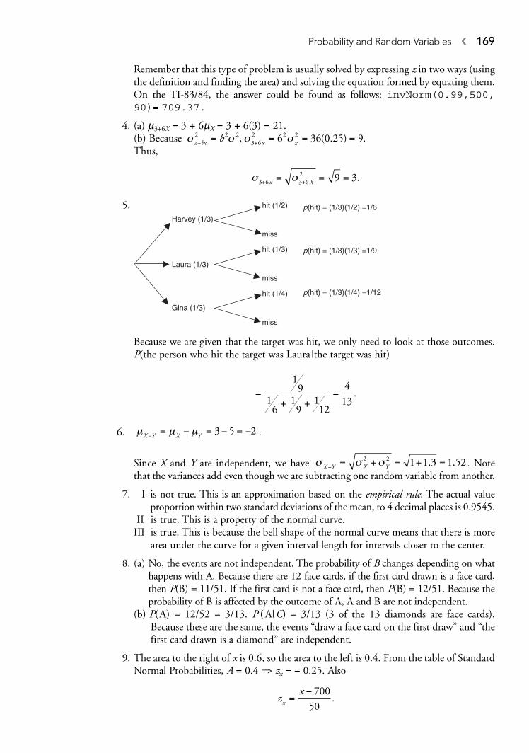
Probability and Random Variables � 169
Remember that this type of problem is usually solved by expressing z in two ways (usingthe definition and finding the area) and solving the equation formed by equating them.On the TI-83/84, the answer could be found as follows: invNorm(0.99,500,90)= 709.37.
4. (a) m3+6X = 3 + 6mX = 3 + 6(3) = 21.(b) Because Thus,
5.
Because we are given that the target was hit, we only need to look at those outcomes.P(the person who hit the target was Laura |the target was hit)
6. .
Since X and Y are independent, we have . Notethat the variances add even though we are subtracting one random variable from another.
7. I is not true. This is an approximation based on the empirical rule. The actual value proportion within two standard deviations of the mean, to 4 decimal places is 0.9545.
II is true. This is a property of the normal curve.III is true. This is because the bell shape of the normal curve means that there is more
area under the curve for a given interval length for intervals closer to the center.
8. (a) No, the events are not independent. The probability of B changes depending on whathappens with A. Because there are 12 face cards, if the first card drawn is a face card,then P(B) = 11/51. If the first card is not a face card, then P(B) = 12/51. Because theprobability of B is affected by the outcome of A, A and B are not independent.
(b) P(A) = 12/52 = 3/13. P ( A|C) = 3/13 (3 of the 13 diamonds are face cards).Because these are the same, the events “draw a face card on the first draw” and “thefirst card drawn is a diamond” are independent.
9. The area to the right of x is 0.6, so the area to the left is 0.4. From the table of StandardNormal Probabilities, A = 0.4 ⇒ zx = − 0.25. Also
zx
x =− 700
50.
σ σ σX Y X Y− = + = + =2 2 1 1 3 1 52. .
μ μ μX Y X Y− = − = − = −3 5 2
=+ +
=1
91
61
9112
4
13.
p(hit) = (1/3)(1/2) =1/6
Harvey (1/3)
p(hit) = (1/3)(1/3) =1/9
Laura (1/3)
hit (1/4) p(hit) = (1/3)(1/4) =1/12
Gina (1/3)
miss
hit (1/3)
miss
hit (1/2)
miss
σ σ3 6 3 62 9 3+ += = =x X .
σ σ σ σa bx x xb+ += = = =2 2 23 62 2 26 36 0 25 9, ( . ) .

So,
60% of the area is to the right of 687.5. The calculator answer is given byinvNorm(0.4,700,50)=687.33.
10. Let D = “a home has a desktop computer”; L = “a home has a laptop computer.” Weare given that P(D) = 0.8 and P(D and L) = 0.3. Thus,
11. The situation can be pictured as shown below.The shaded area is a trapezoid whose area is
.
12. The fact that Harv’s pumpkin is at the 90th percentile means that it is larger than 90%of the pumpkins in the contest. From the table of Standard Normal Probabilities, thearea to the left of a term with a z-score of 1.28 is about 0.90. Thus,
So, Harv’s pumpkin weighed about 148 pounds (for your information, the winningpumpkin at the Half Moon Bay Pumpkin Festival in 2008 weighed over 1528 pounds!).Seven of the 62 pumpkins weighed more than 1000 pounds!
13. Since , we have P (X = 4) = 1 – P (X = 2) – P (X = 3) = 1 – 0.3 – 0.5 = 0.2.Thus, filling in the table for X, we have
Since X and Y are independent, P(X = 4 and Y = 3) = P(X = 4) • P(X = 3). We are giventhat P(X = 4 and Y = 3) = 0.03. Thus, P(X = 4) • P(Y = 3) = 0.03. Since we now know that
P(X = 4) = 0.2, we have (0.2). P(Y = 3) = 0.03, which gives us P (Y = 3) = .
Now, since , we have P(Y = 5) = 1 – P(Y = 3) – P(Y = 4) – P(Y = 6) =1 – 0.15 – 0.1 – 0.4 = 0.35.
14. Let A = “the number is divisible by 24” = {24, 48, 72, 96}. Let B = “the number is divis-ible by 36” = {36, 72}.Note that P(A and B) = (72 is the only number divisible by both 24 and 36).
P(win a pizza) = P(A or B) = P(A) + P(B) – P(A and B) =
15. Because the numbers of men and women in the school are about equal (that is, P(women) = 0.5), let an even number represent a female and an odd number represent a male. Begin on the first line of the table and consider groups of 12 digits.
4
100
2
100
1
100
5
1000 05+ − = = . .
1
100
∑ =P ( )Y 1
0 03
0 20 15
.
..=
X 2 3 4
P (X) 0.3 0.5 0.2
∑ =P ( )X 1
zx
xx = =−
⇒ =1 28125
18148 04. . .
1
20 7 0 2 2 0 2 2 0 7 0 45( . . )[ ( . ) ( . )] .− + =
PP L
P( )
( )
( )
.
..L | D
D
D=
∩= =
0 3
0 8
3
8
zx
xx =−
= − ⇒ =700
500 25 687 5. . .
170 � Step 4. Review the Knowledge You Need to Score High
y = 2x
0 .2 .7 1

Probability and Random Variables � 171
Count the even numbers among the 12. This will be the number of females among thegroup. Repeat five times. The relevant part of the table is shown below, with even num-bers underlined and groups of 12 separated by two slanted bars (\\):
In the five groups of 12 people, there were 3, 6, 3, 8, and 6 women. (Note: The resultwill, of course, vary if a different assignment of digits is made. For example, if you letthe digits 0 − 4 represent a female and 5 − 9 represent a male, there would be 4, 7, 7, 5,and 7 women in the five groups.) So, in 40% of the trials there were 4 or fewer womenin the class even though we would expect the average to be 6 (the average of these 5 trials is 5.2). Hence, it seems that getting only 4 women in a class when we expect 6really isn’t too unusual because it occurs 40% of the time. (It is shown in the next chap-ter that the theoretical probability of getting 4 or fewer women in a group of 12 people,assuming that men and women are equally likely, is about 0.19.)
16. Because P(girl) = 0.6, let the random digits 1, 2, 3, 4, 5, 6 represent the birth of a girland 0, 7, 8, 9 represent the birth of a boy. Start on the second row of the random digittable and move across the line until you find the third digit that represents a girl. Notethe number of digits needed to get three successes. Repeat 5 times and compute theaverage. The simulation is shown below (each success, i.e., girl, is underlined and sep-arate trials are delineated by \\).
79692 51707 73274 12548 91497 11135 81218 79572 06484 87440
Start: 4195\\7 21607 5\\124\\8 54772 \\19481\\ 90392 35268 36234
It took 4, 7, 3, 6, and 5 children before they got their three girls. The average wait was 5.(The theoretical average is exactly 5—we got lucky this time!). As with Exercise 15, theresult will vary with different assignment of random digits.
17. (a) P(x ≤ 22) = P(x = 20) + P(x = 21) + P(x = 22) = 0.2 + 0.3 + 0.2 = 0.7.(b) P(x > 21) = P(x = 22) + P(x = 23) + P(x = 24) = 0.2 + 0.1 + 0.2 = 0.5.(c) P(21 ≤ x < 24) = P(x = 21) + P(x = 22) + P(x = 23) = 0.3 + 0.2 + 0.1 = 0.6.(d) P(x ≤ 21 or x > 23) = P(x = 20) + P(x = 21) + P(x = 24) = 0.2 + 0.3 + 0.2 = 0.7.
18. (a) 18 of the 38 slots are winners, so P(win if bet on red)
(b) The probability distribution for this game is
= =18
380 474. .
79692 51707 73\\274 12548 9149\\7 11135 81218
7\\9572 06484 874\\40 41957 21607\\
Outcome Win Lose
X 1 − 1
P(X ) 2038
1838
The player will lose 5.2¢, on average, for each dollar bet.
E X X( ) ( ) .= =⎛⎝⎜
⎞⎠⎟
+ −⎛⎝⎜
⎞⎠⎟
= −μ18
381
20
380 052 or 5.2 .− ¢

19. From the tables, we see that P(z < − 2.5) = P(z > 2.5) = 0.0062. So the probability thatwe are more than 2.5 standard deviations from the mean is 2(0.0062) = 0.0124. (Thiscan be found on the calculator as follows: 2 normalcdf (2.5,1000).)
20. The situation can be pictured as follows:
If 90% of the area is to the right of 50, then 10% of the area is to the left. So,
.
Solutions to Cumulative Review Problems
1. II is true: the mean is most likely greater than the median. This is because the mean,being nonresistant, is pulled in the direction of outliers or skewness. Because the givenhistogram is clearly skewed to the right, the mean is likely to be to the right of (that is,greater than) the median.
2. The kind of sample you want is a stratified random sample. The sample should have 25 Asian students, 8 African American students, 12 Latino students, and 55 Caucasianstudents. You could get a list of all Asian students from the data clerk and randomlyselect 25 students from the list. Repeat this process for percentages of AfricanAmerican, Latino, and Caucasian students. Now the proportion of each ethnic groupin your sample is the same as its proportion in the population.
3. The five-number summary is 20 − 32 − 42 − 46 − 50. The box plot looks like this:
4. (a) The LSRL line is: #Manatee deaths = − 41.430 + 0.12486(#boats).(b) For each additional registered powerboat, the number of manatee deaths is pre-
dicted to increase by 0.12. You could also say that the number increases, on aver-age, by 0.12.
5. For this set of data, and s = 2.0. Examination of the 25 points in the datasetyields the following.
x = 9 9.
20 32 42 46 50
z50 1 2850
1265 36= − =
−→ =. .
μμ
0.1
–50
172 � Step 4. Review the Knowledge You Need to Score High

Probability and Random Variables � 173
The actual values in the dataset (16, 25, 25) are quite close to the expected values(17, 23.8, 24.9) if this truly were data from a normal population. Hence, it seemsreasonable that the data could have been a random sample drawn from a populationthat is approximately normally distributed.
Percentage expected Number of termsin each interal by the from datasetempirical rule in each interval
9.9 ± 1(2) = ‘7.9,11.9’ 68% (17/25) 16/25 = 64%
9.9 ± 2(2) = ‘5.9,13.9’ 95% (23.8/25) 25/25 = 100%
9.9 ± 3(2) = ‘3.9,15.9’ 99.7% (24.9/25) 25/25 = 100%

CHAPTER 10
174 �
Binomial Distributions, GeometricDistributions, and Sampling
Distributions
IN THIS CHAPTERSummary: In this chapter we finish laying the mathematical (probability) basisfor inference by considering the binomial and geometric situations that occuroften enough to warrant our study. In the last part of this chapter, we beginour study of inference by introducing the idea of a sampling distribution, one of the most important concepts in statistics. Once we’ve mastered thismaterial, we will be ready to plunge into a study of formal inference(Chapters 11–14).
Key Ideas
� Binomial Distributions� Normal Approximation to the Binomial� Geometric Distributions� Sampling Distributions� Central Limit Theorem
Binomial DistributionsA binomial experiment has the following properties:
• The experiment consists of a fixed number, n, of identical trials.• There are only two possible outcomes (that’s the “bi” in “binomial”): success (S ) or
failure (F ).
KEY IDEA

Binomial Distributions, Geometric Distributions, and Sampling Distributions � 175
• The probability of success, p, is the same for each trial.• The trials are independent (that is, knowledge of the outcomes of earlier trials does not
affect the probability of success of the next trial).• Our interest is in a binomial random variable X, which is the count of successes in n
trials. The probability distribution of X is the binomial distribution.
(Taken together, the second, third, and fourth bullets above are called Bernoulli trials.One way to think of a binomial setting is as a fixed number n of Bernoulli trials in whichour random variable of interest is the count of successes X in the n trials. You do not needto know the term Bernoulli trials for the AP exam.)
The short version of this is to say that a binomial experiment consists of n independenttrials of an experiment that has two possible outcomes (success or failure), each trial havingthe same probability of success ( p). The binomial random variable X is the count of successes.
In practice, we may consider a situation to be binomial when, in fact, the independ-ence condition is not quite satisfied. This occurs when the probability of occurrence of agiven trial is affected only slightly by prior trials. For example, suppose that the probabilityof a defect in a manufacturing process is 0.0005. That is, there is, on average, only 1 defectin 2000 items. Suppose we check a sample of 10,000 items for defects. When we check thefirst item, the proportion of defects remaining changes slightly for the remaining 9,999items in the sample. We would expect 5 out of 10,000 (0.0005) to be defective. But if thefirst one we look at is not defective, the probability of the next one being defective haschanged to 5/9999 or 0.0005005. It’s a small change but it means that the trials are not,strictly speaking, independent. A common rule of thumb is that we will consider a situa-tion to be binomial if the population size is at least 10 times the sample size.
Symbolically, for the binomial random variable X, we say X has B(n, p).
example: Suppose Dolores is a 65% free throw shooter. If we assume that thatrepeated shots are independent, we could ask, “What is the probability thatDolores makes exactly 7 of her next 10 free throws?” If X is the binomialrandom variable that gives us the count of successes for this experiment, thenwe say that X has B (10,0.65). Our question is then: P(X = 7) = ?.
We can think of B(n,p,x) as a particular binomial probability. In this example,then, B(10,0.65,7) is the probability that there are exactly 7 successes in 10 repe-titions of a binomial experiment where p = 0.65. This is handy because it is thesame syntax used by the TI-83/84 calculator (binompdf(n,p,x)) whendoing binomial problems.
If X has B(n, p), then X can take on the values 0,1,2, …, n. Then,
gives the binomial probability of exactly x successes for a binomial random variable Xthat has B(n, p).
Now,
On the TI-83/84, nx
⎛
⎝⎜
⎞
⎠⎟=
n rC ,
nx
nx n x
⎛
⎝⎜
⎞
⎠⎟=
−
!
!( )!.
B n p x P X x p pxn x n x( , , ) ( ) ( )= = = ( ) − −1

and this is found in the MATH PRB menu. n! (“n factorial”) means n(n – 1)(n – 2) …(2)(1,), and the factorial symbol can be found in the MATH PRB menu.
example: Find B(15,.3,5). That is, find P(X = 5) for a 15 trials of a binomialrandom variable X that succeeds with probability 3.
solution:
(On the TI-83/84, = nCCrr can be found
in the MATH PRB menu. To get , enter 15nCr5.)
Calculator Tip: On the TI-83/84, the solution to the previous example is given bybinompdf(15,0.3,5). The binompdf function is found in the DISTR menuof the calculator. The syntax for this function is binompdf(n, p, x).The functionbinomcdf(n, p, x) = P(X = 0) + P(X =1) + … P(X = x). That is, it adds up thebinomial probabilities from n = 0 through n = x. You must remember the “npx” order—it’s not optional. Try a mnemonic like “never play xylophone.”
example: Consider once again our free-throw shooter (Dolores) from an earlierexample. Dolores is a 65% free-throw shooter and each shot is independent. IfX is the count of free throws made by Dolores, then X has B(10, 0.65) if sheshoots 10 free throws. What is P(X = 7)?
solution:
example: What is the probability that Dolores makes no more than 5 free throws?That is, what is P(X ≤ 5)?
solution:
There is about a 25% chance that she will make 5 or fewer free throws. The solution to this problem using the calculator is given by binomcdf(10,0.65,5).
P X P X P X P X P X
P X P X
( ) ( ) ( ) ( ) ( )
( ) (
≤ = = + = + = + =
+ = + =
5 0 1 2 3
4 5)) ( . ) ( . ) ( . ) ( .=⎛
⎝⎜
⎞
⎠⎟ +
⎛
⎝⎜
⎞
⎠⎟
100
0 65 0 35 101
0 65 00 10 1 335
105
0 65 0 35 0 249
9
5 5
)
( . ) ( . ) . .+ +⎛
⎝⎜
⎞
⎠⎟ =�
P X( ) ( . ) ( . )!
! !( . ) (= =
⎛
⎝⎜
⎞
⎠⎟ =7 10
70 65 0 35
10
7 30 65 07 3 7 .. )
. .
65
0 252
3
= =binompdf(10,0.65,7)
155
⎛
⎝⎜
⎞
⎠⎟
nr
⎛
⎝⎜
⎞
⎠⎟
P X( ) ( . ) ( . )
!
! !( . )
= =⎛
⎝⎜
⎞
⎠⎟ −
=
−5 155
0 3 1 0 3
15
5 100 3
5 15 5
55 100 7 206( . ) . .=
176 � Step 4. Review the Knowledge You Need to Score High

Binomial Distributions, Geometric Distributions, and Sampling Distributions � 177
example: What is the probability that Dolores makes at least 6 free throws?
solution: P(X ≥ 6) = P(X = 6) + P(X = 7) + … + P(X = 10) = 1-binomcdf(10,0.65,5)=0.751.
(Note that P(X > 6) = 1 − binomcdf(10,0.65,6)).
The mean and standard deviation of a binomial random variable X are given byA binomial distribution for a given n and p (meaning you have
all possible values of x along with their corresponding probabilities) is an example of a prob-ability distribution as defined in Chapter 7. The mean and standard deviation of a binomialrandom variable X could be found by using the formulas from Chapter 7,
but clearly the formulas for the binomial are easier to use. Be careful that you don’t try touse the formulas for the mean and standard deviation of a binomial random variable for adiscrete random variable that is not binomial.
example: Find the mean and standard deviation of a binomial random variable X thathas B(85, 0.6).
solution:
Normal Approximation to the BinomialUnder the proper conditions, the shape of a binomial distribution is approximately normal,and binomial probabilities can be estimated using normal probabilities. Generally, this istrue when np ≥ 10 and n(1 − p) ≥ 10 (some books use np ≥ 5 and n(1 − p) ≥ 5; that’s OK).These conditions are not satisfied in Graph A (X has B(20, 0.1)) below, but they are satis-fied in Graph B (X has B(20, 0.5))
It should be clear that Graph A is noticeably skewed to the right, and Graph B isapproximately normal in shape, so it is reasonable that a normal curve would approximateGraph B better than Graph A. The approximating normal curve clearly fits the binomialhistogram better in Graph B than in Graph A.
When np and n(1 − p) are sufficiently large (that is, they are both greater than or equalto 5 or 10), the binomial random variable X has approximately a normal distribution with
μ = = −np np pand σ ( ).1
Graph A: B (20, 0.1) Graph B: B (20, 0.5)
μ σX X
= = = =( )( . ) ; ( . )( . ) . .85 0 6 51 85 0 6 0 4 4 52
μ μx i i x x i
i
n
i
n
x p x p= = −⎛
⎝
⎜⎜
⎞
⎠
⎟⎟
==
∑∑ and σ ( ) ,2
11
μ σX Xnp np p= = −; ( ).1

178 � Step 4. Review the Knowledge You Need to Score High
Another way to say this is: If X has B(n, p), then X has approximately
, provided that np ≥ 10 and n(1 − p) ≥ 10 (or np ≥ 5 and n(1 − p) ≥ 5).
example: Nationally, 15% of community college students live more than 6 milesfrom campus. Data from a simple random sample of 400 students at one com-munity college are analyzed.
(a) What are the mean and standard deviation for the number of students in thesample who live more than 6 miles from campus?
(b) Use a normal approximation to calculate the probability that at least 65 of thestudents in the sample live more than 6 miles from campus.
solution: If X is the number of students who live more than 6 miles from campus,then X has B(400, 0.15).
(a)
(b) Because 400(0.15) = 60 and 400(0.85) = 340, we can use the normal approxi-mation to the binomial with mean 60 and standard deviation 7.14. The situationis pictured below:
Using Table A, we have = 1 – 0.7580 = 0.242.
By calculator, this can be found as normalcdf(65,1000,60,7.14)= 0.242.
The exact binomial solution to this problem is given by
1-binomcdf(400,0.15,64) = 0.261 (you use x = 64 since P(X ≥ 65) = 1 – P(X ≤ 64)).
In reality, you will need to use a normal approximation to the binomial only in lim-ited circumstances. In the example above, the answer can be arrived at quite easily using theexact binomial capabilities of your calculator. The only time you might want to use anormal approximation is if the size of the binomial exceeds the capacity of your calculator(for example, enter binomcdf(50000000,0.7,3250000). You’ll most likely seeERR:DOMAIN, which means you have exceeded the capacity of your calculator, and youdidn’t have access to a computer. The real concept you need to understand the normalapproximation to a binomial is that another way of looking at binomial data is in terms ofthe proportion of successes rather than the count of successes. We will approximate a distri-bution of sample proportions with a normal distribution and the concepts and conditionsfor it are the same.
P X P z( ).
.≥ = ≥−
=⎛⎝⎜
⎞⎠⎟
6565 60
7 140 70
60 65
?
µ = = 400(0.15)(0.85)400 0 15 60 7 14( . ) ; . .= =σ
N np np p( , ( ))1−

Geometric DistributionsIn Section 8.1, we defined a binomial setting as a experiment in which the following con-ditions are present:
• The experiment consists of a fixed number, n, of identical trials.• There are only two possible outcomes: success (S ) or failure (F ).• The probability of success, p, is the same for each trial.• The trials are independent (that is, knowledge of the outcomes of earlier trials does not
affect the probability of success of the next trial).• Our interest is in a binomial random variable X, which is the count of successes in n
trials. The probability distribution of X is the binomial distribution.
There are times we are interested not in the count of successes out of n fixed trials, butin the probability that the first success occurs on a given trial, or in the average number oftrials until the first success. A geometric setting is defined as follows.
• There are only two possible outcomes: success (S ) or failure (F ).• The probability of success, p, is the same for each trial.• The trials are independent (that is, knowledge of the outcomes of earlier trials does not
affect the probability of success of the next trial).• Our interest is in a geometric random variable X, which is the number of trials neces-
sary to obtain the first success.
Note that if X is a binomial, then X can take on the values 0, 1, 2, …, n. If X is geomet-ric, then it takes on the values 1, 2, 3,…. There can be zero successes in a binomial, but theearliest a first success can come in a geometric setting is on the first trial.
If X is geometric, the probability that the first success occurs on the nth trial is given byP (X = n) = p(1 − p)n−1. The value of P(X = n) in a geometric setting can be found on theTI-83/84 calculator, in the DISTR menu, as geometpdf(p, n) (note that the order ofp and n are, for reasons known only to the good folks at TI, reversed from the binomial).Given the relative simplicity of the formula for P(X = n) for a geometric setting, it’s probablyjust as easy to calculate the expression directly. There is also a geometcdf function thatbehaves analogously to the binomcdf function, but is not much needed in this course.
example: Remember Dolores, the basketball player whose free-throw shootingpercentage was 0.65? What is the probability that the first free throw she man-ages to hit is on her fourth attempt?
solution: P(X = 4) = (0.65) (1−0.65)4-1 = (0.65) (0.35)3 = 0.028. This can be done onthe TI-83/84 as follows: geometpdf(p,n) = geometpdf(0.65,4) = 0.028.
example: In a standard deck of 52 cards, there are 12 face cards. So the probabil-ity of drawing a face card from a full deck is 12/52 = 0.231.
(a) If you draw cards with replacement (that is, you replace the card in the deckbefore drawing the next card), what is the probability that the first face cardyou draw is the 10th card?
(b) If you draw cards without replacement, what is the probability that the firstface card you draw is the 10th card?
solution:
(a) P(X = 10) = (0.231) (1 – 0.231)9 = 0.022. On the TI-83/84: geometpdf(0.231,10)= 0.0217).
Binomial Distributions, Geometric Distributions, and Sampling Distributions � 179

180 � Step 4. Review the Knowledge You Need to Score High
(b) If you don’t replace the card each time, the probability of drawing a face cardon each trial is different because the proportion of face cards in the deckchanges each time a card is removed. Hence, this is not a geometric settingand cannot be answered the by techniques of this section. It can be answered,but not easily by the techniques of the previous chapter.
Rather than the probability that the first success occurs on a specified trial, we may be interested in the average wait until the first success. The average wait until the first success of a geometric random variable is 1/p. (This can be derived by summing(1)•P(X = 1) + (2)•P(X = 2) + (3)•P(X = 3) +... = 1p + 2p(1 – p) + 3p(1 – p)2 + …, whichcan be done using algebraic techniques for summing an infinite series with a commonratio less than 1.)
example: On average, how many free throws will Dolores have to take beforeshe makes one (remember, p = 0.65)?
solution: .
Since, in a geometric distribution, P(X = n) = p(1−p)n−1 the probabilities become less likely as n increases since we are multiplying by 1 − p, a number lessthan one. The geometric distribution has a step-ladder approach that looks likethis:
Sampling DistributionsSuppose we drew a sample of size 10 from a normal population with unknown mean andstandard deviation and got . Two questions arise: (1) what does this sample tellus about the population from which the sample was drawn, and (2) what would happen ifwe drew more samples?
Suppose we drew 5 more samples of size 10 from this population and gotIn answer to question (1), we
might believe that the population from which these samples was drawn had a mean around20 because these averages tend to group there (in fact, the six samples were drawn from anormal population whose mean is 20 and whose standard deviation is 4). The mean of the6 samples is 19.64, which supports our feeling that the mean of the original populationmight have been 20.
The standard deviation of the 6 samples is 0.68 and you might not have any intuitivesense about how that relates to the population standard deviation, although you might sus-pect that the standard deviation of the samples should be less than the standard deviationof the population because the chance of an extreme value for an average should be less thanthat for an individual term (it just doesn’t seem very likely that we would draw a lot ofextreme values in a single sample).
x x x x x= = = = =20 35 20 04 19 20 19 02 20 35. , . , . , . , . .and
x = 18 87.
10 65
1 54.
.=

Suppose we continued to draw samples of size 10 from this population until we wereexhausted or until we had drawn all possible samples of size 10. If we did succeed in draw-ing all possible samples of size 10, and computed the mean of each sample, the distributionof these sample means would be the sampling distribution of .
Remembering that a “statistic” is a value that describes a sample, the sampling distri-bution of a statistic is the distribution of that statistic for all possible samples of a givensize. It’s important to understand that a dotplot of a few samples drawn from a populationis not a distribution (it’s a simulation of a distribution)—it becomes a distribution onlywhen all possible samples of a given size are drawn.
Sampling Distribution of a Sample MeanSuppose we have the sampling distribution of . That is, we have formed a distribution ofthe means of all possible samples of size n from an unknown population (that is, we knowlittle about its shape, center, or spread). Let and represent the mean and standarddeviation of the sampling distribution of , respectively.
Then
for any population with mean μ and standard deviation s.(Note: the value given for above is generally considered correct only if the sample
size (n) is small relative to N, the number in the population. A general rule is that n shouldbe no more than 5% of N to use the value given for (that is, N > 20n). If n is morethan 5% of N, the exact value for the standard deviation of the sampling distribution is
In practice this usually isn’t a major issue because
is close to one whenever N is large in comparison to n. You don’t have to know this forthe AP exam.)
example: A large population is know to have a mean of 23 and a standard deviation of 2.5. What are the mean and standard deviation of the samplingdistribution of means of samples of size 20 drawn from this population?
solution:
Central Limit TheoremThe discussion above gives us measures of center and spread for the sampling distributionof but tells us nothing about the shape of the sampling distribution. It turns out that theshape of the sampling distribution is determined by (a) the shape of the original populationand (b) n, the sample size. If the original population is normal, then it’s easy: the shape ofthe sampling distribution will be normal if the population is normal.
x
μ μ σσ
x xn
= = = = =232 5
200 559,
.. .
N nN
−
−1
σσ
xn
N nN
=−
−1.
σ x
σ x
μ μ σσ
xn
= =andx
xσ xμx
x
x
Binomial Distributions, Geometric Distributions, and Sampling Distributions � 181

182 � Step 4. Review the Knowledge You Need to Score High
If the shape of the original population is not normal, or unknown, and the sample sizeis small, then the shape of the sampling distribution will be similar to that of the originalpopulation. For example, if a population is skewed to the right, we would expect the sam-pling distribution of the mean for small samples also to be somewhat skewed to the right,although not as much as the original population.
When the sample size is large, we have the following result, known as the central limittheorem: For large n, the sampling distribution of will be approximately normal. Thelarger is n, the more normal will be the shape of the sampling distribution.
A rough rule-of-thumb for using the central limit theorem is that n should be at least 30,although the sampling distribution may be approximately normal for much smaller valuesof n if the population doesn’t depart markedly from normal. The central limit theoremallows us to use normal calculations to do problems involving sampling distributions with-out having to have knowledge of the original population. Note that calculations involvingz-procedures require that you know the value of σ, the population standard deviation. Sinceyou will rarely know σ, the large sample size essentially says that the sampling distributionis approximately, but not exactly, normal. That is, technically you should not be using z-procedures unless you know σ but, as a practical matter, z-procedures are numericallyclose to correct for large n. Given that the population size (N) is large in relation to thesample size (n), the information presented in this section can be summarized in the following table:
x
example: Describe the sampling distribution of for samples of size 15 drawnfrom a normal population with mean 65 and standard deviation 9.
solution: Because the original population is normal, is normal with mean 65
and standard deviation
example: Describe the sampling distribution of for samples of size 15 drawnfrom a population that is strongly skewed to the left (like the scores on a veryeasy test) with mean 65 and standard deviation 9.
x
9
152 32 65
9
15=
⎛
⎝⎜⎜
⎞
⎠⎟⎟. . , .That is, hasx N
x
x
POPULATION SAMPLING DISTRIBUTION
Mean μ
Standard σDeviation
Shape Normal Normal
Undetermined If n is “small” shape is similar (skewed, etc.) to shape of original graph
ORIf n is “large” (rule of thumb:
n ≥ 30) shape is approximately normal (central limit theorem)
μ μx =
σσ
xn
=

solution: and as in the above example. However this timethe population is skewed to the left. The sample size is reasonably large, but notlarge enough to argue, based on our rule-of-thumb (n ≥ 30), that the samplingdistribution is normal. The best we can say is that the sampling distribution isprobably more mound shaped than the original but might still be somewhatskewed to the left.
example: The average adult has completed an average of 11.25 years of educationwith a standard deviation of 1.75 years. A random sample of 90 adults isobtained. What is the probability that the sample will have a mean
(a) greater than 11.5 years?
(b) between 11 and 11.5 years?
solution: The sampling distribution of has and
Because the sample size is large (n = 90), the central limit theorem tells us thatlarge sample techniques are appropriate. Accordingly,
(a) The graph of the sampling distribution is shown below:
(b) From part (a), the area to the left of 11.5 is 1 – 0.0869 = 0.9131. Since thesampling distribution is approximately normal, it is symmetric. Since 11 is the same distance to the left of the mean as 11.5 is to the right, we know thatP( < 11) = P( > 11.5) = 0.0869. Hence, P(11 < < 11.5) = 0.9131 –0.0869 = 0.8262. The calculator solution is normalcdf(11,11.5,11,0.184)=0.8258.
example: Over the years, the scores on the final exam for AP Calculus have beennormally distributed with a mean of 82 and a standard deviation of 6. Theinstructor thought that this year’s class was quite dull and, in fact, they onlyaveraged 79 on their final. Assuming that this class is a random sample of
xxx
P x P z( . ). ..
.
..> = >
−= =
⎛
⎝
⎜11 5
11 5 11 251 75
90
0 25
0 1841 36⎜⎜
⎜⎜
⎞
⎠
⎟⎟⎟⎟= 0 0869. .
11 11.25 11.5
σ x = =1 75
900 184
.. .
μx = 11 25.x
σ x = 2 32.μx = 65
Binomial Distributions, Geometric Distributions, and Sampling Distributions � 183
184 � Step 4. Review the Knowledge You Need to Score High
32 students from AP Calculus, what is the probability that the average score onthe final for this class is no more than 79? Do you think the instructor was right?
solution:
If this group really were typical, there is less than a 1% probability of getting anaverage this low by chance alone. That seems unlikely, so we have good evidencethat the instructor was correct.
(The calculator solution for this problem is normalcdf(-1000,79,82,1.06).)
Sampling Distributions of a Sample ProportionIf X is the count of successes in a sample of n trials of a binomial random variable, then theproportion of success is given by is what we use for the sample proportion(a statistic). The true population proportion would then be given by p.
ˆ / . ˆp X n p=
P x P z( ).
. .≤ = ≤−
=−
= −
⎛
⎝
⎜⎜⎜
⎞
⎠
⎟⎟⎟=79
79 826
32
3
1 062 83 0 00223.
Digression: Before introducing , we have used and s as statistics, and μ and σ asparameters. Often we represent statistics with English letters and parameters with Greekletters. However, we depart from that convention here by using as a statistic and p as a parameter. There are texts that are true to the English/Greek convention by usingp for the sample proportion and � for the population proportion.
p
xp
We learned in Section 8.1 that, if X is a binomial random variable, the mean and stan-dard deviation of the sampling distribution of X are given by
We know that if we divide each term in a dataset by the same value n, then the meanand standard deviation of the transformed dataset will be the mean and standard deviationof the original dataset divided by n. Doing the algebra, we find that the mean and standarddeviation of the sampling distribution of are given by:
Like the binomial, the sampling distribution of will be approximately normally dis-tributed if n and p are large enough. The test is exactly the same as it was for the binomial:If X has B(n,p), and , then has approximately
provided that np ≥ 10 and n(1 − p) ≥ 10 (or np ≥ 5 and n(1 − p) ≥ 5).
N pp p
n,
( ),
1−⎛
⎝⎜⎜
⎞
⎠⎟⎟
pp X n= /
p
μ σˆ ˆ
( ).
p pp
p p
n= =
−,
1
p
μ σX Xnp np p= = −, ( ).1

example: Harold fails to study for his statistics final. The final has 100 multiplechoice questions, each with 5 choices. Harold has no choice but to guess ran-domly at all 100 questions. What is the probability that Harold will get at least30% on the test?
solution: Since 100(0.2) and 100(0.8) are both greater than 10, we can use the normal approximation to the sampling distribution of . Since
Therefore,
. The TI-83/84 solution is given by
normalcdf(0.3,100,0.2,0.040)=0.0062.
Harold should have studied.
� Rapid Review
1. A coin is known to be unbalanced in such a way that heads only comes up 0.4 of the time.
(a) What is the probability the first head appears on the 4th toss?(b) How many tosses would it take, on average, to flip two heads?
Answer:
(a) P(first head appears on fourth toss) = 0.4 (1 – 0.4)4−1 = 0.4(0.6)3 = 0.0864
(b) Average wait to flip two heads = 2(average wait to flip one head) = .
2. The coin of problem #1 is flipped 50 times. Let X be the number of heads. What is
(a) the probability of exactly 20 heads?(b) the probability of at least 20 heads?
Answer:
(a) P(X =20) = [on the TI-83/84: binompdf(50,
0.4,20).]
(b) P(X ≥ 20) =
= 1-binomcdf(50,0.4,19)=0.554.
3. A binomial random variable X has B(300, 0.2). Describe the sampling distribution of
Answer: Since 300(0.2) = 60 ≥ 10 and 300(0.8) = 240 ≥ 10, has approximately a
normal distribution with and .
4. A distribution is known to be highly skewed to the left with mean 25 and standarddeviation 4. Samples of size 10 are drawn from this population and the mean of eachsample is calculated. Describe the sampling distribution of .x
σ ˆ
. ( . ).p =
−=
0 2 1 0 2
3000 023μ ˆ .p = 0 2
p
ˆ.p
5020
0 4 0 65021
0 420 30 21⎛⎝⎜
⎞⎠⎟
+⎛⎝⎜
⎞⎠⎟
( . ) ( . ) ( . ) (00 65050
0 4 0 629 50 0. ) ... ( . ) ( . )+ +⎛⎝⎜
⎞⎠⎟
5020
0 4 0 6 0 11520 30⎛⎝⎜
⎞⎠⎟
=( . ) ( . ) .
21
0 45
.
⎛
⎝⎜
⎞
⎠⎟=
P p P z( ˆ . ). .
.. .≥ = ≥
−=
⎛
⎝⎜
⎞
⎠⎟=0 3
0 3 0 2
0 042 5 0 0062
p p p= = =−
=0 2 0 20 2 1 0 2
1000 04. , .
. ( . ). .ˆ ˆμ σand
p
Binomial Distributions, Geometric Distributions, and Sampling Distributions � 185

186 � Step 4. Review the Knowledge You Need to Score High
Answer:
Since the samples are small, the shape of the sampling distribution would proba-bly show some left-skewness but would be more mound shaped than the originalpopulation.
5. What is the probability that a sample of size 35 drawn from a population with mean 65and standard deviation 6 will have a mean less than 64?
Answer: The sample size is large enough that we can use large-sample procedures.Hence,
On the TI-83/84, the solution is given by normalcdf(-100,64, 65, ).
Practice ProblemsMultiple Choice1. A binomial event has n = 60 trials. The probability of success on each trial is 0.4.
Let X be the count of successes of the event during the 60 trials. What are μx
and σx?
(a) 24, 3.79(b) 24, 14.4(c) 4.90, 3.79(d) 4.90, 14.4(e) 2.4, 3.79
2. Consider repeated trials of a binomial random variable. Suppose the probability of thefirst success occurring on the second trial is 0.25. What is the probability of success onthe first trial?
(a) 1/4
(b) 1(c) 1/2
(d) 1/8
(e) 3/16
3. To use a normal approximation to the binomial, which of the following does not haveto be true?
(a) np ≥ 5, n(1 −p)≥ 5 (or: np ≥ 10, n (1−p) ≥10).(b) The individual trials must be independent.(c) The sample size in the problem must be too large to permit doing the problem on
a calculator.(d) For the binomial, the population size must be at least 10 times as large as the
sample size.(e) All of the above are true.
635
P x P z( ) . . .< = <−
= −
⎛
⎝
⎜⎜⎜
⎞
⎠
⎟⎟⎟=64
64 656
35
0 99 0 1611
μ σx x= = =254
101 26, . .

4. You form a distribution of the means of all samples of size 9 drawn from an infinitepopulation that is skewed to the left (like the scores on an easy Stats quiz!). The popula-tion from which the samples are drawn has a mean of 50 and a standard deviation of12. Which one of the following statements is true of this distribution?
(a) the sampling distribution is skewed somewhat to the left.(b) the sampling distribution is skewed somewhat to the left.(c) the sampling distribution is approximately normal.(d) the sampling distribution is approximately normal.(e) the sample size is too small to make any statements about the
shape of the sampling distribution.
5. A 12-sided die has faces numbered from 1–12. Assuming the die is fair (that is, eachface is equally likely to appear each time), which of the following would give the exactprobability of getting at least 10 3s out of 50 rolls?
6. In a large population, 55% of the people get a physical examination at least once everytwo years. An SRS of 100 people are interviewed and the sample proportion is com-puted. The mean and standard deviation of the sampling distribution of the sampleproportion are
(a) 55, 4.97(b) 0.55, 0.002(c) 55, 2(d) 0.55, 0.0497(e) The standard deviation cannot be determined from the given information.
7. Which of the following best describes the sampling distribution of a sample mean?
(a) It is the distribution of all possible sample means of a given size.(b) It is the particular distribution in which and .(c) It is a graphical representation of the means of all possible samples.(d) It is the distribution of all possible sample means from a given population.(e) It is the probability distribution for each possible sample size.
σ σx =μ μx =
(e) 500
0 083 0 917 501
0 0830 50 1⎛
⎝⎜
⎞
⎠⎟ +
⎛
⎝⎜
⎞
⎠⎟( . ) ( . ) ( . ) (( . ) ( . ) ( . ) .0 917 50
100 083 0 91749 10 40+ +
⎛
⎝⎜
⎞
⎠⎟…
(d) 1 500
0 083 0 917 501
0 0830 50−⎛
⎝⎜
⎞
⎠⎟ +
⎛
⎝⎜
⎞
⎠⎟( . ) ( . ) ( . )) ( . ) ( . ) ( . )1 49 9 410 917 50
90 083 0 917+ +
⎛
⎝⎜
⎞
⎠⎟
⎡
⎣⎢
⎤
⎦⎥… ..
(c) 1 500
0 083 0 917 501
0 0830 50−⎛
⎝⎜
⎞
⎠⎟ +
⎛
⎝⎜
⎞
⎠⎟( . ) ( . ) ( . )) ( . ) ( . ) ( . )1 49 10 400 917 50
100 083 0 917+ +
⎛
⎝⎜
⎞
⎠⎟
⎡
⎣⎢
⎤…
⎦⎦⎥ .
(b) 5011
0 083 0 917 5012
0 0811 39⎛
⎝⎜
⎞
⎠⎟ +
⎛
⎝⎜
⎞
⎠⎟( . ) ( . ) ( . 33 0 917 50
500 083 0 91712 38 50 0) ( . ) ( . ) ( . ) .+ +
⎛
⎝⎜
⎞
⎠⎟…
(a) 500
0 083 0 917 501
0 0830 50 1⎛
⎝⎜
⎞
⎠⎟ +
⎛
⎝⎜
⎞
⎠⎟( . ) ( . ) ( . ) (( . ) ( . ) ( . ) .0 917 50
90 083 0 91749 9 41+ +
⎛
⎝⎜
⎞
⎠⎟…
μ σx x= =50 4, ,μ σx x= =50 4, ,μ σx x= =50 12, ,μ σx x= =50 4, ,μ σx x= =50 12, ,
Binomial Distributions, Geometric Distributions, and Sampling Distributions � 187

188 � Step 4. Review the Knowledge You Need to Score High
8. Which of the following is not a common characteristic of binomial and geometricexperiments?
(a) There are exactly two possible outcomes: success or failure.(b) There is a random variable X that counts the number of successes.(c) Each trial is independent (knowledge about what has happened on previous trials
gives you no information about the current trial).(d) The probability of success stays the same from trial to trial.(e) P(success) + P(failure) = 1.
9. A school survey of students concerning which band to hire for the next school dance shows70% of students in favor of hiring The Greasy Slugs. What is the approximate probabilitythat, in a random sample of 200 students, at least 150 will favor hiring The Greasy Slugs?
(a)
(b)
(c)
(d)
(e)
Free Response1. A factory manufacturing tennis balls determines that the probability that a single can
of three balls will contain at least one defective ball is 0.025. What is the probabilitythat a case of 48 cans will contain at least two cans with a defective ball?
2. A population is highly skewed to the left. Describe the shape of the sampling distribu-tion of drawn from this population if the sample size is (a) 3 or (b) 30.
3. Suppose you had gobs of time on your hands and decided to flip a fair coin 1,000,000times and note whether each flip was a head or a tail. Let X be the count of heads. Whatis the probability that there are at least 1000 more heads than tails? (Note: this is a bino-mial but your calculator will not be able to do the binomial computation because thenumbers are too large for it).
4. In Chapter 9, we had an example in which we asked if it would change the proportion ofgirls in the population (assumed to be 0.5) if families continued to have children until theyhad a girl and then they stopped. That problem was to be done by simulation. How couldyou use what you know about the geometric distribution to answer this same question?
5. At a school better known for football than academics (a school its football team can beproud of ), it is known that only 20% of the scholarship athletes graduate within 5 years.The school is able to give 55 scholarships for football. What are the expected mean andstandard deviation of the number of graduates for a group of 55 scholarship athletes?
x
P z >−⎛
⎝⎜⎜
⎞
⎠⎟⎟
140 150
200 0 7 0 3( . )( . ).
P z >−⎛
⎝⎜⎜
⎞
⎠⎟⎟
150 140
150 0 7 0 3( . )( . ).
P z >−⎛
⎝⎜⎜
⎞
⎠⎟⎟
150 140
200 0 7 0 3( . )( . ).
200150
0 3 0 7150 50⎛
⎝⎜
⎞
⎠⎟( . ) ( . ) .
200150
0 7 0 3150 50⎛
⎝⎜
⎞
⎠⎟( . ) ( . ) .

6. Consider a population consisting of the numbers 2, 4, 5, and 7. List all possible sam-ples of size two from this population and compute the mean and standard deviation ofthe sampling distribution of . Compare this with the values obtained by relevant for-mulas for the sampling distribution of . Note that the sample size is large relative tothe population—this may affect how you compute by formula.
7. Approximately 10% of the population of the United States is known to have blood type B.If this is correct, what is the probability that between 11% and 15%, inclusive, of arandom sample of 500 adults will have type B blood?
8. Which of the following is/are true of the central limit theorem? (More than one answermight be true.)
III. The sampling distribution of a sample mean will be approximately normally distrib-uted for sufficiently large samples, regardless of the shape of the original population.
IV. The sampling distribution of a sample mean will be normally distributed if thepopulation from which the samples are drawn is normal.
9. A brake inspection station reports that 15% of all cars tested have brakes in need ofreplacement pads. For a sample of 20 cars that come to the inspection station,
(a) what is the probability that exactly 3 have defective breaks?(b) what is the mean and standard deviation of the number of cars that need replace-
ment pads?
10. A tire manufacturer claims that his tires will last 40,000 miles with a standard devia-tion of 5000 miles.
(a) Assuming that the claim is true, describe the sampling distribution of the mean life-time of a random sample of 160 tires. Remember that “describe” means discusscenter, spread, and shape.
(b) What is the probability that the mean life time of the sample of 160 tires will be less than 39,000 miles? Interpret the probability in terms of the truth of themanufacturer’s claim.
11. The probability of winning a bet on red in roulette is 0.474. The binomial probabilityof winning money if you play 10 games is 0.31 and drops to 0.27 if you play 100games. Use a normal approximation to the binomial to estimate your probability ofcoming out ahead (that is, winning more than 1/2 of your bets) if you play 1000 times.Justify being able to use a normal approximation for this situation.
12. Crabs off the coast of Northern California have a mean weight of 2 lbs with a standarddeviation of 5 oz. A large trap captures 35 crabs.
(a) Describe the sampling distribution for the average weight of a random sample of35 crabs taken from this population.
(b) What would the mean weight of a sample of 35 crabs have to be in order to be inthe top 10% of all such samples?
13. The probability that a person recovers from a particular type of cancer operation is 0.7.Suppose 8 people have the operation. What is the probability that
(a) exactly 5 recover?(b) they all recover?(c) at least one of them recovers?
II. ifσσ
xn
N= ≥( ).10n
I. μ μx
= .
σ x
xx
Binomial Distributions, Geometric Distributions, and Sampling Distributions � 189

190 � Step 4. Review the Knowledge You Need to Score High
14. A certain type of light bulb is advertised to have an average life of 1200 hours. If, infact, light bulbs of this type only average 1185 hours with a standard deviation of80 hours, what is the probability that a sample of 100 bulbs will have an average life ofat least 1200 hours?
15. Your task is to explain to your friend Gretchen, who knows virtually nothing (and careseven less) about statistics, just what the sampling distribution of the mean is. Explainthe idea of a sampling distribution in such a way that even Gretchen, if she pays atten-tion, will understand.
16. Consider the distribution shown at the right.Describe the shape of the sampling distribution of forsamples of size n if
(a) n = 3.(b) n = 40.
17. After the Challenger disaster of 1986, it was discovered that the explosion was caused bydefective O-rings. The probability that a single O-ring was defective and would fail (withcatastrophic consequences) was 0.003 and there were 12 of them (6 outer and 6 inner).What was the probability that at least one of the O-rings would fail (as it actually did)?
18. Your favorite cereal has a little prize in each box. There are 5 such prizes. Each box isequally likely to contain any one of the prizes. So far, you have been able to collect 2 ofthe prizes. What is:
(a) the probability that you will get the third different prize on the next box you buy?(b) the probability that it will take three more boxes to get the next prize?(c) the average number of boxes you will have to buy before getting the third prize?
19. We wish to approximate the binomial distribution B(40, 0.8) with a normal curve N(μ, σ).Is this an appropriate approximation and, if so, what are μ and σ for the approximat-ing normal curve?
20. Opinion polls in 2002 showed that about 70% of the population had a favorable opin-ion of President Bush. That same year, a simple random sample of 600 adults living inthe San Francisco Bay Area showed only 65% had a favorable opinion of PresidentBush. What is the probability of getting a rating of 65% or less in a random sample ofthis size if the true proportion in the population was 0.70?
Cumulative Review Problems1. An unbalanced coin has p = 0.6 of turning up heads. Toss the coin three times and let X
be the count of heads among the three coins. Construct the probability distribution forthis experiment.
2. You are doing a survey for your school newspaper and want to select a sample of 25 seniors. You decide to do this by randomly selecting 5 students from each of the 5 senior-level classes, each of which contains 28 students. The school data clerk assuresyou that students have been randomly assigned, by computer, to each of the 5 classes.Is this sample
(a) a random sample?(b) a simple random sample?
x

3. Data are collected in an experiment to measure a person’s reaction time (in seconds) asa function of the number of milligrams of a new drug. The least squares regression line(LSRL) for the data is Reaction Time = 0.2 + 0.8(mg). Interpret the slope of the regres-sion line in the context of the situation.
4. If P(A) = 0.5, P(B) = 0.3, and P(A or B) = 0.65, are events A and B independent?
5. Which of the following is (are) examples of quantitative data and which is (are) examples ofqualitative data?
(a) The height of an individual, measured in inches.(b) The color of the shirts in my closet.(c) The outcome of a flip of a coin described as “heads” or “tails.”(d) The value of the change in your pocket.(e) Individuals, after they are weighed, are identified as thin, normal, or heavy.(f ) Your pulse rate.(g) Your religion.
Solutions to Practice ProblemsMultiple Choice1. The correct answer is (a).
2. The correct answer is (c). If it is a binomial random variable, the probability of success, p, isthe same on each trial. The probability of not succeeding on the first trial and then succeed-ing on the second trial is (1 – p)(p). Thus, (1 – p)p = 0.25. Solving algebraically, p = 1/2.
3. The correct answer is (c). Although you probably wouldn’t need to use a normalapproximation to the binomial for small sample sizes, there is no reason (except perhapsaccuracy) that you couldn’t.
4. The answer is (b).
For small samples, the shape of the sampling distribution of will resemble the shapeof the sampling distribution of the original population. The shape of the sampling dis-tribution of is approximately normal for n sufficiently large.
5. The correct answer is (d). Because the problem stated “at least 10,” we must include theterm where x = 10. If the problem has said “more than 10,” the correct answer wouldhave been (b) or (c) (they are equivalent). The answer could also have been given as
6. The correct answer is (d)..
7. The correct answer is (a).
μ σˆ ˆ. ,( . )( . )
. .p p
p= = = =0 550 55 0 45
1000 0497
5010
0 083 0 917 5011
0 08310 40 1⎛
⎝⎜
⎞
⎠⎟ +
⎛
⎝⎜
⎞
⎠⎟( . ) ( . ) ( . ) 11 39 50 00 917 50
500 083 0 917( . ) ( . ) ( . ) .+ +
⎛
⎝⎜
⎞
⎠⎟…
x
x
μ μσ
x xn
= =, σ .
μ σX X= = = = =( )( . ) , ( . )( . ) . . .60 0 4 24 60 0 4 0 6 14 4 3 79
Binomial Distributions, Geometric Distributions, and Sampling Distributions � 191

192 � Step 4. Review the Knowledge You Need to Score High
8. The correct answer is (b). This is a characteristic of a binomial experiment. The analo-gous characteristic for a geometric experiment is that there is a random variable X thatis the number of trials needed to achieve the first success.
9. The correct answer is (c). This is actually a binomial situation. If X is the count ofstudents “in favor,” then X has B(200, 0.70). Thus, P(X ≥ 150) = P(X = 150) +P(X =151) + . . . + P(X = 200). Using the TI-83/84, the exact binomial answerequals 1–binomcdf (200,0.7.0,149)= 0.0695. None of the listedchoices shows a sum of several binomial expressions, so we assume this is to be doneas a normal approximation. We note that B(200, 0.7) can be approximated by
N = N(140, 6.4807). A normal approximation is OK since200(0.7) and 200(0.3) are both much greater than 10. Since 75% of 200 is
150, we have
Free Response
1. If X is the count of cans with at least one defective ball, then X has B(48, 0.025).
On the TI-83/84, the solution is given by 1–binomcdf(48,0.025,1).
2. We know that the sampling distribution of will be similar to the shape of the orig-inal population for small n and approximately normal for large n (that’s the central limittheorem). Hence,
(a) if n = 3, the sampling distribution would probably be somewhat skewed to the left.(b) if n = 30, the sampling distribution would be approximately normal.
Remember that using n ≥ 30 as a rule of thumb for deciding whether to assume nor-mality is for a sampling distribution just that: a rule of thumb. This is probably a bitconservative. Unless the original population differs markedly from mound shaped andsymmetric, we would expect to see the sampling distribution of be approximatelynormal for considerably smaller values of n.
3. Since the binomcdf function can’t be used due to calculator overflow, wewill use a normal approximation to the binomial. Let X = the count ofheads. Then μX = (1,000,000)(0.5) = 500,000 (assuming a fair coin) and
. Certainly both np and n(1 – p) are greater than5 (waaaaaay larger!), so the conditions needed to use a normal approximation are present.If we are to have at least 1,000 more heads than tails, then there must be at least 500,500heads (and, of course, no more than 499,500 tails). Thus, P(there are at least 1,000
more heads than tails)
4. The average wait for the first success to occur in a geometric setting is 1/p, where p isthe probability of success on any one trial. In this case, the probability of a girl on any
one birth is p = 0.5. Hence, the average wait for the first girl is So, we have
one boy and one girl, on average, for each two children. The proportion of girls in thepopulation would not change.
1
0 52
..=
= ≥ = ≥−
= =P X P z( ) (, ,
) .500500500 500 500 000
5001 0 15887.
σ X = =( , , )( . )( . )1 000 000 0 5 0 5 500
x
x
P X P X P X( ) ( ) ( )
( . ) ( .
≥ = − = − = =
−⎛
⎝⎜
⎞
⎠⎟
2 1 0 1
1 480
0 025 0 970 55 481
0 025 0 975 0 33848 1 47) ( . ) ( . ) . .−⎛
⎝⎜
⎞
⎠⎟ =
P X P z( ).
. . .≥ = ≥−
=⎛⎝⎜
⎞⎠⎟
=150150 140
6 4871 543 0 614
( ( . ), ( . )( . ))200 0 7 200 0 7 0 3

5. If X is the count of scholarship athletes that graduate from any sample of 55 players,
then X has B(55, 0.20). μX = 55(0.20) = 11 and
6. Putting the numbers 2, 4, 5, and 7 into a list in a calculator and doing 1-Var Stats,we find μ = 4.5 and σ =1.802775638. The set of all samples of size 2 is {(2,4), (2,5),(2,7), (4,5), (4,7), (5,7)} and the means of these samples are {3, 3.5, 4.5, 4.5, 5.5, 6}.Putting the means into a list and doing 1-Var Stats to find and , we get
= 4.5 (which agrees with the formula) and = 1.040833 (which does not agree
with ). Since the sample is large compared with
the population (that is, the population isn’t at least 20 times as large as the sample), we
use , which does agree with the
computed value.
7. There are three different ways to do this problem: exact binomial, using proportions,or using a normal approximation to the binomial. The last two are essentially the same.
(i) Exact binomial. Let X be the count of persons in the sample that have blood type B.Then X has B(500, 0.10). Also, 11% of 500 is 55 and 15% of 500 is 75. Hence,P(55 ≤ X ≤ 75) = P(X ≤ 75) – P(X ≤ 54) = binomcdf(500,0.10,75)–binomcdf(500,0.10,54)=0.2475.
(ii) Proportions. We note that mX = np = 500(0.1) = 50 and n(1 – p) = 500(0.9) = 90,so we are OK to use a normal approximation. Also, = p = 0.10
and =
P(0.7463 ≤ z ≤ 3.731) = 0.2276. On the TI 83/84: normalcdf(0.7463,3.731).
(iii) Normal approximation to the binomial. The conditions for doing a normalapproximation were established in part (ii). Also, and
. P(55 ≤ X ≤ 75) = =
P(0.7454 ≤ z ≤ 3.7268) = 0.2279.
8. All four of these statement are true. However, only III is a statement of the central limittheorem. The others are true of sampling distributions in general.
9. If X is the count of cars with defective pads, then X has B(20, 0.15).
(a) On the TI-83/84, the solution is given by
binompdf(20,0.15,3).
(b)
10. miles and miles.
(a) With n = 160, the sampling distribution of will be approximately normally dis-tributed with mean equal to 40,000 miles and standard deviation 395.28 miles.
( ) ( , ), ,
..b P x P z< = <
−= −
⎛
⎝⎜
⎞39 000
39 000 40 000
395 282 53
⎠⎠⎟ = 0 006. .
x
σ x = =5000
160395 28.μx = 40 000,
μ σX X
np np p= = = = − = − =20 0 3 6 1 20 0 3 1 0 3 2 049( . ) , ( ) ( . )( . ) . ..
P X( ) ( . ) ( . ) . .=⎛⎝⎜
⎞⎠⎟
=3203
0 15 0 85 0 2433 17
P z55 50
6 7082
75 50
6 7082
−≤ ≤
−⎛⎝⎜
⎞⎠⎟. .
σ X = =500 0 1 0 9 6 7082( . )( . ) .
μX = =500 0 1 50( . )
σ ˆ
( . )( . ). . ˆ .
pp P= = ≤ ≤ =
0 1 0 9500
0 01340 11
P(0.11 0.15)−−
≤ ≤−⎛
⎝⎜
⎞
⎠⎟
0 100 0134
0 15 0 100 0134
..
. ..
z
μ p
σσ
xn
N nN
=−
−=
−
−=
1
1 802775638
2
4 2
4 11 040833
..
σσ
xn
= = =1 802775638
21 27475878
..
σ xμx
σ xμx
σ X = =55 0 20 0 80 2 97( . )( . ) . .
Binomial Distributions, Geometric Distributions, and Sampling Distributions � 193

194 � Step 4. Review the Knowledge You Need to Score High
If the manufacturer is correct, there is only about a 0.6% chance of getting an averagethis low or lower. That makes it unlikely to be just a chance occurrence and we shouldhave some doubts about the manufacturer’s claim.
11. If X is the number of times you win, then X has B(1000, 0.474). To come out ahead,you must win more than half your bets. That is, you are being asked for P(X > 500).Because (1000)(0.474) = 474 and 1000(1 – 0.474) = 526 are both greater than 10, weare justified in using a normal approximation to the binomial. Furthermore, we find that
Now,
That is, you have slightly less than a 5% chance of making money if you play 1000games of roulette.
Using the TI-83/84, the normal approximation is given by normalcdf(500,10000,474,15.79) = 0.0498. The exact binomial solution using the calcula-tor is 1-binomcdf(1000,0.474,500)=0.0467.
(a) With samples of size 35, the central limit theorem tells us that the sampling distri-bution of is approximately normal. The mean is 32 oz. and standard deviationis 0.845 oz.
(b) In order for to be in the top 10% of samples, it would have to be at the 90thpercentile, which tells us that its z-score is 1.28 [that’s InvNorm(0.9) on yourcalculator]. Hence,
Solving, we have oz. A crab would have to weigh at least 33.08 oz, or about2 lb 1 oz, to be in the top 10% of samples of this size.
13. If X is the number that recover, then X has B(8, 0.7).
(a) On the TI-83/84, the solution is given by
binompdf(8,0.7,5).
(b) On the TI-83/84, the solution is given by
binompdf(8,0.7,8).
(c) . On the TI-83/84, the solu-
tion is given by 1–binompdf(8,0.7,0).
P X P X( ) ( ) ( . ) ( . ) .≥ = − = = −⎛
⎝⎜
⎞
⎠⎟ =1 1 0 1 8
00 7 0 3 0 9990 8
P X( ) ( . ) ( . ) . .= =⎛⎝⎜
⎞⎠⎟
=888
0 7 0 3 0 0588 0
P X( ) ( . ) ( . ) . .= =⎛⎝⎜
⎞⎠⎟
=585
0 7 0 3 0 2545 3
x = 33 08.
zx
x = =−
1 2832
0 845.
..
x
x
12 lbs oz and oz.. xμx
= = = =2 325
350 845σ .
P X P z( ).
. . .> = >−
=⎛
⎝⎜
⎞
⎠⎟=500
500 474
15 791 65 0 05
μ σx xand= = = =1000 0 474 474 1000 0 474 0 526 15 7( . ) ( . )( . ) . 99.

14. hours, and hours.
15. The first thing Gretchen needs to understand is that a distribution is just the set of allpossible values of some variable. For example the distribution of SAT scores for the current senior class is just the values of all the SAT scores. We can draw samples fromthat population if, say, we want to estimate the average SAT score for the senior classbut don’t have the time or money to get all the data. Suppose we draw samples of sizen and compute for each sample. Imagine drawing ALL possible samples of size nfrom the original distribution (that was the set of SAT scores for everybody in the seniorclass). Now consider the distribution (all the values) of means for those samples. Thatis what we call the sampling distribution of (the short version: the sampling distri-bution of is the set of all possible values of computed from samples of size n.)
16. The distribution is skewed to the right.
(a) If n = 3, the sampling distribution of will have some right skewness, but will bemore mound shaped than the parent population.
(b) If n = 40, the central limit theorem tells us that the sampling distribution of will be approximately normal.
17. If X is the count of O-rings that failed, then X has B(12, 0.003).
P (at least one fails)
On the TI-83/84, the solution is given by 1–binompdf(12,0.003,0).The clear message here is that even though the probability of any one failure seems remote(0.003), the probability of at least one failure (3.5%) is large enough to be worrisome.
18. Because you already have 2 of the 5 prizes, the probability that the next box contains aprize you don’t have is 3/5 = 0.6. If n is the number of trials until the first success, thenP(X = n) = (0.6). (0.4)n−1.(a) P(X = 1) = (0.6)(0.4)1−1 = (0.6)(1) = 0.6. On the TI-83/84 calculator, the answer
can be found by geometpdf(0.6,1).(b) P(X = 3) = On the calculator: geometpdf(0.6,3).(c) The average number of boxes you will have to buy before getting the third prize is
19. 40(0.8) = 32 and 40(0.2) = 8. The rule we have given is that both np and n(1 – p) mustbe greater than 10 to use a normal approximation. However, as noted in Chapter 6,many texts allow the approximation when np ≥ 5 and n(1 – p) ≥ 5. Whether the normalapproximation is valid or not depends on the standard applied. Assuming that, in thiscase, the conditions necessary to do a normal approximation are present, we have =
40(0.8) = 32, and .σ X = =40 0 8 0 2 2 53( . )( . ) .
μX
10 6
1 67.
. .=
( . )( . ) . .0 6 0 4 0 0963 2− =
= = + = + + =
= − = = −⎛
⎝⎜
⎞
⎠⎟
P X P X P X
P X
( ) ( ) ( )
( ) (
1 2 12
1 0 1 120
�
00 003 0 997 0 0350 12. ) ( . ) . .=
x
x
xxx
x
P x P z( ) . . .≥ = ≥−
=⎛⎝⎜
⎞⎠⎟
=12001200 1185
81 875 0 03
σ x = =80
1008μx = 1185
Binomial Distributions, Geometric Distributions, and Sampling Distributions � 195

20. If p = 0.70, then = 0.70 and . Thus, P( ≤ 0.65) =
. Since there is a very small probability of getting
a sample proportion as small as 0.65 if the true proportion is really 0.70, it appears that the SanFrancisco Bay Area may not be representative of the United States as a whole (that is, it is unlikelythat we would have obtained a value as small as 0.65 if the true value were 0.70).
Solutions to Cumulative Review Problems1. The sample space for this event is {HHH, HHT, HTH, THH, HTT, HTH, THH,
TTT}. One way to do this problem, using techniques developed in Chapter 9, is tocompute the probability of each event. Let X = the count of heads. Then, for example(bold faced in the list above), P(X = 2) = (0.6)(0.6)(0.4) + (0.6)(0.4)(0.6) +(0.4)(0.6)(0.6) = 3(0.6)2(0.4) = 0.432. Another way is to take advantage of the tech-niques developed in this chapter (noting that the possible values of X are 0, 1, 2, and 3):
; binompdf(3,0.6,1)=
binompdf(3,0.6,2)= 0.432; and P(X = 3) =
binompdf(3,0.6,3)= 0.216. Either way, the probability dis-
tribution is then:
Be sure to check that the sum of the probabilities is 1 (it is!).
2. (a) Yes, it is a random sample because each student in any of the 5 classes is equallylikely to be included in the sample.
(b) No, it is not a simple random sample (SRS) because not all samples of size 25 areequally likely. For example, in an SRS, one possible sample is having all 25 comefrom the same class. Because we only take 5 from each class, this isn’t possible.
3. The slope of the regression line is 0.8. For each additional milligram of the drug, reac-tion time is predicted to increase by 0.8 seconds. Or you could say for each additionalmilligram of the drug, reaction time will increase by 0.8 seconds, on average.
4. P(A or B) =P (A�B) = P (A) + P(B) – P (A�B) = 0.5 + 0.3 – P (A�B) = 0.65 P(A�B) = 0.15. Now, A and B are independent if P (A�B) = P(A)•P(B). So, P (A)•P (B) = (0.3)(0.5) = 0.15 = P (A�B). Hence, A and B are independent.
5. (a) Quantitative(b) Qualitative(c) Qualitative(d) Quantitative(e) Qualitative(f ) Quantitative(g) Qualitative
⇒
X 0 1 2 3
P(X) 0.064 0.288 0.432 0.216
33
0 6 0 43 0⎛
⎝⎜
⎞
⎠⎟ =( . ) ( . )
0 288 232
0 6 0 42 1. ; ( ) ( . ) ( . )P X = =⎛
⎝⎜
⎞
⎠⎟ =
P X( ) ( . ) ( . )= =⎛⎝⎜
⎞⎠⎟
=131
0 6 0 41 2P X( ) ( . ) .= = =0 0 4 0 0643
P z ≤−
= −⎛
⎝⎜
⎞
⎠⎟=
0 65 0 70
0 0192 63 0 004
. .
.. .
pσ ˆ
. ( . ).p =
−=
0 70 1 0 70
6000 019μ p
196 � Step 4. Review the Knowledge You Need to Score High

� 197
Confidence Intervals andIntroduction to Inference
IN THIS CHAPTERSummary: In this chapter we begin our formal study of inference by introduc-ing the t distribution (as a real-world alternative to z) and talk about estimat-ing a population parameter. We will learn about confidence intervals, a way ofidentifying a range of values that we think might contain our parameter ofinterest. We will develop intervals to estimate a single population mean, asingle population proportion, the difference between two population means,and the difference between two population proportions. We will also beintroduced to the logic behind significance testing as well as to the types oferrors you have to worry about when testing. There’s a lot in this chapter andyou need to internalize most of it.
Key Ideas
� Estimation� Confidence Intervals� t Procedures� Choosing a Sample Size for a Confidence Interval� P-Value� Statistical Significance� Hypothesis-Testing Procedure� Errors in Hypothesis Testing� The Power of a Test
KEY IDEA
CHAPTER 11

Estimation and Confidence IntervalsAs we proceed in statistics, our interest turns to estimating unknown population values. Wehave previously described a statistic as a value that describes a sample and a parameter as avalue that describes a population. Now we want use a statistic as an estimate of a parameter.We know that if we draw multiple samples and compute some statistic of interest, say , thatwe will likely get different values each time even though the samples are all drawn from apopulation with a single mean, μ. What we now do is to develop a process by which wewill use our estimate to generate a range of likely population values for the parameter. Thestatistic itself is called a point estimate, and the range of likely population values fromwhich we might have obtained our estimate is called a confidence interval.
example: We do a sample survey and find that 42% of the sample plans to votefor Normajean for student body treasurer. That is, . Based on this, wegenerate an interval of likely values (the confidence interval) for the true pro-portion of students who will vote for Normajean and find that between 38%and 46% of the students are likely to vote for Normajean. The interval (0.38,0.46) is a confidence interval for the true proportion who will vote forNormajean.
Note that saying a confidence interval is likely to contain the true population value isnot to say that is necessarily does. It may or may not—we will see ways to quantify just how“confident” we are in our interval.
In this chapter, we will construct confidence intervals for a single mean, the differencebetween two means, a single proportion, and the difference between two proportions. Our abil-ity to construct confidence intervals depends on our understanding of the sampling distributionsfor each of the parameters. In Chapter 8, we discussed the concept of sampling distribution forsample means and sample proportions. Similar arguments exist for the sampling distributions ofthe difference between two means or the difference between two proportions.
t ProceduresWhen we discussed the sampling distribution of in Chapter 8, we assumed that weknew the population standard deviation. This is a big and questionable assumption becauseif we know the population standard deviation, we would probably also know the popula-tion mean and, if so, why are we calculating sample estimates of μ? What saves us, ofcourse, is the central limit theorem, which tells us that the sampling distribution of isapproximately normal when the sample size, n, is large enough (roughly, n ≥ 30). If theoriginal population is approximately normal, or the sample size is “large,” there are tech-niques similar to z-procedures for analyzing sampling distributions of sample means. Infact, some texts simply use z-procedures in this situation even though the population stan-dard deviation is unknown. However, the resulting distribution is not normal and it’s bestto employ other procedures. In order to do this, we use the sample standard deviation s asan estimate of the population standard deviation σ. That is,
When we estimate a standard deviation from data, we call the estimator the standard error(some texts define the standard error as the standard deviation of the sampling distribution).
ss
n nx x
= ≈ =σσ
.
x
x
p = 0.42
x
198 � Step 4. Review the Knowledge You Need to Score High

In this case, then,
is the standard error for
We will need the standard error for each different statistic we will use to generate a con-fidence interval. (A mnemonic device to remember what standard error stands for is: we areestimating the standard deviation but, because we are estimating it, there will probably besome error.) We will use this term from now on as we study inference because we will alwaysbe estimating the unknown standard deviation.
When n is small, we cannot safely assume the sampling distribution of is approxi-mately normal. Under certain conditions (see below), the sampling distribution of fol-lows a t distribution, which is similar in many respects to the normal distributions butwhich, because of the error involved in using s to estimate σ, is more variable. How muchmore variable depends on the sample size. The t statistic is given by
This statistic follows a t distribution if the following are true.
• The population from which the sample was drawn is approximately normal, or thesample is large enough (rule of thumb: n ≥ 30).
• The sample is a SRS from the population.
There is a different t distribution for each n. The distribution is determined by thenumber of degrees of freedom, df = n − 1. We will use the symbol t(k) to identify the tdistribution with k degrees of freedom.
As n increases, the t distribution gets closer to the normal distribution. We can see thisin the following graphic:
The table used for t values is set up differently than the table for z. In Table A, the mar-ginal entries are z-scores, and the table entries are the corresponding areas under the normalcurve to the left of z. In the t table, Table B, the left-hand column is degrees of freedom,the top margin gives upper tail probabilities, and the table entries are the corresponding
normal
t(1)
t (2)
t(5)
txs
n
=−
= −μ
, .df n 1
xx
σσ
xn
= .
ss
nx =
Confidence Intervals and Introduction to Inference � 199

critical values of t required to achieve the probability. In this book, we will use t∗ (or z∗) toindicate critical values.
example: For 12 df, and an upper tail probability of 0.05, we see that the criticalvalue of t is 1.782 (t∗ = 1.782). For an upper tail probability of 0.02, the corre-sponding critical value is 2.303 (t∗ = 2.303).
example: For 1000 df, the critical value of t for an upper tail probability of 0.025is 1.962 (t∗ = 1.962). This is very close to the critical z-value for an upper tailprobability of 0.025, which is 1.96 (z∗ = 1.96).
Calculator Tip: The TI-83 and early versions of the TI-84 calculator have no function forinvT analogous to invNorm. If you have one of those calculators, you are pretty wellrestricted to using Table B to find a value of t*. However, if you have a newer TI-84, thereis an invT function in the DISTR menu that makes it quite easy to find t*. It works sim-ilarly to invNorm only you need to indicate the number of degrees of freedom. The syntaxis invT(area of the left of t*, df). In the first example above, then, t* = invT(0.95, 12) = 1.782 and t* = invT(0.98, 12) = 2.303. In thesecond example, t* = invT(0.975,1000) = 1.962.
General Form of a Confidence IntervalA confidence interval is composed of two parts: an estimate of a population value and amargin of error. We identify confidence intervals by how confident we are that they con-tain the true population value.
A level C confidence interval has the following form: (estimate) ± (margin of error).In turn, the margin of error for a confidence interval is composed of two parts: the criticalvalue of z or t (which depends on the confidence level C) and the standard error. Hence, allconfidence intervals take the form:
(estimate) ± (margin of error) = (estimate) ± (critical value)(standard error).
A t confidence interval for μ would take the form:
t∗ is dependent on C, the confidence level; s is the sample standard deviation; and n is thesample size.
The confidence level is often expressed as a percent: a 95% confidence interval meansthat C = 0.95, or a 99% confidence interval means that C = 0.99. Although any value ofC can be used as a confidence level, typical levels are 0.90, 0.95, and 0.99.
IMPORTANT: When we say that “We are 95% confident that the true populationvalue lies in an interval,” we mean that the process used to generate the interval will cap-ture the true population value 95% of the time. We are not making any probability state-ment about the interval. Our “confidence” is in the process that generated the interval. Wedo not know whether the interval we have constructed contains the true population valueor not—it either does or it doesn’t. All we know for sure is that, on average, 95% of theintervals so constructed will contain the true value.
x ts
n±
⎛
⎝⎜
⎞
⎠⎟*
200 � Step 4. Review the Knowledge You Need to Score High
Exam Tip: For the exam, be VERY, VERY clear on the discussion above. Many students seem to think that we can attach a probability to our interpretation of a confidenceinterval. We cannot.
TIP

example: Floyd told Betty that the probability was 0.95 that the 95% confidenceinterval he had constructed contained the mean of the population. Betty cor-rected him by saying that his interval either does contain the value (P = 1) orit doesn’t (P = 0). This interval could be one of the 95 out of every 100 onaverage that does contain the population mean, or it might be one out of the5 out of every 100 that does not. Remember that probability values apply tothe expected relative frequency of future events, not events that have alreadyoccurred.
example: Find the critical value of t required to construct a 99% confidence inter-val for a population mean based on a sample size of 15.
solution: To use the t distribution table (Table B in the Appendix), we need toknow the upper-tail probability. Because C = 0.99, and confidence intervals aretwo sided, the upper-tail probability is
Looking in the row for df = 15 – 1 = 14, and the column for 0.005, we find t∗ = 2.977. Note that the table is set up so that if you look at the bottom of thetable and find 99%, you are in the same column.
Using the newer version of the TI-84, the solution is given byinvT(0.995,14) = 2.977.
example: Find the critical value of z required to construct a 95% confidenceinterval for a population proportion.
solution: We are reading from Table A, the table of Standard NormalProbabilities. Remember that table entries are areas to the left of a givenz-score. With C = 0.95, we want
in each tail, or 0.975 to the left if z∗. Finding 0.975 in the table, we have z∗ = 1.96. On the TI-83/84, the solution is given by invNorm(0.975)=1.960.
Confidence Intervals for Means and ProportionsIn the previous section we discussed the concept of a confidence interval. In this section,we get more specific by actually constructing confidence intervals for each of the parame-ters under consideration. The chart below lists each parameter for which we will constructconfidence intervals, the conditions under which we are justified in constructing the inter-val, and the formula for actually constructing the interval.
1 0 95
20 025
−=
..
1 0 99
20 005
−=
.. .
Confidence Intervals and Introduction to Inference � 201

202 � Step 4. Review the Knowledge You Need to Score High
• PARAMETER• ESTIMATOR CONDITIONS FORMULA
• Population • SRSmean: μ • Normal population
(or very large sample)
• Estimator: • σ known (can use s if n deemed “large” enough) or
• SRS• Population approximately
normal or large samplesize (n > 30)
• Population • SRSproportion: p • Large population size
relative to sample size
• Estimator: •
• Difference • Independent SRSsof population • Both populations normal means: μ1 − μ2 • σ1, σ2 known
• Estimator: or
• Independent SRSs• Approximately
normal populations or n1 df = min{n1 − 1, n2 − 1} orand n2 both “large” df = (computed by software)
• Difference • SRSs from of population independent proportions: populationsp1 − p2 • Large population
sizes relative to sample sizes• Estimator: •
ˆ ˆp p1 2−
x x1 2−
p
x
x zn
± *σ
x ts
nn± = −* ,df 1
ˆ *ˆ( ˆ)
p zp p
n±
−1
n p n p
n p n p1 1 1 1
2 2 2 2
5 1 5
5 1 5
ˆ , ( ˆ )ˆ , ( ˆ )
≥ − ≥
≥ − ≥
np n p
np n p
ˆ , ˆ (ˆ , ˆ )
≥ −( ) ≥
≥ −( ) ≥
5 1 5
10 1 10
or
( ) *x x zn n1 2
12
1
22
2
− ± +σ σ
( ) *x x ts
n
s
n1 212
1
22
2
− ± +
( ˆ ˆ ) *ˆ ( ˆ ) ˆ ( ˆ )
p p zp p
n
p p
n1 21 1
1
2 2
2
1 1− ±
−+
−

Special note concerning the degrees of freedom for the sampling distribution ofthe difference of two means: In most situations, a conservative, and usually acceptable,approach for determining the required number of degrees of freedom is to let df =min{ }. This is “conservative” in the sense that it will give a smaller number ofdegrees of freedom than other methods, which translates to a larger margin of error. If youchoose not to use the conservative approach, there are two cases of interest: (1) the popu-lation variances are assumed to be equal; (2) the population variances are not assumed tobe equal (the usual case).
(1) If we can justify the assumption that the population variances are equal, we can “pool”our estimates of the population standard deviation. In practice, this is rarely done since the statistical test for equal variances is unreliable. However, if we canmake that assumption, then df = n1 + n2 − 2, and the standard error becomes
where . You will never be required to
use this method (since it is very difficult to justify the assumption that the populationvariances are equal), although you should know when it is permitted.
(2) The confidence interval can be constructed by calculator or computer (that’s the“computed by software” notation in the chart). In this case, the degrees of freedom willbe computed using the following expression:
You probably don’t want to do this computation by hand, but you could! Note that thistechnique usually results in a noninteger number of degrees of freedom.
In practice, since most people will be constructing a two-sample confidence intervalusing a calculator, the second method above (referred to as the “computed by software”method in the box above) is acceptable. Just be sure to report the degrees of freedom asgiven by the calculator so that a reader knows that you used a calculator.
example: An airline is interested in determining the average number of unoccu-pied seats for all of its flights. It selects an SRS of 81 flights and determines thatthe average number of unoccupied seats for the sample is 12.5 seats with asample standard deviation of 3.9 seats. Construct a 95% confidence interval forthe true number of unoccupied seats for all flights.
solution: The problem states that the sample is an SRS. The large sample size justifiesthe construction of a one-sample confidence interval for the population mean.For a 95% confidence interval with df = 81 – 1 = 80, we have, from
Table B, t∗ =1.990. We have .
If the problem had stated that n = 80 instead of 81, we would have had df =80 – 1 = 79. There is no entry in Table B for 79 degrees of freedom. In thiscase we would have had to round down and use df = 60, resulting in t∗ = 2.000
12 5 1 993 9
8111 64 13 36. ( . )
.( . , . )±
⎛
⎝⎜⎞
⎠⎟=
df =
+⎛
⎝⎜⎜
⎞
⎠⎟⎟
−
⎛
⎝⎜⎜
⎞
⎠⎟⎟ +
−
s
n
s
n
n
s
n n
12
1
22
2
2
1
12
1
2
2
11
111
22
2
2
s
n
⎛
⎝⎜⎜
⎞
⎠⎟⎟
.
sn s n s
n np2 1 1
22 2
2
1 2
1 1
2=
− + −
+ −
( ) ( ).s s
n nx x p1 2
2
1 2
1 1− = +
⎛
⎝⎜
⎞
⎠⎟,
n n1 21 1− −,
Confidence Intervals and Introduction to Inference � 203

and an interval of . the difference isn’t
large, but the interval is slightly wider. (For the record, we note that the valueof t∗ for df = 79 is given by the TI-84 as invT(0.975,79)= 1.99045.)
You can use the STAT TESTS TInterval function on the TI-83/84 calcu-lator to find a confidence interval for a population mean (a confidence intervalfor a population mean is often called a “one-sample” t interval). It’s recom-mended that you show how the interval was constructed as well as reportingthe calculator answer. And don’t forget to show that the conditions needed toconstruct the interval are present.
example: Interpret the confidence interval from the previous example in the con-text of the problem.
solution: We are 95% confident that the true mean number of unoccupied seatsis between 11.6 and 13.4 seats. (Remember that we are not making any proba-bility statement about the particular interval we have constructed. Either thetrue mean is in the interval or it isn’t.)
For large sample confidence intervals utilizing z-procedures, it is probably worthmemorizing the critical values of z for the most common C levels of 0.90, 0.95,and 0.99. They are:
example: Brittany thinks she has a bad penny because, after 150 flips, she counted88 heads. Find a 99% confidence interval for the true proportion of heads. Doyou think the coin is biased?
solution: First we need to check to see if using a z interval is justified.
Because and are both greater than or equal to 5, we can constructa 99% z interval for the population proportion:
We are 99% confident that the true proportion of heads for this coin isbetween 0.484 and 0.69. If the coin were fair, we would expect, on average,50% heads. Since 0.50 is in the interval, it is a likely population value for thiscoin. We do not have strong evidence that Brittany’s coin is bad.
Generally, you should use t procedures for one- or two-sample problems (thosethat involve means) unless you are given the population standard deviation(s) and z-procedures for one- or two-proportion problems.
0 587 2 5760 587 0 413
1500 587 2 576 0 04. .
( . )( . ). . ( . )± = ±
== ± =0 587 0 103 0 484 0 69. . ( . , . ).
n p( ˆ)1−np
ˆ . , ˆ ( . ) . , ( ˆ)p np n p= = = = − =88
1500 587 150 0 587 88 1 1 1150 0 413 62( . ) .=
C LEVEL z*
0.90 1.6450.95 1.960.99 2.576
12 5 2 003 9
8011 63 13 37. ( . )
.( . , . )±
⎛
⎝⎜⎞
⎠⎟=
204 � Step 4. Review the Knowledge You Need to Score High

Calculator Tip: The STAT TESTS menu on your TI-83/84 contains all of the confidenceintervals you will encounter in this course: ZInterval (rarely used unless you know σ);TInterval (for a population mean, “one-sample”); 2-SampZInt (rarely used unlessyou know both σ1 and σ2); 2-SampTInt (for the difference between two populationmeans); 1-PropZInt (for a single population proportion); 2-PropZInt (for the difference between two population proportions); and LinRegTInt (see Chapter 13,newer TI-84s only). All except the last of these are covered in this chapter.
Confidence Intervals and Introduction to Inference � 205
POPULATION N S
1 20 9.87 4.72 18 7.13 4.2
x
solution: The relatively small values of n tell us that we need to use a two-sample t interval. The conditions necessary for using this interval are given in the problem: SRSs from independent, approximately normal, populations. Using the “conservative” method of choosing the degrees of freedom:
df = min {n1 – 1, n2 – 1} = min {19, 17} = 17 ⇒ t∗ = 1.740.
= (0.227, 5.25).
We are 90% confident that the true difference between the means lies in the interval from 0.227 to 5.25. If the true difference between the means is zero,we would expect to find 0 in the interval. Because it isn’t, this interval provides evidence that there might be a real difference between the means.
If you do the same exercise on your calculator (STAT TESTS 2-SampTInt), you get (0.302, 5.178) with df = 35.999. This interval is narrower, highlighting the conservative nature of using df = min{ }.Also, note the calculator calculates the number of degrees of freedom using
n n1 21 1− −,
( . . ) .. .
. . (9 87 7 13 1 7404 7
20
4 2
182 74 1 740
2 2
− ± + = ± 11 444. )
Exam Tip: You must be careful not to just give answers directly from your calculatorwithout supporting arguments and justifications, as in the solution to the example. Youmust communicate your process to the reader—answers alone, even if correct, will notreceive full credit. The best compromise: do the problem as shown in the examples anduse the calculator to check your answer.
example: The following data were collected as part of a study. Construct a 90%confidence interval for the true difference between the means (μ1 – μ2). Does itseem likely the differences in the sample indicate that there is a real differencebetween the population means? The samples were SRSs from independent,approximately normal, populations.
TIP

example: Construct a 95% confidence interval for p1 − p2 given that n1 = 180, n2 = 250, , Assume that these are data from SRSs fromindependent populations.
solution: 180(0.31) = 55.8, 180(1 – 0.31) = 124.2, 250(0.25) = 62.5, and250(0.75) = 187.5 are all greater than or equal to 5 so, with what is given inthe problem, we have the conditions needed to construct a two-proportion z interval.
Sample SizeIt is always desirable to select as large a sample as possible when doing research becauselarger samples are less variable than small samples. However, it is often expensive or diffi-cult to draw larger samples so that we try to find the optimum sample size: large enough toaccomplish our goals, small enough that we can afford it or manage it. We will look at tech-niques in this section for selecting sample sizes in the case of a large sample test for a singlepopulation mean and for a single population proportion.
Sample Size for Estimating a Population Mean (Large Sample)The large sample confidence interval for a population mean is given by . The
margin of error is given by . Let M be the desired maximum margin of error.
Then, . Solving for n, we have . Using this “recipe,” we can calculate
the minimum n needed for a fixed confidence level and a fixed maximum margin oferror.
One obvious problem with using this expression as a way to figure n is that we will notknow σ, so we need to estimate it in some way. Sometimes you will know the approximaterange of the data (call it R) you will be dealing with (for example, you are going to studychildren from 6 months of age to 18 months of age). If so, and assuming that your data willbe approximately normally distributed, σ could be estimated using R/4 or R/6. This is basedon the fact that most data in a normal distribution are within two or three standard devia-tions of , making for a range of four or six standard deviations.x
nzM
≥⎛⎝⎜
⎞⎠⎟
*σ2
M zn
≤ *σ
zn
*σ
x zn
± *σ
( . . ) .. ( . ) . ( . )
0 31 0 25 1 960 31 1 0 31
180
0 25 1 0 25
250− ±
−+
−== ± = −0 06 1 96 0 044 0 026 0 146. . ( . ) ( . , . ).
ˆ . .p2 0 25=ˆ .p1 0 31=
df =
+⎛
⎝⎜⎜
⎞
⎠⎟⎟
−
⎛
⎝⎜⎜
⎞
⎠⎟⎟ +
−
s
n
s
n
n
s
n n
12
1
22
2
2
1
12
1
2
2
11
111
22
2
2
s
n
⎛
⎝⎜⎜
⎞
⎠⎟⎟
.
206 � Step 4. Review the Knowledge You Need to Score High

Another way would be to utilize some historical knowledge about the standard devia-tion for each type of data we are examining, as shown in the following example:
example: A machine for inflating tires, when properly calibrated, inflates tires to32 lbs, but it is known that the machine varies with a standard deviation ofabout 0.8 lbs. How large a sample is needed in order be 99% confident that themean inflation pressure is within a margin of error of M = 0.10 lbs?
solution:
. Since n must be an integer and n ≥ 424.49, choose
n = 425. You would need a sample of at least 425 tires.
In this course you will not need to find a sample size for constructing a confidence inter-val involving t. This is because you need to know the sample size before you can deter-mine t∗ since there is a different t distribution for each different number of degrees offreedom. For example, for a 95% confidence interval for the mean of a normal distribu-tion, you know that z∗ = 1.96 no matter what sample size you are dealing with, but youcan’t determine t∗ without already knowing n.
Sample Size for Estimating a Population ProportionThe confidence interval for a population proportion is given by:
The margin of error is
Let M be the desired maximum margin of error. Then,
Solving for n,
But we do not have a value of until we collect data, so we need a way to estimateLet P ∗ = estimated value of . Then
There are two ways to choose a value of P∗:
1. Use a previous determined value of . That is, you may already have an idea, based on historical data, about what the value should be close to.p
p
nzM
P P≥⎛
⎝⎜
⎞
⎠⎟ −
**( *).
2
1
p
ˆ.pp
nzM
p p≥⎛
⎝⎜
⎞
⎠⎟ −
* ˆ( ˆ).2
1
M zp p
n≤
−*
ˆ( ˆ).
1
zp p
n*
ˆ( ˆ).
1−
ˆˆ( ˆ)
.*p zp p
n±
−1
n ≥⎛⎝⎜
⎞⎠⎟
=2 576 0 8
0 10424 49
2. ( . )
..
Confidence Intervals and Introduction to Inference � 207

2. Use P ∗ = 0.5. A result from calculus tells us that the expression
achieves its maximum value when P∗ = 0.5. Thus, n will be at its maximum if P∗ = 0.5.If P∗ = 0.5, the formula for n can more easily be expressed as
It is in your interest to choose the smallest value of n that will match your goals, so anyvalue of P ∗ < 0.5 would be preferable if you have some justification for it.
example: Historically, about 60% of a company’s products are purchased bypeople who have purchased products from the company previously. The company is preparing to introduce a new product and wants to generate a 95%confidence interval for the proportion of its current customers who will purchase the new product. They want to be accurate within 3%. How manycustomers do they need to sample?
solution: Based on historical data, choose P∗ = 0.6. Then
The company needs to sample 1025 customers. Had it not had the historicaldata, it would have had to use P∗ = 0.5.
If . You need a sample of at least 1068
customers. By using P∗ = 0.6, the company was able to sample 43 fewer customers.
Statistical Significance and P-ValueStatistical SignificanceIn the first two sections of this chapter, we used confidence intervals to make estimatesabout population values. In one of the examples, we went further and stated that because0 was not in the confidence interval, 0 was not a likely population value from which to havedrawn the sample that generated the interval. Now, of course, 0 could be the true popula-tion value and our interval just happened to miss it. As we progress through techniques ofinference (making predictions about a population from data), we often are interested insample values that do not seem likely.
A finding or an observation is said to be statistically significant if it is unlikely to haveoccurred by chance. That is, if we expect to get a certain sample result and don’t, it could bebecause of sampling variability (in repeated sampling from the same population, we will getdifferent sample results even though the population value is fixed), or it could be becausethe sample came from a different population than we thought. If the result is far enoughfrom expected that we think something other than chance is operating, then the result isstatistically significant.
P n* . ,.
( . ).= ≥
⎛⎝⎜
⎞⎠⎟
=0 51 96
2 0 031067 1
2
n ≥⎛
⎝⎜
⎞
⎠⎟ =
1 96
0 030 6 0 4 1024 4
2.
.( . )( . ) . .
nzM
≥⎛
⎝⎜
⎞
⎠⎟
*.
2
2
zM
P P*
* ( *)⎛⎝⎜
⎞⎠⎟
−1
208 � Step 4. Review the Knowledge You Need to Score High

example: Todd claims that he can throw a football 50 yards. If he throws the ball50 times and averages 49.5 yards, we have no reason to doubt his claim. If heonly averages 30 yards, the finding is statistically significant in that he is unlikelyto have a sample average this low if his claim was true.
In the above example, most people would agree that 49.5 was consistent with Todd’sclaim (that is, it was a likely average if the true value is 50) and that 30 is inconsistent withthe claim (it is statistically significant). It’s a bit more complicated to decide where between30 and 49.5 the cutoff is between “likely” and “unlikely.”
There are some general agreements about how unlikely a finding needs to be in orderto be significant. Typical significance levels, symbolized by the Greek letter a, are probabil-ities of 0.1, 0.5, and 0.01. If a finding has a lower probability of occurring than the signif-icance level, then the finding is statistically significant.
example: The school statistics teacher determined that the probability that Toddwould only average 30 yards per throw if he really could throw 50 yards is0.002. This value is so low that it seems unlikely to have occurred by chance,and so we say that the finding is significant. It is lower than any of the com-monly accepted significance levels.
P-ValueWe said that a finding is statistically significant, or significant, if it is unlikely to have occurredby chance. P-value is what tells us just how unlikely a finding actually is. The P-value is the prob-ability of getting a finding (statistic) as extreme, or more extreme, as we obtained by chance alone.This requires that we have some expectation about what we ought to get. In other words, theP-value is the probability of getting a finding at least as far removed from expected as we got.A decision about significance can then be made by comparing the obtained P-value with astated value of α.
example: Suppose it turns out that Todd’s 50 throws are approximately normallydistributed with mean 47.5 yards and standard deviation 8 yards. His claim isthat he can average 50 yards per throw. What is the probability of getting afinding this far below expected by chance alone (that is, what is the P-value) ifhis true average is 50 yards (assume the population standard deviation is 8yards)? Is this finding significant at α = 0.05? At α = 0.01?
solution: We are assuming the population is normally distributed with mean 50and standard deviation 8. The situation is pictured below:
This is the P-value: it’s the probability of getting a finding as far below 50 as we did bychance alone. This finding is significant at the 0.05 level but not (quite) at the 0.01 level.
P x P z( . ).
. . .< = <−
= −⎛
⎝⎜⎜
⎞
⎠⎟⎟=47 5
47 5 502 21 0 014
850
47.5 50
Confidence Intervals and Introduction to Inference � 209

The Hypothesis-Testing ProcedureSo far we have used confidence intervals to estimate the value of a population parameter (μ, p, μ1 − μ2, p1 − p2). In the coming chapters, we test whether the parameter has a par-ticular value or not. We might ask if p1 − p2 = 0 or if μ = 3, for example. That is, we willtest the hypothesis that, say, p1 − p2 = 0. In the hypothesis-testing procedure, a researcherdoes not look for evidence to support this hypothesis, but instead looks for evidence againstthe hypothesis. The process looks like this.
• State the null and alternative hypotheses in the context of the problem. The first hypoth-esis, the null hypothesis, is the hypothesis we are actually testing. The null hypothesisusually states that there is no bias or that there is no distinction between groups. It issymbolized by H0. An example of a typical null hypothesis would be H0: μ1 – μ2 = 0 orH0: μ1 = μ2. This is the hypothesis that μ1 and μ2 are the same, or that populations 1and 2 have the same mean. Note that μ1 and μ2 must be identified in context (for example,μ1 = the true mean score before training).
The second hypothesis, the alternative hypothesis, is the theory that the researcherwants to confirm by rejecting the null hypothesis. The alternative hypothesis is symbol-ized by HA or Ha. There are three possible forms for the alternative hypothesis: ≠, >, or <.If the null is H0: μ1 − μ2 = 0, then HA could be:
HA: μ1 − μ2 ≠ 0 (this is called a two-sided alternative)orHA: μ1 − μ2 > 0 (this is a one-sided alternative)orHA: μ1 − μ2 < 0 (also a one-sided alternative).
(In the case of the one-sided alternative HA: μ1 − μ2 > 0, the null hypothesis is some-times written: H0: μ1 − μ2 ≤ 0. This actually makes pretty good sense: if the researcheris wrong in a belief that the difference is greater than 0, then any finding less than orequal to 0 fails to provide evidence in favor of the alternative.)
• Identify which test statistic (so far, that’s z or t) you intend to use and show that the con-ditions for its use are present. We identified the conditions for constructing a confidenceinterval in the first two sections of this chapter. We will identify the conditions neededto do hypothesis testing in the following chapters. For the most part, they are similar tothose you have already studied.If you are going to state a significance level α it can be done here.
• Compute the value of the test statistic and the P-value.• Using the value of the test statistic and/or the P-value, give a conclusion in the context
of the problem.
210 � Step 4. Review the Knowledge You Need to Score High
Exam Tip: The four steps above have been incorporated into AP exam scoring for anyquestion involving a hypothesis test. Note that the third item (compute the value of thetest statistic and the P-value), the mechanics in the problem, is only one part of a com-plete solution. All four steps must be present in order to receive a 4 (“completeresponse”) on the problem.
If you stated a significance level in the second step of the process, the conclusion canbe based on a comparison of the P-value with α. If you didn’t state a significance level,you can argue your conclusion based on the value of the P-value alone: if it is small, youhave evidence against the null; if it is not small, you do not have evidence against thenull. Many statisticians will argue that you are better off to argue directly from the
TIP

P-value and not use a significance level. One reason for this is the arbitrariness of the P-value. That is, if α = 0.05, you would reject the null hypothesis for a P-value of0.04999 but not for a P-value of 0.05001 when, in reality, there is no practical differencebetween them.
The conclusion can be (1) that we reject H0 (because of a sufficiently small P-value) or(2) that we do not reject H0 (because the P-value is too large). We do not accept the null:we either reject it or fail to reject it. If we reject H0, we can say that we accept HA or, prefer-ably, that we have evidence in favor of HA.
example: Consider, one last time, Todd and his claim that he can throw a ball50 yards. His average toss, based on 50 throws, was 47.5 yards, and weassumed the population standard deviation was the same as the samplestandard deviation, 8 years. A test of the hypothesis that Todd can throwthe ball 50 yards on average against that alternative that he can’t throw thatfar might look something like the following (we will fill in many of thedetails, especially those in the third part of the process, in the followingchapters):
• Let μ be the true average distance Todd can throw a football. H0: μ = 50 (or H0: μ ≤50, since the alternative is one-sided) HA: μ < 50
• Since we know σ, we will use a z-test. We assume the 50 throws is an SRS of all histhrows and the central limit theorem tells us that the sampling distribution of isapproximately normal. We will use a significance level of α = 0.05.
• In the previous section, we determined that the P-value for this situation (the proba-bility of getting an average as far away from our expected value as we got) is 0.014.
• Since the P-value < α (0.014 < 0.05), we can reject H0. We have good evidence that the true mean distance Todd can throw a football is actually less than 50 yards (note that we aren’t claiming anything about how far Todd can actually throwthe ball on average, just that it’s likely to be less than 50 yards).
Type-I and Type-II Errors and the Power of a TestWhen we do a hypothesis test as described in the previous section, we never really know ifwe have made the correct decision or not. We can try to minimize our chances of beingwrong, but there are trade-offs involved. If we are given a hypothesis, it may be true or itmay be false. We can decide to reject the hypothesis or not to reject it. This leads to fourpossible outcomes:
Decision
Do notReject RejectH
ypothesis
True
False
x
Confidence Intervals and Introduction to Inference � 211

Two of the cells in the table are errors and two are not. Filling those in, we have
The errors have names that are rather unspectacular: If the (null) hypothesis is true, andwe mistakenly reject it, it is a Type-I error. If the hypothesis is false, and we mistakenly failto reject it, it is a Type-II error. We note that the probability of a Type-I error is equal toα, the significance level (this is because a P-value < α causes us to reject H0. If H0 is true,and we still decide to reject it, we have made a Type-I error). We call probability of a Type-IIerror β. Filling in the table with this information, we have:
The cell in the lower right-hand corner is important. An honest person does not wantto foist a false hypothesis on the public and hopes that a study would lead to a correct deci-sion to reject it. The probability of correctly rejecting a false hypothesis (in favor of thealternative) is called the power of the test. The power of the test equals 1 – β. Finally, then,our decision table looks like this:
DecisionDo notReject Reject
Hypothesis
OK Type-I ErrorP(Type-I)=a
Type-II ErrorP(Type-II)=b
OK[power=1−b]
True
False
DecisionDo notReject Reject
Hypothesis
OK Type-I ErrorP(Type-I)=a
Type-II ErrorP(Type-II)=b
OK
True
False
DecisionDo notReject Reject
Hypothesis
OK Error
Error OK
True
False
212 � Step 4. Review the Knowledge You Need to Score High
Exam Tip: You will not need to know how to actually calculate P(Type-II error) or thepower of the test on the AP exam. You will need to understand the concept of each.
TIP

Confidence Intervals and Introduction to Inference � 213
example: Sticky Fingers is arrested for shoplifting. The judge, in her instructionsto the jury, says that Sticky is innocent until proved guilty. That is, the jury’shypothesis is that Sticky is innocent. Identify Type-I and Type-II errors in thissituation and explain the consequence of each.
solution: Our hypothesis is that Sticky is innocent. A Type-I error involves mis-takenly rejecting a true hypothesis. In this case, Sticky is innocent, but becausewe reject innocence, he is found guilty. The risk in a Type-I error is that Stickygoes to jail for a crime he didn’t commit.
A Type-II error involves failing to reject a false hypothesis. If the hypothesis isfalse, then Sticky is guilty, but because we think he’s innocent, we acquit him.The risk in Type-II error is that Sticky goes free even though he is guilty.
In life we often have to choose between possible errors. In the example above, thechoice was between sending an innocent person to jail (a Type-I error) or setting a crimi-nal free (a Type-II error). Which of these is the most serious error is not a statistical question—it’s a social one.
We can decrease the chance of Type-I error by adjusting α. By making α very small, wecould virtually ensure that we would never mistakenly reject a true hypothesis. However,this would result in a large Type-II error because we are making it hard to reject the nullunder any circumstance, even when it is false.
We can reduce the probability of making a Type-II error and, at the same time, increasethe power of the test in the following ways:
• Increase the sample size.• Decrease the standard deviation (this is not usually under the control of the researcher).• Increase the significance level (α).• State an alternative hypothesis that is farther away from the null. In other words, do what
you can to make it easier to reject H0.
example: A package delivery company claims that it is on time 90% of the time.Some of its clients aren’t so sure, thinking that there are often delays in deliverybeyond the time promised. The company states that it will change its deliveryprocedures if it are wrong in its claim. Suppose that, in fact, there are moredelays than claimed by the company. Which of the following is equivalent tothe power of the test?
(a) The probability that the company will not change its delivery procedures
(b) The P-value > α
(c) The probability that the clients are wrong
(d) The probability that the company will change its delivery procedures
(e) The probability that the company will fail to reject H0
solution: The power of the test is the probability of rejecting a false null hypothe-sis in favor of an alternative. In this case, the hypothesis that the company is ontime 90% of the time is false. If we correctly reject this hypothesis, the com-pany will change its delivery procedures. Hence, (d) is the correct answer.

� Rapid Review1. True–False. A 95% confidence interval for a population proportion is given as (0.37,
0.52). This means that the probability is 0.95 that this interval contains the trueproportion.
Answer: False. We are 95% confident that the true proportion is in this interval. Theprobability is 0.95 that the process used to generate this interval will capture the trueproportion.
2. The hypothesis that the Giants would win the World Series in 2002 was held by manyof their fans. What type of error has been made by a very serious fan who refuses toaccept the fact that the Giants actually lost the series to the Angels?
Answer: The hypothesis is false but the fan has failed to reject it. That is a Type-II error.
3. What is the critical value of t for a 99% confidence interval based on a sample size of 26?
Answer: From the table of t distribution critical values, t∗ = 2.787 with 25 df. Using aTI-84 with the invT function, the answer is given by invT(0.995,25). The 99%interval leaves 0.5% = 0.005 in each tail so that the area to the left of t∗ is 0.99 + 0.005 =0.995.
4. What is the critical value of z for a 98% confidence interval for a population whosestandard deviation we know?
Answer: This time we have to use the table of standard normal probabilities, Table A. If C = 0.98, 0.98 of the area lies between z∗ and –z∗. So, because of the symmetry ofthe distribution, 0.01 lies above z∗, which is the same as saying that 0.99 lies to the leftof z∗. The nearest table entry to 0.99 is 0.9901, which corresponds to z∗ = 2.33. Usingthe invNorm function on the TI-83/84, the answer is given by invNorm(0.99).
5. A hypothesis test is conducted with α = 0.01. The P-value is determined to be 0.037.Because the P-value > α, are we justified in rejecting the null hypothesis?
Answer: No. We could only reject the null if the P-value were less than the significancelevel. It is small probabilities that provide evidence against the null.
6. Mary comes running into your office and excitedly tells you that she got a statisticallysignificant finding from the data on her most recent research project. What is she talking about?
Answer: Mary means that the finding she got had such a small probability of occurringby chance that she has concluded it probably wasn’t just chance variation but a real difference from expected.
7. You want to create a 95% confidence interval for a population proportion with amargin of error of no more than 0.05. How large a sample do you need?
Answer: Because there is no indication in the problem that we know about what toexpect for the population proportion, we will use P∗ = 0.5. Then,
You would need a minimum of 385 subjects for your sample.
n ≥⎛
⎝⎜
⎞
⎠⎟ =
1 96
2 0 05384 16
2.
( . ). .
214 � Step 4. Review the Knowledge You Need to Score High

8. Which of the following statements is correct?
I. The t distribution has more area in its tails than the z distribution (normal).
II. When constructing a confidence interval for a population mean, you would alwaysuse z∗ rather than t∗ if you have a sample size of at least 30 (n > 30).
III. When constructing a two-sample t interval, the “conservative” method of choosingdegrees of freedom (df = min {n1 – 1 n2 – 1}) will result in a wider confidence intervalthan other methods.
Answer:
• I is correct. A t distribution, because it must estimate the population standard devi-ation, has more variability than the normal distribution.
• II is not correct. This one is a bit tricky. It is definitely not correct that you wouldalways use z∗ rather than t∗ in this situation. A more interesting question is couldyou use z∗ rather than t∗? The answer to that question is a qualified “yes.” Thedifference between z∗ and t∗ is small for large sample sizes (e.g., for a 95% con-fidence interval based on a sample size of 50, z∗ = 1.96 and t∗ = 2.01) and, whilea t interval would have a somewhat larger margin of error, the intervals con-structed would capture roughly the same range of values. In fact, many tradi-tional statistics books teach this as the proper method. Now, having said that, thebest advice is to always use t when dealing with a one-sample situation (confi-dence interval or hypothesis test) and use z only when you know, or have a verygood estimate of, the population standard deviation.
• III is correct. The conservative method (df = min{n1 – 1, n2 – 1}) will give a larger value of t∗, which, in turn, will create a larger margin of error, which will result in a wider confidence interval than other methods for a given confidence level.
Practice ProblemsMultiple Choice
1. You are going to create a 95% confidence interval for a population proportion and wantthe margin of error to be no more than 0.05. Historical data indicate that the popula-tion proportion has remained constant at about 0.7. What is the minimum size randomsample you need to construct this interval?
a. 385b. 322c. 274d. 275e. 323
2. Which of the following will increase the power of a test?
a. Increase n.b. Increase α.c. Reduce the amount of variability in the sample.d. Consider an alternative hypothesis further from the null.e. All of these will increase the power of the test.
Confidence Intervals and Introduction to Inference � 215

3. Under a null hypothesis, a sample value yields a P-value of 0.015. Which of the follow-ing statements is (are) true?
I. This finding is statistically significant at the 0.05 level of significance.II. This finding is statistically significant at the 0.01 level of significance.
III. The probability of getting a sample value as extreme as this one by chance alone ifthe null hypothesis is true is 0.015.
a. I and III onlyb. I onlyc. III onlyd. II and III onlye. I, II, and III
4. You are going to construct a 90% t confidence interval for a population mean based on asample size of 16. What is the critical value of t (t∗) you will use in constructing this interval?
a. 1.341b. 1.753c. 1.746d. 2.131e. 1.337
5. A 95% confidence interval for the difference between two population proportions isfound to be (0.07, 0.19). Which of the following statements is (are) true?
I. It is unlikely that the two populations have the same proportions.II. We are 95% confident that the true difference between the population proportions
is between 0.07 and 0.19.III. The probability is 0.95 that the true difference between the population proportions
is between 0.07 and 0.19.
a. I onlyb. II onlyc. I and II onlyd. I and III onlye. II and III only
6. A 99% confidence interval for the true mean weight loss (in pounds) for people on theSkinnyQuick diet plan is found to be (1.3, 5.2). Which of the following is (are) correct?
I. The probability is 0.99 that the mean weight loss is between 1.3 lbs and 5.2 lbs.II. The probability is 0.99 that intervals constructed by this process will capture the
true population mean.III. We are 99% confident that the true mean weight loss for this program is between
1.3 lbs and 5.2 lbs.IV. This interval provides evidence that the SkinnyQuick plan is effective in reducing
the mean weight of people on the plan.
a. I and II onlyb. II onlyc. II and III onlyd. II, III, and IV onlye. All of these statements are correct.
7. In a test of the null hypothesis H0 : p = 0.35 with a = 0.01, against the alternativehypothesis HA : p < 0.35, a large random sample produced a z-score of –2.05. Based onthis, which of the following conclusions can be drawn?
216 � Step 4. Review the Knowledge You Need to Score High

a. It is likely that p < 0.35.b. p < 0.35 only 2% of the time.c. If the z-score were positive instead of negative, we would be able to reject the null
hypothesis.d. We do not have sufficient evidence to claim that p < 0.35.e. 1% of the time we will reject the alternative hypothesis in error.
8. A 99% confidence interval for the weights of a random sample high school wrestlers isreported as (125, 160). Which of the following statements about this interval is true?a. At least 99% of the weights of high school wrestlers are in the interval (125, 160).b. The probability is 0.99 that the true mean weight of high school wrestlers is in the
interval (125, 160).c. 99% of all samples of this size will yield a confidence interval of (125,160).d. The procedure used to generate this confidence interval will capture the true mean
weight of high school wrestlers 99% of the time.e. The probability is 0.99 that a randomly selected wrestler will weigh between 125
and 160 lbs.
9. This years’ statistics class was small (only 15 students). This group averaged 74.5 on thefinal exam with a sample standard deviation of 3.2. Assuming that this group is a randomsample of all students who have taken statistics and the scores in the final exam for allstudents are approximately normally distributed, which of the following is an approxi-mate 96% confidence interval for the true population mean of all statistics students?a. 74.5 ± 7.245b. 74.5 ± 7.197c. 74.5 ± 1.871d. 74.5 ± 1.858e. 74.5 ± 1.772
10. A paint manufacturer advertises that one gallon of its paint will cover 400 sq ft of inte-rior wall. Some local painters suspect the average coverage is considerably less anddecide to conduct an experiment to find out. If m represents the true average numberof square feet covered by the paint, which of the following are the correct null and alter-native hypotheses to be tested?
a.
b.
c.
d.
e.
Free Response1. You attend a large university with approximately 15,000 students. You want to con-
struct a 90% confidence interval estimate, within 5%, for the proportion of studentswho favor outlawing country music. How large a sample do you need?
2. The local farmers association in Cass County wants to estimate the mean number ofbushels of corn produced per acre in the county. A random sample of 13 1-acre plotsproduced the following results (in number of bushels per acre): 98, 103, 95, 99, 92, 106,101, 91, 99, 101, 97, 95, 98. Construct a 95% confidence interval for the mean numberof bushels per acre in the entire county. The local association has been advertising thatthe mean yield per acre is 100 bushels. Do you think it is justified in this claim?
H H A0 400 400: , :μ μ≥ <
H H A0 400 400: , :μ μ≠ <
H H A0 400 400: , :μ μ= ≠
H H A0 400 400: , :μ μ≥ ≠
H H A0 400 400: , :μ μ= >
Confidence Intervals and Introduction to Inference � 217

3. Two groups of 40 randomly selected students were selected to be part of a study ondrop-out rates. Members of one group were enrolled in a counseling program designedto give them skill needed to succeed in school and the other group received no specialcounseling. Fifteen of the students who received counseling dropped out of school, and23 of the students who did not receive counseling dropped out. Construct a 90% con-fidence interval for the true difference between the drop-out rates of the two groups.Interpret your answer in the context of the problem.
4. A hotel chain claims that the average stay for its business clients is 5 days. One hotelbelieves that the true stay may actually be fewer than 5 days. A study conducted by thehotel of 100 randomly selected clients yields a mean of 4.55 days with a standard devia-tion of 3.1 days. What is the probability of getting a finding as extreme, or more extremethan 4.55, if the true mean is really 5 days? That is, what is the P-value of this finding?
5. One researcher wants to construct a 99% confidence interval as part of a study. A col-league says such a high level isn’t necessary and that a 95% confidence level will suffice.In what ways will these intervals differ?
6. A 95% confidence interval for the true difference between the mean ages of male andfemale statistics teachers is constructed based on a sample of 95 males and 62 females.Consider each of the following intervals that might have been constructed:
I. (−4.5, 3.2)II. (2.1, 3.9)
III. (−5.2, −1.7)
For each of these intervals,
(a) Interpret the interval, and(b) Describe the conclusion about the difference between the mean ages that might be
drawn from the interval.
7. A 99% confidence interval for a population mean is to be constructed. A sample of size20 will be used for the study. Assuming that the population from which the sample isdrawn is approximately normal, what is the upper critical value needed to construct theinterval?
8. A university is worried that it might not have sufficient housing for its students for thenext academic year. It’s very expensive to build additional housing, so it is operatingunder the assumption (hypothesis) that the housing it has is sufficient, and it will spendthe money to build additional housing only if it is convinced it is necessary (that is, itrejects its hypothesis).
(a) For the university’s assumption, what is the risk involved in making a Type-I error?(b) For the university’s assumption, what is the risk involved in making a Type-II error?
9. A flu vaccine is being tested for effectiveness. Three hundred fifty randomly selectedpeople are given that vaccine and observed to see if they develop the flu during the fluseason. At the end of the season, 55 of the 350 did get the flu. Construct and inter-pret a 95% confidence interval for the true proportion of people who will get the fludespite getting the vaccine.
10. A research study gives a 95% confidence interval for the proportion of subjects helpedby a new anti-inflammatory drug as (0.56, 0.65).
(a) Interpret this interval in the context of the problem.(b) What is the meaning of “95%” confidence interval as stated in the problem?
218 � Step 4. Review the Knowledge You Need to Score High

11. A study was conducted to see if attitudes toward travel have changed over the pastyear. In the prior year, 25% of American families took at least one vacation away fromhome. In a random sample of 100 families this year, 29 families took a vacation awayfrom home. What is the P-value of getting a finding this different from expected?
(Note: is computed somewhat differently for a hypothesis test about a population proportion than for constructing a confidence interval to estimate a populationproportion. Specifically, for a confidence interval,
and, for a hypothesis test,
where p0 is the hypothesized value of p in H0: p = p0 (p0 = 0.25 in this exercise). Wedo more with this in the next chapter, but you should use
for this problem.)
12. A study was conducted to determine if male and female 10th graders differ in perform-ance in mathematics. Twenty-three randomly selected males and 26 randomly selectedfemales were each given a 50-question multiple-choice test as part of the study. The scoreswere approximately normally distributed. The results of the study were as follows:
Construct a 99% confidence interval for the true difference between the mean score formales and the mean score for females. Does the interval suggest that there is a differ-ence between the true means for males and females?
13. Under H0: μ = 35, HA: μ > 35, a decision rule is decided upon that rejects H0 for . For the sample, . If, in reality, μ = 38, what is the power ofthe test?
14. You want to estimate the proportion of Californians who want outlaw cigarette smok-ing in all public places. Generally speaking, by how much must you increase the samplesize to cut the margin of error in half?
15. The Mathematics Department wants to estimate within five students, and with 95%confidence, how many students will enroll in Statistics next year. They plan to ask asample of eligible students whether or not they plan to enroll in Statistics. Over the past5 years, the course has had between 19 and 79 students enrolled. How many studentsshould they sample? (Note: assuming a reasonably symmetric distribution, we can esti-mate the standard deviation by Range/4.)
sx = 0 99.x > 36 5.
MALES FEMALES
Sample size 23 26
Mean 40.3 39.2
Std. deviation 8.3 7.6
sp p
np =−( )0 01
sp p
np =−( )0 01
sp p
np
ˆ ˆ=
−( )1
s p
s p
Confidence Intervals and Introduction to Inference � 219

16. A hypothesis test is conducted with α = 0.05 to determine the true difference betweenthe proportion of male and female students enrolling in Statistics (H0: p1 − p2 = 0). TheP-value of is determined to be 0.03. Is this finding statistically significant?Explain what is meant by a statistically significant finding in the context of the problem.
17. Based on the 2000 census, the population of the United States was about 281.4 millionpeople, and the population of Nevada was about 2 million. We are interested in gener-ating a 95% confidence interval, with a margin of error of 3%, to estimate the propor-tion of people who will vote in the next presidential election. How much larger a samplewill we need to generate this interval for the United States than for the state of Nevada?
18. Professor Olsen has taught statistics for 41 years and has kept the scores of every test hehas ever given. Every test has been worth 100 points. He is interested in the average testscore over the years. He doesn’t want to put all of the scores (there are thousands of them)into a computer to figure out the exact average so he asks his daughter, Anna, to randomlyselect 50 of the tests and use those to come up with an estimate of the population aver-age. Anna has been studying statistics at college and decides to create a 98% confidenceinterval for the true average test score. The mean test score for the 50 random selectedtests she selects is 73.5 with a standard deviation of 7.1. What does she tell her father?
19. A certain type of pen is claimed to operate for a mean of 190 hours. A random sampleof 49 pens is tested, and the mean operating time is found to be 188 hours with a stan-dard deviation of 6 hours.
(a) Construct a 95% confidence interval for the true mean operating time of this typeof pen. Does the company’s claim seem justified?
(b) Describe the steps involved in conducting a hypothesis test, at the 0.05 level of sig-nificance, that the true mean differs from 190 hours. Do not actually carry out thecomplete test, but do state the null and alternative hypotheses.
20. A young researcher thinks there is a difference between the mean ages at which malesand females win Oscars for best actor or actress. The student found the mean age forall best actor winners and all best actress winners and constructed a 95% confidenceinterval for the mean difference between their ages. Is this an appropriate use of a con-fidence interval? Why or why not?
Cumulative Review Problems1. Use a normal approximation to the binomial to determine the probability of getting
between 470 and 530 heads in 1000 flips of a fair coin.
2. A survey of the number of televisions per household found the following probabilitydistribution:
What is the mean number of television sets per household?
TELEVISIONS PROBABILITY
0 0.031 0.372 0.463 0.104 0.04
ˆ ˆp p1 2−
220 � Step 4. Review the Knowledge You Need to Score High

3. A bag of marbles contains four red marbles and five blue marbles. A marble is drawn,its color is observed, and it is returned to the bag.
(a) What is the probability that the first red marble is drawn on trial 3?(b) What is the average wait until a red marble is drawn?
4. A study is conducted to determine which of two competing weight-loss programs is themost effective. Random samples of 50 people from each program are evaluated forlosing and maintaining weight loss over a 1-year period. The average number of poundslost per person over the year is used as a basis for comparison.
(a) Why is this an observational study and not an experiment?(b) Describe an experiment that could be used to compare the two programs.
Assume that you have available 100 overweight volunteers who are not presentlyin any program.
5. The correlation between the first and second statistics tests in a class is 0.78.
(a) Interpret this value.(b) What proportion of the variation in the scores on the second test can be explained
by the scores on the first test?
Solutions to Practice ProblemsMultiple Choice
1. The correct answer is (e).
P = 0.7, M = 0.05, z∗ = 1.96 (for C = 0.95) ⇒
. You need a sample of at least
n = 323.2. The correct answer is (e).
3. The correct answer is (a). It is not significant at the .01 level because .015 is greater than .01.
4. The correct answer is (b). n = 16 ⇒ df = 16 − 1 = 15. Using a table of t distributioncritical values, look in the row for 15 degrees of freedom and the column with 0.05 atthe top (or 90% at the bottom). On a TI-84 with the invT function, the solution isgiven by invT(0.95,15).
5. The correct answer is (c). Because 0 is not in the interval (0.07, 0.19), it is unlikely tobe the true difference between the proportions. III is just plain wrong! We cannot makea probability statement about an interval we have already constructed. All we can say isthat the process used to generate this interval has a 0.95 chance of producing an inter-val that does contain the true population proportion.
6. The correct answer is (d). I is not correct since you cannot make a probability state-ment about a found interval—the true mean is either in the interval (P = 1) or it isn’t(P = 0). II is correct and is just a restatement of “Intervals constructed by this proce-dure will capture the true mean 99% of the time.” III is true—it’s our standard way ofinterpreting a confidence interval. IV is true. Since the interval constructed does not
nzM
P P≥⎛⎝⎜
⎞⎠⎟
− =⎛⎝⎜
⎞⎠⎟
*( *)( *)
.
.( . )
2 2
11 96
0 050 7 (( . ) .0 3 322 7=
Confidence Intervals and Introduction to Inference � 221

contain 0, it’s unlikely that this interval came from a population whose true mean is 0.Since all the values are positive, the interval does provide statistical evidence (but notproof ) that the program is effective at promoting weight loss. It does not give evidencethat the amount lost is of practical importance.
7. The correct answer is (d). To reject the null at the 0.01 level of significance, we wouldneed to have z < –2.33.
8. The correct answer is (d). A confidence level is a statement about the procedure usedto generate the interval, not about any one interval. It’s difficult to use the word “prob-ability” when interpreting a confidence interval and impossible, when describing aninterval that has already been constructed. However, you could say, “The probabilityis 0.99 that an interval constructed in this manner will contain the true populationproportion.”
9. The correct answer is (c). For df = 15 – 1 = 14, t∗ = 2.264 for a 96% confidence interval(from Table B; if you have a TI-84 with the invT function, invT(0.98,14)=2.264.
The interval is 74.5 ± (2.264) = 74.5 ± 1.871.
10. The correct answer is (e). Because we are concerned that the actual amount of cov-erage might be less than 400 sq ft, the only options for the alternative hypothesis are(d) and (e) (the alternative hypothesis in (a) is in the wrong direction and the alterna-tives in ((b) and (c) are two-sided). The null hypothesis given in (d) is not a form wewould use for a null (the only choices are =, ≤, or ≥). We might see H0 : m = 400 ratherthan H0 : m ≥ 400. Both are correct statements of a null hypothesis against the alter-native HA : m < 400.
Free Response
1. .
You would need to survey at least 271 students.
2. The population standard deviation is unknown, and the sample size is small (13), so we needto use a t procedure. The problem tells us that the sample is random. A histogram of the datashows no significant departure from normality:
C z M n= ⇒ = = ≥⎛
⎝⎜
⎞
⎠⎟ =0 90 1 645 0 05
1 645
2 0 0527
2
. * . , . ..
( . )00 6.
3 2
15
.⎛
⎝⎜⎜
⎞
⎠⎟⎟
222 � Step 4. Review the Knowledge You Need to Score High
Now, , s = 4.21, df = 13 − 1 = 12 ⇒ t∗ = 2.179. The 95% confidence interval is
98 1 2 1794 21
1395 56 100 64. .
.. , . .±
⎛
⎝⎜⎜
⎞
⎠⎟⎟= ( )
x = 98 1.

Because 100 is contained in this interval, we do not have strong evidence that themean number of bushels per acre differs from 100, even though the sample mean isonly 98.1.
3. This is a two-proportion situation. We are told that the groups were randomly selected,but we need to check that the samples are sufficiently large:
Since all values are greaterthan or equal to 5, we are justified in constructing a two-proportion z interval. For a90% z confidence interval, z∗ = 1.645.
Thus,
We are 90% confident that the true difference between the dropout rates is between0.02 and 0.38. Since 0 is not in this interval, we have evidence that the counseling pro-gram was effective at reducing the number of dropouts.
4. In this problem, H0: μ = 5 and HA: μ < 5, so we are only interested in the area to theleft of our finding of since the hotel believes that the average stay is less than5 days. We are interested in the area shaded in the graph:
Since we do not know σ, but do have a large sample size, we will use a t
procedure. , df = 100 − 1. Using df = 80 from Table B (rounding
down from 99), we have 0.05 < P-value < 0.10. Using a TI-83/84 with df = 99, the P-value = tcdf(−100,−1.45,99)=0.075.
5. The 99% confidence interval will be more likely to contain the population value beingestimated, but will be wider than a 95% confidence interval.
6. I. (a) We are 95% confident that the true difference between the mean age of malestatistics teachers and female statistics teachers is between –4.5 years and 3.2years.
(b) Since 0 is contained in this interval, we do not have evidence of a statisticallysignificant difference between the mean ages of male and female statisticsteachers.
t =−
= −4 55 5
3 1 1001 45
.
..
A
4.55 5
x = 4 55.
( . ) .( . )( . ) ( . )(
0 575 0375 1 6450 375 1 0 375
40
0 575 1− ±
−+
−00 575
400 02 0 38
. )( . , . ).=
n p n p2 2 2 240 0 575 23 1 40 1 0 575 17ˆ ( . ) , ( ˆ ) ( . )= = − = − = ..
n p n p1 1 1 1
40 0 375 15 1 40 1 0375 25ˆ ( . ) , ( ˆ ) ( ) .= = − = − =
ˆ . , ˆ . .p p1 2
15
400 375
23
400 575= = = =
Confidence Intervals and Introduction to Inference � 223

II. (a) We are 95% confident that the true difference between the mean age of malestatistics teachers and female statistics teachers is between 2.1 years and3.9 years.
(b) Since 0 is not in this interval, we do have evidence of a real differencebetween the mean ages of male and female statistics teachers. In fact, sincethe interval contains only positive values, we have evidence that the meanage of male statistics teachers is greater than the mean age of female statis-tics teachers.
III. (a) We are 95% confident that the true difference between the mean age of malestatistics teachers and female statistics teachers is between –5.2 years and–1.7 years.
(b) Since 0 is not in this interval, we have evidence of a real difference between themean ages of male and female statistics teachers. In fact, since the interval con-tains only negative values, we have evidence that the mean age of male statis-tics teachers is less than the mean age of female statistics teachers.
7. t procedures are appropriate because the population is approximately normal. n = 20 ⇒df = 20 − 1 = 19 ⇒ t∗ = 2.861 for C = 0.99.
8. (a) A Type-I error is made when we mistakenly reject a true null hypothesis. In this situation, that means that we would mistakenly reject the true hypothesis that the available housing is sufficient. The risk would be that a lot of money would bespent on building additional housing when it wasn’t necessary.
(b) A Type-II error is made when we mistakenly fail to reject a false hypothesis. In thissituation that means we would fail to reject the false hypothesis that the availablehousing is sufficient. The risk is that the university would have insufficient hous-ing for its students.
9.
The conditions are present to construct a one-proportion z interval.
We are 95% confident that the true proportion of people who will get the flu despitegetting the vaccine is between 11.9% and 19.5%. To say that we are 95% confidentmeans that the process used to construct this interval will, in fact, capture the true pop-ulation proportion 95% of the time (that is, our “confidence” is in the procedure, notin the interval we found!).
10. (a) We are 95% confident that the true proportion of subjects helped by a new anti-inflammatory drug is (0.56, 0.65).
(b) The process used to construct this interval will capture the true population propor-tion, on average, 95 times out of 100.
11. We have . Because the hypothesis is two
sided, we are concerned about the probability of being in either tail of the curve eventhough the finding was larger than expected.
H p H p pA0 0 25 0 2529
1000 29: . , : . , ˆ .= ≠ = =
0 157 1 960 157 1 0 157
3500 119 0 195. .
. ( . )( . , . ).±
−=
ˆ . , ˆ ( . ) . , ( ˆ)p np n p= = = = ≥ −
=
55
3500 157 350 0 157 54 95 5 1
3550 1 0 157 295 05 5( . ) . .− = ≥
224 � Step 4. Review the Knowledge You Need to Score High

= 0.92 ⇒ upper tail area
= 1 − 0.8212 = 0.1788 (using Table A).
Then, the P-value = 2(0.1788) = 0.3576. Using the TI-83/84, the P-value =2normalcdf(0.92,100).
12. The problem states that the samples were randomly selected and that the scores wereapproximately normally distributed, so we can construct a two-sample t interval using theconservative approach. For C = 0.99, we have df = min{23−1, 26−2} = 22 ⇒ t∗ = 2.819.Using a TI-84 with the invT function, t∗ = invT(0.995,22).
0 is a likely value for the true difference between the means because it is in the inter-val. Hence, we do not have evidence that there is a difference between the true meansfor males and females.Using the STAT TESTS 2-SampTInt function on the TI-83/84, we get an inter-val of (−5.04, 7.24), df = 44.968. Remember that the larger number of degrees of free-dom used by the calculator results in a somewhat narrower interval than theconservative method (df = min{n1 − 1, n2 − 1}) for computing degrees of freedom.
13. The power of the test is our ability to reject the null hypothesis. In this case, we rejectthe null if when μ = 38. We are given . Thus
If the true mean is really 38, we are almost certain to reject the false null hypothesis.
14. For a given margin of error using P∗ = 0.5:
To reduce the margin of error by a factor of 0.5, we have
We need to quadruple the sample size to reduce the margin of error by a factor of 1/2.
nz
M
zM
zM
** * *
=( )
⎛
⎝
⎜⎜⎜
⎞
⎠
⎟⎟⎟
=⎛
⎝⎜
⎞
⎠⎟ =
⎛
⎝⎜
⎞
⎠⎟
22
2
24
2
22 2
== 4n.
nzM
≥⎛
⎝⎜
⎞
⎠⎟
*.
2
2
Power P z= >−
= −⎛⎝⎜
⎞⎠⎟
= − =36 5 38
0 991 52 1 0 0643 0
.
.. . .. .9357
sx = 0 99.x > 36 5.
40 3 39 2 2 8198 3
23
7 6
265 34 7 54
2 2
. . .. .
( . , . ).−( )± + = −
z =−
( )0 29 0 25
0 25 0 75
100
. .
. .
Confidence Intervals and Introduction to Inference � 225

15.
Hence,
The department should ask at least 35 students about their intentions.
16. The finding is statistically significant because the P-value is less than the significancelevel. In this situation, it is unlikely that we would have obtained a value of asdifferent from 0 as we got by chance alone if, in fact,
17. Trick question! The sample size needed for a 95% confidence interval (or any C-levelinterval for that matter) is not a function of population size. The sample size needed isgiven by
n ≥ .
n is a function of z∗ (which is determined by the confidence level), M (the desired margin of error), and P∗ (the estimated value of ). The onlyrequirement is that the population size be at least 20 times as large as the samplesize.
18. Because n = 50, we could use a large-sample confidence interval. For n = 50, z∗ = 2.33(that’s the upper critical z-value if we put 1% in each tail).
Anna tells her father that he can be 98% confident that the true average test score forhis 41 years of teaching is between 71.16 and 75.84.Since we do not know σ, however, a t interval is more appropriate. The TI-83/84 cal-culator returns a t-interval of (71.085, 75.915). Here, t∗ = 2.4049, so that the resultinginterval is slightly wider, as expected, than the interval obtained by assuming an approx-imately normal distribution.
19. The problem states that we have an SRS and n = 49. Since we do not know σ, but havea large sample size, we are justified in using t procedures.(a) C = 0.95 ⇒ t∗ = 2.021 (from Table B with df = 40; from a TI-84 with the
invT function, the exact value of t∗ = 2.0106 with df = 48). Thus,
. Using the TI-83/84, we get (186.28,
189.72) based on 48 degrees of freedom. Since 190 is not in this interval, it is nota likely population value from which we would have gotten this interval. There issome doubt about the company’s claim.
188 2 0216
49186 27 189 73±
⎛
⎝⎜⎜
⎞
⎠⎟⎟=. ( . , . )
73 5 2 337 1
5071 16 75 84. .
.( . , . ).±
⎛
⎝⎜⎜
⎞
⎠⎟⎟=
p
zM
P P*
* ( *)⎛⎝⎜
⎞⎠⎟
−2
1
ˆ ˆ .p p1 2 0− =ˆ ˆp p1 2−
n ≥⎛
⎝⎜
⎞
⎠⎟ =
1 96 15
534 57
2. ( )
. .
σ ≈ =−
=range
4
79 19
415.
226 � Step 4. Review the Knowledge You Need to Score High

(b) Let μ = the true mean operating time of the company’s pens.
• H0: μ = 190.• HA: μ ≠ 190.
(The wording of the questions tells us HA is two sided.)• We will use a one-sample t-test. Justify the conditions needed to use this procedure• Determine the test statistic (t) and use it to identify the P-value• Compare the P-value with α. Give a conclusion in the context of the problem.
20. It is not appropriate because confidence intervals use sample data to make estimatesabout unknown population values. In this case, the actual difference in the ages ofactors and actresses is known, and the true difference can be calculated.
Solutions to Cumulative Review Problems
1. Let X = the number of heads. Then X has B(1000, 0.5) because the coin is fair. Thisbinomial can be approximated by a normal distribution with mean = 1000(0.5) = 500and standard deviation
Using the TI-83/84
calculator, normalcdf(–1.9,1.9).
2. μx = 0(0.3) + 1(0.37) + 2(0.46) + 3(0.10) + 4(0.04) = 1.75.
3. (a) P(draw a red marble) = 4/9
(b) Average wait
4. (a) It is an observational study because the researchers are simply observing the resultsbetween two different groups. To do an experiment, the researcher must manipu-late the variable of interest (different weight-loss programs) in order to comparetheir effects.
(b) Inform the volunteers that they are going to be enrolled in a weight-loss programand their progress monitored. As they enroll, randomly assign them to one of two
= = = =1 1
49
9
42 25
p. .
G 34
91
4
9
4
9
5
90 137
3 1 2
( ) = −⎛⎝⎜
⎞⎠⎟
=⎛⎝⎜
⎞⎠⎟
=−
. .
=−
< <−⎛
⎝⎜
⎞
⎠⎟= − < <P z P z
470 500
15 81
530 500
15 811 90 1
. .. .990 0 94( ) = . .
s P= ( )( ) = < <( )1000 0 5 0 5 15 81 470 530. . . . X
Confidence Intervals and Introduction to Inference � 227

groups, say Group A and Group B (without the subjects’ knowledge that there arereally two different programs). Group A gets one program and Group B the other.After a period of time, compare the average number of pounds lost for the two programs.
5. (a) There is a moderate to strong positive linear relationship between the scores on thefirst and second tests.
(b) 0.782 = 0.61. About 61% of the variation in scores on the second test can beexplained by the regression on the scores from the first test.
228 � Step 4. Review the Knowledge You Need to Score High

� 229
Inference for Means andProportions
IN THIS CHAPTERSummary: In the last chapter, we concentrated on estimating, using a confi-dence interval, the value of a population parameter or the differencebetween two population parameters. In this chapter, we test to see whethersome specific hypothesized value of a population parameter, or the differencebetween two populations parameters, is likely or not. We form hypothesesand test to determine the probability of getting a particular finding if the nullhypothesis is true. We then make decisions about our hypothesis based onthat probability.
Key Ideas
� The Logic of Hypothesis Testing� z-Procedures versus t-Procedures� Inference for a Population Mean� Inference for the Difference between Two Population Means� Inference for a Population Proportion� Inference for the Difference between Two Population Proportions
We began our study of inference in the previous chapter by using confidence intervalsto estimate population values. We estimated a single population mean and a single popula-tion proportion as well as the difference between two population means and between twopopulation proportions. We discussed z- and t-procedures for estimating a populationmean. In this chapter, we build on those techniques to evaluate claims about populationvalues.
KEY IDEA
CHAPTER 12

Significance TestingBefore we actually work our way through inference for means and proportions, we need to review the hypothesis testing procedure introduced in Chapter 11 and to understand how questions involving inference will be scored on the AP exam. In the previous chapter, we identified the steps in the hypothesis-testing procedure as follows:
I. State hypotheses in the context of the problem. The first hypothesis, the null hypoth-esis, is the hypothesis we are actually testing. The null hypothesis usually states thatthere is no bias or that there is no distinction between groups. It is symbolized by H0.
The second hypothesis, the alternative hypothesis, is the theory that the researcherwants to confirm by rejecting the null hypothesis. The alternative hypothesis is symbol-ized by HA. There are three forms for the alternative hypothesis: ≠ , >, or <. That is, ifthe null is H0: m1 − m2 = 0, then HA could be:
HA: m1 − m2 = 0 (this is called a two-sided alternative)
HA: m1 − m2 > 0 (this is a one-sided alternative)
HA: m1 − m2 < 0 (also a one-sided alternative)
(In the case of the one-sided alternative HA: m1 − m2 > 0, the null hypothesis is some-times written H0: m1 − m2 ≤ 0.)
II. Identify which test statistic (so far, that’s z or t) you intend to use and show that theconditions for its use are satisfied. If you are going to state a significance level, α, it canbe done here.
III. Compute the value of the test statistic and the P-value.IV. Using the value of the test statistic and/or the P-value, give a conclusion in the context
of the problem.
If you stated a significance level, the conclusion can be based on a comparison of theP-value with α. If you didn’t state a significance level, you can argue your conclusion basedon the value of the P-value alone: if it is small, you have evidence against the null; if it isnot small, you do not have evidence against the null.
The conclusion can be (1) that we reject H0 (because of a sufficiently small P-value) or(2) that we do not reject H0 (because the P-value is too large). We never accept the null: weeither reject it or fail to reject it. If we reject H0, we can say that we accept HA or, prefer-ably, that we have evidence in favor of HA.
Significance testing involves making a decision about whether or not a finding is statis-tically significant. That is, is the finding sufficiently unlikely so as to provide good evidencefor rejecting the null hypothesis in favor of the alternative? The four steps in the hypothe-sis testing process outlined above are the four steps that are required on the AP exam whendoing inference problems. In brief, every test of a hypothesis should have the following foursteps:
I. State the null and alternative hypotheses in the context of the problem.II. Identify the appropriate test and check that the conditions for its use are present.III. Do the correct mechanics, including calculating the value of the test statistic and the
P-value.IV. State a correct conclusion in the context of the problem.
230 � Step 4. Review the Knowledge You Need to Score High

z-Procedures versus t-ProceduresIn this chapter, we explore inference for means and proportions. When we deal with means,we may use, depending on the conditions, either t-procedures or z-procedures. With pro-portions, assuming the proper conditions are met, we deal only with large samples—thatis, with z-procedures.
When doing inference for a population mean, or for the difference between two pop-ulation means, we will usually use t-procedures. This is because z-procedures assume thatwe know the population standard deviation (or deviations in the two-sample situation)which we rarely do. We typically use t-procedures when doing inference for a populationmean or for the difference between two population means when:
(a) The sample is a simple random sample from the population
and
(b) The sample size is large (rule of thumb: n ≥ 30) or the population from which thesample is drawn is approximately normally distributed (or, at least, does not depart dra-matically from normal)
You can always use z-procedures when doing inference for population means when:
(a) The samples are simple random samples from the population
and
(b) The population(s) from which the sample(s) is (are) drawn is normally distributed (inthis case, the sampling distribution of or will also be normally distributed)
and
(c) The population standard deviation(s) is (are) known.
Historically, many texts allowed you to use z procedures when doing inference for meansif your sample size was large enough to argue, based on the central limit theorem, that the sam-pling distribution of or is approximately normal. The basic assumption is that, forlarge samples, the sample standard deviation s is a reasonable estimate of the population stan-dard deviation σ. Today, most statisticians would tell you that it’s better practice to always uset-procedures when doing inference for a population mean or for the difference between twopopulation means. You can receive credit on the AP exam for doing a large sample problem formeans using z-procedures but it’s definitely better practice to use t-procedures.
When using t-procedures, it is important to check in step II of the hypothesis test procedure, that the data could plausibly have come from an approximately normal population.A stemplot, boxplot, etc., can be used to show there are no outliers or extreme skewness in thedata. t-procedures are robust against these assumptions, which means that the procedures stillwork reasonably well even with some violation of the condition of normality. Some texts usethe following guidelines for sample size when deciding whether of not to use t-procedures:
• n < 15. Use t-procedures if the data are close to normal (no outliers or skewness).• n > 15. Use t-procedures unless there are outliers or marked skewness.• n > 40. Use t-procedures for any distribution.
For the two-sample case discussed later, these guidelines can still be used if you replacen with n1 and n2.
x x1 2−x
x x1 2−x
Exam Tip: You are not required to number the four steps on the exam, but it is a goodidea to do so—then you are sure you have done everything required. Note that the cor-rect mechanics are only worth about 25% of the problem. Calculus students, beware!
Inference for Means and Proportions � 231
TIP

Using Confidence Intervals for Two-Sided AlternativesConsider a two-sided significance test at, say, α = 0.05 and a confidence interval with C = 0.95. A sample statistic that would result in a significant finding at the 0.05 level wouldalso generate a 95% confidence interval that would not contain the hypothesized value.Confidence intervals for two-sided hypothesis tests could then be used in place of generatinga test statistic and finding a P-value. If the sample value generates a C-level confidenceinterval that does not contain the hypothesized value of the parameter, then a significancetest based on the same sample value would reject the null hypothesis at α = 1 − C.
You should not use confidence intervals for hypothesis tests involving one-sided altern-ative hypotheses. For the purposes of this course, confidence intervals are considered to betwo sided (although there are one-sided confidence intervals).
Inference for a Single Population MeanIn step II of the hypothesis-testing procedure, we need to identify the test to be used andjustify the conditions needed. This involves calculating a test statistic. All test statistics havethe following form:
When doing inference for a single mean, the estimator is , the hypothesized value is m0
in the null hypothesis H0: m = m0, and the standard error is the estimate of the standard devi-ation of , which is
This can be summarized in the following table.
• Hypothesis• Estimator• Standard Error Conditions Test Statistic
• Null hypothesis H0: m = m0 • SRS• Estimator: x– • σ known• Standard error: • Population normal or large
sample size
• SRS• Large sample or population
approximately normal
Note: Paired samples (dependent samples) are a special case of one-sample statistics (H0: md = 0)
example: A study was done to determine if 12- to 15-year-old girls who want tobe engineers differ in IQ from the average of all girls. The mean IQ of all girlsin this age range is known to be about 100 with a standard deviation of 15. A random sample of 49 girls is selected, who state that they want to be engi-neers and their IQ is measured. The mean IQ of the girls in the sample is104.5. Does this finding provide evidence, at the 0.05 level of significance, that
ss
nx =
zx
n
o=− μ
σ
ss
nn
x= = −( ).df 1
x
x
Test Statistics =−estimator hypothesized value
stanndard error.
232 � Step 4. Review the Knowledge You Need to Score High
tx
sn
no=−
= −μ
, df 1

the mean IQ of 12- to 15-year-old girls who want to be engineers differs fromthe average? Assume that the population standard deviation is 15 (σ = 15).
solution 1 (test statistic approach): The solution to this problem will be putinto a form that emphasizes the format required when writing out solutions onthe AP exam.
Inference for Means and Proportions � 233
I. Let m = the true mean IQ of girls who want to be engineers.
H0: m = 100.HA: m ≠ 100.(The alternative is two-sided because the problems wants to know if the meanIQ “differs” from 100. It would have been one-sided if it had asked whetherthe mean IQ of girls who want to be engineers is higher than average.)
II. Since σ is known, we will use a one-sample z-test at α = 0.05.
Conditions:
• The problem states that we have a random sample.
• Sample size is large.
• σ is known.
III. (from Table A).
The TI-83/84 gives 2normalcdf(2.10,100)=0.0357)
IV. Because P < α, we reject H0. We have strong evidence that the true mean IQfor girls who want to be engineers differs from the mean IQ of all girls in thisage range.
z P=−
= ⇒ = − =104 5 100
1549
2 10 2 1 0 9821 0 0358.
. ( . ) .-value
Notes on the above solution:
• Had the alternative hypothesis been one-sided, the P-value would have been 1 − 0.9821 = 0.0179. We multiplied by 2 in step III because we needed to considerthe area in both tails.
• The problem told us that the significance level was 0.05. Had it not mentioned a significance level, we could have arbitrarily chosen one, or we could have argued a conclusion based only on the derived P-value without a significance level.
• The linkage between the P-value and the significance level must be made explicit inpart IV. Some sort of statement, such as “Since P < α . . .” or, if no significance levelis stated, “Since the P-value is low . . .” will indicate that your conclusion is basedon the P-value determined in step III.
Calculator Tip: The TI-83/84 can do each of the significance tests described in this chapteras well as those in Chapters 13 and 14. It will also do all of the confidence intervals we consid-ered in Chapter 11. You get to the tests by entering STAT TESTS. Note that Z-Test andT-Test are what are often referred to as “one-sample tests.” The two-sample tests are identi-fied as 2-SampZTest and 2-SampTTest.Most of the tests will give you a choice betweenData and Stats. Datameans that you have your data in a list and Statsmeans that youhave the summary statistics of your data. Once you find the test you are interested in, justfollow the calculator prompts and enter the data requested.

solution 2 (confidence interval approach—ok since HA is two-sided):
234 � Step 4. Review the Knowledge You Need to Score High
I. Let m = the true mean IQ of girls who want to be engineers.
H0: m = 100.HA: m ≠ 100.
II. We will use a 95% z-confidence interval (C = 0.95).
Conditions:
• We have a large sample size (n = 49).• The standard deviation is known (σ = 15).
III. = 104.5, z* = 1.96.
We are 95% confident that the true population mean is in the interval(100.3, 108.7).
IV. Because 100 is not in the 95% confidence interval for μ, we reject H0. We have strong evidence that the true mean IQ for girls who want to beengineers differs from the mean IQ of all girls in this age range.
104 5 1 9615
49100 3 108 7. . ( . , . ).±
⎛
⎝⎜⎜
⎞
⎠⎟⎟=
x
example: A company president believes that there are more absences on Mondaythan on other days of the week. The company has 45 workers. The followingtable gives the number of worker absences on Mondays and Wednesdays for an8-week period. Do the data provide evidence that there are more absences onMondays?
Week 1 Week 2 Week 3 Week 4 Week 5 Week 6 Week 7 Week 8
Monday 5 9 2 3 2 6 4 1Wednesday 2 5 4 0 3 1 2 0
solution: Because the data are paired on a weekly basis, the data we use for thisproblem are the difference between the days of the week for each of the 8 weeks. Adding a row to the table that gives the differences (absences onMonday minus absences on Wednesday), we have:
Week 1 Week 2 Week 3 Week 4 Week 5 Week 6 Week 7 Week 8
Monday 5 9 2 3 2 6 4 1Wednesday 2 5 4 0 3 1 2 1Difference 3 4 −2 3 −1 5 2 0
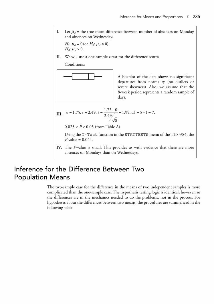
Inference for the Difference Between Two Population Means
The two-sample case for the difference in the means of two independent samples is morecomplicated than the one-sample case. The hypothesis testing logic is identical, however, sothe differences are in the mechanics needed to do the problems, not in the process. Forhypotheses about the differences between two means, the procedures are summarized in thefollowing table.
Inference for Means and Proportions � 235
I. Let md = the true mean difference between number of absences on Mondayand absences on Wednesday.
H0: md = 0(or H0: md ≤ 0).HA: md > 0.
II. We will use a one-sample t-test for the difference scores.
Conditions:
A boxplot of the data shows no significantdepartures from normality (no outliers orsevere skewness). Also, we assume that the8-week period represents a random sample ofdays.
III.
0.025 < P < 0.05 (from Table A).
Using the T-Test function in the STATTESTS menu of the TI-83/84, the P-value = 0.044.
IV. The P-value is small. This provides us with evidence that there are moreabsences on Mondays than on Wednesdays.
x s t= = =−
= = − =1 75 2 491 75 02 49
8
1 99. , . ,..
. , df 8 1 7.

� Hypothesis� Estimator� Standard Error Conditions Test Statistic
� Null hypothesis: � σ 21 and σ 2
2 knownH0: m1 − m2 = 0 OR H0 : m1 = m2
� Estimator: � Normal population (rarely used sincedistribution OR σ 2
1 and σ 22 are rarely
large sample size known)(n1 ≥ 30, n2 ≥ 30)
� Standard error: Two independent random samples from approximately normal populations or large sample sizes df = min{ n1 – 1, n2 – 1}(n1 ≥ 30 and n2 ≥ 30) or
OR df = (software)
If pooled:two
independent random samples from approximately normal populations (rarely used due to
difficulty in showing that )
Notes on the above table:
� Generally speaking, you should not assume the population variances are equal. Thebottom line in the table gives the conditions and test statistic if you can make the nec-essary assumption. The problem is that it is very difficult to justify the assumption.
� The middle rows for conditions and test statistic give the typical t-procedure approach.The first way of computing degrees of freedom is the “conservative” method introducedin Chapter 11. The “software” method is based on the formula given in Chapter 11.
example: A statistics teacher, Mr. Srednih, gave a quiz to his 8:00 AM class and tohis 9:00 AM class. There were 50 points possible on the quiz. The data for thetwo classes were as follows.
n s
Group 1 (8:00 AM) 34 40.2 9.57Group 2 (9:00 AM) 31 44.9 4.86
Before the quiz, some members of the 9:00 AM class had been bragging that laterclasses do better in statistics. Considering these two classes as random samples from thepopulations of 8:00 AM and 9:00 AM classes, do these data provide evidence at the .01level of significance that 9:00 AM classes are better than 8:00 AM classes?
x
σ σ12
22=
σ σ12
22=
ss s
x x1 2
12
1
22
2− = +
n n
x x1 2−
zx x
n n
=−
+
1 2
12
1
22
2
σ σ
236 � Step 4. Review the Knowledge You Need to Score High
tx x
s
n
s
n
=−
+
1 2
12
1
22
2
tx x
sn n
n n
p
=−
+⎛
⎝⎜⎜
⎞
⎠⎟⎟
= + −
1 2
2
1 2
1 2
1 1
2df
s sn n
sn s n s
x x p
p
1 2
2
1 2
2 1 12
2 2
1 1
1 1
−= +
⎛
⎝⎜⎜
⎞
⎠⎟⎟
=− + −( ) ( ) 22
1 22n n+ −

solution:
Inference for Means and Proportions � 237
I. Let m1 = the true mean score for the 8:00 AM class.Let m2 = the true mean score for the 9:00 AM class.H0: m1 − m2 = 0.HA: m1 − m2 < 0.
II. We will use a two-sample t-test at α = 0.01. We assume these samples arerandom samples from independent populations. t-procedures are justifiedbecause both sample sizes are larger than 30.
(Note: if the sample sizes were not large enough, we would need to knowthat the samples were drawn from populations that are approximately nor-mally distributed.)
III. , df = min{34 − 1, 31 − 1} = 30.
From Table B, 0.005 < P-value < 0.01. Using the tcdf funtion from theDISTRmenu of the TI-83/84 yields tcdf(−100, −2.53,30) = 0.0084. Usingthe 2SampTTest function in the STAT TESTS menu of the TI-83/84 forthe whole test yields t = −2.53 and a P-value of 0.007 based on df = 49.92 (the lower P-value being based on a larger number of degrees of freedom).
IV. Because P < 0.01, we reject the null hypothesis. We have good evidence that thetrue mean for 9:00 AM classes is higher than the true mean for 8:00 AM classes.
t =−
+
= −40 2 44 9
9 5734
4 8631
2 532 2
. .
. ..
Inference for a Single Population ProportionWe are usually more interested in estimating a population proportion with a confidenceinterval than we are in testing that a population proportion has a particular value. However,significance testing techniques for a particular population proportion exist and follow a pat-tern similar to those of the previous two sections. The main difference is that the only teststatistic is z. The logic is based on using a normal approximation to the binomial as discussed in Chapter 10.
� Hypothesis� Estimator� Standard Error Conditions Test Statistic
� Null hypothesis � SRSH0: p = p0 � np0 ≥ 5, n(1 − p0) ≥ 5 (or
� Estimator: np0 ≥ 10, n(1 − p0) ≥ 10)
where X is
the count of successes� Standard error:
pX
n=
zp p
p p
n
=−
−
ˆ
( )0
0 01
sp p
np
( )=
−0 01

Notes on the preceding table:
� The standard error for a hypothesis test of a single population proportion is different fora confidence interval for a population proportion. The standard error for a confidenceinterval,
,
is a function of , the sample proportion, whereas the standard error for a significancetest,
is a function of the hypothesized value of p.
� Like the conditions for the use of a z-interval, we require that the np0 and n(1 – p0) belarge enough to justify the normal approximation. As with determining the standarderror, we use the hypothesized value of p rather than the sample value. “Large enough”means either np0 ≥ 5 and n(1 − p0) ≥ 5, or np0 ≥ 10 and n(1 − p0) ≥ 10 (it varies by text).
example: Consider a screening test for prostate cancer that its maker claims willdetect the cancer in 85% of the men who actually have the disease. One hun-dred seventy-five men who have been previously diagnosed with prostate cancerare given the screening test, and 141 of the men are identified as having thedisease. Does this finding provide evidence that the screening test detects thecancer at a rate different from the 85% rate claimed by its manufacturer?
solution:
sp p
np
( )=
−0 01
p
sp p
np
ˆ( ˆ)=
−1
238 � Step 4. Review the Knowledge You Need to Score High
I. Let p = the true proportion of men with prostate cancer who test positive.
H0: p = 0.85.HA: p ≠ 0.85.
II. We want to use a one-proportion z-test. 175(0.85) = 148.75 > 5 and 175(1 − 0.85) = 26.25 > 5, so the conditions are present to use this test(the conditions are met whether we use 5 or 10).
III. .
.
Using the TI-83/84, the same answer is obtained by using 1-PropZTest in the STAT TESTS menu.
IV. Because P is reasonably large, we do not have sufficient evidence to rejectthe null hypothesis. The evidence is insufficient to challenge the company’sclaim that the test is 85% effective.
z P=−
−= ⇒ =
0 806 0 85
0 85 1 0 85175
1 64 0. .
. ( . ). .-value 110
ˆ .p = =141
1750 806

example: Maria has a quarter that she suspects is out of balance. In fact, shethinks it turns up heads more often than it would if it were fair. Being a senior,she has lots of time on her hands, so she decides to flip the coin 300 times andcount the number of heads. There are 165 heads in the 300 flips. Does thisprovide evidence at the 0.05 level that the coin is biased in favor of heads? Atthe 0.01 level?
solution:
Inference for Means and Proportions � 239
I. Let p = the true proportion of heads in 300 flips of a fair coin.
H0: p = 0.50 (or H0: p ≤ 0.50).HA: p > 0.50.
II. We will use a one-proportion z-test.
300(0.50) = 150 > 5 and 300(1 – 0.50) = 150 > 5, so the conditions arepresent for a one-proportion z-test.
III. .
(This can also be done using 1-PropZTest in the STAT TESTSmenu of the TI-83/84.)
IV. No significance level was declared in step II. We note that this findingwould have been significant at α = 0.05 but not at α = 0.01. Accordingly,either of the following conclusions would be acceptable:
(1) Since the P-value is low, we reject the null hypothesis. We have evidence that the true proportion of heads is greater than 0.50.
or
(2) The P-value found in part III is not sufficiently low to persuade us toreject the null hypothesis. We do not have good evidence that the trueproportion of heads is greater than 0.50.
ˆ . ,. .
. .p z= = =
−
−( )165
3000 55
0 55 0 50
0 50 1 0 50
300
== ⇒1 73. P -value = 0.042
Inference for the Difference Between Two PopulationProportions
The logic behind inference for two population proportions is the same as for the others wehave studied. As with the one-sample case, there are some differences between z-intervalsand z-tests in terms of the computation of the standard error. The following table gives theessential details.

� Hypothesis� Estimator� Standard Error Conditions Test Statistic
� Null hypothesis � SRSs fromH0: p1 − p2 = 0 independent populations(or H0: p1 = p2)
� Estimator: � where
where
� Standard error:
where
ˆ ˆp p1 2−
240 � Step 4. Review the Knowledge You Need to Score High
zp p
p pn n
=−
− +⎛
⎝⎜⎜
⎞
⎠⎟⎟
ˆ ˆ
ˆ( ˆ)
1 2
1 2
11 1
pX
n11
1
=
pX
n22
2
=
n p n pn p n p
1 1 1 1
2 2 2 2
5 1 5
5 1 5
ˆ , ( ˆ )ˆ , ( ˆ )
≥ − ≥
≥ − ≥p
X X
n n=
+
+1 2
1 2
s p pn np pˆ ˆ
ˆ( ˆ)1 2
11 1
1 2−
= − +⎛
⎝⎜⎜
⎞
⎠⎟⎟
pX X
n n=
+
+1 2
1 2
example: Two concentrations of a new vaccine designed to prevent infection aredeveloped and a study is conducted to determine if they differ in their effective-ness. The results from the study are given in the following table.
Vaccine A Vaccine B
Infected 102 95Not infected 123 190Total 225 285
Does this study provide statistical evidence at the α = 0.01 level that the vaccines differin their effectiveness?
solution:
I. Let p1 = the population proportion infected after receiving Vaccine A.
Let p2 = the population proportion infected after receiving Vaccine B.
H0: p1 − p2 = 0.HA: p1 − p2 ≠ 0.
II. We will use a two-proportion z-test at a = 0.01.
n p n p1 1 1 1
225 0 453 102 1 225 0 547 123ˆ ( . ) , ( ˆ ) ( . )= = − = = ,,ˆ ( . ) , ( ˆ ) ( . )n p n p
2 2 2 2285 0 333 95 1 225 0 667 19= = − = = 00.
ˆ . , ˆ . ,p p1 2
102
2250 453
95
2850 333= = = =

� Rapid Review1. A researcher reports that a finding of = 3.1 is significant at the 0.05 level of signif-
icance. What is the meaning of this statement?
Answer: Under the assumption that the null hypothesis is true, the probability of get-ting a value at least as extreme as the one obtained is less than 0.05. It was unlikely tohave occurred by chance.
2. Let m1 = the mean score on a test of agility using a new training method and let m2 =the mean score on the test using the traditional method. Consider a test of H0: m1 − m2 = 0.A large sample significance test finds P = 0.04. What conclusion, in the context of theproblem, do you report if
(a) a = 0.05?
(b) a = 0.01?
Answer:
(a) Because the P-value is less than 0.05, we reject the null hypothesis. We have evi-dence that there is a non-zero difference between the traditional and new trainingmethods.
x
Inference for Means and Proportions � 241
All values are larger than 5, so the conditions necessary are present for thetwo-proportion z-test.
(Note: When the counts are given in table form, as in this exercise, thevalues found in the calculation above are simply the table entries! Take alook. Being aware of this could save you some work.)
III. .
= 2.76 ⇒ P-value = 2(1 − 0.9971) =
0.006 (from Table A). (Remember that you have to multiply by 2 since it isa two-sided alternative—you are actually finding the probability of being2.76 standard deviations away from the mean in some direction.) Giventhe z-score, the P-value could also be found using a TI-83/84: 2 × normalcdf(2.76,100).
(Using a TI-83/84, all the mechanics of the exercise could have been doneusing the 2-PropZTest in the STAT TESTS menu. If you do that,remember to show enough work that someone reading your solution cansee where the numbers came from.)
IV. Because P < 0.01, we have grounds to reject the null hypothesis. We havestrong evidence that the two vaccines differ in their effectiveness. Althoughthis was two-sided test, we note that Vaccine A was less effective thanVaccine B.
z =−
− +⎛⎝⎜
⎞⎠⎟
0 453 0 333
0 386 1 0 3861
2251
285
. .
. ( . )
ˆ .p =+
+=
102 95
225 2850 386

(b) Because the P-value is greater than 0.01, we do not have sufficient evidence toreject the null hypothesis. We do not have strong support for the hypothesis thatthe training methods differ in effectiveness.
3. True–False: In a hypothesis test concerning a single mean, we can use either z-proceduresor t-procedures as long as the sample size is at least 20.
Answer: False. With a sample size of only 20, we can not use z-procedures unless weknow that the population from which the sample was drawn is approximately normaland σ is known. We can use t-procedures if the data do not have outliers or severe skew-ness, that is, if the population from which the sample was drawn is approximatelynormal.
4. We are going to conduct a two-sided significance test for a population proportion. Thenull hypothesis is H0: p = 0.3. The simple random sample of 225 subjects yields
. What is the standard error, sp , involved in this procedure if
(a) you are constructing a confidence interval for the true population proportion?
(b) you are doing a significance test for the null hypothesis?
Answer:
(a) For a confidence interval, you use the value of in the standard error.
Hence,
(b) For a significance test, you use the hypothesized value of p. Hence,
5. For the following data,
(a) justify the use of a two-proportion z-test for H0: p1 − p2 = 0.
(b) what is the value of the test statistic for H0: p1 − p2 = 0?
(c) what is the P-value of the test statistic for the two-sided alternative?
s p
( . )( . ). .=
−=
0 3 1 0 3
2250 03055
s p
( . )( . ). .=
−=
0 35 1 0 35
2250 0318
p
ˆ .p = 0 35
242 � Step 4. Review the Knowledge You Need to Score High
n x
Group 1 40 12 0.3Group 2 35 14 0.4
p
Answer:
(a)
Since all values are at least 5, the conditions are present for a two-proportion z-test.
(b) ˆ .p =+
+=
12 14
40 350 35
n p n p
n p1 1 1 1
2 2
40 0 3 12 1 40 0 7 28
3
ˆ ( . ) , ( ˆ ) ( . ) ,ˆ
= = − = =
= 55 0 4 14 1 35 0 6 212 2
( . ) , ( ˆ ) ( . ) .= − = =n p

.
(c) z = −0.91, P-value = 2(0.18) = 0.36 (from Table A). On the TI-83/84, this P-valuecan be found as 2 × normalcdf(−100, −0.91).
6. You want to conduct a one-sample test (t-test) for a population mean. Your randomsample of size 10 yields the following data: 26, 27, 34, 29, 38, 30, 28, 30, 30, 23.Should you proceed with your test? Explain.
Answer: A boxplot of the data shows that the 38 is an outlier. Further, the dotplot ofthe data casts doubt on the approximate normality of the population from which thissample was drawn. Hence, you should not use a t-test on these data.
7. Although it may be difficult to justify, there are conditions under which you can poolyour estimate of the population standard deviation when doing a two-sample test forthe difference between population means. When is this procedure justified? Why is itdifficult to justify?
Answer: This procedure is justified when you can assume that the population variances(or population standard deviations) are equal. This is hard to justify because of the lackof a strong statistical test for the equality of population variances.
Practice ProblemsMultiple Choice
1. A school district claims that the average teacher in the district earns $48,000 per year.The teachers’ organization argues that the average salary is less. A random sample of 25 teachers yields a mean salary of $47,500 with a sample standard deviation of $2000.Assuming that the distribution of all teachers’ salaries is approximately normally dis-tributed, what is the value of the t-test statistic and the P-value for a test of the hypoth-esis H0: m = 48,000 against HA: m < 48,000?
a. t = 1.25, 0.10 < P < 0.15b. t = −1.25, 0.20 < P < 0.30c. t = 1.25, 0.20 < P < 0.30d. t = −1.25, 0.10 < P < 0.15e. t = −1.25, P > 0.25
2. Which of the following conditions is (are) necessary to justify the use of z-proceduresin a significance test about a population proportion?
I. The samples must be drawn from a normal population.II. The population must be much larger (10–20 times) than the sample.
III. np0 ≥ 5 and n(1 – p0) ≥ 5.
20.0 40.035.030.025.0
∗
: ... ...+---------+---------+---------+---------+ −C1
.
z =−
− +⎛⎝⎜
⎞⎠⎟
= −0 3 0 4
0 35 1 0 35140
135
0 91. .
. ( . )
.
Inference for Means and Proportions � 243

a. I onlyb. I and II onlyc. II and III onlyd. III onlye. I, II, and III
3. A minister claims that more than 70% of the adult population attends a religious serv-ice at least once a month. Let p = the proportion of adults who attend church. The nulland alternative hypotheses you would use to test this claim would be:
a. H0: p ≤ 0.7, HA: p > 0.7b. H0: m ≤ 0.7, HA: m > 0.7c H0: p = 0.7, HA: p ≠ 0.7d. H0: p ≤ 0.7, HA: p < 0.7e. H0: p ≥ 0.7, HA: p < 0.7
4. A t-test for the difference between two populations means is to be conducted. The sam-ples, of sizes 12 and 15, are considered to be random samples from independent,approximately normally distributed, populations. Which of the following statements is (are) true?
I. If we can assume the population variances are equal, the number of degrees of free-dom is 25.
II. An appropriate conservative estimate of the number of degrees of freedom is 11.III. The P-value for the test statistic in this situation will be larger for 11 degrees of
freedom than for 25 degrees of freedom.
a. I onlyb. II onlyc. III onlyd. I and II onlye. I, II, and III
5. When is it OK to use a confidence interval instead of computing a P-value in a hypoth-esis test?
a. In any significance testb. In any hypothesis test with a two-sided alternative hypothesisc. Only when the hypothesized value of the parameter is not in the confidence intervald. Only when you are conducting a hypothesis test with a one-sided alternativee. Only when doing a test for a single population mean or a single population
proportion
6. Which of the following is not a required step for a significance test?
a. State null and alternative hypotheses in the context of the problem.b. Identify the test to be used and justify the conditions for using it.c. State the significance level for which you will decide to reject the null hypothesis.d. Compute the value of the test statistic and the P-value.e. State a correct conclusion in the context of the problem.
7. Which of the following best describes what we mean when say that t-procedures arerobust?
a. The t-procedures work well with almost any distribution.b. The numerical value of t is not affected by outliers.c. The t-procedures will still work reasonably well even if the assumption of normal-
ity is violated.d. t-procedures can be used as long as the sample size is at least 40.e. t-procedures are as accurate as z-procedures.
244 � Step 4. Review the Knowledge You Need to Score High

8. For a hypothesis test of H0 : m = m0 against the alternative HA : m < m0, the z-test statis-tic is found to be 2.00. This finding is
a. significant at the 0.05 level but not at the 0.0l level.b. significant at the 0.01 level but not at the 0.05 level.c. significant at both the 0.01 and the 0.05 levels.d. significant at neither the 0.01 nor the 0.05 levels.e. not large enough to be considered significant.
9. Two types of tennis balls were tested to determine which one goes faster on a serve.Eight different players served one of each type of ball and the results were recorded:
Assuming that the speeds are approximately normally distributed, how many degrees offreedom will there be in the appropriate t-test used to determine which type of tennisball travels faster?
a. 6b. 7c. 16d. 15e. 14
10. Two statistics teachers want to compare their teaching methods. They decide to give thesame final exam and use the scores on the exam as a basis for comparison. They decidethat the value of interest to them will be the proportion of students in each class whoscore above 80% on the final. One class has 32 students and one has 27 students.Which of the following would be the most appropriate test for this situation?
a. Two proportion z-testb. Two-sample t-testc. Chi-square goodness-of-fit testd. One-sample z-teste. Chi-square test for independence
Free Response1. A large high school has been waging a campaign against drug use, particularly mari-
juana. Before the campaign began in 2004, a random sample of 100 students from thejunior and senior classes found 27 who admitted to using marijuana (we understandthat some students who used marijuana would be reluctant to admit it on a survey). Toassess the success of their program, in early 2007 they surveyed a random sample of 175 juniors and seniors and 30 responded that they have used marijuana. Is this goodevidence that the use of marijuana has been reduced at the school?
SERVER TYPE A TYPE B
Raphael 120 115
Roger 125 122
Serena 119 114
Venus 110 114
Andy 118 115
Maria 82 91
Lleyton 115 110
Ana 105 106
Inference for Means and Proportions � 245

2. Twenty-six pairs of identical twins are enrolled in a study to determine the impact oftraining on ability to memorize a string of letters. Two programs (A and B) are beingstudied. One member of each pair is randomly assigned to one of the two groups andthe other twin goes into the other group. Each group undergoes the appropriate train-ing program, and then the scores for pairs of twins are compared. The means and stan-dard deviations for groups A and B are determined as well as the mean and standarddeviation for the difference between each twin’s score. Is this study a one-sample or two-sample situation, and how many degrees of freedom are involved in determining the t-value?
3. Which of the following statements is (are) correct? Explain.I. A confidence interval can be used instead of a test statistic in any hypothesis test
involving means or proportions.II. A confidence interval can be used instead of a test statistic in a two-sided hypoth-
esis test involving means or proportions.III. The standard error for constructing a confidence interval for a population propor-
tion and the standard error for a significance test for a population proportion arethe same.
IV. The standard error for constructing a confidence interval for a population meanand the standard error for a significance test for a population mean are the same.
4. The average math SAT score at Hormone High School over the years is 520. The math-ematics faculty believes that this year’s class of seniors is the best the school has ever hadin mathematics. One hundred seventy-five seniors take the exam and achieve an aver-age score of 531 with a sample standard deviation of 96. Does this performance pro-vide good statistical evidence that this year’s class is, in fact, superior?
5. An avid reader, Booker Worm, claims that he reads books that average more than 375 pages in length. A random sample of 13 books on his shelf had the followingnumber of pages: 595, 353, 434, 382, 420, 225, 408, 422, 315, 502, 503, 384, 420.Do the data support Booker’s claim? Test at the 0.05 level of significance.
6. The statistics teacher, Dr. Tukey, gave a 50-point quiz to his class of 10 students andthey didn’t do very well, at least by Dr. Tukey’s standards (which are quite high). Ratherthan continuing to the next chapter, he spent some time reviewing the material andthen gave another quiz. The quizzes were comparable in length and difficulty. Theresults of the two quizzes were as follows.
Student 1 2 3 4 5 6 7 8 9 10
Quiz 1 42 38 34 37 36 26 44 32 38 31Quiz 2 45 40 36 38 34 28 44 35 42 30
Do the data indicate that the review was successful, at the .05 level, at improving theperformance of the students on this material? Give good statistical evidence for yourconclusion.
7. The new reality TV show, “I Want to Marry a Statistician,” has been showing onMonday evenings, and ratings show that it has been watched by 55% of the viewingaudience each week. The producers are moving the show to Wednesday night but areconcerned that such a move might reduce the percentage of the viewing public watch-ing the show. After the show has been moved, a random sample of 500 people whoare watching television on Wednesday night are surveyed and asked what show they
246 � Step 4. Review the Knowledge You Need to Score High

are watching. Two hundred fifty-five respond that they are watching “I Want to Marry aStatistician.” Does this finding provide evidence at the 0.01 level of significance that thepercentage of the viewing public watching “I Want to Marry a Statistician” has declined?
8. Harvey is running for student body president. An opinion poll conducted by the APStatistics class does a survey in an attempt to predict the outcome of the election. Theyrandomly sample 30 students, 16 of whom say they plan to vote for Harvey. Harveyfigures (correctly) that 53.3% of students in the sample intend to vote for him and isoverjoyed at his soon-to-be-celebrated victory. Explain carefully why Harvey shouldnot get too excited until the votes are counted.
9. A company uses two different models, call them model A and model B, of a machineto produce electronic locks for hotels. The company has several hundred of eachmachine in use in its various factories. The machines are not perfect, and the companywould like to phase out of service the one that produces the most defects in the locks.A random sample of 13 model A machines and 11 model B machines are tested andthe data for the average number of defects per week are given in the following table.
Inference for Means and Proportions � 247
n s
Model A 13 11.5 2.3Model B 11 13.1 2.9
x
s
Men 8.56 1.42Women 8.97 1.84Difference (Husband–Wife) −0.38 1.77
x
Dotplots of the data indicate that there are no outliers or strong skewness in the dataand that there are no strong departures from normal. Do these data provide statisti-cally convincing evidence that the two machines differ in terms of the number ofdefects produced?
10. Take another look at the preceding problem. Suppose there were 30 of each modelmachine that were sampled. Assuming that the sample means and standard deviationsare the same as given in question 9, how might this have affected the hypothesis testyou performed in that question?
11. The directors of a large metropolitan airport claim that security procedures are 98%accurate in detecting banned metal objects that passengers may try to carry onto a plane. The local agency charged with enforcing security thinks the security proce-dures are not as good as claimed. A study of 250 passengers showed that screenersmissed nine banned carry-on items. What is the P-value for this test and what conclu-sion would you draw based on it?
12. A group of 175 married couples are enrolled in a study to see if women have a strongerreaction than men to videos that contain violent material. At the conclusion of thestudy, each couple is given a questionnaire designed to measure the intensity of theirreaction. Higher values indicate a stronger reaction. The means and standard deviationsfor all men, all women, and the differences between husbands and wives are as follows:
Do the data give strong statistical evidence that wives have a stronger reaction to violence in videos than do their husbands? Assume that σ for the differences is 1.77.

13. An election is bitterly contested between two rivals. In a poll of 750 potentialvoters taken 4 weeks before the election, 420 indicated a preference for candidateGrumpy over candidate Dopey. Two weeks later, a new poll of 900 randomlyselected potential voters found 465 who plan to vote for Grumpy. Dopey imme-diately began advertising that support for Grumpy was slipping dramatically andthat he was going to win the election. Statistically speaking (say at the 0.05 level),how happy should Dopey be (i.e., how sure is he that support for Grumpy hasdropped)?
14. Consider, once again, the situation of question #7 above. In that problem, a one-sided, two-proportion z-test was conducted to determine if there had been a drop inthe proportion of people who watch the show “I Want to Marry a Statistician” whenit was moved from Monday to Wednesday evenings.
Suppose instead that the producers were interested in whether the popularity ratingsfor the show had changed in any direction since the move. Over the seasons the showhad been broadcast on Mondays, the popularity rating for the show (10 high, 1 low)had averaged 7.3. After moving the show to the new time, ratings were taken for 12consecutive weeks. The average rating was determined to be 6.1 with a sample stan-dard deviation of 2.7. Does this provide evidence, at the 0.05 level of significance, thatthe ratings for the show has changed? Use a confidence interval, rather than a t-test,as part of your argument. A dotplot of the data indicates that the ratings are approx-imately normally distributed.
15. A two-sample study for the difference between two population means will utilizet-procedures and is to be done at the 0.05 level of significance. The sample sizes are23 and 27. What is the upper critical value (t*) for the rejection region if
(a) the alternative hypothesis is one-sided, and the conservative method is used todetermine the degrees of freedom?
(b) the alternative hypothesis is two-sided and the conservative method is used todetermine the degrees of freedom?
(c) the alternative hypothesis is one-sided and you assume that the population variances are equal?
(d) the alternative hypothesis is two-sided, and you assume that the population variances are equal?
Cumulative Review Problems
1. How large a sample is needed to estimate a population proportion within 2.5% at the99% level of confidence ifa. you have no reasonable estimate of the population proportion?b. you have data that show the population proportion should be about 0.7?
2. Let X be a binomial random variable with n = 250 and p = 0.6. Use a normal approx-imation to the binomial to approximate P (X > 160).
3. Write the mathematical expression you would use to evaluate P (X > 2) for a binomialrandom variable X that has B(5, 0.3) (that is, X is a binomial random variable equal tothe number of successes out of 5 trials of an event that occurs with probability of success p = 0.3). Do not evaluate.
248 � Step 4. Review the Knowledge You Need to Score High

4. An individual is picked at random from a group of 55 office workers. Thirty of theworkers are female, and 25 are male. Six of the women are administrators. Given thatthe individual picked is female, what is the probability she is an administrator?
5. A random sample of 25 cigarettes of a certain brand were tested for nicotine content,and the mean was found to be 1.85 mg with a standard deviation of 0.75 mg. Find a 90% confidence interval for the mean number of mg of nicotine in this type of cigarette. Assume that the amount of nicotine in cigarettes is approximately normallydistributed. Interpret the interval in the context of the problem.
Solutions to Practice ProblemsMultiple Choice
1. The correct answer is (d).
for the one-sided alternative. The calculator answer is P = 0.112. Had the alternativebeen two-sided, the correct answer would have been (b).
2. The correct answer is (c). If the sample size conditions are met, it is not necessary thatthe samples be drawn from a normal population.
3. The correct answer is (a). Often you will see the null written as H0: p = 0.7 rather thanH0: p ≤ 0.7. Either is correct.
4. The correct answer is (e). If we can assume that the variances are equal, then df = n1 +n2 − 2 = 12 + 15 − 2 = 25. A conservative estimate for the number of degrees of free-dom is df = min {n1 − 1, n2 − 1} = min {12 − 1, 25 − 1} = 11. For a given test statis-tic, the greater the number of degrees of freedom, the lower the P-value.
5. The correct answer is (b). In this course, we consider confidence intervals to be two-sided.A two-sided α-level significance test will reject the null hypothesis whenever the hypothe-sized value of the parameter is not contained in the C = 1 − α level confidence interval.
6 (c) is not one of the required steps. You can state a significance level that you will latercompare the P-value with, but it is not required. You can simply argue the strength ofthe evidence against the null hypothesis based on the P-value alone—small values of P provide evidence against the null.
7. (c) is the most correct response. (a) is incorrect because t-procedures do not work well with,for example, small samples that come from non-normal populations. (b) is false since thenumerical value of t is, like z, affected by outliers. t-procedures are generally OK to use forsamples of size 40 or larger, but this is not what is meant by robust (so (d) is incorrect), (e)is not correct since the t-distribution is more variable than the standard normal. It becomescloser to z as sample size increases but is “as accurate” only in the limiting case.
8. The correct answer is (d). The alternative hypothesis, H0 : m = m0, would require a neg-ative value of z to be evidence against the null. Because the given value is positive, weconclude that the finding is in the wrong direction to support the alternative and,hence, is not going to be significant at any level.
t P=−
= − ⇒ < <47500 48000
200025
1 25 0 10 0 15. . .
Inference for Means and Proportions � 249

9. The correct answer is (b). Because the data are paired, the appropriate t-test is a one-sample test for the mean of the difference scores. In this case, df = n – 1 = 8 – 1 = 7.
10. The correct answer is (a). The problem states that the teachers will record for compar-ison the number of students in each class who score above 80%. Since the enrollmentsdiffer in the two classes, we need to compare the proportion of students who scoreabove 80% in each class. Thus the appropriate test is a two-proportion z-test. Notethat, although it is not one of the choices, a chi-square test for homogeneity of propor-tions could also be used since we are interested in whether the proportions of those get-ting above 80% are the same across the two populations.
Free Response
1.
250 � Step 4. Review the Knowledge You Need to Score High
2. This is a paired study because the scores for each pair of twins are compared. Hence, itis a one-sample situation, and there are 26 pieces of data to be analyzed, which are the26 difference scores between the twins. Hence, df = 26 − 1 = 25.
3. � I is not correct. A confidence interval, at least in this course, cannot be used in anyone-sided hypothesis test—only two-sided tests.
� II is correct. A confidence interval constructed from a random sample that does notcontain the hypothesized value of the parameter can be considered statistically signif-icant evidence against the null hypothesis.
I. Let p1 = the true proportion of students who admit to using marijuana in 2004.
Let p2 = the true proportion of students who admit to using marijuana in2007.
H0: p1 = p2 (or H0: p1 − p2 = 0; or H0: p1 ≤ p2; or H0: p1 − p2 > 0).HA: p1 > p2 (or H0: p1 > p2).
II. We will use a two-proportion z-test. The survey involved drawing random
samples from independent populations.
100(0.27) = 27, 100(1 − 0.27) = 73, 175(0.171) ≈ 30, and 175(1 − 0.171)≈ 145 are all greater than 10, so the conditions for inference are present.
III.
= 1.949 ⇒ P-value = 0.026.
(This problem can be done using 2-PropZTest in the STAT TESTSmenu.)
IV. Since the P-value is quite small (a finding this extreme would occur onlyabout 2.6% of the time if there had been no decrease in usage), we haveevidence that the rate of marijuana use among students (at least amongjuniors and seniors) has decreased.
ˆ .. .
.
p z=+
+= ⇒ =
−
( ) −
27 30
100 1750 207
0 27 0 171
0 207 1 00 2071
1001
175.( ) +
⎛⎝⎜
⎞⎠⎟
ˆ . , ˆ . .p p1 2
27
1000 27
30
1750 171= = = =

Inference for Means and Proportions � 251
I. Let m = the true mean score for all students taking the exam.
H0: m = 520 (or, H0: m ≤ 520)HA: m > 520
II. We will use a one-sample t-test. We consider the 175 students to be arandom sample of students taking the exam. The sample size is large, sothe conditions for inference are present. (Note: Due to the large samplesize, it is reasonable that the sample standard deviation is a good estimateof the population standard deviation. This means that you would receivecredit on the AP exam for doing this problem as a z-test although a t-test ispreferable.)
III. = 531, s = 96, . ,
df = 175 − 1 = 174 ⇒ 0.05 < P-value < 0.10 (from Table B, with df =100—always round down).
(Using the TI-83/84, P-value = tcdf(1.52,100,174)=0.065. If wehad used s = 96 as an estimate of σ based on a large sample size, and used az-test rather than a t-test, the P-value would have been 0.064. This is veryclose to the P-value determined using t. Remember that is a t-test but thatthe numerical outcome using a z-test is almost identical for large samples.)
IV. The P-value, which is greater than 0.05, is reasonably low but not lowenough to provide strong evidence that the current class is superior in mathability as measured by the SAT.
t =−
=531 52096
175
1 52.sx = =96
1757 26.x
� III is not correct. The standard error for a confidence interval is based on the sampleproportions is
The standard error for a significance test is based on the hypothesized population value is
� IV is correct.
4.
sp p
np
( ).=
−0 0
1
sp p
np
ˆ( ˆ).=
−1

5.
252 � Step 4. Review the Knowledge You Need to Score High
6. The data are paired by individual students, so we need to test the difference scores forthe students rather than the means for each quiz. The differences are given in the following table.
Student 1 2 3 4 5 6 7 8 9 10
Quiz 1 42 38 34 37 36 26 44 32 38 31Quiz 2 45 40 36 38 34 28 44 35 42 30Difference 3 2 2 1 −2 2 0 3 4 −1(Q2-Q1)
I. Let m = the true average number of pages in the books Booker reads.
H0: m ≤ 375.HA: m > 375.
II. We are going to use a one-sample t-test test at α = 0.05. The problemstates that the sample is a random sample. A dotplot of the data showsgood symmetry and no significant departures from normality (although thedata do spread out quite a bit from the mean, there are no outliers):
The conditions for the t-test are present.
III. .
(from Table B). (tcdf(1.48,100,12) gives P-value = 0.082, or youcan use STAT TESTS T-Test.)
IV. Because P > .05, we cannot reject H0. We do not have strong evidence toback up Booker’s claim that the books he reads actually average more than375 pages in length.
t P=−
= = ⇒ < <412 5 37591 35
13
1 48 12 0 05 0 10..
. , . .df
n x s= = =13 412 5 91 35, . , .
.
Pages210 490 560420350280
::: . ... ..+---------+---------+---------+---------+---------+-------

7.
I. Let md = the mean of the differences between the scores of students onQuiz 2 and Quiz 1.
H0: md = 0.HA: md > 0.
II. This is a matched pairs t-test. That is, it is a one-sample t-test for a popula-tion mean. We assume that these are random samples from the populationsof all students who took both quizzes. The significance level is α = 0.05.
A boxplot of the difference scores shows no significant departures fromnormality, so the conditions to use the one-sample t-test are present.
III. .
(from Table B).
(Using the TI-83/84, P-value = tcdf(2.33, 100,9)=0.022, or you canuse STAT TESTS T-Test.)
IV. Because P < 0.05, we reject the null hypothesis. The data provide evidenceat the 0.05 level that the review was successful at improving studentperformance on the material.
t P=−
= = ⇒ < <1 4 0
1 9010
2 33 9 0 02 0 025.
.. , . .df
n x sd b= = =10 1 4 1 90, . , .
I. Let p = the true proportion of Wednesday night television viewers who arewatching “I Want to Marry a Statistician.”
H0: p = 0.55.HA: p < 0.55.
II. We want to use a one-proportion z-test at α = 0.01. 500(0.55) = 275 > 5and 500(1 − 0.55) = 225 > 5. Thus, the conditions needed for this testhave been met.
III. .
.
(On the TI-83/84, normalcdf(−100,−1.80)=0.0359, or you canuse STAT TESTS 1-PropZTest.)
IV. Because P > 0.01, we do not have sufficient evidence to reject the null hypoth-esis. The evidence is insufficient to conclude at the 0.01 level that the propor-tion of viewers has dropped since the program was moved to a different night.
z P=−
−= − ⇒ =
0 51 0 55
0 55 1 0 55500
1 80 0. .
. ( . ). .-value 0036
ˆ .p = =255
5000 51
Inference for Means and Proportions � 253

254 � Step 4. Review the Knowledge You Need to Score High
8. Let’s suppose that the Stat class constructed a 95% confidence interval for the true pro-portion of students who plan to vote for Harvey (we are assuming that this a randomsample from the population of interest, and we note that both n and n(1 − ) are
greater than 10). (as Harvey figured). Then a 95% confidence
interval for the true proportion of votes Harvey can expect to get is
0.533 ± 1.96 = (0.355, 0.712). That is, we are 95% confident
that between 35.5% and 71.2% of students plan to vote for Harvey. He may have a majority, but there is a lot of room between 35.5% and 50% for Harvey not to getthe majority he thinks he has. (The argument is similar with a 90% CI: (0.384,0.683); or with a 99% CI: (0.299, 0.768).)
9.
( . )( . )0 533 1 0 533
30
−
ˆ .p = =16
300 533
pp
I. Let m1 = the true mean number of defects produced by machine A.Let m2 = the true mean number of defects produced by machine B.
H0: m1 − m2 = 0.HA: m1 − m2 ≠ 0.
II. We use a two-sample t-test for the difference between means. The condi-tions that need to be present for this procedure are given in the problem:both samples are simple random samples from independent, approximatelynormal populations.
III. df = min {13 – 1, 11 – 1} = 10.
= −1.48 ⇒ 2(0.05) < P < 2(0.10) ⇔ 0.10 < P < 0.20
(from Table B).
(When read directly from Table B, t = –1.48 with df = 10 is between tailprobabilities of 0.05 and 0.10. However, those are one-sided values andmust be doubled for the two-sided alternative since we are interested in theprobability of getting 1.48 standard deviations away from the mean in anydirection. Using the TI-83/84, P-value = 2tcdf(-100,-1.48,10)=0.170. Using the 2SampTTest from the STAT TESTS menu, P-value = 0.156 with df = 18.99.)
IV. The P-value is too large to be strong evidence against the null hypothesisthat there is no difference between the machines. We do not have strongevidence that the types of machines actually differ in the number of defectsproduced.
t =−
+
11 5 13 1
2 313
2 911
2 2
. .
. .
10. � Using a two-sample t-test, Steps I and II would not change. Step III would change to
= −2.37 ⇒ 0.02 < P < 0.04t =−
+
11 5 13 1
2 330
2 930
2 2
. .
. .

Inference for Means and Proportions � 255
based on df = min{30 − 1,30 − 1} = 29. Step IV would probably arrive at a differentconclusion—reject the null because the P-value is small. Large sample sizes make iteasier to detect statistically significant differences.
11. H0: p ≥ 0.98, HA: p < 0.98,
P-value = 0.035.
This P-value is quite low and provides evidence against the null and in favor of the alternativethat security procedures actually detect less than the claimed percentage of banned objects.
12.
z =−
= −0 964 0 98
0 98 0 02250
1 81. .
( . )( . ). ,
ˆ . .p = =241
2500 964
I. Let md = the mean of the differences between the scores of husbands andwives.
H0: md = 0.HA: md < 0.
II. We are told to assume that σ = 1.77 (Note: This is a reasonable assumption,given the large sample size). This is a matched-pairs situation and we willuse a one-sample z-test for a population mean. We assume that this is arandom sample of married couples.
III. .
(If you are bothered by using z rather than t—after all, we really don’tknow σD—note that for t = −2.84 based on df = 174, P-value = 0.0025,which is very close to the value obtained by using z and results in exactlythe same conclusion.)
IV. Because P is very small, we reject H0. The data provide strong evidence thatwomen have a stronger reaction to violence in videos than do men.
z P=− −
= − ⇒ =0 38 0
1 77175
2 84 0 0023.
.. .-value
13.I. Let p1 = the true proportion of voters who plan to vote for Grumpy
4 weeks before the election.
Let p2 = the true proportion of voters who plan to vote for Grumpy 2 weeks before the election.
H0: p1 − p2 = 0.HA: p1 − p2 > 0.
II. We will use a two-proportion z-test for the difference between two popula-tion proportions. Both samples are random samples of the voting popula-tions at the time.
.ˆ . , ˆ .p p1 2
420
7500 56
465
9000 517= = = =

256 � Step 4. Review the Knowledge You Need to Score High
14.
Also,
All values are larger than 5, so the conditions needed for the two-proportion z-test are present.
III. .
= 1.75 ⇒ P-value = 0.04.
(From the TI-83/84, STAT TESTS 2-PropZTest yields P-value = 0.039.)
IV. Because P < 0.05, we can reject the null hypothesis. Candidate Dopey mayhave cause for celebration—there is evidence that support for candidateGrumpy is dropping.
z =−
+⎛⎝⎜
⎞⎠⎟
0 56 0 517
0 54 0 461
7501
900
. .
. ( . ))
ˆ .p =+
+= =
420 465
750 900
885
16500 54
n pn p
1 1
1 1
750 0 56 420
1 750 0 44 330
ˆ ( . ) ,
( ˆ ) ( . )
= ≈
− = ≈ ,,ˆ ( . ) ,
( ˆ ) ( . )
n pn p
2 2
2 2
900 0 517 465
1 900 0 483
= ≈
− = ≈≈ 435.
I. Let m = the true mean popularity rating for “I Want to Marry aStatistician.”
H0: m = 7.3.HA: m ≠ 7.3.
II. We will use a one-sample t confidence interval (at the direction of theproblem—otherwise we would most likely have chosen to do a one-samplet significance test) at α = 0.05, which, for the two-sided test, is equivalentto a confidence level of 0.95 (C = 0.95). We will assume that the ratingsare a random sample of the population of all ratings. The sample size issmall, but we are told that the ratings are approximately normally distrubuted, so that the conditions necessary fot the inference are present.
III. = 6.1, s = 2.7. For df = 12 − 1 = 11 and a 95% confidence interval, t* = 2.201 A 95% confidence interval for m is given by:
(Note: A one-sample t test for these data yields P-value = 0.15.)
IV. Since 7.3 is in the interval (4.384, 7.816), we cannot reject H0 at the 0.05level of significance. We do not have good evidence that there has been asignificantly significant change in the popularity rating of the show after itsmove to Wednesday night.
6 1 2 2012 7
124 384 7 816. .
.( . , . )±
⎛
⎝⎜
⎞
⎠⎟=
x

15. (a) df = min{23 – 1,27 – 1} = 22 ⇒ t* = 1.717.(b) df = 22 ⇒ t* = 2.074.(c) df = 23 + 27 –2 = 48 ⇒ t* = 1.684 (round down to 40 degrees of freedom
in the table).(d) df = 48 ⇒ t* = 2.021.
Solutions to Cumulative Review Problems
1. a. . Choose n = 2655.
b. . Choose n = 2230.
2. .
P(X > 160) = P = 0.099.
(The exact binomial given by the TI-83/84 is 1-binomcdf(250,0.6,160) =0.087. If you happen to be familiar with using a continuity correction (and you don’t really need to be) for the normal approximation, normalcdf(160.5,1000,150,7.75) = 0.088, which is closer to the exact binomial.)
3. . (On the TI-83/84, this is
equivalent to 1-binomcdf(5,0.3,2).)
4. P (the worker is an administrator | the worker is female)
.
5. A confidence interval is justified because we are dealing with a random sample from anapproximately normally distributed population. df = 25 − 1 = 24 ⇒ t* = 1.711.
.
We are 90% confident that the true mean number of mg per cigarette for this type ofcigarette is between 1.59 mg and 2.11 mg.
1 85 1 7110 75
251 59 2 11. .
.( . , . )±
⎛
⎝⎜⎜
⎞
⎠⎟⎟=
= = = =P
P
( )
( ).
A and F
F
655
3055
6
300 2
53
0 3 0 754
0 3 0 753 2 4 1⎛
⎝⎜⎞⎠⎟
+⎛⎝⎜
⎞⎠⎟
+( . ) ( . ) ( . ) ( . )55
0 3 0 75 0⎛⎝⎜
⎞⎠⎟
( . ) ( . )
z >−
=⎛⎝⎜
⎞⎠⎟
160 150
7 751 29
..
μ σX X= = = =250 0 6 150 250 0 6 0 4 7 75( . ) , ( . )( . ) .
n ≥⎛⎝⎜
⎞⎠⎟
− =2 576
0 0250 7 1 0 7 2229 6
2.
.( . )( . ) .
n ≥⎛⎝⎜
⎞⎠⎟
=2 576
2 0 0252654 3
2.
( . ).
Inference for Means and Proportions � 257

CHAPTER
258 �
Inference for Regression
IN THIS CHAPTERSummary: In the last two chapters, we’ve considered inference for popula-tion means and proportions and for the difference between two populationmeans or two population proportions. In this chapter, we extend the study oflinear regression begun in Chapter 7 to include inference for the slope of aregression line, including both confidence intervals and significance testing.Finally, we will look at the use of technology when doing inference forregression.
Key Ideas
� Simple Linear Regression (Review)� Significance Test for the Slope of a Regression Line� Confidence Interval for the Slope of a Regression Line� Inference for Regression Using Technology
Simple Linear RegressionWhen we studied data analysis earlier in this text, we distinguished between statistics andparameters. Statistics are measurements or values that describe samples, and parameters aremeasurements that describe populations. We have also seen that statistics can be used to esti-mate parameters. Thus, we have used –x to estimate the population mean m, s to estimate thepopulation standard deviation s, etc. In Chapter 7, we introduced the least-squares regres-sion line ( y = a + bx), which was based on a set of ordered pairs. y is actually a statisticbecause it is based on sample data. In this chapter, we study the parameter, my, that is estimated by y.
KEY IDEA
13

Inference for Regression � 259
Before we look at the model for linear regression, let’s consider an example to remindus of what we did in Chapter 7:example: The following data are pulse rates and heights for a group of 10 female statistics
students:
Height 70 60 70 63 59 55 64 64 72 66Pulse 78 70 65 62 63 68 76 58 73 53
a. What is the least-squares regression line for predicting pulse rate from height?b. What is the correlation coefficient between height and pulse rate? Interpret the corre-
lation coefficient in the context of the problem.c. What is the predicted pulse rate of a 67″ tall student?d. Interpret the slope of the regression line in the context of the problem.
solution:
a. Pulse rate = 47.17 + 0.302 (Height). (Done on the TI-83/84 with Height in L1 andPulse in L2, the LSRL can be found STAT CALC LinReg(a+bx) L1,L2,Y1.)
b. r = 0.21. There is a weak, positive, linear relationship between Height and Pulse rate.c. Pulse rate = 47.17 + 0.302(67) = 67.4. (On the Ti-83/84: Y1(67) = 67.42. Remember that
you can paste Y1 to the home screen by entering VARS Y-VARS Function Y1.)d. For each increase in height of one inch, the pulse rate is predicted to increase by 0.302
beats per minute (or: the pulse rate will increase, on average, by 0.302 beats per minute).
When doing inference for regression, we use y = a + bx to estimate the true populationregression line. Similar to what we have done with other statistics used for inference, we usea and b as estimators of population parameters a and b, the intercept and slope of the pop-ulation regression line. The conditions necessary for doing inference for regression are:
• For each given value of x, the values of the response variable y-values are independentand normally distributed.
• For each given value of x, the standard deviation, s, of y-values is the same.• The mean response of the y-values for the fixed values of x are linearly related by the
equation μy = a + bx.
example: Consider a situation in which we are interested in how well a person scores on anagility test after a fixed number of 3-oz. glasses of wine. Let x be the number of glassesconsumed. Let x take on the values 1, 2, 3, 4, 5, and 6. Let y be the score on the agilitytest (scale: 1–100). Then for any given value xi, there will be a distribution of y-valueswith mean . The conditions for inference for regression are that (i) each of these dis-tributions of y-values are normally distributed, (ii) each of these distributions of y-valueshas the same standard deviation s, and (iii) each of the lies on a line.
Remember that a residual was the error involved when making a prediction from aregression equation (residual = actual value of y – predicted value of y = yi – yi ). Not surpris-ingly, the standard error of the predictions is a function of the squared residuals:
s is an estimator of s, the standard deviation of the residuals. Thus, there are actuallythree parameters to worry about in regression: a, b, and s, which are estimated by a, b,and s, respectively.
sn
y y
ni i
=−
=−
−
∑SSRES
2 2
2( ˆ ).
μ yi
μ yi

The final statistic we need to do inference for regression is the standard error of theslope of the regression line:
In summary, inference for regression depends upon estimating my = a + b x withy = a + bx. For each x, the response values of y are independent and follow a normal dis-tribution, each distribution having the same standard deviation. Inference for regressiondepends on the following statistics:
• a, the estimate of the y intercept, a, of my
• b, the estimate of the slope, b, of my
• s, the standard error of the residuals• sb, the standard error of the slope of the regression line
In the section that follows, we explore inference for the slope of a regression line interms of a significance test and a confidence interval for the slope.
Inference for the Slope of a Regression LineInference for regression consists of either a significance test or a confidence interval for theslope of a regression line. The null hypothesis in a significance test is usually H0: b = 0,although it is possible to test H0: b = b0. Our interest is the extent to which a least-squaresregression line is a good model for the data. That is, the significance test is a test of a linearmodel for the data.
We note that in theory we could test whether the slope of the regression line is equalto any specific value. However, the usual test is whether the slope of the regression line iszero or not. If the slope of the line is zero, then there is no linear relationship between the
x and y variables (remember:
The alternative hypothesis is often two sided (i.e., HA: b ≠ 0). We can do a one-sidedtest if we believed that the data were positively or negatively related.
Significance Test for the Slope of a Regression LineThe basic details of a significance test for the slope of a regression line are given in the fol-lowing table:
• HYPOTHESIS
• ESTIMATOR
• STANDARD ERROR CONDITIONS TEST STATISTIC
• Null hypothesis • For each given value of x, (most often: Ho : β = 0 ) the values of the response
• Estimator: b (from: y = a+ bx ) variable y are independent • Standard error of the residuals: and normally distributed.
H0 0: β β=
b rs
sr by
x
= = =; , ).if then0 0
ss
x x
y y
n
x xb
i
i i
i
=−
=
−
−
−∑
∑
∑( )
( )
( )2
2
2
2
�
260 � Step 4. Review the Knowledge You Need to Score High
Continued

Inference for Regression � 261
• For each given value of x,the standard deviationof y is the same.
(Gives the variability of thevertical distances of the y-valuesfrom the regression line) • The mean response of the
y-values for the fixed values• Standard error of the slope: of x are linearly related
by the equationmy = a + bx .
(Gives the variability of theestimates of the slope of theregression line)
example: The data in the following table give the top 15 states in terms of per pupil expen-diture in 1985 and the average teacher salary in the state for that year.
STATE/SALARY PER PUPIL EXPENDITURE
MN 27360 3982
CO 25892 4042
OR 25788 4123
PA 25853 4168
WI 26525 4247
MD 27186 4349
DE 24624 4517
MA 26800 4642
RI 29470 4669
CT 26610 4888
DC 33990 5020
WY 27224 5440
NJ 27170 5536
NY 30678 5710
AK 41480 8349
Test the hypothesis, at the 0.01 level of significance, that there is no straight-line relation-ship between per pupil expenditure and teacher salary. Assume that the conditions neces-sary for inference for linear regression are present.
tb
sbsn
o
b
bo
=−
= =
= −
β
β( ),if
df
0
2
ss
x xb
i
=−∑ ( )2
sn
y y
ni i
=−
=−
−
∑SSRES
2 2
2( ˆ ).

solution:
I. Let b = the true slope of the regression line for predicting salary from per pupilexpenditure.
H0: b = 0.
HA: b ≠ 0.
II. We will use the t-test for the slope of the regression line. The problem states that the conditions necessary for linear regression are present.
III. The regression equation isSalary = 12027 + 3.34 PPE(s = 2281, sb = 0.5536)
.
(To do this significance test for the slope of a regression line on the TI-83/84, firstenter Per Pupil Expenditure (the explanatory variable) in L1 and Salary (the responsevariable) in L2. Then go to STAT TESTS LinRegTTest and enter the infor-mation requested. The calculator will return the values of t, p (the P-value), df, a, b, s,r2, and r. Minitab will not give the the value of r––you’ll have to take the appropriatesquare root of r2––but will give you the value of sb. If you need sb for some reason––suchas constructing a confidence interval for the slope of the regression line—
and only have access to a calculator, you can find it by noting that, since ,
then . Note that Minitab reports the P-value as 0.0000.)
IV. Because P < a, we reject H0. We have evidence that the true slope of the regres-sion line is not zero. We have evidence that there is a linear relationship betweenamount of per pupil expenditure and teacher salary.
A significance test that the slope of a regression line equals zero is closely related to a testthat there is no correlation between the variables. That is, if r is the population correlationcoefficient, then the test statistic for H0: b = 0 is equal to the test statistic for H0: r = 0. Youaren’t required to know it for the AP exam, but the t-test statistic for H0: r = 0, where r isthe sample correlation coefficient, is
Because this and the test for a non-zero slope are equivalent, it should come as no surprise that
Confidence Interval for the Slope of a Regression LineIn addition to doing hypothesis tests on H0: b = b0, we can construct a confidence intervalfor the true slope of a regression line. The details follow:
rn
r
b
sb
−
−=
2
1 2.
t rn
rn=
−
−= −
2
12
2, .df
sb
tb =
tb
sb
=
t
P
=−
= = −
= ⇒ =
3 34 0
0 55366 04 15 2
13 0 00
.
.. ,
.
df
value– 000
262 � Step 4. Review the Knowledge You Need to Score High

Inference for Regression � 263
• PARAMETER• ESTIMATOR CONDITIONS FORMULA
• Population slope: b • For each given value of x, b ± t*sb, df = n – 2• Estimator: b ( from: the values of the response (where t* is the
y = a + bx) variable y are independent upper critical value • Standard error of and normally distributed. of t for a C-level
the residuals: confidence interval)• For each given value
of x, the standarddeviation of y is thesame.
• The mean response of they-values for the fixed
• Standard error of the values of x are linearlyslope: related by the equation
μy = a + bx.
example: Consider once again the earlier example on predicting teacher salaryfrom per pupil expenditure. Construct a 95% confidence interval for the slopeof the population regression line.
solution: When we were doing a test of Ho : b = 0 for that problem, we found that Salary = 12027 + 3.34 PPE. The slope of the regression line for the 15 points, and hence our estimate of b, is b = 3.34. We also had t = 6.04.
Our confidence interval is of the form b ± t*sb . We need to find t* and sb. For C = 0.95, df = 15 – 2 = 13, we have t* = 2.160 (from Table B; if you have aTI-84 with the invT function, use invT(0.975,13)). Now, as mentionedearlier, sb = .
Hence, b ± t*sb = 3.34 ± 2.160(0.5530) = (2.15, 4.53). We are 95% confidentthat the true slope of the regression line is between 2.15 and 4.53. Note that,since 0 is not in this interval, this finding is consistent with our earlier rejectionof the hypothesis that the slope equals 0. This is another way of saying that wehave statistically significant evidence of a predictive linear relationship betweenPPE and Salary.
(If your TI-84 has the invT function in the DISTR menu, it also has, in the STAT TESTS menu, LinRegTInt, which will return the interval (2.146, 4.538). It still doesn’t tell you the value of sb . There is a more com-plete explanation of how to use technology to do inference for regression inthe next section.)
b
t= =
3 34
6 040 5530
.
..
sn
y y
n
i i
=−
=−
−
∑
SSRES
2
2
2( )�
ss
x xb
i
=−∑ ( )2

Inference for Regression Using TechnologyIf you had to do them from the raw data, the computations involved in doing inference forthe slope of a regression line would be daunting.
For example, how would you like to compute
by hand?
Fortunately, you probably will never have to do this by hand, but instead can rely on com-puter output you are given, or you will be able to use your calculator to do the computations.
Consider the following data that were gathered by counting the number of cricketchirps in 15 seconds and noting the temperature.
Number of Chirps 22 27 35 15 28 30 39 23 25 18 35 29Temperature (F) 64 68 78 60 72 76 82 66 70 62 80 74
We want to use technology to test the hypothesis that the slope of the regression line is 0 and to construct a confidence interval for the true slope of the regression line.
First let us look at the Minitab regression output for this data.
The regression equation isTemp = 44.0 + 0.993 Number
Predictor Coef St Dev t ratio PConstant 44.013 1.827 24.09 0.000Number 0.99340 0.06523 15.23 0.000s = 1.538 R-sq = 95.9% R-sq(adj) = 95.5%
You should be able to read most of this table, but you are not responsible for all of it.You see the following table entries:• The regression equation, Temp = 44.0 + 0.993 Number, is the Least Squares Regression
Line (LSRL) for predicting temperature from the number of cricket chirps.• Under “Predictor” are the y-intercept and explanatory variable of the regression equation,
called “Constant” and “Number” in this example.• Under “Coef” are the values of the “Constant” (which equals the y-intercept, the a in
y = a + bx; here, a = 44.013) and the slope of the regression line (which is the coefficientof “Number” in this example, the b in y = a + bx; here, b = 0.99340).
• For the purposes of this course, we are not concerned with the “Stdev,” “t-ratio,” or “p”for “Constant” (the last three entries in the first line of printout––only the “44.013” ismeaningful for us).
• “Stdev” of “Number” is the standard error of the slope (what we have called sb, the variability of the estimates of the slope of the regression line, which equals here
sb = 0.06523); “t-ratio” is the value of the t-test statistic (t = b_sb ,
s
x xi( )−∑ 2
ss
x x
y y
n
x xb
i
i i
i
=−
=
−
−
−∑
∑
∑( )
( ˆ )
( )2
2
2
2
264 � Step 4. Review the Knowledge You Need to Score High

Inference for Regression � 265
df = n − 2; here, t = ); and P is the P-value associated with the test
statistic assuming a two-sided test (here, P = 0.000; if you were doing a one-sided test, youwould need to divide the given P-value by 2).
• s is the standard error of the residuals (which is the variability of the vertical distances of
the y-values from the regression line; ; (here, s = 1.538.)
• “R-sq” is the coefficient of determination (or, r2; here R-sq = 95.9% ⇒ 95.9% of thevariation in temperature that is explained by the regression on the number of chirps
in 15 seconds; note that, here, r = —it’s positive since b = 0.9934 is
positive). You don’t need to worry about “R-sq(adj).”
All of the mechanics needed to do a t-test for the slope of a regression line are containedin this printout. You need only to quote the appropriate values in your write-up. Thus, forthe problem given above, we see that t = 15.23 ⇒ P-value = 0.000.
Exam Tip: You may be given a problem that has both the raw data and the computerprintout based on the data. If so, there is no advantage to doing the computations all overagain because they have already been done for you.
A confidence interval for the slope of a regression line follows the same pattern as all confidence intervals (estimate ± (critical value) × (standard error)): b ± t*sb , based on n – 2 degrees of freedom. A 99% confidence interval for the slope in this situation (df = 10⇒ t* = 3.169 from Table B) is 0.9934 ± 3.169(0.06523) = (0.787, 1.200). (Note: Thenewest software for the TI-84 has a LinRegTInt built in. The TI-83/84 and earlier ver-sions of the TI-84 do not have this program. The program requires that the data be avail-able in lists and, unlike other confidence intervals in the STAT TESTS menu, there is nooption to provide Stats rather than Data.)
To use the calculator to do the regression, enter the data in, say, L1 and L2. Then goto STAT TESTS LinRegTTest. Enter the data as requested (response variable in theYlist:). Assuming the alternative is two sided (HA : b ≠ 0), choose b and r ≠ 0. ThenCalculate. You will get the following two screens of data:
0 959 0 979. .=
sy y
ni i
=−
−
∑( ˆ )2
2
0 99340
0 0652315 23
.
..=
This contains all of the information in the computer printout except sb. It does give thenumber of degrees of freedom, which Mini- Tab does not, as well as greater accuracy. Notethat the calculator lumps together the test for both the slope (b) and the correlation coef-ficient (r) because, as we noted earlier, the test statistics are the same for both.
TIP

266 � Step 4. Review the Knowledge You Need to Score High
If you have to do a confidence interval using the calculator and do not have a TI-84with the LinRegTInt function, you first need to determine sb. Because you know that
, it follows that , which agrees with the standard
error of the slope (“St Dev” of “Number”) given in the computer printout.
A 95% confidence interval for the slope of the regression line for predicting tempera-ture from the number of chirps per minute is then given by 0.9934 ± 2.228(0.0652) =(0.848, 1.139). t* = 2.228 is based on C = 0.95 and df = 12 – 2 = 10. UsingLinRegTInt, if you have it, results in the following (note that the “s” given in the print-out is the standard error of the residuals, not the standard error of the slope):
sb = =0 9934
15 22950 0652
.
..t
b
ss
b
tbb= ⇒ =
� Rapid Review
1. The regression equation for predicting grade point average from number of hoursstudied is determined to be GPA = 1.95 + 0.05(Hours). Interpret the slope of theregression line.
Answer: For each additional hour studied, the GPA is predicted to increase by 0.05 points.
2. Which of the following is not a necessary condition for doing inference for the slope ofa regression line?
a For each given value of the independent variable, the response variable is normallydistributed.
b. The values of the predictor and response variables are independent.c. For each given value of the independent variable, the distribution of the response
variable has the same standard deviation.d. The mean response values lie on a line.
Answer: (b) is not a condition for doing inference for the slope of a regression line. Infact, we are trying to find out the degree to which they are not independent.
3. True–False: Significance tests for the slope of a regression line are always based on thehypothesis H0: b = 0 versus the alternative HA: b ≠ 0.
Answer: False. While the stated null and alternative may be the usual hypotheses in a testabout the slope of the regression line, it is possible to test that the slope has some partic-ular non-zero value so that the alternative can be one sided (HA: B > 0 or HA: b < 0). Notethat most computer programs will test only the two-sided alternative by default. The TI-83/84 will test either a one- or two-sided alternative.

Inference for Regression � 267
4. Consider the following Minitab printout:
The regression equation isy = 282 + 0.634 x
Predictor Coef St Dev t ratio PConstant 282.459 3.928 71.91 0.000x 0.63383 0.07039 9.00 0.000s = 9.282 R-sq = 81.0% R-sq(adj) = 80.0%
a. What is the slope of the regression line?b. What is the standard error of the residuals?c. What is the standard error of the slope?d. Do the data indicate a predictive linear relationship between x and y?
Answer:
a. 0.634b. 9.282c. 0.07039d. Yes, the t-test statistic = 9.00 ⇒ P-value =.000. That is, the probability is close to
zero of getting a slope of 0.634 if, in fact, the true slope was zero.
5. A t-test for the slope of a regression line is to be conducted at the 0.02 level of signifi-cance based on 18 data values. As usual, the test is two sided. What is the upper criti-cal value for this test (that is, find the minimum positive value of t* for which a findingwould be considered significant)?
Answer: There are 18 – 2 = 16 degrees of freedom. Since the alternative is two sided, therejection region has 0.01 in each tail. Using Table B, we find the value at the intersectionof the df = 16 row and the 0.01 column: t* = 2.583. If you have a TI-84 with the invTfunction, invT(0.99,16)=2.583. This is, of course, the same value of t* you woulduse to construct a 98% confidence interval for the slope of the regression line.
6. In the printout from question #4, we were given the regression equation y = 282 +0.634x. The t-test for H0: b = 0 yielded a P-value of 0.000. What is the conclusion youwould arrive at based on these data?
Answer: Because P is very small, we would reject the null hypothesis that the slope of the regres-sion line is 0. We have strong evidence of a predictive linear relationship between x and y.
7. Suppose the computer output for regression reports P = 0.036. What is the P-value forHA: b > 0 (assuming the test was in the correct direction for the data)?
Answer: 0.018. Computer output for regression assumes the alternative is two sided (HA: b ≠ 0). Hence the P-value reported assumes the finding could have been in either tailof the t-distribution. The correct P-value for the one-sided test is one-half of this value.

Practice ProblemsMultiple Choice1. Which of the following statements is (are) true?
I. In the computer output for regression, s is the estimator of s, the standard deviation of the residuals.
II. The t-test statistic for the H0: b = 0 has the same value as the t-test statistic for H0:r = 0.
III. The t-test for the slope of a regression line is always two sided (HA: b ≠ 0).
a. I onlyb. II onlyc. III onlyd. I and II onlye. I and III only
Use the following output in answering questions 2–4:
A study attempted to establish a linear relationship between IQ score and musical aptitude.The following table is a partial printout of the regression analysis and is based on a sampleof 20 individuals.
The regression equation is MusApt = –22.3 + 0.493 IQ
Predictor Coef St Dev t ratio PConstant –22.26 12.94 –1.72 .102IQ 0.4925 0.1215s = 6.143 R-sq = 47.7% R-sq(adj) = 44.8%
2. The value of the t-test statistic for H0: b = 0 is
a. 4.05b. – 1.72c. 0.4925d. 6.143e. 0.0802
3. A 99% confidence interval for the slope of the regression line is
a. 0.4925 ± 2.878(6.143)b. 0.4925 ± 2.861(0.1215)c. 0.4925 ± 2.861(6.143)d. 0.4925 ± 2.845(0.1215)e. 0.4925 ± 2.878(0.1215)
4. Which of the following best interprets the slope of the regression line?
a. For each increase of one IQ point, the Musical Aptitude score increases by 0.4925points.
b. As IQ score increases, so does the Musical Aptitude score.c. For each increase of one IQ point, the Musical Aptitude score is predicted to
increase by 0.4925 points.d. For each additional point of Musical Aptitude, IQ is predicted to increase by
0.4925 points.e. There is a strong predictive linear relationship between IQ score and Musical
Aptitude.
268 � Step 4. Review the Knowledge You Need to Score High

Inference for Regression � 269
5. The two screens shown below were taken from a: TI-83/84 LinRegTTest. Whatis the standard error of the slope of the regression line (sb)?
a. 17033.53b. 6953.91c. 2206.98d. 9225.16 ± 17033.53e. 3115.84
6. A group of 12 students take both the SAT Math and the SAT Verbal. The least-squaresregression line for predicting Verbal Score from Math Score is determined to be VerbalScore = 106.56 + 0.74(Math Score). Further, sb = 0.11. Determine a 95% confidenceinterval for the slope of the regression line.
a. 0.74 ± 0.245b. 0.74 ± 0.242c. 0.74 ± 0.240d. 0.74 ± 0.071e. 0.74 ± 0.199
Free Response1–5. The following table gives the ages in months of a sample of children and their mean
height (in inches) at that age.
Age 18 19 20 21 22 23 24 25 26 27 28Height 30.0 30.7 30.7 30.8 31.0 31.4 31.5 31.9 32.0 32.6 32.9
1. Find the correlation coefficient and the least-squares regression line for predictingheight (in inches) from age (in months).
2. Draw a scatterplot of the data and the LSRL on the plot. Does the line appear to be agood model for the data?
3. Construct a residual plot for the data. Does the line still appear to be a good model forthe data?
4. Use your LSRL to predict the height of a child of 35 months. How confident shouldyou be in this prediction?
5. Interpret the slope of the regression line found in question #1 in the context of theproblem.

270 � Step 4. Review the Knowledge You Need to Score High
6. In 2002, there were 23 states in which more than 50% of high school graduates tookthe SAT test. The following printout gives the regression analysis for predicting SATMath from SAT Verbal from these 23 states.
The regression equation is
Predictor Coef St Dev t ratio PConstant 185.77 71.45 2.60 0.017Verbal 0.6419 0.1420 4.52 0.000s = 7.457 R-sq = 49.3% R-sq(adj) = 46.9%
a. What is the equation of the least-squares regression line for predicting Math SATscore from Verbal SAT score?
b. Interpret the slope of the regression line and interpret in the context of theproblem.
c. Identify the standard error of the slope of the regression line and interpret it inthe context of the problem.
d. Identify the standard error of the residuals and interpret it in the context of theproblem.
e. Assuming that the conditions needed for doing inference for regression are pres-ent, what are the hypotheses being tested in this problem, what test statistic isused in the analysis, what is its value, and what conclusion would you make con-cerning the hypothesis?
7. For the regression analysis of question #6:a. Construct and interpret a 95% confidence interval for the true slope of the regres-
sion line.b. Explain what is meant by “95% confidence interval” in the context of the problem.
8. It has been argued that the average score on the SAT test drops as more students takethe test (nationally, about 46% of graduating students took the SAT). The followingdata are the Minitab output for predicting SAT Math score from the percentage takingthe test (PCT) for each of the 50 states. Assuming that the conditions for doing infer-ence for regression are met, test the hypothesis that scores decline as the proportion ofstudents taking the test rises. That is, test to determine if the slope of the regressionline is negative. Test at the 0.01 level of significance.
The regression equation is SAT Math = 574 – 99.5 PCT
Predictor Coef St Dev t ratio PConstant 574.179 4.123 139.25 0.000PCT –99.516 8.832 –11.27 0.000s = 17.45 R-sq = 72.6% R-sq(adj) = 72.0%
9. Some bored researchers got the idea that they could predict a person’s pulse rate fromhis or her height (earlier studies had shown a very weak linear relationship betweenpulse rate and weight). They collected data on 20 college-age women. The followingtable is part of the Minitab output of their findings.

The regression equation is
Pulse = Height
Predictor Coef St Dev t ratio PConstant 52. 00 37.24 1.40 0.180Height 0.2647 0.5687s = 10.25 R-sq = 1.2% R-sq(adj) = 0.0%
a. Determine the t-ratio and the P-value for the test.b. Construct a 99% confidence interval for the slope of the regression line used to
predict pulse rate from height.
c. Do you think there is a predictive linear relationship between height and pulserate? Explain.
d. Suppose the researcher was hoping to show that there was a positive linear rela-tionship between pulse rate and height. Are the t-ratio and P-value the same as inPart (a)? If not, what are they?
10. The following table gives the number of manatees killed by powerboats along theFlorida coast in the years 1977 to 1990, along with the number of powerboat registra-tions (in thousands) during those years (we saw the printout for these data in aCumulative Review Problem in Chapter 9):
YEAR POWERBOAT REGISTRATIONS MANATEES KILLED
1977 447 13
1978 460 21
1979 481 24
1980 498 16
1981 513 24
1982 512 20
1983 526 15
1984 559 34
1985 585 33
1986 614 33
1987 645 39
1988 675 43
1989 711 50
1990 719 47
a. Test the hypothesis that there is a positive linear relationship between the numberof powerboat registrations and the number of manatees killed by powerboats.Assume that the conditions needed to do inference for regression have been met.
Inference for Regression � 271

b. Use a residual plot to assess the appropriateness of the model.c. Construct and interpret a 90% confidence interval for the true slope of the regres-
sion line (that is, find a 90% confidence interval for the predicted number ofadditional manatees killed for each additional registered powerboat).
Cumulative Review Problems
1. You are testing the hypothesis H0: p = 0.6. You sample 75 people as part of your studyand calculate that p = 0.7.
a. What is sp for a significance test for p?b. What is sp for a confidence interval for p?
2. A manufacturer of light bulbs claims a mean life of 1500 hours. A mean of 1450 hourswould represent a significant departure from this claim. Suppose, in fact, the mean lifeof bulbs is only 1450 hours. In this context, what is meant by the power of the test (nocalculation is required)?
3. Complete the following table by filling in the shape of the sampling distribution of –xfor each situation.
SITUATION SHAPE OF SAMPLING DISTRIBUTION
• Shape of parent population: normal• Sample size: n = 8
• Shape of parent population: normal• Sample size: n = 35
• Shape of parent population: strongly skewed to the left
• Sample size: n = 8
• Shape of parent population: strongly skewed to the left
• Sample size: n = 35
• Shape of parent population: unknown• Sample size: n = 8
• Shape of parent population: unknown• Sample size: n = 50
4. The following is most of a probability distribution for a discrete random variable.
X 2 6 7 9
p(x) 0.15 0.25 0.40
Find mean and standard deviation of this distribution.
272 � Step 4. Review the Knowledge You Need to Score High

5. Consider the following scatterplot and regression line.
a. Would you describe the point marked with a box as an outlier, influential point,neither, or both?
b. What would be the effect on the correlation coefficient of removing the box-point?c. What would be the effect on the slope of the regression line of removing the
box-point?
Solutions to Practice ProblemsMultiple Choice1. The correct answer is (d). II is true since it can be shown that .
III is not true since, although we often use the alternative HA: b ≠ 0, we can certainly
test a null with an alternative that states that there is a positive or a negative associa-
tion between the variables.
2. The correct answer is (a). .
3. The correct answer is (e). For n = 20, df = 20 – 2 = 18 ⇒ t* = 2.878 for C = 0.99.
4. The correct answer is (c). Note that (a) is not correct since it doesn’t have “predicted”or “on average” to qualify the increase. (b) Is a true statement but is not the best interp-retation of the slope. (d) Has mixed up the response and explanatory variables. (e) Isalso true (t = 4.05 ⇒ P-value = 0.0008) but is not an interpretation of the slope.
5. The correct answer is (c). The TI-83/84 does not give the standard error of the slopedirectly. However,
.
6. The correct answer is (a). A 95% confidence interval at 12 – 2 = 10 degrees of free-dom has a critical value of t* = 2.228 (from Table B; if you have a TI-84 with theinvT function, invT(0.975,10)= 2.228). The required interval is 0.74 ±(2.228)(0.11) = 0.74 ± 0.245.
tb
ss
b
tbb= ⇒ = = =
9225 16
4 182206 98
.
..
tb
sb
= = =0 4925
0 12154 05
.
..
tb
sr
n
rb
= =−
−
2
1 2
Inference for Regression � 273

Free Response
1. r = 0.9817, height = 25.41 + 0.261(age)
(Assuming that you have put the age data in L1 and the height data in L2, remember that thiscan be done on the TI-83/84 as follows: STAT CALC LinReg(a+bx) L1,L2,Y1.)
2. The line does appear to be a good model for the data.
(After the regression equation was calculated on the TI-83/84 and the LSRL stored inY1, this was constructed in STAT PLOT by drawing a scatterplot with Xlist:L1and Ylist:L2.)
3. The residual pattern seems quite random. A line still appears to be a good model forthe data.
(This scatterplot was constructed on the TI-83/84 using STAT PLOT with Xlist:L1and Ylist:RESID. Remember that the list of residuals for the most recent regression issaved in a list named RESID.)
4. Height = 25.41 + 0.261(35) = 34.545 (Y1(35) = 34.54). You probably shouldn’tbe too confident in this prediction. 35 is well outside of the data on which the LSRLwas constructed and, even though the line appears to be a good fit for the data, thereis no reason to believe that a linear pattern is going to continue indefinitely. (If it did,a 25-year-old would have a predicted height of 25.41 + 0.261(12 × 25) = 103.71″,or 8.64 feet!)
5. The slope of the regression line is 0.261. This means that, for an increase in age of 1 month, height is predicted to increase by 0.261 inches. You could also say, that, foran increase in age of 1 month, height will increase on average by 0.261 inches.
274 � Step 4. Review the Knowledge You Need to Score High

6. a. Math = 185.77 + 0.6419(Verbal ).
b. b = 0.6419. For each additional point scored on the SAT Verbal test, the score onthe SAT Math test is predicted to increase by 0.6419 points (or: will increase onaverage by 0.6419 points). (Very important on the AP exam: be very sure to say“is predicted” or “on average” if you’d like maximum credit for the problem!)
c. The standard error of the slope is sb = 0.1420. This is an estimate of the variabil-ity of the standard deviation of the estimated slope for predicting SAT Verbal fromSAT Math.
d. The standard error of the residuals is s = 7.457. This value is a measure of varia-tion in SAT Verbal for a fixed value of SAT Math.
e. • The hypotheses being tested are Ho : b = 0 (which is equivalent to Ho : r = 0)and HA b ≠ 0, where b is the slope of the regression line for predicting SATVerbal from SAT Math.
• The test statistic used in the analysis is t = , df = 23 – 2 = 21.
7. a. df = 23 – 2 = 21⇒ t* = 2.080. The 95% confidence interval is: 0.6419 ±2.080(0.1420) = (0.35, 0.94). We are 95% confident that, for each 1 pointincrease in SAT Verbal, the true increase in SAT Math is between 0.35 points and0.94 points.
b. The procedure used to generate the confidence interval would produce intervalsthat contain the true slope of the regression line, on average, 0.95 of the time.
8. I. Let b = the true slope of the regression line for predicting SAT Math scorefrom the percentage of graduating seniors taking the test.
H0: b = 0.
HA: b < 0.
II. We use a linear regression t test with a = 0.01. The problem states that theconditions for doing inference for regression are met.
III. We see from the printout that
based on 50 – 2 = 48 degrees of freedom. The P-value is 0.000. (Note: The P-value in the printout is for a two-sided test. However, since the P-value fora one-sided test would only be half as large, it is still 0.000.)
IV. Because P < 0.01, we reject the null hypothesis. We have very strong evidencethat there is a negative linear relationship between the proportion of studentstaking SAT math and the average score on the test.
9. a. .
b. df = 18 ⇒ t* = 2.878; 0.2647 ± 2.878(0.5687) = (–1.37, 1.90).
tb
sP
b
= = = = − = ⇒ =.
.. , .
2647
56870 47 20 2 18 0df value- 6644
tb
sb
= =−
= −99 516
8 83211 27
.
..
b
sb
= =0 6419
0 14204 52
.
..
Inference for Regression � 275

c. No. The P-value is very large, giving no grounds to reject the null hypothesis thatthe slope of the regression line is 0. Furthermore, the correlation coefficient is
only , which is very close to 0. Finally, the confidence intervalconstructed in Part (b) contains the value 0 as a likely value of the slope of thepopulation regression line.
d. The t-ratio would still be 0.47. The P-value, however, would be half of the 0.644,or 0.322 because the computer output assumes a two-sided test. This is a lowerP-value but is still much too large to infer any significant linear relationshipbetween pulse rate and height.
10. a. I. Let b = the true slope of the regression line for predicting the number ofmanatees killed by powerboats from the number of powerboat registrations.
H0: b = 0.
HA: b > 0.
II. We use a t-test for the slope of the regression line. The problem tells us thatthe conditions necessary to do inference for regression are present.
III. We will do this problem using the TI-83/84 as well as Minitab.
• On the TI-83/84, enter the number of powerboat registration in L1 and thenumber of manatees killed in L2. Then go to STAT TESTS LinRegTTestand set it up as shown below:
After “Calculate,” we have the following two screens.
r = =0 012 0 11. .
276 � Step 4. Review the Knowledge You Need to Score High

The Minitab output for this problem is:
The regression equation is Man = – 41.4 + 0.125 PB Reg
Predictor Coef St Dev t ratio PConstant –41.430 7.412 –5.59 0.000PB Reg 0.12486 0.01290 9.68 0.000s = 4.276 R-sq = 88.6% R-sq(adj) = 87.7%
IV. Because the P-value is very small, we reject the null. We have very strong evidenceof a positive linear relationship between the number of powerboat registrationsand the number of manatees killed by powerboats.
b. Using the residuals generated when we did the linear regression above, we have:
There appears to be no pattern in the residual plot that would cause us to doubt theappropriateness of the model. A line does seem to be a good model for the data.
c. (i) Using the TI-83/84 results, df = 12 ⇒ t*=1.782. We need to determine sb. We
have . The confidence interval is 0.125 ±
1.782(0.013) = (0.10, 0.15).
(ii) Directly from the Minitab output: 0.125 ± 1.782(0.013) = (0.10, 0.15).
Solutions to Cumulative Review Problems
1. a. .
b. .
2. The power of the test is the probability of correctly rejecting a false hypothesis against aparticular alternative. In other words, the power of this test is the probability of reject-ing the claim that the true mean is 1500 hours against the alternative that the truemean is only 1450 hours.
s p
( . )( . ).= =
0 7 0 3
750 053
s p
( . )( . ).= =
0 6 0 4
750 057
tb
ss
b
tbb= ⇒ = = =
0 125
9 680 013
.
..
Inference for Regression � 277

SITUATION SHAPE OF SAMPLING DISTRIBUTION
• Shape of parent population: normal Normal• Sample size: n = 8
• Shape of parent population: normal Normal• Sample size: n = 35
• Shape of parent population: strongly Skewed somewhat to the leftskewed to the left
• Sample size: n = 8
• Shape of parent population: strongly Approximately normal (central limit skewed to the left theorem)
• Sample size: n = 35
• Shape of parent population: unknown Similar to parent population• Sample size: n = 8
• Shape of parent population: unknown Approximately normal (central limit • Sample size: n = 50 theorem)
4. P(7) = 1 – (0.15 + 0.25 + 0.40) = 0.20.
mx = 2(0.15) + 6(0.25) + 7(0.20) + 9(0.40) = 6.8.
.
(Remember that this can be done by putting the X-values in L1, the p(x)-values in L2, anddoing STAT CALC 1-Var Stats L1,L2.)
5. a. The point is both an outlier and an influential point. It is an outlier because it isremoved from the general pattern of the data. It is an influential observationbecause it is an outlier in the x direction and its removal would have an impact onthe slope of the regression line.
b. Removing the point would increase the correlation coefficient. That is, theremaining data are better modeled by a line without the box-point than with it.
c. Removing the point would make the slope of the regression line more positive(steeper) than it is already.
σ X = − + − + −( . ) ( . ) ( . ) ( . ) ( . ) (2 6 8 0 15 6 6 8 0 25 7 6 8 02 2 2 .. ) ( . ) ( . ) .20 9 6 8 0 40 2 362+ − =
278 � Step 4. Review the Knowledge You Need to Score High

� 279
Inference for Categorical Data:Chi-Square
IN THIS CHAPTERSummary: In this final chapter, we will look at inference for categorical variables. Up until now, we have studied primarily data analysis and inferenceonly for one or two numerical variables (those whose outcomes we can measure). The material in this chapter opens up for us a wide range ofresearch topics, allowing us to compare categorical variables across severalvalues. For example, we will ask new questions like, “Are hours studied for anexam and the score on that exam related?”
Key Ideas
� Chi-Square Goodness-of-Fit Test� Chi-Square Test for Independence� Chi-Square Test for Homogeneity of Proportions (Populations)� χ2 versus z2
Chi-Square Goodness-of-Fit TestThe following are the approximate percentages for the different blood types among whiteAmericans: A: 40%; B: 11%; AB: 4%; O: 45%. A random sample of 1000 black Americansyielded the following blood type data: A: 270; B: 200; AB: 40; O: 490. Does this sample
KEY IDEA
CHAPTER 14

provide evidence that the distribution of blood types among black Americans differs from that of white Americans or could the sample values simply be due to sampling variation? This isthe kind of question we can answer with the chi-square goodness-of-fit test. (“Chi” is the Greek letter χ; chi-square is, logically enough, χ2.) With the chi-square goodness-of-fit test, we note that there is one categorical variable (blood type) and one population(black Americans). In this chapter we will also encounter a situation in which there is onecategorical variable measured across two populations (called a chi-square test for homog-eneity of proportions) and a situation in which there are two categorical variables measuredacross a single population (called a chi-square test for independence).
To answer this question, we need to compare the observed values in the sample withthe expected values we would get if the sample of black Americans really had the same dis-tribution of blood types as white Americans. The values we need for this are summarizedin the following table.
PROPORTION OF OBSERVED BLOOD TYPE POPULATION EXPECTED VALUES VALUES
A 0.40 (0.4)(1000) = 400 270
B 0.11 (0.11)(1000) = 110 200
AB 0.04 (0.04)(1000) = 40 40
O 0.45 (0.45)(1000) = 450 490
It appears that the numbers vary noticeably for types A and B, but not as much fortypes AB and O. The table can be rewritten as follows.
BLOOD TYPE OBSERVED VALUES EXPECTED VALUES
A 270 400
B 200 110
AB 40 40
O 490 450
Before working through this problem, a note on symbolism. Often in this book, and in statistics in general, we use English letters for statistics (measurements from data)and Greek letters for parameters (population values). Hence, is a sample mean and μis a population mean; s is a sample standard deviation and σ is a population standard devi-ation, etc. We follow this same convention in this chapter: we will use χ2 when referring to a population value or to the name of a test and use X 2 when referring to the chi-squarestatistic.
The chi-square statistic (X 2) calculates the squared difference between the observed and expected values relative to the expected value for each category. The X 2 statistic is computed as follows:
.XO E
E2
2
=−
=−
∑∑( ) ( )Observed Expected
Expected
2
x
280 � Step 4. Review the Knowledge You Need to Score High

The chi-square distribution is based on the number of degrees of freedom which equals, for the goodness-of-fit test, the number of categories minus 1 (df = n − 1). The X 2 statistic follows approximately a unique chi-square distribution, assuming a randomsample and a large enough sample, for each different number of degrees of freedom. The probability that a sample has a X 2 value as large as it does can be read from a table ofX 2 critical values, or determined from a calculator. There is a X 2 table in the back of thisbook and you will be supplied a table like this on the AP exam. We will demonstrate boththe use of tables and the calculator in the examples and problems that follow.
A hypothesis test for χ2 goodness-of-fit follows the, by now familiar, pattern. The essen-tial parts of the test are summarized in the following table.
• HYPOTHESES CONDITIONS TEST STATISTIC
• Null hypothesis: • Observations are H0: p1 = population based on a random
proportion for category 1 sample.p2 = population proportion for • The number of each
category 2 expected count is at . . . least 5.
pn = population proportion for (Some texts use the category n following condition
• Alternative hypothesis: for expected counts: HA: at least one of the proportions at least 80% of the in H0 is not equal to the claimed counts are greater population proportion. than 5 and none is
less than 1.)
Now, let’s answer the question posed in the opening paragraph of this chapter. We willuse the, by now familiar, four-step hypothesis-testing procedure introduced in Chapter 11.
example: The following are the approximate percentages for the different blood types among white Americans: A: 40%; B: 11%; AB: 4%; O: 45%. A random sample of 1000 black Americans yielded the following blood typedata: A: 270; B: 200; AB: 40; O: 490. Does this sample indicate that the dis-tribution of blood types among black Americans differs from that of whiteAmericans?
solution:
XO E
En
22
1
=−
= −
∑( )
df
Inference for Categorical Data � 281
I. Let pA = proportion with type A blood; pB = proportion with type B blood; pAB
= proportion with type AB blood; pO = proportion with type O blood.H0: pA = 0.40, pB = 0.11, pAB = 0.04, p0 = 0.45.
HA: at least one of these proportions is incorrect.
II. We will use the χ2 goodness-of-fit test. The problem states that the sample is a randomsample. The expected values are type A: 400; type B: 110; type AB: 40; type O: 450.Each of these is greater than 5. The conditions needed for the test are present.

III. The data are summarized in the table:
BLOOD TYPE OBSERVED VALUES EXPECTED VALUES
A 270 400
B 200 110
AB 40 40
O 490 450
From the X 2 table (Table C, which is read very much like Table B), we see that 119.44 is much larger than any value for df = 3. Hence, the P-value < 0.0005. (The TI-83/84 gives a P-value of 1.02 × 10⁻²⁵—more about how to do this coming up next.)
IV. Because P < 0.0005, we reject the null and conclude that not all the proportions are as hypothesized in the null. We have very strong evidence that the proportions ofthe various blood types among black Americans differ from the proportions amongwhite Americans.
XO E
E2
2 2 2270 400
400
200 110
110=
−=
−+
−∑
( ) ( ) ( )
( ) ( ). ,+
−+
−=
=
40 40
40
490 450
450119 44
2 2
df 44 1 3− = .
282 � Step 4. Review the Knowledge You Need to Score High
Calculator Tip: The computations in part III of the above hypothesis test can be done on the TI-83/84 as follows: put the observed values in L1 and the expected values in L2.Let L3=(L1-L2)2/L2. Quit the lists and compute LIST MATH sum(L3). Thiswill return the value of X 2. Alternatively, you could do STAT CALC 1-Var StatsL3 and note the value of Σx.
To find the probability associated with a value of X2, do the following: DISTRχ2cdf(lower bound, upper bound, df). In the above example, thatmight look like χ2cdf(119.44,1000,3)=1.01868518E–25 (which, if youcare, is about. 000000000000000000000000101868518).
The TI-83/84 and early versions of the TI-84 do not have a χ2 goodness-of-fit test built in. Newer versions of the TI-83/84 do have it, however. It is found in theSTAT TESTS menu and is identified as χ2 GOF–Test.
example: The statistics teacher, Mr. Hinders, used his calculator to simulaterolling a die 96 times and storing the results in a list L1. He did this by enteringMATH PRB randInt(1,6,96)→(L1). Next he sorted the list

(STAT SortA(L1)). He then counted the number of each face value. Theresults were as follows (this is called a one-way table).
FACE VALUE OBSERVED
1 19
2 15
3 10
4 14
5 17
6 21
Does it appear that the teacher’s calculator is simulating a fair die? (That is, are theobservations consistent with what you would expect to get if the die were fair?)
solution:
I. Let p1, p2 ,..., p6 be the population proportion for each face of the die to appearon repeated trials of a roll of a fair die.H0: p1 = p2 = p3 = p4 = p5 = p6 = .
HA: Not all of the proportions are equal to 1/6.
II. We will use a χ2 goodness-of-fit test. If the die is fair, we would expect to get
of each face. Because all expected values are greater than 5, the conditions are met for this test.
III. FACE VALUE OBSERVED EXPECTED
1 19 16
2 15 16
3 10 16
4 14 16
5 17 16
6 21 16
X2 = 4.75 (calculator result), df = 6−1 = 5 P-value > 0.25 (Table C) or P-value =0.45 (calculator).(Remember: To get X2 on the calculator, put the Observed values in L1, the Expectedvalues in L2, let L3=(L1-L2)2/L2, then LIST MATH SUM (L3) will be X 2. Thecorresponding probability is then found by DISTR χ2 cdf(4.75,100,5). Thiscan also be done on a TI-84 that has the χ2 GOF–Test.)
IV. Because P > 0.25, we have no evidence to reject the null. We cannot concludethat the calculator is failing to simulate a fair die.
1
696 16
⎛⎝⎜
⎞⎠⎟
=( )
16
Inference for Categorical Data � 283

Inference for Two-Way TablesTwo-Way Tables (Contingency Tables) DefinedA two-way table, or contingency table, for categorical data is simply a rectangular array ofcells. Each cell contains the frequencies for the joint values of the row and column variables.If the row variable has r values, then there will be r rows of data in the table. If the columnvariable has c values, then there will be c columns of data in the table. Thus, there are r × c cells in the table. (The dimension of the table is r × c). The marginal totals are thesums of the observations for each row and each column.
example: A class of 36 students is polled concerning political party preference. Theresults are presented in the following two-way table.
Political Party Preference
Democrat Republican Independent Total
Gender Male 11 7 2 20
Female 7 8 1 16
Total 18 15 3 36
The values of the row variable (Gender) are “Male” and “Female.” The values of thecolumn variable (Political Party Preference) are “Democrat,” “Republican,” and“Independent.” There are r = 2 rows and c = 3 columns. We refer to this as a 2 × 3 table(the number of rows always comes first). The row marginal totals are 20 and 16; the columnmarginal totals are 18, 15, and 3. Note that the sum of the row and column marginal totalsmust both add to the total number in the sample.
In the example above, we had one population of 36 students and two categorical varia-bles (gender and party preference). In this type of situation, we are interested in whether ornot the variables are independent in the population. That is, does knowledge of one variable provide you with information about the other variable? Another study might havedrawn a simple random sample of 20 males from, say, the senior class and another simplerandom sample of 16 females. Now we have two populations rather than one, but only one categorical variable. Now we might ask if the proportions of Democrats, Republicans,and Independents in each population are the same. Either way we do it, we end up withthe same contingency table given in the example. We will look at how these differences indesign play out in the next couple of sections.
Chi-square Test for IndependenceA random sample of 400 residents of large western city are polled to determine their attitudesconcerning the affirmative action admissions policy of the local university. The residents areclassified according to ethnicity (white, black, Asian) and whether or not they favor theaffirmative action policy. The results are presented in the following table.
Attitude Toward Affirmative Action
Favor Do Not Favor Total
White 130 120 250Ethnicity Black 75 35 110
Asian 28 12 40
Total 233 167 400
284 � Step 4. Review the Knowledge You Need to Score High

We are interested in whether or not, in this population of 400 citizens, ethnicity andattitude toward affirmative action are related (note that, in this situations, we have one pop-ulation and two categorical variables). That is, does knowledge of a person’s ethnicity giveus information about that person’s attitude toward affirmative action? Another way ofasking this is, “Are the variables independent in the population?” As part of a hypothesistest, the null hypothesis is that the two variables are independent, and the alternative is thatthey are not: H0: the variables are independent in the population vs. HA: the variables arenot independent in the population. Alternatively, we could say H0: the variables are notrelated in the population vs. HA: the variables are related in the population.
The test statistic for the independence hypothesis is the same chi-square statistic we sawfor the goodness-of-fit test:
.
For a two-way table, the number of degrees of freedom is calculated as (number of rows – 1)(number of columns – 1) = (r − 1)(c − 1). As with the goodness-of-fit test, werequire that we are dealing with a random sample and that the number of expected valuesin each cell be at least 5 (or some texts say there are no empty cells and at least 80% of thecells have more than 5 expected values).
Calculation of the expected values for chi-square can be labor intensive, but is usuallydone by technology (see the next Calculator Tip for details). However, you should knowhow expected values are arrived at.
example (calculation of expected value): Suppose we are testing for independenceof the variables (ethnicity and opinion) in the previous example. For the two-way table with the given marginal values, find the expected value for the cellmarked “Exp.”
Favor Do Not Favor Total
White 250
Ethnicity Black Exp 110
Asian 40
Total 233 167 400
solution: There are two ways to approach finding an expected value, but they arenumerically equivalent and you can use either. The first way is to find the prob-ability of being in the desired location by chance and then multiplying thatvalue times the total in the table (as we found an expected value with discreterandom variables). The probability of being in the “Black” row is and the
probability of being in the “Do Not Favor” column is .
Assuming independence, the probability of being in “Exp” by chance is
then . Thus, Exp = (400) = 45.925.
The second way is to argue, under the assumption that there is no relation between ethnicity and opinion, that we’d expect each cell in the “Do Not Favor” column to showthe same proportion of outcomes. In this case, each row of the “Do Not Favor” column
110
400
167
400
⎛⎝⎜
⎞⎠⎟
⎛⎝⎜
⎞⎠⎟
110
400
167
400
⎛⎝⎜
⎞⎠⎟
⎛⎝⎜
⎞⎠⎟
167
400
110
400
XO E
E2
2
=−
∑( )
Inference for Categorical Data � 285

would contain of the row total. Thus, Exp = (110) = 45.925. Most of you will
probably find this way easier.
Calculator Tip: The easiest way to obtain the expected values is to use your calculator. To do this, let’s use the data from the previous examples:
130 120
75 35
28 12
In mathematics, a rectangular array of numbers such as this is called a matrix. Matrix alge-bra is a separate field of study, but we are only concerned with using the matrix functionon our calculator to find a set of expected values (which we’ll need to check the condi-tions for doing a hypothesis test using the chi-square statistics).
Go to MATRIX EDIT [A]. Note that our data matrix has three rows and two columns,so make the dimension of the matrix (the numbers right after MATRIX [A]) read 3×2.The calculator expects you enter the data by rows, so just enter 130, 120, 75, 35, 28, 12 inorder and the matrix will be correct. Now, QUIT the MATRIX menu and go to STATTESTS χ2-test (Note: Technically we don’t yet know that we have the conditions pres-ent to do a χ2-test, but this is the way we’ll find our expected values.) Enter [A] forObserved and [B] for Expected (you can paste “[A]” by entering MATRIX NAMES[A]). Then choose Calculate. The calculator will return some things we don’t care aboutyet (X 2 = 10.748, p = 0.0046, and df = 2). Now return to the MATRIX menu and selectNAMES [B] and press ENTER. You should get the following matrix of expected values:
Note that the entry in the second row and second column, 45.925, agrees with our handcalculation for “Exp.” in the previous example.
The χ2-test for independence can be summarized as follows.
• HYPOTHESES CONDITIONS TEST STATISTIC
• Null hypothesis: • Observations are H0: The row and column based on a random variables are sample.independent (or: they • The number of each df = (r −1)(c−1)are not related). expected count is
• Alternative hypothesis: at least 5.H0: The row and (Some texts use the column variables are following condition:not independent (or: all expected counts they are related). are greater than 1, and
at least 80% of theexpected counts aregreater than 5.)
XE
E2 =
−∑
(O )2
145 625 104 375
64 075 45 925
23 3 16 7
. .
. .
. .
⎡
⎣
⎢⎢⎢
⎤
⎦
⎥⎥⎥
167
400
⎛⎝⎜
⎞⎠⎟
167
400
286 � Step 4. Review the Knowledge You Need to Score High

example: A study of 150 cities was conducted to determine if crime rate is related tooutdoor temperature. The results of the study are summarized in the following table:
Crime Rate
BELOW NORMAL ABOVE
Temperature Below 12 8 5
Normal 35 41 24
Above 4 7 14
Do these data provide evidence, at the 0.02 level of significance, that the crimerate is related to the temperature at the time of the crime?
solution:
I.
H0: The crime rate is independent of temperature (or, H0: Crime Rate andTemperature are not related).
HA: The crime rate is not independent of temperature (or, HA: Crime Rateand Temperature are related).
II.
We will use a chi-square test for independence. A matrix of expected values(using the TI-83/84 as explained in the previous Calculator Tip) is found to be:
. Since all expected values are greater than 5, the conditions
are present for a chi-square test.
III.
= 12.92, df = (3 − 1)(3 − 1) = 4
⇒0.01 < P-value < 0.02 (from Table C; or P-value =DISTR χ2cdf(12.92,1000,410)=0.012). (Note that the entire problem could be done by entering the observed valuesin MATRIX [A] and using STAT TESTS χ2Test.]
IV.
Since P < 0.02, we reject H0. We have strong evidence that the number ofcrimes committed is related to the temperature at the time of the crime.
Chi-Square Test for Homogeneity of Proportions (or Homogeneityof Populations)In the previous section, we tested for the independence of two categorical variables measuredon a single population. In this section we again use the chi-square statistic but will investigate
XO E
E2
2 2 212 8 5
8 5
14 7 17
7 17=
−=
−+ +
−∑
( ) ( . )
.
( . )
.�
8 5 9 33 7 17
34 37 33 28 67
8 5 9 33 7 17
. . .
. .
. . .
⎡
⎣
⎢⎢⎢
⎤
⎦
⎥⎥⎥⎥
Inference for Categorical Data � 287

whether or not the values of a single categorical variable are proportional among two ormore populations. In the previous section, we considered a situation in which a sample of36 students was selected and were then categorized according to gender and political partypreference. We then asked if gender and party preference are independent in the popula-tion. Now suppose instead that we had selected a random sample of 20 males from thepopulation of males in the school and another, independent, random sample of16 females from the population of females in the school. Within each sample we classifythe students as Democrat, Republican, or Independent. The results are presented in the fol-lowing table, which you should notice is exactly the same table we presented earlier whengender was a category.
Political Party Preference
DEMOCRAT REPUBLICAN INDEPENDENT TOTAL
Gender Male 11 7 2 20
Female 7 8 1 16
Total 18 15 3 36
Because “Male” and “Female” are now considered separate populations, we do not ask ifgender and political party preference are independent in the population of students. We askinstead if the proportions of Democrats, Republicans, and Independents are the same withinthe populations of Males and Females. This is the test for homogeneity of proportions (orhomogeneity of populations). Let the proportion of Male Democrats be p1; the proportion ofFemale Democrats be p2; the proportion of Male Republicans be p3; the proportion of FemaleRepublicans be p4; the proportion of Independent Males be p5; and the proportion ofIndependent Females be p6. Our null and alternative hypotheses are then
H0: p1 = p2, p3 = p4, p5 = p6.HA: Not all of the proportions stated in the null hypothesis are true.
It works just as well, and might be a bit easier, to state the hypotheses as follows.
H0: The proportions of Democrats, Republicans, and Independents are the sameamong Male and Female students.
HA: Not all of the proportions stated in the null hypothesis are equal.
For a given two-way table the expected values are the same under a hypothesis of homogeneity or independence.
example: A university dean suspects that there is a difference between howtenured and nontenured professors view a proposed salary increase. She ran-domly selects 20 nontenured instructors and 25 tenured staff to see if there is adifference. She gets the following results.
FAVOR PLAN DO NOT FAVOR PLAN
Tenured 15 10
Nontenured 8 12
Do these data provide good statistical evidence that tenured and nontenured faculty differ in their attitudes toward the proposed salary increase?
288 � Step 4. Review the Knowledge You Need to Score High

solution:
I. Let p1 = the proportion of tenured faculty who favor the plan and let p2 = theproportion of nontenured faculty who favor the plan.H0: p1 = p2.HA: p1 ≠ p2.
II. We will use a chi-square test for homogeneity of proportions. The samples oftenured and nontenured instructors are given as random. We determine that theexpectedvalues are given by the matrix . Because all expected values are
greater than 5, the conditions for the test are present.
III. X2 = 1.78, df = (2 − 1)(2 − 1) = 1 ⇒ 0.15 < P-value < 0.20 (from Table C; onthe TI-83/84: P = χ2 cdf(1.78,1000,1) = 0.182).
IV. The P-value is not small enough to reject the null hypothesis. These data do notprovide strong statistical evidence that tenured and nontenured faculty differ intheir attitudes toward the proposed salary plan.
X 2 = z2
The example just completed could have been done as a two-proportion z-test wherep1 and p2 are defined the same way as in the example (that is, the proportions of tenuredand nontenured staff that favor the new plan). Then
and
Computation of the z-test statistics for the two-proportion z-test yields z = 1.333. Now,z2 = 1.78. Because the chi-square test and the two-proportion z-test are testing the samething, it should come as little surprise that z2 equals the obtained value of X2 in the example. For a 2 × 2 table, the X 2 test statistic and the value of z2 obtained for the same data in a two-proportion z-test are the same. Note that the z-test is somewhat more flexible in this casein that it allows for the possibility of a one-sided test, whereas the chi-square test is strictly twosided (that is, it is simply a rejection of H0). However, this advantage only holds for a 2 × 2 table since there is no way to use a simple z-test for situations with more than tworows and two columns.
Digression: You aren’t required to know these, but you might be interested in the follow-ing (unexpected) facts about a χ2 distribution with k degrees of freedom:
� The mean of the χ2 distribution=k.� The median of the χ2 distribution (k > 2) ≈k − 2⁄3.� The mode of the χ2 distribution=k − 2.� The variance of the χ2 distribution=2k.
ˆ .p2
8
20=
p1
15
25=
12 78 12 22
10 22 9 78
. .
. .
⎡
⎣⎢
⎤
⎦⎥
Inference for Categorical Data � 289

� Rapid Review1. A study yields a chi-square statistic value of 20 (X 2 = 20). What is the P-value of the test if
a. the study was a goodness-of-fit test with n = 12?b. the study was a test of independence between two categorical variables, the row vari-
able with 3 values and the column variable with 4 values?
Answer:
a. n = 12 ⇒ df = 12 − 1 = 11 ⇒ 0.025 < P < 0.05.(Using the TI-83/84: χ2cdf(20,1000,11) = 0.045.)
b. r = 3, c = 4 ⇒ df. = (3 −1)(4 − 1) = 6 ⇒ 0.0025 < P < 0.005.(Using the TI-83/84: χ2 cdf(20,1000,6) = 0.0028.)
2–4. The following data were collected while conducting a chi-square test for independence:
Preference
BRAND A BRAND B BRAND C
Male 16 22 15
Female 18 (X) 30 28
2. What null and alternative hypotheses are being tested?
Answer:
H0: Gender and Preference are independent (or: H0: Gender and Preference are notrelated).
HA: Gender and Preference are not independent (HA: Gender and Preference arerelated).
3. What is the expected value of the cell marked with the X?
Answer: Identifying the marginals on the table we have
16 22 15 53
18 (X) 30 28 76
34 52 43 129
Since there are 34 values in the column with the X, we expect to find of each row
total in the cells of the first column. Hence, the expected value for the cell containing
X is .
4. How many degrees of freedom are involved in the test?
Answer: df = (2−1)(3−1) = 2.
34
12976 20 03
⎛⎝⎜
⎞⎠⎟
=( ) .
34
129
290 � Step 4. Review the Knowledge You Need to Score High

Inference for Categorical Data � 291
5. The null hypothesis for a chi-square goodness-of-fit test is given as:
H0: p1 = 0.2, p2 = 0.3, p3 = 0.4, p4 = 0.1. Which of the following is an appropriatealternative hypothesis?
a. HA: p1 ≠ 0.2, p2 ≠ 0.3, p3 ≠ 0.4, p4 ≠ 0.1.b. HA: p1 = p2 = p3 = p4.c. HA: Not all of the p’s stated in H0 are correct.d. HA: p1 ≠ p2 ≠ p3 ≠ p4.
Answer: c
Practice ProblemsMultiple Choice1. Find the expected value of the cell marked with the “***” in the following 3 × 2 table
(the bold face values are the marginal totals):
observation observation 19
observation *** 31
observation observation 27
45 32 77
a. 74.60b. 18.12c. 12.88d. 19.65e. 18.70
2. A χ2 goodness-of-fit test is performed on a random sample of 360 individuals to see ifthe number of birthdays each month is proportional to the number of days in themonth. X2 is determined to be 23.5. The P-value for this test is
a. 0.001 < P < 0.005b. 0.02 < P < 0.025c. 0.025 < P < 0.05d. 0.01 < P < 0.02e. 0.05 < P < 0.10
3. Two random samples, one of high school teachers and one of college teachers, areselected and each sample is asked about their job satisfaction. Which of the followingare appropriate null and alternative hypotheses for this situation?
a. H0: The proportion of each level of job satisfaction is the same for high school teachersand college teachers.HA: The proportions of teachers highly satisfied with their jobs is higher for collegeteachers.
b. H0: Teaching level and job satisfaction are independent.HA: Teaching level and job satisfaction are not independent.
c. H0: Teaching level and job satisfaction are related.HA: Teaching level and job satisfaction are not related.

d. H0: The proportion of each level of job satisfaction is the same for high school teachersand college teachers.HA: Not all of the proportions of each level of job satisfaction are the same for highschool teachers and college teachers.
e. H0: Teaching level and job satisfaction are independent.HA: Teaching level and job satisfaction are not related.
4. A group separated into men and women are asked their preference toward certain typesof television shows. The following table gives the results.
Program Type A Program Type B
Men 5 20
Women 3 12
Which of the following statements is (are) true?I. The variables gender and program preference are independent.II. For these data, X 2 = 0.III. The variables gender and program preference are related.
a. I onlyb. I and II onlyc. II onlyd. III onlye. II and III only
5. For the following two-way table, compute the value of X 2.
C D
A 15 25
B 10 30
a. 2.63b. 1.22c. 1.89d. 2.04e. 1.45
6. The main difference between a χ2 test for independence and a χ2 test for homogeneityof proportions is which of the following?
a. They are based on a different number of degrees of freedom.b. One of the tests is for a two-sided alternative and the other is for a one-sided alternative.c. In one case, two variables are compared within a single population. In the other case,
two populations are compared in terms of a single variable.d. For a given value of X 2, they have different P-values.e. There are no differences between the tests. They measure exactly the same thing.
7. A study is to be conducted to help determine if ethnicity is related to blood type.Ethnic groups are identified as White, African-American, Asian, Latino, or Other.Blood types are A, B, O, and AB. How many degrees of freedom are there for a chi-square test of independence between Ethnicity and Blood Type?
292 � Step 4. Review the Knowledge You Need to Score High

a. 5 × 4 = 20b. 5 × 3 = 15c. 4 × 4 = 16d. 5 + 4 − 2 = 7e. 4 × 3 = 12
8. Which of the following statements is (are) correct?
I. A condition for using a χ2 test is that most expected values must be at least 5 andthat all must be at least 1.
II. A χ2 test for goodness of fit tests the degree to which a categorical variable has aspecific distribution.
III. Expected cell counts are computed in the same way for goodness of fit tests andtests of independence.
a. I onlyb. II onlyc. I and II onlyd. II and III onlye. I, II and III
Free Response1. An AP Statistics student noted that the probability distribution for a binomial random
variable with n = 4 and p = 0.3 is approximately given by:
n P
0 0.240
1 0.412
2 0.265
3 0.076
4 0.008
(Note: Σ p = 1.001 rather than 1 due to rounding.)
The student decides to test the randBin function on her TI-83/84 by putting 500values into a list using this function (randBin(4,0.3,500)→ L1) and countingthe number of each outcome. (Can you think of an efficient way to count each out-come?) She obtained
n Observed
0 110
1 190
2 160
3 36
4 4
Do these data provide evidence that the randBin function on the calculator is cor-rectly generating values from this distribution?
Inference for Categorical Data � 293

2. A chi-square test for the homogeneity of proportions is conducted on three pop-ulations and one categorical variable that has four values. Computation of the chi-square statistic yields X 2= 17.2. Is this finding significant at the 0.01 level of significance?
3. Which of the following best describes the difference between a test for independenceand a test for homogeneity of proportions? Discuss the correctness of each answer.
a. There is no difference because they both produce the same value of the chi-squaretest statistic.
b. A test for independence has one population and two categorical variables, whereas a test for homogeneity of proportions has more than one population and only onecategorical variable.
c. A test for homogeneity of proportions has one population and two categorical variables, whereas a test for independence has more than one population and onlyone categorical variable.
d. A test for independence uses count data when calculating chi-square and a test forhomogeneity uses percentages or proportions when calculating chi-square.
4. Compute the expected value for the cell that contains the frog. You are given the marginal distribution.
D E F G Total
A 94
B 96
C 119
Total 74 69 128 38 309
5. Restaurants in two parts of a major city were compared on customer satisfaction to see if location influences customer satisfaction. A random sample of 38 patrons from
294 � Step 4. Review the Knowledge You Need to Score High
Calculator Tip: It’s a bit of a digression, but if you actually wanted to do the experi-ment in question 1, you would need to have an efficient way of counting the numberof each outcome. You certainly don’t want to simply scroll through all 500 entries andtally each one. Even sorting them first and then counting would be tedious (more so ifn were bigger than 4). The easiest way is to draw a histogram of the data and thenTRACE to get the totals. Once you have your 500 values from randBin in L1, goto STAT PLOTS and set up a histogram for L1. Choose a WINDOW something like[–0.5,4.5,1,–1,300,1,1]. Be sure that Xscl is set to 1. You may need toadjust the Ymax from 300 to get a nice picture on your screen. Then simply TRACEacross the bars of the histogram and read the value of n for each outcome off of thescreen. The reason for having x go from –0.5 to 4.5 is so that the (integer) outcomeswill be in the middle of each bar of the histogram.

the Big Steak Restaurant in the eastern part of town and another random sample of 36 patrons from the Big Steak Restaurant on the western side of town were interviewedfor the study. The restaurants are under the same management, and the researcherestablished that they are virtually identical in terms of décor, service, menu, and foodquality. The results are presented in the following table.
Patron’s Ratings of Restaurants
Excellent Good Fair Poor
Eastern 10 12 11 5Western 6 15 7 8
Do these data provide good evidence that location influences customer satisfaction?
6. A chi-square test for goodness-of-fit is done on a variable with 15 categories. What isthe minimum value of X 2 necessary to reject the null hypothesis at the 0.02 level of significance?
7. The number of defects from a manufacturing process by day of the week are as follows:
Monday Tuesday Wednesday Thursday Friday
Number: 36 23 26 25 40
The manufacturer is concerned that the number of defects is greater on Monday andFriday. Test, at the 0.05 level of significance, the claim that the proportion of defectsis the same each day of the week.
8. A study was done on opinions concerning the legalization of marijuana at Mile HighCollege. One hundred fifty-seven respondents were randomly selected from a largepool of faculty, students, and parents at the college. Respondents were given a choiceof favoring the legalization of marijuana, opposing the legalization of marijuana, orfavoring making marijuana a legal but controlled substance. The results of the surveywere as follows.
FAVOR OPPOSE FAVOR LEGALIZATION
LEGALIZATION LEGALIZATION WITH CONTROL
Students 17 9 6
Faculty 33 40 27
Parents 5 8 12
Do these data support, at the 0.05 level, the contention that the type of respondent(student, faculty, or parent) is related to the opinion toward legalization? Is this a testof independence or a test of homogeneity of proportions?
Inference for Categorical Data � 295

Cumulative Review Problems
Use the computer output given below to answer Questions 1 and 2.
The regression equation isy = −136 + 3.98 X
Predictor Coef St Dev t ratio PConstant −136.10 42.47 −3.20 .024X 3.9795 0.6529 6.09 .002
s = 8.434 R-sq = 88.1% R-sq(adj) = 85.8%
1. Based on the computer output above, what conclusion would you draw concerningH0: β = 0? Justify your answer.
2. Use the computer output above to construct a 99% confidence interval for the slopeof the regression line (n = 8). Interpret your interval.
3. If you roll two dice, the probability that you roll a sum of 10 is approximately 0.083.
a. What is the probability that you first roll a ten on the 10th roll?b. What is the average number of rolls until you first roll a 10?
4. An experiment is conducted by taking measurements of a personality trait on identi-cal twins and then comparing the results for each set of twins. Would the analysis ofthe results assume two independent populations or proceed as though there were asingle population? Explain.
5. The lengths and widths of a certain type of fish were measured and the least-squaresregression line for predicting width from length was found to be: width = −0.826 +0.193 (length). The graph that follows is a residual plot for the data:
a. The fish whose width is 3.8 had a length of 25.5.What is the residual for this point?
b. Based on the residual plot, does a line seem like agood model for the data?
Solutions to Practice ProblemsMultiple Choice1. The correct answer is (c). The expected value for that cell can be found as follows:
.
2. The correct answer is (d). Since there are 12 months in a year, we have n = 12 and df = 12−1 = 11. Reading from Table C, 0.01 < P-value < 0.02. The exact value is givenby the TI-83/84 as χ2 cdf(23.5,1000,11)= 0.015.
3. The correct answer is (d). Because we have independent random samples of teachersfrom each of the two levels, this is a test of homogeneity of proportions. It would havebeen a test of independence if there was only one sample broken into categories (correctanswer would be (b) in that case).
32
7731 12 88
⎛⎝⎜
⎞⎠⎟
=( ) .
296 � Step 4. Review the Knowledge You Need to Score High

4. The correct answer is (b). The expected values for the cells are exactly equal to the
observed values (e.g., for the 1st row, 1st column, , so X 2 must
equal 0 ⇒ the variables are independent, and are not related.
5. The correct answer is (e). The expected values for this two-way table are given by the
matrix: .
Then,
6. The correct answer is (c). In a χ2 test for independence, we are interested in whetheror not two categorical variables, measured on a single population, are related. In a χ2
test for homogeneity of proportions, we are interested in whether two or more popu-lations have the same proportions for each of the values of a single categorical variable.
7. The correct answer is (e). Using Ethnicity as the row variable, there are five rows(r = 5) and four columns (c = 4). The number of degrees of freedom for an r × c tableis (r − 1)(c − 1). In this question, (5 − 1)(4 − 1) = 4 × 3 = 12.
8. The correct answer is (c). In III, the expected count for each category in a goodness-of-fit test is found by multiplying the proportion of the distribution of each category bythe sample size. The expected count for a test of independence is found by multiply-ing the row total by the column total and then dividing by n.
Free Response
1. I. Let p1 = the proportion of 0’s, p2 = the proportion of 1’s, p3 = the proportion of 2’s, p4 = the proportion of 3’s, and p5 = the proportion of 4’s.
H0: p1 = 0.24, p2 = 0.41, p3 = 0.27, p4 = 0.07, p5 = 0.01.
HA: Not all of the proportions stated in H0 are correct.
II. We will use a chi-square goodness-of-fit test. The observed and expected values forthe 500 trials are shown in the following table:
N OBSERVED EXPECTED
0 110 (0.24)(500) = 120
1 190 (0.41)(500) = 205
2 160 (0.27)(500) = 135
3 36 (0.07)(500) = 35
4 4 (0.01)(500) = 5
X 22 2 215 12 5
12 5
25 27 5
27 5
10 12 5
12 5=
−+
−+
−( . )
.
( . )
.
( . )
.
+−
=( . )
.. .
30 27 5
27 51 45
2
12 5 27 5
12 5 27 5
. .
. .
⎡
⎣⎢
⎤
⎦⎥
Exp =⎛⎝⎜
⎞⎠⎟
=25
408 5( )
Inference for Categorical Data � 297
Continued

We note that all expected values are at least 5, so the conditions necessary for the chi-square test are present.
III. , df = 4 ⇒ 0.10 < P-value
< 0.15 (from Table C). Using the TI-83/84, χ2 cdf(6.79,1000,40)=0.147.
IV. The P-value is greater than any commonly accepted significance level. Hence, we donot reject H0 and conclude that we do not have good evidence that the calculator isnot correctly generating values from B(4, 0.3).
2. For a 3 × 4 two-way table, df = (3 −1)(4−1) = 6 ⇒ 0.005 < P-value < 0.01 (from Table C).The finding is significant at the 0.01 level of significance. Using the TI-83/84, P-value = χ2cdf(17.2,1000,6)= 0.009.
3. (a) Is not correct. For a given set of observations, they both do produce the same valueof chi-square. However, they differ in that they are different ways to design a study. (b)is correct. A test of independence hypothesizes that two categorical variables are inde-pendent within a given population. A test for homogeneity of proportions hypothesizesthat the proportions of the values of a single categorical variable are the same for morethan one population. (c) Is incorrect. It is a reversal of the actual difference between the twodesigns. (d) Is incorrect. You always use count data when computing chi-square.
4. The expected value of the cell with the frog is (96) = 39.77.
5. Based on the design of the study this is a test of homogeneity of proportions.
I. H0: The proportions of patrons who rate the restaurant Excellent, Good, Fair, andPoor are the same for the Eastern and Western sides of town.
HA: Not all the proportions are the same.
II. We will use the chi-square test for homogeneity of proportions.
Calculation of expected values (using the TI-83/84). yields the following results:
. Since all expected values are at least 5, the conditions
necessary for this test are present.
III. = 2.86, df = (2 − 1)(4 − 1) = 3⇒
P-value > 0.25 (from Table C). χ2 cdf(2.86,1000,3)= 0.414.
IV. The P-value is larger than any commonly accepted significance level. Thus, we cannotreject H0. We do not have evidence that location influences customer satisfaction.
6. If n = 15, then df = 15−1 = 14. In the table we find the entry in the column for tailprobability of 0.02 and the row with 14 degrees of freedom. That value is 26.87. Anyvalue of X 2 larger than 26.87 will yield a P-value less than 0.02.
XO E
E2
2 2 210 8 22
8 22
8 6 32
6 3=
−=
−+ ⋅⋅⋅+
−∑
( ) ( . )
.
( . )
. 22
8 22 13 86 9 24 6 68
7 78 13 14 8 76 6 32
. . . .
. . . .
⎡
⎣⎢
⎤
⎦⎥
128
309
XO E
E2
2 2 2110 120
120
4 5
56 79=
−=
−+ +
−=∑ ( ) ( ) ( )
.�
298 � Step 4. Review the Knowledge You Need to Score High

7.
I. Let p1 be the true proportion of defects produced on Monday.
Let p2 be the true proportion of defects produced on Tuesday.
Let p3 be the true proportion of defects produced on Wednesday.
Let p4 be the true proportion of defects produced on Thursday.
Let p5 be the true proportion of defects produced on Friday.
H0: p1 = p2 = p3 = p4 = p5, (the proportion of defects is the same each day of the week.)
HA: At least one proportion does not equal the others (the proportion of defects isnot the same each day of the week).
II. We will use a chi-square goodness-of-fit test. The number of expected defects isthe same for each day of the week. Because there was a total of 150 defects duringthe week, we would expect, if the null is true, to have 30 defects each day. Becausethe number of expected defects is greater than 5 for each day, the conditions forthe chi-square test are present.
III. , df = 4 ⇒ 0.10 <
P-value < 0.15 (from Table C). (χ2 cdf (7.533.1000,4) = 0.11; or, youcould use the χ2 GOF–Test in the STAT TESTSmenu of a TI-84 if you have it.)
IV. The P-value is larger than any commonly accepted significance level. We do nothave strong evidence that there are more defects produced on Monday and Fridaythan on other days of the week.
8. Because we have a single population from which we drew our sample and we are asking if two variables are related within that population, this is a chi-square test forindependence.
I. H0: Type of respondent and opinion toward the legalization of marijuana are independent.
HA: Type of respondent and opinion toward the legalization of marijuana are not independent.
II. We will do a χ2 test of independence. The following table gives the observed andexpected values for this situation (expected values are the second row in each cell;the expected values were calculated by using the MATRIX function and theχ2–Test item in the STAT TESTS menu):
17 9 611.21 11.62 9.17
33 40 2735.03 36.31 28.66
5 8 128.76 9.08 7.17
XO E
E2
2 2 236 30
30
40 30
307 533=
−=
−+ ⋅⋅⋅+
−=∑
( ) ( ) ( ).
Inference for Categorical Data � 299
Continued

Since all expected values are at least 5, the conditions necessary for the chi-square test are present.
III. , df = (3 –1)(3 –1) =
4 ⇒ 0.025 < P-value < 0.05 (from Table C).
(Using the TI-83/84, P-value = χ2cdf(10.27,1000,4)= 0.036.)IV. Because P < 0.05, reject H0. We have evidence that the type of respondent is
related to opinion concerning the legalization of marijuana.
Solutions to Cumulative Review Problems
1. The t-test statistic for the slope of the regression line (under H0: β = 0) is 6.09. Thistranslates into a P-value of 0.002, as shown in the printout. This low P-value allows us to reject the null hypothesis. We conclude that we have strong evidence of a linearrelationship between X and Y.
2. For C = .99 (a 99% confidence interval) at df = n−2 = 6, t* = 3.707. The requiredinterval is 3.9795 ± 3.707(.6529) = (1.56, 6.40). We are 99% confident that the trueslope of the population regression line lies between 1.56 and 6.40.
3. a. This is a geometric distribution problem. The probability that the first successoccurs on the 10th roll is given by G(10) = (0.083)(1−0.083)9 = 0.038. (On the TI-83/84, G(10) = geometpdf(0.083,10)=0.038.)
b. On average, it will take about 12 rolls before you get a 10.
(Actually, it’s exactly 12 rolls on average since the exact probability of rolling a ten
is not 0.083, and )
4. This is an example of a matched pairs design. The identical twins form a block for com-parison of the treatment. Statistics are based on the differences between the scores ofthe pairs of twins. Hence this is a one-variable situation—one population of values,each constructed as a difference of the matched pairs.
5. a. Residual = actual – predicted = 3.8−[−0.826 + 0.193(25.5)] = 3.8−4.096 = −0.296.b. There does not seem to be any consistent pattern in the residual plot, indicating
that a line is probably a good model for the data.
1112
12= .1
12,
1
0 08312 05
.. .=
XO E
E2
2 2 217 11 21
11 21
12 7 17
7 1710=
−=
−+ +
−=
( ) ( . )
.
( . )
.� ..27∑
300 � Step 4. Review the Knowledge You Need to Score High

Build Your Test-TakingConfidenceAP Statistics Practice Exam 1AP Statistics Practice Exam 2
5STEP

This page intentionally left blank

AP Statistics Practice Exam 1 � 303
Practice Exam 1
ANSWER SHEET FOR SECTION I
1 A B C D E
2 A B C D E
3 A B C D E
4 A B C D E
5 A B C D E
16 A B C D E
17 A B C D E
18 A B C D E
19 A B C D E
20 A B C D E
31 A B C D E
32 A B C D E
33 A B C D E
34 A B C D E
35 A B C D E
6 A B C D E
7 A B C D E
8 A B C D E
9 A B C D E
10 A B C D E
21 A B C D E
22 A B C D E
23 A B C D E
24 A B C D E
25 A B C D E
36 A B C D E
37 A B C D E
38 A B C D E
39 A B C D E
40 A B C D E
11 A B C D E
12 A B C D E
13 A B C D E
14 A B C D E
15 A B C D E
26 A B C D E
27 A B C D E
28 A B C D E
29 A B C D E
30 A B C D E

This page intentionally left blank

AP Statistics Practice Exam 1
SECTION I
Time: 1 hour and 30 minutes
Number of questions: 40
Percentage of total grade: 50
Directions: Solve each of the following problems. Decide which is the best of the choices given and answer in the appropriate place on the answer sheet. No credit will be given for anything written on the exam. Do not spend too much time on any one problem.
AP Statistics Practice Exam 1 � 305
1. A poll was conducted in the San Francisco BayArea after the San Francisco Giants lost theWorld Series to the Anaheim Angels aboutwhether the team should get rid of a pitcher wholost two games during the series. Five hundredtwenty-five adults were interviewed by telephone,and 55% of those responding indicated that theGiants should get rid of the pitcher. It wasreported that the survey had a margin of error of3.5%. Which of the following best describeswhat is meant by a 3.5% margin of error?
a. About 3.5% of the respondents were notGiants fans, and their opinions had to bediscarded.
b. It’s likely that the true percentage that favorgetting rid of the pitcher is between 51.5%and 58.5%.
c. About 3.5% of those contacted refused toanswer the question.
d. About 3.5% of those contacted said they hadno opinion on the matter.
e. About 3.5% thought their answer was inerror and are likely to change their mind.
2. A distribution of SAT Math scores for 130 studentsat a suburban high school provided the followingstatistics: Minimum: 485; First Quartile: 502;Median: 520; Third Quartile: 544; Maximum: 610;Mean: 535; Standard Deviation: 88. Define anoutlier as any score that is at least 1.5 times theinterquartile range above or below the quartiles.Which of the following statements is most likelytrue?
a. The distribution is skewed to the right andthere are no outliers.
b. The distribution is skewed to the right andthere is at least one outlier.
c. The distribution is skewed to the left andthere is at least one outlier.
d. The distribution is skewed to the left and65 students scored better than 520.
e. The distribution is skewed to the right and65 students scored better than 535.
3. A 2008 ballot initiative in California sought aconstitutional ban on same-sex marriage. Supposea survey prior to the election asked the question,“Do you favor a law that would eliminate the rightof same-sex couples to marry?” This questioncould produce biased results. Which of the follow-ing is the most likely reason?
a. The wording of the question could influencethe response.
b. Same-sex couples are likely to be underrepre-sented in the sample.
c. Only those who feel strongly about the issueare likely to respond.
d. Not all registered voters who respond to thesurvey are likely to vote.
e. Married couples are likely to vote the sameway.
GO ON TO THE NEXT PAGE

4. Two plans are being considered for determiningresistance to fading of a certain type of paint.Some 1500 of 9500 homes in a large city areknown to have been painted with the paint inquestion. The plans are:
Plan A: (i) Random sample 100 homes from allthe homes in the city.
(ii) Record the amount of fade over a2-year period.
(iii) Generate a confidence interval for theaverage amount of fade for all 1500homes with the paint in question.
Plan B: (i) Random sample 100 homes from the 1500 homes with the paint inquestion.
(ii) Record the amount of fade over a2-year period.
(iii) Generate a confidence interval for theaverage amount of fade for all 1500homes with the paint in question.
a. Choose Plan A over Plan B.b. Either plan is good—the confidence intervals
will be the same.c. Neither plan is good—neither addresses the
concerns of the study.d. Choose Plan B over Plan A.e. You can’t make a choice—there isn’t enough
information given to evaluate the two plans.
5. Let X be a random variable that follows at-distribution with a mean of 75 and a standarddeviation of 8. Which of the following is (are)equivalent to P (X > 65)?I. P (X < 85)II. P (X 65)III. 1 − P (X < 65)
a. I onlyb. II onlyc. III onlyd. I and III onlye. I, II, and III
6. Which of the following is the best description ofa systematic random sample?
a. A sample chosen in such a way that everypossible sample of a given size has an equalchance to be the sample.
b. After a population is separated into distinctgroups, one or more of these groups are ran-domly selected in their entirety to be thesample.
c. A value is randomly selected from an orderedlist and then every nth value in the list afterthat first value is selected for the sample.
d. Select a sample in such a way that the propor-tion of some variables thought to impact theresponse is approximately the same in thesample as in the population.
e. A sample in which respondents volunteertheir response.
7. In a famous study from the late 1920s, theWestern Electric Company wanted to study theeffect of lighting on productivity. They discov-ered that worker productivity increased with eachchange of lighting, whether the lighting wasincreased or decreased. The workers were awarethat a study was in progress. What is the mostlikely cause of this phenomenon? (This effect isknown as the Hawthorne Effect.)
a. Response biasb. Absence of a control groupc. Lack of randomizationd. Sampling variabilitye. Undercoverage
8. Chris is picked up by the police for stealing hub-caps, but claims that he is innocent, and it is acase of mistaken identity. He goes on trial, andthe judge somberly informs the jury that Chris isinnocent until proved guilty. That is, they shouldfind him guilty only if there is overwhelming evi-dence to reject the assumption of innocence.What risk is involved in the jury making a Type-Ierror?
a. He is guilty, but the jury finds him innocent,and he goes free.
b. He is innocent, and they find him innocent,and he goes free.
c. He is innocent, but the jury finds him guilty,and he goes to jail.
d. He is guilty, and they find him guilty, and hegoes to jail.
e. He is guilty, and they correctly reject theassumption of innocence.
306 � Step 5. Build Your Test-Taking Confidence
GO ON TO THE NEXT PAGE

9. Given P (A) = 0.4, P (B) = 0.3, P (B|A) = 0.2.What are P (A and B) and P (A or B)?
a. P (A and B) = 0.12, P (A or B) = 0.58b. P (A and B) = 0.08, P (A or B) = 0.62c. P (A and B) = 0.12, P (A or B) = 0.62d. P (A and B) = 0.08, P (A or B) = 0.58e. P (A and B) = 0.08, P (A or B) = 0.70
10. A study is to be conducted on a new weather-proofing product for outdoor decks. Four houseswith outdoor decks in one suburban neighbor-hood are selected for the study. Each deck is tobe divided into two halves, one half receivingthe new product and the other half receiving theproduct the company currently has on themarket. Each of the four decks is divided intoNorth/South sections. Either the new or the oldproduct is randomly assigned to the North sideof each of the decks and the other product isassigned to the South side. The major reason fordoing this is that
a. the study is much too small to avoid usingrandomization.
b. there are only two treatments being studied.c. this controls for known differences in the
effect of the sun on the North and Southsides of decks.
d. randomization is a necessary element of anyexperiment.
e. this controls for the unknown differentialeffects of the weather on the North andSouth sides of decks in this neighborhood.
11. Which of the following best describes a clustersample of size 20 from a population of size 320?
a. All 320 names are written on slips of paperand the slips are put into a box. Twenty slipsare selected at random from the box.
b. The 320 names are put into an alphabeticallist. One of the first 16 names on the list isselected at random as part of the sample.Every 16th name on the list is then selectedfor the sample.
c. The sample will consist of the first 20 peoplewho volunteer to be part of the sample.
d. Each of the 320 people is assigned a number.Twenty numbers are randomly selected by acomputer and the people corresponding tothese 20 numbers are the sample.
e. The 320 names are put into an alphabeticallist and the list numbered from 1 to 320. Anumber between 1 and 304 (inclusive) isselected at random. The person correspon-ding to that number and the next 19 peopleon the list are selected for the sample.
12. You are going to conduct an experiment todetermine which of four different brands ofcat food promotes growth best in kittens ages4 months to 1 year. You are concerned that theeffect might vary by the breed of the cat, so youdivide the cats into three different categories bybreed. This gives you eight kittens in each cate-gory. You randomly assign two of the kittens ineach category to one of the four foods. Thedesign of this study is best described as:
a. randomized block, blocked by breed of catand type of cat food.
b. randomized block, blocked by type of catfood.
c. matched pairs where each two cats are con-sidered a pair.
d. a controlled design in which the variousbreed of cats are the controls.
e. randomized block, blocked by breed of cat.
13.
The boxplots above compare the television rat-ings for two competing networks. What conclu-sion(s) can you draw from the boxplots?
I. Network A has more shows than Network B.II. Network A has a greater range of ratings
than Network B.III. Network A is higher rated than Network B.
a. I and II onlyb. II and III onlyc. I and III onlyd. I, II, and IIIe. III only
NETWORK A
NETWORK B
What You Need to Know � 307
GO ON TO THE NEXT PAGE

14. A hypothesis test was used to test H0 : m = 0.3vs. HA : m ≠ 0.3. The finding was significant fora = 0.05 but not for a = 0.04. A two-sided con-fidence interval for m is constructed. Which ofthe following is the smallest confidence level forwhich the confidence interval will not contain0.3?
a. 90%b. 92%c. 95%d. 99%e. 96%
15. Two months before a statewide election, 532respondents in a poll of 1000 randomly selectedregistered voters indicated that they favoredCandidate A for governor ( = 0.532). Onemonth before the election, a second poll of 900registered voters was conducted and 444 respon-dents indicated that they favored CandidateA ( = 0.493). A 95% two-proportion z confi-dence interval for the true difference between theproportions favoring Candidate A in the first andsecond polls was constructed and found to be(– 0.0063, 0.0837). Which of the following is thebest interpretation of this interval?
a. There has not been a significant drop insupport for Candidate A.
b. There has been a significant drop in supportfor Candidate A.
c. There has been no change in support forCandidate A.
d. At the 5% level of significance, a test of H0 : p1 = p2 vs. HA : p1 > p2 would yieldexactly the same conclusion as the foundconfidence interval.
e. Since support for Candidate A has fallenbelow 50%, she is unlikely to win a major-ity of votes in the general election.
16. A kennel club argues that 50% of dog owners inits area own Golden Retrievers, 40% ownShepherds of one kind or another, and 10%own a variety of other breeds. A random sampleof 50 dogs from the area turns up the data in thefollowing table:
GOLDEN RETRIEVER SHEPHERD OTHER
27 22 1
What is the value of the X 2 statistic for the goodness-of-fit test on these data?
a. 3.56b. 2.12c. 4.31d. 3.02e. 2.78
17. A poll is taken to measure the proportion ofvoters who plan to vote for an ex-actor forGovernor. A 95% confidence interval is con-structed, based on a sample survey of prospectivevoters. The conditions needed to construct suchan interval are present and the interval con-structed is (0.35, 0.42). Which of the followingbest describes how to interpret this interval?
a. The probability is 0.95 that about 40% ofthe voters will vote for the ex-actor.
b. The probability is 0.95 that between 35% and42% of the population will vote for the ex-actor.
c. At least 35%, but not more than 42%, ofthe voters will vote for the ex-actor.
d. The sample result is likely to be in the inter-val (0.35, 0.42).
e. It is likely that the true proportion of voterswho will vote for the ex-actor is between35% and 42%.
18. Two sampling distributions of a sample meanfor a random variable are to be constructed. Thefirst (I) has sample size n1 = 8 and the second(II) has sample size n2 = 35 . Which of the fol-lowing statements is not true?
a. Both sampling distributions I and II willhave the same mean.
b. Distribution I is more variable thanDistribution II.
c. The shape of Distribution I will be similarto the shape of the population from whichit was drawn.
d. The shape of each sampling distributionwill be approximately normal.
e. The shape of Distribution II will be approx-imately normal.
p2
p1
308 � Step 5. Build Your Test-Taking Confidence
GO ON TO THE NEXT PAGE

19. A researcher wants to determine if a newlydeveloped anti-smoking program can be suc-cessful. At the beginning of the program, asample of 1800 people who smoked at least10 cigarettes a day were recruited for thestudy. These volunteers were randomlydivided into two groups of 900 people. Eachgroup received a set of anti-smoking materi-als and a lecture from a doctor and a cancerpatient about the dangers of smoking. Inaddition, the treatment group received materi-als from the newly developed program. At theend of 2 months, 252 of the 900 people inthe control group (the group that did notreceive the new materials) reported that theyno longer smoked. Out of the 900 people inthe treatment group, 283 reported that theyno longer smoked. Which of the following isan appropriate conclusion from this study?
a. Because the P-value of this test is greaterthan a = 0.05, we cannot conclude that thenewly developed program is significantlydifferent from the control program atreducing the rate of smoking.
b. Since the proportion of people who havequit smoking in the experimental group isgreater than in the control group, we canconclude that the new program is effectiveat reducing the rate of smoking.
c. Because the P-value of this test is less thana = 0.05, we can conclude that the newlydeveloped program is significantly differentfrom the control program at reducing therate of smoking.
d. Because the difference in the proportions ofthose who have quit smoking in the controlgroup (28%) and the experimental group(31.4%) is so small, we cannot concludethat there is a statistically significant differ-ence between the two groups in terms oftheir rates of quitting smoking.
e. The standard deviation of the differencebetween the two sample proportions isabout 0.022. This is so small as to give usgood evidence that the new program ismore effective at reducing the rate ofsmoking.
Questions 20 and 21 refer to the followinginformation:
At a local community college, 90% of students takeEnglish. 80% of those who don’t take English take artcourses, while only 50% of those who do take Englishtake art.
20. What is the probability that a student takes art?
a. 0.80b. 0.53c. 0.50d. 1.3e. 0.45
21. What is the probability that a student who takesart doesn’t take English?
a. 0.08b. 0.10c. 0.8d. 0.85e. 0.15
22. Which of the following is the best reason to usea t-distribution rather than a normal distribu-tion when testing for a population mean?
a. You should always use a t-distribution forsmall samples.
b. You are unable to compute the sample stan-dard deviation.
c. The normal distribution is too variable.d. The population standard deviation is
unknown.e. t-distributions are very similar to the
normal distribution for large samples.
AP Statistics Practice Exam 1 � 309
GO ON TO THE NEXT PAGE
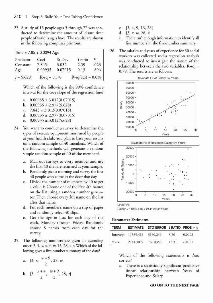
23. A study of 15 people ages 5 through 77 was con-ducted to determine the amount of leisure timepeople of various ages have. The results are shownin the following computer printout:
Time = 7.85 + 0.0094 Age
Predictor Coef St Dev t ratio PConstant 7.845 3.032 2.59 .023Age 0.00935 0.07015 0.13 .896
s = 5.628 R-sq = 0.1% R-sq(adj) = 0.0%
Which of the following is the 99% confidenceinterval for the true slope of the regression line?
a. 0.00935 ± 3.012(0.07015)b. 0.00935 ± 2.977(5.628)c. 7.845 ± 3.012(0.07015)d. 0.00935 ± 2.977(0.07015)e. 0.00935 ± 3.012(5.628)
24. You want to conduct a survey to determine thetypes of exercise equipment most used by peopleat your health club. You plan to base your resultson a random sample of 40 members. Which ofthe following methods will generate a randomsimple random sample of 40 of the members?
a. Mail out surveys to every member and usethe first 40 that are returned as your sample.
b. Randomly pick a morning and survey the first40 people who come in the door that day.
c. Divide the number of members by 40 to geta value k. Choose one of the first kth nameson the list using a random number genera-tor. Then choose every kth name on the listafter that name.
d. Put each member’s name on a slip of paperand randomly select 40 slips.
e. Get the sign-in lists for each day of theweek, Monday through Friday. Randomlychoose 8 names from each day for thesurvey.
25. The following numbers are given in ascendingorder: 3, 4, x, x, 9, w, 13, 28, y, z. Which of the fol-lowing gives a five-number summary of the data?
a. {3, x, , 28, z}
b. {3, , , 28, z}
c. {3, 4, 9, 13, 28]d. {3, x, w, 28, z}e. There isn’t enough information to identify all
five numbers in the five-number summary.
26. The salaries and years of experience for 50 socialworkers was collected and a regression analysiswas conducted to investigate the nature of therelationship between the two variables. R-sq. =0.79. The results are as follows:
Which of the following statements is leastcorrect?a. There is a statistically significant predictive
linear relationship between Years ofExperience and Salary.
w + 9
2
x + 4
2
w + 9
2
310 � Step 5. Build Your Test-Taking Confidence
GO ON TO THE NEXT PAGE
100000 5 10 15
Years
Bivariate Fit of Salary By Years
Linear Fit
Salary = 11369.416 + 2141.3092∗Years
Bivariate Fit of Residuals Salary By Years
20 25 30
20000
30000
40000
50000Sal
ary 60000
70000
80000
90000
100000
–200000 5 10 15
Years
20 25 30
–10000
0
Res
idua
ls S
alar
y
10000
20000
30000
Parameter Estimates
TERM ESTIMATE STD ERROR t RATIO PROB > |t|
Intercept 11369.416 3160.249 3.60 0.0008
Years 2141.3092 160.8358 13.31 <.0001

b. The residual plot indicates that a line is agood model for the data for all years.
c. There appears to be an outlier in the data atabout 28 years of experience.
d. The variability of salaries increases as yearsof experience increases.
e. For each additional year of experience, salaryis predicted to increase by about $2141.
27. A wine maker advertises that the mean alcoholcontent of the wine produced by his winery is11%. A 95% confidence interval, based on arandom sample of 100 bottles of wine yields aconfidence interval for the true alcohol contentof (10.5, 10.9) Could this interval be used aspart of a hypothesis test of the null hypothesisH0: p = 0.11 versus the alternative hypothesis HA: p ≠ 0.11 at the 0.05 level or confidence?
a. No, you cannot use a confidence interval ina hypothesis test.
b. Yes, because 0.11 is not contained in the95% confidence interval, a two-sided test atthe 0.05 level of significance would providegood evidence that the true mean content isdifferent from 11%.
c. No, because we do not know that the distri-bution is approximately normally distributed.
d. Yes, because 0.11 is not contained in the95% confidence interval, a two-sided test atthe 0.05 level of significance would fail toreject the null hypothesis.
e. No, confidence intervals can only be used inone-sided significance tests.
28. Tom’s career batting average is 0.265 with a stan-dard deviation of 0.035. Larry’s career battingaverage is 0.283 with a standard deviation of0.029. The distribution of both averages isapproximately normal. They play for differentteams and there is reason to believe that theircareer averages are independent of each other. Forany given year, what is the probability that Tomwill have a higher batting average than Larry?
a. 0.389b. 0.345c. 0.589d. 0.655e. You cannot answer this question since the
distribution for the difference between theiraverages cannot be determined from thedata given.
29. An advice columnist asks readers to write inabout how happy they are in their marriages.The results indicate that 79% of those respond-ing would not marry the same partner if theyhad it to do all over again. Which of the follow-ing statements is most correct?
a. It’s likely that this result is an accuratereflection of the population.
b. It’s likely that this result is higher than thetrue population proportion because personsunhappy in their marriages are most likelyto respond.
c. It’s likely that this result is lower than thetrue population proportion because personsunhappy in their marriages are unlikely torespond.
d. It’s likely that the results are not accuratebecause people tend to lie in voluntaryresponse surveys.
e. There is really no way of predicting whetherthe results are biased or not.
30. A national polling organization wishes to gener-ate a 98% confidence interval for the proportionof voters who will vote for candidate lam Sleazyin the next election. The poll is to have a marginof error of no more than 3%. What is the mini-mum sample size needed for this interval?
a. 6032b. 1508c. 39d. 6033e. 1509
31. In a test of the hypothesis H0: p = 0.7 againstHA: p > 0.7 the power of the test when p = 0.8would be greatest for which of the following?
a. n = 30, a = 0.10b. n = 30, a = 0.05c. n = 25, a = 0.10d. n = 25, a = 0.05e. It cannot be determined from the informa-
tion given.
AP Statistics Practice Exam 1 � 311
GO ON TO THE NEXT PAGE

32. A research team is interested in determining theextent to which food markets differ in prices forstore-brand items and the same name branditems. They identify a “shopping basket” of 10items for which they know store-brand andname-brand items exist (e.g, peanut butter,canned milk, grape juice, etc.). In order to con-trol market-to-market variability, they decide toconduct the study only at one major marketchain and will select just one market in each oftwelve geographically diverse cities. For eachmarket selected they will compute the mean forthe 10 store-brand items (call it ) and also forthe 10 name-brand items ( ). They thenintend to conduct a two-sample t-test (H0 : mN −mS = 0 vs. HA : mN − mS > 0) in order to determineif there is a statistically significant differencebetween the average prices of the two types ofitems. This procedure is not appropriate because
a. the sample sizes are too small to use a two-sample test.
b. the variances are most likely not the same.c. there is no randomization of treatments.d. the samples are not independent.e. they should be using a two-sample z-test.
33. A researcher was interested in determining therelationship between pulse rate (in beats/minute) and the time (in minutes) it took toswim a fixed distance. Based on 25 trials in thepool, the correlation coefficient between timeand pulse rate was found to be –0.654 (that is,large times—going slowly—were associated withslower pulses). Prior to publication, theresearcher decided to change the time measure-ments to seconds (each of the 25 times was mul-tiplied by 60). What would this conversion do tothe correlation between the two variables?
a. Since the units on only one of the variableswas changed, the correlation between thetwo variables would decrease.
b. The correlation would change proportionalto the change in the units for time.
c. The correlation between the two variableswould change, but there is no way, based onthe information given, to know by how much.
d. Changing the units of measurement has noeffect on the correlation coefficient. Hence,the correlation would be the same.
e. Since changing from minutes to secondswould result in larger times, the correlationwould actually increase.
34. The following histogram displays the scores of33 students on a 20-point Introduction toStatistics quiz. The lowest score, 0, is an outlier.The next lowest score, 2, is not an outlier.
Which of the following boxplots best representsthe data shown in the histogram?
0
2 24
8
12
5
7 14 21
2
6
10
Cou
nt
xN
xS
312 � Step 5. Build Your Test-Taking Confidence
GO ON TO THE NEXT PAGE
a.
b.
c.
d.
e.

35. For which one of the following distributions isthe mean most likely to be less than the median?
36. An SAT test preparation program advertises thatits program will improve scores on the SAT testby at least 30 points. Twelve students who havenot yet taken the SAT were selected for thestudy and were administered the test. The12 students then went through the 3-week test-prep course. The results of the testing were asfollows:
Assuming that the conditions necessary to con-duct the test are present, which of the followingsignificance tests should be used to determine ifthe test-prep course is effective in raising scoreby the amount claimed?
a. A two-sample t-testb. A chi-square test of independencec. A one-sample t-testd. A t-test for the slope of a regression linee. A two-sample z-test
37. Which of the following statements is (are)correct?
I. The area under a probability density curvefor a continuous random variable is 1.
II. A random variable is a numerical outcomeof a random event.
III. The sum of the probabilities for a discreterandom variable is 1.
a. II onlyb. I and IIc. I and IIId. II and IIIe. I, II, and III
AP Statistics Practice Exam 1 � 313
GO ON TO THE NEXT PAGE
Student 1 2 3 4 5 6 7 8 9 10 11 12
Before 475 500 499 477 540 608 510 425 495 502 530 487
After 495 540 495 522 555 684 535 460 522 529 560 512
a.
b.
c.
d.
e.

38. Let X be the number of points awarded for win-ning a game that has the following probabilitydistribution:
X 0 2 3
P(X ) 0.2 0.5 0.3
Let Y be the random variable whose sum is thenumber of points that results from two inde-pendent repetitions of the game. Which of thefollowing is the probability distribution for Y ?
a.Y 0 2 3
P(Y ) 0.2 0.5 0.3b.
Y 0 4 6
P(Y ) 0.2 0.5 0.3
c.
Y 0 2 3 4 6
P(Y ) 0.2 0.25 0.15 0.25 0.15
d.
Y 0 2 3 4 5 6
P(Y) 0.04 0.2 0.12 0.25 0.3 0.09
e.
Y 0 2 3 4 5 6
P(Y ) 0.04 0.10 0.06 0.25 0.15 0.09
39. Each of the following histograms represents asimulation of a sampling distribution for anestimator of a population parameter. The truevalue of the parameter is X, as shown on thescale. The domain of possible outcomes is thesame for each estimator and the frequency axes(not shown) are the same. Which histogramrepresents the best estimator of X?
40. A weight-loss clinic claims an average weightloss over 3 months of at least 15 pounds. Arandom sample of 50 of the clinic’s patronsshows a mean weight loss of 14 pounds with astandard deviation of 2.8 pounds. Assuming thedistribution of weight losses is approximatelynormally distributed, what is the most appro-priate test for this situation, the value of the teststatistic, and the associated P-value?
a. z-test; z = −2.53; P-value = 0.0057b. t-test; t = −2.53; 0.01 < P-value < 0.02c. z-test; z = 2.53; P-value = 0.0057d. t-test; t = −2.53; 0.005 < P-value < 0.01e. z-test; z = 2.53; P-value = 0.9943
314 � Step 5. Build Your Test-Taking Confidence
END OF SECTION I
X X
X
X
X
a.
c.
e.
b.
d.

AP Statistics Practice Exam 1
SECTION II
Time: 1 hour and 30 minutes
Number of problems: 6
Percentage of total grade: 50
General InstructionsThere are two parts to this section of the examination. Part A consists of five equallyweighted problems that represent 75% of the total weight of this section. Spend about 65 minutes on this part of the exam. Part B consists of one longer problem that represents25% of the total weight of this section. Spend about 25 minutes on this part of the exam.You are not necessarily expected to complete all parts of every question. Statistical tablesand formulas are provided.
• Be sure to write clearly and legibly. If you make an error, you may save time by crossingit out rather than trying to erase it. Erased or crossed-out work will not be graded.
• Show all your work. Indicate clearly the methods you use because you will be graded onthe correctness of your methods as well as the accuracy of your final answers. Correctanswers without support work may not receive credit.
Statistics, Section II, Part A, Questions 1–5Spend about 65 minutes on this part of the exam; percentage of Section II grade: 75.
Directions: Show all your work. Indicate clearly the methods you use because you willbe graded on the correctness of your methods as well as on the accuracy of your results andexplanation.
1. David was comparing the number of vocabulary words children know about transp-ortation at various ages. He fit a least-squares regression line to the data. The residualplot and part of the computer output for the regression are given below.
AP Statistics Practice Exam 1 � 315
Predictor Coef St Dev t ratio PConstant 3.371 1.337 2.52 .065Age 2.1143 0.2321 9.11 .001
s = 0.9710 R-sq = 95.4% R-sq(adj) = 94.3%
−1.2
0.0
RESID
Age3.6 4.8 6.0 7.2
xx
xx
xx
GO ON TO THE NEXT PAGE

a. Is a line an appropriate model for these data? Explain.b. What is the equation of the least-square regression line for predicting the number
of words from age?c. What is the predicted number of words for a child of 7.5 years of age?d. Interpret the slope of the regression line in the context of the problem.e. Would it be appropriate to use the model to predict the number of words a 12-year-
old would know?
2. Students at Dot.Com Tech are allowed to sign up for one math class each semester. Thenumbers in each grade level signing up for various classes for next semester are given inthe following table.
GEOMETRY ALGEBRA II ANALYSIS CALCULUS AB TOTAL
10th Grade 125 74 23 3 22511th Grade 41 92 72 25 23012th Grade 12 47 99 62 220Total 178 213 194 90 675
a. What is the probability that a student will take calculus?b. What is the probability that a 12th grader will take either analysis or calculus?c. What is the probability that a person taking algebra II is a 10th grader?d. Consider the events, “A student takes geometry” and “A student is a 10th grader.”
Are these events independent? Justify your answer.
3. The state in which you reside is undergoing a significant budget crisis that will affecteducation. Your school is trying to decide how many sections of upper-level mathematicsclasses to offer next year. It is very expensive to offer sections that aren’t full, so theschool doesn’t want to offer any more sections than it absolutely needs to. The assistantprincipal in charge of scheduling selects a random sample of 60 current sophomoresand juniors. Fifty-five of them return the survey, and 48 indicate that they intend totake math during the coming year. If 80% or more of the students actually sign up formath, the school will need to add a section.
a. On the basis of the survey data, would you recommend to the assistant principalthat an additional class of upper division mathematics should be scheduled? Giveappropriate statistical evidence to support your recommendation.
b. Five of the 60 who received surveys failed to return them. If they had returnedthem, how might it have affected the assistant principal’s decision? Explain.
4. It is known that the symptoms of adult depression can be treated effectively with eithertherapy, antidepressants, or a combination of the two. A pharmaceutical companywants to test a new antidepressant against an older medication that has been on themarket for several years. One hundred fifty volunteers who have been diagnosed withdepression, and who have not been taking any medication for it, are available for thestudy. This group contains 72 men and 78 women. Sixty of the volunteers have beenin therapy for their depression for at least 3 months.
a. Design a completely randomized experiment to test the new medication. Include abrief explanation of the randomization process.
b. Could the experiment you designed in part (a) be improved by blocking? If so,design an improved study that involves blocking. If not, explain why not.
316 � Step 5. Build Your Test-Taking Confidence
GO ON TO THE NEXT PAGE

5. The 1970 draft lottery was suspected to be biased toward birthdays later in the year.Because there are 366 possible birthdays, in a fair drawing we would expect to find,each month, an equal number of selections less than or equal to 183 and greater thanor equal to 184. The following table shows the data from the 1970 draft lottery.
NUMBER SELECTED NUMBER SELECTED≤ 183 ≥ 184 TOTALS
January 12 19 31February 12 17 29March 10 21 31April 11 19 30May 14 17 31June 14 16 30July 14 17 31August 19 12 31September 17 13 30October 13 18 31November 21 9 30December 26 5 31Totals 183 183 366
Do these data give evidence that the 1970 draft lottery was not fair? Give appropriatestatistical evidence to support your conclusion.
Statistics, Section II, Part B, Question 6Spend about 25 minutes on this part of the exam; percentage of Section II grade: 25.
Directions: Show all of your work. Indicate clearly the methods you use because youwill be graded on the correctness of your methods as well as on the accuracy of your resultsand explanation.
6. A lake in the Midwest has a restriction on the size of trout caught in the lake. The aver-age length of trout over the years has been 11 inches with a standard deviation of 0.6 inches. The lengths are approximately normally distributed. Because of overfishingduring the past few years, any fish under 11.5 inches in length must be released.
a. What is the probability that a fisherman will get lucky and catches a fish she cankeep? Round your answer to the nearest tenth.
b. Design a simulation to determine the probability how many fish the fishermanmust catch, on average, in order to be able to take home five trout for dinner.
c. Use the table of random digits between parts (d) and (e) of this problem to con-duct five trials of your simulation. Show your work directly on the table.
d. Based on your simulation, what is your estimate of the average number of fish thatneed to be caught in order to catch five she can keep?
79692 51707 73274 12548 91497 11135 81218 79572 06484 8744041957 21607 51248 54772 19481 90392 35268 36234 90244 0214607094 31750 69426 62510 90127 43365 61167 53938 03694 7692359365 43671 12704 87941 51620 45102 22785 07729 40985 92589
e. What is the theoretical expected number of fish that need to be caught in order tobe able to keep five of them?
AP Statistics Practice Exam 1 � 317
END OF THE PRACTICE EXAM I

� Answers to Practice Exam 1, Section I1. b 21. e2. b 22. d3. a 23. a4. d 24. d5. e 25. a6. c 26. b7. a 27. b8. c 28. b9. b 29. b
10. e 30. e11. e 31. a12. e 32. d13. b 33. d14. e 34. b15. a 35. a16. a 36. c17. e 37. e18. d 38. d19. a 39. d20. b 40. d
318 � Step 5. Build Your Test-Taking Confidence

AP Statistics Practice Exam 1 � 319
� Solutions to Practice Exam 1, Section I
1. The correct answer is (b). The confidence levelisn’t mentioned in the problem, but polls oftenuse 95%. If that is the case, we are 95% confidentthat the true value is within 3.5% of the samplevalue.
2. The correct answer is (b). Since the mean isnoticeably greater than the median, the distribu-tion is likely skewed to the right. Another indica-tion of this is the long “whisker” on a boxplot ofthe five-number summary. IQR = 544 – 502 = 42.An outlier is any value less than 502 – 1.5(542) =439 or greater than 544 + 1.5(42) = 607. Sincethe maximum value given (610) is greater than607, there is at least one outlier.
3. The correct answer is (a). The most likely biaswould be to influence people to oppose such alaw since many voters are resistant to constitu-tional amendments restricting rights. Comparethis to the question, “Do you favor a law thatwould provide that only marriage between a manand a woman is valid or recognized in California?”which could influence voters to favor the amend-ment. This was, in fact, a legal issue in Californiaprior to the election. The original title of theamendment was “Limit on Marriage.” TheAttorney General of California, Jerry Brown,changed the title to include the phrase “eliminates(the) right of same-sex couples to marry.” Whenchallenged in court by proponents of the amend-ment, the title change was upheld based on thefact that the right of same-sex couples to marryhad been given full legal status by the statesupreme court earlier in the year.
4. The correct answer is (d). Choosing your samplefrom only the homes in your population of inter-est gives you a larger sample on which to baseyour confidence interval. If you use Plan A, youwill end up with many homes painted with dif-ferent paint than the paint of interest.
5. The correct answer is (e). The t-distributions aresymmetric about their means. I is the mirrorimage of P (X > 65). II, in a continuous distribu-tion, is equivalent to P (X > 65)—this would notbe true in a discrete distribution (e.g., a binomial).
6. The correct answer is (c). (a) describes a simplerandom sample. (b) describes a cluster sample. (d)describes stratified random sampling. (e) describesa voluntary response sample.
7. The correct answer is (a). There is a natural ten-dency on the part of a subject in an experimentto want to please the researcher. It is likely thatthe employees were increasing their productionbecause they wanted to behave in the way theythought they were expected to.
8. The correct answer is (c). A Type-I error occurswhen a true hypothesis is incorrectly rejected. Inthis case, that means that the assumption ofinnocence is rejected, and he is found guilty.
9. The correct answer is (b). P(A and B) =P(A) • P(A|B) = (0.4)(0.2) = 0.08. P(A or B) =P(A) + P(B) − P(A and B) = 0.4 + 0.3 − 0.08 =0.62.
10. The correct answer is (e). The purpose of ran-domization is to control for the unknowneffects of variables that might affect theresponse, in this case the differential effects ofNorth or South placement. (a) is incorrect sincestudies of any size benefit from randomization.(b) is simply nonsense—the number of treat-ments does not affect the need to randomize.(c) involves blocking and would be correct if weknow in advance that there were differentialeffects based on a North/South placement—butnothing in the problem indicates this. (d) is notincorrect, but it’s not the reason we are random-izing in this situation.
11. The correct answer is (e). By definition a “clustersample” occurs when a population is dividedinto groups and then a group or groups is ran-domly selected. (a) is a simple random sample;(b) is a systematic sample; (c) is a self-selectedsample and is not random; (d) is a simplerandom sample.
12. The correct answer is (e). Be clear on the differ-ence between the treatment (type of cat food inthis problem) and the blocking variable (breed ofcat).

13. The correct answer is (b). The box is longer forNetwork A and the ends of the whiskers are fur-ther apart than Network B ⇒ Network A has agreater range of ratings than Network B. The3rd quartile, the median, and the 1st quartile ofNetwork A are higher than Network B, whichcan be interpreted to mean that Network A ishigher rated than Network B. I is not correctbecause there is no way to tell how many valuesare in a boxplot.
14. The correct answer is (e). If a significance testrejects H0 at α = 0.05, then a two-sided 95%confidence interval will not contain 0.3. If thefinding is not significant at α = 0.04, then atwo-sided 96% confidence interval will contain0.3. Hence, any confidence level 95% or lesswill contain 0.3 and any confidence level 96%or higher will not.
15. The correct answer is (a). Since 0 is in the inter-val, it is possible that the true difference betweenthe proportions is 0, i.e, that there has not beena significant drop in support. Note that a 90%interval, but not a 95% interval, would containonly positive numbers and would provide statis-tically significant evidence of a drop in support.(d) is false since it’s a one-sided test (with a P-value of 0.046) and the confidence interval istwo sided. A two-sided test (HA : P1 ≠ p2) wouldyield the same conclusion (P = 0.092) as theconfidence interval. (b), (c), and (d) are simplywrong.
16. The correct answer is (a). The expected valuesare: 0.5 × 50 = 25 Golden Retrievers, 0.8 × 50 =20 Shepherds; and 0.1 × 50 = 5 Others.
.
17. The answer is (e). We are 95% confident that thetrue proportion who will vote for the former actoris in the interval (0.35, 0.42). This means that thetrue proportion is likely to be in this interval.
18. The correct answer is (d). While the centrallimit theorem argues that the shape ofDistribution II will be approximately normal,the sample size for Distribution I is too smallfor the CLT to apply. The best we can say isthat the distribution of a sampling distributionfor a small sample will be similar to the original
population (hence, (c) is true). Since we are notgiven the shape of the original population, wecannot make the claim that the distribution for thesmaller sample size will be approximately normal.
19. The correct answer is (a). The P-value for thetwo-proportion z-test is 0.055. This isn’t muchover 0.05, but it is enough to say that we do nothave, at the 0.05 level, a statistically significantdifference between the two findings. Note that(a) and (c) are mutually exclusive. If (a) is cor-rect, which it is, then (c) must be false. (b) is notcorrect since it does not take into accountrandom variation. While the conclusion in (d)is correct, the statement is not—the raw differ-ence between two values is not what allows us tomake conclusions about statistical differencesbetween groups. (e), while it does get at the vari-ability between the sample proportions, doesn’ttell us anything by itself.
20. The correct answer is (b). The following tree diagram illustrates the situation:
Now, P (student takes art) = 0.45 + 0.08 = 0.53.
21. The correct answer is (e). P (doesn’t take English |does take art)
22. The correct answer is (d). In general, when test-ing for a population mean, you should use at-distribution unless the population standarddeviation is known—which it rarely is in practice.(a), (b), and (c) are simply incorrect. (e) is acorrect statement but is not the reason you woulduse t rather than z (in fact, if it argues anything, itargues that there is no practical numerical differ-ence between using t or z for large samples).
=+
=0 08
0 45 0 080 15
.
. .. .
0.9
0.10
0.5
0.5
0.8
0.2
Eng.
NoEng.
Art
Art
No Art
No Art
P (Art ⎥ Eng) = (0.9)(0.5) = 0.45
P(No Art ⎥ Eng) = (0.9)(0.5) = 0.45
P (Art ⎥ Eng) = (0.1)(0.8) = 0.08
P (No Art ⎥ Eng) = (0.1)(0.2) = 0.02
X 22 2 227 25
25
22 20
20
1 5
53 56=
−+
−+
−=
( ) ( ) ( ).
320 � Step 5. Build Your Test-Taking Confidence

23. The correct answer is (a). df = n − 2 = 15 − 2 =13 ⇒ t* = 3.012 (if you have a TI-84 with the invT function, invT (0.995, 13)=3.0123). The standard error of the slope of theregression line (found under “St Dev” after“Age”), sb, is 0.07015. The confidence interval,therefore, is 0.00935 ± 3.012(0.07015).(Newer TI-84’s have a LinRegTInt in theSTAT TESTS menu. However, that is of nohelp here since the calculator requires that thedata be in lists—there is no option to entersummary statistics.)
24. The correct answer is (d). To be a simple randomsample, every possible sample of size 40 must beequally likely. Only (d) meets this standard.Note that (c) and (e) are perfectly valid ways ofcollecting a random sample. At the start, eachmember of the population has an equal chanceto be in the sample. But they are not SRS’s.
25. The correct answer is (a). First find the median.Since there are 10 terms, the median is the mean
of the middle two terms: . The first
quartile is the median of the five terms less thanthe median (x) and the third quartile isthe median of the five terms greater than themedian (28). The minimum value is 3 and themaximum is z.
26. The correct answer is (b). Note that the vari-ability of the residuals increases as years ofexperience increases so that the pattern for allyears is not truly random. (a) is correct basedon the t-test for the slope of the regressionline given as “<.0001.” (c) is correct as theresidual of that point is very large comparedto most of the points. (d) is correct and is thereason that (b) is not a true statement. (e) isthe standard interpretation of the slope of aregression line.
27. The correct answer is (b). A confidence intervalcan be used in place of a significance test in ahypothesis test (for a population mean or thedifference between two population means) witha two-sided alternative. In this case, the evidencesupports the alternative.
28. The correct answer is (b). Since the distribu-tions are independent and approximately
normal, we use and
. Tom (T ) has N(0.265,
0.035) and Larry (L) has N(0.283, 0.029). Hence, and
. T – L then
has the distribution N(–0.018, 0.045). We
need to know the probability that T – L is
positive (since we require that T be greater
than L) in this distribution. P (T – L > 0) =
. On the TI-
83/84 calculator, normal cdf(0.4,0.045)=0.3446. Also, normal cdf(0,100,0.018,0.045)=0.3446.
29. The correct answer is (b). The tendency in vol-untary response surveys is for people who feelmost strongly about an issue to respond. Ifpeople are happy in their marriage, they are lesslikely to respond.
30. The correct answer is (e). The upper critical z for a 98% confidence interval is z* = 2.33(from Table A; on the TI-83/84, invNorm(0.99)= 2.326). In the expression
we choose P* = 0.5 since
we are not given any reason to choose some-
thing else. In this case the “recipe”
becomes The sample size needed is
Choose n = 1509.
(Note: If you use z* = 2.326 rather than 2.33,you will get n ≥ 1502.9 ⇒ choose n = 1503.)
31. The correct answer is (a). Power can be increasedby increasing n, increasing α moving the alterna-tive further away from the null, reducing thevariability. This choice provides the best combi-nation of large n and large α.
n ≥⎛
⎝⎜
⎞
⎠⎟ =
2 33
2 0 031508 03
2.
( . ). .
nz
M≥
⎛⎝⎜
⎞⎠⎟
*.
2
2
nzM
P P≥⎛
⎝⎜
⎞
⎠⎟ −
** ( *),
2
1
P z >− −
=⎛
⎝⎜
⎞
⎠⎟=
0 0 018
0 0450 4 0 345
( . )
.. .
σT L− = + =0 035 0 029 0 0452 2. . .
μT L− = − = −0 265 0 283 0 018. . .
σ σ σX Y X Y− = +2 2
μ μ μX Y X Y− = −
w +⎛
⎝⎜
⎞
⎠⎟
9
2
AP Statistics Practice Exam 1 � 321

32. The correct answer is (d). The data are pairedin that two measurements are being takenat each of 12 different stores. The correctanalysis would involve a one-sample t-test ( where d =
for each of the 12 pairings).
33. The correct answer is (d). The correlation coef-ficient is not affected by any linear transforma-tion of the variables. Changing the units ofmeasurement is a linear transformation.
34. The correct answer is (b). The key is to note thatthere is an outlier, which eliminates (a) and (e),and only one outlier, which eliminates (c). Thehistogram is skewed to the left, which shows inthe boxplot for (b) but not for (d) which is,except for the outlier, more symmetric.
35. The correct answer is (a). The mean is pulled inthe direction of skewness.
36. The correct answer is (c). The data are paired,which means that we are testing H0 : md = 30 vs.HA : m >30, where d = Before – After for eachstudent. That is, there is only one sample.
37. The correct answer is (e).
38. The correct answer is (d). The computations areshown in the following table:
39. The correct answer is (d). While all of thegraphs tend to center around X, the true valueof the parameter, (d) has the least variabilityabout X. Since all of the graphs have roughly thesame low bias, the best estimator will be the onewith the least variability.
40. The correct answer is (d). We are told that thedistribution of weight losses is approximatelynormal, but we are not given the population stan-dard deviation. Hence the most appropriate test
is a t-test. Now, , df = 50 – 1
= 49 ⇒ 0.005 < P-value < 0.01 (from Table B, rounding down to df = 40; using the TI-83/84, we have tcdf(-100,-2.53,49)=0.0073). Note that the P-value for the z-test in (a) is quite close. However, a z-test is not themost appropriate test since we do not know thepopulation standard deviation.
t =−
= −14 152 8
50
2 53.
.
x xN S−H Hd A d0 0 0: :μ μ= >vs.
322 � Step 5. Build Your Test-Taking Confidence
Y 0 2 3 4 5 6
0, 2 0,3 2, 3How: 0, 0 or or 2, 2 or 3, 3
2, 0 3, 0 3, 2
P(Y ) (0.2)(0.2) 2(0.2)(0.5) 2(0.2)(0.3) (0.5)(0.5) 2(0.5)(0.3) (0.3)(0.3)
= 0.04 = 0.2 = 0.12 = 0.25 = 0.3 = 0.09
� Solutions to Practice Exam 1, Section II, Part ASolution to #1
a. We note that r2 = 0.954 ⇒ r = 0.98, so there is a strong linear correlation between thevariables. We know that the correlation is positive since the slope of the regression lineis positive. Also, the residual plot shows no obvious pattern, indicating that the line isa good model for the data.
b. Words = 3.371 + 2.1143(Age).
c. Words = 3.371 + 2.1143(7.5) = 19.2.
d. For each year a child grows, the number of words he or she knows about transportationis predicted to grow by 2.1.
e. No. This would require extrapolating beyond the range of the data.
Solution to #2
a. P (a student takes calculus) = 90/675 = 0.133.
b. P (a student takes analysis or calculus given that he/she is in the 12th grade)
c. P (a student is in the 10th grade given that he/she is taking algebra II)
d. Let A = “A student takes geometry” and B = “A student is a 10th grader.” A and B areindependent events if and only if P(A) = P(A | B).
Thus, the events are not independent.
Solution to #3
a. Let p = the true proportion of students who will sign up for upper division mathemat-ics classes during the coming year.
We want to use a one-proportion z-test, at the 0.05 level of significance. We note thatwe are given that the sample was a random sample, and that np = 55(0.8) = 44 and 55 (1 − 0.8) = 11 are both larger than 5 (or 10). Thus the conditions needed for thistest are present.
H p
H pA
00 80
0 80
: . .
: . .
≤
>
P ( ) . .A|B = =125
2250 556
P ( ) . .A = =178
6750 264
= =74
2130 347. .
=+
= =99 62
220
161
2200 732. .
AP Statistics Practice Exam 1 � 323

(from Table A; on
the TI-83/84, the P-value = normalcdf(1.35,100)). Since P > α, we cannotreject the null hypothesis. The survey evidence is not strong enough to justify addinganother section of upper-division mathematics.
b. If all five of the other students returned their surveys, there are two worst-case scenar-ios: all five say they will sign up; all five say they will not sign up. If all five say they willnot sign up, then an even lower percentage say they need the class (48/60 rather than48/55) and our decision not to offer another class would not change.
If all five say they will sign up, then
At the 5% level of significance, this is still not quite enough to reject the null. However,it’s very close, and the assistant principal might want to generate some additional databefore making a final decision.
Solution to #4
a. Randomly divide your 150 volunteers into two groups. One way to do this would beto put each volunteer’s name on a slip of paper, put the papers into a box, and begindrawing them out. The first 75 names selected would be in group A, and the other 75would be in group B. Alternatively, you could flip a coin for each volunteer. If it cameup heads, the volunteer goes into group A; if tails, the volunteer goes into group B. Thesecond method would likely result in unequal size groups.
Administer one group the new medication (treatment group), and administer the oldmedication to the other group (control) for a period of time. After enough time haspassed, have each volunteer evaluated for reduction in the symptoms of depression.Compare the two groups.
b. Because we know that being in therapy can affect the symptoms of depression, blockby having the 60 people who have been in therapy be in one block and the 90 who havenot been in therapy be in the other block. Then, within each block, conduct an exper-iment as described in part (a).
Solution to #5
H0: Month of birth and draft number are independent.HA: Month of birth and draft number are not independent.
ˆ .. .
. ( . ).p z P= = → =
−
−= ⇒
53
600 883
0 883 0 080
0 8 1 0 860
1 61 -vvalue = − =1 0 9463 0 0537. . .
ˆ . .
. ( . ).p z P= = =
−
−= ⇒
48
55
0 873 080
0 8 1 0 855
1 35 -valuue 1 0.9115 0.0885= − =
324 � Step 5. Build Your Test-Taking Confidence

This is a two-way table with 12 rows and 2 columns. A chi-square test of independenceis appropriate. The numbers of expected values are given in the table below:
EXPECTED NUMBER EXPECTED NUMBERSELECTED ≤ 183 SELECTED ≥ 184
January 15.5 15.5February 14.5 14.5March 15.5 15.5April 15 15May 15.5 15.5June 15 15July 15.5 15.5August 15.5 15.5September 15 15October 15.5 15.5November 15 15December 15.5 15.5
Because all expected values are greater than 5, the conditions for the chi-square good-ness-of-fit test are present.
df = (12−1)(2−1) = 11 ⇒ 0.001 < P-value < 0.0025 (from Table C; using theTI-83/84, we have X 2cdf (31.14,1000,11)= 0.00105).
Because the P-value is so small, we have evidence to reject the null and conclude thatbirth month and draft number are not independent. That is, month of birth is relatedto draft numbers. Observation of the data indicates that the lottery was biased againstpeople born later in the year. That is, people born later in the year were more likely toget drafted.
X 22 2 212 15 5
15 5
19 15 5
15 5
26 15 5
15=
−+
−+ +
−( . )
.
( . )
.
( . )�..
( . )
.. .
55 15 5
15 531 14
2
+−
=
AP Statistics Practice Exam 1 � 325

� Solutions to Practice Exam 1, Section II, Part BSolution to #6
a. The situation described is pictured below.
Let X be the length of a fish. Then P (X > 11.5) = = 1− 0.7967 =
0.2033 (from Table A; using the TI-83/84, we have P(X > 11.5) =normalcdf (0.83,100) or normalcdf (11.5, 1000, 11, 0.6)). Rounding to the nearesttenth, P (X > 11.5) = 0.2.
b. Because the probability that the fish is large enough to keep is 0.2, let the digits 0 and1 represent a fish that is large enough to keep and the digits 2, 3, 4, 5, 6, 7, 8, and9 represent fish that must be released. Begin at the first line of the table and count thenumber of digits required before five of the digits 0, 1 are found.
c. On the random number table below, successes (a large enough fish) are in boldface.Backslashes separate the various trials. The number of catches it took to get two suffi-ciently large fish is indicated under each separate trial.
79692 51707 73274 12548 91497 1\\1135 81218 79572 0\\6484 87440(26 fish) (15 fish)
41957 21607 51\\248 54772 19481 90392 35268 36234 90244 0\\2146(21 fish) (34 fish)
07094 31750\\ 69426 62510 90127 43365 61167 53938 03694 76923(14 fish)
59365 43671 12704 87941 51620 45102 22785 07729 40985 92589
d. Based on the five trials, an estimate of the average number of trials required to get twofish of minimum size is (26 + 15 + 21 + 34 + 14)/5 = 22.
e. The expected wait to catch a single fish with P = 0.2 is 1/0.2 = 5 fish. The expectedwait to catch five fish is then 5(5) = 25.
P z(.
.. )>
−=
11 5 11
0 60 83
11 11.5
326 � Step 5. Build Your Test-Taking Confidence

AP Statistics Practice Exam 1 � 327
� Scoring Sheet for Practice Exam 1Section I: Multiple Choice
[ ( / )]number correct(out of 40)
number wrong− × ×1 4 11 25. =
multiple choice
score
(if less than zero,
e
-
nnter zero)
=weighted section I
score(do not rounnd)
Section II: Free Response
Question 1(out of 4)
.× =1 875(do not round)
QQuestion 2(out of 4)
.× =1 875(do not round))
(do not rounQuestion 3
(out of 4).× =1 875
dd)
(do not rouQuestion 4
(out of 4).× =1 875
nnd)
(do not roQuestion 5
(out of 4).× =1 875
uund)
(do not rQuestion 6
(out of 4).× =3 125
oound)
Sumweighted
section II score
(do not
=
rround)
Composite Score
weighted
section Iscore
weighted
section IIsc
+
oore
composite score(round to nearestwhole nu
=
mmber)

This page intentionally left blank

AP Statistics Practice Exam 2
ANSWER SHEET FOR SECTION I
AP Statistics Practice Exam 2 � 329
1 A B C D E
2 A B C D E
3 A B C D E
4 A B C D E
5 A B C D E
16 A B C D E
17 A B C D E
18 A B C D E
19 A B C D E
20 A B C D E
31 A B C D E
32 A B C D E
33 A B C D E
34 A B C D E
35 A B C D E
6 A B C D E
7 A B C D E
8 A B C D E
9 A B C D E
10 A B C D E
21 A B C D E
22 A B C D E
23 A B C D E
24 A B C D E
25 A B C D E
36 A B C D E
37 A B C D E
38 A B C D E
39 A B C D E
40 A B C D E
11 A B C D E
12 A B C D E
13 A B C D E
14 A B C D E
15 A B C D E
26 A B C D E
27 A B C D E
28 A B C D E
29 A B C D E
30 A B C D E

This page intentionally left blank

AP Statistics Practice Exam 2 � 331
AP Statistics Practice Exam 2
SECTION ITime: 1 hour and 30 minutes
Number of questions: 40
Percentage of total grade: 50
Directions: Solve each of the following problems. Decide which is the best of the choices given and answer inthe appropriate place on the answer sheet. No credit will be given for anything written on the exam. Do notspend too much time on any one problem.
1. Given the two boxplots above, which of the following statements is (are) true?
I. The boxplot for Set B has more terms aboveits median than the boxplot for Set B.
II. The boxplot for Set B has a larger IQR thanthe boxplot for Set A.
III. The median for Set A is larger than themedian for Set B.
a. I onlyb. II onlyc. III onlyd. I and II onlye. II and III only
2. An advertiser is trying to decide which televisionstation in town to use for his product. He gathersthe ratings of all prime time shows on each net-work and constructs a boxplot of each. There arethe same number of ratings for each network.The results are as follows:
Based on these boxplots, which of the followingis a correct conclusion about the relative ratingsfor the two networks?
a. The median rating for Network A is greaterthan for Network B.
b. The range for Network A is greater than forNetwork B.
c. The interquartile ranges for the two networksare the same.
d. The median rating for Network B is higherthan for Network A.
e. There are more ratings greater than 28 forNetwork A than for Network B.
3. A statistics class wanted to construct a 90% confi-dence interval for the difference in the number ofadvanced degrees held by male and female facultymembers at their school. They collected degreedata from all the male and female faculty membersand then used these data to construct the desired90% confidence interval. Is this an appropriateway to construct a confidence interval?
a. No, because we don’t know that the distribu-tions involved are approximately normal.
b. Yes, but only if the number of men and thenumber of women are equal because our cal-culations will be based on difference scores.
c. Yes, but only if the distribution of differencescores has no outliers or extreme skewness.
d. No, because all the data were available, there isno need to construct a confidence interval for thetrue difference between the number of degrees.
e. No, confidence intervals can only be con-structed on independent samples, not onpaired differences.
Network A
Network B
10 20 30 40 50
SET A
SET B
GO ON TO THE NEXT PAGE

332 � Step 5. Build Your Test-Taking Confidence
4. You are interested in determining which of twobrands of tires (call them Brand G and Brand F)last longer under differing conditions of use. FiftyToyota Camrys are fitted with Brand G tires and50 Honda Accords are fitted with Brand F tires.Each tire is driven 20,000 miles, and tread wearis measured for each tire, and the average treadwear for the two brands is compared. What iswrong with this experimental design?
a. The type of car is a confounding variable.b. Average tread wear is not a proper measure
for comparison.c. The experiment should have been conducted
on more than two brands of cars.d. Not enough of each type of tire was used in
the study.e. Nothing is wrong with this design—it should
work quite well to compare the two brands oftires.
5. The blood types of 468 people residing in theUnited States (all of whom were Asian, African-American, Arab, or White) were collected in a studyto see if their blood type distribution is related torace. The following results were obtained:
TypeEthnicity O A B AB
Asian 48 33 33 6African-American 45 24 18 3Arab 36 33 30 6White 69 60 18 6
From these data, a c2 value of 19.59 (df = 9) wascomputed. At the 5% level of significance, dothese data indicate that Ethnicity and Blood Typeare related?
a. Yes, because the P-value of the test is greaterthan 0.05.
b. Yes, because the P-value of the test is less than0.05.
c. No, because the P-value of the test is greaterthan 0.05.
d. No, because the P-value of the test is lessthan 0.05.
e. c2 should not be used in this situation sincemore than 20% of the expected values are lessthan 5.
6. Most college-bound students take either the SAT(Scholastic Assessment Test) or the ACT (whichoriginally stood for American College Testing).Scores on both the ACT and the SAT are approx-imately normally distributed. ACT scores have amean of about 21 with a standard deviation ofabout 5. SAT scores have a mean of about 508with a standard deviation of about 110. Nicoletakes the ACT and gets a score of 24. Luis takesthe SAT. What score would Luis have to have onthe SAT to have the same standardized score(z-score) as Nicole’s standardized score on theACT?
a. 548b. 574c. 560d. 583e. 588
7. A researcher conducts a study of the effectivenessof a relaxation technique designed to improve thelength of time a SCUBA diver can stay at a depthof 60 feet with a 80 cu. ft. tank of compressed air.The average bottom time for a group of diversbefore implementation of the program was48 minutes and the average bottom time afterimplementation of the program was 54 minuteswith a P-value of 0.024. Which of the followingis the best interpretation of this finding?
a. There is a 2.4% chance that the new tech-nique is effective at increasing bottom time.
b. If the new technique was not effective, thereis only a 2.4% chance of getting 54 minutesor more by chance alone.
c. 97.6% of the divers in the study increasedtheir bottom times.
d. We can be 97.6% confident that the new tech-nique is effective at increasing bottom time.
e. The new technique does not appear to beeffective at increasing bottom time.
GO ON TO THE NEXT PAGE

AP Statistics Practice Exam 2 � 333
8. Does ultraviolet radiation affect the birth rate offrogs? A study in the Tampa Tribune reported thatwhile 34 of 70 sun-shaded (from ultravioletradiation) eggs hatched, only 31 of 80 unshadedeggs hatched. Which of the following would givea 99% confidence interval for the true differencebetween the proportions of shaded and unshadedeggs that hatched?
9. At Midtown University, the average weight of fresh-men boys is 170 lbs with a standard deviation of9 lbs The average weight of freshmen girls is115 lbs with a standard deviation of 6 lbs. Anew distribution is to be formed of the valuesobtained when the weights of the girls and theboys are added together. What are the meanand standard deviation of this new distribu-tion? Assume that the weights of freshman boysand freshman girls are independent.
a. 285, 15b. 285,117c. 55, 10.8d. 285, 10.8e. The mean is 285 but, under the conditions
stated in the problem, you cannot determinethe standard deviation.
10. A random sample of 875 deaths in the United Statesin the year 2000 showed a mean life span of 75.1years with a sample standard deviation of 16 years.These data were used to generate a 95% confidenceinterval for the true mean lifespan in the UnitedStates. The interval constructed was (74.0, 76.2).Which of the following statements is correct?
a. There is a 95% chance that the averagelifespan in the United States is between74 and 76.2 years.
b. 95% percent of the time, a person in theUnited States will live between 74 years and76.2 years.
c. 95% of the time, on average, intervals pro-duced in this manner will contain the truemean lifespan.
d. On average, 95% of people live less than76.2 years.
e. The probability is 0.95 that this intervalcontains the true mean lifespan in theUnited States.
11.
Which of the following is the best estimate ofthe standard deviation for the approximatelynormal distribution pictured?
a. 10b. 30c. 5d. 9e. 15
5 20 35
GO ON TO THE NEXT PAGE
a.34
70
31
801 96
3470
13470
70
3180
1
−⎛
⎝⎜
⎞
⎠⎟±
−⎛
⎝⎜
⎞
⎠⎟
+
−
.
33180
80
34
70
31
802 576
65
150
⎛
⎝⎜
⎞
⎠⎟
−⎛
⎝⎜
⎞
⎠⎟±
⎛
⎝⎜
⎞
⎠⎟b. .
885
150
1
70
1
80
34
70
31
801 96
⎛
⎝⎜
⎞
⎠⎟ +⎛
⎝⎜
⎞
⎠⎟
−⎛
⎝⎜
⎞
⎠⎟±c. .
665
150
85
150
1
70
1
80
34
70
31
80
⎛
⎝⎜
⎞
⎠⎟⎛
⎝⎜
⎞
⎠⎟ +⎛
⎝⎜
⎞
⎠⎟
−d.⎛⎛
⎝⎜
⎞
⎠⎟±
⎛
⎝⎜
⎞
⎠⎟⎛
⎝⎜
⎞
⎠⎟ +⎛
⎝⎜2 576
65
150
85
150
34
70
31
80.
⎞⎞
⎠⎟
−⎛
⎝⎜
⎞
⎠⎟±
−⎛
⎝⎜
⎞
⎠⎟
+e.34
70
31
802 576
3470
13470
70
3
.
1180
13180
80
−⎛
⎝⎜
⎞
⎠⎟

334 � Step 5. Build Your Test-Taking Confidence
12. The following histograms compare two datasets(A and B):
Which of the following statements is true?
a. Sample A has more values than Sample B.b. The mean of Sample A is greater than the
mean of Sample B.c. The mean of Sample B is greater than the
mean of Sample A.d. The median of Sample A is greater than the
median of Sample B.e. Both graphs are symmetric about their mean.
13. Sometimes, the order in which a question isasked makes a difference in how it is answered.For example, if you ask people if they preferchocolate or strawberry ice cream, you mightget different answers than if you asked them ifthey prefer strawberry or chocolate ice cream.Seventy-five randomly selected people wereasked, “Do you prefer chocolate or strawberry?”and 75 different randomly selected people wereasked, “Do you prefer strawberry or chocolate?”The results are given in the following table.
RESPONSE: RESPONSE:PREFER PREFERCHOCOLATE STRAWBERRY
Question: Do you 42 33prefer chocolate or strawberry?
Question: Do you 34 41prefer strawberry or chocolate?
A two-proportion z-test was performed on thesedata to see if the order of the question made adifference. What is the P-value of the test (hint:you need to think about whether this is a one-sided or a two-sided test)?
a. 0.453b. 0.096c. 0.56d. 0.055e. 0.19
14. Young Atheart is interested in the extent to whichteenagers might favor a dress code for high schoolstudents. He has access to a list of 55,000 teens ina large urban district. He draws a random sampleof 40 students from this list and records thecount of those who say they favor a dress code.He then repeats this process 24 more times.What kind of distribution has he simulated?
a. The sampling distribution of a sample pro-portion with n = 25
b. The sampling distribution of a sample meanwith n = 40
c. The binomial distribution with n = 25d. The sampling distribution of a sample pro-
portion with n = 40e. The geometric distribution
GO ON TO THE NEXT PAGE
80 100 120 140 160 180 200 220
80 100 120 140 160 180 200 220
Sample A
Sample B

AP Statistics Practice Exam 2 � 335
15. Each of the histograms below is of 15 integersfrom 1 through 5. The horizontal and verticalscales are the same for each graph. Which graphhas the smallest standard deviation?
16. Which of the five histograms pictured below hasthe smallest standard deviation?
17. Alligators captured in Florida are found to havea mean length of 2 meters and a standard devia-tion of 0.35 meters. The lengths of alligators arebelieved to be approximately normally distrib-uted. What is the approximate length of an alli-gator at the 67th percentile of alligator lengths?a. 2.01 meters.b. 2.44 meters.c. 2.21 meters.d. 2.15 meters.e. 2.09 meters.
18. Which of the following is not a property of the cor-
relation coefficient ?
a. r is not a function of the units used for thevariables.
b. r can be calculated from either categorical ornumerical variables.
c. r is not affected by which variable is called xand which variable is called y.
d. |r | ≥ 1.e. r is positive when the slope of the regression
line is positive and negative when the slopeof the regression line is negative.
19. A study published in the Journal of the NationalCancer Institute (Feb. 16, 2000) looked at theassociation between cigar smoking and deathfrom cancer. The data reported were as follows:
Death from Cancer
Yes No Total
Never Smoked 782 120,747 121,529Former Smoker 91 7,757 7,848Current Smoker 141 7,725 7,866Total 1,014 136,229 137,243
Which of the following statements is true?a. A former smoker is more likely to have died from
cancer than a person who has never smoked.b. Former smokers and current smokers are
equally likely to have died from cancer. c. The events “Current Smoker Dies from Cancer”
and “Died from Cancer” are independent.d. It is more likely that a person who is a current
smoker dies from cancer than a person hasnever smoked and dies from cancer.
e. Among those whose death was not fromcancer, the proportion of current smokers ishigher than the proportion of former smokers.
rn
x xs
y y
sx y
=−
−⎛
⎝⎜⎜
⎞
⎠⎟⎟
−⎛
⎝⎜⎜
⎞
⎠⎟⎟∑1
1
GO ON TO THE NEXT PAGE
a. b.
c. d.
e.
a. b.
c. d.
e.

336 � Step 5. Build Your Test-Taking Confidence
20. Which of the following is a reason for choosing a z-procedure rather than a t-procedure when makingan inference about the mean of a population?
a. The standard deviation of the population isunknown.
b. The sample was a simple random sample.c. The sample size is greater than 40.d. The shape of the population from which the
sample is drawn is approximately normal.e. The population standard deviation is
known.
21. You play a game that involves rolling a die. Youeither win or lose $1 depending on what numbercomes up on the die. If the number is even, youlose $1, and if it is odd, you win $1. However,the die is weighted and has the following proba-bility distribution for the various faces:
Face 1 2 3 4 5 6Win (x) +1 −1 +1 −1 +1 −1p(x) 0.15 0.20 0.20 0.25 0.1 0.1
Given that you win rather than lose, what is theprobability that you rolled a “5”?
a. 0.50b. 0.10c. 0.45d. 0.22e. 0.55
22. A psychiatrist is studying the effects of regularexercise on stress reduction. She identifies 40 people who exercise regularly and 40 who donot. Each of the 80 people is given a question-naire designed to determine stress levels. Noneof the 80 people who participated in the studyknew that they were part of a study. Which ofthe following statements is true?
a. This is an observational study.b. This is a randomized comparative experiment.c. This is a double-blind study.d. This is a matched-pairs design.e. This is an experiment in which exercise level
is a blocking variable.
23. It is the morning of the day that Willie andBaxter have planned their long-anticipatedpicnic. Willie reads, with some distress, that thereis a 65% probability of rain in their area today.
Which of the following best describes the mostlikely way that probability was arrived at?
a. It rains 65% of the time on this date eachyear.
b. Historically, in the United States, it hasrained 65% of the time on days with simi-lar meteorological conditions as today.
c. Historically, it rains 65% of the days duringthis month.
d. Historically, in this area, it has rained 65%of the time on days with similar meteoro-logical conditions as today.
e. This is the result of a simulation conductedby the weather bureaus.
24. In order to meet air pollution standards, themean emission level for engines of a certain typemust be less than 20 parts per million (ppm) ofcarbon. A study is to be done to determine if theengines from a particular company meet the stan-dard. Which of the following represents the cor-rect null and alternative hypotheses for this study?Let m = the mean parts/million of carbon emit-ted for these cars.
a. H0 : m = 20; HA : m > 20b. H0 : m ≥ 20; HA : m < 20c. H0 : m > 20; HA : m < 20d. H0 : m = 20; HA : m ≥ 20e. H0 : m ≥ 20; HA : m > 20
25. Given P(A) = 0.60, P(B) = 0.30, and P(A|B) =0.50. Find P(A U B).
a. 0.90b. 0.18c. 0.40d. 0.72e. 0.75
Use the following information to answer ques-tions 26–27:
Baxter is a 60% free-throw shooter who getsfouled during a game and gets to shoot what iscalled a “one-and-one” (that is, he gets to take asecond shot—a bonus—if and only if he makeshis first shot; each free throw, if made, is worthone point). Baxter can make 0 points (becausehe misses his first shot), 1 point (he makes thefirst shot, but misses the bonus), or 2 points(he makes his first shot and the bonus).
GO ON TO THE NEXT PAGE

AP Statistics Practice Exam 2 � 337
26. Assuming that each shot is independent, howmany points is Baxter most likely to make in aone-and-one situation?
a. 2b. 1c. 0d. 0.96e. None of these is correct.
27. Assuming that each shot is independent, howmany points will Baxter make on average in aone-and-one situation?
a. 2b. 0.96c. 0d. 1e. 0.36
28.
For the graph given above, which of the follow-ing statements is (are) true?
I. The point marked with the “X” is betterdescribed as an outlier than as an influentialpoint.
II. Removing the point “X” would cause thecorrelation to increase.
III. Removing the point “X” would have a signif-icant effect on the slope of the regression line.
a. I and II onlyb. I onlyc. II onlyd. II and III onlye. I, II, and III
29. A two-proportion large-sample confidenceinterval is to be constructed. Which of the fol-lowing is not usually considered necessary toconstruct such an interval?
a. The two samples should be SRSs fromtheir respective populations.
b. The two samples are independent.
c. The populations from which the samplesare drawn should each be approximatelynormal.
d. .e. The critical value is always z rather than t.
30. Results of an experiment or survey are said to bebiased if
a. Subjects are not assigned randomly to treat-ment and control groups.
b. Some outcomes are systematically favoredover others.
c. There was no control group.d. A double-blind procedure was not used.e. The sample size was too small to control for
sampling variability.
31.
Given the probability histogram pictured for adiscrete random variable X, what is mX ?
a. 3.0b. 0.25c. 2.5d. 3.1e. 2.8
32. A fair die is to be rolled 8 times. What is theprobability of getting at least one 4?
a.
b.
c. 1 –
d.
e. 1 – 80
1
6
5
6
0 8⎛⎝⎜
⎞⎠⎟
⎛⎝⎜
⎞⎠⎟
⎛⎝⎜
⎞⎠⎟
82
16
56
83
16
56
2 6 3⎛
⎝⎜
⎞
⎠⎟⎛⎝⎜
⎞⎠⎟
⎛⎝⎜
⎞⎠⎟ +
⎛
⎝⎜
⎞
⎠⎟⎛⎝⎜
⎞⎠⎟
⎛⎝⎝⎜
⎞⎠⎟ + +
⎛
⎝⎜
⎞
⎠⎟⎛⎝⎜
⎞⎠⎟
⎛⎝⎜
⎞⎠⎟
5 8 088
16
56
�
81
1
6
5
6
1 7⎛⎝⎜
⎞⎠⎟
⎛⎝⎜
⎞⎠⎟
⎛⎝⎜
⎞⎠⎟
81
1
6
5
6
1 7⎛⎝⎜
⎞⎠⎟
⎛⎝⎜
⎞⎠⎟
⎛⎝⎜
⎞⎠⎟
1
6
.10
1 2
.20
.30
.40
3 4 5
n p n p n p n p1 1 1 1 2 2 2 25 1 5 5 1 5ˆ , ( ˆ ) , ˆ , ( ˆ )≥ − ≥ ≥ − ≥
X
GO ON TO THE NEXT PAGE

338 � Step 5. Build Your Test-Taking Confidence
GO ON TO THE NEXT PAGE
33. Which of the following statements is not trueabout the power of a statistical test?
a. You can increase the power of a test byincreasing the significance level.
b. When H0 is false, power = 1 – a.c. The power of a test equals the probability of
rejecting the null hypothesis. d. You can increase the power of a test by
increasing the sample size.e. The power of a test is a function of the true
value of the parameter being tested.
34. 40% of the staff in a local school district have amaster’s degree. One of the schools in the districthas only 4 teachers out of 15 with a master’s degree.You are asked to design a simulation to determinethe probability of getting this few teachers withmaster’s degrees in a group this size. Which of thefollowing assignments of the digits 0 through 9would be appropriate for modeling this situation?
a. Assign “0,1,2” as having a master’s degreeand “4,5,6,7,8,9” as not having a degree.
b. Assign “1,2,3,4,5” as having a master’s degreeand “0,6,7,8,9” as not having a degree.
c. Assign “0,1” as having a master’s degree and“2,3,4,5,6,7,8,9” as not having a degree.
d. Assign “0,1,2,3” as having a master’s degreeand “4,5,6,7,8,9” as not having a degree.
e. Assign “7,8,9” as having a master’s degreeand “0,1,2,3,4,5,6,” as not having a degree.
35. Which of the following statements is (are) trueabout the t-distribution?
I. Its mean, median, and mode are all equal.II. The t-distribution is more spread out than
the z-distribution.III. The greater the number of degrees of freedom,
the greater the variance of a t-distribution.
a. I onlyb. II onlyc. III onlyd. I and II onlye. I and III only
36. A study showed that persons who ate two carrotsa day have significantly better eyesight than thosewho eat fewer than one carrot a week. Which ofthe following statements is (are) correct?
I. This study provides evidence that eatingcarrots contributes to better eyesight.
II. The general health consciousness ofpeople who eat carrots could be a con-founding variable.
III. This is an observational study and not anexperiment.
a. I onlyb. III onlyc. I and II onlyd. II and III onlye. I, II, and III
37. You are designing a study to determine which ofthree brands of golf ball will travel the greatest dis-tance. You intend to use only adult male golfers.There is evidence to indicate that the temperatureat the time of the test affects the distance traveled.There is no evidence that the size of the golfer isrelated to the distance traveled (distance seems tohave more to do with technique than bulk). Thisexperiment would best be done
a. by blocking on type of golf ball.b. by blocking on size of the golfer.c. by blocking on size of the golfer and tem-
perature.d. without blocking.e. by blocking on temperature.
38. Given the cumulative frequency table shownbelow, what are the mean and median of thedistribution?
VALUE CUMULATIVE FREQUENCY
2 0.153 0.255 0.457 0.9510 1.00
a. Mean = 5.6, median = 7b. Mean = 5.6, median = 5c. Mean = 5.4, median = 7d. Mean = 5.4, median = 5e. Mean = 4.8, median = 6

AP Statistics Practice Exam 2 � 339
39. A spelling test was given to 1000 elementarystudents in a large urban school district. Thegraph below is a cumulative frequency graph ofthe results. Which of the following is closest tothe five-number summary (minimum, firstquartile, median, third quartile, maximum) forthe distribution of spelling scores?
a. {10, 30, 50, 70, 90}b. {10, 20, 50, 80, 90}c. {0, 30, 50, 70, 100}d. {20, 40, 60, 80, 100}e. There is not enough information con-
tained in the graph to determine the five-number summary.
40. A well-conducted poll showed that 46% of asample of 1500 potential voters intended tovote for Geoffrey Sleazy for governor. The pollhad a reported margin of error of 3%. Which ofthe following best describes what is meant by“margin of error of 3%”?
a. The probability is 0.97 that between 43%and 49% will vote for candidate Sleazy.
b. Ninety-seven percent of the time, between43% and 49% would vote for candidateSleazy.
c. Between 43% and 49% of voters will votefor Sleazy.
d. Three percent of those interviewed refusedto answer the question.
e. The proportion of voters who will vote for Sleazy is likely to be between 43% and 49%.
END OF SECTION I
200
10 30 50
Test Scores
70 90
400
600
800
Cum
ulat
ive
Fre
quen
cy 1000

340 � Step 5. Build Your Test-Taking Confidence
GO ON TO THE NEXT PAGE
AP Statistics Practice Exam 2
SECTION II
Time: 1 hour and 30 minutes
Number of problems: 6
Percentage of total grade: 50
General InstructionsThere are two parts to this section of the examination. Part A consists of five equallyweighted problems that represent 75% of the total weight of this section. Spend about 65 minutes on this part of the exam. Part B consists of one longer problem that represents25% of the total weight of this section. Spend about 25 minutes on this part of the exam.You are not necessarily expected to complete all parts of every question. Statistical tablesand formulas are provided.
• Be sure to write clearly and legibly. If you make an error, you may save time by crossingit out rather than trying to erase it. Erased or crossed-out work will not be graded.
• Show all your work. Indicate clearly the methods you use because you will be graded onthe correctness of your methods as well as the accuracy of your final answers. Correctanswers without support work may not receive credit.
Statistics, Section II, Part A, Questions 1–5Spend about 65 minutes on this part of the exam; percentage of Section II grade: 75.
Directions: Show all your work. Indicate clearly the methods you use because you willbe graded on the correctness of your methods as well as on the accuracy of your results andexplanation.
1. The following stemplot gives the scores of 20 statistics students on the first quiz of thequarter.
Stem-and-leaf of QuizN = 20Leaf Unit = 1.0
3 045 226 5|2 means 526 22387 58 47899 135578
10 0
a. What is the median score on this quiz for the 20 students?b. Draw a boxplot of the data.c. What is the lowest score a student could get on this quiz and still not be an outlier?
Explain.

AP Statistics Practice Exam 2 � 341
GO ON TO THE NEXT PAGE
2. The 1970 draft lottery involved matching birthdates with a number from 1 to 366. Thelower the number, the more likely the individual with the matching birthday was to bedrafted to fight in Vietnam. The average selection numbers by month are given in thefollowing table.
MONTH AVERAGE NUMBER
January 201.2February 203.0March 225.8April 203.7May 208.0June 195.7July 181.5August 173.5September 157.3October 182.5November 148.7December 121.5
The following is part of the computer output for the least-squares regression line forpredicting draft number from birth month (January = 1, February = 2, etc.).
Predictor Coef St Dev t ratio PConstant 229.402 9.466 24.23 .000Month −7.057 1.286 −5.49 .000
a. What is the equation of the least-squares regression line for predicting average draftnumber from birth month?
b. Interpret the slope of the regression line in the context of the problem.c. Does the computer analysis indicate that there is a useful (predictive) relationship
between birth month and average draft number? Explain.d. Construct a 95% confidence interval for the true slope of the regression line and
interpret the interval in the context of the problem.
3. A sleep researcher wants to know if people get a better quality sleep on expensive mat-tresses than on economy mattresses. The researcher obtains 125 volunteers for thestudy. Eighty of the volunteers purchased their mattresses at EconoSleep, a heavilyadvertised store that caters to working families and the other 45 bought their mattressesat Night of Luxury, an upscale sleep store. The 125 volunteers were given a question-naire to determine the quality of sleep on each mattress. The responses were then com-pared and a report was prepared comparing the two type of mattresses.
a. Is this an experiment or an observational study? Explain.b. Explain what is meant by a confounding variable in the context of this study. Give
an example of a possible confounding variable.c. Suppose the report concluded that people who bought their mattresses from Night
of Luxury slept better than those who bought their mattresses from EconoSleep.Could you conclude that the difference was attributable to the quality of the mattresses in the study? Explain.
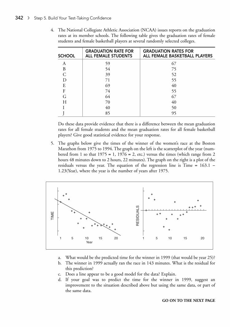
342 � Step 5. Build Your Test-Taking Confidence
4. The National Collegiate Athletic Association (NCAA) issues reports on the graduationrates at its member schools. The following table gives the graduation rates of female students and female basketball players at several randomly selected colleges.
GRADUATION RATE FOR GRADUATION RATES FORSCHOOL ALL FEMALE STUDENTS ALL FEMALE BASKETBALL PLAYERS
A 59 67B 54 75C 39 52D 71 55E 69 40F 74 55G 64 67H 70 40I 40 50J 85 95
Do these data provide evidence that there is a difference between the mean graduationrates for all female students and the mean graduation rates for all female basketballplayers? Give good statistical evidence for your response.
5. The graphs below give the times of the winner of the women’s race at the BostonMarathon from 1975 to 1994. The graph on the left is the scatterplot of the year (num-bered from 1 so that 1975 = 1, 1976 = 2, etc.) versus the times (which range from 2hours 48 minutes down to 2 hours, 22 minutes). The graph on the right is a plot of theresiduals versus the year. The equation of the regression line is Time = 163.1 −1.23(Year), where the year is the number of years after 1975.
1 5 10 15 20 1 2015105Year
TIM
E
RE
SID
UA
LS
a. What would be the predicted time for the winner in 1999 (that would be year 25)?b. The winner in 1999 actually ran the race in 143 minutes. What is the residual for
this prediction?c. Does a line appear to be a good model for the data? Explain.d. If your goal was to predict the time for the winner in 1999, suggest an
improvement to the situation described above but using the same data, or part ofthe same data.
GO ON TO THE NEXT PAGE

AP Statistics Practice Exam 2 � 343
Statistics, Section II, Part B, Question 6Spend about 25 minutes on this part of the exam; percentage of Section II grade: 25
Directions: Show all of your work. Indicate clearly the methods you use because youwill be graded on the correctness of your methods as well as on the accuracy of your resultsand explanation.
6. The casino game of Chuck-a-Luck involves spinning a cage with three dice in it. Youbet $1 on a single number from 1–6 and you win $1 for each face-up appearance ofyour number. Because it is a bet, you lose your dollar only if your number appears onnone of the three dice (e.g., suppose you bet on “5” and it come up on two dice—youreceive $2 and get to keep your original bet). There are 216 ways for three dice to comeup (6 × 6 × 6). Let X = the amount won on each play of the game.
a. Construct the probability distribution for Chuck-a-Luck. (Hint: there are fourvalues of X)
b. What are your expected mean and standard deviation for each $1 that you bet?c. Suppose you hang around the Chuck-a-Luck game for a couple of hours and play
100 times. What is the probability that you make a profit? Suppose that you wereable to place 10,000 bets on Chuck-a-Luck. Now, what is the probability that youmake a profit?
END OF PRACTICE EXAM 2

344 � Step 5. Build Your Test-Taking Confidence
� Answers to Practice Exam 2, Section I
1. e 21. d2. d 22. a3. d 23. d4. a 24. b5. b 25. e6. b 26. c7. b 27. b8. e 28. a9. d 29. c
10. c 30. b11. c 31. d12. c 32. e13. e 33. b14. d 34. d15. a 35. d16. d 36. d17. d 37. e18. b 38. a19. a 39. a20. e 40. e

AP Statistics Practice Exam 2 � 345
1. The correct answer is (e). I is not correct becausethere is no way to tell from a boxplot how manyterms are in a dataset. Thus, you can’t comparethe number above the median in A with thenumber above the median in B.
2. The correct answer is (d). (a) is not correct since themedian for B is greater than for A. (b) is not correctsince the ranges of the two networks appears to bethe same. (c) is not correct since the IQR forNetwork A is greater than the IQR for Network B.(e) is not correct since about 75% of the ratings forNetwork B are greater than 28 but less than half ofthose for Network A are greater than 28.
3. The correct answer is (d). Sample data are used togenerate confidence intervals for unknown popu-lation values. In this case, we have all of the pop-ulation values so that we can compute thedifference in the number of degrees between maleand female faculty members. It make no sense toconstruct a confidence interval if you have all thedata about the population.
4. The correct answer is (a). It’s possible that the typeof car the tire is on influences the tread wear andthat hasn’t been controlled for in the study. A better design would be to block by type of car.Then 25 of each model would be randomlyassigned tire F and 25 would randomly be assignedtire G. Then comparisons would be made withineach block.
5. The correct answer is (b). Using Table C fordf = 9, we find that 19.59 is between 19.02 and19.68. Looking to the top of the columns in whichthose numbers appear, we see that 0.02 <P < 0.025. Hence, the P-value is less than 0.05,which provides statistical evidence that Ethnicityand Blood Type are related at the 5% level of signif-icance. On the TI-83/84, we have P-value = c2
cdf(19.59,1000,9)=0.0206. Note thattwo of the expected values (for African-Americanand Arab of Type AB) are less than 5. However, thisis less than 20% of all expected values so that we arejustified in proceeding with the analysis.
6. The correct answer is (b). Nicole’s z-score on the
ACT is . Let Luis’s score on
the SAT be x. Then, Luis’s z-score on the SAT is
. Thus, .
7. The correct answer is (b). The P-value of a find-ing is the probability of getting a finding as ormore extreme than the one obtained by chancealone if the null hypothesis is true. (a), (c), and(d) are simply misstatements of what P-valuemeans. The P-value is relatively low (0.024),which means that a conclusion like that in part(e) would be arguable. Most would agree thatsuch a low P-value does provide evidence thatthe technique is effective.
8. The correct answer is (e). 1.96 would be thecorrect value of a if the question asked for a95% confidence interval (this rules out (a) and(c), (b), (c), and (d)) all use a pooled estimate ofp, which is correct (at least in (b) and (c)) for ahypothesis test but not for a confidence interval.
9. The correct answer is (d).
mx+y = mx + my = 170 + 115 = 285;
since X and Y are independent,
10. The correct answer is (c). This is exactly what ismeant by a “95% confidence interval.” Theother answers all involve some sort of probabil-ity statement about the constructed interval.Once the interval is constructed, the true meanis either in the interval (probability = 1) or it isn’t(probability = 0). Note the difference betweenthe statements, “The probability is 0.95 that thisinterval contains the true mean” and “The prob-ability is 0.95 that an interval constructed in thismanner will contain the true mean.”
11. The correct answer is (c). It appears from thegraph that most of the data will lie in the interval(5, 35), which means the range of values is about30. In a normal curve, almost all of the data arewithin three standard deviations of the mean, ora range of six standard deviations total. Thus,30/6 = 5 is the best estimate of the standarddeviation.
σ σ σx y x y+ = + = + =2 2 2 29 6 10 8. .
xx
−= ⇒ =
508
1100 6 574.z
x=
− 508
110
z =−
=24 21
50 6.
� Solutions to Practice Exam 2, Section I

346 � Step 5. Build Your Test-Taking Confidence
12. The correct answer is (c). (a) is not correctsince there is no way to tell from a boxplothow many values are in a data set. It is evidentfrom the graphs and the negative skewness ofSample A, that the mean of Sample B will begreater than the mean of Sample A since themean will be pulled in the direction of skew-ness. Hence (b) is incorrect and (c) is correct.(d) is incorrect—the median for Sample A isto the left of the median for Sample B. (e) isincorrect since only Sample B is symmetricabout it’s mean.
13. The correct answer is (e).
H0 : p1 − p2 = 0, HA : p1 − p2 ≠ 0
⇒ P-value =
2(1 – 0.9049) = 0.1902 (from Table A; on the TI-83/84, 2 × normalcdf(1.31,100) =0.1902).
(Note that the given answer is based on theaccuracy provided by the TI-83/84 2-PropZTest function. If you used only two-plade accu-racy and plugged the numbers given in the for-mula for z into the calculator, you would get az-score of 1.35 and a P-value of 0.18.)
14. The correct answer is (d). He is drawing multiplesamples, each of size 40. For each sample, he iscomputing a sample proportion (the count ofsuccesses/40). He would have to take all possi-ble samples of size 40 to actually have the sam-pling distribution.
15. The correct answer is (a). The graph with thesmallest standard deviation is the graph that ismost packed about it’s mean (varies least fromthe center). Note that (b) would be the graphwith the greatest standard deviation.
16. The correct answer is (d). The more the termspack around the center of the distribution, thesmaller the spread ⇒ the smaller the standarddeviation. (d) has more terms bunched in thecenter than the other graphs. The graph withthe most variation appears to be (c).
17. The correct answer is (d). Let x be the unknownlength of an alligator at the 67th percentile.Then zx = 0.44 (from Table A; using theTI-83/84, zx = invNorm(0.67)= 0.4399).
Also, . Equating the two expressions
for z, we find x = 2.15 meters.
18. The correct answer is (b). The formula for rrequires the use of numerical variables.
19. The correct answer is (a). P (former smoker dies
from cancer) = = 0.012. P(a person who
has never smoked dies from cancer) =
= 0.006. (b) is false since P (former
smoker dies from cancer) = 0.012 and P (current
smoker dies from cancer) = .
(c) is false since P (current smoker dies fromcancer) = 0.028 and P (current smoker diesfrom cancer | person died from cancer) =
. Since these probabilities are
not the same, the events are not independent.(d) is false since P (current smoker dies and dies
from cancer) = and
P (a person who never smoked and dies from
cancer) = . (e) is false since
P (current smoker | did not die from cancer) =
and P (former smoker | did
not die from cancer) = (but:
very close!).
20. The correct answer is (e). Use of a z-test assumesthat the population standard deviation is known.Be sure you understand that choice (c) is not areason for choosing z even though, with a samplethat large, the P-value obtained will be very close.For large samples, the population standard devia-tion is a good estimate of the population standarddeviation, but that doesn’t make it a z-procedure—just a stronger justification for using t.
7 757
136 2290 0569
,
,.=
7 725
136 2290 0567
,
,.=
782
137 2430 006
,.=
141
137 2430 001
,.=
141
1 0140 139
,.=
141
7 8660 018
,.=
782
121 529,
91
7848
zx
x=
−2
0 35.
z =−
− +⎛⎝⎜
⎞⎠⎟
=0 56 0 45
0 51 1 0 51175
175
1 31. .
. ( . )
.
ˆ . , ˆ . , ˆp p p1 2
42
750 56
34
750 45
42 34
75 750= = = = =
+
+= ..51

AP Statistics Practice Exam 2 � 347
21. The correct answer is (d).
P(5|win) = P(5|1 or 3 or 5) =
22. The correct answer is (a). Note that this is notan experiment since no treatment is imposed.
23. The correct answer is (d). The probability ofrain on a given day is computed as the relativefrequency of days that it has actually rained inthe past when conditions like those in effecttoday have been present.
24. The correct answer is (b). The hypothesis is onesided and the researcher is interested in knowingif cars produce less than 20 ppm. That elimi-nates (a), (d), and (e) (since the alternativepoints the wrong way). A null hypothesis musthave an equal sign, which means (b) is correct.Note that the correct answer could equally wellbe stated H0 : m = 20; HA : m < 20.
25. The correct answer is (e). P (A ∪ B)= P(A) +P(B) – P(A ∩ B) = 0.60 + 0.30 – P(A ∩ B) =0.90 – P(A ∩ B). Now, P(A ∩ B) = P(B)•P(A|B) =(0.30)(0.50) = 0.15. Thus, P(A ∪ B) = 0.90 –P(A ∩ B) = 0.90 – 0.15 = 0.75.
26. The correct answer is (c). P(0) = 0.4; P(1) =(0.6)(0.4) = 0.24; P(2) = (0.6)(0.6) = 0.36. Sothe most likely number of points scored is 0.
27. The correct answer is (b). From the previousproblem, we have the following probability dis-tribution for this situation.
mx = (0)(0.4) + (1)(0.24) + 2(0.36) = 0.96.
28. The correct answer is (a). The removal of point“X” would have a minimal effect on the slope ofthe regression line, but a major effect on thecorrelation coefficient and the intercept of theregression line.
29. The correct answer is (c). The normality condi-tion is satisfied by the equations in answer (d).It is not necessary that the original populationsbe approximately normal.
30. The correct answer is (b). Some of the otherresponses can contribute to bias, but do not rep-resent what is meant by bias.
31. The correct answer is (d). mX = 1(0.10) +2(0.20) + 3(0.40) + 4(0.10) + 5(0.20) = 3.1.
32. The correct answer is (e). P (at least one 4) =
=
1 – P(0 fours) = 1 – .
33. The correct answer is (b). When H0 is false,power = 1 – b, where b is the probability ofmaking a type II error (the mistake of failing toreject a false null hypothesis). 1 – a is the proba-bility of correctly failing to reject a true nullhypothesis. (a) and (c) make it easier to reject thenull hypothesis, thus increasing power. (c) isessentially a definition of power. (e) is true sinceyou can increase power by increasing the differ-ence between the real and hypothesized value ofthe parameter.
34. The correct answer is (d). You must have 4 outof the 10 possibilities. (d) is the only one thataccomplishes this.
35. The correct answer is (d). The opposite of III iscorrect: the greater the number of degrees offreedom, the less the variance of a t-distribution.
36. The correct answer is (d). I isn’t true becausethis is an observational study and simply showsan association, not a causal relationship.
37. The correct answer is (e) since we are told thatthere is evidence that temperature affects distancetraveled. (a) is incorrect since the type of golf ballis the treatment variable, not a blocking variable.(b) is incorrect since there is no reason to blockby size since we have no evidence that size isrelated to distance. (c) is incorrect for the samereason as (b). (d) is incorrect since there is reasonto believe that some variable not under study isrelated to the outcomes to be measured.
80
16
56
0 8⎛
⎝⎜
⎞
⎠⎟⎛
⎝⎜
⎞
⎠⎟
⎛
⎝⎜
⎞
⎠⎟
81
16
56
82
16
56
1 7 2⎛
⎝⎜
⎞
⎠⎟⎛
⎝⎜
⎞
⎠⎟
⎛
⎝⎜
⎞
⎠⎟ +
⎛
⎝⎜
⎞
⎠⎟⎛
⎝⎜
⎞
⎠⎟
⎛
⎝⎝⎜
⎞
⎠⎟ + +
⎛
⎝⎜
⎞
⎠⎟⎛
⎝⎜
⎞
⎠⎟
⎛
⎝⎜
⎞
⎠⎟
6 8 088
16
56
�
Points Made (x) 0 1 2
p(x) 0.4 0.24 0.36
0 1
0 15 0 20 0 1
10
450 22
.
. . .. .
+ += =

348 � Step 5. Build Your Test-Taking Confidence
38. The correct answer is (a). From the cumulativefrequencies, we can determine the relative fre-quency of each value.
CUMULATIVE RELATIVE VALUE (X) FREQUENCY FREQUENCY
2 0.15 0.153 0.25 0.105 0.45 0.207 0.95 0.5010 1.00 0.05
Then, mX = 2(0.15) + 3(0.10) + 5(0.20) +7(0.50) + 10(0.05) = 5.6. The median is thevalue at the 50th percentile. Because only 45% ofthe scores are at 5 or below, and 95% of thescores are at 7 or below, the median must be at 7.
39. The correct answer is (a). Since there are1000 scores, the five-number summary willoccur at the first (minimum), 250th (25thpercentile), 500th (median), 750th (75thpercentile), and 1000th (maximum) scores.Drawing a horizontal line from each of thesevalues on the vertical axis to the cumulativefrequency graph and then dropping down tothe horizontal axis yields, most closely, thevalues in (a).
40. The correct answer is (e). We are 95% confident(most polls use a 95% confidence interval) that thetrue population proportion of voters who intendto vote for Sleazy is in the interval 46% ± 3% orbetween 43% and 49%. This is equivalent tosaying the proportion is likely to be between 43%and 49%.

AP Statistics Practice Exam 2 � 349
� Solutions to Practice Exam 2, Section II, Part ASolution to #1
a. The median is the middle score. Because there are 20 scores, the median liesbetween the 10th and 11th scores as shown on the stemplot.
3 045 2266 22387 58 47899 13557810 0
The 10th and 11th scores are 84 and 87. Thus the median is .
b.
c. 1.5(IQR) = 1.5(94 − 62) = 1.5(32) = 48. Outliers would be values beyond 62 − 48 = 14 or 94 + 48 = 142. The lowest score a student could get that wouldnot be considered an outlier would be 14.
Solution to #2
a. Number = 229.402 −7.057(birth month)
b. Each month, from January to December, the average draft number is predicted todecrease by 7.057.
c. Yes. The t-statistic of −5.49 is the test statistic for the hypothesis H0: β = 0 against thealternative HA: β ≠ 0. This t-statistic tells us that the P-value is approximately 0. This is very strong evidence against the null hypothesis, which supports the contentionthat there is a predictive relationship between birth month and average draft number. Theconclusion is that the drawing is biased against those born later in the year. That is, thoseborn later in the year are more likely to get drafted than those born early in the year.
d. df = n – 2 = 12 – 2 = 10 ⇒ t* = 2.228 (from Table B; if you have a TI-84 with theinvT function, invT(0.975,10)= 2.228). The 95% confidence interval is–7.057 ± 2.228(1.286) = (–9.92, – 4.19). We are 95% confident that the true slope ofthe regression line is between –9.92 and –4.19. Note that this is consistent with our finding in part (c) that the regression line has a nonzero slope.
Quiz20 40 60 80 100
84 87
285 5
+= .

350 � Step 5. Build Your Test-Taking Confidence
Solution to #3
a. It is an observational study. The researcher is not controlling the treatments to the twodifferent groups in the study. Rather, the groups are self-selected based on where theybought their mattresses. The researcher has simply observed and recorded outcomes. Inan experiment, the researcher would have had control over which volunteers slept onwhich mattress.
b. A confounding variable would be a variable that differentially affects one group ofbuyers more than the other. For example, a possible confounding variable might be thatpeople who buy their mattresses at an upscale location are better off financially thanthose who buy for economy. They might be more content and less stressed as a group,and this could affect the quality of their sleep.
c. No. You cannot infer a cause-and-effect relationship from an observational studybecause of the possible presence of confounding variables as described in (b). All youknow is that the groups experienced different qualities of sleep. You do not know why.
Solution to #4
We note that the scores are paired by school, so we will want to use a matched pairs test.
Let md be the true mean difference between the graduation rates of all female stu-dents and female basketball players.
H0: md = 0.HA: md ≠ 0.
We need to use the paired differences for analysis. Adding a column to the table inthe problem with the differences, we have:
The problem states that the sample is a random sample. A boxplot of the datashows some skewness but no outliers. We can proceed with a one-sample t-test.
−15 0 15 30
SCHOOL ALL BASKETBALL PLAYERS DIFFERENCES (d )
A 59 67 −8B 54 75 −21C 39 52 −13D 71 55 16E 69 40 29F 74 55 19G 64 67 −3H 70 40 30I 40 50 −10J 85 95 −10
Continued

AP Statistics Practice Exam 2 � 351
n = 10 ⇒ df = 10 − 1 = 9.
⇒ P-value > 0.50 (from Table B; using the TI-83/84,
P-value = 2 × tcdf(0.49,9)= 0.636).
t =−
=2 9 0
18 7310
0 49..
.
x sd d= =2 9 18 73. , .
Because the P-value is quite large, we have no evidence to reject the null and concludethat there is a significant difference between the graduation rates of all female collegestudents and female basketball players. (A good research follow-up at this point wouldbe to do the same analysis on male basketball players to see if a difference in graduationrates exists there.)
Solution to #5
a. Time = 163.1 − 1.23(25) = 132.35. The predicted time for 1999 is about 2 hours 12 minutes.
b. Residual = actual − predicted = 143 − 132 = 11 minutes.
c. Not really. The residual plot shows a pattern for underestimating the actual times at thebeginning and end of the 20-year period and overestimating the actual times during themiddle years.
d. The scatterplot for the raw data appears to be more linear beginning about year 5.Because the goal is to predict beyond the data, a line might be a better modelbeginning with year 5 rather than with year 1. That is, redo the regression beginningin 1980 rather than in 1975.

352 � Step 5. Build Your Test-Taking Confidence
� Solutions to Practice Exam 2, Section II, Part BSolution to #6
a. # Faces 0 1 2 3
Win (x) −1 1 2 3
P (x) 33
1
6
5
60 005
3 0⎛⎝⎜
⎞⎠⎟
⎛⎝⎜
⎞⎠⎟
⎛⎝⎜
⎞⎠⎟
= .
32
1
6
5
60 069
2 1⎛⎝⎜
⎞⎠⎟
⎛⎝⎜
⎞⎠⎟
⎛⎝⎜
⎞⎠⎟
= .
31
1
6
5
60 347
1 2⎛⎝⎜
⎞⎠⎟
⎛⎝⎜
⎞⎠⎟
⎛⎝⎜
⎞⎠⎟
= .
30
1
6
5
60 579
0 3⎛⎝⎜
⎞⎠⎟
⎛⎝⎜
⎞⎠⎟
⎛⎝⎜
⎞⎠⎟
= .
b. μX = –1(0.579) + 1(0.347) + 2(0.069) + 3(0.005) = −0.079. Your expected winningson each $1 bet is –7.9¢.
(Remember that this can be done on the TI-83/84 as follows: put the values of X ({–1,1, 2, 3}) in L1 and the values of P(X) ({0.579, 0.347, 0.069, 0.005}) in L2. Then doSTAT CALC 1-VAR STATS L1,L2 to find μx, which is given as on the calculator.)
= 1.114.
(This value can be found on the TI-83/84 as indicated above by putting the X valuesin L1, the P(X) in L2, and doing STAT CALC 1-VAR STATS L1,L2.)
c. With 100 trials, you can assume that the central limit theorem kicks in and that thesampling distribution of is approximately normally distributed. Let be your averagewinning on 100 plays of the game. Then
From part (b) = –0.079 and . Thus P ( > 0) =
P (z > = 0.712) = 1 – 0.7611 = 0.2389 (from Table A; n the TI-83/84:
normalcdf(0.712,100)= 0.239). You have about a 24% chance of making aprofit (or a 76% chance of losing money) after 100 plays.
For 10,000 plays, P( >0) = P(z > ) = 0. (normalcdf
(7.12,100)= 5.434E–13, or 5.434 × 10⁻¹³.) You have essentially no chance ofmaking a profit after 10,000 plays. The casino is virtually guaranteed to make moneyand the players, on average, are guaranteed to lose.
0 0 0791 11
10000
7 12− −
=( . )
..x
0 0 079
0 111
− −( . )
.
xσx
= =1 114
1000 111
..μx
x
x
σ X = − − − + + +( ( . )) ( . ) ( . ) ( . )1 0 079 0 579 1 0 079 0 3472 2 (( . ) ( . ) ( . ) ( . )2 0 079 0 069 3 0 079 0 0052 2+ + +

AP Statistics Practice Exam 2 � 353
� Scoring Sheet for Practice Exam 2Section I: Multiple Choice
[ ( / )]number correct(out of 40)
number wrong− × ×1 4 11 25. =
multiple-choicescore (if less thanzero, eenter zero)
weighted section I
score (do not ro
=
uund)
weighted section I
score
weighted section II
sc
+
oore
composite score(round to nearestwhole nu
=
mmber)
Section II: Free Response
Question 1(out of 4) (do not round)
Qu
.× =1 875
eestion 2(out of 4) (do not round)
Que
.× =1 875
sstion 3(out of 4) (do not round)
Ques
.× =1 875
ttion 4(out of 4) (do not round)
Quest
.× =1 875
iion 5(out of 4) (do not round)
Questi
.× =1 875
oon 6(out of 4) (do not round)
.× =3 125
Sumweighted
=
ssection II score
(do not round)
Composite Score

This page intentionally left blank

� 355
Appendixes
FormulasTables
BibliographyWeb SitesGlossary

I. Descriptive Statistics
II. ProbabilityP(A ∪ B) = P(A) + P(B) – P(A ∩ B)
Var (X) = = Σ (xi – μx)2 pi
If X has a binomial distribution with parameters n and p, then
P X k nk
p pk n k( ) ( )= =⎛
⎝⎜
⎞
⎠⎟ − −1
σ x2
E X x px i i( ) = = ∑μ
PP
P( | )
( )
( )A B
A B
B=
∩
s
y y
n
x xb
i
i
1
2
2
2=
−
−
−
∑
∑
( ˆ)
( )
b rs
sy
x1 =
rn
x x
s
y y
si
x
i
y
=−
−⎛
⎝⎜
⎞
⎠⎟
−⎛
⎝⎜⎜
⎞
⎠⎟⎟∑1
1
b y b x0 1= −
bx x y y
x x
i
i
1
1
2=
− −
−
∑∑( )( )
( )
y b b x= +0 1
sn s n s
n np =− + −
+ + −
( ) ( )
( ) ( )1 1
22 2
2
1 2
1 1
1 1
sn
x xx i=−
−∑1
12( )
xx
ni=
∑
FORMULAS

μx = nk
If is the mean of a random sample of size n from an infinite population with meanμ and standard deviation σ, then
III. Inferential Statistics
Confidence interval: statistic ± (critical value) . (standard deviation of statistic)
Single-Sample
Standardized test statistic:statistic par− aameter
standard deviation of statistic
σσ
xn
=
μ μx =
x
σ ˆ
( )p
p p
n=
−1
μ p p=
σ x np p= −( )1
Appendixes � 357
STATISTIC STANDARD DEVIATION
Sample Mean
Sample Proportion p p
n
( )1−
σ
n
Two-Sample
STATISTIC STANDARD DEVIATION
Difference of sample means(σ1 ≠ σ2)
Difference of sample means(σ1 = σ2)
Difference of sample proportions( p1 ≠ p2)
Difference of sample proportionsp
1= p
2
σ σ12
1
22
2n n+
σ1 1
1 2n n+
p p
n
p p
n1 1
1
2 2
2
1 1( ) ( )−+
−
p pn n
( )11 1
1 2
− +
Chi-square test statistic =observed expecte( − dd
expected
)∑
2

TABLE A Standard Normal Probabilities
z .00 .01 .02 .03 .04 .05 .06 .07 .08 .09
−3.4 .0003 .0003 .0003 .0003 .0003 .0003 .0003 .0003 .0003 .0002−3.3 .0005 .0005 .0005 .0004 .0004 .0004 .0004 .0004 .0004 .0003−3.2 .0007 .0007 .0006 .0006 .0006 .0006 .0006 .0005 .0005 .0005−3.1 .0010 .0009 .0009 .0009 .0008 .0008 .0008 .0008 .0007 .0007−3.0 .0013 .0013 .0013 .0012 .0012 .0011 .0011 .0011 .0010 .0010−2.9 .0019 .0018 .0018 .0017 .0016 .0016 .0015 .0015 .0014 .0014−2.8 .0026 .0025 .0024 .0023 .0023 .0022 .0021 .0021 .0020 .0019−2.7 .0035 .0034 .0033 .0032 .0031 .0030 .0029 .0028 .0027 .0026−2.6 .0047 .0045 .0044 .0043 .0041 .0040 .0039 .0038 .0037 .0036−2.5 .0062 .0060 .0059 .0057 .0055 .0054 .0052 .0051 .0049 .0048−2.4 .0082 .0080 .0078 .0075 .0073 .0071 .0069 .0068 .0066 .0064−2.3 .0107 .0104 .0102 .0099 .0096 .0094 .0091 .0089 .0087 .0084−2.2 .0139 .0136 .0132 .0129 .0125 .0122 .0119 .0116 .0113 .0110−2.1 .0179 .0174 .0170 .0166 .0162 .0158 .0154 .0150 .0146 .0143−2.0 .0228 .0222 .0217 .0212 .0207 .0202 .0197 .0192 .0188 .0183−1.9 .0287 .0281 .0274 .0268 .0262 .0256 .0250 .0244 .0239 .0233−1.8 .0359 .0351 .0344 .0336 .0329 .0322 .0314 .0307 .0301 .0294−1.7 .0446 .0436 .0427 .0418 .0409 .0401 .0392 .0384 .0375 .0367−1.6 .0548 .0537 .0526 .0516 .0505 .0495 .0485 .0475 .0465 .0455−1.5 .0668 .0655 .0643 .0630 .0618 .0606 .0594 .0582 .0571 .0559−1.4 .0808 .0793 .0778 .0764 .0749 .0735 .0721 .0708 .0694 .0681−1.3 .0968 .0951 .0934 .0918 .0901 .0885 .0869 .0853 .0838 .0823−1.2 .1151 .1131 .1112 .1093 .1075 .1056 .1038 .1020 .1003 .0985−1.1 .1357 .1335 .1314 .1292 .1271 .1251 .1230 .1210 .1190 .1170−1.0 .1587 .1562 .1539 .1515 .1492 .1469 .1446 .1423 .1401 .1379−0.9 .1841 .1814 .1788 .1762 .1736 .1711 .1685 .1660 .1635 .1611−0.8 .2119 .2090 .2061 .2033 .2005 .1977 .1949 .1922 .1894 .1867−0.7 .2420 .2389 .2358 .2327 .2296 .2266 .2236 .2206 .2177 .2148−0.6 .2743 .2709 .2676 .2643 .2611 .2578 .2546 .2514 .2483 .2451−0.5 .3085 .3050 .3015 .2981 .2946 .2912 .2877 .2843 .2810 .2776−0.4 .3446 .3409 .3372 .3336 .3300 .3264 .3228 .3192 .3156 .3121−0.3 .3821 .3783 .3745 .3707 .3669 .3632 .3594 .3557 .3520 .3483−0.2 .4207 .4168 .4129 .4090 .4052 .4013 .3974 .3936 .3897 .3859−0.1 .4602 .4562 .4522 .4483 .4443 .4404 .4364 .4325 .4286 .4247−0.0 .5000 .4960 .4920 .4880 .4840 .4801 .4761 .4721 .4681 .4641
Probability
z
Table entry for z is theprobability lying below z.
TABLES
Continued

TABLE A Standard Normal Probabilities (continued )
z .00 .01 .02 .03 .04 .05 .06 .07 .08 .09
0.0 .5000 .5040 .5080 .5120 .5160 .5199 .5239 .5279 .5319 .53590.1 .5398 .5438 .5478 .5517 .5557 .5596 .5636 .5675 .5714 .57530.2 .5793 .5832 .5871 .5910 .5948 .5987 .6026 .6064 .6103 .61410.3 .6179 .6217 .6255 .6293 .6331 .6368 .6406 .6443 .6480 .65170.4 .6554 .6591 .6628 .6664 .6700 .6736 .6772 .6808 .6844 .68790.5 .6915 .6950 .6985 .7019 .7054 .7088 .7123 .7157 .7190 .72240.6 .7257 .7291 .7324 .7357 .7389 .7422 .7454 .7486 .7517 .75490.7 .7580 .7611 .7642 .7673 .7704 .7734 .7764 .7794 .7823 .78520.8 .7881 .7910 .7939 .7967 .7995 .8023 .8051 .8078 .8106 .81330.9 .8159 .8186 .8212 .8238 .8264 .8289 .8315 .8340 .8365 .83891.0 .8413 .8438 .8461 .8485 .8508 .8531 .8554 .8577 .8599 .86211.1 .8643 .8665 .8686 .8708 .8729 .8749 .8770 .8790 .8810 .88301.2 .8849 .8869 .8888 .8907 .8925 .8944 .8962 .8980 .8997 .90151.3 .9032 .9049 .9066 .9082 .9099 .9115 .9131 .9147 .9162 .91771.4 .9192 .9207 .9222 .9236 .9251 .9265 .9279 .9292 .9306 .93191.5 .9332 .9345 .9357 .9370 .9382 .9394 .9406 .9418 .9429 .94411.6 .9452 .9463 .9474 .9484 .9495 .9505 .9515 .9525 .9535 .95451.7 .9554 .9564 .9573 .9582 .9591 .9599 .9608 .9616 .9625 .96331.8 .9641 .9649 .9656 .9664 .9671 .9678 .9686 .9693 .9699 .97061.9 .9713 .9719 .9726 .9732 .9738 .9744 .9750 .9756 .9761 .97672.0 .9772 .9778 .9783 .9788 .9793 .9798 .9803 .9808 .9812 .98172.1 .9821 .9826 .9830 .9834 .9838 .9842 .9846 .9850 .9854 .98572.2 .9861 .9864 .9868 .9871 .9875 .9878 .9881 .9884 .9887 .98902.3 .9893 .9896 .9898 .9901 .9904 .9906 .9909 .9911 .9913 .99162.4 .9918 .9920 .9922 .9925 .9927 .9929 .9931 .9932 .9934 .99362.5 .9938 .9940 .9941 .9943 .9945 .9946 .9948 .9949 .9951 .99522.6 .9953 .9955 .9956 .9957 .9959 .9960 .9961 .9962 .9963 .99642.7 .9965 .9966 .9967 .9968 .9969 .9970 .9971 .9972 .9973 .99742.8 .9974 .9975 .9976 .9977 .9977 .9978 .9979 .9979 .9980 .99812.9 .9981 .9982 .9982 .9983 .9984 .9984 .9985 .9985 .9986 .99863.0 .9987 .9987 .9987 .9988 .9988 .9989 .9989 .9989 .9990 .99903.1 .9990 .9991 .9991 .9991 .9992 .9992 .9992 .9992 .9993 .99933.2 .9993 .9993 .9994 .9994 .9994 .9994 .9994 .9995 .9995 .99953.3 .9995 .9995 .9995 .9996 .9996 .9996 .9996 .9996 .9996 .99973.4 .9997 .9997 .9997 .9997 .9997 .9997 .9997 .9997 .9997 .9998
Probability
Table entry for z is theprobability lying below z.
z
Appendixes � 359

TABLE B t Distribution Critical Values
TAIL PROBABILITY P
df .25 .20 .15 .10 .05 .025 .02 .01 .005 .0025 .001 .0005
1 1.000 1.376 1.963 3.078 6.314 12.71 15.89 31.82 63.66 127.3 318.3 636.62 .816 1.061 1.386 1.886 2.920 4.303 4.849 6.965 9.925 14.09 22.33 31.603 .765 .978 1.250 1.638 2.353 3.182 3.482 4.541 5.841 7.453 10.21 12.924 .741 .941 1.190 1.533 2.132 2.776 2.999 3.747 4.604 5.598 7.173 8.6105 .727 .920 1.156 1.476 2.015 2.571 2.757 3.365 4.032 4.773 5.893 6.8696 .718 .906 1.134 1.440 1.943 2.447 2.612 3.143 3.707 4.317 5.208 5.9597 .711 .896 1.119 1.415 1.895 2.365 2.517 2.998 3.499 4.029 4.785 5.4088 .706 .889 1.108 1.397 1.860 2.306 2.449 2.896 3.355 3.833 4.501 5.0419 .703 .883 1.100 1.383 1.833 2.262 2.398 2.821 3.250 3.690 4.297 4.781
10 .700 .879 1.093 1.372 1.812 2.228 2.359 2.764 3.169 3.581 4.144 4.58711 .697 .876 1.088 1.363 1.796 2.201 2.328 2.718 3.106 3.497 4.025 4.43712 .695 .873 1.083 1.356 1.782 2.179 2.303 2.681 3.055 3.428 3.930 4.31813 .694 .870 1.079 1.350 1.771 2.160 2.282 2.650 3.012 3.372 3.852 4.22114 .692 .868 1.076 1.345 1.761 2.145 2.264 2.624 2.977 3.326 3.787 4.14015 .691 .866 1.074 1.341 1.753 2.131 2.249 2.602 2.947 3.286 3.733 4.07316 .690 .865 1.071 1.337 1.746 2.120 2.235 2.583 2.921 3.252 3.686 4.01517 .689 .863 1.069 1.333 1.740 2.110 2.224 2.567 2.898 3.222 3.646 3.96518 .688 .862 1.067 1.330 1.734 2.101 2.214 2.552 2.878 3.197 3.611 3.92219 .688 .861 1.066 1.328 1.729 2.093 2.205 2.539 2.861 3.174 3.579 3.88320 .687 .860 1.064 1.325 1.725 2.086 2.197 2.528 2.845 3.153 3.552 3.85021 .686 .859 1.063 1.323 1.721 2.080 2.189 2.518 2.831 3.135 3.527 3.81922 .686 .858 1.061 1.321 1.717 2.074 2.183 2.508 2.819 3.119 3.505 3.79223 .685 .858 1.060 1.319 1.714 2.069 2.177 2.500 2.807 3.104 3.485 3.76824 .685 .857 1.059 1.318 1.711 2.064 2.172 2.492 2.797 3.091 3.467 3.74525 .684 .856 1.058 1.316 1.708 2.060 2.167 2.485 2.787 3.078 3.450 3.72526 .684 .856 1.058 1.315 1.706 2.056 2.162 2.479 2.779 3.067 3.435 3.70727 .684 .855 1.057 1.314 1.703 2.052 2.158 2.473 2.771 3.057 3.421 3.69028 .683 .855 1.056 1.313 1.701 2.048 2.154 2.467 2.763 3.047 3.408 3.67429 .683 .854 1.055 1.311 1.699 2.045 2.150 2.462 2.756 3.038 3.396 3.65930 .683 .854 1.055 1.310 1.697 2.042 2.147 2.457 2.750 3.030 3.385 3.64640 .681 .851 1.050 1.303 1.684 2.021 2.123 2.423 2.704 2.971 3.307 3.55150 .679 .849 1.047 1.299 1.676 2.009 2.109 2.403 2.678 2.937 3.261 3.49660 .679 .848 1.045 1.296 1.671 2.000 2.099 2.390 2.660 2.915 3.232 3.46080 .678 .846 1.043 1.292 1.664 1.990 2.088 2.374 2.639 2.887 3.195 3.416
100 .677 .845 1.042 1.290 1.660 1.984 2.081 2.364 2.626 2.871 3.174 3.3901000 .675 .842 1.037 1.282 1.646 1.962 2.056 2.330 2.581 2.813 3.098 3.300∞ .674 .841 1.036 1.282 1.645 1.960 2.054 2.326 2.576 2.807 3.091 3.291
50% 60% 70% 80% 90% 95% 96% 98% 99% 99.5% 99.8% 99.9%
Confidence level C
360 � Appendixes
Probability p
Table entry for p andC is the point t * withprobability p lyingabove it andprobability C lyingbetween –t * and t *.
t *

TABLE C χ2 Critical Values
TAIL PROBABILITY P
df .25 .20 .15 .10 .05 .025 .02 .01 .005 .0025 .001 .0005
1 1.32 1.64 2.07 2.71 3.84 5.02 5.41 6.63 7.88 9.14 10.83 12.122 2.77 3.22 3.79 4.61 5.99 7.38 7.82 9.21 10.60 11.98 13.82 15.203 4.11 4.64 5.32 6.25 7.81 9.35 9.84 11.34 12.84 14.32 16.27 17.734 5.39 5.99 6.74 7.78 9.49 11.14 11.67 13.28 14.86 16.42 18.47 20.005 6.63 7.29 8.12 9.24 11.07 12.83 13.39 15.09 16.75 18.39 20.51 22.116 7.84 8.56 9.45 10.64 12.59 14.45 15.03 16.81 18.55 20.25 22.46 24.107 9.04 9.80 10.75 12.02 14.07 16.01 16.62 18.48 20.28 22.04 24.32 26.028 10.22 11.03 12.03 13.36 15.51 17.53 18.17 20.09 21.95 23.77 26.12 27.879 11.39 12.24 13.29 14.68 16.92 19.02 19.68 21.67 23.59 25.46 27.88 29.67
10 12.55 13.44 14.53 15.99 18.31 20.48 21.16 23.21 25.19 27.11 29.59 31.4211 13.70 14.63 15.77 17.28 19.68 21.92 22.62 24.72 26.76 28.73 31.26 33.1412 14.85 15.81 16.99 18.55 21.03 23.34 24.05 26.22 28.30 30.32 32.91 34.8213 15.98 16.98 18.20 19.81 22.36 24.74 25.47 27.69 29.82 31.88 34.53 36.4814 17.12 18.15 19.41 21.06 23.68 26.12 26.87 29.14 31.32 33.43 36.12 38.1115 18.25 19.31 20.60 22.31 25.00 27.49 28.26 30.58 32.80 34.95 37.70 39.7216 19.37 20.47 21.79 23.54 26.30 28.85 29.63 32.00 34.27 36.46 39.25 41.3117 20.49 21.61 22.98 24.77 27.59 30.19 31.00 33.41 35.72 37.95 40.79 42.8818 21.60 22.76 24.16 25.99 28.87 31.53 32.35 34.81 37.16 39.42 42.31 44.4319 22.72 23.90 25.33 27.20 30.14 32.85 33.69 36.19 38.58 40.88 43.82 45.9720 23.83 25.04 26.50 28.41 31.41 34.17 35.02 37.57 40.00 42.34 45.31 47.5021 24.93 26.17 27.66 29.62 32.67 35.48 36.34 38.93 41.40 43.78 46.80 49.0122 26.04 27.30 28.82 30.81 33.92 36.78 37.66 40.29 42.80 45.20 48.27 50.5123 27.14 28.43 29.98 32.01 35.17 38.08 38.97 41.64 44.18 46.62 49.73 52.0024 28.24 29.55 31.13 33.20 36.42 39.36 40.27 42.98 45.56 48.03 51.18 53.4825 29.34 30.68 32.28 34.38 37.65 40.65 41.57 44.31 46.93 49.44 52.62 54.9526 30.43 31.79 33.43 35.56 38.89 41.92 42.86 45.64 48.29 50.83 54.05 56.4127 31.53 32.91 34.57 36.74 40.11 43.19 44.14 46.96 49.64 52.22 55.48 57.8628 32.62 34.03 35.71 37.92 41.34 44.46 45.42 48.28 50.99 53.59 56.89 59.3029 33.71 35.14 36.85 39.09 42.56 45.72 46.69 49.59 52.34 54.97 58.30 60.7330 34.80 36.25 37.99 40.26 43.77 46.98 47.96 50.89 53.67 56.33 59.70 62.1640 45.62 47.27 49.24 51.81 55.76 59.34 60.44 63.69 66.77 69.70 73.40 76.0950 56.33 58.16 60.35 63.17 67.50 71.42 72.61 76.15 79.49 82.66 86.66 89.5660 66.98 68.97 71.34 74.40 79.08 83.30 84.58 88.38 91.95 95.34 99.61 102.780 88.13 90.41 93.11 96.58 101.9 106.6 108.1 112.3 116.3 120.1 124.8 128.3
100 109.1 111.7 114.7 118.5 124.3 129.6 131.1 135.8 140.2 144.3 149.4 153.2
Appendixes � 361
Probability pTable entry for p is the point(χ2) with probability p lyingabove it.
(χ2)

Advanced Placement Program Course Description,New York: The College Board, 2008–2009.
Bock, D, Velleman, P., De Veaux, R. 2004. Stats:Modeling the World. Boston: Pearson/Addison-Wesley.
Moore, David S. 2006. Introduction to the Practiceof Statistics, 5th ed. New York: W.H. Freeman andCompany.
Peck, R., Olsen, C., Devore, J. 2005. Introduction toStatistics and Data Analysis, 2nd ed., Belmont, CA:Duxbury/Thomson Learning.
Utts, J., Heckard, R. 2004. Mind on Statistics. 2nded. Belmont, CA: Duxbury/Thomson Learning,
Watkins, A., Scheaffer, R., Cobb, G. 2004. Statisticsin Action: Understanding a World of Data. Emeryville,CA: Key Curriculum Press.
Yates, D., Starnes, D., Moore, D. 2005. StatisticsThrough Applications. New York: W.H. Freeman andCompany.
Yates, D., Moore, David, Starnes, D. 2008. The Practiceof Statistics, 3rd ed. New York: W. H. Freeman andCompany.
BIBLIOGRAPHY

Here is a list of web sites that contain information and links that you might find useful inyour preparation for the AP Statistics exam:
AP Central: http://apcentral.collegeboard.com/apc/controller.jpf
Bureau of the Census: http://www.census.gov/
Chance News: http://www.dartmouth.edu/_chance/chance_news/news.html
Data and Story Library (DASL): http://lib.stat.cmu.edu/DASL/
Exploring Data: http://exploringdata.cqu.edu.au/
Statistical Abstract of the U.S.: http://www.census.gov/statab/www/
WEB SITES

Alternative hypothesis—the theory that theresearcher hopes to confirm by rejecting the nullhypothesis
Association—when some of the variability in onevariable can be accounted for by the other
Bar graph—graph in which the frequencies of cate-gories are displayed with bars; analogous to a his-togram for numerical data
Bimodal—distribution with two (or more) mostcommon values; see mode
Binomial distribution—probability distribution for arandom variable X in a binomial setting;
where n is the number of independent trials, p isthe probability of success on each trial, and x is thecount of successes out of the n trials
Binomial setting (experiment)—when each of afixed number, n, of observations either succeeds orfails, independently, with probability p
Bivariate data—having to do with two variablesBlock—a grouping of experimental units thought to
be related to the response to the treatmentBlock design—procedure by which experimental units
are put into homogeneous groups in an attempt tocontrol for the effects of the group on the response
Blocking—see block designBoxplot (box and whisker plot)—graphical represen-
tation of the five-number summary of a dataset.Each value in the five-number summary is locatedover its corresponding value on a number line. Abox is drawn that ranges from Q1 to Q3 and“whiskers” extend to the maximum and minimumvalues from Q1 and Q3.
Categorical data—see qualitative dataCensus—attempt to contact every member of a
populationCenter—the “middle” of a distribution; either the
mean or the medianCentral limit theorem—theorem that states that the
sampling distribution of a sample mean becomesapproximately normal when the sample size is large.
Chi-square (χ2) goodness-of-fit test—compares a setof observed categorical values to a set of expectedvalues under a set of hypothesized proportions forthe categories;
Cluster sample—The population is first divided intosections or “clusters.” Then we randomly select anentire cluster, or clusters, and include all of themembers of the cluster(s) in the sample.
Coefficient of determination (r2)—measures theproportion of variation in the response variableexplained by regression on the explanatory variable
Complement of an event—set of all outcomes in thesample space that are not in the event
Completely randomized design—when all subjects(or experimental units) are randomly assigned totreatments in an experiment
Conditional probability—the probability of oneevent succeeding given that some other event hasalready occurred
Confidence interval—an interval that, with a givenlevel of confidence, is likely to contain a popula-tion value; (estimate) ± (margin of error)
Confidence level—the probability that the proce-dure used to construct an interval will generatean interval that does contain the population value
Confounding variable—has an effect on the out-comes of the study but whose effects cannot beseparated from those of the treatment variable
Contingency table—see two-way tableContinuous data—data that can be measured, or
take on values in an interval; the set of possiblevalues cannot be counted
Continuous random variable—a random variablewhose values are continuous data; takes all valuesin an interval
Control—see statistical controlConvenience sample—sample chosen without any
random mechanism; chooses individuals based onease of selection
Correlation coefficient (r)—measures the strength of thelinear relationship between two quantitative variables;
χ 22
=−∑ ( )O EE
P X x nx
p px n x( ) ( ) ( ) ,= =⎛
⎝⎜
⎞
⎠⎟ − −1
GLOSSARY

Correlation is not causation—just because two vari-ables correlate strongly does not mean that onecaused the other
Critical value—values in a distribution that identifycertain specified areas of the distribution
Degrees of freedom—number of independent data-points in a distribution
Density function—a function that is everywherenon-negative and has a total area equal to 1 under-neath it and above the horizontal axis
Descriptive statistics—process of examining dataanalytically and graphically
Dimension—size of a two-way table; r × cDiscrete data—data that can be counted (possibly
infinite) or placed in orderDiscrete random variable—random variable whose
values are discrete dataDotplot—graph in which data values are identified as
dots placed above their corresponding values on anumber line
Double blind—experimental design in which neitherthe subjects nor the study administrators knowwhat treatment a subject has received
Empirical Rule (68-95-99.7 Rule)—states that, in anormal distribution, about 68% of the terms arewithin one standard deviation of the mean,about 95% are within two standard deviations,and about 99.7% are within three standard deviations
Estimate—sample value used to approximate a valueof a parameter
Event—in probability, a subset of a sample space; a set of one or more simple outcomes
Expected value—mean value of a discrete randomvariable
Experiment—study in which a researcher measuresthe responses to a treatment variable, or variables,imposed and controlled by the researcher
Experimental units—individuals on which experi-ments are conducted
Explanatory variable—explains changes in responsevariable; treatment variable; independent variable
Extrapolation—predictions about the value of a vari-able based on the value of another variable outsidethe range of measured values
First quartile—25th percentile
Five-number summary—for a dataset, [minimumvalue, Q1, median, Q3, maximum value]
Geometric setting—independent observations, eachof which succeeds or fails with the same probabil-ity p; number of trials needed until first success isvariable of interest
Histogram—graph in which the frequencies ofnumerical data are displayed with bars; analogousto a bar graph for categorical data
Homogeneity of proportions—chi-square hypothe-sis in which proportions of a categorical variableare tested for homogeneity across two or morepopulations
Independent events—knowing one event occursdoes not change the probability that the other occurs;
Independent variable—see explanatory variableInferential statistics—use of sample data to make
inferences about populationsInfluential observation—observation, usually in the
x direction, whose removal would have a markedimpact on the slope of the regression line
Interpolation—predictions about the value of a vari-able based on the value of another variable withinthe range of measured values
Interquartile range—value of the third quartileminus the value of the first quartile; containsmiddle 50% of the data
Least-squares regression line—of all possible lines,the line that minimizes the sum of squared errors(residuals) from the line
Line of best fit—see least-squares regression lineLurking variable—one that has an effect on the out-
comes of the study but whose influence was notpart of the investigation
Margin of error—measure of uncertainty in the esti-mate of a parameter; (critical value) . (standard error)
Marginal totals—row and column totals in a two-way table
Matched pairs—experimental units paired by aresearcher based on some common characteristicor characteristic
Matched pairs design—experimental design that uti-lizes each pair as a block; one unit receives one treat-ment, and the other unit receives the other treatment
Mean—sum of all the values in a dataset divided bythe number of values
Median—halfway through an ordered dataset, belowand above which lies an equal number of datavalues; 50th percentile
P A P A B( ) ( | )=
rn
x x
s
y y
si
x
i
yi
n
=−
−⎛
⎝⎜
⎞
⎠⎟
−⎛
⎝⎜⎜
⎞
⎠⎟⎟
=
∑1
1 1
Glossary � 365

Mode—most common value in a distributionMound-shaped (bell-shaped)—distribution in which
data values tend to cluster about the center of the distribution; characteristic of a normal distribution
Mutually exclusive events—events that cannotoccur simultaneously; if one occurs, the otherdoesn’t
Negatively associated—larger values of one variableare associated with smaller values of the other; seeassociated
Nonresponse bias—occurs when subjects selectedfor a sample do not respond
Normal curve—familiar bell-shaped density curve;symmetric about its mean; defined in terms of itsmean and standard deviation;
Normal distribution—distribution of a random vari-able X so that P (a < X < b) is the area under thenormal curve between a and b
Null hypothesis—hypothesis being tested—usually astatement that there is no effect or differencebetween treatments; what a researcher wants todisprove to support his/her alternative
Numerical data—see quantitative dataObservational study—when variables of interest are
observed and measured but no treatment isimposed in an attempt to influence the response
Observed values—counts of outcomes in an experi-ment or study; compared with expected values in achi-square analysis
One-sided alternative—alternative hypothesis thatvaries from the null in only one direction
One-sided test—used when an alternative hypothe-sis states that the true value is less than or greaterthan the hypothesized value
Outcome—simple events in a probability experimentOutlier—a data value that is far removed from the
general pattern of the dataP(A and B)—probability that both A and B occur;
P (A and B ) = P (A ) .P(A or B)—probability that either A or B occurs; P (A
or B ) = P (A ) + P (B ) – P (A and B )P value—probability of getting a sample value at least
as extreme as obtained by chance alone assumingthe null hypothesis is true
Parameter—measure that describes a populationPercentile rank—proportion of terms in the distri-
butions less than the value being consideredPlacebo—an inactive procedure or treatmentPlacebo effect—effect, often positive, attributable to
the patient’s expectation that the treatment willhave an effect
Point estimate—value based on sample data that rep-resents a likely value for a population parameter
Positively associated—larger values of one variableare associated with larger values of the other; seeassociated
Power of the test—probability of rejecting a nullhypothesis against a specific alternative
Probability distribution—identification of the out-comes of a random variable together with theprobabilities associated with those outcomes
Probability histogram—histogram for a probabilitydistribution; horizontal axis are the outcomes, ver-tical axis are the probabilities of those outcomes
Probability of an event—relative frequency of thenumber of ways an event can succeed to the totalnumber of ways it can succeed or fail
Probability sample—sampling technique that uses arandom mechanism to select the members of thesample
Proportion—ratio of the count of a particular out-come to the total number of outcomes
Qualitative data—data whose values range over cat-egories rather than values
Quantitative data—data whose values are numericalQuartiles—25th, 50th, and 75th percentiles of a
datasetRandom phenomenon—unclear how any one trial
will turn out, but there is a regular distribution ofoutcomes in a large number of trials
Random sample—sample in which each member of thesample is chosen by chance and each member of thepopulation has an equal chance to be in the sample
Random variable—numerical outcome of a randomphenomenon (random experiment)
Randomization—random assignment of experimen-tal units to treatments
Range—difference between the maximum and min-imum values of a dataset
Replication—repetition of each treatment enoughtimes to help control for chance variation
Representative sample—sample that possesses theessential characteristics of the population fromwhich it was taken
P A B( | )
f x ex
( ) =− −⎛
⎝⎜
⎞
⎠⎟1
2
12
2
σ π
μσ
366 � Glossary

Residual—in a regression, the actual value minus thepredicted value
Resistant statistic—one whose numerical value isnot influenced by extreme values in the dataset
Response bias—bias that stems from respondents’inaccurate or untruthful response
Response variable—measures the outcome of a studyRobust—when a procedure may still be useful even if
the conditions needed to justify it are not com-pletely satisfied
Robust procedure—procedure that still works rea-sonably well even if the assumptions needed for itare violated; the t-procedures are robust against theassumption of normality as long as there are nooutliers or severe skewness.
Sample space—set of all possible mutually exclusiveoutcomes of a probability experiment
Sample survey—using a sample from a populationto obtain responses to questions from individuals
Sampling distribution of a statistic—distribution ofall possible values of a statistic for samples of agiven size
Sampling frame—list of experimental units fromwhich the sample is selected
Scatterplot—graphical representation of a set ofordered pairs; horizontal axis is first element in thepair, vertical axis is the second
Shape—geometric description of a dataset: mound-shaped; symmetric, uniform; skewed; etc.
Significance level (a)—probability value that, whencompared to the P-value, determines whether afinding is statistically significant
Simple random sample (SRS)—sample in which allpossible samples of the same size are equally likelyto be the sample chosen
Simulation—random imitation of a probabilistic situation
Skewed—distribution that is asymmetricalSkewed left (right)—asymmetrical with more of a
tail on the left (right) than on the right (left)Spread—variability of a distributionStandard deviation—square root of the variance;
Standard error—estimate of population standarddeviation based on sample data
Standard normal distribution—normal distributionwith a mean of 0 and a standard deviation of 1
Standard normal probability—normal probabilitycalculated from the standard normal distribution
Statistic—measure that describes a sample (e.g.,sample mean)
Statistical control—holding constant variables in anexperiment that might affect the response but arenot one of the treatment variables
Statistically significant—a finding that is unlikely tohave occurred by chance
Statistics—science of dataStemplot (stem-and-leaf plot)—graph in which
ordinal data are broken into “stems” and “leaves”;visually similar to a histogram except that all thedata are retained
Stratified random sample—groups of interest(strata) chosen in such a way that they appear inapproximately the same proportions in the sampleas in the population
Subjects—human experimental unitsSurvey—obtaining responses to questions from
individualsSymmetric—data values distributed equally above
and below the center of the distributionSystematic bias—the mean of the sampling distribu-
tion of a statistic does not equal the mean of thepopulation; see unbiased estimate
Systematic sample—probability sample in whichone of the first n subjects is chosen at random forthe sample and then each nth person after that ischosen for the sample
t-distribution—the distribution with n – 1 degrees offreedom for the t statistic
t statistic—
Test statistic—
Third quartile—75th percentileTreatment variable—see explanatory variableTree diagram—graphical technique for showing all
possible outcomes in a probability experimentTwo-sided alternative—alternative hypothesis that
can vary from the null in either direction; valuesmuch greater than or much less than the null pro-vide evidence against the null
estimator hypothesized value
standard error
−
tx
s n=
− μ
/
sx x
n=
−
−
∑( )2
1
Glossary � 367

Two-sided test—a hypothesis test with a two-sidedalternative
Two-way table—table that lists the outcomes of twocategorical variables; the values of one category aregiven as the row variable, and the values of theother category are given as the column variable;also called a contingency table
Type-I error—the error made when a true hypothesisis rejected
Type-II error—the error made when a false hypothe-sis is not rejected
Unbiased estimate—mean of the sampling distribu-tion of the estimate equals the parameter beingestimated
Undercoverage—some groups in a population arenot included in a sample from that population
Uniform—distribution in which all data values havethe same frequency of occurrence
Univariate data—having to do with a single variableVariance—average of the squared deviations from
their mean of a set of observations;
Voluntary response bias—bias inherent when peoplechoose to respond to a survey or poll; bias is typicallytoward opinions of those who feel most strongly
Voluntary response sample—sample in which partic-ipants are free to respond or not to a survey or a poll
Wording bias—creation of response bias attributableto the phrasing of a question
z-score—number of standard deviations a term isabove or below the mean;
zx x
s=
−
sx x
n2
2
1=
−
−
∑( )
368 � Glossary